Electricity magnetism for SA52 - Harvard Universitysites.fas.harvard.edu/.../Electricity_magnetism_for_SA52.pdf · A1.11 Electricity and Magnetism ... Bavarian mathematician/physicist

4/8/05 30

A1.11 Electricity and Magnetism As we shall see in Chapter A2, most of the mass of an atom is contained in its central nucleus. The nucleus of a hydrogen atom consists of a positively charged particle known as a proton. The positive charge on the proton in the hydrogen atom is balanced by the negative charge on the electron that revolves around the nucleus constrained by an electrostatic force that attracts particles of opposite electric charge. The nuclei of atoms more complicated than hydrogen contain multiple protons in addition to specific numbers of electrically neutral particles known as neutrons. Each element (oxygen or iron for example) is associated with a specific number of protons in its nucleus. The number of protons contained in the nucleus defines what is known as the atomic number of an atom. In its electrically neutral (normal) form, the number of electrons orbiting the nucleus is precisely equal to the number of protons contained in the nucleus.

The mass of a neutron is the same as the mass of a proton. An individual element may exist with different numbers of neutrons in its nucleus. Atoms including the same number of protons but different numbers of neutrons in their nuclei are referred to as isotopes of the element in question. The number of protons plus the number of neutrons defines what is known as the mass number of an atom. The nucleus of an oxygen atom, for example, contains eight protons. There are three distinct isotopes of oxygen, containing eight, nine or ten neutrons. The most abundant isotope has eight neutrons corresponding to a mass number of 16 (eight protons plus eight neutrons). The second most abundant has ten neutrons corresponding to a mass number of 18, while the isotope with nine neutrons (mass number 17) is relatively rare.

If an atom in its normal state (number of protons in its nucleus equal to the number of electrons in orbit around the nucleus) loses an electron, it assumes a net positive charge. We refer to it in this case as a positive ion. If an atom in its normal state acquires an extra electron, it develops a net negative charge and we refer to it as a negative ion. Charge in the SI system is measured in units of coulombs (C) named in honor of the French physicist Charles-Augustin de Coulomb (1736-1806). The charge on an electron in these units is equal to –1.602x10-19 C: the charge on a proton has the same magnitude but is of opposite sign to that on the electron.

A particle of charge q1 in the presence of a particle of charge q2 experiences a net force acting in the direction defined by the separation of the two charges. The force on q1 is attractive (it is directed towards q2 ) if the charges on the particles have opposite sign; otherwise, it is repulsive. It is given by what is known as Coulomb’s Law:

221 rrqkqF = (A1.11-1)

where r defines a unit vector directed from q2 to q1 and r denotes the separation between q2 and q1. With charges expressed in C and distances in m and with the constant k = 8.99x109 N m2 C-2, the force is expressed in units of N. The force binding the electron to the proton in a hydrogen atom (mean separation 1.602x10-19 m), for example, has magnitude 8.2x10-8 N:

4/8/05 31

F = (8.99x109)( 1.602x10-19 )2 / (1.602x10-19 )2 = 8.2x10-8 N (A1.11-2) It is comparable to the force with which a particle of mass 8.4x10-9 kg is attracted to the Earth by gravitation: F = mg = (8.4x10-9 kg)(9.8 m s-2 ) = 8.2x10-8 N (A1.11-3) The electrostatic force experienced by a particle of charge q is expressed as qE. The vector quantity E defined in this manner is known as the electric field. The electric field is analogous to the gravitational acceleration (or gravitational field) introduced earlier - the gravitational force acting on a particle of unit mass.. The electric field in the SI system has dimensions of newtons per coulomb (N C-1).

To move a particle of charge q through a displacement ∆r in opposition to an imposed electric field (i.e. in a direction opposite to the direction of the electric field) requires an input of work ∆W given by

∆W = -q E ∆r (A1.11-4)

Note that if E and ∆r are aligned in opposite directions, ∆W is positive: work must be supplied to move the charge. The electric field is conservative in the same sense that the gravitational field is conservative. This implies that the work performed in moving the charge from position a to position b is independent of the path followed in effecting this translation. The work carried out in moving a charge q from a to b may be expressed in terms of a difference in potential energy: Ub – Ua. If the potential energy associated with unit charge is written as V such that U = qV, the work required to move a unit charge from a to b is given by

∆W = Vb – Va = - ∫b

a

E ∆r (A1.11-5)

The quantity V is known as the electric potential (or simply as the potential). In the SI system, the electric potential has dimensions of joules per coulomb. The unit of potential in the SI system is known as the volt (V): 1 V = 1 J C-1. The electric field in this case has dimensions of volts per meter (V m-1). A positive charge q placed in an electric field E will accelerate in the direction of the field and its potential energy will decrease accordingly. Conversely, a negative charge –q placed in an electric field E will accelerate in a direction opposite to the field and its potential energy must increase as a consequence in this direction. The situation in the case of a positive charge is analogous to dropping a mass m from a height ha and letting it fall to a lower height hb: gravitational potential energy decreases in this case. Directions are simply reversed for the case of a negative charge. A material with the property that it can maintain a net flow of charge in the presence of an electric field is known as a conductor. A copper wire fits this bill. The copper atoms that compose the wire readily surrender electrons. The wire is composed then of a matrix of positively charged copper atoms and an approximately equal number of relatively mobile electrons. The electrons are accelerated by the electric field. But

4/8/05 32

their motion is interrupted by collisions with the positive ions that make up the bulk of the mass of the wire. Negatively charged, the electrons move in a direction opposite to the direction of the electric field (recall that the force is proportional to qE and that in this case q is negative). In contrast, the positive ions are relatively immobile. If we were to take a snapshot of the electrons in the wire, we would see that they are moving at high speed, at a speed determined by the temperature of the wire, but in essentially random directions. Superimposed on this random motion would be a small drift in a direction opposite to that of the imposed electric field. Example A1.14: Calculate the average speed of electrons at a temperature of 300K.

Answer: The kinetic energy of the average electron is given by 32 kT, where k is

Boltzmann’s constant. It follows (equation A1.8-1) that

kT23mv

21 2 =

where m denotes the mass of the electron and v is its speed. Thus

mkT3v =

With the mass of the electron equal to 9.109x10-31 kg,

kg10109.9

K)300)(KJ10381.1(3v 31

23

−

−

××

=

=1.17 × 105 m s-1

The charge passing by a point P on the wire in unit time defines what is known as

the current, I: I = neqeAvd (A1.11-6) where ne denotes the number of electrons per unit volume (the number density of electrons), qe is the charge per electron, A defines the cross sectional area of the wire and vd is the translational or drift velocity associated with the bulk motion of the electrons. In the SI system, current has dimensions of coulombs per second (C s –1) and the unit of current in this system is known as the ampere (A) honoring French physicist Andre-Marie Ampere (1775-1836). We assume here, as is indeed the case, that the current in the wire is carried primarily by the electrons. The situation is illustrated in Figure A1.8. The current passing through unit area of the cross section of the wire at P is known as the current density, represented by J. It follows that

dee vqnAIJ == (A1.11-7)

4/8/05 33

Note a peculiarity of the definitions of current and current density as specified by; equations (A1.11-6) and (A1.11-7). Since current is carried mainly by the electrons, it follows that qe is negative. Consequently, the direction of flow of the current (and current density) is indicated in the definitions as opposite to the direction of flow of the electrons. This is simply a matter of convention. Early studies of electricity predated the discovery of the electron and there was not reason for the early investigators to assume that the current should be carried by a flow of negatively charged particles. They made the assumption, reasonable at the time, that the current was carried by positively charged particles. The convention persists, however, and is a source of some confusion. It implies that current flows from a region of high to one of low voltage. As previously noted, the actual flow of charge, carried primarily by the electrons, is in the opposite sense, from regions of low to regions of high voltage.

Experimentally, it is found that the current transported over a segment of wire is

proportional to the corresponding increase in voltage ∆V: ∆V = RI (A1.11-8)

The relationship expressed by (A1.11-8) is known as Ohm’s Law named in honor of the Bavarian mathematician/physicist Georg Simon Ohm (1789-1854). The quantity R is referred to as the resistance. In the SI system, R has dimensions of volts per ampere. The unit of R in this system is referred to as the ohm (Ω). Resistance is a property of the medium carrying the current. It is proportional to the length of the wire, L, and inversely proportional to the area of its cross section, A: R = r L/A (A1.11-9) The proportionality constant r in (A1.11-9) is known as the resistivity (expressed in units of ohm meters). Combining (A1.11-8) and (A1.11-9), we may write

VrLA

RVI ∆=

∆= (A1.11-10)

Example A1.15: The current available through an individual circuit of a typical home in the US to about 15 A, sufficient to power 16, hundred watt, bulbs . Assume that this current is supplied through a copper wire of radius r = .01814 cm (14 guage). Assume further that the density of free electrons in the wire is equal to the density of copper atoms, 8.2x1022 electrons cm-3. Calculate the drift speed of the electrons constituting this current. Answer: According to (A1.11-6), the drift speed is given by

2eeee

d rqnI

AqnIv

π==

Converting ne and the radius of the wire to appropriate SI units, we have

4/8/05 34

( ) 33 melectrons283

1m100cm

cmelectrons22

e 108.2108.2n ×=⋅×= and

m101.814100cm

1m0.01814cmr 4−×=⋅=

Hence

24

electronC19 28

d

m)10(1.814)101.602(8.2x10

15Av

3m

electrons −− ××−

=π

= –0.011 m s-1, or 0.011m s-1 in the direction opposite the current. (By convention, as noted above, current is defined as positive in the direction towards which positive charges move.) A comparison of the results obtained in Example A1.14 and A1.15 verifies that the drift speed of the electrons carrying the current is very much smaller than the average speed associated with their random motion. Consider the charge flowing through a conductor between positions a and b (cf. Figure A1.8). Suppose that in a time interval ∆t, charge equal to ∆q passes position a. A charge of equal magnitude must flow past position b over the same time interval (charge cannot pile up under steady flow conditions). Suppose that the voltage difference between a and b is equal to V. There is a loss of electrical potential energy therefore of magnitude V∆q associated with the change in voltage as the current flows from a to b. Electrical energy is converted to thermal energy as a consequence of the interaction of the electrons with the positive ions representing the bulk of the mass of the conductor. The loss of electrical energy per unit time is obtained by dividing this quantity by the time interval ∆t. But, ∆q/∆t = I. It follows that the rate of energy loss, or the power required to maintain the current, is given by P = IV (A1.11-11) Substituting for V using Ohm’s Law (equation A1.11-8), P = I2 R. (A1.11-12) Or, using the definition of R given in equation (A1.11-9), P = I2 rL/A (A1.11-13)

4/8/05 35

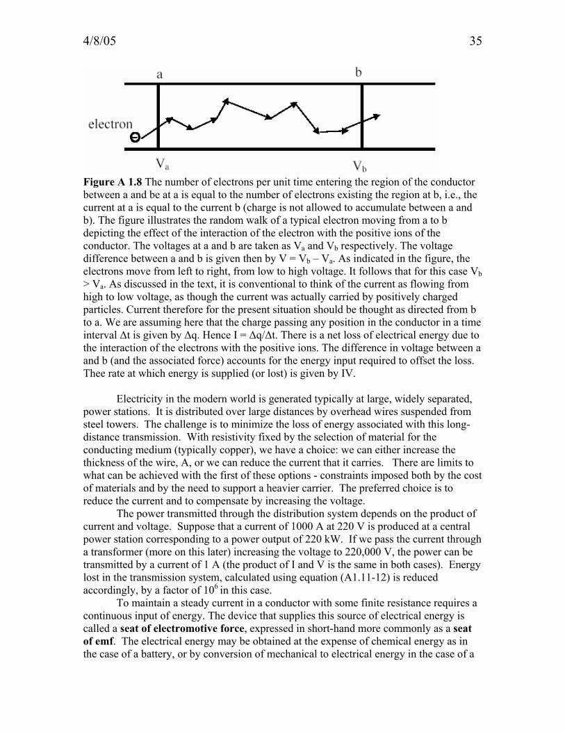
Figure A 1.8 The number of electrons per unit time entering the region of the conductor between a and be at a is equal to the number of electrons existing the region at b, i.e., the current at a is equal to the current b (charge is not allowed to accumulate between a and b). The figure illustrates the random walk of a typical electron moving from a to b depicting the effect of the interaction of the electron with the positive ions of the conductor. The voltages at a and b are taken as Va and Vb respectively. The voltage difference between a and b is given then by V = Vb – Va. As indicated in the figure, the electrons move from left to right, from low to high voltage. It follows that for this case Vb > Va. As discussed in the text, it is conventional to think of the current as flowing from high to low voltage, as though the current was actually carried by positively charged particles. Current therefore for the present situation should be thought as directed from b to a. We are assuming here that the charge passing any position in the conductor in a time interval ∆t is given by ∆q. Hence I = ∆q/∆t. There is a net loss of electrical energy due to the interaction of the electrons with the positive ions. The difference in voltage between a and b (and the associated force) accounts for the energy input required to offset the loss. Thee rate at which energy is supplied (or lost) is given by IV. Electricity in the modern world is generated typically at large, widely separated, power stations. It is distributed over large distances by overhead wires suspended from steel towers. The challenge is to minimize the loss of energy associated with this long- distance transmission. With resistivity fixed by the selection of material for the conducting medium (typically copper), we have a choice: we can either increase the thickness of the wire, A, or we can reduce the current that it carries. There are limits to what can be achieved with the first of these options - constraints imposed both by the cost of materials and by the need to support a heavier carrier. The preferred choice is to reduce the current and to compensate by increasing the voltage. The power transmitted through the distribution system depends on the product of current and voltage. Suppose that a current of 1000 A at 220 V is produced at a central power station corresponding to a power output of 220 kW. If we pass the current through a transformer (more on this later) increasing the voltage to 220,000 V, the power can be transmitted by a current of 1 A (the product of I and V is the same in both cases). Energy lost in the transmission system, calculated using equation (A1.11-12) is reduced accordingly, by a factor of 106 in this case. To maintain a steady current in a conductor with some finite resistance requires a continuous input of energy. The device that supplies this source of electrical energy is called a seat of electromotive force, expressed in short-hand more commonly as a seat of emf. The electrical energy may be obtained at the expense of chemical energy as in the case of a battery, or by conversion of mechanical to electrical energy in the case of a

4/8/05 36

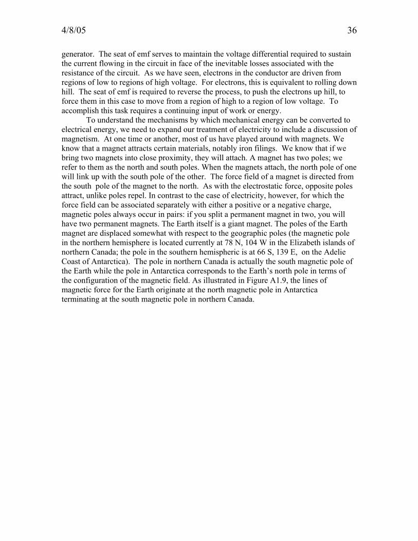
generator. The seat of emf serves to maintain the voltage differential required to sustain the current flowing in the circuit in face of the inevitable losses associated with the resistance of the circuit. As we have seen, electrons in the conductor are driven from regions of low to regions of high voltage. For electrons, this is equivalent to rolling down hill. The seat of emf is required to reverse the process, to push the electrons up hill, to force them in this case to move from a region of high to a region of low voltage. To accomplish this task requires a continuing input of work or energy. To understand the mechanisms by which mechanical energy can be converted to electrical energy, we need to expand our treatment of electricity to include a discussion of magnetism. At one time or another, most of us have played around with magnets. We know that a magnet attracts certain materials, notably iron filings. We know that if we bring two magnets into close proximity, they will attach. A magnet has two poles; we refer to them as the north and south poles. When the magnets attach, the north pole of one will link up with the south pole of the other. The force field of a magnet is directed from the south pole of the magnet to the north. As with the electrostatic force, opposite poles attract, unlike poles repel. In contrast to the case of electricity, however, for which the force field can be associated separately with either a positive or a negative charge, magnetic poles always occur in pairs: if you split a permanent magnet in two, you will have two permanent magnets. The Earth itself is a giant magnet. The poles of the Earth magnet are displaced somewhat with respect to the geographic poles (the magnetic pole in the northern hemisphere is located currently at 78 N, 104 W in the Elizabeth islands of northern Canada; the pole in the southern hemispheric is at 66 S, 139 E, on the Adelie Coast of Antarctica). The pole in northern Canada is actually the south magnetic pole of the Earth while the pole in Antarctica corresponds to the Earth’s north pole in terms of the configuration of the magnetic field. As illustrated in Figure A1.9, the lines of magnetic force for the Earth originate at the north magnetic pole in Antarctica terminating at the south magnetic pole in northern Canada.

4/8/05 37

Figure A1.9 The magnetic field of the Earth is illustrated showing that the direction of the field is oriented generally from south to north. The field lines are more or less vertical at high latitudes, horizontal at low latitudes. As indicated, the magnetic poles are displaced relative to the geographic poles. This is the case for the magnetic equator, where the field lines are horizontal: the magnetic equator is shifted relative the geographic equator. The magnetized needle of a compass points to the geographic north - the north pole of the compass is attracted to the south magnetic pole of the Earth. If you are far removed from the geographic pole, the distinction between magnetic south and geographic north is relatively inconsequential. If you want a more precise definition of direction, or if you are too close to the pole, you need to refer to tables to find the appropriate correction factors. We now know that electric currents are ultimately responsible for the force of magnetism. Ampere was the first to make this critical connection. The magnetic field of the Earth originates in the Earth’s iron-rich conducting core (near the center of the planet). The physical rotation of the Earth plays a critical role in generating the currents responsible for the magnetic field, accounting for the approximate alignment of the planet’s geographic and magnetic poles. There is no particular reason why the north magnetic pole of the Earth should be located necessarily in the geographic southern

4/8/05 38

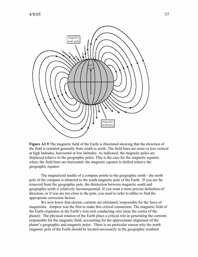
hemisphere as it is today. Indeed we know that from time to time (approximately every million years) the planetary magnetic field reverses direction. The north magnetic field was located in the geographic north about eight hundred thousand years ago. It has flipped many times in the past and will surely do so again, though probably not in our lifetimes (although the strength of the field has been decreasing significantly over the past 150 years giving rise to speculations that the next flip may be imminent). We discussed earlier how charged particles are accelerated in the presence of an electric field. They are subject also to a force associated with the presence of a magnetic field. The force in this case is a little more complicated. Its magnitude is proportional both to the strength of the magnetic field and to the speed of the charged particle. And it operates in a direction perpendicular both to the magnetic field vector, represented by B, and to the velocity vector, v. Expressed mathematically, the force, F, on a particle of charge q is given by F = q v x B (A1.11-14) With F expressed in N, q in C and v in m s-1, B has dimensions of N s C-1 m-1 or N A-1 m1. B is referred to as the magnetic flux vector or as the magnetic induction, or simply as the magnetic field. The unit of magnetic flux in the SI system is known as the tesla (T) named for the Serbian-American inventor/engineer Nikola Tesla (1856-1943), credited over his lifetime with over 700 patents including patents relating to the use of alternating currents for the long-range distribution of electric power (see below). A magnetic field with a flux vector of 1 T will impart a force of 1 N to a charge of 1 C moving at a speed of 1 m s-1. The unit of magnetic flux in the cgs system is known as the gauss (G) (named for the German astronomer/mathematician Johann Carl Friedrich Gauss, 1777-1855): 1 T = 104 G . The strength of the Earth’s magnetic field at mid-latitudes is about 7x10-5 T = 0.7 G. The intensity of the magnetic field produced by a current may be evaluated using what is known as the Biot-Savart Law, named for the French scientists Jean-Baptiste Biot (1774-1862) and Felix Savart (1791-1841) credited with its discovery. According to this law, the contribution to the magnetic field at a position P (see Figure A1.10) due to an element of the current I, ∆l, at Q is given by

2m rrx∆l|I|k∆B = (A1.11-15)

Here km is the magnetic constant equal to 10-7 N A-2, I is the current in A, ∆l is an element of the circuit at Q measured in m, r is the separation between Q and P (m) and r is a unit vector pointed in the direction Q P. To calculate the field produced at P by the current as a whole, we must sum, or more accurately integrate, (A1.11-15) over the entire extent of the circuit. Equation (A1.11-15) indicates that the magnetic field produced at P by an element of current at Q is perpendicular both to ∆l and to the line joining Q to P. For a simple recipe to find the direction of the magnetic field at P, do the following: take your right hand and place your thumb along the direction of current flow at Q; let your hand extend towards P; the resulting natural curl of your fingers will indicate then the direction of B.

4/8/05 39

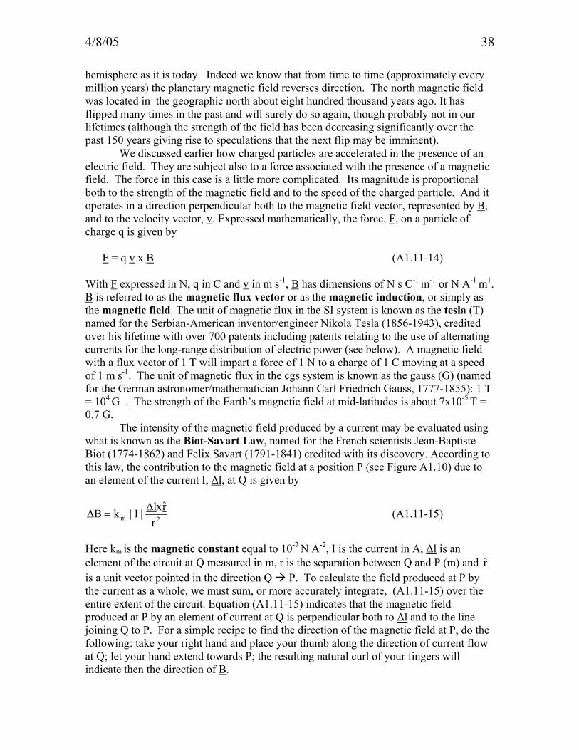
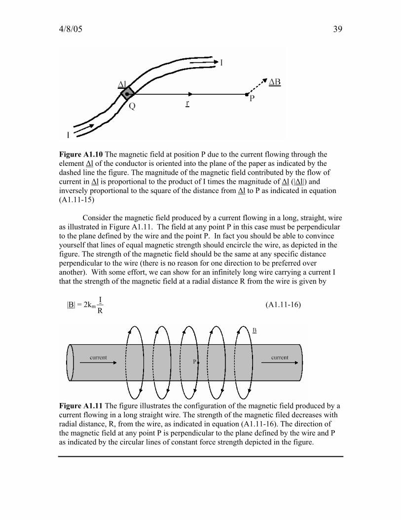
Figure A1.10 The magnetic field at position P due to the current flowing through the element ∆l of the conductor is oriented into the plane of the paper as indicated by the dashed line the figure. The magnitude of the magnetic field contributed by the flow of current in ∆l is proportional to the product of I times the magnitude of ∆l (|∆l|) and inversely proportional to the square of the distance from ∆l to P as indicated in equation (A1.11-15) Consider the magnetic field produced by a current flowing in a long, straight, wire as illustrated in Figure A1.11. The field at any point P in this case must be perpendicular to the plane defined by the wire and the point P. In fact you should be able to convince yourself that lines of equal magnetic strength should encircle the wire, as depicted in the figure. The strength of the magnetic field should be the same at any specific distance perpendicular to the wire (there is no reason for one direction to be preferred over another). With some effort, we can show for an infinitely long wire carrying a current I that the strength of the magnetic field at a radial distance R from the wire is given by

|B| = 2km RI (A1.11-16)

Figure A1.11 The figure illustrates the configuration of the magnetic field produced by a current flowing in a long straight wire. The strength of the magnetic filed decreases with radial distance, R, from the wire, as indicated in equation (A1.11-16). The direction of the magnetic field at any point P is perpendicular to the plane defined by the wire and P as indicated by the circular lines of constant force strength depicted in the figure.

4/8/05 40

Example A1.16: A long straight wire carries a current of 100 A. Calculate the strength of the magnetic field induced by this current at distances of 10 cm and 2 m. Express the answer in units of gauss. Is the field produced by the current small or large compared to the intensity of the background magnetic field of the Earth? Answer: For 10 cm, we convert this distance into meters: 10 cm · 1 m/100 cm = 0.10 m. Also, 1 T (tesla) = 1 N A-1 m-1 = 104 G (gauss). Then from equation (2.11-16), we can calculate the magnetic field strength. For 10 cm,

2.0G1T

G10m1NA

1TmNA102.00.10m100A

AN102

RI2kB

4

11114

27

m =⋅⋅×=⋅⋅== −−−−−−

For 2 m, 0.1G1T

G10m1NA

1TmNA1012m

100AAN102

RI2kB

4

11115

27

m =⋅⋅×=⋅⋅== −−−−−−

The Earth’s magnetic field at mid-latitudes is around 0.7 G. So these calculated strengths are about the same as the strength for the Earth’s magnet. Now consider currents flowing in two contiguous wires. Assume for simplicity that we are dealing with two, long, straight, parallel, wires analogous to the wire discussed above. Wire 1 produces a magnetic field which can exert a force on the electrons flowing in wire 2. The direction of this field, as we have just seen, is perpendicular to the direction corresponding to the orientation of wire 2. The force experienced by the electrons in wire 2 is proportional to the drift speed of the electrons in the wire and to the magnitude of the magnetic field. It is directed normal to both B and vd. With a little thought, we can readily convince ourselves that the force is directed towards wire 1 if the currents in the wires are flowing in the same direction. Similarly, the force on wire 1 due to wire 2 is directed towards 1. If the currents in the two wires are flowing in the same direction, the wires are drawn together. If the currents are flowing in opposite directions, they are driven apart. The magnitude of the force on a segment of wire 2 of length l due to wire 1 separated from wire 1 by a distance R is given by F2 = q(ne Al) vd B1 (A1.11-17) Here ne denotes the density of the electrons carrying the current in wire 2 (charge per electron indicated by q), A defines the cross sectional area of wire 2 and B1 is the strength of the magnetic field at 2 contributed by the current flowing in 1. The quantity in brackets in (A1.11-17) indicates the number of electrons present in wire 2 over the segment of length l. Noting that q ne A vd defines the magnitude of the current I2 flowing in wire 2 and using the expression for the magnetic field at a distance R from wire 1 given by (A1.11-16), we find F2 = 2km l I1 I2 /R (A1.11-18)

4/8/05 41

Example A1.17: Consider two long parallel wires each carrying a current of 20 A. Assume that the wires are separated by a distance of 3 cm. Calculate the magnitude of the electromagnetic force experienced by a segment of one of the wires of length 10 cm. Express your answer in N. Suppose that the wires in question are 14 gauge copper as introduced in Example A1.15 with the mass of a copper atom equal to 1.1x10-22 kg. How does the magnitude of the electromagnetic force evaluated here compare with the magnitude of the corresponding gravitational force? Answer: First, convert centimeters into meters. So R = 3.0 cm × 1 m/100 cm = 0.030 m, and l = 10 cm 1 m/100 cm = 0.10 m. Then F = 2km l I1 I2 /R = 2(10-7 N A-2)(0.030m)(20 A)(20 A)/0.10m = 2.4 × 10-5 N From Example A1.15, the wires have radius r = .01814 cm × 1 m/100 cm = 1.814 × 10-4 m and length l = 0.10 m. Also from Example 2.15, the density of copper atoms is the same as for free electrons: 8.2 × 1022 atoms cm-3(100 cm/1 m)3 = 8.2 × 1028 atoms m-3. Then, for each wire, mass = volume × atoms per unit volume × mass per atom. So m1 = m2 = πr2lnemc = π(1.814 × 10-4 m)2(0.10 m)(8.2 × 1028 atoms m-3)(1.1x10-25 kg atom-1) = 9.3 × 10-5 kg. Then we use Equation (A1.5-2):

N106.4(0.030m)

kg)10(9.3skgm106.67R

GmR

mGmF 162

2521311

2

21

221 −

−−−−

×=×⋅×

===

Thus, the magnitude of the electromagnetic force is far greater than that of the corresponding gravitational force. We showed above how the strength of the magnetic field produced by a current could be evaluated using the Biot-Savart Law. Ampere’s Law offers an alternate approach to this problem. In its most general form, Ampere’s Law states that Imk4∆lB π=⋅∫ (A1.11-19) The integral in (A1.11-19) is carried out along any closed path that includes the current strength I. For the case of the long straight wire, it is convenient to consider a closed path represented by a circle of radius R as in Figure A1.12 (though the Law applies for any path surrounding the wire). We may assume that the magnetic field in this case is tangential to the circular path and, from symmetry, that the magnitude of the magnetic field should be constant along the circle. The vector ∆l in (A1.11-19) defines an element

4/8/05 42

of the circular path enclosing the current oriented in the same direction as the magnetic field B. The integral on the left-hand side of (A1.11-19) is simply equal then to the product of B times the length of the circumference of the circle, 2πR. Thus (A1.11-19) reduces to the simple expression 2πRB = 4π kmI (A1.11-20) indicating that B = 2kmI/R, identical to the result derived earlier using the Biot-Savart approach as summarized in (A1.11-16).

Figure A1.12 Illustrating the configuration of the magnetic field produced by a current I flowing from left to right. ∆l denotes an element of a circular path centered on the wire. The Ampere’s Law reduces in this case to the simple expression by equation (A1.11-20). The Ampere’s Law approach may be used to evaluate the strength of the magnetic field inside a solenoid. A solenoid is a device that can be employed to produce an exceptionally strong magnetic field. It consists of a wire wrapped in a tightly wound helical structure around a central core as illustrated in Figure A1.13. A current flowing in the wire leads to a strong magnetic field in the interior of the core. As we might expect from the symmetry of the situation, this field is oriented along the axis of the core. If we assume, as is in fact the case, that the strength of the magnetic field is much larger in the interior of the core as compared to the exterior, and apply Ampere’s Law to the rectangular path indicated in the Figure, we may note that the only contribution to the path integral indicated on the right-hand side of equation (A1.11-19) is associated with segment A. The contributions from segments B, C and D vanish either because the field in perpendicular to the path (as is the case for the portions of B and D interior to the solenoid) or because the field is assumed to be zero (as is the case for the exterior segment C or for the exterior portions of B and D). It follows from Ampere’s Law in this case that BL = 4πkm N/L I (A1.11-21) where L indicates the length of segment A and N is the number of current loops included in length L of the solenoid. If we denote the number of loops of wire per unit length of the solenoid by n, we may write N = nL. Then

4/8/05 43

B = 4πkm nI (A1.11-22) The more tightly wound the conducting wire and the greater the current carried by the wire, the greater the strength of the resulting magnetic field.

Figure A1.13 Illustrating the configuration of a solenoid with a conducting wire wrapped in a helical configuration around a central core. Example A1.18: Consider a solenoid of length 1m including 1000 loops of connected wire carrying a current of 20 A. Use the formulation given above to calculate the strength of the resulting magnetic field interior to the core of the solenoid. How does the strength of this field compare to the strength of the Earth’s magnetic field for a typical situation at mid-latitudes? Answer: Use formula (2.11-21): B = 4πkm (N/L) I = 4π (10-7 N A-2)(1000/1.00 m)(20.0 A) = 0.0251 T × 104 G/T = 251 G The strength of the earth’s magnetic field for a typical situation at mid-latitudes is 0.7 G, so the magnetic field in the solenoid is much stronger than that of the earth. We have discussed to this point how a current produces a magnetic field. We turn attention now to the flip side – how a current can be produced by a magnetic field. To do this, we must first introduce the concept of magnetic flux. The magnetic flux through an area ∆A is given by Фm = B.n ∆A (A1.11-23) where n denotes a unit vector perpendicular to the element of area ∆A. For the particular case where the magnetic field is constant over the entire area A and directed normal to the area, (A1.11-23) implies that Фm = BA (A1.11-24)

4/8/05 44

noting that ∫∆A=A. Faraday’s Law, named in honor of the English physicist/chemist Michael Faraday (1791-1841), defines a relationship between the electromotive force induced in a circuit and the change in the magnetic flux through the area enclosed by the circuit. Expressed in words, it states that the emf is given by the rate of change of the magnetic flux through the circuit. The mathematical expression of the Law is given by

є = -dt

d mΦ (A1.11-25)

where є is the magnitude of the emf. It is useful at this point to check the compatibility of the units of the quantities on the two sides of equation (A1.11-25). In the SI system, є is given in units of volts, equivalent to J C-1. The right hand side has dimensions of Tm2 s-1. But T has dimensions of NA-1m-1 or N C-1 s m-1 since the dimensions of A are equivalent to C s-1. It follows that the right hand side of (A1.11-25) has dimensions of N C-1 m, the same as Ε, J C-1, since Nm is equivalent to J. Faraday’s law indicates that a change in the magnetic flux through a circuit is required to supply a source of emf. The emf will then drive a current through the circuit inducing a secondary magnetic field. The nature of this secondary field is such as to cancel the changes in the primary field responsible for the initial source of emf. Energy is dissipated inevitably by the current as it flows through the conducting medium. This sink for energy must be offset by a fresh input of energy to maintain the changes in the magnetic flux responsible for the supply of emf in the first place. These complex feedbacks are captured in summary form by Lenz’s Law, named for the Estonian physicist Heinrich Friedrich Emil Lenz (1804-1865), which states that the sense of the emf and the associated induced current are such as to oppose the changes responsible for the emf and the resulting current in the first place. Consider a conducting coil undergoing uniform (constant) rotation in the presence of a fixed magnetic field as illustrated in Figure A1.14. The magnetic flux through the coil is a maximum when the coil is oriented at right angles to the magnetic field. It drops to zero when the coil is aligned with the magnetic field. Let θ denote the angle between the magnetic field and the direction perpendicular to the plane of the coil: θ = 0 when the plane of the coil is perpendicular to the field;θ=90 when the plane of the coil is aligned with the field. Assume at time zero that the coil is aligned perpendicular to the field, θ= 0. Let ω denote the (constant) rotation rate of the coil expressed in units of radians per second. In this case, θ =ωt. For simplicity, assume that the strength of the field is constant, equal to B. The magnetic flux corresponding to orientation θ is given then by BAcosωt where A denotes the area of the coil.

4/8/05 45

Figure A1.14 The figure illustrates a conduction coil rotating at angular velocity ω in a constant magnetic field. The angle θ defines the direction between the magnetic field and a vector oriented perpendicular to the plane defined by the coil. The change of magnetic flux with time may be obtained by differentiating this quantity with respect to time:

dt

d mΦ = dtd [BAcosωt] = -BAωsinωt (A1.11-26)

It follows, according to Faraday’s Law (A1.11-25), that the emf at time t, ε(t), is given by ε(t) = BAωsinωt (A1.11-27) Suppose that the source of emf is connected to a circuit with resistance R. According to Ohm’s Law, the voltage associated with the emf, є, is related to the current and resistance according to the relation є = IR. It follows that

I(t) = R

tBA ωω sin (A1.11-28)

The magnitude of the induced emf and the strength of the associated current are zero

initially. They increase with time reaching a maximum value of BAω at ωt = 2π

in the

case of the emf, Baω/R in the case of the corresponding current. They decrease subsequently, changing sign at ωt=π, falling to minimum (negative) values at

ωt= 2

3π , returning subsequently to the initial conditions when the coil has described a

complete loop around the magnetic field. The induced emf and the associated current oscillate repetitively in time. The emf changes sign and the current switches direction on

4/8/05 46

a time interval given by ωπ∆t = . The overall pattern repeats on a cycle specified by ωt =

2π corresponding to a time interval of ω2π∆t = . The current generated by this time

varying emf is referred to as an alternating current. The frequency of the alternating

current (expressed in cycles per second) is given by πων2

= .

The power dissipated by the induced current (equal to the power produced by the time varying magnetic flux in the generator) is given by єI or by I2 R. The instantaneous rate of power generation is defined thus by the relation

P(t) = I2 (t)R = tRAB ωω 22

22

sin (A1.11-29)

Noting that the time-averaged value of sin2wt is 1/2, it follows that the time-averaged value of the power produced in the alternating generator is given by

Pav = ½ B2A2

R

2ω (A1.11-30)

The necessary power must be supplied mechanically to maintain the required rotation of the coil. We postulated here that the coil intersecting the magnetic field had a single loop. If the coil had incorporated N loops, the resulting emf would have been greater by a factor of N and the power required (or delivered) would be enhanced by a factor of N2. We assumed in the preceding analysis that the configuration of the magnetic field was fixed and that the variation of the magnetic flux through the coil (including its various loops) was produced by rotation of the coil. An entirely equivalent result would have been obtained had we assumed that the coil was fixed and that the rotational motion was imparted to the field rather than to the coil. The power delivered to the electrical circuit depends on the relative velocity of the coil/field system rather than on the absolute velocity of either.

4/8/05 47

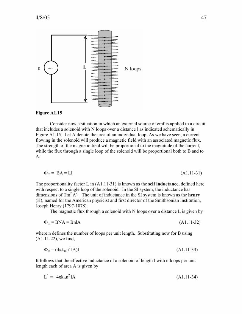
Figure A1.15 Consider now a situation in which an external source of emf is applied to a circuit that includes a solenoid with N loops over a distance l as indicated schematically in Figure A1.15. Let A denote the area of an individual loop. As we have seen, a current flowing in the solenoid will produce a magnetic field with an associated magnetic flux. The strength of the magnetic field will be proportional to the magnitude of the current, while the flux through a single loop of the solenoid will be proportional both to B and to A: Фm = BA = LI (A1.11-31) The proportionality factor L in (A1.11-31) is known as the self inductance, defined here with respect to a single loop of the solenoid. In the SI system, the inductance has dimensions of Tm2 A-1 . The unit of inductance in the SI system is known as the henry (H), named for the American physicist and first director of the Smithsonian Institution, Joseph Henry (1797-1878). The magnetic flux through a solenoid with N loops over a distance L is given by Фm = BNA = BnlA (A1.11-32) where n defines the number of loops per unit length. Substituting now for B using (A1.11-22), we find, Фm = (4πkmn2 lA)I (A1.11-33) It follows that the effective inductance of a solenoid of length l with n loops per unit length each of area A is given by L/ = 4πkmn2 lA (A1.11-34)

4/8/05 48

and the total magnetic flux through the solenoid is given by Фm = L/ I (A1.11-35)

Using Faraday’s Law, it follows that an emf of magnitude dtdI

dtdΦm = would apply if the

strength of the current were to change with time. If a flow of direct current were initiated at time t =0, the build up of the current would be resisted by the emf induced in the solenoid. The strength of the current would build up and eventually would reach a steady

state (dIdt = 0). At this point, the influence of the solenoid would disappear and the strength

of the (steady) current would be determined simply by the magnitude of the external emf and by the overall resistance of the conductor according to Ohm’s Law:

I = Rε (A1.11-36)

The situation is more complicated for an alternating current - if the external emf varies with time as indicated for example by equation (A1.11-27). Suppose that the external emf is given by ε(t) = εmax sin(wt) (A1.11-37) Here, εmax denotes the maximum value of the applied emf. The induced emf persists in this case and

ε(t) = εmax sin(wt) = L dIdt (A1.11-38)

It follows that

I(t) = - εmax /wL cos(wt) = εmax /wL sin(wt -2π ) (A1.11-39)

4/8/05 49

Figure A1.16 Current and voltage vary with time now out of phase as illustrated in Figure A1.16. The change in voltage across the solenoid leads the change in current by one quarter of a period. The voltage across the solenoid is given by

V = dt

dΦN m− t (A1.11-40)

where N defines the number of loops of the solenoid and dt

dΦm indicates the rate of

change in magnetic flux across an individual loop. The power transmitted through the inductor is given by the product of ε(t) and I(t). In the absence of a resistance in the circuit, the power supplied to the inductor vanishes when averaged over time (the time averaged value of sin(ωt)cos(ωt) = 0).

I

V

4/8/05 50

Figure A1.17 Transformer with N1 turns in the primary and N2 turns in the secondary. We noted earlier that loss of power in an electricity distribution system could be minimized if the power was transmitted at high voltage. A transformer is a device that allows the voltage applied to a current to be adjusted either up or down with minimal loss of power in the process. The operation of a transformer is indicated schematically in Figure A1.17. It envisages a primary circuit driven by a generator providing a source of alternating emf represented by є(t). The primary circuit includes a solenoid with N1 loops wound around a core composed of soft iron. A secondary circuit with N2 loops is attached to the same core. The presence of the soft iron core ensures that the change in magnetic flux through a loop of the primary circuit is essentially the same as the change in magnetic flux through a loop of the secondary circuit (assuming that the area encompassed by a loop of the primary circuit is the same as a loop of the secondary). If the voltage induced across the solenoid of the primary circuit is given by V1 and the voltage across the solenoid of the secondary circuit is given by V2, it follows that V2 = N 2 / N1 V1 (A1.11-41) since the number of loops in the secondary circuit exceeds the number in the primary by a factor of N 2 / N1. Suppose now that the secondary circuit is subject to a resistance (we assume that the secondary circuit is employed to transmit electricity over a much greater distance than the primary). Current supplied to the primary circuit by the external source of emf will be transferred in this case to the secondary. It follows that єI 1 = V2 I 2 where I1 and I2 denote the currents flowing in the primary and secondary circuits respectively. Since є = - V1 , it follows using (A1.11-41) that V1 I 1 = - V2 I 2 (A1.11-42) Hence

4/8/05 51

N1 I 1 = - N2 I 2 (A1.11-43) Equation (A1.11-43) implies that the currents flowing in the primary and secondary circuits are out of phase by 180º. Since the current flowing in the primary is in phase with the externally applied emf, it follows that the secondary current (and the voltage associated with this current) are out of phase with the applied emf by this same amount. If the resistance of the secondary circuit is equal to R, using Ohm’s law we infer that I 2 = V2/R. it follows, using (A1.11-41) that I 1 = (N2 /N1)2 є/R (A1.11-44) The primary circuit, coupled to the secondary through the transformer, responds as though it were subject to a resistance of 2

NN )R(

2

1 . If N2 > N1 the voltage is increased by the transformer and the current is reduced accordingly. If N2 < N1 the voltage is decreased and the current is increased. The former case exemplifies what is known as a step-up transformer. The latter defines what is known as a step-down transformer.