Electricity Demand and Supply in Mexico - James A. Baker ... · Electricity Demand and Supply in Mexico Peter Hartley and Eduardo Martinez-Chombo Rice University August 21, 2002 1

Electricity Demand and Supply in Mexico

Peter Hartley and Eduardo Martinez-ChomboRice University

August 21, 2002

1 Introduction

Wherever consumers obtain electricity supply from an integrated network, alter-ing supply to any one consumer generally affects the cost of supplying remainingconsumers connected to the network. In particular, an anticipated expansionof demand in one location could affect the type and level of capital investmentin many parts of the network. This consideration is particularly important in acountry such as Mexico that is likely to experience not only a rapid expansion intotal demand for electricity over the next decade but also a geographical patternof demand growth that differs somewhat from the historical experience.

In this paper, we first present a model for forecasting electricity demand inMexico. The model has two components. Forecasts of the aggregate demand forelectricity are derived by fitting a time series model to the aggregate productiondata. Using data disaggregated to the regional level we also estimate a model ofregional demand shares. The two models are then combined to yield a forecastof demand at the regional level.

In section 3 of the paper, we present a simplified model of the Mexicanelectricity transmission network. We use the model to approximate the marginalcost of supplying electricity to consumers in different locations and at differenttimes of the year. In the final section of the paper, we examine how costs andsystem operation will be affected by proposed investments in generation andtransmission capacity and the forecast growth in regional electricity demands.

The analysis presented in the paper has implications for a number of crit-ical policy issues. In particular, our model reveals that the marginal costs ofsupplying customers differ from electricity prices. Subsets of consumers are ei-ther being taxed or subsidized, albeit often in a hidden or implicit way. Sincesuch taxes or subsidies affect the efficiency of resource use, they ought to beimportant to policy discussions regarding the electricity industry.

The marginal cost of supplying electricity in different locations or under dif-ferent load conditions also has implications for how regulatory reform is likelyto affect different types of customers and therefore the political feasibility ofreform. The largest obstacle to such reforms is that they are likely to inducesubstantial cost reductions, primarily through the elimination of excess employ-ment in the industry. Current employees in the industry therefore constitute a

1

powerful vested interest opposed to reform. Altering the system so that pricesmore closely reflect marginal costs is also likely, however, to make some con-sumers worse off and they, too, are likely to oppose reform.

Our demand forecasts also raise some critical policy issues. They implythat large investments in the Mexican electricity industry will be needed overthe next decade. If the electricity industry remained fully publicly owned, thegovernment of Mexico would need to raise significant revenue to fund theseinvestments. Mexico has many alternative valuable uses for scarce tax revenues,however, and most of these alternatives are far less amenable to private sectorinvolvement than is electricity supply. It therefore is not surprising that thegovernment has turned to the private sector to supply much of the neededgenerating capacity. The route the government has taken, however, is to rely onbuild, lease and transfer (BLT) projects. Under these schemes, the private sectorbuilds the new plant, leases it under a long term contract with the government-owned utility, and ultimately transfers the plant to government ownership at aspecified future date. This approach leaves the government firm in charge ofoperating the plant. It also leaves the government firm bearing all the risksassociated with inaccurate forecasts of future electricity demand.

Another approach would be to reform and restructure the industry in a waythat allows a competitive wholesale electricity market to develop. Private in-vestors then would not only finance investments in the industry, but also wouldtransfer risks from consumers to the capital markets where they can be bornemore efficiently. The reforms would need to split the existing publicly ownedfirms into many separate firms to ensure that the industry remains competitiveenough to protect the interests of Mexican consumers. The transmission, dis-tribution and generation functions of the existing firms would also need to beseparated. New entrants to the industry would not have any confidence thatthey could obtain non-discriminatory access to the transmission and distributionnetworks if the operator of that system continues to own generating plant.

Another advantage of developing a competitive wholesale market is thatprices would more closely reflect the true marginal costs of supply. In particu-lar, a competitive wholesale electricity market would eliminate cross-subsidieshidden in deviations between prices and marginal costs of service.

2 Forecasting regional electricity demands

Electricity demand is measured by the metered final consumption of end users.To supply power to consumers, however, generating plants also have to supplysufficient energy to compensate for the losses incurred in the process.1 Hence,any forecast of power needs must take account of losses that in some cases are

1In the year 1999, for example, Mexican electricity consumption by sectors represented144,922GWh, or about 80% of the total 180,977GWh produced in the country. Net imports ofelectricity into Mexico in 1999 were only 524GWh. Consumption within the generating plantswas about 8,887GWh, or 5% of total production. The remaining 27,621GWh (approximately15% of domestic production) represents transmission and distribution losses in the system andlosses due to theft.

2

hard to identify. In particular, losses in Mexico arise not only from resistancelosses on the transmission and distribution wires, but also from theft. Theapproach we take is to forecast total power generation. This implicitly assumesthat there is a constant relationship between losses and total demand.2

2.1 Modeling aggregate electricity demand

The methodology used to make aggregate demand forecasts is based on theChang and Martinez-Chombo (2002). The model is fit to total power generationdata from Comision Federal de Electricidad (CFE) over the period January 1987to November 2001. Essentially, the logarithm of total power generation (Q) isrelated to GDP (y), the relative price of electricity (p), and a variable (z),based on temperature records, that accounts for seasonal variations. Details ofthe model and the estimated equations can be found in Appendix A.

2.2 Using the model to forecast aggregate demand

In order to use the estimated model to forecast electricity demand, we needto forecast the determinants, y, p and z. We use the average pattern holdingover the sample period for the temperature variable z. To forecast y, we usethe GDP growth forecast for 2002 and 2003 made by specialists and collectedand reported by the Central Bank of Mexico.3 Beyond 2003, we assume thatthe annual GDP growth rate converges gradually to an equilibrium level thatgives an average growth of 5.2% for the rest of the decade. This is the averagegrowth rate assumed by the CFE in its projections of electricity sales and hasthe virtue of making our forecasts more comparable to those of the CFE.4

In order to forecast p, we note that the Mexican government has a statedpolicy of applying a monthly adjustment to electricity prices that is aimed atcompensating for the effect of inflation. In practice, the adjustments have notkept the relative price of electricity constant. Indeed, as we show in Appendix A,the relative price trends to drift over time. The rate of price adjustment hasalso varied for different types of customers.5 Evidently, politics has played arole in setting electricity prices. Since we do not have a model of the politicalprocess, we simply assume that real electricity prices will fluctuate around themean observed in the previous six years. We preserve the monthly seasonalcomponent of p by estimating a regression (also presented in Appendix A) thatallows the mean value of p to differ systematically from one month to the next.

2Given the lack of storability of electricity, the consumption of electricity (losses plusdemand from agents) is always equal to its generation.

3Private Expectation Survey, Bank of Mexico, May 20, 2002. The consensus forecast isreported at http://www.banxico.org.mx/eInfoFinanciera/FSinfoFinanciera.html

4Secretarıa de Energıa. “Prospectiva del sector electrico 2001-2010”. Page 96.5Since January 2001, the montly adjustment for the residential sector has been 1.00526.

This corresponds to an annual increment of 6.5%. For the service sector, the average monthlyadjustment was 1.00682, yielding an annual increment of 8.5%. The adjustment factor for theelectricity price charged to industry is indexed to the price of power generation fuels. Thisinformation was obtained from the CFE, http://www.cfe.gob.mx/www2/Tarifas

3

Table 1: Power needs forecast 2002 - 2010

GDP Total Power Generation

With price increase Without price increase

Year Growth (%) GWh Growth (%) GWh Growth (%)

1991 118,348

1992 3.54 121,604 2.75

1993 1.94 125,864 3.50

1994 4.46 137,684 9.39

1995 -6.22 142,503 3.50

1996 5.14 151,890 6.59

1997 6.78 161,385 6.25

1998 4.91 170,983 5.95

1999 3.84 180,917 5.81

2000 6.92 191,340 5.76

2001 -0.38 191,340 -0.14

2002 1.50 199,857 4.60 203,830 6.68

2003 4.30 207,724 3.94 215,895 5.92

2004 5.45 220,942 6.36 229,921 6.50

2005 5.91 234,428 6.10 244,585 6.38

2006 6.20 247,401 5.53 258,742 5.79

2007 5.96 260,008 5.10 272,487 5.31

2008 5.85 273,247 5.09 286,950 5.31

2009 5.90 288,510 5.59 303,660 5.82

2010 5.90 306,221 6.14 323,103 6.40

Average Growth Rates

1991-2001 3.09 4.94 4.94

2001-2010 5.20 5.38 6.01

1991-2010 4.09 5.15 5.45

Note: The electricity price increase results from the reduction of subsidies

to households. We calculate this will result in a 6.97% increase in p.

4

Substituting the forecast values of y, p and z into the estimated model, wearrive at the forecast of annual electricity demand in Mexico from 2002 to 2010as reported in Table 1. Our model actually delivers monthly total power gener-ation forecasts. These have been aggregated to yield the corresponding annualvalues. For some of the subsequent analysis, however, we will be interested inthe monthly variations.

For comparison, we have included the results before and after the recentprice adjustment that reduced federal subsidies in the residential sector. Thisone time increase in residential electricity prices is estimated to be around 30%.6

To translate the residential price increase into an effect on p, we note that thissector represented 23.23% of total electricity sales over the last five years. Hence,the overall increase in electricity prices from the subsidy reduction will be about6.97%. Our estimated model implies that a price increase of that magnitudewill reduce the average annual growth rate of electricity generation in the period2001-2010 from 6.01% to 5.38%, with the effects concentrated in the first twoyears.7

2.3 Forecasting regional demand shares

Mexico has large contrasts in climate, topography, resource availability, eco-nomic development and population density among its different regions. Thesecontrasts have direct implications for the optimal siting of power generatingplant and the distribution of electricity demand around the country. Regionswith insufficient natural energy resources, underdeveloped infrastructure, or alarge demand for power, are likely to import electricity generated elsewhere.Conversely, regions with substantial hydroelectric generating capacity, or sub-stantial reserves of fossil fuels, are likely to have surplus power available forexport. Differences in climates also mean that peak demands for electricity donot necessarily occur at the same time, allowing regions to save on generatingcapacity by exchanging power with neighboring regions.

To capture the regional differences in the Mexican electricity demand webegan with data on electricity sales in the 14 administrative regions of theCFE. Although sales do not necessarily reflect demand,8 they are likely to bea better indicator than local production. In most of the cases, regional powerconsumption will differ from regional power generation because of trading amongregions through the transmission system. In order to link electricity supplyand demand we also need to account for losses. In this section of the paper,

6According to a report in the newspaper Reforma on February 9, 2002, Banxico estimatedthe reduced subsidy would increase residential electricity prices by 30%.

7This estimated reduction in power needs is probably an upper bound. Although householdelectricity demand is likely to be more elastic than demand in the services sector (wherelighting is the dominant use), it would be less elastic than demand in industry. Using theoverall elasticity may thus overstate the responsiveness of demand to price. In addition, aprice increase for households is likely to raise electricity losses through theft.

8Electricity demand and sales can differ because of billing lags and the theft of electricity.If the latter factors do not differ systematically across regions, however, the pattern of salesought to approximate the geographic distribution of demand.

5

9

In order to use the estimated model to forecast electricity demand, we need to forecast thedeterminants. It is reasonable to postulate that the temperature variables will reflect the averageannual pattern holding over the sample period. We can also use the near-term forecasts of GDPgrowth produced by the Central Bank of Mexico. Beyond the horizon of that forecast, we assumethat annual economic growth converges gradually to the new long run level for Mexico of about5.2% per annum. We have no basis for forecasting movements in the relative price of electricityand therefore simply assume that it remains at its end-of sample value of

Table 5 presents the resulting forecasts of annual electricity demand in Mexico from2000-2010. For comparison, have also included the forecasts made by CFE (2000). Our modelactually delivers monthly demand forecasts, and these have been aggregated to yield thecorresponding annual values. For some of the subsequent analysis, however, we will beinterested in the monthly variations.

Forecasting regional demand

One can view the co-integration analysis used to forecast aggregate electricity demand asfocusing on relationships that are expected to be stable in the longer run. We took a similarapproach to forecasting regional demand. Figure 2 maps the boundaries of the regions, whichcorrespond to the administrative regions of CFE.

Figure 2: The regions identified in the analysis

We expect the regional shares of electricity consumption to change only slowly. We thereforeestimated a set of equations for the shares Sit of demand in region i in period t. These equationswere then projected to the future and used with the aggregate demand forecast to derive regionaldemand forecasts.

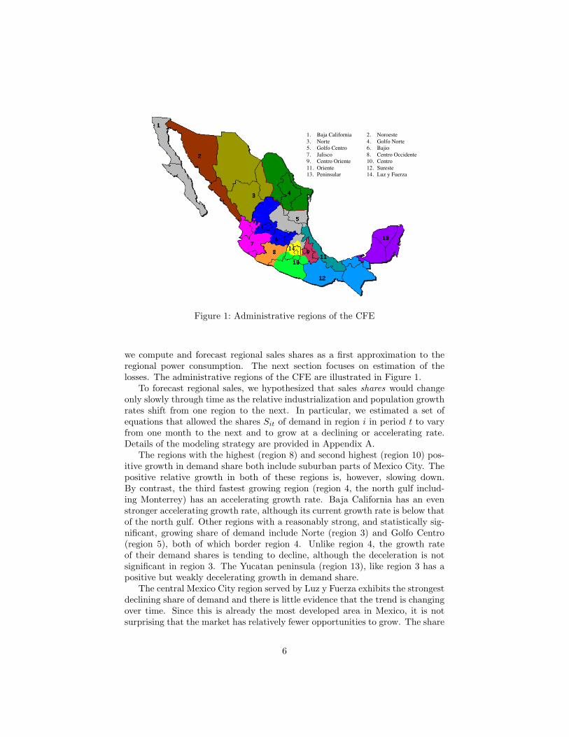
1. Baja California 2. Noroeste3. Norte 4. Golfo Norte5. Golfo Centro 6. Bajio7. Jalisco 8. Centro Occidente9. Centro Oriente 10. Centro11. Oriente 12. Sureste13. Peninsular 14. Luz y Fuerza

Figure 1: Administrative regions of the CFE

we compute and forecast regional sales shares as a first approximation to theregional power consumption. The next section focuses on estimation of thelosses. The administrative regions of the CFE are illustrated in Figure 1.

To forecast regional sales, we hypothesized that sales shares would changeonly slowly through time as the relative industrialization and population growthrates shift from one region to the next. In particular, we estimated a set ofequations that allowed the shares Sit of demand in region i in period t to varyfrom one month to the next and to grow at a declining or accelerating rate.Details of the modeling strategy are provided in Appendix A.

The regions with the highest (region 8) and second highest (region 10) pos-itive growth in demand share both include suburban parts of Mexico City. Thepositive relative growth in both of these regions is, however, slowing down.By contrast, the third fastest growing region (region 4, the north gulf includ-ing Monterrey) has an accelerating growth rate. Baja California has an evenstronger accelerating growth rate, although its current growth rate is below thatof the north gulf. Other regions with a reasonably strong, and statistically sig-nificant, growing share of demand include Norte (region 3) and Golfo Centro(region 5), both of which border region 4. Unlike region 4, the growth rateof their demand shares is tending to decline, although the deceleration is notsignificant in region 3. The Yucatan peninsula (region 13), like region 3 has apositive but weakly decelerating growth in demand share.

The central Mexico City region served by Luz y Fuerza exhibits the strongestdeclining share of demand and there is little evidence that the trend is changingover time. Since this is already the most developed area in Mexico, it is notsurprising that the market has relatively fewer opportunities to grow. The share

6

of demand in region 11 (Sureste, the gulf coast east of Mexico City) is fallingalmost as fast as for Mexico City, but there is stronger evidence that the rate ofdecline is slowing. Region 7 (Jalisco) is the only other region with a strong andstatistically significant declining share of demand, but it also reveals strongerevidence that the rate of decline is slowing.

The estimated monthly changes in shares (presented in Table 23 in Ap-pendix A) allow the regions to be placed into groups with similar patterns ofdemand variation across months. Regions 1 (Baja California) and 2 (Noroeste)have a tendency to show smaller demand shares February–April and largershares June–November. Regions 5 (Golfo Central) and 13 (Peninsula) also havesignificantly smaller demand shares February–April, but do not share the ten-dency of the two northwestern regions to have significantly higher demand sharesin the second half of the year. Region 11 (Oriente), which lies between regions5 and 13 on the Gulf coast, has demand shares that do not differ significantlyfrom month to month. The remaining northern regions, 3 (Norte) and 4 (GolfoNorte) are like regions 1 and 2 in that they have significantly larger demandshares May–November, but they do not have significantly lower shares in firsthalf of the year.

The remaining central (6, 9 and 14) and southern Pacific coastal (7, 8,10, 12) regions tend to have smaller, not larger, demand shares in the secondhalf of the year. In regions 7 (Jalisco), 10 (Centro Sur), 12 (Sureste) and 14(Centro, Luz y Fuerza) the months with significantly lower demand shares lastApril–November. In regions 8 (Centro Occidente) and 9 (Centro Oriente) theperiod with significantly lower demand is only July–October. The northernmostof these regions, 6 (Bajio), only has a significantly lower demand share fromAugust–November. Regions 6, 8 and 9 are also the only ones to have significantlylarger demand shares in the early part of the year. In region 6 it lasts January–June, while in regions 8 and 9 the period of above average demand share isshorter, lasting February–April.

The estimated regional share model can be used to forecast demand sharesby month and year. We can obtain an idea of how the different growth pathsinfluence demand shares by examining forecast annual demand shares for 2005and 2010. These are presented in Table 2. They suggest that by 2005 thedemand in Golfo Norte will be approximately equal to, if not slightly above, thedemand in the Mexico City area served by Luz y Fuerza. The share of the Luzy Fuerza region is expected to decline further by 2010. The regions surroundingMexico City (Bajio, Centro Occidente, Centro Oriente and Centro Sur) will,however, all see growing shares of demand. Baja California, like Golfo Norte, isalso likely to see a substantial increase in its share of demand by 2010.

We obtain a forecast of regional electricity demand by combining the overalldemand forecast derived in the previous section of the paper with the forecasts ofregional shares. Table 3 gives the resulting regional demands (in GWh annually)and total and average annual growth rates for demand in each region.

The substantial differences in forecast regional electricity demand growthrates may have important policy implications. A high overall rate of growthof demand for electricity will require substantial investment in the industry.

7

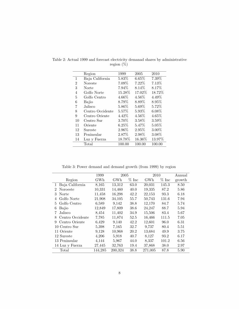
Table 2: Actual 1999 and forecast electricity demanad shares by administrativeregion (%)

Region 1999 2005 20101 Baja California 5.83% 6.65% 7.39%2 Noreste 7.09% 7.22% 7.13%3 Norte 7.94% 8.14% 8.17%4 Golfo Norte 15.28% 17.02% 18.72%5 Golfo Centro 4.66% 4.56% 4.49%6 Bajio 8.79% 8.89% 8.95%7 Jalisco 5.86% 5.69% 5.72%8 Centro Occidente 5.57% 5.93% 6.08%9 Centro Oriente 4.42% 4.56% 4.65%10 Centro Sur 3.70% 3.58% 3.59%11 Oriente 6.25% 5.47% 5.05%12 Sureste 2.96% 2.95% 3.00%13 Peninsular 2.87% 2.98% 3.08%14 Luz y Fuerza 18.78% 16.36% 13.97%

Total 100.00 100.00 100.00

Table 3: Power demand and demand growth (from 1999) by region

1999 2005 2010 AnnualRegion GWh GWh % Inc GWh % Inc growth

1 Baja California 8,165 13,312 63.0 20,031 145.3 8.502 Noroeste 10,331 14,460 40.0 19,335 87.2 5.863 Norte 11,458 16,298 42.2 22,153 93.3 6.184 Golfo Norte 21,908 34,105 55.7 50,743 131.6 7.945 Golfo Centro 6,589 9,142 38.8 12,170 84.7 5.746 Bajio 12,849 17,809 38.6 24,247 88.7 5.947 Jalisco 8,454 11,402 34.9 15,506 83.4 5.678 Centro Occidente 7,785 11,874 52.5 16,466 111.5 7.059 Centro Oriente 6,429 9,140 42.2 12,601 96.0 6.3110 Centro Sur 5,398 7,165 32.7 9,737 80.4 5.5111 Oriente 9,128 10,968 20.2 13,684 49.9 3.7512 Sureste 4,206 5,918 40.7 8,127 93.2 6.1713 Peninsular 4,144 5,967 44.0 8,337 101.2 6.5614 Luz y Fuerza 27,445 32,763 19.4 37,868 38.0 2.97

Total 144,285 200,324 38.8 271,005 87.8 5.90

8

This problem could be exacerbated, however, if the geographical distribution offuture demand differs greatly from the current distribution. The above averagegrowth of demand in the northern regions, for example, is likely to require asubstantial increase in generating plant in the north or a substantial upgradingof the transmission links either from further south in Mexico or from the US.

3 A model of the electricity supply system

In this section, we discuss a model of the Mexican electrical network that allowsus to approximate the spatial and temporal variations in the marginal cost ofsupplying electricity in 1999. Discussion of some of the more technical issues,including an outline of the equations included in the model, can be found inAppendix B.

The model calculates the least cost pattern of electricity production andtransmission required to meet a discrete number of demand loads on the system.The demands are chosen to be “representative” of different times of the year.The geographic dispersion of demand also is approximated in a discrete way byassuming that the demand for a particular region is concentrated at a single“node.” The model delivers an estimate of the “usual” short run marginal costof supplying electricity in different regions and at different times of the year.

The aggregated demand data and the broad assumptions about other tech-nical characteristics of the system make the marginal costs obtained from themodel approximations to the true marginal cost. They are useful for indicatinghow prices might change were they to more closely reflect marginal costs. Themodel also is useful for examining longer run issues, such as the effects of invest-ment and demand growth on average system costs. Our model would not beuseful, however, for dispatching generators to ensure least cost operation of thesystem or for predicting how costs or system operations are likely to be affectedby an emergency.

3.1 Approximating spatial and temporal variation

Geographical structure. In principle, the cost of supplying electricity willdiffer at every single connection point to the transmission network. For ourcurrent purposes, it is impractical to calculate all these nodal prices. We insteadconsider a discrete approximation to the physical layout of the network and thelocation of major centers of supply and demand.

In general, there is no unique method to determine the boundaries of thegeographic regions. The appropriate level of aggregation can depend on theobjective of the analysis. For example, a highly aggregated model may besufficient when the objective is to identify electricity trade among countries,states or utility districts. Small or isolated regions can be subsumed into largerregions without having much of an impact on the questions of interest.

The number of regions included in the model, and the size of each, also de-pends on the available data. We based the geographical division of the country

9

Table 4: Generating capacity, production and estimated demand by transmis-sion region, 1999

Transmission Generators at year end 1999 Total Output DemandRegion Total Typea MW GWh GWh

1. Sonora Norte 4 T 807 3,876 4,6912. Sonora Sur 6 3T, 3H 746 3,343 3,2613. Mochis 8 2T, 6H 1,167 3,050 2,2884. Mazatlan 1 T 616 3,467 9925. Juarez 1 T 316 1,561 4,1976. Chihuahua 7 5T, 2H 1,118 6,289 3,6987. Laguna 5 T 643 3,619 6,1688. Rio Escondido 5 3T, 2H 2,710 18,359 2,2389. Monterrey 10 T 1,215 5,841 19,21410. Huasteca 1 T 800 4,732 3,92211. Reynosa 2 T 521 2,680 3,09012. Guadalajara 9 1T, 8H 1,352 2,147 9,62013. Manzanillo 2 T 1,900 11,194 1,35514. Ags-SLP 4 1T, 3H 720 3,963 7,38415. Bajıo 13 3T, 9H, 1R 1,447 8,895 17,19716. Lazaro Cardenas 3 1T, 2H 3,395 16,043 41417. Central 20 7T, 13H 3,526 19,023 43,08918. Oriental 17 3T, 12H, 1N, 1R 4,719 29,835 14,79619. Acapulco 4 1T, 3H 681 1,498 2,21220. Temascal 3 2H, 1R 358 1,736 1,52121. Minatitlan 1 H 26 119 2,98922. Grijalva 7 H 3,928 17,342 2,91823. Lerma 2 T 164 902 92424. Merida 4 T 277 1,261 2,41525. Chetumal 1 T 14 12 27526. Cancun 7 T 529 1,471 1,19927. Mexicali 5 2T, 3R 684 4,680 3,06128. Tijuana 2 T 830 2,785 5,11829. Ensenada 2 T 69 9 90630. Cd. Constitucion 6 5T, 1R 120 402 19031. La Paz 2 T 156 709 82532. Cabo San Lucas 1 T 30 59 153

Total 164 83T, 73H, 1N, 7R 35,585 180,901 172,319

a. T = oil, coal or gas thermal, H = hydroelectric, N = nuclear,R = plant using “renewable” wind and geothermal energy sources.

10

Figure 2: Mexican electricity transmission network, 1999

on the 32 “transmission regions” defined by the CFE. The regional data ex-amined above was based on the CFE accounting records. In order to calculatecosts or examine optimal investments, we need to relate the demand data tothe physical supply system, primarily the generating plants and transmissionlines. The engineering data supplied by CFE is organized by transmission re-gion. This subdivision highlights the high voltage transmission network thatconnects the most important industrial and population centers of the country.The geographical distribution of such regions and the 1999 transmission network(with its capacities in MW) are illustrated in Figure 2. Table 4 gives basic dataon generating capacity located in the 32 transmission regions.

The number of transmission regions exceeds the number of accounting re-gions, and the boundaries of the two sets of regions sometimes overlap. Weconstructed the demand shares per transmission region by disaggregating theshares for the 14 administrative regions into the 32 transmission regions basedon population data of the main Mexican cities.9 The right-hand column ofTable 4 shows our allocation of the 1999 demand data. The remainder of theanalysis will be based on the transmission regions with demand imputed in thismanner.

By the end of 1999, the Mexican electric supply system had 164 active fixedgenerating plants10 with a total effective capacity of 35,584 MW. While 44% of

9To allocate the forecast future demand shares to the transmission regions, we usedthe population growth projections of the Consejo Nacional de Poblacion (CONAPO),http://www.conapo.gob.mx, the main governmental institution in Mexico involved in demo-graphic analysis.

10Officially, 170 plants were said to be available in December 1999, but not all of them

11

the plants were hydroelectric and 46% thermal, the capacity shares were moreunequal, with these two types of plant supplying 27% and 63% of the totalcapacity respectively. Capacity data for each plant were collected from annualpublic reports of the CFE.11 We approximated the current annual “availability”of each plant by its maximum annual production in the last three years ofoperation.

Temporal structure. An important feature of most electricity systems isthat the demand load on the system varies over time. In particular, extremeweather conditions can significantly affect the demand for electricity.12 Ouranalysis of the regional variation of demand showed that, in the north of Mexico,electricity consumption is considerably higher during the second half of the year.In the southern half of the nation, demand shares tend to be lower during thisperiod.

The demand for electricity for cooking also displays a distinct daily patternthat also tends to coincide with the daily fluctuation in demand for electricityfrom electrified commuter rail systems. Industrial demand for electricity tendsto be higher during daylight hours, although 24 hour operation of some largeplants can also raise the demand for electricity during off-peak periods. Thedemand for electricity for lighting (for which there are no good substitutes) is,of course, highest during the night, but drops substantially in the early morninghours. Electrical water heaters can be operated at night when the demand forelectricity is otherwise relatively low, but in this application natural gas is astrong competitor for electricity.

In addition to the daily and seasonal fluctuations in demand, there are alsosubstantial weekly patterns. Most obviously, demand is lower on the weekendsthan during the week.

The seasonal, weekly and daily fluctuations in demand matter because thecosts of supplying electricity can change substantially as a function of boththe total system load and its geographic distribution. The generating planthave different costs of production, while there are also costs associated withgenerating electricity in one location and transmitting it large distances to beconsumed elsewhere. Furthermore, the difficulty13 of storing electrical energymakes it difficult to arbitrage price differences over time. We therefore need toapproximate the pattern of demand fluctuations over time in order to obtain arealistic idea of how costs vary over time. As with the geographical diversitydiscussed above, however, a discrete approximation to the time variability allowsus to simplify the model.

Again, the optimal level of detail will depend on the purpose for which the

operated at some time during that year.11The relevant CFE reports are titled “Informe de Operacion.”12The seasonal pattern of electricity demand also is affected by the fact that many businesses

have annual and other holidays at the same time.13In some situations, pumped storage can be used to store a limited amount of energy.

More generally, the availability of hydroelectricity increases the intertemporal substitutabilityof electricity supply.

12

North: Fall

0.5

0.6

0.7

0.8

0.9

1.0

1 2 3 4 5 6 7 8 9 10 11 12 13 14 15 16 17 18 19 20 21 22 23 24

North: Summer

0.5

0.6

0.7

0.8

0.9

1.0

1 2 3 4 5 6 7 8 9 10 11 12 13 14 15 16 17 18 19 20 21 22 23 24

Hour of the day

Weekday Holiday

South: Fall

0.5

0.6

0.7

0.8

0.9

1.0

1 2 3 4 5 6 7 8 9 10 11 12 13 14 15 16 17 18 19 20 21 22 23 24

South: Summer

0.5

0.6

0.7

0.8

0.9

1.0

1 2 3 4 5 6 7 8 9 10 11 12 13 14 15 16 17 18 19 20 21 22 23 24

Hour of the day

Weekday Holiday

Figure 3: Representative daily load curves, normalized to the maximum annualdemand, 1999

model is being constructed. As with the geographical information discussedabove, however, the detail we can include in the model is limited by the datathat are available to us.

The Secretary of Energy14 published average daily load curves for the year1999. These curves are available separately for the North and South areas ofthe country,15 for two seasons, Summer (May to August) and Fall (Novemberto February), and for weekdays and holidays. The curves, graphed in Figure 3,represent the average demand per hour during a typical day expressed as per-centage of the maximum annual demand.16 For the remaining months (March,April, September and October) we constructed a daily load curve that was aweighted average of the two published curves, having as weights the electricitydemands in the Summer and Fall seasons. We assume that all the transmis-sion regions within an area (North or South) have the same daily pattern ofelectricity demand and thus the same daily load curve shape.

We derived the total demands (weekdays plus weekends and holidays) ineach of the 32 transmission regions in each season by aggregating the monthlydemands. The daily load curves were used to allocate demand in each seasonto weekdays versus weekends or holidays. Finally, demands in a weekends-holidays “season” were obtained by aggregating the weekend or holiday compo-nents across seasons. In summary, the data allows us to calculate, in each ofthe 32 transmission regions, the electricity demands for four seasons:

14“Prospectiva del sector electricol 2000-2009”, Secretary of Energy.15The North region includes the North and Northeast areas. The South region includes the

Occidental, Central, Oriental and Peninsular areas.16None of the load curves in Figure 3 attain the value since they represent “average” loads

in each season.

13

1. Fall, covering working days for the 4 months from November to February;

2. Summer, for working days for the 4 months from May to August;

3. Shoulder, for working days for the 4 months of March, April, Septemberand October; and

4. Weekends-Holidays, that includes non-working days during the whole year.

To capture the intraday demand dynamics, we could, in principle, use the av-erage daily load curves in each season to construct hourly electricity demand.17

However, to keep the model manageable, we approximate the hourly demandfluctuations using step functions. The details of this approximation procedureare provided in Appendix A.

For constructing the hourly demand in 2005, we assumed that the dailyload curves are the same as those in 1999. This approach was used becauseof the limited nature of our investigation. In principle, one could estimate thechange in the load duration curves over time based on changes in the pricesof electricity (including changes in peak relative to off-peak prices), economicgrowth (as measured by GDP) and weather conditions. In effect, the demandestimation carried out above would be repeated for different load patterns onthe system. The estimated variation in demands by time of day (as determinedby system load) could then be used to make forecasts in place of the aggregateforecasts with an unchanging pattern of demand that we have used.

3.2 Generation and transmission technologies

To calculate the costs of supply, we need information about the generation andtransmission technologies. With regard to the generating plants, we need toknow not only generating costs but also capacities and the average level ofavailability. For the transmission links, we need to know the overall capacityand, to calculate the loss factors, the number of circuits per link.

Generating plant costs. Regardless of the type of generating technology, weassume that the cost function of a plant can be represented by two components.The first component is an annual fixed cost. It includes the fixed componentsof the operation and maintenance costs of the plant, such as the labor forcerequired to keep the plant operational even if it is not generating electricity. Weassume that the fixed costs, given in dollars per MW, are a linear function of thetotal capacity of the plant set at the beginning of the year. The variable cost isthe second component of the generating cost of each plant. It includes the costof fuel and some other operation and maintenance costs, mainly on the cost oflabor, that vary with the amount of electricity that the plant is generating. Weassume that this cost is a linear function of the MWh generated by the plant.The variable cost per MWh is constant during a given period, but could vary

17Even this involves a simplifying assumption that all days in a season have the samedemand pattern that can be scaled up or down according to the monthly demand.

14

from one period to the next as a result of seasonal fluctuations in fuel prices inparticular.

We based the operation and maintenance costs for thermal plants on costestimates provided by the CFE (COPAR, 1999) for “typical plants” in Mexicoclassified by size of the plant and type of technology.18

The fuel cost of thermal plants was calculated using the average technicalefficiency of each plant (fuel/MWh). In turn, we obtained the average efficiencyof a plant by dividing its overall fuel consumption for the year 1999 by its poweroutput in the same year. The monthly cost in pesos was then obtained by mul-tiplying the required fuel input by the monthly fuel prices. The seasonal prices,for example the price for the peak period May-August, were computed as theaverage price in the months falling into that period. The relevant informationwas obtained from the CFE.19

The hydroelectric plants do not have a fuel cost as such but are required topay “resource levies” on the cubic meters of water they use. We shall take these“resource levy” payments as part of the variable cost.

The CFE publications do not provide “typical” operation and maintenancecosts for hydroelectric plants. This may be because such plants are more het-erogeneous than the thermal plants. They vary in size and efficiency muchmore than do the thermal plants, and the MWh of electricity generated onlyapproximates water use. The CFE publications do, however, provide costs forten existing large hydroelectric plants and we use these to extrapolate the costsfor other plant sizes. Specifically, we extrapolated the fixed component of theoperating and maintenance costs of large hydro plants by regressing the log ofcosts for the ten hydro plants on the log of their capacities.20 The relationshipreported on page 5.5 of COPAR(1999)21 was used to compute the variable cost,that is the operation and maintenance costs and resource levies. This equationwas estimated using regression analysis with a larger sample than the ten plantswhose costs were reported. Finally, we assumed small hydroelectric plants (lessthan 50 MW) had constant costs (an average fixed cost of 152,802 pesos perMW per year and a variable cost of 10.58 pesos per MWh).

The generating costs do not include any capital cost (that is, interest pay-ments or depreciation). Implicitly, we are anticipating that investment projectswould be evaluated on a cash flow basis. Any time a firm could expect marketprices to exceed the “short run” costs as calculated here, there would be a pos-itive cash flow that could be offset against the negative up-front costs of a newinvestment.

In particular, in periods or regions where the demand is pushing against18“Costos y Parametros de Referencia”, COPAR, CFE 1999. In practice, costs are also

likely to depend on the age of the plant, but this information was not available to us.19The source for annual power generation and fuel consumption was “Informe de Operacion

1999” and “Unidades Generadoras en Operacion 1999”, CFE. The fuel prices were obtainedfrom “Evolucion de Precios Entregados y Fletes de Combustibles 1999-2000”, CFE.

20The estimated equation for annual fixed costs in pesos/MW was CF = 782, 784K−0.4151

where K is the capacity of the plant in MW.21The equation was Cv = 0.3122Q−0.1271 where CV is average costs in pesos/MWh and Q

is the output of the plant in MWh.

15

capacity, prices would be expected to rise to ration the demand to the availablecapacity. This would provide “rents” in excess of the costs excluding interestpayments and depreciation. In a competitive market, such rents would attractentrants once the net present value of the cash flows flowing from an investmentwould be positive when discounted at the appropriate risk adjusted rate.22 Theadditional capacity would in turn drive prices closer to the short run costs,making entry less attractive to subsequent firms until demand expands furtheror some old plant is retired.23 The latter decision in turn will also depend on anet present value calculation comparing the likely revenue in excess of variableoperating costs with the fixed maintenance and other costs of keeping the plantoperational for another year.

While this argument has been couched in terms of a competitive market, asimilar set of calculations ought to drive the investment decisions of a publiclyowned firm, such as CFE. The main change would be that the word “rents”,interpreted as the “anticipated difference between price and short run costs,”would be replaced by the “appropriately calculated shadow price of additionalcapacity.”

Transmission. The model allows trade in electricity through the high voltagetransmission network (see Figure 2 above). Since the possibility of not using alink at all during the year is not a relevant option, we ignore any managerial,maintenance or capital costs associated with transmission and distribution. Wenevertheless need to compute the transmission losses associated with electricityflows, which in turn requires information about the capacity and other technicalcharacteristics of the links. Specifically, the losses on a transmission link dependon the length, the voltage and the number of circuits per link. This informationwas collected from the Secretary of Energy.24 We approximated the non-lineartransmission losses by piecewise linear functions. Details are provided in Ap-pendix B.

Other losses. The transmission losses are only part of the source of lossesin the system. In 1999, for example, the Mexican electricity system generated180,917 GWh of electricity, but only 145,127 GWh were recorded as sales. Al-most 25% of the electricity generated was either lost in the transmission ordistribution network for technical reasons or was consumed without monetarycompensation. As we shall see later, only about 3 of this 25% can be accounted

22The model does not, however, explicitly incorporate any decisions regarding investmentsin new generation and transmission capacity. In this sense, it is a short run model wherethe optimal generation schedule is based on marginal cost of operating existing plants and agiven transmission network. We shall, however, examine the model in 1999 and again in 2005,when additional investments have been made in both generating and transmission capacityand when demand is higher.

23Since new capacity is added in discrete “lumps,” the gap between equilibrium prices in acompetitive wholesale electricity market and short run marginal costs could be expected tofluctuate over time. Nevertheless, our model is likely to under-estimate the average equilibriumprices in a competitive wholesale market.

24“Prospectiva del sector electricol 2000-2009”, Secretary of Energy.

16

for by losses in the high voltage transmission network. Consumption within thegenerating plants was about 8,887GWh, or 5% of total production. We cannotdirectly measure some sources of losses, including in particular theft of electric-ity by consumers and losses on the lower voltage transmission and distributionnetworks. We therefore calibrate the model by including an additional factorthat substitutes for these unmeasured losses.

The Luz y Fuerza company reported that in 1999 losses approximated 30%of its total sales.25 Since Luz y Fuerza sales accounted for about 19% of totalsales that year, losses in the Mexico City region served by Luz y Fuerza accountfor almost another 6 of the 25% of losses. Luz y Fuerza reports that its losses aremainly in distribution and unbilled consumption. The latter, in turn, includeswaived debts as well as theft of electricity. We apportioned the remaining losses(about 11% of production) on the basis of regional population. A justification isthat the resistance losses in the transformer stations and distribution network,and the losses through undetected leaks and theft, are all likely to increase alongwith regional population and the number of customers.

3.3 The Linear-Optimization Model

We now combine the various components of the model to derive estimates of theleast-cost pattern of generation and transmission required to meet the represen-tative demands in each period and region. Minimizing the cost of generationis the basic objective, but setting this as an objective on its own would makeno sense. The cost could be minimized by generating zero electricity. Theconstraints that have to be met ensure that the solution to the problem is non-trivial. The solution process also yields values for the “co-state” variables, orthe “multipliers” which measure the effects on minimized costs of imposing thevarious constraints. In particular, the multipliers on the demand constraintscan be interpreted as the marginal costs of supplying demand at each node ineach time period.

The main constraints that prevent zero generation of electricity from solvingthe cost minimization problem are that the amounts of electricity supplied needto satisfy the demands of consumers at every node and for every hour in eachof the periods. The minimized cost thus represents the cost of meeting thespecified demands.26

Since electricity can be transmitted over the high voltage network, demandsin each region do not have to meet the demand for electricity in that region.Exchanging electricity through the high voltage network, however, incurs trans-mission losses as discussed above. Many regions are linked by more than oneset of transmission lines. As part of the solution, the model simulates the inter-regional power flows along the high voltage transmission network. The modelalso calculates how to allocate the required down time for maintenance of gen-erating plant in order to minimize the overall annual costs of production.

25“Unidades Generadoras en Operacion 1999”, CFE, March 2000, pp 99.26This section discusses the cost function and constraints in general terms. Appendix B

provides a more precise algebraic formulation of the cost function and the various constraints.

17

Another set of constraints results from the need to maintain plant on aregular basis. Each plant must be off-line a certain amount of time during eachyear. Random technical problems may also take plant out of operation for hoursor several days. Hydroelectric plant may also need to be taken off-line for daysor even months to conserve limited supplies of water.

We focus on the planned maintenance schedule as a key determinant of theavailability of both generating capacity and electrical energy. We representthis restriction as a limit on the total MWh that the plant can generate in thewhole year, while allowing the model to schedule the down time optimally acrossperiods.

As the equations in Appendix B reveal, we treat large “base” plants ina different way to the remaining plants. The large base plants tend to beoperated around the clock when they are used at all. They also typically requirea substantial block of time for planned maintenance. Effectively, they can onlybe off line for complete days and not for just hours.

In addition to generating electricity to satisfy “normal” demand loads, thesystem needs sufficient reserves of capacity to meet unexpected increases indemand or unexpected equipment failures. In most electricity supply systems,consumers are willing to accept some voltage or frequency fluctuation in returnfor a lower price of electricity. Consumers with a strong need for stable supplycan purchase their own on-site generation plant and many find this worthwhile incountries with weaker systems that are more prone to instability. Nevertheless,one of the advantages of an integrated network is that it can supply reservecapacity to cope with emergencies at a relatively low cost.

One can view reserve capacity, or consumers who agree to have their supplyinterrupted in return for a payment, as “options contracts.” Under specifiedcircumstances, the producer or consumer will be called upon to supply a speci-fied amount of output or demand reduction, in return for a specified payment.27

The “ancillary services” provided under such contracts can assist with control-ling voltage, frequency and power flow or with restarting the system in the eventof a failure (when blackouts occur). Contracts to provide ancillary services canbe priced just as financial and commodity options are priced. Firms supplyingthe services could earn revenue even if they are not actually called upon toproduce energy. In fact, Australia is gradually introducing a set of such optionsmarkets and already has an operational market for frequency control services.

In a centralized system managed by a publicly owned monopoly, the amountof reserve capacity should in principle balance the capital cost of excess capacityagainst the benefits to consumers of a more stable power supply. It is unclear tous how one could in practice obtain the required information about the benefitsof reserve capacity in the absence of an ancillary services market. We can,however, calculate the consequences of maintaining a specified level of excessreserves.

27The specified circumstances are analogous to the “strike price” for a financial option,the volume of output or demand reduction is analogous to the number of options contractspurchased, and the specified payment is analogous to the cost of the options contracts.

18

To capture the need to maintain reserve capacity to meet unexpected peakdemand, we calculate the generating capacity and associated transmission amountsfor a set of “virtual” periods of extreme demand. The notion is that such pe-riods last for a brief period and thus do not require a substantial amount ofadditional energy to be produced. They do, however, require plant capacitiesto be higher than would be the case if demand was always at its “normal” level.

4 Base case results

According to data reported by the CFE,28 generation costs accounted for 38%of the total cost of supplying electricity in 1999. Depreciation and capital costsaccounted for 15.2% and 1.6% respectively.29 The remaining 45% of expendi-tures covered administration and the costs of operating the distribution andtransmission networks. The expenditure amounts in pesos were: generationcosts, 35,448 million pesos; depreciation 14,020 million pesos, financial costs1,457 million pesos and total cost, 92,397 million pesos.

The linear programming model objective function represents the generationcosts alone for the period November 1998 to October 1999, which correspondsto the timing of the four seasons considered in the model. The minimized costsof production from the model for this period were 30,376 million pesos. Ourestimation is for the period November 1998-October 1999 rather than calendar1999. Furthermore, some fixed costs that are absent from the model may havebeen included in the accounting data. Finally, the lack of data required usto make various approximations to the demand load curves, generating costsand many other factors, so it is not surprising that our minimized costs differsomewhat from the accounting figures.

4.1 Production, transmission and consumption

Table 5 summarizes the generation, transmission and consumption results forthe Base Case. The central region (17) has the highest electricity consumptionin the country, with a 26% share of total gross demand. However, this regiongenerated only around 10% of the total power supply. The concentration of pop-ulation and industry in the central region resulted not only in high consumptionbut also in levels of losses (or power supplied at zero cost) on the order of 23%of the region’s total annual electricity needs.30 The model results imply thatthe central region imported 60% of its electricity. Two regions neighboring thecentral region, Lazaro Cardenas (16) and Oriental (18) are major exporters ofpower. The Oriental region is also a significant center of electricity consumption.Two other regions connected to the Central one are Bajio (15) and Acapulco(19). Both of these are, however, importers of power. Bajio (the third largest

28“Resultados de Explotacion, 1999.”29The depreciation and capital costs pertain to the transmission and distribution as well as

the generation sectors of the business.30As we noted above, the losses in this region were obtained from a report by Luz y Fuerza.

19

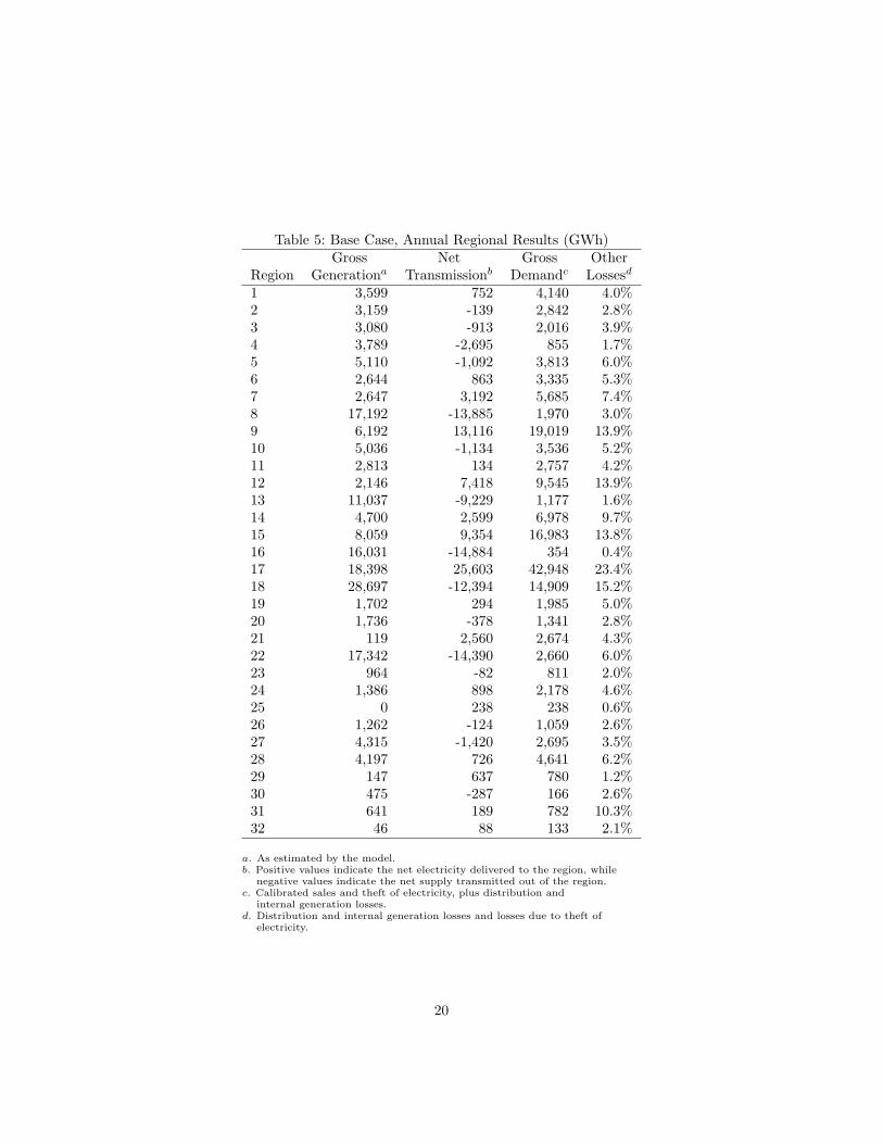
Table 5: Base Case, Annual Regional Results (GWh)Gross Net Gross Other

Region Generationa Transmissionb Demandc Lossesd

1 3,599 752 4,140 4.0%2 3,159 -139 2,842 2.8%3 3,080 -913 2,016 3.9%4 3,789 -2,695 855 1.7%5 5,110 -1,092 3,813 6.0%6 2,644 863 3,335 5.3%7 2,647 3,192 5,685 7.4%8 17,192 -13,885 1,970 3.0%9 6,192 13,116 19,019 13.9%10 5,036 -1,134 3,536 5.2%11 2,813 134 2,757 4.2%12 2,146 7,418 9,545 13.9%13 11,037 -9,229 1,177 1.6%14 4,700 2,599 6,978 9.7%15 8,059 9,354 16,983 13.8%16 16,031 -14,884 354 0.4%17 18,398 25,603 42,948 23.4%18 28,697 -12,394 14,909 15.2%19 1,702 294 1,985 5.0%20 1,736 -378 1,341 2.8%21 119 2,560 2,674 4.3%22 17,342 -14,390 2,660 6.0%23 964 -82 811 2.0%24 1,386 898 2,178 4.6%25 0 238 238 0.6%26 1,262 -124 1,059 2.6%27 4,315 -1,420 2,695 3.5%28 4,197 726 4,641 6.2%29 147 637 780 1.2%30 475 -287 166 2.6%31 641 189 782 10.3%32 46 88 133 2.1%

a. As estimated by the model.b. Positive values indicate the net electricity delivered to the region, while

negative values indicate the net supply transmitted out of the region.c. Calibrated sales and theft of electricity, plus distribution and

internal generation losses.d. Distribution and internal generation losses and losses due to theft of

electricity.

20

importing region) is a high consumption region with a high level of electricitylosses (13.7%). Acapulco on the other hand is primarily an importing regionbecause of its low level of generation.

The hydroelectric plants located on the Grijalva river (region 22) are also amajor source of energy for the central region of the country. These plants totalmore than 3,900 MW of capacity and more than 80% of the electricity theyproduce is exported north not only to the center but also to neighboring regionof Minatitlan (21) and the Yucatan peninsula.

Bajio (15), Guadalajara (12) and Ags-SLP (14) constitute a significant areaof consumption to the north of the Central region. These areas together forman industrial corridor that links the center of the country with the north. Man-zanillo (13) is a major source of energy for these regions as well for the center. Ithas two thermal plants with a joint capacity of 1,900 MW. Another importantregional electricity supplier is Lazaro Cardenas (16), which supplies the corridor(12-14-15) and the center (17), with a thermal plant of 2,100MW capacity anda 1,000MW hydroelectric plant.

The northern city of Monterrey (9) is the second largest consuming andimporting region in the country. The large coal-fired plants in Rio Escondido (8),with a total capacity of 2,600 MW, are a major source of energy for Monterrey.Other regions neighboring Monterrey are Laguna (7) to the west, Huasteca(10) to the south-east and Reynosa (11) to the north-east. Of these, Lagunais also a moderate importing region while Huasteca is a moderate exporter.Further growth of demand in the north-east of the country is clearly going torequire additional generating capacity in the region, or a strengthening of thetransmission links from the south of the country or from Texas.

4.2 Scheduled maintenance

Any least cost scheduling of generation plants to meet power demands and pro-vide reserve capacities has to allow plants to be taken out of service for mainte-nance. The optimal solution may involve some rolling maintenance, dependingon factors such as the seasonal pattern of the regional demand and the seasonalbehavior of fuel prices for different plant types. In our model, plant availabilitiesare choice variables, and the set of availability percentages per plant and perperiod are an important model output.

Table 6 summarizes the calculated availabilities by region and season. Theseasonal variation in availabilities reflects the pattern of aggregate electricitydemand, which attains its lowest values during the Fall and is the highest dur-ing the Summer months. There are, however, some interesting regional varia-tions. In particular, plants in some regions are made fairly uniformly availablethroughout the year, enabling them to compensate for the reduced availabilityof other plant taken off line for maintenance when demands tend to be lower.This backup task appears to be important in Mazatlan (4), which compensatesfor the low availability of plant in the northwest during the Fall, and Huasteca(10) and Oriental (18), which support the low availability of plant in the north-east during the Fall. Oriental (18) and Manzanillo (13) are interesting in so

21

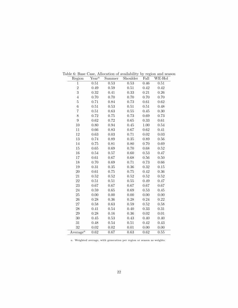
Table 6: Base Case, Allocation of availability by region and seasonRegion Yeara Summer Shoulder Fall WE-Hol

1 0.51 0.53 0.53 0.46 0.512 0.49 0.59 0.51 0.42 0.423 0.32 0.41 0.33 0.21 0.264 0.70 0.70 0.70 0.70 0.705 0.71 0.84 0.73 0.61 0.626 0.51 0.53 0.51 0.51 0.487 0.51 0.63 0.55 0.45 0.308 0.72 0.75 0.73 0.69 0.739 0.62 0.72 0.65 0.33 0.6110 0.80 0.94 0.45 1.00 0.5411 0.66 0.83 0.67 0.62 0.4112 0.63 0.03 0.71 0.02 0.0313 0.74 0.89 0.35 0.89 0.5614 0.75 0.81 0.80 0.70 0.6915 0.65 0.69 0.70 0.68 0.5216 0.54 0.57 0.60 0.53 0.4717 0.61 0.67 0.68 0.56 0.5018 0.70 0.69 0.71 0.73 0.6619 0.31 0.35 0.36 0.32 0.1520 0.61 0.75 0.75 0.42 0.3621 0.52 0.52 0.52 0.52 0.5222 0.51 0.51 0.55 0.49 0.4723 0.67 0.67 0.67 0.67 0.6724 0.59 0.65 0.69 0.53 0.4525 0.00 0.00 0.00 0.00 0.0026 0.28 0.36 0.28 0.24 0.2227 0.58 0.63 0.59 0.52 0.5828 0.41 0.54 0.40 0.33 0.3129 0.28 0.16 0.36 0.02 0.0130 0.45 0.53 0.43 0.40 0.4031 0.48 0.54 0.51 0.42 0.4332 0.02 0.02 0.01 0.00 0.00

Averagea 0.62 0.67 0.63 0.62 0.55

a. Weighted average, with generation per region or season as weights.

22

far as both have lowest availabilities in the Shoulder season, enabling them toprovide greater capacity and output during both the Summer and Fall seasons.By contrast plant in Guadalajara (12) and Ags-SLP (14) have their highestavailabilities during the Shoulder season of the year.

4.3 Calculated costs

A major motivation for constructing the model is that it allows us to examinetotal, average and marginal costs of electricity supply in Mexico. We wish tocompare the marginal costs in particular with current electricity prices. In thenext section of the paper, we study how the forecast increase in demand for 2005,and the completion of the planned new additions to generating and transmissioncapacity over the next few years, both affect costs.

As noted in the introduction to this section, the total generation costs calcu-lated by the model are 30,376 million pesos for 178,664 GWh generated duringthe period under analysis (November 1998 to October 1999). By contrast, theCFE reported that total generation costs for 1999 were 35,448 million pesos. Ittherefore is possible that the calculated marginal costs are too low. The cal-culated marginal costs would not be affected, however, if the accounting dataincludes fixed costs that have been omitted from our objective function.31

Tables 7, 8, 9 and 10 present the calculated marginal costs of power supplyfor each transmission region and in each time period. For the peak periodsin Summer and Fall, the marginal costs have been separated into the compo-nents associated with the demand constraints (14) and those associated withthe reserve constraints (19). Although the latter could in principle bind in anyperiod,32 we find that they bind only in either the summer or fall periods ofpeak demands, and even then not for all regions in both seasons.

The weighted average system-wide marginal cost (with weights determinedby consumption shares) is 32.08 cents Mexican per kWh. By contrast, thecalculated total cost of generation corresponds to an average of only 17.00 centsMexican per kWh, implying that the marginal cost is around 88% higher thanthe average cost.

Evidently, generation of electricity in Mexico is not a “natural monopoly”activity in the sense that average costs exceed marginal costs. This is usuallythe case in all countries, since plant with higher operating costs is used only tosupply electricity in peak periods. The marginal costs in peak periods also reflectthe cost of maintaining additional generating capacity to cope with emergencies.

The finding that the weighted marginal cost exceeds the average cost hasanother important implication. If wholesale prices reflected the marginal costof generation, the revenue raised would exceed the costs of generating the elec-

31Some items that accountants count as costs, including depreciation and interest costs,are appropriately excluded from an economic measure of costs. These items have, however,already been excluded from the reported cost of 35,448 million pesos.

32In particular, it is possible that scheduled maintenance, differences in seasonal demandsor transmission constraints might cause the reserve constraints to bind in periods other thanthose of peak demand.

23

tricity. In fact, the excess revenue would more than cover the reported annual“capital costs” for the CFE.33 If the depreciation and interest charges in theCFE accounts represent a competitive return to capital, then setting wholesaleelectricity prices equal to the marginal costs of generation ought to attract con-siderable entry into the industry, were that to be permitted by law. This isanother sense in which the generation of electricity in Mexico is not a naturalmonopoly. The essence of the natural monopoly idea is that a large incumbentfirm has a cost advantage relative to smaller potential entrants making entryunattractive. Our calculations suggest that, if wholesale electricity prices re-flected marginal costs, new generators would be delighted to set up business inMexico. Entrants would need to be guaranteed the same access to the transmis-sion network, and receive the same wholesale price for electricity supplied at thesame time and location, as the incumbent producers. In reality, this would re-quire the transmission business of the CFE to be separated from the generationbusiness. Effective competition in the wholesale market also would require thatthe existing generating stations be parceled out into many competing companiesand not kept as a monopoly entity.

The spatial and temporal variation of marginal costs is also of interest. Ta-bles 7 and 8 give the costs arising from both the demand and the reserve con-straints for time periods in which the reserve marginal cost is non-zero for atleast one region. The “full” marginal costs include both constraints since anincrease in “normal” demand within a period is assumed to increase extremedemand in the same proportion. To begin with, however, the discussion will fo-cus on the demand constraints only. These determine the energy requirementsfor the system and the “usual” pattern of electricity transmissions. The reserveconstraints indicate how the system behaves under extreme conditions and willbe discussed later.

In the North (regions 1 to 11 and all of Baja California), the demand forelectricity exhibits a strong seasonality with Summer as the peak season. Thisbehavior of the demand is reflected in marginal costs that are higher in thesummer than they are in the fall.

Within a given season, the peak hours represented by periods 1, 2, 6, 11 or16 tend to have the highest cost. Marginal costs are raised not only by the needto use more expensive generating plant, but also by the higher transmissionlosses.

In some regions, relatively abundant hydroelectric resources allow the pricespikes to be smoothed out or even eliminated. Since stored water can be runthrough the turbines at any time, the shadow value of using the water to generateelectricity should be equal in all periods in which it is used. Otherwise, costscould be reduced by saving water in periods when its value is lower and using itinstead when the cost of generating electricity using other technology is higher.Hydroelectric capacity is, in a sense, a substitute for storing electricity. Withoutit, marginal costs would fluctuate much more as the demand load on the system

33As noted earlier, in the 1999 CFE accounts, capital costs, primarily depreciation andinterest payments, were almost equal to 43% of total generation costs.

24

Table 7: Marginal costs by transmission region: Summer (May–August)(cents per kWh, Mexican Pesos)

Demand periods1 2 3 4 5

Region Dem Res Dem Res1 27.3 152.0 27.3 9.5 27.3 26.5 26.52 26.1 149.6 26.1 9.1 26.1 26.1 26.13 24.3 139.4 24.3 0.0 24.3 24.3 24.34 25.4 145.8 25.4 0.0 25.4 25.1 25.15 23.5 238.1 23.5 0.0 23.5 23.5 23.56 26.3 251.5 26.3 0.0 26.3 25.9 25.97 27.4 262.2 27.4 0.0 27.4 27.0 27.08 25.0 241.9 25.0 0.0 25.0 24.6 24.69 26.7 258.4 26.7 0.0 26.7 26.3 26.310 25.5 235.6 25.5 0.0 25.5 25.5 25.511 26.5 261.1 26.5 0.0 26.2 26.2 26.212 27.1 149.5 27.0 0.0 27.0 26.9 26.913 25.2 139.0 25.2 0.0 25.2 25.0 25.014 28.3 240.9 27.9 0.0 27.9 27.9 27.915 28.1 245.8 27.9 0.0 27.9 27.9 27.916 24.5 58.8 24.5 0.0 24.5 24.5 24.517 27.3 238.4 26.9 0.0 26.9 26.9 26.918 24.7 214.0 24.7 0.0 24.7 24.7 24.719 27.1 0.0 27.1 0.0 27.1 27.1 27.120 22.4 83.9 22.4 0.0 22.4 22.4 22.421 21.0 71.4 21.0 0.0 21.0 21.0 21.022 19.7 62.0 19.7 0.0 19.7 19.7 19.723 86.9 190.9 33.6 0.0 33.6 33.1 33.124 90.3 198.3 35.0 0.0 34.9 34.5 34.525 96.0 210.9 37.2 0.0 37.1 36.7 36.726 84.4 185.3 33.9 0.0 33.9 33.9 33.927 125.6 188.4 123.0 0.0 123.0 123.0 121.828 130.3 192.8 130.3 0.0 130.3 130.3 130.329 133.2 196.4 133.2 0.0 133.2 133.2 133.230 103.4 173.5 95.4 0.0 95.1 95.1 95.131 111.5 187.1 102.9 0.0 102.6 102.6 102.632 108.8 182.6 105.1 0.0 105.1 105.1 105.1

Weighted averages across groups of regions (with the sharesof group electricity needs as weights):

1–26 243.4 27.1 26.5 26.4 26.427–29 320.7 128.1 128.1 128.1 127.730–32 294.2 102.0 101.7 101.7 101.71–32 248.6 33.7 33.2 33.0 32.9

25

Table 8: Marginal costs by transmission region: Fall (Nov–Feb)(cents per kWh, Mexican Pesos)


Region Dem Res1 25.1 0.0 24.1 24.1 24.1 24.12 24.7 0.0 23.7 23.7 23.7 23.73 24.1 0.0 24.0 23.6 23.6 23.14 25.2 0.0 25.1 24.7 24.7 24.05 23.4 0.0 23.4 23.4 23.4 23.46 24.6 0.0 24.6 24.6 24.0 24.07 26.1 0.0 26.1 26.1 25.9 25.98 23.4 0.0 23.4 23.4 23.2 23.29 25.0 0.0 25.0 25.0 24.8 24.810 24.2 0.0 24.2 24.2 24.0 24.011 25.3 0.0 25.3 25.2 25.0 25.012 27.1 0.0 27.1 26.6 26.5 25.813 25.2 0.0 25.2 24.7 24.7 24.014 28.0 196.4 27.7 27.2 27.2 27.215 28.5 208.3 28.3 27.7 27.5 27.016 24.5 0.0 24.5 24.5 24.5 24.217 27.7 214.7 27.4 26.9 26.6 26.218 24.7 0.0 24.6 24.1 23.9 23.519 27.1 73.9 27.1 27.1 27.1 27.120 22.4 0.0 22.4 22.3 22.3 22.121 21.0 0.0 21.0 21.0 21.0 21.022 19.7 0.0 19.7 19.7 19.7 19.723 30.9 0.0 30.4 29.7 29.7 28.824 32.1 0.0 31.6 31.0 31.0 31.025 34.1 0.0 33.6 33.0 33.0 31.626 31.1 0.0 31.1 31.1 31.1 31.127 118.1 0.0 117.8 117.8 117.8 117.828 126.4 0.0 126.1 126.1 125.8 125.829 128.7 0.0 128.7 128.4 128.2 128.230 91.9 0.0 91.9 88.3 87.9 87.931 98.3 0.0 98.3 90.6 90.6 90.632 100.7 0.0 100.7 92.9 92.9 92.9

Weighted averages across groups of regions (with theshares of group electricity needs as weights):

1–26 120.7 26.2 25.8 25.6 25.327–29 123.8 123.6 123.5 123.4 123.430–32 97.6 97.6 90.6 90.5 90.51–32 120.8 31.5 30.9 30.6 30.3

26

Table 9: Marginal costs by transmission region:Shoulder (March, April, Sept, Oct)(cents per kWh, Mexican Pesos)

Demand periodsRegion 6 7 8 9 101 26.5 26.5 26.5 26.5 25.42 26.1 26.1 26.1 26.1 25.03 24.3 24.3 24.3 24.3 24.34 25.2 25.2 25.2 25.2 25.25 23.8 23.8 23.8 23.8 23.86 26.1 26.1 26.1 25.9 25.97 27.2 27.2 27.2 27.2 27.28 24.7 24.7 24.7 24.7 24.79 26.4 26.4 26.4 26.4 26.410 25.5 25.5 25.5 25.5 25.511 26.2 26.2 26.2 26.2 26.212 27.1 27.1 27.1 27.1 27.113 26.5 26.5 26.5 26.5 26.514 28.2 28.0 28.0 28.0 28.015 28.4 28.1 28.1 28.1 28.116 24.5 24.5 24.5 24.5 24.517 27.5 27.3 27.1 27.1 27.118 24.7 24.7 24.7 24.7 24.719 27.1 27.1 27.1 27.1 27.120 22.4 22.4 22.4 22.4 22.421 21.0 21.0 21.0 21.0 21.022 19.7 19.7 19.7 19.7 19.723 51.3 33.5 33.0 32.1 31.724 53.3 34.8 34.3 33.4 33.025 56.7 37.0 36.5 35.5 35.126 50.8 33.8 33.8 33.8 33.827 119.6 119.6 119.5 119.5 119.028 127.9 127.9 127.9 127.9 127.329 130.3 130.3 130.3 130.3 129.730 93.0 93.0 93.0 90.5 87.931 100.4 99.8 99.8 92.9 92.932 102.3 102.3 102.3 95.2 95.2

Weighted averages across groups of regions (withthe shares of group electricity needs as weights):

1–26 27.3 26.6 26.6 26.5 26.427–29 125.3 125.3 125.3 125.3 124.830–32 99.4 99.0 99.0 92.8 92.41–32 33.2 32.5 32.3 32.2 32.0

27

Table 10: Marginal costs by transmission region: Weekends–Holidays(cents per kWh, Mexican Pesos)



1–26 26.0 26.0 25.9 25.8 25.827–29 125.7 125.7 124.3 124.3 124.330–32 99.4 92.0 91.7 91.7 91.71–32 32.1 31.8 31.6 31.5 31.5

28

varies and plants with different operating costs become the marginal source ofsupply.

If hydroelectricity is available, but the amount of stored water is limited,prices may still fluctuate seasonally. The water is optimally used first to supplyelectricity at the peak periods. If water remains after doing that, it is used nextin the near-peak periods and so on. In the off-peak periods when water is notused, the price of electricity would be lower than in the periods when water isused.

Transmission losses, and transmission constraints, also influence the regionalpattern of marginal costs. It is simplest to consider first the case where noneof the transmission links is congested. The marginal cost at the sending end ofan active link then has to exceed the marginal cost at the receiving end by themarginal transmission loss. If the marginal costs in the two regions differ by lessthan the transmission loss, transmitting power between them is not worthwhileand the link will be inactive.

Laguna (7) and its neighboring regions (6, 4, 9 and 14) illustrate the effect oftransmission losses. In all periods, the marginal cost is higher in Laguna than inthe three regions Chihuahua (6), Mazatlan (4) and Monterrey (9) to the north,west and east. Evidently, power flows from these latter regions to Laguna. Onthe one hand, in all periods the marginal costs are higher in the Ags-SLP region(14) to the south than they are in Laguna. Power must therefore flow from thenorth to the central region along the Laguna to Ags-SLP link. The differencesin marginal costs along these links reflect the marginal transmission losses.

With an annul demand of 5,685 GWh, Laguna is a medium sized consump-tion center, but its scarce local generating capacity means that about 60% ofits electricity needs are supplied from other regions. Laguna is also a trans-shipment point, however, for power flowing from the north to the large demandload in the center of the country. Even though Laguna is a net importer ofelectricity, the link to the south has power flowing out of the Laguna region.Evidently, the excess demand for power in the central region of the country iseven greater than the excess demand in Leguna.

The Monterrey region (9) has the second highest demand for electricity inthe country and meets about 68% of its electricity needs with imports fromother regions. The marginal costs in Monterrey therefore are higher than in thesurrounding regions (8 and 10) that export power to Monterrey. On the otherhand, we have already seen that the marginal costs in Monterrey are below thosein Laguna so that, even though Monterrey is a net importer of electricity, powernevertheless flows from Monterrey toward Laguna in all of the model periods.

The pattern of marginal costs in Monterrey (9) versus Reynosa (11) is con-sistent with the direction of power flow reversing over the course of the year. Inthe summer and shoulder periods, the marginal costs in Monterrey are higherthan those in Reynosa, implying that power flows west toward Monterrey. Inthe fall, and on weekends and holidays, however, the marginal costs are lowerin Monterrey implying that power flows east toward Reynosa. This may be theresult of the different pattern of scheduled maintenance in the two regions.

There is also a reversal in the direction of power flow between the Huasteca

29

(10) and Oriental (18) regions. For most of the year, the marginal cost inhigher in region 10 than in region 18, implying that power flows north. In thetwo highest demand periods in the fall, however, the marginal cost is higher inregion 18 than in region 10 implying that power flows south. As the estimatedmonthly deviations in demand shares presented in Table 23 show, the seasonalfluctuation in demand is less in the south than in the north and also showsa slight peak in the fall as opposed to the summer. These different seasonalpatterns can explain the reversals in the direction of flow between the seasons.It is also interesting to note that even though power tends to flow south fromHuasteca to Oriental in the fall, for the three lowest demand periods in the fall,the flow is either from south to north or the link is inactive. As the representativedaily load curves in Figure 3 show, the fall season in the south is characterizedby a much greater peak to off-peak daily fluctuation than occurs in either seasonin the north or in the summer in the south. Thus, demand in the south duringthe three lowest demand periods in the fall is still low enough that additionalpower is not required from the north.

The lowest marginal costs occur in the Grijalva region (22). As we notedabove, there is more than 3,900 MW of hydroelectric capacity located on theGrijalva river. The total hydroelectric generating capacity in the Grijalva re-gion is sufficient to ensure that marginal generating costs there are constantthroughout the year. As one moves away from the Grijalva region to the north,marginal costs reflect more seasonal variation as transmission costs fluctuatewith the load and high cost local plant is used to supply peak demands.

Limited transmission capacity also plays a role in allowing costs to fluctuateacross seasons and times of the day as one moves away from the Grijalva region.The Yucatan peninsula (regions 23–26) dramatically illustrates how costs areaffected when transmission links become congested. The power flowing on theweak link34 between Grijalva and neighboring Lerma (region 23) is not sufficientto equilibrate marginal costs net of transmission costs. The higher costs arethen passed on to regions further down the system. In particular, further weaklinks between regions Lerma and Merida (region 24) and Merida and Chetumal(region 25) produce additional large increments in marginal costs. On the otherhand, Cancun (region 26) has marginal costs below those in Merida and almostas low as the marginal costs in Lerma. The Cancun region has the largestconcentration of generating plant in the Yucatan and evidently exports powerto the Merida region despite the high costs of satisfying the local demand.A strengthening of the Cancun to Merida link would actually raise prices inCancun even further as more power was exported to the west.

The large marginal cost differences between two regions linked by a bindingtransmission constraint represents the “shadow value” of increasing the capac-ity of the link. If there were competitive wholesale power markets at both endsof the link, market prices would reflect the marginal costs in each region. Anew entrant building a new link (or strengthening an existing one) could earnthe price differential in each period. If the discounted present value of these

34The capacity is 110 MW at 230 kV.

30

anticipated revenues were sufficient to cover the capital cost of the link up-grade, the project would be profitable and efficient to undertake. Independententrepreneurs have already invested in such network upgrades in the wholesaleelectricity markets in Australia.

The value of additional links in Mexico is even more apparent in the BajaCalifornia peninsula. Currently, there are two systems in Baja that are notconnected to the rest of the Mexican grid, although the system in the northof Baja is connected to the United States via California. The marginal costsof generation are in Baja California are higher than they are anywhere else inthe country. The region currently depends on diesel generating plants that areexpensive to operate. If market prices reflected marginal costs, there would bea large incentive to strengthen connections between Baja California and theremaining networks in both Mexico and the United States.35

A change in one network link is likely to have consequences elsewhere in thesystem. For example, strengthening the Cancun to Merida link also would re-duce the differential in marginal costs between Lerma and Merida and thereforethe implicit value of augmenting the capacity of the Lerma to Merida link. It isnot inefficient, however, for a potential investor in one link to ignore these effectson other links. As in any market, a change in supply or demand conditions canaffect the prices paid or received by other consumers or producers. The pricechanges signal that the opportunity cost of using scarce resources has changedand that supply and demand decisions need to be adjusted accordingly. Thereis, therefore, no need to centrally coordinate network investment decisions onthese grounds.

It might be thought that the need to maintain the physical stability of thenetwork is a different matter. In general, the stability of voltage levels, fre-quencies and power flows depends on the whole network and not just individuallinks. Even in this case, however, if there were competitive markets in ancillaryservices (as discussed above) actions that stabilize, or destabilize, the networkwould be priced and private individuals and firms would receive appropriatesignals to take these factors into account when making their decisions aboutsupply and demand.

Concerns about imperfect competition, however, may justify oversight ofnetwork operation and expansion. Network operation is a “natural monopoly”activity in the sense that only one agency can be responsible for schedulinggenerators to supply demand while maintaining system operating parameterswithin specified bounds.36 A network operator that also owned generating plantor transmission links would have an incentive to manipulate the dispatch ofgenerators to increase returns to its own assets. Similarly, an owner of one

35The model does not consider international electricity trade with the USA. There are plansto place new generating plant in Baja California using imported LNG as fuel. These plans,if brought to fruition, would strengthen the transmission grid in Baja and turn the regioninto a power exporter to the US. One of the perceived advantages of siting the plant in Bajaand exporting the power north is that it would enable US utilities to circumvent politicalconstraints on siting new plants in California.

36Extensive and frequent use of sub-contracting, however, would allow the construction andmaintenance of network facilities to be organized as a competitive industry.

31

network link who owned other links, or generating plants, may have an incentiveto limit transmission capacity in order to drive up the rents on other assets.Regulatory oversight may be needed to prevent the abuse of monopoly if theindustry is not structured to ensure adequate competition.

Tables 7 and 8 also report non-zero marginal costs associated with the re-serve constraints (19). These costs represent the lowest fixed operation andmaintenance costs that the system must incur in order to provide the last kWof capacity reserve required to cope with emergencies. While the reserve con-straints for each region could bind in any period, in practice they do not bindin periods other than 1, 2 or 11,37 which are peak periods of demand for someregions of the country. Summer demand in the south, and demand for the sys-tem as a whole, peaks in period 1, while period 2 corresponds to the summerpeak in the north. Period 11 coincides with the fall peak in the south, which forsome regions exceeds the summer peak in period 1. The generating capacities,gn, associated with the reserve constraints do not vary period by period. Theyare established for the year as a whole and potentially constrain generation out-put in each period. Ensuring that capacity is sufficient to cope with extremedemand fluctuations in the peak periods, however, is likely to guarantee alsothat capacity will be more than sufficient to cope with the same proportionalvariation in demand in off-peak periods.

In all regions except Acapulco (19), the reserve constraints bind in the peakperiod for the system as a whole. If there were no binding transmission con-straints, we would expect to find the reserve constraints binding only in the peakperiod for the system as a whole. Even if demand peaked in other periods inparticular regions, there would have to be surplus capacity elsewhere in systemat those times since the system as a whole needs sufficient capacity to meet thehighest overall demand peak. Although there are transmission losses associatedwith using surplus plant located in other regions to meet local demand surges,such extreme demand surges are brief. The transmission losses generally wouldbe small relative to the cost of keeping additional generating capacity availableto supply output for only short periods of time. Regional demand variationsthat are negatively correlated will not affect the overall system demand as muchas positively correlated demand shocks. Analogously to financial markets, theundiversifiable component of demand variation is the relevant “risk” that givesrise to a demand for the “insurance” supplied by surplus generating capacity.

The argument that there should be only one period when the reserve con-straints bind implicitly assumes, however, that there is an unrestricted ability toarbitrage costs differences between regions. Transmission losses raise the costsof arbitrage, but transmission capacity constraints can prevent arbitrage alto-gether. In particular, the variation in marginal costs associated with the reserveconstraints in Mexico is much more extreme than the variation in marginal costsassociated with the demand constraints. Evidently, many of the transmissionlinks in the Mexican system are weak and become congested under conditions

37The marginal costs associated with all reserve constraints in periods other than 1, 2 or 11are zero and have not been reported in the tables.

32

of extreme demand.The Acapulco region (19) provides an obvious example of the effect of trans-

mission constraints. The fact that the reserve constraint does not bind in thisregion in period 1, despite its connection with the rest of the system, impliesthat the 240MW link between Acapulco and the Central region (17) must becongested. Table 6 provides a further indication of this. The availability of theplant in Acapulco remains at just 35% in the summer season despite the highimplicit return to providing capacity to the Central region in times of extremedemand during those months. The reserve constraint in Acapulco thus dependson local demand variation more than system-wide variation in demand, andhence binds at the local peak in the fall rather than the system peak in thesummer. The associated marginal cost (in cents per kWh) is determined by thelocal cost of providing additional capacity and the number of hours over whichthat cost will be spread.

Transmission constraints also play a role in producing the remaining bindingreserve constraints in periods 2 and 11. These cases are somewhat different,however, in that the reserve constraints also bind during the system peak inperiod 1.

The Ags-SLP (14), Bajıo (15) and Central (17) regions have binding reserveconstraints in the fall as well as the summer. Bajıo and Central both have veryhigh total demand, with a local peak in period 11 during the fall. The reserveconstraint can be binding in both periods 1 and 11 since the transmission levelsare different. In particular, the fact that the reserve constraints are not bindingin regions 7, 12, 16 or 18 in period 11 implies that the transmission links fromthese regions to regions 14, 15 and 17 must be congested under an extremedemand load during period 11. By contrast, under an extreme demand loadduring the system peak period, power flows north from region 14 to region7, for example, so the link from 7 to 14 cannot be congested in the southerndirection. Local reserve capacity in regions 14, 15 and 17 that is sufficient tomeet the local extreme demand in period 11, with maximum import of powerfrom elsewhere in the network, therefore is not sufficient to meet local extremedemand in period 1 when less power is available from other regions.

A similar explanation applies to the Sonora Norte (1) and Sonora Sur (2)regions, which have binding reserve constraints in the second as well as thefirst summer period. These regions (as do all regions in the north) have localpeak demands during period 2 rather than period 1.38 Regions 1 and 2 areconnected to the rest of the network via a relatively weak 220MW link to region3 (Mochis). Since the reserve constraint in region 3 is not binding in period2, the transmission link must be congested under an extreme period 2 load.Under an extreme demand load in period 1, however, the demand for powerin southern regions is substantially greater than it is in period 2, leaving lessavailable to satisfy demand in the north. The transmission link between regions3 and 2 remains uncongested, but more local capacity is required to satisfy the

38Recall, however, that the differences in demand between periods 1 and 2 in the northare slight. This may explain why there are not more northern regions with binding reserveconstraints in period 2 in addition to period 1.

33

slightly reduced extreme demand load.Region 16 (Lazaro Cardenas) has much stronger links (950MW, 460MW and

400MW) to the rest of the network than do the Acapulco or Sonora regions.Nevertheless, it can also be affected by transmission constraints. The marginalreserve cost in period 1 is only 58.8 cents Mexican per kWh in region 16 but149.5, 238.4 and 245.8 in the three neighboring regions 12, 15 and 17. Thesedifferences in marginal cost greatly exceed the transmission losses and indicatecongested transmission lines. Lazaro Cardenas has its local peak in the fall andwill need greatest capacity during a temporary demand surge in period 11. Thelink to region 12 is not congested during period 11, however, and can transmitpower to region 16 from the north. As a result, the reserve capacity needed inregion 16 in the summer is sufficient to also cover a demand surge during period11.

Lazaro Cardenas actually has the smallest reserve marginal cost of any re-gion. As Table reftransregions reveals, this region has only three generatingstations with a 1999 capacity of 3,395MW. The marginal cost of expanding theavailable capacity of these plants evidently is relatively small.

The Grijalva region (22) has marginal reserve costs that are almost as low asthose in Lazaro Cardenas. Table reftransregions shows that the Grijalva regionhas only hydroelectric plants, with capacity that can be made available at ahigher level at relatively low cost. The large jump in marginal reserve cost inperiod 1 between regions 20 and 18 implies that the transmission link betweenthese regions is congested under extreme demand conditions in period 1. Thecongested link between regions 18 and 20 prevents the Grijalva hydroelectricplants from providing further relatively low cost capacity to meet demand surgesin regions further to the north and west of region 18.

From the values presented in Tables 7 and ?? it is clear that the high marginalreserve costs in periods 1 and 11 help drive the weighted average marginal costabove the average cost of generation. As we noted above when introducing thereserve constraints, in an ideally structured wholesale market for electricity atleast some of these payments would take the form of payments for ancillaryservices. Under extreme demand loads, additional generating capacity is placedon standby in case it is needed to maintain voltage and frequency levels, or tore-start the system in the event of a blackout. Owners of plant that is cheap tokeep on stand-by and fast to convert to supplying output could earn a returnfor providing the reserve capacity even if they are not actually called upon tosupply power.

4.4 Prices and marginal costs

The model calculations show that the marginal costs of generating electricityvary by the location of the consumer and the time at which consumption occurs.In reality, the latter dependence primarily reflects different costs of supply asthe total load on the system varies.39 Prices of electricity in Mexico, however,

39Marginal costs also vary by time, however, because of factors such as the need to as-sign contiguous periods for scheduled maintenance, allowing for holiday periods or seasonal

34

Table 11: Average price versus marginal generation cost by region and season

Administrative Summer Shoulder Fallregion price cost price cost price costBaja California 0.6000 1.3445 0.5899 1.2198 0.5312 1.1992Noroeste 0.5272 0.3372 0.4767 0.2568 0.4787 0.2395Norte 0.4527 0.3693 0.4645 0.2588 0.5065 0.2484Golfo Norte 0.4836 0.3770 0.4926 0.2619 0.5166 0.2483Golfo Centro 0.4712 0.3586 0.4829 0.2554 0.4946 0.2418Bajıo 0.4842 0.3977 0.4865 0.2809 0.5207 0.3755Jalisco 0.5602 0.3397 0.5675 0.2705 0.5871 0.2638Centro Occidente 0.4248 0.2740 0.4294 0.2454 0.4453 0.2452Centro Oriente 0.4887 0.3507 0.5007 0.2470 0.5130 0.2414Centro Sur 0.5025 0.2712 0.5256 0.2712 0.5490 0.3071Oriente 0.4617 0.3428 0.4762 0.2449 0.4873 0.2397Sureste 0.5821 0.2364 0.6034 0.2037 0.6338 0.2036Peninsular 0.5949 0.4653 0.6236 0.3560 0.6488 0.3101LyF 0.5831 0.3848 0.6038 0.2714 0.6356 0.3734

typically do not vary much by location or time of demand and thus do notclosely mimic the marginal generation costs. In particular, while there is limitedseasonal variation in prices, there is little variation by time of day.

Electricity suppliers incur costs apart from generation, including the costs ofmaintaining the distribution network and providing customer service, that donot vary as systematically by time or location. Nevertheless, prices are unlikelyto accurately signal the marginal costs of supply to consumers unless they varyby location and time of supply.

Table 11 presents the average electricity price paid in each administrativeregion in the three main seasons. For comparison, it also provides the weightedaverage marginal generating costs calculated from the model. The latter arederived by weighting the marginal costs in Tables 7, 8, 9 and 10 by the cor-responding demands in each transmission region and each season. Since therevenue needs to cover more than generating costs, it is not surprising thatprices on average exceed the marginal generating costs. It is somewhat moreinteresting, however, to note that the average prices vary much less by seasonand region than do the marginal costs. Furthermore, in many cases, the patternof marginal cost variation across regions and seasons is not reflected in the pricevariations. This is particularly apparent for those regions where the reservemarginal costs are positive in periods other than the summer peak. It wouldappear that consumers, and potential generators of electricity, are not beinggiven very appropriate signals about the costs or benefits of changing electricitydemands or supplies at different locations on the network or at different times

availability of water supplies for hydroelectric plant.

35

of the year.The electricity tariffs in Mexico fall into two main categories. One category,

known as “specific rates,” classifies customers by the purpose for which theyuse electricity. The tariffs for residential, commercial, agricultural and publicservices demand largely fall into this category. The second group of tariffs dif-ferentiate between customers based on the amount of energy that they consumeand other characteristics of their supply including in particular the voltage levelat which they draw power. The latter is important because many losses occurin the distribution network or result from transforming power to lower voltagelevels. Hence, it is generally much less costly to supply power to large customersdrawing directly from the high voltage transmission network.

Residential tariffs. The price of electricity for households is a step functionwith three price levels that depend on demand. The prices for each step changeaccording to region and season and thus could, in principle, partially reflectcost differences.40 All residential customers face the same rate scale in non-summer months. During the summer, however, households are charged differentrates according to the average temperature of the region. A common problemwith step function tariffs is that different households pay a different price forelectricity that costs the same amount to supply to each of them. This leads toinefficiencies since the household paying a higher price would be willing to paymore for the marginal power consumed by the household paying the lower pricebut is prevented from doing so.

Agricultural tariffs. Agricultural users face two different tariffs dependingon the voltage level at which they take supply. In either case, the tariff sched-ule is a step function with four levels. As with residential tariffs, prices varysomewhat by region and season.

Commercial tariffs. Commercial users also face a step function tariff, withthe marginal price determined by the maximum demand and the total consump-tion within the billing period. In this case, the prices on the steps of the tariffdo not vary by region or season, but are changed from one billing cycle to thenext via indexation to components of the wholesale price index.

Industrial tariffs. There are 16 different schedules for the industrial sectorand two additional rates for firms willing to allow their service to be interruptedat short notice.41 All but one of the industrial tariffs includes some price dif-ferences by region and by hour of use. The latter differentiation is based on

40Such a price structure could not reflect all cost differences since marginal costs vary withina day or across days of the week in addition to seasons.

41In the latter case, companies enrolled in the program are asked, at least 15 minutesin advance, to reduce their demand for electricity. They are then credited an amount thatdepends on the reduction in demand. There are two categories of such service, one for demandsequal or higher than 10,000 kW in peak hours and another for demands equal or higher than20,000 kW.

36

base, intermediate and either semi-peak or peak demand. Charges are furtherdifferentiated depending on the voltage level at which service is provided, totalenergy consumed within the billing period, the overall maximum demand withinthe billing period or the sum of the maximum daily demands within the periodor whether the firm agrees to pay a fixed charge. In this sector, the price forelectricity is indexed to the variation of fuel prices and to the producer price ofthree industrial components of the wholesale price index.

4.5 Altered plant availability

The base case has demonstrated that hydroelectricity plays a significant rolein the Mexican electricity supply system. An important problem that Mexicofaces, however, is that rainfall is not always reliable and the availability ofhydroelectric plants can be severely curtailed as a result of drought.

To see how the system is affected by reduced hydroelectric plant availability,we re-computed the costs of meeting the 1999 demand levels but using theavailability of plants from 1998. As a result of dry weather, hydroelectric planthad much lower availability levels in 1998 than in 1999. To compensate, manyof the thermal plants were run at higher availability levels.

Table 12 gives the differences in annual availabilities in the two years byregions. The differences between the two years are not only the result of differentavailabilities of hydroelectric plant. Using the actual availabilities from 1998,however, allows us to examine what can happen under an alternative “realistic”scenario.

Comparing Table 12 with Table 4, we see that the main regions with reducedavailability in 1998 relative to 1999 are those with substantial hydroelectricgenerating plant. In particular, the availabilities in regions 21 (Minatitlan)and 22 (Grijalva), which have only hydroelectric plant, were 35.7% and 39.6%lower in 1998 than in 1999. Guadalajara (region 12), which had 57.8% loweravailability in 1998, has 8 hydroelectric generating plant and only 1 thermalplant. Other regions with significantly lower availability in 1998 were Acapulco(region 19, with 3 hydroelectric and 1 thermal plant) and Temascal (region 20,with 2 hydroelectric and 1 renewables plant).

Low water supplies were, however, not the only problem in 1998. Threeregions in Baja California with only thermal plant (Ensenada, 29, Tijuana, 28,and Cabo San Lucas, 32) each had substantially reduced availability, althoughthe very small Ensenada, and particularly the Cabo San Lucas, plants also hadfairly low availabilities in 1999.

The most significant increases in availability in 1998 relative to 1999 typicallywere in regions with substantial thermal generating plant. Examples includeregions 7 (Laguna, with 5 thermal plants), 26 (Cancun, with 7 thermal plants),27 (Mexicali, with 2 thermal and 3 renewable plants) and 5 (Juarez, with 1thermal plant). On the other hand, three regions with significant numbers ofhydroelectric plant also had higher availabilities in 1998 than 1999. These wereCentral (region 17, with 13 hydroelectric and 7 thermal plants), Bajıo (region

37

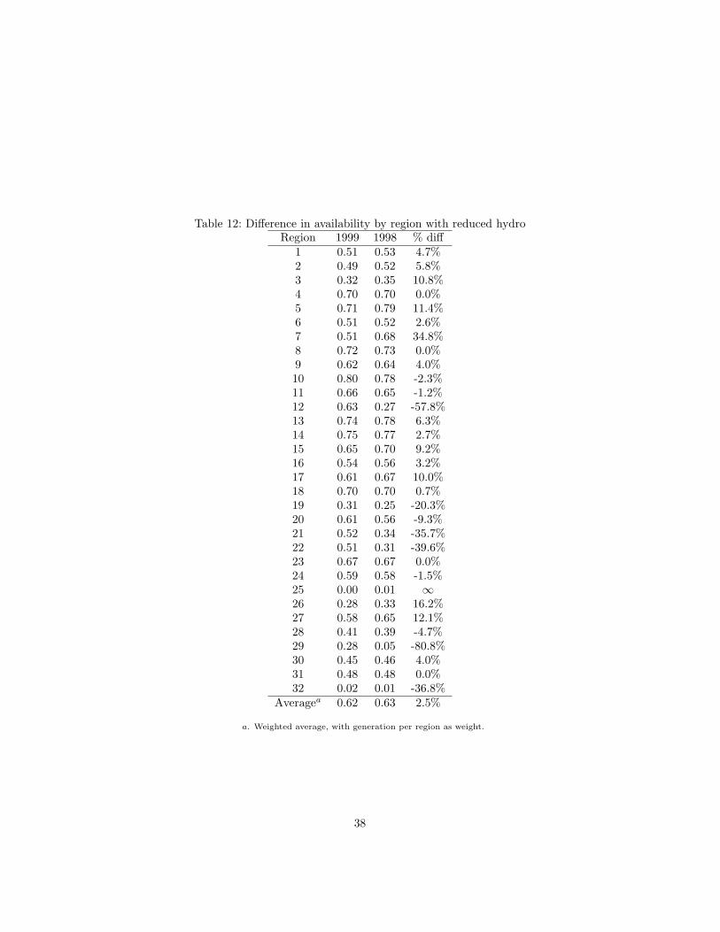
Table 12: Difference in availability by region with reduced hydroRegion 1999 1998 % diff

1 0.51 0.53 4.7%2 0.49 0.52 5.8%3 0.32 0.35 10.8%4 0.70 0.70 0.0%5 0.71 0.79 11.4%6 0.51 0.52 2.6%7 0.51 0.68 34.8%8 0.72 0.73 0.0%9 0.62 0.64 4.0%10 0.80 0.78 -2.3%11 0.66 0.65 -1.2%12 0.63 0.27 -57.8%13 0.74 0.78 6.3%14 0.75 0.77 2.7%15 0.65 0.70 9.2%16 0.54 0.56 3.2%17 0.61 0.67 10.0%18 0.70 0.70 0.7%19 0.31 0.25 -20.3%20 0.61 0.56 -9.3%21 0.52 0.34 -35.7%22 0.51 0.31 -39.6%23 0.67 0.67 0.0%24 0.59 0.58 -1.5%25 0.00 0.01 ∞26 0.28 0.33 16.2%27 0.58 0.65 12.1%28 0.41 0.39 -4.7%29 0.28 0.05 -80.8%30 0.45 0.46 4.0%31 0.48 0.48 0.0%32 0.02 0.01 -36.8%

Averagea 0.62 0.63 2.5%

a. Weighted average, with generation per region as weight.

38

15, with 9 hydroelectric, 3 thermal and 1 renewables plant) and Mochis (region3, with 6 hydroelectric and 2 thermal plants).

It might be thought that if thermal plant can be made more available indrought years they could be made more available in all years. Using thermalplant to generate more electricity is, however, likely to lead to increased mainte-nance problems in the future. Higher availability in one year therefore is likelyto lead to reduced availability in future years as plants are taken out for main-tenance. Running plants harder in one year is also likely to raise the annualmaintenance costs in future years. This factor has been ignored in our costestimates presented below.

We will not discuss all the details of the altered availability scenario.42 Weshall instead focus on the major differences in costs and system operation rela-tive to the base case.

In the scenario with 1998 availabilities, the system generates only 177,971GWh compared with 178,664 GWh generated in the base case. Both scenarioshave the same final demand levels. Hence, the difference between generationlevels implies that transmission losses are lower under the altered availabilityscenario.

The minimized total generating cost of meeting the 1999 demands with the1998 plant availabilities is 31,595 million pesos compared with 30,376 millionpesos in the base case, even though more electricity is generated under thebase case. Changing the plant availabilities raises the minimized total costs,and average costs per kWh of power provided to consumers, by about 4%.The differences in marginal costs between the two scenarios are even larger.The weighted average marginal cost (with final demands as weights) in thereduced availability case is 38.58 cents per kWh compared with 32.08 cents perkWh in the base case, which is an increase of 20.3%. The dramatic increase inmarginal costs resulting from the reduced availability of hydroelectricity reflectsthe higher costs of marginal thermal generating plant. It is another indicationthat electricity generation is not a “natural monopoly” in the sense of exhibitingdeclining costs as output expands.

Although the weighted average marginal cost is higher under the alternativeavailability scenario, the dispersion in marginal costs across regions is less in allperiods, except only for the marginal reserve costs in period 2. This result mayseem surprising. Since stored water can be used to generate hydroelectricity atany time, it generally allows the dispersion in costs across time periods to bereduced. Thus, a lower availability of hydroelectric capacity might be expectedto produce more variable marginal costs. In the Mexican system, however,lower availability of hydroelectricity requires a greater use of localized thermalgeneration to satisfy demand. With less hydroelectricity being produced andtransmitted over long distances, the network becomes less congested. Whenlinks are being used at less than capacity, a marginal change in local demandcan be met by a marginal change in transmission levels. The price differentialsbetween regions then become the marginal transmission losses. These are gen-

42Complete results are available from the authors upon request.

39

erally much smaller than the marginal cost of increasing output from differentlocal thermal plants.

The different marginal costs of reserves under the two scenarios also reflectthe lower extent of network congestion when hydroelectricity is less available.In particular, when it is possible to meet demand fluctuations by adjustingtransmission levels, cost differences can be arbitraged away to a greater extentand the network behaves more like a unified system. Except for regions 1 and2, the reserve marginal costs are positive only in period 1 when the system-widedemand peaks. In particular, transmission links to the central regions 14, 15, 17and 19 can carry more power in the fall than they do in the summer, allowingthe local generating capacity required for the system peak to cope with the localpeak in the fall. From Table 12, generators in regions 14, 15 and 17 were usedmuch more extensively under the 1998 regime.

In regions 1 and 2, marginal reserve costs are positive during both the localpeak (in period 2) and the system-wide peak (in period 1). Since the trans-mission constraint from region 3 to region 2 is constrained in period 2, higherdemand in period 2 can be met only by increased use of local plant.

The marginal costs in the Baja California regions (27–32) are the othermajor difference between the base and the altered availability scenarios. TheBaja California costs are lower under the alternative scenario, while costs inmost other regions are higher. The major explanation, as Table 12 and Table 4show, is that the regions within Baja California that had increased availabilityin 1998 tended to have higher available plant capacities in 1999 than the regionswith reduced availability.

5 The anticipated situation in 2005

In this section, we combine the model of the electricity supply system withthe demand forecasts to investigate how planned additions to generating andtransmission capacity will enable the system to deal with the anticipated growthbetween 1999 and 2005. We focus on 2005 since the investment schedule untilthen has been approved and most of the projects are already under construction.For years beyond 2005, the investment projects are more uncertain.

Table 13 presents the expected construction of generating capacity from2000 to the end of 2004 in each of the 32 transmission regions.43 Table 13 alsogives our estimates of the forecast evolution of electricity sales44 and generationoutput by transmission region.

The state-owned CFE recently has encouraged greater private investmentin electricity generation. This has taken the form of self-generation by largeindustrial plants with sales back to the CFE when output exceeds the firm’s

43The data on planned additions to generating capacity and their costs are fromthe CFE, “Prospectiva del Sector Electrico 2001-10,” the Ministry of Finance andPublic Debt (SHCP), “Presupuesto de Egresos de la Federacion 2002,” available athttp://www.shcp.gob.mx/docs/pe2002/pef/temas/pidiregas/cfe.pdf, and the Energy Regula-tory Commission (CRE), http://www.cre.gob.mx/estadisticas/stat98/electr.html.

44Sales and demand for electricity are different because of the losses.

40

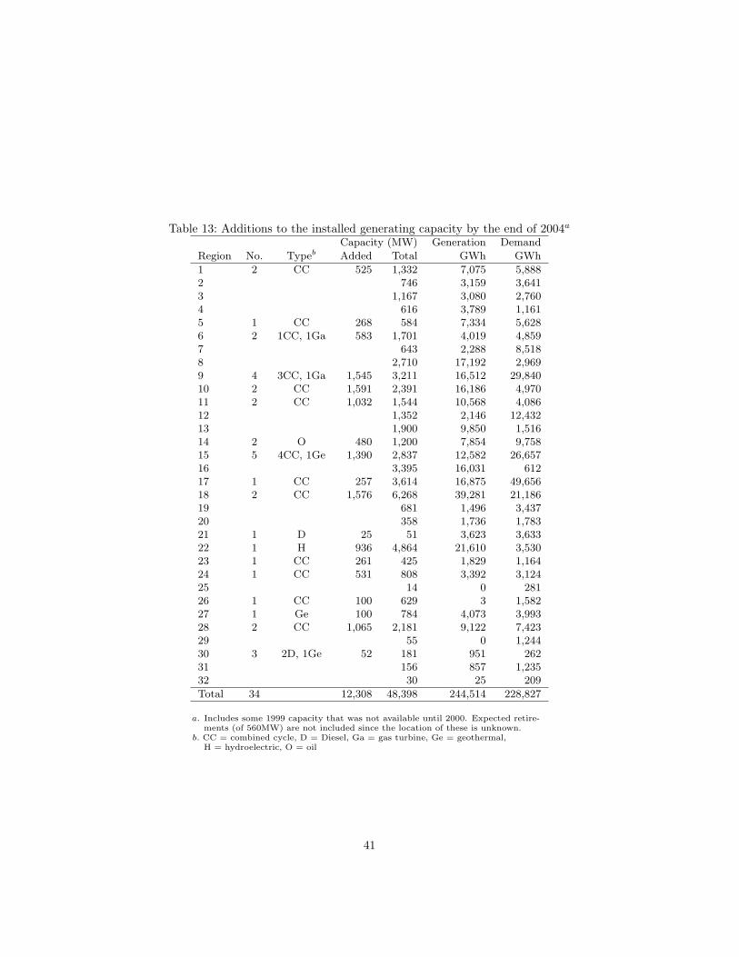
Table 13: Additions to the installed generating capacity by the end of 2004a

Capacity (MW) Generation Demand

Region No. Typeb Added Total GWh GWh

1 2 CC 525 1,332 7,075 5,8882 746 3,159 3,6413 1,167 3,080 2,7604 616 3,789 1,1615 1 CC 268 584 7,334 5,6286 2 1CC, 1Ga 583 1,701 4,019 4,8597 643 2,288 8,5188 2,710 17,192 2,9699 4 3CC, 1Ga 1,545 3,211 16,512 29,84010 2 CC 1,591 2,391 16,186 4,97011 2 CC 1,032 1,544 10,568 4,08612 1,352 2,146 12,43213 1,900 9,850 1,51614 2 O 480 1,200 7,854 9,75815 5 4CC, 1Ge 1,390 2,837 12,582 26,65716 3,395 16,031 61217 1 CC 257 3,614 16,875 49,65618 2 CC 1,576 6,268 39,281 21,18619 681 1,496 3,43720 358 1,736 1,78321 1 D 25 51 3,623 3,63322 1 H 936 4,864 21,610 3,53023 1 CC 261 425 1,829 1,16424 1 CC 531 808 3,392 3,12425 14 0 28126 1 CC 100 629 3 1,58227 1 Ge 100 784 4,073 3,99328 2 CC 1,065 2,181 9,122 7,42329 55 0 1,24430 3 2D, 1Ge 52 181 951 26231 156 857 1,23532 30 25 209

Total 34 12,308 48,398 244,514 228,827

a. Includes some 1999 capacity that was not available until 2000. Expected retire-ments (of 560MW) are not included since the location of these is unknown.

b. CC = combined cycle, D = Diesel, Ga = gas turbine, Ge = geothermal,H = hydroelectric, O = oil

41

Figure 4: Planned changes to the transmission network by 2005

own needs (co-generation), and also private construction under various types ofcontracts with the CFE. The latter category includes BLT, IPP and “turnkey”plants built by the private sector, but with all of the output produced or pur-chased by the CFE. Co-generators are allowed to sell only up to 25% of thecapacity of their plants to the CFE, and only under very restrictive conditions.

Under the BLT, IPP and turnkey schemes, firms bid through public tenderto provide new plants. The BLT plants are operated by the CFE, but leased fora period before being turned over to the CFE. By contrast, the private builderof an IPP plant also operates the plant under a long term contract to supplypower to the CFE. In a turnkey project, the private firm constructs the plantfor the CFE, which then owns and operates the plant.

Table 13 covers all private and public sector projects. In fact, of the ex-pected 69,084 million pesos (in year 2001 currency) of proposed investments ingenerating plant between 2000 and 2004, 66,891 million pesos will be under-taken by private firms. Seven of these are co-generation projects expected toprovide about 1,889 MW of capacity by the end of 2004. Of the 12,308 MW ofadditional capacity by the end of 2004, 7,303 MW will be built by private firms,with 6,198 MW of this in combined cycle plants. Public investment is expectedin just two plants – a 114 MW hydroelectric plant and a 125 MW combinedcycle plant.

In addition to new generating plant, the CFE have plans for substantialenhancements to the transmission network. These involve building new linksbetween some regions and enhancing some of the existing links. Figure 4 illus-trates the changes that are expected to be in place for the period November2004 to October 2005.

42

As with the generation investments, much of the investment in the trans-mission system is being undertaken by the private sector. Of the 75,272 millionpesos (in 2001 currency) required to undertake the transmission investmentsillustrated in Figure 4, 46,684 will be financed by the private sector and 28,588by the public sector. The private schemes are BLT and turnkey projects, or elsetransmission investments associated with co-generation projects.

The estimated total generation costs in 2005 (in year 2000 currency) are40,116 million pesos. The forecast power generated for the period November2004 to October 2005 is 244,539 GWh. Recall that the corresponding numbersfor 1999 were a cost of 30,376 million pesos and a total output of 178,664 GWh.The average generation cost in 2005 is 16.40 cents per kWh compared with 17.00in 1999. The average generating costs are thus predicted to decline slightly de-spite a forecast growth in production of almost 6.5% per year. Whether ornot the investments are justified depends on the magnitude of the investmentsrelative to the value of the additional electricity generation for consumers. Wedo not have sufficient information to make this judgment. The rather low priceelasticity of demand estimated in the first section of the paper implies, how-ever, that the loss in consumer surplus associated with a reduction in electricityconsumption is likely to be quite large.

If all the planned investments are completed, our model also forecasts thatthe demand-weighted marginal costs will decline from 32.08 cents per kWh in1999 to 25.46 cents per kWh in 2005. This is an even larger percentage declinethan for the average costs. The geographical and temporal variation of marginalcosts is also forecast to change. Tables 14, 15, 16 and 17, corresponding toTables 7, 8, 9 and 10 in the base case, present the forecast marginal costs in 2005.In particular, reserve costs are expected to be non-zero only in the summer peakperiod in 2005, while the marginal costs associated with the demand constraintsare also expected to vary less than in 1999. Both of these results suggest thatthe transmission network is likely to be less constrained in 2005 than it was in1999.

5.1 Reduced transmission investment

The level of planned investment in generating and transmission capacity from2000–2004 is 144,356 million pesos (in 2001 currency). Of this amount, over30,000 million pesos is slated to come from the public sector. There are alsolarge planned expenditures for investments in the distribution system and themaintenance of existing capital. The public sector is expected to finance over50,000 million of the more than 62,000 million pesos expected to be invested inthe distribution system, while maintenance expenditure of almost 30,000 millionpesos will also need to be financed by the public sector.

The proposed transmission investments rely much more heavily upon directpublic expenditures than do the generation investments. If the Mexican govern-ment encounters fiscal problems in the next two years, some of the transmissioninvestments may be postponed. We therefore considered a scenario where allthe generation investments are made as planned, but some of the investments

43

Table 14: Marginal costs by transmission region: Summer (May–August)(cents per kWh, Mexican Pesos)


Region Dem Res1 25.9 192.1 25.9 25.7 24.4 24.42 25.6 189.9 25.6 25.6 24.7 24.73 25.1 180.0 25.1 25.1 25.1 25.14 26.0 186.2 26.0 26.0 25.8 25.85 26.1 195.6 25.7 25.2 24.0 23.96 26.5 199.3 26.2 25.7 24.5 24.47 28.3 218.3 27.9 27.5 26.5 26.58 25.0 195.0 24.7 24.2 23.5 23.39 26.8 206.3 26.4 25.8 25.1 24.910 25.2 186.3 24.8 24.8 24.8 24.811 25.7 198.0 25.3 24.8 24.1 23.912 26.8 188.6 26.7 26.5 26.5 26.513 24.7 174.1 24.7 24.7 24.7 24.714 27.1 203.8 26.7 26.3 26.0 26.015 27.5 202.3 27.1 26.9 26.7 26.716 24.9 170.0 24.9 24.9 24.9 24.917 26.3 183.5 25.5 25.5 25.5 25.518 24.4 170.1 24.4 24.4 24.4 24.419 25.9 180.3 25.9 25.9 25.9 25.920 22.3 148.4 22.3 22.3 22.3 22.321 20.8 132.6 20.8 20.8 20.8 20.822 20.4 124.9 20.4 20.4 20.4 20.423 21.2 176.4 21.2 21.2 20.8 20.724 21.7 183.2 21.5 21.5 21.2 20.925 22.0 185.8 21.8 21.8 21.5 21.226 21.9 185.3 21.8 21.8 21.4 21.227 24.2 329.0 24.2 24.2 24.2 22.028 23.8 312.7 23.8 23.8 23.8 22.429 24.8 325.8 24.8 24.8 24.2 22.730 101.2 180.5 97.6 97.6 97.6 86.331 106.9 189.9 103.4 103.4 102.6 90.832 105.1 186.8 105.1 105.1 104.3 92.3

Weighted averages across groups of regions (with theshares of group electricity needs as weights):

1–26 215.5 25.6 25.4 25.0 25.027–29 343.3 24.1 24.1 24.0 22.330–32 293.7 102.7 102.7 102.0 90.31–32 225.3 26.2 26.0 25.6 25.4

44

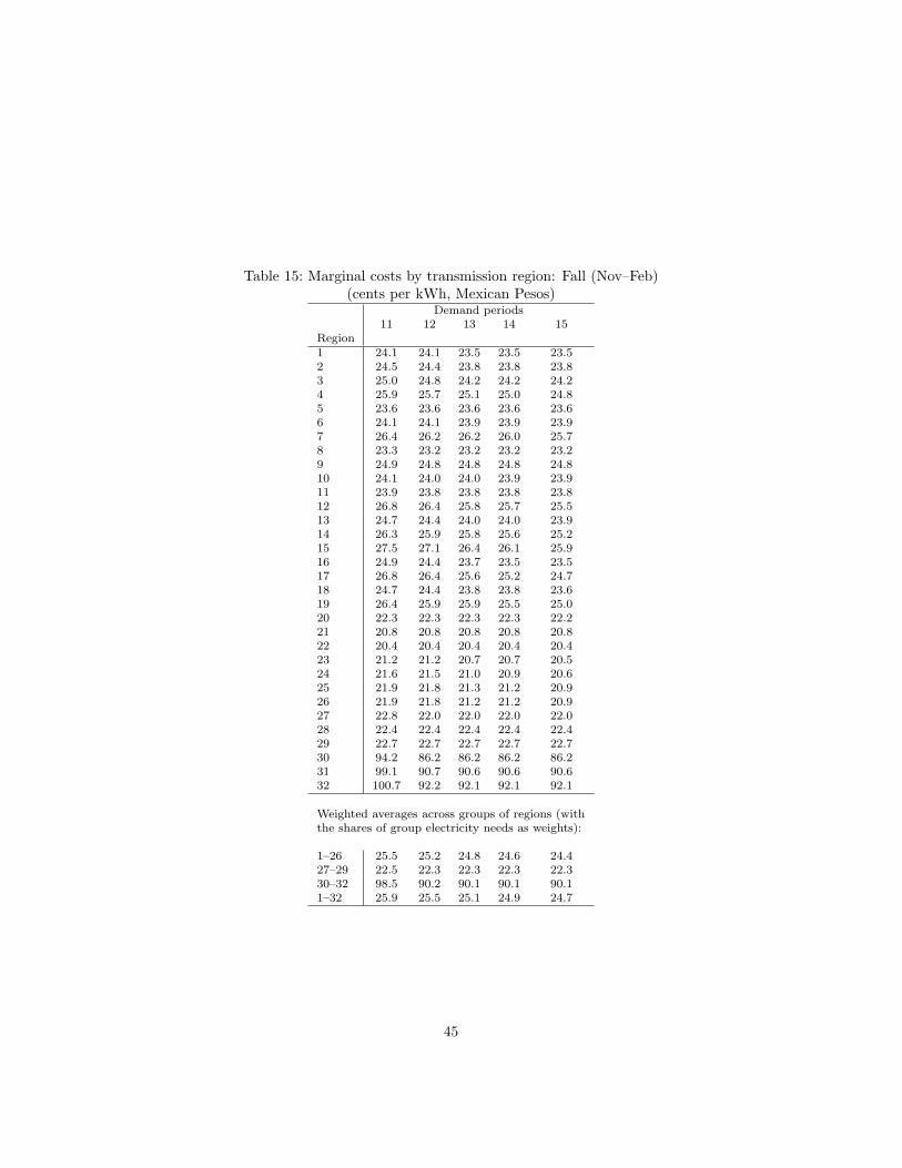
Table 15: Marginal costs by transmission region: Fall (Nov–Feb)(cents per kWh, Mexican Pesos)


Region1 24.1 24.1 23.5 23.5 23.52 24.5 24.4 23.8 23.8 23.83 25.0 24.8 24.2 24.2 24.24 25.9 25.7 25.1 25.0 24.85 23.6 23.6 23.6 23.6 23.66 24.1 24.1 23.9 23.9 23.97 26.4 26.2 26.2 26.0 25.78 23.3 23.2 23.2 23.2 23.29 24.9 24.8 24.8 24.8 24.810 24.1 24.0 24.0 23.9 23.911 23.9 23.8 23.8 23.8 23.812 26.8 26.4 25.8 25.7 25.513 24.7 24.4 24.0 24.0 23.914 26.3 25.9 25.8 25.6 25.215 27.5 27.1 26.4 26.1 25.916 24.9 24.4 23.7 23.5 23.517 26.8 26.4 25.6 25.2 24.718 24.7 24.4 23.8 23.8 23.619 26.4 25.9 25.9 25.5 25.020 22.3 22.3 22.3 22.3 22.221 20.8 20.8 20.8 20.8 20.822 20.4 20.4 20.4 20.4 20.423 21.2 21.2 20.7 20.7 20.524 21.6 21.5 21.0 20.9 20.625 21.9 21.8 21.3 21.2 20.926 21.9 21.8 21.2 21.2 20.927 22.8 22.0 22.0 22.0 22.028 22.4 22.4 22.4 22.4 22.429 22.7 22.7 22.7 22.7 22.730 94.2 86.2 86.2 86.2 86.231 99.1 90.7 90.6 90.6 90.632 100.7 92.2 92.1 92.1 92.1


1–26 25.5 25.2 24.8 24.6 24.427–29 22.5 22.3 22.3 22.3 22.330–32 98.5 90.2 90.1 90.1 90.11–32 25.9 25.5 25.1 24.9 24.7

45

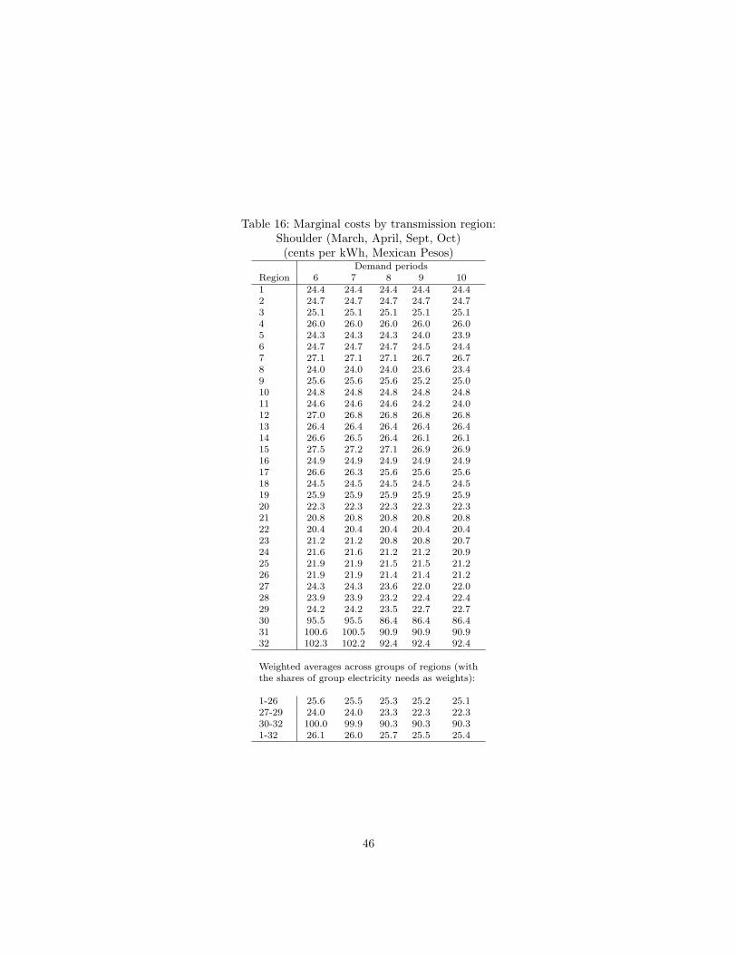
Table 16: Marginal costs by transmission region:Shoulder (March, April, Sept, Oct)(cents per kWh, Mexican Pesos)



1-26 25.6 25.5 25.3 25.2 25.127-29 24.0 24.0 23.3 22.3 22.330-32 100.0 99.9 90.3 90.3 90.31-32 26.1 26.0 25.7 25.5 25.4

46

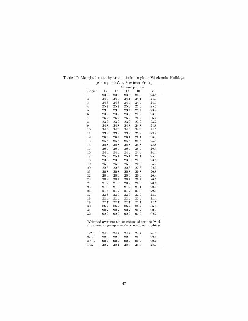
Table 17: Marginal costs by transmission region: Weekends–Holidays(cents per kWh, Mexican Pesos)



1-26 24.8 24.7 24.7 24.7 24.727-29 22.5 22.3 22.3 22.3 22.330-32 90.2 90.2 90.2 90.2 90.21-32 25.2 25.1 25.0 25.0 25.0

47

in the transmission system do not eventuate.Excluding all transmission investments expected to be completed beyond the

end of 2002 made it impossible to meet the forecast demands for 2005 with theplanned additions to generating capacity. If planned transmission investmentsbeyond 2002 do not eventuate, therefore, additional investment in generatingcapacity would be needed to meet the forecast demand growth.

We then examined the transmission investments expected to be completedby the end of 2003. Five major transmission projects should be completed inthat year. There are three new links between nodes 1 and 5 (380MW), nodes 9and 14 (568MW) and nodes 10 and 14 (1,500MW). There are also two significantupgrades between nodes 18 and 20 (an additional 1,600MW of capacity) andnodes 20 and 22 (an additional 1,000MW of capacity).

The projects to upgrade the links between regions 22–18 increase the amountof power that can be transmitted from the hydroelectric plants in the Grijalvariver region (22) to the central part of the nation. We found that these projectsare critical. If they are not completed by the end of 2004, the forecast demandsfrom November 2004 to October 2005 cannot be met without building moregenerating capacity.

On the other hand, if the upgrade projects are completed on time whilethe three new links slated for completion in 2003 are not, the resulting system(with all new generating plant completed on schedule) is capable of satisfying theforecast demand in 2005. The resulting average cost of generation is 16.57 centsper kWh instead of 16.40 cents per kWh if all planned transmission investmentsare completed. On the other hand, the weighted marginal cost (at 25.34 centsper kWh) is actually lower if the new links are not built. The marginal costs aremore variable across regions and seasons when the system is less well-connected.In the two regions with the largest demands (the central and Monterrey areas),however, the marginal costs are lower in the system with weaker links. Theseresults show that marginal and average costs do not necessarily move in thesame direction as a result of new investments. In particular, if prices reflectedmarginal costs, stronger transmission links could make some consumers worseoff by facilitating increased arbitrage and equilibration of marginal costs acrossthe network.

Another interesting consequence of not building the 1,500MW link from re-gion 10 to region 14, while nevertheless adding all the new generating capacityplanned for region 10, is that the reserve constraint does not bind in region 10in any season. This result illustrates how transmission and generating invest-ments interact. Without the accompanying transmission investment, some ofthe investment in new generating capacity can be wasted.

6 Conclusion

Our analysis implies that substantial investment is needed to meet the growingdemand for electricity over the next decade. The Mexican government hasturned to the private sector to help finance much of the needed investment.

48

It is questionable, however, whether the best method that has been chosento encourage private investment. In particular, BLT, IPP and turnkey projectsleave the public sector bearing most of the risks. One of the major functionsof privately-owned firms, and the trade in stocks, is to share risks optimallyand facilitate the financing of large, long-term risky investments. The risk ad-justed return required to compensate investors for the risks they are bearingalso signals the appropriate return for evaluating investments. In the absence ofsuch information, it is much harder for publicly owned firms to decide whetherinvestments are worthwhile.

Another potential defect of BLT and turnkey projects is that they leavethe publicly owned firm in charge of operations. One of the major inefficienciesassociated with public ownership is that the firm does not have a strong incentiveto minimize operating costs. Even investors in IPP projects may have a reducedincentive to control costs if the contract price for their output depends on theircosts, as it typically does.

The second major conclusion from our analysis is that there are substantialdifferences between electricity prices in Mexico and the marginal costs of supply.In particular, the regional and temporal variation of prices is not closely relatedto the corresponding variations in marginal costs. As a result, consumers are notreceiving accurate information about the costs of meeting their demands and arenot receiving accurate signals about the benefits of changing their location, orthe timing of their electricity demands, so as to reduce the costs for the systemas a whole.

Allowing private entry into the wholesale market for electricity, and set-ting prices through an auction mechanism, may also assist in making pricesmore reflective of costs. Before introducing such reforms, however, the ex-isting publicly-owned suppliers would need to be separated along functionallines (with transmission and distribution separated from generation) and theremaining generating assets allocated to many competing firms. It may even becounter-productive to introduce a wholesale market for electricity that is notcompetitive. The price signals sent to consumers and potential entrant produc-ers would be distorted measures of the costs and would encourage inefficientconsumption and production decisions.

The third major conclusion from our analysis is that the hydroelectric gener-ating plant in Mexico is quite valuable as a mechanism to smooth temporal andgeographical variations in marginal costs of generation. In effect, the storageof water substitutes to some extent for the inability to store electricity. Thebenefits of hydroelectricity are limited, however, by weaknesses in the existingtransmission network. The major hydroelectric generating plants are located inthe Grijalva river region in the south of the country and the transmission linksto other regions can often become congested. Upgrading the transmission linksis thus a major priority. The public sector is expected to remain the majorinvestor in the transmission network for the immediate future, however, andthere is a risk that the needed investments may be sacrificed for fiscal reasonsthat have nothing to do with the needs of the electricity industry.

49

Appendix A: Modeling electricity demand

As we noted in the text, the aggregate demand forecast is derived by relating thelogarithm of total power generation to GDP, the relative price of electricity, anda variable, based on temperature records, that accounts for seasonal variations.

Income. The GDP can be viewed as a proxy either for “household income”or for “industrial input demand.” The data was converted from a quarterly toa monthly frequency using the relationship between industrial production andGDP. Specifically, the GDP for each quarter was allocated to each month inthe quarter using the relative values of industrial production for each of thosemonths in the quarter. The variable included in the analysis, denoted yt, isthe natural logarithm of the estimated monthly GDP. Information other thanthe electricity data obtained from the CFE was obtained from the InstitutoNacional de Geografıa e Informatica. 45

Electricity prices. The relative price of electricity was calculated by dividingan implicit price for electricity by the producer price index. The implicit pricefor electricity was in turn obtained by dividing CFE monthly revenues by thequantity of electricity that CFE sold in each month. We use lagged prices inthe regression to allow for the lags between consumption and billing (when mostof the consumers realize how much they consumed). The variable included inthe analysis, denoted pt, is actually the natural logarithm of the relative pricelagged three periods.46 When forecasting the relative price of electricity, weneed to preserve the monthly seasonal component. To do so, we estimated thefollowing regression:

pt = αo +11∑

i=1

αiDi + ωt, (1)

where α0 represents the mean value of p in December, Di is an indicator variablefor months i other than December and hence αi represents the difference in theaverage value of p in month i relative to its value on December. The samplecovers the period from February 1996 to November 2001. The estimates fromthis regression are reported in Table 18.

Seasonality. The aggregate demand for electricity is known to depend onseasonal factors in addition to GDP and the relative price of electricity. Sinceweather is the main determinant of seasonality in electricity demand, temper-ature variables should capture seasonality in a more parsimonious way than aset of monthly indicator variables.47

45Instituto Nacional de Geografıa e Informatica (INEGI), http://www.inegi.gob.mx46Although most bills are issued every two months, there is an additional one month grace

period for paying the bill.47Factors such as holidays, or even variations in the number of days in each month may,

however, also contribute to seasonal effects that are not readily captured by temperaturechanges.

50

Table 18: Estimated montly component of relative electricity pricesParameter Coefficient t value

α0 0.1897 (133.7234)

α3 -0.0074 (-2.7073)

α4 -0.0120 (-4.4114)

α5 -0.0110 (-3.9850)

α6 -0.0123 (-4.5365)

α7 -0.0096 (-3.5232)

α8 -0.0085 (-3.1285)

α9 -0.0061 (-2.2384)

α10 -0.0080 (-2.9543)

α11 -0.0061 (-2.2607)

R2 0.30

Observations 70

Some studies attempt to model the effects of weather on electricity demandby including the average temperature as an explanatory variable. The effectof temperature on electricity demand is, however, likely to be non-linear withboth very cold and very hot days raising the demand. Some studies attempt toallow for this by using the number of heating and cooling days within a periodas explanatory variables.

Chang and Martinez-Chombo (2002), allow for a very general functionalrelationship g(τt) between the demand for electricity and the temperature τt attime t. In this paper, we use a quadratic to approximate g:

g(τt) = π0 + π1τt + π2τ2t (2)

In particular, the second order term allows electricity demand to increase inresponse to both abnormally high and abnormally low temperatures.

While electricity consumption is measured monthly, weather data is mea-sured much more often. In addition, the electricity demand covers the countryas a whole while weather data varies from one region to the next. For eachmonth in their sample period, Chang and Martinez-Chombo (2002) gathereddata on temperatures measured in six cities every three hours. The cities werechosen partly to represent different regions of the country and partly based onthe quality of their weather records.48 For each city i, and each month t in thesample, there will be roughly 240 temperature readings τip, p ∈ t. A probabilitydensity function fit(τip) is then fit to these temperatures using a kernel den-sity estimator.49 The expected effect on electricity demand at location i of the

48The cities chosen for the study were Mexico City, Monterrey, Oaxaca, Merida, Culiacanand Colima.

49A normal kernel was used, with a fixed bandwidth chosen to minimize the approximationmean integrated square error for normal kernels.

51

temperatures experienced in month t will then be given from (2) by:∫p∈t

g(τip)fit(τip)dτip = π0 + π1

∫p∈t

τipfit(τip)dτip + π2

∫p∈t

τ2ipfit(τip)dτip (3)

The production data available relate, however, to aggregate demand in thewhole CFE network rather than the demand in particular locations. Two newvariables are defined as the weighted sum of the two expected values on theright hand side of 3:

z1t =6∑

i=1

Sit

∫p∈t

τipfit(τip)dτip (4)

z2t =6∑

i=1

Sit

∫p∈t

τ2ipfit(τip)dτip (5)

where the weights Sit correspond to the shares of electricity consumption in theregions for which city i is representative.

Even having the two variables z1t and z2t as defined in 4 and 5 will lead to alarge number of parameters when we estimate the dynamic adjustment model.We therefore used z1t and z2t to derive a single variable zt to capture the seasonalcomponent of total power generation. Specifically, total power generation Qt

was decomposed into an annual moving average50 and a “short run” deviation,denoted qt, from that moving average. The short run component was thenrelated to temperature using the following regression (observations N = 179,R2 = 0.8657, t-values of the coefficients are in parentheses):

qt = −0.1833 + 0.1333 · z1t + 0.3522 · z2t + εt (6)(−5.57) (0.899) (2.395)

The variable zt was then defined as the predicted value of qt based on (6).

Long run relationships. Variables that are systematically related to eachother in the long run display a consistent pattern in their trends. Deviationsfrom these long run relationships constitute stationary shocks that graduallydisappear over time.

For most time series of economic variables, trends primarily result frompermanent shocks that accumulate over time and lead to “unit roots” in theseries. While the series itself displays a trend, changes in the series from oneperiod to the next are driven by shocks drawn from a stationary distribution.Table 19 presents results of tests for the presence of unit roots in the naturallogarithms of total power generation (denoted Qt), GDP and the relative priceof electricity. If a unit root is absent, the series itself is stationary, and the teststatistic presented in Table 19 should be below the 5% critical values listed inthe bottom row of the table. The tests for the presence of stochastic trends

50For a given month t, the moving average was calculated as (1/13)∑6

l=−6 Qt+l.

52

can be affected if the series have trends that are deterministic functions of timeor if the variables are strongly serially correlated. The tests were performedusing two different criteria (Akike and Schwartz) to select the number of lagsincluded to eliminate serial correlation. Two separate sets of tests allowing forthe presence or absence of a deterministic time trend also were conducted. Ineleven of the twelve results, the evidence indicates the presence of a unit rootin the series.

Although each of the variables Q, y and p is non-stationary, if the demandfor electricity is a stable function of these variables the relationship betweenthem will be stationary (the variables will be “co-integrated”). One of theinnovative features of the model of electricity demand presented in Chang andMartinez-Chombo (2002) is that the authors allow the long run relationshipbetween the dependent variable, in this case Q, and its determinants, in thiscase y and p, to change gradually over time in a deterministic fashion. Thismodification may be especially important in a country such as Mexico that hasrecently undergone substantial economic change. In particular, the recent rapidgrowth of the Mexican economy, and the change in industry structure resultingfrom the NAFTA, both are likely to have changed the relationship betweenelectricity demand and its key determinants. Following Chang and Martinez-Chombo (2002), the time varying elasticities of total power generation withrespect to GDP and the relative price, γt and δt in the equation:

Qt = π + γtyt + δtpt + φzt + ut, (7)

are approximated by a Fourier Flexible Form (FFF) function, using the Schwartzcriterion to select the number of terms in the functions. The estimates werederived using the method of canonical co-integrating regression (CCR) suggestedby Park and Hahn (1999). The results are reported in Table 20.51

We found that the long run elasticity of Qt with respect to the GDP, γt, canbe approximated by a series function that includes a constant coefficient βγ,k,1)and a linear trend (with slope βγ,k,2). The parameter estimates imply that γt

has been decreasing over time from 0.426 at the beginning of the sample toabout 0.4099 at the end of the sample. This is consistent with industrializationand economic growth leading to more widespread use of grid electricity.

In the case of the relative price of electricity, the results in Table 20 implythat the elasticity, δt, of power generation with respect to p can be approximatedby a linear trend (βδ,k,2) and a trigonometric function (cos(4πi), i = 1 . . . n). Theestimated coefficients on the relative price variables imply that, while electricitydemand was insensitive to price at the beginning of the sample by the end of theperiod the elasticity of demand with respect to price was about -0.5006. Sucha change might again be consistent with a growth in the relative importance ofindustry in the economy, which probably has more options to alter demand inresponse to price variations.

51Although zt is stationary, it is included in the co-integrating regression to help controlfor seasonality in Q, y and p. In the estimation of the adjustment process presented below,we allow zt and its lags to enter separately from ut, so including zt in equation 7 does notrestrict the dynamic adjustment of Q to z.

53

Table 19: Augmented Dickey-Fuller (ADF) tests for stationarityVariable Demeaned series lags Detrended series lags

Lag selection criteriona

Total power generation, Qt

AIC 0.4167 12 -2.641 12

SC 0.4167 12 -4.798 7

GDP, yt

AIC 0.6244 16 -1.110 16

SC 0.6244 16 -1.110 16

Relative prices, pt

AIC -2.013 14 -1.4549 14

SC -1.330 4 -1.9035 5

5% critical values -2.86 -3.41

a. Akike (AIC) and Schwartz (SC) criterion

Table 20: Estimated co-integrating relationship for total power generationVariable Coefficients (t valuesa)Constant (π) 7.0766 (4.7866)

zt (φ) 1.0632 (20.4203)

Parameters of the TVC: γt

k 0b

βγ,k,1 0.4261 (5.9735)

βγ,k,2 -0.0161 (-2.2235)

Parameters of the TVC: δt

k 2

βδ,k,2 -0.5025c (-6.5293)

βδ,k,3 0.0047d (2.3271)

SC = -6.7665 R2 =0.9839 DW =2.01

observations N = 176Long run variance of the CCR errors

Ω∗11 0.0010

Unit root test for estationary of the errors ut of the regressione

τ∗ 10.6039 Critical value 1%: 13.28

a. Computed using CCR standard errors.b. Indicates that there are no trigonometric terms.c. Coefficient of the linear trend.d. Coefficient of the trigonometric term cos(4πr).e. τ∗ ∼ χ2(4) for H0 : errors are stationary. Park and Hahn (1999) statistic.

54

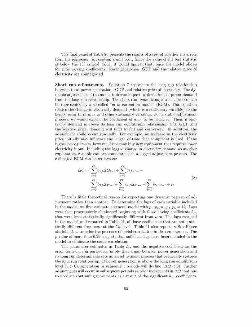
The final panel of Table 20 presents the results of a test of whether the errorsfrom the regression, ut, contain a unit root. Since the value of the test statisticis below the 1% critical value, it would appear that, once the model allowsfor time varying coefficients, power generation, GDP and the relative price ofelectricity are cointegrated.

Short run adjustments. Equation 7 represents the long run relationshipbetween total power generation , GDP and relative price of electricity. The dy-namic adjustment of the model is driven in part by deviations of power demandfrom the long run relationship. The short run dynamic adjustment process canbe represented by a so-called “error-correction model” (ECM). This equationrelates the change in electricity demand (which is a stationary variable) to thelagged error term ut−1 and other stationary variables. For a stable adjustmentprocess, we would expect the coefficient of ut−1 to be negative. Then, if elec-tricity demand is above its long run equilibrium relationship with GDP andthe relative price, demand will tend to fall and conversely. In addition, theadjustment could occur gradually. For example, an increase in the electricityprice initially may influence the length of time that equipment is used. If thehigher price persists, however, firms may buy new equipment that requires lowerelectricity input. Including the lagged change in electricity demand as anotherexplanatory variable can accommodate such a lagged adjustment process. Theestimated ECM can be written as:

∆Qt =p1∑

l=1

b1,l∆Qt−l +p2∑

l=1

b2,lut−l+

p3∑l=0

b3,l∆yt−l +p4∑

l=0

b4,l∆pt−l +p5∑

l=0

b5,lzt−l + εt

(8)

There is little theoretical reason for expecting one dynamic pattern of ad-justment rather than another. To determine the lags of each variable includedin the model, we first estimate a general model with p1, p2, p3, p4, p5 = 12. Lagswere then progressively eliminated beginning with those having coefficients bj,l

that were least statistically significantly different from zero. The lags retainedin the model, and reported in Table 21, all have coefficients that are not statis-tically different from zero at the 5% level. Table 21 also reports a Box-Piercestatistic that tests for the presence of serial correlation in the error term ε. Thep-value of more than 0.29 suggests that sufficient lags have been included in themodel to eliminate the serial correlation.

The parameter estimates in Table 21, and the negative coefficient on theerror term ut−1 in particular, imply that a gap between power generation andits long run determinants sets up an adjustment process that eventually restoresthe long run relationship. If power generation is above the long run equilibriumlevel (u > 0), generation in subsequent periods will decline (∆Q < 0). Furtheradjustments will occur in subsequent periods as prior movements in ∆Q continueto produce continuing movements as a result of the significant b1,l coefficients.

55

Table 21: Estimated dynamic adjustment equation for ∆Qt

Parameter Variable

∆Qt−l (j = 1) ut−l (j = 2)Coeff. (t val.) Coeff. (t val.)

bj,1 -0.1695 (-3.86) -0.4631 (-7.78)bj,4 0.1231 (2.94)bj,5 0.1480 (3.78)bj,12 0.5263 (12.74)

∆yt−l (j = 3) ∆pt−l (j = 4) zt−l (j = 5)Coeff. ( t val.) Coeff. ( t val.) Coeff. ( t val.)

bj,0 0.3469 (8.02) -0.1662 (-2.39) 0.5835 (7.30)bj,3 0.1717 (5.00)bj,4 -0.1295 (-2.41)bj,5 0.1514 (2.76)bj,8 0.1430 (2.79)bj,11 0.3130 (3.91)bj,12 -0.2340 (-5.35) 0.1065 (2.07) -0.2910 (-3.40)

R2 0.9115Box-Pierce χ2

40 44.3359 p-value 0.2938

-0.7

-0.6

-0.5

-0.4

-0.3

-0.2

-0.1

0

0.1

0.2

0.3

0.4

0.5

0.6

0.7

0.8

0 2 4 6 8 10 12 14 16 18 20 22 24 26 28 30 32 34 36 38 40 42 44 46 48 50 52 54 56 58 60Months after shock

Effe

ct o

n po

wer

gen

erat

ion

Permanent yPermanent pTemporary z

Figure 5: Implied dynamic adjustment of power generation to shocks

56

Eventually, however, the adjustments will decay to zero.The dynamic adjustment process implied by the estimated ECM is illus-

trated in Figure 5. This graphs the response of Q to a one percent permanentshock to GDP, y, and relative prices of electricity, p, and a 1% temporary shockto z. The adjustments graphed in 5 have been calculated setting the long runelasticities of power demand with respect to y and p to their values at the end ofthe sample period. In reality, we would expect these elasticities will continue tochange over time, making the adjustment process a function of the time whenthe shocks occur.

As Figure 5 illustrates, ∆Q → γT = 0.4099 for a permanent 1% shockto y, ∆Q → δT = −0.50057 for a permanent 1% shock to p, and ∆Q → 0for a temporary shock to the stationary variable z. In all cases, there is aseasonality to the response with “patterns” in the adjustment process being“mirrored” with 12-month lags. The annual seasonality is also evident in thelarge estimated coefficients at lag 12 in Table 21. Any change in income, pricesor weather that induces a home or business to alter their stock of electricalequipment or appliances is likely to have continuing effects on power demand insimilar seasons in subsequent years.

The response of total power generation to a permanent increase in GDPis, for the first two months, somewhat below the ultimate long run response.Generation then “overshoots” the long run response for the remainder of the firstyear. Thereafter, the pattern is more or less repeated on an annual frequencywith ever smaller fluctuations around the ultimate long run effect.

An increase in the relative price of electricity produces a different type ofadjustment process. Whereas a permanent increase in y causes Q to jump almostimmediately to values in the proximity of the long run effect, the response toprice changes is more gradual. Such a delay in the responsiveness of demandto price changes may be explained in part by the infrequent billing schedule,and perhaps by the fact that a significant amount of electricity appears to betaken illegally. It is also possible that the seasonal component in prices makes itdifficult for consumers to clearly identify price changes. In addition to displayinga more gradual adjustment of Q toward its long run value, the price responsepath displays much less “overshooting” than does the response to y. Again,however, the adjustment pattern set for months 4 through 16 has a tendencyto be repeated, albeit with oscillations of declining magnitude, in months 16through 28, 28 through 40 and so on.

A temporary shock to the temperature variable z also ultimately produces anadjustment path that tends to repeat in an annual cycle. In this case, however,the initial period of response lasts about 10 months instead of 4. The responseof Q to z, like its response to a GDP shock, is rapid. On the other hand, likethe response to p, the response to z does not involve sustained “overshooting”.

Regional demand shares. The regional shares of aggregate demand are, bydefinition, bounded between 0 and 1. In addition, as the share of demand inany one region increases toward 1 (or decreases toward zero) we would expect

57

further increases (respectively, decreases) to be much less likely. A naturalway of representing such behavior in a way that is also likely to yield normallydistributed error terms (which range from −∞ to +∞) is to use a logisticfunctional form:

ln(

Sit

1− Sit

)= X ′

itϕi + eit (9)

Since we do not have data on regional GDP or industrial production we usedmonthly indicator variables, time and time2 as components of X. The monthlyindicators capture differences in the seasonal patterns of demand across regions.The linear trend terms indicate regions where electricity demand is growingfaster (the coefficient of time is positive), or slower (the coefficient is negative),than in the nation as a whole. The coefficient on time2 indicates whether thetrend is accelerating (the quadratic and linear coefficients have the same sign)or decelerating (the coefficients have opposite signs). When making forecasts,we proportionally adjust the estimated shares in each region to ensure that theyalways sum to 1.0 in all periods.52

Table 22 gives the estimated quadratic equations for the regional demandshares. Table 23 presents the estimated monthly effects on the demand sharesfor January through November relative to shares in the month of December.

Daily demand variation. Since the load on the system is the most importantfeature of the demand fluctuations, we first convert the load curves in Figure 3 toload duration curves. A daily load duration curve is analogous to a probabilitydistribution function and plots the number of hours in the day that electricitydemand exceeds a given load. For the minimum load of the day, the loadduration curve will have a value of 24 hours. For the maximum load of the day,the load duration curve will be 0 hours. Essentially, the load duration curveorders times of the day not according to where they come by the clock butby what the demand load on the electricity system was at that time. A stepfunction approximation to the load duration curve then divides the day intoperiods of roughly constant levels of demand.

In the present model, we need to divide each day into time periods that coverthe same hours of the day in both the north and the south of the country. Thebottom two panels in Figure 3 show that, during the summer season, the peakdemand is in the afternoon hours in the north, but in the evening hours in thesouth. It therefore is not possible to define a time period that yields a coincidentpeak in both regions. More generally, since the load curves are different shapesit is difficult to group hours into a small number of blocks of roughly constantdemand. Instead of approximating the individual load duration curves, wepartitioned the curves in such a way that the durations of the steps coincide inboth regions.

52Although the error terms in the share equations will be correlated, there is no value inestimating the equations as a seemingly unrelated set since they have identical regressors.

58

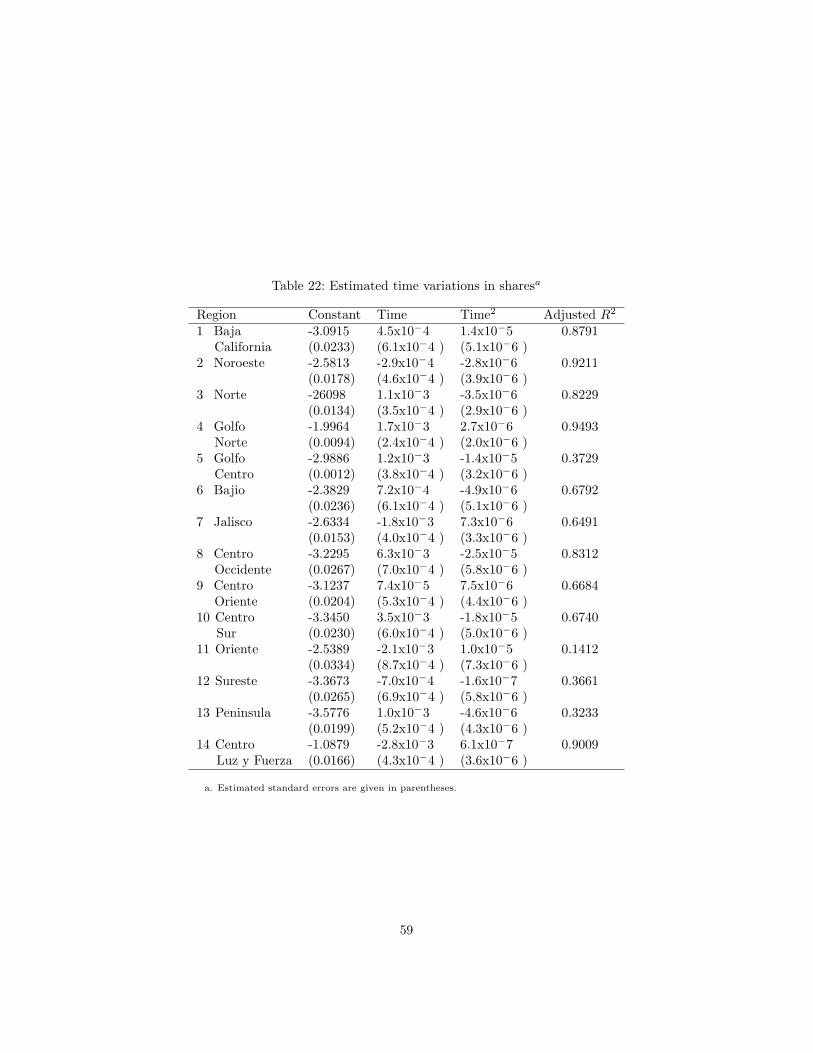
Table 22: Estimated time variations in sharesa

Region Constant Time Time2 Adjusted R2

1 Baja -3.0915 4.5x10−4 1.4x10−5 0.8791California (0.0233) (6.1x10−4 ) (5.1x10−6 )

2 Noroeste -2.5813 -2.9x10−4 -2.8x10−6 0.9211(0.0178) (4.6x10−4 ) (3.9x10−6 )

3 Norte -26098 1.1x10−3 -3.5x10−6 0.8229(0.0134) (3.5x10−4 ) (2.9x10−6 )

4 Golfo -1.9964 1.7x10−3 2.7x10−6 0.9493Norte (0.0094) (2.4x10−4 ) (2.0x10−6 )

5 Golfo -2.9886 1.2x10−3 -1.4x10−5 0.3729Centro (0.0012) (3.8x10−4 ) (3.2x10−6 )

6 Bajio -2.3829 7.2x10−4 -4.9x10−6 0.6792(0.0236) (6.1x10−4 ) (5.1x10−6 )

7 Jalisco -2.6334 -1.8x10−3 7.3x10−6 0.6491(0.0153) (4.0x10−4 ) (3.3x10−6 )

8 Centro -3.2295 6.3x10−3 -2.5x10−5 0.8312Occidente (0.0267) (7.0x10−4 ) (5.8x10−6 )

9 Centro -3.1237 7.4x10−5 7.5x10−6 0.6684Oriente (0.0204) (5.3x10−4 ) (4.4x10−6 )

10 Centro -3.3450 3.5x10−3 -1.8x10−5 0.6740Sur (0.0230) (6.0x10−4 ) (5.0x10−6 )

11 Oriente -2.5389 -2.1x10−3 1.0x10−5 0.1412(0.0334) (8.7x10−4 ) (7.3x10−6 )

12 Sureste -3.3673 -7.0x10−4 -1.6x10−7 0.3661(0.0265) (6.9x10−4 ) (5.8x10−6 )

13 Peninsula -3.5776 1.0x10−3 -4.6x10−6 0.3233(0.0199) (5.2x10−4 ) (4.3x10−6 )

14 Centro -1.0879 -2.8x10−3 6.1x10−7 0.9009Luz y Fuerza (0.0166) (4.3x10−4 ) (3.6x10−6 )

a. Estimated standard errors are given in parentheses.

59

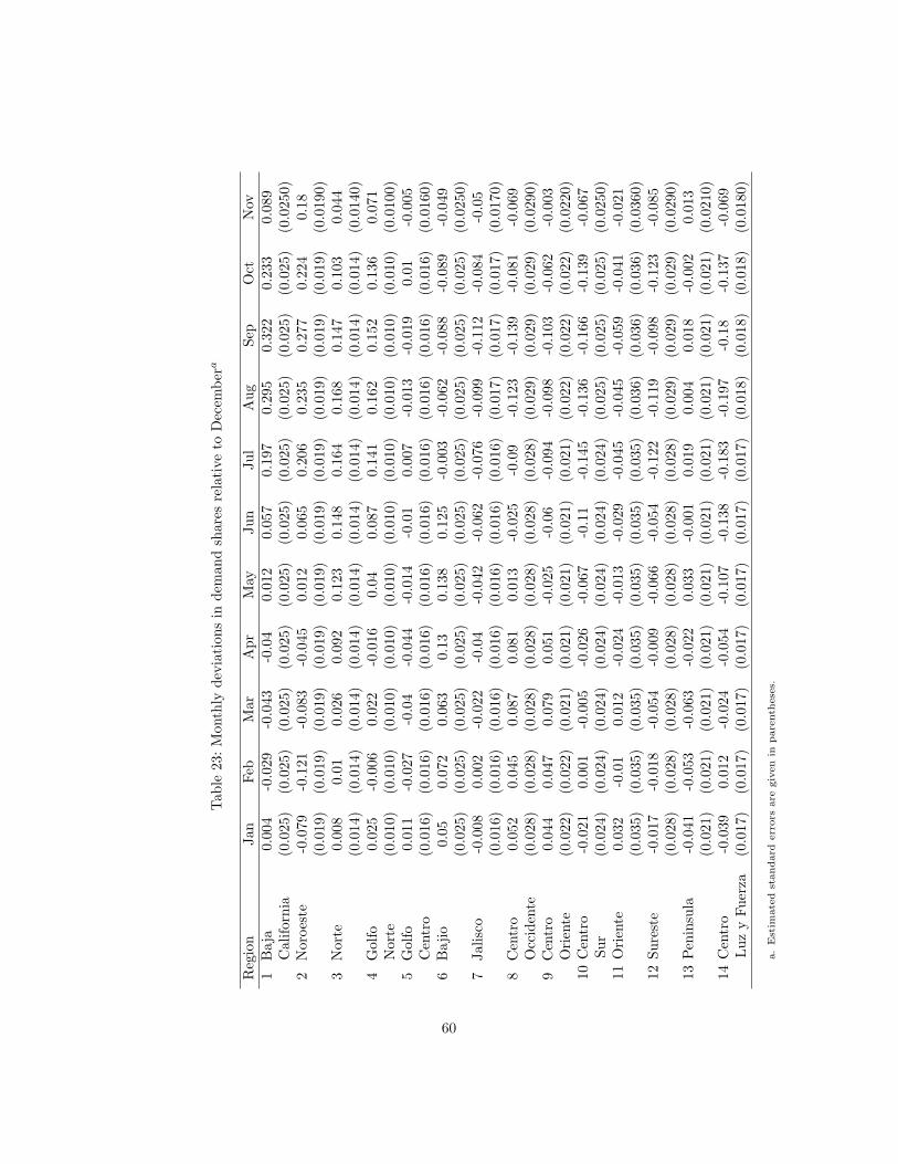
Tab

le23

:M

onth

lyde

viat

ions

inde

man

dsh

ares

rela

tive

toD

ecem

bera

Reg

ion

Jan

Feb

Mar

Apr

May

Jun

Jul

Aug

Sep

Oct

Nov

1B

aja

0.00

4-0

.029

-0.0

43-0

.04

0.01

20.

057

0.19

70.

295

0.32

20.

233

0.08

9C

alifo

rnia

(0.0

25)

(0.0

25)

(0.0

25)

(0.0

25)

(0.0

25)

(0.0

25)

(0.0

25)

(0.0

25)

(0.0

25)

(0.0

25)

(0.0

250)

2N

oroe

ste

-0.0

79-0

.121

-0.0

83-0

.045

0.01

20.

065

0.20

60.

235

0.27

70.

224

0.18

(0.0

19)

(0.0

19)

(0.0

19)

(0.0

19)

(0.0

19)

(0.0

19)

(0.0

19)

(0.0

19)

(0.0

19)

(0.0

19)

(0.0

190)

3N

orte

0.00

80.

010.

026

0.09

20.

123

0.14

80.

164

0.16

80.

147

0.10

30.

044

(0.0

14)

(0.0

14)

(0.0

14)

(0.0

14)

(0.0

14)

(0.0

14)

(0.0

14)

(0.0

14)

(0.0

14)

(0.0

14)

(0.0

140)

4G

olfo

0.02

5-0

.006

0.02

2-0

.016

0.04

0.08

70.

141

0.16

20.

152

0.13

60.

071

Nor

te(0

.010

)(0

.010

)(0

.010

)(0

.010

)(0

.010

)(0

.010

)(0

.010

)(0

.010

)(0

.010

)(0

.010

)(0

.010

0)5

Gol

fo0.

011

-0.0

27-0

.04

-0.0

44-0

.014

-0.0

10.

007

-0.0

13-0

.019

0.01

-0.0

05C

entr

o(0

.016

)(0

.016

)(0

.016

)(0

.016

)(0

.016

)(0

.016

)(0

.016

)(0

.016

)(0

.016

)(0

.016

)(0

.016

0)6

Baj

io0.

050.

072

0.06

30.

130.

138

0.12

5-0

.003

-0.0

62-0

.088

-0.0

89-0

.049

(0.0

25)

(0.0

25)

(0.0

25)

(0.0

25)

(0.0

25)

(0.0

25)

(0.0

25)

(0.0

25)

(0.0

25)

(0.0

25)

(0.0

250)

7Ja

lisco

-0.0

080.

002

-0.0

22-0

.04

-0.0

42-0

.062

-0.0

76-0

.099

-0.1

12-0

.084

-0.0

5(0

.016

)(0

.016

)(0

.016

)(0

.016

)(0

.016

)(0

.016

)(0

.016

)(0

.017

)(0

.017

)(0

.017

)(0

.017

0)8

Cen

tro

0.05

20.

045

0.08

70.

081

0.01

3-0

.025

-0.0

9-0

.123

-0.1

39-0

.081

-0.0

69O

ccid

ente

(0.0

28)

(0.0

28)

(0.0

28)

(0.0

28)

(0.0

28)

(0.0

28)

(0.0

28)

(0.0

29)

(0.0

29)

(0.0

29)

(0.0

290)

9C

entr

o0.

044

0.04

70.

079

0.05

1-0

.025

-0.0

6-0

.094

-0.0

98-0

.103

-0.0

62-0

.003

Ori

ente

(0.0

22)

(0.0

22)

(0.0

21)

(0.0

21)

(0.0

21)

(0.0

21)

(0.0

21)

(0.0

22)

(0.0

22)

(0.0

22)

(0.0

220)

10C

entr

o-0

.021

0.00

1-0

.005

-0.0

26-0

.067

-0.1

1-0

.145

-0.1

36-0

.166

-0.1

39-0

.067

Sur

(0.0

24)

(0.0

24)

(0.0

24)

(0.0

24)

(0.0

24)

(0.0

24)

(0.0

24)

(0.0

25)

(0.0

25)

(0.0

25)

(0.0

250)

11O

rien

te0.

032

-0.0

10.

012

-0.0

24-0

.013

-0.0

29-0

.045

-0.0

45-0

.059

-0.0

41-0

.021

(0.0

35)

(0.0

35)

(0.0

35)

(0.0

35)

(0.0

35)

(0.0

35)

(0.0

35)

(0.0

36)

(0.0

36)

(0.0

36)

(0.0

360)

12Su

rest

e-0

.017

-0.0

18-0

.054

-0.0

09-0

.066

-0.0

54-0

.122

-0.1

19-0

.098

-0.1

23-0

.085

(0.0

28)

(0.0

28)

(0.0

28)

(0.0

28)

(0.0

28)

(0.0

28)

(0.0

28)

(0.0

29)

(0.0

29)

(0.0

29)

(0.0

290)

13Pen

insu

la-0

.041

-0.0

53-0

.063

-0.0

220.

033

-0.0

010.

019

0.00

40.

018

-0.0

020.

013

(0.0

21)

(0.0

21)

(0.0

21)

(0.0

21)

(0.0

21)

(0.0

21)

(0.0

21)

(0.0

21)

(0.0

21)

(0.0

21)

(0.0

210)

14C

entr

o-0

.039

0.01

2-0

.024

-0.0

54-0

.107

-0.1

38-0

.183

-0.1

97-0

.18

-0.1

37-0

.069

Luz

yFu

erza

(0.0

17)

(0.0

17)

(0.0

17)

(0.0

17)

(0.0

17)

(0.0

17)

(0.0

17)

(0.0

18)

(0.0

18)

(0.0

18)

(0.0

180)

a.

Est

imate

dst

andard

err

ors

are

giv

en

inpare

nth

ese

s.

60

Figure 3 shows that the north has a higher peak demand in the summer,while the south has a higher peak demand in the remaining periods. Thus,we arranged the hours according to the load duration curve for the north inthe summer period while we used the load duration curves for the south forthe remaining periods. Table 24 shows, however, that we defined period 1 inthe summer season and period 6 in the shoulder season to correspond with thedaily peak periods for the south. Total demand in the south (which includes thecentral region) is so much larger than in the north, and the differences betweenpeak and second highest demand in the north are so small, that the overallsystem peak demand corresponds with the southern one.

Figure 6 illustrates the step function approximations to the load durationcurve for the north in the summer season and the load duration curves in thesouth for the remaining seasons. We used five steps in the approximationsfor each of four seasons, yielding a total of twenty time periods in our model.Figure 6 also graphs the load curves for the south during the summer season,and for the north during the remaining seasons, with clock time rearrangedin the same manner as was done to obtain the load duration curves. Thedifferent shapes of the northern and southern load curves are reflected in thefact that the rearranged southern curve in the summer, and the rearrangednorthern curves in the other seasons, do not appear as load duration curvesordered from highest to lowest demand. Finally, Figure 6 also shows how weapproximated the rearranged loan curves using the same time periods as for theload duration curve approximations in each period. The durations and sizesof each the steps in the approximations were determined to maximize the fitbetween the approximations and the real load curves subject to the constraintthat the areas under the step function approximations equaled the areas underthe real load curves. As Figure 6 shows, five steps allowed us to fit the shapes ofthe curves reasonably well. The worst fit is for the south in the summer season.

The step function approximations were converted back to demands in eachtransmission region using the following procedure. Use SL to denote the seasonlength (in days). An aggregated seasonal step load duration function in hoursper season is obtained by multiplying the daily period length of each step (PL)by the number of days in the season (PL×SL). The share of total power demandthat is consumed at a specific period of time t in season s in the Northern(k = N) or Southern (k = S) regions the country can be computed from thisseasonal step function as follows:

dks,t =

RLSk,s,t · SLs,t · PLs,t∑t∈s RLSk,s,t · SLs,t · PLs,t

,

where RLSk,s,t is the relative demand load in region k, period t, and season s.Table 24 provides numerical values for these variables in our approximation.

To compute the level of power demand for each transmission region i in aparticular time period and season, we used the formula:

di,s,t = δi,s · dks,t · ds

61

Fall, Weekdays

0.6

0.7

0.8

0.9

1.0

1 2 3 4 5 6 7 8 9 10 11 12 13 14 15 16 17 18 19 20 21 22 23 24

Summer, Weekdays

0.6

0.7

0.8

0.9

1.0

1 2 3 4 5 6 7 8 9 10 11 12 13 14 15 16 17 18 19 20 21 22 23 24

Shoulder, Weekdays

0.6

0.7

0.8

0.9

1.0

1 2 3 4 5 6 7 8 9 10 11 12 13 14 15 16 17 18 19 20 21 22 23 24

Weekends-Holidays

0.5

0.6

0.7

0.8

0.9

1 2 3 4 5 6 7 8 9 10 11 12 13 14 15 16 17 18 19 20 21 22 23 24

Duration in Hours

North South Step approximation Steps

Figure 6: Step function approximations to the 1999 load curves

62

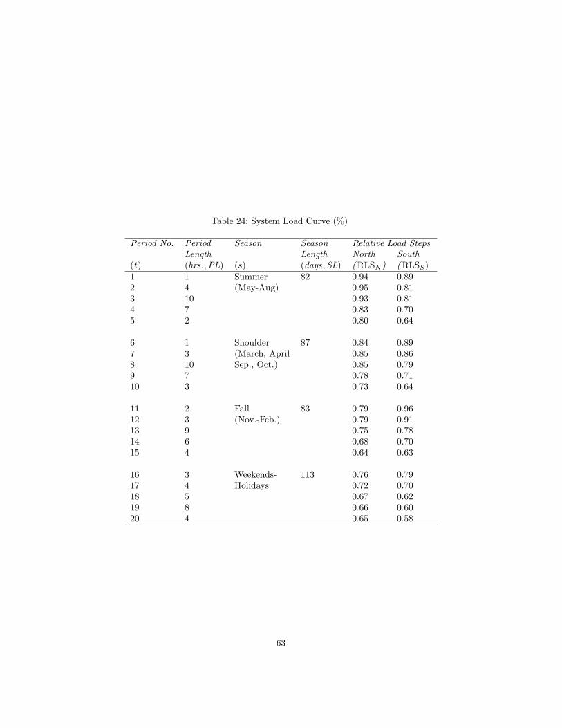
Table 24: System Load Curve (%)

Period No. Period Season Season Relative Load StepsLength Length North South

(t) (hrs.,PL) (s) (days,SL) (RLSN ) (RLSS)1 1 Summer 82 0.94 0.892 4 (May-Aug) 0.95 0.813 10 0.93 0.814 7 0.83 0.705 2 0.80 0.64

6 1 Shoulder 87 0.84 0.897 3 (March, April 0.85 0.868 10 Sep., Oct.) 0.85 0.799 7 0.78 0.7110 3 0.73 0.64

11 2 Fall 83 0.79 0.9612 3 (Nov.-Feb.) 0.79 0.9113 9 0.75 0.7814 6 0.68 0.7015 4 0.64 0.63

16 3 Weekends- 113 0.76 0.7917 4 Holidays 0.72 0.7018 5 0.67 0.6219 8 0.66 0.6020 4 0.65 0.58

63

where δki,s is the share of total demand in region k and season s originating

in transmission area i and ds is the aggregate demand in GWh in season s.Including a set of multiplicative scaling factors Zs > 0 in this formula allows usto calibrate demand to compensate for the (unknown) power losses per season:

di,s,t = δi,s · dks,t · ds · Zs.

Appendix B: Modeling electricity supply

Since details of system operation at hourly or finer time scales are not relevantto our main objectives, most of the stochastic components are eliminated fromthe problem.53 We instead examine a deterministic linear programming modelbased on expected values of demand and supply variables. We also modifythe model, however, to incorporate “normal” levels of excess capacity that aremaintained to cope with unusual emergencies.

Generating costs. The generating plant costs were based on data providedby the CFE as discussed in the text. The total cost of generation for N plantsin the system during the year is approximated by

C =N∑

n=1

bngn +N∑

n=1

T∑t=1

htcntgnt, (10)

where n = 1, ...N indexes the plants, t = 1, ...T denotes the period (where nowone period represents a set of hours of the day throughout a season), and ht isthe number of hours in period t (number of hours per day times number of daysper season). The annual fixed cost per MW of total capacity of plant n is bn.The total capacity of plant n, gn, is set for the whole year and constrains thevariable output levels, gnt, of each plant n in each period t:

0 ≤ gnt ≤ gn, ∀t, n (11)0 ≤ gn ≤ Gn, ∀t, n (12)

where Gn is the designed capacity of the plant. The variable cost of plant n inperiod t is cnt.

Transmission losses. Transmission losses on a link are a function of thepower flowing between two nodes and the resistance of the line. Specifically,transmission losses rise with the square of the current being transmitted on alink:

Lij = 3Rijτ2ij (13)

53For stochastic programming models of power markets look at Wallace, Stein W. andFleten Stein-Erik. (2002) “Stochastic programming models in energy,” Working Paper 01-02,Department of Industrial Economics and Technology Management, Norwegian University ofScience and Technology. http://ideas.uqam.ca/ideas/data/Papers/wpawuwpge0201001.html

64

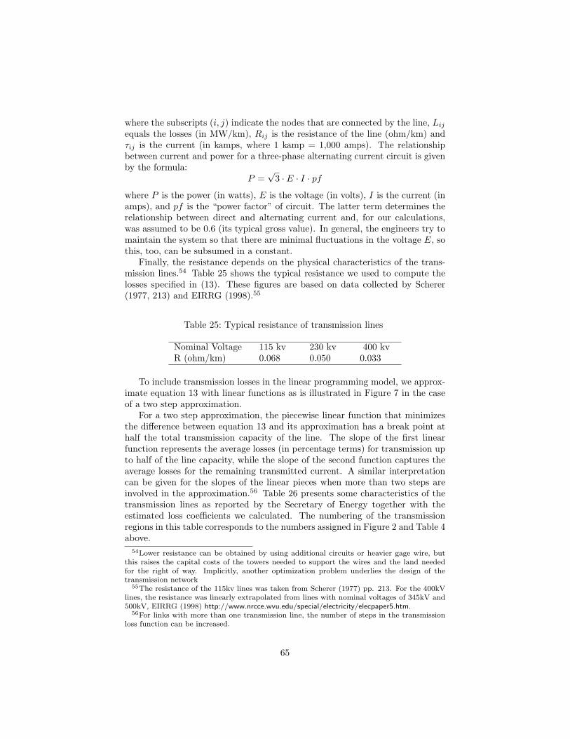
where the subscripts (i, j) indicate the nodes that are connected by the line, Lij

equals the losses (in MW/km), Rij is the resistance of the line (ohm/km) andτij is the current (in kamps, where 1 kamp = 1,000 amps). The relationshipbetween current and power for a three-phase alternating current circuit is givenby the formula:

P =√

3 · E · I · pf

where P is the power (in watts), E is the voltage (in volts), I is the current (inamps), and pf is the “power factor” of circuit. The latter term determines therelationship between direct and alternating current and, for our calculations,was assumed to be 0.6 (its typical gross value). In general, the engineers try tomaintain the system so that there are minimal fluctuations in the voltage E, sothis, too, can be subsumed in a constant.

Finally, the resistance depends on the physical characteristics of the trans-mission lines.54 Table 25 shows the typical resistance we used to compute thelosses specified in (13). These figures are based on data collected by Scherer(1977, 213) and EIRRG (1998).55

Table 25: Typical resistance of transmission lines

Nominal Voltage 115 kv 230 kv 400 kvR (ohm/km) 0.068 0.050 0.033

To include transmission losses in the linear programming model, we approx-imate equation 13 with linear functions as is illustrated in Figure 7 in the caseof a two step approximation.

For a two step approximation, the piecewise linear function that minimizesthe difference between equation 13 and its approximation has a break point athalf the total transmission capacity of the line. The slope of the first linearfunction represents the average losses (in percentage terms) for transmission upto half of the line capacity, while the slope of the second function captures theaverage losses for the remaining transmitted current. A similar interpretationcan be given for the slopes of the linear pieces when more than two steps areinvolved in the approximation.56 Table 26 presents some characteristics of thetransmission lines as reported by the Secretary of Energy together with theestimated loss coefficients we calculated. The numbering of the transmissionregions in this table corresponds to the numbers assigned in Figure 2 and Table 4above.

54Lower resistance can be obtained by using additional circuits or heavier gage wire, butthis raises the capital costs of the towers needed to support the wires and the land neededfor the right of way. Implicitly, another optimization problem underlies the design of thetransmission network

55The resistance of the 115kv lines was taken from Scherer (1977) pp. 213. For the 400kVlines, the resistance was linearly extrapolated from lines with nominal voltages of 345kV and500kV, EIRRG (1998) http://www.nrcce.wvu.edu/special/electricity/elecpaper5.htm.

56For links with more than one transmission line, the number of steps in the transmissionloss function can be increased.

65

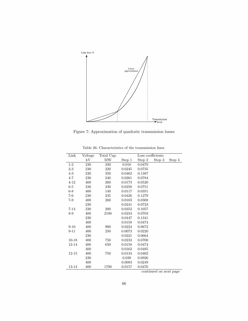
Line loss %

Transmissionlevel

Linearapproximation

Figure 7: Approximation of quadratic transmission losses

Table 26: Characteristics of the transmission lines

Link Voltage Total Cap. Loss coefficientskV MW Step 1 Step 2 Step 3 Step 4

1-2 230 330 0.016 0.04792-3 230 220 0.0245 0.07354-3 230 350 0.0462 0.13874-7 230 240 0.0261 0.07844-12 400 260 0.0173 0.05206-5 230 230 0.0250 0.07516-8 400 140 0.0117 0.03517-6 230 235 0.0426 0.12797-9 400 260 0.0103 0.0308

230 0.0241 0.07237-14 230 200 0.0352 0.10578-9 400 2100 0.0234 0.0703

230 0.0447 0.1341400 0.0158 0.0474

9-10 400 900 0.0224 0.06729-11 400 250 0.0073 0.0220

230 0.0221 0.066410-18 400 750 0.0233 0.070012-14 400 650 0.0158 0.0474

400 0.0162 0.048512-15 400 750 0.0134 0.0402

230 0.039 0.0926400 0.0083 0.0249

13-14 400 1700 0.0157 0.0470

continued on next page

66

Table 26 Continued

Link Voltage Total Cap. Loss coefficientskV MW Step 1 Step 2 Step 3 Step 4

400 0.0173 0.0520230 0.0250 0.0749

15-14 230 600 0.0202 0.0606230 0.0350 0.1049

15-17 400 750 0.0216 0.0647230 0.0398 0.1194230 0.0310 0.0929

16-15 400 450 0.0204 0.061116-12 400 400 0.0235 0.070616-17 400 950 0.0193 0.058018-17 400 3100 0.0105 0.0316

400 0.0263 0.0790400 0.0239 0.0718400 0.0206 0.0618230 0.0463 0.1390230 0.0507 0.1521

18-20 400 2100 0.0146 0.0437 0.0728 0.1020400 0.0135 0.04040 0.0673 0.0943230 0.0200 0.0599 0.0998 0.1397

19-17 230 240 0.0199 0.059720-21 400 1400 0.0174 0.0522 0.0871 0.121920-22 400 1000 0.0136 0.0407 0.0678 0.095021-22 400 2200 0.0149 0.0448 0.0746 0.104522-23 230 110 0.0188 0.056423-24 230 150 0.0134 0.0403

115 0.0090 0.0270115 0.0162 0.0487115 0.0083 0.0249

24-26 230 100 0.0104 0.0312115 0.0105 0.0314115 0.0105 0.0449

24-25 115 45 0.0135 0.040527-28 230 250 0.0233 0.070028-29 230 180 0.0187 0.056030-31 115 60 0.0168 0.050431-32 115 40 0.0160 0.048024-26 230 100 0.0104 0.0312

115 0.0105 0.0314115 0.0105 0.0449

24-25 115 45 0.0135 0.040527-28 230 250 0.0233 0.070028-29 230 180 0.0187 0.056030-31 115 60 0.0168 0.050431-32 115 40 0.0160 0.0480

67

The general regional demand constraint can be written:

∑n∈N(i)

ηngnt +∑

j∈S(i)

`(i,j)∑l

τ lji,t =

∑j∈S(i)

`(i,j)∑l

(1 + ρlij)τ

lij,t + dit, ∀i, t (14)

where i = 1, ....., D denotes the region, N(i) denotes the set of generation plantslocated in region i, ηn is the fraction of electricity generated by plant i that issent out to the electrical system (so (1− ηn)gnt is consumed within the plant),S(i) denotes the set of regions connected to region i, `(i, j) denotes number ofsteps in transmission loss function for the link between i and j, τ l

ji,t is the powertransmission flow from region j to region i in period t and on step l of the lossfunction, ρl

ij is the loss factor on step l of the transmission loss function of link(i, j), and dit is the hourly electricity demand at region i in period t.

The demand restrictions allow transmission to incur in either direction. Sinceall variables in the model are required to be non-negative, we double the numberof transmission variables. The links (i, j) and (j, i) represent the same physicalwires but the different indices indicate opposite directions of the flow. Thephysical wires limit the amount of electricity that can be transmitted betweentwo regions. Thus, if τij denotes the transmission capacity between regions iand j in MW:

`(i,j)∑l

τ lji,t +

`(i,j)∑l

τ lij,t ≤ τij , ∀t, (i, j) ∈ L (15)

where L is the set of transmission links in the system. Since all the variablesare non-negative, (15) implies 0 ≤ τ l

ij,t ≤ τ lij , ∀t,∀i, j ∈ S(i),∀l. Furthermore,

since transmissions involve losses, the program will not choose to have powerflowing in both directions at once, that is, only one of

∑`(i,j)l τ l

ij,t or∑`(j,i)

l τ lji,t

will be strictly positive.

Availability constraints. The plant availability restrictions can be repre-sented algebraically as follows:

T∑t=1

htgnt ≤ 8760αnGn, ∀n, (16)

where 8, 760 is the number of hours in a year and αn is the faction of hours thatplan n is available for generation in the whole year.

For the subset of large “base” plants, we imposed additional restrictions:

gbnt ≤ gb

ns, ∀s, with s = 1, .....S, (17)S∑

s=1

hsgbns ≤ 8760αb

nGbn, (18)

where the superscript b indicates a “base” plant, S is the number of seasons ina year and hs is the number of hours in season s. With this restriction, the

68

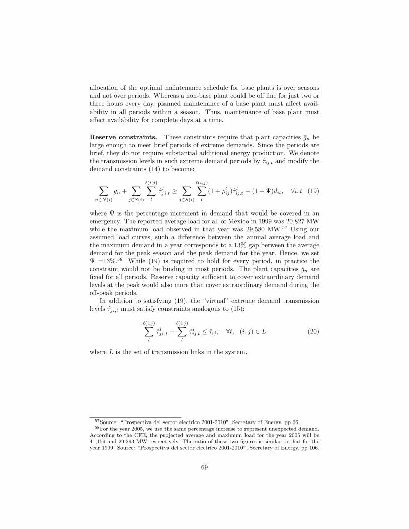
allocation of the optimal maintenance schedule for base plants is over seasonsand not over periods. Whereas a non-base plant could be off line for just two orthree hours every day, planned maintenance of a base plant must affect avail-ability in all periods within a season. Thus, maintenance of base plant mustaffect availability for complete days at a time.

Reserve constraints. These constraints require that plant capacities gn belarge enough to meet brief periods of extreme demands. Since the periods arebrief, they do not require substantial additional energy production. We denotethe transmission levels in such extreme demand periods by τij,t and modify thedemand constraints (14) to become:

∑n∈N(i)

gn +∑

j∈S(i)

`(i,j)∑l

τ lji,t ≥

∑j∈S(i)

`(i,j)∑l

(1 + ρlij)τ

lij,t + (1 + Ψ)dit, ∀i, t (19)

where Ψ is the percentage increment in demand that would be covered in anemergency. The reported average load for all of Mexico in 1999 was 20,827 MWwhile the maximum load observed in that year was 29,580 MW.57 Using ourassumed load curves, such a difference between the annual average load andthe maximum demand in a year corresponds to a 13% gap between the averagedemand for the peak season and the peak demand for the year. Hence, we setΨ =13%.58 While (19) is required to hold for every period, in practice theconstraint would not be binding in most periods. The plant capacities gn arefixed for all periods. Reserve capacity sufficient to cover extraordinary demandlevels at the peak would also more than cover extraordinary demand during theoff-peak periods.

In addition to satisfying (19), the “virtual” extreme demand transmissionlevels τji,t must satisfy constraints analogous to (15):

`(i,j)∑l

τ lji,t +

`(i,j)∑l

τ lij,t ≤ τij , ∀t, (i, j) ∈ L (20)

where L is the set of transmission links in the system.

57Source: “Prospectiva del sector electrico 2001-2010”, Secretary of Energy, pp 66.58For the year 2005, we use the same percentage increase to represent unexpected demand.

According to the CFE, the projected average and maximum load for the year 2005 will be41,159 and 29,293 MW respectively. The ratio of these two figures is similar to that for theyear 1999. Source: “Prospectiva del sector electrico 2001-2010”, Secretary of Energy, pp 106.

69

Data Sources

1. Bank of Mexico.Web site: http://www.banxico.org.mx/

2. Comision Federal de Electricidad (CFE).Web site: http://www.cfe.gob.mx

3. CFE. Costos y Parametros de Referencia para la Formulacion de Proyec-tos de Inversion en el Sector Electrico. Generacion.(COPAR) Gerenciade Evaluacion y Programacion de Inversiones. Several years. Mexico.

4. CFE, 1994. El Sector Electrico en Mexico. Fondo de Cultura Economica,Mexico.

5. CFE, 2001. Evolucion de Precios Entregados y Fletes de Combustibles1999-2000. Gerencia de Estudios Economicos. Mexico.

6. CFE. Informe de Operacion. Several years. Mexico.

7. CFE, 1999.Precios Internos y Externos de Referencia de los PrincipalesEnergeticos, Periodo 1970-1998,1999. Gerencia de Estudios Economicos.Mexico.

8. CFE. Resultados de Explotacion, 1999.

9. CFE. Resultados de Operacion. Several years. Mexico.

10. CFE, 2000. Unidades Generadoras en Operacion 1999.

11. Comision Reguladora de Energıa (CRE).Web site: http://www.cre.gob.mx

12. Consejo Nacional de Poblacion (CONAPO).Web site: http://www.conapo.gob.mx

13. Instituto Nacional de Geografıa e Informatica (INEGI),Web site: http://www.inegi.gob.mx

14. Secretarıa de Energıa, 2001. Prospectiva del sector electrico 2000-2009.Mexico.

15. Secretarıa de Energıa, 2002. Prospectiva del sector electrico 2001-2010.Mexico.

16. Secretarıa de Energıa.Web site: http://www.energia.gob.mx

17. Secretarıa de Hacienda y Credito Publico (SHCP). Presupuesto de Egresosde la Federacion 2002. Mexico.Web site: http://www.shcp.gob.mx

70

References

[1] Chang, Yoosoon and Martinez-Chombo, Eduardo, 2002. “Electricity De-mand Analysis Using Cointegrating and Error Correction Models withTime Varying Parameters: The Mexican Case,” Working Paper. Depart-ment of Economics, Rice University.

[2] Hartley, Peter and Trengove Chris, 1984. “The Marginal Cost of ElectricitySupply in Victoria,” The Economic Record v60, n171, December 1984. 340-355.

[3] Jones, Brian, 1972. New Approaches to the Design and Economics of EHVTransmission Plant. Pergamon Press. UK.

[4] Joskow, Paul L. and Schmalensee, 1983. Markets for Power, Boston, MA:The MIT Press.

[5] Park, J.Y. and Hahn, S.B., 1999. “Cointegrating regressions with timevarying coefficients,” Econometric Theory, 15 (5) (October), 664-703.

[6] Scherer R. Charles, 1977. Estimating Electricity Power System MarginalCost. North Holland. Netherlands.

[7] Schweppe, Fred C.; Caraminis, Michael C.; Tabors, Richard D. and Bohn,Roger E, 1988. Spot Pricing of Electricity. Kluwer Academic Publishers.

[8] Steven Stoft. 2002. Power System Economics: Designing Markets for Elec-tricity. IEEE-Wiley Press, May, 2002.

[9] Wallace, Stein W. and Fleten, Stein-Erik. 2002. “Stochastic ProgrammingModels in Energy,” preprint submitted to Elsevier Science, 8 January 2002.

[10] Zhang, Yin, 1997. “Solving Large-Scale Linear Programs by Interior-PointMethods Under the MATLAB Enviroment”. Working Paper. Departmentof Computatinal and Applied Mathematics, Rice University.

71

Electricity Demand and Supply in Mexico - James A. Baker ... · Electricity Demand and Supply in Mexico Peter Hartley and Eduardo Martinez-Chombo Rice University August 21, 2002 1

Documents