Welcome message from author
This document is posted to help you gain knowledge. Please leave a comment to let me know what you think about it! Share it to your friends and learn new things together.
Transcript
Electric Power Engineering HandbookSecond Edition
Edited by
Leonard L. Grigsby
Electric Power Generation, Transmission, and DistributionEdited by Leonard L. Grigsby
Electric Power Transformer Engineering, Second Edition
Edited by James H. Harlow
Electric Power Substations Engineering, Second Edition
Edited by John D. McDonald
Power SystemsEdited by Leonard L. Grigsby
Power System Stability and ControlEdited by Leonard L. Grigsby
� 2006 by Taylor & Francis Group, LLC.
The Electrical Engineering Handbook Series
Series Editor
Richard C. DorfUniversity of California, Davis
Titles Included in the Series
The Handbook of Ad Hoc Wireless Networks, Mohammad IlyasThe Biomedical Engineering Handbook, Third Edition, Joseph D. BronzinoThe Circuits and Filters Handbook, Second Edition, Wai-Kai ChenThe Communications Handbook, Second Edition, Jerry GibsonThe Computer Engineering Handbook, Second Edtion, Vojin G. OklobdzijaThe Control Handbook, William S. LevineThe CRC Handbook of Engineering Tables, Richard C. DorfThe Digital Avionics Handbook, Second Edition Cary R. SpitzerThe Digital Signal Processing Handbook, Vijay K. Madisetti and Douglas WilliamsThe Electrical Engineering Handbook, Third Edition, Richard C. DorfThe Electric Power Engineering Handbook, Second Edition, Leonard L. GrigsbyThe Electronics Handbook, Second Edition, Jerry C. WhitakerThe Engineering Handbook, Third Edition, Richard C. DorfThe Handbook of Formulas and Tables for Signal Processing, Alexander D. PoularikasThe Handbook of Nanoscience, Engineering, and Technology, Second Edition,
William A. Goddard, III, Donald W. Brenner, Sergey E. Lyshevski, and Gerald J. IafrateThe Handbook of Optical Communication Networks, Mohammad Ilyas and
Hussein T. MouftahThe Industrial Electronics Handbook, J. David IrwinThe Measurement, Instrumentation, and Sensors Handbook, John G. WebsterThe Mechanical Systems Design Handbook, Osita D.I. Nwokah and Yidirim HurmuzluThe Mechatronics Handbook, Second Edition, Robert H. BishopThe Mobile Communications Handbook, Second Edition, Jerry D. GibsonThe Ocean Engineering Handbook, Ferial El-HawaryThe RF and Microwave Handbook, Second Edition, Mike GolioThe Technology Management Handbook, Richard C. DorfThe Transforms and Applications Handbook, Second Edition, Alexander D. PoularikasThe VLSI Handbook, Second Edition, Wai-Kai Chen
� 2006 by Taylor & Francis Group, LLC.
Electric Power Engineering HandbookSecond Edition
ELECTRIC POWER GENERATION, TRANSMISSION, and DISTRIBUTION
Edited by
Leonard L. Grigsby
� 2006 by Taylor & Francis Group, LLC.
CRC PressTaylor & Francis Group6000 Broken Sound Parkway NW, Suite 300Boca Raton, FL 33487-2742
© 2007 by Taylor & Francis Group, LLC CRC Press is an imprint of Taylor & Francis Group, an Informa business
No claim to original U.S. Government worksPrinted in the United States of America on acid-free paper10 9 8 7 6 5 4 3 2 1
International Standard Book Number-10: 0-8493-9292-6 (Hardcover)International Standard Book Number-13: 978-0-8493-9292-4 (Hardcover)
This book contains information obtained from authentic and highly regarded sources. Reprinted material is quoted with permission, and sources are indicated. A wide variety of references are listed. Reasonable efforts have been made to publish reliable data and information, but the author and the publisher cannot assume responsibility for the validity of all materials or for the consequences of their use.
No part of this book may be reprinted, reproduced, transmitted, or utilized in any form by any electronic, mechanical, or other means, now known or hereafter invented, including photocopying, microfilming, and recording, or in any informa-tion storage or retrieval system, without written permission from the publishers.
For permission to photocopy or use material electronically from this work, please access www.copyright.com (http://www.copyright.com/) or contact the Copyright Clearance Center, Inc. (CCC) 222 Rosewood Drive, Danvers, MA 01923, 978-750-8400. CCC is a not-for-profit organization that provides licenses and registration for a variety of users. For orga-nizations that have been granted a photocopy license by the CCC, a separate system of payment has been arranged.
Trademark Notice: Product or corporate names may be trademarks or registered trademarks, and are used only for identification and explanation without intent to infringe.
Library of Congress Cataloging-in-Publication Data
Electric power generation, transmission, and distribution / editor, Leonard Lee Grigsby.p. cm.
Includes bibliographical references and index.ISBN-13: 978-0-8493-9292-4 (alk. paper)ISBN-10: 0-8493-9292-6 (alk. paper)1. Electric power production. 2. Electric power distribution. 3. Electric power transmission. I.
Grigsby, Leonard L. II. Title.
TK1001.E25 2007621.31--dc22 2007006454
Visit the Taylor & Francis Web site athttp://www.taylorandfrancis.com
and the CRC Press Web site athttp://www.crcpress.com
� 2006 by Taylor & Francis Group, LLC.
� 2006 by Taylor & Francis Group, LLC.
Table of Contents
Preface
Editor
Contributors
I Electric Power Generation: Nonconventional Methods
1 Wind Power
Gary L. Johnson
2 Advanced Energy Technologies
Saifur Rahman
3 Photovoltaics
Roger A. Messenger
II Electric Power Generation: Conventional Methods
4 Hydroelectric Power Generation
Steven R. Brockschink, James H. Gurney, and Douglas B. Seely
5 Synchronous Machinery
Paul I. Nippes
6 Thermal Generating Plants
Kenneth H. Sebra
7 Distributed Utilities
John R. Kennedy
III Transmission System
8 Concept of Energy Transmission and Distribution
George G. Karady
9 Transmission Line Structures
Joe C. Pohlman
10 Insulators and Accessories
George G. Karady and Richard G. Farmer
11 Transmission Line Construction and Maintenance
Wilford Caulkins and Kristine Buchholz
12 Insulated Power Cables Used in Underground Applications
Michael L. Dyer
13 Transmission Line Parameters
� 2006
Manuel Reta-Hernandez
14 Sag and Tension of Conductor
D.A. Douglass and Ridley Thrash
15 Corona and Noise
Giao N. Trinh
16 Geomagnetic Disturbances and Impacts upon Power System Operation
John G. Kappenman
17 Lightning Protection
William A. Chisholm
18 Reactive Power Compensation
Rao S. Thallam
19 Environmental Impact of Transmission Lines
George G. Karady
IV Distribution Systems
20 Power System Loads
Raymond R. Shoults and Larry D. Swift
21 Distribution System Modeling and Analysis
William H. Kersting
22 Power System Operation and Control
George L. Clark and Simon W. Bowen
23 Hard to Find Information (on Distribution System Characteristics and Protection)
Jim Burke
24 Real-Time Control of Distributed Generation
Murat Dilek and Robert P. Broadwater
V Electric Power Utilization
25 Metering of Electric Power and Energy
John V. Grubbs
26 Basic Electric Power Utilization—Loads, Load Characterization and Load Modeling
Andrew Hanson
27 Electric Power Utilization: Motors
Charles A. Gross
VI Power Quality
28 Introduction
S.M. Halpin
29 Wiring and Grounding for Power Quality
Christopher J. Melhorn
30 Harmonics in Power Systems
S.M. Halpin
31 Voltage Sags
Math H.J. Bollen
32 Voltage Fluctuations and Lamp Flicker in Power Systems
S.M. Halpin
by Taylor & Francis Group, LLC.

33 Power Quality Monitoring
� 2006
Patrick Coleman
by Taylor & Francis Group, LLC.

� 2006 by Taylor & Francis Group, LLC.

� 2006 by Taylor & Francis Group, LLC.
Preface
The generation, delivery, and utilization of electric power and energy remain one of the most challen-
ging and exciting fields of electrical engineering. The astounding technological developments of our age
are highly dependent upon a safe, reliable, and economic supply of electric power. The objective of
Electric Power Engineering Handbook, 2nd Edition is to provide a contemporary overview of this far-
reaching field as well as to be a useful guide and educational resource for its study. It is intended to
define electric power engineering by bringing together the core of knowledge from all of the many topics
encompassed by the field. The chapters are written primarily for the electric power engineering
professional who is seeking factual information, and secondarily for the professional from other
engineering disciplines who wants an overview of the entire field or specific information on one aspect
of it.
The handbook is published in five volumes. Each is organized into topical sections and chapters in an
attempt to provide comprehensive coverage of the generation, transformation, transmission, distribu-
tion, and utilization of electric power and energy as well as the modeling, analysis, planning, design,
monitoring, and control of electric power systems. The individual chapters are different from most
technical publications. They are not journal-type chapters nor are they textbook in nature. They are
intended to be tutorials or overviews providing ready access to needed information while at the same
time providing sufficient references to more in-depth coverage of the topic. This work is a member of
the Electrical Engineering Handbook Series published by CRC Press. Since its inception in 1993, this
series has been dedicated to the concept that when readers refer to a handbook on a particular topic they
should be able to find what they need to know about the subject most of the time. This has indeed been
the goal of this handbook.
This volume of the handbook is devoted to the subjects of electric power generation by both
conventional and nonconventional methods, transmission systems, distribution systems, power utiliza-
tion, and power quality. If your particular topic of interest is not included in this list, please refer to the
list of companion volumes seen at the beginning of this book.
In reading the individual chapters of this handbook, I have been most favorably impressed by how
well the authors have accomplished the goals that were set. Their contributions are, of course, most key
to the success of the work. I gratefully acknowledge their outstanding efforts. Likewise, the expertise and
dedication of the editorial board and section editors have been critical in making this handbook
possible. To all of them I express my profound thanks. I also wish to thank the personnel at Taylor &
Francis who have been involved in the production of this book, with a special word of thanks to Nora
Konopka, Allison Shatkin, and Jessica Vakili. Their patience and perseverance have made this task most
pleasant.
Leo Grigsby
Editor-in-Chief

� 2006 by Taylor & Francis Group, LLC.
� 2006 by Taylor & Francis Group, LLC.
Editor
Leonard L. (‘‘Leo’’) Grigsby received his BS and MS in electrical engineering from Texas Tech University
and his PhD from Oklahoma State University. He has taught electrical engineering at Texas Tech,
Oklahoma State University, and Virginia Polytechnic Institute and University. He has been at Auburn
University since 1984 first as the Georgia power distinguished professor, later as the Alabama power
distinguished professor, and currently as professor emeritus of electrical engineering. He also spent nine
months during 1990 at the University of Tokyo as the Tokyo Electric Power Company endowed chair of
electrical engineering. His teaching interests are in network analysis, control systems, and power
engineering.
During his teaching career, Professor Grigsby has received 13 awards for teaching excellence.
These include his selection for the university-wide William E. Wine Award for Teaching Excellence at
Virginia Polytechnic Institute and University in 1980, his selection for the ASEE AT&T Award for
Teaching Excellence in 1986, the 1988 Edison Electric Institute Power Engineering Educator Award,
the 1990–1991 Distinguished Graduate Lectureship at Auburn University, the 1995 IEEE Region 3
Joseph M. Beidenbach Outstanding Engineering Educator Award, the 1996 Birdsong Superior Teaching
Award at Auburn University, and the IEEE Power Engineering Society Outstanding Power Engineering
Educator Award in 2003.
Professor Grigsby is a fellow of the Institute of Electrical and Electronics Engineers (IEEE). During
1998–1999 he was a member of the board of directors of IEEE as director of Division VII for power and
energy. He has served the Institute in 30 different offices at the chapter, section, regional, and
international levels. For this service, he has received seven distinguished service awards, the IEEE
Centennial Medal in 1984, the Power Engineering Society Meritorious Service Award in 1994, and the
IEEE Millennium Medal in 2000.
During his academic career, Professor Grigsby has conducted research in a variety of projects related
to the application of network and control theory to modeling, simulation, optimization, and control of
electric power systems. He has been the major advisor for 35 MS and 21 PhD graduates. With his
students and colleagues, he has published over 120 technical papers and a textbook on introductory
network theory. He is currently the series editor for the Electrical Engineering Handbook Series
published by CRC Press. In 1993 he was inducted into the Electrical Engineering Academy at Texas
Tech University for distinguished contributions to electrical engineering.

� 2006 by Taylor & Francis Group, LLC.

Math H.J. Bollen
STRI
Ludvika, Sweden
Simon W. Bowen
Alabama Power Company
Birmingham, Alabama
Robert P. Broadwater
Virginia Polytechnic Institute
and State University
Blacksburg, Virginia
Steven R. Brockschink
Stantec Consulting
Portland, Oregon
Kristine Buchholz
Pacific Gas & Electric Company
Danville, California
Jim Burke
InfraSource Technology
Cary, North Carolina
Wilford Caulkins
Sherman & Reilly
Chattanooga, Tennessee
William A. Chisholm
Kinectrics=UQAC
Toronto, Ontario, Canada
George L. Clark
Alabama Power Company
Birmingham, Alabama
� 2006 by Taylor & Francis Group, LLC.
Contributors
Patrick Coleman
Alabama Power Company
Birmingham, Alabama
Murat Dilek
Electrical Distribution
Design, Inc.
Blacksburg, Virginia
D.A. Douglass
Power Delivery Consultants, Inc.
Niskayuna, New York
Michael L. Dyer
Salt River Project
Phoenix, Arizona
Richard G. Farmer
Arizona State University
Tempe, Arizona
Charles A. Gross
Auburn University
Auburn, Alabama
John V. Grubbs
Alabama Power Company
Birmingham, Alabama
James H. Gurney
BC Transmission Corporation
Vancouver, British Columbia, Canada
S.M. Halpin
Auburn University
Auburn, Alabama

Andrew Hanson
PowerComm Engineering
Raleigh, North Carolina
Gary L. Johnson
Kansas State University
Manhattan, Kansas
John G. Kappenman
Metatech Corporation
Duluth, Minnesota
George G. Karady
Arizona State University
Tempe, Arizona
John R. Kennedy
Georgia Power Company
Atlanta, Georgia
William H. Kersting
New Mexico State University
Las Cruces, New Mexico
Christopher J. Melhorn
EPRI
Knoxville, Tennessee
Roger A. Messenger
Florida Atlantic University
Boca Raton, Florida
Paul I. Nippes
Magnetic Products and Services, Inc.
Holmdel, New Jersey
Joe C. Pohlman
Consultant
Pittsburgh, Pennsylvania
Saifur Rahman
Virginia Polytechnic Institute
and State University
Alexandria, Virginia
Rama Ramakumar
Oklahoma State University
Stillwater, Oklahoma
Manuel Reta-Hernandez
Universidad Autonoma
de Zacatecas
Zacatecas, Mexico
Kenneth H. Sebra
Baltimore Gas and
Electric Company
Dameron, Maryland
Douglas B. Seely
Stantec Consulting
Portland, Oregon
Raymond R. Shoults
University of Texas at Arlington
Arlington, Texas
Larry D. Swift
University of Texas at Arlington
Arlington, Texas
Rao S. Thallam
Salt River Project
Phoenix, Arizona
Ridley Thrash
Southwire Company
Carollton, Georgia
Giao N. Trinh
Retired from Hydro-Quebec
Institute of Research
Boucherville, Quebec, Canada
� 2006 by Taylor & Francis Group, LLC.

I
Electric PowerGeneration:NonconventionalMethods Saifur RahmanVirginia Polytechnic Institute and State University1 Wind Power Gary L. Johnson ............................................................................................ 1-1
Applications . Wind Variability
2 Advanced Energy Technologies Saifur Rahman ............................................................ 2-1
Storage Systems . Fuel Cells . Summary
3 Photovoltaics Roger A. Messenger ..................................................................................... 3-1
Types of PV Cells . PV Applications
� 2006 by Taylor & Francis Group, LLC.

� 2006 by Taylor & Francis Group, LLC.
1
� 2006 by Taylor & Francis Group, LLC.
Wind Power
Gary L. JohnsonKansas State University
1.1 Applications ......................................................................... 1-2Small, Non-Grid Connected . Small, Grid Connected .
Large, Non-Grid Connected . Large, Grid Connected
1.2 Wind Variability .................................................................. 1-4Land Rights
The wind is a free, clean, and inexhaustible energy source. It has served humankind well for many
centuries by propelling ships and driving wind turbines to grind grain and pump water. Denmark was
the first country to use wind for generation of electricity. The Danes were using a 23-m diameter wind
turbine in 1890 to generate electricity. By 1910, several hundred units with capacities of 5 to 25 kW were
in operation in Denmark (Johnson, 1985). By about 1925, commercial wind-electric plants using two-
and three-bladed propellers appeared on the American market. The most common brands were
Wincharger (200 to 1200 W) and Jacobs (1.5 to 3 kW). These were used on farms to charge storage
batteries which were then used to operate radios, lights, and small appliances with voltage ratings of 12,
32, or 110 volts. A good selection of 32-VDC appliances was developed by the industry to meet this
demand.
In addition to home wind-electric generation, a number of utilities around the world have built
larger wind turbines to supply power to their customers. The largest wind turbine built before the late
1970s was a 1250-kW machine built on Grandpa’s Knob, near Rutland, Vermont, in 1941. This turbine,
called the Smith-Putnam machine, had a tower that was 34 m high and a rotor 53 m in diameter. The
rotor turned an ac synchronous generator that produced 1250 kW of electrical power at wind speeds
above 13 m=s.
After World War II, we entered the era of cheap oil imported from the Middle East. Interest in wind
energy died and companies making small turbines folded. The oil embargo of 1973 served as a wakeup
call, and oil-importing nations around the world started looking at wind again. The two most important
countries in wind power development since then have been the U.S. and Denmark (Brower et al., 1993).
The U.S. immediately started to develop utility-scale turbines. It was understood that large turbines
had the potential for producing cheaper electricity than smaller turbines, so that was a reasonable
decision. The strategy of getting large turbines in place was poorly chosen, however. The Department of
Energy decided that only large aerospace companies had the manufacturing and engineering capability
to build utility-scale turbines. This meant that small companies with good ideas would not have the
revenue stream necessary for survival. The problem with the aerospace firms was that they had no desire
to manufacture utility-scale wind turbines. They gladly took the government’s money to build test
turbines, but when the money ran out, they were looking for other research projects. The government
funded a number of test turbines, from the 100 kW MOD-0 to the 2500 kW MOD-2. These ran for brief
periods of time, a few years at most. Once it was obvious that a particular design would never be cost
competitive, the turbine was quickly salvaged.
Denmark, on the other hand, established a plan whereby a landowner could buy a turbine and sell the
electricity to the local utility at a price where there was at least some hope of making money. The early
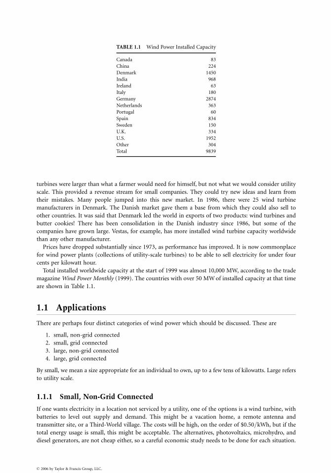
TABLE 1.1 Wind Power Installed Capacity
Canada 83
China 224
Denmark 1450
India 968
Ireland 63
Italy 180
Germany 2874
Netherlands 363
Portugal 60
Spain 834
Sweden 150
U.K. 334
U.S. 1952
Other 304
Total 9839
turbines were larger than what a farmer would need for himself, but not what we would consider utility
scale. This provided a revenue stream for small companies. They could try new ideas and learn from
their mistakes. Many people jumped into this new market. In 1986, there were 25 wind turbine
manufacturers in Denmark. The Danish market gave them a base from which they could also sell to
other countries. It was said that Denmark led the world in exports of two products: wind turbines and
butter cookies! There has been consolidation in the Danish industry since 1986, but some of the
companies have grown large. Vestas, for example, has more installed wind turbine capacity worldwide
than any other manufacturer.
Prices have dropped substantially since 1973, as performance has improved. It is now commonplace
for wind power plants (collections of utility-scale turbines) to be able to sell electricity for under four
cents per kilowatt hour.
Total installed worldwide capacity at the start of 1999 was almost 10,000 MW, according to the trade
magazine Wind Power Monthly (1999). The countries with over 50 MW of installed capacity at that time
are shown in Table 1.1.
1.1 Applications
There are perhaps four distinct categories of wind power which should be discussed. These are
1. small, non-grid connected
2. small, grid connected
3. large, non-grid connected
4. large, grid connected
By small, we mean a size appropriate for an individual to own, up to a few tens of kilowatts. Large refers
to utility scale.
1.1.1 Small, Non-Grid Connected
If one wants electricity in a location not serviced by a utility, one of the options is a wind turbine, with
batteries to level out supply and demand. This might be a vacation home, a remote antenna and
transmitter site, or a Third-World village. The costs will be high, on the order of $0.50=kWh, but if the
total energy usage is small, this might be acceptable. The alternatives, photovoltaics, microhydro, and
diesel generators, are not cheap either, so a careful economic study needs to be done for each situation.
� 2006 by Taylor & Francis Group, LLC.
1.1.2 Small, Grid Connected
The small, grid connected turbine is usually not economically feasible. The cost of wind-generated
electricity is less because the utility is used for storage rather than a battery bank, but is still not competitive.
In order for the small, grid connected turbine to have any hope of financial breakeven, the turbine
owner needs to get something close to the retail price for the wind-generated electricity. One way this is
done is for the owner to have an arrangement with the utility called net metering. With this system, the
meter runs backward when the turbine is generating more than the owner is consuming at the moment.
The owner pays a monthly charge for the wires to his home, but it is conceivable that the utility will
sometimes write a check to the owner at the end of the month, rather than the other way around. The
utilities do not like this arrangement. They want to buy at wholesale and sell at retail. They feel it is
unfair to be used as a storage system without remuneration.
For most of the twentieth century, utilities simply refused to connect the grid to wind turbines. The
utility had the right to generate electricity in a given service territory, and they would not tolerate
competition. Then a law was passed that utilities had to hook up wind turbines and pay them the avoided
cost for energy. Unless the state mandated net metering, the utility typically required the installation of a
second meter, one measuring energy consumption by the home and the other energy production by the
turbine. The owner would pay the regular retail rate, and the utility would pay their estimate of avoided
cost, usually the fuel cost of some base load generator. The owner might pay $0.08 to $0.15 per kWh, and
receive $0.02 per kWh for the wind-generated electricity. This was far from enough to economically
justify a wind turbine, and had the effect of killing the small wind turbine business.
1.1.3 Large, Non-Grid Connected
These machines would be installed on islands or in native villages in the far north where it is virtually
impossible to connect to a large grid. Such places are typically supplied by diesel generators, and have a
substantial cost just for the imported fuel. One or more wind turbines would be installed in parallel
with the diesel generators, and act as fuel savers when the wind was blowing.
This concept has been studied carefully and appears to be quite feasible technically. One would expect
the market to develop after a few turbines have been shown to work for an extended period in hostile
environments. It would be helpful if the diesel maintenance companies would also carry a line of wind
turbines so the people in remote locations would not need to teach another group of maintenance
people about the realities of life at places far away from the nearest hardware store.
1.1.4 Large, Grid Connected
We might ask if the utilities should be forced to buy wind-generated electricity from these small
machines at a premium price which reflects their environmental value. Many have argued this over
the years. A better question might be whether the small or the large turbines will result in a lower net
cost to society. Given that we want the environmental benefits of wind generation, should we get the
electricity from the wind with many thousands of individually owned small turbines, or should we use a
much smaller number of utility-scale machines?
If we could make the argument that a dollar spent on wind turbines is a dollar not spent on hospitals,
schools, and the like, then it follows that wind turbines should be as efficient as possible. Economies of
scale and costs of operation and maintenance are such that the small, grid connected turbine will always
need to receive substantially more per kilowatt hour than the utility-scale turbines in order to break
even. There is obviously a niche market for turbines that are not connected to the grid, but small, grid
connected turbines will probably not develop a thriving market. Most of the action will be from the
utility-scale machines.
Sizes of these turbines have been increasing rapidly. Turbines with ratings near 1 MWare now common,
with prototypes of 2 MW and more being tested. This is still small compared to the needs of a utility, so
clusters of turbines are placed together to form wind power plants with total ratings of 10 to 100 MW.
� 2006 by Taylor & Francis Group, LLC.
1.2 Wind Variability
One of the most critical features of wind generation is the variability of wind. Wind speeds vary with
time of day, time of year, height above ground, and location on the earth’s surface. This makes wind
generators into what might be called energy producers rather than power producers. That is, it is easier
to estimate the energy production for the next month or year than it is to estimate the power that will be
produced at 4:00 PM next Tuesday. Wind power is not dispatchable in the same manner as a gas turbine.
A gas turbine can be scheduled to come on at a given time and to be turned off at a later time, with full
power production in between. A wind turbine produces only when the wind is available. At a good site,
the power output will be zero (or very small) for perhaps 10% of the time, rated for perhaps another
10% of the time, and at some intermediate value the remaining 80% of the time.
This variability means that some sort of storage is necessary for a utility to meet the demands of its
customers, when wind turbines are supplying part of the energy. This is not a problem for penetrations
of wind turbines less than a few percent of the utility peak demand. In small concentrations, wind
turbines act like negative load. That is, an increase in wind speed is no different in its effect than a
customer turning off load. The control systems on the other utility generation sense that generation is
greater than load, and decrease the fuel supply to bring generation into equilibrium with load. In this
case, storage is in the form of coal in the pile or natural gas in the well.
An excellent form of storage is water in a hydroelectric lake. Most hydroelectric plants are sized large
enough to not be able to operate full-time at peak power. They therefore must cut back part of the time
because of the lack of water. A combination hydro and wind plant can conserve water when the wind is
blowing, and use the water later, when the wind is not blowing.
When high-temperature superconductors become a little less expensive, energy storage in a magnetic
field will be an exciting possibility. Each wind turbine can have its own superconducting coil storage
unit. This immediately converts the wind generator from an energy producer to a peak power producer,
fully dispatchable. Dispatchable peak power is always worth more than the fuel cost savings of an energy
producer. Utilities with adequate base load generation (at low fuel costs) would become more interested
in wind power if it were a dispatchable peak power generator.
The variation of wind speed with time of day is called the diurnal cycle. Near the earth’s surface, winds
are usually greater during the middle of the day and decrease at night. This is due to solar heating, which
causes ‘‘bubbles’’ of warm air to rise. The rising air is replaced by cooler air from above. This thermal
mixing causes wind speeds to have only a slight increase with height for the first hundred meters or so
above the earth. At night, however, the mixing stops, the air near the earth slows to a stop, and the winds
above some height (usually 30 to 100 m) actually increase over the daytime value. A turbine on a short
tower will produce a greater proportion of its energy during daylight hours, while a turbine on a very
tall tower will produce a greater proportion at night.
As tower height is increased, a given generator will produce substantially more energy. However, most
of the extra energy will be produced at night, when it is not worth very much. Standard heights have
been increasing in recent years, from 50 to 65 m or even more. A taller tower gets the blades into less
turbulent air, a definite advantage. The disadvantages are extra cost and more danger from overturning
in high winds. A very careful look should be given the economics before buying a tower that is
significantly taller than whatever is sold as a standard height for a given turbine.
Wind speeds also vary strongly with time of year. In the southern Great Plains (Kansas, Oklahoma,
and Texas), the winds are strongest in the spring (March and April) and weakest in the summer (July
and August). Utilities here are summer peaking, and hence need the most power when winds are the
lowest and the least power when winds are highest. The diurnal variation of wind power is thus a fairly
good match to utility needs, while the yearly variation is not.
The variability of wind with month of year and height above ground is illustrated in Table 1.2. These
are actual wind speed data for a good site in Kansas, and projected electrical generation of a Vestas
turbine (V47-660) at that site. Anemometers were located at 10, 40, and 60 m above ground. Wind
� 2006 by Taylor & Francis Group, LLC.
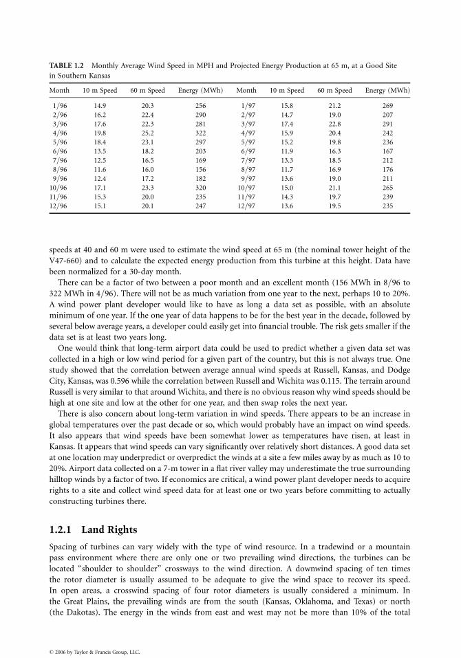
TABLE 1.2 Monthly Average Wind Speed in MPH and Projected Energy Production at 65 m, at a Good Site
in Southern Kansas
Month 10 m Speed 60 m Speed Energy (MWh) Month 10 m Speed 60 m Speed Energy (MWh)
1=96 14.9 20.3 256 1=97 15.8 21.2 269
2=96 16.2 22.4 290 2=97 14.7 19.0 207
3=96 17.6 22.3 281 3=97 17.4 22.8 291
4=96 19.8 25.2 322 4=97 15.9 20.4 242
5=96 18.4 23.1 297 5=97 15.2 19.8 236
6=96 13.5 18.2 203 6=97 11.9 16.3 167
7=96 12.5 16.5 169 7=97 13.3 18.5 212
8=96 11.6 16.0 156 8=97 11.7 16.9 176
9=96 12.4 17.2 182 9=97 13.6 19.0 211
10=96 17.1 23.3 320 10=97 15.0 21.1 265
11=96 15.3 20.0 235 11=97 14.3 19.7 239
12=96 15.1 20.1 247 12=97 13.6 19.5 235
speeds at 40 and 60 m were used to estimate the wind speed at 65 m (the nominal tower height of the
V47-660) and to calculate the expected energy production from this turbine at this height. Data have
been normalized for a 30-day month.
There can be a factor of two between a poor month and an excellent month (156 MWh in 8=96 to
322 MWh in 4=96). There will not be as much variation from one year to the next, perhaps 10 to 20%.
A wind power plant developer would like to have as long a data set as possible, with an absolute
minimum of one year. If the one year of data happens to be for the best year in the decade, followed by
several below average years, a developer could easily get into financial trouble. The risk gets smaller if the
data set is at least two years long.
One would think that long-term airport data could be used to predict whether a given data set was
collected in a high or low wind period for a given part of the country, but this is not always true. One
study showed that the correlation between average annual wind speeds at Russell, Kansas, and Dodge
City, Kansas, was 0.596 while the correlation between Russell and Wichita was 0.115. The terrain around
Russell is very similar to that around Wichita, and there is no obvious reason why wind speeds should be
high at one site and low at the other for one year, and then swap roles the next year.
There is also concern about long-term variation in wind speeds. There appears to be an increase in
global temperatures over the past decade or so, which would probably have an impact on wind speeds.
It also appears that wind speeds have been somewhat lower as temperatures have risen, at least in
Kansas. It appears that wind speeds can vary significantly over relatively short distances. A good data set
at one location may underpredict or overpredict the winds at a site a few miles away by as much as 10 to
20%. Airport data collected on a 7-m tower in a flat river valley may underestimate the true surrounding
hilltop winds by a factor of two. If economics are critical, a wind power plant developer needs to acquire
rights to a site and collect wind speed data for at least one or two years before committing to actually
constructing turbines there.
1.2.1 Land Rights
Spacing of turbines can vary widely with the type of wind resource. In a tradewind or a mountain
pass environment where there are only one or two prevailing wind directions, the turbines can be
located ‘‘shoulder to shoulder’’ crossways to the wind direction. A downwind spacing of ten times
the rotor diameter is usually assumed to be adequate to give the wind space to recover its speed.
In open areas, a crosswind spacing of four rotor diameters is usually considered a minimum. In
the Great Plains, the prevailing winds are from the south (Kansas, Oklahoma, and Texas) or north
(the Dakotas). The energy in the winds from east and west may not be more than 10% of the total
� 2006 by Taylor & Francis Group, LLC.

energy. In this situation, a spacing of ten rotor diameters north–south and four rotor diameters east–
west would be minimal. Adjustments would be made to avoid roads, pipelines, power lines, houses,
ponds, and creeks.
The results of a detailed site layout will probably not predict much more than 20 MW of installed
capacity per square mile (640 acres). This figure can be used for initial estimates without great error.
That is, if a developer is considering installing a 100-MW wind plant, rights to at least five square miles
should be acquired.
One issue that has not received much attention in the wind power community is that of a fair
compensation to the land owner for the privilege of installing wind turbines. The developer could buy
the land, hopefully with a small premium. The original deal could be an option to buy at some agreed
upon price, if two years of wind data were satisfactory. The developer might lease the land back to the
original landowner, since the agricultural production capability is only slightly affected by the presence
of wind turbines. Outright purchase between a willing and knowledgeable buyer and seller would be as
fair an arrangement as could be made.
But what about the case where the landowner does not want to sell? Rights have been acquired by a large
variety of mechanisms, including a large one-time payment for lease signing, a fixed yearly fee, a royalty
payment based on energy produced, and combinations of the above. The one-time payment has been
standard utility practice for right-of-way acquisitions, and hence will be preferred by at least some utilities.
A key difference is that wind turbines require more attention than a transmission line. Roads are not
usually built to transmission line towers, while they are built to wind turbines. Roads and maintenance
operations around wind turbines provide considerably more hassle to the landowner. The original owner
got the lease payment, and 20 years later the new owner gets the nuisance. There is no incentive for the new
landowner to be cooperative or to lobby county or state officials on behalf of the developer.
A one-time payment also increases the risk to the developer. If the project does not get developed,
there has been a significant outlay of cash which will have no return on it. These disadvantages mean that
the one-time payment with no yearly fees or royalties will probably not be the long-term norm in the
industry.
To discuss what might be a fair price for a lease, it will be helpful to use an example. We will assume
the following:
. 20 MW per square mile
. Land fair-market value $500=acre
. Plant factor 0.4
. Developer desired internal rate of return 0.2
. Electricity value $0.04=kWh
. Installed cost of wind turbine $1000=kW
A developer that purchased the land at $500=acre would therefore want a return of $(500)
(0.2)¼ $100=acre. America’s cheap food policy means that production agriculture typically gets a
much smaller return on investment than the developer wants. Actual cash rent on grassland might be
$15=acre, or a return of 0.03 on investment. We see an immediate opportunity for disagreement, even
hypocrisy. The developer might offer the landowner $15=acre when the developer would want $100=acre
if he bought the land. This hardly seems equitable.
The gross income per acre is
I ¼ (20,000 kW) (0:4) (8760 hours=year) ($0:04)
640 acres¼ $4380=acre=year (1:1)
The cost of wind turbines per acre is
CTa ¼(20,000 kW) ($1000=kW)
640 acres¼ $31,250=acre (1:2)
� 2006 by Taylor & Francis Group, LLC.

We see that the present fair-market value for the land is tiny compared with the installed cost of the
wind turbines. A lease payment of $100=acre=year is slightly over 2% of the gross income. It is hard to
imagine financial arrangements so tight that they would collapse if the landowner (either rancher or
developer) were paid this yearly fee. That is, it seems entirely reasonable for a figure like 2% of gross
income to be a starting point for negotiations.
There is another factor that might result in an even higher percentage. Landowners throughout the
Great Plains are accustomed to royalty payments of 12.5% of wholesale price for oil and gas leases.
This is determined independently of any agricultural value for the land. The most worthless mesquite
in Texas gets the same terms as the best irrigated corn ground in Kansas. We might ask if this rate is
too high. A royalty of 12.5% of wholesale amounts to perhaps 6% of retail. Cutting the royalty in
half would have the potential of reducing the price of gasoline about 3%. In a market where gasoline
prices swing by 20%, this reduction is lost in the noise. If a law were passed which cut royalty
payments in half, it is hard to argue that it would have much impact on our gasoline buying habits,
the size of vehicles we buy, or the general welfare of the nation.
One feature of the 12.5% royalty is that it is high enough to get most oil and gas producing land under
lease. Would 6.25% have been enough to get the same amount of land leased? If we assumed that some
people would sign a lease for 12.5% that would not sign if the offer were 6.25%, then we have the
interesting possibility that the supply would be less. If we assume the law of supply and demand to apply,
the price of gasoline and natural gas would increase. The possible increase is shear speculation, but could
easily be more than the 6.25% that was ‘‘saved’’ by cutting the royalty payment in half.
The point is that the royalty needs to be high enough to get the very best sites under lease. If the best
site produces 10% more energy than the next best, it makes no economic sense to pay a 2% royalty for
the second best when a 6% royalty would get the best site. In this example, the developer would get 10%
more energy for 4% more royalty. The developer could either pocket the difference or reduce the price of
electricity a proportionate amount.
References
Brower, M.C., Tennis, M.W., Denzler, E.W., and Kaplan, M.M., Powering the Midwest, A Report by the
Union of Concerned Scientists, 1993.
Johnson, G.L., Wind Energy Systems, Prentice-Hall, New York, 1985.
Wind Power Monthly, 15(6), June, 1999.
� 2006 by Taylor & Francis Group, LLC.

� 2006 by Taylor & Francis Group, LLC.
2
� 2006 by Taylor & Francis Group, LLC.
Advanced EnergyTechnologies
Saifur RahmanVirginia Polytechnic Institute and
State University
2.1 Storage Systems ................................................................... 2-1Flywheel Storage . Compressed Air Energy Storage .
Superconducting Magnetic Energy Storage . Battery Storage
2.2 Fuel Cells .............................................................................. 2-4Basic Principles . Types of Fuel Cells . Fuel Cell Operation
2.3 Summary.............................................................................. 2-7
2.1 Storage Systems
Energy storage technologies are of great interest to electric utilities, energy service companies,
and automobile manufacturers (for electric vehicle application). The ability to store large amounts of
energy would allow electric utilities to have greater flexibility in their operation because with this
option the supply and demand do not have to be matched instantaneously. The availability of the
proper battery at the right price will make the electric vehicle a reality, a goal that has eluded
the automotive industry thus far. Four types of storage technologies (listed below) are discussed in
this section, but most emphasis is placed on storage batteries because it is now closest to being
commercially viable. The other storage technology widely used by the electric power industry,
pumped-storage power plants, is not discussed as this has been in commercial operation for more
than 60 years in various countries around the world.
. Flywheel storage
. Compressed air energy storage
. Superconducting magnetic energy storage
. Battery storage
2.1.1 Flywheel Storage
Flywheels store their energy in their rotating mass, which rotates at very high speeds (approach-
ing 75,000 rotations per minute), and are made of composite materials instead of steel because of
the composite’s ability to withstand the rotating forces exerted on the flywheel. In order to store energy
the flywheel is placed in a sealed container which is then placed in a vacuum to reduce air resistance.
Magnets embedded in the flywheel pass near pickup coils. The magnet induces a current in the
coil changing the rotational energy into electrical energy. Flywheels are still in research and development,
and commercial products are several years away.
2.1.2 Compressed Air Energy Storage
As the name implies, the compressed air energy storage (CAES) plant uses electricity to compress air
which is stored in underground reservoirs. When electricity is needed, this compressed air is withdrawn,
heated with gas or oil, and run through an expansion turbine to drive a generator. The compressed air
can be stored in several types of underground structures, including caverns in salt or rock formations,
aquifers, and depleted natural gas fields. Typically the compressed air in a CAES plant uses about one
third of the premium fuel needed to produce the same amount of electricity as in a conventional plant.
A 290-MW CAES plant has been in operation in Germany since the early 1980s with 90% availability
and 99% starting reliability. In the U.S., the Alabama Electric Cooperative runs a CAES plant that stores
compressed air in a 19-million cubic foot cavern mined from a salt dome. This 110-MW plant has a
storage capacity of 26 h. The fixed-price turnkey cost for this first-of-a-kind plant is about $400=kW in
constant 1988 dollars.
The turbomachinery of the CAES plant is like a combustion turbine, but the compressor and the
expander operate independently. In a combustion turbine, the air that is used to drive the turbine is
compressed just prior to combustion and expansion and, as a result, the compressor and the expander
must operate at the same time and must have the same air mass flow rate. In the case of a CAES plant,
the compressor and the expander can be sized independently to provide the utility-selected ‘‘optimal’’
MW charge and discharge rate which determines the ratio of hours of compression required for each
hour of turbine-generator operation. The MW ratings and time ratio are influenced by the utility’s
load curve, and the price of off-peak power. For example, the CAES plant in Germany requires 4 h
of compression per hour of generation. On the other hand, the Alabama plant requires 1.7 h of
compression for each hour of generation. At 110-MW net output, the power ratio is 0.818 kW output
for each kilowatt input. The heat rate (LHV) is 4122 BTU=kWh with natural gas fuel and 4089
BTU=kWh with fuel oil. Due to the storage option, a partial-load operation of the CAES plant is also
very flexible. For example, the heat rate of the expander increases only by 5%, and the airflow decreases
nearly linearly when the plant output is turned down to 45% of full load. However, CAES plants have
not reached commercial viability beyond some prototypes.
2.1.3 Superconducting Magnetic Energy Storage
A third type of advanced energy storage technology is superconducting magnetic energy storage (SMES),
which may someday allow electric utilities to store electricity with unparalled efficiency (90% or more).
A simple description of SMES operation follows.
The electricity storage medium is a doughnut-shaped electromagnetic coil of superconducting wire.
This coil could be about 1000 m in diameter, installed in a trench, and kept at superconducting
temperature by a refrigeration system. Off-peak electricity, converted to direct current (DC), would be
fed into this coil and stored for retrieval at any moment. The coil would be kept at a low-temperature
superconducting state using liquid helium. The time between charging and discharging could be as little
as 20 ms with a round-trip AC–AC efficiency of over 90%.
Developing a commercial-scale SMES plant presents both economic and technical challenges. Due to
the high cost of liquiud helium, only plants with 1000-MW, 5-h capacity are economically attractive.
Even then the plant capital cost can exceed several thousand dollars per kilowatt. As ceramic supercon-
ductors, which become superconducting at higher temperatures (maintained by less expensive liquid
nitrogen), become more widely available, it may be possible to develop smaller scale SMES plants at a
lower price.
2.1.4 Battery Storage
Even though battery storage is the oldest and most familiar energy storage device, significant advances
have been made in this technology in recent years to deserve more attention. There has been renewed
interest in this technology due to its potential application in non-polluting electric vehicles. Battery
� 2006 by Taylor & Francis Group, LLC.
systems are quiet and non-polluting, and can be installed near load centers and existing suburban
substations. These have round-trip AC–AC efficiencies in the range of 85%, and can respond to load
changes within 20 ms. Several U.S., European, and Japanese utilities have demonstrated the application
of lead–acid batteries for load-following applications. Some of them have been as large as 10 MW with
4 h of storage.
The other player in battery development is the automotive industry for electric vehicle application. In
1991, General Motors, Ford, Chrysler, Electric Power Research Institute (EPRI), several utilities, and
the U.S. Department of Energy (DOE) formed the U.S. Advanced Battery Consortium (USABC)
to develop better batteries for electric vehicle (EV) applications. A brief introduction to some of
the available battery technologies as well some that are under study is presented in the following
(Source: http:==www.eren.doe.gov=consumerinfo=refbriefs=fa1=html).
2.1.4.1 Battery Types
Chemical batteries are individual cells filled with a conducting medium-electrolyte that, when connected
together, form a battery. Multiple batteries connected together form a battery bank. At present, there are
two main types of batteries: primary batteries (non-rechargeable) and secondary batteries (recharge-
able). Secondary batteries are further divided into two categories based on the operating temperature of
the electrolyte. Ambient operating temperature batteries have either aqueous (flooded) or nonaqueous
electrolytes. High operating temperature batteries (molten electrodes) have either solid or molten
electrolytes. Batteries in EVs are the secondary-rechargeable-type and are in either of the two sub-
categories. A battery for an EV must meet certain performance goals. These goals include quick
discharge and recharge capability, long cycle life (the number of discharges before becoming unservice-
able), low cost, recyclability, high specific energy (amount of usable energy, measured in watt-hours per
pound [lb] or kilogram [kg]), high energy density (amount of energy stored per unit volume), specific
power (determines the potential for acceleration), and the ability to work in extreme heat or cold. No
battery currently available meets all these criteria.
2.1.4.2 Lead–Acid Batteries
Lead–acid starting batteries (shallow-cycle lead–acid secondary batteries) are the most common battery
used in vehicles today. This battery is an ambient temperature, aqueous electrolyte battery. A cousin to
this battery is the deep-cycle lead–acid battery, now widely used in golf carts and forklifts. The first
electric cars built also used this technology. Although the lead–acid battery is relatively inexpensive, it is
very heavy, with a limited usable energy by weight (specific energy). The battery’s low specific energy and
poor energy density make for a very large and heavy battery pack, which cannot power a vehicle as far as
an equivalent gas-powered vehicle. Lead–acid batteries should not be discharged by more than 80% of
their rated capacity or depth of discharge (DOD). Exceeding the 80% DOD shortens the life of the
battery. Lead–acid batteries are inexpensive, readily available, and are highly recyclable, using the
elaborate recycling system already in place. Research continues to try to improve these batteries.
A lead–acid nonaqueous (gelled lead acid) battery uses an electrolyte paste instead of a liquid. These
batteries do not have to be mounted in an upright position. There is no electrolyte to spill in an accident.
Nonaqueous lead–acid batteries typically do not have as high a life cycle and are more expensive than
flooded deep-cycle lead–acid batteries.
2.1.4.3 Nickel Iron and Nickel Cadmium Batteries
Nickel iron (Edison cells) and nickel cadmium (nicad) pocket and sintered plate batteries have been in
use for many years. Both of these batteries have a specific energy of around 25 Wh=lb (55 Wh=kg), which
is higher than advanced lead–acid batteries. These batteries also have a long cycle life. Both of these
batteries are recyclable. Nickel iron batteries are non-toxic, while nicads are toxic. They can also be
discharged to 100% DOD without damage. The biggest drawback to these batteries is their cost.
Depending on the size of battery bank in the vehicle, it may cost between $20,000 and $60,000 for the
batteries. The batteries should last at least 100,000 mi (160,900 km) in normal service.
� 2006 by Taylor & Francis Group, LLC.

2.1.4.4 Nickel Metal Hydride Batteries
Nickel metal hydride batteries are offered as the best of the next generation of batteries. They have a high
specific energy: around 40.8 Wh=lb (90 Wh=kg). According to a U.S. DOE report, the batteries are
benign to the environment and are recyclable. They also are reported to have a very long cycle life. Nickel
metal hydride batteries have a high self-discharge rate: they lose their charge when stored for long
periods of time. They are already commercially available as ‘‘AA’’ and ‘‘C’’ cell batteries, for small
consumer appliances and toys. Manufacturing of larger batteries for EV applications is only available
to EV manufacturers. Honda is using these batteries in the EV Plus, which is available for lease in
California.
2.1.4.5 Sodium Sulfur Batteries
This battery is a high-temperature battery, with the electrolyte operating at temperatures of 5728F
(3008C). The sodium component of this battery explodes on contact with water, which raises certain
safety concerns. The materials of the battery must be capable of withstanding the high internal
temperatures they create, as well as freezing and thawing cycles. This battery has a very high specific
energy: 50 Wh=lb (110 Wh=kg). The Ford Motor Company uses sodium sulfur batteries in their Ecostar,
a converted delivery minivan that is currently sold in Europe. Sodium sulfur batteries are only available
to EV manufacturers.
2.1.4.6 Lithium Iron and Lithium Polymer Batteries
The USABC considers lithium iron batteries to be the long-term battery solution for EVs. The batteries
have a very high specific energy: 68 Wh=lb (150 Wh=kg). They have a molten-salt electrolyte and share
many features of a sealed bipolar battery. Lithium iron batteries are also reported to have a very long
cycle life. These are widely used in laptop computers. These batteries will allow a vehicle to travel
distances and accelerate at a rate comparable to conventional gasoline-powered vehicles. Lithium
polymer batteries eliminate liquid electrolytes. They are thin and flexible, and can be molded into a
variety of shapes and sizes. Neither type will be ready for EV commercial applications until early in the
21st century.
2.1.4.7 Zinc and Aluminum Air Batteries
Zinc air batteries are currently being tested in postal trucks in Germany. These batteries use either
aluminum or zinc as a sacrificial anode. As the battery produces electricity, the anode dissolves into the
electrolyte. When the anode is completely dissolved, a new anode is placed in the vehicle. The aluminum
or zinc and the electrolyte are removed and sent to a recycling facility. These batteries have a specific
energy of over 97 Wh=lb (200 Wh=kg). The German postal vans currently carry 80 kWh of energy in
their battery, giving them about the same range as 13 gallons (49.2 liters) of gasoline. In their tests, the
vans have achieved a range of 615 mi (990 km) at 25 miles per hour (40 km=h).
2.2 Fuel Cells
In 1839, a British Jurist and an amateur physicist named William Grove first discovered the principle of
the fuel cell. Grove utilized four large cells, each containing hydrogen and oxygen, to produce electricity
and water which was then used to split water in a different container to produce hydrogen and oxygen.
However, it took another 120 years until NASA demonstrated its use to provide electricity and water for
some early space flights. Today the fuel cell is the primary source of electricity on the space shuttle. As a
result of these successes, industry slowly began to appreciate the commercial value of fuel cells. In
addition to stationary power generation applications, there is now a strong push to develop fuel cells for
automotive use. Even though fuel cells provide high performance characterisitics, reliability, durability,
and environmental benefits, a very high investment cost is still the major barrier against large-scale
deployments.
� 2006 by Taylor & Francis Group, LLC.

2.2.1 Basic Principles
The fuel cell works by processing a hydrogen-rich fuel—usually natural gas or methanol—into
hydrogen, which, when combined with oxygen, produces electricity and water. This is the reverse
electrolysis process. Rather than burning the fuel, however, the fuel cell converts the fuel to electricity
using a highly efficient electrochemical process. A fuel cell has few moving parts, and produces very little
waste heat or gas.
A fuel cell power plant is basically made up of three subsystems or sections. In the fuel-processing
section, the natural gas or other hydrocarbon fuel is converted to a hydrogen-rich fuel. This is normally
accomplished through what is called a steam catalytic reforming process. The fuel is then fed to the
power section, where it reacts with oxygen from the air in a large number of individual fuel cells to
produce direct current (DC) electricity, and by-product heat in the form of usable steam or hot water.
For a power plant, the number of fuel cells can vary from several hundred (for a 40-kW plant) to several
thousand (for a multi-megawatt plant). In the final, or third stage, the DC electricity is converted in the
power conditioning subsystem to electric utility-grade alternating current (AC).
In the power section of the fuel cell, which contains the electrodes and the electrolyte, two separate
electrochemical reactions take place: an oxidation half-reaction occurring at the anode and a reduction
half-reaction occurring at the cathode. The anode and the cathode are separated from each other by the
electrolyte. In the oxidation half-reaction at the anode, gaseous hydrogen produces hydrogen ions, which
travel through the ionically conducting membrane to the cathode. At the same time, electrons travel
through an external circuit to the cathode. In the reduction half-reaction at the cathode, oxygen supplied
from air combines with the hydrogen ions and electrons to form water and excess heat. Thus, the final
products of the overall reaction are electricity, water, and excess heat.
2.2.2 Types of Fuel Cells
The electrolyte defines the key properties, particularly the operating temperature, of the fuel cell.
Consequently, fuel cells are classified based on the types of electrolyte used as described below.
1. Polymer Electrolyte Membrane (PEM)
2. Alkaline Fuel Cell (AFC)
3. Phosphoric Acid Fuel Cell (PAFC)
4. Molten Carbonate Fuel Cell (MCFC)
5. Solid Oxide Fuel Cell (SOFC)
These fuel cells operate at different temperatures and each is best suited to particular applications.
The main features of the five types of fuel cells are summarized in Table 2.1.
2.2.3 Fuel Cell Operation
Basic operational characteristics of the four most common types of fuel cells are discussed in the
following.
2.2.3.1 Polymer Electrolyte Membrane (PEM)
The PEM cell is one in a family of fuel cells that are in various stages of development. It is being
considered as an alternative power source for automotive application for electric vehicles. The electrolyte
in a PEM cell is a type of polymer and is usually referred to as a membrane, hence the name. Polymer
electrolyte membranes are somewhat unusual electrolytes in that, in the presence of water, which the
membrane readily absorbs, the negative ions are rigidly held within their structure. Only the positive (H)
ions contained within the membrane are mobile and are free to carry positive charges through the
membrane in one direction only, from anode to cathode. At the same time, the organic nature of
the polymer electrolyte membrane structure makes it an electron insulator, forcing it to travel through
the outside circuit providing electric power to the load. Each of the two electrodes consists of porous
� 2006 by Taylor & Francis Group, LLC.
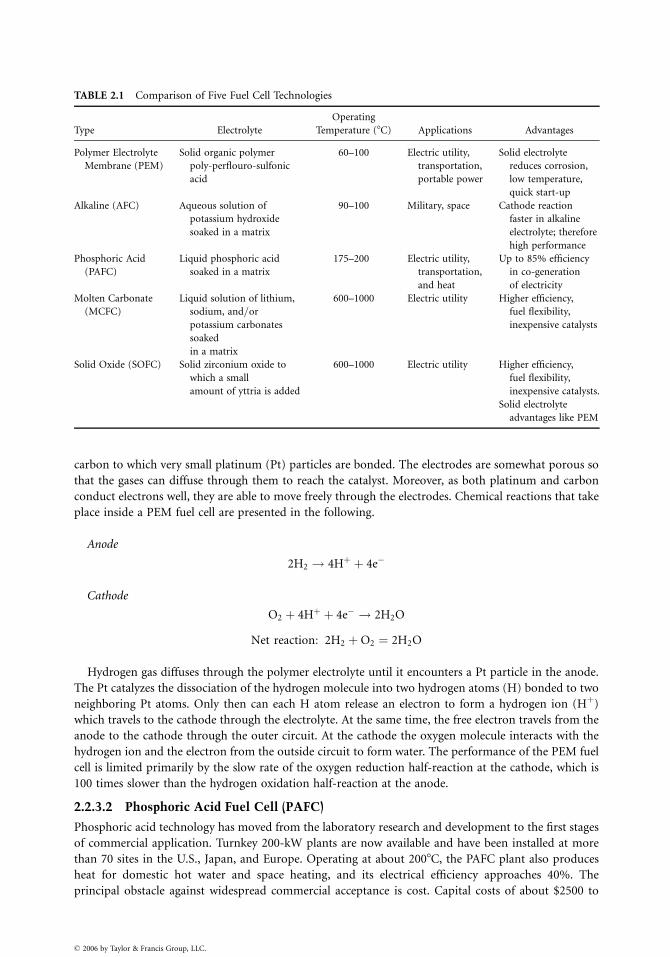
TABLE 2.1 Comparison of Five Fuel Cell Technologies
Type Electrolyte
Operating
Temperature (8C) Applications Advantages
Polymer Electrolyte
Membrane (PEM)
Solid organic polymer
poly-perflouro-sulfonic
acid
60–100 Electric utility,
transportation,
portable power
Solid electrolyte
reduces corrosion,
low temperature,
quick start-up
Alkaline (AFC) Aqueous solution of
potassium hydroxide
soaked in a matrix
90–100 Military, space Cathode reaction
faster in alkaline
electrolyte; therefore
high performance
Phosphoric Acid
(PAFC)
Liquid phosphoric acid
soaked in a matrix
175–200 Electric utility,
transportation,
and heat
Up to 85% efficiency
in co-generation
of electricity
Molten Carbonate
(MCFC)
Liquid solution of lithium,
sodium, and=or
potassium carbonates
soaked
in a matrix
600–1000 Electric utility Higher efficiency,
fuel flexibility,
inexpensive catalysts
Solid Oxide (SOFC) Solid zirconium oxide to
which a small
amount of yttria is added
600–1000 Electric utility Higher efficiency,
fuel flexibility,
inexpensive catalysts.
Solid electrolyte
advantages like PEM
carbon to which very small platinum (Pt) particles are bonded. The electrodes are somewhat porous so
that the gases can diffuse through them to reach the catalyst. Moreover, as both platinum and carbon
conduct electrons well, they are able to move freely through the electrodes. Chemical reactions that take
place inside a PEM fuel cell are presented in the following.
Anode
2H2 ! 4Hþ þ 4e�
Cathode
O2 þ 4Hþ þ 4e� ! 2H2O
Net reaction: 2H2 þO2 ¼ 2H2O
Hydrogen gas diffuses through the polymer electrolyte until it encounters a Pt particle in the anode.
The Pt catalyzes the dissociation of the hydrogen molecule into two hydrogen atoms (H) bonded to two
neighboring Pt atoms. Only then can each H atom release an electron to form a hydrogen ion (Hþ)
which travels to the cathode through the electrolyte. At the same time, the free electron travels from the
anode to the cathode through the outer circuit. At the cathode the oxygen molecule interacts with the
hydrogen ion and the electron from the outside circuit to form water. The performance of the PEM fuel
cell is limited primarily by the slow rate of the oxygen reduction half-reaction at the cathode, which is
100 times slower than the hydrogen oxidation half-reaction at the anode.
2.2.3.2 Phosphoric Acid Fuel Cell (PAFC)
Phosphoric acid technology has moved from the laboratory research and development to the first stages
of commercial application. Turnkey 200-kW plants are now available and have been installed at more
than 70 sites in the U.S., Japan, and Europe. Operating at about 2008C, the PAFC plant also produces
heat for domestic hot water and space heating, and its electrical efficiency approaches 40%. The
principal obstacle against widespread commercial acceptance is cost. Capital costs of about $2500 to
� 2006 by Taylor & Francis Group, LLC.
$4000=kW must be reduced to $1000 to $1500=kW if the technology is to be accepted in the electric
power markets.
The chemical reactions occurring at two electrodes are written as follows:
At anode: 2H2 ! 4Hþ þ 4e�
At cathode: O2 þ 4Hþ þ 4e� ! 2H2O
2.2.3.3 Molten Carbonate Fuel Cell (MCFC)
Molten carbonate technology is attractive because it offers several potential advantages over PAFC.
Carbon monoxide, which poisons the PAFC, is indirectly used as a fuel in the MCFC. The higher
operating temperature of approximately 6508C makes the MCFC a better candidate for combined cycle
applications whereby the fuel cell exhaust can be used as input to the intake of a gas turbine or the boiler
of a steam turbine. The total thermal efficiency can approach 85%. This technology is at the stage of
prototype commercial demonstrations and is estimated to enter the commercial market by 2003 using
natural gas, and by 2010 with gas made from coal. Capital costs are expected to be lower than PAFC.
MCFCs are now being tested in full-scale demonstration plants. The following equations illustrate the
chemical reactions that take place inside the cell.
At anode: 2H2 þ 2CO2�3 ! 2H2Oþ 2CO2 þ 4e�
and 2COþ 2CO2�3 ! 4CO2 þ 4e�
At cathode: O2 þ 2CO2 þ 4e� ! 2O2�3
2.2.3.4 Solid Oxide Fuel Cell (SOFC)
A solid oxide fuel cell is currently being demonstrated at a 100-kW plant. Solid oxide technology
requires very significant changes in the structure of the cell. As the name implies, the SOFC uses a solid
electrolyte, a ceramic material, so the electrolyte does not need to be replenished during the operational
life of the cell. This simplifies design, operation, and maintenance, as well as having the potential to
reduce costs. This offers the stability and reliability of all solid-state construction and allows higher
temperature operation. The ceramic make-up of the cell lends itself to cost-effective fabrication
techniques. The tolerance to impure fuel streams make SOFC systems especially attractive for utilizing
H2 and CO from natural gas steam-reforming and coal gasification plants. The chemical reactions inside
the cell may be written as follows:
At anode: 2H2 þ 2O2� ! 2H2Oþ 4e�
and 2COþ 2O2� ! 2CO2 þ 4e�
At cathode: O2 þ 4e� ! 2O2�
2.3 Summary
Fuel cells can convert a remarkably high proportion of the chemical energy in a fuel to electricity. With
the efficiencies approaching 60%, even without co-generation, fuel cell power plants are nearly twice as
efficient as conventional power plants. Unlike large steam plants, the efficiency is not a function of the
plant size for fuel cell power plants. Small-scale fuel cell plants are just as efficient as the large ones,
whether they operate at full load or not. Fuel cells contribute significantly to the cleaner environment;
they produce dramtically fewer emissions, and their by-products are primarily hot water and carbon
dioxide in small amounts. Because of their modular nature, fuel cells can be placed at or near load
centers, resulting in savings of transmission network expansion.
� 2006 by Taylor & Francis Group, LLC.

� 2006 by Taylor & Francis Group, LLC.
3
� 2006 by Taylor & Francis Group, LLC.
Photovoltaics
Roger A. MessengerFlorida Atlantic University
3.1 Types of PV Cells................................................................. 3-1Silicon Cells . Gallium Arsenide Cells . Copper Indium
(Gallium) Diselenide Cells . Cadmium Telluride Cells .
Emerging Technologies
3.2 PV Applications ................................................................... 3-4Utility-Interactive PV Systems . Stand-Alone PV Systems
3.1 Types of PV Cells
3.1.1 Silicon Cells
Silicon PV cells come in several varieties. The most common cell is the single-crystal silicon cell. Other
variations include multicrystalline (polycrystalline), thin silicon (buried contact) cells, and amorphous
silicon cells.
3.1.1.1 Single-Crystal Silicon Cells
While single crystal silicon cells are still the most common cells, the fabrication process of these cells is
relatively energy intensive, resulting in limits to cost reduction for these cells. Since single-crystal silicon
is an indirect bandgap semiconductor (Eg¼ 1.1 eV), its absorption constant is smaller than that of direct
bandgap materials. This means that single-crystal silicon cells need to be thicker than other cells in order
to absorb a sufficient percentage of incident radiation. This results in the need for more material and
correspondingly more energy involved in cell processing, especially since the cells are still produced
mostly by sawing of single-crystal silicon ingots into wafers that are about 200 mm thick. To achieve
maximum fill of the module, round ingots are first sawed to achieve closer to a square cross-section
prior to wafering.
After chemical etching to repair surface damage from sawing, the junction is diffused into the wafers.
Improved cell efficiency can then be achieved by using a preferential etch on the cell surfaces to produce
textured surfaces. The textured surfaces reflect photons back toward the junction at an angle, thus
increasing the path length and increasing the probability of the photon being absorbed within a minority
carrier diffusion length of the junction. Following the chemical etch, contacts, usually aluminum, are
evaporated and annealed and the front surface is covered with an antireflective coating.
The cells are then assembled into modules, consisting of approximately 33 to 36 individual cells
connected in series. Since the open-circuit output voltage of an individual silicon cell typically ranges
from 0.5 to 0.6 V, depending upon irradiance level and cell temperature, this results in a module open-
circuit voltage between 18 and 21.6 V. The cell current is directly proportional to the irradiance and the
cell area. A 4-ft2 (0.372-m2) module (active cell area) under full sun will typically produce a maximum
power close to 55 W at approximately 17 V and 3.2 A.
3.1.1.2 Multicrystalline Silicon Cells
By pouring molten silicon into a crucible and controlling the cooling rate, it is possible to grow
multicrystalline silicon with a rectangular cross-section. This eliminates the ‘‘squaring-up’’ process
and the associated loss of material. The ingot must still be sawed into wafers, but the resulting wafers
completely fill the module. The remaining processing follows the steps of single-crystal silicon, and cell
efficiencies in excess of 15% have been achieved for relatively large area cells. Multicrystalline material
still maintains the basic properties of single-crystal silicon, including the indirect bandgap. Hence,
relatively thick cells with textured surfaces have the highest conversion efficiencies. Multicrystalline
silicon modules are commercially available and are recognized by their ‘‘speckled’’ surface appearance.
3.1.1.3 Thin Silicon (Buried Contact) Cells
The current flow direction in most PV cells is between the front surface and the back surface. In the thin
silicon cell, a dielectric layer is deposited on an insulating substrate, followed by alternating layers of
n-type and p-type silicon, forming multiple pn junctions. Channels are then cut with lasers and contacts
are buried in the channels, so the current flow is parallel to the cell surfaces in multiple parallel
conduction paths. These cells minimize resistance from junction to contact with the multiple
parallel conduction paths and minimize blocking of incident radiation by the front contact. Although
the material is not single crystal, grain boundaries cause minimal degradation of cell efficiency. The
collection efficiency is very high, since essentially all photon-generated carriers are generated within
a diffusion length of a pn junction. This technology is relatively new, but has already been licensed to a
number of firms worldwide (Green and Wenham, 1994).
3.1.1.4 Amorphous Silicon Cells
Amorphous silicon has no predictable crystal structure. As a result, the uniform covalent bond structure
of single-crystal silicon is replaced with a random bonding pattern with many open covalent bonds.
These bonds significantly degrade the performance of amorphous silicon by reducing carrier mobilities
and the corresponding diffusion lengths. However, if hydrogen is introduced into the material, its
electron will pair up with the dangling bonds of the silicon, thus passivating the material. The result is a direct
bandgap material with a relatively high absorption constant. A film with a thickness of a few micrometers
will absorb nearly all incident photons with energies higher than the 1.75 eV bandgap energy.
Maximum collection efficiency for a-Si:H is achieved by fabricating the cell with a pin junction. Early
work on the cells revealed, however, that if the intrinsic region is too thick, cell performance will degrade
over time. This problem has now been overcome by the manufacture of multi-layer cells with thinner
pin junctions. In fact, it is possible to further increase cell efficiency by stacking cells of a-SiC:H on top,
a-Si:H in the center, and a-SiGe:H on the bottom. Each successive layer from the top has a smaller
bandgap, so the high-energy photons can be captured soon after entering the material, followed by
middle-energy photons and then lower energy photons.
While the theoretical maximum efficiency of a-Si:H is 27% (Zweibel, 1990), small-area lab cells
have been fabricated with efficiencies of 14% and large-scale devices have efficiencies in the 10% range
(Yang et al., 1997).
Amorphous silicon cells have been adapted to the building integrated PV (BIPV) market by fabri-
cating the cells on stainless steel (Guha et al., 1997) and polymide substrates (Huang et al., 1997). The
‘‘solar shingle’’ is now commercially available, and amorphous silicon cells are commonly used in solar
calculators and solar watches.
3.1.2 Gallium Arsenide Cells
Gallium arsenide (GaAs), with its 1.43 eV direct bandgap, is a nearly optimal PV cell material. The only
problem is that it is very costly to fabricate cells. GaAs cells have been fabricated with conversion
efficiencies above 30% and with their relative insensitivity to severe temperature cycling and radiation
exposure, they are the preferred material for extraterrestrial applications, where performance and weight
are the dominating factors.
� 2006 by Taylor & Francis Group, LLC.
Gallium and arsenic react exothermically when combined, so formation of the host material is more
complicated than formation of pure, single-crystal silicon. Modern GaAs cells are generally fabricated by
growth of a GaAs film on a suitable substrate, such as Ge. A typical GaAs cell has a Ge substrate with a layer of
n-GaAs followed by a layer of p-GaAs and then a thin layer of p-GaAlAs between the p-GaAs and the top
contacts. The p-GaAlAs has a wider bandgap (1.8 eV) than the GaAs, so the higher energy photons are not
absorbed at the surface, but are transmitted through to the GaAs pn junction, where they are then absorbed.
Recent advances in III-V technology have produced tandem cells similar to the a-Si:H tandem cell.
One cell consists of two tandem GaAs cells, separated by thin tunnel junctions of GaInP, followed by a
third tandem GaInP cell, separated by AlInP tunnel junctions (Lammasniemi et al., 1997). The tunnel
junctions mitigate voltage drop of the otherwise forward-biased pn junction that would appear between
any two tandem pn junctions in opposition to the photon-induced cell voltage. Cells have also been
fabricated of InP (Hoffman et al., 1997).
3.1.3 Copper Indium (Gallium) Diselenide Cells
Another promising thin film material is copper indium (gallium) diselenide (CIGS). While the basic
copper indium diselenide cell has a bandgap of 1.0 eV, the addition of gallium increases the bandgap to
closer to 1.4 eV, resulting in more efficient collection of photons near the peak of the solar spectrum.
CIGS has a high absorption constant and essentially all incident photons are absorbed within a distance
of 2 mm, as in a-Si:H. Indium is the most difficult component to obtain, but the quantity needed for a
module is relatively minimal.
The CIGS cell is fabricated on a soda glass substrate by first applying a thin layer of molybdenum as
the back contact, since the CIGS will form an ohmic contact with Mo. The next layer is p-type CIGS,
followed by a layer of n-type CdS, rather than n-type CIGS, because the pn homojunction in CIGS is
neither stable nor efficient. While the cells discussed thus far have required metals to obtain ohmic front
contacts, it is possible to obtain an ohmic contact on CdS with a transparent conducting oxide (TCO)
such as ZnO. The top surface is first passivated with a thin layer (50 nm) of intrinsic ZnO to prevent
minority carrier surface recombination. Then a thicker layer (350 nm) of nþ ZnO is added, followed by
an MgF2 antireflective coating.
Efficiencies of laboratory cells are now near 18% (Tuttle et al., 1996), with a module efficiency of
11.1% reported in 1998 (Tarrant and Gay, 1998). Although at the time of this writing, CIGS modules
were not commercially available, the technology has been under field tests for nearly 10 years. It has been
projected that the cells may be manufactured on a large scale for $1=W or less. At this cost level, area-
related costs become significant, so that it becomes important to increase cell efficiency to maximize
power output for a given cell area.
3.1.4 Cadmium Telluride Cells
Of the II-VI semiconductor materials, CdTe has a theoretical maximum efficiency of near 25%. The
material has a favorable direct bandgap (1.44 eV) and a large absorption constant. As in the other thin
film materials, a 2-mm thickness is adequate for the absorption of most of the incident photons. Small
laboratory cells have been fabricated with efficiencies near 15% and module efficiencies close to 10%
have been achieved (Ullal et al., 1997). Some concern has been expressed about the Cd content of the
cells, particularly in the event of fire dispersing the Cd. It has been determined that anyone endangered
by Cd in a fire would be far more endangered by the fire itself, due to the small quantity of Cd in the
cells. Decommissioning of the module has also been analyzed and it has been concluded that the cost to
recycle module components is pennies per watt (Fthenakis and Moskowitz, 1997).
The CdTe cell is fabricated on a glass superstrate covered with a thin TCO (1 mm). The next layer is
n-type CdS with a thickness of approximately 100 nm, followed by a 2-mm thick CdTe layer and a
back contact of an appropriate metal for ohmic contact, such as Au, Cu=Au, Ni, Ni=Al, ZnTe:Cu or
(Cu, HgTe). The back contact is then covered with a layer of ethylene vinyl acetate (EVA) or other
suitable encapsulant and another layer of glass. The front glass is coated with an antireflective coating.
� 2006 by Taylor & Francis Group, LLC.
Experimental CdTe arrays up to 25 kW have been under test for several years with no reports
of degradation. It has been estimated that the cost for large-scale production can be reduced to
below $1=W. Once again, as in the CIGS case, module efficiency needs to be increased to reduce the
area-related costs.
3.1.5 Emerging Technologies
The PV field is moving so quickly that by the time information appears in print, it is generally outdated.
Reliability of cells, modules, and system components continues to improve. Efficiencies of cells and
modules continue to increase, and new materials and cell fabrication techniques continue to evolve.
One might think that Si cells will soon become historical artifacts. This may not be the case. Efforts are
underway to produce Si cells that have good charge carrier transport properties while improving photon
absorption and reducing the energy for cell production. Ceramic and graphite substrates have been used
with thinner layers of Si. Processing steps have been doubled up. Metal insulator semiconductor
inversion layer (MIS-IL) cells have been produced in which the diffused junction is replaced with a
Schottky junction. By use of clever geometry of the back electrode to reduce the rear surface recom-
bination velocity along with front surface passivation, an efficiency of 18.5% has been achieved for a
laboratory MIS-IL cell. Research continues on ribbon growth in an effort to eliminate wafering, and
combining crystalline and amorphous Si in a tandem cell to take advantage of the two different
bandgaps for increasing photon collection efficiency has been investigated.
At least eight different CIS-based materials have been proposed for cells. The materials have direct
bandgaps ranging from 1.05 to 2.56 eV. A number of III-V materials have also emerged that have
favorable photon absorption properties. In addition, quantum well cells have been proposed that
have theoretical efficiencies in excess of 40% under concentrating conditions.
The PV market seems to have taken a strong foothold, with the likelihood that annual PV module
shipments will exceed 200 MW before the end of the century and continue to increase by approximately
15% annually as new markets open as cost continues to decline and reliability continues to improve.
3.2 PV Applications
PV cells were first used to power satellites. Through the middle of the 1990s the most common terrestrial
PV applications were stand-alone systems located where connection to the utility grid was impractical.
By the end of the 1990s, PV electrical generation was cost-competitive with the marginal cost of central
station power when it replaced gas turbine peaking in areas with high afternoon irradiance levels.
Encouraged by consumer approval, a number of utilities have introduced utility-interactive PV systems
to supply a portion of their total customer demand. Some of these systems have been residential and
commercial rooftop systems and other systems have been larger ground-mounted systems. PV systems
are generally classified as utility interactive (grid connected) or stand-alone.
Orientation of the PV modules for optimal energy collection is an important design consideration,
whether for a utility interactive system or for a stand-alone system. Best overall energy collection on an
annual basis is generally obtained with a south-facing collector having a tilt at an angle with the
horizontal approximately 90% of the latitude of the site. For optimal winter performance, a tilt of
latitude þ158 is best and for optimal summer performance a tilt of latitude �158 is best. In some cases,
when it is desired to have the PV output track utility peaking requirements, a west-facing array may be
preferred, since its maximum output will occur during summer afternoon utility peaking hours.
Monthly peak sun tables for many geographical locations are available from the National Renewable
Energy Laboratory (Sandia National Laboratories, 1996; Florida Solar Energy Center).
3.2.1 Utility-Interactive PV Systems
Utility-interactive PV systems are classified by IEEE Standard 929 as small, medium, or large
(ANSI=IEEE, 1999). Small systems are less than 10 kW, medium systems range from 10 to 500 kW,
� 2006 by Taylor & Francis Group, LLC.
and large systems are larger than 500 kW. Each size range requires different consideration for the utility
interconnect. In addition to being able to offset utility peak power, the distributed nature of PV systems
also results in the reduction of load on transmission and distribution lines. Normally, utility-interactive
systems do not incorporate any form of energy storage—they simply supply power to the grid when they
are operating. In some instances, however, where grid power may not be as reliable as the user may
desire, battery back-up is incorporated to ensure uninterrupted power.
Since the output of PV modules is DC, it is necessary to convert the module output to AC before
connecting it to the grid. This is done with an inverter, also known as a power conditioning unit (PCU).
Modern PCUs must meet the standards set by IEEE 929. If the PCU is connected on the customer side of
the revenue meter, the PV system must meet the requirements of the National Electrical Code1 (NEC1)
(National Fire Protection Association, 1998). For a system to meet NEC requirements, it must consist of
UL listed components. In particular, the PCU must be tested under UL 1741 (Underwriters Laborator-
ies, 1997). But UL 1741 has been set up to test for compliance with IEEE 929, so any PCU that passes the
UL 1741 test is automatically qualified under the requirements of the NEC.
Utility-interactive PCUs are generally pulse code modulated (PCM) units with nearly all NEC-
required components, such as fusing of PV output circuits, DC and AC disconnects, and automatic
utility disconnect in the event of loss of utility voltage. They also often contain surge protectors on input
and output, ground fault protection circuitry, and maximum power tracking circuitry to ensure that the
PV array is loaded at its maximum power point. The PCUs act as current sources, synchronized by the
utility voltage. Since the PCUs are electronic, they can sample the line voltage at a high rate and readily
shut down under conditions of utility voltage or frequency as specified by IEEE 929.
The typical small utility-interactive system of a few kilowatts consists of an array of modules selected
by either a total cost criterion or, perhaps, by an available roof area criterion. The modules are connected
to produce an output voltage ranging from 48 V to 300 V, depending upon the DC input requirements
of the PCU. One or two PCUs are used to interface the PV output to the utility at 120 V or, perhaps,
120=240 V. The point of utility connection is typically the load side of a circuit breaker in the
distribution panel of the occupancy if the PV system is connected on the customer side of the revenue
meter. Connections on the utility side of the meter will normally be with double lugs on the line side of
the meter. Section 690 of the NEC provides the connection and installation requirements for systems
connected on the customer side of the revenue meter. Utility-side interconnects are regulated by the
local utility.
Since the cost of PCUs is essentially proportional to their power handling capability, to date there has
been no particular economy of scale for PV system size. As a result, systems are often modular. One form
of modularity is the AC module. The AC module incorporates a small PCU (�300 W) mounted on the
module itself so the output of the module is 120 V AC. This simplifies the hook-up of the PV system,
since NEC requirements for PV output circuits are avoided and only the requirements for PCU output
circuits need to be met.
Medium- and large-scale utility-interactive systems differ from small-scale systems only in the possi-
bility that the utility may require different interfacing conditions relating to power quality and=or
conditions for disconnect. Since medium-and large-scale systems require more area than is typically
available on the rooftop of a residential occupancy, they are more typically found either on commercial
industrial rooftops or, in the case of large systems, are typically ground-mounted. Rooftop mounts are
attractive since they require no additional space other than what is already available on the rooftop. The
disadvantage is when roof repair is needed, the PV system may need to be temporarily removed and then
reinstalled. Canopies for parking lots present attractive possibilities for large utility-interactive PV
systems.
3.2.2 Stand-Alone PV Systems
Stand-alone PV systems are used when it is impractical to connect to the utility grid. Common stand-
alone systems include PV-powered fans, water pumping systems, portable highway signs, and power
� 2006 by Taylor & Francis Group, LLC.
systems for remote installations, such as cabins, communications repeater stations, and marker buoys.
The design criteria for stand-alone systems is generally more complex than the design criteria for utility-
interactive systems, where most of the critical system components are incorporated in the PCU. The PV
modules must supply all the energy required unless another form of backup power, such as a gasoline
generator, is also incorporated into the system. Stand-alone systems also often incorporate battery
storage to run the system under low sun or no sun conditions.
3.2.2.1 PV-Powered Fans
Perhaps the simplest of all PV systems is the connection of the output of a PV module directly to a DC
fan. When the module output is adequate, the fan operates. When the sun goes down, the fan stops.
Such an installation is reasonable for use in remote bathrooms or other locations where it is desirable to
have air circulation while the sun is shining, but not necessarily when the sun goes down. The advantage
of such a system is its simplicity. The disadvantage is that it does not run when the sun is down, and
under low sun conditions, the system operates very inefficiently due to a mismatch between the fan I-V
characteristic and the module I-V characteristic that results in operation far from the module maximum
power point.
If the fan is to run continuously, or beyond normal sunlight hours, then battery storage will be
needed. The PV array must then be sized to provide the daily ampere-hour (Ah) load of the fan, plus any
system losses. A battery system must be selected to store sufficient energy to last for several days of low
sun, depending upon whether the need for the fan is critical, and an electronic controller is normally
provided to prevent overcharge or overdischarge of the batteries.
3.2.2.2 PV-Powered Water Pumping System
If the water reservoir is adequate to provide a supply of water at the desired rate of pumping, then a
water pumping system may not require battery storage. Instead, the water pumped can be stored in a
storage tank for availability during low sun times. If this is the case, then the PV array needs to be sized
to meet the power requirements of the water pump plus any system losses. If the reservoir provides water
at a limited rate, the pumping rate may be limited by the reservoir replenishment rate, and battery
storage may be required to extend the pumping time.
While it is possible to connect the PV array output directly to the pump, it is generally better to
employ the use of an electronic maximum power tracker (MPT) to better match the pump to the PV
array output. The MPT is a DC–DC converter that either increases or decreases pump voltage as needed
to maximize pump power. This generally results in pumping approximately 20% more water in a day.
Alternatively, it allows for the use of a smaller pump with a smaller array to pump the same amount of
water, since the system is being used more efficiently.
3.2.2.3 PV-Powered Highway Information Sign
The PV-powered highway information sign is now a familiar sight to most motorists. The simpler signs
simply employ bidirectional arrows to direct traffic to change lanes. The more complex signs display a
message. The array size for a PV-powered highway information sign is limited by how it can be mounted
without becoming a target for vandalism. Generally this means the modules must be mounted on the
top of the sign itself to get them sufficiently above grade level to reduce temptation. This limits the array
dimensions to the width of the trailer (about 8 ft) and the length of the modules (about 4 ft). At full sun,
such a 32-ft2 array, if 15% efficient, can produce approximately 450 W. Depending on location and time
of year, about 5 h of full sun is typically available on an average day. This means the production of
approximately 2250 Wh of energy on the typical day. Taking into account system losses in the batteries,
the control circuitry, and degraded module performance due to dirty surfaces, about 70 to 75% of this
energy can be delivered to the display, or about 1600 Wh=d. Hence, the average power available to the
display over a 24-h period is 67 W. While this may not seem to be very much power, it is adequate for
efficient display technology to deliver a respectable message.
� 2006 by Taylor & Francis Group, LLC.
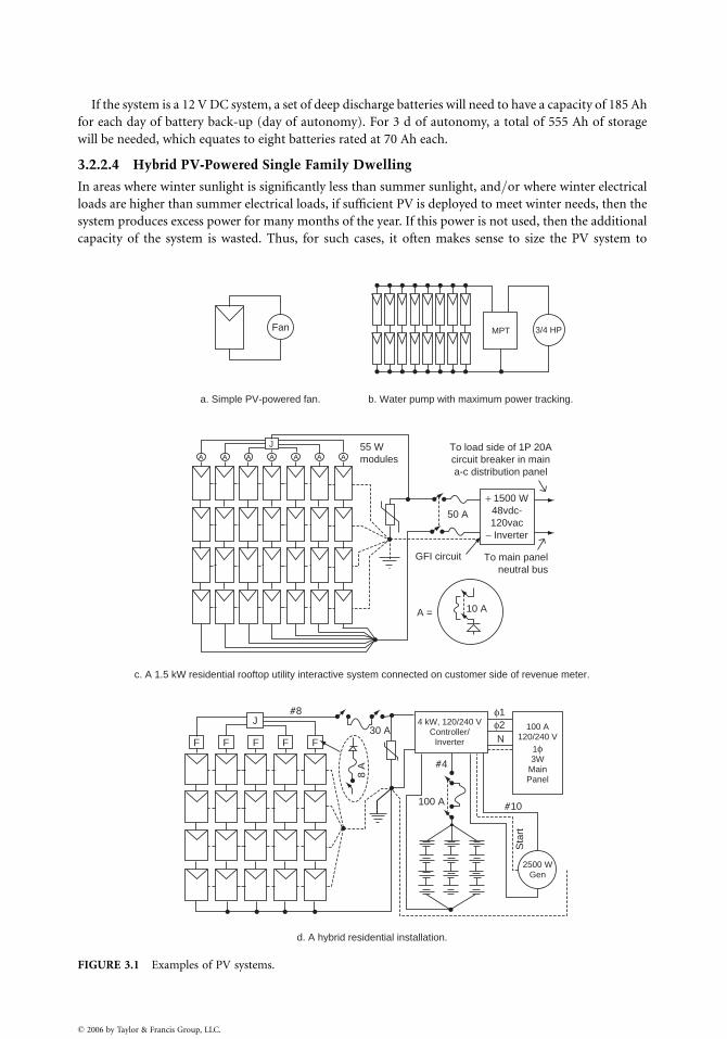
If the system is a 12 V DC system, a set of deep discharge batteries will need to have a capacity of 185 Ah
for each day of battery back-up (day of autonomy). For 3 d of autonomy, a total of 555 Ah of storage
will be needed, which equates to eight batteries rated at 70 Ah each.
3.2.2.4 Hybrid PV-Powered Single Family Dwelling
In areas where winter sunlight is significantly less than summer sunlight, and=or where winter electrical
loads are higher than summer electrical loads, if sufficient PV is deployed to meet winter needs, then the
system produces excess power for many months of the year. If this power is not used, then the additional
capacity of the system is wasted. Thus, for such cases, it often makes sense to size the PV system to
3/4 HPMPT
A A A A
J
A A A
F F F F F
J
a. Simple PV-powered fan. b. Water pump with maximum power tracking.
55 W modules
50 A
+ 1500 W 48vdc- 120vac
− Inverter
To main panel neutral bus
GFI circuit
10 A
30 A
d. A hybrid residential installation.
8 A
A =
Sta
rt
100 A
φ2φ1
2500 W Gen
4 kW, 120/240 V Controller/
Inverter
100 A 120/240 V
1φ 3W
Main Panel
# 8
# 10
# 4
c. A 1.5 kW residential rooftop utility interactive system connected on customer side of revenue meter.
To load side of 1P 20A circuit breaker in main a-c distribution panel
Fan
N
FIGURE 3.1 Examples of PV systems.
� 2006 by Taylor & Francis Group, LLC.

completely meet the system needs during the month(s) with the most sunlight, and then provide backup
generation of another type, such as a gasoline generator, to provide the difference in energy during the
remaining months.
Such a system poses an interesting challenge for the system controller. It needs to be designed to make
maximum use of PV power before starting the generator. Since generators operate most efficiently at
about 90% of full load, the controller must provide for battery charging by the generator at the
appropriate rate to maximize generator efficiency. Typically the generator will be sized to
charge the batteries from 20 to 70% charge in about 5 h. When the batteries have reached 70% charge,
the generator shuts down to allow available sunlight to complete the charging cycle. If the sunlight is not
available, the batteries discharge to 20% and the cycle is repeated.
Figure 3.1 shows schematic diagrams of a few typical PV applications.
References
ANSI=IEEE P929, IEEE Recommended Practice for Utility Interface of Residential and Intermediate
Photovoltaic (PV) Systems, IEEE Standards Coordinating Committee 21, Photovoltaics, Draft 10,
February 1999.
Florida Solar Energy Center site with extensive links to other sites, including solar radiation tables.
http:==alpha.fsec.ucf.edu=�pv=inforesource=links=
Fthenakis, V.M. and Moskowitz, P.D., Emerging photovoltaic technologies: environmental and health
issues update, NREL=SNL Photovoltaics Program Review, AIP Press, New York, 1997.
Green, M.A. and Wenham, S.R., Novel parallel multijunction solar cell, Appl. Phys. Lett., 65, 2907, 1994.
Guha, S., Yang, J., et al., Proc. 26th IEEE PV Spec. Conf., 607–610, 1997.
Hoffman, R., et al., Proc. 26th IEEE PV Spec. Conf., 815–818, 1997.
Huang, J., Lee, Y., et al., Proc. 26th IEEE PV Spec. Conf., 699–702, 1997.
Lammasniemi, J., et al., Proc. 26th IEEE PV Spec. Conf., 823–826, 1997.
Messenger, R., and Ventre, J., Photovoltaic Systems Engineering, CRC Press, Boca Raton, FL, 1999.
NFPA 70 National Electrical Code, 1999 Edition, National Fire Protection Association, Quincy, MA, 1998.
Stand-Alone Photovoltaic Systems: A Handbook of Recommended Design Practices, Sandia National
Laboratories, Albuquerque, NM, 1996.
Tarrant, D.E. and Gay, R.R., CIS-Based Thin Film PV Technology, Phase 2 Technical Report, October
1996—October 1997, NREL, Golden, CO, May 1998.
Tuttle, J.R., et al., Proc. 14th NREL PV Program Review, AIP Conf. Proceedings 394, Lakewood, CO,
1996, 83–105.
UL Subject 1741, Standard for Power Conditioning Units for Use in Residential Photovoltaic Power
Systems, Underwriters Laboratories Inc., 1997.
Ullal, H.S., Zweibel, K., and von Roedern, B., Proc. 26th IEEE PV Spec. Conf., 301–305, 1997.
Yang, J., Banerjee, A., et al., Proc. 26th IEEE PV Spec Conf., 563–568, 1997.
Zweibel, K., Harnessing Solar Power, Plenum Press, New York, 1990.
� 2006 by Taylor & Francis Group, LLC.
II
Electric PowerGeneration:ConventionalMethods Rama RamakumarOklahoma State University4 Hydroelectric Power Generation Steven R. Brockschink, James H. Gurney,
and Douglas B. Seely ............................................................................................................ 4-1
Planning of Hydroelectric Facilities . Hydroelectric Plant Features .
Special Considerations Affecting Pumped Storage Plants . Commissioning
of Hydroelectric Plants
5 Synchronous Machinery Paul I. Nippes ........................................................................... 5-1
General . Construction . Performance
6 Thermal Generating Plants Kenneth H. Sebra ................................................................ 6-1
Plant Auxiliary System . Plant One-Line Diagram . Plant Equipment
Voltage Ratings . Grounded vs. Ungrounded Systems . Miscellaneous
Circuits . DC Systems . Power Plant Switchgear . Auxiliary Transformers .
Motors . Main Generator . Cable . Electrical Analysis . Maintenance
and Testing . Start-Up
7 Distributed Utilities John R. Kennedy .............................................................................. 7-1
Available Technologies . Fuel Cells . Microturbines . Combustion Turbines .
Storage Technologies . Interface Issues . Applications . Conclusions
� 2006 by Taylor & Francis Group, LLC.

� 2006 by Taylor & Francis Group, LLC.

4
� 2006 by Taylor & Francis Group, LLC.
Hydroelectric PowerGeneration
Steven R. BrockschinkStantec Consulting
James H. GurneyBC Transmission Corporation
Douglas B. SeelyStantec Consulting
4.1 Planning of Hydroelectric Facilities................................... 4-1Siting . Hydroelectric Plant Schemes . Selection of Plant
Capacity, Energy, and Other Design Features
4.2 Hydroelectric Plant Features .............................................. 4-2Turbine . Flow Control Equipment . Generator . Generator
Terminal Equipment . Generator Switchgear . Generator
Step-Up Transformer . Excitation System . Governor System .
Control Systems . Protection Systems . Plant Auxiliary
Equipment
4.3 Special Considerations Affecting PumpedStorage Plants .................................................................... 4-10Pump Motor Starting . Phase Reversing of the
Generator=Motor . Draft Tube Water Depression
4.4 Commissioning of Hydroelectric Plants ......................... 4-11
Hydroelectric power generation involves the storage of a hydraulic fluid, water, conversion of the
hydraulic (potential) energy of the fluid into mechanical (kinetic) energy in a hydraulic turbine, and
conversion of the mechanical energy to electrical energy in an electric generator.
The first hydroelectric power plants came into service in the 1880s and now comprise approximately
20% (700 GW) of the world’s installed generation capacity (World Energy Council, 2001). Hydroelec-
tricity is an important source of renewable energy and provides significant flexibility in base loading,
peaking, and energy storage applications. While initial capital costs are high, the inherent simplicity of
hydroelectric plants, coupled with their low operating and maintenance costs, long service life, and high
reliability, make them a very cost-effective and flexible source of electricity generation. Especially
valuable is their operating characteristic of fast response for start-up, loading, unloading, and following
of system load variations. Other useful features include their ability to start without the availability of
power system voltage (black start capability), ability to transfer rapidly from generation mode to
synchronous-condenser mode, and pumped storage application.
Hydroelectric units have been installed in capacities ranging from a few kilowatts to nearly 1 GW.
Multi-unit plant sizes range from a few kilowatts to a maximum of 18 GW.
4.1 Planning of Hydroelectric Facilities
4.1.1 Siting
Hydroelectric plants are located in geographic areas where they will make economic use of hydraulic
energy sources. Hydraulic energy is available wherever there is a flow of liquid and accumulated head.
Head represents potential energy and is the vertical distance through which the fluid falls in the energy
conversion process. The majority of sites utilize the head developed by freshwater; however, other

liquids such as saltwater and treated sewage have been utilized. The siting of a prospective hydroelectric
plant requires careful evaluation of technical, economic, environmental, and social factors. A significant
portion of the project cost may be required for mitigation of environmental effects on fish and wildlife
and relocation of infrastructure and population from flooded areas.
4.1.2 Hydroelectric Plant Schemes
There are three main types of hydroelectric plant arrangements, classified according to the method of
controlling the hydraulic flow at the site:
1. Run-of-the-river plants, having small amounts of water storage and thus little control of the flow
through the plant.
2. Storage plants, having the ability to store water and thus control the flow through the plant on a
daily or seasonal basis.
3. Pumped storage plants, in which the direction of rotation of the turbines is reversed during off-
peak hours, pumping water from a lower reservoir to an upper reservoir, thus ‘‘storing energy’’
for later production of electricity during peak hours.
4.1.3 Selection of Plant Capacity, Energy, and Other Design Features
The generating capacity of a hydroelectric plant is a function of the head and flow rate of water
discharged through the hydraulic turbines, as shown in the following equation:
P ¼ 9:8 h Q H (4:1)
where P¼ power (kilowatts)
� 200
h¼ plant efficiency
Q¼ discharge flow rate (m3=s)
H¼ head (m)
Flow rate and head are influenced by reservoir inflow, storage characteristics, plant and equipment
design features, and flow restrictions imposed by irrigation, minimum downstream releases, or flood
control requirements. Historical daily, seasonal, maximum (flood), and minimum (drought) flow
conditions are carefully studied in the planning stages of a new development. Plant capacity, energy,
and physical features such as the dam and spillway structures are optimized through complex economic
studies that consider the hydrological data, planned reservoir operation, performance characteristics of
plant equipment, construction costs, the value of capacity and energy, and financial discount rates. The
costs of substation, transmission, telecommunications, and off-site control facilities are also important
considerations in the economic analysis. If the plant has storage capability, then societal benefits from
flood control may be included in the economic analysis.
Another important planning consideration is the selection of the number and size of generating units
installed to achieve the desired plant capacity and energy, taking into account installed unit costs, unit
availability, and efficiencies at various unit power outputs (American Society of Mechanical Engineers–
Hydropower Technical Committee, 1996).
4.2 Hydroelectric Plant Features
Figures 4.1 and 4.2 illustrate the main components of a hydroelectric generating unit. The generating
unit may have its shaft oriented in a vertical, horizontal, or inclined direction depending on the physical
conditions of the site and the type of turbine applied. Figure 4.1 shows a typical vertical shaft Francis
turbine unit and Fig. 4.2 shows a horizontal shaft propeller turbine unit. The following sections will
describe the main components such as the turbine, generator, switchgear, and generator transformer, as
well as the governor, excitation system, and control systems.
6 by Taylor & Francis Group, LLC.
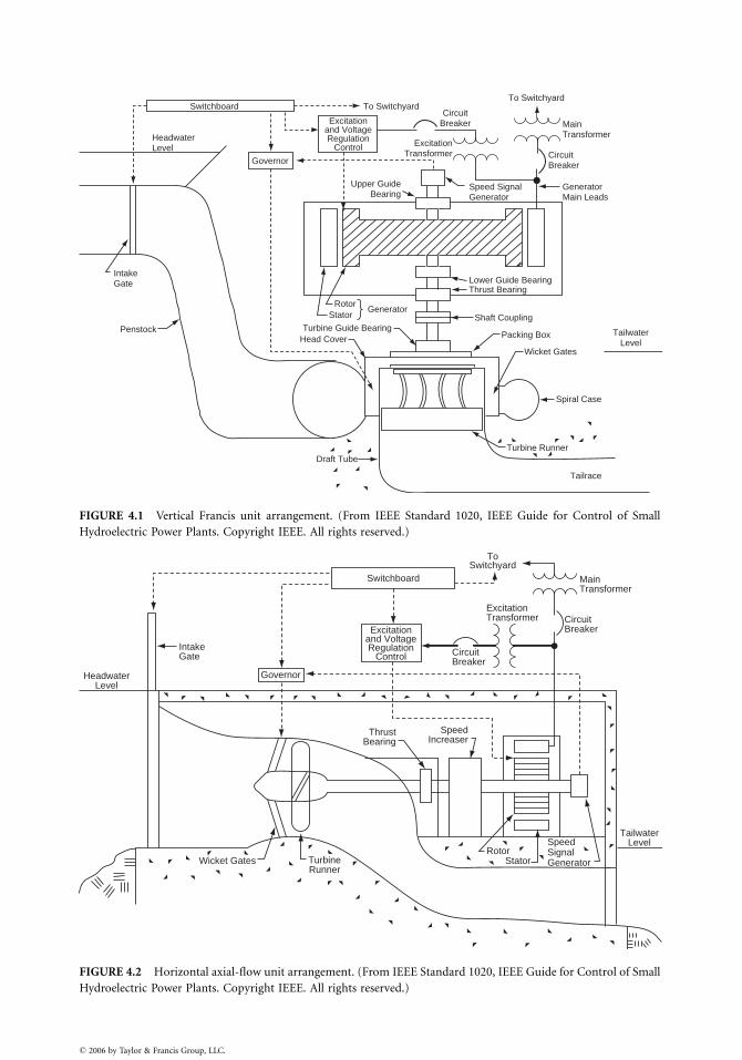
Switchboard
HeadwaterLevel
Governor
To SwitchyardTo Switchyard
MainTransformer
CircuitBreaker
GeneratorMain Leads
Speed SignalGenerator
ExcitationTransformer
Upper GuideBearing
IntakeGate
Penstock
Generator
Lower Guide BearingThrust Bearing
Shaft Coupling
Packing Box
Wicket Gates
Spiral Case
Turbine Runner
Tailrace
Draft Tube
TailwaterLevel
Turbine Guide BearingHead Cover
Rotor
Excitationand VoltageRegulation
Control
CircuitBreaker
Stator
FIGURE 4.1 Vertical Francis unit arrangement. (From IEEE Standard 1020, IEEE Guide for Control of Small
Hydroelectric Power Plants. Copyright IEEE. All rights reserved.)
ToSwitchyard
Main Transformer
CircuitBreaker
ExcitationTransformer
CircuitBreaker
Switchboard
IntakeGate
HeadwaterLevel
Governor
ThrustBearing
SpeedIncreaser
RotorStator
TailwaterLevel
TurbineRunner
Wicket Gates
SpeedSignalGenerator
Excitationand VoltageRegulation
Control
FIGURE 4.2 Horizontal axial-flow unit arrangement. (From IEEE Standard 1020, IEEE Guide for Control of Small
Hydroelectric Power Plants. Copyright IEEE. All rights reserved.)
� 2006 by Taylor & Francis Group, LLC.
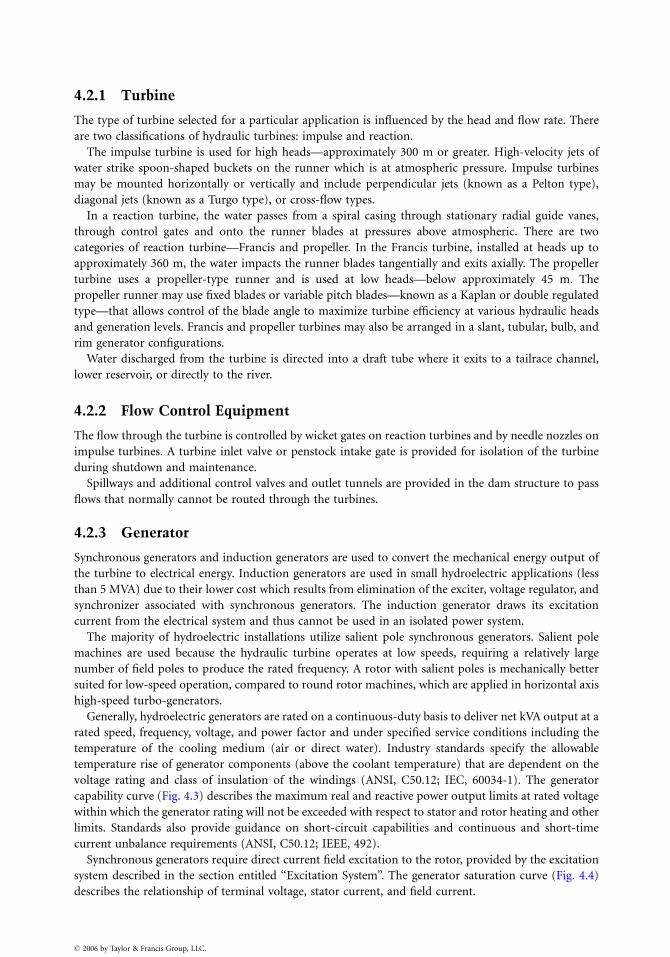
4.2.1 Turbine
The type of turbine selected for a particular application is influenced by the head and flow rate. There
are two classifications of hydraulic turbines: impulse and reaction.
The impulse turbine is used for high heads—approximately 300 m or greater. High-velocity jets of
water strike spoon-shaped buckets on the runner which is at atmospheric pressure. Impulse turbines
may be mounted horizontally or vertically and include perpendicular jets (known as a Pelton type),
diagonal jets (known as a Turgo type), or cross-flow types.
In a reaction turbine, the water passes from a spiral casing through stationary radial guide vanes,
through control gates and onto the runner blades at pressures above atmospheric. There are two
categories of reaction turbine—Francis and propeller. In the Francis turbine, installed at heads up to
approximately 360 m, the water impacts the runner blades tangentially and exits axially. The propeller
turbine uses a propeller-type runner and is used at low heads—below approximately 45 m. The
propeller runner may use fixed blades or variable pitch blades—known as a Kaplan or double regulated
type—that allows control of the blade angle to maximize turbine efficiency at various hydraulic heads
and generation levels. Francis and propeller turbines may also be arranged in a slant, tubular, bulb, and
rim generator configurations.
Water discharged from the turbine is directed into a draft tube where it exits to a tailrace channel,
lower reservoir, or directly to the river.
4.2.2 Flow Control Equipment
The flow through the turbine is controlled by wicket gates on reaction turbines and by needle nozzles on
impulse turbines. A turbine inlet valve or penstock intake gate is provided for isolation of the turbine
during shutdown and maintenance.
Spillways and additional control valves and outlet tunnels are provided in the dam structure to pass
flows that normally cannot be routed through the turbines.
4.2.3 Generator
Synchronous generators and induction generators are used to convert the mechanical energy output of
the turbine to electrical energy. Induction generators are used in small hydroelectric applications (less
than 5 MVA) due to their lower cost which results from elimination of the exciter, voltage regulator, and
synchronizer associated with synchronous generators. The induction generator draws its excitation
current from the electrical system and thus cannot be used in an isolated power system.
The majority of hydroelectric installations utilize salient pole synchronous generators. Salient pole
machines are used because the hydraulic turbine operates at low speeds, requiring a relatively large
number of field poles to produce the rated frequency. A rotor with salient poles is mechanically better
suited for low-speed operation, compared to round rotor machines, which are applied in horizontal axis
high-speed turbo-generators.
Generally, hydroelectric generators are rated on a continuous-duty basis to deliver net kVA output at a
rated speed, frequency, voltage, and power factor and under specified service conditions including the
temperature of the cooling medium (air or direct water). Industry standards specify the allowable
temperature rise of generator components (above the coolant temperature) that are dependent on the
voltage rating and class of insulation of the windings (ANSI, C50.12; IEC, 60034-1). The generator
capability curve (Fig. 4.3) describes the maximum real and reactive power output limits at rated voltage
within which the generator rating will not be exceeded with respect to stator and rotor heating and other
limits. Standards also provide guidance on short-circuit capabilities and continuous and short-time
current unbalance requirements (ANSI, C50.12; IEEE, 492).
Synchronous generators require direct current field excitation to the rotor, provided by the excitation
system described in the section entitled ‘‘Excitation System’’. The generator saturation curve (Fig. 4.4)
describes the relationship of terminal voltage, stator current, and field current.
� 2006 by Taylor & Francis Group, LLC.
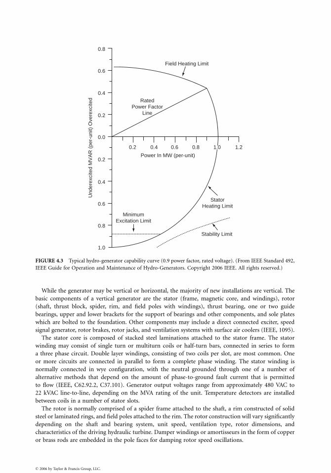
RatedPower Factor
Line
Field Heating Limit
Power In MW (per-unit)
StatorHeating Limit
Stability Limit
MinimumExcitation Limit
0.2
0.8
0.6
0.4
0.2
0.0
0.2
0.4
0.6
0.8
1.0
Und
erex
cite
d M
VA
R (
per-
unit)
Ove
rexc
ited
0.4 0.6 0.8 1.0 1.2
FIGURE 4.3 Typical hydro-generator capability curve (0.9 power factor, rated voltage). (From IEEE Standard 492,
IEEE Guide for Operation and Maintenance of Hydro-Generators. Copyright 2006 IEEE. All rights reserved.)
While the generator may be vertical or horizontal, the majority of new installations are vertical. The
basic components of a vertical generator are the stator (frame, magnetic core, and windings), rotor
(shaft, thrust block, spider, rim, and field poles with windings), thrust bearing, one or two guide
bearings, upper and lower brackets for the support of bearings and other components, and sole plates
which are bolted to the foundation. Other components may include a direct connected exciter, speed
signal generator, rotor brakes, rotor jacks, and ventilation systems with surface air coolers (IEEE, 1095).
The stator core is composed of stacked steel laminations attached to the stator frame. The stator
winding may consist of single turn or multiturn coils or half-turn bars, connected in series to form
a three phase circuit. Double layer windings, consisting of two coils per slot, are most common. One
or more circuits are connected in parallel to form a complete phase winding. The stator winding is
normally connected in wye configuration, with the neutral grounded through one of a number of
alternative methods that depend on the amount of phase-to-ground fault current that is permitted
to flow (IEEE, C62.92.2, C37.101). Generator output voltages range from approximately 480 VAC to
22 kVAC line-to-line, depending on the MVA rating of the unit. Temperature detectors are installed
between coils in a number of stator slots.
The rotor is normally comprised of a spider frame attached to the shaft, a rim constructed of solid
steel or laminated rings, and field poles attached to the rim. The rotor construction will vary significantly
depending on the shaft and bearing system, unit speed, ventilation type, rotor dimensions, and
characteristics of the driving hydraulic turbine. Damper windings or amortisseurs in the form of copper
or brass rods are embedded in the pole faces for damping rotor speed oscillations.
� 2006 by Taylor & Francis Group, LLC.
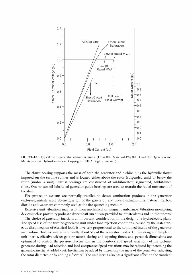
Air Gap Line Open CircuitSaturation
0.90 pf Rated MVA
1.0 pf Rated MVA
Short CircuitSaturation
Full LoadField Current
Field Current (pu)
1.4
1.2
1.0
0.8
0.6
0.4
0.2
0.0
0.0 0.8 1.6 2.4
0.0
0.1
0.2
0.3
0.4
0.5
0.6
0.7
0.8
0.9
1.0
Sta
tor
Cur
rent
(pu
)
Sta
tor
Ter
min
al V
olta
ge (
pu)
FIGURE 4.4 Typical hydro-generator saturation curves. (From IEEE Standard 492, IEEE Guide for Operation and
Maintenance of Hydro-Generators. Copyright IEEE. All rights reserved.)
The thrust bearing supports the mass of both the generator and turbine plus the hydraulic thrust
imposed on the turbine runner and is located either above the rotor (suspended unit) or below the
rotor (umbrella unit). Thrust bearings are constructed of oil-lubricated, segmented, babbit-lined
shoes. One or two oil-lubricated generator guide bearings are used to restrain the radial movement of
the shaft.
Fire protection systems are normally installed to detect combustion products in the generator
enclosure, initiate rapid de-energization of the generator, and release extinguishing material. Carbon
dioxide and water are commonly used as the fire quenching medium.
Excessive unit vibrations may result from mechanical or magnetic unbalance. Vibration monitoring
devices such as proximity probes to detect shaft run out are provided to initiate alarms and unit shutdown.
The choice of generator inertia is an important consideration in the design of a hydroelectric plant.
The speed rise of the turbine-generator unit under load rejection conditions, caused by the instantan-
eous disconnection of electrical load, is inversely proportional to the combined inertia of the generator
and turbine. Turbine inertia is normally about 5% of the generator inertia. During design of the plant,
unit inertia, effective wicket gate or nozzle closing and opening times, and penstock dimensions are
optimized to control the pressure fluctuations in the penstock and speed variations of the turbine-
generator during load rejection and load acceptance. Speed variations may be reduced by increasing the
generator inertia at added cost. Inertia can be added by increasing the mass of the generator, adjusting
the rotor diameter, or by adding a flywheel. The unit inertia also has a significant effect on the transient
� 2006 by Taylor & Francis Group, LLC.
stability of the electrical system, as this factor influences the rate at which energy can be moved in or out
of the generator to control the rotor angle acceleration during system fault conditions. [see Power System
Stability and Control, Kundur (1994) and Section 2 of title Power System Stability and Control of this
handbook.]
4.2.4 Generator Terminal Equipment
The generator output is connected to terminal equipment via cable, busbar, or isolated phase bus. The
terminal equipment comprises current transformers (CTs), voltage transformers (VTs), and surge
suppression devices. The CTs and VTs are used for unit protection, metering and synchronizing, and
for governor and excitation system functions. The surge protection devices, consisting of surge arresters
and capacitors, protect the generator and low-voltage windings of the step-up transformer from
lightning and switching-induced surges.
4.2.5 Generator Switchgear
The generator circuit breaker and associated isolating disconnect switches are used to connect and
disconnect the generator to and from the power system. The generator circuit breaker may be located on
either the low-voltage or high-voltage side of the generator step-up transformer. In some cases, the
generator is connected to the system by means of circuit breakers located in the switchyard of the
generating plant. The generator circuit breaker may be of the oil filled, air magnetic, air blast, or
compressed gas insulated type, depending on the specific application. The circuit breaker is closed as
part of the generator synchronizing sequence and is opened (tripped) either by operator control, as part
of the automatic unit stopping sequence, or by operation of protective relay devices in the event of unit
fault conditions.
4.2.6 Generator Step-Up Transformer
The generator transformer steps up the generator terminal voltage to the voltage of the power system or
plant switchyard. Generator transformers are generally specified and operated in accordance with
international standards for power transformers, with the additional consideration that the transformer
will be operated close to its maximum rating for the majority of its operating life. Various types of
cooling systems are specified depending on the transformer rating and physical constraints of the
specific application. In some applications, dual low-voltage windings are provided to connect two
generating units to a single bank of step-up transformers. Also, transformer tertiary windings are
sometimes provided to serve the AC station service requirements of the power plant.
4.2.7 Excitation System
The excitation system fulfills two main functions:
1. It produces DC voltage (and power) to force current to flow in the field windings of the generator.
There is a direct relationship between the generator terminal voltage and the quantity of current
flowing in the field windings as described in Fig. 4.4.
2. It provides a means for regulating the terminal voltage of the generator to match a desired
setpoint and to provide damping for power system oscillations.
Prior to the 1960s, generators were generally provided with rotating exciters that fed the generator field
through a slip ring arrangement, a rotating pilot exciter feeding the main exciter field, and a regulator
controlling the pilot exciter output. Since the 1960s, the most common arrangement is thyristor bridge
rectifiers fed from a transformer connected to the generator terminals, referred to as a ‘‘potential source
controlled rectifier high initial response exciter’’ or ‘‘bus-fed static exciter’’ (IEEE, 421.1, 421.2, 421.4,
421.5). Another system used for smaller high-speed units is a brushless exciter with a rotating AC
generator and rotating rectifiers.
� 2006 by Taylor & Francis Group, LLC.
Modern static exciters have the advantage of providing extremely fast response times and high field
ceiling voltages for forcing rapid changes in the generator terminal voltage during system faults. This is
necessary to overcome the inherent large time constant in the response between terminal voltage and
field voltage (referred to as T 0do0, typically in the range of 5–10 s). Rapid terminal voltage forcing is
necessary to maintain transient stability of the power system during and immediately after system faults.
Power system stabilizers are also applied to static exciters to cause the generator terminal voltage to vary
in phase with the speed deviations of the machine, for damping power system dynamic oscillations. [see
Power System Stability and Control, Kundur (1994) and Section 2 of title Power System Stability and
Control of this handbook.]
Various auxiliary devices are applied to the static exciter to allow remote setting of the generator
voltage and to limit the field current within rotor thermal and under excited limits. Field flashing
equipment is provided to build up generator terminal voltage during starting to the point at which the
thyristor can begin gating. Power for field flashing is provided either from the station battery or
alternating current station service.
4.2.8 Governor System
The governor system is the key element of the unit speed and power control system (IEEE, 125, 1207;
IEC, 61362; ASME, 29). It consists of control and actuating equipment for regulating the flow of
water through the turbine, for starting and stopping the unit, and for regulating the speed and power
output of the turbine generator. The governor system includes setpoint and sensing equipment for
speed, power and actuator position, compensation circuits, and hydraulic power actuators which convert
governor control signals to mechanical movement of the wicket gates (Francis and Kaplan turbines),
runner blades (Kaplan turbine), and nozzle jets (Pelton turbine). The hydraulic power actuator system
includes high-pressure oil pumps, pressure tanks, oil sump, actuating valves, and servomotors.
Older governors are of the mechanical-hydraulic type, consisting of ballhead speed sensing, mechan-
ical dashpot and compensation, gate limit, and speed droop adjustments. Modern governors are of the
electro-hydraulic type where the majority of the sensing, compensation, and control functions are
performed by electronic or microprocessor circuits. Compensation circuits utilize proportional plus
integral (PI) or proportional plus integral plus derivative (PID) controllers to compensate for the phase
lags in the penstock–turbine–generator–governor control loop. PID settings are normally adjusted
to ensure that the hydroelectric unit remains stable when serving an isolated electrical load. These
settings ensure that the unit contributes to the damping of system frequency disturbances when
connected to an integrated power system. Various techniques are available for modeling and tuning
the governor (IEEE Standard P1207).
A number of auxiliary devices are provided for remote setting of power, speed, and actuator limits and
for electrical protection, control, alarming, and indication. Various solenoids are installed in the
hydraulic actuators for controlling the manual and automatic start-up and shutdown of the turbine-
generator unit.
4.2.9 Control Systems
Detailed information on the control of hydroelectric power plants is available in industry standards
(IEEE, 1010, 1020, 1249). A general hierarchy of control is illustrated in Table 4.1. Manual controls,
normally installed adjacent to the device being controlled, are used during testing and maintenance, and
as a backup to the automatic control systems. Figure 4.5 illustrates the relationship of control locations
and typical functions available at each location. Details of the control functions available at each location
are described in IEEE 1249. Automatic sequences implemented for starting, synchronizing, and shut-
down of hydroelectric units are detailed in IEEE 1010.
Modern hydroelectric plants and plants undergoing rehabilitation and life extension are
incorporating higher levels of computer automation (IEEE, 1249, 1147). The relative simplicity of
� 2006 by Taylor & Francis Group, LLC.
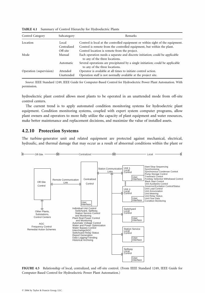
TABLE 4.1 Summary of Control Hierarchy for Hydroelectric Plants
Control Category Subcategory Remarks
Location Local Control is local at the controlled equipment or within sight of the equipment.
Centralized Control is remote from the controlled equipment, but within the plant.
Off-site Control location is remote from the project.
Mode Manual Each operation needs a separate and discrete initiation; could be applicable
to any of the three locations.
Automatic Several operations are precipitated by a single initiation; could be applicable
to any of the three locations.
Operation (supervision) Attended Operator is available at all times to initiate control action.
Unattended Operation staff is not normally available at the project site.
Source: IEEE Standard 1249, IEEE Guide for Computer-Based Control for Hydroelectric Power Plant Automation. With
permission.
hydroelectric plant control allows most plants to be operated in an unattended mode from off-site
control centers.
The current trend is to apply automated condition monitoring systems for hydroelectric plant
equipment. Condition monitoring systems, coupled with expert system computer programs, allow
plant owners and operators to more fully utilize the capacity of plant equipment and water resources,
make better maintenance and replacement decisions, and maximize the value of installed assets.
4.2.10 Protection Systems
The turbine-generator unit and related equipment are protected against mechanical, electrical,
hydraulic, and thermal damage that may occur as a result of abnormal conditions within the plant or
Off-Site Centralized Local
Off-Site
Control
Other Plants,Substations,
Control Centers
AGCFrequency Control
Remedial Action Schemes
Centralized
Control
Unit 1LocalControl
Unit nLocalControl
SwitchyardLocalControl
Station ServiceLocalControl
SpillwayLocalControl
UserInterface
UserInterface
UserInterface
UserInterface
UserInterface
UserInterface
Remote CommunicationLink
Station CommunicationLinks
Start /Stop SequencingSynchronizingSynchronous Condenser ControlPump Storage ControlTrashrack ControlForebay Selective Withdrawal ControlBlack Start ControlUnit Auxiliaries ControlGovernor/Excitation Control/StatusUnit Load ControlUnit AnnunciationUnit MeteringUnit Relay StatusUnit Flow DataCondition Monitoring
Individual Unit Control Switchyard, Spillway, Station Service Control and MonitoringPlant Real Power Control and MonitoringAutomatic Voltage ControlWater and Power OptimizationWater Bypass ControlInterchange/AGCSwitchyard Relay StatusReport GenerationData Logging/TrendingHistorical Archiving
FIGURE 4.5 Relationship of local, centralized, and off-site control. (From IEEE Standard 1249, IEEE Guide for
Computer-Based Control for Hydroelectric Power Plant Automation.)
� 2006 by Taylor & Francis Group, LLC.

on the power system to which the plant is connected. Abnormal conditions are detected automatically
by means of protective relays and other devices and measures are taken to isolate the faulty equipment as
quickly as possible while maintaining the maximum amount of equipment in service. Typical protective
devices include electrical fault detecting relays, temperature, pressure, level, speed, and fire sensors, and
vibration monitors associated with the turbine, generator, and related auxiliaries. The protective devices
operate in various isolation and unit shutdown sequences, depending on the severity of the fault.
The type and extent of protection will vary depending on the size of the unit, manufacturer’s
recommendations, owner’s practices, and industry standards.
Specific guidance on application of protection systems for hydroelectric plants is provided in IEEE
1010, 1020, C37.102, C37.91.
4.2.11 Plant Auxiliary Equipment
A number of auxiliary systems and related controls are provided throughout the hydroelectric plant to
support the operation of the generating units (IEEE, 1010, 1020). These include:
1. Switchyard systems (see Chapter 5).
2. Alternating current (AC) station service. Depending on the size and criticality of the plant,
multiple sources are often supplied, with emergency backup provided by a diesel generator.
3. Direct current (DC) station service. It is normally provided by one or more battery banks, for
supply of protection, control, emergency lighting, and exciter field flashing.
4. Lubrication systems, particularly for supply to generator and turbine bearings and bushings.
5. Drainage pumps, for removing leakage water from the plant.
6. Air compressors, for supply to the governors, generator brakes, and other systems.
7. Cooling water systems, for supply to the generator air coolers, generator and turbine bearings,
and step-up transformer.
8. Fire detection and extinguishing systems.
9. Intake gate or isolation valve systems.
10. Draft tube gate systems.
11. Reservoir and tailrace water level monitoring.
12. Synchronous condenser equipment, for dewatering the draft tube to allow the runner to spin in
air during synchronous condenser operation. In this case, the generator acts as a synchronous
motor, supplying or absorbing reactive power.
13. Service water systems.
14. Overhead crane.
15. Heating, ventilation, and air conditioning.
16. Environmental systems.
4.3 Special Considerations Affecting Pumped Storage Plants
A pumped storage unit is one in which the turbine and generator are operated in the reverse direction to
pump water from the lower reservoir to the upper reservoir. The generator becomes a motor, drawing
its energy from the power system, and supplies mechanical power to the turbine which acts as a pump.
The motor is started with the wicket gates closed and the draft tube water depressed with compressed
air. The motor is accelerated in the pump direction and when at full speed and connected to the power
system, the depression air is expelled, the pump is primed, and the wicket gates are opened to commence
pumping action.
4.3.1 Pump Motor Starting
Various methods are utilized to accelerate the generator=motor in the pump direction during starting
(IEEE, 1010). These include:
� 2006 by Taylor & Francis Group, LLC.
1. Full voltage, across the line starting—Used primarily on smaller units, the unit breaker is closed
and the unit is started as an induction generator. Excitation is applied near rated speed and
machine reverts to synchronous motor operation.
2. Reduced voltage, across the line starting—A circuit breaker connects the unit to a starting bus
tapped from the unit step-up transformer at one third to one half rated voltage. Excitation is
applied near rated speed and the unit is connected to the system by means of the generator circuit
breaker. Alternative methods include use of a series reactor during starting and energization of
partial circuits on multiple circuit machines.
3. Pony motor starting—A variable speed wound-rotor motor attached to the AC station service and
coupled to the motor=generator shaft is used to accelerate the machine to synchronous speed.
4. Synchronous starting—A smaller generator, isolated from the power system, is used to start the
motor by connecting the two in parallel on a starting bus, applying excitation to both units, and
opening the wicket gates on the smaller generator. When the units reach synchronous speed, the
motor unit is disconnected from the starting bus and connected to the power system.
5. Semisynchronous (reduced frequency, reduced voltage) starting—An isolated generator is accel-
erated to about 80% rated speed and paralleled with the motor unit by means of a starting bus.
Excitation is applied to the generating unit and the motor unit starts as an induction motor.
When the speed of the two units is approximately equal, excitation is applied to the motor unit,
bringing it into synchronism with the generating unit. The generating unit is then used to
accelerate both units to rated speed and the motor unit is connected to the power system.
6. Static starting—A static converter=inverter connected to the AC station service is used to provide
variable frequency power to accelerate the motor unit. Excitation is applied to the motor unit at the
beginning of the start sequence and the unit is connected to the power system when it reaches
synchronous speed. The static starting system can be used for dynamic braking of the motor unit
after disconnection from the power system, thus extending the life of the unit’s mechanical brakes.
4.3.2 Phase Reversing of the Generator=Motor
It is necessary to reverse the direction of rotation of the generator=motor by interchanging any two of
the three phases. This is achieved with multipole motor operated switches or with circuit breakers.
4.3.3 Draft Tube Water Depression
Water depression systems using compressed air are provided to lower the level of the draft tube water
below the runner to minimize the power required to accelerate the motor unit during the transition to
pumping mode. Water depression systems are also used during motoring operation of a conventional
hydroelectric unit while in synchronous condenser mode. Synchronous condenser operation is used to
provide voltage support for the power system and to provide spinning reserve for rapid loading response
when required by the power system.
4.4 Commissioning of Hydroelectric Plants
The commissioning of a new hydroelectric plant, rehabilitation of an existing plant, or replacement of
existing equipment requires a rigorous plan for inspection and testing of equipment and systems and for
organizing, developing, and documenting the commissioning program (IEEE, 1248).
References
American Society of Mechanical Engineers–Hydropower Technical Committee, The Guide to Hydro-
power Mechanical Design, HCI Publications, Kansas City, KS, 1996.
ANSI Standard C50.12, Synchronous Generators and Generator=Motors for Hydraulic Turbine
Applications.
� 2006 by Taylor & Francis Group, LLC.

ASME PTC 29, Speed Governing Systems for Hydraulic Turbine Generator Units.
IEC Standard 60034-1, Rotating Electrical Machines—Part 1: Rating and Performance.
IEC Standard 61362, Guide to Specification of Hydraulic Turbine Control Systems.
IEEE Standard C37.91, IEEE Guide for Protective Relay Applications to Power Transformers.
IEEE Standard 421.1, IEEE Standard Definitions for Excitation Systems for Synchronous Machines.
IEEE Standard 1010, IEEE Guide for Control of Hydroelectric Power Plants.
IEEE Standard 125, IEEE Recommended Practice for Preparation of Equipment Specifications for
Speed-Governing of Hydraulic Turbines Intended to Drive Electric Generators.
IEEE Standard 1207, IEEE Guide for the Application of Turbine Governing Systems for Hydroelectric
Generating Units.
IEEE Standard 1020, IEEE Guide for Control of Small Hydroelectric Power Plants.
IEEE Standard C62.92.2, IEEE Guide for the Application of Neutral Grounding in Electrical Utility
Systems, Part II—Grounding of Synchronous Generator Systems.
IEEE Standard 1095, IEEE Guide for Installation of Vertical Generators and Generator=Motors for
Hydroelectric Applications.
IEEE Standard 421.2, IEEE Guide for Identification, Testing and Evaluation of the Dynamic Performance
of Excitation Control Systems.
IEEE Standard 421.4, IEEE Guide for the Preparation of Excitation System Specifications.
IEEE Standard 1147, IEEE Guide for the Rehabilitation of Hydroelectric Power Plants.
IEEE Standard 421.5, IEEE Recommended Practice for Excitation Systems for Power Stability Studies.
IEEE Standard C37.101, IEEE Guide for Generator Ground Protection.
IEEE Standard C37.102, IEEE Guide for AC Generator Protection.
IEEE Standard 1249, IEEE Guide for Computer-Based Control for Hydroelectric Power Plant
Automation.
IEEE Standard 1248, IEEE Guide for the Commissioning of Electrical Systems in Hydroelectric Power
Plants.
IEEE Standard 492, IEEE Guide for Operation and Maintenance of Hydro-Generators.
Kundur, P., Power System Stability and Control, McGraw-Hill, New York, 1994.
Working Group on Prime Mover and Energy Supply Models for System Dynamic Performance Studies,
Hydraulic turbine and turbine control models for system dynamic studies, IEEE Transactions on
Power Systems, 7(1), February 1992.
World Energy Council, Survey of Energy Resources, 2001.
� 2006 by Taylor & Francis Group, LLC.
5
� 2006 by Taylor & Francis Group, LLC.
SynchronousMachinery
Paul I. NippesMagnetic Products and Services, Inc.
5.1 General ................................................................................. 5-1
5.2 Construction ........................................................................ 5-2Stator . Rotor
5.3 Performance ......................................................................... 5-4Synchronous Machines, in General . Synchronous
Generator Capability . Synchronous Motor and
Condenser Starting
5.1 General
Synchronous motors convert electrical power to mechanical power; synchronous generators convert
mechanical power to electrical power; and synchronous condensers supply only reactive power to
stabilize system voltages.
Synchronous motors, generators, and condensers perform similarly, except for a heavy cage winding
on the rotor of motors and condensers for self-starting.
A rotor has physical magnetic poles, arranged to have alternating north and south poles around the
rotor diameter which are excited by electric current, or uses permanent magnets, having the same
number of poles as the stator electromagnetic poles.
The rotor RPM¼ 120� Electrical System Frequency=Poles.
The stator winding, fed from external AC multi-phase electrical power, creates rotating electromag-
netic poles.
At speed, rotor poles turn in synchronism with the stator rotating electromagnetic poles, torque being
transmitted magnetically across the ‘‘air gap’’ power angle, lagging in generators and leading in motors.
Synchronous machine sizes range from fractional watts, as in servomotors, to 1500 MW, as in large
generators.
Voltages vary, up to 25,000 V AC stator and 1500 V DC rotor.
Installed horizontal or vertical at speed ranges up to 130,000 RPM, normally from 40 RPM (water-
wheel generators) to 3600 RPM (turbine generators).
Frequency at 60 or 50 Hz mostly, 400 Hz military; however, synthesized variable frequency electrical
supplies are increasingly common and provide variable motor speeds to improve process efficiency.
Typical synchronous machinery construction and performance are described; variations may exist on
special smaller units.
This document is intentionally general in nature. Should the reader want specific application informa-
tion, refer to standards: NEMA MG-1; IEEE 115, C50-10 and C50-13; IEC 600034: 1-11, 14-16, 18, 20, 44,
72, and 136, plus other applicable specifications.
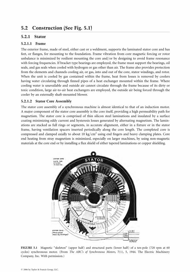
5.2 Construction (See Fig. 5.1)
5.2.1 Stator
5.2.1.1 Frame
The exterior frame, made of steel, either cast or a weldment, supports the laminated stator core and has
feet, or flanges, for mounting to the foundation. Frame vibration from core magnetic forcing or rotor
unbalance is minimized by resilient mounting the core and=or by designing to avoid frame resonance
with forcing frequencies. If bracket type bearings are employed, the frame must support the bearings, oil
seals, and gas seals when cooled with hydrogen or gas other than air. The frame also provides protection
from the elements and channels cooling air, or gas, into and out of the core, stator windings, and rotor.
When the unit is cooled by gas contained within the frame, heat from losses is removed by coolers
having water circulating through finned pipes of a heat exchanger mounted within the frame. Where
cooling water is unavailable and outside air cannot circulate through the frame because of its dirty or
toxic condition, large air-to-air heat exchangers are employed, the outside air being forced through the
cooler by an externally shaft-mounted blower.
5.2.1.2 Stator Core Assembly
The stator core assembly of a synchronous machine is almost identical to that of an induction motor.
A major component of the stator core assembly is the core itself, providing a high permeability path for
magnetism. The stator core is comprised of thin silicon steel laminations and insulated by a surface
coating minimizing eddy current and hysteresis losses generated by alternating magnetism. The lamin-
ations are stacked as full rings or segments, in accurate alignment, either in a fixture or in the stator
frame, having ventilation spacers inserted periodically along the core length. The completed core is
compressed and clamped axially to about 10 kg=cm2 using end fingers and heavy clamping plates. Core
end heating from stray magnetism is minimized, especially on larger machines, by using non-magnetic
materials at the core end or by installing a flux shield of either tapered laminations or copper shielding.
FIGURE 5.1 Magnetic ‘‘skeleton’’ (upper half) and structural parts (lower half) of a ten-pole (720 rpm at 60
cycles) synchronous motor. (From The ABC’s of Synchronous Motors, 7(1), 5, 1944. The Electric Machinery
Company, Inc. With permission.)
� 2006 by Taylor & Francis Group, LLC.
A second major component is the stator winding made up of insulated coils placed in axial slots of
the stator core inside diameter. The coil make-up, pitch, and connections are designed to produce
rotating stator electromagnetic poles in synchronism with the rotor magnetic poles. The stator coils are
retained into the slots by slot wedges driven into grooves in the top of the stator slots. Coil end windings
are bound together and to core-end support brackets. If the synchronous machine is a generator, the
rotating rotor pole magnetism generates voltage in the stator winding which delivers power to an electric
load. If the synchronous machine is a motor, its electrically powered stator winding generates rotating
electromagnetic poles and the attraction of the rotor magnets, operating in synchronism, produces
torque and delivery of mechanical power to the drive shaft.
5.2.2 Rotor
5.2.2.1 The Rotor Assembly
The rotor of a synchronous machine is a highly engineered unitized assembly capable of rotating
satisfactorily at synchronous speed continuously according to standards or as necessary for the appli-
cation. The central element is the shaft, having journals to support the rotor assembly in bearings.
Located at the rotor assembly axial mid-section is the rotor core embodying magnetic poles. When the
rotor is round it is called ‘‘non-salient pole’’, or turbine generator type construction and when the rotor
has protruding pole assemblies, it is called ‘‘salient pole’’ construction.
The non-salient pole construction, used mainly on turbine generators (and also as wind tunnel fan
drive motors), has two or four magnetic poles created by direct current in coils located in slots at the
rotor outside diameter. Coils are restrained in the slots by slot wedges and at the ends by retaining rings
on large high-speed rotors, and fiberglass tape on other units where stresses permit. This construction is
not suited for use on a motor requiring self-starting as the rotor surface, wedges, and retaining rings
overheat and melt from high currents of self-starting.
A single piece forging is sometimes used on salient pole machines, usually with four or six poles.
Salient poles can also be integral with the rotor lamination and can be mounted directly to the shaft or
fastened to an intermediate rotor spider. Each distinct pole has an exciting coil around it carrying
excitation current or else it employs permanent magnets. In a generator, a moderate cage winding in
the face of the rotor poles, usually with pole-to-pole connections, is employed to dampen shaft torsional
oscillation and to suppress harmonic variation in the magnetic waveform. In a motor, heavy bars and end
connections are required in the pole face to minimize and withstand the high heat of starting duty.
Direct current excites the rotor windings of salient, and non-salient pole motors and generators,
except when permanent magnets are employed. The excitation current is supplied to the rotor from
either an external DC supply through collector rings or a shaft-mounted brushless exciter. Positive and
negative polarity bus bars or cables pass along and through the shaft as required to supply excitation
current to the windings of the field poles.
When supplied through collector rings, the DC current could come from a shaft-driven DC or AC
exciter rectified output, from an AC-DC motor-generator set, or from plant power. DC current supplied
by a shaft-mounted AC generator is rectified by a shaft-mounted rectifier assembly.
As a generator, excitation current level is controlled by the voltage regulator. As a motor, excitation
current is either set at a fixed value, or is controlled to regulate power factor, motor current, or system
stability.
In addition, the rotor also has shaft-mounted fans or blowers for cooling and heat removal from the
unit plus provision for making balance weight additions or corrections.
5.2.2.2 Bearings and Couplings
Bearings on synchronous machinery are anti-friction, grease, or oil-lubricated on smaller machines, journal
type oil-lubricated on large machines, and tilt-pad type on more sophisticated machines, especially
where rotor dynamics are critical. Successful performance of magnetic bearings, proving to be successful
on turbo-machinery, may also come to be used on synchronous machinery as well.
� 2006 by Taylor & Francis Group, LLC.
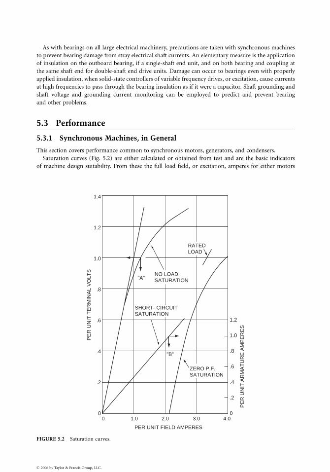
As with bearings on all large electrical machinery, precautions are taken with synchronous machines
to prevent bearing damage from stray electrical shaft currents. An elementary measure is the application
of insulation on the outboard bearing, if a single-shaft end unit, and on both bearing and coupling at
the same shaft end for double-shaft end drive units. Damage can occur to bearings even with properly
applied insulation, when solid-state controllers of variable frequency drives, or excitation, cause currents
at high frequencies to pass through the bearing insulation as if it were a capacitor. Shaft grounding and
shaft voltage and grounding current monitoring can be employed to predict and prevent bearing
and other problems.
5.3 Performance
5.3.1 Synchronous Machines, in General
This section covers performance common to synchronous motors, generators, and condensers.
Saturation curves (Fig. 5.2) are either calculated or obtained from test and are the basic indicators
of machine design suitability. From these the full load field, or excitation, amperes for either motors
PER UNIT FIELD AMPERES
PE
R U
NIT
AR
MA
TU
RE
AM
PE
RE
S
PE
R U
NIT
TE
RM
INA
L V
OLT
S
4.00
.2
.4
.6
.8
1.0
1.2
3.02.01.000
.2
.4
.6
.8
1.0
1.2
1.4
"B"
"A"
ZERO P.F.SATURATION
NO LOADSATURATION
RATEDLOAD
SHORT- CIRCUITSATURATION
FIGURE 5.2 Saturation curves.
� 2006 by Taylor & Francis Group, LLC.
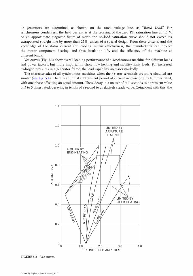
or generators are determined as shown, on the rated voltage line, as ‘‘Rated Load.’’ For
synchronous condensers, the field current is at the crossing of the zero P.F. saturation line at 1.0 V.
As an approximate magnetic figure of merit, the no-load saturation curve should not exceed its
extrapolated straight line by more than 25%, unless of a special design. From these criteria, and the
knowledge of the stator current and cooling system effectiveness, the manufacturer can project
the motor component heating, and thus insulation life, and the efficiency of the machine at
different loads.
Vee curves (Fig. 5.3) show overall loading performance of a synchronous machine for different loads
and power factors, but more importantly show how heating and stability limit loads. For increased
hydrogen pressures in a generator frame, the load capability increases markedly.
The characteristics of all synchronous machines when their stator terminals are short-circuited are
similar (see Fig. 5.4). There is an initial subtransient period of current increase of 8 to 10 times rated,
with one phase offsetting an equal amount. These decay in a matter of milliseconds to a transient value
of 3 to 5 times rated, decaying in tenths of a second to a relatively steady value. Coincident with this, the
PER UNIT FIELD AMPERES
0.95
PF
LE
AD
1.0
PF
0.0
PF
LEA
D
PE
R U
NIT
kV
A
00
0.2
0.4
0.6
0.8
1.0
1.2
1.4
1.0 2.0 3.0 4.0
LIMITED BYFIELD HEATING
LIMITED BYARMATUREHEATING
LIMITED BYEND HEATING
30 P
SIG H 2
0.9
PF
LAG
0.0
PF L
AG
60 P
SIG
H2
45 P
SIG H 2
FIGURE 5.3 Vee curves.
� 2006 by Taylor & Francis Group, LLC.
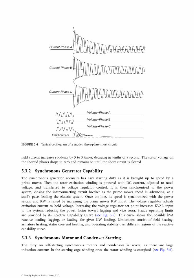
Voltage -Phase A
Voltage -Phase B
Voltage -Phase C
Field current
Current-Phase C
Current-Phase B
Current-Phase A
FIGURE 5.4 Typical oscillogram of a sudden three-phase short circuit.
field current increases suddenly by 3 to 5 times, decaying in tenths of a second. The stator voltage on
the shorted phases drops to zero and remains so until the short circuit is cleared.
5.3.2 Synchronous Generator Capability
The synchronous generator normally has easy starting duty as it is brought up to speed by a
prime mover. Then the rotor excitation winding is powered with DC current, adjusted to rated
voltage, and transferred to voltage regulator control. It is then synchronized to the power
system, closing the interconnecting circuit breaker as the prime mover speed is advancing, at a
snail’s pace, leading the electric system. Once on line, its speed is synchronized with the power
system and KW is raised by increasing the prime mover KW input. The voltage regulator adjusts
excitation current to hold voltage. Increasing the voltage regulator set point increases KVAR input
to the system, reducing the power factor toward lagging and vice versa. Steady operating limits
are provided by its Reactive Capability Curve (see Fig. 5.5). This curve shows the possible kVA
reactive loading, lagging, or leading, for given KW loading. Limitations consist of field heating,
armature heating, stator core end heating, and operating stability over different regions of the reactive
capability curve.
5.3.3 Synchronous Motor and Condenser Starting
The duty on self-starting synchronous motors and condensors is severe, as there are large
induction currents in the starting cage winding once the stator winding is energized (see Fig. 5.6).
� 2006 by Taylor & Francis Group, LLC.
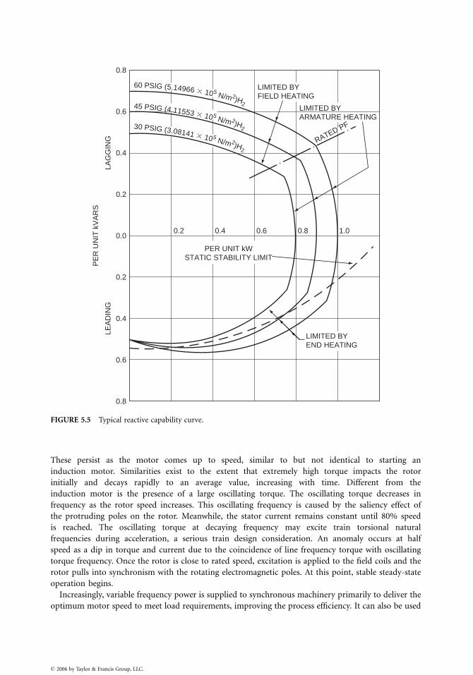
LIMITED BYEND HEATING
LEA
DIN
G
PE
R U
NIT
kV
AR
S
LAG
GIN
G
PER UNIT kWSTATIC STABILITY LIMIT
0.8
0.6
0.4
0.2
0.2 0.4 0.6 0.8 1.00.0
0.2
0.4
0.6
0.8
LIMITED BYFIELD HEATING
LIMITED BYARMATURE HEATING
60 PSIG (5.14966 � 105 N/m2)H245 PSIG (4.11553 � 105 N/m2)H230 PSIG (3.08141 � 105 N/m2)H2
RATED PF
FIGURE 5.5 Typical reactive capability curve.
These persist as the motor comes up to speed, similar to but not identical to starting an
induction motor. Similarities exist to the extent that extremely high torque impacts the rotor
initially and decays rapidly to an average value, increasing with time. Different from the
induction motor is the presence of a large oscillating torque. The oscillating torque decreases in
frequency as the rotor speed increases. This oscillating frequency is caused by the saliency effect of
the protruding poles on the rotor. Meanwhile, the stator current remains constant until 80% speed
is reached. The oscillating torque at decaying frequency may excite train torsional natural
frequencies during acceleration, a serious train design consideration. An anomaly occurs at half
speed as a dip in torque and current due to the coincidence of line frequency torque with oscillating
torque frequency. Once the rotor is close to rated speed, excitation is applied to the field coils and the
rotor pulls into synchronism with the rotating electromagnetic poles. At this point, stable steady-state
operation begins.
Increasingly, variable frequency power is supplied to synchronous machinery primarily to deliver the
optimum motor speed to meet load requirements, improving the process efficiency. It can also be used
� 2006 by Taylor & Francis Group, LLC.
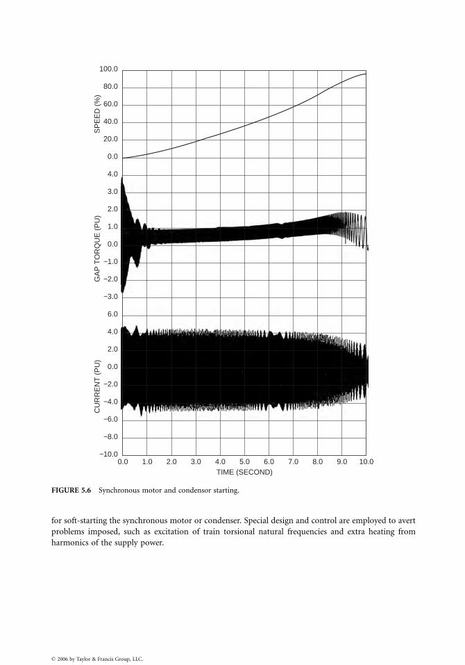
TIME (SECOND)
CU
RR
EN
T (
PU
)G
AP
TO
RQ
UE
(P
U)
SP
EE
D (
%)
0.0−10.0
−8.0
−6.0
−4.0
−2.0
0.0
2.0
4.0
6.0
−3.0
−2.0
−1.0
0.0
1.0
2.0
3.0
4.0
0.0
20.0
40.0
60.0
80.0
100.0
1.0 2.0 3.0 4.0 5.0 6.0 7.0 8.0 9.0 10.0
FIGURE 5.6 Synchronous motor and condensor starting.
for soft-starting the synchronous motor or condenser. Special design and control are employed to avert
problems imposed, such as excitation of train torsional natural frequencies and extra heating from
harmonics of the supply power.
� 2006 by Taylor & Francis Group, LLC.

6
� 2006 by Taylor & Francis Group, LLC.
Thermal GeneratingPlants
Kenneth H. SebraBaltimore Gas and Electric Company
6.1 Plant Auxiliary System...................................................... 6-2Selection of Auxiliary System Voltages . Auxiliary System
Loads . Auxiliary System Power Sources . Auxiliary System
Voltage Regulation Requirements
6.2 Plant One-Line Diagram .................................................. 6-3
6.3 Plant Equipment Voltage Ratings .................................... 6-3
6.4 Grounded vs. Ungrounded Systems ................................ 6-3Ungrounded . Grounded . Low-Resistance Grounding .
High-Resistance Grounding
6.5 Miscellaneous Circuits ...................................................... 6-3Essential Services . Lighting Supply
6.6 DC Systems ........................................................................ 6-4125-V DC . 250-V DC
6.7 Power Plant Switchgear .................................................... 6-4High-Voltage Circuit Breakers . Medium-Voltage Switchgear .
Low-Voltage Switchgear . Motor Control Centers .
Circuit Interruption
6.8 Auxiliary Transformers ..................................................... 6-5Selection of Percent Impedance . Rating of Voltage Taps
6.9 Motors ................................................................................ 6-6Selection of Motors . Types of Motors
6.10 Main Generator ................................................................. 6-6Associated Equipment . Electronic Exciters . Generator
Neutral Grounding . Isolated Phase Bus
6.11 Cable................................................................................... 6-7
6.12 Electrical Analysis .............................................................. 6-7Load Flow . Short-Circuit Analysis . Surge Protection .
Phasing . Relay Coordination Studies
6.13 Maintenance and Testing.................................................. 6-8
6.14 Start-Up.............................................................................. 6-8
Thermal generating plants are designed and constructed to convert energy from fuel (coal, oil, gas, or
radiation) into electric power. The actual conversion is accomplished by a turbine-driven generator.
Thermal generating plants differ from industrial plants in that the nature of the product never
changes. The plant will always produce electric energy. The things that may change are the fuel used
(coal, oil, or gas) and environmental requirements. Many plants that were originally designed for coal
were later converted to oil, converted back to coal, and then converted to gas. Environmental
requirements have changed, which has required the construction of air and water emissions control
systems. Plant electrical systems should be designed to allow for further growth. Sizing of
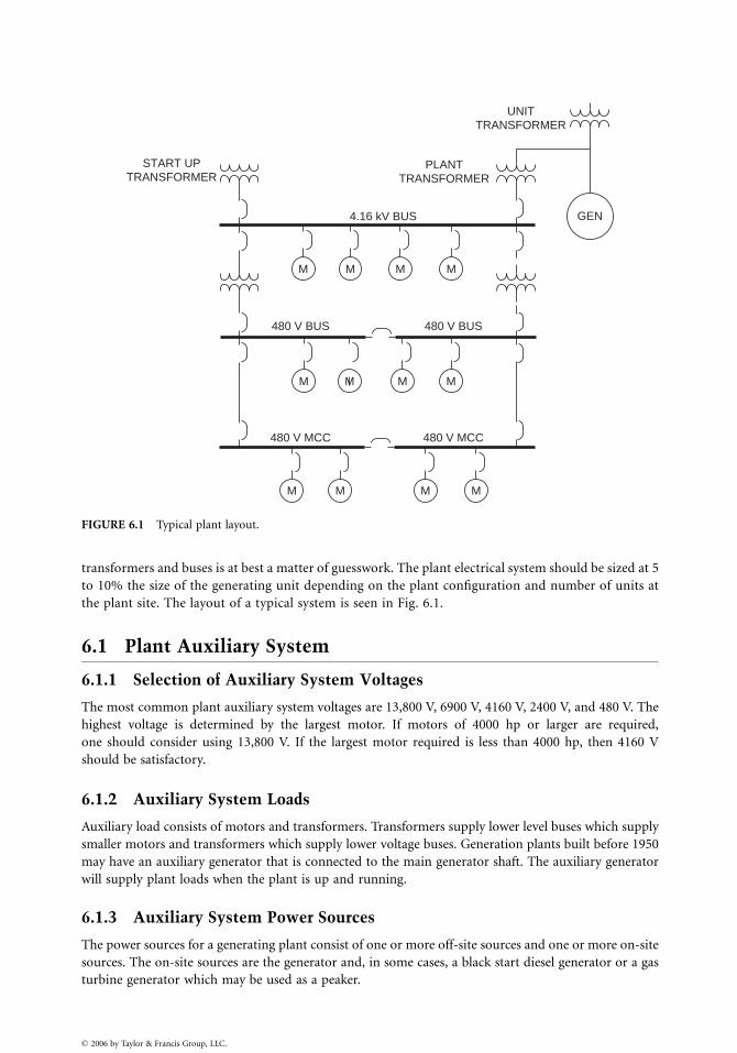
PLANTTRANSFORMER
START UPTRANSFORMER
4.16 kV BUS
480 V BUS 480 V BUS
480 V MCC 480 V MCC
UNITTRANSFORMER
GEN
MMM
M M
MMMM
M
M
M
FIGURE 6.1 Typical plant layout.
transformers and buses is at best a matter of guesswork. The plant electrical system should be sized at 5
to 10% the size of the generating unit depending on the plant configuration and number of units at
the plant site. The layout of a typical system is seen in Fig. 6.1.
6.1 Plant Auxiliary System
6.1.1 Selection of Auxiliary System Voltages
The most common plant auxiliary system voltages are 13,800 V, 6900 V, 4160 V, 2400 V, and 480 V. The
highest voltage is determined by the largest motor. If motors of 4000 hp or larger are required,
one should consider using 13,800 V. If the largest motor required is less than 4000 hp, then 4160 V
should be satisfactory.
6.1.2 Auxiliary System Loads
Auxiliary load consists of motors and transformers. Transformers supply lower level buses which supply
smaller motors and transformers which supply lower voltage buses. Generation plants built before 1950
may have an auxiliary generator that is connected to the main generator shaft. The auxiliary generator
will supply plant loads when the plant is up and running.
6.1.3 Auxiliary System Power Sources
The power sources for a generating plant consist of one or more off-site sources and one or more on-site
sources. The on-site sources are the generator and, in some cases, a black start diesel generator or a gas
turbine generator which may be used as a peaker.
� 2006 by Taylor & Francis Group, LLC.
6.1.4 Auxiliary System Voltage Regulation Requirements
Most plants will not require voltage regulation. A load flow study will indicate if voltage regulation
is required. Transformers with tap changers, static var compensators, or induction regulators may be
used to keep plant bus voltages within acceptable limits. Switched capacitor banks and overexcited
synchronous motors may also be used to regulate bus voltage.
6.2 Plant One-Line Diagram
The one-line diagram is the most important document you will use. Start with a conceptual one-line
and add detail as it becomes available. The one-line diagram will help you think about your design and
make it easier to discuss with others. Do not be afraid to get something on paper very early and modify
as you get more information about the design. Consider how the plant will be operated. Will there be a
start-up source and a running source? Are there on-site power sources?
6.3 Plant Equipment Voltage Ratings
Establish at least one bus for each voltage rating in the plant. Two or more buses may be required
depending on how the plant will be operated.
6.4 Grounded vs. Ungrounded Systems
A method of grounding must be determined for each voltage level in the plant.
6.4.1 Ungrounded
Most systems will be grounded in some manner with the exception for special cases of 120-V control
systems which may be operated ungrounded for reliability reasons. An ungrounded system may be
allowed to continue to operate with a single ground on the system. Ungrounded systems are undesirable
because ground faults are difficult to locate. Also, ground faults can result in system overvoltage, which
can damage equipment that is connected to the ungrounded system.
6.4.2 Grounded
Most systems 480 V and lower will be solidly grounded.
6.4.3 Low-Resistance Grounding
Low-resistance grounding systems are used at 2400 V and above. This system provides enough ground
fault current to allow relay coordination and limits ground fault current to a value low enough to
prevent equipment damage.
6.4.4 High-Resistance Grounding
High-resistance grounding systems limit ground fault current to a very low value but make relay
coordination for ground faults difficult.
6.5 Miscellaneous Circuits
6.5.1 Essential Services
Essential services such as critical control required for plant shutdown, fire protection, and emergency
lighting should be supplied by a battery-backed inverter. This is equipment that must continue to
� 2006 by Taylor & Francis Group, LLC.

operate after a loss of off-site power. Some of these loads may be supplied by an on-site diesel generator
or gas turbine if a delay after loss of off-site power is acceptable.
6.5.2 Lighting Supply
Lighting circuits should be designed with consideration to emergency lighting to the control room and
other vital areas of the plant. Consideration should be given to egress lighting and lighting requirements
for plant maintenance.
6.6 DC Systems
The plant will require at least one DC system for control and operation of essential systems when off-site
power is lost. The required operating time for the emergency equipment that will be operated from the
DC systems must be established in order to size the batteries. The installation of a diesel generator may
reduce the size of the battery.
6.6.1 125-V DC
A 125-V DC system is supplied for circuit breaker and protective relaying. The system voltage may
collapse to close to zero during fault conditions and would not be capable of supplying relay control and
breaker trip current when it is needed to operate.
6.6.2 250-V DC
A 250-V DC system may be required to supply turbine generator emergency motors such as turning gear
motors and emergency lube oil motors.
6.7 Power Plant Switchgear
6.7.1 High-Voltage Circuit Breakers
High-voltage circuit breakers of 34.5 kV and above may be used in the switchyard associated with the
generating plant, but are rarely used in a generating plant.
6.7.2 Medium-Voltage Switchgear
Medium-voltage breakers are 2.4 to 13.8 kV. Breakers in this range are used for large motors in the plant.
The most prevalent is 4.16 kV.
6.7.2.1 Medium-Voltage Air Circuit Breakers
Air circuit breakers were the most common type of breaker until about 1995. Due to large size and high
maintenance requirements of air circuit breakers, they have been replaced by vacuum breakers.
6.7.2.2 Medium-Voltage Vacuum Circuit Breakers
Vacuum circuit breakers are the most common type of circuit breaker used in new installations. Vacuum
circuit breakers are being used to replace air circuit breakers. Vacuum breakers are smaller and can
provide additional space if the plant needs to be expanded to meet new requirements. Before using
vacuum circuit breakers, a transient analysis study should be performed to determine if there is a need
for surge protection. If required, surge protection can be supplied by the installation of capacitors
and=or surge suppressors can be used to eliminate voltage surge problems.
� 2006 by Taylor & Francis Group, LLC.
6.7.2.3 Medium-Voltage SF6 Circuit Breakers
SF6 circuit breakers have the same advantages as vacuum circuit breakers but there is some environ-
mental concern with the SF6 gas.
6.7.3 Low-Voltage Switchgear
Low voltage is 600 V and below. The most common voltage used is 480 V.
6.7.3.1 Low-Voltage Air Circuit Breakers
Air circuit breakers are used in load centers that may include a power transformer. Air circuit breakers
are used for motors greater than 200 hp and less than about 600 hp. Low-voltage circuit breakers are self-
contained in that fault protection is an integral part of the breaker. Low-voltage devices, which do not
contain fault protection devices, are referred to as low-voltage switches. Low-voltage breakers may be
obtained with various combinations of trip elements. Long time, short time, and ground trip elements
may be obtained in various combinations.
Low-voltage breakers manufactured before 1970 will contain oil dashpot time delay trip elements.
Breakers manufactured after the mid-1970s until about 1990 will contain solid-state analog trip
elements. Breakers manufactured after 1990 will contain digital trip elements. The digital elements
provide much more flexibility.
A circuit that may be large enough for a load center circuit breaker but is operated several times a day
should not be put on a load center circuit breaker. The circuit breaker would be put through its useful
life in a very short time. A motor starter would be a better choice.
6.7.4 Motor Control Centers
Motor control centers are self-contained and may include molded case breakers or combination starters.
Molded case breakers are available as either magnetic or thermal-magnetic. The magnetic trip breakers
are instantaneous trip only and the thermal-magnetic trip breakers are time delay with instantaneous
trip. Magnetic breakers can be used with a contactor to make a combination starter. Time delay trip is
provided by overload relays mounted on the contactor. Solid-state equipment is available to use in
motor control centers and allows much greater flexibility.
6.7.5 Circuit Interruption
The purpose of a circuit breaker is to provide a method of interrupting the circuit either to turn the load
on and off or to interrupt fault current. The first requirement is based on the full load current of the
load. The second requirement is based on the maximum fault current as determined by the fault current
study. There is no relationship between the load current and the fault current. If modifications are made
to the electric power system, the fault interrupting current requirement may increase. Failure to
recognize this could result in the catastrophic failure of a breaker.
6.8 Auxiliary Transformers
6.8.1 Selection of Percent Impedance
The transformer impedance is always compromised. High transformer impedance will limit fault
current and reduce the required interrupting capability of switchgear and, therefore, reduce the cost.
Low impedance will reduce the voltage drop through the transformer and therefore improve voltage
regulation. A careful analysis using a load flow study will help in arriving at the best compromise.
� 2006 by Taylor & Francis Group, LLC.
6.8.2 Rating of Voltage Taps
Transformers should be supplied with taps to allow adjustment in bus voltage. Optimum tap settings can
be determined using a load flow study.
6.9 Motors
6.9.1 Selection of Motors
Many motors are required in a thermal generating plant and range in size from fractional horsepower to
several thousand horsepower. These motors may be supplied with the equipment they drive or they may
be specified by the electrical engineer and purchased separately. The small motors are usually supplied by
the equipment supplier and the large motors specified by the electrical engineer. How this will be
handled must be resolved very early in the project. The horsepower cut-off point for each voltage level
must be decided. The maximum plant voltage level must be established. A voltage of 13.8 kV may be
required if very large horsepower motors are to be used. This must be established very early in the plant
design so that a preliminary one-line diagram may be developed.
6.9.2 Types of Motors
6.9.2.1 Squirrel Cage Induction Motors
The squirrel cage induction motor is the most common type of large motor used in a thermal generating
plant. Squirrel cage induction motors are very rugged and require very little maintenance.
6.9.2.2 Wound Rotor Induction Motors
The wound rotor induction motor has a rotor winding which is brought out of the motor through slip
rings and brushes. While more flexible than a squire cage induction motor, the slip rings and brushes
are an additional maintenance item. Wound rotor motors are only used in special applications in a
power plant.
6.9.2.3 Synchronous Motors
Synchronous motors may be required in some applications. Large slow-speed, 1800 rpm or less may
require a synchronous motor. A synchronous motor may used to supply VARs and improve voltage
regulation. If the synchronous motor is going to be used as a VAR source, the field supply must be sized
large enough to over-excite the field.
6.9.2.4 Direct Current Motors
Direct current motors are used primarily on emergency systems such as turbine lube oil and turbine
turning gear. Direct current motors may also be used on some control valves.
6.9.2.5 Single-Phase Motors
Single-phase motors are fractional horsepower motors and are usually supplied with the equipment.
6.9.2.6 Motor Starting Limitations
The starting current for induction motors is about 6 times full load current. This must be taken into
account when sizing transformers and should be part of the load flow analysis. If the terminal voltage is
allowed to drop too low, below 80%, the motor will stall. Methods of reduced voltage starting are
available, but should be avoided if possible. The most reliable designs are the simplest.
6.10 Main Generator
The turbine generator will be supplied as a unit. The size and characteristics are usually determined by
the system planners as a result of system load requirements and system stability requirements.
� 2006 by Taylor & Francis Group, LLC.
6.10.1 Associated Equipment
6.10.1.1 Exciters and Excitation Equipment
The excitation system will normally be supplied with the generator.
6.10.2 Electronic Exciters
Modern excitation systems are solid state and, in recent years, most have digital control systems.
6.10.3 Generator Neutral Grounding
The generator neutral is never connected directly to ground. The method used to limit the phase to
ground fault current to a value equal to or less than the three-phase fault current is determined by the
way the generator is connected to the power system. If the generator is connected directly to the power
system, a resistor or inductor connected between the neutral of the generator and ground will be used to
limit the ground fault current. If the generator is connected to the power system through a transformer
in a unit configuration, the neutral of the generator may be connected to ground through a distribution
transformer with a resistor connected across the secondary of the transformer. The phase-to-ground
fault current can be limited to 5 to 10 A using this method.
6.10.4 Isolated Phase Bus
The generator is usually connected to the step-up transformer through an isolated phase bus. This
separated phase greatly limits the possibility of a phase-to-phase fault at the terminals of the generator.
6.11 Cable
Large amounts of cable are required in a thermal generating plant. Power, control, and instrumentation
cable should be selected carefully with consideration given to long life. Great care should be given in the
installation of all cable. Cable replacement can be very expensive.
6.12 Electrical Analysis
All electrical studies should be well-documented for use in plant modifications. These studies will be of
great value in evaluating plant problems.
6.12.1 Load Flow
A load flow study should be performed as early in the design as possible even if the exact equipment is
not known. The load flow study will help in getting an idea of transformer size and potential voltage
drop problems.
A final load flow study should be performed to document the final design and will be very helpful if
modifications are required in the future.
6.12.2 Short-Circuit Analysis
Short-circuit studies must be performed to determine the requirements for circuit breaker interrupting
capability. Relay coordination should be studied as well.
6.12.3 Surge Protection
Surge protection may be required to limit transient overvoltage caused by lightning and circuit
switching. A surge study should be performed to determine the needs of each plant configuration.
Surge arrestors and=or capacitors may be required to limit transient voltages to acceptable levels.
� 2006 by Taylor & Francis Group, LLC.

6.12.4 Phasing
A phasing diagram should be made to determine correct transformer connections. An error here could
prevent busses from being paralleled.
6.12.5 Relay Coordination Studies
Relay coordination studies should be performed to ensure proper coordination of the relay protection
system. The protective relay system may include overcurrent relays, bus differential relays, transformer
differential relays, voltage relays, and various special function relays.
6.13 Maintenance and Testing
A good plant design will take into account maintenance and testing requirements. Equipment must be
accessible for maintenance and provisions should be made for test connections.
6.14 Start-Up
A start-up plan should be developed to ensure equipment will perform as expected. This plan should
include insulation testing. Motor starting current magnitude and duration should be recorded and
relay coordination studies verified. Voltage level and load current readings should be taken to verify
load flow studies. This information will also be very helpful when evaluating plant operating conditions
and problems.
References
General
Beeman, D., Ed., Industrial Power Systems Handbook, McGraw-Hill, New York.
Electrical Transmission and Distribution Reference Book, Westinghouse Electric Corporation.
IEEE Standard 666-1991, IEEE Design Guide for Electric Power Service Systems for Generating Stations.
Grounding
IEEE 665-1955, IEEE Guide for Generating Station Grounding.
IEEE 1050-1996, IEEE Guide for Instrumentation and control Grounding in Generating Stations.
DC Systems
IEEE 485-1997, IEEE Recommended Practice for Sizing Lead-Acid Batteries for Station Applications.
IEEE 946-1992, IEEE Recommended Practice for the Design of DC Auxiliary Power Systems for
Generating Stations.
Switchgear
IEEE Standards Collection: Power and Energy-Switchgear, 1998 Edition.
Auxiliary Transformers
IEEE Distribution, Power and Regulating Transformers Standards Collection, 1998 Edition.
Motors
IEEE Electric Machinery Standards Collection, 1997 Edition.
Cable
IEEE 835-1994, IEEE Standard Power Cable Ampacity Tables.
Electrical Analysis
Clarke, E., Circuit Analysis of AC Power Systems, General Electric Company, 1961.
Stevenson, W.D., Elements of Power Systems Analysis, McGraw-Hill, New York, 1962.
Wager, C.F. and Evans, R.D., Symmetrical Components, McGraw-Hill, New York, 1933.
� 2006 by Taylor & Francis Group, LLC.
7
� 2006 by Taylor & Francis Group, LLC.
Distributed Utilities
John R. KennedyGeorgia Power Company
7.1 Available Technologies ........................................................ 7-1
7.2 Fuel Cells .............................................................................. 7-2
7.3 Microturbines ...................................................................... 7-3
7.4 Combustion Turbines ......................................................... 7-5
7.5 Storage Technologies ........................................................... 7-6
7.6 Interface Issues..................................................................... 7-6Line-Commutated Inverters . Self-Commutated Inverters
7.7 Applications ......................................................................... 7-8Ancillary Services . ‘‘Traditional Utility’’ Applications .
Customer Applications . Third-Party Service Providers
7.8 Conclusions.......................................................................... 7-9
Distributed utilities (sometimes referred to as DU) is the current term used in describing distributed
generation and storage devices operating separately and in parallel with the utility grid. In most cases,
these devices are small in comparison to traditional utility base or peaking generation, but can range up to
several megawatts. For the purposes of this section, DU will be limited to devices 5 MWand below applied
at either the secondary voltage level, 120 V single phase to 480 V three phase, and at the medium voltage
level, 2.4 kV to 25 kV, although many of the issues discussed would apply to the larger units as well.
In this section, we will give an overview of the different issues associated with DU, including available
technologies, interfacing, a short discussion on economics and possible regulatory treatment, appli-
cations, and some practical examples. Emerging technologies discussed will include fuel cells, micro-
turbines, and small turbines. A brief discussion of storage technologies is also included. Interfacing
issues include general protection, overcurrent protection, islanding issues, communication and control,
voltage regulation, frequency control, fault detection, safety issues, and synchronization. In the appli-
cations section, deferred investment, demand reduction, peak shaving, ancillary services, reliability, and
power quality will be discussed. Economics and possible regulatory treatment will be discussed briefly.
7.1 Available Technologies
Many of the ‘‘new’’ technologies have been around for several years, but the relative cost per kilowatt of
small generators compared to conventional power plants has made their use limited. Utility rules and
interconnect requirements have also limited the use of small generators and storage devices to mostly
emergency, standby, and power quality applications. The prospect of deregulation has changed all that.
Utilities are no longer assured that they can recover the costs of large base generation plants, and
stranded investment of transmission and distribution facilities is a subject of debate. This, coupled
with improvements in the cost and reliability of DU technologies, has opened an emerging market for
small power plants. In the near future, these new technologies should be competitive with conventional
plants, providing high reliability with less investment risk. Some of the technologies are listed below. All
of the energy storage devices and many of the small emerging generation devices are inverter=converter
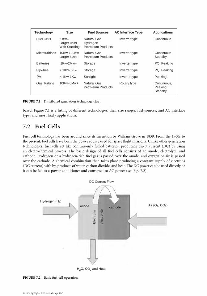
Technology Size Fuel Sources AC Interface Type Applications
Fuel Cells
Microturbines
Batteries
Flywheel
PV
Gas Turbine
.5Kw–Larger units With Stacking
10Kw-100KwLarger sizes
.1Kw-2Mw+
>.1Kw-.5Kw
>.1Kw-1Kw
10Kw–5Mw+
Natural Gas Hydrogen Petroleum Products
Inverter type Continuous
Continuous Standby
PQ, Peaking
PQ, Peaking
Peaking
Continuous,PeakingStandby
Inverter type
Inverter type
Inverter type
Inverter type
Rotary type
Natural GasPetroleum Products
Storage
Storage
Sunlight
Natural Gas Petroleum Products
FIGURE 7.1 Distributed generation technology chart.
based. Figure 7.1 is a listing of different technologies, their size ranges, fuel sources, and AC interface
type, and most likely applications.
7.2 Fuel Cells
Fuel cell technology has been around since its invention by William Grove in 1839. From the 1960s to
the present, fuel cells have been the power source used for space flight missions. Unlike other generation
technologies, fuel cells act like continuously fueled batteries, producing direct current (DC) by using
an electrochemical process. The basic design of all fuel cells consists of an anode, electrolyte, and
cathode. Hydrogen or a hydrogen-rich fuel gas is passed over the anode, and oxygen or air is passed
over the cathode. A chemical combination then takes place producing a constant supply of electrons
(DC current) with by-products of water, carbon dioxide, and heat. The DC power can be used directly or
it can be fed to a power conditioner and converted to AC power (see Fig. 7.2).
Hydrogen (H2)
H2O, CO2 and Heat
DC Current Flow
Air (O2, CO2)anode
Ele
ctro
ns
cathode
elec
trol
yte
FIGURE 7.2 Basic fuel cell operation.
� 2006 by Taylor & Francis Group, LLC.
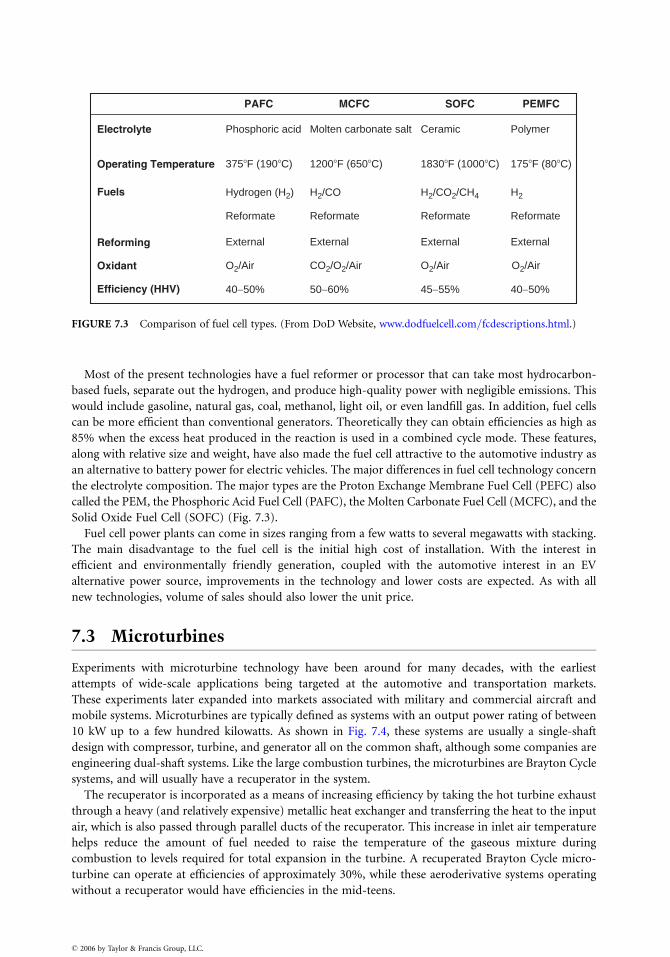
PAFC MCFC SOFC PEMFC
Electrolyte
Operating Temperature
Fuels
Reforming
Oxidant
Efficiency (HHV)
Phosphoric acid
Reformate
External
O2/Air O2/Air O2/Air
40−50% 50−60% 45−55% 40−50%
CO2/O2/Air
External External External
Reformate Reformate Reformate
375�F (190�C)
Hydrogen (H2) H2/CO H2/CO2/CH4 H2
1200�F (650�C) 1830�F (1000�C) 175�F (80�C)
Molten carbonate salt Ceramic Polymer
FIGURE 7.3 Comparison of fuel cell types. (From DoD Website, www.dodfuelcell.com=fcdescriptions.html.)
Most of the present technologies have a fuel reformer or processor that can take most hydrocarbon-
based fuels, separate out the hydrogen, and produce high-quality power with negligible emissions. This
would include gasoline, natural gas, coal, methanol, light oil, or even landfill gas. In addition, fuel cells
can be more efficient than conventional generators. Theoretically they can obtain efficiencies as high as
85% when the excess heat produced in the reaction is used in a combined cycle mode. These features,
along with relative size and weight, have also made the fuel cell attractive to the automotive industry as
an alternative to battery power for electric vehicles. The major differences in fuel cell technology concern
the electrolyte composition. The major types are the Proton Exchange Membrane Fuel Cell (PEFC) also
called the PEM, the Phosphoric Acid Fuel Cell (PAFC), the Molten Carbonate Fuel Cell (MCFC), and the
Solid Oxide Fuel Cell (SOFC) (Fig. 7.3).
Fuel cell power plants can come in sizes ranging from a few watts to several megawatts with stacking.
The main disadvantage to the fuel cell is the initial high cost of installation. With the interest in
efficient and environmentally friendly generation, coupled with the automotive interest in an EV
alternative power source, improvements in the technology and lower costs are expected. As with all
new technologies, volume of sales should also lower the unit price.
7.3 Microturbines
Experiments with microturbine technology have been around for many decades, with the earliest
attempts of wide-scale applications being targeted at the automotive and transportation markets.
These experiments later expanded into markets associated with military and commercial aircraft and
mobile systems. Microturbines are typically defined as systems with an output power rating of between
10 kW up to a few hundred kilowatts. As shown in Fig. 7.4, these systems are usually a single-shaft
design with compressor, turbine, and generator all on the common shaft, although some companies are
engineering dual-shaft systems. Like the large combustion turbines, the microturbines are Brayton Cycle
systems, and will usually have a recuperator in the system.
The recuperator is incorporated as a means of increasing efficiency by taking the hot turbine exhaust
through a heavy (and relatively expensive) metallic heat exchanger and transferring the heat to the input
air, which is also passed through parallel ducts of the recuperator. This increase in inlet air temperature
helps reduce the amount of fuel needed to raise the temperature of the gaseous mixture during
combustion to levels required for total expansion in the turbine. A recuperated Brayton Cycle micro-
turbine can operate at efficiencies of approximately 30%, while these aeroderivative systems operating
without a recuperator would have efficiencies in the mid-teens.
� 2006 by Taylor & Francis Group, LLC.
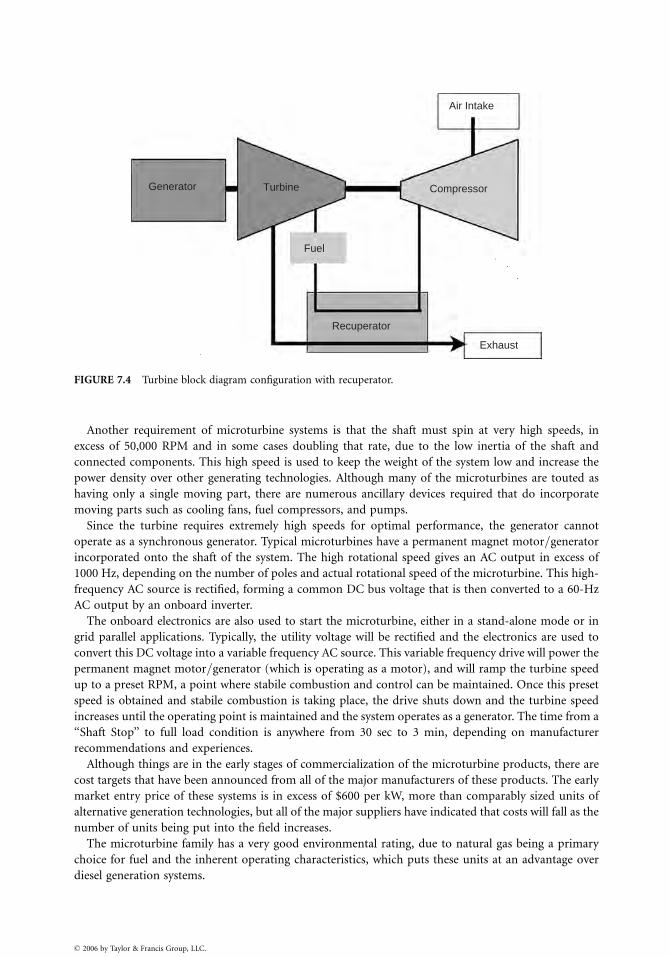
Generator Turbine
Fuel
Recuperator
Exhaust
Compressor
Air Intake
FIGURE 7.4 Turbine block diagram configuration with recuperator.
Another requirement of microturbine systems is that the shaft must spin at very high speeds, in
excess of 50,000 RPM and in some cases doubling that rate, due to the low inertia of the shaft and
connected components. This high speed is used to keep the weight of the system low and increase the
power density over other generating technologies. Although many of the microturbines are touted as
having only a single moving part, there are numerous ancillary devices required that do incorporate
moving parts such as cooling fans, fuel compressors, and pumps.
Since the turbine requires extremely high speeds for optimal performance, the generator cannot
operate as a synchronous generator. Typical microturbines have a permanent magnet motor=generator
incorporated onto the shaft of the system. The high rotational speed gives an AC output in excess of
1000 Hz, depending on the number of poles and actual rotational speed of the microturbine. This high-
frequency AC source is rectified, forming a common DC bus voltage that is then converted to a 60-Hz
AC output by an onboard inverter.
The onboard electronics are also used to start the microturbine, either in a stand-alone mode or in
grid parallel applications. Typically, the utility voltage will be rectified and the electronics are used to
convert this DC voltage into a variable frequency AC source. This variable frequency drive will power the
permanent magnet motor=generator (which is operating as a motor), and will ramp the turbine speed
up to a preset RPM, a point where stabile combustion and control can be maintained. Once this preset
speed is obtained and stabile combustion is taking place, the drive shuts down and the turbine speed
increases until the operating point is maintained and the system operates as a generator. The time from a
‘‘Shaft Stop’’ to full load condition is anywhere from 30 sec to 3 min, depending on manufacturer
recommendations and experiences.
Although things are in the early stages of commercialization of the microturbine products, there are
cost targets that have been announced from all of the major manufacturers of these products. The early
market entry price of these systems is in excess of $600 per kW, more than comparably sized units of
alternative generation technologies, but all of the major suppliers have indicated that costs will fall as the
number of units being put into the field increases.
The microturbine family has a very good environmental rating, due to natural gas being a primary
choice for fuel and the inherent operating characteristics, which puts these units at an advantage over
diesel generation systems.
� 2006 by Taylor & Francis Group, LLC.
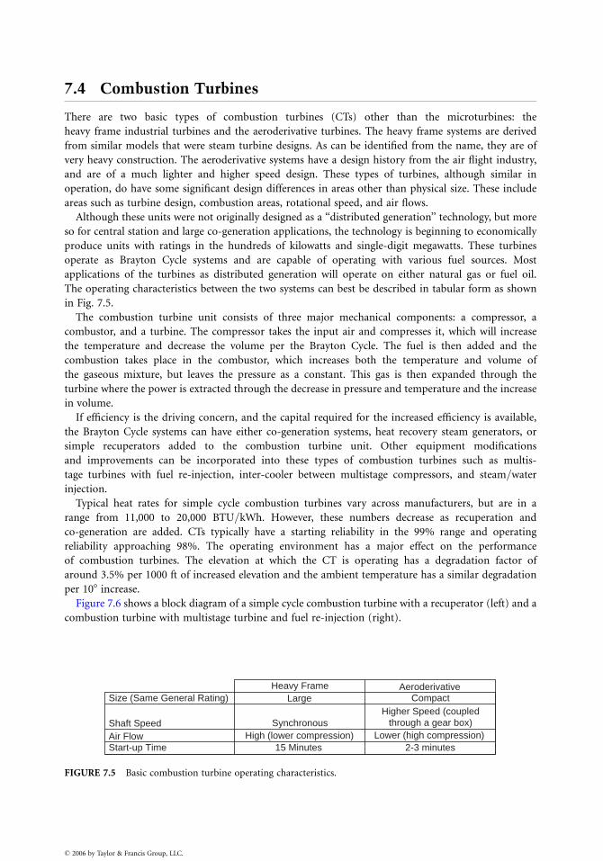
7.4 Combustion Turbines
There are two basic types of combustion turbines (CTs) other than the microturbines: the
heavy frame industrial turbines and the aeroderivative turbines. The heavy frame systems are derived
from similar models that were steam turbine designs. As can be identified from the name, they are of
very heavy construction. The aeroderivative systems have a design history from the air flight industry,
and are of a much lighter and higher speed design. These types of turbines, although similar in
operation, do have some significant design differences in areas other than physical size. These include
areas such as turbine design, combustion areas, rotational speed, and air flows.
Although these units were not originally designed as a ‘‘distributed generation’’ technology, but more
so for central station and large co-generation applications, the technology is beginning to economically
produce units with ratings in the hundreds of kilowatts and single-digit megawatts. These turbines
operate as Brayton Cycle systems and are capable of operating with various fuel sources. Most
applications of the turbines as distributed generation will operate on either natural gas or fuel oil.
The operating characteristics between the two systems can best be described in tabular form as shown
in Fig. 7.5.
The combustion turbine unit consists of three major mechanical components: a compressor, a
combustor, and a turbine. The compressor takes the input air and compresses it, which will increase
the temperature and decrease the volume per the Brayton Cycle. The fuel is then added and the
combustion takes place in the combustor, which increases both the temperature and volume of
the gaseous mixture, but leaves the pressure as a constant. This gas is then expanded through the
turbine where the power is extracted through the decrease in pressure and temperature and the increase
in volume.
If efficiency is the driving concern, and the capital required for the increased efficiency is available,
the Brayton Cycle systems can have either co-generation systems, heat recovery steam generators, or
simple recuperators added to the combustion turbine unit. Other equipment modifications
and improvements can be incorporated into these types of combustion turbines such as multis-
tage turbines with fuel re-injection, inter-cooler between multistage compressors, and steam=water
injection.
Typical heat rates for simple cycle combustion turbines vary across manufacturers, but are in a
range from 11,000 to 20,000 BTU=kWh. However, these numbers decrease as recuperation and
co-generation are added. CTs typically have a starting reliability in the 99% range and operating
reliability approaching 98%. The operating environment has a major effect on the performance
of combustion turbines. The elevation at which the CT is operating has a degradation factor of
around 3.5% per 1000 ft of increased elevation and the ambient temperature has a similar degradation
per 108 increase.
Figure 7.6 shows a block diagram of a simple cycle combustion turbine with a recuperator (left) and a
combustion turbine with multistage turbine and fuel re-injection (right).
Size (Same General Rating)Heavy Frame Aeroderivative
CompactHigher Speed (coupled
through a gear box)Lower (high compression)
2-3 minutes
Large
SynchronousHigh (lower compression)
15 Minutes
Shaft SpeedAir FlowStart-up Time
FIGURE 7.5 Basic combustion turbine operating characteristics.
� 2006 by Taylor & Francis Group, LLC.
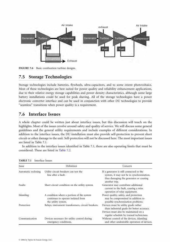
Generator
Recuperator
FuelFuel Fuel
Turbine
Exhaust
exhaust
Compressor Turbine Turbine CompressorGenerator
Air Intake Air Intake
FIGURE 7.6 Basic combustion turbine designs.
7.5 Storage Technologies
Storage technologies include batteries, flywheels, ultra-capacitors, and to some extent photovoltaics.
Most of these technologies are best suited for power quality and reliability enhancement applications,
due to their relative energy storage capabilities and power density characteristics, although some large
battery installations could be used for peak shaving. All of the storage technologies have a power
electronic converter interface and can be used in conjunction with other DU technologies to provide
‘‘seamless’’ transitions when power quality is a requirement.
7.6 Interface Issues
A whole chapter could be written just about interface issues, but this discussion will touch on the
highlights. Most of the issues revolve around safety and quality of service. We will discuss some general
guidelines and the general utility requirements and include examples of different considerations. In
addition to the interface issues, the DU installation must also provide self-protection to prevent short
circuit or other damage to the unit. Self-protection will not be discussed here. The most important issues
are listed in Table 7.1.
In addition to the interface issues identified in Table 7.1, there are also operating limits that must be
considered. These are listed in Table 7.2.
TABLE 7.1 Interface Issues
Issue Definition Concern
Automatic reclosing Utility circuit breakers can test the
line after a fault.
If a generator is still connected to the
system, it may not be in synchronization,
thus damaging the generator or causing
another trip.
Faults Short circuit condition on the utility system. Generator may contribute additional
current to the fault, causing a miss
operation of relay equipment.
Islanding A condition where a portion of the system
continues to operate isolated from
the utility system.
Power quality, safety, and protection
may be compromised in addition to
possible synchronization problems.
Protection Relays, instrument transformers, circuit breakers. Devices must be utility grade rather
than industrial grade for better accuracy.
Devices must also be maintained on a
regular schedule by trained technicians.
Communication Devices necessary for utility control during
emergency conditions.
Without control of the devices, islanding
and other undesirable operation of devices.
� 2006 by Taylor & Francis Group, LLC.
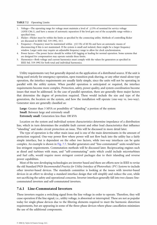
TABLE 7.2 Operating Limits
1. Voltage—The operating range for voltage must maintain a level of +15% of nominal for service voltage
(ANSI C84.1), and have a means of automatic separation if the level gets out of the acceptable range within a
specified time.
2. Flicker—Flicker must be within the limits as specified by the connecting utility. Methods of controlling flicker
are discussed in IEEE Std. 519-1992, 10.5.
3. Frequency—Frequency must be maintained within +0.5 Hz of 60 Hz and have an automatic means of
disconnecting if this is not maintained. If the system is small and isolated, there might be a larger frequency
window. Larger units may require an adjustable frequency range to allow for clock synchronizaton.
4. Power factor—The power factor should be within 0.85 lagging or leading for normal operation. Some systems that
are designed for compensation may operate outside these limits.
5. Harmonics—Both voltage and current harmonics must comply with the values for generators as specified in
IEEE Std. 519-1992 for both total and individual harmonics.
Utility requirements vary but generally depend on the application of a distributed source. If the unit is
being used strictly for emergency operation, open transition peak shaving, or any other stand-alone type
operation, the interface requirements are usually fairly simple, since the units will not be operating in
parallel with the utility system. When parallel operation is anticipated or required, the interface
requirements become more complex. Protection, safety, power quality, and system coordination become
issues that must be addressed. In the case of parallel operation, there are generally three major factors
that determine the degree of protection required. These would include the size and type of the
generation, the location on the system, and how the installation will operate (one-way vs. two-way).
Generator sizes are generally classified as:
Large: Greater than 3 MVA or possibility of ‘‘islanding’’ a portion of the system
Small: Between large and extremely small
Extremely small: Generation less than 100 kVA
Location on the system and individual system characteristics determine impedance of a distribution
line, which in turn determines the available fault current and other load characteristics that influence
‘‘islanding’’ and make circuit protection an issue. This will be discussed in more detail later.
The type of operation is the other main issue and is one of the main determinants in the amount of
protection required. One-way power flow where power will not flow back into the utility has a fairly
simple interface, but is dependent on the other two factors, while two-way interfaces can be quite
complex. An example is shown in Fig. 7.7. Smaller generators and ‘‘line-commutated’’ units would have
less stringent requirements. Commutation methods will be discussed later. Reciprocating engines such
as diesel and turbines with mass, and ‘‘self-commutating’’ units which could include microturbines
and fuel cells, would require more stringent control packages due to their islanding and reverse
power capabilities.
Most of the new developing technologies are inverter based and there are efforts now in IEEE to revise
the old Standard P929 Recommended Practice for Utility Interface of Photovoltaic (PV) Systems to include
other inverter-based devices. The standards committee is looking at the issues with inverter-based
devices in an effort to develop a standard interface design that will simplify and reduce the cost, while
not sacrificing the safety and operational concerns. Inverter interfaces generally fall into two classes: line-
commutated inverters and self-commutated inverters.
7.6.1 Line-Commutated Inverters
These inverters require a switching signal from the line voltage in order to operate. Therefore, they will
cease operation if the line signal, i.e., utility voltage, is abnormal or interrupted. These are not as popular
today for single-phase devices due to the filtering elements required to meet the harmonic distortion
requirements, but are appearing in some of the three-phase devices where phase cancellation minimizes
the use of the additional components.
� 2006 by Taylor & Francis Group, LLC.
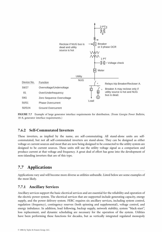
∗
∗
Relays trip Breaker/Recloser A.
Breaker A may reclose only if utility source is hot and NUGbus is dead.
NUG
Load
Utility
BC
G
A
M
Device No.
59/27 Overvoltage/Undervoltage
Over/Underfrequency
Zero Sequence Overvoltage
Phase Overcurrent
Ground Overcurrent
81
59G
50/51
50/51N
Function
Reclose if NUG bus isdead and utilitysource is hot
Breakeror 3 phase OCR
Meter
1 PT
Voltage check
3 PT's
FIGURE 7.7 Example of large generator interface requirements for distribution. (From Georgia Power Bulletin,
18–8, generator interface requirements.)
7.6.2 Self-Commutated Inverters
These inverters, as implied by the name, are self-commutating. All stand-alone units are self-
commutated, but not all self-commutated inverters are stand-alone. They can be designed as either
voltage or current sources and most that are now being designed to be connected to the utility system are
designed to be current sources. These units still use the utility voltage signal as a comparison and
produce current at that voltage and frequency. A great deal of effort has gone into the development of
non-islanding inverters that are of this type.
7.7 Applications
Applications vary and will become more diverse as utilities unbundle. Listed below are some examples of
the most likely.
7.7.1 Ancillary Services
Ancillary services support the basic electrical services and are essential for the reliability and operation of
the electric power system. The electrical services that are supported include generating capacity, energy
supply, and the power delivery system. FERC requires six ancillary services, including system control,
regulation (frequency), contingency reserves (both spinning and supplemental), voltage control, and
energy imbalance. In addition, load following, backup supply, network stability, system ‘‘black-start’’,
loss replacement, and dynamic scheduling are necessary for the operation of the system. Utilities
have been performing these functions for decades, but as vertically integrated regulated monopoly
� 2006 by Taylor & Francis Group, LLC.
organizations. As these begin to disappear, and a new structure with multiple competing parties
emerges, distributed utilities might be able to supply several of these.
The distributed utilities providing these services could be owned by the former traditional utility,
customers, or third-party brokers, depending on the application. The main obstacles to this approach
are aggregation and communication when dealing with many small resources rather than large central
station sources.
7.7.2 ‘‘Traditional Utility’’ Applications
Traditional utilities may find the use of DU a practical way to solve loading and reliability problems if each
case is evaluated on a stand-alone individual basis. Deferring investment is one likely way that DU can be
applied. In many areas, substations and lines have seasonal peaks that are substantially higher than the rest of
the year. In these cases, the traditional approach has been to increase the capacity to meet the demand. Based
on the individual situation, delaying the upgrade for 2 to 5 years with a DU system could be a more
economical solution. This would be especially true if different areas had different seasonal peaks and the DU
system was portable, thus deferring two upgrades. DU could also be used instead of conventional facilities
when backup feeds are required or to improve reliability or power quality.
In addition, peak shaving and generation reserve could be provided with strategically placed DU
systems that take advantage of reducing system losses as well as offsetting base generation. Again, these
have to be evaluated on an individual case basis and not a system average basis as is done in many
economic studies. The type of technology used will depend on the particular requirements. In general,
storage devices such as flywheels and batteries are better for power quality applications due to their
fast response time, in many cases half a cycle. Generation devices are better suited for applications
that require more than 30 min of supply, such as backup systems, alternate feeds, peak shaving,
and demand deferrals. Generation sources can also be used instead of conventional facilities in
certain cases.
7.7.3 Customer Applications
Individual customers with special requirements may find DU technologies that meet their
needs. Customers who require ‘‘enhanced’’ power quality and reliability of service already utilize UPS
systems with battery backup to condition the power to sensitive equipment, and many hospitals, waste
treatment plants, and other emergency services providers have emergency backup systems supplied
by standby generator systems. As barriers go down and technologies improve, customer-sited DU
facilities could provide many of the ancillary services as well as sell excess power into the grid. Fuel
cell and even diesel generators could be especially attractive for customers with requirements of heat and
steam. Many of the fuel cell technologies are now looking at the residential market with small units that
would be connected to the grid but supply the additional requirements for customers with special power
quality needs.
7.7.4 Third-Party Service Providers
Third-party service providers could provide all the services listed above for the utilities and customers,
in addition to selling power across the grid. In many cases, an end user does not have the expertise to
operate and maintain generation systems and would prefer to purchase the services.
7.8 Conclusions
Disbursed generation will be a part of the distribution utility system of the future. Economics, regulatory
requirements, and technology improvements will determine the speed at which they are integrated.
� 2006 by Taylor & Francis Group, LLC.

References
ANSI=IEEE Std. 1001–1998, IEEE Guide for Interfacing Dispersed Storage and Generation Facilities with
Electric Utility Systems, IEEE Standards Coordinating Committee 23, Feb. 9, 1989.
Davis, M.W. Microturbines—An Economic and Reliability Evaluation for Commercial, Residential, and
Remote Load Applications, IEEE Transactions PE-480-PWRS-0-10-1998.
Delmerico, R.W., Miller, N.W., and Owen, E.L. Power System Integration Strategies for Distributed
Generation, Power Systems Energy Consulting GE International, Inc., Distributed Electricity
Generation Conference, Denver, CO, Jan. 25, 1999.
Department of Defense Website, www.dodfuelcell.com=fcdescriptions.html.
Goldstein, H.L. Small Turbines in Distributed Utility Application Natural Gas Pressure Supply
Requirements, NREL=SP-461-21073, May, 1996.
Hirschenhofer, J.H. DOE Forum on Fuel Cell Technologies, IEEE Winter Power Meeting, Parsons
Corporation Presentation, Feb. 4, 1999.
Kirby, B. Distributed Generation: A Natural for Ancillary Services, Distributed Electric Generation
Conference, Denver CO, Jan. 25, 1999.
Oplinger, J.L. Methodology to Assess the Market Potential of Distributed Generation, Power Systems Energy
Consulting GE International, Inc., Distributed Electric Generation Conference, Denver, CO,
Jan. 25, 1999.
Recommended Practice for Utility Interface of Photovoltaic (PV) Systems, IEEE Standard P929, Draft 10,
Feb. 1999.
Southern Company Parallel Operation Requirements, Protection and Control Committee, Aug. 4, 1998.
Technology Overviews, DOE Forum on Fuel Cell Technology, IEEE Winter Power Meeting, Feb. 4, 1999.
� 2006 by Taylor & Francis Group, LLC.
III
TransmissionSystem George G. KaradyArizona State University8 Concept of Energy Transmission and Distribution George G. Karady ...................... 8-1
Generation Stations . Switchgear . Control Devices . Concept of
Energy Transmission and Distribution
9 Transmission Line Structures Joe C. Pohlman ............................................................... 9-1
Traditional Line Design Practice . Current Deterministic Design Practice .
Improved Design Approaches . Appendix A General Design
Criteria—Methodology
10 Insulators and Accessories George G. Karady and Richard G. Farmer........................ 10-1
Electrical Stresses on External Insulation . Ceramic (Porcelain and Glass)
Insulators . Nonceramic (Composite) Insulators . Insulator Failure
Mechanism . Methods for Improving Insulator Performance
11 Transmission Line Construction and Maintenance Wilford Caulkins
and Kristine Buchholz ........................................................................................................ 11-1
Tools . Equipment . Procedures . Helicopters
12 Insulated Power Cables Used in Underground Applications Michael L. Dyer ....... 12-1
Underground System Designs . Conductor . Insulation . Medium- and
High-Voltage Power Cables . Shield Bonding Practice . Installation Practice .
System Protection Devices . Common Calculations used with Cable
13 Transmission Line Parameters Manuel Reta-Hernandez ............................................ 13-1
Equivalent Circuit . Resistance . Current-Carrying Capacity (Ampacity) .
Inductance and Inductive Reactance . Capacitance and Capacitive Reactance .
Characteristics of Overhead Conductors
14 Sag and Tension of Conductor D.A. Douglass and Ridley Thrash............................... 14-1
Catenary Cables . Approximate Sag-Tension Calculations . Numerical
Sag-Tension Calculations . Ruling Span Concept . Line Design
Sag-Tension Parameters . Conductor Installation . Defining Terms
� 2006 by Taylor & Francis Group, LLC.
15 Corona and Noise Giao N. Trinh ................................................................................... 15-1
Corona Modes . Main Effects of Corona Discharges on Overhead Lines .
Impact on the Selection of Line Conductors . Conclusions
16 Geomagnetic Disturbances and Impacts upon Power System Operation
John G. Kappenman .......................................................................................................... 16-1
Introduction . Power Grid Damage and Restoration Concerns . Weak Link
in the Grid: Transformers . An Overview of Power System Reliability and
Related Space Weather Climatology . Geological Risk Factors and Geoelectric
Field Response . Power Grid Design and Network Topology Risk Factors .
Extreme Geomagnetic Disturbance Events—Observational Evidence .
Power Grid Simulations for Extreme Disturbance Events . Conclusions
17 Lightning Protection William A. Chisholm .................................................................. 17-1
Ground Flash Density . Stroke Incidence to Power Lines . Stroke
Current Parameters . Calculation of Lightning Overvoltages on
Shielded Lines . Insulation Strength . Mitigation Methods . Conclusion
18 Reactive Power Compensation Rao S. Thallam ........................................................... 18-1
The Need for Reactive Power Compensation . Application of Shunt Capacitor
Banks in Distribution Systems—A Utility Perspective . Static VAR Control .
Series Compensation . Series Capacitor Bank . Defining Terms
19 Environmental Impact of Transmission Lines George G. Karady ............................. 19-1
Introduction . Aesthetical Effects of Lines . Magnetic Field Generated
by HV Lines . Electrical Field Generated by HV Lines . Audible Noise .
Electromagnetic Interference
� 2006 by Taylor & Francis Group, LLC.
8
� 2006 by Taylor & Francis Group, LLC.
Concept of EnergyTransmission and
Distribution
George G. KaradyArizona State University
8.1 Generation Stations............................................................. 8-1
8.2 Switchgear ............................................................................ 8-3
8.3 Control Devices ................................................................... 8-4
8.4 Concept of Energy Transmission and Distribution ......... 8-4High-Voltage Transmission Lines . High-Voltage DC Lines .
Sub-Transmission Lines . Distribution Lines
The purpose of the electric transmission system is the interconnection of the electric energy producing
power plants or generating stations with the loads. A three-phase AC system is used for most transmis-
sion lines. The operating frequency is 60 Hz in the U.S. and 50 Hz in Europe, Australia, and part of Asia.
The three-phase system has three phase conductors. The system voltage is defined as the rms voltage
between the conductors, also called line-to-line voltage. The voltage between the phase conductor and
ground, called line-to-ground voltage, is equal to the line-to-line voltage divided by the square root of
three. Figure 8.1 shows a typical system.
The figure shows the Phoenix area 230-kV system, which interconnects the local power plants and the
substations supplying different areas of the city. The circles are the substations and the squares are the
generating stations. The system contains loops that assure that each load substation is supplied by at
least two lines. This assures that the outage of a single line does not cause loss of power to any customer.
For example, the Aqua Fria generating station (marked: Power plant) has three outgoing lines. Three
high-voltage cables supply the Country Club Substation (marked: Substation with cables). The Pinnacle
Peak Substation (marked: Substation with transmission lines) is a terminal for six transmission lines.
This example shows that the substations are the node points of the electric system. The system is
interconnected with the neighboring systems. As an example, one line goes to Glen Canyon and the
other to Cholla from the Pinnacle Peak substation.
In the middle of the system, which is in a congested urban area, high-voltage cables are used. In open
areas, overhead transmission lines are used. The cost per mile of overhead transmission lines is 6 to 10%
less than underground cables.
The major components of the electric system, the transmission lines, and cables are described
briefly below [1].
8.1 Generation Stations
The generating station converts the stored energy of gas, oil, coal, nuclear fuel, or water position to
electric energy. The most frequently used power plants are:
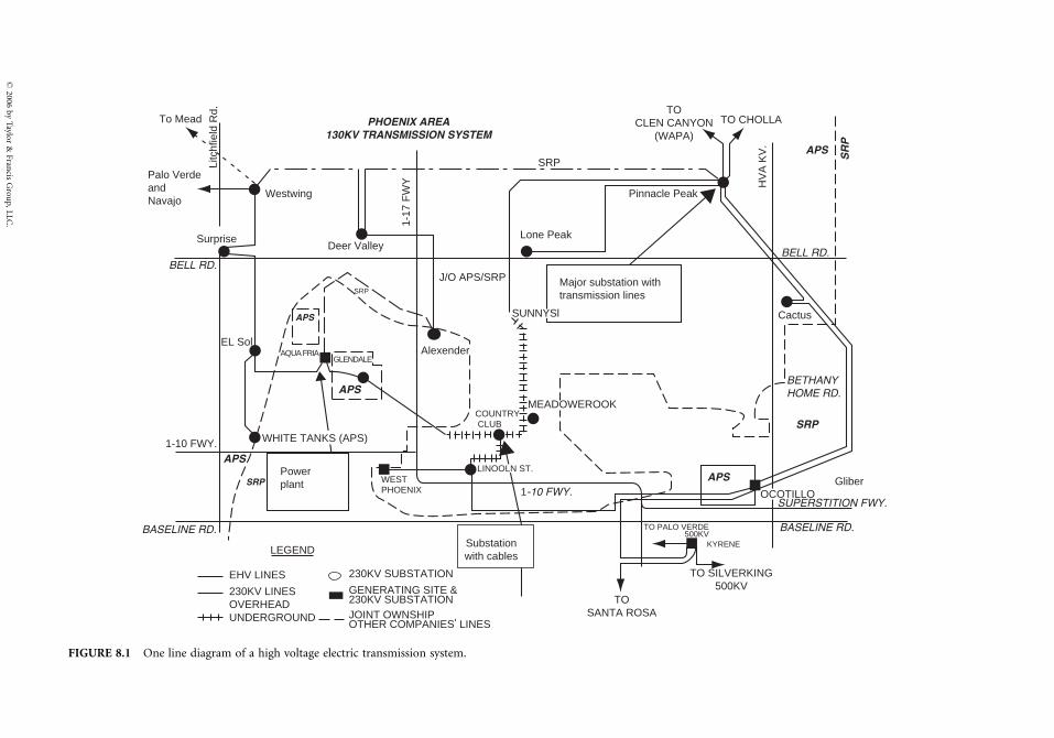
To Mead
Palo VerdeandNavajo
Westwing
Surprise
EL SolAQUA FRIA
GLENDALE
WESTPHOENIX
1-10 FWY.
1-10 FWY.
Substationwith cables
230KV SUBSTATIONEHV LINES
230KV LINESOVERHEADUNDERGROUND
GENERATING SITE &230KV SUBSTATIONJOINT OWNSHIPOTHER COMPANIES' LINES
Powerplant
Deer Valley
SRP SR
P
SRP
HV
A K
V. APS
APS
TOCLEN CANYON
(WAPA)
TO CHOLLA
J/O APS/SRPSRP
Lone Peak
Alexender
COUNTRY CLUB
Pinnacle Peak
Cactus
BETHANYHOME RD.
GliberOCOTILLO
TO PALO VERDE500KV
TO SILVERKING500KV
TO SANTA ROSA
KYRENE
SUPERSTITION FWY.
BASELINE RD.
Major substation withtransmission lines
1-17
FW
Y
APS
APS
PHOENIX AREA130KV TRANSMISSION SYSTEM
APS
SRP
BELL RD.BELL RD.
BASELINE RD.
LEGEND
SUNNYSl
MEADOWEROOK
WHITE TANKS (APS)
LINOOLN ST.
Litc
hfie
ld R
d.
FIGURE 8.1 One line diagram of a high voltage electric transmission system.
�2
00
6b
yT
aylor
&F
rancis
Gro
up
,L
LC
.
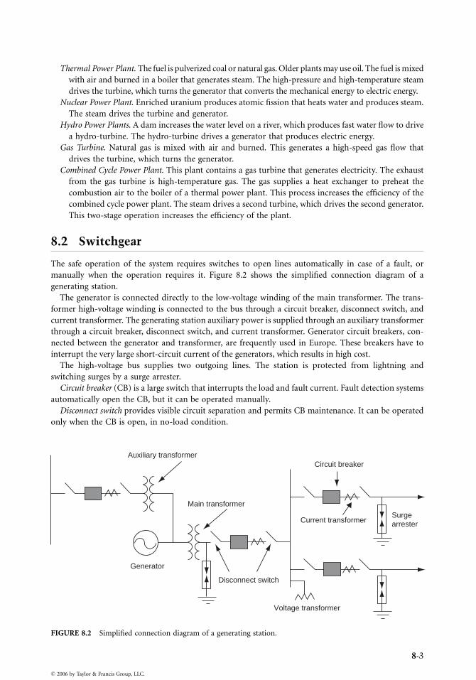
Thermal Power Plant. The fuel is pulverized coal or natural gas. Older plants may use oil. The fuel is mixed
with air and burned in a boiler that generates steam. The high-pressure and high-temperature steam
drives the turbine, which turns the generator that converts the mechanical energy to electric energy.
Nuclear Power Plant. Enriched uranium produces atomic fission that heats water and produces steam.
The steam drives the turbine and generator.
Hydro Power Plants. A dam increases the water level on a river, which produces fast water flow to drive
a hydro-turbine. The hydro-turbine drives a generator that produces electric energy.
Gas Turbine. Natural gas is mixed with air and burned. This generates a high-speed gas flow that
drives the turbine, which turns the generator.
Combined Cycle Power Plant. This plant contains a gas turbine that generates electricity. The exhaust
from the gas turbine is high-temperature gas. The gas supplies a heat exchanger to preheat the
combustion air to the boiler of a thermal power plant. This process increases the efficiency of the
combined cycle power plant. The steam drives a second turbine, which drives the second generator.
This two-stage operation increases the efficiency of the plant.
8.2 Switchgear
The safe operation of the system requires switches to open lines automatically in case of a fault, or
manually when the operation requires it. Figure 8.2 shows the simplified connection diagram of a
generating station.
The generator is connected directly to the low-voltage winding of the main transformer. The trans-
former high-voltage winding is connected to the bus through a circuit breaker, disconnect switch, and
current transformer. The generating station auxiliary power is supplied through an auxiliary transformer
through a circuit breaker, disconnect switch, and current transformer. Generator circuit breakers, con-
nected between the generator and transformer, are frequently used in Europe. These breakers have to
interrupt the very large short-circuit current of the generators, which results in high cost.
The high-voltage bus supplies two outgoing lines. The station is protected from lightning and
switching surges by a surge arrester.
Circuit breaker (CB) is a large switch that interrupts the load and fault current. Fault detection systems
automatically open the CB, but it can be operated manually.
Disconnect switch provides visible circuit separation and permits CB maintenance. It can be operated
only when the CB is open, in no-load condition.
Auxiliary transformer
Main transformer
Generator
Disconnect switch
Current transformer
Circuit breaker
Surgearrester
Voltage transformer
FIGURE 8.2 Simplified connection diagram of a generating station.
8-3
� 2006 by Taylor & Francis Group, LLC.
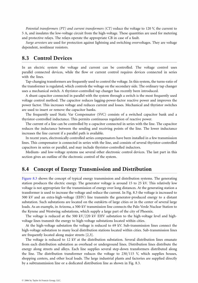
Potential transformers (PT) and current transformers (CT) reduce the voltage to 120 V, the current to
5 A, and insulates the low-voltage circuit from the high-voltage. These quantities are used for metering
and protective relays. The relays operate the appropriate CB in case of a fault.
Surge arresters are used for protection against lightning and switching overvoltages. They are voltage
dependent, nonlinear resistors.
8.3 Control Devices
In an electric system the voltage and current can be controlled. The voltage control uses
parallel connected devices, while the flow or current control requires devices connected in series
with the lines.
Tap-changing transformers are frequently used to control the voltage. In this system, the turns-ratio of
the transformer is regulated, which controls the voltage on the secondary side. The ordinary tap changer
uses a mechanical switch. A thyristor-controlled tap changer has recently been introduced.
A shunt capacitor connected in parallel with the system through a switch is the most frequently used
voltage control method. The capacitor reduces lagging-power-factor reactive power and improves the
power factor. This increases voltage and reduces current and losses. Mechanical and thyristor switches
are used to insert or remove the capacitor banks.
The frequently used Static Var Compensator (SVC) consists of a switched capacitor bank and a
thyristor-controlled inductance. This permits continuous regulation of reactive power.
The current of a line can be controlled by a capacitor connected in series with the line. The capacitor
reduces the inductance between the sending and receiving points of the line. The lower inductance
increases the line current if a parallel path is available.
In recent years, electronically controlled series compensators have been installed in a few transmission
lines. This compensator is connected in series with the line, and consists of several thyristor-controlled
capacitors in series or parallel, and may include thyristor-controlled inductors.
Medium- and low-voltage systems use several other electronic control devices. The last part in this
section gives an outline of the electronic control of the system.
8.4 Concept of Energy Transmission and Distribution
Figure 8.3 shows the concept of typical energy transmission and distribution systems. The generating
station produces the electric energy. The generator voltage is around 15 to 25 kV. This relatively low
voltage is not appropriate for the transmission of energy over long distances. At the generating station a
transformer is used to increase the voltage and reduce the current. In Fig. 8.3 the voltage is increased to
500 kV and an extra-high-voltage (EHV) line transmits the generator-produced energy to a distant
substation. Such substations are located on the outskirts of large cities or in the center of several large
loads. As an example, in Arizona, a 500-kV transmission line connects the Palo Verde Nuclear Station to
the Kyrene and Westwing substations, which supply a large part of the city of Phoenix.
The voltage is reduced at the 500 kV=220 kV EHV substation to the high-voltage level and high-
voltage lines transmit the energy to high-voltage substations located within cities.
At the high-voltage substation the voltage is reduced to 69 kV. Sub-transmission lines connect the
high-voltage substation to many local distribution stations located within cities. Sub-transmission lines
are frequently located along major streets [2,3].
The voltage is reduced to 12 kV at the distribution substation. Several distribution lines emanate
from each distribution substation as overhead or underground lines. Distribution lines distribute the
energy along streets and alleys. Each line supplies several step-down transformers distributed along
the line. The distribution transformer reduces the voltage to 230=115 V, which supplies houses,
shopping centers, and other local loads. The large industrial plants and factories are supplied directly
by a subtransmission line or a dedicated distribution line as shown in Fig. 8.3.
� 2006 by Taylor & Francis Group, LLC.
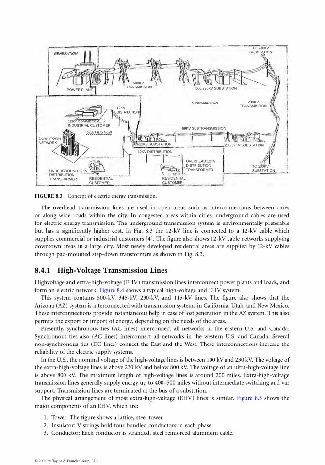
POWER PLANT
12KV COMMERCIAL or INDUSTRIAL CUSTOMER
DOWNTOWNNETWORK 69/12KV SUBSTATION
69KV SUBTRANSMISSION
230/69KV SUBSTATION
TO 230KVSUBSTATION
12KV DISTRIBUTION
OVERHEAD 12KVDISTRIBUTIONTRANSFORMER
RESIDENTIALCUSTOMER
UNDERGROUND 12KVDISTRIBUTIONTRANSFORMER RESIDENTIAL
CUSTOMER
12KVDISTRIBUTION
500KVTRANSMISSION
TO 230KVSUBSTATION
500/230KV SUBSTATION
TRANSMISSION 230KVTRANSMISSION
GENERATION
DISTRIBUTION
FIGURE 8.3 Concept of electric energy transmission.
The overhead transmission lines are used in open areas such as interconnections between cities
or along wide roads within the city. In congested areas within cities, underground cables are used
for electric energy transmission. The underground transmission system is environmentally preferable
but has a significantly higher cost. In Fig. 8.3 the 12-kV line is connected to a 12-kV cable which
supplies commercial or industrial customers [4]. The figure also shows 12-kV cable networks supplying
downtown areas in a large city. Most newly developed residential areas are supplied by 12-kV cables
through pad-mounted step-down transformers as shown in Fig. 8.3.
8.4.1 High-Voltage Transmission Lines
Highvoltage and extra-high-voltage (EHV) transmission lines interconnect power plants and loads, and
form an electric network. Figure 8.4 shows a typical high-voltage and EHV system.
This system contains 500-kV, 345-kV, 230-kV, and 115-kV lines. The figure also shows that the
Arizona (AZ) system is interconnected with transmission systems in California, Utah, and New Mexico.
These interconnections provide instantaneous help in case of lost generation in the AZ system. This also
permits the export or import of energy, depending on the needs of the areas.
Presently, synchronous ties (AC lines) interconnect all networks in the eastern U.S. and Canada.
Synchronous ties also (AC lines) interconnect all networks in the western U.S. and Canada. Several
non-synchronous ties (DC lines) connect the East and the West. These interconnections increase the
reliability of the electric supply systems.
In the U.S., the nominal voltage of the high-voltage lines is between 100 kV and 230 kV. The voltage of
the extra-high-voltage lines is above 230 kV and below 800 kV. The voltage of an ultra-high-voltage line
is above 800 kV. The maximum length of high-voltage lines is around 200 miles. Extra-high-voltage
transmission lines generally supply energy up to 400–500 miles without intermediate switching and var
support. Transmission lines are terminated at the bus of a substation.
The physical arrangement of most extra-high-voltage (EHV) lines is similar. Figure 8.5 shows the
major components of an EHV, which are:
1. Tower: The figure shows a lattice, steel tower.
2. Insulator: V strings hold four bundled conductors in each phase.
3. Conductor: Each conductor is stranded, steel reinforced aluminum cable.
� 2006 by Taylor & Francis Group, LLC.
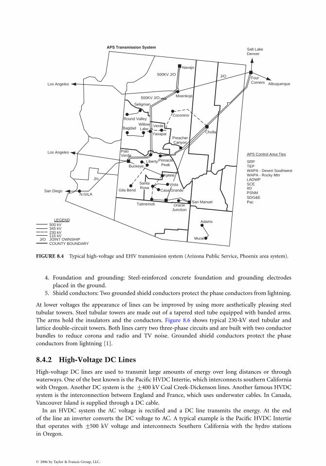
APS Transmission System
FourCorners
Salt LakeDenver
Albuquerque
N.GILASan Diego
Los Angeles
Los Angeles
J/o
Navajo
J/O500KV J/O
500KV J/O
Seligman
Round ValleyWillowLake
PaloVerde
LibertyPinnaclePeakBuckeye
Gila Bend
Vista
Kyrene
Casa Grande
San Manuel
Adams
Mural
Tatmemoli OracleJunction
SantaRosa
Bagdad Verde
YavapaiPreacherCanyon
Cholla
Moenkopi
Coconino
LEGEND500 kV345 kV230 kV115 kVJOINT OWNSHIPCOUNTY BOUNDARY
J/O
APS Control Area Ties
SRPTEPWAPA - Desert SouthwestWAPA - Rocky MtnLADWPSCEIIDPSNMSDG&EPac
FIGURE 8.4 Typical high-voltage and EHV transmission system (Arizona Public Service, Phoenix area system).
4. Foundation and grounding: Steel-reinforced concrete foundation and grounding electrodes
placed in the ground.
5. Shield conductors: Two grounded shield conductors protect the phase conductors from lightning.
At lower voltages the appearance of lines can be improved by using more aesthetically pleasing steel
tubular towers. Steel tubular towers are made out of a tapered steel tube equipped with banded arms.
The arms hold the insulators and the conductors. Figure 8.6 shows typical 230-kV steel tubular and
lattice double-circuit towers. Both lines carry two three-phase circuits and are built with two conductor
bundles to reduce corona and radio and TV noise. Grounded shield conductors protect the phase
conductors from lightning [1].
8.4.2 High-Voltage DC Lines
High-voltage DC lines are used to transmit large amounts of energy over long distances or through
waterways. One of the best known is the Pacific HVDC Intertie, which interconnects southern California
with Oregon. Another DC system is the +400 kV Coal Creek-Dickenson lines. Another famous HVDC
system is the interconnection between England and France, which uses underwater cables. In Canada,
Vancouver Island is supplied through a DC cable.
In an HVDC system the AC voltage is rectified and a DC line transmits the energy. At the end
of the line an inverter converts the DC voltage to AC. A typical example is the Pacific HVDC Intertie
that operates with +500 kV voltage and interconnects Southern California with the hydro stations
in Oregon.
� 2006 by Taylor & Francis Group, LLC.
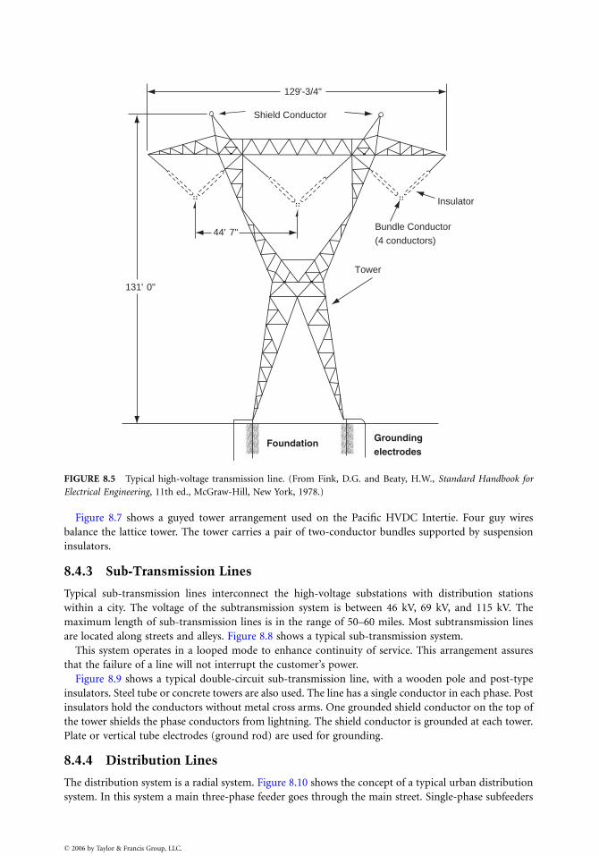
129'-3/4"
44' 7"
131' 0"
Shield Conductor
Insulator
Tower
Groundingelectrodes
Foundation
Bundle Conductor
(4 conductors)
FIGURE 8.5 Typical high-voltage transmission line. (From Fink, D.G. and Beaty, H.W., Standard Handbook for
Electrical Engineering, 11th ed., McGraw-Hill, New York, 1978.)
Figure 8.7 shows a guyed tower arrangement used on the Pacific HVDC Intertie. Four guy wires
balance the lattice tower. The tower carries a pair of two-conductor bundles supported by suspension
insulators.
8.4.3 Sub-Transmission Lines
Typical sub-transmission lines interconnect the high-voltage substations with distribution stations
within a city. The voltage of the subtransmission system is between 46 kV, 69 kV, and 115 kV. The
maximum length of sub-transmission lines is in the range of 50–60 miles. Most subtransmission lines
are located along streets and alleys. Figure 8.8 shows a typical sub-transmission system.
This system operates in a looped mode to enhance continuity of service. This arrangement assures
that the failure of a line will not interrupt the customer’s power.
Figure 8.9 shows a typical double-circuit sub-transmission line, with a wooden pole and post-type
insulators. Steel tube or concrete towers are also used. The line has a single conductor in each phase. Post
insulators hold the conductors without metal cross arms. One grounded shield conductor on the top of
the tower shields the phase conductors from lightning. The shield conductor is grounded at each tower.
Plate or vertical tube electrodes (ground rod) are used for grounding.
8.4.4 Distribution Lines
The distribution system is a radial system. Figure 8.10 shows the concept of a typical urban distribution
system. In this system a main three-phase feeder goes through the main street. Single-phase subfeeders
� 2006 by Taylor & Francis Group, LLC.
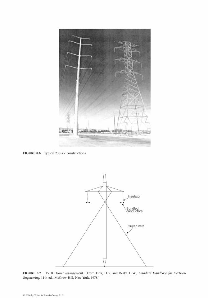
FIGURE 8.6 Typical 230-kV constructions.
Insulator
Bundledconductors
Guyed wire
FIGURE 8.7 HVDC tower arrangement. (From Fink, D.G. and Beaty, H.W., Standard Handbook for Electrical
Engineering, 11th ed., McGraw-Hill, New York, 1978.)
� 2006 by Taylor & Francis Group, LLC.
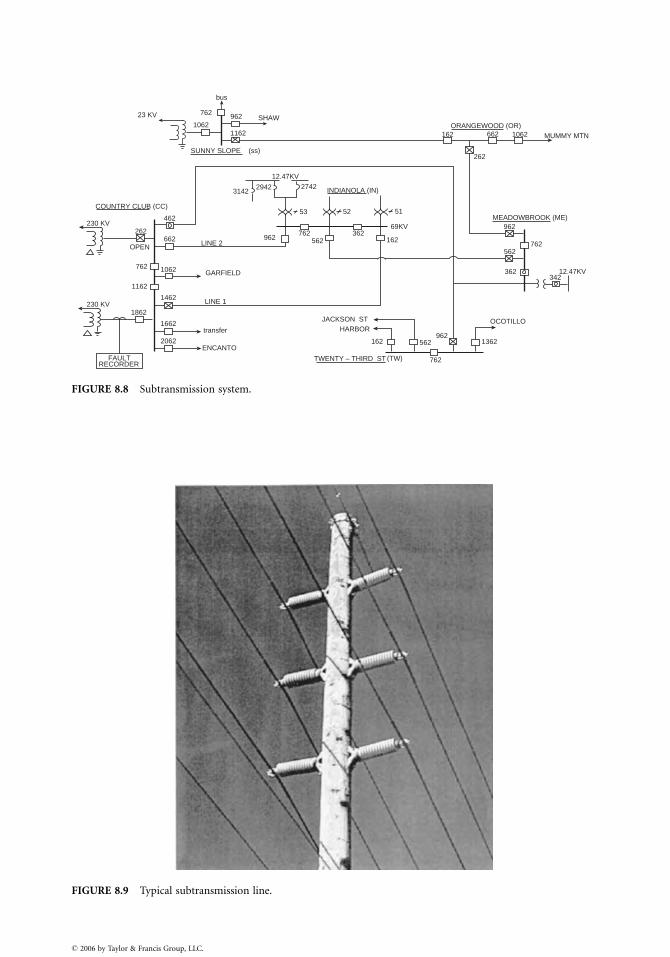
23 KV
bus
962
31422942 2742
762562962
462
262
762
1162
1862230 KV
230 KV
662
1062
1462
1662
2062
LINE 2OPEN
LINE 1
ENCANTOFAULT
GARFIELD
transfer
362162
69KV
INDIANOLA (IN)
ORANGEWOOD (OR)
12.47KV
1162
SHAW762
1062
SUNNY SLOPE (ss)
COUNTRY CLUB (CC)53 52 51
162 662
262
762
12.47KV342
962
562
362
1062 MUMMY MTN
MEADOWBROOK (ME)
OCOTILLO
1362562962
162
762
JACKSON STHARBOR
TWENTY – THIRD ST (TW)RECORDER
FIGURE 8.8 Subtransmission system.
FIGURE 8.9 Typical subtransmission line.
� 2006 by Taylor & Francis Group, LLC.
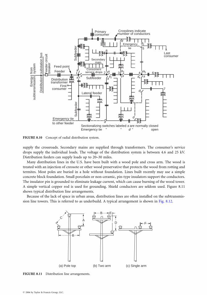
Primaryconsumer
Feed point
Distributiontransformer
Firstconsumer
Sectionalizing switches labeled s are normally closedEmergency tie " " d " " open
Emergency tieto other feeder
Subfeeder
Lateral feeder
Sub
feed
er
x
x
Sub
feed
er
Fee
der
circ
uit
brea
ker
subs
tatio
n bu
sD
istr
ibut
ion
Ene
rgy
subt
rans
mis
sion
from
syst
em
Feeder s
s2
85
d2
d1
d
dd
3 4 6
7
s s3 s5
s4ss ss2s
Crosslines indicatenumber of conductors
Lastconsumer
Emergencytie
Secondarymain
Consumersservice drops
FIGURE 8.10 Concept of radial distribution system.
supply the crossroads. Secondary mains are supplied through transformers. The consumer’s service
drops supply the individual loads. The voltage of the distribution system is between 4.6 and 25 kV.
Distribution feeders can supply loads up to 20–30 miles.
Many distribution lines in the U.S. have been built with a wood pole and cross arm. The wood is
treated with an injection of creosote or other wood preservative that protects the wood from rotting and
termites. Most poles are buried in a hole without foundation. Lines built recently may use a simple
concrete block foundation. Small porcelain or non-ceramic, pin-type insulators support the conductors.
The insulator pin is grounded to eliminate leakage current, which can cause burning of the wood tower.
A simple vertical copper rod is used for grounding. Shield conductors are seldom used. Figure 8.11
shows typical distribution line arrangements.
Because of the lack of space in urban areas, distribution lines are often installed on the subtransmis-
sion line towers. This is referred to as underbuild. A typical arrangement is shown in Fig. 8.12.
C
B
(a) Pole top (b) Two arm (c) Single arm
B E
D FA
FIGURE 8.11 Distribution line arrangements.
� 2006 by Taylor & Francis Group, LLC.
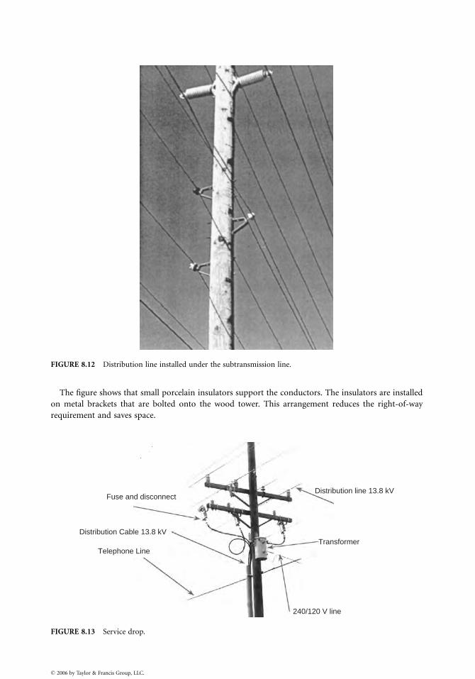
FIGURE 8.12 Distribution line installed under the subtransmission line.
The figure shows that small porcelain insulators support the conductors. The insulators are installed
on metal brackets that are bolted onto the wood tower. This arrangement reduces the right-of-way
requirement and saves space.
Fuse and disconnectDistribution line 13.8 kV
Transformer
240/120 V line
Distribution Cable 13.8 kV
Telephone Line
FIGURE 8.13 Service drop.
� 2006 by Taylor & Francis Group, LLC.

Transformers mounted on distribution poles frequently supply individual houses or groups of houses.
Figure 8.13 shows a typical transformer pole, consisting of a transformer that supplies a 240=120-V
service drop, and a 13.8-kV distribution cable. The latter supplies a nearby shopping center, located on
the other side of the road. The 13.8-kV cable is protected by a cut-off switch that contains a fuse
mounted on a pivoted insulator. The lineman can disconnect the cable by pulling the cut-off open with a
long insulated rod (hot stick).
References
1.
� 2
Electric Power Research Institute, Transmission Line Reference Book, 345 kV and Above, Electric Power
Research Institute, Palo Alto, CA, 1987.
2.
Fink, D.G. and Beaty, H.W., Standard Handbook for Electrical Engineering, 11th ed., McGraw-Hill,New York, Sec. 18, 1978.
3.
Gonen, T., Electric Power Distribution System Engineering, Wiley, New York, 1986.4.
Gonen, T., Electric Power Transmission System Engineering, Wiley, New York, 1986.006 by Taylor & Francis Group, LLC.
9
� 2006 by Taylor & Francis Group, LLC.
Transmission LineStructures
Joe C. PohlmanConsultant
9.1 Traditional Line Design Practice........................................ 9-1Structure Types in Use . Factors Affecting
Structure Type Selection
9.2 Current Deterministic Design Practice.............................. 9-5Reliability Level . Security Level
9.3 Improved Design Approaches ............................................ 9-9
Appendix A General Design Criteria—Methodology ............ 9-9
An overhead transmission line (OHTL) is a very complex, continuous, electrical=mechanical system. Its
function is to transport power safely from the circuit breaker on one end to the circuit breaker on the
other. It is physically composed of many individual components made up of different materials having a
wide variety of mechanical properties, such as:
. flexible vs. rigid
. ductile vs. brittle
. variant dispersions of strength
. wear and deterioration occurring at different rates when applied in different applications within
one micro-environment or in the same application within different micro-environments
This discussion will address the nature of the structures which are required to provide the clearances
between the current-carrying conductors, as well as their safe support above the earth. During this
discussion, reference will be made to the following definitions:
Capability: Capacity (�) availability
Reliability level: Ability of a line (or component) to perform its expected capability
Security level: Ability of a line to restrict progressive damage after the failure of the first component
Safety level: Ability of a line to perform its function safely
9.1 Traditional Line Design Practice
Present line design practice views the support structure as an isolated element supporting half span of
conductors and overhead ground wires (OHGWs) on either side of the structure. Based on the voltage
level of the line, the conductors and OHGWs are configured to provide, at least, the minimum
clearances mandated by the National Electrical Safety Code (NESC) (IEEE, 1990), as well as other
applicable codes. This configuration is designed to control the separation of:
. energized parts from other energized parts
. energized parts from the support structure of other objects located along the r-o-w
. energized parts above ground

The NESC divides the U.S. into three large global loading zones: heavy, medium, and light and
specifies radial ice thickness=wind pressure=temperature relationships to define the minimum load
levels that must be used within each loading zone. In addition, the Code introduces the concept of an
Overload Capacity Factor (OCF) to cover uncertainties stemming from the:
. likelihood of occurrence of the specified load
. dispersion of structure strength
. grade of construction
. deterioration of strength during service life
. structure function (suspension, dead-end, angle)
. other line support components (guys, foundations, etc.)
Present line design practice normally consists of the following steps:
1. The owning utility prepares an agenda of loading events consisting of:. mandatory regulations from the NESC and other codes. climatic events believed to be representative of the line’s specific location. contingency loading events of interest; i.e., broken conductor. special requirements and expectations
Each of these loading events is multiplied by its own OCF to cover uncertainties associated with it to
produce an agenda of final ultimate design loads (see Fig. 9.1).
2. A ruling span is identified based on the sag=tension requirements for the preselected conductor.
3. A structure type is selected based on past experience or on recommendations of potential structure
suppliers.
4. Ultimate design loads resulting from the ruling span are applied statically as components in the
longitudinal, transverse, and vertical directions, and the structure deterministically designed.
5. Using the loads and structure configuration, ground line reactions are calculated and used to
accomplish the foundation design.
6. The ruling span line configuration is adjusted to fit the actual r-o-w profile.
7. Structure=foundation designs are modified to account for variation in actual span lengths,
changes in elevation, and running angles.
8. Since most utilities expect the tangent structure to be the weakest link in the line system, hardware,
insulators, and other accessory components are selected to be stronger than the structure.
Inasmuch as structure types are available in a wide variety of concepts, materials, and costs, several
iterations would normally be attempted in search of the most cost effective line design based on total
installed costs (see Fig. 9.2).
Event A � OCFa
Event B � OCFb
Event C � OCFc
NESC � OCF (from Code)
LOAD0 LoadingEvent
DesignLoad
FIGURE 9.1 Development of a loading agenda.
� 2006 by Taylor & Francis Group, LLC.
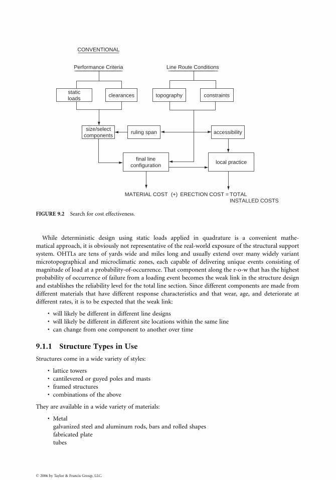
MATERIAL COST (+) ERECTION COST = TOTALINSTALLED COSTS
final lineconfiguration
CONVENTIONAL
Performance Criteria Line Route Conditions
staticloads
clearances topography constraints
accessibilityruling spansize/select
components
local practice
FIGURE 9.2 Search for cost effectiveness.
While deterministic design using static loads applied in quadrature is a convenient mathe-
matical approach, it is obviously not representative of the real-world exposure of the structural support
system. OHTLs are tens of yards wide and miles long and usually extend over many widely variant
microtopographical and microclimatic zones, each capable of delivering unique events consisting of
magnitude of load at a probability-of-occurrence. That component along the r-o-w that has the highest
probability of occurrence of failure from a loading event becomes the weak link in the structure design
and establishes the reliability level for the total line section. Since different components are made from
different materials that have different response characteristics and that wear, age, and deteriorate at
different rates, it is to be expected that the weak link:
. will likely be different in different line designs
. will likely be different in different site locations within the same line
. can change from one component to another over time
9.1.1 Structure Types in Use
Structures come in a wide variety of styles:
. lattice towers
. cantilevered or guyed poles and masts
. framed structures
. combinations of the above
They are available in a wide variety of materials:
. Metal
� 2006 by
galvanized steel and aluminum rods, bars and rolled shapes
fabricated plate
tubes
Taylor & Francis Group, LLC.
. Concrete
� 2006 by
spun with pretensioned or post-tensioned reinforcing cable
statically cast nontensioned reinforcing steel
single or multiple piece
. Woodas grown
glued laminar
. Plastics. Composites. Crossarms and braces. Variations of all of the aboveDepending on their style and material contents, structures vary considerably in how they respond to
load. Some are rigid. Some are flexible. Those structures that can safely deflect under load and absorb
energy while doing so, provide an ameliorating influence on progressive damage after the failure of the
first element (Pohlman and Lummis, 1969).
9.1.2 Factors Affecting Structure Type Selection
There are usually many factors that impact on the selection of the structure type for use in an OHTL.
Some of the more significant are briefly identified below.
Erection Technique: It is obvious that different structure types require different erection techniques. As an
example, steel lattice towers consist of hundreds of individual members that must be bolted together,
assembled, and erected onto the four previously installed foundations. A tapered steel pole, on the other
hand, is likely to be produced in a single piece and erected directly on its previously installed foundation in
one hoist. The lattice tower requires a large amount of labor to accomplish the considerable number of
bolted joints, whereas the pole requires the installation of a few nuts applied to the foundation anchor bolts
plus a few to install the crossarms. The steel pole requires a large-capacity crane with a high reach which
would probably not be needed for the tower. Therefore, labor needs to be balanced against the need for large,
special equipment and the site’s accessibility for such equipment.
Public Concerns: Probably the most difficult factors to deal with arise as a result of the concerns of the
general public living, working, or coming in proximity to the line. It is common practice to hold public
hearings as part of the approval process for a new line. Such public hearings offer a platform for
neighbors to express individual concerns that generally must be satisfactorily addressed before the
required permit will be issued. A few comments demonstrate this problem.
The general public usually perceives transmission structures as ‘‘eyesores’’ and distractions in the local
landscape. To combat this, an industry study was made in the late 1960s (Dreyfuss, 1968) sponsored by
the Edison Electric Institute and accomplished by Henry Dreyfuss, the internationally recognized
industrial designer. While the guidelines did not overcome all the objections, they did provide a
means of satisfying certain very highly controversial installations (Pohlman and Harris, 1971).
Parents of small children and safety engineers often raise the issue of lattice masts, towers, and guys,
constituting an ‘‘attractive challenge’’ to determined climbers, particularly youngsters.
Inspection, Assessment, and Maintenance: Depending on the owning utility, it is likely their in-house
practices will influence the selection of the structure type for use in a specific line location. Inspections and
assessment are usually made by human inspectors who use diagnostic technologies to augment their
personal senses of sight and touch. The nature and location of the symptoms of critical interest are such
that they can be most effectively examined from specific perspectives. Inspectors must work from the most
advantageous location when making inspections. Methods can include observations from ground or fly-by
patrol, climbing, bucket trucks, or helicopters. Likewise, there are certain maintenance activities that are
known or believed to be required for particular structure types. The equipment necessary to maintain the
structure should be taken into consideration during the structure type selection process to assure there will
be no unexpected conflict between maintenance needs and r-o-w restrictions.
Taylor & Francis Group, LLC.

Future Upgrading or Uprating : Because of the difficulty of procuring r-o-w’s and obtaining the
necessary permits to build new lines, many utilities improve their future options by selecting structure
types for current line projects that will permit future upgrading and=or uprating initiatives.
9.2 Current Deterministic Design Practice
Figure 9.3 shows a loading agenda for a double-circuit, 345-kV line built in the upper Midwest region of
the U.S. on steel lattice towers. Over and above the requirements of the NESC, the utility had specified
these loading events:
. a heavy wind condition (Pohlman and Harris, 1971)
. a wind on bare tower (Carton and Peyrot, 1992)
. two maximum vertical loads on the OHGWand conductor supports (Osterdorp, 1998; CIGRE, 1995)
. two broken wire contingencies (Pohlman and Lummis, 1969; Dreyfuss, 1968)
It was expected that this combination of loading events would result in a structural support design with
the capability of sustaining 50-year recurrence loads likely to occur in the general area where the line was
TANGENT AND LIGHT ANGLE SUSPENSION TOWER – 345 DOUBLE CIRCUIT
OHGW:Conductors:Weight span:Wind span:Line angle:
Two 7/16'' diameter galvanized steel strandSix twin conductor bundles of 1431 KCM 45/7 ACSR1,650 feet1,100 feet08 to 28
OCF
2.54 1.65 1.27
1.01.0 1.0
1.0 1.0 1.0
1.0 1.0 1.0
1.0 1.0 1.0
1.0
1.0
T LV
TLV
TLV
TLV
TLV
V
V
5.1
13.0
13.0
42.0
46.2
0
0
4
8
8
16
0
0
0
1/2
1/2
1/2
0
0
0
0
1
2
3
4
5
6
7
NESC Heavy
One broken OHGWcombined with windand ice
One broken conductorbundle combined withwind and ice
Heavy wind
Wind on bare tower(no conductors or OHGW)
Vertical load at anyOHGW support of 3780 lbs.(not simultaneously)
Vertical load at anyconductor support of17,790 lbs.(not simultaneously)
LoadDirection
RadialIce ('')Load Event
LoadCase
WindPressureStructure(psf)
WindPressureWire(psf)
FIGURE 9.3 Example of loading agenda.
� 2006 by Taylor & Francis Group, LLC.
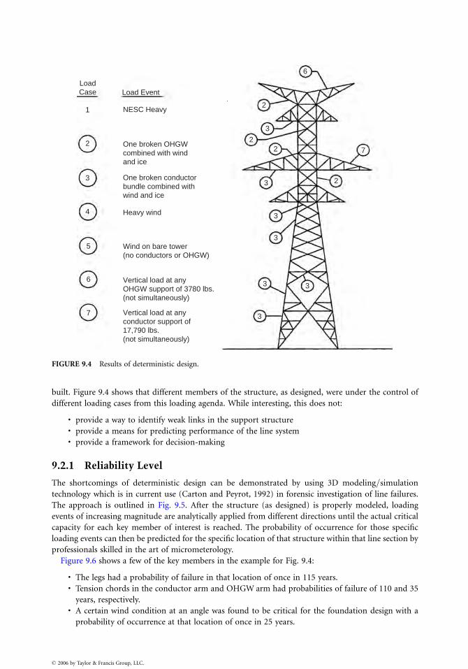
LoadCase
1
6
7
2
3
3
3
3
3 3
3
22
2
2
3
4
5
6
7
Load Event
NESC Heavy
One broken OHGWcombined with windand ice
One broken conductorbundle combined withwind and ice
Heavy wind
Wind on bare tower(no conductors or OHGW)
Vertical load at anyconductor support of17,790 lbs.(not simultaneously)
Vertical load at anyOHGW support of 3780 lbs.(not simultaneously)
FIGURE 9.4 Results of deterministic design.
built. Figure 9.4 shows that different members of the structure, as designed, were under the control of
different loading cases from this loading agenda. While interesting, this does not:
. provide a way to identify weak links in the support structure
. provide a means for predicting performance of the line system
. provide a framework for decision-making
9.2.1 Reliability Level
The shortcomings of deterministic design can be demonstrated by using 3D modeling=simulation
technology which is in current use (Carton and Peyrot, 1992) in forensic investigation of line failures.
The approach is outlined in Fig. 9.5. After the structure (as designed) is properly modeled, loading
events of increasing magnitude are analytically applied from different directions until the actual critical
capacity for each key member of interest is reached. The probability of occurrence for those specific
loading events can then be predicted for the specific location of that structure within that line section by
professionals skilled in the art of micrometerology.
Figure 9.6 shows a few of the key members in the example for Fig. 9.4:
. The legs had a probability of failure in that location of once in 115 years.
. Tension chords in the conductor arm and OHGW arm had probabilities of failure of 110 and 35
years, respectively.. A certain wind condition at an angle was found to be critical for the foundation design with a
probability of occurrence at that location of once in 25 years.
� 2006 by Taylor & Francis Group, LLC.
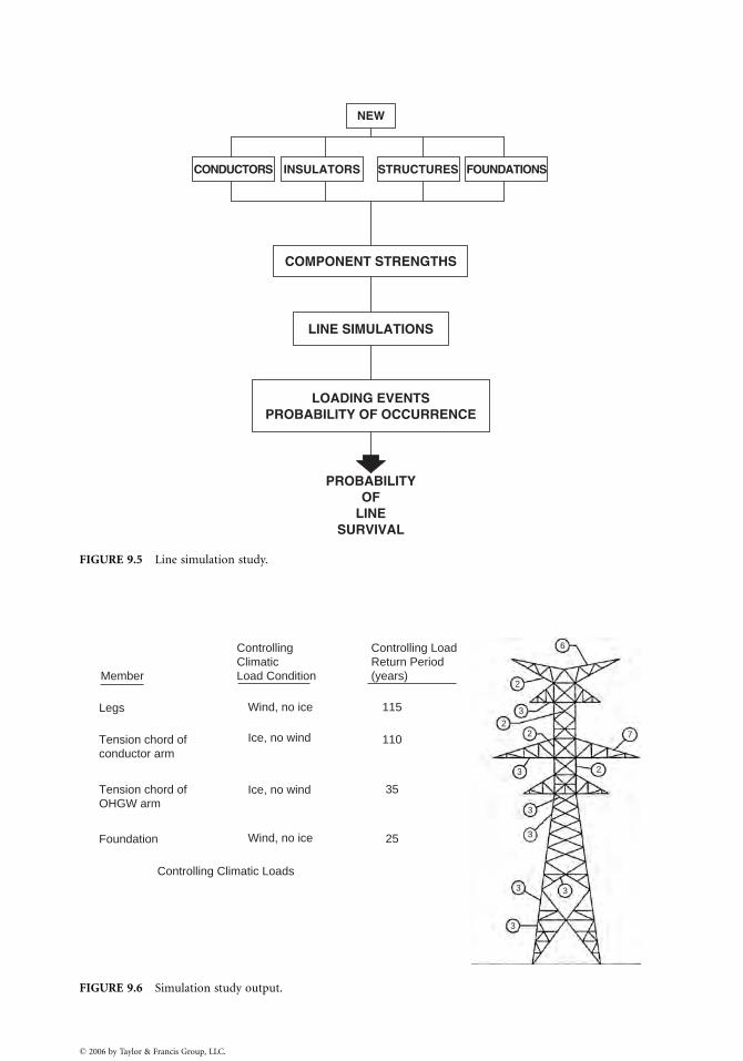
NEW
CONDUCTORS INSULATORS STRUCTURES FOUNDATIONS
COMPONENT STRENGTHS
LINE SIMULATIONS
LOADING EVENTSPROBABILITY OF OCCURRENCE
PROBABILITYOF
LINESURVIVAL
FIGURE 9.5 Line simulation study.
Member
Legs
Tension chord ofconductor arm
Tension chord ofOHGW arm
Foundation
Wind, no ice 115
110
35
25
6
2
22
2
3
3
3
3
3 3
3
7
Wind, no ice
Controlling Climatic Loads
Ice, no wind
Ice, no wind
ControllingClimaticLoad Condition
Controlling LoadReturn Period(years)
FIGURE 9.6 Simulation study output.
� 2006 by Taylor & Francis Group, LLC.
Some interesting observations can be drawn:
. The legs were conservatively designed.
. The loss of an OHGW is a more likely event than the loss of a conductor.
. The foundation was found to be the weak link.
In addition to the interesting observations on relative reliability levels of different components within
the structural support system, the output of the simulation study also provides the basis for a decision-
making process which can be used to determine the cost effectiveness of management initiatives. Under
the simple laws of statistics, when there are two independent outcomes to an event, the probability of the
first outcome is equal to one minus the probability of the second. When these outcomes are survival and
failure:
Annual probability of survival ¼ 1� Annual probability of failure
Ps ¼ 1� Pf(9:1)
If it is desired to know what the probability of survival is over an extended length of time, i.e., n years
of service life:
Ps1� Ps2� Ps3� . . . Psn½ � ¼ psð Þn (9:2)
Applying this principle to the components in the deterministic structure design and considering a
50-year service life as expected by the designers:
. the legs had a Ps of 65%
. the tension chord in the conductor arm had a Ps of 63%
. the tension chord of the OHGW arm had a Ps of 23%
. the foundation had a Ps of 13%
9.2.2 Security Level
It should be remembered, however, that the failure of every component does not necessarily progress
into extensive damage. A comparison of the total risk that would result from the initial failure of
components of interest can be accomplished by making a security-level check of the line design
(Osterdorp, 1998).
Since the OHTL is a contiguous mechanical system, the forces from the conductors and OHGWs on
one side of each tangent structure are balanced and restrained by those on the other side. When a critical
component in the conductor=OHGW system fails, energy stored within the conductor system is released
suddenly and sets up unbalanced transients that can cause failure of critical components at the next
structure. This can set off a cascading effect that will continue to travel downline until it encounters a
point in the line strong enough to withstand the unbalance. Unfortunately, a security check of the total
line cannot be accomplished from the information describing the one structure in Fig. 9.4; but perhaps
some generalized observations can be drawn for demonstration purposes.
Since the structure was designed for broken conductor bundle and broken OHGW contingencies, it
appears the line would not be subjected to a cascade from a broken bare conductor, but what if
the conductor was coated with ice at the time? Since ice increases the energy trapped within the
conductor prior to release, it might be of interest to determine how much ice would be ‘‘enough.’’
Three-dimensional modeling would be employed to simulate ice coating of increasing thicknesses until
the critical amount is defined. A proper micrometerological study could then identify the probability of
occurrence of a storm system capable of delivering that amount of ice at that specific location.
In the example, a wind condition with no ice was identified that would be capable of
causing foundation failure once every 25 years. A security-level check would predict the amount
� 2006 by Taylor & Francis Group, LLC.
of resulting losses and damages that would be expected from this initiating event compared to the
broken-conductor-under-ice-load contingencies.
9.3 Improved Design Approaches
The above discussion indicates that technologies are available today for assessing the true capability of an
OHTL that was created using the conventional practice of specifying ultimate static loads and designing
a structure that would properly support them. Because there are many different structure types made
from different materials, this was not always straightforward. Accordingly, many technical societies
prepared guidelines on how to design the specific structure needed. These are listed in the accompanying
references. The interested reader should realize that these documents are subject to periodic review and
revision and should, therefore, seek the most current version.
While the technical fraternity recognizes that the mentioned technologies are useful for analyzing
existing lines and determining management initiatives, something more direct for designing new lines
is needed. There are many efforts under way. The most promising of these is Improved Design Criteria
of OHTLs Based on Reliability Concepts (Ostendorp, 1998), currently under development by CIGRE
Study Committee 22: Recommendations for Overhead Lines. Appendix A outlines the methodology
involved in words and in a diagram. The technique is based on the premise that loads and strengths are
stochastic variables and the combined reliability is computable if the statistical functions of loads and
strength are known. The referenced report has been circulated internationally for trial use and comment.
It is expected that the returned comments will be carefully considered, integrated into the report, and the
final version submitted to the International Electrotechnical Commission (IEC) for consideration as an
International Standard.
References
1.
� 200
Carton, T. and Peyrot, A., Computer Aided Structural and Geometric Design of Power Lines, IEEE
Trans. on Power Line Syst., 7(1), 1992.
2.
Dreyfuss, H., Electric Transmission Structures, Edison Electric Institute Publication No. 67–61, 1968.3.
Guide for the Design and Use of Concrete Poles, ASCE 596–6, 1987.4.
Guide for the Design of Prestressed Concrete Poles, ASCE=PCI Joint Commission on ConcretePoles, February, 1992. Draft.
5.
Guide for the Design of Transmission Towers, ASCE Manual on Engineering Practice, 52, 1988.6.
Guide for the Design Steel Transmission Poles, ASCE Manual on Engineering Practice, 72, 1990.7.
IEEE Trial-Use Design Guide for Wood Transmission Structures, IEEE Std. 751, February, 1991.8.
Improved Design Criteria of Overhead Transmission Lines Based on Reliability Concepts, CIGRE SC-22Report, October 1995.
9.
National Electrical Safety Code ANSI C-2, IEEE, 1990.10.
Ostendorp, M., Longitudinal Loading and Cascading Failure Assessment for Transmission LineUpgrades, ESMO Conference ’98, Orlando, Florida, April 26–30, 1998.
11.
Pohlman, J. and Harris, W., Tapered Steel H-Frames Gain Acceptance Through Scenic Valley, ElectricLight and Power Magazine, 48(vii), 55–58, 1971.
12.
Pohlman, J. and Lummis, J., Flexible Structures Offer Broken Wire Integrity at Low Cost, ElectricLight and Power, 46(V, 144–148.4), 1969.
Appendix A General Design Criteria—Methodology
The recommended methodology for designing transmission line components is summarized in Fig. 9.7
and can be described as follows:
6 by Taylor & Francis Group, LLC.
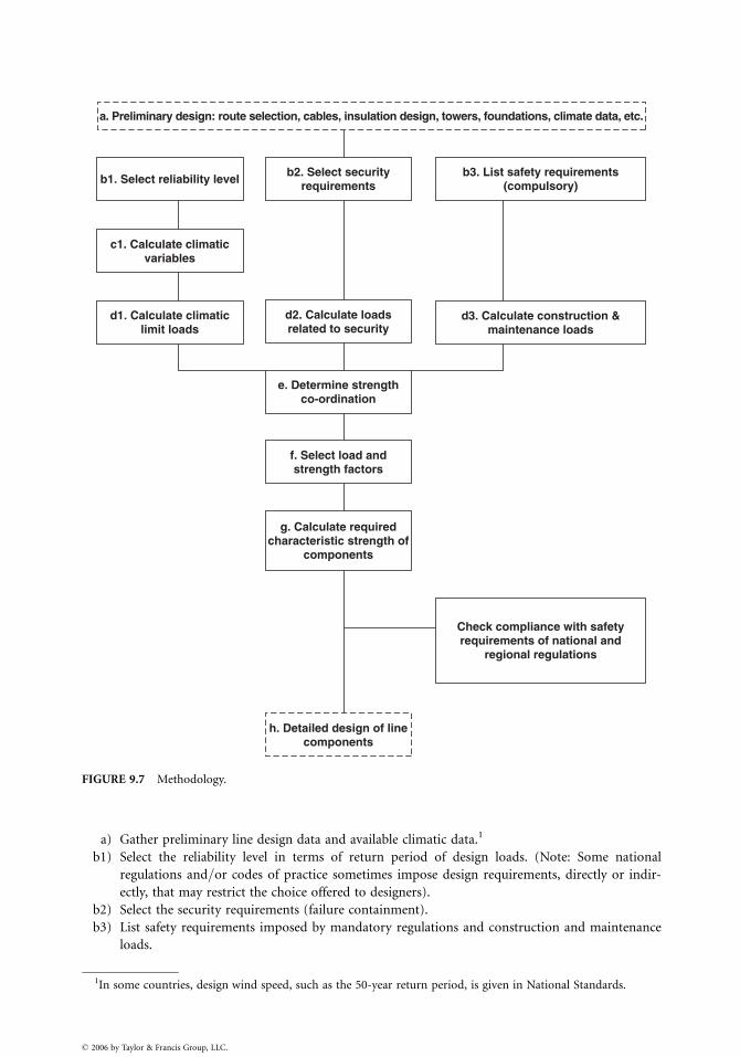
d1. Calculate climaticlimit loads
d2. Calculate loadsrelated to security
e. Determine strengthco-ordination
f. Select load andstrength factors
g. Calculate requiredcharacteristic strength of
components
h. Detailed design of linecomponents
Check compliance with safetyrequirements of national and
regional regulations
b1. Select reliability level
c1. Calculate climaticvariables
b2. Select securityrequirements
b3. List safety requirements(compulsory)
d3. Calculate construction &maintenance loads
a. Preliminary design: route selection, cables, insulation design, towers, foundations, climate data, etc.
FIGURE 9.7 Methodology.
a) Gather preliminary line design data and available climatic data.1
b1) Select the reliability level in terms of return period of design loads. (Note: Some national
regulations and=or codes of practice sometimes impose design requirements, directly or indir-
ectly, that may restrict the choice offered to designers).
b2) Select the security requirements (failure containment).
b3) List safety requirements imposed by mandatory regulations and construction and maintenance
loads.
1In some countries, design wind speed, such as the 50-year return period, is given in National Standards.
� 2006 by Taylor & Francis Group, LLC.

c) Calculate climatic variables corresponding to selected return period of design loads.
d1) Calculate climatic limit loadings on components.
d2) Calculate loads corresponding to security requirements.
d3) Calculate loads related to safety requirements during construction and maintenance.
e) Determine the suitable strength coordination between line components.
f) Select appropriate load and strength factors applicable to load and strength equations.
g) Calculate the characteristic strengths required for components.
h) Design line components for the above strength requirements.
This document deals with items b) to g). Items a) and h) are not part of the scope of this document.
They are identified by a dotted frame in Fig. 9.7.
Source : Improved design criteria of overhead transmission lines based on reliability concepts, CIGRE
SC22 Report, October, 1995.
� 2006 by Taylor & Francis Group, LLC.

� 2006 by Taylor & Francis Group, LLC.
10
� 2006 by Taylor & Francis Group, LLC.
Insulators andAccessories
George G. KaradyArizona State University
Richard G. FarmerArizona State University
10.1 Electrical Stresses on External Insulation...................... 10-1Transmission Lines and Substations . Electrical Stresses .
Environmental Stresses . Mechanical Stresses
10.2 Ceramic (Porcelain and Glass) Insulators..................... 10-7Materials . Insulator Strings . Post-Type Insulators .
Long Rod Insulators
10.3 Nonceramic (Composite) Insulators ............................. 10-9Composite Suspension Insulators . Composite Post Insulators
10.4 Insulator Failure Mechanism ....................................... 10-13Porcelain Insulators . Insulator Pollution . Effects of
Pollution . Composite Insulators . Aging of Composite
Insulators
10.5 Methods for Improving Insulator Performance ......... 10-18
Electric insulation is a vital part of an electrical power system. Although the cost of insulation is only a
small fraction of the apparatus or line cost, line performance is highly dependent on insulation integrity.
Insulation failure may cause permanent equipment damage and long-term outages. As an example, a
short circuit in a 500-kV system may result in a loss of power to a large area for several hours. The
potential financial losses emphasize the importance of a reliable design of the insulation.
The insulation of an electric system is divided into two broad categories:
1. Internal insulation
2. External insulation
Apparatus or equipment has mostly internal insulation. The insulation is enclosed in a grounded
housing which protects it from the environment. External insulation is exposed to the environment. A
typical example of internal insulation is the insulation for a large transformer where insulation between
turns and between coils consists of solid (paper) and liquid (oil) insulation protected by a steel tank. An
overvoltage can produce internal insulation breakdown and a permanent fault.
External insulation is exposed to the environment. Typical external insulation is the porcelain
insulators supporting transmission line conductors. An overvoltage caused by flashover produces only
a temporary fault. The insulation is self-restoring.
This section discusses external insulation used for transmission lines and substations.
10.1 Electrical Stresses on External Insulation
The external insulation (transmission line or substation) is exposed to electrical, mechanical, and
environmental stresses. The applied voltage of an operating power system produces electrical stresses.
The weather and the surroundings (industry, rural dust, oceans, etc.) produce additional environmental
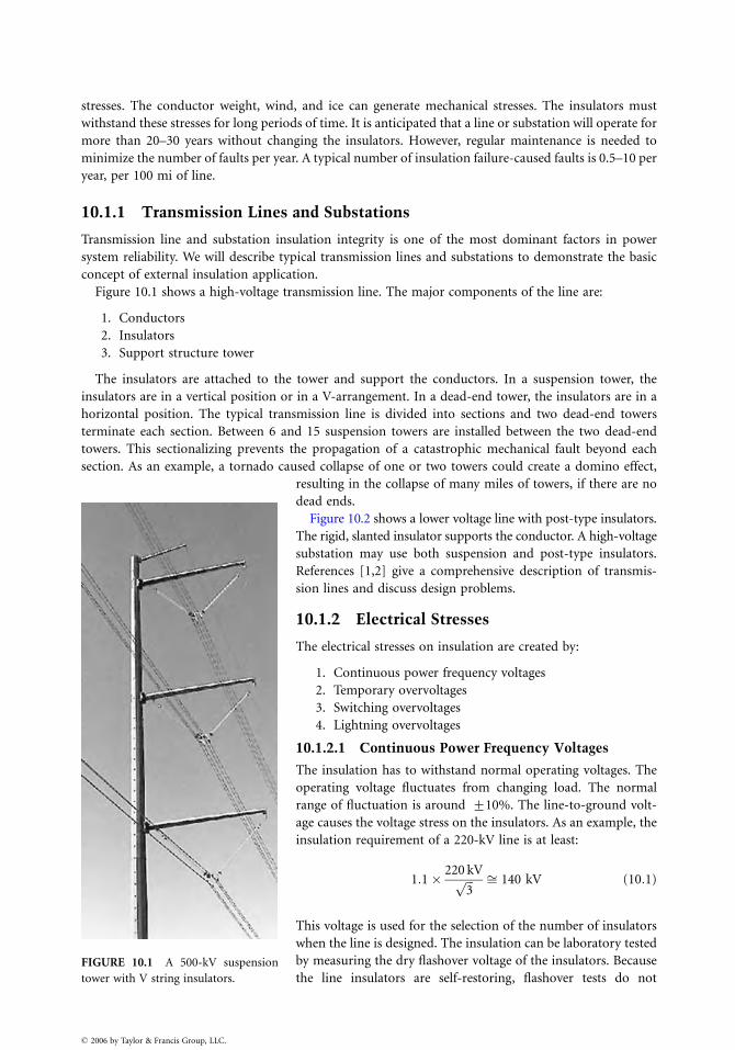
stresses. The conductor weight, wind, and ice can generate mechanical stresses. The insulators must
withstand these stresses for long periods of time. It is anticipated that a line or substation will operate for
more than 20–30 years without changing the insulators. However, regular maintenance is needed to
minimize the number of faults per year. A typical number of insulation failure-caused faults is 0.5–10 per
year, per 100 mi of line.
10.1.1 Transmission Lines and Substations
Transmission line and substation insulation integrity is one of the most dominant factors in power
system reliability. We will describe typical transmission lines and substations to demonstrate the basic
concept of external insulation application.
Figure 10.1 shows a high-voltage transmission line. The major components of the line are:
1. Conductors
2. Insulators
3. Support structure tower
The insulators are attached to the tower and support the conductors. In a suspension tower, the
insulators are in a vertical position or in a V-arrangement. In a dead-end tower, the insulators are in a
horizontal position. The typical transmission line is divided into sections and two dead-end towers
terminate each section. Between 6 and 15 suspension towers are installed between the two dead-end
towers. This sectionalizing prevents the propagation of a catastrophic mechanical fault beyond each
section. As an example, a tornado caused collapse of one or two towers could create a domino effect,
FIGURE 10.1 A 500-kV suspension
tower with V string insulators.
� 2006 by Taylor & Francis Group, LLC.
resulting in the collapse of many miles of towers, if there are no
dead ends.
Figure 10.2 shows a lower voltage line with post-type insulators.
The rigid, slanted insulator supports the conductor. A high-voltage
substation may use both suspension and post-type insulators.
References [1,2] give a comprehensive description of transmis-
sion lines and discuss design problems.
10.1.2 Electrical Stresses
The electrical stresses on insulation are created by:
1. Continuous power frequency voltages
2. Temporary overvoltages
3. Switching overvoltages
4. Lightning overvoltages
10.1.2.1 Continuous Power Frequency Voltages
The insulation has to withstand normal operating voltages. The
operating voltage fluctuates from changing load. The normal
range of fluctuation is around +10%. The line-to-ground volt-
age causes the voltage stress on the insulators. As an example, the
insulation requirement of a 220-kV line is at least:
1:1� 220 kVffiffiffi
3p ffi 140 kV (10:1)
This voltage is used for the selection of the number of insulators
when the line is designed. The insulation can be laboratory tested
by measuring the dry flashover voltage of the insulators. Because
the line insulators are self-restoring, flashover tests do not
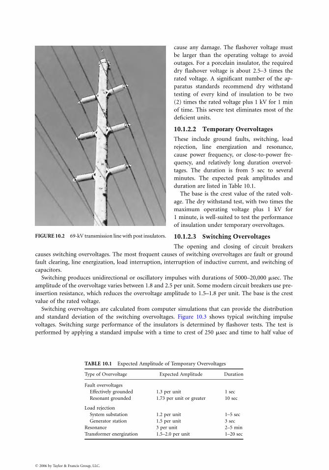
FIGURE 10.2 69-kV transmission line with post insulators.
TABLE 10.1 Expected Amplitude of T
Type of Overvoltage Expec
Fault overvoltages
Effectively grounded 1.3 per
Resonant grounded 1.73 per
Load rejection
System substation 1.2 per
Generator station 1.5 per
Resonance 3 per un
Transformer energization 1.5–2.0
� 2006 by Taylor & Francis Group, LLC.
cause any damage. The flashover voltage must
be larger than the operating voltage to avoid
outages. For a porcelain insulator, the required
dry flashover voltage is about 2.5–3 times the
rated voltage. A significant number of the ap-
paratus standards recommend dry withstand
testing of every kind of insulation to be two
(2) times the rated voltage plus 1 kV for 1 min
of time. This severe test eliminates most of the
deficient units.
10.1.2.2 Temporary Overvoltages
These include ground faults, switching, load
rejection, line energization and resonance,
cause power frequency, or close-to-power fre-
quency, and relatively long duration overvol-
tages. The duration is from 5 sec to several
minutes. The expected peak amplitudes and
duration are listed in Table 10.1.
The base is the crest value of the rated volt-
age. The dry withstand test, with two times the
maximum operating voltage plus 1 kV for
1 minute, is well-suited to test the performance
of insulation under temporary overvoltages.
10.1.2.3 Switching Overvoltages
The opening and closing of circuit breakers
causes switching overvoltages. The most frequent causes of switching overvoltages are fault or ground
fault clearing, line energization, load interruption, interruption of inductive current, and switching of
capacitors.
Switching produces unidirectional or oscillatory impulses with durations of 5000–20,000 msec. The
amplitude of the overvoltage varies between 1.8 and 2.5 per unit. Some modern circuit breakers use pre-
insertion resistance, which reduces the overvoltage amplitude to 1.5–1.8 per unit. The base is the crest
value of the rated voltage.
Switching overvoltages are calculated from computer simulations that can provide the distribution
and standard deviation of the switching overvoltages. Figure 10.3 shows typical switching impulse
voltages. Switching surge performance of the insulators is determined by flashover tests. The test is
performed by applying a standard impulse with a time to crest of 250 msec and time to half value of
emporary Overvoltages
ted Amplitude Duration
unit 1 sec
unit or greater 10 sec
unit 1–5 sec
unit 3 sec
it 2–5 min
per unit 1–20 sec
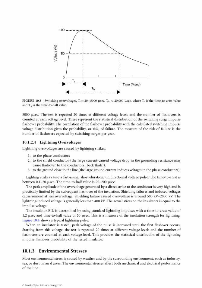
50
0Tr
Th
Time (Msec)
100
Vol
tage
(%
)
FIGURE 10.3 Switching overvoltages. Tr¼ 20�5000 msec, Th < 20,000 msec, where Tr is the time-to-crest value
and Th is the time-to-half value.
5000 msec. The test is repeated 20 times at different voltage levels and the number of flashovers is
counted at each voltage level. These represent the statistical distribution of the switching surge impulse
flashover probability. The correlation of the flashover probability with the calculated switching impulse
voltage distribution gives the probability, or risk, of failure. The measure of the risk of failure is the
number of flashovers expected by switching surges per year.
10.1.2.4 Lightning Overvoltages
Lightning overvoltages are caused by lightning strikes:
1. to the phase conductors
2. to the shield conductor (the large current-caused voltage drop in the grounding resistance may
cause flashover to the conductors [back flash]).
3. to the ground close to the line (the large ground current induces voltages in the phase conductors).
Lighting strikes cause a fast-rising, short-duration, unidirectional voltage pulse. The time-to-crest is
between 0.1–20 msec. The time-to-half value is 20–200 msec.
The peak amplitude of the overvoltage generated by a direct strike to the conductor is very high and is
practically limited by the subsequent flashover of the insulation. Shielding failures and induced voltages
cause somewhat less overvoltage. Shielding failure caused overvoltage is around 500 kV–2000 kV. The
lightning-induced voltage is generally less than 400 kV. The actual stress on the insulators is equal to the
impulse voltage.
The insulator BIL is determined by using standard lightning impulses with a time-to-crest value of
1.2 msec and time-to-half value of 50 msec. This is a measure of the insulation strength for lightning.
Figure 10.4 shows a typical lightning pulse.
When an insulator is tested, peak voltage of the pulse is increased until the first flashover occurs.
Starting from this voltage, the test is repeated 20 times at different voltage levels and the number of
flashovers are counted at each voltage level. This provides the statistical distribution of the lightning
impulse flashover probability of the tested insulator.
10.1.3 Environmental Stresses
Most environmental stress is caused by weather and by the surrounding environment, such as industry,
sea, or dust in rural areas. The environmental stresses affect both mechanical and electrical performance
of the line.
� 2006 by Taylor & Francis Group, LLC.
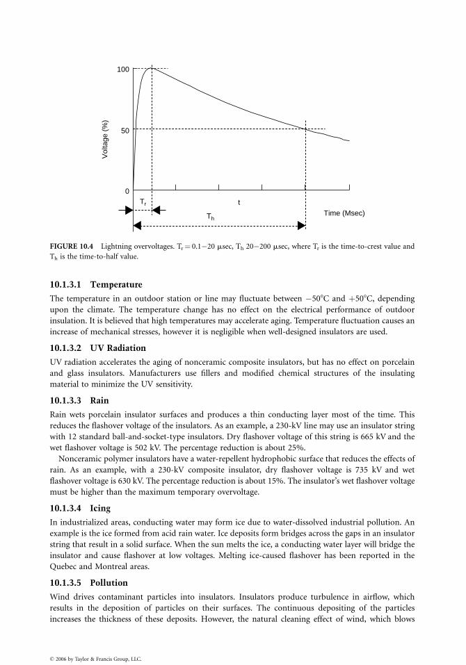
Time (Msec)
t
Th
Tr
0
50
Vol
tage
(%
)
100
FIGURE 10.4 Lightning overvoltages. Tr¼ 0.1�20 msec, Th 20�200 msec, where Tr is the time-to-crest value and
Th is the time-to-half value.
10.1.3.1 Temperature
The temperature in an outdoor station or line may fluctuate between �508C and þ508C, depending
upon the climate. The temperature change has no effect on the electrical performance of outdoor
insulation. It is believed that high temperatures may accelerate aging. Temperature fluctuation causes an
increase of mechanical stresses, however it is negligible when well-designed insulators are used.
10.1.3.2 UV Radiation
UV radiation accelerates the aging of nonceramic composite insulators, but has no effect on porcelain
and glass insulators. Manufacturers use fillers and modified chemical structures of the insulating
material to minimize the UV sensitivity.
10.1.3.3 Rain
Rain wets porcelain insulator surfaces and produces a thin conducting layer most of the time. This
reduces the flashover voltage of the insulators. As an example, a 230-kV line may use an insulator string
with 12 standard ball-and-socket-type insulators. Dry flashover voltage of this string is 665 kV and the
wet flashover voltage is 502 kV. The percentage reduction is about 25%.
Nonceramic polymer insulators have a water-repellent hydrophobic surface that reduces the effects of
rain. As an example, with a 230-kV composite insulator, dry flashover voltage is 735 kV and wet
flashover voltage is 630 kV. The percentage reduction is about 15%. The insulator’s wet flashover voltage
must be higher than the maximum temporary overvoltage.
10.1.3.4 Icing
In industrialized areas, conducting water may form ice due to water-dissolved industrial pollution. An
example is the ice formed from acid rain water. Ice deposits form bridges across the gaps in an insulator
string that result in a solid surface. When the sun melts the ice, a conducting water layer will bridge the
insulator and cause flashover at low voltages. Melting ice-caused flashover has been reported in the
Quebec and Montreal areas.
10.1.3.5 Pollution
Wind drives contaminant particles into insulators. Insulators produce turbulence in airflow, which
results in the deposition of particles on their surfaces. The continuous depositing of the particles
increases the thickness of these deposits. However, the natural cleaning effect of wind, which blows
� 2006 by Taylor & Francis Group, LLC.
TABLE 10.2 Site Severity (IEEE Definitions)
Description ESDD (mg=cm2)
Very light 0–0.03
Light 0.03–0.06
Moderate 0.06–0.1
Heavy <0.1
loose particles away, limits the growth of deposits. Occasionally, rain washes part of the pollution away.
The continuous depositing and cleaning produces a seasonal variation of the pollution on the insulator
surfaces. However, after a long time (months, years), the deposits are stabilized and a thin layer of solid
deposit will cover the insulator. Because of the cleaning effects of rain, deposits are lighter on the top of
the insulators and heavier on the bottom. The development of a continuous pollution layer is com-
pounded by chemical changes. As an example, in the vicinity of a cement factory, the interaction
between the cement and water produces a tough, very sticky layer. Around highways, the wear of car tires
produces a slick, tar-like carbon deposit on the insulator’s surface.
Moisture, fog, and dew wet the pollution layer, dissolve the salt, and produce a conducting layer,
which in turn reduces the flashover voltage. The pollution can reduce the flashover voltage of a standard
insulator string by about 20–25%.
Near the ocean, wind drives salt water onto insulator surfaces, forming a conducting salt-water layer
which reduces the flashover voltage. The sun dries the pollution during the day and forms a white salt
layer. This layer is washed off even by light rain and produces a wide fluctuation in pollution levels.
The Equivalent Salt Deposit Density (ESDD) describes the level of contamination in an area.
Equivalent Salt Deposit Density is measured by periodically washing down the pollution from selected
insulators using distilled water. The resistivity of the water is measured and the amount of salt that
produces the same resistivity is calculated. The obtained mg value of salt is divided by the surface area of
the insulator. This number is the ESDD. The pollution severity of a site is described by the average ESDD
value, which is determined by several measurements.
Table 10.2 shows the criteria for defining site severity.
The contamination level is light or very light in most parts of the U.S. and Canada. Only the seashores
and heavily industrialized regions experience heavy pollution. Typically, the pollution level is very high
in Florida and on the southern coast of California. Heavy industrial pollution occurs in the industri-
alized areas and near large highways. Table 10.3 gives a summary of the different sources of pollution.
The flashover voltage of polluted insulators has been measured in laboratories. The correlation
between the laboratory results and field experience is weak. The test results provide guidance, but
insulators are selected using practical experience.
TABLE 10.3 Typical Sources of Pollution
Pollution Type Source of Pollutant Deposit Characteristics Area
Rural areas Soil dust High resitivity layer, effective rain washing Large areas
Desert Sand Low resistivity Large areas
Coastal area Sea salt Very low resistivity, easily
washed by rain
10–20 km from the sea
Industrial Steel mill, coke plants,
chemical plants, generating
stations, quarries
High conductivity, extremely
difficult to remove, insoluble
Localized to the
plant area
Mixed Industry, highway, desert Very adhesive, medium resistivity Localized to the
plant area
� 2006 by Taylor & Francis Group, LLC.
10.1.3.6 Altitude
The insulator’s flashover voltage is reduced as altitude increases. Above 1500 feet, an increase in the
number of insulators should be considered. A practical rule is a 3% increase of clearance or insulator
strings’ length per 1000 ft as the elevation increases.
10.1.4 Mechanical Stresses
Suspension insulators need to carry the weight of the conductors and the weight of occasional ice and
wind loading.
In northern areas and in higher elevations, insulators and lines are frequently covered by ice in
the winter. The ice produces significant mechanical loads on the conductor and on the insulators. The
transmission line insulators need to support the conductor’s weight and the weight of the ice in
the adjacent spans. This may increase the mechanical load by 20–50%.
The wind produces a horizontal force on the line conductors. This horizontal force increases
the mechanical load on the line. The wind-force-produced load has to be added vectorially to the
weight-produced forces. The design load will be the larger of the combined wind and weight, or ice and
wind load.
The dead-end insulators must withstand the longitudinal load, which is higher than the simple weight
of the conductor in the half span.
A sudden drop in the ice load from the conductor produces large-amplitude mechanical oscillations,
which cause periodic oscillatory insulator loading (stress changes from tension to compression and back).
The insulator’s one-minute tension strength is measured and used for insulator selection. In addition,
each cap-and-pin or ball-and-socket insulator is loaded mechanically for one minute and simultan-
eously energized. This mechanical and electrical (M&E) value indicates the quality of insulators. The
maximum load should be around 50% of the M&E load.
The Bonneville Power Administration uses the following practical relation to determine the required
M&E rating of the insulators.
1. M&E > 5* Bare conductor weight=span
2. M&E > Bare conductor weight þWeight of 3.81 cm (1.5 in) of ice on the conductor (3 lb=sq ft)
3. M&E > 2* (Bare conductor weight þ Weight of 0.63 cm (1=4 in) of ice on the conductor and
loading from a wind of 1.8 kg=sq ft (4 lb=sq ft)
The required M&E value is calculated from all equations above and the largest value is used.
10.2 Ceramic (Porcelain and Glass) Insulators
10.2.1 Materials
Porcelain is the most frequently used material for insulators. Insulators are made of wet, processed
porcelain. The fundamental materials used are a mixture of feldspar (35%), china clay (28%), flint
(25%), ball clay (10%), and talc (2%). The ingredients are mixed with water. The resulting mixture has
the consistency of putty or paste and is pressed into a mold to form a shell of the desired shape. The
alternative method is formation by extrusion bars that are machined into the desired shape. The shells
are dried and dipped into a glaze material. After glazing, the shells are fired in a kiln at about 12008C.
The glaze improves the mechanical strength and provides a smooth, shiny surface. After a cooling-down
period, metal fittings are attached to the porcelain with Portland cement. Reference [3] presents the
history of porcelain insulators and discusses the manufacturing procedure.
Toughened glass is also frequently used for insulators [4]. The melted glass is poured into a mold to
form the shell. Dipping into hot and cold baths cools the shells. This thermal treatment shrinks the
surface of the glass and produces pressure on the body, which increases the mechanical strength of the
glass. Sudden mechanical stresses, such as a blow by a hammer or bullets, will break the glass into small
pieces. The metal end-fitting is attached by alumina cement.
� 2006 by Taylor & Francis Group, LLC.
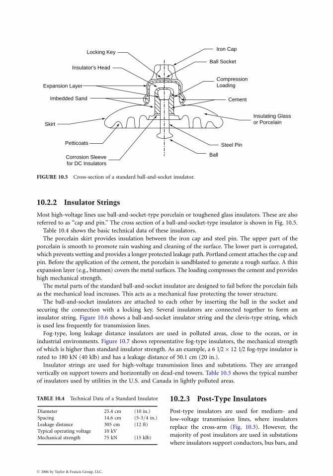
Ball
Steel Pin
Insulating Glassor Porcelain
Cement
CompressionLoading
Ball Socket
Iron CapLocking Key
Insulator's Head
Expansion Layer
Imbedded Sand
Skirt
Petticoats
Corrosion Sleevefor DC Insulators
FIGURE 10.5 Cross-section of a standard ball-and-socket insulator.
10.2.2 Insulator Strings
Most high-voltage lines use ball-and-socket-type porcelain or toughened glass insulators. These are also
referred to as ‘‘cap and pin.’’ The cross section of a ball-and-socket-type insulator is shown in Fig. 10.5.
Table 10.4 shows the basic technical data of these insulators.
The porcelain skirt provides insulation between the iron cap and steel pin. The upper part of the
porcelain is smooth to promote rain washing and cleaning of the surface. The lower part is corrugated,
which prevents wetting and provides a longer protected leakage path. Portland cement attaches the cup and
pin. Before the application of the cement, the porcelain is sandblasted to generate a rough surface. A thin
expansion layer (e.g., bitumen) covers the metal surfaces. The loading compresses the cement and provides
high mechanical strength.
The metal parts of the standard ball-and-socket insulator are designed to fail before the porcelain fails
as the mechanical load increases. This acts as a mechanical fuse protecting the tower structure.
The ball-and-socket insulators are attached to each other by inserting the ball in the socket and
securing the connection with a locking key. Several insulators are connected together to form an
insulator string. Figure 10.6 shows a ball-and-socket insulator string and the clevis-type string, which
is used less frequently for transmission lines.
Fog-type, long leakage distance insulators are used in polluted areas, close to the ocean, or in
industrial environments. Figure 10.7 shows representative fog-type insulators, the mechanical strength
of which is higher than standard insulator strength. As an example, a 6 1=2� 12 1=2 fog-type insulator is
rated to 180 kN (40 klb) and has a leakage distance of 50.1 cm (20 in.).
Insulator strings are used for high-voltage transmission lines and substations. They are arranged
vertically on support towers and horizontally on dead-end towers. Table 10.5 shows the typical number
of insulators used by utilities in the U.S. and Canada in lightly polluted areas.
TABLE 10.4 Technical Data of a Standard Insulator
Diameter 25.4 cm (10 in.)
Spacing 14.6 cm (5-3=4 in.)
Leakage distance 305 cm (12 ft)
Typical operating voltage 10 kV
Mechanical strength 75 kN (15 klb)
� 2006 by Taylor & Francis Group, LLC.
10.2.3 Post-Type Insulators
Post-type insulators are used for medium- and
low-voltage transmission lines, where insulators
replace the cross-arm (Fig. 10.3). However, the
majority of post insulators are used in substations
where insulators support conductors, bus bars, and
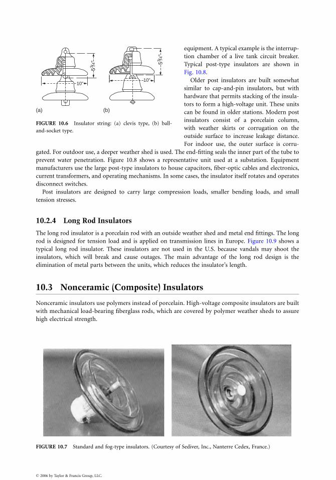
(a)
10"10"
53 /4" 53 /
4"
(b)
FIGURE 10.6 Insulator string: (a) clevis type, (b) ball-
and-socket type.
FIGURE 10.7 Standard and fog-type insulators. (Courtesy of S
� 2006 by Taylor & Francis Group, LLC.
equipment. A typical example is the interrup-
tion chamber of a live tank circuit breaker.
Typical post-type insulators are shown in
Fig. 10.8.
Older post insulators are built somewhat
similar to cap-and-pin insulators, but with
hardware that permits stacking of the insula-
tors to form a high-voltage unit. These units
can be found in older stations. Modern post
insulators consist of a porcelain column,
with weather skirts or corrugation on the
outside surface to increase leakage distance.
For indoor use, the outer surface is corru-
gated. For outdoor use, a deeper weather shed is used. The end-fitting seals the inner part of the tube to
prevent water penetration. Figure 10.8 shows a representative unit used at a substation. Equipment
manufacturers use the large post-type insulators to house capacitors, fiber-optic cables and electronics,
current transformers, and operating mechanisms. In some cases, the insulator itself rotates and operates
disconnect switches.
Post insulators are designed to carry large compression loads, smaller bending loads, and small
tension stresses.
10.2.4 Long Rod Insulators
The long rod insulator is a porcelain rod with an outside weather shed and metal end fittings. The long
rod is designed for tension load and is applied on transmission lines in Europe. Figure 10.9 shows a
typical long rod insulator. These insulators are not used in the U.S. because vandals may shoot the
insulators, which will break and cause outages. The main advantage of the long rod design is the
elimination of metal parts between the units, which reduces the insulator’s length.
10.3 Nonceramic (Composite) Insulators
Nonceramic insulators use polymers instead of porcelain. High-voltage composite insulators are built
with mechanical load-bearing fiberglass rods, which are covered by polymer weather sheds to assure
high electrical strength.
ediver, Inc., Nanterre Cedex, France.)
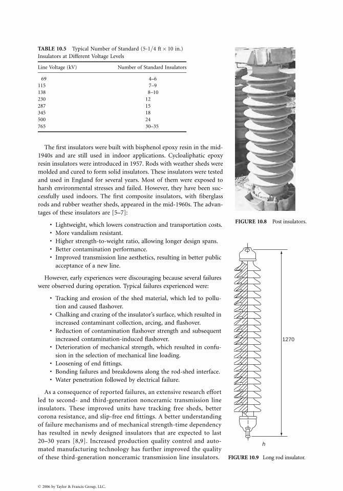
TABLE 10.5 Typical Number of Standard (5-1=4 ft� 10 in.)
Insulators at Different Voltage Levels
Line Voltage (kV) Number of Standard Insulators
69 4–6
115 7–9
138 8–10
230 12
287 15
345 18
500 24
765 30–35
� 2006 by Taylor & Francis Group, LLC.
FIGURE 10.8 Post insulators.
1270
h
FIGURE 10.9 Long rod insulator.
The first insulators were built with bisphenol epoxy resin in the mid-
1940s and are still used in indoor applications. Cycloaliphatic epoxy
resin insulators were introduced in 1957. Rods with weather sheds were
molded and cured to form solid insulators. These insulators were tested
and used in England for several years. Most of them were exposed to
harsh environmental stresses and failed. However, they have been suc-
cessfully used indoors. The first composite insulators, with fiberglass
rods and rubber weather sheds, appeared in the mid-1960s. The advan-
tages of these insulators are [5–7]:
. Lightweight, which lowers construction and transportation costs.
. More vandalism resistant.
. Higher strength-to-weight ratio, allowing longer design spans.
. Better contamination performance.
. Improved transmission line aesthetics, resulting in better public
acceptance of a new line.
However, early experiences were discouraging because several failures
were observed during operation. Typical failures experienced were:
. Tracking and erosion of the shed material, which led to pollu-
tion and caused flashover.. Chalking and crazing of the insulator’s surface, which resulted in
increased contaminant collection, arcing, and flashover.. Reduction of contamination flashover strength and subsequent
increased contamination-induced flashover.. Deterioration of mechanical strength, which resulted in confu-
sion in the selection of mechanical line loading.. Loosening of end fittings.. Bonding failures and breakdowns along the rod-shed interface.. Water penetration followed by electrical failure.
As a consequence of reported failures, an extensive research effort
led to second- and third-generation nonceramic transmission line
insulators. These improved units have tracking free sheds, better
corona resistance, and slip-free end fittings. A better understanding
of failure mechanisms and of mechanical strength-time dependency
has resulted in newly designed insulators that are expected to last
20–30 years [8,9]. Increased production quality control and auto-
mated manufacturing technology has further improved the quality
of these third-generation nonceramic transmission line insulators.
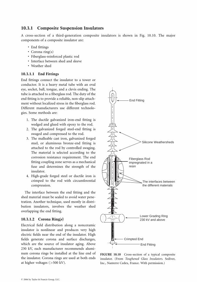
10.3.1 Composite Suspension Insulators
A cross-section of a third-generation composite insulators is shown in Fig. 10.10. The major
components of a composite insulator are:
. End fittings
. Corona ring(s)
. Fiberglass-reinforced plastic rod
. Interface between shed and sleeve
. Weather shed
10.3.1.1 End Fittings
End Fitting
Silicone Weathersheds
Fiberglass Rod impregnated in aresin
The interfaces betweenthe different materials
Lower Grading Ring230 kV and above
Crimpted End
End Fitting
FIGURE 10.10 Cross-section of a typical composite
insulator. (From Toughened Glass Insulators. Sediver,
Inc., Nanterre Cedex, France. With permission.)
End fittings connect the insulator to a tower or
conductor. It is a heavy metal tube with an oval
eye, socket, ball, tongue, and a clevis ending. The
tube is attached to a fiberglass rod. The duty of the
end fitting is to provide a reliable, non-slip attach-
ment without localized stress in the fiberglass rod.
Different manufacturers use different technolo-
gies. Some methods are:
1. The ductile galvanized iron-end fitting is
wedged and glued with epoxy to the rod.
2. The galvanized forged steel-end fitting is
swaged and compressed to the rod.
3. The malleable cast iron, galvanized forged
steel, or aluminous bronze-end fitting is
attached to the rod by controlled swaging.
The material is selected according to the
corrosion resistance requirement. The end
fitting coupling zone serves as a mechanical
fuse and determines the strength of the
insulator.
4. High-grade forged steel or ductile iron is
crimped to the rod with circumferential
compression.
The interface between the end fitting and the
shed material must be sealed to avoid water pene-
tration. Another technique, used mostly in distri-
bution insulators, involves the weather shed
overlapping the end fitting.
10.3.1.2 Corona Ring(s)
Electrical field distribution along a nonceramic
insulator is nonlinear and produces very high
electric fields near the end of the insulator. High
fields generate corona and surface discharges,
which are the source of insulator aging. Above
230 kV, each manufacturer recommends alumi-
num corona rings be installed at the line end of
the insulator. Corona rings are used at both ends
at higher voltages (>500 kV).
� 2006 by Taylor & Francis Group, LLC.
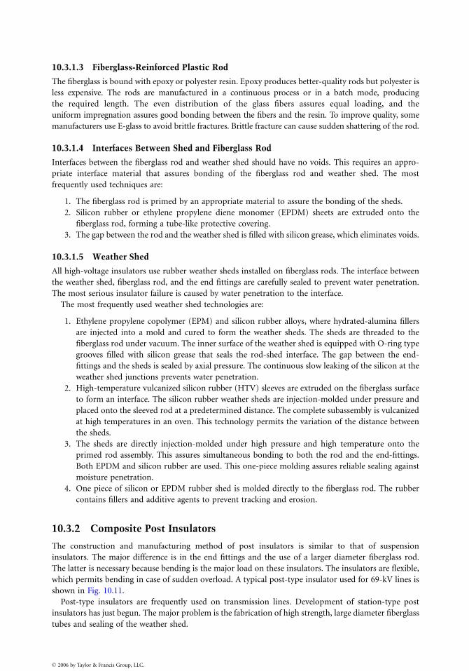
10.3.1.3 Fiberglass-Reinforced Plastic Rod
The fiberglass is bound with epoxy or polyester resin. Epoxy produces better-quality rods but polyester is
less expensive. The rods are manufactured in a continuous process or in a batch mode, producing
the required length. The even distribution of the glass fibers assures equal loading, and the
uniform impregnation assures good bonding between the fibers and the resin. To improve quality, some
manufacturers use E-glass to avoid brittle fractures. Brittle fracture can cause sudden shattering of the rod.
10.3.1.4 Interfaces Between Shed and Fiberglass Rod
Interfaces between the fiberglass rod and weather shed should have no voids. This requires an appro-
priate interface material that assures bonding of the fiberglass rod and weather shed. The most
frequently used techniques are:
1. The fiberglass rod is primed by an appropriate material to assure the bonding of the sheds.
2. Silicon rubber or ethylene propylene diene monomer (EPDM) sheets are extruded onto the
fiberglass rod, forming a tube-like protective covering.
3. The gap between the rod and the weather shed is filled with silicon grease, which eliminates voids.
10.3.1.5 Weather Shed
All high-voltage insulators use rubber weather sheds installed on fiberglass rods. The interface between
the weather shed, fiberglass rod, and the end fittings are carefully sealed to prevent water penetration.
The most serious insulator failure is caused by water penetration to the interface.
The most frequently used weather shed technologies are:
1. Ethylene propylene copolymer (EPM) and silicon rubber alloys, where hydrated-alumina fillers
are injected into a mold and cured to form the weather sheds. The sheds are threaded to the
fiberglass rod under vacuum. The inner surface of the weather shed is equipped with O-ring type
grooves filled with silicon grease that seals the rod-shed interface. The gap between the end-
fittings and the sheds is sealed by axial pressure. The continuous slow leaking of the silicon at the
weather shed junctions prevents water penetration.
2. High-temperature vulcanized silicon rubber (HTV) sleeves are extruded on the fiberglass surface
to form an interface. The silicon rubber weather sheds are injection-molded under pressure and
placed onto the sleeved rod at a predetermined distance. The complete subassembly is vulcanized
at high temperatures in an oven. This technology permits the variation of the distance between
the sheds.
3. The sheds are directly injection-molded under high pressure and high temperature onto the
primed rod assembly. This assures simultaneous bonding to both the rod and the end-fittings.
Both EPDM and silicon rubber are used. This one-piece molding assures reliable sealing against
moisture penetration.
4. One piece of silicon or EPDM rubber shed is molded directly to the fiberglass rod. The rubber
contains fillers and additive agents to prevent tracking and erosion.
10.3.2 Composite Post Insulators
The construction and manufacturing method of post insulators is similar to that of suspension
insulators. The major difference is in the end fittings and the use of a larger diameter fiberglass rod.
The latter is necessary because bending is the major load on these insulators. The insulators are flexible,
which permits bending in case of sudden overload. A typical post-type insulator used for 69-kV lines is
shown in Fig. 10.11.
Post-type insulators are frequently used on transmission lines. Development of station-type post
insulators has just begun. The major problem is the fabrication of high strength, large diameter fiberglass
tubes and sealing of the weather shed.
� 2006 by Taylor & Francis Group, LLC.
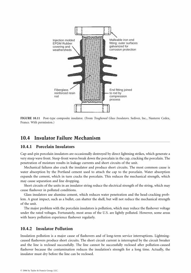
Injection molded EPDM Rubbercovering andweathersheds
Fiberglassreinforced resinrod
End fitting joinedto rod bycompressionprocess
Malleable iron endfitting; outer surfacesgalvanized forcorrosion protection
FIGURE 10.11 Post-type composite insulator. (From Toughened Glass Insulators. Sediver, Inc., Nanterre Cedex,
France. With permission.)
10.4 Insulator Failure Mechanism
10.4.1 Porcelain Insulators
Cap-and-pin porcelain insulators are occasionally destroyed by direct lightning strikes, which generate a
very steep wave front. Steep-front waves break down the porcelain in the cap, cracking the porcelain. The
penetration of moisture results in leakage currents and short circuits of the unit.
Mechanical failures also crack the insulator and produce short circuits. The most common cause is
water absorption by the Portland cement used to attach the cap to the porcelain. Water absorption
expands the cement, which in turn cracks the porcelain. This reduces the mechanical strength, which
may cause separation and line dropping.
Short circuits of the units in an insulator string reduce the electrical strength of the string, which may
cause flashover in polluted conditions.
Glass insulators use alumina cement, which reduces water penetration and the head-cracking prob-
lem. A great impact, such as a bullet, can shatter the shell, but will not reduce the mechanical strength
of the unit.
The major problem with the porcelain insulators is pollution, which may reduce the flashover voltage
under the rated voltages. Fortunately, most areas of the U.S. are lightly polluted. However, some areas
with heavy pollution experience flashover regularly.
10.4.2 Insulator Pollution
Insulation pollution is a major cause of flashovers and of long-term service interruptions. Lightning-
caused flashovers produce short circuits. The short circuit current is interrupted by the circuit breaker
and the line is reclosed successfully. The line cannot be successfully reclosed after pollution-caused
flashover because the contamination reduces the insulation’s strength for a long time. Actually, the
insulator must dry before the line can be reclosed.
� 2006 by Taylor & Francis Group, LLC.
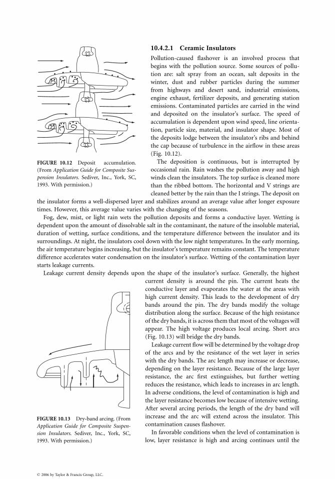
FIGURE 10.12 Deposit accumulation.
(From Application Guide for Composite Sus-
pension Insulators. Sediver, Inc., York, SC,
1993. With permission.)
FIGURE 10.13 Dry-band arcing. (From
Application Guide for Composite Suspen-
sion Insulators. Sediver, Inc., York, SC,
1993. With permission.)
� 2006 by Taylor & Francis Group, LLC.
10.4.2.1 Ceramic Insulators
Pollution-caused flashover is an involved process that
begins with the pollution source. Some sources of pollu-
tion are: salt spray from an ocean, salt deposits in the
winter, dust and rubber particles during the summer
from highways and desert sand, industrial emissions,
engine exhaust, fertilizer deposits, and generating station
emissions. Contaminated particles are carried in the wind
and deposited on the insulator’s surface. The speed of
accumulation is dependent upon wind speed, line orienta-
tion, particle size, material, and insulator shape. Most of
the deposits lodge between the insulator’s ribs and behind
the cap because of turbulence in the airflow in these areas
(Fig. 10.12).
The deposition is continuous, but is interrupted by
occasional rain. Rain washes the pollution away and high
winds clean the insulators. The top surface is cleaned more
than the ribbed bottom. The horizontal and V strings are
cleaned better by the rain than the I strings. The deposit on
the insulator forms a well-dispersed layer and stabilizes around an average value after longer exposure
times. However, this average value varies with the changing of the seasons.
Fog, dew, mist, or light rain wets the pollution deposits and forms a conductive layer. Wetting is
dependent upon the amount of dissolvable salt in the contaminant, the nature of the insoluble material,
duration of wetting, surface conditions, and the temperature difference between the insulator and its
surroundings. At night, the insulators cool down with the low night temperatures. In the early morning,
the air temperature begins increasing, but the insulator’s temperature remains constant. The temperature
difference accelerates water condensation on the insulator’s surface. Wetting of the contamination layer
starts leakage currents.
Leakage current density depends upon the shape of the insulator’s surface. Generally, the highest
current density is around the pin. The current heats the
conductive layer and evaporates the water at the areas with
high current density. This leads to the development of dry
bands around the pin. The dry bands modify the voltage
distribution along the surface. Because of the high resistance
of the dry bands, it is across them that most of the voltages will
appear. The high voltage produces local arcing. Short arcs
(Fig. 10.13) will bridge the dry bands.
Leakage current flow will be determined by the voltage drop
of the arcs and by the resistance of the wet layer in series
with the dry bands. The arc length may increase or decrease,
depending on the layer resistance. Because of the large layer
resistance, the arc first extinguishes, but further wetting
reduces the resistance, which leads to increases in arc length.
In adverse conditions, the level of contamination is high and
the layer resistance becomes low because of intensive wetting.
After several arcing periods, the length of the dry band will
increase and the arc will extend across the insulator. This
contamination causes flashover.
In favorable conditions when the level of contamination is
low, layer resistance is high and arcing continues until the

sun or wind dries the layer and stops the arcing. Continuous arcing is harmless for ceramic insulators,
but it ages nonceramic and composite insulators.
The mechanism described above shows that heavy contamination and wetting may cause insulator
flashover and service interruptions. Contamination in dry conditions is harmless. Light contamination
and wetting causes surface arcing and aging of nonceramic insulators.
10.4.2.2 Nonceramic Insulators
Nonceramic insulators have a dirt and water repellent (hydrophobic) surface that reduces pollution
accumulation and wetting. The different surface properties slightly modify the flashover mechanism.
Contamination buildup is similar to that in porcelain insulators. However, nonceramic insulators
tend to collect less pollution than ceramic insulators. The difference is that in a composite insulator, the
diffusion of low-molecular-weight silicone oil covers the pollution layer after a few hours. Therefore,
the pollution layer will be a mixture of the deposit (dust, salt) and silicone oil. A thin layer of silicone oil,
which provides a hydrophobic surface, will also cover this surface.
Wetting produces droplets on the insulator’s hydrophobic surface. Water slowly migrates to the
pollution and partially dissolves the salt in the contamination. This process generates high resistivity
in the wet region. The connection of these regions starts leakage current. The leakage current dries the
surface and increases surface resistance. The increase of surface resistance is particularly strong on
the shaft of the insulator where the current density is higher.
Electrical fields between the wet regions increase. These high electrical fields produce spot discharges
on the insulator’s surface. The strongest discharge can be observed at the shaft of the insulator. This
discharge reduces hydrophobicity, which results in an increase of wet regions and an intensification of
the discharge. At this stage, dry bands are formed at the shed region. In adverse conditions,
this phenomenon leads to flashover. However, most cases of continuous arcing develop as the wet and
dry regions move on the surface.
The presented flashover mechanism indicates that surface wetting is less intensive in nonceramic
insulators. Partial wetting results in higher surface resistivity, which in turn leads to significantly higher
flashover voltage. However, continuous arcing generates local hot spots, which cause aging of the
insulators.
10.4.3 Effects of Pollution
The flashover mechanism indicates that pollution reduces flashover voltage. The severity of flashover
voltage reduction is shown in Fig. 10.14. This figure shows the surface electrical stress (field), which
causes flashover as a function of contamination, assuming that the insulators are wet. This means that
the salt in the deposit is completely dissolved. The Equivalent Salt Deposit Density (ESDD) describes the
level of contamination.
These results show that the electrical stress, which causes flashover, decreases by increasing the level of
pollution on all of the insulators. This figure also shows that nonceramic insulator performance is better
than ceramic insulator performance. The comparison between EPDM and silicone shows that flashover
performance is better for the latter.
Table 10.6 shows the number of standard insulators required in contaminated areas. This table can be
used to select the number of insulators, if the level of contamination is known.
Pollution and wetting cause surface discharge arcing, which is harmless on ceramic
insulators, but produces aging on composite insulators. Aging is a major problem and will be discussed
in the next section.
10.4.4 Composite Insulators
The Electric Power Research Institute (EPRI) conducted a survey analyzing the cause of composite
insulator failures and operating conditions. The survey was based on the statistical evaluation of failures
reported by utilities.
� 2006 by Taylor & Francis Group, LLC.
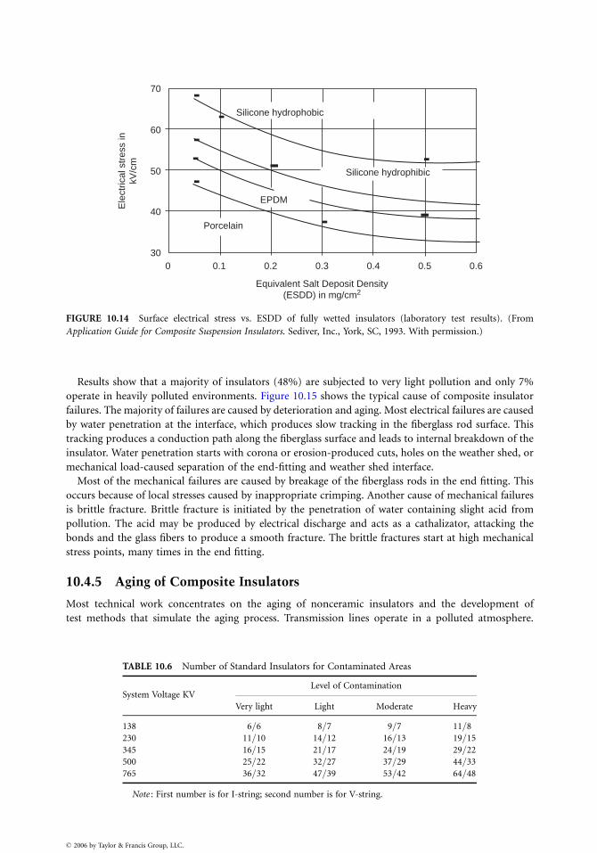
0.1 0.2
Equivalent Salt Deposit Density(ESDD) in mg/cm2
Ele
ctric
al s
tres
s in
kV/c
m
0.3
Silicone hydrophobic
Porcelain
Silicone hydrophibic
EPDM
0.4 0.5 0.6030
40
50
60
70
FIGURE 10.14 Surface electrical stress vs. ESDD of fully wetted insulators (laboratory test results). (From
Application Guide for Composite Suspension Insulators. Sediver, Inc., York, SC, 1993. With permission.)
Results show that a majority of insulators (48%) are subjected to very light pollution and only 7%
operate in heavily polluted environments. Figure 10.15 shows the typical cause of composite insulator
failures. The majority of failures are caused by deterioration and aging. Most electrical failures are caused
by water penetration at the interface, which produces slow tracking in the fiberglass rod surface. This
tracking produces a conduction path along the fiberglass surface and leads to internal breakdown of the
insulator. Water penetration starts with corona or erosion-produced cuts, holes on the weather shed, or
mechanical load-caused separation of the end-fitting and weather shed interface.
Most of the mechanical failures are caused by breakage of the fiberglass rods in the end fitting. This
occurs because of local stresses caused by inappropriate crimping. Another cause of mechanical failures
is brittle fracture. Brittle fracture is initiated by the penetration of water containing slight acid from
pollution. The acid may be produced by electrical discharge and acts as a cathalizator, attacking the
bonds and the glass fibers to produce a smooth fracture. The brittle fractures start at high mechanical
stress points, many times in the end fitting.
10.4.5 Aging of Composite Insulators
Most technical work concentrates on the aging of nonceramic insulators and the development of
test methods that simulate the aging process. Transmission lines operate in a polluted atmosphere.
TABLE 10.6 Number of Standard Insulators for Contaminated Areas
System Voltage KVLevel of Contamination
Very light Light Moderate Heavy
138 6=6 8=7 9=7 11=8
230 11=10 14=12 16=13 19=15
345 16=15 21=17 24=19 29=22
500 25=22 32=27 37=29 44=33
765 36=32 47=39 53=42 64=48
Note : First number is for I-string; second number is for V-string.
� 2006 by Taylor & Francis Group, LLC.
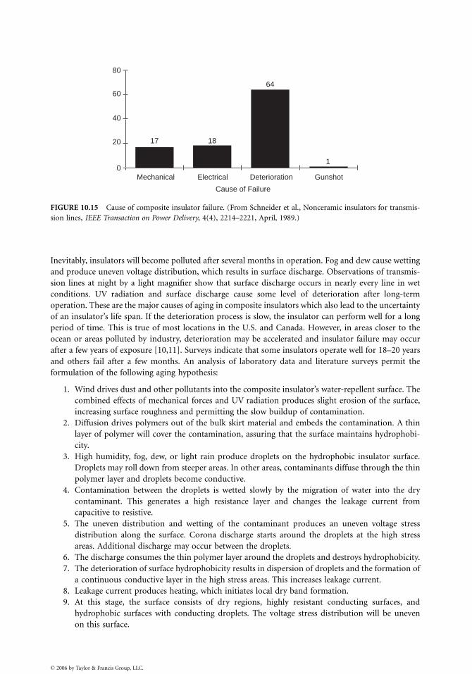
0Mechanical
17 18
64
1
Electrical GunshotDeterioration
Cause of Failure
20
40
60
80
FIGURE 10.15 Cause of composite insulator failure. (From Schneider et al., Nonceramic insulators for transmis-
sion lines, IEEE Transaction on Power Delivery, 4(4), 2214–2221, April, 1989.)
Inevitably, insulators will become polluted after several months in operation. Fog and dew cause wetting
and produce uneven voltage distribution, which results in surface discharge. Observations of transmis-
sion lines at night by a light magnifier show that surface discharge occurs in nearly every line in wet
conditions. UV radiation and surface discharge cause some level of deterioration after long-term
operation. These are the major causes of aging in composite insulators which also lead to the uncertainty
of an insulator’s life span. If the deterioration process is slow, the insulator can perform well for a long
period of time. This is true of most locations in the U.S. and Canada. However, in areas closer to the
ocean or areas polluted by industry, deterioration may be accelerated and insulator failure may occur
after a few years of exposure [10,11]. Surveys indicate that some insulators operate well for 18–20 years
and others fail after a few months. An analysis of laboratory data and literature surveys permit the
formulation of the following aging hypothesis:
1. Wind drives dust and other pollutants into the composite insulator’s water-repellent surface. The
combined effects of mechanical forces and UV radiation produces slight erosion of the surface,
increasing surface roughness and permitting the slow buildup of contamination.
2. Diffusion drives polymers out of the bulk skirt material and embeds the contamination. A thin
layer of polymer will cover the contamination, assuring that the surface maintains hydrophobi-
city.
3. High humidity, fog, dew, or light rain produce droplets on the hydrophobic insulator surface.
Droplets may roll down from steeper areas. In other areas, contaminants diffuse through the thin
polymer layer and droplets become conductive.
4. Contamination between the droplets is wetted slowly by the migration of water into the dry
contaminant. This generates a high resistance layer and changes the leakage current from
capacitive to resistive.
5. The uneven distribution and wetting of the contaminant produces an uneven voltage stress
distribution along the surface. Corona discharge starts around the droplets at the high stress
areas. Additional discharge may occur between the droplets.
6. The discharge consumes the thin polymer layer around the droplets and destroys hydrophobicity.
7. The deterioration of surface hydrophobicity results in dispersion of droplets and the formation of
a continuous conductive layer in the high stress areas. This increases leakage current.
8. Leakage current produces heating, which initiates local dry band formation.
9. At this stage, the surface consists of dry regions, highly resistant conducting surfaces, and
hydrophobic surfaces with conducting droplets. The voltage stress distribution will be uneven
on this surface.
� 2006 by Taylor & Francis Group, LLC.

10. Uneven voltage distribution produces arcing and discharges between the different dry bands.
These cause further surface deterioration, loss of hydrophobicity, and the extension of the dry areas.
11. Discharge and local arcing produces surface erosion, which ages the insulator’s surface.
12. A change in the weather, such as the sun rising, reduces the wetting. As the insulator dries, the
discharge diminishes.
13. The insulator will regain hydrophobicity if the discharge-free dry period is long enough.
Typically, silicon rubber insulators require 6–8 h; EPDM insulators require 12–15 h to regain
hydrophobicity.
14. Repetition of the described procedure produces erosion on the surface. Surface roughness
increases and contamination accumulation accelerates aging.
15. Erosion is due to discharge-initiated chemical reactions and a rise in local temperature. Surface
temperature measurements, by temperature indicating point, show local hot-spot temperatures
between 2608C and 4008C during heavy discharge.
The presented hypothesis is supported by the observation that the insulator life spans in dry areas are
longer than in areas with a wetter climate. Increasing contamination levels reduce an insulator’s life span.
The hypothesis is also supported by observed beneficial effects of corona rings on insulator life.
DeTourreil et al. (1990) reported that aging reduces the insulator’s contamination flashover voltage.
Different types of insulators were exposed to light natural contamination for 36–42 months at two
different sites. The flashover voltage of these insulators was measured using the ‘‘quick flashover salt fog’’
technique, before and after the natural aging. The quick flashover salt fog procedure subjects the
insulators to salt fog (80 kg=m3 salinity). The insulators are energized and flashed over 5–10 times.
Flashover was obtained by increasing the voltage in 3% steps every 5 min from 90% of the estimated
flashover value until flashover. The insulators were washed, without scrubbing, before the salt fog test.
The results show that flashover voltage on the new insulators was around 210 kV and the aged insulators
flashed over around 184–188 kV. The few years of exposure to light contamination caused a 10–15%
reduction of salt fog flashover voltage.
Natural aging and a follow-up laboratory investigation indicated significant differences between the
performance of insulators made by different manufacturers. Natural aging caused severe damage on
some insulators and no damage at all on others.
10.5 Methods for Improving Insulator Performance
Contamination caused flashovers produce frequent outages in severely contaminated areas. Lines closer
to the ocean are in more danger of becoming contaminated. Several countermeasures have been
proposed to improve insulator performance. The most frequently used methods are:
1. Increasing leakage distance by increasing the number of units or by using fog-type insulators.
The disadvantages of the larger number of insulators are that both the polluted and the impulse
flashover voltages increase. The latter jeopardizes the effectiveness of insulation coordination
because of the increased strike distance, which increases the overvoltages at substations.
2. Application insulators are covered with a semiconducting glaze. A constant leakage current
flows through the semiconducting glaze. This current heats the insulator’s surface and reduces the
moisture of the pollution. In addition, the resistive glaze provides an alternative path when dry
bands are formed. The glaze shunts the dry bands and reduces or eliminates surface arcing. The
resistive glaze is exceptionally effective near the ocean.
3. Periodic washing of the insulators with high-pressure water. The transmission lines are washed
by a large truck carrying water and pumping equipment. Trained personnel wash the insulators
by aiming the water spray toward the strings. Substations are equipped with permanent washing
systems. High-pressure nozzles are attached to the towers and water is supplied from a central
pumping station. Safe washing requires spraying large amounts of water at the insulators in a
� 2006 by Taylor & Francis Group, LLC.

short period of time. Fast washing prevents the formation of dry bands and pollution-caused
flashover. However, major drawbacks of this method include high installation and operational
costs.
4. Periodic cleaning of the insulators by high pressure driven abrasive material, such as ground
corn cobs or walnut shells. This method provides effective cleaning, but cleaning of the residual
from the ground is expensive and environmentally undesirable.
5. Replacement of porcelain insulators with nonceramic insulators. Nonceramic insulators have
better pollution performance, which eliminates short-term pollution problems at most sites.
However, insulator aging may affect the long-term performance.
6. Covering the insulators with a thin layer of room-temperature vulcanized (RTV) silicon
rubber coating. This coating has a hydrophobic and dirt-repellent surface, with pollution
performance similar to nonceramic insulators. Aging causes erosion damage to the thin layer
after 5–10 years of operation. When damage occurs, it requires surface cleaning and a reappli-
cation of the coating. Cleaning by hand is very labor intensive. The most advanced method is
cleaning with high pressure driven abrasive materials like ground corn cobs or walnut shells. The
coating is sprayed on the surface using standard painting techniques.
7. Covering the insulators with a thin layer of petroleum or silicon grease. Grease provides a
hydrophobic surface and absorbs the pollution particles. After one or two years of operation, the
grease saturates the particles and it must be replaced. This requires cleaning of the insulator and
application of the grease, both by hand. Because of the high cost and short life span of the grease,
it is not used anymore.
References
1.
� 200
Transmission Line Reference Book (345 kV and Above), 2nd ed., EL 2500 Electric Power Research
Institute (EPRI), Palo Alto, CA, 1987.
2.
Fink, D.G. and Beaty, H.W., Standard Handbook for Electrical Engineers, 11th ed., McGraw-Hill,New York, 1978.
3.
Looms, J.S.T., Insulators for High Voltages, Peter Peregrinus Ltd., London, 1988.4.
Toughened Glass Insulators. Sediver Inc., Nanterre Cedex, France.5.
Application Guide for Composite Suspension Insulators, Sediver Inc., York, SC, 1993.6.
Hall, J.F., History and bibliography of polymeric insulators for outdoor application, IEEE Transac-tion on Power Delivery, 8(1), 376–385, January, 1993.
7.
Schneider, H., Hall, J.F., Karady, G., and Rendowden, J., Nonceramic insulators for transmissionlines, IEEE Transaction on Power Delivery, 4(4), 2214–2221, April, 1989.
8.
Karady, G.G., Outdoor insulation, Proceedings of the Sixth International Symposium on High VoltageEngineering, New Orleans, LA, September, 1989, 30.01–30.08.
9.
DeTourreil, C.H. and Lambeth, P.J., Aging of composite insulators: Simulation by electrical tests,IEEE Trans. on Power Delivery, 5(3), 1558–1567, July, 1990.
10.
Karady, G.G., Rizk, F.A.M., and Schneider, H.H., Review of CIGRE and IEEE Research intoPollution Performance of Nonceramic Insulators: Field Aging Effect and Laboratory Test Tech-
niques, in International Conference on Large Electric High Tension Systems (CIGRE), Group 33,
(33–103), Paris, 1–8, August, 1994.
11.
Gorur, R.S., Karady, G.G., Jagote, A., Shah, M., and Yates, A., Aging in silicon rubber used foroutdoor insulation, IEEE Transaction on Power Delivery, 7(2), 525–532, March, 1992.
6 by Taylor & Francis Group, LLC.

� 2006 by Taylor & Francis Group, LLC.
11
� 2006 by Taylor & Francis Group, LLC.
Transmission LineConstruction and
Maintenance
Wilford CaulkinsSherman & Reilly
Kristine BuchholzPacific Gas & Electric Company
11.1 Tools ................................................................................. 11-2
11.2 Equipment........................................................................ 11-3
11.3 Procedures........................................................................ 11-3
11.4 Helicopters ....................................................................... 11-4Conductor Stringing . Structure and Material Setting .
Insulator Replacement . Replacing Spacers . Insulator
Washing . Inspections . Helicopter Method Considerations
The information herein was derived from personal observation and participation in the construction of
overhead transmission lines for over 40 years. Detailed information, specific tools and equipment have
been provided previously and are available in IEEE Standard 524-2003 and IEEE Standard 524A-1993.
The purpose of this chapter is to give a general overview of the steps that are necessary in the planning
and construction of a typical overhead transmission line, to give newcomers to the trade a general
format to follow, and assist transmission design engineers in understanding how such lines are built.
Stringing overhead conductors in transmission is a very specialized type of construction requiring
years of experience, as well as equipment and tools that have been designed, tried, and proven to do the
work. Because transmission of electrical current is normally at higher voltages (69 kV and above),
conductors must be larger in diameter and span lengths must be longer than in normal distribution.
Although proximity to other energized lines may be limited on the right-of-way, extra care must be
exercised to protect the conductor so that when energized, power loss and corona are not a problem.
There are four methods that can be used to install overhead transmission conductors:
1. Slack stringing
2. Semi-tension stringing
3. Full-tension stringing
4. Helicopter stringing
Slack stringing can only be utilized if it is not necessary to keep the conductor off of the ground, and if
no energized lines lie beneath the line being strung. In this method the pulling lines are pulled out on the
ground, threaded through the stringing blocks, and the conductor is pulled in with less tension than is
required to keep it off the ground. This is not considered to be an acceptable method when demands
involve maximum utilization of transmission requirements.
Semi-tension methods are merely an upgrading of slack stringing, but do not necessarily keep the
conductor completely clear of the ground, or the lines used to pull.
Full-tension stringing is a method of installing the conductors and overhead groundwire in which
sufficient pulling capabilities on one end and tension capabilities on the other, keep the wires clear of any
obstacles during the movement of the conductor from the reel to its final sag position. This ensures that

these current-carrying cables are ‘‘clipped’’ into the support clamps in the best possible condition, which
is the ultimate goal of the work itself.
Stringing with helicopters, which is much more expensive per hour of work, can be much less
expensive when extremely arduous terrain exists along the right-of-way and when proper pre-planning
is utilized. Although pulling conductors themselves with a helicopter can be done, it is limited and
normally not practical. Maximum efficiency can be achieved when structures are set and pilot lines
are pulled with the helicopter, and then the conductor stringing is done in a conventional manner.
Special tools (such as stringing blocks) are needed if helicopters are used.
So that maximum protection of the conductor is realized and maximum safety of personnel is
attained, properly designed and constructed tools and equipment are tantamount to a successful job.
Because the initial cost of these tools and equipment represent such a small percentage of the overall cost
of the project, the highest quality should be used, thus minimizing ‘‘down time’’ and possible failure
during the course of construction.
11.1 Tools
Basic tools needed to construct overhead transmission lines are as follows:
1. Conductor blocks
2. Overhead groundwire blocks
3. Catch-off blocks
4. Sagging blocks
5. Pulling lines
6. Pulling grips
7. Catch-off grips
8. Swivels
9. Running boards
10. Conductor lifting hooks
11. Hold-down blocks
Conductor blocks are made in the following configurations:
1. Single conductor
2. Multiple conductor
3. Multiversal type (can be converted from bundle to single, and vice versa)
4. Helicopter
Conductor blocks should be large enough to properly accommodate the conductor and be lined
with a resilient liner such as neoprene or polyurethane and constructed of lightweight, high-strength
materials. Some sheaves are made of synthetic material such as nylatron. Sheaves should be mounted
on anti-friction ball bearings to reduce the tension required in stringing and facilitate proper
sagging. Conductor blocks are available for stringing single conductors or multiple conductors.
Some are convertible, thus enhancing their versatility. When stringing multiple conductors, it is
desirable to pull all conductors with a single pulling line so that all conductors in the bundle have
identical tension history. The running board makes this possible. Pulling lines are divided into two
categories:
1. Steel cable
2. Synthetic rope
Because of the extra high tension required in transmission line construction, steel pulling lines and
pilot lines are most practical to use. Torque-resistant, stranded, and swagged cable are used so that ball
bearing swivels can be utilized to prevent torque buildup from being transferred to the conductor. Some
� 2006 by Taylor & Francis Group, LLC.
braided or woven steel cables are also used. If synthetic ropes are utilized, the most important features
should include:
1. No torque
2. Very minimum elongation
3. No ‘‘kinking’’
4. Easily spliced
5. High strength=small diameter
6. Excellent dielectric properties
Stringing overhead groundwires does not normally require the care of current-carrying conductors.
Most overhead groundwires are stranded steel construction and the use of steel wire with a fiber-optic
core for communications has become a common practice. Special care should be taken to ensure that
excessive bending does not occur when erecting overhead groundwires with fiber-optic centers, such
as OPT-GW (Optical Power Telecommunications—Ground Wire) and ADSS (All Dielectric Self-
Supporting Cable). New types of conductor such as ACCR, Aluminum Conductor Composite
Reinforced, need special care. Use of array (multi-sheave in tandem) blocks may be necessary. Special
instructions are available from the manufacturer, which specify minimum sheave and bullwheel diameter
for construction. OPT-GW should be strung using an antirotational device to prevent the cable from
twisting.
11.2 Equipment
Pullers are used to bring in the main pulling line. Multi-drum pullers, called pilot line winders, are used
to tension string the heavy pulling cable.
Primary pullers are used to tension string the conductors. These pullers are either drum type or
bullwheel type. The drum type is used more extensively in many areas of North America because the
puller and pulling cable are stored on one piece of equipment, but it is not practical in other areas
because it is too heavy. Thus, the bullwheel type is used allowing the puller and pulling cable to be
separated onto two pieces of equipment. Also, the pulling cable can be separated into shorter lengths to
allow easier handling, especially if manual labor is preferred.
Tensioners should be bullwheel type using multigroove wheels for more control. Although V groove
machines are used on some lighter, smaller conductors, they are not recommended in transmission work
because of the crushing effect on the conductor. Tensioners are either mounted on a truck or trailer.
Reel stands are used to carry the heavy reels of conductor and are equipped with brakes to hold
‘‘tailing tension’’ on the conductor as it is fed into the bullwheel tensioner. These stands are usually
mounted on a trailer separated from the tensioner.
Helicopters are normally used to fly in a light line which can be used to pull in the heavier cable.
11.3 Procedures
Once the right-of-way has been cleared, the following are normal steps taken in construction:
1. Framing
2. Pulling
3. Pulling overhead groundwire up to sag and installation
4. Pulling in main line with pilot line
5. Stringing conductors
6. Sagging conductors
7. Clipping in conductors
8. Installing spacer or spacer dampers where applicable
Framing normally consists of erecting poles, towers, or other structures, including foundations and
anchors on guyed structures. It is desirable for the stringing blocks to be installed, with finger lines, on
� 2006 by Taylor & Francis Group, LLC.

the ground before structures are set, to eliminate an extra climb later. Helicopters are used to set
structures, especially where rough terrain exists or right-of-way clearances are restricted.
Once structures are secure, overhead groundwire and pilot lines are pulled in together with a piece of
equipment such as a caterpillar or other track vehicle. A helicopter is also used to fly in these lines. Once
the overhead groundwires are in place, they are sagged and secured, thus giving the structures more
stability for the stringing of the conductors. This is especially important for guyed structures.
Normally the three pilot lines (typically 3=8 in. diameter swagged steel cable) pull in the heavier
pulling line (typically 3=4 in. diameter or 7=8 in. diameter swagged steel) under tension. The
main pulling line is then attached to the conductor which is strung under full tension. Once
the conductor is ‘‘caught off,’’ the main pulling line is returned for pulling of the next phase.
Once the conductors are in place, they are then brought up to final sag and clipped into the conductor
clamps provided. If the conductor is a part of a bundle per phase, the spacers or spacer dampers are
installed, using a spacer cart which is either pulled along from the ground or self-propelled.
Coordination between design engineers and construction personnel is very important in the planning
and design of transmission lines. Although it is sometimes impossible to accommodate the most
efficient capabilities of the construction department (or line contractor), much time and money can
be conserved if predesign meetings are held to discuss items such as the clearances needed for installing
overhead groundwire blocks, hardware equipped with ‘‘work’’ holes to secure lifting hooks or blocks,
conductor reel sizes compatible with existing reel stands, length of pull most desirable, or towers
equipped to facilitate climbing.
For maximum safety of personnel constructing transmission lines, proper and effective grounding
procedures should be utilized. Grounding can be accomplished by:
1. adequate grounding of conductors being strung and pulling cables being used, or
2. fully insulating equipment and operator,
3. isolating equipment and personnel.
All equipment, conductors, anchors, and structures within a defined work area must be bonded
together and connected to the ground source. The recommended procedures of personnel protection are
the following:
1. Establish equipotential work zones.
2. Select grounding equipment for the worst-case fault.
3. Discontinue all work when the possibility of lightning exists which may affect the work site.
In addition to the grounding system, the best safety precaution is to treat all equipment as if it could
become energized.
11.4 Helicopters
As already mentioned, the use of helicopters is another option that is being chosen more frequently for
transmission system construction and maintenance. There are a wide variety of projects where helicop-
ters become involved, making the projects easier, safer, or more economical. When choosing any
construction or maintenance method, identify the work to be accomplished, analyze the potential safety
aspects, list the possible alternatives, and calculate the economics. Helicopters add a new dimension to
this analytical process by adding to the alternatives, frequently reducing the risks of accident or injury,
and potentially reducing costs. The most critical consideration in the use of a helicopter is the ability to
safely position the helicopter and line worker at the work location.
11.4.1 Conductor Stringing
Helicopters are used for conductor stringing on towers through the use of pilot lines. Special stringing
blocks are installed at each tower and a helicopter is brought in and attached to a pilot line. The
� 2006 by Taylor & Francis Group, LLC.
helicopter flies along the tower line and slips the pilot line in through each stringing block until it
reaches the end of the set of towers for conductor pulling, where it disconnects and the pilot line is
transferred to a ground crew. The ground crew then proceeds to pull the conductor in the conventional
manner (Caulkins, 1987). The helicopter may also be used to monitor the conductor pulling and is
readily available to assist if the conductor stalls at any tower location.
11.4.2 Structure and Material Setting
The most obvious use of helicopters is in the setting of new towers and structures. Helicopters are
frequently used in rough terrain to fly in the actual tower to a location where a ground crew is waiting to
spot the structure into a preconstructed foundation. In addition, heavy material can be transported to
remote locations, as well as the construction crew.
The use of helicopters can be especially critical if the tower line is being replaced following a
catastrophe or failure. Frequently, roads and even construction paths are impassable or destroyed
following natural disasters. Helicopters can carry crews and materials with temporary structures that
can be erected within hours to restore tower lines. Again, depending on the terrain and current
conditions, whether the existing structure is repaired or temporary tower structures are utilized, the
helicopter is invaluable to carry in the needed supplies and personnel.
11.4.3 Insulator Replacement
A frequent maintenance requirement on a transmission system is replacing insulators. This need is
generated for various reasons, including line upgrading, gunshots, environmental damage, or defects in
the original insulator manufacturing. With close coordinated crews, helicopters can maximize the
efficiency of the replacement project.
Crews are located at several towers to perform the actual insulator removal and installation. The crews
will do the required setup for a replacement, but the helicopter can be used to bring in the necessary
tools and equipment. The crew removes the old insulator string and sets it to one side of the work
location. When the crews are ready, the helicopter flies in the new insulator string to each tower. The
crew on the tower detaches the new insulator string from the helicopter, positions it, and then attaches
the old string to the helicopter, which removes the string to the staging area. With a well-coordinated
team of helicopters and experienced line workers, it is not unusual to achieve a production rate of
replacing all insulators on four three-phase structures per crew per day. Under ideal conditions, crews
are able to replace the insulators on a structure in one hour (Buchholz, 1987).
11.4.4 Replacing Spacers
One of the first uses of helicopters in live-line work was the replacement of spacers in the early 1980s.
This method was a historic step in live-line work since it circumvented the need for hot sticks or
insulated aerial lift devices.
The first projects involved a particular spacer wearing into the conductor strands, causing the
separation of the conductor. Traditionally, the transmission line would have been de-energized,
grounded, and either a line worker would have utilized a spacer cart to move out on the line to replace
the spacer, or the line would have been lowered and the spacer replaced and the conductor strengthened.
The obvious safety dilemma was whether the conductor could support a line worker on a spacer cart or
whether it was physically able to withstand the tensions of lowering it to the ground. By utilizing a
helicopter and bare-hand work methods, the spacers were able to be replaced and the conductor
strengthened where necessary with full-tension compression splices while providing total safety to the
line workers and a continuous supply of energy over the transmission lines. One of the early
projects achieved a replacement and installation of 25,000 spacers without a single accident or injury.
A typical spacer replacement required about 45 sec, including the travel time between work locations
(Buchholz, 1987).
� 2006 by Taylor & Francis Group, LLC.
11.4.5 Insulator Washing
Another common practice is to utilize helicopters for insulator washing. Again, this is a method that
allows for the line to remain energized during the process. The helicopter carries a water tank that is
refilled at a staging area near the work location. A hose and nozzle are attached to a structure on the
helicopter and are operated by a qualified line worker who directs the water spray and adequately cleans
the insulator string. Again, with the ease of access afforded by the helicopter, the speed of this operation
can result in a typical three-phase tower being cleaned in a few minutes.
11.4.6 Inspections
Helicopters are invaluable for tower line and structure inspections. Due to the ease of the practice and
the large number of inspections that can be accomplished, utilities have increased the amount of
maintenance inspections being done, thus promoting system reliability.
Helicopters typically carry qualified line workers who utilize stabilizing binoculars to visually inspect
the transmission tower for signs of rusting or weakness and the transmission hardware and conductor
for damage and potential failure. Infrared inspections and photographic imaging can also be accom-
plished from the helicopter, either by mounting the cameras on the helicopter or through direct use by
the crew. During these inspections, the helicopter provides a comfortable situation for accomplishing
the necessary recording of specific information, tower locations, etc. In addition, inspections from
helicopters are required following a catastrophic event or system failure. It is the only logical method of
quickly inspecting a transmission system for the exact location and extent of damage.
11.4.7 Helicopter Method Considerations
The ability to safely position a helicopter and worker at the actual work site is the most critical
consideration when deciding if a helicopter method can be utilized for construction or maintenance.
The terrain and weather conditions are obvious factors, as well as the physical spacing needed to
position the helicopter and worker in the proximity required for the work method. If live-line work
methods are to be utilized, the minimum approach distance required for energized line work must be
calculated very carefully for every situation. The geometry of each work structure, the geometry of the
individual helicopter, and the positioning of the helicopter and worker for the specific work method
must be analyzed. There are calculations that are available to analyze the approach distances (IEEE Task
Force 15.07.05.05, 1999).
When choosing between construction and maintenance work methods, the safety of the line workers
is the first consideration. Depending on circumstances, a helicopter method may be the safest work
method. Terrain has always been a primary reason for choosing helicopters to assist with projects since
the ability to drive to each work site may not be possible. However, helicopters may still be the easiest
and most economic alternative when the terrain is open and flat, especially when there are many
individual tower locations that will be contacted. Although helicopters may seem to be expensive on a
per person basis, the ability to quickly position workers and easily move material can drastically reduce
costs. When live-line methods can be utilized, the positioning of workers, material, and equipment
becomes comparatively easier.
Finally, if the safe use of the helicopter allows the transmission systems to remain energized
throughout the project, the helicopter may be the only possible alternative. Since the transmission
system is a major link in the competitive energy markets, transmission operation will have reliability
performance measures which must be achieved. Purchasing replacement energy through alternate
transmission paths, as was done in the regulated world, is no longer an option. Transmission system
managers are required to keep systems operational and will be fined if high levels of performance are not
attained. The option of de-energizing systems for maintenance practices may be too costly in the
deregulated world.
� 2006 by Taylor & Francis Group, LLC.

References
Buchholz, F., Helicopter application in transmission system maintenance and repair, in IEEE=CSEE Joint
Conference on High-Voltage Transmission Systems in China, October 1987.
Caulkins, III., W., Practical applications and experiences in the installation of overhead transmission line
conductors, in IEEE=CSEE Joint Conference on High-Voltage Transmission Systems in China,
October, 1987.
Guide to Grounding During the Installation of Overhead Transmission Line Conductors: Supplement to
IEEE Guide to the Installation of Overhead Transmission Line Conductors, IEEE 524A–1993, 1998.
Guide to the Installation of Overhead Transmission Line Conductors, IEEE 524–1992, 1998.
IEEE Task Force 15.07.05.05, PE 046 PRD (04–99), Recommended Practices for Helicopter Bonding
Procedures for Live Line Work.
� 2006 by Taylor & Francis Group, LLC.

� 2006 by Taylor & Francis Group, LLC.
12
� 2006 by Taylor & Francis Group, LLC.
Insulated PowerCables Used in
UndergroundApplications
Michael L. DyerSalt River Project
12.1 Underground System Designs ........................................ 12-1
12.2 Conductor ........................................................................ 12-2
12.3 Insulation ......................................................................... 12-3
12.4 Medium- and High-Voltage Power Cables ................... 12-3
12.5 Shield Bonding Practice.................................................. 12-6
12.6 Installation Practice......................................................... 12-6
12.7 System Protection Devices.............................................. 12-8
12.8 Common Calculations used with Cable........................ 12-8
Aesthetics is primarily the major reason for installing power cables underground, providing open views
of the landscape free of poles and wires. One could also argue that underground lines are more reliable
than overhead lines as they are not susceptible to weather and tree caused outages, common to overhead
power lines. This is particularly true of temporary outages caused by wind, which represents approxi-
mately 80% of all outages occurring on overhead systems. However, underground lines are susceptible to
being damaged by excavations (reason behind ‘‘call before digging’’ locating programs implemented by
many states in the U.S.). The time required to repair a damaged underground line may be considerably
longer than an overhead line. Underground lines are typically ten times more expensive to install than
overhead lines. The ampacity, current carrying capacity, of an underground line is less than an
equivalent sized overhead line. Underground lines require a higher degree of planning than overhead,
because it is costly to add or change facilities in an existing system. Underground cables do not have an
infinite life, because the dielectric insulation is subjected to aging; therefore, systems should be designed
with future replacement or repair as a consideration.
12.1 Underground System Designs
There are two types of underground systems (Fig. 12.1).
A. Radial—where the transformers are served from a single source.
B. Looped—where the transformers are capable of being served from one of two sources. During
normal operation an open is located at one of the transformers, usually the midpoint.
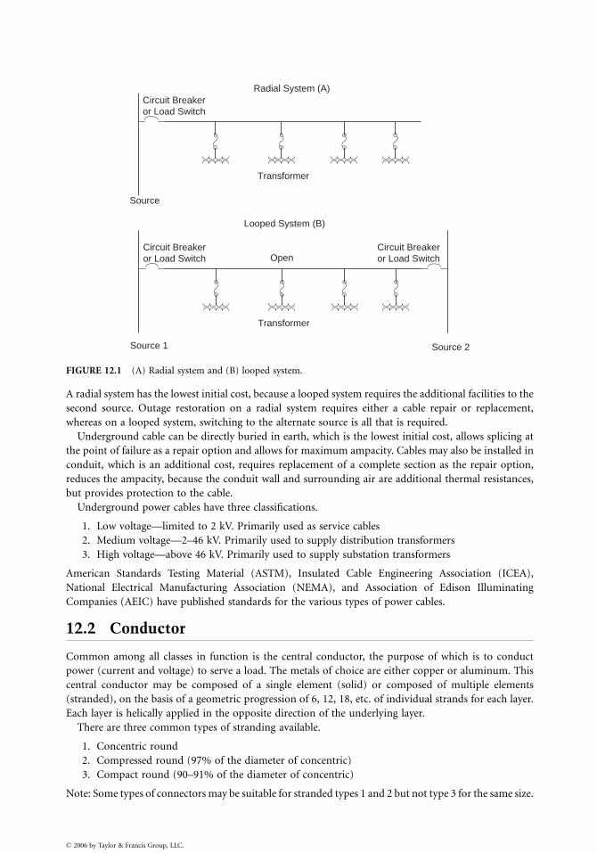
Source
Circuit Breakeror Load Switch
Transformer
Radial System (A)
Looped System (B)
Source 1 Source 2
Circuit Breakeror Load Switch
Circuit Breaker or Load Switch
Transformer
Open
FIGURE 12.1 (A) Radial system and (B) looped system.
A radial system has the lowest initial cost, because a looped system requires the additional facilities to the
second source. Outage restoration on a radial system requires either a cable repair or replacement,
whereas on a looped system, switching to the alternate source is all that is required.
Underground cable can be directly buried in earth, which is the lowest initial cost, allows splicing at
the point of failure as a repair option and allows for maximum ampacity. Cables may also be installed in
conduit, which is an additional cost, requires replacement of a complete section as the repair option,
reduces the ampacity, because the conduit wall and surrounding air are additional thermal resistances,
but provides protection to the cable.
Underground power cables have three classifications.
1. Low voltage—limited to 2 kV. Primarily used as service cables
2. Medium voltage—2–46 kV. Primarily used to supply distribution transformers
3. High voltage—above 46 kV. Primarily used to supply substation transformers
American Standards Testing Material (ASTM), Insulated Cable Engineering Association (ICEA),
National Electrical Manufacturing Association (NEMA), and Association of Edison Illuminating
Companies (AEIC) have published standards for the various types of power cables.
12.2 Conductor
Common among all classes in function is the central conductor, the purpose of which is to conduct
power (current and voltage) to serve a load. The metals of choice are either copper or aluminum. This
central conductor may be composed of a single element (solid) or composed of multiple elements
(stranded), on the basis of a geometric progression of 6, 12, 18, etc. of individual strands for each layer.
Each layer is helically applied in the opposite direction of the underlying layer.
There are three common types of stranding available.
1. Concentric round
2. Compressed round (97% of the diameter of concentric)
3. Compact round (90–91% of the diameter of concentric)
Note: Some types of connectors may be suitable for stranded types 1 and 2 but not type 3 for the same size.
� 2006 by Taylor & Francis Group, LLC.
To improve manufacturing, 19 wire combination unilay stranding (helically applied in one
direction one operation) has become popular in low-voltage applications, where some of the outer
strands are of a smaller diameter, but the same outside diameter as compressed round is retained.
Another stranding method which retains the same overall diameter is single input wire (SIW)
compressed, which can be used to produce a wide range of conductors using a smaller range of the
individual strands.
Conductors used at transmission voltages may have exotic stranding to reduce the voltage stress.
Cables requiring greater flexibility such as portable power cable utilize very fine strands with a rope
type stranding.
Typical sizes for power conductors are #6 American Wire Gage (AWG) through 1000 kcmils. One cmil
is defined as the area of a circle having a diameter of one mil (0.0001 in.). Solid conductors are usually
limited to a maximum of #1=0 because of flexibility.
The metal type and size determines the ampacity and losses (I2R). Copper having a higher intrinsic
conductivity will have a greater ampacity and lower resistance than an equivalent size aluminum
conductor. Aluminum 1350 alloy medium hardness is typical for power cable use.
12.3 Insulation
In order to install power cables underground, the conductor must be insulated. For low-voltage
applications, a layer of insulation is extruded onto the conductor. Many types of insulation compounds
have been used from natural or synthetic rubber, polyvinyl chloride (PVC), high molecular weight
polyethylene (HMWPE), and cross-linked polyethylene (XLPE) to name a few. Although each insulation
type has various characteristics, operating temperature and durability are probably the most important.
XLPE is probably the most widely used insulation for low-voltage cables. XLPE is a thermoset plastic
with its hydrocarbon molecular chains cross-linked. Cross-linking is a curing process, which occurs
under heat and pressure, or as used for low-voltage cables, moisture and allows an operating tempera-
ture of 908C.
Multiple layer cable insulation composed of a softer compound under a harder compound, a single
layer harder insulation, or a self-healing insulation are used to address protection of the conductor,
typically for direct buried low-voltage power cables.
12.4 Medium- and High-Voltage Power Cables
Medium- and high-voltage power cables, in addition to being insulated, are shielded to contain and
evenly distribute the electric field within the insulation.
The components and function of a medium- and high-voltage cable are as follows (Figs. 12.2A
and 12.2B):
1. The center conductor—metallic path to carry power.
2. The conductor shield—a semiconducting layer placed over the conductor to provide a smooth
conducting cylinder around the conductor. Typical of today’s cables, this layer is a semiconduct-
ing plastic, polymer with a carbon filler, extruded directly over the conductor. This layer
represents a very smooth surface, which, because of direct contact with the conductor, is elevated
to the applied voltage on the conductor.
3. The insulation—a high dielectric material to isolate the conductor. The two basic types used
today are XLPE or ethylene propylene rubber (EPR). Because of an aging effect known as treeing
(Fig. 12.3), on the basis of its visual appearance, caused by moisture in the presence of an electric
field, a modified version of XLPE designated tree retardant (TRXLPE) has replaced the use of
XLPE for medium-voltage applications. High-voltage transmission cables still utilize XLPE, but
they usually have a moisture barrier. TRXLPE is a very low loss dielectric that is reasonably
� 2006 by Taylor & Francis Group, LLC.
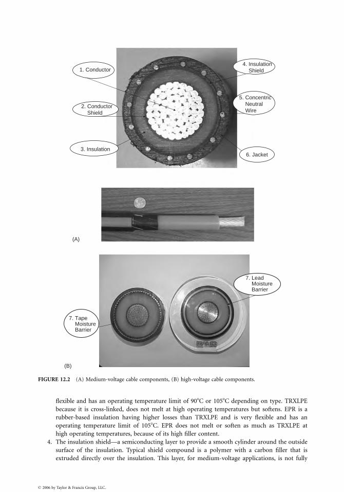
6. Jacket
4. Insulation Shield
3. Insulation
2. Conductor Shield
1. Conductor
5. Concentric Neutral Wire
(A)
7. Lead Moisture Barrier
7. Tape Moisture Barrier
(B)
FIGURE 12.2 (A) Medium-voltage cable components, (B) high-voltage cable components.
flexible and has an operating temperature limit of 908C or 1058C depending on type. TRXLPE
because it is cross-linked, does not melt at high operating temperatures but softens. EPR is a
rubber-based insulation having higher losses than TRXLPE and is very flexible and has an
operating temperature limit of 1058C. EPR does not melt or soften as much as TRXLPE at
high operating temperatures, because of its high filler content.
4. The insulation shield—a semiconducting layer to provide a smooth cylinder around the outside
surface of the insulation. Typical shield compound is a polymer with a carbon filler that is
extruded directly over the insulation. This layer, for medium-voltage applications, is not fully
� 2006 by Taylor & Francis Group, LLC.
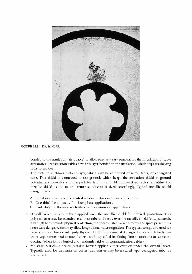
FIGURE 12.3 Tree in XLPE.
bonded to the insulation (strippable) to allow relatively easy removal for the installation of cable
accessories. Transmission cables have this layer bonded to the insulation, which requires shaving
tools to remove.
5. The metallic shield—a metallic layer, which may be composed of wires, tapes, or corrugated
tube. This shield is connected to the ground, which keeps the insulation shield at ground
potential and provides a return path for fault current. Medium-voltage cables can utilize the
metallic shield as the neutral return conductor if sized accordingly. Typical metallic shield
sizing criteria:
A. Equal in ampacity to the central conductor for one phase applications.
B. One-third the ampacity for three-phase applications.
C. Fault duty for three-phase feeders and transmission applications.
6. Overall jacket—a plastic layer applied over the metallic shield for physical protection. This
polymer layer may be extruded as a loose tube or directly over the metallic shield (encapsulated).
Although both provide physical protection, the encapsulated jacket removes the space present in a
loose tube design, which may allow longitudinal water migration. The typical compound used for
jackets is linear low density polyethylene (LLDPE), because of its ruggedness and relatively low
water vapor transmission rate. Jackets can be specified insulating (most common) or semicon-
ducting (when jointly buried and randomly laid with communication cables).
7. Moisture barrier—a sealed metallic barrier applied either over or under the overall jacket.
Typically used for transmission cables, this barrier may be a sealed tape, corrugated tube, or
lead sheath.
� 2006 by Taylor & Francis Group, LLC.
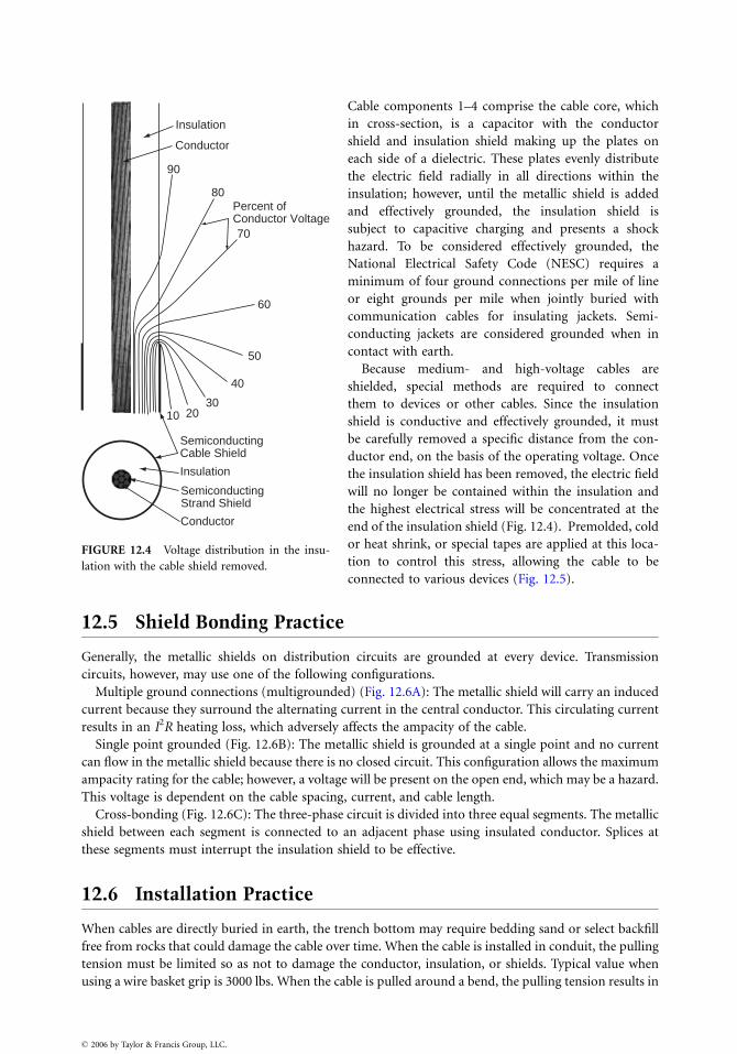
Insulation
Conductor
90
80
70
60
50
40
302010
Percent of Conductor Voltage
Semiconducting Cable Shield
Semiconducting Strand Shield
Conductor
Insulation
FIGURE 12.4 Voltage distribution in the insu-
lation with the cable shield removed.
� 2006 by Taylor & Francis Group, LLC.
Cable components 1–4 comprise the cable core, which
in cross-section, is a capacitor with the conductor
shield and insulation shield making up the plates on
each side of a dielectric. These plates evenly distribute
the electric field radially in all directions within the
insulation; however, until the metallic shield is added
and effectively grounded, the insulation shield is
subject to capacitive charging and presents a shock
hazard. To be considered effectively grounded, the
National Electrical Safety Code (NESC) requires a
minimum of four ground connections per mile of line
or eight grounds per mile when jointly buried with
communication cables for insulating jackets. Semi-
conducting jackets are considered grounded when in
contact with earth.
Because medium- and high-voltage cables are
shielded, special methods are required to connect
them to devices or other cables. Since the insulation
shield is conductive and effectively grounded, it must
be carefully removed a specific distance from the con-
ductor end, on the basis of the operating voltage. Once
the insulation shield has been removed, the electric field
will no longer be contained within the insulation and
the highest electrical stress will be concentrated at the
end of the insulation shield (Fig. 12.4). Premolded, cold
or heat shrink, or special tapes are applied at this loca-
tion to control this stress, allowing the cable to be
connected to various devices (Fig. 12.5).
12.5 Shield Bonding Practice
Generally, the metallic shields on distribution circuits are grounded at every device. Transmission
circuits, however, may use one of the following configurations.
Multiple ground connections (multigrounded) (Fig. 12.6A): The metallic shield will carry an induced
current because they surround the alternating current in the central conductor. This circulating current
results in an I2R heating loss, which adversely affects the ampacity of the cable.
Single point grounded (Fig. 12.6B): The metallic shield is grounded at a single point and no current
can flow in the metallic shield because there is no closed circuit. This configuration allows the maximum
ampacity rating for the cable; however, a voltage will be present on the open end, which may be a hazard.
This voltage is dependent on the cable spacing, current, and cable length.
Cross-bonding (Fig. 12.6C): The three-phase circuit is divided into three equal segments. The metallic
shield between each segment is connected to an adjacent phase using insulated conductor. Splices at
these segments must interrupt the insulation shield to be effective.
12.6 Installation Practice
When cables are directly buried in earth, the trench bottom may require bedding sand or select backfill
free from rocks that could damage the cable over time. When the cable is installed in conduit, the pulling
tension must be limited so as not to damage the conductor, insulation, or shields. Typical value when
using a wire basket grip is 3000 lbs. When the cable is pulled around a bend, the pulling tension results in
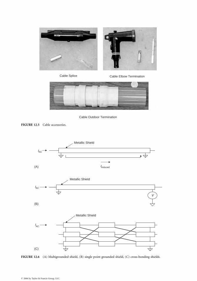
Cable Splice Cable Elbow Termination
Cable Outdoor Termination
FIGURE 12.5 Cable accessories.
Metallic Shield
Metallic Shield
IAC
Iinduced(A)
(B)
(C)
V
IAC
Metallic Shield
IAC
FIGURE 12.6 (A) Multigrounded shield, (B) single point grounded shield, (C) cross-bonding shields.
� 2006 by Taylor & Francis Group, LLC.
a side-wall bearing force against the inside surface of the elbow. This force must be limited to avoid
crushing the cable components. Cables also have a minimum bending radius limit that prevents
distortion of the cable components.
12.7 System Protection Devices
Two types of protecting devices are used on cable systems.
A. Overcurrent—fuses or circuit breakers. These devices isolate the cable from its source, preventing
the flow of damaging levels of current during an overload, or remove a faulted cable from the
system allowing restoration of the unfaulted parts.
B. Overvoltage—surge arrester. This device prevents damaging overvoltages caused by lightning or
switching surges from entering the cable by clamping the voltage to a level tolerated by the cable
insulation.
12.8 Common Calculations used with Cable
Inductance
Lcable ¼mo
2pln
2scable
d
� �
þ 1
4
� �
mo ¼ 4p10�7 H
m,
where scable¼ center-to-center conductor spacing
for three single cables scable ¼ cube root of each conductor spacing
d ¼ conductor diameter
mo¼ permeability of free space
Inductive reactance
Xcable ¼ vLcableL v ¼ 2pf ,
where f ¼ frequency
Lcable¼ inductance
L ¼ length
Capacitance
Ccable ¼2p«o«
lnD
d
� � «o ¼10�9
36p
F
m,
where « ¼ relative dielectric constant of the insulation (2.4 – XLPE, 2.9 – EPR)
«o¼ free space permittivity
D ¼ diameter of insulation under insulation shield when present
d ¼ diameter of the conductor in inches over the conductor shield when present
Charging current
Icap ¼ Vn vCcableLð Þ,
where Ccable¼ capacitance
Vn ¼ voltage line to neutral
L ¼ length
� 2006 by Taylor & Francis Group, LLC.
Ampacity
Iamp ¼ffiffiffiffiffiffiffiffiffiffiffiffiffiffiffiffi
Tc � Ta
RacRth
r
,
where Tc ¼ conductor temperature
Ta ¼ ambient temperature
Rac ¼ AC resistance at the operating temperature
Rth ¼ thermal resistance of surrounding environment
Voltage drop
Voltage drop ¼ Icable Rcable cos fð Þ þ Xcable sin fð Þð Þ,
where Icable ¼ current in conductor
Rcable ¼ total ac resistance of the cable
Xcable ¼ total ac reactance of the cable
f ¼ phase angle between supply voltage and current
For single-phase calculations the values of the main and the return conductors must be used.
Pulling tension single cable in straight conduit
T ¼ mWL,
where m ¼ coefficient of dynamic friction (0.2–0.7 dependent on cable exterior and type of conduit)
W¼ cable weight per unit length
L ¼ length
Pulling tension single cable through conduit bend
Tout ¼ Tin emf (pounds),
where Tin¼ the tension entering the bend
m ¼ coefficient of dynamic friction (0.2–0.7 dependent on cable exterior and type of conduit)
f ¼ bend angle in radians
The pulling tensions of each segment of the conduit path are added together to determine the total
pulling tension.
When multiple single cables are installed in a conduit, a multiplier must be applied to the cable
weight, accounting for configuration as follows:
For three cables with a triangular configuration the weight multiplier is
Wmultiplier triangular ¼2
ffiffiffiffiffiffiffiffiffiffiffiffiffiffiffiffiffiffiffiffiffiffiffiffiffiffiffiffiffiffi
1� d
D � d
� �2s :
For three cables with a cradled configuration
Wmultiplier cradled ¼ 1þ 4
3
d
D � d
� �2
,
where d ¼ single cable outside diameter
D¼ conduit inside diameter.
� 2006 by Taylor & Francis Group, LLC.

General References
Aluminum Electrical Conductor Handbook, edited by Mark Walker, The Aluminum Association, 1982.
ANSI=IEEE 575-1988, IEEE Guide for the Application of Sheath-Bonding Methods for Single-
Conductor Cables and the Calculation of Induced Voltages and Currents in Cable Sheaths.
Association of Edison Illuminating Companies, AEIC.
CS8-05, Specification for Extruded Dielectric, Shielded Power Cables Rated 5 through 46 kV.
IEEE 404-1993, IEEE Standard for Cable Joints for use with Extruded Dielectric Cable Rated
5000–138,000 V and Cable Joints for use with Laminated Dielectric Cable Rated 2500–500,000 V.
IEEE 48-1996, IEEE Standard Test Procedures and Requirements for Alternating Current Cable
Terminations 2.5 kV through 765 kV.
IEEE 1215-2001, IEEE Guide for the Application of Separable Insulated Connectors.
IEEE 386-2005, IEEE Standard for Separable Insulated Connector Systems for Power Distribution
Systems above 600 V.
Insulated Cable Engineering Association, ICEA standards.
P-53-426, Ampacities, 15–69 kV 1=c Power Cable Including Effect of Shield Losses (Solid Dielectric).
S-81-570-2005, 600 Volt Rated Cables of Ruggedized Design for Direct Burial Installations as Single
Conductors or Assemblies of Single Conductors.
S-94-694-2004, Concentric Neutral Cables Rated 5 through 46 kV.
S-97-682-2000, Utility Shielded Power Cables Rated 5 through 46 kV.
S-105-692-2004, 600 Volt Single layer Thermoset Insulated Utility Underground Distribution Cables.
S-108-720-2004, Extruded Insulation Power Cables Rated above 46 through 345 kV.
Southwire Company Power Cable Manual, Second edition, edited by Thomas P. Arnold, Southwire
Company, 1997.
� 2006 by Taylor & Francis Group, LLC.
13
� 2006 by Taylor & Francis Group, LLC.
Transmission LineParameters
Manuel Reta-HernandezUniversidad Autonoma de Zacatecas
13.1 Equivalent Circuit ........................................................... 13-1
13.2 Resistance ......................................................................... 13-2Frequency Effect . Temperature Effect . Spiraling and
Bundle Conductor Effect
13.3 Current-Carrying Capacity (Ampacity) ........................ 13-5
13.4 Inductance and Inductive Reactance ............................. 13-6Inductance of a Solid, Round, Infinitely Long Conductor .
Internal Inductance Due to Internal Magnetic Flux . External
Inductance . Inductance of a Two-Wire Single-Phase Line .
Inductance of a Three-Phase Line . Inductance of Transposed
Three-Phase Transmission Lines
13.5 Capacitance and Capacitive Reactance........................ 13-14Capacitance of a Single-Solid Conductor . Capacitance
of a Single-Phase Line with Two Wires . Capacitance of a
Three-Phase Line . Capacitance of Stranded Bundle
Conductors . Capacitance Due to Earth’s Surface
13.6 Characteristics of Overhead Conductors .................... 13-28
The power transmission line is one of the major components of an electric power system. Its major
function is to transport electric energy, with minimal losses, from the power sources to the load
centers, usually separated by long distances. The design of a transmission line depends on four electrical
parameters:
1. Series resistance
2. Series inductance
3. Shunt capacitance
4. Shunt conductance
The series resistance relies basically on the physical composition of the conductor at a given temperature.
The series inductance and shunt capacitance are produced by the presence of magnetic and electric fields
around the conductors, and depend on their geometrical arrangement. The shunt conductance is due to
leakage currents flowing across insulators and air. As leakage current is considerably small compared to
nominal current, it is usually neglected, and therefore, shunt conductance is normally not considered for
the transmission line modeling.
13.1 Equivalent Circuit
Once evaluated, the line parameters are used to model the transmission line and to perform design
calculations. The arrangement of the parameters (equivalent circuit model) representing the line
depends upon the length of the line.
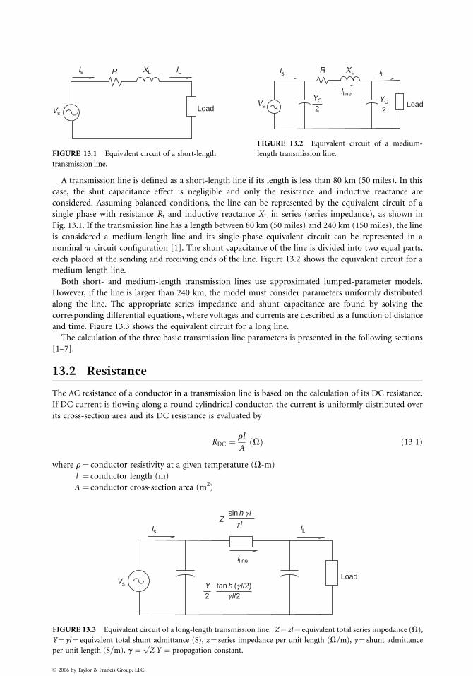
XLIs
Load
R
Vs
IL
FIGURE 13.1 Equivalent circuit of a short-length
transmission line.
XLIs
Load
R
Vs
IL
IlineYC
2YC
2
FIGURE 13.2 Equivalent circuit of a medium-
length transmission line.
Vs
Is
Z
tan2Y
FIGURE 13.3 Equivalent circuit of a long-length tran
Y¼ yl¼ equivalent total shunt admittance (S), z¼ ser
per unit length (S=m), g ¼ffiffiffiffiffiffiffiffi
Z Yp
¼ propagation con
� 2006 by Taylor & Francis Group, LLC.
A transmission line is defined as a short-length line if its length is less than 80 km (50 miles). In this
case, the shut capacitance effect is negligible and only the resistance and inductive reactance are
considered. Assuming balanced conditions, the line can be represented by the equivalent circuit of a
single phase with resistance R, and inductive reactance XL in series (series impedance), as shown in
Fig. 13.1. If the transmission line has a length between 80 km (50 miles) and 240 km (150 miles), the line
is considered a medium-length line and its single-phase equivalent circuit can be represented in a
nominal p circuit configuration [1]. The shunt capacitance of the line is divided into two equal parts,
each placed at the sending and receiving ends of the line. Figure 13.2 shows the equivalent circuit for a
medium-length line.
Both short- and medium-length transmission lines use approximated lumped-parameter models.
However, if the line is larger than 240 km, the model must consider parameters uniformly distributed
along the line. The appropriate series impedance and shunt capacitance are found by solving the
corresponding differential equations, where voltages and currents are described as a function of distance
and time. Figure 13.3 shows the equivalent circuit for a long line.
The calculation of the three basic transmission line parameters is presented in the following sections
[1–7].
13.2 Resistance
The AC resistance of a conductor in a transmission line is based on the calculation of its DC resistance.
If DC current is flowing along a round cylindrical conductor, the current is uniformly distributed over
its cross-section area and its DC resistance is evaluated by
RDC ¼rl
AVð Þ (13:1)
where r¼ conductor resistivity at a given temperature (V-m)
l ¼ conductor length (m)
A ¼ conductor cross-section area (m2)
Load
IL
Iline
sin h g l
h (g l/2)
g l
g l/2
smission line. Z¼ zl¼ equivalent total series impedance (V),
ies impedance per unit length (V=m), y¼ shunt admittance
stant.
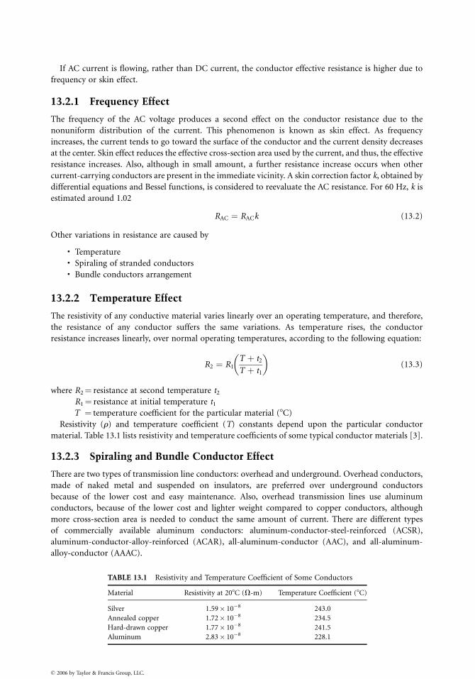
If AC current is flowing, rather than DC current, the conductor effective resistance is higher due to
frequency or skin effect.
13.2.1 Frequency Effect
The frequency of the AC voltage produces a second effect on the conductor resistance due to the
nonuniform distribution of the current. This phenomenon is known as skin effect. As frequency
increases, the current tends to go toward the surface of the conductor and the current density decreases
at the center. Skin effect reduces the effective cross-section area used by the current, and thus, the effective
resistance increases. Also, although in small amount, a further resistance increase occurs when other
current-carrying conductors are present in the immediate vicinity. A skin correction factor k, obtained by
differential equations and Bessel functions, is considered to reevaluate the AC resistance. For 60 Hz, k is
estimated around 1.02
RAC ¼ RACk (13:2)
Other variations in resistance are caused by
. Temperature
. Spiraling of stranded conductors
. Bundle conductors arrangement
13.2.2 Temperature Effect
The resistivity of any conductive material varies linearly over an operating temperature, and therefore,
the resistance of any conductor suffers the same variations. As temperature rises, the conductor
resistance increases linearly, over normal operating temperatures, according to the following equation:
R2 ¼ R1
T þ t2
T þ t1
� �
(13:3)
where R2¼ resistance at second temperature t2
R1¼ resistance at initial temperature t1
T ¼ temperature coefficient for the particular material (8C)
Resistivity (r) and temperature coefficient (T) constants depend upon the particular conductor
material. Table 13.1 lists resistivity and temperature coefficients of some typical conductor materials [3].
13.2.3 Spiraling and Bundle Conductor Effect
There are two types of transmission line conductors: overhead and underground. Overhead conductors,
made of naked metal and suspended on insulators, are preferred over underground conductors
because of the lower cost and easy maintenance. Also, overhead transmission lines use aluminum
conductors, because of the lower cost and lighter weight compared to copper conductors, although
more cross-section area is needed to conduct the same amount of current. There are different types
of commercially available aluminum conductors: aluminum-conductor-steel-reinforced (ACSR),
aluminum-conductor-alloy-reinforced (ACAR), all-aluminum-conductor (AAC), and all-aluminum-
alloy-conductor (AAAC).
TABLE 13.1 Resistivity and Temperature Coefficient of Some Conductors
Material Resistivity at 208C (V-m) Temperature Coefficient (8C)
Silver 1.59� 10�8 243.0
Annealed copper 1.72� 10�8 234.5
Hard-drawn copper 1.77� 10�8 241.5
Aluminum 2.83� 10�8 228.1
� 2006 by Taylor & Francis Group, LLC.
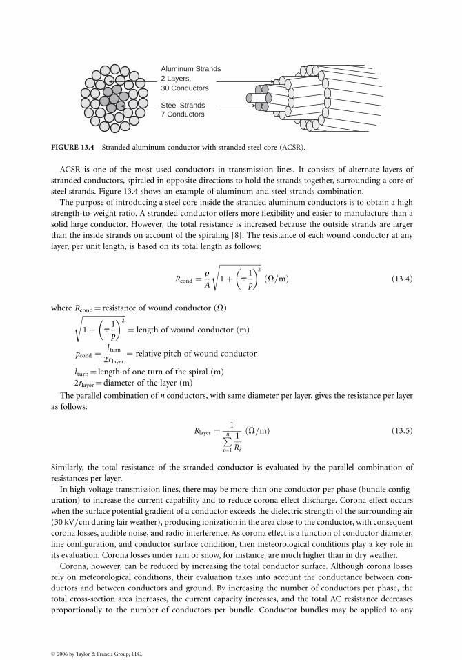
Aluminum Strands2 Layers, 30 Conductors
Steel Strands7 Conductors
FIGURE 13.4 Stranded aluminum conductor with stranded steel core (ACSR).
ACSR is one of the most used conductors in transmission lines. It consists of alternate layers of
stranded conductors, spiraled in opposite directions to hold the strands together, surrounding a core of
steel strands. Figure 13.4 shows an example of aluminum and steel strands combination.
The purpose of introducing a steel core inside the stranded aluminum conductors is to obtain a high
strength-to-weight ratio. A stranded conductor offers more flexibility and easier to manufacture than a
solid large conductor. However, the total resistance is increased because the outside strands are larger
than the inside strands on account of the spiraling [8]. The resistance of each wound conductor at any
layer, per unit length, is based on its total length as follows:
Rcond ¼r
A
ffiffiffiffiffiffiffiffiffiffiffiffiffiffiffiffiffiffiffiffiffiffiffi
1þ p1
p
� �2s
V=mð Þ (13:4)
where Rcond¼ resistance of wound conductor (V)ffiffiffiffiffiffiffiffiffiffiffiffiffiffiffiffiffiffiffiffiffiffiffiffi
1þ p1
p
� �2s
¼ length of wound conductor (m)
pcond ¼l turn
2r layer
¼ relative pitch of wound conductor
lturn¼ length of one turn of the spiral (m)
2rlayer¼diameter of the layer (m)
The parallel combination of n conductors, with same diameter per layer, gives the resistance per layer
as follows:
Rlayer ¼1
P
n
i¼1
1
Ri
V=mÞð (13:5)
Similarly, the total resistance of the stranded conductor is evaluated by the parallel combination of
resistances per layer.
In high-voltage transmission lines, there may be more than one conductor per phase (bundle config-
uration) to increase the current capability and to reduce corona effect discharge. Corona effect occurs
when the surface potential gradient of a conductor exceeds the dielectric strength of the surrounding air
(30 kV=cm during fair weather), producing ionization in the area close to the conductor, with consequent
corona losses, audible noise, and radio interference. As corona effect is a function of conductor diameter,
line configuration, and conductor surface condition, then meteorological conditions play a key role in
its evaluation. Corona losses under rain or snow, for instance, are much higher than in dry weather.
Corona, however, can be reduced by increasing the total conductor surface. Although corona losses
rely on meteorological conditions, their evaluation takes into account the conductance between con-
ductors and between conductors and ground. By increasing the number of conductors per phase, the
total cross-section area increases, the current capacity increases, and the total AC resistance decreases
proportionally to the number of conductors per bundle. Conductor bundles may be applied to any
� 2006 by Taylor & Francis Group, LLC.
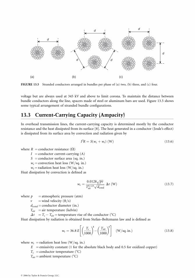
d
d
d
d
d
d
(a) (b) (c)
FIGURE 13.5 Stranded conductors arranged in bundles per phase of (a) two, (b) three, and (c) four.
voltage but are always used at 345 kV and above to limit corona. To maintain the distance between
bundle conductors along the line, spacers made of steel or aluminum bars are used. Figure 13.5 shows
some typical arrangement of stranded bundle configurations.
13.3 Current-Carrying Capacity (Ampacity)
In overhead transmission lines, the current-carrying capacity is determined mostly by the conductor
resistance and the heat dissipated from its surface [8]. The heat generated in a conductor (Joule’s effect)
is dissipated from its surface area by convection and radiation given by
I2R ¼ S(wc þ wr) Wð Þ (13:6)
where R ¼ conductor resistance (V)
I ¼ conductor current-carrying (A)
S ¼ conductor surface area (sq. in.)
wc¼ convection heat loss (W=sq. in.)
wr¼ radiation heat loss (W=sq. in.)
Heat dissipation by convection is defined as
wc ¼0:0128
ffiffiffiffiffi
pvp
T 0:123air
ffiffiffiffiffiffiffiffiffiffi
dcond
p Dt Wð Þ (13:7)
where p ¼ atmospheric pressure (atm)
v ¼wind velocity (ft=s)
dcond¼ conductor diameter (in.)
Tair ¼ air temperature (kelvin)
Dt ¼Tc�Tair¼ temperature rise of the conductor (8C)
Heat dissipation by radiation is obtained from Stefan–Boltzmann law and is defined as
wr ¼ 36:8 ETc
1000
� �4
� Tair
1000
� �4" #
W=sq: in:ð Þ (13:8)
where wr ¼ radiation heat loss (W=sq. in.)
E ¼ emissivity constant (1 for the absolute black body and 0.5 for oxidized copper)
Tc ¼ conductor temperature (8C)
Tair¼ ambient temperature (8C)
� 2006 by Taylor & Francis Group, LLC.
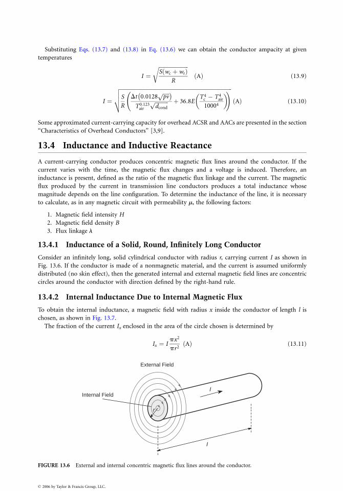
Substituting Eqs. (13.7) and (13.8) in Eq. (13.6) we can obtain the conductor ampacity at given
temperatures
I ¼ffiffiffiffiffiffiffiffiffiffiffiffiffiffiffiffiffiffiffiffiffiffi
S wc þ wrð ÞR
r
Að Þ (13:9)
I ¼
ffiffiffiffiffiffiffiffiffiffiffiffiffiffiffiffiffiffiffiffiffiffiffiffiffiffiffiffiffiffiffiffiffiffiffiffiffiffiffiffiffiffiffiffiffiffiffiffiffiffiffiffiffiffiffiffiffiffiffiffiffiffiffiffiffiffiffiffiffiffiffiffiffiffiffiffiffiffiffiffiffiffiffi
S
R
Dt 0:0128ffiffiffiffiffi
pvp� �
T 0:123air
ffiffiffiffiffiffiffiffiffiffi
dcond
p þ 36:8ET 4
c � T 4air
10004
� �
!
v
u
u
t Að Þ (13:10)
Some approximated current-carrying capacity for overhead ACSR and AACs are presented in the section
‘‘Characteristics of Overhead Conductors’’ [3,9].
13.4 Inductance and Inductive Reactance
A current-carrying conductor produces concentric magnetic flux lines around the conductor. If the
current varies with the time, the magnetic flux changes and a voltage is induced. Therefore, an
inductance is present, defined as the ratio of the magnetic flux linkage and the current. The magnetic
flux produced by the current in transmission line conductors produces a total inductance whose
magnitude depends on the line configuration. To determine the inductance of the line, it is necessary
to calculate, as in any magnetic circuit with permeability m, the following factors:
1. Magnetic field intensity H
2. Magnetic field density B
3. Flux linkage l
13.4.1 Inductance of a Solid, Round, Infinitely Long Conductor
Consider an infinitely long, solid cylindrical conductor with radius r, carrying current I as shown in
Fig. 13.6. If the conductor is made of a nonmagnetic material, and the current is assumed uniformly
distributed (no skin effect), then the generated internal and external magnetic field lines are concentric
circles around the conductor with direction defined by the right-hand rule.
13.4.2 Internal Inductance Due to Internal Magnetic Flux
To obtain the internal inductance, a magnetic field with radius x inside the conductor of length l is
chosen, as shown in Fig. 13.7.
The fraction of the current Ix enclosed in the area of the circle chosen is determined by
Ix ¼ Ipx2
pr2Að Þ (13:11)
I
IInternal Field
External Field
r
FIGURE 13.6 External and internal concentric magnetic flux lines around the conductor.
� 2006 by Taylor & Francis Group, LLC.
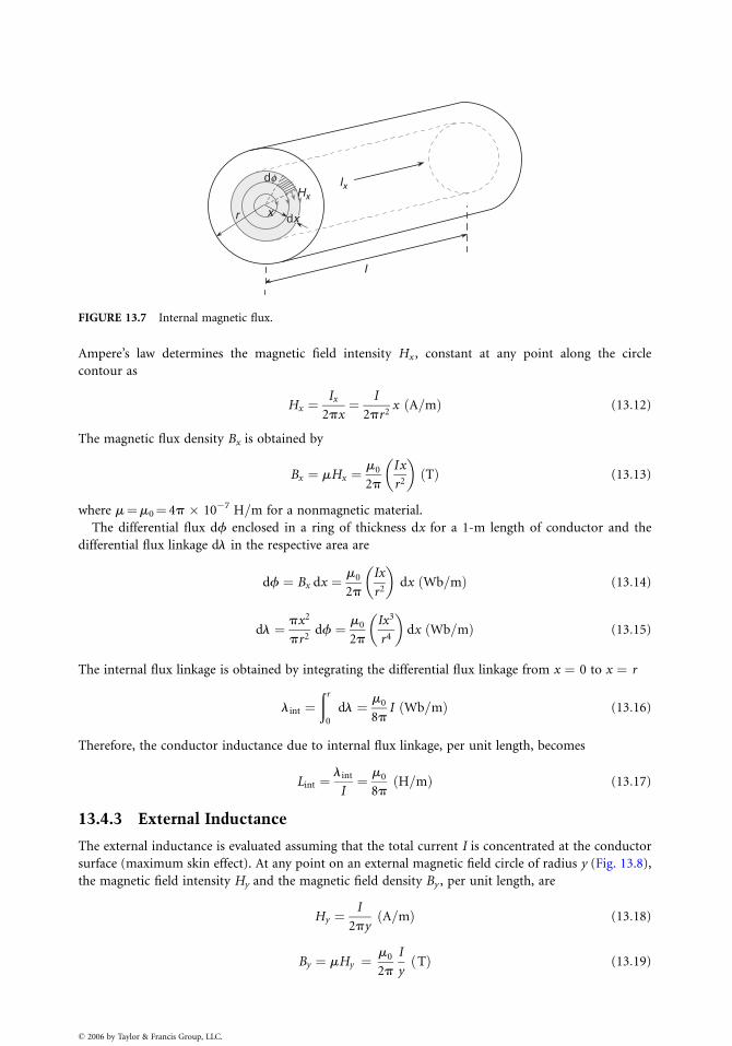
df
x
I
r
Hx
Ix
dx
FIGURE 13.7 Internal magnetic flux.
Ampere’s law determines the magnetic field intensity Hx , constant at any point along the circle
contour as
Hx ¼Ix
2px¼ I
2pr2x A=mð Þ (13:12)
The magnetic flux density Bx is obtained by
Bx ¼ mHx ¼m0
2p
Ix
r2
� �
Tð Þ (13:13)
where m¼m0¼ 4p � 10�7 H=m for a nonmagnetic material.
The differential flux df enclosed in a ring of thickness dx for a 1-m length of conductor and the
differential flux linkage dl in the respective area are
df ¼ Bx dx ¼ m0
2p
Ix
r2
� �
dx Wb=mð Þ (13:14)
dl ¼ px2
pr2df ¼ m0
2p
Ix3
r4
� �
dx Wb=mð Þ (13:15)
The internal flux linkage is obtained by integrating the differential flux linkage from x ¼ 0 to x ¼ r
lint ¼ðr
0
dl ¼ m0
8pI Wb=mð Þ (13:16)
Therefore, the conductor inductance due to internal flux linkage, per unit length, becomes
Lint ¼lint
I¼ m0
8pH=mð Þ (13:17)
13.4.3 External Inductance
The external inductance is evaluated assuming that the total current I is concentrated at the conductor
surface (maximum skin effect). At any point on an external magnetic field circle of radius y (Fig. 13.8),
the magnetic field intensity Hy and the magnetic field density By , per unit length, are
Hy ¼I
2pyA=mð Þ (13:18)
By ¼ mHy ¼m0
2p
I
yTð Þ (13:19)
� 2006 by Taylor & Francis Group, LLC.
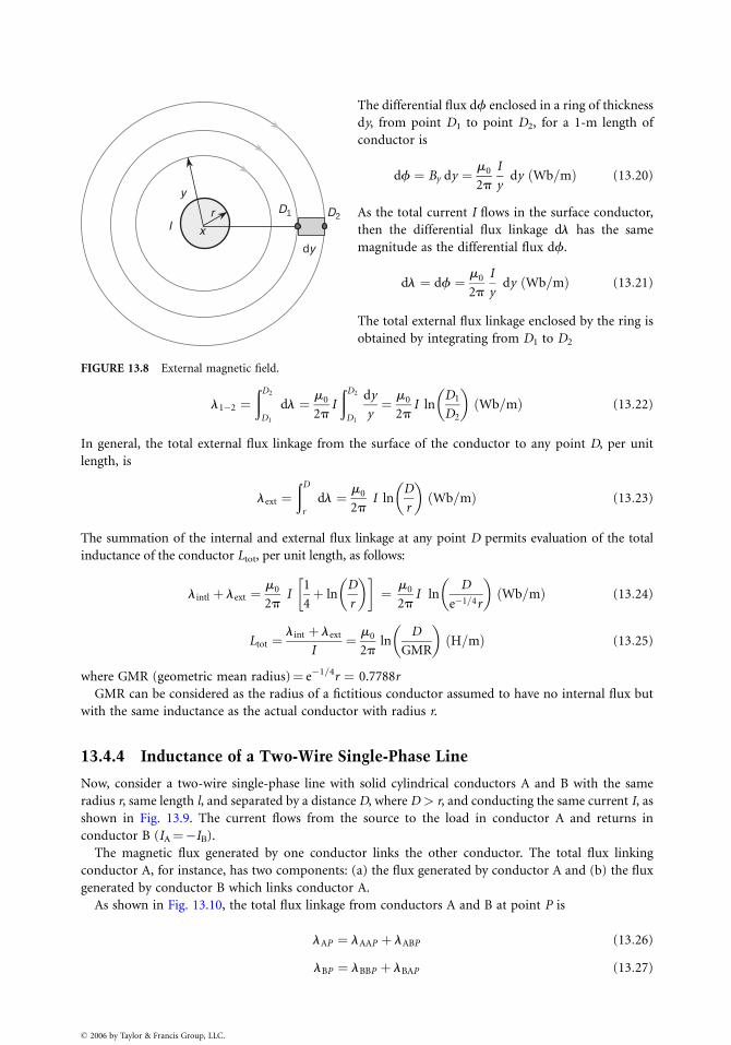
Ir
dy
y
D2D1
x
� 2006 by Taylor & Francis Group, LLC.
The differential flux df enclosed in a ring of thickness
dy, from point D1 to point D2, for a 1-m length of
conductor is
df ¼ By dy ¼ m0
2p
I
ydy Wb=mð Þ (13:20)
As the total current I flows in the surface conductor,
then the differential flux linkage dl has the same
magnitude as the differential flux df.
dl ¼ df ¼ m0
2p
I
ydy Wb=mð Þ (13:21)
The total external flux linkage enclosed by the ring is
obtained by integrating from D1 to D2
l1�2 ¼ðD2
D1
dl ¼ m0
2pI
ðD2
D1
dy
y¼ m0
2pI ln
D1
D2
� �
Wb=mð Þ (13:22)
In general, the total external flux linkage from the surface of the conductor to any point D, per unit
length, is
lext ¼ðD
r
dl ¼ m0
2pI ln
D
r
� �
Wb=mð Þ (13:23)
The summation of the internal and external flux linkage at any point D permits evaluation of the total
inductance of the conductor Ltot, per unit length, as follows:
lintl þ lext ¼m0
2pI
1
4þ ln
D
r
� �� �
¼ m0
2pI ln
D
e�1=4r
� �
Wb=mð Þ (13:24)
Ltot ¼lint þ lext
I¼ m0
2pln
D
GMR
� �
H=mð Þ (13:25)
where GMR (geometric mean radius)¼ e�1=4r ¼ 0.7788r
GMR can be considered as the radius of a fictitious conductor assumed to have no internal flux but
with the same inductance as the actual conductor with radius r.
FIGURE 13.8 External magnetic field.
13.4.4 Inductance of a Two-Wire Single-Phase Line
Now, consider a two-wire single-phase line with solid cylindrical conductors A and B with the same
radius r, same length l, and separated by a distance D, where D > r, and conducting the same current I, as
shown in Fig. 13.9. The current flows from the source to the load in conductor A and returns in
conductor B (IA¼�IB).
The magnetic flux generated by one conductor links the other conductor. The total flux linking
conductor A, for instance, has two components: (a) the flux generated by conductor A and (b) the flux
generated by conductor B which links conductor A.
As shown in Fig. 13.10, the total flux linkage from conductors A and B at point P is
lAP ¼ lAAP þ lABP (13:26)
lBP ¼ lBBP þ lBAP (13:27)
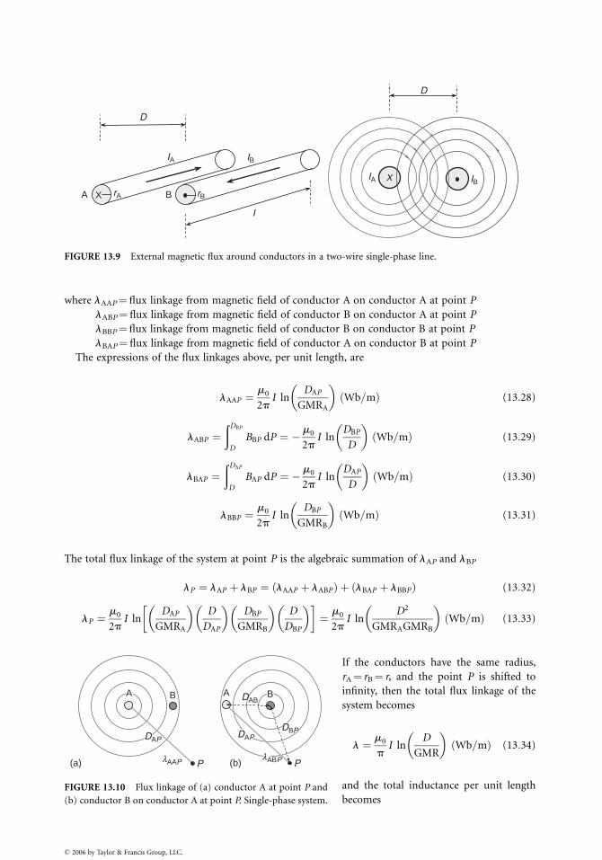
rA
X
rB
D
BA
IBIA
I
IBIA
X
D
FIGURE 13.9 External magnetic flux around conductors in a two-wire single-phase line.
where lAAP¼ flux linkage from magnetic field of conductor A on conductor A at point P
lABP¼ flux linkage from magnetic field of conductor B on conductor A at point P
lBBP¼flux linkage from magnetic field of conductor B on conductor B at point P
lBAP¼ flux linkage from magnetic field of conductor A on conductor B at point P
The expressions of the flux linkages above, per unit length, are
lAAP ¼m0
2pI ln
DAP
GMRA
� �
Wb=mð Þ (13:28)
lABP ¼ðDBP
D
BBP dP ¼ � m0
2pI ln
DBP
D
� �
Wb=mð Þ (13:29)
lBAP ¼ðDAP
D
BAP dP ¼ � m0
2pI ln
DAP
D
� �
Wb=mð Þ (13:30)
lBBP ¼m0
2pI ln
DBP
GMRB
� �
Wb=mð Þ (13:31)
The total flux linkage of the system at point P is the algebraic summation of lAP and lBP
lP ¼ lAP þ lBP ¼ lAAP þ lABPð Þ þ lBAP þ lBBPð Þ (13:32)
lP ¼m0
2pI ln
DAP
GMRA
� �
D
DAP
� �
DBP
GMRB
� �
D
DBP
� �� �
¼ m0
2pI ln
D2
GMRAGMRB
� �
Wb=mð Þ (13:33)
B
(a) (b)P
DAP
A
P
DBP
DAB
lABPlAAP
DAP
A B
FIGURE 13.10 Flux linkage of (a) conductor A at point P and
(b) conductor B on conductor A at point P. Single-phase system.
� 2006 by Taylor & Francis Group, LLC.
If the conductors have the same radius,
rA¼ rB¼ r, and the point P is shifted to
infinity, then the total flux linkage of the
system becomes
l ¼ m0
pI ln
D
GMR
� �
Wb=mð Þ (13:34)
and the total inductance per unit length
becomes
L1-phase system ¼l
I¼ m0
pln
D
GMR
� �
H=mð Þ (13:35)
Comparing Eqs. (13.25) and (13.35), it can be seen that the inductance of the single-phase system is
twice the inductance of a single conductor.
For a line with stranded conductors, the inductance is determined using a new GMR value
named GMRstranded, evaluated according to the number of conductors. If conductors A and B in the
single-phase system, are formed by n and m solid cylindrical identical subconductors in parallel, respect-
ively, then
GMRA stranded ¼
ffiffiffiffiffiffiffiffiffiffiffiffiffiffiffiffiffiffiffiffi
Y
n
i¼1
Y
n
j¼1
Dijn 2
v
u
u
t (13:36)
GMRB stranded ¼
ffiffiffiffiffiffiffiffiffiffiffiffiffiffiffiffiffiffiffiffi
Y
m
i¼1
Y
m
j¼1
Dijm 2
v
u
u
t (13:37)
Generally, the GMRstranded for a particular cable can be found in conductor tables given by the
manufacturer.
If the line conductor is composed of bundle conductors, the inductance is reevaluated taking
into account the number of bundle conductors and the separation among them. The GMRbundle is
introduced to determine the final inductance value. Assuming the same separation among bundle
conductors, the equation for GMRbundle, up to three conductors per bundle, is defined as
GMRn bundle conductors ¼ffiffiffiffiffiffiffiffiffiffiffiffiffiffiffiffiffiffiffiffiffiffiffiffiffiffiffiffiffiffiffiffi
dn�1GMRstrandednp
(13:38)
where n¼ number of conductors per bundle
GMRstranded¼GMR of the stranded conductor
d¼ distance between bundle conductors
For four conductors per bundle with the same separation between consecutive conductors, the
GMRbundle is evaluated as
GMR4 bundle conductors ¼ 1:09ffiffiffiffiffiffiffiffiffiffiffiffiffiffiffiffiffiffiffiffiffiffiffiffiffiffiffiffi
d3GMRstranded4p
(13:39)
13.4.5 Inductance of a Three-Phase Line
The derivations for the inductance in a single-phase system can be extended to obtain the inductance per
phase in a three-phase system. Consider a three-phase, three-conductor system with solid cylindrical
conductors with identical radius rA, rB, and rC, placed horizontally with separation DAB, DBC, and DCA
(where D > r) among them. Corresponding currents IA, IB, and IC flow along each conductor as shown
in Fig. 13.11.
The total magnetic flux enclosing conductor A at a point P away from the conductors is the sum of the
flux produced by conductors A, B, and C as follows:
fAP ¼ fAAP þ fABP þ fACP (13:40)
where fAAP¼flux produced by current IA on conductor A at point P
fABP¼ flux produced by current IB on conductor A at point P
fACP¼ flux produced by current IC on conductor A at point P
Considering 1-m length for each conductor, the expressions for the fluxes above are
� 2006 by Taylor & Francis Group, LLC.
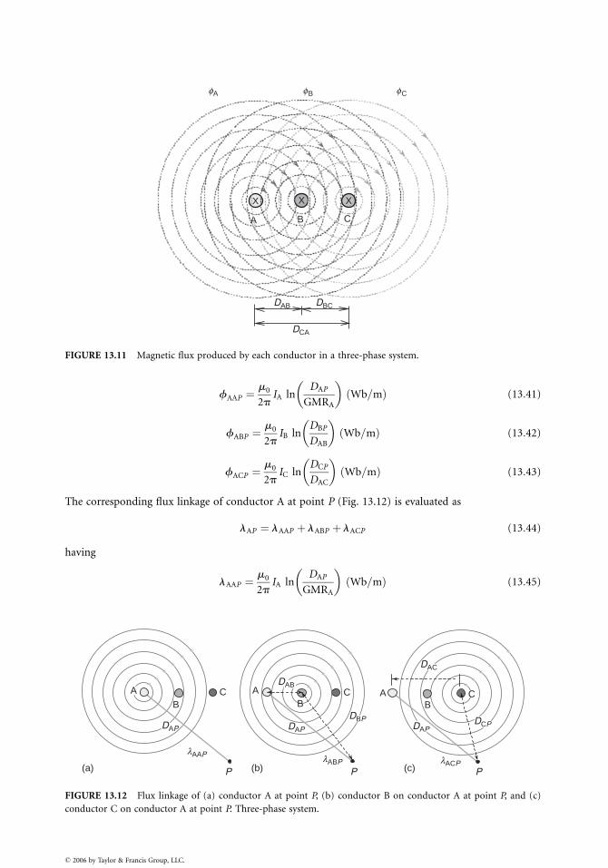
A B C
fA f B f C
DAB DBC
DCA
X X X
FIGURE 13.11 Magnetic flux produced by each conductor in a three-phase system.
fAAP ¼m0
2pIA ln
DAP
GMRA
� �
Wb=mð Þ (13:41)
fABP ¼m0
2pIB ln
DBP
DAB
� �
Wb=mð Þ (13:42)
fACP ¼m0
2pIC ln
DCP
DAC
� �
Wb=mð Þ (13:43)
The corresponding flux linkage of conductor A at point P (Fig. 13.12) is evaluated as
lAP ¼ lAAP þ lABP þ lACP (13:44)
having
lAAP ¼m0
2pIA ln
DAP
GMRA
� �
Wb=mð Þ (13:45)
C
DAP
B
P
lAAP lABP lACPP P
DAC
DAP DAPDCP
DBP
A AB B
C C
(a) (b) (c)
ADAB
FIGURE 13.12 Flux linkage of (a) conductor A at point P, (b) conductor B on conductor A at point P, and (c)
conductor C on conductor A at point P. Three-phase system.
� 2006 by Taylor & Francis Group, LLC.
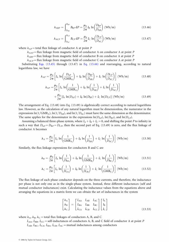
lABP ¼ðDBP
DAB
BBP dP ¼ m0
2pIB ln
DBP
DAB
� �
Wb=mð Þ (13:46)
lACP ¼ðDCP
DAC
BCP dP ¼ m0
2pIC ln
DCP
DAC
� �
Wb=mð Þ (13:47)
where lAP¼ total flux linkage of conductor A at point P
lAAP¼flux linkage from magnetic field of conductor A on conductor A at point P
lABP¼ flux linkage from magnetic field of conductor B on conductor A at point P
lACP¼ flux linkage from magnetic field of conductor C on conductor A at point P
Substituting Eqs. (13.45) through (13.47) in Eq. (13.44) and rearranging, according to natural
logarithms law, we have
lAP ¼m0
2pIA ln
DAP
GMRA
� �
þ IB lnDBP
DAB
� �
þ IC lnDCP
DAC
� �� �
Wb=mð Þ (13:48)
lAP ¼m0
2pIA ln
1
GMRA
� �
þ IB ln1
DAB
� �
þ IC ln1
DAC
� �� �
þ m0
2pIA ln DAPð Þ þ IB ln DBPð Þ þ IC ln DCPð Þ½ � Wb=mð Þ (13:49)
The arrangement of Eq. (13.48) into Eq. (13.49) is algebraically correct according to natural logarithms
law. However, as the calculation of any natural logarithm must be dimensionless, the numerator in the
expressions ln(1=GMRA), ln(1=DAB), and ln(1=DAC) must have the same dimension as the denominator.
The same applies for the denominator in the expressions ln(DAP), ln(DBP), and ln(DCP).
Assuming a balanced three-phase system, where IAþ IBþ IC¼ 0, and shifting the point P to infinity in
such a way that DAP¼DBP¼DCP, then the second part of Eq. (13.49) is zero, and the flux linkage of
conductor A becomes
lA ¼m0
2pIA ln
1
GMRA
� �
þ IB ln1
DAB
� �
þ IC ln1
DAC
� �� �
Wb=mð Þ (13:50)
Similarly, the flux linkage expressions for conductors B and C are
lB ¼m0
2pIA ln
1
DBA
� �
þ IB ln1
GMRB
� �
þ IC ln1
DBC
� �� �
Wb=mð Þ (13:51)
lC ¼m0
2pIA ln
1
DCA
� �
þ IB ln1
DCB
� �
þ IC ln1
GMRC
� �� �
Wb=mð Þ (13:52)
The flux linkage of each phase conductor depends on the three currents, and therefore, the inductance
per phase is not only one as in the single-phase system. Instead, three different inductances (self and
mutual conductor inductances) exist. Calculating the inductance values from the equations above and
arranging the equations in a matrix form we can obtain the set of inductances in the system
lA
lB
lC
2
4
3
5 ¼LAA LAB LAC
LBA LBB LBC
LCA LCB LCC
2
4
3
5
IA
IB
IC
2
4
3
5
(13:53)
where lA, lB, lC¼ total flux linkages of conductors A, B, and C
LAA, LBB, LCC¼ self-inductances of conductors A, B, and C field of conductor A at point P
LAB, LBC, LCA, LBA, LCB, LAC¼mutual inductances among conductors
� 2006 by Taylor & Francis Group, LLC.
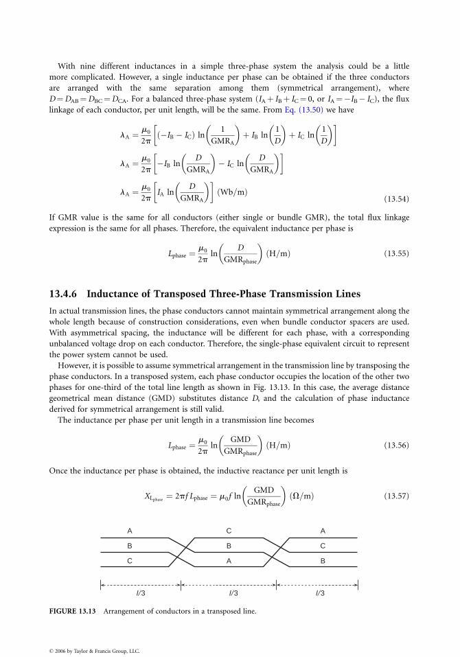
With nine different inductances in a simple three-phase system the analysis could be a little
more complicated. However, a single inductance per phase can be obtained if the three conductors
are arranged with the same separation among them (symmetrical arrangement), where
D¼DAB¼DBC¼DCA. For a balanced three-phase system (IAþ IBþ IC¼ 0, or IA¼�IB� IC), the flux
linkage of each conductor, per unit length, will be the same. From Eq. (13.50) we have
lA ¼m0
2p�IB � ICð Þ ln
1
GMRA
� �
þ IB ln1
D
� �
þ IC ln1
D
� �� �
lA ¼m0
2p�IB ln
D
GMRA
� �
� IC lnD
GMRA
� �� �
lA ¼m0
2pIA ln
D
GMRA
� �� �
Wb=mð Þ(13:54)
If GMR value is the same for all conductors (either single or bundle GMR), the total flux linkage
expression is the same for all phases. Therefore, the equivalent inductance per phase is
Lphase ¼m0
2pln
D
GMRphase
� �
H=mð Þ (13:55)
13.4.6 Inductance of Transposed Three-Phase Transmission Lines
In actual transmission lines, the phase conductors cannot maintain symmetrical arrangement along the
whole length because of construction considerations, even when bundle conductor spacers are used.
With asymmetrical spacing, the inductance will be different for each phase, with a corresponding
unbalanced voltage drop on each conductor. Therefore, the single-phase equivalent circuit to represent
the power system cannot be used.
However, it is possible to assume symmetrical arrangement in the transmission line by transposing the
phase conductors. In a transposed system, each phase conductor occupies the location of the other two
phases for one-third of the total line length as shown in Fig. 13.13. In this case, the average distance
geometrical mean distance (GMD) substitutes distance D, and the calculation of phase inductance
derived for symmetrical arrangement is still valid.
The inductance per phase per unit length in a transmission line becomes
Lphase ¼m0
2pln
GMD
GMRphase
� �
H=mð Þ (13:56)
Once the inductance per phase is obtained, the inductive reactance per unit length is
XLphase¼ 2pf Lphase ¼ m0f ln
GMD
GMRphase
� �
V=mð Þ (13:57)
A
B
C
C
B
A
A
C
B
l/ 3 l/ 3 l/ 3
FIGURE 13.13 Arrangement of conductors in a transposed line.
� 2006 by Taylor & Francis Group, LLC.
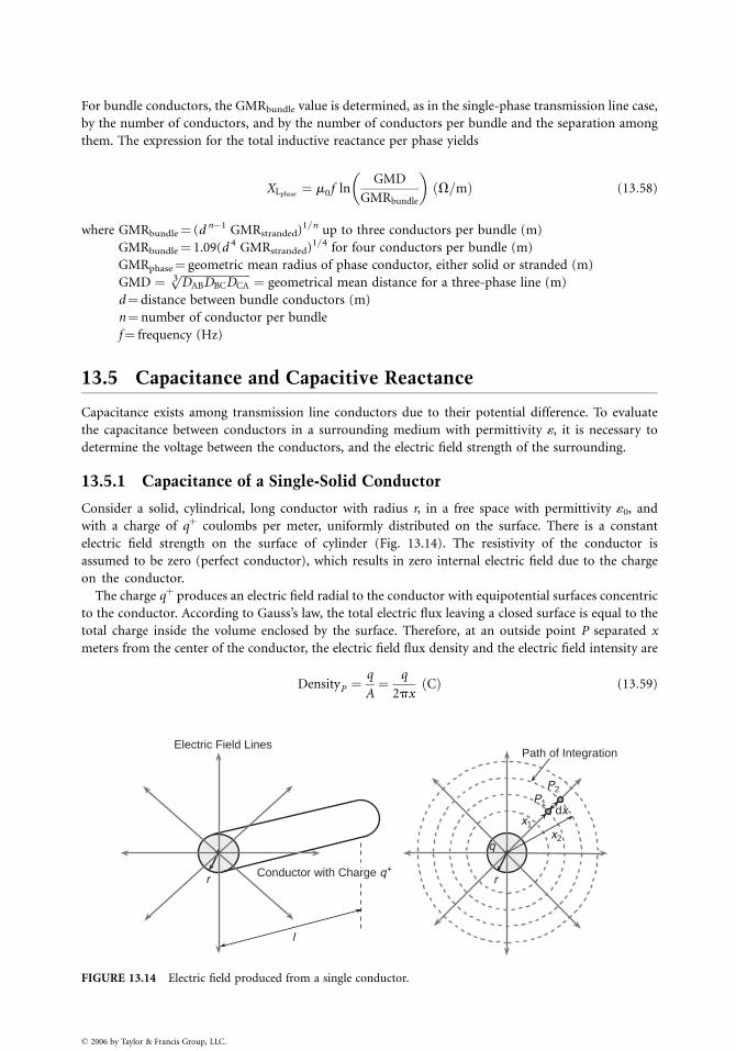
For bundle conductors, the GMRbundle value is determined, as in the single-phase transmission line case,
by the number of conductors, and by the number of conductors per bundle and the separation among
them. The expression for the total inductive reactance per phase yields
XLphase¼ m0f ln
GMD
GMRbundle
� �
V=mð Þ (13:58)
where GMRbundle¼ (d n�1 GMRstranded)1=n up to three conductors per bundle (m)
GMRbundle¼ 1.09(d 4 GMRstranded)1=4 for four conductors per bundle (m)
GMRphase¼ geometric mean radius of phase conductor, either solid or stranded (m)
GMD ¼ffiffiffiffiffiffiffiffiffiffiffiffiffiffiffiffiffiffiffiffiffiffiffiffi
DABDBCDCA3p
¼ geometrical mean distance for a three-phase line (m)
d¼ distance between bundle conductors (m)
n¼ number of conductor per bundle
f¼ frequency (Hz)
13.5 Capacitance and Capacitive Reactance
Capacitance exists among transmission line conductors due to their potential difference. To evaluate
the capacitance between conductors in a surrounding medium with permittivity «, it is necessary to
determine the voltage between the conductors, and the electric field strength of the surrounding.
13.5.1 Capacitance of a Single-Solid Conductor
Consider a solid, cylindrical, long conductor with radius r, in a free space with permittivity «0, and
with a charge of qþ coulombs per meter, uniformly distributed on the surface. There is a constant
electric field strength on the surface of cylinder (Fig. 13.14). The resistivity of the conductor is
assumed to be zero (perfect conductor), which results in zero internal electric field due to the charge
on the conductor.
The charge qþ produces an electric field radial to the conductor with equipotential surfaces concentric
to the conductor. According to Gauss’s law, the total electric flux leaving a closed surface is equal to the
total charge inside the volume enclosed by the surface. Therefore, at an outside point P separated x
meters from the center of the conductor, the electric field flux density and the electric field intensity are
DensityP ¼q
A¼ q
2pxCð Þ (13:59)
r
P1
P2
++
dx
l
r
x1x2
Electric Field LinesPath of Integration
Conductor with Charge q+
q
FIGURE 13.14 Electric field produced from a single conductor.
� 2006 by Taylor & Francis Group, LLC.
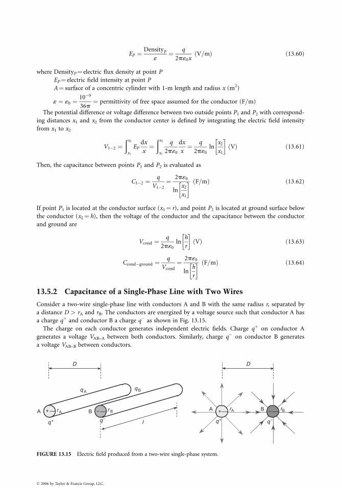
EP ¼DensityP
«¼ q
2p«0xV=mð Þ (13:60)
where DensityP¼ electric flux density at point P
EP¼ electric field intensity at point P
A¼ surface of a concentric cylinder with 1-m length and radius x (m2)
« ¼ «0 ¼10�9
36p¼ permittivity of free space assumed for the conductor (F=m)
The potential difference or voltage difference between two outside points P1 and P2 with correspond-
ing distances x1 and x2 from the conductor center is defined by integrating the electric field intensity
from x1 to x2
V1�2 ¼ðx2
x1
EP
dx
x¼ðx2
x1
q
2p«0
dx
x¼ q
2p«0
lnx2
x1
� �
Vð Þ (13:61)
Then, the capacitance between points P1 and P2 is evaluated as
C1�2 ¼q
V1�2
¼ 2p«0
lnx2
x1
� � F=mð Þ (13:62)
If point P1 is located at the conductor surface (x1¼ r), and point P2 is located at ground surface below
the conductor (x2¼ h), then the voltage of the conductor and the capacitance between the conductor
and ground are
Vcond ¼q
2p«0
lnh
r
� �
Vð Þ (13:63)
Ccond�ground ¼q
Vcond
¼ 2p«0
lnh
r
� � F=mð Þ (13:64)
13.5.2 Capacitance of a Single-Phase Line with Two Wires
Consider a two-wire single-phase line with conductors A and B with the same radius r, separated by
a distance D > rA and rB. The conductors are energized by a voltage source such that conductor A has
a charge qþ and conductor B a charge q� as shown in Fig. 13.15.
The charge on each conductor generates independent electric fields. Charge qþ on conductor A
generates a voltage VAB–A between both conductors. Similarly, charge q� on conductor B generates
a voltage VAB–B between conductors.
l
r A r B
D
BA
q A
+ −
q B
rA rBBA + -
D
q+ q− q+ q−
−
FIGURE 13.15 Electric field produced from a two-wire single-phase system.
� 2006 by Taylor & Francis Group, LLC.
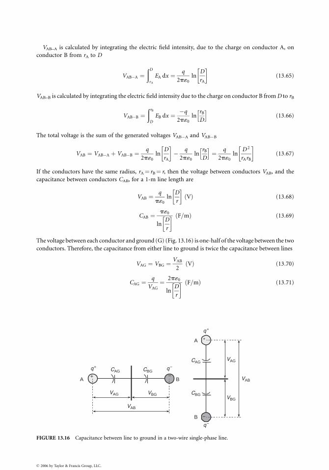
VAB–A is calculated by integrating the electric field intensity, due to the charge on conductor A, on
conductor B from rA to D
VAB�A ¼ðD
rA
EA dx ¼ q
2p«0
lnD
rA
� �
(13:65)
VAB–B is calculated by integrating the electric field intensity due to the charge on conductor B from D to rB
VAB�B ¼ðrB
D
EB dx ¼ �q
2p«0
lnrB
D
h i
(13:66)
The total voltage is the sum of the generated voltages VAB�A and VAB�B
VAB ¼ VAB�A þ VAB�B ¼q
2p«0
lnD
rA
� �
� q
2p«0
lnrB
D
h i
¼ q
2p«0
lnD 2
rArB
� �
(13:67)
If the conductors have the same radius, rA¼ rB¼ r, then the voltage between conductors VAB, and the
capacitance between conductors CAB, for a 1-m line length are
VAB ¼q
p«0
lnD
r
� �
Vð Þ (13:68)
CAB ¼p«0
lnD
r
� � F=mð Þ (13:69)
The voltage between each conductor and ground (G) (Fig. 13.16) is one-half of the voltage between the two
conductors. Therefore, the capacitance from either line to ground is twice the capacitance between lines
VAG ¼ VBG ¼VAB
2Vð Þ (13:70)
CAG ¼q
VAG
¼ 2p«0
lnD
r
� � F=mð Þ (13:71)
CAG
A
CBG
VAG VBG
VAB
+
q−
q−
q+
q+
−B
VBG
VAG
VAB
CAG
CBG
B
A
−
FIGURE 13.16 Capacitance between line to ground in a two-wire single-phase line.
� 2006 by Taylor & Francis Group, LLC.
13.5.3 Capacitance of a Three-Phase Line
Consider a three-phase line with the same voltage magnitude between phases, and assuming a balanced
system with abc (positive) sequence such that qAþ qBþ qC¼ 0. The conductors have radii rA, rB, and rC,
and the space between conductors are DAB, DBC, and DAC (where DAB, DBC, and DAC > rA, rB, and rC).
Also, the effect of earth and neutral conductors is neglected.
The expression for voltages between two conductors in a single-phase system can be extended to
obtain the voltages between conductors in a three-phase system. The expressions for VAB and VAC are
VAB ¼1
2p«0
qA lnDAB
rA
� �
þ qB lnrB
DAB
� �
þ qC lnDBC
DAC
� �� �
Vð Þ (13:72)
VAC ¼1
2p«0
qA lnDCA
rA
� �
þ qB lnDBC
DAB
� �
þ qC lnrC
DAC
� �� �
Vð Þ (13:73)
If the three-phase system has triangular arrangement with equidistant conductors such
that DAB¼DBC¼DAC¼D, with the same radii for the conductors such that rA¼ rB¼ rC¼ r (where
D > r), the expressions for VAB and VAC are
VAB ¼1
2p«0
qA ln
"
D
r
#
þ qB ln
"
r
D
#
þ qC ln
"
D
D
#" #
¼ 1
2p«0
qA ln
"
D
r
#
þ qB ln
"
r
D
#" #
Vð Þ (13:74)
VAC ¼1
2p«0
qA ln
"
D
r
#
þ qB ln
"
D
D
#
þ qC ln
"
r
D
#" #
¼ 1
2p«0
qA ln
"
D
r
#
þ qC ln
"
r
D
#" #
Vð Þ (13:75)
Balanced line-to-line voltages with sequence abc, expressed in terms of the line-to-neutral voltage are
VAB ¼ffiffiffi
3p
VAN ff 30� and VAC ¼ �VCA ¼ffiffiffi
3p
VAN ff �30�;
where VAN is the line-to-neutral voltage. Therefore, VAN can be expressed in terms of VAB and VAC as
VAN ¼VAB þ VAC
3(13:76)
and thus, substituting VAB and VAC from Eqs. (13.67) and (13.68) we have
VAN ¼1
6p«0
qA ln
"
D
r
#
þ qB ln
"
r
D
#" #
þ qA ln
"
D
r
#
þ qC ln
"
r
D
#" #" #
¼ 1
6p«0
2qA ln
"
D
r
#
þ qB þ qC
!
ln
"
r
D
# #
Vð Þ"
(13:77)
Under balanced conditions qAþ qBþ qC¼ 0, or �qA¼ (qBþ qC ) then, the final expression for the line-
to-neutral voltage is
VAN ¼1
2p«0
qA lnD
r
� �
Vð Þ (13:78)
� 2006 by Taylor & Francis Group, LLC.
The positive sequence capacitance per unit length between phase A and neutral can now be obtained.
The same result is obtained for capacitance between phases B and C to neutral
CAN ¼qA
VAN
¼ 2p«0
lnD
r
� � F=mð Þ (13:79)
13.5.4 Capacitance of Stranded Bundle Conductors
The calculation of the capacitance in the equation above is based on
1. Solid conductors with zero resistivity (zero internal electric field)
2. Charge uniformly distributed
3. Equilateral spacing of phase conductors
In actual transmission lines, the resistivity of the conductors produces a small internal electric field and
therefore, the electric field at the conductor surface is smaller than the estimated. However, the
difference is negligible for practical purposes.
Because of the presence of other charged conductors, the charge distribution is nonuniform, and
therefore the estimated capacitance is different. However, this effect is negligible for most practical
calculations. In a line with stranded conductors, the capacitance is evaluated assuming a solid conductor
with the same radius as the outside radius of the stranded conductor. This produces a negligible
difference.
Most transmission lines do not have equilateral spacing of phase conductors. This causes differences
between the line-to-neutral capacitances of the three phases. However, transposing the phase conductors
balances the system resulting in equal line-to-neutral capacitance for each phase and is developed in the
following manner.
Consider a transposed three-phase line with conductors having the same radius r, and with space
between conductors DAB, DBC, and DAC , where DAB, DBC, and DAC > r.
Assuming abc positive sequence, the expressions for VAB on the first, second, and third section of the
transposed line are
VAB first ¼1
2p«0
qA lnDAB
r
� �
þ qB lnr
DAB
� �
þ qC lnDAB
DAC
� �� �
Vð Þ (13:80)
VAB second ¼1
2p«0
qA lnDBC
r
� �
þ qB lnr
DBC
� �
þ qC lnDAC
DAB
� �� �
Vð Þ (13:81)
VAB third ¼1
2p«0
qA lnDAC
r
� �
þ qB lnr
DAC
� �
þ qC lnDAB
DBC
� �� �
Vð Þ (13:82)
Similarly, the expressions for VAC on the first, second, and third section of the transposed line are
VAC first ¼1
2p«0
qA lnDAC
r
� �
þ qB lnDBC
DAB
� �
þ qC lnr
DAC
� �� �
(13:83)
VAC second ¼1
2p«0
qA lnDAB
r
� �
þ qB lnDAC
DBC
� �
þ qC lnr
DAB
� �� �
(13:84)
VAC third ¼1
2p«0
qA lnDBC
r
� �
þ qB lnDAB
DAC
� �
þ qC lnr
DBC
� �� �
(13:85)
Taking the average value of the three sections, we have the final expressions of VAB and VAC in the
transposed line
� 2006 by Taylor & Francis Group, LLC.
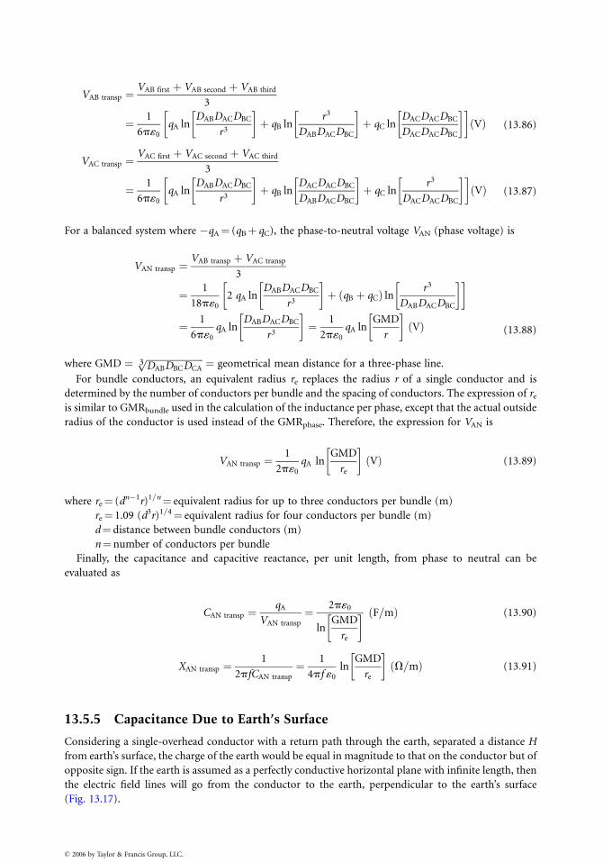
VAB transp ¼VAB first þ VAB second þ VAB third
3
¼ 1
6p«0
qA lnDABDACDBC
r3
� �
þ qB lnr3
DABDACDBC
� �
þ qC lnDACDACDBC
DACDACDBC
� �� �
Vð Þ (13:86)
VAC transp ¼VAC first þ VAC second þ VAC third
3
¼ 1
6p«0
qA lnDABDACDBC
r3
� �
þ qB lnDACDACDBC
DABDACDBC
� �
þ qC lnr3
DACDACDBC
� �� �
Vð Þ (13:87)
For a balanced system where �qA¼ (qBþ qC), the phase-to-neutral voltage VAN (phase voltage) is
VAN transp ¼VAB transp þ VAC transp
3
¼ 1
18p«0
2 qA lnDABDACDBC
r3
� �
þ qB þ qCð Þ lnr3
DABDACDBC
� �� �
¼ 1
6p«0
qA lnDABDACDBC
r3
� �
¼ 1
2p«0
qA lnGMD
r
� �
Vð Þ (13:88)
where GMD ¼ ffiffiffiffiffiffiffiffiffiffiffiffiffiffiffiffiffiffiffiffiffiffiffiffi
DABDBCDCA3p ¼ geometrical mean distance for a three-phase line.
For bundle conductors, an equivalent radius re replaces the radius r of a single conductor and is
determined by the number of conductors per bundle and the spacing of conductors. The expression of re
is similar to GMRbundle used in the calculation of the inductance per phase, except that the actual outside
radius of the conductor is used instead of the GMRphase. Therefore, the expression for VAN is
VAN transp ¼1
2p«0
qA lnGMD
re
� �
Vð Þ (13:89)
where re¼ (dn�1r)1=n¼ equivalent radius for up to three conductors per bundle (m)
re¼ 1.09 (d3r)1=4¼ equivalent radius for four conductors per bundle (m)
d¼ distance between bundle conductors (m)
n¼ number of conductors per bundle
Finally, the capacitance and capacitive reactance, per unit length, from phase to neutral can be
evaluated as
CAN transp ¼qA
VAN transp
¼ 2p«0
lnGMD
re
� � F=mð Þ (13:90)
XAN transp ¼1
2pfCAN transp
¼ 1
4pf «0
lnGMD
re
� �
V=mð Þ (13:91)
13.5.5 Capacitance Due to Earth’s Surface
Considering a single-overhead conductor with a return path through the earth, separated a distance H
from earth’s surface, the charge of the earth would be equal in magnitude to that on the conductor but of
opposite sign. If the earth is assumed as a perfectly conductive horizontal plane with infinite length, then
the electric field lines will go from the conductor to the earth, perpendicular to the earth’s surface
(Fig. 13.17).
� 2006 by Taylor & Francis Group, LLC.
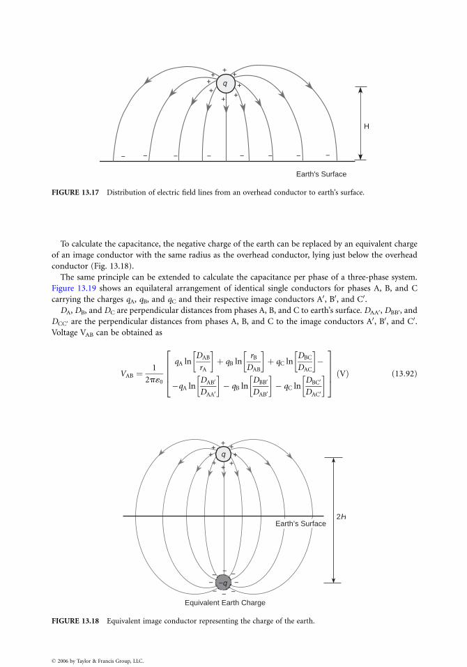
− − −
+
Earth's Surface
H
+
+++
+
++ q
− − − −−
FIGURE 13.17 Distribution of electric field lines from an overhead conductor to earth’s surface.
To calculate the capacitance, the negative charge of the earth can be replaced by an equivalent charge
of an image conductor with the same radius as the overhead conductor, lying just below the overhead
conductor (Fig. 13.18).
The same principle can be extended to calculate the capacitance per phase of a three-phase system.
Figure 13.19 shows an equilateral arrangement of identical single conductors for phases A, B, and C
carrying the charges qA, qB, and qC and their respective image conductors A0, B0, and C0.
DA, DB, and DC are perpendicular distances from phases A, B, and C to earth’s surface. DAA0, DBB0, and
DCC0 are the perpendicular distances from phases A, B, and C to the image conductors A0, B0, and C0.
Voltage VAB can be obtained as
VAB ¼1
2p«0
qA lnDAB
rA
� �
þ qB lnrB
DAB
� �
þ qC lnDBC
DAC
� �
�
�qA lnDAB0
DAA0
� �
� qB lnDBB0
DAB0
� �
� qC lnDBC0
DAC0
� �
2
6
6
6
4
3
7
7
7
5
Vð Þ (13:92)
+
q+
-−-
− −−
−
−−−
+
+ +
++
+
++
−q
q
2HEarth’s Surface
Equivalent Earth Charge
FIGURE 13.18 Equivalent image conductor representing the charge of the earth.
� 2006 by Taylor & Francis Group, LLC.
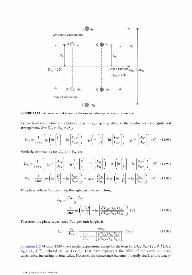
A�
B�
C�
B
A C
DA DC
qB
qA qC
−qA −qC
−qB
Image Conductors
Overhead Conductors
DCC� = 2DC
DB
DBB� = 2DBDAA� = 2DAEarth’s Surface
FIGURE 13.19 Arrangement of image conductors in a three-phase transmission line.
As overhead conductors are identical, then r¼ rA¼ rB¼ rC. Also, as the conductors have equilateral
arrangement, D¼DAB¼DBC¼DCA
VAB ¼1
2p«0
qA ln
"
D
r
#
� ln
"
DAB0
DAA0
# !
þ qB
ln
"
r
D
#
� ln
"
DBB0
DAB0
#!
� qC ln
"
DBC0
DAC0
#" #
VÞð (13:93)
Similarly, expressions for VBC and VAC are
VBC ¼1
2p«0
"
�qA ln
"
DCA0
DBA0
#
þ qB
lnD
r
#
� ln
"
DCB0
DBB0
#!
þ qC
ln
"
r
D
#
� ln
"
DCC0
DBC0
#!" #
VÞð (13:94)
VAC ¼1
2p«0
"
qA ln
"
D
r
#
� ln
"
DCA0
DAA0
#!
� qB ln
"
DCB0
DAB0
#
þ qC
ln
"
r
D
#
� ln
"
DCC0
DAC0
#!#
VÞð (13:95)
The phase voltage VAN becomes, through algebraic reduction,
VAN ¼VAB þ VAC
3
¼ 1
2p«0
qA lnD
r
� �
� ln
"
ffiffiffiffiffiffiffiffiffiffiffiffiffiffiffiffiffiffiffiffiffiffiffiffiffiffiffi
DAB0DBC0DCA03pffiffiffiffiffiffiffiffiffiffiffiffiffiffiffiffiffiffiffiffiffiffiffiffiffiffiffi
DAA0DBB0DCC03p
# !
VÞð (13:96)
Therefore, the phase capacitance CAN, per unit length, is
CAN ¼qA
VAN
¼ 2p«0
lnh
Dr
i
� ln
ffiffiffiffiffiffiffiffiffiffiffiffiffiffiffiffiffiffiffiffiffiffiffiffiffiffiffi
DAB0DBC0DCA03pffiffiffiffiffiffiffiffiffiffiffiffiffiffiffiffiffiffiffiffiffiffiffiffiffiffiffi
DAA0DBB0DCC03p� � F=mð Þ (13:97)
Equations (13.79) and (13.97) have similar expressions, except for the term ln ((DAB0 DBC0 DCA0)1=3=(DAA0
DBB0 DCC0)1=3) included in Eq. (13.97). That term represents the effect of the earth on phase
capacitance, increasing its total value. However, the capacitance increment is really small, and is usually
� 2006 by Taylor & Francis Group, LLC.
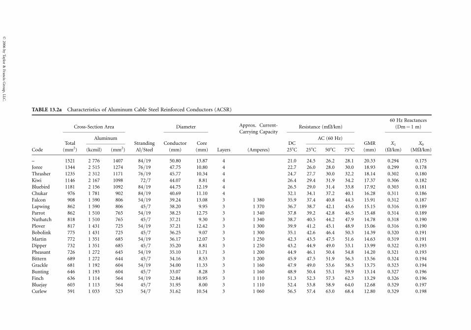
TABLE 13.2a Characteristics of Aluminum Cable Steel Reinforced Conductors (ACSR)
Cross-Section Area Diameter Approx. Current-
Carrying CapacityResistance (mV/km)
60 Hz Reactances
(Dm¼ 1 m)
TotalAluminum
Stranding Conductor Core DCAC (60 Hz)
GMR X1 X0
Code (mm2) (kcmil) (mm2) Al=Steel (mm) (mm) Layers (Amperes) 258C 258C 508C 758C (mm) (V/km) (MV/km)
– 1521 2 776 1407 84=19 50.80 13.87 4 21.0 24.5 26.2 28.1 20.33 0.294 0.175
Joree 1344 2 515 1274 76=19 47.75 10.80 4 22.7 26.0 28.0 30.0 18.93 0.299 0.178
Thrasher 1235 2 312 1171 76=19 45.77 10.34 4 24.7 27.7 30.0 32.2 18.14 0.302 0.180
Kiwi 1146 2 167 1098 72=7 44.07 8.81 4 26.4 29.4 31.9 34.2 17.37 0.306 0.182
Bluebird 1181 2 156 1092 84=19 44.75 12.19 4 26.5 29.0 31.4 33.8 17.92 0.303 0.181
Chukar 976 1 781 902 84=19 40.69 11.10 4 32.1 34.1 37.2 40.1 16.28 0.311 0.186
Falcon 908 1 590 806 54=19 39.24 13.08 3 1 380 35.9 37.4 40.8 44.3 15.91 0.312 0.187
Lapwing 862 1 590 806 45=7 38.20 9.95 3 1 370 36.7 38.7 42.1 45.6 15.15 0.316 0.189
Parrot 862 1 510 765 54=19 38.23 12.75 3 1 340 37.8 39.2 42.8 46.5 15.48 0.314 0.189
Nuthatch 818 1 510 765 45=7 37.21 9.30 3 1 340 38.7 40.5 44.2 47.9 14.78 0.318 0.190
Plover 817 1 431 725 54=19 37.21 12.42 3 1 300 39.9 41.2 45.1 48.9 15.06 0.316 0.190
Bobolink 775 1 431 725 45=7 36.25 9.07 3 1 300 35.1 42.6 46.4 50.3 14.39 0.320 0.191
Martin 772 1 351 685 54=19 36.17 12.07 3 1 250 42.3 43.5 47.5 51.6 14.63 0.319 0.191
Dipper 732 1 351 685 45=7 35.20 8.81 3 1 250 43.2 44.9 49.0 53.1 13.99 0.322 0.193
Pheasant 726 1 272 645 54=19 35.10 11.71 3 1 200 44.9 46.1 50.4 54.8 14.20 0.321 0.193
Bittern 689 1 272 644 45=7 34.16 8.53 3 1 200 45.9 47.5 51.9 56.3 13.56 0.324 0.194
Grackle 681 1 192 604 54=19 34.00 11.33 3 1 160 47.9 49.0 53.6 58.3 13.75 0.323 0.194
Bunting 646 1 193 604 45=7 33.07 8.28 3 1 160 48.9 50.4 55.1 59.9 13.14 0.327 0.196
Finch 636 1 114 564 54=19 32.84 10.95 3 1 110 51.3 52.3 57.3 62.3 13.29 0.326 0.196
Bluejay 603 1 113 564 45=7 31.95 8.00 3 1 110 52.4 53.8 58.9 64.0 12.68 0.329 0.197
Curlew 591 1 033 523 54=7 31.62 10.54 3 1 060 56.5 57.4 63.0 68.4 12.80 0.329 0.198
�2
00
6b
yT
aylor
&F
rancis
Gro
up
,L
LC
.
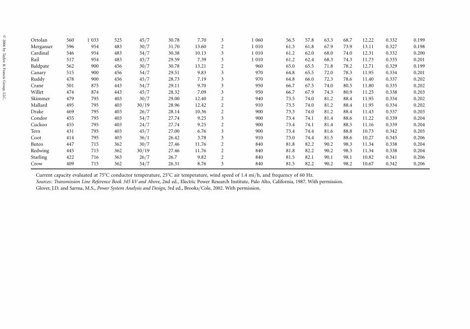
Ortolan 560 1 033 525 45=7 30.78 7.70 3 1 060 56.5 57.8 63.3 68.7 12.22 0.332 0.199
Merganser 596 954 483 30=7 31.70 13.60 2 1 010 61.3 61.8 67.9 73.9 13.11 0.327 0.198
Cardinal 546 954 483 54=7 30.38 10.13 3 1 010 61.2 62.0 68.0 74.0 12.31 0.332 0.200
Rail 517 954 483 45=7 29.59 7.39 3 1 010 61.2 62.4 68.3 74.3 11.73 0.335 0.201
Baldpate 562 900 456 30=7 30.78 13.21 2 960 65.0 65.5 71.8 78.2 12.71 0.329 0.199
Canary 515 900 456 54=7 29.51 9.83 3 970 64.8 65.5 72.0 78.3 11.95 0.334 0.201
Ruddy 478 900 456 45=7 28.73 7.19 3 970 64.8 66.0 72.3 78.6 11.40 0.337 0.202
Crane 501 875 443 54=7 29.11 9.70 3 950 66.7 67.5 74.0 80.5 11.80 0.335 0.202
Willet 474 874 443 45=7 28.32 7.09 3 950 66.7 67.9 74.3 80.9 11.25 0.338 0.203
Skimmer 479 795 403 30=7 29.00 12.40 2 940 73.5 74.0 81.2 88.4 11.95 0.334 0.202
Mallard 495 795 403 30=19 28.96 12.42 2 910 73.5 74.0 81.2 88.4 11.95 0.334 0.202
Drake 469 795 403 26=7 28.14 10.36 2 900 73.3 74.0 81.2 88.4 11.43 0.337 0.203
Condor 455 795 403 54=7 27.74 9.25 3 900 73.4 74.1 81.4 88.6 11.22 0.339 0.204
Cuckoo 455 795 403 24=7 27.74 9.25 2 900 73.4 74.1 81.4 88.5 11.16 0.339 0.204
Tern 431 795 403 45=7 27.00 6.76 3 900 73.4 74.4 81.6 88.8 10.73 0.342 0.205
Coot 414 795 403 36=1 26.42 3.78 3 910 73.0 74.4 81.5 88.6 10.27 0.345 0.206
Buteo 447 715 362 30=7 27.46 11.76 2 840 81.8 82.2 90.2 98.3 11.34 0.338 0.204
Redwing 445 715 362 30=19 27.46 11.76 2 840 81.8 82.2 90.2 98.3 11.34 0.338 0.204
Starling 422 716 363 26=7 26.7 9.82 2 840 81.5 82.1 90.1 98.1 10.82 0.341 0.206
Crow 409 715 362 54=7 26.31 8.76 3 840 81.5 82.2 90.2 98.2 10.67 0.342 0.206
Current capacity evaluated at 758C conductor temperature, 258C air temperature, wind speed of 1.4 mi=h, and frequency of 60 Hz.
Sources : Transmission Line Reference Book 345 kV and Above, 2nd ed., Electric Power Research Institute, Palo Alto, California, 1987. With permission.
Glover, J.D. and Sarma, M.S., Power System Analysis and Design, 3rd ed., Brooks=Cole, 2002. With permission.
�2
00
6b
yT
aylor
&F
rancis
Gro
up
,L
LC
.
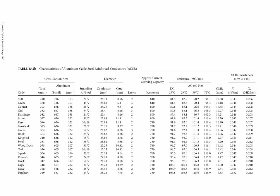
TA 13.2b Characteristics of Aluminum Cable Steel Reinforced Conductors (ACSR)
Cross-Section Area Diameter Approx. Current-
Carrying CapacityResistance (mV/km)
60 Hz Reactances
(Dm¼ 1 m)
TotalAluminum
Stranding Conductor Core DCAC (60 Hz)
GMR X1 X0
Co (mm2) (kcmil) (mm2) Al=Steel (mm) (mm) Layers (Amperes) 258C 258C 508C 758C (mm) (V/km) (MV/km)
Sti 410 716 363 24=7 26.31 8.76 2 840 81.5 82.2 90.2 98.1 10.58 0.343 0.206
Gr 388 716 363 45=7 25.63 6.4 3 840 81.5 82.5 90.4 98.4 10.18 0.346 0.208
Ga t 393 666 338 26=7 25.76 9.5 2 800 87.6 88.1 96.6 105.3 10.45 0.344 0.208
Gu 382 667 338 54=7 25.4 8.46 3 800 87.5 88.1 96.8 105.3 10.27 0.345 0.208
Fla go 382 667 338 24=7 25.4 8.46 2 800 87.4 88.1 96.7 105.3 10.21 0.346 0.208
Sc 397 636 322 30=7 25.88 11.1 2 800 91.9 92.3 101.4 110.4 10.70 0.342 0.207
Eg 396 636 322 30=19 25.88 11.1 2 780 91.9 92.3 101.4 110.4 10.70 0.342 0.207
Gr ak 375 636 322 26=7 25.15 9.27 2 780 91.7 92.2 101.2 110.3 10.21 0.346 0.209
Go 364 636 322 54=7 24.82 8.28 3 770 91.8 92.4 101.4 110.4 10.06 0.347 0.208
Ro 363 636 322 24=7 24.82 8.28 2 770 91.7 92.3 101.3 110.3 10.06 0.347 0.209
Ki rd 340 636 322 18=1 23.88 4.78 2 780 91.2 92.2 101.1 110.0 9.27 0.353 0.211
Sw 331 636 322 36=1 23.62 3.38 3 780 91.3 92.4 101.3 110.3 9.20 0.353 0.212
Wo Duck 378 605 307 30=7 25.25 10.82 2 760 96.7 97.0 106.5 116.1 10.42 0.344 0.208
Te 376 605 307 30=19 25.25 10.82 2 770 96.7 97.0 106.5 116.1 10.42 0.344 0.208
Sq 356 605 356 26=7 25.54 9.04 2 760 96.5 97.0 106.5 116.0 9.97 0.347 0.208
Pe k 346 605 307 24=7 24.21 8.08 2 760 96.4 97.0 106.4 115.9 9.72 0.349 0.210
Du 347 606 307 54=7 24.21 8.08 3 750 96.3 97.0 106.3 115.8 9.81 0.349 0.210
Ea 348 557 282 30=7 24.21 10.39 2 730 105.1 105.4 115.8 126.1 10.00 0.347 0.210
Do 328 556 282 26=7 23.55 8.66 2 730 104.9 105.3 115.6 125.9 9.54 0.351 0.212
Pa et 319 557 282 24=7 23.22 7.75 2 730 104.8 105.3 115.6 125.9 9.33 0.352 0.212
�2
00
6b
yT
aylor
&F
rancis
Gro
up
,L
LC
.
BLE
de
lt
ebe
nne
ll
min
oter
ret
osbe
ose
ok
ngbi
irl
od
al
uab
acoc
ck
gle
ve
rake
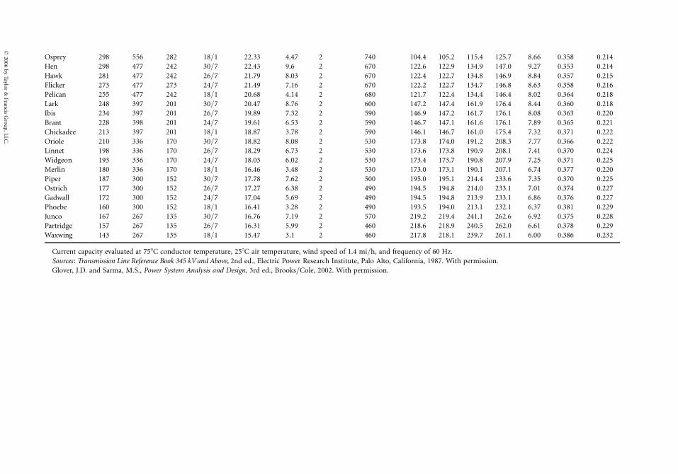
Osprey 298 556 282 18=1 22.33 4.47 2 740 104.4 105.2 115.4 125.7 8.66 0.358 0.214
Hen 298 477 242 30=7 22.43 9.6 2 670 122.6 122.9 134.9 147.0 9.27 0.353 0.214
Hawk 281 477 242 26=7 21.79 8.03 2 670 122.4 122.7 134.8 146.9 8.84 0.357 0.215
Flicker 273 477 273 24=7 21.49 7.16 2 670 122.2 122.7 134.7 146.8 8.63 0.358 0.216
Pelican 255 477 242 18=1 20.68 4.14 2 680 121.7 122.4 134.4 146.4 8.02 0.364 0.218
Lark 248 397 201 30=7 20.47 8.76 2 600 147.2 147.4 161.9 176.4 8.44 0.360 0.218
Ibis 234 397 201 26=7 19.89 7.32 2 590 146.9 147.2 161.7 176.1 8.08 0.363 0.220
Brant 228 398 201 24=7 19.61 6.53 2 590 146.7 147.1 161.6 176.1 7.89 0.365 0.221
Chickadee 213 397 201 18=1 18.87 3.78 2 590 146.1 146.7 161.0 175.4 7.32 0.371 0.222
Oriole 210 336 170 30=7 18.82 8.08 2 530 173.8 174.0 191.2 208.3 7.77 0.366 0.222
Linnet 198 336 170 26=7 18.29 6.73 2 530 173.6 173.8 190.9 208.1 7.41 0.370 0.224
Widgeon 193 336 170 24=7 18.03 6.02 2 530 173.4 173.7 190.8 207.9 7.25 0.371 0.225
Merlin 180 336 170 18=1 16.46 3.48 2 530 173.0 173.1 190.1 207.1 6.74 0.377 0.220
Piper 187 300 152 30=7 17.78 7.62 2 500 195.0 195.1 214.4 233.6 7.35 0.370 0.225
Ostrich 177 300 152 26=7 17.27 6.38 2 490 194.5 194.8 214.0 233.1 7.01 0.374 0.227
Gadwall 172 300 152 24=7 17.04 5.69 2 490 194.5 194.8 213.9 233.1 6.86 0.376 0.227
Phoebe 160 300 152 18=1 16.41 3.28 2 490 193.5 194.0 213.1 232.1 6.37 0.381 0.229
Junco 167 267 135 30=7 16.76 7.19 2 570 219.2 219.4 241.1 262.6 6.92 0.375 0.228
Partridge 157 267 135 26=7 16.31 5.99 2 460 218.6 218.9 240.5 262.0 6.61 0.378 0.229
Waxwing 143 267 135 18=1 15.47 3.1 2 460 217.8 218.1 239.7 261.1 6.00 0.386 0.232
Current capacity evaluated at 758C conductor temperature, 258C air temperature, wind speed of 1.4 mi=h, and frequency of 60 Hz.
Sources : Transmission Line Reference Book 345 kV and Above, 2nd ed., Electric Power Research Institute, Palo Alto, California, 1987. With permission.
Glover, J.D. and Sarma, M.S., Power System Analysis and Design, 3rd ed., Brooks=Cole, 2002. With permission.
�2
00
6b
yT
aylor
&F
rancis
Gro
up
,L
LC
.
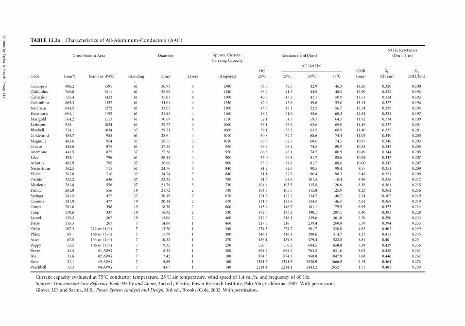
TABLE 13.3a Characteristics of All-Aluminum-Conductors (AAC)
Cross-Section Area Diameter Approx. Current-
Carrying CapacityResistance (mV=km)
60 Hz Reactances
(Dm¼ 1 m)
DCAC (60 Hz)
GMR XL XC
Code (mm2) kcmil or AWG Stranding (mm) Layers (Amperes) 258C 258C 508C 758C (mm) (V=km) (MV=km)
Coreopsis 806.2 1591 61 36.93 4 1380 36.5 39.5 42.9 46.3 14.26 0.320 0.190
Glaldiolus 765.8 1511 61 35.99 4 1340 38.4 41.3 44.9 48.5 13.90 0.322 0.192
Carnation 725.4 1432 61 35.03 4 1300 40.5 43.3 47.1 50.9 13.53 0.324 0.193
Columbine 865.3 1352 61 34.04 4 1250 42.9 45.6 49.6 53.6 13.14 0.327 0.196
Narcissus 644.5 1272 61 33.02 4 1200 45.5 48.1 52.5 56.7 12.74 0.329 0.194
Hawthorn 604.1 1192 61 31.95 4 1160 48.7 51.0 55.6 60.3 12.34 0.331 0.197
Marigold 564.2 1113 61 30.89 4 1110 52.1 54.3 59.3 64.3 11.92 0.334 0.199
Larkspur 524 1034 61 29.77 4 1060 56.1 58.2 63.6 69.0 11.49 0.337 0.201
Bluebell 524.1 1034 37 29.71 3 1060 56.1 58.2 63.5 68.9 11.40 0.337 0.201
Goldenrod 483.7 955 61 28.6 4 1010 60.8 62.7 68.6 74.4 11.03 0.340 0.203
Magnolia 483.6 954 37 28.55 3 1010 60.8 62.7 68.6 74.5 10.97 0.340 0.203
Crocus 443.6 875 61 27.38 4 950 66.3 68.1 74.5 80.9 10.58 0.343 0.205
Anemone 443.5 875 37 27.36 3 950 66.3 68.1 74.5 80.9 10.49 0.344 0.205
Lilac 403.1 796 61 26.11 4 900 73.0 74.6 81.7 88.6 10.09 0.347 0.207
Arbutus 402.9 795 37 26.06 3 900 73.0 74.6 81.7 88.6 10.00 0.347 0.207
Nasturtium 362.5 715 61 24.76 4 840 81.2 82.6 90.5 98.4 9.57 0.351 0.209
Violet 362.8 716 37 24.74 3 840 81.1 82.5 90.4 98.3 9.48 0.351 0.209
Orchid 322.2 636 37 23.32 3 780 91.3 92.6 101.5 110.4 8.96 0.356 0.212
Mistletoe 281.8 556 37 21.79 3 730 104.4 105.5 115.8 126.0 8.38 0.361 0.215
Dahlia 281.8 556 19 21.72 2 730 104.4 105.5 115.8 125.9 8.23 0.362 0.216
Syringa 241.5 477 37 20.19 3 670 121.8 122.7 134.7 146.7 7.74 0.367 0.219
Cosmos 241.9 477 19 20.14 2 670 121.6 122.6 134.5 146.5 7.62 0.368 0.219
Canna 201.6 398 19 18.36 2 600 145.9 146.7 161.1 175.5 6.95 0.375 0.224
Tulip 170.6 337 19 16.92 2 530 172.5 173.2 190.1 207.1 6.40 0.381 0.228
Laurel 135.2 267 19 15.06 2 460 217.6 218.1 239.6 261.0 5.70 0.390 0.233
Daisy 135.3 267 7 14.88 1 460 217.5 218 239.4 260.8 5.39 0.394 0.233
Oxlip 107.3 212 or (4=0) 7 13.26 1 340 274.3 274.7 301.7 328.8 4.82 0.402 0.239
Phlox 85 168 or (3=0) 7 11.79 1 300 346.4 346.4 380.6 414.7 4.27 0.411 0.245
Aster 67.5 133 or (2=0) 7 10.52 1 270 436.1 439.5 479.4 522.5 3.81 0.40 0.25
Poppy 53.5 106 or (1=0) 7 9.35 1 230 550 550.2 604.5 658.8 3.38 0.429 0.256
Pansy 42.4 #1 AWG 7 8.33 1 200 694.2 694.2 763.2 831.6 3.02 0.438 0.261
Iris 33.6 #2 AWG 7 7.42 1 180 874.5 874.5 960.8 1047.9 2.68 0.446 0.267
Rose 21.1 #3 AWG 7 5.89 1 160 1391.5 1391.5 1528.9 1666.3 2.13 0.464 0.278
Peachbell 13.3 #4 AWG 7 4.67 1 140 2214.4 2214.4 2443.2 2652 1.71 0.481 0.289
Current capacity evaluated at 758C conductor temperature, 258C air temperature, wind speed of 1.4 mi=h, and frequency of 60 Hz.
Sources : Transmission Line Reference Book 345 kV and Above, 2nd ed., Electric Power Research Institute, Palo Alto, California, 1987. With permission.
Glover, J.D. and Sarma, M.S., Power System Analysis and Design, 3rd ed., Brooks=Cole, 2002. With permission.
�2
00
6b
yT
aylor
&F
rancis
Gro
up
,L
LC
.
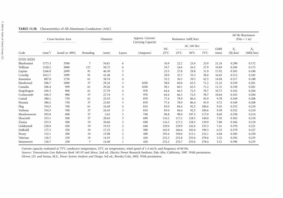
TABLE 13.3b Characteristics of All-Aluminum-Conductors (AAC)
Cross-Section Area Diameter Approx. Current-
Carrying CapacityResistance (mV=km)
60 Hz Reactances
(Dm¼ 1 m)
DCAC (60 Hz)
GMR XL XC
Code (mm2) kcmil or AWG Stranding (mm) Layers (Amperes) 258C 258C 508C 758C (mm) (V=km) (MV=km)
EVEN SIZES
Bluebonnet 1773.3 3500 7 54.81 6 16.9 22.2 23.6 25.0 21.24 0.290 0.172
Trillium 1520.2 3000 127 50.75 6 19.7 24.6 26.2 27.9 19.69 0.296 0.175
Lupine 1266.0 2499 91 46.30 5 23.5 27.8 29.8 31.9 17.92 0.303 0.180
Cowslip 1012.7 1999 91 41.40 5 29.0 32.7 35.3 38.0 16.03 0.312 0.185
Jessamine 887.0 1750 61 38.74 4 33.2 36.5 39.5 42.5 14.94 0.317 0.188
Hawkweed 506.7 1000 37 29.24 3 1030 58.0 60.0 65.5 71.2 11.22 0.339 0.201
Camelia 506.4 999 61 29.26 4 1030 58.1 60.1 65.5 71.2 11.31 0.338 0.201
Snapdragon 456.3 900 61 27.79 4 970 64.4 66.3 72.5 78.7 10.73 0.342 0.204
Cockscomb 456.3 900 37 27.74 3 970 64.4 66.3 72.5 78.7 10.64 0.343 0.204
Cattail 380.1 750 61 25.35 4 870 77.4 78.9 86.4 93.9 9.78 0.349 0.208
Petunia 380.2 750 37 23.85 3 870 77.4 78.9 86.4 93.9 9.72 0.349 0.208
Flag 354.5 700 61 24.49 4 810 83.0 84.4 92.5 100.6 9.45 0.352 0.210
Verbena 354.5 700 37 24.43 3 810 83.0 84.4 92.5 100.6 9.39 0.352 0.210
Meadowsweet 303.8 600 37 2.63 3 740 96.8 98.0 107.5 117.0 8.69 0.358 0.214
Hyacinth 253.1 500 37 20.65 3 690 116.2 117.2 128.5 140.0 7.92 0.365 0.218
Zinnia 253.3 500 19 20.60 2 690 116.2 117.2 128.5 139.9 7.80 0.366 0.218
Goldentuft 228.0 450 19 19.53 2 640 129.0 129.9 142.6 155.3 7.41 0.370 0.221
Daffodil 177.3 350 19 17.25 2 580 165.9 166.6 183.0 199.3 6.52 0.379 0.227
Peony 152.1 300 19 15.98 2 490 193.4 194.0 213.1 232.1 6.04 0.385 0.230
Valerian 126.7 250 19 14.55 2 420 232.3 232.8 255.6 278.6 5.52 0.392 0.235
Sneezewort 126.7 250 7 14.40 1 420 232.2 232.7 255.6 278.4 5.21 0.396 0.235
Current capacity evaluated at 758C conductor temperature, 258C air temperature, wind speed of 1.4 mi=h, and frequency of 60 Hz.
Sources : Transmission Line Reference Book 345 kV and Above, 2nd ed., Electric Power Research Institute, Palo Alto, California, 1987. With permission.
Glover, J.D. and Sarma, M.S., Power System Analysis and Design, 3rd ed., Brooks=Cole, 2002. With permission.
�2
00
6b
yT
aylor
&F
rancis
Gro
up
,L
LC
.
neglected, because distances from overhead conductors to ground are always greater than distances
among conductors.
13.6 Characteristics of Overhead Conductors
Tables 13.2a and 13.2b present typical values of resistance, inductive reactance and capacitance react-
ance, per unit length, of ACSR conductors. The size of the conductors (cross-section area) is specified in
square millimeters and kcmil, where a cmil is the cross-section area of a circular conductor with a
diameter of 1=1000 in. The tables include also the approximate current-carrying capacity of the
conductors assuming 60 Hz, wind speed of 1.4 mi=h, and conductor and air temperatures of 758C
and 258C, respectively. Tables 13.3a and 13.3b present the corresponding characteristics of AACs.
References
1.
� 2
Yamayee, Z.A. and Bala, J.L. Jr., Electromechanical Energy Devices and Power Systems, John Wiley and
Sons, Inc., New York, 1994.
2.
Glover, J.D. and Sarma, M.S., Power System Analysis and Design, 3rd ed., Brooks=Cole, 2002.3.
Stevenson, W.D. Jr., Elements of Power System Analysis, 4th ed. McGraw-Hill, New York, 1982.4.
Saadat, H., Power System Analysis, McGraw-Hill, Boston, MA, 1999.5.
Gross, Ch.A., Power System Analysis, John Wiley and Sons, New York, 1979.6.
Gungor, B.R., Power Systems, Harcourt Brace Jovanovich, Orlando, FL, 1988.7.
Zaborszky, J. and Rittenhouse, J.W., Electric Power Transmission. The Power System in the Steady State,The Ronald Press Company, New York, 1954.
8.
Barnes, C.C., Power Cables. Their Design and Installation, 2nd ed., Chapman and Hall, London, 1966.9.
Electric Power Research Institute, Transmission Line Reference Book 345 kV and Above, 2nd ed., PaloAlto, CA, 1987.
006 by Taylor & Francis Group, LLC.
14
� 2006 by Taylor & Francis Group, LLC.
Sag and Tension ofConductor
D.A. DouglassPower Delivery Consultants, Inc.
Ridley ThrashSouthwire Company
14.1 Catenary Cables ............................................................... 14-2Level Spans . Conductor Length . Conductor Slack .
Inclined Spans . Ice and Wind Conductor Loads .
Conductor Tension Limits
14.2 Approximate Sag-Tension Calculations......................... 14-9Sag Change with Thermal Elongation . Sag Change
Due to Combined Thermal and Elastic Effects . Sag
Change Due to Ice Loading
14.3 Numerical Sag-Tension Calculations ........................... 14-14Stress-Strain Curves . Sag-Tension Tables
14.4 Ruling Span Concept .................................................... 14-22Tension Differences for Adjacent Dead-End Spans .
Tension Equalization by Suspension Insulators . Ruling
Span Calculation . Stringing Sag Tables
14.5 Line Design Sag-Tension Parameters........................... 14-25Catenary Constants . Wind Span . Weight Span .
Uplift at Suspension Structures . Tower Spotting
14.6 Conductor Installation.................................................. 14-28Conductor Stringing Methods . Tension
Stringing Equipment and Setup . Sagging Procedure
14.7 Defining Terms .............................................................. 14-39
The energized conductors of transmission and distribution lines must be placed to totally eliminate the
possibility of injury to people. Overhead conductors, however, elongate with time, temperature, and
tension, thereby changing their original positions after installation. Despite the effects of weather
and loading on a line, the conductors must remain at safe distances from buildings, objects, and people
or vehicles passing beneath the line at all times. To ensure this safety, the shape of the terrain along
the right-of-way, the height and lateral position of the conductor support points, and the position of the
conductor between support points under all wind, ice, and temperature conditions must be known.
Bare overhead transmission or distribution conductors are typically quite flexible and uniform in
weight along their length. Because of these characteristics, they take the form of a catenary (Ehrenberg,
1935; Winkelmann, 1959) between support points. The shape of the catenary changes with conductor
temperature, ice and wind loading, and time. To ensure adequate vertical and horizontal clearance under
all weather and electrical loadings, and to ensure that the breaking strength of the conductor is not
exceeded, the behavior of the conductor catenary under all conditions must be known before the line is
designed. The future behavior of the conductor is determined through calculations commonly referred
to as sag-tension calculations.
Sag-tension calculations predict the behavior of conductors based on recommended tension limits
under varying loading conditions. These tension limits specify certain percentages of the conductor’s
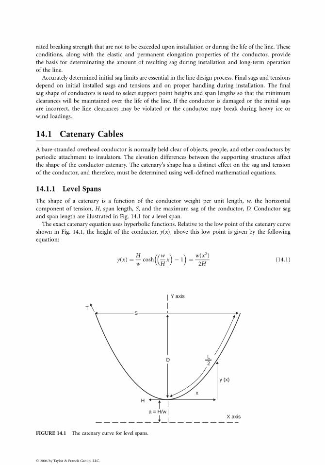
rated breaking strength that are not to be exceeded upon installation or during the life of the line. These
conditions, along with the elastic and permanent elongation properties of the conductor, provide
the basis for determinating the amount of resulting sag during installation and long-term operation
of the line.
Accurately determined initial sag limits are essential in the line design process. Final sags and tensions
depend on initial installed sags and tensions and on proper handling during installation. The final
sag shape of conductors is used to select support point heights and span lengths so that the minimum
clearances will be maintained over the life of the line. If the conductor is damaged or the initial sags
are incorrect, the line clearances may be violated or the conductor may break during heavy ice or
wind loadings.
14.1 Catenary Cables
A bare-stranded overhead conductor is normally held clear of objects, people, and other conductors by
periodic attachment to insulators. The elevation differences between the supporting structures affect
the shape of the conductor catenary. The catenary’s shape has a distinct effect on the sag and tension
of the conductor, and therefore, must be determined using well-defined mathematical equations.
14.1.1 Level Spans
The shape of a catenary is a function of the conductor weight per unit length, w, the horizontal
component of tension, H, span length, S, and the maximum sag of the conductor, D. Conductor sag
and span length are illustrated in Fig. 14.1 for a level span.
The exact catenary equation uses hyperbolic functions. Relative to the low point of the catenary curve
shown in Fig. 14.1, the height of the conductor, y(x), above this low point is given by the following
equation:
y(x) ¼ H
wcosh
w
Hx
� �
� 1� �
¼ w(x2)
2H(14:1)
S
DL2
x
X axis
y (x)
H
a = H/w
Y axis
T
FIGURE 14.1 The catenary curve for level spans.
� 2006 by Taylor & Francis Group, LLC.
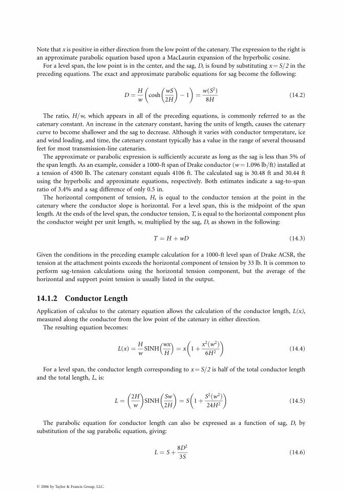
Note that x is positive in either direction from the low point of the catenary. The expression to the right is
an approximate parabolic equation based upon a MacLaurin expansion of the hyperbolic cosine.
For a level span, the low point is in the center, and the sag, D, is found by substituting x¼ S=2 in the
preceding equations. The exact and approximate parabolic equations for sag become the following:
D ¼ H
wcosh
wS
2H
� �
� 1
� �
¼ w(S2)
8H(14:2)
The ratio, H=w, which appears in all of the preceding equations, is commonly referred to as the
catenary constant. An increase in the catenary constant, having the units of length, causes the catenary
curve to become shallower and the sag to decrease. Although it varies with conductor temperature, ice
and wind loading, and time, the catenary constant typically has a value in the range of several thousand
feet for most transmission-line catenaries.
The approximate or parabolic expression is sufficiently accurate as long as the sag is less than 5% of
the span length. As an example, consider a 1000-ft span of Drake conductor (w¼ 1.096 lb=ft) installed at
a tension of 4500 lb. The catenary constant equals 4106 ft. The calculated sag is 30.48 ft and 30.44 ft
using the hyperbolic and approximate equations, respectively. Both estimates indicate a sag-to-span
ratio of 3.4% and a sag difference of only 0.5 in.
The horizontal component of tension, H, is equal to the conductor tension at the point in the
catenary where the conductor slope is horizontal. For a level span, this is the midpoint of the span
length. At the ends of the level span, the conductor tension, T, is equal to the horizontal component plus
the conductor weight per unit length, w, multiplied by the sag, D, as shown in the following:
T ¼ H þ wD (14:3)
Given the conditions in the preceding example calculation for a 1000-ft level span of Drake ACSR, the
tension at the attachment points exceeds the horizontal component of tension by 33 lb. It is common to
perform sag-tension calculations using the horizontal tension component, but the average of the
horizontal and support point tension is usually listed in the output.
14.1.2 Conductor Length
Application of calculus to the catenary equation allows the calculation of the conductor length, L(x),
measured along the conductor from the low point of the catenary in either direction.
The resulting equation becomes:
L(x) ¼ H
wSINH
wx
H
� �
¼ x 1þ x2 w2ð Þ6H2
� �
(14:4)
For a level span, the conductor length corresponding to x¼ S=2 is half of the total conductor length
and the total length, L, is:
L ¼ 2H
w
� �
SINHSw
2H
� �
¼ S 1þ S2 w2ð Þ24H2
� �
(14:5)
The parabolic equation for conductor length can also be expressed as a function of sag, D, by
substitution of the sag parabolic equation, giving:
L ¼ S þ 8D2
3S(14:6)
� 2006 by Taylor & Francis Group, LLC.
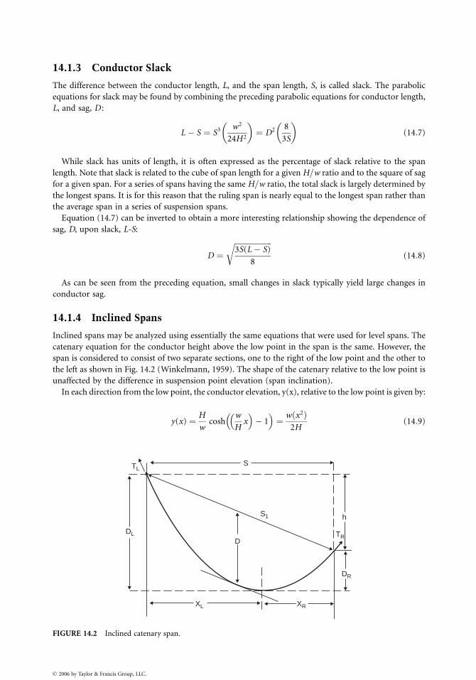
14.1.3 Conductor Slack
The difference between the conductor length, L, and the span length, S, is called slack. The parabolic
equations for slack may be found by combining the preceding parabolic equations for conductor length,
L, and sag, D :
L � S ¼ S3 w2
24H2
� �
¼ D2 8
3S
� �
(14:7)
While slack has units of length, it is often expressed as the percentage of slack relative to the span
length. Note that slack is related to the cube of span length for a given H=w ratio and to the square of sag
for a given span. For a series of spans having the same H=w ratio, the total slack is largely determined by
the longest spans. It is for this reason that the ruling span is nearly equal to the longest span rather than
the average span in a series of suspension spans.
Equation (14.7) can be inverted to obtain a more interesting relationship showing the dependence of
sag, D, upon slack, L-S:
D ¼ffiffiffiffiffiffiffiffiffiffiffiffiffiffiffiffiffiffiffiffi
3S(L � S)
8
r
(14:8)
As can be seen from the preceding equation, small changes in slack typically yield large changes in
conductor sag.
14.1.4 Inclined Spans
Inclined spans may be analyzed using essentially the same equations that were used for level spans. The
catenary equation for the conductor height above the low point in the span is the same. However, the
span is considered to consist of two separate sections, one to the right of the low point and the other to
the left as shown in Fig. 14.2 (Winkelmann, 1959). The shape of the catenary relative to the low point is
unaffected by the difference in suspension point elevation (span inclination).
In each direction from the low point, the conductor elevation, y(x), relative to the low point is given by:
y(x) ¼ H
wcosh
w
Hx
� �
� 1� �
¼ w x2ð Þ2H
(14:9)
S
S1
TRD
DR
XRXL
DL
TL
h
FIGURE 14.2 Inclined catenary span.
� 2006 by Taylor & Francis Group, LLC.
Note that x is considered positive in either direction from the low point.
The horizontal distance, xL, from the left support point to the low point in the catenary is:
xL ¼S
21þ h
4D
� �
(14:10)
The horizontal distance, xR, from the right support point to the low point of the catenary is:
xR ¼S
21� h
4D
� �
(14:11)
where S ¼ horizontal distance between support points.
h ¼ vertical distance between support points.
Sl¼ straight-line distance between support points.
D¼ sag measured vertically from a line through the points of conductor support to a line tangent
to the conductor.
The midpoint sag, D, is approximately equal to the sag in a horizontal span equal in length to the
inclined span, Sl.
Knowing the horizonal distance from the low point to the support point in each direction, the
preceding equations for y(x), L, D, and T can be applied to each side of the inclined span.
The total conductor length, L, in the inclined span is equal to the sum of the lengths in the xR and xL
sub-span sections:
L ¼ S þ x3R þ x3
L
� � w2
6H2
� �
(14:12)
In each sub-span, the sag is relative to the corresponding support point elevation:
DR ¼wx2
R
2HDL ¼
wx2L
2H(14:13)
or in terms of sag, D, and the vertical distance between support points:
DR ¼ D 1� h
4D
� �2
DL ¼ D 1þ h
4D
� �2
(14:14)
and the maximum tension is:
TR ¼ H þ wDR TL ¼ H þ wDL (14:15)
or in terms of upper and lower support points:
Tu ¼ Tl þ wh (14:16)
where DR¼ sag in right sub-span section
DL ¼ sag in left sub-span section
TR ¼ tension in right sub-span section
TL ¼ tension in left sub-span section
Tu ¼ tension in conductor at upper support
Tl ¼ tension in conductor at lower support
� 2006 by Taylor & Francis Group, LLC.
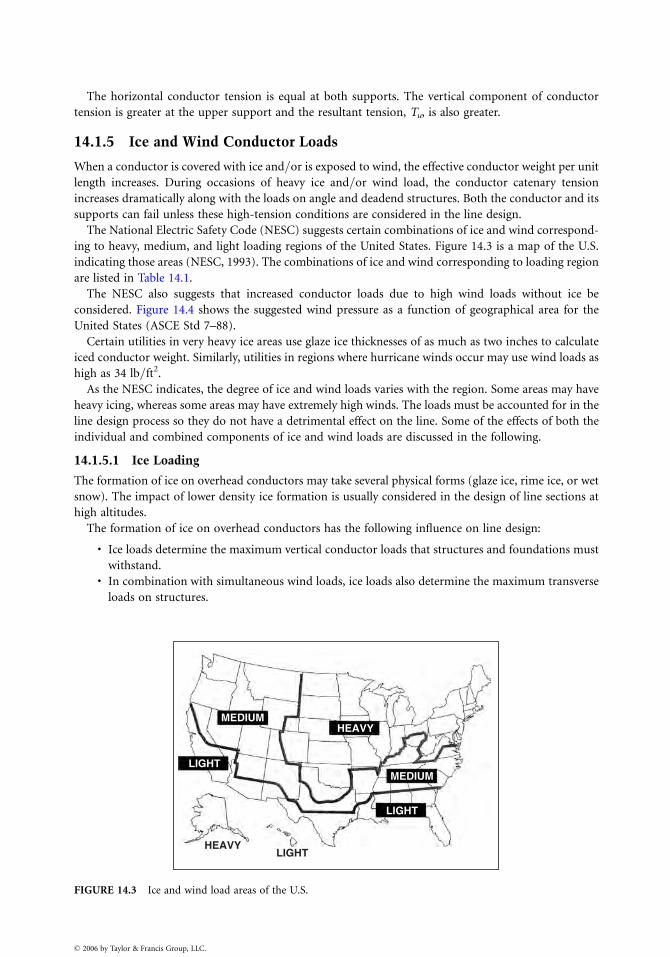
The horizontal conductor tension is equal at both supports. The vertical component of conductor
tension is greater at the upper support and the resultant tension, Tu, is also greater.
14.1.5 Ice and Wind Conductor Loads
When a conductor is covered with ice and=or is exposed to wind, the effective conductor weight per unit
length increases. During occasions of heavy ice and=or wind load, the conductor catenary tension
increases dramatically along with the loads on angle and deadend structures. Both the conductor and its
supports can fail unless these high-tension conditions are considered in the line design.
The National Electric Safety Code (NESC) suggests certain combinations of ice and wind correspond-
ing to heavy, medium, and light loading regions of the United States. Figure 14.3 is a map of the U.S.
indicating those areas (NESC, 1993). The combinations of ice and wind corresponding to loading region
are listed in Table 14.1.
The NESC also suggests that increased conductor loads due to high wind loads without ice be
considered. Figure 14.4 shows the suggested wind pressure as a function of geographical area for the
United States (ASCE Std 7–88).
Certain utilities in very heavy ice areas use glaze ice thicknesses of as much as two inches to calculate
iced conductor weight. Similarly, utilities in regions where hurricane winds occur may use wind loads as
high as 34 lb=ft2.
As the NESC indicates, the degree of ice and wind loads varies with the region. Some areas may have
heavy icing, whereas some areas may have extremely high winds. The loads must be accounted for in the
line design process so they do not have a detrimental effect on the line. Some of the effects of both the
individual and combined components of ice and wind loads are discussed in the following.
14.1.5.1 Ice Loading
The formation of ice on overhead conductors may take several physical forms (glaze ice, rime ice, or wet
snow). The impact of lower density ice formation is usually considered in the design of line sections at
high altitudes.
The formation of ice on overhead conductors has the following influence on line design:
. Ice loads determine the maximum vertical conductor loads that structures and foundations must
withstand.. In combination with simultaneous wind loads, ice loads also determine the maximum transverse
loads on structures.
MEDIUM
MEDIUMLIGHT
LIGHT
LIGHT
HEAVY
HEAVY
FIGURE 14.3 Ice and wind load areas of the U.S.
� 2006 by Taylor & Francis Group, LLC.
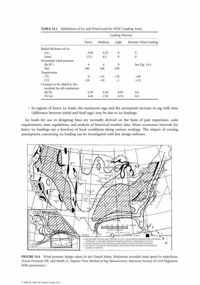
TABLE 14.1 Definitions of Ice and Wind Load for NESC Loading Areas
Loading Districts
Heavy Medium Light Extreme Wind Loading
Radial thickness of ice
(in.) 0.50 0.25 0 0
(mm) 12.5 6.5 0 0
Horizontal wind pressure
(lb=ft2) 4 4 9 See Fig. 14.4
(Pa) 190 190 430
Temperature
(8F) 0 þ15 þ30 þ60
(8C) �20 �10 �1 þ15
Constant to be added to the
resultant for all conductors
(lb=ft) 0.30 0.20 0.05 0.0
(N=m) 4.40 2.50 0.70 0.0
. In regions of heavy ice loads, the maximum sags and the permanent increase in sag with time
(difference between initial and final sags) may be due to ice loadings.
Ice loads for use in designing lines are normally derived on the basis of past experience, code
requirements, state regulations, and analysis of historical weather data. Mean recurrence intervals for
heavy ice loadings are a function of local conditions along various routings. The impact of varying
assumptions concerning ice loading can be investigated with line design software.
BASIC WIND SPEED 70 MPHNOTES:G U L F O F M E X I C O
SPECIAL WIND REGION90
90
8080
70
7070
80
80
70
7070
Tacom
a
Cheyenne
Lincoln
Des Moines
Rapid City
Billings
BismarckDuluthFargo
Minneapolis
Davenport
Chicago
Kansas City
Columbus
Detroit
LansingBuffalo
Pittsburgh
Richmond
Knoxville
Birmingham
Shreveport
Little Rock
St. Louis
JacksonJackson
Atlanta
Raleigh
Norfolk
Columbia
Tampa
Miami
New Orleans
PhoenixAmarillo
PA
CI
FI
C
OC
EA
N
AT
LA
NT
IC
O
CE
AN
80
8080
80100
110
110
110
110110
1008090
70
100
110
0 50 100ALASKA
110
110
90
8070
70
70
70
90
90
90
100
0 100 200
SCALE 1: 20,000,000
300 400 500 MILES
1. VALUES ARE FASTEST-MILE SPEEDS AT 33 FT (10 M) ABOVE GROUND FOR EXPOSURE CATEGORY C AND ARE ASSOCIATED WITH AN ANNUAL PROBABILITY OF 0.02.2. LINEAR INTERPOLATION BETWEEN WIND SPEED CONTOURS IS ACCEPTABLE.3. CAUTION IN THE USE OF WIND SPEED CONTOURS IN MOUNTAINOUS REGIONS OF ALASKA IS ADVISED.
110
Seattle
Salt Lake City
Salem
Denver
Las Vegas
San Diego
San Francisco
Fresno
Los Angeles
9080
70
Albuquerque
Fort Worth
Oklahoma City
Dodge City
FIGURE 14.4 Wind pressure design values in the United States. Maximum recorded wind speed in miles/hour.
(From Overend, P.R. and Smith, S., Impulse Time Method of Sag Measurement, American Society of Civil Engineers.
With permission.)
� 2006 by Taylor & Francis Group, LLC.
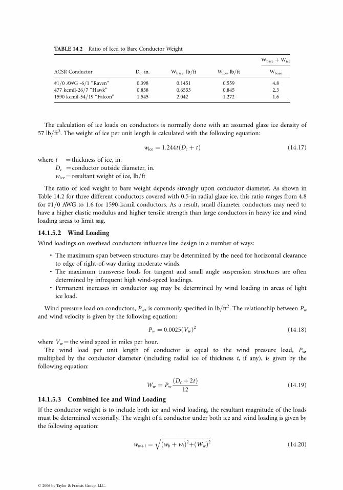
TABLE 14.2 Ratio of Iced to Bare Conductor Weight
Wbare þ Wice
ACSR Conductor Dc, in. Wbare, lb=ft Wice, lb=ft Wbare
#1=0 AWG -6=1 ‘‘Raven’’ 0.398 0.1451 0.559 4.8
477 kcmil-26=7 ‘‘Hawk’’ 0.858 0.6553 0.845 2.3
1590 kcmil-54=19 ‘‘Falcon’’ 1.545 2.042 1.272 1.6
The calculation of ice loads on conductors is normally done with an assumed glaze ice density of
57 lb=ft3. The weight of ice per unit length is calculated with the following equation:
wice ¼ 1:244t Dc þ tð Þ (14:17)
where t ¼ thickness of ice, in.
Dc ¼ conductor outside diameter, in.
wice¼ resultant weight of ice, lb=ft
The ratio of iced weight to bare weight depends strongly upon conductor diameter. As shown in
Table 14.2 for three different conductors covered with 0.5-in radial glaze ice, this ratio ranges from 4.8
for #1=0 AWG to 1.6 for 1590-kcmil conductors. As a result, small diameter conductors may need to
have a higher elastic modulus and higher tensile strength than large conductors in heavy ice and wind
loading areas to limit sag.
14.1.5.2 Wind Loading
Wind loadings on overhead conductors influence line design in a number of ways:
. The maximum span between structures may be determined by the need for horizontal clearance
to edge of right-of-way during moderate winds.. The maximum transverse loads for tangent and small angle suspension structures are often
determined by infrequent high wind-speed loadings.. Permanent increases in conductor sag may be determined by wind loading in areas of light
ice load.
Wind pressure load on conductors, Pw, is commonly specified in lb=ft2. The relationship between Pw
and wind velocity is given by the following equation:
Pw ¼ 0:0025(Vw )2 (14:18)
where Vw¼ the wind speed in miles per hour.
The wind load per unit length of conductor is equal to the wind pressure load, Pw,
multiplied by the conductor diameter (including radial ice of thickness t, if any), is given by the
following equation:
Ww ¼ PwDc þ 2tð Þ
12(14:19)
14.1.5.3 Combined Ice and Wind Loading
If the conductor weight is to include both ice and wind loading, the resultant magnitude of the loads
must be determined vectorially. The weight of a conductor under both ice and wind loading is given by
the following equation:
wwþi ¼ffiffiffiffiffiffiffiffiffiffiffiffiffiffiffiffiffiffiffiffiffiffiffiffiffiffiffiffiffiffiffiffiffiffiffiffiffiffi
wb þ wið Þ2þ Wwð Þ2q
(14:20)
� 2006 by Taylor & Francis Group, LLC.
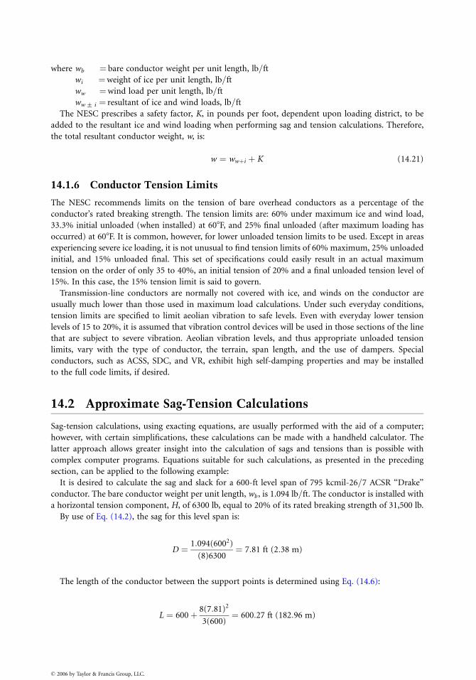
where wb ¼ bare conductor weight per unit length, lb=ft
wi ¼weight of ice per unit length, lb=ft
ww ¼wind load per unit length, lb=ft
ww+ i ¼ resultant of ice and wind loads, lb=ft
The NESC prescribes a safety factor, K, in pounds per foot, dependent upon loading district, to be
added to the resultant ice and wind loading when performing sag and tension calculations. Therefore,
the total resultant conductor weight, w, is:
w ¼ wwþi þ K (14:21)
14.1.6 Conductor Tension Limits
The NESC recommends limits on the tension of bare overhead conductors as a percentage of the
conductor’s rated breaking strength. The tension limits are: 60% under maximum ice and wind load,
33.3% initial unloaded (when installed) at 608F, and 25% final unloaded (after maximum loading has
occurred) at 608F. It is common, however, for lower unloaded tension limits to be used. Except in areas
experiencing severe ice loading, it is not unusual to find tension limits of 60% maximum, 25% unloaded
initial, and 15% unloaded final. This set of specifications could easily result in an actual maximum
tension on the order of only 35 to 40%, an initial tension of 20% and a final unloaded tension level of
15%. In this case, the 15% tension limit is said to govern.
Transmission-line conductors are normally not covered with ice, and winds on the conductor are
usually much lower than those used in maximum load calculations. Under such everyday conditions,
tension limits are specified to limit aeolian vibration to safe levels. Even with everyday lower tension
levels of 15 to 20%, it is assumed that vibration control devices will be used in those sections of the line
that are subject to severe vibration. Aeolian vibration levels, and thus appropriate unloaded tension
limits, vary with the type of conductor, the terrain, span length, and the use of dampers. Special
conductors, such as ACSS, SDC, and VR, exhibit high self-damping properties and may be installed
to the full code limits, if desired.
14.2 Approximate Sag-Tension Calculations
Sag-tension calculations, using exacting equations, are usually performed with the aid of a computer;
however, with certain simplifications, these calculations can be made with a handheld calculator. The
latter approach allows greater insight into the calculation of sags and tensions than is possible with
complex computer programs. Equations suitable for such calculations, as presented in the preceding
section, can be applied to the following example:
It is desired to calculate the sag and slack for a 600-ft level span of 795 kcmil-26=7 ACSR ‘‘Drake’’
conductor. The bare conductor weight per unit length, wb , is 1.094 lb=ft. The conductor is installed with
a horizontal tension component, H, of 6300 lb, equal to 20% of its rated breaking strength of 31,500 lb.
By use of Eq. (14.2), the sag for this level span is:
D ¼ 1:094(6002)
(8)6300¼ 7:81 ft (2:38 m)
The length of the conductor between the support points is determined using Eq. (14.6):
L ¼ 600þ 8(7:81)2
3(600)¼ 600:27 ft (182:96 m)
� 2006 by Taylor & Francis Group, LLC.
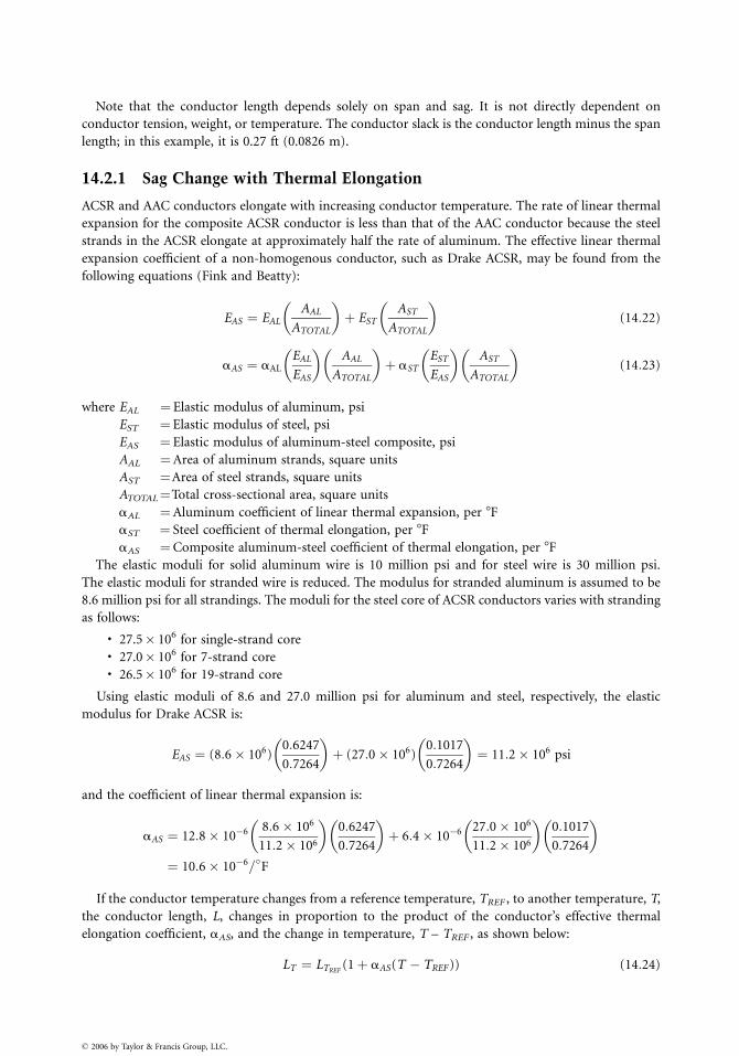
Note that the conductor length depends solely on span and sag. It is not directly dependent on
conductor tension, weight, or temperature. The conductor slack is the conductor length minus the span
length; in this example, it is 0.27 ft (0.0826 m).
14.2.1 Sag Change with Thermal Elongation
ACSR and AAC conductors elongate with increasing conductor temperature. The rate of linear thermal
expansion for the composite ACSR conductor is less than that of the AAC conductor because the steel
strands in the ACSR elongate at approximately half the rate of aluminum. The effective linear thermal
expansion coefficient of a non-homogenous conductor, such as Drake ACSR, may be found from the
following equations (Fink and Beatty):
EAS ¼ EAL
AAL
ATOTAL
� �
þ EST
AST
ATOTAL
� �
(14:22)
aAS ¼ aAL
EAL
EAS
� �
AAL
ATOTAL
� �
þ aST
EST
EAS
� �
AST
ATOTAL
� �
(14:23)
where EAL ¼Elastic modulus of aluminum, psi
EST ¼Elastic modulus of steel, psi
EAS ¼ Elastic modulus of aluminum-steel composite, psi
AAL ¼Area of aluminum strands, square units
AST ¼Area of steel strands, square units
ATOTAL¼Total cross-sectional area, square units
aAL ¼Aluminum coefficient of linear thermal expansion, per 8F
aST ¼ Steel coefficient of thermal elongation, per 8F
aAS ¼Composite aluminum-steel coefficient of thermal elongation, per 8F
The elastic moduli for solid aluminum wire is 10 million psi and for steel wire is 30 million psi.
The elastic moduli for stranded wire is reduced. The modulus for stranded aluminum is assumed to be
8.6 million psi for all strandings. The moduli for the steel core of ACSR conductors varies with stranding
as follows:
. 27.5� 106 for single-strand core
. 27.0� 106 for 7-strand core
. 26.5� 106 for 19-strand core
Using elastic moduli of 8.6 and 27.0 million psi for aluminum and steel, respectively, the elastic
modulus for Drake ACSR is:
EAS ¼ (8:6� 106)0:6247
0:7264
� �
þ (27:0� 106)0:1017
0:7264
� �
¼ 11:2� 106 psi
and the coefficient of linear thermal expansion is:
aAS ¼ 12:8� 10�6 8:6� 106
11:2� 106
� �
0:6247
0:7264
� �
þ 6:4� 10�6 27:0� 106
11:2� 106
� �
0:1017
0:7264
� �
¼ 10:6� 10�6=�F
If the conductor temperature changes from a reference temperature, TREF , to another temperature, T,
the conductor length, L, changes in proportion to the product of the conductor’s effective thermal
elongation coefficient, aAS, and the change in temperature, T – TREF , as shown below:
LT ¼ LTREF(1þ aAS(T � TREF )) (14:24)
� 2006 by Taylor & Francis Group, LLC.
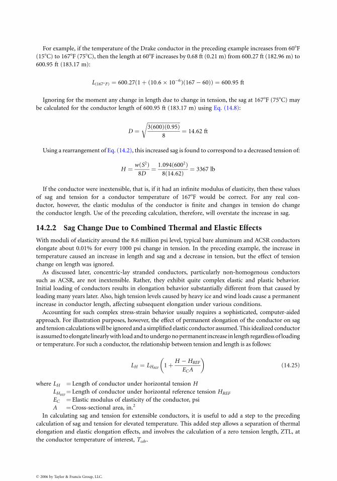
For example, if the temperature of the Drake conductor in the preceding example increases from 608F
(158C) to 1678F (758C), then the length at 608F increases by 0.68 ft (0.21 m) from 600.27 ft (182.96 m) to
600.95 ft (183.17 m):
L(167�F) ¼ 600:27(1þ (10:6� 10�6)(167� 60)) ¼ 600:95 ft
Ignoring for the moment any change in length due to change in tension, the sag at 1678F (758C) may
be calculated for the conductor length of 600.95 ft (183.17 m) using Eq. (14.8):
D ¼ffiffiffiffiffiffiffiffiffiffiffiffiffiffiffiffiffiffiffiffiffiffiffiffiffi
3(600)(0:95)
8
r
¼ 14:62 ft
Using a rearrangement of Eq. (14.2), this increased sag is found to correspond to a decreased tension of:
H ¼ w(S2)
8D¼ 1:094(6002)
8(14:62)¼ 3367 lb
If the conductor were inextensible, that is, if it had an infinite modulus of elasticity, then these values
of sag and tension for a conductor temperature of 1678F would be correct. For any real con-
ductor, however, the elastic modulus of the conductor is finite and changes in tension do change
the conductor length. Use of the preceding calculation, therefore, will overstate the increase in sag.
14.2.2 Sag Change Due to Combined Thermal and Elastic Effects
With moduli of elasticity around the 8.6 million psi level, typical bare aluminum and ACSR conductors
elongate about 0.01% for every 1000 psi change in tension. In the preceding example, the increase in
temperature caused an increase in length and sag and a decrease in tension, but the effect of tension
change on length was ignored.
As discussed later, concentric-lay stranded conductors, particularly non-homogenous conductors
such as ACSR, are not inextensible. Rather, they exhibit quite complex elastic and plastic behavior.
Initial loading of conductors results in elongation behavior substantially different from that caused by
loading many years later. Also, high tension levels caused by heavy ice and wind loads cause a permanent
increase in conductor length, affecting subsequent elongation under various conditions.
Accounting for such complex stress-strain behavior usually requires a sophisticated, computer-aided
approach. For illustration purposes, however, the effect of permanent elongation of the conductor on sag
and tension calculations will be ignored and a simplified elastic conductor assumed. This idealized conductor
is assumed to elongate linearly with load and to undergo no permanent increase in length regardless of loading
or temperature. For such a conductor, the relationship between tension and length is as follows:
LH ¼ LHREF1þH �HREF
ECA
� �
(14:25)
where LH ¼ Length of conductor under horizontal tension H
LHREF¼ Length of conductor under horizontal reference tension HREF
EC ¼ Elastic modulus of elasticity of the conductor, psi
A ¼Cross-sectional area, in.2
In calculating sag and tension for extensible conductors, it is useful to add a step to the preceding
calculation of sag and tension for elevated temperature. This added step allows a separation of thermal
elongation and elastic elongation effects, and involves the calculation of a zero tension length, ZTL, at
the conductor temperature of interest, Tcdr.
� 2006 by Taylor & Francis Group, LLC.
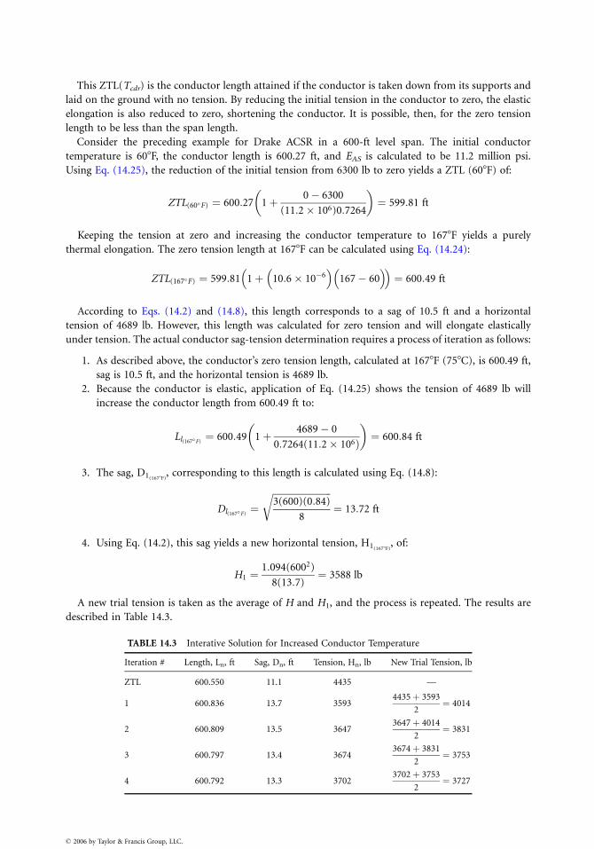
This ZTL(Tcdr) is the conductor length attained if the conductor is taken down from its supports and
laid on the ground with no tension. By reducing the initial tension in the conductor to zero, the elastic
elongation is also reduced to zero, shortening the conductor. It is possible, then, for the zero tension
length to be less than the span length.
Consider the preceding example for Drake ACSR in a 600-ft level span. The initial conductor
temperature is 608F, the conductor length is 600.27 ft, and EAS is calculated to be 11.2 million psi.
Using Eq. (14.25), the reduction of the initial tension from 6300 lb to zero yields a ZTL (608F) of:
ZTL(60�F) ¼ 600:27 1þ 0� 6300
(11:2� 106)0:7264
� �
¼ 599:81 ft
Keeping the tension at zero and increasing the conductor temperature to 1678F yields a purely
thermal elongation. The zero tension length at 1678F can be calculated using Eq. (14.24):
ZTL(167�F) ¼ 599:81�
1þ�
10:6� 10�6��
167� 60��
¼ 600:49 ft
According to Eqs. (14.2) and (14.8), this length corresponds to a sag of 10.5 ft and a horizontal
tension of 4689 lb. However, this length was calculated for zero tension and will elongate elastically
under tension. The actual conductor sag-tension determination requires a process of iteration as follows:
1. As described above, the conductor’s zero tension length, calculated at 1678F (758C), is 600.49 ft,
sag is 10.5 ft, and the horizontal tension is 4689 lb.
2. Because the conductor is elastic, application of Eq. (14.25) shows the tension of 4689 lb will
increase the conductor length from 600.49 ft to:
Ll(167�F)¼ 600:49 1þ 4689� 0
0:7264(11:2� 106Þ
� �
¼ 600:84 ft
3. The sag, D1(1678F), corresponding to this length is calculated using Eq. (14.8):
Dl(167�F)¼
ffiffiffiffiffiffiffiffiffiffiffiffiffiffiffiffiffiffiffiffiffiffiffiffiffi
3(600)(0:84)
8
r
¼ 13:72 ft
4. Using Eq. (14.2), this sag yields a new horizontal tension, H1(1678F), of:
H1 ¼1:094(6002)
8(13:7)¼ 3588 lb
A new trial tension is taken as the average of H and H1, and the process is repeated. The results are
described in Table 14.3.
TABLE 14.3 Interative Solution for Increased Conductor Temperature
Iteration # Length, Ln, ft Sag, Dn, ft Tension, Hn, lb New Trial Tension, lb
ZTL 600.550 11.1 4435 —
1 600.836 13.7 35934435þ 3593
2¼ 4014
2 600.809 13.5 36473647þ 4014
2¼ 3831
3 600.797 13.4 36743674þ 3831
2¼ 3753
4 600.792 13.3 37023702þ 3753
2¼ 3727
� 2006 by Taylor & Francis Group, LLC.
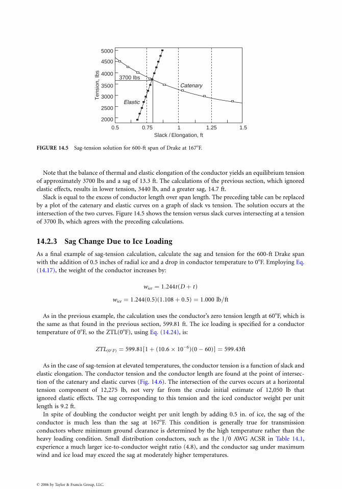
5000
4500
4000
3500
3700 Ibs
Elastic
Catenary
3000
2500
2000
0.5 0.75 1.25 1.51Slack / Elongation, ft
Ten
sion
, Ibs
FIGURE 14.5 Sag-tension solution for 600-ft span of Drake at 1678F.
Note that the balance of thermal and elastic elongation of the conductor yields an equilibrium tension
of approximately 3700 lbs and a sag of 13.3 ft. The calculations of the previous section, which ignored
elastic effects, results in lower tension, 3440 lb, and a greater sag, 14.7 ft.
Slack is equal to the excess of conductor length over span length. The preceding table can be replaced
by a plot of the catenary and elastic curves on a graph of slack vs tension. The solution occurs at the
intersection of the two curves. Figure 14.5 shows the tension versus slack curves intersecting at a tension
of 3700 lb, which agrees with the preceding calculations.
14.2.3 Sag Change Due to Ice Loading
As a final example of sag-tension calculation, calculate the sag and tension for the 600-ft Drake span
with the addition of 0.5 inches of radial ice and a drop in conductor temperature to 08F. Employing Eq.
(14.17), the weight of the conductor increases by:
wice ¼ 1:244t(D þ t)
wice ¼ 1:244(0:5)(1:108þ 0:5) ¼ 1:000 lb=ft
As in the previous example, the calculation uses the conductor’s zero tension length at 608F, which is
the same as that found in the previous section, 599.81 ft. The ice loading is specified for a conductor
temperature of 08F, so the ZTL(08F), using Eq. (14.24), is:
ZTL(0�F) ¼ 599:81[1þ (10:6� 10�6)(0� 60)] ¼ 599:43ft
As in the case of sag-tension at elevated temperatures, the conductor tension is a function of slack and
elastic elongation. The conductor tension and the conductor length are found at the point of intersec-
tion of the catenary and elastic curves (Fig. 14.6). The intersection of the curves occurs at a horizontal
tension component of 12,275 lb, not very far from the crude initial estimate of 12,050 lb that
ignored elastic effects. The sag corresponding to this tension and the iced conductor weight per unit
length is 9.2 ft.
In spite of doubling the conductor weight per unit length by adding 0.5 in. of ice, the sag of the
conductor is much less than the sag at 1678F. This condition is generally true for transmission
conductors where minimum ground clearance is determined by the high temperature rather than the
heavy loading condition. Small distribution conductors, such as the 1=0 AWG ACSR in Table 14.1,
experience a much larger ice-to-conductor weight ratio (4.8), and the conductor sag under maximum
wind and ice load may exceed the sag at moderately higher temperatures.
� 2006 by Taylor & Francis Group, LLC.
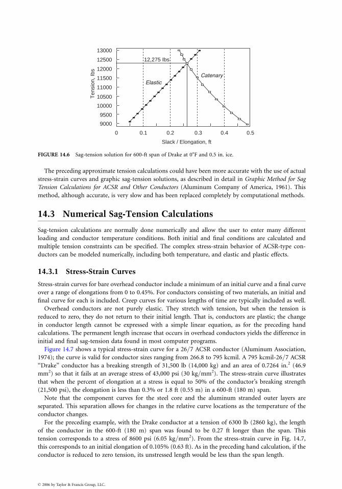
12,275 Ibs
ElasticCatenary
Slack / Elongation, ft
0
9000
9500
10000
10500
11000
11500
12000
12500
13000
Ten
sion
, Ibs
0.1 0.2 0.3 0.4 0.5
FIGURE 14.6 Sag-tension solution for 600-ft span of Drake at 08F and 0.5 in. ice.
The preceding approximate tension calculations could have been more accurate with the use of actual
stress-strain curves and graphic sag-tension solutions, as described in detail in Graphic Method for Sag
Tension Calculations for ACSR and Other Conductors (Aluminum Company of America, 1961). This
method, although accurate, is very slow and has been replaced completely by computational methods.
14.3 Numerical Sag-Tension Calculations
Sag-tension calculations are normally done numerically and allow the user to enter many different
loading and conductor temperature conditions. Both initial and final conditions are calculated and
multiple tension constraints can be specified. The complex stress-strain behavior of ACSR-type con-
ductors can be modeled numerically, including both temperature, and elastic and plastic effects.
14.3.1 Stress-Strain Curves
Stress-strain curves for bare overhead conductor include a minimum of an initial curve and a final curve
over a range of elongations from 0 to 0.45%. For conductors consisting of two materials, an initial and
final curve for each is included. Creep curves for various lengths of time are typically included as well.
Overhead conductors are not purely elastic. They stretch with tension, but when the tension is
reduced to zero, they do not return to their initial length. That is, conductors are plastic; the change
in conductor length cannot be expressed with a simple linear equation, as for the preceding hand
calculations. The permanent length increase that occurs in overhead conductors yields the difference in
initial and final sag-tension data found in most computer programs.
Figure 14.7 shows a typical stress-strain curve for a 26=7 ACSR conductor (Aluminum Association,
1974); the curve is valid for conductor sizes ranging from 266.8 to 795 kcmil. A 795 kcmil-26=7 ACSR
‘‘Drake’’ conductor has a breaking strength of 31,500 lb (14,000 kg) and an area of 0.7264 in.2 (46.9
mm2) so that it fails at an average stress of 43,000 psi (30 kg=mm2). The stress-strain curve illustrates
that when the percent of elongation at a stress is equal to 50% of the conductor’s breaking strength
(21,500 psi), the elongation is less than 0.3% or 1.8 ft (0.55 m) in a 600-ft (180 m) span.
Note that the component curves for the steel core and the aluminum stranded outer layers are
separated. This separation allows for changes in the relative curve locations as the temperature of the
conductor changes.
For the preceding example, with the Drake conductor at a tension of 6300 lb (2860 kg), the length
of the conductor in the 600-ft (180 m) span was found to be 0.27 ft longer than the span. This
tension corresponds to a stress of 8600 psi (6.05 kg=mm2). From the stress-strain curve in Fig. 14.7,
this corresponds to an initial elongation of 0.105% (0.63 ft). As in the preceding hand calculation, if the
conductor is reduced to zero tension, its unstressed length would be less than the span length.
� 2006 by Taylor & Francis Group, LLC.
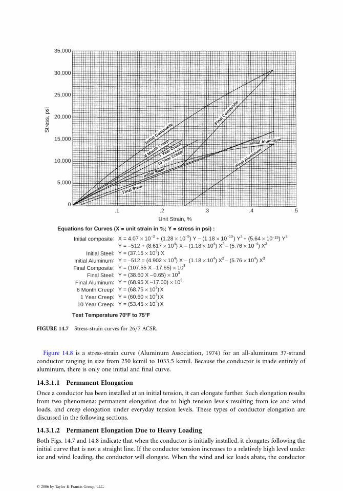
35,000
30,000
25,000
20,000
Str
ess,
psi
15,000
10,000
5,000
0.1 .2 .3
Unit Strain, %
Initial C
omposite
Initial Steel
Final Steel
Final Aluminum
Final
Com
posite
Initial Aluminum
6 Month Creep
1 Year Creep
10 Year Creep
Equations for Curves (X = unit strain in %; Y = stress in psi) :
Initial composite
Initial Steel Initial Aluminum Final Composite
Final SteelFinal Aluminum6 Month Creep 1 Year Creep
10 Year Creep
.4 .5
: X = 4.07 × 10⁻³ + (1.28 × 10⁻⁵) Y − (1.18 × 10⁻¹⁰) Y2 + (5.64 × 10⁻¹⁵) Y3
Y = −512 + (8.617 × 10⁴) X − (1.18 × 104) X2 − (5.76 × 10−4) X3
: Y = (37.15 × 10³) X: Y = −512 = (4.902 × 10⁴) X − (1.18 × 104) X2 − (5.76 × 104) X3
: Y = (107.55 X −17.65) × 103
: Y = (38.60 X −0.65) × 103
: Y = (68.95 X −17.00) × 103
: Y = (68.75 × 10³) X: Y = (60.60 × 10³) X: Y = (53.45 × 10³) X
Test Temperature 708F to 758F
FIGURE 14.7 Stress-strain curves for 26=7 ACSR.
Figure 14.8 is a stress-strain curve (Aluminum Association, 1974) for an all-aluminum 37-strand
conductor ranging in size from 250 kcmil to 1033.5 kcmil. Because the conductor is made entirely of
aluminum, there is only one initial and final curve.
14.3.1.1 Permanent Elongation
Once a conductor has been installed at an initial tension, it can elongate further. Such elongation results
from two phenomena: permanent elongation due to high tension levels resulting from ice and wind
loads, and creep elongation under everyday tension levels. These types of conductor elongation are
discussed in the following sections.
14.3.1.2 Permanent Elongation Due to Heavy Loading
Both Figs. 14.7 and 14.8 indicate that when the conductor is initially installed, it elongates following the
initial curve that is not a straight line. If the conductor tension increases to a relatively high level under
ice and wind loading, the conductor will elongate. When the wind and ice loads abate, the conductor
� 2006 by Taylor & Francis Group, LLC.
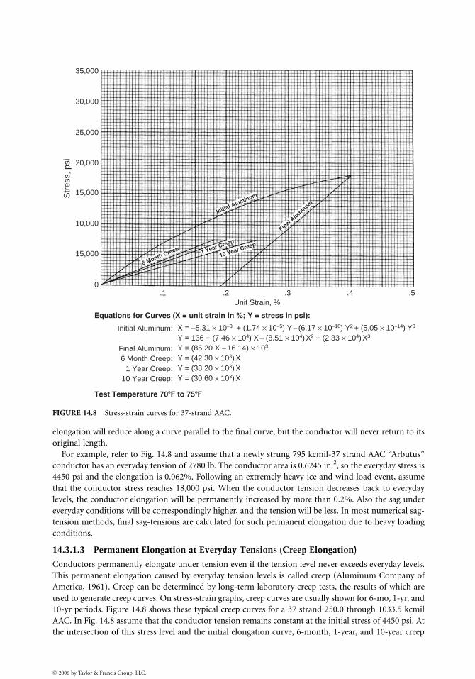
35,000
30,000
25,000
20,000
15,000
10,000
15,000
0.1 .2
Unit Strain, %
Str
ess,
psi
6 Month Creep 1 Year Creep
10 Year Creep
Initial Aluminum
Final Aluminum
Equations for Curves (X = unit strain in %; Y = stress in psi):
Test Temperature 708F to 758F
X = −5.31 × 10⁻³ + (1.74 × 10⁻⁵) Y − (6.17 × 10⁻¹⁰) Y2 + (5.05 × 10⁻¹⁴) Y3
Y = 136 + (7.46 × 10⁴) X − (8.51 × 104) X2 + (2.33 × 104) X3
Y = (85.20 X − 16.14) × 103
Y = (42.30 × 10³) XY = (38.20 × 10³) XY = (30.60 × 10³) X
Initial Aluminum:
Final Aluminum:6 Month Creep:
1 Year Creep:10 Year Creep:
.3 .4 .5
FIGURE 14.8 Stress-strain curves for 37-strand AAC.
elongation will reduce along a curve parallel to the final curve, but the conductor will never return to its
original length.
For example, refer to Fig. 14.8 and assume that a newly strung 795 kcmil-37 strand AAC ‘‘Arbutus’’
conductor has an everyday tension of 2780 lb. The conductor area is 0.6245 in.2, so the everyday stress is
4450 psi and the elongation is 0.062%. Following an extremely heavy ice and wind load event, assume
that the conductor stress reaches 18,000 psi. When the conductor tension decreases back to everyday
levels, the conductor elongation will be permanently increased by more than 0.2%. Also the sag under
everyday conditions will be correspondingly higher, and the tension will be less. In most numerical sag-
tension methods, final sag-tensions are calculated for such permanent elongation due to heavy loading
conditions.
14.3.1.3 Permanent Elongation at Everyday Tensions (Creep Elongation)
Conductors permanently elongate under tension even if the tension level never exceeds everyday levels.
This permanent elongation caused by everyday tension levels is called creep (Aluminum Company of
America, 1961). Creep can be determined by long-term laboratory creep tests, the results of which are
used to generate creep curves. On stress-strain graphs, creep curves are usually shown for 6-mo, 1-yr, and
10-yr periods. Figure 14.8 shows these typical creep curves for a 37 strand 250.0 through 1033.5 kcmil
AAC. In Fig. 14.8 assume that the conductor tension remains constant at the initial stress of 4450 psi. At
the intersection of this stress level and the initial elongation curve, 6-month, 1-year, and 10-year creep
� 2006 by Taylor & Francis Group, LLC.
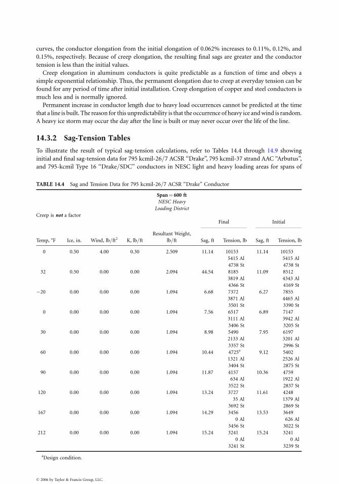
curves, the conductor elongation from the initial elongation of 0.062% increases to 0.11%, 0.12%, and
0.15%, respectively. Because of creep elongation, the resulting final sags are greater and the conductor
tension is less than the initial values.
Creep elongation in aluminum conductors is quite predictable as a function of time and obeys a
simple exponential relationship. Thus, the permanent elongation due to creep at everyday tension can be
found for any period of time after initial installation. Creep elongation of copper and steel conductors is
much less and is normally ignored.
Permanent increase in conductor length due to heavy load occurrences cannot be predicted at the time
that a line is built. The reason for this unpredictability is that the occurrence of heavy ice and wind is random.
A heavy ice storm may occur the day after the line is built or may never occur over the life of the line.
14.3.2 Sag-Tension Tables
To illustrate the result of typical sag-tension calculations, refer to Tables 14.4 through 14.9 showing
initial and final sag-tension data for 795 kcmil-26=7 ACSR ‘‘Drake’’, 795 kcmil-37 strand AAC ‘‘Arbutus’’,
and 795-kcmil Type 16 ‘‘Drake=SDC’’ conductors in NESC light and heavy loading areas for spans of
TABLE 14.4 Sag and Tension Data for 795 kcmil-26=7 ACSR ‘‘Drake’’ Conductor
Span¼ 600 ft
NESC Heavy
Loading District
Creep is not a factor
Final Initial
Temp, 8F Ice, in. Wind, lb=ft2 K, lb=ft
Resultant Weight,
lb=ft Sag, ft Tension, lb Sag, ft Tension, lb
0 0.50 4.00 0.30 2.509 11.14 10153 11.14 10153
5415 Al 5415 Al
4738 St 4738 St
32 0.50 0.00 0.00 2.094 44.54 8185 11.09 8512
3819 Al 4343 Al
4366 St 4169 St
�20 0.00 0.00 0.00 1.094 6.68 7372 6.27 7855
3871 Al 4465 Al
3501 St 3390 St
0 0.00 0.00 0.00 1.094 7.56 6517 6.89 7147
3111 Al 3942 Al
3406 St 3205 St
30 0.00 0.00 0.00 1.094 8.98 5490 7.95 6197
2133 Al 3201 Al
3357 St 2996 St
60 0.00 0.00 0.00 1.094 10.44 4725a 9.12 5402
1321 Al 2526 Al
3404 St 2875 St
90 0.00 0.00 0.00 1.094 11.87 4157 10.36 4759
634 Al 1922 Al
3522 St 2837 St
120 0.00 0.00 0.00 1.094 13.24 3727 11.61 4248
35 Al 1379 Al
3692 St 2869 St
167 0.00 0.00 0.00 1.094 14.29 3456 13.53 3649
0 Al 626 Al
3456 St 3022 St
212 0.00 0.00 0.00 1.094 15.24 3241 15.24 3241
0 Al 0 Al
3241 St 3239 St
aDesign condition.
� 2006 by Taylor & Francis Group, LLC.
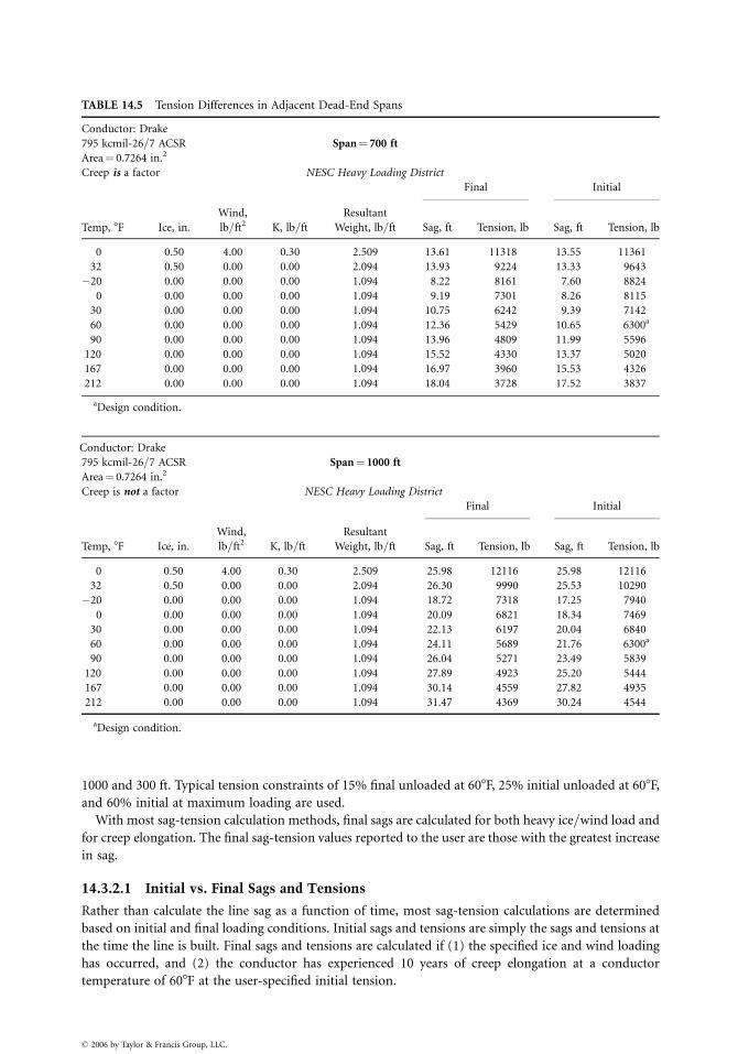
TABLE 14.5 Tension Differences in Adjacent Dead-End Spans
Conductor: Drake
795 kcmil-26=7 ACSR Span¼ 700 ft
Area¼ 0.7264 in.2
Creep is a factor NESC Heavy Loading District
Resultant
Weight, lb=ft
Final Initial
Temp, 8F Ice, in.
Wind,
lb=ft2 K, lb=ft Sag, ft Tension, lb Sag, ft Tension, lb
0 0.50 4.00 0.30 2.509 13.61 11318 13.55 11361
32 0.50 0.00 0.00 2.094 13.93 9224 13.33 9643
�20 0.00 0.00 0.00 1.094 8.22 8161 7.60 8824
0 0.00 0.00 0.00 1.094 9.19 7301 8.26 8115
30 0.00 0.00 0.00 1.094 10.75 6242 9.39 7142
60 0.00 0.00 0.00 1.094 12.36 5429 10.65 6300a
90 0.00 0.00 0.00 1.094 13.96 4809 11.99 5596
120 0.00 0.00 0.00 1.094 15.52 4330 13.37 5020
167 0.00 0.00 0.00 1.094 16.97 3960 15.53 4326
212 0.00 0.00 0.00 1.094 18.04 3728 17.52 3837
aDesign condition.
Conductor: Drake
795 kcmil-26=7 ACSR Span¼ 1000 ft
Area¼ 0.7264 in.2
Creep is not a factor NESC Heavy Loading District
Resultant
Weight, lb=ft
Final Initial
Temp, 8F Ice, in.
Wind,
lb=ft2 K, lb=ft Sag, ft Tension, lb Sag, ft Tension, lb
0 0.50 4.00 0.30 2.509 25.98 12116 25.98 12116
32 0.50 0.00 0.00 2.094 26.30 9990 25.53 10290
�20 0.00 0.00 0.00 1.094 18.72 7318 17.25 7940
0 0.00 0.00 0.00 1.094 20.09 6821 18.34 7469
30 0.00 0.00 0.00 1.094 22.13 6197 20.04 6840
60 0.00 0.00 0.00 1.094 24.11 5689 21.76 6300a
90 0.00 0.00 0.00 1.094 26.04 5271 23.49 5839
120 0.00 0.00 0.00 1.094 27.89 4923 25.20 5444
167 0.00 0.00 0.00 1.094 30.14 4559 27.82 4935
212 0.00 0.00 0.00 1.094 31.47 4369 30.24 4544
aDesign condition.
1000 and 300 ft. Typical tension constraints of 15% final unloaded at 608F, 25% initial unloaded at 608F,
and 60% initial at maximum loading are used.
With most sag-tension calculation methods, final sags are calculated for both heavy ice=wind load and
for creep elongation. The final sag-tension values reported to the user are those with the greatest increase
in sag.
14.3.2.1 Initial vs. Final Sags and Tensions
Rather than calculate the line sag as a function of time, most sag-tension calculations are determined
based on initial and final loading conditions. Initial sags and tensions are simply the sags and tensions at
the time the line is built. Final sags and tensions are calculated if (1) the specified ice and wind loading
has occurred, and (2) the conductor has experienced 10 years of creep elongation at a conductor
temperature of 608F at the user-specified initial tension.
� 2006 by Taylor & Francis Group, LLC.
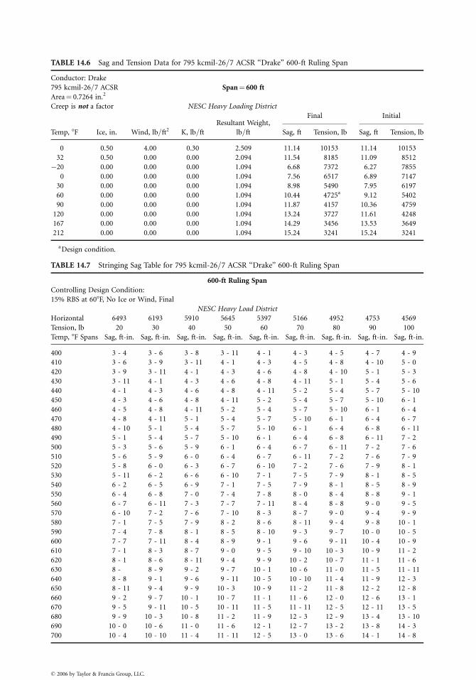
TABLE 14.6 Sag and Tension Data for 795 kcmil-26=7 ACSR ‘‘Drake’’ 600-ft Ruling Span
Conductor: Drake
795 kcmil-26=7 ACSR Span¼ 600 ft
Area¼ 0.7264 in.2
Creep is not a factor NESC Heavy Loading District
Resultant Weight,
lb=ft
Final Initial
Temp, 8F Ice, in. Wind, lb=ft2 K, lb=ft Sag, ft Tension, lb Sag, ft Tension, lb
0 0.50 4.00 0.30 2.509 11.14 10153 11.14 10153
32 0.50 0.00 0.00 2.094 11.54 8185 11.09 8512
�20 0.00 0.00 0.00 1.094 6.68 7372 6.27 7855
0 0.00 0.00 0.00 1.094 7.56 6517 6.89 7147
30 0.00 0.00 0.00 1.094 8.98 5490 7.95 6197
60 0.00 0.00 0.00 1.094 10.44 4725a 9.12 5402
90 0.00 0.00 0.00 1.094 11.87 4157 10.36 4759
120 0.00 0.00 0.00 1.094 13.24 3727 11.61 4248
167 0.00 0.00 0.00 1.094 14.29 3456 13.53 3649
212 0.00 0.00 0.00 1.094 15.24 3241 15.24 3241
aDesign condition.
TABLE 14.7 Stringing Sag Table for 795 kcmil-26=7 ACSR ‘‘Drake’’ 600-ft Ruling Span
600-ft Ruling Span
Controlling Design Condition:
15% RBS at 608F, No Ice or Wind, Final
NESC Heavy Load District
Horizontal 6493 6193 5910 5645 5397 5166 4952 4753 4569
Tension, lb 20 30 40 50 60 70 80 90 100
Temp, 8F Spans Sag, ft-in. Sag, ft-in. Sag, ft-in. Sag, ft-in. Sag, ft-in. Sag, ft-in. Sag, ft-in. Sag, ft-in. Sag, ft-in.
400 3 - 4 3 - 6 3 - 8 3 - 11 4 - 1 4 - 3 4 - 5 4 - 7 4 - 9
410 3 - 6 3 - 9 3 - 11 4 - 1 4 - 3 4 - 5 4 - 8 4 - 10 5 - 0
420 3 - 9 3 - 11 4 - 1 4 - 3 4 - 6 4 - 8 4 - 10 5 - 1 5 - 3
430 3 - 11 4 - 1 4 - 3 4 - 6 4 - 8 4 - 11 5 - 1 5 - 4 5 - 6
440 4 - 1 4 - 3 4 - 6 4 - 8 4 - 11 5 - 2 5 - 4 5 - 7 5 - 10
450 4 - 3 4 - 6 4 - 8 4 - 11 5 - 2 5 - 4 5 - 7 5 - 10 6 - 1
460 4 - 5 4 - 8 4 - 11 5 - 2 5 - 4 5 - 7 5 - 10 6 - 1 6 - 4
470 4 - 8 4 - 11 5 - 1 5 - 4 5 - 7 5 - 10 6 - 1 6 - 4 6 - 7
480 4 - 10 5 - 1 5 - 4 5 - 7 5 - 10 6 - 1 6 - 4 6 - 8 6 - 11
490 5 - 1 5 - 4 5 - 7 5 - 10 6 - 1 6 - 4 6 - 8 6 - 11 7 - 2
500 5 - 3 5 - 6 5 - 9 6 - 1 6 - 4 6 - 7 6 - 11 7 - 2 7 - 6
510 5 - 6 5 - 9 6 - 0 6 - 4 6 - 7 6 - 11 7 - 2 7 - 6 7 - 9
520 5 - 8 6 - 0 6 - 3 6 - 7 6 - 10 7 - 2 7 - 6 7 - 9 8 - 1
530 5 - 11 6 - 2 6 - 6 6 - 10 7 - 1 7 - 5 7 - 9 8 - 1 8 - 5
540 6 - 2 6 - 5 6 - 9 7 - 1 7 - 5 7 - 9 8 - 1 8 - 5 8 - 9
550 6 - 4 6 - 8 7 - 0 7 - 4 7 - 8 8 - 0 8 - 4 8 - 8 9 - 1
560 6 - 7 6 - 11 7 - 3 7 - 7 7 - 11 8 - 4 8 - 8 9 - 0 9 - 5
570 6 - 10 7 - 2 7 - 6 7 - 10 8 - 3 8 - 7 9 - 0 9 - 4 9 - 9
580 7 - 1 7 - 5 7 - 9 8 - 2 8 - 6 8 - 11 9 - 4 9 - 8 10 - 1
590 7 - 4 7 - 8 8 - 1 8 - 5 8 - 10 9 - 3 9 - 7 10 - 0 10 - 5
600 7 - 7 7 - 11 8 - 4 8 - 9 9 - 1 9 - 6 9 - 11 10 - 4 10 - 9
610 7 - 1 8 - 3 8 - 7 9 - 0 9 - 5 9 - 10 10 - 3 10 - 9 11 - 2
620 8 - 1 8 - 6 8 - 11 9 - 4 9 - 9 10 - 2 10 - 7 11 - 1 11 - 6
630 8 - 8 - 9 9 - 2 9 - 7 10 - 1 10 - 6 11 - 0 11 - 5 11 - 11
640 8 - 8 9 - 1 9 - 6 9 - 11 10 - 5 10 - 10 11 - 4 11 - 9 12 - 3
650 8 - 11 9 - 4 9 - 9 10 - 3 10 - 9 11 - 2 11 - 8 12 - 2 12 - 8
660 9 - 2 9 - 7 10 - 1 10 - 7 11 - 1 11 - 6 12 - 0 12 - 6 13 - 1
670 9 - 5 9 - 11 10 - 5 10 - 11 11 - 5 11 - 11 12 - 5 12 - 11 13 - 5
680 9 - 9 10 - 3 10 - 8 11 - 2 11 - 9 12 - 3 12 - 9 13 - 4 13 - 10
690 10 - 0 10 - 6 11 - 0 11 - 6 12 - 1 12 - 7 13 - 2 13 - 8 14 - 3
700 10 - 4 10 - 10 11 - 4 11 - 11 12 - 5 13 - 0 13 - 6 14 - 1 14 - 8
� 2006 by Taylor & Francis Group, LLC.
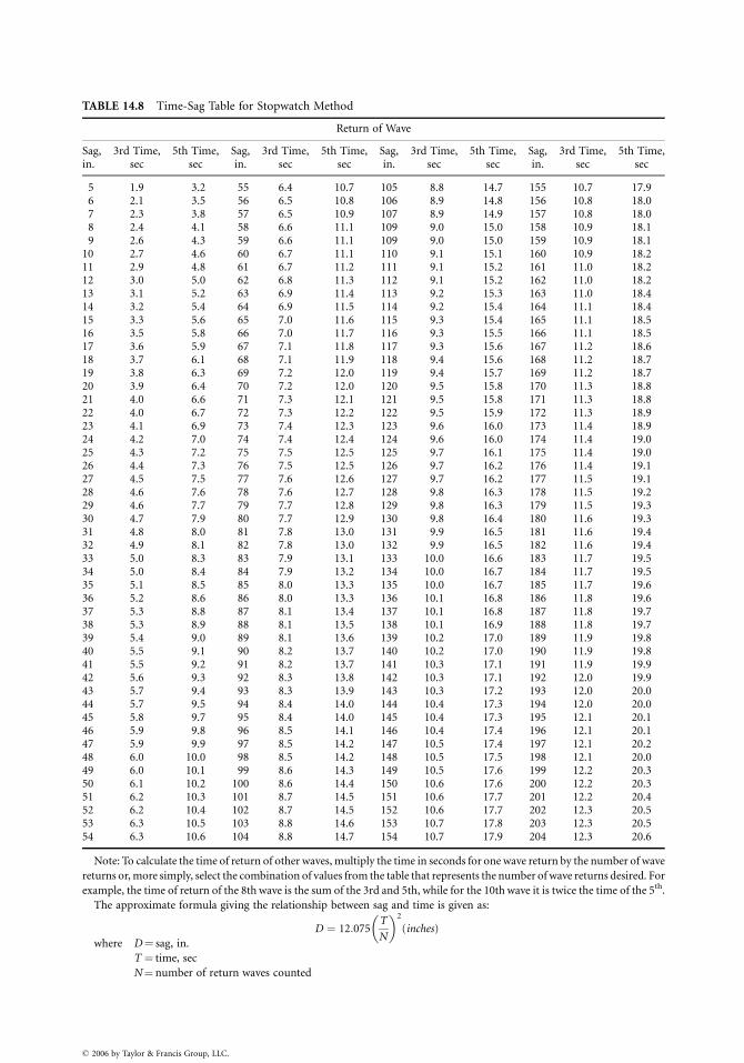
TABLE 14.8 Time-Sag Table for Stopwatch Method
Return of Wave
Sag,in.
3rd Time,sec
5th Time,sec
Sag,in.
3rd Time,sec
5th Time,sec
Sag,in.
3rd Time,sec
5th Time,sec
Sag,in.
3rd Time,sec
5th Time,sec
5 1.9 3.2 55 6.4 10.7 105 8.8 14.7 155 10.7 17.96 2.1 3.5 56 6.5 10.8 106 8.9 14.8 156 10.8 18.07 2.3 3.8 57 6.5 10.9 107 8.9 14.9 157 10.8 18.08 2.4 4.1 58 6.6 11.1 109 9.0 15.0 158 10.9 18.19 2.6 4.3 59 6.6 11.1 109 9.0 15.0 159 10.9 18.1
10 2.7 4.6 60 6.7 11.1 110 9.1 15.1 160 10.9 18.211 2.9 4.8 61 6.7 11.2 111 9.1 15.2 161 11.0 18.212 3.0 5.0 62 6.8 11.3 112 9.1 15.2 162 11.0 18.213 3.1 5.2 63 6.9 11.4 113 9.2 15.3 163 11.0 18.414 3.2 5.4 64 6.9 11.5 114 9.2 15.4 164 11.1 18.415 3.3 5.6 65 7.0 11.6 115 9.3 15.4 165 11.1 18.516 3.5 5.8 66 7.0 11.7 116 9.3 15.5 166 11.1 18.517 3.6 5.9 67 7.1 11.8 117 9.3 15.6 167 11.2 18.618 3.7 6.1 68 7.1 11.9 118 9.4 15.6 168 11.2 18.719 3.8 6.3 69 7.2 12.0 119 9.4 15.7 169 11.2 18.720 3.9 6.4 70 7.2 12.0 120 9.5 15.8 170 11.3 18.821 4.0 6.6 71 7.3 12.1 121 9.5 15.8 171 11.3 18.822 4.0 6.7 72 7.3 12.2 122 9.5 15.9 172 11.3 18.923 4.1 6.9 73 7.4 12.3 123 9.6 16.0 173 11.4 18.924 4.2 7.0 74 7.4 12.4 124 9.6 16.0 174 11.4 19.025 4.3 7.2 75 7.5 12.5 125 9.7 16.1 175 11.4 19.026 4.4 7.3 76 7.5 12.5 126 9.7 16.2 176 11.4 19.127 4.5 7.5 77 7.6 12.6 127 9.7 16.2 177 11.5 19.128 4.6 7.6 78 7.6 12.7 128 9.8 16.3 178 11.5 19.229 4.6 7.7 79 7.7 12.8 129 9.8 16.3 179 11.5 19.330 4.7 7.9 80 7.7 12.9 130 9.8 16.4 180 11.6 19.331 4.8 8.0 81 7.8 13.0 131 9.9 16.5 181 11.6 19.432 4.9 8.1 82 7.8 13.0 132 9.9 16.5 182 11.6 19.433 5.0 8.3 83 7.9 13.1 133 10.0 16.6 183 11.7 19.534 5.0 8.4 84 7.9 13.2 134 10.0 16.7 184 11.7 19.535 5.1 8.5 85 8.0 13.3 135 10.0 16.7 185 11.7 19.636 5.2 8.6 86 8.0 13.3 136 10.1 16.8 186 11.8 19.637 5.3 8.8 87 8.1 13.4 137 10.1 16.8 187 11.8 19.738 5.3 8.9 88 8.1 13.5 138 10.1 16.9 188 11.8 19.739 5.4 9.0 89 8.1 13.6 139 10.2 17.0 189 11.9 19.840 5.5 9.1 90 8.2 13.7 140 10.2 17.0 190 11.9 19.841 5.5 9.2 91 8.2 13.7 141 10.3 17.1 191 11.9 19.942 5.6 9.3 92 8.3 13.8 142 10.3 17.1 192 12.0 19.943 5.7 9.4 93 8.3 13.9 143 10.3 17.2 193 12.0 20.044 5.7 9.5 94 8.4 14.0 144 10.4 17.3 194 12.0 20.045 5.8 9.7 95 8.4 14.0 145 10.4 17.3 195 12.1 20.146 5.9 9.8 96 8.5 14.1 146 10.4 17.4 196 12.1 20.147 5.9 9.9 97 8.5 14.2 147 10.5 17.4 197 12.1 20.248 6.0 10.0 98 8.5 14.2 148 10.5 17.5 198 12.1 20.049 6.0 10.1 99 8.6 14.3 149 10.5 17.6 199 12.2 20.350 6.1 10.2 100 8.6 14.4 150 10.6 17.6 200 12.2 20.351 6.2 10.3 101 8.7 14.5 151 10.6 17.7 201 12.2 20.452 6.2 10.4 102 8.7 14.5 152 10.6 17.7 202 12.3 20.553 6.3 10.5 103 8.8 14.6 153 10.7 17.8 203 12.3 20.554 6.3 10.6 104 8.8 14.7 154 10.7 17.9 204 12.3 20.6
Note: To calculate the time of return of other waves, multiply the time in seconds for one wave return by the number of wave
returns or, more simply, select the combination of values from the table that represents the number of wave returns desired. For
example, the time of return of the 8th wave is the sum of the 3rd and 5th, while for the 10th wave it is twice the time of the 5th.
The approximate formula giving the relationship between sag and time is given as:
D ¼ 12:075T
N
� �2
(inches)
where D¼ sag, in.
T ¼ time, sec
N¼ number of return waves counted
� 2006 by Taylor & Francis Group, LLC.
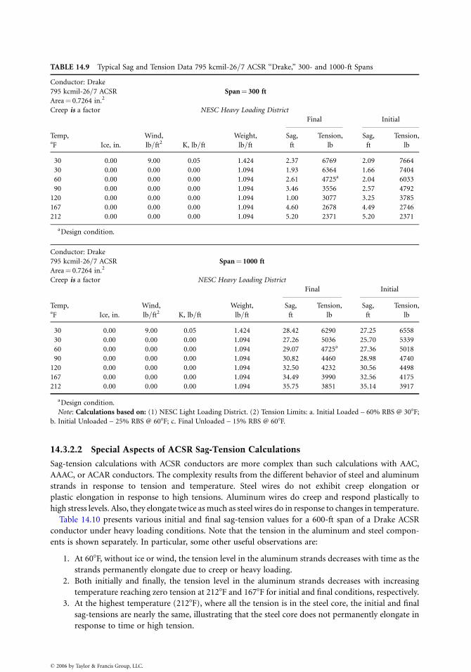
TABLE 14.9 Typical Sag and Tension Data 795 kcmil-26=7 ACSR ‘‘Drake,’’ 300- and 1000-ft Spans
Conductor: Drake
795 kcmil-26=7 ACSR Span¼ 300 ft
Area¼ 0.7264 in.2
Creep is a factor NESC Heavy Loading District
Weight,
lb=ft
Final Initial
Temp,
8F Ice, in.
Wind,
lb=ft2 K, lb=ft
Sag,
ft
Tension,
lb
Sag,
ft
Tension,
lb
30 0.00 9.00 0.05 1.424 2.37 6769 2.09 7664
30 0.00 0.00 0.00 1.094 1.93 6364 1.66 7404
60 0.00 0.00 0.00 1.094 2.61 4725a 2.04 6033
90 0.00 0.00 0.00 1.094 3.46 3556 2.57 4792
120 0.00 0.00 0.00 1.094 1.00 3077 3.25 3785
167 0.00 0.00 0.00 1.094 4.60 2678 4.49 2746
212 0.00 0.00 0.00 1.094 5.20 2371 5.20 2371
aDesign condition.
Conductor: Drake
795 kcmil-26=7 ACSR Span¼ 1000 ft
Area¼ 0.7264 in.2
Creep is a factor NESC Heavy Loading District
Weight,
lb=ft
Final Initial
Temp,
8F Ice, in.
Wind,
lb=ft2 K, lb=ft
Sag,
ft
Tension,
lb
Sag,
ft
Tension,
lb
30 0.00 9.00 0.05 1.424 28.42 6290 27.25 6558
30 0.00 0.00 0.00 1.094 27.26 5036 25.70 5339
60 0.00 0.00 0.00 1.094 29.07 4725a 27.36 5018
90 0.00 0.00 0.00 1.094 30.82 4460 28.98 4740
120 0.00 0.00 0.00 1.094 32.50 4232 30.56 4498
167 0.00 0.00 0.00 1.094 34.49 3990 32.56 4175
212 0.00 0.00 0.00 1.094 35.75 3851 35.14 3917
aDesign condition.
Note: Calculations based on: (1) NESC Light Loading District. (2) Tension Limits: a. Initial Loaded – 60% RBS @ 308F;
b. Initial Unloaded – 25% RBS @ 608F; c. Final Unloaded – 15% RBS @ 608F.
14.3.2.2 Special Aspects of ACSR Sag-Tension Calculations
Sag-tension calculations with ACSR conductors are more complex than such calculations with AAC,
AAAC, or ACAR conductors. The complexity results from the different behavior of steel and aluminum
strands in response to tension and temperature. Steel wires do not exhibit creep elongation or
plastic elongation in response to high tensions. Aluminum wires do creep and respond plastically to
high stress levels. Also, they elongate twice as much as steel wires do in response to changes in temperature.
Table 14.10 presents various initial and final sag-tension values for a 600-ft span of a Drake ACSR
conductor under heavy loading conditions. Note that the tension in the aluminum and steel compon-
ents is shown separately. In particular, some other useful observations are:
1. At 608F, without ice or wind, the tension level in the aluminum strands decreases with time as the
strands permanently elongate due to creep or heavy loading.
2. Both initially and finally, the tension level in the aluminum strands decreases with increasing
temperature reaching zero tension at 2128F and 1678F for initial and final conditions, respectively.
3. At the highest temperature (2128F), where all the tension is in the steel core, the initial and final
sag-tensions are nearly the same, illustrating that the steel core does not permanently elongate in
response to time or high tension.
� 2006 by Taylor & Francis Group, LLC.
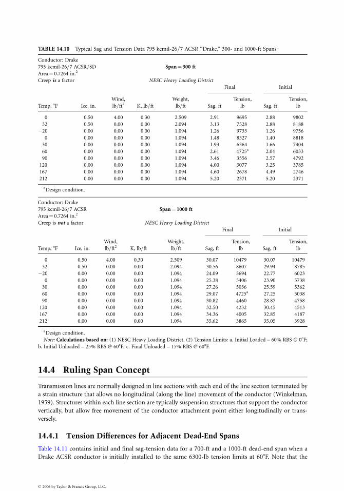
TABLE 14.10 Typical Sag and Tension Data 795 kcmil-26=7 ACSR ‘‘Drake,’’ 300- and 1000-ft Spans
Conductor: Drake
795 kcmil-26=7 ACSR=SD Span¼ 300 ft
Area¼ 0.7264 in.2
Creep is a factor NESC Heavy Loading District
Final Initial
Temp, 8F Ice, in.
Wind,
lb=ft2 K, lb=ft
Weight,
lb=ft Sag, ft
Tension,
lb Sag, ft
Tension,
lb
0 0.50 4.00 0.30 2.509 2.91 9695 2.88 9802
32 0.50 0.00 0.00 2.094 3.13 7528 2.88 8188
�20 0.00 0.00 0.00 1.094 1.26 9733 1.26 9756
0 0.00 0.00 0.00 1.094 1.48 8327 1.40 8818
30 0.00 0.00 0.00 1.094 1.93 6364 1.66 7404
60 0.00 0.00 0.00 1.094 2.61 4725a 2.04 6033
90 0.00 0.00 0.00 1.094 3.46 3556 2.57 4792
120 0.00 0.00 0.00 1.094 4.00 3077 3.25 3785
167 0.00 0.00 0.00 1.094 4.60 2678 4.49 2746
212 0.00 0.00 0.00 1.094 5.20 2371 5.20 2371
aDesign condition.
Conductor: Drake
795 kcmil-26=7 ACSR Span¼ 1000 ft
Area¼ 0.7264 in.2
Creep is not a factor NESC Heavy Loading District
Final Initial
Temp, 8F Ice, in.
Wind,
lb=ft2 K, lb=ft
Weight,
lb=ft Sag, ft
Tension,
lb Sag, ft
Tension,
lb
0 0.50 4.00 0.30 2.509 30.07 10479 30.07 10479
32 0.50 0.00 0.00 2.094 30.56 8607 29.94 8785
�20 0.00 0.00 0.00 1.094 24.09 5694 22.77 6023
0 0.00 0.00 0.00 1.094 25.38 5406 23.90 5738
30 0.00 0.00 0.00 1.094 27.26 5036 25.59 5362
60 0.00 0.00 0.00 1.094 29.07 4725a 27.25 5038
90 0.00 0.00 0.00 1.094 30.82 4460 28.87 4758
120 0.00 0.00 0.00 1.094 32.50 4232 30.45 4513
167 0.00 0.00 0.00 1.094 34.36 4005 32.85 4187
212 0.00 0.00 0.00 1.094 35.62 3865 35.05 3928
aDesign condition.
Note: Calculations based on: (1) NESC Heavy Loading District. (2) Tension Limits: a. Initial Loaded – 60% RBS @ 08F;
b. Initial Unloaded – 25% RBS @ 608F; c. Final Unloaded – 15% RBS @ 608F.
14.4 Ruling Span Concept
Transmission lines are normally designed in line sections with each end of the line section terminated by
a strain structure that allows no longitudinal (along the line) movement of the conductor (Winkelman,
1959). Structures within each line section are typically suspension structures that support the conductor
vertically, but allow free movement of the conductor attachment point either longitudinally or trans-
versely.
14.4.1 Tension Differences for Adjacent Dead-End Spans
Table 14.11 contains initial and final sag-tension data for a 700-ft and a 1000-ft dead-end span when a
Drake ACSR conductor is initially installed to the same 6300-lb tension limits at 608F. Note that the
� 2006 by Taylor & Francis Group, LLC.
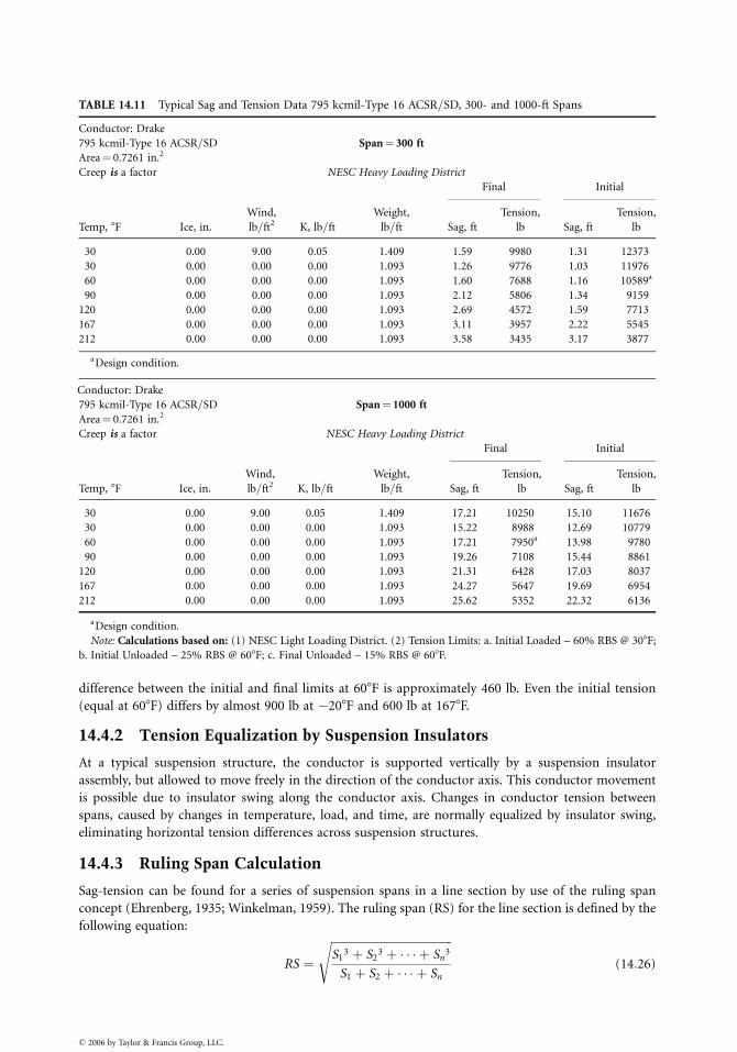
TABLE 14.11 Typical Sag and Tension Data 795 kcmil-Type 16 ACSR=SD, 300- and 1000-ft Spans
Conductor: Drake
795 kcmil-Type 16 ACSR=SD Span¼ 300 ft
Area¼ 0.7261 in.2
Creep is a factor NESC Heavy Loading District
Final Initial
Temp, 8F Ice, in.
Wind,
lb=ft2 K, lb=ft
Weight,
lb=ft Sag, ft
Tension,
lb Sag, ft
Tension,
lb
30 0.00 9.00 0.05 1.409 1.59 9980 1.31 12373
30 0.00 0.00 0.00 1.093 1.26 9776 1.03 11976
60 0.00 0.00 0.00 1.093 1.60 7688 1.16 10589a
90 0.00 0.00 0.00 1.093 2.12 5806 1.34 9159
120 0.00 0.00 0.00 1.093 2.69 4572 1.59 7713
167 0.00 0.00 0.00 1.093 3.11 3957 2.22 5545
212 0.00 0.00 0.00 1.093 3.58 3435 3.17 3877
aDesign condition.
Conductor: Drake
795 kcmil-Type 16 ACSR=SD Span¼ 1000 ft
Area¼ 0.7261 in.2
Creep is a factor NESC Heavy Loading District
Final Initial
Temp, 8F Ice, in.
Wind,
lb=ft2 K, lb=ft
Weight,
lb=ft Sag, ft
Tension,
lb Sag, ft
Tension,
lb
30 0.00 9.00 0.05 1.409 17.21 10250 15.10 11676
30 0.00 0.00 0.00 1.093 15.22 8988 12.69 10779
60 0.00 0.00 0.00 1.093 17.21 7950a 13.98 9780
90 0.00 0.00 0.00 1.093 19.26 7108 15.44 8861
120 0.00 0.00 0.00 1.093 21.31 6428 17.03 8037
167 0.00 0.00 0.00 1.093 24.27 5647 19.69 6954
212 0.00 0.00 0.00 1.093 25.62 5352 22.32 6136
aDesign condition.
Note: Calculations based on: (1) NESC Light Loading District. (2) Tension Limits: a. Initial Loaded – 60% RBS @ 308F;
b. Initial Unloaded – 25% RBS @ 608F; c. Final Unloaded – 15% RBS @ 608F.
difference between the initial and final limits at 608F is approximately 460 lb. Even the initial tension
(equal at 608F) differs by almost 900 lb at �208F and 600 lb at 1678F.
14.4.2 Tension Equalization by Suspension Insulators
At a typical suspension structure, the conductor is supported vertically by a suspension insulator
assembly, but allowed to move freely in the direction of the conductor axis. This conductor movement
is possible due to insulator swing along the conductor axis. Changes in conductor tension between
spans, caused by changes in temperature, load, and time, are normally equalized by insulator swing,
eliminating horizontal tension differences across suspension structures.
14.4.3 Ruling Span Calculation
Sag-tension can be found for a series of suspension spans in a line section by use of the ruling span
concept (Ehrenberg, 1935; Winkelman, 1959). The ruling span (RS) for the line section is defined by the
following equation:
RS ¼
ffiffiffiffiffiffiffiffiffiffiffiffiffiffiffiffiffiffiffiffiffiffiffiffiffiffiffiffiffiffiffiffiffiffiffiffiffiffiffiffiffiffi
S13 þ S2
3 þ � � � þ Sn3
S1 þ S2 þ � � � þ Sn
s
(14:26)
� 2006 by Taylor & Francis Group, LLC.
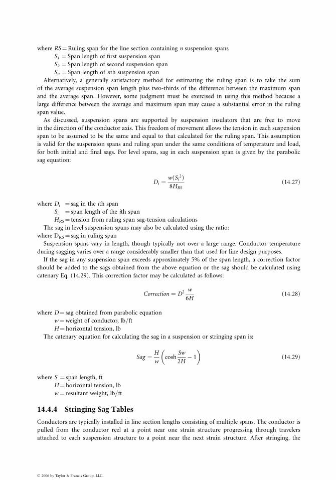
where RS¼Ruling span for the line section containing n suspension spans
S1 ¼ Span length of first suspension span
S2 ¼ Span length of second suspension span
Sn ¼ Span length of nth suspension span
Alternatively, a generally satisfactory method for estimating the ruling span is to take the sum
of the average suspension span length plus two-thirds of the difference between the maximum span
and the average span. However, some judgment must be exercised in using this method because a
large difference between the average and maximum span may cause a substantial error in the ruling
span value.
As discussed, suspension spans are supported by suspension insulators that are free to move
in the direction of the conductor axis. This freedom of movement allows the tension in each suspension
span to be assumed to be the same and equal to that calculated for the ruling span. This assumption
is valid for the suspension spans and ruling span under the same conditions of temperature and load,
for both initial and final sags. For level spans, sag in each suspension span is given by the parabolic
sag equation:
Di ¼w(Si
2)
8HRS
(14:27)
where Di ¼ sag in the ith span
Si ¼ span length of the ith span
HRS¼ tension from ruling span sag-tension calculations
The sag in level suspension spans may also be calculated using the ratio:
where DRS¼ sag in ruling span
Suspension spans vary in length, though typically not over a large range. Conductor temperature
during sagging varies over a range considerably smaller than that used for line design purposes.
If the sag in any suspension span exceeds approximately 5% of the span length, a correction factor
should be added to the sags obtained from the above equation or the sag should be calculated using
catenary Eq. (14.29). This correction factor may be calculated as follows:
Correction ¼ D2 w
6H(14:28)
where D¼ sag obtained from parabolic equation
w¼weight of conductor, lb=ft
H¼ horizontal tension, lb
The catenary equation for calculating the sag in a suspension or stringing span is:
Sag ¼ H
wcosh
Sw
2H� 1
� �
(14:29)
where S ¼ span length, ft
H¼ horizontal tension, lb
w ¼ resultant weight, lb=ft
14.4.4 Stringing Sag Tables
Conductors are typically installed in line section lengths consisting of multiple spans. The conductor is
pulled from the conductor reel at a point near one strain structure progressing through travelers
attached to each suspension structure to a point near the next strain structure. After stringing, the
� 2006 by Taylor & Francis Group, LLC.
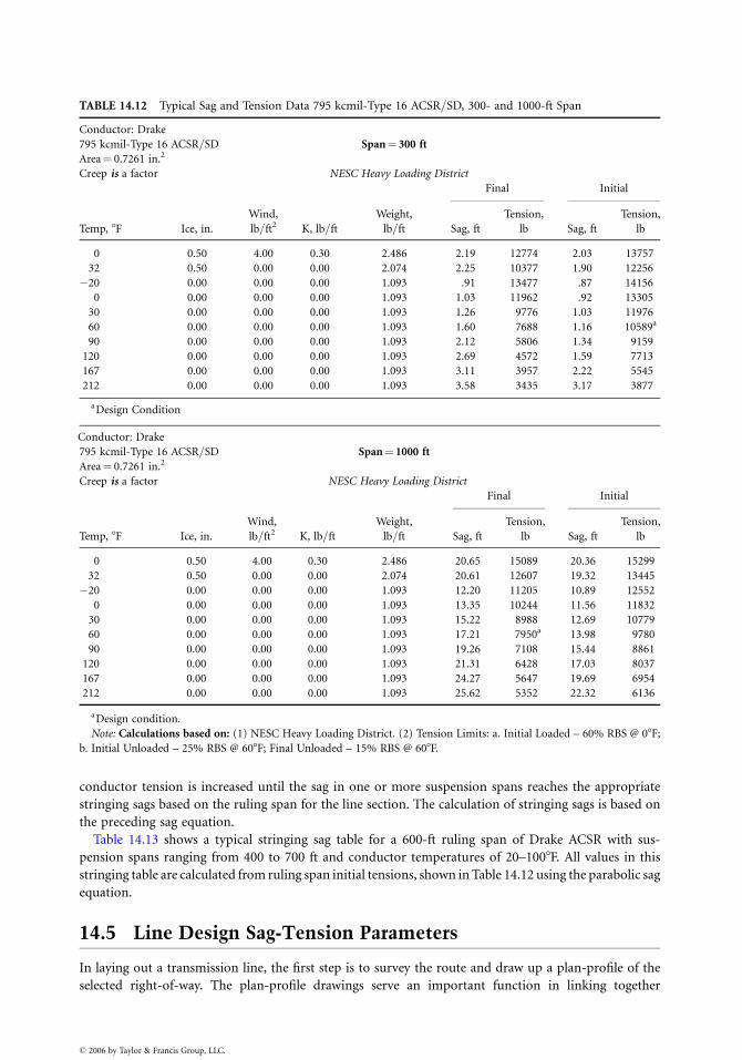
TABLE 14.12 Typical Sag and Tension Data 795 kcmil-Type 16 ACSR=SD, 300- and 1000-ft Span
Conductor: Drake
795 kcmil-Type 16 ACSR=SD Span¼ 300 ft
Area¼ 0.7261 in.2
Creep is a factor NESC Heavy Loading District
Final Initial
Temp, 8F Ice, in.
Wind,
lb=ft2 K, lb=ft
Weight,
lb=ft Sag, ft
Tension,
lb Sag, ft
Tension,
lb
0 0.50 4.00 0.30 2.486 2.19 12774 2.03 13757
32 0.50 0.00 0.00 2.074 2.25 10377 1.90 12256
�20 0.00 0.00 0.00 1.093 .91 13477 .87 14156
0 0.00 0.00 0.00 1.093 1.03 11962 .92 13305
30 0.00 0.00 0.00 1.093 1.26 9776 1.03 11976
60 0.00 0.00 0.00 1.093 1.60 7688 1.16 10589a
90 0.00 0.00 0.00 1.093 2.12 5806 1.34 9159
120 0.00 0.00 0.00 1.093 2.69 4572 1.59 7713
167 0.00 0.00 0.00 1.093 3.11 3957 2.22 5545
212 0.00 0.00 0.00 1.093 3.58 3435 3.17 3877
aDesign Condition
Conductor: Drake
795 kcmil-Type 16 ACSR=SD Span¼ 1000 ft
Area¼ 0.7261 in.2
Creep is a factor NESC Heavy Loading District
Final Initial
Temp, 8F Ice, in.
Wind,
lb=ft2 K, lb=ft
Weight,
lb=ft Sag, ft
Tension,
lb Sag, ft
Tension,
lb
0 0.50 4.00 0.30 2.486 20.65 15089 20.36 15299
32 0.50 0.00 0.00 2.074 20.61 12607 19.32 13445
�20 0.00 0.00 0.00 1.093 12.20 11205 10.89 12552
0 0.00 0.00 0.00 1.093 13.35 10244 11.56 11832
30 0.00 0.00 0.00 1.093 15.22 8988 12.69 10779
60 0.00 0.00 0.00 1.093 17.21 7950a 13.98 9780
90 0.00 0.00 0.00 1.093 19.26 7108 15.44 8861
120 0.00 0.00 0.00 1.093 21.31 6428 17.03 8037
167 0.00 0.00 0.00 1.093 24.27 5647 19.69 6954
212 0.00 0.00 0.00 1.093 25.62 5352 22.32 6136
aDesign condition.
Note: Calculations based on: (1) NESC Heavy Loading District. (2) Tension Limits: a. Initial Loaded – 60% RBS @ 08F;
b. Initial Unloaded – 25% RBS @ 608F; Final Unloaded – 15% RBS @ 608F.
conductor tension is increased until the sag in one or more suspension spans reaches the appropriate
stringing sags based on the ruling span for the line section. The calculation of stringing sags is based on
the preceding sag equation.
Table 14.13 shows a typical stringing sag table for a 600-ft ruling span of Drake ACSR with sus-
pension spans ranging from 400 to 700 ft and conductor temperatures of 20–1008F. All values in this
stringing table are calculated from ruling span initial tensions, shown in Table 14.12 using the parabolic sag
equation.
14.5 Line Design Sag-Tension Parameters
In laying out a transmission line, the first step is to survey the route and draw up a plan-profile of the
selected right-of-way. The plan-profile drawings serve an important function in linking together
� 2006 by Taylor & Francis Group, LLC.
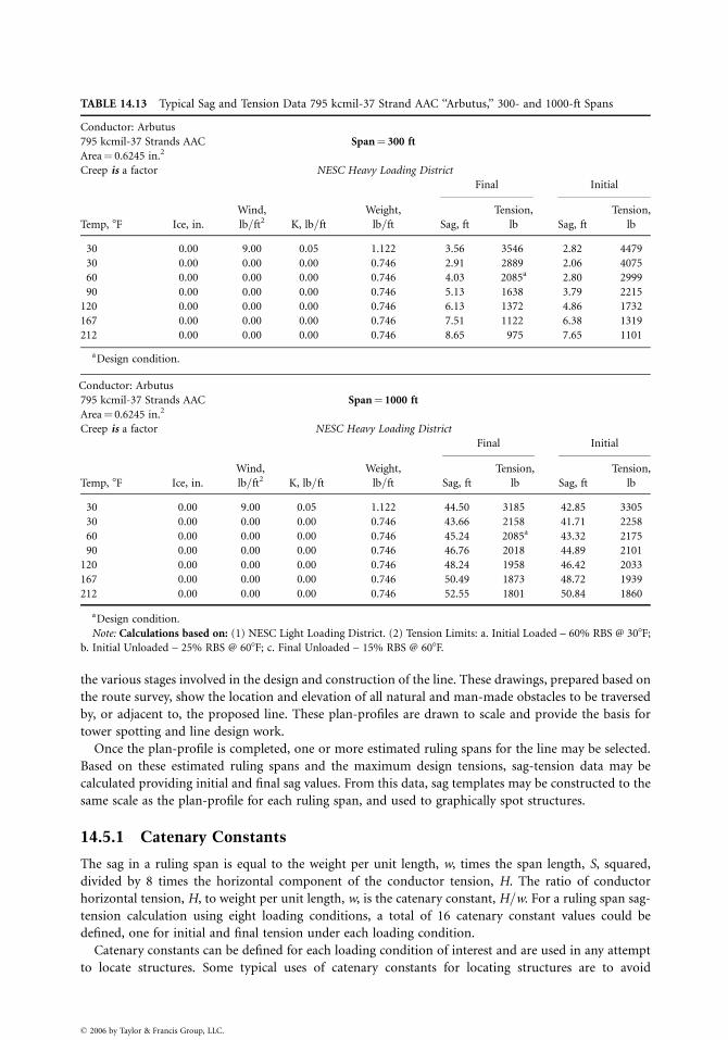
TABLE 14.13 Typical Sag and Tension Data 795 kcmil-37 Strand AAC ‘‘Arbutus,’’ 300- and 1000-ft Spans
Conductor: Arbutus
795 kcmil-37 Strands AAC Span¼ 300 ft
Area¼ 0.6245 in.2
Creep is a factor NESC Heavy Loading District
Final Initial
Temp, 8F Ice, in.
Wind,
lb=ft2 K, lb=ft
Weight,
lb=ft Sag, ft
Tension,
lb Sag, ft
Tension,
lb
30 0.00 9.00 0.05 1.122 3.56 3546 2.82 4479
30 0.00 0.00 0.00 0.746 2.91 2889 2.06 4075
60 0.00 0.00 0.00 0.746 4.03 2085a 2.80 2999
90 0.00 0.00 0.00 0.746 5.13 1638 3.79 2215
120 0.00 0.00 0.00 0.746 6.13 1372 4.86 1732
167 0.00 0.00 0.00 0.746 7.51 1122 6.38 1319
212 0.00 0.00 0.00 0.746 8.65 975 7.65 1101
aDesign condition.
Conductor: Arbutus
795 kcmil-37 Strands AAC Span¼ 1000 ft
Area¼ 0.6245 in.2
Creep is a factor NESC Heavy Loading District
Final Initial
Temp, 8F Ice, in.
Wind,
lb=ft2 K, lb=ft
Weight,
lb=ft Sag, ft
Tension,
lb Sag, ft
Tension,
lb
30 0.00 9.00 0.05 1.122 44.50 3185 42.85 3305
30 0.00 0.00 0.00 0.746 43.66 2158 41.71 2258
60 0.00 0.00 0.00 0.746 45.24 2085a 43.32 2175
90 0.00 0.00 0.00 0.746 46.76 2018 44.89 2101
120 0.00 0.00 0.00 0.746 48.24 1958 46.42 2033
167 0.00 0.00 0.00 0.746 50.49 1873 48.72 1939
212 0.00 0.00 0.00 0.746 52.55 1801 50.84 1860
aDesign condition.
Note: Calculations based on: (1) NESC Light Loading District. (2) Tension Limits: a. Initial Loaded – 60% RBS @ 308F;
b. Initial Unloaded – 25% RBS @ 608F; c. Final Unloaded – 15% RBS @ 608F.
the various stages involved in the design and construction of the line. These drawings, prepared based on
the route survey, show the location and elevation of all natural and man-made obstacles to be traversed
by, or adjacent to, the proposed line. These plan-profiles are drawn to scale and provide the basis for
tower spotting and line design work.
Once the plan-profile is completed, one or more estimated ruling spans for the line may be selected.
Based on these estimated ruling spans and the maximum design tensions, sag-tension data may be
calculated providing initial and final sag values. From this data, sag templates may be constructed to the
same scale as the plan-profile for each ruling span, and used to graphically spot structures.
14.5.1 Catenary Constants
The sag in a ruling span is equal to the weight per unit length, w, times the span length, S, squared,
divided by 8 times the horizontal component of the conductor tension, H. The ratio of conductor
horizontal tension, H, to weight per unit length, w, is the catenary constant, H=w. For a ruling span sag-
tension calculation using eight loading conditions, a total of 16 catenary constant values could be
defined, one for initial and final tension under each loading condition.
Catenary constants can be defined for each loading condition of interest and are used in any attempt
to locate structures. Some typical uses of catenary constants for locating structures are to avoid
� 2006 by Taylor & Francis Group, LLC.
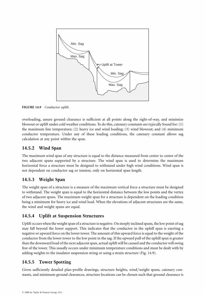
Min. Sag
Max. Sag
Uplift at Tower
Min. Sag
Max. Sag
FIGURE 14.9 Conductor uplift.
overloading, assure ground clearance is sufficient at all points along the right-of-way, and minimize
blowout or uplift under cold weather conditions. To do this, catenary constants are typically found for: (1)
the maximum line temperature; (2) heavy ice and wind loading; (3) wind blowout; and (4) minimum
conductor temperature. Under any of these loading conditions, the catenary constant allows sag
calculation at any point within the span.
14.5.2 Wind Span
The maximum wind span of any structure is equal to the distance measured from center to center of the
two adjacent spans supported by a structure. The wind span is used to determine the maximum
horizontal force a structure must be designed to withstand under high wind conditions. Wind span is
not dependent on conductor sag or tension, only on horizontal span length.
14.5.3 Weight Span
The weight span of a structure is a measure of the maximum vertical force a structure must be designed
to withstand. The weight span is equal to the horizontal distance between the low points and the vertex
of two adjacent spans. The maximum weight span for a structure is dependent on the loading condition
being a minimum for heavy ice and wind load. When the elevations of adjacent structures are the same,
the wind and weight spans are equal.
14.5.4 Uplift at Suspension Structures
Uplift occurs when the weight span of a structure is negative. On steeply inclined spans, the low point of sag
may fall beyond the lower support. This indicates that the conductor in the uphill span is exerting a
negative or upward force on the lower tower. The amount of this upward force is equal to the weight of the
conductor from the lower tower to the low point in the sag. If the upward pull of the uphill span is greater
than the downward load of the next adjacent span, actual uplift will be caused and the conductor will swing
free of the tower. This usually occurs under minimum temperature conditions and must be dealt with by
adding weights to the insulator suspension string or using a strain structure (Fig. 14.9).
14.5.5 Tower Spotting
Given sufficiently detailed plan-profile drawings, structure heights, wind=weight spans, catenary con-
stants, and minimum ground clearances, structure locations can be chosen such that ground clearance is
� 2006 by Taylor & Francis Group, LLC.
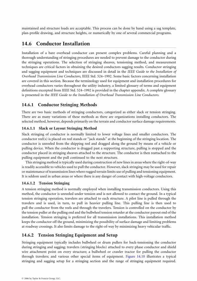
maintained and structure loads are acceptable. This process can be done by hand using a sag template,
plan-profile drawing, and structure heights, or numerically by one of several commercial programs.
14.6 Conductor Installation
Installation of a bare overhead conductor can present complex problems. Careful planning and a
thorough understanding of stringing procedures are needed to prevent damage to the conductor during
the stringing operations. The selection of stringing sheaves, tensioning method, and measurement
techniques are critical factors in obtaining the desired conductors sagging results. Conductor stringing
and sagging equipment and techniques are discussed in detail in the IEEE Guide to the Installation of
Overhead Transmission Line Conductors, IEEE Std. 524–1992. Some basic factors concerning installation
are covered in this section. Because the terminology used for equipment and installation procedures for
overhead conductors varies throughout the utility industry, a limited glossary of terms and equipment
definitions excerpted from IEEE Std. 524–1992 is provided in the chapter appendix. A complete glossary
is presented in the IEEE Guide to the Installation of Overhead Transmission Line Conductors.
14.6.1 Conductor Stringing Methods
There are two basic methods of stringing conductors, categorized as either slack or tension stringing.
There are as many variations of these methods as there are organizations installing conductors. The
selected method, however, depends primarily on the terrain and conductor surface damage requirements.
14.6.1.1 Slack or Layout Stringing Method
Slack stringing of conductor is normally limited to lower voltage lines and smaller conductors. The
conductor reel(s) is placed on reel stands or ‘‘jack stands’’ at the beginning of the stringing location. The
conductor is unreeled from the shipping reel and dragged along the ground by means of a vehicle or
pulling device. When the conductor is dragged past a supporting structure, pulling is stopped and the
conductor placed in stringing sheaves attached to the structure. The conductor is then reattached to the
pulling equipment and the pull continued to the next structure.
This stringing method is typically used during construction of new lines in areas where the right-of-way
is readily accessible to vehicles used to pull the conductor. However, slack stringing may be used for repair
or maintenance of transmission lines where rugged terrain limits use of pulling and tensioning equipment.
It is seldom used in urban areas or where there is any danger of contact with high-voltage conductors.
14.6.1.2 Tension Stringing
A tension stringing method is normally employed when installing transmission conductors. Using this
method, the conductor is unreeled under tension and is not allowed to contact the ground. In a typical
tension stringing operation, travelers are attached to each structure. A pilot line is pulled through the
travelers and is used, in turn, to pull in heavier pulling line. This pulling line is then used to
pull the conductor from the reels and through the travelers. Tension is controlled on the conductor by
the tension puller at the pulling end and the bullwheel tension retarder at the conductor payout end of the
installation. Tension stringing is preferred for all transmission installations. This installation method
keeps the conductor off the ground, minimizing the possibility of surface damage and limiting problems
at roadway crossings. It also limits damage to the right-of-way by minimizing heavy vehicular traffic.
14.6.2 Tension Stringing Equipment and Setup
Stringing equipment typically includes bullwheel or drum pullers for back-tensioning the conductor
during stringing and sagging; travelers (stringing blocks) attached to every phase conductor and shield
wire attachment point on every structure; a bullwheel or crawler tractor for pulling the conductor
through travelers; and various other special items of equipment. Figure 14.10 illustrates a typical
stringing and sagging setup for a stringing section and the range of stringing equipment required.
� 2006 by Taylor & Francis Group, LLC.
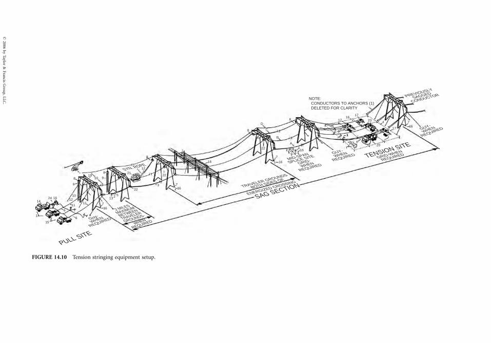
PULL SITE
Guy-WHEN
REQUIRED
TRAVELER GROUNDS
BOTH SIDES OF
ENERGIZED CROSSINGMID-SPAN
SPLICE SITE
GRID-
WHEN
REQUIRED
GUY-
WHEN
REQUIRED GRID-WHEN
REQUIRED
GUY-
WHEN
REQUIRED
PREVIOUSLY
SAGGED
CONDUCTOR
WHEN
REQUIRED
SAG SECTION
TENSION SITE
2 MILES
MAXIMUM
BETWEEN
TRAVELER
GROUNDS-
1424 16
1
15
6
6
1210
9
819
10
8
9
13
716
2 5
22
2112
8
18
8
22
16
16
6
1623 4
17
716
17
NOTE: CONDUCTORS TO ANCHORS (1) DELETED FOR CLARITY
17
620
1
4
7
B
C
8
A
D
3
22
167
SYN. ROPE
1111
FIGURE 14.10 Tension stringing equipment setup.
�2
00
6b
yT
aylor
&F
rancis
Gro
up
,L
LC
.
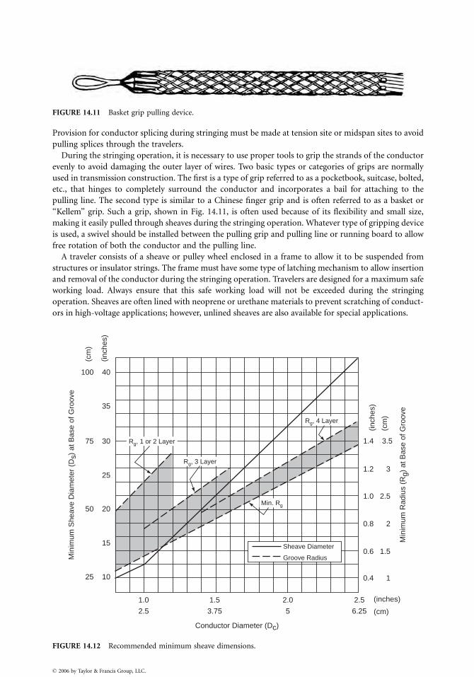
FIGURE 14.11 Basket grip pulling device.
Provision for conductor splicing during stringing must be made at tension site or midspan sites to avoid
pulling splices through the travelers.
During the stringing operation, it is necessary to use proper tools to grip the strands of the conductor
evenly to avoid damaging the outer layer of wires. Two basic types or categories of grips are normally
used in transmission construction. The first is a type of grip referred to as a pocketbook, suitcase, bolted,
etc., that hinges to completely surround the conductor and incorporates a bail for attaching to the
pulling line. The second type is similar to a Chinese finger grip and is often referred to as a basket or
‘‘Kellem’’ grip. Such a grip, shown in Fig. 14.11, is often used because of its flexibility and small size,
making it easily pulled through sheaves during the stringing operation. Whatever type of gripping device
is used, a swivel should be installed between the pulling grip and pulling line or running board to allow
free rotation of both the conductor and the pulling line.
A traveler consists of a sheave or pulley wheel enclosed in a frame to allow it to be suspended from
structures or insulator strings. The frame must have some type of latching mechanism to allow insertion
and removal of the conductor during the stringing operation. Travelers are designed for a maximum safe
working load. Always ensure that this safe working load will not be exceeded during the stringing
operation. Sheaves are often lined with neoprene or urethane materials to prevent scratching of conduct-
ors in high-voltage applications; however, unlined sheaves are also available for special applications.
100 40
75 30 1.4 3.5
1.2 3
1.0 2.5
0.8 2
0.6 1.5
0.4 1
50 20
25 10
15
1.0
2.5
1.5
3.75
Conductor Diameter (Dc)
2.0
Sheave Diameter
Groove Radius
5
2.5 (inches)
(cm)
(inch
es)
(cm
)
(inch
es)
(cm
)
Min
imum
She
ave
Dia
met
er (
Ds)
at B
ase
of G
roov
e
Min
imum
Rad
ius
(Rg)
at B
ase
of G
roov
e
6.25
25
35
Rg, 1 or 2 Layer
Rg, 3 Layer
Min. Rg
Rg, 4 Layer
FIGURE 14.12 Recommended minimum sheave dimensions.
� 2006 by Taylor & Francis Group, LLC.
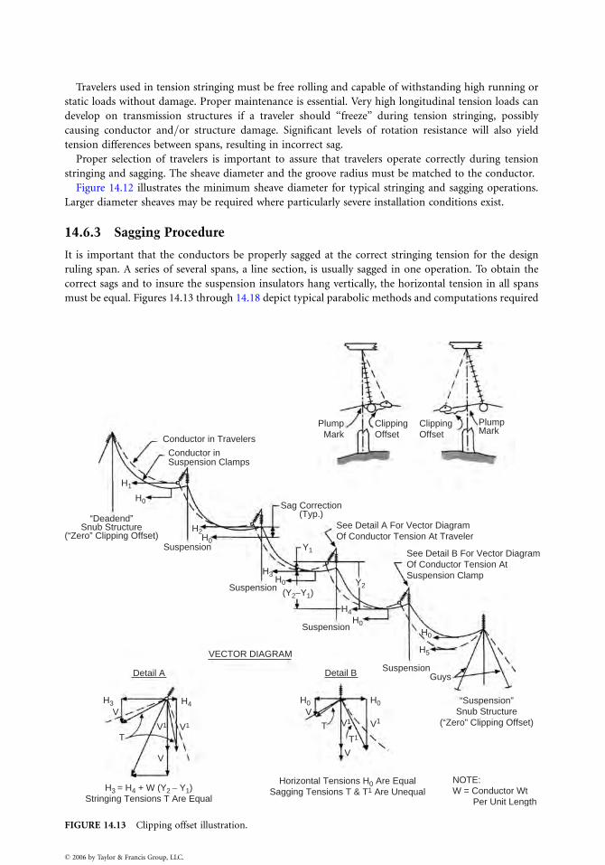
Travelers used in tension stringing must be free rolling and capable of withstanding high running or
static loads without damage. Proper maintenance is essential. Very high longitudinal tension loads can
develop on transmission structures if a traveler should ‘‘freeze’’ during tension stringing, possibly
causing conductor and=or structure damage. Significant levels of rotation resistance will also yield
tension differences between spans, resulting in incorrect sag.
Proper selection of travelers is important to assure that travelers operate correctly during tension
stringing and sagging. The sheave diameter and the groove radius must be matched to the conductor.
Figure 14.12 illustrates the minimum sheave diameter for typical stringing and sagging operations.
Larger diameter sheaves may be required where particularly severe installation conditions exist.
14.6.3 Sagging Procedure
It is important that the conductors be properly sagged at the correct stringing tension for the design
ruling span. A series of several spans, a line section, is usually sagged in one operation. To obtain the
correct sags and to insure the suspension insulators hang vertically, the horizontal tension in all spans
must be equal. Figures 14.13 through 14.18 depict typical parabolic methods and computations required
Conductor in Travelers
Sag Correction(Typ.)
See Detail A For Vector DiagramOf Conductor Tension At Traveler
See Detail B For Vector DiagramOf Conductor Tension At Suspension Clamp
Conductor in Suspension Clamps
“Deadend”Snub Structure
(“Zero” Clipping Offset)
“Suspension”Snub Structure
(“Zero” Clipping Offset)
Suspension
Suspension
PlumpMark
PlumpMark
ClippingOffset
ClippingOffset
Suspension
SuspensionGuysDetail BDetail A
H3 H0 H0
H5
H0
H0
H4
Y2
Y1
H1
H0
H2
H3H0
(Y2−Y1)
H0
V1 V1 V1
V
T
T1
V1
V
T
V VH4
H3 = H4 + W (Y2 − Y1)Stringing Tensions T Are Equal
Horizontal Tensions H0 Are EqualSagging Tensions T & T1 Are Unequal
NOTE:W = Conductor Wt Per Unit Length
VECTOR DIAGRAM
FIGURE 14.13 Clipping offset illustration.
� 2006 by Taylor & Francis Group, LLC.
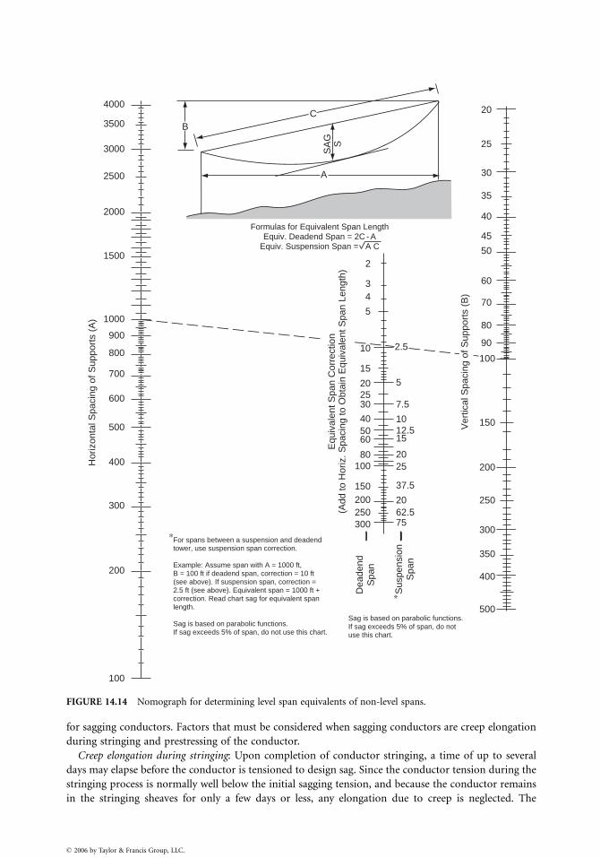
400020
25
30
35
40
45
50
60
70
80
902.5
150
200
250
300
350
400
500
BC
A
Formulas for Equivalent Span LengthEquiv. Deadend Span = 2C - A
Equiv. Suspension Span = A C
SA
GS
3500
3000
2500
2000
1500
1000
2
34
5
10
15
20 5
7.5
1012.515
2025
37.5
2062.575
2530
405060
80100
150200250300
For spans between a suspension and deadendtower, use suspension span correction.
Example: Assume span with A = 1000 ft,B = 100 ft if deadend span, correction = 10 ft(see above). If suspension span, correction =2.5 ft (see above). Equivalent span = 1000 ft +correction. Read chart sag for equivalent spanlength.
Sag is based on parabolic functions.If sag exceeds 5% of span, do not use this chart.
Sag is based on parabolic functions.If sag exceeds 5% of span, do notuse this chart.
Dea
dend
Spa
n
Sus
pens
ion
Spa
n
Hor
izon
tal S
paci
ng o
f Sup
port
s (A
)
900
800
700
600
500
400
300
200
100
∗
∗
Equ
ival
ent S
pan
Cor
rect
ion
(Add
to H
oriz
. Spa
cing
to O
btai
n E
quiv
alen
t Spa
n Le
ngth
)
Ver
tical
Spa
cing
of S
uppo
rts
(B)
100
FIGURE 14.14 Nomograph for determining level span equivalents of non-level spans.
for sagging conductors. Factors that must be considered when sagging conductors are creep elongation
during stringing and prestressing of the conductor.
Creep elongation during stringing: Upon completion of conductor stringing, a time of up to several
days may elapse before the conductor is tensioned to design sag. Since the conductor tension during the
stringing process is normally well below the initial sagging tension, and because the conductor remains
in the stringing sheaves for only a few days or less, any elongation due to creep is neglected. The
� 2006 by Taylor & Francis Group, LLC.
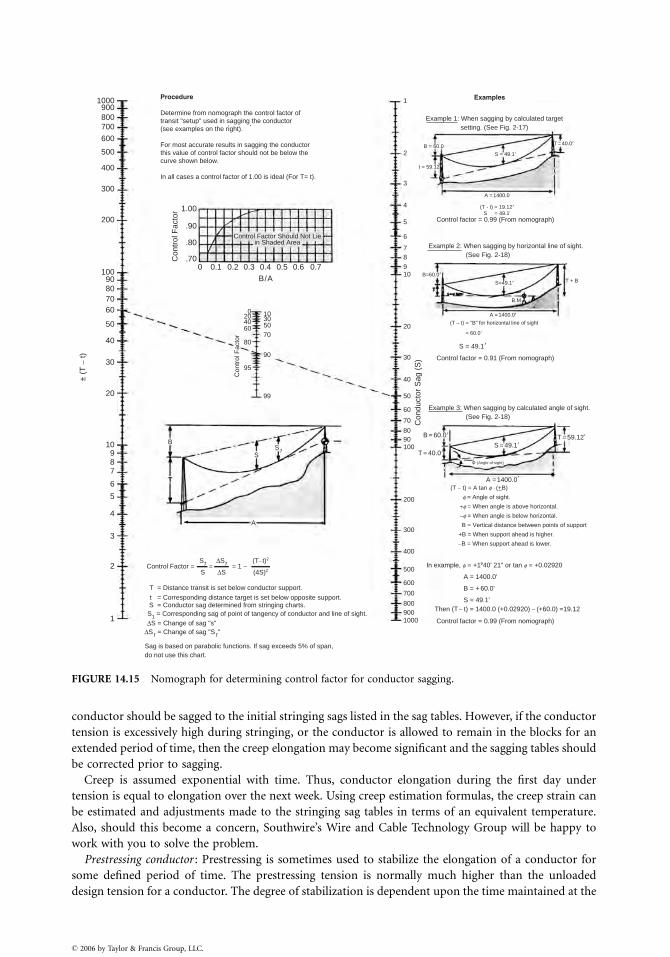
Procedure
Determine from nomograph the control factor of transit "setup" used in sagging the conductor(see examples on the right).
For most accurate results in sagging the conductorthis value of control factor should not be below the curve shown below.
In all cases a control factor of 1.00 is ideal (For T= t).
1000 Examples
B = 60.0
B=60.09
S=49.19 T + B
B.M
T
t = 59.12
T = 40.09
A = 1400.0
(T - t) = 19.129 S = 49.1'
A = 1400.09
(T − t) = "B" for horizontal line of sight
S = 49.1'
1
2
3
4
5
6
78910
20
30
S = 49.1�
Con
duct
or S
ag (
S)
40
50
60
70
8090100
200
300
400
500
600
700
8009001000
Control factor = 0.99 (From nomograph)
Control factor = 0.91 (From nomograph)
B = 60.0�
T = 40.0�S = 49.19
T = 59.129
A = 1400.0�
(T − t) = A tan f (+_B)
f = Angle of sight.
+f = When angle is above horizontal.
−f = When angle is below horizontal.
B = Vertical distance between points of support
+B = When support ahead is higher.
−B = When support ahead is lower.
φ (Angle of sight)
Control factor = 0.99 (From nomograph)
Then (T − t) = 1400.0 (+0.02920) − (+60.0) =19.12
Example 1: When sagging by calculated targetsetting. (See Fig. 2-17)
Example 2: When sagging by horizontal line of sight. (See Fig. 2-18)
Example 3: When sagging by calculated angle of sight. (See Fig. 2-18)
In example, f = +1840' 21" or tan f = +0.02920
A = 1400.0'
B = + 60.0'
S = 49.1'
900800700
600
500
400
300
2001.00
.90
.80
.70
0204060
80
95
Con
trol
Fac
tor
99
B
T
A
T = Distance transit is set below conductor support.
SS1
90
70
3050
10
0
Con
trol
Fac
tor
0.1 0.2 0.3 0.4
Control Factor Should Not Liein Shaded Area
0.5 0.6 0.7B/A
10090807060
50
40
30
± (
T −
t)
20
10987
6
5
4
3
Control Factor = = 1 −=2
1
S1
S
ΔS1
ΔS
(T−t)2
(4S)2
= 60.0�
t = Corresponding distance target is set below opposite support.S = Conductor sag determined from stringing charts.S1 = Corresponding sag of point of tangency of conductor and line of sight.ΔS = Change of sag "s"
Sag is based on parabolic functions. If sag exceeds 5% of span,do not use this chart.
ΔS1 = Change of sag "S1"
·
FIGURE 14.15 Nomograph for determining control factor for conductor sagging.
conductor should be sagged to the initial stringing sags listed in the sag tables. However, if the conductor
tension is excessively high during stringing, or the conductor is allowed to remain in the blocks for an
extended period of time, then the creep elongation may become significant and the sagging tables should
be corrected prior to sagging.
Creep is assumed exponential with time. Thus, conductor elongation during the first day under
tension is equal to elongation over the next week. Using creep estimation formulas, the creep strain can
be estimated and adjustments made to the stringing sag tables in terms of an equivalent temperature.
Also, should this become a concern, Southwire’s Wire and Cable Technology Group will be happy to
work with you to solve the problem.
Prestressing conductor : Prestressing is sometimes used to stabilize the elongation of a conductor for
some defined period of time. The prestressing tension is normally much higher than the unloaded
design tension for a conductor. The degree of stabilization is dependent upon the time maintained at the
� 2006 by Taylor & Francis Group, LLC.
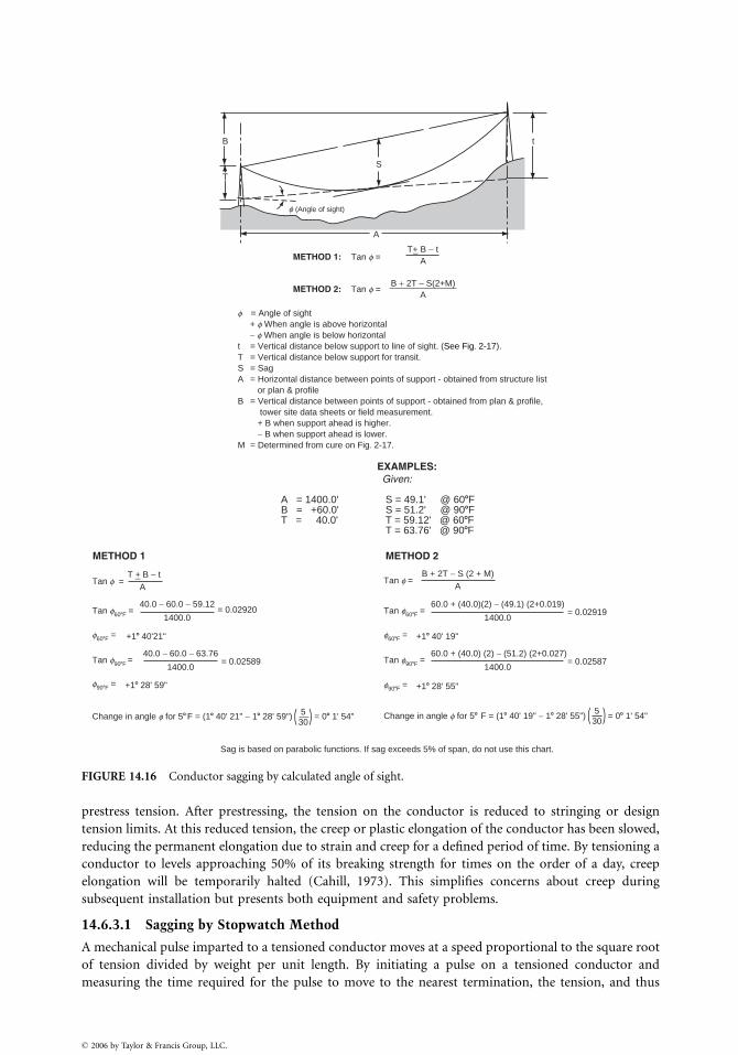
B
TS
A
METHOD 1: Tan f =
METHOD 2: Tan f =
f = Angle of sight + f When angle is above horizontal − f When angle is below horizontalt = Vertical distance below support to line of sight. (See Fig. 2-17).T = Vertical distance below support for transit.S = Sag A = Horizontal distance between points of support - obtained from structure list or plan & profileB = Vertical distance between points of support - obtained from plan & profile, tower site data sheets or field measurement. + B when support ahead is higher. − B when support ahead is lower.M = Determined from cure on Fig. 2-17.
T+_ B − t
B + 2T − S(2+M)
A
A
f (Angle of sight)
t
METHOD 1 METHOD 2
Tan f =
Tan f608F =
Tan f908F =
f608F =
f908F =
EXAMPLES: Given:
A = 1400.0' S = 49.1' @ 608FB = +60.0' S = 51.2' @ 908FT = 40.0' T = 59.12' @ 608F T = 63.76' @ 908F
Sag is based on parabolic functions. If sag exceeds 5% of span, do not use this chart.
T +_ B − t
40.0 − 60.0 − 59.12
1400.0
+18 40'21" f608F = +18 40' 19"
f908F = +18 28' 55"+18 28' 59"
= 0.02920
= 0.02589
ATan f =
B + 2T − S (2 + M)A
Tan f608F =60.0 + (40.0)(2) − (49.1) (2+0.019)
1400.0= 0.02919
Tan f908F =60.0 + (40.0) (2) − (51.2) (2+0.027)
1400.0= 0.02587
40.0 − 60.0 − 63.76
1400.0
Change in angle f for 58F = (18 40' 21" − 18 28' 59") = 08 1' 54"5 30( ) Change in angle f for 58 F = (18 40' 19" − 18 28' 55") = 08 1' 54"5
30( )
FIGURE 14.16 Conductor sagging by calculated angle of sight.
prestress tension. After prestressing, the tension on the conductor is reduced to stringing or design
tension limits. At this reduced tension, the creep or plastic elongation of the conductor has been slowed,
reducing the permanent elongation due to strain and creep for a defined period of time. By tensioning a
conductor to levels approaching 50% of its breaking strength for times on the order of a day, creep
elongation will be temporarily halted (Cahill, 1973). This simplifies concerns about creep during
subsequent installation but presents both equipment and safety problems.
14.6.3.1 Sagging by Stopwatch Method
A mechanical pulse imparted to a tensioned conductor moves at a speed proportional to the square root
of tension divided by weight per unit length. By initiating a pulse on a tensioned conductor and
measuring the time required for the pulse to move to the nearest termination, the tension, and thus
� 2006 by Taylor & Francis Group, LLC.
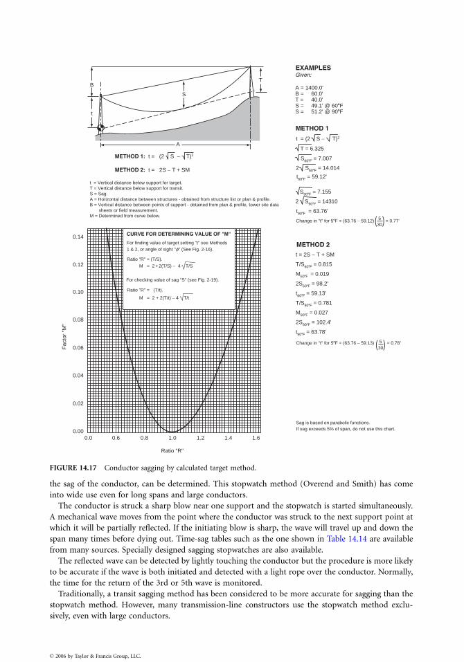
B
t
S
A
T
METHOD 1: t = (2 S − T)2
EXAMPLES
METHOD 1
METHOD 2
t = 2S − T + SM
T/S608F = 0.815
M608F = 0.019
2S608F = 98.2'
t608F = 59.13'
T/S908F = 0.781
M908F = 0.027
2S908F = 102.4'
t908F = 63.78'
Given:
A = 1400.0'B = 60.0'T = 40.0'S = 49.1' @ 608FS = 51.2' @ 908F
t = (2 S − T)2
T = 6.325
S608F = 7.007
2 S608F = 14.014
2 S908F = 14310
t908F = 63.76'
S908F = 7.155
t608F = 59.12'
0.14
0.12
0.10
0.08
0.06
0.04
0.02
0.000.0 0.6 0.8 1.0 1.2 1.4 1.6
Ratio "R"
CURVE FOR DETERMINING VALUE OF "M"
For finding value of target setting "t" see Methods1 & 2, or angle of sight "f" (See Fig. 2-16).
Change in "t" for 58F = (63.76 − 59.12) = 0.77'
For checking value of sag "S" (see Fig. 2-19).
Ratio "R" = (T/S).
Ratio "R" = (T/t).
M = 2 + 2(T/S) − 4 T/S
Fac
tor
"M"
METHOD 2: t = 2S − T + SM
t = Vertical distance below support for target.T = Vertical distance below support for transit.S = Sag.A = Horizontal distance between structures - obtained from structure list or plan & profile.B = Vertical distance between points of support - obtained from plan & profile, tower site data sheets or field measurement.M = Determined from curve below.
M = 2 + 2(T/t) − 4 T/t
530( )
Change in "t" for 58F = (63.76 − 59.13) = 0.78�
Sag is based on parabolic functions.If sag exceeds 5% of span, do not use this chart.
530( )
FIGURE 14.17 Conductor sagging by calculated target method.
the sag of the conductor, can be determined. This stopwatch method (Overend and Smith) has come
into wide use even for long spans and large conductors.
The conductor is struck a sharp blow near one support and the stopwatch is started simultaneously.
A mechanical wave moves from the point where the conductor was struck to the next support point at
which it will be partially reflected. If the initiating blow is sharp, the wave will travel up and down the
span many times before dying out. Time-sag tables such as the one shown in Table 14.14 are available
from many sources. Specially designed sagging stopwatches are also available.
The reflected wave can be detected by lightly touching the conductor but the procedure is more likely
to be accurate if the wave is both initiated and detected with a light rope over the conductor. Normally,
the time for the return of the 3rd or 5th wave is monitored.
Traditionally, a transit sagging method has been considered to be more accurate for sagging than the
stopwatch method. However, many transmission-line constructors use the stopwatch method exclu-
sively, even with large conductors.
� 2006 by Taylor & Francis Group, LLC.
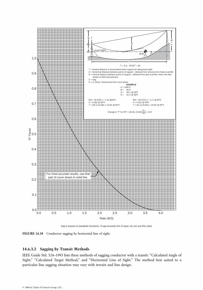
B
T
S
B.M
(Level Sight)
A
T +
B
T = S (1 − B/4S)2 = SK
T = Vertical distance of transit below lower support for taking level sight.A = Horizontal distance between points of support - obtained from structure list of plan & profile.B = Vertical distance between points of support - obtained from plan & profile, tower site data sheets or field measurement.S = Sag.K = (1−B/4s)2–Determined from curve below. EXAMPLE A = 1400.0' B = 60.0' S = 49.1' @ 608F S = 51.2' @ 908F
B/S = 60.0/49.1 = 1.22 @608F B/S = 60.0 / 51.2 = 1.17 @ 908FK = 0.482 @ 608F K = 0.501 @ 908FT = (49.1) (0.482) = 23.66' @ 608F T = (51.2) (0.501) = 25.65' @ 908F
Change in "T" for 58F = (25.65−23.66) = 0.33'5
30 ( )
1.0
0.9
0.8
0.7
0.6
0.5
0.4
0.3
0.2
0.1
0.00.0 0.5 1.0 1.5 2.0
Ratio (B/S)
"K"
Fac
tor
2.5 3.0 3.5 4.0
Sag is based on parabolic functions. If sag exceeds 5% of span, do not use this chart.
For most accurate results, use thatpart of curve drawn in solid line.
FIGURE 14.18 Conductor sagging by horizontal line of sight.
14.6.3.2 Sagging by Transit Methods
IEEE Guide Std. 524–1993 lists three methods of sagging conductor with a transit: ‘‘Calculated Angle of
Sight,’’ ‘‘Calculated Target Method,’’ and ‘‘Horizontal Line of Sight.’’ The method best suited to a
particular line sagging situation may vary with terrain and line design.
� 2006 by Taylor & Francis Group, LLC.
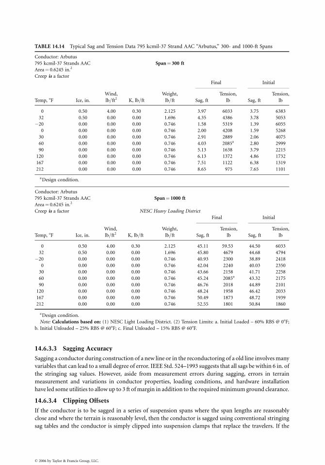
TABLE 14.14 Typical Sag and Tension Data 795 kcmil-37 Strand AAC ‘‘Arbutus,’’ 300- and 1000-ft Spans
Conductor: Arbutus
795 kcmil-37 Strands AAC Span¼ 300 ft
Area¼ 0.6245 in.2
Creep is a factor
Final Initial
Temp, 8F Ice, in.
Wind,
lb=ft2 K, lb=ft
Weight,
lb=ft Sag, ft
Tension,
lb Sag, ft
Tension,
lb
0 0.50 4.00 0.30 2.125 3.97 6033 3.75 6383
32 0.50 0.00 0.00 1.696 4.35 4386 3.78 5053
�20 0.00 0.00 0.00 0.746 1.58 5319 1.39 6055
0 0.00 0.00 0.00 0.746 2.00 4208 1.59 5268
30 0.00 0.00 0.00 0.746 2.91 2889 2.06 4075
60 0.00 0.00 0.00 0.746 4.03 2085a 2.80 2999
90 0.00 0.00 0.00 0.746 5.13 1638 3.79 2215
120 0.00 0.00 0.00 0.746 6.13 1372 4.86 1732
167 0.00 0.00 0.00 0.746 7.51 1122 6.38 1319
212 0.00 0.00 0.00 0.746 8.65 975 7.65 1101
aDesign condition.
Conductor: Arbutus
795 kcmil-37 Strands AAC Span¼ 1000 ft
Area¼ 0.6245 in.2
Creep is a factor NESC Heavy Loading District
Final Initial
Temp, 8F Ice, in.
Wind,
lb=ft2 K, lb=ft
Weight,
lb=ft Sag, ft
Tension,
lb Sag, ft
Tension,
lb
0 0.50 4.00 0.30 2.125 45.11 59.53 44.50 6033
32 0.50 0.00 0.00 1.696 45.80 4679 44.68 4794
�20 0.00 0.00 0.00 0.746 40.93 2300 38.89 2418
0 0.00 0.00 0.00 0.746 42.04 2240 40.03 2350
30 0.00 0.00 0.00 0.746 43.66 2158 41.71 2258
60 0.00 0.00 0.00 0.746 45.24 2085a 43.32 2175
90 0.00 0.00 0.00 0.746 46.76 2018 44.89 2101
120 0.00 0.00 0.00 0.746 48.24 1958 46.42 2033
167 0.00 0.00 0.00 0.746 50.49 1873 48.72 1939
212 0.00 0.00 0.00 0.746 52.55 1801 50.84 1860
aDesign condition.
Note: Calculations based on: (1) NESC Light Loading District. (2) Tension Limits: a. Initial Loaded – 60% RBS @ 08F;
b. Initial Unloaded – 25% RBS @ 608F; c. Final Unloaded – 15% RBS @ 608F.
14.6.3.3 Sagging Accuracy
Sagging a conductor during construction of a new line or in the reconductoring of a old line involves many
variables that can lead to a small degree of error. IEEE Std. 524–1993 suggests that all sags be within 6 in. of
the stringing sag values. However, aside from measurement errors during sagging, errors in terrain
measurement and variations in conductor properties, loading conditions, and hardware installation
have led some utilities to allow up to 3 ft of margin in addition to the required minimum ground clearance.
14.6.3.4 Clipping Offsets
If the conductor is to be sagged in a series of suspension spans where the span lengths are reasonably
close and where the terrain is reasonably level, then the conductor is sagged using conventional stringing
sag tables and the conductor is simply clipped into suspension clamps that replace the travelers. If the
� 2006 by Taylor & Francis Group, LLC.
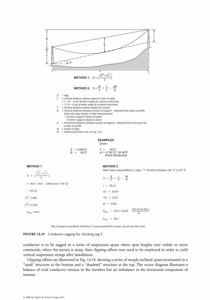
B
T
S
A
METHOD 1: S = ( )
METHOD 2: S =
METHOD 1 METHOD 2Note: When using Method 2, value, "T" should lie between 3/4 "S" & 4/3 "S"
S = ( )S =
t = 59.12'
t/2 = 29.56'
T/2 = 20.0�
M = 0.061
S608F = 20.0 + 29.56 −
S608F = 49.1'
EXAMPLES Given:
A = 1400.0' T = 40.0'B = 60.0' f = +1840' 21� @ 608F (Field Measured)
S = Sagt = Vertical distance below support to line of sight. = T +_ B − A tan f when angle f is above horizontal. = T+_ B + A tan f when angle f is below horizontal.T = Vertical distance below support for transit.B = Vertical distance between points of support - obtanied from plan & profile, tower site data sheets or field measurement. + B when support ahead is higher. − B when support ahead is lower.A = Horizontal distance between points of support - obtained from structure list or plan & profile f = Angle of sightM = Determined from cure on Fig. 2.17.
f
t
T + t 2
2
B t tM2 2 8
+ −
T + t 2
2 B2
t2
tM8
+ −
(59.12) (0.061)
Sag is based on parabolic functions. if sag exceeds 5% of span, do not use this chart.
t = 40.0 + 60.0 − 1400.0 tan 18 40' 21"
= 59.12'
t = 7.689
T = 6.325
S608F = 49.1' 8
FIGURE 14.19 Conductor sagging for checking sag S.
conductor is to be sagged in a series of suspension spans where span lengths vary widely or more
commonly, where the terrain is steep, then clipping offsets may need to be employed in order to yield
vertical suspension strings after installation.
Clipping offsets are illustrated in Fig. 14.19, showing a series of steeply inclined spans terminated in a
‘‘snub’’ structure at the bottom and a ‘‘deadend’’ structure at the top. The vector diagram illustrates a
balance of total conductor tension in the travelers but an imbalance in the horizontal component of
tension.
� 2006 by Taylor & Francis Group, LLC.
14.7 Defining Terms
Block—A device designed with one or more single sheaves, a wood or metal shell, and an attachment
hook or shackle. When rope is reeved through two of these devices, the assembly is commonly
referred to as a block and tackle. A set of 4s refers to a block and tackle arrangement utilizing two
4-inch double-sheave blocks to obtain four load-bearing lines. Similarly, a set of 5s or a set of 6s refers
to the same number of load bearing lines obtained using two 5-inch or two 6-inch double-sheave
blocks, respectively.
Synonyms: set of 4s, set of 5s, set of 6s.
Bullwheel—A wheel incorporated as an integral part of a bullwheel puller or tensioner to generate
pulling or braking tension on conductors or pulling lines, or both, through friction. A puller or
tensioner normally has one or more pairs arranged in tandem incorporated in its design. The physical
size of the wheels will vary for different designs, but 17-in. (43 cm) face widths and diameters of 5 ft
(150 cm) are common. The wheels are power driven or retarded and lined with single- or multiple-
groove neoprene or urethane linings. Friction is accomplished by reeving the pulling line or conductor
around the groove of each pair.
Clipping-in—The transferring of sagged conductors from the traveler to their permanent suspension
positions and the installing of the permanent suspension clamps.
Synonyms: clamping, clipping.
Clipping offset—A calculated distance, measured along the conductor from the plum mark to a
point on the conductor at which the center of the suspension clamp is to be placed. When stringing
in rough terrain, clipping offset may be required to balance the horizontal forces on each suspension
structure.
Grip, conductor—A device designed to permit the pulling of conductor without splicing on fittings,
eyes, etc. It permits the pulling of a continuous conductor where threading is not possible. The designs of
these grips vary considerably. Grips such as the Klein (Chicago) and Crescent utilize an open-sided rigid
body with opposing jaws and swing latch. In addition to pulling conductors, this type is commonly used
to tension guys and, in some cases, pull wire rope. The design of the come-along (pocketbook, suitcase,
four bolt, etc.) incorporates a bail attached to the body of a clamp which folds to completely surround
and envelope the conductor. Bolts are then used to close the clamp and obtain a grip.
Synonyms: buffalo, Chicago grip, come-along, Crescent, four bolt, grip, Klein, pocketbook, seven
bolt, six bolt, slip-grip, suitcase.
Line, pilot—A lightweight line, normally synthetic fiber rope, used to pull heavier pulling lines which in
turn are used to pull the conductor. Pilot lines may be installed with the aid of finger lines or by
helicopter when the insulators and travelers are hung.
Synonyms: lead line, leader, P-line, straw line.
Line, pulling—A high-strength line, normally synthetic fiber rope or wire rope, used to pull the
conductor. However, on reconstruction jobs where a conductor is being replaced, the old conductor
often serves as the pulling line for the new conductor. In such cases, the old conductor must be closely
examined for any damage prior to the pulling operations.
Synonyms: bull line, hard line, light line, sock line.
Puller, bullwheel—A device designed to pull pulling lines and conductors during stringing operations.
It normally incorporates one or more pairs of urethane- or neoprene-lined, power-driven, single- or
multiple-groove bullwheels where each pair is arranged in tandem. Pulling is accomplished by friction
generated against the pulling line which is reeved around the grooves of a pair of the bullwheels. The
puller is usually equipped with its own engine which drives the bullwheels mechanically, hydraulically,
or through a combination of both. Some of these devices function as either a puller or tensioner.
Synonym: puller.
Puller, drum—A device designed to pull a conductor during stringing operations. It is normally
equipped with its own engine which drives the drum mechanically, hydraulically, or through a
combination of both. It may be equipped with synthetic fiber rope or wire rope to be used as the
� 2006 by Taylor & Francis Group, LLC.

pulling line. The pulling line is payed out from the unit, pulled through the travelers in the sag section
and attached to the conductor. The conductor is then pulled in by winding the pulling line back onto
the drum. This unit is sometimes used with synthetic fiber rope acting as a pilot line to pull heavier
pulling lines across canyons, rivers, etc.
Synonyms: hoist, single drum hoist, single drum winch, tugger.
Puller, reel—A device designed to pull a conductor during stringing operations. It is normally equipped
with its own engine which drives the supporting shaft for the reel mechanically, hydraulically, or
through a combination of both. The shaft, in turn, drives the reel. The application of this unit is
essentially the same as that for the drum puller previously described. Some of these devices function as
either a puller or tensioner.
Reel stand—A device designed to support one or more reels and having the possibility of being skid,
trailer, or truck mounted. These devices may accommodate rope or conductor reels of varying sizes
and are usually equipped with reel brakes to prevent the reels from turning when pulling is stopped.
They are used for either slack or tension stringing. The designation of reel trailer or reel truck
implies that the trailer or truck has been equipped with a reel stand (jacks) and may serve as a reel
transport or payout unit, or both, for stringing operations. Depending upon the sizes of the reels to be
carried, the transporting vehicles may range from single-axle trailers to semi-trucks with trailers
having multiple axles.
Synonyms: reel trailer, reel transporter, reel truck.
Running board—A pulling device designed to permit stringing more than one conductor simultan-
eously with a single pulling line. For distribution stringing, it is usually made of lightweight tubing
with the forward end curved gently upward to provide smooth transition over pole cross-arm rollers.
For transmission stringing, the device is either made of sections hinged transversely to the direction of
pull or of a hard-nose rigid design, both having a flexible pendulum tail suspended from the rear. This
configuration stops the conductors from twisting together and permits smooth transition over the
sheaves of bundle travelers.
Synonyms: alligator, bird, birdie, monkey tail, sled.
Sag section—The section of line between snub structures. More than one sag section may be required in
order to properly sag the actual length of conductor which has been strung.
Synonyms: pull, setting, stringing section.
Site, pull—The location on the line where the puller, reel winder, and anchors (snubs) are located. This
site may also serve as the pull or tension site for the next sag section.
Synonyms: reel setup, tugger setup.
Site, tension—The location on the line where the tensioner, reel stands and anchors (snubs) are located.
This site may also serve as the pull or tension site for the next sag section.
Synonyms: conductor payout station, payout site, reel setup.
Snub structure—A structure located at one end of a sag section and considered as a zero point for
sagging and clipping offset calculations. The section of line between two such structures is the sag
section, but more than one sag section may be required in order to sag properly the actual length of
conductor which has been strung.
Synonyms: 0 structure, zero structure.
Tensioner, bullwheel—A device designed to hold tension against a pulling line or conductor during the
stringing phase. Normally, it consists of one or more pairs of urethane- or neoprene-lined, power
braked, single- or multiple-groove bullwheels where each pair is arranged in tandem. Tension is
accomplished by friction generated against the conductor which is reeved around the grooves of a pair
of the bullwheels. Some tensioners are equipped with their own engines which retard the bullwheels
mechanically, hydraulically, or through a combination of both. Some of these devices function as
either a puller or tensioner. Other tensioners are only equipped with friction-type retardation.
Synonyms: retarder, tensioner.
Tensioner, reel—A device designed to generate tension against a pulling line or conductor during the
stringing phase. Some are equipped with their own engines which retard the supporting shaft for
� 2006 by Taylor & Francis Group, LLC.

the reel mechanically, hydraulically, or through a combination of both. The shaft, in turn, retards the
reel. Some of these devices function as either a puller or tensioner. Other tensioners are only equipped
with friction type retardation.
Synonyms: retarder, tensioner.
Traveler—A sheave complete with suspension arm or frame used separately or in groups and suspended
from structures to permit the stringing of conductors. These devices are sometimes bundled with a
center drum or sheave, and another traveler, and used to string more than one conductor simultan-
eously. For protection of conductors that should not be nicked or scratched, the sheaves are often
lined with nonconductive or semiconductive neoprene or with nonconductive urethane. Any one of
these materials acts as a padding or cushion for the conductor as it passes over the sheave. Traveler
grounds must be used with lined travelers in order to establish an electrical ground.
Synonyms: block, dolly, sheave, stringing block, stringing sheave, stringing traveler.
Winder reel—A device designed to serve as a recovery unit for a pulling line. It is normally equipped
with its own engine which drives a supporting shaft for a reel mechanically, hydraulically, or through a
combination of both. The shaft, in turn, drives the reel. It is normally used to rewind a pulling line as
it leaves the bullwheel puller during stringing operations. This unit is not intended to serve as a puller,
but sometimes serves this function where only low tensions are involved.
Synonyms: take-up reel.
References
Cahill, T., Development of Low-Creep ACSR Conductor, Wire Journal, July 1973.
Ehrenburg, D.O., Transmission Line Catenary Calculations, AIEE Paper, Committee on Power Trans-
mission & Distribution, July 1935.
Fink, D.G. and Beaty, H.W., Standard Handbook for Electrical Engineers, 13th ed., McGraw-Hill.
IEEE Guide to the Installation of Overhead Transmission Line Conductors, IEEE Standard 524-1993, IEEE,
New York, 1993.
Graphic Method for Sag Tension Calculations for ACSR and Other Conductors, Aluminum Company of
America, 1961.
Minimum Design Loads for Buildings and Other Structures, American Society of Civil Engineers Stand-
ard, ASCE 7–88.
National Electrical Safety Code, 1993 edition.
Overend, P.R. and Smith, S., Impulse Time Method of Sag Measurement.
Stress-Strain-Creep Curves for Aluminum Overhead Electrical Conductors, Aluminum Association, 1974.
Winkelman, P.F., Sag-Tension Computations and Field Measurements of Bonneville Power Administra-
tion, AIEE Paper 59-900, June 1959.
� 2006 by Taylor & Francis Group, LLC.

� 2006 by Taylor & Francis Group, LLC.
15
� 2006 by Taylor & Francis Group, LLC.
Corona and Noise
Giao N. TrinhRetired from Hydro-Quebec Institute of
Research
15.1 Corona Modes ................................................................. 15-1Negative Corona Modes . Positive Corona Modes .
AC Corona
15.2 Main Effects of Corona Discharges onOverhead Lines .............................................................. 15-10Corona Losses . Electromagnetic Interference .
Audible Noise . Example of Calculation
15.3 Impact on the Selection of Line Conductors ............. 15-16Corona Performance of HV Lines . Approach to Control
the Corona Performance . Selection of Line Conductors
15.4 Conclusions.................................................................... 15-21
Modern electric power systems are often characterized by generating stations located far away from the
consumption centers, with long overhead transmission lines to transmit the energy from the generating
sites to the load centers. From the few tens of kilovolts in the early years of the 20th century, the line
voltage has reached the extra-high voltage (EHV) levels of 800-kV AC (Lacroix and Charbonneau, 1968)
and 500-kV DC (Bateman et al., 1969) in the 1970s, and touched the ultrahigh voltage (UHV) levels of
1200-kV AC (Bortnik et al., 1988) and 600-kV DC (Krishnayya et al., 1988). Although overhead lines
operating at high voltages are the most economical means of transmitting large amounts of energy over
long distances, their exposure to atmospheric conditions constantly alters the surface conditions of the
conductors and causes large variations in the corona activities on the line conductors.
Corona discharges follow an electron avalanche process whereby neutral molecules are ionized by
electron impacts under the effect of the applied field (Raether, 1964). Since air is a particular mixture of
nitrogen (79%), oxygen (20%), and various impurities, the discharge development is significantly
conditioned by the electronegative nature of oxygen molecules, which can readily capture free electrons
to form negative ions and thus hamper the electron avalanche process (Loeb, 1965). Several modes
of corona discharge can be distinguished; and while all corona modes produce energy losses, the
streamer discharges also generate electromagnetic interference, and audible noise in the immediate
vicinity of high-voltage (HV) lines (Trinh and Jordan, 1968; Trinh, 1995a,b). These parameters are
currently used to evaluate the corona performance of conductor bundles and to predict the energy losses
and environmental impact of HV lines before their installation.
Adequate control of line corona is obtained by controlling the surface gradient at the line conductors.
The introduction of bundled conductors by Whitehead in 1910 has greatly influenced the development of
HV lines to today’s EHVs (Whitehead, 1910). In effect, HV lines as we know them today would not exist
without the bundled conductors. This chapter reviews the physical processes leading to the development of
corona discharges on the line conductors and presents the current practices in selecting the line conductors.
15.1 Corona Modes (Trinh and Jordan, 1968; Trinh, 1995a)
In a nonuniform field gap in atmospheric air, corona discharges can develop over a whole range of
voltages in a small region near the highly stressed electrode before the gap breaks down. Several criteria
have been developed for the onset of corona discharge, the most familiar being the streamer criterion.
They are all related to the development of an electron avalanche in the gas gap and can be expressed as
1� g exp
ð
a� hð Þ dx
� �
¼ 0 (15:1)
where a0 ¼a�h is the net coefficient of ionization by electron impact of the gas, a and h are
respectively the ionization and attachment coefficients in air, and g is a coefficient representing the
efficiency of secondary processes in maintaining the ionization activities in the gap. The net coefficient
of ionization varies with the distance x from the highly stressed electrode and the integral is evaluated for
values of x where a0 is positive.
A physical meaning may be given to the above corona onset criteria. The onset conditions can be
rewritten as
exp
ð
a� hð Þdx
� �
¼ 1
g(15:2)
The left-hand side represents the avalanche development from a single electron and 1=g the critical size
of the avalanche to assure the stable development of the discharge.
The nonuniform field necessary for the development of corona discharges and the electronegative
nature of air favor the formation of negative ions during the discharge development. Due to their
relatively slow mobility, ions of both polarities from several consecutive electron avalanches accumulate
in the low-field region of the gap and form ion space charges. To properly interpret the development of
corona discharges, account must be taken of the active role of these ion space charges, which continu-
ously modify the local field intensity and, hence, the development of corona discharges according to
their relative build-up and removal from the region around the highly stressed electrode.
15.1.1 Negative Corona Modes
When the highly stressed electrode is at a negative potential, electron avalanches are initiated at the
cathode and develop toward the anode in a continuously decreasing field. Referring to Fig. 15.1, the
nonuniformity of the field distribution causes the electron avalanche to stop at the boundary surface S0,
where the net ionization coefficient is zero, that is, a¼h. Since free electrons can move much faster than
ions under the influence of the applied field, they concentrate at the avalanche head during its
progression. A concentration of positive ions thus forms in the region of the gap between the cathode
and the boundary surface, while free electrons continue to migrate across the gap. In air, free electrons
rapidly attach themselves to oxygen molecules to form negative ions, which, because of the slow drift
velocity, start to accumulate in the region of the gap beyond S0. Thus, as soon as the first electron
avalanche has developed, there are two ion space charges in the gap.
The presence of these space charges increases the field near the cathode, but it reduces the field
intensity at the anode end of the gap. The boundary surface of zero ionization activity is therefore
displaced toward the cathode. The subsequent electron avalanche develops in a region of slightly higher
field intensity but covers a shorter distance than its predecessor. The influence of the ion space charge is
such that it actually conditions the development of the discharge at the highly stressed electrode, producing
three modes of corona discharge with distinct electrical, physical, and visual characteristics (Fig. 15.2). These
are, respectively, with increasing field intensity: Trichel streamer, negative pulseless glow, and negative
streamer. An interpretation of the physical mechanism of different corona modes is given below.
15.1.1.1 Trichel Streamer
Figure 15.2a shows the visual aspect of the discharge; its current and light characteristics are shown
in Fig. 15.3. The discharge develops along a narrow channel from the cathode and follows a regular
� 2006 by Taylor & Francis Group, LLC.
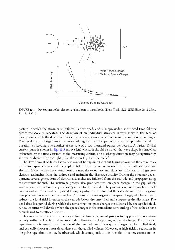
Distance from the Cathode
Fie
ld In
tens
ity
With Space ChargeWithout Space Charge
r0
E0
S0
FIGURE 15.1 Development of an electron avalanche from the cathode. (From Trinh, N.G., IEEE Electr. Insul. Mag.,
11, 23, 1995a.)
pattern in which the streamer is initiated, is developed, and is suppressed; a short dead time follows
before the cycle is repeated. The duration of an individual streamer is very short, a few tens of
nanoseconds, while the dead time varies from a few microseconds to a few milliseconds, or even longer.
The resulting discharge current consists of regular negative pulses of small amplitude and short
duration, succeeding one another at the rate of a few thousand pulses per second. A typical Trichel
current pulse is shown in Fig. 15.3 (above left) where, it should be noted, the wave shape is somewhat
influenced by the time constant of the measuring circuit. The discharge duration may be significantly
shorter, as depicted by the light pulse shown in Fig. 15.3 (below left).
The development of Trichel streamers cannot be explained without taking account of the active roles
of the ion space charges and the applied field. The streamer is initiated from the cathode by a free
electron. If the corona onset conditions are met, the secondary emissions are sufficient to trigger new
electron avalanches from the cathode and maintain the discharge activity. During the streamer devel-
opment, several generations of electron avalanches are initiated from the cathode and propagate along
the streamer channel. The avalanche process also produces two ion space charges in the gap, which
gradually moves the boundary surface S0 closer to the cathode. The positive ion cloud thus finds itself
compressed at the cathode and, in addition, is partially neutralized at the cathode and by the negative
ions produced in subsequent avalanches. This results in a net negative ion space charge, which eventually
reduces the local field intensity at the cathode below the onset field and suppresses the discharge. The
dead time is a period during which the remaining ion space charges are dispersed by the applied field.
A new streamer will develop when the space charges in the immediate surrounding of the cathode have
been cleared to a sufficient extent.
This mechanism depends on a very active electron attachment process to suppress the ionization
activity within a few tens of nanoseconds following the beginning of the discharge. The streamer
repetition rate is essentially a function of the removal rate of ion space charges by the applied field,
and generally shows a linear dependence on the applied voltage. However, at high fields a reduction in
the pulse repetition rate may be observed, which corresponds to the transition to a new corona mode.
� 2006 by Taylor & Francis Group, LLC.
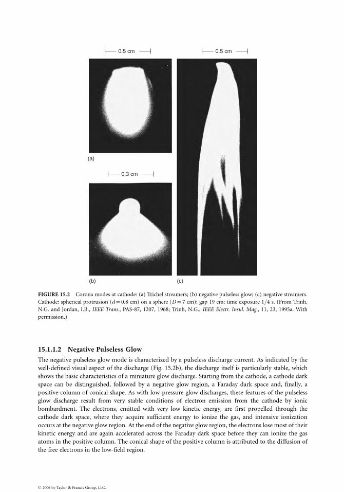
0.5 cm
0.3 cm
(a)
(b) (c)
0.5 cm
FIGURE 15.2 Corona modes at cathode: (a) Trichel streamers; (b) negative pulseless glow; (c) negative streamers.
Cathode: spherical protrusion (d¼ 0.8 cm) on a sphere (D¼ 7 cm); gap 19 cm; time exposure 1=4 s. (From Trinh,
N.G. and Jordan, I.B., IEEE Trans., PAS-87, 1207, 1968; Trinh, N.G., IEEE Electr. Insul. Mag., 11, 23, 1995a. With
permission.)
15.1.1.2 Negative Pulseless Glow
The negative pulseless glow mode is characterized by a pulseless discharge current. As indicated by the
well-defined visual aspect of the discharge (Fig. 15.2b), the discharge itself is particularly stable, which
shows the basic characteristics of a miniature glow discharge. Starting from the cathode, a cathode dark
space can be distinguished, followed by a negative glow region, a Faraday dark space and, finally, a
positive column of conical shape. As with low-pressure glow discharges, these features of the pulseless
glow discharge result from very stable conditions of electron emission from the cathode by ionic
bombardment. The electrons, emitted with very low kinetic energy, are first propelled through the
cathode dark space, where they acquire sufficient energy to ionize the gas, and intensive ionization
occurs at the negative glow region. At the end of the negative glow region, the electrons lose most of their
kinetic energy and are again accelerated across the Faraday dark space before they can ionize the gas
atoms in the positive column. The conical shape of the positive column is attributed to the diffusion of
the free electrons in the low-field region.
� 2006 by Taylor & Francis Group, LLC.
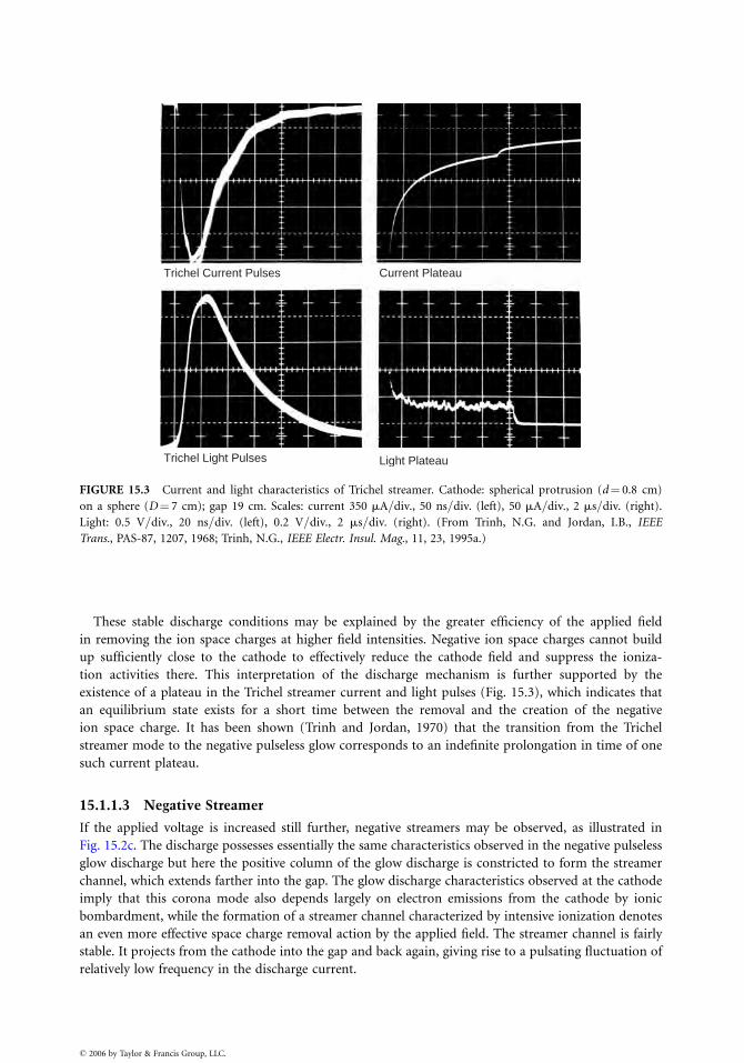
Trichel Current Pulses
Trichel Light Pulses
Current Plateau
Light Plateau
FIGURE 15.3 Current and light characteristics of Trichel streamer. Cathode: spherical protrusion (d¼ 0.8 cm)
on a sphere (D¼ 7 cm); gap 19 cm. Scales: current 350 mA=div., 50 ns=div. (left), 50 mA=div., 2 ms=div. (right).
Light: 0.5 V=div., 20 ns=div. (left), 0.2 V=div., 2 ms=div. (right). (From Trinh, N.G. and Jordan, I.B., IEEE
Trans., PAS-87, 1207, 1968; Trinh, N.G., IEEE Electr. Insul. Mag., 11, 23, 1995a.)
These stable discharge conditions may be explained by the greater efficiency of the applied field
in removing the ion space charges at higher field intensities. Negative ion space charges cannot build
up sufficiently close to the cathode to effectively reduce the cathode field and suppress the ioniza-
tion activities there. This interpretation of the discharge mechanism is further supported by the
existence of a plateau in the Trichel streamer current and light pulses (Fig. 15.3), which indicates that
an equilibrium state exists for a short time between the removal and the creation of the negative
ion space charge. It has been shown (Trinh and Jordan, 1970) that the transition from the Trichel
streamer mode to the negative pulseless glow corresponds to an indefinite prolongation in time of one
such current plateau.
15.1.1.3 Negative Streamer
If the applied voltage is increased still further, negative streamers may be observed, as illustrated in
Fig. 15.2c. The discharge possesses essentially the same characteristics observed in the negative pulseless
glow discharge but here the positive column of the glow discharge is constricted to form the streamer
channel, which extends farther into the gap. The glow discharge characteristics observed at the cathode
imply that this corona mode also depends largely on electron emissions from the cathode by ionic
bombardment, while the formation of a streamer channel characterized by intensive ionization denotes
an even more effective space charge removal action by the applied field. The streamer channel is fairly
stable. It projects from the cathode into the gap and back again, giving rise to a pulsating fluctuation of
relatively low frequency in the discharge current.
� 2006 by Taylor & Francis Group, LLC.
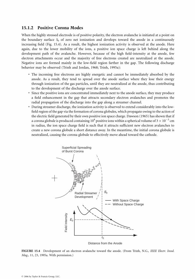
15.1.2 Positive Corona Modes
When the highly stressed electrode is of positive polarity, the electron avalanche is initiated at a point on
the boundary surface S0 of zero net ionization and develops toward the anode in a continuously
increasing field (Fig. 15.4). As a result, the highest ionization activity is observed at the anode. Here
again, due to the lower mobility of the ions, a positive ion space charge is left behind along the
development path of the avalanche. However, because of the high field-intensity at the anode, few
electron attachments occur and the majority of free electrons created are neutralized at the anode.
Negative ions are formed mainly in the low-field region farther in the gap. The following discharge
behavior may be observed (Trinh and Jordan, 1968; Trinh, 1995a):
. The incoming free electrons are highly energetic and cannot be immediately absorbed by the
anode. As a result, they tend to spread over the anode surface where they lose their energy
through ionization of the gas particles, until they are neutralized at the anode, thus contributing
to the development of the discharge over the anode surface.. Since the positive ions are concentrated immediately next to the anode surface, they may produce
a field enhancement in the gap that attracts secondary electron avalanches and promotes the
radial propagation of the discharge into the gap along a streamer channel.. During streamer discharge, the ionization activity is observed to extend considerably into the low-
field region of the gap via the formation of corona globules, which propagate owing to the action of
the electric field generated by their own positive ion space charge. Dawson (1965) has shown that if
a corona globule is produced containing 108 positive ions within a spherical volume of 3� 10�3 cm
in radius, the ion space charge field is such that it attracts sufficient new electron avalanches to
create a new corona globule a short distance away. In the meantime, the initial corona globule is
neutralized, causing the corona globule to effectively move ahead toward the cathode.
Distance from the Anode
With Space Charge
Radial StreamerDevelopment
Superficial Spreadingof Burst Corona
Without Space Charge
Fie
ld In
tens
ity
r0
E0
S0
FIGURE 15.4 Development of an electron avalanche toward the anode. (From Trinh, N.G., IEEE Electr. Insul.
Mag., 11, 23, 1995a. With permission.)
� 2006 by Taylor & Francis Group, LLC.
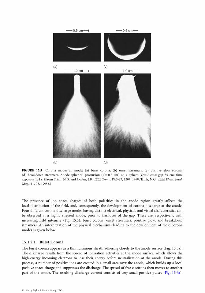
0.5 cm 0.5 cm
1.0 cm(a) (c)
(b) (d)
1.0 cm
FIGURE 15.5 Corona modes at anode: (a) burst corona; (b) onset streamers; (c) positive glow corona;
(d) breakdown streamers. Anode spherical protrusion (d¼ 0.8 cm) on a sphere (D¼ 7 cm); gap 35 cm; time
exposure 1=4 s. (From Trinh, N.G. and Jordan, I.B., IEEE Trans., PAS-87, 1207, 1968; Trinh, N.G., IEEE Electr. Insul.
Mag., 11, 23, 1995a.)
The presence of ion space charges of both polarities in the anode region greatly affects the
local distribution of the field, and, consequently, the development of corona discharge at the anode.
Four different corona discharge modes having distinct electrical, physical, and visual characteristics can
be observed at a highly stressed anode, prior to flashover of the gap. These are, respectively, with
increasing field intensity (Fig. 15.5): burst corona, onset streamers, positive glow, and breakdown
streamers. An interpretation of the physical mechanisms leading to the development of these corona
modes is given below.
15.1.2.1 Burst Corona
The burst corona appears as a thin luminous sheath adhering closely to the anode surface (Fig. 15.5a).
The discharge results from the spread of ionization activities at the anode surface, which allows the
high-energy incoming electrons to lose their energy before neutralization at the anode. During this
process, a number of positive ions are created in a small area over the anode, which builds up a local
positive space charge and suppresses the discharge. The spread of free electrons then moves to another
part of the anode. The resulting discharge current consists of very small positive pulses (Fig. 15.6a),
� 2006 by Taylor & Francis Group, LLC.
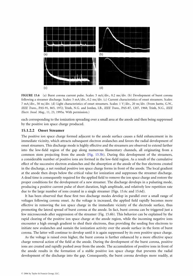
(a) (b)
(c) (d)
FIGURE 15.6 (a) Burst corona current pulse. Scales: 5 mA=div., 0.2 ms=div. (b) Development of burst corona
following a streamer discharge. Scales: 5 mA=div., 0.2 ms=div. (c) Current characteristics of onset streamers. Scales:
7 mA=div., 50 ns=div. (d) Light characteristics of onset streamers. Scales: 1 V=div., 20 ns=div. (From Juette, G.W.,
IEEE Trans., PAS-91, 865, 1972; Trinh, N.G. and Jordan, I.B., IEEE Trans., PAS-87, 1207, 1968; Trinh, N.G., IEEE
Electr. Insul. Mag., 11, 23, 1995a. With permission.)
each corresponding to the ionization spreading over a small area at the anode and then being suppressed
by the positive ion space charge produced.
15.1.2.2 Onset Streamer
The positive ion space charge formed adjacent to the anode surface causes a field enhancement in its
immediate vicinity, which attracts subsequent electron avalanches and favors the radial development of
onset streamers. This discharge mode is highly effective and the streamers are observed to extend farther
into the low-field region of the gap along numerous filamentary channels, all originating from a
common stem projecting from the anode (Fig. 15.5b). During this development of the streamers,
a considerable number of positive ions are formed in the low-field region. As a result of the cumulative
effect of the successive electron avalanches and the absorption at the anode of the free electrons created
in the discharge, a net residual positive ion space charge forms in front of the anode. The local gradient
at the anode then drops below the critical value for ionization and suppresses the streamer discharge.
A dead time is consequently required for the applied field to remove the ion space charge and restore the
proper conditions for the development of a new streamer. The discharge develops in a pulsating mode,
producing a positive current pulse of short duration, high amplitude, and relatively low repetition rate
due to the large number of ions created in a single streamer (Figs. 15.6c and 15.6d).
It has been observed that these first two discharge modes develop in parallel over a small range of
voltages following corona onset. As the voltage is increased, the applied field rapidly becomes more
effective in removing the ion space charge in the immediate vicinity of the electrode surface, thus
promoting the lateral spread of burst corona at the anode. In fact, burst corona can be triggered just a
few microseconds after suppression of the streamer (Fig. 15.6b). This behavior can be explained by the
rapid clearing of the positive ion space charge at the anode region, while the incoming negative ions
encounter a high enough gradient to shed their electrons, thus providing the seeding free electrons to
initiate new avalanches and sustain the ionization activity over the anode surface in the form of burst
corona. The latter will continue to develop until it is again suppressed by its own positive space charge.
As the voltage is raised even higher, the burst corona is further enhanced by a more effective space
charge removal action of the field at the anode. During the development of the burst corona, positive
ions are created and rapidly pushed away from the anode. The accumulation of positive ions in front of
the anode results in the formation of a stable positive ion space charge that prevents the radial
development of the discharge into the gap. Consequently, the burst corona develops more readily, at
� 2006 by Taylor & Francis Group, LLC.

the expense of the onset streamer, until the latter is completely suppressed. A new mode, the positive
glow discharge, is then established at the anode.
15.1.2.3 Positive Glow
A photograph of a positive glow discharge developing at a spherical protrusion is presented in Fig. 15.5.
This discharge is due to the development of the ionization activity over the anode surface, which forms a
thin luminous layer immediately adjacent to the anode surface, where intense ionization activity takes
place. The discharge current consists of a direct current superimposed by a small pulsating component
with a high repetition rate, in the hundreds of kilohertz range. By analyzing the light signals obtained
with photomultipliers pointing to different regions of the anode, it may be found that the luminous
sheath is composed of a stable central region, from there, bursts of ionization activity may develop and
project the ionizing sheath outward and back again, continuously, giving rise to the pulsating current
component.
The development of the positive glow discharge may be interpreted as resulting from a particular
combination of removal and creation of positive ions in the gap. The field is high enough for the positive
ion space charge to be rapidly removed from the anode, thus promoting surface ionization activity.
Meanwhile, the field intensity is not sufficient to allow radial development of the discharge and the
formation of streamers. The main contribution of the negative ions is to supply the necessary triggering
electrons to sustain ionization activity at the anode.
15.1.2.4 Breakdown Streamer
If the applied voltage is further increased, streamers are again observed and they eventually lead to
breakdown of the gap. The development of breakdown streamers is preceded by local streamer spots of
intense ionization activity, which may be seen moving slowly over the anode surface. The development
of streamer spots is not accompanied by any marked change in the current or the light signal. Only when
the applied field becomes sufficiently high to rapidly clear the positive ion space charges from the anode
region does radial development of the discharge become possible, resulting in breakdown streamers.
Positive breakdown streamers develop more and more intensively with higher applied voltage and
eventually cause the gap to break down. The discharge is essentially the same as the onset streamer type
but can extend much farther into the gap. The streamer current is more intense and may occur at a
higher repetition rate. A streamer crossing the gap does not necessarily result in gap breakdown, which
proves that the filamentary region of the streamer is not fully conducting.
15.1.3 AC Corona
When alternating voltage is used, the gradient at the highly stressed electrode varies continuously, both
in intensity and in polarity. Different corona modes can be observed in the same cycle of the applied
voltage. Figure 15.7 illustrates the development of different corona modes at a spherical protrusion as a
function of the applied voltage. The corona modes can be readily identified by the discharge current. The
following observations can be made:
. For short gaps, the ion space charges created in one half-cycle are absorbed by the electrodes in
the same half-cycle. The same corona modes that develop near onset voltages can be observed,
namely: negative Trichel streamers, positive onset streamers, and burst corona.. For long gaps, the ion space charges created in one half-cycle are not completely absorbed by the
electrodes, leaving residual space charges in the gap. These residual space charges are drawn back
to the region of high field intensity in the following half-cycle and can influence discharge
development. Onset streamers are suppressed in favor of the positive glow discharge. The
following corona modes can be distinguished: negative Trichel streamers, negative glow discharge,
positive glow discharge, and positive breakdown streamers.. Negative streamers are not observed under AC voltage, owing to the fact that their onset gradient
is higher than the breakdown voltage that occurs during the positive half-cycle.
� 2006 by Taylor & Francis Group, LLC.
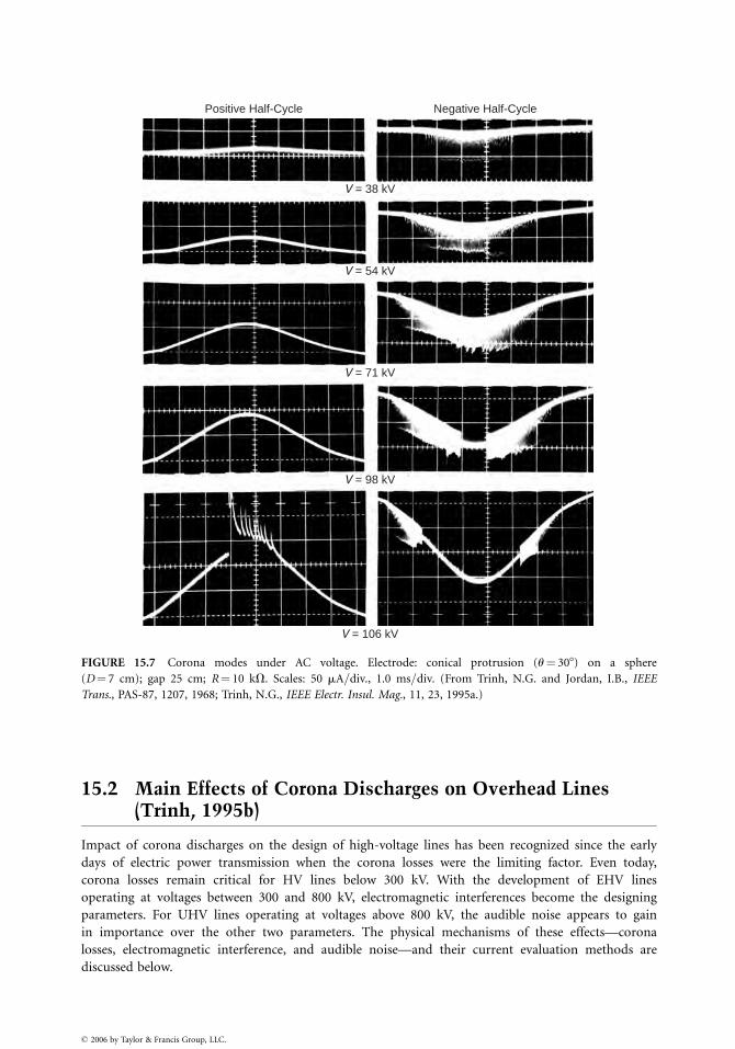
Positive Half-Cycle Negative Half-Cycle
V = 38 kV
V = 54 kV
V = 71 kV
V = 98 kV
V = 106 kV
FIGURE 15.7 Corona modes under AC voltage. Electrode: conical protrusion (u¼ 308) on a sphere
(D¼ 7 cm); gap 25 cm; R¼ 10 kV. Scales: 50 mA=div., 1.0 ms=div. (From Trinh, N.G. and Jordan, I.B., IEEE
Trans., PAS-87, 1207, 1968; Trinh, N.G., IEEE Electr. Insul. Mag., 11, 23, 1995a.)
15.2 Main Effects of Corona Discharges on Overhead Lines(Trinh, 1995b)
Impact of corona discharges on the design of high-voltage lines has been recognized since the early
days of electric power transmission when the corona losses were the limiting factor. Even today,
corona losses remain critical for HV lines below 300 kV. With the development of EHV lines
operating at voltages between 300 and 800 kV, electromagnetic interferences become the designing
parameters. For UHV lines operating at voltages above 800 kV, the audible noise appears to gain
in importance over the other two parameters. The physical mechanisms of these effects—corona
losses, electromagnetic interference, and audible noise—and their current evaluation methods are
discussed below.
� 2006 by Taylor & Francis Group, LLC.
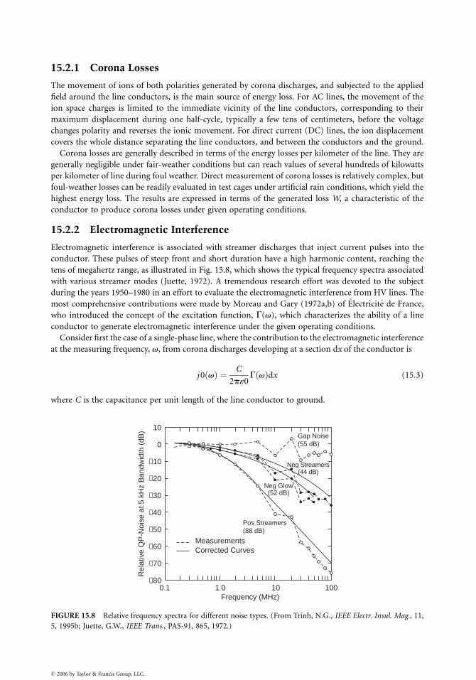
15.2.1 Corona Losses
The movement of ions of both polarities generated by corona discharges, and subjected to the applied
field around the line conductors, is the main source of energy loss. For AC lines, the movement of the
ion space charges is limited to the immediate vicinity of the line conductors, corresponding to their
maximum displacement during one half-cycle, typically a few tens of centimeters, before the voltage
changes polarity and reverses the ionic movement. For direct current (DC) lines, the ion displacement
covers the whole distance separating the line conductors, and between the conductors and the ground.
Corona losses are generally described in terms of the energy losses per kilometer of the line. They are
generally negligible under fair-weather conditions but can reach values of several hundreds of kilowatts
per kilometer of line during foul weather. Direct measurement of corona losses is relatively complex, but
foul-weather losses can be readily evaluated in test cages under artificial rain conditions, which yield the
highest energy loss. The results are expressed in terms of the generated loss W, a characteristic of the
conductor to produce corona losses under given operating conditions.
15.2.2 Electromagnetic Interference
Electromagnetic interference is associated with streamer discharges that inject current pulses into the
conductor. These pulses of steep front and short duration have a high harmonic content, reaching the
tens of megahertz range, as illustrated in Fig. 15.8, which shows the typical frequency spectra associated
with various streamer modes (Juette, 1972). A tremendous research effort was devoted to the subject
during the years 1950–1980 in an effort to evaluate the electromagnetic interference from HV lines. The
most comprehensive contributions were made by Moreau and Gary (1972a,b) of Electricite de France,
who introduced the concept of the excitation function, G(v), which characterizes the ability of a line
conductor to generate electromagnetic interference under the given operating conditions.
Consider first the case of a single-phase line, where the contribution to the electromagnetic interference
at the measuring frequency, v, from corona discharges developing at a section dx of the conductor is
j 0 vð Þ ¼ C
2p«0G vð Þdx (15:3)
where C is the capacitance per unit length of the line conductor to ground.
Frequency (MHz)
MeasurementsCorrected Curves
Pos Streamers(88 dB)
Gap Noise(55 dB)
Neg Glow(52 dB)
Neg Streamers(44 dB)
Rel
ativ
e Q
P-N
oise
at 5
kH
z B
andw
idth
(dB
)
0.1−80
−70
−60
−50
−40
−30
−20
−10
0
10
1.0 10 100
FIGURE 15.8 Relative frequency spectra for different noise types. (From Trinh, N.G., IEEE Electr. Insul. Mag., 11,
5, 1995b; Juette, G.W., IEEE Trans., PAS-91, 865, 1972.)
� 2006 by Taylor & Francis Group, LLC.
Upon injection, the discharge current pulse splits itself into two identical current pulses of half
amplitude propagating in opposite directions away from the discharge site. At a point of observation
located at a distance x along the line from the discharge site, the noise current is distorted according to
i v, xð Þ dx ¼ i 0 vð Þ exp �g xð Þ dx ¼ i 0 vð Þ exp �axð Þ dx (15:4)
where g represents the propagation constant, which can be approximated by its real component a.
The total noise current circulating in the line conductor is the sum of all contributions from the
corona discharges along the conductor and is given by
I vð Þ ¼
ffiffiffiffiffiffiffiffiffiffiffiffiffiffiffiffiffiffiffiffiffiffiffiffiffiffiffiffiffiffiffiffi
ð
1
�1
i v, xð Þ½ �2 dx
v
u
u
u
t ¼ i 0 vð Þffiffiffi
ap (15:5)
For a multiphase line, because of the high-frequency nature of the noise current, the calculation of the
interference field must take account of the mutual coupling among the conductors, which further
complicates the process (Gary, 1972; Moreau and Gary, 1972a,b). Modal analysis provides a convenient
means of evaluating the noise currents on the line conductors. In this approach, the noise currents are
first transposed into their modal components, which propagate without distortion along the line
conductors at their own velocity according to the relation
i 0 vð Þ dx½ � ¼ M½ � j0 vð Þ dx½ � (15:6)
Consequently,
j0 vð Þ dx½ � ¼ M½ ��1i 0 vð Þ dx½ � (15:7)
where [M] is the modal transposition matrix and j0(v) are the modal components of the injected noise
current. The modal current at the measuring point located at a distance x from the injection point is
j v, xð Þ dx ¼ j0 vð Þ exp �a xð Þ dx (15:8)
and the modal current component at the measuring point is
J vð Þ ¼
ffiffiffiffiffiffiffiffiffiffiffiffiffiffiffiffiffiffiffiffiffiffiffiffiffiffiffiffiffiffiffiffiffi
ð
1
�1
j v, xð Þ½ �2 dx
v
u
u
u
t ¼ j0 vð Þffiffiffi
ap (15:9)
or, in a general way
J vð Þ½ � ¼ 1ffiffiffi
ap½ � j0 vð Þ½ � ¼ 1
ffiffiffi
ap½ � M½ ��1
i 0 vð Þ½ � (15:10)
Finally, the line current can be obtained from
I vð Þ½ � ¼ M½ � J vð Þ½ � (15:11)
The magnetic and electric fields produced by the noise currents in the line conductors can then be
evaluated for assessment of the electromagnetic interferences. Moreau and Gary (1972a,b) obtained
good agreement between calculated and experimental results with the symmetrical modes of Clarke for
the modal transposition:
� 2006 by Taylor & Francis Group, LLC.
M½ � ¼1=
ffiffiffi
6p
1=2 1=ffiffiffi
3p
�2=ffiffiffi
6p
0 1=ffiffiffi
3p
1=ffiffiffi
6p
�1=2 1=ffiffiffi
3p
2
6
4
3
7
5
(15:12)
The attenuation coefficients at 0.5 MHz are 11.1, 54, and 342 Np=m for the modal currents, and the
magnetic ground was assumed to be located at a depth equal to the penetration depth of the magnetic
field, dp, as defined by
dp ¼ 2
ffiffiffiffiffiffiffi
r
mv
r
(15:13)
For a typical soil resistivity of 100 Vm and a measuring frequency of 0.5 MHz, the depth of the magnetic
ground is equal to 7.11 m. It is equal to 5.03 m at a measuring frequency of 1.0 MHz.
Circulation of the noise current in the line conductor effectively generates an electromagnetic
interference field around the conductors, which is readily picked up by any radio or television receiver
located in the vicinity of the HV line. The current practices characterize the interference field in terms of
its electric component, E(v), expressed in decibels (dB) above a reference level of 1 mV=m. Evaluation of
the electromagnetic interference is usually made by first calculating the magnetic interference field H(v)
at the measuring point
H vð Þ ¼X
j
1
2p rj
Ij vð Þ ar (15:14)
The summation was made with respect to the number of phase conductors of the lines and their images
with respect to the magnetic ground. The electric interference field can next be related to the magnetic
interference field according to
E vð Þ ¼ffiffiffiffiffiffiffi
m0
«0
r
H vð Þ (15:15)
15.2.2.1 Television Interference
The frequency spectrum of corona discharges has cut-off frequencies around a few tens of megahertz. As
a result, the interference levels at the television frequencies are very much attenuated. In fact, gap
discharges, which generate sharp current pulse with nanosecond rise times, are the principal discharges
that effectively interfere with the television reception. These discharges are produced by loose connec-
tions, a problem common on low-voltage distribution lines but rarely observed on high-voltage
transmission lines. Another source of interference is related to reflections of television signals at high-
voltage line towers, producing ghost images. However, the problem is not related in any way to corona
activities on the line conductors (Juette, 1972).
15.2.3 Audible Noise
The high temperature in the discharge channel produced by the streamer creates a corresponding
increase in the local air pressure. Consequently, a pulsating sound wave is generated from the discharge
site, propagates through the surrounding ambient air, and is perfectly audible in the immediate vicinity
of the HV lines. The typical octave-band frequency spectra of line corona in Fig. 15.9 contain discrete
components corresponding to the second and higher harmonics of the line voltage superimposed on a
relatively broadband noise, extending well into the ultrasonic range (Ianna et al., 1974). The octave-band
measurements in this figure show a sharp drop at frequencies over 20 kHz, due principally to the limited
frequency response of the microphone and associated sound-level meter.
� 2006 by Taylor & Francis Group, LLC.
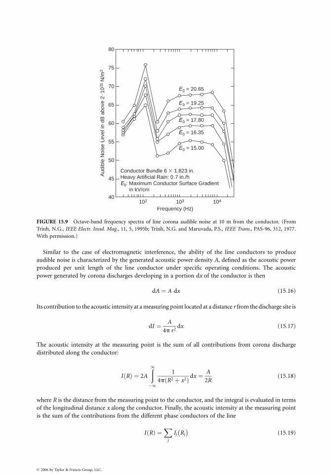
Frequency (Hz)
E0 = 15.00
E0 = 16.35
E0 = 17.80
E0 = 19.25
E0 = 20.65
Conductor Bundle 6 � 1.823 in.Heavy Artificial Rain: 0 .7 in./hE0: Maximum Conductor Surface Gradient in kV/cm
Aud
ible
Noi
se L
evel
in d
B a
bove
2 . 1
0−5
N/m
2
40
45
50
55
60
65
70
75
80
102 103 104
FIGURE 15.9 Octave-band frequency spectra of line corona audible noise at 10 m from the conductor. (From
Trinh, N.G., IEEE Electr. Insul. Mag., 11, 5, 1995b; Trinh, N.G. and Maruvada, P.S., IEEE Trans., PAS-96, 312, 1977.
With permission.)
Similar to the case of electromagnetic interference, the ability of the line conductors to produce
audible noise is characterized by the generated acoustic power density A, defined as the acoustic power
produced per unit length of the line conductor under specific operating conditions. The acoustic
power generated by corona discharges developing in a portion dx of the conductor is then
dA ¼ A dx (15:16)
Its contribution to the acoustic intensity at a measuring point located at a distance r from the discharge site is
dI ¼ A
4p r2dx (15:17)
The acoustic intensity at the measuring point is the sum of all contributions from corona discharge
distributed along the conductor:
I Rð Þ ¼ 2A
ð
1
�1
1
4p R2 þ x2ð Þ dx ¼ A
2R(15:18)
where R is the distance from the measuring point to the conductor, and the integral is evaluated in terms
of the longitudinal distance x along the conductor. Finally, the acoustic intensity at the measuring point
is the sum of the contributions from the different phase conductors of the line
I Rð Þ ¼X
j
Ij Rj
� �
(15:19)
� 2006 by Taylor & Francis Group, LLC.
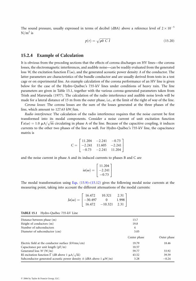
The sound pressure, usually expressed in terms of decibel (dBA) above a reference level of 2� 10�5
N=m2 is
p rð Þ ¼ffiffiffiffiffiffiffiffiffiffiffiffiffiffi
r0 C Ip
(15:20)
15.2.4 Example of Calculation
It is obvious from the preceding sections that the effects of corona discharges on HV lines—the corona
losses, the electromagnetic interferences, and audible noise—can be readily evaluated from the generated
loss W, the excitation function G(v), and the generated acoustic power density A of the conductor. The
latter parameters are characteristics of the bundle conductor and are usually derived from tests in a test
cage or on experimental line. An example calculation of the corona performance of an HV line is given
below for the case of the Hydro-Quebec’s 735-kV lines under conditions of heavy rain. The line
parameters are given in Table 15.1, together with the various corona-generated parameters taken from
Trinh and Maruvada (1977). The calculation of the radio interference and audible noise levels will be
made for a lateral distance of 15 m from the outer phase, i.e., at the limit of the right of way of the line.
Corona losses: The corona losses are the sum of the losses generated at the three phases of the
line, which amount to 127.63 kW=km.
Radio interference: The calculation of the radio interference requires that the noise current be first
transformed into its modal components. Consider a noise current of unit excitation function
Ga(v) ¼ 1:0 mA=ffiffiffiffi
mp
circulating in phase A of the line. Because of the capacitive coupling, it induces
currents to the other two phases of the line as well. For Hydro-Quebec’s 735-kV line, the capacitance
matrix is
C ¼11:204 �2:241 �0:73
�2:241 11:605 �2:241
�0:73 �2:241 11:204
2
4
3
5
and the noise current in phase A and its induced currents to phases B and C are
ia vð Þ ¼11:204
�2:241
�0:73
2
4
3
5
The modal transformation using Eqs. (15.9)–(15.12) gives the following modal noise currents at the
measuring point, taking into account the different attenuations of the modal currents:
Ja vð Þ ¼16:472 10:321 2:31
�30:497 0 1:998
16:472 �10:321 2:31
2
4
3
5
TABLE 15.1 Hydro-Quebec 735-kV Line
Distance between phase (m) 13.7
Height of conductors (m) 19.8
Number of subconductors 4
Diameter of subconductor (cm) 3.05
Center phase Outer phase
Electric field at the conductor surface (kVrms=cm) 19.79 18.46
Capacitance per unit length (pF=m) 10.57
Generated loss W (W=m) 59.77 33.92
RI excitation function G (dB above 1 mA=ffiffiffiffi
mp
) 43.52 39.59
Subconductor generated acoustic power density A (dBA above 1 mW=m) 3.28 �0.24
� 2006 by Taylor & Francis Group, LLC.
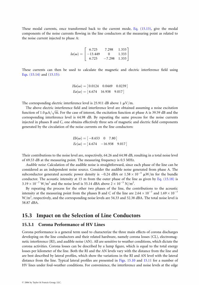
These modal currents, once transformed back to the current mode, Eq. (15.13), give the modal
components of the noise currents flowing in the line conductors at the measuring point as related to
the noise current injected to phase A:
Ia vð Þ ¼6:725 7:298 1:333
�13:449 0 1:333
6:725 �7:298 1:333
2
4
3
5
These currents can then be used to calculate the magnetic and electric interference field using
Eqs. (15.14) and (15.15):
Ha vð Þ ¼ 0:0124 0:0449 0:0239½ �Ea vð Þ ¼ 4:674 16:938 9:017½ �
The corresponding electric interference level is 25.911 dB above 1 mV=m.
The above electric interference field and interference level are obtained assuming a noise excitation
function of 1:0 mA=ffiffiffiffi
mp
. For the case of interest, the excitation function at phase A is 39.59 dB and the
corresponding interference level is 64.98 dB. By repeating the same process for the noise currents
injected in phases B and C, one obtains effectively three sets of magnetic and electric field components
generated by the circulation of the noise currents on the line conductors:
Eb vð Þ ¼ �8:653 0 7:80½ �Ec vð Þ ¼ 4:674 �16:938 9:017½ �
Their contributions to the noise level are, respectively, 64.26 and 64.98 dB, resulting in a total noise level
of 69.53 dB at the measuring point. The measuring frequency is 0.5 MHz.
Audible noise: Calculation of the audible noise is straightforward, since each phase of the line can be
considered as an independent noise source. Consider the audible noise generated from phase A. The
subconductor generated acoustic power density is �0.24 dBA or 1.58� 10�5 mW=m for the bundle
conductor. The acoustic intensity at 15 m from the outer phase of the line as given by Eq. (15.18) is
3.19� 10�7 W=m2 and the noise level is 55.14 dBA above 2� 10�5 N=m2.
By repeating the process for the other two phases of the line, the contributions to the acoustic
intensity at the measuring point from the phases B and C of the line are 2.64� 10�7 and 1.69� 10�7
W=m2, respectively, and the corresponding noise levels are 54.33 and 52.38 dBA. The total noise level is
58.87 dBA.
15.3 Impact on the Selection of Line Conductors
15.3.1 Corona Performance of HV Lines
Corona performance is a general term used to characterize the three main effects of corona discharges
developing on the line conductors and their related hardware, namely corona losses (CL), electromag-
netic interference (RI), and audible noise (AN). All are sensitive to weather conditions, which dictate the
corona activities. Corona losses can be described by a lump figure, which is equal to the total energy
losses per kilometer of the line. Both the RI and the AN levels vary with the distance from the line and
are best described by lateral profiles, which show the variations in the RI and AN level with the lateral
distance from the line. Typical lateral profiles are presented in Figs. 15.10 and 15.11 for a number of
HV lines under foul-weather conditions. For convenience, the interference and noise levels at the edge
� 2006 by Taylor & Francis Group, LLC.
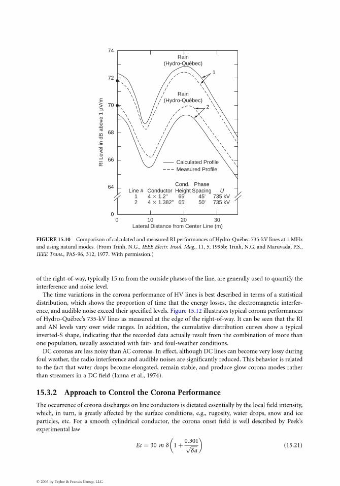
Lateral Distance from Center Line (m)
Calculated Profile
2
1
Rain(Hydro-Québec)
Rain(Hydro-Québec)
Measured Profile
Line #1 4 � 1.2" 65' 45' 735 kV
735 kV50'65'4 � 1.382"2
UConductorCond.Height
PhaseSpacing
RI L
evel
in d
B a
bove
1 µ
V/m
00
64
66
68
70
72
74
10 20 30
FIGURE 15.10 Comparison of calculated and measured RI performances of Hydro-Quebec 735-kV lines at 1 MHz
and using natural modes. (From Trinh, N.G., IEEE Electr. Insul. Mag., 11, 5, 1995b; Trinh, N.G. and Maruvada, P.S.,
IEEE Trans., PAS-96, 312, 1977. With permission.)
of the right-of-way, typically 15 m from the outside phases of the line, are generally used to quantify the
interference and noise level.
The time variations in the corona performance of HV lines is best described in terms of a statistical
distribution, which shows the proportion of time that the energy losses, the electromagnetic interfer-
ence, and audible noise exceed their specified levels. Figure 15.12 illustrates typical corona performances
of Hydro-Quebec’s 735-kV lines as measured at the edge of the right-of-way. It can be seen that the RI
and AN levels vary over wide ranges. In addition, the cumulative distribution curves show a typical
inverted-S shape, indicating that the recorded data actually result from the combination of more than
one population, usually associated with fair- and foul-weather conditions.
DC coronas are less noisy than AC coronas. In effect, although DC lines can become very lossy during
foul weather, the radio interference and audible noises are significantly reduced. This behavior is related
to the fact that water drops become elongated, remain stable, and produce glow corona modes rather
than streamers in a DC field (Ianna et al., 1974).
15.3.2 Approach to Control the Corona Performance
The occurrence of corona discharges on line conductors is dictated essentially by the local field intensity,
which, in turn, is greatly affected by the surface conditions, e.g., rugosity, water drops, snow and ice
particles, etc. For a smooth cylindrical conductor, the corona onset field is well described by Peek’s
experimental law
Ec ¼ 30 m d 1þ 0:301ffiffiffiffiffi
dap
� �
(15:21)
� 2006 by Taylor & Francis Group, LLC.

Lateral Distance from Center Line (m)
Line #1 65' 41' 745 kV
735 kV
735 kV525 kV
525 kV
45'34'
34'50'
65'40'65'40'
4 � 1.165"4 � 1.2"4 � 1.602"4 � 1.382"4 � 1.302"
2345
ConductorCond. Height
PhaseSpacing U
Rain(BPA)
Rain(BPA)
MorningFog (AEP)
Calculated Profile
Measured Profile
(Apple Grove)
5
43
2
1
(4)
Light Rain(Hydro-Québec)
Rain(Hydro-Québec)
AN
Lev
el in
dB
A a
bove
2 �
10−5
N/m
2
0
50
52
54
56
58
60
62
10 20 30
FIGURE 15.11 Comparison of calculated and measured AN performances of HV lines. (From Trinh, N.G., IEEE
Electr. Insul. Mag., 11, 5, 1995b; Trinh, N.G. and Maruvada, P.S., IEEE Trans., PAS-96, 312, 1977.)
where Ec is the corona onset field, a is the radius of the conductor, and m is an experimental factor to
take account of the surface conditions. Typical values of m are 0.8–0.9 for a dry-aged conductor, 0.5–0.7
for a conductor under foul-weather conditions, and d is the relative air density factor.
The above corona-onset condition emphasizes the great sensitivity of corona activities to the con-
ductor surface condition and, hence, to changes in weather conditions. In effect, although the line
voltage and the nominal conductor surface gradient remain constant, the surface condition factor varies
continuously due to the exposure of line conductors to atmospheric conditions. The changes are
particularly pronounced during foul weather as a result of the numerous discharge sites associated
with water drops, snow, and ice particles deposited on the conductor surface.
Adequate corona performance of HV lines is generally achieved by a proper control of the field
intensity at the surface of the conductor. It can be well illustrated by the simple case of a single-phase,
single-conductor line for which the field intensity at the conductor surface is
� 2006 by Taylor & Francis Group, LLC.
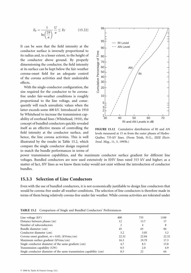
RI and AN Levels in dB
RI
AN
AN LevelRI Level
Cum
ulat
ive
Per
cent
age
of T
ime
301
235
10
20
30
40
50
60
70
80
90
95
99
40 50 60 70
FIGURE 15.12 Cumulative distribution of RI and AN
levels measured at 15 m from the outer phases of Hydro-
Quebec 735-kV lines. (From Trinh, N.G., IEEE Electr.
Insul. Mag., 11, 5, 1995b.)
E0 ¼1
ln2h
a
� �
U
a� Ec (15:22)
It can be seen that the field intensity at the
conductor surface is inversely proportional to
its radius and, to a lesser extent, to the height of
the conductor above ground. By properly
dimensioning the conductor, the field intensity
at its surface can be kept below the fair-weather
corona-onset field for an adequate control
of the corona activities and their undesirable
effects.
With the single-conductor configuration, the
size required for the conductor to be corona-
free under fair-weather conditions is roughly
proportional to the line voltage, and conse-
quently will reach unrealistic values when the
latter exceeds some 400 kV. Introduced in 1910
by Whitehead to increase the transmission cap-
ability of overhead lines (Whitehead, 1910), the
concept of bundled conductors quickly revealed
itself as an effective means of controlling the
field intensity at the conductor surface, and
hence, the line corona activities. This is well
illustrated by the results in Table 15.2, which
compare the single conductor design required
to match the bundle performances in terms of
power transmission capabilities, and the maximum conductor surface gradient for different line
voltages. Bundled conductors are now used extensively in EHV lines rated 315 kV and higher; as a
matter of fact, HV lines as we know them today would not exist without the introduction of conductor
bundles.
15.3.3 Selection of Line Conductors
Even with the use of bundled conductors, it is not economically justifiable to design line conductors that
would be corona-free under all weather conditions. The selection of line conductors is therefore made in
terms of them being relatively corona-free under fair weather. While corona activities are tolerated under
TABLE 15.2 Comparison of Single and Bundled Conductors’ Performances
Line voltage (kV) 400 735 1100
Distance between phases (m) 12 13.7 17
Number of subconductors 2 4 8
Bundle diameter (cm) 45 65 84
Conductor diameter (cm) 3.2 3.05 3.2
Corona onset gradient, m¼ 0.85, (kVrms=cm) 22.32 22.04 22.32
Maximum surface gradient (kVrms=cm) 16.3 19.79 17.3
Single conductor diameter of the same gradient (cm) 4.7 8.5 13.8
Transmission capability (GW) 0.5 2.0 4.9
Single conductor diameter of the same transmission capability (cm) 8.5 22 64
� 2006 by Taylor & Francis Group, LLC.

foul weather, their effects are controlled to acceptable levels at the edge of the rights-of-way of the line.
For AC lines, the design levels of 70 dB for the radio interference and 60 dBA for the audible noise at the
edge of the right-of-way are often used (Trinh et al., 1974). These levels may be reached during
periods of foul weather, and for a specified annual proportion of time, typically 15–20%, depending
on the local distribution of the weather pattern. The design process involves extensive field calcula-
tions and experimental testing to determine the number and size of the line conductors required to
minimize the undesirable effects of corona discharges. Current practices in dimensioning HV-line
conductors usually involve two stages of selection according to their worst-case and long-term corona
performances.
15.3.3.1 Worst-Case Performance
Several conductor configurations (number, spacing, and diameter of the subconductors) are selected
with respect to their worst-case performances which, for AC lines, correspond to foul-weather condi-
tions, in particular heavy-rain. Evaluation of the conductor worst-case performance is best done in test
cages under artificial heavy-rain conditions (Trinh and Maruvada, 1977). Test cages of square section,
typically 3 m� 3 m, and a few tens of meters long, are adequate for evaluating full-size conductor
bundles located along its central axis, for lines up to the 1500-kV class. The advantages of this
experimental setup are the relatively modest test voltage required to reproduce the same field distribu-
tion on real-size bundled conductors, and the possibility of artificially producing the heavy-rain
conditions. The worst-case performance of various bundled conductors can then be determined over
a wide range of surface gradients.
Under DC voltage, the worst-case corona performance is not directly related to foul-weather condi-
tions. Although heavy rain was found to produce the highest losses, both the electromagnetic interfer-
ence and the audible noise levels decrease under rain conditions. This behavior is related to the fact that
under DC field conditions, the water droplets have an optimum shape, favorable to the development of
stable glow-corona modes (Ianna et al., 1974). For this reason, test cage is less effective in evaluating the
worst-case DC performance of bundled conductors.
A significant amount of data was gathered in cage tests at IREQ during the 1970s and provided the
database for the development of a method to predict the worst-case performance of bundled conductors
for AC voltage (Trinh and Maravuda, 1977). The results presented in Figs. 15.10 and 15.11, which
compare the calculated and measured lateral RI and AN profiles of a number of HV lines, illustrate the
good concordance of this approach. Commercial software exist that evaluate the worst-case performance
of HV-line conductors using available experimental data obtained in cage tests under conditions of
artificial heavy rain, making it possible to avoid undergoing tedious and expensive tests to help select the
best configurations for line conductors for a given rating of the line.
15.3.3.2 Long-Term Corona Performance
Because of their wide range of variation in different weather conditions, representative corona perform-
ances of HV line are best evaluated in their natural environment. Test lines are generally used in this
study that involves energizing the conductors for a sufficiently long period, usually 1 year to cover most
of the weather conditions, and recording their corona performances together with the weather condi-
tions. The higher cost of the long-term corona performance study usually limits its application to a small
number of conductor configurations selected from their worst-case performance.
It should be noted that best results for the long-term corona performance evaluated on test lines
are obtained when the weather pattern at the test site is similar to that existing along the actual HV
line. A direct transposition of the results is then possible. If this condition is not met, some
interpretation of the experimental data is needed. This is done by first decomposing the recorded
long-term data into two groups, corresponding to the fair- and foul-weather conditions, then
recombining these data according to the local weather pattern to predict the long-term corona
performance along the line.
� 2006 by Taylor & Francis Group, LLC.

15.4 Conclusions
This chapter on transmission systems has reviewed the physics of corona discharges and discussed their
impact on the design of high-voltage lines, specifically in the selection of the line conductors. The
following conclusions can be drawn.
Corona discharges can develop in different modes, depending on the equilibrium state existing under
a given test condition, between the buildup and removal of ion space charges from the immediate
vicinity of the highly stressed electrode. Three different corona modes—Trichel streamer, negative glow,
and negative streamer—can be observed at the cathode with increasing applied field intensities. With
positive polarity, four different corona modes are observed, namely burst corona, onset streamers,
positive glow, and breakdown streamers.
While all corona modes produce energy losses, the streamer discharges also generate electromagnetic
interference and audible noise in the immediate vicinity of HV lines. These parameters are currently
used to evaluate the corona performance of conductor bundles and to predict the energy losses and
environmental impact of HV lines before their installation.
Adequate control of line corona is obtained by controlling the surface gradient at the line conductors.
The introduction of bundled conductors in 1910 has greatly influenced the development of HV lines to
today’s EHVs.
Commercial software is available to select the bundle configuration: number and size of the sub-
conductors, with respect to corona performances, which can be verified in test cages and lines in the
early stage of new HV-line projects.
References
Bateman, L.A., Haywood, R.W., and Brooks, R.F., Nelson River DC Transmission Project, IEEE Trans.,
PAS-88, 688, 1969.
Bortnik, I.M., Belyakov, N.N., Djakov, A.F., Horoshev, M.I., Ilynichin, V.V., Kartashev, I.I., Nikitin, O.A.,
Rashkes, V.S., Tikhodeyev, N.N., and Volkova, O.V., 1200 kV Transmission Line in the USSR: The
First Results of Operation, in CIGRE Report No. 38-09, Paris, August 1988.
Dawson, G.A., A model for streamer propagation, Zeitchrift fur Physic, 183, 159, 1965.
Gary, C.H., The theory of the excitation function: A demonstration of its physical meaning, IEEE Trans.,
PAS-91, 305, 1972.
Ianna, F., Wilson, G.L., and Bosak, D.J., Spectral characteristics of acoustic noise from metallic protru-
sion and water droplets in high electric fields, IEEE Trans., PAS-93, 1787, 1974.
Juette, G.W., Evaluation of television interference from high-voltage transmission lines, IEEE Trans.,
PAS-91, 865, 1972.
Krishnayya, P.C.S., Lambeth, P.J., Maruvada, P.S., Trinh, N.G., and Desilets, G., An Evaluation of the
R&D Requirements for Developing HVDC Converter Stations for Voltages above +600 kV, in
CIGRE Report No. 14–07, Paris, August 1988.
Lacroix, R. and Charbonneau, H., Radio interference from the first 735-kV line of Hydro-Quebec, IEEE
Trans., PAS-87, 932, 1968.
Loeb, L.B., Electrical Corona, University of California Press, Berkeley, LA, 1965.
Moreau, M.R. and Gary, C.H., Predetermination of the radio-interference level of high voltage trans-
mission lines—I: Predetermination of the excitation function, IEEE Trans., PAS-91, 284, 1972a.
Moreau, M.R. and Gary, C.H., Predetermination of the radio-interference level of high voltage trans-
mission lines—II: Field calculating method, IEEE Trans., PAS-91, 292, 1972b.
Raether, H., Electron Avalanches and Breakdown in Gases, Butterworth Co., London, 1964.
Trinh, N.G., Partial discharge XIX: Discharge in air—Part I: Physical mechanisms, IEEE Electr. Insul.
Mag., 11, 23, 1995a.
Trinh, N.G., Partial discharge XX: Partial discharges in air—Part II: Selection of line conductors, IEEE
Electr. Insul. Mag., 11, 5, 1995b.
� 2006 by Taylor & Francis Group, LLC.

Trinh, N.G. and Jordan, I.B., Modes of corona discharges in air, IEEE Trans., PAS-87, 1207, 1968.
Trinh, N.G. and Jordan, I.B., Trichel streamers and their transition into the pulseless glow discharge,
J. Appl. Physics, 41, 3991, 1970.
Trinh, N.G. and Maruvada, P.S., A method of predicting the corona performance of conductor bundles
based on cage test results, IEEE Trans., PAS-96, 312, 1977.
Trinh, N.G., Maruvada, P.S., and Poirier, B., A comparative study of the corona performance of
conductor bundles for 1200-kV transmission lines, IEEE Trans., PAS-93, 940, 1974.
Whitehead, J.B., Systems of Electrical Transmission, U.S. Patent No. 1,078,711, 1910.
� 2006 by Taylor & Francis Group, LLC.
16
� 2006 by Taylor & Francis Group, LLC.
GeomagneticDisturbances and
Impacts upon PowerSystem Operation
John G. KappenmanMetatech Corporation
16.1 Introduction..................................................................... 16-1
16.2 Power Grid Damage and Restoration Concerns .......... 16-3
16.3 Weak Link in the Grid: Transformers ........................... 16-3
16.4 An Overview of Power System Reliabilityand Related Space Weather Climatology....................... 16-8
16.5 Geological Risk Factors and GeoelectricField Response ................................................................. 16-9
16.6 Power Grid Design and Network TopologyRisk Factors.................................................................... 16-13
16.7 Extreme Geomagnetic Disturbance Events—Observational Evidence................................................. 16-17
16.8 Power Grid Simulations for ExtremeDisturbance Events........................................................ 16-19
16.9 Conclusions.................................................................... 16-22
16.1 Introduction
Reliance of society on electricity for meeting essential needs has steadily increased for many years. This
unique energy service requires coordination of electrical supply, demand, and delivery—all occurring at
the same instant. Geomagnetic disturbances which arises from phenomena driven by solar activity
commonly called space weather can cause correlated and geographically widespread disruption to
these complex power grids. The disturbances to the Earth’s magnetic field causes geomagnetically
induced currents (GICs, a near-DC current typically with f< 0.01 Hz) to flow through the power
system, entering and exiting the many grounding points on a transmission network. GICs are produced
when shocks resulting from sudden and severe magnetic storms subject portions of the Earth’s surface to
fluctuations in the planet’s normally quiescent magnetic field. These fluctuations induce electric fields
across the Earth’s surface—which causes GICs to flow through transformers, power system lines, and
grounding points. Only a few amperes (A) are needed to disrupt transformer operation, but over 300 A
have been measured in the grounding connections of transformers in affected areas. Unlike threats due
to ordinary weather, space weather can readily create large-scale problems because the footprint of a
storm can extend across a continent. As a result, simultaneous widespread stress occurs across a power
grid to the point where correlated widespread failures and even regional blackouts may occur.
Large impulsive geomagnetic field disturbances pose the greatest concern for power grids in close
proximity to these disturbance regions. Large GICs are most closely associated with geomagnetic field
disturbances that have high rate-of-change; hence a high-cadence and region-specific analysis of
dB=dt of the geomagnetic field provides a generally scalable means of quantifying the relative level
of GIC threat. These threats have traditionally been understood as associated with auroral electrojet
intensifications at an altitude of �100 km which tend to locate at mid- and high-latitude locations
during geomagnetic storms. However, both research and observational evidence have determined that
the geomagnetic storm and associated GIC risks are broader and more complex than this traditional
view (Kappenman, 2005). Large GIC and associated power system impacts have been observed for
differing geomagnetic disturbance source regions and propagation processes and in power grids at
low geomagnetic latitudes (Erinmez et al., 2002). This includes the traditionally perceived impulsive
disturbances originating from ionospheric electrojet intensifications. However, large GICs have also
been associated with impulsive geomagnetic field disturbances such as those during an arrival shock
of a large solar wind structure called coronal mass ejection (CME) that will cause brief impulsive
disturbances even at very low latitudes. As a result, large GICs can be observed even at low- and
midlatitude locations for brief periods of time during these events (Kappenman, 2004). Recent
observations also confirm that geomagnetic field disturbances usually associated with equatorial
current system intensifications can be a source of large magnitude and long duration GIC in
power grids at low and equatorial regions (Erinmez et al., 2002). High solar wind speed can also
be the source of sustained pulsation of the geomagnetic field (Kelvin–Helmholtz shearing), which has
caused large GICs. The wide geographic extent of these disturbances implies GIC risks to power grids
that have never considered the risk of GIC previously, largely because they were not at high-latitude
locations.
Geomagnetic disturbances will cause the simultaneous flow of GICs over large portions of the
interconnected high-voltage transmission network, which now span most developed regions of
the world. As the GIC enters and exits the thousands of ground points on the high-voltage network,
the flow path takes this current through the windings of large high-voltage transformers. GIC, when
present in transformers on the system will produce half-cycle saturation of these transformers, the root
cause of all related power system problems. Since this GIC flow is driven by large geographic-scale
magnetic field disturbances, the impacts to power system operation of these transformers
will be occurring simultaneously throughout large portions of the interconnected network. Half-
cycle saturation produces voltage regulation and harmonic distortion effects in each transformer in
quantities that build cumulatively over the network. The result can be sufficient to overwhelm the
voltage regulation capability and the protection margins of equipment over large regions of the
network. The widespread but correlated impacts can rapidly lead to systemic failures of the network.
Power system designers and operators expect networks to be challenged by the terrestrial weather,
and where those challenges were fully understood in the past, the system design has worked extraor-
dinarily well. Most of these terrestrial weather challenges have largely been confined to much smaller
regions than those encountered due to space weather. The primary design approach undertaken by
the industry for decades has been to weave together a tight network, which pools resources and
provides redundancy to reduce failures. In essence, an unaffected neighbor helps out the temporarily
weakened neighbor. Ironically, the reliability approaches that have worked to make the electric power
industry strong for ordinary weather, introduce key vulnerabilities to the electromagnetic coupling
phenomena of space weather. As will be explained, the large continental grids have become in effect a
large antenna to these storms. Further, space weather has a planetary footprint, such that the concept
of unaffected neighboring system and sharing the burden is not always realizable. To add to the degree
of difficulty, the evolution of threatening space weather conditions are amazingly fast. Unlike ordinary
weather patterns, the electromagnetic interactions of space weather are inherently instantaneous.
Therefore, large geomagnetic field disturbances can erupt on a planetary-scale within the span of a
few minutes.
� 2006 by Taylor & Francis Group, LLC.
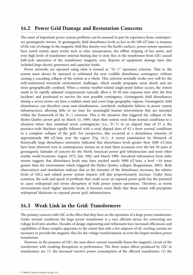
16.2 Power Grid Damage and Restoration Concerns
The onset of important power system problems can be assessed in part by experience from contempor-
ary geomagnetic storms. At geomagnetic field disturbance levels as low as 60–100 nT=min (a measure
of the rate of change in the magnetic field flux density over the Earth’s surface), power system operators
have noted system upset events such as relay misoperation, the offline tripping of key assets, and
even high levels of transformer internal heating due to stray flux in the transformer from GIC-caused
half-cycle saturation of the transformer magnetic core. Reports of equipment damage have also
included large electric generators and capacitor banks.
Power networks are operated using what is termed as ‘‘N – 1’’ operation criterion. That is, the
system must always be operated to withstand the next credible disturbance contingency without
causing a cascading collapse of the system as a whole. This criterion normally works very well for the
well-understood terrestrial environment challenges, which usually propagate more slowly and are
more geographically confined. When a routine weather-related single-point failure occurs, the system
needs to be rapidly adjusted (requirements typically allow a 10–30 min response time after the first
incident) and positioned to survive the next possible contingency. Geomagnetic field disturbances
during a severe storm can have a sudden onset and cover large geographic regions. Geomagnetic field
disturbances can therefore cause near-simultaneous, correlated, multipoint failures in power system
infrastructures, allowing little or no time for meaningful human interventions that are intended
within the framework of the N – 1 criterion. This is the situation that triggered the collapse of the
Hydro Quebec power grid on March 13, 1989, when their system went from normal conditions to a
situation where they sustained seven contingencies (i.e., N – 7) in an elapsed time of 57 s; the
province-wide blackout rapidly followed with a total elapsed time of 92 s from normal conditions
to a complete collapse of the grid. For perspective, this occurred at a disturbance intensity of
approximately 480 nT=min over the region (Fig. 16.1). A recent examination by Metatech of
historically large disturbance intensities indicated that disturbance levels greater than 2000 nT=min
have been observed even in contemporary storms on at least three occasions over the last 30 years at
geomagnetic latitudes of concern for the North American power grid infrastructure and most other
similar world locations: August 1972, July 1982, and March 1989. Anecdotal information from older
storms suggests that disturbance levels may have reached nearly 5000 nT=min, a level �10 times
greater than the environment which triggered the Hydro Quebec collapse (Kappenman, 2005). Both
observations and simulations indicate that as the intensity of the disturbance increases, the relative
levels of GICs and related power system impacts will also proportionately increase. Under these
scenarios, the scale and speed of problems that could occur on exposed power grids has the potential
to cause widespread and severe disruption of bulk power system operations. Therefore, as storm
environments reach higher intensity levels, it becomes more likely that these events will precipitate
widespread blackouts to exposed power grid infrastructures.
16.3 Weak Link in the Grid: Transformers
The primary concern with GIC is the effect that they have on the operation of a large power transformer.
Under normal conditions the large power transformer is a very efficient device for converting one
voltage level into another. Decades of design engineering and refinement have increased efficiencies and
capabilities of these complex apparatus to the extent that only a few amperes of AC exciting current are
necessary to provide the magnetic flux for the voltage transformation in even the largest modern power
transformer.
However, in the presence of GIC, the near-direct current essentially biases the magnetic circuit of the
transformer with resulting disruptions in performance. The three major effects produced by GIC in
transformers are (1) the increased reactive power consumption of the affected transformer, (2) the
� 2006 by Taylor & Francis Group, LLC.
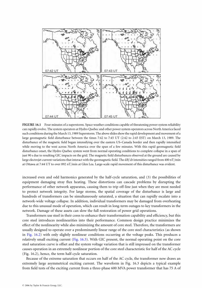
07:43 UT
07:45 UT07:44 UT
07:42 UT
FIGURE 16.1 Four minutes of a superstorm. Space weather conditions capable of threatening power system reliability
can rapidly evolve. The system operators at Hydro Quebec and other power system operators across North America faced
such conditions during the March 13, 1989 Superstorm. The above slides show the rapid development and movement of a
large geomagnetic field disturbance between the times 7:42 to 7:45 UT (2:42 to 2:45 EST) on March 13, 1989. The
disturbance of the magnetic field began intensifying over the eastern US–Canada border and then rapidly intensified
while moving to the west across North America over the span of a few minutes. With this rapid geomagnetic field
disturbance onset, the Hydro Quebec system went from normal operating conditions to complete collapse in a span of
just 90 s due to resulting GIC impacts on the grid. The magnetic field disturbances observed at the ground are caused by
large electrojet current variations that interact with the geomagnetic field. The dB=dt intensities ranged from 400 nT=min
at Ottawa at 7:44 UT to over 892 nT=min at Glen Lea. Large-scale rapid movement of this disturbance was evident.
increased even and odd harmonics generated by the half-cycle saturation, and (3) the possibilities of
equipment damaging stray flux heating. These distortions can cascade problems by disrupting the
performance of other network apparatus, causing them to trip off-line just when they are most needed
to protect network integrity. For large storms, the spatial coverage of the disturbance is large and
hundreds of transformers can be simultaneously saturated, a situation that can rapidly escalate into a
network-wide voltage collapse. In addition, individual transformers may be damaged from overheating
due to this unusual mode of operation, which can result in long-term outages to key transformers in the
network. Damage of these assets can slow the full restoration of power grid operations.
Transformers use steel in their cores to enhance their transformation capability and efficiency, but this
core steel introduces nonlinearities into their performance. Common design practice minimizes the
effect of the nonlinearity while also minimizing the amount of core steel. Therefore, the transformers are
usually designed to operate over a predominantly linear range of the core steel characteristics (as shown
in Fig. 16.2) with only slightly nonlinear conditions occurring at the voltage peaks. This produces a
relatively small exciting current (Fig. 16.3). With GIC present, the normal operating point on the core
steel saturation curve is offset and the system voltage variation that is still impressed on the transformer
causes operation in an extremely nonlinear portion of the core steel characteristic for half of the AC cycle
(Fig. 16.2), hence, the term half-cycle saturation.
Because of the extreme saturation that occurs on half of the AC cycle, the transformer now draws an
extremely large asymmetrical exciting current. The waveform in Fig. 16.3 depicts a typical example
from field tests of the exciting current from a three-phase 600 MVA power transformer that has 75 A of
� 2006 by Taylor & Francis Group, LLC.
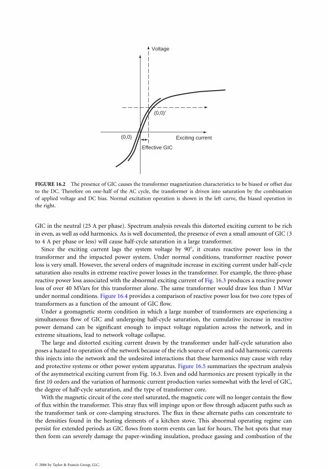
Effective GIC
Exciting current
(0,0)�
(0,0)
Voltage
FIGURE 16.2 The presence of GIC causes the transformer magnetization characteristics to be biased or offset due
to the DC. Therefore on one-half of the AC cycle, the transformer is driven into saturation by the combination
of applied voltage and DC bias. Normal excitation operation is shown in the left curve, the biased operation in
the right.
GIC in the neutral (25 A per phase). Spectrum analysis reveals this distorted exciting current to be rich
in even, as well as odd harmonics. As is well documented, the presence of even a small amount of GIC (3
to 4 A per phase or less) will cause half-cycle saturation in a large transformer.
Since the exciting current lags the system voltage by 908, it creates reactive power loss in the
transformer and the impacted power system. Under normal conditions, transformer reactive power
loss is very small. However, the several orders of magnitude increase in exciting current under half-cycle
saturation also results in extreme reactive power losses in the transformer. For example, the three-phase
reactive power loss associated with the abnormal exciting current of Fig. 16.3 produces a reactive power
loss of over 40 MVars for this transformer alone. The same transformer would draw less than 1 MVar
under normal conditions. Figure 16.4 provides a comparison of reactive power loss for two core types of
transformers as a function of the amount of GIC flow.
Under a geomagnetic storm condition in which a large number of transformers are experiencing a
simultaneous flow of GIC and undergoing half-cycle saturation, the cumulative increase in reactive
power demand can be significant enough to impact voltage regulation across the network, and in
extreme situations, lead to network voltage collapse.
The large and distorted exciting current drawn by the transformer under half-cycle saturation also
poses a hazard to operation of the network because of the rich source of even and odd harmonic currents
this injects into the network and the undesired interactions that these harmonics may cause with relay
and protective systems or other power system apparatus. Figure 16.5 summarizes the spectrum analysis
of the asymmetrical exciting current from Fig. 16.3. Even and odd harmonics are present typically in the
first 10 orders and the variation of harmonic current production varies somewhat with the level of GIC,
the degree of half-cycle saturation, and the type of transformer core.
With the magnetic circuit of the core steel saturated, the magnetic core will no longer contain the flow
of flux within the transformer. This stray flux will impinge upon or flow through adjacent paths such as
the transformer tank or core-clamping structures. The flux in these alternate paths can concentrate to
the densities found in the heating elements of a kitchen stove. This abnormal operating regime can
persist for extended periods as GIC flows from storm events can last for hours. The hot spots that may
then form can severely damage the paper-winding insulation, produce gassing and combustion of the
� 2006 by Taylor & Francis Group, LLC.
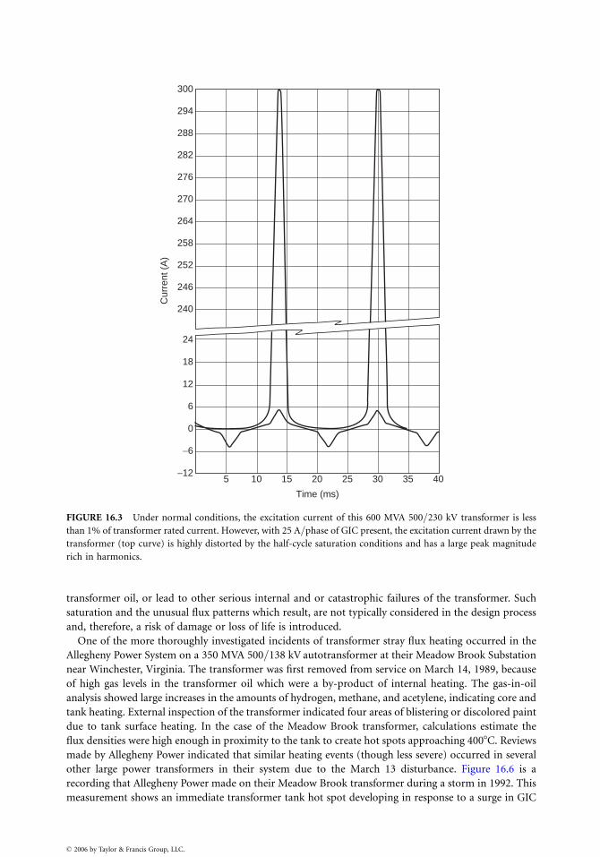
5−12
−6
0
6
12
18
24
240
246
252
258
264
270
276
282
288
294
300
10
Cur
rent
(A
)
15 20
Time (ms)
25 30 35 40
FIGURE 16.3 Under normal conditions, the excitation current of this 600 MVA 500=230 kV transformer is less
than 1% of transformer rated current. However, with 25 A=phase of GIC present, the excitation current drawn by the
transformer (top curve) is highly distorted by the half-cycle saturation conditions and has a large peak magnitude
rich in harmonics.
transformer oil, or lead to other serious internal and or catastrophic failures of the transformer. Such
saturation and the unusual flux patterns which result, are not typically considered in the design process
and, therefore, a risk of damage or loss of life is introduced.
One of the more thoroughly investigated incidents of transformer stray flux heating occurred in the
Allegheny Power System on a 350 MVA 500=138 kV autotransformer at their Meadow Brook Substation
near Winchester, Virginia. The transformer was first removed from service on March 14, 1989, because
of high gas levels in the transformer oil which were a by-product of internal heating. The gas-in-oil
analysis showed large increases in the amounts of hydrogen, methane, and acetylene, indicating core and
tank heating. External inspection of the transformer indicated four areas of blistering or discolored paint
due to tank surface heating. In the case of the Meadow Brook transformer, calculations estimate the
flux densities were high enough in proximity to the tank to create hot spots approaching 4008C. Reviews
made by Allegheny Power indicated that similar heating events (though less severe) occurred in several
other large power transformers in their system due to the March 13 disturbance. Figure 16.6 is a
recording that Allegheny Power made on their Meadow Brook transformer during a storm in 1992. This
measurement shows an immediate transformer tank hot spot developing in response to a surge in GIC
� 2006 by Taylor & Francis Group, LLC.
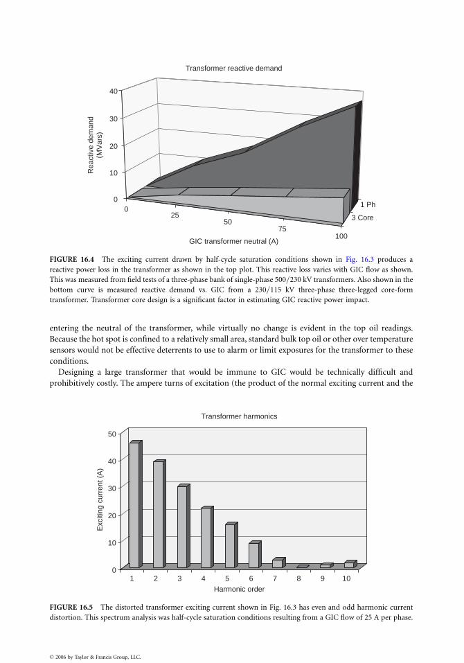
025
5075
100
3 Core
1 Ph0
10
20
30
40R
eact
ive
dem
and
(MV
ars)
GIC transformer neutral (A)
Transformer reactive demand
FIGURE 16.4 The exciting current drawn by half-cycle saturation conditions shown in Fig. 16.3 produces a
reactive power loss in the transformer as shown in the top plot. This reactive loss varies with GIC flow as shown.
This was measured from field tests of a three-phase bank of single-phase 500=230 kV transformers. Also shown in the
bottom curve is measured reactive demand vs. GIC from a 230=115 kV three-phase three-legged core-form
transformer. Transformer core design is a significant factor in estimating GIC reactive power impact.
entering the neutral of the transformer, while virtually no change is evident in the top oil readings.
Because the hot spot is confined to a relatively small area, standard bulk top oil or other over temperature
sensors would not be effective deterrents to use to alarm or limit exposures for the transformer to these
conditions.
Designing a large transformer that would be immune to GIC would be technically difficult and
prohibitively costly. The ampere turns of excitation (the product of the normal exciting current and the
0
10
20
30
40
50
Exc
iting
cur
rent
(A
)
1 2 3 4 5 6 7 8 9 10
Harmonic order
Transformer harmonics
FIGURE 16.5 The distorted transformer exciting current shown in Fig. 16.3 has even and odd harmonic current
distortion. This spectrum analysis was half-cycle saturation conditions resulting from a GIC flow of 25 A per phase.
� 2006 by Taylor & Francis Group, LLC.
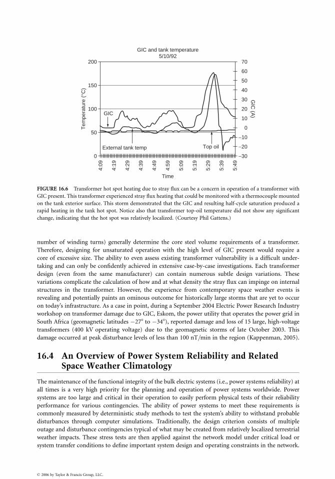
GIC
0
50
100
150
200
External tank temp Top oil
Tem
pera
ture
(°C
)
Time
GIC and tank temperature5/10/92
GIC
(A)
−30
−20
−10
0
10
20
30
40
50
60
70
4:09
4:19
4:29
4:39
4:49
4:59
5:09
5:19
5:29
5:39
5:49
FIGURE 16.6 Transformer hot spot heating due to stray flux can be a concern in operation of a transformer with
GIC present. This transformer experienced stray flux heating that could be monitored with a thermocouple mounted
on the tank exterior surface. This storm demonstrated that the GIC and resulting half-cycle saturation produced a
rapid heating in the tank hot spot. Notice also that transformer top-oil temperature did not show any significant
change, indicating that the hot spot was relatively localized. (Courtesy Phil Gattens.)
number of winding turns) generally determine the core steel volume requirements of a transformer.
Therefore, designing for unsaturated operation with the high level of GIC present would require a
core of excessive size. The ability to even assess existing transformer vulnerability is a difficult under-
taking and can only be confidently achieved in extensive case-by-case investigations. Each transformer
design (even from the same manufacturer) can contain numerous subtle design variations. These
variations complicate the calculation of how and at what density the stray flux can impinge on internal
structures in the transformer. However, the experience from contemporary space weather events is
revealing and potentially paints an ominous outcome for historically large storms that are yet to occur
on today’s infrastructure. As a case in point, during a September 2004 Electric Power Research Industry
workshop on transformer damage due to GIC, Eskom, the power utility that operates the power grid in
South Africa (geomagnetic latitudes �278 to �348), reported damage and loss of 15 large, high-voltage
transformers (400 kV operating voltage) due to the geomagnetic storms of late October 2003. This
damage occurred at peak disturbance levels of less than 100 nT=min in the region (Kappenman, 2005).
16.4 An Overview of Power System Reliability and RelatedSpace Weather Climatology
The maintenance of the functional integrity of the bulk electric systems (i.e., power systems reliability) at
all times is a very high priority for the planning and operation of power systems worldwide. Power
systems are too large and critical in their operation to easily perform physical tests of their reliability
performance for various contingencies. The ability of power systems to meet these requirements is
commonly measured by deterministic study methods to test the system’s ability to withstand probable
disturbances through computer simulations. Traditionally, the design criterion consists of multiple
outage and disturbance contingencies typical of what may be created from relatively localized terrestrial
weather impacts. These stress tests are then applied against the network model under critical load or
system transfer conditions to define important system design and operating constraints in the network.
� 2006 by Taylor & Francis Group, LLC.
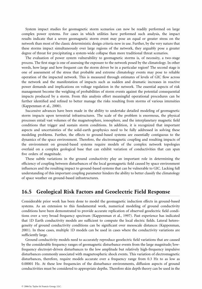
System impact studies for geomagnetic storm scenarios can now be readily performed on large
complex power systems. For cases in which utilities have performed such analysis, the impact
results indicate that a severe geomagnetic storm event may pose an equal or greater stress on the
network than most of the classic deterministic design criteria now in use. Further, by the very nature that
these storms impact simultaneously over large regions of the network, they arguably pose a greater
degree of threat for precipitating a system-wide collapse than more traditional threat scenarios.
The evaluation of power system vulnerability to geomagnetic storms is, of necessity, a two-stage
process. The first stage is one of assessing the exposure to the network posed by the climatology. In other
words, how large and how frequent can the storm driver be in a particular region? The second stage is
one of assessment of the stress that probable and extreme climatology events may pose to reliable
operation of the impacted network. This is measured through estimates of levels of GIC flow across
the network and the manifestation of impacts such as sudden and dramatic increases in reactive
power demands and implications on voltage regulation in the network. The essential aspects of risk
management become the weighing of probabilities of storm events against the potential consequential
impacts produced by a storm. From this analysis effort meaningful operational procedures can be
further identified and refined to better manage the risks resulting from storms of various intensities
(Kappenman et al., 2000).
Successive advances have been made in the ability to undertake detailed modeling of geomagnetic
storm impacts upon terrestrial infrastructures. The scale of the problem is enormous, the physical
processes entail vast volumes of the magnetosphere, ionosphere, and the interplanetary magnetic field
conditions that trigger and sustain storm conditions. In addition, it is recognized that important
aspects and uncertainties of the solid-earth geophysics need to be fully addressed in solving these
modeling problems. Further, the effects to ground-based systems are essentially contiguous to the
dynamics of the space environment. Therefore, the electromagnetic coupling and resulting impacts of
the environment on ground-based systems require models of the complex network topologies
overlaid on a complex geological base that can exhibit variation of conductivities that can span
five orders of magnitude.
These subtle variations in the ground conductivity play an important role in determining the
efficiency of coupling between disturbances of the local geomagnetic field caused by space environment
influences and the resulting impact to ground-based systems that can be vulnerable to GIC. Lacking full
understanding of this important coupling parameter hinders the ability to better classify the climatology
of space weather on ground-based infrastructures.
16.5 Geological Risk Factors and Geoelectric Field Response
Considerable prior work has been done to model the geomagnetic induction effects in ground-based
systems. As an extension to this fundamental work, numerical modeling of ground conductivity
conditions have been demonstrated to provide accurate replication of observed geoelectric field condi-
tions over a very broad frequency spectrum (Kappenman et al., 1997). Past experience has indicated
that 1D Earth conductivity models are sufficient to compute the local electric fields. Lateral hetero-
geneity of ground conductivity conditions can be significant over mesoscale distances (Kappenman,
2001). In these cases, multiple 1D models can be used in cases where the conductivity variations are
sufficiently large.
Ground conductivity models need to accurately reproduce geoelectric field variations that are caused
by the considerable frequency ranges of geomagnetic disturbance events from the large magnitude=low-
frequency electrojet-driven disturbances to the low amplitude but relatively high-frequency impulsive
disturbances commonly associated with magnetospheric shock events. This variation of electromagnetic
disturbances, therefore, require models accurate over a frequency range from 0.3 Hz to as low as
0.00001 Hz. At these low frequencies of the disturbance environments, diffusion aspects of ground
conductivities must be considered to appropriate depths. Therefore skin depth theory can be used in the
� 2006 by Taylor & Francis Group, LLC.
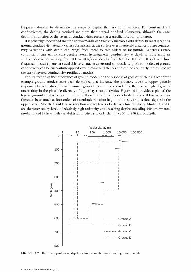
frequency domain to determine the range of depths that are of importance. For constant Earth
conductivities, the depths required are more than several hundred kilometers, although the exact
depth is a function of the layers of conductivities present at a specific location of interest.
It is generally understood that the Earth’s mantle conductivity increases with depth. In most locations,
ground conductivity laterally varies substantially at the surface over mesoscale distances; these conduct-
ivity variations with depth can range from three to five orders of magnitude. Whereas surface
conductivity can exhibit considerable lateral heterogeneity, conductivity at depth is more uniform,
with conductivities ranging from 0.1 to 10 S=m at depths from 600 to 1000 km. If sufficient low-
frequency measurements are available to characterize ground conductivity profiles, models of ground
conductivity can be successfully applied over mesoscale distances and can be accurately represented by
the use of layered conductivity profiles or models.
For illustration of the importance of ground models on the response of geoelectric fields, a set of four
example ground models have been developed that illustrate the probable lower to upper quartile
response characteristics of most known ground conditions, considering there is a high degree of
uncertainty in the plausible diversity of upper layer conductivities. Figure 16.7 provides a plot of the
layered ground conductivity conditions for these four ground models to depths of 700 km. As shown,
there can be as much as four orders of magnitude variation in ground resistivity at various depths in the
upper layers. Models A and B have very thin surface layers of relatively low resistivity. Models A and C
are characterized by levels of relatively high resistivity until reaching depths exceeding 400 km, whereas
models B and D have high variability of resistivity in only the upper 50 to 200 km of depth.
800
700
600
500
400
Dep
th (
km)
300
200
100
01 10 100 1,000
Resistivity (Ω m)
10,000 100,000
Ground A
Ground B
Ground C
Ground D
FIGURE 16.7 Resistivity profiles vs. depth for four example layered earth ground models.
� 2006 by Taylor & Francis Group, LLC.
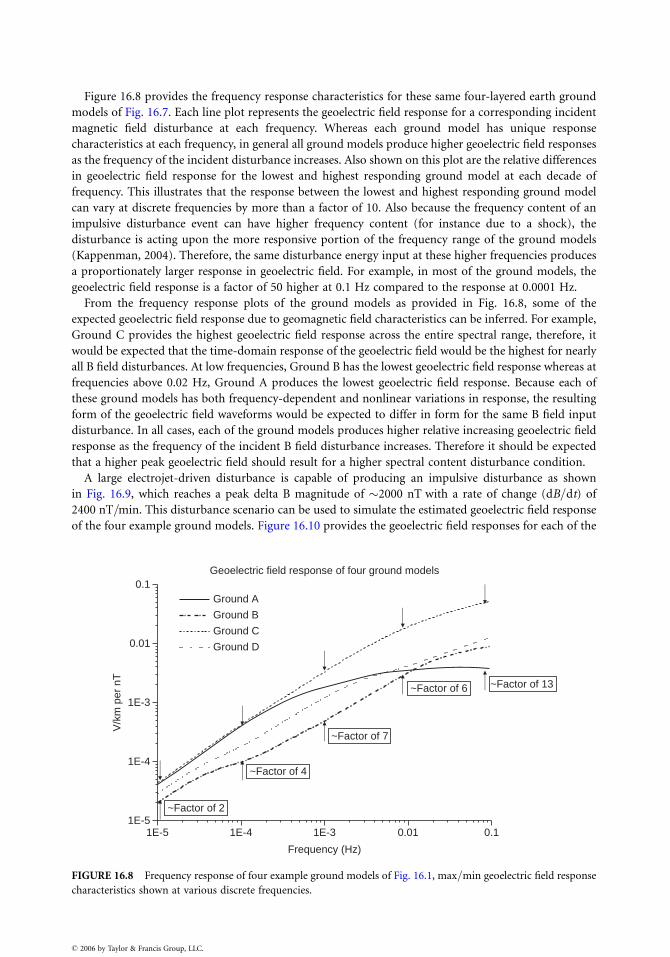
Figure 16.8 provides the frequency response characteristics for these same four-layered earth ground
models of Fig. 16.7. Each line plot represents the geoelectric field response for a corresponding incident
magnetic field disturbance at each frequency. Whereas each ground model has unique response
characteristics at each frequency, in general all ground models produce higher geoelectric field responses
as the frequency of the incident disturbance increases. Also shown on this plot are the relative differences
in geoelectric field response for the lowest and highest responding ground model at each decade of
frequency. This illustrates that the response between the lowest and highest responding ground model
can vary at discrete frequencies by more than a factor of 10. Also because the frequency content of an
impulsive disturbance event can have higher frequency content (for instance due to a shock), the
disturbance is acting upon the more responsive portion of the frequency range of the ground models
(Kappenman, 2004). Therefore, the same disturbance energy input at these higher frequencies produces
a proportionately larger response in geoelectric field. For example, in most of the ground models, the
geoelectric field response is a factor of 50 higher at 0.1 Hz compared to the response at 0.0001 Hz.
From the frequency response plots of the ground models as provided in Fig. 16.8, some of the
expected geoelectric field response due to geomagnetic field characteristics can be inferred. For example,
Ground C provides the highest geoelectric field response across the entire spectral range, therefore, it
would be expected that the time-domain response of the geoelectric field would be the highest for nearly
all B field disturbances. At low frequencies, Ground B has the lowest geoelectric field response whereas at
frequencies above 0.02 Hz, Ground A produces the lowest geoelectric field response. Because each of
these ground models has both frequency-dependent and nonlinear variations in response, the resulting
form of the geoelectric field waveforms would be expected to differ in form for the same B field input
disturbance. In all cases, each of the ground models produces higher relative increasing geoelectric field
response as the frequency of the incident B field disturbance increases. Therefore it should be expected
that a higher peak geoelectric field should result for a higher spectral content disturbance condition.
A large electrojet-driven disturbance is capable of producing an impulsive disturbance as shown
in Fig. 16.9, which reaches a peak delta B magnitude of �2000 nT with a rate of change (dB=dt) of
2400 nT=min. This disturbance scenario can be used to simulate the estimated geoelectric field response
of the four example ground models. Figure 16.10 provides the geoelectric field responses for each of the
1E-5 1E-4 1E-3 0.01 0.11E-5
1E-4
1E-3
0.01
0.1Ground A
Ground B
Ground C
Ground D
Geoelectric field response of four ground models
V/k
m p
er n
T
Frequency (Hz)
~Factor of 2
~Factor of 4
~Factor of 7
~Factor of 6 ~Factor of 13
FIGURE 16.8 Frequency response of four example ground models of Fig. 16.1, max=min geoelectric field response
characteristics shown at various discrete frequencies.
� 2006 by Taylor & Francis Group, LLC.
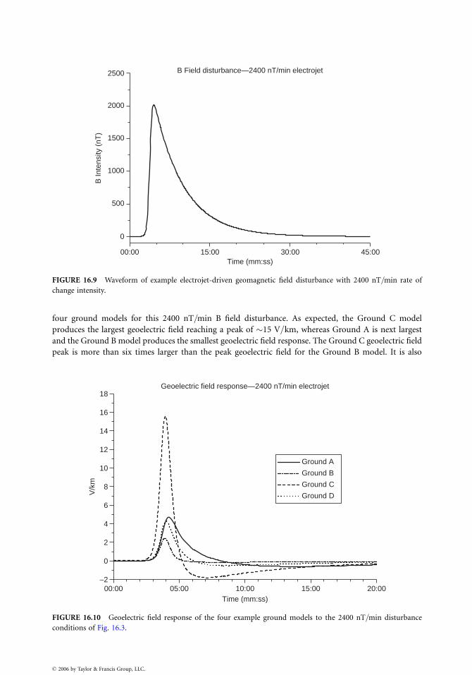
00:00 15:00 30:00 45:00
0
500
1000
1500
2000
2500 B Field disturbance—2400 nT/min electrojet
B In
tens
ity (
nT)
Time (mm:ss)
FIGURE 16.9 Waveform of example electrojet-driven geomagnetic field disturbance with 2400 nT=min rate of
change intensity.
four ground models for this 2400 nT=min B field disturbance. As expected, the Ground C model
produces the largest geoelectric field reaching a peak of �15 V=km, whereas Ground A is next largest
and the Ground B model produces the smallest geoelectric field response. The Ground C geoelectric field
peak is more than six times larger than the peak geoelectric field for the Ground B model. It is also
00:00 05:00 10:00 15:00 20:00−2
0
2
4
6
8
10
12
14
16
18Geoelectric field response—2400 nT/min electrojet
Ground A
Ground B
Ground C
Ground DV/k
m
Time (mm:ss)
FIGURE 16.10 Geoelectric field response of the four example ground models to the 2400 nT=min disturbance
conditions of Fig. 16.3.
� 2006 by Taylor & Francis Group, LLC.
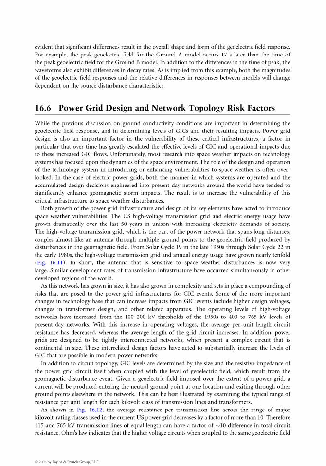
evident that significant differences result in the overall shape and form of the geoelectric field response.
For example, the peak geoelectric field for the Ground A model occurs 17 s later than the time of
the peak geoelectric field for the Ground B model. In addition to the differences in the time of peak, the
waveforms also exhibit differences in decay rates. As is implied from this example, both the magnitudes
of the geoelectric field responses and the relative differences in responses between models will change
dependent on the source disturbance characteristics.
16.6 Power Grid Design and Network Topology Risk Factors
While the previous discussion on ground conductivity conditions are important in determining the
geoelectric field response, and in determining levels of GICs and their resulting impacts. Power grid
design is also an important factor in the vulnerability of these critical infrastructures, a factor in
particular that over time has greatly escalated the effective levels of GIC and operational impacts due
to these increased GIC flows. Unfortunately, most research into space weather impacts on technology
systems has focused upon the dynamics of the space environment. The role of the design and operation
of the technology system in introducing or enhancing vulnerabilities to space weather is often over-
looked. In the case of electric power grids, both the manner in which systems are operated and the
accumulated design decisions engineered into present-day networks around the world have tended to
significantly enhance geomagnetic storm impacts. The result is to increase the vulnerability of this
critical infrastructure to space weather disturbances.
Both growth of the power grid infrastructure and design of its key elements have acted to introduce
space weather vulnerabilities. The US high-voltage transmission grid and electric energy usage have
grown dramatically over the last 50 years in unison with increasing electricity demands of society.
The high-voltage transmission grid, which is the part of the power network that spans long distances,
couples almost like an antenna through multiple ground points to the geoelectric field produced by
disturbances in the geomagnetic field. From Solar Cycle 19 in the late 1950s through Solar Cycle 22 in
the early 1980s, the high-voltage transmission grid and annual energy usage have grown nearly tenfold
(Fig. 16.11). In short, the antenna that is sensitive to space weather disturbances is now very
large. Similar development rates of transmission infrastructure have occurred simultaneously in other
developed regions of the world.
As this network has grown in size, it has also grown in complexity and sets in place a compounding of
risks that are posed to the power grid infrastructures for GIC events. Some of the more important
changes in technology base that can increase impacts from GIC events include higher design voltages,
changes in transformer design, and other related apparatus. The operating levels of high-voltage
networks have increased from the 100–200 kV thresholds of the 1950s to 400 to 765 kV levels of
present-day networks. With this increase in operating voltages, the average per unit length circuit
resistance has decreased, whereas the average length of the grid circuit increases. In addition, power
grids are designed to be tightly interconnected networks, which present a complex circuit that is
continental in size. These interrelated design factors have acted to substantially increase the levels of
GIC that are possible in modern power networks.
In addition to circuit topology, GIC levels are determined by the size and the resistive impedance of
the power grid circuit itself when coupled with the level of geoelectric field, which result from the
geomagnetic disturbance event. Given a geoelectric field imposed over the extent of a power grid, a
current will be produced entering the neutral ground point at one location and exiting through other
ground points elsewhere in the network. This can be best illustrated by examining the typical range of
resistance per unit length for each kilovolt class of transmission lines and transformers.
As shown in Fig. 16.12, the average resistance per transmission line across the range of major
kilovolt-rating classes used in the current US power grid decreases by a factor of more than 10. Therefore
115 and 765 kV transmission lines of equal length can have a factor of �10 difference in total circuit
resistance. Ohm’s law indicates that the higher voltage circuits when coupled to the same geoelectric field
� 2006 by Taylor & Francis Group, LLC.
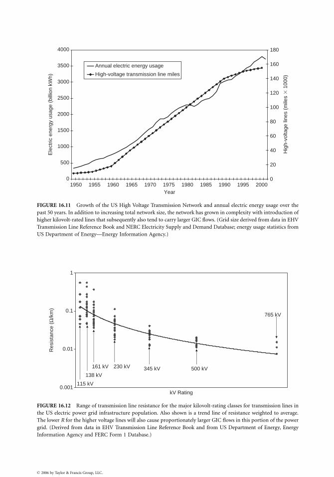
0
500
1000
1500
2000
2500
3000
3500
4000
1950 1955 1960 1965 1970 1975 1980 1985 1990 1995 2000Year
Ele
ctric
ene
rgy
usag
e (b
illio
n kW
h)
0
20
40
60
80
100
120
140
160
180
Hig
h-vo
ltage
line
s (m
iles
� 1
000)
Annual electric energy usage
High-voltage transmission line miles
FIGURE 16.11 Growth of the US High Voltage Transmission Network and annual electric energy usage over the
past 50 years. In addition to increasing total network size, the network has grown in complexity with introduction of
higher kilovolt-rated lines that subsequently also tend to carry larger GIC flows. (Grid size derived from data in EHV
Transmission Line Reference Book and NERC Electricity Supply and Demand Database; energy usage statistics from
US Department of Energy—Energy Information Agency.)
0.001
0.01
0.1
1
kV Rating
Res
ista
nce
(Ω/k
m)
115 kV
138 kV
161 kV 230 kV 345 kV 500 kV
765 kV
FIGURE 16.12 Range of transmission line resistance for the major kilovolt-rating classes for transmission lines in
the US electric power grid infrastructure population. Also shown is a trend line of resistance weighted to average.
The lower R for the higher voltage lines will also cause proportionately larger GIC flows in this portion of the power
grid. (Derived from data in EHV Transmission Line Reference Book and from US Department of Energy, Energy
Information Agency and FERC Form 1 Database.)
� 2006 by Taylor & Francis Group, LLC.
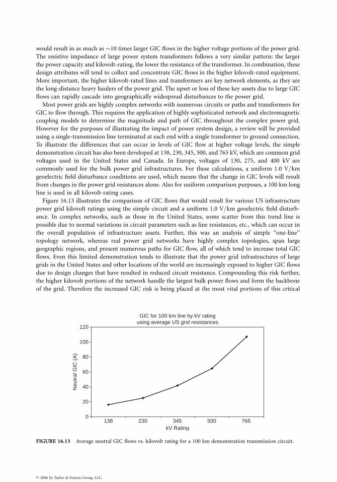
would result in as much as �10 times larger GIC flows in the higher voltage portions of the power grid.
The resistive impedance of large power system transformers follows a very similar pattern: the larger
the power capacity and kilovolt-rating, the lower the resistance of the transformer. In combination, these
design attributes will tend to collect and concentrate GIC flows in the higher kilovolt-rated equipment.
More important, the higher kilovolt-rated lines and transformers are key network elements, as they are
the long-distance heavy haulers of the power grid. The upset or loss of these key assets due to large GIC
flows can rapidly cascade into geographically widespread disturbances to the power grid.
Most power grids are highly complex networks with numerous circuits or paths and transformers for
GIC to flow through. This requires the application of highly sophisticated network and electromagnetic
coupling models to determine the magnitude and path of GIC throughout the complex power grid.
However for the purposes of illustrating the impact of power system design, a review will be provided
using a single-transmission line terminated at each end with a single transformer to ground connection.
To illustrate the differences that can occur in levels of GIC flow at higher voltage levels, the simple
demonstration circuit has also been developed at 138, 230, 345, 500, and 765 kV, which are common grid
voltages used in the United States and Canada. In Europe, voltages of 130, 275, and 400 kV are
commonly used for the bulk power grid infrastructures. For these calculations, a uniform 1.0 V=km
geoelectric field disturbance conditions are used, which means that the change in GIC levels will result
from changes in the power grid resistances alone. Also for uniform comparison purposes, a 100 km long
line is used in all kilovolt-rating cases.
Figure 16.13 illustrates the comparison of GIC flows that would result for various US infrastructure
power grid kilovolt ratings using the simple circuit and a uniform 1.0 V=km geoelectric field disturb-
ance. In complex networks, such as those in the United States, some scatter from this trend line is
possible due to normal variations in circuit parameters such as line resistances, etc., which can occur in
the overall population of infrastructure assets. Further, this was an analysis of simple ‘‘one-line’’
topology network, whereas real power grid networks have highly complex topologies, span large
geographic regions, and present numerous paths for GIC flow, all of which tend to increase total GIC
flows. Even this limited demonstration tends to illustrate that the power grid infrastructures of large
grids in the United States and other locations of the world are increasingly exposed to higher GIC flows
due to design changes that have resulted in reduced circuit resistance. Compounding this risk further,
the higher kilovolt portions of the network handle the largest bulk power flows and form the backbone
of the grid. Therefore the increased GIC risk is being placed at the most vital portions of this critical
GIC for 100 km line by kV ratingusing average US grid resistances
0
20
40
60
80
100
120
138 230 345 500 765kV Rating
Neu
tral
GIC
(A
)
FIGURE 16.13 Average neutral GIC flows vs. kilovolt rating for a 100 km demonstration transmission circuit.
� 2006 by Taylor & Francis Group, LLC.
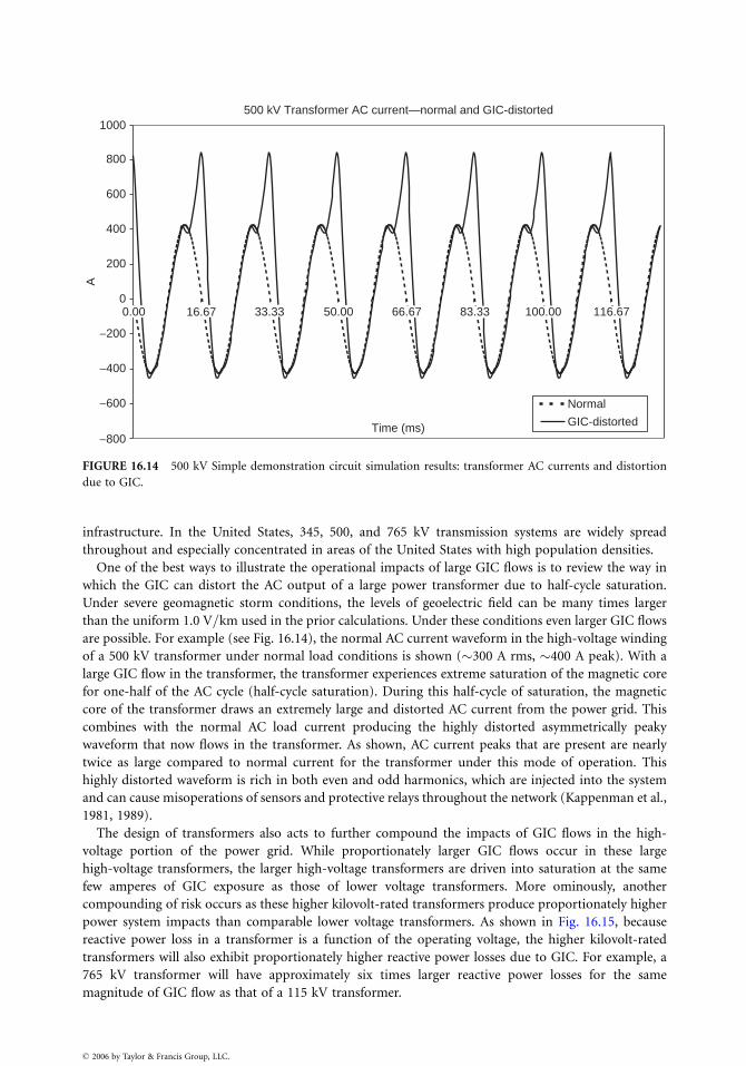
500 kV Transformer AC current—normal and GIC-distorted
−800
−600
−400
−200
0
200
400
600
800
1000
Time (ms)
A
Normal
GIC-distorted
116.67100.0083.3366.6750.0033.3316.670.00
FIGURE 16.14 500 kV Simple demonstration circuit simulation results: transformer AC currents and distortion
due to GIC.
infrastructure. In the United States, 345, 500, and 765 kV transmission systems are widely spread
throughout and especially concentrated in areas of the United States with high population densities.
One of the best ways to illustrate the operational impacts of large GIC flows is to review the way in
which the GIC can distort the AC output of a large power transformer due to half-cycle saturation.
Under severe geomagnetic storm conditions, the levels of geoelectric field can be many times larger
than the uniform 1.0 V=km used in the prior calculations. Under these conditions even larger GIC flows
are possible. For example (see Fig. 16.14), the normal AC current waveform in the high-voltage winding
of a 500 kV transformer under normal load conditions is shown (�300 A rms, �400 A peak). With a
large GIC flow in the transformer, the transformer experiences extreme saturation of the magnetic core
for one-half of the AC cycle (half-cycle saturation). During this half-cycle of saturation, the magnetic
core of the transformer draws an extremely large and distorted AC current from the power grid. This
combines with the normal AC load current producing the highly distorted asymmetrically peaky
waveform that now flows in the transformer. As shown, AC current peaks that are present are nearly
twice as large compared to normal current for the transformer under this mode of operation. This
highly distorted waveform is rich in both even and odd harmonics, which are injected into the system
and can cause misoperations of sensors and protective relays throughout the network (Kappenman et al.,
1981, 1989).
The design of transformers also acts to further compound the impacts of GIC flows in the high-
voltage portion of the power grid. While proportionately larger GIC flows occur in these large
high-voltage transformers, the larger high-voltage transformers are driven into saturation at the same
few amperes of GIC exposure as those of lower voltage transformers. More ominously, another
compounding of risk occurs as these higher kilovolt-rated transformers produce proportionately higher
power system impacts than comparable lower voltage transformers. As shown in Fig. 16.15, because
reactive power loss in a transformer is a function of the operating voltage, the higher kilovolt-rated
transformers will also exhibit proportionately higher reactive power losses due to GIC. For example, a
765 kV transformer will have approximately six times larger reactive power losses for the same
magnitude of GIC flow as that of a 115 kV transformer.
� 2006 by Taylor & Francis Group, LLC.
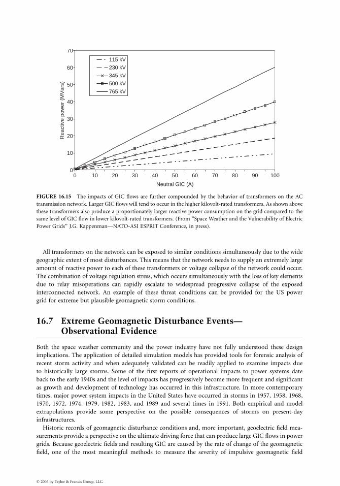
0
10
20
30
40
50
60
70
0 10 20 30 40 50 60 70 80 90 100
Neutral GIC (A)
Rea
ctiv
e po
wer
(M
Var
s)115 kV
230 kV
345 kV
500 kV
765 kV
FIGURE 16.15 The impacts of GIC flows are further compounded by the behavior of transformers on the AC
transmission network. Larger GIC flows will tend to occur in the higher kilovolt-rated transformers. As shown above
these transformers also produce a proportionately larger reactive power consumption on the grid compared to the
same level of GIC flow in lower kilovolt-rated transformers. (From ‘‘Space Weather and the Vulnerability of Electric
Power Grids’’ J.G. Kappenman—NATO-ASI ESPRIT Conference, in press).
All transformers on the network can be exposed to similar conditions simultaneously due to the wide
geographic extent of most disturbances. This means that the network needs to supply an extremely large
amount of reactive power to each of these transformers or voltage collapse of the network could occur.
The combination of voltage regulation stress, which occurs simultaneously with the loss of key elements
due to relay misoperations can rapidly escalate to widespread progressive collapse of the exposed
interconnected network. An example of these threat conditions can be provided for the US power
grid for extreme but plausible geomagnetic storm conditions.
16.7 Extreme Geomagnetic Disturbance Events—Observational Evidence
Both the space weather community and the power industry have not fully understood these design
implications. The application of detailed simulation models has provided tools for forensic analysis of
recent storm activity and when adequately validated can be readily applied to examine impacts due
to historically large storms. Some of the first reports of operational impacts to power systems date
back to the early 1940s and the level of impacts has progressively become more frequent and significant
as growth and development of technology has occurred in this infrastructure. In more contemporary
times, major power system impacts in the United States have occurred in storms in 1957, 1958, 1968,
1970, 1972, 1974, 1979, 1982, 1983, and 1989 and several times in 1991. Both empirical and model
extrapolations provide some perspective on the possible consequences of storms on present-day
infrastructures.
Historic records of geomagnetic disturbance conditions and, more important, geoelectric field mea-
surements provide a perspective on the ultimate driving force that can produce large GIC flows in power
grids. Because geoelectric fields and resulting GIC are caused by the rate of change of the geomagnetic
field, one of the most meaningful methods to measure the severity of impulsive geomagnetic field
� 2006 by Taylor & Francis Group, LLC.
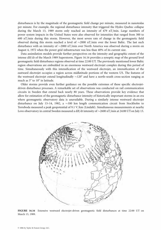
disturbances is by the magnitude of the geomagnetic field change per minute, measured in nanoteslas
per minute. For example, the regional disturbance intensity that triggered the Hydro Quebec collapse
during the March 13, 1989 storm only reached an intensity of 479 nT=min. Large numbers of
power system impacts in the United States were also observed for intensities that ranged from 300 to
600 nT=min during this storm. However, the most severe rate of change in the geomagnetic field
observed during this storm reached a level of �2000 nT=min over the lower Baltic. The last such
disturbance with an intensity of �2000 nT=min over North America was observed during a storm on
August 4, 1972 when the power grid infrastructure was less than 40% of its current size.
Data assimilation models provide further perspectives on the intensity and geographic extent of the
intense dB=dt of the March 1989 Superstorm. Figure 16.16 provides a synoptic map of the ground level
geomagnetic field disturbance regions observed at time 22:00 UT. The previously mentioned lower Baltic
region observations are embedded in an enormous westward electrojet complex during this period of
time. Simultaneously with this intensification of the westward electrojet, an intensification of the
eastward electrojet occupies a region across midlatitude portions of the western US. The features of
the westward electrojet extend longitudinally �1208 and have a north–south cross-section ranging as
much as 58 to 108 in latitude.
Older storms provide even further guidance on the possible extremes of these specific electrojet-
driven disturbance processes. A remarkable set of observations was conducted on rail communication
circuits in Sweden that extend back nearly 80 years. These observations provide key evidence that
allow for estimation of the geomagnetic disturbance intensity of historically important storms in an era
where geomagnetic observatory data is unavailable. During a similarly intense westward electrojet
disturbance on July 13–14, 1982, a �100 km length communication circuit from Stockholm to
Torreboda measured a peak geopotential of 9.1 V=km (Lindahl). Simultaneous measurements at nearby
Lovo observatory in central Sweden measured a dB=dt intensity of�2600 nT=min at 24:00 UTon July 13.
FIGURE 16.16 Extensive westward electrojet-driven geomagnetic field disturbances at time 22:00 UT on
March 13, 1989.
� 2006 by Taylor & Francis Group, LLC.
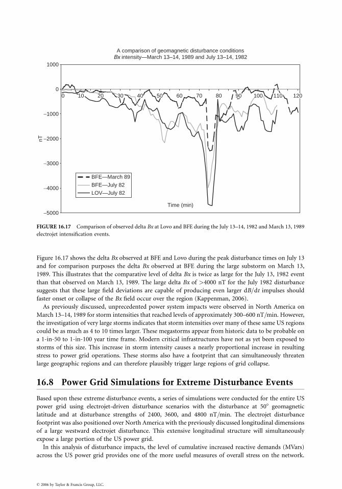
A comparison of geomagnetic disturbance conditionsBx intensity—March 13–14, 1989 and July 13–14, 1982
−5000
−4000
−3000
−2000
−1000
0
1000
0 60 70 80
Time (min)
nT
BFE—March 89
BFE—July 82
LOV—July 82
10 20 30 40 50 90 100 110 120
FIGURE 16.17 Comparison of observed delta Bx at Lovo and BFE during the July 13–14, 1982 and March 13, 1989
electrojet intensification events.
Figure 16.17 shows the delta Bx observed at BFE and Lovo during the peak disturbance times on July 13
and for comparison purposes the delta Bx observed at BFE during the large substorm on March 13,
1989. This illustrates that the comparative level of delta Bx is twice as large for the July 13, 1982 event
than that observed on March 13, 1989. The large delta Bx of >4000 nT for the July 1982 disturbance
suggests that these large field deviations are capable of producing even larger dB=dt impulses should
faster onset or collapse of the Bx field occur over the region (Kappenman, 2006).
As previously discussed, unprecedented power system impacts were observed in North America on
March 13–14, 1989 for storm intensities that reached levels of approximately 300–600 nT=min. However,
the investigation of very large storms indicates that storm intensities over many of these same US regions
could be as much as 4 to 10 times larger. These megastorms appear from historic data to be probable on
a 1-in-50 to 1-in-100 year time frame. Modern critical infrastructures have not as yet been exposed to
storms of this size. This increase in storm intensity causes a nearly proportional increase in resulting
stress to power grid operations. These storms also have a footprint that can simultaneously threaten
large geographic regions and can therefore plausibly trigger large regions of grid collapse.
16.8 Power Grid Simulations for Extreme Disturbance Events
Based upon these extreme disturbance events, a series of simulations were conducted for the entire US
power grid using electrojet-driven disturbance scenarios with the disturbance at 508 geomagnetic
latitude and at disturbance strengths of 2400, 3600, and 4800 nT=min. The electrojet disturbance
footprint was also positioned over North America with the previously discussed longitudinal dimensions
of a large westward electrojet disturbance. This extensive longitudinal structure will simultaneously
expose a large portion of the US power grid.
In this analysis of disturbance impacts, the level of cumulative increased reactive demands (MVars)
across the US power grid provides one of the more useful measures of overall stress on the network.
� 2006 by Taylor & Francis Group, LLC.
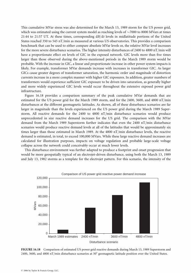
This cumulative MVar stress was also determined for the March 13, 1989 storm for the US power grid,
which was estimated using the current system model as reaching levels of �7000 to 8000 MVars at times
21:44 to 21:57 UT. At these times, corresponding dB=dt levels in midlatitude portions of the United
States reached 350 to 545 nT=min as measured at various US observatories. This provides a comparison
benchmark that can be used to either compare absolute MVar levels or, the relative MVar level increases
for the more severe disturbance scenarios. The higher intensity disturbances of 2400 to 4800 nT=min will
have a proportionate effect on levels of GIC in the exposed network. GIC levels more than five times
larger than those observed during the above-mentioned periods in the March 1989 storm would be
probable. With the increase in GIC, a linear and proportionate increase in other power system impacts is
likely. For example, transformer MVar demands increase with increases in transformer GIC. As larger
GICs cause greater degrees of transformer saturation, the harmonic order and magnitude of distortion
currents increase in a more complex manner with higher GIC exposures. In addition, greater numbers of
transformers would experience sufficient GIC exposure to be driven into saturation, as generally higher
and more widely experienced GIC levels would occur throughout the extensive exposed power grid
infrastructure.
Figure 16.18 provides a comparison summary of the peak cumulative MVar demands that are
estimated for the US power grid for the March 1989 storm, and for the 2400, 3600, and 4800 nT=min
disturbances at the different geomagnetic latitudes. As shown, all of these disturbance scenarios are far
larger in magnitude than the levels experienced on the US power grid during the March 1989 Super-
storm. All reactive demands for the 2400 to 4800 nT=min disturbance scenarios would produce
unprecedented in size reactive demand increases for the US grid. The comparison with the MVar
demand from the March 1989 Superstorm further indicates that even the 2400 nT=min disturbance
scenarios would produce reactive demand levels at all of the latitudes that would be approximately six
times larger than those estimated in March 1989. At the 4800 nT=min disturbance levels, the reactive
demand is estimated, in total, to exceed 100,000 MVars. While these large reactive demand increases are
calculated for illustration purposes, impacts on voltage regulation and probable large-scale voltage
collapse across the network could conceivably occur at much lower levels.
This disturbance environment was further adapted to produce a footprint and onset progression that
would be more geospatially typical of an electrojet-driven disturbance, using both the March 13, 1989
and July 13, 1982 storms as a template for the electrojet pattern. For this scenario, the intensity of the
Comparison of US power grid reactive power demand increase
0
20,000
40,000
60,000
80,000
100,000
120,000
March 1989 estimates 2400 nT/min 3600 nT/min 4800 nT/min
Disturbance scenario
MV
ars
FIGURE 16.18 Comparison of estimated US power grid reactive demands during March 13, 1989 Superstorm and
2400, 3600, and 4800 nT=min disturbance scenarios at 508 geomagnetic latitude position over the United States.
� 2006 by Taylor & Francis Group, LLC.
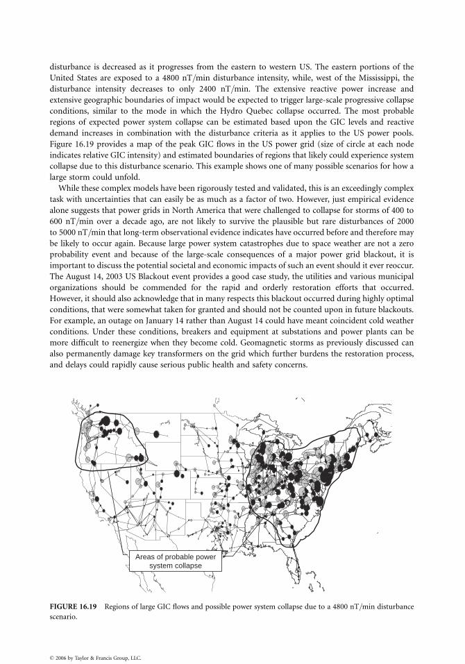
disturbance is decreased as it progresses from the eastern to western US. The eastern portions of the
United States are exposed to a 4800 nT=min disturbance intensity, while, west of the Mississippi, the
disturbance intensity decreases to only 2400 nT=min. The extensive reactive power increase and
extensive geographic boundaries of impact would be expected to trigger large-scale progressive collapse
conditions, similar to the mode in which the Hydro Quebec collapse occurred. The most probable
regions of expected power system collapse can be estimated based upon the GIC levels and reactive
demand increases in combination with the disturbance criteria as it applies to the US power pools.
Figure 16.19 provides a map of the peak GIC flows in the US power grid (size of circle at each node
indicates relative GIC intensity) and estimated boundaries of regions that likely could experience system
collapse due to this disturbance scenario. This example shows one of many possible scenarios for how a
large storm could unfold.
While these complex models have been rigorously tested and validated, this is an exceedingly complex
task with uncertainties that can easily be as much as a factor of two. However, just empirical evidence
alone suggests that power grids in North America that were challenged to collapse for storms of 400 to
600 nT=min over a decade ago, are not likely to survive the plausible but rare disturbances of 2000
to 5000 nT=min that long-term observational evidence indicates have occurred before and therefore may
be likely to occur again. Because large power system catastrophes due to space weather are not a zero
probability event and because of the large-scale consequences of a major power grid blackout, it is
important to discuss the potential societal and economic impacts of such an event should it ever reoccur.
The August 14, 2003 US Blackout event provides a good case study, the utilities and various municipal
organizations should be commended for the rapid and orderly restoration efforts that occurred.
However, it should also acknowledge that in many respects this blackout occurred during highly optimal
conditions, that were somewhat taken for granted and should not be counted upon in future blackouts.
For example, an outage on January 14 rather than August 14 could have meant coincident cold weather
conditions. Under these conditions, breakers and equipment at substations and power plants can be
more difficult to reenergize when they become cold. Geomagnetic storms as previously discussed can
also permanently damage key transformers on the grid which further burdens the restoration process,
and delays could rapidly cause serious public health and safety concerns.
Areas of probable powersystem collapse
FIGURE 16.19 Regions of large GIC flows and possible power system collapse due to a 4800 nT=min disturbance
scenario.
� 2006 by Taylor & Francis Group, LLC.
Because of the possible large geographic lay down of a severe storm event and resulting power grid
collapse, the ability to provide meaningful emergency aid and response to an impacted population
that may be in excess of 100 million people will be a difficult challenge. Even basic necessities such as
potable water and replenishment of foods may need to come from boundary regions that are unaffected
and these unaffected regions could be very remote to portions of the impacted US population centers.
As previously suggested adverse terrestrial weather conditions could cause further complications in
restoration and resupply logistics.
16.9 Conclusions
Contemporary models of large power grids and the electromagnetic coupling to these infrastructures by
the geomagnetic disturbance environment have matured to a level in which it is possible to achieve very
accurate benchmarking of storm geomagnetic observations and the resulting GIC. As abilities advance to
model the complex interactions of the space environment with the electric power grid infrastructures,
the ability to more rigorously quantify the impacts of storms on these critical systems also advances. This
quantification of impacts due to extreme space weather events is leading to the recognition that
geomagnetic storms are an important threat that has not been well recognized in the past.
References
Erinmez, I.A., Majithia, S., Rogers, C., Yasuhiro, T., Ogawa, S., Swahn, H., and Kappenman, J.G.,
Application of modelling techniques to assess geomagnetically induced current risks on the
NGC transmission system, CIGRE Paper 39-304, Session 2002.
Kappenman, J.G., Chapter 13: An introduction to power grid impacts and vulnerabilities from space
weather, in NATO-ASI Book on Space Storms and Space Weather Hazards, Vol. 38, edited by I.A.
Daglis, Kluwer Academic Publishers, NATO Science Series, 2001, pp. 335–361.
Kappenman, J.G., Chapter 14: Space weather and the vulnerability of electric power grids, in Effects of
Space Weather on Technology Infrastructure, Vol. 176, edited by I.A. Daglis, Kluwer Academic
Publishers, Norwell, 2004, pp. 257–286.
Kappenman, J.G., An overview of the impulsive geomagnetic field disturbances and power grid impacts
associated with the violent Sun–Earth connection events of 29–31 October 2003 and a compara-
tive evaluation with other contemporary storms, Space Weather, 3, S08C01, 2005, doi:10.1029=
2004SW000128.
Kappenman, J.G., Great geomagnetic storms and extreme impulsive geomagnetic field disturbance
events—an analysis of observational evidence including the great storm of May 1921, Advances
in Space Research, 38(2), 188–199, 2006.
Kappenman, J.G., Albertson, V.D., and Mohan, N., Current transformer and relay performance in the
presence of geomagnetically-induced currents, IEEE PAS Transactions, PAS-100, 1078–1088,
March 1981.
Kappenman, J.G., Carlson, D.L., and Sweezy, G.A., GIC effects on relay and CT performance,
Paper Presented at the EPRI Conference on Geomagnetically-Induced Currents, November 8–10,
San Francisco, CA, 1989.
Kappenman, J.G., Zanetti, L.J., and Radasky, W.A., Space weather from a user’s perspective: Geomag-
netic storm forecasts and the power industry, EOS Transactions of the American Geophysical Union,
78(4), 37–45, January 1997.
Kappenman, J.G., Radasky, W.A., Gilbert, J.L., and Erinmez, I.A., Advanced geomagnetic storm fore-
casting: A risk management tool for electric power operations, IEEE Plasma Society Special Issue on
Space Plasmas, 28(6), 2114–2121, December 2000.
� 2006 by Taylor & Francis Group, LLC.
17
� 2006 by Taylor & Francis Group, LLC.
Lightning Protection
William A. ChisholmKinectrics/UQAC
17.1 Ground Flash Density ..................................................... 17-1
17.2 Stroke Incidence to Power Lines.................................... 17-2
17.3 Stroke Current Parameters ............................................. 17-3
17.4 Calculation of Lightning Overvoltages on ShieldedLines ................................................................................. 17-3
17.5 Insulation Strength.......................................................... 17-4
17.6 Mitigation Methods ........................................................ 17-4
17.7 Conclusion ....................................................................... 17-4
The study of lightning predates electric power systems by many centuries. Observations of thunder were
maintained in some areas for more than a millennium. Franklin and others established the electrical
nature of lightning, and introduced the concepts of shielding and grounding to protect structures.
Early power transmission lines used as many as six overhead shield wires, strung above the phase
conductors and grounded at the towers for effective lightning protection. Later in the twentieth century,
repeated strikes to tall towers, buildings, and power lines, contradicting the adage that ‘‘it never strikes
twice,’’ allowed systematic study of stroke current parameters. Improvements in electronics, computers,
telecommunications, rocketry, and satellite technologies have all extended our knowledge about light-
ning, while at the same time exposing us to ever-increasing risks of economic damage from its
consequences.
17.1 Ground Flash Density
The first, negative, downward, cloud-to-ground lightning stroke is the dominant risk element to power
system components. Positive first strokes, negative subsequent strokes, and continuing currents can also
cause specific problems. A traditional indicator of cloud-to-ground lightning activity is given by thunder
observations, collected to World Meteorological Organization standards and converted to ground flash
density (GFD) [1,2]:
GFD ¼ 0:04TD1:25 (17:1)
GFD ¼ 0:054TH1:1 (17:2)
where TD is the number of days with thunder per year, TH is the number of hours with thunder per
year, and GFD is the number of first cloud-to-ground strokes per square kilometer per year.
Long-term thunder data suggest that GFD has a relative standard deviation of 30%. Observations of
optical transient density have been performed using satellites starting from 1995. These data have some
of the same defects as thunder observations: cloud-flash and ground-flash activity is equally weighted
and the observations are sporadic. However, statistical considerations now favor the use of optical
transient density, for example, as reported by Christian et al. [5] over thunder observations.
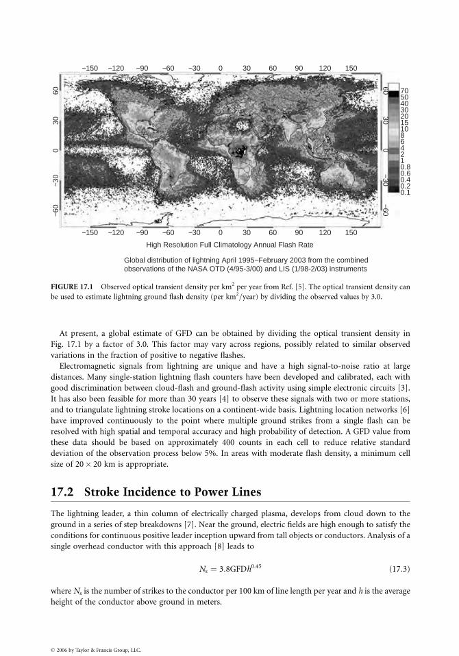
High Resolution Full Climatology Annual Flash Rate
Global distribution of lightning April 1995−February 2003 from the combinedobservations of the NASA OTD (4/95-3/00) and LIS (1/98-2/03) instruments
−150
−60
−30
030
60
6030
−30−60
0
−120 −90 −60 −30 30 60 90 120 150
70504030201510864210.80.60.40.20.1
0
−150 −120 −90 −60 −30 30 60 90 120 1500
FIGURE 17.1 Observed optical transient density per km2 per year from Ref. [5]. The optical transient density can
be used to estimate lightning ground flash density (per km2=year) by dividing the observed values by 3.0.
At present, a global estimate of GFD can be obtained by dividing the optical transient density in
Fig. 17.1 by a factor of 3.0. This factor may vary across regions, possibly related to similar observed
variations in the fraction of positive to negative flashes.
Electromagnetic signals from lightning are unique and have a high signal-to-noise ratio at large
distances. Many single-station lightning flash counters have been developed and calibrated, each with
good discrimination between cloud-flash and ground-flash activity using simple electronic circuits [3].
It has also been feasible for more than 30 years [4] to observe these signals with two or more stations,
and to triangulate lightning stroke locations on a continent-wide basis. Lightning location networks [6]
have improved continuously to the point where multiple ground strikes from a single flash can be
resolved with high spatial and temporal accuracy and high probability of detection. A GFD value from
these data should be based on approximately 400 counts in each cell to reduce relative standard
deviation of the observation process below 5%. In areas with moderate flash density, a minimum cell
size of 20� 20 km is appropriate.
17.2 Stroke Incidence to Power Lines
The lightning leader, a thin column of electrically charged plasma, develops from cloud down to the
ground in a series of step breakdowns [7]. Near the ground, electric fields are high enough to satisfy the
conditions for continuous positive leader inception upward from tall objects or conductors. Analysis of a
single overhead conductor with this approach [8] leads to
Ns ¼ 3:8GFDh0:45 (17:3)
where Ns is the number of strikes to the conductor per 100 km of line length per year and h is the average
height of the conductor above ground in meters.
� 2006 by Taylor & Francis Group, LLC.
In areas of moderate- to high-GFD, one or more overhead shield wires are usually installed above the
phase conductors. This shielding usually has a success rate of greater than 95%, but adds nearly 10% to
the cost of line construction and also wastes energy from induced currents. The leader inception model
[8] has also been used to analyze shielding failures.
17.3 Stroke Current Parameters
Once the downward leader contacts a power system component through an upward-connecting leader,
the stored charge will be impressed through a high-channel impedance of 600 to 2000 V. With this high
source impedance, compared to grounded towers or lines, an impulse current source model is suitable.
Berger made the most reliable direct measurements of negative downward cloud-to-ground lightning
parameters on an instrumented tower from 1947 to 1977 [9]. Additional observations have been
provided by many researchers and then summarized [10,11]. The overall stroke current distribution
can be approximated [11] as lognormal with a mean of 31 kA and a log standard deviation of 0.48. The
waveshape rises with a concave front, giving the maximum steepness near the crest of the wave, and then
decays with a time to half-value of 50 ms or more. The median value of maximum steepness [11] is
24 kA=ms, with a log standard deviation of 0.60. Steepness has a positive correlation to the peak
amplitude [11] that allows simplified modeling using a single equivalent front time (peak current
divided by peak rate of rise). The mean equivalent front is 1.4 ms for the median 31 kA current, rising
to 2.7 ms as peak stroke current increases to the 5% level of 100 kA [11]. An equivalent front time of 2 ms
is recommended for simplified analysis [12].
17.4 Calculation of Lightning Overvoltages on Shielded Lines
The voltage rise VR of the ground resistance R at each tower will be proportional to peak stroke current:
VR¼RI. A relation between the tower base geometry and its resistance is
R ¼ r
2pgln
11:8g2
A
� �
þ r
l(17:4)
where r is the soil resistivity (V m), g is the square root of the sum of the squares of the insulator extent
in each direction (m), A is the surface area (sidesþ base) of the hole needed to excavate the electrode
(m2), and l is the total length (m) of wire in the wire-frame approximation to the electrode (infinite for
solid electrodes).
For large surge currents, local ionization will reduce the second r=l contact resistance term but not the
first geometric resistance term in Eq. (17.4).
The voltage rise VL associated with conductor and tower series inductance L and the equivalent front
time (dt¼ 2 ms) is VL¼ LI=dt. The VL term will add to, and sometimes dominate, VR. Lumped
inductance can be approximated from the expression
L ¼ Zt ¼ 60 ln2h
r
� �
� l
c(17:5)
L is the inductance (H), Z is the element antenna impedance (V), t is the travel time (s), h is the
wire height above conducting ground (m), r is the wire radius (m), l is the wire length (m), and c is
the speed of light (3� 108 m=s).
In numerical analyses, series and shunt impedance elements can be populated using the same
procedure. Tall transmission towers have longer travel times and thus higher inductance, which further
exacerbates the increase of stroke incidence with line height.
� 2006 by Taylor & Francis Group, LLC.
The high electromagnetic fields surrounding any stricken conductor will induce currents and
couple voltages in nearby, unstricken conductors through their mutual surge impedances. In the
case where lightning strikes a grounded overhead shield wire, this coupling increases common-mode
voltage and reduces differential voltage across insulators. Additional shield wires and corona [11,12]
can improve this desirable surge–impedance coupling to mitigate half of the total tower potential rise
(VRþVL).
The strong electromagnetic fields from vertical lightning strokes can induce large overvoltages in
nearby overhead lines without striking them directly. This is a particular concern only for MV and LV
systems.
17.5 Insulation Strength
Power system insulation is designed to withstand all anticipated power system overvoltages. Unfortu-
nately, even the weakest direct stroke from a shielding failure to a phase conductor will cause a lightning
flashover. Once an arc appears across an insulator, the power system fault current keeps this arc alive
until voltage is removed by protective relay action. Effective overhead shielding is essential on trans-
mission lines in areas with moderate- to high-GFD.
When the overhead shield wire is struck, the potential difference on insulators is the sum of the
resistive and inductive voltage rises on the tower, minus the coupled voltage on the phase conductors.
The potential difference can lead to a ‘‘backflashover’’ from the tower to the phase conductor. Back-
flashover is more frequent when the stroke current is large (5%> 100 kA), when insulation strength is
low (<1 m or 600 kV basic impulse level), and=or when footing resistance is high (>30 V). Simplified
models [11,12] are available to carry out the overvoltage calculations and coordinate the results with
insulator strength, giving lightning outage rates, in units of interruptions per 100 km=year.
17.6 Mitigation Methods
Lightning mitigation methods need to be appropriate for the expected long-term GFD and power
system reliability requirements. Table 17.1 summarizes typical practices at five different levels of
lightning activity to achieve a reliability of one outage per 100 km of line per year on an HV line.
17.7 Conclusion
Direct lightning strokes to any overhead transmission line are likely to cause impulse flashover of
supporting insulation, leading to a circuit interruption. The use of overhead shield wires, located
above the phase conductors and grounded adequately at each tower, can reduce the risk of flashover
by 95–99.5%, depending on system voltage.
TABLE 17.1 Lightning Mitigation Methods for Transmission Lines
Ground Flash Density Range Typical Design Approaches
0.1–0.3 Ground flashes=km2 per year Unshielded, one- or three-pole reclosing
0.3–1 Ground flashes=km2 per year Single overhead shield wire
1–3 Ground flashes=km2 per year Two overhead shield wires
3–10 Ground flashes=km2 per year Two overhead shield wires with good grounding or line surge arresters
10–30 Ground flashes=km2 per year Three or more overhead and underbuilt shield wires with good grounding, line
surge arresters; underground transmission cables
� 2006 by Taylor & Francis Group, LLC.

References
1.
� 200
Anderson, R.B., Eriksson, A.J., Kroninger, H., and Meal, D.V., Lightning and thunderstorm para-
meters, IEE conference publication 236, Lightning and Power Systems, London, June 1984.
2.
MacGorman, D.R., Maier, M.W., and Rust, W.D., Lightning Strike Density for the Contiguous UnitedStates from Thunderstorm Duration Records. Report to U.S. Nuclear Regulatory Commission,
NUREG=CR-3759, 1984.
3.
Heydt, G., Instrumentation, in Handbook of Atmospherics, Vol. II, edited by Volland, H., CRC Press,Boca Raton, FL, 1982, pp. 203–256.
4.
Krider, E.P., Noggle, R.C., and Uman, M.A., A gated, wideband direction finder for lightning returnstrokes, Journal of Applied Meteorology, 15, 301, 1976.
5.
Christian, H.J., Blakeslee, R.J., Boccippio, D., Boeck, W., Buechler, D., Driscoll, K., Goodman, Hall, J.,Koshak, W., Mach, D., and Stewart, M., Global frequency and distribution of lightning as observed
from space by the optical transient detector, Journal of Geophysical Research, 108(D1), 4005, 2003 or
http:==thunder.msfc.nasa.gov.
6.
http:==www.vaisala.com=businessareas=measurementsystems=thunderstorm=products=networks7.
Rakov, V.A. and Uman M.A., Lightning: Physics and Effects, Cambridge University Press, Cambridge,2003.
8.
Rizk, F.A.M., Modeling of transmission line exposure to direct lightning strokes, IEEE Transactionson PWRD, 5(4), p. 1983, 1990.
9.
Berger, K., The earth flash, in Lightning, edited by Golde, R., Academic Press, London, 1977,pp. 119–190.
10.
Anderson, R.B. and Eriksson, A.J., Lightning parameters for engineering applications, Electra 69,65–102, 1980.
11.
CIGRE Working Group 01 (Lightning) of Study Committee 33, Guide to Procedures for Estimatingthe Lightning Performance of Transmission Lines, CIGRE Brochure 63, Paris, October 1991.
12.
IEEE Guide for Improving the Lightning Performance of Transmission Lines, IEEE Standard1243–1997, December 1997.
6 by Taylor & Francis Group, LLC.

� 2006 by Taylor & Francis Group, LLC.
18
� 2006 by Taylor & Francis Group, LLC.
Reactive PowerCompensation
Rao S. ThallamSalt River Project
18.1 The Need for Reactive Power Compensation ............... 18-1Shunt Reactive Power Compensation . Shunt Capacitors
18.2 Application of Shunt Capacitor Banks inDistribution Systems—A Utility Perspective ................ 18-2
18.3 Static VAR Control.......................................................... 18-3Description of SVC . How Does SVC Work?
18.4 Series Compensation....................................................... 18-5
18.5 Series Capacitor Bank ..................................................... 18-6Description of Main Components . Subsynchronous
Resonance . Adjustable Series Compensation . Thyristor
Controlled Series Compensation . STATic
COMpensator
18.6 Defining Terms .............................................................. 18-12
18.1 The Need for Reactive Power Compensation
Except in a very few special situations, electrical energy is generated, transmitted, distributed, and
utilized as alternating current (AC). However, alternating current has several distinct disadvantages. One
of these is the necessity of reactive power that needs to be supplied along with active power. Reactive
power can be leading or lagging. While it is the active power that contributes to the energy consumed, or
transmitted, reactive power does not contribute to the energy. Reactive power is an inherent part of the
‘‘total power.’’ Reactive power is either generated or consumed in almost every component of the system,
generation, transmission, and distribution and eventually by the loads. The impedance of a branch of a
circuit in an AC system consists of two components, resistance and reactance. Reactance can be either
inductive or capacitive, which contribute to reactive power in the circuit. Most of the loads are inductive,
and must be supplied with lagging reactive power. It is economical to supply this reactive power closer to
the load in the distribution system.
In this chapter, reactive power compensation, mainly in transmission systems installed at substations,
is discussed. Reactive power compensation in power systems can be either shunt or series. Both will be
discussed.
18.1.1 Shunt Reactive Power Compensation
Since most loads are inductive and consume lagging reactive power, the compensation required
is usually supplied by leading reactive power. Shunt compensation of reactive power can be
employed either at load level, substation level, or at transmission level. It can be capacitive (leading)
or inductive (lagging) reactive power, although in most cases as explained before, compensation is

capacitive. The most common form of leading reactive power compensation is by connecting shunt
capacitors to the line.
18.1.2 Shunt Capacitors
Shunt capacitors are employed at substation level for the following reasons:
1. Voltage regulation: The main reason that shunt capacitors are installed at substations is to control
the voltage within required levels. Load varies over the day, with very low load from midnight to
early morning and peak values occurring in the evening between 4 PM and 7 PM. Shape of the load
curve also varies from weekday to weekend, with weekend load typically low. As the load varies,
voltage at the substation bus and at the load bus varies. Since the load power factor is always
lagging, a shunt connected capacitor bank at the substation can raise voltage when the load is
high. The shunt capacitor banks can be permanently connected to the bus (fixed capacitor bank)
or can be switched as needed. Switching can be based on time, if load variation is predictable, or
can be based on voltage, power factor, or line current.
2. Reducing power losses: Compensating the load lagging power factor with the bus connected
shunt capacitor bank improves the power factor and reduces current flow through the transmission
lines, transformers, generators, etc. This will reduce power losses (I2R losses) in this equipment.
3. Increased utilization of equipment: Shunt compensation with capacitor banks reduces kVA
loading of lines, transformers, and generators, which means with compensation they can be
used for delivering more power without overloading the equipment.
Reactive power compensation in a power system is of two types—shunt and series. Shunt compen-
sation can be installed near the load, in a distribution substation, along the distribution feeder, or in a
transmission substation. Each application has different purposes. Shunt reactive compensation can be
inductive or capacitive. At load level, at the distribution substation, and along the distribution feeder,
compensation is usually capacitive. In a transmission substation, both inductive and capacitve reactive
compensation are installed.
18.2 Application of Shunt Capacitor Banks in DistributionSystems—A Utility Perspective
The Salt River Project (SRP) is a public power utility serving more than 720,000 (April 2000) customers
in central Arizona. Thousands of capacitor banks are installed in the entire distribution system. The
primary usage for capacitor banks in the distribution system is to maintain a certain power factor at
peak loading conditions. The target power factor is .98 leading at system peak. This figure was set as an
attempt to have a unity power factor on the 69-kV side of the substation transformer. The leading power
factor compensates for the industrial substations that have no capacitors. The unity power factor
maintains a balance with ties to other utilities.
The main purpose of the capacitors is not for voltage support, as the case may be at utilities with long
distribution feeders. Most of the feeders in the SRP service area do not have long runs (substations are about
two miles apart) and load tap changers on the substation transformers are used for voltage regulation.
The SRP system is a summer peaking system. After each summer peak, a capacitor study is performed
to determine the capacitor requirements for the next summer. The input to the computer program for
evaluating capacitor additions consists of three major components:
. Megawatts and megavars for each substation transformer at peak.
. A listing of the capacitor banks with size and operating status at time of peak.
. The next summer’s projected loads.
By looking at the present peak MW and Mvars and comparing the results to the projected MW loads,
Mvar deficiencies can be determined. The output of the program is reviewed and a listing of potential
� 2006 by Taylor & Francis Group, LLC.
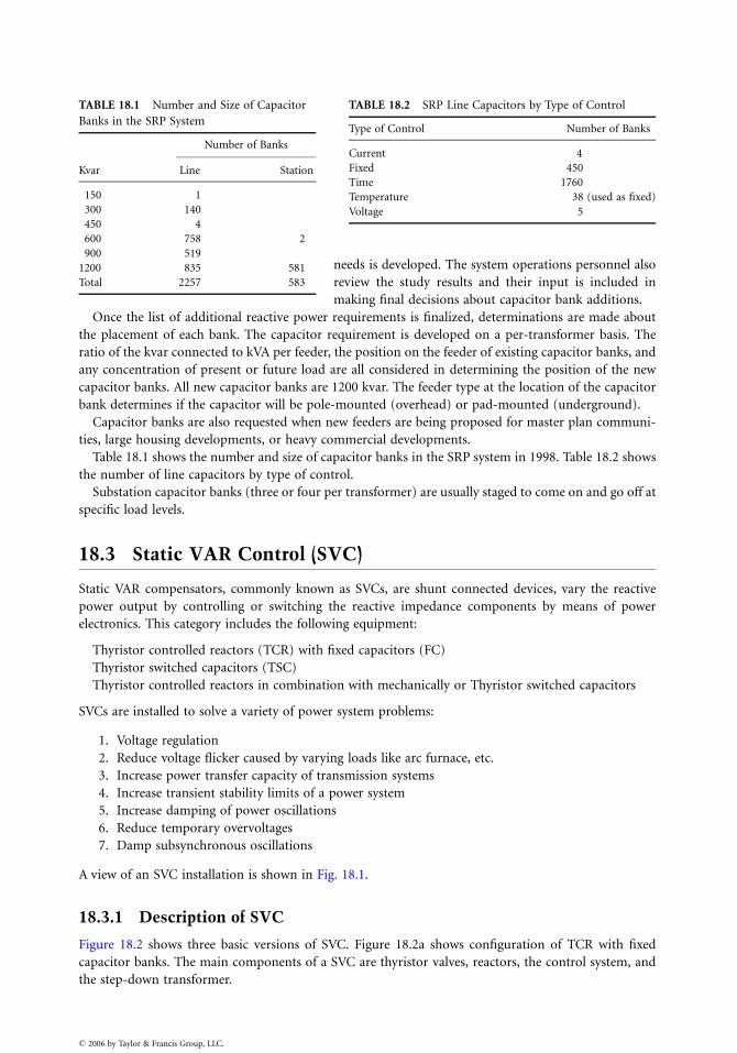
TABLE 18.1 Number and Size of Capacitor
Banks in the SRP System
Number of Banks
Kvar Line Station
150 1
300 140
450 4
600 758 2
900 519
1200 835 581
Total 2257 583
TABLE 18.2 SRP Line Capacitors by Type of Control
Type of Control Number of Banks
Current 4
Fixed 450
Time 1760
Temperature 38 (used as fixed)
Voltage 5
� 2006 by Taylor & Francis Group, LLC.
needs is developed. The system operations personnel also
review the study results and their input is included in
making final decisions about capacitor bank additions.
Once the list of additional reactive power requirements is finalized, determinations are made about
the placement of each bank. The capacitor requirement is developed on a per-transformer basis. The
ratio of the kvar connected to kVA per feeder, the position on the feeder of existing capacitor banks, and
any concentration of present or future load are all considered in determining the position of the new
capacitor banks. All new capacitor banks are 1200 kvar. The feeder type at the location of the capacitor
bank determines if the capacitor will be pole-mounted (overhead) or pad-mounted (underground).
Capacitor banks are also requested when new feeders are being proposed for master plan communi-
ties, large housing developments, or heavy commercial developments.
Table 18.1 shows the number and size of capacitor banks in the SRP system in 1998. Table 18.2 shows
the number of line capacitors by type of control.
Substation capacitor banks (three or four per transformer) are usually staged to come on and go off at
specific load levels.
18.3 Static VAR Control (SVC)
Static VAR compensators, commonly known as SVCs, are shunt connected devices, vary the reactive
power output by controlling or switching the reactive impedance components by means of power
electronics. This category includes the following equipment:
Thyristor controlled reactors (TCR) with fixed capacitors (FC)
Thyristor switched capacitors (TSC)
Thyristor controlled reactors in combination with mechanically or Thyristor switched capacitors
SVCs are installed to solve a variety of power system problems:
1. Voltage regulation
2. Reduce voltage flicker caused by varying loads like arc furnace, etc.
3. Increase power transfer capacity of transmission systems
4. Increase transient stability limits of a power system
5. Increase damping of power oscillations
6. Reduce temporary overvoltages
7. Damp subsynchronous oscillations
A view of an SVC installation is shown in Fig. 18.1.
18.3.1 Description of SVC
Figure 18.2 shows three basic versions of SVC. Figure 18.2a shows configuration of TCR with fixed
capacitor banks. The main components of a SVC are thyristor valves, reactors, the control system, and
the step-down transformer.
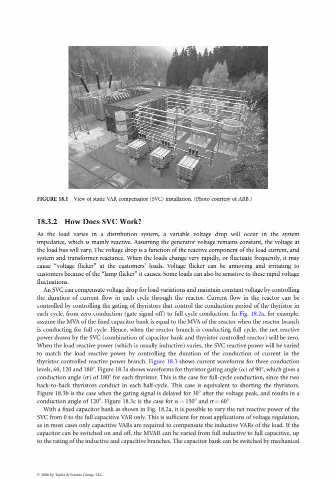
FIGURE 18.1 View of static VAR compensator (SVC) installation. (Photo courtesy of ABB.)
18.3.2 How Does SVC Work?
As the load varies in a distribution system, a variable voltage drop will occur in the system
impedance, which is mainly reactive. Assuming the generator voltage remains constant, the voltage at
the load bus will vary. The voltage drop is a function of the reactive component of the load current, and
system and transformer reactance. When the loads change very rapidly, or fluctuate frequently, it may
cause ‘‘voltage flicker’’ at the customers’ loads. Voltage flicker can be annoying and irritating to
customers because of the ‘‘lamp flicker’’ it causes. Some loads can also be sensitive to these rapid voltage
fluctuations.
An SVC can compensate voltage drop for load variations and maintain constant voltage by controlling
the duration of current flow in each cycle through the reactor. Current flow in the reactor can be
controlled by controlling the gating of thyristors that control the conduction period of the thyristor in
each cycle, from zero conduction (gate signal off) to full-cycle conduction. In Fig. 18.2a, for example,
assume the MVA of the fixed capacitor bank is equal to the MVA of the reactor when the reactor branch
is conducting for full cycle. Hence, when the reactor branch is conducting full cycle, the net reactive
power drawn by the SVC (combination of capacitor bank and thyristor controlled reactor) will be zero.
When the load reactive power (which is usually inductive) varies, the SVC reactive power will be varied
to match the load reactive power by controlling the duration of the conduction of current in the
thyristor controlled reactive power branch. Figure 18.3 shows current waveforms for three conduction
levels, 60, 120 and 1808. Figure 18.3a shows waveforms for thyristor gating angle (a) of 908, which gives a
conduction angle (s) of 1808 for each thyristor. This is the case for full-cycle conduction, since the two
back-to-back thyristors conduct in each half-cycle. This case is equivalent to shorting the thyristors.
Figure 18.3b is the case when the gating signal is delayed for 308 after the voltage peak, and results in a
conduction angle of 1208. Figure 18.3c is the case for a¼ 1508 and s¼ 608
With a fixed capacitor bank as shown in Fig. 18.2a, it is possible to vary the net reactive power of the
SVC from 0 to the full capacitive VAR only. This is sufficient for most applications of voltage regulation,
as in most cases only capacitive VARs are required to compensate the inductive VARs of the load. If the
capacitor can be switched on and off, the MVAR can be varied from full inductive to full capacitive, up
to the rating of the inductive and capacitive branches. The capacitor bank can be switched by mechanical
� 2006 by Taylor & Francis Group, LLC.
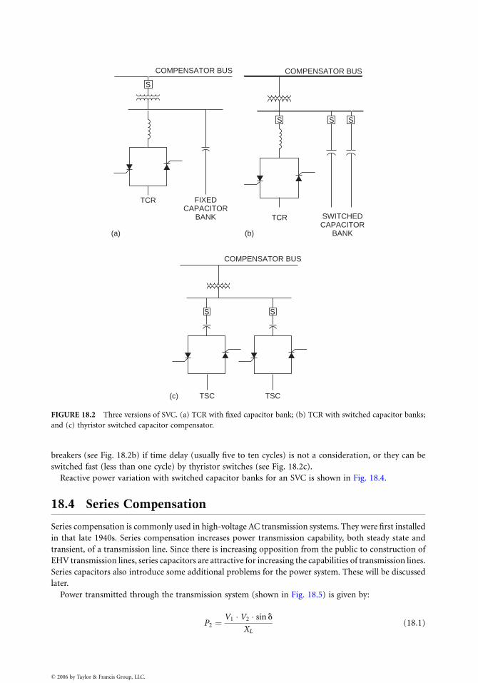
TCR FIXEDCAPACITOR
BANK
S
COMPENSATOR BUS
(a)
COMPENSATOR BUS
S
TCR SWITCHEDCAPACITOR
BANK
S S
(b)
TSC(c) TSC
COMPENSATOR BUS
S S
FIGURE 18.2 Three versions of SVC. (a) TCR with fixed capacitor bank; (b) TCR with switched capacitor banks;
and (c) thyristor switched capacitor compensator.
breakers (see Fig. 18.2b) if time delay (usually five to ten cycles) is not a consideration, or they can be
switched fast (less than one cycle) by thyristor switches (see Fig. 18.2c).
Reactive power variation with switched capacitor banks for an SVC is shown in Fig. 18.4.
18.4 Series Compensation
Series compensation is commonly used in high-voltage AC transmission systems. They were first installed
in that late 1940s. Series compensation increases power transmission capability, both steady state and
transient, of a transmission line. Since there is increasing opposition from the public to construction of
EHV transmission lines, series capacitors are attractive for increasing the capabilities of transmission lines.
Series capacitors also introduce some additional problems for the power system. These will be discussed
later.
Power transmitted through the transmission system (shown in Fig. 18.5) is given by:
P2 ¼V1 � V2 � sin d
XL
(18:1)
� 2006 by Taylor & Francis Group, LLC.
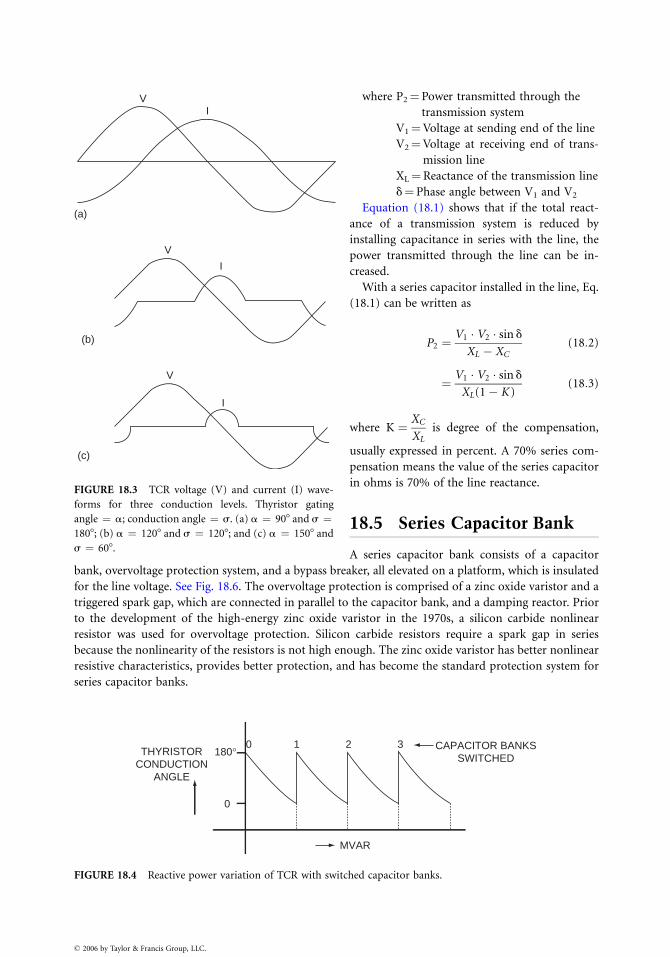
VI
(a)
V
I
(b)
V
I
(c)
FIGURE 18.3 TCR voltage (V) and current (I) wave-
forms for three conduction levels. Thyristor gating
angle ¼ a; conduction angle ¼ s. (a) a ¼ 908 and s ¼1808; (b) a ¼ 1208 and s ¼ 1208; and (c) a ¼ 1508 and
s ¼ 608.
M
THYRISTORCONDUCTION
ANGLE
210
0
180°
FIGURE 18.4 Reactive power variation of TCR with switc
� 2006 by Taylor & Francis Group, LLC.
where P2¼ Power transmitted through the
transmission system
V1¼Voltage at sending end of the line
V2¼Voltage at receiving end of trans-
mission line
XL¼Reactance of the transmission line
d¼Phase angle between V1 and V2
Equation (18.1) shows that if the total react-
ance of a transmission system is reduced by
installing capacitance in series with the line, the
power transmitted through the line can be in-
creased.
With a series capacitor installed in the line, Eq.
(18.1) can be written as
P2 ¼V1 � V2 � sin d
XL � XC
(18:2)
¼ V1 � V2 � sin d
XL(1� K )(18:3)
where K ¼ XC
XL
is degree of the compensation,
usually expressed in percent. A 70% series com-
pensation means the value of the series capacitor
in ohms is 70% of the line reactance.
18.5 Series Capacitor Bank
A series capacitor bank consists of a capacitor
bank, overvoltage protection system, and a bypass breaker, all elevated on a platform, which is insulated
for the line voltage. See Fig. 18.6. The overvoltage protection is comprised of a zinc oxide varistor and a
triggered spark gap, which are connected in parallel to the capacitor bank, and a damping reactor. Prior
to the development of the high-energy zinc oxide varistor in the 1970s, a silicon carbide nonlinear
resistor was used for overvoltage protection. Silicon carbide resistors require a spark gap in series
because the nonlinearity of the resistors is not high enough. The zinc oxide varistor has better nonlinear
resistive characteristics, provides better protection, and has become the standard protection system for
series capacitor banks.
VAR
CAPACITOR BANKSSWITCHED
3
hed capacitor banks.
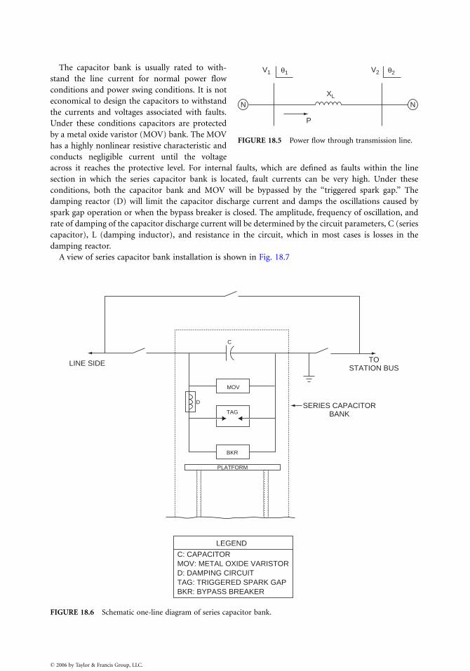
P
N N
XL
V2 θ2θ1V1
FIGURE 18.5 Power flow through transmission line.
The capacitor bank is usually rated to with-
stand the line current for normal power flow
conditions and power swing conditions. It is not
economical to design the capacitors to withstand
the currents and voltages associated with faults.
Under these conditions capacitors are protected
by a metal oxide varistor (MOV) bank. The MOV
has a highly nonlinear resistive characteristic and
conducts negligible current until the voltage
across it reaches the protective level. For internal faults, which are defined as faults within the line
section in which the series capacitor bank is located, fault currents can be very high. Under these
conditions, both the capacitor bank and MOV will be bypassed by the ‘‘triggered spark gap.’’ The
damping reactor (D) will limit the capacitor discharge current and damps the oscillations caused by
spark gap operation or when the bypass breaker is closed. The amplitude, frequency of oscillation, and
rate of damping of the capacitor discharge current will be determined by the circuit parameters, C (series
capacitor), L (damping inductor), and resistance in the circuit, which in most cases is losses in the
damping reactor.
A view of series capacitor bank installation is shown in Fig. 18.7
LINE SIDE
MOV
D
C
TAG
PLATFORM
LEGEND
C: CAPACITORMOV: METAL OXIDE VARISTORD: DAMPING CIRCUITTAG: TRIGGERED SPARK GAP BKR: BYPASS BREAKER
TOSTATION BUS
SERIES CAPACITORBANK
BKR
FIGURE 18.6 Schematic one-line diagram of series capacitor bank.
� 2006 by Taylor & Francis Group, LLC.
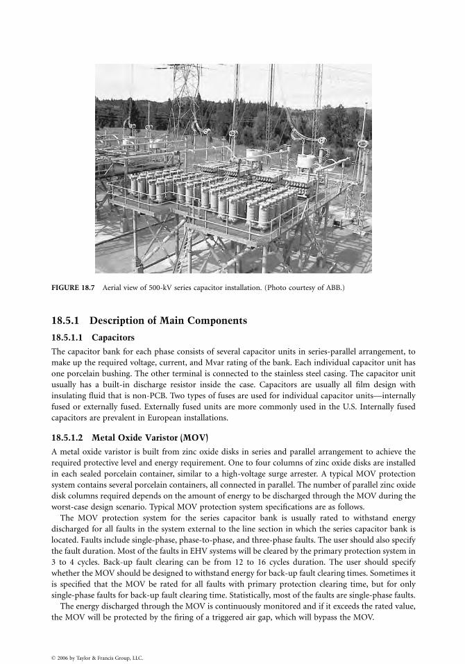
FIGURE 18.7 Aerial view of 500-kV series capacitor installation. (Photo courtesy of ABB.)
18.5.1 Description of Main Components
18.5.1.1 Capacitors
The capacitor bank for each phase consists of several capacitor units in series-parallel arrangement, to
make up the required voltage, current, and Mvar rating of the bank. Each individual capacitor unit has
one porcelain bushing. The other terminal is connected to the stainless steel casing. The capacitor unit
usually has a built-in discharge resistor inside the case. Capacitors are usually all film design with
insulating fluid that is non-PCB. Two types of fuses are used for individual capacitor units—internally
fused or externally fused. Externally fused units are more commonly used in the U.S. Internally fused
capacitors are prevalent in European installations.
18.5.1.2 Metal Oxide Varistor (MOV)
A metal oxide varistor is built from zinc oxide disks in series and parallel arrangement to achieve the
required protective level and energy requirement. One to four columns of zinc oxide disks are installed
in each sealed porcelain container, similar to a high-voltage surge arrester. A typical MOV protection
system contains several porcelain containers, all connected in parallel. The number of parallel zinc oxide
disk columns required depends on the amount of energy to be discharged through the MOV during the
worst-case design scenario. Typical MOV protection system specifications are as follows.
The MOV protection system for the series capacitor bank is usually rated to withstand energy
discharged for all faults in the system external to the line section in which the series capacitor bank is
located. Faults include single-phase, phase-to-phase, and three-phase faults. The user should also specify
the fault duration. Most of the faults in EHV systems will be cleared by the primary protection system in
3 to 4 cycles. Back-up fault clearing can be from 12 to 16 cycles duration. The user should specify
whether the MOV should be designed to withstand energy for back-up fault clearing times. Sometimes it
is specified that the MOV be rated for all faults with primary protection clearing time, but for only
single-phase faults for back-up fault clearing time. Statistically, most of the faults are single-phase faults.
The energy discharged through the MOV is continuously monitored and if it exceeds the rated value,
the MOV will be protected by the firing of a triggered air gap, which will bypass the MOV.
� 2006 by Taylor & Francis Group, LLC.
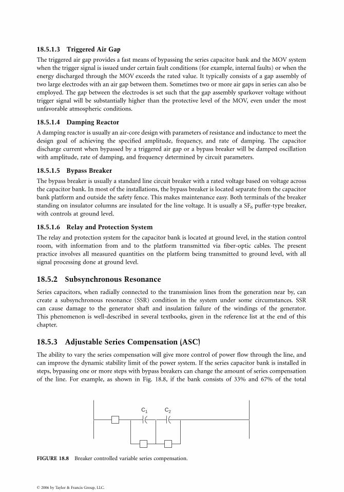
18.5.1.3 Triggered Air Gap
The triggered air gap provides a fast means of bypassing the series capacitor bank and the MOV system
when the trigger signal is issued under certain fault conditions (for example, internal faults) or when the
energy discharged through the MOV exceeds the rated value. It typically consists of a gap assembly of
two large electrodes with an air gap between them. Sometimes two or more air gaps in series can also be
employed. The gap between the electrodes is set such that the gap assembly sparkover voltage without
trigger signal will be substantially higher than the protective level of the MOV, even under the most
unfavorable atmospheric conditions.
18.5.1.4 Damping Reactor
A damping reactor is usually an air-core design with parameters of resistance and inductance to meet the
design goal of achieving the specified amplitude, frequency, and rate of damping. The capacitor
discharge current when bypassed by a triggered air gap or a bypass breaker will be damped oscillation
with amplitude, rate of damping, and frequency determined by circuit parameters.
18.5.1.5 Bypass Breaker
The bypass breaker is usually a standard line circuit breaker with a rated voltage based on voltage across
the capacitor bank. In most of the installations, the bypass breaker is located separate from the capacitor
bank platform and outside the safety fence. This makes maintenance easy. Both terminals of the breaker
standing on insulator columns are insulated for the line voltage. It is usually a SF6 puffer-type breaker,
with controls at ground level.
18.5.1.6 Relay and Protection System
The relay and protection system for the capacitor bank is located at ground level, in the station control
room, with information from and to the platform transmitted via fiber-optic cables. The present
practice involves all measured quantities on the platform being transmitted to ground level, with all
signal processing done at ground level.
18.5.2 Subsynchronous Resonance
Series capacitors, when radially connected to the transmission lines from the generation near by, can
create a subsynchronous resonance (SSR) condition in the system under some circumstances. SSR
can cause damage to the generator shaft and insulation failure of the windings of the generator.
This phenomenon is well-described in several textbooks, given in the reference list at the end of this
chapter.
18.5.3 Adjustable Series Compensation (ASC)
The ability to vary the series compensation will give more control of power flow through the line, and
can improve the dynamic stability limit of the power system. If the series capacitor bank is installed in
steps, bypassing one or more steps with bypass breakers can change the amount of series compensation
of the line. For example, as shown in Fig. 18.8, if the bank consists of 33% and 67% of the total
C1 C2
FIGURE 18.8 Breaker controlled variable series compensation.
� 2006 by Taylor & Francis Group, LLC.
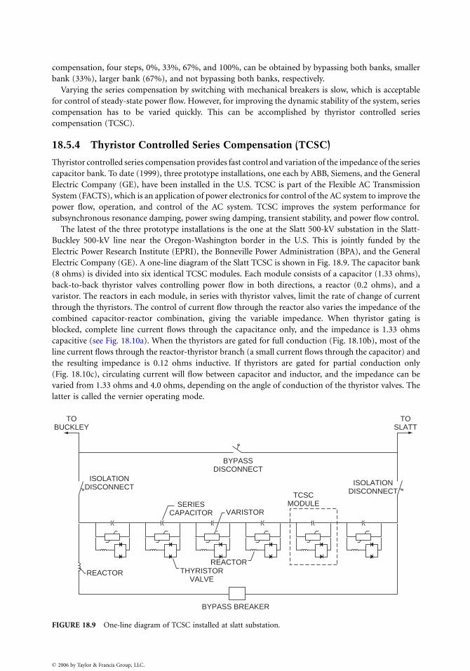
compensation, four steps, 0%, 33%, 67%, and 100%, can be obtained by bypassing both banks, smaller
bank (33%), larger bank (67%), and not bypassing both banks, respectively.
Varying the series compensation by switching with mechanical breakers is slow, which is acceptable
for control of steady-state power flow. However, for improving the dynamic stability of the system, series
compensation has to be varied quickly. This can be accomplished by thyristor controlled series
compensation (TCSC).
18.5.4 Thyristor Controlled Series Compensation (TCSC)
Thyristor controlled series compensation provides fast control and variation of the impedance of the series
capacitor bank. To date (1999), three prototype installations, one each by ABB, Siemens, and the General
Electric Company (GE), have been installed in the U.S. TCSC is part of the Flexible AC Transmission
System (FACTS), which is an application of power electronics for control of the AC system to improve the
power flow, operation, and control of the AC system. TCSC improves the system performance for
subsynchronous resonance damping, power swing damping, transient stability, and power flow control.
The latest of the three prototype installations is the one at the Slatt 500-kV substation in the Slatt-
Buckley 500-kV line near the Oregon-Washington border in the U.S. This is jointly funded by the
Electric Power Research Institute (EPRI), the Bonneville Power Administration (BPA), and the General
Electric Company (GE). A one-line diagram of the Slatt TCSC is shown in Fig. 18.9. The capacitor bank
(8 ohms) is divided into six identical TCSC modules. Each module consists of a capacitor (1.33 ohms),
back-to-back thyristor valves controlling power flow in both directions, a reactor (0.2 ohms), and a
varistor. The reactors in each module, in series with thyristor valves, limit the rate of change of current
through the thyristors. The control of current flow through the reactor also varies the impedance of the
combined capacitor-reactor combination, giving the variable impedance. When thyristor gating is
blocked, complete line current flows through the capacitance only, and the impedance is 1.33 ohms
capacitive (see Fig. 18.10a). When the thyristors are gated for full conduction (Fig. 18.10b), most of the
line current flows through the reactor-thyristor branch (a small current flows through the capacitor) and
the resulting impedance is 0.12 ohms inductive. If thyristors are gated for partial conduction only
(Fig. 18.10c), circulating current will flow between capacitor and inductor, and the impedance can be
varied from 1.33 ohms and 4.0 ohms, depending on the angle of conduction of the thyristor valves. The
latter is called the vernier operating mode.
BYPASS BREAKER
THYRISTORVALVE
SERIESCAPACITOR
ISOLATIONDISCONNECT
TOBUCKLEY
TOSLATT
BYPASSDISCONNECT
TCSCMODULE
ISOLATIONDISCONNECT
REACTORREACTOR
VARISTOR
FIGURE 18.9 One-line diagram of TCSC installed at slatt substation.
� 2006 by Taylor & Francis Group, LLC.
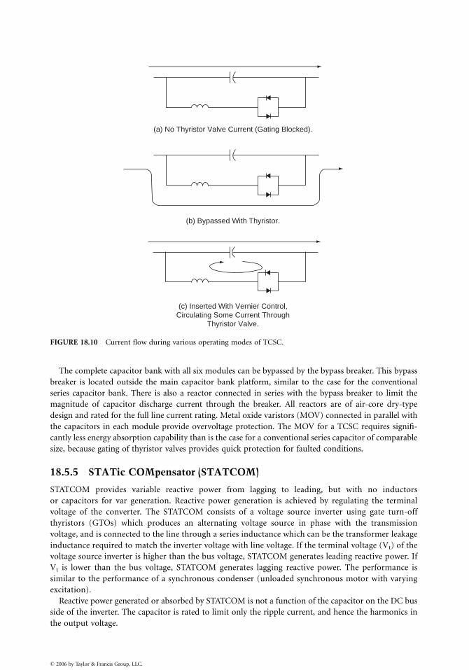
(a) No Thyristor Valve Current (Gating Blocked).
(b) Bypassed With Thyristor.
(c) Inserted With Vernier Control,Circulating Some Current Through
Thyristor Valve.
FIGURE 18.10 Current flow during various operating modes of TCSC.
The complete capacitor bank with all six modules can be bypassed by the bypass breaker. This bypass
breaker is located outside the main capacitor bank platform, similar to the case for the conventional
series capacitor bank. There is also a reactor connected in series with the bypass breaker to limit the
magnitude of capacitor discharge current through the breaker. All reactors are of air-core dry-type
design and rated for the full line current rating. Metal oxide varistors (MOV) connected in parallel with
the capacitors in each module provide overvoltage protection. The MOV for a TCSC requires signifi-
cantly less energy absorption capability than is the case for a conventional series capacitor of comparable
size, because gating of thyristor valves provides quick protection for faulted conditions.
18.5.5 STATic COMpensator (STATCOM)
STATCOM provides variable reactive power from lagging to leading, but with no inductors
or capacitors for var generation. Reactive power generation is achieved by regulating the terminal
voltage of the converter. The STATCOM consists of a voltage source inverter using gate turn-off
thyristors (GTOs) which produces an alternating voltage source in phase with the transmission
voltage, and is connected to the line through a series inductance which can be the transformer leakage
inductance required to match the inverter voltage with line voltage. If the terminal voltage (Vt) of the
voltage source inverter is higher than the bus voltage, STATCOM generates leading reactive power. If
Vt is lower than the bus voltage, STATCOM generates lagging reactive power. The performance is
similar to the performance of a synchronous condenser (unloaded synchronous motor with varying
excitation).
Reactive power generated or absorbed by STATCOM is not a function of the capacitor on the DC bus
side of the inverter. The capacitor is rated to limit only the ripple current, and hence the harmonics in
the output voltage.
� 2006 by Taylor & Francis Group, LLC.

The first demonstration STATCOM of +100 Mvar rating was installed at the Tennessee Valley
Authority’s Sullivan substation in 1994.
18.6 Defining Terms
Shunt capacitor bank—A large number of capacitor units connected in series and parallel arrangement
to make up the required voltage and current rating, and connected between the high-voltage line and
ground, between line and neutral, or between line-to-line.
Voltage flicker—Commonly known as ‘‘flicker’’ and ‘‘lamp flicker,’’ this is a rapid and frequent
fluctuation of supply voltage that causes lamps to flicker. Lamp flicker can be annoying, and some
loads are sensitive to these frequent voltage fluctuations.
Subsynchronous resonance—Per IEEE, subsynchronous resonance is an electric power system condi-
tion where the electric network exchanges energy with a turbine generator at one or more of the
natural frequencies of the combined system below the synchronous frequency of the system.
References
Anderson, P.M., Agrawal, B.L., and Van Ness, J.E., Subsynchronous Resonance in Power Systems, IEEE
Press, 1990.
Anderson, P.M. and Farmer, R.G., Series Compensation in Power Systems, PBLSH! Inc. 1996.
Gyugyi, L., Otto, R.A., and Putman, T.H., Principles and application of thyristor-controlled shunt
compensators, IEEE Trans. on Power Appar. and Syst., 97, 1935–1945, Sept=Oct 1978.
Gyugyi, L. and Taylor, Jr., E.R., Characteristics of static thyristor-controlled shunt compensators for
power transmission applications, IEEE Trans. on Power Appar. and Syst., PAS-99, 1795–1804, 1980.
Hammad, A.E., Analysis of power system stability enhancement by static VAR compensators, IEEE
Trans. on Power Syst., 1, 222–227, 1986.
Miller, T.J.E., Ed., Reactive Power Control in Electric Systems, John Wiley & Sons, New York, 1982.
Miske, Jr., S.A. et al., Recent Series Capacitor Applications in North America, Paper presented at CEA
Electricity ’95 Vancouver Conference, March 1995.
Padiyar, K.R., Analysis of Subsynchronous Resonance in Power Systems, Kluwer Academic Publishers, 1999.
Schauder, C. et al., Development of a +100 MVAR static condenser for voltage control of transmission
systems, IEEE Trans. on Power Delivery, 10(3), 1486–1496, July 1995.
� 2006 by Taylor & Francis Group, LLC.
19
� 2006 by Taylor & Francis Group, LLC.
Environmental Impactof Transmission Lines
George G. KaradyArizona State University
19.1 Introduction..................................................................... 19-1
19.2 Aesthetical Effects of Lines ............................................. 19-2
19.3 Magnetic Field Generated by HV Lines ........................ 19-4Magnetic Field Calculation . Health Effect of Magnetic Field
19.4 Electrical Field Generated by HV Lines ........................ 19-8Electric Charge Calculation . Electric Field Calculation .
Environmental Effect of Electric Field
19.5 Audible Noise ................................................................ 19-13
19.6 Electromagnetic Interference........................................ 19-14
19.1 Introduction
The appearance of the first transmission lines more than one hundred years ago immediately started
discussion and public concerns. When the first transmission line was built, more electrocutions occurred
because of people climbing up the towers, flying kites, and touching wet conducting ropes. As the public
became aware of the danger of electrocution, the aesthetical effect of the transmission lines generated
pubic discussion. In fact, there is a story of Frank Lloyd Wright, the famous architect, calling President
Roosevelt and demanding the removal of high-voltage lines obstructing his view in Scottsdale, Arizona.
Undoubtedly, a transmission line corridor with several lines would disturb the appearance of a quite
green valley.
The rapid increase of radio and television transmission has produced the occurrence of electromagnetic
interference (EMI) problems. The high voltage on the transmission line produces corona discharge that
generates electromagnetic waves. These waves disturb the radio and television reception, which resulted in
public protests and opposition to build lines too near towns.
In the 1960s, the electrical field surrounding the high-voltage lines became subject to public concerns.
The electrical field can produce minor sparks and small electric shocks under a high-voltage line. An
example of this would be, if a woman were to walk under a line holding an umbrella, the woman would
feel the electric shocks produced by these small discharges.
In the 1970s, the transmission line current produced magnetic fields and became a public issue.
Several newspaper articles discussed the adverse health effects of magnetic fields. This generated
intensive research all over the world. The major concern is that exposure to magnetic fields caused
cancer, mostly leukemia. The U.S. government report concluded that there was no evidence that
moderate 60 Hz magnetic field caused cancer. However, this opinion is not shared by all.
This chapter will discuss the listed environmental effects of transmission lines.
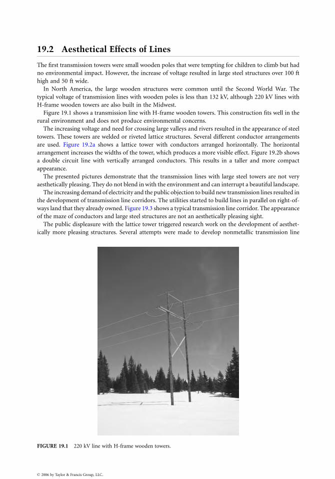
19.2 Aesthetical Effects of Lines
The first transmission towers were small wooden poles that were tempting for children to climb but had
no environmental impact. However, the increase of voltage resulted in large steel structures over 100 ft
high and 50 ft wide.
In North America, the large wooden structures were common until the Second World War. The
typical voltage of transmission lines with wooden poles is less than 132 kV, although 220 kV lines with
H-frame wooden towers are also built in the Midwest.
Figure 19.1 shows a transmission line with H-frame wooden towers. This construction fits well in the
rural environment and does not produce environmental concerns.
The increasing voltage and need for crossing large valleys and rivers resulted in the appearance of steel
towers. These towers are welded or riveted lattice structures. Several different conductor arrangements
are used. Figure 19.2a shows a lattice tower with conductors arranged horizontally. The horizontal
arrangement increases the widths of the tower, which produces a more visible effect. Figure 19.2b shows
a double circuit line with vertically arranged conductors. This results in a taller and more compact
appearance.
The presented pictures demonstrate that the transmission lines with large steel towers are not very
aesthetically pleasing. They do not blend in with the environment and can interrupt a beautiful landscape.
The increasing demand of electricity and the public objection to build new transmission lines resulted in
the development of transmission line corridors. The utilities started to build lines in parallel on right-of-
ways land that they already owned. Figure 19.3 shows a typical transmission line corridor. The appearance
of the maze of conductors and large steel structures are not an aesthetically pleasing sight.
The public displeasure with the lattice tower triggered research work on the development of aesthet-
ically more pleasing structures. Several attempts were made to develop nonmetallic transmission line
FIGURE 19.1 220 kV line with H-frame wooden towers.
� 2006 by Taylor & Francis Group, LLC.
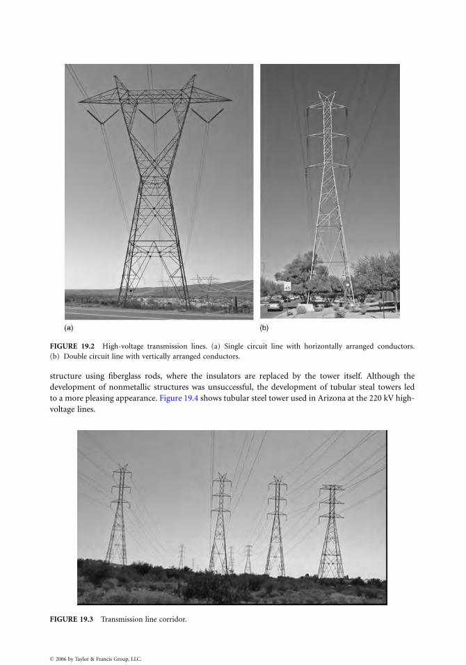
FIGURE 19.2 High-voltage transmission lines. (a) Single circuit line with horizontally arranged conductors.
(b) Double circuit line with vertically arranged conductors.
structure using fiberglass rods, where the insulators are replaced by the tower itself. Although the
development of nonmetallic structures was unsuccessful, the development of tubular steal towers led
to a more pleasing appearance. Figure 19.4 shows tubular steel tower used in Arizona at the 220 kV high-
voltage lines.
FIGURE 19.3 Transmission line corridor.
� 2006 by Taylor & Francis Group, LLC.

FIGURE 19.4 A 220 kV suspension tower.
Figure 19.4 demonstrates that the slender tubular structure is less disturbing and aesthetically more
pleasing. These towers blend in better with the desert environment and cause less visual interruptions.
The presented examples prove that the aesthetical appearance of the transmission lines is improving
although even the best tower structures disturb the environment. The ultimate solution is the replace-
ment of the lines by an underground cable system. Unfortunately, both technical and economic
problems are preventing the use of underground energy transmission systems.
19.3 Magnetic Field Generated by HV Lines
Several newspaper articles presented survey results showing that the exposure to magnetic fields
increases the cancer occurrence. Studies linked the childhood leukemia to transmission line generated
magnetic field exposure. This triggered research in both biological and electrical engineering fields. The
biological research studied the magnetic field effect on cells and performed statistical studies to
determine the correlation between field exposure and cancer occurrence. The electrical engineering
research aimed the determination of magnetic field strength near to transmission lines, electric equip-
ment, motors, and appliances. A related engineering problem is the reduction of magnetic field
generated by lines and other devices.
� 2006 by Taylor & Francis Group, LLC.
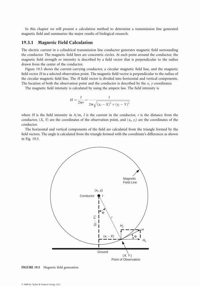
In this chapter we will present a calculation method to determine a transmission line generated
magnetic field and summarize the major results of biological research.
19.3.1 Magnetic Field Calculation
The electric current in a cylindrical transmission line conductor generates magnetic field surrounding
the conductor. The magnetic field lines are concentric circles. At each point around the conductor, the
magnetic field strength or intensity is described by a field vector that is perpendicular to the radius
drawn from the center of the conductor.
Figure 19.5 shows the current-carrying conductor, a circular magnetic field line, and the magnetic
field vector H in a selected observation point. The magnetic field vector is perpendicular to the radius of
the circular magnetic field line. The H field vector is divided into horizontal and vertical components.
The location of both the observation point and the conductor is described by the x , y coordinates.
The magnetic field intensity is calculated by using the ampere law. The field intensity is
H ¼ I
2pr¼ I
2p
ffiffiffiffiffiffiffiffiffiffiffiffiffiffiffiffiffiffiffiffiffiffiffiffiffiffiffiffiffiffiffiffiffiffiffiffiffiffiffiffiffiffi
xi � Xð Þ2þ (yi � Y )2q
where H is the field intensity in A=m, I is the current in the conductor, r is the distance from the
conductor, (X, Y) are the coordinates of the observation point, and (xi, yi) are the coordinates of the
conductor.
The horizontal and vertical components of the field are calculated from the triangle formed by the
field vectors. The angle is calculated from the triangle formed with the coordinate’s differences as shown
in Fig. 19.5.
Conductor
(xi, yi)
Magnetic Field Line
I
Ground
Hx
HyH
r
(xi − X )
(yi −
Y )
Φ
Φ
Point of Observation(X, Y )
FIGURE 19.5 Magnetic field generation.
� 2006 by Taylor & Francis Group, LLC.
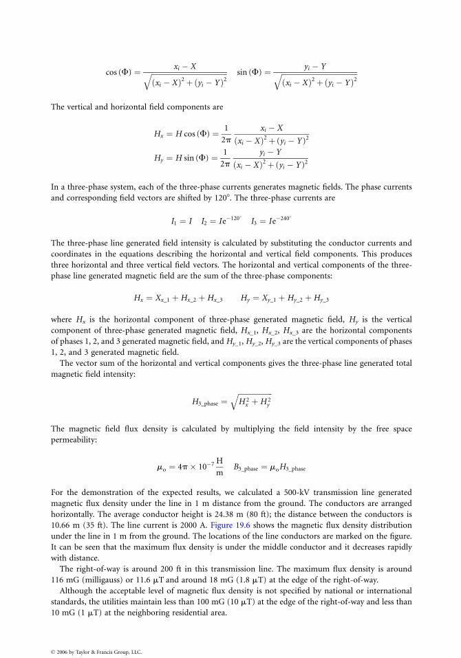
cos (F) ¼ xi � Xffiffiffiffiffiffiffiffiffiffiffiffiffiffiffiffiffiffiffiffiffiffiffiffiffiffiffiffiffiffiffiffiffiffiffiffiffiffiffiffiffiffi
xi � Xð Þ2þ yi � Yð Þ2q sin (F) ¼ yi � Y
ffiffiffiffiffiffiffiffiffiffiffiffiffiffiffiffiffiffiffiffiffiffiffiffiffiffiffiffiffiffiffiffiffiffiffiffiffiffiffiffiffiffi
xi � Xð Þ2þ yi � Yð Þ2q
The vertical and horizontal field components are
Hx ¼ H cos (F) ¼ 1
2p
xi � X
xi � Xð Þ2þ (yi � Y )2
Hy ¼ H sin (F) ¼ 1
2p
yi � Y
xi � Xð Þ2þ (yi � Y )2
In a three-phase system, each of the three-phase currents generates magnetic fields. The phase currents
and corresponding field vectors are shifted by 1208. The three-phase currents are
I1 ¼ I I2 ¼ Ie�1208 I3 ¼ Ie�2408
The three-phase line generated field intensity is calculated by substituting the conductor currents and
coordinates in the equations describing the horizontal and vertical field components. This produces
three horizontal and three vertical field vectors. The horizontal and vertical components of the three-
phase line generated magnetic field are the sum of the three-phase components:
Hx ¼ Xx_1 þHx_2 þHx_3 Hy ¼ Xy_1 þHy_2 þHy_3
where Hx is the horizontal component of three-phase generated magnetic field, Hy is the vertical
component of three-phase generated magnetic field, Hx_1, Hx_2, Hx_3 are the horizontal components
of phases 1, 2, and 3 generated magnetic field, and Hy_1, Hy_2, Hy_3 are the vertical components of phases
1, 2, and 3 generated magnetic field.
The vector sum of the horizontal and vertical components gives the three-phase line generated total
magnetic field intensity:
H3_phase ¼ffiffiffiffiffiffiffiffiffiffiffiffiffiffiffiffiffiffiffi
H 2x þH 2
y
q
The magnetic field flux density is calculated by multiplying the field intensity by the free space
permeability:
mo ¼ 4p� 10�7 H
mB3_phase ¼ moH3_phase
For the demonstration of the expected results, we calculated a 500-kV transmission line generated
magnetic flux density under the line in 1 m distance from the ground. The conductors are arranged
horizontally. The average conductor height is 24.38 m (80 ft); the distance between the conductors is
10.66 m (35 ft). The line current is 2000 A. Figure 19.6 shows the magnetic flux density distribution
under the line in 1 m from the ground. The locations of the line conductors are marked on the figure.
It can be seen that the maximum flux density is under the middle conductor and it decreases rapidly
with distance.
The right-of-way is around 200 ft in this transmission line. The maximum flux density is around
116 mG (milligauss) or 11.6 mT and around 18 mG (1.8 mT) at the edge of the right-of-way.
Although the acceptable level of magnetic flux density is not specified by national or international
standards, the utilities maintain less than 100 mG (10 mT) at the edge of the right-of-way and less than
10 mG (1 mT) at the neighboring residential area.
� 2006 by Taylor & Francis Group, LLC.

−300 300−240 240−180 180−120 120−60 600
10
20
30
40
50
60
70
80
90
100
110
120
Distance in ft
Mag
netic
Flu
x D
ensi
ty in
mG
0
Transmission Line Conductors
FIGURE 19.6 Magnetic field density under a 500-kV line when the load current is 2000 A.
19.3.2 Health Effect of Magnetic Field
The health effects of magnetic fields are a controversial subject, which generated an emotional discus-
sion. The first study that linked the occurrence of childhood leukemia to electrical current generated
magnetic fields was published in 1979 by Wertheimer and Leeper [1]. This was a statistical study where
the electric wiring configuration near the house of the victim was related to the occurrence of childhood
cancer. The researchers compared the wiring of the configuration including transmission lines close to
the childhood leukemia victim’s house and close to the house of a controlled population group. The
study found a correlation between the occurrence of cancer and the power lines carrying high current.
The study was dismissed because of inconsistencies and repeated in 1988 by Savitz et al. [2]. They
measured the magnetic field in the victim’s house and used the electric wiring configuration. The study
found a modest statistical correlation between the cancer and wiring code but not between the cancer
and the measured magnetic field. These findings initiated worldwide research on magnetic field health
effects. The studies can be divided into three major categories:
. Epidemiological studies
. Laboratory studies
. Exposure assessment studies
Epidemiological studies: These statistical studies connect the exposure to magnetic and electric fields to
health effects, particularly to occurrence of cancer. The early studies investigated the childhood cancer
occurrence and residential wiring [1–3]. This was followed by studies relating the occupation (electrical
worker) to cancer occurrence. In this category, the most famous one is a Swedish study [4], which found
elevated risk for lymphoma among electric workers. However, other studies found no elevated cancer
risk [5]. The uncertainty in all of these studies is the assessment of actual exposure to electromagnetic
fields. As an example, some of the studies estimated the exposure to magnetic field using the job title of the
worker or the postal code where the worker lived. The results of these studies are inconclusive, some of
the studies showed elevated risk to cancer, most of them not.
Laboratory studies: These studies are divided into two categories: tissue studies and live animal studies.
The tissue studies investigated the effect of electric and magnetic field on animal tissues. The studies
showed that the electromagnetic field could cause chromosomal changes, single strand breaks, or
alteration of ornithine decarboxylase, etc. [6,7]. Some of the studies speculate that the electromagnetic
� 2006 by Taylor & Francis Group, LLC.
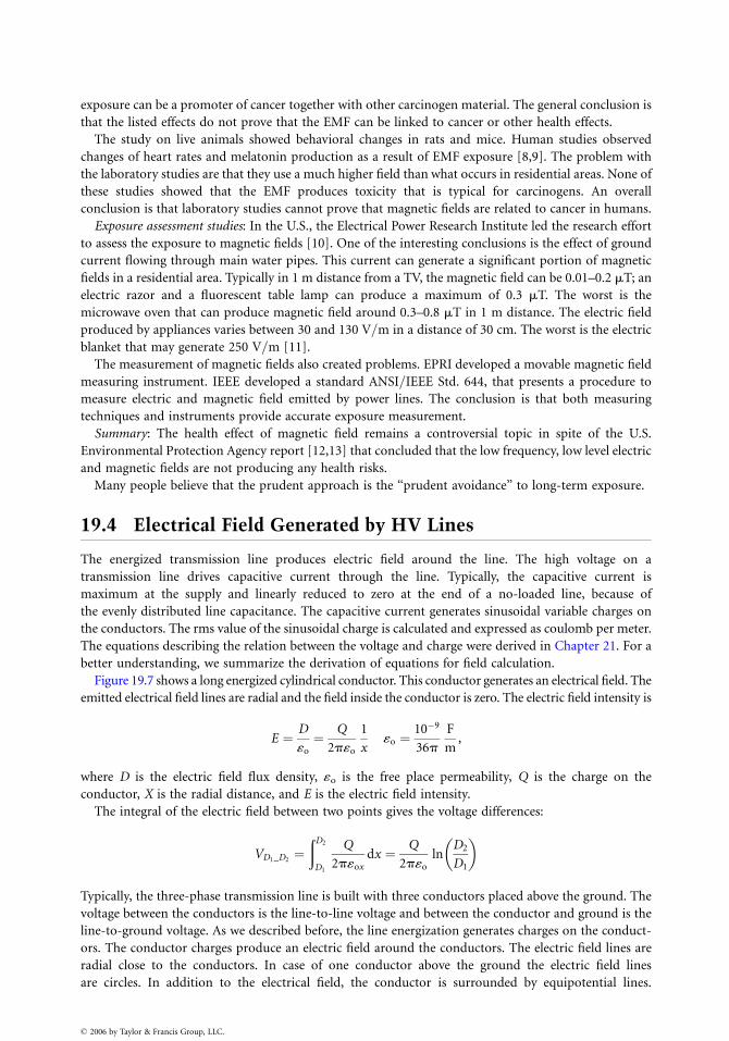
exposure can be a promoter of cancer together with other carcinogen material. The general conclusion is
that the listed effects do not prove that the EMF can be linked to cancer or other health effects.
The study on live animals showed behavioral changes in rats and mice. Human studies observed
changes of heart rates and melatonin production as a result of EMF exposure [8,9]. The problem with
the laboratory studies are that they use a much higher field than what occurs in residential areas. None of
these studies showed that the EMF produces toxicity that is typical for carcinogens. An overall
conclusion is that laboratory studies cannot prove that magnetic fields are related to cancer in humans.
Exposure assessment studies: In the U.S., the Electrical Power Research Institute led the research effort
to assess the exposure to magnetic fields [10]. One of the interesting conclusions is the effect of ground
current flowing through main water pipes. This current can generate a significant portion of magnetic
fields in a residential area. Typically in 1 m distance from a TV, the magnetic field can be 0.01–0.2 mT; an
electric razor and a fluorescent table lamp can produce a maximum of 0.3 mT. The worst is the
microwave oven that can produce magnetic field around 0.3–0.8 mT in 1 m distance. The electric field
produced by appliances varies between 30 and 130 V=m in a distance of 30 cm. The worst is the electric
blanket that may generate 250 V=m [11].
The measurement of magnetic fields also created problems. EPRI developed a movable magnetic field
measuring instrument. IEEE developed a standard ANSI=IEEE Std. 644, that presents a procedure to
measure electric and magnetic field emitted by power lines. The conclusion is that both measuring
techniques and instruments provide accurate exposure measurement.
Summary: The health effect of magnetic field remains a controversial topic in spite of the U.S.
Environmental Protection Agency report [12,13] that concluded that the low frequency, low level electric
and magnetic fields are not producing any health risks.
Many people believe that the prudent approach is the ‘‘prudent avoidance’’ to long-term exposure.
19.4 Electrical Field Generated by HV Lines
The energized transmission line produces electric field around the line. The high voltage on a
transmission line drives capacitive current through the line. Typically, the capacitive current is
maximum at the supply and linearly reduced to zero at the end of a no-loaded line, because of
the evenly distributed line capacitance. The capacitive current generates sinusoidal variable charges on
the conductors. The rms value of the sinusoidal charge is calculated and expressed as coulomb per meter.
The equations describing the relation between the voltage and charge were derived in Chapter 21. For a
better understanding, we summarize the derivation of equations for field calculation.
Figure 19.7 shows a long energized cylindrical conductor. This conductor generates an electrical field. The
emitted electrical field lines are radial and the field inside the conductor is zero. The electric field intensity is
E ¼ D
«o
¼ Q
2p«o
1
x«o ¼
10�9
36p
F
m,
where D is the electric field flux density, «o is the free place permeability, Q is the charge on the
conductor, X is the radial distance, and E is the electric field intensity.
The integral of the electric field between two points gives the voltage differences:
VD1_D2¼ðD2
D1
Q
2p«ox
dx ¼ Q
2p«o
lnD2
D1
� �
Typically, the three-phase transmission line is built with three conductors placed above the ground. The
voltage between the conductors is the line-to-line voltage and between the conductor and ground is the
line-to-ground voltage. As we described before, the line energization generates charges on the conduct-
ors. The conductor charges produce an electric field around the conductors. The electric field lines are
radial close to the conductors. In case of one conductor above the ground the electric field lines
are circles. In addition to the electrical field, the conductor is surrounded by equipotential lines.
� 2006 by Taylor & Francis Group, LLC.
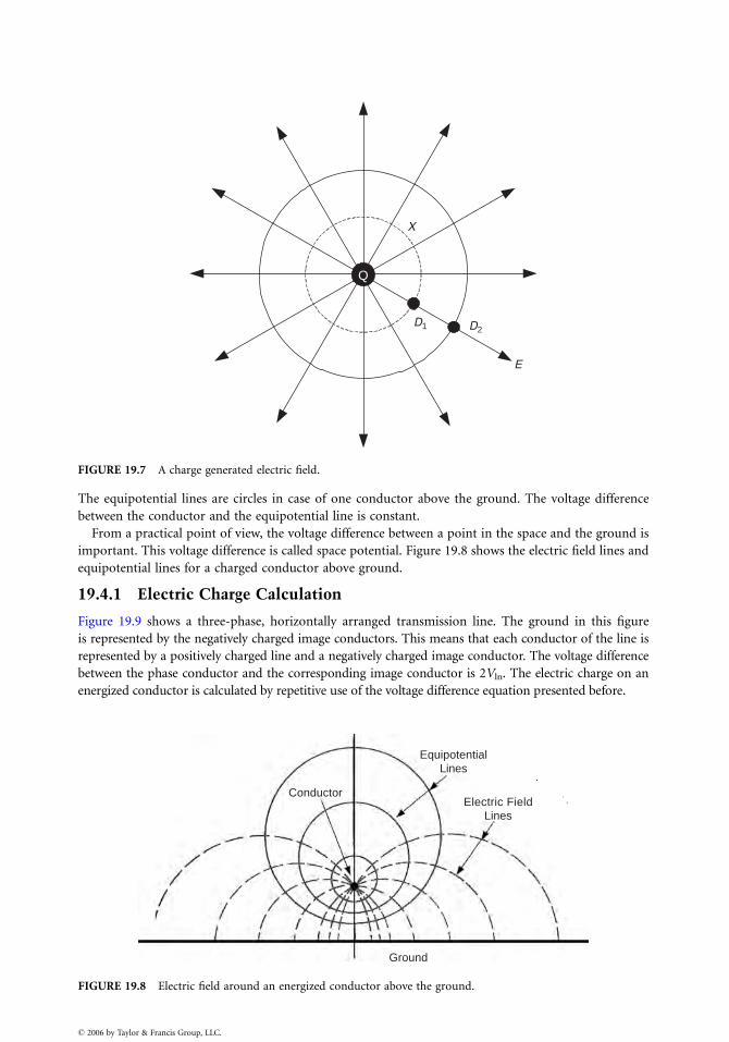
E
D1 D2
Q
X
FIGURE 19.7 A charge generated electric field.
The equipotential lines are circles in case of one conductor above the ground. The voltage difference
between the conductor and the equipotential line is constant.
From a practical point of view, the voltage difference between a point in the space and the ground is
important. This voltage difference is called space potential. Figure 19.8 shows the electric field lines and
equipotential lines for a charged conductor above ground.
19.4.1 Electric Charge Calculation
Figure 19.9 shows a three-phase, horizontally arranged transmission line. The ground in this figure
is represented by the negatively charged image conductors. This means that each conductor of the line is
represented by a positively charged line and a negatively charged image conductor. The voltage difference
between the phase conductor and the corresponding image conductor is 2Vln. The electric charge on an
energized conductor is calculated by repetitive use of the voltage difference equation presented before.
Electric Field Lines
Equipotential Lines
Conductor
Ground
FIGURE 19.8 Electric field around an energized conductor above the ground.
� 2006 by Taylor & Francis Group, LLC.
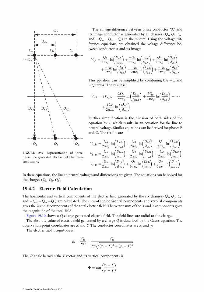
−Qa −Qb −Qc
Da,A Da,B Da,C
Qa Qb Qc
r = da,a
da,b
da,c
FIGURE 19.9 Representation of three-
phase line generated electric field by image
conductors.
� 2006 by Taylor & Francis Group, LLC.
The voltage difference between phase conductor ‘‘A’’ and
its image conductor is generated by all charges (Qa, Qb, Qc,
and �Qa, �Qb, �Qc) in the system. Using the voltage dif-
ference equations, we obtained the voltage difference be-
tween conductor A and its image:
Va,A ¼QA
2p«o
lnDa,A
rcond
� �
þ �QA
2p«o
lnrcond
Da,A
� �
þ QB
2p«o
lnDa,B
da,b
� �
þ �QB
2p«o
lnda,b
Da,B
� �
þ QC
2p«o
lnDa,C
da,c
� �
þ �QC
2p«o
lnda,c
Da,C
� �
This equation can be simplified by combining the þQ and
�Q terms. The result is
Va,A ¼ 2Va_ ln ¼2QA
2p«o
lnDa,A
rcond
� �
þ 2QB
2p«o
lnDa,B
da,b
� �
þ � � �
þ 2QC
2p«o
lnDa,C
da,c
� �
Further simplification is the division of both sides of the
equation by 2, which results in an equation for the line to
neutral voltage. Similar equations can be derived for phases B
and C. The results are
Va_ ln ¼QA
2p«o
lnDa,A
rcond
� �
þ QB
2p«o
lnDa,B
da,b
� �
þ QC
2p«o
lnDa,C
da,c
� �
Vb_ ln ¼QA
2p«o
lnD b,A
da,b
� �
þ QB
2p«o
lnD b,B
rcond
� �
þ QC
2p«o
lnD b,C
db,c
� �
Vc_ ln ¼QA
2p«o
lnDc,A
dc,b
� �
þ QB
2p«o
lnDc,B
db,c
� �
þ QC
2p«o
lnDc,C
rcond
� �
In these equations, the line to neutral voltages and dimensions are given. The equations can be solved for
the charges (Qa, Qb, Qc).
19.4.2 Electric Field Calculation
The horizontal and vertical components of the electric field generated by the six charges (Qa, Qb, Qc,
and �Qa, �Qb, �Qc) are calculated. The sum of the horizontal components and vertical components
gives the X and Y components of the total electric field. The vector sum of the X and Y components gives
the magnitude of the total field.
Figure 19.10 shows a Q charge generated electric field. The field lines are radial to the charge.
The absolute value of electric field generated by a charge Q is described by the Gauss equation. The
observation point coordinates are X and Y. The conductor coordinates are xi and yi.
The electric field magnitude is
Ei ¼Qi
2pr¼ Qi
2p
ffiffiffiffiffiffiffiffiffiffiffiffiffiffiffiffiffiffiffiffiffiffiffiffiffiffiffiffiffiffiffiffiffiffiffiffiffiffiffiffiffiffiffi
(xi � X)2 þ (yi � Y )2q
The F angle between the E vector and its vertical components is
F ¼ atnxi � X
yi � Y
� �
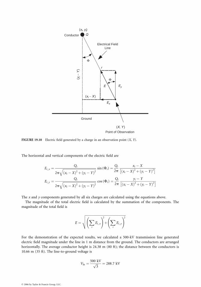
Conductor
(xi, yi)
Electrical Field Line
Q
Ground
Ex
EyE
r
(xi − X )
(yi −
Y)
Φ
Point of Observation
(X, Y )
Φ
FIGURE 19.10 Electric field generated by a charge in an observation point (X, Y).
The horizontal and vertical components of the electric field are
Ei_x ¼Qi
2p
ffiffiffiffiffiffiffiffiffiffiffiffiffiffiffiffiffiffiffiffiffiffiffiffiffiffiffiffiffiffiffiffiffiffiffiffiffiffiffiffiffiffi
xi � Xð Þ2þ yi � Yð Þ2q sin (Fi) ¼
Qi
2p
xi � X
xi � Xð Þ2þ yi � Yð Þ2� �
Ei_y ¼Qi
2p
ffiffiffiffiffiffiffiffiffiffiffiffiffiffiffiffiffiffiffiffiffiffiffiffiffiffiffiffiffiffiffiffiffiffiffiffiffiffiffiffiffiffi
xi � Xð Þ2þ yi � Yð Þ2q cos (Fi) ¼
Qi
2p
yi � Y
xi � Xð Þ2þ yi � Yð Þ2� �
The x and y components generated by all six charges are calculated using the equations above.
The magnitude of the total electric field is calculated by the summation of the components. The
magnitude of the total field is
E ¼
ffiffiffiffiffiffiffiffiffiffiffiffiffiffiffiffiffiffiffiffiffiffiffiffiffiffiffiffiffiffiffiffiffiffiffiffiffiffiffiffiffiffiffiffiffiffiffiffiffiffiffi
X
i
Ei_x
!2
þX
i
Ei_y
!2v
u
u
t
For the demonstration of the expected results, we calculated a 500-kV transmission line generated
electric field magnitude under the line in 1 m distance from the ground. The conductors are arranged
horizontally. The average conductor height is 24.38 m (80 ft); the distance between the conductors is
10.66 m (35 ft). The line-to-ground voltage is
Vln ¼500 kV
ffiffiffi
3p ¼ 288:7 kV
� 2006 by Taylor & Francis Group, LLC.
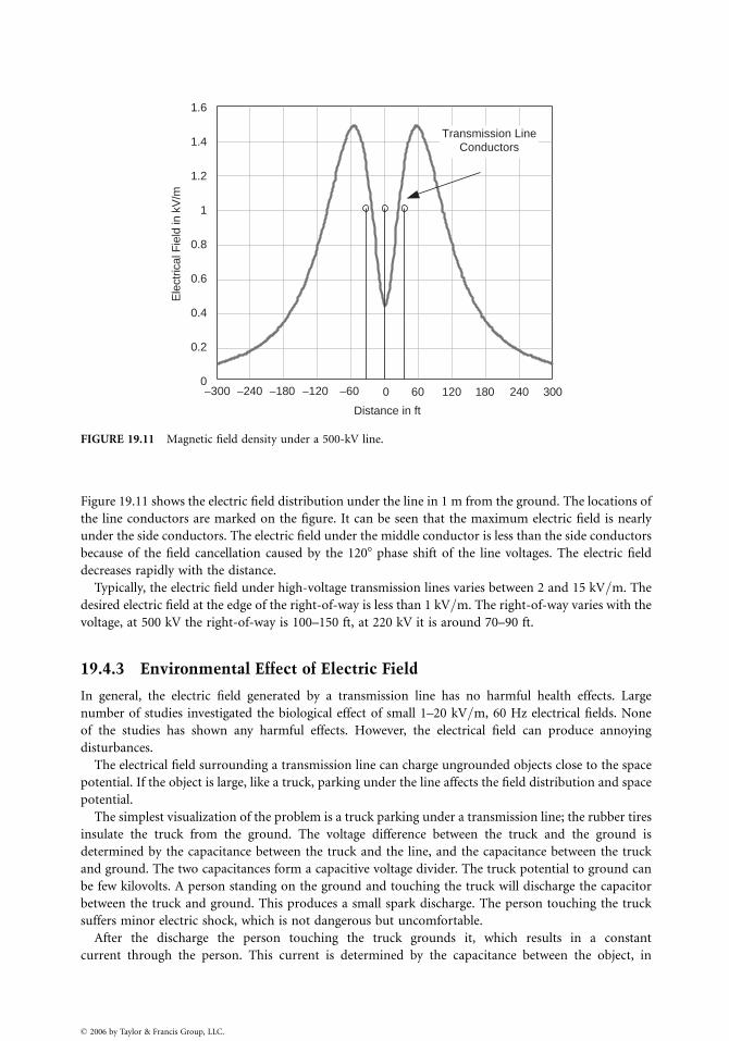
−300 −240 240−180 180−120 120−60 600 3000
0.2
0.4
0.6
0.8
1
1.2
1.4
1.6
Distance in ft
Ele
ctric
al F
ield
in k
V/m
Transmission Line Conductors
FIGURE 19.11 Magnetic field density under a 500-kV line.
Figure 19.11 shows the electric field distribution under the line in 1 m from the ground. The locations of
the line conductors are marked on the figure. It can be seen that the maximum electric field is nearly
under the side conductors. The electric field under the middle conductor is less than the side conductors
because of the field cancellation caused by the 1208 phase shift of the line voltages. The electric field
decreases rapidly with the distance.
Typically, the electric field under high-voltage transmission lines varies between 2 and 15 kV=m. The
desired electric field at the edge of the right-of-way is less than 1 kV=m. The right-of-way varies with the
voltage, at 500 kV the right-of-way is 100–150 ft, at 220 kV it is around 70–90 ft.
19.4.3 Environmental Effect of Electric Field
In general, the electric field generated by a transmission line has no harmful health effects. Large
number of studies investigated the biological effect of small 1–20 kV=m, 60 Hz electrical fields. None
of the studies has shown any harmful effects. However, the electrical field can produce annoying
disturbances.
The electrical field surrounding a transmission line can charge ungrounded objects close to the space
potential. If the object is large, like a truck, parking under the line affects the field distribution and space
potential.
The simplest visualization of the problem is a truck parking under a transmission line; the rubber tires
insulate the truck from the ground. The voltage difference between the truck and the ground is
determined by the capacitance between the truck and the line, and the capacitance between the truck
and ground. The two capacitances form a capacitive voltage divider. The truck potential to ground can
be few kilovolts. A person standing on the ground and touching the truck will discharge the capacitor
between the truck and ground. This produces a small spark discharge. The person touching the truck
suffers minor electric shock, which is not dangerous but uncomfortable.
After the discharge the person touching the truck grounds it, which results in a constant
current through the person. This current is determined by the capacitance between the object, in
� 2006 by Taylor & Francis Group, LLC.
this case the truck and the line. EPRI-published Redbook (Transmission Line Reference Book—345 kV and
Above) [14] gives an approximate formula for the expected current:
Icap ¼ 2pf «oEy surface,
where Ey is the vertical component of the electric field, f is the frequency (60 Hz), ‘‘surface’’ is the
equivalent charge collecting area of the object, and Icap is the capacitive current flowing through
the person grounding the object.
Another potentially dangerous accident scenario is when a worker climbs on a wooden ladder to
repair something close to a transmission line. A grounded coworker hands him a tool. This produces a
discharge and a minor spark, which is harmless. However, the shock may cause dropping the tool or
falling off the ladder.
People walking under the line may experience a tingling sensation on their skin and hair stimulation if
the electrical field is larger than 6–7 kV=m. This is an annoying but harmless effect.
The electric field effect is discussed in great details in the Transmission Line Reference Book—345 kV
and Above [14].
19.5 Audible Noise
The corona discharge on the high-voltage transmission line generates audible noise. The corona
discharge produced by a well-designed transmission line is very low in fair weather. Consequently, the
transmission line produced audible noise in fair weather conditions is negligible.
Fog and light rain produce droplets on the surface of line conductors. The droplets increase the local
electric field and generate corona discharge. The corona discharge produced air movement or pressure
wave generates the audible noise. The light rain and fog generated noise intensity varies, fluctuates
depending on the level of wetting.
Heavy rain produces more or less constant noise. The corona discharge bursts the water droplets and
disperses the water. However, the heavy rain replacing the dispersed water drops immediately.
Snowflakes also can increase corona level and audible noise. The dry, low temperature snow generally
does not produce audible noise. The audible noise generated by wet melting snow can be significant and
the noise level will be similar to the heavy rain generated noise.
Typically the line generated noise has two components:
. Broadband noise, which is mainly generated by the discharge on water droplets. This is a hissing,
crackling noise with significant high-frequency components.. Low-frequency humming noise with 120, 240 Hz, etc. components. This noise is generated by the
oscillatory movement of the corona generated ions around the conductors. The humming noise
occurs mostly in good weather condition, if the line corona level is low.
From a practical point of view, the broadband noise is the most important. The utilities accept a noise
level of 50–52 dB at the edge of right-of-way. The noise level is measured in dB. The base is 20 mPa. The
noise attenuates with the distance due to the divergence of the sound and the absorption of trees and
other objects. Practical value is around 3 dB, when the distance is doubled.
A numerical example is presented to estimate the approximate sound level in a residential area if
the sound level is 52 dB at the edge of the right-of-way. The distance between the line and the edge of
right-of-way is 100 ft. The sound level in a distance of 200 ft is 52 dB – 3 dB¼ 49 dB and in a distance
of 400 ft is 49 dB – 3 dB¼ 46 dB.
The transmission line generated noise level can be reduced by reduction of corona discharge level. The
most effective method is the use of bundle conductors. The rearrangement of the line conductors also
can reduce corona discharge and audible noise.
� 2006 by Taylor & Francis Group, LLC.
Section 15.2.3 in Chapter 15 presents a method to calculate the approximate sound level produced by
a high-voltage line. The EPRI-published Transmission Line Reference Book—345 kV and Above [14] gives
curves to determine the expected audible noise level produced by a transmission line.
19.6 Electromagnetic Interference (EMI)
The corona discharge produces radio noise and in lesser extent television (TV) disturbances around
high-voltage transmission lines. This can be easily observed by all of us when we drive under a
high-voltage line. The radio produces hissing, crackling noise close to the line or under the line, but
disturbance diapering fast as we drive away from the line crossing the highway. In a similar way, TV
picture disturbance can be observed close to a transmission line. The disturbance varies from the snowy
picture to the collapse of the picture.
The corona discharge causes short duration (few microseconds) repetitive current pulses. The
repetition frequency can be in the MHz range. As was discussed before, the corona discharge is low in
fair weather and increases rapidly in foul weather. The most severe EMI disturbance was observed during
heavy rain, when the water droplets on the conductor caused corona discharge.
Additional sources of the EMI disturbance are discharge in faulty insulators or discharge generated by
spikes, needles, and other sharp objects subjected to electric field. The sharp object produces an increase
in the local electric field, which can lead to surface discharge. This discharge can produce EMI and
unacceptable disturbances of local TV or radio reception.
The generated EMI disturbance decreases with the distance from the line. Typically, a 100 MHz signal
decreases about 20 dB if we move 100 m from the line; simultaneously, a 1 MHz components
attenuation is around 35–40 dB in the same distance. The radio and TV noise is measured in dB; the
base is 1 mV=m.
The actual disturbance depends on the signal-to-noise ratio. As an example, the same level of EMI
disturbance can produce an unacceptable radio or TV reception if the broadcasted signal is weak, and no
disturbance in case of strong signal.
The EPRI-published Transmission Line Reference Book—345 kV and Above [14] gives curves to
determine the expected radio or TV disturbance level produced by a transmission line.
References
1.
� 200
Wertheimer, N., Leeper, E., Electric wiring configuration and childhood cancer, American Journal
of Epidemiology, 109 (3), 273–284, March 1979.
2.
Savitz, D.A., Wachtel, H., Barnes, F.A., John, E.M., and Tvrdik, R.G., Case control study ofchildhood cancer and residential exposure to electric and magnetic fields, American Journal
of Epidemiology, 128 (1), 21–38, January 1988.
3.
London, S.J., et al., Exposure to residential electric and magnetic fields and risk of childhoodleukemia, American Journal of Epidemiology, 131 (9), 923–937, November 1992.
4.
Floderus, B., Persson, T., Stenlund, et al., Occupational exposure to electromagnetic fields in relationto leukemia and brain tumor, Department of Neuromedicine, National Institute of Occupational
Health, Solna, Sweden, 1992.
5.
Tynes, T., Hanevik, M., Vistnes, A.I., A nested case-control study of leukemia and brain tumors inNorwegian railway workers, Conference Proceedings Fifteenth Annual Meeting of the Bioelectro-
magnetic Society, Los Angeles, CA, June 1993.
6.
Scarfi, M.R., Bersani, F., Brooks, A.L., et al., 50 Hz, sinusoidal electric field do not exert genotaxiseffects (micronucleus formation) in human lymphocytes, Radiation Research, 135(1), 64–68, 1992.
7.
Byus, C.V., Piper, S.A., Adey, W.R., The effect of low energy 60 Hz environmental electromagneticfields upon the growth related enzyme ornithine decarboxylase, Carcinogenesis, 8, 1385–1389, 1987.
6 by Taylor & Francis Group, LLC.

8.
� 200
Korpinen L., Influence of 50 Hz electric and magnetic fields on the human heart, Bioelectro-
magnetics, 14 (4), 329–340, 1993.
9.
Graham, C., et al., EMF suppression of nocturnal melatonin in human volunteers, Annual Review ofResearch in Biological Effects of Electric and Magnetic Fields from the Generation, Delivery and Use
of Electricity, Savannah, GA, October 31–November 4, 98–99, 1994.
10.
EPRI Report, TR-100194, Survey of Residential Power Magnetic Field Sources, Phase 1, RP2942,Electric Power Research Institute, Palo Alto, CA, 1990.
11.
Electric and Magnetic Field Fundamentals, Electric Power Research Institute, Palo Alto, CA,March 1994.
12.
U.S. Environmental Protection Agency, Evaluation of the potential carcinogenicity of electro-magnetic fields, EAP=600=6-90=005B, October 1990.
13.
U.S. Environmental Protection Agency, Office of Research and Development, Electric and MagneticFields Annual Environmental Protection Agency, Prospective on Research Needs and Priorities for
Improving Health Risk Assessment, Washington D.C., U.S. Government Printing, 1992.
14.
Transmission Line Reference Book—345 kV and Above, 2nd ed., Electric Power Research Institute,Palo Alto, CA, 1987.
15.
Kaune, W.T., Zaffranella, L.E., Analysis of magnetic fields produced far from electric power lines,IEEE Transactions on Power Delivery, 7 (4), 2082–2091, October 1992.
6 by Taylor & Francis Group, LLC.

� 2006 by Taylor & Francis Group, LLC.

IV
DistributionSystems William H. KerstingNew Mexico State University20 Power System Loads Raymond R. Shoults and Larry D. Swift .................................... 20-1
Load Classification . Modeling Applications . Load Modeling Concepts
and Approaches . Load Characteristics and Models . Static
Load Characteristics . Load Window Modeling
21 Distribution System Modeling and Analysis William H. Kersting ............................. 21-1
Modeling . Analysis
22 Power System Operation and Control George L. Clark and Simon W. Bowen .......... 22-1
Implementation of Distribution Automation . Distribution SCADA
History . Field Devices . Integrated SCADA System . Security . Practical
Considerations . Standards . Deployment Considerations
23 Hard to Find Information (on Distribution System Characteristics
and Protection) Jim Burke .............................................................................................. 23-1
Overcurrent Protection . Transformers . Instrument Transformers . Loading .
Miscellaneous Loading Information
24 Real-Time Control of Distributed Generation Murat Dilek and
Robert P. Broadwater.......................................................................................................... 24-1
Local Site DG Control . Hierarchical Control: Real-Time Control .
Control of DGs at Circuit Level . Hierarchical Control: Forecasting Generation
� 2006 by Taylor & Francis Group, LLC.

� 2006 by Taylor & Francis Group, LLC.
20
� 2006 by Taylor & Francis Group, LLC.
Power System Loads
Raymond R. ShoultsUniversity of Texas at Arlington
Larry D. SwiftUniversity of Texas at Arlington
20.1 Load Classification .......................................................... 20-1
20.2 Modeling Applications.................................................... 20-2
20.3 Load Modeling Concepts and Approaches ................... 20-3
20.4 Load Characteristics and Models................................... 20-3
20.5 Static Load Characteristics ............................................. 20-5Exponential Models . Polynomial Models . Combined
Exponential and Polynomial Models . Comparison of
Exponential and Polynomial Models . Devices Contributing
to Modeling Difficulties
20.6 Load Window Modeling................................................. 20-9
The physical structure of most power systems consists of generation facilities feeding bulk power into
a high-voltage bulk transmission network, that in turn serves any number of distribution substations.
A typical distribution substation will serve from one to as many as ten feeder circuits. A typical
feeder circuit may serve numerous loads of all types. A light to medium industrial customer may
take service from the distribution feeder circuit primary, while a large industrial load complex
may take service directly from the bulk transmission system. All other customers, including residen-
tial and commercial, are typically served from the secondary of distribution transformers that are in
turn connected to a distribution feeder circuit. Figure 20.1 illustrates a representative portion of a
typical configuration.
20.1 Load Classification
The most common classification of electrical loads follows the billing categories used by the utility
companies. This classification includes residential, commercial, industrial, and other. Residential cus-
tomers are domestic users, whereas commercial and industrial customers are obviously business and
industrial users. Other customer classifications include municipalities, state and federal government
agencies, electric cooperatives, educational institutions, etc.
Although these load classes are commonly used, they are often inadequately defined for certain types
of power system studies. For example, some utilities meter apartments as individual residential cus-
tomers, while others meter the entire apartment complex as a commercial customer. Thus, the common
classifications overlap in the sense that characteristics of customers in one class are not unique to that
class. For this reason some utilities define further subdivisions of the common classes.
A useful approach to classification of loads is by breaking down the broader classes into individual
load components. This process may altogether eliminate the distinction of certain of the broader classes,
but it is a tried and proven technique for many applications. The components of a particular load, be it
residential, commercial, or industrial, are individually defined and modeled. These load components as
a whole constitute the composite load and can be defined as a ‘‘load window.’’
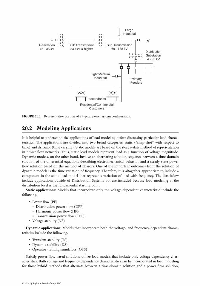
Generation 15 - 35 kV
Bulk Transmission230 kV & higher
Sub-Transmission69 - 138 kV
LargeIndustrial
DistributionSubstation4 - 35 kV
PrimaryFeeders
Light/MediumIndustrial
secondaries
Residential/CommercialCustomers
FIGURE 20.1 Representative portion of a typical power system configuration.
20.2 Modeling Applications
It is helpful to understand the applications of load modeling before discussing particular load charac-
teristics. The applications are divided into two broad categories: static (‘‘snap-shot’’ with respect to
time) and dynamic (time varying). Static models are based on the steady-state method of representation
in power flow networks. Thus, static load models represent load as a function of voltage magnitude.
Dynamic models, on the other hand, involve an alternating solution sequence between a time-domain
solution of the differential equations describing electromechanical behavior and a steady-state power
flow solution based on the method of phasors. One of the important outcomes from the solution of
dynamic models is the time variation of frequency. Therefore, it is altogether appropriate to include a
component in the static load model that represents variation of load with frequency. The lists below
include applications outside of Distribution Systems but are included because load modeling at the
distribution level is the fundamental starting point.
Static applications: Models that incorporate only the voltage-dependent characteristic include the
following.
. Power flow (PF)* Distribution power flow (DPF)* Harmonic power flow (HPF)* Transmission power flow (TPF)
. Voltage stability (VS)
Dynamic applications: Models that incorporate both the voltage- and frequency-dependent charac-
teristics include the following.
. Transient stability (TS)
. Dynamic stability (DS)
. Operator training simulators (OTS)
Strictly power-flow based solutions utilize load models that include only voltage dependency char-
acteristics. Both voltage and frequency dependency characteristics can be incorporated in load modeling
for those hybrid methods that alternate between a time-domain solution and a power flow solution,
� 2006 by Taylor & Francis Group, LLC.
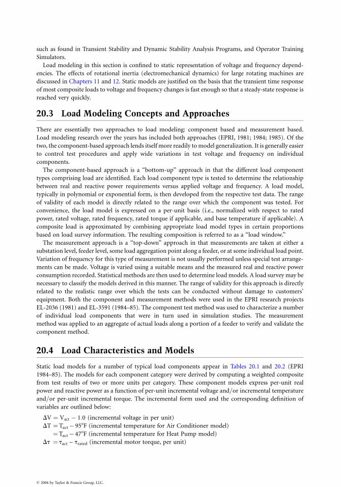
such as found in Transient Stability and Dynamic Stability Analysis Programs, and Operator Training
Simulators.
Load modeling in this section is confined to static representation of voltage and frequency depend-
encies. The effects of rotational inertia (electromechanical dynamics) for large rotating machines are
discussed in Chapters 11 and 12. Static models are justified on the basis that the transient time response
of most composite loads to voltage and frequency changes is fast enough so that a steady-state response is
reached very quickly.
20.3 Load Modeling Concepts and Approaches
There are essentially two approaches to load modeling: component based and measurement based.
Load modeling research over the years has included both approaches (EPRI, 1981; 1984; 1985). Of the
two, the component-based approach lends itself more readily to model generalization. It is generally easier
to control test procedures and apply wide variations in test voltage and frequency on individual
components.
The component-based approach is a ‘‘bottom-up’’ approach in that the different load component
types comprising load are identified. Each load component type is tested to determine the relationship
between real and reactive power requirements versus applied voltage and frequency. A load model,
typically in polynomial or exponential form, is then developed from the respective test data. The range
of validity of each model is directly related to the range over which the component was tested. For
convenience, the load model is expressed on a per-unit basis (i.e., normalized with respect to rated
power, rated voltage, rated frequency, rated torque if applicable, and base temperature if applicable). A
composite load is approximated by combining appropriate load model types in certain proportions
based on load survey information. The resulting composition is referred to as a ‘‘load window.’’
The measurement approach is a ‘‘top-down’’ approach in that measurements are taken at either a
substation level, feeder level, some load aggregation point along a feeder, or at some individual load point.
Variation of frequency for this type of measurement is not usually performed unless special test arrange-
ments can be made. Voltage is varied using a suitable means and the measured real and reactive power
consumption recorded. Statistical methods are then used to determine load models. A load survey may be
necessary to classify the models derived in this manner. The range of validity for this approach is directly
related to the realistic range over which the tests can be conducted without damage to customers’
equipment. Both the component and measurement methods were used in the EPRI research projects
EL-2036 (1981) and EL-3591 (1984–85). The component test method was used to characterize a number
of individual load components that were in turn used in simulation studies. The measurement
method was applied to an aggregate of actual loads along a portion of a feeder to verify and validate the
component method.
20.4 Load Characteristics and Models
Static load models for a number of typical load components appear in Tables 20.1 and 20.2 (EPRI
1984–85). The models for each component category were derived by computing a weighted composite
from test results of two or more units per category. These component models express per-unit real
power and reactive power as a function of per-unit incremental voltage and=or incremental temperature
and=or per-unit incremental torque. The incremental form used and the corresponding definition of
variables are outlined below:
DV ¼ Vact � 1:0 (incremental voltage in per unit)
DT ¼Tact� 958F (incremental temperature for Air Conditioner model)
¼Tact� 478F (incremental temperature for Heat Pump model)
Dt ¼ tact – trated (incremental motor torque, per unit)
� 2006 by Taylor & Francis Group, LLC.
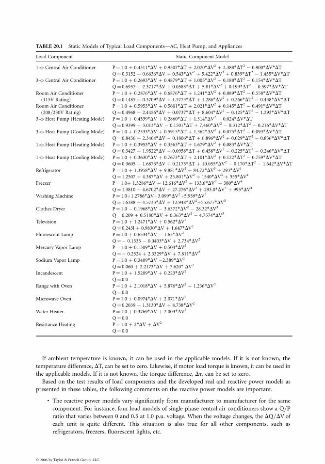
TABLE 20.1 Static Models of Typical Load Components—AC, Heat Pump, and Appliances
Load Component Static Component Model
1-f Central Air Conditioner P¼ 1.0 þ 0.4311*DV þ 0.9507*DT þ 2.070*DV2 þ 2.388*DT2 � 0.900*DV*DT
Q¼ 0.3152 þ 0.6636*DV þ 0.543*DV2 þ 5.422*DV3 þ 0.839*DT2 � 1.455*DV*DT
3-f Central Air Conditioner P¼ 1.0 þ 0.2693*DV þ 0.4879*DT þ 1.005*DV2 � 0.188*DT2 � 0.154*DV*DT
Q¼ 0.6957 þ 2.3717*DV þ 0.0585*DT þ 5.81*DV2 þ 0.199*DT2 � 0.597*DV*DT
Room Air Conditioner
(115V Rating)
P¼ 1.0 þ 0.2876*DV þ 0.6876*DT þ 1.241*DV2 þ 0.089*DT2 � 0.558*DV*DT
Q¼ 0.1485 þ 0.3709*DV þ 1.5773*DT þ 1.286*DV2 þ 0.266*DT2 � 0.438*DV*DT
Room Air Conditioner
(208=230V Rating)
P¼ 1.0 þ 0.5953*DV þ 0.5601*DT þ 2.021*DV2 þ 0.145*DT2 � 0.491*DV*DT
Q¼ 0.4968 þ 2.4456*DV þ 0.0737*DT þ 8.604*DV2 � 0.125*DT2 � 1.293*DV*DT
3-f Heat Pump (Heating Mode) P¼ 1.0 þ 0.4539*DV þ 0.2860*DT þ 1.314*DV2 � 0.024*DV*DT
Q¼ 0.9399 þ 3.013*DV � 0.1501*DT þ 7.460*DV2 � 0.312*DT2 � 0.216*DV*DT
3-f Heat Pump (Cooling Mode) P¼ 1.0 þ 0.2333*DV þ 0.5915*DT þ 1.362*DV2 þ 0.075*DT2 � 0.093*DV*DT
Q¼ 0.8456 þ 2.3404*DV � 0.1806*DT þ 6.896*DV2 þ 0.029*DT2 � 0.836*DV*DT
1-f Heat Pump (Heating Mode) P¼ 1.0 þ 0.3953*DV þ 0.3563*DT þ 1.679*DV2 þ 0.083*DV*DT
Q¼ 0.3427 þ 1.9522*DV � 0.0958*DT þ 6.458*DV2 � 0.225*DT2 � 0.246*DV*DT
1-f Heat Pump (Cooling Mode) P¼ 1.0 þ 0.3630*DV þ 0.7673*DT þ 2.101*DV2 þ 0.122*DT2 � 0.759*DV*DT
Q¼ 0.3605 þ 1.6873*DV þ 0.2175*DT þ 10.055*DV2 � 0.170*DT2 � 1.642*DV*DT
Refrigerator P¼ 1.0 þ 1.3958*DV þ 9.881*DV2 þ 84.72*DV3 þ 293*DV4
Q¼ 1.2507 þ 4.387*DV þ 23.801*DV2 þ 1540*DV3 þ 555*DV4
Freezer P¼ 1.0þ 1.3286*DV þ 12.616*DV2 þ 133.6*DV3 þ 380*DV4
Q¼ 1.3810 þ 4.6702*DV þ 27.276*DV2 þ 293.0*DV3 þ 995*DV4
Washing Machine P¼ 1.0þ1.2786*DVþ3.099*DV2þ5.939*DV3
Q¼ 1.6388 þ 4.5733*DV þ 12.948*DV2þ55.677*DV3
Clothes Dryer P¼ 1.0 � 0.1968*DV � 3.6372*DV2 � 28.32*DV3
Q¼ 0.209 þ 0.5180*DV þ 0.363*DV2 � 4.7574*DV3
Television P¼ 1.0 þ 1.2471*DV þ 0.562*DV2
Q¼ 0.243l þ 0.9830*DV þ 1.647*DV2
Fluorescent Lamp P¼ 1.0 þ 0.6534*DV � 1.65*DV2
Q¼� 0.1535 � 0.0403*DV þ 2.734*DV2
Mercury Vapor Lamp P¼ 1.0 þ 0.1309*DV þ 0.504*DV2
Q¼� 0.2524 þ 2.3329*DV þ 7.811*DV2
Sodium Vapor Lamp P¼ 1.0 þ 0.3409*DV �2.389*DV2
Q¼ 0.060 þ 2.2173*DV þ 7.620* DV2
Incandescent P¼ 1.0 þ 1.5209*DV þ 0.223*DV2
Q¼ 0.0
Range with Oven P¼ 1.0 þ 2.1018*DV þ 5.876*DV2 þ 1.236*DV3
Q¼ 0.0
Microwave Oven P¼ 1.0 þ 0.0974*DV þ 2.071*DV2
Q¼ 0.2039 þ 1.3130*DV þ 8.738*DV2
Water Heater P¼ 1.0 þ 0.3769*DV þ 2.003*DV2
Q¼ 0.0
Resistance Heating P¼ 1.0 þ 2*DV þ DV2
Q¼ 0.0
If ambient temperature is known, it can be used in the applicable models. If it is not known, the
temperature difference, DT, can be set to zero. Likewise, if motor load torque is known, it can be used in
the applicable models. If it is not known, the torque difference, Dt, can be set to zero.
Based on the test results of load components and the developed real and reactive power models as
presented in these tables, the following comments on the reactive power models are important.
. The reactive power models vary significantly from manufacturer to manufacturer for the same
component. For instance, four load models of single-phase central air-conditioners show a Q=P
ratio that varies between 0 and 0.5 at 1.0 p.u. voltage. When the voltage changes, the DQ=DV of
each unit is quite different. This situation is also true for all other components, such as
refrigerators, freezers, fluorescent lights, etc.
� 2006 by Taylor & Francis Group, LLC.
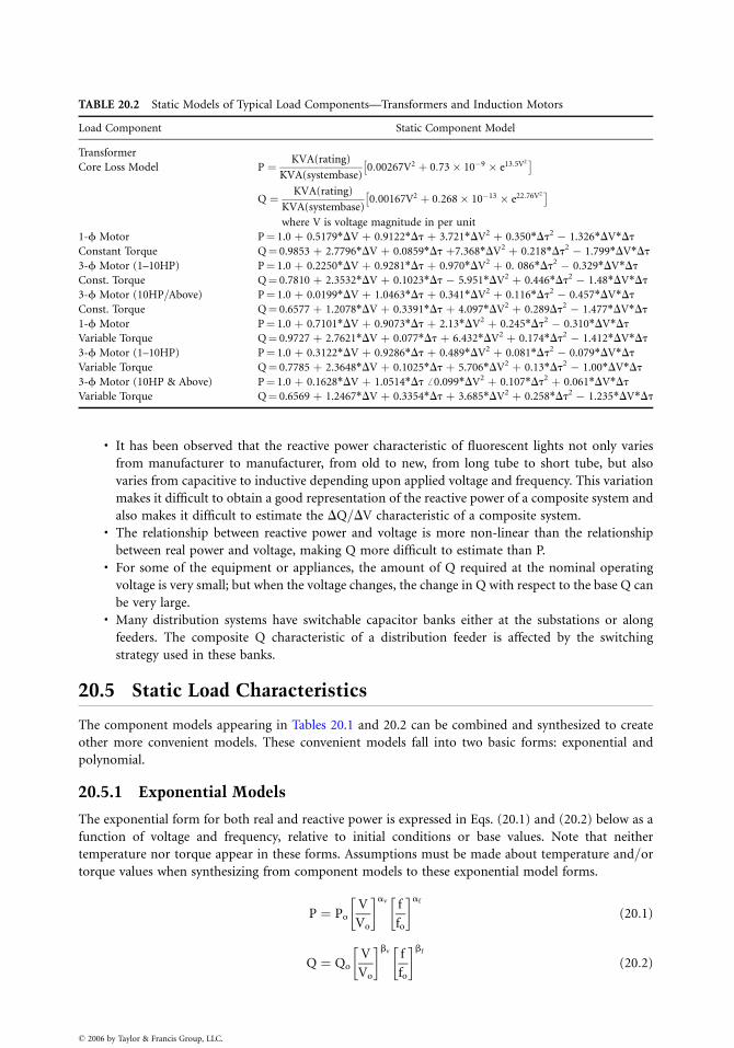
TABLE 20.2 Static Models of Typical Load Components—Transformers and Induction Motors
Load Component Static Component Model
Transformer
Core Loss Model P ¼ KVA(rating)
KVA(systembase)0:00267V2 þ 0:73� 10�9 � e13:5V2� �
Q ¼ KVA(rating)
KVA(systembase)0:00167V2 þ 0:268� 10�13 � e22:76V2� �
where V is voltage magnitude in per unit
1-f Motor P¼ 1.0 þ 0.5179*DV þ 0.9122*Dt þ 3.721*DV2 þ 0.350*Dt2 � 1.326*DV*Dt
Constant Torque Q¼ 0.9853 þ 2.7796*DV þ 0.0859*Dt þ7.368*DV2 þ 0.218*Dt2 � 1.799*DV*Dt
3-f Motor (1–10HP) P¼ 1.0 þ 0.2250*DV þ 0.9281*Dt þ 0.970*DV2 þ 0. 086*Dt2 � 0.329*DV*Dt
Const. Torque Q¼ 0.7810 þ 2.3532*DV þ 0.1023*Dt � 5.951*DV2 þ 0.446*Dt2 � 1.48*DV*Dt
3-f Motor (10HP=Above) P¼ 1.0 þ 0.0199*DV þ 1.0463*Dt þ 0.341*DV2 þ 0.116*Dt2 � 0.457*DV*Dt
Const. Torque Q¼ 0.6577 þ 1.2078*DV þ 0.3391*Dt þ 4.097*DV2 þ 0.289Dt2 � 1.477*DV*Dt
1-f Motor P¼ 1.0 þ 0.7101*DV þ 0.9073*Dt þ 2.13*DV2 þ 0.245*Dt2 � 0.310*DV*Dt
Variable Torque Q¼ 0.9727 þ 2.7621*DV þ 0.077*Dt þ 6.432*DV2 þ 0.174*Dt2 � 1.412*DV*Dt
3-f Motor (1–10HP) P¼ 1.0 þ 0.3122*DV þ 0.9286*Dt þ 0.489*DV2 þ 0.081*Dt2 � 0.079*DV*Dt
Variable Torque Q¼ 0.7785 þ 2.3648*DV þ 0.1025*Dt þ 5.706*DV2 þ 0.13*Dt2 � 1.00*DV*Dt
3-f Motor (10HP & Above) P¼ 1.0 þ 0.1628*DV þ 1.0514*Dt ff0.099*DV2 þ 0.107*Dt2 þ 0.061*DV*Dt
Variable Torque Q¼ 0.6569 þ 1.2467*DV þ 0.3354*Dt þ 3.685*DV2 þ 0.258*Dt2 � 1.235*DV*Dt
. It has been observed that the reactive power characteristic of fluorescent lights not only varies
from manufacturer to manufacturer, from old to new, from long tube to short tube, but also
varies from capacitive to inductive depending upon applied voltage and frequency. This variation
makes it difficult to obtain a good representation of the reactive power of a composite system and
also makes it difficult to estimate the DQ=DV characteristic of a composite system.. The relationship between reactive power and voltage is more non-linear than the relationship
between real power and voltage, making Q more difficult to estimate than P.. For some of the equipment or appliances, the amount of Q required at the nominal operating
voltage is very small; but when the voltage changes, the change in Q with respect to the base Q can
be very large.. Many distribution systems have switchable capacitor banks either at the substations or along
feeders. The composite Q characteristic of a distribution feeder is affected by the switching
strategy used in these banks.
20.5 Static Load Characteristics
The component models appearing in Tables 20.1 and 20.2 can be combined and synthesized to create
other more convenient models. These convenient models fall into two basic forms: exponential and
polynomial.
20.5.1 Exponential Models
The exponential form for both real and reactive power is expressed in Eqs. (20.1) and (20.2) below as a
function of voltage and frequency, relative to initial conditions or base values. Note that neither
temperature nor torque appear in these forms. Assumptions must be made about temperature and=or
torque values when synthesizing from component models to these exponential model forms.
P ¼ PoV
Vo
� �av f
fo
� �af
(20:1)
Q ¼ QoV
Vo
� �bv f
fo
� �bf
(20:2)
� 2006 by Taylor & Francis Group, LLC.
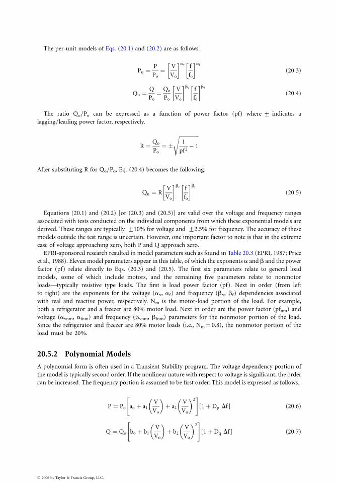
The per-unit models of Eqs. (20.1) and (20.2) are as follows.
Pu ¼P
Po
¼ V
Vo
� �av f
fo
� �af
(20:3)
Qu ¼Q
Po
¼ Qo
Po
V
Vo
� �bv f
fo
� �bf
(20:4)
The ratio Qo=Po can be expressed as a function of power factor (pf) where + indicates a
lagging=leading power factor, respectively.
R ¼ Qo
Po
¼ �ffiffiffiffiffiffiffiffiffiffiffiffiffiffiffi
1
pf 2� 1
s
After substituting R for Qo=Po, Eq. (20.4) becomes the following.
Qu ¼ RV
Vo
� �bv f
fo
� �bf
(20:5)
Equations (20.1) and (20.2) [or (20.3) and (20.5)] are valid over the voltage and frequency ranges
associated with tests conducted on the individual components from which these exponential models are
derived. These ranges are typically +10% for voltage and +2.5% for frequency. The accuracy of these
models outside the test range is uncertain. However, one important factor to note is that in the extreme
case of voltage approaching zero, both P and Q approach zero.
EPRI-sponsored research resulted in model parameters such as found in Table 20.3 (EPRI, 1987; Price
et al., 1988). Eleven model parameters appear in this table, of which the exponents a and b and the power
factor (pf) relate directly to Eqs. (20.3) and (20.5). The first six parameters relate to general load
models, some of which include motors, and the remaining five parameters relate to nonmotor
loads—typically resistive type loads. The first is load power factor (pf). Next in order (from left
to right) are the exponents for the voltage (av, af) and frequency (bv, bf) dependencies associated
with real and reactive power, respectively. Nm is the motor-load portion of the load. For example,
both a refrigerator and a freezer are 80% motor load. Next in order are the power factor (pfnm) and
voltage (avnm, afnm) and frequency (bvnm, bfnm) parameters for the nonmotor portion of the load.
Since the refrigerator and freezer are 80% motor loads (i.e., Nm¼ 0.8), the nonmotor portion of the
load must be 20%.
20.5.2 Polynomial Models
A polynomial form is often used in a Transient Stability program. The voltage dependency portion of
the model is typically second order. If the nonlinear nature with respect to voltage is significant, the order
can be increased. The frequency portion is assumed to be first order. This model is expressed as follows.
P ¼ Po ao þ a1V
Vo
� �
þ a2V
Vo
� �2" #
[1þ Dp Df ] (20:6)
Q ¼ Qo bo þ b1
V
Vo
� �
þ b2
V
Vo
� �2" #
[1þDq Df ] (20:7)
� 2006 by Taylor & Francis Group, LLC.
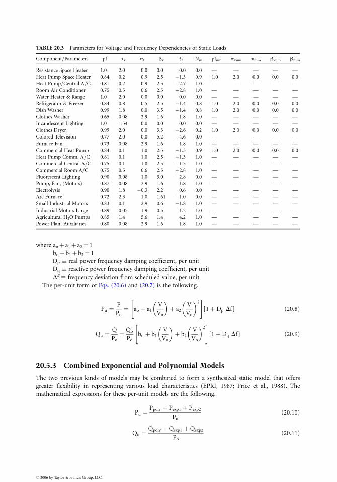
TABLE 20.3 Parameters for Voltage and Frequency Dependencies of Static Loads
Component=Parameters pf av af bv bf Nm pfnm avnm afnm bvnm bfnm
Resistance Space Heater 1.0 2.0 0.0 0.0 0.0 0.0 — — — — —
Heat Pump Space Heater 0.84 0.2 0.9 2.5 �1.3 0.9 1.0 2.0 0.0 0.0 0.0
Heat Pump=Central A=C 0.81 0.2 0.9 2.5 �2.7 1.0 — — — — —
Room Air Conditioner 0.75 0.5 0.6 2.5 �2.8 1.0 — — — — —
Water Heater & Range 1.0 2.0 0.0 0.0 0.0 0.0 — — — — —
Refrigerator & Freezer 0.84 0.8 0.5 2.5 �1.4 0.8 1.0 2.0 0.0 0.0 0.0
Dish Washer 0.99 1.8 0.0 3.5 �1.4 0.8 1.0 2.0 0.0 0.0 0.0
Clothes Washer 0.65 0.08 2.9 1.6 1.8 1.0 — — — — —
Incandescent Lighting 1.0 1.54 0.0 0.0 0.0 0.0 — — — — —
Clothes Dryer 0.99 2.0 0.0 3.3 �2.6 0.2 1.0 2.0 0.0 0.0 0.0
Colored Television 0.77 2.0 0.0 5.2 �4.6 0.0 — — — — —
Furnace Fan 0.73 0.08 2.9 1.6 1.8 1.0 — — — — —
Commercial Heat Pump 0.84 0.1 1.0 2.5 �1.3 0.9 1.0 2.0 0.0 0.0 0.0
Heat Pump Comm. A=C 0.81 0.1 1.0 2.5 �1.3 1.0 — — — — —
Commercial Central A=C 0.75 0.1 1.0 2.5 �1.3 1.0 — — — — —
Commercial Room A=C 0.75 0.5 0.6 2.5 �2.8 1.0 — — — — —
Fluorescent Lighting 0.90 0.08 1.0 3.0 �2.8 0.0 — — — — —
Pump, Fan, (Motors) 0.87 0.08 2.9 1.6 1.8 1.0 — — — — —
Electrolysis 0.90 1.8 �0.3 2.2 0.6 0.0 — — — — —
Arc Furnace 0.72 2.3 �1.0 1.61 �1.0 0.0 — — — — —
Small Industrial Motors 0.83 0.1 2.9 0.6 �1.8 1.0 — — — — —
Industrial Motors Large 0.89 0.05 1.9 0.5 1.2 1.0 — — — — —
Agricultural H2O Pumps 0.85 1.4 5.6 1.4 4.2 1.0 — — — — —
Power Plant Auxiliaries 0.80 0.08 2.9 1.6 1.8 1.0 — — — — —
where aoþ a1þ a2¼ 1
boþ b1þ b2¼ 1
Dp � real power frequency damping coefficient, per unit
Dq � reactive power frequency damping coefficient, per unit
Df � frequency deviation from scheduled value, per unit
The per-unit form of Eqs. (20.6) and (20.7) is the following.
Pu ¼P
Po
¼ ao þ a1
V
Vo
� �
þ a2
V
Vo
� �2" #
[1þ Dp Df] (20:8)
Qu ¼Q
Po
¼ Qo
Po
bo þ b1V
Vo
� �
þ b2V
Vo
� �2" #
[1þ Dq Df] (20:9)
20.5.3 Combined Exponential and Polynomial Models
The two previous kinds of models may be combined to form a synthesized static model that offers
greater flexibility in representing various load characteristics (EPRI, 1987; Price et al., 1988). The
mathematical expressions for these per-unit models are the following.
Pu ¼Ppoly þ Pexp1 þ Pexp2
Po
(20:10)
Qu ¼Qpoly þQexp1 þQexp2
Po
(20:11)
� 2006 by Taylor & Francis Group, LLC.
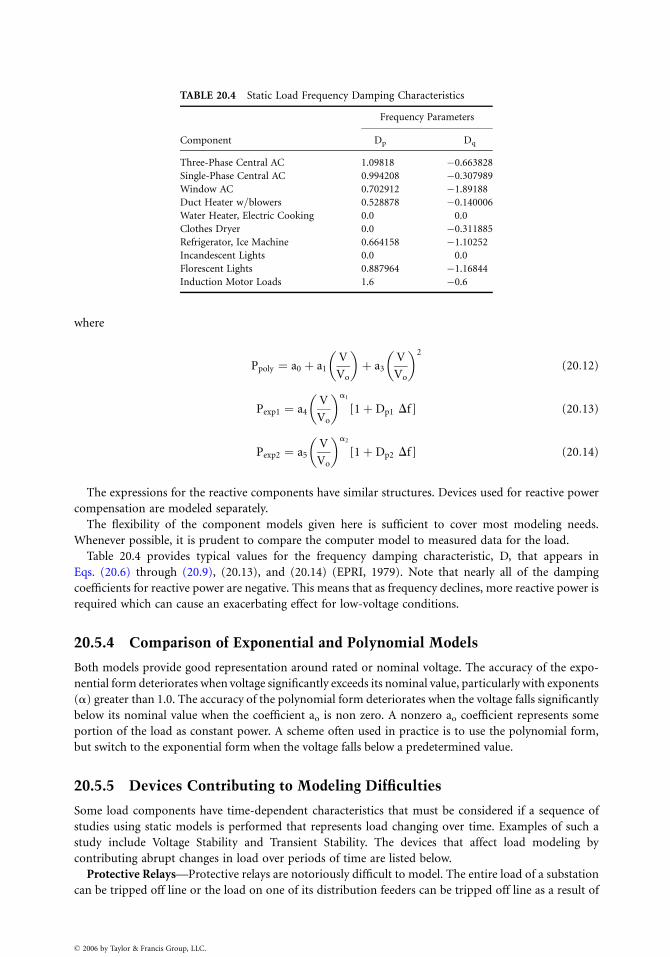
TABLE 20.4 Static Load Frequency Damping Characteristics
Frequency Parameters
Component Dp Dq
Three-Phase Central AC 1.09818 �0.663828
Single-Phase Central AC 0.994208 �0.307989
Window AC 0.702912 �1.89188
Duct Heater w=blowers 0.528878 �0.140006
Water Heater, Electric Cooking 0.0 0.0
Clothes Dryer 0.0 �0.311885
Refrigerator, Ice Machine 0.664158 �1.10252
Incandescent Lights 0.0 0.0
Florescent Lights 0.887964 �1.16844
Induction Motor Loads 1.6 �0.6
where
Ppoly ¼ a0 þ a1V
Vo
� �
þ a3V
Vo
� �2
(20:12)
Pexp1 ¼ a4
V
Vo
� �a1
[1þ Dp1 Df ] (20:13)
Pexp2 ¼ a5V
Vo
� �a2
[1þ Dp2 Df ] (20:14)
The expressions for the reactive components have similar structures. Devices used for reactive power
compensation are modeled separately.
The flexibility of the component models given here is sufficient to cover most modeling needs.
Whenever possible, it is prudent to compare the computer model to measured data for the load.
Table 20.4 provides typical values for the frequency damping characteristic, D, that appears in
Eqs. (20.6) through (20.9), (20.13), and (20.14) (EPRI, 1979). Note that nearly all of the damping
coefficients for reactive power are negative. This means that as frequency declines, more reactive power is
required which can cause an exacerbating effect for low-voltage conditions.
20.5.4 Comparison of Exponential and Polynomial Models
Both models provide good representation around rated or nominal voltage. The accuracy of the expo-
nential form deteriorates when voltage significantly exceeds its nominal value, particularly with exponents
(a) greater than 1.0. The accuracy of the polynomial form deteriorates when the voltage falls significantly
below its nominal value when the coefficient ao is non zero. A nonzero ao coefficient represents some
portion of the load as constant power. A scheme often used in practice is to use the polynomial form,
but switch to the exponential form when the voltage falls below a predetermined value.
20.5.5 Devices Contributing to Modeling Difficulties
Some load components have time-dependent characteristics that must be considered if a sequence of
studies using static models is performed that represents load changing over time. Examples of such a
study include Voltage Stability and Transient Stability. The devices that affect load modeling by
contributing abrupt changes in load over periods of time are listed below.
Protective Relays—Protective relays are notoriously difficult to model. The entire load of a substation
can be tripped off line or the load on one of its distribution feeders can be tripped off line as a result of
� 2006 by Taylor & Francis Group, LLC.
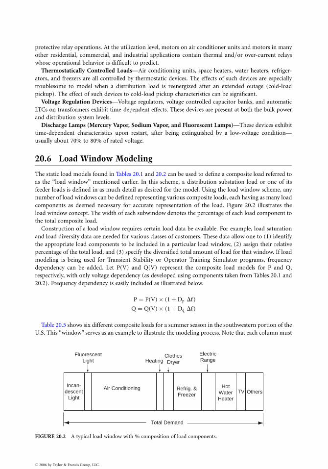
protective relay operations. At the utilization level, motors on air conditioner units and motors in many
other residential, commercial, and industrial applications contain thermal and=or over-current relays
whose operational behavior is difficult to predict.
Thermostatically Controlled Loads—Air conditioning units, space heaters, water heaters, refriger-
ators, and freezers are all controlled by thermostatic devices. The effects of such devices are especially
troublesome to model when a distribution load is reenergized after an extended outage (cold-load
pickup). The effect of such devices to cold-load pickup characteristics can be significant.
Voltage Regulation Devices—Voltage regulators, voltage controlled capacitor banks, and automatic
LTCs on transformers exhibit time-dependent effects. These devices are present at both the bulk power
and distribution system levels.
Discharge Lamps (Mercury Vapor, Sodium Vapor, and Fluorescent Lamps)—These devices exhibit
time-dependent characteristics upon restart, after being extinguished by a low-voltage condition—
usually about 70% to 80% of rated voltage.
20.6 Load Window Modeling
The static load models found in Tables 20.1 and 20.2 can be used to define a composite load referred to
as the ‘‘load window’’ mentioned earlier. In this scheme, a distribution substation load or one of its
feeder loads is defined in as much detail as desired for the model. Using the load window scheme, any
number of load windows can be defined representing various composite loads, each having as many load
components as deemed necessary for accurate representation of the load. Figure 20.2 illustrates the
load window concept. The width of each subwindow denotes the percentage of each load component to
the total composite load.
Construction of a load window requires certain load data be available. For example, load saturation
and load diversity data are needed for various classes of customers. These data allow one to (1) identify
the appropriate load components to be included in a particular load window, (2) assign their relative
percentage of the total load, and (3) specify the diversified total amount of load for that window. If load
modeling is being used for Transient Stability or Operator Training Simulator programs, frequency
dependency can be added. Let P(V) and Q(V) represent the composite load models for P and Q,
respectively, with only voltage dependency (as developed using components taken from Tables 20.1 and
20.2). Frequency dependency is easily included as illustrated below.
P ¼ P(V)� (1þDp Df )
Q ¼ Q(V)� (1þ Dq Df )
Table 20.5 shows six different composite loads for a summer season in the southwestern portion of the
U.S. This ‘‘window’’ serves as an example to illustrate the modeling process. Note that each column must
FluorescentLight
Incan-descent
Light
Air Conditioning Refrig. &Freezer
HotWater Heater
TV Others
HeatingClothes Dryer
Electric Range
Total Demand
FIGURE 20.2 A typical load window with % composition of load components.
� 2006 by Taylor & Francis Group, LLC.
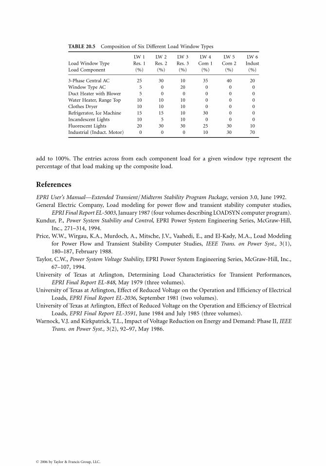
TABLE 20.5 Composition of Six Different Load Window Types
LW 1 LW 2 LW 3 LW 4 LW 5 LW 6
Load Window Type Res. 1 Res. 2 Res. 3 Com 1 Com 2 Indust
Load Component (%) (%) (%) (%) (%) (%)
3-Phase Central AC 25 30 10 35 40 20
Window Type AC 5 0 20 0 0 0
Duct Heater with Blower 5 0 0 0 0 0
Water Heater, Range Top 10 10 10 0 0 0
Clothes Dryer 10 10 10 0 0 0
Refrigerator, Ice Machine 15 15 10 30 0 0
Incandescent Lights 10 5 10 0 0 0
Fluorescent Lights 20 30 30 25 30 10
Industrial (Induct. Motor) 0 0 0 10 30 70
add to 100%. The entries across from each component load for a given window type represent the
percentage of that load making up the composite load.
References
EPRI User’s Manual—Extended Transient=Midterm Stability Program Package, version 3.0, June 1992.
General Electric Company, Load modeling for power flow and transient stability computer studies,
EPRI Final Report EL-5003, January 1987 (four volumes describing LOADSYN computer program).
Kundur, P., Power System Stability and Control, EPRI Power System Engineering Series, McGraw-Hill,
Inc., 271–314, 1994.
Price, W.W., Wirgau, K.A., Murdoch, A., Mitsche, J.V., Vaahedi, E., and El-Kady, M.A., Load Modeling
for Power Flow and Transient Stability Computer Studies, IEEE Trans. on Power Syst., 3(1),
180–187, February 1988.
Taylor, C.W., Power System Voltage Stability, EPRI Power System Engineering Series, McGraw-Hill, Inc.,
67–107, 1994.
University of Texas at Arlington, Determining Load Characteristics for Transient Performances,
EPRI Final Report EL-848, May 1979 (three volumes).
University of Texas at Arlington, Effect of Reduced Voltage on the Operation and Efficiency of Electrical
Loads, EPRI Final Report EL-2036, September 1981 (two volumes).
University of Texas at Arlington, Effect of Reduced Voltage on the Operation and Efficiency of Electrical
Loads, EPRI Final Report EL-3591, June 1984 and July 1985 (three volumes).
Warnock, V.J. and Kirkpatrick, T.L., Impact of Voltage Reduction on Energy and Demand: Phase II, IEEE
Trans. on Power Syst., 3(2), 92–97, May 1986.
� 2006 by Taylor & Francis Group, LLC.
21
� 2006 by Taylor & Francis Group, LLC.
Distribution SystemModeling and Analysis
William H. Kersting
21.1 Modeling .......................................................................... 21-1Line Impedance . Shunt Admittance . Line Segment
Models . Step-Voltage Regulators . Transformer Bank
Connections . Load Models . Shunt Capacitor Models
21.2 Analysis........................................................................... 21-44Power-Flow Analysis
New Mexico State University21.1 Modeling
Radial distribution feeders are characterized by having only one path for power to flow from the source
(distribution substation) to each customer. A typical distribution system will consist of one or more
distribution substations consisting of one or more ‘‘feeders.’’ Components of the feeder may consist of
the following:
. Three-phase primary ‘‘main’’ feeder
. Three-phase, two-phase (‘‘V’’ phase), and single-phase laterals
. Step-type voltage regulators or load tap changing transformer (LTC)
. In-line transformers
. Shunt capacitor banks
. Three-phase, two-phase, and single-phase loads
. Distribution transformers (step-down to customer’s voltage)
The loading of a distribution feeder is inherently unbalanced because of the large number of unequal
single-phase loads that must be served. An additional unbalance is introduced by the nonequilateral
conductor spacings of the three-phase overhead and underground line segments.
Because of the nature of the distribution system, conventional power-flow and short-circuit programs
used for transmission system studies are not adequate. Such programs display poor convergence
characteristics for radial systems. The programs also assume a perfectly balanced system so that a
single-phase equivalent system is used.
If a distribution engineer is to be able to perform accurate power-flow and short-circuit studies, it is
imperative that the distribution feeder be modeled as accurately as possible. This means that three-phase
models of the major components must be utilized. Three-phase models for the major components will
be developed in the following sections. The models will be developed in the ‘‘phase frame’’ rather than
applying the method of symmetrical components.
Figure 21.1 shows a simple one-line diagram of a three-phase feeder; it illustrates the major
components of a distribution system. The connecting points of the components will be referred to as
‘‘nodes.’’ Note in the figure that the phasing of the line segments is shown. This is important if the most
accurate models are to be developed.
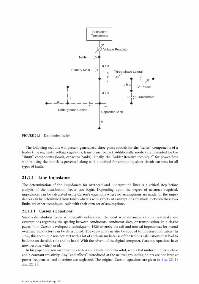
SubstationTransformer
Voltage Regulator
Three-phase Lateral
Transformer
“V” Phase
Node
a b c
c b a
a b c
c
a
ca
a
abc
bc
Primary Main
Underground CablesCapacitor Bank
FIGURE 21.1 Distribution feeder.
The following sections will present generalized three-phase models for the ‘‘series’’ components of a
feeder (line segments, voltage regulators, transformer banks). Additionally, models are presented for the
‘‘shunt’’ components (loads, capacitor banks). Finally, the ‘‘ladder iterative technique’’ for power-flow
studies using the models is presented along with a method for computing short-circuit currents for all
types of faults.
21.1.1 Line Impedance
The determination of the impedances for overhead and underground lines is a critical step before
analysis of the distribution feeder can begin. Depending upon the degree of accuracy required,
impedances can be calculated using Carson’s equations where no assumptions are made, or the impe-
dances can be determined from tables where a wide variety of assumptions are made. Between these two
limits are other techniques, each with their own set of assumptions.
21.1.1.1 Carson’s Equations
Since a distribution feeder is inherently unbalanced, the most accurate analysis should not make any
assumptions regarding the spacing between conductors, conductor sizes, or transposition. In a classic
paper, John Carson developed a technique in 1926 whereby the self and mutual impedances for ncond
overhead conductors can be determined. The equations can also be applied to underground cables. In
1926, this technique was not met with a lot of enthusiasm because of the tedious calculations that had to
be done on the slide rule and by hand. With the advent of the digital computer, Carson’s equations have
now become widely used.
In his paper, Carson assumes the earth is an infinite, uniform solid, with a flat uniform upper surface
and a constant resistivity. Any ‘‘end effects’’ introduced at the neutral grounding points are not large at
power frequencies, and therefore are neglected. The original Carson equations are given in Eqs. (21.1)
and (21.2).
� 2006 by Taylor & Francis Group, LLC.
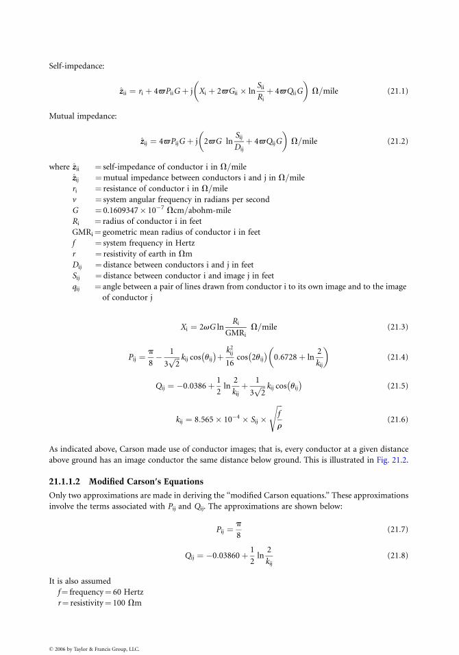
Self-impedance:
zzii ¼ ri þ 4ˆPiiG þ j Xi þ 2ˆGii � lnSii
Ri
þ 4ˆQiiG
� �
V=mile (21:1)
Mutual impedance:
zzij ¼ 4ˆPijG þ j 2ˆG lnSij
Dij
þ 4ˆQijG
� �
V=mile (21:2)
where zzii ¼ self-impedance of conductor i in V=mile
zzij ¼mutual impedance between conductors i and j in V=mile
ri ¼ resistance of conductor i in V=mile
v ¼ system angular frequency in radians per second
G ¼ 0.1609347� 10�7 Vcm=abohm-mile
Ri ¼ radius of conductor i in feet
GMRi¼ geometric mean radius of conductor i in feet
f ¼ system frequency in Hertz
r ¼ resistivity of earth in Vm
Dij ¼ distance between conductors i and j in feet
Sij ¼ distance between conductor i and image j in feet
qij ¼ angle between a pair of lines drawn from conductor i to its own image and to the image
of conductor j
Xi ¼ 2vG lnRi
GMRi
V=mile (21:3)
Pij ¼p
8� 1
3ffiffiffi
2p kij cos uij
� �
þk2
ij
16cos 2uij
� �
0:6728þ ln2
kij
� �
(21:4)
Qij ¼ �0:0386þ 1
2ln
2
kij
þ 1
3ffiffiffi
2p kij cos uij
� �
(21:5)
kij ¼ 8:565� 10�4 � Sij �
ffiffiffi
f
r
s
(21:6)
As indicated above, Carson made use of conductor images; that is, every conductor at a given distance
above ground has an image conductor the same distance below ground. This is illustrated in Fig. 21.2.
21.1.1.2 Modified Carson’s Equations
Only two approximations are made in deriving the ‘‘modified Carson equations.’’ These approximations
involve the terms associated with Pij and Qij. The approximations are shown below:
Pij ¼p
8(21:7)
Qij ¼ �0:03860þ 1
2ln
2
kij
(21:8)
It is also assumed
f¼ frequency¼ 60 Hertz
r¼ resistivity¼ 100 Vm
� 2006 by Taylor & Francis Group, LLC.
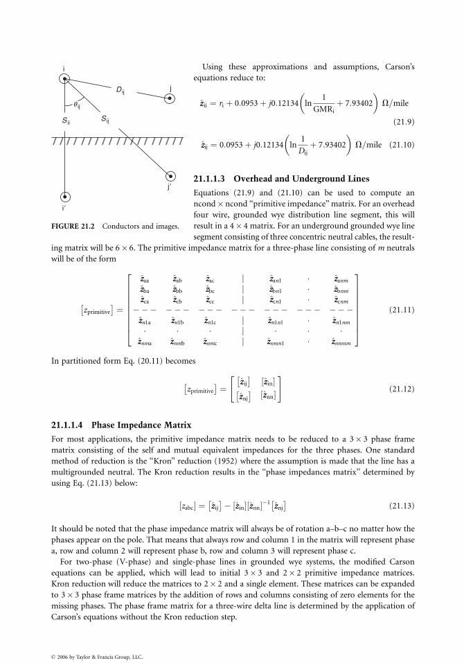
i
j
i�
j�
D ij
S ijS ii
q ij
FIGURE 21.2 Conductors and images.
� 2006 by Taylor & Francis Group, LLC.
Using these approximations and assumptions, Carson’s
equations reduce to:
zzii ¼ ri þ 0:0953þ j0:12134 ln1
GMRi
þ 7:93402
� �
V=mile
(21:9)
zzij ¼ 0:0953þ j0:12134 ln1
Dij
þ 7:93402
� �
V=mile (21:10)
21.1.1.3 Overhead and Underground Lines
Equations (21.9) and (21.10) can be used to compute an
ncond� ncond ‘‘primitive impedance’’ matrix. For an overhead
four wire, grounded wye distribution line segment, this will
result in a 4� 4 matrix. For an underground grounded wye line
segment consisting of three concentric neutral cables, the result-
ing matrix will be 6� 6. The primitive impedance matrix for a three-phase line consisting of m neutrals
will be of the form
zprimitive
� �
¼
zzaa zzab zzac j zzan1 � zzanm
zzba zzbb zzbc j zzbn1 � zzbnm
zzca zzcb zzcc j zzcn1 � zzcnm
��� ��� ��� ��� ��� ��� ���zzn1a zzn1b zzn1c j zzn1n1 � zzn1nm
� � � j � � �zznma zznmb zznmc j zznmn1 � zznmnm
2
6
6
6
6
6
6
6
6
4
3
7
7
7
7
7
7
7
7
5
(21:11)
In partitioned form Eq. (20.11) becomes
zprimitive
� �
¼"
zzij
� �
zzin½ �zznj
� �
zznn½ �
#
(21:12)
21.1.1.4 Phase Impedance Matrix
For most applications, the primitive impedance matrix needs to be reduced to a 3� 3 phase frame
matrix consisting of the self and mutual equivalent impedances for the three phases. One standard
method of reduction is the ‘‘Kron’’ reduction (1952) where the assumption is made that the line has a
multigrounded neutral. The Kron reduction results in the ‘‘phase impedances matrix’’ determined by
using Eq. (21.13) below:
zabc½ � ¼ zzij
� �
� zzin½ � zznn½ ��1zznj
� �
(21:13)
It should be noted that the phase impedance matrix will always be of rotation a–b–c no matter how the
phases appear on the pole. That means that always row and column 1 in the matrix will represent phase
a, row and column 2 will represent phase b, row and column 3 will represent phase c.
For two-phase (V-phase) and single-phase lines in grounded wye systems, the modified Carson
equations can be applied, which will lead to initial 3� 3 and 2� 2 primitive impedance matrices.
Kron reduction will reduce the matrices to 2� 2 and a single element. These matrices can be expanded
to 3� 3 phase frame matrices by the addition of rows and columns consisting of zero elements for the
missing phases. The phase frame matrix for a three-wire delta line is determined by the application of
Carson’s equations without the Kron reduction step.
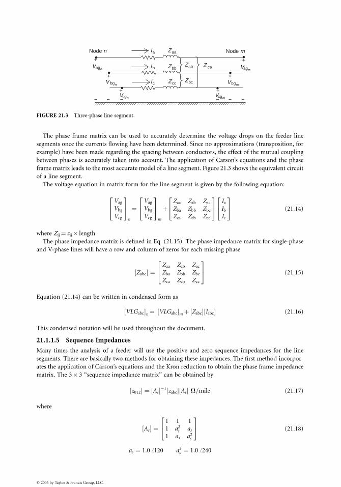
Node n Node m
Vagn
V bgn
VcgnVcgm
Vbgm
VagmZ caZab
ZbcZcc
Zbb
ZaaIa
Ib
Ic
+ +
+
+
+
+
− − − − − −
FIGURE 21.3 Three-phase line segment.
The phase frame matrix can be used to accurately determine the voltage drops on the feeder line
segments once the currents flowing have been determined. Since no approximations (transposition, for
example) have been made regarding the spacing between conductors, the effect of the mutual coupling
between phases is accurately taken into account. The application of Carson’s equations and the phase
frame matrix leads to the most accurate model of a line segment. Figure 21.3 shows the equivalent circuit
of a line segment.
The voltage equation in matrix form for the line segment is given by the following equation:
Vag
Vbg
Vcg
2
4
3
5
n
¼Vag
Vbg
Vcg
2
4
3
5
m
þZaa Zab Zac
Zba Zbb Zbc
Zca Zcb Zcc
2
4
3
5
Ia
Ib
Ic
2
4
3
5 (21:14)
where Zij¼ zij� length
The phase impedance matrix is defined in Eq. (21.15). The phase impedance matrix for single-phase
and V-phase lines will have a row and column of zeros for each missing phase
Zabc½ � ¼Zaa Zab Zac
Zba Zbb Zbc
Zca Zcb Zcc
2
4
3
5 (21:15)
Equation (21.14) can be written in condensed form as
VLGabc½ �n¼ VLGabc½ �mþ Zabc½ � Iabc½ � (21:16)
This condensed notation will be used throughout the document.
21.1.1.5 Sequence Impedances
Many times the analysis of a feeder will use the positive and zero sequence impedances for the line
segments. There are basically two methods for obtaining these impedances. The first method incorpor-
ates the application of Carson’s equations and the Kron reduction to obtain the phase frame impedance
matrix. The 3� 3 ‘‘sequence impedance matrix’’ can be obtained by
z012½ � ¼ As½ ��1 zabc½ � As½ � V=mile (21:17)
where
As½ � ¼1 1 1
1 a2s as
1 as a2s
2
4
3
5 (21:18)
as ¼ 1:0 ff120 a2s ¼ 1:0 ff240
� 2006 by Taylor & Francis Group, LLC.
The resulting sequence impedance matrix is of the form:
z012½ � ¼z00 z01 z02
z10 z11 z12
z20 z21 z22
2
4
3
5 V=mile (21:19)
where z 00¼ the zero sequence impedance
z11¼ the positive sequence impedance
z22¼ the negative sequence impedance
In the idealized state, the off-diagonal terms of Eq. (21.19) would be zero. When the off-diagonal terms
of the phase impedance matrix are all equal, the off-diagonal terms of the sequence impedance matrix
will be zero. For high-voltage transmission lines, this will generally be the case because these lines are
transposed, which causes the mutual coupling between phases (off-diagonal terms) to be equal.
Distribution lines are rarely if ever transposed. This causes unequal mutual coupling between phases,
which causes the off-diagonal terms of the phase impedance matrix to be unequal. For the nontran-
sposed line, the diagonal terms of the phase impedance matrix will also be unequal. In most cases, the
off-diagonal terms of the sequence impedance matrix are very small compared to the diagonal terms and
errors made by ignoring the off-diagonal terms are small.
Sometimes the phase impedance matrix is modified such that the three diagonal terms are equal and
all of the off-diagonal terms are equal. The usual procedure is to set the three diagonal terms of the phase
impedance matrix equal to the average of the diagonal terms of Eq. (21.15) and the off-diagonal terms
equal to the average of the off-diagonal terms of Eq. (21.15). When this is done, the self and mutual
impedances are defined as
zs ¼1
3zaa þ zbb þ zccð Þ (21:20)
zm ¼1
3zab þ zbc þ zcað Þ (21:21)
The phase impedance matrix is now defined as
zabc½ � ¼zs zm zm
zm zs zm
zm zm zs
2
4
3
5 (21:22)
When Eq. (21.17) is used with this phase impedance matrix, the resulting sequence matrix is diagonal
(off-diagonal terms are zero). The sequence impedances can be determined directly as
z00 ¼ zs þ 2zm
z11 ¼ z22¼ zs � zm
(21:23)
A second method that is commonly used to determine the sequence impedances directly is to employ
the concept of geometric mean distances (GMDs). The GMD between phases is defined as
Dij ¼ GMDij ¼ffiffiffiffiffiffiffiffiffiffiffiffiffiffiffiffiffiffiffiffiffi
DabD bcDca3p
(21:24)
The GMD between phases and neutral is defined as
Din ¼ GMDin ¼ffiffiffiffiffiffiffiffiffiffiffiffiffiffiffiffiffiffiffiffiffiffi
DanD bnDcn3p
(21:25)
� 2006 by Taylor & Francis Group, LLC.
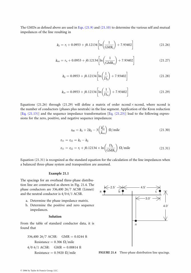
The GMDs as defined above are used in Eqs. (21.9) and (21.10) to determine the various self and mutual
impedances of the line resulting in
zzii ¼ ri þ 0:0953þ j0:12134 ln1
GMRi
� �
þ 7:93402
(21:26)
zznn ¼ rn þ 0:0953þ j0:12134 ln1
GMRn
� �
þ 7:93402
(21:27)
zzij ¼ 0:0953þ j0:12134 ln1
Dij
� �
þ 7:93402
(21:28)
zzin ¼ 0:0953þ j0:12134 ln1
Din
� �
þ 7:93402
(21:29)
Equations (21.26) through (21.29) will define a matrix of order ncond� ncond, where ncond is
the number of conductors (phases plus neutrals) in the line segment. Application of the Kron reduction
[Eq. (21.13)] and the sequence impedance transformation [Eq. (21.23)] lead to the following expres-
sions for the zero, positive, and negative sequence impedances:
z00 ¼ zzii þ 2zzij � 3zz2
in
zznn
� �
V=mile (21:30)
z11 ¼ z22 ¼ zzii � zzij
z11 ¼ z22 ¼ ri þ j0:12134� lnDij
GMRi
� �
V=mile (21:31)
Equation (21.31) is recognized as the standard equation for the calculation of the line impedances when
a balanced three-phase system and transposition are assumed.
Example 21.1
a b c
n
4.5�
3.0�
4.0�
2.5�
FIGURE 21.4 Three-phase distribution line spacings.
The spacings for an overhead three-phase distribu-
tion line are constructed as shown in Fig. 21.4. The
phase conductors are 336,400 26=7 ACSR (Linnet)
and the neutral conductor is 4=0 6=1 ACSR.
a. Determine the phase impedance matrix.
b. Determine the positive and zero sequence
impedances.
Solution
From the table of standard conductor data, it is
found that
336,400 26=7 ACSR: GMR ¼ 0:0244 ft
Resistance ¼ 0:306 V=mile
4=0 6=1 ACSR: GMR ¼ 0:00814 ft
Resistance ¼ 0:5920 V=mile
� 2006 by Taylor & Francis Group, LLC.
From Fig. 21.4 the following distances between conductors can be determined:
Dab ¼ 2:5 ft D bc ¼ 4:5 ft Dca ¼ 7:0 ft
Dan ¼ 5:6569 ft D bn ¼ 4:272 ft Dcn ¼ 5:0 ft
Applying Carson’s modified equations [Eqs. (21.9) and (21.10)] results in the primitive impedance
matrix.
zz½ � ¼
0:4013þ j1:4133 0:0953þ j0:8515 0:0953þ j0:7266 0:0953þ j0:7524
0:0953þ j0:8515 0:4013þ j1:4133 0:0953þ j0:7802 0:0953þ j0:7865
0:0953þ j0:7266 0:0953þ j0:7802 0:4013þ j1:4133 0:0953þ j0:7674
0:0953þ j0:7524 0:0953þ j0:7865 0:0953þ j:7674 0:6873þ j1:5465
2
6
6
4
3
7
7
5
(21:32)
The Kron reduction of Eq. (21.13) results in the phase impedance matrix
zabc½ � ¼0:4576þ j1:0780 0:1560þ j0:5017 0:1535þ j0:3849
0:1560þ j0:5017 0:4666þ j1:0482 0:1580þ j0:4236
0:1535þ j0:3849 0:1580þ j0:4236 0:4615þ j1:0651
2
4
3
5 V=mile (21:33)
The phase impedance matrix of Eq. (21.33) can be transformed into the sequence impedance matrix
with the application of Eq. (21.17)
z012½ � ¼0:7735þ j1:9373 0:0256þ j0:0115 �0:0321þ j0:0159
�0:0321þ j0:0159 0:3061þ j0:6270 �0:0723� j0:0060
0:0256þ j0:0115 0:0723� j0:0059 0:3061þ j0:6270
2
4
3
5 V=mile (21:34)
In Eq. (21.34), the 1,1 term is the zero sequence impedance, the 2,2 term is the positive sequence
impedance, and the 3,3 term is the negative sequence impedance. Note that the off-diagonal terms
are not zero, which implies that there is mutual coupling between sequences. This is a result of the
nonsymmetrical spacing between phases. With the off-diagonal terms nonzero, the three sequence
networks representing the line will not be independent. However, it is noted that the off-diagonal
terms are small relative to the diagonal terms.
In high-voltage transmission lines, it is usually assumed that the lines are transposed and that the
phase currents represent a balanced three-phase set. The transposition can be simulated in this example
by replacing the diagonal terms of Eq. (21.33) with the average value of the diagonal terms
(0.4619þ j1.0638) and replacing each off-diagonal term with the average of the off-diagonal terms
(0.1558þ j0.4368). This modified phase impedance matrix becomes
z1abc½ � ¼0:3619þ j1:0638 0:1558þ j0:4368 0:1558þ j0:4368
0:1558þ j0:4368 0:3619þ j1:0638 0:1558þ j0:4368
0:1558þ j0:4368 0:1558þ j0:4368 0:3619þ j1:0638
2
4
3
5 V=mile (21:35)
Using this modified phase impedance matrix in the symmetrical component transformation, Eq. (21.17)
results in the modified sequence impedance matrix
z1012½ � ¼0:7735þ j1:9373 0 0
0 0:3061þ j0:6270 0
0 0 0:3061þ j0:6270
2
4
3
5 V=mile (21:36)
Note now that the off-diagonal terms are all equal to zero, meaning that there is no mutual coupling
between sequence networks. It should also be noted that the zero, positive, and negative sequence
impedances of Eq. (21.36) are exactly equal to the same sequence impedances of Eq. (21.34).
� 2006 by Taylor & Francis Group, LLC.
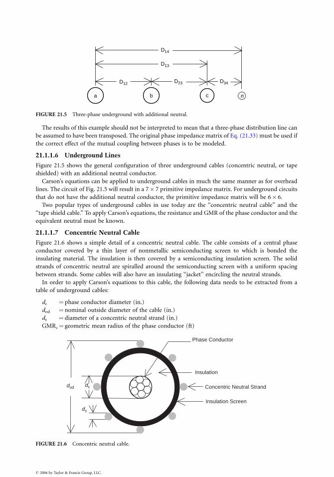
D14
D13
D12
a b c n
D23 D34
FIGURE 21.5 Three-phase underground with additional neutral.
The results of this example should not be interpreted to mean that a three-phase distribution line can
be assumed to have been transposed. The original phase impedance matrix of Eq. (21.33) must be used if
the correct effect of the mutual coupling between phases is to be modeled.
21.1.1.6 Underground Lines
Figure 21.5 shows the general configuration of three underground cables (concentric neutral, or tape
shielded) with an additional neutral conductor.
Carson’s equations can be applied to underground cables in much the same manner as for overhead
lines. The circuit of Fig. 21.5 will result in a 7� 7 primitive impedance matrix. For underground circuits
that do not have the additional neutral conductor, the primitive impedance matrix will be 6� 6.
Two popular types of underground cables in use today are the ‘‘concentric neutral cable’’ and the
‘‘tape shield cable.’’ To apply Carson’s equations, the resistance and GMR of the phase conductor and the
equivalent neutral must be known.
21.1.1.7 Concentric Neutral Cable
Figure 21.6 shows a simple detail of a concentric neutral cable. The cable consists of a central phase
conductor covered by a thin layer of nonmetallic semiconducting screen to which is bonded the
insulating material. The insulation is then covered by a semiconducting insulation screen. The solid
strands of concentric neutral are spiralled around the semiconducting screen with a uniform spacing
between strands. Some cables will also have an insulating ‘‘jacket’’ encircling the neutral strands.
In order to apply Carson’s equations to this cable, the following data needs to be extracted from a
table of underground cables:
dc ¼ phase conductor diameter (in.)
dod ¼ nominal outside diameter of the cable (in.)
ds ¼ diameter of a concentric neutral strand (in.)
GMRc¼ geometric mean radius of the phase conductor (ft)
Phase Conductor
Insulation
dod dc
ds
Insulation Screen
Concentric Neutral Strand
FIGURE 21.6 Concentric neutral cable.
� 2006 by Taylor & Francis Group, LLC.
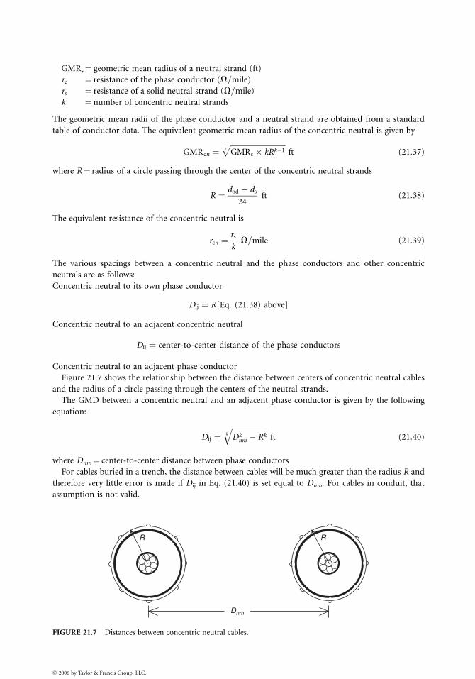
GMRs¼ geometric mean radius of a neutral strand (ft)
rc ¼ resistance of the phase conductor (V=mile)
rs ¼ resistance of a solid neutral strand (V=mile)
k ¼ number of concentric neutral strands
The geometric mean radii of the phase conductor and a neutral strand are obtained from a standard
table of conductor data. The equivalent geometric mean radius of the concentric neutral is given by
GMRcn ¼ffiffiffiffiffiffiffiffiffiffiffiffiffiffiffiffiffiffiffiffiffiffiffiffiffiffiffiffiffiffi
GMRs � kRk�1kp
ft (21:37)
where R¼ radius of a circle passing through the center of the concentric neutral strands
R ¼ dod � ds
24ft (21:38)
The equivalent resistance of the concentric neutral is
rcn ¼rs
kV=mile (21:39)
The various spacings between a concentric neutral and the phase conductors and other concentric
neutrals are as follows:
Concentric neutral to its own phase conductor
Dij ¼ R[Eq: (21:38) above]
Concentric neutral to an adjacent concentric neutral
Dij ¼ center-to-center distance of the phase conductors
Concentric neutral to an adjacent phase conductor
Figure 21.7 shows the relationship between the distance between centers of concentric neutral cables
and the radius of a circle passing through the centers of the neutral strands.
The GMD between a concentric neutral and an adjacent phase conductor is given by the following
equation:
Dij ¼ffiffiffiffiffiffiffiffiffiffiffiffiffiffiffiffiffiffiffi
Dknm � Rkk
q
ft (21:40)
where Dnm¼ center-to-center distance between phase conductors
For cables buried in a trench, the distance between cables will be much greater than the radius R and
therefore very little error is made if Dij in Eq. (21.40) is set equal to Dnm. For cables in conduit, that
assumption is not valid.
Dnm
R R
FIGURE 21.7 Distances between concentric neutral cables.
� 2006 by Taylor & Francis Group, LLC.
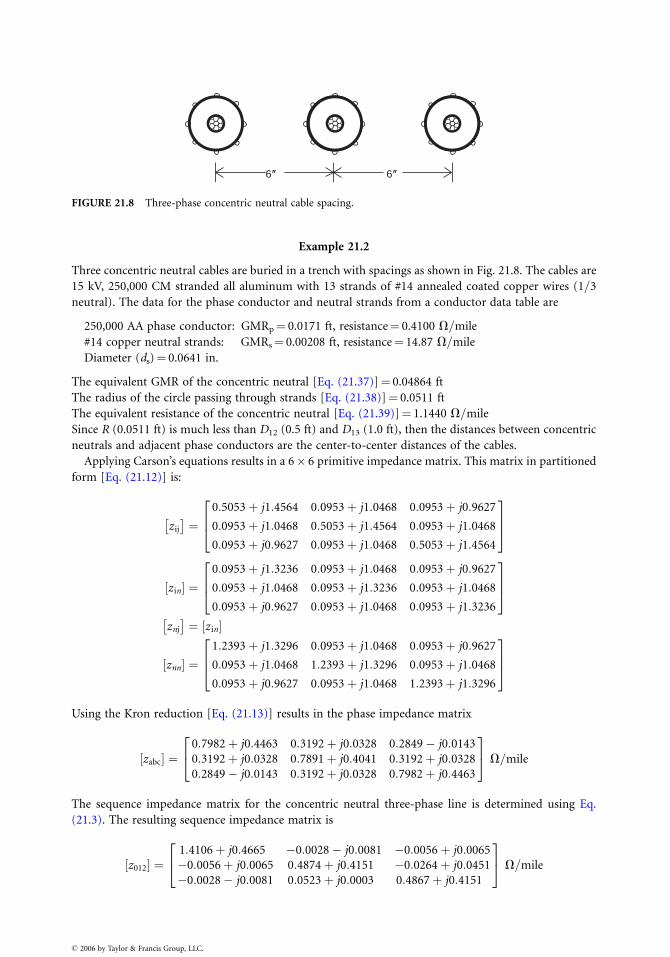
6 0 6 0
FIGURE 21.8 Three-phase concentric neutral cable spacing.
Example 21.2
Three concentric neutral cables are buried in a trench with spacings as shown in Fig. 21.8. The cables are
15 kV, 250,000 CM stranded all aluminum with 13 strands of #14 annealed coated copper wires (1=3
neutral). The data for the phase conductor and neutral strands from a conductor data table are
250,000 AA phase conductor: GMRp¼ 0.0171 ft, resistance¼ 0.4100 V=mile
#14 copper neutral strands: GMRs¼ 0.00208 ft, resistance¼ 14.87 V=mile
Diameter (ds)¼ 0.0641 in.
The equivalent GMR of the concentric neutral [Eq. (21.37)]¼ 0.04864 ft
The radius of the circle passing through strands [Eq. (21.38)]¼ 0.0511 ft
The equivalent resistance of the concentric neutral [Eq. (21.39)]¼ 1.1440 V=mile
Since R (0.0511 ft) is much less than D12 (0.5 ft) and D13 (1.0 ft), then the distances between concentric
neutrals and adjacent phase conductors are the center-to-center distances of the cables.
Applying Carson’s equations results in a 6� 6 primitive impedance matrix. This matrix in partitioned
form [Eq. (21.12)] is:
z ij
� �
¼0:5053þ j1:4564 0:0953þ j1:0468 0:0953þ j0:9627
0:0953þ j1:0468 0:5053þ j1:4564 0:0953þ j1:0468
0:0953þ j0:9627 0:0953þ j1:0468 0:5053þ j1:4564
2
6
4
3
7
5
z in½ � ¼0:0953þ j1:3236 0:0953þ j1:0468 0:0953þ j0:9627
0:0953þ j1:0468 0:0953þ j1:3236 0:0953þ j1:0468
0:0953þ j0:9627 0:0953þ j1:0468 0:0953þ j1:3236
2
6
4
3
7
5
znj
� �
¼ z in½ �
znn½ � ¼1:2393þ j1:3296 0:0953þ j1:0468 0:0953þ j0:9627
0:0953þ j1:0468 1:2393þ j1:3296 0:0953þ j1:0468
0:0953þ j0:9627 0:0953þ j1:0468 1:2393þ j1:3296
2
6
4
3
7
5
Using the Kron reduction [Eq. (21.13)] results in the phase impedance matrix
zabc½ � ¼0:7982þ j0:4463 0:3192þ j0:0328 0:2849� j0:0143
0:3192þ j0:0328 0:7891þ j0:4041 0:3192þ j0:0328
0:2849� j0:0143 0:3192þ j0:0328 0:7982þ j0:4463
2
4
3
5 V=mile
The sequence impedance matrix for the concentric neutral three-phase line is determined using Eq.
(21.3). The resulting sequence impedance matrix is
z012½ � ¼1:4106þ j0:4665 �0:0028� j0:0081 �0:0056þ j0:0065
�0:0056þ j0:0065 0:4874þ j0:4151 �0:0264þ j0:0451
�0:0028� j0:0081 0:0523þ j0:0003 0:4867þ j0:4151
2
4
3
5 V=mile
� 2006 by Taylor & Francis Group, LLC.
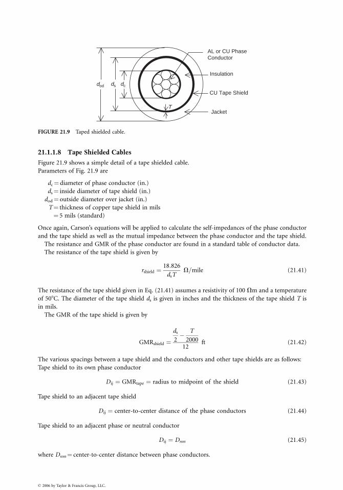
AL or CU PhaseConductor
Insulation
dod ds dc
JacketT
CU Tape Shield
FIGURE 21.9 Taped shielded cable.
21.1.1.8 Tape Shielded Cables
Figure 21.9 shows a simple detail of a tape shielded cable.
Parameters of Fig. 21.9 are
dc¼diameter of phase conductor (in.)
ds¼ inside diameter of tape shield (in.)
dod¼ outside diameter over jacket (in.)
T¼ thickness of copper tape shield in mils
¼ 5 mils (standard)
Once again, Carson’s equations will be applied to calculate the self-impedances of the phase conductor
and the tape shield as well as the mutual impedance between the phase conductor and the tape shield.
The resistance and GMR of the phase conductor are found in a standard table of conductor data.
The resistance of the tape shield is given by
rshield ¼18:826
dsTV=mile (21:41)
The resistance of the tape shield given in Eq. (21.41) assumes a resistivity of 100 Vm and a temperature
of 508C. The diameter of the tape shield ds is given in inches and the thickness of the tape shield T is
in mils.
The GMR of the tape shield is given by
GMRshield ¼ds
2� T
200012
ft (21:42)
The various spacings between a tape shield and the conductors and other tape shields are as follows:
Tape shield to its own phase conductor
Dij ¼ GMRtape ¼ radius to midpoint of the shield (21:43)
Tape shield to an adjacent tape shield
Dij ¼ center-to-center distance of the phase conductors (21:44)
Tape shield to an adjacent phase or neutral conductor
Dij ¼ Dnm (21:45)
where Dnm¼ center-to-center distance between phase conductors.
� 2006 by Taylor & Francis Group, LLC.
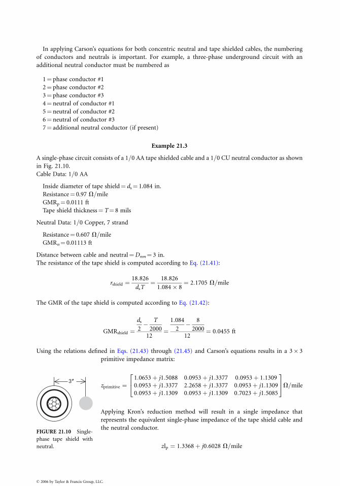
In applying Carson’s equations for both concentric neutral and tape shielded cables, the numbering
of conductors and neutrals is important. For example, a three-phase underground circuit with an
additional neutral conductor must be numbered as
1¼ phase conductor #1
2¼ phase conductor #2
3¼ phase conductor #3
4¼ neutral of conductor #1
5¼ neutral of conductor #2
6¼ neutral of conductor #3
7¼ additional neutral conductor (if present)
Example 21.3
A single-phase circuit consists of a 1=0 AA tape shielded cable and a 1=0 CU neutral conductor as shown
in Fig. 21.10.
Cable Data: 1=0 AA
Inside diameter of tape shield¼ ds¼ 1.084 in.
Resistance¼ 0.97 V=mile
GMRp¼ 0.0111 ft
Tape shield thickness¼T¼ 8 mils
Neutral Data: 1=0 Copper, 7 strand
Resistance¼ 0.607 V=mile
GMRn¼ 0.01113 ft
Distance between cable and neutral¼Dnm¼ 3 in.
The resistance of the tape shield is computed according to Eq. (21.41):
rshield ¼18:826
dsT¼ 18:826
1:084� 8¼ 2:1705 V=mile
The GMR of the tape shield is computed according to Eq. (21.42):
GMRshield ¼ds
2� T
200012
¼1:084
2� 8
200012
¼ 0:0455 ft
Using the relations defined in Eqs. (21.43) through (21.45) and Carson’s equations results in a 3� 3
3 0
FIGURE 21.10 Single-
phase tape shield with
neutral.
� 2006 by Taylor & Francis Group, LL
primitive impedance matrix:
zprimitive ¼1:0653þ j1:5088 0:0953þ j1:3377 0:0953þ 1:1309
0:0953þ j1:3377 2:2658þ j1:3377 0:0953þ j1:1309
0:0953þ j1:1309 0:0953þ j1:1309 0:7023þ j1:5085
2
4
3
5V=mile
Applying Kron’s reduction method will result in a single impedance that
represents the equivalent single-phase impedance of the tape shield cable and
the neutral conductor.
zlp ¼ 1:3368þ j0:6028 V=mile
C.
21.1.2 Shunt Admittance
When a high-voltage transmission line is less than 50 miles in length, the shunt capacitance of the line is
typically ignored. For lightly loaded distribution lines, particularly underground lines, the shunt
capacitance should be modeled.
The basic equation for the relationship between the charge on a conductor to the voltage drop
between the conductor and ground is given by
Qn ¼ CngVng (21:46)
where Qn¼ charge on the conductor
Cng¼ capacitance between the conductor and ground
Vng¼ voltage between the conductor and ground
For a line consisting of ncond (number of phase plus number of neutral) conductors, Eq. (21.46) can be
written in condensed matrix form as
Q½ � ¼ C½ � V½ � (21:47)
where [Q]¼ column vector of order ncond
[C]¼ ncond� ncond matrix
[V]¼ column vector of order ncond
Equation (21.47) can be solved for the voltages
V½ � ¼ C½ ��1Q½ � ¼ P½ � Q½ � (21:48)
where P½ � ¼ C½ ��1(21:49)
21.1.2.1 Overhead Lines
The determination of the shunt admittance of overhead lines starts with the calculation of the ‘‘potential
coefficient matrix’’ (Glover and Sarma, 1994). The elements of the matrix are determined by
P ii ¼ 11:17689� lnS ii
RD i
(21:50)
P ij ¼ 11:17689� lnS ij
D ij
(21:51)
See Fig. 21.2 for the following definitions.
Sii¼ distance between a conductor and its image below ground in feet
Sij¼ distance between conductor i and the image of conductor j below ground in feet
Dij¼ overhead spacing between two conductors in feet
RDi¼ radius of conductor i in feet
The potential coefficient matrix will be an ncond� ncond matrix. If one or more of the conductors
is a grounded neutral, then the matrix must be reduced using the Kron method to an nphase� nphase
matrix [Pabc].
The inverse of the potential coefficient matrix will give the nphase� nphase capacitance matrix [Cabc].
The shunt admittance matrix is given by
yabc½ � ¼ jv Cabc½ � mS/mile (21:52)
where v¼ 2pf¼ 376.9911
� 2006 by Taylor & Francis Group, LLC.
Example 21.4
Determine the shunt admittance matrix for the overhead line of Example 21.1. Assume that the neutral
conductor is 25 ft above ground.
Solution
For this configuration, the image spacing matrix is computed to be
S½ � ¼
58 58:0539 58:4209 54:1479
58:0539 58 58:1743 54:0208
58:4209 58:1743 58 54:0833
54:1479 54:0208 54:0835 50
2
6
6
4
3
7
7
5
ft
The primitive potential coefficient matrix is computed to be
Pprimitive
� �
¼
84:56 35:1522 23:7147 25:2469
35:4522 84:56 28:6058 28:359
23:7147 28:6058 84:56 26:6131
25:2469 28:359 26:6131 85:6659
2
6
6
4
3
7
7
5
Kron reduce to a 3� 3 matrix
P½ � ¼77:1194 26:7944 15:8714
26:7944 75:172 19:7957
15:8714 19:7957 76:2923
2
4
3
5
Invert [P] to determine the shunt capacitance matrix
Yabc½ � ¼ j376:9911 Cabc½ � ¼j5:6711 �j1:8362 �j0:7033
�j1:8362 j5:9774 �j1:169
�j0:7033 �j1:169 j5:391
2
4
3
5 mS=mile
Multiply [Cabc] by the radian frequency to determine the final three-phase shunt admittance matrix.
21.1.2.2 Underground Lines
Because the electric fields of underground cables are confined to the space between the phase conductor
and its concentric neutral to tape shield, the calculation of the shunt admittance matrix requires only the
determination of the ‘‘self ’’ admittance terms.
21.1.2.3 Concentric Neutral
The self-admittance in mS=mile for a concentric neutral cable is given by
Ycn ¼ j77:582
lnRb
Ra
� �
� 1
kln
kRn
Rb
� � (21:53)
where Rb¼ radius of a circle to center of concentric neutral strands (ft)
Ra¼ radius of phase conductor (ft)
Rn¼ radius of concentric neutral strand (ft)
k ¼ number of concentric neutral strands
� 2006 by Taylor & Francis Group, LLC.
Example 21.5
Determine the three-phase shunt admittance matrix for the concentric neutral line of Example 21.2.
Solution
Rb ¼ R ¼ 0:0511 ft
Diameter of the 250,000 AA phase conductor¼ 0.567 in.
Ra ¼0:567
24¼ 0:0236 ft
Diameter of the #14 CU concentric neutral strand¼ 0.0641 in.
Rn ¼0:0641
24¼ 0:0027 ft
Substitute into Eq. (21.53):
Ycn ¼ j77:582
lnRb
Ra
� �
� 1
kln
kRn
Rb
� � ¼ j77:582
ln0:0511
0:0236
� �
� 1
13ln
13� 0:0027
0:0511
� � ¼ j96:8847
The three-phase shunt admittance matrix is:
Yabc½ � ¼j96:8847 0 0
0 j96:8847 0
0 0 j96:8847
2
4
3
5 mS=mile
21.1.2.4 Tape Shield Cable
The shunt admittance in mS=mile for tape shielded cables is given by
Yts ¼ j77:586
lnRb
Ra
� � mS=mile (21:54)
where Rb¼ inside radius of the tape shield
Ra¼ radius of phase conductor
Example 21.6
Determine the shunt admittance of the single-phase tape shielded cable of Example 21.3 in
Section 21.1.1.
Solution
Rb ¼ds
24¼ 1:084
24¼ 0:0452
The diameter of the 1=0 AA phase conductor¼ 0.368 in.
Ra ¼dp
24¼ 0:368
24¼ 0:0153
� 2006 by Taylor & Francis Group, LLC.
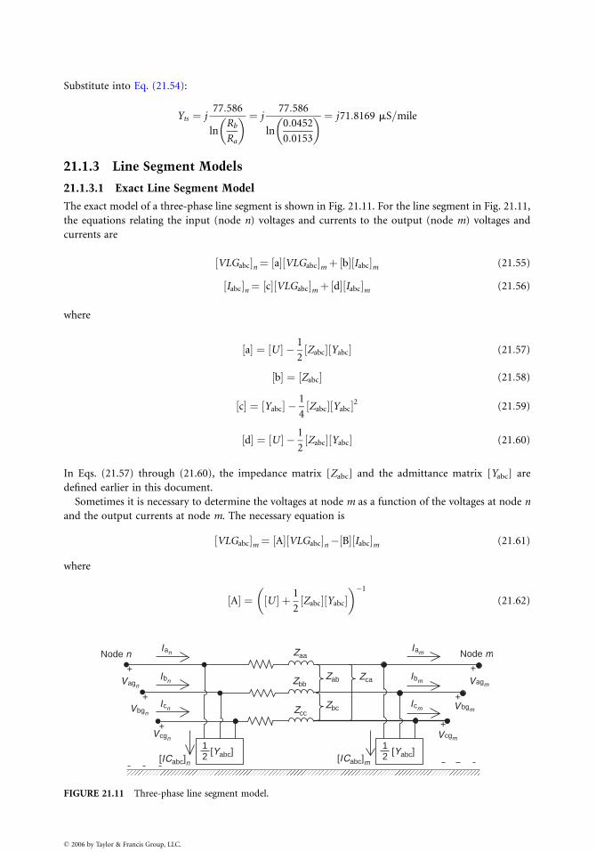
Substitute into Eq. (21.54):
Yts ¼ j77:586
lnRb
Ra
� � ¼ j77:586
ln0:0452
0:0153
� � ¼ j71:8169 mS=mile
21.1.3 Line Segment Models
21.1.3.1 Exact Line Segment Model
The exact model of a three-phase line segment is shown in Fig. 21.11. For the line segment in Fig. 21.11,
the equations relating the input (node n) voltages and currents to the output (node m) voltages and
currents are
VLGabc½ �n¼ a½ � VLGabc½ �mþ b½ � Iabc½ �m (21:55)
Iabc½ �n¼ c½ � VLGabc½ �mþ d½ � Iabc½ �m (21:56)
where
a½ � ¼ U½ � � 1
2Zabc½ � Yabc½ � (21:57)
b½ � ¼ Zabc½ � (21:58)
c½ � ¼ Yabc½ � � 1
4Zabc½ � Yabc½ �2 (21:59)
d½ � ¼ U½ � � 1
2Zabc½ � Yabc½ � (21:60)
In Eqs. (21.57) through (21.60), the impedance matrix [Zabc] and the admittance matrix [Yabc] are
defined earlier in this document.
Sometimes it is necessary to determine the voltages at node m as a function of the voltages at node n
and the output currents at node m. The necessary equation is
VLGabc½ �m¼ A½ � VLGabc½ �n� B½ � Iabc½ �m (21:61)
where
A½ � ¼ U½ � þ 1
2Zabc½ � Yabc½ �
� ��1
(21:62)
NNNNNNNode n
Vagn
Vcgn
Zaa
Zbb
Zcc
Zca
Zbc
[Yabc][ICabc]n [ICabc]m
12
Zab
Icn
Ibn
Ian
Icm
Ibm
Iam
Vbgn
Node m
Vagm
Vcgm
V bgm
12 [Yabc]
+
+
+
+
+
+
FIGURE 21.11 Three-phase line segment model.
� 2006 by Taylor & Francis Group, LLC.
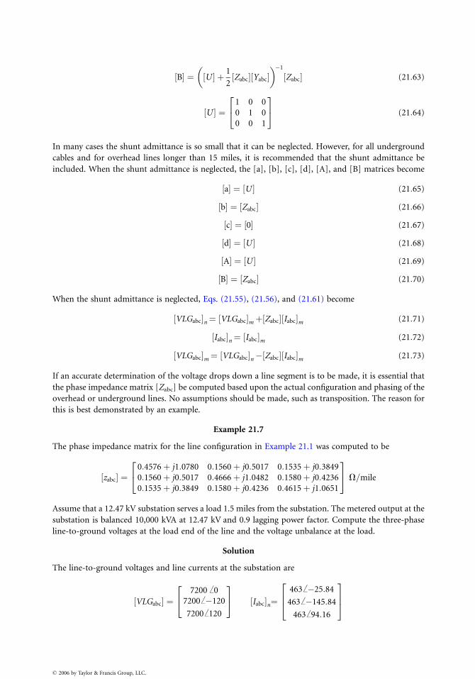
B½ � ¼ U½ � þ 1
2Zabc½ � Yabc½ �
� ��1
Zabc½ � (21:63)
U½ � ¼1 0 0
0 1 0
0 0 1
2
4
3
5 (21:64)
In many cases the shunt admittance is so small that it can be neglected. However, for all underground
cables and for overhead lines longer than 15 miles, it is recommended that the shunt admittance be
included. When the shunt admittance is neglected, the [a], [b], [c], [d], [A], and [B] matrices become
a½ � ¼ U½ � (21:65)
b½ � ¼ Zabc½ � (21:66)
c½ � ¼ 0½ � (21:67)
d½ � ¼ U½ � (21:68)
A½ � ¼ U½ � (21:69)
B½ � ¼ Zabc½ � (21:70)
When the shunt admittance is neglected, Eqs. (21.55), (21.56), and (21.61) become
VLGabc½ �n¼ VLGabc½ �mþ Zabc½ � Iabc½ �m (21:71)
Iabc½ �n¼ Iabc½ �m (21:72)
VLGabc½ �m¼ VLGabc½ �n� Zabc½ � Iabc½ �m (21:73)
If an accurate determination of the voltage drops down a line segment is to be made, it is essential that
the phase impedance matrix [Zabc] be computed based upon the actual configuration and phasing of the
overhead or underground lines. No assumptions should be made, such as transposition. The reason for
this is best demonstrated by an example.
Example 21.7
The phase impedance matrix for the line configuration in Example 21.1 was computed to be
zabc½ � ¼0:4576þ j1:0780 0:1560þ j0:5017 0:1535þ j0:3849
0:1560þ j0:5017 0:4666þ j1:0482 0:1580þ j0:4236
0:1535þ j0:3849 0:1580þ j0:4236 0:4615þ j1:0651
2
4
3
5 V=mile
Assume that a 12.47 kV substation serves a load 1.5 miles from the substation. The metered output at the
substation is balanced 10,000 kVA at 12.47 kV and 0.9 lagging power factor. Compute the three-phase
line-to-ground voltages at the load end of the line and the voltage unbalance at the load.
Solution
The line-to-ground voltages and line currents at the substation are
VLGabc½ � ¼7200ff0
7200ff�120
7200ff120
2
4
3
5 Iabc½ �n¼463ff�25:84
463ff�145:84
463ff94:16
2
6
4
3
7
5
� 2006 by Taylor & Francis Group, LLC.

Solve Eq. (21.71) for the load voltages:
VLGabc½ �m¼ VLGabc½ �n�1:5 Zabc½ � Iabc½ �n¼6761:10ff 2:32
6877:7ff�122:43
6836:33ff117:21
2
6
4
3
7
5
The voltage unbalance at the load using the NEMA definition is
Vunbalance ¼max (Vdeviation)
Vavg
100 ¼ 0:937%
The point of Example 21.7 is to demonstrate that even though the system is perfectly balanced at the
substation, the unequal mutual coupling between the phases results in a significant voltage unbalance at
the load; significant because NEMA requires that induction motors be derated when the voltage
unbalance is 1% or greater.
21.1.3.2 Approximate Line Segment Model
Many times the only data available for a line segment will be the positive and zero sequence impedances.
An approximate three-phase line segment model can be developed by applying the ‘‘reverse impedance
transformation’’ from symmetrical component theory.
Using the known positive and zero sequence impedances, the ‘‘sequence impedance matrix’’ is given by
Zseq
� �
¼Z0 0 0
0 Zþ 0
0 0 Zþ
2
4
3
5 (21:74)
The reverse impedance transformation results in the following ‘‘approximate phase impedance matrix:’’
Zapprox
� �
¼ As½ � Zseq
� �
As½ ��1¼ 1
3
2Zþ � Z0ð Þ Z0 � Zþð Þ Z0 � Zþð ÞZ0 � Zþð Þ 2Zþ � Z0ð Þ Z0 � Zþð ÞZ0 � Zþð Þ Z0 � Zþð Þ 2Zþ � Z0ð Þ
2
4
3
5 (21:75)
Notice that the approximate phase impedance matrix is characterized by the three diagonal terms being
equal and all mutual terms being equal. This is the same result that is achieved if the line is assumed to
be transposed. Substituting the approximate phase impedance matrix into Eq. (21.71) results in
Van
Vbn
Vcn
2
4
3
5
n
¼Van
Vbn
Vcn
2
4
3
5
m
þ 1
3
2Zþ � Z0ð Þ Z0 � Zþð Þ Z0 � Zþð ÞZ0 � Zþð Þ 2Zþ � Z0ð Þ Z0 � Zþð ÞZ0 � Zþð Þ Z0 � Zþð Þ 2Zþ � Z0ð Þ
2
4
3
5
Ia
Ib
Ic
2
4
3
5
n
(21:76)
Equation (21.76) can be expanded and an equivalent circuit for the approximate line segment model can
be developed. This approximate model is shown in Fig. 21.12.
The errors made by using this approximate line segment model are demonstrated in the following
example.
Example 21.8
For the line of Example 21.7, the positive and zero sequence impedances were determined to be
Zþ ¼ 0:3061þ j0:6270 V=mile
Z0 ¼ 0:7735þ j1:9373 V=mile
� 2006 by Taylor & Francis Group, LLC.
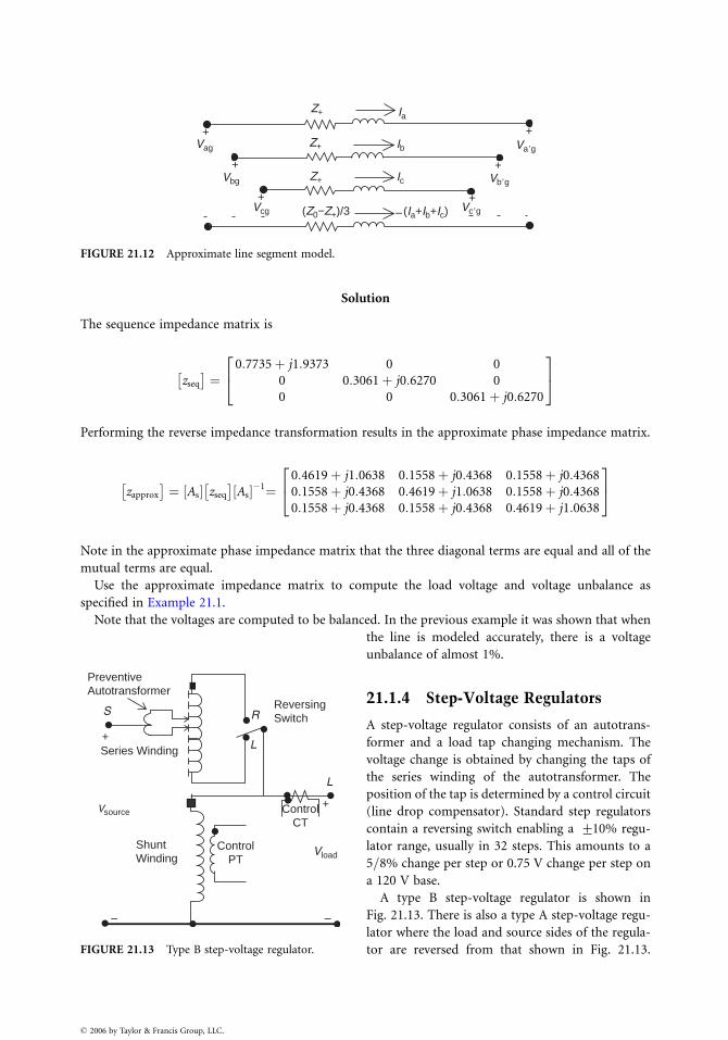
++
+
+
+
+
Z+
Z+
Z+
Ia
(Ia+Ib+Ic)(Z0−Z+)/3
Ib
Ic
Vc�g
Vb�g
Va�g
Vcg
Vbg
Vag
–
FIGURE 21.12 Approximate line segment model.
Solution
The sequence impedance matrix is
zseq
� �
¼0:7735þ j1:9373 0 0
0 0:3061þ j0:6270 0
0 0 0:3061þ j0:6270
2
4
3
5
Performing the reverse impedance transformation results in the approximate phase impedance matrix.
zapprox
� �
¼ As½ � zseq
� �
As½ ��1¼0:4619þ j1:0638 0:1558þ j0:4368 0:1558þ j0:4368
0:1558þ j0:4368 0:4619þ j1:0638 0:1558þ j0:4368
0:1558þ j0:4368 0:1558þ j0:4368 0:4619þ j1:0638
2
4
3
5
Note in the approximate phase impedance matrix that the three diagonal terms are equal and all of the
mutual terms are equal.
Use the approximate impedance matrix to compute the load voltage and voltage unbalance as
specified in Example 21.1.
Note that the voltages are computed to be balanced. In the previous example it was shown that when
NNNNNN
––
+
+
S R
L
L
ControlPT
ControlCT
ShuntWinding
ReversingSwitch
Series Winding
V source
V load
PreventiveAutotransformer
FIGURE 21.13 Type B step-voltage regulator.
� 2006 by Taylor & Francis Group, LLC.
the line is modeled accurately, there is a voltage
unbalance of almost 1%.
21.1.4 Step-Voltage Regulators
A step-voltage regulator consists of an autotrans-
former and a load tap changing mechanism. The
voltage change is obtained by changing the taps of
the series winding of the autotransformer. The
position of the tap is determined by a control circuit
(line drop compensator). Standard step regulators
contain a reversing switch enabling a +10% regu-
lator range, usually in 32 steps. This amounts to a
5=8% change per step or 0.75 V change per step on
a 120 V base.
A type B step-voltage regulator is shown in
Fig. 21.13. There is also a type A step-voltage regu-
lator where the load and source sides of the regula-
tor are reversed from that shown in Fig. 21.13.
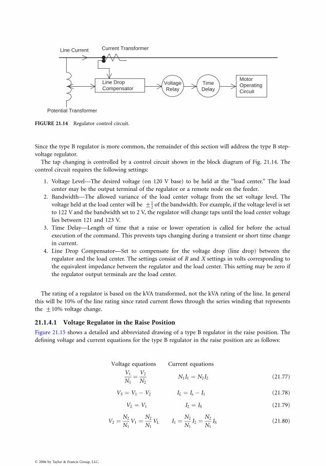
Line Current
VoltageRelay
TimeDelay
MotorOperatingCircuit
Current Transformer
Line DropCompensator
Potential Transformer
FIGURE 21.14 Regulator control circuit.
Since the type B regulator is more common, the remainder of this section will address the type B step-
voltage regulator.
The tap changing is controlled by a control circuit shown in the block diagram of Fig. 21.14. The
control circuit requires the following settings:
1. Voltage Level—The desired voltage (on 120 V base) to be held at the ‘‘load center.’’ The load
center may be the output terminal of the regulator or a remote node on the feeder.
2. Bandwidth—The allowed variance of the load center voltage from the set voltage level. The
voltage held at the load center will be +12
of the bandwidth. For example, if the voltage level is set
to 122 V and the bandwidth set to 2 V, the regulator will change taps until the load center voltage
lies between 121 and 123 V.
3. Time Delay—Length of time that a raise or lower operation is called for before the actual
execution of the command. This prevents taps changing during a transient or short time change
in current.
4. Line Drop Compensator—Set to compensate for the voltage drop (line drop) between the
regulator and the load center. The settings consist of R and X settings in volts corresponding to
the equivalent impedance between the regulator and the load center. This setting may be zero if
the regulator output terminals are the load center.
The rating of a regulator is based on the kVA transformed, not the kVA rating of the line. In general
this will be 10% of the line rating since rated current flows through the series winding that represents
the +10% voltage change.
21.1.4.1 Voltage Regulator in the Raise Position
Figure 21.15 shows a detailed and abbreviated drawing of a type B regulator in the raise position. The
defining voltage and current equations for the type B regulator in the raise position are as follows:
Voltage equations Current equations
V1
N1
¼ V2
N2
N1I1 ¼ N2I2 (21:77)
VS ¼ V1 � V2 IL ¼ Is � I1 (21:78)
VL ¼ V1 I2 ¼ IS (21:79)
V2 ¼N2
N1
V1 ¼N2
N1
VL I1 ¼N2
N1
I2 ¼N2
N1
IS (21:80)
� 2006 by Taylor & Francis Group, LLC.
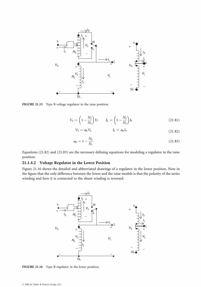
ls
Rs s
SL
L
SL
L L
ls N2
VS
V1 VLN1
V2
l2
lL lL
lS
VS
VL
I1
+
+
+++
−
−
− −
− −
+
FIGURE 21.15 Type B voltage regulator in the raise position.
VS ¼ 1� N2
N1
� �
Vl IL ¼ 1�N2
N1
� �
IS (21:81)
VS ¼ aRVL IL ¼ aRIS (21:82)
aR ¼ 1�N2
N1
(21:83)
Equations (21.82) and (21.83) are the necessary defining equations for modeling a regulator in the raise
position.
21.1.4.2 Voltage Regulator in the Lower Position
Figure 21.16 shows the detailed and abbreviated drawings of a regulator in the lower position. Note in
the figure that the only difference between the lower and the raise models is that the polarity of the series
winding and how it is connected to the shunt winding is reversed.
IS
IS
I2
V2
I1
VLV1
VS
N1
N2
+
+
SL
+
s
−
−
VL
IS
IL
+
+
−−
− −
R
L
IL LL
SL
s
VS+
FIGURE 21.16 Type B regulator in the lower position.
� 2006 by Taylor & Francis Group, LLC.
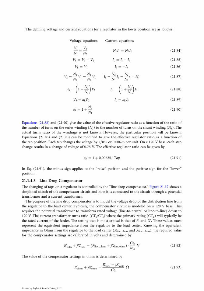
The defining voltage and current equations for a regulator in the lower position are as follows:
Voltage equations Current equations
V1
N1
¼ V2
N2
N1I1 ¼ N2I2 (21:84)
VS ¼ V1 þ V2 IL ¼ Is � I1 (21:85)
VL ¼ V1 I2 ¼ �IS (21:86)
V2 ¼N2
N1
V1 ¼N2
N1
VL I1 ¼N2
N1
I2 ¼N2
N1
(� IS) (21:87)
VS ¼ 1þN2
N1
� �
Vl IL ¼ 1þ N2
N1
� �
IS (21:88)
VS ¼ aRVL IL ¼ aRIS (21:89)
aR ¼ 1þN2
N1
(21:90)
Equations (21.83) and (21.90) give the value of the effective regulator ratio as a function of the ratio of
the number of turns on the series winding (N2) to the number of turns on the shunt winding (N1). The
actual turns ratio of the windings is not known. However, the particular position will be known.
Equations (21.83) and (21.90) can be modified to give the effective regulator ratio as a function of
the tap position. Each tap changes the voltage by 5=8% or 0.00625 per unit. On a 120 V base, each step
change results in a change of voltage of 0.75 V. The effective regulator ratio can be given by
aR ¼ 1� 0:00625 � Tap (21:91)
In Eq. (21.91), the minus sign applies to the ‘‘raise’’ position and the positive sign for the ‘‘lower’’
position.
21.1.4.3 Line Drop Compensator
The changing of taps on a regulator is controlled by the ‘‘line drop compensator.’’ Figure 21.17 shows a
simplified sketch of the compensator circuit and how it is connected to the circuit through a potential
transformer and a current transformer.
The purpose of the line drop compensator is to model the voltage drop of the distribution line from
the regulator to the load center. Typically, the compensator circuit is modeled on a 120 V base. This
requires the potential transformer to transform rated voltage (line-to-neutral or line-to-line) down to
120 V. The current transformer turns ratio (CTp:CTs) where the primary rating (CTp) will typically be
the rated current of the feeder. The setting that is most critical is that of R0 and X0. These values must
represent the equivalent impedance from the regulator to the load center. Knowing the equivalent
impedance in Ohms from the regulator to the load center (Rline ohms and Xline ohms), the required value
for the compensator settings are calibrated in volts and determined by
R0volts þ jX 0volts ¼ Rline ohms þ jXline ohmsð Þ � Ctp
Npt
V (21:92)
The value of the compensator settings in ohms is determined by
R0ohms þ jX 0ohms ¼R0volts þ jX 0volts
Cts
V (21:93)
� 2006 by Taylor & Francis Group, LLC.
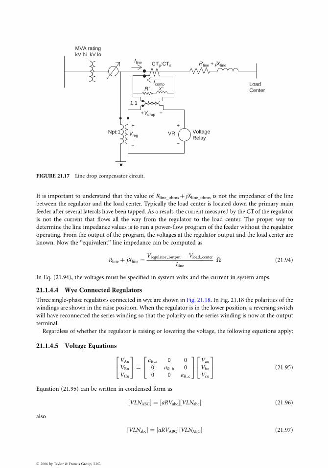
MVA ratingkV hi–kV lo
I line
Npt:1
+V drop −
V reg VR
R � X �
1:1
+ +
−−
I comp LoadCenter
CTp:CTs R line + jX line
VoltageRelay
FIGURE 21.17 Line drop compensator circuit.
It is important to understand that the value of Rline_ohmsþ jXline_ohms is not the impedance of the line
between the regulator and the load center. Typically the load center is located down the primary main
feeder after several laterals have been tapped. As a result, the current measured by the CTof the regulator
is not the current that flows all the way from the regulator to the load center. The proper way to
determine the line impedance values is to run a power-flow program of the feeder without the regulator
operating. From the output of the program, the voltages at the regulator output and the load center are
known. Now the ‘‘equivalent’’ line impedance can be computed as
Rline þ jXline ¼Vregulator output � Vload center
Iline
V (21:94)
In Eq. (21.94), the voltages must be specified in system volts and the current in system amps.
21.1.4.4 Wye Connected Regulators
Three single-phase regulators connected in wye are shown in Fig. 21.18. In Fig. 21.18 the polarities of the
windings are shown in the raise position. When the regulator is in the lower position, a reversing switch
will have reconnected the series winding so that the polarity on the series winding is now at the output
terminal.
Regardless of whether the regulator is raising or lowering the voltage, the following equations apply:
21.1.4.5 Voltage Equations
VAn
VBn
VCn
2
4
3
5 ¼aR a 0 0
0 aR b 0
0 0 aR c
2
4
3
5
Van
Vbn
Vcn
2
4
3
5 (21:95)
Equation (21.95) can be written in condensed form as
VLNABC½ � ¼ aRVabc½ � VLNabc½ � (21:96)
also
VLNabc½ � ¼ aRVABC½ � VLNABC½ � (21:97)
� 2006 by Taylor & Francis Group, LLC.
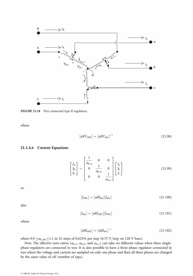
B
A
+
+
−−
VAnVan
C
IB
Ia
Ib
a
b
Icc
IA
IC
FIGURE 21.18 Wye connected type B regulators.
where
aRVABC½ � ¼ aRVabc½ ��1(21:98)
21.1.4.6 Current Equations
IA
IB
IC
2
4
3
5 ¼
1
aR a
0 0
01
aR b
0
0 01
aR c
2
6
6
6
6
6
4
3
7
7
7
7
7
5
Ia
Ib
Ic
2
4
3
5 (21:99)
or
IABC½ � ¼ aRIabc½ � Iabc½ � (21:100)
also
Iabc½ � ¼ aRIABC½ � IABC½ � (21:101)
where
aRIABC½ � ¼ aRIabc½ ��1(21:102)
where 0.9�aR abc�1.1 in 32 steps of 0.625% per step (0.75 V=step on 120 V base).
Note: The effective turn ratios (aR a, aR b, and aR c) can take on different values when three single-
phase regulators are connected in wye. It is also possible to have a three-phase regulator connected in
wye where the voltage and current are sampled on only one phase and then all three phases are changed
by the same value of aR (number of taps).
� 2006 by Taylor & Francis Group, LLC.
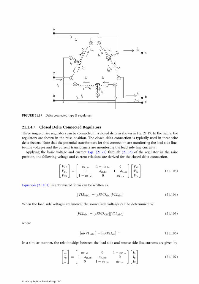
A
a
S
L
C
B
IA
IA
IC
Ibc IB
IB
IC
Ic�
Ia�
Ib� Ibb
cIc
Ica
Iab
Ia
SL
L
S
L
SSL
SL
FIGURE 21.19 Delta connected type B regulators.
21.1.4.7 Closed Delta Connected Regulators
Three single-phase regulators can be connected in a closed delta as shown in Fig. 21.19. In the figure, the
regulators are shown in the raise position. The closed delta connection is typically used in three-wire
delta feeders. Note that the potential transformers for this connection are monitoring the load side line-
to-line voltages and the current transformers are monitoring the load side line currents.
Applying the basic voltage and current Eqs. (21.77) through (21.83) of the regulator in the raise
position, the following voltage and current relations are derived for the closed delta connection.
VAB
VBC
VCA
2
4
3
5 ¼aR ab 1� aR bc 0
0 aR bc 1� aR ca
1� aR ab 0 aR ca
2
4
3
5
Vab
Vbc
Vca
2
4
3
5 (21:103)
Equation (21.101) in abbreviated form can be written as
VLLABC½ � ¼ aRVDabc½ � VLLabc½ � (21:104)
When the load side voltages are known, the source side voltages can be determined by
VLLabc½ � ¼ aRVDABC½ � VLLABC½ � (21:105)
where
aRVDABC½ � ¼ aRVDabc½ ��1(21:106)
In a similar manner, the relationships between the load side and source side line currents are given by
Ia
Ib
Ic
2
4
3
5 ¼aR ab 0 1� aR ca
1� aR ab aR bc 0
0 1� aR bc aR ca
2
4
3
5
IA
IB
IC
2
4
3
5 (21:107)
� 2006 by Taylor & Francis Group, LLC.

or
Iabc½ � ¼ AIDABC½ � IABC½ � (21:108)
also
IABC½ � ¼ AIDabc½ � Iabc½ � (21:109)
where
IADabc½ � ¼ IADABC½ ��1(21:110)
The closed delta connection can be difficult to apply. Note in both the voltage and current equations that
a change of the tap position in one regulator will affect voltages and currents in two phases. As a result,
increasing the tap in one regulator will affect the tap position of the second regulator. In most cases the
bandwidth setting for the closed delta connection will have to be wider than that for wye connected
regulators.
21.1.4.8 Open Delta Connection
Two single-phase regulators can be connected in the ‘‘open’’ delta connection. Shown in Fig. 21.20 is an
open delta connection where two single-phase regulators have been connected between phases AB and CB.
Two other open connections can also be made where the single-phase regulators are connected
between phases BC and AC and also between phases CA and BA.
The open delta connection is typically applied to three-wire delta feeders. Note that the potential
transformers monitor the line-to-line voltages and the current transformers monitor the line currents.
Once again, the basic voltage and current relations of the individual regulators are used to determine the
relationships between the source side and load side voltages and currents.
For all three open connections, the following general equations will apply:
VLLABC½ � ¼ aRVabc½ � VLLabc½ � (21:111)
VLLabc½ � ¼ aRVABC½ � VLLABC½ � (21:112)
A
C
IA
Ia aVCA
VBC
Vab
Vca
Vbc
Ic
b
c
Iab
Icb
Ib
VAB
IC
B
IB
+
+
+
+
+
+
−
−
−
−
−
−
s
s
L
SL
SL
L
FIGURE 21.20 Open delta type B regulator connection.
� 2006 by Taylor & Francis Group, LLC.
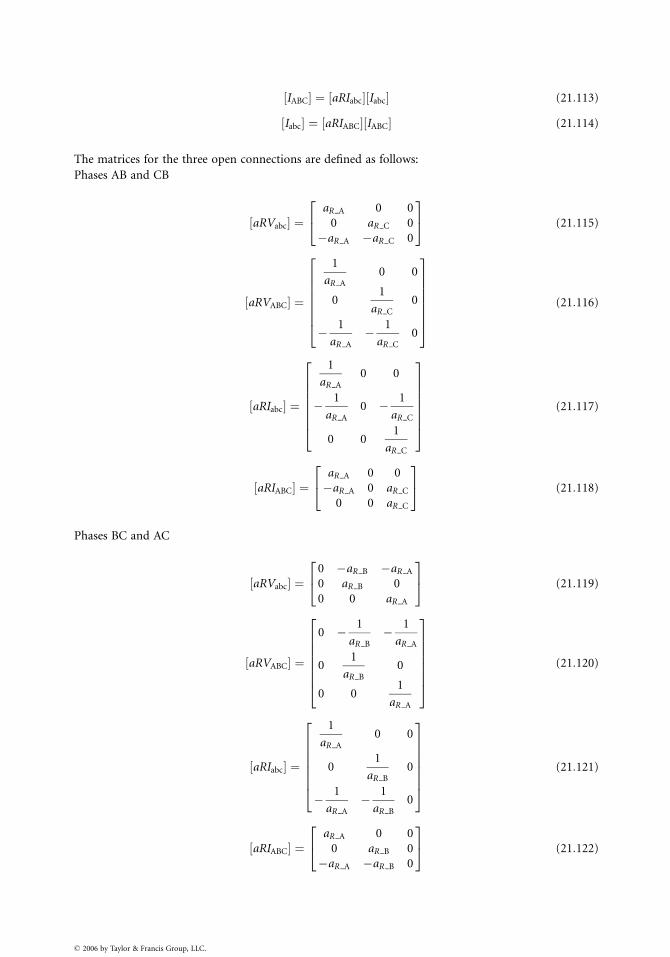
IABC½ � ¼ aRIabc½ � Iabc½ � (21:113)
Iabc½ � ¼ aRIABC½ � IABC½ � (21:114)
The matrices for the three open connections are defined as follows:
Phases AB and CB
aRVabc½ � ¼aR A 0 0
0 aR C 0
�aR A �aR C 0
2
4
3
5 (21:115)
aRVABC½ � ¼
1
aR A
0 0
01
aR C
0
� 1
aR A
� 1
aR C
0
2
6
6
6
6
6
6
4
3
7
7
7
7
7
7
5
(21:116)
aRIabc½ � ¼
1
aR A
0 0
� 1
aR A
0 � 1
aR C
0 01
aR C
2
6
6
6
6
6
6
4
3
7
7
7
7
7
7
5
(21:117)
aRIABC½ � ¼aR A 0 0
�aR A 0 aR C
0 0 aR C
2
4
3
5 (21:118)
Phases BC and AC
aRVabc½ � ¼0 �aR B �aR A
0 aR B 0
0 0 aR A
2
4
3
5 (21:119)
aRVABC½ � ¼
0 � 1
aR B
� 1
aR A
01
aR B
0
0 01
aR A
2
6
6
6
6
6
6
4
3
7
7
7
7
7
7
5
(21:120)
aRIabc½ � ¼
1
aR A
0 0
01
aR B
0
� 1
aR A
� 1
aR B
0
2
6
6
6
6
6
6
4
3
7
7
7
7
7
7
5
(21:121)
aRIABC½ � ¼aR A 0 0
0 aR B 0
�aR A �aR B 0
2
4
3
5 (21:122)
� 2006 by Taylor & Francis Group, LLC.
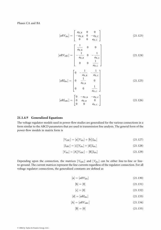
Phases CA and BA
aRVabc½ � ¼aR B 0 0
�aR B 0 �aR C
0 0 aR C
2
4
3
5 (21:123)
aRVABC½ � ¼
1
aR B
0 0
� 1
aR B
0 � 1
aR C
0 01
aR C
2
6
6
6
6
6
6
4
3
7
7
7
7
7
7
5
(21:124)
aRIabc½ � ¼
0 � 1
aR B
� 1
aR C
01
aR B
0
0 01
aR C
2
6
6
6
6
6
6
4
3
7
7
7
7
7
7
5
(21:125)
aRIABC½ � ¼0 �aR B �aR C
0 aR B 0
0 0 aR C
2
4
3
5 (21:126)
21.1.4.9 Generalized Equations
The voltage regulator models used in power-flow studies are generalized for the various connections in a
form similar to the ABCD parameters that are used in transmission line analysis. The general form of the
power-flow models in matrix form is
VABC½ � ¼ a½ � Vabc½ � þ b½ � Iabc½ � (21:127)
IABC½ � ¼ c½ � Vabc½ � þ d½ � Iabc½ � (21:128)
Vabc½ � ¼ A½ � VABC½ � � B½ � Iabc½ � (21:129)
Depending upon the connection, the matrices [VABC] and [Vabc] can be either line-to-line or line-
to-ground. The current matrices represent the line currents regardless of the regulator connection. For all
voltage regulator connections, the generalized constants are defined as
a½ � ¼ aRVabc½ � (21:130)
b½ � ¼ 0½ � (21:131)
c½ � ¼ 0½ � (21:132)
d½ � ¼ aRIabc½ � (21:133)
A½ � ¼ aRVABC½ � (21:134)
B½ � ¼ 0½ � (21:135)
� 2006 by Taylor & Francis Group, LLC.
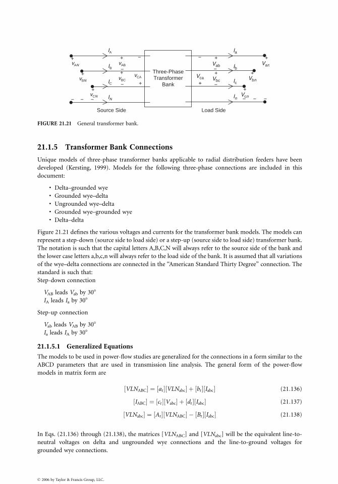
IA Ia
VanVab
Vbn
Vcn
Vca Vbc
Ib
In
Ic
vAN
vBN
vCN
vAB
vBCvCA
IB
IC
IN
+
− −
− −
−
− − −
−−
−
−
+
+ +
+
+ +
+
+
+
+
+
Source Side Load Side
Three-PhaseTransformer
Bank
FIGURE 21.21 General transformer bank.
21.1.5 Transformer Bank Connections
Unique models of three-phase transformer banks applicable to radial distribution feeders have been
developed (Kersting, 1999). Models for the following three-phase connections are included in this
document:
. Delta–grounded wye
. Grounded wye–delta
. Ungrounded wye–delta
. Grounded wye–grounded wye
. Delta–delta
Figure 21.21 defines the various voltages and currents for the transformer bank models. The models can
represent a step-down (source side to load side) or a step-up (source side to load side) transformer bank.
The notation is such that the capital letters A,B,C,N will always refer to the source side of the bank and
the lower case letters a,b,c,n will always refer to the load side of the bank. It is assumed that all variations
of the wye–delta connections are connected in the ‘‘American Standard Thirty Degree’’ connection. The
standard is such that:
Step-down connection
VAB leads Vab by 308
IA leads Ia by 308
Step-up connection
Vab leads VAB by 308
Ia leads IA by 308
21.1.5.1 Generalized Equations
The models to be used in power-flow studies are generalized for the connections in a form similar to the
ABCD parameters that are used in transmission line analysis. The general form of the power-flow
models in matrix form are
VLNABC½ � ¼ at½ � VLNabc½ � þ bt½ � Iabc½ � (21:136)
IABC½ � ¼ ct½ � Vabc½ � þ dt½ � Iabc½ � (21:137)
VLNabc½ � ¼ At½ � VLNABC½ � � Bt½ � Iabc½ � (21:138)
In Eqs. (21.136) through (21.138), the matrices [VLNABC] and [VLNabc] will be the equivalent line-to-
neutral voltages on delta and ungrounded wye connections and the line-to-ground voltages for
grounded wye connections.
� 2006 by Taylor & Francis Group, LLC.
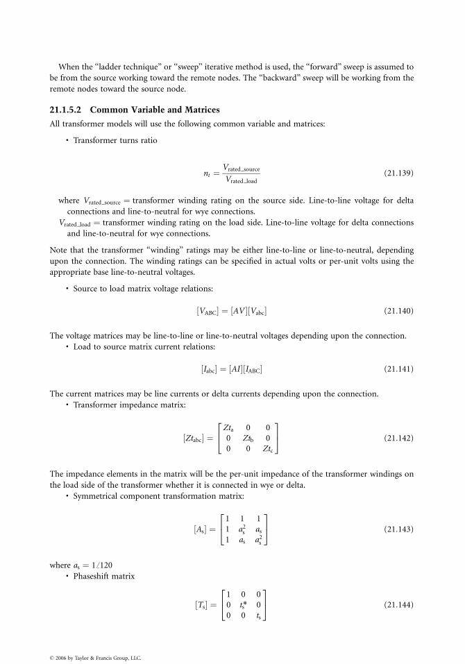
When the ‘‘ladder technique’’ or ‘‘sweep’’ iterative method is used, the ‘‘forward’’ sweep is assumed to
be from the source working toward the remote nodes. The ‘‘backward’’ sweep will be working from the
remote nodes toward the source node.
21.1.5.2 Common Variable and Matrices
All transformer models will use the following common variable and matrices:
. Transformer turns ratio
nt ¼Vrated source
Vrated load
(21:139)
where Vrated source ¼ transformer winding rating on the source side. Line-to-line voltage for delta
connections and line-to-neutral for wye connections.
Vrated load ¼ transformer winding rating on the load side. Line-to-line voltage for delta connections
and line-to-neutral for wye connections.
Note that the transformer ‘‘winding’’ ratings may be either line-to-line or line-to-neutral, depending
upon the connection. The winding ratings can be specified in actual volts or per-unit volts using the
appropriate base line-to-neutral voltages.
. Source to load matrix voltage relations:
VABC½ � ¼ AV½ � Vabc½ � (21:140)
The voltage matrices may be line-to-line or line-to-neutral voltages depending upon the connection.. Load to source matrix current relations:
Iabc½ � ¼ AI½ � IABC½ � (21:141)
The current matrices may be line currents or delta currents depending upon the connection.. Transformer impedance matrix:
Ztabc½ � ¼Zta 0 0
0 Ztb 0
0 0 Ztc
2
4
3
5 (21:142)
The impedance elements in the matrix will be the per-unit impedance of the transformer windings on
the load side of the transformer whether it is connected in wye or delta.. Symmetrical component transformation matrix:
As½ � ¼1 1 1
1 a2s as
1 as a2s
2
4
3
5 (21:143)
where as ¼ 1ff120. Phaseshift matrix
Ts½ � ¼1 0 0
0 ts* 0
0 0 ts
2
4
3
5 (21:144)
� 2006 by Taylor & Francis Group, LLC.
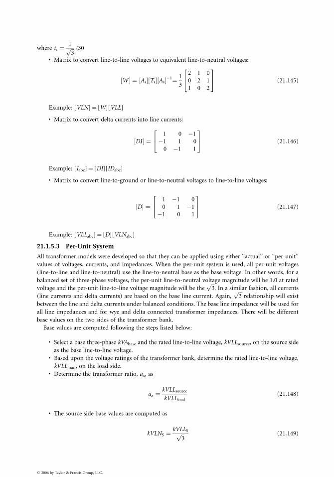
where ts ¼1ffiffiffi
3p ff30
. Matrix to convert line-to-line voltages to equivalent line-to-neutral voltages:
W½ � ¼ As½ � Ts½ � As½ ��1¼ 1
3
2 1 0
0 2 1
1 0 2
2
4
3
5 (21:145)
Example: [VLN]¼ [W][VLL]
. Matrix to convert delta currents into line currents:
DI½ � ¼1 0 �1
�1 1 0
0 �1 1
2
4
3
5 (21:146)
Example: [Iabc]¼ [DI][IDabc]
. Matrix to convert line-to-ground or line-to-neutral voltages to line-to-line voltages:
D½ � ¼1 �1 0
0 1 �1
�1 0 1
2
4
3
5 (21:147)
Example: [VLLabc]¼ [D][VLNabc]
21.1.5.3 Per-Unit System
All transformer models were developed so that they can be applied using either ‘‘actual’’ or ‘‘per-unit’’
values of voltages, currents, and impedances. When the per-unit system is used, all per-unit voltages
(line-to-line and line-to-neutral) use the line-to-neutral base as the base voltage. In other words, for a
balanced set of three-phase voltages, the per-unit line-to-neutral voltage magnitude will be 1.0 at rated
voltage and the per-unit line-to-line voltage magnitude will be theffiffiffi
3p
. In a similar fashion, all currents
(line currents and delta currents) are based on the base line current. Again,ffiffiffi
3p
relationship will exist
between the line and delta currents under balanced conditions. The base line impedance will be used for
all line impedances and for wye and delta connected transformer impedances. There will be different
base values on the two sides of the transformer bank.
Base values are computed following the steps listed below:
. Select a base three-phase kVAbase and the rated line-to-line voltage, kVLLsource, on the source side
as the base line-to-line voltage.. Based upon the voltage ratings of the transformer bank, determine the rated line-to-line voltage,
kVLLload, on the load side.. Determine the transformer ratio, ax, as
ax ¼kVLLsource
kVLLload
(21:148)
. The source side base values are computed as
kVLNS ¼kVLLSffiffiffi
3p (21:149)
� 2006 by Taylor & Francis Group, LLC.
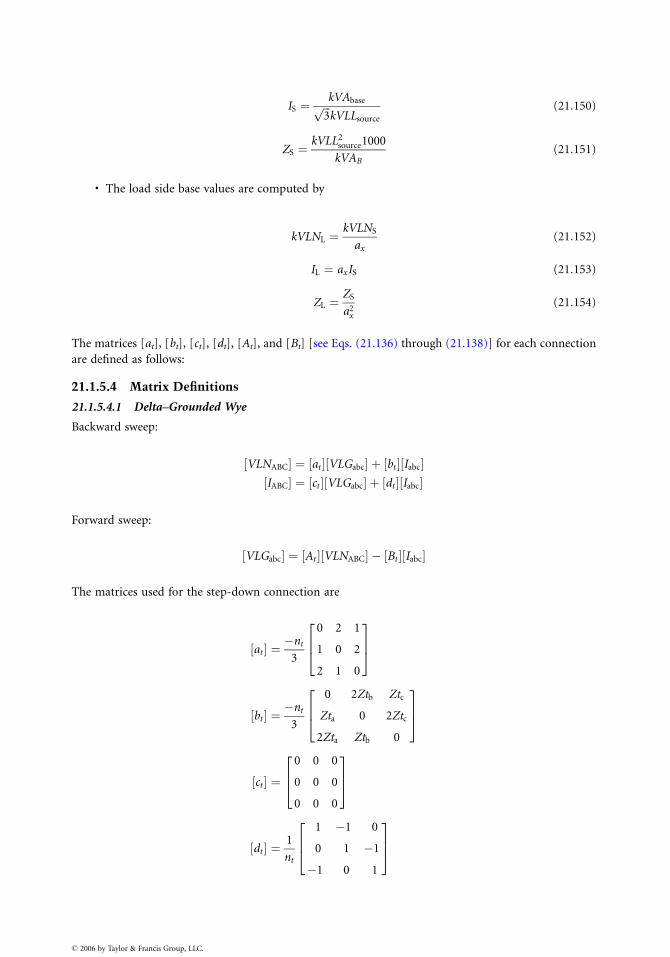
IS ¼kVAbaseffiffiffi
3p
kVLLsource
(21:150)
ZS ¼kVLL2
source1000
kVAB
(21:151)
. The load side base values are computed by
kVLNL ¼kVLNS
ax
(21:152)
IL ¼ axIS (21:153)
ZL ¼ZS
a2x
(21:154)
The matrices [at], [bt], [ct], [dt], [At], and [Bt] [see Eqs. (21.136) through (21.138)] for each connection
are defined as follows:
21.1.5.4 Matrix Definitions
21.1.5.4.1 Delta–Grounded Wye
Backward sweep:
VLNABC½ � ¼ at½ � VLGabc½ � þ bt½ � Iabc½ �IABC½ � ¼ ct½ � VLGabc½ � þ dt½ � Iabc½ �
Forward sweep:
VLGabc½ � ¼ At½ � VLNABC½ � � Bt½ � Iabc½ �
The matrices used for the step-down connection are
at½ � ¼�nt
3
0 2 1
1 0 2
2 1 0
2
6
4
3
7
5
bt½ � ¼�nt
3
0 2Ztb Ztc
Zta 0 2Ztc
2Zta Ztb 0
2
6
4
3
7
5
ct½ � ¼0 0 0
0 0 0
0 0 0
2
6
4
3
7
5
dt½ � ¼1
nt
1 �1 0
0 1 �1
�1 0 1
2
6
4
3
7
5
� 2006 by Taylor & Francis Group, LLC.
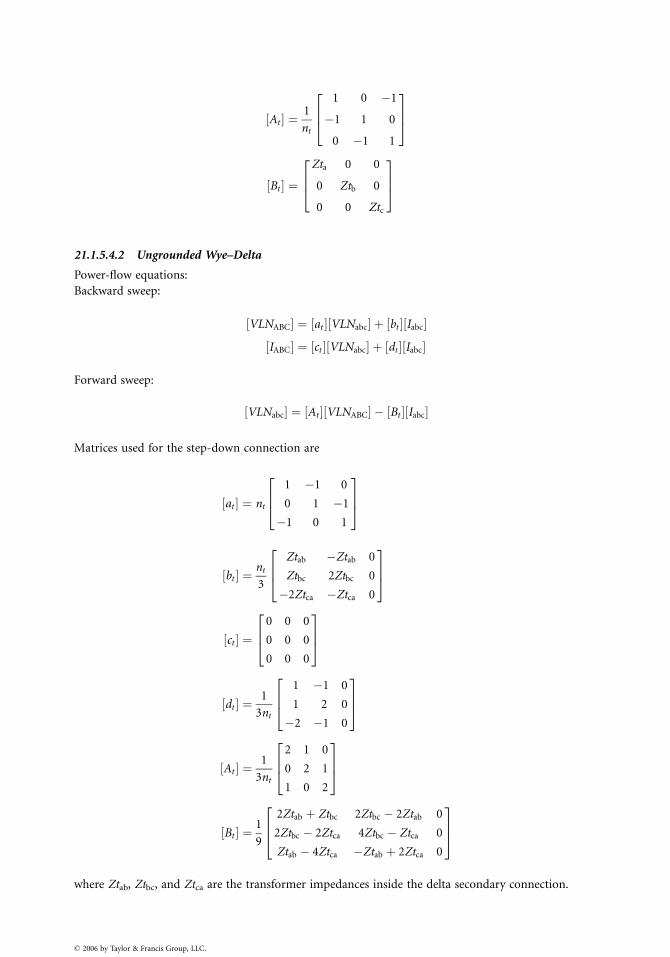
At½ � ¼1
nt
1 0 �1
�1 1 0
0 �1 1
2
6
4
3
7
5
Bt½ � ¼Zta 0 0
0 Ztb 0
0 0 Ztc
2
6
4
3
7
5
21.1.5.4.2 Ungrounded Wye–Delta
Power-flow equations:
Backward sweep:
VLNABC½ � ¼ at½ � VLNabc½ � þ bt½ � Iabc½ �
IABC½ � ¼ ct½ � VLNabc½ � þ dt½ � Iabc½ �
Forward sweep:
VLNabc½ � ¼ At½ � VLNABC½ � � Bt½ � Iabc½ �
Matrices used for the step-down connection are
at½ � ¼ nt
1 �1 0
0 1 �1
�1 0 1
2
6
4
3
7
5
bt½ � ¼nt
3
Ztab �Ztab 0
Ztbc 2Ztbc 0
�2Ztca �Ztca 0
2
6
4
3
7
5
ct½ � ¼0 0 0
0 0 0
0 0 0
2
6
4
3
7
5
dt½ � ¼1
3nt
1 �1 0
1 2 0
�2 �1 0
2
6
4
3
7
5
At½ � ¼1
3nt
2 1 0
0 2 1
1 0 2
2
6
4
3
7
5
Bt½ � ¼1
9
2Ztab þ Ztbc 2Ztbc � 2Ztab 0
2Ztbc � 2Ztca 4Ztbc � Ztca 0
Ztab � 4Ztca �Ztab þ 2Ztca 0
2
6
4
3
7
5
where Ztab, Ztbc, and Ztca are the transformer impedances inside the delta secondary connection.
� 2006 by Taylor & Francis Group, LLC.
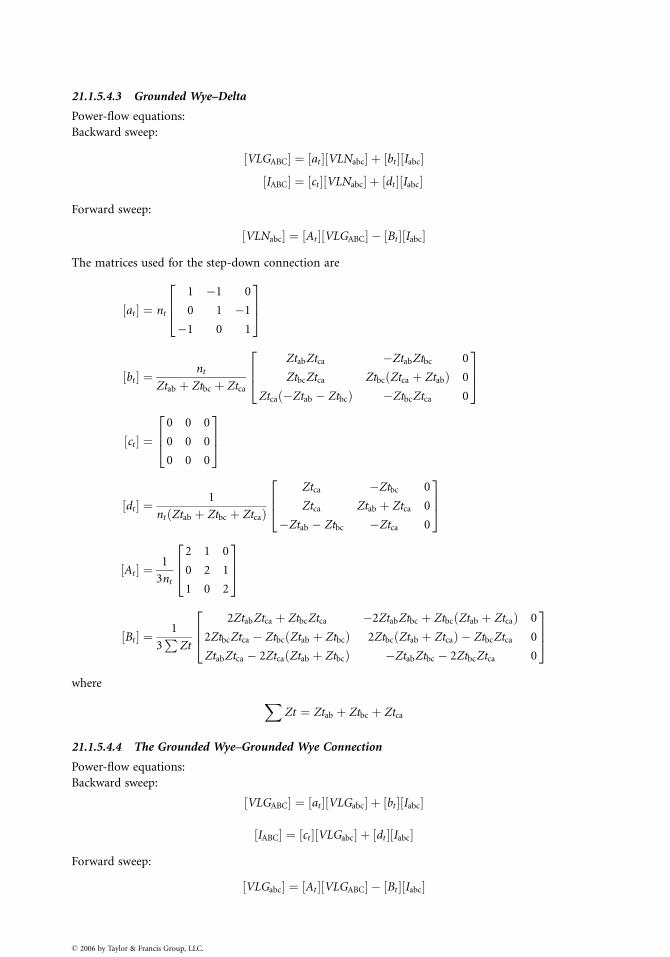
21.1.5.4.3 Grounded Wye–Delta
Power-flow equations:
Backward sweep:
VLGABC½ � ¼ at½ � VLNabc½ � þ bt½ � Iabc½ �
IABC½ � ¼ ct½ � VLNabc½ � þ dt½ � Iabc½ �
Forward sweep:
VLNabc½ � ¼ At½ � VLGABC½ � � Bt½ � Iabc½ �
The matrices used for the step-down connection are
at½ � ¼ nt
1 �1 0
0 1 �1
�1 0 1
2
6
4
3
7
5
bt½ � ¼nt
Ztab þ Ztbc þ Ztca
ZtabZtca �ZtabZtbc 0
ZtbcZtca Ztbc Ztca þ Ztabð Þ 0
Ztca �Ztab � Ztbcð Þ �ZtbcZtca 0
2
6
4
3
7
5
ct½ � ¼0 0 0
0 0 0
0 0 0
2
6
4
3
7
5
dt½ � ¼1
nt Ztab þ Ztbc þ Ztcað Þ
Ztca �Ztbc 0
Ztca Ztab þ Ztca 0
�Ztab � Ztbc �Ztca 0
2
6
4
3
7
5
At½ � ¼1
3nt
2 1 0
0 2 1
1 0 2
2
6
4
3
7
5
Bt½ � ¼1
3P
Zt
2ZtabZtca þ ZtbcZtca �2ZtabZtbc þ Ztbc Ztab þ Ztcað Þ 0
2ZtbcZtca � Ztbc Ztab þ Ztbcð Þ 2Ztbc Ztab þ Ztcað Þ � ZtbcZtca 0
ZtabZtca � 2Ztca Ztab þ Ztbcð Þ �ZtabZtbc � 2ZtbcZtca 0
2
6
4
3
7
5
where
X
Zt ¼ Ztab þ Ztbc þ Ztca
21.1.5.4.4 The Grounded Wye–Grounded Wye Connection
Power-flow equations:
Backward sweep:
VLGABC½ � ¼ at½ � VLGabc½ � þ bt½ � Iabc½ �
IABC½ � ¼ ct½ � VLGabc½ � þ dt½ � Iabc½ �
Forward sweep:
VLGabc½ � ¼ At½ � VLGABC½ � � Bt½ � Iabc½ �
� 2006 by Taylor & Francis Group, LLC.
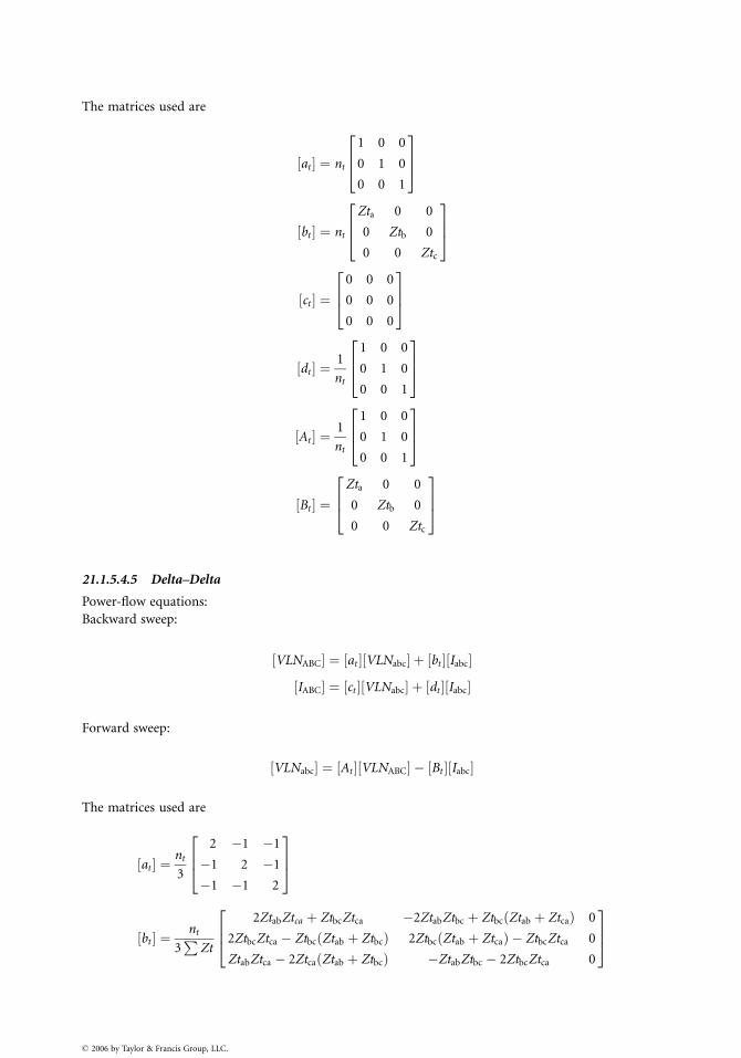
The matrices used are
at½ � ¼ nt
1 0 0
0 1 0
0 0 1
2
6
4
3
7
5
bt½ � ¼ nt
Zta 0 0
0 Ztb 0
0 0 Ztc
2
6
4
3
7
5
ct½ � ¼0 0 0
0 0 0
0 0 0
2
6
4
3
7
5
dt½ � ¼1
nt
1 0 0
0 1 0
0 0 1
2
6
4
3
7
5
At½ � ¼1
nt
1 0 0
0 1 0
0 0 1
2
6
4
3
7
5
Bt½ � ¼Zta 0 0
0 Ztb 0
0 0 Ztc
2
6
4
3
7
5
21.1.5.4.5 Delta–Delta
Power-flow equations:
Backward sweep:
VLNABC½ � ¼ at½ � VLNabc½ � þ bt½ � Iabc½ �
IABC½ � ¼ ct½ � VLNabc½ � þ dt½ � Iabc½ �
Forward sweep:
VLNabc½ � ¼ At½ � VLNABC½ � � Bt½ � Iabc½ �
The matrices used are
at½ � ¼nt
3
2 �1 �1
�1 2 �1
�1 �1 2
2
6
4
3
7
5
bt½ � ¼nt
3P
Zt
2ZtabZtca þ ZtbcZtca �2ZtabZtbc þ Ztbc Ztab þ Ztcað Þ 0
2ZtbcZtca � Ztbc Ztab þ Ztbcð Þ 2Ztbc Ztab þ Ztcað Þ � ZtbcZtca 0
ZtabZtca � 2Ztca Ztab þ Ztbcð Þ �ZtabZtbc � 2ZtbcZtca 0
2
6
4
3
7
5
� 2006 by Taylor & Francis Group, LLC.
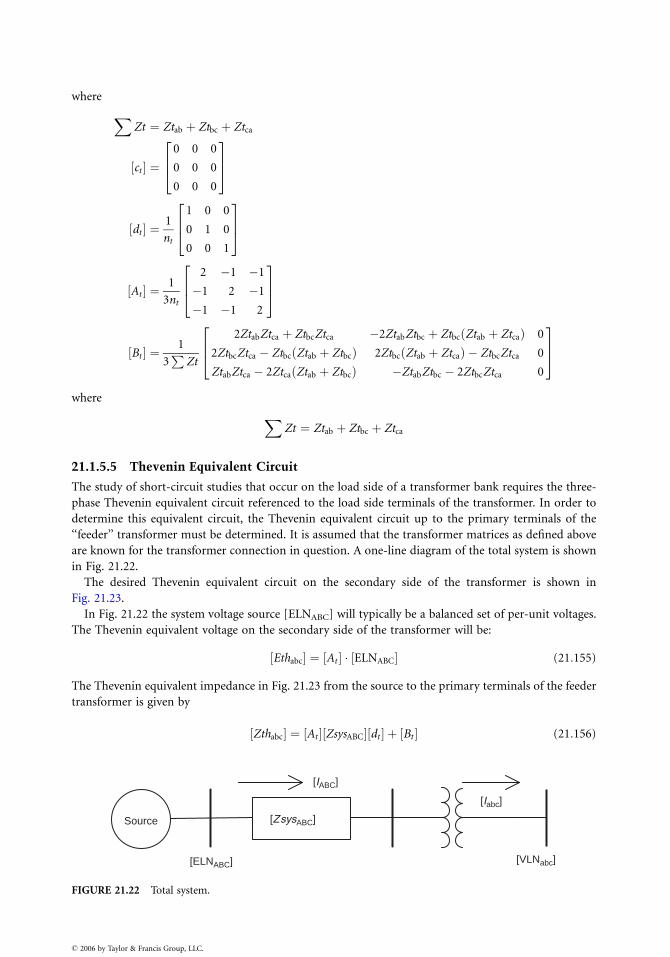
where
X
Zt ¼ Ztab þ Ztbc þ Ztca
ct½ � ¼0 0 0
0 0 0
0 0 0
2
6
4
3
7
5
dt½ � ¼1
nt
1 0 0
0 1 0
0 0 1
2
6
4
3
7
5
At½ � ¼1
3nt
2 �1 �1
�1 2 �1
�1 �1 2
2
6
4
3
7
5
Bt½ � ¼1
3P
Zt
2ZtabZtca þ ZtbcZtca �2ZtabZtbc þ Ztbc Ztab þ Ztcað Þ 0
2ZtbcZtca � Ztbc Ztab þ Ztbcð Þ 2Ztbc Ztab þ Ztcað Þ � ZtbcZtca 0
ZtabZtca � 2Ztca Ztab þ Ztbcð Þ �ZtabZtbc � 2ZtbcZtca 0
2
6
4
3
7
5
where
X
Zt ¼ Ztab þ Ztbc þ Ztca
21.1.5.5 Thevenin Equivalent Circuit
The study of short-circuit studies that occur on the load side of a transformer bank requires the three-
phase Thevenin equivalent circuit referenced to the load side terminals of the transformer. In order to
determine this equivalent circuit, the Thevenin equivalent circuit up to the primary terminals of the
‘‘feeder’’ transformer must be determined. It is assumed that the transformer matrices as defined above
are known for the transformer connection in question. A one-line diagram of the total system is shown
in Fig. 21.22.
The desired Thevenin equivalent circuit on the secondary side of the transformer is shown in
Fig. 21.23.
In Fig. 21.22 the system voltage source [ELNABC] will typically be a balanced set of per-unit voltages.
The Thevenin equivalent voltage on the secondary side of the transformer will be:
Ethabc½ � ¼ At½ � � ELNABC½ � (21:155)
The Thevenin equivalent impedance in Fig. 21.23 from the source to the primary terminals of the feeder
transformer is given by
Zthabc½ � ¼ At½ � ZsysABC½ � dt½ � þ Bt½ � (21:156)
[ZsysABC]Source
[ELNABC]
[IABC]
[Iabc]
[VLNabc]
FIGURE 21.22 Total system.
� 2006 by Taylor & Francis Group, LLC.
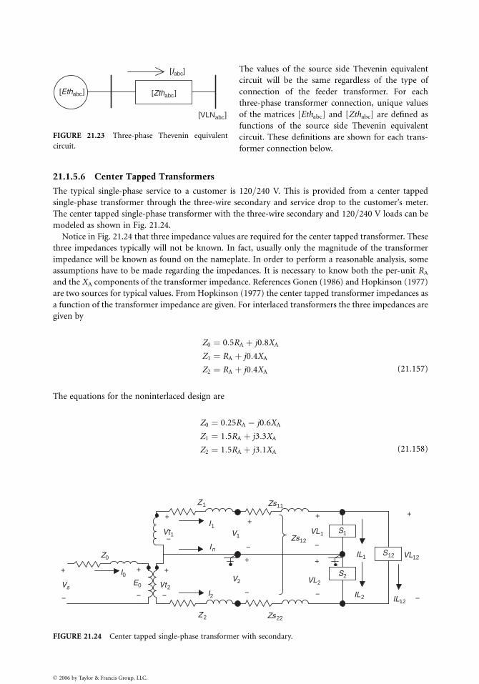
[Iabc]
[VLNabc]
[Ethabc] [Zthabc]
FIGURE 21.23 Three-phase Thevenin equivalent
circuit.
Vs
Z0
E0 Vt2
Z1
I1
In
Z2
I2
V1
V
Vt1
+
−
+
−
+
−
I0+
−
FIGURE 21.24 Center tapped single-phase transformer
� 2006 by Taylor & Francis Group, LLC.
The values of the source side Thevenin equivalent
circuit will be the same regardless of the type of
connection of the feeder transformer. For each
three-phase transformer connection, unique values
of the matrices [Ethabc] and [Zthabc] are defined as
functions of the source side Thevenin equivalent
circuit. These definitions are shown for each trans-
former connection below.
21.1.5.6 Center Tapped Transformers
The typical single-phase service to a customer is 120=240 V. This is provided from a center tapped
single-phase transformer through the three-wire secondary and service drop to the customer’s meter.
The center tapped single-phase transformer with the three-wire secondary and 120=240 V loads can be
modeled as shown in Fig. 21.24.
Notice in Fig. 21.24 that three impedance values are required for the center tapped transformer. These
three impedances typically will not be known. In fact, usually only the magnitude of the transformer
impedance will be known as found on the nameplate. In order to perform a reasonable analysis, some
assumptions have to be made regarding the impedances. It is necessary to know both the per-unit RA
and the XA components of the transformer impedance. References Gonen (1986) and Hopkinson (1977)
are two sources for typical values. From Hopkinson (1977) the center tapped transformer impedances as
a function of the transformer impedance are given. For interlaced transformers the three impedances are
given by
Z0 ¼ 0:5RA þ j0:8XA
Z1 ¼ RA þ j0:4XA
Z2 ¼ RA þ j0:4XA (21:157)
The equations for the noninterlaced design are
Z0 ¼ 0:25RA � j0:6XA
Z1 ¼ 1:5RA þ j3:3XA
Z2 ¼ 1:5RA þ j3:1XA (21:158)
+Zs11
Zs12
2
Zs22
VL1
VL2
S1
S2
IL1
IL2
S12 VL12
IL12 −
+
−
+
−
+
−
+
−
with secondary.
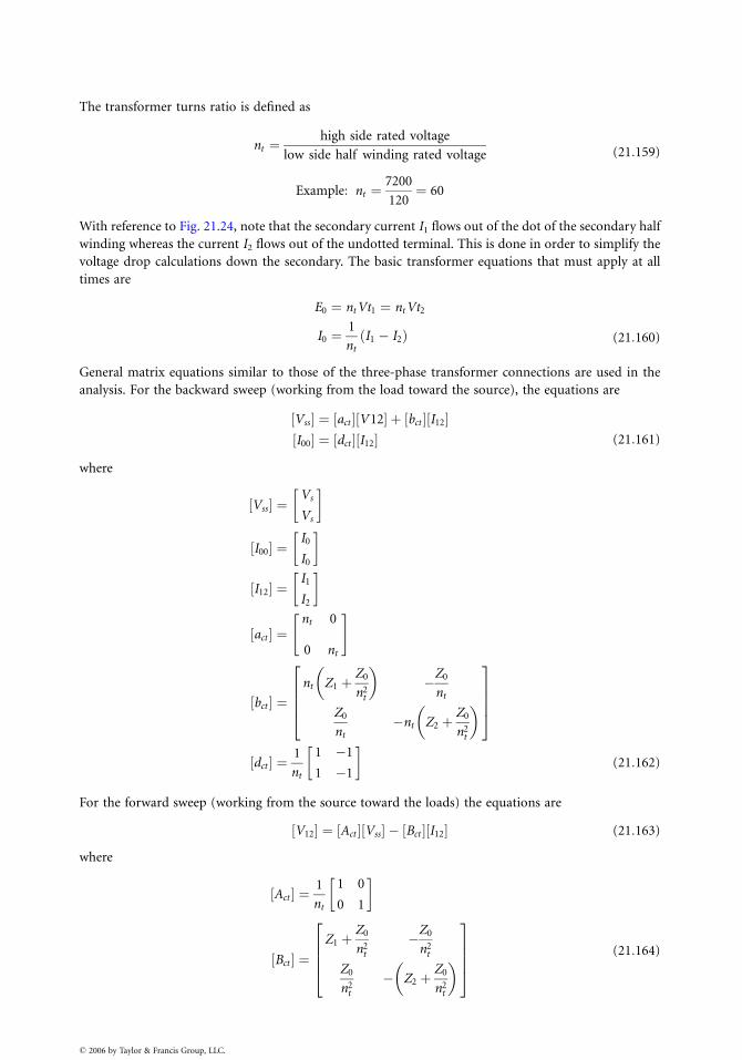
The transformer turns ratio is defined as
nt ¼high side rated voltage
low side half winding rated voltage (21:159)
Example: nt ¼7200
120¼ 60
With reference to Fig. 21.24, note that the secondary current I1 flows out of the dot of the secondary half
winding whereas the current I2 flows out of the undotted terminal. This is done in order to simplify the
voltage drop calculations down the secondary. The basic transformer equations that must apply at all
times are
E0 ¼ nt Vt1 ¼ nt Vt2
I0 ¼1
nt
I1 � I2ð Þ (21:160)
General matrix equations similar to those of the three-phase transformer connections are used in the
analysis. For the backward sweep (working from the load toward the source), the equations are
Vss½ � ¼ act½ � V 12½ � þ bct½ � I12½ �I00½ � ¼ dct½ � I12½ � (21:161)
where
Vss½ � ¼Vs
Vs
I00½ � ¼I0
I0
I12½ � ¼I1
I2
act½ � ¼nt 0
0 nt
" #
bct½ � ¼nt Z1 þ
Z0
n2t
� �
�Z0
nt
Z0
nt
�nt Z2 þZ0
n2t
� �
2
6
6
6
4
3
7
7
7
5
dct½ � ¼1
nt
1 �1
1 �1
(21:162)
For the forward sweep (working from the source toward the loads) the equations are
V12½ � ¼ Act½ � Vss½ � � Bct½ � I12½ � (21:163)
where
Act½ � ¼1
nt
1 0
0 1
Bct½ � ¼Z1 þ
Z0
n2t
�Z0
n2t
Z0
n2t
� Z2 þZ0
n2t
� �
2
6
6
6
4
3
7
7
7
5
(21:164)
� 2006 by Taylor & Francis Group, LLC.
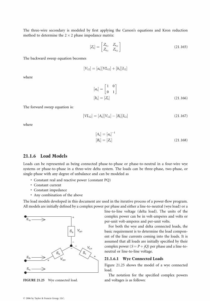
The three-wire secondary is modeled by first applying the Carson’s equations and Kron reduction
method to determine the 2� 2 phase impedance matrix:
Zs½ � ¼Zs11
Zs12
Zs21Zs22
(21:165)
The backward sweep equation becomes
V12½ � ¼ as½ � VL12½ � þ bs½ � I12½ �
where
as½ � ¼1 0
0 1
bs½ � ¼ Zs½ � (21:166)
The forward sweep equation is:
VL12½ � ¼ As½ � V12½ � � Bs½ � I12½ � (21:167)
where
As½ � ¼ as½ ��1
Bs½ � ¼ Zs½ � (21:168)
21.1.6 Load Models
Loads can be represented as being connected phase-to-phase or phase-to-neutral in a four-wire wye
systems or phase-to-phase in a three-wire delta system. The loads can be three-phase, two-phase, or
single-phase with any degree of unbalance and can be modeled as
. Constant real and reactive power (constant PQ)
. Constant current
. Constant impedance
. Any combination of the above
The load models developed in this document are used in the iterative process of a power-flow program.
All models are initially defined by a complex power per phase and either a line-to-neutral (wye load) or a
+
++
−−
−
Van
Vcn
Sc
Sa
Sb
VbnILb
ILc
ILa
FIGURE 21.25 Wye connected load.
� 2006 by Taylor & Francis Group, LLC.
line-to-line voltage (delta load). The units of the
complex power can be in volt-amperes and volts or
per-unit volt-amperes and per-unit volts.
For both the wye and delta connected loads, the
basic requirement is to determine the load compon-
ent of the line currents coming into the loads. It is
assumed that all loads are initially specified by their
complex power (S¼Pþ jQ) per phase and a line-to-
neutral or line-to-line voltage.
21.1.6.1 Wye Connected Loads
Figure 21.25 shows the model of a wye connected
load.
The notation for the specified complex powers
and voltages is as follows:
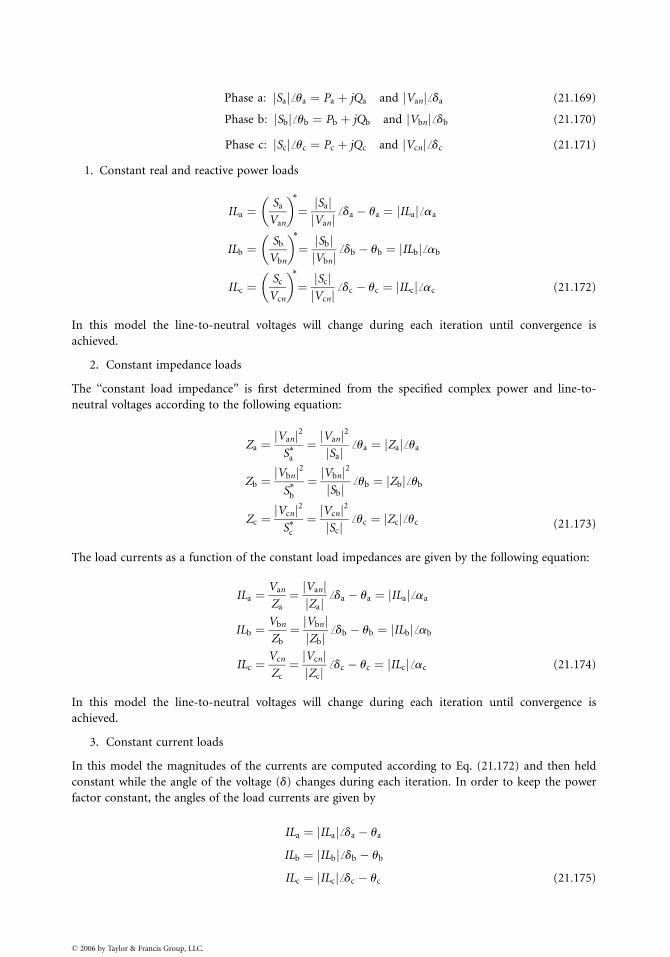
Phase a: Saj jffua ¼ Pa þ jQa and Vanj jffda (21:169)
Phase b: Sbj jffub ¼ Pb þ jQb and Vbnj jffdb (21:170)
Phase c: Scj jffuc ¼ Pc þ jQc and Vcnj jffdc (21:171)
1. Constant real and reactive power loads
ILa ¼Sa
Van
� �*
¼ Saj jVanj j ffda � ua ¼ ILaj jffaa
ILb ¼Sb
Vbn
� �*
¼ Sbj jVbnj j ffdb � ub ¼ ILbj jffab
ILc ¼Sc
Vcn
� �*
¼ Scj jVcnj j ffdc � uc ¼ ILcj jffac (21:172)
In this model the line-to-neutral voltages will change during each iteration until convergence is
achieved.
2. Constant impedance loads
The ‘‘constant load impedance’’ is first determined from the specified complex power and line-to-
neutral voltages according to the following equation:
Za ¼Vanj j2
S*a
¼ Vanj j2
Saj jffua ¼ Zaj jffua
Zb ¼Vbnj j2
S*b
¼ Vbnj j2
Sbj jffub ¼ Zbj jffub
Zc ¼Vcnj j2
S*c
¼ Vcnj j2
Scj jffuc ¼ Zcj jffuc (21:173)
The load currents as a function of the constant load impedances are given by the following equation:
ILa ¼Van
Za
¼ Vanj jZaj jffda � ua ¼ ILaj jffaa
ILb ¼Vbn
Zb
¼ Vbnj jZbj jffdb � ub ¼ ILbj jffab
ILc ¼Vcn
Zc
¼ Vcnj jZcj jffdc � uc ¼ ILcj jffac (21:174)
In this model the line-to-neutral voltages will change during each iteration until convergence is
achieved.
3. Constant current loads
In this model the magnitudes of the currents are computed according to Eq. (21.172) and then held
constant while the angle of the voltage (d) changes during each iteration. In order to keep the power
factor constant, the angles of the load currents are given by
ILa ¼ ILaj jffda � ua
ILb ¼ ILbj jffdb � ub
ILc ¼ ILcj jffdc � uc (21:175)
� 2006 by Taylor & Francis Group, LLC.
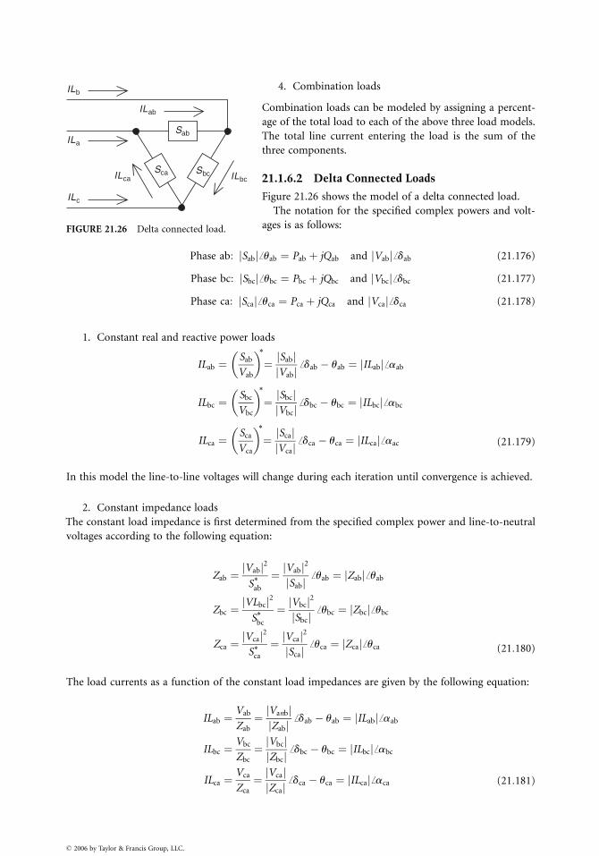
ILb
ILa
ILc
ILca
ILab
ILbc
Sab
Sca Sbc
� 2006 by Taylor & Francis Group, LLC.
4. Combination loads
Combination loads can be modeled by assigning a percent-
age of the total load to each of the above three load models.
The total line current entering the load is the sum of the
three components.
21.1.6.2 Delta Connected Loads
Figure 21.26 shows the model of a delta connected load.
The notation for the specified complex powers and volt-
ages is as follows:
Phase ab: Sabj jffuab ¼ Pab þ jQab and Vabj jffdab (21:176)
Phase bc: Sbcj jffubc ¼ Pbc þ jQbc and Vbcj jffdbc (21:177)
Phase ca: Scaj jffuca ¼ Pca þ jQca and Vcaj jffdca (21:178)
1. Constant real and reactive power loads
ILab ¼Sab
Vab
� �*
¼ Sabj jVabj j ffdab � uab ¼ ILabj jffaab
ILbc ¼Sbc
Vbc
� �*
¼ Sbcj jVbcj j ffdbc � ubc ¼ ILbcj jffabc
ILca ¼Sca
Vca
� �*
¼ Scaj jVcaj j ffdca � uca ¼ ILcaj jffaac (21:179)
In this model the line-to-line voltages will change during each iteration until convergence is achieved.
2. Constant impedance loads
The constant load impedance is first determined from the specified complex power and line-to-neutral
voltages according to the following equation:
Zab ¼Vabj j2
S*ab
¼ Vabj j2
Sabj jffuab ¼ Zabj jffuab
Zbc ¼VLbcj j2
S*bc
¼ Vbcj j2
Sbcj jffubc ¼ Zbcj jffubc
Zca ¼Vcaj j2
S*ca
¼ Vcaj j2
Scaj jffuca ¼ Zcaj jffuca (21:180)
The load currents as a function of the constant load impedances are given by the following equation:
ILab ¼Vab
Zab
¼ Vanbj jZabj j ffdab � uab ¼ ILabj jffaab
ILbc ¼Vbc
Zbc
¼ Vbcj jZbcj j ffdbc � ubc ¼ ILbcj jffabc
ILca ¼Vca
Zca
¼ Vcaj jZcaj j ffdca � uca ¼ ILcaj jffaca (21:181)
FIGURE 21.26 Delta connected load.

In this model the line-to-line voltages in Eq. (21.181) will change during each iteration until conver-
gence is achieved.
3. Constant current loads
In this model the magnitudes of the currents are computed according to Eq. (21.179) and then held
constant while the angle of the voltage (d) changes during each iteration. This keeps the power factor of
the load constant.
ILab ¼ ILabj jffdab � uab
ILbc ¼ ILbcj jffdbc � ubc
ILca ¼ ILcaj jffdca � uca (21:182)
4. Combination loads
Combination loads can be modeled by assigning a percentage of the total load to each of the above three
load models. The total delta current for each load is the sum of the three components.
The line currents entering the delta connected load for all models are determined by
ILa
ILb
ILc
2
4
3
5 ¼1 0 �1
�1 1 0
0 �1 1
2
4
3
5
ILab
ILbc
ILca
2
4
3
5 (21:183)
In both the wye and delta connected loads, single-phase and two-phase loads are modeled by setting the
complex powers of the missing phases to zero. In other words, all loads are modeled as three-phase loads
and by setting the complex power of the missing phases to zero, the only load currents computed using
the above equations will be for the nonzero loads.
21.1.7 Shunt Capacitor Models
Shunt capacitor banks are commonly used in a distribution system to help in voltage regulation and to
provide reactive power support. The capacitor banks are modeled as constant susceptances connected in
either wye or delta. Similar to the load model, all capacitor banks are modeled as three-phase banks with
the kVAr of missing phases set to zero for single-phase and two-phase banks.
21.1.7.1 Wye Connected Capacitor Bank
A wye connected capacitor bank is shown in Fig. 21.27. The individual phase capacitor units are
specified in kVAr and kV. The constant susceptance for each unit can be computed in either Siemans
or per unit. When per unit is desired, the specified kVAr of the capacitor must be divided by the base
+
++
−−
−
Van
Vcn
Vbn
jBa
jBb
jBc
ICa
ICb
ICc
FIGURE 21.27 Wye connected capacitor bank.
� 2006 by Taylor & Francis Group, LLC.
single-phase kVAr and the kV must be divided by the
base line-to-neutral kV.
The susceptance of a capacitor unit is computed by
Bactual ¼kVAr
kV21000Siemans (21:184)
Bpu ¼kVArpu
V2pu
per unit (21:185)
where kVArpu ¼kVAractual
kVAsingle phase base
(21:186)
Vpu ¼kVactual
kVline to neutral base
(21:187)
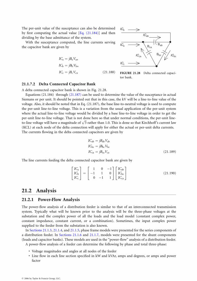
ICab
Bab
Bbc
Bca
ICca ICbc
ICa
ICb
ICc
FIGURE 21.28 Delta connected capaci-
tor bank.
The per-unit value of the susceptance can also be determined
by first computing the actual value [Eq. (21.184)] and then
dividing by the base admittance of the system.
With the susceptance computed, the line currents serving
the capacitor bank are given by
ICa ¼ jBaVan
ICb ¼ jBbVbn
ICc ¼ jBcVcn (21:188)
21.1.7.2 Delta Connected Capacitor Bank
A delta connected capacitor bank is shown in Fig. 21.28.
Equations (21.184) through (21.187) can be used to determine the value of the susceptance in actual
Siemans or per unit. It should be pointed out that in this case, the kV will be a line-to-line value of the
voltage. Also, it should be noted that in Eq. (21.187), the base line-to-neutral voltage is used to compute
the per-unit line-to-line voltage. This is a variation from the usual application of the per-unit system
where the actual line-to-line voltage would be divided by a base line-to-line voltage in order to get the
per-unit line-to-line voltage. That is not done here so that under normal conditions, the per-unit line-
to-line voltage will have a magnitude offfiffiffi
3p
rather than 1.0. This is done so that Kirchhoff ’s current law
(KCL) at each node of the delta connection will apply for either the actual or per-unit delta currents.
The currents flowing in the delta connected capacitors are given by
ICab ¼ jBabVab
ICbc ¼ jBbcVbc
ICca ¼ jBcaVca (21:189)
The line currents feeding the delta connected capacitor bank are given by
ICa
ICb
ICc
2
4
3
5 ¼1 0 �1
�1 1 0
0 �1 1
2
4
3
5
ICab
ICbc
ICca
2
4
3
5 (21:190)
21.2 Analysis
21.2.1 Power-Flow Analysis
The power-flow analysis of a distribution feeder is similar to that of an interconnected transmission
system. Typically what will be known prior to the analysis will be the three-phase voltages at the
substation and the complex power of all the loads and the load model (constant complex power,
constant impedance, constant current, or a combination). Sometimes, the input complex power
supplied to the feeder from the substation is also known.
In Sections 21.1.3, 21.1.4, and 21.1.5, phase frame models were presented for the series components of
a distribution feeder. In Sections 21.1.6 and 21.1.7, models were presented for the shunt components
(loads and capacitor banks). These models are used in the ‘‘power-flow’’ analysis of a distribution feeder.
A power-flow analysis of a feeder can determine the following by phase and total three-phase:
. Voltage magnitudes and angles at all nodes of the feeder
. Line flow in each line section specified in kW and kVAr, amps and degrees, or amps and power
factor
� 2006 by Taylor & Francis Group, LLC.
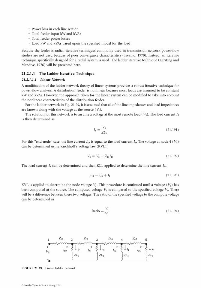
. Power loss in each line section
. Total feeder input kW and kVAr
. Total feeder power losses
. Load kW and kVAr based upon the specified model for the load
Because the feeder is radial, iterative techniques commonly used in transmission network power-flow
studies are not used because of poor convergence characteristics (Trevino, 1970). Instead, an iterative
technique specifically designed for a radial system is used. The ladder iterative technique (Kersting and
Mendive, 1976) will be presented here.
21.2.1.1 The Ladder Iterative Technique
21.2.1.1.1 Linear Network
A modification of the ladder network theory of linear systems provides a robust iterative technique for
power-flow analysis. A distribution feeder is nonlinear because most loads are assumed to be constant
kW and kVAr. However, the approach taken for the linear system can be modified to take into account
the nonlinear characteristics of the distribution feeder.
For the ladder network in Fig. 21.29, it is assumed that all of the line impedances and load impedances
are known along with the voltage at the source (Vs).
The solution for this network is to assume a voltage at the most remote load (V5). The load current I5
is then determined as
I5 ¼V5
ZL5
(21:191)
For this ‘‘end-node’’ case, the line current I45 is equal to the load current I5. The voltage at node 4 (V4)
can be determined using Kirchhoff ’s voltage law (KVL):
V4 ¼ V5 þ Z45I45 (21:192)
The load current I4 can be determined and then KCL applied to determine the line current I34.
I34 ¼ I45 þ I4 (21:193)
KVL is applied to determine the node voltage V3. This procedure is continued until a voltage (V1) has
been computed at the source. The computed voltage V1 is compared to the specified voltage Vs. There
will be a difference between these two voltages. The ratio of the specified voltage to the compute voltage
can be determined as
Ratio ¼ Vs
V1
(21:194)
1
+
−
2 3 4 5Z12
I12I2 I3 I4 I5I23 I34 I45
Z23 Z34 Z45
ZL5ZL4ZL3ZL2
VS
FIGURE 21.29 Linear ladder network.
� 2006 by Taylor & Francis Group, LLC.
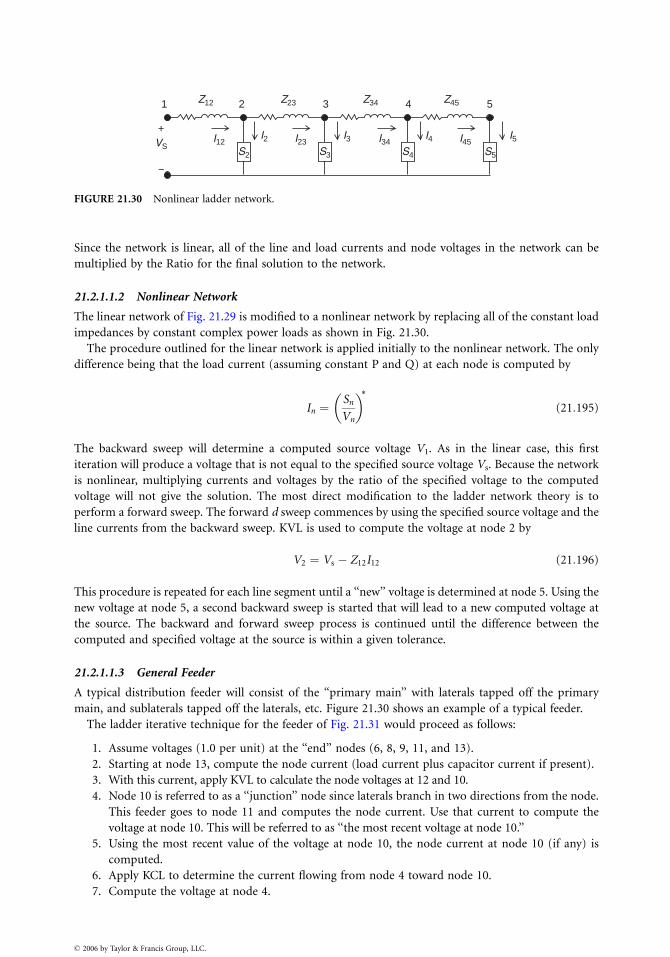
1
+
−
2 3 4 5Z12
I12I2 I3 I4 I5I23 I34 I45
Z23 Z34 Z45
VS S5S4S3S2
FIGURE 21.30 Nonlinear ladder network.
Since the network is linear, all of the line and load currents and node voltages in the network can be
multiplied by the Ratio for the final solution to the network.
21.2.1.1.2 Nonlinear Network
The linear network of Fig. 21.29 is modified to a nonlinear network by replacing all of the constant load
impedances by constant complex power loads as shown in Fig. 21.30.
The procedure outlined for the linear network is applied initially to the nonlinear network. The only
difference being that the load current (assuming constant P and Q) at each node is computed by
In ¼Sn
Vn
� �*
(21:195)
The backward sweep will determine a computed source voltage V1. As in the linear case, this first
iteration will produce a voltage that is not equal to the specified source voltage Vs. Because the network
is nonlinear, multiplying currents and voltages by the ratio of the specified voltage to the computed
voltage will not give the solution. The most direct modification to the ladder network theory is to
perform a forward sweep. The forward d sweep commences by using the specified source voltage and the
line currents from the backward sweep. KVL is used to compute the voltage at node 2 by
V2 ¼ Vs � Z12I12 (21:196)
This procedure is repeated for each line segment until a ‘‘new’’ voltage is determined at node 5. Using the
new voltage at node 5, a second backward sweep is started that will lead to a new computed voltage at
the source. The backward and forward sweep process is continued until the difference between the
computed and specified voltage at the source is within a given tolerance.
21.2.1.1.3 General Feeder
A typical distribution feeder will consist of the ‘‘primary main’’ with laterals tapped off the primary
main, and sublaterals tapped off the laterals, etc. Figure 21.30 shows an example of a typical feeder.
The ladder iterative technique for the feeder of Fig. 21.31 would proceed as follows:
1. Assume voltages (1.0 per unit) at the ‘‘end’’ nodes (6, 8, 9, 11, and 13).
2. Starting at node 13, compute the node current (load current plus capacitor current if present).
3. With this current, apply KVL to calculate the node voltages at 12 and 10.
4. Node 10 is referred to as a ‘‘junction’’ node since laterals branch in two directions from the node.
This feeder goes to node 11 and computes the node current. Use that current to compute the
voltage at node 10. This will be referred to as ‘‘the most recent voltage at node 10.’’
5. Using the most recent value of the voltage at node 10, the node current at node 10 (if any) is
computed.
6. Apply KCL to determine the current flowing from node 4 toward node 10.
7. Compute the voltage at node 4.
� 2006 by Taylor & Francis Group, LLC.
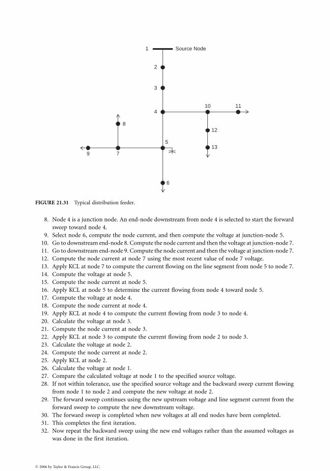
Source Node
10
12
135
6
7
8
2
1
3
4
9
11
FIGURE 21.31 Typical distribution feeder.
8. Node 4 is a junction node. An end-node downstream from node 4 is selected to start the forward
sweep toward node 4.
9. Select node 6, compute the node current, and then compute the voltage at junction-node 5.
10. Go to downstream end-node 8. Compute the node current and then the voltage at junction-node 7.
11. Go to downstream end-node 9. Compute the node current and then the voltage at junction-node 7.
12. Compute the node current at node 7 using the most recent value of node 7 voltage.
13. Apply KCL at node 7 to compute the current flowing on the line segment from node 5 to node 7.
14. Compute the voltage at node 5.
15. Compute the node current at node 5.
16. Apply KCL at node 5 to determine the current flowing from node 4 toward node 5.
17. Compute the voltage at node 4.
18. Compute the node current at node 4.
19. Apply KCL at node 4 to compute the current flowing from node 3 to node 4.
20. Calculate the voltage at node 3.
21. Compute the node current at node 3.
22. Apply KCL at node 3 to compute the current flowing from node 2 to node 3.
23. Calculate the voltage at node 2.
24. Compute the node current at node 2.
25. Apply KCL at node 2.
26. Calculate the voltage at node 1.
27. Compare the calculated voltage at node 1 to the specified source voltage.
28. If not within tolerance, use the specified source voltage and the backward sweep current flowing
from node 1 to node 2 and compute the new voltage at node 2.
29. The forward sweep continues using the new upstream voltage and line segment current from the
forward sweep to compute the new downstream voltage.
30. The forward sweep is completed when new voltages at all end nodes have been completed.
31. This completes the first iteration.
32. Now repeat the backward sweep using the new end voltages rather than the assumed voltages as
was done in the first iteration.
� 2006 by Taylor & Francis Group, LLC.
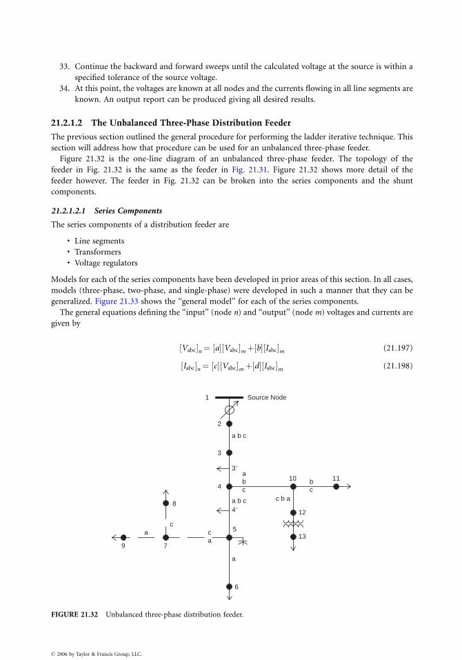
33. Continue the backward and forward sweeps until the calculated voltage at the source is within a
specified tolerance of the source voltage.
34. At this point, the voltages are known at all nodes and the currents flowing in all line segments are
known. An output report can be produced giving all desired results.
21.2.1.2 The Unbalanced Three-Phase Distribution Feeder
The previous section outlined the general procedure for performing the ladder iterative technique. This
section will address how that procedure can be used for an unbalanced three-phase feeder.
Figure 21.32 is the one-line diagram of an unbalanced three-phase feeder. The topology of the
feeder in Fig. 21.32 is the same as the feeder in Fig. 21.31. Figure 21.32 shows more detail of the
feeder however. The feeder in Fig. 21.32 can be broken into the series components and the shunt
components.
21.2.1.2.1 Series Components
The series components of a distribution feeder are
. Line segments
. Transformers
. Voltage regulators
Models for each of the series components have been developed in prior areas of this section. In all cases,
models (three-phase, two-phase, and single-phase) were developed in such a manner that they can be
generalized. Figure 21.33 shows the ‘‘general model’’ for each of the series components.
The general equations defining the ‘‘input’’ (node n) and ‘‘output’’ (node m) voltages and currents are
given by
Vabc½ �n¼ a½ � Vabc½ �mþ b½ � Iabc½ �m (21:197)
Iabc½ �n¼ c½ � Vabc½ �mþ d½ � Iabc½ �m (21:198)
Source Node
10
12
135
6
7
8
2
a b c
a b c c b a
a
4�
3�abc
b c
ca
ac
1
3
4
9
11
FIGURE 21.32 Unbalanced three-phase distribution feeder.
� 2006 by Taylor & Francis Group, LLC.
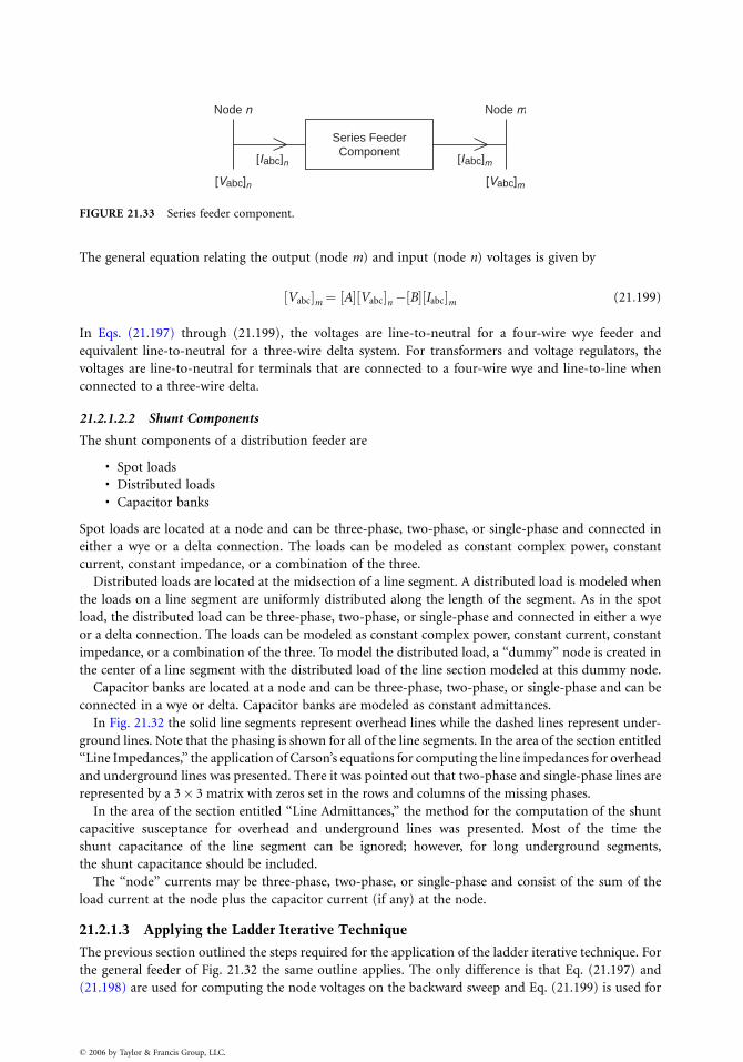
Node n Node m
Series FeederComponent
[Vabc]n [Vabc]m
[Iabc]n [Iabc]m
FIGURE 21.33 Series feeder component.
The general equation relating the output (node m) and input (node n) voltages is given by
Vabc½ �m¼ A½ � Vabc½ �n� B½ � Iabc½ �m (21:199)
In Eqs. (21.197) through (21.199), the voltages are line-to-neutral for a four-wire wye feeder and
equivalent line-to-neutral for a three-wire delta system. For transformers and voltage regulators, the
voltages are line-to-neutral for terminals that are connected to a four-wire wye and line-to-line when
connected to a three-wire delta.
21.2.1.2.2 Shunt Components
The shunt components of a distribution feeder are
. Spot loads
. Distributed loads
. Capacitor banks
Spot loads are located at a node and can be three-phase, two-phase, or single-phase and connected in
either a wye or a delta connection. The loads can be modeled as constant complex power, constant
current, constant impedance, or a combination of the three.
Distributed loads are located at the midsection of a line segment. A distributed load is modeled when
the loads on a line segment are uniformly distributed along the length of the segment. As in the spot
load, the distributed load can be three-phase, two-phase, or single-phase and connected in either a wye
or a delta connection. The loads can be modeled as constant complex power, constant current, constant
impedance, or a combination of the three. To model the distributed load, a ‘‘dummy’’ node is created in
the center of a line segment with the distributed load of the line section modeled at this dummy node.
Capacitor banks are located at a node and can be three-phase, two-phase, or single-phase and can be
connected in a wye or delta. Capacitor banks are modeled as constant admittances.
In Fig. 21.32 the solid line segments represent overhead lines while the dashed lines represent under-
ground lines. Note that the phasing is shown for all of the line segments. In the area of the section entitled
‘‘Line Impedances,’’ the application of Carson’s equations for computing the line impedances for overhead
and underground lines was presented. There it was pointed out that two-phase and single-phase lines are
represented by a 3� 3 matrix with zeros set in the rows and columns of the missing phases.
In the area of the section entitled ‘‘Line Admittances,’’ the method for the computation of the shunt
capacitive susceptance for overhead and underground lines was presented. Most of the time the
shunt capacitance of the line segment can be ignored; however, for long underground segments,
the shunt capacitance should be included.
The ‘‘node’’ currents may be three-phase, two-phase, or single-phase and consist of the sum of the
load current at the node plus the capacitor current (if any) at the node.
21.2.1.3 Applying the Ladder Iterative Technique
The previous section outlined the steps required for the application of the ladder iterative technique. For
the general feeder of Fig. 21.32 the same outline applies. The only difference is that Eq. (21.197) and
(21.198) are used for computing the node voltages on the backward sweep and Eq. (21.199) is used for
� 2006 by Taylor & Francis Group, LLC.
computing the downstream voltages on the forward sweep. The [a], [b], [c], [d], [A], and [B] matrices
for the various series components are defined in the following areas of this section:
. Line segments: Line segment models
. Voltage regulators: Step-voltage regulators
. Transformer banks: Transformer bank connections
The node currents are defined in the following area:
. Loads: Load models
. Capacitors: Shunt capacitor models
21.2.1.4 Final Notes
21.2.1.4.1 Line Segment Impedances
It is extremely important that the impedances and admittances of the line segments be computed using
the exact spacings and phasing. Because of the unbalanced loading and resulting unbalanced line currents,
the voltage drops due to the mutual coupling of the lines become very important. It is not unusual to
observe a voltage rise on a lightly loaded phase of a line segment that has an extreme current unbalance.
21.2.1.4.2 Power Loss
The real power losses of a line segment must be computed as the difference (by phase) of the input
power to a line segment minus the output power of the line segment. It is possible to observe a negative
power loss on a phase that is lightly loaded compared to the other two phases. Computing power
loss as the phase current squared times the phase resistance does not give the actual real power loss in
the phases.
21.2.1.4.3 Load Allocation
Many times the input complex power (kW and kVAr) to a feeder is known because of the metering at the
substation. This information can be either total three-phase or for each individual phase. In some cases
the metered data may be the current and power factor in each phase.
It is desirable to have the computed input to the feeder match the metered input. This can be
accomplished (following a converged iterative solution) by computing the ratio of the metered input to
the computed input. The phase loads can now be modified by multiplying the loads by this ratio.
Because the losses of the feeder will change when the loads are changed, it is necessary to go through the
ladder iterative process to determine a new computed input to the feeder. This new computed input will
be closer to the metered input, but most likely not within a specified tolerance. Again, a ratio can be
determined and the loads modified. This process is repeated until the computed input is within a
specified tolerance of the metered input.
21.2.1.5 Short-Circuit Analysis
The computation of short-circuit currents for unbalanced faults in a normally balanced three-phase
system has traditionally been accomplished by the application of symmetrical components. However,
this method is not well-suited to a distribution feeder that is inherently unbalanced. The unequal mutual
coupling between phases leads to mutual coupling between sequence networks. When this happens,
there is no advantage to using symmetrical components. Another reason for not using symmetrical
components is that the phases between which faults occur is limited. For example, using symmetrical
components, line-to-ground faults are limited to phase a to ground. What happens if a single-phase
lateral is connected to phase b or c? This section will present a method for short-circuit analysis of an
unbalanced three-phase distribution feeder using the phase frame (Kersting, 1980).
21.2.1.5.1 General Theory
Figure 21.34 shows the unbalanced feeder as modeled for short-circuit calculations. In Fig. 21.34, the
voltage sources Ea, Eb, and Ec represent the Thevenin equivalent line-to-ground voltages at the faulted
� 2006 by Taylor & Francis Group, LLC.
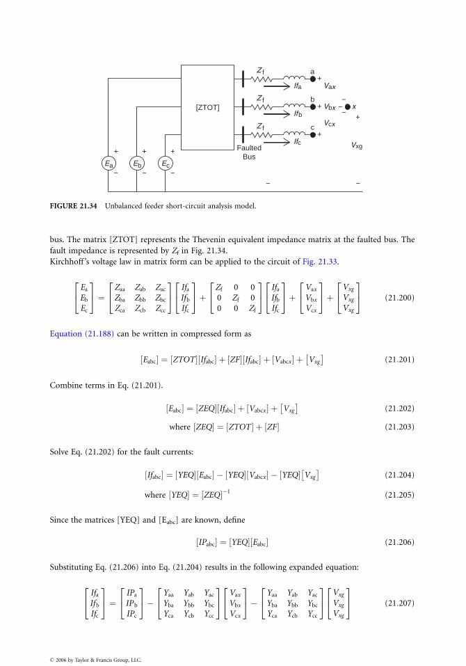
[ZTOT]
Z f a
Ifa Vax+
Z f b
IfbVbx+ x
+
+
−
−
−−
−
Z f c
IfcFaulted
Bus
Vcx
+
Vxg
−Ec
+
−Eb
+
−Ea
FIGURE 21.34 Unbalanced feeder short-circuit analysis model.
bus. The matrix [ZTOT] represents the Thevenin equivalent impedance matrix at the faulted bus. The
fault impedance is represented by Zf in Fig. 21.34.
Kirchhoff ’s voltage law in matrix form can be applied to the circuit of Fig. 21.33.
Ea
Eb
Ec
2
4
3
5 ¼Zaa Zab Zac
Zba Zbb Zbc
Zca Zcb Zcc
2
4
3
5
Ifa
Ifb
Ifc
2
4
3
5þZf 0 0
0 Zf 0
0 0 Zf
2
4
3
5
Ifa
Ifb
Ifc
2
4
3
5þVax
Vbx
Vcx
2
4
3
5þVxg
Vxg
Vxg
2
4
3
5 (21:200)
Equation (21.188) can be written in compressed form as
Eabc½ � ¼ ZTOT½ � Ifabc½ � þ ZF½ � Ifabc½ � þ Vabcx½ � þ Vxg
� �
(21:201)
Combine terms in Eq. (21.201).
Eabc½ � ¼ ZEQ½ � Ifabc½ � þ Vabcx½ � þ Vxg
� �
(21:202)
where ZEQ½ � ¼ ZTOT½ � þ ZF½ � (21:203)
Solve Eq. (21.202) for the fault currents:
Ifabc½ � ¼ YEQ½ � Eabc½ � � YEQ½ � Vabcx½ � � YEQ½ � Vxg
� �
(21:204)
where YEQ½ � ¼ ZEQ½ ��1(21:205)
Since the matrices [YEQ] and [Eabc] are known, define
IPabc½ � ¼ YEQ½ � Eabc½ � (21:206)
Substituting Eq. (21.206) into Eq. (21.204) results in the following expanded equation:
Ifa
If b
Ifc
2
4
3
5 ¼IPa
IP b
IPc
2
4
3
5�Yaa Yab Yac
Yba Ybb Ybc
Yca Ycb Ycc
2
4
3
5
Vax
Vbx
Vcx
2
4
3
5�Yaa Yab Yac
Yba Ybb Ybc
Yca Ycb Ycc
2
4
3
5
Vxg
Vxg
Vxg
2
4
3
5 (21:207)
� 2006 by Taylor & Francis Group, LLC.
Performing the matrix operations in Eq. (21.195):
Ifa ¼ IPa � YaaVax þ YabVbx þ YacVcxð Þ � YaVxg
If b ¼ IPb � YbaVax þ YbbVbx þ YbcVcxð Þ � YbVxg
If ¼ IPc � YcaVax þ YcbVbx þ YccVcxð Þ � YcVxg (21:208)
where
Ya ¼ Yaa þ Yab þ Yac
Yb ¼ Yba þ Ybb þ Ybc
Yc ¼ Yca þ Ycb þ Ycc (21:209)
Equations (21.208) become the general equations that are used to simulate all types of short circuits.
Basically there are three equations and seven unknowns (Ifa, Ifb, Ifc, Vax , Vbx , Vcx, and Vxg). The other
three variables in the equations (IPa, IPb, and IPc) are functions of the total impedance and the Thevenin
voltages and are therefore known. In order to solve Eq. (21.208), it will be necessary to specify four of the
seven unknowns. These specifications are functions of the type of fault being simulated. The additional
required four knowns for various types of faults are given below:
Three-phase faults
Vax ¼ Vbx ¼ Vcx ¼ 0
Ia þ Ib þ Ic ¼ 0 (21:210)
Three-phase-to-ground faults
Vax ¼ Vbx ¼ Vcx ¼ Vxg ¼ 0 (21:211)
Line-to-line faults (assume i–j fault with phase k unfaulted)
Vix ¼ Vjx ¼ 0
If k ¼ 0
If i þ If j ¼ 0 (21:212)
Line-to-line-to-ground faults (assume i–j to ground fault with k unfaulted)
Vix ¼ Vjx ¼ Vxg ¼ 0
Vkx ¼IPk
Ykk(21:213)
Line-to-ground faults (assume phase k fault with phases i and j unfaulted)
Vkx ¼ Vxg ¼ 0
If i ¼ If j ¼ 0 (21:214)
Notice that Eqs. (21.212) through (21.214) will allow the simulation of line-to-line, line-to-line-to-
ground, and line-to-ground faults for all phases. There is no limitation to b–c faults for line-to-line and
a–g for line-to-ground as is the case when the method of symmetrical components is employed.
� 2006 by Taylor & Francis Group, LLC.

References
Carson, J.R., Wave propagation in overhead wires with ground return, Bell Syst. Tech. J., 5, 1926.
Glover, J.D. and Sarma, M., Power System Analysis and Design, 2nd ed., PWS Publishing Company,
Boston, Chap. 5, 1994.
Gonen, T., Electric Power Distribution System Engineering, McGraw-Hill Book Company, 1986.
Hopkinson, R.H., Approximate Distribution Transformer Impedances, from an internal GE Memo
dated August 30, 1977.
Kersting, W.H., Distribution system short circuit analysis, 25th Intersociety Energy Conversion Confer-
ence, Reno, Nevada, August 1980.
Kersting, W.H., Milsoft Transformer Models—Theory, Research Report, Milsoft Integrated Solutions, Inc.,
Abilene, TX, 1999.
Kersting, W.H. and Mendive, D.L., An application of ladder network theory to the solution of three-
phase radial load-flow problems, IEEE Conference Paper presented at the IEEE Winter Power
Meeting, New York, January 1976.
Kron, G., Tensorial analysis of integrated transmission systems, Part I: The six basic reference frames,
AIEE Trans., 71, 1952.
Trevino, C., Cases of difficult convergence in load-flow problems, IEEE Paper no. 71-62-PWR, presented
at the IEEE Summer Power Meeting, Los Angeles, CA, 1970.
� 2006 by Taylor & Francis Group, LLC.

� 2006 by Taylor & Francis Group, LLC.
22
� 2006 by Taylor & Francis Group, LLC.
Power SystemOperation and Control
George L. ClarkAlabama Power Company
Simon W. BowenAlabama Power Company
22.1 Implementation of Distribution Automation............... 22-1
22.2 Distribution SCADA History ......................................... 22-2SCADA System Elements . Distribution SCADA . Host
Equipment . Host Computer System . Communication
Front-End Processors . Full Graphics User Interface .
Relational Databases, Data Servers, and Web Servers .
Host to Field Communications
22.3 Field Devices .................................................................... 22-5Modern RTU . PLCs and IEDs . Substation . Line .
Tactical and Strategic Implementation Issues . Distribution
Management Platform . Advanced Distribution Applications
22.4 Integrated SCADA System.............................................. 22-8Trouble Call and Outage Management System . Distribution
Operations Training Simulator
22.5 Security............................................................................. 22-9
22.6 Practical Considerations ............................................... 22-10Choosing the Vendor
22.7 Standards........................................................................ 22-10Internal Standards . Industry Standards
22.8 Deployment Considerations......................................... 22-11Support Organization
22.1 Implementation of Distribution Automation
The implementation of ‘‘distribution automation’’ within the continental U.S. is as diverse and
numerous as the utilities themselves. Particular strategies of implementation utilized by various
utilities have depended heavily on environmental variables such as size of the utility, urbanization,
and available communication paths. The current level of interest in distribution automation is the
result of:
. The August 14, 2003 northeast blackout, which focused attention on infrastructure deficiencies
and increased industry attention on sensor technology and digital control systems.. Recent initiatives such as the DOE’s GridWise program and EPRI’s IntelliGrid program that have
funded distribution research and development projects.. The availability of low-cost, high-performance general purpose microprocessors, embedded
processors, and digital signal processors, which have extended technology choices by blurring
the lines between traditional RTU, PLC, meter, and relay technologies, specifically capabilities that
include meter accuracy measurements and calculations with power quality information including
harmonic content.
. Increased performance in host servers for the same or lower cost, lower cost of memory, and in
particular the movement to Windows and Linux architectures.. The threat of deregulation and competition as a catalyst to automate.. Strategic benefits to be derived (e.g., potential of reduced labor costs, better planning from
better information, optimizing of capital expenditures, reduced outage time, increased customer
satisfaction).
While not meant to be all-inclusive, this section on distribution automation attempts to provide some
dimension to the various alternatives available to the utility engineer. The focus will be on providing
insight on the elements of automation that should be included in a scalable and extensible system. The
approach will be to describe the elements of a ‘‘typical’’ distribution automation system in a simple
manner, offering practical observations as required.
The supervisory control and data acquisition (SCADA) vendors are now delivering systems on the
Windows platform running on PC workstations. The PC-based systems provide opportunities to
distribute the SCADA technology throughout the electric distribution network.
22.2 Distribution SCADA History
SCADA is the foundation for the distribution automation system. The ability to remotely monitor and
control electric power system facilities found its first application within the power generation and
transmission sectors of the electric utility industry. The ability to significantly influence the utility
bottom line through the effective dispatch of generation and the marketing of excess generating
capacity provided economic incentive. The interconnection of large power grids in the Midwestern
and the Southern U.S. (1962) created the largest synchronized system in the world. The blackout of
1965 prompted the U.S. Federal Power Commission to recommend closer coordination between
regional coordination groups (Electric Power Reliability Act of 1967), and gave impetus to the
subsequent formation of the National Electric Reliability Council (1970). From that time (1970)
forward, the priority of the electric utility has been to engineer and build a highly reliable and secure
transmission infrastructure. The importance and urgency of closer coordination was re-emphasized
with the northeast blackout of 2003. Transmission SCADA became the base for the large energy
management systems that were required to manage the transmission grid.
Distribution SCADA was not given equal consideration during this period. For electric utilities,
justification for automating the distribution system, while being highly desirable, was not readily
attainable based on a high cost=benefit ratio due to the size of the distribution infrastructure and cost
of communication circuits. Still there were tactical applications deployed on parts of distribution
systems that were enough to keep the dream alive.
The first real deployments of distribution SCADA systems began in the late 1980s and early
1990s when SCADA vendors delivered reasonably priced ‘‘small’’ SCADA systems on low-cost
hardware architectures to the small co-ops and municipality utilities. As the market expanded,
SCADA vendors who had been providing transmission SCADA began to take notice of the distribution
market. These vendors initially provided host architectures based on VAX=VMS and later on
Alpha=OpenVMS platforms and on UNIX platforms. These systems were required for the large
distribution utility (100,000–250,000 point ranges). These systems often resided on company-owned
LANs with communication front-end (CFE) processors and user interface (UI) attached either locally on
the same LAN or across a WAN.
In the mid-1980s, EPRI published definitions for distribution automation and associated elements.
The industry generally associates distribution automation with the installation of automated distribu-
tion line devices such as switches, reclosers, sectionalizers, etc. The author’s definition of distribution
automation encompasses the automation of the distribution substations and the distribution line
� 2006 by Taylor & Francis Group, LLC.
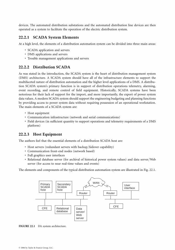
devices. The automated distribution substations and the automated distribution line devices are then
operated as a system to facilitate the operation of the electric distribution system.
22.2.1 SCADA System Elements
At a high level, the elements of a distribution automation system can be divided into three main areas:
. SCADA application and servers
. DMS applications and servers
. Trouble management applications and servers
22.2.2 Distribution SCADA
As was stated in the introduction, the SCADA system is the heart of distribution management system
(DMS) architecture. A SCADA system should have all of the infrastructure elements to support the
multifaceted nature of distribution automation and the higher level applications of a DMS. A distribu-
tion SCADA system’s primary function is in support of distribution operations telemetry, alarming,
event recording, and remote control of field equipment. Historically, SCADA systems have been
notorious for their lack of support for the import, and more importantly, the export of power system
data values. A modern SCADA system should support the engineering budgeting and planning functions
by providing access to power system data without requiring possession of an operational workstation.
The main elements of a SCADA system are:
. Host equipment
. Communication infrastructure (network and serial communications)
. Field devices (in sufficient quantity to support operations and telemetry requirements of a DMS
platform)
22.2.3 Host Equipment
The authors feel that the essential elements of a distribution SCADA host are:
. Host servers (redundant servers with backup=failover capability)
. Communication front-end nodes (network based)
. Full graphics user interfaces
. Relational database server (for archival of historical power system values) and data server=Web
server (for access to near real-time values and events)
The elements and components of the typical distribution automation system are illustrated in Fig. 22.1.
Primary SCADAhost
SecondarySCADAhost
Router
WAN
Router
Relationaldatabase
Dataserver/Webserver
CFECFE
Userinterface
FIGURE 22.1 DA system architecture.
� 2006 by Taylor & Francis Group, LLC.
22.2.4 Host Computer System
22.2.4.1 SCADA Servers
As SCADA has proven its value in operation during inclement weather conditions, service restoration,
and daily operations, the dependency on SCADA has created a requirement for highly available and
high-performance systems. High-performance servers with abundant physical memory, RAID hard disk
systems, and LAN connection are typical of today’s SCADA high-performance servers. Redundant server
hardware operating in a ‘‘live’’ backup=failover mode is required to meet the high availability criteria. In
meeting the high availability criteria, electric utilities may also include a remote SCADA host configur-
ation for disaster recovery.
22.2.5 Communication Front-End Processors
Most utilities will utilize more than one communication medium with the particular choice based on
system requirements and other variables (e.g., radio coverage). However the preponderance of host to
field device communications still depends heavily on serial communications. That is to say no matter
what the communication medium used, the electrical interface to the SCADA system (CFE) is still most
often a serial interface, not a network interface. The host=RTU interface requirement is filled by the CFE.
The CFE can come in several forms based on bus architecture (older CFE technologies were most often
based on VME or PCI bus systems with custom serial controllers). Currently CFE architectures are
moving to Intel=Windows architectures with the serial controller function performed by the main
processor instead of having the serial controllers located on the serial card. Location of the CFE in
relation to the SCADA server can vary based on requirement. In some configurations the CFE is located
on the LAN with the SCADA server. In other cases, existing communications hubs may dictate that the
CFE resides at the communication hub. The incorporation of the WAN into the architecture requires a
more robust CFE application to compensate for intermittent interruptions of network connectivity
(relatively speaking—comparing WAN to LAN communication reliability).
The advent of new architectures for CFEs will offer new capabilities and opportunities for sharing data
within the utility. The ability to serve data through a nonproprietary protocol such as ICCP offers the
possibility for rethinking SCADA architectures within large utilities that may have more than one
SCADA system or more than one audience for SCADA information.
In general the CFE will include three functional devices: a network=CPU board, serial cards, and
possibly a time code receiver. Functionality should include the ability to download configuration and
scan tables. The CFE should also support the ability to dead band values (i.e., report only those analog
values that have changed by a user-defined amount). Even when exception scanning=reporting is used, the
CFE, network and SCADA servers should be capable of supporting worst-case conditions (i.e., all points
changing outside of the dead band limits), which typically occur during severe system disturbances.
Deterministic communications with known data solicitation rates facilitate the sizing of the SCADA
database and the performance of the SCADA system during wide-area storm events. Deterministic serial
communications with the RTU are required for secure predictable data acquisition and supervisory control.
22.2.6 Full Graphics User Interface
The current distribution SCADA UI is a full graphics (FG) user interface. While character graphics
consoles are still in use by some utilities today, SCADA vendors have aggressively moved their platforms
to an FGUI. Initially the SCADA vendors implemented their FGUI on low-cost NT and XP workstations
using third-party applications to emulate the X11 window system. Today the UI is being more natively
integrated into the Windows architecture or as ‘‘browser’’-like application. Full graphic displays provide
the ability to display power system data along with the electric distribution facilities in a geographical
(or semigeographical) perspective. The advantage of using a full graphics interface becomes evident
(particularly for distribution utilities) as SCADA is deployed beyond the substation fence where feeder
diagrams become critical to distribution operations.
� 2006 by Taylor & Francis Group, LLC.
22.2.7 Relational Databases, Data Servers, and Web Servers
The traditional SCADA systems were poor providers of data to anyone not connected to the SCADA
system by an operational console. This occurred due to the proprietary nature of the performance (in
memory) database and its design optimization for putting scanned data in and pushing display values
out. Power system quantities such as bank and feeder loading (MW, MWH, MQH, and ampere loading)
and bus volts provide valuable information to the distribution planning engineer. The maintenance
engineer frequently uses the externalized SCADA data to identify trends and causality information to
provide more effective and efficient equipment maintenance. The availability of event (log) data is
important in postmortem analysis. The use of relational databases, data servers, and Web servers by the
corporate and engineering functions provides access to power system information and data while
isolating the SCADA server from nonoperations personnel.
22.2.8 Host to Field Communications
There are many communication mediums available to distribution SCADA for host=remote commu-
nications today. Some SCADA implementations utilize a network protocol over fiber to connect the
SCADA hosts to substation automation systems; typically this is more often found in a small co-op or
PUD who may have a relatively small substation count. Communication technologies such as frame-
relay, multiple address system (MAS) radio, 900 MHz unlicensed, and even satellite find common usage
today. Additionally there are new technologies emerging that may enter the mix of host=RTU commu-
nications (e.g., WiFi, WiMAX, and even broadband over power line [BPL] are possibilities at least for
data acquisition). The authors do not recommend supervisory control over BPL.
Radio technologies offer good communications value. One such technology is the MAS radio. The
MAS operates in the 900 MHz range and is omni-directional, providing radio coverage in an area with
radius up to 20–25 miles depending on terrain. A single MAS master radio can communicate with
many remote sites. The 900 MHz remote radio depends on a line-of-sight path to the MAS master
radio. Protocol and bandwidth limit the number of remote terminal units that can be communicated
with by a master radio. The protocol limit is simply the address range supported by the protocol.
Bandwidth limitations can be offset by the use of efficient protocols, or slowing down the scan rate to
include more remote units. Spread-spectrum and point-to-point radio (in combination with MAS)
offer an opportunity to address specific communication problems, e.g., terrain changes or buildings
within the MAS radio line-of-sight. At the present time MAS radio is preferred (authors’ opinion) to
packet radio (another new radio technology); MAS radio communications tend to be more deter-
ministic providing for smaller timeout values on communication no-responses and controls.
22.3 Field Devices
Distribution automation (DA) field devices are multifeatured installations meeting a broad range of
control, operations, planning, and system performance issues for the utility personnel. Each device
provides specific functionality, supports system operations, includes fault detection, captures planning
data, and records power quality information. These devices are found in the distribution substation and
at selected locations along the distribution line. The multifeatured capability of the DA device increases
its ability to be integrated into the electric distribution system. The functionality and operations
capabilities complement each other with regard to the control and operation of the electric distribution
system. The fault detection feature is the ‘‘eyes and ears’’ for the operating personnel. The fault detection
capability becomes increasingly more useful with the penetration of DA devices on the distribution line.
The real-time data collected by the SCADA system are provided to the planning engineers for inclusion
in the radial distribution line studies. As the distribution system continues to grow, the utility makes
annual investments to improve the electric distribution system to maintain adequate facilities to meet the
� 2006 by Taylor & Francis Group, LLC.
increasing load requirements. The use of the real-time data permits the planning engineers to optimize the
annual capital expenditures required to meet the growing needs of the electric distribution system.
The power quality information includes capturing harmonic content to the 15th harmonic and
recording percent total harmonic distortion (%THD). This information is used to monitor the per-
formance of the distribution electric system.
22.3.1 Modern RTU
Today’s modern RTU is modular in construction with advanced capabilities to support functions that
heretofore were not included in the RTU design. The modular design supports installation configur-
ations ranging from the small point count required for the distribution line pole-mounted units to the
very large point count required for large bulk-power substations and power plant switchyard installa-
tions. The modern RTU modules include analog units with 9 points, control units with 4 control pair
points, status units with 16 points, and communication units with power supply. The RTU installation
requirements are met by accumulating the necessary number of modern RTU modules to support the
analog, control, status, and communication requirements for the site to be automated. Packaging of the
minimum point count RTUs is available for the distribution line requirement. The substation automation
requirement has the option of installing the traditional RTU in one cabinet with connections to the
substation devices or distributing the RTU modules at the devices within the substation with fiber optic
communications between the modules. The distributed RTU modules are connected to a data concen-
trating unit which in turn communicates with the host SCADA computer system.
The modern RTU accepts direct AC inputs from a variety of measurement devices including line-post
sensors, current transformers, potential transformers, station service transformers, and transducers.
Direct AC inputs with the processing capability in the modern RTU support fault current detection and
harmonic content measurements. The modern RTU has the capability to report the magnitude,
direction, and duration of fault current with time tagging of the fault event to 1-ms resolution.
Monitoring and reporting of harmonic content in the distribution electric circuit are capabilities that
are included in the modern RTU. The digital signal processing capability of the modern RTU supports
the necessary calculations to report %THD for each voltage and current measurement at the automated
distribution line or substation site.
The modern RTU includes logic capability to support the creation of algorithms to meet specific
operating needs. Automatic transfer schemes have been built using automated switches and modern
RTUs with the logic capability. This capability provides another option to the distribution line engineer
when developing the method of service and addressing critical load concerns. The logic capability in the
modern RTU has been used to create the algorithm to control distribution line switched capacitors for
operation on a per-phase basis. The capacitors are switched on at zero voltage crossing and switched off
at zero current crossing. The algorithm can be designed to switch the capacitors for various system
parameters such as voltage, reactive load, time, etc. The remote control capability of the modern RTU
then allows the system operator to take control of the capacitors to meet system reactive load needs.
The modern RTU has become a dynamic device with increased capabilities. The new logic and input
capabilities are being exploited to expand the uses and applications of the modern RTU.
22.3.2 PLCs and IEDs
Programmable logic controllers (PLCs) and intelligent electronic devices (IEDs) are components of the
distribution automation system, which meet specific operating and data gathering requirements. While
there is some overlap in capability with the modern RTU, the authors are familiar with the use of PLCs
for automatic isolation of the faulted power transformer in a two-bank substation and automatic
transfer of load to the unfaulted power transformer to maintain an increased degree of reliability. The
PLC communicates with the modern RTU in the substation to facilitate the remote operation of the
substation facility. The typical PLC can support serial communications to a SCADA server. The modern
RTU has the capability to communicate via an RS-232 interface with the PLC.
� 2006 by Taylor & Francis Group, LLC.
IEDs include electronic meters, electronic relays, and controls on specific substation equipment such
as breakers, regulators, LTC on power transformers, etc. The IEDs also have the capability to support
serial communications to a SCADA server. The authors’ experience indicates that substation IEDs are
either connected to a substation automation master via a substation LAN or reporting to the modern
RTU (and thus to the SCADA host) via a serial interface using ASCII or vendor-specific protocol. Recent
improvement in measurement accuracy and inclusion of power quality (harmonic content) especially in
the realm of electronic relays are making the IED an important part of the substation protection and
automation strategy.
22.3.3 Substation
The installation of the SCADA technology in the DA substation provides for the full automation of the
distribution substation functions and features. The modular RTU supports the various substation sizes
and configuration. The load on the power transformer is monitored and reported on a per-phase basis.
The substation low-side bus voltage is monitored on a per-phase basis. The distribution feeder breaker is
fully automated. Control of all breaker control points is provided including the ability to remotely set up
the distribution feeder breaker to support energized distribution line work. The switched capacitor
banks and substation regulation are controlled from the typical modular RTU installation. The load on
the distribution feeder breaker is monitored and reported on a per-phase basis as well as on a three-
phase basis. This capability is used to support the normal operations of the electric distribution system
and to respond to system disturbances. The installation of the SCADA technology in the DA substation
eliminates the need to dispatch personnel to the substation except for periodic maintenance and
equipment failure.
22.3.4 Line
The DA distribution line applications include line monitoring, pole-mounted reclosers, gang-operated
switches equipped with motor operators, switched capacitor banks, pole-mounted regulators, and pad-
mounted automatic transfer switchgear. The modular RTU facilitates the automation of the distribution
line applications. The use of the line post sensor facilitates the monitoring capability on a per-phase
basis. The direct AC input from the sensors to the RTU supports monitoring of the normal load, voltage,
and power factor measurements, and also the detection of fault current. The multifeatured distribution
line DA device can be used effectively to identify the faulted sections of the distribution circuit during
system disturbances, isolate the faulted sections, and restore service to the unfaulted sections of the
distribution circuit. The direct AC inputs to the RTU also support the detection and reporting
of harmonics and the %THD per phase for voltage and current. Fault detection (forward and reverse)
per phase as well as fault detection on the residual current is supported in the RTU.
22.3.5 Tactical and Strategic Implementation Issues
As the threat of deregulation and competition emerges, retention of industrial and large commercial
customers will become the priority for the electric utility. Every advantage will be sought by the electric
utility to differentiate itself from other utilities. Reliable service, customer satisfaction, fast storm
restorations, and power quality will be the goals of the utility. Differing strategies will be employed
based on the customer in question and the particular mix of goals that the utility perceives will bring
customer loyalty.
For large industrial and commercial customers, where the reliability of the electric service is important
and outages of more than a few seconds can mean lost production runs or lost revenue, tactical
automation solutions may be required. Tactical solutions are typically transfer schemes or switching
schemes that can respond independently of operator action, reporting the actions that were initiated in
response to loss of‘ preferred service and=or line faults. The requirement to transfer source power, or
� 2006 by Taylor & Francis Group, LLC.
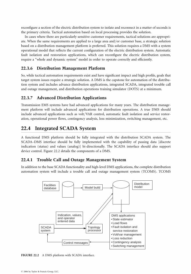
reconfigure a section of the electric distribution system to isolate and reconnect in a matter of seconds is
the primary criteria. Tactical automation based on local processing provides the solution.
In cases where there are particularly sensitive customer requirements, tactical solutions are appropri-
ate. When the same requirements are applied to a large area and=or customer base, a strategic solution
based on a distribution management platform is preferred. This solution requires a DMS with a system
operational model that reflects the current configuration of the electric distribution system. Automatic
fault isolation and restoration applications, which can reconfigure the electric distribution system,
require a ‘‘whole and dynamic system’’ model in order to operate correctly and efficiently.
22.3.6 Distribution Management Platform
So, while tactical automation requirements exist and have significant impact and high profile, goals that
target system issues require a strategic solution. A DMS is the capstone for automation of the distribu-
tion system and includes advance distribution applications, integrated SCADA, integrated trouble call
and outage management, and distribution operations training simulator (DOTS) at a minimum.
22.3.7 Advanced Distribution Applications
Transmission EMS systems have had advanced applications for many years. The distribution manage-
ment platform will include advanced applications for distribution operations. A true DMS should
include advanced applications such as volt=VAR control, automatic fault isolation and service restor-
ation, operational power flows, contingency analysis, loss minimization, switching management, etc.
22.4 Integrated SCADA System
A functional DMS platform should be fully integrated with the distribution SCADA system. The
SCADA–DMS interface should be fully implemented with the capability of passing data [discrete
indication (status) and values (analog)] bi-directionally. The SCADA interface should also support
device control. Figure 22.2 details the components of a DMS.
22.4.1 Trouble Call and Outage Management System
In addition to the base SCADA functionality and high-level DMS applications, the complete distribution
automation system will include a trouble call and outage management system (TCOMS). TCOMS
Facilities database
Indication, values,and operatorentered data
SCADAsystem
Model build
Topologyprocessor
Control messages
Distributionmodel
DMS applications• State estimator• Load flows• Fault isolation and service restoration• Volt/var management• Loss reduction • Contingency analysis • Switching management
FIGURE 22.2 A DMS platform with SCADA interface.
� 2006 by Taylor & Francis Group, LLC.
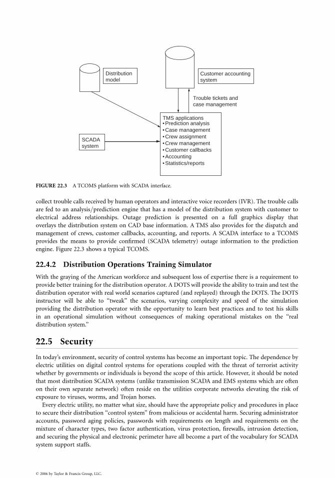
Distributionmodel
SCADAsystem
Customer accountingsystem
Trouble tickets andcase management
TMS applications• Prediction analysis• Case management• Crew assignment• Crew management• Customer callbacks• Accounting • Statistics/reports
FIGURE 22.3 A TCOMS platform with SCADA interface.
collect trouble calls received by human operators and interactive voice recorders (IVR). The trouble calls
are fed to an analysis=prediction engine that has a model of the distribution system with customer to
electrical address relationships. Outage prediction is presented on a full graphics display that
overlays the distribution system on CAD base information. A TMS also provides for the dispatch and
management of crews, customer callbacks, accounting, and reports. A SCADA interface to a TCOMS
provides the means to provide confirmed (SCADA telemetry) outage information to the prediction
engine. Figure 22.3 shows a typical TCOMS.
22.4.2 Distribution Operations Training Simulator
With the graying of the American workforce and subsequent loss of expertise there is a requirement to
provide better training for the distribution operator. A DOTS will provide the ability to train and test the
distribution operator with real world scenarios captured (and replayed) through the DOTS. The DOTS
instructor will be able to ‘‘tweak’’ the scenarios, varying complexity and speed of the simulation
providing the distribution operator with the opportunity to learn best practices and to test his skills
in an operational simulation without consequences of making operational mistakes on the ‘‘real
distribution system.’’
22.5 Security
In today’s environment, security of control systems has become an important topic. The dependence by
electric utilities on digital control systems for operations coupled with the threat of terrorist activity
whether by governments or individuals is beyond the scope of this article. However, it should be noted
that most distribution SCADA systems (unlike transmission SCADA and EMS systems which are often
on their own separate network) often reside on the utilities corporate networks elevating the risk of
exposure to viruses, worms, and Trojan horses.
Every electric utility, no matter what size, should have the appropriate policy and procedures in place
to secure their distribution ‘‘control system’’ from malicious or accidental harm. Securing administrator
accounts, password aging policies, passwords with requirements on length and requirements on the
mixture of character types, two factor authentication, virus protection, firewalls, intrusion detection,
and securing the physical and electronic perimeter have all become a part of the vocabulary for SCADA
system support staffs.
� 2006 by Taylor & Francis Group, LLC.
22.6 Practical Considerations
22.6.1 Choosing the Vendor
22.6.1.1 Choosing a Platform Vendor
In choosing a platform (SCADA, DMS, TCOMS) vendor there are several characteristics that should be
kept in mind (these should be considered as a rule of thumb based on experience of what works and
what does not). Choosing the right vendor is as important as choosing the right software package.
Vendor characteristics that the authors consider important are:
. A strong ‘‘product’’ philosophy. Having a strong product philosophy is typically a chicken and egg
proposition. Which came first, the product or the philosophy? Having a baseline SCADA
application can be a sign of maturity and stability. Did the platform vendor get there by design
or did they back into it? Evidence of a product philosophy includes a baseline system that is in
production and enhancements that are integrated in a planned manner with thorough testing on
the enhancement and regression testing on the product along with complete and comprehensive
documentation.. A documented development and release path projected three to five years into the future.. By inference from the first two bullets, a vendor who funds planned product enhancements from
internal funds.. A strong and active user group that is representative of the industry and industry drivers.. A platform vendor that actively encourages its user group by incentive (e.g., dedicating part of its
enhancement funding to user group initiatives).. A vendor that is generally conservative in moving its platform to a new technology; one that does
not overextend its own resources.. Other considerations.. As much as possible, purchase the platform as an off-the-shelf product (i.e., resist the urge to ask
for customs that drive your system away from the vendor’s baseline).. If possible, maintain=develop your own support staff.
All ‘‘customization’’ should be built around the inherent capabilities and flexibility of the system (i.e., do
not generate excessive amounts of new code). Remember, you will have to reapply any code that you may
have developed to every new release; or worse, you will have to pay the vendor to do it for you.
22.7 Standards
22.7.1 Internal Standards
The authors highly recommend the use of standards (internal to your organization) as a basis for
ensuring a successful distribution automation or SCADA program. Well-documented construction
standards that specify installation of RTUs, switches, and line sensors with mechanical and electrical
specifications will ensure consistent equipment installations from site to site. Standards that cover
nontrivial, but often overlooked issues can often spell the difference between acceptance and rejection
by operational users and provide the additional benefit of having a system that is ‘‘maintainable’’ over
the 10–20 years (or more) life of a system. Standards that fall in this category include standards that
cover point-naming conventions, symbol standards, display standards, and the all-important operations
manual.
22.7.2 Industry Standards
In general, standards fall into two categories: standards that are developed by organizations and
commissions (e.g., EPRI, IEEE, ANSI, CCITT, ISO, etc.) and de facto standards that become standards
� 2006 by Taylor & Francis Group, LLC.
by virtue of widespread acceptance. As an example of what can occur, the reader is invited to consider
what has happened in network protocols over the recent past with regard to the OSI model and TCP=IP.
Past history of SCADA and automation has been dominated by the proprietary nature of the various
system vendor offerings. Database schemas and RTU communication protocols are exemplary of
proprietary design philosophies utilized by SCADA platform and RTU vendors. Electric utilities that
operate as part of the interconnected power grid have been frustrated by the lack of ability to share
power system data between dissimilar energy management systems. The same frustration exists at the
device level; RTU vendors, PLC vendors, electronic relay vendors, and meter vendors each having their
own product protocols have created a ‘‘tower of babel’’ problem for utilities. Recently several commu-
nications standards organizations and vendor consortiums have proposed standards to address these
deficiencies in intersystem data exchange, intrasystem data exchange (corporate data exchange), and
device level interconnectivity. Some of the more notable examples of network protocol communication
standards are ICCP (intercontrol center protocol), UCA (utility communication architecture), CCAPI
(control center applications interface), and UIB (utility integration bus). For database schemas, EPRI’s
CIM (common information model) is gaining supporters. In RTU, PLC, and IED communications,
DNP 3.0 has also received much attention from the industry’s press.
In light of the number of standards that have appeared (and then disappeared) and the number of
possibly competing ‘‘standards’’ that are available today, the authors, while acknowledging the value of
standards, prefer to take (and recommend) a cautious approach to standards. A wait-and-see posture
may be an effective strategy. Standards by definition must have proven themselves over time. Difficulties
in immediately embracing new standards are due in part to vendors having been allowed to implement
only portions of a standard, thereby nullifying the hopefully ‘‘plug-and-play’’ aspect for adding new
devices. Also, the trend in communication protocols has been to add functionality in an attempt to be
all-inclusive, which has resulted in an increased requirement on bandwidth. Practically speaking, utilities
that have already existing infrastructure may find it economical to resist the deployment of new
protocols. In the final analysis, as in any business decision, a ‘‘standard’’ should be accepted only if it
adds value and benefit that exceeds the cost of implementation and deployment.
22.8 Deployment Considerations
The definition of the automation technology to be deployed should be clearly delineated. This definition
includes the specification of the host systems, the communication infrastructure, the automated end-use
devices, and the support infrastructure. This effort begins with the development of a detailed installation
plan that takes into consideration the available resources. The pilot installation will never be any more
than a pilot project until funding and manpower resources are identified and dedicated to the enterprise
of implementing the technologies required to automate the electric distribution system. The implemen-
tation effort is best managed on an annual basis with stated incremental goals and objectives for the
installation of automated devices. With the annual goals and objectives identified, then the budget
process begins to ensure that adequate funding is available to support the implementation plan. To
ensure adequate time to complete the initial project tasks, the planning should begin 18 to 24 months
prior to the budget year. During this period, the identification of specific automation projects is
completed. The initial design work is commenced with the specification of field automation equipment
(e.g., substation RTU based on specific point count requirements and distribution line RTU). The
verification of the communication to the selected automation site is an urgent early consideration in
order to minimize the cost of achieving effective remote communications. As the installation year
approaches, the associated automation equipment (e.g., switches, motor operators, sensors, etc.) must
be verified to ensure that adequate supplies are stocked to support the implementation plan.
The creation of a SCADA database and display is on the critical path for new automated sites.
The database and display are critical to the efficient completion of the installation and checkout tasks.
Data must be provided to the database and display team with sufficient lead time to create the database
and display for the automated site. The database and display are subsequently used to check out the
� 2006 by Taylor & Francis Group, LLC.
completed automated field device. The point assignment (PA) sheet is a project activity that merits
serious attention. The PA sheet is the basis for the creation of the site-specific database in the SCADA
system. The PA sheet should be created in a consistent and standard fashion. The importance of an
accurate database and display cannot be overemphasized. The database and display form the basis for the
remote operational decisions for the electric distribution system using the SCADA capability. Careful
coordination of these project tasks is essential to the successful completion of the annual automation plans.
Training is another important consideration during the deployment of the automation technology.
The training topics are as varied as the multidisciplined nature of the distribution automation project.
Initial training requirements include the system support personnel in the use and deployment of the
automation platform, the end user (operator) training, and installation teams. Many utilities now install
new distribution facilities using energized line construction techniques. The automated field device adds
a degree of complexity to the construction techniques to ensure adherence to safe practices and
construction standards. These training issues should be addressed at the outset of the planning effort
to ensure a successful distribution automation project.
22.8.1 Support Organization
The support organization must be as multidisciplined as the distribution automation system is multi-
featured. The support to maintain a deployed distribution automation system should not be underesti-
mated. Functional teams should be formed to address each discipline represented within the distribution
automation system. The authors recommend forming a core team that is made up of representation
from each area of discipline or area of responsibility within the distribution automation project. These
areas of discipline include the following:
. Host SCADA system
. User interface
. Communication infrastructure
. Facilities design personnel for automated distribution substation and distribution line devices
. System software and interface developments
. Installation teams for automated distribution substation and distribution line devices
. End users (i.e., the operating personnel)
The remaining requirement for the core team is project leadership with responsibility for the project
budget, scheduling, management reports, and overall direction of the distribution automation project.
The interaction of the various disciplines within the distribution automation team will ensure that all
project decisions are supporting the overall project goals. The close coordination of the various project
teams through the core team is essential to minimizing decision conflict and maximizing the synergy of
project decisions. The involvement of the end user at the very outset of the distribution automation
project planning cannot be overemphasized. The operating personnel are the primary users of the
distribution automation technology. The participation of the end user in all project decisions is essential
to ensure that the distribution automation product meets business needs and improves the operating
environment in the operating centers. One measure of good project decisions is found in the response
of the end user. When the end user says, ‘‘I like it,’’ then the project decision is clearly targeting the end
user’s business requirements. With this goal achieved, the distribution automation system is then in a
position to begin meeting other corporate business needs for real-time data from the electric distribu-
tion system.
� 2006 by Taylor & Francis Group, LLC.
23
� 2006 by Taylor & Francis Group, LLC.
Hard to FindInformation (on
Distribution SystemCharacteristics and
Protection)
Jim BurkeInfraSource Technology
23.1 Overcurrent Protection.................................................. 23-1Introduction . Fault Levels . Surface Current Levels .
Reclosing and Inrush . Cold Load Pickup . Calculation
of Fault Current . Current Limiting Fuses . Rules for
Application of Fuses . More Overcurrent Rules .
Capacitor Fusing . Conductor Burndown . Protective
Device Numbers . Protection Abbreviations . Simple
Coordination Rules . Lightning Characteristics .
Arc Impedance
23.2 Transformers ................................................................. 23-16Saturation Curve . Insulation Levels .
D-Y Transformer Banks
23.3 Instrument Transformers............................................. 23-17Two Types . Accuracy . Potential Transformers .
Current Transformer . H-Class . Current Transformer
Facts . Glossary of Transducer Terms
23.4 Loading.......................................................................... 23-21Transformer Loading Basics . Examples of Substation
Transformer Loading Limits . Distribution Transformers .
Ampacity of Overhead Conductors . Emergency Ratings of
Equipment
23.5 Miscellaneous Loading Information........................... 23-24
23.1 Overcurrent Protection
23.1.1 Introduction
The distribution system shown in Fig. 23.1 illustrates many of the features of a distribution system
making it unique. The voltage level of a distribution system can be anywhere from about 5 kV to as high
as 35 kV with the most common voltages in the 15 kV class. Areas served by a given voltage are
proportional to the voltage itself, indicating that, for the same load density, a 35 kV system can serve
considerably longer lines. Lines can be as short as a mile or two and as long as 20 or 30 miles. Typically,
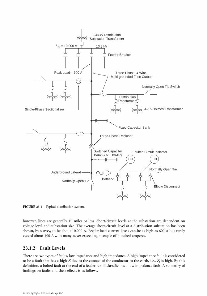
S
R
138 kV DistributionSubstation Transformer
13.8 kVISC = 10,000 A
Feeder Breaker
Peak Load = 600 A Three-Phase, 4-Wire,Multi-grounded Fuse Cutout
Normally Open Tie Switch
Single-Phase Sectionalizer
DistributionTransformers
4–15 Holmes/ Transformer
Fixed Capacitor Bank
Three-Phase Recloser
Switched CapacitorBank (= 600 kVAR)
Pothead
Faulted Circuit Indicator
Elbow Disconnect
Normally Open Tie
Normally Open TieUnderground Lateral
FCI FCI
FIGURE 23.1 Typical distribution system.
however, lines are generally 10 miles or less. Short-circuit levels at the substation are dependent on
voltage level and substation size. The average short-circuit level at a distribution substation has been
shown, by survey, to be about 10,000 A. Feeder load current levels can be as high as 600 A but rarely
exceed about 400 A with many never exceeding a couple of hundred amperes.
23.1.2 Fault Levels
There are two types of faults, low impedance and high impedance. A high impedance fault is considered
to be a fault that has a high Z due to the contact of the conductor to the earth, i.e., Zf is high. By this
definition, a bolted fault at the end of a feeder is still classified as a low impedance fault. A summary of
findings on faults and their effects is as follows.
� 2006 by Taylor & Francis Group, LLC.
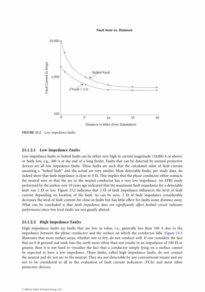
10,000
1,000
100
Z Fault = 2 Ω
Bolted Fault
Fau
lt C
urre
nt in
Am
ps
0 5 10 15 20
Distance in Miles (from Substation)
Fault level vs. Distance
FIGURE 23.2 Low impedance faults.
23.1.2.1 Low Impedance Faults
Low impedance faults or bolted faults can be either very high in current magnitude (10,000 A or above)
or fairly low, e.g., 300 A at the end of a long feeder. Faults that can be detected by normal protective
devices are all low impedance faults. These faults are such that the calculated value of fault current
assuming a ‘‘bolted fault’’ and the actual are very similar. Most detectable faults, per study data, do
indeed show that fault impedance is close to 0 V. This implies that the phase conductor either contacts
the neutral wire or that the arc to the neutral conductor has a very low impedance. An EPRI study
performed by the author over 10 years ago indicated that the maximum fault impedance for a detectable
fault was 2 V or less. Figure 23.2 indicates that 2 V of fault impedance influences the level of fault
current depending on location of the fault. As can be seen, 2 V of fault impedance considerably
decreases the level of fault current for close-in faults but has little effect for faults some distance away.
What can be concluded is that fault impedance does not significantly affect faulted circuit indicator
performance since low level faults are not greatly altered.
23.1.2.2 High Impedance Faults
High impedance faults are faults that are low in value, i.e., generally less than 100 A due to the
impedance between the phase conductor and the surface on which the conductor falls. Figure 23.3
illustrates that most surface areas, whether wet or dry, do not conduct well. If one considers the fact
that an 8-ft ground rod sunk into the earth more often than not results in an impedance of 100 V or
greater, then it is not hard to visualize the fact that a conductor simply lying on a surface cannot
be expected to have a low impedance. These faults, called high impedance faults, do not contact
the neutral and do not arc to the neutral. They are not detectable by any conventional means and are
not to be considered at all in the evaluation of fault current indicators (FCIs) and most other
protective devices.
� 2006 by Taylor & Francis Group, LLC.
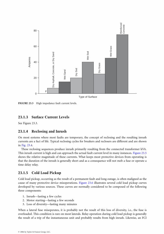
High impedance fault current levels 0
F
20
40
60
80
Type of Surface
Am
pere
s
Dry
Asp
halt,
Con
cret
e, o
r D
ry S
and
Wet
San
d
Dry
Sod
Wet
Sod
Dry
Gra
ss
Wet
Gra
ss
Rei
nfor
ced
Con
cret
e
FIGURE 23.3 High impedance fault current levels.
23.1.3 Surface Current Levels
See Figure 23.3.
23.1.4 Reclosing and Inrush
On most systems where most faults are temporary, the concept of reclosing and the resulting inrush
currents are a fact of life. Typical reclosing cycles for breakers and reclosers are different and are shown
in Fig. 23.4.
These reclosing sequences produce inrush primarily resulting from the connected transformer kVA.
This inrush current is high and can approach the actual fault current level in many instances. Figure 23.5
shows the relative magnitude of these currents. What keeps most protective devices from operating is
that the duration of the inrush is generally short and as a consequence will not melt a fuse or operate a
time delay relay.
23.1.5 Cold Load Pickup
Cold load pickup, occurring as the result of a permanent fault and long outage, is often maligned as the
cause of many protective device misoperations. Figure 23.6 illustrates several cold load pickup curves
developed by various sources. These curves are normally considered to be composed of the following
three components:
1. Inrush—lasting a few cycles
2. Motor starting—lasting a few seconds
3. Loss of diversity—lasting many minutes
When a lateral fuse misoperates, it is probably not the result of this loss of diversity, i.e., the fuse is
overloaded. This condition is rare on most laterals. Relay operation during cold load pickup is generally
the result of a trip of the instantaneous unit and probably results from high inrush. Likewise, an FCI
� 2006 by Taylor & Francis Group, LLC.
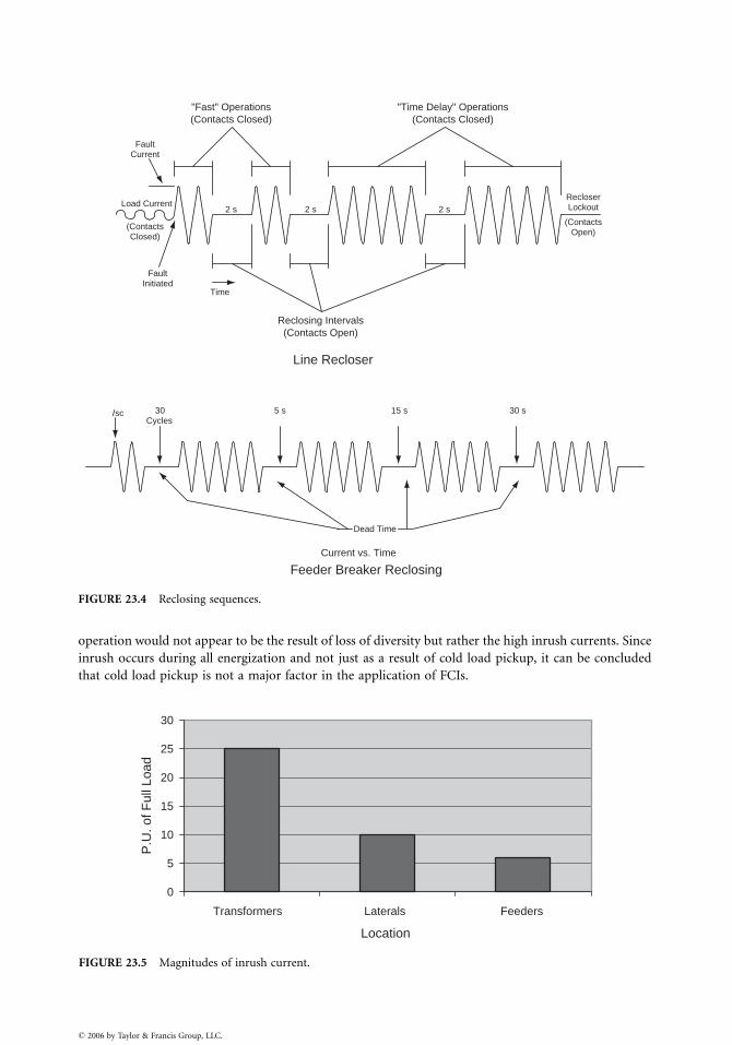
Load Current
FaultCurrent
FaultInitiated
(ContactsClosed)
2 s 2 s 2 s
Time
Reclosing Intervals(Contacts Open)
"Fast" Operations(Contacts Closed)
"Time Delay" Operations(Contacts Closed)
RecloserLockout
(ContactsOpen)
Line Recloser
Dead Time
I sc 30Cycles
5 s 15 s 30 s
Current vs. Time
Feeder Breaker Reclosing
FIGURE 23.4 Reclosing sequences.
operation would not appear to be the result of loss of diversity but rather the high inrush currents. Since
inrush occurs during all energization and not just as a result of cold load pickup, it can be concluded
that cold load pickup is not a major factor in the application of FCIs.
0
5
10
15
20
25
30
Transformers Laterals Feeders
Location
P.U
. of F
ull L
oad
FIGURE 23.5 Magnitudes of inrush current.
� 2006 by Taylor & Francis Group, LLC.
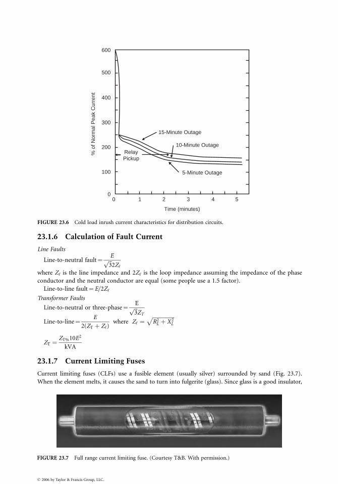
600
500
400
300
200
100
00 1 2
Time (minutes)
3 4 5
% o
f Nor
mal
Pea
k C
urre
nt
RelayPickup
15-Minute Outage
10-Minute Outage
5-Minute Outage
FIGURE 23.6 Cold load inrush current characteristics for distribution circuits.
23.1.6 Calculation of Fault Current
Line Faults
Line-to-neutral fault¼ Effiffiffi
3p
2Z‘where Z‘ is the line impedance and 2Z‘ is the loop impedance assuming the impedance of the phase
conductor and the neutral conductor are equal (some people use a 1.5 factor).
Line-to-line fault¼ E=2Z‘
Transformer Faults
Line-to-neutral or three-phase¼ Effiffiffi
3p
ZT
Line-to-line¼ E
2(ZT þ Z‘)where Z‘ ¼
ffiffiffiffiffiffiffiffiffiffiffiffiffiffiffiffiffi
R2L þ X2
L
p
ZT ¼ZT%10E2
kVA
23.1.7 Current Limiting Fuses
Current limiting fuses (CLFs) use a fusible element (usually silver) surrounded by sand (Fig. 23.7).
When the element melts, it causes the sand to turn into fulgerite (glass). Since glass is a good insulator,
FIGURE 23.7 Full range current limiting fuse. (Courtesy T&B. With permission.)
� 2006 by Taylor & Francis Group, LLC.

FIGURE 23.8 Back-up CLF.
this results in a high resistance in series with the faults. This not only limits the magnitude of the fault
but also the energy. All this can happen in less than a half cycle.
CLFs are very good at interrupting high currents (e.g., 50,000 A). They historically have had trouble
(General Purpose, and Back-up) with low level fault currents and overloads, where the fuse tube melts
before the element (i.e., these two fuses are not considered to be ‘‘full range,’’ since they do not
necessarily interrupt low currents that melt the element). There are now ‘‘full range’’ CLFs in the market
(see Fig. 23.7).
The three types of CLFs are defined as follows:
. General purpose—A fuse capable of interrupting all currents from the rated maximum inter-
rupting current down to the current that causes melting of the fusible element in 1 h.. Back-up—A fuse capable of interrupting all currents from the rated maximum interrupting
current down to the rated minimum interrupting current (Fig. 23.8).. Full range—A fuse capable of interrupting all currents from the rated maximum current down to
any current that melts the element.
23.1.8 Rules for Application of Fuses
1. Cold load pickup.
� 2006 by Taylor & Francis Group, LLC.
After 15-min outage
200% for 0.5 s140% for 5 s
After 4 h, all electric
300% for 5 min2. ‘‘Damage’’ curve—75% of minimum melt.
3. Two expulsion fuses cannot be coordinated if the available fault current is great enough to
indicate an interruption of less than 0.8 cycles.
4. ‘‘T’’-SLOW and ‘‘K’’-FAST.
5. CLFs can be coordinated in the subcycle region.
6. Capacitor protection:. The fuse should be rated for 165% of the normal capacitor current. The fuse should also clear
within 300 s for the minimum short-circuit current.
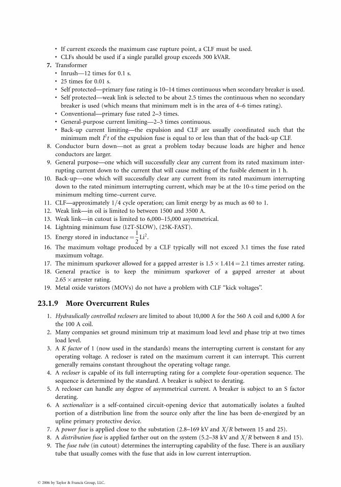
. If current exceeds the maximum case rupture point, a CLF must be used.
. CLFs should be used if a single parallel group exceeds 300 kVAR.
7. Transformer. Inrush—12 times for 0.1 s.. 25 times for 0.01 s.. Self protected—primary fuse rating is 10–14 times continuous when secondary breaker is used.. Self protected—weak link is selected to be about 2.5 times the continuous when no secondary
breaker is used (which means that minimum melt is in the area of 4–6 times rating).. Conventional—primary fuse rated 2–3 times.. General-purpose current limiting—2–3 times continuous.. Back-up current limiting—the expulsion and CLF are usually coordinated such that the
minimum melt I2t of the expulsion fuse is equal to or less than that of the back-up CLF.
8. Conductor burn down—not as great a problem today because loads are higher and hence
conductors are larger.
9. General purpose—one which will successfully clear any current from its rated maximum inter-
rupting current down to the current that will cause melting of the fusible element in 1 h.
10. Back-up—one which will successfully clear any current from its rated maximum interrupting
down to the rated minimum interrupting current, which may be at the 10-s time period on the
minimum melting time–current curve.
11. CLF—approximately 1=4 cycle operation; can limit energy by as much as 60 to 1.
12. Weak link—in oil is limited to between 1500 and 3500 A.
13. Weak link—in cutout is limited to 6,000–15,000 asymmetrical.
14. Lightning minimum fuse (12T-SLOW), (25K-FAST).
15. Energy stored in inductance¼ 1
2Li2.
16. The maximum voltage produced by a CLF typically will not exceed 3.1 times the fuse rated
maximum voltage.
17. The minimum sparkover allowed for a gapped arrester is 1.5� 1.414¼ 2.1 times arrester rating.
18. General practice is to keep the minimum sparkover of a gapped arrester at about
2.65� arrester rating.
19. Metal oxide varistors (MOVs) do not have a problem with CLF ‘‘kick voltages’’.
23.1.9 More Overcurrent Rules
1. Hydraulically controlled reclosers are limited to about 10,000 A for the 560 A coil and 6,000 A for
the 100 A coil.
2. Many companies set ground minimum trip at maximum load level and phase trip at two times
load level.
3. A K factor of 1 (now used in the standards) means the interrupting current is constant for any
operating voltage. A recloser is rated on the maximum current it can interrupt. This current
generally remains constant throughout the operating voltage range.
4. A recloser is capable of its full interrupting rating for a complete four-operation sequence. The
sequence is determined by the standard. A breaker is subject to derating.
5. A recloser can handle any degree of asymmetrical current. A breaker is subject to an S factor
derating.
6. A sectionalizer is a self-contained circuit-opening device that automatically isolates a faulted
portion of a distribution line from the source only after the line has been de-energized by an
upline primary protective device.
7. A power fuse is applied close to the substation (2.8–169 kV and X=R between 15 and 25).
8. A distribution fuse is applied farther out on the system (5.2–38 kV and X=R between 8 and 15).
9. The fuse tube (in cutout) determines the interrupting capability of the fuse. There is an auxiliary
tube that usually comes with the fuse that aids in low current interruption.
� 2006 by Taylor & Francis Group, LLC.
10. Some expulsion fuses can handle 100% continuous and some 150%.
11. Type ‘‘K’’ is a fast fuse link with a speed ratio of melting time–current characteristics from 6 to 8.1.
(Speed is the ratio of the 0.1-s minimum melt current to the 300-s minimum melt current. Some of
the larger fuses use the 600-s point.)
12. Type ‘‘T’’ is a slow fuse link with a speed ratio of melt time–current characteristics from 10 to 13.
13. After about ten fuse link operations, the fuse holder should be replaced.
14. Slant ratings can be used on grounded wye, wye, or delta systems as long as the line-to-neutral
voltage of the system is lower than the smaller number and the line-to-line voltage is lower than
the higher number. A slant rated cutout can withstand the full line-to-line voltage whereas a
cutout with a single voltage rating could not withstand the higher line-to-line voltage.
15. Transformer fusing—25 at 0.01; 12 at 0.1; 3 at 10 s.
16. Unsymmetrical transformer connections (delta=wye)
� 2006 by Taylor & Francis Group, LLC.
Fault Type Multiplying Factor
Three-phase
NPhase-to-phase
87 (N)Phase-to-ground
1.73 (N)where N is the ratio of Vprimary=Vsecondary.
17. Multiply the high side device current points by the appropriate factor.
18. K factor for load side fuses
a. Two fast operations and dead time 1–2 s¼ 1.35.
19. K factor for source side fuses
a. Two fast—Two delayed and dead time of 2 s¼ 1.7.
b. Two fast—Two delayed and dead time of 10 s¼ 1.35.
c. Sometimes these factors go as high as 3.5 so check.
20. Sequence coordination—Achievement of true ‘‘trip coordination’’ between an upline electronic
recloser and a downline recloser is made possible through a feature known as ‘‘sequence’’
coordination. Operation of sequence coordination requires that the upline electronic recloser
be programmed with ‘‘fast curves’’ whose control response time is slower than the clearing time of
the downline recloser fast operation, through the range of fault currents within the reach of the
upline recloser. Assume a fault beyond the downline recloser that exceeds the minimum trip
setting of both reclosers. The downline recloser trips and clears before the upline recloser has a
chance to trip. However, the upline control does see the fault and the subsequent cutoff of fault
current. The sequence coordination feature then advances its control through its fast operation,
such that both controls are at their second operation, even though only one of them has actually
tripped. Should the fault persist, and a second fast trip occur, sequence coordination repeats the
procedure. Sequence coordination is active only on the programmed fast operations of the upline
recloser. In effect, sequence coordination maintains the downline recloser as the faster device.
21. Recloser time–current characteristics
a. Some curves are average. Maximum is 10% higher.
b. Response curves are the responses of the sensing device and do not include arc extinction.
c. Clearing time is measured from fault initiation to power arc extinction.
d. The response time of the recloser is sometimes the only curve given. To obtain the interrupt-
ing time, you must add approximately 0.045 s to the curve (check . . . they are different).
e. Some curves show maximum clearing time. On the new electronic reclosers, you usually get a
control response curve and a clearing curve.
f. Z‘ � g¼ (2Z1 þ Z0)=3
22. The ‘‘75% Rule’’ considers TCC tolerances, ambient temperature, pre-loading, and pre-damage.
Pre-damage only uses 90%.

23. A back-up CLF with a designation like ‘‘12 K’’ means that the fuse will coordinate with a K link
rated 12 A or less.
24. Capacitor Fusing:
a. The 1.35 factor may result in nuisance fuse operations. Some utilities use 1.65.
b. Case rupture is not as big a problem as years ago due to all film designs.
c. Tank rupture curves may be probable or definite in nature. Probable means there is a
probability chance of not achieving coordination. Definite indicates there is effectively no
chance of capacitor tank rupture with the proper 0% probability curve.
d. T links are generally used up to about 25 A and K link above that to reduce nuisance fuse
operations from lightning.
25. Line Impedance—Typical values for line impedance (350 kcm) on a per mile basis are as follows:
� 2006 by Taylor & Francis Group, LLC.
Zpositive Z0
Cable UG
0.31 þ j 0.265 1.18 þ j 0.35Spacer
0.3 þ j 0.41 1.25 þ j 2.87Tree wire
0.3 þ j 0.41 1.25 þ j 2.87Armless
0.3 þ j 0.61 0.98 þ j 2.5Open
0.29 þ j 0.66 0.98 þ j 2.3726. 1A–3B is necessary when sectionalizers are used downstream from the recloser.
27. Vacuum reclosers have interrupting ratings as high as 10–20 kA.
28. Highest recloser continuous ratings are 800 and 1200 A.
29. Sectionalizer actuating current should be <80% of back-up device trip current.
30. Interrupting ratings of cutouts are approximately 7–10 kA symmetrical.
31. K factor can mean a ‘‘voltage range’’ factor or a ‘‘shift factor’’ caused by the recloser heating up the fuse.
32. Sectionalizer counts should normally be one count less than the operations to lockout of the
breaker or recloser.
33. Sectionalizer memory time must be greater than cumulative trip and recloser time.
34. Fuses melt at about 200% of rating.
35. Sectionalizers have momentary ratings for 1 and 10 s.
36. Twenty five percent rule for fuses includes pre-load, ambient temperature, and pre-damage.
37. Characteristics of Chance Sectionalizers include:. 100 A continuous. 160 A actuating. 2 counts. 12,000 A momentary. 4,000 A at 1 s. 2,500 A at 10 s. 0.3 A detector threshold. Minimum time delay¼ 80 ms. Reset time approximately 25 s. Minimum duration of current impulse approximately 1–3 cycles. Short time curves are 20% of the normal curve (in time). Long time curves are ten times the normal
23.1.10 Capacitor Fusing
1. Purpose of fusing:
a. To isolate faulted bank from system
b. To protect against bursting
c. To give indication
d. To allow manual switching (fuse control)
e. To isolate faulted capacitor from bank
2. Recommended rating:
a. The continuous-current capability of the fuse should be at least 165% of the normal
capacitor bank (for delta and floating wye banks the factor may be reduced to 150%
if necessary).
b. The total clearing characteristics of the fuse link must be coordinated with the capacitor ‘‘case
bursting’’ curves.
3. Tests have shown that expulsion fuse links will not satisfactorily protect against violent rupture
where the fault current through the capacitor is greater than 5000 A.
4. The capacitor bank may be connected in a floating wye to limit short-circuit current to less
than 5000 A.
5. Inrush—for a single bank, the inrush current is always less than the short-circuit value at the bank
location.
6. Inrush—for parallel banks, the inrush current is always much greater than for a single bank.
7. Expulsion fuses offer the following advantages:
a. They are inexpensive and easily replaced
b. They offer a positive indication of operation
8. CLFs are used where:
a. a high available short circuit exceeds the expulsion or non-vented fuse rating.
b. a CLF is needed to limit the high energy discharge from adjacent parallel capacitors
effectively.
c. a non-venting fuse is needed in an enclosure.
9. The fuse link rating should be such that the link will melt in 300 s at 240–350% of normal
load current.
10. The fuse link rating should be such that it melts in 1 s at not over 220 A and in 0.015 s at not over
1700 A.
11. The fuse rating must be chosen through the use of melting time–current characteristic curves,
because fuse links of the same rating, but of different types and makes have a wide variation in the
melting time at 300 s and at high currents.
12. Safe zone—usually greater damage than a slight swelling.
a. Zone 1—suitable for locations where case rupture or fluid leakage would present no hazard.
b. Zone 2—suitable for locations that have been chosen after careful consideration of possible
consequences associated with violent case ruptures.
c. Hazardous zone—unsafe for most applications. The case will often rupture with sufficient
violence to damage adjacent units.
13. Manufacturers normally recommend that the group fuse size be limited by the 50% probability
curve or the upper boundary of Zone 1.
14. Short-circuit current in an open wye bank is limited to approximately three times the normal
current.
15. CLFs can be used for delta or grounded wye banks, provided there is sufficient short-circuit
current to melt the fuse within 1⁄2 cycle.
23.1.11 Conductor Burndown
Conductor burndown is a function of (i) conductor size, (ii) whether the wire is bare or covered, (iii) the
magnitude of the fault current, (iv) climatic conditions such as wind, and (v) the duration of the
fault current.
� 2006 by Taylor & Francis Group, LLC.
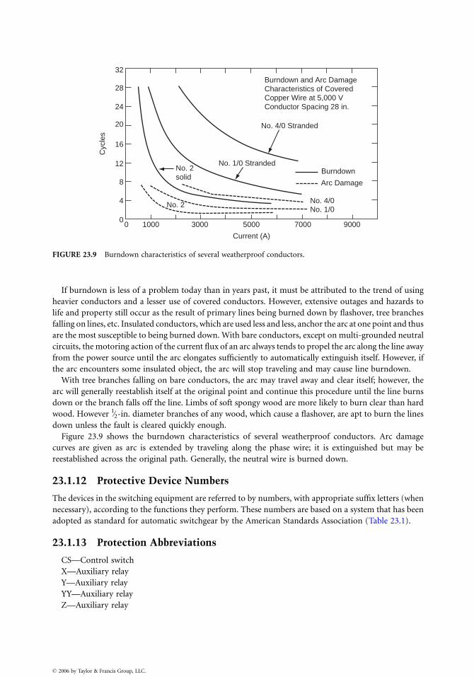
Burndown and Arc Damage Characteristics of Covered Copper Wire at 5,000 VConductor Spacing 28 in.
No. 4/0 Stranded
No. 1/0 StrandedNo. 2 solid
No. 2 No. 4/0No. 1/0
Burndown
Arc Damage
Current (A)
3000 5000 7000 900010000
32
28
24
20
16
12
8
4
0
Cyc
les
FIGURE 23.9 Burndown characteristics of several weatherproof conductors.
If burndown is less of a problem today than in years past, it must be attributed to the trend of using
heavier conductors and a lesser use of covered conductors. However, extensive outages and hazards to
life and property still occur as the result of primary lines being burned down by flashover, tree branches
falling on lines, etc. Insulated conductors, which are used less and less, anchor the arc at one point and thus
are the most susceptible to being burned down. With bare conductors, except on multi-grounded neutral
circuits, the motoring action of the current flux of an arc always tends to propel the arc along the line away
from the power source until the arc elongates sufficiently to automatically extinguish itself. However, if
the arc encounters some insulated object, the arc will stop traveling and may cause line burndown.
With tree branches falling on bare conductors, the arc may travel away and clear itself; however, the
arc will generally reestablish itself at the original point and continue this procedure until the line burns
down or the branch falls off the line. Limbs of soft spongy wood are more likely to burn clear than hard
wood. However 1⁄2-in. diameter branches of any wood, which cause a flashover, are apt to burn the lines
down unless the fault is cleared quickly enough.
Figure 23.9 shows the burndown characteristics of several weatherproof conductors. Arc damage
curves are given as arc is extended by traveling along the phase wire; it is extinguished but may be
reestablished across the original path. Generally, the neutral wire is burned down.
23.1.12 Protective Device Numbers
The devices in the switching equipment are referred to by numbers, with appropriate suffix letters (when
necessary), according to the functions they perform. These numbers are based on a system that has been
adopted as standard for automatic switchgear by the American Standards Association (Table 23.1).
23.1.13 Protection Abbreviations
CS—Control switch
X—Auxiliary relay
Y—Auxiliary relay
YY—Auxiliary relay
Z—Auxiliary relay
� 2006 by Taylor & Francis Group, LLC.

TABLE 23.1 Protective Device Numbers
Device No. Function and Definition
11 Control power transformer is a transformer that serves as the source of AC control power for
operating AC devices.
24 Bus-tie circuit breaker serves to connect buses or bus sections together.
27 AC undervoltage relay is one which functions on a given value of single-phase AC under voltage.
43 Transfer device is a manually operated device that transfers the control circuit to modify the plan of
operation of the switching equipment or of some of the devices.
50 Short-circuit selective relay is one which functions instantaneously on an excessive value of current.
51 AC overcurrent relay (inverse time) is one which functions when the current in an AC circuit exceeds a
given value.
52 AC circuit breaker is one whose principal function is usually to interrupt short-circuit or fault currents.
64 Ground protective relay is one which functions on failure of the insulation of a machine, transformer,
or other apparatus to ground. This function is, however, not applied to devices 51N and 67N connected
in the residual or secondary neutral circuit of current transformers.
67 AC power directional or AC power directional overcurrent relay is one which functions on a desired value
of power flow in a given direction or on a desired value of overcurrent with AC power flow in a
given direction.
78 Phase–angle measuring relay is one which functions at a predetermined phase angle between voltage
and current.
87 Differential current relay is a fault-detecting relay that functions on a differential current of a given
percentage or amount.
1. To denote the location of the main device in the circuit or the type of circuit in which the device is
used or with which it is associated, or otherwise identify its application in the circuit or
equipment, the following are used:
� 2006 by
N—Neutral
SI—Seal-in
2. To denote parts of the main device, the following are used:
H—High set unit of relay
L—Low set unit of relay
OC—Operating coil
RC—Restraining coil
TC—Trip coil
3. To denote parts of the main device such as auxiliary contacts that move as part of the main device
and are not actuated by external means. These auxiliary switches are designated as follows:
‘‘a’’—closed when main device is in energized or operated position
‘‘b’’—closed when main device is in de-energized or non-operated position
4. To indicate special features, characteristics, the conditions when the contacts operate, or are made
operative or placed in the circuit, the following are used:
A—Automatic
ER—Electrically reset
HR—Hand rest
M—Manual
TDC—Time-delay closing
TDDO—Time-delay dropping out
TDO—Time-delay opening
To prevent any possible conflict, one letter or combination of letters has only one meaning on individual
equipment. Any other words beginning with the same letter are written out in full each time, or some
other distinctive abbreviation is used.
Taylor & Francis Group, LLC.
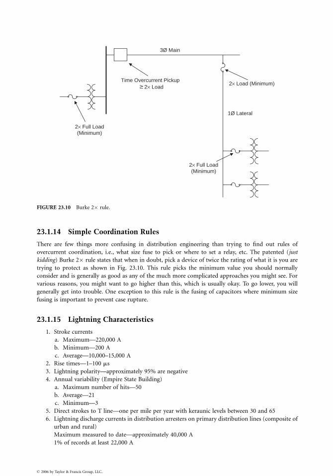
2× Full Load(Minimum)
3Ø Main
2× Load (Minimum)
1Ø Lateral
2× Full Load(Minimum)
Time Overcurrent Pickup 2× Load
FIGURE 23.10 Burke 2� rule.
23.1.14 Simple Coordination Rules
There are few things more confusing in distribution engineering than trying to find out rules of
overcurrent coordination, i.e., what size fuse to pick or where to set a relay, etc. The patented (just
kidding) Burke 2� rule states that when in doubt, pick a device of twice the rating of what it is you are
trying to protect as shown in Fig. 23.10. This rule picks the minimum value you should normally
consider and is generally as good as any of the much more complicated approaches you might see. For
various reasons, you might want to go higher than this, which is usually okay. To go lower, you will
generally get into trouble. One exception to this rule is the fusing of capacitors where minimum size
fusing is important to prevent case rupture.
23.1.15 Lightning Characteristics
1. Stroke currents
a. Maximum—220,000 A
b. Minimum—200 A
c. Average—10,000–15,000 A
2. Rise times—1–100 ms
3. Lightning polarity—approximately 95% are negative
4. Annual variability (Empire State Building)
a. Maximum number of hits—50
b. Average—21
c. Minimum—3
5. Direct strokes to T line—one per mile per year with keraunic levels between 30 and 65
6. Lightning discharge currents in distribution arresters on primary distribution lines (composite of
urban and rural)
� 2006 by
Maximum measured to date—approximately 40,000 A
1% of records at least 22,000 A
Taylor & Francis Group, LLC.
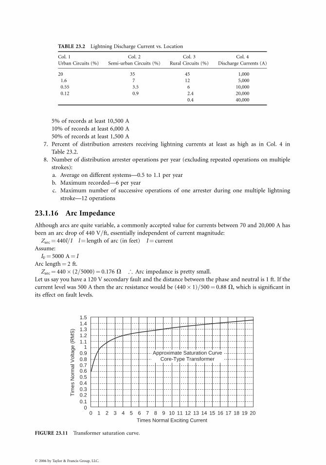
TABLE 23.2 Lightning Discharge Current vs. Location
Col. 1 Col. 2 Col. 3 Col. 4
Urban Circuits (%) Semi-urban Circuits (%) Rural Circuits (%) Discharge Currents (A)
20 35 45 1,000
1.6 7 12 5,000
0.55 3.5 6 10,000
0.12 0.9 2.4 20,000
0.4 40,000
FIGUR
� 2006 by
5% of records at least 10,500 A
10% of records at least 6,000 A
50% of records at least 1,500 A
7. Percent of distribution arresters receiving lightning currents at least as high as in Col. 4 in
Table 23.2.
8. Number of distribution arrester operations per year (excluding repeated operations on multiple
strokes):
a. Average on different systems—0.5 to 1.1 per year
b. Maximum recorded—6 per year
c. Maximum number of successive operations of one arrester during one multiple lightning
stroke—12 operations
23.1.16 Arc Impedance
Although arcs are quite variable, a commonly accepted value for currents between 70 and 20,000 A has
been an arc drop of 440 V=ft, essentially independent of current magnitude:
Zarc¼ 440l=I l¼ length of arc (in feet) I¼ current
Assume:
IF¼ 5000 A¼ I
Arc length¼ 2 ft.
Zarc¼ 440� (2=5000)¼ 0.176 V ; Arc impedance is pretty small.
Let us say you have a 120 V secondary fault and the distance between the phase and neutral is 1 ft. If the
current level was 500 A then the arc resistance would be (440� 1)=500¼ 0.88 V, which is significant in
its effect on fault levels.
Approximate Saturation CurveCore-Type Transformer
Times Normal Exciting Current0
00.10.20.30.40.50.60.70.80.9
11.11.21.31.41.5
1 2 3 4 5 6 7 8 9 10 11 12 13 14 15 16 17 18 19 20
Tim
es N
orm
al V
olta
ge (
RM
S)
E 23.11 Transformer saturation curve.
Taylor & Francis Group, LLC.
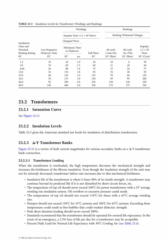
TABLE 23.3 Insulation Levels for Transformer Windings and Bushings
Insulation
Class and
Nominal
Bushing Rating
Low-frequency
Dielectric Tests
Windings Bushings
Impulse Tests (1.2� 50 Wave) Bushing Withstand Voltages
Chopped Wave
Minimum Time
to FlashoverFull Wave
60-cycle
1-min Dry
60-cycle
10-s Wet
Impulse
1.2� 50
Wave
kV kV kV ms kV kV (Rms) kV (Rms) kV (Crest)
1.2 10 36 1.0 10 10 6 30
5.0 19 69 1.5 60 21 20 60
8.66 26 88 1.6 75 27 24 75
15.0 34 110 1.8 95 35 30 95
25.0 40 145 1.9 125 70 60 150
34.5 70 175 3.0 150 95 95 200
46.0 95 290 3.0 250 120 120 250
69.0 140 400 3.0 350 175 175 350
23.2 Transformers
23.2.1 Saturation Curve
See Figure 23.11.
23.2.2 Insulation Levels
Table 23.3 gives the American standard test levels for insulation of distribution transformers.
23.2.3 D-Y Transformer Banks
Figure 23.12 is a review of fault current magnitudes for various secondary faults on a D-Y transformer
bank connection.
23.2.3.1 Transformer Loading
When the transformer is overloaded, the high temperature decreases the mechanical strength and
increases the brittleness of the fibrous insulation. Even though the insulation strength of the unit may
not be seriously decreased, transformer failure rate increases due to this mechanical brittleness.
. Insulation life of the transformer is where it loses 50% of its tensile strength. A transformer may
continue beyond its predicted life if it is not disturbed by short-circuit forces, etc.. The temperature of top oil should never exceed 1008C for power transformers with a 558 average
winding rise insulation system. Oil overflow or excessive pressure could result.. The temperature of top oil should not exceed 1108C for those with a 658C average winding
rise.. Hotspot should not exceed 1508C for 558C systems and 1808C for 658C systems. Exceeding these
temperature could result in free bubbles that could weaken dielectric strength.. Peak short duration loading should never exceed 200%.. Standards recommend that the transformer should be operated for normal life expectancy. In the
event of an emergency, a 2.5% loss of life per day for a transformer may be acceptable.. Percent Daily Load for Normal Life Expectancy with 308C Cooling Air (see Table 23.4).
� 2006 by Taylor & Francis Group, LLC.
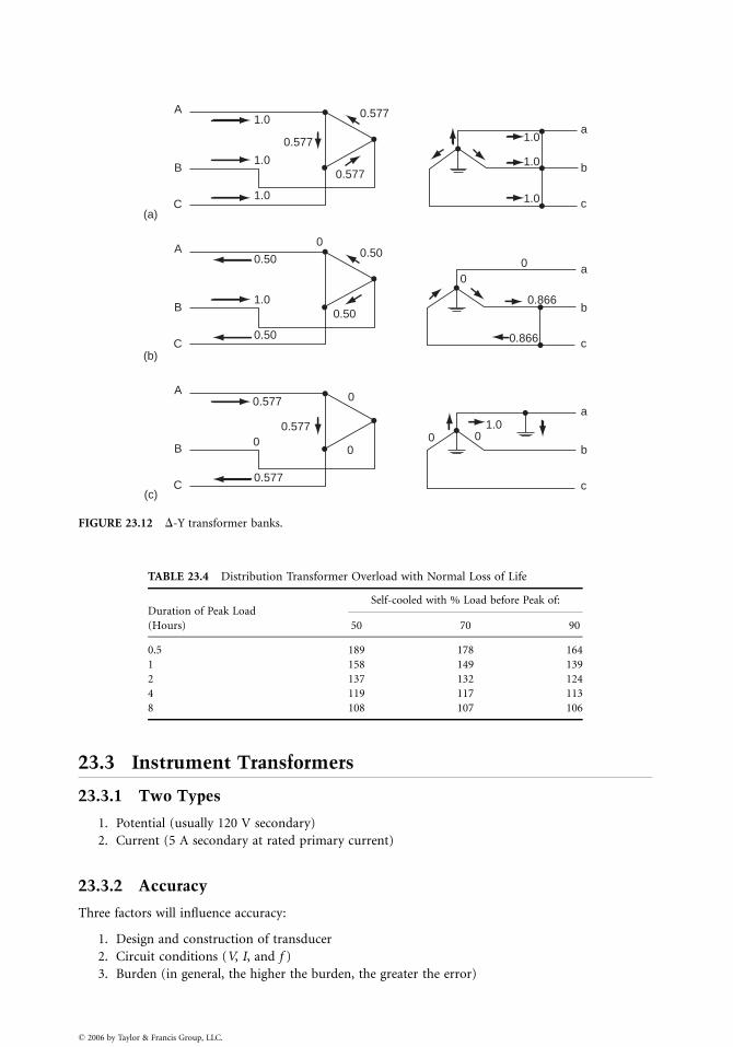
1.0A
(a)
(b)
(c)
B
C
1.0
1.0
1.0
1.000
00
0.866
0.866
b
a
c
b
a
c
b
a
c
1.0
1.0
0.577
0.577
0.577
0.50A
B
C
A
B
C
1.0
0.50
0.577
0.577
0.577
00
0
0.50
0.500
FIGURE 23.12 D-Y transformer banks.
TABLE 23.4 Distribution Transformer Overload with Normal Loss of Life
Duration of Peak LoadSelf-cooled with % Load before Peak of:
(Hours) 50 70 90
0.5 189 178 164
1 158 149 139
2 137 132 124
4 119 117 113
8 108 107 106
23.3 Instrument Transformers
23.3.1 Two Types
1. Potential (usually 120 V secondary)
2. Current (5 A secondary at rated primary current)
23.3.2 Accuracy
Three factors will influence accuracy:
1. Design and construction of transducer
2. Circuit conditions (V, I, and f )
3. Burden (in general, the higher the burden, the greater the error)
� 2006 by Taylor & Francis Group, LLC.
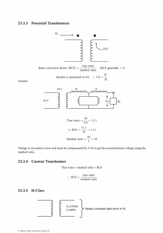
23.3.3 Potential Transformers
IN
OUT
Ratio correction factor (RCF) ¼ true ratio
marked ratio(RCF generally > 1)
Burden is measured in VA ;VA ¼ E2
ZbAssume
10:1
10 V Zb0.9
R X
True ratio ¼ 10
0:9¼ 11:1
) RCF ¼ 11:1
10¼ 1:11
Marked ratio ¼ 10
1¼ 10
Voltage at secondary is low and must be compensated by 11% to get the actual primary voltage using the
marked ratio.
23.3.4 Current Transformer
True ratio¼marked ratio�RCF
; RCF ¼ true ratio
marked ratio
23.3.5 H-Class
Vs is fixedIs varies Nearly constant ratio error in %
� 2006 by Taylor & Francis Group, LLC.
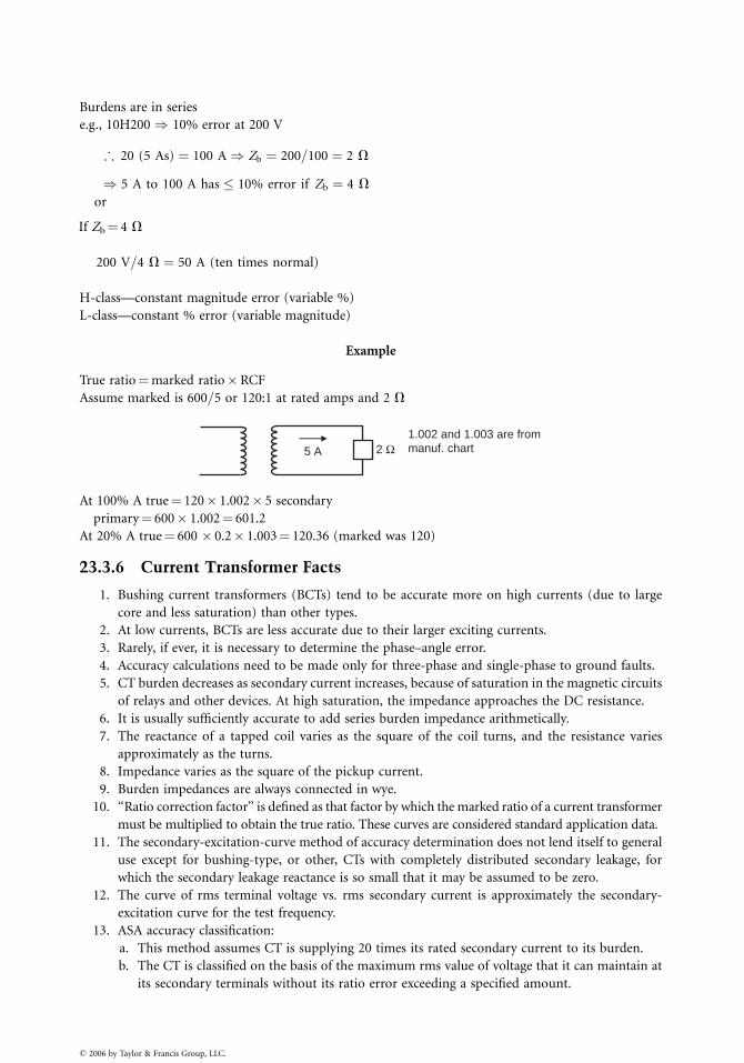
Burdens are in series
e.g., 10H200) 10% error at 200 V
; 20 (5 As) ¼ 100 A) Zb ¼ 200=100 ¼ 2 V
) 5 A to 100 A has � 10% error if Zb ¼ 4 V
or
If Zb¼ 4 V
200 V=4 V ¼ 50 A (ten times normal)
H-class—constant magnitude error (variable %)
L-class—constant % error (variable magnitude)
Example
True ratio¼marked ratio�RCF
Assume marked is 600=5 or 120:1 at rated amps and 2 V
2 Ω5 A
1.002 and 1.003 are from manuf. chart
At 100% A true¼ 120� 1.002� 5 secondary
primary¼ 600� 1.002¼ 601.2
At 20% A true¼ 600 � 0.2� 1.003¼ 120.36 (marked was 120)
23.3.6 Current Transformer Facts
1. Bushing current transformers (BCTs) tend to be accurate more on high currents (due to large
core and less saturation) than other types.
2. At low currents, BCTs are less accurate due to their larger exciting currents.
3. Rarely, if ever, it is necessary to determine the phase–angle error.
4. Accuracy calculations need to be made only for three-phase and single-phase to ground faults.
5. CT burden decreases as secondary current increases, because of saturation in the magnetic circuits
of relays and other devices. At high saturation, the impedance approaches the DC resistance.
6. It is usually sufficiently accurate to add series burden impedance arithmetically.
7. The reactance of a tapped coil varies as the square of the coil turns, and the resistance varies
approximately as the turns.
8. Impedance varies as the square of the pickup current.
9. Burden impedances are always connected in wye.
10. ‘‘Ratio correction factor’’ is defined as that factor by which the marked ratio of a current transformer
must be multiplied to obtain the true ratio. These curves are considered standard application data.
11. The secondary-excitation-curve method of accuracy determination does not lend itself to general
use except for bushing-type, or other, CTs with completely distributed secondary leakage, for
which the secondary leakage reactance is so small that it may be assumed to be zero.
12. The curve of rms terminal voltage vs. rms secondary current is approximately the secondary-
excitation curve for the test frequency.
13. ASA accuracy classification:
a. This method assumes CT is supplying 20 times its rated secondary current to its burden.
b. The CT is classified on the basis of the maximum rms value of voltage that it can maintain at
its secondary terminals without its ratio error exceeding a specified amount.
� 2006 by Taylor & Francis Group, LLC.
�
c. ‘‘H’’ stands for high internal secondary impedance.
d. ‘‘L’’ stands for low internal secondary impedance (bushing type).
e. 10H800 means the ratio error is 10% at 20 times rated voltage with a maximum secondary
voltage of 800 and high internal secondary impedance.
f. Burden (max)—maximum specified voltage=20� rated second.
g. The higher the number after the letter, the better the CT.
h. A given 1200=5 bushing CT with 240 secondary turns is classified as 10L400: if a 120-turn
completely distributed tap is used, then the applicable classification is 10L200.
i. For the same voltage and error classifications, the H transformer is better than the L for
currents up to 20 times rated.
23.3.7 Glossary of Transducer Terms
Voltage transformers—They are used whenever the line voltage exceeds 480 V or whatever lower voltage
may be established by the user as a safe voltage limit. They are usually rated on a basis of 120 V
secondary voltage and used to reduce primary voltage to usable levels for transformer-rated meters.
Current transformers—Current transformers are usually rated on a basis of 5 A secondary current and
used to reduce primary current to usable levels for transformer-rated meters and to insulate and isolate
meters from high-voltage circuits.
Current transformer ratio—Current transformer ratio is the ratio of primary to secondary current. For
current transformer rated 200:5, the ratio is 200:5 or 40:1.
Voltage transformer ratio—Voltage transformer ratio is the ratio of primary to secondary voltage. For
voltage transformer rated 480:120, the ratio is 4:1, 7200:120, or 60:1.
Transformer ratio (TR)—Transformer ratio is the total ratio of current and voltage transformers. For
200:5 CT and 480:120 PT, TR¼ 40� 4¼ 160.
Weatherability—Transformers are rated as indoor or outdoor, depending on construction (including
hardware).
Accuracy classification—Accuracy classification is the accuracy of an instrument transformer at
specified burdens. The number used to indicate accuracy is the maximum allowable error of the
transformer for specified burdens. For example, 0.3 accuracy class means the maximum error will not
exceed 0.3% at stated burdens.
Rated burden—Rated burden is the load that may be imposed on the transformer secondaries by
associated meter coils, leads, and other connected devices without causing an error greater than the
stated accuracy classification.
Current transformer burdens—Current transformer burdens are normally expressed in ohms impedance
such as B-0.1, B-0.2, B-0.5, B-0.9, or B-1.8.Corresponding volt–ampere values are 2.5, 5.0, 12.5, 22.5, and 45.
Voltage transformer burdens—Voltage transformer burdens are normally expressed as volt–amperes at
a designated power factor. May be W, X, M, Y, or Z where W is 12.5 VA at 0.10 pf, X is 25 VA at 0.70 pf,
M is 35 VA at 0.20 pf, Y is 75 VA at 0.85 pf, and Z is 200 VA at 0.85 pf. The complete expression for a
current transformer accuracy classification might be 0.3 at B-0.1, B-0.2, and B-0.5, while the potential
transformer might be 0.3 at W, X, M, and Y.
Continuous thermal rating factor (TRF)—Continuous TRF is normally designated for current trans-
formers and is the factor by which the rated primary current is multiplied to obtain the maximum
allowable primary current without exceeding temperature rise standards and accuracy requirements. For
example, if a 400:5 CT has a TRF of 4.0, the CT will continuously accept 400� 4 or 1600 primary
amperes with 5� 4 or 20 A from the secondary. The thermal burden rating of a voltage transformer shall
be specified in terms of the maximum burden in volt–amperes that the transformer can carry at rated
secondary voltage without exceeding a given temperature rise.
Rated insulation class—Rated insulation class denotes the nominal (line-to-line) voltage of the
circuit on which it should be used. Associated Engineering Company has transformers rated for 600 V
through 138 kV.
2006 by Taylor & Francis Group, LLC.
Polarity—The relative polarity of the primary and secondary windings of a current transformer is
indicated by polarity marks (usually white circles), associated with one end of each winding. When current
enters at the polarity end of the primary winding, a current in phase with it leaves the polarity end of the
secondary winding. Representation of primary marks on wiring diagrams is shown as black squares.
Hazardous open circulating—The operation of CTs with the secondary winding open can result in a
high voltage across the secondary terminals, which may be dangerous to personnel or equipment.
Therefore, the secondary terminals should always be short circuited before a meter is removed from
service. This may be done automatically with a bypass in the socket or by a test switch for A-base meters.
23.4 Loading
Probably no area of distribution engineering causes more confusion than does loading. Reading the
standards does not seem to help much since everyone appears to have their own interpretation.
Manufacturers of equipment are very conservative since they really never know how the user will
actually put the product to use so they must expect the worst. On the other hand, many users seem
to take the approach that since it did not fail last year with traditional overloading values, it will not fail
this year either. In fact, it will not fail until after retirement. Heck! ‘‘Save a buck and get a promotion.’’
The author of this document is not a psychology major and frankly has no idea of what the thinking was
when much of the following was produced. The material that follows, however, was taken from sources
with excellent reputation. Use it with caution.
23.4.1 Transformer Loading Basics
. All modern transformers have insulation systems designed for operation at 658C average winding
temperature and 808C hottest-spot winding rise over ambient in an average ambient of 308C.
This means:* 658C average winding rise þ 308C ambient¼ 958C average winding temperature* 808C hottest-spot rise þ 308C ambient¼ 1108C hottest spot
(Old system: 558C winding rise þ 308C ambient¼ 858C average winding temperature)* 658C hotttest spot þ 308C ambient¼ 958C hottest spot
. Notice that 958C is the average winding temperature for the new insulation system and the hottest
spot for the old—A source of immense confusion for many of us.. The temperature of the top oil should not exceed 1008C. Obviously, top-oil temperature is always
less than hottest spot.. The maximum hotspot temperature should not exceed 1508C for a 558C rise transformer or
1808C for a 658C rise transformer.. Peak 0.5 h loading should not exceed 200%.. The conditions of 308C ambient temperature and 100% load factor establish the basis of
transformer ratings.. The ability of the transformer to carry more than nameplate rating under certain conditions
without exceeding 958C is basically due to the fact that top-oil temperature does not instantan-
eously follow changes in transformer load due to thermal storage.
� 2006 by Taylor & Francis Group, LLC.
. An average loss of life of 1% per year (or 5% in any emergency) incurred during emergency
operations is considered reasonable.. Most companies do not allow normal daily peaks to exceed the permissible load for normal life
expectancy.. The firm capacity is usually the load that the substation can carry with one supply line or one
transformer out of service.. ‘‘Emergency 24-h firm capacity’’ usually means a loss of life of 1% but is sometimes as much as
5% or 6%.. The following measures can be used for emergency conditions lasting more than 24 h:
* Portable fans* Water spray* Interconnect cooling equipment of FOA units* Use transformer thermal relays to drop certain loads
23.4.2 Examples of Substation Transformer Loading Limits
The following is an example of maximum temperature limits via the IEEE for a 658C rise transformer:
� 2006 by Taylor & Francis Group, LLC.
IEEE Normal Life Expectancy
Top-oil temperature
1058CHotspot temperature
1208CThis next example shows the loading practice of various utilities for substation transformers:
Utility A Utility B Utility C Utility D Utility E Utility F Utility G
Normal Conditions
Top-oil
95 110 95 95 95 110 110Hotspot
125 130 120 110 120 140 120Emergency Conditions
Top-oil
110 110 110 110 110 110 110Hotspot
140 140 140 130 140 140 140What happens when the hotspot is raised from 1258C to 1308C? This is shown as follows:
Maximum Hotspot (8C) % Loss of Life, Annual
125
0.3366130
0.5372An example of the effect of load cycle (3-h peak with 70% pre-load for 13 h and 45% load for 8 h) and
ambient on transformer capability via the ANSI guide is shown below:
Peak Load for Normal Life Expectancy Emergency Peak Load with 24-h Loss of Life
Transformer Type
108C Ambient 308C Ambient 0.25% 1.0%20,000—OA
30,000 24,200 28,400 32,00015,000=2,000—OA=FA
28,700 23,800 27,500 30,70012,000=16,000=
20,000—OA=FA=FOA
27,500
23,200 26,800 29,70020,000—FOA
27,500 23,200 26,800 29,700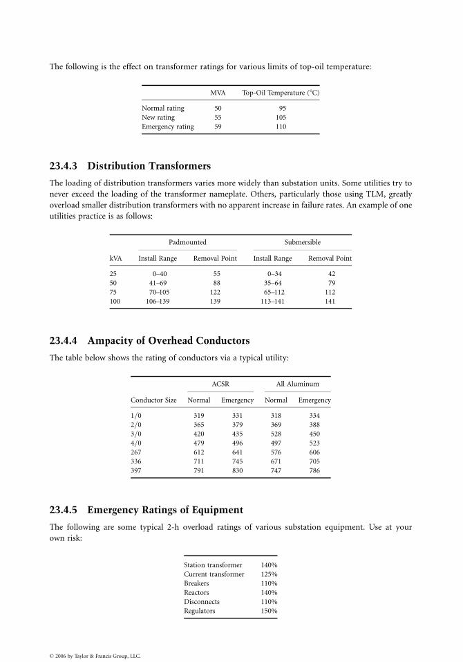
The following is the effect on transformer ratings for various limits of top-oil temperature:
� 2006 by Taylor & Francis Group, LLC
MVA Top-Oil Temperature (8C)
.
Normal rating
50 95New rating
55 105Emergency rating
59 11023.4.3 Distribution Transformers
The loading of distribution transformers varies more widely than substation units. Some utilities try to
never exceed the loading of the transformer nameplate. Others, particularly those using TLM, greatly
overload smaller distribution transformers with no apparent increase in failure rates. An example of one
utilities practice is as follows:
Padmounted Submersible
kVA
Install Range Removal Point Install Range Removal Point25
0–40 55 0–34 4250
41–69 88 35–64 7975
70–105 122 65–112 112100
106–139 139 113–141 14123.4.4 Ampacity of Overhead Conductors
The table below shows the rating of conductors via a typical utility:
ACSR All Aluminum
Conductor Size
Normal Emergency Normal Emergency1=0
319 331 318 3342=0
365 379 369 3883=0
420 435 528 4504=0
479 496 497 523267
612 641 576 606336
711 745 671 705397
791 830 747 78623.4.5 Emergency Ratings of Equipment
The following are some typical 2-h overload ratings of various substation equipment. Use at your
own risk:
Station transformer
140%Current transformer
125%Breakers
110%Reactors
140%Disconnects
110%Regulators
150%
23.5 Miscellaneous Loading Information
The following are some miscellaneous loading information and thoughts from a number of actual
utilities:
a. Commercial and industrial transformer loading
� 2006 by Taylor & Francis Group, LLC.
Load Factor (%) Transformer Load Limit (%)
0–64
13065–74
12575–100
120b. Demand factor
Lights—50%
Air conditioning—70%
Major appliances—40%
c. Transformer loading. Distribution transformer life is in excess of five times the present guide levels.. Distribution guide shows that life expectancy is about 500,000 h for 1008C hottest-spot
operation, compared to 200,000 h for a power transformer. Same insulation system.. Using present loading guides, only 2.5% of power transformer thermal life is used up after
15 years.. Results of one analysis showed that the transition from acceptable to unacceptable risk
(approximately an order of magnitude) was accompanied (by this utility) by only an 8.5%
investment savings and a 12% increase in transformer loading.. Application of transformers in excess of normal loading can cause the following:
* Evolution of free gas from insulation of winding and lead conductors.* Evolution of free gas from insulation adjacent to metallic structural parts linked by magnetic
flux produced by winding or lead currents may also reduce dielectric strength.* Operation at high temperatures will cause reduced mechanical strength of both conductor and
structural insulation.* Thermal expansion of conductors, insulation materials, or structural parts at high temperature
may result in permanent deformations that could contribute to mechanical or dielectric failures.* Pressure buildup in bushings for currents above rating could result in leaking gaskets, loss of
oil, and ultimate dielectric failure.* Increased resistance in the contacts of tap changers can result from a buildup of oil decom-
position products in a very localized high temperature region.* Reactors and current transformers are also at risk.* Oil expansion could become greater than the holding capacity of the tank.
. Aging or deterioration of insulation is a time function of temperature, moisture content, and
oxygen content. With modern oil preservation systems, the moisture and oxygen contributions
to insulation deterioration can be minimized, leaving insulation temperature as the controlling
parameter.. Distribution and power transformer model tests indicate that the normal life expectancy at a
continuous hottest-spot temperature of 1108C is 20.55 years.. Input into a transformer loading program should be as follows:
* Transformer characteristics (loss ratio, top-oil rise, hottest-spot rise, total loss, gallons of oil,
and weight of tank and fittings)* Ambient temperatures* Initial continuous load
* Peak load durations and the specified daily percent loss of life* Repetitive 24-h load cycle if desired
. Maximum permitted loading is 200% for a power transformer and 300% for a distribution
transformer.. Suggested limits of loading for distribution transformers are as follows:
* Top oil—1208C* Hottest spot—2008C* Short time (0.5 h)—300%
. Suggested limits for power transformers are as follows:* Top oil—1008C* Hottest spot—1808C* Maximum loading—200%
. Overload limits for coordination of bushings with transformers are as follows:* Ambient air—408C maximum* Transformer top oil—1108C maximum* Maximum current—two times bushing rating* Bushing insulation hottest spot—1508C maximum
. Current ratings for the load tap changer (LTC) are:* Temperature rise limit of 208C for any current carrying contact in oil when carrying 1.2 times
the maximum rated current of the LTC* Capable of 40 breaking operations at twice the rate current and kVA
. Planned loading beyond nameplate rating defines a condition wherein a transformer is so loaded
that its hottest-spot temperature is in the temperature range of 120–1308C.. Long term emergency loading defines a condition wherein a power transformer is so loaded that
its hottest-spot temperature is in the temperature range of 120–1408C.. The principal gases found dissolved in the mineral oil of a transformer are as follows:
* Nitrogen: from external atmosphere or from gas blanket over the free surface of the oil.* Oxygen: from external atmosphere.* Water: from moisture absorbed in cellulose insulation or from decomposition of the cellulose.* Carbon dioxide: from thermal decomposition of cellulose insulation.* Carbon monoxide: from thermal decomposition of cellulose insulation.* Other gases: may be present in very small amounts (e.g., acetylene) as a result of oil or
insulation decomposition by overheated metal, partial discharge, arcing, etc. These are very
important in any analysis of transformers, which may be in the process of failing.. Moisture affects insulation strength, power factor, aging, losses, and the mechanical strength of
the insulation. Bubbles can form at 1408C, which enhance the chances of partial discharge and
the eventual breakdown of the insulation as they rise to the top of the insulation. If a
transformer is to be overloaded, it is important to know the moisture content of the insulation,
especially if it is an older transformer. Bubbles evolve fast, so temperature is important to bubble
formation but not the time at that temperature. Transformer insulation with 3.5% moisture
content should not be operated above nameplate for a hottest spot of 1208C. Tests have shown
that the use of circulated oil for the drying process takes some time. For a processing time of
70 h the moisture content of the test transformers was reduced from 2% to 1.9% at a
temperature of 50–758C. Apparently only surface moisture was affected. A more effective
method is to remove the oil and heat the insulation under vacuum.
� 2006 by Taylor & Francis Group, LLC.

� 2006 by Taylor & Francis Group, LLC.
24
� 2006 by Taylor & Francis Group, LLC.
Real-Time Controlof Distributed
Generation
Murat DilekElectrical Distribution Design, Inc.
Robert P. BroadwaterVirginia Polytechnic Institute and
State University
24.1 Local Site DG Control .................................................... 24-2
24.2 Hierarchical Control: Real-Time Control ..................... 24-2Data Flow to Upper Layers . Data Flow to Lower Layers
24.3 Control of DGs at Circuit Level..................................... 24-5Estimating Loading throughout Circuit . Siting DGs for
Improving Efficiency and Reliability
24.4 Hierarchical Control: Forecasting Generation............ 24-12
Distributed generation (DG) can be operated to control voltages and power flows within the distribu-
tion system. Improvements in distribution system reliability and overall power system efficiency can be
realized. For load growth with short-lived peaks that occur during extreme weather, DGs may provide
lower-cost solutions than other approaches to system capacity upgrades.
DG provides a means for increasing the capacity of existing distribution facilities. When considering
increasing distribution system capacity, DGs can be an alternative to new substation addition and
replacing existing equipment with larger ones. A DG installed at the distribution level releases capacity
throughout the system, from transmission through distribution. Transmission system losses are elim-
inated, and distribution system losses are reduced.
Some customer facilities have DGs that are installed for back-up power. These DGs are employed
during grid-power outages or periods of high-cost grid power. They are operated for only a small
fraction of time over the year. Moreover, back-up DGs are usually oversized, which means that they can
provide more power than their facility loads need. These DGs can be equipped with a set of devices that
will enable them to seamlessly interconnect to the grid and be dispatched if needed. The available
capacity from such DGs can then be used for utility purposes.
DGs across many circuits in distribution areas can be controlled from a single control point. That is,
such DGs can be aggregated into a block of generation and made available for transmission system use.
Although specifically intended for DGs, the aggregate control may also include other means of
capacity release. When equipped with the necessary control and interconnection instrumentation,
capacitors can be involved in aggregate control also. Some loads may also participate in the aggregation
process in the form of curtailable or interruptible load. The aggregate control handles the collection of
all of these participating entities.
The total power made available to the transmission system by the aggregate control is exhibited as a
capacity release. That is, it is not the power injected into the transmission system from the distribution
side, rather it is less power drawn by the distribution side. In the discussion to follow, the phrases DG
power by aggregate control and capacity release by aggregate control are used interchangeably.
The aggregate control of DGs may serve a number of purposes. For instance, aggregated DGs can be
activated if the transmission system or the distribution utility is having supply emergencies. Thus, DG
aggregation provides a means to increase operating reserve. DGs can also help utilities manage energy
purchases during times when the transmission grid electricity price is excessively high.
In the next section, local control for common DGs is discussed first. Next, controlling a group of DGs
as an aggregate is addressed. Then, the DG as part of a hierarchical control system for controlling
voltages and system power flows is investigated. Finally, load estimation for real-time DG control and
also for forecasting aggregate control of DGs is presented.
24.1 Local Site DG Control
A DG operates basically in two modes in regard to being connected to the utility grid. In parallel mode, the
DG remains connected to the grid. Hence, both the DG and the grid provide power for the local load in the
customer facility (or DG site). In stand-alone (isolated or island) mode the DG is the sole power source to
the local loads. In this section, consideration will be given only to DGs operating in parallel with the grid.
There are several forms of control for parallel DG. In one form of control, a local controller maintains
a constant kW and kVar generation. In most cases, the local load is greater than the DG. Therefore, the
power mismatch is supplied by the grid.
In another form of local control, the DG is controlled in order to maintain a constant power flow at
the point of common coupling (PCC)—the point where the DG site interfaces with the grid, which is
basically the metering point. The power flow maintained might be from the grid into the DG site
(import) or from the site into the grid (export). As the local load varies, the local controller acts to
change the kW and kVar generation at the DG in an attempt to keep the power flow constant at the PCC.
The most common DGs in service utilize synchronous machines. They prevail in grid-scale power
exchanges between the utility and DG sites. Internal combustion (IC) engines and combustion turbines
are the main prime movers for the synchronous generators. IC engines are much more common. Diesel
fuel and natural gas are chosen for powering these engines.
The control of a synchronous machine is achieved by adjusting the fuel flow into the engine and the
excitation of the generator. The fuel flow control by the governor determines the horsepower (kW)
developed on the shaft of the engine. In a parallel DG, the shaft speed must be maintained very close to
system frequency. The governor uses the kW set-point signal from the local controller and the speed
signal from the DG output. The governor adjusts the fuel control to cause the kW output of the DG to
match the kW set point that is set by the local controller.
The excitation control achieved by the voltage regulator determines terminal voltage and kVar output
of the generator. Parallel DGs are required not to actively participate in regulating voltage at the PCC
where the grid is supposed to set the voltage. Therefore, the excitation control is used to adjust kVar
generation only. Rather than a kVar set point, a power factor (pf) set point is used for the excitation
control. The local controller feeds the pf set point to the regulator. The regulator then adjusts the
excitation to match the pf measured at the DG to the provided pf setting.
Basic functionality of the control system for parallel-connected DGs can be seen in Fig. 24.1. For
simplicity, it is assumed that the customer facility has only one DG. The local control receives the desired
kW and kVar generation set points from an upper-level controller. The strategy can be a constant kW and
kVar generation level for the DG or a constant kW and kVar flow at the PCC. Based on the control
strategy, the local controller sends the required set points to the controller of the DG. An operator can
supervise the control process and intervene as needed.
24.2 Hierarchical Control: Real-Time Control
The hierarchical DG control consists of three levels and is illustrated in Fig. 24.2. The control
functionality is used for two purposes: (1) for real-time DG control and (2) for forecasting future
generation.
� 2006 by Taylor & Francis Group, LLC.
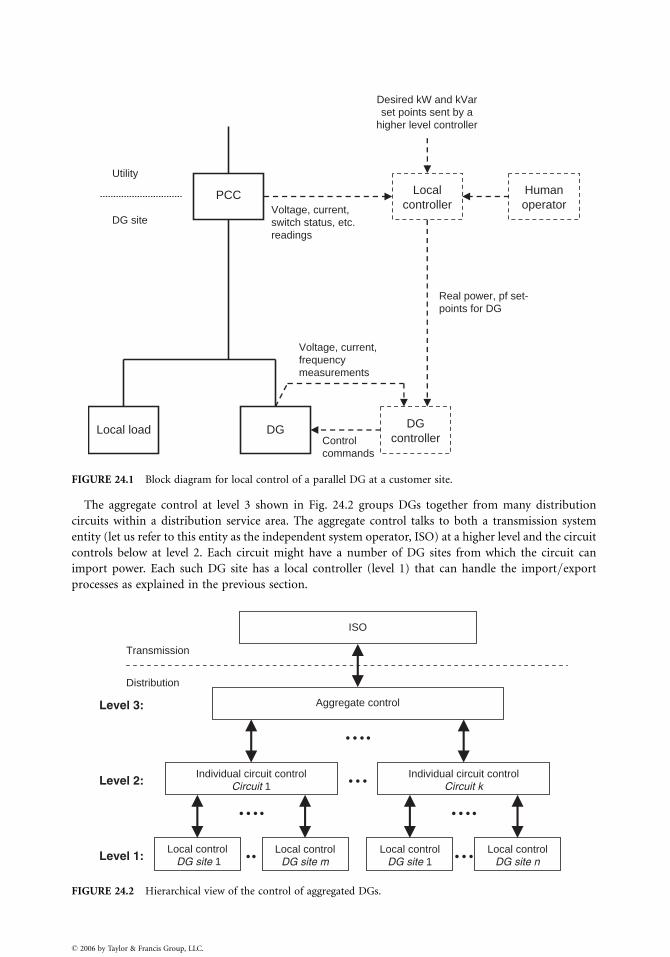
Local load
PCC
Utility
DG site
DG DGcontroller
LocalcontrollerVoltage, current,
switch status, etc.readings
Controlcommands
Real power, pf set-points for DG
Desired kW and kVarset points sent by a
higher level controller
Humanoperator
Voltage, current,frequencymeasurements
FIGURE 24.1 Block diagram for local control of a parallel DG at a customer site.
The aggregate control at level 3 shown in Fig. 24.2 groups DGs together from many distribution
circuits within a distribution service area. The aggregate control talks to both a transmission system
entity (let us refer to this entity as the independent system operator, ISO) at a higher level and the circuit
controls below at level 2. Each circuit might have a number of DG sites from which the circuit can
import power. Each such DG site has a local controller (level 1) that can handle the import=export
processes as explained in the previous section.
Individual circuit controlCircuit 1
Local control DG site 1Level 1: .. Local control
DG site m…
Level 2:
Aggregate control
…
Level 3:
ISO
Transmission
Distribution
….
…. ….
Individual circuit control Circuit k
Local controlDG site 1
Local controlDG site n
FIGURE 24.2 Hierarchical view of the control of aggregated DGs.
� 2006 by Taylor & Francis Group, LLC.
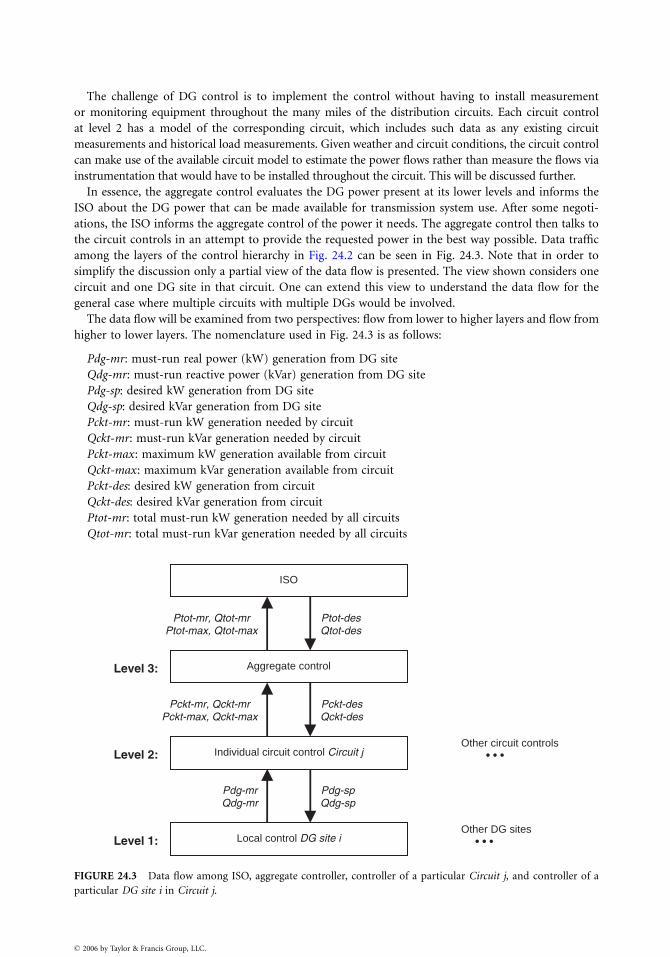
The challenge of DG control is to implement the control without having to install measurement
or monitoring equipment throughout the many miles of the distribution circuits. Each circuit control
at level 2 has a model of the corresponding circuit, which includes such data as any existing circuit
measurements and historical load measurements. Given weather and circuit conditions, the circuit control
can make use of the available circuit model to estimate the power flows rather than measure the flows via
instrumentation that would have to be installed throughout the circuit. This will be discussed further.
In essence, the aggregate control evaluates the DG power present at its lower levels and informs the
ISO about the DG power that can be made available for transmission system use. After some negoti-
ations, the ISO informs the aggregate control of the power it needs. The aggregate control then talks to
the circuit controls in an attempt to provide the requested power in the best way possible. Data traffic
among the layers of the control hierarchy in Fig. 24.2 can be seen in Fig. 24.3. Note that in order to
simplify the discussion only a partial view of the data flow is presented. The view shown considers one
circuit and one DG site in that circuit. One can extend this view to understand the data flow for the
general case where multiple circuits with multiple DGs would be involved.
The data flow will be examined from two perspectives: flow from lower to higher layers and flow from
higher to lower layers. The nomenclature used in Fig. 24.3 is as follows:
Pdg-mr: must-run real power (kW) generation from DG site
Qdg-mr: must-run reactive power (kVar) generation from DG site
Pdg-sp: desired kW generation from DG site
Qdg-sp: desired kVar generation from DG site
Pckt-mr: must-run kW generation needed by circuit
Qckt-mr: must-run kVar generation needed by circuit
Pckt-max : maximum kW generation available from circuit
Qckt-max : maximum kVar generation available from circuit
Pckt-des: desired kW generation from circuit
Qckt-des: desired kVar generation from circuit
Ptot-mr: total must-run kW generation needed by all circuits
Qtot-mr: total must-run kVar generation needed by all circuits
Local control DG site iLevel 1: …
Pdg-spQdg-sp
Level 2:
Aggregate control
…
Level 3:
Pdg-mrQdg-mr
Other DG sites
Pckt-mr, Qckt-mrPckt-max, Qckt-max
Individual circuit control Circuit jOther circuit controls
Pckt-desQckt-des
ISO
Ptot-mr, Qtot-mrPtot-max, Qtot-max
Ptot-desQtot-des
FIGURE 24.3 Data flow among ISO, aggregate controller, controller of a particular Circuit j, and controller of a
particular DG site i in Circuit j.
� 2006 by Taylor & Francis Group, LLC.
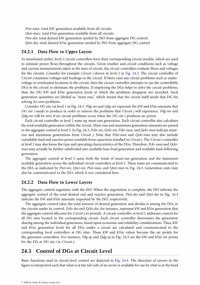
Ptot-max : total kW generation available from all circuits
Qtot-max : total kVar generation available from all circuits
Ptot-des: total desired kW generation needed by ISO from aggregate DG control
Qtot-des: total desired kVar generation needed by ISO from aggregate DG control
24.2.1 Data Flow to Upper Layers
As mentioned earlier, level-2 circuit controllers have their corresponding circuit models, which are used
to estimate power flows throughout the circuits. Given weather and circuit conditions such as voltage
and current measurements taken at the start of circuit, the circuit controllers evaluate flows and voltages
for the circuits. Consider for example Circuit j shown in level 2 in Fig. 24.3. The circuit controller of
Circuit j examines voltages and loadings in the circuit. If there exist any circuit problems such as under-
voltage or overloaded locations in the circuit, then the circuit controller attempts to use the controllable
DGs in the circuit to eliminate the problems. If employing the DGs helps to solve the circuit problems,
then the DG kW and kVar generation levels at which the problems disappear are recorded. Such
generation quantities are labeled as ‘‘must run,’’ which means that the circuit itself needs that DG for
solving its own problems.
Consider DG site i at level 1 in Fig. 24.3. Pdg-mr and Qdg-mr represent the kW and kVar amounts that
DG site i needs to produce in order to remove the problems that Circuit j will experience. Pdg-mr and
Qdg-mr will be zero if no circuit problems occur when the DG site i produces no power.
Each circuit controller at level 2 sums up must-run generation. Each circuit controller also calculates
the total available generation within the circuit. Must-run and maximum generation amounts are passed
to the aggregate control at level 3. In Fig. 24.3, Pckt-mr, Qckt-mr, Pckt-max, and Qckt-max indicate must-
run and maximum generations from Circuit j. Note that Pckt-max and Qckt-max may also include
curtailable load and reactive power available from capacitors installed in Circuit j. The Circuit j controller
at level 2 may also know the type and operating characteristics of the DGs. Therefore, Pckt-max and Qckt-
max may actually be further subdivided into available base-load generation and available load-following
generation.
The aggregate control at level 3 sums both the totals of must-run generation and the maximum
available generation across the individual circuit controllers at level 2. These sums are communicated to
the ISO, as indicated by Ptot-mr, Qtot-mr, Ptot-max, and Qtot-max in Fig. 24.3. Generation costs may
also be communicated to the ISO, which is not considered here.
24.2.2 Data Flow to Lower Layers
The aggregate control negotiates with the ISO. When the negotiation is complete, the ISO informs the
aggregate control of the total desired real and reactive generation. Ptot-des and Qtot-des in Fig. 24.3
indicate the kW and kVar amounts requested by the ISO, respectively.
The aggregate control takes the total amount of desired generation and divides it among the DGs in
the circuits under its control. Pckt-des and Qckt-des, for instance, represent kW and kVar generation that
the aggregate control allocates for Circuit j to provide. A circuit controller at level 2 addresses control for
all DG sites located in the corresponding circuit. Each circuit controller determines the generation
sharing among the individual generators, based upon economic and reliability considerations. Thus, kW
and kVar generation levels for all DGs under a circuit are calculated and communicated to the
corresponding local controllers at DG sites. These kW and kVar values become the set points for
the generator controllers. For instance, Pdg-sp and Qdg-sp in Fig. 24.3 are the kW and kVar set points
for the DG at DG site i in Circuit j.
24.3 Control of DGs at Circuit Level
Basic functions used in circuit-level control are depicted in Fig. 24.4. The direction of arrows in the
figure is interpreted such that what is at the tail-side of an arrow is available for use by what is at the head
� 2006 by Taylor & Francis Group, LLC.
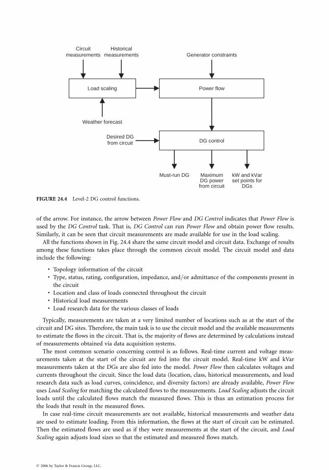
DG control
Generator constraints
Must-run DG MaximumDG powerfrom circuit
kW and kVarset points for
DGs
Desired DGfrom circuit
Power flowLoad scaling
Circuitmeasurements
Historicalmeasurements
Weather forecast
FIGURE 24.4 Level-2 DG control functions.
of the arrow. For instance, the arrow between Power Flow and DG Control indicates that Power Flow is
used by the DG Control task. That is, DG Control can run Power Flow and obtain power flow results.
Similarly, it can be seen that circuit measurements are made available for use in the load scaling.
All the functions shown in Fig. 24.4 share the same circuit model and circuit data. Exchange of results
among these functions takes place through the common circuit model. The circuit model and data
include the following:
. Topology information of the circuit
. Type, status, rating, configuration, impedance, and=or admittance of the components present in
the circuit. Location and class of loads connected throughout the circuit. Historical load measurements. Load research data for the various classes of loads
Typically, measurements are taken at a very limited number of locations such as at the start of the
circuit and DG sites. Therefore, the main task is to use the circuit model and the available measurements
to estimate the flows in the circuit. That is, the majority of flows are determined by calculations instead
of measurements obtained via data acquisition systems.
The most common scenario concerning control is as follows. Real-time current and voltage meas-
urements taken at the start of the circuit are fed into the circuit model. Real-time kW and kVar
measurements taken at the DGs are also fed into the model. Power Flow then calculates voltages and
currents throughout the circuit. Since the load data (location, class, historical measurements, and load
research data such as load curves, coincidence, and diversity factors) are already available, Power Flow
uses Load Scaling for matching the calculated flows to the measurements. Load Scaling adjusts the circuit
loads until the calculated flows match the measured flows. This is thus an estimation process for
the loads that result in the measured flows.
In case real-time circuit measurements are not available, historical measurements and weather data
are used to estimate loading. From this information, the flows at the start of circuit can be estimated.
Then the estimated flows are used as if they were measurements at the start of the circuit, and Load
Scaling again adjusts load sizes so that the estimated and measured flows match.
� 2006 by Taylor & Francis Group, LLC.
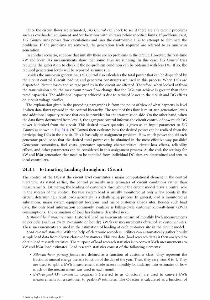
Once the circuit flows are estimated, DG Control can check to see if there are any circuit problems
such as overloaded equipment and=or locations with voltages below specified limits. If problems exist,
DG Control runs power flow calculations and uses the controllable DGs to attempt to eliminate the
problems. If the problems are removed, the generation levels required are referred to as must-run
generation.
In another scenario, suppose that initially there are no problems in the circuit. However, the real-time
kW and kVar DG measurements show that some DGs are running. In this case, DG Control tries
reducing the generation to check if the no-problem condition can be obtained with less DG. If so, the
reduced generation levels will be reported as must run.
Besides the must-run generation, DG Control also calculates the total power that can be dispatched by
the circuit control. Circuit loading and generator constraints are used in this process. When DGs are
dispatched, circuit losses and voltage profiles in the circuit are affected. Therefore, when looked at from
the transmission side, the maximum power flow change that the DGs can achieve is greater than their
rated capacities. The additional capacity achieved is due to reduced losses in the circuit and DG effects
on circuit voltage profiles.
The explanation given in the preceding paragraphs is from the point of view of what happens in level
2 when data flows upward in the control hierarchy. The result of this flow is must-run generation levels
and additional capacity release that can be provided for the transmission side. On the other hand, when
the data flows downward from level 3, the aggregate control informs the circuit control of how much DG
power is desired from the circuit. This desired power quantity is given as an input parameter to DG
Control as shown in Fig. 24.4. DG Control then evaluates how the desired power can be realized from the
participating DGs in the circuit. This is basically an assignment problem: How much power should each
generator produce so that the desired total power can be obtained in the most effective way possible?
Generator constraints, fuel costs, generator operating characteristics, circuit-loss effects, reliability
effects, and other parameters can be considered in this assignment process. At the end, the settings for
kW and kVar generation that need to be supplied from individual DG sites are determined and sent to
local controllers.
24.3.1 Estimating Loading throughout Circuit
The control of the DGs at the circuit level constitutes a major computational element in the control
hierarchy. As stated earlier, the control primarily uses estimates of circuit conditions rather than
measurements. Estimating the loading of customers throughout the circuit model plays a central role
in the success of the control. Because system load is usually monitored at only a few points in the
circuit, determining circuit loads accurately is a challenging process. In general, load is monitored at
substations, major system equipment locations, and major customer (load) sites. Besides such load
data, the only load information commonly available is billing-cycle customer kilowatt-hour (kWh)
consumptions. The estimation of load has features described next.
Historical load measurements: Historical load measurements consist of monthly kWh measurements
or periodic (such as every 15-minute or hourly) kW=kVar measurements obtained at customer sites.
These measurements are used in the estimation of loading at each customer site in the circuit model.
Load research statistics: With the help of electronic recorders, utilities can automatically gather hourly
sample load data from diverse classes of customers. This raw data (load research data) is then analyzed to
obtain load research statistics. The purpose of load research statistics is to convert kWh measurements to
kW and kVar load estimates. Load research statistics consist of the following elements:
. Kilowatt-hour parsing factors are defined as a function of customer class. They represent the
fractional annual energy use as a function of the day of the year. Thus, they vary from 0 to 1. They
are used to split a kWh measurement made across monthly boundaries into estimates of how
much of the measurement was used in each month.. kWh-to-peak-kW conversion coefficients (referred to as C-factors) are used to convert kWh
measurements for a customer to peak-kW estimates. The C-factor is calculated as a function of
� 2006 by Taylor & Francis Group, LLC.
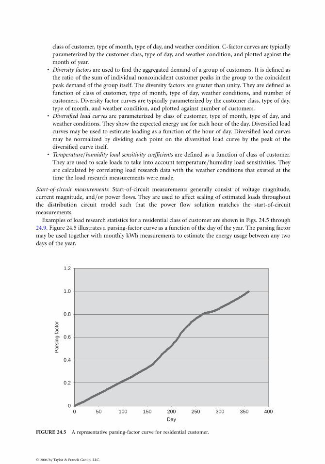
class of customer, type of month, type of day, and weather condition. C-factor curves are typically
parameterized by the customer class, type of day, and weather condition, and plotted against the
month of year.. Diversity factors are used to find the aggregated demand of a group of customers. It is defined as
the ratio of the sum of individual noncoincident customer peaks in the group to the coincident
peak demand of the group itself. The diversity factors are greater than unity. They are defined as
function of class of customer, type of month, type of day, weather conditions, and number of
customers. Diversity factor curves are typically parameterized by the customer class, type of day,
type of month, and weather condition, and plotted against number of customers.. Diversified load curves are parameterized by class of customer, type of month, type of day, and
weather conditions. They show the expected energy use for each hour of the day. Diversified load
curves may be used to estimate loading as a function of the hour of day. Diversified load curves
may be normalized by dividing each point on the diversified load curve by the peak of the
diversified curve itself.. Temperature=humidity load sensitivity coefficients are defined as a function of class of customer.
They are used to scale loads to take into account temperature=humidity load sensitivities. They
are calculated by correlating load research data with the weather conditions that existed at the
time the load research measurements were made.
Start-of-circuit measurements: Start-of-circuit measurements generally consist of voltage magnitude,
current magnitude, and=or power flows. They are used to affect scaling of estimated loads throughout
the distribution circuit model such that the power flow solution matches the start-of-circuit
measurements.
Examples of load research statistics for a residential class of customer are shown in Figs. 24.5 through
24.9. Figure 24.5 illustrates a parsing-factor curve as a function of the day of the year. The parsing factor
may be used together with monthly kWh measurements to estimate the energy usage between any two
days of the year.
0
0.2
0.4
0.6
0.8
1.0
1.2
0 50 100 150 200 250 300 350 400
Day
Par
sing
fact
or
FIGURE 24.5 A representative parsing-factor curve for residential customer.
� 2006 by Taylor & Francis Group, LLC.
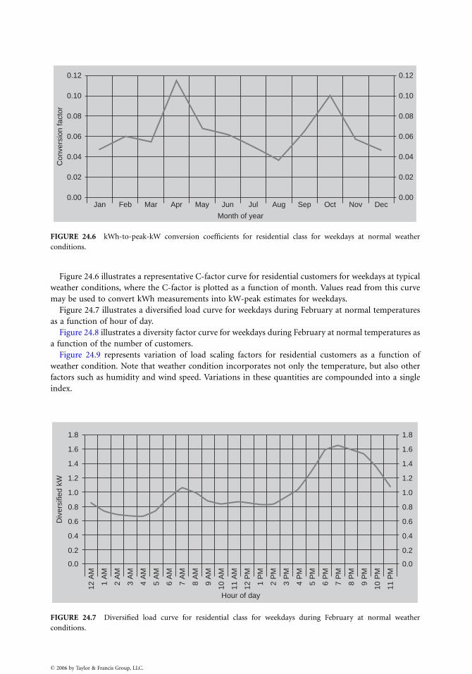
Jan Feb Mar Apr May Jun Jul
Month of year
Con
vers
ion
fact
or
Aug Sep Oct Nov Dec0.00
0.02
0.04
0.06
0.08
0.10
0.12
0.00
0.02
0.04
0.06
0.08
0.10
0.12
FIGURE 24.6 kWh-to-peak-kW conversion coefficients for residential class for weekdays at normal weather
conditions.
Figure 24.6 illustrates a representative C-factor curve for residential customers for weekdays at typical
weather conditions, where the C-factor is plotted as a function of month. Values read from this curve
may be used to convert kWh measurements into kW-peak estimates for weekdays.
Figure 24.7 illustrates a diversified load curve for weekdays during February at normal temperatures
as a function of hour of day.
Figure 24.8 illustrates a diversity factor curve for weekdays during February at normal temperatures as
a function of the number of customers.
Figure 24.9 represents variation of load scaling factors for residential customers as a function of
weather condition. Note that weather condition incorporates not only the temperature, but also other
factors such as humidity and wind speed. Variations in these quantities are compounded into a single
index.
1.8
1.6
1.4
1.2
1.0
0.8
0.6
0.4
0.2
0.0
1.8
1.6
1.4
1.2
1.0
0.8
0.6
0.4
0.2
0.0
12 A
M
1 A
M
2 A
M
3 A
M
4 A
M
5 A
M
6 A
M
7 A
M
8 A
M
9 A
M
10 A
M
11 A
M
12 P
M
1 P
M
2 P
M
3 P
M
4 P
M
5 P
M
6 P
M
7 P
M
8 P
M
9 P
M
10 P
M
11 P
M
Hour of day
Div
ersi
fied
kW
FIGURE 24.7 Diversified load curve for residential class for weekdays during February at normal weather
conditions.
� 2006 by Taylor & Francis Group, LLC.
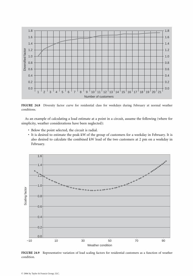
1.8
1.6
1.4
1.2
1.0
0.8
0.6
0.4
0.2
0.0
1.8
1.6
1.4
1.2
1.0
0.8
0.6
0.4
0.2
0.0
Number of customers
1 2 3 4 5 6 7 8 9 10 11 12 13 14 15 16 17 18 19 20 21
Div
ersi
fied
fact
or
FIGURE 24.8 Diversity factor curve for residential class for weekdays during February at normal weather
conditions.
As an example of calculating a load estimate at a point in a circuit, assume the following (where for
simplicity, weather considerations have been neglected):
. Below the point selected, the circuit is radial.
. It is desired to estimate the peak-kW of the group of customers for a weekday in February. It is
also desired to calculate the combined kW load of the two customers at 2 pm on a weekday in
February.
0.0
1.6
−10
Weather condition
Sca
ling
fact
or
9070503010
1.2
0.2
0.4
0.6
0.8
1.0
1.4
FIGURE 24.9 Representative variation of load scaling factors for residential customers as a function of weather
condition.
� 2006 by Taylor & Francis Group, LLC.
. There are only two customers of the same load research class, say Class R, fed from the selected
point.
Assume that each customer only has monthly kWh measurements as given by:
KWHm1(Jan18, Feb16) ¼ Measured kWh usage of first customer between the dates January 18 and
February 16.
KWHm1(Feb17, Mar17) ¼ Measured kWh usage of first customer between the dates February 17 and
March 17.
KWHm2(Jan20, Feb17) ¼ Measured kWh usage of second customer between the dates January 20
and February 17.
KWHm2(Feb18, Mar19) ¼ Measured kWh usage of second customer between the dates February 18
and March 19.
The first step is to estimate the energy usages of each customer during the month of February. Note that
the recorded measurements do not directly reflect the February usages. Parsing factors provide the
ability to estimate the February energy usage from the two measurements available.
Let p(MonX ) represent the parsing-factor value for customers of Class R for day X in month Mon.
Then using the kWh measurements given above, the estimated kWh energy use of Customer 1 during
February is calculated as follows:
KWHe1(Feb1, Feb16) ¼ KWHm1(Jan18, Feb16)xp(Feb16)� p(Feb1)
p(Feb16)� p(Jan18)
KWHe1(Feb17, Feb28) ¼ KWHm1(Feb17, Mar17)xp(Feb28)� p(Feb17)
p(Mar17)� p(Feb17)
KWHe1(Feb) ¼ KWHe1(Feb1, Feb16)þ KWHe1(Feb17, Feb28)
where KWHe1(Feb) ¼ Estimated kWh usage of Customer 1 during February.
KWHe1(Feb1, Feb16) ¼ Estimated kWh usage of Customer 1 between February 1 and
February 16.
KWHe1(Feb17, Feb28) ¼ Estimated kWh usage of Customer 1 between February 17 and
February 28.
A similar calculation can be performed to estimate the kWh usage of Customer 2 during February:
KWHe2(Feb1, Feb17) ¼ KWHm2(Jan20, Feb17)xp(Feb17)� p(Feb1)
p(Feb17)� p(Jan20)
KWHe2(Feb18, Feb28) ¼ KWHm2(Feb18, Mar19)xp(Feb28)� p(Feb18)
p(Mar19)� p(Feb18)
KWHe2(Feb) ¼ KWHe2(Feb1, Feb17)þ KWHe2(Feb18, Feb28)
The next step is to estimate the peak kW demand by the two customers together. For this, we use the
C-factors and diversity factors (d) from the load research statistics. Consider the following:
C (weekday, Feb, R) ¼ The kWh-to-peak-kW factor value for customers of Class R for weekdays
during February.
d(weekday, Feb, R, 2) ¼ The diversity-factor value for two customers of Class R for weekdays during
February.
KWpeak(Sum) ¼ Sum of the individual kW peaks (noncoincident peaks) for the two customers.
KWpeak(Group) ¼ The group peak (coincident peak) for the two customers.
� 2006 by Taylor & Francis Group, LLC.

Then,
KWpeak(Sum) ¼ C (weekday, Feb, R) � (KWHe1(Feb)þKWHe2(Feb))
KWpeak(Group) ¼ KWpeak(Sum)=d(weekday, Feb, R, 2)
This is the first answer that was sought, which is the estimated peak of the group of customers on a
weekday in February. The diversified load curve corresponding to the given conditions can be referred to
for finding the time point (hour) of day at which the peak would occur. One can examine kW demands
at any other time points, say at 2 pm, as well. The normalized diversified load curve is used for this
purpose. The normalized curve has the maximum value of unity at its peak-kW time point. To estimate
the load of the two customers at 2 pm on a weekday in February, let k(2 pm, weekday, Feb) be the
normalized diversified load curve value for customers of Class R at 2 pm for weekdays during February.
Then, the estimated load at 2 pm, KWe(Group, 2 pm, weekday, Feb) is given by
KWe(Group, 2pm, weekday, Feb) ¼ k(2pm, weekday, Feb)� KWpeak(Group)
24.3.2 Siting DGs for Improving Efficiency and Reliability
Along with voltage and power flow control, DGs can be placed within the distribution system for
simultaneously improving efficiency and reliability. That is, there are many locations within a circuit
from which a DG can implement some desired voltage or flow control, and of these many locations, the
location that results in the optimum improvement in efficiency and=or reliability can be selected.
Within a system of circuits, the circuits can be reconfigured via switching operations and DG can be
shifted from one circuit to another in order to implement some desired control. With such switching
operations, the DG does not necessarily need to be operated as an island. That is, a DG that is connected
to an unenergized circuit may be switched to an energized circuit, and then brought on line. Thus, a DG
can be placed to serve a number of circuits, and can be looked at as increasing both efficiency and
reliability for the system of circuits.
For a single circuit or a system of circuits, the DG site placement for best reliability is generally not the
same as the placement for best efficiency. Percent changes in system reliability and efficiency can be used
to determine desirable locations from a limited set of geographical locations where the DG may be
placed.
To obtain good locations for efficiency and=or reliability improvements, exhaustive searches and=or
optimization methods may be applied. The exhaustive search approach often works well because there
are generally only a very limited number of physical sites for placing DGs. This is due to constraints
placed on the siting from community impact and available land considerations.
The method that is used to site the DG should take into account the time-varying loading of the
circuits involved. Placing a DG based upon just peak loading conditions will generally not result in the
best reliability or efficiency when the entire time-varying load pattern is considered.
24.4 Hierarchical Control: Forecasting Generation
The load estimation discussed above is combined with a weather forecast and used to forecast system
loading on an hourly basis. This load forecast is used to provide a generation schedule to the ISO, and is
typically performed for the 24 hours of the next day. Forecasting the next day’s generation uses
functionality found in levels 2 and 3 of the hierarchical control shown in Fig. 24.2.
The load forecast is used to predict a schedule of must-run generation located in the distribution
system. The forecast is also used to provide the ISO with the amount of base load and load following
generation available at the distribution level. The amount of available generation is a function of the
circuit loading. DGs provide the possibility of causing the power to flow from the distribution system to
the transmission system. Since typical distribution systems are not designed to handle reverse power
flows, including reverse fault currents, IEEE 1574 recommends that DGs be operated at a generation
� 2006 by Taylor & Francis Group, LLC.

level that is 25% or less of existing circuit loading. This is taken into account when calculating the
maximum amount of generation available from the distribution system.
In the forecast, DG that is just for standby must be treated specially. The load that the standby
generation serves is what must be reported to the ISO as a capacity release, and not the capability of the
standby generation itself. Load research statistics coupled with the weather forecast are used to estimate
the hourly variation of the load that is served by the standby generation. It is this release of load estimate
that is then reported to the ISO.
References
Broadwater, R.P., Sargent, A., Yarali, A., Shaalan, H.E., and Nazarko, J., Estimating substation peaks from
load research data, IEEE Transactions on Power Delivery, 12(1), 451–456, 1997.
Daley, J.M. and Siciliano, R.L., Application of emergency and standby generation for distributed
generation. I. Concepts and hypotheses, IEEE Transactions on Industry Applications, 39(4),
1214–1225, 2003.
IEEE Std. 1547-2003, Standard for Interconnecting Distributed Resources with Electric Power Systems.
NREL SR-560-34779, Aggregation of Distributed Generation Assets in New York State, National Renewable
Energy Laboratory (NREL), Colorado, 2004.
Sargent, A., Broadwater, R.P., Thompson, J.C., and Nazarko, J., Estimation of diversity and kWHR-
to-peak-kW factors from load research data, IEEE Transactions on Power Systems, 9(3), 1450–
1456, 1994.
Westinghouse Electric Cooperation, Electric Utility Engineering Reference Book—Distribution Systems,
vol. 3, Westinghouse Electric Cooperation, East Pittsburg, PA, 1965.
� 2006 by Taylor & Francis Group, LLC.

� 2006 by Taylor & Francis Group, LLC.

V
Electric PowerUtilization Andrew HansonPowerComm Engineering25 Metering of Electric Power and Energy John V. Grubbs .............................................. 25-1
The Electromechanical Meter . Blondel’s Theorem . The Electronic
Meter . Special Metering . Instrument Transformers . Defining Terms
26 Basic Electric Power Utilization—Loads, Load Characterization and
Load Modeling Andrew Hanson ...................................................................................... 26-1
Basic Load Characterization . Composite Loads and Composite Load
Characterization . Composite Load Modeling . Other Load-Related Issues
27 Electric Power Utilization: Motors Charles A. Gross.................................................... 27-1
Some General Perspectives . Operating Modes . Motor, Enclosure,
and Controller Types . System Design
� 2006 by Taylor & Francis Group, LLC.

� 2006 by Taylor & Francis Group, LLC.
25
� 2006 by Taylor & Francis Group, LLC.
Metering of ElectricPower and Energy
John V. GrubbsAlabama Power Company
25.1 The Electromechanical Meter......................................... 25-1Single Stator Electromechanical Meter
25.2 Blondel’s Theorem........................................................... 25-2
25.3 The Electronic Meter ...................................................... 25-3Multifunction Meter . Voltage Ranging and
Multiform Meter . Site Diagnostic Meter
25.4 Special Metering .............................................................. 25-5Demand Metering . Time of Use Metering . Interval
Data Metering . Pulse Metering . Totalized Metering
25.5 Instrument Transformers.............................................. 25-10Measuring kVA
25.6 Defining Terms .............................................................. 25-11
Electrical metering deals with two basic quantities: energy and power. Energy is equivalent to work.
Power is the rate of doing work. Power applied (or consumed) for any length of time is energy. In
mathematical terms, power integrated over time is energy. The basic electrical unit of energy is the
watthour. The basic unit of power is the watt. The watthour meter measures energy (in watthours),
while the wattmeter measures the rate of energy, power (in watthours per hour or simply watts). For a
constant power level, power multiplied by time is energy. For example, a watthour meter connected for
two hours in a circuit using 500 watts (500 watthours per hour) will register 1000 watthours.
25.1 The Electromechanical Meter
The electromechanical watthour meter is basically a very specialized electric motor, consisting of
. A stator and a rotor that together produce torque
. A brake that creates a counter torque
. A register to count and display the revolutions of the rotor
25.1.1 Single Stator Electromechanical Meter
A two-wire single stator meter is the simplest electromechanical meter. The single stator consists of two
electromagnets. One electromagnet is the potential coil connected between the two circuit conductors.
The other electromagnet is the current coil connected in series with the load current. Figure 25.1 shows
the major components of a single stator meter.
The electromagnetic fields of the current coil and the potential coil interact to generate torque on the
rotor of the meter. This torque is proportional to the product of the source voltage, the line current, and
the cosine of the phase angle between the two. Thus, the torque is also proportional to the power in the
metered circuit.
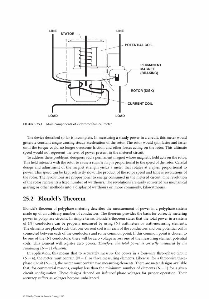
LINESTATOR
LINE
LOAD LOAD
POTENTIAL COIL
PERMANENTMAGNET(BRAKING)
ROTOR (DISK)
CURRENT COIL
FIGURE 25.1 Main components of electromechanical meter.
The device described so far is incomplete. In measuring a steady power in a circuit, this meter would
generate constant torque causing steady acceleration of the rotor. The rotor would spin faster and faster
until the torque could no longer overcome friction and other forces acting on the rotor. This ultimate
speed would not represent the level of power present in the metered circuit.
To address these problems, designers add a permanent magnet whose magnetic field acts on the rotor.
This field interacts with the rotor to cause a counter torque proportional to the speed of the rotor. Careful
design and adjustment of the magnet strength yields a meter that rotates at a speed proportional to
power. This speed can be kept relatively slow. The product of the rotor speed and time is revolutions of
the rotor. The revolutions are proportional to energy consumed in the metered circuit. One revolution
of the rotor represents a fixed number of watthours. The revolutions are easily converted via mechanical
gearing or other methods into a display of watthours or, more commonly, kilowatthours.
25.2 Blondel’s Theorem
Blondel’s theorem of polyphase metering describes the measurement of power in a polyphase system
made up of an arbitrary number of conductors. The theorem provides the basis for correctly metering
power in polyphase circuits. In simple terms, Blondel’s theorem states that the total power in a system
of (N) conductors can be properly measured by using (N) wattmeters or watt-measuring elements.
The elements are placed such that one current coil is in each of the conductors and one potential coil is
connected between each of the conductors and some common point. If this common point is chosen to
be one of the (N) conductors, there will be zero voltage across one of the measuring element potential
coils. This element will register zero power. Therefore, the total power is correctly measured by the
remaining (N� 1) elements.
In application, this means that to accurately measure the power in a four-wire three-phase circuit
(N¼ 4), the meter must contain (N� 1) or three measuring elements. Likewise, for a three-wire three-
phase circuit (N¼ 3), the meter must contain two measuring elements. There are meter designs available
that, for commercial reasons, employ less than the minimum number of elements (N� 1) for a given
circuit configuration. These designs depend on balanced phase voltages for proper operation. Their
accuracy suffers as voltages become unbalanced.
� 2006 by Taylor & Francis Group, LLC.
25.3 The Electronic Meter
Since the 1980s, meters available for common use have evolved from (1) electromechanical mechanisms
driving mechanical, geared registers to (2) the same electromechanical devices driving electronic
registers to (3) totally electronic (or solid state) designs. All three types remain in wide use, but the
type that is growing in use is the solid state meter.
The addition of the electronic register to an electromechanical meter provides a digital display of
energy and demand. It supports enhanced capabilities and eliminates some of the mechanical complex-
ity inherent in the geared mechanical registers.
Electronic meters contain no moving mechanical parts—rotors, shafts, gears, bearings. They are built
instead around large-scale integrated circuits, other solid state components, and digital logic. Such
meters are much more closely related to computers than to electromechanical meters.
The operation of an electronic meter is very different than that described in earlier sections for an
electromechanical meter. Electronic circuitry samples the voltage and current waveforms during each
electrical cycle and converts these samples to digital quantities. Other circuitry then manipulates these
values to determine numerous electrical parameters, such as kW, kWh, kvar, kvarh, kQ, kQh, power
factor, kVA, rms current, rms voltage.
Various electronic meter designs also offer some or all of the following capabilities:
. Time of use (TOU). The meter keeps up with energy and demand in multiple daily periods. (See
section on Time of Use Metering.). Bi-directional. The meter measures (as separate quantities) energy delivered to and received from
a customer. This feature is used for a customer that is capable of generating electricity and feeding
it back into the utility system.. Loss compensation. The meter can be programmed to automatically calculate watt and var losses
in transformers and electrical conductors based on defined or tested loss characteristics of the
transformers and conductors. It can internally add or subtract these calculated values from its
measured energy and demand. This feature permits metering to be installed at the most
economical location. For instance, we can install metering on the secondary (e.g., 4 kV) side of
a customer substation, even when the contractual service point is on the primary (e.g., 110 kV)
side. The 4 kV metering installation is much less expensive than a corresponding one at 110 kV.
Under this situation, the meter compensates its secondary-side energy and demand readings to
simulate primary-side readings.. Interval data recording. The meter contains solid state memory in which it can record up to
several months of interval-by-interval data. (See section on Interval Data Metering.). Remote communications. Built-in communications capabilities permit the meter to be interro-
gated remotely via telephone, radio, or other communications media.. Diagnostics. The meter checks for the proper voltages, currents, and phase angles on the meter
conductors. (See section on Site Diagnostic Meter.). Power quality. The meter can measure and report on momentary voltage or current variations
and on harmonic conditions.
Note that many of these features are available only in the more advanced (and expensive) models of
electronic meters.
As an example of the benefits offered by electronic meters, consider the following two methods of
metering a large customer who is capable of generating and feeding electricity back to the utility. In this
example, the metering package must perform these functions:
Measure kWh delivered to the customer
Measure kWh received from the customer
Measure kvarh delivered
Measure kvarh received
� 2006 by Taylor & Francis Group, LLC.

Measure kW delivered
Measure kW received
Compensate received quantities for transformer losses
Record the measured quantities for each demand interval
Method A. (2) kW=kWh electromechanical meters with pulse generators (one for delivered, one
for received)
(2) kWh electromechanical meters with pulse generators (to measure kvarh)
(2) Phase shifting transformers (used along with the kWh meters to measure kvarh)
(2) Transformer loss compensators
(1) Pulse data recorder
Method B. (1) Electronic meter
Obviously, the electronic installation is much simpler. In addition, it is less expensive to purchase and
install and is easier to maintain.
Benefits common to most solid state designs are high accuracy and stability. Another less obvious
advantage is in the area of error detection. When an electromechanical meter develops a serious
problem, it may produce readings in error by any arbitrary amount. An error of 10%, 20%, or even
30% can go undetected for years, resulting in very large over- or under-billings. However, when an
electronic meter develops a problem, it is more likely to produce an obviously bad reading (e.g., all
zeroes; all 9s; a demand 100 times larger than normal; or a blank display). This greatly increases the
likelihood that the error will be noticed and reported soon after it occurs. The sooner such a problem is
recognized and corrected, the less inconvenience and disruption it causes to the utility and to the
customer.
25.3.1 Multifunction Meter
Multifunction or extended function refers to a meter that can measure reactive or apparent power (e.g.,
kvar or kVA) in addition to real power (kW). By virtue of their designs, many electronic meters
inherently measure the quantities and relationships that define reactive and apparent power. It is a
relatively simple step for designers to add meter intelligence to calculate and display these values.
25.3.2 Voltage Ranging and Multiform Meter
Electronic meter designs have introduced many new features to the watthour metering world. Two
features, typically found together, offer additional flexibility, simplified application, and opportunities
for reduced meter inventories for utilities.
. Voltage ranging – Many electronic meters incorporate circuitry that can sense the voltage level
of the meter input signals and adjust automatically to meter correctly over a wide range of
voltages. For example, a meter with this capability can be installed on either a 120 volt or 277 volt
service.. Multiform – Meter form refers to the specific combination of voltage and current signals, how
they are applied to the terminals of the meter, and how the meter uses these signals to measure
power and energy. For example, a Form 15 meter would be used for self-contained application on
a 120=240 volt 4-wire delta service, while a Form 16 meter would be used on a self-contained
120=208 volt 4-wire wye service. A multiform 15=16 meter can work interchangeably on either of
these services.
25.3.3 Site Diagnostic Meter
Newer meter designs incorporate the ability to measure, display, and evaluate the voltage and current
magnitudes and phase relationships of the circuits to which they are attached. This capability offers
important advantages:
� 2006 by Taylor & Francis Group, LLC.
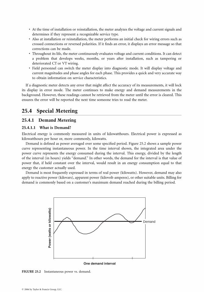
. At the time of installation or reinstallation, the meter analyzes the voltage and current signals and
determines if they represent a recognizable service type.. Also at installation or reinstallation, the meter performs an initial check for wiring errors such as
crossed connections or reversed polarities. If it finds an error, it displays an error message so that
corrections can be made.. Throughout its life, the meter continuously evaluates voltage and current conditions. It can detect
a problem that develops weeks, months, or years after installation, such as tampering or
deteriorated CT or VT wiring.. Field personnel can switch the meter display into diagnostic mode. It will display voltage and
current magnitudes and phase angles for each phase. This provides a quick and very accurate way
to obtain information on service characteristics.
If a diagnostic meter detects any error that might affect the accuracy of its measurements, it will lock
its display in error mode. The meter continues to make energy and demand measurements in the
background. However, these readings cannot be retrieved from the meter until the error is cleared. This
ensures the error will be reported the next time someone tries to read the meter.
25.4 Special Metering
25.4.1 Demand Metering
25.4.1.1 What is Demand?
Electrical energy is commonly measured in units of kilowatthours. Electrical power is expressed as
kilowatthours per hour or, more commonly, kilowatts.
Demand is defined as power averaged over some specified period. Figure 25.2 shows a sample power
curve representing instantaneous power. In the time interval shown, the integrated area under the
power curve represents the energy consumed during the interval. This energy, divided by the length
of the interval (in hours) yields ‘‘demand.’’ In other words, the demand for the interval is that value of
power that, if held constant over the interval, would result in an energy consumption equal to that
energy the customer actually used.
Demand is most frequently expressed in terms of real power (kilowatts). However, demand may also
apply to reactive power (kilovars), apparent power (kilovolt-amperes), or other suitable units. Billing for
demand is commonly based on a customer’s maximum demand reached during the billing period.
Po
wer
(w
atts
or
kilo
wat
ts)
One demand interval
Demand
FIGURE 25.2 Instantaneous power vs. demand.
� 2006 by Taylor & Francis Group, LLC.
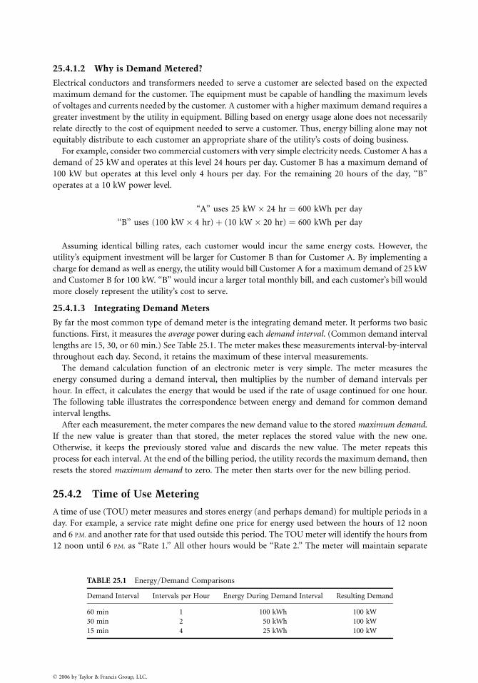
25.4.1.2 Why is Demand Metered?
Electrical conductors and transformers needed to serve a customer are selected based on the expected
maximum demand for the customer. The equipment must be capable of handling the maximum levels
of voltages and currents needed by the customer. A customer with a higher maximum demand requires a
greater investment by the utility in equipment. Billing based on energy usage alone does not necessarily
relate directly to the cost of equipment needed to serve a customer. Thus, energy billing alone may not
equitably distribute to each customer an appropriate share of the utility’s costs of doing business.
For example, consider two commercial customers with very simple electricity needs. Customer A has a
demand of 25 kW and operates at this level 24 hours per day. Customer B has a maximum demand of
100 kW but operates at this level only 4 hours per day. For the remaining 20 hours of the day, ‘‘B’’
operates at a 10 kW power level.
‘‘A’’ uses 25 kW� 24 hr ¼ 600 kWh per day
‘‘B’’ uses (100 kW� 4 hr)þ (10 kW� 20 hr) ¼ 600 kWh per day
Assuming identical billing rates, each customer would incur the same energy costs. However, the
utility’s equipment investment will be larger for Customer B than for Customer A. By implementing a
charge for demand as well as energy, the utility would bill Customer A for a maximum demand of 25 kW
and Customer B for 100 kW. ‘‘B’’ would incur a larger total monthly bill, and each customer’s bill would
more closely represent the utility’s cost to serve.
25.4.1.3 Integrating Demand Meters
By far the most common type of demand meter is the integrating demand meter. It performs two basic
functions. First, it measures the average power during each demand interval. (Common demand interval
lengths are 15, 30, or 60 min.) See Table 25.1. The meter makes these measurements interval-by-interval
throughout each day. Second, it retains the maximum of these interval measurements.
The demand calculation function of an electronic meter is very simple. The meter measures the
energy consumed during a demand interval, then multiplies by the number of demand intervals per
hour. In effect, it calculates the energy that would be used if the rate of usage continued for one hour.
The following table illustrates the correspondence between energy and demand for common demand
interval lengths.
After each measurement, the meter compares the new demand value to the stored maximum demand.
If the new value is greater than that stored, the meter replaces the stored value with the new one.
Otherwise, it keeps the previously stored value and discards the new value. The meter repeats this
process for each interval. At the end of the billing period, the utility records the maximum demand, then
resets the stored maximum demand to zero. The meter then starts over for the new billing period.
25.4.2 Time of Use Metering
A time of use (TOU) meter measures and stores energy (and perhaps demand) for multiple periods in a
day. For example, a service rate might define one price for energy used between the hours of 12 noon
and 6 P.M. and another rate for that used outside this period. The TOU meter will identify the hours from
12 noon until 6 P.M. as ‘‘Rate 1.’’ All other hours would be ‘‘Rate 2.’’ The meter will maintain separate
TABLE 25.1 Energy=Demand Comparisons
Demand Interval Intervals per Hour Energy During Demand Interval Resulting Demand
60 min 1 100 kWh 100 kW
30 min 2 50 kWh 100 kW
15 min 4 25 kWh 100 kW
� 2006 by Taylor & Francis Group, LLC.
measurements of Rate 1 energy (and demand) and Rate 2 energy (and demand) for the entire
billing period. Actual TOU service rates can be much more complex than this example, including
features such as
. more than two periods per day,
. different periods for weekends and holidays, and
. different periods for different seasons of the year.
A TOU meter depends on an internal clock=calendar for proper operation. It includes battery backup
to maintain its clock time during power outages.
25.4.3 Interval Data Metering
The standard method of gathering billing data from a meter is quite simple. The utility reads the meter
at the beginning of the billing period and again at the end of the billing period. From these readings, it
determines the energy and maximum demand for that period. This information is adequate to
determine the bills for the great majority of customers. However, with the development of more complex
service rates and the need to study customer usage patterns, the utility sometimes wants more detail
about how a customer uses electricity. One option would be to read the meter daily. That would allow
the utility to develop a day-by-day pattern of the customer’s usage. However, having someone visit the
meter site every day would quickly become very expensive. What if the meter could record usage data
every day? The utility would have more detailed usage data, but would only have to visit the meter when
it needed the data, for instance, once per month. And if the meter is smart enough to do that, why not
have it record data even more often, for instance every hour?
In very simple terms, this is what interval data metering does. The interval meter includes sufficient
circuitry and intelligence to record usage multiple times per hour. The length of the recording interval is
programmable, often over a range from 1 to 60 minutes. The meter includes sufficient solid state
memory to accumulate these interval readings for a minimum of 30 days at 15-minute intervals.
Obviously, more frequent recording times reduce the days of storage available.
A simple kWh=kW recording meter typically records one set of data representing kWh. This provides
the detailed usage patterns that allow the utility to analyze and evaluate customer ‘‘load profiles’’ based
on daily, weekly, monthly, or annual bases. An extended function meter is commonly programmed to
record two channels of data, e.g., kWh and kvarh. This provides the additional capability of analyzing
customers’ power factor patterns over the same periods. Though the meter records information in
energy units (kWh or kvarh), it is a simple matter to convert this data to equivalent demand (kW or
kvar). Since demand represents energy per unit time, simply divide the energy value for one recorder
interval by the length of the interval (in hours). If the meter records 16.4 kWh in a 30-minute period, the
equivalent demand for that period is 16.4 kWh=(0.5 hours)¼ 32.8 kW.
A sample 15-minute interval load shape for a 24-hour period is shown in the graph in Fig. 25.3. The
minimum demand for that period was 10.5 kW, occurring during the interval ending at 04:30.
The maximum demand was 28.7 kW, occurring during the interval ending at 15:15, or 3:15 P.M.
25.4.4 Pulse Metering
Metering pulses are signals generated in a meter for use outside the meter. Each pulse represents a
discrete quantity of the metered value, such as kWh, kVAh, or kvarh. The device receiving the pulses
determines the energy or demand at the meter by counting the number of pulses occurring in some time
interval. A pulse is indicated by the transition (e.g., open to closed) of the circuit at the meter end. Pulses
are commonly transmitted on small conductor wire circuits. Common uses of pulses include providing
signals to
. customer’s demand indicator
. customer’s energy management system
� 2006 by Taylor & Francis Group, LLC.
35
30
25
20KW
15
10
5
0
min
max
00:0
001
:1502
:3003
:4505
:0006
:1507
:3008
:4510
:0011
:1512
:3013
:4515
:0016
:1517
:3018
:4520
:0021
:1522
:3023
:45
FIGURE 25.3 Graph of interval data.
. a totalizer (see section on Totalized Metering)
. a metering data recorder
. a telemetering device that converts the pulses to other signal forms (e.g., telephone line tones or
optical signals) for transmission over long distances
Pulse metering is installed when customer service requirements, equipment configurations, or other
special requirements exceed the capability of conventional metering. Pulse metering is also used to
transmit metered data to a remote location.
25.4.4.1 Recording Pulses
A meter pulse represents a quantity of energy, not power. For example, a pulse is properly expressed in
terms of watthours (or kWh) rather than watts (or kW). A pulse recorder will associate time with pulses
as it records them. If set up for a 15-minute recording interval, the recorder counts pulses for 15 min,
then records that number of pulses. It then counts pulses for the next 15 min, records that number, and
so on, interval after interval, day after day. It is a simple matter to determine the number of pulses
recorded in a chosen length of time. Since the number of pulses recorded represents a certain amount of
energy, simply divide this energy by the corresponding length of time (in hours) to determine average
power for that period.
Example: For a metering installation, we are given that each pulse represents 2400 watthours or
2.4 kWh. In a 15-minute period, we record 210 pulses. What is the corresponding energy (kWh) and
demand (kW) during this 15-minute interval?
Total energy in interval ¼ 2:4 kWh per pulse� 210 pulses
¼ 504 kWh
Demand ¼ Energy=Time ¼ 504 kWh=0:25 hour
¼ 2016 kW
Often, a customer asks for the demand value of a pulse, rather than the energy value. The demand
value is dependent on demand interval length. The demand pulse value is equal to the energy pulse value
divided by the interval length in hours.
For the previous example, the kW pulse value would be:
2:4 kWh per pulse=0:25 hours ¼ 9:6 kW per pulse
� 2006 by Taylor & Francis Group, LLC.

Form A
Form C
FIGURE 25.4 Pulse circuits.
� 2006 by Taylor & Francis Group, LLC.
and the resulting demand calculation is:
Demand ¼ 9:6 kW per pulse� 210 pulses
¼ 2016kW
Remember, however, that a pulse demand value is meaningful
only for a specific demand interval. In the example above, count-
ing pulses for any period other than 15 minutes and then apply-
ing the kW pulse value will yield incorrect results for demand.
25.4.4.2 Pulse Circuits
Pulse circuits commonly take two forms (Fig. 25.4):
. Form A, a two-wire circuit where a switch toggles between closed and open. Each transition of the
circuit (to open or to closed) represents one pulse.. Form C, a three-wire circuit where the switch flip-flops. Each transition (from closed on one side
to closed on the other) represents one pulse.
Use care in interpreting pulse values for these circuits. The value will normally be expressed per
transition. With Form C circuits, a transition is a change from closed on the first side to closed on the
second side. Most receiving equipment interprets this properly. However, with Form A circuits, the
transition is defined as a change from open to closed or from closed to open. An initially open Form A
circuit that closes, then opens has undergone two (2) transitions. If the receiving equipment counts only
circuit closures, it will record only half of the actual transitions. This is not a problem if the applicable
pulse value of the Form A circuit is doubled from the rated pulse weight per transition. For example, if
the value of a Form A meter pulse is 3.2 kWh per transition, the value needed for a piece of equipment
that only counted circuit closures would be 3.2� 2¼ 6.4 kWh per pulse.
25.4.5 Totalized Metering
Totalized metering refers to the practice of combining data to make multiple service points look as if
they were measured by a single meter. This is done by combining two or more sets of data from separate
meters to generate data equivalent to what would be produced by a single ‘‘virtual meter’’ that measured
the total load. This combination can be accomplished by:
. Adding recorded interval data from multiple meters, usually on a computer
. Adding (usually on-site) meter pulses from multiple meters by a special piece of metering
equipment known as a totalizer. Paralleling the secondaries of current transformers located in multiple circuits and feeding the
combined current into a conventional meter (this works only when the service voltages and ratios
of the current transformers are identical). Using a multi-circuit meter, which accepts the voltage and current inputs from multiple services
Totalized demand is the sum of the coincident demands and is usually less than the sum of the
individual peak demands registered by the individual meters. Totalized energy equals the sum of
the energies measured by the individual meters.
Table 25.2 illustrates the effects of totalizing a customer served by three delivery (and metering)
points. It presents the customer’s demands over a period of four demand intervals and illustrates the
difference in the maximum totalized demand compared to the sum of the individual meter maximum
demands.
The peak kW demand for each meter point is shown in bold. The sum of these demands is 2240 kW.
However, when summed interval-by-interval, the peak of the sums is 2180 kW. This is the totalized
demand. The difference in the two demands, 60 kW, represents a cost savings to the customer. It should
be clear why many customers with multiple service points desire to have their demands totalized.
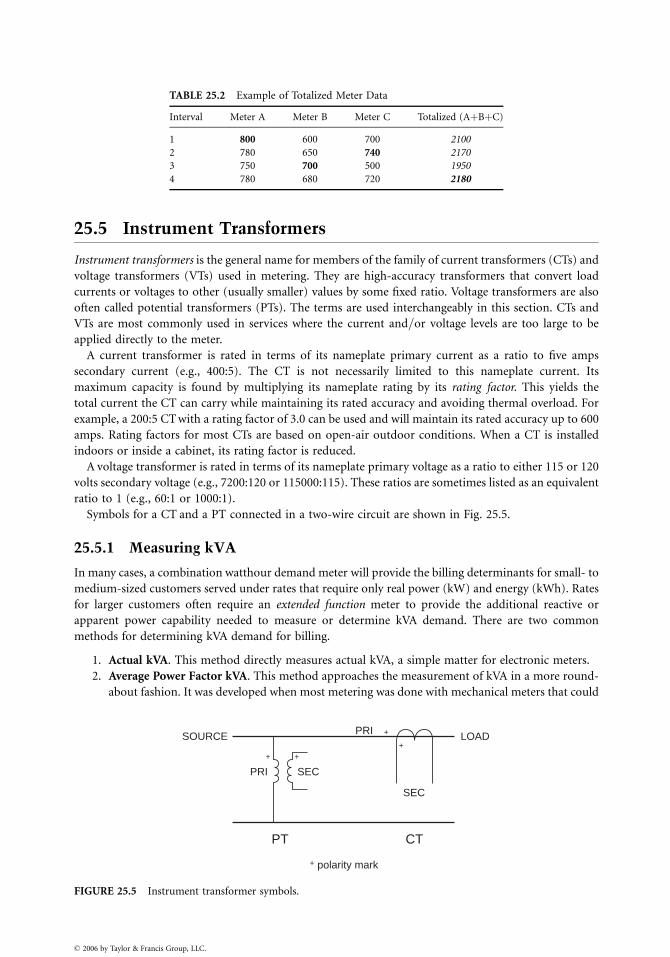
TABLE 25.2 Example of Totalized Meter Data
Interval Meter A Meter B Meter C Totalized (AþBþC)
1 800 600 700 2100
2 780 650 740 2170
3 750 700 500 1950
4 780 680 720 2180
25.5 Instrument Transformers
Instrument transformers is the general name for members of the family of current transformers (CTs) and
voltage transformers (VTs) used in metering. They are high-accuracy transformers that convert load
currents or voltages to other (usually smaller) values by some fixed ratio. Voltage transformers are also
often called potential transformers (PTs). The terms are used interchangeably in this section. CTs and
VTs are most commonly used in services where the current and=or voltage levels are too large to be
applied directly to the meter.
A current transformer is rated in terms of its nameplate primary current as a ratio to five amps
secondary current (e.g., 400:5). The CT is not necessarily limited to this nameplate current. Its
maximum capacity is found by multiplying its nameplate rating by its rating factor. This yields the
total current the CT can carry while maintaining its rated accuracy and avoiding thermal overload. For
example, a 200:5 CT with a rating factor of 3.0 can be used and will maintain its rated accuracy up to 600
amps. Rating factors for most CTs are based on open-air outdoor conditions. When a CT is installed
indoors or inside a cabinet, its rating factor is reduced.
A voltage transformer is rated in terms of its nameplate primary voltage as a ratio to either 115 or 120
volts secondary voltage (e.g., 7200:120 or 115000:115). These ratios are sometimes listed as an equivalent
ratio to 1 (e.g., 60:1 or 1000:1).
Symbols for a CT and a PT connected in a two-wire circuit are shown in Fig. 25.5.
25.5.1 Measuring kVA
In many cases, a combination watthour demand meter will provide the billing determinants for small- to
medium-sized customers served under rates that require only real power (kW) and energy (kWh). Rates
for larger customers often require an extended function meter to provide the additional reactive or
apparent power capability needed to measure or determine kVA demand. There are two common
methods for determining kVA demand for billing.
1. Actual kVA. This method directly measures actual kVA, a simple matter for electronic meters.
2. Average Power Factor kVA. This method approaches the measurement of kVA in a more round-
about fashion. It was developed when most metering was done with mechanical meters that could
SOURCE LOADPRI
PT CT
+ polarity mark
PRI
SEC
SEC
++
+
+
FIGURE 25.5 Instrument transformer symbols.
� 2006 by Taylor & Francis Group, LLC.
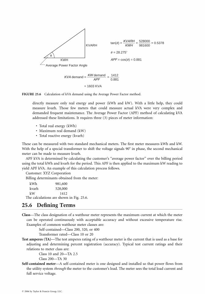
θKWH
KVARH
Average Power Factor Angle
KWHKVARHtan(q ) =
q = 28.275�
APF = cos(q ) = 0.881
= 981600528000 = 0.5378
APFKW demandKVA demand =
= 1603 KVA
= 0.8811412
FIGURE 25.6 Calculation of kVA demand using the Average Power Factor method.
directly measure only real energy and power (kWh and kW). With a little help, they could
measure kvarh. Those few meters that could measure actual kVA were very complex and
demanded frequent maintenance. The Average Power Factor (APF) method of calculating kVA
addressed these limitations. It requires three (3) pieces of meter information:
. Total real energy (kWh)
. Maximum real demand (kW)
. Total reactive energy (kvarh)
These can be measured with two standard mechanical meters. The first meter measures kWh and kW.
With the help of a special transformer to shift the voltage signals 908 in phase, the second mechanical
meter can be made to measure kvarh.
APF kVA is determined by calculating the customer’s ‘‘average power factor’’ over the billing period
using the total kWh and kvarh for the period. This APF is then applied to the maximum kW reading to
yield APF kVA. An example of this calculation process follows.
Customer: XYZ Corporation
Billing determinants obtained from the meter:
kWh 981,600
kvarh 528,000
kW 1412The calculations are shown in Fig. 25.6.
25.6 Defining Terms
Class—The class designation of a watthour meter represents the maximum current at which the meter
can be operated continuously with acceptable accuracy and without excessive temperature rise.
Examples of common watthour meter classes are:
Self-contained—Class 200, 320, or 400
Transformer rated—Class 10 or 20
Test amperes (TA)—The test amperes rating of a watthour meter is the current that is used as a base for
adjusting and determining percent registration (accuracy). Typical test current ratings and their
relations to meter class are:
Class 10 and 20—TA 2.5
Class 200—TA 30
Self-contained meter—A self-contained meter is one designed and installed so that power flows from
the utility system through the meter to the customer’s load. The meter sees the total load current and
full service voltage.
� 2006 by Taylor & Francis Group, LLC.
Transformer rated meter—A transformer rated meter is one designed to accept reduced levels of current
and=or voltage that are directly proportional to the service current and voltage. The primary
windings of current transformers and=or voltage transformers are placed in the customer’s service
and see the total load current and full service voltage. The transformer rated meter connects into the
secondary windings of these transformers.
Meter element—A meter element is the basic energy and power measurement circuit for one set of
meter input signals. It consists of a current measurement device and a voltage measurement device
for one phase of the meter inputs. Usually, a meter will have one less element than the number of
wires in the circuit being metered. That is, a 4-wire wye or delta circuit will be metered by a 3-element
meter; a 3-wire delta circuit will be metered by a 2-element meter, although there are numerous
exceptions.
CT PT ratio—A number or factor obtained by multiplying the current transformer ratio by the potential
transformer ratio. Example: If a meter is connected to 7200:120 volt PTs (60:1) and 600:5 CTs (120:1),
the CT PT ratio is 60� 120¼ 7200. A metering installation may have current transformers but no
potential transformer in which case the CT PT ratio is just the CT ratio.
Meter multiplier—Also called the dial constant or kilowatthour constant, this is the multiplier used to
convert meter kWh readings to actual kWh. The meter multiplier is the CT PT ratio. For a self-
contained meter, this constant is 1.
Further Information
Further information and more detail on many of the topics related to metering can be found in the
Handbook for Electricity Metering, published by Edison Electric Institute. This authoritative book
provides extensive explanations of many aspects of metering, from fundamentals of how meters and
instrument transformers operate, to meter testing, wiring, and installation.
� 2006 by Taylor & Francis Group, LLC.
26
� 2006 by Taylor & Francis Group, LLC.
Basic Electric PowerUtilization—Loads,
Load Characterizationand Load Modeling
Andrew HansonPowerComm Engineering
26.1 Basic Load Characterization........................................... 26-1
26.2 Composite Loads and Composite LoadCharacterization .............................................................. 26-2Coincidence and Diversity . Load Curves and Load Duration
26.3 Composite Load Modeling............................................. 26-4
26.4 Other Load-Related Issues.............................................. 26-6Cold Load Pickup . Harmonics and Other
Nonsinusoidal Loads
Utilization is the ‘‘end result’’ of the generation, transmission, and distribution of electric power. The
energy carried by the transmission and distribution system is turned into useful work, light, heat, or a
combination of these items at the utilization point. Understanding and characterizing the utilization of
electric power is critical for proper planning and operation of power systems. Improper characterization
of utilization can result of over or under building of power system facilities and stressing of system
equipment beyond design capabilities. This chapter describes some of the basic concepts used to
characterize and model loads in electric power systems.
The term load refers to a device or collection of devices that draw energy from the power system.
Individual loads (devices) range from small light bulbs to large induction motors to arc furnaces. The
term load is often somewhat arbitrarily applied, at times being used to describe a specific device, and
other times referring to an entire facility and even being used to describe the lumped power require-
ments of power system components and connected utilization devices downstream of a specific point in
large-scale system studies.
26.1 Basic Load Characterization
A number of terms are used to characterize the magnitude and intensity of loads. Several such terms are
defined and uses outlined below.
Energy—Energy use (over a specified period of time) is a key identifying parameter for power system
loads. Energy use is often recorded for various portions of the power system (e.g., homes, businesses,
feeders, substations, districts). Utilities report aggregate system energy use over a variety of time frames
(daily, weekly, monthly, and annually). System energy use is tied directly to sales and thus is often used
as a measure of the utility or system performance from one period to another.

Demand—Loads require specific amounts of energy over short periods of time. Demand is a measure
of this energy and is expressed in terms of power (kilowatts or Megawatts). Instantaneous demand is the
peak instantaneous power use of a device, facility, or system. Demand, as commonly referred to in utility
discussions, is an integrated demand value, most often integrated over 10, 15, or 30 min. Integrated
demand values are determined by dividing the energy used by the time interval of measurement or
the demand interval.
Demand ¼ Energy Use Over Demand Interval
Demand Interval(26:1)
Integrated demand values can be much lower than peak instantaneous demand values for a load
or facility.
Demand Factor—Demand factor is a ratio of the maximum demand to the total connected load of a
system or the part of the system under consideration. Demand factor is often used to express the
expected diversity of individual loads within a facility prior to construction. Use of demand factors
allows facility power system equipment to be sized appropriately for the expected loads.
Demand Factor ¼ Maximum Demand
Total Connected Load(26:2)
Load Factor—Load factor is similar to demand factor and is calculated from the energy use, the
demand, and the period of time associated with the measurement.
Load Factor ¼ Energy Use
Demand� Time(26:3)
A high load factor is typically desirable, indicating that a load or group of loads operates near its peak
most of the time, allowing the greatest benefit to be derived from any facilities installed to serve the load.
26.2 Composite Loads and Composite Load Characterization
It is impractical to model each individual load connected to a power system to the level of detail at which
power is delivered to each individual utilization device. Loads are normally lumped together to represent
all of the ‘‘downstream’’ power system components and individual connected loads. This grouping
occurs as a result of metering all downstream power use from a certain point in the power system, or as a
result of model simplification in which effects of the downstream power system and connected loads are
represented by a single load in system analysis.
26.2.1 Coincidence and Diversity
Although individual loads vary unpredictably from hour to hour and minute to minute, an averaging
effect occurs as many loads are examined in aggregate. This effect begins at individual facilities (home,
commercial establishment, or industrial establishment) where all devices are seldom if ever in operation
at the same instant. Progressing from an individual facility to the distribution and transmission systems,
the effect is compounded, resulting in somewhat predictable load characteristics.
Diversity is a measure of the dispersion of the individual loads of a system under observation over
time. Diversity is generally low in individual commercial and industrial installations. However, at a
feeder level, diversity is a significant factor, allowing more economical choices for equipment since the
feeder needs to supply power to the aggregate peak load of the connected customers, not the sum of the
customer individual (noncoincident) peak loads.
� 2006 by Taylor & Francis Group, LLC.

Groups of customers of the same class (i.e., residential, commercial, industrial) tend to have an
aggregate peak load per customer that decreases as the number of customers increases. This tendency is
termed coincidence and has significant impact on the planning and construction of power systems
(Willis, 1997). For example, load diversity would allow a feeder or substation to serve a number of
customers whose individual (noncoincident) peak demands may exceed the feeder or substation rating
by a factor of two or more.
Coincidence Factor ¼ Aggregate Demand for a Group of Customers
Sum of Individual Customer Demands(26:4)
Note that there is a minor but significant difference between coincidence (and its representation as a
coincidence factor) and the demand factor discussed above. The coincidence factor is based on
the observed peak demand for individuals and groups, whereas the demand factor is based on the
connected load.
26.2.2 Load Curves and Load Duration
Load curves and load duration curves graphically convey very detailed information about the character-
istics of loads over time. Load curves typically display the load of a customer class, feeder, or other
portion of a power system over a 24-hour period. Load duration curves display the cumulative amount
of time that load levels are experienced over a period of time.
Load curves represent the demand of a load or groups of load over a period of time, typically 24
hours. The curves provide ‘‘typical’’ load levels for a customer class on an hour-by-hour or minute-by-
minute basis. The curves themselves represent the demand of a certain class of customers or portion of
the system. The area under the curve represents the corresponding energy use over the time period
under consideration. Load curves provide easily interpreted information regarding the peak load
duration as well as the variation between minimum and maximum load levels. Load curves provide
key information for daily load forecasts allowing planners and operators to ensure system capacity is
available to meet customer needs. Three sample load curves (for residential, commercial, and industrial
customer classes) are shown in Figs. 26.1 through 26.3.
Load curves can also be developed on a feeder or substation basis, as a composite representation of the
load profile of a portion of the system.
Load duration curves quickly convey the duration of the peak period for a portion of a power system
over a given period of time. Load duration curves plot the cumulative amount of time that load levels are
0
0
20
40
60
80 Residential
Per
cen
t P
eak
Lo
ad
100
3 6 9 12
Hour
15 18 21 24
FIGURE 26.1 Residential load curve.
� 2006 by Taylor & Francis Group, LLC.
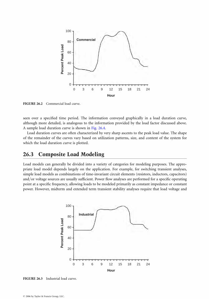
0
0
20
40
60
80
100
3 6 9 12
Hour
Commercial
Per
cen
t P
eak
Lo
ad
15 18 21 24
FIGURE 26.2 Commercial load curve.
seen over a specified time period. The information conveyed graphically in a load duration curve,
although more detailed, is analogous to the information provided by the load factor discussed above.
A sample load duration curve is shown in Fig. 26.4.
Load duration curves are often characterized by very sharp ascents to the peak load value. The shape
of the remainder of the curves vary based on utilization patterns, size, and content of the system for
which the load duration curve is plotted.
26.3 Composite Load Modeling
Load models can generally be divided into a variety of categories for modeling purposes. The appro-
priate load model depends largely on the application. For example, for switching transient analyses,
simple load models as combinations of time-invariant circuit elements (resistors, inductors, capacitors)
and=or voltage sources are usually sufficient. Power flow analyses are performed for a specific operating
point at a specific frequency, allowing loads to be modeled primarily as constant impedance or constant
power. However, midterm and extended term transient stability analyses require that load voltage and
0 3 6 9 12
Hour
15 18 21 240
20
40
60
80
100
Per
cen
t P
eak
Lo
ad
Industrial
FIGURE 26.3 Industrial load curve.
� 2006 by Taylor & Francis Group, LLC.
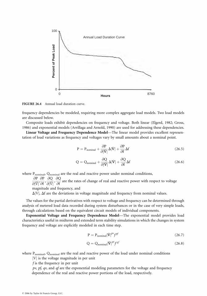
0 8760Hours
0
100
Annual Load Duration Curve
Per
cen
t o
f P
eak
Lo
ad
FIGURE 26.4 Annual load duration curve.
frequency dependencies be modeled, requiring more complex aggregate load models. Two load models
are discussed below.
Composite loads exhibit dependencies on frequency and voltage. Both linear (Elgerd, 1982; Gross,
1986) and exponential models (Arrillaga and Arnold, 1990) are used for addressing these dependencies.
Linear Voltage and Frequency Dependence Model—The linear model provides excellent represen-
tation of load variations as frequency and voltages vary by small amounts about a nominal point.
P ¼ Pnominal þ@P
@ �VVj jD�VVj j þ @P
@fDf (26:5)
Q ¼ Qnominal þ@Q
@ �VVj jD�VVj j þ @Q
@fDf (26:6)
where Pnominal, Qnominal are the real and reactive power under nominal conditions,
@P
@jVj,@P
@f,@Q
@jVj,@Q
@fare the rates of change of real and reactive power with respect to voltage
magnitude and frequency, and
DjVj, Df are the deviations in voltage magnitude and frequency from nominal values.
The values for the partial derivatives with respect to voltage and frequency can be determined through
analysis of metered load data recorded during system disturbances or in the case of very simple loads,
through calculations based on the equivalent circuit models of individual components.
Exponential Voltage and Frequency Dependence Model—The exponential model provides load
characteristics useful in midterm and extended term stability simulations in which the changes in system
frequency and voltage are explicitly modeled in each time step.
P ¼ Pnominal�VVj jpv
f pf (26:7)
Q ¼ Qnominal�VVj jqv
f q f (26:8)
where Pnominal, Qnominal are the real and reactive power of the load under nominal conditions
jVj is the voltage magnitude in per unit
f is the frequency in per unit
pv, pf, qv, and qf are the exponential modeling parameters for the voltage and frequency
dependence of the real and reactive power portions of the load, respectively.
� 2006 by Taylor & Francis Group, LLC.
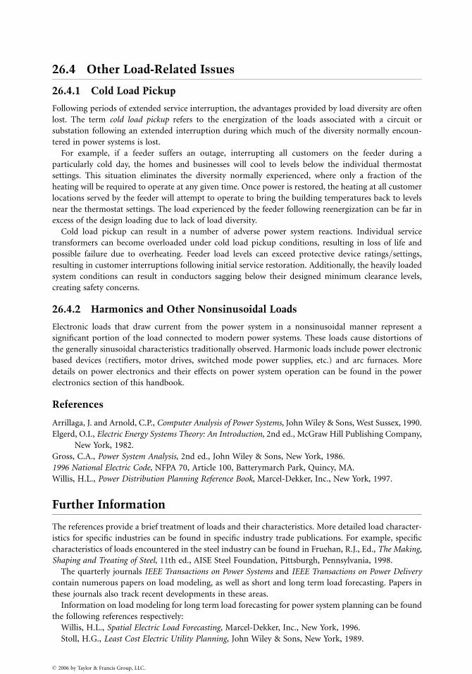
26.4 Other Load-Related Issues
26.4.1 Cold Load Pickup
Following periods of extended service interruption, the advantages provided by load diversity are often
lost. The term cold load pickup refers to the energization of the loads associated with a circuit or
substation following an extended interruption during which much of the diversity normally encoun-
tered in power systems is lost.
For example, if a feeder suffers an outage, interrupting all customers on the feeder during a
particularly cold day, the homes and businesses will cool to levels below the individual thermostat
settings. This situation eliminates the diversity normally experienced, where only a fraction of the
heating will be required to operate at any given time. Once power is restored, the heating at all customer
locations served by the feeder will attempt to operate to bring the building temperatures back to levels
near the thermostat settings. The load experienced by the feeder following reenergization can be far in
excess of the design loading due to lack of load diversity.
Cold load pickup can result in a number of adverse power system reactions. Individual service
transformers can become overloaded under cold load pickup conditions, resulting in loss of life and
possible failure due to overheating. Feeder load levels can exceed protective device ratings=settings,
resulting in customer interruptions following initial service restoration. Additionally, the heavily loaded
system conditions can result in conductors sagging below their designed minimum clearance levels,
creating safety concerns.
26.4.2 Harmonics and Other Nonsinusoidal Loads
Electronic loads that draw current from the power system in a nonsinusoidal manner represent a
significant portion of the load connected to modern power systems. These loads cause distortions of
the generally sinusoidal characteristics traditionally observed. Harmonic loads include power electronic
based devices (rectifiers, motor drives, switched mode power supplies, etc.) and arc furnaces. More
details on power electronics and their effects on power system operation can be found in the power
electronics section of this handbook.
References
Arrillaga, J. and Arnold, C.P., Computer Analysis of Power Systems, John Wiley & Sons, West Sussex, 1990.
Elgerd, O.I., Electric Energy Systems Theory: An Introduction, 2nd ed., McGraw Hill Publishing Company,
New York, 1982.
Gross, C.A., Power System Analysis, 2nd ed., John Wiley & Sons, New York, 1986.
1996 National Electric Code, NFPA 70, Article 100, Batterymarch Park, Quincy, MA.
Willis, H.L., Power Distribution Planning Reference Book, Marcel-Dekker, Inc., New York, 1997.
Further Information
The references provide a brief treatment of loads and their characteristics. More detailed load character-
istics for specific industries can be found in specific industry trade publications. For example, specific
characteristics of loads encountered in the steel industry can be found in Fruehan, R.J., Ed., The Making,
Shaping and Treating of Steel, 11th ed., AISE Steel Foundation, Pittsburgh, Pennsylvania, 1998.
The quarterly journals IEEE Transactions on Power Systems and IEEE Transactions on Power Delivery
contain numerous papers on load modeling, as well as short and long term load forecasting. Papers in
these journals also track recent developments in these areas.
Information on load modeling for long term load forecasting for power system planning can be found
the following references respectively:
Willis, H.L., Spatial Electric Load Forecasting, Marcel-Dekker, Inc., New York, 1996.
Stoll, H.G., Least Cost Electric Utility Planning, John Wiley & Sons, New York, 1989.
� 2006 by Taylor & Francis Group, LLC.
27
� 2006 by Taylor & Francis Group, LLC.
Electric PowerUtilization: Motors
Charles A. GrossAuburn University
27.1 Some General Perspectives ............................................. 27-1
27.2 Operating Modes............................................................. 27-3
27.3 Motor, Enclosure, and Controller Types ....................... 27-3
27.4 System Design.................................................................. 27-3Load Requirements . Environmental Requirements .
Electrical Source Options . Preliminary System Design .
System Ratings . System Data Acquisition .
Engineering Studies . Final System Design . Field Testing
A major application of electric energy is in its conversion to mechanical energy. Electromagnetic, or
‘‘EM’’ devices designed for this purpose are commonly called ‘‘motors.’’ Actually the machine is the
central component of an integrated system consisting of the source, controller, motor, and load. For
specialized applications, the system may be, and frequently is, designed as a integrated whole.
Many household appliances (e.g., a vacuum cleaner) have in one unit, the controller, the motor, and
the load. However, there remain a large number of important stand-alone applications that require
the selection of a proper motor and associated control, for a particular load. It is this general issue that
is the subject of this chapter.
The reader is cautioned that there is no ‘‘magic bullet’’ to deal with all motor-load applications. Like
many engineering problems, there is an artistic, as well as a scientific dimension to its solution. Likewise,
each individual application has its own peculiar characteristics, and requires significant experience to
manage. Nevertheless, a systematic formulation of the issues can be useful to a beginner in this area of
design, and even for experienced engineers faced with a new or unusual application.
27.1 Some General Perspectives
Consider the general situation in Fig. 27.1a. The flow of energy through the system is from left to right,
or from electrical source to mechanical load. Also, note the positive definitions of currents, voltages,
speed, and torques. These definitions are collectively called the ‘‘motor convention,’’ and are logically
used when motor applications are under study. Likewise, when generator applications are considered,
the sign conventions of Fig. 27.1b (called generation convention) will be adopted. This means that
variables will be positive under ‘‘normal’’ conditions (motors operating in the motor mode, generators
in the generator mode), and negative under some abnormal conditions (motors running ‘‘backwards,’’
for example). Using motor convention:
Tdev � Tm þ TRLð Þ ¼ Tdev � T 0m ¼ J dvrm=dtð Þ (27:1)
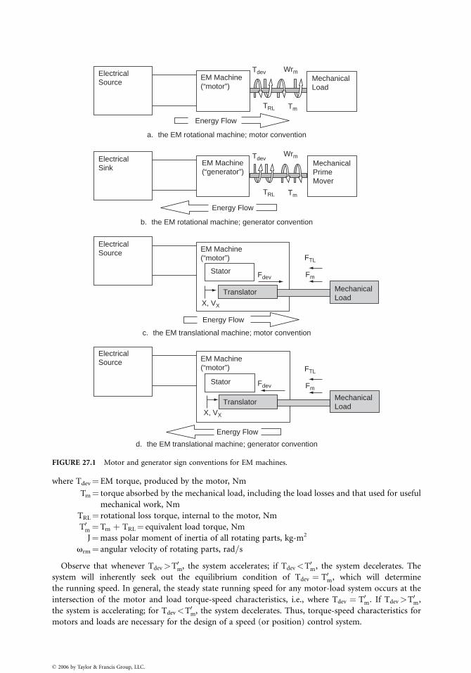
ElectricalSource Mechanical
Load
MechanicalLoad
Translator
Translator
Stator
Stator
MechanicalLoad
MechanicalPrimeMover
Energy Flow
Energy Flow
X, VX
Energy Flow
Energy Flow
a. the EM rotational machine; motor convention
b. the EM rotational machine; generator convention
c. the EM translational machine; motor convention
d. the EM translational machine; generator convention
Tdev
TRL Tm
Wrm
Tdev
Fdev
Fdev
TRL
FTL
Fm
Tm
Wrm
EM Machine(“motor”)
EM Machine(“motor”)
EM Machine(“motor”)
EM Machine(“generator”)
ElectricalSource
ElectricalSource
ElectricalSink
FTL
Fm
X, VX
FIGURE 27.1 Motor and generator sign conventions for EM machines.
where Tdev¼EM torque, produced by the motor, Nm
Tm¼ torque absorbed by the mechanical load, including the load losses and that used for useful
mechanical work, Nm
TRL¼ rotational loss torque, internal to the motor, Nm
T0m¼Tm þ TRL¼ equivalent load torque, Nm
J¼mass polar moment of inertia of all rotating parts, kg-m2
vrm¼ angular velocity of rotating parts, rad=s
Observe that whenever Tdev>T0m, the system accelerates; if Tdev<T0m, the system decelerates. The
system will inherently seek out the equilibrium condition of Tdev ¼ T0m, which will determine
the running speed. In general, the steady state running speed for any motor-load system occurs at the
intersection of the motor and load torque-speed characteristics, i.e., where Tdev ¼ T0m. If Tdev>T0m,
the system is accelerating; for Tdev<T0m, the system decelerates. Thus, torque-speed characteristics for
motors and loads are necessary for the design of a speed (or position) control system.
� 2006 by Taylor & Francis Group, LLC.

GeneratorReverse(GR)
GeneratorForward(GF)
MororForward(MF)
Tdev
ωrmMotorReverse(MR)
FIGURE 27.2 Operating modes.
The corresponding system powers are:
Pdev¼Tdev vrm¼EM power, converted by the motor into
mechanical form, W
Pm¼Tm vrm¼ power absorbed by the mechanical load,
including the load losses and that used for useful
mechanical work, W
PRL¼TRL vrm¼ rotational power loss, internal to the
motor, W
27.2 Operating Modes
Equation (27.1) implies that torque and speed are positive.
Consider positive speed as ‘‘forward,’’ meaning rotation in the ‘‘normal’’ direction, which should be
obvious in a specific application. ‘‘Reverse’’ is defined to mean rotation in the direction opposite to
‘‘forward,’’ and corresponds to vrm< 0. Positive EM torque is in the positive speed direction. Using
motor convention, first quadrant operation means that (1) speed is positive (‘‘forward’’) and (2) Tdev is
positive (also forward), and transferring energy from motor to load (‘‘motoring’’). There are four
possible operating modes specific to the four quadrants of Fig. 27.2. In any application, a primary
consideration is to determine which of these operating modes will be required.
27.3 Motor, Enclosure, and Controller Types
The general types of enclosures, motors, and controllers are summarized in Tables 27.1, 27.2, and 27.3.
27.4 System Design
The design of a proper motor-enclosure-controller system for a particular application is a significant
engineering problem requiring engineering expertise and experience. The following issues must be faced
and resolved.
TABLE 27.1 General Enclosure Typesa
Types
Open
Drip-proof
Splash-proof
Semi-guarded
Weather protected
Type I
Type II
Totally enclosed
Nonventillated
Fan-cooled
Explosion-proof
Dust-ignition-proof
Water-proof
Pipe-ventilated
Water-cooled
Water-air-cooled
Air-to-air-cooled
Air-over-cooled
aSee NEMA Standard MG 1.1.25-1.1.27 for definitions.
� 2006 by Taylor & Francis Group, LLC.

TABLE 27.2 General Motor Typesa
Type
DC motors (commutator devices)
Permanent magnet field
Wound field
Series
Shunt
Compound
AC motors
Single-phase
Cage rotor
Split phase
Resistance-start
Capacitor start
Single capacitor (start-run)
Capacitor start=capacitor run
Shaded pole
Wound rotor
Repulsion
Repulsion start=induction run
Universal
Synchronous
Hysteresis
Three-phase
Synchronous
Permanent magnet field
Wound field
Induction
Cage rotor
NEMA Design A,B,C,D,F
Wound rotor
aSee NEMA Standard MG 1.1.1-1.1.21 for definitions.
27.4.1 Load Requirements
1. The steady-state duty cycle with torque-speed (position) requirements at each load step.
2. What operating modes are required.
3. Dynamic performance requirements, including starting and stopping, and maximum and
minimum accelerations.
4. The relevant torque-speed (position) characteristics.
5. All load inertias (J).
6. Coupling options (direct drive, belt-drive, gearing).
7. Reliability of service. How critical is a system failure?
8. Future modifications.
27.4.2 Environmental Requirements
1. Ambient atmospheric conditions (pressure, temperature, humidity, content)
2. Indoor, outdoor application
3. Wet, dry location
4. Ventilation
5. Acceptable acoustical noise levels
6. Electrical=mechanical hazards to personnel
7. Accessibility for inspection and maintenance
� 2006 by Taylor & Francis Group, LLC.
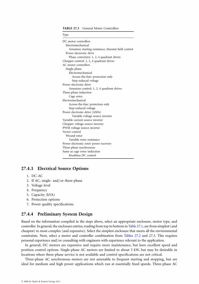
TABLE 27.3 General Motor Controllers
Type
DC motor controllers
Electromechanical
Armature starting resistance; rheostat field control
Power electronic drive
Phase converters: 1, 2, 4 quadrant drives
Chopper control: 1, 2, 4 quadrant drives
AC motor controllers
Single-phase
Electromechanical
Across-the-line: protection only
Step-reduced voltage
Power electronic drive
Armature control: 1, 2, 4 quadrant drives
Three-phase induction
Cage rotor
Electromechanical
Across-the-line: protection only
Step-reduced voltage
Power electronic drive (ASDs)
Variable voltage source inverter
Variable current source inverter
Chopper voltage source inverter
PWM voltage source inverter
Vector control
Wound rotor
Variable rotor resistance
Power electronic rotor power recovery
Three-phase synchronous
Same as cage rotor induction
Brushless DC control
27.4.3 Electrical Source Options
1. DC-AC
2. If AC, single- and=or three-phase
3. Voltage level
4. Frequency
5. Capacity (kVA)
6. Protection options
7. Power quality specifications
27.4.4 Preliminary System Design
Based on the information compiled in the steps above, select an appropriate enclosure, motor type, and
controller. In general, the enclosure entries, reading from top to bottom in Table 27.1, are from simplest (and
cheapest) to most complex (and expensive). Select the simplest enclosure that meets all the environmental
constraints. Next, select a motor and controller combination from Tables 27.2 and 27.3. This requires
personal experience and=or consulting with engineers with experience relevant to the application.
In general, DC motors are expensive and require more maintenance, but have excellent speed and
position control options. Single-phase AC motors are limited to about 5 kW, but may be desirable in
locations where three-phase service is not available and control specifications are not critical.
Three-phase AC synchronous motors are not amenable to frequent starting and stopping, but are
ideal for medium and high power applications which run at essentially fixed speeds. Three-phase AC
� 2006 by Taylor & Francis Group, LLC.

cage rotor induction motors are versatile and economical, and will be the preferred choice for most
applications, particularly in the medium power range. Three-phase AC wound rotor induction motors
are expensive, and only appropriate for some unusual applications.
The controller must be compatible with the motor selected; the best choice is the most economical
that meets all load specifications. If the engineer’s experience with the application under study is lacking,
two or more systems should be selected.
27.4.5 System Ratings
Based on the steps above, select appropriate power, voltage, and frequency ratings. For cyclic loads, the
power rating may tenatively be selected based on the ‘‘rms horsepower’’ method (calculating the rms
power requirements over the load cycle).
27.4.6 System Data Acquisition
Request data from at least two vendors on all systems selected in the steps above, including:
. circuit diagrams
. performance test data
. equivalent circuit values, including inertia constants
. cost data
. warranties and guarantees
27.4.7 Engineering Studies
Perform the following studies using data from the system data acquisition step above.
1. Steady state performance. Verify that each candidate system meets all steady state load
requirements.
2. Dynamic performance. Verify that each system meets all dynamic load requirements.
3. Load cycle efficiency. Determine the energy efficiency over the load cycle.
4. Provide a cost estimate for each system, including capital investment, maintenance, and annual
operating costs.
5. Perform a power quality assessment.
Based on these studies, select a final system design.
27.4.8 Final System Design
Request a competitive bid on the final design from appropriate vendors. Select a vendor based on cost,
expectation of continuing technical support, reputation, warranties, and past customer experience.
27.4.9 Field Testing
Whenever practical, customer and vendor engineers should design and perform field tests on the
installed system, demonstrating that it meets or exceeds all specifications. If multiple units are involved,
one proto-unit should be installed, tested, and commissioned before delivery is made on the balance of
the order.
Further Information
The design of a properly engineered motor-controller system for a particular application requires access
to several technical resources, including standards, the technical literature, manufacturers’ publications,
textbooks, and handbooks. The following section provides a list of references and resource material that
� 2006 by Taylor & Francis Group, LLC.

the author recommends for work in this area. In many cases, more recent versions of publications listed
are available and should be used.
Organizations
American National Standards Institute (ANSI), 1430 Broadway, New York, NY 10018.
Institute of Electrical and Electronics Engineers (IEEE), 445 Hoes Lane, Piscataway, NJ 08855.
International Organization for Standardization (ISO) 1, rue de Varembe, 1211 Geneva 20, Switzerland.
American Society for Testing and Materials (ASTM), 1916 Race Street, Philadelphia, PA 19103.
National Electrical Manufacturers Association (NEMA), 2101 L Street, NW, Washington, D.C. 20037.
National Fire Protection Association (NFPA), Batterymarch Park Quincy, MA 02269.
The Rubber Manufacturers Association, Inc., 1400 K Street, NW, Suite 300, Washington, D.C. 20005.
Mechanical Power Transmission Association, 1717 Howard Street, Evanston, IL 60201.
Standards
NEMA MG 1-1987, Motors and Generators.
NEMA MG 2-1983, Safety Standard for Construction and Guide for Selection, Installation and Use of
Electric Motors and Generators.
NEMA MG 3-1984, Sound Level Prediction for Installed Rotating Electrical Machines.
NEMA MG 13-1984, Frame Assignments for Alternating-Current Integral-horsepower Induction Motors.
ANSI=NFPA 70-1998, National Electrical Code.
IEEE Std 1-1969, General Principles for Temperature Limits in the Rating of Electric Equipment.
IEEE Std 85-1980, Test Procedure for Airborne Sound Measurements on Rotating Electric Machinery.
ANSI=IEEE Std 100-1984, IEEE Standard Dictionary of Electrical and Electronics Terms.
IEEE Std 112-1984, Standard Test Procedure for Potyphase Induction Motors and Generators.
IEEE Std 113-1985, Guide on Test Procedures for DC Machines.
ANSI=IEEE Std 114-1984, Test Procedure for Single-Phase Induction Motors.
ANSI=IEEE Std 115-1983, Test Procedures for Synchronous Machines.
ANSI=IEEE Std 117-1985, Standard Test Procedure for Evaluation of Systems of Insulating Materials for
Random-Wound AC Electric Machinery.
ANSI=IEEE Std 304-1982, Test Procedure for Evaluation and Classification of Insulation Systems for DC
Machines.
ISO R-1000, SI Units and Recommendations for the Use of their Multiples and of Certain Other Units.
Books (an abridged sample)
Acarnley, P.P., Stepping Motors, 2nd ed., Peter Peregrinus, Ltd., London, 1984.
Anderson, L.R., Electric Machines and Transformers, Reston Publishing, Reston, VA, 1981.
Bergseth, F.R. and Venkata, S.S., Introduction to Electric Energy Devices, Prentice-Hall, Englewood Cliffs,
NJ, 1987.
Bose, B.K., Power Electronics and AC Drives, Prentice-Hall, Englewood Cliffs, NJ, 1985.
Brown, D. and Hamilton 111, E.P., Electromechanical Energy Conversion, Macmillan, New York, 1984.
Chapman, S.J., Electric Machinery Fundamentals, McGraw-Hill, New York, 1985.
DC Motors-Speed Controls-Servo Systems—An Engineering Handbook, 5th ed., Electro-Craft Corpor-
ation, Hopkins, MN, 1980.
Del Toro, V, Electric Machinery and Power Systems, Prentice-Hall, Englewood Cliffs, NJ, 1986.
Electro-Craft Corporation, DC Motors, Speed Controls, Servo Systems, 3rd ed., Pergamon Press, Ltd.,
Oxford, 1977.
Fitzgerald, A.E., Kingsley, Jr., C., and Umans, S.D., Electric Machinery, 5th ed., McGraw-Hill,
New York, 1990.
Gonen, T., Engineering Economy for Engineering Managers, Wiley, New York, 1990.
� 2006 by Taylor & Francis Group, LLC.

Kenjo, T. and S. Nagamori, Permanent-Magnet and Brush-less DC Motors, Oxford, Claredon, 1985.
Krause, P.C. and Wasynezk, O., Electromechanical Machines and Devices, McGraw-Hill, New York, 1989.
Krein, P., Elements of Power Electronics; Oxford Press, 1998.
Moha, N., Undeland, and Robbins, Power Electronics; Converters, Application, and Design, 2nd ed., John
Wiley & Sons, New York, 1995.
Nasar, S.A. and Boldea, I., Linear Motion Electric Machines, John Wiley & Sons, New York, 1976.
Nasar, S.A., Ed., Handbook of Electric Machines, McGraw-Hill, New York, 1987.
Patrick, D.R. and Fardo, S.W., Rotating Electrical Machines and Power Systems, Prentice-Hall, Englewood
Cliffs, NJ, 1985.
Ramshaw, R. and Van Heeswijk, R.G., Energy Conversion: Electric Motors and Generators, Saunders
College Publishing, Orlando, FL, 1990.
Rashid, M.H., Power Electronics: Circuits, Devices, and Applications, 2nd ed., Prentice-Hall, Englewood
Cliffs, NJ, 1993.
Sarma, M.S., Electric Machines: Steady-State Theory and Dynamic Performance, Brown Publishers,
Dubuque, IA, 1985.
Smeatson, R.W., Ed., Motor Application and Maintenance Handbook, McGraw-Hill, New York, 1969.
Stein, R., and Hunt, W.T., Electric Power System Components: Transformers and Rotating Machines, Van
Nostrand, New York, 1979.
Veinott, C.G. and Martin, J.E., Fractional- and Subfractional-Horsepower Electric Motors, 4th ed.,
McGraw-Hill, New York, 1986.
Wenick, E.H., ed., Electric Motor Handbook, McGraw-Hill, London, 1978.
� 2006 by Taylor & Francis Group, LLC.

VI
Power Quality S.M. HalpinAuburn University28 Introduction S.M. Halpin ................................................................................................ 28-1
29 Wiring and Grounding for Power Quality Christopher J. Melhorn ............................ 29-1
Definitions and Standards . Reasons for Grounding . Typical
Wiring and Grounding Problems . Case Study
30 Harmonics in Power Systems S.M. Halpin ................................................................... 30-1
31 Voltage Sags Math H.J. Bollen ......................................................................................... 31-1
Voltage Sag Characteristics . Equipment Voltage Tolerance .
Mitigation of Voltage Sags
32 Voltage Fluctuations and Lamp Flicker in Power Systems S.M. Halpin................... 32-1
33 Power Quality Monitoring Patrick Coleman ................................................................. 33-1
Selecting a Monitoring Point . What to Monitor .
Selecting a Monitor . Summary
� 2006 by Taylor & Francis Group, LLC.

� 2006 by Taylor & Francis Group, LLC.
28
� 2006 by Taylor & Francis Group, LLC.
Introduction
S.M. HalpinAuburn University
Electric power quality has emerged as a major area of electric power engineering. The predominant
reason for this emergence is the increase in sensitivity of end-use equipment. This chapter is devoted to
various aspects of power quality as it impacts utility companies and their customers and includes
material on (1) grounding, (2) voltage sags, (3) harmonics, (4) voltage flicker, and (5) long-term
monitoring. While these five topics do not cover all aspects of power quality, they provide the reader
with a broad-based overview that should serve to increase overall understanding of problems related to
power quality.
Proper grounding of equipment is essential for safe and proper operation of sensitive electronic
equipment. In times past, it was thought by some that equipment grounding as specified in the U.S. by
the National Electric Code was in contrast with methods needed to insure power quality. Since those
early times, significant evidence has emerged to support the position that, in the vast majority of
instances, grounding according to the National Electric Code is essential to insure proper and trouble-
free equipment operation, and also to insure the safety of associated personnel.
Other than poor grounding practices, voltage sags due primarily to system faults are probably the
most significant of all power quality problems. Voltage sags due to short circuits are often seen at
distances very remote from the fault point, thereby affecting a potentially large number of utility
customers. Coupled with the wide-area impact of a fault event is the fact that there is no effective
preventive for all power system faults. End-use equipment will, therefore, be exposed to short periods of
reduced voltage which may or may not lead to malfunctions.
Like voltage sags, the concerns associated with flicker are also related to voltage variations. Voltage
flicker, however, is tied to the likelihood of a human observer to become annoyed by the variations in the
output of a lamp when the supply voltage amplitude is varying. In most cases, voltage flicker considers
(at least approximately) periodic voltage fluctuations with frequencies less than about 30–35 Hz that are
small in size. Human perception, rather than equipment malfunction, is the relevant factor when
considering voltage flicker.
For many periodic waveform (either voltage or current) variations, the power of classical Fourier
series theory can be applied. The terms in the Fourier series are called harmonics; relevant harmonic
terms may have frequencies above or below the fundamental power system frequency. In most cases,
nonfundamental frequency equipment currents produce voltages in the power delivery system at those
same frequencies. This voltage distortion is present in the supply to other end-use equipment and can
lead to improper operation of the equipment.
Harmonics, like most other power quality problems, require significant amounts of measured data in
order for the problem to be diagnosed accurately. Monitoring may be short- or long-term and may be

relatively cheap or very costly and often represents the majority of the work required to develop power
quality solutions.
In summary, the power quality problems associated with grounding, voltage sags, harmonics, and
voltage flicker are those most often encountered in practice. It should be recognized that the voltage and
current transients associated with common events like lightning strokes and capacitor switching can also
negatively impact end-use equipment. Because transients are covered in a separate chapter of this book,
they are not considered further in this chapter.
� 2006 by Taylor & Francis Group, LLC.
29
� 2006 by Taylor & Francis Group, LLC.
Wiring and Groundingfor Power Quality
Christopher J. MelhornEPRI
29.1 Definitions and Standards .............................................. 29-1The National Electric Code . From the IEEE Dictionary —
Std. 100 . Green Book (IEEE Std. 142) Definitions .
NEC Definitions
29.2 Reasons for Grounding................................................... 29-3Personal Safety . Protective Device Operation . Noise Control
29.3 Typical Wiring and Grounding Problems..................... 29-5Insulated Grounds . Ground Loops . Missing Safety
Ground . Multiple Neutral to Ground Bonds . Additional
Ground Rods . Insufficient Neutral Conductor . Summary
29.4 Case Study...................................................................... 29-12Case Study—Flickering Lights
Perhaps one of the most common problems related to power quality is wiring and grounding. It has
been reported that approximately 70 to 80% of all power quality related problems can be attributed to
faulty connections and=or wiring. This chapter describes wiring and grounding issues as they relate
to power quality. It is not intended to replace or supercede the National Electric Code (NEC) or any local
codes concerning grounding.
29.1 Definitions and Standards
Defining grounding terminology is outside the scope of this chapter. There are several publications on
the topic of grounding that define grounding terminology in various levels of detail. The reader is
referred to these publications for the definitions of grounding terminology.
The following is a list of standards and recommended practice pertaining to wiring and grounding
issues. See the section on References for complete information.
National Electric Code Handbook, 1996 edition.
IEEE Std. 1100–1999. IEEE Recommended Practice for Powering and Grounding Electronic Equipment.
IEEE Std. 142–1991. IEEE Recommended Practice for Grounding Industrial and Commercial Power
Systems.
FIPS-94 Publication
Electrical Power Systems Quality
29.1.1 The National Electric Code
NFPAs National Electrical Code Handbook pulls together all the extra facts, figures, and explanations
readers need to interpret the 1999 NEC. It includes the entire text of the Code, plus expert commentary,
real-world examples, diagrams, and illustrations that clarify requirements. Code text appears in blue
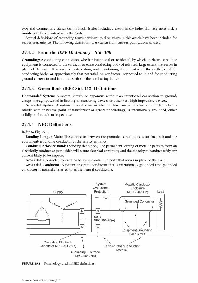
type and commentary stands out in black. It also includes a user-friendly index that references article
numbers to be consistent with the Code.
Several definitions of grounding terms pertinent to discussions in this article have been included for
reader convenience. The following definitions were taken from various publications as cited.
29.1.2 From the IEEE Dictionary—Std. 100
Grounding: A conducting connection, whether intentional or accidental, by which an electric circuit or
equipment is connected to the earth, or to some conducting body of relatively large extent that serves in
place of the earth. It is used for establishing and maintaining the potential of the earth (or of the
conducting body) or approximately that potential, on conductors connected to it; and for conducting
ground current to and from the earth (or the conducting body).
29.1.3 Green Book (IEEE Std. 142) Definitions
Ungrounded System: A system, circuit, or apparatus without an intentional connection to ground,
except through potential indicating or measuring devices or other very high impedance devices.
Grounded System: A system of conductors in which at least one conductor or point (usually the
middle wire or neutral point of transformer or generator windings) is intentionally grounded, either
solidly or through an impedance.
29.1.4 NEC Definitions
Refer to Fig. 29.1.
Bonding Jumper, Main: The connector between the grounded circuit conductor (neutral) and the
equipment-grounding conductor at the service entrance.
Conduit=Enclosure Bond: (bonding definition) The permanent joining of metallic parts to form an
electrically conductive path which will assure electrical continuity and the capacity to conduct safely any
current likely to be imposed.
Grounded: Connected to earth or to some conducting body that serves in place of the earth.
Grounded Conductor: A system or circuit conductor that is intentionally grounded (the grounded
conductor is normally referred to as the neutral conductor).
Grounding ElectrodeConductor NEC 250-26(b)
Grounding ElectrodeNEC 250-26(c)
Earth or Other ConductingMaterial
Equipment GroundingConductors
Load
Metallic ConductorEnclosure
NEC 250-91(b)Supply
BondNEC 250-26(e)
N N
GG
SystemOvercurrentProtection
Grounded Conductor
FIGURE 29.1 Terminology used in NEC definitions.
� 2006 by Taylor & Francis Group, LLC.
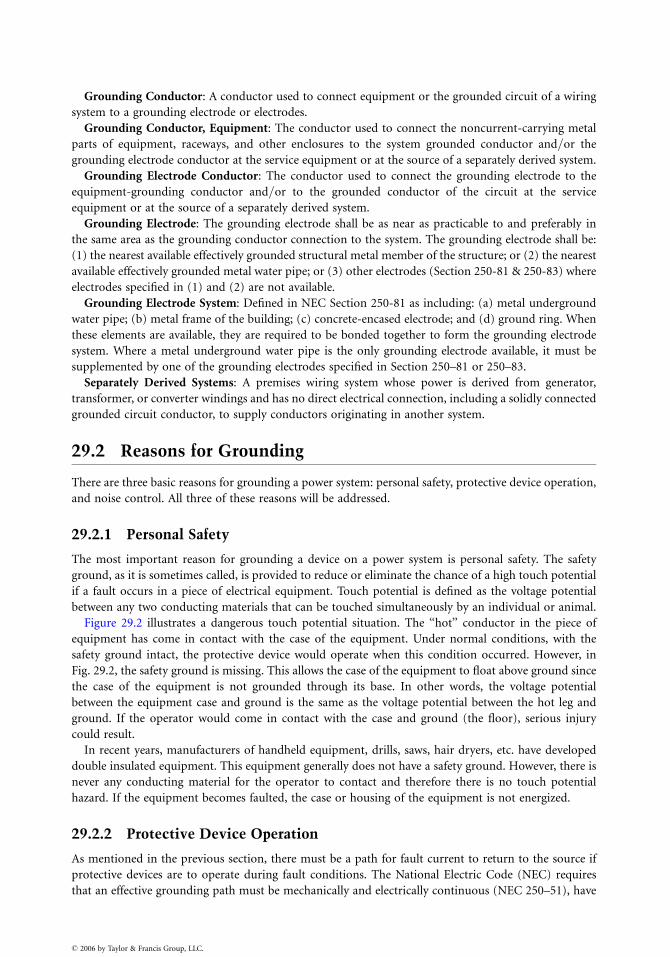
Grounding Conductor: A conductor used to connect equipment or the grounded circuit of a wiring
system to a grounding electrode or electrodes.
Grounding Conductor, Equipment: The conductor used to connect the noncurrent-carrying metal
parts of equipment, raceways, and other enclosures to the system grounded conductor and=or the
grounding electrode conductor at the service equipment or at the source of a separately derived system.
Grounding Electrode Conductor: The conductor used to connect the grounding electrode to the
equipment-grounding conductor and=or to the grounded conductor of the circuit at the service
equipment or at the source of a separately derived system.
Grounding Electrode: The grounding electrode shall be as near as practicable to and preferably in
the same area as the grounding conductor connection to the system. The grounding electrode shall be:
(1) the nearest available effectively grounded structural metal member of the structure; or (2) the nearest
available effectively grounded metal water pipe; or (3) other electrodes (Section 250-81 & 250-83) where
electrodes specified in (1) and (2) are not available.
Grounding Electrode System: Defined in NEC Section 250-81 as including: (a) metal underground
water pipe; (b) metal frame of the building; (c) concrete-encased electrode; and (d) ground ring. When
these elements are available, they are required to be bonded together to form the grounding electrode
system. Where a metal underground water pipe is the only grounding electrode available, it must be
supplemented by one of the grounding electrodes specified in Section 250–81 or 250–83.
Separately Derived Systems: A premises wiring system whose power is derived from generator,
transformer, or converter windings and has no direct electrical connection, including a solidly connected
grounded circuit conductor, to supply conductors originating in another system.
29.2 Reasons for Grounding
There are three basic reasons for grounding a power system: personal safety, protective device operation,
and noise control. All three of these reasons will be addressed.
29.2.1 Personal Safety
The most important reason for grounding a device on a power system is personal safety. The safety
ground, as it is sometimes called, is provided to reduce or eliminate the chance of a high touch potential
if a fault occurs in a piece of electrical equipment. Touch potential is defined as the voltage potential
between any two conducting materials that can be touched simultaneously by an individual or animal.
Figure 29.2 illustrates a dangerous touch potential situation. The ‘‘hot’’ conductor in the piece of
equipment has come in contact with the case of the equipment. Under normal conditions, with the
safety ground intact, the protective device would operate when this condition occurred. However, in
Fig. 29.2, the safety ground is missing. This allows the case of the equipment to float above ground since
the case of the equipment is not grounded through its base. In other words, the voltage potential
between the equipment case and ground is the same as the voltage potential between the hot leg and
ground. If the operator would come in contact with the case and ground (the floor), serious injury
could result.
In recent years, manufacturers of handheld equipment, drills, saws, hair dryers, etc. have developed
double insulated equipment. This equipment generally does not have a safety ground. However, there is
never any conducting material for the operator to contact and therefore there is no touch potential
hazard. If the equipment becomes faulted, the case or housing of the equipment is not energized.
29.2.2 Protective Device Operation
As mentioned in the previous section, there must be a path for fault current to return to the source if
protective devices are to operate during fault conditions. The National Electric Code (NEC) requires
that an effective grounding path must be mechanically and electrically continuous (NEC 250–51), have
� 2006 by Taylor & Francis Group, LLC.
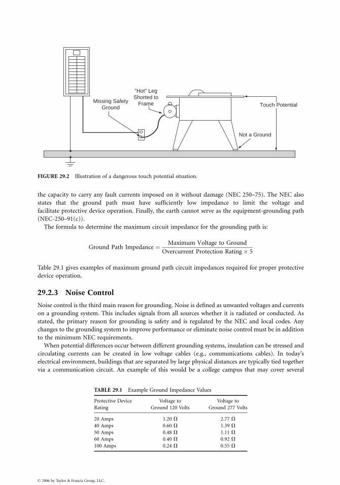
Missing SafetyGround
"Hot" LegShorted to
Frame Touch Potential
Not a Ground
FIGURE 29.2 Illustration of a dangerous touch potential situation.
the capacity to carry any fault currents imposed on it without damage (NEC 250–75). The NEC also
states that the ground path must have sufficiently low impedance to limit the voltage and
facilitate protective device operation. Finally, the earth cannot serve as the equipment-grounding path
(NEC-250–91(c)).
The formula to determine the maximum circuit impedance for the grounding path is:
Ground Path Impedance ¼ Maximum Voltage to Ground
Overcurrent Protection Rating� 5
Table 29.1 gives examples of maximum ground path circuit impedances required for proper protective
device operation.
29.2.3 Noise Control
Noise control is the third main reason for grounding. Noise is defined as unwanted voltages and currents
on a grounding system. This includes signals from all sources whether it is radiated or conducted. As
stated, the primary reason for grounding is safety and is regulated by the NEC and local codes. Any
changes to the grounding system to improve performance or eliminate noise control must be in addition
to the minimum NEC requirements.
When potential differences occur between different grounding systems, insulation can be stressed and
circulating currents can be created in low voltage cables (e.g., communications cables). In today’s
electrical environment, buildings that are separated by large physical distances are typically tied together
via a communication circuit. An example of this would be a college campus that may cover several
TABLE 29.1 Example Ground Impedance Values
Protective Device
Rating
Voltage to
Ground 120 Volts
Voltage to
Ground 277 Volts
20 Amps 1.20 V 2.77 V
40 Amps 0.60 V 1.39 V
50 Amps 0.48 V 1.11 V
60 Amps 0.40 V 0.92 V
100 Amps 0.24 V 0.55 V
� 2006 by Taylor & Francis Group, LLC.
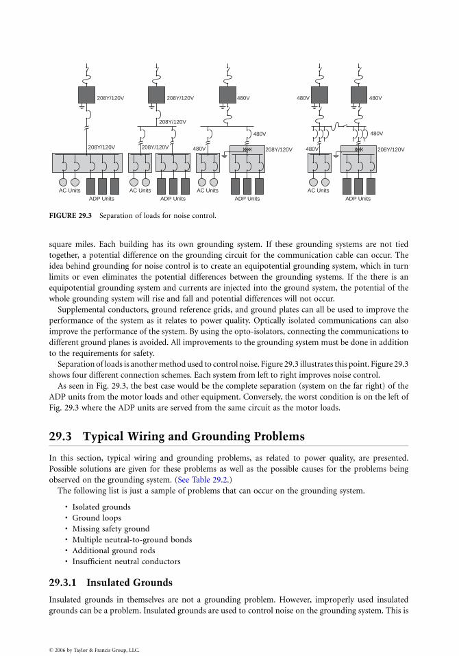
208Y/120V
208Y/120V 208Y/120V
208Y/120V
208Y/120V 208Y/120V
ADP Units
AC Units
ADP Units
AC Units
ADP Units
AC Units
ADP Units
AC Units
208Y/120V
480V
480V
480V
480V
480V
480V
480V
FIGURE 29.3 Separation of loads for noise control.
square miles. Each building has its own grounding system. If these grounding systems are not tied
together, a potential difference on the grounding circuit for the communication cable can occur. The
idea behind grounding for noise control is to create an equipotential grounding system, which in turn
limits or even eliminates the potential differences between the grounding systems. If the there is an
equipotential grounding system and currents are injected into the ground system, the potential of the
whole grounding system will rise and fall and potential differences will not occur.
Supplemental conductors, ground reference grids, and ground plates can all be used to improve the
performance of the system as it relates to power quality. Optically isolated communications can also
improve the performance of the system. By using the opto-isolators, connecting the communications to
different ground planes is avoided. All improvements to the grounding system must be done in addition
to the requirements for safety.
Separation of loads is another method used to control noise. Figure 29.3 illustrates this point. Figure 29.3
shows four different connection schemes. Each system from left to right improves noise control.
As seen in Fig. 29.3, the best case would be the complete separation (system on the far right) of the
ADP units from the motor loads and other equipment. Conversely, the worst condition is on the left of
Fig. 29.3 where the ADP units are served from the same circuit as the motor loads.
29.3 Typical Wiring and Grounding Problems
In this section, typical wiring and grounding problems, as related to power quality, are presented.
Possible solutions are given for these problems as well as the possible causes for the problems being
observed on the grounding system. (See Table 29.2.)
The following list is just a sample of problems that can occur on the grounding system.
. Isolated grounds
. Ground loops
. Missing safety ground
. Multiple neutral-to-ground bonds
. Additional ground rods
. Insufficient neutral conductors
29.3.1 Insulated Grounds
Insulated grounds in themselves are not a grounding problem. However, improperly used insulated
grounds can be a problem. Insulated grounds are used to control noise on the grounding system. This is
� 2006 by Taylor & Francis Group, LLC.
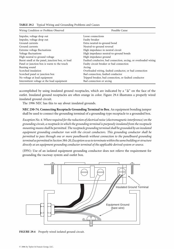
TABLE 29.2 Typical Wiring and Grounding Problems and Causes
Wiring Condition or Problem Observed Possible Cause
Impulse, voltage drop out Loose connections
Impulse, voltage drop out Faulty breaker
Ground currents Extra neutral-to-ground bond
Ground currents Neutral-to-ground reversal
Extreme voltage fluctuations High impedance in neutral circuit
Voltage fluctuations High impedance neutral-to-ground bonds
High neutral to ground voltage High impedance ground
Burnt smell at the panel, junction box, or load Faulted conductor, bad connection, arcing, or overloaded wiring
Panel or junction box is warm to the touch Faulty circuit breaker or bad connection
Buzzing sound Arcing
Scorched insulation Overloaded wiring, faulted conductor, or bad connection
Scorched panel or junction box Bad connection, faulted conductor
No voltage at load equipment Tripped breaker, bad connection, or faulted conductor
Intermittent voltage at the load equipment Bad connection or arcing
accomplished by using insulated ground receptacles, which are indicated by a ‘‘D’’ on the face of the
outlet. Insulated ground receptacles are often orange in color. Figure 29.4 illustrates a properly wired
insulated ground circuit.
The 1996 NEC has this to say about insulated grounds.
NEC 250-74. Connecting Receptacle Grounding Terminal to Box. An equipment bonding jumper
shall be used to connect the grounding terminal of a grounding-type receptacle to a grounded box.
Exception No. 4. Where required for the reduction of electrical noise (electromagnetic interference) on the
grounding circuit, a receptacle in which the grounding terminal is purposely insulated from the receptacle
mounting means shall be permitted. The receptacle grounding terminal shall be grounded by an insulated
equipment grounding conductor run with the circuit conductors. This grounding conductor shall be
permitted to pass through one or more panelboards without connection to the panelboard grounding
terminal as permitted in Section 384-20, Exception so as to terminate within the same building or structure
directly at an equipment grounding conductor terminal of the applicable derived system or source.
(FPN): Use of an isolated equipment grounding conductor does not relieve the requirement for
grounding the raceway system and outlet box.
Equipment Ground(bare wire)
Insulated Ground Terminal
FIGURE 29.4 Properly wired isolated ground circuit.
� 2006 by Taylor & Francis Group, LLC.
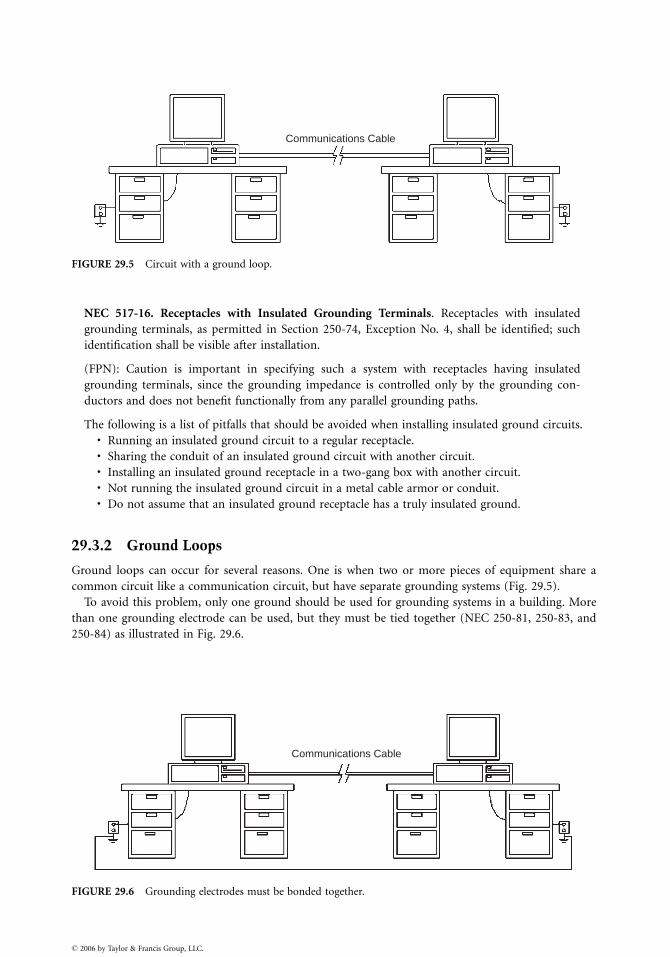
Communications Cable
FIGURE 29.5 Circuit with a ground loop.
NEC 517-16. Receptacles with Insulated Grounding Terminals. Receptacles with insulated
grounding terminals, as permitted in Section 250-74, Exception No. 4, shall be identified; such
identification shall be visible after installation.
(FPN): Caution is important in specifying such a system with receptacles having insulated
grounding terminals, since the grounding impedance is controlled only by the grounding con-
ductors and does not benefit functionally from any parallel grounding paths.
The following is a list of pitfalls that should be avoided when installing insulated ground circuits.. Running an insulated ground circuit to a regular receptacle.. Sharing the conduit of an insulated ground circuit with another circuit.. Installing an insulated ground receptacle in a two-gang box with another circuit.. Not running the insulated ground circuit in a metal cable armor or conduit.. Do not assume that an insulated ground receptacle has a truly insulated ground.
29.3.2 Ground Loops
Ground loops can occur for several reasons. One is when two or more pieces of equipment share a
common circuit like a communication circuit, but have separate grounding systems (Fig. 29.5).
To avoid this problem, only one ground should be used for grounding systems in a building. More
than one grounding electrode can be used, but they must be tied together (NEC 250-81, 250-83, and
250-84) as illustrated in Fig. 29.6.
Communications Cable
FIGURE 29.6 Grounding electrodes must be bonded together.
� 2006 by Taylor & Francis Group, LLC.
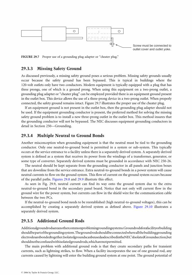
Screw must be connected tooutlet cover and outlet yoke.
FIGURE 29.7 Proper use of a grounding plug adapter or ‘‘cheater plug.’’
29.3.3 Missing Safety Ground
As discussed previously, a missing safety ground poses a serious problem. Missing safety grounds usually
occur because the safety ground has been bypassed. This is typical in buildings where the
120-volt outlets only have two conductors. Modern equipment is typically equipped with a plug that has
three prongs, one of which is a ground prong. When using this equipment on a two-prong outlet, a
grounding plug adapter or ‘‘cheater plug’’ can be employed provided there is an equipment ground present
in the outlet box. This device allows the use of a three-prong device in a two-prong outlet. When properly
connected, the safety ground remains intact. Figure 29.7 illustrates the proper use of the cheater plug.
If an equipment ground is not present in the outlet box, then the grounding plug adapter should not
be used. If the equipment grounding conductor is present, the preferred method for solving the missing
safety ground problem is to install a new three-prong outlet in the outlet box. This method insures that
the grounding conductor will not be bypassed. The NEC discusses equipment grounding conductors in
detail in Section 250—Grounding.
29.3.4 Multiple Neutral to Ground Bonds
Another misconception when grounding equipment is that the neutral must be tied to the grounding
conductor. Only one neutral-to-ground bond is permitted in a system or sub-system. This typically
occurs at the service entrance to a facility unless there is a separately derived system. A separately derived
system is defined as a system that receives its power from the windings of a transformer, generator, or
some type of converter. Separately derived systems must be grounded in accordance with NEC 250-26.
The neutral should be kept separate from the grounding conductor in all panels and junction boxes
that are downline from the service entrance. Extra neutral-to-ground bonds in a power system will cause
neutral currents to flow on the ground system. This flow of current on the ground system occurs because
of the parallel paths. Figures 29.8 and 29.9 illustrate this effect.
As seen in Fig. 29.9, neutral current can find its way onto the ground system due to the extra
neutral-to-ground bond in the secondary panel board. Notice that not only will current flow in the
ground wire for the power system, but currents can flow in the shield wire for the communication cable
between the two PCs.
If the neutral-to-ground bond needs to be reestablished (high neutral-to-ground voltages), this can be
accomplished by creating a separately derived system as defined above. Figure 29.10 illustrates a
separately derived system.
29.3.5 Additional Ground Rods
Additionalgroundrodsareanothercommonproblemingroundingsystems.Groundrodsforafacilityorbuilding
shouldbepartofthegroundingsystem.Thegroundrodsshouldbeconnectedwhereallthebuildinggrounding
electrodesarebondedtogether.IsolatedgroundscanbeusedasdescribedintheNEC’sIsolatedGroundsection,but
shouldnotbeconfusedwithisolatedgroundrods,whicharenotpermitted.
The main problem with additional ground rods is that they create secondary paths for transient
currents, such as lightning strikes, to flow. When a facility incorporates the use of one ground rod, any
currents caused by lightning will enter the building ground system at one point. The ground potential of
� 2006 by Taylor & Francis Group, LLC.
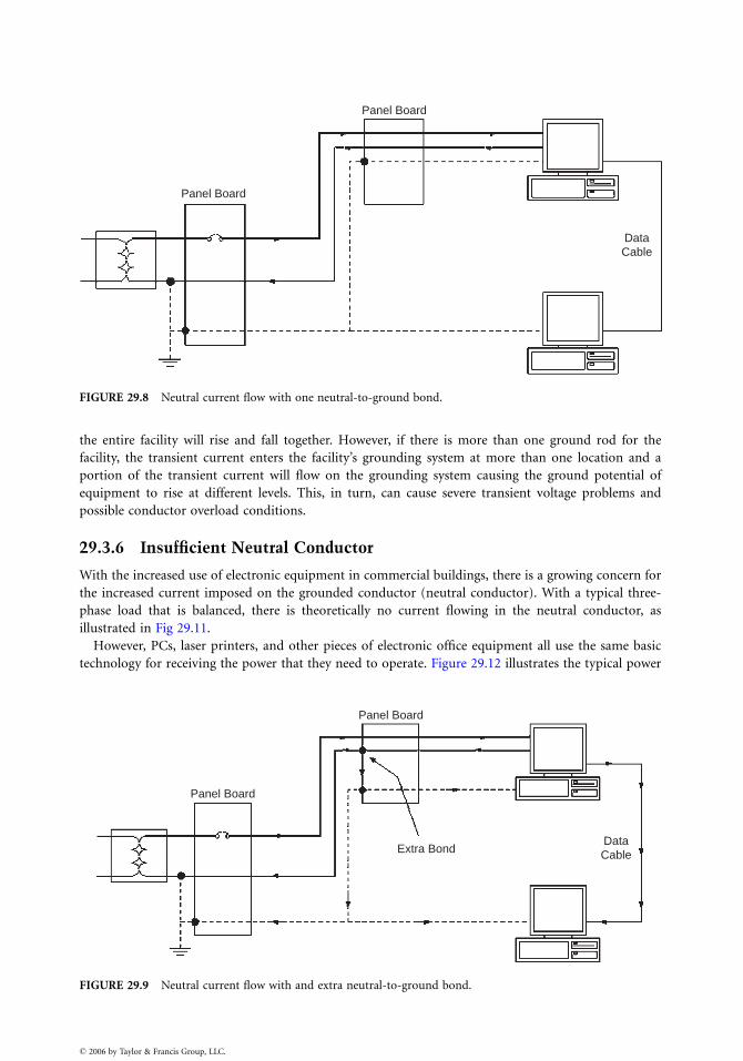
Panel Board
Panel Board
DataCable
FIGURE 29.8 Neutral current flow with one neutral-to-ground bond.
the entire facility will rise and fall together. However, if there is more than one ground rod for the
facility, the transient current enters the facility’s grounding system at more than one location and a
portion of the transient current will flow on the grounding system causing the ground potential of
equipment to rise at different levels. This, in turn, can cause severe transient voltage problems and
possible conductor overload conditions.
29.3.6 Insufficient Neutral Conductor
With the increased use of electronic equipment in commercial buildings, there is a growing concern for
the increased current imposed on the grounded conductor (neutral conductor). With a typical three-
phase load that is balanced, there is theoretically no current flowing in the neutral conductor, as
illustrated in Fig 29.11.
However, PCs, laser printers, and other pieces of electronic office equipment all use the same basic
technology for receiving the power that they need to operate. Figure 29.12 illustrates the typical power
DataCable
Panel Board
Panel Board
Extra Bond
FIGURE 29.9 Neutral current flow with and extra neutral-to-ground bond.
� 2006 by Taylor & Francis Group, LLC.
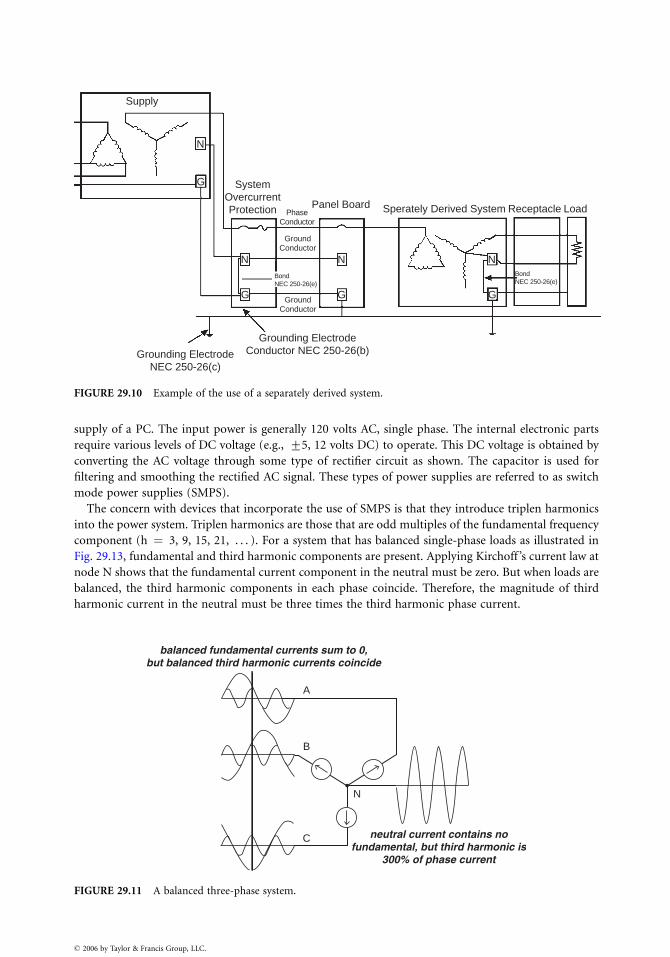
Supply
N
N N N
G
G G G
SystemOvercurrentProtection Panel Board Sperately Derived System Receptacle Load
BondNEC 250-26(e)
BondNEC 250-26(e)
PhaseConductor
GroundConductor
GroundConductor
Grounding ElectrodeNEC 250-26(c)
Grounding ElectrodeConductor NEC 250-26(b)
FIGURE 29.10 Example of the use of a separately derived system.
supply of a PC. The input power is generally 120 volts AC, single phase. The internal electronic parts
require various levels of DC voltage (e.g., +5, 12 volts DC) to operate. This DC voltage is obtained by
converting the AC voltage through some type of rectifier circuit as shown. The capacitor is used for
filtering and smoothing the rectified AC signal. These types of power supplies are referred to as switch
mode power supplies (SMPS).
The concern with devices that incorporate the use of SMPS is that they introduce triplen harmonics
into the power system. Triplen harmonics are those that are odd multiples of the fundamental frequency
component (h ¼ 3, 9, 15, 21, . . . ). For a system that has balanced single-phase loads as illustrated in
Fig. 29.13, fundamental and third harmonic components are present. Applying Kirchoff ’s current law at
node N shows that the fundamental current component in the neutral must be zero. But when loads are
balanced, the third harmonic components in each phase coincide. Therefore, the magnitude of third
harmonic current in the neutral must be three times the third harmonic phase current.
neutral current contains nofundamental, but third harmonic is
300% of phase current
balanced fundamental currents sum to 0,but balanced third harmonic currents coincide
A
B
C
N
FIGURE 29.11 A balanced three-phase system.
� 2006 by Taylor & Francis Group, LLC.
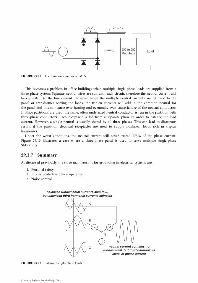
LoadDC to DCRegulator
FIGURE 29.12 The basic one-line for a SMPS.
This becomes a problem in office buildings when multiple single-phase loads are supplied from a
three-phase system. Separate neutral wires are run with each circuit, therefore the neutral current will
be equivalent to the line current. However, when the multiple neutral currents are returned to the
panel or transformer serving the loads, the triplen currents will add in the common neutral for
the panel and this can cause over heating and eventually even cause failure of the neutral conductor.
If office partitions are used, the same, often undersized neutral conductor is run in the partition with
three-phase conductors. Each receptacle is fed from a separate phase in order to balance the load
current. However, a single neutral is usually shared by all three phases. This can lead to disastrous
results if the partition electrical receptacles are used to supply nonlinear loads rich in triplen
harmonics.
Under the worst conditions, the neutral current will never exceed 173% of the phase current.
Figure 29.13 illustrates a case where a three-phase panel is used to serve multiple single-phase
SMPS PCs.
29.3.7 Summary
As discussed previously, the three main reasons for grounding in electrical systems are:
1. Personal safety
2. Proper protective device operation
3. Noise control
neutral current contains nofundamental, but third harmonic is
300% of phase current
balanced fundamental currents sum to 0,but balanced third harmonic currents coincide
A
B
C
N
FIGURE 29.13 Balanced single-phase loads.
� 2006 by Taylor & Francis Group, LLC.
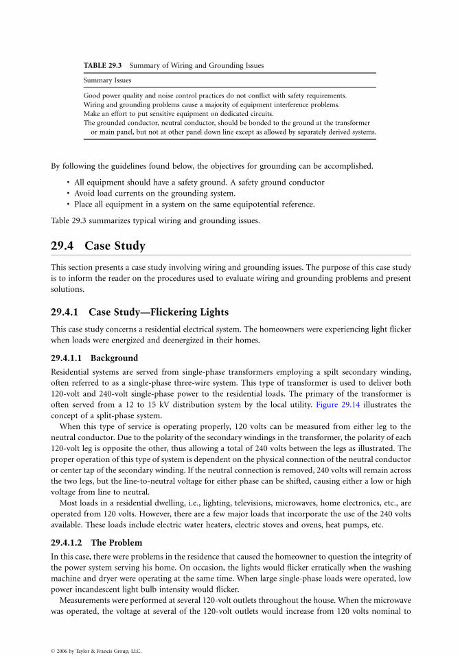
TABLE 29.3 Summary of Wiring and Grounding Issues
Summary Issues
Good power quality and noise control practices do not conflict with safety requirements.
Wiring and grounding problems cause a majority of equipment interference problems.
Make an effort to put sensitive equipment on dedicated circuits.
The grounded conductor, neutral conductor, should be bonded to the ground at the transformer
or main panel, but not at other panel down line except as allowed by separately derived systems.
By following the guidelines found below, the objectives for grounding can be accomplished.
. All equipment should have a safety ground. A safety ground conductor
. Avoid load currents on the grounding system.
. Place all equipment in a system on the same equipotential reference.
Table 29.3 summarizes typical wiring and grounding issues.
29.4 Case Study
This section presents a case study involving wiring and grounding issues. The purpose of this case study
is to inform the reader on the procedures used to evaluate wiring and grounding problems and present
solutions.
29.4.1 Case Study—Flickering Lights
This case study concerns a residential electrical system. The homeowners were experiencing light flicker
when loads were energized and deenergized in their homes.
29.4.1.1 Background
Residential systems are served from single-phase transformers employing a spilt secondary winding,
often referred to as a single-phase three-wire system. This type of transformer is used to deliver both
120-volt and 240-volt single-phase power to the residential loads. The primary of the transformer is
often served from a 12 to 15 kV distribution system by the local utility. Figure 29.14 illustrates the
concept of a split-phase system.
When this type of service is operating properly, 120 volts can be measured from either leg to the
neutral conductor. Due to the polarity of the secondary windings in the transformer, the polarity of each
120-volt leg is opposite the other, thus allowing a total of 240 volts between the legs as illustrated. The
proper operation of this type of system is dependent on the physical connection of the neutral conductor
or center tap of the secondary winding. If the neutral connection is removed, 240 volts will remain across
the two legs, but the line-to-neutral voltage for either phase can be shifted, causing either a low or high
voltage from line to neutral.
Most loads in a residential dwelling, i.e., lighting, televisions, microwaves, home electronics, etc., are
operated from 120 volts. However, there are a few major loads that incorporate the use of the 240 volts
available. These loads include electric water heaters, electric stoves and ovens, heat pumps, etc.
29.4.1.2 The Problem
In this case, there were problems in the residence that caused the homeowner to question the integrity of
the power system serving his home. On occasion, the lights would flicker erratically when the washing
machine and dryer were operating at the same time. When large single-phase loads were operated, low
power incandescent light bulb intensity would flicker.
Measurements were performed at several 120-volt outlets throughout the house. When the microwave
was operated, the voltage at several of the 120-volt outlets would increase from 120 volts nominal to
� 2006 by Taylor & Francis Group, LLC.
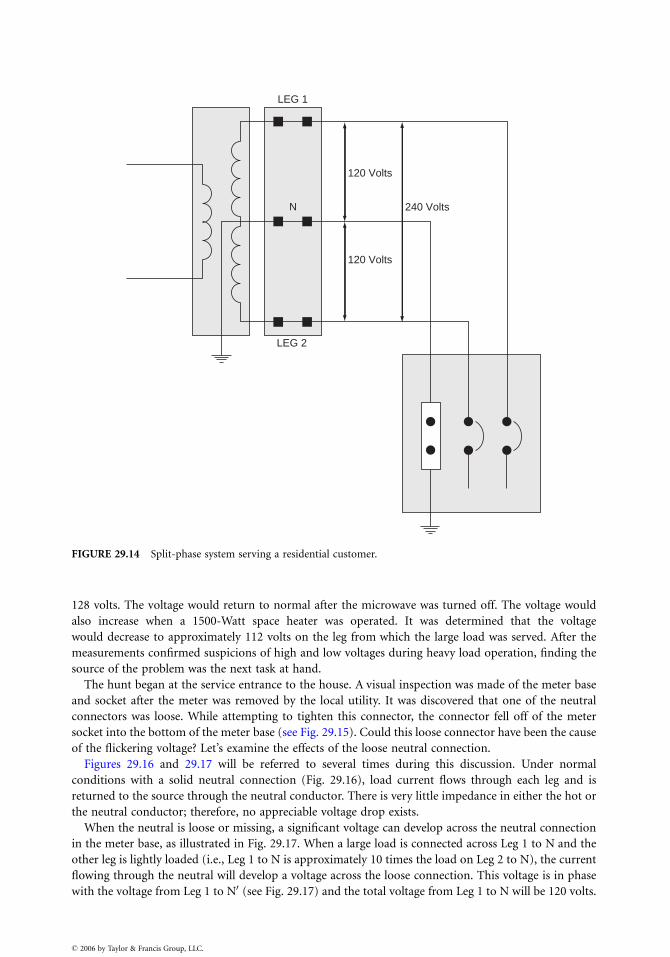
120 Volts
240 Volts
120 Volts
LEG 1
LEG 2
N
FIGURE 29.14 Split-phase system serving a residential customer.
128 volts. The voltage would return to normal after the microwave was turned off. The voltage would
also increase when a 1500-Watt space heater was operated. It was determined that the voltage
would decrease to approximately 112 volts on the leg from which the large load was served. After the
measurements confirmed suspicions of high and low voltages during heavy load operation, finding the
source of the problem was the next task at hand.
The hunt began at the service entrance to the house. A visual inspection was made of the meter base
and socket after the meter was removed by the local utility. It was discovered that one of the neutral
connectors was loose. While attempting to tighten this connector, the connector fell off of the meter
socket into the bottom of the meter base (see Fig. 29.15). Could this loose connector have been the cause
of the flickering voltage? Let’s examine the effects of the loose neutral connection.
Figures 29.16 and 29.17 will be referred to several times during this discussion. Under normal
conditions with a solid neutral connection (Fig. 29.16), load current flows through each leg and is
returned to the source through the neutral conductor. There is very little impedance in either the hot or
the neutral conductor; therefore, no appreciable voltage drop exists.
When the neutral is loose or missing, a significant voltage can develop across the neutral connection
in the meter base, as illustrated in Fig. 29.17. When a large load is connected across Leg 1 to N and the
other leg is lightly loaded (i.e., Leg 1 to N is approximately 10 times the load on Leg 2 to N), the current
flowing through the neutral will develop a voltage across the loose connection. This voltage is in phase
with the voltage from Leg 1 to N0 (see Fig. 29.17) and the total voltage from Leg 1 to N will be 120 volts.
� 2006 by Taylor & Francis Group, LLC.
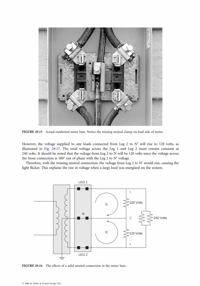
FIGURE 29.15 Actual residential meter base. Notice the missing neutral clamp on load side of meter.
However, the voltage supplied to any loads connected from Leg 2 to N0 will rise to 128 volts, as
illustrated in Fig. 29.17. The total voltage across the Leg 1 and Leg 2 must remain constant at
240 volts. It should be noted that the voltage from Leg 2 to N will be 120 volts since the voltage across
the loose connection is 1808 out of phase with the Leg 2 to N0 voltage.
Therefore, with the missing neutral connection, the voltage from Leg 2 to N0 would rise, causing the
light flicker. This explains the rise in voltage when a large load was energized on the system.
LEG 1
LEG 2
N
I1 120 Volts
120 Volts
240 Volts
+
+
−
I2
FIGURE 29.16 The effects of a solid neutral connection in the meter base.
� 2006 by Taylor & Francis Group, LLC.
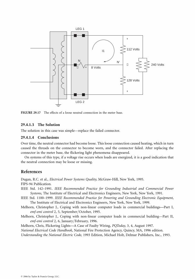
LEG 1
LEG 2
I1
N'
112 Volts
8 Volts
128 Volts
240 Volts
+
+
−N
− +
FIGURE 29.17 The effects of a loose neutral connection in the meter base.
29.4.1.3 The Solution
The solution in this case was simple—replace the failed connector.
29.4.1.4 Conclusions
Over time, the neutral connector had become loose. This loose connection caused heating, which in turn
caused the threads on the connector to become worn, and the connector failed. After replacing the
connector in the meter base, the flickering light phenomena disappeared.
On systems of this type, if a voltage rise occurs when loads are energized, it is a good indication that
the neutral connection may be loose or missing.
References
Dugan, R.C. et al., Electrical Power Systems Quality, McGraw-Hill, New York, 1995.
FIPS-94 Publication.
IEEE Std. 142–1991. IEEE Recommended Practice for Grounding Industrial and Commercial Power
Systems, The Institute of Electrical and Electronics Engineers, New York, New York, 1991.
IEEE Std. 1100–1999. IEEE Recommended Practice for Powering and Grounding Electronic Equipment,
The Institute of Electrical and Electronics Engineers, New York, New York, 1999.
Melhorn, Christopher J., Coping with non-linear computer loads in commercial buildings—Part I,
emf-emi control 2, 5, September=October, 1995.
Melhorn, Christopher J., Coping with non-linear computer loads in commercial building—Part II,
emf-emi control 2, 6, January=February, 1996.
Melhorn, Chris, Flickering Lights—A Case of Faulty Wiring, PQToday, 3, 4, August 1997.
National Electrical Code Handbook, National Fire Protection Agency, Quincy, MA, 1996 edition.
Understanding the National Electric Code, 1993 Edition, Michael Holt, Delmar Publishers, Inc., 1993.
� 2006 by Taylor & Francis Group, LLC.

� 2006 by Taylor & Francis Group, LLC.
30
� 2006 by Taylor & Francis Group, LLC.
Harmonics in PowerSystems
S.M. HalpinAuburn University
Power system harmonics are not a new topic, but the proliferation of high-power electronics used in
motor drives and power controllers has necessitated increased research and development in many areas
relating to harmonics. For many years, high-voltage direct current (HVDC) stations have been a major
focus area for the study of power system harmonics due to their rectifier and inverter stations. Roughly
two decades ago, electronic devices that could handle several kW up to several MW became commer-
cially viable and reliable products. This technological advance in electronics led to the widespread use of
numerous converter topologies, all of which represent nonlinear elements in the power system.
Even though the power semiconductor converter is largely responsible for the large-scale interest in
power system harmonics, other types of equipment also present a nonlinear characteristic to the power
system. In broad terms, loads that produce harmonics can be grouped into three main categories
covering (1) arcing loads, (2) semiconductor converter loads, and (3) loads with magnetic saturation
of iron cores. Arcing loads, like electric arc furnaces and florescent lamps, tend to produce harmonics
across a wide range of frequencies with a generally decreasing relationship with frequency. Semicon-
ductor loads, such as adjustable-speed motor drives, tend to produce certain harmonic patterns with
relatively predictable amplitudes at known harmonics. Saturated magnetic elements, like overexcited
transformers, also tend to produce certain ‘‘characteristic’’ harmonics. Like arcing loads, both semicon-
ductor converters and saturated magnetics produce harmonics that generally decrease with frequency.
Regardless of the load category, the same fundamental theory can be used to study power quality
problems associated with harmonics. In most cases, any periodic distorted power system waveform
(voltage, current, flux, etc.) can be represented as a series consisting of a DC term and an infinite sum of
sinusoidal terms as shown in Eq. (30.1) where v0 is the fundamental power frequency.
f tð Þ ¼ F0 þX
1
i¼1
ffiffiffi
2p
Fi cos iv0tþ uið Þ (30:1)
A vast amount of theoretical mathematics has been devoted to the evaluation of the terms in the infinite
sum in Eq. (30.1), but such rigor is beyond the scope of this chapter. For the purposes here, it is
reasonable to presume that instrumentation is available that will provide both the magnitude Fi and the
phase angle ui for each term in the series. Taken together, the magnitude and phase of the ith term
completely describe the ith harmonic.
It should be noted that not all loads produce harmonics that are integer multiples of the power
frequency. These noninteger multiple harmonics are generally referred to as interharmonics and are
commonly produced by arcing loads and cycloconverters. All harmonic terms, both integer and
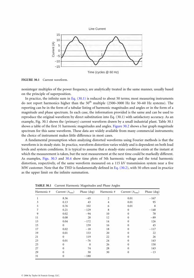
Line Current
Cur
rent
(A
)
Time (cycles @ 60 Hz)
15
10
5
1−5
−15
−10
020
FIGURE 30.1 Current waveform.
noninteger multiples of the power frequency, are analytically treated in the same manner, usually based
on the principle of superposition.
In practice, the infinite sum in Eq. (30.1) is reduced to about 50 terms; most measuring instruments
do not report harmonics higher than the 50th multiple (2500–3000 Hz for 50–60 Hz systems). The
reporting can be in the form of a tabular listing of harmonic magnitudes and angles or in the form of a
magnitude and phase spectrum. In each case, the information provided is the same and can be used to
reproduce the original waveform by direct substitution into Eq. (30.1) with satisfactory accuracy. As an
example, Fig. 30.1 shows the (primary) current waveform drawn by a small industrial plant. Table 30.1
shows a table of the first 31 harmonic magnitudes and angles. Figure 30.2 shows a bar graph magnitude
spectrum for this same waveform. These data are widely available from many commercial instruments;
the choice of instrument makes little difference in most cases.
A fundamental presumption when analyzing distorted waveforms using Fourier methods is that the
waveform is in steady state. In practice, waveform distortion varies widely and is dependent on both load
levels and system conditions. It is typical to assume that a steady-state condition exists at the instant at
which the measurement is taken, but the next measurement at the next time could be markedly different.
As examples, Figs. 30.3 and 30.4 show time plots of 5th harmonic voltage and the total harmonic
distortion, respectively, of the same waveform measured on a 115 kV transmission system near a five
MW customer. Note that the THD is fundamentally defined in Eq. (30.2), with 50 often used in practice
as the upper limit on the infinite summation.
TABLE 30.1 Current Harmonic Magnitudes and Phase Angles
Harmonic # Current (Arms) Phase (deg) Harmonic # Current (Arms) Phase (deg)
1 8.36 �65 2 0.01 �167
3 0.13 43 4 0.01 95
5 0.76 102 6 0.01 8
7 0.21 �129 8 0 �148
9 0.02 �94 10 0 78
11 0.08 28 12 0 �89
13 0.04 �172 14 0 126
15 0 159 16 0 45
17 0.02 �18 18 0 �117
19 0.01 153 20 0 22
21 0 119 22 0 26
23 0.01 �76 24 0 143
25 0 0 26 0 150
27 0 74 28 0 143
29 0 50 30 0 �13
31 0 �180
� 2006 by Taylor & Francis Group, LLC.
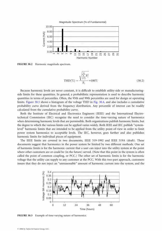
0.001 3 5 7 9 11 13 15 17 19 21 23 25 27 29 31
Harmonic Number
2.00
4.00C
urre
nt (
%A
)
6.00
8.00
10.00
Magnitude Spectrum (% of Fundamental)
FIGURE 30.2 Harmonic magnitude spectrum.
THD %ð Þ ¼
ffiffiffiffiffiffiffiffiffiffiffi
P
1
i¼2
F2i
s
F1*100% (30:2)
Because harmonic levels are never constant, it is difficult to establish utility-side or manufacturing-
side limits for these quantities. In general, a probabilistic representation is used to describe harmonic
quantities in terms of percentiles. Often, the 95th and 99th percentiles are used for design or operating
limits. Figure 30.5 shows a histogram of the voltage THD in Fig. 30.4, and also includes a cumulative
probability curve derived from the frequency distribution. Any percentile of interest can be readily
calculated from the cumulative probability curve.
Both the Institute of Electrical and Electronics Engineers (IEEE) and the International Electro-
technical Commission (IEC) recognize the need to consider the time-varying nature of harmonics
when determining harmonic levels that are permissible. Both organizations publish harmonic limits, but
the degree to which the various limits can be applied varies widely. Both IEEE and IEC publish ‘‘system-
level’’ harmonic limits that are intended to be applied from the utility point-of-view in order to limit
power system harmonics to acceptable levels. The IEC, however, goes further and also publishes
harmonic limits for individual pieces of equipment.
The IEEE limits are covered in two documents, IEEE 519-1992 and IEEE 519A (draft). These
documents suggest that harmonics in the power system be limited by two different methods. One set
of harmonic limits is for the harmonic current that a user can inject into the utility system at the point
where other customers are or could be (in the future) served. (Note that this point in the system is often
called the point of common coupling, or PCC.) The other set of harmonic limits is for the harmonic
voltage that the utility can supply to any customer at the PCC. With this two-part approach, customers
insure that they do not inject an ‘‘unreasonable’’ amount of harmonic current into the system, and the
00
Vol
tage
5th
Har
mon
ic (
%)
0.05
0.1
0.15
0.2
0.3
0.4
0.35
0.25
12 24 36
Time (hours)
48 60
FIGURE 30.3 Example of time-varying nature of harmonics.
� 2006 by Taylor & Francis Group, LLC.
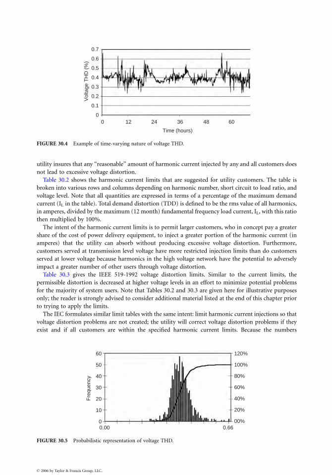
00
0.1
0.2
0.3V
olta
ge T
HD
(%
)
0.4
0.5
0.6
0.7
12 24 36
Time (hours)
48 60
FIGURE 30.4 Example of time-varying nature of voltage THD.
utility insures that any ‘‘reasonable’’ amount of harmonic current injected by any and all customers does
not lead to excessive voltage distortion.
Table 30.2 shows the harmonic current limits that are suggested for utility customers. The table is
broken into various rows and columns depending on harmonic number, short circuit to load ratio, and
voltage level. Note that all quantities are expressed in terms of a percentage of the maximum demand
current (IL in the table). Total demand distortion (TDD) is defined to be the rms value of all harmonics,
in amperes, divided by the maximum (12 month) fundamental frequency load current, IL, with this ratio
then multiplied by 100%.
The intent of the harmonic current limits is to permit larger customers, who in concept pay a greater
share of the cost of power delivery equipment, to inject a greater portion of the harmonic current (in
amperes) that the utility can absorb without producing excessive voltage distortion. Furthermore,
customers served at transmission level voltage have more restricted injection limits than do customers
served at lower voltage because harmonics in the high voltage network have the potential to adversely
impact a greater number of other users through voltage distortion.
Table 30.3 gives the IEEE 519-1992 voltage distortion limits. Similar to the current limits, the
permissible distortion is decreased at higher voltage levels in an effort to minimize potential problems
for the majority of system users. Note that Tables 30.2 and 30.3 are given here for illustrative purposes
only; the reader is strongly advised to consider additional material listed at the end of this chapter prior
to trying to apply the limits.
The IEC formulates similar limit tables with the same intent: limit harmonic current injections so that
voltage distortion problems are not created; the utility will correct voltage distortion problems if they
exist and if all customers are within the specified harmonic current limits. Because the numbers
60
50
40
30
20
10
0 00%
20%
40%
60%
80%
100%
120%
0.00 0.66
Fre
quen
cy
FIGURE 30.5 Probabilistic representation of voltage THD.
� 2006 by Taylor & Francis Group, LLC.
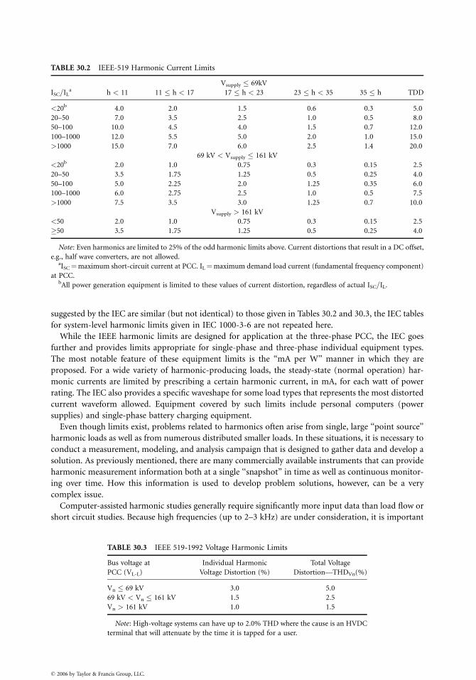
TABLE 30.2 IEEE-519 Harmonic Current Limits
Vsupply � 69kV
ISC=ILa h < 11 11 � h < 17 17 � h < 23 23 � h < 35 35 � h TDD
<20b 4.0 2.0 1.5 0.6 0.3 5.0
20–50 7.0 3.5 2.5 1.0 0.5 8.0
50–100 10.0 4.5 4.0 1.5 0.7 12.0
100–1000 12.0 5.5 5.0 2.0 1.0 15.0
>1000 15.0 7.0 6.0 2.5 1.4 20.0
69 kV < Vsupply � 161 kV
<20b 2.0 1.0 0.75 0.3 0.15 2.5
20–50 3.5 1.75 1.25 0.5 0.25 4.0
50–100 5.0 2.25 2.0 1.25 0.35 6.0
100–1000 6.0 2.75 2.5 1.0 0.5 7.5
>1000 7.5 3.5 3.0 1.25 0.7 10.0
Vsupply > 161 kV
<50 2.0 1.0 0.75 0.3 0.15 2.5
�50 3.5 1.75 1.25 0.5 0.25 4.0
Note : Even harmonics are limited to 25% of the odd harmonic limits above. Current distortions that result in a DC offset,
e.g., half wave converters, are not allowed.aISC¼maximum short-circuit current at PCC. IL¼maximum demand load current (fundamental frequency component)
at PCC.bAll power generation equipment is limited to these values of current distortion, regardless of actual ISC=IL.
suggested by the IEC are similar (but not identical) to those given in Tables 30.2 and 30.3, the IEC tables
for system-level harmonic limits given in IEC 1000-3-6 are not repeated here.
While the IEEE harmonic limits are designed for application at the three-phase PCC, the IEC goes
further and provides limits appropriate for single-phase and three-phase individual equipment types.
The most notable feature of these equipment limits is the ‘‘mA per W’’ manner in which they are
proposed. For a wide variety of harmonic-producing loads, the steady-state (normal operation) har-
monic currents are limited by prescribing a certain harmonic current, in mA, for each watt of power
rating. The IEC also provides a specific waveshape for some load types that represents the most distorted
current waveform allowed. Equipment covered by such limits include personal computers (power
supplies) and single-phase battery charging equipment.
Even though limits exist, problems related to harmonics often arise from single, large ‘‘point source’’
harmonic loads as well as from numerous distributed smaller loads. In these situations, it is necessary to
conduct a measurement, modeling, and analysis campaign that is designed to gather data and develop a
solution. As previously mentioned, there are many commercially available instruments that can provide
harmonic measurement information both at a single ‘‘snapshot’’ in time as well as continuous monitor-
ing over time. How this information is used to develop problem solutions, however, can be a very
complex issue.
Computer-assisted harmonic studies generally require significantly more input data than load flow or
short circuit studies. Because high frequencies (up to 2–3 kHz) are under consideration, it is important
TABLE 30.3 IEEE 519-1992 Voltage Harmonic Limits
Bus voltage at
PCC (VL-L)
Individual Harmonic
Voltage Distortion (%)
Total Voltage
Distortion—THDVn(%)
Vn � 69 kV 3.0 5.0
69 kV < Vn � 161 kV 1.5 2.5
Vn > 161 kV 1.0 1.5
Note : High-voltage systems can have up to 2.0% THD where the cause is an HVDC
terminal that will attenuate by the time it is tapped for a user.
� 2006 by Taylor & Francis Group, LLC.
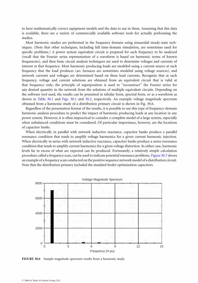
to have mathematically correct equipment models and the data to use in them. Assuming that this data
is available, there are a variety of commercially available software tools for actually performing the
studies.
Most harmonic studies are performed in the frequency domain using sinusoidal steady-state tech-
niques. (Note that other techniques, including full time-domain simulation, are sometimes used for
specific problems.) A power system equivalent circuit is prepared for each frequency to be analyzed
(recall that the Fourier series representation of a waveform is based on harmonic terms of known
frequencies), and then basic circuit analysis techniques are used to determine voltages and currents of
interest at that frequency. Most harmonic producing loads are modeled using a current source at each
frequency that the load produces (arc furnaces are sometimes modeled using voltage sources), and
network currents and voltages are determined based on these load currents. Recognize that at each
frequency, voltage and current solutions are obtained from an equivalent circuit that is valid at
that frequency only; the principle of superposition is used to ‘‘reconstruct’’ the Fourier series for
any desired quantity in the network from the solutions of multiple equivalent circuits. Depending on
the software tool used, the results can be presented in tabular form, spectral form, or as a waveform as
shown in Table 30.1 and Figs. 30.1 and 30.2, respectively. An example voltage magnitude spectrum
obtained from a harmonic study of a distribution primary circuit is shown in Fig. 30.6.
Regardless of the presentation format of the results, it is possible to use this type of frequency-domain
harmonic analysis procedure to predict the impact of harmonic producing loads at any location in any
power system. However, it is often impractical to consider a complete model of a large system, especially
when unbalanced conditions must be considered. Of particular importance, however, are the locations
of capacitor banks.
When electrically in parallel with network inductive reactance, capacitor banks produce a parallel
resonance condition that tends to amplify voltage harmonics for a given current harmonic injection.
When electrically in series with network inductive reactance, capacitor banks produce a series resonance
condition that tends to amplify current harmonics for a given voltage distortion. In either case, harmonic
levels far in excess of what are expected can be produced. Fortunately, a relatively simple calculation
procedure called a frequency scan, can be used to indicate potential resonance problems. Figure 30.7 shows
an example of a frequency scan conducted on the positive sequence network model of a distribution circuit.
Note that the distribution primary included the standard feeder optimization capacitors.
8000
6000
4000
2000
00 3 6
Frequency (H pu)
Voltage Magnitude Spectrum
9 12 15
FIGURE 30.6 Sample magnitude spectrum results from a harmonic study.
� 2006 by Taylor & Francis Group, LLC.
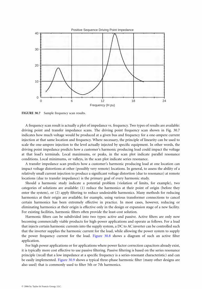
40
30
20
10
00 6 12
Frequency (H pu)
Positive Sequence Driving Point Impedance
18 24
FIGURE 30.7 Sample frequency scan results.
A frequency scan result is actually a plot of impedance vs. frequency. Two types of results are available:
driving point and transfer impedance scans. The driving point frequency scan shown in Fig. 30.7
indicates how much voltage would be produced at a given bus and frequency for a one-ampere current
injection at that same location and frequency. Where necessary, the principle of linearity can be used to
scale the one-ampere injection to the level actually injected by specific equipment. In other words, the
driving point impedance predicts how a customer’s harmonic producing load could impact the voltage
at that load’s terminals. Local maximums, or peaks, in the scan plot indicate parallel resonance
conditions. Local minimums, or valleys, in the scan plot indicate series resonance.
A transfer impedance scan predicts how a customer’s harmonic producing load at one location can
impact voltage distortions at other (possibly very remote) locations. In general, to assess the ability of a
relatively small current injection to produce a significant voltage distortion (due to resonance) at remote
locations (due to transfer impedance) is the primary goal of every harmonic study.
Should a harmonic study indicate a potential problem (violation of limits, for example), two
categories of solutions are available: (1) reduce the harmonics at their point of origin (before they
enter the system), or (2) apply filtering to reduce undesirable harmonics. Many methods for reducing
harmonics at their origin are available; for example, using various transformer connections to cancel
certain harmonics has been extremely effective in practice. In most cases, however, reducing or
eliminating harmonics at their origin is effective only in the design or expansion stage of a new facility.
For existing facilities, harmonic filters often provide the least-cost solution.
Harmonic filters can be subdivided into two types: active and passive. Active filters are only now
becoming commercially viable products for high-power applications and operate as follows. For a load
that injects certain harmonic currents into the supply system, a DC to AC inverter can be controlled such
that the inverter supplies the harmonic current for the load, while allowing the power system to supply
the power frequency current for the load. Figure 30.8 shows a diagram of such an active filter
application.
For high power applications or for applications where power factor correction capacitors already exist,
it is typically more cost effective to use passive filtering. Passive filtering is based on the series resonance
principle (recall that a low impedance at a specific frequency is a series-resonant characteristic) and can
be easily implemented. Figure 30.9 shows a typical three-phase harmonic filter (many other designs are
also used) that is commonly used to filter 5th or 7th harmonics.
� 2006 by Taylor & Francis Group, LLC.
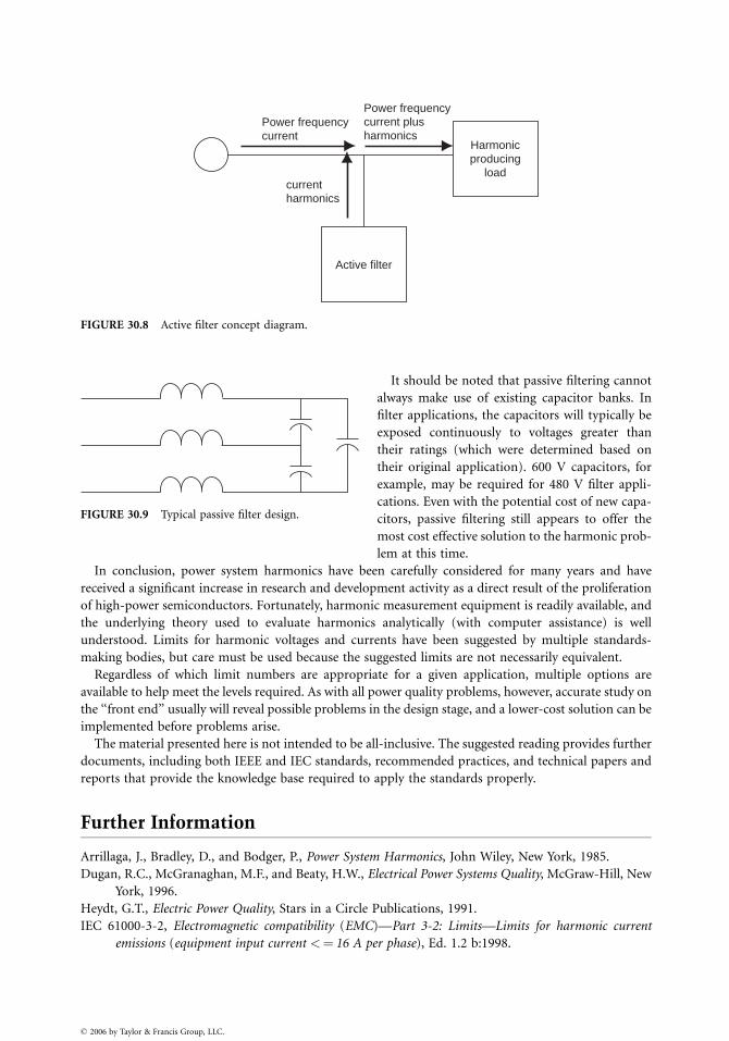
Power frequencycurrent
currentharmonics
Power frequencycurrent plusharmonics
Harmonicproducing
load
Active filter
FIGURE 30.8 Active filter concept diagram.
FIGURE 30.9 Typical passive filter design.
� 2006 by Taylor & Francis Group, LLC.
It should be noted that passive filtering cannot
always make use of existing capacitor banks. In
filter applications, the capacitors will typically be
exposed continuously to voltages greater than
their ratings (which were determined based on
their original application). 600 V capacitors, for
example, may be required for 480 V filter appli-
cations. Even with the potential cost of new capa-
citors, passive filtering still appears to offer the
most cost effective solution to the harmonic prob-
lem at this time.
In conclusion, power system harmonics have been carefully considered for many years and have
received a significant increase in research and development activity as a direct result of the proliferation
of high-power semiconductors. Fortunately, harmonic measurement equipment is readily available, and
the underlying theory used to evaluate harmonics analytically (with computer assistance) is well
understood. Limits for harmonic voltages and currents have been suggested by multiple standards-
making bodies, but care must be used because the suggested limits are not necessarily equivalent.
Regardless of which limit numbers are appropriate for a given application, multiple options are
available to help meet the levels required. As with all power quality problems, however, accurate study on
the ‘‘front end’’ usually will reveal possible problems in the design stage, and a lower-cost solution can be
implemented before problems arise.
The material presented here is not intended to be all-inclusive. The suggested reading provides further
documents, including both IEEE and IEC standards, recommended practices, and technical papers and
reports that provide the knowledge base required to apply the standards properly.
Further Information
Arrillaga, J., Bradley, D., and Bodger, P., Power System Harmonics, John Wiley, New York, 1985.
Dugan, R.C., McGranaghan, M.F., and Beaty, H.W., Electrical Power Systems Quality, McGraw-Hill, New
York, 1996.
Heydt, G.T., Electric Power Quality, Stars in a Circle Publications, 1991.
IEC 61000-3-2, Electromagnetic compatibility (EMC)—Part 3-2: Limits—Limits for harmonic current
emissions (equipment input current <¼ 16 A per phase), Ed. 1.2 b:1998.

IEC 61000-3-6 TR3, Electromagnetic compatibility (EMC)—Part 3: Limits—Section 6: Assessment of
emission limits for distorting loads in MV and HV power systems—Basic EMC Publication, Ed. 1.0
b:1996.
IEC 61000-4-7, Electromagnetic compatibility (EMC)—Part 4: Testing and measurement techniques-
Section 7: General guide on harmonics and interharmonics measurements and instrumentation, for
power supply systems and equipment connected thereto, Ed. 1.0 b:1991.
IEEE Harmonics Modeling and Simulation Task Force, IEEE Special Publication #98-TP-125-0: IEEE
Tutorial on Harmonics Modeling and Simulation, IEEE Press, 1998.
IEEE Standard 519-1992: Recommended Practices and Requirements for Harmonic Control in Electrical
Power Systems, IEEE Press, April 1993.
Mohan, N., Undeland, T.M., and Robbins, W.P., Power Electronics: Converters, Applications, and Design,
John Wiley, New York, 1989.
P519A Task Force of the Harmonics Working Group and SCC20-Power Quality, Guide for Applying
Harmonic Limits on Power Systems (draft), IEEE, May 1996.
UIE, Guide to Quality of Electrical Supply for Industrial Installations, Part 3: Harmonics, 1998.
� 2006 by Taylor & Francis Group, LLC.

� 2006 by Taylor & Francis Group, LLC.
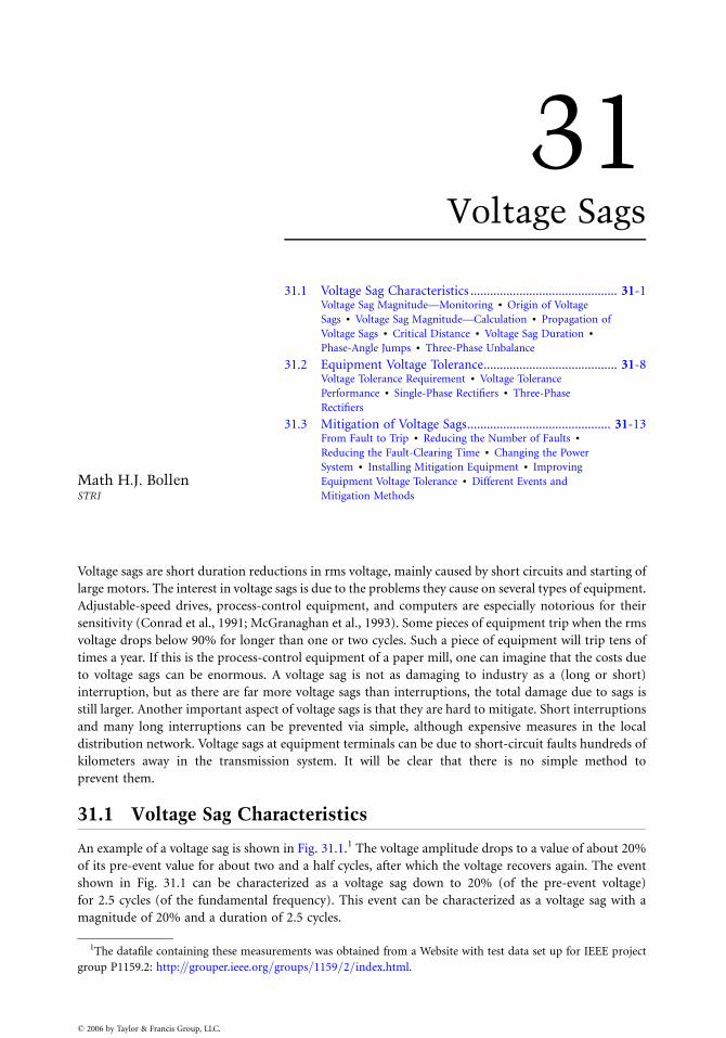
31
1The datafile containing these measure
group P1159.2: http:==grouper.ieee.org=g
� 2006 by Taylor & Francis Group, LLC.
Voltage Sags
Math H.J. BollenSTRI
31.1 Voltage Sag Characteristics ............................................. 31-1Voltage Sag Magnitude—Monitoring . Origin of Voltage
Sags . Voltage Sag Magnitude—Calculation . Propagation of
Voltage Sags . Critical Distance . Voltage Sag Duration .
Phase-Angle Jumps . Three-Phase Unbalance
31.2 Equipment Voltage Tolerance......................................... 31-8Voltage Tolerance Requirement . Voltage Tolerance
Performance . Single-Phase Rectifiers . Three-Phase
Rectifiers
31.3 Mitigation of Voltage Sags............................................ 31-13From Fault to Trip . Reducing the Number of Faults .
Reducing the Fault-Clearing Time . Changing the Power
System . Installing Mitigation Equipment . Improving
Equipment Voltage Tolerance . Different Events and
Mitigation Methods
Voltage sags are short duration reductions in rms voltage, mainly caused by short circuits and starting of
large motors. The interest in voltage sags is due to the problems they cause on several types of equipment.
Adjustable-speed drives, process-control equipment, and computers are especially notorious for their
sensitivity (Conrad et al., 1991; McGranaghan et al., 1993). Some pieces of equipment trip when the rms
voltage drops below 90% for longer than one or two cycles. Such a piece of equipment will trip tens of
times a year. If this is the process-control equipment of a paper mill, one can imagine that the costs due
to voltage sags can be enormous. A voltage sag is not as damaging to industry as a (long or short)
interruption, but as there are far more voltage sags than interruptions, the total damage due to sags is
still larger. Another important aspect of voltage sags is that they are hard to mitigate. Short interruptions
and many long interruptions can be prevented via simple, although expensive measures in the local
distribution network. Voltage sags at equipment terminals can be due to short-circuit faults hundreds of
kilometers away in the transmission system. It will be clear that there is no simple method to
prevent them.
31.1 Voltage Sag Characteristics
An example of a voltage sag is shown in Fig. 31.1.1 The voltage amplitude drops to a value of about 20%
of its pre-event value for about two and a half cycles, after which the voltage recovers again. The event
shown in Fig. 31.1 can be characterized as a voltage sag down to 20% (of the pre-event voltage)
for 2.5 cycles (of the fundamental frequency). This event can be characterized as a voltage sag with a
magnitude of 20% and a duration of 2.5 cycles.
ments was obtained from a Website with test data set up for IEEE project
roups=1159=2=index.html.
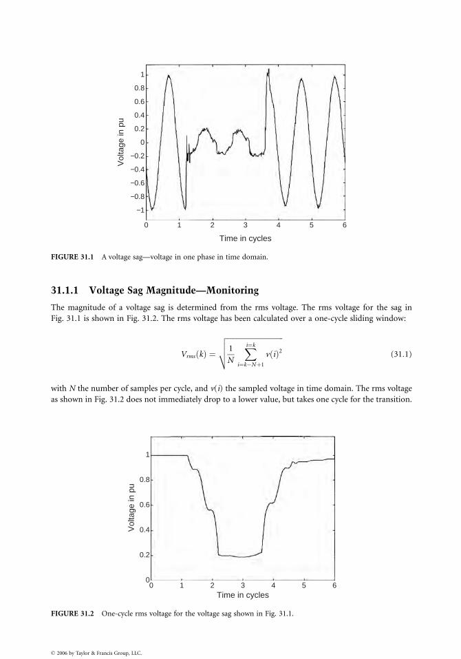
1
0.8
0.6
0.4
0.2
0
0 1 2 3
Time in cycles
Vol
tage
in p
u
4 5 6
−0.2
−0.4
−0.6
−0.8
−1
FIGURE 31.1 A voltage sag—voltage in one phase in time domain.
31.1.1 Voltage Sag Magnitude—Monitoring
The magnitude of a voltage sag is determined from the rms voltage. The rms voltage for the sag in
Fig. 31.1 is shown in Fig. 31.2. The rms voltage has been calculated over a one-cycle sliding window:
Vrms kð Þ ¼
ffiffiffiffiffiffiffiffiffiffiffiffiffiffiffiffiffiffiffiffiffiffiffiffiffiffiffiffiffiffiffi
1
N
X
i¼k
i¼k�Nþ1
v ið Þ2v
u
u
t (31:1)
with N the number of samples per cycle, and v(i) the sampled voltage in time domain. The rms voltage
as shown in Fig. 31.2 does not immediately drop to a lower value, but takes one cycle for the transition.
1
0.8
0.6
0.4
0.2
00 1 2 3
Time in cycles
Vol
tage
in p
u
4 5 6
FIGURE 31.2 One-cycle rms voltage for the voltage sag shown in Fig. 31.1.
� 2006 by Taylor & Francis Group, LLC.
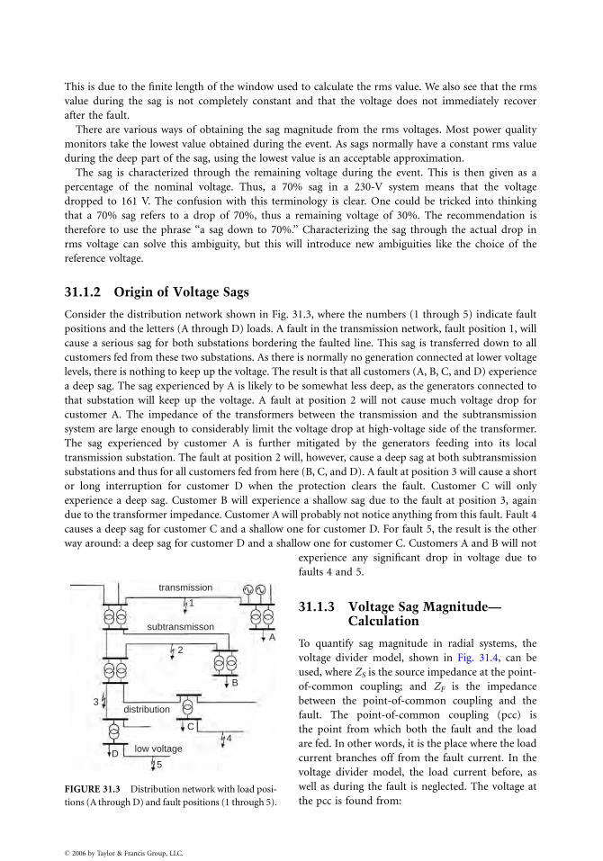
This is due to the finite length of the window used to calculate the rms value. We also see that the rms
value during the sag is not completely constant and that the voltage does not immediately recover
after the fault.
There are various ways of obtaining the sag magnitude from the rms voltages. Most power quality
monitors take the lowest value obtained during the event. As sags normally have a constant rms value
during the deep part of the sag, using the lowest value is an acceptable approximation.
The sag is characterized through the remaining voltage during the event. This is then given as a
percentage of the nominal voltage. Thus, a 70% sag in a 230-V system means that the voltage
dropped to 161 V. The confusion with this terminology is clear. One could be tricked into thinking
that a 70% sag refers to a drop of 70%, thus a remaining voltage of 30%. The recommendation is
therefore to use the phrase ‘‘a sag down to 70%.’’ Characterizing the sag through the actual drop in
rms voltage can solve this ambiguity, but this will introduce new ambiguities like the choice of the
reference voltage.
31.1.2 Origin of Voltage Sags
Consider the distribution network shown in Fig. 31.3, where the numbers (1 through 5) indicate fault
positions and the letters (A through D) loads. A fault in the transmission network, fault position 1, will
cause a serious sag for both substations bordering the faulted line. This sag is transferred down to all
customers fed from these two substations. As there is normally no generation connected at lower voltage
levels, there is nothing to keep up the voltage. The result is that all customers (A, B, C, and D) experience
a deep sag. The sag experienced by A is likely to be somewhat less deep, as the generators connected to
that substation will keep up the voltage. A fault at position 2 will not cause much voltage drop for
customer A. The impedance of the transformers between the transmission and the subtransmission
system are large enough to considerably limit the voltage drop at high-voltage side of the transformer.
The sag experienced by customer A is further mitigated by the generators feeding into its local
transmission substation. The fault at position 2 will, however, cause a deep sag at both subtransmission
substations and thus for all customers fed from here (B, C, and D). A fault at position 3 will cause a short
or long interruption for customer D when the protection clears the fault. Customer C will only
experience a deep sag. Customer B will experience a shallow sag due to the fault at position 3, again
due to the transformer impedance. Customer A will probably not notice anything from this fault. Fault 4
causes a deep sag for customer C and a shallow one for customer D. For fault 5, the result is the other
way around: a deep sag for customer D and a shallow one for customer C. Customers A and B will not
transmission
subtransmisson
distribution
low voltage
1
2A
B
3
D5
4C
FIGURE 31.3 Distribution network with load posi-
tions (A through D) and fault positions (1 through 5).
� 2006 by Taylor & Francis Group, LLC.
experience any significant drop in voltage due to
faults 4 and 5.
31.1.3 Voltage Sag Magnitude—Calculation
To quantify sag magnitude in radial systems, the
voltage divider model, shown in Fig. 31.4, can be
used, where ZS is the source impedance at the point-
of-common coupling; and ZF is the impedance
between the point-of-common coupling and the
fault. The point-of-common coupling (pcc) is
the point from which both the fault and the load
are fed. In other words, it is the place where the load
current branches off from the fault current. In the
voltage divider model, the load current before, as
well as during the fault is neglected. The voltage at
the pcc is found from:
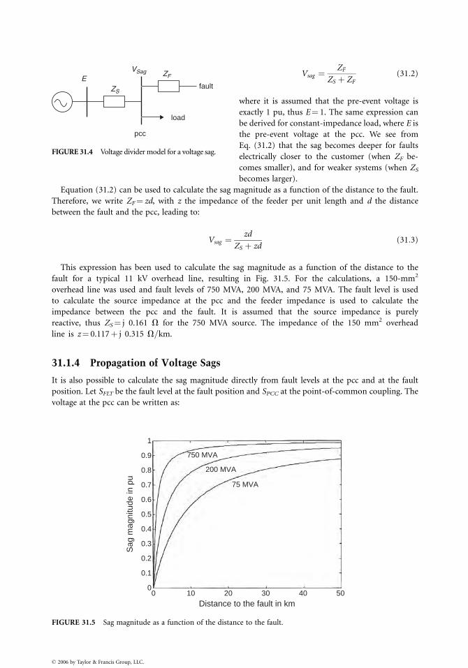
EZS
VSag ZF
pcc
load
fault
FIGURE 31.4 Voltage divider model for a voltage sag.
1
0.9
0.8
0.7
0.6
0.5
0.4
0.3
0.2
0.1
00 10 20
750 MVA
200 MVA
7
Distance t
Sag
mag
nitu
de in
pu
FIGURE 31.5 Sag magnitude as a function of the distan
� 2006 by Taylor & Francis Group, LLC.
Vsag ¼ZF
ZS þ ZF
(31:2)
where it is assumed that the pre-event voltage is
exactly 1 pu, thus E¼ 1. The same expression can
be derived for constant-impedance load, where E is
the pre-event voltage at the pcc. We see from
Eq. (31.2) that the sag becomes deeper for faults
electrically closer to the customer (when ZF be-
comes smaller), and for weaker systems (when ZS
becomes larger).
Equation (31.2) can be used to calculate the sag magnitude as a function of the distance to the fault.
Therefore, we write ZF¼ zd, with z the impedance of the feeder per unit length and d the distance
between the fault and the pcc, leading to:
Vsag ¼zd
ZS þ zd(31:3)
This expression has been used to calculate the sag magnitude as a function of the distance to the
fault for a typical 11 kV overhead line, resulting in Fig. 31.5. For the calculations, a 150-mm2
overhead line was used and fault levels of 750 MVA, 200 MVA, and 75 MVA. The fault level is used
to calculate the source impedance at the pcc and the feeder impedance is used to calculate the
impedance between the pcc and the fault. It is assumed that the source impedance is purely
reactive, thus ZS¼ j 0.161 V for the 750 MVA source. The impedance of the 150 mm2 overhead
line is z¼ 0.117þ j 0.315 V=km.
31.1.4 Propagation of Voltage Sags
It is also possible to calculate the sag magnitude directly from fault levels at the pcc and at the fault
position. Let SFLT be the fault level at the fault position and SPCC at the point-of-common coupling. The
voltage at the pcc can be written as:
30
5 MVA
o the fault in km40 50
ce to the fault.
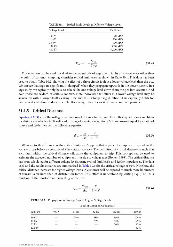
TABLE 30.1 Typical Fault Levels at Different Voltage Levels
Voltage Level Fault Level
400 V 20 MVA
11 kV 200 MVA
33 kV 900 MVA
132 kV 3000 MVA
400 kV 17,000 MVA
Vsag ¼ 1� SFLT
SPCC
(31:4)
This equation can be used to calculate the magnitude of sags due to faults at voltage levels other than
the point-of-common coupling. Consider typical fault levels as shown in Table 30.1. This data has been
used to obtain Table 30.2, showing the effect of a short circuit fault at a lower voltage level than the pcc.
We can see that sags are significantly ‘‘damped’’ when they propagate upwards in the power system. In a
sags study, we typically only have to take faults one voltage level down from the pcc into account. And
even those are seldom of serious concern. Note, however, that faults at a lower voltage level may be
associated with a longer fault-clearing time and thus a longer sag duration. This especially holds for
faults on distribution feeders, where fault-clearing times in excess of one second are possible.
31.1.5 Critical Distance
Equation (31.3) gives the voltage as a function of distance to the fault. From this equation we can obtain
the distance at which a fault will lead to a sag of a certain magnitude V. If we assume equal X=R ratio of
source and feeder, we get the following equation:
dcrit ¼ZS
z� V
1� V(31:5)
We refer to this distance as the critical distance. Suppose that a piece of equipment trips when the
voltage drops below a certain level (the critical voltage). The definition of critical distance is such that
each fault within the critical distance will cause the equipment to trip. This concept can be used to
estimate the expected number of equipment trips due to voltage sags (Bollen, 1998). The critical distance
has been calculated for different voltage levels, using typical fault levels and feeder impedances. The data
used and the results obtained are summarized in Table 30.3 for the critical voltage of 50%. Note how the
critical distance increases for higher voltage levels. A customer will be exposed to much more kilometers
of transmission lines than of distribution feeder. This effect is understood by writing Eq. (31.5) as a
function of the short-circuit current Iflt at the pcc:
dcrit ¼Vnom
zIflt
� V
1� V(31:6)
TABLE 30.2 Propagation of Voltage Sags to Higher Voltage Levels
Point-of-Common Coupling at:
Fault at: 400 V 11 kV 33 kV 132 kV 400 kV
400 V — 90% 98% 99% 100%
11 kV — — 78% 93% 99%
33 kV — — — 70% 95%
132 kV — — — — 82%
� 2006 by Taylor & Francis Group, LLC.
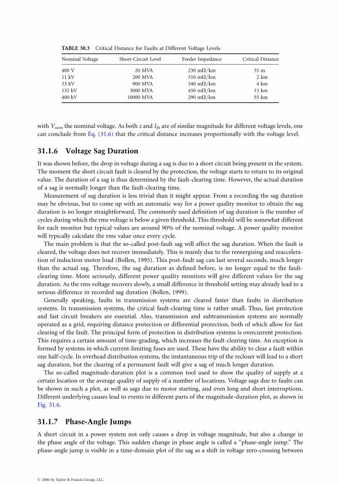
TABLE 30.3 Critical Distance for Faults at Different Voltage Levels
Nominal Voltage Short-Circuit Level Feeder Impedance Critical Distance
400 V 20 MVA 230 mV=km 35 m
11 kV 200 MVA 310 mV=km 2 km
33 kV 900 MVA 340 mV=km 4 km
132 kV 3000 MVA 450 mV=km 13 km
400 kV 10000 MVA 290 mV=km 55 km
with Vnom the nominal voltage. As both z and Iflt are of similar magnitude for different voltage levels, one
can conclude from Eq. (31.6) that the critical distance increases proportionally with the voltage level.
31.1.6 Voltage Sag Duration
It was shown before, the drop in voltage during a sag is due to a short circuit being present in the system.
The moment the short circuit fault is cleared by the protection, the voltage starts to return to its original
value. The duration of a sag is thus determined by the fault-clearing time. However, the actual duration
of a sag is normally longer than the fault-clearing time.
Measurement of sag duration is less trivial than it might appear. From a recording the sag duration
may be obvious, but to come up with an automatic way for a power quality monitor to obtain the sag
duration is no longer straightforward. The commonly used definition of sag duration is the number of
cycles during which the rms voltage is below a given threshold. This threshold will be somewhat different
for each monitor but typical values are around 90% of the nominal voltage. A power quality monitor
will typically calculate the rms value once every cycle.
The main problem is that the so-called post-fault sag will affect the sag duration. When the fault is
cleared, the voltage does not recover immediately. This is mainly due to the reenergizing and reaccelera-
tion of induction motor load (Bollen, 1995). This post-fault sag can last several seconds, much longer
than the actual sag. Therefore, the sag duration as defined before, is no longer equal to the fault-
clearing time. More seriously, different power quality monitors will give different values for the sag
duration. As the rms voltage recovers slowly, a small difference in threshold setting may already lead to a
serious difference in recorded sag duration (Bollen, 1999).
Generally speaking, faults in transmission systems are cleared faster than faults in distribution
systems. In transmission systems, the critical fault-clearing time is rather small. Thus, fast protection
and fast circuit breakers are essential. Also, transmission and subtransmission systems are normally
operated as a grid, requiring distance protection or differential protection, both of which allow for fast
clearing of the fault. The principal form of protection in distribution systems is overcurrent protection.
This requires a certain amount of time-grading, which increases the fault-clearing time. An exception is
formed by systems in which current-limiting fuses are used. These have the ability to clear a fault within
one half-cycle. In overhead distribution systems, the instantaneous trip of the recloser will lead to a short
sag duration, but the clearing of a permanent fault will give a sag of much longer duration.
The so-called magnitude-duration plot is a common tool used to show the quality of supply at a
certain location or the average quality of supply of a number of locations. Voltage sags due to faults can
be shown in such a plot, as well as sags due to motor starting, and even long and short interruptions.
Different underlying causes lead to events in different parts of the magnitude-duration plot, as shown in
Fig. 31.6.
31.1.7 Phase-Angle Jumps
A short circuit in a power system not only causes a drop in voltage magnitude, but also a change in
the phase angle of the voltage. This sudden change in phase angle is called a ‘‘phase-angle jump.’’ The
phase-angle jump is visible in a time-domain plot of the sag as a shift in voltage zero-crossing between
� 2006 by Taylor & Francis Group, LLC.
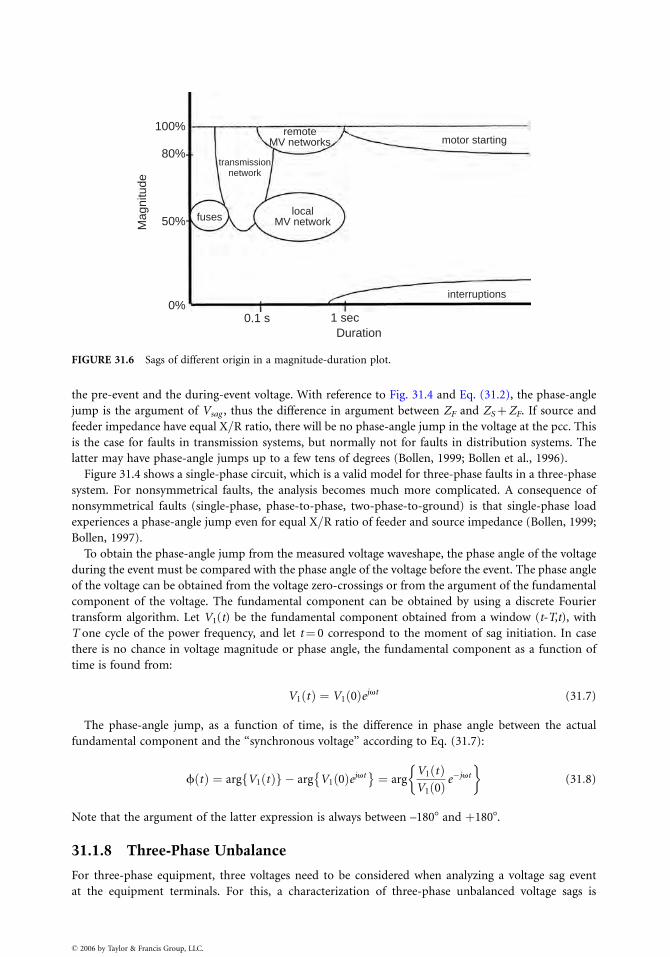
100%
80%
50%
0%0.1 s 1 sec
Duration
Mag
nitu
de
interruptions
motor startingremote
MV networks
localMV network
transmissionnetwork
fuses
FIGURE 31.6 Sags of different origin in a magnitude-duration plot.
the pre-event and the during-event voltage. With reference to Fig. 31.4 and Eq. (31.2), the phase-angle
jump is the argument of Vsag , thus the difference in argument between ZF and ZSþZF. If source and
feeder impedance have equal X=R ratio, there will be no phase-angle jump in the voltage at the pcc. This
is the case for faults in transmission systems, but normally not for faults in distribution systems. The
latter may have phase-angle jumps up to a few tens of degrees (Bollen, 1999; Bollen et al., 1996).
Figure 31.4 shows a single-phase circuit, which is a valid model for three-phase faults in a three-phase
system. For nonsymmetrical faults, the analysis becomes much more complicated. A consequence of
nonsymmetrical faults (single-phase, phase-to-phase, two-phase-to-ground) is that single-phase load
experiences a phase-angle jump even for equal X=R ratio of feeder and source impedance (Bollen, 1999;
Bollen, 1997).
To obtain the phase-angle jump from the measured voltage waveshape, the phase angle of the voltage
during the event must be compared with the phase angle of the voltage before the event. The phase angle
of the voltage can be obtained from the voltage zero-crossings or from the argument of the fundamental
component of the voltage. The fundamental component can be obtained by using a discrete Fourier
transform algorithm. Let V1(t) be the fundamental component obtained from a window (t-T,t), with
T one cycle of the power frequency, and let t¼ 0 correspond to the moment of sag initiation. In case
there is no chance in voltage magnitude or phase angle, the fundamental component as a function of
time is found from:
V1 tð Þ ¼ V1 0ð Þejvt (31:7)
The phase-angle jump, as a function of time, is the difference in phase angle between the actual
fundamental component and the ‘‘synchronous voltage’’ according to Eq. (31.7):
f tð Þ ¼ arg V1 tð Þf g � arg V1 0ð Þejvt� �
¼ argV1 tð ÞV1 0ð Þ e�jvt
� �
(31:8)
Note that the argument of the latter expression is always between –1808 and þ1808.
31.1.8 Three-Phase Unbalance
For three-phase equipment, three voltages need to be considered when analyzing a voltage sag event
at the equipment terminals. For this, a characterization of three-phase unbalanced voltage sags is
� 2006 by Taylor & Francis Group, LLC.
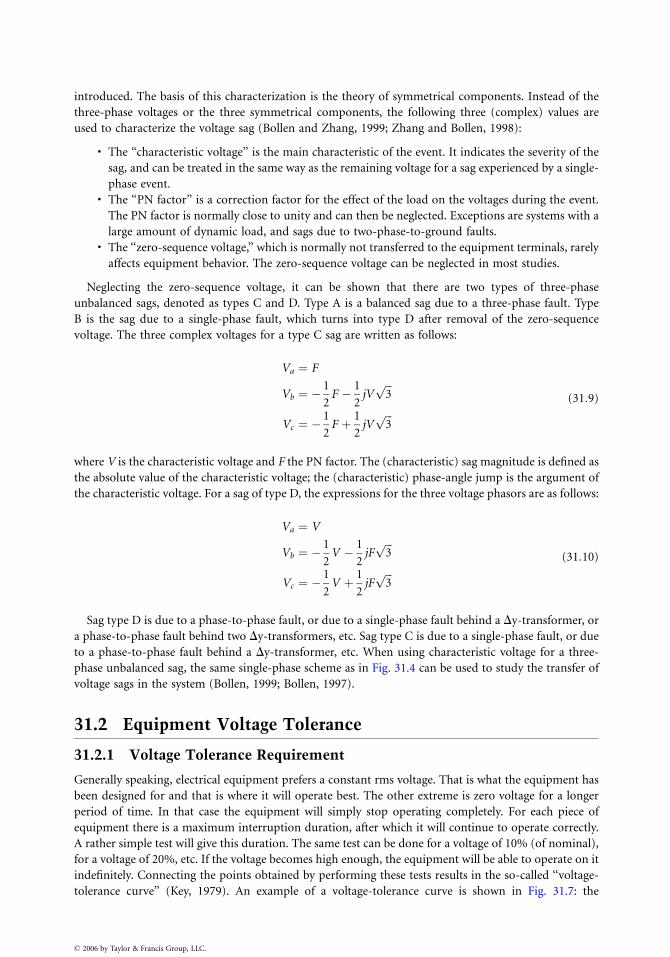
introduced. The basis of this characterization is the theory of symmetrical components. Instead of the
three-phase voltages or the three symmetrical components, the following three (complex) values are
used to characterize the voltage sag (Bollen and Zhang, 1999; Zhang and Bollen, 1998):
. The ‘‘characteristic voltage’’ is the main characteristic of the event. It indicates the severity of the
sag, and can be treated in the same way as the remaining voltage for a sag experienced by a single-
phase event.. The ‘‘PN factor’’ is a correction factor for the effect of the load on the voltages during the event.
The PN factor is normally close to unity and can then be neglected. Exceptions are systems with a
large amount of dynamic load, and sags due to two-phase-to-ground faults.. The ‘‘zero-sequence voltage,’’ which is normally not transferred to the equipment terminals, rarely
affects equipment behavior. The zero-sequence voltage can be neglected in most studies.
Neglecting the zero-sequence voltage, it can be shown that there are two types of three-phase
unbalanced sags, denoted as types C and D. Type A is a balanced sag due to a three-phase fault. Type
B is the sag due to a single-phase fault, which turns into type D after removal of the zero-sequence
voltage. The three complex voltages for a type C sag are written as follows:
Va ¼ F
Vb ¼ �1
2F � 1
2jV
ffiffiffi
3p
Vc ¼ �1
2F þ 1
2jV
ffiffiffi
3p
(31:9)
where V is the characteristic voltage and F the PN factor. The (characteristic) sag magnitude is defined as
the absolute value of the characteristic voltage; the (characteristic) phase-angle jump is the argument of
the characteristic voltage. For a sag of type D, the expressions for the three voltage phasors are as follows:
Va ¼ V
Vb ¼ �1
2V � 1
2jF
ffiffiffi
3p
Vc ¼ �1
2V þ 1
2jF
ffiffiffi
3p
(31:10)
Sag type D is due to a phase-to-phase fault, or due to a single-phase fault behind a Dy-transformer, or
a phase-to-phase fault behind two Dy-transformers, etc. Sag type C is due to a single-phase fault, or due
to a phase-to-phase fault behind a Dy-transformer, etc. When using characteristic voltage for a three-
phase unbalanced sag, the same single-phase scheme as in Fig. 31.4 can be used to study the transfer of
voltage sags in the system (Bollen, 1999; Bollen, 1997).
31.2 Equipment Voltage Tolerance
31.2.1 Voltage Tolerance Requirement
Generally speaking, electrical equipment prefers a constant rms voltage. That is what the equipment has
been designed for and that is where it will operate best. The other extreme is zero voltage for a longer
period of time. In that case the equipment will simply stop operating completely. For each piece of
equipment there is a maximum interruption duration, after which it will continue to operate correctly.
A rather simple test will give this duration. The same test can be done for a voltage of 10% (of nominal),
for a voltage of 20%, etc. If the voltage becomes high enough, the equipment will be able to operate on it
indefinitely. Connecting the points obtained by performing these tests results in the so-called ‘‘voltage-
tolerance curve’’ (Key, 1979). An example of a voltage-tolerance curve is shown in Fig. 31.7: the
� 2006 by Taylor & Francis Group, LLC.
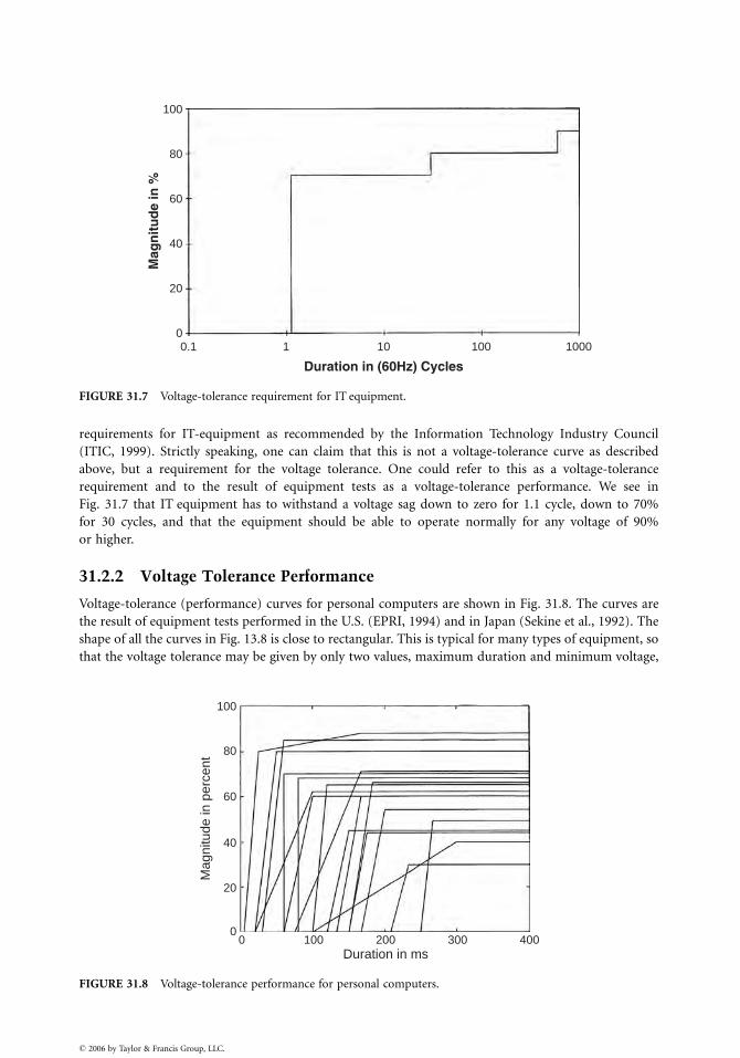
100
80
60
40
20
00.1 1 10
Duration in (60Hz) Cycles
Mag
nit
ud
e in
%
100 1000
FIGURE 31.7 Voltage-tolerance requirement for IT equipment.
requirements for IT-equipment as recommended by the Information Technology Industry Council
(ITIC, 1999). Strictly speaking, one can claim that this is not a voltage-tolerance curve as described
above, but a requirement for the voltage tolerance. One could refer to this as a voltage-tolerance
requirement and to the result of equipment tests as a voltage-tolerance performance. We see in
Fig. 31.7 that IT equipment has to withstand a voltage sag down to zero for 1.1 cycle, down to 70%
for 30 cycles, and that the equipment should be able to operate normally for any voltage of 90%
or higher.
31.2.2 Voltage Tolerance Performance
Voltage-tolerance (performance) curves for personal computers are shown in Fig. 31.8. The curves are
the result of equipment tests performed in the U.S. (EPRI, 1994) and in Japan (Sekine et al., 1992). The
shape of all the curves in Fig. 13.8 is close to rectangular. This is typical for many types of equipment, so
that the voltage tolerance may be given by only two values, maximum duration and minimum voltage,
100
80
60
40
20
00 100 200
Duration in ms
Mag
nitu
de in
per
cent
300 400
FIGURE 31.8 Voltage-tolerance performance for personal computers.
� 2006 by Taylor & Francis Group, LLC.
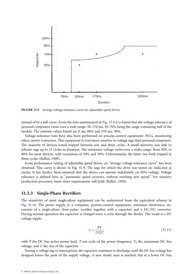
100%
85%
70%
50%
33ms 100ms 170ms 1000ms
Mag
nitu
de
Duration
FIGURE 31.9 Average voltage-tolerance curve for adjustable-speed drives.
instead of by a full curve. From the tests summarized in Fig. 13.8 it is found that the voltage tolerance of
personal computers varies over a wide range: 30–170 ms, 50–70% being the range containing half of the
models. The extreme values found are 8 ms, 88% and 210 ms, 30%.
Voltage-tolerance tests have also been performed on process-control equipment: PLCs, monitoring
relays, motor contactors. This equipment is even more sensitive to voltage sags than personal computers.
The majority of devices tested tripped between one and three cycles. A small minority was able to
tolerate sags up to 15 cycles in duration. The minimum voltage varies over a wider range: from 50% to
80% for most devices, with exceptions of 20% and 30%. Unfortunately, the latter two both tripped in
three cycles (Bollen, 1999).
From performance testing of adjustable-speed drives, an ‘‘average voltage-tolerance curve’’ has been
obtained. This curve is shown in Fig. 31.9. The sags for which the drive was tested are indicated as
circles. It has further been assumed that the drives can operate indefinitely on 85% voltage. Voltage
tolerance is defined here as ‘‘automatic speed recovery, without reaching zero speed.’’ For sensitive
production processes, more strict requirements will hold (Bollen, 1999).
31.2.3 Single-Phase Rectifiers
The sensitivity of most single-phase equipment can be understood from the equivalent scheme in
Fig. 31.10. The power supply to a computer, process-control equipment, consumer electronics, etc.
consists of a single-phase (four-pulse) rectifier together with a capacitor and a DC=DC converter.
During normal operation the capacitor is charged twice a cycle through the diodes. The result is a DC
voltage ripple:
e ¼ PT
2V 20 C
(31:11)
with P the DC bus active-power load, T one cycle of the power frequency, V0 the maximum DC bus
voltage, and C the size of the capacitor.
During a voltage sag or interruption, the capacitor continues to discharge until the DC bus voltage has
dropped below the peak of the supply voltage. A new steady state is reached, but at a lower DC bus
� 2006 by Taylor & Francis Group, LLC.
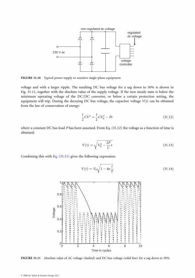
230 V ac
non-regulated dc voltageregulateddc voltage
voltagecontroller
FIGURE 31.10 Typical power supply to sensitive single-phase equipment.
voltage and with a larger ripple. The resulting DC bus voltage for a sag down to 50% is shown in
Fig. 31.11, together with the absolute value of the supply voltage. If the new steady state is below the
minimum operating voltage of the DC=DC converter, or below a certain protection setting, the
equipment will trip. During the decaying DC bus voltage, the capacitor voltage V(t) can be obtained
from the law of conservation of energy:
1
2CV 2 ¼ 1
2CV 2
0 � Pt (31:12)
where a constant DC bus load P has been assumed. From Eq. (31.12) the voltage as a function of time is
obtained:
V tð Þ ¼ffiffiffiffiffiffiffiffiffiffiffiffiffiffiffiffiffiffiffiffi
V 20 �
2P
Ct
r
(31:13)
Combining this with Eq. (31.11) gives the following expression:
V tð Þ ¼ V0
ffiffiffiffiffiffiffiffiffiffiffiffiffiffiffiffiffi
1� 4et
T
r
(31:14)
1
0.8
0.6
0.4
0.2
00 2 4
Time in cycles
Vol
tage
6 8 10
FIGURE 31.11 Absolute value of AC voltage (dashed) and DC bus voltage (solid line) for a sag down to 50%.
� 2006 by Taylor & Francis Group, LLC.
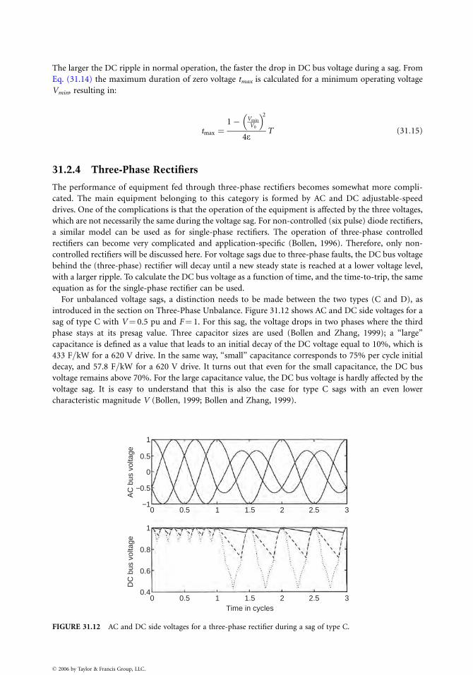
The larger the DC ripple in normal operation, the faster the drop in DC bus voltage during a sag. From
Eq. (31.14) the maximum duration of zero voltage tmax is calculated for a minimum operating voltage
Vmin, resulting in:
tmax ¼1� Vmin
V0
� �2
4eT (31:15)
31.2.4 Three-Phase Rectifiers
The performance of equipment fed through three-phase rectifiers becomes somewhat more compli-
cated. The main equipment belonging to this category is formed by AC and DC adjustable-speed
drives. One of the complications is that the operation of the equipment is affected by the three voltages,
which are not necessarily the same during the voltage sag. For non-controlled (six pulse) diode rectifiers,
a similar model can be used as for single-phase rectifiers. The operation of three-phase controlled
rectifiers can become very complicated and application-specific (Bollen, 1996). Therefore, only non-
controlled rectifiers will be discussed here. For voltage sags due to three-phase faults, the DC bus voltage
behind the (three-phase) rectifier will decay until a new steady state is reached at a lower voltage level,
with a larger ripple. To calculate the DC bus voltage as a function of time, and the time-to-trip, the same
equation as for the single-phase rectifier can be used.
For unbalanced voltage sags, a distinction needs to be made between the two types (C and D), as
introduced in the section on Three-Phase Unbalance. Figure 31.12 shows AC and DC side voltages for a
sag of type C with V¼ 0.5 pu and F¼ 1. For this sag, the voltage drops in two phases where the third
phase stays at its presag value. Three capacitor sizes are used (Bollen and Zhang, 1999); a ‘‘large’’
capacitance is defined as a value that leads to an initial decay of the DC voltage equal to 10%, which is
433 F=kW for a 620 V drive. In the same way, ‘‘small’’ capacitance corresponds to 75% per cycle initial
decay, and 57.8 F=kW for a 620 V drive. It turns out that even for the small capacitance, the DC bus
voltage remains above 70%. For the large capacitance value, the DC bus voltage is hardly affected by the
voltage sag. It is easy to understand that this is also the case for type C sags with an even lower
characteristic magnitude V (Bollen, 1999; Bollen and Zhang, 1999).
00.4
0.6
0.8
1
−1
0
1
−0.5
0.5
0.5 1 1.5Time in cycles
DC
bus
vol
tage
AC
bus
vol
tage
2.52 3
0 0.5 1 1.5 2.52 3
FIGURE 31.12 AC and DC side voltages for a three-phase rectifier during a sag of type C.
� 2006 by Taylor & Francis Group, LLC.
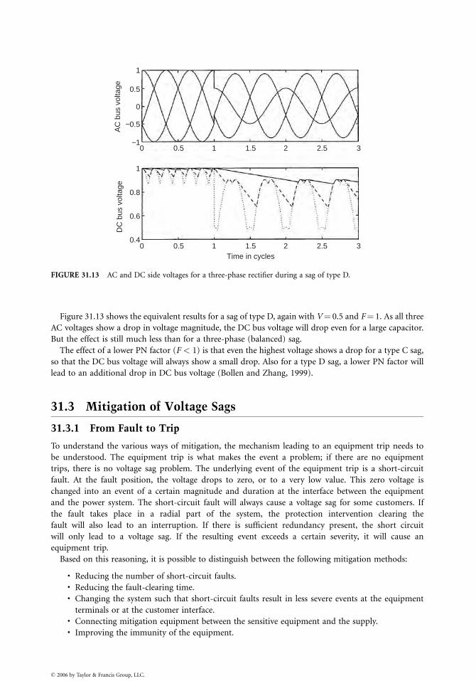
0.40 0.5 1 21.5
Time in cycles2.5 3
0 0.5 1 21.5 2.5 3
0.6
DC
bus
vol
tage
AC
bus
vol
tage
0.8
1
1
0.5
−0.5
−1
0
FIGURE 31.13 AC and DC side voltages for a three-phase rectifier during a sag of type D.
Figure 31.13 shows the equivalent results for a sag of type D, again with V¼ 0.5 and F¼ 1. As all three
AC voltages show a drop in voltage magnitude, the DC bus voltage will drop even for a large capacitor.
But the effect is still much less than for a three-phase (balanced) sag.
The effect of a lower PN factor (F < 1) is that even the highest voltage shows a drop for a type C sag,
so that the DC bus voltage will always show a small drop. Also for a type D sag, a lower PN factor will
lead to an additional drop in DC bus voltage (Bollen and Zhang, 1999).
31.3 Mitigation of Voltage Sags
31.3.1 From Fault to Trip
To understand the various ways of mitigation, the mechanism leading to an equipment trip needs to
be understood. The equipment trip is what makes the event a problem; if there are no equipment
trips, there is no voltage sag problem. The underlying event of the equipment trip is a short-circuit
fault. At the fault position, the voltage drops to zero, or to a very low value. This zero voltage is
changed into an event of a certain magnitude and duration at the interface between the equipment
and the power system. The short-circuit fault will always cause a voltage sag for some customers. If
the fault takes place in a radial part of the system, the protection intervention clearing the
fault will also lead to an interruption. If there is sufficient redundancy present, the short circuit
will only lead to a voltage sag. If the resulting event exceeds a certain severity, it will cause an
equipment trip.
Based on this reasoning, it is possible to distinguish between the following mitigation methods:
. Reducing the number of short-circuit faults.
. Reducing the fault-clearing time.
. Changing the system such that short-circuit faults result in less severe events at the equipment
terminals or at the customer interface.. Connecting mitigation equipment between the sensitive equipment and the supply.. Improving the immunity of the equipment.
� 2006 by Taylor & Francis Group, LLC.
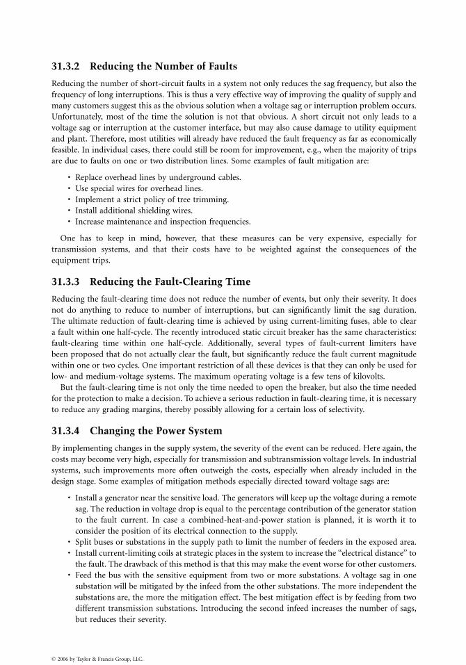
31.3.2 Reducing the Number of Faults
Reducing the number of short-circuit faults in a system not only reduces the sag frequency, but also the
frequency of long interruptions. This is thus a very effective way of improving the quality of supply and
many customers suggest this as the obvious solution when a voltage sag or interruption problem occurs.
Unfortunately, most of the time the solution is not that obvious. A short circuit not only leads to a
voltage sag or interruption at the customer interface, but may also cause damage to utility equipment
and plant. Therefore, most utilities will already have reduced the fault frequency as far as economically
feasible. In individual cases, there could still be room for improvement, e.g., when the majority of trips
are due to faults on one or two distribution lines. Some examples of fault mitigation are:
. Replace overhead lines by underground cables.
. Use special wires for overhead lines.
. Implement a strict policy of tree trimming.
. Install additional shielding wires.
. Increase maintenance and inspection frequencies.
One has to keep in mind, however, that these measures can be very expensive, especially for
transmission systems, and that their costs have to be weighted against the consequences of the
equipment trips.
31.3.3 Reducing the Fault-Clearing Time
Reducing the fault-clearing time does not reduce the number of events, but only their severity. It does
not do anything to reduce to number of interruptions, but can significantly limit the sag duration.
The ultimate reduction of fault-clearing time is achieved by using current-limiting fuses, able to clear
a fault within one half-cycle. The recently introduced static circuit breaker has the same characteristics:
fault-clearing time within one half-cycle. Additionally, several types of fault-current limiters have
been proposed that do not actually clear the fault, but significantly reduce the fault current magnitude
within one or two cycles. One important restriction of all these devices is that they can only be used for
low- and medium-voltage systems. The maximum operating voltage is a few tens of kilovolts.
But the fault-clearing time is not only the time needed to open the breaker, but also the time needed
for the protection to make a decision. To achieve a serious reduction in fault-clearing time, it is necessary
to reduce any grading margins, thereby possibly allowing for a certain loss of selectivity.
31.3.4 Changing the Power System
By implementing changes in the supply system, the severity of the event can be reduced. Here again, the
costs may become very high, especially for transmission and subtransmission voltage levels. In industrial
systems, such improvements more often outweigh the costs, especially when already included in the
design stage. Some examples of mitigation methods especially directed toward voltage sags are:
. Install a generator near the sensitive load. The generators will keep up the voltage during a remote
sag. The reduction in voltage drop is equal to the percentage contribution of the generator station
to the fault current. In case a combined-heat-and-power station is planned, it is worth it to
consider the position of its electrical connection to the supply.. Split buses or substations in the supply path to limit the number of feeders in the exposed area.. Install current-limiting coils at strategic places in the system to increase the ‘‘electrical distance’’ to
the fault. The drawback of this method is that this may make the event worse for other customers.. Feed the bus with the sensitive equipment from two or more substations. A voltage sag in one
substation will be mitigated by the infeed from the other substations. The more independent the
substations are, the more the mitigation effect. The best mitigation effect is by feeding from two
different transmission substations. Introducing the second infeed increases the number of sags,
but reduces their severity.
� 2006 by Taylor & Francis Group, LLC.
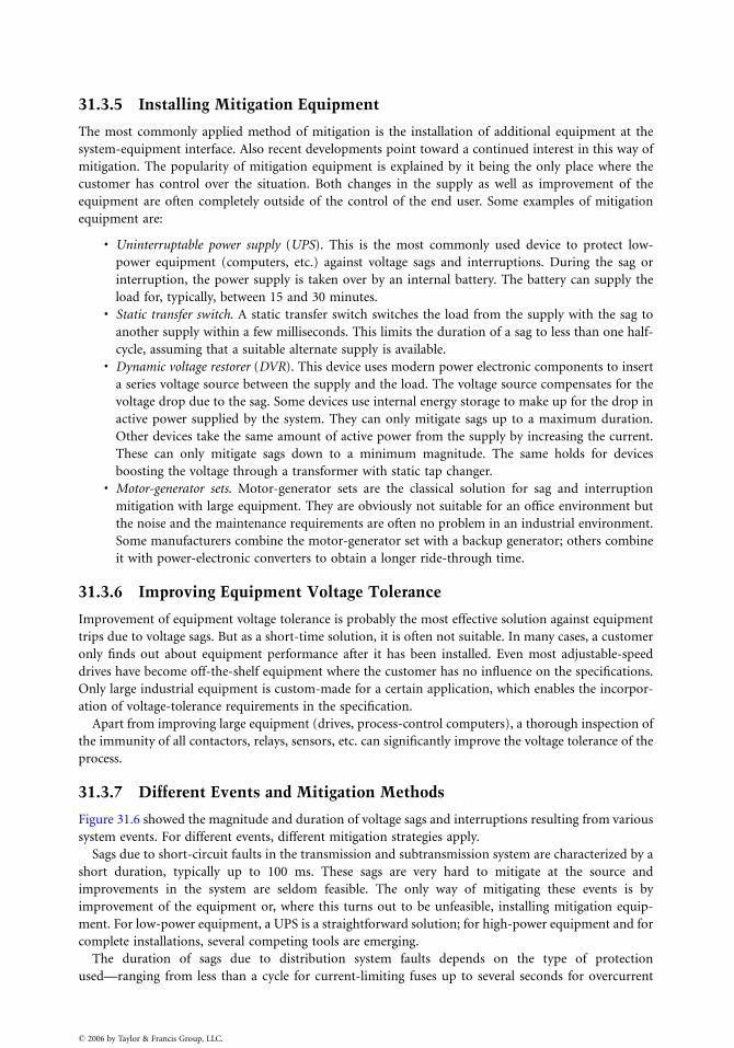
31.3.5 Installing Mitigation Equipment
The most commonly applied method of mitigation is the installation of additional equipment at the
system-equipment interface. Also recent developments point toward a continued interest in this way of
mitigation. The popularity of mitigation equipment is explained by it being the only place where the
customer has control over the situation. Both changes in the supply as well as improvement of the
equipment are often completely outside of the control of the end user. Some examples of mitigation
equipment are:
. Uninterruptable power supply (UPS). This is the most commonly used device to protect low-
power equipment (computers, etc.) against voltage sags and interruptions. During the sag or
interruption, the power supply is taken over by an internal battery. The battery can supply the
load for, typically, between 15 and 30 minutes.. Static transfer switch. A static transfer switch switches the load from the supply with the sag to
another supply within a few milliseconds. This limits the duration of a sag to less than one half-
cycle, assuming that a suitable alternate supply is available.. Dynamic voltage restorer (DVR). This device uses modern power electronic components to insert
a series voltage source between the supply and the load. The voltage source compensates for the
voltage drop due to the sag. Some devices use internal energy storage to make up for the drop in
active power supplied by the system. They can only mitigate sags up to a maximum duration.
Other devices take the same amount of active power from the supply by increasing the current.
These can only mitigate sags down to a minimum magnitude. The same holds for devices
boosting the voltage through a transformer with static tap changer.. Motor-generator sets. Motor-generator sets are the classical solution for sag and interruption
mitigation with large equipment. They are obviously not suitable for an office environment but
the noise and the maintenance requirements are often no problem in an industrial environment.
Some manufacturers combine the motor-generator set with a backup generator; others combine
it with power-electronic converters to obtain a longer ride-through time.
31.3.6 Improving Equipment Voltage Tolerance
Improvement of equipment voltage tolerance is probably the most effective solution against equipment
trips due to voltage sags. But as a short-time solution, it is often not suitable. In many cases, a customer
only finds out about equipment performance after it has been installed. Even most adjustable-speed
drives have become off-the-shelf equipment where the customer has no influence on the specifications.
Only large industrial equipment is custom-made for a certain application, which enables the incorpor-
ation of voltage-tolerance requirements in the specification.
Apart from improving large equipment (drives, process-control computers), a thorough inspection of
the immunity of all contactors, relays, sensors, etc. can significantly improve the voltage tolerance of the
process.
31.3.7 Different Events and Mitigation Methods
Figure 31.6 showed the magnitude and duration of voltage sags and interruptions resulting from various
system events. For different events, different mitigation strategies apply.
Sags due to short-circuit faults in the transmission and subtransmission system are characterized by a
short duration, typically up to 100 ms. These sags are very hard to mitigate at the source and
improvements in the system are seldom feasible. The only way of mitigating these events is by
improvement of the equipment or, where this turns out to be unfeasible, installing mitigation equip-
ment. For low-power equipment, a UPS is a straightforward solution; for high-power equipment and for
complete installations, several competing tools are emerging.
The duration of sags due to distribution system faults depends on the type of protection
used—ranging from less than a cycle for current-limiting fuses up to several seconds for overcurrent
� 2006 by Taylor & Francis Group, LLC.

relays in underground or industrial distribution systems. The long sag duration also enables equip-
ment to trip due to faults on distribution feeders fed from other HV=MV substations. For deep
long-duration sags, equipment improvement becomes more difficult and system improvement easier.
The latter could well become the preferred solution, although a critical assessment of the various options
is certainly needed.
Sags due to faults in remote distribution systems and sags due to motor starting should not lead to
equipment tripping for sags down to 85%. If there are problems, the equipment needs to be improved. If
equipment trips occur for long-duration sags in the 70–80% magnitude range, changes in the system
have to be considered as an option.
For interruptions, especially the longer ones, equipment improvement is no longer feasible. System
improvements or a UPS in combination with an emergency generator are possible solutions here.
References
Bollen, M.H.J., Characterization of voltage sags experienced by three-phase adjustable-speed drives,
IEEE Trans. on Power Delivery, 12, 4, 1666–1671, Oct. 1997.
Bollen, M.H.J., The influence of motor reacceleration on voltage sags, IEEE Trans. on Ind. Appl., 31, 4,
667–674, July 1995.
Bollen, M.H.J., Method of critical distances for stochastic assessment of voltage sags, IEE Proceedings—
Generation, Transmission and Distribution, 145, 1, 70–76, Jan. 1998.
Bollen, M.H.J., Solving Power Quality Problems, Voltage Sags and Interruptions, IEEE Press, 1999.
Bollen, M.H.J., Wang, P., Jenkins, N., Analysis and consequences of the phase jump associated with a
voltage sag, in Power Systems Computation Conference, Dresden, Germany, Aug. 1996.
Bollen, M.H.J., Zhang, L.D., Analysis of voltage tolerance of adjustable-speed drives for three-phase
balanced and unbalanced sags, in IEEE Industrial and Commercial Power Systems Technical
Conference, Sparks, Nevada, May 1999. Scheduled to appear in IEEE Transactions on Industry
Applications, May=June 2000.
Conrad, L., Little, K., Grigg, C., Predicting and preventing problems associated with remote fault-
clearing voltage dips, IEEE Trans. on Ind. Appl., 27, 1, 167–172, Jan. 1991.
Information Technology Industry Council, Interteq, http:==www.itic.com (1999).
Key, T.S., Diagnosing power-quality related computer problems, IEEE Trans. on Ind. Appl., 15, 4,
381–393, July 1979.
McGranaghan, M.F., Mueller, D.R., Samotej, M.J., Voltage sags in industrial power systems, IEEE Trans.
on Ind. Appl., 29, 2, 397–403, March 1993.
Morgan, L., Power Quality Event Characterization (1159.2), Duke Power, (updated Dec. 29, 1999),
http:==grouper.ieee.org=groups=1159=21index.html.
PQTN Brief 7: Undervoltage Ride-through Performance of Off-the-Shelf Personal Computers, EPRI
Power Electronics Application Centre, Knoxville, TN, 1994.
Sekine, Y., Yamamoto, T., Mori, S., Saito, N., Kurokawa, H., Present state of momentary voltage dip
interferences and the countermeasures in Japan, Int. Conf. on Large Electric Networks (CIGRE),
34th Session, Paris, France, Sept. 1992.
Zhang, L.D., Bollen, M.H.J., A method for characterizing unbalanced voltage dips (sags) with symmet-
rical components, IEEE Power Engineering Review, 18, 7, 50–52, July 1998.
Further Information
European standard EN-50160, Voltage Characteristics of Electricity Supplied by Public Distribution
Systems, CENELEC, Brussels, Belgium, 1994.
IEEE Recommended Practice for Monitoring Electric Power Quality, IEEE Std. 1159–1995, IEEE,
New York, 1995.
� 2006 by Taylor & Francis Group, LLC.

IEEE Recommended Practice for Powering and Grounding Sensitive Electronic Equipment, IEEE Std.
1100–1992.
IEEE Recommended Practice for the Design of Reliable Industrial and Commercial Power Systems (The
Gold Book), IEEE Std. 493–1997.
IEEE Recommended Practice for Evaluating Electric Power System Compatibility with Electronic Process
Equipment, IEEE Std. 1346–1998.
IEC 61000-4-11, Electromagnetic Compatibility (EMC) Voltage Dips, Short Interruptions and Voltage
Variations Immunity Tests.
Bollen, M.H.J., Tayjasajant, T., Yalcinkaya, G., Assessment of the number of voltage sags experienced by a
large industrial customer, IEEE Trans. on Ind. Appl., 33, 6, 1465–1471, Nov. 1997.
Bollen, M.H.J., Fast assessment methods for voltage sags in distribution systems, IEEE Trans. on Ind.
Appl., 31, 6, 1414–1423, Nov. 1996.
Collins, E.R., Morgan, R.L., A three-phase sag generator for testing industrial equipment, IEEE Trans. on
Power Delivery, 11, 1, 526–532, Jan. 1996.
Conrad, L.E., Bollen, M.H.J., Voltage sag coordination for reliable plant operation, IEEE Trans. on Ind.
Appl., 33, 6, 1459–1464, Nov. 1997.
Diliberti, T.W., Wagner, V.E., Staniak, J.P., Sheppard, S.L., Orfloff, T.L., Power quality requirements of a
large industrial user: a case study, IEEE Industrial and Commercial Power Systems Technical
Conference, Detroit, MI, May 1990, 1–4.
Dorr, D.S., Point of utilization power quality study results, IEEE Trans. on Ind. Appl., 31, 4, 658–666,
July 1995.
Dorr, D.S., Hughes, M.B., Gruzs, T.M., Jurewicz, R.E., McClaine, J.L., Interpreting recent power quality
surveys to define the electrical environment, IEEE Trans. on Ind. Appl., 33, 6, 1480–1487, Nov. 1997.
Dorr, D.S., Mansoor, A., Morinec, A.G., Worley, J.C., Effects of power line voltage variations on
different types of 400-W high-pressure sodium ballasts, IEEE Trans. on Ind. Appl., 33, 2,
472–476, March 1997.
Dugan, R.C., McGranaghan, M.F., Beaty, H.W., Electric Power Systems Quality, McGraw-Hill,
New York, 1996.
Gunther, E.W., Mehta, H., A survey of distribution system power quality—Preliminary results, IEEE
Trans. on Power Delivery, 10, 1, 322–329, Jan. 1995.
Holtz, J., Lotzhat, W., Stadfeld, S., Controlled AC drives with ride-through capacity at power interrup-
tion, IEEE Trans. on Ind. Appl., 30, 5, 1275–1283, Sept. 1994.
Kojovic, L.J., Hassler, S., Application of current limiting fuses in distribution systems for improved
power quality and protection, IEEE Trans. on Power Delivery, 12, 2, 791–800, April 1997.
Koval, D.O., Leonard, J.J., Rural power profiles, IEEE Trans. on Ind. Appl., 30, 2, 469–75, March–
April 1994.
Koval, D.O., R.A. Bocancea, M.B. Hughes, Canadian national power quality survey: Frequency
of industrial and commercial voltage sags, IEEE Trans. on Ind. Appl., 35, 5, 904–910, Sept. 1998.
Lamoree, J., Mueller, D., Vinett, P., Jones, W., Samotyj, M., Voltage sag analysis case studies, IEEE Trans.
on Ind. Appl., 30, 4, 1083–1089, July 1994.
Mansoor, A., Collins, E.R., Morgan, R.L., Effects of unsymmetrical voltage sags on adjustable-speed
drives, 7th IEEE Int. Conf on Harmonics and Quality of Power (ICHPQ), Las Vegas, NV, Oct. 1996,
467–472.
Middlekauff, S.W., Collins, E.R., System and customer impact: considerations for series custom power
devices, IEEE Trans. on Power Delivery, 13, 1, 278–282, Jan. 1998.
Pilay, P., Ed., Motor drive=power systems interactions, IEEE Industry Applications Society Tutorial
Course, Oct. 1997.
Pumar, C., Amantegui, J., Torrealday, J.R., Ugarte, C., A comparison between DC and AC drives as
regards their behavior in the presence of voltage dips: new techniques for reducing the suscepti-
bility of AC drives, Int. Conf. on Electricity Distribution (CIRED), June 2–5 1997, Birmingham,
U.K., 9=1–5.
� 2006 by Taylor & Francis Group, LLC.

Rioual, P., Pouliquen, H., Louis, J.-P., Regulation of a PWM rectifier in the unbalanced network state
using a generalized model, IEEE Trans. on Power Electronics, 11, 3, 495–502, May 1996.
Schwartzenberg, J.W., DeDoncker, R.W., 15 kV medium voltage transfer switch, IEEE Industry Applica-
tions Society Annual Meeting, Oct. 1995, Orlando, FL, 2515–2520.
Smith, R.K., Slade, P.G., Sarkozi, M., Stacey, E.J., Bonk, J.J., Mehta, H., Solid state distribution current
limiter and circuit breaker: application requirements and control strategies, IEEE Trans. on Power
Delivery, 8, 3, 1155–1164, July 1993.
Strangas, E.G., Wagner, V.E., Unruh, T.D., Variable speed drives evaluation test, IEEE Industry Applica-
tions Society Annual Meeting, Oct. 1996, San Diego, CA, 2239–2243.
van Zyl, A., Enslin, J.H.R., Spee, R., Converter-based solution to power quality problems on radial
distribution lines, IEEE Trans. on Ind. Appl., 32, 6, 1323–1330, Nov. 1996.
Wang, P., Jenkins, N., Bollen, M.H.J., Experimental investigation of voltage sag mitigation by an
advanced static VAr compensator, IEEE Trans. on Power Delivery, 13, 4, 1461–1467, Oct. 1998.
Woodley, N., Sarkozi, M., Lopez, F., Tahiliani, V., Malkin, P., Solid-state 13-kV distribution class circuit
breaker: planning, development and demonstration, IEE Conf on Trends in Distribution Switch-
gear, Nov. 1994, London, U.K., 163–167.
Woodley, N.H., Morgan, L., Sundaram, A., Experience with an inverter-based dynamic voltage restorer,
IEEE Trans. on Power Delivery, 14, 3, 1181–1186, July 1999.
Yalcinkaya, G., Bollen, M.H.J., Crossley, P.A., Characterisation of voltage sags in industrial distribution
systems, IEEE Trans. on Ind. Appl., 34, 4, 682–688, July 1998.
Zhang, L.D., Bollen, M.H.J., A method for characterisation of three-phase unbalanced dips (sags) from
recorded voltage waveshapes, International Telecommunications Energy Conference (INTELEC),
Copenhagen, Denmark, June 1999.
� 2006 by Taylor & Francis Group, LLC.
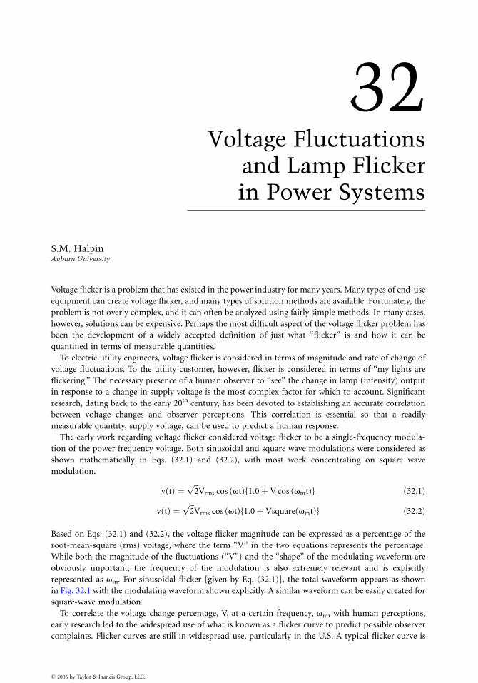
32
� 2006 by Taylor & Francis Group, LLC.
Voltage Fluctuationsand Lamp Flickerin Power Systems
S.M. HalpinAuburn University
Voltage flicker is a problem that has existed in the power industry for many years. Many types of end-use
equipment can create voltage flicker, and many types of solution methods are available. Fortunately, the
problem is not overly complex, and it can often be analyzed using fairly simple methods. In many cases,
however, solutions can be expensive. Perhaps the most difficult aspect of the voltage flicker problem has
been the development of a widely accepted definition of just what ‘‘flicker’’ is and how it can be
quantified in terms of measurable quantities.
To electric utility engineers, voltage flicker is considered in terms of magnitude and rate of change of
voltage fluctuations. To the utility customer, however, flicker is considered in terms of ‘‘my lights are
flickering.’’ The necessary presence of a human observer to ‘‘see’’ the change in lamp (intensity) output
in response to a change in supply voltage is the most complex factor for which to account. Significant
research, dating back to the early 20th century, has been devoted to establishing an accurate correlation
between voltage changes and observer perceptions. This correlation is essential so that a readily
measurable quantity, supply voltage, can be used to predict a human response.
The early work regarding voltage flicker considered voltage flicker to be a single-frequency modula-
tion of the power frequency voltage. Both sinusoidal and square wave modulations were considered as
shown mathematically in Eqs. (32.1) and (32.2), with most work concentrating on square wave
modulation.
v(t) ¼ffiffiffi
2p
Vrms cos (vt){1:0þ V cos (vmt)} (32:1)
v(t) ¼ffiffiffi
2p
Vrms cos (vt){1:0þ Vsquare(vmt)} (32:2)
Based on Eqs. (32.1) and (32.2), the voltage flicker magnitude can be expressed as a percentage of the
root-mean-square (rms) voltage, where the term ‘‘V’’ in the two equations represents the percentage.
While both the magnitude of the fluctuations (‘‘V’’) and the ‘‘shape’’ of the modulating waveform are
obviously important, the frequency of the modulation is also extremely relevant and is explicitly
represented as vm. For sinusoidal flicker [given by Eq. (32.1)], the total waveform appears as shown
in Fig. 32.1 with the modulating waveform shown explicitly. A similar waveform can be easily created for
square-wave modulation.
To correlate the voltage change percentage, V, at a certain frequency, vm, with human perceptions,
early research led to the widespread use of what is known as a flicker curve to predict possible observer
complaints. Flicker curves are still in widespread use, particularly in the U.S. A typical flicker curve is
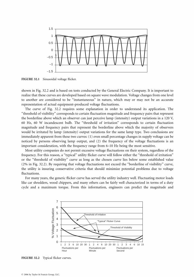
1.5
0.5
−0.5
−1.5
−1
1
1
0
FIGURE 32.1 Sinusoidal voltage flicker.
shown in Fig. 32.2 and is based on tests conducted by the General Electric Company. It is important to
realize that these curves are developed based on square wave modulation. Voltage changes from one level
to another are considered to be ‘‘instantaneous’’ in nature, which may or may not be an accurate
representation of actual equipment-produced voltage fluctuations.
The curve of Fig. 32.2 requires some explanation in order to understand its application. The
‘‘threshold of visibility’’ corresponds to certain fluctuation magnitude and frequency pairs that represent
the borderline above which an observer can just perceive lamp (intensity) output variations in a 120 V,
60 Hz, 60 W incandescent bulb. The ‘‘threshold of irritation’’ corresponds to certain fluctuation
magnitude and frequency pairs that represent the borderline above which the majority of observers
would be irritated by lamp (intensity) output variations for the same lamp type. Two conclusions are
immediately apparent from these two curves: (1) even small percentage changes in supply voltage can be
noticed by persons observing lamp output, and (2) the frequency of the voltage fluctuations is an
important consideration, with the frequency range from 6–10 Hz being the most sensitive.
Most utility companies do not permit excessive voltage fluctuations on their system, regardless of the
frequency. For this reason, a ‘‘typical’’ utility flicker curve will follow either the ‘‘threshold of irritation’’
or the ‘‘threshold of visibility’’ curve as long as the chosen curve lies below some established value
(2% in Fig. 32.2). By requiring that voltage fluctuations not exceed the ‘‘borderline of visibility’’ curve,
the utility is insuring conservative criteria that should minimize potential problems due to voltage
fluctuations.
For many years, the generic flicker curve has served the utility industry well. Fluctuating motor loads
like car shredders, wood chippers, and many others can be fairly well characterized in terms of a duty
cycle and a maximum torque. From this information, engineers can predict the magnitude and
7
6
5
4
3
2
1
01 1 1 2 3 4 6 10 152 4 6 10 20 302
Fluctuations perHour
Fluctuations perMinute
Threshold of Irritation
Threshold of Visibility
% V
olta
ge F
luct
uatio
n
"Typical" Flicker Curve
Fluctuations perSecond
3 6 10 20 30
FIGURE 32.2 Typical flicker curves.
� 2006 by Taylor & Francis Group, LLC.
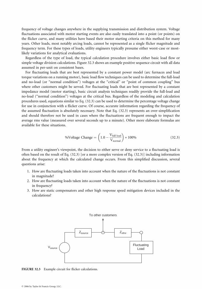
frequency of voltage changes anywhere in the supplying transmission and distribution system. Voltage
fluctuations associated with motor starting events are also easily translated into a point (or points) on
the flicker curve, and many utilities have based their motor starting criteria on this method for many
years. Other loads, most notably arcing loads, cannot be represented as a single flicker magnitude and
frequency term. For these types of loads, utility engineers typically presume either worst-case or most-
likely variations for analytical evaluations.
Regardless of the type of load, the typical calculation procedure involves either basic load flow or
simple voltage division calculations. Figure 32.3 shows an example positive sequence circuit with all data
assumed in per-unit on consistent bases.
For fluctuating loads that are best represented by a constant power model (arc furnaces and load
torque variations on a running motor), basic load flow techniques can be used to determine the full-load
and no-load (or ‘‘normal condition’’) voltages at the ‘‘critical’’ or ‘‘point of common coupling’’ bus
where other customers might be served. For fluctuating loads that are best represented by a constant
impedance model (motor starting), basic circuit analysis techniques readily provide the full-load and
no-load (‘‘normal condition’’) voltages at the critical bus. Regardless of the modeling and calculation
procedures used, equations similar to Eq. (32.3) can be used to determine the percentage voltage change
for use in conjunction with a flicker curve. Of course, accurate information regarding the frequency of
the assumed fluctuation is absolutely necessary. Note that Eq. (32.3) represents an over-simplification
and should therefore not be used in cases where the fluctuations are frequent enough to impact the
average rms value (measured over several seconds up to a minute). Other more elaborate formulas are
available for these situations.
%Voltage Change ¼ 1:0� Vfull load
Vnormal
� �
� 100% (32:3)
From a utility engineer’s viewpoint, the decision to either serve or deny service to a fluctuating load is
often based on the result of Eq. (32.3) [or a more complex version of Eq. (32.3)] including information
about the frequency at which the calculated change occurs. From this simplified discussion, several
questions arise:
1. How are fluctuating loads taken into account when the nature of the fluctuations is not constant
in magnitude?
2. How are fluctuating loads taken into account when the nature of the fluctuations is not constant
in frequency?
3. How are static compensators and other high response speed mitigation devices included in the
calculations?
To other customers
ZxfmrZsource
VsourceFluctuating
Load
FIGURE 32.3 Example circuit for flicker calculations.
� 2006 by Taylor & Francis Group, LLC.
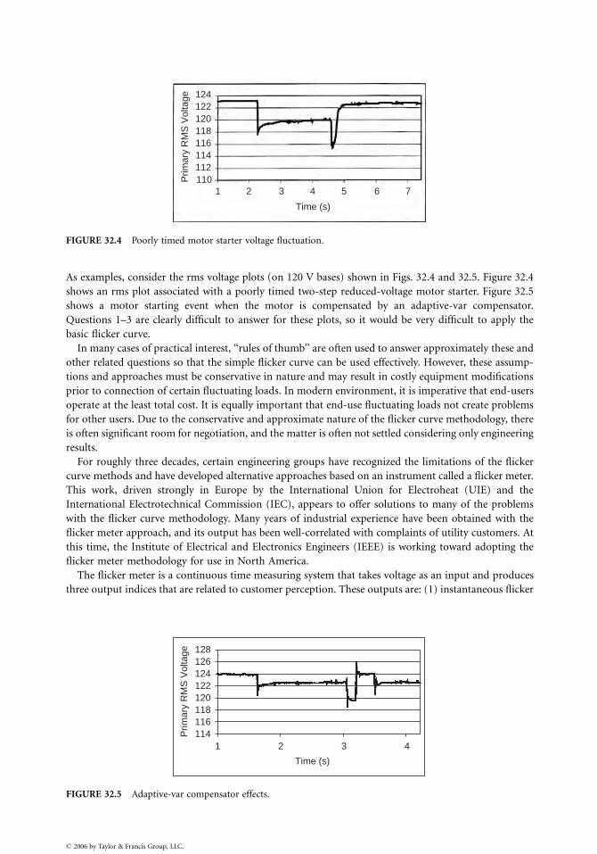
Time (s)
1110112
Prim
ary
RM
S V
olta
ge
114116118120122124
2 3 4 5 6 7
FIGURE 32.4 Poorly timed motor starter voltage fluctuation.
As examples, consider the rms voltage plots (on 120 V bases) shown in Figs. 32.4 and 32.5. Figure 32.4
shows an rms plot associated with a poorly timed two-step reduced-voltage motor starter. Figure 32.5
shows a motor starting event when the motor is compensated by an adaptive-var compensator.
Questions 1–3 are clearly difficult to answer for these plots, so it would be very difficult to apply the
basic flicker curve.
In many cases of practical interest, ‘‘rules of thumb’’ are often used to answer approximately these and
other related questions so that the simple flicker curve can be used effectively. However, these assump-
tions and approaches must be conservative in nature and may result in costly equipment modifications
prior to connection of certain fluctuating loads. In modern environment, it is imperative that end-users
operate at the least total cost. It is equally important that end-use fluctuating loads not create problems
for other users. Due to the conservative and approximate nature of the flicker curve methodology, there
is often significant room for negotiation, and the matter is often not settled considering only engineering
results.
For roughly three decades, certain engineering groups have recognized the limitations of the flicker
curve methods and have developed alternative approaches based on an instrument called a flicker meter.
This work, driven strongly in Europe by the International Union for Electroheat (UIE) and the
International Electrotechnical Commission (IEC), appears to offer solutions to many of the problems
with the flicker curve methodology. Many years of industrial experience have been obtained with the
flicker meter approach, and its output has been well-correlated with complaints of utility customers. At
this time, the Institute of Electrical and Electronics Engineers (IEEE) is working toward adopting the
flicker meter methodology for use in North America.
The flicker meter is a continuous time measuring system that takes voltage as an input and produces
three output indices that are related to customer perception. These outputs are: (1) instantaneous flicker
Time (s)
1114P
rimar
y R
MS
Vol
tage
116118120122124126128
2 3 4
FIGURE 32.5 Adaptive-var compensator effects.
� 2006 by Taylor & Francis Group, LLC.
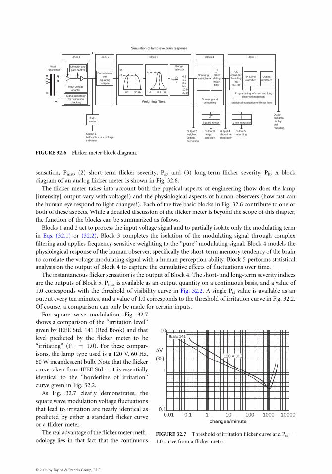
InputTransformer
Block 1 Block 2
dB1
−3
.05 0 8.8
Rangeselector
0.51.02.05.010.020.0
%ΔV
V
Hz
Weighting filters
35 Hz
Block 3 Block 4 Block 5
A/DconverterSampling
rate≥50 Hz
Squaringmultiplier
Squaring andsmoothing
Square rooter 1 min integrator
Statistical evaluation of flicker level
Programming of short and longobservation periods
Outputand datadisplayandrecording
Output 5recording
Output 4short timeintegration
Output 3rangeselection
Output 2weightedvoltagefluctuation
64 Levelclassifier
Outputinterfaces
1st
orderslidingmeanfilter
Simulation of lamp-eye brain response
Detector andgain control
Demodulatorwith
squaringmultiplier
Signal generatorfor calibration
checking
Input voltageadaptor
R.M.Smeter
Output 1half cycle r.m.s. voltageindication
√ ∫
FIGURE 32.6 Flicker meter block diagram.
sensation, Pinst, (2) short-term flicker severity, Pst, and (3) long-term flicker severity, Plt. A block
diagram of an analog flicker meter is shown in Fig. 32.6.
The flicker meter takes into account both the physical aspects of engineering (how does the lamp
[intensity] output vary with voltage?) and the physiological aspects of human observers (how fast can
the human eye respond to light changes?). Each of the five basic blocks in Fig. 32.6 contribute to one or
both of these aspects. While a detailed discussion of the flicker meter is beyond the scope of this chapter,
the function of the blocks can be summarized as follows.
Blocks 1 and 2 act to process the input voltage signal and to partially isolate only the modulating term
in Eqs. (32.1) or (32.2). Block 3 completes the isolation of the modulating signal through complex
filtering and applies frequency-sensitive weighting to the ‘‘pure’’ modulating signal. Block 4 models the
physiological response of the human observer, specifically the short-term memory tendency of the brain
to correlate the voltage modulating signal with a human perception ability. Block 5 performs statistical
analysis on the output of Block 4 to capture the cumulative effects of fluctuations over time.
The instantaneous flicker sensation is the output of Block 4. The short- and long-term severity indices
are the outputs of Block 5. Pinst is available as an output quantity on a continuous basis, and a value of
1.0 corresponds with the threshold of visibility curve in Fig. 32.2. A single Pst value is available as an
output every ten minutes, and a value of 1.0 corresponds to the threshold of irritation curve in Fig. 32.2.
Of course, a comparison can only be made for certain inputs.
IEEE 141
120 V UIE
0.010.1
1
10
ΔV
(%)
0.1 1 10 100changes/minute
1000 10000
FIGURE 32.7 Threshold of irritation flicker curve and Pst ¼1.0 curve from a flicker meter.
For square wave modulation, Fig. 32.7
shows a comparison of the ‘‘irritation level’’
given by IEEE Std. 141 (Red Book) and that
level predicted by the flicker meter to be
‘‘irritating’’ (Pst ¼ 1.0). For these compar-
isons, the lamp type used is a 120 V, 60 Hz,
60 W incandescent bulb. Note that the flicker
curve taken from IEEE Std. 141 is essentially
identical to the ‘‘borderline of irritation’’
curve given in Fig. 32.2.
As Fig. 32.7 clearly demonstrates, the
square wave modulation voltage fluctuations
that lead to irritation are nearly identical as
predicted by either a standard flicker curve
or a flicker meter.
The real advantage of the flicker meter meth-
odology lies in that fact that the continuous
� 2006 by Taylor & Francis Group, LLC.
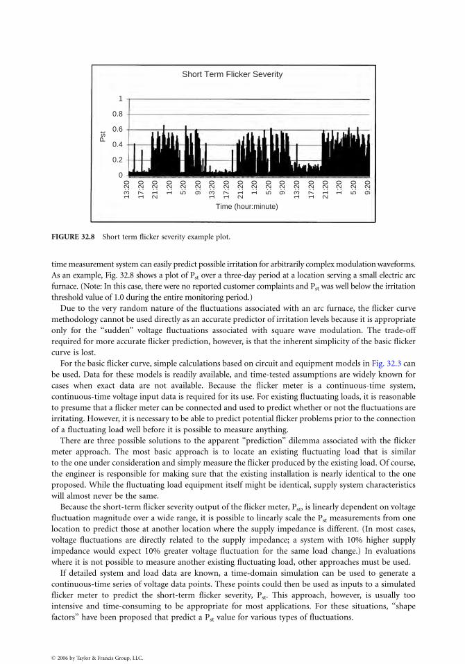
Short Term Flicker Severity
Time (hour:minute)
0
0.2
0.4
0.6
0.8
1
13:2
0
13:2
0
17:2
0
17:2
0
17:2
0
21:2
0
1:20
1:20
1:20
5:20
5:20
5:20
9:20
9:20
9:20
13:2
0
21:2
0
21:2
0
Pst
FIGURE 32.8 Short term flicker severity example plot.
time measurement system can easily predict possible irritation for arbitrarily complex modulation waveforms.
As an example, Fig. 32.8 shows a plot of Pst over a three-day period at a location serving a small electric arc
furnace. (Note: In this case, there were no reported customer complaints and Pst was well below the irritation
threshold value of 1.0 during the entire monitoring period.)
Due to the very random nature of the fluctuations associated with an arc furnace, the flicker curve
methodology cannot be used directly as an accurate predictor of irritation levels because it is appropriate
only for the ‘‘sudden’’ voltage fluctuations associated with square wave modulation. The trade-off
required for more accurate flicker prediction, however, is that the inherent simplicity of the basic flicker
curve is lost.
For the basic flicker curve, simple calculations based on circuit and equipment models in Fig. 32.3 can
be used. Data for these models is readily available, and time-tested assumptions are widely known for
cases when exact data are not available. Because the flicker meter is a continuous-time system,
continuous-time voltage input data is required for its use. For existing fluctuating loads, it is reasonable
to presume that a flicker meter can be connected and used to predict whether or not the fluctuations are
irritating. However, it is necessary to be able to predict potential flicker problems prior to the connection
of a fluctuating load well before it is possible to measure anything.
There are three possible solutions to the apparent ‘‘prediction’’ dilemma associated with the flicker
meter approach. The most basic approach is to locate an existing fluctuating load that is similar
to the one under consideration and simply measure the flicker produced by the existing load. Of course,
the engineer is responsible for making sure that the existing installation is nearly identical to the one
proposed. While the fluctuating load equipment itself might be identical, supply system characteristics
will almost never be the same.
Because the short-term flicker severity output of the flicker meter, Pst, is linearly dependent on voltage
fluctuation magnitude over a wide range, it is possible to linearly scale the Pst measurements from one
location to predict those at another location where the supply impedance is different. (In most cases,
voltage fluctuations are directly related to the supply impedance; a system with 10% higher supply
impedance would expect 10% greater voltage fluctuation for the same load change.) In evaluations
where it is not possible to measure another existing fluctuating load, other approaches must be used.
If detailed system and load data are known, a time-domain simulation can be used to generate a
continuous-time series of voltage data points. These points could then be used as inputs to a simulated
flicker meter to predict the short-term flicker severity, Pst. This approach, however, is usually too
intensive and time-consuming to be appropriate for most applications. For these situations, ‘‘shape
factors’’ have been proposed that predict a Pst value for various types of fluctuations.
� 2006 by Taylor & Francis Group, LLC.
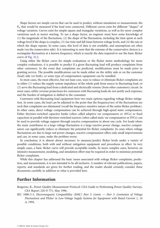
Shape factors are simple curves that can be used to predict, without simulation or measurement, the
Pst that would be measured if the load were connected. Different curves exist for different ‘‘shapes’’ of
voltage variation. Curves exist for simple square and triangular variations, as well as for more complex
variations such as motor starting. To use a shape factor, an engineer must have some knowledge of
(1) the magnitude of the fluctuation, (2) the shape of the fluctuation, including the time spent at each
voltage level if the shape is complex, (3) rise time and fall times between voltage levels, and (4) the rate at
which the shape repeats. In some cases, this level of data is not available, and assumptions are often
made (on the conservative side). It is interesting to note that the extreme of the conservative choices is a
rectangular fluctuation at a known frequency; which is exactly the data required to use the basic flicker
curve of Fig. 32.2.
Using either the flicker curve for simple evaluations or the flicker meter methodology for more
complex evaluations, it is possible to predict if a given fluctuating load will produce complaints from
other customers. In the event that complaints are predicted, modifications must be made prior to
granting service. The possible modifications can be made either on the utility side or on the customer
(load) side (or both), or some type of compensation equipment can be installed.
In most cases, the most effective, but not least cost, ways to reduce or eliminate flicker complaints are
to either (1) reduce the supply system impedance of the whole path from source to fluctuating load, or
(2) serve the fluctuating load from a dedicated and electrically remote (from other customers) circuit. In
most cases, utility revenue projections for customers with fluctuating loads do not justify such expenses,
and the burden of mitigation is shifted to the consumer.
Customers with fluctuating load equipment have two main options regarding voltage flicker mitiga-
tion. In some cases, the load can be adjusted to the point that the frequency(ies) of the fluctuations are
such that complaints are eliminated (recall the frequency-sensitive nature of the entire flicker problem).
In other cases, direct voltage compensation can be achieved through high-speed static compensators.
Either thyristor-switched capacitor banks (often called adaptive var compensators or AVCs) or fixed
capacitors in parallel with thyristor-switched reactors (often called static var compensators or SVCs) can
be used to provide voltage support through reactive compensation in about one cycle. For loads where
the main contributor to a large voltage fluctuation is a large reactive power change, reactive compen-
sators can significantly reduce or eliminate the potential for flicker complaints. In cases where voltage
fluctuations are due to large real power changes, reactive compensation offers only small improvements
and can, in some cases, make the problem worse.
In conclusion, it is almost always necessary to measure=predict flicker levels under a variety of
possible conditions, both with and without mitigation equipment and procedures in effect. In very
simple cases, a basic flicker curve will provide acceptable results. In more complex cases, however, an
intensive measurement, modeling, and simulation effort may be required in order to minimize potential
flicker complaints.
While this chapter has addressed the basic issues associated with voltage flicker complaints, predic-
tion, and measurement, it is not intended to be all-inclusive. A number of relevant publications, papers,
reports, and standards are given for further reading, and the reader should certainly consider these
documents carefully in addition to what is provided here.
Further Information
Bergeron, R., Power Quality Measurement Protocol: CEA Guide to Performing Power Quality Surveys,
CEA Report 220 D 771, May 1996.
IEC 1000-3-3, Electromagnetic Compatibility (EMC) Part 3: Limits — Part 3: Limitation of Voltage
Fluctuations and Flicker in Low-Voltage Supply Systems for Equipment with Rated Current � 16
A, 1994.
� 2006 by Taylor & Francis Group, LLC.

IEC 1000-3-5, Electromagnetic Compatibility (EMC) Part 3: Limits — Part 5: Limitation of Voltage
Fluctuations and Flicker in Low-Voltage Supply Systems for Equipment with Rated Current > 16
A, 1994.
IEC 1000-3-7, Electromagnetic Compatibility (EMC) Part 3: Limits — Part 7: Assessment of Emission
Limits for Fluctuating Loads in MV and HV Power Systems, 1996.
IEC 1000-3-11,Electromagnetic Compatibility (EMC) Part 3: Limits — Part 11: Limitation of Voltage
Changes, Voltage Fluctuations, and Flicker in Public Low Voltage Supply Systems with Rated Current
� 75 A and Subject to Conditional Connection, 1996.
IEC 61000-4-15, Flickermeter-Functional and Design Specifications, 1997–11.
IEC Publication 868, Flickermeter-Functional and Design Specifications, 1986.
IEEE Standard 141-1993: Recommended Practice for Power Distribution in Industrial Plants,
IEEE, 1993.
Sakulin, M. and Key, T.S., UIE=IEC Flicker Standard for Use in North America: Measuring Techniques
and Practical Applications, in Proceedings of PQA’97, March 1997.
Seebald, R.C., Buch, J.F., and Ward, D.J., Flicker Limitations of Electric Utilities, IEEE Trans. on Power
Appar. Syst., PAS-104, 9, September 1985.
UIE WG on Disturbances, Flicker Measurement and Evaluations: 2nd Revised Edition, 1992.
UIE WG on Disturbances, Connection of Fluctuating Loads, 1998.
UIE WG on Disturbances, Guide to Quality of Electrical Supply for Industrial Installations, Part 5:
Flicker and Voltage Fluctuations, 1999.
Xenis, C.P. and Perine, W., Slide rule yields lamp flicker data, Electrical World, October 1937.
� 2006 by Taylor & Francis Group, LLC.

33
� 2006 by Taylor & Francis Group, LLC.
Power QualityMonitoring
Patrick ColemanAlabama Power Company
33.1 Selecting a Monitoring Point ......................................... 33-1
33.2 What to Monitor ............................................................. 33-2
33.3 Selecting a Monitor ......................................................... 33-2Voltage . Voltage Waveform Disturbances . Current
Recordings . Current Waveshape Disturbances .
Harmonics . Flicker . High Frequency Noise .
Other Quantities
33.4 Summary.......................................................................... 33-8
Many power quality problems are caused by inadequate wiring or improper grounding. These problems
can be detected by simple examination of the wiring and grounding systems. Another large population
of power quality problems can be solved by spotchecks of voltage, current, or harmonics using hand held
meters. Some problems, however, are intermittent and require longer-term monitoring for solution.
Long-term power quality monitoring is largely a problem of data management. If an RMS value of
voltage and current is recorded each electrical cycle, for a three-phase system, about 6 gigabytes of data
will be produced each day. Some equipment is disrupted by changes in the voltage waveshape that may
not affect the rms value of the waveform. Recording the voltage and current waveforms will result in
about 132 gigabytes of data per day. While modern data storage technologies may make it feasible to
record every electrical cycle, the task of detecting power quality problems within this mass of data is
daunting indeed.
Most commercially available power quality monitoring equipment attempts to reduce the recorded
data to manageable levels. Each manufacturer has a generally proprietary data reduction algorithm. It is
critical that the user understand the algorithm used in order to properly interpret the results.
33.1 Selecting a Monitoring Point
Power quality monitoring is usually done to either solve an existing power quality problem, or to
determine the electrical environment prior to installing new sensitive equipment. For new equipment, it
is easy to argue that the monitoring equipment should be installed at the point nearest the point of
connection of the new equipment. For power quality problems affecting existing equipment, there is
frequently pressure to determine if the problem is being caused by some external source, i.e., the utility.
This leads to the installation of monitoring equipment at the service point to try to detect the source of
the problem. This is usually not the optimum location for monitoring equipment. Most studies suggest
that 80% of power quality problems originate within the facility. A monitor installed on the equipment
being affected will detect problems originating within the facility, as well as problems originating on the
utility. Each type of event has distinguishing characteristics to assist the engineer in correctly identifying
the source of the disturbance.
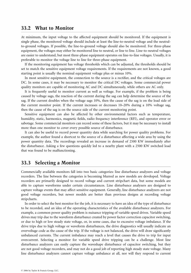
33.2 What to Monitor
At minimum, the input voltage to the affected equipment should be monitored. If the equipment is
single phase, the monitored voltage should include at least the line-to-neutral voltage and the neutral-
to-ground voltages. If possible, the line-to-ground voltage should also be monitored. For three-phase
equipment, the voltages may either be monitored line to neutral, or line to line. Line-to-neutral voltages
are easier to understand, but most three-phase equipment operates on line-to-line voltages. Usually, it is
preferable to monitor the voltage line to line for three-phase equipment.
If the monitoring equipment has voltage thresholds which can be adjusted, the thresholds should be
set to match the sensitive equipment voltage requirements. If the requirements are not known, a good
starting point is usually the nominal equipment voltage plus or minus 10%.
In most sensitive equipment, the connection to the source is a rectifier, and the critical voltages are
DC. In some cases, it may be necessary to monitor the critical DC voltages. Some commercial power
quality monitors are capable of monitoring AC and DC simultaneously, while others are AC only.
It is frequently useful to monitor current as well as voltage. For example, if the problem is being
caused by voltage sags, the reaction of the current during the sag can help determine the source of the
sag. If the current doubles when the voltage sags 10%, then the cause of the sag is on the load side of
the current monitor point. If the current increases or decreases 10–20% during a 10% voltage sag,
then the cause of the sag is on the source side of the current monitoring point.
Sensitive equipment can also be affected by other environmental factors such as temperature,
humidity, static, harmonics, magnetic fields, radio frequency interference (RFI), and operator error or
sabotage. Some commercial monitors can record some of these factors, but it may be necessary to install
more than one monitor to cover every possible source of disturbance.
It can also be useful to record power quantity data while searching for power quality problems. For
example, the author found a shortcut to the source of a disturbance affecting a wide area by using the
power quantity data. The recordings revealed an increase in demand of 2500 KW immediately after
the disturbance. Asking a few questions quickly led to a nearby plant with a 2500 KW switched load
that was found to be malfunctioning.
33.3 Selecting a Monitor
Commercially available monitors fall into two basic categories: line disturbance analyzers and voltage
recorders. The line between the categories is becoming blurred as new models are developed. Voltage
recorders are primarily designed to record voltage and current stripchart data, but some models are
able to capture waveforms under certain circumstances. Line disturbance analyzers are designed to
capture voltage events that may affect sensitive equipment. Generally, line disturbance analyzers are not
good voltage recorders, but newer models are better than previous designs at recording voltage
stripcharts.
In order to select the best monitor for the job, it is necessary to have an idea of the type of disturbance
to be recorded, and an idea of the operating characteristics of the available disturbance analyzers. For
example, a common power quality problem is nuisance tripping of variable speed drives. Variable speed
drives may trip due to the waveform disturbance created by power factor correction capacitor switching,
or due to high or low steady state voltage, or, in some cases, due to excessive voltage imbalance. If the
drive trips due to high voltage or waveform disturbances, the drive diagnostics will usually indicate an
overvoltage code as the cause of the trip. If the voltage is not balanced, the drive will draw significantly
unbalanced currents. The current imbalance may reach a level that causes the drive to trip for input
overcurrent. Selecting a monitor for variable speed drive tripping can be a challenge. Most line
disturbance analyzers can easily capture the waveshape disturbance of capacitor switching, but they
are not good voltage recorders, and may not do a good job of reporting high steady state voltage. Many
line disturbance analyzers cannot capture voltage unbalance at all, nor will they respond to current
� 2006 by Taylor & Francis Group, LLC.
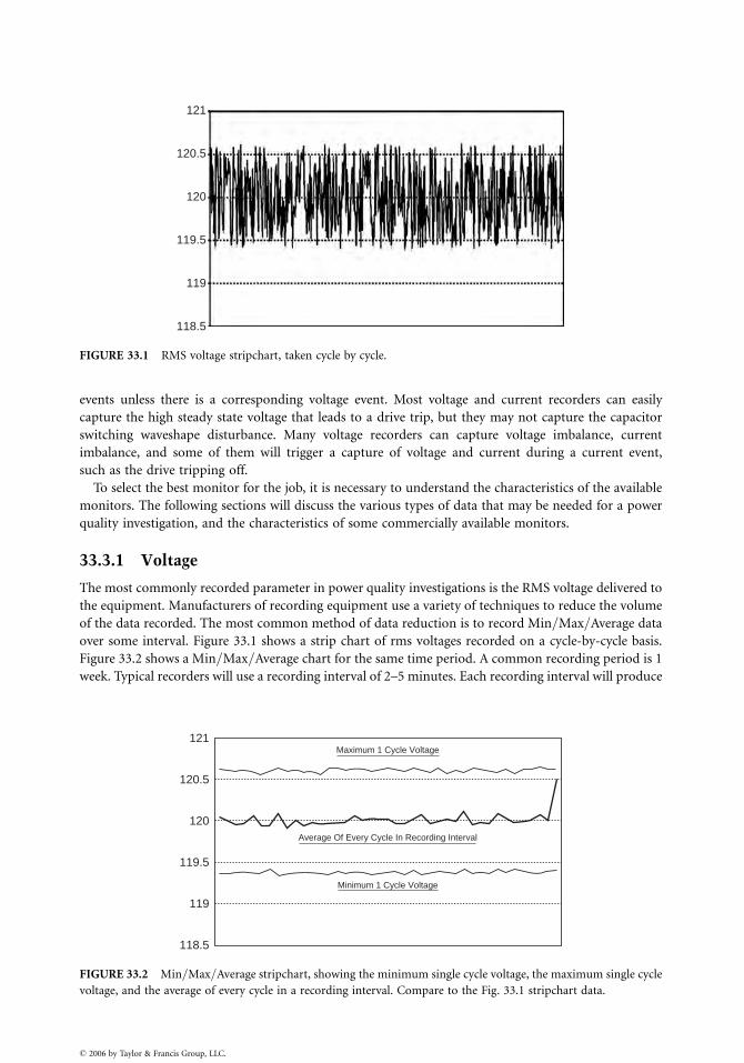
121
120.5
120
119
119.5
118.5
FIGURE 33.1 RMS voltage stripchart, taken cycle by cycle.
events unless there is a corresponding voltage event. Most voltage and current recorders can easily
capture the high steady state voltage that leads to a drive trip, but they may not capture the capacitor
switching waveshape disturbance. Many voltage recorders can capture voltage imbalance, current
imbalance, and some of them will trigger a capture of voltage and current during a current event,
such as the drive tripping off.
To select the best monitor for the job, it is necessary to understand the characteristics of the available
monitors. The following sections will discuss the various types of data that may be needed for a power
quality investigation, and the characteristics of some commercially available monitors.
33.3.1 Voltage
The most commonly recorded parameter in power quality investigations is the RMS voltage delivered to
the equipment. Manufacturers of recording equipment use a variety of techniques to reduce the volume
of the data recorded. The most common method of data reduction is to record Min=Max=Average data
over some interval. Figure 33.1 shows a strip chart of rms voltages recorded on a cycle-by-cycle basis.
Figure 33.2 shows a Min=Max=Average chart for the same time period. A common recording period is 1
week. Typical recorders will use a recording interval of 2–5 minutes. Each recording interval will produce
Maximum 1 Cycle Voltage121
120.5
120
119.5
119
118.5
Minimum 1 Cycle Voltage
Average Of Every Cycle In Recording Interval
FIGURE 33.2 Min=Max=Average stripchart, showing the minimum single cycle voltage, the maximum single cycle
voltage, and the average of every cycle in a recording interval. Compare to the Fig. 33.1 stripchart data.
� 2006 by Taylor & Francis Group, LLC.
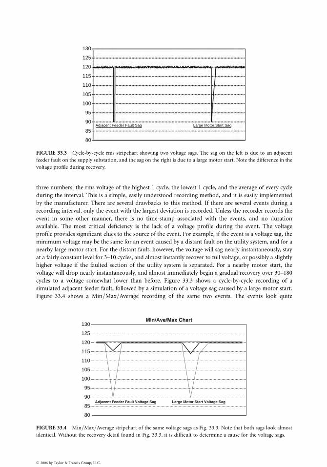
Adjacent Feeder Fault Sag
80
85
90
95
100
105
110
115
120
125
130
Large Motor Start Sag
FIGURE 33.3 Cycle-by-cycle rms stripchart showing two voltage sags. The sag on the left is due to an adjacent
feeder fault on the supply substation, and the sag on the right is due to a large motor start. Note the difference in the
voltage profile during recovery.
three numbers: the rms voltage of the highest 1 cycle, the lowest 1 cycle, and the average of every cycle
during the interval. This is a simple, easily understood recording method, and it is easily implemented
by the manufacturer. There are several drawbacks to this method. If there are several events during a
recording interval, only the event with the largest deviation is recorded. Unless the recorder records the
event in some other manner, there is no time-stamp associated with the events, and no duration
available. The most critical deficiency is the lack of a voltage profile during the event. The voltage
profile provides significant clues to the source of the event. For example, if the event is a voltage sag, the
minimum voltage may be the same for an event caused by a distant fault on the utility system, and for a
nearby large motor start. For the distant fault, however, the voltage will sag nearly instantaneously, stay
at a fairly constant level for 3–10 cycles, and almost instantly recover to full voltage, or possibly a slightly
higher voltage if the faulted section of the utility system is separated. For a nearby motor start, the
voltage will drop nearly instantaneously, and almost immediately begin a gradual recovery over 30–180
cycles to a voltage somewhat lower than before. Figure 33.3 shows a cycle-by-cycle recording of a
simulated adjacent feeder fault, followed by a simulation of a voltage sag caused by a large motor start.
Figure 33.4 shows a Min=Max=Average recording of the same two events. The events look quite
130Min/Ave/Max Chart
Adjacent Feeder Fault Voltage Sag Large Motor Start Voltage Sag
125
120
115
110
105
100
95
90
85
80
FIGURE 33.4 Min=Max=Average stripchart of the same voltage sags as Fig. 33.3. Note that both sags look almost
identical. Without the recovery detail found in Fig. 33.3, it is difficult to determine a cause for the voltage sags.
� 2006 by Taylor & Francis Group, LLC.
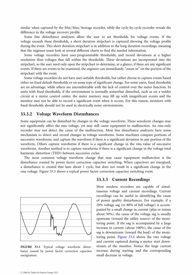
similar when captured by the Min=Max=Average recorder, while the cycle-by-cycle recorder reveals the
difference in the voltage recovery profile.
Some line disturbance analyzers allow the user to set thresholds for voltage events. If the
voltage exceeds these thresholds, a short duration stripchart is captured showing the voltage profile
during the event. This short duration stripchart is in addition to the long duration recordings, meaning
that the engineer must look at several different charts to find the needed information.
Some voltage recorders have user-programmable thresholds, and record deviations at a higher
resolution than voltages that fall within the thresholds. These deviations are incorporated into the
stripchart, so the user need only open the stripchart to determine, at a glance, if there are any significant
events. If there are events to be examined, the engineer can immediately ‘‘zoom in’’ on the portion of the
stripchart with the event.
Some voltage recorders do not have user-settable thresholds, but rather choose to capture events based
either on fixed default thresholds or on some type of significant change. For some users, fixed thresholds
are an advantage, while others are uncomfortable with the lack of control over the meter function. In
units with fixed thresholds, if the environment is normally somewhat disturbed, such as on a welder
circuit at a motor control center, the meter memory may fill up with insignificant events and the
monitor may not be able to record a significant event when it occurs. For this reason, monitors with
fixed thresholds should not be used in electrically noisy environments.
33.3.2 Voltage Waveform Disturbances
Some equipment can be disturbed by changes in the voltage waveform. These waveform changes may
not significantly affect the rms voltage, yet may still cause equipment to malfunction. An rms-only
recorder may not detect the cause of the malfunction. Most line disturbance analyzers have some
mechanism to detect and record changes in voltage waveforms. Some machines compare portions of
successive waveforms, and capture the waveform if there is a significant deviation in any portion of the
waveform. Others capture waveforms if there is a significant change in the rms value of successive
waveforms. Another method is to capture waveforms if there is a significant change in the voltage total
harmonic distortion (THD) between successive cycles.
The most common voltage waveform change that may cause equipment malfunction is the
disturbance created by power factor correction capacitor switching. When capacitors are energized,
a disturbance is created that lasts about 1 cycle, but does not result in a significant change in the
rms voltage. Figure 33.5 shows a typical power factor correction capacitor switching event.
FIGURE 33.5 Typical voltage waveform distur-
bance caused by power factor correction capacitor
energization.
� 2006 by Taylor & Francis Group, LLC.
33.3.3 Current Recordings
Most modern recorders are capable of simul-
taneous voltage and current recordings. Current
recordings can be useful in identifying the cause
of power quality disturbances. For example, if a
20% voltage sag (to 80% of full voltage) is accom-
panied by a small change in current (plus or minus
about 30%), the cause of the voltage sag is usually
upstream (toward the utility source) of the moni-
toring point. If the sag is accompanied by a large
increase in current (about 100%), the cause of the
sag is downstream (toward the load) of the moni-
toring point. Figure 33.6 shows the rms voltage
and current captured during a motor start down-
stream of the monitor. Notice the large current
increase during starting and the corresponding
small decrease in voltage.
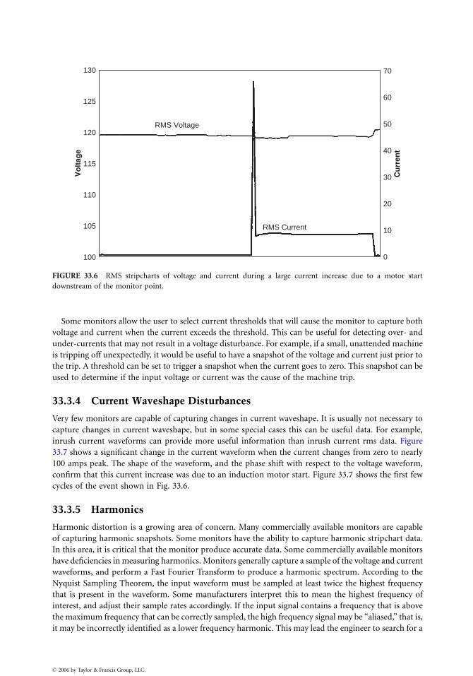
100
105
110
115
120
125
130 70
60
50
40
30
20
10
0
Vo
ltag
e
RMS Voltage
RMS Current
Cu
rren
t
FIGURE 33.6 RMS stripcharts of voltage and current during a large current increase due to a motor start
downstream of the monitor point.
Some monitors allow the user to select current thresholds that will cause the monitor to capture both
voltage and current when the current exceeds the threshold. This can be useful for detecting over- and
under-currents that may not result in a voltage disturbance. For example, if a small, unattended machine
is tripping off unexpectedly, it would be useful to have a snapshot of the voltage and current just prior to
the trip. A threshold can be set to trigger a snapshot when the current goes to zero. This snapshot can be
used to determine if the input voltage or current was the cause of the machine trip.
33.3.4 Current Waveshape Disturbances
Very few monitors are capable of capturing changes in current waveshape. It is usually not necessary to
capture changes in current waveshape, but in some special cases this can be useful data. For example,
inrush current waveforms can provide more useful information than inrush current rms data. Figure
33.7 shows a significant change in the current waveform when the current changes from zero to nearly
100 amps peak. The shape of the waveform, and the phase shift with respect to the voltage waveform,
confirm that this current increase was due to an induction motor start. Figure 33.7 shows the first few
cycles of the event shown in Fig. 33.6.
33.3.5 Harmonics
Harmonic distortion is a growing area of concern. Many commercially available monitors are capable
of capturing harmonic snapshots. Some monitors have the ability to capture harmonic stripchart data.
In this area, it is critical that the monitor produce accurate data. Some commercially available monitors
have deficiencies in measuring harmonics. Monitors generally capture a sample of the voltage and current
waveforms, and perform a Fast Fourier Transform to produce a harmonic spectrum. According to the
Nyquist Sampling Theorem, the input waveform must be sampled at least twice the highest frequency
that is present in the waveform. Some manufacturers interpret this to mean the highest frequency of
interest, and adjust their sample rates accordingly. If the input signal contains a frequency that is above
the maximum frequency that can be correctly sampled, the high frequency signal may be ‘‘aliased,’’ that is,
it may be incorrectly identified as a lower frequency harmonic. This may lead the engineer to search for a
� 2006 by Taylor & Francis Group, LLC.
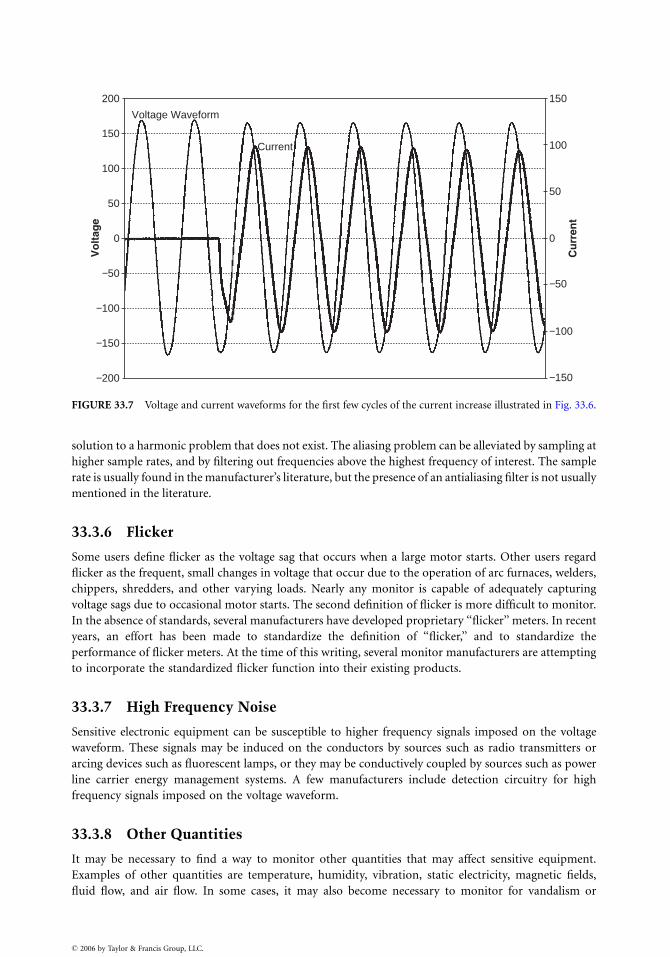
Voltage Waveform
200
150
100
50
0
−50
−100
−150
−200
150
100
50
0
−50
−100
−150
Cu
rren
t
Vo
ltag
e
Current
FIGURE 33.7 Voltage and current waveforms for the first few cycles of the current increase illustrated in Fig. 33.6.
solution to a harmonic problem that does not exist. The aliasing problem can be alleviated by sampling at
higher sample rates, and by filtering out frequencies above the highest frequency of interest. The sample
rate is usually found in the manufacturer’s literature, but the presence of an antialiasing filter is not usually
mentioned in the literature.
33.3.6 Flicker
Some users define flicker as the voltage sag that occurs when a large motor starts. Other users regard
flicker as the frequent, small changes in voltage that occur due to the operation of arc furnaces, welders,
chippers, shredders, and other varying loads. Nearly any monitor is capable of adequately capturing
voltage sags due to occasional motor starts. The second definition of flicker is more difficult to monitor.
In the absence of standards, several manufacturers have developed proprietary ‘‘flicker’’ meters. In recent
years, an effort has been made to standardize the definition of ‘‘flicker,’’ and to standardize the
performance of flicker meters. At the time of this writing, several monitor manufacturers are attempting
to incorporate the standardized flicker function into their existing products.
33.3.7 High Frequency Noise
Sensitive electronic equipment can be susceptible to higher frequency signals imposed on the voltage
waveform. These signals may be induced on the conductors by sources such as radio transmitters or
arcing devices such as fluorescent lamps, or they may be conductively coupled by sources such as power
line carrier energy management systems. A few manufacturers include detection circuitry for high
frequency signals imposed on the voltage waveform.
33.3.8 Other Quantities
It may be necessary to find a way to monitor other quantities that may affect sensitive equipment.
Examples of other quantities are temperature, humidity, vibration, static electricity, magnetic fields,
fluid flow, and air flow. In some cases, it may also become necessary to monitor for vandalism or
� 2006 by Taylor & Francis Group, LLC.

sabotage. Most power quality monitors cannot record these quantities, but other devices exist that can
be used in conjunction with power quality monitors to find a solution to the problem.
33.4 Summary
Most power quality problems can be solved with simple hand-tools and attention to detail. Some
problems, however, are not so easily identified, and it may be necessary to monitor to correctly identify
the problem. Successful monitoring involves several steps. First, determine if it is really necessary to
monitor. Second, decide on a location for the monitor. Generally, the monitor should be installed close
to the affected equipment. Third, decide what quantities need to be monitored, such as voltage, current,
harmonics, and power data. Try to determine the types of events that can disturb the equipment, and
select a meter that is capable of detecting those types of events. Fourth, decide on a monitoring period.
Usually, a good first choice is at least one business cycle, or at least 1 day, and more commonly, 1 week. It
may be necessary to monitor until the problem recurs. Some monitors can record indefinitely by
discarding older data to make space for new data. These monitors can be installed and left until the
problem recurs. When the problem recurs, the monitoring should be stopped before the event data is
discarded.
After the monitoring period ends, the most difficult task begins — interpreting the data. Modern
power quality monitors produce reams of data during a disturbance. Data interpretation is largely a
matter of experience, and Ohm’s law. There are many examples of disturbance data in books such as
The BMI Handbook of Power Signatures, Second Edition, and the Dranetz Field Handbook for Power
Quality Analysis.
� 2006 by Taylor & Francis Group, LLC.
Related Documents