Iowa State University Digital Repository @ Iowa State University Retrospective eses and Dissertations 1996 Electric power auction market implementation and simulation Jayant Kumar Iowa State University Follow this and additional works at: hp://lib.dr.iastate.edu/rtd Part of the Business Commons , Economics Commons , Electrical and Computer Engineering Commons , Oil, Gas, and Energy Commons , and the Operational Research Commons is Dissertation is brought to you for free and open access by Digital Repository @ Iowa State University. It has been accepted for inclusion in Retrospective eses and Dissertations by an authorized administrator of Digital Repository @ Iowa State University. For more information, please contact [email protected]. Recommended Citation Kumar, Jayant, "Electric power auction market implementation and simulation " (1996). Retrospective eses and Dissertations. Paper 11545.

Welcome message from author
This document is posted to help you gain knowledge. Please leave a comment to let me know what you think about it! Share it to your friends and learn new things together.
Transcript
Iowa State UniversityDigital Repository @ Iowa State University
Retrospective Theses and Dissertations
1996
Electric power auction market implementation andsimulationJayant KumarIowa State University
Follow this and additional works at: http://lib.dr.iastate.edu/rtd
Part of the Business Commons, Economics Commons, Electrical and Computer EngineeringCommons, Oil, Gas, and Energy Commons, and the Operational Research Commons
This Dissertation is brought to you for free and open access by Digital Repository @ Iowa State University. It has been accepted for inclusion inRetrospective Theses and Dissertations by an authorized administrator of Digital Repository @ Iowa State University. For more information, pleasecontact [email protected].
Recommended CitationKumar, Jayant, "Electric power auction market implementation and simulation " (1996). Retrospective Theses and Dissertations. Paper11545.

EVFORMATION TO USERS
This nuinuscript has been reproduced from the microfilm master. UMI
films the t^ directly from the original or copy submitted. Thus, some
thesis and dissertation copies are in typewriter face, while others may be
from any type of computer printer.
The quality of this reproduction is dependent upon the quality of the
copy submitted. Broken or indistinct print, colored or poor quality
illustrations and photographs, print bleedthrough, substandard margins,
and improper alignment can adversely affect reproduction.
In the unlikely event that the author did not send UMI a complete
manuscript and there are missing pages, these will be noted. Also, if
unauthorized copyright material had to be removed, a note will indicate
the deletion.
Oversize materials (e.g., maps, drawings, charts) are reproduced by
sectioning the original, beginning at the upper left-hand comer and
continuing from left to right in equal sections with small overlaps. Each
original is also photographed in one exposure and is included in reduced
form at the back of the book.
Photographs included in the original manuscript have been reproduced
xerographically in this copy. Higher quality 6" x 9" black and white
photographic prints are available for any photographs or illustrations
appearing in this copy for an additional charge. Contact UMI directly to
order.
UMI A Bell & Howell Information Company
300 North Zed) Road, Ann Arbor MI 48106-1346 USA 313/761-4700 800/521-0600

Electric power auction market implementation and simulation
by
Jayant Kumar
A dissertation submitted to diie graduate faculty
in partial fiiiflllment of the requirements for the degree of
DOCTOR OF PHILOSOPHY
Department: Electrical and Computer Engineering
Major. Electrical Engineering (Electric Power)
Major Professor: Gerald B. Sheble
Iowa State University
Ames, Iowa
1996
Copyright @ Jayant Kumar, 1996. All rights reserved
UMI N\iit±)er: 9712573
UMI Microform 9712573 Copyright 1997, by UMI Company. All rights reserved.
This microfonn edition is protected against unauthorized copying under Title 17, United States Code.
UMI 300 North Zeeb Road Ann Arbor, MI 48103

ii
Graduate College
Iowa State University
This is to certify tliat the doaoral disseitation of
Jayant Kumar
has met the dissertation requirements of Iowa State University
For the M^or Department
Edr the Graduate College
Signature was redacted for privacy.
Signature was redacted for privacy.
Signature was redacted for privacy.

iii
This dissertation is dedicated
to the immortal memories of my mother Sbashi Bala and father Madan Murari Prasad,
to my major professor Gerry Shebl^ and to the Iowa State University
iv
TABLE OF CONTENTS
ACKNOWLEDGMENTS vii
1. INTRODUCTION 1
1.1 The Overall Problem 1
1.2 Regulation of Pricing of Ancillary Services 3
1.3 Scope of This Work 4
1.4 Content of This Dissertation 5
2. LITERATURE REVIEW 6
2.1 Developments in the Policy Context 6
2.1.1 The Federal Power Act of 1935 7
2.1.2 The Public Utility Holding Company Act of 1935 7
2.1.3 The Clean Air Aa of 1970 7
2.1.4 The Public Utility Regulatory Policy Aa of 1978 8
2.1.5 The CAA Amendments of 1990 8
2.1.6 National Energy Policy Aa of 1992 9
2.1.7 The FERC's Electric Industry Restruauring NOPR of 1993 9
2.1.8 The FERC's Ancillary Services NOPR of 1995 10
2.2 Overview of Brokerage/auction Systems 10
2.2.1 Auction as a Market Institution 10
2.2.2 Auctions in Industrial Market 12
2.2.3 Examples of Auction System for Electric Energy 13
2.3 Overview of Optimization Theory 15
2.3.1 Principles of Nonlinear Programming 15
2.3.2 Principles of Linear Programming 20
2.3.3 General Techniques of Optimization 25
2.3.4 Auction Optimization Mechanisms for Electric Energy 30
2.4 Schweppe's Theory of Spot Pricing 30
V
3. THEORETICAL DEVELOPMENT 31
3.1 Basic Framework 31
3.1.1 Definitions 31
3.1.2 Ancillary Services 32
3.1.3 Auction Market Structure 33
3.1.4 Assumptions 35
3.2 Framework for Pricing of Reserve Margins and Transmission Losses 36
3.2.1 Development of Auction Model 36
3.2.2 Adaptation for Linear Prograimning 41
3.2.3 Consideration of Security Constraints 42
3.3 AGC Simulator in Price-Based Operation 44
3.3.1 Introduction to Load Following Contracts 44
3.3.2 Classical AGC Scheme 46
3.3.3 AGC Simulator for New R^ework 47
3.3.4 Simulator Features and Capabilities 50
3.4 Auction Market Simulator 51
3.4.1 Assumptions 51
3.4.2 Rules of the Auction Market 52
3.4.3 Bidding Models 53
3.4.4 Allocation of Funires Contract 55
3.4.5 The OveraU Scheme for Auction Market Simulator 57
4. RESULTS 59
4.1 Illusiradve Examples 59
4.1.1 Example 1 (Transaction 1: Case of Nonbtnding Reserve Constraints) 59
4.1.2 Example 2 (Transaction 2: Case of Binding Reserve Constraints) 60
4.1.3 Example 3 (Transaction 3: Consideration of a Security Constraint) 62
4.2 Simulation Examples 63
4.2.1 The Test System 63
4.2.2 AGC Simulation 64
4.2.3 Auction Market Simulation 76
vi
5. CONCLUSION AND SUMMARY 80
5.1 The Energy Brokerage Model 80
5.2 AGC Simulator 81
5.3 Auction Market Simulator 82
5.4 Practical Implications: ISO V/S ICA 83
APPENDIX A. DERIVATION OF INCREMENTAL POWER LOSS FUNCTIONS 84
APPENDIX B. DERIVATION OF MATRICES T AND TolbSjj 87
APPENDIX C. STATE SPACE EQUATIONS OF AGC SCHEMES 90
APPENDIX D. SYSTEM DATA FOR ILLUSTRATIVE EXAMPLES 1 AND 2 92
BIBUOGRAPHY 94

vii
ACKNOWLEDGMENTS
I am deeply indebted to my major professor. Dr. Gerald B. Sheblf, for his guidance, support and
encouragement during this research. My thanks to Dr. Vijay Vittal, Dr. James D. McCalley Dr. V. Ajjarapu,
Dr. Shashi Gadia, Dr. Stefano Athanasoulis and Dr. Sharon Filipowski for generously providing time as
committee members. I sincerely thank Dr. Joseph Herridges for serving as a substitute for Dr. Stefano
Athanasoulis in my final examination.
It has been wonderful time as a graduate student in the power group at Iowa State University. 1 am
thankful to my colleagues. Kah-Hoe, Somgiat and Chuck for sharing their time in valuable discussions.
1 have received major afflatus from my eldest brother, Jeewan Kumar for pursuing the higher studies. I
am grateful for support and encouragement of my family members during my entire student life. I thank my
wife Seema for her understanding and encouragement in the last part of this woric.
1
1. INTRODUCTION
1.1 The Overall Problem
The objective of this work is to develop the theoretical foundation for market based pricing of ancillary
services in electric power transaction. The developed foundation is used to design an auction market simulator
to experimentally study the price-based operation. The simulation market structure is kept generic enough to
capture all possibilities of different contracts in a deregulated utility environment The developed simulation
package can also be used as a training tool for the system operators in the new environment
This work is motivated by the recent changes in regulatory policies towards inter utility-power
interchange practices. Regulators believe that electric pricing must be regulated by ftee market forces rather than
by a commission. A major focus of the changing policies is 'competition' as a replacement of 'regulation* to
achieve economic efficiency. However, if competition replaces regulation as the norm of electric power
generation and bulk power supply, a number of changes would be required. The coordination arrangements
presently existing among the different players of the electric market would change firom operational, planning
and organizational standpoints.
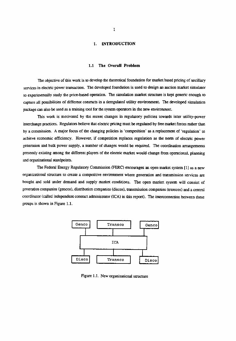
The Federal Energy Regulatory Commission (FERC) encourages an open market system [1] as a new
organizational structure to create a competitive environment where generation and transmission services are
bought and sold under demand and supply market conditions. The open market system will consist of
generation companies (gencos), distribution companies (discos), transmission companies (transcos) and a central
coordinator (called independent contract adminisuator GCA) in this report). The interconnection between these
groups is shown in Rgure 1.1.
Genco
Disco
Genco
Disco TransCO
TransCO
ICA
Figure 1.1. New organizational structure
2
The ICA is independent and a disassociated agent for market participants. Hie role and responsibilities
of the ICA in the new marketplace are yet not clear. This work assumes that the ICA is responsible for
coordinating among the market players (gencos, discos, and transcos) to provide a reliable power system
operation. Under this assumption, the ICA would require a new class of optimization algorithms to perfonn
price-based operation. Efficient tools would be needed to verify that the system remains in operation with all
contracts in place. This work proposes an energy brokerage model for ancillary services as a novel framework
for price-based optimization. The proposed foundation is used to develop a simulation tool to study the
implementational aspects of various cono^ts in a deregulated environment.
Although it is concepmally clean to have separate functionality for the gencos, discos, transcos. and the
ICA. the overall mode of real time operation is still evolving. Presently, two possible versions of market
operations are debated in the industry - poolco based transactions and bilateral transactions. Both types of
transactions are based on the premise of price-based operation and market driven demand. This work presents an
analytical comparison of the two approaches. With the developed simulator, both poolco and bilateral
agreements can be snidied.
In achieving the goal of economic efficiency, one should not forget that the reliability of the electric
services is of the utmost importance. The electric utility industry in North America, in the words of its North
American Electric Reliability Council (NERC), uses reliability in a bulk electric system to indicate " the degree
to which the performance of the elements of that system results in electricity being delivered to customers
within accepted standards arui in the amount desired The degree of reliability may be measured by the frequency,
duration, and magnitude of adverse effects on the electric supply". The council also suggests that reliability can
be addressed by considering the two basic and functional aspects of the bulk electric system - adequacy and
security. In this work, the discussion is focused on the adequacy aspect of power system reliability, which is
defined as the static evaluation of the system's ability to satisfy the system load requirements. In context of the
new business environment, market demand is interpreted as the system load. However, a secure implementation
of electric power transaction concerns power system operation and stability issues:
(1) Transient instability issue: The electric power system is a nonlinear dynamic system comprising of
numerous machines in synchronism with each other. Stable operation of these machines following disturbances
in the network often requires limitations on various operating conditions, such as generation levels, load levels,
and power transfer. These machines together with other system components, being under the influence of
various inertial forces require extra energy (reserve margins and load following capability) to safely actuate
electric power transfer.
(2) Thermal overload issue: The electric power transmission is limited by the electrical network
capacity and losses (congestion management and transmission losses).
3
(3) Operating voltage issue: Enough amount of VAR support (reactive power support) should
accompany the real power transfer to maintain the bus voltages at the specified levels.
In the new organizational structure, the services used for supporting a reliable deliver^' of electric
energy, such as reserve margins, load following, congestion management, transmission losses, reactive power
support, etc. are termed as ancillary services. In this context, the term 'ancillary services* is misleading since
the referred services are not ancillary rather essentially bundled with the electric power transfer as described
earlier. The open market system should consider all of these ancillary services as an integral part of power
transaction.
Tliis work proposes a set up in which ancillary services as a whole becomes a competitive player in the
energy market with the other energy market participants. It is embedded so that no matter what, the
(operationally) centralized ancillary service would have to take the obligation to deliver and keep the system
together according to the adopted operating constraints. As such, although competitive, it is burdened by
additional goals of ensuring reliability rather than profit only. The proposed pricing framework which aaempts
to become economically efficient by moving from cost-based to price-based operation introduces a mathematical
framework for making the ancillary services players sufficiently informed in decision making when serving the
other competitive energy market players.
1.2 Regulation of Pricing of Ancillary Services
Recently, the FERC has issued a notice of proposed rulemaking (NOPR) [2] seeking comments on six
ancillary services: reserve margins, transmission losses, load following, reactive power, energy imbalance, and
redispatch. The nature of the comments requested indicate that this is an area that is largely new to the FERC,
and that it feels itself on rather shaky ground. The NOPR establishes pricing for stage one since this is
necessary to enable the FERC to get open access tariffs in place promptly. Specific pricing of two ancillary
services, namely transmission losses and energy imbalances are proposed. The charges for transmission losses
are defined as 3% loss factor and 110% of sellers incremental cost. The tariff for energy imhalanrps is set at 100
mills/kwh for imbalances in excess of ±1.5%. There is no separate charge (included in account 556) for
redispatch. Pricing of other ancillary services, such as load following, reserve margins and reactive power is
defined by 1 mill/kwh ceiling for the group.
Utilities are free to propose revisions to these rates. Utilities must charge themselves prices for
ancillary services when they make off-system sales that are the same as they charge others for ancillary services.
Thus, a utility that charges high prices for ancillary services reduces its ability to compete for off-system sales.
This may cause the FERC to desire to put a floor under rates for ancillary services. The resolution of such
4
issues demands that adequate study and analysis be invested to gracefully change the industry into a more
competitive electric marketplace.
The role of ancillary services is very important in achieving a reliable power system operation. The
stage one pricing scheme proposed by the FERC does not take into account the network configurations, system
conditions and the reliability desired by the market participants. Thus, the intent of achieving a true market
optimum in price based operation, as well as, maintaining the reliability of power system is completely
defeated. Unbundling of ancillary services should be viewed in the context of dis-aggregated utilities and
competitive markets. The end-state should be management of ancillary services through specified requirements
for all grid users and competitive bidding. The competitive environment brings a new set of complicated
problems in designing an efficient market for ancillary services to provide reliable power system operation.
This requires a comprehensive analysis of price based operation by including ancillary services which are
presently embedded within the vertically integrated industry.
1.3 Scope of This Work
This work has developed the foundation for market based pricing of ancillary services in electric power
transaction. A framework for price-based operation is developed to study the proposed pricing mechanism. The
future business environment for electric utilities is incompletely defined as of this writing. Hence, the proposed
market structure is kept generic enough to capture a variety of possibilities in marketing electric power and the
ancillary services in the new environment The concept of various contracts required to provide a reliable electric
marketplace are introduced. The research develops bidding process along with the proper definition of
obUgations of the grid users to facilitate the electric marketplace with simplicity.
The price based operation will involve more faaors of uncertainty, such as fluctuating market prices,
load forecasts (market demand), and unit availability (market supply). This will adversely affect the power
system reliability resulting in risk of unserved energy and loss of opportunities. This work illustrates how
decision analysis methodology can be applied to use the proposed approach for developing techniques for risk
management.
The developed foundation has been used to design an auction market simulator to perform experimental
simulation of price based operation. The simulator technology developed by this project will help the electric
power system industry by analyzing models that satisfy the dual objectives of reliable and economic operation in
the price-based environment. In the new enviroimient, the system operators are required to submit the price-
based bids to perform electric power transaction. This is quite different from what the system operators are
accustomed to in a vertically integrated industry. The proposed simulator can be used to train the operators how
to bid in the new environmenL
5
1.4 Contents of This Dissertation
Chapter 2 of this dissenation reviews the literature related to this work. The first section summarizes
developments in regulatory policies in the United States. Principle impacts of the proposed changes on power
system operation and optimization are also discussed. The second section describes the earlier development of
energy brokerage/auction models for electric power systems. A few remarks are made to highlight how this
proposed work differs from the previous ones. The third section presents an overview of classical opdmization
theory. The smicture and madiematical foundation of linear programming (LP) and nonlinear programming
(NLP) are presented. The basic concepts of linear programming and the solution techniques are discussed
elaborately to provide theoretical basis to develop the auction market simulator.
Chapter 3 presents the theoretical foundation for pricing of ancillary services in an auction market
structure. Different types of contracts required in the price-based operation are identified. A scheme for
automatic generation control (AGC) simulauon in the new environment is presented. The developed theoretical
foundation is integrated to design the electric power auction market simulator.
Chapter 4 contains the research results. The illustrative examples demonstrate how the cost of
ancillary services are affected by the coupled operational characteristics of energy market and ancillary services
market. The simulation results from the proposed AGC simulator and auction market simulator are presented.
Chapter 5 gives conclusions and recommendations for future work.
6
2. LITERATURE REVIEW
2.1 Developments in the Policy Context
For nearly half a century, the US utility companies operated as regulated monopoplies. characterized by
controlled prices, closed entrv- and cost-based rates. The electric utility industry was considered as natural
monopolies, marked by economies in scale and size of output making competition wasteful. This hypothesis
appeared to be faulty as the economy of the nation grew. Consequently, a number of changes in regulatory
arrangements took place from time to time depending on needs of the nation's economy. This section presents a
brief historical background of the US electric industry followed by description of major legislations related to the
utility industry.
There was no radical change in regulatory arrangements until late 1960s. The 1970s was a decade of
unprecedented changes for the US utility industry. The 1973-74 Arab oil embargo adversely affected fuel prices.
The construction cost of new power plants rose dramatically because of a combination of factors, such as high
interest rate and increased environmental requirements. As a consequence, there was an inaease in electricity
prices, which forced customers to use less electricity. Large industrial customers incurred financial loss because
of high production costs. Many industrial customers felt that the option of purchasing competitive generation
could be more economical. Many similar policies resulted into uncertain electric demand growth. Such
uncertainties caused planning activity problems. Rising electrical costs and fear of loosing customers became
major concerns for the utilities. Power system companies decided to revise their plaiuiing process. Issues
included a number of topics, such as. whether to allow units to be included in the rate base until they were
operational, if at all. On the other band, regulators tried to analyze how to promote energy conservation while
keeping electrical costs to minimum.
The above problems challenged the regulatory environment of power system companies. The trend
towards large, capital-intensive power plants was delayed because of the demand growth uncertainty. Policy
makers decided to restructure the power industry to keep pace with the economic conditions by promoting
competition. Many Federal U.S. legislations affecting the electric utility industry were enacted. The regulatory
policies for utility industry till date can be summarized by the following acts and regulations:
• The Federal Power Act (FPA) of 1935
• The Public Utility Holding Company Aa (PUHCA) of 1935
• The Clean Air Aa of (CAA) 1970
• The Public Utility Regulatory Policy Act CPURPA) of 1978
• The Clean Air Act Amendments (CAAA) of 1990
7
• The National Heccric Policy Act (NEPA) of 1992
• The FERC's electric industry restructuring NOPR of 1993
• The FERC's ancillary services pricing NOPR of 1995
2.1.1 The Federal Power Act of 1935 [3]
The history of regulation in the US electric industry began with the Federal Power Act of 1935. This
act was motivated by the growth of transmission and subsequent interconnection between utilities which enabled
the utilities to buy and sell energy across state lines. The basic aim of the ITA was to confer regulatory
authority for wholesale, interstate energy transactions to the Federal Power Cotnmission (FPC), which was the
precursor to the FERC created in 1977. The complete document of the act consisted of two parts. Pan I
explained the creation of the FPC. The pan II dealt with description of the FPC's jurisdiction and its
responsibilities to coordinate interstate transactions.
2.1.2 The Public Utility Holding Company Act of 1935 [4]
The Public Utility Holding Company Act of 1935 was passed to give die Securities and Exchange
Commission (SEC) the authority to break up utility holding companies. A big company possessing enough
securities of utility companies to control their operation was termed as a utility holding company. The
controlled utilities were caUed operating companies. The holding companies charged the operating companies
excessive prices for equipment's, supplies, etc. This excessive charge was eventually recovered from the utility
customers by the operating companies. The intent of PUHCA was to check such practices. The act formalized
the requirements for a holding company to seek approvals on various activities, such as selling additional
securities, performing company transactions, etc. Consequently, break up of a number of utility holding
companies took place and malpractice of excessive charges were curbed.
2.1.3 The Clean Air Act of 1970
The Clean Air Act of 1970 conferred the responsibilities of monitoring the environmental standards to
the Environmental Protection Agency (EPA). The Federal environmental standards established ambient air
quality standards for the United Stales. The National Ambient Air Quality Standards (NAAQS) [5] resulted from
this act. Majority of electric power generation, being dependent on fossil fuel were affected by this regulation.
Consequently, the utility companies started investigating various compliance strategies, such as scrubbers, fuel
switching, furnace modification, software modifications in dispatching strategies [6,7], etc.
g
2.1.4 The Public Utility Regulatory Policy Act of 1978 [8]
The Public Utility Regulatory Policy Act of 1978 was one of the significant early developments to
restructure the electric industry. The complete document of the act consisted of seven titles of which Titles I. II,
and IV were related to the utility industry. Title I described the retail regulatory policies for electric utility, such
as cost-based rates for each customer class, time of day rates, seasonal rates, interruptible rates, etc. Title n of
the PURPA brought the elements of competition in electric utility industry for the first time as described later
in this section. Title IV of the act was focused on small hydroelectric power projects.
Title n of the PURPA was intended to encourage construction of non utility generators (NUGs) by
requiring utilities to purchase power produced by such facilities. The idea was that the power firom NUGs must
be purchased by the local utility at a price that the utility would have incurred to generate the same power. The
limits of such avoided costs had been set administratively by state utility commissions. Some states set prices
even higher than actual utility costs in an effort to inaease NUGs. Many cogenerations and alternative energy
facilities appearing since 1978 were built as a result of the favorable conditions due to PURPA. The act also
inspired a growing interest in independently owned, largely non utility power plants (IPPs), which would sell
their generation to either utilities or customers.
The desire to stimulate competition lead to the allowance of any qualifying facilities (QFs) to supply
energy. However, there was considerable controversy over the calculation of avoided costs set by state utility
commissions. Discussions were held to argue whether avoided costs were set at levels too high, encouraging
too many facilities at consumers' expense, or too low. discouraging innovative development In 1988, the
FERC proposed changes to regulations [9] to promote competition in bidding and independent power
production. The proposal was also projected as a means of determining avoided costs under state regulatory
programs. The FERC's proposal led to increased pressure for wheeling and for the emergence of NUGs. That
required redefinition of transmission network access and of future power transmission. As a result, FERC
proposed a new framework of power transmission through the 'open transmission access' [10]. In that new
paradigm, the utility owned and operated the network as a separate transmission company and utility provided
conditions for pricing its service independent of generation or distribution.
2.1.5 The CAA Amendments of 1990 [11]
The 1990 CAA amendments were signed into law on November 15,1990. The amendments consisted
of eleven titles, of which the title IV was the most significant Title IV of the act attempted to control overall
emissions by costing compliance [8]. The compliance was economically regulated through units of emission
allowances fEA). The units of EA were issued by the Enviroimiental Protection Agency (EPA). There was
9
provision for purchase and open-maricet trading of EAs. The approach implied that utilities could choose to
comply by cutting emissions or by buying extra allowances. The each utility could economically decide on
which option was more cost effective. Individual utilities could choose their own solution for meeting the
C.\AA. In addition to the use of EAs. utilities could, for example, switch fuels or install scrubbers. In April
1993. the Chicago Board of Trade started trading the Emission allowances.
2.1.6 National Energy Policy Act (NEPA) of 1992 [12]
To facilitate the growth of free market electricity, the US Senate passed a comprehensive National
Energy Policy Act (NEPA) [9] in 1992. The complete document of the act consisted of thirty titles, of which
title 1 and title VII were most significant Title I of the aa focused on energy efficiency issues by encouraging
integrated resource planning (IRP). demand side management (DSM). The act introduced a new set of
ratemaldng standards. The state utility commissions were required to assess the economic impaa of bulk power
electric transactions under the proposed ratemaking standards. Emphasis was placed on reducing the costs of
efficiency improvements for generation, transmission, and distribution facilities.
Title vn of the act defined exempt wholesale generators (EWGs) as any company owning or operating
all or part of an eligible facility and selling electricity at wholesale cost The FERC was given disaetion to
decide whether an EWG could be exempt from the Public Utility Holding Company ACT (PUHCA). Utilities
were permitted to purchase from an affiliated EWG under the jurisdiction of a state commission. The FERC
could issue a transmission order if such an order met certain requirements and would be in the public interest A
utility had 60 days to respond to a transmission request before an applicant could file for a wheeling order with
FERC.
2.1.7 The FERC's Electric Industry Restructuring NOPR of 1993 [1]
The FERC's electric industry restructuring NOPR of 1993 was motivated to change the vertically
integrated structure of the electric utility industry. The NOPR proposed the functional unbundling of the utility
companies into three parts: Genco (generation company), Transco (transmission company), and disco
(distribution company). The policy makers felt a need for a central coordinating body, who could make unbiased
decisions for economic operation while ensuring the bulk system's reliability and security. The NOPR
encouraged the development of regional transmission groups (RTG). The commission expected RTGs to be a
means to enable a free market for electric power to operate in a more competitive and efficient way. The
commission believed that RTGs could provide a means of coordinating regional planning of the transmission
system while assuring that system capabilities be always adequate to meet system demands.
10
2.1.8 The FERC's Ancillary Services NOPR of 1995 [2]
In March 1995, the FERC issued the ancillary services NOPR presenting the FERC policy on
unbundling and pricing of ancillary services. Under NOPR comparable services model, the transmission
provider was required to supply ancillary service. Provision of ancillary services by third parties was voluntar>'.
There was no need to develop cost-based rates if utility was prepared to live with the stage one rates in the
NOPR as described in chapter 1. However, the supplier of ancillary services could develop cost-based rates if the
supplier wanted to change one or more of the stage one rates that did not justify market-based rates or the
supplier wanted to sell any one of the services that fell under the I mill ceiling.
It appears that the FERC is. preparing to move far beyond previous pricing policies for ancillary
services. In doing so. the FERC will need all the help &om the industrial and research communides to analyze
the pricing of ancillary services. Various state utility commissions have already taken initiatives to restructure
the uulity industry in accordance with the federal proposal. The California Public Utility Commission (CPUC)
has announced that the state of California would have an independent system operator GSO) and a competitive
wholesale spot power market (Power Exchange - PX) by no later than January 1,1998 [13]. The PX will allow
power producers to compete using nondiscriminatory and transparent rules for bidding into exchange. The
exchange will submit the proposed schedule for delivery of power to the ISO. The ISO will coordinate the day-
ahead .scheduling and real-time balancing for all users of the grid.
2.2 Overview of Brokerage/auction Systems
2.2.1 Auction as a Market Institution
An aucuon market can be considered as a trading institution where buyers and sellers can readily meet
to maximize their trade gains. McAfee and McMilan [ 14] define auction as "a market institution with an
explicit set of rules determining resource allocation and prices on the basis of bids from market participants". In
standard auction institutions such as Chicago Board of Trade (CBOT) [15] and New York Mercantile exchange
(NYMEX) [16], all the trade units are standardized. The only component of a trade unit that varies is the price.
This removes all the informational asymmetries prevailing in the market mstitution on the trading floor. The
market participants efficiently decide for transactions on the basis of prices only. In another words, an auction
system is a very efficient way to move from a cost-based operation to price-based operation. In this context, the
study of aucuon institutions and their application for electric power system in the proposed deregulated
environment becomes very significant.
11
Post and Sliebl6 [17,18] present a detailed study of auction institutions. Post [17] has described four
standard types of auction institution: English aucuon, Dutch auction, the first-pnce sealed-bid auction, and the
second-price sealed-bid auction. These aucdon mechanisms employ different methodologies of trading. In the
English auction, the auction bids begin with a low price. The bids are progressively announced until no
purchaser wishes to make a higher bid. The auction result is pareto-optimal since the winner is the bidder who
values the trade unit the most [19]. In the Dutch auction, auctioneer calls a decreasing set of bids beginning
with a high price. The bidding proceeds until one bidder accepts the current price. Thus, the Dutch auction is a
game that rewards the player who wishes to maximize his expected gain (not the gain itself). In the first-price
sealed-bid auction, buyers submit sealed bids. The highest bidder is awarded the item for the price he bid. The
second-price sealed-bid auction is based on the premise that the highest bidder wins the item but pays a price
equal to the second highest bid. Buyers submit sealed bids similar to die first-price sealed-bid auction, but with
the above information at hand. Both the fu^t-price sealed-bid auction and the second-price sealed-bid auction
maximize the trade gains of the market participants.
There exists numerous variations of the four standard auction institutions. The examples are multiple
auctions [20], mulQple sales by sealed bids [21], and double auctions [22, 23]. Smith [23] presents a slight
variation of the first-price sealed-bid auction called a discriminative sealed bid auction. In this case, the sale
quantity is fixed at a specified amount Buyers are dien invited to tender bids at a stated price for a stated
quantity. Bids are accepted from highest to lowest until the specified amount of bid units are exhausted. Ties at
the lowest bids are accepted on a random basis. Smith also presents a variant of the second-price sealed-bid
auction for a homogeneous conmiodity. This variant is called the competitive sealed-bid auction which is the
same as discriminative sealed bid auction except tiiat aU bids are GDed at the price of the lowest accepted bid
[23],
Of the various auction institutions, double auction institution and sealed-bid methods appear to be
operationally and structurally suitable for the deregulated electric industiy. In die double auction institution, the
buyers and sellers subnut bids and offers. After the bids have been placed, the broker detemiines the buyers and
sellers by what is called the high-low algorithm [24]. The highest buy bid is matched with the lowest sell bid.
The procedure continues with die next highest buy bid and die next lowest sell bid, and finishes when die
highest remaining buy bid is the lower dian die next lowest sell bid. If a proposed match violates an
operational constraint, it is omitted and the next match is detennined.
Although die theory of double auctions is not well developed, experimental results for double auctions
have shed considerable light on the subject. Vemon Smith has presented a number of propositions based on his
experimental results [22, 23]. The experiments have been conducted by implementing the use of computers for
selection of optimal contracts [25]. This research is performed in a laboratory setting with individuals acting as
buyers, sellers, or both. Participants enter their bid (offer) quotes into a computer tenninal. A central computer
12
then applies an optimization algorithm to detennine the prices and allocations that maximize the gains on the
basis of the bids (offers), and budget and capacity constraints of the individual market participants. These
experimental market mechanisms produce strong equilibrating tendencies, even when rental rewards to buyers
and sellers are not balanced.
2.2.2 Auctions in Industrial Markets
In the past, many other regulated industries applied some form of auction methods to move from
regulated rate of return pricing to market-based pricing. Some examples are the natural gas industry and the air
line industry. Post [17] has described the market institutions and auction optimization methods used in these
industries. Most of these methods are based on competiuve sealed-bid aucuons and double oral auctions. Smith
[23] presents a detailed description of implementational issues involved with these methods.
The case of the natural gas industry is of particular interest since the electric utility industry and the gas
industry have some similar operational characteristics. Natural gas flows from wells located in the distant
producing fields, through pipelines to users. Interstate pipelines end at state borders or at gateways to urban
markets, where gas is transferred to a distribution system for delivery to consumers. Thus, field wells, interstate
pipelines, and gas distribution system are structurally and operationally similar to the concept of genco, transco
and disco respectively in the electric power system. The electric utility industry seems to follow the natural gas
industry in deregulation activities and is expected to continue to do so.
A series of regulatory crises has forced deregulation in the natural gas industry: first, well-head prices,
next gas contracts, and finally pipeline transportation. As the deregulation proceeded, the FERC came up with
"open access" ruling for interstate pipelines to facilitate tiie implementation of gas contracts. The emergence of
a competitive gas market has showed tiiat the hypothesis, "Interstate natural gas pipelines are natural
monopolies and hence they cannot be competitively organized" is completely wrong. Competiuve prices of
natural gas have moved together witiiin a band related to transportation costs, so Uiat price differences within
bands are not so large that a profit can be made by arbitrage. Also, the price differences have narrowed over
time and eventually have become correlated. The initial narrowing and eventual correlation are one of the
significant properties of competitive markets. The natural gas market has shown that monopoly power of the
pipelines can be made nonexistent by making transmission an asset that can be ti-aded in a market open to
producers, distributors, customers, brokers, and others.
Rassenti et al [26] presents a number of different market institutions for production and exchange of
natural gas. The examples are Bargaining environment, Posted-offer pricing. Multiple decenualized markets, and
Computer-assisted markets. Many of these institutions are based on the premise of sealed-bid and double
auction mechanisms. McCabe et al. [27] has developed a computer assisted market called gas auction network
13
(GAN). The purpose of GAN is to evaluate the price and performance characteristics of a sealed-bid auction
mechanism for the simultaneous allocation of natural gas and pipeline capacity rights among buyers, sellers, and
transporters of wellhead gas. The experimental results [28, 29] with GAN mechanism have shown that the
nodal prices tend to converge towards market equilibrium.
Discussion of operational and implementational issues concerning the various institutions in the gas
industry provides a good insight on how auctions can be applied to the electric utility industry. However, it is
important to note that the technical constraints (network (active and reactive power) flows and security-
constraints) and nanire of commodity (electric energy and ancillary services) of the utility industry are different
from those in natural gas industry. Unlike natural gas, electricity cannot be stored in so called 'energy tanks'.
Research into energy storage devices for storing huge amount of electricity is still in infancy [30]. Hence,
generation of electricity requires immediate consumption. The instant generation and instant distribution must
be coordinated properly by the transmission system. A secure transmission of electrical power requires a
number of ancillary services as described in chapter 1. Additionally, the transmission path for a given
uansaction can not be chosen apriori. The path of power flow is governed by KirchofT s laws. The path
followed by energy can cause problems when wheeling power across intermediate systems resulting in voltage
dipping, reactive power flow, increased losses, reliability problems, etc.
In short, all the operational issues, such as transmission access [31], reliability standards [32], etc. are
required to be re-examined in the deregulated enviroimienL In general, administration of a complete auction
institution to electric power industry requires a thorough analysis in terms of mathematical framework and
implementational issues. References [33], [34], [35] and [36] describe such implementational and technical
issues in great details.
2.2.3 Examples of Auction Systems for Electric Energy
The main stated purpose of the new FERC proposed rulings (open access, comparability, ancillary
services, etc.) is to reduce the cost of electricity. Previous attempts by electric utilities to solve such economic
problems led to the formation of power pools based on cost-based operation. Energy brokerage/auction systems
is a way to reduce the operational costs in price-based framework. The function of an energy auction system is
to establish multilateral transactions among participating market players in such a manner as to maximize the
total trade gain. Research study has shown that the multilateral power transactions cross subsidize bilateral
transactions [37] and hence, they are required to achieve efficiency. Auction system is an efficient way to set up
to establish multilateral contracts. Some of the real-life examples of power brokerage systems have shown
significant advantages of power brokerage pools, compared to the traditionally integrated pools. This subsection
presents two such real-life examples.
14
2.2.3.1 Florida Power Brokerage System
The most prominent example of power brokerage system in the United States is the Florida brokerage
system [38.39]. The goal of Florida brokerage system was to encourage short term transfer of electric power to
reduce the aggregate cost of generation. The broker of Florida system used to ask for buy and sell quotes on an
hourly basis. The hourly quotes were matched to set up bilateral contracts. A research study on the Florida
brokerage system [40] indicated that the net savings in the brokerage system was almost twice that of a centrally
operated pool system. The total operation costs in a brokerage type pool system turned out to be less than the
centrally operated pool system. This was because the utiliues retained the responsibilities of local operational
decisions, such as unit commitment, fuel scheduling, etc. However, the Florida brokerage system did not
survive because the market was too small to provide enough trading opportunities.
2.2.3.2 England and Wales System in the UK
A recent example of bidding arrangement for electric power interchange is the England and Wales
system in the United Kingdom. The UK electric industry comprises of twelve regional electricity companies
(RECs) and one national grid corporation (NGC). The main activities of the RECs are distribution and supply.
The NGC has all transmission assets plus 2 GW of pumped hydro facility. The generation companies make
offers to the NGC. Based on these offers and its own estimate of demand, the NGC produces a unconstrained
schedule. This "unconstrained schedule " is used to develop the pool price for every half hour. Actual operation
is also scheduled by the NGC. Differences between actual operation and planned unconstrained schedule arise
due to error in demand estimate, forced outages, and transmission related constraints. The unscheduled units are
called into operation to meet the shortfall of generation and are paid their offer prices. Generating units which
run in the unconstrained schedule but not in the event (spinning reserves) are compensated by being paid the
difference between the pool purchase price and the offer price. The pool selling price is calculated by adding the
ancillary services cost to pool purchase price.
The England and Wales power grid is the largest competitive electricity market in the worid. Hence,
the experiences of UK electric market should be carefully examined carefully to learn lessons. Although the
objectives of generating companies (to maximize profit witiiout regard for the effect of their actions on system
security) differ from tiiose of the NGC (i.e. to maintain secure and economic operation of the system), the
arrangements are working. This is because there is much commonalty of purpose in practice. The market has a
unique feature of determining the security costs after the fact However, exclusion of transmission constraints
prohibit tiie pool prices to account tiie true operational cost. References [41], [42], and [43] describe operational
and planning issues and recent experiences with independent generators of the UK and the N(jC in details.
15
2.3 Overview Of Optimization Theory
This section is a summary of the theory for constrained optimization problems. Constrained
optimization problems can be broadly classified into two classes - linear programming and non-linear
programming. Reference [43] and [44] provide a good overview of linear and nonlinear programming theorv*.
The chapter begins with a general discussion of nonlinear programming. The theoretical foundation of non
linear programming is explained in detail as it plays an important role in understanding basic principles of
optimization. Various methods of nonlinear programming, such as Quadratic Programming, Augmented
Lagrangian method, Lagrangian Relaxation method. Network Flow algorithms, and Artificial Neural Network
approach are discussed. Next, principles and methods of linear programming are presented. The chapter
concludes by elaborating on a list of classical optimization algorithms that have been used for energy auction
mechanism.
2.3.1 Principles of Nonlinear Programming (NLP)
The NLP problem arises in a myriad of forms in engineering economics. As the name suggests, NLP
problem consists of optimizing a nonlinear cost function subject to a set of nonlinear constraints. The theory
of nonlinear programming is based on the advancements in the field of calculus, linear algebra, and convex
analysis. This section states necessary notations and definitions needed to analyze a NLP problem followed by
discussion of some important developments.
2.3.1.1 Notations and Definitions
A nonlinear program /• is of the form given below:
Minimize
f ( x )
Subject to: g j i x ) < 0 for all] e { 1 , 2 r]
h i ( x ) = 0 for alii e { 1,2 m]
(2.1)
A vector x is called a feasible solution of NLP iff x satisfies the r+m constraints of NLP.
A set X c i?" is said to be convex iff for any a,b 6 X implies [a,b ] c X , where [a,b ] is defined as
follows:
[ a j } ] = { X e / e ^lx = X a + (1-A ) b , 0 < A < 1 (2 2)
16
Let X c be a non empty convex set. then the function f : x -^R is said to be convex iff
/ ( A X + (1-A ) y ) < -l/U) + (1-A )/(y ), x.y 6 X 0 < A < 1
(2.3)
The function/" : x -*R is said to be concave if -f is convex. An affine function f : x -^R is a
function that is convex and concave. H is a hyperplane in i?if there exists
o r e / ? " , a * 0 , a e R (2.4)
such that
H = [x e R'^ \ <a, x> = a } (2.5)
where. <. > is the Euclidean inner product onR^ and a is a normal vector of the hyperplane H. An
inequality gj (x) <0 is said to be binding for a point x* if
g j ( . x * ) = 0 f o r a l l j (2.6)
A point x* satisfying a set of hyperplanes A,- ( x ) = 0 and g j ( x ) = 0 is said to be a regular point x* of
the set if the gradients
VA," (x * ) Vgj (x •) V ij e hyperplanes p ^
satisfy linear independence in their corresponding vector space.
2.3.1.2 First Order Necessary Condition (FONC)
The first order necessary condition is also known as Karush-Kuhn-Tucker's (KKT) conditions. Let 3c
be a feasible solution to (2.1). Suppose that each gj is differentiable at 3c. Furthermore, assume that 3c is a
regular poinL Then, x is a relative minimum point in the solution space of (2.1) if and only if there exists
A = [ A ] , A 2 , . . . , A r I ^ f i = [ p . - [ , f X j , . . . (2.8)

17
such that
U) A,- > 0 g i ( J ) S O
(2.9)
an A," gi ( x ) = 0 i = 1 r
(2.10)
( H i ) f i j h f i (.r ) = 0 y = 1 m
(2.11) r r
(jv) V/(x) + I A,- (X) + I Hj hj ( X ) = 0
(2.12)
The variables A," and Hj are known as Lagrange multipliers.
2.3.1.3 Second Order Necessary Condition (SONC)
The vector^ is a relative minimum point in the solution space of (2.1), if the KKT conditions are
satisfied and such that
is a positive semidefinite matrix on the tangent subspace of the active constraint at 3c. The matrices F, G, and
H are the corresponding Hessian mattices of the functions f, g, and h respectively. Matrix L is called the
Hessian ofLagrangian.
2.3.1.4 Second Order Sufficient Condition (SOSC)
The vectors: is & strict minimum point , i.e., the optimum point in the solution space of (2.1), if
PONG and SONC are satisfied and the Hessian of the Lagrangian is positive definite on the subspace
M ' = { y : VA ( x ) y = 0. V g j (x )y = 0 } for all J e J
L ( x ) = F ( x ) + A ^ f ^ ( x ) + n ' ^ G L x )
(2.13)
(2.14)
18
where,
J = {y : gj (F)y =0. Ay > 0}
(2.15)
The equation 2.15 together with h(x*) = 0 comprises the set known as binding seL The set of
remaining constraints is termed as non-binding constraints. It is the binding set of constraints that define the
optimum solution for a given problem.
A generalized NLP is convex program if/and gj are finite convex functions on /?" and hj are affine
functions. In the case of convex program, the Hessian matrices are always positive semidefinite. Thus, the
requirements of second order conditions are always satisfied. Thus, the optimality conditions of convex program
are reduced to satisfying Kuhn-Tucker's conditions only.
2.3.1.5 Reduced NLP and optimality conditions
Any nonlinear program can be reduced to minimizing a nonlinear objective fimction subject to a set of
inequality constraints only. This is possible, because an equality, in mathematical sense, is a coupled set of
inequalities. The reduced representation can be achieved by defining some new Lagrange multiplier as follows:
Define
H j ^ = m a x \ t i j . 0] ^ij, = min {fij . 0]
(2.16)
Then
My = My+ + My- for \ < j < m
(2.17)
The corresponding term in the condition (iv) of the KKT condition can be written as:
H j V h j ) V h j = H j + V h j + (-My-)(-V/iy)
Since only one of fij+ or fij. is non zero, and hj = 0, condition (iv) can be extended by using conditions
stipulating mutually exclusive terms hj < 0 and Ay > 0 as follows:
19
m V/ + I A/ gi + 
20
2.3.1.6 Penalty Function Approach for NLP
The penally function approach approximates the constrained optimization problem into an
unconstrained optimization problem by adding a penalty function to objective function. The penalty term
assigns a high cost to the constraint violation. The assignment of cost is made using a suitable value for the
penalty parameter. Thus, the objective function of the reduced NLP can be written as:
-, /• + 2m . L(sk^) = f(x) + ^ (x))2 (2.25)
Where, gf (x) is the constraint violation and sj^}" is a nonnegative, strictly increasing sequence
tending to infinity. The parameter s is known as the penalty factor. The optimal condition for tbe augmented
objective function is given as:
Let the minimizer ofL (sj^, x) be and the NLP be convex. Then, any limit point in the sequence
Xjt is an optimal solution to equation (2.25).
Furthermore, if xj^ -» x, and x is a regular point, then -> A,-, which is the
corresponding Lagrange multiplier. Thus, the penalty function approach and Lagrangian method have strong
correspondence. A detailed analysis of penalty approach is described in reference [45].
2.3.2 Principles of Linear Programming (LP)
2.3.2.1 Notations and Definitions
Within the area of optimization, the most widely known and implemented technique for modeling and
solution is, by far, the methodology denoted as linear programming. A linear program is a mathematical
program in which the objective function is linear in the unknowns and the constraints consist of linear equalities
and linear inequalities. The theory of linear programming can be explained by using the principles of linear
algebra and convexity theory. A linear program can always be transfomied in the following form.
Minimize
Subjea to
cTx
Ax - b = 0
Xi > 0. ¥ i = 1.2 n
(2.26)
(2.27)
21
Here, C is an n-dimensional column vector representing the cost per unit element of column vector x.
A is an m»n matrix, and is an m-dimensional column vector. The basic definitions used in linear
programming are described in the following paragraphs.
Def. 1: A feasible solution to the linear program (2.26-2.27) is defined by a vector x satisfying
equation {227).
Def. 2: A basis matrix is an m*m nonsingular matrix formed from some m columns of the constraint
matrix B.
Def. 3: A basic solution to a linear program is the unique vector of dimension n-m by selecting n-m
decision variables to zero and solving the basis matrix system for remaining decision variables. The
components of basic solution are called basic variables and remaining decision variables are called nonbasic
variables.
Def. 4: A basic feasible solution to a linear program is a basic solution in which all variables have
nonnegative values.
Def. S: A nondegeiuate basic feasible solution to a toear program is a basic feasible solution with
exactly m positive values.
Def. 6: An optimal solution to a linear program is a basic feasible solution that minimizes f in (2.26)
Def. 7: The reduced cost veaor to a linear program is defined as the partial cost gradient of objective
function with respect to nonbasic decision variables.
Def. 8: A point x in a convex set X is called an extreme point of X. if x cannot be represented as a
strict convex combination of two distinct points in X.
The optimality conditions are described by the theorems given below. Proofs of theorems may be
found in Gass [46].
Theorem 1: A vector x is an extreme point of the constraint set of a linear program iff x is a basic
feasible solution of (2.27).
Theorem 2: The objective function f, assumes its minimum at an extreme point of the constraint set
If it assumes its minimum at more than one extreme point, then it takes on the same value at every point of the
hyperplane joining any two optimal extreme points.
Theorem 3: A basic feasible solution is an optimal (minimal) solution if all the components of reduced
cost vector are nonnegative. In addition, if components of reduced cost vector are strictly positive, then the
optimal solution is a nondegenerate solution and if one or more of the components of reduced cost veaor are
zero, then the optimal solution is a degenerate solution.
22
2.3.2.2 Duality Theory and Sensitivity Analysis
One of the most important concepts in optimization is duality theory. Given any linear program
Maximize
aTx
(2.28)
Subject to:
Bx - e < 0
Xi >0, ¥ i = 1.2 n
(2.29)
there exists a related linear program
Minimize
eTk
(2.30)
Subject to :
- A > 0
A,- > 0, ¥ i = 1,2 m
(2.31)
If the linear program (228 - 229) is termed as the primal problem, the linear program (2.30 - 2.31) is
called the dual problem. The two problems are related to eacfa otber in such a way that the optimal solution of
one provides enough infonnation to determine the solution of other. The dual variables are essentially Lagrange
multipliers as described in section 2.3.1. In LP theory, the dual variables are also called shadow prices as they
indicate the marginal benefit of incremental change in the resource capacity associated with the primal
constraint Thus, the solution of dual problems provide insight for economic analysis of the problem. There are
number of useful properties of primal-dual relationship that are used extensively to design fast and efficient
optimization algorithms:
Property 1: The dual of the dual is the primal
Property 2: Each primal constraint is related to a dual variable and vice versa.
Property 3: Each primal variable is related to a dual constraint and vice versa.
Property 4: If primal has an optimal solution, the dual also has an optimal solution, and vice-versa.
23
Property 5: If the primal is unbounded, the dual is infeasible.
Property 6: If the primal is infeasible, the dual may be either unbounded or infeasible.
Property 7: Given the canonical form of the linear programs in (2.28 - 2.29) and (2.30 - 2.31). the
relationship z < z* = Z* < Z holds.
The above mentioned properties are extensively used to analyze the impact of fluctuations in model
parameters, such as change in cost coefficient, resource capacity or constraint coefficient and addition of a new
variable or new constraint. This is called sensitivity analysis. The duality theory approach enhances the speed
of algorithm with simplicity. For example, if a new constraint is added, the optimality can be analyzed by
forming the dual and checking whether the corresponding dual variable enters the basis or noL Similarly, if a
new variable is added, the optimality can be checked by forming the dual and verifying whether the associated
dual constraint is binding or nonbinding. A detailed description of duality theory and sensitivity analysis is
available in number of literature [47,48].
2.3.2.3 Methods of Linear Programming
The simplex method [49,50] is the most commonly used technique to solve LP problem. The simplex
method has been applied to linear programming in single as well as multiple objective optimization problems.
The method constructs a set of basic and nonbasic variables by choosing the linearly independent columns of a
basis matrix B. A basic feasible solution is achieved by letting the nonbasic variables equal to zero. The basic
feasible solution is an optimal solution, if the gradient of objective function with respect to each nonbasic
variable is positive. The algorithm proceeds by exchanging the nonbasic variable having most negative
gradient vector with the most restriaing basic variable until the optimal solution is achieved.
Many variants of simplex methods have been developed for different types of linear programs. One of
the most common types is a linear program having variables with upper bounds. A linear program having
general lower bounds and upper bounds can always be reduced to a formulation having variables with upper
bounds only. This is accomplished by proper transformation of the coordinates of the associated variables.
Then, the simplex method is modified to solve such linear programs by using the following definition and
theorem.
Def. 9; An extended basic feasible solution to a linear program with upper bounded variables is a basic
feasible solution where nonbasic variables are either at zero or at upper bounds.
Theorem 4: An extended basic feasible solution for a linear program with upper bounded variables is
optimal if the reduced cost vector of nonbasic variables at zero value are nonnegative and those at upper bound
are nonpositive.
24
A more recent algorithm for LP has iterates which are in the interior of the feasible region to find the
solution. The interior-point algorithm was introduced by Narendra Karmakar [51] at Bell labs in 1984.
(Carmarkar's algorithm differs from the simplex method in that it starts with an interior feasible solution rather
than a basic feasible solution. It is called interior-point algorithm because its iterates are not on the boundary of
feasible region as in Simplex method. Kannaikar's algorithm rescales the variables to place the solution in the
center of a scaled feasible solution, allowing it to take a large step toward the optimal solution.
Methods for solving large scale linear programs employ various decomposition principles. The
examples are: Dantzig-Wolfe Decomposition principle. Rosen's Partitioning Procedure for Angular and Dual-
Angular Problems, Decomposition by Elight-Hand-Side Allocation and Colunm-Generation Procedures. These
methods are suitable for linear programs of special structure. Reference [52] explains these decomposition
approaches and their applications.
2.3.2.4 LP with Piecewise Linear (PWL) Cost Functions
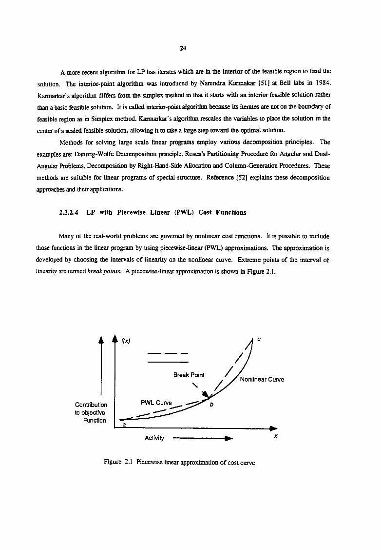
Many of the real-world problems are governed by nonUnear cost functions. It is possible to include
those functions in the linear program by using piecewise-Iinear (PWL) approximations. The approximation is
developed by choosing the intervals of linearity on the nonlinear curve. Extreme points of the interval of
linearity are termed break points. A piecewise-Iinear approximation is shown m Hgure 2.1.
A
Break Point Nonlinear Curve
PWL Curve Contribution to objective
Function
Activity
Figure 2.1 Piecewise linear approximation of cost curve
25
This PWL approximation contains two line segments, the first of which approximates the curve over
the range [a.b ] and the second of which is valid over [b,c]. Point b is called break point Different linear
programs use the PWL cost function in variety of ways.
The simplex algorithm would represent PWL firaction. shown in Figure 2.1 by two variables, xj and
x-y. The variables that represent PWL segments are known as segment variables. Then, we have the constraint
that
x= xj + X2_
(2J2))
While the fiinction value is determined by
f ix) = Sjxj + S2X2 .
(2.33)
where the 5, is the slope of segment /. Also, note that xj and X2 can not be in the basis at the same time,
otherwise the function defined above would be meaningless. The simplex method incorporates extra logic into
the routine to implement this restricted basis erary constraint The technique described for transforming a
nonlinear function into a PWL approximation is taken from Reference [53]. A more detailed analysis and
description of the method is available in Reference [54].
Another method of solving LP with a PWL objective function includes guessing the active segment
and performing the linear programming for the selected segment successively until all the constraints are
satisfied. The identification of the active segment employs heuristics specific to the problem under
consideration. This method allows the application of apriori knowledge to a deterministic algorithm, which is
expected to be more efficient
2.3.3 General Techniques of Optimization
2.3.3.1 Quadratic Programming (QP)
A nonlinear programming problem is a quadratic programming problem if the objective function is
a quadratic polynomial in the decision variables and the constraints are linear. Often, QP assumes convex
objective function. Quadratic programming arises in many applications and it forms the basis for most
methods of general nonlinear programming. A quadratic programming problem is represented by the
following form:
26
Minimize
0(x) = A^jc + l /2x^Gx
Subject to
f(x) = Bx - e > 0
(2.34)
where A and X are q-vectors, and f and e are p-vectors, B is a (p * q) symmetric positive definite matrix. Linear
programming (LP) is a special case of the quadratic programming (Q P), where the matrix G reduces to zero.
Theory and methods of solving quadratic programming problem are very mature [55].
2.3.3.2 Lagrangian Relaxation (LR) Method [56]
Lagrangian Relaxation method converts a large scale constrained optimization problem into
unconstrained master and slave subproblems. The advantage of the LR approach lies in reduction of problem
size by creating subproblems of lower dimensions. The method is well suited for the problems which are
additively separable over each component of the decision vector r. This allows the subproblems to be solved
independently. The LR method solves subproblems in dual space. The approach is based on the premise that if
the KKT optimality conditions are met, then a feasible solution to the dual problem leads to an optimal
solution of the primal problem. Consider a primal problem where function is to be optimized.
Minimize
^>(x)
Subject to
A x= b
xe X.
(2.35)
The LR method converts the constrained problem in (2.27) into following unconstrained primal
problem and the corresponding dual function:
Minimize
Z, (x, A ) = 0 ( x) + A (A X - Z>)
27
Subject to
A x = b
(2.36)
and dual function,
m U ) = m i n [ 0 ( x ) + A ( A x - b ) : x s X ]
(2.37)
where, the factors Aj, i = 1, / are called the Lagrange multipliers. Essentially, the Lagrange multipliers are dual
variables of the primal problem as described in section 2.3.2. To obtain a solution to the primal problem, the
dual function m (X) and the corresponding dual problems are defmed as follows:
Maximize
m(X)
Subject to:
A e r
(2.38)
The LR solution sets up a two step iterative procedure between the master problem (max m ( X ) ) and
the slave problem (min L(x,X)) as follows:
Step 1: Fmd a value for each A which moves m*(X) towards a larger value.
Step 2: Keeping A fixed at the value found in the step I, adjustx to find min L(x,X).
The updated x is used to find new value of A in step L The iterative process continues till A converges to X*.
The solution of subproblems gives the optimal solution of the primal problem %*•
2.3.3.3 Augmented Lagrangian Method [57]
Augmented Lagrangian method is a penalty function method that converts a constrained optimization
problem to an unconstrained subproblem with an objective function such that ill-conditioning can be avoided.
This is done by choosing a penalty parameter p. The objective function of the unconstrained subproblem is
known as Augmented Lagrangian function (L A). The choice of p is very critical for optimization of augmented
Lagrangian function. If p is too small, then the LA becomes unbounded from below. On the other hand, if the
p is too big, then the ill-conditioning occurs. The careful choice of p and proper estimate of Lagrange
multiplier A yield a local minimum solution of the augmented Lagrangian.
28
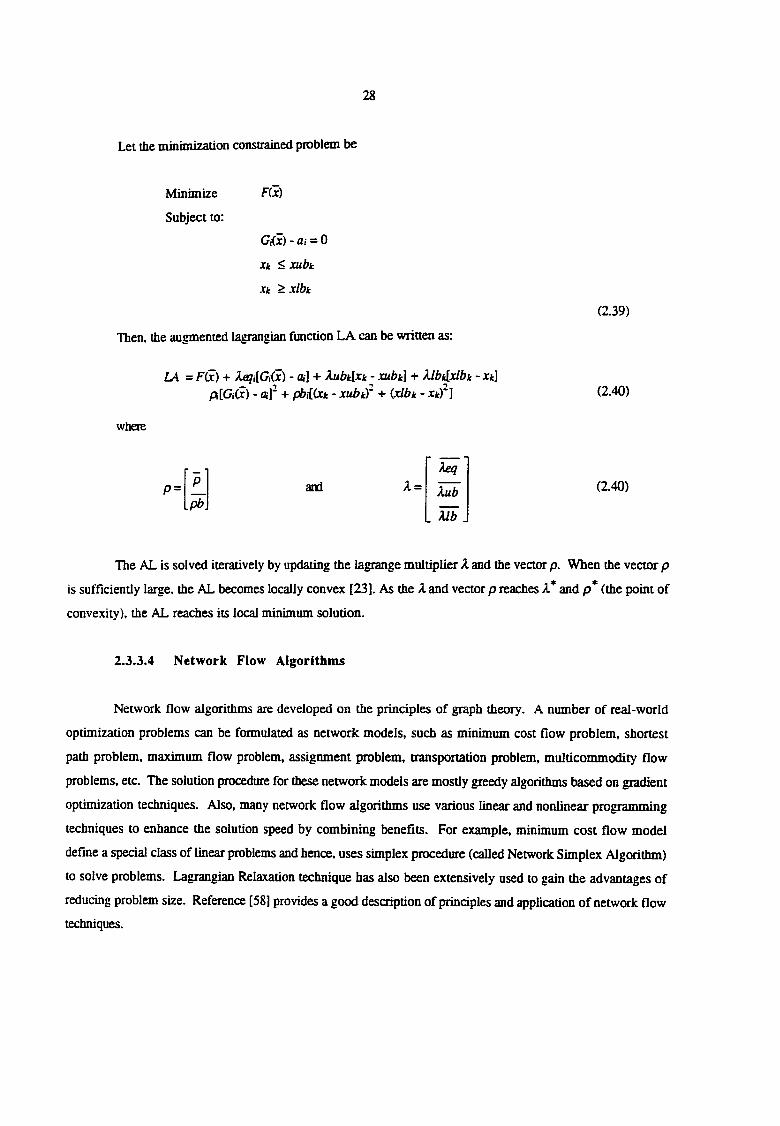
Let the minimization constrained problem be
Minimize Fix)
Subject to:
GKx) - a, = 0
Xk ^ xubk
Xk ^ xlbk
(2.39)
Then, the augmented lagrangian function LA can be written as:
LA = F(x) + keqi[Gi(x) - m] + ̂ .ubtlxk - xubk] + klbtixlbk - xt] Pi[Gi(x) - Oi]' + pbi[(Xk - xubk)' + (xlbk - Xkf] (2.40)
where
(2.40)
The AL is solved iteratively by updating the lagrange multiplier A and the veaor p. When the vector p
is sufficiently large, the AL becomes locally convex [23]. As the A and vector p reaches k* and p* (the point of
convexity), the AL reaches its local minimum solution.
2.3.3.4 Network Flow Algorithms
Network flow algorithms are developed on the principles of graph theory. A number of real-world
optimization problems can be formulated as network models, such as minimum cost flow problem, shortest
path problem, maximum flow problem, assignment problem, transportation problem, multicommodity flow
problems, etc. The solution procedure for these network models are mostly greedy algorithms based on gradient
optimization techniques. Also, many network flow algorithms use various linear and nonlinear programming
techniques to enhance the solution speed by combining benefits. For example, minimum cost flow model
define a special class of linear problems and hence, uses simplex procedure (called Network Simplex Algorithm)
to solve problems. Lagrangian Relaxation technique has also been extensively used to gain the advantages of
reducing problem size. Reference [58] provides a good description of principles and application of network flow
techniques.
P = P
Vpb
and A = Xeq
hib
Mb
29
2.3.3.5 Artiflcial Neural Network Algorithms
The application of artificial neural networks to optimization problems has been an active area of
research since the early eighties [59]. Research work has shown that artificial neural networks are nonlinear
dynamic systems from system theory point of view. A neural network with the following properties in the
state space of interest can perfonn the task of system optimization:
• Every network trajectory always converges to a stable equilibrium point.
• Every state equilibrium point corresponds to an optimal solution of the problem.
The first property guarantees thai given any initial point to the network, the ensuing network trajectory
leads to a stable steady state. The second property ensures that every steady state of the network is a solution of
the underlying optimization problem. A sufficient condition for a neural network to possess the first property is
the existence of the energy function associated with the network. The second property can be relaxed such that
the state of every stable equilibrium point is close to an optimal solution point of the problem.
The ability of processing feedback in a collective parallel analog mode enables a neural network to
simulate the dynamics that represent the optimization of an objective function subjected to its constraints for a
given optimization model. Kumar and Sheble [60,61] have applied the Kennedy, Chua and Lin neural network
[62,63] to solve linear and quadratic programmhig problems in power system optimization. Kennedy Chua and
Lin neural network is a nonlinear dynamic system from a system theory view point [64]. Kumar and Sheble
have proposed a novel method called clamped state variable method to simulate the neural network dynamics.
The proposed algorithm begins with formulating the control system matrices for the neural network.
Development of system matrices proceeds in two phases. First, the state space representation of the neural
network is formulated. The functional relationship of the nonlinear variables with the state space variables is
represented in a matrix form. For realization of a linear state space system, the nonlinear variables are treated as
the clamped-state variables of the system. Finally, the state model of the system is converted to homogeneous
equivalents for the state models. Thus, the nonlinear architecture of the Kennedy, Chua and Lin artificial neural
network is modeled as a linear homogeneous state space system. The classical matrix exponential technique for
calculating state transition matrix of a linear causal relaxed and time-invariant system is used as the basis of the
simulation algoritimu
30
2.3.4 Auction Optimization Mechanisms for Electric Energy
Various optimization schemes have been applied to energy auction mechanisms. Reference [65]
summarizes the application of number of optimization techniques, such as high-low matching algorithm,
network flow algorithm dynamic programming, etc. to energy auction system. These mechanisms are based on
different assumptions. References [66,67] describe the implementation of energy brokerage system using linear
programming. The data required for an elementary interchange brokerage system are the amount of power
available for trading, and the buy and sell quotes. Economic dispatch has been considered as the source for this
data in reference [66]. Reference [67] computes the data with network constraints to provide a complete analysis
of the power system. Implementation of brokerage system using augmented lagrangian technique has also been
investigated [68]. Reference [69] shows how a sequential sealed-bid/sealed-offer auction mechanism could be
applied to the pricing of electnc power. Interchange of electric power by using a double auction mechanism has
been discussed in reference [70]. Reference [71] presents an energy brokerage system with emission trading and
allocation of cost savings.
2.4 Schweppe's Theory of Spot Pricing [72]
Schweppe introduced the concept of optimal spot pricing in a vertically integrated industry. The
proposed theory took the perspective of a global controller who wished to maximize the social welfare function
by adjusting the level of each generating unit and the usage level of each consumer device. The optimal spot
price denoted the summation of marginal fuel cost, energy balance quality of supply premium, and transmission
network quality of supply premium. Schweppe came up with a set of rates related to spot prices and discussed
their applicability in view of different customer characteristics. The proposed rates included cost of rationing,
cost of equipment, and value of electricity usage in addition to the variable and fuel costs. Thus, the developed
foundation was a cost-based approach for power system operation. The introduced notion of component based
costing presented a number of issues related to customer response and utility revenues. The proposed spot
pricing ^proach highlighted a number of issues which should also be carefully examined in a deregulated power
system operation.
31
3. THEORETICAL DEVELOPMENT
3.1 Basic Framework
This chapter presents the theoretical foundation for market-based pricing of ancillary services. The
development is based on a very general auction market model [33. 73]. The developed foundation is used to
design an AGC simulator and electric power auction simulator for the new environment The basic firamework
of the proposed approach is described by stating necessary definitions and describing an auction market structure
together with underlying assumptions.
3.1.1 Definitions
Def 3.1: Energy Auction/Brokerage System is defined as a central auction mechanism which provides
trading opportunities to the market participants and maintains reliability of power system operation by
coordinating generation, transmission and distribution fimctions.
Def. 3.2: Ancillary services are the services used for supporting a reliable delivery of electric energy in
power system operation.
Def. 3.3: Spinning reserve is defined as the unused capacity of generating units which are on line in
operation. Spinning reserve can be called into operation almost instantaneously.
Def. 3.4: Ready reserve is defined as the unused cecity of generation which are not on line but can be
brought on line withm 15 minutes in operation.
Def. 3.5: Transmission losses is defined as the amount of electric energy (contracted with seUers)
dissipated in the electrical transmission network during the process of power delivery.
Def. 3.6: Load following is defined as the amount of electric energy provided to maintain the contracted
tie line flow and frequency in power system operation. The load following energy is required to respond in 5-10
minutes of ume frame.
Def. 3.7: An unbundled ancillary service is defined as the service for which the end user is explicidy
known at the time of contract.
Def. 3.8: A bundled ancillary service is defined as the service for which the end user is not explicitly
known at the tnne of contract.
Def. 3.9: Industry cost is defined as the cost of providing bundled ancillary services. The Industry cost
should be recovered by some acceptable allocation mechanism [74].
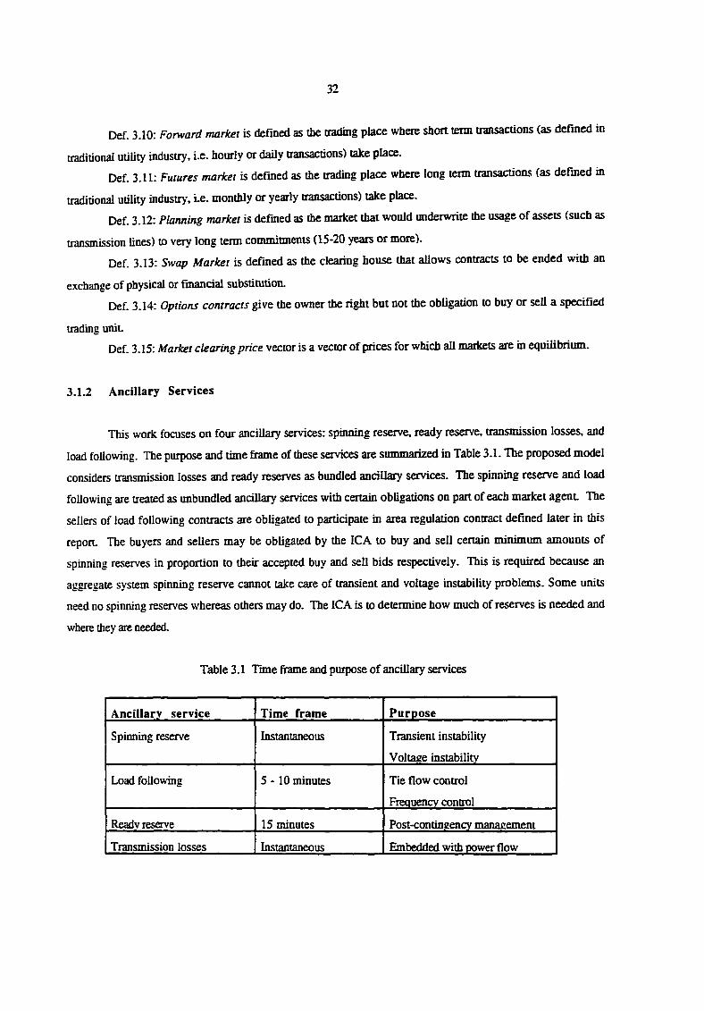
32
Def. 3.10: Forward market is defined as the trading place where short term transactions (as defined in
traditional utility industry, i.e. hourly or daily transactions) take place.
Def. 3.11: Futures market is defined as the trading place where long term transactions (as defined in
traditional utility industry, i.e. monthly or yearly transactions) take place.
Def. 3.12: Planning market is defined as the market that would underwrite the usage of assets (such as
transmission lines) to very long term commitments (15-20 years or more).
Def. 3.13: Swap Market is defined as the clearing house that allows contracts to be ended with an
exchange of physical or financial substitution.
Def. 3.14: Options contracts give the owner the right but not the obligation to buy or sell a specified
trading unit.
Def. 3.15: Market clearing price vector is a vector of prices for which all markets are in equilibrium.
3.1.2 Ancillary Services
This work focuses on four ancillary services: spinning reserve, ready reserve, transmission losses, and
load following. The purpose and time firame of these services are summarized in Table 3.1. The proposed model
considers transmission losses and ready reserves as bundled ancillary services. The spinning reserve and load
following are treated as unbundled ancillary services with certain obligations on part of each market agent. The
sellers of load following contracts are obligated to participate in area regulation contract defined later in this
report. The buyers and sellers may be obligated by the ICA to buy and sell certain minimum amounts of
spinning reserves in proportion to their accepted buy and sell bids respectively. This is required because an
aggregate system spinning reserve cannot take care of transient and voltage instability problems. Some units
need no spinning reserves whereas others may do. The ICA is to determine how much of reserves is needed and
where they are needed.
Table 3.1 Time frame and purpose of ancillary services
Ancillary service Time frame Purpose
Spinning reserve Instantaneous Transient instability
Voltase instabilitv
Load following 5-10 minutes Tie flow control
Frequencv control
Readv reserve 15 minutes Post-contineency manasement
Transmission losses Instantaneous Embedded with power flow
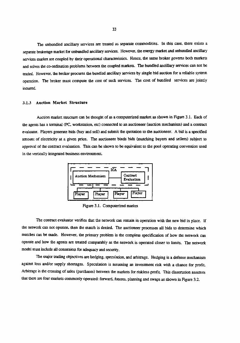
33
The unbundled ancillary services are treated as separate commodities. In this case, there exists a
separate brokerage market for unbundled ancillary services. However, the energy market and unbundled ancillary
services market are coupled by their operational characteristics. Hence, the same broker governs both markets
and solves the co-ordination problems between the coupled markets. The bundled ancillary services can not be
traded. However, the broker procures the bundled ancillary services by single bid auction for a reliable system
operation. The broker must compute the cost of such services. The cost of bundled services are jointly
incurred.
3.1.3 Auction Market Structure
Auction market structure can be thought of as a computerized market as shown in Hgure 3.1. Each of
the agents has a terminal (PC, workstation, etc) connected to an auctioneer (auction mechanism) and a contract
evaluator. Players generate bids (buy and sell) and submit the quotation to the auctioneer. A bid is a specified
amount of electricity at a given price. The auctioneer binds bids (matching buyers and sellers) subject to
approval of the contract evaluation. This can be shown to be equivalent to the pool operating convention used
in the vertically integrated business environment
Player Player Player Player
Contract Evaluation
Auction Mechanism
ICA
Figure 3.1. Computerized market
The contract evaluator verifies that the network can remain in operation with the new bid in place. If
the network can not operate, then the match is denied. The auctioneer processes all bids to determine which
matches can be made. However, the primary problem is the complete specification of how the network can
operate and how the agents are treated comparably as the network is operated closer to limits. The network
model must include all constraints for adequacy and security.
The major tradmg objectives are hedging, speculation, and arbitrage. Hedging is a defense mechanism
against loss and/or supply shortages. Speculation is assuming an investment risk with a chance for profit
Arbitrage is the crossing of sales (purchases) between the markets for riskless profit. This dissertation assumes
that there are four markets commonly operated forward, futures, planning and swaps as shown in Figure 3.2.
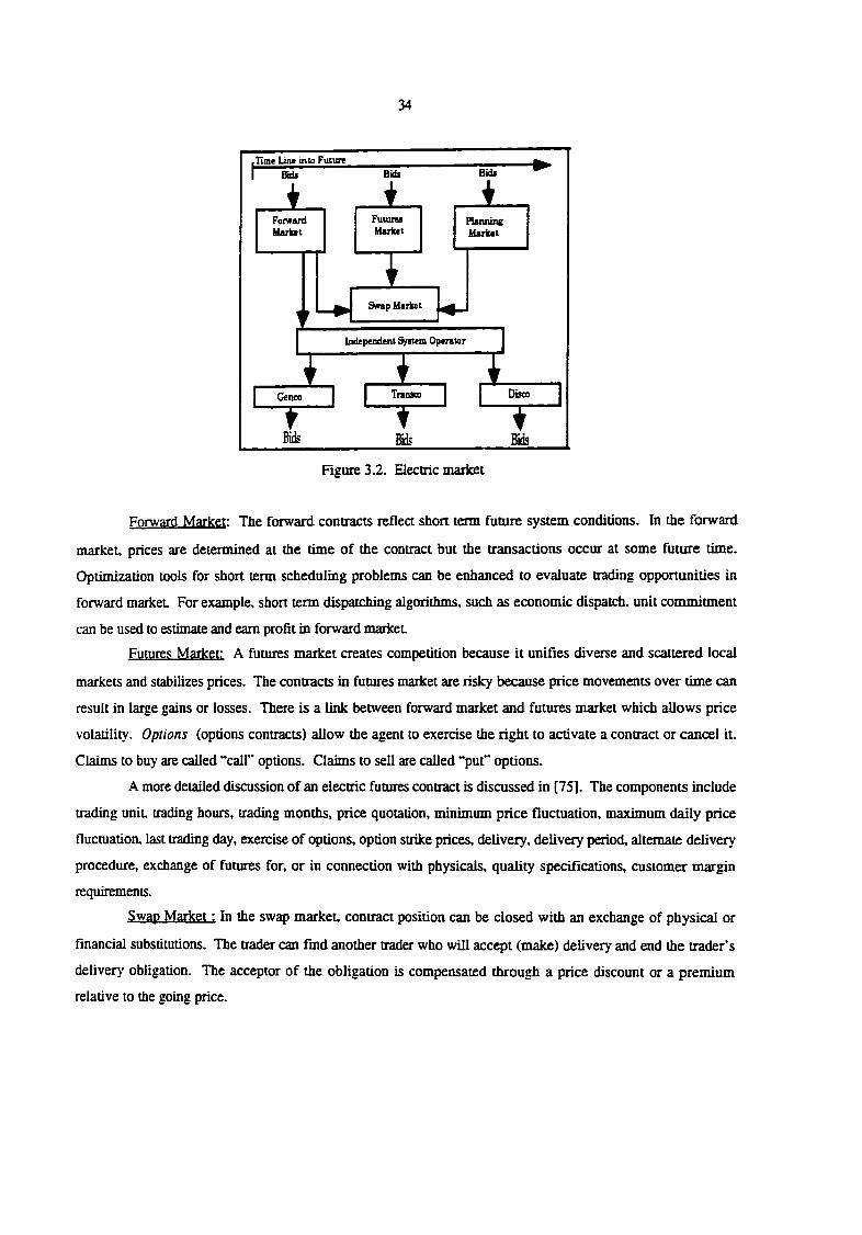
34
iUme Line into Futurg Bids Bids Bids
Independent %stem Operator
Genco
Bids
Traosm Disco
Forward Market
FututBS Market
Swap Market
Rgiire3.2. Electric market
Forward Market: The forward contracts reflea short term future system conditions. In the forward
market, prices are determined at the time of the contract but the transactions occur at some future time.
Optimization tools for short term scheduling problems can be enhanced to evaluate trading opportunities in
forward market. For example, short term dispatching algorithms, such as economic dispatch, unit commitment
can be used to estimate and earn profit in forward market
Futures Market: A futures market creates competition because it unifies diverse and scattered local
markets and stabilizes prices. The contracts in fumres market are risky because price movements over time can
result in large gains or losses. There is a link between forward market and futures market which allows price
volatility. Options (options contracts) allow the agent to exercise the right to activate a contract or cancel it.
Claims to buy are called "call" options. Claims to sell are called "put" options.
A more detailed discussion of an electric futures contract is discussed in [75]. The components include
trading unit, trading hours, trading months, price quotation, minimum price fluctuation, maximum daily price
fluctuation, last trading day, exercise of options, option strike prices, delivery, delivery period, alternate delivery
procedure, exchange of futures for, or in connection with physicals, quality specifications, customer margin
requirements.
Swap Market: In the swap market, contract position can be closed with an exchange of physical or
financial substitutions. The trader can find another trader who will accept (make) delivery and end the trader's
deliver\' obligation. The acceptor of the obligation is compensated through a price discount or a premium
relative to the going price.
35
The financial drain inflicted on traders when hedging their operations in the futures market is slightly
higher than the one inflicted through direct placement in the forward market An optimal mix of options,
forward commitments, futures contracts and physical inventories is difficult to assess and depends on hedging,
consttaints imposed by different contracts, and cost of different contracts. The exchange of various energy
instruments is handled by a clearing house such as a swap market
Planning M?iricet: The growth of transmission grid requires transmission companies to make contracts
based on the expected usage to finance projects. The planning market would underwrite the usage of equipment
subject to the long term commitments to which distribution and generation companies are bound by the rules of
network expansion to maintain a fair market place. The network expansion would have to be done to maximize
the use of transmission grid for all agents. Collaboration would have to be overseen and prohibited with a
sufficiently high financial penalty.
3.1.4. Assumptions
This work aims to develop the pricing mechanism for reserve margins, transmission losses, and load
following in elecuic power transaction. To simplify the discussion, the problem is restricted with the
assumptions below; however, the theory developed in this paper is flexible enough to allow these assumptions
to be relaxed if desired.
Assumption 1:. The auctioneer will establish interchange schedules (multilateral transactions) between
the participating agents on hourly basis. Bilateral transactions may be established outside the auction but are
still subjected to scrutiny with respect to operating constraints. Furthermore, u is assumed that transcos are not
economic agents, i.e. they are exogenous to the model. This assumption can be relaxed by including transcos
bids and evaluating them on the S/MW-Mile basis. Post [70] has shown an auction simulation with the
transmission bidding. However, the transmission bid evaluation should include the cost of control (such as
phase shifters) to direct the power flow in accordance with the established contract Since, transmission is still
considered to be monopoly, this work has not hicluded transco bidding.
Assumption 2: The agents (discos and gencos) are obligated to buy or sell the binding bids declared by
the auctioneer. Hence, all local operational constraints (such as ramp rate constraints, emission constraints, fuel
constraints, minimum down times, minimum up times, start-up procedure curves, etc.) must be considered by
the agents while generating bids for the next trading session or round.
Assumption 3: The auctioneer is the sole authority to verify that the network remains in operation
with the new bids in place. The control center operators are responsible to implement the contracts given by the
auctioneer.
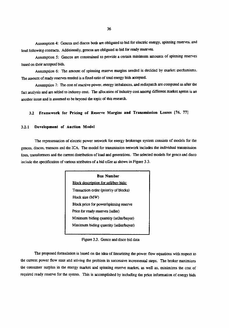
36
Assumption 4: Gencos and discos both are obUgated to bid for electric energy, spinning reserves, and
load following contracts. Additionally, gencos are obligated to bid for ready reserves.
Assumption 5: Gencos are constrained to provide a certain minimum amounts of spinning reserves
based on their accepted bids.
Assumption 6: The amount of spinning reserve margins needed is decided by market mechanisms.
The amount of ready reserves needed is a fixed ratio of total energy bids accepted.
Assumption 7: The cost of reactive power, energy imbalances, and redispatch are computed as after the
fact analysis and are added to industry cost. The allocation of industry cost among different market agents is an
another issue and is assumed to be beyond the topic of this research.
3,2 Framework for Pricing of Reserve Margins and Transmission Losses (76, 77]
3.2.1 Development of Auction Model
The representation of electric power network for energy brokerage system consists of models for the
gencos, discos, transcos and the ICA. The model for transmission network includes the individual transmission
lines, transformers and the current distribution of load and generations. The selected models for genco and disco
include the specification of various attributes of a bid offer as shown in Figure 33.
Bus Number
Block descripUon for sell/buv bids:
Transaction order (priority of blocks)
Block size (MW)
Block price for power/spinning reserve
Price for ready reserves (seller)
Minimum biding quantity (seller/buyer)
Maximum bidmg quantity (seller/buyer)
Figure 33. Genco and disco bid fiata
The proposed formulation is based on the idea of linearizing the power flow equations with respea to
the current power flow state and solving the problem in successive incremental steps. The broker maTTmiypc
the consumer surplus in the energy market and spinning reserve market, as well as, minimizes the cost of
required ready reserve for the system. This is accomplished by including the price information of energy bids
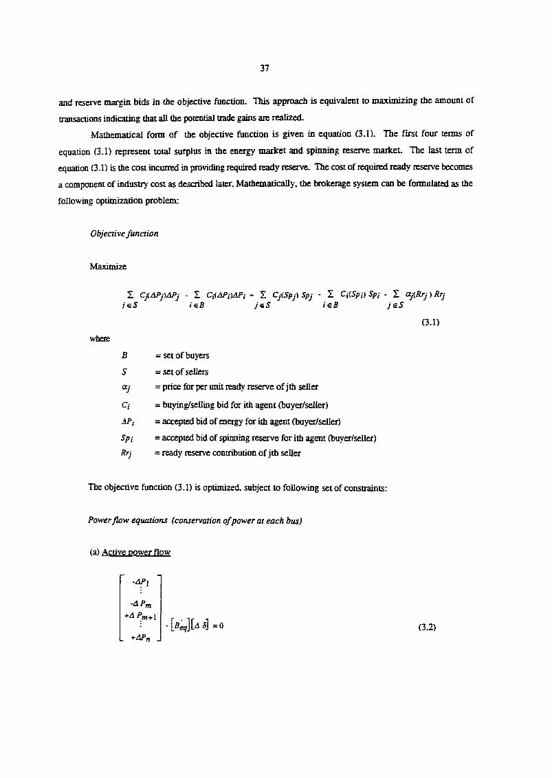
37
and reserve margin bids in tlie objective function. This approach is equivalent to maximizing the amount of
transactions indicating thai all the potential trade gains are realized.
Mathematical form of the objective function is given in equation (3.1). The first four terms of
equation (3.1) represent total surplus in the energy market and spiiming reserve market. The last term of
equation (3.1) is the cost incurred in providing required ready reserve. The cost of required ready reserve becomes
a component of industry cost as described later. Mathematically, the brokerage system can be formulated as the
following optimization problem:
Objeaive funaion
Maximize
X CjlAPp^Pj - I CHAPD^Pi + s Cj(Spj) Spj - S Ci(Spi) Spi - I ajiRrj) Rrj i e S i e B i sB j e S
(3.1)
where
B = set of buyers
S = set of sellers
ocj = price for per unit ready reserve of jth seller
Ci = buying/seUing bid for ith agent (buyer/seller)
APi - accepted bid of energy for ith agent (buyer/seller)
Sp i = accepted bid of spinning reserve for ith agent (buyer/seller)
Rrj = ready reserve contribution of jth seller
The objective function (3.1) is optimized, subjea to following set of constraints:
Powerflow equations (conservation of power at each bus)
(a) Active power flow
-APi
-AP, m
(3.2) L J
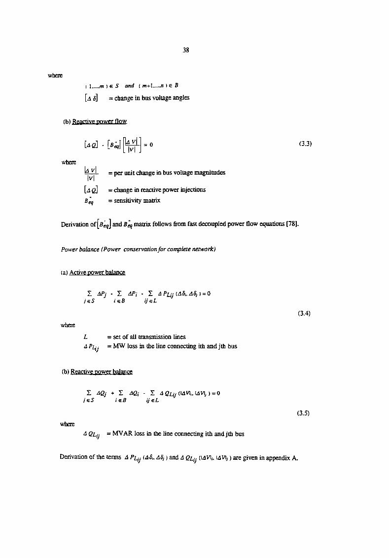
38
where
( I m ) 6 S and ( m+1 n ) e B
[4 5] = change in bus voltage angles
fh^ Reactive power flow
Ue] -
where
kzl LM
= 0 (3.3)
U v\ = per unit change in bus voltage magnitudes
[d g] = change in reactive power injecdons
Bgq = sensitivity matrix
Derivation of [figj and Beq matrix follows from fast decoupled power flow equations [78].
Power balance (Power conservation for complete network)
(a) Active power balance
Z APj - Z APi - Z A Piij {A5i, aSj ) = 0 i s S i s B i j e L
where
L = set of all transmission lines
A Pi^j = MW loss in the line connecting ith and jth bus
(b) Reactive power balance
Z AQj + z AQi - Z (LdVl,. l4Vlj ) =0 / 6 5 i e 5 i j s L
where
^ Qlij = MVAR loss in the line connecting ith and jth bus
(3.4)
(3.5)
Derivation of the terms A Pi-j (ASi. ASj) and A Q l- j (14VI„ idVi^) are given in appendix A.
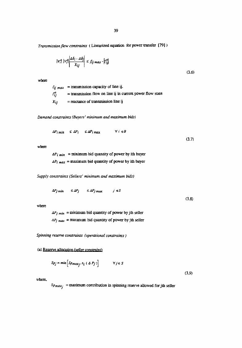
39
Transmission flow constraints ( Linearized equation for power transfer [79])
iv/i \v^ ASj - ASj
Xij - fi jmax'yi
(3.6)
where
fij max = transmission capacity of line ij.
if J = transmission flow on line ij in current power flow state
Xij = reactance of transmission line ij
Demand constraints (Buyers' minimum and maximum bids)
^imin - -^inutx
where
min = minimum bid quantity of power by ith buyer
^Pi max = maximum bid quantity of power by ith buyer
Supply constraints (Sellers' minimum and maximum bids)
^jmin S fnax J
where
APy min = minimum bid quantity of power by jth seller
max - maximum bid quantity of power by jth seller
Spinning reserve constraints (operational constraints)
fa) Reserve allocation f<«;ller constraint)
Spj = min ̂ Spmaxj- i ( 4 Pj )j Vy e S
where,
^Pmaxj = maximum contribution in spinning reserve aUowed for jth seller
(3.7)
(3.8)
(3.9)
40
s J = percentage paiticipation in spinning reserve for a seller (an obligation)
rh) Obligation to huv fhnver constraint)
Spi = (3.10)
where
S2 = percentage participation in spinning reserve for a buyer (an obligation)
fc) Spinning reserve balance
I Spi - S Spj = 0 ieS JeB
(3.11)
Ready reserve constraints (Reliability constraints)
(a) Reserve allocation
Rri = min q ( 4 P/}] V ieS
(3.12)
where
Rrmaxf = maximum contribution in ready reserve allowed for jtfa seller
rj = percentage participation in ready reserve for a seller (an obligation)
(b) system constraint
Y.Rri s ri X 4P,-1 e5
(3.13)
where
r2 = net generation to ready reserve ratio.
The industry cost or social welfare cost (SWC) can be computed by adding costs of ready reserves and
transmission losses at marginal selling price as follows.
SWC = Z + 21 ^^Lii j ^ S ij e L
(3.14)
41
where Rrj = optimal value of ready reserve contribution by jth agent
A = marginal cost of sell at the transaction
4Px,iy = transmission loss in line ij at optimal point
Social welfare cost can be allocated among buyers by the ratio of their participation or contribution to
the system load. A novel method of cost allocation using Shapely value criteria has recently been reported in
reference (711.
3.2.2 Adaptation for Linear Programming
The proposed formulation as described earlier can easily be adapted for linear programming application.
The objective function of equation (3.1) is a piecewise linear objective function because of the bids being in
blocks. Such a problem is solved by applying LP successively and iteratively switching from one cost segment
to another until an optimal solution is found as described in Section 23.2.4.
Constraint equations (3.6), (3.9), and (3.11) include nonlinear operations such as "mod' (absolute value
function) and "min' functions. These functions can be accommodated in LP formulation by making proper
substitutions as follows.
•Mod' operation
Replace:
Ixl byxl +x2
X by xl - x2
xl >= 0 and x2 >= 0
(3.15)
•Min'operation
The "min' operation can be accommodated in LP formulation by making following substitutions:
xl = min (b, x2)
Replace: xl =x2-s
x2- s <= b
s>= 0
(3.16)
42
Equations representing linear programming formulation of the energy brokerage system can be
rearranged by keeping all the local constraints before the system constraints. The system constraints include
(3.2.3.3.3.4,3.5.3.10,3.12) and the local constraints include (3.6,3.7,3.8.3.9,3.11,3.13). This arrangement
leads to an angular block structure. The use of price decomposition approach (such as Dantzig-Wolfe) is the
rinciiral method of solving problems with the angular block structure .
Dimensionality of the proposed formulation can further be reduced by identifying a suitable
transformation. In the proposed formulation, equation (3.2) presents an explicit relationship between ASf and
APi, which can be used to define a transformation matrix T juch that
[AS] = [r] [ap]
(3.17)
Derivation of [r] is given in appendix B. Equation (3.17) can be used to replace all A5i in terms of
APf. Note that the column vector [^d 5] does not contain the slack bus voltage angle since the derivation of [r]
is obtained by calculating the power flow Jacobian which does not contain slack bus variables. However, by
definition, the slack bus voltage angle is zero and hence, it does not affect the transformation. The substitution
given in equation (3.17) eliminates all the bus angle variables resulting in 50% reduction in number of
variables. The constraint set defined by equation (3.2) is also eliminated.
Note that the proposed formulation is based on the network sensitivities of the system. Hence, a large
transaction problem needs to be solved in incremental steps by applying LP successively. At each incremental
step, network sensitivity matrices need to be updated.
3.2.3 Consideration of Security Constraints
Power system security calculation using linear programming has been an active area of research [80,
81, 82, 83]. The approach behind all the work is based on linearization of the system about the initial system
operating state and evaluating the security constraints using sensitivity analysis. The approach presented in this
work can easily be extended to consider various security constraints by using such techniques. One such
extension is described in this section for illustration purpose.
Consider a two-dimensional operating limit boundary surface (OLBS) [84] defined by a locus
representing sum of the power flows on two transmission lines not exceeding a certain value. This kind of
OLBS is of practical interest as sub areas of a typical power system network are connected with a few (usually
around two) tie lines for transfer of electrical power between the regions. Such a typical locus is shown in
Figure 3.4.
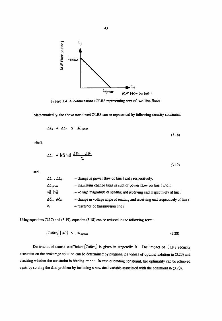
43
MW Flow on line i
Figure 3.4 A 2-dimensional OLBS representing sum of two line flows
Mathematically, the above mentioned OLBS can be represented by following security constraint:
+ A L f j ^ Al^ijmax
(3.18)
where,
ALi = h°J|v,01 Xi
(3.19)
and.
AL,, ALj = change in power flow on line i andj respectively.
AJLijmax = maximum change limit in sum of power flow on line t and j.
|v-i |v3 = voltage magnitude of sending and receiving end respectively of line i
ASisf ASir = change in voltage angle of sending and receiving end respectively of line i
Xi = reactance of transmission line i
Using equations (3.17) and (3.19), equation (3.18) can be reduced in the following form:
[Tolbsij][AP] < ALijmax (3.20)
Derivation of matrix coefficient \Tolbsij[ is given in Appendix B. The impact of OLBS security
constraint on the brokerage solution can be determined by plugging the values of optimal solution in (3.20) and
checking whether the constraint is binding or not. In case of binding constraint, the optimality can be achieved
again by solving the dual problem by including a new dual variable associated with the constraint in (3.20).
44
33 AGC Simulator in Price-Based Operation [85, 86]
3.3.1 Introduction to Load Following Contracts
In a vertically integrated industry, AGC operation aims to satisfy the MERC control performance
criteria [87] while mitigating growing system problems. The main objectives of AGC are (a) to hold system
frequency at or very close to a specified nominal value, (b) to maintain the correct value of interchange power
between control areas, and (c) to maintain each unit's generation at the most economic value. Implementation
of AGC schemes is typically in a central location where information pertaining to the system, such as unit
megawatt output, megawatt flow over tie lines, and system frequency are monitored. Rnally, the output of
AGC is transmitted to each of the participating generating units to meet the aforementioned objectives.
Under the new paradigm, AGC operation is accountable to load following contracts described later in
this section. However, implementation of these contracts will also meet the NERC control performance criteria
as long as the area control error (ACE) is a part of the control objective. This can be done by choosing a
suitable market structure and operating mechanism. In such a market place, the AGC simulator will need all the
information required in a vertically operated utility industry plus the contract data and measurements.
An overview of load frequency control issues in power system operation after dereguladon is reported in
reference [88]. The discussion is focused on addressing the operational structures likely to result from
deregulation, the possible approaches to load frequency control, and other associated technical issues. The
proposed market structure in this work combines features of all the operational structures described in [88].
The focus of this work is to introduce the idea of different load following contracts and provide
evidence that the proposed ideas are implementable. Players violating the contractual agreements should be
subjected to high penalty. In real time operation, the contract violation is reflected in higher cost of area
regulation requirement The traditional notion of control area and tie lines is retained in the proposed
development
The new framework requires establishment of standards for the electronic communication of contract
data, as well as, measurements among the ICA and the market agents. Increased magnitude of computerized
accounting needed by the explosion in the number of transactions is an another technical issue to be solved. In
general, a variety of technical regulations will be needed to ensure secure system operation and a fair
marketplace.
The growth of transactions between control areas and demands at levels far greater than for rla.ssif^l
AGC will require extended algorithms to perform load following in power system operation. One such
algorithm with a modified control concept is presented in reference [89]. The AGC simulator proposed in this
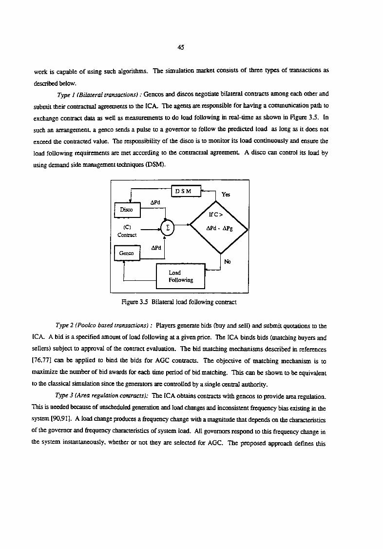
45
work is capable of using such algorithms. The simulation market consists of three types of transactions as
described below.
Type I (Bilateral transactions): Gencos and discos negotiate bilateral contracts among each other and
submit their contractual agreements to the ICA. The agents are responsible for having a communication path to
exchange contract rfata as well as measurements to do load following in real-time as shown in Figure 3.5. In
such an arrangement, a genco sends a pulse to a governor to follow the predicted load as long as it does not
exceed the contracted value. The responsibility of the disco is to monitor its load continuously and ensure the
load following requirements are met according to the contractual agreement A disco can control its load by
using demand side management techniques (DSM).
D S M Yes
Disco IfO
APd- APg Contract
APd Genco
Load Following
Figure 3.5 Bilateral load following contract
Type 2 (Poolco based transaaions): Players generate bids (buy and sell) and submit quotations to the
ICA. A bid is a specified amount of load following at a given price. The ICA binds bids (matching buyers and
sellers) subject to approval of the contract evaluation. The bid matching mechanisms described in references
[76,77] can be applied to bind the bids for AGC contracts. The objective of matching mechanism is to
maximize the number of bid awards for each time period of bid matching. This can be shown to be equivalent
to the classical simulation since the generators are controlled by a single central authority.
Type 3 (Area regulation contracts): The ICA obtains contracts with gencos to provide area regulation.
This is needed because of unscheduled generation and load changes and inconsistent frequency bias existing in the
system [90,91]. A load change produces a frequency change with a magnitude that depends on the characteristics
of the governor and frequency characteristics of system load. All governors respond to this frequency change in
the system instantaneously, whether or not they are selected for AGC. The proposed approach defines this
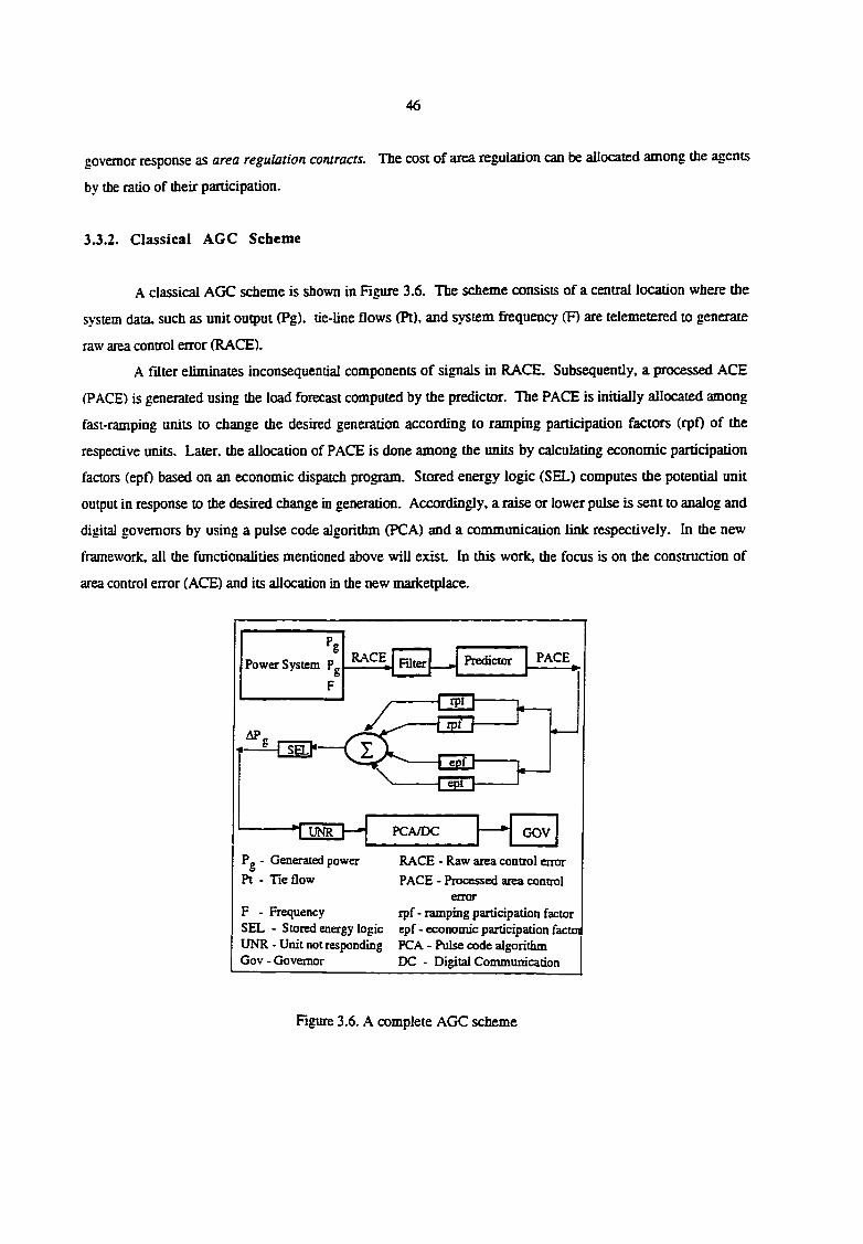
46
governor response as area regulation contracts. The cost of area regulation can be allocated among the agents
by the ratio of their participation.
3.3.2. Classical AGC Scheme
A classical AGC scheme is shown in Figure 3.6. The scheme consists of a central location where the
system data, such as unit output (Pg). tie-line flows (Pt), and system frequency CR are telemetered to generate
raw area control error (RACE).
A filter eliminates inconsequential components of signals in RACE. Subsequently, a processed ACE
(PACE) is generated using the load forecast computed by the predictor. The PACE is initially allocated among
fast-ramping units to change the desired generation according to ramping participation factors (rpf) of the
respective units. Later, the allocation of PACE is done among the units by calculating economic participation
factors (epf) based on an economic dispatch program. Stored energy logic (SEL) computes the potential unit
output in response to the desired change in generation. Accordingly, a raise or lower pulse is sent to analog and
digital governors by using a pulse code algorithm (PCA) and a communication link respectively. In the new
framework, all the functionalities mentioned above will exist In this work, the focus is on the construction of
area control error (ACE) and its allocation in the new marketplace.
Pg
Power System Pg
F
RACE Filter Pg
Power System Pg
F
Predictor PACE
-*1 UNR I—' PCA/DC GOV
Pg - Generated power Pt - He flow
F - Frequency SEL - Stored energy logic UNR - Unit not responding Gov - Governor
RACE - Raw area control error PACE - Processed area control
error rpf - ramping participation factor epf - economic participation factoi PCA - Pulse code algorithm DC - Digital Communication
Figure 3.6. A complete AGC scheme
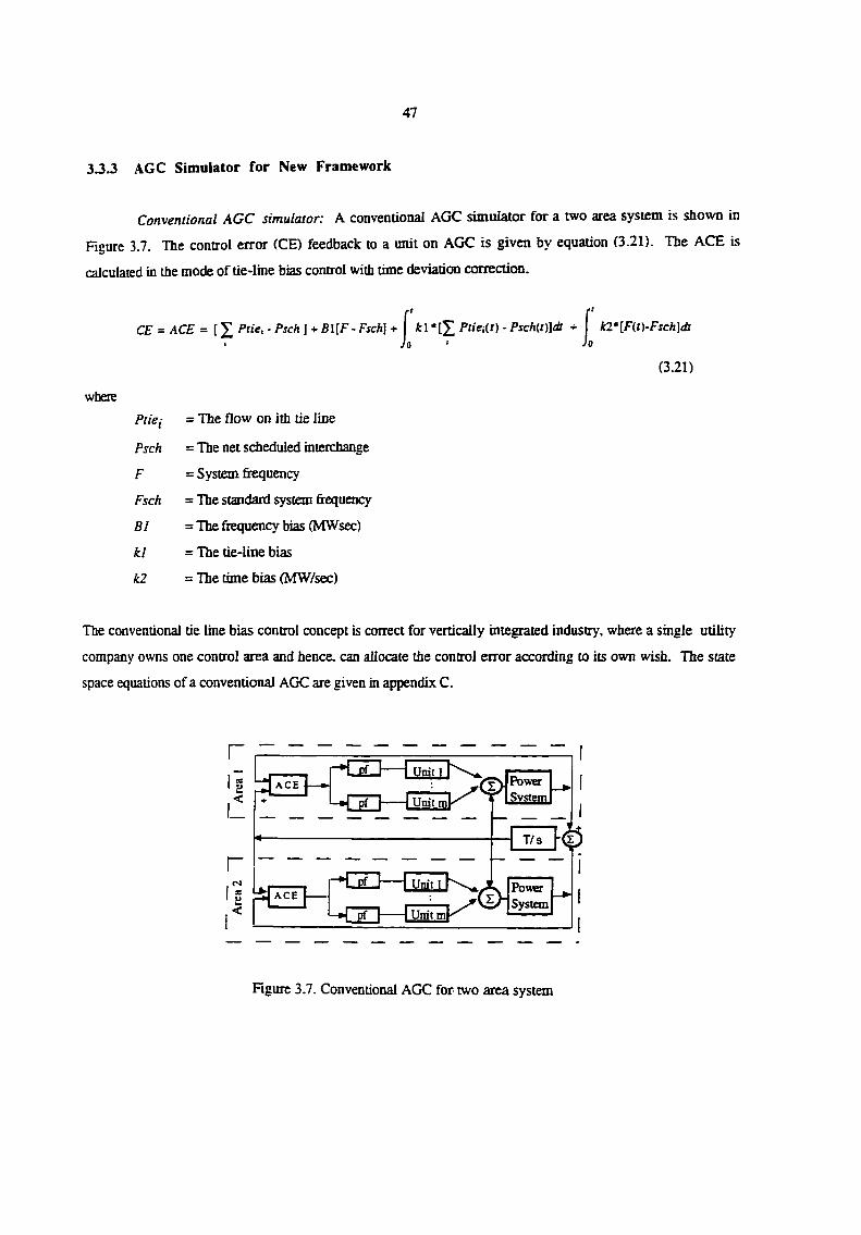
47
3.3.3 AGC Simulator for New Framework
Conventional AGC simulator: A conventional AGC simulator for a two area system is shown in
Ficure 3.7. The control error (CE) feedback to a unit on AGC is given by equation (3.21). The ACE is
calculated in the mode of tie-lme bias control with time deviation correction.
CE = ACE = [ £ Ptie. - Psch ] + BllF-Fsch] + ifcl PHeM - Pxh(t)]dt + k2'[Fit)-Fsch]d: i Jo ' Jo
(3.21)
where
Piiei = The flow on ith tie line
Psch = The net scheduled interchange
F = System frequency
Fsch = The standard system frequency
BI = The frequency bias (MWsec)
kl = The tie-line bias
k2 = The time bias (MW/sec)
The conventional tie line bias control concept is correct for vertically integrated industry-, where a single utility
company owns one control area and hence, can allocate the control error according to its own wish. The state
space equations of a conventional AGC are given in appendix C.
r
l!
r
Unit 1
^ Pf I 1 Unit
Power System
T/s -<P
1 Unit 1
-H pf I [ Unit m
Power System
Figure 3.7. Conventional AGC for two area system
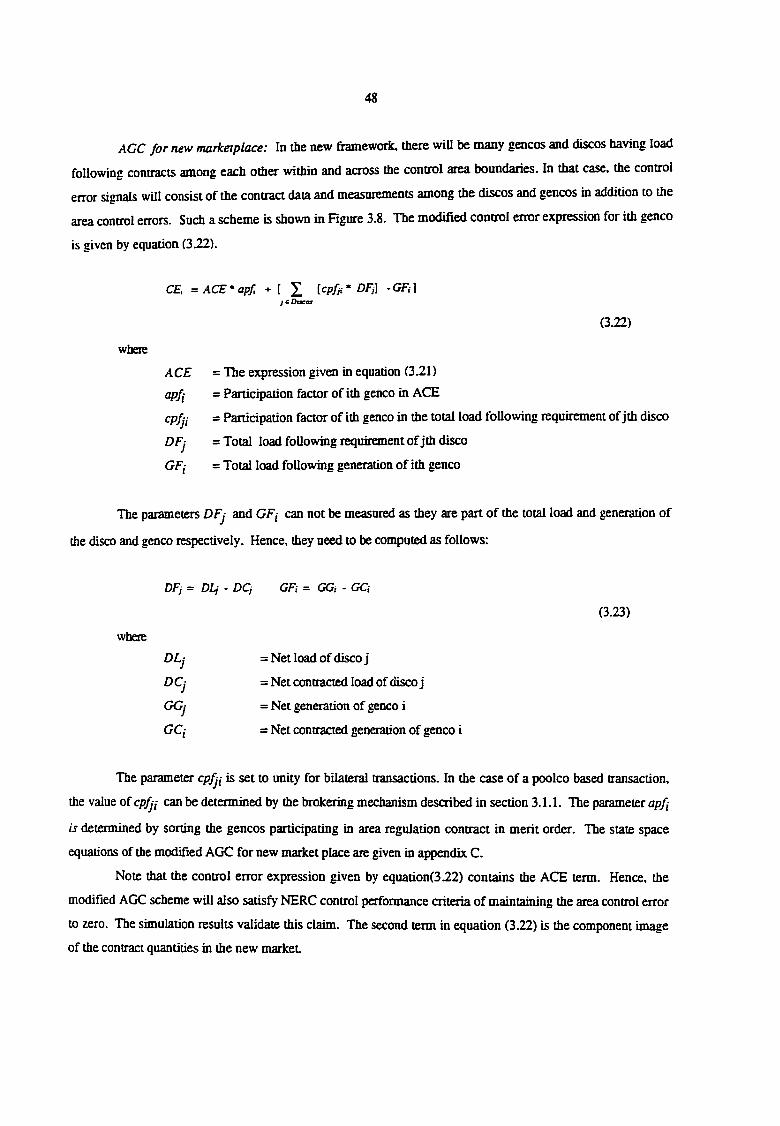
48
AGC for new marketplace: In the new frameworfc. there will be many gencos and discos having load
following contracts among each other within and across the control area boundaries. In that case, the control
error signals will consist of the contraa data and measurements among the discos and gencos in addition to the
area control errors. Such a scheme is shown in Rgure 3.8. The modified control error expression for ith genco
is given by equation (3.22).
CE, = ACE" apfi + [ ^ [cpfji' DFj\ - GFi ] j^Dtscos
(3.22)
where
ACE = The expression given in equation (3.21)
''Pfi = Participation factor of ith genco in ACE
cpfji = Participation factor of ith genco in the total load following requirement of jth disco
DFj = Total load following requirement of jth disco
GFi = Total load following generation of ith genco
The parameters DFj and GF,- can not be measured as they are part of the total load and generation of
the disco and genco respectively. Hence, they need to be computed as follows:
DFj = DQ - DCj GFi = CO, - GQ
(3.23)
where
DLj = Net load of disco j
DCj = Net contracted load of disco j
GGj = Net generation of genco i
GCi = Net contracted generation of genco i
The parameter cpfjj is set to unity for bilateral U'ansactions. In the case of a poolco based transaction,
the value of cpfji can be determined by the brokering mechanism described in section 3.1.1. The parameter apfi
is determined by sorting the gencos participating in area regulation contract in merit order. The state space
equations of the modified AGC for new market place are given in appendix C.
Note that the control error expression given by equation(322) contains the ACE term. Hence, the
modified AGC scheme will also satisfy NERC control performance criteria of maintaining the area control enor
to zero. The simulation results validate this claim. The second term in equation (3.22) is the component image
of the contract quantities in the new market.
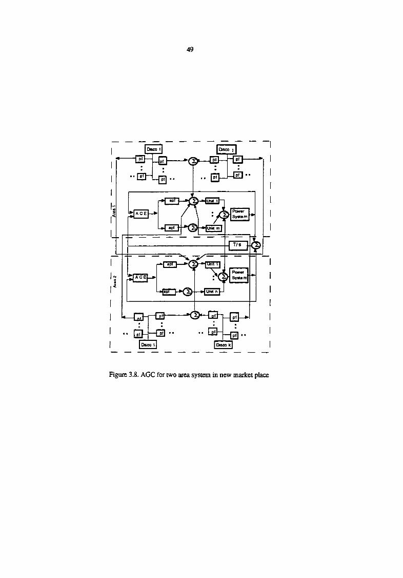
49
"GIH_0 •'(p—[ill—HZl— • •
.. [pjj—MiD"
yHH-* Sy«t«m
Unit m
1 - f c r s p H — " " " ' I
^ ACE|-» Syitam
«—rn-[—G3
I pit— —I p'l •• I pti—
iDsea ll r-Iii]
Deco k|
Figure 3.8. AGC for two area system in new market place
50
place. These component images are continuous, regular and quiescent. Hence, they are very well suited for
generation control as suggested in research literature [89]. The AGC scheme shown for the two area system in
Figure 3.8 can easily be extended to multiple area systems.
3.3.4 Simulator Features and Capabilities
The proposed approach is used to develop an AGC simulator for a 3 area test system. The development
of test system and the simulation results are described in Chapter 4. The software can simulate bilateral
contracts, poolco based contracts, and a combination of both, within and across control area boundaries. The
program can simulate any pattern of load changes.
The proposed simulation scheme can be used to study all possible scenarios of contract violation. The
approach is based on the premise that the ACE is an integral pan of the control error feedback to gencos. If the
excess demand (equivalent to shortfall of generation from simulation point of view) is not contracted out to any
genco. the change in load appears only in terms of area control enors. Hence, the additional demand or the
shortfall of generation is shared by all the gencos of the area in which the contract violation occurs.
The details of contract implementation can be used to teach students the issues involved in load
following in a price-based operation. More case studies can be presented to encourage thinking about required
technical regulations to ensure secure system operation and a fair marketplace. A number of interesting
discussions can be motivated by asking questions such as those described below;
• What are the possible ways in which people can breach the contract?
• How should one detect if somebody is violating the contract?
• What kind of penalty should be designed to prevent such contract violations?
• What should the ICA do to minimize the requirement of area regulation contracts?
• What kind of modifications should the ICA do so that primary generation mechanism can be used to
reduce the tie-line oscillations?
• How should one use the enhanced AGC algorithms [89] to reduce the operational overheads (such as
filtering, processing RACE) to meet the increased demand of transactions?
• What modifications should one need to make in control steps for an efficient implementation of
contracts?
• What trends should be monitored for technical scrutiny and what kind of correction logic should be
applied?
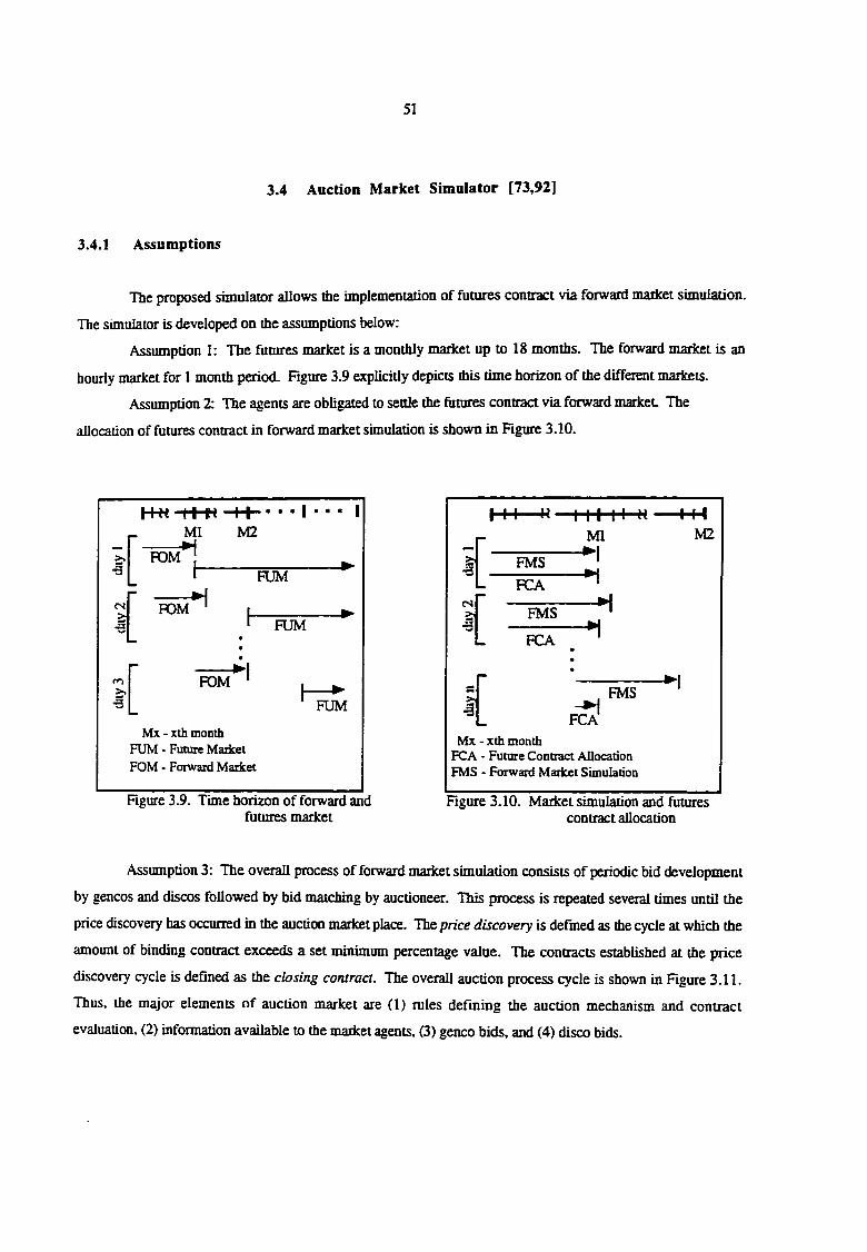
51
3.4 Auction Market Simulator [73,92]
3.4.1 Assumptions
The proposed cimiilatnr allows the implementation of futures contract via forward market simulation.
The simulator is developed on the assumptions below:
Assumption 1: The futures market is a monthly market up to 18 months. The forward market is an
hourly market for 1 month period. Figure 3.9 explicitly depicts this time horizon of the different markets.
Assumption 2: The agents are obligated to settle the futures contraa via forward market The
allocation of futures contract in forward market simulation is shown in Rgure 3.10.
H-H-H-H -+ + - • • • 1 • • • 1 Ml M2
POM'^ 1 FUM
is POM '
' FUM • •
•
>% FOM
• •1
"3
Mx - xth month
FUM
FUM - Future Madcet FOM - Forward Market
I-H H—I I I I I H l-M
FMS
FCA
FMS
FCA
Ml
•^1 -H
M2
4 FMS
FCA Mx - xtb month
FCA - Future Contract Allocation FMS - Forward Market Simulation
figure 3.9. Time horizon of forward and Figure 3.10. Market simulation and futures futures market contract allocation
Assumption 3: The overall process of forward market simulation consists of periodic bid development
by gencos and discos followed by bid matching by auctioneer. This process is repeated several times until the
price discovery has occurred in the auction market place. The price discovery is defined as the cycle at which the
amount of binding contract exceeds a set minimum percentage value. The contracts established at the price
discovery cycle is defined as the closing contract. The overall auction process cycle is shown in Figure 3.11.
Thus, the major elements of auction market are (1) rules defining the auction mechanism and contract
evaluation, (2) information available to the market agents, (3) genco bids, and (4) disco bids.
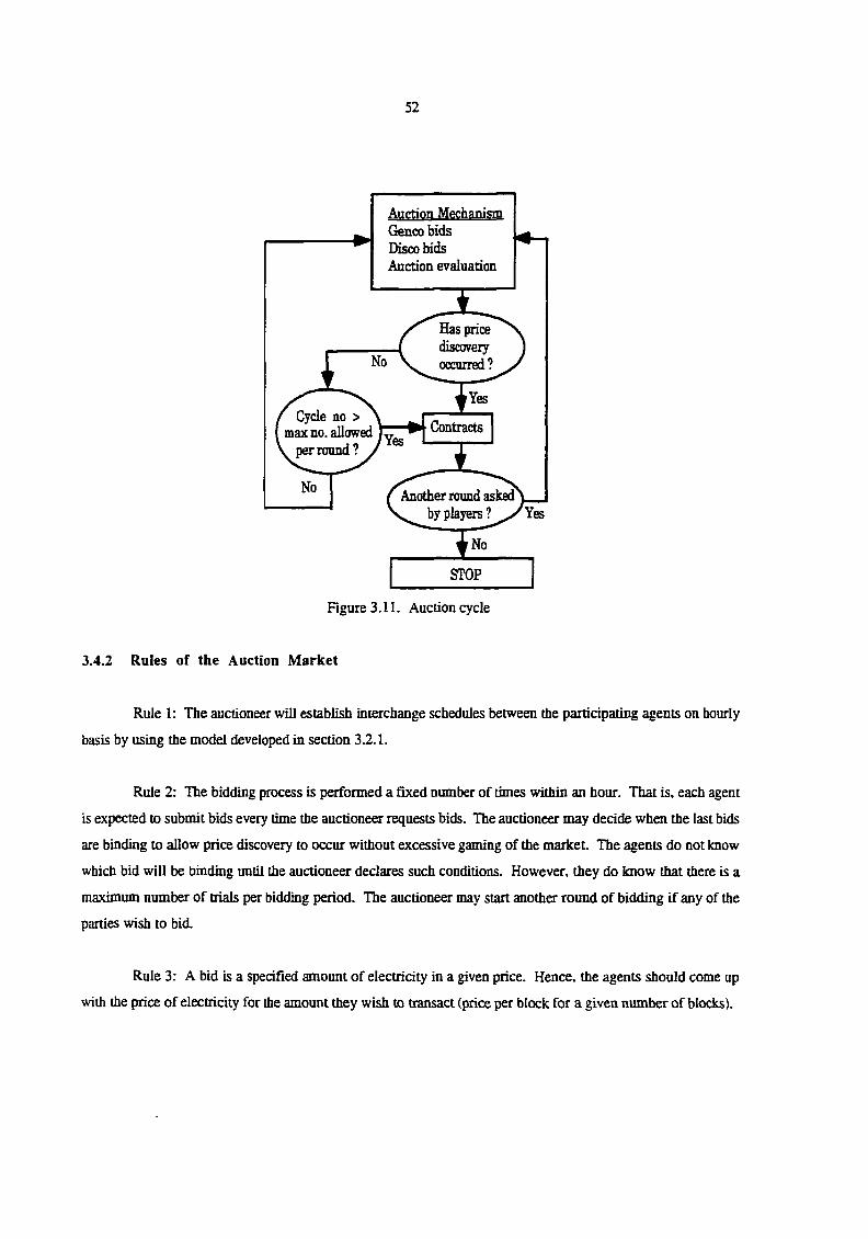
52
Has price discovery CKCurred?
Yes
Another round asked ^ . by players ? Yes
Cycle no > \ max no. allowed
L perround? /
Contracts
STOP
Auction MMhanism Genco bids Disco bids Auction evaluation
Figure 3.11. Auction cycle
3.4.2 Rules of the Auction Market
Rule 1: The auctioneer will establish interchange schedules between the participating agents on hourly
basis by using the model developed in section 3.2.1.
Rule 2: The bidding process is performed a fixed number of times within an hour. That is, each agent
is expected to submit bids every time the auctioneer requests bids. The auctioneer may decide when the last bids
are binding to allow price discovery to occur without excessive gaming of the market The agents do not know
which bid will be binding until the auctioneer declares such conditions. However, they do know that there is a
maximum number of trials per bidding period. The auctioneer may start another round of bidding if any of the
parties wish to bid.
Rule 3: A bid is a specified amount of electricity in a given price. Hence, the agents should come up
with the price of electricity for the amount they wish lo transact (price per block for a given number of blocks).
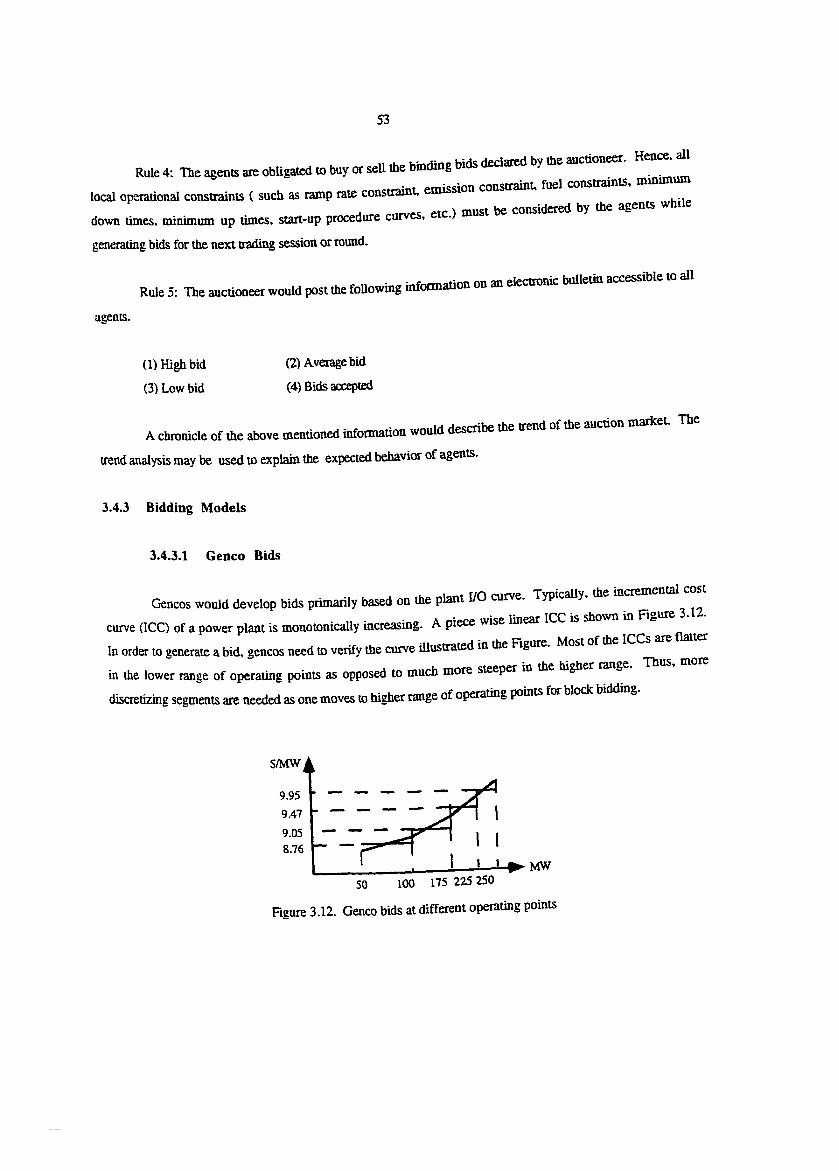
53
Rule 4: The agents are obligated to buy or sell the binding bids declared by the auctioneer. Hence, all
local operational constraints ( such as ramp rate constraint, emission constraint, fuel constraints, minimum
down times, miniminn up times, start-up procedure curves, etc.) must be considered by the agents while
generating bids for the next trading session or round.
Rule 5: The auctioneer would post the following infonnauon on an electronic bulletin accessible to all
agents.
(1) High bid (2) Average bid
(3) Low bid (4) Bids accepted
A cironicle of ite above menUoned infonnaUon would describe tie trend of ffie aucbon markeL The
trend analysis may be used to explain the expected behavior of agents.
3.4.3 Bidding Models
3.4.3.1 Genco Bids
Gencos would develop bids primarily based on the plant I/O curve. Typically, the incremental cost
curve (ICC) of a power plant is monotonically increasing. A piece wise linear ICC is shown in Figure 3.12.
In order to generate a bid, gencos need to verify tbe curve illustrated in the Figure. Most of the ICCs are flatter
in the lower range of operating points as opposed to much more steeper in the higher range. Thus, more
discretizing segments are needed as one moves to higher range of operating points for block bidding.
S/MW A
9.95
9.47
9.05 8.76
1
1 1 ^ MW
SO 100 175 225 250
Figure 3.12. Genco bids at different operating points
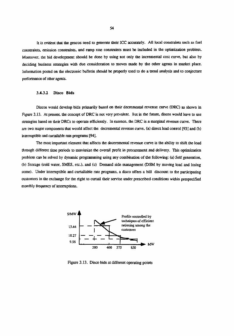
54
It is evident tbat tbe gencos need to generate their ICC accurately. All local constraints such as fuel
constraints, emission constraints, and ramp rate constraints must be included in the optimization problem.
Moreover, the bid development should be done by using not only the incremental cost curve, but also by
deciding business strategies with due consideration to moves made by tbe other agents in market place.
Information posted on the electronic bulletin should be properly used to do a trend analysis and to conjecture
performance of other agents.
3.4.3.2 Disco Bids
Discos would develop bids primarily based on their decremental revenue curve (DRC) as shown in
Figure 3.13. At present, the concept of DRC is not very prevalent But in the future, discos would have to use
strategies based on their DRCs to operate efficiently. In essence, the DRC is a marginal revenue curve. There
are two major components that would affect the decremental revenue curve, (a) direct load control [93] and (b)
inteiTuptible and curtailable rate programs [94].
The most important element that affects the deceremental revenue curve is the abili^ to shift the load
through different time periods to maximize the overall profit in procurement and delivery. This optimization
problem can be solved by dynamic programming using any combination of the following: (a) Self generation,
(b) Storage (cold water, SMES, etc.), and (c) Denoand side management (DSM by moving load and losing
some). Under interruptible and curtailable rate programs, a disco offers a bill discount to the participating
customers in the exchange for the right to curtail their service under prescribed conditions within prespecified
monthly frequency of interruptions.
S/MW A Profile controlled by
of efRcient nong the 13.44
10.27
9.56
customers
^ MW 200 400 575 850
Rgure 3.13. Disco bids at different operating points
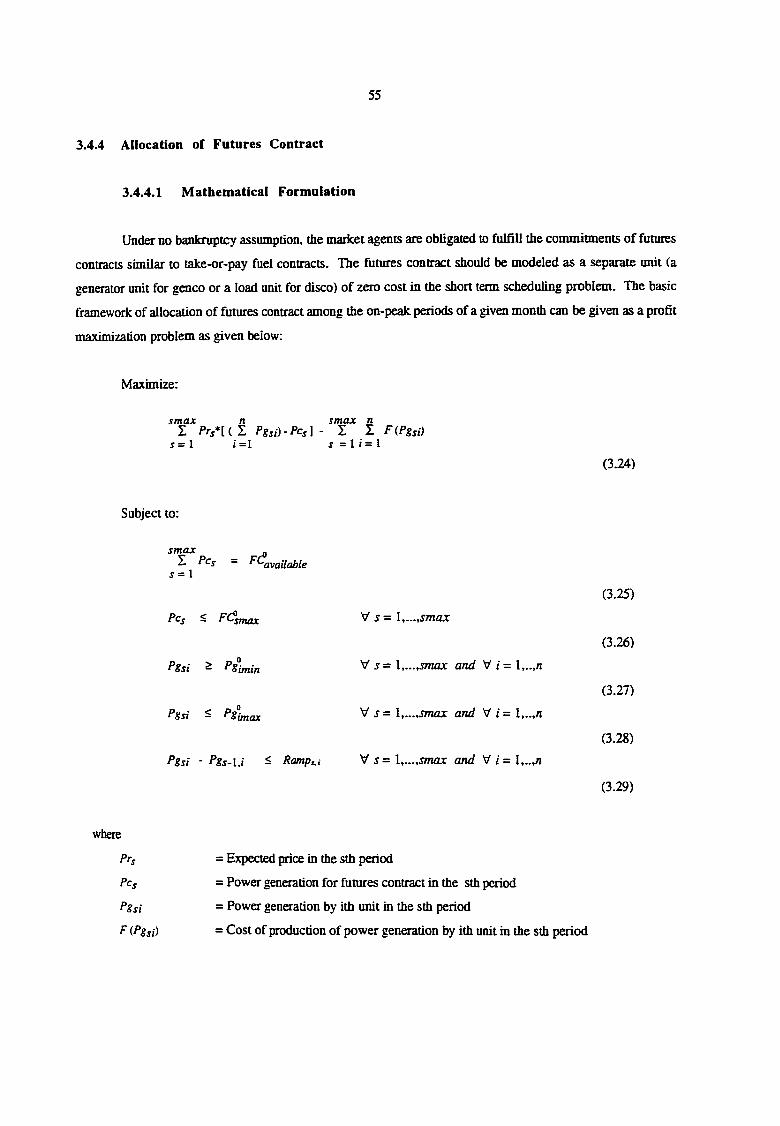
55
3.4.4 Allocation of Futures Contract
3.4.4.1 Mathematical Formulation
Under no bankruptcy assumption, the market agents are obligated to fulHll the coounitments of futures
contracts similar to take-or-pay fuel contracts. The futures contract should be modeled as a separate unit (a
generator unit for genco or a load unit for disco) of zero cost in the short term scheduling problem. The basic
framework of allocation of futures contract among the on-peak periods of a given month can be given as a profit
maximization problem as given below:
Maximize;
smax n smax n I P8si)-Pcs]- I I F(Pgsi)
5 = 1 1 = 1 f = 1 I = 1
Subject to:
(3.24)
smax „ I Pcs =
j = 1 available
pcs S smax
Pgsi ^ Pin imin
Pgsi S Pgl
V s = l,...,smax
V 5= l,...,i7nax and V i = l,..,n
V s = l,...,smax and V i = l,..,n
Pgsi - Pgs-l.i ^ Ramp,.i V j = l,...,jmar and Vi = l,..,n
(3.25)
(3.26)
(3.27)
(3.28)
(3.29)
where
prs
pcs
Pgsi
F(Pgsi)
= Expected price in the sth period
= Power generation for futures contract in the sth period
= Power generation by ith unit in the sth period
= Cost of production of power generation by ith unit in the sth period
56
available = The unsealed amount of futures contract
= Maximum allowable settlement of futures contract in one on-peak period FC?, '^^smax pg° .
a imin
psi, max
= Bidding limit for minimum generation of the ith unit
= Bidding limit for maximum generation of tbe ith unit
Ramp,, i
smax = The maximum number of periods in a given forward market simulation.
= Minimum up/down time ramping limit of tbe ith unit
The Grst and second teim of objective function (equation (3.24)) are the total revenue generated and the
cost of production respectively. Thus, the objective is to maximize the profit for a given time horizon.
Equations (3.25) and (3.26) are futures contract allocation constraints. Equations (3.27) and (328) are bidding
constraints for minimum and maximum generation c^acity limits respectively. Equation (3.29) is operational
constraint for minimum up and down time ramping limits.
An equivalent formulation can be used by discos to solve the futures contract allocation problem. The
operational constraints of specific units (such as hydro generation) should be included in the overall profit
maximization problem. The aforementioned firamework can be easily modified to accommodate such needs.
3.4.4.2 The Decision Analysis (DA) Approach for Contract Allocation
Decision analysis can be viewed as a methodology for making decisions with uncertain outcomes.
Comprehensive treatments can be found in many volumes [95,96]. Note that the decision analysis method is
not a competitor to the other modeling methodologies. Rather, it is complementary in that it integrates the
results of various models and applies them to decision making. Reference [97] and [98] describe the application
of decision analysis to bulk power marketing problem. A part of this work has developed the framework of
transaction selection and evaluation using decision analysis in a competitive electric market [99]. The developed
approach can easily be modified for application in this model.
The futures contract allocation problem is difficult to solve due to risk and uncertainties associated with
the fluctuating market prices. In view of these uncertainties, the contract allocation problem is a stochastic
optimization problem. The DA approach converts the stochastic optimization problem into a set of
deterministic optimization subproblems by developing decision tree as shown in Figure 3.14. The square and
oval nodes represent decision and chance nodes respectively. A path of the decision tree represents a sequence of
decisions after the corresponding price trends are resolved. Thus, each path of the decision tree has profit
associated with the solution of deterministic optimization subproblem given in equations (3.25) through (329).
The solution of these deterministic optimization subproblems are then combined to obtain the solution of the
original problem.
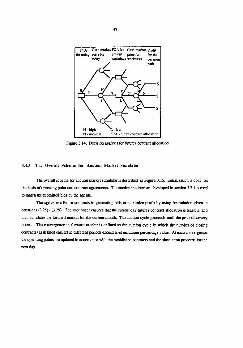
57
FCA Cash maikec FCA for Cash market Profit for today pnce for present price for for the
today weekdays weekdays decision y path
N - nominal FCA - future contract allocation
Figure 3.14. IDecision analysis for futures contraa allocation
3.4.5 The Overall Scheme for Auction Market Simulator
The overall scheme for auction market simulator is described m Figure 3.15. Initialization is done on
the basis of operating point and contract agreements. The auction mecbanism developed in section 3.2.1 is used
to match the submitted bids by the agents.
Tbe agents use future contracts in generating bids to maximize profit by using formulation given in
equations (3.25) - (329). The auctioneer ensures that the current day futures contract allocation is feasible, and
then simulates the forward market for the current month. The auction cycle proceeds until the price discovery
occurs. The convergence in forward market is defined as the auction cycle in which the number of closing
contracts (as defined earlier) in different periods exceed a set minimum percentage value. At each convergence,
the operating points are updated in accordance with the established contracts and the simulation proceeds for die
next day.
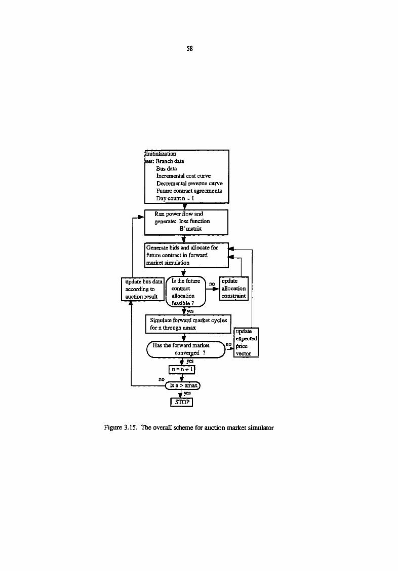
58
Initialization set: Branch data
Bus data Incremental cost curve Decremental revenue curve Future contract agreements Day count n = I
Run power flow and generate: loss function
B'matrix
I Generate bids and allocate for future contract in forward market simulation
update bus data ^Is the future^ no update according to contract allocation auction result allocation constramt
c
Simulate forward market cycles for n through nmax
i ~ Has the forward market
converged ? i y«
vector
n = n+ ]
no { Isn>nmax^
^yes
I STOP I
Figure 3.15. The overall scheme for auction market simulator
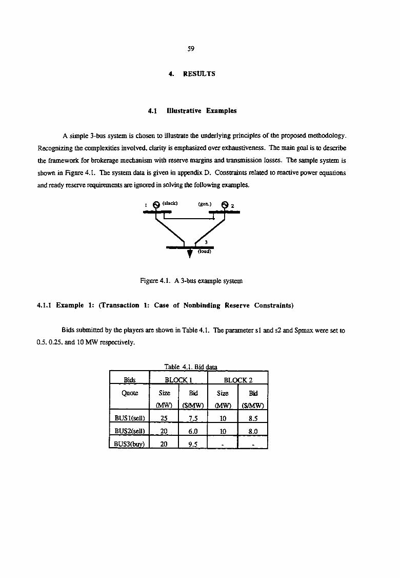
59
4. RESULTS
4.1 niustrative Examples
A simple 3-bus system is cbosen to illustrate tbe underlying principles of tbe proposed methodology.
Recognizing the complexities involved, clarity is emphasized over exhaustiveness. The main goal is to describe
the framework for brokerage mechanism with reserve margins and transmission losses. The sample system is
shown in Rgure 4.1. The system data is given in appendix D. Constraints related to reactive power equations
and ready reserve requirements are ignored in solving the following examples.
(slack) (gen.)
Goad)
Rgure 4.1. A 3-bus example system
4.1.1 Example 1: (Transaction 1: Case of Nonbinding Reserve Constraints)
Bids submitted by the players are shown in Table 4.1. The parameter si and s2 and Spmax were set to
0.5, 0.25, and 10 MW respectively.
Table 4.1. Bid data
Bids BLOCK 1 BLOCK2
Quote Size
(MW)
Bid
(S/MW)
Size
(MW)
Bid
(S/MW)
BUSKseU) 25 7.5 10 8.5
BUS2(seU) 20 6.0 10 8.0
BUS3(buv) 20 9.5 _
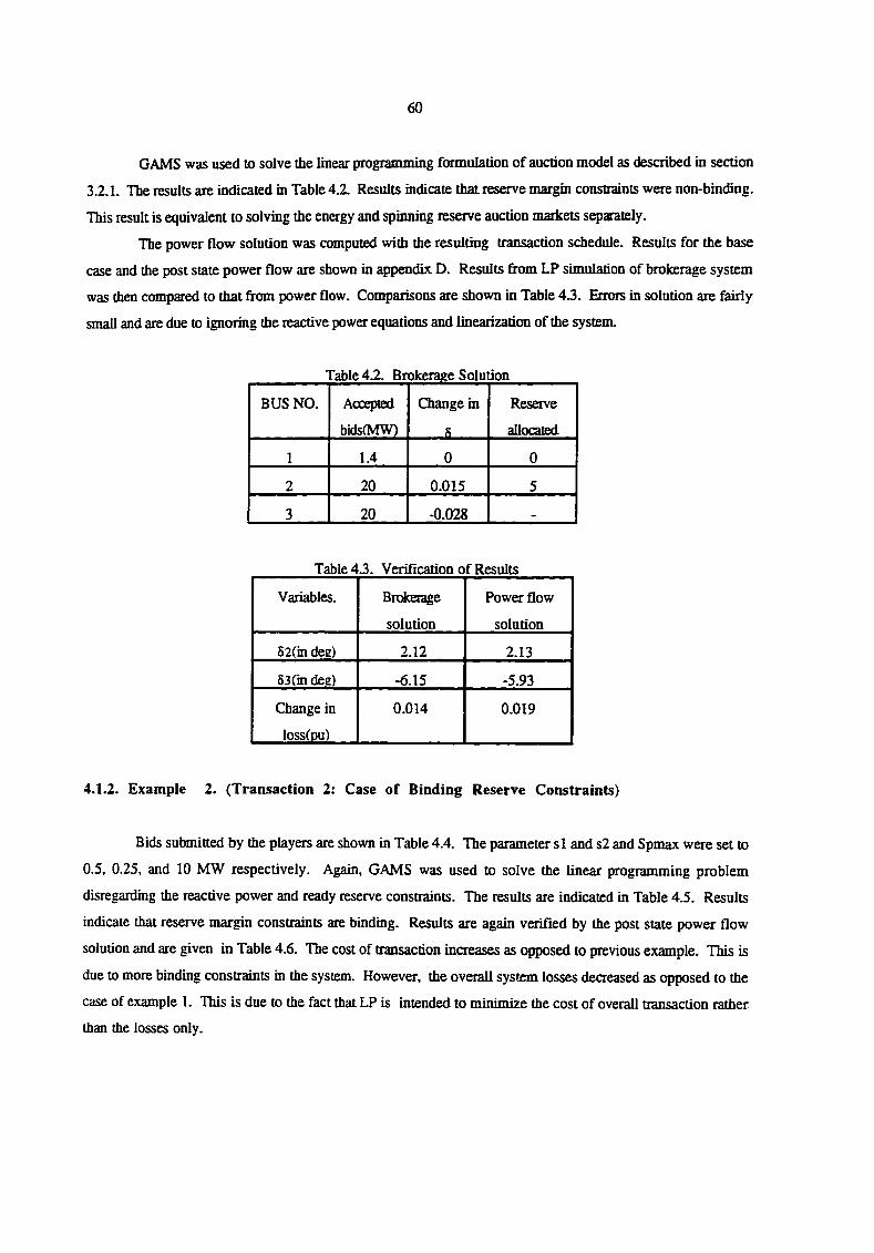
60
GAMS was used to solve the linear programming formulation of auction model as described in section
3.2.1. The results are indicated in Table 4.2. Results indicate that reserve margin constraints were non-binding.
This result is equivalent to solving the energy and spinning reserve auction markets separately.
The power flow solution was computed with the resulting transaction schedule. Results for the base
case and the post state power flow are shown in appendix D. Results from LP simulation of brokerage system
was then compared to that from power flow. Comparisons are shown in Table 43. Errors in soludon are fairly
«mail and are due to ignoring the reactive power equations and linearization of the system.
Table 4.2. Brokerage Solution
BUS NO. Accepted
bidsfMW)
Change in
s
Reserve
allocated
1 1.4 0 0
2 20 0.015 5
3 20 -0.028 -
Table 43. Verification of Results
Variables. Brokerage
solution
Power flow
solution
S2(in deg) 2.12 2.13
53 (in deg) -6.15 -5.93
Change in
loss(pu)
0.014 0.019
4.1.2. Example 2. (Transaction 2: Case of Binding Reserve Constraints)
Bids submitted by the players are shown in Table 4.4. The parameter si and s2 and Spmax were set to
0.5, 0.25, and 10 MW respectively. Again, GAMS was used to solve the linear programming problem
disregarding the reactive power and ready reserve constraints. The results are indicated in Table 4.5. Results
indicate that reserve margin constraints are binding. Results are again verified by the post state power flow
solution and are given in Table 4.6. The cost of transaction increases as opposed to previous example. This is
due to more binding constraints in the system. However, the overall system losses decreased as opposed to the
case of example 1. This is due to the fact that LP is intended to minimize the cost of overall transaction rather
than the losses only.
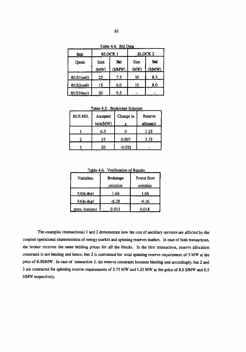
61
Table 4.4. Bid Data
Bids BLOCK 1 BLOCK 2
Quote Size
(MW)
Bid
(S/MW)
Size
(MW)
Bid
(S/MW)
BUSUseU) 25 7.5 10 8.5
BUS2(seU) 15 6.0 10 8.0
BUS3(buv) 20 9.5 - -
Fable 4.5. Brokerage Solution
BUS NO. Accepted
bids(MW)
Change in
fi
Reserve
aUocated
1 6.3 0 1.25
2 15 0.007 3.75
3 20 -0.032 •
Table 4.6. Verification of Results
Variables. Brokerage
solution
Power flow
solution
52(in deg) 1.66 1.66
53(in deg) -6.38 -6.16
trans. loss(pu) 0.013 0.018
The examples (transactions) 1 and 2 demonstrate how the cost of ancillary services are affected by the
coupled operational characteristics of energy market and spinning reserves market In case of both transactions,
the broker receives the same bidding prices for all the blocks. In the first transaction, reserve allocation
constraint is not binding and hence, bus 2 is contracted for total spinning reserve requirement of 5 MW at the
price of 8.0S/MW. In case of transaction 2, the reserve constraint becomes binding and accordingly, bus 2 and
3 are contracted for spinning reserve requirements of 3.75 MW and 1.25 MW at the price of 8.0 S/MW and 8.5
S/MW respectively.
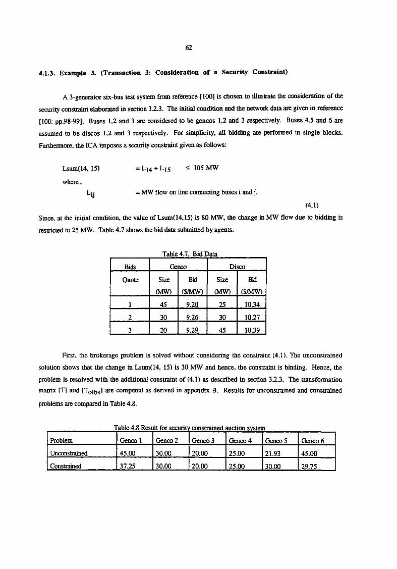
62
4.1.3. Example 3. (Transaction 3: Consideration of a Security Constraint)
A 3-generator six-bus test system firom reference [100] is chosen to illustrate the consideration of the
security constraint elaborated in section 32.3. The initial condition and the network data are given in reference
[100: pp.98-99]. Buses 1,2 and 3 are considered to be gencos 1,2 and 3 respectively. Buses 4,5 and 6 are
assumed to be discos 1,2 and 3 respectively. For simplicity, all bidding are performed in single blocks.
Furthermore, the ICA imposes a security constraint given as follows:
Lsum(14, 15) = Li4 + L15 < 105 MW
where,
Ly =MW flow on line connecting buses i and j.
(4.1)
Since, at the initial condition, the value of Lsum(14,15) is 80 MW, the change in MW flow due to bidding is
restricted to 25 MW. Table 4.7 shows the bid data submitted by agents.
Table 4.7. Bid Data
Bids Genco Disco
(Juote Size Bkl Size Bkl
(MW) (S/MW) (MW) (S/MW)
1 45 9.20 25 1034
2 30 9.26 30 1027
3 20 9.29 45 1039
First, the brokerage problem is solved without considering the constraint (4.1). The unconstrained
solution shows that the change in Lsum(14, 15) is 30 MW and hence, die constraint is binding. Hence, the
problem is resolved with the additional constraint of (4.1) as described in section 323. The transformation
matrix [T] and [Tgibs] ars computed as derived in appendix B. Results for unconstrained and constrained
problems are compared in Table 4.8.
Table 4.8 Result for security constrained auction system
Problem Cienco 1 Genco 2 Genco3 (jenco4 Genco5 Genco 6
Unconstrained 45.00 30.00 20.00 25.00 21.93 45.00
Constrained 37.25 30.00 20.00 25.00 30.00 29.75
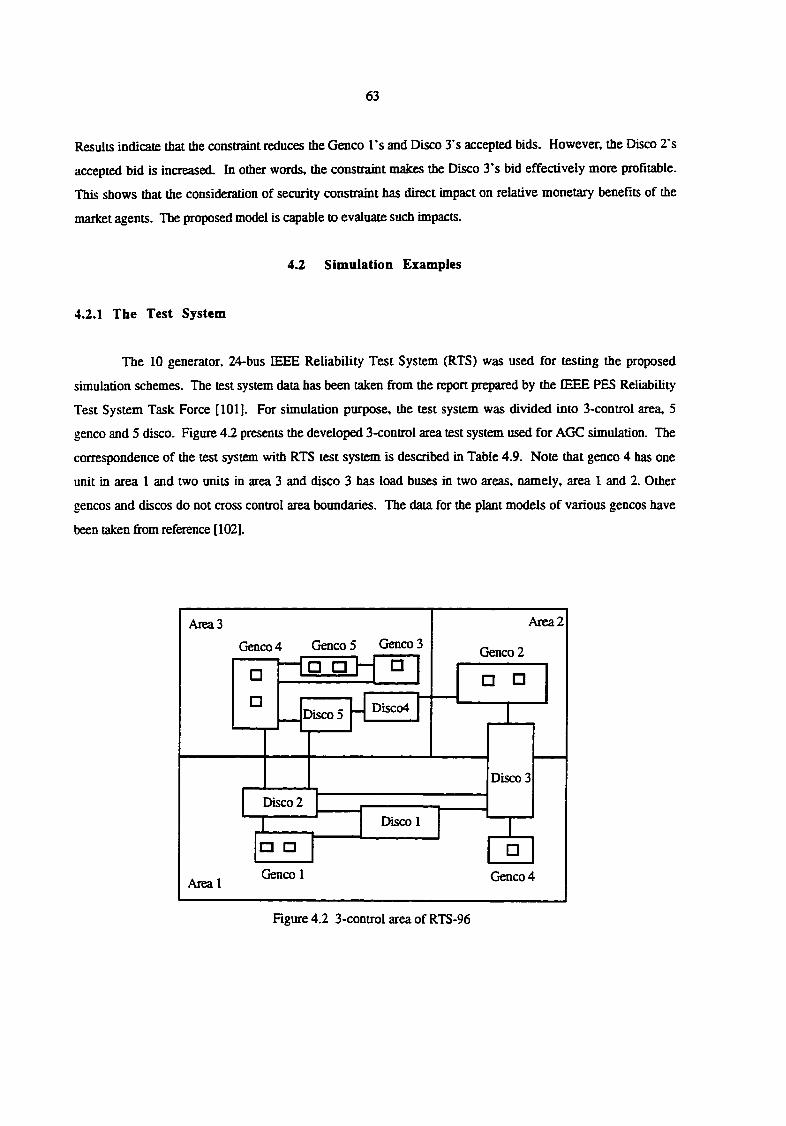
63
Results indiratp that the constraint reduces the Genco I's and Disco 3's accepted bids. However, the Disco 2's
accepted bid is increased. In other words, the constraint makes the Disco 3's bid effectively more profitable.
This shows that the consideration of security constraint has direct impact on relative monetary benefits of the
market agents. The proposed model is capable to evaluate such impacts.
4.2 Simulation Examples
4.2.1 The Test System
The 10 generator. 24-bus EEEE Reliability Test System (RTS) was used for testing the proposed
simulation schemes. The test system data has been taken from the report prepared by the EEEE PES Reliability
Test System Task Force [101]. For simulation purpose, the test system was divided into 3-control area, 5
genco and 5 disco. Figure A1 presents the developed 3-control area test system used for AGC simulation. The
correspondence of the test system with RTS test system is described in Table 4.9. Note that genco 4 has one
unit in area 1 and two units in area 3 and disco 3 bas load buses in two areas, namely, area I and 2. Other
gencos and discos do not cross control area boundaries. The data for the plant models of various gencos have
been taken from reference [1021.
Area2 AreaS
Genco 5 Genco 3
• g h-1 •
Genco4 Genco 2
Disco 1
Genco 1 Genco4 Area 1
Disco4 Disco5
a •
Disco 2
Disco 3
Hgure 4.2 3-control area of RTS-96
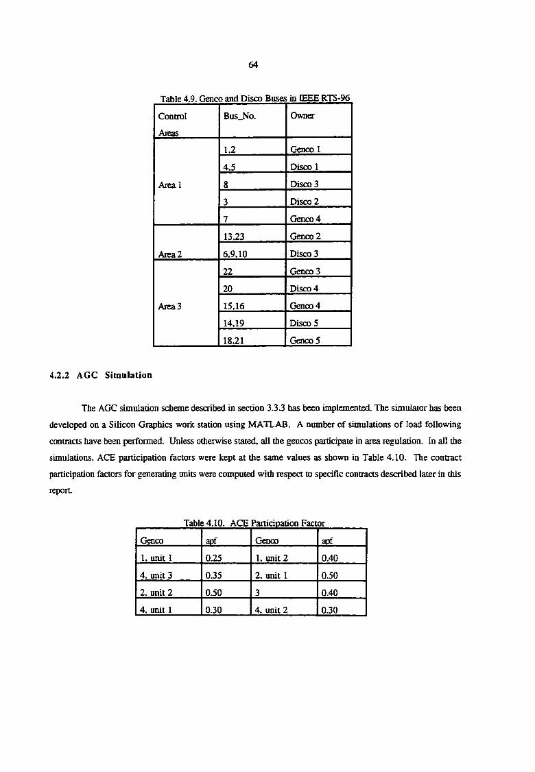
64
Table 43. Genco and Disco Buses in IEEE RTS-96
Control
Areas
Bus_No. Owner
Areal
1.2 Genco 1
Areal
4,5 Disco 1
Areal 8 Disco 3 Areal
3 Disco 2
Areal
7 Genco 4
Area2
13,23 Genco 2
Area2 6,9.10 Disco 3
Area3
22 Genco3
Area3
20 Disco 4
Area3 15,16 Genco 4 Area3
14,19 Disco 5
Area3
18,21 Genco 5
4.2.2 AGC Simulation
The AGC simulation scheme described in section 3.33 has been implemented. The simulator has been
developed on a Silicon Graphics work station using MATLAB. A number of simulations of load following
contracts have been performed. Unless otherwise stated, ail the gencos participate in area regulation. In all the
simulations, ACE participation factors were kept at the same values as shown in Table 4.10. The contract
participation factors for generating units were computed with respect to specific contracts described later in this
report.
Table 4.10. ACE Participation Factor
Genco at)f Genco apf
1, unit 1 0.25 1, unit 2 0.40
4, unit 3 0.35 2. unit 1 0.50
2, unit 2 0.50 3 0.40
4, unit 1 0.30 4, unit 2 0.30
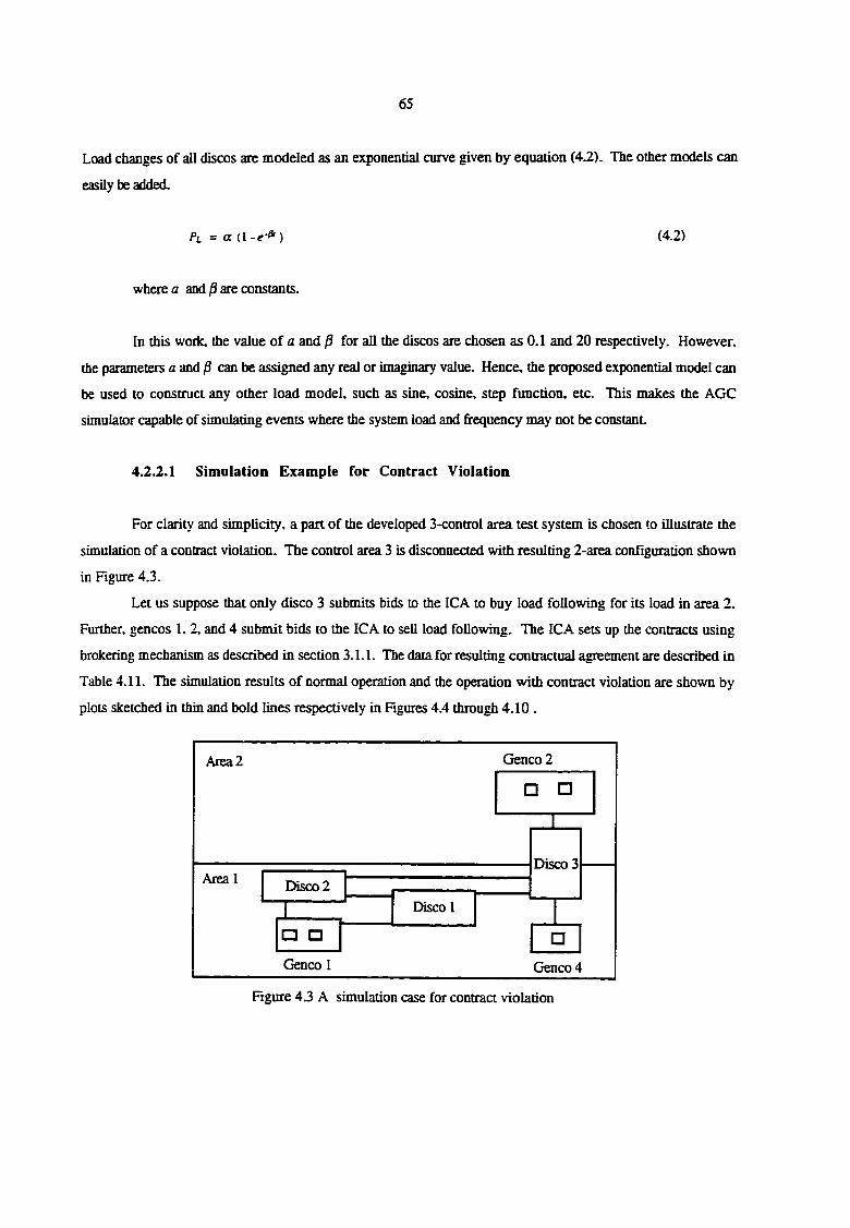
65
Load changes of all discos are modeled as an exponential curve given by equation (4.2). The other models can
easily be added.
P L = a a - e - » ) ( 4 . 2 )
where a and ^ are constants.
In this work, the value of a and P for all the discos are chosen as 0.1 and 20 respectively. However,
the parameters a and P can be assigned any real or imaginary value. Hence, the proposed exponential model can
be used to construct any other load model, such as sine, cosine, step fimction, etc. This makes the AGC
simulator capable of simulating events where the system load and frequency may not be constant
4.2.2.1 Simulation Example for Contract Violation
For clarity and simplicity, a part of the developed 3-control area test system is chosen to illustrate the
simulation of a contract violation. The control area 3 is disconnected with resulting 2-area configuration shown
in Figure 4.3.
Let us suppose that only disco 3 submits bids to the ICA to buy load following for its load in area 2.
Further, gencos 1. 2, and 4 submit bids to the ICA to sell load following. The ICA sets up the contracts using
brokering mechanism as described in section 3.1.1. The data for resulting contractual agreement are described in
Table 4.11. The simulation results of normal operation and the operation with contract violation are shown by
plots sketched in thin and bold lines respectively in Figures 4.4 through 4.10 .
1=1 •
Disco2 Area 1
Area2
(jenco 1
Disco 1
Genco 2
Genco4
Disco 3
figure 4.3 A simulation case for contraa violation
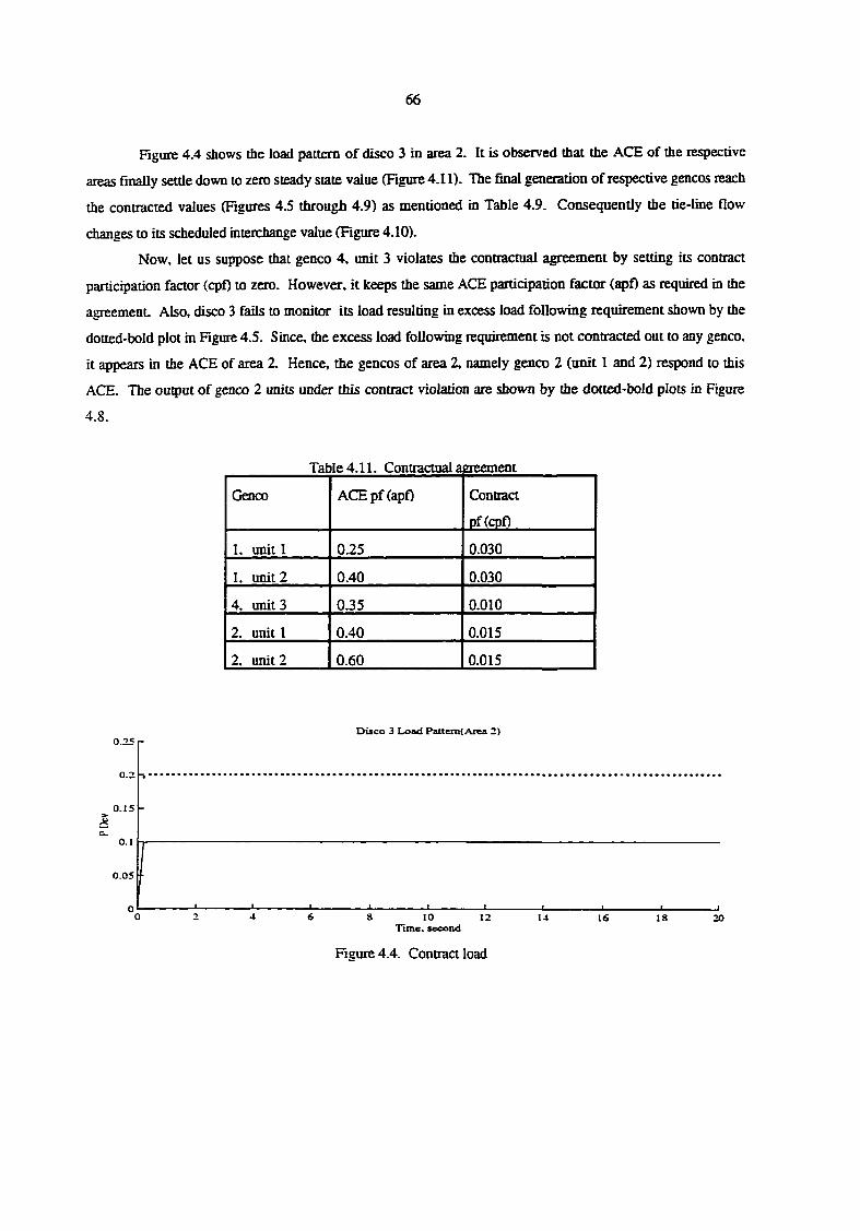
66
Figure 4.4 shows the load pattern of disco 3 in area 2. It is observed that the ACE of the respective
areas finally settle down to zero steady state value (Hgure 4.11). The final generation of respective gencos reach
the contracted values (Figures 4.5 through 4.9) as mentioned in Table 4.9. Consequently the tie-line flow
changes to its scheduled interchange value (Figure 4.10).
Now, let us suppose that genco 4, unit 3 violates the contractual agreement by setting its contract
participation faaor (cpf) to zero. However, it keeps the same ACE participation factor (apf) as required in the
agreement Also, disco 3 fails to monitor its load resulting in excess load following requirement shown by the
dotted-bold plot in Figure 4.5. Since, the excess load following requirement is not contracted out to any genco,
it appears in the ACE of area 2. Hence, the gencos of area 2, namely genco 2 (unit 1 and 2) respond to this
ACE. The output of genco 2 units under this contract violation are shown by the dotted-bold plots in Figure
4.8.
Table 4.11. Contractual agreement
Genco ACE pf (apf) Contract
pf(cpf)
1, unit 1 0.25 0.030
1. unit 2 0.40 0.030
4. unit 3 0.35 0.010
2. unit 1 0.40 0.015
2. unit 2 0.60 0.015
Disco 3 Load Panem(Arca 2) 0.25 -
0.2 -
0.15 -> m
0* ' 1 > ' 1 1 1 I t I 0 2 4 6 8 10 12 14 16 18 20
Time, second
Figure 4.4. Contract load
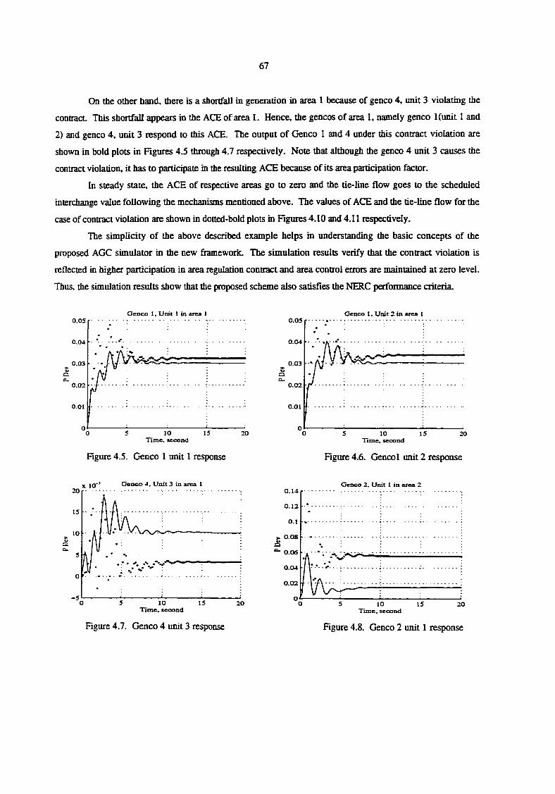
67
On the other band, there is a shortfall in generation in area 1 because of genco 4, unit 3 violating the
contract This shortfall appears in the ACE of area 1. Hence, the gencos of area 1, namely genco Kunit 1 and
2) and genco 4, unit 3 respond to this ACE. The output of Genco 1 and 4 under this contract violation are
shown in bold plots in Figures 4.5 through 4.7 respectively. Note that although the genco 4 unit 3 causes the
contract violation, it has to participate in the resulting ACE because of its area participation factor.
In steady state, the ACE of respective areas go to zero and the tie-line flow goes to tbe scheduled
interchange value following the mechanisms mentioned above. The values of ACE and the tie-line flow for the
case of contract violation are shown in dotted-bold plots in Engures 4.10 and 4.11 respectively.
The simplicity of the above described example helps in understanding the basic concepts of the
proposed AGC simulator in dae new framework. The simulation results verify that the contract violation is
reflected in higher participation in area regulation contract and area control errors are maintained at zero level.
Thus, the simulation results show that die proposed scheme also satisfies the NERC performance criteria.
Genco 1. Unit I in area 1 0.05
0.04
0.03
0.02
0.01
• /L *A • ̂
T • 1
5 10 15 Time, second
20
0.05
0.04
0.03
0.02
0.01
Genco 1. Unit 2 in area 1
Time, second
Figure 4.5. Genco 1 unit 1 response Rgure 4.6. Genco 1 unit 2 response
X 10~* Genco 4. Unit 3 in area 1
Time, second
0.14
0.12
0.1
0.08
0.06
0.04
0.02
O
Genco 2, Unit I in area 2
•
i KA i KA
5 10 15 Time, second
20
Figure 4.7. Genco 4 unit 3 response Figure 4.8. Genco 2 unit 1 response
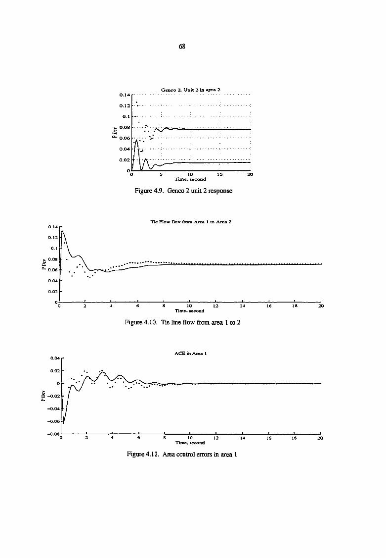
68
Cenco 2. Unit 2 in area. Z
0.12
0.1
0.08
0.06
0.02
15 20 10 Time, second
Figure 4.9. Genco 2 unit 2 response
Tie Flow Dev from Area 1 to Area 2 0.14
0.12
0.1
0.08
0.06
0.04
0.02
10 Time, second
18 12 14 16 20
Rgure 4.10. Tie line flow from area 1 to 2
ACE in Area 1 0.04
0.02
0 -
-0.02
-0.04
-0.06
-0.08 10
Time, second 12 14 16 18 20
Figure 4.11. Area control errors in area 1
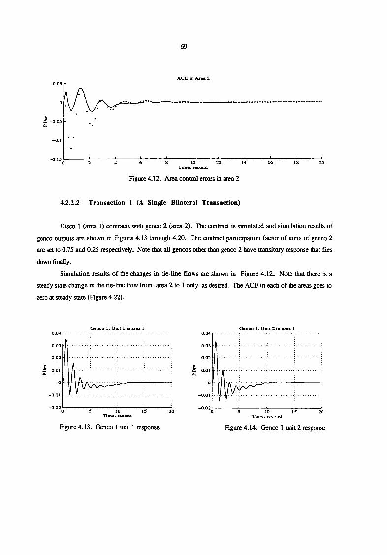
69
ACE in Area 2 0.05
0 -
-O.I -
-0.15 16 10 Time, second
12 18 20
Figure 4.12. Area control errors in area 2
4.2.2.2 Transaction 1 (A Single Bilateral Transaction)
Disco 1 (area 1) contracts with genco 2 (area 2). The contraa is simulated and simulation results of
genco outputs are shown in Figures 4.13 through 4.20. The contract participation factor of units of genco 2
are set to 0.75 and 0.25 respectively. Note that all gencos other than genco 2 have transitory response that dies
down finally.
Simulation results of the changes in tie-line flows are shown in Figure 4.12. Note that there is a
steady state change in the tie-line flow &x)m area 2 to 1 only as desired. The ACE in each of the areas goes to
zero at steady state (Hgure 4.22).
Genco 1. Unit I in area 1 Genco 1. Unit 2 in area I 0.04
0.03
0.02
ft. 0.01
-0.01
-0.02 10
Time, second 20
0.04
0.03
0.02
0.01
-0.01
-0.02 10
Time, second 20
Figure 4.13. Genco 1 unit 1 response Figure 4.14. Genco 1 unit 2 response
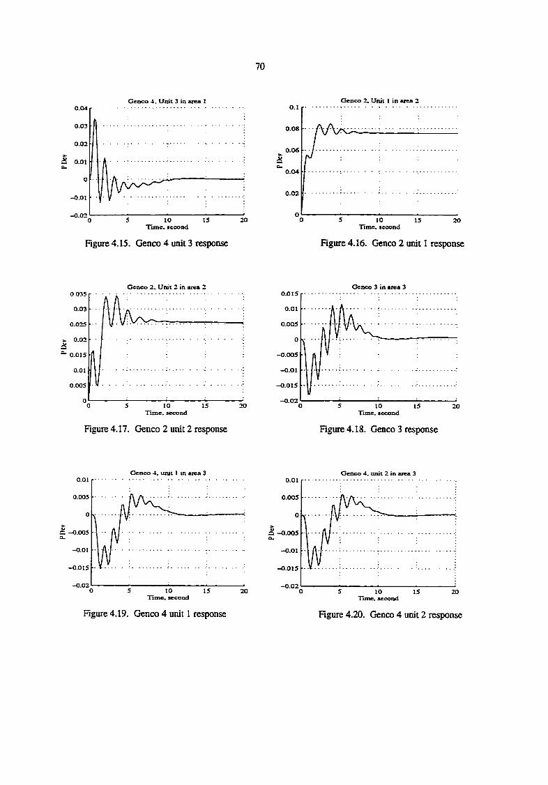
70
Genco 4. Unit 3 in area 1 Genco 2. Unit I in area 2
5 10 Time, second
15 20
0.08
0.06
0.04
0.02
5 10 15 Time, second
20
Figure 4.15. Genco 4 unit 3 response Rgure 4.16. Genco 2 unit 1 response
Genco 2. Unit 2 in area 2 Genco 3 in area 3
5 10 Hme. second
0-015
0,005
0.015
-0.02 10
Time, second
Rgure 4.17. Genco 2 unit 2 response Rgure 4.18. Genco 3 response
Genco 4. unit 1 in area 3 Genco 4. unit 2 in area 3
lime, second
0.005
a -0.005
-O.OI
-0.015
-0.02 10 15
Time, second
Rgure 4.19. Genco 4 unit 1 response Rgure 4.20. Genco 4 unit 2 response
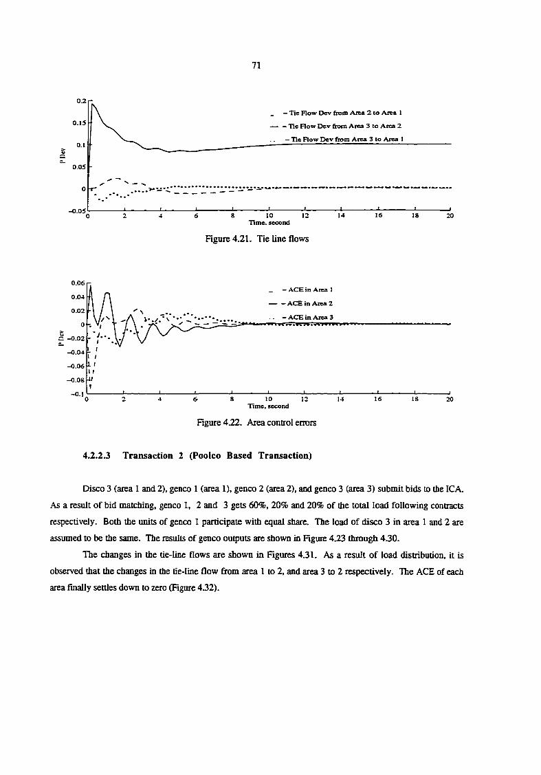
71
— Tie Flow Dcv from Afca 2 to Aiea 1
0.15 — — Tie Row Dev from Area 3 to Area 2
— Tie Flow Dev ftom Area 3 to Area I 0.1 > u
0.05
-0.05 16
Time, second
Rgure 4.21. Tie line flows
0.06 — ACE in Area I
0.04 — — ACE in Area 2
0.02 ' ACE in Area 3
0
a -0.02
-0.04
-0.06 J- '
-O.I 10 Hme, second
16 20
Hgure422. Area control errors
4.2.2.3 Transaction 2 (Pooico Based Transaction)
Disco 3 (area 1 and 2), genco 1 (area 1), genco 2 (area 2), and genco 3 (area 3) submit bids to the ICA.
As a result of bid matching, genco 1, 2 and 3 gets 60%, 20% and 20% of the total load following contracts
respectively. Both the units of genco 1 participate with equal share. The load of disco 3 in area 1 and 2 are
assumed to be the same. The results of genco outputs are shown in Rgure 4.23 through 4J0.
The changes in the tie-line flows are shown in Hgures 4.31. As a result of load distribution, it is
observed that the changes in the tie-line flow from area 1 to 2, and area 3 to 2 respectively. The ACE of each
area finally settles down to zero (Rgure 432).
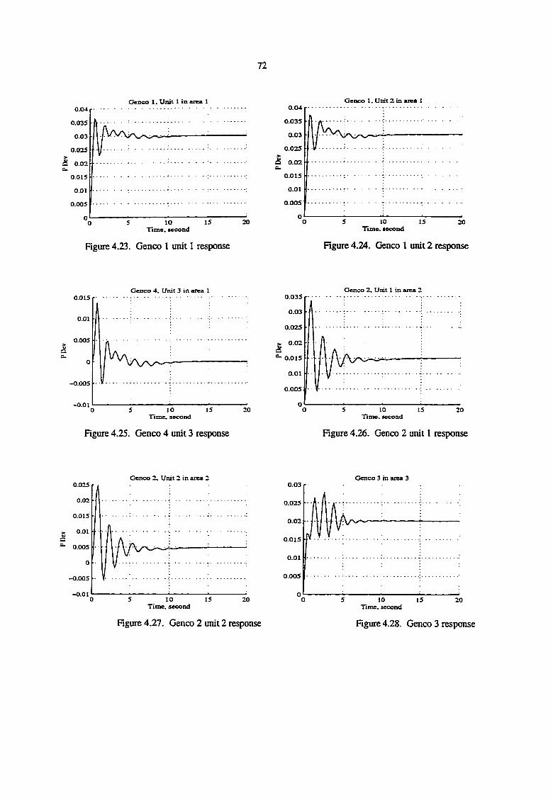
72
Cenco 1. Unit 1 in area 1 Genco 1. Umi 2 in area I 0.04
0.035
0.03
0.02S
iS 0.02 a.
0.015
0.01
0.005
20 Time, second
0.04
0.035
0.03
0.025
0.02
0.015
0.01
0.005
20 Time, second
Figure 4.23. Genco 1 unit 1 response Rgure 4.24. Genco 1 unit 2 response
Genco 4. Unit 3 in area 1 Cenco 2, Unit 1 in area 2 0.035
0.03
0.025
0.02 u
^ 0.015
0.01
0.005
20 Time, second
0.015
0.01
0.005
-0.005
-0.01 20 10
Time, second
Rgure 4.25. Genco 4 unit 3 response Rgure 4.26. Genco 2 unit 1 response
Cenco 2. Unit 2 in area 2 Cenco 3 in area 3 0.03
0.025
0.02
0.015
0.01
0.005
20 Time, second
0.025
0.02
0.015
0.01
0.005
-0.005
-0.01 10
Time, second 20
Rgure 4.27. Genco 2 unit 2 response Rgure 4.28. Genco 3 response
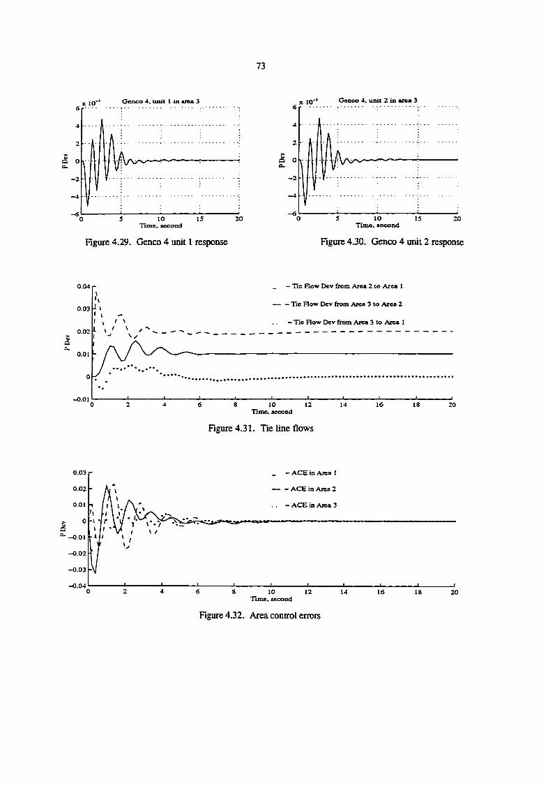
73
Genco 4. unit 1 in area 3 6
1
1 1 l\ i ;
11 0
1 F :
-6
If
Time, second
Figure 4.29. Genco 4 unit 1 response
3C 10*' Genco 4, unit 2 in area 3
>• u n a*
-2
10 Time, second
15 20
Figure 4.30. Genco 4 unit 2 response
— TIC Flow Dcv from Area 2 to Area 1 0.04
— — Tie Flow Dcv from Area 3 to Area 2 0.03
— Tie Row Dcv from Area 3 to Area 1
0.02
0.01
-0.01 16 20
Time, second
Figure 4.31. Tie line flows
0.03 — ACE in Area 1
— — ACE in Area 2 0.02
0.01 — ACE in Area 3
0 -
-0.01
-0.02
-0.03
-0.04 0 2 6 4 8 10 12 14 18 20
Time, second
Figure 4.32. Area control errors

74
4.2.2.4 Transaction 3 (Simultaneous Contracts)
This transaction considers various contracts existing simultaneously as shown in Table 4.12. Genco 2
and 4 have unit 1 and 2 on AGC respectively. Both the units of genco 1 are on AGC with equal participation
factor. The simulation results of genco outputs are shown in Rgure 433 through 4.40.
The changes in the tie-line flows between different areas are shown in Figure 4.41. Note that the tie-
line flows due to various contracts tend to cancel each other. The ACE of all the areas settle to zero steady state
values as shown in Figure 4.42.
Table 4.12. Simultaneous Contracts in the new market place
Trans.
Type
Disco Geiico(cpf)
Bilateral Disco 5 Genco3
Bilateral Disco 4 Genco4
Poolco Disco 3 Genco 1(20%)
Genco 2(60%)
Genco 4(20%)
Poolco Disco 1
Disco 2
Genco 1(20%)
Genco 2(36%)
Genco 4(44%)
Genco I. Unit I in area 1 Genco 1. Unit 2 in area 1
0.08
0.06 > u
0.04
0.02
20 Time, second
0.1
0.08
0.06 >• w a a.
0.04
0.02
10 Time, second
20
Figure 4.33. Genco 1 unit 1 response Figure 4.24. Genco 1 unit 2 response
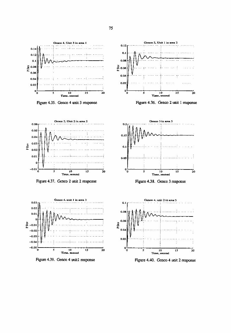
75
Genco 4. Unit 3 in area 1 Genco 2, Unit 1 in area 2
10 Time, second
a 0.06
10 15 Hme. second
Rgure 4.35. Genco 4 unit 3 response Figure 4.36. Genco 2 unit 1 response
Genco 2. Unit 2 in area 2
5 10 15 Time, second
20
Figure 4.37. Genco 2 unit 2 response
Genco 3 in area 3 0.2
0.15
0.1
0.05
lime, second
Rgure 4.38. Genco 3 response
Genco 4. unit 1 in area 3 Genco 4. unit 2 in area 3
10 Time, second
0.08
0.06
O a.
Time, second
0.04
0.02
Figure 4.39. Genco 4 unitl response Hgiffe 4.40. Genco 4 unit 2 response
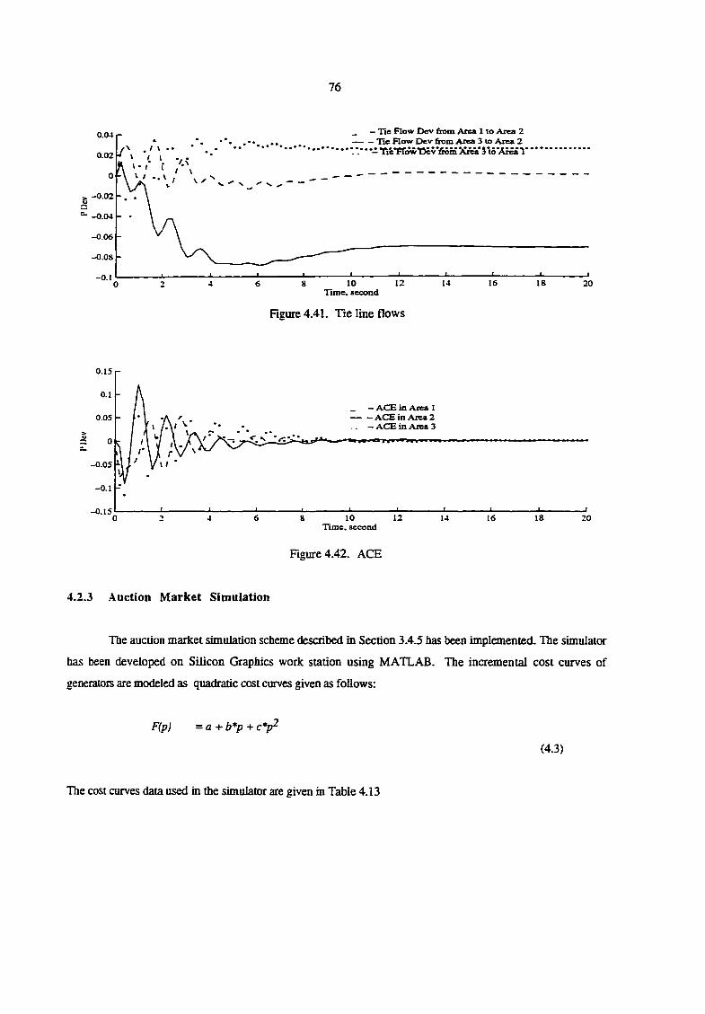
76
— He Flow Dev &om Aiea 1 to Area 2 — Tie Flow Dev from Area 3 to Area 2
• ••iT.'e-ffow-Dev fioni XraT 3 to'Areal'
0.04
0.02
-0.04
-0.06
-0.08
-O.I 18 10
Time, second 20
Rgure 4.41. Tie line flows
0.15
0.1
- ACE in Area 1 ACE in Aica 2
— ACE in Aica 3 O.OS
>
-0.05
-0.1
-0.15 12 20
Time, second
Figure 4.42. ACE
4.2.3 Auction Market Simulation
The auction market simulation scheme described in Section 3.4.5 has been implemented. The simulator
has been developed on Silicon Graphics work station using MATLAB. The incremental cost curves of
generators are modeled as quadratic cost curves given as follows:
F{p) =a + b*p +
(4.3)
The cost curves data used in the simulator are given in Table 4.13
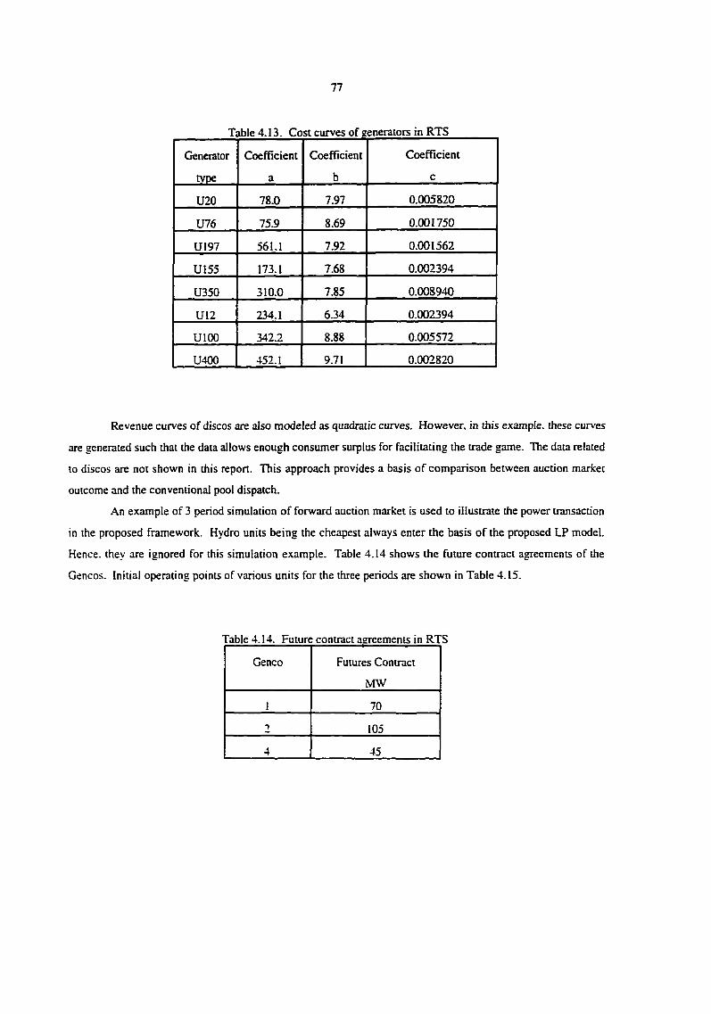
77
Table 4.13. Cost curves of generators in RTS
Generator
tvpe
Coefficient
a
Coefficient
b
Coefficient
c
U20 78.0 7.97 0.005820
U76 75.9 8.69 0.001750
U197 561.1 7.92 0.001562
U155 173.1 7.68 0.002394
U350 310.0 7.85 0.008940
U12 234.1 6.34 0.002394
UlOO 342.2 8.88 0.005572
U400 452.1 9.71 0.002820
Revenue curves of discos are also modeled as quadratic curves. However, in this example, these curves
are generated such that the data allows enough consumer surplus for facilitating the trade game. The data related
to discos are not shown in this report. This approach provides a basis of comparison between auction market
outcome and the conventional pool dispatch.
An example of 3 period simulation of forward auction market is used to illustrate the power transaction
in the proposed framework. Hydro units being the cheapest always enter the basis of the proposed LP model.
Hence, they are ignored for this simulation example. Table 4.14 shows the future contract agreements of the
Gencos. Initial operating points of various units for the three periods are shown in Table 4.15.
Table 4.14. Future contract agreements in RTS
Genco Futures Contract
MW
I 70
2 105
4 45
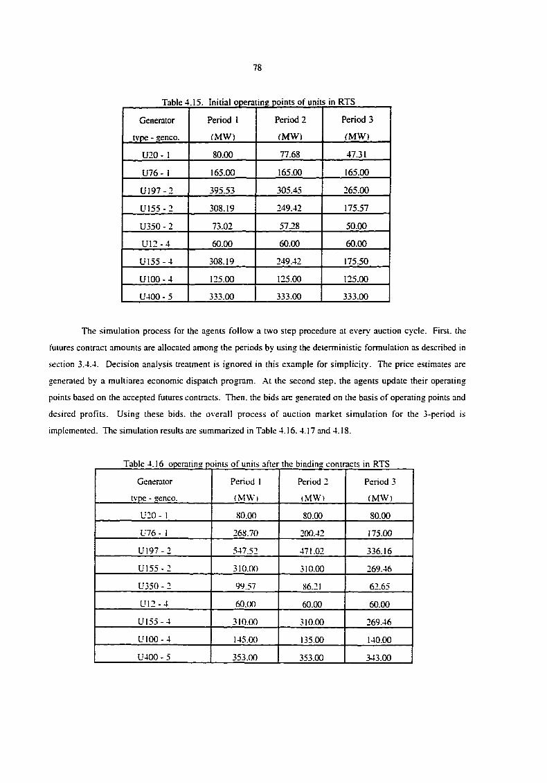
78
Table 4.15. Initial operating points of units in RTS
Generator
tvpe - genco.
Period I
(MW)
Period 2
fMW)
Period 3
rMW)
U20 - 1 80.00 77.68 47.31
U76- I 165.00 165.00 165.00
UI97-2 395.53 305.45 265.00
U155-2 308.19 249.42 17557
U350 - 2 73.02 57.28 50.00
U12-4 60.00 60.00 60.00
U155-4 308.19 249.42 175.50
UlOO-4 125.00 125.00 125.00
U400 -5 333.00 333.00 333.00
The simulation process for the agents follow a two step procedure at every auction cycle. First, the
futures contract amounts are allocated among the periods by using the deterministic formulation as described in
section 3.4.4. Decision analysis treatment is ignored in this e.xample for simplicity. The price estimates are
generated by a multiarea economic dispatch program. M the second step, the agents update their operating
points based on the accepted futures contracts. Then, the bids are generated on the basis of operating points and
desired profits. Using these bids, the overall process of auction market simulation for the 3-period is
implemented. The simulation results are summarized in Table 4.16.4.17 and 4.18.
Table 4.16 operating points of units after the binding contracts in RTS
Generator Period I Period 2 Period 3
tvpe - genco. (MW) (MW) (MW)
U20- 1 80.00 80.00 80.00
U76 - 1 268.70 200.42 175.00
U197-2 547.52 471.02 336.16
U155-2 310.00 310.00 269.46
U350- 2 99.57 86.21 62.65
LM2-4 60.00 60.00 60.00
U155-4 310.00 310.00 269.46
UlOO-4 145.00 135.00 140.00
U400 - 5 353.00 353.00 343.00
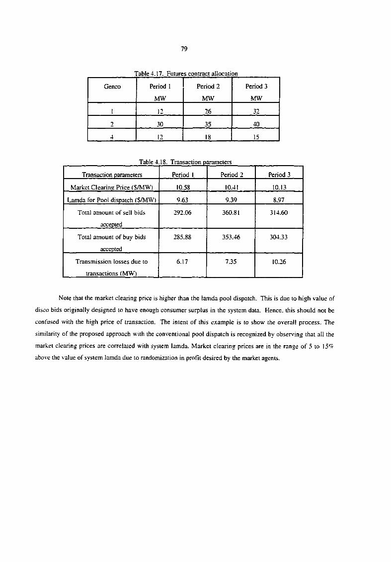
79
Table 4.17. Futures contract allocation
Genco Period 1 Period 2 Period 3
MW MW MW
1 12 26 32
2 30 35 40
4 12 18 15
Table 4.18. Transaction parameters
Transaction parameters Period 1 Period 2 Period 3
Market Clearing Price (S/MW) 10.58 10.41 10.13
Lamda for Pool dispatch (S/MW) 9.63 9.39 8.97
Total amount of sell bids
accepted
292.06 360.81 314.60
Total amount of buy bids
accepted
285.88 353.46 304.33
Transmission losses due to
transactions (MW)
6.17 7.35 10.26
Note that the market clearing price is higher than the lamda pool dispatch. This is due to high value of
disco bids originally designed to have enough consumer surplus in the system data. Hence, this should not be
confused with the high price of transaction. The intent of this example is to show the overall process. The
similarity of the proposed approach with the conventional pool dispatch is recognized by observing that all the
market clearing prices are correlated with system lamda. Market clearing prices are in the range of 5 to 15'^r
above the value of system lamda due to randomization in profit desired by the market agents.
80
5. CONCLUSION AND SUMMARY
This research has developed the foundation of market-based pricing of electric energy and ancillar}'
services in an auction market structure. It has been shown that the proposed approach can easily be extended to
accommodate any changes in operational and fimctional structure of the assumed model. Concept of different
types of contracts in price-based operation were introduced. The proposed foundation was used to develop an
automatic generation control simulator and an auction market simulator for price-based environment These
developed simulators can be used for several advantageous purposes. This chapter summarizes some of the
salient features, advantages and limitations of the proposed approach along with suggestion of possible future
research work.
5.1 The Energy Brokerage Model
Although the separate functionalities of gencos, discos, transcos and RTG are clearly mentioned, the
implementation of such functions is much more involved. In future, it is possible to have some other
organizations (such as NERC) and/or companies with responsibility to coordinate these fimctions. Even then,
the proposed model will not loss its generality as the basic assumptions would still be the same. The proposed
model has following attractive characterisdcs;
• Energy brokerage systems, discussed so far in the literature do not consider mechanisms to include
ancillary services. In this work, reserve margins and transmission losses are included in the brokerage
system in order to design an efficient pricing mechanism for providing correa incentives to achieve a
reliable electric market place.
• The model includes network configuration, system conditions and the reliability desired by market
participants. This represents the system operation much more closer to true market optimum as
opposed to other bidding models, such as sequential bidding approach [17],
• The proposed mathematical framework is very close to traditional optimal power flow type of problem.
Thus, the existing tools for optimal power flow can easily be modified to develop the brokerage
software.
81
It has been shown that the developed fonnulation can be ad^ted for linear programming application.
Techniques that can lead to better linear programming models have also been illustrated. Furthermore,
the formulation has angular block structure which can be exploited to apply efficient decomposition
techniques to solve a large scale power system problem. This enhances the practicability of the model.
• This work considers transco as an exogenous agent in the electric market place. Thus, the transmission
pricing issue has not been dealt with. The proposed approach can be extended to include transco
endogenous to the model. Such an exercise will provide the cost-benefit analysis of transmission
components and control equipments.
The merchandising surplus is defined as the profit made by the market participants (difference between
the cost of gencos and benefit of discos). In the proposed model, the merchandising surplus can be used
to compensate the transco. This matter can be a subject of future research.
The developed model provides a unified framework for merchandising and technical functions. This
provides better coordination among the market participants as opposed to two-tier models.
5.2 AGC Simulator
This work has proposed a new framework for implementing load following contracts in price based
operation. The developed AGC simulator can be used to study the power system behavior with several load
following contracts in place. Salient characteristics of the simulator is summarized as follows:
• The modified AGC scheme includes the contract data and measurements, which are continuous regular
and quiescent and hence, greatly improves control signals to unit dispatch and controllers.
• The proposed simulator is generic enough to simulate ail possible types of load following contracts
(bilateral, poolco and multilateral). The need of a new contract called area regulation contract is
identified in the price-based electric system operation. In real time operation, a contract violation is
reflected in higher requirement of area regulation. This should be interpreted as higher (penalty) costs.
• The proposed scheme includes ACE as a part of control error signal and thus also satisfies the NERC
performance criteria. The NERC performance criteria should b expanded to include all of the future
contract types.
82
• The new firamewoik requires establishment of standards for the electronic communication of contract data
as well as measurements among the ICA and the market players. Increased magnitude of computerized
accounting needed by the explosion in the number of transactions is an another technical issue to be
solved. In general, a variety of technical scrutiny will be needed to ensure secure system operation and a
fair market place. This is a reason to give the ICA substantive authority.
The PTTiphasis of the developed software is to analyze proposed contract implementation as implemented
for operational control. The strength of the approach is the segregation of the competitive market tools
from the control emulation tool.
• The tool described should enable the analysis of proposed rules for the new environment The contract
violation case presented shows the level of analysis required to determine if such rules are appropriate.
The details of contract implementation can be used to teach students the issues involved in load
following in a price-based operation. More case studies can be presented to encourage thinking about
required technical regulations to ensure secure system operation and a fair marketplace.
• The developed simulator does not include network conHguration and system condition. Thus,
transmission losses are ignored. The network equations can be added to the simulator as done in case of
a conventional simulator.
5.3 Auction Market Simulator
This research has developed an auction market simulator for price based operation. The proposed
approach allows the implementation of futures contract via forward market simulation. This simulator can be
used to experimentally study various aspects of the deregulated environment Some of the potential application
and usage of the simulator are summarized as follows;
• Many technical and legal problems need to be resolved for the suggested industry transition to be
successful. The proposed simulator can be used to address such problems, at least in part The issues,
such as pricing of transmission losses, priority of transactions, emergency power, etc. can be studied and
analyzed by experimental simulation of electric market The ultimate goal of the developed simulator
should be to discover the problems associated with the new environment via computer/operator
simulation instead of using the actual power grid.
83
• In the new environment, the plant operators are required to submit the price-based bids to perform
electric power transaction. This is quite different fix)m what the system operators are accustomed in a
vertically integrated industry. The proposed simulator can be used to train the operators how to bid in
the new environment.
5.4 Practical Implications: ISO V/s ICA
The state of California is restructuring its electric market by introducing a two-tier arrangemenL The
merchandising and technical functions are separated by forming two different organization, namely the Power
Exchange CPX) and the Independent System Operator (ISO) respectively. The PX provides a competitive
wholesale market where, buyers and sellers submit the bids. The PX ranks the least-cost bids and submits
proposed schedule for delivery of power to the ISO. The ISO evaluates those bids to coordinate the day-ahead
scheduling and real-time balancing for all of the grid. The ISO manages transmission congestion and constraints
on the network basis and procures ancillary services on a competitive and unbundled basis.
The proposed model provides a single central entity, the ICA responsible for merchandising as well as
technical functions. This will facilitate the bidding process as the bids are directly evaluated in conjunction with
the operating conditions and constraints as opposed to the California model where bid evaluation is a two step
process. The issue of acceptance and rejection of bids are resolved disregarding the order of transactions. This is
one of the key features of the model which will reduce the legalities involved in real-time implementation of a
deregulated market operation. Furthermore, the practical implementation of the proposed model will reduce
burden on the communication requirement This is highly desirable due to intensive communication needs
arising from the inaeased number of transactions in the new marketplace.
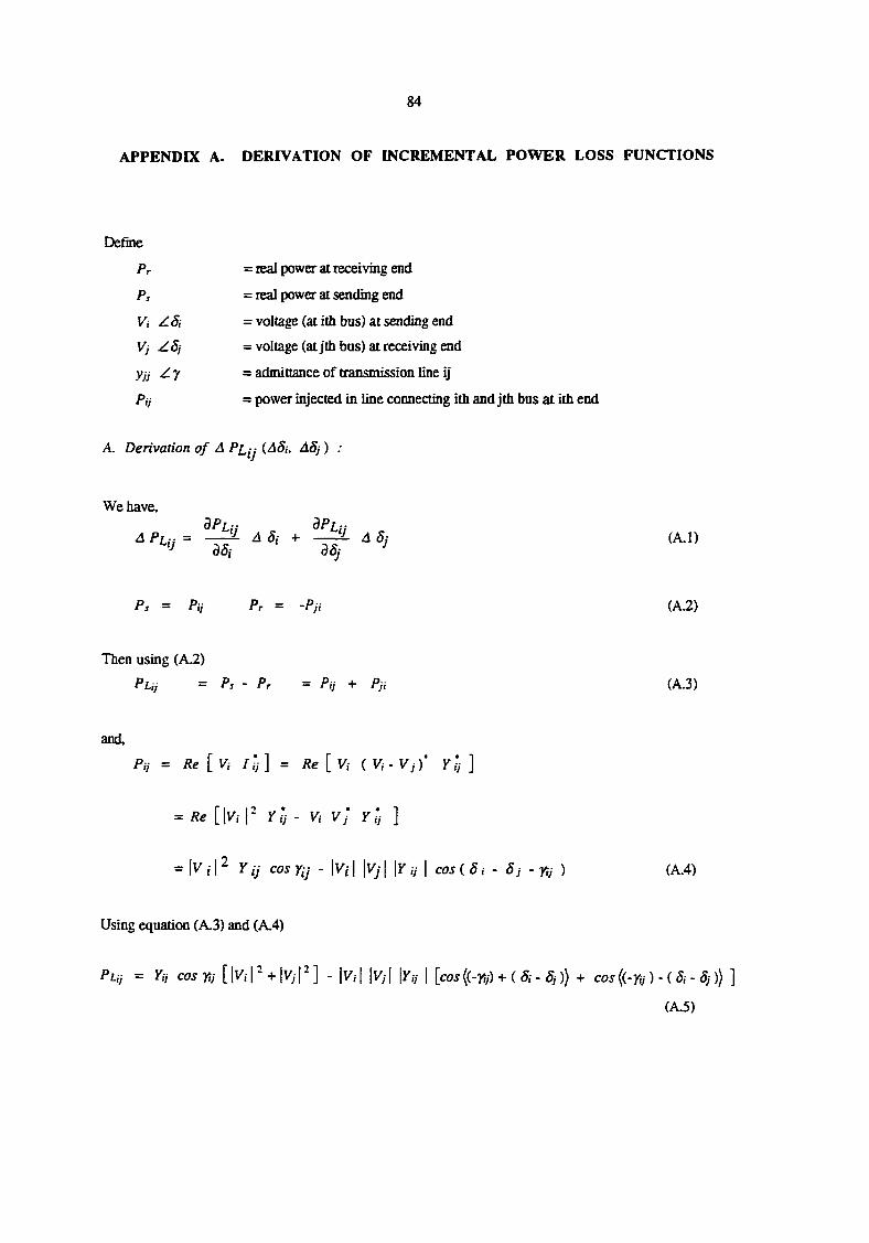
84
APPENDIX A. DERIVATION OF INCREMENTAL POWER LOSS FUNCTIONS
Define
Pr = real power at receiving end
P, = real power at sending end
Vi Z5i = voltage (at ith bus) at sending end
Vj ZS j = voltage (atjth bus) at receiving end
y j j Zy = admittance of transmission line ij
Pij - power injected in line connecting itb and jth bus at itb end
A. Derivation of A P[^-j (45/, A5j ) ;
We have, SPLu _ dPiii ^ ^Sj (A. . ,
Ps — Pij Pr — 'Pji (.A.JZ)
Then using (A^)
Piij = Ps - Pr = Pij + Pji (A.3)
and,
Pi j = Re [ V , - / ; ; ] = Re [V i { V i -V j ) Y ' j ]
= Re [ \V i \ - Y j j - V i vJ Y j j ]
= |V /1 2 Y ij cos Yij - \Vi I \Vj I \Y ij | co^ ( 5 - Sj - Yij ) (A.4)
Using equation (A.3) and (A.4)
Piij = Yij cos r.j [ |Vf I - + I - ] - \Vi 1 IV) I \Yij I [cos {(-r,i) + (5i- Sj)) + C05 ((-yj;) - (5; - Sj))
(A.5)
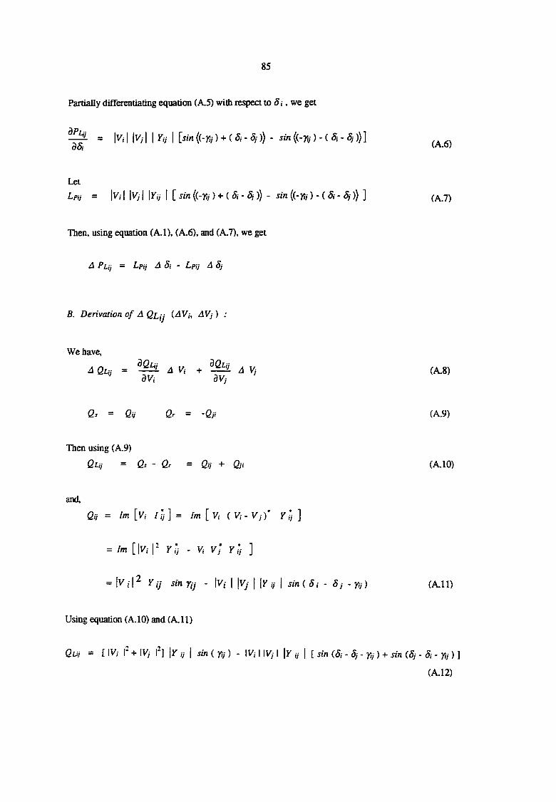
85
Partially differentiating equation (A.5) with respea to , we get
= \Vi I \Vj M I [«"n {(-r>} ) + (Si-Sj)) - sin {i-yij ) - ( S i - S j ) ) ]
Let
Lpi j = \V i I |V> I \Y i i I [ sin - ^-)) - sin {{ -Y i j ) - ( .S i -5 j ) ) ] (^j)
Then, using equation (A.1), (A.6), and (A.7), we get
A Piij = Lpij A Si - Lpij A 5j
B. Derivation of A Qi^-j {AVi, AVj ) :
We have,
~ A V , ( ^ 8 ,
Qs — Qij Qr — -Qji (A.9)
Then using (A.9)
Quj = Qs ' Qr = Qij + Qji (A.10)
and,
Qij = Im [Vi I ' i j ] = Im [ V i ( - V j ) ' Y ! j ]
= Im I ' Y l j - V i V ' j Y ' i j ]
= | V / | 2 Yi j sin Yi j - \V i I \V j | {Y i j | sin{ 5 i - 5 j - Y j ) (A.11)
Using equation (A.10) and (A.11)
Quj = [ IV, F + \V j I-] \Y i j I sin ( yj;) - Wi I \V j I \Y ,y | [ sin (S i -S j -Y . i ) + sin (S j - S i - ) ]
(A.12)
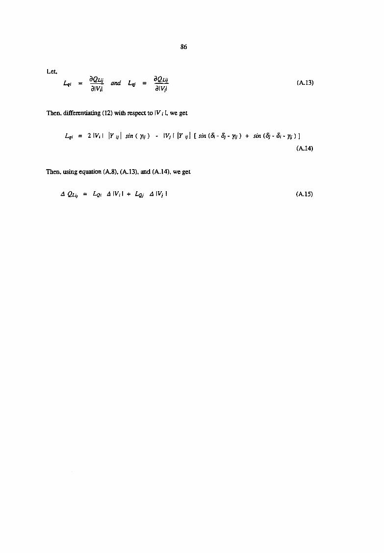
86
Let,
L,, = and (A.13) dWA 3IV;i
Then, diffeientiating (12) with respect to IV ,• I, we get
Lqi = 2 IV, I |Kiy| sin( Y i j ) - IK/ l l i ' ; / ! [ sin (5i - Sj - yij) + sin {Sj - 5i - ytj) ]
(A.14)
Then, using equation (A.8), (A.13), and (A.14), we get
4 Qlij = Lqi A IV.- \ + LQJ A IV; I (A.15)
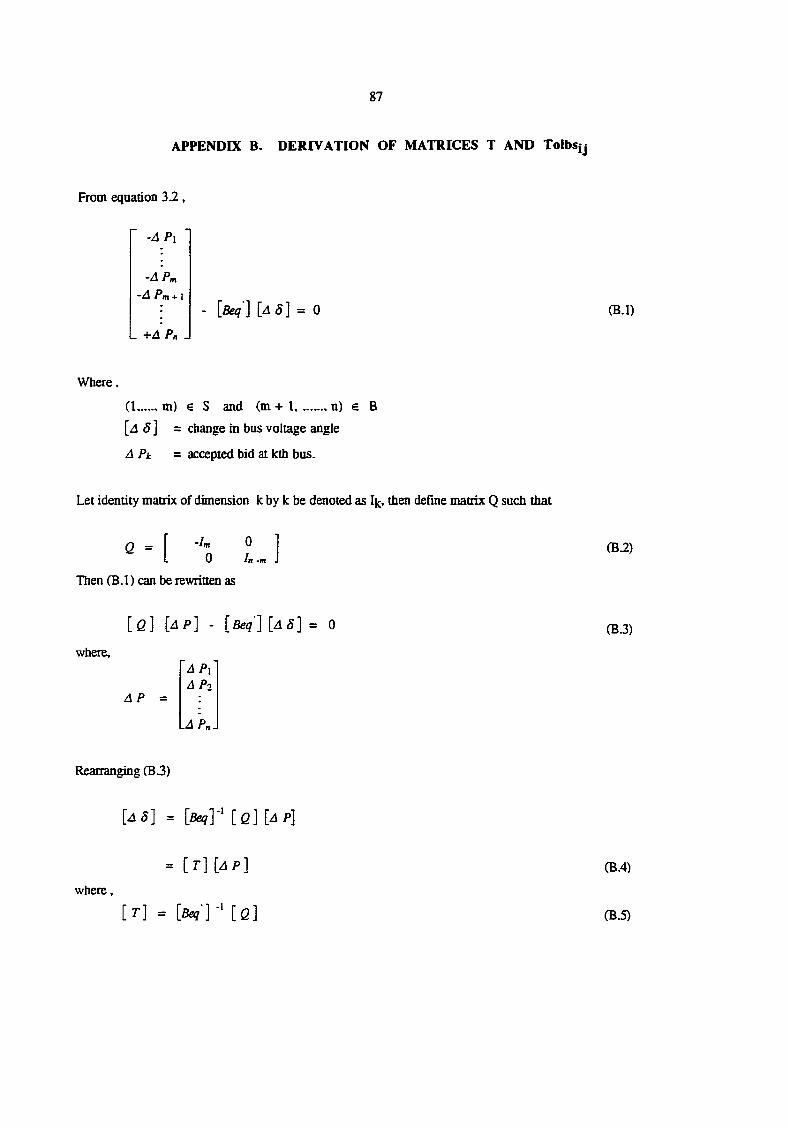
87
APPENDIX B. DERIVATION OF MATRICES T AND Tolbs
From equation 1 2 ,
• - A P i '
L + A P „ A
Where.
(1. m) e S and (m + 1, n) e B
[id 5 ] = change in bus voltage angle
A PK = accepted bid at ktb bus.
Let identity matrix of dimension k by k be denoted as tben define matrix Q sucb that
- A P M * \ [Seq ] [4 5 ] = 0
Then CB.l) can be rewritten as
[Q ] [4P ] - [Beq] [4 5 ] = 0
where. A P x
AP2 AP
\.AP„\
Rearranging CB3)
[ A S ] = [ B E Q ] - ' [ Q ] [ A P ]
= [ r ] [ 4 P ]
where,
[ T ] = [Beq ' ] •' [ Q ]

88
and [Q] is defined in (B^).
From (B.4),
[ A S ] = [ r ] [ a p ]
Or,
A S k = [ T k ] [ A P ] ( B . 6 )
where Tjc = row of matrix T
Let tbe Kth bus be connected to line i, then we augment the notion in (B.6) by
A Q k i = [ T f c , ] [ a p ] ( B . 7 )
From equation 3.9
A L i = I V?.. i |Vr°, I ^ (B.8)
where,
A L i = c h a n g e i n p o w e r f l o w i n l i n e i
A 5 n , A 5 St = voltage angle at receiving end and sending end of line i
Xi = reactance of line i
I ^. I I i I = voltage magnitude at sending and receiving end of line i respectively.
Putting (B.7) in (B.8),
A L i = \ V t , \ \ V r i I [ Tn] U P] Xi
= Ai [ r , , ] [ 4 P ] ( B . 9 )
where,
A, = Xi
and.
T l i = [r r.-] - [ T , . ] (B. l l )
From eqn 3.18
A L i + A L j < A L i j „ u i x (B.12)
Putting (B.9) in (B.12),
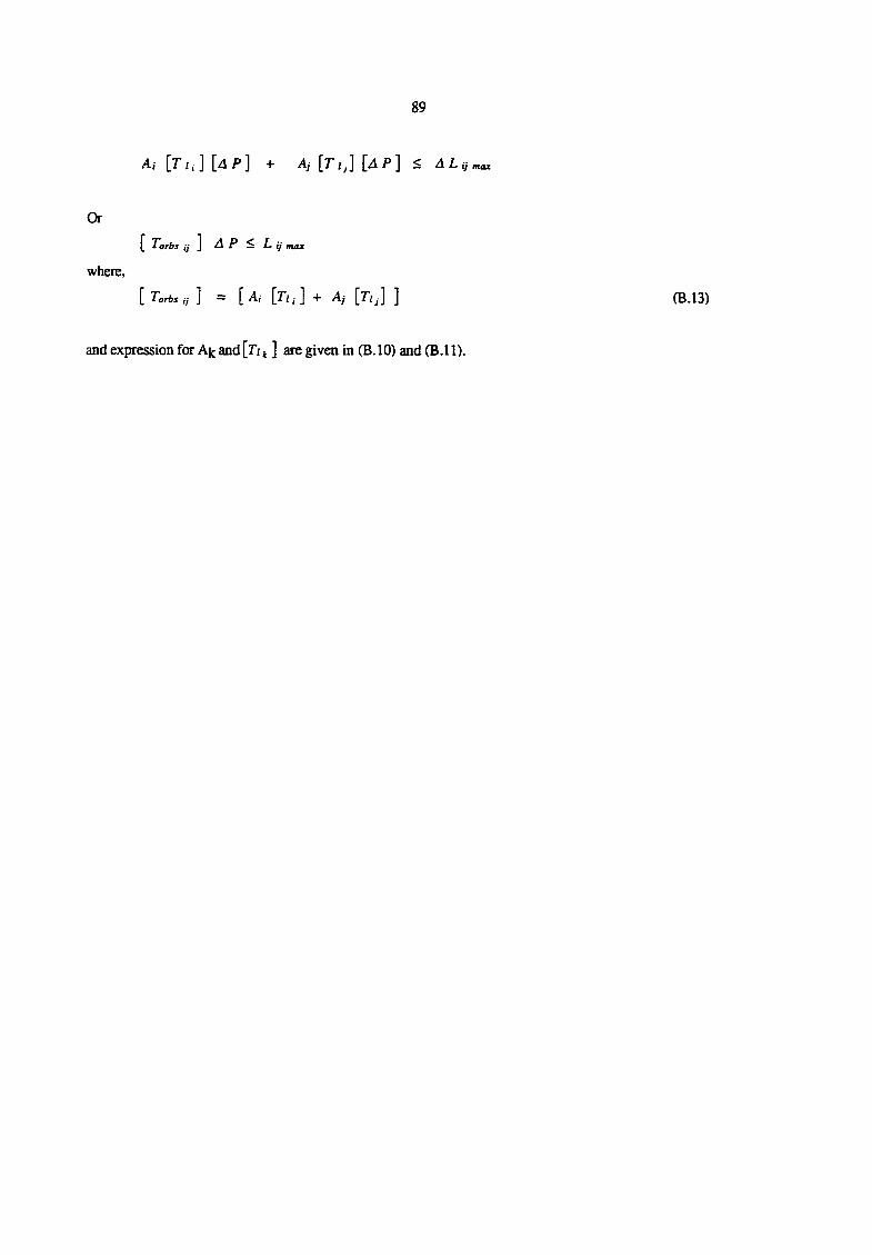
89
A, [ r / . ] [4P] + A; [ r j J [AP] < A L i j „ a x
f Torbs ij 1 A P ^ ij max
where,
[ Torbs ij ] = [Ai [ r ; , . ] + Aj [Tij] ] (B.13)
and expression for Ak and [r/t ] are given in (B.IO) and (B.11).
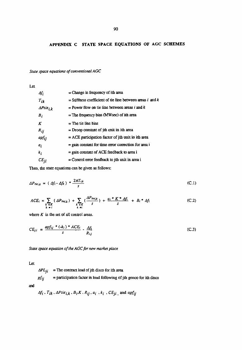
90
APPENDIX C STATE SPACE EQUATIONS OF AGC SCHEMES
State space equations of conventional AGC
Let
Afi = Change in frequency of ith area
Tij^ = Stiffness coefficient of tie line between areas i and k
APtiei = Power flow on tie line between areas i and k
Bi = The frequency bias (MWsec) of ith area
K = The tie line bias
Rl j = Droop cons tan t o f j th uni t in i th a rea
apfij = ACE participation factor of jth unit in ith area
ai = gain constant for dme error correction for area i
ki = gain constant of ACE feedback to area i
CEji = Control error feedback to jth unit in area i
Then, the state equations can be given as follows:
APneijc = (Afi- Afk ) * (C.I)
ACEi = X (4Pr .> , j f c ) + X Af i ^ 2 ) k eK k eK ^ ^ k k * i
where K is the set of all control areas.
^ ap f i j * { -k i )*ACEi _ ^
~ S R (C.3)
'J
State space equation of the AGC for new market place
Let
APLji = The contract load of jth disco for ith area
pflj = participation factor in load following of jth genco for ith disco
and
Af^ , i , k * ' ̂ i * ^ i * ^ ^J i , ^P f i j
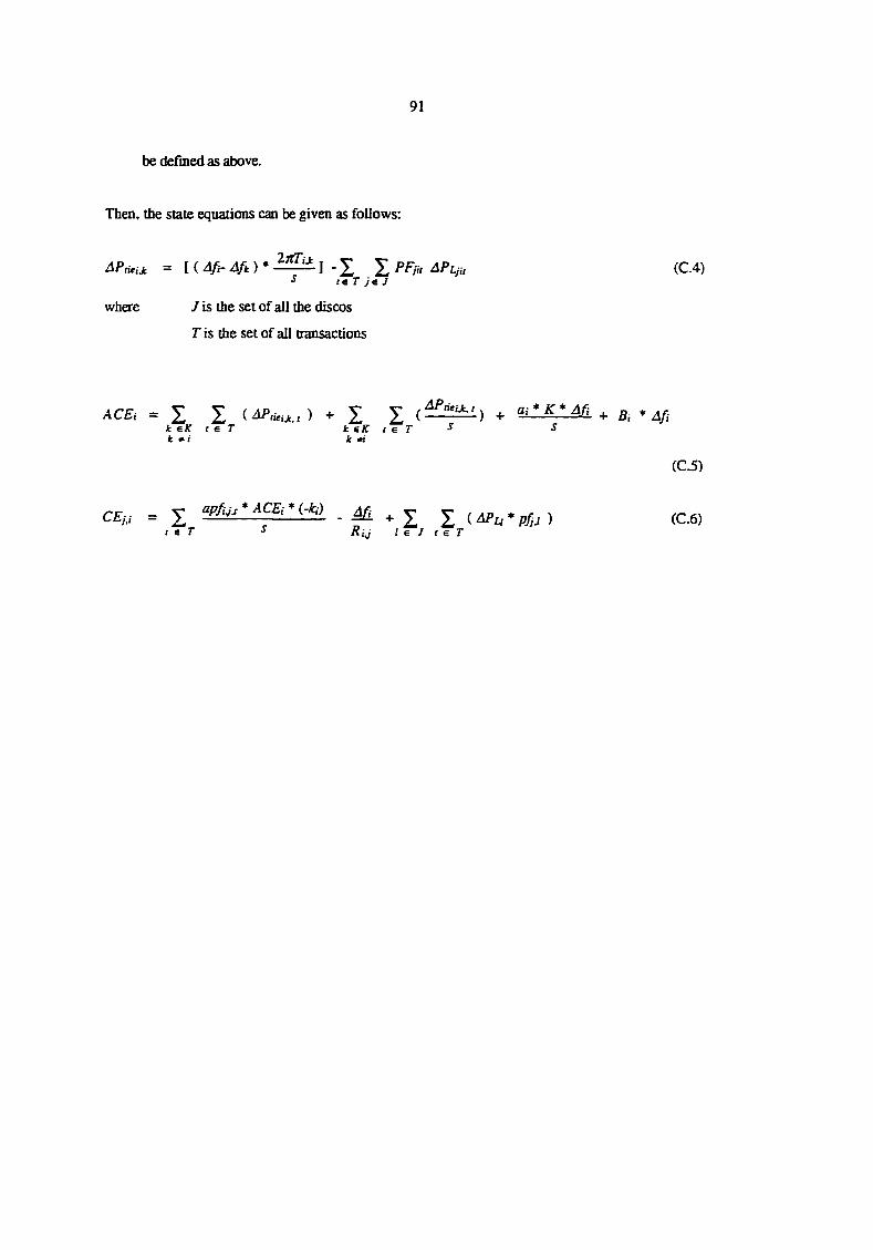
91
be defined as above.
Then, the state equations can be given as follows:
APtieiM = [ (4/i- 4A) * 1 -1 X PF}u APiju (C.4) ^ te T Je J
where J is the set of all the discos
r is the set of all transactions
ACBi = s I ) + I 2 + iiisue. B, 'if, k gK C G T k &K f € r ^ k k
(C.5)
CEiJ = I 1 ) t € T ̂ Rij I e J t e T
(C.6)
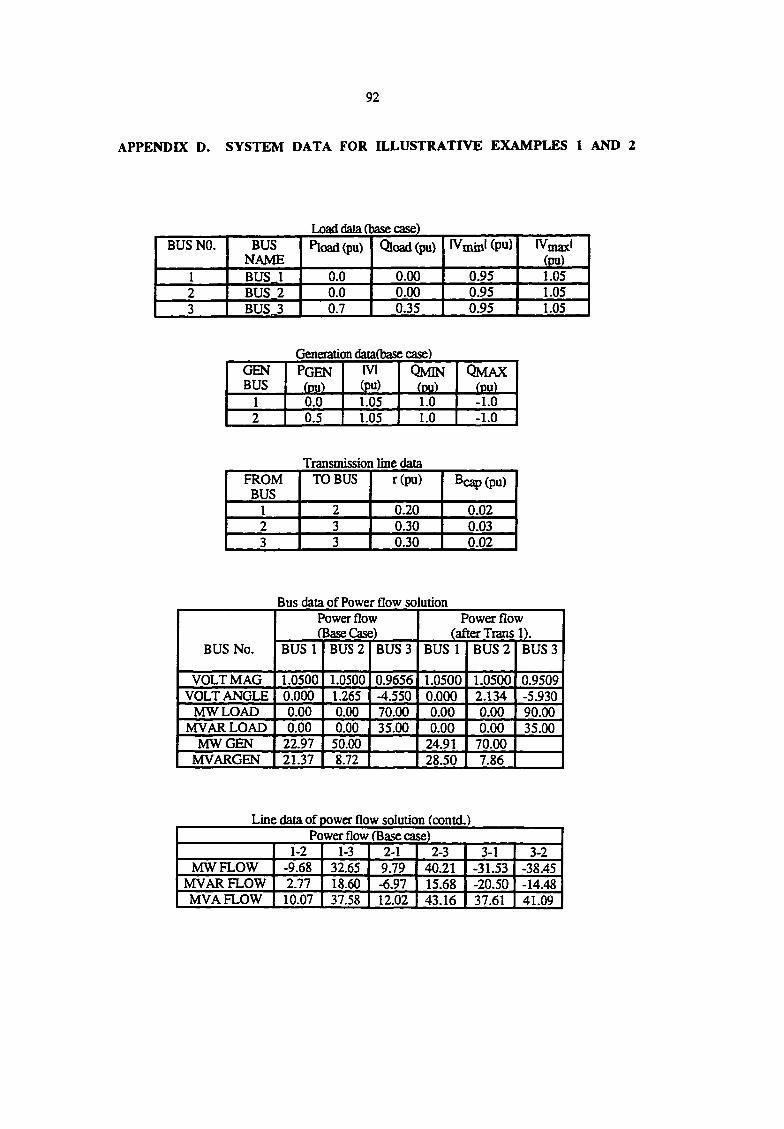
92
APPENDIX D. SYSTEM DATA FOR ILLUSTRATIVE EXAMPLES 1 AND 2
Load daia (base case) BUS NO. BUS Pload(pu) Qload (pu) IVmin' (pu) IVjnax'
NAME Pload(pu) Qload (pu)
(pu) I BUS_1 0.0 0.00 0.95 1.05 2 BUS_2 0.0 0.00 0.95 1.05 3 BUS_3 0.7 0.35 0.95 1.05
Generation data(base case) (JEN PGEN IVI QMIN QMAX BUS (DU) (pu) (pu) (PU)
1 0.0 1.05 1.0 -1.0 2 0.5 1.05 1.0 -1.0
Transmission line data FROM
BUS TO BUS r(pu) Bcap(pu)
1 2 0.20 0.02 2 3 0.30 0.03 3 3 0.30 0.02
Bus data of Power flow solution
BUS No.
F f 'ower flow 3ase(3ase)
Power flow (after Trans 1).
BUS No. BUS 1 BUS 2 BUS 3 BUS 1 BUS 2 BUS 3
VOLT MAG L0500 1.0500 0.9656 1.0500 1.0500 0.9509 VOLT ANGLE 0.000 U65 -4.550 0.000 2.134 -5.930
MWLOAD 0.00 0.00 70.00 0.00 0.00 90.00 MVARLOAD 0.00 0.00 35.00 0.00 0.00 35.00
MW GBJ 22.97 50.00 24.91 70.00 MVARGEN 2L37 8.72 28.50 7.86
Line data of power flow solution (contd.) Power flow (Base case)
1-2 1-3 2-1 2-3 3-1 3-2 MWFLOW -9.68 32.65 9.79 40.21 -31.53 -38.45
MVARFLOW 2.77 18.60 -6.97 15.68 -20.50 -14.48 MVAFLOW 10.07 37.58 12.02 43.16 37.61 41.09
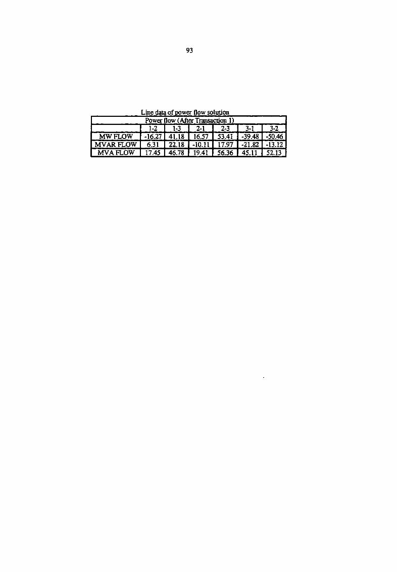
93
Line data of power flow solution Power flow (After Transaction 1) 1-2 1-3 2-1 2-3 3-1 3-2
MWFLOW -16.27 41.18 16.57 53.41 -39.48 -50.46 MVARFLOW 6.31 22.18 -10.11 17.97 -21.82 -13.12 MVAFLOW 17.45 46.78 19.41 56.36 45.11 52.13

94
BIBLIOGRAPHY
1. Federal Energy Regulatory commission. "Notice Of Proposed Rulemaking: Docket No. Rf.I93-3,"
rnnyressinnal Record. July 3Q. 1993.
2. Federal Energy Regulatory commission. "Notice Of Proposed Rulemaking: Docket No. RM95-8-000,"
Cnngressional Record. March 29,1995.
3. McCalley., JD. and G. B. Shebl6. 1994. Class notes from EE653A: Evaluation of Transmission
Service for Secure Power System Operation in a less Regulated Utility Environment," Department of
Electrical and Computer Engineering, Iowa State University, Ames, Iowa.
4. Lazarus, E. "The Public Utility Holding Act of 1935: Legislative History and Background,"
Congressional Research Service Report 92-226 A, The Library of Congress, February 26,1992.
5. U.S. Environmental Protection Agency, Office of Air Quality Planning and Standards. National Air
Pollution Estimates. Research Triangle Park, North Carolina, 1982.
6. Gent, M. R. and J. W. Lamont "Minimum-Emission Dispatch," IKKK Transactions. Vol. PAS-90, pp.
2650-2660. 1971.
7. Lamont, J. W. and M. R. Gent "Environmentallv - Oriented Dispatching Techniques." Prnceedinys nf
the 8th PICA Conference. Minneapolis, Minnesota, 1973.
8. Abel, A. "Public Utility Regulatory Policies Act of 1978: A Fact Sheet," Congressional Research
Service. The Library of Congress, July 30,1992.
9. U. S. Congress. "Notice of Proposed Rulemaking: Docket no. RM88-4, RM88-5, RM88-6,"
Congressional Record. March 16, 1988.
10. "Focus on Wheeling & Access," Electric Light And Power, pp. 12-15, March 1992.
11. U.S. Congress. Senate. Summary of S. 1630 "Clean Air Act Amendments of 1990,"
Record. April 20, 1990.
12.
95
"Energy Policy Act of 1992: Summary and Implications," Congressional Research Service. The Library
of Congress February 1, 1993.
13. Ballance, J.W. "Setting Up The Western Power Exchange," presented at Potential Impacts of FERC
Mega NOPR on System Operations - Panel Discussion, IEEE 96 Winter Power Meeting. Baltimore,
Maryland, January 22. 1996.
14. McAfee, R. and J.McMilIan. "Auctions and Bidding," Journal of Economic Literature 25. pp. 699-738.
June 1987.
15. "Actions in the Marketplace," Chicago Board of Trade. Publication Department, Chicago, IL, 1996.
16. "Fmancial Options: Hexibiiity, Control & Opportunity," New York Mercantile Exchange. Publication
Department, New York, NY, 1995.
17. Post, D. "Electric Power Interchange Analysis and Selection," Master's thesis. Iowa State University,
Ames, Iowa, May 1994.
18. Shebl6, G. B. " Energy As A Commodity," Power Seminar. Iowa State University, Ames, Iowa, April
6. 1993.
19. Henderson, J. M. and R. E. Quandt. "Microeconomic Theory: A Mathematical Approach, third edition,"
NewYork: McGraw Hill, 1980.
20. Vickery, W. "Counterspeculation, Auctions, and Competitive Sealed Tenders," Journal of Finance. Vol.
16, pp. 8-37. 1961.
21. Wilson, R. "Incentive Efficiency of Double Auctions," Econometrica. Vol. 53, pp. 1101-1115, 1985.
22. Smith, V. L. "Microeconomic Systems as an Experimental Science," American Economic Review.
Vol. 72, pp. 923-55, 1982.
23. Smith, V. L. "Bidding and Auctioning Institutions: Experimental Results," Division of Humanities and
Social Sciences, California Institute of Technology, Pasadena, California, Social Science Working Paper.
1974.
24. Smith, V. L. "Experimental Studies of Discrimination Versus Competition in Sealed-Bid Auction
Markets." Journal of Business. Vol. 40. pp. 56-84, 1967.
96
25. Smitb, V. L. -Experimental Auction Markets and the Walrasian Hypothesis," Journal of Political
Economy.. Vol. 73, pp. 387-393, 1965.
26. Rassenti, S. J., V. L. Smith and R. L. BulGn. "^A Combinatorial Auction Mechanism for Airport Tune
Slot Allocation," BcU Journal of Economics. Vol. 13, pp. 402-417, 1982.
27. McCabe, K. A., S. J. Rassenti and V. L. Smith. "Auction IDesign for Composite Goods: The Natural
Gas Industry." Journal of Economic Behavior and Organization. Vol. 14. pp.127-149, 1990.
28. Rassenti, S. J., S. S. Reynolds and V. L. Smitb. "Cotenancy and Competition in an Experimental
Auction Market for Natural Gas Pipeline Networks," To appear in Economic Theory, pp. 1-51, February
1992.
29. Smith. V. L. "Electric Power Deregulation: Background and Prospects," Contemporarv Policy Issues.
Vol. 6, pp. 14-24, July 1988.
30. Bently, W. G. and J. C. Evelyn. "Customer Thermal Energy Storage: A Marketing Opportunity for
Cooling off Electric Peak Demand," IEEE Trans, on Power Systems. Vol. 1, No. 4, pp. 973-979,
November 1987.
31. Vojdani. A.f., C.F. Imparto, N.K.Saini, BP.WoUenberg and H.HJIapp. "Transmission Access Issues,"
presented at IEEE 95 Whiter Meeting. 95 WM 121-4 PWRS, New York, January 19.1995.
32. Felak. R.P. "Reliability and Transmission Access," Public Utilities Fortnightly. July 15,1992.
33. Shebl6. G.B. "Price Based Operation in an Auction Market Structure." presented at IEEE PES Winter
Meeting. 96 WM 191-7 PWRS, 1996.
34. O'Neill, R. P. and C. S. Whitmore. "Network Oligopoly Regulation: An Approach to Electric
Federalism," Electricity and Federalism Symposium. June 24,1993 (Revised March 16, 1994).
35. Wu. F. and P. Varaiya. "What is Wrong With Hogan's Contract Network." University of California at
Berkeley Research ReporL June. 1995.
36. Wu, F.. S. Oren, P. Spiller. and P. Varaiya. "Folk Theorems On Transmission Access: Proofs and
Counter Examples," University of California at Berkeley Research Report. February 28, 1995.
97
37. Wu, F. and P. Varaiya. "Coordinated Multi-lateral Trades For Electric Power Networks: Theory and
rmplPTncTitatinn," TTnivRfsitv of ralifomia at Berkeley Research Renort. June. 199S.
38. Oren, S. S., P. Spiller, P. Variya and F. Wu. "Nodal Prices and Transmission Rights: A Critical
Appraisal." University of California at Berkeley Research RenorL December. 1994.
39. Resource Planning Associates, Inc. "The Florida Electric Power Coordinating Group: An Eyolying
Power Pool," Report for U.S. Department of Energy. October, 1979.
40. Florida Electric Power Coordinating Group, Inc. Penin.sular Florida Central Di.spatch Study. Part 1
Rnal Report May 14, 1980.
41. Russel, T. "Working with an Independent Grid in the UK - A Generator's View," Proceedings of the
24th Annual North American Power Symposium. Manhattan, Kansas, pp. 270-275, September, 1992.
42. Russel . T. and L. Mogridge. "Some Operational Issues between Independent Generators and an
Independent Grid," Proceedings of the 27th Annual North American Power Symposium. Manhattan,
Kansas, pp. 1183-1188, September, 1995.
43. Hillier, F. S. and G. J. Liberman. Introduction to Operations Re.search- New York: McGraw Hill, 1990.
44. Luenberger. D. G. Linear And Nonlinear Programming. Addison-Wesley Publishing Co., Menlo Park,
CA, 1984.
45. Zangwill, W. I. "Nonlinear Programming yia Penalty Functions," Management Science. Vol. 13, No.
5, pp. 344-358, 1967.
46. Gass, S. I. Linear Programming : Methods and Applications. McGraw-Hill Inc., New Yoric, 1958.
47. Ignizio James P. Linear Programming in Single and Multiple Obiectiye Systems. Englewood Cliffs,
New Jersey: Printice Hall Inc., 1982.
48. Bazarra, H. S., J. J. Jarvis, and H. D. Sherali. Linear Programs and Network flows. New York: John
Wiley and Sons, 1990.
49. Dantzig, G. B. and P. Wolfe. "The Decomposition Algorithm for Linear Programs," Operations
Research. Vol. 8, pp.101-111, 1960.
98
50. CPLEX Optimization, Inc. 1993. Using the CPLEX Callable Library and CPLEX Mixed Integer
Library, Incline Village Nevada.
51. Karmarkar, N. ~A New Polyncmial-Traie Algorithm for Linear Programming," Comhinatorica. 4, pp.
373-395, 1984.
52. Lasdon, L. S., Optimization Theory for Large Systems. Macmillan Publishing Co., Inc, New York,
NY, 1970.
53. Day, J. T. "Forecasting Minimum Production Costs with Linear Programming," IKKK Trans, on Power
Apparatus and Systems. Vol. PAS-90, No. 2, pp.814-823, March/April 1971.
54. Cooper. L. and D. Steinberg. Methods and Applications of Linear Programniinp. Philadelphia: W.B.
Saunders Company, 1974.
55. Simmons, D. M. Nonlinear Programming for Operations Research. Englewood Cliffs, New Jersey:
Prentice-Hall Inc., 1975.
56 Shebl6, G. B. and J. W. Lamont 1992. Class notes form EE553: " Steady State Analysis of Power
Systems," Department of Electrical and Computer Engineering, Iowa State Uniyersity, Ames, Iowa.
57. ShebI6, G. B. 1993. Class notes from EE653E: " Power System Optimization," Department of
Electrical and Computer Engineering, Iowa State University, Ames, Iowa.
58. Ahuja, R. k.. T. L. Magnanti. and J. B. Orlin. Netwoiic Flows: Theory . Alyoridims and Applications.
Prentice Hall. Englewood Cliffs, NJ 1993.
59. Lippmann, R. P. "An Introduction to Computing with Neural Nets," IEEE Acoustics. Speech and
Signal Processing Magazine, pp. 4-21, April 1987.
60. Kumar, J. and G. B. Shebl6. "Clamped State Solution Of Artificial Neural Network For Real Time
Economic Dispatch," IEEE Trans, on PWRS. Vol. 10, No. 2, pp. 925-931, 1995.
61. Kumar, J. "Application of Artificial Neural Networks to Optimization Problem," Master's Thesis, Iowa
State University, Ames, Iowa, December, 93.

99
62. Kennedy, M. P. and L. O. Chua. "Unifying the Tank and HopGeld Linear Programming Circuit and the
Canonical Nonlinear Circuit of Chua and Lin," TFEE Transactions on Circuit and Svstem.s. CAS - 34,
pp. 210-21, February 1987.
63. Kennedy, M. P. and L. O. Chua. "Neural Networks for Nonlinear Programming," THEE Transactions on
rirniit and Systems. CAS - 35, pp. 554-562, May 1988.
64. Chua, L. O. and G. N. Lin. "Nonlinear Programming without Computauon," IEEE Transactions on
rimiit and Svstem.s. CAS - 31. PP. 182-188. February 1984.
65. Doty, K. W. and P. L. McEntire. "An Analysis of Electric Power Brokerage Systems," IEEE Trans, on
PAS. Vol. PAS-101, No.2, pp. 389-396, 1982.
66. Fahd, G., D. A. Richards, and G. B. Shebl6. "The Implementation of an Energy Brokerage System
Using Linear Programming," IEEE Trans, on power systems. Vol. 7, No. 1, pp. 90-96, 1991.
67. Fahd, G. and G.B. Shebl6. "Optimal Power Flow Emulation of Interchange Brokerage System Using
Linear ftogramming," IEEE Trans, on power systems. Vol. 7, No. 2, pp. 497-504, 1992.
68. Anwar, D. and G. B. Shebl6. "Application of Optimal Power Flow to Interchange Brokerage
Transaction," Electric Power System Research Journal. Vol. 30, No. 1, pp. 83-90,1995.
69. Post, D., S.S. Coppinger, and G.B.Shebl6. "Application of Auctions as a Pricing Mechanism for the
biterchange of Electric Power," IEEE Trans, on power systems. Vol. 10, No. 3, pp. 1580 - 1584, 1995.
70. Coppinger, S. S. and G.B. Sheble', "Interchange of Electric Power By Using a Double Auction
Mechanism," Proceedings of the 27th Annual North American Power Symposium, pp. 299-303,
Bozeman, MT, 1995.
71. Chattopadhyay. "An Energy Brokerage System with Emission Trading and Allocation of Cost Sayings,"
IEEE Trans, on Power Systems. Vol. 10, No. 4, pp. 1939-1945, 1995.
72. Caramanis, M. C., R. E. Bohn, and F. C. Schweppe. "Optimal Spot Pricing: Practice and Theory,"
IEEE Trans, on Power Apparatus and Systems. Vol. PAS-101, No. 9, pp.3234-3244, 1982.
100
73. Kumar, J. and G. B. Shebl6. "Auction Game in Electric Marketplace." Proceedings of 58tli American
Power Conference. Chicago, n, pp. 356-364, 1996.
74. Harsyani, J. C. Rational Behavior and Bargaining Eanilibrinm in Games and Social Sciences. Cambridge
University E»ress, New York, NY, 1977.
75. Shebl6, G. B. "Electric Energy in a Fully Evolved Marketplace." Proceedings of the 26th Annual North
American Power Svmposium. Manhattan. Kansas, pp. 81-90, September, 1994.
76. Kumar, J. and G. B. Shebld. "Framework for Energy Brokerage System with Reserve Margins and
Transmission Losses," presented at ihfcfc PES Winter Meeting. 96 WM 190-9 PWRS, 1996.
77. Kumar, J and G. B. Shebld. "Framework for Energy Brokerage Systems with Reserve Margin
Constraints," Proceedings of the 27th Annual North American Power Symposium, pp. 41-46, Bozeman,
MT, 1995.
78. Stott, B. and O. Alsac. "Fast Decoupled Load Row," IEEE Trans, on PAS. Vol. 93, No. 3, pp. 859-
867, 1974.
79. Kirschen, D. S. and H. P. Van Meeteren. "MW/voltage Control in a Linear Programming Based
Optimal Power Flow," IEEE Trans, on PWS. Vol. 3, No. 2, pp. 481-489, 1988.
80. Stott, B. and E. Hobscn. "Power System Security Control Calculation Using Linear Programming, Part
I" IfcbE trans, on PAS. Vol. 97, No. 5, pp.1713-1720, Sept'78.
81. Stott, B. and E. Hobson. "Power System Security Control Calculation Using Linear Programming, Part
n." IfchE trans, on PAS. Vol. 97, No. 5, pp.1721-1731, Sept'78.
82. Stott, B. and J. L. Marinho. "Linear Programming for Power System Network Security Applications,"
IEHE Trans.. Vol. PAS-98, No. 3 May / June, 1979.
83. Olofsson, M., G. Andersson, and L. Soder. "Linear Programming Based Optimal Power Flow Using
Second Order Sens i t iv i t ies , " lEbE / PES Winter Meet ing . January 1995, New York .
84. Alvarado, F, Y. Hu, D. Ray, R. Stevension and E Cashmam. "Engineering Foundation for the
Determination of Security Costs," IEEE trans, on PWS. pp.1175-1182, Aug'91.
101
85. Kumar. J., K. H. Ng, and G.B. SbebM. "AGC Simulator For Price Based Operation, Part 1: A Model,"
to be presented at IKEE PES Summer Meeting. 96 SM 588-4 PWRS, 1996.
86. Kumar, J., K. H. Ng, and G.B. Shebl6. "AGC Simulator For Price Based Operation, Part II: Case Study
Results," to be presented at IEEE PRS Summer Meeting. 96 SM 373-1 PWRS, 1996.
87. "NERC Control Performance Criteria," Supplement to NERC Operating Manual. North American
Reliability Council, Princeton, NJ.
88. Christie, R. D. and A. Bose. "Load Frequency Control Issues in Power System Operations after
Deregulation." Proceedings of the 1995 PICA Conference, pp.18-23.1995.
89. Schulte, R. P. "An Automatic Generation Control Modification for Present Demands on Interconnected
Power Systems," nre.sented at ihfch. PES Simimer Meeting. 95 SM 187-7 PWRS, 1995.
90. Jaleeli, N., L. VanSlyck. "Tie Line Bias Prioritized Energy Control," 93 WM 160 PWRS, WPM,
presented at the IEEE PRS Whiter Meeting. Columbus, Ohio, 1993.
91. Jaleeli, N., L. VanSlyck, D. Ewart, L. Fmk, and A. Hof&nan. "Understanding Automatic Generation
Control", Ihfcfc Trans, on Power Systems. Vol. 7, pp. 1106-1122, 1992.
92. Kumar, J. and G. B. Shebl6. "Electric Market Simulator for Price Based Operation", to be submitted lo
IEEE Power System Transactions.
93. Chu, W., B. Chen, and C. Fu. " Scheduling of Direct Load Control to Minimize Load Reduction for a
Utility Suffering from Generation Shortage," IEEE / PES Winter Meeting. 1993 , Columbus, Ohio.
94. Chao, H. P. "Peak Load Wcing And Capacity Planning with Demand and Supply Uncertainty," Bell
Journal of Economics. Vol. 14, No.l, 1983, pp. 179-190.
95. Howard, R A. " Decision Analysis: Practice And Promise," Management Science. 1988: 679- 675.
96. "MIDAS, Multi Objective Integrated Decision Analysis System," EPRI ioiimaL Vol. 12 May'87:57-58.
97. Howard, R. A. "Decision Analysis: Practice and Promise," Management Science, pp.675-679,1988.
102
98. Kumar, J. and G. B. Shebl6. ** A framework for Transaction Selection Using Decision Analysis Based
Upon Risk and Cost of Insurance," Pmceedinps of the 29th North American Power Symposium. Kansas
State University, KS, pp.548-557, 1994.
99. Kumar, J. and G. B. Shebl6. "A Decision Analysis Approach to Transaction Selection Problem in a
Competitive Electric Market," To be published in Electric Power Systems Research Journal.
100. Wood, A. J. and B. F. Woolenberg. Power Generation , Operation, and Control, John Wiley & Sons,
New York, NY, 1984.
101. IEEE Power System Reliability Subcommittee. "Reliability Test System," presented at IEEE PES
Winter Meeting. 96 WM 183-7 PWRS, 1996.
102. IEEE Committee Report. "Dynamic Models for Steam and Hydro Turbines in Power System Studies,"
Vol. PAS-92, November/December 1973, pp. 1904-1915.
Related Documents