Elastoplastic Integration Method of Mohr-Coulomb Criterion

Citation: Zhang, T.; Lin, S.; Zheng,

H.; Chen, Y. Elastoplastic Integration

Method of Mohr-Coulomb Criterion.

Geotechnics 2022, 2, 599–614. https://

doi.org/10.3390/geotechnics2030029

Academic Editor: Yong Sheng

Received: 10 June 2022

Accepted: 11 July 2022

Published: 12 July 2022

Publisher’s Note: MDPI stays neutral

with regard to jurisdictional claims in

published maps and institutional affil-

iations.

Copyright: © 2022 by the authors.

Licensee MDPI, Basel, Switzerland.

This article is an open access article

distributed under the terms and

conditions of the Creative Commons

Attribution (CC BY) license (https://

creativecommons.org/licenses/by/

4.0/).

Article

Elastoplastic Integration Method of Mohr-Coulomb CriterionTan Zhang 1,2,*, Songtao Lin 1, Hong Zheng 2 and Yanjiang Chen 2

1 MCC Central Research Institute of Building and Construction, No.33 Xitucheng Road, Haidian District,Beijing 100088, China; [email protected]

2 Key Laboratory of Urban Security and Disaster Engineering, Ministry of Education,Beijing University of Technology, Beijing 100124, China; [email protected] (H.Z.);[email protected] (Y.C.)

* Correspondence: [email protected]

Abstract: A new method for implicit integration of the Mohr-Coulomb non-smooth multisurfaceplasticity models is presented, and Koiter’s requirements are incorporated exactly within the proposedalgorithm. Algorithmic and numerical complexities are identified and introduced by the nonsmoothintersections of the Mohr-Coulomb surfaces; then, a projection contraction algorithm is applied tosolve the classical Kuhn–Tucker complementary equations which provide the only characterizationof possible active yield surfaces as a special class of variational inequalities, and the actual activeyield surface is further determined by iteration. The basic idea is to calculate derivatives of theyield and potential functions with the expressions in the principal stresses and perform the returnmanipulations in the general stress space. Based on the principal stress characteristic equation,partial derivatives of principal stresses are calculated. The proposed algorithm eliminates the errorcaused by smoothing the corner of Mohr-Coulomb surfaces, avoids the numerical singularity at theintersections in the general stress space, and does not require the stress transformation needed in theprincipal stress space method. Lastly, several numerical examples are given to verify the validity ofthe proposed method.

Keywords: Mohr-Coulomb criterion; elastoplastic; complementary problem

1. Introduction

In geotechnical engineering, plastic models possessing non-smooth multiple yieldsurfaces are widely used in engineering applications, among which the Mohr-Coulombcriterion is the most typical. As is well known, the Mohr-Coulomb yielding surface is anirregular hexagonal cone in the principal stress space, which is composed of six facets withsix edges and one apex. When the orthogonal law is applied at a point on an edge of theyielding surface, the normal is not unique and the final active yield surface is unknown,which introduces severe algorithmic and numerical complexities.

Huge efforts have been paid to the constitutive integration of plasticity with Mohr-Coulomb criterion. By applying the loading criterion for each yield surface of the singularpoint separately, Koiter proposed the evolution of plastic strain for multiple yield sur-faces [1], which sets the foundation for the calculation of non-smooth multisurface plasticity.In order to overcome the serious numerical singularity at the corner of the Mohr-Coulombcriterion, the methods mentioned in the existing literature can be divided into three cat-egories: (1) substitution method, Zienkiewicz et al. suggested that the suitable smoothyield criterion should be used to replace the yield criterion with singularity [2], that is, theDrucker–Prager criterion should be used to replace the Mohr-Coulomb criterion; near thecorner of Mohr-Coulomb criterion, Owen and Hinton used the Drucker–Prager criterion tocalculate the increment of plastic strain [3], so as to cut the corner of the Mohr-Coulombyield surface. Marque [4] adopted a similar processing method, but such substitutionwould result in inaccurate numerical calculation results and affect the convergence speed of

Geotechnics 2022, 2, 599–614. https://doi.org/10.3390/geotechnics2030029 https://www.mdpi.com/journal/geotechnics

Geotechnics 2022, 2 600

the overall equilibrium equation. (2) corner rounding method: Zienkiewicz and Pande [5]modified the Mohr-Coulomb yield surfaces and obtained a new yield criterion in the formof a curve, which eliminates the corners of Mohr-Coulomb on the meridional plane andπ plane; Sloan and Booker [6] proposed a similar modified Mohr-Coulomb criterion forrounding corners, which is continuous and differentiable for all stress components; Abboand Sloan [7] also smoothed the corners of Mohr-Coulomb, and the approximate yield func-tion obtained is not only continuous but also second-order differentiable. Although thesemethods smoothed the Mohr-Coulomb yield surfaces approximately, the rapid change ofderivative gradient near the corner point would lead to the instability of the numericalcalculation. (3) principal stress space method: Larsson and Runesson [8] may be the firstto perform the stress return in the principal stress space to avoid the singularity of Mohr-Coulomb functions expressed by invariants; then, Peric and de Souza Neto [9] extendedthis method to incorporate hardening; in the works of de Souza Neto et al. [10], the abovemethod is further elaborated and extended to various common yield criteria and advancedyield criteria, such as modified Cam-clay and capped Drucker-Prager models.

Meanwhile, in order to handle the problem of unknown final active yield surfaces,the methods adopted in the literature can also be divided into three categories: (1) stressindicator method, De Borst proposed the concept of stress indicator factor to determinewhich group of yield surfaces are finally activated according to its sign [11]. Pankaj andBicanic further developed this technology [12]. The generality of this method is limitedbecause stress indication factors corresponding to different yield functions are different.(2) geometric method, according to the geometric properties of Mohr-Coulomb yieldsurfaces in the principal stress space, Clausen et al. [13] derived the corresponding stressreturn geometry method, and this idea was later extended to other plastic models [14].(3) Kuhn–Tucker method, Kuhn–Tucker complementarity theory has been widely used inan elastic-plastic constitutive integral [15,16]. Simo et al. adopted the mathematical idea ofconvex programming and, combined with the nearest point projection algorithm, the finalactive surface can be determined by iteration [17]. This method was continuously improvedand applied to more complex elastic-plastic models [18–20]. The last method is the mostwidely used method at present because it provides a general and robust framework.

Based on Koiter’s rule and the Kuhn–Tucker complementarity condition, a constitutiveintegral method suitable for the Mohr-Coulomb criterion is proposed in this paper. Koiter’srule determines the evolution of plastic strain and Kuhn–Tucker conditions characterizethe possible active yield surfaces. The Kuhn–Tucker complementary equation is treated asa special class of variational inequalities and solved by a projection contraction algorithm.

Partial derivatives of principal stresses are calculated on the basis of the characteristicequation; then, the stress is returned in the general stress space, which not only avoids thesingularity at the corner, but there is also no need for spectral decomposition and coordi-nate transformation. The algorithm can accommodate various widely used non-smoothmultisurface plasticity models; single surface plasticity is also included. To avoid unnec-essary algorithmic complexity, we restrict ourselves to the case of perfect plasticity. Thegeneralization to isotropic hardening (or softening) can be made without any conceptualdifficulties.

2. The Causes of Corner Problem of Mohr-Coulomb Criterion

The classical Mohr-Coulomb criterion can be expressed in the following form:

τ = c− σn tan φ (1)

where τ represents the shear stress; σn represents the normal stress; c is cohesion; φ is theinternal friction angle. The geometric interpretation of Equation (1) is shown in Figure 1,and the Mohr-Coulomb yield function can also be expressed as follows:

Geotechnics 2022, 2 601

σmax − σmin

2cos φ = c− (

σmax + σmin

2+

σmax − σmin

2sin φ) tan φ (2)

which, rearranged, gives

(σmax − σmin) + (σmax + σmin) sin φ = 2c cos φ (3)

Geotechnics 2022, 2, FOR PEER REVIEW 3

max min max min max mincos ( sin ) tan2 2 2

c

(2)

Figure 1. The Mohr-Coulomb criterion.

which, rearranged, gives

max min max min( ) ( )sin 2ccos (3)

Letting 1 2 3 , Equation (3) can be written as

1 3 1 3( ) 2ccos ( )sin (4)

Complete yield surface can be obtained after considering all possible stress combina-

tions. Generally, the Mohr-Coulomb yield function expressed by the invariant instead of

the principal stress is used in calculation, namely

2 1

sin 1(cos sin ) sin cos 0

3 6 63J I c

(5)

in which

1 33/2

2

271sin

3 2( )

J

J

(6)

2 2 2 2 2 22

1[( ) ( ) ( ) 6( )]

6x y y z z x xy yz zxJ (7)

0

3

0

0

x xy xz

yx y yz

zx zy z

J

(8)

1 x y zI (9)

0

1( )

3x y z (10)

According to Koiter’s law, when the Mohr-Coulomb criterion is used to calculate

plastic strain, we have

1

( )m

p f

(11)

Figure 1. The Mohr-Coulomb criterion.

Letting σ1 ≥ σ2 ≥ σ3, Equation (3) can be written as

(σ1 − σ3) = 2c cos φ− (σ1 + σ3) sin φ (4)

Complete yield surface can be obtained after considering all possible stress combina-tions. Generally, the Mohr-Coulomb yield function expressed by the invariant instead ofthe principal stress is used in calculation, namely

√J2(cos θσ −

sin φ√3

sin θσ) +13

I1 sin φ− c cos φ = 0− π

6≤ θσ ≤

π

6(5)

in which

θσ =13

sin−1

[−√

27J3

2(J2)3/2

](6)

J2 =16[(σx − σy)

2 + (σy − σz)2 + (σz − σx)

2 + 6(τ2xy + τ2

yz + τ2zx)] (7)

J3 =

∣∣∣∣∣∣σx − σ0 τxy τxz

τyx σy − σ0 τyzτzx τzy σz − σ0

∣∣∣∣∣∣ (8)

I1 = σx + σy + σz (9)

σ0 =13(σx + σy + σz) (10)

Geotechnics 2022, 2 602

According to Koiter’s law, when the Mohr-Coulomb criterion is used to calculateplastic strain, we have

εp =m

∑α=1

γα∂σ fα(σ) (11)

Here, γα represents the plastic multiplier corresponding to the yield surface α. A partialderivative of the Mohr-Coulomb yield function to stress component can be calculated basedon the chain derivation rule:

∂ f∂σ

=∂ f∂I1

∂I1

∂σ+

∂ f∂J2

∂J2

∂σ+

∂ f∂J3

∂J3

∂σ(12)

in which

∂ f∂J2

=1

2√

3J2cos θσ[

√3(1 + tan θσ tan 3θσ) + sin φ(tan 3θσ − tan θσ)] (13)

∂ f∂J3

=cos θσ

2J2 cos 3θσ(√

3 tan θσ + sin φ) (14)

As we can see, when θσ = ±π6 (the corner of Mohr-Coulomb yield surface), tan 3θσ and

1cos 3θσ

in Equations (13) and (14) are undefined, that is, singularity arises from undefinedpartial derivatives.

On the other hand, when the Mohr-Coulomb criterion is used for calculation, the finalactive yield surface at its corner is unknown. In the incremental form of the elastoplasticconstitutive integral, after the strain increment is applied, whether the stress point isin elastic state or plastic loading state is judged in the form of test stress based on thefollowing conditions:{

f trialα,n+1 ≤ 0 for all α ∈ (1, 2, · · · , 6)⇒ elastic state

f trialα,n+1 > 0 for some α ∈ (1, 2, · · · , 6)⇒ plastic state

(15)

where f trialα,n+1 represents the test state of yield surface α corresponding to the strain increment,

and the specific calculation method is introduced later.It should be noted that, if only one yield surface is activated, namely, only one

f trialα,n+1 > 0, then the yield surface is the final active yield surface, that is, fα,n+1 > 0. How-

ever, when multiple yield surfaces are activated, f trialα,n+1 > 0 cannot guarantee that the yield

surface is the final active yield surface, namely, there may be f trialα,n+1 > 0 but fα,n+1 < 0. As

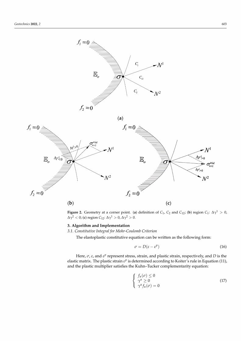
we can see in Figure 2, N1 and N2 are the normal direction of yield surface f1 and f2, C1, C2,and C12 form the corner cone of f1 and f2 together. When σtrial

n+1 ∈ C12, we have f trial1,n+1 > 0

and f trial2,n+1 > 0; at the same time, the plastic multiplier ∆γα > 0,α = 1, 2; therefore, the

activated yield surfaces f1 and f2 both are the final active yield surfaces; when σtrialn+1 ∈ C1 or

σtrialn+1 ∈ C2, although f trial

1,n+1 > 0 and f trial2,n+1 > 0 can be obtained, it can be seen that ∆γ2 < 0

in C1 and ∆γ1 < 0 in C2, that is, although the activated yield surfaces are two, there is onlyone final active surface in the end.

Geotechnics 2022, 2 603

Geotechnics 2022, 2, FOR PEER REVIEW 5

(a)

(b) (c)

Figure 2. Geometry at a corner point. (a) definition of C1, C2 and C12; (b) region C1: 1 0 ,

2 0 ; (c) region C12: 1 0 ,

2 0 .

3. Algorithm and Implementation

3.1. Constitutive Integral for Mohr-Coulomb Criterion

The elastoplastic constitutive equation can be written as the following form:

( )pD (16)

Here, , , and p represent stress, strain, and plastic strain, respectively, and D

is the elastic matrix. The plastic strain p is determined according to Koiter’s rule in

Equation (11), and the plastic multiplier satisfies the Kuhn–Tucker complementarity equa-

tion:

( ) 0

0

( ) 0

f

f

(17)

For the Mohr-Coulomb model with multiple yield surfaces, it is necessary to define

the elastic space, which can be represented by E and defined as:

| ( ) 0, [1, 2, ,6]E f (18)

Furthermore, Equation (18) can be analytically written in terms of the principal

stresses 1 , 2 , 3 as:

Figure 2. Geometry at a corner point. (a) definition of C1, C2 and C12; (b) region C1: ∆γ1 > 0,∆γ2 < 0; (c) region C12: ∆γ1 > 0, ∆γ2 > 0.

3. Algorithm and Implementation3.1. Constitutive Integral for Mohr-Coulomb Criterion

The elastoplastic constitutive equation can be written as the following form:

σ = D(ε− εp) (16)

Here, σ, ε, and εp represent stress, strain, and plastic strain, respectively, and D is theelastic matrix. The plastic strain εp is determined according to Koiter’s rule in Equation (11),and the plastic multiplier satisfies the Kuhn–Tucker complementarity equation:

fα(σ) ≤ 0γα ≥ 0γα fα(σ) = 0

(17)

Geotechnics 2022, 2 604

For the Mohr-Coulomb model with multiple yield surfaces, it is necessary to definethe elastic space, which can be represented by Eσ and defined as:

Eσ = {σ| fα(σ) ≤ 0, α ∈ [1, 2, . . . , 6]} (18)

Furthermore, Equation (18) can be analytically written in terms of the principal stressesσ1, σ2, σ3 as:

f1 = (σ1 − σ3) + (σ1 + σ3) sin φ− 2c cos φf2 = (σ2 − σ3) + (σ2 + σ3) sin φ− 2c cos φf3 = (σ1 − σ2) + (σ1 + σ2) sin φ− 2c cos φf4 = (σ3 − σ1) + (σ3 + σ1) sin φ− 2c cos φf5 = (σ3 − σ2) + (σ3 + σ2) sin φ− 2c cos φf6 = (σ2 − σ1) + (σ2 + σ1) sin φ− 2c cos φ

(19)

Considering a time discretization of interest, and letting{

σn, εn, εpn

}be the initial

stress and strain, then, given an incremental strain ∆ε and applying an implicit backwardEuler difference to Equations (11) and (16), we have

εn+1 = εn + ∆ε

σn+1 = D(εn+1 − εpn+1)

εpn+1 = ε

pn + ∑ ∆γα∂σ fα(σn+1)

(20)

Accordingly, the discrete form of Equation (17) is expressed as:fα(σn+1) ≤ 0∆γα ≥ 0∆γα fα(σn+1) = 0

(21)

Finally, by setting ∆γα = 0 in Equations (20) and (21), the trial state is obtained formally:εtrial

e,n+1 = εn+1 − εpn

σtrialn+1 = Dεtrial

e,n+1εtrial

p,n+1 = εpn

f trialα,n+1 = fα(σtrial

n+1)

(22)

A yield surface fα,n+1 is termed active if the condition fα,n+1 > 0 holds; once the trialstate is obtained, an initial set of trial constraints of Mohr-Coulomb model is defined as:

Jtrialact =

{α ∈ (1, 2, . . . , 6)

∣∣∣ f trialα,n+1(σ

trialn+1) > 0

}(23)

If Jtrialact =∅, it indicates that it is currently in an elastic state, and the test state is the

real stress state. Then, assuming plastic loading, it holds that Jtrialact 6=∅; the trial stress state

σtrialn+1 lays beyond the elastic region Eσ and is considered inadmissible. The solution σn+1 to

the discrete problem can be expressed as:

σn+1 = σn + ∆σ = σn + D(∆ε− ∆εp) = σn + D∆ε−m

∑α=1

D∆γα∂σ fα(σn+1) (24)

Substituting (24) into Kuhn–Tucker conditions (21), we have

Geotechnics 2022, 2 605

∆γα fα(σn + D∆ε−m

∑α=1

D∆γα∂σ fα(σn+1)) = 0 (25)

Equation (25) can be solved by a project contract algorithm (PCA) introduced inSection 3.3. By enforcing the Kuhn–Tucker conditions iteratively, the solution constructs aworking set of constraints at each step, denoted as J(k)act . The working set of constraints isconsidered fixed during the iteration. It should be noted that the plastic multipliers ∆γα

obtained by PCA are non-negative, when all constraints f (k)n+1 = 0 are satisfied for α ∈ J(k)act ,

admissibility of the solution is naturally satisfied, namely, ∆γ(k) ≥ 0 for all α ∈ J(k)act . Insummary, the iteration performed on each Gauss-point proceeds by the following steps:

1 Compute elastic predictor

σtrialn+1 = D

(εn+1 − ε

pn

)= σn + D∆ε

f trialα,n+1 = fα

(σtrial

n+1), f or α ∈ {1, 2, . . . , 6}

2 Check for plastic process

If f trialα,n+1 ≤ 0 for all α ∈ {1, 2, . . . , 6}, Set σn+1 = σtrial

n+1; εpn+1 = ε

pn, Exit

ElseJ(0)act =

{α ∈ {1, 2, . . . , m}

∣∣∣ f trialα,n+1 > 0

}ε(0)p,n+1 = εp,n, ∆γ

(0)α = 0

3 Evaluate stress at iteration (k)

σ(k)n+1 = D(εn+1 − ε

(k)p,n+1)

4 Check convergence

f (k)α,n+1 = fα(σ(k)n+1), for α ∈ J(k)act

If f (k)α,n+1 < ToL = 0.1 for all α ∈ J(k)act , ExitElse continue

5 Computate plastic multiplier

∆γ(k)α fα

(σn + D∆ε−

m∑

α=1D∆γ

(k)α ∂σ fα(σ

(k)n+1)

)= 0

Call PCA in Section 3.3→ ∆γ(k)α

6 Update plastic strain

ε(k+1)p,n+1 = εp,n +

m∑

α=1∆γ

(k)α ∂σ fα(σ

(k)n+1)

Set k = k + 1, Go to 3.In elastoplastic computations using the finite element method, the load is applied

incrementally. By performing the above iteration, the stress state after applying the strainincrement is obtained.

3.2. Partial Derivatives of Principal Stresses with Regard to Stress Components

For Mohr-Coulomb surfaces, which have sharp corners and can be explicitly expressedin terms of principal stresses,σi, i = 1, 2, and 3. While calculating plastic strains, knowingpartial derivatives of principal stresses with regard to stress components will give usgreat convenience.

Principal stress σi satisfies the following characteristic equation:

σ3 − I1σ2 − I2σ− I3 = 0 (26)

Geotechnics 2022, 2 606

where the coefficients I1, I2, and I3 are functions of the six stress components σx, σy, . . . ,τxy, defined as

I1 = σx + σy + σz (27)

I2 = −(σxσy + σyσz + σzσx) + τ2xy + τ2

yz + τ2zx (28)

I3 =

∣∣∣∣∣∣σx τxy τxzτyx σy τyzτzx τzy σz

∣∣∣∣∣∣ (29)

Differentiating Equation (26) with regard to one of σx, σy, . . . , τxy, we have

3σ2σ′ − I′1σ2 − I1 · 2σσ′ − I′2σ− I2σ′ − I′3 = 0 (30)

with the single quote ′ associated with a quantity denoting the derivative of the quantitywith regard to one of σx, σy, . . . , τxy, or, equivalently,

(3σ2 − 2I1σ− I2)σ′ = I′1σ2 + I′2σ + I′3 (31)

Thus, we have

σ′ =I′1σ2 + I′2σ + I′33σ2 − 2I1σ− I2

(32)

with∂I1∂σx

= 1, ∂I1∂τxy

= 0, ∂I2∂σx

= −(σy + σz

),

∂I2∂τxy

= 2τxy, ∂I3∂σx

= σyσz − τ2yz, ∂I3

∂τxy= τyzτzx − 2σzτxy, etc.

Similarly, we can obtain the second derivative of the principal stress with regard to σx,σy, . . . , τxy.

σ′′ =[4I′1 + (2I1 − 6σ)σ′ + 2I′2]σ

′ + I ′′2 + I ′′33σ2 − 2I1σ− I2

(33)

with∂2 I1∂σ2

x= 0

∂2 I2∂σ2

x= 0, ∂2 I2

∂σx∂σy= −1, ∂2 I2

∂τ2xy

= 2, ∂2 I2∂τxy∂τyz

= 0

∂2 I3∂σ2

x= 0, ∂2 I3

∂σx∂σy= σz, ∂2 I3

∂σx∂τyz= −2τyz, ∂2 I3

∂τ2xy

= −2σz, ∂2 J3∂τxy∂τyz

= τzx, etc.

3.3. Algorithm PCA

Given a subset K of Euclidean n-dimensional space Rn and a mapping F : K → Rn ,the variational inequality finds a vector x ∈ K such that

(y− x)T F(x) ≥ 0, ∀y ∈ K (34)

Given a mapping F : Rn+ → Rn , the nonlinear complementarity problem is to find a

vector x ∈ Rn satisfying0 ≤ x⊥F(x) ≥ 0 (35)

In fact, when the subset K in the variational inequality is non-negative, the nonlinearcomplementarity problem is equivalent to the variational inequality [21]. As a method forsolving convex optimization problems under the framework of variational inequalities, justas the name implies, the projection contraction algorithm is a contraction algorithm basedon projection. Here, we only refer to the algorithm part; for more details, see [22].

Rewrite complementary equation system (21) to vector form:

0 ≤ ∆γ⊥F(∆γ) ≥ 0 (36)

Geotechnics 2022, 2 607

in which ∆γ = (∆γ1, . . . , ∆γm), F(∆γ) = (− f1(∆γ1), . . . ,− fm(∆γm)). As we can see fromEquation (35), the complementary system in (36) can be summarized as a typical nonlinearcomplementarity problem, which can be solved by the projection contraction method.

The projection contraction algorithm (PCA) is invoked in this way:

(∆γ) = PCA(∆γ0, F) (37)

The input arguments of ∆γ0 is the initial guess of plastic multiplier ∆γ. In general,∆γ0 = 0.

The pseudocode of PCA is listed as follows, and He proposed [22] three parameters inPCA as ξ = 0.9, η = 0.4, and λ = 1.9, which is also adopted in this paper. It should be notedthat the parameters have little effect on the result.

Step 0: Let step size β = 1; k = 0; error tolerance ε = 0.1%Step 1: F = FA(∆γ); ∆γ = max[∆γ− βF, 0]d(∆γ, ∆γ) = ∆γ− ∆γif ‖d(∆γ, ∆γ)‖ ≤ ε then ∆γ = ∆γ; breakF = FA(∆γ); F(∆γ, ∆γ) = F− F; r = β‖F(∆γ,∆γ)‖2

‖d(∆γ,∆γ)‖2;

while r > ξ

β = 0.7 ∗ β ∗min(

1, 1r

); ∆γ = max[∆γ− βF, 0]; F = FA(∆γ);

F(∆γ, ∆γ) = F− F; d(∆γ, ∆γ) = ∆γ− ∆γ; r = β‖F(∆γ,∆γ)‖2‖d(∆γ,∆γ)‖2

;end(while)

D(∆γ, ∆γ) = d(∆γ, ∆γ)− βF(∆γ, ∆γ); α = [d(∆γ,∆γ)]TD(∆γ,∆γ)

‖D(∆γ,∆γ)‖22

;

∆γ = ∆γ− λαd(∆γ, ∆γ);if r ≤ η then β = 1.5 ∗ β;Step 2. k = k + 1; go to Step 1.

4. Numerical Examples

The practical application of the proposed algorithm is illustrated in this section bytwo different numerical examples. For all the examples, four node isoparametric elementswith four Gaussian points are adopted, and the error tolerance for unbalanced force in theequilibrium iteration is 0.1%.

4.1. Strip Footing Collapse

The bearing capacity of a strip footing is calculated under undrained conditions bythe proposed method. The soil is assumed weightless, isotropic, and is modeled as a Mohr-Coulomb perfectly plastic material. There is no friction at the footing/soil interface. Thecomputational model and discretized mesh are shown in Figure 3. The material parametersare assumed as follows: Young’s modulus: E = 107 MPa, Poisson’s ratio: v = 0.48, cohesionc = 490 kPa, and internal friction angle φ = 20

◦. A plane strain state is assumed.

The strip footing is subjected to a vertical pressure P and the aim of present analysis isto obtain the limit pressure Plim. A solution to this problem has been derived by Prandtland Hill [23]:

Plim = c[eπ tan ϕ tan2(45

◦+

ϕ

2)− 1

]cot ϕ (38)

The pressure P is increased incrementally to failure and corresponding load/settlement(average) curves obtained are plotted in Figure 4.

Geotechnics 2022, 2 608

Geotechnics 2022, 2, FOR PEER REVIEW 10

4. Numerical Examples

The practical application of the proposed algorithm is illustrated in this section by

two different numerical examples. For all the examples, four node isoparametric elements

with four Gaussian points are adopted, and the error tolerance for unbalanced force in the

equilibrium iteration is 0.1%.

4.1. Strip Footing Collapse

The bearing capacity of a strip footing is calculated under undrained conditions by

the proposed method. The soil is assumed weightless, isotropic, and is modeled as a

Mohr-Coulomb perfectly plastic material. There is no friction at the footing/soil interface.

The computational model and discretized mesh are shown in Figure 3. The material pa-

rameters are assumed as follows: Young’s modulus: E = 107 MPa, Poisson’s ratio: v = 0.48,

cohesion c = 490 kPa, and internal friction angle 20 . A plane strain state is assumed.

(a)

(b)

Figure 3. Strip footing: (a) problem geometry; (b) adopted mesh.

The strip footing is subjected to a vertical pressure P and the aim of present analysis

is to obtain the limit pressure Plim. A solution to this problem has been derived by Prandtl

and Hill [23]:

tan 2lim tan (45 ) 1 cot

2P c e

(38)

The pressure P is increased incrementally to failure and corresponding load/settle-

ment (average) curves obtained are plotted in Figure 4.

Figure 3. Strip footing: (a) problem geometry; (b) adopted mesh.

Geotechnics 2022, 2, FOR PEER REVIEW 11

Figure 4. Pressure versus displacement.

The limit loads obtained are

lim 15NP

c (39)

This value is in good agreement with Prandtl’s solution (1.2% above)

lim 14.82P

c (40)

The equivalent plastic strain at the failure load is shown in Figure 5. As we can see

from Figure 5, at the moment that the foundation enters flow, the global shear failure of

the foundation develops downward to a certain depth and extends to the ground The

failure mechanism captured in the finite element analysis is in good agreement with the

slip-line field of strip footing as shown in Figure 6 [24].

Figure 5. Equivalent plastic strain at the failure load.

0 1 2 3 4 50

1

2

3

4

Eps

0.0190.0180.0170.0160.0150.0140.0130.0120.0110.010.0090.0080.0070.0060.0050.0040.0030.0020.001

Figure 4. Pressure versus displacement.

The limit loads obtained arePN

limc≈ 15 (39)

This value is in good agreement with Prandtl’s solution (1.2% above)

Plimc≈ 14.82 (40)

The equivalent plastic strain at the failure load is shown in Figure 5. As we can seefrom Figure 5, at the moment that the foundation enters flow, the global shear failure of thefoundation develops downward to a certain depth and extends to the ground The failuremechanism captured in the finite element analysis is in good agreement with the slip-linefield of strip footing as shown in Figure 6 [24].

Geotechnics 2022, 2 609

Geotechnics 2022, 2, FOR PEER REVIEW 11

Figure 4. Pressure versus displacement.

The limit loads obtained are

lim 15NP

c (39)

This value is in good agreement with Prandtl’s solution (1.2% above)

lim 14.82P

c (40)

The equivalent plastic strain at the failure load is shown in Figure 5. As we can see

from Figure 5, at the moment that the foundation enters flow, the global shear failure of

the foundation develops downward to a certain depth and extends to the ground The

failure mechanism captured in the finite element analysis is in good agreement with the

slip-line field of strip footing as shown in Figure 6 [24].

Figure 5. Equivalent plastic strain at the failure load.

0 1 2 3 4 50

1

2

3

4

Eps

0.0190.0180.0170.0160.0150.0140.0130.0120.0110.010.0090.0080.0070.0060.0050.0040.0030.0020.001

Figure 5. Equivalent plastic strain at the failure load.

Geotechnics 2022, 2, FOR PEER REVIEW 12

Figure 6. Slip-line field of strip footing.

4.2. Slope Stability

In this example, the plane strain analysis of a slope subjected to self-weight is carried

out. To assess the safety of the slope shown in Figure 7, the strength reduction method is

adopted. Table 1 lists the mechanical parameters. The materials comply with the perfectly

Mohr-Coulomb criterion. Horizontal displacements are fixed for nodes along the left and

right boundaries while both horizontal and vertical displacements are fixed along the bot-

tom boundary.

(a)

(b)

Figure 7. Slope stability: (a) problem geometry; (b) adopted mesh.

Figure 6. Slip-line field of strip footing.

4.2. Slope Stability

In this example, the plane strain analysis of a slope subjected to self-weight is carriedout. To assess the safety of the slope shown in Figure 7, the strength reduction method isadopted. Table 1 lists the mechanical parameters. The materials comply with the perfectlyMohr-Coulomb criterion. Horizontal displacements are fixed for nodes along the left andright boundaries while both horizontal and vertical displacements are fixed along thebottom boundary.

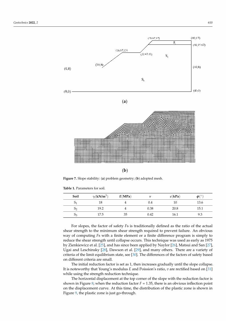
Geotechnics 2022, 2 610

Geotechnics 2022, 2, FOR PEER REVIEW 12

Figure 6. Slip-line field of strip footing.

4.2. Slope Stability

In this example, the plane strain analysis of a slope subjected to self-weight is carried

out. To assess the safety of the slope shown in Figure 7, the strength reduction method is

adopted. Table 1 lists the mechanical parameters. The materials comply with the perfectly

Mohr-Coulomb criterion. Horizontal displacements are fixed for nodes along the left and

right boundaries while both horizontal and vertical displacements are fixed along the bot-

tom boundary.

(a)

(b)

Figure 7. Slope stability: (a) problem geometry; (b) adopted mesh.

Figure 7. Slope stability: (a) problem geometry; (b) adopted mesh.

Table 1. Parameters for soil.

Soil γ(kN/m3) E(MPa) ν c(kPa) φ(◦)

S1 18 4 0.4 10 13.6

S2 19.2 4 0.38 20.8 15.1

S3 17.5 35 0.42 16.1 9.3

For slopes, the factor of safety Fs is traditionally defined as the ratio of the actualshear strength to the minimum shear strength required to prevent failure. An obviousway of computing Fs with a finite element or a finite difference program is simply toreduce the shear strength until collapse occurs. This technique was used as early as 1975by Zienkiewicz et al. [25], and has since been applied by Naylor [26], Matsui and San [27],Ugai and Leschinsky [28], Dawson et al. [29], and many others. There are a variety ofcriteria of the limit equilibrium state, see [30]. The differences of the factors of safety basedon different criteria are small.

The initial reduction factor is set as 1, then increases gradually until the slope collapse.It is noteworthy that Young’s modulus E and Poission’s ratio, v are rectified based on [31]while using the strength reduction technique.

The horizontal displacement at the top corner of the slope with the reduction factor isshown in Figure 8; when the reduction factor F = 1.35, there is an obvious inflection pointon the displacement curve. At this time, the distribution of the plastic zone is shown inFigure 9, the plastic zone is just go-through.

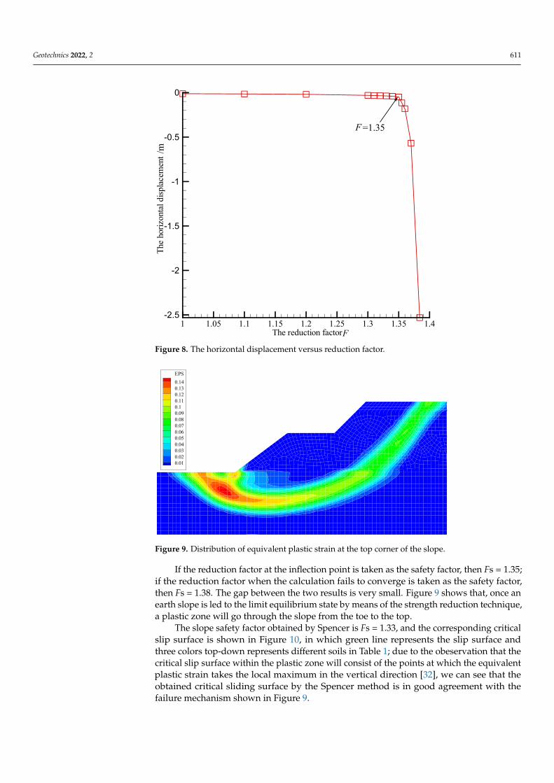
Geotechnics 2022, 2 611

Geotechnics 2022, 2, FOR PEER REVIEW 13

Table 1. Parameters for soil.

Soil kN m3( / ) MPa( )E kPa( )c ( )

S1 18 4 0.4 10 13.6

S2 19.2 4 0.38 20.8 15.1

S3 17.5 35 0.42 16.1 9.3

For slopes, the factor of safety Fs is traditionally defined as the ratio of the actual

shear strength to the minimum shear strength required to prevent failure. An obvious

way of computing Fs with a finite element or a finite difference program is simply to re-

duce the shear strength until collapse occurs. This technique was used as early as 1975 by

Zienkiewicz et al. [25], and has since been applied by Naylor [26], Matsui and San [27],

Ugai and Leschinsky [28], Dawson et al. [29], and many others. There are a variety of

criteria of the limit equilibrium state, see [30]. The differences of the factors of safety based

on different criteria are small.

The initial reduction factor is set as 1, then increases gradually until the slope col-

lapse. It is noteworthy that Young’s modulus E and Poission’s ratio, v are rectified based

on [31] while using the strength reduction technique.

The horizontal displacement at the top corner of the slope with the reduction factor

is shown in Figure 8; when the reduction factor F = 1.35, there is an obvious inflection

point on the displacement curve. At this time, the distribution of the plastic zone is shown

in Figure 9, the plastic zone is just go-through.

Figure 8. The horizontal displacement versus reduction factor.

If the reduction factor at the inflection point is taken as the safety factor, then Fs =

1.35; if the reduction factor when the calculation fails to converge is taken as the safety

factor, then Fs = 1.38. The gap between the two results is very small. Figure 9 shows that,

once an earth slope is led to the limit equilibrium state by means of the strength reduction

technique, a plastic zone will go through the slope from the toe to the top.

The slope safety factor obtained by Spencer is Fs = 1.33, and the corresponding critical

slip surface is shown in Figure 10, in which green line represents the slip surface and three

colors top-down represents different soils in Table 1; due to the obeservation that the

critical slip surface within the plastic zone will consist of the points at which the equivalent

plastic strain takes the local maximum in the vertical direction [32], we can see that the

The reduction factor

The

hori

zont

ald

ispl

acem

ent

1 1.05 1.1 1.15 1.2 1.25 1.3 1.35 1.4-2.5

-2

-1.5

-1

-0.5

0

F

/m

F =1.35

Figure 8. The horizontal displacement versus reduction factor.

Geotechnics 2022, 2, FOR PEER REVIEW 14

obtained critical sliding surface by the Spencer method is in good agreement with the

failure mechanism shown in Figure 9.

Figure 9. Distribution of equivalent plastic strain at the top corner of the slope.

Figure 10. The critical slip surface of Spencer.

A comparison about computational efficiency is made between the PCA and the clas-

sic mapping return method in [17]. Integral points that are undergoing plastic defor-

mation are selected. A comparison is made based on the computation time for 10,000

stress returns, and is implemented in Matlab on a computer with Intel(R) Core(TM) i5-

3230M 2.60 GHz processor. Table 2 lists the results.

Table 2. Comparison of time spending.

Number of Activated Surface Time (Classic) Time (Present) Ratio

1 1.692 1.373 1.232

2 2.438 1.464 1.665

It can be seen that the present PCA is substantially more efficient than the classic

mapping return method, especially when more than one yield surface is ever activated.

5. Conclusions

Based on the complementarity theory, the elasto-plastic complementarity equation is

established. The corner problems of multiple surfaces are unified into a set of complemen-

tary equations by using Koiter’s law, and then solved by using the projection contraction

algorithm. The theory and examples show that: the projection contraction algorithm for

the complementary equation with multiple yield surfaces avoids the accuracy and con-

vergence problems caused by corner smoothing; the stress return operation is carried out

in the general stress space, and the partial derivative of the corresponding stress compo-

EPS

0.140.130.120.110.10.090.080.070.060.050.040.030.020.01

Figure 9. Distribution of equivalent plastic strain at the top corner of the slope.

If the reduction factor at the inflection point is taken as the safety factor, then Fs = 1.35;if the reduction factor when the calculation fails to converge is taken as the safety factor,then Fs = 1.38. The gap between the two results is very small. Figure 9 shows that, once anearth slope is led to the limit equilibrium state by means of the strength reduction technique,a plastic zone will go through the slope from the toe to the top.

The slope safety factor obtained by Spencer is Fs = 1.33, and the corresponding criticalslip surface is shown in Figure 10, in which green line represents the slip surface andthree colors top-down represents different soils in Table 1; due to the obeservation that thecritical slip surface within the plastic zone will consist of the points at which the equivalentplastic strain takes the local maximum in the vertical direction [32], we can see that theobtained critical sliding surface by the Spencer method is in good agreement with thefailure mechanism shown in Figure 9.

Geotechnics 2022, 2 612

Geotechnics 2022, 2, FOR PEER REVIEW 14

obtained critical sliding surface by the Spencer method is in good agreement with the

failure mechanism shown in Figure 9.

Figure 9. Distribution of equivalent plastic strain at the top corner of the slope.

Figure 10. The critical slip surface of Spencer.

A comparison about computational efficiency is made between the PCA and the clas-

sic mapping return method in [17]. Integral points that are undergoing plastic defor-

mation are selected. A comparison is made based on the computation time for 10,000

stress returns, and is implemented in Matlab on a computer with Intel(R) Core(TM) i5-

3230M 2.60 GHz processor. Table 2 lists the results.

Table 2. Comparison of time spending.

Number of Activated Surface Time (Classic) Time (Present) Ratio

1 1.692 1.373 1.232

2 2.438 1.464 1.665

It can be seen that the present PCA is substantially more efficient than the classic

mapping return method, especially when more than one yield surface is ever activated.

5. Conclusions

Based on the complementarity theory, the elasto-plastic complementarity equation is

established. The corner problems of multiple surfaces are unified into a set of complemen-

tary equations by using Koiter’s law, and then solved by using the projection contraction

algorithm. The theory and examples show that: the projection contraction algorithm for

the complementary equation with multiple yield surfaces avoids the accuracy and con-

vergence problems caused by corner smoothing; the stress return operation is carried out

in the general stress space, and the partial derivative of the corresponding stress compo-

EPS

0.140.130.120.110.10.090.080.070.060.050.040.030.020.01

Figure 10. The critical slip surface of Spencer.

A comparison about computational efficiency is made between the PCA and the classicmapping return method in [17]. Integral points that are undergoing plastic deformation areselected. A comparison is made based on the computation time for 10,000 stress returns,and is implemented in Matlab on a computer with Intel(R) Core(TM) i5-3230M 2.60 GHzprocessor. Table 2 lists the results.

Table 2. Comparison of time spending.

Number of Activated Surface Time (Classic) Time (Present) Ratio

1 1.692 1.373 1.232

2 2.438 1.464 1.665

It can be seen that the present PCA is substantially more efficient than the classicmapping return method, especially when more than one yield surface is ever activated.

5. Conclusions

Based on the complementarity theory, the elasto-plastic complementarity equation isestablished. The corner problems of multiple surfaces are unified into a set of complemen-tary equations by using Koiter’s law, and then solved by using the projection contractionalgorithm. The theory and examples show that: the projection contraction algorithm for thecomplementary equation with multiple yield surfaces avoids the accuracy and convergenceproblems caused by corner smoothing; the stress return operation is carried out in thegeneral stress space, and the partial derivative of the corresponding stress component iscalculated in the principal stress space, which not only avoids the numerical singularity atthe corner, but also eliminates the stress transformation of the stress return in the principalstress space.

Author Contributions: Formal analysis, T.Z.; funding acquisition, H.Z.; supervision, Y.C.; writing—original draft, T.Z.; writing—review & editing, S.L. All authors have read and agreed to the publishedversion of the manuscript.

Funding: This research was funded by National Natural Science Foundation of China, grantnumber 52130905.

Institutional Review Board Statement: Not applicable.

Informed Consent Statement: Not applicable.

Conflicts of Interest: The authors declare no conflict of interest.

Geotechnics 2022, 2 613

References1. Koiter, W.T. Stress-strain relations, uniqueness and variational theorems for elastic-plastic materials with a singular yield surface.

Q. Appl. Math. 1953, 11, 350–354. [CrossRef]2. Zienkiewicz, O.C.; Valliappan, S.; King, I.P. Elasto-plastic solutions of engineering problems ‘initial stress’, finite element approach.

Int. J. Numer. Methods Eng. 1969, 1, 75–100. [CrossRef]3. Hinton, E.; Owen, D.R.J. Finite Elements in Plasticity: Theory and Practice; Pineridge Press: Swansea, UK, 1980; pp. 20–45.4. Marques, J. Stress computation in elastoplasticity. Eng. Comput. 1984, 1, 42–51. [CrossRef]5. Zienkiewicz, O.C.; Pande, G.N. Some useful forms for isotropic yield surfaces for soils and rock mechanics. In Finite Elements in

Geomechanics; Gudehus, G., Ed.; John Wiley & Sons: Hoboken, NJ, USA, 1977; pp. 179–190.6. Sloan, S.W.; Booker, J.R. Removal of singularities in tresca and Mohr-Coulomb yield functions. Commun. Appl. Numer. Methods

1986, 2, 173–179. [CrossRef]7. Abbo, A.; Lyamin, A.; Sloan, S.; Hambleton, J. A C2 continuous approximation to the Mohr–Coulomb yield surface. Int. J. Solids

Struct. 2011, 48, 3001–3010. [CrossRef]8. Larsson, R.; Runesson, K. Implicit integration and consistent linearization for yield criteria of the Mohr-Coulomb type. Mech.

Cohesive -Frict. Mater. 1996, 1, 367–383. [CrossRef]9. Peric, D.; Neto, E.D.S. A new computational model for Tresca plasticity at finite strains with an optimal parametrization in the

principal space. Comput. Methods Appl. Mech. Eng. 1999, 171, 463–489. [CrossRef]10. Neto, E.A.D.S.; Peri, D.; Owen, D.R.J. Computational Methods for Plasticity: Theory and Applications; John Wiley & Sons: Hoboken,

NJ, USA, 2008. [CrossRef]11. de Borst, R. Integration of plasticity equations for singular yield functions. Comput. Struct. 1987, 26, 823–829. [CrossRef]12. Pankaj, P.; Bicanic, N. Detection of multiple active yield conditions for Mohr-Coulomb elasto-plasticity. Comput. Struct. 1997, 62,

51–61. [CrossRef]13. Clausen, J.; Damkilde, L.; Andersen, L. An efficient return algorithm for non-associated plasticity with linear yield criteria in

principal stress space. Comput. Struct. 2007, 85, 1795–1807. [CrossRef]14. Coombs, W.M.; Crouch, R.S.; Augarde, C.E. Reuleaux plasticity: Analytical backward Euler stress integration and consistent

tangent. Comput. Methods Appl. Mech. Eng. 2010, 199, 1733–1743. [CrossRef]15. Amouzou, G.; Soulaïmani, A. Numerical Algorithms for Elastoplacity: Finite Elements Code Development and Implementation

of the Mohr–Coulomb Law. Appl. Sci. 2021, 11, 4637. [CrossRef]16. Zhao, R.; Li, C.; Zhou, L.; Zheng, H. A sequential linear complementarity problem for multisurface plasticity. Appl. Math. Model.

2021, 103, 557–579. [CrossRef]17. Simo, J.C.; Kennedy, J.G.; Govindjee, S. Non-smooth multisurface plasticity and viscoplasticity. Loading/unloading conditions

and numerical algorithms. Int. J. Numer. Methods Eng. 1988, 26, 2161–2185. [CrossRef]18. Karaoulanis, F.E. Implicit Numerical Integration of Nonsmooth Multisurface Yield Criteria in the Principal Stress Space. Arch.

Comput. Methods Eng. 2013, 20, 263–308. [CrossRef]19. Clausen, J.; Damkilde, L. An exact implementation of the Hoek–Brown criterion for elasto-plastic finite element calculations. Int.

J. Rock Mech. Min. Sci. 2008, 45, 831–847. [CrossRef]20. Adhikary, D.P.; Jayasundara, C.T.; Podgorney, R.K.; Wilkins, A.H. A robust return-map algorithm for general multisurface

plasticity. Int. J. Numer. Methods Eng. 2017, 109, 218–234. [CrossRef]21. Facchinei, F.; Pang, J.-S. Finite-Dimensional Variational Inequalities and Complementarity Problems; Springer: Berlin/Heidelberg,

Germany, 2004. [CrossRef]22. He, B. A Class of Projection and Contraction Methods for Monotone Variational Inequalities. Appl. Math. Optim. 1997, 35, 69–76.

[CrossRef]23. Hill, R. The Mathematical Theory of Plasticity; Oxford University Press: London, UK, 1950; pp. 253–260.24. Vo, T.; Russell, A.R. Bearing capacity of strip footings on unsaturated soils by the slip line theory. Comput. Geotech. 2015, 74,

122–131. [CrossRef]25. Zienkiewicz, O.C.; Humpheson, C.; Lewis, R.W. Associated and nonassociated viscoplasticity in soil mechanics. Géotechnique

1975, 25, 671–689. [CrossRef]26. Naylor, D.J. Finite elements and slope stability. In Numerical Methods in Geomechanics; Springer: Dordrecht, The Netherland, 1981;

pp. 229–244.27. Matsui, T.; San, K.-C. Finite Element Slope Stability Analysis by Shear Strength Reduction Technique. Soils Found. 1992, 32, 59–70.

[CrossRef]28. Ugai, K.; Leshchinsky, D. Three-Dimensional Limit Equilibrium and Finite Element Analyses: A Comparison of Results. Soils

Found. 1995, 35, 1–7. [CrossRef]29. Dawson, E.M.; Roth, W.H.; Drescher, A. Slope stability analysis by strength reduction. Géotechnique 1999, 49, 835–840. [CrossRef]30. Griffiths, D.V.; Lane, P.A. Slope stability analysis by finite elements. Géotechnique 1999, 49, 387–403. [CrossRef]

Geotechnics 2022, 2 614

31. Zheng, H.; Liu, D.F.; Li, C.G. Slope stability analysis based on elasto-plastic finite element method. Int. J. Numer. Methods Eng.2005, 64, 1871–1888. [CrossRef]

32. Zheng, H.; Sun, G.; Liu, D. A practical procedure for searching critical slip surfaces of slopes based on the strength reductiontechnique. Comput. Geotech. 2009, 16, 1–5. [CrossRef]