Elasticity - BrainMassPrimer+of+Microeconomics+Chp+4.pdf · is unit-elastic demand, has an elasticity coeffi cient of 1.0. A ten percent increase in price will cause a ten percent

CHAPTER 4

Elasticity

By the end of this chapter you will be able to:

1. Describe and apply the concept of elasticity.2. Interpret the terms elastic, inelastic, and unit elastic as related to

price elasticity of demand.3. Use the intuitive “percentage change” formula and the midpoint for-

mula to measure price elasticity of demand.4. Apply the total revenue test to predict the eff ect on total revenue of a

price change, given diff erent price elasticity circumstances.5. List and explain the eff ects of the determinants of price elasticity of

demand.6. Calculate and interpret income elasticity of demand and cross-price

elasticity of demand using the intuitive “percentage change” formula.7. Calculate and interpret elasticity values for the price elasticity of

supply.

Have you ever shopped around for the best price on airline tickets or hotel accommodation? Most of us have and, nowadays, the Internet helps us to do this with sites such as Travelocity and Expedia. But have you ever shopped around for the best price on electricity service for your home? Probably not, because, for most of us, the electricity company we have is a “take it or leave it” situation and we have little fl exibility short of installing our own solar panels. In the case of airline tickets, we can be choosy and responsive to price diff erences, but in the case of electricity, we can’t. Th is brings us to a consideration of “elasticity.”

Chapter Preview: In this chapter we consider ways of quantifying some of the relationships we discussed qualitatively in Chapter 2. In a way, this entire chapter may be seen as a series of applications of concepts that you have already learned.Co

pyright © 2013. Business Expert Press. All rights reserved. May not be reproduced in any form without permission from the publisher, except fair uses permitted under

U.S. or applicable copyright law.

EBSCO Publishing : eBook Academic Collection (EBSCOhost) - printed on 12/4/2016 5:27 PM via TRIDENTUNIVERSITYAN: 699493 ; Beveridge, Thomas M..; A Primer on MicroeconomicsAccount: s3642728

74 A PRIMER ON MICROECONOMICS

Elasticity—A Measure of Responsiveness

The Big Idea of Elasticity

Students of economics frequently complain that, although there is lots of theory, there are few practical numbers based on real-world experi-ence. We know, for example, that an increase in price causes a decrease in quantity demanded but we don’t know how much of a decrease there is. Is it a big decrease or a small decrease? Elasticity (a fancy word for “responsiveness” or “sensitivity”) answers this sort of a question. Price elasticity of demand measures how responsive or sensitive demanders are to a change in price—how much they react to a price change? Income elasticity of demand measures how much demanders respond when income level changes—if there is a recession and income levels fall, how much will the demand for cars decrease? Cross-price elasticity of demand measures how much the demand for one good changes when the price of a related good changes—if the price of Coca-Cola increases, how much does the demand for Pepsi increase? Price elasticity of supply measures how much the quantity supplied of a good will increase as its price rises—is it a large response (relatively “elastic”) or a small response (relatively “inelastic”)?

In any elasticity calculation, we measure the extent of the change in one variable relative to the change in another variable. We could, for example, develop an “advertising elasticity of demand” to show how much the demand for our product changes as our advertising budget increases.

Price Elasticity of Demand

Considering price elasticity of demand, we can establish an “intuitive” formula that will answer many of our questions quite simply. Price elas-ticity of demand (Ed) measures how much quantity demanded (Q d) changes as price (P) changes. Our intuitive formula would look like this:

Ed = percentage change in quantity demanded/percentage change in price. Co




ELASTICITY 75

We can make this look a bit more mathematical by translating it in the following way:

Ed = %Δ Q d / %ΔP

where “Δ” is the mathematical symbol (delta) for “change in.”Comment: Note that the “dollars” term is in the denominator and the

“numbers” term is in the numerator. Th is is the typical elasticity pattern and we’ll see it repeated in each elasticity formula in this chapter—numbers on top and dollars on the bottom.

To see how this formula works, think of a good like gasoline. Suppose that the price of gas jumps by ten percent. (At the time of writing, a gallon of gas costs about $3.75, so we’re talking about a price hike of almost 40¢ to about a price of $4.10.) We know quantity demanded will decrease, but probably it will not decrease by much. After all, most of us buy what we need and it’s diffi cult and inconvenient to change our habits. Let’s say quantity demanded may fall by two percent. Using the intuitive formula:

Ed = %Δ Q d/ %ΔP = −2/+10 = −0.2.

In absolute values, Ed is 0.2.

Price Elasticity of Demand—An Absolute Value?

Because negative values are diffi cult to work with and because we know from the Law of Demand that there is a negative relationship between price and quantity demanded, from now on we’ll use the absolute value for price elasticity of demand. In this example, then, Ed = 0.2.

An elasticity value (“coeffi cient”) of 0.2 indicates that demand is not very responsive to a price change. We know that demand is relatively inelastic because, although price has risen by ten percent, drivers are still buying almost the same amount of gas at the pumps. Th e lower the elas-ticity coeffi cient the less responsive (less elastic) demand is.

Now consider a product such as Coca-Cola. Suppose the price of Coke increases by ten percent. Although some buyers will continue to favor Coke, many will switch to alternatives such as Pepsi or Dr. Pepper. Co





Th ere will be a vigorous (elastic) response. One study reported a price elasticity value of 3.8 for Coca-Cola. To interpret this number, go back to the intuitive formula.

Ed = %Δ Q d / %ΔP = %Δ Q d / +10 = 3.8

So the percentage change in quantity demanded is thirty-eight percent. We conclude that a ten percent increase in the price of Coke will result in a thirty-eight percent decline in the quantity demanded of Coke.

Lower elasticity numbers are relatively inelastic and higher elasticity numbers are relatively elastic. A coeffi cient of zero would tell us that buyers are completely unresponsive to changes in price (perfectly inelastic demand) whereas the more extremely sensitive buyers are to even tiny price changes, then the closer the elasticity value approaches its maximum value of infi n-ity. Th e boundary between “inelastic” and “elastic” demand, where demand is unit-elastic demand, has an elasticity coeffi cient of 1.0. A ten percent increase in price will cause a ten percent decrease in quantity demanded.

Th e following line diagram (Figure 4-1) summarizes what we have learned so far about price elasticity of demand.Challenge: Use the intuitive formula to verify that zero is the coeffi cient when demand is perfectly inelastic and that infi nity is the coeffi cient when demand is perfectly elastic.

InfinityZero 1.0

Inelastic Unit elastic Elastic

Figure 4-1. Price elasticity of demand.

As shown in Figure 4-2, the perfectly inelastic demand curve graphs as a vertical line and the perfectly elastic demand curve graphs as a horizontal line.

Total Revenue Test

Th e Total Revenue Test is a convenient way to determine a good’s elastic-ity within a given price range. Total Revenue (TR) or total spending is defi ned as price (P) multiplied by quantity demanded (Q).

TR = P × QCopyright © 2013. Business Expert Press. All rights reserved. May not be reproduced in any form without permission from the publisher, except fair uses permitted under



ELASTICITY 77

First, consider gasoline. Th e demand for gas is inelastic (Ed < 1.0), because we have very little ability to buy less when the price increases. What would happen to the number of dollars you’d have to spend on gas if the price rose? Would you spend more dollars, or fewer? If you resemble most buyers, then you’d spend more money at the pumps. We can conclude that, for a good with an inelastic demand, if price increases, then total revenue will increase. Similarly, if price decreases then, if we have a good with an inelastic demand, total spending on that good would decrease.

Consider Coca-Cola, however. Coke, we know is a good with an elas-tic demand (Ed > 1.0). If the price of Coke increases, many buyers will switch to other alternatives, such as Pepsi or Sprite. Th e total number of dollars spent on Coke will decrease. For a good with an elastic demand, if price increases, then total revenue will decrease. Similarly, if we have a good with an elastic demand, then total spending on that good would increase when price decreases.

For a good with a unit elastic demand (Ed = 1.0), total revenue does not change as price increases or decreases.

Total Revenue Test Summary:As price increases, demand is inelastic if total revenue increases.As price increases, demand is elastic if total revenue decreases.As price increases, demand is unit elastic if total revenue is unaff ected.

Slope ≠ Elasticity: From what has been said so far, and from the previ-ous fi gures, it would be tempting to infer that, the steeper the demand curve, the smaller the price elasticity of demand, but this is incorrect.

Q0

D

D

Perfectly inelastic demand Perfectly elastic demand

P

Q0

P

Figure 4-2. Perfectly inelastic and perfectly elastic demand curves.

Copyright © 2013. Business Expert Press. All rights reserved. May not be reproduced in any form without permission from the publisher, except fair uses permitted under




Consider the following demand schedule for apples and its associated demand curve (Table 4-1).

Table 4-1. Demand and Total Revenue

Price Quantity Demanded Total RevenueS6 2 $12

S5 4 $20

S4 6 $24

$3 8 $24

$2 10 $20

$1 12 $12

$1

$2

$3

$4

$5

$6

0 2 4 6 8 10 12

P

Q

D

Figure 4-3. Slope ≠ elasticity.

Note that, as price rises from $5 to $6, total revenue decreases from $20 to $12. Using the total revenue test, the decrease in total revenue as a consequence of the price increase is enough to tell us that demand is elastic in that price range.

Challenge: Use the total revenue test to classify elasticity in the price ranges $4 to $5, $3 to $4, $2 to $3, and $1 to $2. (It should be elastic, unit elastic, inelastic, and inelastic, respectively.) In each of the examples, price increased. Does it make any diff erence to your results if, instead, price decreases? It doesn’t!

Th e demand curve in Figure 4-3 graphs as a straight line—its slope is constant—but the elasticity is not constant. Using the total revenue test, we can see that, at high prices, demand is elastic whereas, at low prices, demand is inelastic and that there is an inelastic area in the middle of the range. Accordingly, although elasticity certainly is related to the slope of the demand curve, it is distinct from it.




ELASTICITY 79

The Midpoint Formula

Th e total revenue test allows us to categorize elasticity in a price range as “elastic,” “inelastic,” or “unit elastic,” but it does not provide precise elasticity values. Th e “intuitive” formula that we’ve already seen can be used if the percentage changes in price and quantity are known but, if only the prices and quantities are known, then the best approach is to use the “midpoint” formula.

Given that price changes from P1 to P2, the intent behind the mid-point formula is to derive the average of the initial price (P1) and the fi nal price (P2) to get (P2 + P1)/2 and, similarly, to derive the average of the initial quantity (Q 1) and the fi nal quantity (Q 2) to get (Q 2 + Q 1)/2. Th e change in price is (P2 − P1) while the change in quantity is (Q 2 − Q 1). To interpret: Th e formula is comparing the change in quantity (Q 2 − Q 1) to an “average” or midpoint quantity, (Q 2 + Q 1)/2 and, similarly, com-paring the change in price (P2 − P1) to an “average” or midpoint price, (P2 + P1)/2.

By canceling the 2s in the formula, it can be simplifi ed (a little!) to:

− +− +

2 1 2 1

2 1 2 1

(Q Q )/(Q Q )(P P )/(P P )

Simplifi ed, but still quite intimidating! Let us return to Table 4-1 and determine the elasticity coeffi cient between $5 and $6. From the total revenue test, we know that we should expect to get a coeffi cient that is greater than 1.0 (elastic). Let P1 be $5; P2 be $6; Q 1 be 4; and Q 2 be 2. Plug the values into the midpoint formula.

Ed = [(2 − 4)/(2 + 4)]/[($6 − $5)/($6 + $5)] = 3.67 (in absolute terms)

Challenge: Calculate the elasticity coeffi cients in each of the following price ranges—$4 to $5, $3 to $4, $2 to $3, and $1 to $2. (Your results should be 1.80, 1.00, 0.56, and 0.27, respectively, in absolute terms.)

Review: What do the numbers mean again? Th e elasticity number tells us how much quantity demanded changes in response to a change in price. Use the intuitive formula to interpret the coeffi cients. Given that Ed = 3.67, we could state that “If there is a 10 percent increase in Co





the price of this good, then we’d expect to see a 36.7 percent decrease in quantity demanded and, because this coeffi cient shows an elastic demand, the price increase would cause total revenue to decrease.”

Learning Tip: If all you need is to determine whether demand is “elas-tic” or “inelastic,” then the total revenue test is suffi cient. Use the mid-point formula only if you require a numerical result.

Determinants of Price Elasticity of Demand

What factors infl uence our ability or willingness to respond when the price of a good changes? Responsiveness can be aff ected by the availability of substitutes, the importance of the item in the buyer’s overall budget, whether the good is perceived as a necessity, the length of time involved in adjusting to the price change, and whether the user of the good is also the buyer of the good.

Availability of substitutes: Th e greater the number of close substi-tutes the easier it is to switch from one product to another. Frequently, companies will advertise to increase brand loyalty or will off er incentives to returning customers in order to blunt sensitivity to price diff erences between their own and other products. Store- or product-specifi c credit cards or coupons, frequent buyer discount cards, and preferential treat-ment are designed to increase loyalty and to reduce the impulse to shop around.

Th e broader the defi nition of a product, the less elastic the demand for it. While the price elasticity of demand for Miller beer may be quite high, the price elasticity of demand for beer in general is less so.

THINK IT THROUGH: Can you see that advertising frequently is intended to diff erentiate between “our” product and the competitors’ products in order to reduce price elasticity?

Importance of the item in the buyer’s overall budget: Th e more sig-nifi cant an item is in one’s overall budget, the more likely it is that a price change will have an impact on the buyer’s behavior. Th e less important an item is, the less likely it is that buyers will be sensitive to a price change. Evidence to support this view includes studies showing that teenage




ELASTICITY 81

cigarette smokers, while having an inelastic demand for cigarettes, have a less inelastic demand than that of their more affl uent parents.

THINK IT THROUGH: By this argument, which should have the greater (more elastic) demand, gasoline or bottled water? If the price of table salt doubled, how much would most consumers care?

Necessity or luxury: By defi nition, a necessity is something that the buyer cannot do without, even if the price increases, while a luxury is optional. Prescription medicines are likely to have low price elasticities, while elective “vanity” surgeries may not.

Length of time to adjust to the price change: It may be quite diffi cult to fi nd satisfactory substitutes for the good whose price has increased in the period immediately following the price increase. As time goes by, though, more alternatives may become available. Th e longer the buyer has to shop around and adjust to a price change the more eff ective that adjustment will be. We would expect price elasticities to increase as time passes.

THINK IT THROUGH: Suppose that, tomorrow, the price of a gallon of gaso-line doubled permanently. How eff ectively could you respond the next day or week? Th e next month? Th e next year? Most car owners would complain bitterly but, initially, would have to pay and suff er at the pump. We might trim back on some trips but, beyond that, it would be diffi cult to reduce fuel consumption. Car-pooling, public transport, or biking might be feasible alternatives but many consumers are reluctant to change their preferred behaviors and traditions. With the passage of time, we might buy a new more fuel-effi cient car, or move closer to work, or adjust our schedule to work at home one day, and so on, but all these responses take time to implement.

Whether the user of the good is also the buyer of the good: Demand may be less price-sensitive if there is a disconnect between the person who uses a good and the person who pays for it.

THINK IT THROUGH: If you have an expense account, or will be reimbursed for a purchase, are you really as discriminating about purchases as you would be if it were your “own” money?





Income Elasticity of Demand

Income elasticity of demand (Yd) looks at how much the demand (D) for a good changes as income level (Y) changes. From Chapter 2 we know that there are normal goods and inferior goods. With a normal good, if income increases, then the demand for the good will increase—there is a posi-tive relationship between “percentage change in income” and “percentage change in demand” when we have a normal good. However, the income elasticity of demand coeffi cient will be negative for an inferior good—as income level increases, the demand for an inferior good will decrease.Our intuitive formula would look like this:

Yd = percentage change in demand/percentage change in income.

More mathematically, this could be expressed the following way:

Yd = %ΔD/ %ΔY

Comment: Note that the fi nancial term is in the denominator and the “numbers” term is in the numerator, as we saw with price elasticity of demand and as we’ll see again with the other elasticity formulas that follow. Th is is the typical “elasticity” pattern.

Figure 4-4 summarizes what we have learned so far about income elasticity of demand.

Inferior Luxury

Normal

PositiveNegative 1.00

Figure 4-4. Income elasticity of demand.

Th e farther from zero (no response) we go, in either direction, the greater the buyers’ response to a change in income. Goods whose income elasticity exceeds +1.0 are sometimes termed “luxury” or “supernormal” goods.

Th e income elasticity of demand for cars is very high (+2.46, accord-ing to one study). What does this value mean? First, because the number Copyright © 2013. Business Expert Press. All rights reserved. May not be reproduced in any form without permission from the publisher, except fair uses permitted under



ELASTICITY 83

is positive, we know that this is a normal good. Choosing ten percent as a convenient value for the percentage change in income, we get

Yd = %ΔD/ +10 = +2.46

Solving this, the percentage increase in the demand for cars would be 24.6 percent if income increased by ten percent. You can see why execu-tives in the car industry would be concerned if there was a likelihood of recession!

Th e income elasticity of demand for public transport is negative (−0.36, according to a study). Because the number is negative, we know that this is an inferior good. Again choosing ten percent as a convenient value for the percentage change in income, we get

Yd = %ΔD/ +10 = −0.36

Solving this, the percentage decrease in the demand for public transport would be 3.6 percent if income increased by ten percent. We would predict increased ridership on public transport during an economic slowdown.

Challenge: Many states have introduced lotteries. One argument against lotteries is that they act like a tax (albeit a voluntary one), and that poor citizens tend to be taxed more. In other words, lotteries are a form of regressive taxation. A study showed that the income elasticity of demand for lottery tickets was −0.7. Does this evidence lend support to the objection to lottery tickets?

Cross-Price Elasticity of Demand

Cross-price elasticity of demand (Xd) measures the degree by which the demand for one good changes when the price of a related good changes. In Chapter 2 we learned that if the price of Good B increases, then the demand for a substitute Good A will increase—there is a positive relation-ship between “percentage change in the price of Good B” and “percentage change in the demand for Good A” when the goods are substitutes. By contrast, the relationship will be negative in the case of complements. If goods are independent, the elasticity value will be zero.Co





Our intuitive formula would look like this:

XdAB = percentage change in demand for Good A/percentage change in price of Good B.

Th is could be expressed the following way:

XdAB = %ΔDA/ %ΔPB

THINK IT THROUGH: We know that two goods that are substitutes have a positive cross-price elasticity. Coke and Pepsi are such goods but so are Coke and Sprite. However, Coke and Sprite are less close substitutes than are Coke and Pepsi. Will the cross-price elasticity coeffi cient between Coke and Sprite be higher than or lower than that between Coke and Pepsi? (Th e answer follows!)

Figure 4-5 summarizes what we have learned about cross-price elastic-ity of demand.

Complements SubstitutesIndependent

PositiveNegative 0

Figure 4-5. Cross-price elasticity of demand.

Th e cross-price elasticity relationship between Coke and Pepsi is esti-mated to be about +0.5. Th e positive sign confi rms our belief that the two goods are substitutes. We would interpret the value as meaning that, if Coke hiked its price by ten percent, then the demand for Pepsi would increase by fi ve percent. Coke and Sprite are substitutes but, because the relationship is weaker, the eff ect of Coke’s price increase would lead to a comparatively weak increase in the demand for Sprite.

If rum and Coke are complements, then an increase in the price of Coke would lead to a decrease in the demand for rum. Bacardi would prefer Coca-Cola to keep its prices low and has an interest in U.S. agri-cultural policy’s stance toward abundant corn production and low-price high fructose corn syrup.

THINK IT THROUGH: Suppose the cross-price elasticity relationship between Good A and Good B is EdAB = +0.7. Would you expect the reverse rela-tionship to have the same value? In other words, would EdBA = +0.7?




ELASTICITY 85

Probably not. One of the goods may have many uses. For cooks, butter and margarine are substitutes but the impact on the demand for butter of an increase in the price of margarine is likely to be small. However, an increase in the price of butter may see many more cooks switching to margarine.

Price Elasticity of Supply

Price elasticity of supply (Es) measures how much quantity supplied (Q s) changes as price (P) changes. Our intuitive formula would look like this:

Es = percentage change in quantity supplied/percentage change in price.

A more mathematical representation is

Es = %Δ Qs/ %ΔP

Th e law of supply convinces us to expect that the price elasticity of supply values will be positive because an increase in the price of a good should cause an increase in its quantity supplied. If the price of gasoline increases, then we’d expect to see an increase in the production of gasoline. At one extreme, if a price increase caused no change in production then supply would be perfectly inelastic and the coeffi cient would be zero. At the other extreme, if a price increase provoked a very vigorous expansion in production then supply would be perfectly elastic and the coeffi cient would be infi nitely large.

THINK IT THROUGH: Can the price elasticity of supply value be negative? What would this mean and why might it happen? What would the supply curve look like in such a case? (Answers follow.)

Th e interpretation of the elasticity coeffi cient for supply is quite simi-lar to that of demand. Lower elasticity numbers are relatively inelastic and higher elasticity numbers are relatively elastic. A value that is less than one is inelastic, while a value greater than one is elastic. An elasticity coeffi -cient of 0.2 indicates that supply is not very responsive to a price change but a coeffi cient of 2.4 shows that output is highly responsive.





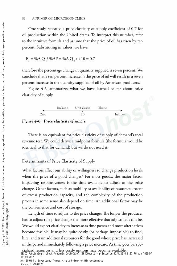
One study reported a price elasticity of supply coeffi cient of 0.7 for oil production within the United States. To interpret this number, refer to the intuitive formula and assume that the price of oil has risen by ten percent. Substituting in values, we have

ES = %Δ Q S/ %ΔP = %Δ Q S / +10 = 0.7

therefore the percentage change in quantity supplied is seven percent. We conclude that a ten percent increase in the price of oil will result in a seven percent increase in the quantity supplied of oil by American producers.

Figure 4-6 summarizes what we have learned so far about price elasticity of supply.

InfinityZero 1.0

Inelastic Unit elastic Elastic

Figure 4-6. Price elasticity of supply.

Th ere is no equivalent for price elasticity of supply of demand’s total revenue test. We could derive a midpoint formula (the formula would be identical to that for demand) but we do not need it.

Determinants of Price Elasticity of Supply

What factors aff ect our ability or willingness to change production levels when the price of a good changes? For most goods, the major factor impacting responsiveness is the time available to adjust to the price change. Other factors, such as mobility or availability of resources, extent of excess production capacity, and the complexity of the production process in some sense also depend on time. An additional factor may be the convenience and cost of storage.

Length of time to adjust to the price change: Th e longer the producer has to adjust to a price change the more eff ective that adjustment can be. We would expect elasticity to increase as time passes and more alternatives become feasible. It may be quite costly (or perhaps impossible) to fi nd, hire, and train additional resources for the good whose price has increased in the period immediately following a price increase. As time goes by, spe-cialized resources and less costly options may become available.




ELASTICITY 87

We would expect elasticity to be greater in the aftermath of a reces-sion, with machines and factories idle and many workers unemployed and highly motivated to work, than at the height of an economic boom. Also, goods with simple production processes, requiring little in the way of specialized resources, should be responsive more quickly than goods with highly specialized requirements, such as research and development facilities or expensive capital.

THINK IT THROUGH: With fewer steps and less complexity in the produc-tion process, will eggs sold locally have a greater elasticity of supply than store-bought “oven ready” chicken? What might reduce the ability of the local farmer to expand production quickly?

Convenience and cost of storage: Th ese factors infl uence inventory holdings. Recall from Chapter 2 that supply refers to the willingness and ability to produce (and make available for sale) a quantity of a good or ser-vice. Markets are not concerned with production or the number of items stored in a warehouse but, rather, with the presence of that output where it can be sold. Th e supply of fi reworks is concentrated around the Fourth of July, but stockpiling goes on for months before that time.

Th e producer’s wish to hold inventory may depend on a desire to smooth production over time—as we’ve noted, spikes in production can be costly. But storage can be costly too. Perishable or bulky low-value items are likely to have a less elastic supply than stable or small items with a high value.

THINK IT THROUGH: Compare wheat and corn. Wheat is a “dry” grain, while corn contains more moisture and requires more careful storage. Which good has the greater price elasticity of supply? It is wheat.

Th e Short Run and the Long Run: Over 100 years ago, the British economist Alfred Marshall was spending a lot of his time thinking about time as it applies to economics. He had developed the concept of elastic-ity and realized that price elasticity of supply was strongly aff ected by the time frame involved. He defi ned two conceptual time periods—the short run and the long run.

Th e short run is defi ned as a period of time during which all but one of a fi rm’s resources can be varied. In the short run, at least one resource is fi xed in quantity. Because human resources can be hired or





fi red fairly readily the fi xed resource is usually thought of as some sort of capital resource such as a nuclear reactor (electricity generation), an oil rig (oil production), a Mack truck (trucking industry), and so on. Clearly, though, the skills of a brain surgeon might be quite infl exible.

All resources are variable in the long run—any resource can be increased, decreased, or discarded. It is only in the long run that a fi rm can enter or leave an industry. In the short run, you may cut production, or even close your doors but, until you reach the long run, you still have the doors! Only when the fi rm has sold off all of its resources can it truly be said to have left the industry. Similarly, a fi rm seeking to enter an industry from scratch may be able to assemble some of its resources in the short run, but, because at least one resource is fi xed at zero, it cannot be said to have entered the industry.

Th is is a conceptual distinction, not a calendar one. Th e time neces-sary to reach the long run will diff er from industry to industry. A fi rm seeking to begin generating nuclear power faces a long road while an entrepreneur wishing to open a family restaurant will move through the process more rapidly.

Negative Price Elasticity of Supply—Is It Possible?: Th e law of supply suggests that the price elasticity of supply will be positive (higher price, so higher quantity supplied) but, in some rare instances, especially in the labor market, negative elasticities have been discovered.

THINK IT THROUGH: What can this mean for the appearance of the supply curve and when might it occur? A negative elasticity would imply that the supply curve is negatively sloped or “backward bending.” Th is may occur at high income levels where the value of leisure time becomes more prized. Leisure is a normal good, so the demand for leisure increases as income increases until, eventually, the incentive to substitute work for leisure is overcome by the preference for leisure. With a salary increase, a rich lawyer or surgeon may decide to trim back on appointments or take early retirement and spend more time on the golf course.

THINK IT THROUGH: In Chapter 3 we discussed the substitution eff ect and the income eff ect as an explanation for the shape of the demand curve. Can you apply those concepts to explain the backward-bending labor sup-ply curve? As the reward for labor increases, workers will substitute labor Copyright © 2013. Business Expert Press. All rights reserved. May not be reproduced in any form without permission from the publisher, except fair uses permitted under



ELASTICITY 89

for leisure, working more intensively. Time-and-a-half, double time, or bonuses are off ers intended to have this substitution eff ect. However, there is also an income eff ect if wage is increased. Because leisure is a normal good, the income eff ect of a wage increase is to reduce labor supply. If the income eff ect dominates the substitution eff ect, then the result is a back-ward-bending labor supply curve and a negative price elasticity of supply.

Applications

Th e Incidence of Taxes: Earlier in this chapter we concluded that the slope of a demand curve is not the same thing as its elasticity and as a general state-ment that is correct. However, if two demand curves with diff ering slopes intersect then we can say that the steeper demand curve is relatively less elastic than the other. We can use this result to analyze the incidence of taxes.

Let’s suppose we have two states, West Carolina and East Carolina, that are similar in all respects except one—the residents of West Carolina are heavily addicted to locally produced whiskey while the residents of East Carolina are not.

We should expect to see the more inelastic (price-insensitive) demand for whiskey in West Carolina. Th e two demand curves are drawn in Figure 4-7, with West Carolina’s demand labeled DW and East Carolina’s labeled DE. Let us now suppose that the production of whiskey is the same in the two states and draw a single supply curve (S)—think of this as two supply curves, one on top of the other. In each state, the equilib-rium price of whiskey is $6.00 per bottle and the equilibrium quantity is 10,000 bottles sold each week.

$6.00

$6.25

$6.80$7.00

0 Q3000 9000 10,000

P

DW

DE

ST

S

Figure 4-7. Incidence of a tax.





Th e governor of each state imposes a $1.00 tax on each bottle of whis-key produced. Th is tax will be collected from the sellers. Th is excise tax is similar to the “per gallon” tax imposed by many states on gasoline and the eff ect is best thought of as shifting the supply curve vertically upwards by the extent of the tax. Th e new supply curve is labeled ST .

THINK IT THROUGH: Can you see why the supply curve will shift vertically by a dollar? A supply curve shows the relationship between the lowest price a supplier is willing to accept and the quantity supplied. If suppliers were willing to accept $6.00 per bottle before the tax in order to supply 10,000 bottles, then, after the introduction of the tax, the lowest price they’ll be willing to accept to supply 10,000 bottles will be $7.00 per bottle.

As we’d expect, the imposition of the tax increases the price of whis-key. Note that it increases more in West Carolina because demand is rela-tively less elastic. Th e (nonaddicted) East Carolinians are more sensitive to price changes and, as price starts to increase, they will cut back in purchases.

Someone must pay the $1.00 tax on each bottle of whiskey pur-chased. Does elasticity aff ect who pays? We can see that the price in West Carolina has risen a great deal—most (80¢ per bottle) of the burden of the tax is being borne by consumers with only 20¢ per bottle being paid by producers. In East Carolina, by contrast, although some of the tax (25¢ per bottle) has been passed on to consumers, the bulk of the tax (the remaining 75¢ per bottle) is being paid by the producers.

We can conclude that the lower the price elasticity of demand the greater the fraction of the tax that can be passed on by producers to consumers.

Elasticity and Tax Revenues: We can take this story farther—which sort of good should a government seek to tax if it wishes to maximize its tax revenues? Goods that have an inelastic demand! In East Carolina, tax receipts will be $3,000 per day because only 3,000 bottles are being sold but, in West Carolina, where inelastic demand has kept sales high, the government will receive $9,000.

We can conclude that the lower the price elasticity of demand the greater the amount of tax revenues that will be collected.Copyright © 2013. Business Expert Press. All rights reserved. May not be reproduced in any form without permission from the publisher, except fair uses permitted under



ELASTICITY 91

THINK IT THROUGH: If demand is perfectly inelastic then it will be impos-sible for consumers to avoid the tax and tax revenues will be maximized. Th inking about the kinds of goods that might have an extremely inelas-tic demand, why do governments tend to shy away from this approach? Might many of those goods be necessities?

Employment Concerns: Frankly, politicians wish to remain in offi ce and, to do so, their policies must appeal to voters. Th e imposition of a tax will raise the price of the taxed good, reduce the size of the market, and cause unemployment for workers in the industry. Politically, it is wise to tax foreign goods. If, however, we must tax a locally produced good, then what lessons does elasticity teach? Tax goods with an inelastic demand! In West Carolina, job loss will be small but East Carolina’s job loss is likely to be quite severe.

Conclusion: Sales taxes can raise the greatest revenues and minimize job losses if levied on goods with a relatively inelastic demand. Politi-cally, this is an attractive option. However, inelastic goods may be neces-sities for which there are few substitutes and taxes may therefore impose hardships. Th e policy maker would prefer to tax a good with an inelastic demand that is not a necessity. Th e ideal targets are inelastic goods that are addictive or detrimental in some way—“bads” such as cigarettes, alco-hol, and gasoline. One argument for the legalization of marijuana is that the government would then be able to slap a tax on it!

Who Is Responsible for Gas Price Volatility?: Consumers habitu-ally grumble about high gas prices, but also complain about the volatility of gas prices. Prices seem to fl uctuate daily. Who is responsible for such volatile gas prices? Th e oil producers are among the “usual suspects” and, to be sure, oil supplies can be aff ected by political instability, and bad weather or other natural disasters. Oil companies, however, anticipate such occurrences and have inventories in hand to smooth out some of the fl uctuations.

Assuming a given supply-side decrease, the reason for extreme move-ments in the market price must lie on the demand side of the market. In fact, the very inelasticity of demand is a prime reason for oil price elasticity. When we grumble about rapidly rising prices at the pumps, we should concede that the major culprit is the one whose hand is on the pump!Co





Review: In this chapter we have explored how economists quantify the relationship between price and quantity demanded, and what conclusions may be drawn from that information. In addition, other “elasticities” can be measured and these may be useful for managers seeking insight into future conditions in their own particular markets.




Elasticity - BrainMassPrimer+of+Microeconomics+Chp+4.pdf · is unit-elastic demand, has an elasticity coeffi cient of 1.0. A ten percent increase in price will cause a ten percent

Documents