Elastic-plastic nonlinearities considering fracture mechanics

0045.7949/87 13.00 + 0.00 Pqamon JoumJs Ltd.

ELASTIC-PLASTIC NONLINEARITIES CONSIDERING FRACTURE MECHANICS

JOSEPH G. MRRCER* and ANTHONY N. PALAZO~~O~

*Air Force Institute of Technology (AFIT), Wright-Patterson AFB, OH 43433, U.S.A. TDepartmcnt of Aeronautic8 and A8tronautics (AFIT), Wright-Patterson AFB, OH 45433, U.S.A.

(Received 28 July 1986)

Ab6hct-The solution of fracture mechanics type problems including material and geometric non- linearities along with time-independent and time-dependent constitutive relation8 is diatxwed. The effect of solution tolerance8 on a fracture type problem arc discussed and the uaa of Green’8 strain tensor and the Piola-Kirchhoff 8tres8 tensor is caamined in a 1-D analysis and a 2-D fracture problem. A comparison of large and small displacement analysis for a ccnter-crackcd panel with elastic-plastic material is made. Small displacement, viscoplastic analysis results also arc presented for a center-cracked panel.

INTRODUCIION

In recent years the United States Air Force has placed an increased emphasis on the structural integrity of turbine engine components. This-includes the appli- cation of fracture mechanics in the initial design and for establishing operational inspection intervals. Major component metal temperatures exceed 1080°F (540°C) and the high-stress environment may cause nonlinear material behavior which ought to be con- sidered when analyzing fracture problems. The authors previously have used the VISCO finite element program [1] to model crack behavior with viscoplastic material response. In this work the au- thors consider both material and geometric non- linearity in analyzing a center-cracked panel.

The theory of nonlinear finite elements is discussed in numerous publications [2-4). Gadala [S] provides an update and summary of the various formulations which are in common use. In this paper the authors discuss the finite element theory for use with materi- ally and geometrically nonlinear probkms. A com- puter program has been developed and is used to examine large displacement stress-strain relations in a 1-D model. A comparison of large and small displacement analysis, for a center-cracked panel with elastic-plastic material, is made. The effect of solution tolerances for a small displacement visco- plastic analysis of a crack is also examined.

THRORY

Equations of motion

Figure 1 represents the neighboring deformed states of a body, (k - 1) and (k), along with the original undeformed state, (0), within the rectangular co-ordinate systems. The a, represent the co-ordinate system corresponding to the original undeformed body. The x, and zi are the co-ordinate systems for the deformed body at states (k - 1) and (k), respectively.

The displacement vector (k _ ,+I is the displacement of the body at the (k - 1) state from the undeformed position, and II is the incremental displacement be- tween the two deformed states, (k - 1) and (k).

The theory of large deformations may be found in numerous texts such as [q and [71. The finite element fommlation for large deformation used by the au- thors in this work was contained in a program called SNAP, written by Brockman, who is also the author of MAGNA [8]. A brief description of the formu- lation and solution is provided herein.

A finite element expression in total Lagrangian form for the equation of motion of the body from state (k - 1) to state (k) may be written as

lt([W + &l)b1= k{T] - k{$ (1)

where [Kr] is the tangent stiffness matrix, [&I is the geometric stiffness matrix, {u} is the vector of nodal displacement corrections, (T} is the applied external force vector and {I} is the internal or quilibrating force vector.

The Appendix contains the appropriate expres- sions for each of the above quantities.

In the total Lagrangian formulation, the in- cremental stress-strain relation is given by

where

(2)

i.9, is the second Piola-Kirchhoff stress tensor:

f-411

331 1 J s12

at state (k), referred to original state (0);

04

C.A.S. ZJ/bH 919

920 JOSEPH G. MERCER and ANTHONY N PALAZO~O

Fig. 1. Neighboring states of a body.

=3

D,, is the incremental material constitutive matrix;

E,, is Green’s strain tensor

= l/2&.,+ %k + 4n,/+ %.kl (2b)

f EH 1 {E}= (24

For small displacements, the incremental equation reduces to

k[Kliu} = klT) -k{l). (3)

In the small displacement case, the incremental stress-strain relation is

da,, = D,, d% (4)

where a,, is the Cauchy stress tensor, and Q., is the infinitesimal strain tensor, equal to 1/2[u,, , + u,, k].

SOLUTION

The incremental equations of motion, eqns (1) and (2), may be nonlinear due to material or geometric

nonlinearity. An overview of the nonlinear solution process is shown in Fig. 2. The solution for a given load increment (k) is performed via an iterative loop, indicated by the superscript (n), in which incremental displacements (~1” are calculated and added to current displacements k{a}“-’ until the convergence parameters are satisfied. In the process, the force imbalance on the right side of eqn (1) or eqn (3) approaches zero. Some of the key parts of this process are the constitutive laws, solution strategy and convergence checks.

Constitutive models

The element routine which calculates total strains and elemental stiffness may call any existing or user-supplied constitutive model routine to calculate stress, plastic strains, and constitutive stiffness matrix, [D]. Currently available are:

(a) linear elastic, (b) elastic-plastic (isotropic), (c) Bodner viscoplastic (isotropic).

Each of these is described below. a. Linear elastic. The linear elastic constitutive

model calculates stress using the elastic constitutive matrix:

Elastic-plastic nonlinearities and fracture mechanics 921

where

and [D] is the appropriate plane stress or plane strain elastic constitutive matrix.

b. Elastic-plastic. In the elastic-plastic model, total strains are decomposed into elastic and plastic parts:

CQ=C;+Cfp (6)

Incremental plastic strains are calculated via a Prandtl-Reuss relation as

dfc = d%S,, (7)

where

dl=;$$ (74

su is the deviatoric stress, H’ is the slope of the stress-plastic strain curve, and 6 is the effective stress, equal to (1/2S,S,)1~. A Von Mises yield criterion is used, as is the elastic-plastic constitutive matrix given by Yamada [9]:

WI = ~4plIW

dependent viscoplastic model which is described in [lo]. For small strains, the elastic and plastic strain rates may be decomposed by

iv = i;z;, (10)

where it is the elastic strain rate, and Lt is the viscoplastic strain rate.

The viscoplastic strain rates are calculated using a Prandtl-Reuss type relation:

where S, is the deviatoric stress and J; is the second deviatoric stress invariant. The constant n controls the model’s strain rate sensitivity, while D,, is the maximum value of strain rate in shear. The Z, an internal state variable, expresses the degree of mat- erial work hardening. The state-variable equation is

Z=Z,+(Z,-Z,)exp(-mW,), (12)

where Z, and Z, are the material’s initial and max- imum values of hardness respectively, and m is a constant that controls the rate of work hardening. The term W, in eqn (12) accounts for the plastic work including thermal recovery of hardening at high temperature, and is defined as

‘= dt . m(Z, -Z)

(13)

where for plane strain:

E [bl* I+v

(_!z__$ (L&s&) (_&3&) (-5-p)

L

c= 2 -62 I+!2 3 [ 1 3G

(k&y (_&F) (q)

p-_-y (I+%)

1 s:2 ( ) ---

2 c

(9)

J

c. Bodner-Parrom viscoplastic. The Bodner- Panom isotropic constitutive model is a rate-

The rate of thermal recovery of hardness is

where Z2 is the minimum expected value of the hardening at a given temperature. A and r are material constants chosen to match low strain rate (secondary creep) test data. This recovery term he- comes important for high temperatures. Table 1

922 JOSEPH G. MERCER and ANTHONY N. PALAZOTTO

Iteration Loop (n) . .

#----------_-_----~ I

I------------~

I Element Routine

I ’ Constitutlve Laws

-1 f-i I

I [D{:-‘I [K, I’“,” [Kc ]‘“:“{l}:-’ I a. ElastlceElastic

k * I b. Elastic-Plastic f L ------- ----_--

I

J I I c. Bodner Vtscoplastic , I_ _-_-_-_-----_J

r-------

_-----_ 1

Restdual Force Calculatton I I I

r------- L--___--,

Convergence Check

a. Displacement

I a. Step-by-step I I b. Constant Stiffness I

c. Modified Newton Raphson I d. Newton Raphson I

I I L e. Combined

r , Solve Equations: I

1 MT + K, 1

-1 I I Update Displacements i

L---,---,,--,-J

Fig. 2. Solution overview.

shows a list of the Bodner material parameters for one may use plastic strain rates calculated at the IN100 at 1350°F developed by Stouffer [15]. beginning of the time step, rates calculated at the end

Stresses may be calculated via of the time step, or a combination of the two. as

described by Owen and Hinton [l I] and Hughes and {da} = [Dl[{dc} I- {dO), (15) Taylor [12].

For a given time step, n, where [D] is the elastic stiffness matrix.

In general, when calculating viscoplastic strains A;=Ar[(l -B)C;+&;-“I. (16)

Table I _ Bodner-Partom material parameters developed for IN 100 at 1350°F

Bodner’s material parameters Description Value

E

A r

Elastic modulus

Strain rate exponent Limiting value of strain rate Limiting value of hardness

Maximum value of hardness

Minimum value of hardness

Hardening rate exponent

Hardening recovery coefficient Hardening recovery exponent

26.3 x 10) ksi (1.8134 x 105MPa)

0.7 to’sec-’

915.0 ksi (6304 MPa) 1015.0 ksi (6993 MPa)

600.0 ksi (4134 MPa)

2.57 ksi-’ (3727 MPa-‘) 1.9 x lo-‘set-’

2.66

Elastic-plastic nonlinearities and fracture mechanics 923

For 0 = 0, we obtain the Euler integration scheme (fully explicit), for 8 = 1, we obtain a fully implicit scheme, and for 8 = l/2, we have what is known as the Crank-Nicolson rule.

In VISCO [I], a program that we have also used to solve viscoplastic problems, the Euler integration scheme is employed, with viscoplastic strains calcu- lated based on strain rates at the beginning of the time step. This method is easiest to implement, but requires careful time step selection for numerical stability. Zienkiewicx and Cormeau [ 131 provide guid- ance for time step selection.

An advantage of the implicit schemes is that they are unconditionally stable since they are based upon a backward difference technique. This allows larger time steps, hence larger load increments, to be applied and maintain numerical stability. However, the user is not guaranteed that the solution will be accurate with very large time steps. Typically, halving the time step, and comparing results, will provide the user with an allowable time step for a given problem. Within SNAP, an implicit scheme for calculating plastic strains was developed by Brockman and Rajendran [8]. Plastic strains are calculated based upon an average of rates at the beginning and the end of a sub-increment. Initial estimates of conditions at the end of the increment are obtained using Euler extrapolation. An iteration loop is then used to recalculate stresses, plastic strains, and plastic work, until convergence is obtained in calculated stress values.

The incremental constitutive matrix [o,,] is re- quired if the element stiffness is to be updated during a load increment. Within SNAP, the method devel- oped by Pierce et al. [14] is used, eliminating the need for matrix inversion as is commonly done.

The elastic-plastic and the viscoplastic models both employ a strain sub-incrementation scheme on an element-by-element basis. Within a load step, element incremental strains dka at each Gauss integra- tion point are either divided to allow a maximum component strain of 2 x IO-’ (elastic-plastic) or 5 x lo-’ (viscoplastic). Stresses and plastic strains are calculated for each sub-increment, allowing the ele- ment to follow the stress-strain behavior for the appropriate constitutive model even when the load step is large. Since this operation is done on an elemental basis, only those elements undergoing large strains are subjected to sub-incrementation, hence providing a more efficient computation for the model as a whole.

Solution/strategy

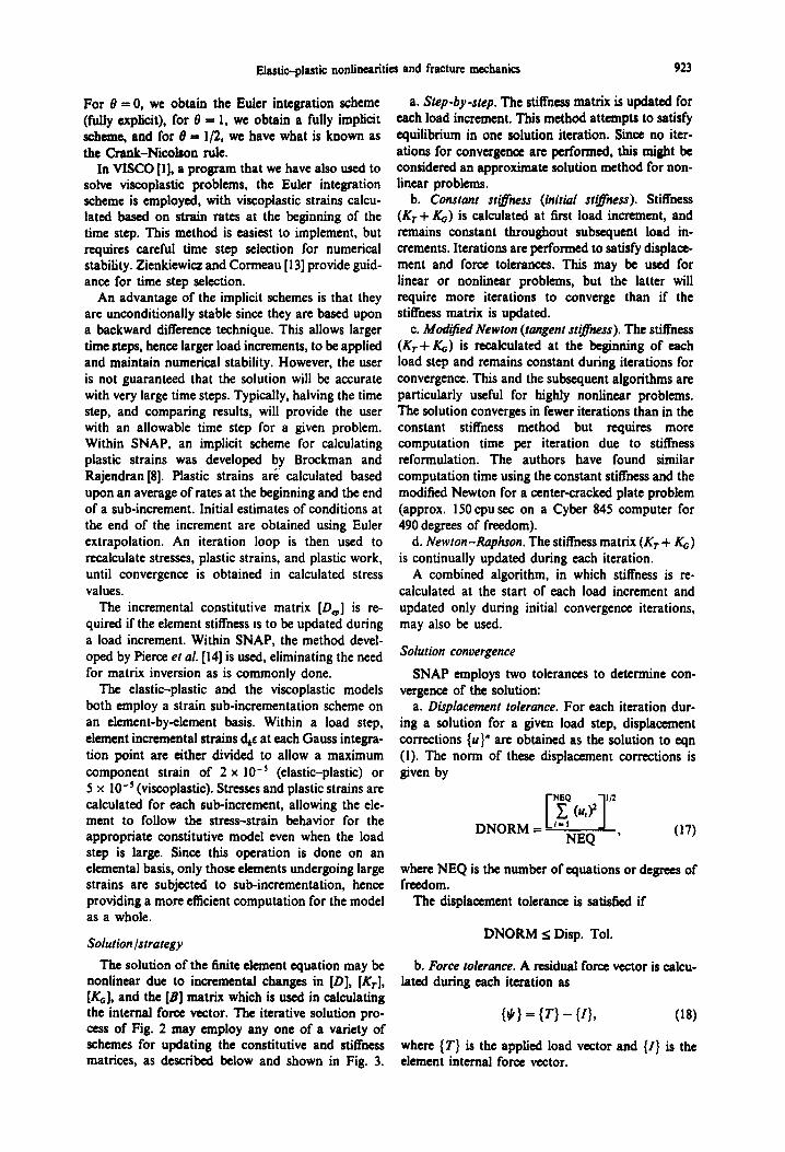
The solution of the finite element equation may be nonlinear due to incremental changes in [D], [Kr], [K-J, and the [B] matrix which is used in calculating the internal force vector. The iterative solution pro- cess of Fig. 2 may employ any one of a variety of schemes for updating the constitutive and stiffness matrices, as described below and shown in Fig. 3.

a. Step-by-step. The stiffness matrix is updated for each load increment. This method attempts to satisfy equilibrium in one solution iteration. Since no iter- ations for convergence are performed, this might be considered an approximate solution method for non- linear problems.

b. Constant st@iiss (initial st@ess). Stiffness (Kr+ &) is calculated at first load increment, and remains constant throughout subsequent load in- crements. Iterations are performed to satisfy displace- ment and force tolerances. This may be used for linear or nonlinear problems, but the latter will require more iterations to converge than if the stiffness matrix is updated.

c. Modt$ed Newton (tangent sttjiiss). The stiffness (Kr+ j(G) is recalculated at the beginning of each load step and remains constant during iterations for convergence. This and the subsequent algorithms arc particularly useful for highly nonlinear problems. The solution converges in fewer iterations than in the constant stiffness method but requires more computation time per iteration due to stiffness reformulation. The authors have found similar computation time using the constant stiffness and the modified Newton for a center-cracked plate problem (approx. 15Ocpu set on a Cyber 845 computer for 490 degrees of freedom).

d. Newton-hphson. The stiffness matrix (Kr + j(G) is continually updated during each iteration.

A combined algorithm, in which stiffness is re- calculated at the start of each load increment and updated only during initial convergence iterations, may also be used.

Solution convergence

SNAP employs two tolerances to determine con- vergence of the solution:

a. Displacement tolerance. For each iteration dur- ing a solution for a given load step, displacement corrections {u}” are obtained as the solution to eqn (1). The norm of these displacement corrections is given by

(17)

where NEQ is the number of quations or degrees of freedom.

The displacement tolerance is satisfied if

DNORM s Disp. Tol.

b. Force tolerance. A residual force vector is calcu- lated during each iteration as

(18)

where {T} is the applied load vector and {I} is the element internal force vector.

a)

ST

EP

-BY

-ST

EP

l

Up

dat

e st

iffn

ess

a N

o

iter

atio

ns

l

Att

emp

ts

to

sati

sfy

Eq

uili

bri

um

cl

MO

DIF

IED

N

EW

TO

N

RA

PH

SO

N

I

l

Up

dat

e st

iffn

ess

at

beg

inn

ing

o

f lo

ad

incr

emen

t

0 C

on

verg

ence

it

erat

ion

s

l

Fo

r m

ore

h

igh

ly

no

nlin

ear

pro

ble

ms

b)

CO

NS

TA

NT

S

TIF

FN

ES

S

dl

FU

LL

N

EW

TO

N

RA

PH

SO

N

a In

itia

l st

ress

es u

sed

th

rou

gh

ou

t

a C

on

verg

ence

it

erat

ion

s

l

Fo

r m

ild

ly

no

nlin

ear

pro

ble

ms F

ig

3.

So

luti

on

al

go

rith

ms

l

Up

dat

e st

iffn

ess

du

rin

g

each

it

erat

ion

0 C

on

verg

ence

it

erat

ion

s

l

Fo

r h

igh

ly

no

nlin

ear

pro

ble

ms

Elastic-plastic nonlincarities and fracture mechanics 925

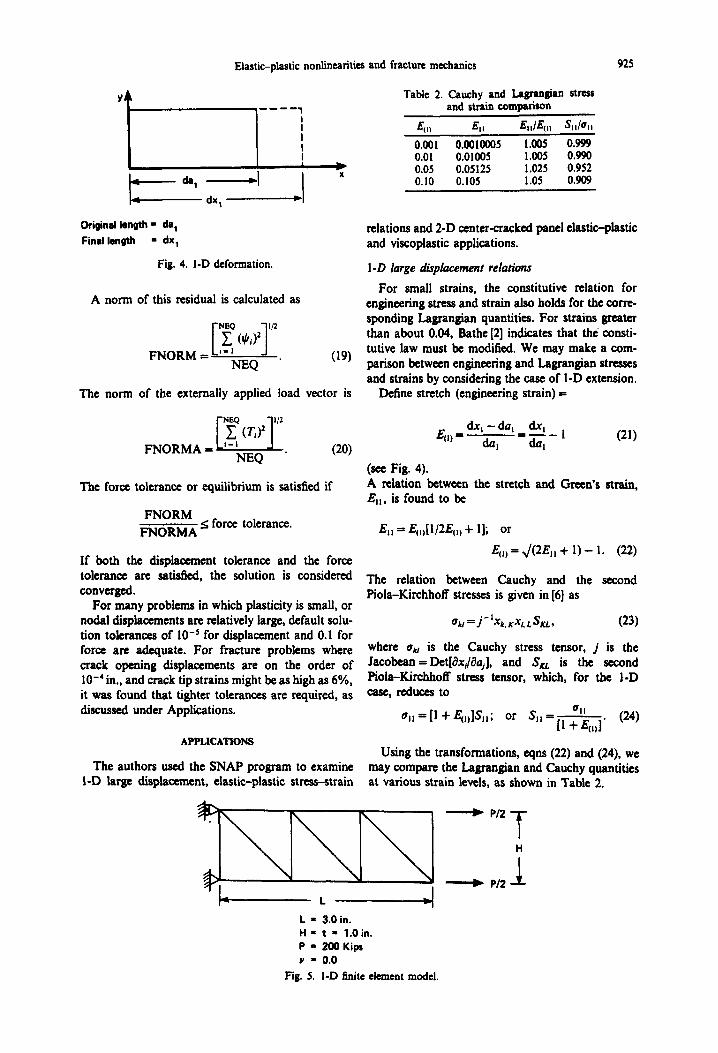
Original length - da,

Final length = dx,

Fig. 4. 1-D deformation.

A norm of this residual is calculated as

NEQ

[ 1 ‘/2 c (*i)* FNORM= I-’

NEQ * (19)

The norm of the externally applied load vector is

NEQ

[ 1 112

1 (T,)’ FNORMA = ‘-I

NEQ * (20)

The force tolerance or equilibrium is satisfied if

sttiA 5 force tolerance.

If both the displacement tolerance and the force tolerance are satisfied, the solution is considered converged.

For many problems in which plasticity is small, or nodal displacements are relatively large, default solu- tion tolerances of 10mJ for displacement and 0.1 for force are adequate. For fracture problems where crack opening displacements are on the order of lo-’ in., and crack tip strains might be as high as 6%, it was found that tighter tolerances arc required, as discussed under Applications.

APPLlCATlONS

The authors used the SNAP program to examine 1-D large displacement, elastic-plastic stress-strain

Table 2. Cauchy and Lagrangian stress and strain comparison

E (1) EII &/41, W’,I

0.001 0.001ooo5 1.005 0.999 0.01 0.01005 1.005 0.990 0.05 0.05125 1.025 0.952 0.10 0.105 1.05 0.909

relations and 2-D center-cracked panel elastic-plastic and viscoplastic applications.

1-D large dkplacement relations

For small strains, the constitutive relation for engineering stress and strain also holds for the corre- sponding Lagrangian quantities. For strains greater than about 0.04, Bathe [2] indicates that the consti- tutive law must be modified. We may make a com- parison between engineering and Lagrangian stresses and strains by considering the case of I-D extension.

Define stretch (engineering strain) 5:

dx, -da, dx, E,,, = - da, =ziy (21)

(see Fig. 4). A relation between the stretch and Green’s strain, E,, , IS found to be

E II = 41JW4~~ + 11; or E,,, = ,/(2E,, + 1) - 1. (22)

The relation between Cauchy and the second Piola-Kirchhoff stresses is given in [6] as

cu =j-‘xk,Kx,,LL (23)

where a, is the Cauchy stress tensor, j is the Jacobean = Det[ax,/aa,], and S, is the second Piola-KirchhofT stress tensor, which, for the 1-D case, reduces to

Using the transformations, eqns (22) and (24). we may compare the Lagrangian and Cauchy quantities at various strain levels, as shown in Table 2.

L = 3.0 in. Ii = t = 1.0 in. P = 2OOKips Y = 0.0

Fig. 5. 1-D finite element model.

926 JOSEPH G. MERCER and ANTHONY N. PALAZOITO

- Displacement based on eng’r u - E

0 Small displ. F.E., uy = 170 kri, H’ = 186

0 Large displ. F.E., oy = 170 ksi. H’ = 13

b Large displ. F.E., 17” = 170 kri, H’ = 186

.20 .30 .4O .50 .6O .7Q

Displacement (in.)

Fig. 6 I-D finite element results.

We see from Table 2 that for small values of strain, the Lagrangian and Cauchy quantities are nearly equal. Certainly, for stresses below yield, where strains are typically less than 0.01, there is minimal difference. For small strain, with either large or small displacement analysis, the engineering stress-strain data might be used. However, as 5% strain is ap- proached, we begin to see a marked difference in the Lagrangian and Cauchy values. This must be consid- ered when performing large displacement, finite strain analysis.

In the current elastic-plastic finite element consti- tutive model, we assume a linear decomposition of elastic and plastic strain increments, although this is not necessarily always true [5]. Keeping within this framework, we now examine the suitability of transforming stress-strain data to Lagrangian form using eqns (22) and (24) for use in large displacement/ strain analysis. This concept is used in the MAGNA program (81. To examine this method, the 1-D model of Fig. 5 was initially employed.

An elastic-plastic material with linear hardening was assumed to have engineering stress-strain prop- erties of E = 23,568 ksi, uylc,,, = 170 ksi and H’ = 186 ksi. Using eqns (22) and (24), H’ = 13 was obtained for the transformed material properties.

The model was loaded monotonically in 10 equal increments to peak load, with the results shown in Fig. 6. Both the small displacement finite element formulation using the engineering properties and the large displacement formulation with transformed properties matched the predicted result based on the engineering stress-strain response. When the en- gineering stress-strain data were used with the large displacement formulation, considerable error was obtained in the plastic region. The error in displace- ment reached 50% at maximum load.

2-D application-center-cracked panel

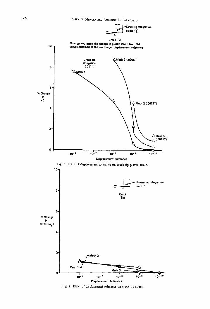
Convergence tolerance selecrion. It was found early in this work that solution tolerances can have a large effect on the results of fracture mechanics problems. Crack tip opening displacements are small, on the order of IO-‘in., and plastic strains at the crack tip may be greater than 5%. The effect of solution tolerance was examined for the center-cracked panel (CCP) finite element model shown in Fig. 7. Four plane stress finite element models were used with crack tip element sizes ranging from 0.011 to 0.0015 in. and for 351 to 570 degrees of freedom. The Bodner viscoplastic constitutive law and the IN-100 material properties of Table 1 were used. All elements were of the I-noded isoparametric variety, using Cpoint integration.

Each finite element model was loaded mono- tonically in 0.1 set to peak load (a applied = 53.54 ksi) in 10 increments. This load is equivalent to an elastic stress intensity of 35 ksi ,/in. Displacement tolerances were varied from lo-’ to lo-to. The force tolerance was not adjusted in this work since satisfaction of the displacement tolerance resulted in extremely small force unbalances (_ 10-l). The solution was performed using a Cyber 845 computer.

As the tolerance was reduced, any changes in stress (a,) and plastic strain (CT) in the element nearest the crack tip were noted, as shown in Figs 8 and 9. The points shown indicate the per cent change in plastic strain or stress as the tolerance was decreased from the next higher value.

For each finite element mesh the change m calcu- lated strain reduced as the tolerance was decreased, with the change being less than 1.4% for a change in tolerance from low9 to lo-“. Stresses changed very

Elastic-plastic nonlincarities and fracture mechanics 927

Lines of Symmetry

t L ‘+i, o.5

Fig. 7. Center-cracked panel finite element modes.

I

928 JOSEPH G. MERCER and ANTHONY N. PALAZO~~O

ia

6

% Change in P Y

4

-p_

Stress at Integration * point @

Crack Tip Changes represent the change in plattlc strain from the values obtained at the next larwr displacement tolerance

10-s lo- 7 10-a 10-a 10-10

lo-

8-

8-

% Change in

Stress (0” )

Displacement Tolerance

Fig. 8. Effect of displacement tolerance on crack tip plastic swam.

==P Stresses at integration + point 1

Crack lip

f Mesh2

Displacement Toleranca

Fig. 9. Effect of displacement tolerance on crack tip stress.

Elastic-plastic nonlinearities and fracture mechanics 929

L_

0

,

930 JOSEPH G. MERCER and ANTHONY N. PALAZOITO

little due to the fact that the stress-strain curve is ahead of the crack tip were compared for large and nearly horizontal at the calculated crack up strains. small displacement formulations.

An additional consideration for nonlinear finite element analysis is solution time. The effect of dis- placement tolerance on solution time is shown in Fig. 10. As the solution tolerance is decreased, the required computation time increases, particularly for the more refined meshes (3 and 4). A sharp rise in computation time (c 100 set) for these meshes is also seen as the displacement tolerance is decreased from 10e9 to lo-“. At such tight tolerances, round-off error may contribute to the rapid rise in computation time. For this problem then, it appeared that 10m9 was a suitable displacement tolerance.

CUD. The crack opening displacement for large displacement formulation was found to be about 3% lower than for small displacement directly behind the crack tip, with the difference on the order of only 1% away from the crack tip. Figure 13 shows a typical comparison for the lowest yield strength (110 ksi) which resulted in the largest crack tip deformation.

For an additional check, the solution was repeated with reduced load step sizes to check for accuracy. Figure 11 shows this process for three of the meshes at two different solutton tolerances. For the large solution tolerance (lo-‘), we see that the crack tip plastic strain varies with time step. However, for a small specified tolerance (10m9), the solution is invariant.

Plastic zones. Plastic zone sizes at peak load are shown for the three yield strengths in Fig. 14. No difference in plastic zone size was found between large and small deformation analysis. This is to be expected since at yield the displacements and strains are small for this problem.

Crack tip deformation. The deformation of ele- ments at the crack tip is shown to scale in Fig. 15. Y-Direction nodal displacements to the left of the crack tip were 26% less for the large displacement formulation at the lowest (110) yield stress. For higher yield strengths, the difference between large and small displacement analysis was slightly less.

CCP-large and.small displacement formulation

The center-cracked panel (CCP) shown m Fig. 7 was analyzed using small and large displacement formulation, The properties used are shown in Fig. 12 along with the corresponding engineering stress-strain response. The model was loaded in 10 increments to a maximum far field stress of 68.8 ksi, equivalent to an elastic stress intensity of 45 ksi Jin. Crack opening displacement (COD), plastic zone size. crack tip element deformations, and stresses

Stress. The Lagrangian formulation uses the sec- ond Piola-Kirchhoff stress tensor, SU,, which is related to the Cauchy stress tensor (au) used in the small displacement formulation by eqn (23).

For large deformations where x,,, differs greatly from the identity matrix, the Cauchy and Piola-Kirchhoff stresses will have different values. This is the case in the region of the crack tip, as shown in Fig. 16 for cylcld = 140 ksi. The difference between the two stresses is on the order of the _r-dnection strain or about 15% for the 140 ksr yield

c 140 156 Small D 139.2 13 Large

I I E 110 125 Small F 109.5 13 Large

Of I I

I I I I 1 1 7 0 ,025 .05 .lO .15 .20

Stram (m/in.)

Fig 12. Material stress-dram response.

Elastic-plastic nonlinearities and fracture mechanics 931

0 yHld = 110 ksi o Large displacement

1.50 A Small displacement

RI

b * 1.20: 1 5

;;

Maximum difference = 3%

.45-’

.OO~~~,....,,.~.,....,....~.~.~,rrrrrrbr.,~.l.,....,....,....,....,...? .lO .ll .12 .13 .14 .15 .16 .17

Location (in.)

Fig. 13. Crack opening displacement, elastic-plastic solution.

oy = 110 ksi

t Crack Tip

Small and large displacement results identical

Fig. 14. Plastic zone size vs yield stress 45 ksi ,/in.

LARGE DISPLACEMENT SMALL DISPLACEMENT

- UNDEFORMED ----- DEFORMED

r Rotetion (de@

6-- ----+-_,_ -----cm___

I ,

CRACK TIP\ 3% Differenw

Fig. IS. Crack tip element deformation.

932 JOSEPH G MERCER and ANTHONY N. PALAZOT-TO

s R

8 d

?

(KY) *D - ssalls

(!S)o *D - ssws

Elastic-plastic nonlincarities and fracture mechanics 933

I% 250.00

cmltorcradcd P-1 35 krih.

6odner viscoplrrtic

* Snap ---- Visco I161

Distance from crack (in. x lo-’ 1

Fig. 18. Stress and plastic zone, Bodner viscoplastic solution.

strength case shown. Away from the crack tip, the two stresses have identical values as expected.

Using the transformation law of eqn (21), the Cauchy stresses calculated via small displacement analysis were transformed into Piola-Kirchhoff stresses which were compared with those obtained via the large displacement analysis (Fig. 17). These stresses were in exact agreement away from the crack tip (O.OlOin.), and were within about 2% near the crack tip for yield stresses of 140 and 170 ksi. At 110 ksi yield stress, there was a 6% difference, limited only to the element integration point nearest the crack tip (O.OW3 in. away).

From these results, we conclude that the technique of transforming the input stress-strain data via eqns (22) and (24) to Lagran$an form for large displace- ment analysis is appropriate for the type of problem considered. Furthermore, we see very little difference

between large and small displacement analysis for the center-cracked panel at 45 ksi Jin.

Vkcoplastic analysis

The centercracked panel was also analyzed using the Bodner constitutive law with the IN-100 material properties of Table 1 in a small displacement analysis. The model was loaded to a peak applied load of 53.54 ksi equivalent to an elastic stress intensity of 35 ksi Jin. Plastic zone size and stress profile ahead of the crack tip are shown in Fig. 18 and were found to agree with those reported by Henkel[16].

Large disphe4nent, finite strain viscoplastic ana- lysis has not been examhi by the ruthors in this work. Tsena [17] shows that total Lagran&n strains do not additively decompose under these conditions. This o&n leads to a decomposition of the form d, = d;+ d$, where d, ate the deformation rates.

934 JOSEPH G. MERCER and ANTHONY N. PALAZOTTO

Tseng introduced a method based upon the updated Lagrangian approach and a generalized logarithmic strain measure which unlike the total Lagrangian strain may be additively decomposed.

CONCLUSlOlri

The finite element formulatton and nonlinear solu- tion procedure used in this analysis have been presented. Solution convergence in the SNAP program is governed by force and displacement tolerances. For the fracture problem examined, the displacement tolerance appeared to govern, and a value of 10e9 gave acceptable results which were not influenced by the time step. We note that this toler- ance is five orders of magnitude less than the crack- opening displacement. For monotonic loading of the elastic-plastic center-cracked panel, large displace- ment analysis could be performed by using material properties transformed into a Lagrangian co- ordinate system. It was shown that for yield strengths of 11 O-i 70 ksi, and an elastic stress intensity of 45 ksi Jin., in a center-cracked panel (CCP), large and small displacement analysis gave nearly identical results. Viscoplastic analysis of the CCP using the implicit Bodner formulation in the SNAP program agreed with published results [16] using the VISCO program which incorporates an explicit Euler integra- tion scheme.

REFERENCES The individual terms are defined as follows:

I. T. D. Hinnerichs, Vrscoplastlc and creep crack growth analysis by the finite element method. AFWAL, TR-80- 4146, Wright-Patterson AFB (1981).

2. K. J. Bathe, Finite Element Procedures in Engineering Analysis. Prentice-Hall, Englewood Cliffs, NJ (1982).

3. K. J. Bathe and H. Ozdemir. Elastic-nlastic large

x dVol = tangent stiffness (25)

4.

5.

6.

I.

8.

9.

10.

11.

12.

deformation static and dynamic analysis: J. Cotnp;r. Strucr. 6, 81-92 (1976). 0. C. Zienkiewicz, The Fiture Element Melhod in Engineering Science, 3rd Edn. McGraw-Hill, London (1977). M. S. Gadala, M. A. Dokainisa and A. E. Oravas, Formulation methods of geometric and material non- linearity problems. br. J. numer. Meths Engng 20, 887-914 (1984). A. C. Eringen, Mechanics of Conrinua. John Wiley, New York (I 967). K. Wash& Variation Methods in Elasticity and Plas- riciry. Pergamon Press, Oxford (1982). R. A. Brockman, MAGNA: a finite element program for the materially and geometrically nonlinear analysis of three-dimensional structures subjected to static and transient loading. AFWAL-TR-80-3152, Wright- Patterson AFB (1981). Y. Yamada, N. Yoshimura and T. Sakuri, Plastic stress-strain matrix and its application for the solution of elastic-plastic problems by the finite element method. Inr. J. mech. Sci. 10, 343-354 (1968). S. R. Bodner and Y. Partom, Constitutive equations for elastic-viscoplastic strain hardening materials. J. appl. Mech. Trans. ASME 42, 385-389 (1975). D. R. Gwen and E. Hinton, Finite Elements in Plas- ticity. Pineridge Press, Swansea (1980). T. J. Hughes and R. L. Taylor, Unconditionally stable

13.

14.

IS.

16.

17.

algorithms for quasi-state ela.sto/visco-plastic finite eie- ment analysis. Compul. Srrucr. 8(Z). 169-173 (1978). 0. C. Zienkiewicz and I. C. Cormeau, Visco-plasticity- plasticity and creep in elastic solids-a unified numer- ical solution approach. Inr J. namer. Merhs Engng 8, 821-845 (1974). D. Pierce, C. F. Shih and A. Needleman. A tangent modulus method for rate-dependent solids. Compur. Struct. 18(S). 875-887 (1984). . I.

D. C. Stouffer, A con&itutive representation for IN- 100. AFWAL-TR-81-4039, Wright-Patterson AFB (1975). C. L. Henkel, Crack closure characteristics considering center-cracked and compact tension specimens. M.S. Thesis, Air Force Institute of Technology, Wright- Patterson AFB (1984). N. T. Tseng and G. C. Lee, Inelastic finite strain analysis of structures subjected to nonproportional loading. Int. J. numer Meths Engng 21.941-957 (1985)

APPENDIX

The finite element equations of motion given by eqns (1) or (3) contain expressions for the element stiffness and the internal and applied loads which are explained here in further detail.

Lurge displacement

The large deformation equation of motion given by eqn (1) is repeated here:

x dVol = geometric stiffness (26)

x surface traction load vector (or vector of applied nodal forces)

kW = Y [ wlr,wkISl ov,

(27)

x dVo1 = internal force vector (28)

{u) is the vector of incremental displacements. (29)

Integration is carried out via the Gauss quadrature. The foIlowing quantities are evaluated at the Gauss integration points:

[N,,,N, I... N&, 0 0 . . .

“d.2 N;2 ::: N’2 ;,, N” ::: N”

0 0 . . . 0 N,,, N”,; . . . IV;;: I

for 8.noded element. (30)

Elastic-plastic nonlincarities and fracture mechanics

. 03)

Strains: Gm’s strain tensor: E, p: I/au,,, + u,, + yr t u,J;