Eindhoven University of Technology MASTER Supply chain finance as a value added service offered by a lead logistics provider Careaga Franco, V.G. Award date: 2016 Link to publication Disclaimer This document contains a student thesis (bachelor's or master's), as authored by a student at Eindhoven University of Technology. Student theses are made available in the TU/e repository upon obtaining the required degree. The grade received is not published on the document as presented in the repository. The required complexity or quality of research of student theses may vary by program, and the required minimum study period may vary in duration. General rights Copyright and moral rights for the publications made accessible in the public portal are retained by the authors and/or other copyright owners and it is a condition of accessing publications that users recognise and abide by the legal requirements associated with these rights. • Users may download and print one copy of any publication from the public portal for the purpose of private study or research. • You may not further distribute the material or use it for any profit-making activity or commercial gain

Welcome message from author
This document is posted to help you gain knowledge. Please leave a comment to let me know what you think about it! Share it to your friends and learn new things together.
Transcript

Eindhoven University of Technology
MASTER
Supply chain finance as a value added service offered by a lead logistics provider
Careaga Franco, V.G.
Award date:2016
Link to publication
DisclaimerThis document contains a student thesis (bachelor's or master's), as authored by a student at Eindhoven University of Technology. Studenttheses are made available in the TU/e repository upon obtaining the required degree. The grade received is not published on the documentas presented in the repository. The required complexity or quality of research of student theses may vary by program, and the requiredminimum study period may vary in duration.
General rightsCopyright and moral rights for the publications made accessible in the public portal are retained by the authors and/or other copyright ownersand it is a condition of accessing publications that users recognise and abide by the legal requirements associated with these rights.
• Users may download and print one copy of any publication from the public portal for the purpose of private study or research. • You may not further distribute the material or use it for any profit-making activity or commercial gain

Eindhoven, January 2016
Supply Chain Finance as a Value Added Service offered by a
Lead Logistics Provider by
Victor Gerardo Careaga Franco
in partial fulfilment of the requirements for the degree of
Master of Science
in Operations Management and Logistics
Student nr. 0885706
Supervisors
Prof. dr. ir. Jan Fransoo, Eindhoven University of Technology
Prof. dr. Arjan van Weele, Eindhoven University of Technology
Dr. Maximiliano Udenio, Eindhoven University of Technology
Sander van den Berg, DHL
Joeri Kuik, DHL

– i –
TU/e School of Industrial Engineering. Series Master Theses Operations Management and Logistics
Subject headings: Supply Chain Finance, Reverse Factoring, Lead Logistics Partner, Logistics Service
Providers, Discrete Event Simulation, Arena

– ii –
Abstract
This study covers the proposition of a Supply Chain Finance (SCF) arrangement from a typically
overlooked perspective, the one of a lead logistics provider (LLP). To validate past studies made on
idealised models, and to generate better understanding, we measure value creation of SCF solutions
under stochastic and complex systems. Our findings convey that companies with lower margins, higher
risk profiles, with higher demand uncertainty and low payment terms benefit the most from SCF. Also,
we show that payment terms extensions under SCF reduce supplier benefits and induce a non-linear
effect on their total cost of managing an inventory and cash system. The magnitude of this effect
depends on suppliers cost structure and degree of demand uncertainty. Finally, we present the case of a
LLP as a provider of SCF solutions. We discuss two possible scenarios: SCF with no refinancing and SCF
with refinancing. We also discuss several managerial implications, potential target groups and strategic
considerations.

– iii –
Executive Summary
Supply chain integration has become crucial to gain competitive advantage in a global economy.
While the flows of goods are increasingly integrated and optimised, attention from practitioners and the
academy to financial flows has been reduced. Thus, whilst companies cooperate, coordinate their
activities and improve visibility of the Physical Supply Chain (PSC), they do not do so for the Financial
Supply Chain (FSC), leading to a structural weakness in supply chains (SCs). Typically, large corporations
face lower financing costs than what their Small and Medium-sized Enterprise suppliers can realise.
However, many corporations follow aggressive cash management practices such as extending payment
terms, which hinder overall supply chain performance. Hence, there is a sub-optimal and inefficient
allocation of financial resources in SCs.
In an effort to manage the FSC with an equally integrated view similar to the one applied to the PSC,
Supply Chain Finance (SCF) has been suggested as a suitable solution to stabilise links in supply chains,
reduce counterparty risk to prevent the disruption of production lines resulting from financial problems,
and to optimise total costs within the supply chain. The most common SCF solution is reverse factoring
(RF), a post-shipment financial arrangement where a creditworthy buyer systematically informs a
financial institution of payment obligations to selected suppliers, enabling the latter to receive a
discounted payment of an invoice due to be paid by the buyer, at a cheap rate. Literature has reported
that SCF and RF create value in SCs by providing funding and liquidity savings, balance sheet
improvement, borrowing and transaction costs savings for suppliers, increased cash flow transparency
and decreased cash flow volatility and risk. However, several companies have reported concerns about
SCF solutions. Some of these include the need of developing a good understanding of finance, working
capital management and SCF solutions; increased pressure of buyers to guarantee payments to Financial
Service Providers (FSPs) and fear of buyers that suppliers may misuse extra liquidity obtained through
SCF. A very common concern for suppliers is that many buyers demand payment terms extension when
offering SCF to suppliers, which decreases suppliers’ benefits from the financial arrangement.
Despite many reports about promising results from SCF programmes, many companies are still hesitant
to embark on SCF solutions, because it is unclear for them how the benefits will materialise and how
they should implement them successfully. In this dissertation we argue that logistics companies,
especially lead logistics providers (LLPs), are in a good position to offer their customers SCF solutions as
a value added service. We believe that by being execution champions with a privileged position in the
SC, possessing significant data and integration capabilities, LLPs are good candidates for this task.
With the objective of better understanding the direct benefits emanating from SCF solutions, predicting
value creation via SCF and determining target groups for this new service, we simulated the operations
and cash flow transactions of a material supplier with uncertain demand. The supplier sells finished
goods to a single buyer, sources raw material from a tier 2 supplier and manufactures the goods in an
internal plant. We considered two scenarios: business as usual (BAU) and SCF. In the BAU scenario, the
supplier has access to conventional financing in the way of a line of credit, and in the SCF scenario the
supplier is offered a reverse factoring arrangement, where the supplier obtains cash at a cheaper rate.

– iv –
We measured value creation at each of the scenarios. Our findings suggest that SCF creates value
through financial savings provided by the interest rate arbitrage between the SCF rate and the supplier’s
cost of borrowing. Also, by giving suppliers the possibility of unlocking cash located in their balance
sheets at a cheap rate, they need lower cash levels and financing from the line of credit, generating
financial savings. We have found that companies with lower margins, higher borrowing rates, with
higher demand uncertainty and low payment terms benefit the most from SCF. Furthermore, SCF
arrangements reduce cash flow volatility substantially, which lets suppliers develop a lower risk
perception and hence an improved capital sourcing cost, and thus a higher enterprise value. Also, by
having lower cash flow volatility, suppliers improve their analytic capabilities, enhance forecasting
processes and make better decisions.
We also modelled suppliers’ concern on the effect of payment terms extension when being offered SCF.
We show that payment terms extensions reduce supplier benefits and induce a non-linear effect on the
total cost of managing an inventory and cash system for the supplier. This effect depends on the
supplier’s cost structure and the magnitude of demand uncertainty. We conclude that managers should
study carefully the effects of payment terms extension under a stochastic setting.
Based on our findings, we present the case of a LLP as a provider of SCF solutions. We discuss two
possible scenarios: SCF with no refinancing and SCF with refinancing. In the former, the LLP gathers
information of the material and financial flows of the supply chain and designs an appropriate SCF
solution in collaboration with the SC partners and a FSP. The solution should guarantee that there is
value creation for all partners, and that the proposed solution does not hurt (significantly) the interests
of a particular partner. In order to do so, the LLP provides (with the support of the FSP) an electronic
platform for the exchange of information between the parties, and simultaneously orchestrates the
operations and financial activities of the supply chain. By improving information visibility, we expect
several efficiencies to be achieved, which would yield improved performance and savings. In the
scenario with refinancing, the only difference is that additionally the LLP provides financing directly to
the supply chain and refinances this amount from a FSP. Hence, the tier 1 financing is given by the LLP
and the tier 2 by the FSP. This lets the LLP obtain a new stream of revenue at a controlled risk, which
may significantly affect its margins positively.
We have also identified customer target groups. Mostly, industries with low margins e.g. Automotive,
Grocery and Food, General and Online) Aerospace/Defence, Hospitals/Healthcare Facilities, Chemical,
Construction and Building, Packaging & Container, Paper, Shipbuilding & Marine, Rubber & Tires,
Electronics, Metals & Mining, Semiconductor Equipment and Machinery are good candidates for SCF.
Also, commoditising industries are good candidates, as these have shrinking margins over time.
Likewise, suppliers located in emerging economies have a substantial benefit, because financing in these
geographies is quite limited, expensive and difficult to obtain.
We also pointed several managerial issues to be considered by LLPs. The first is to identify the strategic
objective of the buyer: on one hand the buyer may seek to implement SCF as a way of generating
transactional benefits in the way of working capital benefits or savings in capital cost. On the other
hand, the buyer may seek to improve supply chain competences e.g. agility, for which suppliers are

– v –
offered SCF to generate savings and facilitate their investment activity. This has to be taken into account
when designing the corresponding SCF arrangement. A second managerial consideration is to define
implementation tactics. Implementations may be done in a uniform way, where, where a roughly similar
specification is given to all SCF arrangements. Otherwise, implementations can be customised, where
tailor made solutions are designed for the objectives and nature of each supplier. This lets achieve
higher value creation, albeit at an increased effort. We also discuss that companies’ internal
sponsorship, especially from CEOs, are crucial for successful implementations and that supplier
involvement is a critical success factor. Past literature suggests that at least a 60% of the supplier base
needs to be included in the first implementation.
All in all, SCF may prove to be a successful new path for LLPs. If LLPs succeed in meeting the market
opportunity and provide innovative solutions that integrate the PSC with the FSC, they will aid their
customers in becoming more competitive, and by becoming fully supply chain integrators, they will also
differentiate from other firms in a commoditising industry and become more profitable. Being execution
champions, LLPs could bring in new possibilities for companies that are still unsure to embark on SCF
implementations. Yet, this is not an easy task and it is still necessary that LLPs generate better
understanding of SCF solutions. SCF implementations represent also an IT challenge, and only LLPs with
good integration and analytical capabilities may provide positive results. Finally, there is a general
consensus that the market is not yet fully mature to embark on SCF solutions. This poses a challenge to
supply chains and LLPs, as it may be required to educate firms, especially suppliers, on financial and
working capital management, to unleash the full potential of SCF solutions.
In any case, there is definitely a market for SCF solutions, but corporations and their CFOs have not yet
found ways to integrate their physical and financial supply chains successfully, or have not yet seen the
need of integrating them. Considering the discussed structural weakness in supply chains, it is
imperative to look for a new design to overcome the described difficulties that suppliers face. In a world
where competition is no longer between corporations but between value chains, LLPs may prove to be
the entities that achieve a paradigm shift and bring SCF solutions to life.

– vi –

– vii –
To My Parents

– viii –

– ix –
Preface
This publication presents the results of a MSc graduation project on Supply Chain Finance, which
was conducted in cooperation with DHL Lead Logistics. In recent years and with a growing awareness of
the importance of Supply Chain Integration, multinationals are increasingly interested in managing their
financial supply chains with an equally integrated view similar to the one that they apply to the physical
supply chains. Hence, solutions that take a holistic view at managing financial flows in supply chains
have grown substantially, leading to the development of Supply Chain Finance solutions, which are
arrangements where favourable financing options for SC participants are introduced to achieve mutual
benefits for everyone.
As a student with a clear interest in Operations Management and Finance, I became fascinated about
doing research about a subject with clear connections to the Operations-Finance interface. Even though
the important role of logistics service providers in Supply Chain Finance solutions has been
acknowledged in past research, until now no effort had been made to explore in depth the possibilities
these firms have in the integration of the Physical with the Financial Supply Chain. Having the possibility
of conducting this study at a logistics company like DHL, there was an ideal match for this research.
Being a very innovative subject within the Supply Chain Finance research field, where the role of the
logistics service provider has received little attention, this study aims at making an addition to the
existing academic literature by approaching this question directly. Also, other research gaps are
addressed to provide better understanding of SCF solutions and a more integral view of this subject.
There is definitely a market for SCF solutions, but corporations and their CFOs have not yet found ways
to integrate their physical and financial supply chains successfully. Also, some other corporations have
not acknowledged this need and still follow aggressive cash management practices. In a world where
competition is no longer between corporations but between value chains attention should be given to
strengthening the weakest links in a supply chain. We believe that logistics service providers, especially
lead logistics partners, may be the entities that serve as facilitators for this task due to their data and
integration capabilities. Hence, being execution champions, lead logistics partners may prove to be the
entities that are able to bring SCF solutions to life and achieve full supply chain integration.
Victor Gerardo Careaga Franco
Eindhoven, January 2016

– x –
Acknowledgments
This thesis concludes my studies at Eindhoven University of Technology, for which I would like to
express my gratitude to a several persons that have accompanied me on this process. First and
foremost, I am immensely grateful to my family for the support they provided me through my studies
and on every step in order to get here. Additionally, I would like to thank my university supervisors, Dr
Jan Fransoo, Dr Arjan van Weele and Dr Maxi Udenio, who apart from guiding me during my whole
project, challenged me and helped me set the bar higher. Their supervision contributed considerably to
my overall graduate experience. I would also like to thank my company supervisors Sander van den Berg
and Joeri Kuik from DHL, who apart from giving me the opportunity to conduct research at DHL, always
supported me on this project and never stopped showing belief on my investigation. I am also grateful
with Dr Matthew Reindorp, not only for introducing me to Supply Chain Finance, but also for motivating
me to follow this path and for his counselling during my project.
I also owe many thanks to many friends who counselled and judged my progress during my whole thesis
project, especially Dr Chris Mejía, Javier Careaga, André Snoeck and Eduardo Vázquez. Your feedback
has made my project much more valuable and interesting. Thanks also to my friends who took the
initiative of reading and commenting on my thesis, mainly Hugo Padilla, Matthias Lampaert, Rob
Neggers, Françoise Charbit, Hugo Garza and Daniel Juárez. I am also very grateful with Kim Weinrich for
her unconditional support and company during my master studies. Finally, thanks to Torben Schäfer,
Leander Hartenauer and all my other friends and fellow students for our great and unforgettable time
together in Eindhoven.
– xi –
Table of Contents
1 Introduction .......................................................................................................................................... 1
1.1 Structural Weakness in Supply Chains .......................................................................................... 2
1.2 Efforts to integrate the Financial Supply Chain ............................................................................ 3
1.3 Motivation for Study .................................................................................................................... 4
1.4 Significance of the study ............................................................................................................... 5
1.5 Structure of the Thesis .................................................................................................................. 5
2 Literature Review .................................................................................................................................. 6
2.1 Supply Chain Integration ............................................................................................................... 6
2.2 Supply Chain Finance .................................................................................................................... 8
2.3 Supply Chain Finance and SCI ..................................................................................................... 12
2.4 Research gaps in SCF literature .................................................................................................. 13
3 Methodology ....................................................................................................................................... 16
3.1 Research Design .......................................................................................................................... 16
3.2 Design of Experiments ................................................................................................................ 19
3.3 Discrete Event Simulation ........................................................................................................... 20
4 BAU Model .......................................................................................................................................... 21
4.1 Conceptual Model ....................................................................................................................... 21
4.2 Model Specification .................................................................................................................... 25
4.3 Model Validation ......................................................................................................................... 26
5 SCF Model ........................................................................................................................................... 27
5.1 Conceptual Model ....................................................................................................................... 27
5.2 Model Specification .................................................................................................................... 28
5.3 Model Validation ......................................................................................................................... 28
6 Experiments and Numerical Results ................................................................................................... 29
6.1 Design of Experiments ............................................................................................................... 29
6.2 Numerical results ........................................................................................................................ 31
7 The potential role of a LLP ................................................................................................................. 41
7.1 The potential role of a logistics company .................................................................................. 41
7.2 Strategic considerations .............................................................................................................. 46

– xii –
8 Conclusion ........................................................................................................................................... 52
8.1 Main takeaways from experiments ............................................................................................ 52
8.2 Final thoughts ............................................................................................................................. 53
8.3 Limitations and further research ................................................................................................ 54
Bibliography ................................................................................................................................................ 56
Appendix ..................................................................................................................................................... 62
Appendix 1. List of deterministic parameters ..................................................................................... 62
Appendix 2. List of stochastic parameters .......................................................................................... 66
Appendix 3. List of variables ............................................................................................................... 67
Appendix 4. Conceptual Model: BAU .................................................................................................. 68
Appendix 5. Conceptual Model: SCF ................................................................................................... 73
Appendix 6. Key Performance Indicators ............................................................................................ 75
Appendix 7. Detailed Description of Simulation Model ...................................................................... 79
Appendix 8. Model Validation: BAU .................................................................................................... 93
Appendix 9. Model Validation: SCF ..................................................................................................... 97
Appendix 10. Optimisation equations ............................................................................................. 100
Appendix 11. List of industries and margins ................................................................................... 102
Appendix 12. List of Abbreviations ................................................................................................. 105

– 1 –
1 Introduction
A supply chain is a network of companies whose aim is the production and delivery of a product or
service to an end customer (van der Vliet, 2015). Supply chain integration (SCI) has become crucial to
gain competitive advantage in a global economy (Hertz & Alfredsson, 2003; Jayaram & Tan, 2010;
Silvestro & Lustrato, 2014). To achieve this, supply chain management (SCM) has emerged as an
interdisciplinary management concept which is based on the idea of holistic optimisation of the various
flows constituting a supply chain (Pfohl & Gomm, 2009), namely the flow of goods, information and the
financial flow, within and between companies by functional and cross-company integration (Lambert, et
al., 1998; Mentzer, et al., 2001; Pfohl, 2000; Pfohl & Gomm, 2009). SCM aims at better aligning internal
departments and external trading partners to achieve cost reductions and higher efficiency in order to
drive firm and supply chain (SC) profitability.
Over the past decades, the operations and supply chain management literature has focused primarily on
the design and optimisation of the physical supply chain (PSC), which comprises the flows of goods and
information. Remarkably, most research has left aside the financial supply chain (FSC), which runs
parallel to the flow of goods and information (Pfohl & Gomm, 2009; Randall & Farris, 2009; Seifert &
Seifert, 2011; Caldentey & Chen, 2010; Silvestro & Lustrato, 2014). Meanwhile, whilst considerable
managerial effort has been expended on improving supply chain performance in terms of the flow of
goods and information, the management of FSCs has lagged behind, hindering the PSC performance
(Blount, 2008; Mathis & Cavinato, 2010). Croft (2007) argues that many companies have already wrung
out most cost efficiencies from their PSC, by for instance, sourcing from lower-cost economies and
removing all waste out of their processes. With competition no longer among individual companies but
among entire supply chains, and by facing economic recession and the increasing complexity of global
supply chains, buyers and suppliers explore every area of end-to-end cost reduction and efficiency
increase. This has led to a growth in the interest in the financial side of the supply chain as an area for
further efficiencies (Croft, 2007). Particularly, opportunities to improve the efficiency of working capital
(WC) by unlocking cash trapped in the FSC have been recognised as a potential area of improvement.
The integration of the physical and financial supply chain (P/FSC) is a critical and ubiquitous aspect of SCI
(Silvestro & Lustrato, 2014). The demand for increasing efficiency of the FSCs, the higher interest in
managing the FSC with an equally integrated view similar to the one applied to the PSC, and the goal of
integrating the financial flows with the material and information flows, have led to the development of
Supply Chain Finance (SCF) solutions, which are arrangements where favourable financing options for SC
participants are introduced to achieve mutual benefits for everyone (Dello Iacono, 2012).
Despite reported benefits, many firms are hesitant to embark on SCF solutions, because it is unclear for
them how the benefits will materialise and how they should implement them successfully. Being
execution and implementation champions, we consider the case of a lead logistics partner (LLP)1 who
offers SCF as a value added service (VAS). Being an innovative product for an LLP, it is required to
1 LLPs are outsourced partners who assume the organisation of all or key logistics processes for their customers, managing the
activities within the end to end supply chain to deliver cost optimizations.

– 2 –
generate deep understanding of the underlying SCF mechanism, as well as the benefits and challenges
of SCF to determine the specific role a LLP may follow to maximise SC performance and profitability.
1.1 Structural Weakness in Supply Chains
While the flows of goods are increasingly integrated and optimised, information and finance flows are
often fragmented (Steeman, 2014), and unlike the PSC management, SC partners typically do not
cooperate to improve the FSC. Immediate consequences for the lack of the P/FSC integration include
aggressive cash management practices from buyers, higher prices charged by suppliers and above
everything, higher supplier weakness, which leads to higher SC disruption risk and ultimately to higher
SC losses. This structural weakness of current SC systems can be envisaged from two perspectives: (1)
the opportunity for improvement; and (2) exposure to external (financial) shocks.
Research on small business finance has shown that the financing costs faced by large corporations are
significantly lower than what their Small and Medium-sized Enterprise (SME) suppliers can realise
(Tanrisever, et al., 2012) as these face higher market frictions such as information asymmetries and
more severe transaction costs (Cornell & Shapiro, 1988; Shane, 2003). Consequently, whereas large
corporates are often seen as ‘investment grade’, their non-investment grade suppliers have a Weighted
Average Cost of Capital (WACC) which approaches 20% or more (Gustin, 2006) – 10 to 50 times the rate
of the end buyer (Steeman, 2014) – causing high overhead costs. However, many big firms and
corporations have not considered this financial issue when designing their supply chains, and have
adopted aggressive cash management policies that have not addressed overall SC financial performance.
Many buyers have sought to decrease their assets to free up cash, and have recurred to practices such
as pushing inventory upwards in the supply chain e.g. via vendor-managed inventory (VMI) and
consignment stock, or by extending payment terms. The belief is that freeing up cash increases
opportunities for investments, dividends pay-outs, or share buybacks (Ng, 2013). Also, many companies
under shareholder pressure aim at “cleaning up” their balance sheets by reducing their assets to
increase cash and liquidity, which subsequently improves shareholder value. These practices have
created higher financial burdens on suppliers, which have mostly reacted by increasing prices to their
customers (He, et al., 2011) and similarly squeezing their suppliers. Therefore, SC inventory and working
capital are being financed by a weaker party, which signifies that there is a sub-optimal allocation of
financial resources in supply chains i.e. there is an inefficient use of capital, which has a detrimental
impact in supply chains’ bottom line. This represents a big opportunity to ameliorate SC profitability and
performance by approaching the sub-optimal allocation of financial resources in supply chains.
Parallel to the opportunity of improving SC performance, external shocks have also highlighted the need
to address the malfunctioning and weakness of this system. The latest financial crisis has had two major
negative effects on the world economy: a collapse in the demand for goods and services, severely
reducing the order inflow and backlog; and financial institutions tightened their criteria for business
financing and an increased cost of financing for SMEs, leading to liquidity scarcity or a “credit crunch”.
As a result, many firms adopted even more aggressive cash management strategies to safeguard their

– 3 –
cash levels in the face of declining credit from financial institutions. These strategies include extending
(further) payment terms and aggressively pushing inventory upwards in the SC (van Laere, 2012). When
customers hold on to cash longer, they create deficits at suppliers, and under a credit crunch, suppliers
have been forced to accept reluctantly very unfavourable financing, if possible and accessible. This has
led to an increase in supplier disruption risk, and has endangered many supply chains’ functionality.
Empirical evidence has confirmed this structural weakness. It has been suggested that credit-
constrained firms pass on more than a fourth of liquidity shocks upstream in their supply chain (Boissay
& Gropp, 2007). US data also shows that relative accounts receivable (AR) and payable (AP) increase the
further upstream they are in the supply chain (Seifert & Seifert, 2011). Also, a recent study in France
(Roubert, 2013) has revealed that inefficiencies in inter-company processing, especially poorly managed
inventories, payment terms and delays, lead to an excess of working capital of more than 200 billion
euros. Consequently, the sheer extension of payment terms and movement of inventory upstream
ultimately reduces the liquidity of the supplier, making the company weaker and more susceptible to
external shocks during financial crises. This inefficiency in capital use subsequently leaves the buyer
vulnerable to supplier disruptions. Thus, aggressive cash management practices may harm the buyer
and the whole supply chain in the long run. A supply chain is only as strong as its weakest link.
1.2 Efforts to integrate the Financial Supply Chain
Multinationals are increasingly interested in managing the FSC with an equally integrated view similar to
the one that they apply to the PSC (Protopappa-Sieke & Seifert, 2010). In order to overcome the
challenges of FSC integration, Supply Chain Finance (SCF) has been suggested as a “[…] suitable solution
to reduce counterparty risk and sustainably stabilise the different links in the supply chains, to prevent
the disruption of whole production lines resulting from financial problems of one important party
involved, and to optimise total costs within the supply chain” (Hofmann, 2013, p. 2). Under SCF,
arrangements are designed, where favourable financing options for supply chain participants are
introduced to achieve mutual benefits for all SC participants (Dello Iacono, 2012), achieving financial and
operational improvements for the whole supply chain.
There are several examples of large multinationals using SCF to improve their financial supply chains.
Unilever freed up 2 billion USD in overall WC (Seifert & Seifert, 2011) and firms implementing SCF
solutions on average reduce WC by 13% (Seifert & Seifert, 2009). However, most of these have been
implemented as pilot projects, or have not covered a significant amount of the value chain (mostly, only
Tier 1 and Tier 2 suppliers have been included).
However, there is a growing complexity of global supply networks, which reach up to 25 tiers, often
including hundreds of parts suppliers scattered all over the world, who have differing financial
technologies, platforms and regulatory frameworks2 (Uzureau & Knox, 2009; Mathis & Cavinato, 2010;
2 For instance, Incoterms are very often not very well managed by both trading companies with the LSP in between, creating
operations and financial frictions.

– 4 –
Fellenz, et al., 2009). Hence, information transparency along the supply chain is becoming a challenge
and priority for buyers and suppliers. Also, these SCs work with a very complex string of (financing)
arrangements and interdependencies between suppliers, buyers, financial service providers (FSPs) e.g.
banks and logistics service providers (LSPs) (Hurtrez & Gesua’ sive salvadori, 2010). This large network of
agreements creates a clear Information Technology (IT) challenge, with the risk of data being
fragmented and the challenges of common sharing and interfacing (Steeman, 2014).
Consequently, many firms have reported concerns towards implementing SCF solutions. Reported main
reasons include an insufficient understanding of SCF solutions – especially under complex systems, the
difficulty of explaining and predicting performance under SCF due to the complicated string of
arrangements in today’s supply chain networks, and lack of experience in the implementation of SCF
solutions. Hence, several firms in the supply chain are hesitant to embark on SCF solutions, because it is
unclear which and how the benefits for each supply chain participant will materialise and how they
should implement it successfully (Seifert & Seifert, 2009).
1.3 Motivation for Study
This study explores the possibility that specialised logistics companies such as LLPs introduce SCF
solutions to their portfolio of value added services in order to approach the described structural
weakness of supply chains. While literature has highlighted the important role of logistics companies in
the PSC integration, logistics service providers have rarely been mentioned as contributors to the P/FSC
integration (Hofmann, 2009). This is remarkable as LLPs are recognised as execution champions, operate
between suppliers and buyers, have a good visibility, knowledge and understanding of their customers’
supply chains, and possess significant data and integration capabilities. We argue that these firms are
good candidates to fulfil the design, implementation and execution tasks for the introduction of SCF
arrangements and thus relieve supply chains from these tasks.
However, LLPs require a deep understanding of SCF before venturing into this direction. There has been
a growing volume of research on SCF that has provided with very useful insights with respect to the
explanation of the value creation mechanism of SCF solutions, as well as their benefits and concerns for
all involved parties. Yet, past studies have had a shortcoming: their mathematic models have been built
under idealised and simplified assumptions, for which their validity on a realistic setting may be
doubted. In order to follow on this path, LLPs are required to understand the mechanism of value
creation of SCF arrangements under a more complex and realistic setting. A study that captures the
operations of a supply chain under realistic circumstances in order to describe, explain and predict
benefits from SCF would be of great value for LLPs and SC partners. It is also of equal importance to
generate understanding about the conditions in which SCF solutions create value, to detect which kind
of firms would benefit the most and to produce a design that matches SC characteristics and needs.
This research project contributes to literature by explaining the value creation of SCF in a realistic and
complex system under several scenarios to generate better understanding. Later, we position an LLP as
the party involved in the design, implementation, execution and orchestration of a SCF arrangement.

– 5 –
1.4 Significance of the study
Research has not yet pointed out the role that a logistics company can have in introducing a SCF solution
to the supply chains they serve. Therefore, this research is a pioneering study within the field of SCF as it
analyses the subject from the perspective of a LLP. We have achieved new insights into SCF solutions
and acquired more understanding on the explanation of value creation of SCF arrangements in complex
systems. Also, our study complements the work of existing literature with respect to assessing the
impact of payment term extension under a stochastic inventory system. Finally, this study contributes
methodologically by modelling with Discrete Event Simulation (DES), a technique that to the best of our
knowledge has not yet been applied in the context of Supply Chain Finance.
This project contributes both to a logistics provider and academic research on SCF in the following ways:
1. Relevance: by assisting logistics companies in explaining the value creation mechanism of a SCF
solution that justifies its implementation. Also, the study explores the possible roles that an LLP
could have at the SCF implementation and gives initial insights into possible business models
that could derive based on this research’s generic findings.
2. Academic: by filling gaps in literature on SCF by exploring a) value creation of SCF solutions in
complex systems; b) trade-off of payment term extension and price reduction in a continuous-
time stochastic inventory and cash system; and c) the role of an LLP in SCF solutions. We do so
by following a design of experiments to uncover the underlying structure of an operations-
finance model, aiming at theory building within Operations Management (OM).
3. Methodological: by following a new methodology for the analysis of a SCF solution, namely
discrete event simulation, this research builds a model that better resembles reality.
1.5 Structure of the Thesis
After this introduction, we proceed on Chapter 2 with a Literature Review, wherein we point out several
research gaps and state our research questions. In Chapter 3 we delineate the research methodology for
this study. In Chapter 4 and 5 we conceptualise the business as usual and SCF models respectively. In
Chapter 6 we describe the experiments and discuss the numerical results. In Chapter 7 we discuss the
potential role of an LLP in a SCF solution, as well as several managerial and strategic considerations. In
chapter 8 we conclude this dissertation by discussing our findings, main takeaways, limitations and
possible future research paths.

– 6 –
2 Literature Review
LLPs require a deep understanding of SCF before venturing into this direction. In this chapter, we
review past research on supply chain integration and SCF. This chapter is the first step towards providing
understanding about the value creation mechanism of SCF solutions, as well as their benefits and
concerns for all involved parties in a supply chain. We finalise by pointing out identified research gaps.
2.1 Supply Chain Integration
Supply chains have three parallel flows: goods and services, financial and information (Lambert &
Pohlen, 2001; Hofmann & Belin, 2011):
Flow of goods and services: encompasses services or products that move between the suppliers
and buyers within the supply chain.
Financial flow: consists of invoices, credit notes, investments and cash payments. It flows
typically in the opposite direction of the flow of goods and services.
Information flow: comprises information associated with products and services as well as
payments flows through the SC. It includes purchase orders (POs), inventory documents,
confirmations and invoices, among others. The information flow initiates the other two flows.
These three elements co-exist, where both the information and financial flows (the financial supply
chain) support and underpin the products and services and information that move between the supplier
and buyer (the physical supply chain) (Braun, 2008). The FSC moves parallel and in the opposite
direction of the PSC (Hofmann & Belin, 2011). As pointed out hereinbefore, organisations have rather
focused on improving the PSC and less attention has been given to the FSC performance.
SCI has been advocated as critical to SC performance (Pagell, 2004), and is defined as:
[. . .] the degree to which a manufacturer strategically collaborates with its supply chain partners and
collaboratively manages intra- and inter-organisation processes. The goal is to achieve effective and
efficient flows of products and services, information, money and decisions, to provide maximum value to
the customer at low cost and high speed (Flynn, et al., 2010, p. 59).
Flynn et al. (2010) identify three dimensions of SCI: customer integration (between the manufacturer
and the buyer), supplier integration (between the manufacturer and its supplier) and internal
integration, which refers to the extent to which a manufacturer integrates its organisational strategies,
practices and processes into collaborative, synchronized processes, in order to fulfil customer
requirements. Silvestro & Lustrato (2014) argue that despite the financial flows are recognised in the
definition of Flynn et al. (2010) as a way of SCI, almost all SCI research is based on the exchange of goods
and flows of information, rather than financial transactions and actual cash flows. Despite great
improvements in PSC performance, the FSC remains fragmented, complex and not integrated with the

– 7 –
PSC. This has caused on many occasions that goods move faster than money, creating financial pressure
on companies awaiting cash inflows.
In a globalised world, with competition no longer among individual companies but among entire supply
chains, and by facing economic recession and the increasing complexity of global supply chains, the
need to integrate the FSC with the PSC is common ground. Fairchild (2005, p. 244) explains how the
physical supply chain can be disrupted through poor integration with the financial supply chain:
The financial information in the supply chain runs parallel to the physical movement of goods, and
represents all transactions that occur in relation to that movement. The fact that the information flows at a
different rate than the good or service is important, as gaps separating physical supply chain activities from
their associated financial information, continue to frustrate companies that have focused on efficiency in
their physical supply chains but found only partial success.
There is little or not much literature about P/FSC integration. SCM and Operations literature of the past
two decades has conceptualised supply chain as a series of buyer/supplier dyads (Harland, et al., 2007;
Choi & Wu, 2009). Consequently, supply chain performance is still mostly analysed purely from the
perspective of series of dyadic relationships between suppliers and buyers (Silvestro & Lustrato, 2014)
and the flow of material between them, meaning that its performance corresponds only to the material
flow. This narrow focus on dyadic relationships and material flows may explain why the FSC has been
excluded from supply chain integration and optimisation efforts.
Silvestro & Lustrato (2014) have identified three emergent themes of SCI: (1) the need to integrate
activities along the supply chain; (2) the need for organisational integration; and (3) the need for
information integration. Furthermore, the authors note that integration of supply chain activities is
enabled through supply chain coordination; organisational integration is enabled through collaboration;
and information integration is enabled through information sharing and information visibility. Their
study acknowledges that these four enablers have been very well studied in within PSC activities.3
Focus on these enablers within the FSC has been reduced. Van der Vliet (2015) notes that models within
OM literature do not consider financing alternatives available to a firm e.g. opportunities that arise from
inter-company collaboration initiatives. Also, several authors have noted that companies in a supply
chain can pro-actively lower each other’s interest premiums by sharing information and visibility with
capital providers (van der Vliet, 2015; Pfohl & Gomm, 2009; Wuttke, et al., 2013; Hofmann & Belin,
2011). For instance, a creditworthy company can inform a financial service provider of its intention to
make a payment to a supplier in the future. Subsequently, the capital provider can make a custom credit
offer to the supplier for the corresponding cash flow. Consequently, when firms cooperate and
3 For instance, coordination of the material flow can reduce buffer stock at every location where time buckets differ
(Childerhouse & Towill, 2003). With respect to collaboration, Chandra and Kumar (2001) argue that increased collaboration
between supply chain partners can lead to cost and lead time reductions and overall SC performance improvement.
Furthermore, Fiala (2005) argues that information integration through centralization of IT leads to synergistic SCs and higher
effectiveness. Finally, Kim et al. (2011) argue that inter-organisational information systems visibility is an important predictor of
SC performance, particularly from the supplier’s perspective

– 8 –
coordinate activities to facilitate financing to each other in such a way, new financial opportunities may
emerge to create value.
Arrangements and activities that take a cooperative approach to financing in the supply chain are
becoming known as Supply Chain Finance. The research stream on SCF proposes several mechanisms
that serve to integrate the P/FSC with a clear focus on these four enablers, and in such a way attaining a
higher overall supply chain performance and higher profitability for all the involved parties. The most
common, well-defined, and standardised SCF arrangement is reverse factoring (RF). The mechanism of
RF is covered in detail in the following section.
2.2 Supply Chain Finance
This section reviews the definition of SCF, a framework for SCF, the mechanism of reverse factoring, and
the general benefits and concerns of SCF solutions.
2.2.1 Definition of Supply Chain Finance
Supply Chain Finance is defined as the “inter-company optimisation of financing as well as the
integration of financing processes with customers, suppliers, and service providers in order to increase
the value of all participating companies” (Pfohl & Gomm, 2009, p. 151). From this definition it follows
that SCF aims at saving capital costs by means of better mutual adjustment and understanding or
developing new financing concepts within the supply chain. SCF is based on the premise that SC
collaboration leads to increased profit and competitive advantage, as well as risk reduction (Randall &
Farris, 2009). SCF is a business model designed to cope with the problems and risks of funding trade
(Hofmann, 2013) by means of supply chain financial integrated arrangements designed collaboratively in
order to increase transparency, reduce risks and costs and improve the bottom line of all participants.
The collaborative element of SCF can be discerned in a vast range of activities: pre-shipment finance,
such as the pre-shipment micro-financing of rural entrepreneurs (KIT and IIRR, 2010); inventory-in-
transit finance, like the case of Swiss Post Logistics (Hofmann, 2009); to post-shipment finance, as occurs
in the automotive industry (Wuttke, et al., 2013). Another possibility of SCF practices is investments to
support R&D activities at a supplier, like it is practised by Intel and ASML (Nuttall, 2012). SCF is largely
‘event-driven’. Each intervention (finance, risk mitigation or payment) in the financial supply chain is
driven by an event in the physical supply chain. The development of advanced technologies to track and
control events in the physical supply chain creates opportunities to automate the initiation of SCF
interventions (Camerinelli, 2014).
Reverse factoring (also called approved payables finance), the main focus of this study, is a post-
shipment kind of SCF where a creditworthy buyer systematically informs a financial institution of
payment obligations to selected suppliers, enabling the latter to receive a discounted payment of an
invoice due to be paid by a buyer, at a cheap rate (Klapper, 2005). The buyer approves the invoice for

– 9 –
payment and finance is raised separately against the payable by the supplier from a bank or other
finance provider, who relies on the creditworthiness of the buyer. The buyer pays at the normal (or
another, mutually agreed) invoice due date, whereas the supplier receives a discounted payment
through the financing facility. The attraction to the supplier is based on an ‘arbitrage’ between the
higher credit rating of the buyer and the typically higher cost of financing for the supplier, as well as the
attraction of the availability of the finance (Camerinelli, 2014)
RF is an approach to reduce working capital for SC participants by using a combination of technology
solutions and services that link suppliers, buyers, financial institutions and service providers to optimise
visibility, financing costs, availability, delivery of cash and improved WC on the occurrence of one or
several SC events. (JPMorganChase, 2007; He, et al., 2012). RF enhances enterprise value as it decreases
tied-up working capital and enables higher capital efficiency (Hofmann & Belin, 2011).
2.2.2 Framework of SCF
Pfohl and Gomm (2009) conceptualised SCF by identifying which assets (objects) within a supply chain
are financed by whom (actors) and on what terms (levers). These are identified in Figure 2-1. Objects
under SCF refer to both long-term (fixed) assets and current assets such as working capital of a firm.
Actors in a SCF arrangement are divided in two groups, primary members: suppliers and customers; and
supporting members: financial service providers, logistics service providers, etc. The levers specify the
three dimensions of financing: which amount of assets (volume of financing) needs to be financed, for
how long (duration of financing), and at which capital cost rate4.
Figure 2-1 A SCF Framework
Source: Pfohl and Gomm (2009)
By multiplying the three levers in SCF, they represent the capital costs that a company has to generate
at least for the investment to be profitable:
Capital Costs (€) = 𝑉𝑜𝑙𝑢𝑚𝑒 (€) × 𝐷𝑢𝑟𝑎𝑡𝑖𝑜𝑛 (𝑡𝑖𝑚𝑒) × 𝐶𝑎𝑝𝑖𝑡𝑎𝑙 𝑐𝑜𝑠𝑡 𝑟𝑎𝑡𝑒 (%/𝑡𝑖𝑚𝑒)
(2-1)
4 The capital cost rate depends on the expected return of investment and risk expectance of investors (obtained typically via
the Expected Loss model), on the demands of outside creditors, as well as the financial structure of the company (Weighed Average Cost of Capital-approach).

– 10 –
SCM professionals have influence on all three levers of SCF e.g. by decreasing or extending the amount
of money raised for financing (volume); by accepting (proposing) a payment terms extension (reduction)
from a buyer (duration); or by negotiating a lower capital cost rate with the FSP. It is important to note
that the three generic levers are not fully independent of each other. For instance, an extension in
duration typically leads to an increase in the capital cost rate offered by a FSP. Firms and SCM
professionals aim at reducing capital costs, since a decrease of capital costs leads to an increase in
shareholder value (ceteris paribus) (Gomm, 2010).
Research on SCF has included the FSP as a supportive member, who provides financing and possibly
technical expertise and the electronic platform. Furthermore, although literature acknowledges the
importance of LSPs (cf. Pfohl & Gomm, 2009), not much research has been undertaken with respect to
the role of logistics companies in SCF. Hofmann (2009) has conducted the only study of SCF initiated by a
LSP, where a case study about a Swiss logistics company providing inventory financing is presented. In
general, literature has ignored the role of logistics companies in SCF solutions.
2.2.3 Mechanism of reverse factoring
Whilst the underlying mechanism of RF is factoring, it has fundamental differences from conventional
factoring as it overcomes the problem of information asymmetry between FSPs and suppliers. First, the
company that approaches the factor is a financially strong buyer, not the seller, thus it is reversed.
Secondly, the technique is buyer-centric, meaning that factors do not need to evaluate heterogeneous
buyer portfolios as in conventional factoring and concentrate solely on the single creditworthy buyer’s
risk profile (Klapper, 2005). Thirdly, buyers are typically investment grade companies, and since factors
carry less risk, they may charge lower interest rates. This is possible because the transaction is fully and
transparently collateralised by the payment guarantee of the buyer, irrespective of the financial
condition of the supplier. Fourthly, as buyers participate actively, factors obtain better information and
can release funds earlier (Seifert & Seifert, 2009; 2011). Hence, reverse factoring serves as a mechanism
of mitigating the informational asymmetries regarding the supplier’s assets (Pfohl & Gomm, 2009) and
thereby enables cheaper financing (Tanrisever, et al., 2012), consequently adding value to firms from an
integral perspective (van der Vliet, 2015). The RF process involves several steps, which are depicted in
Figure 2-3.
1. A supplier sends the buyer an invoice for goods / services delivered. Typically invoices, and not
purchase orders, are used for RF arrangements to obtain financing.
2. The buyer approves the invoice, and thus, creates an irrevocable payment obligation.
3. The seller may present the invoice to the financial service provider in case it desires early
payment for the delivered goods / services.
4. The financial service provider pays the supplier the value of the invoice minus a discount. In
turn, the financial service provider takes over all the rights and obligations of the receivable
from the supplier.
5. The buyer eventually settles the invoice with the financial service provider at maturity.

– 11 –
Figure 2-2: Mechanism of reverse factoring
Source: Dello Iacono (2012)
The core of SCF relies on optimising the working capital of a SC, eventually in combination with a
changed role or task sharing or supply chain actors (Pfohl & Gomm, 2009). RF accomplishes this by
interest rate arbitrage – leveraging the difference in cost of capital between large buyers and their
smaller suppliers (Dello Iacono, 2012). RF is a case where companies in the supply chain can pro-actively
lower each other’s risk premiums by informing or committing to capital providers (van der Vliet, 2015).
Importantly enough, a reverse factoring transaction brings no additional risk for the buyer, since it is
already obligated to pay the account receivable held by the supplier (He, et al., 2012).
The terms SCF and reverse factoring are often used interchangeably, especially by practitioners (cf.
Seifert & Seifert, 2011). However, the definition of SCF provided by Pfohl and Gomm (2009) positions it
as a general concept that can encompass reverse factoring and many other financial supply chain
solutions. Nonetheless, for the sake of simplicity, both terms will be used interchangeably for the
remainder of this document.
2.2.4 Benefits and concerns of Supply Chain Finance
Literature suggests that benefits of SCF can be separated into direct and indirect benefits for buyers and
suppliers. Direct benefits are funding and liquidity savings for buyers and suppliers; balance sheet
improvement, borrowing and transaction costs savings for suppliers; increased cash flow transparency
and decreased cash flow volatility for both parties; decreased risk in the supply chain; and increased
analytics capabilities due to less cash flow volatility, as well as reduction of prices, among others. An
important advantage as well for the buyer is that through SCF she effectively outsources to the FSP the
supplier payment management, decreasing administrative and processing costs (Klapper, 2005).
Furthermore, indirect benefits include enhanced supply chain relationships, better integrated buyer-
supplier information systems, higher supplier portfolio stability for the buyer and funding diversification
for the supplier, standardisation of payment terms, improvements of order-to-cash and record-to-report
processes and fewer disputes due to more transparency. Finally, FSPs benefit from new relationship
development with suppliers, to which they probably had no access before. Also, FSPs can effectively
build credit history of firms and serve companies once inaccessible, especially SMEs. Likewise, as

– 12 –
solutions like RF only include high quality receivables, FSPs increase their operations without
substantially increasing their risk exposure.
Despite the benefits of SCF, companies also have several concerns when deciding to implement SCF.
First, companies require being well-educated in finance and WCM in order to fully understand and
successfully apply a SCF solution, especially SMEs. Buyers following a SCF programme also feel an
increased pressure to guarantee payments to the FSP. Furthermore, buyers fear a bad financial
management by suppliers e.g. by misusing the extra liquidity they earn through SCF e.g. to pay down
long-term debt instead of investing to improve performance. Concerns for the supplier are bigger. Milne
(2009) has reported that certain corporations have introduced reverse factoring as a ‘sweetener’ to an
unpopular decision to increase payment terms to suppliers from 45 to 90 days. Research has pointed
out that small increases in payment delay may entail a relatively large decrease in suppliers’ benefit
from reverse factoring, proving to be an inefficient strategy, since it interacts with the operations of the
supplier and reduces the total benefits available to the supply chain (Tanrisever, et al., 2012; van der
Vliet, et al., 2015). Thus, the decision to extend payment terms has to be well studied.5
2.3 Supply Chain Finance and SCI
As discussed in Section 2.1, three emergent themes of SCI and four enablers of SCI have been identified.
Most research has focused on these enablers within the PSC. Recent research on SCF claims that SCF
solutions approach SCI via these enablers. These claims are reviewed now.
A fundamental aim of SCF is to provide liquidity to international trade while adequately addressing the
risks associated with the transactions (Global Business Intelligence, 2007) via additional transparency
and visibility offered to capital providers on supply chain processes. Hofmann (2013) points out that this
is achieved by building a bridge between financial and physical supply chain processes across borders
(companies and countries) and sharing the acquired information. Randall & Farris (2009) note that SCF is
based on making decisions and coordinating activities at the aggregate; collaborating to obtain better
financing opportunities; opening up the flow of information; and encouraging commitment among
partners to make decisions; activities that result in the best value for the customer. By taking a more
holistic view of flows of trade, overall costs and risks for all affiliated parties can be reduced by focusing
on collaboration between trading partners, increased transparency, automation and dematerialization
of the entire supply chain.
Therefore, SCF integrates the FSC by coordinating the financial activities that each partner undertakes.
For instance, through RF a buyer commits to pay an invoice at a certain date and let the supplier borrow
against the receivable. Likewise, SCF provides organisational integration through collaboration. Buyers
aim at improving the financial strength of their suppliers by letting the latter utilise their risk profile to
borrow against a receivable. Finally, SCF integrates information within the FSC by providing more
visibility and supporting information sharing within parties, typically through a shared electronic
5 This suppliers’ concern is studied in more detail later in this document, specifically in Research Questions 3 and 4.

– 13 –
platform. By emphasising on SC integration, SCF drives supply chain performance and better bottom line
for the involved parties. However, despite past research has delivered key insights, there are still
important research gaps that have been unaddressed. These are reviewed in the following section.
2.4 Research gaps in SCF literature
Despite past research has delivered key insights, there are still important research gaps that have been
unaddressed. Past academic research on SCF has conceptualised SCF and measured the direct benefits
of it by employing mathematical models that have simplified reality (e.g. less complex material and
financial flows, single periods and products, perfect information visibility and transparency) in order to
have a manageable model. This stream of studies have been successful at showing the direct benefits of
SCF solutions and under which circumstances and scenarios SCF creates value, albeit in simplified
settings. In this sense, despite the great given insights, the liability of these studies has been its reduced
and simplified setting, which employs assumptions and predefined inputs that may not fairly represent
reality. Therefore, the validity of the given insights depends on the degree of resemblance of the model
to reality, its generalizability and the quality of the assumptions made. Consequently, it has not been
explained how SCF creates value under a more complex setting.
Considering this research gap, it is hence necessary to generate better understanding of SCF under a
complex setting. Thus, this study aims at answering the following research questions:
RQ 1. To what extent do SCF solutions create value and improve performance in more
complex settings, as it is predicted by more simplified models? Under which
circumstances do SCF solutions create (more or less) value?
RQ 2. What are the benefits and concerns of SCF for the involved parties under a complex
setting? What influences do these have on firms’ bottom-line?
The following to research questions refer to specific circumstances under which SCF arrangements are
very often introduced, concerns that very often are raised, and their effect on supplier performance.
As reported hereinbefore, a typical suppliers’ concern is when buyers introduce reverse factoring and
demand a payment term extension from their suppliers. Thus, there is a trade-off between cheaper
financing and longer financing periods. Companies usually analyse the cost of trade credit by multiplying
the WACC times the average value of outstanding receivables, which in turn is the product of average
daily volume of credit sales and average number of days until payment (Brealey, et al., 2011). This
approach assumes that the cost of trade credit is a linear function of payment terms and that it is
independent of e.g. demand variability and other operation measures. By doing so it presumes that the
configuration of trade credit can be addressed independently from operations (van der Vliet, et al.,
2015). Furthermore, there is evidence that inventory decisions can interact with the receipt and/or
provision of trade credit (Protopappa-Sieke & Seifert, 2010), making it difficult to predict the overall

– 14 –
impact of payment term extension on firm performance. From stochastic inventory theory it is known
that longer replenishment lead times require higher levels of safety stock in order to hedge against
demand uncertainty (Zipkin, 2000). Van der Vliet, et al. (2015) have theorised that viewing payment
terms as a cash inflow lead time, it can be expected that a firm’s financial position is exposed to more
variability when extending payment. Hence, cash flow uncertainty can be associated with the need to
borrow money and/or hold more cash. Their study has found that payment terms extension induces a
non-linear financing cost for the supplier, and that the size of the payment terms extension that they
can accommodate depends on demand uncertainty and supplier’s cost structure. Therefore, to better
understand suppliers’ concern regarding payment terms extension in a complex setting, this study aims
at answering the following research question:
RQ 3. What impact does extending payment terms have on the suppliers’ cost of managing a
stochastic inventory operation?
It has been reported that very often suppliers increase prices when customers demand longer payment
terms, in such a way that the increased working capital financing is transferred to the customer. When
reverse factoring is introduced to reduce financing costs at the supplier, a trade-off emerges in the form
of increased payment of payment term and a price cut offered to the buyer. We seek for the price cut 𝑦
that would also leave the supplier indifferent between conventional financing and reverse factoring with
a payment term extension of 𝑥 periods. Specifically, we look for the supplier indifference curve, where
in order to decrease her working capital, a buyer offers reverse factoring with a smaller payment term
extension and a price cut. As this relationship may be difficult to predict, we developed a continuous-
time stochastic inventory and cash management to test this trade-off. We follow on the steps of van der
Vliet, et al. (2015) by measuring the impact of extending payment terms and reducing the unit price on
the overall cost of managing a stochastic inventory operation. By doing so, we aim at answering the
following research question:
RQ 4. What is the minimum price that a supplier can offer when facing a payment term
extension through reverse factoring that would leave him indifferent?
Companies are usually faced with the temporal decoupled flow of goods and cash flows in their supply
chains. Firms aim at achieving a certain production level with the lowest possible costs accompanied by
a minimal tied-up capital (Wilson, 1991). They aim at minimising asset levels used to deliver value by
managing factors such as capital utilisation, cash velocity, inventory turns, and cycle time reduction,
which impact how effectively a firm manages its assets (Presutti & Mawhinney, 2007). However, the
achievement of these goals is rare (Hofmann, 2009), leading to a strong demand for integrated logistics
services, as well as financial services.

– 15 –
Until now the role of logistics companies, especially LLPs, has been to integrate the PSC. The role of the
FSC integration by logistics companies has not been explored.6 Specialised logistics companies, like third
party logistics (3PLs), fourth party logistics (4PLs) and LLPs, have blossomed rapidly by providing
solutions for the PSC. Certain logistics companies have offered their clients several conventional
financial solutions e.g. on- or off-balance sheet inventory financing, supplier financing, among others.
However, the potential of introducing cooperative financial solutions like SCF remains largely
unexplored. Despite logistics enterprises have been striving to tap the value of their services, they had
never been able to expand accordingly due to the limits of operation scope and funds available (Meng &
Hui, 2011). Thus, LLPs have mostly limited their scope of VAS offering to the PSC solely. By taking a more
integral approach and shifting their attention also towards the FSC, logistics companies could expand
their original service that manages the PSC, and incorporate financial supply chain management within
their service portfolio. Their customers on the other hand could benefit from a provider with an integral
approach towards the simultaneous optimisation of the PSC and FSC, and who also acts on the best
interests of the whole supply chain and not of individual entities.
Business research has only recently started to deal with financing in supply chains in general and with
financing working capital from a logistics provider’s perspective in particular (Hofmann, 2009).
Consequently, only few conceptual or empirical studies have been conducted and logistics firms have
been entirely excluded from the existing studies. Additionally, most research has aimed at
conceptualising SCF, but it has not been discussed how these firms could participate in SCF
arrangements. With the exception of Hofmann (2009), literature has not discussed the possible
involvement of logistics companies in a SCF solution. Hence, there is a gap in literature with respect to
the role of logistics providers in SCF arrangements, for which additional research into this topic is
required. Facing this research gap, this study aims at answering these two research questions:
RQ 5. What is the role of a logistics company, namely a LLP, under a SCF arrangement? To
what extent are LLPs in the position to design SCF solutions for their clients?
RQ 6. What is the most appropriate SCF structure for a given scenario? What is the role of
other players, such as FSPs?
Literature has to a large extent only concentrated on direct financial benefits of SCF. However, on a
practical setting, apart from these direct benefits, there are many other aspects and managerial issues
that need to be considered. In the case of an LLP offering SCF as a value added service, there are more
specific managerial issues that need to be observed when e.g. approaching customers, deciding which
role to follow, among others. As literature has not yet fully concentrated on this matter, we recognise
this as another research gap. Hence, we aim at answering this final research question:
RQ 7. Which other (non-financial) aspects and managerial issues should LLPs consider when
offering SCF as a value-added service to their customers? What are the customer target
groups that would best benefit from a SCF offered by a LLP?
6 However, LLPs have integrated the financial flows between their clients and the transportation providers e.g. 3PLs and
carriers.

– 16 –
3 Methodology
The purpose of this chapter is to outline the methodology used in this study in more detail. A
discussion of the overall research design is carried out in Section 3.1. Section 3.2 briefly outlines the
approach towards the design of experiments. Finally, Section 3.3 gives a brief introduction to Discrete
Event Simulation (DES), as well as a justification for the selection of DES as this research’s tool.
3.1 Research Design
This study is carried out within the field of Operations Management. Bertrand and Fransoo (2002) state
that Operations Research (OR) should study models that are closer to real-life processes, and that their
analysis results should be tested in real life. Thus, theoretical quantitative research should be combined
with empirical quantitative research7. Specifically, two models were developed to analyse the stated
problem. We assumed that relationships are casual and quantitative, for which we sought to accurately
explain and predict future performance and behaviour. We have designed a set of experiments that
approaches a theoretic case study of a supplier of certain characteristics in order to facilitate theory
building in OM (Eisenhardt & Graebner, 2007; Meredith, 1998). Although the scope of this study is to
strive for generic findings through the design of experiments, our model was designed in such a way that
it can easily be tested in the field. Likewise, our approach does not only aim at contributing to academic
literature, but also we seek to support and guide LLPs at recognising opportunities, engineering solution
designs and improving managerial decision-making processes.
We developed a stochastic inventory model that reflects business as usual (BAU). Based on this model
we designed a SCF model, where a reverse factoring mechanism is introduced with the aim of improving
performance, in a way to measure the potential value creation that a LLP could deliver through SCF.
BAU Model: The objective of this model is to imitate the behaviour of the operations of a
supplier under a theoretical BAU setting. This model is of descriptive nature, which means that it
aims at adequately describing the casual relationships that may exist in a theorised system,
leading to more understanding of the internal processes.
SCF Model: The objective of this model is to develop policies, strategies and actions to improve
performance vis-à-vis the BAU setting.
It may be very hard, or impossible, to empirically assess the changes in performance due to changes in
specific actions or structure e.g. by controlling relevant variables. Also, very often conducting empirical
experiments may deem too expensive or hard to execute. Likewise, due to the immense quantity of
flows and complexity of the system under study, the problem cannot be approached analytically.
7 The original objective of this study was to develop a model with empiric data. Due to several complications, we were not able
to follow this path, for which we opted for a design of experiments instead.

– 17 –
We have developed our models with discrete event simulation. We have tested performance
improvement of SCF over BAU with DES, answering RQ1 and RQ2, which have a quantitative nature. To
test RQ3 and RQ4, DES was also used. Additionally, to address RQ5, RQ6 and RQ7, our numerical
findings served as input to a qualitative approach, which resulted in better understanding of the main
drivers, causal relationships and structure of the system to better gauge impact on performance based
on the roles of each party and the structure of the solution.
Based on Mitroff et al.’s (1974) model of the OR approach (see Figure 3-1), this research is classified as
follows. The BAU setting follows the cycle of “conceptualisation – modelling – validation”. First, a
conceptual model was built, which was later translated into a DES model. Once fed with data the
model’s behaviour and output was validated, mainly via face, concurrent and internal validity tests. The
SCF setting, a normative model, follows a “conceptualisation – modelling – model solving –
implementation” cycle. The SCF model was first conceptualised and translated into a DES model. The
model was solved to get specific answers and insights to generate recommendations for its future
implementation. This last step is limited to the generation of a list of recommendations and the actual
implementation is set out of scope of this research project.
The structure of this document also corresponds to this procedure. Based on Chapter 2 and 3, Sections
4.1 and 5.1 conceptualise the problem for the BAU and SCF scenarios respectively. Sections 4.1 - 4.2 and
5.1 - 5.2 deal with formulating the system conceptually and specifying the scientific model in the
simulation environment. Sections 4.3 and 5.3 cover the testing and validation of the model. Finally,
Chapter 6 reviews the numerical results and Chapter 7 addresses the strategic considerations, policy
formulation and guides towards the implementation of a SCF solution. The steps are discussed briefly in
the next sections where an overview of the study is presented.
Figure 3-1: Mitroff et al.’s (1974) OR model approach

– 18 –
3.1.1 BAU Model
The BAU model aims at imitating the supply chain operations of a generic firm. The procedure to follow
for this modelled is explained in detail below.
Conceptualisation
An initial literature review was conducted to gather understanding of the typical business model of
logistics companies e.g. 3PLs, 4PLs and LLPs and the business environment within this industry. Also,
information shared by DHL LLP via interviews, presentations and spreadsheets was used for better
comprehension of the current business operations of DHL and of the supply chains they serve.
Qualitative information about two specific customers was acquired to obtain better understanding of
these companies’ operations. When necessary, we also theorised about the inter-company flows i.e.
information, material and cash. Based on this, a conceptual model was delineated (see Section 4.1).
Modelling
At this step, a DES model was developed based on the conceptual model. The model was later specified
to a developed design of experiments.
Validation
DES offers great possibilities to model complex systems. However, as it deals with higher complexity, it
becomes a challenge to formulate the relations between various parameters. For this reason, it is
necessary to continuously test the model in order to verify its robustness and its validity i.e. whether the
model exhibits the expected behaviour. Also, as the objective of this model is to imitate a real business
setting, it is necessary to validate if it fulfils this purpose. For this end, robustness tests were
undertaken. All these tests were done iteratively, which included parameter and structure validation,
sensitivity analyses and carrying out face, concurrent and internal validity tests
3.1.2 SCF Model
The SCF model corresponds to a redesign and reengineering of the BAU model. The steps for the
development of this model are outlined below.
Conceptualisation
The conducted literature review was directed towards exploring suggestions to address the outlined
problem. The mechanism of SCF was studied to generate understanding of SCF solutions. The BAU
model was thus reconceptualised to a SCF design (see Section 5.1).
Modelling
A DES model was developed based on the conceptual SCF model, and was built over the BAU model.
Model solving and validation
The model was run and adjusted until it performed according to expectations and specific functional
requirements. To test model validity, reliability, we undertook the same tests as for the BAU model.
– 19 –
Implementation
With the results of several experiments, we have outlined strategic and tactical operations for logistics
companies who aim at including SCF solutions to its portfolio of VAS.
3.2 Design of Experiments
We have made a design of experiments and provided it with material necessary to answer the research
questions and create theories within OM. In order to make a good design, we conducted desk research
and interviews with supply chain specialists to get a better sense of the critical relationships and
causalities in supply chain operations and financial structures.
3.2.1 Desk research
Desk research provided a general understanding of the system under study. The following is a non-
exhaustive list of the tasks that were undertaken:
Market analysis: use of several surveys to obtain data for buyers and suppliers, especially
average payment terms, interest rates, relative working capital, relative liquidity, etc.
Results of SCF implementations: use of several sources to obtain numeric data on results of SCF
implementation programmes.
Online databases: used to obtain industry data e.g. margins
3.2.2 Interviews
Interviews with supply chain specialists also provided a general understanding of the operations and
financial models at supply chains. Interviewees were primarily university staff or professionals at control
towers within DHL, as well as SC managers working within the aerospace and automotive industries.
3.2.3 Model parameters and design of experiments
We have carefully chosen a set of model parameters to feed the simulation model. We based our
selection on information obtained during our preliminary research. Simple parameters with a low scale
were chosen in order to be able to better trace the model’s behaviour. Based on literature, the scope of
the conceptual models and the aforementioned research, we drafted a set of experiments to answer our
research questions. Section 6.1 describes in detail the experiments that were carried out. The main
focus of the experiments is to uncover the underlying structure of the system under study in order to be
able to explain how SCF solutions create value. Also, the experiments aim at providing with key insights
to generate better understanding of SCF solutions and to assist logistics companies in this process.
Finally, our aim is as well to contribute to academic literature by filling the identified research gaps.

– 20 –
3.3 Discrete Event Simulation
Simulation denotes the process of building a physical or logical model that mimics the behaviour of a
real-world system of interest at an arbitrary level of detail, with a high level of experiment control, on a
short period of time and with a big amount of modelling flexibility. Therefore, it gives the modeller the
possibility of conducting sensitivity and scenario analyses. Also, simulation permits to imitate key input
variables that have high volatility and uncertainty, evaluating system under different variability levels.
DES was chosen as the simulation technique for this study. DES is a logical type of simulation, where
systems are governed by logical and mathematical relationships. Reasons for choosing DES over other
simulation techniques include its focus on mathematical and logical relationships and random
components, the possibility it offers of making statistically valid inferences about system performance,
its focus on processes, its suitability for decision and prediction making and its ability of keeping track of
the state of system as time progresses. Finally, although DES does not offer the possibility of optimising,
the flexibility of this modelling technique lets the modeller carry out sensitivity analyses to find near-
optimal solutions, and to understand the internal structure of SCF
In DES, a computer generates numerical data that simulates the random elements of the system. This
includes, but is not limited to, time-related elements (Hughes, et al., 2008). A DES model can thus be
developed as a decision support tool. DES enables imitating a real business setting, where several
scenarios, operating conditions, assumptions, policies, configuration choices, etc. are represented.
Hence, DES can be used to simulate a BAU setting to be compared with a SCF mechanism with the
certainty that changes on performance are a consequence of the followed interventions.
DES may prove more valid than the methodologies used in past literature as it lets consider more
complex settings that better resemble reality. Elements such as the consideration of several financing
periods, stochastic events, company policies, decision making processes and the effects of these
decisions made on firm and supply chain performance, are integrated to the model, increasing its
validity and reliability.
The Simulation model was made in Arena® Version 14.70.00007 from Rockwell Automation
Technologies, Inc. with an Academic Licence. Arena is one of the leading software packages for DES. It
uses a SIMAN processor and simulation language. Arena is one of the most advanced DES software
packages. It has a very friendly user interface in the form of modules and connector lines to specify the
flow of entities. Statistical data on experiments is easily recorded and outputted as reports.
Furthermore, it has enhanced animation and a developed optimisation tool “OptQuest”. Likewise, there
is a good and consolidated body of literature regarding modelling supply chains with Arena (e.g. Altiok &
Melamed, 2007; Kelton, et al.; 2011). For these reasons, Arena was selected over other DES programs
e.g. Enterprise Dynamics®, ProModel® and SAS Simulation Studio®.

– 21 –
4 BAU Model
This chapter presents the conceptual Business As Usual model, as well as information on its
specification and validation.
4.1 Conceptual Model
This section gives a description of the conceptual model. This step produces a conceptual model that
forms the basis of the qualitative and quantitative analysis of the BAU processes. The conceptual
analysis presented in this chapter will append insights from the problem statement and the literature
review (see Chapters 1 and 2) but is self-contained in order to understand the conceptual foundations of
the simulation model and experiments in the subsequent chapters. We refer to Appendix 4 for a
detailed view of the conceptual model and to Appendix 1 to Appendix 3 for the complete list of
parameters and variables. The entire conceptual model is depicted schematically in Figure 4-1.
We developed a simulation of a continuous review stochastic inventory model for multiple echelons8.
Specifically, the model covers the case of a set 𝑖 = {1… 𝐼} of tier 1 suppliers (𝑇1𝑆), that sell set of
products 𝑘 = {1…𝐾} over a set of periods 𝑡 = {1…𝑇}, where one period represents 𝑙 ∈ ℝ+ years.
Suppliers own a manufacturing plant (𝑃) and a warehouse (𝑊𝐻), from which material is shipped to a
single creditworthy buyer. Suppliers source raw material from a tier 2 supplier (𝑇2𝑆). The
manufacturing plant interacts with two buffers: an input buffer (𝐼𝐵) storing incoming raw material, and
an output buffer (𝑂𝐵) storing outgoing finished product. The system can be envisaged as a
multiechelon supply chain. We focus mainly on echelons 𝑒 = [1,2,3], where the WH corresponds to
echelon 1, the OB as echelon 2 and the IB as echelon 3. Echelons 𝑒 = 0, the buyer and 𝑒 = 4, the T2S
are not subject to a deep analysis in this study.
Tier 1 suppliers face a customer demand stream of 𝐷𝑡𝑖,𝑘 units per period at the 𝑊𝐻 and use a
continuous-review (𝑄1𝑖,𝑘 , 𝑅1
𝑖,𝑘) control policy, based only on information at the 𝑊𝐻. If the warehouse
has sufficient inventory, the order lead time consists only of transportation delay. Excess demand at the
WH is backordered, and additional delays are experienced due to additional transportation delays and
possible upstream stock-outs. The WH orders 𝑄1𝑖,𝑘 units from the output buffer (𝑂𝐵) whenever the
inventory position (inventory on-hand plus outstanding orders minus backorders) down-crosses 𝑅1𝑖,𝑘.
The plant’s manufacturing policy is a continuous-review (𝑟2𝑖,𝑘 , 𝑅2
𝑖,𝑘 , ) policy. The plant starts producing a
batch size 𝑏𝑠𝑖,𝑘 once the OB inventory down-crosses level 𝑟2𝑖,𝑘. Production consumes one unit of raw
material at the IB for each unit of OB. Production is stopped once inventory at the OB equals or exceeds
𝑅2𝑖,𝑘. Furthermore, shortages of raw material in the IB may lead to starvation, causing production to
stop. The IB orders to the 𝑇2𝑆 with a continuous-review inventory control policy (𝑄3𝑖,𝑘 , 𝑅3
𝑖,𝑘). The 𝑇2𝑆 is
8 This model is an adaptation and extension of the Multiechelon Supply Chain example found in Altiok & Melamed (2007).

– 22 –
assumed to have unlimited capacity in such a way that lead time is limited to transportation delay and
plant’s orders are always fully satisfied.
Figure 4-1: Multiechelon supply chain
Each time that a 𝑇1𝑆 supplier orders from the 𝑇2𝑆, she pays 𝑐𝑖,𝑘 per unit ordered plus a fixed price 𝑓𝑖.
Specifically, upon arrival of raw material orders, suppliers book quantity 𝐻𝑡𝑖,𝑘 = 𝑄3
𝑖,𝑘 × 𝑐𝑖,𝑘 + 𝑓𝑖 into
accounts payable, and after 𝑇𝑆𝑖 ∈ ℕ+ periods transfer 𝐻𝑡𝑖,𝑘 to the 𝑇2𝑆 and simultaneously balance the
AP account. At the Plant, once raw material is processed, it increases its value to 𝑤𝑖,𝑘 > 𝑐𝑖,𝑘.
Every period, the 𝑇1𝑆 supplier receives stochastic demand 𝐷𝑡𝑖,𝑘 from a single buyer, and sells each unit
at price 𝑝𝑖,𝑘 > 𝑤𝑖,𝑘. Once the goods are picked up, ownership is transferred to the buyer. Upon arrival
to the buyer’s facility, the supplier books quantity 𝐺𝑡𝑖,𝑘 = 𝐷𝑡
𝑖,𝑘 × 𝑝𝑖,𝑘 to accounts receivable. The supplier
offers the buyer to pay after 𝑇𝐵𝑖 ∈ ℕ+ periods. Hence, after 𝑇𝐵𝑖 periods, the buyer transfers 𝐺𝑡𝑖,𝑘 to
supplier, who balances the AR. We assume the buyer has a stronger bargaining position, and thus
𝑇𝐵𝑖 ≥ 𝑇𝑆𝑖 holds. Each backlogged unit at the warehouse entails a unit penalty cost per period 𝑏𝑖,𝑘 and
for each unsold unit, the supplier incurs a unit storage cost per period ℎ𝑖,𝑘,𝑒. We assume that the holding
cost at all echelons is less than the backorder cost at the 𝑊𝐻 i.e. ℎ𝑖,𝑘,𝑒 < 𝑏𝑖,𝑘 ∀𝑒.
The cash management policy also follows a continuous review. The supplier meets periodic expenses
with cash level 𝐶𝑡𝑖 retained from previous periods or by borrowing from a bank, which is made via a line
of credit (LOC). The supplier 𝑖 requires a minimum cash threshold level 𝑇𝐻𝑖𝑚𝑖𝑛 ≥ 0 and has a maximum
cash threshold 𝑇𝐻𝑖𝑚𝑎𝑥 > 𝑇𝐻𝑖𝑚𝑖𝑛. Whenever cash levels are below 𝑇𝐻𝑖𝑚𝑖𝑛, or if the supplier is to pay
an invoice that will make that her cash level below 𝑇𝐻𝑖𝑚𝑖𝑛, she borrows from the LOC the quantity so
that 𝐶𝑡𝑖 = 𝑇𝐻𝑖𝑚𝑖𝑛 holds after paying the invoice. In case of excess cash, the supplier uses the excess
𝑇𝐻𝑖𝑚𝑎𝑥 − 𝐶𝑡𝑖 to pay down debt, and in case the LOC balance is zero, it pays out the excess as dividends.
Thus, period cash inflows comprise sales from previous periods as well as loans from the LOC. Period

– 23 –
cash outflows comprise periodic expenses 𝑃𝑀𝑇𝑡𝑖 (holding costs and interest expenses), as well as debt
repayments and dividend pay-outs.
The annualised interest rate for borrowing equals 𝛽𝑖 per monetary unit per period. Also, as shareholders
could have invested retained cash elsewhere, an annualised opportunity cost of 𝛼𝑖 is assessed on each
monetary unit retained. In perfect capital markets (Modigliani & Miller, 1958), we should expect 𝛼𝑖 =
𝛽𝑖, but we assume that capital market frictions may entail 𝛼𝑖 < 𝛽𝑖 or 𝛼𝑖 > 𝛽𝑖 (Myers & Majluf, 1984;
van der Vliet, et al., 2015; van der Vliet, 2015). We assume an opportunity cost rate of 𝜂𝑖 per year on
each monetary unit of AR that result from the payment term. We also assume 𝜂𝑖 < 𝛼𝑖 as the risk of
investing in an AR is lower than the one of investing in the firm itself. Van der Vliet, et al. (2015) argue
that this occurs because contrary to the settlement of the AR, which are due after a known delay, the
timing of cash dividends from the firm depends on demand and realised profits, making dividends more
uncertain than a future customer payment.
We define a joint base stock and cash management policy as 𝑍𝑖(𝑄1𝑖,𝑘, 𝑅1
𝑖,𝑘 , 𝑅2𝑖,𝑘 , 𝑟2
𝑖,𝑘 , 𝑄3𝑖,𝑘 , 𝑅3
𝑖,𝑘 ,
𝑇𝐻𝑖𝑚𝑖𝑛 , 𝑇𝐻𝑖𝑚𝑎𝑥 ). For a specific base stock and cash management policy, we define 𝐺𝐶𝑖(𝑍𝑖) as the
average cost per period as follows:
𝐺𝐶𝐵𝐴𝑈
𝑖 (𝑍𝑖) =1
𝑇 ∑{𝑒𝛽𝑑
𝑖 𝐿𝑂𝐶𝑡
𝑖 + 𝑒𝛼𝑑𝑖 𝐶𝑡𝑖 + 𝑒𝜂𝑑
𝑖 𝐴𝑅𝑡
𝑖 +∑∑ℎ𝑖,𝑘,𝑒 ∙ 𝐼𝑡𝑖,𝑘,𝑒
3
𝑒=1
+∑𝑏𝑖,𝑘 ∙ 𝐵𝑡𝑖,𝑘,3+
𝐾
𝑘=1
𝐾
𝑘=1
}
𝑇
𝑡=1
(4-1)
where 𝐿𝑂𝐶𝑡𝑖 refers to the line of credit balance at time 𝑡, 𝐶𝑡
𝑖 refers to the cash balance at time 𝑡, 𝐴𝑅𝑡𝑖 to
the accounts receivable balance at time 𝑡, 𝐼𝑡𝑖,𝑘,𝑒 refers to inventory hold and 𝐵𝑡
𝑖,𝑘,3 refers to backordered
items at time 𝑡 and 𝑇 denotes total periods. Sub index 𝑑 at 𝛼, 𝛽 and 𝜂 indicates the rate converted to
the equivalent of the period length 𝑡 assuming continuous compounding. Thus, the average cost per
period includes holding and penalty costs, borrowing expenses, the opportunity cost of holding cash and
the opportunity cost of holding AR.
With the defined model, we would like to make several remarks. Note that the cash management cost is
linked to uncertainty in the match between incoming and outgoing cash flows. Similarly as it occurs with
the material flow and safety stock, if demand were deterministic, suppliers would be able to match cash
inflows and outflows and there would be no need to borrowing and/or retaining cash reserves. Also,
there is an interaction between the inventory policies at the supplier and the cash retention level via
thresholds 𝑇𝐻𝑖𝑚𝑖𝑛 and 𝑇𝐻𝑖𝑚𝑎𝑥 . Replenishment cost in period 𝑡 depends on the demand of the previous
periods and the cash level available to replenish inventory depends on 𝑇𝐻𝑖𝑚𝑖𝑛 and 𝑇𝐻𝑖𝑚𝑎𝑥 . Finally,
even if the payment term comprises one period, a deficit could still arise. Supplier’s backlogged
demands are included in the replenishment cost but the actual payment from the buyer is delayed until
the material arrives to the customer (van der Vliet, et al., 2015).
The system is subject to the following assumptions:

– 24 –
Material Flows
1. The warehouse faces customer demand that arrives each period with a demand quantity that
follows a lognormal distribution.
2. At all echelons, the unsatisfied portions of demands are backordered. The order fulfilment i.e.
the shipment takes place until the full order becomes available. Consequently, there is no
shipping of partial backordered demands.
3. There is a delay in material transfer between all echelons denoted by 𝐿𝑆𝑒𝑖 . Between the input
and output buffers there is specifically a manufacturing delay, and between all the other
echelons there is a transport delay. Likewise, there is a transportation delay 𝐿𝐵𝑖 between the
warehouse and the buyer. All delays follow an Erlang distribution, specifically 𝐸𝑟𝑙(𝑘 = 2, 𝜆 = 1)
periods for transportation delays and 𝐸𝑟𝑙(𝑘 = 3, 𝜆 = 5) periods for the manufacturing delay.9
4. Material ownership is transferred from the suppliers to the buyer immediately when the goods
are picked up at the warehouse.
5. There is an infinite transportation capacity. Once a transport request is sent, it will be fulfilled
after a certain lead time. There is no probability of material being lost, stolen or damaged during
transportation. Hence, the probability of shipment acceptance at the buyer equals 100%.
6. At all echelons, orders are received in the order they were placed i.e. there is no overtaking
7. Suppliers are dedicated to a single creditworthy buyer.
8. We do not theoretically demonstrate optimality of constant inventory policies.
Financial Flows
1. Payment terms are deterministic amounts and there are no payment defaults.
2. There is no lead time in the flow of cash.
3. Although the model could impose a limit to the line of credit, doing so may force our focus on
default events instead of on suppliers’ financing needs due to trade credit provision and the cost
attached to it. Thus, we assume unlimited borrowing capacity from the LOC.
4. The buyer always has sufficient cash to pay for orders. There is no probability of default.
5. The costs related to adding value to raw materials at the production are assumed to be fixed,
independent and/or uncorrelated to the operations, for which they are not considered.
6. The supplier only generates cash by direct sales. Other kind of income e.g. yields on short term
investments like securities are not considered. Likewise, as the supplier does not make short
term investments, there are no corresponding cash inflows of maturing securities.
7. Other kind of expenses e.g. taxes, or capital expenditures are not considered.
8. Dividend pay-outs do not consider future cash positions or requirements. Dividends are paid out
based solely on the cash balance 𝐶𝑡𝑖 at a certain point in time 𝑡. This is not the case in reality,
where managers base their decision on future cash positions forecasts. For instance, if a
manager expects important cash outflows in the following periods, she would rather keep the
excess cash in order to use it for future payments rather than for dividend pay-outs.10
9 These Erlang distribution parameters were taken from Altiok & Melamed’s (2007, p. 294) example of a multiechelon supply
chain system. 10
For a cash model that relaxes this assumption, please refer to Stone’s (1972) model.

– 25 –
9. We assume that suppliers have only one bank. The “cash allocation problem” referred by Stone
(1972), which refers to the allocation of cash balances among several banks, is out of scope.
10. We do not theoretically demonstrate optimality of constant cash threshold policy.
11. Our proposed cash management policy is analogous to a s,S inventory policy, where 𝛼 and 𝛽
correspond to a holding and shortage costs of cash. In reality, cash management practices may
be more complex. This policy is a simplification of the dual threshold model of Stone (1972).
12. Contextual factors that motivate cash policies are absent of model e.g. bank agreements that
require a minimum average cash balance (Stone, 1972). When a minimum average cash balance
is required, the opportunity cost of holding cash, unless cash is hold in excess of this amount, is
zero because these balances must be met. We ignore this situation and assume an opportunity
cost 𝛼𝑖 for each monetary unit on the cash balance.
Information Flow
1. We assume full information visibility and transparency, which is updated on a real time basis.
4.2 Model Specification
This section discusses the translation from the conceptual model to a DES model. The model is based on
the assumptions and theoretical structure described in the conceptual model and the literature review.
4.2.1 From Conceptual Model to Simulation Model
In order to translate the conceptual model into a DES model, initial parameters need to be defined. We
define 𝑖 = 1 as we consider the case of a single or a pool of suppliers. Similarly, we define 𝑘 = 1, as we
consider the case of a pool of products instead of several individual products. Consequently, the
simulation model is based on average values of the pool of suppliers and products. It follows that, from
these definitions indexes 𝑖 and 𝑘 are omitted from this point.
4.2.2 Model Structure
The Arena model is composed of eight segments, of which four comprise the inventory-holding buffer in
a system echelon: the warehouse, IB, OB and the Tier 2 Supplier. Each buffer is subjected to the
following events: order arrival, inventory updating, replenishment, order triggering, and shipment.
Likewise, additional supply chain activities are modelled, such as order arrival at the downstream end
i.e. the warehouse, product manufacturing at the plant, order backordering, among others. The other
four segments comprise the cash management at the supplier: a) booking of accounts receivable and
administration of excess cash: 2) booking of accounts payable and administrations of cash shortfalls, 3)
payment of periodic expenses and 4) computation of periodic total costs. Appendix 7 offers a detailed
description of the Arena simulation model.

– 26 –
4.2.3 Data and Parameters
We carefully selected a set of parameters for our experiments to feed the simulation model. The
parameters related to the inventory and cash management policy 𝑍 were obtained via optimisation. An
(near) optimal policy 𝑍∗ that minimises the average cost per period 𝐺𝐶(𝑍∗) was sought using the
Arena’s tool “OptQuest”.11 Given the complexity of the optimisation, we broke down in four parts the
optimisation: first we optimised the inventory policy at the warehouse, then at the output buffer, then
at the input buffer and at last the cash management policy. For the warehouse, we demanded a service
level of at least 95% and for the other two echelons 90%. By having a high service level, the impact on
operations cost can be considered to be negligible. Hence, we were able to minimise the impact of the
cash policy on the inventory management policies. See Appendix 1 and 2 for the value of all parameters.
We use 𝑍∗ = (𝑄1∗, 𝑅1
∗, 𝑅2∗ , 𝑟2
∗, 𝑄3∗ , 𝑅3
∗, 𝑇𝐻∗𝑚𝑖𝑛 , 𝑇𝐻∗𝑚𝑎𝑥 ) to denote the optimal policy. We rewrite
the objective function as 𝐺𝐶𝐵𝐴𝑈∗ suppressing the immediate dependence on 𝑍∗. For a detailed review
on the optimisation equations, consult Appendix 10.
4.2.4 Key Performance Indicators
We defined relevant key performance indicators (KPIs). All KPIs were computed per individual supplier
and include average cost per period, operating margin, quick ratio, average earnings before taxes
margin, net working capital, interest expenses, short-term debt to current assets ratio and cash
conversion cycle. Consult Appendix 6 for a description of all the KPIs and the formulas to compute them
4.3 Model Validation
We have tested the validity and reliability of the simulation model. For a review on validity, we refer to
Howit & Cramer (2011). We conducted face, concurrent and internal validity tests by conducting several
sensitivity analyses and checking that model behaviour was as expected. Face validity measures if the
items measure what they claim to measure. We have assessed this validity informally, by interpreting
experiments results and analysing model behaviour. By analysing the form and behaviour of certain
graphs, we confirmed validity. Concurrent validity refers whether scales correlate well with other
measures of the same concept taken at a different setting. We made this by comparing scenarios with
different coefficients of variation under the same conditions. We obtained consistent and coherent
results for higher volatility. Finally, internal validity evaluates whether the experiment design closely
follows the principle of cause and effect. Hence, by conducting sensitivity analyses and several scenarios
we assured that changes in model inputs caused expected outcomes. All tests were successful and
satisfactory and the model behaved as expected. Appendix 8 reviews these tests in detail.
11
OptQuest uses internal heuristic algorithms by changing input controls to move toward an optimum configuration.
Consequently, OptQuest may report near-optimal solutions.

– 27 –
5 SCF Model
This chapter presents the conceptual SCF model, as well as information on its specification and
validation.
5.1 Conceptual Model
This section presents the conceptual design for the SCF mechanism at the SC under study. Under a SCF
structure and specifically under RF there is a change of roles in supply chain partners. This model
considers the situation in which suppliers discount receivables at a cheaper rate, provided by
collaboration with the buyer and a FSP. Furthermore, since the supplier’s opportunity cost of holding
receivables 𝜂 may influence its use of RF, we consider two possible scenarios: automatic discounting
(AD) and manual discounting (MD). This model is built upon the BAU model with certain extra
considerations and modifications. We define parameter 𝛾𝑖 ∈ (0,1) as the annualised fraction of face
value that suppliers should pay to discount a receivable. For example, if 𝛾𝑖 = 4% is applied to a
receivable to be received within 3 months, the supplier could get immediately 99% of the face value
(= 100 − 4 × 3/12 = 99). This discount is applied at the moment the supplier requests a discounted
receivable. Therefore, the discount cost increases with the remaining days to the payment term
maturity, motivating suppliers to discount the receivables that are due sooner. We set 𝛾𝑖 < 𝛽𝑖 so cash
from discounting is preferred to cash from borrowing. If the supplier discounts all receivables and still
requires extra cash, she borrows via the LOC. Appendix 5 discusses the SCF conceptual model in detail.
5.1.1 Automatic discounting
Under automatic discounting, the supplier discounts the full value of any receivable as soon as it is
possible to do so. We assume that a minimum of 𝜒𝑖 days need to pass after the arrival of the goods to
the buyer before the supplier can discount the receivable. After this time, the supplier can discount the
receivable booked 𝜒𝑖 periods ago. Consequently, holding costs for receivables are still incurred for the
periods that the receivable is owned by the supplier i.e. 𝜒𝑖.
We define a joint base stock and cash management policy as 𝑍𝑖(𝑄1𝑖,𝑘, 𝑅1
𝑖,𝑘 , 𝑅2𝑖,𝑘 , 𝑟2
𝑖,𝑘 , 𝑄3𝑖,𝑘 , 𝑅3
𝑖,𝑘 ,
𝑇𝐻𝑖𝑚𝑖𝑛 , 𝑇𝐻𝑖𝑚𝑎𝑥 ). For a specific base stock and cash management policy, we define 𝐺𝐶𝐴𝐷
𝑖 (𝑍𝑖) as the
average cost per period as follows:
𝐺𝐶𝐴𝐷
𝑖 (𝑍𝑖) =1
𝑇 ∑{𝑒𝛽𝑑
𝑖 𝐿𝑂𝐶𝑡
𝑖 + 𝑒𝛼𝑑𝑖 𝐶𝑡𝑖 + 𝑒𝜂𝑑
𝑖 𝐴𝑅𝑡
𝑖 + 𝑒𝛾𝑑𝑖 𝑗𝐴𝑅𝐹𝑡
𝑖
𝑇
𝑡=1
+∑[ℎ𝑖,𝑘[𝑁𝐼𝑡𝑖,𝑘]
++ 𝑏𝑖,𝑘[−𝑁𝐼𝑡
𝑖,𝑘]+]
𝐾
𝑘=1
}
(5-1)

– 28 –
where 𝐴𝑅𝐹𝑡𝑖 refers to the amount per period that was discounted, 𝛾𝑑
𝑖 represents the discounting cost per period
assuming continuous discounting, 𝑗 represents the time to maturity of the discounted invoice, and all other
variables are as in the BAU model.
5.1.2 Manual discounting
Under manual discounting, the supplier prefers to discount receivables rather than borrowing to cover
cash deficits, but does not discount receivables if enjoying a cash surplus i.e. if 𝐶𝑡𝑖 ≥ 𝑇𝑚𝑖𝑛
𝑖 . We also
assume that a minimum of 𝜒𝑖 days has to pass after delivery for discounting receivables.
We define a joint base stock and cash management policy as 𝑍𝑖(𝑄1𝑖,𝑘, 𝑅1
𝑖,𝑘 , 𝑅2𝑖,𝑘 , 𝑟2
𝑖,𝑘 , 𝑄3𝑖,𝑘 , 𝑅3
𝑖,𝑘 ,
𝑇𝐻𝑖𝑚𝑖𝑛 , 𝑇𝐻𝑖𝑚𝑎𝑥 ). For a specific base stock and cash management policy, we define 𝐺𝐶𝑀𝐷
𝑖 (𝑍𝑖) as the
average cost per period as follows:
𝐺𝐶𝑀𝐷
𝑖 (𝑍𝑖) =1
𝑇 ∑{𝑒𝛽𝑑
𝑖 𝐿𝑂𝐶𝑡
𝑖 + 𝑒𝛼𝑑𝑖 𝐶𝑡𝑖 + 𝑒𝜂𝑑
𝑖 𝐴𝑅𝑡
𝑖 + 𝑒𝛾𝑑𝑖 𝑗𝑀𝑅𝐹𝑡
𝑖
𝑇
𝑡=1
+∑[ℎ𝑖,𝑘[𝑁𝐼𝑡𝑖,𝑘]
++ 𝑏𝑖,𝑘[−𝑁𝐼𝑡
𝑖,𝑘]+]
𝐾
𝑘=1
}
(5-2)
where 𝑀𝑅𝐹𝑡𝑖 refers to the amount per period that was discounted, and all other variables as above.
We point out that in order to minimise costs, suppliers select the invoices that yield the lowest cost i.e.
they discount specifically the invoices whose maturity is due the soonest.
5.2 Model Specification
The model was built based on the BAU model. Therefore, all the specifications made for the BAU hold
except the changes related to the RF mechanism. Appendix 7 offers a detailed description of the Arena
simulation model. Likewise, for every instance of the model we used OptQuest to find an optimal policy
𝑍∗ that minimises the average cost per period 𝐺𝐶(𝑍∗). Furthermore, we measured the same KPIs as for
the BAU case.
5.3 Model Validation
We have tested the validity and reliability of the simulation model by following the same steps as for the
BAU model. As in the BAU case, all tests were successful and satisfactory and the model behaved as
expected. Appendix 9 reviews these tests in detail.

– 29 –
6 Experiments and Numerical Results
This chapter discusses the conducted experiments, presents the numerical results and provides an
analysis of the model output that links the results to the research questions.
6.1 Design of Experiments
We designed two sets of experiments: Experiment 1 (a)-(f) and Experiment 2 (a)-(d). In all experiments
one period corresponds to one day. Annual financing rates are converted to daily rates by assuming
continuous compounding. Also, we defined two dimensions to identify supplier profiles: by categorising
them according to industry profile with gross margin defined as 𝜔 =𝑟𝑒𝑣𝑒𝑛𝑢𝑒−𝑐𝑜𝑠𝑡 𝑜𝑓 𝑔𝑜𝑜𝑑𝑠 𝑠𝑜𝑙𝑑
𝑟𝑒𝑣𝑒𝑛𝑢𝑒, which
was calculated at the end of the simulation run, and with risk profile 𝜙 = 𝛽/𝛼. Conventional finance
literature argues that the main motivation for companies to retain and/or optimise cash is capital
market frictions, which can cause that 𝛼 ≠ 𝛽. We assume that companies with higher firm-specific risk
have a higher borrowing cost 𝛽. Hence, we vary only parameter 𝛽 under the assumption that the
opportunity cost of holding cash 𝛼 is the return shareholders could obtain by inverting elsewhere e.g.
securities in the capital markets12. This return is less volatile than firm specific risk. Hence, 𝜙 represents
firm riskiness13. Furthermore, since the firm’s opportunity cost of holding receivables may influence its
use of reverse factoring, we consider automatic and manual discounting. We consider two scenarios:
when 𝜂, the cost of holding AR, is zero, and when 𝜂 equals the cost of discounting through reverse
factoring: 𝛾 = 0.03. 14 15 On the former case, the firm employs manual discounting (MD) and on the
latter automatic discounting (AD). Finally, we consider a periodic demand with a lognormal distribution
with mean 𝜇𝐷 = 10. To test effects of higher demand uncertainty on supplier’s performance, we
consider two scenarios, one with a coefficient of variation 𝑐. 𝑣. =𝜎𝐷
𝜇𝐷= 0.25 and another with 𝑐. 𝑣. = 1.
For the list of all parameters used at the experiments, consult Appendix 1.
We look for an optimal policy 𝑍∗ for every experimental instance to compare system performance
across different scenarios. We use 𝑍∗ = (𝑄1∗, 𝑅1
∗, 𝑅2∗, 𝑟2
∗, 𝑄3∗ , 𝑅3
∗, 𝑇𝐻∗𝑚𝑖𝑛 , 𝑇𝐻∗𝑚𝑎𝑥 ) to denote the
optimal policy. We rewrite the objective function as 𝐺𝐶(.)∗ suppressing the immediate dependence on
𝑍∗. For a specific review on the optimisation equations, consult Appendix 10. Finally, we declare
financial costs function 𝐹𝐶(.)∗ as follows:
12
From 1926 to 2008, the average market premium i.e. the return on top of the risk-free rate (𝑟𝑓) in the US has been 7%
(Metrick & Yasuda, 2011). Treasury yields are selected as a proxy for 𝑟𝑓. As these are at the moment close to zero, we assume
𝑟𝑓 = 1, and we define 𝛼 = 𝑟𝑓 + 7% = 8%. 13
We defined a range for 𝜙 between 0.5 and 2, implying a maximum 𝛽 = 16%. This may be conservative. According to
literature, in the case of SMEs, their cost of financing may approach 20% or more (Gustin, 2006). 14
We selected 𝛾 = 3% assuming 𝑟𝑓 = 1 and a spread of 2%. However, creditworthy buyers may currently have costs of
financing equal or lower to 1%. Hence, 𝛾 = 3%is very conservative. 15
If 𝜂 > 𝛾 then the benefits of reverse factoring are bigger. Hence we limit our scenarios to 𝜂 = 0 and 𝜂 = 𝛾 in order to
measure the benefits for companies with a low cost of holding AR and that benefit less from RF.

– 30 –
𝐹𝐶(.)
∗ =1
𝑇 ∑{𝑒𝛽𝑑 𝐿𝑂𝐶𝑡 + 𝑒
𝛼𝑑 𝐶𝑡 + 𝑒𝜂𝑑 𝐴𝑅𝑡 + 𝑒
𝛾𝑑𝑗𝐴𝑅𝐹𝑡}
𝑇
𝑡=1
(6-1)
As seen, 𝐹𝐶(.)∗ comprises only the financial costs i.e. cost of holding cash, cost of borrowing, cost of
discounting receivables and cost of holding account receivables.
Experiment 1: Supplier direct benefits when introducing SCF.
a) Supplier financial (𝐹𝐶(.)∗ ) and total (𝐺𝐶(.)
∗ ) cost savings for varying levels of risk profile 𝜙 and
different gross margin 𝜔, with a negligible cost of opportunity of holding AR 𝜂 = 0.
We explore the savings for different supplier risk and industry profiles by varying the borrowing
cost and gross margin. The firm employs MD.
b) Average reduction in cash flow volatility for varying levels of 𝜙 and a different 𝜔 with 𝜂 = 0.
We aim at confirming previous studies that suggest that SCF reduces cash flow volatility. We do
so by taking the average of standard deviation reduction for companies of several risk profiles
and compare these with those of firms with different gross margins.
c) Financial and overall cost savings for different payment terms 𝑇𝐵 for a supplier with risk level 𝜙
and industry profile 𝜔, with 𝜂 = 0.
d) Supplier financial and overall cost savings for varying levels of 𝜙 and different 𝜔, where the cost
of opportunity of holding AR equals the reverse factoring discounting cost, i.e. 𝜂 = 𝛾.
As the cost of holding AR is equal to the cost if discounting, the firm employs AD.
e) Average reduction in cash flow volatility for varying levels of 𝜙 and varying 𝜔, with 𝜂 = 𝛾.
f) Financial and overall cost savings for different payment terms 𝑇𝐵 for a supplier with risk level 𝜙
and industry profile 𝜔, with 𝜂 = 𝛾.
Experiment 2: The impact of payment terms extension and the supplier indifference curve for the trade-
off of payment term extension and price cut.
a) Total costs when extending payment terms under BAU and SCF with no opportunity cost rate for
holding receivables.
We explore the trade-off between cheaper credit and extended payment terms in RF when
𝜂 = 0.
b) Necessary price cut to make a supplier indifferent between BAU and reverse factoring with
payment term extension
Here we look for price cut 𝑦 to make supplier indifferent between BAU and SCF with a payment
term extension and a price cut, for starting 𝑇𝐵 = 30, risk profiles 𝜙 = (1.0,2.0) and 𝜂 = 0.
In all experiments we let the system start with cash position equal to the maximum threshold 𝑇𝐻𝑚𝑎𝑥 .
Likewise, starting inventories on hand at all echelons were set above the reorder point. Receivables,
payables, the LOC Balance and accumulated dividends had a starting value of zero. We assess
performance after 500 warm-up periods i.e. days. Also, at period 𝑡 = 𝑇𝐵 we reset back to zero the 𝐿𝑂𝐶
balance to compensate for the extra borrowing the supplier had while not receiving cash inflows. We
calculate 95 percent confidence intervals from 30 independent replications with a run-length of 4000
periods including the warm-up.

– 31 –
6.2 Numerical results
In this section we cover the results from each experiment. Section 6.2.1 covers the results from
Experiment 1, while 6.2.2 from Experiment 2.
6.2.1 Results from Experiment 1
Here we discuss the results on the first block of experiments, which aims at answering RQ1 and RQ2.
Experiment 1a: Supplier financial and cost savings for different risk and industrial profiles and a
negligible cost of holding receivables
In all configurations of this experiment, we observe the following general relationship between cost
savings, risk profile 𝜙 and gross margin and industry profile through gross margin 𝜔:
The financial and total savings achieved through manual discounting with respect to the BAU
setting increase monotonically with risk profile, and are higher for companies with lower gross margin.
Figure 6-1 illustrates this finding. We calculated financial savings by employing the formula 𝐹𝐶𝐵𝐴𝑈
∗ −𝐹𝐶𝑀𝐷∗
𝐹𝐶𝐵𝐴𝑈∗
and we followed the same procedure for total savings. We see that companies with a lower risk 𝜙 (and
hence lower cost of borrowing) have smaller savings through reverse factoring. This is because they
already have a cheap financing rate. However, companies with a high borrowing rate – typically SME
suppliers – have a substantial amount of savings due to a bigger interest rate arbitrage 𝛽 − 𝛾. Likewise,
companies with access to MD face less cash flow uncertainty due to shorter effective payment terms,
meaning that they require less cash to hedge against uncertainty. Thus, they also have a lower
opportunity cost of holding cash. On the other hand, firms with lower margins benefit more than
companies with higher margins. The reason for this is because the former have lower liquidity levels,
hence are in need of higher level of financing and as a result have higher financial costs.
Figure 6-1: Financial and total savings with 𝜼 = 𝟎
(a) Financial savings with fixed parameters 𝑐. 𝑣.= 0.25
and 𝜂 = 0 (b) Total savings with fixed parameters 𝑐. 𝑣. = 0.25 and
𝜂 = 0

– 32 –
We also conducted this experiment with a higher coefficient of variation c. v. = 1 to measure the impact
of higher demand volatility on financial and total savings and we arrived to this conclusion:
The financial savings are higher for firms with higher demand uncertainty, but total savings are
expected to be lower compared to firms with lower demand uncertainty.
We conducted an experiment for two suppliers with margin 𝜔 = 0.29, several 𝜙 and demand volatilities
𝑐. 𝑣. = 0.25 and 𝑐. 𝑣. = 1. We can see in Figure 6-2 (a) that financial savings are higher for the firm with
higher demand volatility. When having higher demand uncertainty, firms need more liquidity to
maintain operations with the same customer service levels. They achieve this by holding on to more
cash when interest rates are high, or borrowing more when interest rates are low. When implementing
SCF suppliers have access to quick cheap cash, decreasing dramatically their need for borrowing and/or
holding on to extra cash. Financial savings are bigger for firms with higher demand volatility.
However, when looking at Figure 6-2 (b) we see that overall savings are less for firms with higher
demand volatility, which may be misleading. The reason of lower savings is because higher demand
volatility forces the supplier to also hold on to more inventory to satisfy the same customer service
levels. Financial costs have a lower share of the overall costs than the operations costs, making the
financial saving, albeit higher with 𝑐. 𝑣. = 1, to be smaller when considered as an overall saving.
Therefore, savings through MD on firms with higher volatility have a lesser effect on total costs than
firms with lower volatility because operations costs, which have a higher share, increase as well and as a
result make financial savings, have a smaller effect on the total cost savings.
Figure 6-2: Comparison of Financial and total savings with 𝜼 = 𝟎 for 𝒄. 𝒗. = 𝟎. 𝟐𝟓 and 𝒄. 𝒗. = 𝟏. 𝟎
(a) Financial savings with fixed parameters 𝑐. 𝑣.= 1 and
𝜂 = 0 for 𝜔 = 0.29
(b) Total savings with fixed parameters 𝑐. 𝑣. = 1 and
𝜂 = 0 for 𝜔 = 0.29
Experiment 1b: Average reduction in cash flow volatility for different industrial profiles
In this experiment, we measured cash inflow and outflow volatility and we always found significant
reductions. This experiment yielded the following finding:
There is a substantial reduction in cash inflow and outflow volatility when adopting manual
discounting, which is more pronounced for companies with lower gross margins.
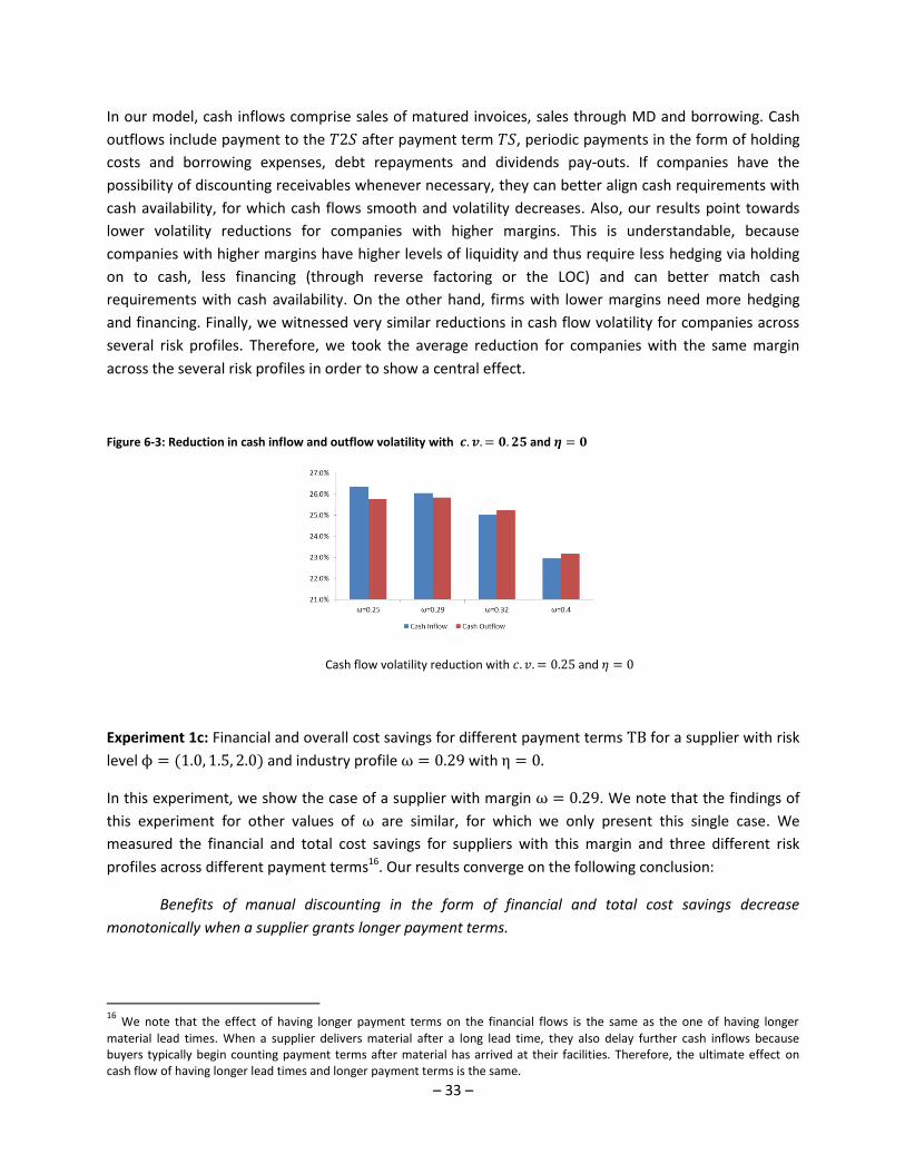
– 33 –
In our model, cash inflows comprise sales of matured invoices, sales through MD and borrowing. Cash
outflows include payment to the 𝑇2𝑆 after payment term 𝑇𝑆, periodic payments in the form of holding
costs and borrowing expenses, debt repayments and dividends pay-outs. If companies have the
possibility of discounting receivables whenever necessary, they can better align cash requirements with
cash availability, for which cash flows smooth and volatility decreases. Also, our results point towards
lower volatility reductions for companies with higher margins. This is understandable, because
companies with higher margins have higher levels of liquidity and thus require less hedging via holding
on to cash, less financing (through reverse factoring or the LOC) and can better match cash
requirements with cash availability. On the other hand, firms with lower margins need more hedging
and financing. Finally, we witnessed very similar reductions in cash flow volatility for companies across
several risk profiles. Therefore, we took the average reduction for companies with the same margin
across the several risk profiles in order to show a central effect.
Figure 6-3: Reduction in cash inflow and outflow volatility with 𝒄. 𝒗. = 𝟎. 𝟐𝟓 and 𝜼 = 𝟎
Cash flow volatility reduction with 𝑐. 𝑣. = 0.25 and 𝜂 = 0
Experiment 1c: Financial and overall cost savings for different payment terms TB for a supplier with risk
level ϕ = (1.0, 1.5, 2.0) and industry profile ω = 0.29 with η = 0.
In this experiment, we show the case of a supplier with margin ω = 0.29. We note that the findings of
this experiment for other values of ω are similar, for which we only present this single case. We
measured the financial and total cost savings for suppliers with this margin and three different risk
profiles across different payment terms16. Our results converge on the following conclusion:
Benefits of manual discounting in the form of financial and total cost savings decrease
monotonically when a supplier grants longer payment terms.
16
We note that the effect of having longer payment terms on the financial flows is the same as the one of having longer
material lead times. When a supplier delivers material after a long lead time, they also delay further cash inflows because buyers typically begin counting payment terms after material has arrived at their facilities. Therefore, the ultimate effect on cash flow of having longer lead times and longer payment terms is the same.

– 34 –
When a firm discounts a receivable, the total financial cost it pays for doing so depends on the volume
of the invoice, the interest rate and the time to maturity. Provided that invoice amount and interest rate
are fixed, the longer the time to maturity is, the higher the financial cost will be. Hence, if payment
terms are longer, the time to maturity will be higher too. For this reason, companies that already offer
long payment terms to their customers benefit less from MD than firms who offer shorter terms. This
can be seen in the figure below. Both financial and total cost savings decrease for suppliers with higher
payment terms. Consistent with earlier experiments, we can also appreciate that companies with higher
𝜙 benefit more than companies with lower 𝜙 irrespective of the 𝑇𝐵 level.
Figure 6-4: Financial and total savings for several payment terms with 𝜼 = 𝟎
(a) Financial savings for different 𝑇𝐵 with fixed
parameters ω = 0.29, 𝑐. 𝑣. = 0.25 and 𝜂 = 0 (b) Total savings for different 𝑇𝐵 with fixed parameters,
ω = 0.29 c. v. = 0.25 and η = 0
Experiment 1d: Supplier financial and cost savings for different risk and industrial profiles and with cost
of holding receivables 𝜂 equal to the cost of discounting 𝛾.
In this experiment we also observe a general relationship between cost savings, 𝜙 and 𝜔:
The financial and total savings achieved through automatic discounting with respect to the BAU
setting increase monotonically with risk profile, and are higher for companies with higher gross margin.
As in experiment 1a, financial and total cost savings increase for companies with a higher risk profile
relative to companies with lower risk profile. This occurs due to the interest rate arbitrage 𝛽 − 𝛾.
Contrary to experiment 1a, companies with higher margins benefit more than firms with lower margins.
As a first consideration, benefits from AD are considerably less than in experiment 1a. The reason for
this is the following. When there is a cost of holding receivables equal to the cost of discounting, firms
would rather cash in the receivables than leave them on their balance sheet. Consequently, there are
considerable savings on the cost of holding receivables, which are however mostly offset by the cost of
discounting as 𝜂 = 𝛾. Furthermore, the cash management model dictates that all excess cash
𝐶𝑡 − 𝑇𝐻𝑚𝑎𝑥 is paid out in the form of dividends. Consequently, most of the extra liquidity achieved
through AD is lost as dividends and the supplier still has a similar borrowing behaviour, leading to only a
small reduction in borrowing costs. Likewise, cash levels are slightly lower as in the BAU case due to
quicker cash, which changes the cash policy. Therefore, financial and total savings in the form of AD are

– 35 –
much lower than in the MD case. However, we expect that if a firm values the cost of holding
receivables to be higher than the cost of discounting, savings will be higher.
Also, we saw that under AD benefits are higher for companies with higher gross margin. As discussed,
extra liquidity obtained through AD usually leaves the company early through expenses, debt
repayments or dividends, meaning that suppliers still have significant borrowing costs. Companies with
higher margins have higher liquidity than those with lower margins, meaning that they have a lower
need of financing. Companies with lower margins still have similar borrowing and cash holding
behaviour. As well, quicker cash and at a higher margin means that these firms need less amount of
cash to hedge against uncertainty, from which it follows that they have a lower opportunity cost of
holding cash relative to firms with lower margins. Thus, benefits from AD are higher for these suppliers.
Our results are summarised in Figure 6-5.
Figure 6-5: Financial and total savings with 𝜼 = 𝜸
(a) Financial savings with fixed parameters 𝑐. 𝑣.= 0.25
and 𝜂 = 𝛾 = 3% (b) Total savings with fixed parameters 𝑐. 𝑣. = 0.25 and
𝜂 = 𝛾 = 3%
Experiment 1e: Average reduction in cash flow volatility for different industrial profiles with 𝜂 = 𝛾
In this experiment we also measured cash inflow and outflow volatility. Although we also found
reductions as in Experiment 1b, our results contrasted in the following way:
There is a substantial reduction in cash inflow and outflow volatility when adopting automatic
discounting, which is more pronounced for companies with higher gross margins.
The reason for cash flow volatility reduction through AD is the same as in the case of MD. There are two
differences: AD reduces volatility considerably more than MD, and suppliers with higher gross margins
reduce cash flow volatility at a higher degree. When applying AD, there is no decision to discount, as all
receivables are discounted 𝜒 days irrespective of the cash position. This smooths cash flow levels. We
also know from literature that longer payment terms and lead times induce higher variance. Being able
to reduce considerably payment delays and at an automatic manner makes cash flow volatility to be cut
dramatically. The same rationale applies for cash outflows. Suppliers who have a constant stream of
cash inflows are able to smooth their cash outflows, especially dividends and debt repayments.

– 36 –
With respect to higher variance reduction for suppliers with higher margins, we can apply the same line
of thought as in Experiment 1d. As discussed, companies with higher margins require less financing and
cash when applying AD relative to companies with lower margins. This enables a lower amount of and
more predictable cash transactions, especially borrowing, repaying debt and paying out dividends.
Hence, they enjoy a higher reduction in cash inflow variance relative to suppliers with lower margins.
Figure 6-6: Reduction in cash inflow and outflow volatility with 𝜼 = 𝜸
Financial savings with fixed parameters 𝑐. 𝑣.= 0.25 and 𝜂 = 𝛾
Experiment 1f: Financial and overall cost savings for different payment terms TB for a supplier with risk
level ϕ = (1.0, 1.5, 2.0) and industry profile ω = 0.29 with η = γ.
As in Experiment 1c we selected the case of a supplier with margin ω = 0.29. We measured the
financial and total cost savings for suppliers with this margin and three different risk profiles across
different payment terms. Our results converge on the following conclusion:
Benefits of automatic discounting in the form of financial cost savings decrease monotonically
when a supplier faces longer payment terms but increase slightly in the form of total cost savings.
The reason why reverse factoring becomes less attractive for companies with longer payment terms in
terms of financing savings is the same as in the case of AD: longer payment terms entail a higher time to
maturity and thus higher financing costs. Therefore, financial savings decrease to lower payment terms.
We can also appreciate that the impact of longer payment terms on savings is much smaller when
considering total costs, and we even see a small reverse in the trend. Whilst in the MD case benefits on
total savings decrease with payment terms, in the AD case the opposite occurs. We have not found a
clear explanation for this effect. However, we theorise that this is due to the cash policy design, which
causes that extra liquidity via AD leaves the firm in the way of dividends, causes financial savings to be
much smaller than in the MD case. Also, having in fraction 1 − 𝐺𝐶𝐴𝐷∗ /𝐺𝐶𝐵𝐴𝑈
∗ , financial costs less than 1
and operations costs bigger than 1, coupled with financially small savings and no operations savings,
might be the cause for the change of trend.

– 37 –
Figure 6-7: Financial and total savings for several payment terms with 𝜼 = 𝜸
(a) Financial savings with fixed parameters
𝑐. 𝑣. = 0.25 and 𝜂 = 𝛾 = 3% (b) Total savings with fixed parameters 𝑐. 𝑣. = 0.25 and
𝜂 = 𝛾 = 3%
6.2.2 Results from Experiment 2
Here we discuss the results on the second block of experiments, which aims at answering RQ3 and RQ4.
Experiment 2a: Effect on total costs for supplier when extending payment terms for scenarios BAU and
MD with no opportunity cost rate for holding receivables
In this experiment we explore the effect of extended payment terms on conventional financing i.e. BAU
and on reverse factoring with MD and 𝜂 = 0. Also, we study the trade-off between cheaper financing
and extended payment terms through reverse factoring. These studies support the following assertion:
The extension of payment terms induces a non-linear effect on the total cost for the supplier.
This effect can be seen in Figure 6-8 (a), where we assumed an initial payment term of 30 days, and
measured the total cost for the supplier by extending payment terms in steps of 10 days for the BAU
case. Our findings are consistent with literature (cf. van der Vliet, et al., 2015). When extending payment
terms, the overall effect on the total cost that the supplier incurs increases non-linearly.
We have also measured the total cost a supplier faces when being offered reverse factoring with a credit
term extension and also found a non-linearity. We depict this cost in Figure 6-8 (b). The blue line is the
same as in Figure 6-8 (a) but due to the scale it looks linear. The red line is the total cost with MD. As
seen, it has a curvilinear form and it grows at a much higher rate than the BAU blue line. The green line
denotes 𝐺𝐶𝐵𝐴𝑈∗ with initial 𝑇𝐵 = 30. In this specific scenario, we even see that after an extension to 100
days the cost under MD is higher than both the BAU cost with the original and with the extended
payment terms. Consequently, we conclude the following:
When extending payment terms, benefits for the supplier decrease relative to the equivalent
BAU total cost with extended payment terms and also relative to the BAU scenario with the original
payment terms.

– 38 –
Figure 6-8: Extended payment terms with 𝒄. 𝒗. = 𝟎. 𝟐𝟓,𝝓 = 𝟏. 𝟎 and 𝜼 = 𝟎
(a) Total BAU costs with 𝑐. 𝑣.= 0.25,𝜙 = 1.0, 𝜔 =0.29 and 𝜂 = 0%
(b) Total BAU and MD costs with 𝑐. 𝑣.= 0.25,𝜙 = 1.0,𝜔 = 0.29 and 𝜂 = 0
We made the same experiment for a supplier with a higher risk profile 𝜙, which is depicted in Figure 6-9.
We can observe the same effects as in Figure 6-8: non-linearity in total cost when payment terms
extension and a decrease in benefits with the increase on payment terms. When comparing Figure 6-9
(b) with Figure 6-8 (b) we find that suppliers with a higher risk profile have higher benefits 𝐺𝐶𝐵𝐴𝑈∗ −
𝐺𝐶𝑀𝐷∗ when being offered reverse factoring with payment term extension 𝑇𝐵 + 𝑥 than suppliers with a
lower risk profile. We assert the following:
The effect of a payment term extension on the supplier depends on the supplier’s cost structure.
Suppliers with higher risk profile 𝜙 have higher benefits when facing a payment term extension 𝑇𝐵 + 𝑥
than suppliers with lower risk profile when offered reverse factoring with extended payment terms.
Figure 6-9: Extended payment terms with 𝒄. 𝒗. = 𝟎. 𝟐𝟓,𝝓 = 𝟐. 𝟎 and 𝜼 = 𝟎
(a) Total BAU costs with 𝑐. 𝑣.= 0.25,𝜙 = 2.0, 𝜔 =
0.29 and 𝜂 = 0% (b) Total BAU and MD costs with 𝑐. 𝑣.= 0.25,𝜙 = 2.0,
𝜔 = 0.29 and 𝜂 = 0
In order to test the effects of demand volatility, we have repeated the experiment with a higher
coefficient of variation. These results are summarised in Figure 6-10. From these, we suggest:

– 39 –
The effect of a payment term extension on the supplier also depends on demand volatility.
Higher volatility induces a higher non-linearity effect on the total cost. Under higher demand volatility,
suppliers with higher risk profile 𝜙 also have higher benefits when facing a payment term extension
through reverse factoring than suppliers with lower risk profile.
Figure 6-10 shows a similar effect than in the previous two figures, with the difference that there is a
higher non-linearity in the total cost curves. Thus, we also infer:
The higher the demand uncertainty is, the higher the non-linearity effect induced to the total
cost of managing a cash and inventory system.
Likewise, we can see that unlike in Figure 6-8 (b), the cost of reverse factoring with payment terms
extension becomes higher after a longer extension (120 days versus 100 days).
Figure 6-10: Extended payment terms with 𝒄. 𝒗. = 𝟏. 𝟎,𝝓 = (𝟏. 𝟎, 𝟐. 𝟎) and 𝜼 = 𝟎
(a) Total BAU and MD costs with 𝑐. 𝑣.= 1.0, 𝜙 = 1.0, 𝜔 = 0.29 and 𝜂 = 0
(b) Total BAU and MD costs with 𝑐. 𝑣.= 1.0, 𝜙 = 2.0, 𝜔 = 0.29 and 𝜂 = 0
Experiment 2b: Supplier indifference curve between BAU and reverse factoring with payment term
extension and price reduction
In this experiment we looked for the supplier indifference curve between net profit at BAU and SCF. We
specifically looked for MD with a price cut 𝑦 and a payment term extension 𝑥 that yields the same profit
to the supplier as in the BAU case with 𝑥 = 𝑦 = 0. Payment term extensions impact the supplier’s cost,
but a price cut changes the supplier’s revenue. Therefore, we need to consider net profit when drawing
the supplier indifference curve. We calculate average net profit per period as follows:
𝐴𝑣𝑒𝑟𝑎𝑔𝑒 𝑛𝑒𝑡 𝑝𝑟𝑜𝑓𝑖𝑡 𝑝𝑒𝑟 𝑝𝑒𝑟𝑖𝑜𝑑 = 𝐴𝑣𝑒𝑟𝑎𝑔𝑒 𝑟𝑒𝑣𝑒𝑛𝑢𝑒 𝑝𝑒𝑟 𝑝𝑒𝑟𝑖𝑜𝑑 − 𝐴𝑣𝑒𝑟𝑎𝑔𝑒 𝐶𝑂𝐺𝑆 𝑝𝑒𝑟 𝑝𝑒𝑟𝑖𝑜𝑑 − 𝐺𝐶(.)
∗
=1
𝑇∑𝑝 ∙ 𝐷𝑡
𝑇
𝑡=1
−1
𝑇∑𝑦 ∙ {𝑐 ∙ 𝑄3 + 𝑓}
𝑇
𝑡=1
− 𝐺𝐶(.)∗
(6-2)

– 40 –
where the first term refers to average demand per period, the second term refers to the average
expenses when ordering 𝑄3 from the 𝑇2𝑆 and 𝑦 ∈ (0,1) is equal to 1 when the 𝑇1𝑆 orders raw material
at period 𝑡 and is 0 when he does not order.
As reported by SC professionals and academics collaborating in this project, typically buyers want to
extend payment terms that are currently low i.e. 30 days to 60 or 90 days, and it is less common that
they demand extensions when payment terms are already high. Likewise, in many European countries
average payment terms are around 30 days (EOS Group, 2014). We also know that benefits of SCF are
lower for suppliers who have already long payment terms. Hence, our experiment considers the case of
a supplier, who currently offers payment terms 𝑇𝐵 = 30, and measure the effect when 𝑇𝐵 is increased
in steps of 10 days. Also, we consider risk profiles 𝜙 = (1.0, 2.0) and 𝜂 = 0. We conclude the following:
The price cut 𝑦 coupled with payment term extension 𝑥 that leaves the supplier indifferent
between BAU and SCF is too small to justify its implementation.
As seen in Figure 6-11, the price reductions necessary to leave the supplier indifferent are well below
0.3%. This is because the financial cost savings through SCF are very small with respect to the overall
costs. Likewise, the impact of payment terms extension on total cost and net profit is minimal. In this
sense, even though SCF has a big effect on financial and total costs, it does not affect much net profit.
Hence, the necessary price cut to leave the supplier indifferent has to be very small. These findings are
consistent with common supply chain practices, where price reductions are not conceded by suppliers
when joining a SCF programme. In any case, suppliers with higher risk profile and with higher demand
volatility are better positioned to concede higher price cuts. This is consistent with our earlier findings:
suppliers with higher risk profiles and higher demand volatility benefit the most from SCF solutions.
Even though these findings suggest that price cuts are not sufficient to justify their implementation, we
can expect that on a real setting, a company with a very high leverage, high financial costs and high
demand volatility could concede a more significant price reduction to remain indifferent. Therefore, we
suggest that the decision, if considered, should be studied carefully.
Figure 6-11: Supplier indifference curve for payment term extension and price cut
(a) Admissible cost reduction 𝑦 for payment term
extension 𝑥 with 𝑇𝐵 = 30, 𝑐. 𝑣. = 0.25, 𝜙 = (1.0, 2.0), 𝜔 = 0.29 and 𝜂 = 0
(b) Admissible cost reduction 𝑦 for payment term extension 𝑥 with 𝑇𝐵 = 30, 𝑐. 𝑣. = 1.0, 𝜙 = (1.0, 2.0), 𝜔 = 0.29 and 𝜂 = 0

– 41 –
7 The potential role of a LLP
The experiments and numerical results have provided a better understanding of SCF solutions under
complex systems. Based on our findings, we address the potential role of a LLP in SCF solutions. We also
point out several managerial insights, strategic considerations and special recommendations. Therefore,
this chapter answers research questions RQ5, RQ6 and RQ7.
7.1 The potential role of a logistics company
Logistics companies have been successful in the provision of transportation and logistics services to
physical supply chains. LLPs have taken over the role of providing SCI services for the PSC in order to
improve SC efficiency and operations performance. However, not much has been discussed about the
role of these companies in the P/FSC integration. In the following paragraphs we study how logistics
companies could tap their potential and direct their activities to also integrating the financial supply
chain. We discuss three scenarios in which LLPs could operate: business as usual, SCF with no
refinancing and SCF with refinancing.
7.1.1 Business as usual
In this section we describe the BAU model followed currently by certain LLPs. LLPs are firms that take
over the transportation, logistics and supply chain management activities of their customers, typically
material goods buyers. They are the party that serves as the interface between transportation providers
or carriers and their buyer or receiver. By integrating information flows, they look for efficiencies and
cost savings in the PSC in order to improve their customers’ performance and bottom-line results.
Generally the BAU model operates as follows: the buyer sends purchase orders (POs) to material
suppliers, who bundle them and send transportation requests (TRs) to LLPs.17 Based on contractual
agreements, strategic considerations or operations convenience, LLPs select the most suitable
transportation supplier i.e. a carrier, who will deliver the goods to the buyer. The buyer compensates
the material supplier for the goods and the LLP for the transportation activities. On top of that, the LLP
charges a (fixed) management fee to the buyer. The LLP subsequently compensates the carriers for the
transportation services.18 In parallel, the material supplier goes to a FSP e.g. a bank to finance her
working capital, albeit typically at a high cost. This model is represented schematically in Figure 7-1.
Under BAU the LLP serves as a PSC integrator: all information flows related to the PSC converge to the
LLP, who increases visibility and commits to operational improvements. In this sense, by centralising
17
The LLP is also responsible for bundling i.e. consolidating POs and/or TRs into consolidated shipments. In many cases the LLP
is dependent on the supplier to provide the actual ready to ship date, hence the supplier bundles POs ready at the same day. However the LLP checks, triggers and consolidates further if possible and necessary. 18
By collecting payments for transportation services on behalf of carriers, the LLP already integrates to some extent the FSC,
although this does not purely represent a SCF solution.

– 42 –
information and the decision making process, the LLP improves the SC network design to achieve
savings and efficiencies. In this scenario there is no integration of the FSC – there is no entity that
actively aims at integrating it and look for efficiencies. Hence, each company independently manages its
financial policy irrespective and very often at the expense of other firms. As shown in Figure 7-1, the
supplier requests credit from a FSP independently of the financial activities of other SC partners.19
Figure 7-1: Conceptual framework – BAU
7.1.2 SCF with no refinancing
As reported in literature, typically when SCF is implemented, it is done independently of the LLPs: buyers
approach a FSP, which provides financing via reverse factoring to the buyer’s material suppliers. Even
though this has proven to be an effective way of decreasing working capital volume and its related cost,
sometimes SCF implementations have failed (Seifert & Seifert, 2011), arguably either due to errors in
implementation and execution and/or bad designs.
There are several conflicts of interests that permeate a supply chain. While buyers want to increase
payment terms to reduce days payable outstanding (DPO) and reduce their cash conversion cycle (CCC),
suppliers want to reduce payment terms to reduce days sales outstanding (DSO) and also reduce their
CCC. This creates a conflict of interests, which is usually solved via negotiation. Even though SCF
solutions help to (partly) resolve these conflicts of interests (Hofmann, 2009), very often suppliers – who
have a lower bargaining power – are unsatisfied after SCF implementations. This is exemplified by Milne
(2009), who has reported that certain corporations have introduced RF as a ‘sweetener’ to an unpopular
decision to increase payment terms to suppliers. Several researchers and this study have concluded that
this is an inefficient strategy since it induces a non-linear financing cost beyond the opportunity cost of
carrying additional receivables (Tanrisever, et al., 2012; van der Vliet, et al., 2015), which may be difficult
to predict under stochastic settings.
19
Although each company requests financing from FSPs, for simplicity we do not show this in our schematic model. Also, since
supplier performance is the focus of this study, we only concentrate on the supplier financial activities.

– 43 –
Another conflict of interests emerges when a company borrows from a FSP, where the latter demands a
risk-adjusted price for the provided debt capital in the form of interest. In order to calculate the price,
the FSPs have an internal rating process to assess the creditworthiness of the borrower, which requires
information provided by this company. As Hofmann (2009) discusses, the borrower (agent) knows his
own creditworthiness very well but he does not wish to share this information to the full extent with the
lender (principal), leading to problems of asymmetric information distribution, for which transaction
costs arise (e.g. information costs, negotiation costs, monitoring costs).
These two conflicts pose a challenge to SCs. The possibility to design a solution to circumvent these may
prove to be a valuable proposition for SC participants. We suggest that a good possibility to solve the
described issues is to add an external company to the FSC that can proactively seek for a solution that
mitigates the conflicts of interests and creates value for all the involved parties. This necessitates that
this party has also sufficient knowledge and information about the SC, its operations and risk. Also, this
entity needs to be an expert in implementations and executions. LLPs are recognised for being execution
champions, which makes them a good candidate to fit this role. Also, LLPs are firms that already work
close to the PSC of its customers and have sufficient knowledge of the supply chains they serve.
Furthermore, LLPs are companies with experience on supply chain integration, possess a good IT
infrastructure and analytical capabilities, and have sufficient data of the SCs they manage. They could
leverage their position to design, plan and orchestrate the activities of the FSC and integrate the P/FSC.
This new potential role does not represent a trivial challenge for the FSC integrator. Firstly, having to
mediate between SC companies with conflicting interests is by itself a very hard task. Secondly, as
buyers usually want to increase payment terms, the SC integrator would have to carefully gauge the
non-linear effects on the total costs of the supplier and on overall SC performance. This task is made
harder under a stochastic setting and long payment terms. Moreover, the overall impact on the supplier
depends on the cost structure of these firms, especially under manual discounting (van der Vliet, et al.,
2015). This causes that the analysis and design of an appropriate solution to be more complex and
demanding, for which an experienced firm is required. Also, knowing well the SC and having the right
experience to approach the lack of integration of the FSC is vital to engineer a good solution, which by
no means is an easy undertaking. An LLP may prove to be the company with the necessary knowledge of
the supply chain that also has good analytic means and experience to carry out this analysis and design.
Finally, another advantage of having an LLP as the designer and orchestrator of SCF solutions is that this
firm can use its position in order to look for the most competitive interest rate for the supply chain in
the ways of providing better information visibility and transparency to the FSP. This will lessen the
second conflict of interest pointed out hereinbefore: FSPs will have more and better access to the
operations and financial activities of the supply chain, reducing thus the transaction costs and in this
way the interest rate they charge.
Figure 7-2 proposes a conceptual framework of how a LLP could provide P/FSC services. Under this
model, the LLP gathers information of the material and financial flows of the supply chain and designs
an appropriate SCF solution in collaboration with the SC partners that guarantees that there is value
creation for all partners, and that the proposed solution does not hurt (significantly) the interests of a
particular partner. Also, the LLP pays special attention in reducing information asymmetries, and works

– 44 –
towards integration the material and the corresponding financial flows. For this end, an electronic
platform is set for the exchange of information between the parties, and simultaneously orchestrates
the operations and financial activities of the supply chain. By improving information visibility, several
efficiencies are to be found, which will yield higher performance and savings. However, despite these
benefits, the information asymmetry issue between capital providers and the supply chain may not be
completely solved and asymmetries may always remain. Also, FSP participation and commitment is a
critical success factor. The LLP also needs a very deep understanding of SCF, as well as analytic and IT
capabilities to deliver sufficient value creation to supply chains. Finally, the LLP may be required to
engage in certain costs e.g. by hiring financial specialists and investing in an (improved) electronic
platform. However, the platform could be provided by the FSP.
A specific and deep business model for the LLP for this scenario is left out of scope of this dissertation.
However, based on the current business model for the PSC integration, we infer that LLPs could charge a
(fixed) management fee for their commitment to cost savings and higher performance. Also, a possibility
where the LLPs can obtain a fraction of savings above expectations may further align SC interests.
Figure 7-2: Conceptual framework – SCF with no refinancing
7.1.3 SCF with refinancing
In the scenario without refinancing, the FSP is the only party that provides financing to the supply chain.
There exists however another possibility, where the LLP provides direct financing to the supply chain
and that she refinances with a FSP. Hence, the tier 1 financing is given by the LLP and the tier 2 by the
FSP. This scenario is represented schematically in Figure 7-3. This new possibility brings in further
benefits and challenges for the supply chain. These are discussed below.
The first and foremost advantage for the supply chain is that having the LLP directly financing the SC
causes that there is a better alignment of interests between the LLP and the SC partners. Furthermore,
being a party that better understands the SC risks, and by having a lower information asymmetry, the
LLP could provide a more competitive rate than the one the FSP would offer. When the LLP also faces SC

– 45 –
risk, she will be inclined to be more selective when deciding which parties and invoices to finance20. By
taking over this risk (instead of the FSP), the interest charged by the FSP may be even lower, as the LLP
will only take over manageable risks. Also, for the LLP this may represent a further opportunity of
increasing revenues and increasing overall margins. Specifically, the new revenue stream will be the
difference between the interest the LLP offers to the supply chain via RF and the interest that she pays
to the FSP for refinancing this volume. Also, in case that the LLP is a creditworthy company, this could
improve her profitability as it may be offered a lower refinancing interest.
There are certain disadvantages of this scenario. First, a potential conflict of interests between the LLP
and the SC could take place. As the new revenue stream for the LLP improves with a higher interest
charged to the supply chain, the LLP may be motivated to charge a higher interest to borrowers. This
opportunistic behaviour can be contractually controlled by committing the LLP to deliver certain cost
savings and efficiencies and setting good rewards in case performance is higher as expected. Another
disadvantage of this scenario is that it necessitates that the LLP has a very high creditworthiness in order
to (1) guarantee a low refinancing rate and (2) assure that its credit rating is not impacted considerably
by increasing its risk exposure to payment defaults. The LLP needs to also understand very well all the
risks that she is assuming e.g. country (political and economic), industry, firm specific risks, etc. Failure
to understand them may prove to be highly dangerous. Finally, a final drawback is that the LLP may be
required to engage in certain costs e.g. by hiring financial specialists and investing in an (improved)
electronic platform, which otherwise would be provided by the FSP. However, Aberdeen Group (2007)
notes an average investment of € 0.1-1.5 million in the electronic platform may be quickly recovered.
Figure 7-3: Conceptual framework – SCF with refinancing
In the table below, we present an overview of the advantages and concerns from each of the three
possible scenarios that have been discussed hereinbefore.
20
Nevertheless, the LLP has resources to significantly reduce this risk. A possibility is having a frame contract between the SC
parties at place, and also having a payment guarantee contract with the buyer to assure that no default will take place.

– 46 –
Table 7-1: Advantages and Concerns of SCF Scenarios
Scenario Advantages Concerns
Business As Usual Every party is independent and flexible to decide its own cash management policy.
Convenient when supplier-buyer relationship is short term and/or not strategic.
Inefficient allocation of capital in supply chains.
Supplier weakening and higher disruption risk.
No party proactively integrates FSC.
No long-term value creation.
Lack of integration of P/FSC
SCF with No Refinancing LLP actively seeks to create value and find efficiencies.
FSP has better access to SC information and visibility, enabling lower borrowing cost.
Full participation of FSP may bring in better experience and know-how of SCF to supply chain.
LLP concentrates solely on solution orchestration.
No conflict of interests between LLP and supply chain.
Challenge to mediate between SC partners and between SC and FSP.
LLP requires deep financial understanding, as well as analytic and IT capabilities to create value.
FSP participation and commitment is critical success factor.
Information asymmetry (though lessened) between supply chain and capital provider remains.
LLP may require investing in resources to provide orchestration activities.
SCF with Refinancing LLP actively seeks to create value and find efficiencies while controlling for risk exposure.
Supply chain outsources transaction costs related to finding financing to the LLP.
Information asymmetry between capital provider i.e. LLP and supply chain is minimal.
LLP may offer lower interest rate than FSP due to better SC understanding.
SC and LLP interests are aligned thanks to LLP’s risk exposure.
LLP has new source of income.
Convenient when LLP has better credit rating than buyer.
Challenge to mediate between SC partners and between SC
LLP requires deep financial understanding, as well as analytic and IT capabilities to create value.
LLP has to be a very creditworthy company.
LLP is exposed to new default risks, for which its credit rating and borrowing rate may be impacted.
LLP has motivation to charge higher rate to achieve higher profits (this behaviour can be minimised through contracts).
LLP may require investing in resources to provide orchestration and financing activities.
7.2 Strategic considerations
Having discussed the main takeaways of this study and the potential roles of a LLP in a SCF solution, we
proceed now with strategic considerations, which are mostly based on the experiments. With these, we
aim at pointing out managerial issues to be addressed to assure that the LLP can propose a value adding
solution to its customers and their supply chains.

– 47 –
7.2.1 Customers to approach / target groups
Based on the experiments, suppliers with lower gross margins benefit the most from SCF solutions.
Based on the research of Damodaran (2015), where he obtained the margins for several industries in the
US, we propose certain manufacturing industries that could potentially benefit from SCF. In this study
we used gross margin (revenue minus cost of goods sold) to define one of the dimensions of supplier
profile. The closest indicator to our definition of gross margin in Damodaran’s survey is 𝐸𝐵𝐼𝑇𝐷𝐴+𝑆𝐺&𝐴
𝑅𝑒𝑣𝑒𝑛𝑢𝑒.21
Based on the data published by Damodaran (2015), the average gross margin of all industries was
30.42%. As a rule of a thumb, we selected the industries that are below or slightly above this average.
We found that Steel, Auto Parts and Trucking, Retail (Automotive, Grocery and Food, General and
Online) Aerospace/Defence, Hospitals/Healthcare Facilities, Chemical, Construction and Building,
Packaging & Container, Paper, Shipbuilding & Marine, Rubber & Tires, Electronics, Metals & Mining,
Semiconductor Equipment and Machinery are good candidates for SCF, as all these have a margin
between 14 and 35%. The complete list of industries and margins is found in Appendix 11.
It is also well known that industries begin after certain time to “commoditise”, for which margins tend to
become smaller and competition rougher. The LLP should pay attention to this trend and find
commoditising industries, since they may become excellent recipients of SCF solutions.
It is also important to select the kind of companies that would be more interested in SCF as a VAS by the
LLP. We recommend that the LLP addresses clients, with whom she already has a long relationship,
rather than new customers. Having more trust, knowledge of the customer and her supply chain, and a
story of successes may serve as arguments for the LLP to better persuade the customer to join a SCF
programme. Nevertheless, we do not discard a possible scenario in which a new customer may be
motivated to join a SCF programme.
Furthermore, depending on whether the approached LLP customer would act as a supplier or as a buyer,
we recommend the LLP to specifically follow these points to assure higher success possibilities:
Suppliers – In case the party is a supplier, we consider an outbound supply chain, where the supplier
sells his goods to several customers. We recommend the following buyer profile to approach:
The supplier needs to have a moderate to high risk and hence a high cost of financing to
maximise interest rate arbitrage and thus financial savings.
SCF relies on coordination, cooperation and information sharing, for which the supplier needs
to have a well-developed and long-term relationship with the buyer to assure buyer interest
If a buyer wants to extend payment terms, SCF may prove to be a win-win solution for the
companies. The role of the LLP may prove crucial to assure that the supplier obtains a good deal
and does not lose too much value when extending payment terms.
21
EBITDA refers to Earnings before Interests, Taxes, Depreciation and Amortization. SG&A denotes Selling, General and
Administrative Expenses. By summing these two amounts we arrive to Gross Revenue.

– 48 –
If customer demand is uncertain, the supplier benefits more. The LLP should look for these
kinds of suppliers to increase savings.
If the supplier already grants long payment terms, SCF may let her have access to have cheap
financing, despite benefits being lower to firms who grant shorter payment terms.
Suppliers located in developing economies, and especially SMEs, have limited sources of
financing, which are often expensive and require significant collateral. Suppliers in developing
markets are very good candidates for SCF.
Buyers – In case the approached party is a buyer, we consider the case where a buyer offers SCF to a
group of suppliers. We recommend the following buyer profile to approach:
Buyers that are looking to improve the overall performance of their SC, reduce disruption risk
and increase supply chain strength may find in SCF a good strategy to achieve these goals.
Buyers that strongly rely on specific suppliers may feel more inclined to help these suppliers
become (financially) stronger.
Buyers that are interested in including a considerable amount of their supply base (at least 60%)
in the first wave have better possibilities of success (Seifert & Seifert, 2009)
Buyers that are interested to propose SCF to their suppliers but that are unsure about its
consequences, how to design it, negotiate and implement it, may be also excellent candidates to
hire the LLP to conduct the design and orchestration activities.
Buyers dealing with suppliers located in developing countries may be even keener on exploring
offering SCF to their suppliers.
7.2.2 Defining the role to follow
We have pointed out two roles that the LLP could follow. Now, we provide certain factors LLPS may
consider when deciding which role to follow. Nevertheless, we emphasize that it is possible that the LLP
follows both roles simultaneously, depending on several strategic considerations.
SCF with no refinancing: We recommend SCF with no refinancing if:
The LLP does not have a competitive borrowing rate and good credit rating.
The LLP has strong reasons to believe that financing the supply chain would have an impact in its
creditworthiness and credit rating due to higher risk exposure.
There are no sufficient resources to limit risk exposure for financing supply chain.
The supplier in question is located in a geography with high perceived country risk (political and
economic), currency risk (exchange rate, devaluation) and cultural risk (cultural patterns,
honouring contractual obligations), for which selecting a (local) FSP may be more convenient.22
The supplier is located in a geography where the LLP cannot find a landscape to serve the needs
of the LLP’s customer
22
This represents an example in which the LLP may not provide financing to a specific supplier within the whole supplier base
e.g. due to her higher geographic risk, but may simultaneously finance other suppliers.

– 49 –
SCF with refinancing: We recommend SCF with refinancing if:
There is a considerable positive spread between the offered rate to the SC and the LLP
borrowing rate, which would justify the new risk exposure.
The new revenue flow has a considerable good impact on LLP margins and profitability.
The internal due diligence has positive results and the LLP has good resources to limit risk
exposure e.g. via a guarantee contract.
The SC supports LLP financing in order to align the LLP interests (especially via risk exposure)
with the ones of the SC.
It is possible to set a good contractual structure in order to control conflict of interests where
the LLP wants to maximise profit at the expense of the SC. This can be done by commitments of
the LLP to deliver SC savings and increased performance.
7.2.3 Approach to the Financial Service Provider
Similar as in the case of the customer, we believe that the best FSPs to approach are the ones with
whom the LLP or the buyer already has a long relationship and trust. This may enable that better
knowledge facilitates the introduction of a SCF solution. However, a new FSP may also prove to be a
good option if current or past FSPs have not been very successful. Also, we recommend LLPs to look for
FSPs that already have experience in providing SCF and reverse factoring. Finally, Seifert & Seifert (2009)
suggest that having a FSP with a good bank’s geographic reach, legal expertise and its financial muscle is
crucial for a successful SCF implementation.
Once a FSP has been selected, the LLP may approach her accompanied with the buyer, especially in the
case of no refinancing, since the latter is the party that ultimately borrows from the FSP, even though
the suppliers pay the financial cost. By committing to provide further visibility and information to the
FSP, information asymmetries should decrease and with it transaction costs, leading to a more
competitive interest rate offered to the SC. The LLP and the buyer should also make sure that the FSP is
also considered a partner under the SCF mechanism and not a mere financial provider. As such, the FSP
should also be provided with a win-win deal that satisfies her interests. Furthermore, it should be
emphasised that the FSP gets access to new markets and new customers. Also, special attention needs
to be given that the FSP has new sources of income at a low risk. And despite the interest rate is low, the
transaction volume may prove to be a sufficient flow of income to justify the FSP participation. Another
advantage for the FSP is that she can effectively build credit history of the borrowers (possibly for future
commercial relations) and serve companies that were once inaccessible, especially SMEs. Also, in the
case of suppliers located in emerging economies, whose access to conventional financing is low due to
market frictions and lack of maturity of the financing industry, the FSP could educate them and facilitate
future commercial relationships. Hence, this could prove to be a good chance for the financing sector to
penetrate a new market without facing a significant risk.
If the FSP is approached for a refinancing deal, the risk does not lie anymore (or at least directly) with
the buyer and the supply chain, but with the LLP. Therefore, the creditworthiness of the LLP will be

– 50 –
crucial to assure that the FSP wants to join the programme and that she offers a competitive interest
rate. Consequently, the LLP should exhaust all resources to reduce her exposure to risk.
7.2.4 Other strategic considerations
LLPs also need to pay attention to van der Vliet’s (2015, p. 18) typology of SCF practices. The author has
defined two dimensions for SCF practices: strategic objectives and implementation tactics. These
dimensions are considered strategic and tactical because they concern decisions on the aims of SCF and
on the methods used to reach those aims respectively. As a first step, the LLP needs to identify and if
necessary, guide the strategic objectives of the customer. This dimension has Transaction-oriented SCF
on one extreme and Competence-oriented SCF on the other. Each one is defined as:
Transaction-oriented SCF: focus on achieving transactional benefits through working capital
benefits or savings in capital cost e.g. payment terms extension and/or price reduction.
Competence-oriented SCF: enhance a supply chain competence, such as supply base agility. In
order to realise supply chain competencies it is generally required that firms invest in resources.
As pointed out hereinbefore, the motivation of the buyer could be to improve her working capital
position and achieve savings through SCF. On the other hand, the buyer may be seeking to improve the
competencies of her supply chain, for which SCF may be adopted to demand supplier investments in
performance. For instance, savings may be used by the material supplier to increase capacity, product
quality and reduce lead times. As these two ends in this dimension are opposites, it is important that the
LLP recognises the buyer’s objectives, and possibly guides the supply chain (through his role as
mediator) to a goal that brings value to each entity in the supply chain.
The second dimension, Implementation Tactics, has also two opposite dimensions:
Uniform Implementations: the initiating firm follows roughly a single specification for all SCF
arrangements with participating suppliers
Customised Implementations: the initiating firm adjusts the type and terms of the agreement to
fit the nature their supply relationship(s). Terms offered to each supplier are tailored to the size
of the transactional benefits that SCF yields for each supplier
In the case of uniform implementations, the initiator (typically the buyer) aims at providing several
suppliers roughly the same arrangement. It can be assumed that initiators follow uniform
implementations to avoid the costs of customisation, very often at the expense of suppliers, who may
face an arrangement that harms their performance.
Being execution champions, LLPs could bring supply chains a higher degree of customisation than the
one they would achieve on their own. Van der Vliet (2015) reports that customisation measures may
increase total return of an SCF arrangement, for which a great investment in technology and
administration is necessitated. This investment could be accordingly done by the LLP, possibly with the
cooperation of the FSP. Also, customisation may also entail a more prominent role for the FSP due to
this party’s specialization in financial analysis. Furthermore, for a competence-oriented SCF

– 51 –
arrangement, a customization tactic may even bring about further complexities. For instance, buyers
may be exposed to agency and moral hazard problems. Suppliers may divert extra liquidity and funding
for personal interests or to serve other investments other than the one agreed between the parties e.g.
investment on performance. However, literature on customisation measures for ensuring effective
supply chain investment from SCF arrangements is yet limited (van der Vliet, 2015).
Apart from the discussed strategic considerations, we present other success factors that LLPs should
contemplate. The first and foremost is internal sponsorship. Seifert & Seifert (2009) have found that SCF
implementations are twice as much successful when the CEO leads them rather than the CFO. Hence,
LLPs need to assure a high degree of sponsorship from customers. Likewise, their study acknowledges
that supplier involvement is vital success factor. Their study found out that implementations are most
successful when they include at least 60% of the supply-base in the first wave. Finally, another
important issue to consider is the degree of complexity existing at the SC. As mentioned in the literature
review, SCF entails very often a clear IT challenge, with the risk of data being fragmented and the
challenges of common sharing and interfacing (Steeman, 2014). Despite LLPs are parties that already
deal with high complexity in the PSC, it may be advisable to ask for a more collaborative partnership of
the FSP, especially regarding the IT Platform.
All in all, being an execution expert that serves as a mediator between SC partners, the LLP could
provide a solution that yields better benefits for SC participants than the one they would have on their
own. This can be achieved by delivering a solution that matches the interests of the supply chain (or
convince the SC of a better objective), and by implementing a more customised solution that maximises
total return of the SCF arrangement.

– 52 –
8 Conclusion
This chapter concludes this dissertation. We do so by pointing out the main takeaways from the
experiments, by briefly discussing the potential role of LLPs in SCF solutions and by stating the
limitations to this research, as well as further research opportunities.
8.1 Main takeaways from experiments
In order to provide LLPs with the necessary understanding about SCF solutions, this study built on
previous academic efforts to create a more complex model in order to describe, explain and predict how
SCF creates value in supply chains. For this goal we developed a continuous-time stochastic inventory
and cash management model of a supplier firm that sells finished goods to a single buyer, sources raw
material from a tier 2 supplier and manufactures the goods in an internal plant. In the BAU scenario, the
supplier has a cash management policy that allows him to borrow money from a line of credit in case
the cash level is below a certain threshold, and to repay the debt or pay out dividends in case the cash
level is above a certain threshold. By assuming that the buyer is a creditworthy one, we modelled for the
scenario in which the buyer offers SCF to the supplier in the way of reverse factoring, letting him obtain
quicker cash at a cheaper rate. Specifically, the supplier has the option of discounting all receivables
automatically i.e. as soon as it is possible to sell the receivable to the factor, or manually i.e. whenever
he is required according to the cash management policy.
Our findings are consistent with previous literature that has employed more simplified models. SCF
solutions also create value and improve performance at more complex systems. As this study
acknowledges that a supply chain is as strong as its weakest link – typically suppliers – we have focused
mainly on the performance of these firms. Our approach had its main focus on financial and total cost
savings. When firms reduce their costs, their profitability and their bottom-line improves. Likewise, we
have found that cash flow volatility is significantly reduced through SCF. When firms reduce cash flow
volatility, they also reduce their risk perception and therefore improve their capital sourcing cost, or its
weighted average cost of capital (Brealey, et al., 2011), which enables a higher enterprise value. Also, by
having lower cash flow volatility, suppliers and supply chains can improve their analytic capabilities,
enhance forecasts and make better decisions.
In order to test under which circumstances SCF solutions create (more) value, we have proposed two
main supplier profiles: risk and gross margin. Also, we tested these profiles for suppliers with different
demand uncertainty and with different payment terms. We have found that generally suppliers with a
higher risk profile (and thus higher borrowing costs), lower gross margins, with higher demand
uncertainty and with lower offered payment terms benefit the most. We argue that despite these kinds
of firms are the better recipients of SCF solutions, other suppliers may benefit as well and the decision
to implement SCF should be studied by every firm carefully.

– 53 –
With the purpose of testing company concerns regarding the decision to adopt SCF, we have found in
literature that suppliers mostly are affected when their buyers condition the introduction of SCF with
payment terms extension. Past studies have found out that when buyers extend payment terms, the
total benefits for the supplier are reduced, making it an inefficient strategy (Tanrisever, et al., 2012; van
der Vliet, et al., 2015). These studies have been made with the aid of simplified simulation models. We
were able to validate previous findings on a more complex setting and we have found out that payment
terms extension induces a non-linear effect to the total cost for the supplier, which may be hard to
measure. The extension reduces the benefits that the supplier gains from a SCF solution, and this
reduction depends on the supplier’s cost structure and demand volatility. Hence, we argue that the
decision to extend payment terms under a stochastic setting has to be very well studied by managers.
Finally, this dissertation addresses an uncovered topic in literature – the trade-off between payment
terms extension and price cut. The main motivation for this study is the fact that suppliers typically
transfer their working capital financing costs to their customers when these have aggressive cash
management practices (He, et al., 2011). We looked for the price for a given payment term extension
under reverse factoring that would yield the same profit to the supplier as the one under an initial BAU
scenario with no payment term extension and price cut. Our findings suggest that the price cut required
to leave the supplier indifferent between BAU and SCF with extended payment terms is too low to
justify its implementation. This may explain why this possibility is not practiced in supply chains.
8.2 Final thoughts
In the first pages of this dissertation we have pointed out how the lack of integration in the FSC has led
to a higher disruption risk, lower performance, higher costs, and above all, a structural weakness. When
a supplier has no access to competitive sources to finance working capital, his performance may be
impacted, which ultimately could lead to a disruption. Also, we have discussed that the financial side of
the supply chain could be an area of further efficiencies. This has led to a higher firms’ interest in
managing the FSC with an equally integrated view similar to the applied to the PSC, where the financial
flows can be integrated with the material and information flows. Particularly, opportunities to improve
the efficiency of working capital by unlocking cash trapped in the FSC have been recognised as a
potential area of improvement. We theorise that an LLP could be a good candidate to be the entity that
directs efforts to achieve these objectives. In this sense, the LLP could drive and facilitate the
introduction of SCF arrangements, which account for SC strategies and firm-specific interests.
In order to assist LLPs in generating better understanding of SCF solutions, we have explained how value
can be created with reverse factoring in a complex system. We have provided the conditions, supply
chain characteristics and situations under which SCF creates value. We accomplished this with the aid of
a discrete event simulation model. By following a design of experiments, we have found that companies
with lower margins, higher risk profiles, with higher demand uncertainty and low payment terms benefit
the most from reverse factoring. Also, we have tested the effect on the total cost of extending payment
terms. Our findings are consistent with previous literature. Extending payment terms induces a non-

– 54 –
linear effect on the total cost of managing an inventory and cash system and the benefits of SCF reduce
with longer payment terms. Especially, the effect depends on the supplier cost structure and demand
uncertainty. In our last experiment we also concluded that offering reverse factoring with payment
terms extension and price cuts may not be a reasonable proposition, as the price cut to leave the
supplier indifferent between BAU and reverse factoring with extended payment terms is too small to
justify its implementation.
We have also discussed several strategic considerations such as target groups and supply chain
characteristics that facilitate a more successful SCF adoption. Similarly, we proposed two roles that the
LLP could follow: (1) solely as a designer and orchestrator; or (2) as designer, orchestrator and first
provider of financing. Based on these, we discussed several considerations LLPs need to bear in mind for
a successful programme. LLPs need to put special focus on which customers to seek, the role to follow
and the approach to the FSP. All this also has to be done following several managerial considerations,
such as the mentioned Strategic Objectives and Implementation Tactics.
All in all, SCF may prove to be a successful new path for LLPs. If LLPs succeed in meeting the demand for
consolidating and innovative solutions to integrate the PSC with the FSC, they will not only aid their
customers in becoming more competitive, but they will differentiate from other logistics firms in a
commoditising industry and become more profitable. More than that, if LLPs take a more integral
approach and shift their attention towards the FSC, they could integrate the FSC via SCF as a value
added service and release their potential to become full supply chain integrators. Being execution
champions, LLPs could bring in new possibilities for companies that are still unsure to embark on SCF
implementations. Yet, this is not an easy task and it is still necessary that LLPs generate better
understanding of SCF solutions. SCF implementations represent also an IT challenge, and only LLPs with
good integration and analytical capabilities may provide positive results. Finally, there is a general
consensus that the market is not yet fully mature to embark on SCF solutions. This poses a challenge to
supply chains and LLPs, as it may be required to educate firms, especially suppliers, on financial and
working capital management, to unleash the full potential of SCF solutions.
In any case, there is definitely a market for SCF solutions, but corporations and their CFOs have not yet
found ways to integrate their P/FSCs successfully, or have not yet seen the need of integrating them.
Bearing in mind that there is no more expensive money than the one a firm lacks, and that there is
currently a structural weakness in supply chains, it is imperative to look for a new design to overcome
the described difficulties that suppliers face. . In a world where competition is no longer between
corporations but between value chains, LLPs may prove to be the entities that achieve a paradigm shift
and bring SCF solutions to life.
8.3 Limitations and further research
Despite this study provided a good amount of insights, it is not exempt of limitations. First of all, due to
certain constraints with the optimisation software, the optimisation procedure needed to be simplified
and certain assumptions were made. With the described method, the impact of the financial

– 55 –
management on the operations was minimised. In reality, operations and finance are interconnected.
There is evidence that inventory decisions can interact with the receipt and/or provision of trade credit
(Protopappa-Sieke & Seifert, 2010). Also, the financial mechanism also impacts inventory decisions and
performance (van der Vliet, 2015). A follow up study may be necessary, in which our assumptions are
relaxed and the effect of cheaper credit through reverse factoring on operations is studied in depth.
Our study has assumed full and complete information availability, transmission and access. In a real
setting this does not occur – there are always frictions and information imperfections that may hold. A
study that measures the value creation of SCF on a system with imperfect information may be a fruitful
research path.
Another limitation is the fact that our model was not tested on actual data. Bertrand and Fransoo (2002)
state that Operations Research (OR) should study models that are closer to real-life processes, and that
their analysis results should be tested in real life. Thus, theoretical quantitative research should be
combined with empirical quantitative research. The original objective of this study was to conduct the
simulation with empiric data. For several reasons, this path had to be abandoned. A follow-up study that
models a stochastic inventory and cash management system of a SC based on a true case study with
empiric data may support theory building within OM (Eisenhardt & Graebner, 2007; Meredith, 1998).
Furthermore, due to lack of information on the operations and cash management policy of an empiric
case study, our model was rather generic. It would be of great interest to develop a model based on a
specific supply chain to describe, explain and predict SCF value creation not only on a more complex
system, but at a real setting.
Finally, we present several possible future investigation paths that we believe may prove fruitful. First,
developing a model that has a more realistic cash management policy may deliver further insights into
the effects of SCF. A policy that considers future cash outflows and position to its decision making
process may better resemble reality, especially when applying automatic discounting. Also, a model that
is expanded to include various products and suppliers, and thus more complexity, may be an interesting
path for buyers interested in implementing SCF on a larger scale. As well, a study that investigates SCF
with reversed roles, where the supplier – and not the buyer – is the party with the higher
creditworthiness and bargaining power, may provide great insights for customers that are under such
circumstances and that are in need of financing. Examples of these firms are retailers. Another possible
research path is considering SCF for financing services e.g. transportation. Under this scenario, the LLP
would be able to finance payments to its 3PLs and carriers. This research also mentioned that SCF could
be used to improve SC agility and performance. A study that links SCF with improvements in
performance may be of great value to SCF initiators. Finally, this study did not address specifically the
subject of the electronic platform that the LLP would use in order to integrate the FSC.

– 56 –
Bibliography
Aberdeen Group, 2007. Technology Platforms for Supply Chain Finance, Boston, MA: Aberdeen Group,
Inc..
Altiok, T. & Melamed, B., 2007. Simulation Modeling and Analysis with Arena. s.l.:Elsevier Inc..
Atkinson, W., 2008. Supply Chain Finance: The Next Big Opportunity. Supply Chain Management Review,
12(3), pp. 57-60.
Bertrand, M. & Fransoo, J. C., 2002. Operations management research methodologies using quantitative
modeling. International Journal of Operations & Production Management, 22(2), pp. 241-264.
Blount, C., 2008. Physical and financial supply chains meet. Commercial Lending Review, pp. 13-46.
Boissay, F. & Gropp, R., 2007. Trade credit defaults and liquidity provision by firms, s.l.: Working Paper
753, European Central Bank.
Braun, A., 2008. Corporate cash management trends—part 3: the financial supply chain.. [Online]
Available at: http://www.gtnews.com/article/6715.cfm
[Accessed 12 September 2008].
Brealey, R. A., Myers, S. C. & Allen, F., 2011. Principles of Corporate Finance. 10th ed. New York:
McGraw-Hill/Irwin.
Caldentey, R. & Chen, X. F., 2010. The role of financial services in procurement contracts. Handbook of
integrated risk management in global supply chains.
Camerinelli, E., 2014. A study of the business case for supply chain finance. The Association of Chartered
Certified Accountants.
Carswell, K., 2007. Supply chain finance: a new way for trade banks to strengthen customer
relationships. CGI Group Inc White Paper, pp. 1-11.
Chandra, C. & Grabis, J., 2007. Supply Chain Configuration; Concepts, Solutions and Applications.
Springer Science and Business Media, Berlin.
Chandra, C. & Kumar, S., 2001. Enterprise architectural framework for supply-chain integration.
Industrial Management and Data Systems, 101(5/6), pp. 290-303.
Childerhouse, P. & Towill, D., 2003. Simplified material flow holds the key to supply chain integration.
International Journal of Management Science, Volume 31, pp. 17-27.
Choi, T. & Wu, Z. (., 2009. Taking the leap from dyads to triads: buyer-supplier relationships in supply
networks. Journal of Purchasing and Supply Management, 15(4), pp. 263-266.
Cornell, B. & Shapiro, A., 1988. Financing corporate growth. J. Appl. Corp. Finance, Volume 1, pp. 6-22.

– 57 –
Croft, J., 2007. Supply chain finance utilised to save money. Financial Times, 30 January.
Damodaran, A., 2015. Margins by Sector (US). [Online]
Available at: http://pages.stern.nyu.edu/~adamodar/New_Home_Page/datafile/margin.html
[Accessed 26 December 2015].
Dello Iacono, U., 2012. Understanding Supply Chain Finance market dynamics through System Dynamics
modelling: Implications for financial service providers, Eindhoven: TUE. School of Industrial
Engineering. Series Master Theses Operations Management and Logistics.
Deutsche Post DHL Group, 2015. 2014 Annual Report, Bonn: s.n.
Eisenhardt, K. & Graebner, M., 2007. Theory building from cases: opportunities and challenges”,.
Academy of Management Journal,, 50(1), pp. 25-32.
EOS Group, 2014. EOS Survey 2014 ‚European Payment Practices‘, s.l.: s.n.
Fairchild, A., 2005. Intelligent matching: integrating efficiencies in the financial supply chain. Supply
Chain Management: An International Journal, 10(3/4), pp. 244-248.
Fellenz, M., Augustenborg, C., Brady, M. & Greene, J., 2009. Requirement for an evolving model of
supply chain finance: a technology and service providers perspective. Communications of the
International Business Information Management Association, 10(1), pp. 227-235.
Fiala, P., 2005. Information sharing in supply chains. OMEGA International Journal of Management
Science, Volume 33, pp. 419-423.
Flynn, B., Huo, B. & Zhao, X., 2010. The impact of supply chain integration on performance: a
contingency and configuration approach. Journal of Operations Management , Volume 28, pp.
58-71.
Global Business Intelligence, 2007. Global Supply Chain Finance - Empowering CFOs and Treasurers
around Emerging Global Supply Chain Finance Issues and Solutions. Vancouver, British Columbia,
July 2007: working paper, Global Business Intelligence,.
Gomm, M. L., 2010. Supply chain finance: applying finance theory to supply chain management to
enhance finance in supply chains. International Journal of Logistics Research and Applications,
13(2), pp. pp. 133-142.
Gustin, D., 2006. A perspective on Corporates and their Global Supply Chains. Vancouver: GBI, pp. 1-22.
Harland, C., Caldwell, N., Powell, P. & Zheng, J., 2007. Barriers to supply chain information integration:
SMEs adrift of elands. Journal of Operations Management, Volume 25, pp. 1234-1254.
He, M., Ren, C., Wang, Q. & Dong, J., 2011. An innovative stochastic dynamic model to three-stage supply
chain finance. Paper presented at the Service Operations, Logistics, and Informatics (SOLI), 2011
IEEE International Conference on Service Operations, Logistics, and Informatics., s.n.

– 58 –
He, M., Ren, C., Wang, Q. & Dong, J., 2012. Supply Chain Finance: Concept and Modeling, Beijing, China:
IBM Research – China.
Hertz, S. & Alfredsson, M., 2003. Strategic development of third party logistics providers. Industrial
Marketing Management, Issue 32, pp. pp. 139-149.
Hofmann, E., 2009. Inventory financing in supply chains: A logistics service provider-approach.
International Journal of Physical Distribution & Logistics Management, 39(9), pp. 716 - 740.
Hofmann, E., 2013. Research on Supply Chain Finance: A review, a framework and suggestions for the
future. In Past and Future in Logistics Research, Gothenburg: Chalmers University of Technology.
Hofmann, E. & Belin, O., 2011. Supply Chain Finance Solutions, Heidelberg: Springer.
Howitt, D. & Cramer, D., 2011. Introduction to Research Methods in Psychology. Thrid Edition ed. Essex:
Pearson Education Limited.
Hughes, E., Chen, H., Lada, E. L. & Meanor, P., 2008. SAS/OR®: Introducing SAS® Simulation Studio, SAS
Institute Inc., Cary, NC: SAS Global Forum 2008.
Hurtrez, N. & Gesua’ sive salvadori, M., 2010. Supply chain finance : From myth to reality. Mckinsey on
Payment,, October.pp. 22-28.
Jayaram, J. & Tan, K.-C., 2010. Supply chain integration with third-party logistics providers. Int. J.
Production Economics, Volume 125, pp. 262-271.
JPMorganChase, 2007. Global Supply Chain Finance - First Edition. [Online]
[Accessed 01 06 2015].
Kelton, W. D., Sadowski, R. P. & Sadowski, D. A., 2011. Simulation with Arena. 5th ed. s.l.:McGraw-Hill.
Kim, K., Ryoo, S. & Jung, M., 2011. Inter-organizational information systems visibility in buyer-supplier
relationships: the case of telecommunication equipment component manufacturing industry.
Omega, 39(6), pp. 667-676.
KIT and IIRR, 2010. Value Chain Finance: Beyond Microfinance for Rural Entrepreneurs, Amsterdam: KIT
Publishers.
Klapper, L., 2005. The role of factoring for financing small and medium enterprises, available at: SSRN
748344: World Bank Policy Research Working Paper No. 3593.
Kunc, M., 2008. Using systems thinking to enhance strategy maps. Management Decision, 46(5), pp. 761-
778.
Lambert, D., Cooper, M. & Pagh, J., 1998. Supply chain management: implementation issues and
research opportunities. International Journal Logistic Management, 9(2), pp. pp. 1-19.
Lambert, D. & Pohlen, T., 2001. Supply chain metrics.. Int J Logist Manag , 12(1), p. 1–19.

– 59 –
Mathis, F. & Cavinato, J., 2010. Financing the global supply chain: growing need for management action.
Thunderbird International Business Review, 52(6), pp. 467-474.
Meng, Z. & Hui, H. G., 2011. Optimal system design of supply chain finance based on game analysis.
Paper presented at the E -Business and E -Government (ICEE), 2011 International Conference,
s.n.
Mentzer, J. et al., 2001. Defining supply chain management. Journal of Business Logistics, 22(2), pp. pp.
1-25.
Meredith, J., 1998. Building operations management theory through case and field research. Journal of
Operations Management, Volume 16, pp. 441-454.
Metrick, A. & Yasuda, A., 2011. Venture Finance & the Finance of Innovation. Second Edition. s.l.:Wiley.
Milne, R., 2009. Financial sweetener for suppliers. Financial Times.
Mitroff, I., Betz, F., Pondy, L. & Sagasti, F., 1974. On managing science in the systems age: two schemas
for the study of science as a whole systems phenomenon. Interfaces, 4(3), pp. 46-58.
Modigliani, F. & Miller, M., 1958. The cost of capital, corporation finance and the theory of investment.
The American economic review, 48(3), pp. 261-297.
Myers, S. & Majluf, N., 1984. Corporate financing and investment decisions when firms have information
that investors do not have. Journal of Financial Economics, 13(2), pp. 187-221.
Ng, S., 2013. P&G, Big Companies Pinch Suppliers on Payments. [Online]
Available at:
http://www.wsj.com/news/articles/SB10001424127887324010704578418361635041842
[Accessed 9 September 2015].
Nuttall, C., 2012. Intel invests $4bn in ASML to back R&D. [Online]
Available at: www.ft.com/cms/s/0/9a298d0a-ca15-11e1-844e-00144feabdc0.html
[Accessed 17 June 2015].
Opler, T., Pinkowitz, L., Stulz, R. & Williamson, R., 1999. The determinants and implications of corporate
cash holdings. Journal of Financial Economics, 1(3-46), p. 52.
Orbian, 2011. Steps to SCF Success. Global Finance, 25(11).
Pagell, M., 2004. Understanding the factors that enable and inhibit the integration of operations,
purchasing and logistics. Journal of Operations Management, Volume 22, pp. 459-487.
Pfohl, H., 2000. Supply chain management: Konzepte, Trends, Strategien. Pfohl, H-C (Hrsg.) Supply chain
management: Logistik plus? Logistikkette—Marketingkette—Finanzkette, pp. pp. 1-42.

– 60 –
Pfohl, H. & Gomm, M., 2009. Supply chain finance: optimizing financial flows in supply chains. Logistics
research, 1(3), pp. pp. 149-161.
Presutti, W. & Mawhinney, J., 2007. The supply chain-finance link. Supply Chain Management Review,
11(6), pp. 32-38.
Protopappa-Sieke, M. & Seifert, R. W., 2010. Interrelating operational and financial performance
measurements in inventory control.. European Journal of Operational Research,, 204(3), p. 439–
448..
Randall, W. & Farris, M. I., 2009. Supply chain financing: using cash-to-cash variables to. International
Journal of Physical Distribution & Logistics Management, Vol. 39, pp. pp. 669 - 689.
Richards, V. & Laughlin, E., 1980. A Cash Conversion Cycle Approach to Liquidity Analysis. Financial
Management, 9(1), pp. 32-38.
Roubert, E., 2013. Working capital : facteur de croissance et de compétitivité. Lettre mensuelle publiée
par IDEO. [Online]
Available at: http://www.innovationonline.eu/working-capital--facteur-de-croissance-etde~
[Accessed 11 June 2015].
Seifert, R. W. & Seifert, D., 2009. Supply Chain Finance - What is it Worth?, s.l.: IMD - Perspective for
Managers. No. 178.
Seifert, R. W. & Seifert, D., 2011. Financing the Chain. International Commerce Review, 10(1), pp. 1-13.
Shane, S., 2003. A general theory of entrepreneurship, Massachusetts: Edward Elgar Publishing.
Silvestro, R. & Lustrato, P., 2014. Integrating financial and physical supply chains: the role of banks in
enabling supply chain integration. International Journal of Operations & Production
Management, 34(3), pp. 298-324.
Steeman, M., 2014. The Power of Supply Chain Finance. Windesheimreeks kennis en onderzoek, Volume
50.
Sterman, J., 2000. Business Dynamics: Systems Thinking and Modelling for a Complex World. New York:
McGraw-Hill/Irwin.
Stone, B. K., 1972. The use of forecasts and smoothing in control-limit models for cash management.
Financial Management , 1(1), pp. 72-84.
Tanrisever, F., Cetinay, H., Reindorp, M. & Fransoo, J., 2012. Value of Reversed Factoring in Multi-stage
Supply Chains, s.l.: available at: SSRN 2183991.
Uzureau, C. & Knox, M., 2009. What’s in a payment services hub? Building the next generation of banks’
payment architecture. Gartner Industry Research, ID No: G00165791, pp. 1-18.

– 61 –
van Aken, J. E., Berends, H. & Van der Bij, H., 2007. Problem-solving in organizations : a methodological
handbook for business students. Cambridge University Press.
van der Vliet, K., 2015. Concepts and Trade-offs in Supply Chain Finance. Eindhoven: Technische
Universiteit Eindhoven.
van der Vliet, K., Reindorp, M. J. & Fransoo, J. C., 2015. The price of reverse factoring: Financing rates vs.
payment delays. European Journal of Operational Research, 242(4), pp. 842-853.
van Laere, M., 2012. Modelling international reverse factoring - and the future of supply chain finance,
Eindhoven: TUE. School of Industrial Engineering. Series Master Theses Operations Management
and Logistics.
Walters, D., 2004. A business model for the new economy. International Journal of Physical Distribution
& Logistics Management,, 34(3), pp. 346-357.
Wilson, J., 1991. Supplier credit in the economic order quantity model. International Journal of
Operations & Production Management, 11(9), pp. 64-71.
Wuttke, D., Blome, C. & Henke, M., 2013. Focusing the financial flow of supply chains: An empirical
investigation of financial supply chain management. Int. J.ProductionEconomics, Volume 145, pp.
pp. 773-789.
Zipkin, P., 2000. Foundations of inventory management (vol 2). New York: McGraw-Hill.

– 62 –
Appendix
Appendix 1. List of deterministic parameters
Table A-1: Deterministic parameters
Symbol Name Value Unit
𝒃 Supplier penalty cost 1 EUR/(unit*day)
𝒃𝒔 Production batch size 10 Units
𝒄 Unit cost paid by supplier See below EUR/unit
𝒆 Echelon number (1,2,3) Dimensionless
𝒇 Fixed ordering cost paid by supplier See below EUR/order
𝒉𝒆 Supplier holding cost (0.04,0.05,0.05) EUR/(unit*day)
𝒍 Length of one period 1 Day
𝒑 Supplier offered price to buyer 10 EUR/unit
𝒘 Unit value after supplier processing 8 EUR/unit
𝒚 Binary variable indicating when supplier 𝑖 orders (0,1) Dimensionless
𝜶 Opportunity cost of retaining cash for supplier 𝑖 0.08 %/year
𝜷 Interest borrowing rate for supplier 𝑖 Depending on experiment
%/year
𝜸 Reverse factoring discount 0.03 %/year
𝜼 Opportunity cost of holding AR for supplier 𝑖 Depending on experiment
%/year
𝝌 Minimum of periods to elapse before discounting is possible
10 Days
𝑸𝒆 Fixed order under R,Q inventory policy for 𝑒 = 1,3
See below Units
𝑹𝒆 Reorder point under R,Q inventory policy for 𝑒 = 1,3
See below Units
𝒓𝟐 Minimum inventory level at output buffer See below Units
𝑹𝟐 Maximum inventory level at output buffer See below Units
𝑻𝑯𝒎𝒂𝒙 Maximum supplier cash threshold See below EUR
𝑻𝑯𝒎𝒊𝒏 Minimum supplier cash threshold See below EUR
𝑻𝑩 Payment term granted to buyer Depending on experiment
Days
𝑻𝑺 Payment term granted to supplier 30 Days

– 63 –
Table A-2: Deterministic parameters for experiments with 𝒄. 𝒗. = 𝟎. 𝟐𝟓
Parameters ω =0.25 ω =0.29 ω =0.32 ω =0.4
𝒄 6.65 6.3 5.6 4.9
𝒇 28.5 27 24 21
𝑹𝟏 43 44 45 41
𝑸𝟏 14 15 15 14
𝒓𝟐 20 16 25 25
𝑹𝟐 42 44 35 30
𝑹𝟑 14 17 18 18
𝑸𝟑 35 32 20 20
Table A-3: Deterministic parameters for experiments with 𝒄. 𝒗. = 𝟏. 𝟎
Parameters ω =0.29
𝒄 6.65
𝒇 28.5
𝑹𝟏 41
𝑸𝟏 195
𝒓𝟐 200
𝑹𝟐 400
𝑹𝟑 20
𝑸𝟑 40
Table A-4: BAU Cash management policy, 𝒄. 𝒗. = 𝟎. 𝟐𝟓 and 𝜼 = 𝟎
Scenario φ=0.50 φ =0.75 φ =1.00 φ =1.25 φ =1.5 φ =1.75 φ =2.00
ω=0.25 𝑻𝑯𝒎𝒂𝒙
200.0
200.0
200.0
200.0
200.0
200.0
200.0
𝑻𝑯𝒎𝒊𝒏
199.0
199.0
199.0
199.0
199.0
199.0
199.0
ω =0.29 𝑻𝑯𝒎𝒂𝒙
219.5
200.0
200.0
200.0
200.0
200.0
200.0
𝑻𝑯𝒎𝒊𝒏
197.7
196.3
188.3
199.0
199.0
199.0
199.0
ω =0.32 𝑻𝑯𝒎𝒂𝒙
297.7
200.0
200.0
200.0
200.0
200.0
200.0
𝑻𝑯𝒎𝒊𝒏
100.0
199.0
199.0
199.0
198.0
199.0
199.0
ω =0.4 𝑻𝑯𝒎𝒂𝒙
200.0
200.0
200.0
200.0
200.0
200.0
200.0
𝑻𝑯𝒎𝒊𝒏
181.3
199.0
199.0
199.0
198.0
199.0
199.0

– 64 –
Table A-5: MD Cash management policy, 𝒄. 𝒗. = 𝟎. 𝟐𝟓 and 𝜼 = 𝟎
Scenario φ=0.50 φ =0.75 φ =1.00 φ =1.25 φ =1.5 φ =1.75 φ =2.00
ω =0.25 𝑻𝑯𝒎𝒂𝒙
326.3
326.3
326.3
326.3
326.3
326.3
326.3
𝑻𝑯𝒎𝒊𝒏
103.5
100.0
100.0
100.0
103.5
100.0
100.0
ω =0.29 𝑻𝑯𝒎𝒂𝒙
200.0
200.0
200.0
200.0
200.0
200.0
200.0
𝑻𝑯𝒎𝒊𝒏
196.3
188.3
199.0
199.0
199.0
199.0
199.0
ω =0.32 𝑻𝑯𝒎𝒂𝒙
200.0
200.0
200.0
200.0
200.0
200.0
200.0
𝑻𝑯𝒎𝒊𝒏
100.0
100.0
100.0
100.0
100.0
100.0
100.0
ω =0.4 𝑻𝑯𝒎𝒂𝒙
200.0
200.0
200.0
200.0
200.0
200.0
200.0
𝑻𝑯𝒎𝒊𝒏
100.0
100.0
100.0
100.0
100.0
100.0
100.0
Table A-6: BAU Cash management policy, 𝒄. 𝒗. = 𝟏. 𝟎 and 𝜼 = 𝟎
Scenario φ=0.50 φ =0.75 φ =1.00 φ =1.25 φ =1.5 φ =1.75 φ =2.00
ω =0.29 𝑻𝑯𝒎𝒂𝒙
200.0
200.0
200.0
200.0
912.3
1,459.8
1,588.9
𝑻𝑯𝒎𝒊𝒏
100.0
100.0
100.0
100.0
100.0
100.1
103.6
Table A-7: MD Cash management policy, 𝒄. 𝒗. = 𝟏. 𝟎 and 𝜼 = 𝟎
Scenario φ=0.50 φ =0.75 φ =1.00 φ =1.25 φ =1.5 φ =1.75 φ =2.00
ω =0.29 𝑻𝑯𝒎𝒂𝒙
200.0
200.0
200.0
200.0
200.0
200.0
200.0
𝑻𝑯𝒎𝒊𝒏
100.0
100.0
100.0
100.0
100.0
100.0
100.0

– 65 –
Table A-8: BAU Cash management policy, 𝒄. 𝒗. = 𝟎. 𝟐𝟓 and 𝜼 = 𝜸
Scenario φ=0.50 φ =0.75 φ =1.00 φ =1.25 φ =1.5 φ =1.75 φ =2.00
ω =0.25 𝑻𝑯𝒎𝒂𝒙
200.0
200.0
200.0
200.0
200.0
200.0
200.0
𝑻𝑯𝒎𝒊𝒏
199.0
199.0
199.0
199.0
199.0
199.0
199.0
ω =0.29 𝑻𝑯𝒎𝒂𝒙
200.0
200.0
200.0
200.0
200.0
200.0
200.0
𝑻𝑯𝒎𝒊𝒏
196.3
199.0
199.0
199.0
199.0
199.0
199.0
ω =0.32 𝑻𝑯𝒎𝒂𝒙
200.0
200.0
200.0
200.0
200.0
200.0
200.0
𝑻𝑯𝒎𝒊𝒏
199.0
199.0
199.0
199.0
199.0
199.0
199.0
ω =0.4 𝑻𝑯𝒎𝒂𝒙
200.0
200.0
200.0
200.0
200.0
200.0
200.0
𝑻𝑯𝒎𝒊𝒏
199.0
199.0
199.0
199.0
199.0
199.0
199.0
Table A-9: AD Cash management policy, 𝒄. 𝒗. = 𝟎. 𝟐𝟓 and 𝜼 = 𝜸
Scenario φ=0.50 φ =0.75 φ =1.00 φ =1.25 φ =1.5 φ =1.75 φ =2.00
ω =0.25 𝑻𝑯𝒎𝒂𝒙
200.0
200.0
200.0
200.0
200.0
200.0
200.0
𝑻𝑯𝒎𝒊𝒏
100.0
100.0
100.0
100.0
100.0
100.0
100.0
ω =0.29 𝑻𝑯𝒎𝒂𝒙
200.0
200.0
200.0
200.0
200.0
200.0
200.0
𝑻𝑯𝒎𝒊𝒏
100.0
100.0
100.0
100.0
100.0
100.0
100.0
ω =0.32 𝑻𝑯𝒎𝒂𝒙
200.0
200.0
200.0
200.0
200.0
200.0
200.0
𝑻𝑯𝒎𝒊𝒏
100.0
100.0
100.0
100.0
100.0
100.0
100.0
ω =0.4 𝑻𝑯𝒎𝒂𝒙
200.0
200.0
200.0
200.0
200.0
200.0
200.0
𝑻𝑯𝒎𝒊𝒏
100.0
100.0
100.0
100.0
100.0
100.0
100.0

– 66 –
Appendix 2. List of stochastic parameters
Table A-10: Stochastic parameters
Symbol Name Parameters Unit
𝝁𝑫 Mean demand per period 10 Units/Day
𝝈𝑫 Demand standard deviation (2.5,10) Units/Day
𝑫𝒕 Customer demand for supplier 𝑖 product 𝑘 at time 𝑡
𝐿𝑂𝐺𝑁~(𝜇𝐷 , 𝝈𝑫) Units/Day
𝑬 PO inter arrival time 1 Day
𝑳𝑩𝟎 Supplier incoming order processing time 1 Day
𝑳𝑩𝟏 LSP pick up delay 0 Days
𝑳𝑩𝟐 Time on transit 𝐸𝑟𝑙(𝑘 = 2, 𝜆 = 1) Days
𝑳𝑩𝟑 Logistics lead time 1 + 𝐸𝑟𝑙(𝑘 = 2, 𝜆 = 1) Days
𝑳𝑩 Total delivery lead time to buyer 1 + 𝐸𝑟𝑙(𝑘 = 2, 𝜆 = 1) Days
𝑳𝑺𝟐 Production lead time 𝐸𝑟𝑙(𝑘 = 3, 𝜆 = 5)
𝑳𝑺𝟏,𝟑 Total delivery lead time to echelon 𝑒 𝐸𝑟𝑙(𝑘 = 2, 𝜆 = 1) Days

– 67 –
Appendix 3. List of variables
Table A-11: Variables
Symbol Name Unit
𝑨𝑷𝒕 Supplier accounts payable balance EUR
𝑨𝑹𝒕 Supplier accounts receivable balance EUR
𝑩𝒕𝒆 Supplier backordered units Units
𝑪𝒕 Supplier cash balance EUR
𝑫𝑰𝑽𝒕 Supplier dividend pay-outs on period 𝑡 EUR
𝑭𝒕 Supplier borrowing on period 𝑡 EUR
𝑮𝑪 Average cost per period EUR/day
𝑮𝒕 Invoiced amount for buyer purchase order 𝑃𝑂𝑡𝑖,𝑘 EUR
𝑯𝒕 Invoiced amount for supplier order 𝐼𝑂𝑡𝑖,𝑘 EUR
𝑰𝒕𝒆 Supplier inventory on hand Units
𝑰𝑷𝒕𝒆 Supplier inventory position Units
𝑳𝑶𝑪𝒕 Supplier level of line of credit at time 𝑡 EUR
𝑷𝑴𝑻𝒕 Supplier expenses on period 𝑡 EUR
𝑷𝑶𝒕 Buyer purchase order Orders
𝑹𝑷𝒕 Supplier debt repayment on period 𝑡 EUR
𝒁 Joint base stock and cash management policy -

– 68 –
Appendix 4. Conceptual Model: BAU
The system can be envisaged as a multiechelon supply chain of four echelons 𝑒 = [1,2,3], where the
warehouse corresponds to echelon 1, the output buffer as echelon 2 and the input buffer as echelon 3.
Tier 1 suppliers face a customer demand stream at the 𝑊𝐻 and use a continuous-review (𝑄1𝑖,𝑘 , 𝑅1
𝑖,𝑘)
control policy, based only on information at the 𝑊𝐻. If the warehouse has sufficient inventory, then the
order lead time consists only of transportation delay. Excess demand at the warehouse is backordered,
and additional delays are experienced due to additional transportation delays and possible upstream
stock-outs. The warehouse replenishes its stocks from the output buffer (𝑂𝐵) whenever the inventory
position (inventory on-hand plus outstanding orders minus backorders) down-crosses level 𝑅1𝑖,𝑘.
The plant’s manufacturing policy is a continuous-review (𝑅2𝑖,𝑘 , 𝑟2
𝑖,𝑘) policy. The plant starts producing a
batch size 𝑏𝑠𝑖,𝑘 once the OB inventory down-crosses level 𝑟2𝑖,𝑘. Production consumes one unit of raw
material at the IB for each unit of OB. Production is stopped once inventory at the OB equals or exceeds
𝑅2𝑖,𝑘. Furthermore, shortages in raw material in the IB may lead to starvation, causing production to
stop. The IB orders from the 𝑇2𝑆 with a continuous-review inventory control policy (𝑄3𝑖,𝑘 , 𝑅3
𝑖,𝑘), who is
assumed to have unlimited capacity in such a way that lead time is limited to transportation delay and
plant’s orders are always fully satisfied.
The buyer sends stochastic purchase orders 𝑃𝑂𝑡𝑖,𝑘 to the warehouse of supplier 𝑖 at time 𝑡 that contain
the demand for one specific product type 𝑘 with a quantity 𝐷𝑡𝑖,𝑘, which follows a lognormal distribution.
Inventory on hand units for each echelon 𝑒 of supplier 𝑖, product 𝑘 at time 𝑡 is denoted as 𝐼𝑡𝑖,𝑘,𝑒 . Once a
demand arrives at echelon 1 and 3, if it cannot be fully met from inventory, the available inventory is
committed immediately and the unmet portion is back-ordered until the total portion is available. The
amount of backordered units of 𝑘 for supplier 𝑖, at time 𝑡 is denoted by 𝐵𝑡𝑖,𝑘,𝑒, where 𝑒 = 1,3. Note that
the input buffer does not have backorders. However, in case of not having enough raw material the
production can be starved.
Echelons 1 and 3 review inventory position in a continuous way, which is calculated as 𝐼𝑃𝑡𝑖,𝑘,𝑒 = 𝐼𝑃𝑡−1
𝑖,𝑘,𝑒 −
𝐷𝑡𝑖,𝑘 + 𝐼𝑂𝑡
𝑖,𝑘,𝑒. Thus, the inventory position is reduced each time a demand is committed (demands are
allocated to inventory on-hand or backorder). Demands to the warehouse are denoted by 𝐷𝑡𝑖,𝑘 and
demands to the input buffer are denoted are production batch sizes, denoted by 𝑏𝑠𝑖,𝑘. When inventory
position at echelons 1 and 3 get to a level lower than 𝑅𝑒𝑖,𝑘, inventory 𝐼𝑂𝑡
𝑖,𝑘,𝑒 is ordered. Based on the
inventory policies, it follows that 𝐼𝑂𝑡𝑖,𝑘,1 = 𝑄1
𝑖,𝑘 and 𝐼𝑂𝑡𝑖,𝑘,2 = 𝑄2
𝑖,𝑘.
Lead times of material ordered by echelon 𝑒 is defined as 𝐿𝑆𝑒𝑖 , where 𝐿𝑆1
𝑖 and 𝐿𝑆3𝑖 refer to
transportation delays and 𝐿𝑆2𝑖 refers to manufacturing delay. All delays follow a Gamma distribution.
Suppliers pay price 𝑐𝑖,𝑘 per unit of raw material needed to produce a unit of product 𝑘 and pay a fixed
cost 𝑓𝑖 per order. Upon delivery to the IB, suppliers pay after a payment term of 𝑇𝑆𝑖 ∈ ℕ+ periods. This
means that upon arrival of the ordered goods demanded 𝐿𝑆1𝑖 periods ago, the supplier books a quantity

– 69 –
𝐻𝑡𝑖,𝑘 = 𝐼𝑂𝑡
𝑖,𝑘,1 × 𝑐𝑖,𝑘 + 𝑓𝑖 to the accounts payable account 𝐴𝑃𝑡𝑖 and after 𝑇𝑆𝑖 periods he transfers the
amount 𝐻𝑡𝑖,𝑘 and balances the AP.
Upon arrival of raw material, the supplier processes the goods, consequently adding value to them. The
processing time is denoted by 𝐿𝑆2𝑖 and due to the added value, the inventory unitary value increases to
𝑤𝑖,𝑘 > 𝑐𝑖,𝑘. We assume that suppliers hold only raw and finished goods inventory and that work-in-
process inventory is negligible. Suppliers sell finished goods from the warehouse at price 𝑝𝑖,𝑘 > 𝑤𝑖,𝑘 per
unit. Each backlogged unit at the warehouse entails a penalty cost 𝑏𝑖,𝑘 and for each unsold unit, the
supplier incurs a storage cost ℎ𝑖,𝑘,𝑒 < 𝑏𝑖,𝑘, where 𝑒 = 1,2,3, where both costs are per unit per period.
We assume that the supplier has a delay of processing incoming customer purchase orders denoted by
𝐿𝐵0𝑖 . Once a supplier 𝑖 processes an incoming demand, he orders a transport request (TR) to deliver a PO
to the buyer, there is a delay until the LSP picks up the order from supplier 𝑖 which is denoted by 𝐿𝐵1𝑖 .
The time that a product remains on transit is denoted as 𝐿𝐵2𝑖 . Thus, the total logistics lead time since a
transport request is sent until it goods arrive to the buyer equals 𝐿𝐵3𝑖 = 𝐿𝐵1
𝑖 + 𝐿𝐵2𝑖 and the total lead
time for the buyer to receive an order equals 𝐿𝐵𝑖 = 𝐿𝐵0𝑖 + 𝐿𝐵3
𝑖 . We assume that there exists an
unlimited transportation capacity and that the buyer covers the transportation costs.
The supplier 𝑖 grants the buyer a payment term of 𝑇𝐵𝑖 ∈ ℕ+ periods. We assume that, as the buyer has
a stronger bargaining position than the supplier, 𝑇𝐵𝑖 ≥ 𝑇𝑆𝑖 holds. The payment terms starts to count
from the moment that a demanded order is delivered to the buyer. Upon arrival, the buyer accepts the
order and commits to pay the monetary quantity of 𝐺𝑡𝑖,𝑘 = 𝐷𝑡
𝑖,𝑘 × 𝑝𝑖,𝑘 after 𝑇𝐵𝑖 periods. The supplier
books 𝐺𝑡𝑖,𝑘 to the accounts receivable 𝐴𝑅𝑡
𝑖. At maturity i.e. at time 𝑡 + 𝑇𝐵𝑖 the buyer transfers a
monetary quantity equal to 𝐺𝑡𝑖,𝑘 and the supplier balances the AR to convert them into cash.
The supplier meets periodic expenses and maturing accounts payable with cash retained from previous
periods or by borrowing from a bank. Borrowing is made via a line of credit (LOC), and only occurs
whenever retained cash is insufficient. The supplier 𝑖 requires a minimum cash threshold level
𝑇𝐻𝑖𝑚𝑖𝑛 ≥ 0. At every moment, the cash level 𝐶𝑡𝑖 is updated, which considers cash inflows from sales
made 𝑇𝐵𝑖periods ago and bank loans, and cash outflows from periodic payments 𝑃𝑀𝑇𝑡𝑖, which include
fixed costs, variable expenses, holding and shortage costs and interest expenses. Other cash outflows
include cash repayments to the LOC or dividend pay-outs. After each cash outflow, the supplier checks
cash level, and if it is insufficient i.e. if 𝑇𝐻𝑖𝑚𝑖𝑛 > 𝐶𝑡𝑖, the supplier borrows from the line of credit the
difference 𝐹𝑡𝑖 = 𝑇𝐻𝑖𝑚𝑖𝑛 − 𝐶𝑡
𝑖. Also, before each invoice payment to the 𝑇2𝑆, the supplier checks what
would be the cash level after paying the due invoice, and if cash level falls is expected below minimum
threshold i.e. if 𝐶𝑡𝑖 −𝐻
𝑡−𝑇𝑆𝑖𝑖,𝑘 < 𝑇𝐻𝑖𝑚𝑖𝑛, the supplier borrows the quantity so that her cash level equals
𝑇𝐻𝑖𝑚𝑖𝑛 after the transaction by borrowing 𝐹𝑡𝑖 = 𝑇𝐻𝑖𝑚𝑖𝑛 − 𝐶𝑡
𝑖 +𝐻𝑡−𝑇𝑆𝑖𝑖,𝑘 .
If the cash level exceeds the maximum cash threshold 𝑇𝐻𝑖𝑚𝑎𝑥 ≥ 𝑇𝐻𝑖𝑚𝑖𝑛, the supplier balances the line
of credit i.e. pays back to the FSP the surplus denoted by 𝑅𝑃𝑡𝑖 = 𝐶𝑡
𝑖 − 𝑇𝐻𝑖𝑚𝑎𝑥 . If at any moment 𝑡 it
occurs that 𝐿𝑂𝐶𝑡𝑖 = 0 and 𝐶𝑡
𝑖 > 𝑇𝐻𝑖𝑚𝑎𝑥 , then the surplus is paid out as dividends to the shareholders
for the amount of 𝐷𝐼𝑉𝑡𝑖 = 𝐶𝑡
𝑖 − 𝑇𝐻𝑖𝑚𝑎𝑥 .

– 70 –
The annualised interest rate for borrowing equals 𝛽𝑖 per unit per period. We assume unlimited
borrowing capacity. Also, as shareholders could have invested retained cash elsewhere, an annualised
opportunity cost of 𝛼𝑖 is assessed on each monetary unit retained. In perfect capital markets (Modigliani
& Miller, 1958), we should expect 𝛼𝑖 = 𝛽𝑖, but we assume that capital market frictions may entail
𝛼𝑖 < 𝛽𝑖 or 𝛼𝑖 > 𝛽𝑖 (Myers & Majluf, 1984; van der Vliet, et al., 2015; van der Vliet, 2015). We assume
an opportunity cost rate of 𝜂𝑖per year on each monetary unit of AR that result from the payment term.
We also assume 𝜂𝑖 < 𝛼𝑖 as the risk of investing in an account receivable is lower than the one of
investing in the firm itself. Van der Vliet, et al. (2015) argue that this occurs because contrary to the
settlement of the AR, which are due after a known delay, the timing of cash dividends from the firm
depends on demand and realised profits, making dividends more uncertain than a future customer
payment.
Figure A-1: Sequence of events at single period (BAU)
Based on the model description, Figure A-1 summarises the sequences of events in a period. At the start
of the period, each echelon 𝑒 at supplier 𝑖 observes system state. At step (2), each echelon receives
demands and assigns them by reducing inventory position 𝐼𝑃𝑡𝑖,𝑘,𝑒 by the demanded quantity for 𝑒 = 1,3.
Also, each echelon reduces physical inventory by the demanded quantity and increases backorders in
case demands are not fully met. At step (3) each echelon places orders quantity 𝑄𝑒𝑖,𝑘 if inventory
position 𝐼𝑃𝑡𝑖,𝑘,𝑒 is below reorder point 𝑅𝑒
𝑖,𝑘 for 𝑒 = 1,3, and for 𝑒 = 2 the plant begins manufacturing if
inventory position is below 𝑟2𝑖,𝑘. At step (4) the delivered orders to the customer (after transportation
delay) are added to accounts receivables. On step (5) the supplier collects sales from period 𝑡 − 𝑇𝐵𝑖. At
step (6) the supplier computes how much the ending cash position would be after paying the maturing
invoice and borrows if necessary to have a cash level equal to 𝑇𝐻𝑖𝑚𝑖𝑛 after the transaction. At step (7)
the supplier transfers to the 𝑇2𝑆. Incoming orders placed at 𝑡 − 𝐿𝑆𝑖 arrive at step (8) and the supplier

– 71 –
adds the invoiced amount to accounts payable. On step (9) the supplier uses the new inventory to
realise pending backordered items. At step (10) supplier borrows from the LOC if necessary. On step (11)
the supplier pays periodic expenses 𝑃𝑀𝑇𝑡𝑖 i.e. interest expenses and holding costs. On step (12) the
supplier repays debt and/or pays out dividends.
When suppliers finance their operations solely from internal cash and conventional borrowing, the
transition equations for inventory, payables, receivables, cash level and LOC balance are as follows:
𝐼𝑃𝑡+1𝑖,𝑘,𝑒 = 𝐼𝑃𝑡
𝑖,𝑘,𝑒 − 𝐷𝑡𝑖,𝑘 + 𝐼𝑂𝑡
𝑖,𝑘,𝑒 (A3-1)
𝐴𝑃𝑡𝑖 = 𝐴𝑃𝑡−1
𝑖 +∑[𝐻𝑡𝑖,𝑘 −𝐻
𝑡−𝑇𝑆𝑖𝑖,𝑘 ]
𝐾
𝑘=1
(A3-2)
𝐴𝑅𝑡𝑖 = 𝐴𝑅𝑡−1
𝑖 +∑[𝐺𝑡𝑖,𝑘 − 𝐺
𝑡−𝑇𝐵𝑖𝑖,𝑘 ]
𝐾
𝑘=1
(A3-3)
𝐶𝑡+1𝑖 = 𝐶𝑡
𝑖 +∑𝐺𝑡−𝑇𝐵𝑖𝑖,𝑘
𝐾
𝑘=1
+ 𝐹𝑡𝑖 − 𝑃𝑀𝑇𝑡
𝑖 − 𝑅𝑃𝑡𝑖 − 𝐷𝐼𝑉𝑡
𝑖 (A3-4)
𝐿𝑂𝐶𝑡+1
𝑖 = 𝐿𝑂𝐶𝑡𝑖 + 𝐹𝑡
𝑖 − 𝑅𝑃𝑡𝑖 . (A3-5)
where
𝑃𝑀𝑇𝑡
𝑖 =∑ ∑ℎ𝑖,𝑘,𝑒 𝐼𝑡𝑖,𝑘,𝑒
3
𝑒=1
𝐾
𝑘=1+ 𝑒𝛽𝑑
𝑖 𝑡 𝐿𝑂𝐶𝑡𝑖 (A3-6)
𝑦 = {
01
𝑖𝑓 𝐼𝑂𝑡−𝑇𝑆𝑖 = 0
𝑖𝑓 𝐼𝑂𝑡−𝑇𝑆𝑖 > 0 (A3-7)
𝐹𝑡
𝑖 = [𝑇𝐻𝑖𝑚𝑖𝑛 − 𝐶𝑡𝑖 +𝐻
𝑡−𝑇𝑆𝑖𝑖,𝑘
]+
𝑖𝑓 𝐶𝑡𝑖 < 𝑇𝐻𝑖
𝑚𝑖𝑛 (A3-8)
𝑅𝑃𝑡𝑖 = {
𝐶𝑡𝑖 − 𝑇𝐻𝑖 𝑚𝑎𝑥𝐿𝑂𝐶𝑡
𝑖
0
𝑖𝑓 𝐶𝑡𝑖 > 𝑇𝐻𝑖𝑚𝑎𝑥 ; 𝐿𝑂𝐶𝑡
𝑖 ≥ 𝐶𝑡𝑖 − 𝑇𝐻𝑖 𝑚𝑎𝑥
𝑖𝑓 𝐶𝑡𝑖 > 𝑇𝐻𝑖𝑚𝑎𝑥 ; 𝐿𝑂𝐶𝑡
𝑖 < 𝐶𝑡𝑖 − 𝑇𝐻𝑖 𝑚𝑎𝑥
𝑂𝑡ℎ𝑒𝑟𝑤𝑖𝑠𝑒 (A3-9)
𝐷𝐼𝑉𝑡𝑖 = {
𝐶𝑡𝑖 − 𝑇𝐻𝑖 𝑚𝑎𝑥
𝐶𝑡𝑖 − 𝑇𝐻𝑖 𝑚𝑎𝑥 − 𝐿𝑂𝐶𝑡
𝑖
0
𝑖𝑓 𝐶𝑡𝑖 > 𝑇𝐻𝑖𝑚𝑎𝑥 ; 𝐿𝑂𝐶𝑡
𝑖 = 0 𝑖𝑓 𝐶𝑡
𝑖 > 𝑇𝐻𝑖𝑚𝑎𝑥 ; 𝐿𝑂𝐶𝑡𝑖 < 𝐶𝑡
𝑖 − 𝑇𝐻𝑖 𝑚𝑎𝑥 𝑂𝑡ℎ𝑒𝑟𝑤𝑖𝑠𝑒
(A3-10)
Equation (4-1) computes net inventory position at the start of a period 𝑡 + 1. Equation (4-2) reduces the
AP by the amount paid to tier 2 supplier at period 𝑡 i.e. the inventory received at period 𝑡 − 𝑇𝑆𝑖 and
increases it by the monetary amount received at period 𝑡. Equation (4-3) reduces the AR by the amount
of cash collected at period 𝑡 i.e. the sales from period 𝑡 − 𝑇𝐵𝑖 and increases it by the amount of sales of

– 72 –
period 𝑡, where the moment of sales is considered at the arrival of goods. Equation (4-4) balances the
amount of cash at period 𝑡 + 1 and equation (4-5) balances the amount borrowed from the LOC at
period 𝑡 + 1. Equation (4-6) computes all the period expenses. Equation (4-7) sets 𝑦 as a binary variable,
which is equal to 1 when supplier makes a raw material order and equal to zero when the supplier does
not order. Equation (4-8) computes the amount of cash borrowed from the LOC each period, Equation
(4-9) calculates the amount that is repaid to the LOC per period, and equation (4-10) calculates the
amount of cash that is paid out as dividend per period.
We define a joint base stock and cash management policy as 𝑍𝑖(𝑄1𝑖,𝑘, 𝑅1
𝑖,𝑘 , 𝑅2𝑖,𝑘 , 𝑟2
𝑖,𝑘 , 𝑄3𝑖,𝑘 , 𝑅3
𝑖,𝑘 ,
𝑇𝐻𝑖𝑚𝑖𝑛 , 𝑇𝐻𝑖𝑚𝑎𝑥 ). For a specific base stock and cash management policy, we define 𝐺𝐶𝑖(𝑍𝑖) as the
average cost per period as follows:
𝐺𝐶𝑖(𝑍𝑖) =
1
𝑇 ∑{𝑒𝛽𝑑
𝑖 𝐿𝑂𝐶𝑡
𝑖 + 𝑒𝛼𝑑𝑖 𝐶𝑡𝑖 + 𝑒𝜂𝑑
𝑖 𝐴𝑅𝑡
𝑖 +∑∑ℎ𝑖,𝑘,𝑒 ∙ 𝐼𝑡𝑖,𝑘,𝑒
3
𝑒=1
+∑𝑏𝑖,𝑘 ∙ 𝐵𝑡𝑖,𝑘,3+
𝐾
𝑘=1
𝐾
𝑘=1
}
𝑇
𝑡=1
(A3-11)
where 𝐿𝑂𝐶𝑡𝑖 refers to the line of credit balance at time 𝑡, 𝐶𝑡
𝑖 refers to the cash balance at time 𝑡, and
𝐴𝑅𝑡𝑖 to the accounts receivable balance at time 𝑡. Also, the index 𝑑 at 𝛼, 𝛽 and 𝜂 indicates the rate
converted to the equivalent of period length 𝑡 assuming continuous compounded. Thus, the average
cost per period include holding, penalty costs, interest expenses, the opportunity cost of holding cash
and the opportunity cost of holding AR.

– 73 –
Appendix 5. Conceptual Model: SCF
The SCF model is built upon the BAU model with certain extra considerations and modifications. We
define parameter 𝛾𝑖 ∈ (0,1) as the annualised fraction of face value that suppliers should pay to
discount a receivable. For example, if 𝛾𝑖 = 4% is applied to a receivable to be received within 3 months,
the supplier could get immediately 99% of the face value (= 100 − 4 × 3/12 = 99). This discount is
applied at the moment the supplier requests a discounted receivable. Therefore, the discount increases
with the remaining days to the payment term maturity, motivating suppliers to discount the receivables
that are due sooner. To measure this, we set 𝑡0 as the moment in which the buyer sends a purchase
order; 𝑡1 = 𝑡0 + 𝐿𝐵𝑖 as the time in which the goods of the corresponding PO arrive at the buyer;
𝑡2 = 𝑡1 + 𝑇𝐵𝑖 as the date in which the buyer will make the payment for the PO; and 𝑗 = 𝑡2 − 𝑡 as the
remaining time to payment maturity for of the specific PO, where 𝑡1 ≤ 𝑡 ≤ 𝑡2.
We set 𝛾𝑖 < 𝛽𝑖 so cash from discounted is preferred to cash from borrowing. If the supplier discounts all
receivables and still requires extra cash, he will borrow via the LOC. Consequently, the sequence of
events is the same as in Figure A-1 with the sole exception that at step (4) the firm discounts receivables
as required and according to availability before borrowing via the LOC. Also, we consider two ways in
which suppliers can apply RF: automatic and MD. These are covered now in detail.
Automatic discounting
Under automatic discounting, the supplier discounts the full value of any receivable as soon as it is
possible to do so. We assume that a minimum of 𝜒𝑖 days need to pass after the arrival of the goods to
the buyer before the supplier can discount the receivable. After this time, the supplier can discount the
receivable booked 𝜒𝑖 periods ago. Consequently, holding costs for receivables are still incurred for the
periods that the receivable is owned by the supplier. We denote 𝐴𝑅𝐹𝑡𝑖 as the monetary amount that has
been discounted via automatic RF on period 𝑡 and define it as follows:
𝐴𝑅𝐹𝑡
𝑖 =∑𝐺𝑡−𝜒𝑖𝑖,𝑘
𝐾
𝑘=1
(0-12)
All these assumptions entail changes in equations 4-3 and 4-4 and 4-8.
𝐴𝑅𝑡
𝑖 = 𝐴𝑅𝑡−1𝑖 +∑𝐺𝑡
𝑖,𝑘
𝐾
𝑘=1
− 𝐴𝑅𝐹𝑡𝑖 (0-13)
𝐶𝑡+1
𝑖 = 𝐶𝑡𝑖 + 𝐴𝑅𝐹𝑡
𝑖 + 𝐹𝑡𝑖 − 𝑃𝑀𝑇𝑡
𝑖 − 𝑅𝑃𝑡𝑖 − 𝐷𝐼𝑉𝑡
𝑖 (0-14) 𝐹𝑡
𝑖 = [𝑇𝐻𝑖𝑚𝑖𝑛 − 𝐶𝑡𝑖 +𝐻
𝑡−𝑇𝑆𝑖𝑖,𝑘
]+
𝑖𝑓 𝐶𝑡𝑖 < 𝑇𝐻𝑖
𝑚𝑖𝑛; 𝐴𝑅𝑡 = 0 (0-15)

– 74 –
We define a joint base stock and cash management policy as 𝑍𝑖(𝑆𝑡𝑖,𝑘 , 𝑇𝐻𝑖𝑚𝑖𝑛 , 𝑇𝐻
𝑖𝑚𝑎𝑥 ). For a specific
base stock and cash management policy, we define 𝐺𝐶𝐴𝐷𝑖 (𝑍𝑖) as the average cost per period as follows:
𝐺𝐶𝐴𝐷
𝑖 (𝑍𝑖) =1
𝑇 ∑{𝑒𝛽𝑑
𝑖 𝐿𝑂𝐶𝑡
𝑖 + 𝑒𝛼𝑑𝑖 𝐶𝑡𝑖 + 𝑒𝜂𝑑
𝑖 𝐴𝑅𝑡
𝑖 + 𝑒𝛾𝑑𝑖 𝑗𝐴𝑅𝐹𝑡
𝑖
𝑇
𝑡=1
+∑[ℎ𝑖,𝑘[𝑁𝐼𝑡𝑖,𝑘]
++ 𝑏𝑖,𝑘[−𝑁𝐼𝑡
𝑖,𝑘]+]
𝐾
𝑘=1
}
(0-16)
Manual discounting
Under manual discounting, the supplier prefers to discount receivables rather than borrowing to cover
cash deficits, but does not discount receivables if enjoying a cash surplus i.e. if 𝐶𝑡𝑖 ≥ 𝑇𝑚𝑖𝑛
𝑖 . We also
assume that a minimum of 𝜒𝑖 days has to pass after delivery for discounting receivables. Therefore, we
define the monetary amount of discounted receivables per period 𝑡 as follows:
𝑀𝑅𝐹𝑡𝑖 =
{
∑ 𝐺𝑡−𝜒𝑖𝑖,𝑘 | 𝐶𝑡
𝑖 ≥ 𝑇𝐻𝑚𝑖𝑛𝑖
𝐾
𝑘=1𝑡1≤𝑡≤𝑡2
0
𝒊𝒇 𝑪𝒕𝒊 < 𝑻𝒎𝒊𝒏
𝒊
𝒊𝒇 𝑪𝒕𝒊 ≥ 𝑻𝒎𝒊𝒏
𝒊
(0-17)
These considerations also entails changes in equations 4-3 and 4-4 and 4-8.
𝐴𝑅𝑡
𝑖 = 𝐴𝑅𝑡−1𝑖 +∑[𝐺𝑡
𝑖,𝑘 − 𝐺𝑡−𝑇𝐵𝑖𝑖,𝑘 ] − 𝑀𝑅𝐹𝑡
𝑖
𝐾
𝑘=1
(0-18)
𝐶𝑡+1
𝑖 = 𝐶𝑡𝑖 +𝑀𝑅𝐹𝑡
𝑖 + 𝐹𝑡𝑖 − 𝑃𝑀𝑇𝑡
𝑖 − 𝑅𝑃𝑡𝑖 − 𝐷𝐼𝑉𝑡
𝑖 (0-19) 𝐹𝑡
𝑖 = [𝑇𝐻𝑖𝑚𝑖𝑛 − 𝐶𝑡𝑖 +𝐻
𝑡−𝑇𝑆𝑖𝑖,𝑘
]+
𝑖𝑓 𝐶𝑡𝑖 < 𝑇𝐻𝑖
𝑚𝑖𝑛; 𝐴𝑅𝑡 = 0 (0-20)
We define a joint base stock and cash management policy as 𝑍𝑖(𝑆𝑡𝑖,𝑘 , 𝑇𝐻𝑖𝑚𝑖𝑛 , 𝑇𝐻
𝑖𝑚𝑎𝑥 ). For a specific
base stock and cash management policy, we define 𝐺𝐶𝑀𝐷𝑖 (𝑍𝑖) as the average cost per period as follows:
𝐺𝐶𝑀𝐷
𝑖 (𝑍𝑖) =1
𝑇 ∑{𝑒𝛽𝑑
𝑖 𝐿𝑂𝐶𝑡
𝑖 + 𝑒𝛼𝑑𝑖 𝐶𝑡𝑖 + 𝑒𝜂𝑑
𝑖 𝐴𝑅𝑡
𝑖 + 𝑒𝛾𝑑𝑖 𝑗𝑀𝑅𝐹𝑡
𝑖
𝑇
𝑡=1
+∑[ℎ𝑖,𝑘[𝑁𝐼𝑡𝑖,𝑘]
++ 𝑏𝑖,𝑘[−𝑁𝐼𝑡
𝑖,𝑘]+]
𝐾
𝑘=1
}
(0-21)
As a final remark, equation (5-6) points out that whenever the cash level is below the minimum
threshold, suppliers discount the invoices before borrowing from the LOC. In order to minimise costs,
they select the invoices that yield the lowest cost i.e. they discount specifically the invoices whose
maturity is due the soonest i.e. the ones who have a smaller 𝑗.

– 75 –
Appendix 6. Key Performance Indicators
Average cost per period (G)
The first and foremost KPI is the average cost per period, denoted by 𝐺𝑖(𝑍𝑖) in Equation 4-10. This is the
main driver of this model as suppliers aim at minimising this quantity by choosing a certain base stock
level and the cash thresholds. While we do not theoretically demonstrate optimality of this constant
base stock policy, we present later in this document sensitivity analyses for certain parameters to guide
managerial decision.
Total Inventory Value
The inventory value reflects the resources that the company has spent for the inventory at a certain
moment in time. This is subdivided in the cost that the company spends on raw material, as well as the
cost that the firm spends on adding value to it at the production e.g. labour. The Inventory Value 𝐼𝑉𝑡𝑖 for
supplier 𝑖 at time 𝑡 is defined as follows:
𝐼𝑉𝑡
𝑖 =∑{𝑐𝑖,𝑘, 𝐼𝑡𝑖,𝑘,1 +∑𝑤𝑖,𝑘, 𝐼𝑡
𝑖,𝑘,𝑒
3
𝑒=2
}
𝐾
𝑘=1
(0-22)
In order to compute the average inventory value, it is necessary to sum over all the periods and divide
by the amount of periods as follows:
𝐴𝑣𝑔 𝐼𝑉𝑖 =
1
𝑇∑∑{𝑐𝑖,𝑘, 𝐼𝑡
𝑖,𝑘,1 +∑𝑤𝑖,𝑘, 𝐼𝑡𝑖,𝑘,𝑒
3
𝑒=2
}
𝐾
𝑘=1
𝑇
𝑡=1
(0-23)
Operating margin (OPM)
This margin measures how much of every monetary unity of revenue is kept by the supplier 𝑖 as earnings
before other expenses e.g. interests and taxes. It is calculated as the difference of the sales minus all
cost of goods sold (COGS) and Selling, General and Administrative (SG&A) Expenses. However, as our
model ignores or leaves out of scope SG&A expenses, only COGS are taken into account for this KPI. The
formula to obtain this margin is the following:
𝑂𝑃𝑀𝑖 =
𝑆𝑎𝑙𝑒𝑠 − 𝑂𝑝𝑒𝑟𝑎𝑡𝑖𝑛𝑔 𝐸𝑥𝑝𝑒𝑛𝑠𝑒𝑠
𝑆𝑎𝑙𝑒𝑠 (0-24)

– 76 –
=1
𝑇∙∑ ∑ 𝐺
𝑡−𝑇𝐵𝑖𝑖,𝑘𝐾
𝑘=1 − ∑ ∑ [ 𝑐𝑖,𝑘 𝐼𝑂𝑡−𝑇𝑆𝑖𝑖,𝑘 + ∑ ℎ𝑖,𝑘,𝑒 𝐼𝑡
𝑖,𝑘,𝑒3𝑒=1 + 𝑏𝑖,𝑘 𝐵𝑡
𝑖,𝑘,3]𝐾𝑘=1
𝑇𝑡=1
𝑇𝑡=1
∑ ∑ 𝐺𝑡−𝑇𝐵𝑖𝑖,𝑘𝐾
𝑘=1𝑇𝑡=1
Quick Ratio
The quick ratio is an indicator of a company’s short-term liquidity by measuring a firm’s ability of
meeting its short-term obligations with its most liquid assets. Consequently, the ratio ignores
inventories from current assets. It is calculated as follows:
𝑄𝑅𝑖 =
𝑐𝑎𝑠ℎ + 𝑎𝑐𝑐𝑜𝑢𝑛𝑡𝑠 𝑟𝑒𝑐𝑒𝑖𝑣𝑎𝑏𝑙𝑒
𝑐𝑢𝑟𝑟𝑒𝑛𝑡 𝑙𝑖𝑎𝑏𝑖𝑙𝑖𝑡𝑖𝑒𝑠=𝐶𝑡𝑖 + 𝐴𝑅𝑡
𝑖
𝐿𝑂𝐶𝑡𝑖
(0-25)
The average quick ratio is calculated as follows:
𝐴𝑣𝑔. 𝑄𝑅𝑖 =
1
𝑇∙∑
𝐶𝑡𝑖 + 𝐴𝑅𝑡
𝑖
𝐿𝑂𝐶𝑡𝑖
𝑇
𝑡=1
(0-26)
Average Earnings Before Taxes margin (EBTM)
This margin measures how much of every monetary unity of revenue is kept by the supplier 𝑖 as earnings
before taxes. It is calculated as the difference of the sales minus all expenses, including interest
expenses.
𝐸𝐵𝑇𝑀𝑖 =
𝑆𝑎𝑙𝑒𝑠 − 𝐸𝑥𝑝𝑒𝑛𝑠𝑒𝑠
𝑆𝑎𝑙𝑒𝑠=∑ ∑ 𝐺
𝑡−𝑇𝐵𝑖𝑖,𝑘𝐾
𝑘=1 − ∑ 𝑃𝑀𝑇𝑡𝑖𝑇
𝑡=1𝑇𝑡=1
∑ ∑ 𝐺𝑡−𝑇𝐵𝑖𝑖,𝑘𝐾
𝑘=1𝑇𝑡=1
(0-27)
Net Working Capital (NWC)
The net working capital is the aggregate amount of all assets and current liabilities. Firms use this figure
to measure the short-term liquidity and their ability to utilise assets efficiently. Net working capital for a
certain period 𝑡 and a supplier 𝑖 is calculated as follows:
𝑁𝑊𝐶𝑡𝑖 = Current assets − current liabilities = Cash + Inventory + AR − AP
= 𝐶𝑡𝑖 + 𝐼𝑉𝑡
𝑖 + 𝐴𝑅𝑡𝑖 − 𝐴𝑃𝑡
𝑖
(0-28)
In order to compute the average net working capital, then the sum over a period 𝑇 is taken divided by
the amount of periods.

– 77 –
𝐴𝑣𝑔.𝑁𝑊𝐶𝑖 =
1
𝑇∑𝑁𝑊𝐶𝑡
𝑖
𝑇
𝑡=1
=1
𝑇∑{𝐶𝑡
𝑖 + 𝐼𝑉𝑡𝑖 + 𝐴𝑅𝑡
𝑖 − 𝐴𝑃𝑡𝑖}
𝑇
𝑡=1
(0-29)
*Interest Expenses (IE)
Interest expenses are costs incurred by firms for borrowed funds. They are non-operating expenses that
represent interest payable on a borrowing e.g. bonds, loans, convertible debt or lines of credit. In this
case, the latter borrowing applies. It is calculated as the multiplication of the interest rate times the
outstanding principal amount of the debt.
𝐼𝐸𝑡𝑖 = 𝑖𝑛𝑡𝑒𝑟𝑒𝑠𝑡 𝑟𝑎𝑡𝑒 × 𝑜𝑢𝑡𝑠𝑡𝑎𝑛𝑑𝑖𝑛𝑔 𝑝𝑟𝑖𝑛𝑐𝑖𝑝𝑎𝑙 = 𝑒𝛽
𝑖𝑡 𝐿𝑂𝐶𝑡𝑖 (0-30)
The average interest expense over a period 𝑇 is calculated as the sum of the interest payments accrued
over a period divided by the number of periods.
𝐴𝑣𝑔. 𝐼𝐸𝑖 =
1
𝑇∑𝐼𝐸𝑡
𝑖
𝑇
𝑡=1
=1
𝑇∑𝑒𝛽
𝑖𝑡 𝐿𝑂𝐶𝑡𝑖
𝑇
𝑡=1
(0-31)
Short-term Debt to Current Assets Ratio (DAR)
The short-term debt to current assets ratio is a leverage ratio that defines the current debt relative to
current assets. The higher the ratio, the higher the degree of leverage, and consequently the higher the
financial risk. It is calculated as follows:
𝐷𝐴𝑅𝑡
𝑖 =𝑆ℎ𝑜𝑟𝑡 𝑡𝑒𝑟𝑚 𝑑𝑒𝑏𝑡
𝐶𝑢𝑟𝑟𝑒𝑛𝑡 𝐴𝑠𝑠𝑒𝑡𝑠 =
𝐿𝑂𝐶 𝑏𝑎𝑙𝑎𝑛𝑐𝑒
𝐶𝑎𝑠ℎ + 𝐼𝑛𝑣𝑒𝑛𝑡𝑜𝑟𝑦 + 𝐴/𝑅=
𝐿𝑂𝐶𝑡𝑖
𝐶𝑡𝑖 + 𝐼𝑉𝑡
𝑖 + 𝐴𝑅𝑡𝑖 (0-32)
The average DAR ratio over a period 𝑇 is calculated as the sum of the interest payments accrued over a
period divided by the number of periods.
𝐷𝐴𝑅𝑖 =
1
𝑇∑𝐷𝐴𝑅𝑡
𝑖
𝑇
𝑡=1
=1
𝑇∑
𝐿𝑂𝐶𝑡𝑖
𝐶𝑡𝑖 + 𝐼𝑉𝑡
𝑖 + 𝐴𝑅𝑡𝑖
𝑇
𝑡=1
(0-33)
Cash Conversion Cycle (CCC)
The cash conversion cycle (CCC) cycle, also known as the cash-conversion cycle, is also an important
figure to be examined. CCC was introduced by Richards and Laughlin (1980) and is a metric that
expresses the length of time that a company needs to convert resource inputs into cash flows. It
considers the amount of time the firms needs to sell inventory, the amount it needs to collect
receivables and the length of time the company is afforded to pay its bills without incurring penalties
(Brealey, et al., 2011). Companies aim at minimising the cycle length in order to improve their e.g.

– 78 –
liquidity and (re)investment opportunities and reduce working capital costs. This figure is therefore used
to treat dynamically and holistically the net working capital performance.
CCCi = DIHi + DSOi − DPOi (0-34)
where each element represents a working capital sub cycle. 𝐷𝐼𝐻 refers to days inventory held or
average days in inventory, 𝐷𝑆𝑂 refers to days sales outstanding or average collection period, and 𝐷𝑃𝑂
refers to days payable outstanding or average payment period. Figure A-2 shows the CCC cycle and its
components in a more graphical manner.
In order to compute each of these elements, the following formulas are used for each supplier 𝑖.
DIHi =
Avg. Inventory
Daily Cost of Goods Sold× 365 =
𝐴𝑣𝑔 𝐼𝑉𝑖
1𝑇 ∙ 𝑤
𝑖,𝑘 ∑ ∑ 𝐷𝑡𝑖,𝑘𝐾
𝑘=1𝑇𝑡=1
(0-35)
DSOi =Avg. Accounts Receivable
Daily Net Sales× 365 =
∑ 𝐴𝑅𝑡𝑖𝑇
𝑡=1
1𝑇∙ 𝑝𝑖,𝑘 ∑ ∑ 𝐷𝑡
𝑖,𝑘𝐾𝑘=1
𝑇𝑡=1
(0-36)
DPOi =Avg. Accounts Payable
Daily Cost of Goods Sold× 365 =
∑ 𝐴𝑃𝑡𝑖𝑇
𝑡=1
1𝑇∙ 𝑤𝑖,𝑘 ∑ ∑ 𝐷𝑡
𝑖,𝑘𝐾𝑘=1
𝑇𝑡=1
(0-37)
The Cash Conversion Cycle is then calculated using those three variables.
Figure A-2: The CCC and its components
Source: Hofmann & Belin (2011)

– 79 –
Appendix 7. Detailed Description of Simulation Model
In this section we describe each model segment in more detail, starting with the extreme downstream
echelon and moving upstream the supply chain. Later, we describe the cash management segments. Our
inventory Arena model was based in great part to Altiok & Melamed’s (2007, p. 293) model of a
Multiechelon Supply Chain, for which there will be certain modelling similarities. The cash management
model was developed in its entirety by us.
Inventory Management Segment for Warehouse
Figure A-3 depicts the warehouse inventory management segment of the Arena model. This segment
generates the demand stream, handles demand fulfilment, and triggers replenishment orders from the
plant’s output buffer. Every period, a single demand is generated by the Create module, called
“Customer Demand Arrival at WH”. Upon arrival, management needs one day to process demand, for
which there is a Delay of 1 day. Each demand has a demand quantity, which following a Lognormal
distribution 𝐷𝑡~𝐿𝑂𝐺𝑁(𝜇𝐷 , 𝜎𝐷). The demand quantity is determined within the Assign module “Assign
Customer Demand” which assigns this demand as an entity attribute, which is followed by a Record
module that tallies demand order quantities. Afterwards, the Assign module “Take Away From WH
Inventory Position” deducts the demand quantity from the warehouse inventory position with the
formula 𝐼𝑃𝑡1 − 𝐷𝑡. Afterwards, the customer entity proceeds to a Decide module, where it is tested
whether the Warehouse Inventory Position is below the Warehouse Reorder Point i.e. 𝐼𝑃𝑡1 < 𝑅1. In case
affirmative, Assign Module “Order From Output Buffer And Update WH Inventory Position “ changes
variable “Order_Output” to 1, which would promptly release a pending order entity currently detained
in the Hold module, called Shall We Release WH Order?, in the output inventory management segment
(see Figure A-4). Also, within this Assign Module the ordered quantity 𝑄1 is summed to the Warehouse
Inventory Position. In case negative, the entity skips this Assign module. The customer entity then
proceeds to test whether the warehouse has sufficient inventory on hand by entering the Decide
module, called “Check WH Inventory”, where 𝐼𝑡1 ≥ 𝐷𝑡 is tested. The test has two possible outcomes.
First, if the condition Inventory at the Warehouse equals or exceeds the customer demand, then the
customer entity takes the True exit to the Assign module, called “Take Away From WH Inventory”,
where it decrements the on-hand inventory 𝐼𝑡1 by the 𝐷𝑡. This is followed by a Record module, which
tallies fully satisfied demands to later compute the customer service level. Second, if the condition
Inventory at the warehouse is below customer demand, then the customer entity takes the False exit. In
this case, the demand is not fully satisfied, and the unsatisfied portion is backordered from the
manufacturing plant. To this end, the order entity proceeds to the Assign module, called “Increase
Backorders”, where two assignments take place:
1. Attribute UnsatisfiedPortionDemand_WH is assigned value 𝐷𝑡 − 𝐼𝑡1
2. Variable 𝐵𝑡1 is assigned value 𝐵𝑡
1 + 𝐷𝑡 − 𝐼𝑡1
The customer entity later enters a second Assign module, where variable 𝐼𝑡1 is set to zero, and proceeds
to Hold module “Enough in WH?”, where it is detained until sufficient inventory accumulates in the

– 80 –
output buffer to satisfy the shortage. Specifically, the Hold module scans for condition AvailableFor-
Backorders_WH>= UnsatisfiedPortionDemand_WH. The first variable is used to track the number of
inventory product units on hand that are currently available to satisfy backorders during stock-out
periods. Consequently, this entity is detained in this Hold module until sufficient inventory becomes
available to satisfy the unsatisfied portion defined as an attribute. Note that multiple order entities may
be simultaneously detained in this Hold module. We look that the orders are satisfied in their order of
arrival at this module, for which we set the Hold module’s queue discipline is FIFO. When the Hold
module’s condition is satisfied, then the order entity is released and proceeds to the Assign module
called “Decrease Available Items For Backorders in WH”, where the variable AvailableFor-
Backorders_WH is decremented by the value of the variable UnsatisfiedPortionDemand_WH.
Afterwards, the two Decide module’s paths join. At this point, the order entity is now ready for
shipment to the customer. Recall that we assumed that product units are processed sequentially in the
transportation system, so as to preclude overtaking. To enforce this rule, we use the Process module,
called “Order Arrival At Customer”, to model the transportation delay from the warehouse to the
customer. The order entity next enters the Assign module, called “Update Met Demand”, to update the
warehouse met demand by making a cumulative sum of customer demand 𝐷𝑡.Finally, the order entity
proceeds to be routed towards the financial management section via Route module “Route to AR
Management”.
Figure A-3: Arena model of the inventory management segment for the warehouse
Inventory Management Segment for Supplier Finished Goods Warehouse
DemandTal ly WH
Pos itionWH Inv entory
Tak e Away FromTr ue
False
B uffer?
Order From Output
Pos itionInv entory
And Update WHOutput BufferOrder From
Tr ue
False
Check W H Inventory
WH Inv entoryTak e Away From
Bac kordersInc rease
in WHFor Back ordersAvailable Items
Dec rease
DemandUpdate Met
Cus tomerOrder Arriv al AtE nough in W H ?
WH Inv entory .Tak e Away From
at WHDemand Arrival
Cus tomer
DemandCus tomer
Ass ign
Management
Route to A R
Demand_WHRec ord Fully Sat
P rocessing
Delay Demand
0
0
0
0
0
0

– 81 –
Inventory Management Segment for Output Buffer
Figure A-4 depicts the output buffer inventory management segment of the Arena model. This model
segment satisfies warehouse orders, generates OB orders, updates the OB inventory level, triggers
resumption of suspended manufacturing as necessary, sends shipments to the warehouse, and updates
the warehouse inventory level.
The Create module, called “Demand Arrival At Output Buffer” creates a single order entity at time 0,
which later generates a pending order to be shipped from the WH. The order entity enters the Hold
module called “Shall We Release WH Order?”, and is released once the variable Order_Output is set to
1, whereupon the order entity proceeds to the Assign module, called “Change Flag For Order From WH”,
and sets Order_WH to 0. The order entity then proceeds to the Separate module, called Separate 1,
where it duplicates itself. The order entity itself proceeds to enter the system as a WH order, while its
duplicate loops back to the Hold module “Shall We Release WH Order?” to generate the next WH
pending order.
The WH order entity is next tallied in the Record module, called Tally Output Buffer Demand, and then
enters the Decide module called “Check Output Buffer Inventory”, where It then proceeds to the Decide
module, called “Check Output Buffer Inventory”, to check whether the output buffer has sufficient
inventory on hand to satisfy its demand. Two outcomes are possible. (1) If the condition 𝐼𝑡2 ≥ 𝑄1 holds,
then the order entity takes the True exit to the Assign module called “Take Away from Output
Inventory”, where it decrements the on-hand inventory by 𝑄1. (2) If the condition 𝐼𝑡2 < 𝑄1holds, then
the order entity takes the False exit. In this case, the demand is not fully satisfied and is backordered
from the output buffer, and the order entity enters the Assign module, called “Increase OB Backorders”,
to perform two assignments:
1. The UnsatisfiedPortionDemand_Output attribute of the order entity is assigned the unsatisfied
portion of the demand 𝑄1 − 𝐼𝑡2.
2. Variable 𝐵𝑡2 is assigned value 𝐵𝑡
2 + 𝑄1 − 𝐼𝑡2
This is followed by a second Assign module called Take Away From Output Inventory, where variable 𝐼𝑡2
is set to zero. Consequently, the order entity enters Hold module “Enough In Output?”, which scans for
condition AvailableForBackorders_Output >= UnsatisfiedPortionDemand_Output. Noteworthy, the logic
of this section is similar as in the previous segment. Once the condition is fulfilled, the order entity
proceeds to module Assign module called “Decrease Available Items For Backorders In Output Buffer”,
where variable AvailableForBackorders_Output is decreased by attribute UnsatisfiedPortionDemand-
_Output. After this, the two Decide paths merge in Decide module “Restart Production At Plant?”,
where it is tested whether 𝐼𝑡2 < 𝑟2 . In case it has, the entity proceeds to Assign module “Restart
Production”, where variable “Production_Plant” is set to 1, which would promptly release the pending
production entity currently detained in the Hold module, called Shall We Produce?, in the input-buffer
inventory/production management segment (see Figure A-5), resuming the production process.
The order entity is now ready for shipment to the warehouse. To this end, it proceeds to the Process
module, called Order Arrival At WH, to model the transportation delay from the output buffer to the

– 82 –
warehouse. The order entity next proceeds to the Decide module, called “Update WH Inventory”, where
three outcomes are possible:
1. If the condition 𝐵𝑡1 ≥ 𝑄1 holds, then the order entity takes the exit for the Assign module, called
“Decrease WH Backorders Only”, where it decrements𝐵𝑡1 by 𝑄1 and increments
AvailableForBackorders_WH by 𝑄1.
2. If the condition 𝐵𝑡1 = 0 holds, then the order entity takes the exit for the Assign module, called
“Increase WH Inventory Only”, where it increments 𝐼𝑡1 by 𝑄1.
3. If the condition 0 < 𝐵𝑡1 < 𝑄1 holds, then the order entity takes the exit for the Assign module,
called “Increase WH Inventory”, where inventory is set to value 𝐼𝑡1 + 𝑄1 −𝐵𝑡
1 and variable
AvailableForBackorders_WH is set to formula AvailableForBackorders_WH+𝐵𝑡1. The entity
proceeds to Assign module “Decrease WH Backorders”, where 𝐵𝑡1 is set to zero.
Finally, the order entity proceeds to be disposed of in the Dispose module, called “Dispose WH
Demand”.
Figure A-4: Arena model of the inventory management segment for the output buffer.
Inventory Management Segment for Output Buffer
A t Output B ufferDemand A rrival
Order?
Release WH
Shall We
Order From W HChange Flag For
Ori g i n a l
Du p l i c a t e
S eparate 1B uffer Demand
Tally Output
T ru e
F a l s e
Inventory
Check Output BufferOutput InventoryTake A way From
B ackordersIncrease OB
In Output BufferFor BackordersA vailable Items
Decrease
Output?
Enough In
T ru e
F a l s e
Plant?
Restart Production At
P roductionRestart
WHOrder A rrival A t
Update WH Inventory
E l s eB a c k o rd e r_ W H > = Q_ W H
B a c k o rd e r_ W H = = 0
B ackorders OnlyDecrease W H
Inventory OnlyIncrease WH
InventoryIncrease WH
DemandDispose WH
B ackordersDecrease W H
Output Inventory.Take A way From
Demand_OutputRecord Fully S at
0
0
0
0
0
0
0
0
0

– 83 –
Inventory Management Segment for Input Buffer
Figure A-5 depicts the input-buffer production/inventory management segment of the Arena model.
This model segment manages raw-material consumption and finished goods production by keeping
track of a circulating control entity that modulates the suspension and resumption of production.
We recall that to manufacture a product unit, the plant removes one unit of raw material from the input
buffer, processes it, and adds the resulting finished product to the output buffer inventory and updates
its level. Since the Plant has an 𝑟2, 𝑅2 policy, once target level 𝑅2 is reached, production is suspended.
Production is re-started when the reorder point 𝑟2 is down-crossed. Production may also be stopped
due to starvation resulting from depletion of raw material in the input buffer, until it is replenished from
the 𝑇2𝑆 supplier.
This segment begins with Create module called “Production Process At Plant”, which generates a single
control entity at time 0, which cycles in the segment such that each cycle represents a production cycle.
The control entity first enters the Hold module, called “Shall We Produce?” and is detained there until
the production is allowed to re-start i.e. when condition 𝑃𝑟𝑜𝑑𝑢𝑐𝑡𝑖𝑜𝑛_𝑃𝑙𝑎𝑛𝑡 = 1, meaning that
inventory level in the OB down-crosses the reorder level there. Once production is allowed to resume,
the control entity enters the Record module, called “Tally Input Buffer Demand”, to tally the next
product unit. The control entity then proceeds to the Decide module, called “Check Input Buffer
Inventory”, where it is checked if there is enough raw material in the input buffer to produce a complete
batch size 𝑏𝑠. Recall that one unit of raw material generates one unit of finished goods. If true, it
proceeds to the Assign module, called “Proceed to Production”, to update the number of satisfied
demands. If false, starvation is in effect and the control entity takes the False exit to the Hold module,
called “Wait For Inventory In Input Buffer”, until the condition 𝐼𝑡3 >= 𝑏𝑠 becomes true. Once this
condition is fulfilled, the control entity proceeds to the Seize module, called “Seize Plant”, where it
seizes the single Plant resource. To model the consumption of 𝑏𝑠 units of raw material, the control
entity enters the Assign module, called “Take Away From Input Buffer Inventory”, and decrements by 𝑏𝑠
both the inventory on-hand variable 𝐼𝑡3 and the inventory position variable𝐼𝑃𝑡
3
Similarly to the previous segments, the control entity next proceeds to the Decide module, called “Order
From Supplier”, to check whether the reorder point at the input buffer has been down-crossed. If it has,
a raw material replenishment is promptly triggered by releasing the order entity currently detained in
the Hold module, called Shall We Release Plant Order?, in the supplier inventory management segment
(see Figure A_6). The control entity next enters the Assign module, called “Order From Supplier And
Update Input Buffer Inventory Position”, where it updates the input buffer inventory position 𝐼𝑃𝑡3 by
adding 𝑄3 and triggers a supplier order by setting the variable Order_Supplier to 1.
Afterwards, the two paths of the last Decide module converge in Decide module called “Production”,
where the manufacturing time delay of a batch size is modelled. This module is followed by the
“Release” module called “Release Plant”, where the Plant resource is released. In order to add inventory
correctly, entity enters Decide module “Update Output Buffer Inventory” to check if there are any
pending backorders in the output buffer. Three outcomes are possible:

– 84 –
1. If the condition 𝐵𝑡2 ≥ 𝑏𝑠 holds, then the order entity takes the exit for the Assign module, called
“Decrease Output Backorder Only”, where it decrements 𝐵𝑡2 by 𝑏𝑠 and increments
AvailableForBackorders_Output by 𝑏𝑠.
2. If the condition 𝐵𝑡2 = 0 holds, then the order entity takes the exit for the Assign module, called
“Increase Output Inventory Only”, where it increments 𝐼𝑡2 by 𝑄2.
3. If the condition 0 < 𝐵𝑡3 < 𝑏𝑠 holds, then the order entity takes the exit for the Assign
module, called “Increase Output Inventory”, where inventory is set to value 𝐼𝑡2 + 𝑏𝑠 − 𝐵𝑡
2 and
variable AvailableForBackorders_Output is set to formula AvailableForBackorders_Output+𝐵𝑡2.
The entity proceeds to Assign module “Decrease Output Backorders”, where 𝐵𝑡2 is set to zero.
The control entity then proceeds to the Decide module, called “Check Output Buffer Target Inventory”,
to check whether the inventory level 𝐼𝑡2 at the output buffer has reached its target level 𝑅2. If it has,
then the control entity takes the True exit for the Assign module, called “Stop Production”, and sets
Production_Plant to a value of zero to suspend production, after which it cycles back to the Hold
module, called “Shall We Produce?”, to wait until the next production cycle triggered. Otherwise, the
control entity takes the False exit and cycles back to the Record module, called “Tally Input Buffer
Demand”, to start the next production cycle.
Figure A-5: Arena model of the production/inventory management segment for the input buffer
Inventory Management Segment for Input Buffer
Process At PlantProduction
P roduce?
S hall W eBuffer Demand
Tally InputTrue
False
Inventory
Check Input B uffer
ProductionProceed to
Input B uffer
Inventory In
W ait For
S eize P lant
Stop Production
InventoryInput Buffer
Take Away From
True
False
Order From S upplier?
PositionBUffer Inventory
Update InputSupplier AndOrder From
P roduction
Release P lant
Else
Backorder_O ut put >= Bat chSize_Plant
Backorder_O ut put == 0
Inventory
Update Output B uffer Backorder OnlyOutput
Decrease
Inventory OnlyIncrease Output
True
False
Target Inventory
Check Output B uffer
InventoryIncrease Output
BackordersOutput
Decrease
Demand_InputRecord Fully Sat
0
0
0
0
0
0
0

– 85 –
Inventory Management Segment for Tier 2 Supplier
Figure A-6 depicts the Tier 2 Supplier inventory management segment of the Arena model. This model
segment generates input buffer orders, sends shipments from the 𝑇2𝑆 to the input buffer, and updates
the input buffer inventory level. The logic of generating input buffer orders to the supplier is virtually
identical to the generation logic used in the previous segments, and therefore will not be repeated.
Noteworthy, this model segment is simpler than the previous because we assume that the 𝑇2𝑆 has
infinite capacity and inventory on hand, for which replenishment delays reduce to transportation delays.
At the end of this segment, the order entity goes to Route module called “Route to AP Management”.
Figure A-6: Arena model of the production/inventory management segment for the T2S
Cash Management: Accounts Receivable and Cash Outflows (Dividends, LOC Repayment)
Figure A-7 depicts the cash management system related to accounts receivable and cash outflows
related to LOC repayment and dividends pay-out. This segment books the accounts receivable, records
sales and cost of goods sold (COGS), decides whether to discount via reverse factoring, either by
automatic discounting (AD) or manual discounting (MD) or to wait until maturity in the BAU case. Cash
level is updated after inflow, and excess cash is either used to repay debt or pay-out dividends.
Entities entering this segment come from segment “Inventory Management Segment for Warehouse”
(see Figure A-3), and proceed to Assign module “Increase AR. Plan Cash Inflow” where several
assignments take place:
1. Attribute Invoice Price 𝐺𝑡, which is the amount invoiced to customers, is defined as customer
demand 𝐷𝑡 multiplied times the unit price 𝑝
2. Variable Accounts Receivable 𝐴𝑅𝑡 is defined as 𝐴𝑅𝑡 + 𝑝 ∙ 𝐷𝑡
3. Attribute Invoice COGS is defined as 𝐷𝑡 ∙ 𝐶𝑂𝐺𝑆 𝑝𝑒𝑟 𝑈𝑛𝑖𝑡, where the latter equals 𝑐 + 𝑓/𝑄3
4. Variable CumNetSales is defined as the cumulative sum of attribute Invoice Price
5. Variable CumCOGS is defined as the cumulative sum of attribute Invoice COGS
6. Attribute InvoiceDate is defined as 𝑇𝑁𝑂𝑊, which is the current time in the simulation run
7. Attribute InvoiceMaturity is defined as 𝑇𝑁𝑂𝑊 + 𝑇𝐵
Inventory Management Segment for Supplier
S upplierDemand A rrival A t
Plant Order?
Shall we Release
B ufferORder From InputChange Flag For
Or i g i n a l
D u p l i c a t e
S eparate 3
S upplierTally Demand
P lantOrder A rrival A t
InventoryUpdate Input B uffer
Management
Route to AP
To T2STally Total Orders
0
0
0
0

– 86 –
The entity proceeds to a Record module, where the attribute 𝐺𝑡 is tallied to tally net sales. It proceeds to
an Assign module called “Assign Avg Net Sales”, which divides cumulative sales over the current
simulation run in order to compute average net sales per period. This amount is recorded in a Record
module. The same steps are done to compute the average COGS per period. The entity proceeds to a
Decide module called “Decide if Discounting”, which has three outcomes:
1. If variable 𝐴𝑢𝑡𝑜𝑚𝑎𝑡𝑖𝑐 𝐷𝑖𝑠𝑐𝑜𝑢𝑛𝑡𝑖𝑛𝑔 = 1, the entity proceeds to Delay module “Delay to Autom
Disc”. The variable Automatic Discounting is defined before the simulation is run. At the Delay
module, the entity waits for a period of 𝜒 = 10 days. After the delay, the entity proceeds to an
Assign module called “Assign CF After Autom Discounting”, where the attribute cash flow
amount 𝐶𝐹𝐴𝐷 is defined as 𝐺𝑡/𝑒(𝐼𝑛𝑣𝑜𝑖𝑐𝑒𝑀𝑎𝑡𝑢𝑟𝑖𝑡𝑦−𝑇𝑁𝑂𝑊)∗𝛾𝑑, where 𝛾𝑑represents the daily RF
discounting rate assuming continuous computing. The entity proceeds to Assign module
“AutomDiscount AR. Increase Cash”, where several assignments are done:
a. Variable 𝐴𝑅𝑡 is reduced by attribute 𝐺𝑡
b. Cash level variable 𝐶𝑡 is augmented by attribute 𝐶𝐹𝐴𝐷
c. Control variable to measure total cash inflows 𝐶𝑎𝑠ℎ 𝐼𝑛𝑓𝑙𝑜𝑤 is augmented by 𝐶𝐹𝐴𝐷
d. Attribute Factoring Cost is defined as 𝐺𝑡 − 𝐶𝐹𝐴𝐷
e. Variable CumFactoringCost, the cumulative cost of factoring, is defined as
CumFactoringCost + 𝐺𝑡 − 𝐶𝐹𝐴𝐷
The entity proceeds to a Record module, where Factoring cost is counted and later to an Assign
module, where the average factoring cost is computed as CumFactoringCost/TNOW
2. If variable 𝑀𝑎𝑛𝑢𝑎𝑙 𝐷𝑖𝑠𝑐𝑜𝑢𝑛𝑡𝑖𝑛𝑔 = 1, the entity proceeds to Delay module “Delay to Manual
Disc”. Like in the previous point, variable Manual Discounting is defined before the simulation is
run. At the Delay module, the entity waits for a period of 𝜒 = 10 days. The entity proceeds to
Hold module “Hold Invoice”, where it waits for condition 𝑇𝑁𝑂𝑊 >= 𝐼𝑛𝑣𝑜𝑖𝑐𝑒𝑀𝑎𝑡𝑢𝑟𝑖𝑡𝑦 to be
fulfilled. At this hold module, invoices will be held and removed in following segments in case
the supplier decides to discount non-matured invoices. Once the invoice matures and the
condition is fulfilled, it proceeds to Assign module “Decrease AR. Increase Cash”, where the
following assignments are made:
a. Variable 𝐴𝑅𝑡 is reduced by attribute 𝐺𝑡
b. Cash level variable 𝐶𝑡 is augmented by attribute 𝐺𝑡
c. Control variable 𝐶𝑎𝑠ℎ 𝐼𝑛𝑓𝑙𝑜𝑤 is augmented by 𝐺𝑡
3. If 𝐴𝑢𝑡𝑜𝑚𝑎𝑡𝑖𝑐 𝐷𝑖𝑠𝑐𝑜𝑢𝑛𝑡𝑖𝑛𝑔 = 𝑀𝑎𝑛𝑢𝑎𝑙 𝐷𝑖𝑠𝑐𝑜𝑢𝑛𝑡𝑖𝑛𝑔 = 0, then the entity proceeds to Delay
module “Delay AR Payment Terms”, where it is held for 𝑇𝐵 days. Later, it proceeds to Assign
module “Decrease AR. Increase Cash”, where the assignments shown above are made.
All decide paths converge in Decide module “Cash Level_s above THmax_s?”, where it is tested whether
𝐶𝑡 > 𝑇𝐻𝑚𝑎𝑥. In case the condition is not fulfilled, the entity is disposed. In case it is, then it continues to
Design module “LOC Balance_s greater than zero?”, where three outcomes are possible:
1. If 𝐿𝑂𝐶𝑡 > 𝐶𝑡 − 𝑇𝐻𝑚𝑎𝑥 holds, the entity proceeds to Assign module “Balance LOC”, which
deduces 𝐿𝑂𝐶𝑡 by 𝐶𝑡 − 𝑇𝐻𝑚𝑎𝑥. Also, control variable Cash Outflow is augmented by quantity

– 87 –
𝐶𝑡 − 𝑇𝐻𝑚𝑎𝑥. The entity proceeds to Assign module “Update Cash Level_s after Debt
Repayment”, which sets 𝐶𝑡 = 𝑇𝐻𝑚𝑎𝑥.
2. If 𝐿𝑂𝐶𝑡 = 0, the entity exits to Assign module “Pay out dividends”, where attribute Dividend is
defined as 𝐶𝑡 − 𝑇𝐻𝑚𝑎𝑥, variable Accumulated Dividends is augmented by amount 𝐶𝑡 − 𝑇𝐻𝑚𝑎𝑥
and control variable Cash Outflow is augmented by quantity 𝐶𝑡 − 𝑇𝐻𝑚𝑎𝑥. Likewise, the entity
proceeds to Assign module “Update Cash Level_s after Dividends_s”, which sets 𝐶𝑡 = 𝑇𝐻𝑚𝑎𝑥.
3. If 0 < 𝐿𝑂𝐶𝑡 < 𝐶𝑡 − 𝑇𝐻𝑚𝑎𝑥, the entity exits to Assign module “Pay out Dividends and Balance
LOC”, where attribute Dividend is defined as 𝐶𝑡 − 𝑇𝐻𝑚𝑎𝑥 − 𝐿𝑂𝐶𝑡, variable Accumulated
Dividends is augmented by amount 𝐶𝑡 − 𝑇𝐻𝑚𝑎𝑥 − 𝐿𝑂𝐶𝑡 and control variable Cash Outflow is
augmented by quantity 𝐶𝑡 − 𝑇𝐻𝑚𝑎𝑥. Likewise, the entity proceeds to Assign module “Update
Cash Level_s after Dividends_s and LOC Balance”, which sets 𝐶𝑡 = 𝑇𝐻𝑚𝑎𝑥 and 𝐿𝑂𝐶𝑡 = 0.
The last two paths converge to Record module “Tally Dividends” and then all paths converge in a
Dispose module.
Figure A-7: Accounts Receivable and Cash Outflows (Dividends, LOC Repayment)
Dispose 1
T r u e
F a ls e
THmax_s?
Cash Level_s above
Pay out dividends
Els e
L O C Ba la n c e _ s > ( Ca s h L e v e l_ s - T Hm a x _ s )
L O C Ba la n c e _ s = = 0
t han zero?
LO C Balance_s great er
Balance LO C
Dividends_sLevel_s af t erUpdat e Cash
Repaym entLevel_s af t er Debt
Updat e Cash
Tally Dividends
Supplier AR, Cash Inflow through Sales, Dividends and LOC Payout
and Balance LO CPay out Dividends
LO C BalanceDividends_s andLevel_s af t erUpdat e Cash
Plan Cash I nf lowI ncr ease AR.AR Management
Paym ent Ter m sDelay AR
ValueTally CO G STally Net Sales
Sales and CO G SAssign Tot al
Els e
Au t o m a t ic Dis c o u n t in g = = 1
M a n u a l Dis c o u n t in g = = 1
Decide if Discount ingDisc
Delay t o Aut om
CashAR. I ncr easeAut om Discount
Discount ingAut om
Assign CF Af t er
Cost _ADFact or ingAver age
Disc
Delay t o Manual
Hold I nvoiceI nvoices
Tally M at ur ed
I nvoicesTally Tot al AD
Fact or ing Cost
SalesAssign Avg Net
SalesRecor d Avg Net
CO G SAssign Avg
CO G SRecor d Avg
Dispose 8
I ncr ease CashDecr ease AR.
0
0
0
0
0

– 88 –
Cash Management: Accounts Payable, cash Inflow through LOC
Figure A-8 depicts the cash management system related to accounts payable and cash inflows through
LOC. This segment books the accounts payable, borrows from the LOC, triggers manual discounting and
pays maturing invoices to the 𝑇2𝑆.
Entities entering this segment come from segment “Inventory Management Segment for Tier 2 Supplier”
(see Figure A-6), and proceed to Assign module “Increase AP. Plan Payment” where several assignments
take place:
1. Attribute 𝐻𝑡 is defined as 𝑓 + 𝑐 ∙ 𝑄3
2. Variable 𝐴𝑃𝑡 is augmented by amount 𝑓 + 𝑐 ∙ 𝑄3
3. Variable CumProcurement is augmented by amount 𝑓 + 𝑐 ∙ 𝑄3
The entity proceeds to Assign attribute Assign Avg Procurement, which computes average procurement
cost per period as 𝐶𝑢𝑚𝑃𝑟𝑜𝑐𝑢𝑟𝑒𝑚𝑒𝑛𝑡/𝑇𝑁𝑂𝑊, which is later recorded in a Record module. The entity
proceeds to Delay module “Delay AP Payment Terms”, where entities are delayed by 𝑇𝑆 days. Entities
proceed to Decide module “Cash Level_s after payment below THmin_s?”, where it is tested whether
paying the current invoice would lead to a cash level below the minimum cash threshold. It does so by
testing if 𝐶𝑡 − 𝐻𝑡 < 𝑇𝐻𝑚𝑖𝑛. In case this occurs, the entity proceeds to Assign module “Amout to
Finance”. In case it does not occur, then it proceeds to Decide module “Cash Level_s below THmin_s?”
If the condition is fulfilled, it proceeds to Assign module “Amount to Finance”, where variable
𝐴𝑚𝑜𝑢𝑛𝑡𝑇𝑜𝐹𝑖𝑛𝑎𝑛𝑐𝑒 is defined as 𝑇𝐻𝑚𝑖𝑛 − 𝐶𝑡 +𝐻𝑡 , which is exactly the quantity needed to finance in
order to have a cash level equal to the minimum threshold after paying the invoice. The entity proceeds
to a Decide module, where it is tested if there are invoices waiting in the “Hold Invoice” Hold module
(see Figure A-7). This is done with the formula 𝑁𝑄(𝐻𝑜𝑙𝑑 𝐼𝑛𝑣𝑜𝑖𝑐𝑒. 𝑄𝑢𝑒𝑢𝑒) == 0. In case there are no
pending invoices, the entity leaves the True exit towards Assign module “Request Credit from LOC”,
where the 𝐿𝑂𝐶𝑡 is augmented by variable 𝐴𝑚𝑜𝑢𝑛𝑡𝑇𝑜𝐹𝑖𝑛𝑎𝑛𝑐𝑒 and to Assign module Increase Cash
Level_s, where variables 𝐶𝑡 and control variable 𝐶𝑎𝑠ℎ 𝐼𝑛𝑓𝑙𝑜𝑤 are also augmented by
𝐴𝑚𝑜𝑢𝑛𝑡𝑇𝑜𝐹𝑖𝑛𝑎𝑛𝑐𝑒. The entity then proceeds to Assign module “Decrease AP. Decrease Cash”. If the
condition is not fulfilled, then the entity proceeds to trigger manual discounting.
In manual discounting, the entity leaves through the False exit towards Remove module “Remove
Invoice From Queue”, which removes the first entity in the Hold Invoice.Queue. The original entity i.e.
the entity that triggered the removal of the entity proceeds to a Hold module “Wait to Update Cash”,
which waits for a Signal sent from the row below, the one of the removed entity. This signal is sent via a
predefined unique number e.g. 8. Once the signal is received, the entity proceeds to Decide module
“Enough factored for THmin after payment?”, which checks whether
𝐶𝑡 >= 𝑇𝐻𝑚𝑖𝑛 + 𝐴𝑚𝑜𝑢𝑛𝑡𝑇𝑜𝐹𝑖𝑛𝑎𝑛𝑐𝑒 holds. In case it is fulfilled, the entity proceeds to Assign module
“Decrease AP. Decrease Cash”. In case it is not, the entity flows back to Decide module “No Invoices
Pending on Queue?”. The removed entity from the Remove module proceeds to Assign module “Assign
CF After MD”, where variable 𝐶𝐹𝑀𝐷 is defined as 𝐺𝑡/𝑒(𝐼𝑛𝑣𝑜𝑖𝑐𝑒𝑀𝑎𝑡𝑢𝑟𝑖𝑡𝑦−𝑇𝑁𝑂𝑊)∗𝛾𝑑. In the next Assign
module “MD AR. Increase Cash”, several assignments are made:

– 89 –
Variable 𝐴𝑅𝑡 is reduced by attribute 𝐺𝑡
Cash level variable 𝐶𝑡 is augmented by attribute 𝐶𝐹𝑀𝐷
Control variable to measure total cash inflows 𝐶𝑎𝑠ℎ 𝐼𝑛𝑓𝑙𝑜𝑤 is augmented by 𝐶𝐹𝑀𝐷
Attribute Factoring Cost is defined as 𝐺𝑡 − 𝐶𝐹𝑀𝐷
Variable 𝐶𝑢𝑚𝐹𝑎𝑐𝑡𝑜𝑟𝑖𝑛𝑔𝐶𝑜𝑠𝑡, the cumulative cost of factoring, is defined as
CumFactoringCost + 𝐺𝑡 − 𝐶𝐹𝑀𝐷
The entity proceeds to a Record module, that counts attribute Factoring Cost, and later by Assign
module “Average Factoring Cost_MD”, where variable 𝐴𝑣𝑔𝐹𝑎𝑐𝑡𝑜𝑟𝑖𝑛𝑔𝐶𝑜𝑠𝑡 is defined as
𝐶𝑢𝑚𝐹𝑎𝑐𝑡𝑜𝑟𝑖𝑛𝑔𝐶𝑜𝑠𝑡/𝑇𝑁𝑂𝑊. The entity proceeds to Signal module, which sends a signal to the Hold
module above by sending an unique value e.g. 8. The entity is later disposed.
If condition of Decide module “Cash Level_s below THmin_s?” is not fulfilled, it proceeds to a Decide
module “Cash Level_s below THmin_s?”, where it is tested if 𝐶𝑡 < 𝑇𝐻𝑚𝑖𝑛. If the condition is fulfilled,
then exactly the same manual discounting scheme as above is followed and the entity later proceeds to
Assign module “Decrease AP. Decrease Cash”. In case this condition does not hold, the entity proceeds
directly to the Assign module “Decrease AP. Decrease Cash”.
At Assign module “Decrease AP. Decrease Cash” three assignments take place:
Variable 𝐴𝑃𝑡 is reduced by 𝐻𝑡
Variable 𝐶𝑡 is reduced by 𝐻𝑡
Control variable 𝐶𝑎𝑠ℎ 𝑂𝑢𝑡𝑓𝑙𝑜𝑤 is augmented by 𝐻𝑡
Figure A-8: Accounts Payable, cash Inflow through LOC
Paym entI ncr ease AP. PlanAP M anagem ent
Paym ent Ter m sDelay AP
Dispose 3
Decr ease CashDecr ease AP.
T r u e
F a ls e
THm in_s?
Cash Level_s below
Request Cr edit Level at supplierI ncr ease Cash
Supplier AP and Cash I nflow through LOC
M anual Discount ingAssign CF Af t er
Cost of M DAver age Fact or ing
O r ig in a l
Re m o v e d En t it y
Fr om Q ueue
Rem ove I nvoice
AR. I ncr ease CashM anualDiscount
Signal 3
Updat e
Wait f or Cash
No I nvoices Pending?T r u e
F a ls e
Tally M D I nvoices 1
Fact or ing Cost M D
T r u e
F a ls e
paym ent below THm in_s?
Cash Level_s af t er
LO CRequest Cr edit f r om
Level_sI ncr ease Cash
M DAssign CF Af t er
Cost _M DAver age Fact or ing
O r ig in a l
Re m o v e d En t it y
Fr om Q ueue. .
Rem ove I nvoice
CashM D AR. I ncr ease Signal 5
Cash
Wait t o Updat e
Q ueue?
No I nvoices Pending on T r u e
F a ls e
Tally M D I nvoices 3
Fact or ing Cost M D3
Dispose 5
Dispose 6
Am out t o Finance
af t er paym ent ?
Enough f act or ed f or THm inT r u e
F a ls e
Pr ocur em entAssign Avg
Pr ocur em entRecor d Avg
0
0
0
0
0
0
0
0
0
0
0
0
0
0

– 90 –
Cash Management: Periodic Payments
Figure A-9 depicts the cash management system related to periodic payments 𝑃𝑀𝑇𝑡. This segment
requests credit and triggers manual discounting to assure sufficient cash is available before paying down
periodic payments.
Single entities are generated every day at Create module “Create Periodic Costs” and proceed to Decide
module “Is cash Level_s below THmin_s?”, where it is tested whether 𝐶𝑡 < 𝑇𝐻𝑚𝑖𝑛. In case the condition
is fulfilled, the entity proceeds to a Decide module “Are there no Invoices Pending?”. From this point on,
the structure is just the same as in Figure A-8, where the supplier borrows from the LOC in case there
are no pending invoices available for discounting, or it triggers manual discounting. If the condition at
the first Decide module does not hold, it proceeds directly to Assign module “Assign InvPeriodCost”,
where variable 𝑃𝑒𝑟𝑖𝑜𝑑 𝐼𝑛𝑣𝑒𝑛𝑡𝑜𝑟𝑦 𝐶𝑜𝑠𝑡 is defined as 𝐼𝑡1 ∗ ℎ1 + 𝐼𝑡
2 ∗ ℎ2 + 𝐼𝑡3 ∗ ℎ3. In the next Assign
module “Assign Cum Period Holding Cost”, the cumulative holding cost is computed, and this amount is
recorded in the following module. Later, in Assign module “Assign Borrowing Expenses” the interests
paid on the LOC are computed, where variable 𝐵𝑜𝑟𝑟𝑜𝑤𝑖𝑛𝑔𝐶𝑜𝑠𝑡 is defined as 𝐿𝑂𝐶𝑡 ∙ 𝛽𝑑. We recall that
𝛽𝑑 is the interest rate converted to daily periods under the assumption of continuous compounding. The
borrowing cost is recorded in the following module. Finally, in Assign module “Reduce Cash Position”
variable 𝐶𝑡 is reduced by 𝑃𝑒𝑟𝑖𝑜𝑑 𝐼𝑛𝑣𝑒𝑛𝑡𝑜𝑟𝑦 𝐶𝑜𝑠𝑡 and 𝐵𝑜𝑟𝑟𝑜𝑤𝑖𝑛𝑔𝐶𝑜𝑠𝑡. Also, control variable
𝐶𝑎𝑠ℎ 𝑂𝑢𝑡𝑓𝑙𝑜𝑤 is augmented by 𝑃𝑒𝑟𝑖𝑜𝑑 𝐼𝑛𝑣𝑒𝑛𝑡𝑜𝑟𝑦 𝐶𝑜𝑠𝑡 and 𝐵𝑜𝑟𝑟𝑜𝑤𝑖𝑛𝑔𝐶𝑜𝑠𝑡.
Figure A-9: Periodic Payments
Total Cost Computation
Figure A-10 depicts the cash management system related to total cost computation. This value was used
for the optimisation at OptQuest. This segment calculates the total cost on each period and the
cumulative cost. At time 1 Create module “Create Cost Sums” generates a single entity, which proceeds
to Assign module “Assign Cumulative Cost”. Therein, attribute 𝑃𝑒𝑟𝑖𝑜𝑑𝐶𝑜𝑠𝑡𝑉𝑎𝑟 is defined as 𝐺𝐶(.) And
variable 𝐶𝑢𝑚𝑇𝑜𝑡𝑎𝑙𝐶𝑜𝑠𝑡 is defined as +𝐺𝐶(.) . An average period cost 𝐴𝑣𝑔𝑃𝑒𝑟𝑖𝑜𝑑𝐶𝑜𝑠𝑡 is computed in
the following Assign module as 𝐶𝑢𝑚𝑇𝑜𝑡𝑎𝑙𝐶𝑜𝑠𝑡/𝑇𝑁𝑂𝑊. The entity is delayed for 1 day and flows back
to the first Assign module.
Supplier Periodic Payments
Cost sCr eat e Per iodic
I nvPer iodCostAssign Expenses
Assign Bor r owing
Posit ionReduce Cash
I nvPer iodCostRecor d
Bor r owingCostRecor d
Dispose 4
CostPer iod HoldingAssign Cum
T r u e
F a ls e
THm in_s?
I s cash Level_s below
Request Cr edit . Balance_s.Level_s and LO C
I ncr ease Cash
Discount ing.M anual
Assign CF Af t er
Cost _M D.Aver age Fact or ing
O r ig in a l
Re m o v e d En t it y
Fr om Q ueue.
Rem ove I nvoice
Cash.AR. I ncr easeM anualDiscount
Signal 4
Updat e 2
Wait f or Cash
Pending?
Ar e t her e no I nvoices T r u e
F a ls e
2Tally M D I nvoices
M D2Fact or ing Cost
0
0
0
0
0
0
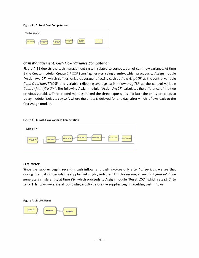
– 91 –
Figure A-10: Total Cost Computation
Cash Management: Cash Flow Variance Computation
Figure A-11 depicts the cash management system related to computation of cash flow variance. At time
1 the Create module “Create CIF COF Sums” generates a single entity, which proceeds to Assign module
“Assign Avg CF”, which defines variable average reflecting cash outflow 𝐴𝑣𝑔𝐶𝑂𝐹 as the control variable
𝐶𝑎𝑠ℎ 𝑂𝑢𝑡𝑓𝑙𝑜𝑤/𝑇𝑁𝑂𝑊 and variable reflecting average cash inflow 𝐴𝑣𝑔𝐶𝐼𝐹 as the control variable
𝐶𝑎𝑠ℎ 𝐼𝑛𝑓𝑙𝑜𝑤/𝑇𝑁𝑂𝑊. The following Assign module “Assign AvgCF” calculates the difference of the two
previous variables. Three record modules record the three expressions and later the entity proceeds to
Delay module “Delay 1 day CF”, where the entity is delayed for one day, after which it flows back to the
first Assign module.
Figure A-11: Cash Flow Variance Computation
LOC Reset
Since the supplier begins receiving cash inflows and cash invoices only after 𝑇𝐵 periods, we see that
during the first 𝑇𝐵 periods the supplier gets highly indebted. For this reason, as seen in Figure A-12, we
generate a single entity at time 𝑇𝐵, which proceeds to Assign module “Reset LOC”, which sets 𝐿𝑂𝐶𝑡 to
zero. This way, we erase all borrowing activity before the supplier begins receiving cash inflows.
Figure A-12: LOC Reset
Create Cost SumsCost
Assign Cumulative CostAssign Avg Period Delay 1 day
Total Cost Record
PeriodCostRecord Avg
Cum CostKPI_Record Total
0
SumsCreate CIF COF Assign Avg CF
Delay 1 day CF
Cash Flow
Assign AvgCFRecord Avg COF Record Avg CIF Record Avg CF
0
Create 13 Reset LOCDispose 7
0 0

– 92 –
Statistics Collection
Figure A-13 displays the spreadsheet view of the Statistics module. The spreadsheet includes Time-
Persistent statistics of all inventory levels (stock, backorder, cash, LOC, etc). It also includes the Time-
Persistent statistic of costs, several KPIs and of plant utilization, that is, the percentage of time the plant
is busy producing. Finally, the Output statistics estimate customer service levels at each echelon in
terms of the fill rate, namely, the probability (fraction) of orders that were satisfied from on-hand
inventory, without experiencing backordering.
Figure A-13: Dialog spreadsheet of the Statistic module

– 93 –
Appendix 8. Model Validation: BAU
We have conducted face, concurrent and internal validity tests. For a review on validity, we refer to
Howit & Cramer (2011). Face validity measures if the items measure what they claim to measure. We
have assessed this validity informally, by interpreting experiments results and analysing model
behaviour. By analysing the form and behaviour of certain graphs, we confirmed validity. Concurrent
validity refers whether scales correlate well with other measures of the same concept taken at a
different setting. We made this by comparing scenarios with different coefficients of variation under the
same conditions. The graphs below also show this experiment. We obtained consistent and coherent
results for higher volatility. Finally, internal validity evaluates whether the experiment design closely
follows the principle of cause and effect. Hence, by conducting sensitivity analyses and several scenarios
we assured that changes in model inputs caused expected outcomes. We confirmed this by selecting
diverse levels of margins and risk profiles. This validity test can be seen in Section 6.2. Now, we present
several tests we conducted in order to evaluate these three kind of validity.
The first test that we conducted was face validity. We have conducted these analyses for several
scenarios. However, here we present the case of a supplier with margin 𝜔 = 0.29, risk profile 𝜑 = 2.0
and coefficients of variation 𝑐. 𝑣. = 0.25 and 𝑐. 𝑣. = 1.0. We note that all the instances of this
experiment yielded similar results.
In all experiments we let the system start with cash position equal to the maximum threshold 𝑇𝐻𝑚𝑎𝑥 .
Likewise, starting inventories on hand at all echelons were set above the reorder point. Receivables,
payables, the LOC Balance and accumulated dividends had a starting value of zero. We assess
performance after 500 warm-up periods i.e. days. Also, at period 𝑡 = 𝑇𝐵 we reset back to zero the 𝐿𝑂𝐶
balance to compensate for the extra borrowing the supplier had while not receiving cash inflows. We
calculate 95 percent confidence intervals from 30 independent replications with a run-length of 4000
periods including the warm-up.
First, we analyse inventory on hand at the warehouse, which is shown in the figure below. The graph on
the left shows the case of 𝑐. 𝑣. = 0.25 and the one on the right 𝑐. 𝑣. = 1.0, both at times 𝑡 =
(1000,2000). According to theory, when facing higher volatility, the supplier has an inventory policy
that requires him to hold on to more inventory to hedge against higher uncertainty, which is confirmed
in our model. Furthermore, having less inventory requires that the supplier orders more often. Also,
higher demand volatility also increases inventory volatility too, which can be seen in the graph as well.
Finally, analysing the shape of the inventory, we realise that it resembles very well the shape of a typical
Economic Order Quantity model.

– 94 –
Figure A-14: WH Inventory on Hand
(a) WH inventory on hand and reorder point 𝑐. 𝑣. = 0.25 (b) WH inventory on hand and ROP 𝑐. 𝑣. = 1.0
We conducted the same test for the Output Buffer and we arrive at the same conclusions: the effects of
higher uncertainty force the supplier to have higher inventory levels, and inevitably higher volatility.
Likewise, the graph resembles very well the one of an Economic Production Quantity.
Figure A-15: OB Inventory on Hand
(a) OB inventory on hand and reorder point 𝑐. 𝑣. = 0.25 (b) OB inventory on hand and reorder point 𝑐. 𝑣. = 1.0
For the case of the Inventory at the Input Buffer, we have the same results. However, contrary to the
other echelons, the inventory level is very similar on both scenarios. This occurs because higher demand
volatiltiy forces the first two echelons to hold on to more inventory, for which they absorve a higher part
of the volatility.
Figure A-16: IB Inventory on Hand
(a) IB inventory on hand and reorder point 𝑐. 𝑣. = 0.25 (b) IB inventory on hand and reorder point 𝑐. 𝑣. = 1.0

– 95 –
We have also tested cash level for both variability scenarios. With lower demand uncertainty, the
optimised cash policy dictates a single threshold equal to 200. More volatility forces the supplier to hold
on to much more cash, and the spread between the minimum and maximum threshold is much wider.
This causes also more volatility and unpredictability in cash level amount.
Figure A-17: BAU cash Level
(a) Cash level and thresholds 𝑐. 𝑣. = 0.25 (b) Cash level and thresholds 𝑐. 𝑣. = 1.0
In the case of the LOC, we see also a less volatile balance for lower demand volatility. Also, we see that
the supplier borrows much less often and smaller quantities from the LOC with 𝑐. 𝑣. = 1.0. This is
consistent, because the borrowing rate is much higher than the cash holding cost. Hence, the supplier
prefers to hold on to more cash. We also conducted this experiment for a lower level of 𝜑 and the result
was the opposite: the supplier had a much higher borrowing activity and held a smaller amount of cash.
Figure A-18: BAU LOC Level
(a) LOC Balance 𝑐. 𝑣. = 0.25 (b) LOC Balance 𝑐. 𝑣. = 1.0
Accounts Receivable and Payable also are impacted by volatility. Higher demand volatility directly causes
higher volatility in AR. Also, demand uncertainty causes the supplier to have a much more irregular
ordering activity, causing AP volatility to increase.

– 96 –
Figure A-19: BAU AP and AR
(a) Accounts Receivable and Payable 𝑐. 𝑣. = 0.25 (b) Accounts Receivable and Payable 𝑐. 𝑣. = 1.0
Finally, we show the average cost per period. On both cases it is quite stable, but volatility causes a
much higher cost for the supplier due to higher inventory, cash and credit levels.
Figure A-20: BAU average Cost per Period
(a) Average Cost per Period 𝑐. 𝑣. = 0.25 (b) Average Cost per Period 𝑐. 𝑣. = 1.0
We test cash, LOC and AR levels for different payment terms. First, we see in figure (a) that LOC level
increases with payment terms. This makes sense as the firm needs more financing if there she has to
want longer for the cash inflow. Cash level decreases because the firm still has the same expenses to pay
on the same frequency; hence cash on hand (either obtained by sales or by financing) is lower. Figure(b)
shows that AR increases linearly with payment terms, which is reasonable as TB also increases linearly.
FigureA-21: BAU average cash, LOC and AR
(a) Average Cash (left y axis) and LOC (right y axis), with
𝜑 = 2.0,𝜔 = 0.29, 𝑐. 𝑣.= 1.0
(b) Average AR, with 𝜑 = 2.0, 𝜔 = 0.29, 𝑐. 𝑣. = 1.0

– 97 –
Appendix 9. Model Validation: SCF
We conducted the same experiments as in the BAU model to test validity of the SCF model. We now
present the tests for manual and automatic discounting. However, since operations behaviour is the
same as in the BAU case, we limit our analysis to financial flow measures.
Manual Discounting
Looking at the graphs below we see that cash level under MD has a much higher volatility. Even though
the policy is the same i.e. the optimisation yields the same values for the cash thresholds, we see that
the figure on the right has much more variance.
Figure A-22: MD cash Level
(a) Cash level and thresholds 𝑐. 𝑣. = 0.25 (b) Cash level and thresholds 𝑐. 𝑣. = 1.0
Accounts Receivable and Payable have a same behaviour as cash too. Also, compared to the BAU case
we see that AR has a lower level due to discounting of several receivables, and AP has almost an
identical behaviour.
Figure A-23: MD AR and AP
(a) Accounts Receivable and Payable 𝑐. 𝑣. = 0.25 (b) Accounts Receivable and Payable 𝑐. 𝑣. = 1.0
Furthermore, as in the case of MD the supplier does not borrow anything from the LOC, we omit these
graphs in this analysis. Finally, we show the average cost per period. We see again a quite stable
amount. Also, higher volatility induces a higher cost for the supplier.

– 98 –
Figure A-24: MD average Cost per Period
(a) Average Cost per Period 𝑐. 𝑣. = 0.25 (b) Average Cost per Period 𝑐. 𝑣. = 1.0
Automatic Discounting
The results under AD for cash level are very similar to the ones of manual discounting.
Figure A-25: AD cash level
(a) Cash level and thresholds 𝑐. 𝑣. = 0.25 (b) Cash level and thresholds 𝑐. 𝑣. = 1.0
Analysing the behaviour of the LOC, we immediately see that borrowing activity is much higher and has
a higher amount of variance for higher demand volatility. As we also pointed out in the main body of
this dissertation, through AD most of the extra liquidity the supplier earns leaves the firm in the way of
dividends. Therefore, borrownig activity does not decrease.
Figure A-26: AD LOC level
(a) Line of Credit 𝑐. 𝑣. = 0.25 (b) Line of Credit 𝑐. 𝑣. = 1.0

– 99 –
Below we see that AR are much lower than in the BAU and MD scenarios because receivables are quickly
discounted. AP behaviour remains constant because there is no change in payment terms to the T2S.
Figure A-27: AD AR and AP
(a) Accounts Receivable and Payable 𝑐. 𝑣. = 0.25 (b) Accounts Receivable and Payable 𝑐. 𝑣. = 1.0
We can draw the same conclusions with respect to the average cost per period.
Figure A-28: AD average Cost per Period
(a) Average Cost per Period 𝑐. 𝑣. = 0.25 (b) Average Cost per Period 𝑐. 𝑣. = 1.0
Finally, we note that the AD discounting cost increases linearly with payment terms, while the MD cost
does not increase in this manner. This is because under AD payment terms increase linearly and hence
the time to maturity too. Under MD this does not occur because the supplier discounts only if needed.
Figure A-29: Average MD and AD cost per period
(a) Average MD cost per period, with
𝜑 = 2.0,𝜔 = 0.29, 𝑐. 𝑣.= 1.0 (b) Average AD cost per period, with
𝜑 = 2.0,𝜔 = 0.29, 𝑐. 𝑣.= 1.0

– 100 –
Appendix 10. Optimisation equations
Here we present the optimisation equations that were done for the scenarios 𝑐. 𝑣. = 0.25 and 𝑐. 𝑣. =
1.0. As pointed out hereinbefore, the approach towards the optimisation was made in four steps for
each different instance of the model: first by optimising the inventory policy at the warehouse, then at
the output buffer, then at the input buffer and at last the cash management policy.
OptQuest demands a starting suggested value. For all parameters, we defined this as the maximum
amount as dictated in the constraints of each optimisation equation. Finally, the minimum amount for
each constraint was set to the average demand per day i.e. 10 units for the inventory policies, and the
monetary value of the average demand for the cash policy.
Case 𝒄. 𝒗. = 𝟎. 𝟐𝟓
Warehouse
𝑀𝑖𝑛 𝐺𝐶(.)
𝑠. 𝑡. 𝑆𝑒𝑟𝑣𝑖𝑐𝑒 𝑙𝑒𝑣𝑒𝑙𝑊𝐻 =
𝐹𝑢𝑙𝑙𝑦 𝑠𝑎𝑡𝑖𝑠𝑓𝑖𝑒𝑑 𝑜𝑟𝑑𝑒𝑟𝑠
𝑇𝑜𝑡𝑎𝑙 𝑜𝑟𝑑𝑒𝑟𝑠 ≥ 0.95
10 ≤ 𝑄1 ≤ 50 10 ≤ 𝑅1 ≤ 50 𝑄1, 𝑅1 ∈ ℤ
Output Buffer
𝑀𝑖𝑛 𝐺𝐶(.)
𝑠. 𝑡. 𝑆𝑒𝑟𝑣𝑖𝑐𝑒 𝑙𝑒𝑣𝑒𝑙𝑂𝐵 ≥ 0.90 𝑆𝑒𝑟𝑣𝑖𝑐𝑒 𝑙𝑒𝑣𝑒𝑂𝐵 ≥ 0.90 10 ≤ 𝑟2 ≤ 30 30 ≤ 𝑅2 ≤ 50 𝑅2 > 𝑟2 𝑟2, 𝑅2 ∈ ℤ
Input Buffer
𝑀𝑖𝑛 𝐺𝐶(.)
𝑠. 𝑡. 𝑆𝑒𝑟𝑣𝑖𝑐𝑒 𝑙𝑒𝑣𝑒𝑙𝑊𝐻 ≥ 0.95 𝑆𝑒𝑟𝑣𝑖𝑐𝑒 𝑙𝑒𝑣𝑒𝑙𝑂𝐵 ≥ 0.90 𝑆𝑒𝑟𝑣𝑖𝑐𝑒 𝑙𝑒𝑣𝑒𝑙𝐼𝐵 ≥ 0.90 10 ≤ 𝑄3 ≤ 50 10 ≤ 𝑅3 ≤ 50 𝑄3, 𝑅3 ∈ ℤ

– 101 –
Cash Management
𝑀𝑖𝑛 𝐺𝐶(.)
𝑠. 𝑡. 𝑇𝐻𝑚𝑎𝑥 > 𝑇𝐻𝑚𝑖𝑛 200 ≤ 𝑇𝐻𝑚𝑎𝑥 ≤ 500 100 ≤ 𝑇𝐻𝑚𝑖𝑛 ≤ 400
Case 𝒄. 𝒗. = 𝟏. 𝟎
Here, we selected a much higher value for minimum amount of the constraints. We conducted at first
experiments that assessed model behaviour, with which we selected the minimum values.
Warehouse
𝑀𝑖𝑛 𝐺𝐶(.)
𝑠. 𝑡. 𝑆𝑒𝑟𝑣𝑖𝑐𝑒 𝑙𝑒𝑣𝑒𝑙𝑊𝐻 ≥ 0.95 20 ≤ 𝑄1 ≤ 500 20 ≤ 𝑅1 ≤ 500 𝑄1, 𝑅1 ∈ ℤ
Output Buffer
𝑀𝑖𝑛 𝐺𝐶(.)
𝑠. 𝑡. 𝑆𝑒𝑟𝑣𝑖𝑐𝑒 𝑙𝑒𝑣𝑒𝑙𝑂𝐵 ≥ 0.90 𝑆𝑒𝑟𝑣𝑖𝑐𝑒 𝑙𝑒𝑣𝑒𝑂𝐵 ≥ 0.90 100 ≤ 𝑟2 ≤ 300 301 ≤ 𝑅2 ≤ 500 𝑅2 > 𝑟2 𝑟2, 𝑅2 ∈ ℤ
Input Buffer
𝑀𝑖𝑛 𝐺𝐶(.)
𝑠. 𝑡. 𝑆𝑒𝑟𝑣𝑖𝑐𝑒 𝑙𝑒𝑣𝑒𝑙𝑊𝐻 ≥ 0.95 𝑆𝑒𝑟𝑣𝑖𝑐𝑒 𝑙𝑒𝑣𝑒𝑙𝑂𝐵 ≥ 0.90 𝑆𝑒𝑟𝑣𝑖𝑐𝑒 𝑙𝑒𝑣𝑒𝑙𝐼𝐵 ≥ 0.90 40 ≤ 𝑄3 ≤ 100 20 ≤ 𝑅3 ≤ 100 𝑄3, 𝑅3 ∈ ℤ
Cash Management
𝑀𝑖𝑛 𝐺𝐶(.)
𝑠. 𝑡. 𝑇𝐻𝑚𝑎𝑥 > 𝑇𝐻𝑚𝑖𝑛 200 ≤ 𝑇𝐻𝑚𝑎𝑥 ≤ 3000 100 ≤ 𝑇𝐻𝑚𝑖𝑛 ≤ 1000

– 102 –
Appendix 11. List of industries and margins
The list below presents all the industries and their margins from the study of Damodaran (2015). The
columns marked in grey represent the relevant industries that may prove to be good recipients of SCF
from a LLP. Also, we show margins based on EBITDA. As discussed in the main body of this dissertation,
the column EBITDA + SG&A / Sales is the closest indicator to gross margin.
Table A-12: List of industries and margins
Net Income Based
EBITDA Based
Industry Number of
firms Net Margin
EBITDA/ Sales
EBITDA +SG&A/
Sales
EBITDA + R&D/ Sales
Oilfield Svcs/Equip. 161 3.81% 7.50% 10.44% 7.87%
Farming/Agriculture 37 3.33% 6.74% 11.29% 7.71%
Oil/Gas Distribution 85 3.04% 9.73% 12.37% 9.73%
Reinsurance 4 8.52% 12.10% 12.43% 12.10%
Engineering/Construction 56 1.56% 6.17% 13.00% 6.18%
Transportation 21 4.96% 12.31% 13.63% 12.33%
Healthcare Support Services 138 2.16% 5.27% 13.83% 5.35%
Steel 40 -4.33% 7.86% 14.34% 7.93%
Air Transport 22 9.32% 10.63% 14.57% 10.70%
Real Estate (General/Diversified) 11 34.38% 8.97% 15.62% 8.97%
Auto Parts 75 3.44% 8.80% 15.79% 11.47%
Auto & Truck 22 3.16% 8.23% 17.25% 12.71%
Food Wholesalers 14 1.79% 4.22% 17.50% 4.22%
Coal & Related Energy 42 -4.44% 14.63% 19.03% 15.42%
Retail (Automotive) 30 3.12% 6.09% 19.79% 6.09%
Trucking 30 3.78% 13.51% 19.84% 13.51%
Insurance (Life) 25 8.19% 10.74% 20.59% 10.74%
Homebuilding 35 6.82% 9.37% 20.70% 9.38%
Aerospace/Defense 93 7.64% 13.61% 21.13% 17.68%
Hospitals/Healthcare Facilities 56 4.50% 18.12% 21.56% 18.12%
Chemical (Diversified) 10 7.43% 14.42% 21.78% 17.96%
Construction Supplies 55 6.14% 12.61% 21.97% 15.16%
Chemical (Basic) 46 5.98% 15.93% 22.05% 16.50%
Insurance (General) 24 8.47% 18.13% 22.09% 18.15%
Oil/Gas (Integrated) 8 9.99% 18.98% 22.95% 19.26%
Packaging & Container 26 4.90% 13.34% 23.47% 13.98%

– 103 –
Retail (Grocery and Food) 21 2.71% 4.74% 23.56% 4.74%
Paper/Forest Products 22 2.58% 12.18% 23.85% 12.27%
Computer Services 119 5.56% 11.28% 24.78% 13.43%
Shipbuilding & Marine 14 13.96% 16.38% 24.79% 16.38%
Insurance (Prop/Cas.) 52 9.00% 16.15% 24.98% 16.15%
Rubber& Tires 4 3.16% 11.28% 25.00% 13.28%
Building Materials 39 4.09% 9.80% 25.78% 10.55%
Utility (General) 21 8.71% 25.72% 26.05% 25.76%
Furn/Home Furnishings 27 3.98% 10.75% 26.66% 12.47%
Retail (General) 23 2.67% 7.08% 26.74% 7.08%
Electronics (General) 189 6.18% 12.75% 26.86% 17.72%
Retail (Distributors) 90 4.23% 9.17% 27.59% 9.21%
Metals & Mining 124 1.63% 23.80% 28.22% 24.22%
Real Estate (Development) 18 1.26% 16.99% 28.79% 16.99%
Electronics (Consumer & Office) 28 3.56% 9.03% 29.78% 15.58%
Food Processing 96 6.87% 14.82% 29.83% 15.52%
Power 82 8.03% 27.09% 30.35% 27.20%
Total Market 7887 7.84% 15.18% 30.42% 17.21%
Semiconductor Equip 47 4.73% 16.53% 30.83% 29.76%
Environmental & Waste Services 103 3.08% 19.34% 31.01% 19.35%
Retail (Special Lines) 128 3.46% 8.79% 31.26% 8.83%
Business & Consumer Services 177 4.29% 12.93% 31.94% 13.18%
Diversified 23 10.12% 20.04% 32.18% 22.12%
Retail (Online) 46 2.34% 7.15% 32.55% 8.50%
Restaurant/Dining 79 9.40% 19.67% 32.74% 19.71%
Retail (Building Supply) 5 6.00% 12.04% 33.96% 12.04%
Machinery 137 8.54% 15.46% 34.42% 17.29%
Advertising 52 3.98% 15.08% 34.77% 15.29%
Computers/Peripherals 64 13.69% 23.66% 34.86% 28.59%
Electrical Equipment 126 5.64% 15.67% 35.02% 18.08%
Publshing & Newspapers 43 13.54% 14.43% 35.24% 15.60%
Financial Svcs. (Non-bank & Insurance) 288 34.14% 6.18% 35.25% 6.25%
Office Equipment & Services 25 4.47% 10.97% 35.68% 12.39%
Chemical (Specialty) 103 10.01% 18.63% 37.49% 21.49%
Transportation (Railroads) 10 18.29% 37.58% 37.70% 37.58%
Brokerage & Investment Banking 46 12.48% 0.45% 39.59% 0.50%
Semiconductor 100 13.70% 27.15% 40.07% 45.72%
Recreation 68 8.69% 18.64% 40.13% 21.12%
Hotel/Gaming 80 3.72% 23.93% 41.85% 24.25%
Entertainment 84 12.59% 23.84% 41.91% 23.87%

– 104 –
Telecom. Equipment 126 14.51% 22.86% 43.06% 37.59%
Drugs (Biotechnology) 400 11.18% 16.75% 44.16% 50.32%
Heathcare Information and Technology 127 6.72% 16.13% 44.45% 22.15%
Software (Entertainment) 20 10.11% 18.22% 45.10% 37.08%
Precious Metals 147 -13.91% 37.41% 45.18% 39.03%
Shoe 13 8.95% 13.71% 45.99% 13.82%
Information Services 67 13.78% 25.64% 46.17% 27.16%
Utility (Water) 19 15.03% 41.72% 46.30% 41.77%
Real Estate (Operations & Services) 52 4.96% 12.02% 47.62% 12.02%
Beverage (Alcoholic) 22 14.21% 22.27% 47.93% 22.29%
Investments & Asset Management 148 19.11% 17.67% 48.65% 17.95%
R.E.I.T. 213 19.01% 40.02% 48.75% 40.04%
Telecom (Wireless) 21 -2.93% 18.85% 49.13% 18.92%
Broadcasting 28 11.56% 28.72% 50.97% 28.73%
Education 42 1.99% 13.13% 51.14% 13.99%
Apparel 64 7.46% 14.77% 51.15% 15.34%
Banks (Regional) 676 22.23% 0.00% 51.35% 0.00%
Software (Internet) 327 15.57% 22.88% 51.41% 36.79%
Bank (Money Center) 13 18.90% 0.00% 51.56% 0.00%
Green & Renewable Energy 26 0.36% 34.77% 52.16% 34.80%
Oil/Gas (Production and Exploration) 392 7.52% 45.00% 52.43% 45.10%
Household Products 135 8.99% 19.79% 52.80% 21.59%
Healthcare Products 261 9.49% 22.26% 55.18% 30.03%
Cable TV 18 9.31% 28.90% 55.48% 28.96%
Software (System & Application) 259 17.34% 29.84% 56.67% 45.50%
Beverage (Soft) 46 12.66% 21.81% 57.96% 22.33%
Telecom. Services 77 11.47% 36.72% 58.62% 37.26%
Tobacco 20 22.42% 44.12% 61.21% 45.16%
Drugs (Pharmaceutical) 151 15.95% 32.81% 61.46% 47.69%
Unclassified 8 -43.05% -10.84% 102.36% -7.18%

– 105 –
Appendix 12. List of Abbreviations
Term Meaning
4PL, 3PL 4th and 3rd-party logistics provider
AR Accounts Receivable
AP Accounts Payable
BAU Business as Usual
BPO Business Process Outsourcing
CDF Cumulative Distribution Function
CLD Causal Loop Diagram
COGS Cost of Goods Sold
EBT Earnings Before Taxes
EMEA Europe, Middle East and Africa
FSP Financial Supply Chain
FSP Financial Service Provider
IT Information Technology
KPI Key Performance Indicators
LLP Lead Logistics Provider
LOC Line of Credit
LSP Logistics Service Provider
OM Operations Management
OR Operations Research
PO Purchase Order
P/FSC Physical/Financial Supply Chain
PSC Physical Supply Chain
RF Reverse Factoring
SC Supply Chain
SCF Supply Chain Finance
SCI Supply Chain Integration
SCM Supply Chain Management
SG&A Selling, General and Administrative (Expenses)
SME Small and Medium-sized Enterprise
SO Sales Order
VAS Value Added Services
VMI Vendor-managed Inventory
WACC Weighted Average Cost of Capital
WC Working Capital
WCM Working Capital Management
Related Documents