Eidesstattliche Versicherung - CORE

Eidesstattliche Versicherung

Ich versichere, dass ich die vorliegende Arbeit selbständig angefertigt und keine

anderen als die angegebenen Quellen und Hilfsmittel benutzt habe.

Clausthal-Zellerfeld, den 15-06-2012

Technische Universität

Clausthal

Institut für Elektrische Informationstechnik

Diplomarbeit

“Monopulse Range-Doppler FMCW

Radar Signal Processing for Spatial

Localization of Moving Targets”

Iván Lozano Mármol

Matriculation Nr: 409647

Supervisor: Eng. Faiza Ali

Evaluator: Dr.-Ing. Christian Bohn, Dr.-Ing. Georg Bauer

Index

Zusammenfassung V

Literature VI

Picture references VIII

Table references X

CD-ROM content XI

Appendix XII

Abstract XIV

Project Breakdown / Contents Listing XV

1. Introduction 1

2. Approaching the problem 6

3. Monopulse phase-comparison method 8

4. FMCW radar interpretation and parameters estimation 11

4.1. CW Frequency-Modulated Radar (FMCW-Radar) 11

4.1.1. Signal interpretation in FMCW-Radar 11

4.1.2. Theoretical development 12

4.2. Distance and relative Velocity estimation using FMCW-Radar 15

4.2.1. Doppler frequency and velocity in FMCW theory 15

4.2.2. Range-Doppler method 15

4.3. Spatial localization scheme of moving targets 18

4.3.1. Angle parameter calculation over 2D range-Doppler scheme 18

4.3.2. Spatial Localization schemes 18

5. The monopulse/FMCW radar signal processing simulation in Matlab 20

5.1. Signal processing Block Diagram 20

5.2. Matlab functions 21

5.3. Simulation results 23

5.4. Error function 29

6. Radar System Setup 35

6.1. Radar system structure 35

6.2. Hardware 36

6.2.1. Signal processing hardware 37

6.2.2. USB interface 38

6.2.3. Voltage supply 39

6.2.4. Radar interface 43

6.3. Software 44

6.3.1. Board Design software, Eagle 45

6.3.2. Matlab software 46

7. Measurements Results 48

7.1. Reflectors used 48

7.2. Exemplary experiments 49

7.3. Error Function 59

8. Conclusions 65

V

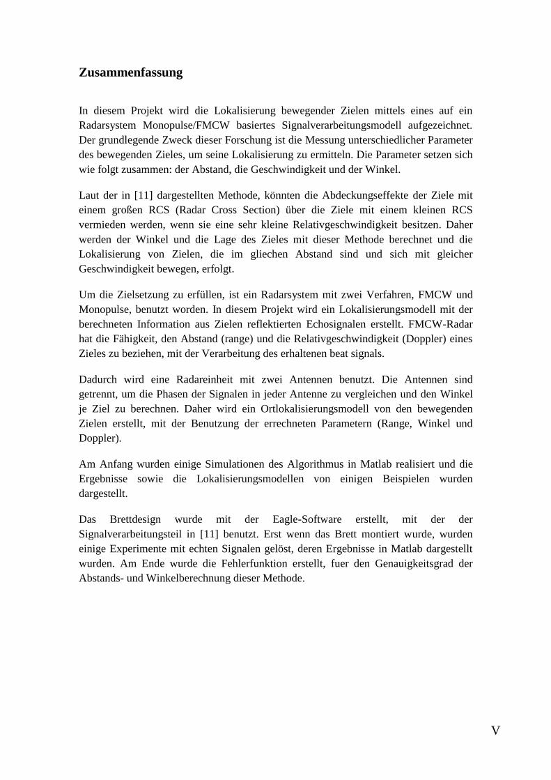
Zusammenfassung

In diesem Projekt wird die Lokalisierung bewegender Zielen mittels eines auf ein

Radarsystem Monopulse/FMCW basiertes Signalverarbeitungsmodell aufgezeichnet.

Der grundlegende Zweck dieser Forschung ist die Messung unterschiedlicher Parameter

des bewegenden Zieles, um seine Lokalisierung zu ermitteln. Die Parameter setzen sich

wie folgt zusammen: der Abstand, die Geschwindigkeit und der Winkel.

Laut der in [11] dargestellten Methode, könnten die Abdeckungseffekte der Ziele mit

einem großen RCS (Radar Cross Section) über die Ziele mit einem kleinen RCS

vermieden werden, wenn sie eine sehr kleine Relativgeschwindigkeit besitzen. Daher

werden der Winkel und die Lage des Zieles mit dieser Methode berechnet und die

Lokalisierung von Zielen, die im gliechen Abstand sind und sich mit gleicher

Geschwindigkeit bewegen, erfolgt.

Um die Zielsetzung zu erfüllen, ist ein Radarsystem mit zwei Verfahren, FMCW und

Monopulse, benutzt worden. In diesem Projekt wird ein Lokalisierungsmodell mit der

berechneten Information aus Zielen reflektierten Echosignalen erstellt. FMCW-Radar

hat die Fähigkeit, den Abstand (range) und die Relativgeschwindigkeit (Doppler) eines

Zieles zu beziehen, mit der Verarbeitung des erhaltenen beat signals.

Dadurch wird eine Radareinheit mit zwei Antennen benutzt. Die Antennen sind

getrennt, um die Phasen der Signalen in jeder Antenne zu vergleichen und den Winkel

je Ziel zu berechnen. Daher wird ein Ortlokalisierungsmodell von den bewegenden

Zielen erstellt, mit der Benutzung der errechneten Parametern (Range, Winkel und

Doppler).

Am Anfang wurden einige Simulationen des Algorithmus in Matlab realisiert und die

Ergebnisse sowie die Lokalisierungsmodellen von einigen Beispielen wurden

dargestellt.

Das Brettdesign wurde mit der Eagle-Software erstellt, mit der der

Signalverarbeitungsteil in [11] benutzt. Erst wenn das Brett montiert wurde, wurden

einige Experimente mit echten Signalen gelöst, deren Ergebnisse in Matlab dargestellt

wurden. Am Ende wurde die Fehlerfunktion erstellt, fuer den Genauigkeitsgrad der

Abstands- und Winkelberechnung dieser Methode.

VI

Literature

[1]http://www.siversima.com/wp-content/uploads/2011/10/FMCW-Radar-App-Notes-

Applications.pdf, date: 5-May 2012.

[2]http://www.century-of-

flight.net/Aviation%20history/WW2/radar%20in%20world%20war%20two.htm, date:

5-May 2012

[3] Merril Ivan Skolnik, “Introduction to RADAR systems” Third Edition, McGraw-

Hill Book Company, Edition 1981, pag. 12-13, 70-71, 81-84.

[4] Igor V. Komarov & Sergey M. Smolskiy, “Fundamentals of Short-Range FM

Radar“, Artech House INC, September 2003, pag. 3-9

[5] Philip E. Pace, “Detecting and Classifying Low Probability of Intercept Radar”

Second Edition, Artech House, year 2009, pag. 41-42,82.

[6] S. Sharenson, “Angle Estimation Accuracy with Monopulse Radar in the Search

Mode”, September 1962, pag. 1

[7] Samuel M. Sherman & David K. Barton, “Monopulse Principles and Techniques”

Second Edition, Artech House, July 2010, pag.1-5

[8] Merril Ivan Skolnik, “Radar Handbook” Second Edition, McGraw-Hill Professional,

year 1990, pag. 18.9, 18.17.

[9] Simon Kingsley & Shaun Quegan, “Understanding Radar Systems”, McGraw-Hill

Book Company Europe, year 1992, pag. 52

[10] http://encyclopedia2.thefreedictionary.com/Monopulse+Radar, date: 10-May 2012

[11] Faiza Ali & Martin Vossiek, “Detection of Weak Moving Targets Based on 2-D

Range-Doppler FMCW Radar Fourier Processing”, March 2010, pag. 1-2

[12] Erwin Baur, “Einführung in die Radartechnik”, Teubner Stdienskripten, December

1984, pag. 189-191

[13] LM317M-D datasheet

[14] http://en.wikipedia.org/wiki/Corner_reflector, date: 21-May 2012

[15]http://actualidad.orange.es/sociedad/un-edificio-se-derrumba-en-centro-rio-

janeiro.html, date: 21-May 2012

[16]http://temblor-sismo-terremoto.blogspot.de/2010/01/terremoto-en-haiti-fotos.html,

date : 21-May 2012

VII

Picture references

Fig.1.1 Antennas scheme of a Vehicle Collision Warning System (VCWS) 3

Fig.1.2 General Monopulse Radar scheme 4

Fig. 2.1 Monopulse localization scheme 7

Fig. 3.1 Monopulse phase-comparison situation 8

Fig. 3.2 Localization area available in Monopulse-radar 10

Fig. 3.3 Echo profile 10

Fig. 4.1 Modulated signal of the FMCW-Radar 11

Fig. 4.2 FMCW-Radar block diagram 12

Fig. 4.3 Frequency-Time ramp of the FMCW-Radar 12

Fig. 4.4 Target situation 12

Fig. 4.5 Frequency-Time ramp of the FMCW-Radar 14

Fig. 4.6 Frequency-Time ramp with Doppler effect 15

Fig. 4.7 Measurement scheme 16

Fig. 4.8 Exemplary 2D range-Doppler spectrum 18

Fig. 4.9 Localization schemes 19

Fig. 5.1 Block diagram of the signal processing 20

Fig. 5.2 Beat signal for the antenna 1 (in time and frequency domain) 24

Fig. 5.3 Beat signal for the antenna 2 (in time and frequency domain) 25

Fig. 5.4 2D range-Doppler spectrum of antenna 1 & antenna 2 (example 1) 25

Fig. 5.5 2D range-Doppler multiplied spectrum of antenna 1 & 2 (example 1) 26

Fig. 5.6 Polar scheme (example 1) 26

Fig. 5.7 Spatial localization scheme with R is range, A is angle, Sp is speed (ex. 1) 27

Fig. 5.8 Mixed Spectrum (example 2) 28

Fig. 5.9 Polar scheme (example 2) 28

Fig. 5.10 Spatial localization scheme with R is range, A is angle, Sp is speed (ex. 2) 29

Fig. 5.11 Range error function with not moving targets 32

Fig. 5.12 Range error function with moving targets 32

Fig. 5.13 Angle error function with not moving targets 33

Fig. 5.14 Angle error function with moving targets 33

Fig. 6.1 System setup 35

VIII

Fig. 6.2 Photo of the complete sensor system 36

Fig. 6.3 The signal processing and data transfer hardware 37

Fig. 6.4 GODIL50 FPGA with IDC-Headers 38

Fig. 6.5 USB FT 232-RL 38

Fig. 6.6 USB interface schematic 39

Fig. 6.7 LM 317 DC-DC converters 40

Fig. 6.8 Voltage conversion schematic 41

Figure 6.9 Heatsink U-shaped for TO-220 43

Fig. 6.10 Innosent Radar interface 43

Fig. 6.11 Radar connector pins 44

Fig. 6.12 Frequency-modulated ramp 45

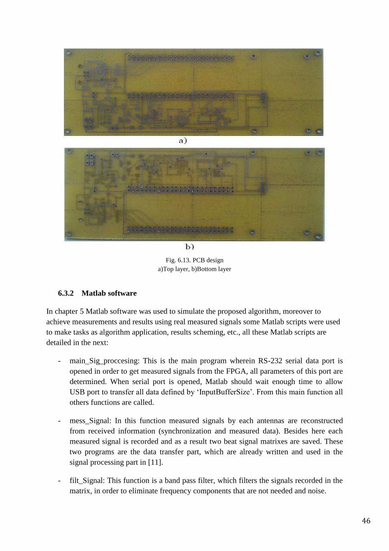
Fig. 6.13 PCB design 46

Fig. 7.1 Plane reflectors 48

Fig. 7.2 Corner reflector 49

Fig. 7.3 Detected beat signals 49

Fig. 7.4 Experiment 1 schemes 50

Fig. 7.5 Spatial localization scheme with R is range, A is angle, Sp is speed (exp. 1) 50

Fig. 7.6 Experiment 2.1 schemes 51

Fig. 7.7 Spatial localization scheme with R is range, A is angle, Sp is speed (exp.2.1) 51

Fig. 7.8 Experiment 2.2 schemes 52

Fig. 7.9 Spatial localization scheme with R is range, A is angle, Sp is speed (exp.2.2) 52

Fig. 7.10 Experiment 2.3 schemes 53

Fig. 7.11 Spatial localization scheme with R is range, A is angle, Sp is speed(exp.2.3)53

Fig. 7.12 Experiment 3 schemes 54

Fig. 7.13 Spatial localization scheme with R is range, A is angle, Sp is speed (exp.3) 54

Fig. 7.14 Experiment 4 schemes 55

Fig. 7.15 Spatial localization scheme with R is range, A is angle, Sp is speed (exp.4) 55

Fig. 7.16 Experiment 5 schemes 56

Fig. 7.17 Spatial localization scheme with R is range, A is angle, Sp is speed (exp.5) 56

Fig. 7.18 Experiment 6 schemes 57

Fig. 7.19 Spatial localization scheme with R is range, A is angle, Sp is speed (exp.6) 57

Fig. 7.20 3D localization schemes (experiment 5) 58

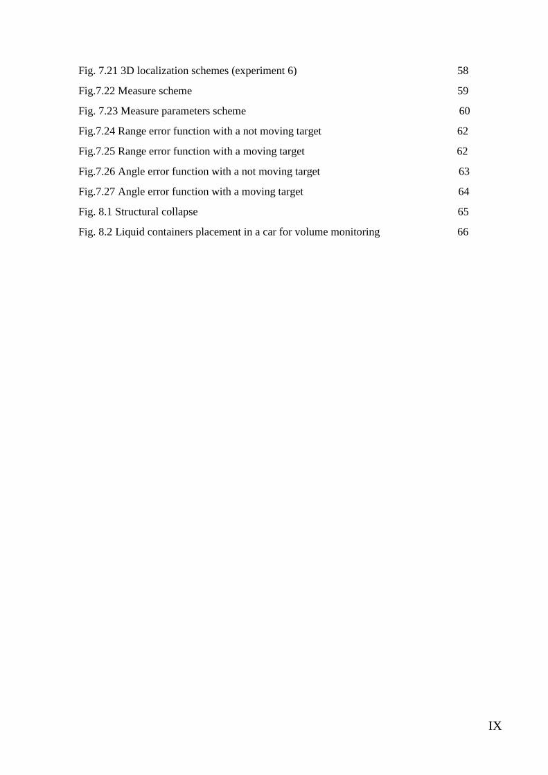
IX

Fig. 7.21 3D localization schemes (experiment 6) 58

Fig.7.22 Measure scheme 59

Fig. 7.23 Measure parameters scheme 60

Fig.7.24 Range error function with a not moving target 62

Fig.7.25 Range error function with a moving target 62

Fig.7.26 Angle error function with a not moving target 63

Fig.7.27 Angle error function with a moving target 64

Fig. 8.1 Structural collapse 65

Fig. 8.2 Liquid containers placement in a car for volume monitoring 66

X

Table references

Table 5.1 Simulation parameters 23

Table 5.2 Targets parameters in example 1 24

Table 5.3 Targets parameters in example 2 27

Table 5.4 Real and simulated parameters value 30

Table 6.1 Voltage supply 39

Table 6.2 DC-DC resistors value 41

Table 6.3 Ramp parameters 44

Table 7.1 Real and measured parameters value 60

XI

CD-ROM content

- Datasheets of the integrated circuit explained.

- Eagle files of the schematic and PCB design.

- Matlab programs used in the simulation.

- Matlab programs explained in 6.3.2.

- A copy of the writing of this project.

XII

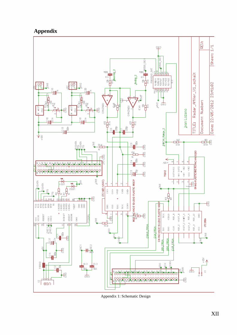
Appendix

Appendix 1: Schematic Design

XIII

Appendix 2: PCB Design

XIV

Abstract

Spatial localization of moving targets using a Monopulse/FMCW Radar system signal

processing scheme is presented in this work.

During many years radar sensor application has been used to measure different target

parameters and consecutively leading to spatial localization systems, so that has been an

active research area in many important fields, from military to civilian applications.

Spatial localization of moving targets consists of sensing and estimating the coordinates

where the target is located and its speed and direction.

The immediate goal of this work is to measure the distance, velocity and angle

parameters of each target detected basing on a set of FMCW-Radar measurements and a

monopulse phase comparison method, therefore obtaining spatial localization of moving

targets scheme, taking into account that the localization area should be limited

depending on the radar sensor used and its features.

Like this, there is a need to achieve the localization with the best possible measurement

accuracy and in any situation, and this can be solved with a simple and cheap

technology as mm-wave FMCW radars, that are remarkable because work-well in harsh

environments and have a very high resolution for ranging, velocity and imaging

method, a distance measurement resolution of 2 cm can be easily achieved over 30-40

meters working at 24GHz. Moreover the method presented is especially suited to detect

very weak moving targets.

Many applications where FMCW radar and Monopulse radar are playing an important

role are: disaster situations of buried alive people, level-measuring systems, dimension

verification systems, wall penetrating applications, air traffic control, terrain avoidance

systems, etc [1]. It is clear that all cited applications could become more attractive and

useful by using a suitable localization method as presented in this work.

Besides the theoretical development and explanation of the proposed method,

exemplary situations and measurements results will be presented to illustrate the

capability of the algorithm.

Real measurements will be made using a Monopulse/FSK/FMCW Radar with one

transmitter / two receiver antennas at K-band. The signal evaluation was applied on a

field programmable gate array (FPGA) to facilitate real time processing.

XV

Project Breakdown / Contents Listing

To explain the performance of this project, this work is divided into the following

chapters:

Chapter 1 consists of an introduction in order to present the kind or radar

systems that used in this work and its development, and some information about

the important applications about FMCW-radar and Monopulse radar systems.

Chapter 2 deals with the main goal of this work. It is clearly explained and

reviewed the main idea in practical situations.

Chapter 3 is related with Monopulse radar technology. Therefore focusing in

theoretical development about analysis of phase-difference comparison and

evaluation in Monopulse radars.

In chapter 4 the theoretical development and signal analysis in FMCW-radar and

how to obtain target parameters information as distance (range) and velocity

(Doppler) is shown, and also the implementation of the Monopulse technology

with a 24 GHz FMCW-Radar to achieve spatial localization scheme.

In chapter 5, first tests and results using the proposed method are made, with the

aid of Matlab software the algorithm simulation will be implemented, in order to

show in an illustrating way application results of the method explained in

previous paragraphs, describing in detail algorithms and programs used in

Matlab and finally some exemplary situations will be simulated and localization

schemes will be shown to see the capability of the algorithm.

The real radar system setup used in this work is explained in chapter 6,

describing the entire radar system parts used (with features and operations), from

the physical block (hardware) to the software that used to implement the radar

system.

In chapter 7 is explained how this project works in a real environment,

measurements and results using the radar system described, therefore the

performance of this algorithm applied in many real cases is seen and schemes of

some exemplary and practical situations will be illustrated, trying to take full

advantage of its performance and explaining in which scenarios this method has

another advantages.

To conclude this work, chapter 8 is presented with the conclusions, this

paragraph tells about measurements and results obtained with the radar system.

Advantages and disadvantages of the presented algorithm and practical uses in

practical situations are discussed.

1

1. Introduction

Radar (Radio Detection And Ranging) systems goes hand in hand with the concept of

localization, in this way radar systems are employed to measure and obtain targets

information (parameters) with the main objective of identifying and locating them. Therefore

it can be understandable the period of time when this idea was investigated in deep, thus

achieving a big development of radar technology was in the terrifying World War II. Radar

was considered as a revolutionary range observation tool, both military, and after WW II, also

civilian [2].

During years many applications of these radar systems have been largely employed in

different environments as on the ground, in the air, in the space, on the sea with the main goal

of detection, localization and tracking of aircrafts, ships or space targets. For example

shipboard radars are used as a navigation aid and safety systems to locate vessels, shore lines,

etc., airborne radar are used to detect other aircraft, or land either sea vehicles, even may be

used for mapping the land, navigation and natural disaster avoidance (as storms,

avalanches,…), in space, radar can assists in the guidance of spacecraft and for the remote

sensing of the land and sea [3].

There are many different ways to use the concept of Radar, depending on the information

needed from the target, the environments and its implementation. In this way, a several

different radar systems are currently functioning. The method to explain in this work is based

on the theoretical development of one radar system with two techniques, FMCW-Radar and

Monopulse radar.

FMCW-Radar

Round the 1920s one development of Radar systems was appeared for ranging reflectors

(targets) using continuous wave (CW) Radar technology. A measure of range was achieved

by modulating in frequency the transmitter radar signal, in this way the concept of FMCW

(Frequency-Modulated Continuous-Wave)-Radar appeared.

First FMCW-Radar practical application was in 1928, year in which J.O. Bentley filed an

American patent on an “airplane altitude indicating system”. But few years later the theory

and engineering of pulse radar began to be developed, and therefore FMCW radar technology

development was largely hindered by pulse radar, and has been utilized only when

requirements about measure very small ranges, from fractions of a meter to a few meters,

were needed. Nevertheless increases the number of applications in important fields where

FMCW-Radar plays an important role. But before talk about them it is necessary to present

the advantages which make this technology an attractive way to solve detection and

localization problems [4], as:

- Ability to measure with high accuracy small and very small ranges to the target,

minimal measured range being comparable to the transmitted wavelength.

2

- Ability to measure simultaneously the target range and its relative velocity respect to

the radar system.

- Small weight and small energy consumption due to absence of high circuit voltages.

- Functions well in many types of weather and atmospheric conditions as rain, snow,

humidity, fog and dusty conditions.

- FMCW modulation is compatible with solid-state transmitters, and moreover

represents the best use of output power available from these devices.

- Can penetrate variety of non-metallic materials as wood, concrete, bricks, polymers…

that makes FMCW radar suitable to detect targets trough them.

The small size, simplicity and economy of FMCW-Radar systems were the basic reasons of

wide application in many areas as aviation, military, security, navigation, automotive, etc.

Especially FMCW radio altimeters were largely used in military and civil aircrafts. An

altimeter is an instrument that measures the vertical distance (or altitude) of an object (such as

a missile) with respect to a reference level. In fact, at present a low altitude FMCW radio

altimeter is a necessary element for most aircrafts, and also for space vehicles for landing

operations [5].

In addition to radio altimetry, FMCW radars have been developed for applications such as

merchant marine navigation. The ability to measure very short ranges, makes possible

realization of very important functions as searching the water surface of the port, measuring

range and relative speed of any target within the port, and collision avoidance. This last

problem can be easily solved by placing FMCW radar at the bow and stern of the ship for

measure the distance to the wall of the port either another ship.

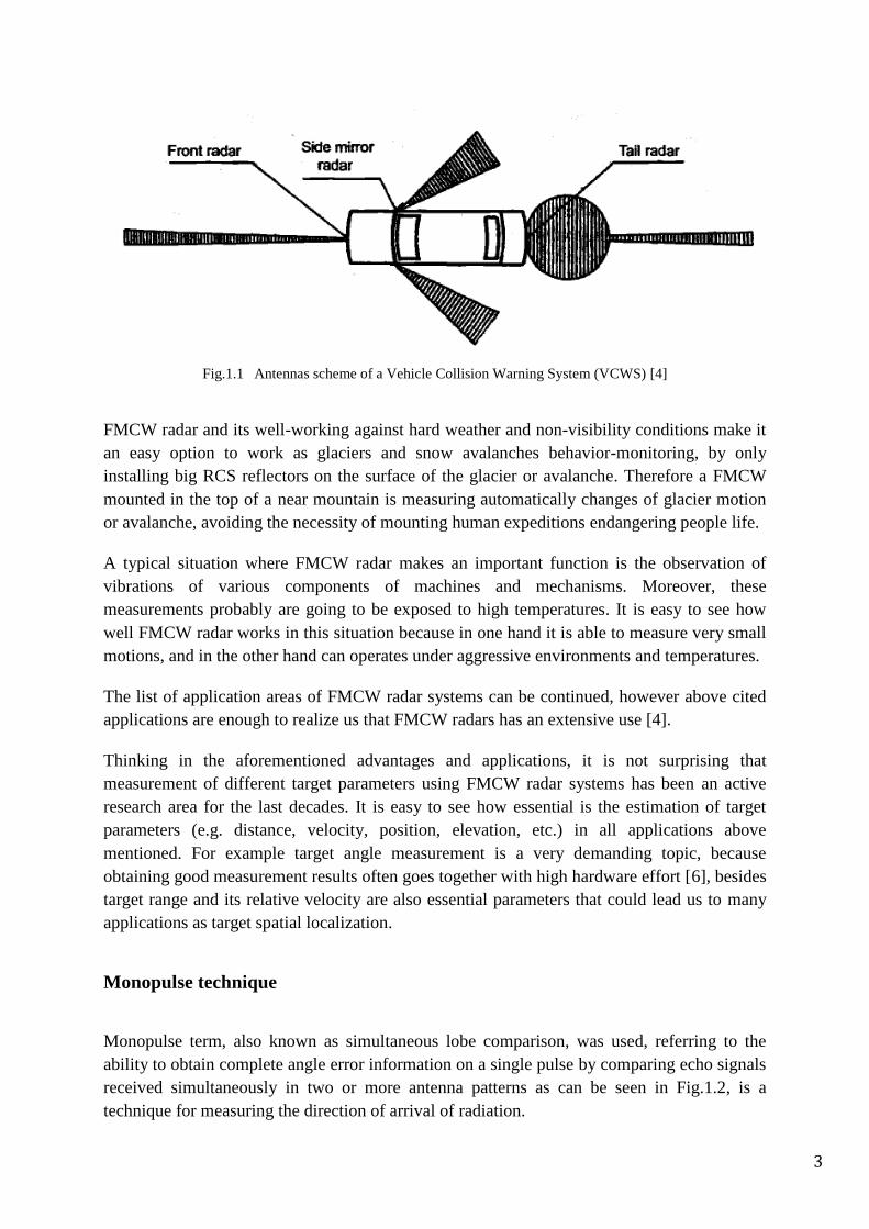
Another interesting area is automotive, Fig.1.1 shows a Vehicle Collision Warning Systems

(VCWS) that has a complex design composed by four radar sensors mounted in the vehicle.

The specifications of the radar sensors in this system, as continuous measure of short

distances and velocity, are perfectly covered by FMCW radar features, that becomes it a

cheaper and easier alternative and a good approach of VCW systems [4].

3

Fig.1.1 Antennas scheme of a Vehicle Collision Warning System (VCWS) [4]

FMCW radar and its well-working against hard weather and non-visibility conditions make it

an easy option to work as glaciers and snow avalanches behavior-monitoring, by only

installing big RCS reflectors on the surface of the glacier or avalanche. Therefore a FMCW

mounted in the top of a near mountain is measuring automatically changes of glacier motion

or avalanche, avoiding the necessity of mounting human expeditions endangering people life.

A typical situation where FMCW radar makes an important function is the observation of

vibrations of various components of machines and mechanisms. Moreover, these

measurements probably are going to be exposed to high temperatures. It is easy to see how

well FMCW radar works in this situation because in one hand it is able to measure very small

motions, and in the other hand can operates under aggressive environments and temperatures.

The list of application areas of FMCW radar systems can be continued, however above cited

applications are enough to realize us that FMCW radars has an extensive use [4].

Thinking in the aforementioned advantages and applications, it is not surprising that

measurement of different target parameters using FMCW radar systems has been an active

research area for the last decades. It is easy to see how essential is the estimation of target

parameters (e.g. distance, velocity, position, elevation, etc.) in all applications above

mentioned. For example target angle measurement is a very demanding topic, because

obtaining good measurement results often goes together with high hardware effort [6], besides

target range and its relative velocity are also essential parameters that could lead us to many

applications as target spatial localization.

Monopulse technique

Monopulse term, also known as simultaneous lobe comparison, was used, referring to the

ability to obtain complete angle error information on a single pulse by comparing echo signals

received simultaneously in two or more antenna patterns as can be seen in Fig.1.2, is a

technique for measuring the direction of arrival of radiation.

4

Fig.1.2 General Monopulse Radar scheme

To understand the concept of monopulse radar, we should start highlighting the concept of

tracking radar. It consists in angle monitoring targets by keeping a range gate centered on it.

So that the most known angle-tracking methods are lobe switching and conical scanning, in

lobe switching (similar to monopulse amplitude comparison) the radar beam points slightly to

one side and then to the other side, alternating with a quick motion and the two echo signals

amplitude are compared, so that depending which lobe more amplitude has the antenna is

corrected to point directly to the target automatically. This operation can be correctly

interleaved (lobe switching in elevation and traverse) to obtain a complete angle tracking, but

for this is preferably to move the antenna lobe in a circular way, this method is the well-

known conical scanning. But some of the disadvantages of above methods give to the

monopulse technique a big importance in tracking and localization methods [7].

Moreover monopulse method has an inherent capability for high-precision angle measurement

because is not sensitive to fluctuations in the amplitude of the received signals, and this has

made possible the development of tracking radars with requirements of around 0.003° angle-

tracking precision [8]. Therefore monopulse has reached a particularly high state of

development in certain types of radar, but nowadays has various important applications as

tracking radars systems, e.g. surface-based tracking radars, airbone monopulse radars and

homing seekers, and furthermore non-tracking applications as monopulse 3-D and secondary

surveillance radars, terrain-avoidance, aircraft low approach radar, etc.

However, a considerable disadvantage in this kind of radars is practical operation of

monopulse radar requires a complicated design of the receiving circuit in the radar station

because of the necessity of using several receiving channels.

The two main types of monopulse methods are based in the information compared in each

receiver signal. One is based on amplitude comparison of the signals, and the other, on phase

5

difference. There is no need to deepen in amplitude comparison method, in a general way, in

this method the radar senses the target displacement by comparing the amplitude of the echo

signal excited in each of the identical receive channels [10].

Monopulse Phase-Comparison (patented in 1943) consists in the use of multiple antennas

fixed adjacent parallel to each other and separated a very small distance (usually λ/2) and by

comparing the phase of the signals from each receive antenna the determination of the angle

value is possible. If the target were on the antenna boresight axis, echo signals detected in

each antenna would be in phase, i.e. difference phase value is equal to zero. As the target

moves off axis in either direction, the amplitude signal detected will be the same in all

antennas but there is a change in difference phase, so that the output of the angle detector is

determined by the relative phase only [8][9]. This is the type of monopulse comparison

utilized in this work, the method will be explained in detail in next paragraphs.

6

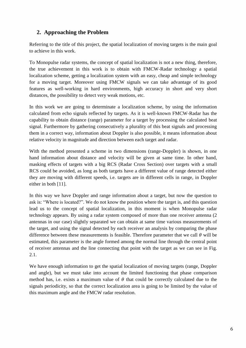
2. Approaching the Problem

Referring to the title of this project, the spatial localization of moving targets is the main goal

to achieve in this work.

To Monopulse radar systems, the concept of spatial localization is not a new thing, therefore,

the true achievement in this work is to obtain with FMCW-Radar technology a spatial

localization scheme, getting a localization system with an easy, cheap and simple technology

for a moving target. Moreover using FMCW signals we can take advantage of its good

features as well-working in hard environments, high accuracy in short and very short

distances, the possibility to detect very weak motions, etc.

In this work we are going to determinate a localization scheme, by using the information

calculated from echo signals reflected by targets. As it is well-known FMCW-Radar has the

capability to obtain distance (range) parameter for a target by processing the calculated beat

signal. Furthermore by gathering consecutively a plurality of this beat signals and processing

them in a correct way, information about Doppler is also possible, it means information about

relative velocity in magnitude and direction between each target and radar.

With the method presented a scheme in two dimensions (range-Doppler) is shown, in one

hand information about distance and velocity will be given at same time. In other hand,

masking effects of targets with a big RCS (Radar Cross Section) over targets with a small

RCS could be avoided, as long as both targets have a different value of range detected either

they are moving with different speeds, i.e. targets are in different cells in range, in Doppler

either in both [11].

In this way we have Doppler and range information about a target, but now the question to

ask is: “Where is located?”. We do not know the position where the target is, and this question

lead us to the concept of spatial localization, in this moment is when Monopulse radar

technology appears. By using a radar system composed of more than one receiver antenna (2

antennas in our case) slightly separated we can obtain at same time various measurements of

the target, and using the signal detected by each receiver an analysis by comparing the phase

difference between these measurements is feasible. Therefore parameter that we call will be

estimated, this parameter is the angle formed among the normal line through the central point

of receiver antennas and the line connecting that point with the target as we can see in Fig.

2.1.

We have enough information to get the spatial localization of moving targets (range, Doppler

and angle), but we must take into account the limited functioning that phase comparison

method has, i.e. exists a maximum value of that could be correctly calculated due to the

signals periodicity, so that the correct localization area is going to be limited by the value of

this maximum angle and the FMCW radar resolution.

7

Fig. 2.1 Monopulse localization scheme

However, FMCW radar by itself has the disadvantage of localization, but the spatial

localization can be solved in some difficult situations by using monopulse technique together

with the FMCW method. For example, in a situation where two different targets are located at

same distance (or almost the same) respect to the radar no matter if they are in motion or not

monopulse algorithm by itself is not capable to locate them in a correct way, because of the

wrong value of phase difference calculated that leads to a wrong localization. But by using the

2D range-Doppler processing if both targets are moving with different velocities, both targets

will be shown separately in the 2D scheme and applying phase difference method on it, both

targets angle could be correctly calculated, thus achieving a correct localization of them.

Even if both targets are at same distance and are moving with the same velocity but in

different directions (it means same velocity magnitude but different direction) the right angle

of each target is also calculable.

In conclusion, Monopulse and FMCW radar technology will be used together in this method

to solve cited localization situations.

In order to explain the proposed method in an easy and understandable way, firstly we are

going to see the monopulse phase comparison method and then this algorithm will be applied

to FMCW 2D range-Doppler scheme (that will be explained in detail too) to achieve spatial

localization of moving targets.

8

3. Monopulse Phase-comparison method

In this paragraph the analytic method and formulas will be treated in order to illustrate the

way where the angle parameter can be estimated by comparing the phase of the echo signals

detected in several receiver antennas with monopulse technique.

Fig. 3.1 Monopulse phase-comparison situation

The Monopulse/FMCW radar interface used in this project is composed by 2 receiver

antennas with a very small separation (value around ) which are parallel to each

other, and due to this separation both receiver antennas detect practically the same distance

value for each sensed target, but in fact exists a very small difference in range detected for

each antenna, as we can see in Fig. 3.1, that we can calculate as [12]:

(3.1)

(3.2)

It can be shown in equations (3.1) & (3.2) that one of the antennas receives the reflected

signal with a delay time than the other one, where corresponds to distance between target

and antenna 1 and between target and antenna 2, so that detected signal from one antenna

travels more distance than the other, and the distance difference can be calculated as:

(3.3)

9

Where is the separation of the antennas in m and is the wanted angle. The distance

can be expressed as a fraction of the radar wavelength to give the difference in phase

(expressed in radians) between the two signals as:

(3.4)

The factor in equation above arises because the phase difference increases by radians

for every complete wavelength travelled by the signal. Note that for small angles the

approximation can be done, leading to:

(3.5)

Depending on the phase shift existing between both antennas signal, the calculation of angle

parameter is feasible by solving for it in eq. (3.4):

(3.6)

Due to the periodicy of the phase, the angle measure only can be estimated in the

difference phase interval , so that exists a maximum (and minimum) value of that

can be correctly calculated limiting thus the localization area, defined as:

(3.7)

In (3.7) is shown that the maximum area available depends on the separation distance between

receivers and also on the wavelength used in the system, this wavelength in the case of

FMCW-Radar corresponds to the so-called central wavelength ( ) and it is associated with

the center frequency of the FM modulation, so that depending on the radar system features

used we could make the correct localization area bigger.

In Fig. 3.2 can be seen how affects the limitation of the maximum angle calculated in the

proposed method, the red line represents the limit zone (mottled) based on the limit angle

where targets can be correctly detected.

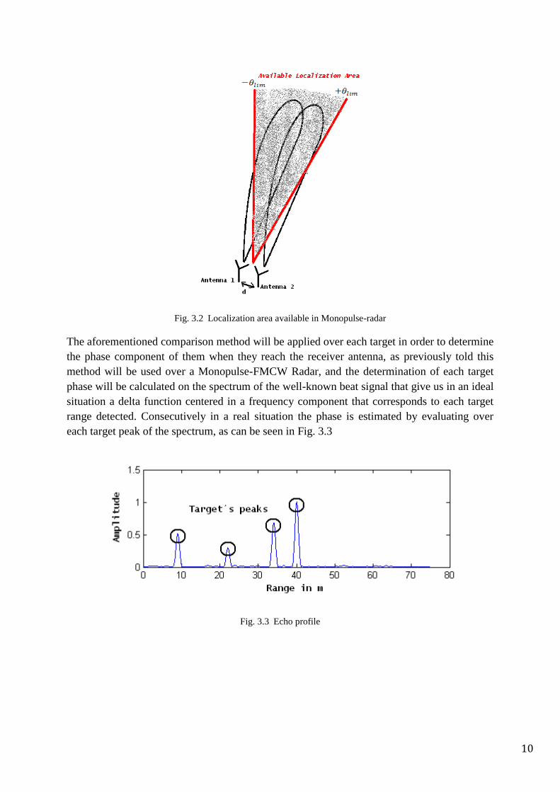
10

Fig. 3.2 Localization area available in Monopulse-radar

The aforementioned comparison method will be applied over each target in order to determine

the phase component of them when they reach the receiver antenna, as previously told this

method will be used over a Monopulse-FMCW Radar, and the determination of each target

phase will be calculated on the spectrum of the well-known beat signal that give us in an ideal

situation a delta function centered in a frequency component that corresponds to each target

range detected. Consecutively in a real situation the phase is estimated by evaluating over

each target peak of the spectrum, as can be seen in Fig. 3.3

Fig. 3.3 Echo profile

11

4. FMCW radar interpretation and parameters estimation

In this episode all theoretical development and formulas of FMCW-Radar technique needed

to obtain the correct localization method are shown. The FMCW algorithm said will give us

the possibility to determine distance and relative speed parameters of a target, thus obtaining a

2D range-Doppler scheme with a suitable Fourier signal processing. Herein by employing a

Monopulse radar composed by more than one receiver, the same number of 2D schemes as

receivers will be calculated. Moreover with the aid of the previously shown phase comparison

technique applied over the calculated 2D schemes, the angler will be calculated and

consequently an illustrative spatial localization scheme will be presented.

4.1 CW Frequency-Modulated Radar (FMCW-Radar)

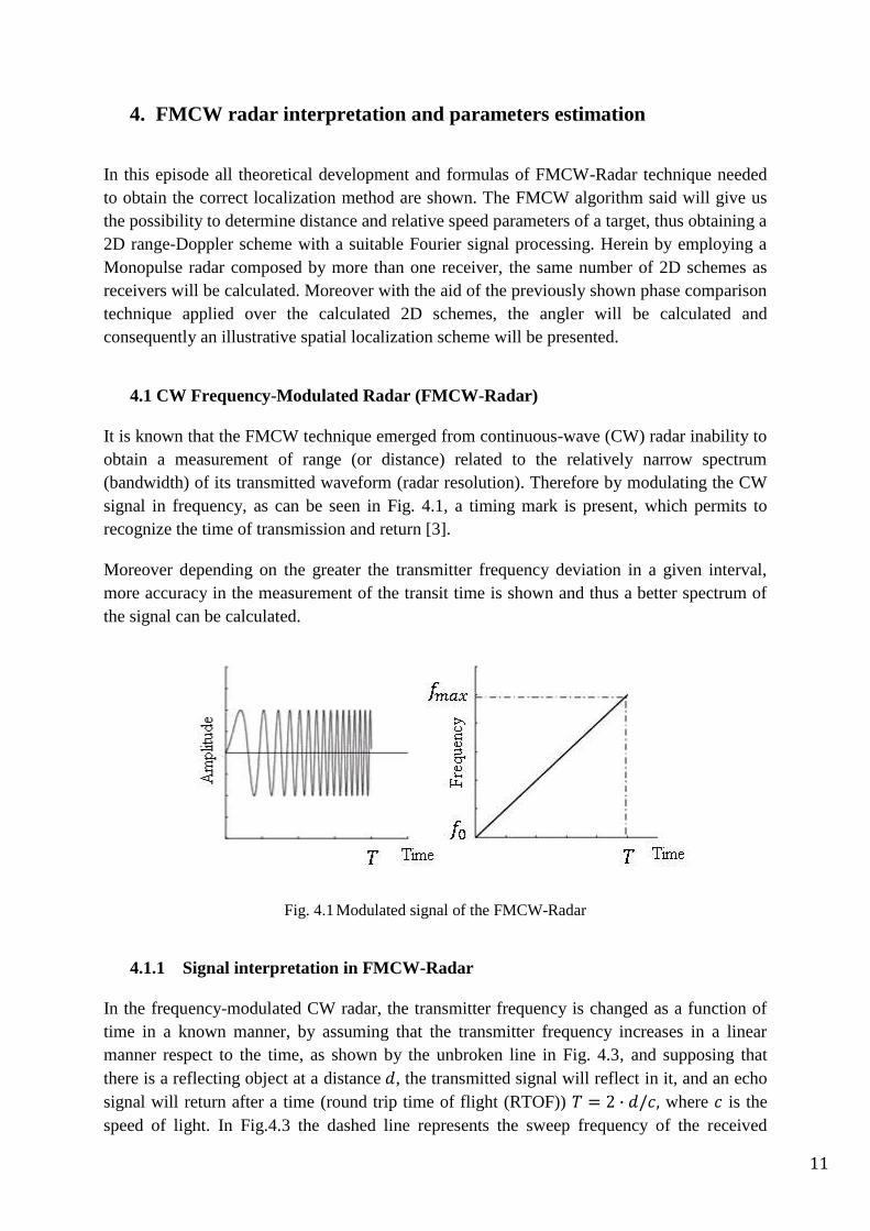
It is known that the FMCW technique emerged from continuous-wave (CW) radar inability to

obtain a measurement of range (or distance) related to the relatively narrow spectrum

(bandwidth) of its transmitted waveform (radar resolution). Therefore by modulating the CW

signal in frequency, as can be seen in Fig. 4.1, a timing mark is present, which permits to

recognize the time of transmission and return [3].

Moreover depending on the greater the transmitter frequency deviation in a given interval,

more accuracy in the measurement of the transit time is shown and thus a better spectrum of

the signal can be calculated.

Fig. 4.1 Modulated signal of the FMCW-Radar

4.1.1 Signal interpretation in FMCW-Radar

In the frequency-modulated CW radar, the transmitter frequency is changed as a function of

time in a known manner, by assuming that the transmitter frequency increases in a linear

manner respect to the time, as shown by the unbroken line in Fig. 4.3, and supposing that

there is a reflecting object at a distance , the transmitted signal will reflect in it, and an echo

signal will return after a time (round trip time of flight (RTOF)) where is the

speed of light. In Fig.4.3 the dashed line represents the sweep frequency of the received

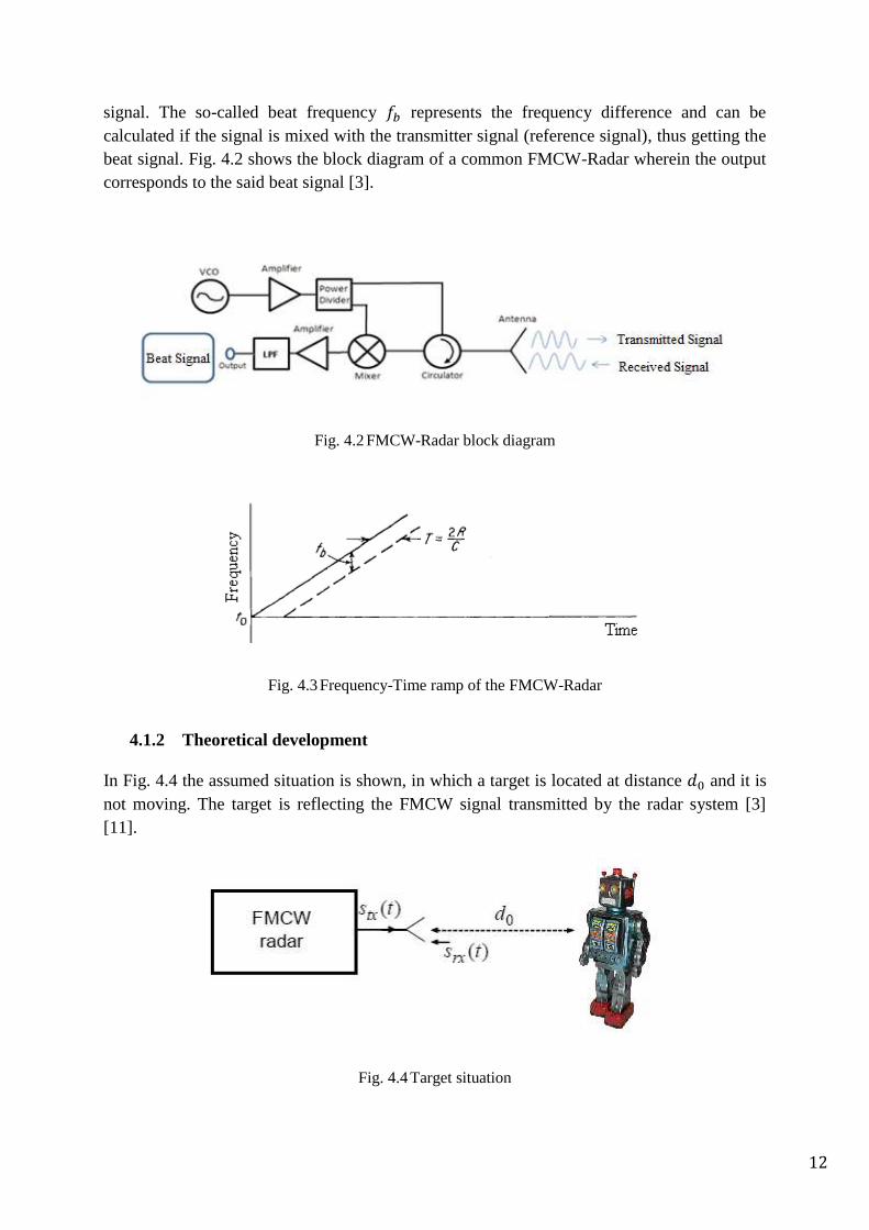
12

signal. The so-called beat frequency represents the frequency difference and can be

calculated if the signal is mixed with the transmitter signal (reference signal), thus getting the

beat signal. Fig. 4.2 shows the block diagram of a common FMCW-Radar wherein the output

corresponds to the said beat signal [3].

Fig. 4.2 FMCW-Radar block diagram

Fig. 4.3 Frequency-Time ramp of the FMCW-Radar

4.1.2 Theoretical development

In Fig. 4.4 the assumed situation is shown, in which a target is located at distance and it is

not moving. The target is reflecting the FMCW signal transmitted by the radar system [3]

[11].

Fig. 4.4 Target situation

13

The function of the radar signal round trip time of flight (RTOF), between radar and

target, indicates how long the signal takes until it reaches the receiver and can be defined as:

(4.1)

Supposing a transmitter signal with a linear frequency modulated as:

(4.2)

Where the signal amplitude and is its phase that is given by:

(4.3)

And assuming a null value of the initial phase of the transmitter signal :

(4.4)

Where the sweep-rate is defined as the quotient of the modulation sweep bandwidth (in

radians/s) and the modulation period . The carrier frequency where the modulation started is

denoted as .

The reflected signal , which reaches the radar receiver, is a replica of the transmitter

signal but delayed by the RTOF. The change of amplitude and phase caused by the signal

transmission and reflection is considered by a complex amplitude . Hence, we get:

(4.5)

In the mixer the receive and the transmit signals, and are multiplied and then a

LPF (low-pass filter) is applied to suppress the double carrier frequency components of the

mixed signal. By solving the multiplication and by considering (4.1) and (4.3), finally is got

the beat signal as:

(4.6)

Where the term in brackets is the phase of the beat signal as:

(4.7)

Basing in the above formula, the instantaneous frequency can be calculated as:

,with (4.8)

14

So that the range can be obtained from the as:

(4.9)

(4.10)

Taking into account that the target is not moving, the difference frequency ( ) corresponds

with the target range, therefore , where is the beat frequency due only to the

target range.

By considering a changing rate of the signal frequency , the beat frequency is given as:

(4.11)

Normally in practical FMCW radar is necessary a periodicity in the modulation, as a

triangular frequency modulation waveform shown in Fig. 4.5_a. Even a sawtooth form, either

sinusoidal or other shape can be used.

The resulting beat frequency using a triangular shape as a function of time is shown in Fig.

4.5_b, the beat frequency remains constant except in the change of modulation direction

shown in Fig. 4.5_a. Considering now a frequency modulated rate the beat frequency, and

thus the range can be calculated as:

(4.12)

Fig. 4.5 Frequency-Time ramp of the FMCW-Radar

a) Triangular frequency modulation, b) beat frequency of a)

15

4.2 Distance and relative Velocity estimation using FMCW-Radar

4.2.1 Doppler frequency and velocity in FMCW theory

If the reflector sensed is moving with a velocity , which is relative to the radar, a frequency

shift of the received signal respect the transmitted will be made, that called Doppler frequency

( ), and can be calculated depending on the velocity as it can be seen in (4.13). The sign

of the Doppler frequency depends on the target motion direction (approaching either moving

away).

(4.13)

Looking this effect in the FMCW technique, a Doppler frequency shift will be superimposed

on the FM range beat note, thus leading to an erroneous range measurement.

The Doppler frequency effect causes the frequency-time scheme of the received sweep

frequency to be moved up or down as is shown in Fig. 4.6_a. The resulting beat frequency is

increased in some portions and decreased in others as we can see in Fig. 4.6_b.

Fig. 4.6 Frequency-Time ramp with Doppler effect

a) Triangular frequency modulation, b) beat frequency of a)

4.2.2 Range-Doppler method

By considering a moving target, changes in the FMCW equations shown in paragraph 4.1.2

will be illustrated. Thus getting information about range and Doppler.

Let us consider the target in Fig.4.4 in motion with a value of relative speed , so that the new

value of RTOF is:

16

(4.14)

Assuming the same transmitted signal of (4.4), there is at receiver the same transmitted signal

but delayed by the new RTOF:

(4.15)

And calculating the beat signal as above explained, i.e. multiplying transmitted and reflected

signals in a mixer and subsequently filtered with a LPF:

(4.16)

Should be noted that in the above equation all quadratics terms are ignored, that is valid when

and are quite small.

Now a set of beat signals should be repeated periodically and gathered. The time between

each measure is the measure period called , so that the time when measure with index

starts is:

(4.17)

Fig. 4.7 Measurement scheme

a) measurement scheme in 2D, b) measurement scheme in 3D

17

In Fig. 4.7_a is shown a time-frequency plot of the number of beat signals measured, and in

Fig. 4.7_b is shown the same information but axis represents the time at each measure starts.

Note that if a Doppler shift exists, caused by the moving target, a sinusoidal wave form will

be presented in plane. So that, sinusoidal waveforms in two different dimensions could be

possible, thus indicating range in one and Doppler information in the other dimension which

can be got by considering the known Fourier modulation theorem [11].

Using the measure method previous explained, the RTOF for each measure at time is

defined as:

(4.18)

Taking into account (4.18) and getting the complex analytic signal of (4.16), a 2-D beat signal

is determined as:

(4.19)

A linear expression is used instead of the nonlinear phase term in (4.19), so that

the function developed around the center point ( ) is:

(4.20)

We finally get:

(4.21)

Where comprises all constant phase terms and and are the target frequency

variables in range and Doppler defined as:

(4.22)

(4.23)

wherein is the center frequency of the modulation.

Finally the 2D Fourier transform of this signal is calculated using the Fourier modulation

theorem. The frequency variables and are in range and Doppler direction, therefore the

resulting spectrum is defined as:

(4.24)

18

Herein, in one hand velocity parameter can be obtained by solving in (4.23), and in the other

hand, with that speed inserted in (4.22), the range of the target can be obtained, based on the

measured pseudo-ranges from .

4.3 Spatial localization scheme of moving targets

4.3.1 Angle parameter calculation over 2D range-Doppler scheme

As can be shown in equation (4.24), each target will be positioned in the 2D Fourier scheme

depending of its speed and range, represented with a Dirac delta theoretically speaking. The

Dirac delta shape is impossible to obtain in real situation, therefore target information will be

in the peak of each “mountain-shaped” of the resulting spectrum as is shown in Fig. 4.8. So

that the measured situation with a Monopulse/FMCW Radar system will give as a result a 2D

range-Doppler scheme for each receiver antenna.

Fig. 4.8 Exemplary 2D range-Doppler spectrum

In next exemplary simulations is shown that each 2D range-Doppler scheme detected from

each antenna has identical appearance, it means, that amplitude detected is almost the same in

each antenna. But the phase detected of each spectrum is not similar, so that carrying out the

explained phase comparison method over the detected targets in 2D schemes, the angle of

each target will be calculated and the spatial localization scheme will be possible.

4.3.2 Spatial Localization schemes

When the needed information (range, angle and velocity) is given, a localization scheme of

moving targets is feasible. In this project the software through which this task will be made is

Matlab.

19

The localization schemes used in this work are shown in Fig. 4.9, the first scheme illustrates

the localization of each target based on the range and the angle calculated, each target is

represented with a blue square.

Fig. 4.9 Localization schemes

a) Polar scheme, b) Spatial localization scheme with R is range, A is angle, Sp is speed

With the scheme shown in Fig.4.9_b is intended to illustrate all information possible at a

glance. In it, not only each target is located with a triangle, furthermore parameters estimated

from it are shown in a label (R=range; A=angle; Sp=Speed). Also the dark dashed line

represents the available localization area, which limited by the antenna parameters.

Moreover in this scheme is shown a color bar that represents the point spread function (PSF)

as an imaging quality metric, so that the color and size that each triangle has depends on it

detection intensity.

20

5. The monopulse/FMCW radar signal processing simulation in Matlab

In this chapter all theoretical methods and formulas explained in previous paragraphs are

going to be simulated in Matlab. Results of exemplary situations will be shown, and finally

the accuracy of the parameters estimated will be calculated, thus illustrating the performance

with the so-called error function.

5.1 Signal processing block diagram

The Fig. 5.1 presents a block diagram of the whole simulation system, in which is shown the

path traveled by the transmitted signal from leaving the transmission unit until the target

sensed parameters are calculated and represented.

Fig. 5.1 Block diagram of the signal processing

This block diagram represents also operations and functions utilized and the information got

in the simulation with Matlab to achieve targets spatial localization.

Analyzing the scheme step by step, in the simulation program, parameters of the antenna and

the parameters of each target are initialized, thus defining their

. So that basing on each target information the correspondents FMCW beat

signals are calculated for each receiver antenna, called .

With the beat signal detected in each antenna, a LPF (Low-Pass Filter) is applied to suppress

non-desired frequency components appeared by its calculation and the noise. As well the

21

signal resulted is repeated a number of times and saved into a 2D matrix of data, so that we

will have two matrixes filled with beat signals, one for each receiver.

A 2D Hamming is used over each matrix in order to make finite the signal spectrum in range

and Doppler direction, as previously said, it could appear in the matrix sinusoidal waveforms

in each direction. Then each beat matrix in time domain is transformed to frequency domain

by a 2D-FFT (two dimension-Fast Fourier Transform), therefore achieving the 2D spectrums

signals .

Two resulting spectrums will be multiplied together in order to calculate the angle value,

noted that before multiplying, one of the spectrum must be conjugated, getting thus the phase

difference ( ). From the multiplication, a new spectrum in two dimension (range-Doppler)

is resulted.

As previously explained, with the multiplied spectrum , information about range

and speed is calculated by evaluating the frequency components in both directions,

determining the range ( ) and the speed ( ) of the target detected. And finally the angle

is also calculated by applying the monopulse phase comparison method and spatial

localization of the simulated moving target is estimated with the parameters obtained.

5.2 Matlab functions

The FMCW beat signals calculated in the simulation ( ), after the low-pass

filtering, are given by:

(5.1)

(5.2)

wherein:

is the carrier frequency where the modulation started

are RTOF functions of each received signal from each

antenna at

are the amplitudes of each beat signal, due to the change in amplitude and

phase of the transmitted and reflected signal, these values are complex.

are the distance between target and antenna 1 & antenna 2

When each 2D beat signal matrix is recorded and the 2D-FFT is applied over them, both

spectrums matrix are multiplied as:

(5.3)

22

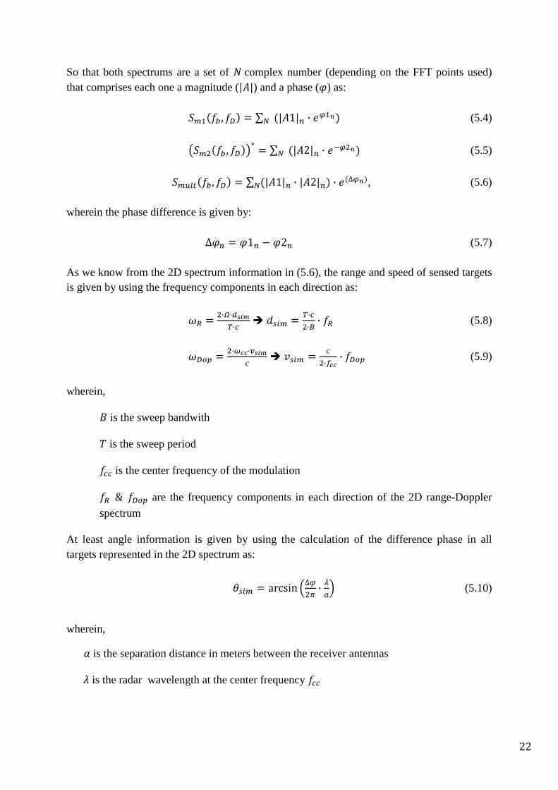
So that both spectrums are a set of complex number (depending on the FFT points used)

that comprises each one a magnitude ( ) and a phase ( ) as:

(5.4)

(5.5)

, (5.6)

wherein the phase difference is given by:

(5.7)

As we know from the 2D spectrum information in (5.6), the range and speed of sensed targets

is given by using the frequency components in each direction as:

(5.8)

(5.9)

wherein,

is the sweep bandwith

is the sweep period

is the center frequency of the modulation

are the frequency components in each direction of the 2D range-Doppler

spectrum

At least angle information is given by using the calculation of the difference phase in all

targets represented in the 2D spectrum as:

(5.10)

wherein,

is the separation distance in meters between the receiver antennas

is the radar wavelength at the center frequency

23

5.3 Simulation results

Now some examples will be simulated in Matlab, in order to illustrate the localization

schemes and the performance of the proposed method.

The value of the measurement parameters used in Matlab to simulate the different examples

are:

Parameter Value

Table 5.1 Simulation parameters

Before show any measurement result, based on the previously described method, angle limit

should be calculated, in order to see how big it´s the aperture zone wherein targets can be

correctly sensed and located.

Using equation (3.7):

In the first example is shown how a Monopulse/FMCW radar works illustrating the results of

the proposed method, by plotting some signals and showing images in which the spatial

localization is achieved.

Radar system detects 4 targets all of them with clearly different values of range, speed and

angle, so that real targets situation is:

24

Target Range in m Speed in m/s Angle in º |A|(normalized)

1 7 0.43 -23 1

2 20 0.02 +4 0.5

3 34 0 -25 0.25

4 2 0.32 -15 0.7

Table 5.2 Targets parameters (example 1)

As a result of the simulated example, each beat signal calculated ,and gathered by each

antenna, have the same form as Fig. 5.2 & Fig. 5.3 in time and frequency domain. Is shown

from the echo profile that the four targets are easily identified depending on their range,

velocity and amplitude values.

The result of the 2D-FFT over each beat signal matrix is shown in Fig. 5.4, and thw

multiplied espectrumis shown in Fig. 5.5, in which each target is represented by its range and

Doppler value. In Fig. 5.4 is shown that both detected spectrums have very similar

appearance, as was explained in previous chapters the magnitude detected by each receiver

antenna is practically identical. Therefore is obtained a multiplied spectrum with similar

appearance in magnitude and information of the difference phase is in each point of the

multiplied spectrum.

Fig. 5.2 Beat signal for the antenna 1 (in time and frequency domain)

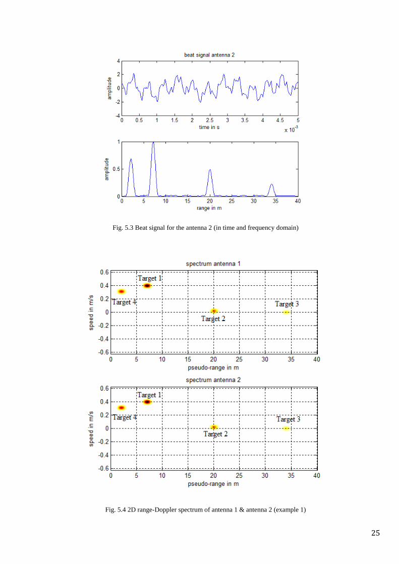
25

Fig. 5.3 Beat signal for the antenna 2 (in time and frequency domain)

Fig. 5.4 2D range-Doppler spectrum of antenna 1 & antenna 2 (example 1)

26

Fig. 5.5 2D range-Doppler multiplied spectrum of antenna 1 & 2 (example 1)

At least, the spatial localization schemes are represented as is shown in Fig. 5.6 and Fig.

5.7. In the polar scheme is shown the spatial localization using information about angle

and range of the targets and furthermore in localization scheme of Fig. 5.7, all targets

information is given, as range, velocity, angle and intensity.

Fig. 5.6 Polar scheme (example 1)

27

Fig. 5.7 Spatial localization scheme with R is range, A is angle, Sp is speed (example 1)

The second example, tries to solve some special situations explained in chapter 2. Radar

system detects 4 targets, 2 of them are at the same range and have the same speed magnitude

but they are moving in different directions, and the other 2 targets are at same range but with a

small different in the motion speed and moreover one of the targets has a very small RCS

compared with the other, all targets are located in different positions, so that target parameters

value are:

Target Range in m Speed in m/s Angle in º |A|(normalized)

1 29 0.12 +2 0.6

2 29 -0.12 -24 0.7

3 17 0.4 -24 1

4 17 0.41 +15 0.5

Table 5.3 Targets parameters (example 2)

28

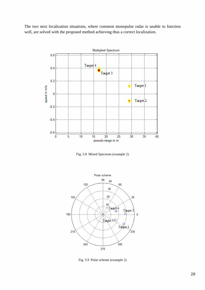
The two next localization situations, where common monopulse radar is unable to function

well, are solved with the proposed method achieving thus a correct localization.

Fig. 5.8 Mixed Spectrum (example 2)

Fig. 5.9 Polar scheme (example 2)

29

Fig. 5.10 Spatial localization scheme with R is range, A is angle, Sp is speed (example 2)

In the multiplied spectrum (Fig. 5.8), is shown the four said targets correctly sensed. Target 1

and target 2 are situated in the 2D scheme in the same range cell but one is in the opposite

moving direction than the other, it means same speed value but one is receding and the other

is approaching respect to the radar sensor. In this situation is illustrated that is possible to

detect both targets separately and make a correct localization of them.

In spectrum (Fig. 5.8) a target with a big RCS is located too near in range to a target with a

small RCS, target 3 with a big RCS of detection can be seen clearly separable from target 4

with a very small RCS only with a small difference in Doppler direction. The same thing

occurs in the case of a big not moving target is near to small moving one with a very weak

motion, thus avoiding masking effects from the big target over the small one.

Consecutively we can conclude that both experiments are solved as is shown in Fig. 5.9 and

Fig. 5.10, where the four targets are correctly sensed and positioned.

5.4 Error function

To conclude this chapter, the accuracy of the parameters estimation with Matlab is shown.

The accuracy will be represented with the so-called error function, which is calculated as the

difference between the real value of a parameter and the value simulated by the program. In

this project the main goal is to obtain a high accuracy in angle and range, so that error

functions associated to these two parameters will be estimated, but in two different cases, with

30

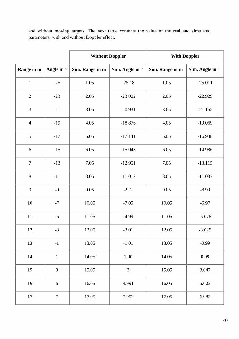
and without moving targets. The next table contents the value of the real and simulated

parameters, with and without Doppler effect.

Without Doppler With Doppler

Range in m Angle in ° Sim. Range in m Sim. Angle in ° Sim. Range in m Sim. Angle in °

1 -25 1.05 -25.18 1.05 -25.011

2 -23 2.05 -23.002 2.05 -22.929

3 -21 3.05 -20.931 3.05 -21.165

4 -19 4.05 -18.876 4.05 -19.069

5 -17 5.05 -17.141 5.05 -16.988

6 -15 6.05 -15.043 6.05 -14.986

7 -13 7.05 -12.951 7.05 -13.115

8 -11 8.05 -11.012 8.05 -11.037

9 -9 9.05 -9.1 9.05 -8.99

10 -7 10.05 -7.05 10.05 -6.97

11 -5 11.05 -4.99 11.05 -5.078

12 -3 12.05 -3.01 12.05 -3.029

13 -1 13.05 -1.01 13.05 -0.99

14 1 14.05 1.00 14.05 0.99

15 3 15.05 3 15.05 3.047

16 5 16.05 4.991 16.05 5.023

17 7 17.05 7.092 17.05 6.982

31

18 9 18.05 9.047 18.05 8.951

19 11 19.05 10.956 19.05 11.119

20 13 20.05 12.946 20.05 13.068

21 15 21.05 15.126 21.05 14.979

22 17 22.05 17.043 22.05 16.946

23 19 23.05 18.979 23.05 19.122

24 21 24.05 20.998 24.05 20.978

25 23 25.05 23.136 25.05 22.956

26 25 26.05 25.053 26.05 24.93

27 23 27.05 22.882 27.05 23.154

28 21 28.05 20.94 28.05 21.01

29 19 29.05 19.141 29.05 18.963

30 17 30.05 17.035 30.05 16.981

Table 5.4 Real and simulated parameters value.

32

- Error function in Range:

Fig. 5.11 Range error function with not moving targets.

Fig. 5.12 Range error function with moving targets.

33

- Error function in Angle:

Fig. 5.13 Angle error function with not moving targets.

Fig. 5.14 Angle error function with moving targets.

34

On the previous error function graphics can be concluded that range error is constant in both

cases, with and without moving targets, showing a value of -0.05 meters.

Angle error function, in the case of not-moving targets, shows a maximum error of around

0.2º. The same happens with the angle error graphic of moving targets, with a maximum error

value around 0.2º, but is shown that exists a small difference between both cases, so that these

results show a good angle error.

The error functions estimated from the simulation with Matlab also depend on the FFT points

used to convert time domain signals into frequency domain, so that the accuracy will be

bigger if zero padding technique is used. Error in range and angle above illustrated is good to

get a sensor system with a high accuracy in spatial localization.

35

6. Radar system setup

This chapter deals with the setup of the complete sensor system utilized in this work. Before

talk about results and measurements, each part of the circuit used (hardware) and the different

software utilized will be described.

6.1 Radar system structure

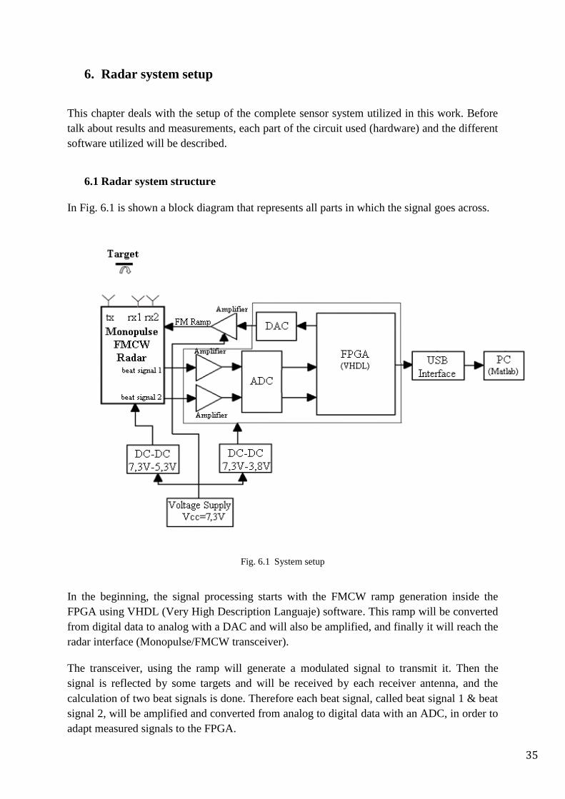
In Fig. 6.1 is shown a block diagram that represents all parts in which the signal goes across.

Fig. 6.1 System setup

In the beginning, the signal processing starts with the FMCW ramp generation inside the

FPGA using VHDL (Very High Description Languaje) software. This ramp will be converted

from digital data to analog with a DAC and will also be amplified, and finally it will reach the

radar interface (Monopulse/FMCW transceiver).

The transceiver, using the ramp will generate a modulated signal to transmit it. Then the

signal is reflected by some targets and will be received by each receiver antenna, and the

calculation of two beat signals is done. Therefore each beat signal, called beat signal 1 & beat

signal 2, will be amplified and converted from analog to digital data with an ADC, in order to

adapt measured signals to the FPGA.

36

Then, inside the FPGA, the sampled beat signals are sent via USB interface to the computer,

where the algorithm explained will be applied over the beat signals measured and results and

schemes will be shown using the software Matlab. All this process will be repeated

automatically.

Fig. 6.2 Photo of the complete sensor system

A general photo of the complete system hardware is shown in Fig. 6.2, thus showing the

circuit used and also the equipment, which helps us with the operation of the project. This

equipment comprises a voltage supply, an oscilloscope where the signal parameters can be

measured and a computer where the proposed algorithm will be applied over the sampled

signals and where measured signals and schemes will be plotted.

6.2 Hardware

In Fig. 6.3, there is a photo of the signal processing and data transfer hardware in this work.

To make an easy explanation, hardware will be divided to different blocks depending on its

function, as is shown in the same image, which with the related software already explained

clearly in [11].

The hardware blocks are:

Signal processing hardware, this part contains all ICs (integrated circuits) and

components used from the ramp generated amplification to beat signals

sampling before getting the FPGA and the FPGA.

USB interface, this block deals with connecting FPGA to a computer, thus

making easy the transference of measured signals.

37

Power supply, provides the correct voltage and current that each component

requires (as Radar, ADC, DAC, etc.).

Radar interface, this part comprises from the transmission of the signal by the

radar to the calculation of the beat signals from each receiver antenna,

describing the radar unit used.

Fig. 6.3 The signal processing and data transfer hardware

6.2.1 Signal processing hardware

This block contains digital to analog (or vice versa) conversions, amplifications and the

processing in the FPGA.

The ramp, which generated in the FPGA, will be sending to the 16 bit DAC (Digital to

Analog Converter) LTC 2604.

After that the amplifier TS912 will amplify the ramp generated, which will be sending to the

radar.

Monopulse/FMCW radar will use the ramp information to emit a transmitted signal, which

will be used to obtain the beat signal by mixing with the received one. So that a beat signal

from each receiver antenna is provided and the amplification of the two measured signals is

made through a rail to rail operational amplifier OPA-2340U.

An analog to digital conversion and thus a sampling of the signal should be made, through an

LTC 1407-1, this is a 14 bit, 3Msps ADC it contains two separate differential inputs that are

sampled simultaneously, the sampling frequency rate of each channel is 1.5Msps.

38

Fig. 6.4 GODIL50 FPGA with IDC-Headers

Finally in Fig. 6.4 a photo of the GODIL50 FPGA module used is shown, it consists in a low

cost and versatile Spartan 3E FPGA-module with two 50 Pins IDC Header, 48 I/Os of the

Xilinx XC3S500E-4VQG100C FPGA.

6.2.2 USB interface

To connect the FPGA module with a computer, a USB interface is used in order to transfer

radar measured signals to a PC.

The USB block is mainly composed by the IC FT 232-RL (shown in Fig. 6.5), that is a single

chip USB to asynchronous serial data UART transfer interface. With a data transfer rate from

300 baud to 3 Mbaud, a receive buffer of 128 byte and a transmit one of 256 byte.

Fig. 6.5 USB FT 232-RL

Fig. 6.6 illustrates the schematic design of the USB interface, in this figure can be seen all

components included in the design.

39

The voltage supply ( ) of this block is given by the computer used, moreover the

CBUS0 and CBUS1 pins have been configured as TXLED# and RXLED# and are used to

drive two LEDs which will be lit it depends on the transmit or receive data situation.

Fig. 6.6 USB interface schematic

6.2.3 Voltage supply

Some integrated circuits and components in system must be supplied with the correct value of

voltage, trying to use the less number of voltage converters as possible to supply all the circuit

Table 6.1 shows the chosen voltage for each component and its allowable voltage range:

Component Voltage range in V Voltage supplied in V

Radar transceiver 5.3-6 5.3

FPGA 3.5-5.5 3.8

ADC (LTC1407-1) 2.7-4 3.8

DAC (LTC2604) 2.5-5.5 3.8

Amplifier (TS912) 2.7-16 7.2

Amplifier (OPA2340U) 2.7-5 3.8

USB (FT232RL) 3.3-5.25 5

40

Table 6.1 Voltage supply

As previously explained, USB supply ( ) comes from the pin of the USB port

used which is connected to the PC.

About the others components, the way of using the same voltage supply unit to the entire

circuit and at same time supply the correct voltage to each component is by using DC-DC

converters.

Fig. 6.7 LM 317 DC-DC converters

a) package TO-220, b) package SOT-223

At first, the DC-DC converted used was the LM-317 package SOT-223 (Fig. 6.7b) but it was

changed to the package TO-220 (Fig. 6.7a) due to problems of lack of space in the designed

board.

This IC is an adjustable three-terminal positive voltage regulator capable of supplying in

excess of 500 mA over an output voltage range of 1.2 V to 37 V.

In this DC-DC converter an easy supplying is feasible because only is needed two external

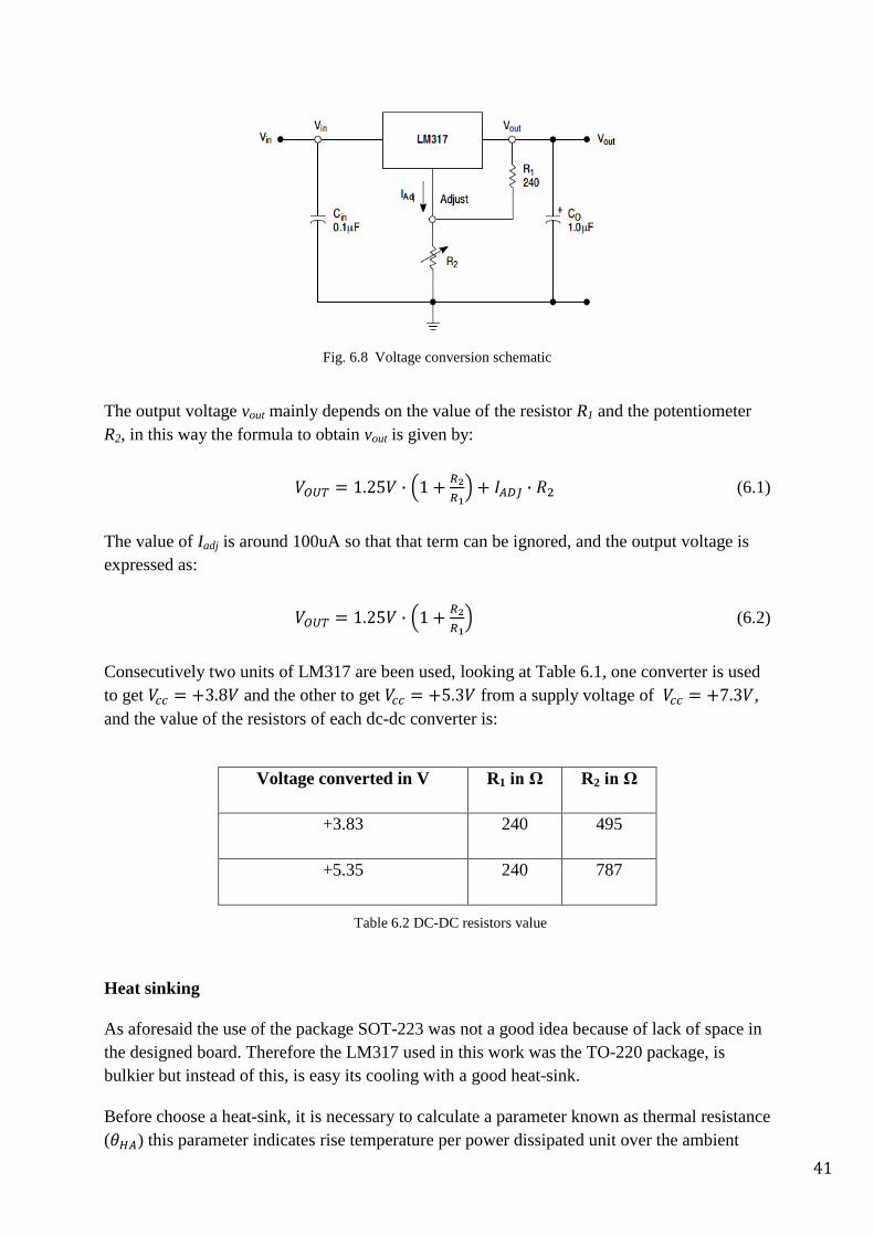
resistors to set the output voltage, so that in Fig. 6.8 it can be seen the voltage conversion

schematic used.

41

Fig. 6.8 Voltage conversion schematic

The output voltage vout mainly depends on the value of the resistor R1 and the potentiometer

R2, in this way the formula to obtain vout is given by:

(6.1)

The value of Iadj is around 100uA so that that term can be ignored, and the output voltage is

expressed as:

(6.2)

Consecutively two units of LM317 are been used, looking at Table 6.1, one converter is used

to get and the other to get from a supply voltage of ,

and the value of the resistors of each dc-dc converter is:

Voltage converted in V R1 in Ω R2 in Ω

+3.83 240 495

+5.35 240 787

Table 6.2 DC-DC resistors value

Heat sinking

As aforesaid the use of the package SOT-223 was not a good idea because of lack of space in

the designed board. Therefore the LM317 used in this work was the TO-220 package, is

bulkier but instead of this, is easy its cooling with a good heat-sink.

Before choose a heat-sink, it is necessary to calculate a parameter known as thermal resistance

( ) this parameter indicates rise temperature per power dissipated unit over the ambient

42

temperature, so that a good heat-sink will be that one with a value of less or equal than

the value estimated from the circuit used, the calculation of this parameter can be seen in any

DC-DC converter datasheet [13] as:

(6.3)

Where is given in the dc-dc converter datasheet and is very small (with a maximum

possible value of 0.5ºC/W) and the parameter is the resistance from the IC junction to

ambient temperature, it depends on the maximum power dissipated by the dc-dc converter

( ) and the maximum ambient temperature affecting the circuit ( ), can be calculated

as:

(6.4)

In our case parameter values are:

So that, we should calculate the for each DC-DC depending on the voltage converted:

Now the value of the heat-sink needed can be calculated as:

The heatsink needed must have a thermal resistance value of at maximum the more restrictive

value calculated, i.e. .

In Fig. 6.9 is shown the heat-sink used for both dc-dc and the value of it thermal resistance is:

43

Figure 6.9 Heatsink U-shaped for TO-220

a) Heatsink image, b) Heatsink installed on DC-DC converter

6.2.4 Radar interface

The Innosent Monopulse/FMCW radar was used as radar interface, as is shown in Fig. 6.10,

the exact and detailed definition read in its datasheet is:

“Monopulse / FSK / FMCW – capable K – Band VCO – Transceiver with

one transmit / two receive antenna”

Fig. 6.10 Innosent Radar interface

44

Receiver antennas in this module are separated a distance , furthermore this

transceiver has RF-preamplifier for lowest noise operation and IF-preamplifier and separate

transmit and receive paths to achieve the maximum sensitivity.

Lobe width at -3dB of the transmit antenna is 23º in azimuth and receiver antennas have a

lobe width of 55º in azimuth.

The radar sensor provides a LIF connector with 20 pins, in Fig. 6.11 a picture of this

connector is shown where are indicated all pins used in this project and where were

connected.

Fig. 6.11 Radar connector pins

6.3 Software

From the beginning (board design) to the end (spatial localization scheme presentation) three

programs were employ. At first Eagle software was used for making the preliminary design of

the circuit board and Matlab was used for facilitating signal processing and showing results

and schemes.

Another program used was VHDL, in which some complex operations are made as ramp

determination, ramp linearization, signal sampling, etc. In this Project it was not written the

VHDL-program, which was already written and explained in [11]. Fig. 6.12 illustrates the

frequency ramp utilized whose parameters are:

Sweep Bandwidth 1.2 GHz

Center Frequency 24 GHz

Ramp period 3.9 mseg

Measure period 68.9 mseg

Table 6.3 Ramp parameters

45

Fig. 6.12 Frequency-modulated ramp

As it is well known, with the above cited parameters, the available detection area can be

calculated, determining the maximum and minimum limit angle by using (3.7) as:

6.3.1 Board Design software (Eagle)

With this software two main tasks, related with the design of the board, were done:

- Schematic design (Appendix 1), this step is where all integrated circuits, resistors,

connectors and all components were placed in a plane, known as schematic, using the

suitable libraries. Moreover in this schematic, connections between components are

made and values and names of components are set. In this work the same schematic

design was used, which was already made in [11], in addition to using another dc-dc

converter and USB interface.

- PCB design (Appendix 2), the final step is to convert all connections in schematic to a

real situation as the PCB. The PCB is the circuit board wherein all components will be

mounted. So that, in PCB design all connections using two layers (Top and Bottom),

position of the components, holes and board size are set.

In Fig.6.13, the different layers of the resulting board used in the project are shown.

46

Fig. 6.13. PCB design

a)Top layer, b)Bottom layer

6.3.2 Matlab software

In chapter 5 Matlab software was used to simulate the proposed algorithm, moreover to

achieve measurements and results using real measured signals some Matlab scripts were used

to make tasks as algorithm application, results scheming, etc., all these Matlab scripts are

detailed in the next:

- main_Sig_proccesing: This is the main program wherein RS-232 serial data port is

opened in order to get measured signals from the FPGA, all parameters of this port are

determined. When serial port is opened, Matlab should wait enough time to allow

USB port to transfer all data defined by „InputBufferSize‟. From this main function all

others functions are called.

- mess_Signal: In this function measured signals by each antennas are reconstructed

from received information (synchronization and measured data). Besides here each

measured signal is recorded and as a result two beat signal matrixes are saved. These

two programs are the data transfer part, which are already written and used in the

signal processing part in [11].

- filt_Signal: This function is a band pass filter, which filters the signals recorded in the

matrix, in order to eliminate frequency components that are not needed and noise.

47

- Filt_Dopp: As the previous function, this script deals with the application of a low

pass filter in Doppler dimension.

- Fourier_proccesing: The transformation from 2D time-domain to 2D frequency-

domain of the signals is done in this function, but before applying 2D-FFT function a

two-dimension Hamming window is multiplied with each signal. Finally spectrum of

antenna 1 and antenna 2 are multiplied to achieve only one 2D-spectrum.

- imaging_RDA: The algorithm explained in this work to obtain angle is used with the

multiplied spectrum, so that range, Doppler and angle information of each detected

target is calculated, and at least some images illustrating spatial localization of moving

targets are shown.

- max_matrix: Matlab has a function similar to this one, but this function was created to

find local maximums in a matrix data, so that each maximum peak located in the 2D-

Fourier transform is detected and information about position of each maximum, their

value and number of maximums found is given. Must be remarkable that this function

finds maximums that are over a limit value of the 2% from the maximum amplitude

received.

- Radar_Parm: This is like a parameter sheet wherein all parameters needed are

presented, this parameters are sweep bandwidth, sweep period, sample frequency, FFT

points, center frequency and wavelength.

48

7. Measurements Results

The real performance of the proposed method applied on the radar system described will be

shown in this chapter, trying to solve practical situations in which this method works-well and

has others advantages.

To make an easy understanding, some examples were measured with the radar system using

specific reflectors. In next paragraphs each situation will be described clearly, identifying

each target detected and explaining the experiment solved.

Finally, in the same way as chapter 5, error function will be calculated in order to get the

accuracy of the radar system.

7.1 Reflectors used

In order to achieve specific experiments, a set of reflectors was used. Each one has a different

shape and therefore different RCS (radar cross section).

In Fig. 7.1 can be seen 4 four plane reflectors used, from target labeled a) to target labeled d)

the RCS value are:

Fig. 7.1 Plane reflectors

49

Furthermore, another target used was a corner reflector shown in Fig. 7.2, this target consists

in three mutually perpendicular surfaces which reflects the transmitter signal back directly

towards the radar sensor, i.e. the signal is reflected three times and as a result the direction

changes to the opposite one, thus returning to the sensor with a direction parallel to the

incident one. These kinds of reflectors are very used for its capability of reflecting waves

strongly, so that the reflector shown in Fig.7.2_a was used for measure the error function from

1 to 25 meters [14].

Fig. 7.2 Corner reflector

a) Corner reflector used, b) Reflection scheme [14]

7.2 Exemplary experiments

Fig. 7.3 illustrates one example of the measured and sampled beat signals in each antenna that

have been used in this work:

Fig. 7.3 Detected beat signals

50

One by one, the different measured experiments are going to be illustrated:

Experiment 1:

A first scenario comprises 3 not moving targets, targets labeled a), with RCS=742 m2

at 2

meters, and c), with RCS=5026 m2

at 8 meters, are two of the plane reflectors explained. And

target labeled b) is a wall of 65 cm of thickness and located at 5 meters.

Fig. 7.4 Experiment 1 schemes

a) Multiplied spectrum, b) Polar scheme

Fig. 7.5 Spatial localization scheme with R is range, A is angle, Sp is speed(experiment 1)

51

Clearly all targets are detectable, as is shown in the spectrum in Fig. 7.3, all targets are

centered in the range axis without any shift in Doppler axis, because all targets are not

moving. Moreover, each target is sensed with the correct range, and targets a), c) are sensed at

the position that both were placed, as is shown in the polar and spatial localization scheme

(Fig. 7.4 & Fig. 7.5).

Experiment 2:

Now are shown 3 different measurements in order to illustrate Doppler effect of moving

targets. In the first one, targets c) and d) are the same as targets b) and c) of the previous

experiment, and target labeled a) is a moving plane target with RCS=35 m2 at 1.5 m, and it is

held by one person located at 2.4 m labeled as b). Can be seen in the spectrum a very small

shift in Doppler axis of a) and furthermore Fig. 7.7 shows the correct positions of all targets.

Fig. 7.6 Experiment 2.1 schemes

a) Multiplied spectrum, b) Polar scheme

Fig. 7.7 Spatial localization scheme with R is range, A is angle, Sp is speed (experiment 2.1)

52

The second scenario tries to illustrate a bigger Doppler value as is shown in spectrum in Fig.

7.8, where clearly the small moving reflector with RCS=37 m2 labeled a) located at same

distance than corner reflector labeled b) is detectable, and target c) is a wall located at range 5

m. Can be appreciated that intensity of detection of a) is very small compared with the other 2

reflectors, this is due to the big RCS of the corner reflector and the wall.

Fig. 7.8 Experiment 2.2 schemes

a) Multiplied spectrum, b) Polar scheme

Fig. 7.9 Spatial localization scheme with R is range, A is angle, Sp is speed (experiment 2.2)

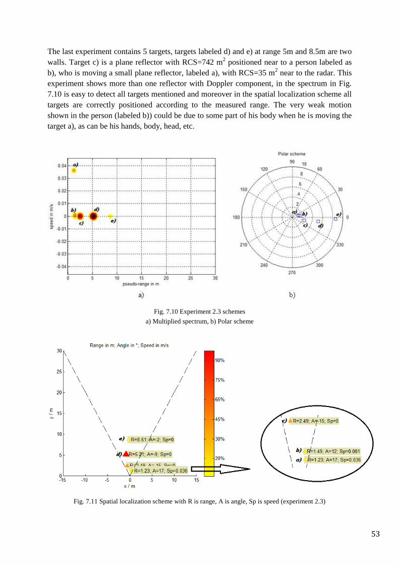
53

The last experiment contains 5 targets, targets labeled d) and e) at range 5m and 8.5m are two

walls. Target c) is a plane reflector with RCS=742 m2 positioned near to a person labeled as

b), who is moving a small plane reflector, labeled a), with RCS=35 m2 near to the radar. This

experiment shows more than one reflector with Doppler component, in the spectrum in Fig.

7.10 is easy to detect all targets mentioned and moreover in the spatial localization scheme all

targets are correctly positioned according to the measured range. The very weak motion

shown in the person (labeled b)) could be due to some part of his body when he is moving the

target a), as can be his hands, body, head, etc.

Fig. 7.10 Experiment 2.3 schemes

a) Multiplied spectrum, b) Polar scheme

Fig. 7.11 Spatial localization scheme with R is range, A is angle, Sp is speed (experiment 2.3)

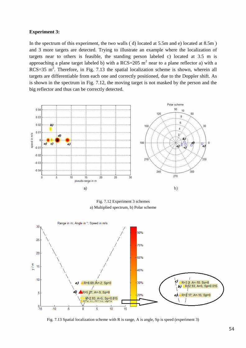
54

Experiment 3:

In the spectrum of this experiment, the two walls ( d) located at 5.5m and e) located at 8.5m )

and 3 more targets are detected. Trying to illustrate an example where the localization of

targets near to others is feasible, the standing person labeled c) located at 3.5 m is

approaching a plane target labeled b) with a RCS=205 m2 near to a plane reflector a) with a

RCS=35 m2. Therefore, in Fig. 7.13 the spatial localization scheme is shown, wherein all

targets are differentiable from each one and correctly positioned, due to the Doppler shift. As

is shown in the spectrum in Fig. 7.12, the moving target is not masked by the person and the

big reflector and thus can be correctly detected.

Fig. 7.12 Experiment 3 schemes

a) Multiplied spectrum, b) Polar scheme

Fig. 7.13 Spatial localization scheme with R is range, A is angle, Sp is speed (experiment 3)

55

Experiment 4:

Targets labeled a) and b) are small reflectors positioned at 1.5 and 2.5 meters approximately,

both with RCS=35 m2 and target labeled e) located at 8.3m has a RCS=742 m

2. The

interesting thing is that a person is moving very slowly next to the wall labeled d) which

located at 5m, so that the person has a very small shift in Doppler shown in the spectrum in

Fig. 7.14, and thus his localization is feasible as is shown in Fig. 7.15.

Fig. 7.14 Experiment 4 schemes

a) Multiplied spectrum, b) Polar scheme

Fig. 7.15 Spatial localization scheme with R is range, A is angle, Sp is speed (experiment 4)

56

Experiment 5:

In this experiment target a) is a plane reflector placed at 2m with RCS=204 m2 and target

labeled b) is a wall located at 5m, but now a person is located behind a door of this wall. The

door is made of wood and has some metal parts ,and its thickness is around 7 cm. Must be

remarkable that the person behind the door was not moving, the only moving part was his

breast needed to breath. A normal breath makes that the breast moves with a speed around

0.03 m/s [11]. In the spectrum, in Fig. 7.16, is shown how this technique detects the person

behind a door, and furthermore the speed indicated by the person breathing complies with the

previous said value.

Fig. 7.16 Experiment 5 schemes

a) Multiplied spectrum, b) Polar scheme

Fig. 7.17 Spatial localization scheme with R is range, A is angle, Sp is speed (experiment 5)

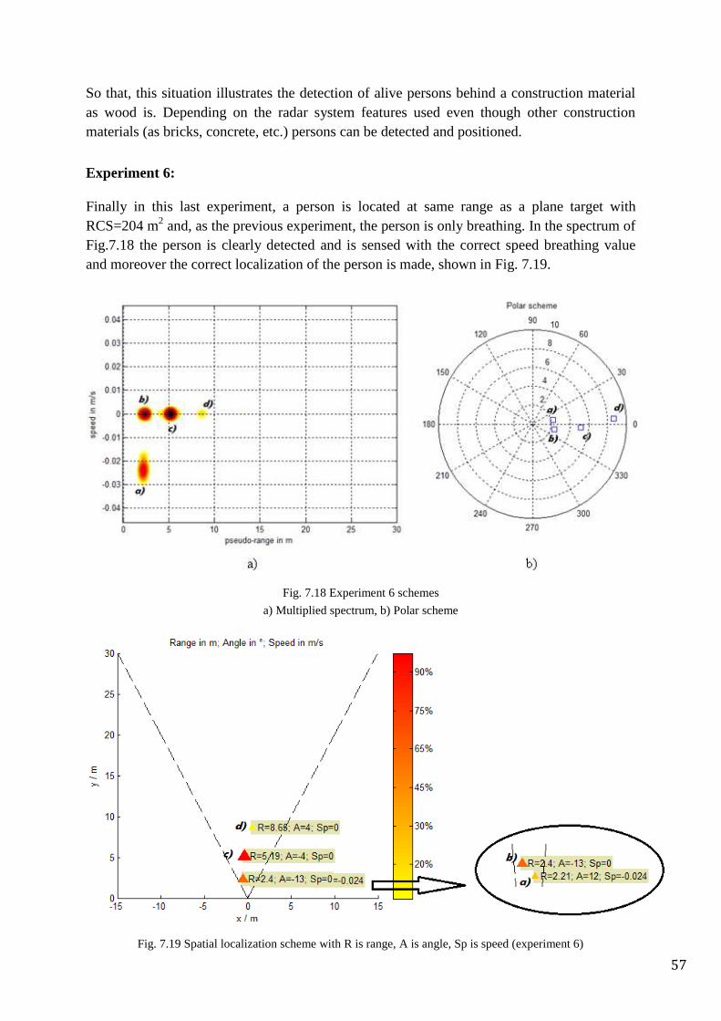
57

So that, this situation illustrates the detection of alive persons behind a construction material

as wood is. Depending on the radar system features used even though other construction

materials (as bricks, concrete, etc.) persons can be detected and positioned.

Experiment 6:

Finally in this last experiment, a person is located at same range as a plane target with

RCS=204 m2 and, as the previous experiment, the person is only breathing. In the spectrum of

Fig.7.18 the person is clearly detected and is sensed with the correct speed breathing value

and moreover the correct localization of the person is made, shown in Fig. 7.19.

Fig. 7.18 Experiment 6 schemes

a) Multiplied spectrum, b) Polar scheme

Fig. 7.19 Spatial localization scheme with R is range, A is angle, Sp is speed (experiment 6)

58

Finally Fig. 7.20 and Fig. 7.21 illustrate two localization schemes in 3D that corresponds to

the experiments 5 and 6. In the first scheme, the plane x-y (Fig. 7.20_a & Fig. 7.21_a)

corresponds to the coordinates, where targets are located and z axis corresponds to Doppler

value of the targets. The second scheme, (Fig. 7.20_b & Fig. 7.21_b) is similar to the first

one, but z axis corresponds to the received amplitude of each target. Moreover, in both

schemes, can be seen a color bar that represents the point spread function (PSF) as an imaging

quality metric, so that the color and size of each square in the first scheme and the height and

color of each peak in the second scheme, depends on its detection intensity.

Fig. 7. 20 3D localization schemes (experiment 5)

a) Position-Doppler scheme, b) Position-amplitude scheme

Fig. 7. 21 3D localization schemes (experiment 6)

a) Position-Doppler scheme, b) Position-amplitude scheme

59

7.3 Error Function

After analyzing experiments, where the spatial localization using the presented method is

achieved correctly, the accuracy of these results is going to be calculated, i.e. how capable this

method is to give a reliable result.

In this chapter, as in Matlab simulation chapter, the error function is the tool used to illustrate

the accuracy, this error function is calculated about range and angle. To make different

measures at different ranges a big and empty place was chosen in order to avoid some kind of

undesired reflections or multireflection.

Real target parameters were measured using a laser-meter, therefore real range was easy to

know. For measuring the real angle was used two laser measurements, as is shown in Fig.

7.22 & Fig. 7.23. The first measurement was the direct range between radar and target and the

other was the range shifted only in one axis. With this information real angle information can

be given by using trigonometry as:

(7.1)

Fig.7.22 Measure scheme

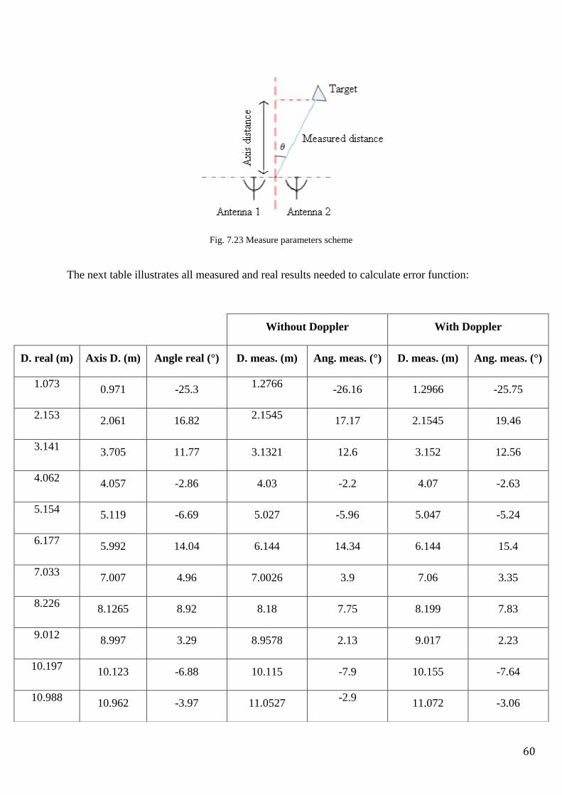
60

Fig. 7.23 Measure parameters scheme

The next table illustrates all measured and real results needed to calculate error function:

Without Doppler With Doppler

D. real (m) Axis D. (m) Angle real (°) D. meas. (m) Ang. meas. (°) D. meas. (m) Ang. meas. (°)

1.073 0.971 -25.3

1.2766 -26.16 1.2966 -25.75

2.153 2.061 16.82

2.1545 17.17 2.1545 19.46

3.141 3.705 11.77 3.1321 12.6 3.152 12.56

4.062 4.057 -2.86 4.03 -2.2 4.07 -2.63

5.154 5.119 -6.69 5.027 -5.96 5.047 -5.24

6.177 5.992 14.04 6.144 14.34 6.144 15.4

7.033 7.007 4.96 7.0026 3.9 7.06 3.35

8.226 8.1265 8.92 8.18 7.75 8.199 7.83

9.012 8.997 3.29 8.9578 2.13 9.017 2.23

10.197 10.123 -6.88 10.115 -7.9 10.155 -7.64

10.988 10.962 -3.97 11.0527

-2.9 11.072 -3.06

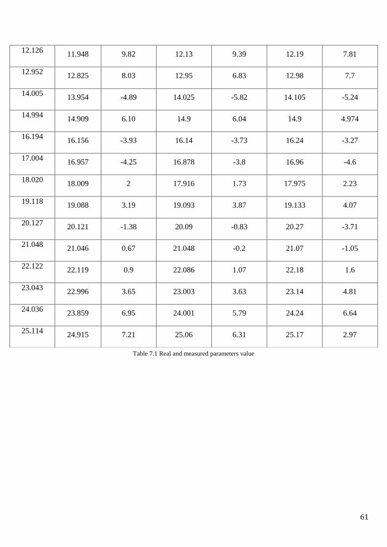
61

Table 7.1 Real and measured parameters value

12.126 11.948 9.82 12.13 9.39 12.19 7.81

12.952 12.825 8.03 12.95 6.83 12.98 7.7

14.005 13.954 -4.89 14.025 -5.82 14.105 -5.24

14.994 14.909 6.10 14.9 6.04 14.9 4.974

16.194 16.156 -3.93 16.14 -3.73 16.24 -3.27

17.004 16.957 -4.25 16.878 -3.8 16.96 -4.6

18.020 18.009 2 17.916 1.73 17.975 2.23

19.118 19.088 3.19 19.093 3.87 19.133 4.07

20.127 20.121 -1.38 20.09 -0.83 20.27 -3.71

21.048 21.046 0.67 21.048 -0.2 21.07 -1.05

22.122 22.119 0.9 22.086 1.07 22.18 1.6

23.043 22.996 3.65 23.003 3.63 23.14 4.81

24.036 23.859 6.95 24.001 5.79 24.24 6.64

25.114 24.915 7.21 25.06 6.31 25.17 2.97

62

Range error function:

Fig.7.24 Range error function with a not moving target

Fig.7.25 Range error function with a moving target

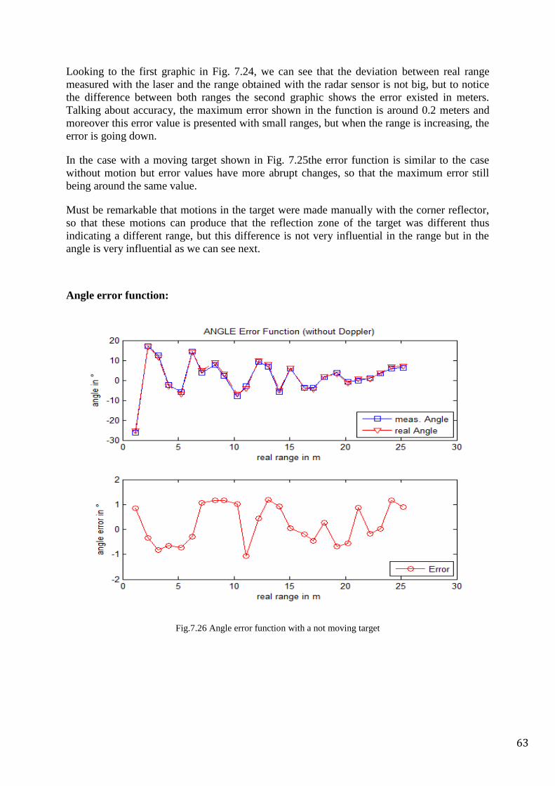
63

Looking to the first graphic in Fig. 7.24, we can see that the deviation between real range

measured with the laser and the range obtained with the radar sensor is not big, but to notice

the difference between both ranges the second graphic shows the error existed in meters.

Talking about accuracy, the maximum error shown in the function is around 0.2 meters and

moreover this error value is presented with small ranges, but when the range is increasing, the

error is going down.

In the case with a moving target shown in Fig. 7.25the error function is similar to the case

without motion but error values have more abrupt changes, so that the maximum error still

being around the same value.

Must be remarkable that motions in the target were made manually with the corner reflector,

so that these motions can produce that the reflection zone of the target was different thus

indicating a different range, but this difference is not very influential in the range but in the

angle is very influential as we can see next.

Angle error function:

Fig.7.26 Angle error function with a not moving target

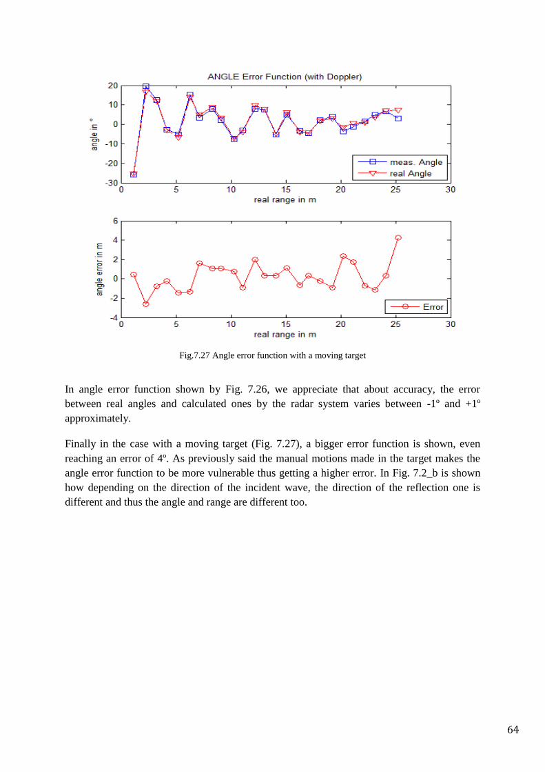
64

Fig.7.27 Angle error function with a moving target

In angle error function shown by Fig. 7.26, we appreciate that about accuracy, the error

between real angles and calculated ones by the radar system varies between -1º and +1º

approximately.

Finally in the case with a moving target (Fig. 7.27), a bigger error function is shown, even

reaching an error of 4º. As previously said the manual motions made in the target makes the

angle error function to be more vulnerable thus getting a higher error. In Fig. 7.2_b is shown

how depending on the direction of the incident wave, the direction of the reflection one is

different and thus the angle and range are different too.

65

8. Conclusions

Mainly the goal of this project was the coordinate determination of moving targets, and also it

was tried to take full advantage of the explained method in order to illustrate its skills.

The previous results shown, in chapter 7, have demonstrated that the described experiments,

in which each FMCW-Radar and monopulse technique alone are unable to achieve a good

result, are correctly solved by employing the algorithm proposed in which both techniques are

implemented together. Therefore, achieving a proper spatial localization of moving targets

scheme.

Cited situations are from the localization of targets at different ranges to the positioning of

targets with very weak motions (even less than a normal man breathing motion) near either

behind some kind of materials with a big RCS and under hard weather conditions. In addition

the shown localization accuracy becomes this project in a reliable and competent choice.

It can be concluded saying that the spatial localization method presented would be useful in

some real life circumstances. One of the previously cited applications was the detection of

buried alive people in case of disaster as structural collapse (as we can see in Fig. 8.1),snow

avalanches, sand storms, etc.; beyond the feasible live signs detection under construction

elements as bricks, beams, etc. due only to a very weak motion of the person (as breathing,

body motions, etc.). The correct spatial localization of him could be critical in some extreme

cases where time to find him alive is limited and in this way by knowing exactly the position

could reduce rescue time and even save his live, overcoat in scenarios with heavy materials or

severe an dark weather conditions as the picture shows. Moreover people buried located at

different positions (it means different angle) and at same distance of the radar can be perfectly

positioned by only these persons are moving with a weak motion difference, even if more

than one person are only breathing.

Fig. 8.1 Structural collapse [15][16]

In these disaster cases, the breast motions of each person could be different depending on

their gender, age, panic, etc, and in this way the different breathing speed can allow to the

correct calculation of the angle of each one.

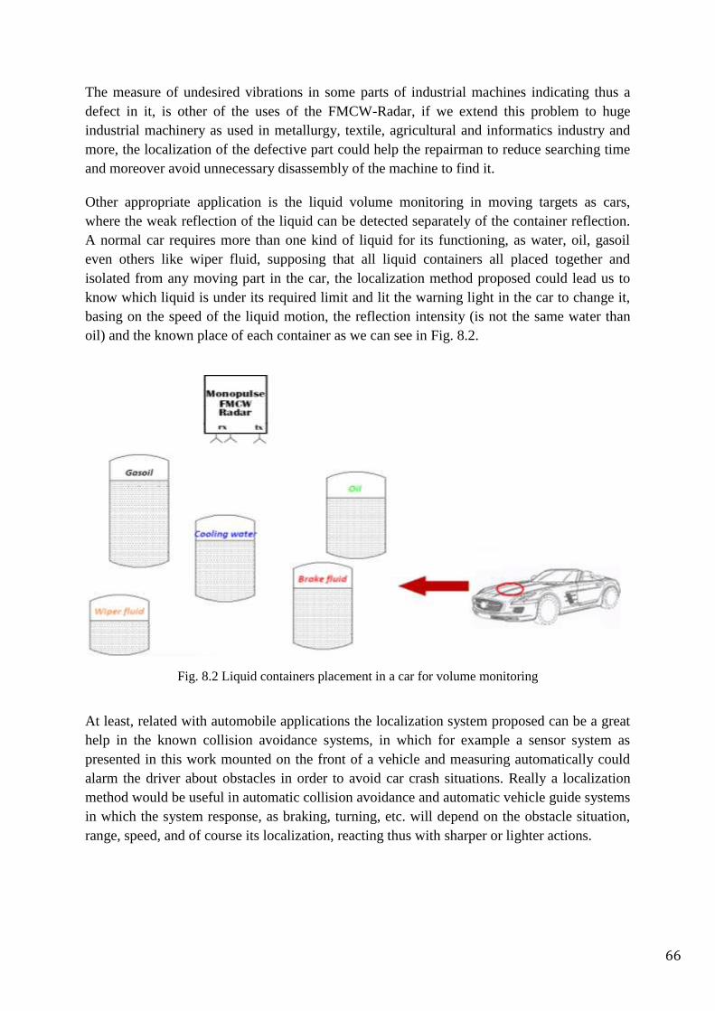
66

The measure of undesired vibrations in some parts of industrial machines indicating thus a

defect in it, is other of the uses of the FMCW-Radar, if we extend this problem to huge

industrial machinery as used in metallurgy, textile, agricultural and informatics industry and

more, the localization of the defective part could help the repairman to reduce searching time

and moreover avoid unnecessary disassembly of the machine to find it.

Other appropriate application is the liquid volume monitoring in moving targets as cars,

where the weak reflection of the liquid can be detected separately of the container reflection.

A normal car requires more than one kind of liquid for its functioning, as water, oil, gasoil

even others like wiper fluid, supposing that all liquid containers all placed together and

isolated from any moving part in the car, the localization method proposed could lead us to

know which liquid is under its required limit and lit the warning light in the car to change it,

basing on the speed of the liquid motion, the reflection intensity (is not the same water than

oil) and the known place of each container as we can see in Fig. 8.2.

Fig. 8.2 Liquid containers placement in a car for volume monitoring

At least, related with automobile applications the localization system proposed can be a great

help in the known collision avoidance systems, in which for example a sensor system as

presented in this work mounted on the front of a vehicle and measuring automatically could

alarm the driver about obstacles in order to avoid car crash situations. Really a localization

method would be useful in automatic collision avoidance and automatic vehicle guide systems

in which the system response, as braking, turning, etc. will depend on the obstacle situation,

range, speed, and of course its localization, reacting thus with sharper or lighter actions.