P ROACTIVE AUTO -S CALING T ECHNIQUES FOR C ONTAINERISED A PPLICATIONS A thesis submitted in fulfilment of the requirements for the degree of Doctor of Philosophy Eidah Juman A. Alzahrani Master of Information Technology (La Trobe University) School of Science College of Science, Engineering, and Health RMIT University December, 2019

Welcome message from author
This document is posted to help you gain knowledge. Please leave a comment to let me know what you think about it! Share it to your friends and learn new things together.
Transcript
PROACTIVE AUTO-SCALING TECHNIQUES FOR
CONTAINERISED APPLICATIONS
A thesis submitted in fulfilment of the requirements
for the degree of Doctor of Philosophy
Eidah Juman A. Alzahrani
Master of Information Technology (La Trobe University)
School of Science
College of Science, Engineering, and Health
RMIT University
December, 2019
Declaration
I certify that except where due acknowledgement has been made, the work is that of the author
alone; the work has not been submitted previously, in whole or in part, to qualify for any other
academic award; the content of the thesis is the result of work which has been carried out since
the official commencement date of the approved research program; any editorial work, paid
or unpaid, carried out by a third party is acknowledged; and, ethics procedures and guidelines
have been followed.
Eidah Juman A. Alzahrani
School of Science
RMIT University
19 December 2019
i
Acknowledgements
This thesis not possible without the guidance and support of many people over many years.
First and foremost, my deepest gratitude extends to my PhD supervisor, Prof. Zahir Tari, for
all the support he has provided, past and present, and for everything I have learned from him.
His high degree of skills in research, problem solving, and time management have forged
this thesis. Furthermore, his patience and absolute trust helped me to develop and build skills
beyond research, to a personal and social level. Thank you from the bottom of my heart for
your enduring giving.
I was very lucky to interact with the skillful mathematicians at RMIT University. Prof. Panlop
Zeephongsekul (1950-2017), thank you for your guidance, kindness, and help during your
time in RMIT University. Also, my warmest regards go to Dr. Vural Aksakalli, who joined my
supervisory team and provided me with much appreciated help and motivation.
The research presented in this thesis is a result of many collaborations. I am grateful to have
worked with Prof. Albert Zomaya, Dr. Young Choon Lee (이영춘) and Dr Hoang Dau, who
all provided me with motivation and close cooperation. Their interest in my work and their
comments have helped me to build my ambition and improve my work. I would not forget to
thank the staff in Virtual Experiences Laboratory (VXLab), especially the technical manager
Dr. Ian Peake. The different experiments in this thesis could not have been carried out in a re-
alistic environment without their efforts and help. The ORACLE cloud credit for researchers is
acknowledged as part of this thesis is implemented and analysed on ORACLE’s infrastructure.
Also, thanks to Deafallah Alsaedi, Ahmed Alharith, Ahmed Fallatah, Tawfeeq Alsanoosy, and
all my other friends and colleagues at RMIT University. The meetings and conversations that I
had with them were probably not the most productive things, but definitely contributed to the
joyful time I had during my research experience at RMIT University. You guys made my life
at RMIT University memorable.
I would like to acknowledge the constant support and encouragement that I have received from:
my mother (Sharifa), sister (Saadia), brothers (Saeed, Abdullah, Ahmad, Mutaib and Mishary)
and I am grateful for their wholehearted love and support.
Most importantly, I want to thank my wife (Faten Alzahrani) for her unlimited love and care
ii
that helped me to attain this achievement. I would not have had the determination to complete
my Ph.D. journey without Faten’s constant support and encouragement. Also, I want to express
my warmest thanks to my kids (Azzam and Zeyad), who have made our life full of joy, laugh,
happiness.
Last but not least, I acknowledge the financial support I have received for my country (Saudi
Arabia) through the provision of the Saudi Arabian Cultural Mission in Australia-Canberra
(SACM). Moreover, I am deeply indebted to Albaha University (Saudi Arabia) for providing
me with a scholarship to pursue my research at RMIT University.
iii
Credits
Portions of the material in this thesis have previously appeared in the following publications:
• E. J. Alzahrani, Z. Tari, P. Zeephongsekul, Y. C. Lee, D. Alsadie, and A. Y. Zomaya.
Sla-aware resource scaling for energy efficiency. In Proceedings of the 18th IEEE Inter-
national Conference on High Performance Computing and Communications (HPCC),
pages 852-859, 2016.
• E. J. Alzahrani, Z. Tari, Y. C. Lee, D. Alsadie, and A. Y. Zomaya. adcfs: Adaptive com-
pletely fair scheduling policy for containerised workflows systems. In Proceedings of the
16th IEEE International Symposium on Network Computing and Applications (NCA),
pages 245-252, 2017. [Best Student Paper Award]
Scholarly activities on cloud computing resource management
• D. Alsadie, Z. Tari, E. J. Alzahrani, and A. Y. Zomaya. Energy-efficient tailoring of
VM size and tasks in cloud data centers. In Proceedings of the 16th IEEE International
Symposium on Network Computing and Applications (NCA), pages 99-103, 2017.
• D. Alsadie, Z. Tari, E. J. Alzahrani, and A. Y. Zomaya. LIFE: A predictive approach for
VM placement in cloud environments. In Proceedings of the 16th IEEE International
Symposium on Network Computing and Applications (NCA), pages 91-98, 2017.
• Andrzej M. Goscinski, Zahir Tari, Izzatdin Abdul Aziz, E. J. Alzahrani. Fog Computing
as a Critical Link Between a Central Cloud and IoT in Support of Fast Discovery of New
Hydrocarbon Reservoirs. In Proceedings of the 9th International Conference on Mobile
Networks and Management (MONAMI), pages 247-261, 2017
• D. Alsadie, Z. Tari, E. J. Alzahrani, and A. Y. Zomaya. Dynamic resource allocation
for an energy efficient VM architecture for cloud computing. In Proceedings of the Aus-
tralasian Computer Science Week Multiconference (ACSW), pages 1-8, 2018.
iv
• D. Alsadie, Z. Tari, E. J. Alzahrani, and A. Alshammari. LIFE-MP: Online virtual ma-
chine consolidation with multiple resource usages in cloud environments. In Proceedings
of the 19th International Conference on Web Information Systems Engineering (WISE),
pages 490-501, 2018.
• D. Alsadie, Z. Tari, E. J. Alzahrani, and A. Y. Zomaya. DTFS: A dynamic threshold-
based fuzzy approach for power efficient vm consolidation. In Proceedings of the 17th
IEEE International Symposium on Network Computing and Applications (NCA), pages
91-98, 2018.
• D. Alsadie, Z. Tari and E. J. Alzahrani. Online VM Consolidation in Cloud Environ-
ments. In Proceedings of the 12th IEEE International Conference on Cloud Computing
(CLOUD) , pages 137-145, 2019
v

The thesis was written in overleafOnline LaTeX Editor, and typeset using the LATEX 2ε doc-
ument preparation system.
All trademarks are the property of their respective owners.
vi
Dedication
I dedicate this thesis to my father’s soul
i�Êg. áK. àAªÔg.(1946 - 2010)
I miss you DAD
May god have mercy on your soul.
vii
Contents
Abstract 1
1 Introduction 3
1.1 Motivation . . . . . . . . . . . . . . . . . . . . . . . . . . . . . . . . . . . . . 3
1.2 Summary of existing techniques . . . . . . . . . . . . . . . . . . . . . . . . . 5
1.2.1 Threshold-based techniques . . . . . . . . . . . . . . . . . . . . . . . 6
1.2.2 Reinforcement learning-based techniques . . . . . . . . . . . . . . . . 7
1.2.3 Queuing-based techniques . . . . . . . . . . . . . . . . . . . . . . . . 7
1.2.4 Control theory-based techniques . . . . . . . . . . . . . . . . . . . . . 8
1.2.5 Time series-based techniques . . . . . . . . . . . . . . . . . . . . . . . 9
1.3 Limitations of existing auto-scaling techniques . . . . . . . . . . . . . . . . . 10
1.4 Research questions . . . . . . . . . . . . . . . . . . . . . . . . . . . . . . . . 12
1.5 Thesis Scope . . . . . . . . . . . . . . . . . . . . . . . . . . . . . . . . . . . 17
1.6 Thesis contributions . . . . . . . . . . . . . . . . . . . . . . . . . . . . . . . . 18
1.7 Thesis organisation . . . . . . . . . . . . . . . . . . . . . . . . . . . . . . . . 20
2 Background 23
2.1 Virtualisation . . . . . . . . . . . . . . . . . . . . . . . . . . . . . . . . . . . 23
2.1.1 Virtual machine (VM) . . . . . . . . . . . . . . . . . . . . . . . . . . 25
2.1.2 Containers . . . . . . . . . . . . . . . . . . . . . . . . . . . . . . . . 26
2.1.3 Difference between VMs and containers . . . . . . . . . . . . . . . . . 28
2.2 Inter-Cloud distributed applications . . . . . . . . . . . . . . . . . . . . . . . 29
2.2.1 Sensitive applications . . . . . . . . . . . . . . . . . . . . . . . . . . . 29
viii
2.2.2 Batch-based jobs . . . . . . . . . . . . . . . . . . . . . . . . . . . . . 29
2.3 Container scalability . . . . . . . . . . . . . . . . . . . . . . . . . . . . . . . 30
2.4 Proactive auto-scaling technique . . . . . . . . . . . . . . . . . . . . . . . . . 31
2.5 Summary . . . . . . . . . . . . . . . . . . . . . . . . . . . . . . . . . . . . . 32
3 SLA-Aware Dynamic Resource Scaling for Sensitive Containerised Applications 33
3.1 Introduction . . . . . . . . . . . . . . . . . . . . . . . . . . . . . . . . . . . . 34
3.2 Related work . . . . . . . . . . . . . . . . . . . . . . . . . . . . . . . . . . . 37
3.3 The EBAS approach . . . . . . . . . . . . . . . . . . . . . . . . . . . . . . . 42
3.3.1 System architecture . . . . . . . . . . . . . . . . . . . . . . . . . . . . 43
3.3.2 Workload estimator . . . . . . . . . . . . . . . . . . . . . . . . . . . . 44
3.3.3 Power scaling unit (PSU) . . . . . . . . . . . . . . . . . . . . . . . . . 47
3.3.4 SLA quality monitor . . . . . . . . . . . . . . . . . . . . . . . . . . . 50
3.3.5 The auto-scaler agent . . . . . . . . . . . . . . . . . . . . . . . . . . . 51
3.4 Experimental evaluation . . . . . . . . . . . . . . . . . . . . . . . . . . . . . 52
3.4.1 Workload . . . . . . . . . . . . . . . . . . . . . . . . . . . . . . . . . 52
3.4.2 Evaluation metrics . . . . . . . . . . . . . . . . . . . . . . . . . . . . 53
3.4.3 Benchmark algorithms . . . . . . . . . . . . . . . . . . . . . . . . . . 54
3.4.4 Experiment setup . . . . . . . . . . . . . . . . . . . . . . . . . . . . . 55
3.4.5 Experimental results . . . . . . . . . . . . . . . . . . . . . . . . . . . 57
3.4.6 Evaluation of the prediction model . . . . . . . . . . . . . . . . . . . 61
3.4.7 Discussion . . . . . . . . . . . . . . . . . . . . . . . . . . . . . . . . 63
3.5 Conclusion . . . . . . . . . . . . . . . . . . . . . . . . . . . . . . . . . . . . 64
4 adCFS Policy for Containerised Batch Applications (Scientific Workflows) 65
4.1 Introduction . . . . . . . . . . . . . . . . . . . . . . . . . . . . . . . . . . . . 66
4.2 Related work . . . . . . . . . . . . . . . . . . . . . . . . . . . . . . . . . . . 69
4.3 Architecture . . . . . . . . . . . . . . . . . . . . . . . . . . . . . . . . . . . . 73
4.4 The adCFS sharing policy . . . . . . . . . . . . . . . . . . . . . . . . . . . . 74
4.4.1 CPU State Predictor (CSP) . . . . . . . . . . . . . . . . . . . . . . . . 75
4.4.2 Container’s CPU weight scaler . . . . . . . . . . . . . . . . . . . . . . 78
ix
4.5 Experimental results . . . . . . . . . . . . . . . . . . . . . . . . . . . . . . . 80
4.5.1 Montage system workload . . . . . . . . . . . . . . . . . . . . . . . . 80
4.5.2 Benchmark algorithms . . . . . . . . . . . . . . . . . . . . . . . . . . 86
4.5.3 Experimental environment . . . . . . . . . . . . . . . . . . . . . . . . 87
4.5.4 Experimental results . . . . . . . . . . . . . . . . . . . . . . . . . . . 89
4.6 Conclusion . . . . . . . . . . . . . . . . . . . . . . . . . . . . . . . . . . . . 94
5 A CPU Interference Detection Approach for Containerised Scientific Workflow
Systems 96
5.1 Introduction . . . . . . . . . . . . . . . . . . . . . . . . . . . . . . . . . . . . 98
5.2 Related work . . . . . . . . . . . . . . . . . . . . . . . . . . . . . . . . . . . 100
5.3 weiMetric as a System Design . . . . . . . . . . . . . . . . . . . . . . . . . 105
5.3.1 Software Event Counters of weiMetric . . . . . . . . . . . . . . . . . 107
5.3.2 weiMetric Construction Unit . . . . . . . . . . . . . . . . . . . . . . . 109
5.3.3 Interference Detector . . . . . . . . . . . . . . . . . . . . . . . . . . . 112
5.3.4 Interference Remedy Planning . . . . . . . . . . . . . . . . . . . . . . 114
5.4 Experimental evaluation . . . . . . . . . . . . . . . . . . . . . . . . . . . . . 115
5.4.1 Benchmarks . . . . . . . . . . . . . . . . . . . . . . . . . . . . . . . . 117
5.4.2 Montage as a case study . . . . . . . . . . . . . . . . . . . . . . . . . 118
5.4.3 Memcached servers workloads as a case study . . . . . . . . . . . . . 125
5.5 Conclusion . . . . . . . . . . . . . . . . . . . . . . . . . . . . . . . . . . . . 127
6 Predictive Co-location Technique to Maximise CPU Workloads of Data Centre
Servers 129
6.1 Introduction . . . . . . . . . . . . . . . . . . . . . . . . . . . . . . . . . . . . 130
6.2 Related work . . . . . . . . . . . . . . . . . . . . . . . . . . . . . . . . . . . 133
6.3 The M2-AutScale Method . . . . . . . . . . . . . . . . . . . . . . . . . . . . 142
6.3.1 Monitoring and metrics feeder . . . . . . . . . . . . . . . . . . . . . . 143
6.3.2 Sensitive application CPU demand estimator . . . . . . . . . . . . . . 145
6.3.3 Safety margin constructor . . . . . . . . . . . . . . . . . . . . . . . . 151
6.3.4 Containers’ scalability model . . . . . . . . . . . . . . . . . . . . . . 153
x
6.4 Evaluation . . . . . . . . . . . . . . . . . . . . . . . . . . . . . . . . . . . . . 153
6.4.1 Methodology and experimental setup . . . . . . . . . . . . . . . . . . 153
6.4.2 Datasets . . . . . . . . . . . . . . . . . . . . . . . . . . . . . . . . . . 154
6.4.3 Benchmarks . . . . . . . . . . . . . . . . . . . . . . . . . . . . . . . . 158
6.4.4 Experimental results . . . . . . . . . . . . . . . . . . . . . . . . . . . 160
6.5 Conclusion . . . . . . . . . . . . . . . . . . . . . . . . . . . . . . . . . . . . 163
7 Conclusion 165
7.1 Summary . . . . . . . . . . . . . . . . . . . . . . . . . . . . . . . . . . . . . 165
7.2 Overall Contributions . . . . . . . . . . . . . . . . . . . . . . . . . . . . . . . 166
7.3 Future Research Direction . . . . . . . . . . . . . . . . . . . . . . . . . . . . 168
7.3.1 Proactive auto-scaling for different computing resources . . . . . . . . 168
7.3.2 CPU sharing and interference categorisation . . . . . . . . . . . . . . . 169
7.3.3 Harvest more types of computing resources . . . . . . . . . . . . . . . 169
Bibliography 171
xi
List of Figures
1.1 Thesis organisation . . . . . . . . . . . . . . . . . . . . . . . . . . . . . . . . . . 22
2.1 VM-based virtualisation vs. container-based virtualisation . . . . . . . . . . . . . 24
2.2 Type I and type II hypervisors . . . . . . . . . . . . . . . . . . . . . . . . . . . . 25
2.3 Layer structure of container . . . . . . . . . . . . . . . . . . . . . . . . . . . . . . 27
2.4 Operations to manage image and container . . . . . . . . . . . . . . . . . . . . . . 27
2.5 Container development lifecycle . . . . . . . . . . . . . . . . . . . . . . . . . . . 28
3.1 Frequency over-provisioning in on-demand governor. . . . . . . . . . . . . . . . . 36
3.2 MAPE Model. . . . . . . . . . . . . . . . . . . . . . . . . . . . . . . . . . . . . . 41
3.3 EBAS architecture. . . . . . . . . . . . . . . . . . . . . . . . . . . . . . . . . . . 43
3.4 An overview of EBAS. . . . . . . . . . . . . . . . . . . . . . . . . . . . . . . . . 45
3.5 The different functions of the Auto-Scaler Agent. . . . . . . . . . . . . . . . . . . 52
3.6 Using Memcached as caching layer to speed up dynamic web applications. . . . . 53
3.7 Scalability in the EPFL Data caching benchmark. . . . . . . . . . . . . . . . . . . 57
3.8 CPU utilisation for one minute. . . . . . . . . . . . . . . . . . . . . . . . . . . . . 58
3.9 Data caching server when handling 10k rps workload. . . . . . . . . . . . . . . . 59
3.10 Memcached server throughput. . . . . . . . . . . . . . . . . . . . . . . . . . . . . 60
3.11 95% and 99% latency under variant workloads. . . . . . . . . . . . . . . . . . . . 60
3.12 Energy consumption evaluation. . . . . . . . . . . . . . . . . . . . . . . . . . . . 62
3.13 Total CPU predictions for the data caching benchmark with a prediction interval
of 3 minutes. . . . . . . . . . . . . . . . . . . . . . . . . . . . . . . . . . . . . . 62
3.14 EBAS cores selections. . . . . . . . . . . . . . . . . . . . . . . . . . . . . . . . . 63
3.15 EBAS frequency selection (green line) against ondemand governor (red line). . . . 64
xii
4.1 Example for directed acyclic graph (DAG). . . . . . . . . . . . . . . . . . . . . . 67
4.2 A containerised workflow architecture. . . . . . . . . . . . . . . . . . . . . . . . . 74
4.3 CPU states and transitions with their corresponding probabilities. . . . . . . . . . . 77
4.4 Montage workflow. The computational workflow tasks are the coloured circles
which each colour represent different task type . . . . . . . . . . . . . . . . . . . 82
4.5 Example of grayscale mosaic in JPEG format . . . . . . . . . . . . . . . . . . . . 86
4.6 State occurrence and job submission intervals . . . . . . . . . . . . . . . . . . . . 88
4.7 State occurrence and job submission intervals . . . . . . . . . . . . . . . . . . . . 89
4.8 Completely Fair Scheduler–CFS . . . . . . . . . . . . . . . . . . . . . . . . . . . 90
4.9 Response time means on different CPU-sharing policies . . . . . . . . . . . . . . 90
4.10 adCFS performance . . . . . . . . . . . . . . . . . . . . . . . . . . . . . . . . . . 91
4.11 Accuracy of CSP for the corresponding CPU states . . . . . . . . . . . . . . . . . 91
4.12 Accuracy of CSP during the experiments . . . . . . . . . . . . . . . . . . . . . . . 92
4.13 CPU portions on adCFS for Montage containers. . . . . . . . . . . . . . . . . . . 92
5.1 The compulsory LLC-load-misses for mProjectPP container . . . . . . . . . . . . 102
5.2 Cache misses, LLC-load-misses and CPI and for mProjectPP container . . . . . . . 104
5.3 weiMetric system architecture. . . . . . . . . . . . . . . . . . . . . . . . . . . . . 107
5.4 Reaction of the software event counters to interference. The x-axis represents
mProjectPP task indices and the y-axis represents the event counters (Task-Clock,
Context-Switches, and CPU-Migrations) during the execution of mProjectPP tasks.
The container CPU resource was artificially exposed to CPU-bound workload (i.e.,
cpuBomb workload) within tasks 231–318 of the mProjectPP tasks and the coun-
ters demonstrated outliers (spikes) accordingly. . . . . . . . . . . . . . . . . . . . 109
5.5 Waiting times and noise length. The left side summarises the waiting time between
batch jobs submissions. The right side shows the run times length for the noisy
workloads cpuBomb, mallocBomb, and forkBomb. . . . . . . . . . . . . . . . . . 118
5.6 Host CPU usage during the experiment . . . . . . . . . . . . . . . . . . . . . . . . 120
5.7 Inner CPU Interference for mProjectPP container caused by new mProjectPP tasks
that increase the CPU demand for this container . . . . . . . . . . . . . . . . . . . 120
xiii
5.8 Detection false positive rate when using weiMetric . . . . . . . . . . . . . . . . . 121
5.9 Outer and inner CPU interference for mBackground container, the green shaded
areas are the outer CPU interference while the red shaded area is internal CPU
interference caused by increasing the CPU demands . . . . . . . . . . . . . . . . . 122
5.10 weiMetric performance . . . . . . . . . . . . . . . . . . . . . . . . . . . . . . . 123
5.11 weiMetric performance on data caching workloads . . . . . . . . . . . . . . . . 126
5.12 weiMetric overhead . . . . . . . . . . . . . . . . . . . . . . . . . . . . . . . . . 127
6.1 Container ID#c 11101 CPU usage . . . . . . . . . . . . . . . . . . . . . . . . . . 141
6.2 P-value frequencies during Augmented Dickey-Fuller (ADF) test . . . . . . . . . . 141
6.3 The CPU exhibits a non-stationary behaviour at time 6. Both ARIMA components
Autoregression (AR) and Moving Average (MA) were not able to anticipate this
non-stationary behaviour. . . . . . . . . . . . . . . . . . . . . . . . . . . . . . . . 142
6.4 The workflow of the Interference-aware proactive CPU workload co-location com-
ponents.Two monitored input data are essential to operate the predictive co-location
model. First, CPU usage for containers. Second, the CPU-related interference met-
rics. . . . . . . . . . . . . . . . . . . . . . . . . . . . . . . . . . . . . . . . . . . 143
6.5 Pre-processing the relative CPU usage and converting it to an absolute usage out
of 100% . . . . . . . . . . . . . . . . . . . . . . . . . . . . . . . . . . . . . . . . 144
6.6 The main software event counters of weiMetric: Task-Clock, Context-Switch, and
CPU-Migrations. . . . . . . . . . . . . . . . . . . . . . . . . . . . . . . . . . . . 145
6.7 Illustration of a two-level nested Markov chains for the CPU usage time series. . . 147
6.8 Illustration of the actual CPU usage time series versus the ARIMA’s predictions
and the proposed hybrid Markov-ARIMA’s predictions for container c 11101 of
app 489 [1]. . . . . . . . . . . . . . . . . . . . . . . . . . . . . . . . . . . . . . . 150
6.9 The Resource Estimator takes as inputs the predicted CPU usage, the requested
CPU usage, and the safety margin for every container and outputs the number of
CPU cores assigned to all containers as well as the CPU share, which specifies the
fraction of each core that each container can utilise. In this way, it can guarantee
sufficient CPU usage for each container and avoid bursty workload. . . . . . . . . 153
xiv
6.10 Applications’ distribution on servers . . . . . . . . . . . . . . . . . . . . . . . . . 155
6.11 Histogram of number of containers running in each time interval . . . . . . . . . . 156
6.12 CPU usage for web service containers . . . . . . . . . . . . . . . . . . . . . . . . 157
6.13 CPU usage for data caching containers . . . . . . . . . . . . . . . . . . . . . . . . 158
6.14 CPU usage for MapReduce containers . . . . . . . . . . . . . . . . . . . . . . . . 158
6.15 MapReduce containers . . . . . . . . . . . . . . . . . . . . . . . . . . . . . . . . 161
6.16 Memcached containers . . . . . . . . . . . . . . . . . . . . . . . . . . . . . . . . 161
6.17 Web server containers . . . . . . . . . . . . . . . . . . . . . . . . . . . . . . . . . 161
6.18 Server’s CPU usage and safety margin resources . . . . . . . . . . . . . . . . . . . 162
6.19 Server’s CPU usage for completion of batch jobs . . . . . . . . . . . . . . . . . . 163
xv
List of Tables
1.1 Examples of threshold-based rules. . . . . . . . . . . . . . . . . . . . . . . . . . . 6
3.1 Frequently used notations for EBAS. . . . . . . . . . . . . . . . . . . . . . . . . . 44
3.2 Evaluation Metrics. . . . . . . . . . . . . . . . . . . . . . . . . . . . . . . . . . . 54
3.3 EBAS performance w.r.t. different workloads. . . . . . . . . . . . . . . . . . . . . 58
4.1 Frequently used notations for adCFS . . . . . . . . . . . . . . . . . . . . . . . . 76
4.2 Tasks consumption rate of resources. . . . . . . . . . . . . . . . . . . . . . . . . . 83
4.3 Example of mosaic geometry information. . . . . . . . . . . . . . . . . . . . . . 85
5.1 Frequently used notations . . . . . . . . . . . . . . . . . . . . . . . . . . . . . . . 106
5.2 VMs Configuration . . . . . . . . . . . . . . . . . . . . . . . . . . . . . . . . . . 116
5.3 weiMetric Performance for Montage Containers . . . . . . . . . . . . . . . . . . 124
6.1 Model notation and terminology . . . . . . . . . . . . . . . . . . . . . . . . . . . 146
6.2 A demonstration of Algorithm 1 on a part of the data extracted from Alibaba
dataset [1] (app 489, c 11101). The columns yt and mt correspond to the origi-
nal ARIMA’s prediction and the proposed hybrid Markov-ARIMA’s prediction for
yt, respectively. In this sample, we observe that our prediction mt is almost always
closer to the actual value yt or as good as ARIMA’s prediction. The bold font en-
tries are the places where our prediction outperforms ARIMA’s. Note that here, t
is measured in the 10-second scale (e.g., t = 129100 then t− 1 = 129090). . . . . 150
6.3 Different co-existing applications . . . . . . . . . . . . . . . . . . . . . . . . . . . 154
6.4 Batch jobs in each workflow . . . . . . . . . . . . . . . . . . . . . . . . . . . . . 154
6.5 Scheme description for Alibaba trace . . . . . . . . . . . . . . . . . . . . . . . . . 156
xvi
Abstract
Data centres provide remarkably high computational capacity for running various container-
ised applications. These data centres are comprised of heterogeneous devices that consume a
significant amount of energy. This large energy consumption is controversial owing to the asso-
ciated concerns, such as the high cost, environmental impact, and their effect on performance.
Energy consumption in data centres is driven by a wide range of infrastructures that include IT
equipment (i.e., computing resources) and non-IT equipment (i.e., facilities). Energy wastage
in facilities can be reduced through the development of best-practice technologies; thus, more
effort is needed to design energy-efficient systems that reduce the considerable consumption of
energy by IT equipment, particularly by the CPU. To address the problem of excessive energy
consumption by CPU resources, in this thesis, various proactive CPU auto-scaling methods are
proposed to improve energy efficiency in data centres.
We began by developing efficacious prediction models for managing CPU resources for
different containerised application types in a data centre. For these sensitive containerised
applications, we introduced a new SLA-aware auto-scaling technique, called Energy-Based
Auto-Scaling (EBAS), which is powered by a novel time-series-based hybrid prediction model.
EBAS achieved 14% more energy, on average, compared with the currently favoured state-of-
the-art techniques. We also proposed a new CPU sharing policy, called Adaptive Completely
Fair Scheduling policy (adCFS), to control the CPU sharing for batch-based containerised
applications. This policy uses the profiling workload characterisations to dynamically scale
the CPU quota or/and CPU set for containers. Experimental results showed that adCFS had
faster CPU response time for containers running data-heavy and large jobs, with a 12% faster
response time compared with the state-of-the-art CPU sharing policies.
To facilitate the co-location of different containerised applications types on virtualised and
1
non-virtualised cloud resources, a novel CPU interference detection metric, called weiMetric
is proposed. This metric uses the built-in kernel counters in an operating system to detect CPU
interference during task execution. Extensive experiments found that weiMetric was able to
detect CPU interference with a false-positive rate less than 1.03%.
Finally, weiMetric was employed in a new interference-aware proactive auto-scaling tech-
nique called (M2-AutScale) to enable the safe co-existence of batch-based containerised ap-
plications and sensitive containerised applications. M2-AutScale technique is powered by a
novel nested Markovian time-series prediction model used to detect future state changes in
CPU time series. Extensive experiments showed that M2-AutScale can improve the efficiency
of the utilisation of the CPUs by 30% compared to predictive AWS-scheduled scaling actions.
Through extensive experiments using various real-world workloads on cloud-based phys-
ical machines, we found that the proposed auto-scaling techniques achieved substantial energy
savings compared to current state-of-the-art CPU resource management techniques. Thus, our
proposed techniques show great promise in terms of practical implementation for the efficient
management of CPU resources in cloud data centres.
2
CHAPTER 1Introduction
1.1 Motivation
Cloud computing data centres have transformed the world of computing resources. The tech-
nology of cloud computing data centres has provided a set of diverse computing resources that
users can hire flexibly on demand. The main characteristic that distinguishes the cloud com-
puting era is elasticity [2, 3]. This feature enables infrastructure or software to be scaled dy-
namically on-the-fly to align with users’ workloads and requirements. Most cloud computing
data centres are built on virtualisation technology, whereby virtual machines (VMs) or con-
tainers act as servers to execute user tasks on hardware within the constraints of Service Level
Agreements (SLAs) between users and cloud providers. Both VMs and containers are elastic
resources that can be scaled up or down dynamically based on user demand. These resources
must be fully available to meet users’ dynamic demands without violating the SLAs. How-
ever, it is also important to consider the consequences of resource over-/under-provisioning.
For example, unused central processing unit (CPU) cores which continue working (i.e., idle)
contribute significantly to the power consumption of the overall system [4], and resource
under-provisioning causes SLA violations. Hence, it is essential to provision resources wisely
and to dynamically scale them up or down based on the actual demand to avoid the negative
consequences of the under- or over-provisioning of cloud resources [5].
Physical machines (PMs) require time to allow their resources to warm up or cool down,
3
SECTION 1.1: MOTIVATION
which enables them to be available on demand. For example, a cloud VM’s startup time is
96.9–810.2 seconds which is required to launch a new VM instance on the Amazon Web Ser-
vices (AWS) platform [6]. This time is essential to allow the VM to work efficiently [6, 7].
Consequently, the time element is a major concern when provisioning resources and supplying
them promptly. The startup time varies when provisioning different types of resources (e.g.,
CPU, RAM, or I/O).
Cloud providers appear to have diverse resources (e.g., CPUs, memory, and I/O) which
are launched dynamically and on-demand within the SLA between the cloud providers and its
users. The SLA defines a commitment to specific service-level objectives (SLOs) so that fines
will apply when an SLO is violated. Cloud providers commit to satisfying their users’ SLAs by
provisioning resources as required and in a timely manner. Therefore, nowadays, we see that
several web applications globally tend to use superior cloud environments that provide them
with unlimited computing resources. This trend will force cloud providers to satisfy users by
provisioning extra resources to deal with peak workloads or else risk losing revenue [8]. In
addition, cloud providers can release idle computing resources and switch them off when they
are not needed.
Many commercial and government agencies have moved their services to the cloud, of-
ten in an effort to reduce the overheads incurred by their information technology (IT) infras-
tructure, by taking advantage of ‘pay as you use’ cloud computing services. This trend has
encouraged cloud providers to build massive data centres that provide a professional IT infras-
tructure. However, these data centres consume an enormous amount of energy. The US Natural
Resources Defense Council estimated the energy consumption of US data centres in 2013 at 91
billion kilowatt-hours annually, predicting that this energy consumption will reach 140 billion
kilowatt-hours annually by 2020 [9]. Moreover, a reasonable estimate based on international
experience showed that Australian data centres consumed nearly 1% of Australia’s total elec-
tricity supply, which was equivalent to around 2–3 billion kWh in 2006 [10]. The enormous
amount of energy consumed by cloud data centres is accompanied by carbon dioxide (CO2)
emissions that exacerbate the greenhouse effect. By 2030, the total energy supplied to data
centres is predicted to be around 3-–13% of global electricity [11].
One of the causes of energy wastage in data centres is the inefficient utilisation of comput-
4
SECTION 1.2: SUMMARY OF EXISTING TECHNIQUES
ing resources. This phenomenon is clearly seen nowadays in many commercial cloud comput-
ing data centres. For instance, the collected CPU usages from Google’s production cluster [12]
and Microsoft Azure [13] data centres show that CPU resources rarely reach their full capac-
ity [14, 15]. CPU resources are used inefficiently, and their energy consumption accounts for
most of the total energy consumption in the data centre. Specifically, idle server resources con-
sume considerable amounts of energy [16]. Statically, an idle server consumes up to 70% of
the supplied energy, and the majority of this amount goes to the CPU [17].
The focus of this research is on improving energy efficiency at the virtualisation level
by means of dynamic CPU scaling and allocation. We examine optimisation in terms of both
energy and PM performance in data centres. This can be achieved by making the CPU re-
sources manager aware of the energy consumption and to take steps to increase the efficient
use of resources. The computing resources manager could initiate auto-scaling policies and
algorithms to keep energy consumption at the desired level while simultaneously maintain-
ing adequate performance and SLA. Principally, the major considerations of this research are
the energy consumption of cloud-computing resources and ensuring that performance com-
plies with the SLA. In conjunction with a control-theory-based-model, a light and accurate
resource-utilisation prediction model will be used to determine future utilisation and to pre-
arrange resources to accommodate the predicted utilisations. This process allows resources to
warm up or cool down as necessary for efficient auto-scaling that avoids unnecessary energy
consumption.
1.2 Summary of existing techniques
Numerous studies have focused on energy-efficient systems for cloud data centres [18, 19,
20, 21, 22, 23, 24, 25, 26, 27, 28, 29, 30, 31, 32]. To present a summary of the existing
works, we group them into meaningful classifications. More specifically, we adopted the clas-
sification which is suggested by [33] to categorise these auto-scaling techniques. The work
in [33] offers a comprehensive classification which categorises auto-scaling techniques based
on the underlying theory used to build up the auto-scaler. Therefore, the categories used in
this comprise threshold-based techniques, reinforcement-learning-based techniques, queuing-
5
SECTION 1.2: SUMMARY OF EXISTING TECHNIQUES
based techniques, control theory-based techniques and time series analysis-based techniques.
1.2.1 Threshold-based techniques
This technique monitors resource utilisation to detect whether the usage of a particular resource
is outside (e.g., above or below) predefined thresholds. The auto-scaler then dynamically de-
creases or increases resources accordingly [34]. For example, AWS’s CloudWatch [35] moni-
tors resource utilisation; if the mean usage of a resource, such as a CPU, exceeds a predefined
threshold (i.e., 80%) for a defined period (i.e., 5 minutes), the auto-scaler triggers a pre-set
rule by, for example, launching a new VM instance. From a MAPE viewpoint [36], the cloud
user feeds the desired rules into the decision-maker tool (planning phase) and these rules are
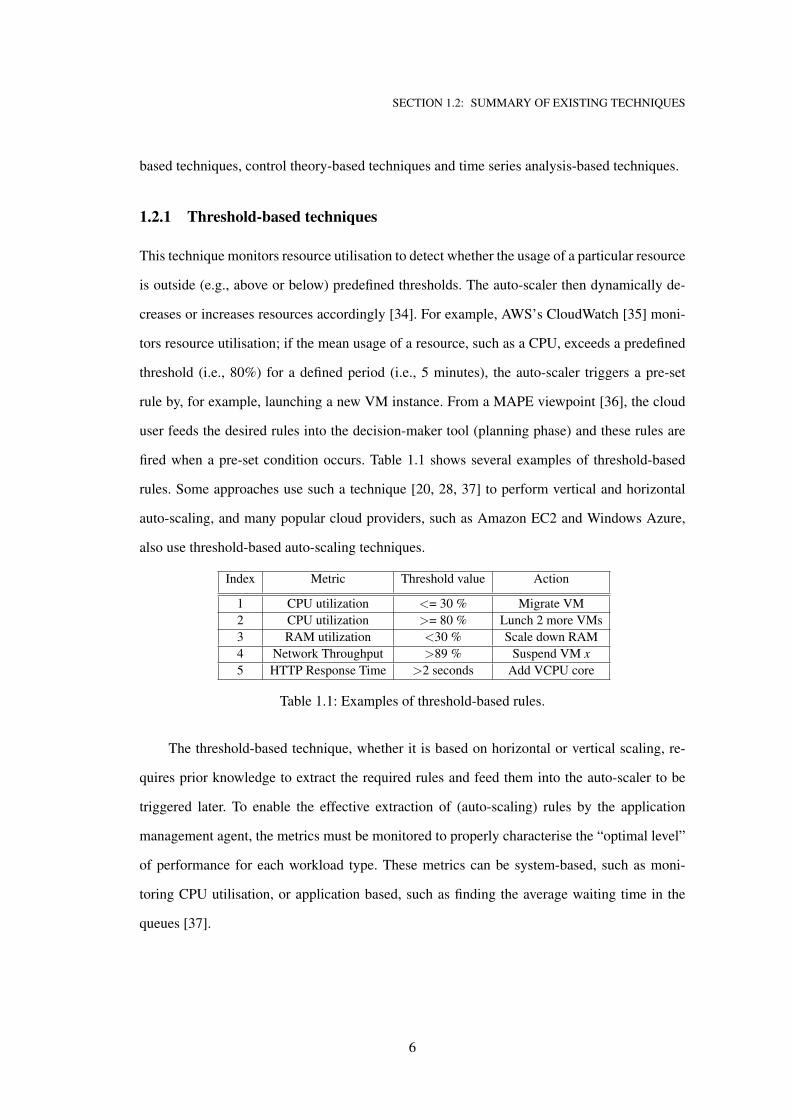
fired when a pre-set condition occurs. Table 1.1 shows several examples of threshold-based
rules. Some approaches use such a technique [20, 28, 37] to perform vertical and horizontal
auto-scaling, and many popular cloud providers, such as Amazon EC2 and Windows Azure,
also use threshold-based auto-scaling techniques.
Index Metric Threshold value Action
1 CPU utilization <= 30 % Migrate VM
2 CPU utilization >= 80 % Lunch 2 more VMs
3 RAM utilization <30 % Scale down RAM
4 Network Throughput >89 % Suspend VM x
5 HTTP Response Time >2 seconds Add VCPU core
Table 1.1: Examples of threshold-based rules.
The threshold-based technique, whether it is based on horizontal or vertical scaling, re-
quires prior knowledge to extract the required rules and feed them into the auto-scaler to be
triggered later. To enable the effective extraction of (auto-scaling) rules by the application
management agent, the metrics must be monitored to properly characterise the “optimal level”
of performance for each workload type. These metrics can be system-based, such as moni-
toring CPU utilisation, or application based, such as finding the average waiting time in the
queues [37].
6
SECTION 1.2: SUMMARY OF EXISTING TECHNIQUES
1.2.2 Reinforcement learning-based techniques
Many studies have used the reinforcement learning-based technique for automatic decision
making in cloud computing [29, 30, 31, 32]. From a MAPE [36] viewpoint, the reinforcement
learning (RL) approach is implemented to analyse previous scaling actions, and then rewards
the effective (most successful) scaling actions found in the scaling history. This process is
repeated every time an auto-scaling action is needed.
There are two characteristics which distinguish RL from other learning approaches: trial-
and-error and delayed reward. The auto-scaler attempts to produce an appropriate scaling ac-
tion (trial-and-error) that suits the workload of the current computing resources. Once the de-
cision is made and executed, the auto-scaler rewards that executed scaling action to record it
for further usage. The reward value represents the extent to which the action taken was effec-
tive (i.e., 100% win, -100% loss). Moreover, the auto-scaler not only determines the scaling
action; it also predicts the next state of the workload and learns from the previous prediction
results [38].
The auto-scaler maps each application state with the highest scaling action reward. The
aim of the reinforcement-learning agent (i.e., the auto-scaler) is to find a policy π that is as-
signed to a s state which will be considered as the best scaling action a [30].
Jia et al. [31] introduced an auto-scaling technique that automates the VM configuration
process by using RL algorithms in the context of neural networks. Even though the RL-based
technique contributes to the design of smart self-scaling systems that can trigger most possible
scaling actions [39], it leads to undesirable performance degradation and scaling actions. This
is due to the long time required to train the model until it finds satisfactory actions. The use of
the principle of trial-and-error can, in many cases, lead to performance degradation. Moreover,
the complexity of the RL-based scaling model requires too much computation time to obtain
all possible scaling cases.
1.2.3 Queuing-based techniques
The queuing-based theory has been used to control (measure) the performance of traditional
web servers [40, 41]. It consists of many mathematical theories for modelling several perfor-
7
SECTION 1.2: SUMMARY OF EXISTING TECHNIQUES
mance parameters, such as waiting time and slow down. The service requests (SRs) (i.e., HTTP
requests, tasks, I/O disk readings/writings) are placed in queues to wait until the servers are free
to work. The service providers remain idle while waiting for a SR [42]. The study of queuing
theory examines the policies of service disciplines or priority orders for SR. For instance, First-
In First-Out (FIFO) handles SRs based on arrival time; that is, the first request received will be
the first served. Conversely, Last-in First-out (LIFO) serves the last request first.
Cloud computing researchers have proposed queuing-based auto-scaling models to mea-
sure the performance of servers [43, 44, 45]. From the MAPE [36] perspective, these models
are used to analyse the servers’ performance and enable the auto-scaler to decide the most ef-
fective action to enhance server performance in efficiently provisioning resources. Hu et al. [46]
proposed a performance model to deliver response time guarantees by allocating the minimal
number of servers in the cloud. They used two allocation policies: 1) a shared allocation (SA)
policy where all SRs are queued in the same line, and 2) a dedicated allocation (DA) policy
which places SRs in multiple queues based on the arrival time. The auto-scaling algorithm de-
cides which policy is to be used to ensure adequate quality of service (QoS) while providing
the SRs with the minimal number of servers.
Queuing-based auto-scaling techniques are effective for accessing computing resources
when there is a linear relation between the SR and the amount of computing resources in the
data centres (i.e., 1k SRs served by single VM, 2k SRs served by two instances). Moreover, this
technique is useful for classifying SRs, as some SRs are tolerant while other SRs are sensitive
to deadlines [47].
1.2.4 Control theory-based techniques
These techniques have been widely used in auto-scaling tasks in cloud computing [48, 49, 50,
51]. It manipulates different resource matrices (i.e., CPU frequency, network throughput, num-
ber of instances) in order to maintain a specific metric (i.e., response time, energy consumption,
QoS) within SLA ranges. This technique is classified based on the usage of system outcomes:
open loop (non-feedback) and closed loop (feedback) [52].
• The open loop auto-scaling models execute predefined models (rules) without observing
8
SECTION 1.3: SUMMARY OF EXISTING TECHNIQUES
the resource to be controlled. For example, they adjust the memory for workload types
that are identified as memory-intensive. This type of auto-scaling is helpful in the VM
initialisation phase (horizontal scaling) when: 1) the VM has not yet received any task,
and 2) the VMM is certain about the initial intensity of the workload. However, the use
of an open loop for auto-scaling (vertical scaling) in a cloud environment is not best
practice due to the variability in the workload intensity.
• The closed loop auto-scaling models use the current resource state to generate an ad-
equate scaling plan. This is required whenever uncertainty exists in the resource to be
controlled. Farokhi et al. [53] applied a synthesis feedback controller to vertically scale
the memory using the application response time as a decision-making criterion.
The problem with controller-based auto-scaling relates to the issue of creating a reli-
able performance model that covers the state of every resources (input-output). This issue
is complex in the cloud environment due to the variety of resources and different workload
behaviours.
1.2.5 Time series-based techniques
These techniques investigate the past usage of a particular resource or previous workload, then
inputs this observed usage into a time series forecasting model to generate predictions for this
kind of resource. A wide range of prediction methods are available to forecast the utilisation or
the load.
Auto-Regression Moving Average (ARMA) is an example of a time series-based tech-
nique used to estimate workloads [22, 23, 24]. For example, [23] includes auto-regression with
neutral networks to estimate the network load on a data centre. It has a controller unit that mon-
itors the network performance and determines whether the network devices are over-loaded or
at their optimal performance. Roy et al. [25] used ARMA to predict future workload based on
limited historical information because it anticipates the number of users and later adjusts the
number of VMs to be allocated.
9
SECTION 1.3: LIMITATIONS OF EXISTING AUTO-SCALING TECHNIQUES
1.3 Limitations of existing auto-scaling techniques
Existing auto-scaling techniques such as [54, 55, 56, 26, 57, 58] basically have embedded
heuristics and mathematical/prediction models to provide automatic and flexible solutions for
hosted applications. They aim to anticipate the workloads of applications and optimise comput-
ing resources accordingly. Several factors, such as the accuracy and prediction overhead, affect
the design of proactive auto-scaling techniques. The efficiency of auto-scaling techniques de-
pends on the careful consideration of the following factors.
Prediction accuracy and overheads
Many studies have investigated resource management for cloud computing data centres, includ-
ing automatic resource scaling [26, 19, 59, 27, 29, 30, 31, 32, 23, 24, 25]. Mainly, they adopted
predictive models which are computationally expensive to provide an estimation of resource
consumption. However, owing to the complexity of the predictive models used, most studies
do not consider prediction model overheads. The costs and performances of several forecasting
models used in state-of-the-art auto-scaling techniques have been tested and compared in this
study [22]. The findings of this study indicate that traditional models do not consider dynamic
length prediction because they mostly make fixed CPU interval predictions.
Energy saving
Performance and power consumption are traded-off by dynamically adjusting the CPU volt-
age while using the Dynamic Voltage and Frequency Scaling (DVFS) policy [60]. This policy
is currently in the Linux operation system, although it does not consider the SLA metrics.
DFVS-based auto-scaling techniques e.g., [61, 62, 63, 64] are energy-efficient but slow down
CPU speeds when workloads decrease, and boost the speed when workloads increase. The CPU
speed is updated in a reactive way; therefore, CPU resources may be under-provisioned when
fewer CPU clocks than required are allocated. Indeed, resource under-provisioning causes SLA
violations owing to resource shortages to execute sudden workload bursts. Experimentally, we
have examined the on-demand DVFS governor [65] in Chapter 3 and found that DVFS causes
resource over-provisioning which scales up the CPU to an unnecessary frequency, thereby
10
SECTION 1.3: LIMITATIONS OF EXISTING AUTO-SCALING TECHNIQUES
leading to increased energy consumption. Specifically, the advanced configuration and power
interface (ACPI) which manages power consummation in the physical machine responds im-
mediately when the workload increases, and the CPU utilisation is 35% lower by mounting
the core’s frequency. This is done to prevent SLA violations; however, such responses would
consume unnecessary energy. To address the resource shortage and unnecessary resource allo-
cation, it is vital to change from reactive to proactive resource scaling.
CPU sharing fairness
The most controversial problem faced during workflow execution is the selection of fair con-
tainer CPU resources configuration [66, 67]. This occurs mainly during the co-location of
multiple containers to execute workflow tasks. This issue commonly appears after many at-
tempts to customise workflow systems and deploy them in reusable containers across different
knowledge fields. For instance, in biomedical research, Galaxy [68, 69] is an efficient workflow
system with many functions which was recently designed to run in docker containers. In the
Galaxy workflow system, many scientific tools are made available in containers and are hosted
by the BioContainers platform [69]. This platform has been publicly published to make scien-
tific tools that been used in the Galaxy workflow system more reusable and independent. Most
containers use predefined scheduling policies for sharing CPU resources. Such policies include
Dynamic Completely Fair Scheduler (DCFS) [70] and Completely Fair Scheduler (CFS) [71].
However, most of these policies do not consider task features such as the CPU usage, type, and
size of the task; therefore, some of them (e.g., CFS) cannot guarantee the quality of service
(QoS) during the execution of these tasks [72]. The DCFS policy customises generic metrics to
control CPU sharing, and CFS allocates identical CPU shares to the hosted containers. How-
ever, CFS cannot maintain equity for co-located workloads owing to load imbalances [72].
Similarly, DCFS cannot appropriate the scientific workflow system to partition a CPU running
multiple container workloads. This case mostly occurs when workloads vary among workflow
tasks.
11
SECTION 1.4: RESEARCH QUESTIONS
Contention of CPU shared resources
Several approaches e.g., [73, 74, 75, 76, 77, 78, 79, 80, 81] have been proposed in literature to
detect CPU interference. However, most of these do not work well for containerised scientific
workflow systems running in VMs. Specifically, hardware-based approaches [74, 75, 82, 64]
often require increased access to physical resource metrics (e.g., LLC-miss, cache-miss), which
are usually not available. For instance, Google researchers [75] proposed a combination of
hardware performance metrics (CPU cycles and instructions) to estimate the deviation of ex-
isting jobs. However, this set of metrics requires access to host information and is there-
fore not accessible to the subscribers of data centres. On the other hand, software-based ap-
proaches [77, 79, 83, 73, 80, 81] must use customised software probes to execute a set of
benchmarks to detect resource contention, which accumulates additional resource overheads.
For instance, probes may require up to 3.2% of the CPU shared cache [80] and increase the
application response time up to 7% [81]. Furthermore, benchmarks are often designed to fit
specific domains and therefore might not accurately model the real-world workloads of scien-
tific workflow systems. For example, using the task response time as in [73, 78] is not relevant
to the context of scientific workflows because the workflow tasks often have highly deviated
response times (deviation may reach 128% of the mean value [84]), which may lead to high
false positive rates.
1.4 Research questions
This research study is related to three main areas of CPU resource management for cloud
computing data centres. These areas are concerned by CPU workload co-locations statues. Ac-
cording to the real production clusters traces [15, 13, 14], CPU workload co-location statuses
are:
• CPU runs only sensitive containerised applications (addressed by Q1 in Chapter 5).
• CPU runs only batch containerised applications (workflows or DAGs) (addressed by Q2
in Chapter 6).
12
SECTION 1.4: RESEARCH QUESTIONS
• CPU runs both batch and sensitive containerised applications (addressed by Q3 & Q4 in
Chapters 5 & 6 respectively).
To address workload co-location concerns, this study is guided by four overarching research
questions.
1. How to efficiently estimate the CPU demand and proactively scale up/down only
the required CPU cores and frequency in an energy-efficient manner?
The proactive provisioning of CPU cores and frequency requires a preparation period to
enable these computing resources to interact with the actual workload. It is essential to
provide computing resources at the right time to ensure a certain QoS. Thus, it is neces-
sary to have a predictive model to forecast the CPU workload and accordingly to prepare
CPU computing resources for the expected workload. This proactive scaling enables the
dynamic provision of resources based on the load expected in the future. Current cloud
computing data centres often struggle to efficiently deal with resource provisioning in
terms of performance and energy efficiency. A data centre workload exhibits dynamic
resource usage over time; resources are often overly provisioned, based on peak loads.
This creates challenges for data centre operators who need to handle peaks in applica-
tion loads as well as unexpected load spikes. Scaling to ensure just the right amount
of resources is an efficient way to save energy by using only the computing resources
required while providing an adequate QoS. The question here is how to determine the
correct amount of computing resources as well as how to provision them in advance
without violating any SLA objectives while maintaining maximum efficiency in energy
consumption. The answer to this question is outlined in Chapter 3. If we do not adapt the
CPU cores and CPU frequency dynamically and in advance, one of two scenarios will
occur: (1) resource over-provisioning where the number of cores and CPU frequency
is higher than the actual demand, resulting in wasted resources and unnecessary energy
consumption, (2) or resource under-provisioning where the actual demand requires ad-
ditional cores or a higher CPU frequency to ensure a certain level of performance, as
stated in the SLAs.
13
SECTION 1.4: RESEARCH QUESTIONS
2. How is the CPU portion estimated and scaled up/down fairly between containers
when executing containerised scientific workflows?
Estimating the appropriate CPU portion for containers is essential to ensure the fair dis-
tribution of the CPU computing power. Since workflow system containers have different
workload characteristics, a CPU resource provisioning technique could affect the work-
flow finishing time. Speeding up some tasks would contribute to finishing the workflow
earlier and save resources. Computing resources need to be efficiently used and allow
a data centre to increase CPU utilisation. Traditional CPU fairness scheduling policies
(e.g., CFS) implement fairness operations at a very low level (CPU process or thread)
without considering multiple threads/processes as one group.
Technically, a container is a group of CPU processes managed by a combination of
Linux namespaces and control groups (cgroups) mechanisms [85]. These mechanisms
are core features which limit and isolate the CPU usage for group of CPU processes (i.e.,
container) [86]. The fairness of CPU processes is managed by the CFS [71] technique,
which in its default implementation cannot ensure complete fairness between containers
because fairness is implemented in processes, and it cannot distinguish between each
process class or group. Thus, container engines [87, 88] extended the CFS scheduler and
dynamically enabled changes to the limits of the CPU CFS quota and the period to a
group of processes (container). Therefore, container managers can customise the CFS
and dynamically overwrite the CFS parameters using APIs [89] to design their own fair-
ness policies. When a customised CFS for containerised scientific workflow systems is
being designed, workflow tasks need to be characterised and these characteristics should
be taken into account to establish an adaptive CFS policy that maintains fairness at the
container level.Chapter 4 provides a proposed solution to customise CFS and consider
the workload characteristics when distributing the CPU resources between containers.
Fair CPU sharing for containers can be achieved by examining the running workloads
and proactively recomputing the CPU weights according to the workload characteristics
and the CPU contention status. The environment of a scientific workflow system is dy-
namic by nature, and the task arrival rate and finishing time are not known in advance.
14
SECTION 1.4: RESEARCH QUESTIONS
Thus, dynamically recomputing the CPU weights would help to improve the fairness for
tasks that run longer with intensive CPU rates. This dynamic reconfiguration would en-
able containers that have (1) intensive CPU requirements, (2) large number of tasks, and
(3) longer run time to obtain higher priorities on the CPU. This will reduce the impact of
real CPU bottlenecks when executing multiple workflows. Tasks with larger CPU usage
and longer runtime will be executed faster.
3. How can CPU interference for virtualised resources be detected in the presence of
noisy neighbouring containers?
Imperfect isolation techniques for CPU resources across multiple tenants affect the per-
formance of hosted applications. Although CPU resources can be partitioned between
containers, it can still create a CPU interference. An interference can be caused by in-
ternal CPU components including cache and memory bandwidth. These components
are very difficult to isolate without designing new special hardware to isolate them for
containers. The interference that has occurred in these shared resources cannot be de-
tected by the end user. This is because existing detection metrics, such as cache-miss
and LLC-miss, are inaccessible and are allowed only when we have full access to the
host information, which is not the case when we hire virtual resources from a cloud data
centre. Indeed, contention on shared CPU resources degrades performance, especially
when cloud users rely on it too heavily and put their full trust in cloud providers to de-
tect and mitigate CPU interference. CPU interference will become even more difficult
to manage as current technology trends head toward the construction of large sophisti-
cated multi-core CPUs with hundreds or even thousands of cores on one single physical
machine.
In addition, service providers might overcommit resources to maximise their utilisation,
resulting in resources being shared between containers/VMs in a fair-share manner [71].
The sharing of CPU resources in this way will likely cause interference, which could
severely compromise the reliability of the system and potentially violate SLAs. As a
result, a CPU interference would diminish the trust of cloud users and prevent cloud
resources from delivering the expected performance. CPU interference can degrade the
15
SECTION 1.4: RESEARCH QUESTIONS
performance of the whole system when multiple CPU-intensive applications run simul-
taneously. Containerised applications can potentially be affected by a denial of service
caused by CPU contention generated by co-located containers. Furthermore, containers
can utilise more CPU resources than originally allocated by the respective cgroup be-
cause current cgroup mechanisms do not take into account the computational burden of
processing network traffic [90]. Consequently, this may create CPU interference in co-
located containers. The interference between containers is becoming a notable concern
in vitalised resources and Chapter 5 addresses this concern.
4. How can workload prediction be used by cloud providers to increase efficiency of
CPU resources and maximise CPU utilisation?
The typical approach to maximising CPU utilisation in data centres is to co-locate batch
jobs with sensitive containerised application workloads while meeting the sensitive ap-
plication SLO. The primary obstacle to improving resource efficiency is performance
interference arising from co-located workloads. The probability of such interference oc-
curring increases with the number of co-located workloads on the same server. This
approach involves challenges related to how: (1) to proactively quantify the appropriate
residual resources, and (2) to reduce the impact of the interference caused by batch jobs
and awareness about the auto-scaling technique with the interference, which severely
affects the SLO of a sensitive containerised application. Indeed, a small amount of CPU
interference would produce notable SLO violations, which may severely compromise
the system’s reliability and potentially violate the SLA. CPU interference can also de-
grade the performance of the whole system when multiple CPU-intensive applications
run simultaneously.
The proactive quantifying of residual resources requires an estimation model that can
predict workloads. However, the collection and use of residual resources for batch jobs
based on predictions is often error-prone. The prediction inevitably introduces errors;
however, they are variable and depend on the prediction approach used for forecast-
ing. Therefore, designing an accurate prediction model would help to reduce the impact
of prediction errors and would facilitate the proactive and careful co-location of batch
16
SECTION 1.5: THESIS SCOPE
jobs with sensitive applications on the same machine. Therefore, an accurate prediction
model is important to enable the CPU to continue to be scaled, and to maximise server
utilisation. Chapter 6 provides a proactive approach to increase the efficiency of CPU
resources and maximise CPU utilisation.
1.5 Thesis Scope
Our aim in this thesis is to address the research questions stated in Section 1.4, and therefore
design energy-efficient resource provisioning techniques for data centres. More specifically, we
propose proactive techniques that control the provisioning of CPU resources (Frequency, CPU
cores) through the efficient allocation of CPU resources for containerised applications while
maintaining an acceptable performance. Moreover, we focus on managing the CPU resources
for container-based platforms that host complex, cloud-based applications. These applications
could be either hosted individually or co-located as a combination of sensitive and batch-based
containerised applications. The proposed auto-scaling techniques concentrate on the efficient
use of CPU resources at the infrastructure level. The DVFS and vertical container scalability
were utilised as conservative methodologies to optimise the allocation of resources and reduce
the energy wastage. Several online-prediction models are proposed that help with the planning
of CPU allocation for containers. In all the experimental work carried in this research study,
we used real-world containerised workloads (e.g., memcached system) representing sensitive
and batch containerised applications (i.e., Montage workflows system).
In addition, all the experimental work is implemented and validated in a realistic environ-
ment. The experimental environment has been built on top of bare-metal machines provided
by RMIT VX-Lab [91]. These machines run a Linux-based OS version which this OS family
runs currently (i.e., November 2019 list) all the top 500 supercomputers in worldwide1.
In this thesis, several programming languages were used to implement different solu-
tions. Precisely, Python (i.e., v2.7 and v3) is used to coordinate the work between different
mathematical algorithms and resource management models. For the mathematical modelling
and prediction works, the statistical computing programming language R is used to process
1https://www.top500.org/statistics/list/
17
SECTION 1.6: THESIS CONTRIBUTIONS
the forecasting. Moreover, GNU Bash (docker commands) and Python library for the Docker
Engine APIs were used to perform the scalability actions for the containers’ CPU resources.
1.6 Thesis contributions
By successfully addressing the research questions outlined in Section 1.4, this thesis makes
multiple original contributions to effectively manage the CPU resource for containerised ap-
plications and reduce the energy:
This thesis contributes to updating the review of existing proactive auto-scaling techniques
to understand the current status of the used prediction models and to display existing solutions
with their pros and cons. This thesis strongly considers time series prediction models which
have less overheads on resources and are usable to predict the CPU utilisation for containers.
Firstly, this thesis provides a novel proactive SLA-aware resource scaling approach that
carefully considers SLAs when updating container CPU resources for sensitive containerised
applications [92]. The proposed approach is called Energy-Based Auto-Scaling (EBAS); it
proactively scales container resources at the CPU core level in terms of both the number and
the frequency of allocated CPU cores. EBAS incorporates the DVFS technique to dynamically
adjust CPU frequencies. Tow main components are involved to finalise the scaling decision:
(A) hybrid prediction model and (B) workload consolidation model. The hybrid prediction
model anticipates the CPU utilisation to efficiently provision resources. It uses two mathe-
matical models (i.e., spectral fast Fourier transform smoothing and AutoRegressive Integrated
Moving Average (ARIMA) time-series) to reduce the overhead of the predictions and avoid
cyclic predictions. In this way, the designed prediction model accurately predicts the number
of points ahead for CPU utilisation. This work relates to Q1 and has been published as:
• E. J. Alzahrani, Z. Tari, P. Zeephongsekul, Y. C. Lee, D. Alsadie, and A. Y. Zomaya,
“SLA-Aware Resource Scaling for Energy Efficiency,” In Proceedings of the 18th IEEE
International Conference on High Performance Computing and Communications (HPCC),
pp. 852-859, 2016.
In this thesis, we design a new CPU sharing policy, called the Adaptive Completely Fair
18
SECTION 1.6: THESIS CONTRIBUTIONS
Scheduling policy (adCFS) [93], to fairly accommodate different workload types. A new con-
tainerised workflow architecture is proposed and is applied to a realistic workflow system
(Montage). In this containerised workflow architecture, several containers are created to indi-
vidually execute each workflow task type. In addition, the adCFS policy has been customised
for batch-based jobs, that is, scientific workflows. The execution of scientific workflows goes
though many stages, where each stage has different runtime values as well as different CPU
utilisations. This creates many contention states on the CPU; this thesis suggests classifying
these states as high, medium, or low contention states. A Markovian-based CPU state pre-
diction model is used to detect various CPU states, particularly when high CPU usage has
occurred. This prediction model is used to dynamically trigger adCFS, which can rethink con-
tainers’ CPU sharing metrics. The adCFS policy proactively allocates fairer CPU portions to
containers based on their workload statuses. The CPU quotas are estimated based on the cor-
responding weight of different workload metrics (e.g., CPU usage, task runtime, #tasks). This
work relates to Q2 and has been published as:
• Alzahrani, Eidah J., Zahir Tari, Young Choon Lee, Deafallah Alsadie and Albert Y.
Zomaya. “adCFS: Adaptive completely fair scheduling policy for containerised work-
flow systems.” In Proceedings of the 16th IEEE International Symposium on Network
Computing and Applications (NCA), pp. 245-25, 2017. [Best Student Paper Award]
In this thesis, we propose a novel CPU-based metric called weiMetric which uses the
built-in kernel counters in an OS to detect CPU interference occurring between containers. The
proposed metric offers multiple advantages compared to the metrics presented in the literature.
First, it requires no hardware metrics, and therefore, it works for both virtualised and non-
virtualised resources. Second, it requires no extra probes as in a typical software-based method
and therefore does not incur additional overheads for CPU resources. Further, it can be used
by cloud subscribers without assistance from cloud providers. Specifically, a set of weiMetric
time series is created to monitor the CPU contention during task execution. Outliers in the
weiMetric time series are detected when the weiMetric values are not within the confidence
intervals.
19
SECTION 1.7: THESIS ORGANISATION
Finally, to improve server utilisation and co-locate sensitive applications with batch jobs,
a novel interference-aware automatic workload orchestration technique called M2-AutScale
has been introduced in this thesis. It uses weiMetric developed in the previous contribution and
safely allocates batch jobs on sensitive application resources in order to improve server utilisa-
tion. SLA violations are attributed to the CPU interference of neighbouring applications. These
violations have been avoided by imposing a safety margin for containers’ CPU resources. In
M2-AutScale, a new hybrid multi-level Markovian time series prediction model is proposed to
predict containers’ CPU demands. The proposed prediction model extends the ARIMA models
to make them aware of the states of future time series by combining them with nested Marko-
vian models that can detect future state changes in the time series. A two-level Markovian
structure is used in which a fine level structure is embedded within a coarse one in order to
better capture state transitions in the CPU usage time series. The CPU usage is partitioned
into several percentile ranges to define Markov states at fine levels. The coarse levels in the
proposed prediction model structure are referred to as a ‘state’ and the fine levels, as a ‘sub-
state’. A discrete-time Markov chain has stationary or homogeneous transition probabilities
that represent the transition of the CPU usage value between a limited number of states and
substates.
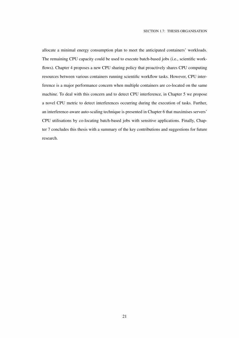
1.7 Thesis organisation
The thesis is logically structured in terms of the dependencies between chapters. Figure 1.1
shows the organisation of the chapters in the thesis. This thesis contains seven chapters. Chap-
ter 1 discusses the basics of the research problems and the contributions made to overcome
them. Followed by Chapter 2 which introduces cloud computing elasticity in terms of con-
tainerisation and its related terms and concepts. This thesis is comprised of four main self-
contained chapters, each of which contains its own related work, experimental setup, and
results. Chapter 3 presents a new resource auto-scaling approach that proactively scales the
CPU resources for containerised applications in response to dynamic changes in load as well
as to the SLA requirements. The proposed auto-scaling technique in chapter 3 combined the
DVFS technique with a resource estimation model to dynamically adjust CPU frequencies and
20
SECTION 1.7: THESIS ORGANISATION
allocate a minimal energy consumption plan to meet the anticipated containers’ workloads.
The remaining CPU capacity could be used to execute batch-based jobs (i.e., scientific work-
flows). Chapter 4 proposes a new CPU sharing policy that proactively shares CPU computing
resources between various containers running scientific workflow tasks. However, CPU inter-
ference is a major performance concern when multiple containers are co-located on the same
machine. To deal with this concern and to detect CPU interference, in Chapter 5 we propose
a novel CPU metric to detect interferences occurring during the execution of tasks. Further,
an interference-aware auto-scaling technique is presented in Chapter 6 that maximises servers’
CPU utilisations by co-locating batch-based jobs with sensitive applications. Finally, Chap-
ter 7 concludes this thesis with a summary of the key contributions and suggestions for future
research.
21
SECTION 1.7: THESIS ORGANISATION
Chapter1Introduction
Chapter3SLA-AwareDynamic
ResourceScaling(EBAS)
Chapter4AdaptiveCompletelyFairSchedulingPolicy(adCFS)
Chapter5CPUInterferenceDetection
Metric(weiMetric)
Chapter6PredictiveCo-locationTechniquetoMaximise
CPUWorkloads
Chapter7Conclusion&FutureWork
Contribution1 Contribution2 Contribution3
Contribution4
Chapter2Background
Figure 1.1: Thesis organisation
22
CHAPTER 2Background
This chapter provides a brief background of the main concepts used in this thesis. This includes
an introduction to the virtualisation technology in cloud computing systems. More specifically,
this chapter displays the different types of virtualisation in the data centre, which are virtual
machines and containers. Moreover, the main differences between containers and VMs are
presented in this chapter. Similarly to VMs, containers can be scaled vertically and horizon-
tally; therefore, this chapter shows the essential scaling mechanisms and presents them from
a container perspective. Finally, we explain the proactive auto-scaling concept as all the pro-
vided auto-scaling techniques in this thesis are classified as proactive auto-scaling techniques
for containerised applications.
2.1 Virtualisation
Cloud computing data centres rely on virtualisation technology, which is an attractive option
for hosting different application types1. Virtualisation can offer great solutions that are cost-
effective and resource-efficient. The critical feature of virtualisation is dividing a single phys-
ical server resource into multiple virtual environments which ensures both performance and
failure isolation.
1Indeed, not all cloud data centres adopt virtualisation technology to build their computing resources. For
instance, Google uses OS containers to host applications directly on top of physical resources.
23
SECTION 2.1: VIRTUALISATION
Virtualisation has transformed traditional data centres toward a software-based architec-
ture which compensates for failures and delivers unprecedented resiliency at a pay-as-you-use
cost. Data centres use complete virtualisation in which guest operating systems are not aware
of being virtualised. Virtualisation technology provides the illusion of dedicated computing re-
sources accessible to the end-users, whereas, in practice, the data centre owner retains complete
control of the underlying resources. Moreover, the hosted OS on virtualised resources has no
way of knowing that it shares computing resources with other OSs. Thus, all virtualised OSs
running on a single computer can operate entirely independently of each other and be seen as
separate computers on a network.
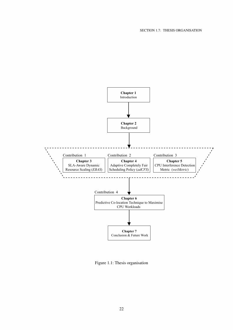
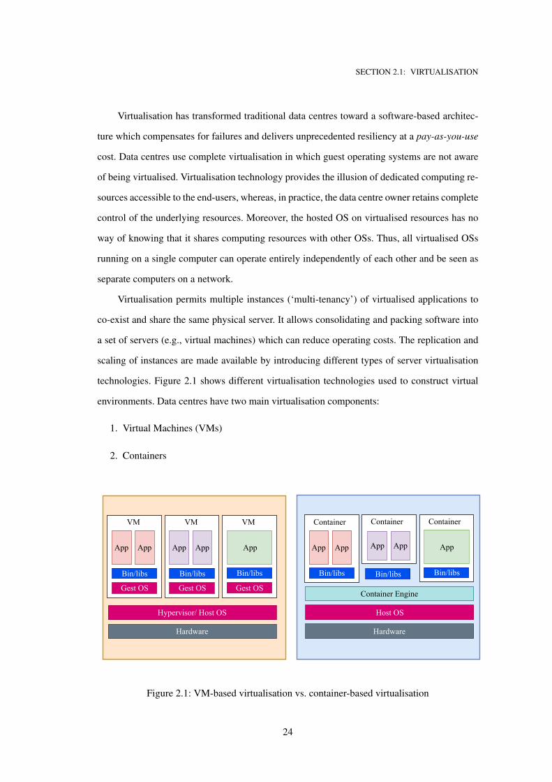
Virtualisation permits multiple instances (‘multi-tenancy’) of virtualised applications to
co-exist and share the same physical server. It allows consolidating and packing software into
a set of servers (e.g., virtual machines) which can reduce operating costs. The replication and
scaling of instances are made available by introducing different types of server virtualisation
technologies. Figure 2.1 shows different virtualisation technologies used to construct virtual
environments. Data centres have two main virtualisation components:
1. Virtual Machines (VMs)
2. Containers
Hypervisor/HostOS
GestOS
Bin/libs
App App
VM
Hardware
GestOS
Bin/libs
App
VM
GestOS
Bin/libs
App App
VM
HostOS
Bin/libs
App App
Container
Hardware
Bin/libs
App
ContainerContainer
Bin/libs
App App
Container
ContainerEngine
Figure 2.1: VM-based virtualisation vs. container-based virtualisation
24
SECTION 2.1: VIRTUALISATION
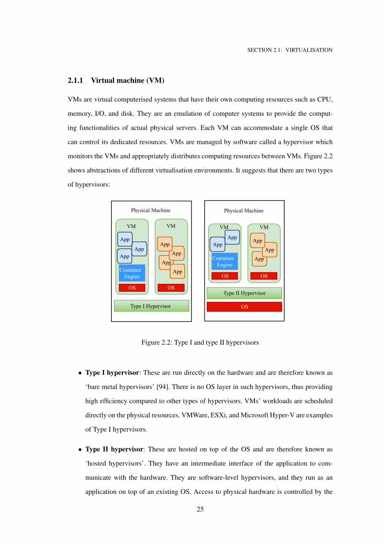
2.1.1 Virtual machine (VM)
VMs are virtual computerised systems that have their own computing resources such as CPU,
memory, I/O, and disk. They are an emulation of computer systems to provide the comput-
ing functionalities of actual physical servers. Each VM can accommodate a single OS that
can control its dedicated resources. VMs are managed by software called a hypervisor which
monitors the VMs and appropriately distributes computing resources between VMs. Figure 2.2
shows abstractions of different virtualisation environments. It suggests that there are two types
of hypervisors:
OS
Type IIHypervisor
OS
ContainerEngine
OS
AppApp
VM VM
PhysicalMachine
App
App
App
Type IHypervisor
OS
ContainerEngine
OS
AppApp
VM VM
PhysicalMachine
App
App
App
App
App
Figure 2.2: Type I and type II hypervisors
• Type I hypervisor: These are run directly on the hardware and are therefore known as
‘bare metal hypervisors’ [94]. There is no OS layer in such hypervisors, thus providing
high efficiency compared to other types of hypervisors. VMs’ workloads are scheduled
directly on the physical resources. VMWare, ESXi, and Microsoft Hyper-V are examples
of Type I hypervisors.
• Type II hypervisor: These are hosted on top of the OS and are therefore known as
‘hosted hypervisors’. They have an intermediate interface of the application to com-
municate with the hardware. They are software-level hypervisors, and they run as an
application on top of an existing OS. Access to physical hardware is controlled by the
25
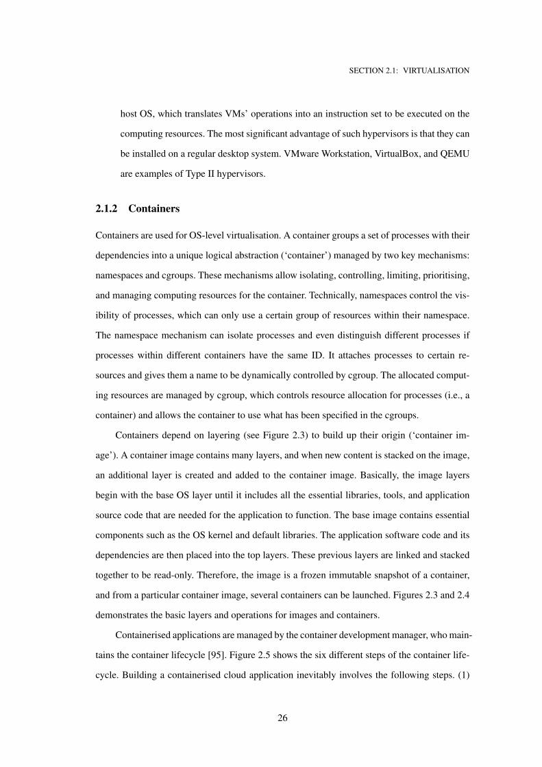
SECTION 2.1: VIRTUALISATION
host OS, which translates VMs’ operations into an instruction set to be executed on the
computing resources. The most significant advantage of such hypervisors is that they can
be installed on a regular desktop system. VMware Workstation, VirtualBox, and QEMU
are examples of Type II hypervisors.
2.1.2 Containers
Containers are used for OS-level virtualisation. A container groups a set of processes with their
dependencies into a unique logical abstraction (‘container’) managed by two key mechanisms:
namespaces and cgroups. These mechanisms allow isolating, controlling, limiting, prioritising,
and managing computing resources for the container. Technically, namespaces control the vis-
ibility of processes, which can only use a certain group of resources within their namespace.
The namespace mechanism can isolate processes and even distinguish different processes if
processes within different containers have the same ID. It attaches processes to certain re-
sources and gives them a name to be dynamically controlled by cgroup. The allocated comput-
ing resources are managed by cgroup, which controls resource allocation for processes (i.e., a
container) and allows the container to use what has been specified in the cgroups.
Containers depend on layering (see Figure 2.3) to build up their origin (‘container im-
age’). A container image contains many layers, and when new content is stacked on the image,
an additional layer is created and added to the container image. Basically, the image layers
begin with the base OS layer until it includes all the essential libraries, tools, and application
source code that are needed for the application to function. The base image contains essential
components such as the OS kernel and default libraries. The application software code and its
dependencies are then placed into the top layers. These previous layers are linked and stacked
together to be read-only. Therefore, the image is a frozen immutable snapshot of a container,
and from a particular container image, several containers can be launched. Figures 2.3 and 2.4
demonstrates the basic layers and operations for images and containers.
Containerised applications are managed by the container development manager, who main-
tains the container lifecycle [95]. Figure 2.5 shows the six different steps of the container life-
cycle. Building a containerised cloud application inevitably involves the following steps. (1)
26
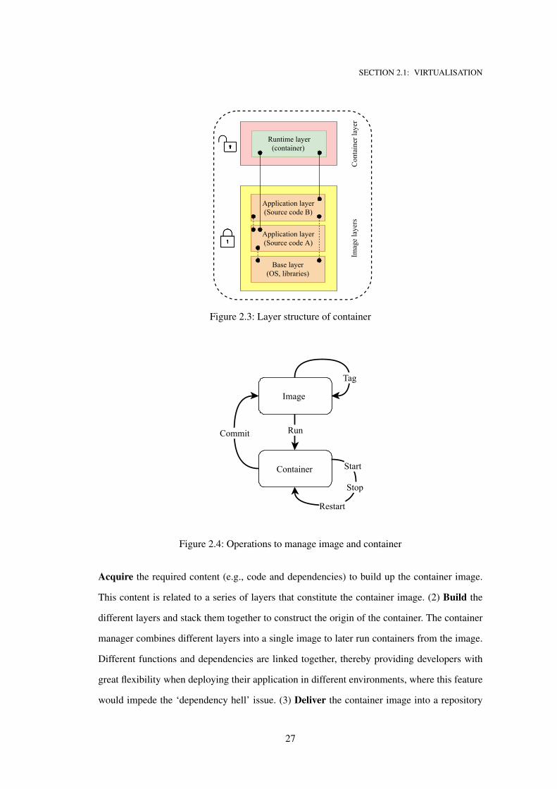
SECTION 2.1: VIRTUALISATION
Baselayer(OS,libraries)
Runtimelayer(container)
Imagelayers
Containerlayer
Applicationlayer(SourcecodeB)
Applicationlayer(SourcecodeA)
Figure 2.3: Layer structure of container
Run
Image
Commit
Container
Tag
Start
Stop
Restart
Figure 2.4: Operations to manage image and container
Acquire the required content (e.g., code and dependencies) to build up the container image.
This content is related to a series of layers that constitute the container image. (2) Build the
different layers and stack them together to construct the origin of the container. The container
manager combines different layers into a single image to later run containers from the image.
Different functions and dependencies are linked together, thereby providing developers with
great flexibility when deploying their application in different environments, where this feature
would impede the ‘dependency hell’ issue. (3) Deliver the container image into a repository
27
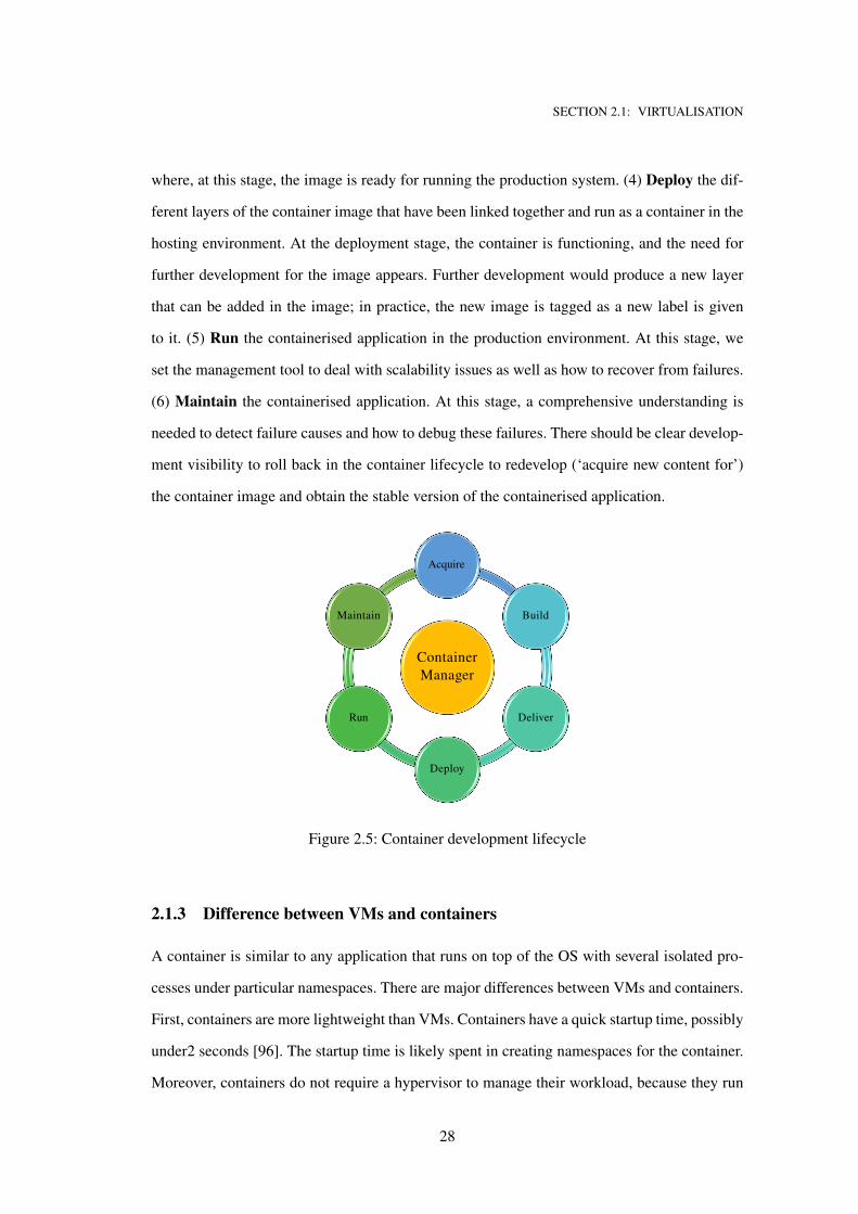
SECTION 2.1: VIRTUALISATION
where, at this stage, the image is ready for running the production system. (4) Deploy the dif-
ferent layers of the container image that have been linked together and run as a container in the
hosting environment. At the deployment stage, the container is functioning, and the need for
further development for the image appears. Further development would produce a new layer
that can be added in the image; in practice, the new image is tagged as a new label is given
to it. (5) Run the containerised application in the production environment. At this stage, we
set the management tool to deal with scalability issues as well as how to recover from failures.
(6) Maintain the containerised application. At this stage, a comprehensive understanding is
needed to detect failure causes and how to debug these failures. There should be clear develop-
ment visibility to roll back in the container lifecycle to redevelop (‘acquire new content for’)
the container image and obtain the stable version of the containerised application.
Container Manager
Acquire
Build
Deliver
Deploy
Run
Maintain
Figure 2.5: Container development lifecycle
2.1.3 Difference between VMs and containers
A container is similar to any application that runs on top of the OS with several isolated pro-
cesses under particular namespaces. There are major differences between VMs and containers.
First, containers are more lightweight than VMs. Containers have a quick startup time, possibly
under2 seconds [96]. The startup time is likely spent in creating namespaces for the container.
Moreover, containers do not require a hypervisor to manage their workload, because they run
28
SECTION 2.2: INTER-CLOUD DISTRIBUTED APPLICATIONS
immediately on top of computing infrastructure and can only depend on specific libraries in
the operating system/kernel. Further, containers share their image layers with co-existing con-
tainers. In particular, a container image may have several layers that could be cached locally;
when new content is added to the image, a new image is created which contains the difference
between the two images. Finally, there is no emulation of the physical resources. Theoretically,
containers are lightweight resources that show little performance overheads. This is because
containers directly communicate with the host OS through system calls, thereby eliminating
the need for operating a hypervisor to translate a VM’s instructions into low-level instructions
that can be executed on the host resources.
2.2 Inter-Cloud distributed applications
Cloud data centres are designed to deliver computing resources for different types of container-
ised applications. These containerised applications have many layers/ systems that interact with
each other in a distributed fashion. They are classified based on the responsiveness sensitivity
into 1) sensitive applications and 2) batch-based jobs.
2.2.1 Sensitive applications
Sensitive applications are user-facing applications that are also known as latency-demanding
systems. They require instant response time, for which the turn-around time should be between
20-200 ms [97]. For instance, they include cloud-based applications such as online gaming,
social media and image processing applications. These applications are being containerised
and deployed on cloud resources with strict latency requirements. For example, memcached
system is a distributed memory caching system used to speed up web applications. memcached
system is being used for Facebook systems to handle billion of requests per second [98].
2.2.2 Batch-based jobs
Batch-based jobs are a sequence of tasks submitted to the cloud resources and then executed
without any further user intervention. Jobs are processed in batch mode as some jobs run only
29
SECTION 2.3: CONTAINER SCALABILITY
once, or it might be rescheduled automatically and placed for re-execution upon failure. These
types of applications represent systems that run on Grid or Cluster computing resources. A
singular job may have multiple sub-jobs/tasks to solve optimisation models or build complex
simulations. Scientific workflow tasks are a typical example of batch singular run jobs [99]
2.3 Container scalability
This section introduces different approaches to accomplish container resource management.
Despite our research focus on a particular resource management approach, we will present
both approaches to distinguish our scalability model and define which approach is selected in
designing our auto-scaling technique.
Container scalability is the reconfiguration of container resources to gracefully handle the
increased/decreased workload of containerised applications. It indicates the ability of container
engines to smoothly enlarge the containerised application’s workloads. The reconfiguration of
container resources is processed by the provision (i.e., scale up) of additional resources for the
hosted containers. Container scalability falls into two categories.
• Horizontal scaling (scale-out): Horizontal scaling of containers means adding more con-
tainers to the system. Multi-tenant containers can achieve better scalability by adding/removing
containers by creating several replicas [100]. For example, Google App Engine used hor-
izontal container scaling to replicate components belonging to different applications [101].
High-performance containerised applications that require parallel executions, such as
scientific workflows and biotechnology systems, are scaled horizontally to accelerate
tasks that require more and expensive resources. Recently created cluster management
container engines such as Docker Swarm and Kubernetes support horizontal scaling.
Data centre operators such as Google and Microsoft have assembled their own container
engines to support high efficiency in managing systems. Such tools manage the instances
of migrations between different host in the cluster to achieve load balancing and efficient
resources allocation.
• Vertical scaling (scale-up): Vertical scaling is related to the reconfiguration of the con-
30
SECTION 2.5: PROACTIVE AUTO-SCALING TECHNIQUE
tainers’ resources by adding to (or removing from) computing resources on the fly to
handle load variation. Our proposed technique falls under this category which attempts
to increase/decrease the capacity of a single container. This type of scalability is known
to support the finer resource allocated to a specific task (i.e., container) to handle certain
requirements such as throughput and latency. It eliminates the overhead of initialising
new instances that is created via horizontal scaling. Vertical elasticity supports the split-
ting of different components of the applications to be distributed to different containers,
enabling the management of resource-intensive tasks indivisibly. For example, Web ap-
plications have been containerised and CPU-intensive tasks, such as database queries
and search information tasks, can be vertically scaled individually [102].
2.4 Proactive auto-scaling technique
The proactive auto-scaling technique deals with autonomic resource provisioning for systems.
Given the complexity of data centre system, proactive auto-scaling technique aims to reduce
the complexity and cost of system administration. In particular, the system should be able
to 1) monitor its resource utilisation, performance and energy consumption and 2) optimise
and re-configure its resources to reach an optimal state for both energy consumption as well
as SLA obligations. Proactive auto-scaling enables forecasting techniques to determine when
the current computing resources capacity is insufficient to optimally accomplish workloads.
It invokes practical resource management algorithms to optimise resource capacity for hosted
applications. The optimisation, which is carried out here, is triggered on demand to either al-
locate additional resources (scale up) before the resource capacity is exceeded or deallocate
(scale down) computing resources when they are not in service. Proactive resources manage-
ment (proactive auto-scaling) techniques are designed to fulfil the QoS for cloud-based appli-
cations. The dynamic resource reconfiguration aims to achieve efficient elasticity for hosted
applications. The scaling action is predictively triggered as a response to changes in resource
workloads. This process allows the application to span out over the data centre infrastructure
and enables computing resources to warm up without interruptions.
31

SECTION 2.5: SUMMARY
2.5 Summary
In this chapter, we described different aspects of virtualisation in data centres. We displayed the
main virtualisation components used to deploy different types of Internet-based systems. These
components are VMs and containers that can host multiple, isolated services on data centres.
This chapter also described the major differences between VMs and containers, particularly the
aspect of building different applications, scale, and managing their computing resources in the
cloud environment. Additionally, this chapter described different container scalability meth-
ods, which could be horizontal (i.e., add/ remove instances) or vertical (i.e., adding/ remove
computing resource). Since this thesis pursues the proactive scaling method, this approach is
explained and aims to reduce the complexity and cost of system administration in data centres.
32
CHAPTER 3SLA-Aware Dynamic Resource Scaling for
Sensitive Containerised Applications
Cloud data centers (CDCs) with abundant resource capacities have flourished during the past
decade. However, these CDCs often struggle to efficiently deal with resource provisioning in
terms of performance and energy efficiency. This chapter describes Energy-Based Auto Scaling
(EBAS) as a new resource auto-scaling approach—that takes into account the Service Level
Agreement (SLA)—for CDCs. EBAS proactively scales resources at the CPU core level in
terms of both the number and frequency of cores. It incorporates the dynamic voltage and fre-
quency scaling (DVFS) technique to dynamically adjust CPU frequencies. The proactive deci-
sions on resource scaling are enabled primarily by the proposed CPU usage prediction model
and the workload consolidation model of EBAS. The experiment results show that EBAS can
save 14% more energy, on average, than the Linux governor. In particular, EBAS improves the
DVFS by making it aware of SLA conditions, which leads to the conservation of computer
power and, in turn, energy.
Copyright/credit/reuse notice:
The contents of this chapter are based on material that has been previously published as:
• E. J. Alzahrani, Z. Tari, P. Zeephongsekul, Y. C. Lee, D. Alsadie, and A. Y. Zomaya, “SLA-Aware
Resource Scaling for Energy Efficiency,” in Proceedings of the 18th IEEE International Conference
on High Performance Computing and Communications (HPCC), pp. 852-859, 2016.
33
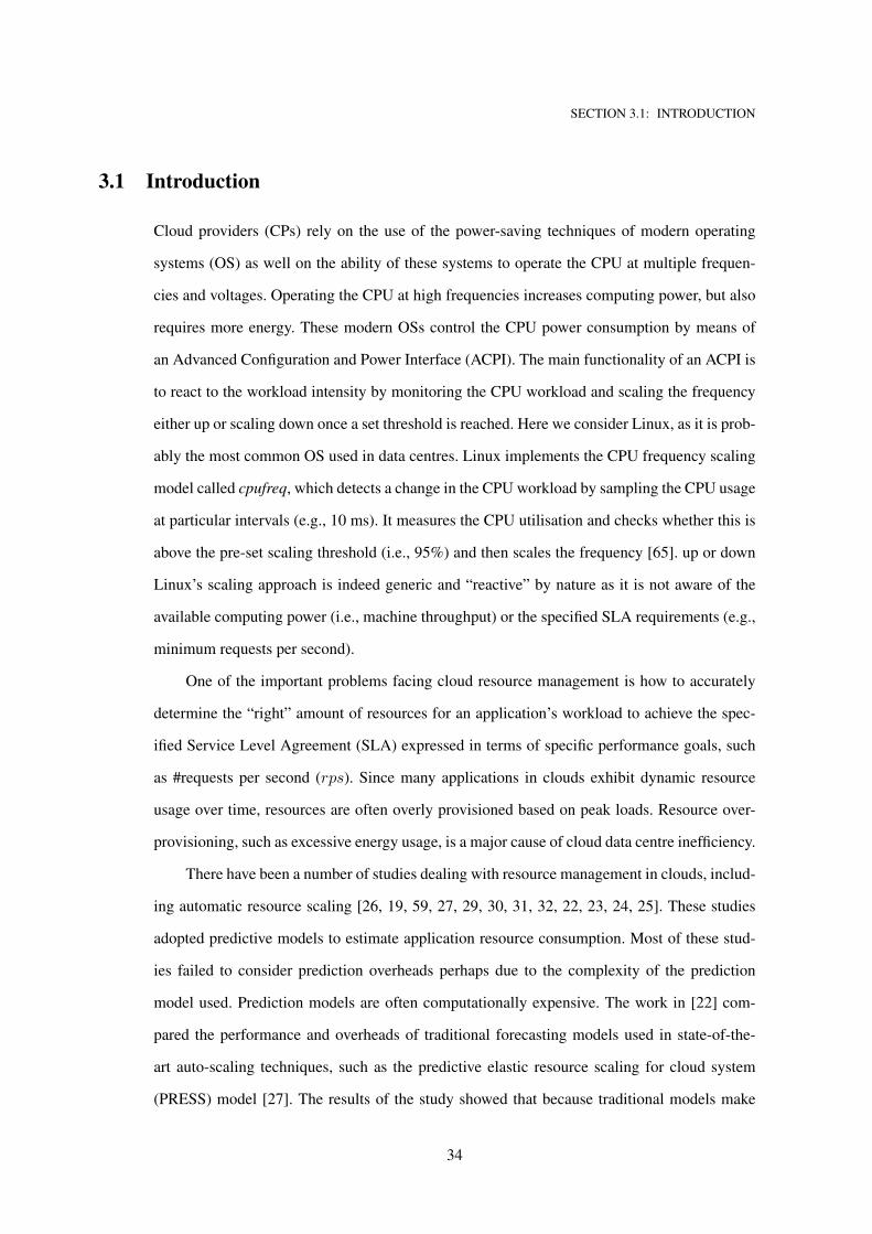
SECTION 3.1: INTRODUCTION
3.1 Introduction
Cloud providers (CPs) rely on the use of the power-saving techniques of modern operating
systems (OS) as well on the ability of these systems to operate the CPU at multiple frequen-
cies and voltages. Operating the CPU at high frequencies increases computing power, but also
requires more energy. These modern OSs control the CPU power consumption by means of
an Advanced Configuration and Power Interface (ACPI). The main functionality of an ACPI is
to react to the workload intensity by monitoring the CPU workload and scaling the frequency
either up or scaling down once a set threshold is reached. Here we consider Linux, as it is prob-
ably the most common OS used in data centres. Linux implements the CPU frequency scaling
model called cpufreq, which detects a change in the CPU workload by sampling the CPU usage
at particular intervals (e.g., 10 ms). It measures the CPU utilisation and checks whether this is
above the pre-set scaling threshold (i.e., 95%) and then scales the frequency [65]. up or down
Linux’s scaling approach is indeed generic and “reactive” by nature as it is not aware of the
available computing power (i.e., machine throughput) or the specified SLA requirements (e.g.,
minimum requests per second).
One of the important problems facing cloud resource management is how to accurately
determine the “right” amount of resources for an application’s workload to achieve the spec-
ified Service Level Agreement (SLA) expressed in terms of specific performance goals, such
as #requests per second (rps). Since many applications in clouds exhibit dynamic resource
usage over time, resources are often overly provisioned based on peak loads. Resource over-
provisioning, such as excessive energy usage, is a major cause of cloud data centre inefficiency.
There have been a number of studies dealing with resource management in clouds, includ-
ing automatic resource scaling [26, 19, 59, 27, 29, 30, 31, 32, 22, 23, 24, 25]. These studies
adopted predictive models to estimate application resource consumption. Most of these stud-
ies failed to consider prediction overheads perhaps due to the complexity of the prediction
model used. Prediction models are often computationally expensive. The work in [22] com-
pared the performance and overheads of traditional forecasting models used in state-of-the-
art auto-scaling techniques, such as the predictive elastic resource scaling for cloud system
(PRESS) model [27]. The results of the study showed that because traditional models make
34
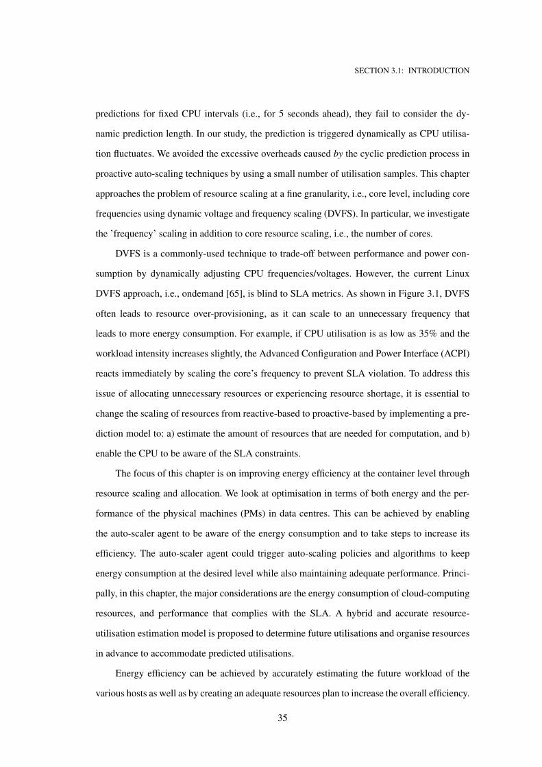
SECTION 3.1: INTRODUCTION
predictions for fixed CPU intervals (i.e., for 5 seconds ahead), they fail to consider the dy-
namic prediction length. In our study, the prediction is triggered dynamically as CPU utilisa-
tion fluctuates. We avoided the excessive overheads caused by the cyclic prediction process in
proactive auto-scaling techniques by using a small number of utilisation samples. This chapter
approaches the problem of resource scaling at a fine granularity, i.e., core level, including core
frequencies using dynamic voltage and frequency scaling (DVFS). In particular, we investigate
the ’frequency’ scaling in addition to core resource scaling, i.e., the number of cores.
DVFS is a commonly-used technique to trade-off between performance and power con-
sumption by dynamically adjusting CPU frequencies/voltages. However, the current Linux
DVFS approach, i.e., ondemand [65], is blind to SLA metrics. As shown in Figure 3.1, DVFS
often leads to resource over-provisioning, as it can scale to an unnecessary frequency that
leads to more energy consumption. For example, if CPU utilisation is as low as 35% and the
workload intensity increases slightly, the Advanced Configuration and Power Interface (ACPI)
reacts immediately by scaling the core’s frequency to prevent SLA violation. To address this
issue of allocating unnecessary resources or experiencing resource shortage, it is essential to
change the scaling of resources from reactive-based to proactive-based by implementing a pre-
diction model to: a) estimate the amount of resources that are needed for computation, and b)
enable the CPU to be aware of the SLA constraints.
The focus of this chapter is on improving energy efficiency at the container level through
resource scaling and allocation. We look at optimisation in terms of both energy and the per-
formance of the physical machines (PMs) in data centres. This can be achieved by enabling
the auto-scaler agent to be aware of the energy consumption and to take steps to increase its
efficiency. The auto-scaler agent could trigger auto-scaling policies and algorithms to keep
energy consumption at the desired level while also maintaining adequate performance. Princi-
pally, in this chapter, the major considerations are the energy consumption of cloud-computing
resources, and performance that complies with the SLA. A hybrid and accurate resource-
utilisation estimation model is proposed to determine future utilisations and organise resources
in advance to accommodate predicted utilisations.
Energy efficiency can be achieved by accurately estimating the future workload of the
various hosts as well as by creating an adequate resources plan to increase the overall efficiency.
35
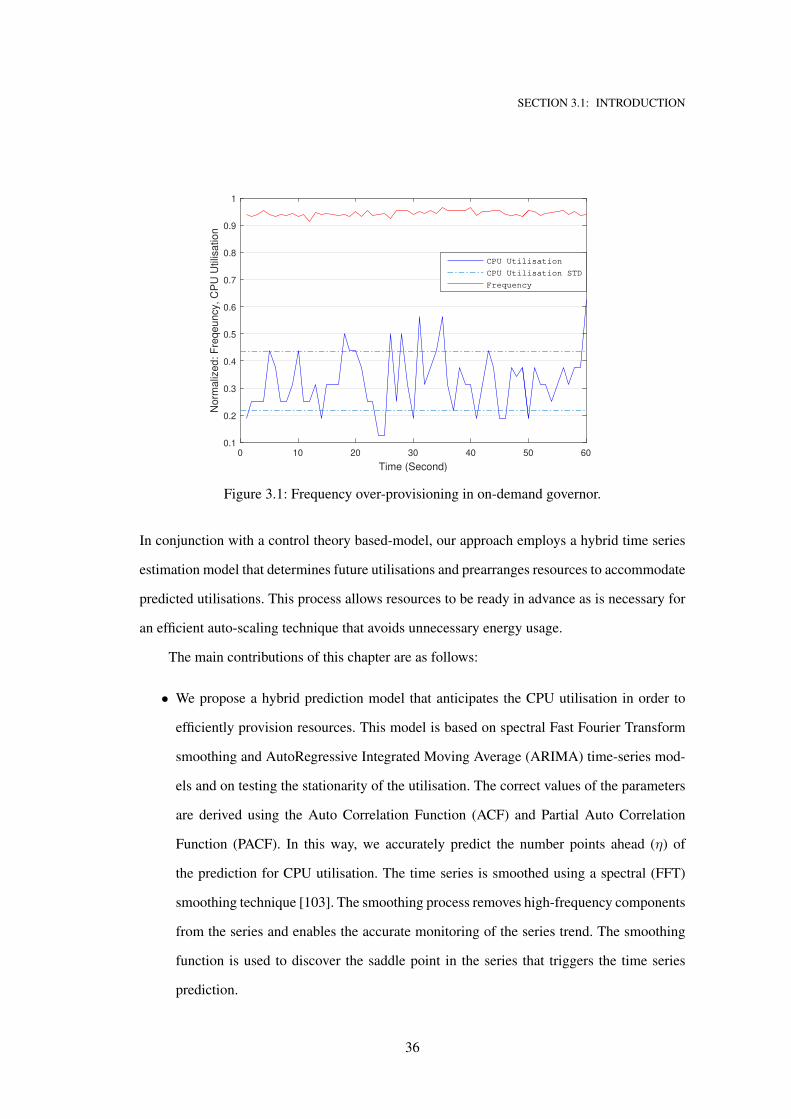
SECTION 3.1: INTRODUCTION
0 10 20 30 40 50 60
Time (Second)
0.1
0.2
0.3
0.4
0.5
0.6
0.7
0.8
0.9
1
Norm
aliz
ed: F
reqeuncy, C
PU
Utilis
ation
CPU Utilisation
CPU Utilisation STD
Frequency
Figure 3.1: Frequency over-provisioning in on-demand governor.
In conjunction with a control theory based-model, our approach employs a hybrid time series
estimation model that determines future utilisations and prearranges resources to accommodate
predicted utilisations. This process allows resources to be ready in advance as is necessary for
an efficient auto-scaling technique that avoids unnecessary energy usage.
The main contributions of this chapter are as follows:
• We propose a hybrid prediction model that anticipates the CPU utilisation in order to
efficiently provision resources. This model is based on spectral Fast Fourier Transform
smoothing and AutoRegressive Integrated Moving Average (ARIMA) time-series mod-
els and on testing the stationarity of the utilisation. The correct values of the parameters
are derived using the Auto Correlation Function (ACF) and Partial Auto Correlation
Function (PACF). In this way, we accurately predict the number points ahead (η) of
the prediction for CPU utilisation. The time series is smoothed using a spectral (FFT)
smoothing technique [103]. The smoothing process removes high-frequency components
from the series and enables the accurate monitoring of the series trend. The smoothing
function is used to discover the saddle point in the series that triggers the time series
prediction.
36
SECTION 3.2: RELATED WORK
• We also propose Energy-Based Auto Scaling (EBAS) as a new SLA-aware resource scal-
ing approach that dynamically changes the allocation (of cores to containers) as well as
the core’s frequency. Based on the proposed hybrid prediction model, several allocation
plans are derived with all their corresponding costs (in terms of consumed energy and
SLA). The best allocation plan is the one that has the lowest energy consumption.
As cloud services are increasingly provided with containers in addition to traditional VMs,
we conducted our experiments using Docker containers (https://www.docker.com/) with the
data caching benchmark [104]. The experiment results show that EBAS outperforms Linux’s
frequency governor by up to 38% and by 14% on average in terms of energy consumption.
This chapter is organised as follow: Previous studies discussed in Section 3.2. The differ-
ent types of container scalability are presented in Section 2.3. Section 3.3 provides details of
the EBAS approach, and Section 3.4 shows the experimental results. Section 3.5 summarises
the chapter and presents conclusions.
3.2 Related work
A large body of knowledge has addressed the issue of (proactive) auto-scaling in CDCs. A
wide range of prediction methods have been proposed to forecast resource utilisation, and the
precision of the prediction models decides the capacity of the auto-scaler to scale applications
proactively. This section examines the auto-scaling techniques that have been used in the state-
of-the-art studies.
Auto-scaling can be done in either a horizontal or vertical way [105, 33]. For horizon-
tal scaling [106, 107, 108], the auto-scaler can acquire or release containers for a particular
application. It can monitor the performance of resources and react once a set threshold is
reached. The auto-scaler can increase or decrease resources (e.g., the number of PMs, VMs
or containers) to maintain performance at the desired level. For vertical scaling [26, 109, 110],
only the allocated amount of resources (e.g., CPU cores, memory, CPU frequency) will be
added/removed to/from a container when a specific metric (e.g., CPU utilisation, available
memory space) exceeds a predefined value or range.
37
SECTION 3.2: RELATED WORK
A prediction algorithm works periodically at a defined interval to anticipate an applica-
tion’s average or maximum workload, forming the prediction horizon. The prediction results
chosen for use from the prediction horizon determine the approach that will be adopted. There
are two main approaches taken by the auto-scaler tools when using the prediction results. The
first approach takes the whole prediction horizon as the control interval [111, 112]. It antici-
pates the required resources during the deployment of the applications and allocates resources
based on that estimation. A major limitation of this approach is the length of the horizon. If the
prediction horizon is too short, this approach leads to short-sighted scaling decisions. However,
if a longer horizon is used, the scaling decisions are negatively influenced by the inaccuracy of
a longer prediction term; either case can lead to under- or over-provisioning.
The second approach is called Model Predictive Control (MPC) [113, 114, 26, 25], which
dynamically scales resources based on the application demand. The scaling decision is depends
on part of the prediction horizon. The control interval is set similar to the prediction length and
disregards all the future intervals in the prediction horizon. However, the weakness of this
approach is that the auto-scaler uses a fixed prediction interval length which makes it hard to
determine the prediction length under a highly fluctuating application workload. Many studies
divide the prediction horizon equally into a set of intervals (e.g., five data-points) [115, 27,
116]; thus, the scaling decisions will not be accurate due to the changes in the workload of the
application, as workload can fluctuate during an individual prediction interval. Moreover, the
resource allocation takes a while to be in effect and the auto-scaler needs to take into account
the resources needed during that time. For example, virtual machines take a couple of seconds
before they use the newly allocated resources [96].
The study in [117] introduced a cost-aware auto-scaling technique based on Linear Re-
gression (LR) to predict the workload and dynamically provide resources. The prediction
model collects the server cluster’s history logs and uses them to anticipate the cloud services’
workloads. Their approach scales resources for cloud services at both horizontal and vertical
levels. It uses self-healing scaling when multiple VMs coexist in the same cluster node. VMs
exchange CPU resources when they are not required. The resources of low CPU utilisation
VMs are removed and given to the VM where they are needed. However, if no resources are
available from neighbouring VMs, the resources controller adds unused resources to the pre-
38
SECTION 3.2: RELATED WORK
dicted high demand VM. This approach uses both vertical and horizontal scaling although it
has several limitations that obstruct its implementation.
A holistic approach was proposed by [118] to auto-scale servers and distribute them
across geographically-dispersed data centres. The proposed approach uses analysis and pre-
diction modules to model the resource demand and anticipate future resource needs and re-
source prices. A prediction model is used to dynamically adjust the number of leased servers
to maintain SLA requirements for hosted applications. This approach is applicable for cloud
brokers or service providers and helps them to increase their profits by dynamically allocat-
ing servers across different regions and taking advantage of dynamic prices that change daily.
The study by [118] uses a time series-based prediction model, mainly ARIMA, to predict the
service requests. The number of requests is estimated to minimise the cost, and systems are
proactively scaling in and out of their infrastructure. However, this approach did not specify
ARIMA parameters. The Worldcup 98 dataset was part of the experiment conducted in this
work, and showed that non-stationary phases with fixed parameters cannot provide accurate
solutions. Our work differs from that of Zhang because we consider the effect of dynamically
changing the ARIMA parameters based on the autocorrelation function (ACF) and the partial
autocorrelation function (PACF).
In regard to flexible applications, the proactive auto-scaling approach [119][120] has been
widely used to anticipate future demands. The most straightforward prediction method is the
Moving Average (MA). Exponential Smoothing (ES) is another method that gives better re-
sults than MA as it uses the last error history to adjust the new prediction. Brown’s quadratic
exponential smoothing predicative model was used in [21] to estimate future workloads, and
later a genetic algorithm was applied to find an “optimal” reconfiguration policy that suited the
last estimation.
Auto-Regression Moving Average (ARMA) is another method that estimates workloads [23,
25]. For example, [23] includes auto-regression with neutral networks to estimate the network
load on a data center. It uses a controller unit that monitors the network performance and de-
termines whether the network devices are over-loaded or at their optimal performance. Roy
et al. [25] used ARMA to predict future workloads based on limited historical information.
ARMA anticipates the number of users and later adjusts the number of VMs to be allocated. In
39
SECTION 3.2: RELATED WORK
our work, we extend the ARMA model and use the AutoRegressive Integrated Moving Aver-
age that dynamically chooses the best parameter values to provide accurate real-time workload
predictions.
The discovery of past usage patterns can be applied to anticipate future usage. For exam-
ple, the PRESS model [27] is an elastic predictive resource scaling scheme that uses a Fast
Fourier Transform (FFT) technique to extract repeated patterns (cyclic workloads) from his-
torical usage. It adjusts resource usage accordingly. For non-cyclic workloads, a discrete-time
Markov chain was used to discover the highest probability transitions for demand. For this,
a CPU Scheduler reconfigures the VM resources dynamically. This model has been extended
in [18] by adding a mechanism to support modern processors that can operate at different
voltages. Although these mechanisms are effective in scaling resources that have a cyclic and
non-cyclic workload, this may increase the amount of time required for searching patterns that
will cause the mechanism to miss the appropriate time at which to scale resources.
The DVSF technique has been widely used in energy efficient scheduling algorithms. For
example, [121] used DVFS to adjust the CPU frequency to reduce the total energy consumption
for the execution of tasks while meeting the completion deadline. However, the DVFS is not al-
ways efficient as the tasks’ execution time may be extended. The efficient application of DVFS
should ensure that the execution time will not be affected. In our work, the over-utilisation of
the CPU core is considered, and the proposed EBAS approach checks whether the allocated
cores and frequency can cause delays in the execution time for jobs. Rodrigo and Rajkumar in
[122] proposed a scheduling algorithm with the objective of keeping the CPU frequency at a
minimum level while meeting the users’ deadlines. They defined high performance computing
applications as “urgent” applications, such as disaster management and healthcare applications.
Their algorithm can be used with EBAS to schedule requests for such applications.
Bodik et al. [108] presented a power management strategy to associate performance met-
rics (i.e., response times) with variables representing the workload being processed. The com-
plexity of the various data centre configuration options would make it hard to include all
of these options when providing a real-time optimal auto-scaling action. Chen et al. [123]
provided a DVFS energy-aware scheduling algorithm called EASLA that was applied to the
precedence-constrained applications represented by a directed acyclic graph (DAG). EASLA
40
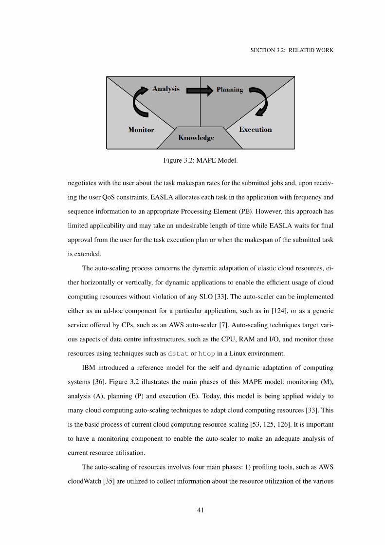
SECTION 3.2: RELATED WORK
Figure 3.2: MAPE Model.
negotiates with the user about the task makespan rates for the submitted jobs and, upon receiv-
ing the user QoS constraints, EASLA allocates each task in the application with frequency and
sequence information to an appropriate Processing Element (PE). However, this approach has
limited applicability and may take an undesirable length of time while EASLA waits for final
approval from the user for the task execution plan or when the makespan of the submitted task
is extended.
The auto-scaling process concerns the dynamic adaptation of elastic cloud resources, ei-
ther horizontally or vertically, for dynamic applications to enable the efficient usage of cloud
computing resources without violation of any SLO [33]. The auto-scaler can be implemented
either as an ad-hoc component for a particular application, such as in [124], or as a generic
service offered by CPs, such as an AWS auto-scaler [7]. Auto-scaling techniques target vari-
ous aspects of data centre infrastructures, such as the CPU, RAM and I/O, and monitor these
resources using techniques such as dstat or htop in a Linux environment.
IBM introduced a reference model for the self and dynamic adaptation of computing
systems [36]. Figure 3.2 illustrates the main phases of this MAPE model: monitoring (M),
analysis (A), planning (P) and execution (E). Today, this model is being applied widely to
many cloud computing auto-scaling techniques to adapt cloud computing resources [33]. This
is the basic process of current cloud computing resource scaling [53, 125, 126]. It is important
to have a monitoring component to enable the auto-scaler to make an adequate analysis of
current resource utilisation.
The auto-scaling of resources involves four main phases: 1) profiling tools, such as AWS
cloudWatch [35] are utilized to collect information about the resource utilization of the various
41
SECTION 3.3: THE EBAS APPROACH
VMs; 2) the collected information is fed into the analysis model, which interprets the informa-
tion to generate reasonable action for future resource utilization; 3) based on this analysis, the
data centre manager generates plans to adapt resources to cater for the analysed workload and
4) after the VMM has evaluated the generated plans, an “optimal plan” is selected based on
specific criteria and is executed by the auto-scaler manager.
Vertical scaling performs better (i.e., less SLO violation and higher throughput) than hor-
izontal scaling, as no interruption occurs in applications when vertical scaling is triggered. The
resource is attached on the fly and no overhead is incurred by the booting of new instances, as is
the case with horizontal scaling. For instance, when the controller adds and removes instances,
which generally impacts the application performance, the response time for the resource is the
lowest when using vertical scaling [127]. The work in [128] shows a significant improvement
in performance for vertical scaling in terms of power, cost and server density when compared
to horizontal scaling. The vertical scaling mechanism could be limited, as the applications may
run out of computing resources. This limitation is imposed by the fact that cloud providers
enable the user to choose only from a set of computing resource configurations which show
the maximum limit of the resource capacity. Moreover, several studies have provided predic-
tive resource management techniques [26, 19, 59, 27]. These studies have adopted predictive
models, which are computationally expensive, to provide an estimation of resource consump-
tion. However, our work takes the prediction overhead into account, and EBAS triggers the
prediction only when it is needed.
3.3 The EBAS approach
This section explains how vertical scaling can improve performance by increasing capacity,
saving energy and reducing costs for sensitive containerised applications. The EBAS approach
is designed to maintain SLA punctuality and proactively auto-scale up/down CPU resources
for sensitive containerised applications. We begin by explaining the various components in the
model. We describe each component and the model’s design configurations. EBAS is an auto-
scaling technique based on dynamic prediction length. The proposed technique uses a hybrid
time series prediction model to anticipate the demand of sensitive containerised applications.
42
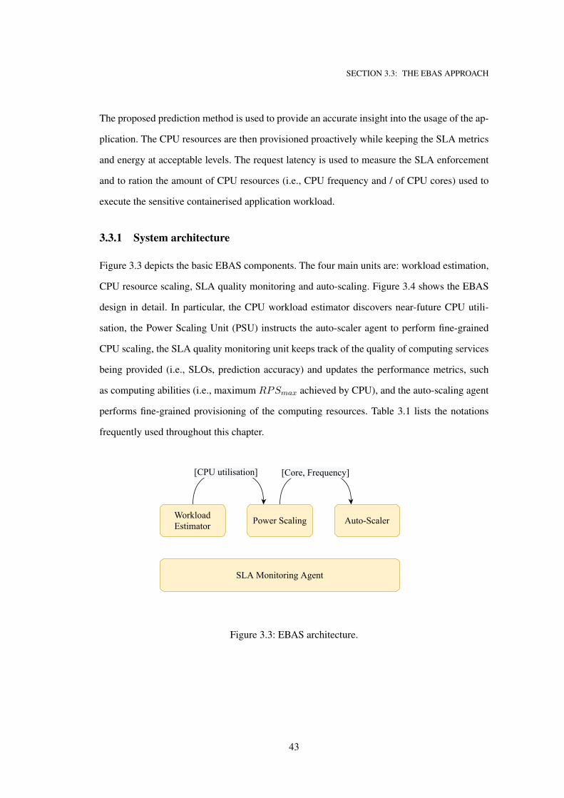
SECTION 3.3: THE EBAS APPROACH
The proposed prediction method is used to provide an accurate insight into the usage of the ap-
plication. The CPU resources are then provisioned proactively while keeping the SLA metrics
and energy at acceptable levels. The request latency is used to measure the SLA enforcement
and to ration the amount of CPU resources (i.e., CPU frequency and / of CPU cores) used to
execute the sensitive containerised application workload.
3.3.1 System architecture
Figure 3.3 depicts the basic EBAS components. The four main units are: workload estimation,
CPU resource scaling, SLA quality monitoring and auto-scaling. Figure 3.4 shows the EBAS
design in detail. In particular, the CPU workload estimator discovers near-future CPU utili-
sation, the Power Scaling Unit (PSU) instructs the auto-scaler agent to perform fine-grained
CPU scaling, the SLA quality monitoring unit keeps track of the quality of computing services
being provided (i.e., SLOs, prediction accuracy) and updates the performance metrics, such
as computing abilities (i.e., maximum RPSmax achieved by CPU), and the auto-scaling agent
performs fine-grained provisioning of the computing resources. Table 3.1 lists the notations
frequently used throughout this chapter.
[CPUutilisation]
WorkloadEstimator PowerScaling
SLAMonitoringAgent
Auto-Scaler
[Core,Frequency]
Figure 3.3: EBAS architecture.
43
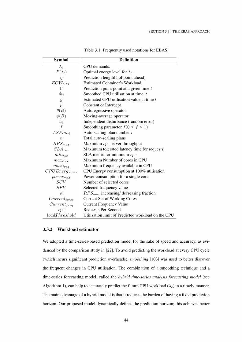
SECTION 3.3: THE EBAS APPROACH
Table 3.1: Frequently used notations for EBAS.
Symbol Definition
λc CPU demands.
E(λc) Optimal energy level for λc.
η Prediction length(# of point ahead)
ECWCPU Estimated Container’s Workload
Γ Prediction point point at a given time tmt Smoothed CPU utilisation at time. ty Estimated CPU utilisation value at time tµ Constant or Intercept
θ(B) Autoregressive operator
φ(B) Moving-average operator
at Independent disturbance (random error)
f Smoothing parameter f(0 ≤ f ≤ 1)ASPlani Auto-scaling plan number i
n Total auto-scaling plans
RPSmax Maximum rps server throughput
SLALat Maximum tolerated latency time for requests.
minrps SLA metric for minimum rpsmaxcore Maximum Number of cores in CPU
maxfreq Maximum frequency available in CPU
CPUEnergymax CPU Energy consumption at 100% utilisation
powermax Power consumption for a single core
SCV Number of selected cores
SFV Selected frequency value
α RPSmax increasing/ decreasing fraction
Currentcores Current Set of Working Cores
Currentfreq Current Frequency Value
rps Requests Per Second
loadThreshold Utilisation limit of Predicted workload on the CPU
3.3.2 Workload estimator
We adopted a time-series-based prediction model for the sake of speed and accuracy, as evi-
denced by the comparison study in [22]. To avoid predicting the workload at every CPU cycle
(which incurs significant prediction overheads), smoothing [103] was used to better discover
the frequent changes in CPU utilisation. The combination of a smoothing technique and a
time-series forecasting model, called the hybrid time-series analysis forecasting model (see
Algorithm 1), can help to accurately predict the future CPU workload (λc) in a timely manner.
The main advantage of a hybrid model is that it reduces the burden of having a fixed prediction
horizon. Our proposed model dynamically defines the prediction horizon; this achieves better
44
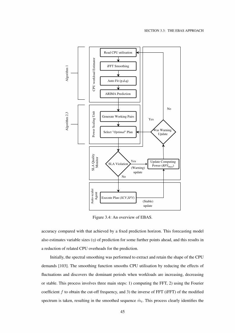
SECTION 3.3: THE EBAS APPROACH
Figure 3.4: An overview of EBAS.
accuracy compared with that achieved by a fixed prediction horizon. This forecasting model
also estimates variable sizes (η) of prediction for some further points ahead, and this results in
a reduction of related CPU overheads for the prediction.
Initially, the spectral smoothing was performed to extract and retain the shape of the CPU
demands [103]. The smoothing function smooths CPU utilisation by reducing the effects of
fluctuations and discovers the dominant periods when workloads are increasing, decreasing
or stable. This process involves three main steps: 1) computing the FFT, 2) using the Fourier
coefficient f to obtain the cut-off frequency, and 3) the inverse of FFT (iFFT) of the modified
spectrum is taken, resulting in the smoothed sequence mt. This process clearly identifies the
45
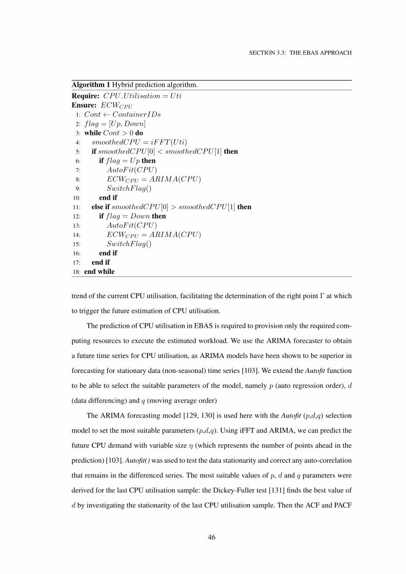
SECTION 3.3: THE EBAS APPROACH
Algorithm 1 Hybrid prediction algorithm.
Require: CPU Utilisation = UtiEnsure: ECWCPU
1: Cont← ContainerIDs2: flag = [Up,Down]3: while Cont > 0 do
4: smoothedCPU = iFFT (Uti)5: if smoothedCPU [0] < smoothedCPU [1] then
6: if flag = Up then
7: AutoF it(CPU)8: ECWCPU = ARIMA(CPU)9: SwitchF lag()
10: end if
11: else if smoothedCPU [0] > smoothedCPU [1] then
12: if flag = Down then
13: AutoF it(CPU)14: ECWCPU = ARIMA(CPU)15: SwitchF lag()16: end if
17: end if
18: end while
trend of the current CPU utilisation, facilitating the determination of the right point Γ at which
to trigger the future estimation of CPU utilisation.
The prediction of CPU utilisation in EBAS is required to provision only the required com-
puting resources to execute the estimated workload. We use the ARIMA forecaster to obtain
a future time series for CPU utilisation, as ARIMA models have been shown to be superior in
forecasting for stationary data (non-seasonal) time series [103]. We extend the Autofit function
to be able to select the suitable parameters of the model, namely p (auto regression order), d
(data differencing) and q (moving average order)
The ARIMA forecasting model [129, 130] is used here with the Autofit (p,d,q) selection
model to set the most suitable parameters (p,d,q). Using iFFT and ARIMA, we can predict the
future CPU demand with variable size η (which represents the number of points ahead in the
prediction) [103]. Autofit() was used to test the data stationarity and correct any auto-correlation
that remains in the differenced series. The most suitable values of p, d and q parameters were
derived for the last CPU utilisation sample: the Dickey-Fuller test [131] finds the best value of
d by investigating the stationarity of the last CPU utilisation sample. Then the ACF and PACF
46
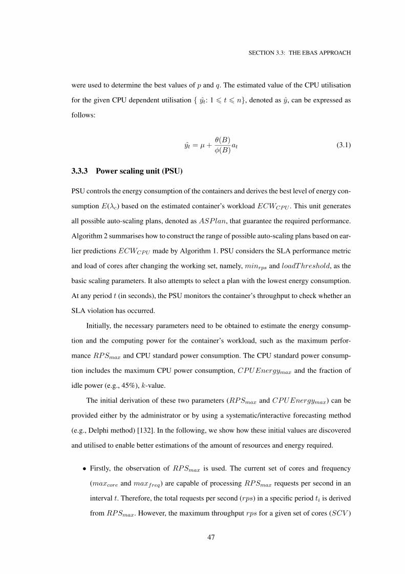
SECTION 3.3: THE EBAS APPROACH
were used to determine the best values of p and q. The estimated value of the CPU utilisation
for the given CPU dependent utilisation { yt: 1 6 t 6 n}, denoted as y, can be expressed as
follows:
yt = µ+θ(B)
φ(B)at (3.1)
3.3.3 Power scaling unit (PSU)
PSU controls the energy consumption of the containers and derives the best level of energy con-
sumption E(λc) based on the estimated container’s workload ECWCPU . This unit generates
all possible auto-scaling plans, denoted as ASPlan, that guarantee the required performance.
Algorithm 2 summarises how to construct the range of possible auto-scaling plans based on ear-
lier predictions ECWCPU made by Algorithm 1. PSU considers the SLA performance metric
and load of cores after changing the working set, namely, minrps and loadThreshold, as the
basic scaling parameters. It also attempts to select a plan with the lowest energy consumption.
At any period t (in seconds), the PSU monitors the container’s throughput to check whether an
SLA violation has occurred.
Initially, the necessary parameters need to be obtained to estimate the energy consump-
tion and the computing power for the container’s workload, such as the maximum perfor-
mance RPSmax and CPU standard power consumption. The CPU standard power consump-
tion includes the maximum CPU power consumption, CPUEnergymax and the fraction of
idle power (e.g., 45%), k-value.
The initial derivation of these two parameters (RPSmax and CPUEnergymax) can be
provided either by the administrator or by using a systematic/interactive forecasting method
(e.g., Delphi method) [132]. In the following, we show how these initial values are discovered
and utilised to enable better estimations of the amount of resources and energy required.
• Firstly, the observation of RPSmax is used. The current set of cores and frequency
(maxcore and maxfreq) are capable of processing RPSmax requests per second in an
interval t. Therefore, the total requests per second (rps) in a specific period ti is derived
from RPSmax. However, the maximum throughput rps for a given set of cores (SCV )
47
SECTION 3.3: THE EBAS APPROACH
Algorithm 2 Generate Working pairs.
Require: ECWCPU , loadThreshold,minrps
Ensure: List of ASPlan[rps, SFV, core, P (u)]1: for P = 1 to η do
2: for SCV = 1 to maxcore do
3: for SFV = minFreq to maxfreq do
4: PredLoad←− compute Predicted load {Eq. 3.5}5: if PredLoad ≤ loadThreshold {Eq.3.6} then
6: rps←− compute rps {Eq. 3.2}7: if rps > minrps then
8: Calculate powermax(SCV, SFV ) {Eq.3.4}9: Calculate Energy for predictions {Eq.3.7}
10: P (u)←− Energy for all predictions η {Eq.3.8}11: add to ASPlan[rps, SFV, SCV, P, P (u)]12: end if
13: end if
14: end for{Frequency Loop}15: end for{CPU Cores Loop}16: end for{All Predictions}
and selected frequency value (SFV ) is defined as:
rps(SCV,SFV ) = RPSmax ×SFV
maxfreq× SCV
maxcore(3.2)
• Secondly, the PSU needs to be aware of the maximum power consumption of indi-
vidual cores’ powermax; this can be done using existing energy evaluation tools (e.g.,
SPECpower ssj2008)1. powermax of a core c working at the maximum frequency maxfreq
is defined as:
powermax = CPUEnergymax
maxcore(3.3)
Then, the power consumption of a given number of cores SCV and frequency SFV is
defined as:
powermax(SCV, SFV ) = SFVmaxfreq
× powermax × SCV (3.4)
The PSU analyses a range of candidate vertical scaling plans by investigating the predicted
CPU workload λc for different cores and varying frequencies. This is carried out using Equa-
tion (3.5). Then, candidate plans are those that execute the predicted workload without any
1The total energy consumption of a CPU is obtained by using SPECpower benchmark https://www.spec.org.
48
SECTION 3.3: THE EBAS APPROACH
delay/over-usage in the execution. Condition (3.6) is used, and any plan that might cause core
over-utilisation will be ignored. In this case, we define a threshold, denoted as loadThreshold,
to represent the maximum core utilisation after scaling up/down the working cores as well as
their frequencies. This threshold could be set (i.e., 0.80%). Note that a different working set
(SCV , SFV ) will change the load of each CPU core.
Predload = ECWCPU × (Currentcores
SCV)× (
CurrentfreqSFV
) (3.5)
Predload ≤ loadThreshold (3.6)
The PSU unit produces a range of vertical scaling plans {ASPlani, i = 1 · · ·n}, with
each plan ASPlani having two values: SCVi (for the allocated cores) and SFVi (for the core’s
frequency). Using Algorithm 3, the PSU selects the best CPU core and frequency that will
ensure the following: a) the reduction of the energy consumption for the predicted utilisation,
and b) the operation of the server within the performance range in the SLA.
The selection of the “best” scaling plans is done as follows: the current state of the server’s
performance and its throughput is taken into consideration. This includes the number of work-
ing cores (Currentcores), each core’s frequency (Currentfreq) and the SLA metric (# of rps).
Therefore, to find the “best” plan, determine the best resources (SCV , SFV ) that satisfy the
condition (3.6) and have the lowest level of energy consumption.
CPU utilisation varies over time due to workload fluctuations. To compute the energy con-
sumption at each predicted CPU utilisation, Equation (3.7) is used, where powermax derived
by (Equation 3.4) is the maximum energy consumed by the CPU’s core (i.e., 100% utilisation).
Likewise, k represents the power consumption of the idle server over the total server energy
consumption at u of 100% CPU utilisation (i.e., 25%). The energy estimation model that was
introduced in [133] is used to calculate the total energy consumption for a particular predicted
workload, using Equation(3.8). The integral function of CPU utilisations within a given period
is the amount of energy consumed.
49
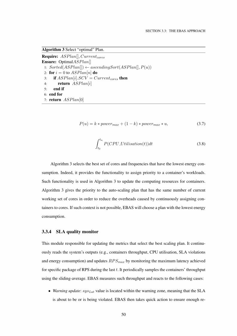
SECTION 3.3: THE EBAS APPROACH
Algorithm 3 Select “optimal” Plan.
Require: ASPlan[], CurrentcoresEnsure: OptimalASPlan[]
1: Sorted(ASPlan[])← ascendingSort(ASPlan[], P (u))2: for i = 0 to ASPlan[n] do
3: if ASPlan[i].SCV = Currentcores then
4: return ASPlan[i]5: end if
6: end for
7: return ASPlan[0]
P (u) = k ∗ powermax + (1− k) ∗ powermax ∗ u, (3.7)
∫ tn
t0
P (CPU Utilisation(t))dt (3.8)
Algorithm 3 selects the best set of cores and frequencies that have the lowest energy con-
sumption. Indeed, it provides the functionality to assign priority to a container’s workloads.
Such functionality is used in Algorithm 3 to update the computing resources for containers.
Algorithm 3 gives the priority to the auto-scaling plan that has the same number of current
working set of cores in order to reduce the overheads caused by continuously assigning con-
tainers to cores. If such context is not possible, EBAS will choose a plan with the lowest energy
consumption.
3.3.4 SLA quality monitor
This module responsible for updating the metrics that select the best scaling plan. It continu-
ously reads the system’s outputs (e.g., containers throughput, CPU utilisation, SLA violations
and energy consumption) and updates RPSmax by monitoring the maximum latency achieved
for specific package of RPS during the last t. It periodically samples the containers’ throughput
using the sliding-average. EBAS measures such throughput and reacts to the following cases:
• Warning update: sysLat value is located within the warning zone, meaning that the SLA
is about to be or is being violated. EBAS then takes quick action to ensure enough re-
50
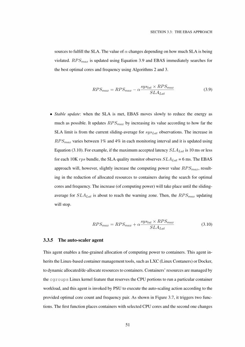
SECTION 3.3: THE EBAS APPROACH
sources to fulfill the SLA. The value of α changes depending on how much SLA is being
violated. RPSmax is updated using Equation 3.9 and EBAS immediately searches for
the best optimal cores and frequency using Algorithms 2 and 3.
RPSmax = RPSmax − αsyslat ×RPSmax
SLALat
(3.9)
• Stable update: when the SLA is met, EBAS moves slowly to reduce the energy as
much as possible. It updates RPSmax by increasing its value according to how far the
SLA limit is from the current sliding-average for sysLat observations. The increase in
RPSmax varies between 1% and 4% in each monitoring interval and it is updated using
Equation (3.10). For example, if the maximum accepted latency SLALat is 10 ms or less
for each 10K rps bundle, the SLA quality monitor observes SLALat = 6 ms. The EBAS
approach will, however, slightly increase the computing power value RPSmax, result-
ing in the reduction of allocated resources to containers during the search for optimal
cores and frequency. The increase (of computing power) will take place until the sliding-
average for SLALat is about to reach the warning zone. Then, the RPSmax updating
will stop.
RPSmax = RPSmax + αsyslat ×RPSmax
SLALat
(3.10)
3.3.5 The auto-scaler agent
This agent enables a fine-grained allocation of computing power to containers. This agent in-
herits the Linux-based container management tools, such as LXC (Linux Contaners) or Docker,
to dynamic allocated/de-allocate resources to containers. Containers’ resources are managed by
the cgroups Linux kernel feature that reserves the CPU portions to run a particular container
workload, and this agent is invoked by PSU to execute the auto-scaling action according to the
provided optimal core count and frequency pair. As shown in Figure 3.7, it triggers two func-
tions. The first function places containers with selected CPU cores and the second one changes
51
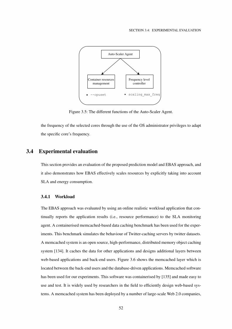
SECTION 3.4: EXPERIMENTAL EVALUATION
Figure 3.5: The different functions of the Auto-Scaler Agent.
the frequency of the selected cores through the use of the OS administrator privileges to adapt
the specific core’s frequency.
3.4 Experimental evaluation
This section provides an evaluation of the proposed prediction model and EBAS approach, and
it also demonstrates how EBAS effectively scales resources by explicitly taking into account
SLA and energy consumption.
3.4.1 Workload
The EBAS approach was evaluated by using an online realistic workload application that con-
tinually reports the application results (i.e., resource performance) to the SLA monitoring
agent. A containerised memcached-based data caching benchmark has been used for the exper-
iments. This benchmark simulates the behaviour of Twitter-caching servers by twitter datasets.
A memcached system is an open source, high-performance, distributed memory object caching
system [134]. It caches the data for other applications and designs additional layers between
web-based applications and back-end users. Figure 3.6 shows the memcached layer which is
located between the back-end users and the database-driven applications. Memcached software
has been used for our experiments. This software was containerised by [135] and made easy to
use and test. It is widely used by researchers in the field to efficiently design web-based sys-
tems. A memcached system has been deployed by a number of large-scale Web 2.0 companies,
52
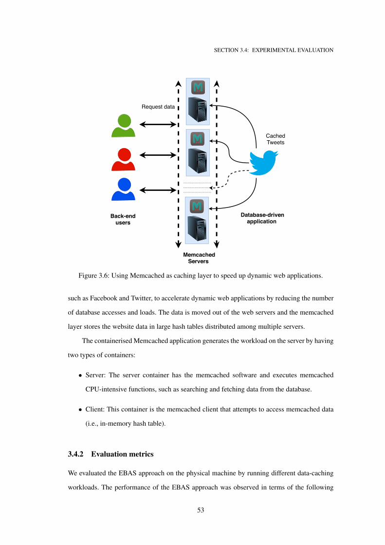
SECTION 3.4: EXPERIMENTAL EVALUATION
MemcachedServers
CachedTweets
Request data
Back-endusers
Database-drivenapplication
Figure 3.6: Using Memcached as caching layer to speed up dynamic web applications.
such as Facebook and Twitter, to accelerate dynamic web applications by reducing the number
of database accesses and loads. The data is moved out of the web servers and the memcached
layer stores the website data in large hash tables distributed among multiple servers.
The containerised Memcached application generates the workload on the server by having
two types of containers:
• Server: The server container has the memcached software and executes memcached
CPU-intensive functions, such as searching and fetching data from the database.
• Client: This container is the memcached client that attempts to access memcached data
(i.e., in-memory hash table).
3.4.2 Evaluation metrics
We evaluated the EBAS approach on the physical machine by running different data-caching
workloads. The performance of the EBAS approach was observed in terms of the following
53
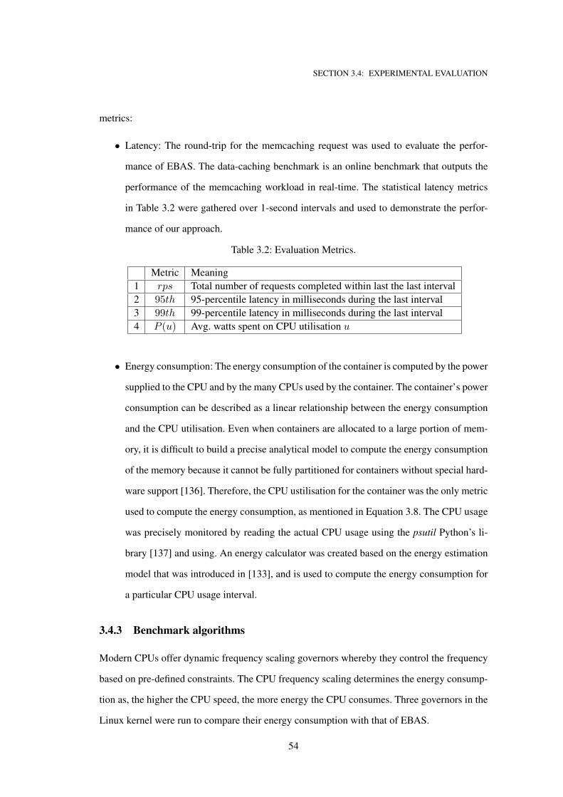
SECTION 3.4: EXPERIMENTAL EVALUATION
metrics:
• Latency: The round-trip for the memcaching request was used to evaluate the perfor-
mance of EBAS. The data-caching benchmark is an online benchmark that outputs the
performance of the memcaching workload in real-time. The statistical latency metrics
in Table 3.2 were gathered over 1-second intervals and used to demonstrate the perfor-
mance of our approach.
Table 3.2: Evaluation Metrics.
Metric Meaning
1 rps Total number of requests completed within last the last interval
2 95th 95-percentile latency in milliseconds during the last interval
3 99th 99-percentile latency in milliseconds during the last interval
4 P (u) Avg. watts spent on CPU utilisation u
• Energy consumption: The energy consumption of the container is computed by the power
supplied to the CPU and by the many CPUs used by the container. The container’s power
consumption can be described as a linear relationship between the energy consumption
and the CPU utilisation. Even when containers are allocated to a large portion of mem-
ory, it is difficult to build a precise analytical model to compute the energy consumption
of the memory because it cannot be fully partitioned for containers without special hard-
ware support [136]. Therefore, the CPU ustilisation for the container was the only metric
used to compute the energy consumption, as mentioned in Equation 3.8. The CPU usage
was precisely monitored by reading the actual CPU usage using the psutil Python’s li-
brary [137] and using. An energy calculator was created based on the energy estimation
model that was introduced in [133], and is used to compute the energy consumption for
a particular CPU usage interval.
3.4.3 Benchmark algorithms
Modern CPUs offer dynamic frequency scaling governors whereby they control the frequency
based on pre-defined constraints. The CPU frequency scaling determines the energy consump-
tion as, the higher the CPU speed, the more energy the CPU consumes. Three governors in the
Linux kernel were run to compare their energy consumption with that of EBAS.
54
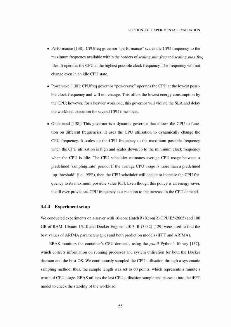
SECTION 3.4: EXPERIMENTAL EVALUATION
• Performance [138]: CPUfreq governor “performance” scales the CPU frequency to the
maximum frequency available within the borders of scaling min freq and scaling max freq
files. It operates the CPU at the highest possible clock frequency. The frequency will not
change even in an idle CPU state.
• Powersave [138]: CPUfreq governor “powersave” operates the CPU at the lowest possi-
ble clock frequency and will not change. This offers the lowest energy consumption by
the CPU; however, for a heavier workload, this governor will violate the SLA and delay
the workload execution for several CPU time slices.
• Ondemand [138]: This governor is a dynamic governor that allows the CPU to func-
tion on different frequencies. It uses the CPU utilisation to dynamically change the
CPU frequency. It scales up the CPU frequency to the maximum possible frequency
when the CPU utilisation is high and scales down/up to the minimum clock frequency
when the CPU is idle. The CPU scheduler estimates average CPU usage between a
predefined ’sampling rate’ period. If the average CPU usage is more than a predefined
’up threshold’ (i.e., 95%), then the CPU scheduler will decide to increase the CPU fre-
quency to its maximum possible value [65]. Even though this policy is an energy saver,
it still over-provisions CPU frequency as a reaction to the increase in the CPU demand.
3.4.4 Experiment setup
We conducted experiments on a server with 16-core (Intel(R) Xeon(R) CPU E5-2665) and 100
GB of RAM. Ubuntu 15.10 and Docker Engine 1.10.3. R (3.0.2) [129] were used to find the
best values of ARIMA parameters (p,q) and both prediction models (iFFT and ARIMA).
EBAS monitors the container’s CPU demands using the psutil Python’s library [137],
which collects information on running processes and system utilisation for both the Docker
daemon and the host OS. We continuously sampled the CPU utilisation through a systematic
sampling method; thus, the sample length was set to 60 points, which represents a minute’s
worth of CPU usage. EBAS utilises the last CPU utilisation sample and passes it into the iFFT
model to check the stability of the workload.
55
SECTION 3.4: EXPERIMENTAL EVALUATION
EBAS triggers the prediction function ARIMA once the iFFT’s function produces a new
peak (minima or maxima). EBAS searches through various prediction outputs to identify a min-
imal set of resources (i.e., CPU cores and frequency) to be allocated to containers. It undertakes
scaling for frequency by overwriting the system frequency file (i.e., cpuinfo max freq)
and allocates and deallocates the cores using docker update. The value of cpuset repre-
sents the number of cores allocated to containers. Docker Engine updates the containers cores
and deallocates unwanted cores according to the selected ASPlan by Algorithm 3.
To improve the efficiency of resource usage, EBAS has a fixed size of CPU samples as
input, i.e., 60 points with one-second intervals. CPU overheads are computed for the current
version of EBAS (i.e., 60 points), which is less than 1% of the total CPU utilisation.
The data-caching benchmark [104] is commonly used in high-performance machines in
data centres. This uses the Memcached system in the data caching server, simulating the be-
haviour of a Twitter data caching server using a Twitter dataset. The server’s containers run
the data caching system, and the client’s containers request data caching from the server’s con-
tainers. As this benchmark is network-intensive, the two container types are hosted within the
same server to stress only the CPU. Accordingly, the CPU has to handle the right amount of
data caching requests per second within the SLA objectives. We considered the SLALat at 10
ms according to the QoS restrictions in the benchmark documentations [104].
The aim of EBAS is to allocate the minimum amount of cores and frequency needed
to meet the desired performance level with minimum violation. Initially, it is necessary to
know the maximum number of aggregated throughput (RPSmax) for the entire working cores
(maxcore) and maximum frequency (maxfreq) in the machine. We used the benchmark at the
maximum throughput state, then we observed RPSmax for a limited period T . The average
number of rps handled during period T was calculated. The maximum number of throughput
RPSmax was then identified; this enabled us to derive the computing power for any set of
given cores SCV and frequency SFV .
Initially, the experiments were conducted by running the benchmark [104] with the default
DVFS configurations (i.e., ondemand). A snapshot of the light workload (i.e., 15%) was studied
for the purpose of achieving a clear visibility of data points. When containers experience a light
workload, they utilise the CPU randomly, which leads to a higher utilisation of CPU. Figure
56
SECTION 3.4: EXPERIMENTAL EVALUATION
Figure 3.7: Scalability in the EPFL Data caching benchmark.
3.8 depicts the CPU utilisation during the processing of a light workload (i.e., 10k) and also
shows that EBAS provides the required resources. Consequently, the quantum of energy-saving
is greater for a low workload because the over-provisioning of resources needs to be saved and
applied; EBAS allocates the minimum resources that are required. The energy-saving feature is
inversely proportional to the workload. In other words, when the workload is high, the degree
of energy saving is limited as the majority of resources are “fully” used regardless of resource
scaling.
3.4.5 Experimental results
Although the server processes at 10k rps, which is around 5% of its computing power, the
default OS frequency governor (i.e., ondemand) arbitrarily scales the CPU frequency to the
maximum frequency (Figure 3.9), resulting in excessive energy consumption. It is apparent
from Figure 3.9 that EBAS judiciously sets CPU frequency taking the SLA conditions into
account. In this context, energy saving could be up to 38% compared with the on-demand
governor, as shown in Table 3.3. Different workloads have been tested and the performance of
EBAS has been evaluated. For different workloads, we have gradually tested the throughput
of the Memcached system, and recorded results for EBAS against the on demand frequency
57
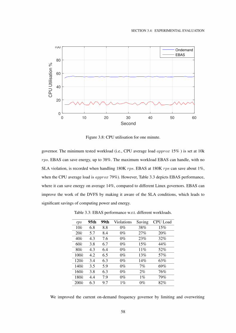
SECTION 3.4: EXPERIMENTAL EVALUATION
0 10 20 30 40 50 60
Second
0
20
40
60
80
100C
PU
Utilis
ation %
Ondemand
EBAS
Figure 3.8: CPU utilisation for one minute.
governor. The minimum tested workload (i.e., CPU average load approx 15% ) is set at 10k
rps. EBAS can save energy, up to 38%. The maximum workload EBAS can handle, with no
SLA violation, is recorded when handling 180K rps. EBAS at 180K rps can save about 1%,
when the CPU average load is approx 79%). However, Table 3.3 depicts EBAS performance,
where it can save energy on average 14%, compared to different Linux governors. EBAS can
improve the work of the DVFS by making it aware of the SLA conditions, which leads to
significant savings of computing power and energy.
Table 3.3: EBAS performance w.r.t. different workloads.
rps 95th 99th Violations Saving CPU Load
10k 6.8 8.8 0% 38% 15%
20k 5.7 8.4 0% 27% 20%
40k 4.3 7.6 0% 23% 32%
60k 3.8 6.7 0% 15% 44%
80k 4.3 6.4 0% 11% 52%
100k 4.2 6.5 0% 13% 57%
120k 3.4 6.3 0% 14% 63%
140k 3.5 5.9 0% 7% 69%
160k 3.8 6.3 0% 2% 76%
180k 4.4 7.9 0% 1% 79%
200k 6.3 9.7 1% 0% 82%
We improved the current on-demand frequency governor by limiting and overwriting
58

SECTION 3.4: EXPERIMENTAL EVALUATION
0 10 20 30 40 50 60
Second
1
1.5
2
2.5
Fre
quency G
Hz
Ondemand
EBAS
Figure 3.9: Data caching server when handling 10k rps workload.
the frequency value in the scaling max freq file. The value of SFV selected by Algo-
rithm 3 was used to perform the frequency scaling. Additionally, the Docker Engine updates
Memcached servers by modifying --cpuset-cpus specifications according to the SCV
value in the selected “optimal” plan. The results are depicted in Table 3.3 which shows the
energy-saving capacity of EBAS for different workloads. EBAS enables extra energy savings
for such data caching servers when processing light to medium workloads. Additionally, the
over-provisioned resources can be dynamically scaled down, and EBAS provides performance
at scale for these types of servers. The total throughput was recorded for both the Linux gov-
ernor and EBAS, and both of them successfully produced almost the same throughput. Figure
3.10 gives a close view of the total throughput in one minute. The average throughput for EBAS
meets the SLA objective, i.e., 10k rps. While the Linux default on-demand governor delivers
similar performance, its CPU resource consumption/utilisation is more than double compared
with that of EBAS (Figure 3.8).
As shown in Figure 3.10, SLA violations occur as the memcached servers do not fulfil the
same amount of requests by the client’s container. Although the processed requests are less than
the SLA metric (#rps) at some points, this is due to the client requests generator requests only
that amount. Furthermore, the computing resources are provided according to the estimated
demand.
59
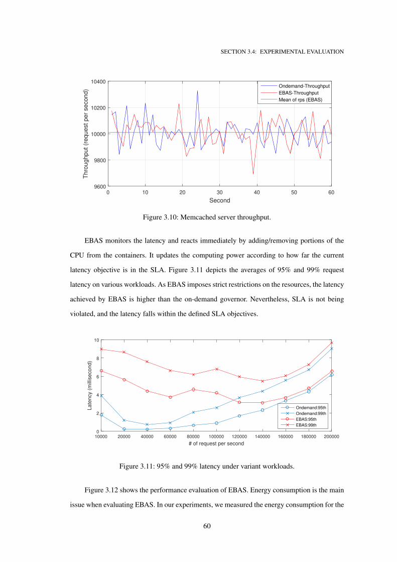
SECTION 3.4: EXPERIMENTAL EVALUATION
0 10 20 30 40 50 60
Second
9600
9800
10000
10200
10400T
hro
ug
hp
ut
(re
qu
est
pe
r se
co
nd
)Ondemand-Throughput
EBAS-Throughput
Mean of rps (EBAS)
Figure 3.10: Memcached server throughput.
EBAS monitors the latency and reacts immediately by adding/removing portions of the
CPU from the containers. It updates the computing power according to how far the current
latency objective is in the SLA. Figure 3.11 depicts the averages of 95% and 99% request
latency on various workloads. As EBAS imposes strict restrictions on the resources, the latency
achieved by EBAS is higher than the on-demand governor. Nevertheless, SLA is not being
violated, and the latency falls within the defined SLA objectives.
10000 20000 40000 60000 80000 100000 120000 140000 160000 180000 200000
# of request per second
0
2
4
6
8
10
Late
ncy (
mill
isecond)
Ondemand:95th
Ondemand:99th
EBAS:95th
EBAS:99th
Figure 3.11: 95% and 99% latency under variant workloads.
Figure 3.12 shows the performance evaluation of EBAS. Energy consumption is the main
issue when evaluating EBAS. In our experiments, we measured the energy consumption for the
60
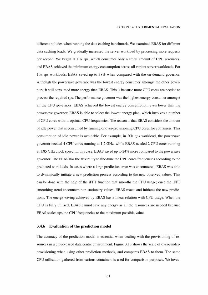
SECTION 3.4: EXPERIMENTAL EVALUATION
different policies when running the data caching benchmark. We examined EBAS for different
data caching loads. We gradually increased the server workload by processing more requests
per second. We began at 10k rps, which consumes only a small amount of CPU resources,
and EBAS achieved the minimum energy consumption across all variant server workloads. For
10k rps workloads, EBAS saved up to 38% when compared with the on-demand governor.
Although the powersave governor was the lowest energy consumer amongst the other gover-
nors, it still consumed more energy than EBAS. This is because more CPU cores are needed to
process the required rps. The performance governor was the highest energy consumer amongst
all the CPU governors. EBAS achieved the lowest energy consumption, even lower than the
powersave governor. EBAS is able to select the lowest energy plan, which involves a number
of CPU cores with its optimal CPU frequencies. The reason is that EBAS considers the amount
of idle power that is consumed by running or over-provisioning CPU cores for containers. This
consumption of idle power is avoidable. For example, in 20k rps workload, the powersave
governor needed 4 CPU cores running at 1.2 GHz, while EBAS needed 2 CPU cores running
at 1.85 GHz clock speed. In this case, EBAS saved up to 24% more compared to the powersave
governor. The EBAS has the flexibility to fine-tune the CPU cores frequencies according to the
predicted workloads. In cases where a large prediction error was encountered, EBAS was able
to dynamically initiate a new prediction process according to the new observed values. This
can be done with the help of the iFFT function that smooths the CPU usage; once the iFFT
smoothing trend encounters non-stationary values, EBAS reacts and initiates the new predic-
tions. The energy-saving achieved by EBAS has a linear relation with CPU usage. When the
CPU is fully utilised, EBAS cannot save any energy as all the resources are needed because
EBAS scales ups the CPU frequencies to the maximum possible value.
3.4.6 Evaluation of the prediction model
The accuracy of the prediction model is essential when dealing with the provisioning of re-
sources in a cloud-based data centre environment. Figure 3.13 shows the scale of over-/under-
provisioning when using other prediction methods, and compares EBAS to them. The same
CPU utilisation gathered from various containers is used for comparison purposes. We inves-
61
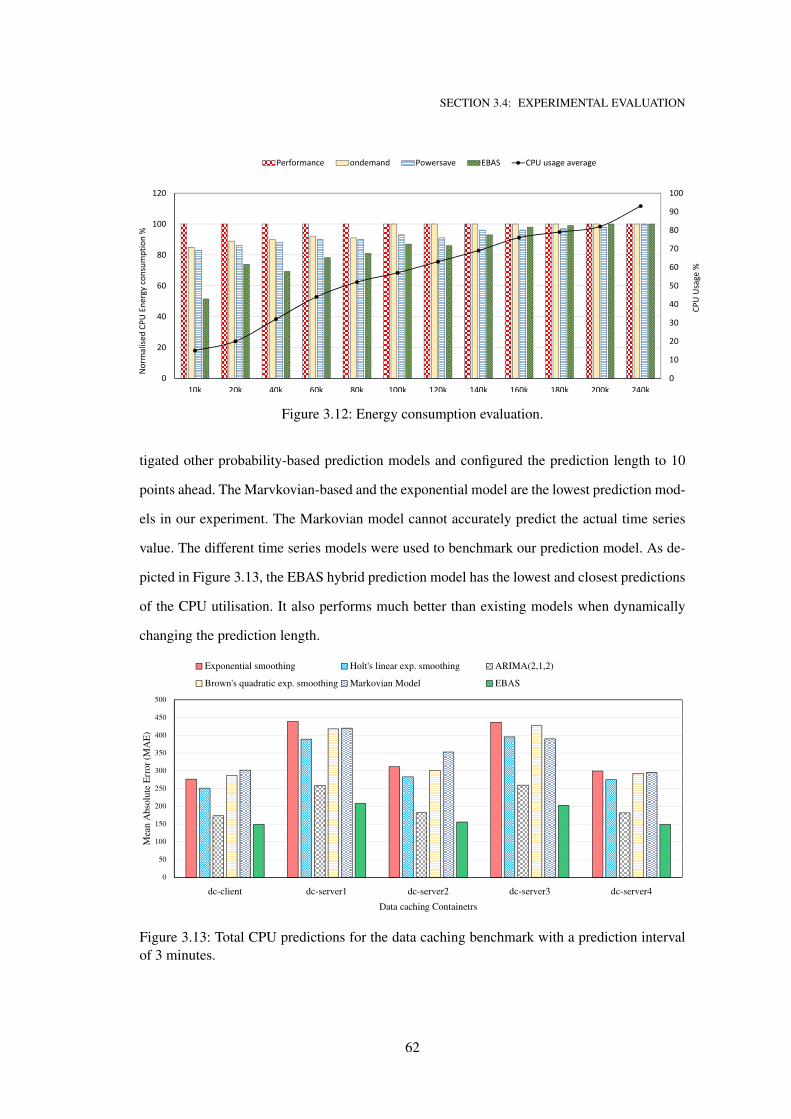
SECTION 3.4: EXPERIMENTAL EVALUATION
0
10
20
30
40
50
60
70
80
90
100
0
20
40
60
80
100
120
10k 20k 40k 60k 80k 100k 120k 140k 160k 180k 200k 240k
Norm
alise
d CP
U En
ergy co
nsum
ption %
Request per second
Performance ondemand Powersave EBAS CPU usage average
CPUUs
age %
Figure 3.12: Energy consumption evaluation.
tigated other probability-based prediction models and configured the prediction length to 10
points ahead. The Marvkovian-based and the exponential model are the lowest prediction mod-
els in our experiment. The Markovian model cannot accurately predict the actual time series
value. The different time series models were used to benchmark our prediction model. As de-
picted in Figure 3.13, the EBAS hybrid prediction model has the lowest and closest predictions
of the CPU utilisation. It also performs much better than existing models when dynamically
changing the prediction length.
0
50
100
150
200
250
300
350
400
450
500
dc-client dc-server1 dc-server2 dc-server3 dc-server4
Mea
n A
bso
lute
Err
or
(MA
E)
Data caching Containetrs
Exponential smoothing Holt's linear exp. smoothing ARIMA(2,1,2)
Brown's quadratic exp. smoothing Markovian Model EBAS
Figure 3.13: Total CPU predictions for the data caching benchmark with a prediction interval
of 3 minutes.
62
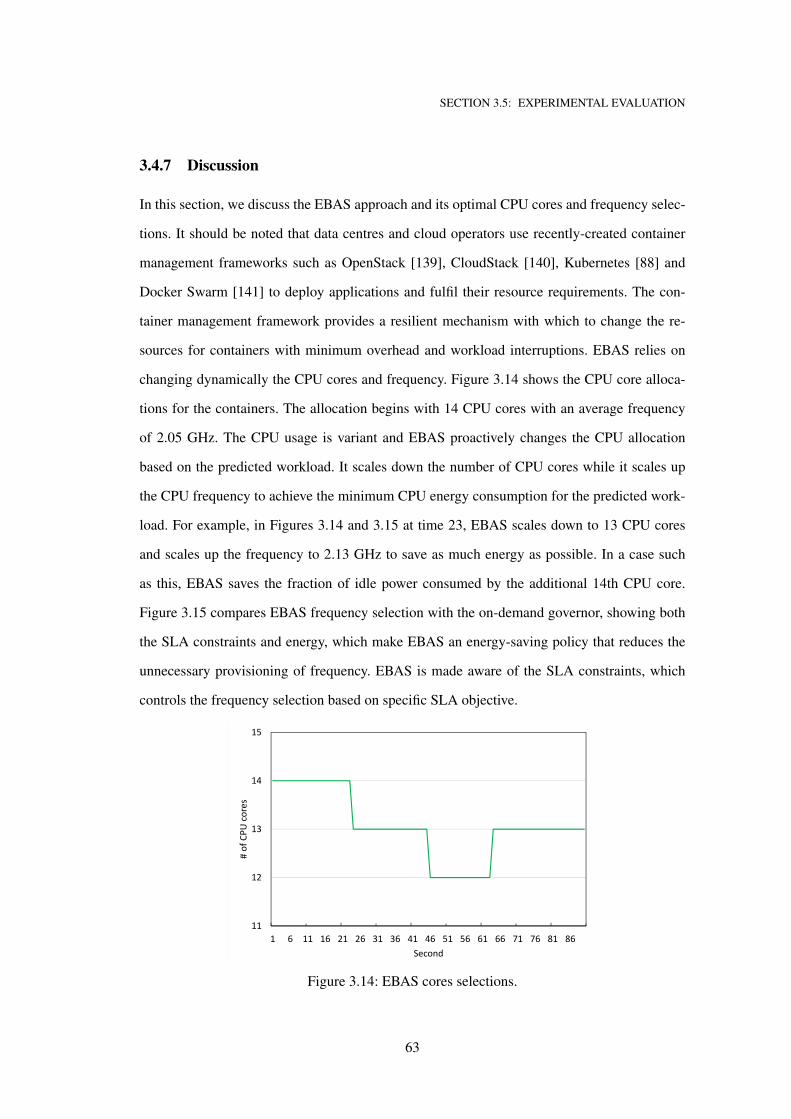
SECTION 3.5: EXPERIMENTAL EVALUATION
3.4.7 Discussion
In this section, we discuss the EBAS approach and its optimal CPU cores and frequency selec-
tions. It should be noted that data centres and cloud operators use recently-created container
management frameworks such as OpenStack [139], CloudStack [140], Kubernetes [88] and
Docker Swarm [141] to deploy applications and fulfil their resource requirements. The con-
tainer management framework provides a resilient mechanism with which to change the re-
sources for containers with minimum overhead and workload interruptions. EBAS relies on
changing dynamically the CPU cores and frequency. Figure 3.14 shows the CPU core alloca-
tions for the containers. The allocation begins with 14 CPU cores with an average frequency
of 2.05 GHz. The CPU usage is variant and EBAS proactively changes the CPU allocation
based on the predicted workload. It scales down the number of CPU cores while it scales up
the CPU frequency to achieve the minimum CPU energy consumption for the predicted work-
load. For example, in Figures 3.14 and 3.15 at time 23, EBAS scales down to 13 CPU cores
and scales up the frequency to 2.13 GHz to save as much energy as possible. In a case such
as this, EBAS saves the fraction of idle power consumed by the additional 14th CPU core.
Figure 3.15 compares EBAS frequency selection with the on-demand governor, showing both
the SLA constraints and energy, which make EBAS an energy-saving policy that reduces the
unnecessary provisioning of frequency. EBAS is made aware of the SLA constraints, which
controls the frequency selection based on specific SLA objective.
11
12
13
14
15
1 6 11 16 21 26 31 36 41 46 51 56 61 66 71 76 81 86
# of CPU
cores
Second
Figure 3.14: EBAS cores selections.
63
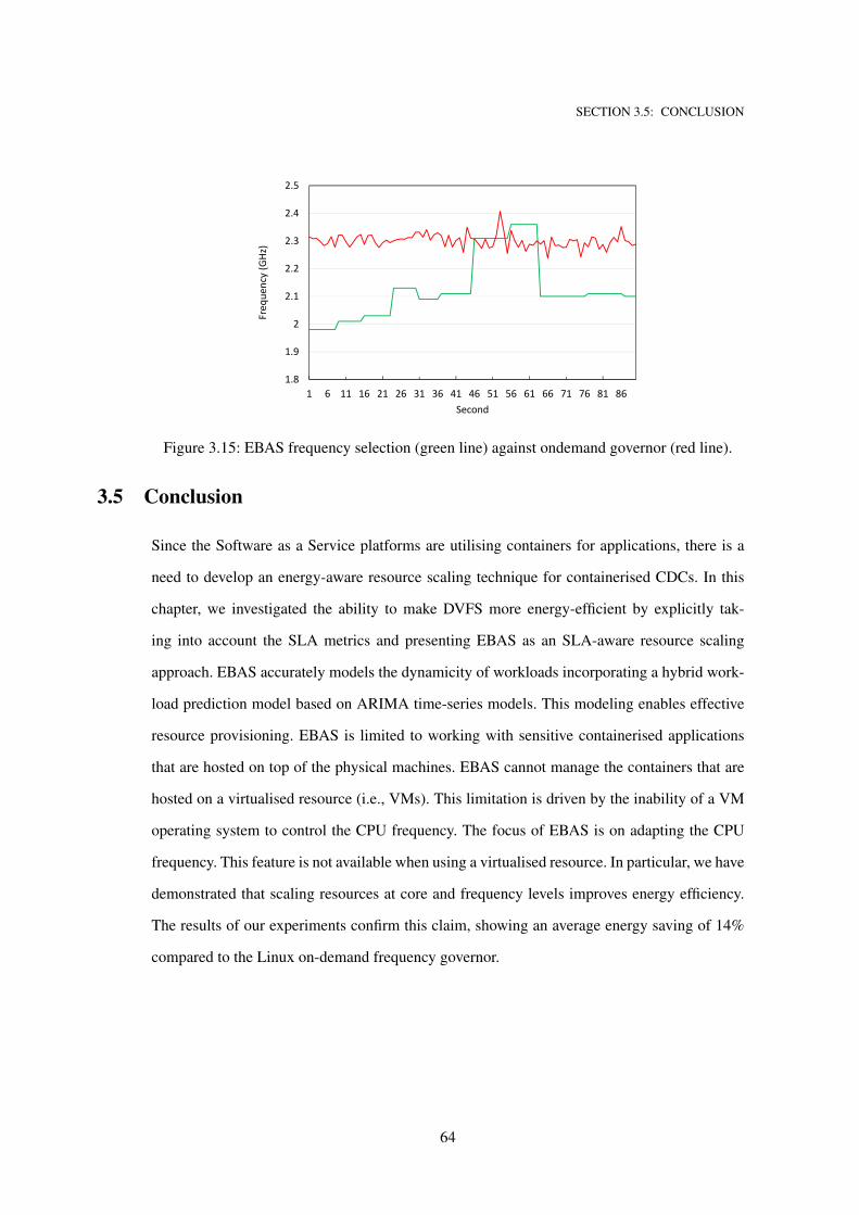
SECTION 3.5: CONCLUSION
1.8
1.9
2
2.1
2.2
2.3
2.4
2.5
1 6 11 16 21 26 31 36 41 46 51 56 61 66 71 76 81 86
Freq
uency (GHz
)
Second
EBAS Ondemand
Figure 3.15: EBAS frequency selection (green line) against ondemand governor (red line).
3.5 Conclusion
Since the Software as a Service platforms are utilising containers for applications, there is a
need to develop an energy-aware resource scaling technique for containerised CDCs. In this
chapter, we investigated the ability to make DVFS more energy-efficient by explicitly tak-
ing into account the SLA metrics and presenting EBAS as an SLA-aware resource scaling
approach. EBAS accurately models the dynamicity of workloads incorporating a hybrid work-
load prediction model based on ARIMA time-series models. This modeling enables effective
resource provisioning. EBAS is limited to working with sensitive containerised applications
that are hosted on top of the physical machines. EBAS cannot manage the containers that are
hosted on a virtualised resource (i.e., VMs). This limitation is driven by the inability of a VM
operating system to control the CPU frequency. The focus of EBAS is on adapting the CPU
frequency. This feature is not available when using a virtualised resource. In particular, we have
demonstrated that scaling resources at core and frequency levels improves energy efficiency.
The results of our experiments confirm this claim, showing an average energy saving of 14%
compared to the Linux on-demand frequency governor.
64
CHAPTER 4adCFS Policy for Containerised Batch
Applications (Scientific Workflows)
Scientific workflows are increasingly containerised, which requires rethinking CPU sharing
policies to accommodate different workload types. However, container engines running con-
tainerised scientific workflows struggle to share the CPU fairly when CPU overcommitting
is required. Previously, Chapter 3 addressed the issue of proactively auto-scaling container
CPU resources based on the Service Level Agreement (SLA) for containerised applications. It
scales resources at the CPU core level in terms of both the number and frequency of the cores.
It incorporates the dynamic voltage and frequency scaling (DVFS) technique to dynamically
adjust CPU frequencies. The proactive decisions on resource scaling are enabled primarily by
the proposed CPU usage prediction model and the workload consolidation model of EBAS.
In this chapter, we propose a sharing policy, called the Adaptive Completely Fair Scheduling
policy (adCFS), which considers the future state of CPU usage and proactively shares CPU
cycles between various containers based on their corresponding workload metrics (e.g., CPU
usage, task runtime, #tasks). adCFS estimates the weight of workload characteristics and re-
distributes the CPU based on the corresponding weights. The Markov chain model is used to
predict CPU state use, and the adCFS policy is triggered to dynamically allocate containers to
the proper CPU portions. Experimental results show enhanced container CPU response time
for those containers that run heavy and large jobs; these display a 12% faster response time
65
SECTION 4.1: INTRODUCTION
compared with the default CFS (Completely Fair Scheduler). adCFS therefore enhances CFS
by considering workload metrics, which leads to the CPU being shared fairly when it is fully
utilised.
4.1 Introduction
Over recent years, cloud computing data centres have started to host and manage scientific
workflow systems. Cloud data centres offer a wide range of heterogeneous, distributed and
elastic resources to execute multi-stage computations of scientific workflow tasks. Therefore,
scientific workflow systems are an important class of cloud computing applications. A scien-
tific workflow is typically modelled as a Directed Acyclic Graph (DAG), which is executed in
a systematic manner. Tasks are connected according to their dependencies, and a task depen-
dency represents the data flowing from one task to another. As appears in Figure 4.1, the output
data for a task represents the input data for the following task/s. The task of the workflow may
involve one or more jobs in order to achieve the task objectives. The DAG-based workflow
structure is classified into sequence, parallelism, and choice [142]. The sequence task orders
workflow tasks in a series, where one new task starts after the previous one has finished. The
parallelism task runs tasks simultaneously, as they may share the same output as the previ-
ous tasks. The choice task represents many options when, at runtime, the next task is selected
when a predefined condition is true. These three structure types are used to build complex and
small/large scales of scientific workflows that are hosted in cloud-based data centres.
Scientific workflow systems are used in many scientific domains to solve complex com-
putational tasks. These systems are hosted on top of high performance computing resources.
These resources are managed by data centres which offer users a wide range of on-demand
resource configurations to execute scientific workflows. However, most recently, a lightweight
container technology has emerged that alters the complete virtualisation technology; moving
it towards containerised applications [143, 144]. Many scientific workflows have been con-
tainerised and hosted in Docker containers [145, 146] to benefit fully from the superiority of
the containers’ performance (e.g., memory speed, low performance loss) [147, 96]. From a
deployment perspective, the recent advancement in container technology (e.g., the Docker En-
66
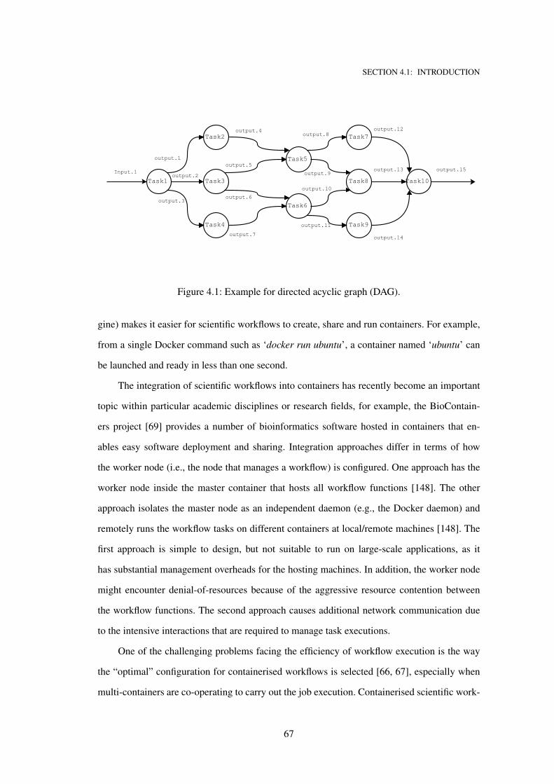
SECTION 4.1: INTRODUCTION
Figure 4.1: Example for directed acyclic graph (DAG).
gine) makes it easier for scientific workflows to create, share and run containers. For example,
from a single Docker command such as ‘docker run ubuntu’, a container named ‘ubuntu’ can
be launched and ready in less than one second.
The integration of scientific workflows into containers has recently become an important
topic within particular academic disciplines or research fields, for example, the BioContain-
ers project [69] provides a number of bioinformatics software hosted in containers that en-
ables easy software deployment and sharing. Integration approaches differ in terms of how
the worker node (i.e., the node that manages a workflow) is configured. One approach has the
worker node inside the master container that hosts all workflow functions [148]. The other
approach isolates the master node as an independent daemon (e.g., the Docker daemon) and
remotely runs the workflow tasks on different containers at local/remote machines [148]. The
first approach is simple to design, but not suitable to run on large-scale applications, as it
has substantial management overheads for the hosting machines. In addition, the worker node
might encounter denial-of-resources because of the aggressive resource contention between
the workflow functions. The second approach causes additional network communication due
to the intensive interactions that are required to manage task executions.
One of the challenging problems facing the efficiency of workflow execution is the way
the “optimal” configuration for containerised workflows is selected [66, 67], especially when
multi-containers are co-operating to carry out the job execution. Containerised scientific work-
67
SECTION 4.1: INTRODUCTION
flow systems have revealed recently after many attempts [68, 69] to customise workflow’s func-
tions into reusable containers. For example, Galaxy [68] is a scientific workflow system that is
accessible, reproducible, transparent, computational and biomedical research. Many common
tools (i.e., toolSheed [149]) have been integrated into containers to make them independent
and re-usable.
Containers share computing resources using predefined scheduling policies (e.g., Com-
pletely Fair Scheduler (CFS) [71] and Dynamic Completely Fair Scheduler (DCFS) [70]).
However, these policies ignore the task’s characteristics (e.g., type of task, CPU usage, task
size); therefore, the CFS is unable to uphold a proper quality of service (QoS) while main-
taining fairness between tasks [72]. The CFS policy allocates equal portions of the CPU to the
hosted containers, while the DCFS uses generic metrics (e.g., number of users, change in load)
to manage CPU sharing. Indeed, the generic metrics used by the DCFS do not fit scientific
workflow workloads to partition the CPU for running containers. Moreover, the CFS cannot
maintain fairness for co-located workloads because of the thread’s load imbalance [72]. This
issue clearly arises in containerised workflow applications where the workload patterns vary
among the workflow tasks. To this end, workload characterisations are necessary to adapt CFS
to maintain acceptable fairness for task executions.
Fair CPU sharing for containers can be achieved by examining the running workloads and
proactively re-computing the CPU weights according to (1) the workload characteristics and
(2) the CPU contention status. The scientific workflow systems environment is dynamic and
the task arrival rate and tasks finishing time are not known. Dynamically re-computing the CPU
weights would therefore contribute to enhancing the fairness for tasks that run for a longer time
with intensive CPU rates. In this chapter, a Markov chain model is used to dynamically estimate
fairer CPU weights and apply a suitable CPU-sharing policy. A Markov chain model helps to
detect the transition between multi-stage computations that occurs in the workflow executions.
A Markov chain model can also build the transitions matrix for the workflow execution which
can then be used to predict the multi-stages in executing the workflow tasks.
The proposed approach redistributes the CPU computing power between containers ac-
cording to pre-extracted workload characteristics. A case study is used based on the Montage
workflow system [150], and we encapsulate its different tasks into containers. This chapter s
68
SECTION 4.2: RELATED WORK
main contributions are as follows:
• Containerised workflow architecture: this is applied to the Montage workflow system
assigned to several containers based on the type of tasks. The scientific workflow sys-
tem has many tasks, each of which is concerned with the implementation of part of the
workflow. A co-ordinator component (i.e., container) dispatches tasks when the preset
task status is marked as finished. The aim is to allocate each task type (e.g., mProjectPP)
to a specific container to better evaluate the running workloads inside the containers.
• Customisable sharing policy, known as the Adaptive Completely Fair Scheduling policy
(adCFS): this uses the profiling workload characterisations given in [84] to achieve better
CPU sharing. The weights of different metrics (i.e., CPU usage, runtime, #tasks) are
used to estimate the workload weight of the containers and, based on the CPU state, the
computing power is re-distributed accordingly.
• A Markovian-based CPU state predictor: a Markov chain model is used to detect vari-
ous CPU states, particularly when high CPU usage has occurred. This is important for
dynamically triggering adCFS so that high priorities are assigned to containers hosting
large and heavy tasks.
4.2 Related work
Many attempts have been made with CFS [71] to customise the policy in relation to specific
applications. For example, Google has applied a customised version of CFS in its Borg sys-
tem [151] to manage its clusters, which run hundreds of thousands of jobs in containers. More-
over, several CPU-sharing policies have been proposed [72, 152, 75, 153] that individually
track tasks and change the CPU execution priority, based on certain predefined service level
agreement (SLA) metrics (e.g., deadlines). However, using such policies for containerised dis-
tributed workflows with a huge number of jobs incurs substantial overheads caused by intensive
communication between the containers and the master node (scheduler) with the aim of chang-
ing CPU priorities for certain individual jobs. Our proposed work controls CPU sharing at the
task level rather than job level, as workflow tasks consist of many jobs with similar resource-
69
SECTION 4.2: RELATED WORK
consumption patterns. Hence, the complexity of managing jobs is reduced by considering the
task level. Moreover, the Slurm job scheduler [154] traces the submitted jobs in clusters and
allocates them according to predefined roles that are specified in the configuration file (i.e.,
slurm.conf ). However, it neglects both the states of the CPU usage and future workloads when
assigning jobs. Our work thus predicts the CPU states and adjusts the CPU portions for tasks
accordingly. Moreover, Slurm is inefficient when resources are limited; long queuing delays
might occur while waiting for resources to be freed. In addition, scheduling delays accrue
when allocating jobs to specific CPU cores, and these delays increase with high CPU usage,
which leads to high latency for processes to access the CPU [151]. For scientific workflows
where some tasks are too short, managing a job’s execution over clusters will be affected by
high network latency. Our work considers resource shortages for high and cumbersome tasks,
and applies a suitable policy (i.e., adCFS level 2) that fairly redistributes the CPU portions
between tasks.
Scientific workflows have recently been integrated with Linux container technology to
change the development, deployment sharing and reuse of software [148, 155]. For example, a
BioContainer [69] (biocontainers.pro) community-driven project has been established to build
and deploy bioinformatics tools using Docker containers. This project provides a variety of
containers with scientific workflows that run over either local desktop environments, cloud
environments or High-Performance Computing (HPC) clusters. Moreover, [156] presents an
open-source tool named BioDepotworkflow-Builder (BwB) for creating bioinformatics work-
flows. This tool is created using a Docker container that enables the portability of running
containers across different operating systems and hardware architectures. However, neither
[69] nor [156] discusses CPU sharing between containers when experiencing aggressive CPU
contention. Therefore, the adCFS is applicable in these projects by characterising containers’
workloads and later using this characterised workload to inspire the default CPU-sharing policy
(i.e., CFS) on different workload metrics.
The CPU usage transition state has also gained significant attention in other research.
Beloglazov et al. [157] proposes a prediction model that detects overloaded hosts. CPU us-
age is divided into a number of states that represent the host’s CPU state, and a Markovian
chain-based prediction model is used to detect when the host is overloaded. This allows the
70
SECTION 4.2: RELATED WORK
optimal resource-controlling policy to be chosen for a given stationary workload and a partic-
ular state configuration. This work can be integrated with our approach; it provides full control
for all containers’ resource configurations and enables us to detect when a container migration
(reallocation) is needed. The discovery of past usage patterns can be applied to anticipate fu-
ture usage. Gong, Gu and Wilkes in [27], present a predictive elastic resource scaling schema
called PRESS that uses a signal-processing technique to extract repeating patterns (cyclic work-
loads) from historical usage and adjusts resource usage accordingly. For non-cyclic workloads,
a discrete-time Markov chain (DTMC) is used to discover the highest probability transitions
for demand. The authors employ a workload generator RUBiS benchmark to evaluate their ap-
proach. For this, a CPU scheduler reconfigures the virtual machine resources dynamically. The
adCFS can be included in PRESS by using the workload characteristic as additional scaling
metrics when allocating the CPU to containers.
As surveyed in [33], many control theory-based techniques have been widely used for per
task resource auto-scaling in cloud computing. They manipulate different resource matrices
(e.g., CPU frequency, network throughput, number of instances) to maintain a specific metric
(e.g., response time, energy consumption, QoS) within SLA ranges. These metrics are primar-
ily web-based application metrics, meaning that these techniques are limited when used for
workflows systems, as most of the scientific workflows are resource-intensive. In our work, we
only consider those metrics that relate to scientific workflow workloads (e.g., CPU usage rate,
#tasks) and that adopt a pre-extracted workload characteristic [84].
Most of the research work in the literature focused on the Linux kernel and its perfor-
mance [158, 159]. Linux 2.6 CFS and 2.6 O(1) schedulers work were described by [160], who
noted that it is vital to task fairness to ensure the avoidance of thread starvation before process-
ing. A detailed comparison of 2.6 O(1) and CFS Linux schedulers was conducted by Won et
al. [161], who, in their study, highlighted the CPU time distribution efficiency of CFS Linux
without affecting the performance of iterative processes. In addition, the authors showed that,
empirically, CFS is more efficient due to complex algorithms that identify iterative tasks in
2.6 O(1). However, another study [162] has depicted that Linux CFS algorithms can allow a
task(s) to consume an excess CPU share, an incident that could result in intolerable utilisation
and latency in idle systems. In order to avoid such scenarios, researchers proposed the use of
71
SECTION 4.2: RELATED WORK
lower and upper bounds to limit the minimum and maximum resources that a task, process or
program can use respectively.
A Linux 2.6 O(1) scheduler can starve processes due to miscalculations of non-interactive
network applications, that could be mistaken as interactive ones, to an extent of unjustifiably
obtaining 95% of CPU resources [163]. Both schedulers 2.6 O(1) and CFS identified and
analysed the starvation problem and determined it was due to running on a single-processor
mainboard. The work in [163] proposed a generic algorithm, based on a global minimum in-
teractivity threshold, to filter out all idle processes and send them to sleep mode to address the
starvation issue.
Kang et al. [164] experimentally displayed the fact that unpredicted real-time scheduler
implementation latency in Linux 2.6 O(1) is triggered by resource starvation issues. The au-
thors in [164] proposed an alternative Linux scheduling algorithm that would be based on
a Weighted Average Priority Inheritance Protocol (WAPIP). WAPIP is an algorithm that im-
proves latency and is a variation of the Priority Inheritance Protocol (PIP) to assigns precedence
to kernel-level real-time tasks. The implementation and application of WAPIP significantly re-
duces real-time tasks’ latency.
Linux CPU-bound process starvation occurs in both Linux scheduler 2.6 O (1) and the
recently released Linux 2.6 Completely Fair Scheduler (CFS). The underlying root causes of
this starvation are analysed in [165].The effectiveness of the solutions is empirically evaluated
on the basis of execution time and incoming traffic load. Two forms of mainboard architectures
namely Uni-Processing (UP) and Symmetric Multi-Processing (SMP) are considered for ex-
perimental studies and exploration. The empirical outputs of the wished-for solutions illustrate
the effective mitigation of the CPU-bound processes’ starvation menace without a negative
impact on the performance of network I/O-bound processes.
Computing resources are managed using OS level metrics such as per core utilisation, I/O
capacities and energy usage of resources while disregarding negative performances caused by
interference at the shared resources (LLC/memory bandwidth). The use of a predictive-based
model is common in computing systems. A multi-input multi-output (MIMO) resource con-
troller was proposed to automatically adapt to the dynamic changes in a shared infrastructure.
Such models try to estimate the complex relationship between application performance and
72
SECTION 4.3: ARCHITECTURE
resource allocation then adjust the embedded model through measuring the client’s response
time. Paragon [166] is an online and scalable DC scheduler designed to be heterogeneous
and interference-aware, it uses filtering techniques that swiftly and accurately categorise all
unidentified incoming workload. It does so by identifying resemblances to previously planned
applications.
4.3 Architecture
A data centre is composed of heterogeneous computing servers that are entirely interrelated.
These servers are always running, and host containerised workflow systems that are acces-
sible to external users, who submit workflow tasks that follow a particular distribution. The
containerised workflows systems comprise of several tools that are hosted in containers. Each
container carries out a specific task; tasks consists of one or more jobs that vary in terms of
resource consumption, and tasks are either CPU-bound or I/O-bound. A problem arises when
submitted tasks arrive according to Poisson distribution, as at each interval t the system may
aggregate important CPU-bound jobs that create aggressive contention on the CPU. Addition-
ally, these tasks have different CPU usage rates, and when executed in parallel with other tasks,
the CPU is not fairly shared because of the high variance of the tasks’ CPU requirements.
Figure 4.2 depicts a global view of the working environment, where containers construct
the workflow system. This system is assigned to containers based on the functionalities of its
components. Each task type (of the workflow) is assigned to a container to better understand the
container’s workload. This is applied to the Montage workflow system (Figure 4.2 shows the
various task types). Montage has been precisely characterised and work by [84] has provided
information about the CPU, memory and I/O utilisation of Montage workflow tasks. Montage
is selected as realistic workload in our approach because it has tasks with different resource
requirements (i.e., CPU-bound, I/O-bound) and they are distinguishable. Our approach can be
tested by using the proposed characterised workloads to estimate the required resources.
Montage is comprised of nine task types that carry out the final sky mosaic of a cer-
tain sky region [84]. The workload interference between containers might cause a denial-of-
resource [96]; therefore, it is better to isolate the estimation scripts into an additional container
73
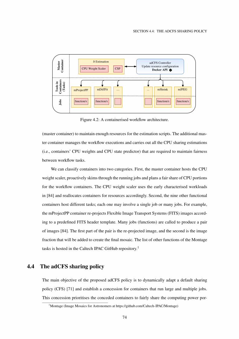
SECTION 4.4: THE ADCFS SHARING POLICY
Figure 4.2: A containerised workflow architecture.
(master container) to maintain enough resources for the estimation scripts. The additional mas-
ter container manages the workflow executions and carries out all the CPU sharing estimations
(i.e., containers’ CPU weights and CPU state predictor) that are required to maintain fairness
between workflow tasks.
We can classify containers into two categories. First, the master container hosts the CPU
weight scaler, proactively skims through the running jobs and plans a fair share of CPU portions
for the workflow containers. The CPU weight scaler uses the early characterised workloads
in [84] and reallocates containers for resources accordingly. Second, the nine other functional
containers host different tasks; each one may involve a single job or many jobs. For example,
the mProjectPP container re-projects Flexible Image Transport Systems (FITS) images accord-
ing to a predefined FITS header template. Many jobs (functions) are called to produce a pair
of images [84]. The first part of the pair is the re-projected image, and the second is the image
fraction that will be added to create the final mosaic. The list of other functions of the Montage
tasks is hosted in the Caltech IPAC GitHub repository.1
4.4 The adCFS sharing policy
The main objective of the proposed adCFS policy is to dynamically adapt a default sharing
policy (CFS) [71] and establish a concession for containers that run large and multiple jobs.
This concession prioritises the conceded containers to fairly share the computing power por-
1Montage (Image Mosaics for Astronomers at https://github.com/Caltech-IPAC/Montage)
74
SECTION 4.4: THE ADCFS SHARING POLICY
tions. Containers voluntarily concede a part of the CPU to other containers and claim it back
when needed (i.e., when there is a change to the workload). In addition, adCFS enhances the
execution time for large/intensive CPU-bound jobs and collaboratively share the CPU when
experiencing high usage. The characterised metrics of scientific workflows are used to notify
the CPU scheduler of the nature of the running workloads. These metrics are the tasks process-
ing runtime (RT ), task CPU usage (U ) and a number of running tasks (T ) for each task type
(i). This helps us derive the appropriate weight, denoted as δ, to share the computing power
between containers. However, the value RT is highly variable among the same task types.
For example, the characterised scientific workflow workload in [84] has the highest runtime
variation for the mAdd task type, while the mProjectPP task type has low runtime variation;
therefore, for simplicity, the task runtime and the CPU usage means are used as the RT , U
respectively. The adCFS sharing policy comprises the CPU state predictor (CSP) and the con-
tainer’s CPU weight scaler to ensure fair resource sharing.
In the rest of this chapter, the notations in Table 4.1 are used to model the various parts of
adCFS.
4.4.1 CPU State Predictor (CSP)
The CSP module uses a discrete first-order Markov chain model that is machine learning-based
to fit and predict stochastic sequential data. The CSP model digitises the CPU usage into several
states (bins) according to predefined state thresholds. In addition, it creates the transition matrix
(P) by reading the CPU, and associates each state with corresponding transition probabilities.
The transition probabilities between different CPU states are called the transition kernel values.
From the transition kernel values, we can see the probability of transition from a specific CPU
state to various other CPU states in the transition matrix. The transition probability describes
how often a transition may occur from one state to the next possible state/s. The CPU usage
of a host is measured at a discrete time, where each point of the CPU usage u is assigned a
defined Discrete Time Markov Chain (DTMC) state, where u ⊆ R+ = [ 0, 100) (i.e., u has
a positive value). DTMC consists of a set of states S, where a transition from a state Sx to a
state Sy can be described by a matrix P of ergodic DTMC where all the transition probabilities
75
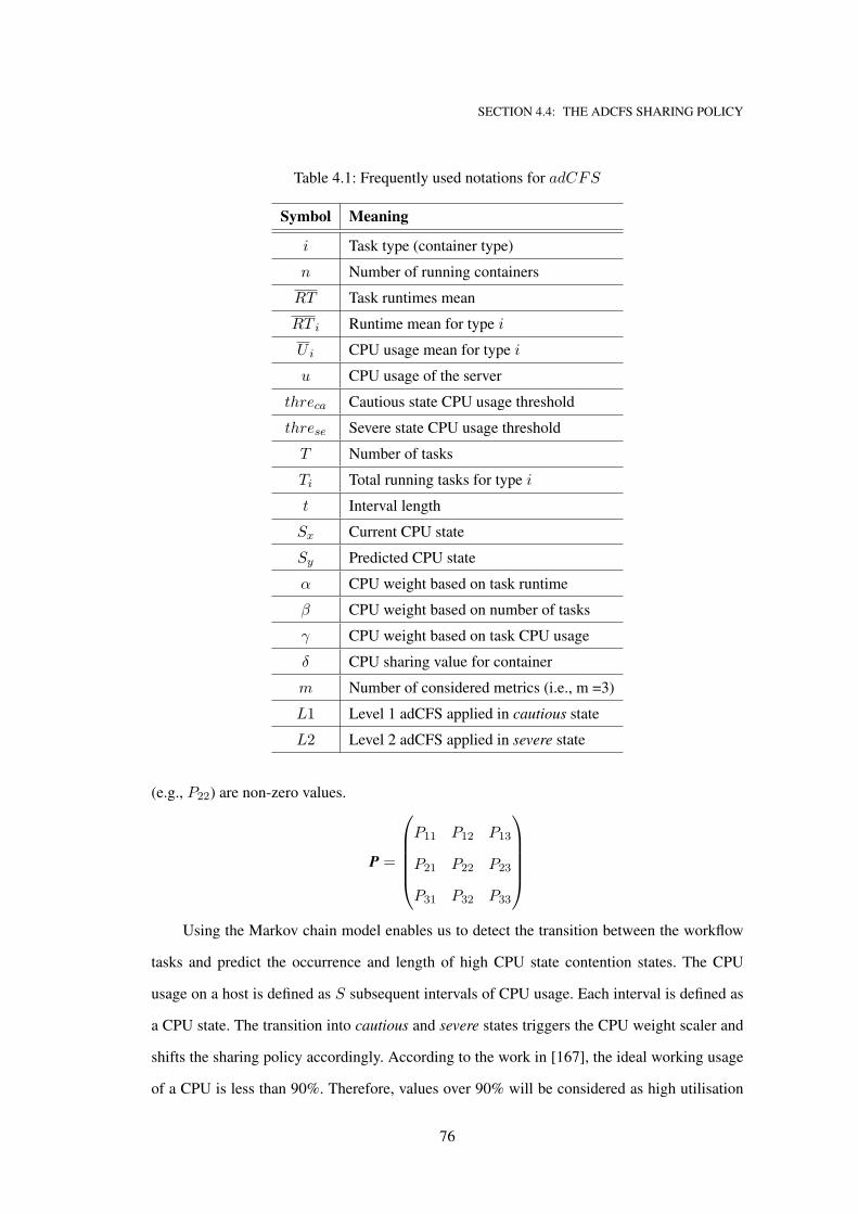
SECTION 4.4: THE ADCFS SHARING POLICY
Table 4.1: Frequently used notations for adCFS
Symbol Meaning
i Task type (container type)
n Number of running containers
RT Task runtimes mean
RT i Runtime mean for type i
U i CPU usage mean for type i
u CPU usage of the server
threca Cautious state CPU usage threshold
threse Severe state CPU usage threshold
T Number of tasks
Ti Total running tasks for type i
t Interval length
Sx Current CPU state
Sy Predicted CPU state
α CPU weight based on task runtime
β CPU weight based on number of tasks
γ CPU weight based on task CPU usage
δ CPU sharing value for container
m Number of considered metrics (i.e., m =3)
L1 Level 1 adCFS applied in cautious state
L2 Level 2 adCFS applied in severe state
(e.g., P22) are non-zero values.
P =
P11 P12 P13
P21 P22 P23
P31 P32 P33
Using the Markov chain model enables us to detect the transition between the workflow
tasks and predict the occurrence and length of high CPU state contention states. The CPU
usage on a host is defined as S subsequent intervals of CPU usage. Each interval is defined as
a CPU state. The transition into cautious and severe states triggers the CPU weight scaler and
shifts the sharing policy accordingly. According to the work in [167], the ideal working usage
of a CPU is less than 90%. Therefore, values over 90% will be considered as high utilisation
76
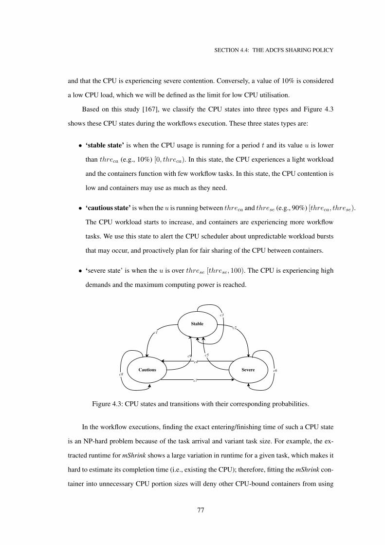
SECTION 4.4: THE ADCFS SHARING POLICY
and that the CPU is experiencing severe contention. Conversely, a value of 10% is considered
a low CPU load, which we will be defined as the limit for low CPU utilisation.
Based on this study [167], we classify the CPU states into three types and Figure 4.3
shows these CPU states during the workflows execution. These three states types are:
• ‘stable state’ is when the CPU usage is running for a period t and its value u is lower
than threca (e.g., 10%) [0, threca). In this state, the CPU experiences a light workload
and the containers function with few workflow tasks. In this state, the CPU contention is
low and containers may use as much as they need.
• ‘cautious state’ is when the u is running between threca and threse (e.g., 90%) [threca, threse).
The CPU workload starts to increase, and containers are experiencing more workflow
tasks. We use this state to alert the CPU scheduler about unpredictable workload bursts
that may occur, and proactively plan for fair sharing of the CPU between containers.
• ‘severe state’ is when the u is over threse [threse, 100). The CPU is experiencing high
demands and the maximum computing power is reached.
Figure 4.3: CPU states and transitions with their corresponding probabilities.
In the workflow executions, finding the exact entering/finishing time of such a CPU state
is an NP-hard problem because of the task arrival and variant task size. For example, the ex-
tracted runtime for mShrink shows a large variation in runtime for a given task, which makes it
hard to estimate its completion time (i.e., existing the CPU); therefore, fitting the mShrink con-
tainer into unnecessary CPU portion sizes will deny other CPU-bound containers from using
77
SECTION 4.4: THE ADCFS SHARING POLICY
the computing resources. adCFS is mainly used for severe states, when aggressive CPU com-
petition occurs between containers. In the severe state, the CPU-bound containers experience
high CPU contention with other non-CPU-bound containers, or with containers that have few
tasks. Thus, differentiating the workload characteristics (i.e., runtime, CPU usage, #tasks) is
crucial to fairly redistributing the CPU resources.
Containerised workflow systems are allocated and hosted in separate containers. Each
container uses part of the CPU capacity and all of its tasks form the host workload (i.e., Mon-
tage workflow processing). By classifying containers, as shown in Figure 4.2, the workload of
a container is known in advance, which can contribute to profiling the resource consumption
for each task type.
4.4.2 Container’s CPU weight scaler
The container’s CPU weight scaler monitors the host’s CPU usage u. It predicts the next state
and changes the CPU share policy, where the new state is either stable, cautious, or severe.
In the stable state, the machine is experiencing a low workload and the containers are free to
use as many resources as they can. In the cautious and severe states, the CPU contention is
increasing and the highest contention level might be reached. However, the workload metrics,
namely RT , U , T are not considered when applying CFS in the highest CPU contentions. The
default CPU-sharing policy (CFS) allocates the same proportion of CPU cycles to all running
containers in the host; therefore, it is beneficial to design a policy that reallocates computing
power fairly and divides that power when containers experience high CPU contention. Thus, in
this work, we change the CPU sharing constraint between running containers by considering
the following metrics: 1) the task’s runtime RT i , 2) the number of running tasks in the system
Ti and 3) the task CPU usage U i. These metrics are used to derive the CPU portion weights δ
for each of the working containers in the workflow system. The weighted averages for RT , U
and T are computed as follows:
α =RT i
∑i=ni=1 RTi
(4.1)
γ =U i
∑i=ni=1 U i
(4.2)
78
SECTION 4.4: THE ADCFS SHARING POLICY
β =Ti
∑i=ni=1 Ti
(4.3)
δ =α+ γ + β
m:= α, γ, β = ]0, 1[ ∴
n∑
1
δ = 1 (4.4)
where α, γ and β represent the average weight of the task runtime, the number of tasks
and the task CPU usage respectively. The weight of the allocated portion δ is the average of the
workload metrics (i.e., RT , T and U ) and the total weight of δ must equal one.
The CPU weight scaler shifts the CPU share policy and dynamically allocates the new
CPU portions δ to each container i. We propose two variations of the proposed sharing policy:
soft (L1) and f orce (L2). The former is applied when the CPU is functioning in the cautious
state, while the latter applied in the severe state and forces containers not to exceed the assigned
weight of the CPU cycles.
• soft (L1) imposes the first level of CPU sharing, which does not force the container to
use the assigned weight constantly. In the case of a sudden workload change and the
CPU usage rate going over the threse, the container will not exceed the relevant weight
of the CPU cycles. L1 manipulates the --cpu-shares parameters according to the
estimated value of δ.
• f orce (L2) in L2 CPU sharing, at all times, a container only has access to the CPU
according to its corresponding weights δ. As the predicted CPU contention is high status,
we apply an additional layer that restricts CPU usage for containers. L2 applies the
estimated δ weights to specific containers’ engine parameters (i.e., --cpu-period,
--cpu-quota) to force the CPU access for containers.
Algorithm 4 shows the different steps to trigger adCFS in order to enable fair CPU sharing.
In the stable state, the CPU weight scaler keeps monitoring the CPU usage as the current CPU
usage state is light and containers are free to use as much CPU power as they need. When
the CPU usage is in the cautious state, meaning that there is still CPU capacity remaining
for additional task processing, the CPU weight scaler imposes the first level of CPU sharing
L1. When the CPU usage is in the severe state, the CPU weight scaler applies the second
79
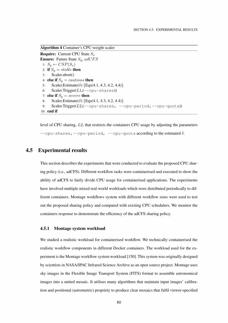
SECTION 4.5: EXPERIMENTAL RESULTS
Algorithm 4 Container’s CPU weight scaler
Require: Current CPU State Sx
Ensure: Future State Sy, adCFS1: Sy ← CSP (Sx)2: if Sy = stable then
3: Scaler.abort()
4: else if Sy = cautious then
5: Scaler.Estimate(δ) {Eqs(4.1, 4.3, 4.2, 4.4)}6: Scaler.Trigger(L1,(--cpu-shares))
7: else if Sy = severe then
8: Scaler.Estimate(δ) {Eqs(4.1, 4.3, 4.2, 4.4)}9: Scaler.Trigger(L2,(--cpu-shares, --cpu-period,--cpu-quota))
10: end if
level of CPU sharing, L2, that restricts the containers CPU usage by adjusting the parameters
--cpu-shares,--cpu-period, --cpu-quota according to the estimated δ.
4.5 Experimental results
This section describes the experiments that were conducted to evaluate the proposed CPU shar-
ing policy (i.e., adCFS). Different workflow tasks were containerised and executed to show the
ability of adCFS to fairly divide CPU usage for containerised applications. The experiments
have involved multiple mixed real-world workloads which were distributed periodically to dif-
ferent containers. Montage workflows system with different workflow sizes were used to test
out the proposed sharing policy and compared with existing CPU schedulers. We monitor the
containers response to demonstrate the efficiency of the adCFS sharing policy.
4.5.1 Montage system workload
We studied a realistic workload for containerised workflow. We technically containerised the
realistic workflow components in different Docker containers. The workload used for the ex-
periment is the Montage workflow system workload [150]. This system was originally designed
by scientists in NASA/IPAC Infrared Science Archive as an open source project. Montage uses
sky images in the Flexible Image Transport System (FITS) format to assemble astronomical
images into a united mosaic. It utilises many algorithms that maintain input images’ calibra-
tion and positional (astrometric) propriety to produce clear mosaics that fulfil viewer-specified
80
SECTION 4.5: EXPERIMENTAL RESULTS
projection, co-ordinates, and spatial scale parameters. There are four basic steps to produce the
image mosaic in Montage system:
• The geometry of the output image on the sky is calculated using the input FITS key-
words, such as the centre of the image.
• Reproject input images to have the same spatial scale, co-ordinate system, world co-
ordinate system projection, and image rotation.
• Correct the background radiation to achieve common flux scales and background levels
across the mosaics.
• The corrected images are joined to form the output mosaic.
The Montage system has been built, tested and the output displayed across many different
computing platforms such as Unix platforms, including Linux, Solaris, Mac OSX, and IBM
AIX [150]. It is highly scalable to run a large set of mosaic sizes. The size of a Montage work-
flow relies on the number of inputs used to create the final sky mosaic. The workflow structure
also varies in order to adapt to the changes in the number of inputs. Figure 4.4 shows the basic
levels in a Montage workflow structure. Montage has different tasks which are structured in
several levels (i.e., vertices) as depicted in Figure 4.4. These vertices represent computational
tasks that are linked with other vertices via edges. These edges represent the data dependencies
between vertices.
mProjectPP:
The first task in the workflow is mProjectPP and it is located at the top of the workflow, this
primarily scales the astronomical images according to defined measurements in the Flexible
Image Transport System (FITS) header template. It is the first task to be executed in the work-
flow and there is one mProjectPP task for each input image. Hence, the number of the mPro-
jectPP tasks is variable that depends on the captured degree size of the two micron all sky
survey (2MASS). The input images are centred in specific co-ordinates or an object name;
mProjectPP performs a plane-to-plane transformation on the FITS images allowing them to
81
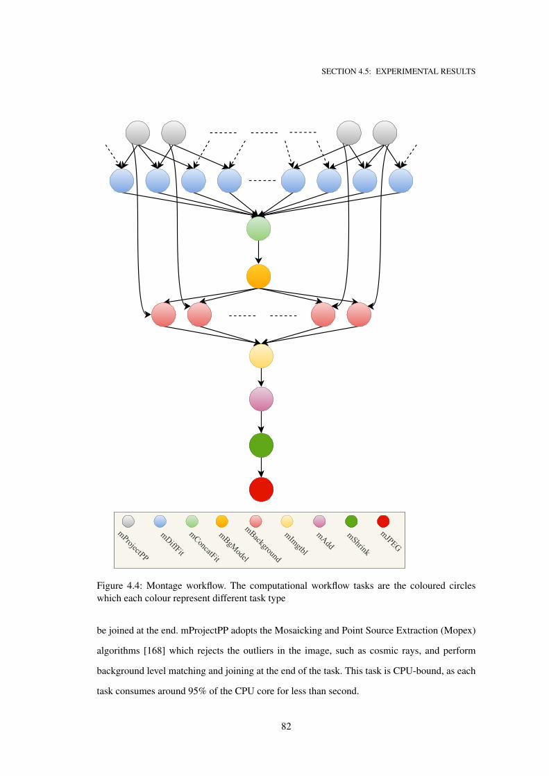
SECTION 4.5: EXPERIMENTAL RESULTS
mProjectPP
mDiffFit
mConcatFit
mBgModel
mBackground
mImgtbl
mAddmShrink
mJPEG
Figure 4.4: Montage workflow. The computational workflow tasks are the coloured circles
which each colour represent different task type
be joined at the end. mProjectPP adopts the Mosaicking and Point Source Extraction (Mopex)
algorithms [168] which rejects the outliers in the image, such as cosmic rays, and perform
background level matching and joining at the end of the task. This task is CPU-bound, as each
task consumes around 95% of the CPU core for less than second.
82
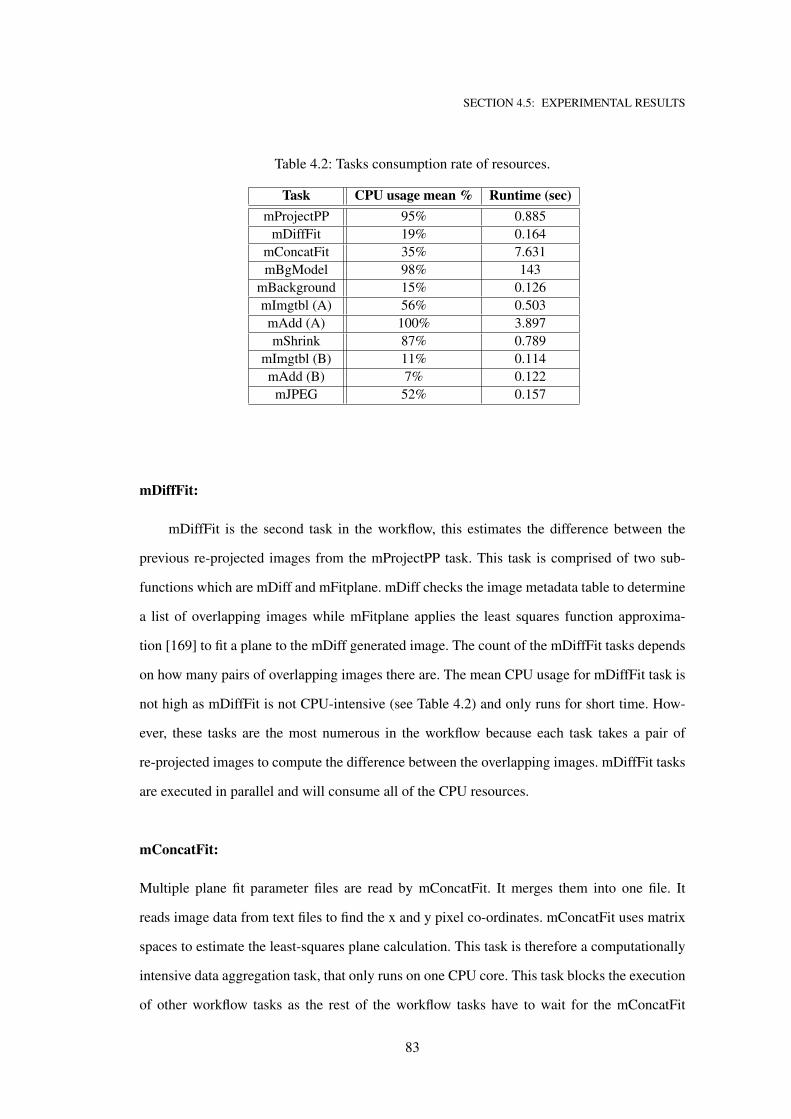
SECTION 4.5: EXPERIMENTAL RESULTS
Table 4.2: Tasks consumption rate of resources.
Task CPU usage mean % Runtime (sec)
mProjectPP 95% 0.885
mDiffFit 19% 0.164
mConcatFit 35% 7.631
mBgModel 98% 143
mBackground 15% 0.126
mImgtbl (A) 56% 0.503
mAdd (A) 100% 3.897
mShrink 87% 0.789
mImgtbl (B) 11% 0.114
mAdd (B) 7% 0.122
mJPEG 52% 0.157
mDiffFit:
mDiffFit is the second task in the workflow, this estimates the difference between the
previous re-projected images from the mProjectPP task. This task is comprised of two sub-
functions which are mDiff and mFitplane. mDiff checks the image metadata table to determine
a list of overlapping images while mFitplane applies the least squares function approxima-
tion [169] to fit a plane to the mDiff generated image. The count of the mDiffFit tasks depends
on how many pairs of overlapping images there are. The mean CPU usage for mDiffFit task is
not high as mDiffFit is not CPU-intensive (see Table 4.2) and only runs for short time. How-
ever, these tasks are the most numerous in the workflow because each task takes a pair of
re-projected images to compute the difference between the overlapping images. mDiffFit tasks
are executed in parallel and will consume all of the CPU resources.
mConcatFit:
Multiple plane fit parameter files are read by mConcatFit. It merges them into one file. It
reads image data from text files to find the x and y pixel co-ordinates. mConcatFit uses matrix
spaces to estimate the least-squares plane calculation. This task is therefore a computationally
intensive data aggregation task, that only runs on one CPU core. This task blocks the execution
of other workflow tasks as the rest of the workflow tasks have to wait for the mConcatFit
83
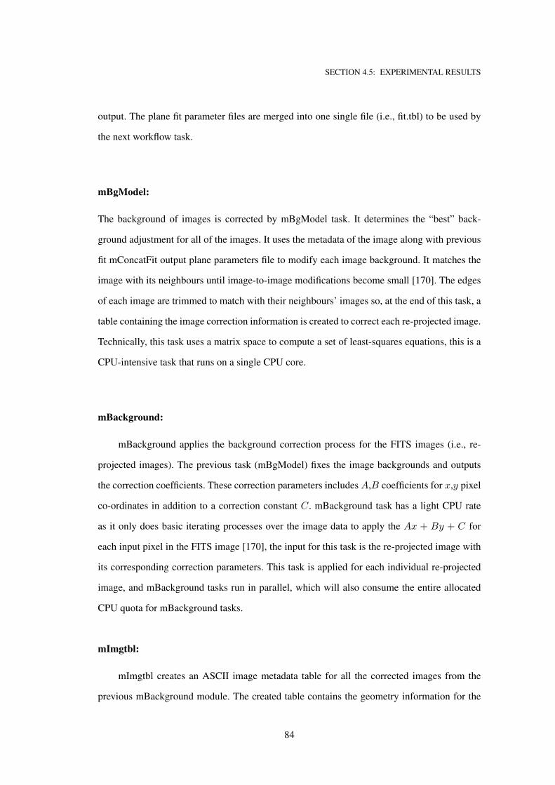
SECTION 4.5: EXPERIMENTAL RESULTS
output. The plane fit parameter files are merged into one single file (i.e., fit.tbl) to be used by
the next workflow task.
mBgModel:
The background of images is corrected by mBgModel task. It determines the “best” back-
ground adjustment for all of the images. It uses the metadata of the image along with previous
fit mConcatFit output plane parameters file to modify each image background. It matches the
image with its neighbours until image-to-image modifications become small [170]. The edges
of each image are trimmed to match with their neighbours’ images so, at the end of this task, a
table containing the image correction information is created to correct each re-projected image.
Technically, this task uses a matrix space to compute a set of least-squares equations, this is a
CPU-intensive task that runs on a single CPU core.
mBackground:
mBackground applies the background correction process for the FITS images (i.e., re-
projected images). The previous task (mBgModel) fixes the image backgrounds and outputs
the correction coefficients. These correction parameters includes A,B coefficients for x,y pixel
co-ordinates in addition to a correction constant C. mBackground task has a light CPU rate
as it only does basic iterating processes over the image data to apply the Ax + By + C for
each input pixel in the FITS image [170], the input for this task is the re-projected image with
its corresponding correction parameters. This task is applied for each individual re-projected
image, and mBackground tasks run in parallel, which will also consume the entire allocated
CPU quota for mBackground tasks.
mImgtbl:
mImgtbl creates an ASCII image metadata table for all the corrected images from the
previous mBackground module. The created table contains the geometry information for the
84
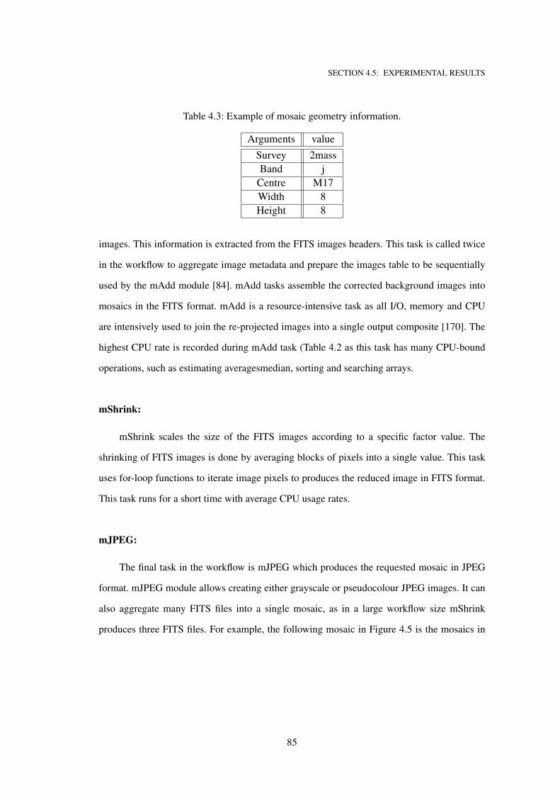
SECTION 4.5: EXPERIMENTAL RESULTS
Table 4.3: Example of mosaic geometry information.
Arguments value
Survey 2mass
Band j
Centre M17
Width 8
Height 8
images. This information is extracted from the FITS images headers. This task is called twice
in the workflow to aggregate image metadata and prepare the images table to be sequentially
used by the mAdd module [84]. mAdd tasks assemble the corrected background images into
mosaics in the FITS format. mAdd is a resource-intensive task as all I/O, memory and CPU
are intensively used to join the re-projected images into a single output composite [170]. The
highest CPU rate is recorded during mAdd task (Table 4.2 as this task has many CPU-bound
operations, such as estimating averagesmedian, sorting and searching arrays.
mShrink:
mShrink scales the size of the FITS images according to a specific factor value. The
shrinking of FITS images is done by averaging blocks of pixels into a single value. This task
uses for-loop functions to iterate image pixels to produces the reduced image in FITS format.
This task runs for a short time with average CPU usage rates.
mJPEG:
The final task in the workflow is mJPEG which produces the requested mosaic in JPEG
format. mJPEG module allows creating either grayscale or pseudocolour JPEG images. It can
also aggregate many FITS files into a single mosaic, as in a large workflow size mShrink
produces three FITS files. For example, the following mosaic in Figure 4.5 is the mosaics in
85
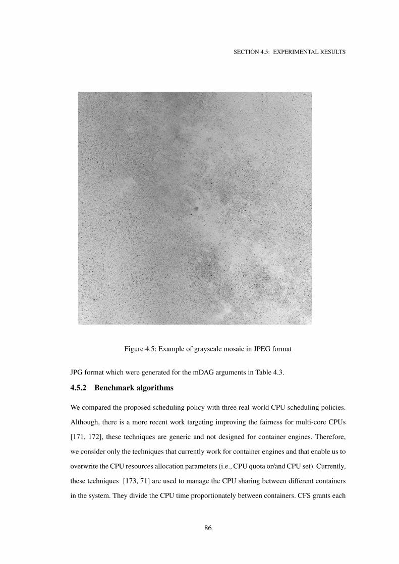
SECTION 4.5: EXPERIMENTAL RESULTS
Figure 4.5: Example of grayscale mosaic in JPEG format
JPG format which were generated for the mDAG arguments in Table 4.3.
4.5.2 Benchmark algorithms
We compared the proposed scheduling policy with three real-world CPU scheduling policies.
Although, there is a more recent work targeting improving the fairness for multi-core CPUs
[171, 172], these techniques are generic and not designed for container engines. Therefore,
we consider only the techniques that currently work for container engines and that enable us to
overwrite the CPU resources allocation parameters (i.e., CPU quota or/and CPU set). Currently,
these techniques [173, 71] are used to manage the CPU sharing between different containers
in the system. They divide the CPU time proportionately between containers. CFS grants each
86
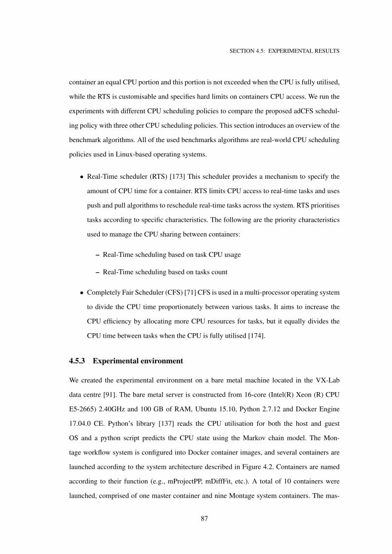
SECTION 4.5: EXPERIMENTAL RESULTS
container an equal CPU portion and this portion is not exceeded when the CPU is fully utilised,
while the RTS is customisable and specifies hard limits on containers CPU access. We run the
experiments with different CPU scheduling policies to compare the proposed adCFS schedul-
ing policy with three other CPU scheduling policies. This section introduces an overview of the
benchmark algorithms. All of the used benchmarks algorithms are real-world CPU scheduling
policies used in Linux-based operating systems.
• Real-Time scheduler (RTS) [173] This scheduler provides a mechanism to specify the
amount of CPU time for a container. RTS limits CPU access to real-time tasks and uses
push and pull algorithms to reschedule real-time tasks across the system. RTS prioritises
tasks according to specific characteristics. The following are the priority characteristics
used to manage the CPU sharing between containers:
– Real-Time scheduling based on task CPU usage
– Real-Time scheduling based on tasks count
• Completely Fair Scheduler (CFS) [71] CFS is used in a multi-processor operating system
to divide the CPU time proportionately between various tasks. It aims to increase the
CPU efficiency by allocating more CPU resources for tasks, but it equally divides the
CPU time between tasks when the CPU is fully utilised [174].
4.5.3 Experimental environment
We created the experimental environment on a bare metal machine located in the VX-Lab
data centre [91]. The bare metal server is constructed from 16-core (Intel(R) Xeon (R) CPU
E5-2665) 2.40GHz and 100 GB of RAM, Ubuntu 15.10, Python 2.7.12 and Docker Engine
17.04.0 CE. Python’s library [137] reads the CPU utilisation for both the host and guest
OS and a python script predicts the CPU state using the Markov chain model. The Mon-
tage workflow system is configured into Docker container images, and several containers are
launched according to the system architecture described in Figure 4.2. Containers are named
according to their function (e.g., mProjectPP, mDiffFit, etc.). A total of 10 containers were
launched, comprised of one master container and nine Montage system containers. The mas-
87
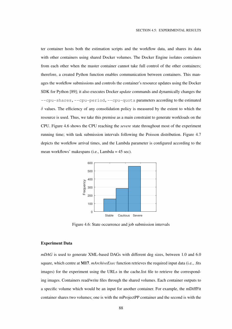
SECTION 4.5: EXPERIMENTAL RESULTS
ter container hosts both the estimation scripts and the workflow data, and shares its data
with other containers using shared Docker volumes. The Docker Engine isolates containers
from each other when the master container cannot take full control of the other containers;
therefore, a created Python function enables communication between containers. This man-
ages the workflow submissions and controls the container’s resource updates using the Docker
SDK for Python [89]; it also executes Docker update commands and dynamically changes the
--cpu-shares,--cpu-period,--cpu-quota parameters according to the estimated
δ values. The efficiency of any consolidation policy is measured by the extent to which the
resource is used. Thus, we take this premise as a main constraint to generate workloads on the
CPU. Figure 4.6 shows the CPU reaching the severe state throughout most of the experiment
running time; with task submission intervals following the Poisson distribution. Figure 4.7
depicts the workflow arrival times, and the Lambda parameter is configured according to the
mean workflows’ makespans (i.e., Lambda = 45 sec).
Stable Cautious Severe
CPU State
0
100
200
300
400
500
600
Fre
qu
en
cy
Figure 4.6: State occurrence and job submission intervals
Experiment Data
mDAG is used to generate XML-based DAGs with different deg sizes, between 1.0 and 6.0
square, which centre at M17. mArchiveExec function retrieves the required input data (i.e., .fits
images) for the experiment using the URLs in the cache.list file to retrieve the correspond-
ing images. Containers read/write files through the shared volumes. Each container outputs to
a specific volume which would be an input for another container. For example, the mDiffFit
container shares two volumes; one is with the mProjectPP container and the second is with the
88
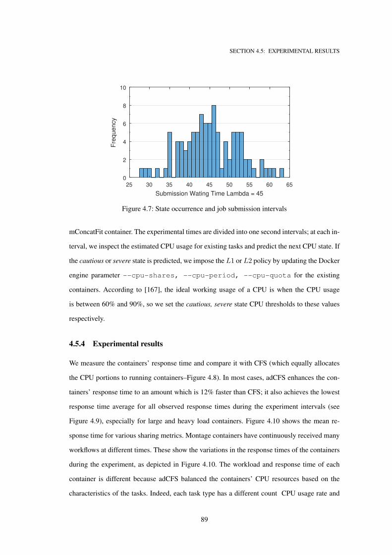
SECTION 4.5: EXPERIMENTAL RESULTS
25 30 35 40 45 50 55 60 65
Submission Wating Time Lambda = 45
(b)
0
2
4
6
8
10
Fre
quency
Figure 4.7: State occurrence and job submission intervals
mConcatFit container. The experimental times are divided into one second intervals; at each in-
terval, we inspect the estimated CPU usage for existing tasks and predict the next CPU state. If
the cautious or severe state is predicted, we impose the L1 or L2 policy by updating the Docker
engine parameter --cpu-shares, --cpu-period, --cpu-quota for the existing
containers. According to [167], the ideal working usage of a CPU is when the CPU usage
is between 60% and 90%, so we set the cautious, severe state CPU thresholds to these values
respectively.
4.5.4 Experimental results
We measure the containers’ response time and compare it with CFS (which equally allocates
the CPU portions to running containers–Figure 4.8). In most cases, adCFS enhances the con-
tainers’ response time to an amount which is 12% faster than CFS; it also achieves the lowest
response time average for all observed response times during the experiment intervals (see
Figure 4.9), especially for large and heavy load containers. Figure 4.10 shows the mean re-
sponse time for various sharing metrics. Montage containers have continuously received many
workflows at different times. These show the variations in the response times of the containers
during the experiment, as depicted in Figure 4.10. The workload and response time of each
container is different because adCFS balanced the containers’ CPU resources based on the
characteristics of the tasks. Indeed, each task type has a different count CPU usage rate and
89
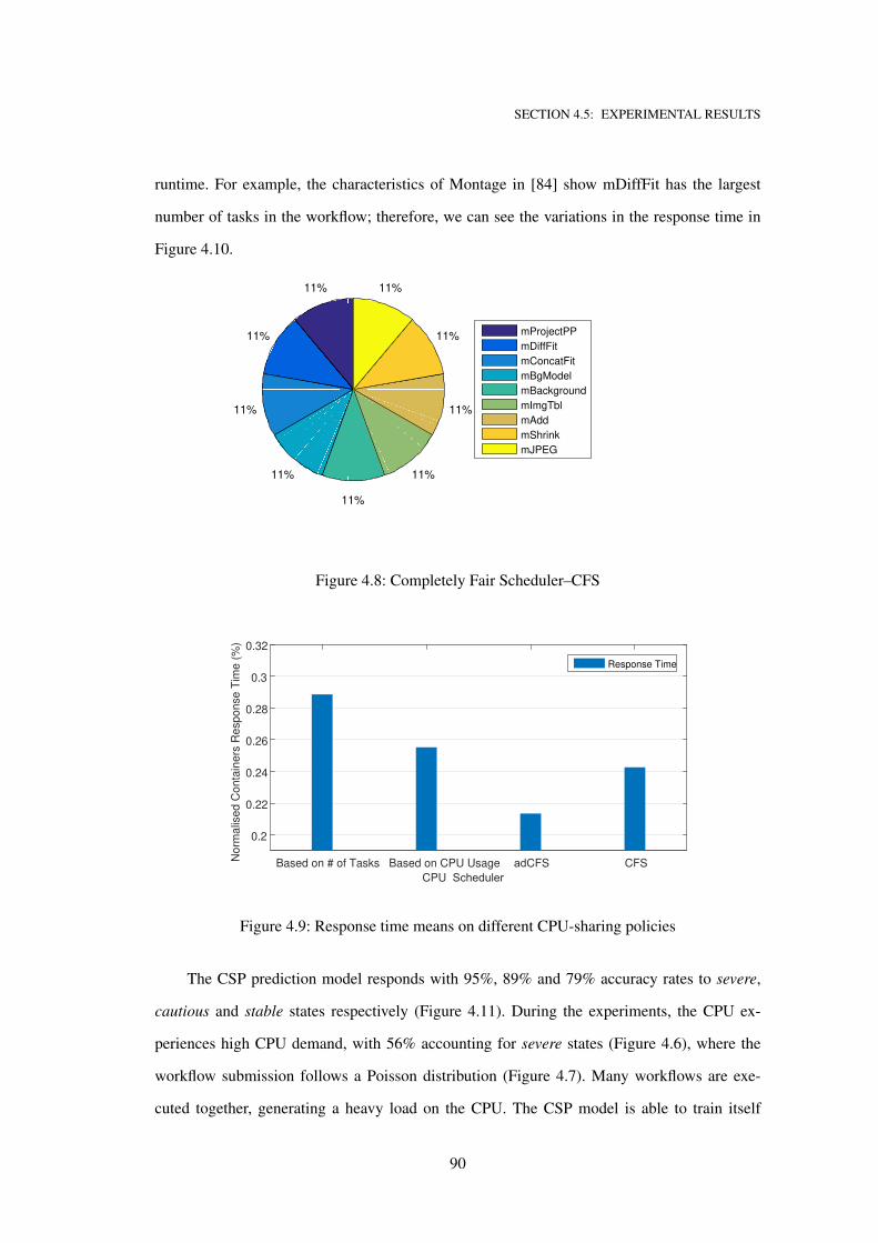
SECTION 4.5: EXPERIMENTAL RESULTS
runtime. For example, the characteristics of Montage in [84] show mDiffFit has the largest
number of tasks in the workflow; therefore, we can see the variations in the response time in
Figure 4.10.
11%
11%
11%
11%
11%
11%
11%
11%
11%
mProjectPP
mDiffFit
mConcatFit
mBgModel
mBackground
mImgTbl
mAdd
mShrink
mJPEG
Figure 4.8: Completely Fair Scheduler–CFS
Based on # of Tasks Based on CPU Usage adCFS CFS
CPU Scheduler
0.2
0.22
0.24
0.26
0.28
0.3
0.32
No
rma
lise
d C
on
tain
ers
Re
sp
on
se
Tim
e (
%)
Response Time
Figure 4.9: Response time means on different CPU-sharing policies
The CSP prediction model responds with 95%, 89% and 79% accuracy rates to severe,
cautious and stable states respectively (Figure 4.11). During the experiments, the CPU ex-
periences high CPU demand, with 56% accounting for severe states (Figure 4.6), where the
workflow submission follows a Poisson distribution (Figure 4.7). Many workflows are exe-
cuted together, generating a heavy load on the CPU. The CSP model is able to train itself
90
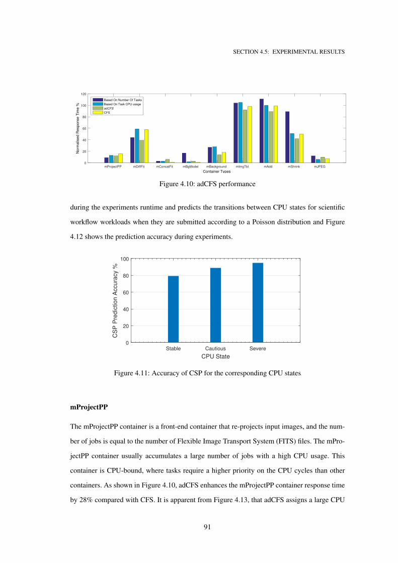
SECTION 4.5: EXPERIMENTAL RESULTS
mProjectPP mDiffFit mConcatFit mBgModel mBackground mImgTbl mAdd mShrink mJPEG
Container Types
0
20
40
60
80
100
120
Norm
alis
ed R
esponse T
ime %
Based On Number Of Tasks Based On Task CPU usage adCFS
CFS
Figure 4.10: adCFS performance
during the experiments runtime and predicts the transitions between CPU states for scientific
workflow workloads when they are submitted according to a Poisson distribution and Figure
4.12 shows the prediction accuracy during experiments.
Stable Cautious Severe
CPU State
0
20
40
60
80
100
CS
P P
redic
tion A
ccura
cy %
Figure 4.11: Accuracy of CSP for the corresponding CPU states
mProjectPP
The mProjectPP container is a front-end container that re-projects input images, and the num-
ber of jobs is equal to the number of Flexible Image Transport System (FITS) files. The mPro-
jectPP container usually accumulates a large number of jobs with a high CPU usage. This
container is CPU-bound, where tasks require a higher priority on the CPU cycles than other
containers. As shown in Figure 4.10, adCFS enhances the mProjectPP container response time
by 28% compared with CFS. It is apparent from Figure 4.13, that adCFS assigns a large CPU
91
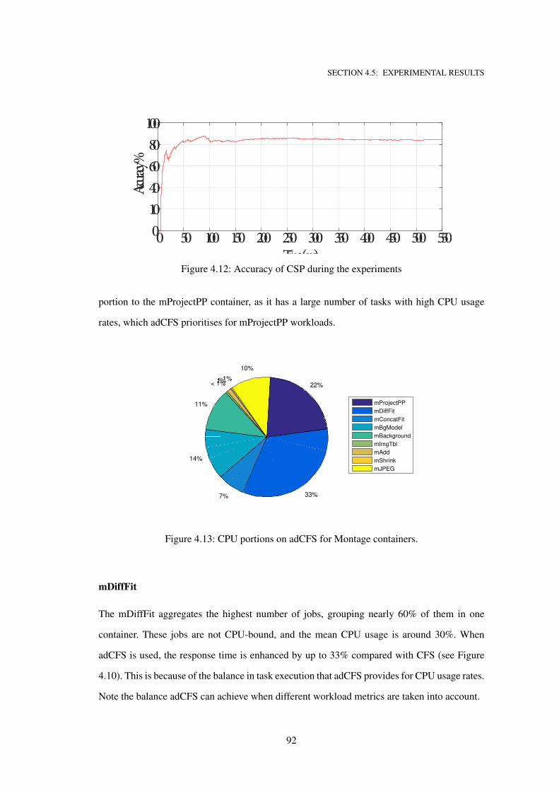
SECTION 4.5: EXPERIMENTAL RESULTS
0 50 100 150 200 250 300 350 400 450 500 550Time (sec)
010406080
100Accu
racy %
Figure 4.12: Accuracy of CSP during the experiments
portion to the mProjectPP container, as it has a large number of tasks with high CPU usage
rates, which adCFS prioritises for mProjectPP workloads.
22%
33%7%
14%
11%
< 1%1%< 1%
10%
mProjectPP
mDiffFit
mConcatFit
mBgModel
mBackground
mImgTbl
mAdd
mShrink
mJPEG
Figure 4.13: CPU portions on adCFS for Montage containers.
mDiffFit
The mDiffFit aggregates the highest number of jobs, grouping nearly 60% of them in one
container. These jobs are not CPU-bound, and the mean CPU usage is around 30%. When
adCFS is used, the response time is enhanced by up to 33% compared with CFS (see Figure
4.10). This is because of the balance in task execution that adCFS provides for CPU usage rates.
Note the balance adCFS can achieve when different workload metrics are taken into account.
92
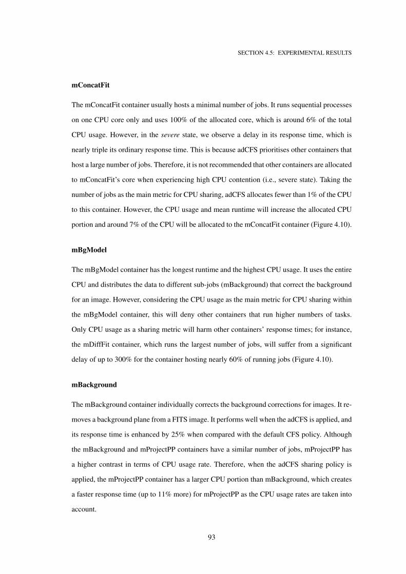
SECTION 4.5: EXPERIMENTAL RESULTS
mConcatFit
The mConcatFit container usually hosts a minimal number of jobs. It runs sequential processes
on one CPU core only and uses 100% of the allocated core, which is around 6% of the total
CPU usage. However, in the severe state, we observe a delay in its response time, which is
nearly triple its ordinary response time. This is because adCFS prioritises other containers that
host a large number of jobs. Therefore, it is not recommended that other containers are allocated
to mConcatFit’s core when experiencing high CPU contention (i.e., severe state). Taking the
number of jobs as the main metric for CPU sharing, adCFS allocates fewer than 1% of the CPU
to this container. However, the CPU usage and mean runtime will increase the allocated CPU
portion and around 7% of the CPU will be allocated to the mConcatFit container (Figure 4.10).
mBgModel
The mBgModel container has the longest runtime and the highest CPU usage. It uses the entire
CPU and distributes the data to different sub-jobs (mBackground) that correct the background
for an image. However, considering the CPU usage as the main metric for CPU sharing within
the mBgModel container, this will deny other containers that run higher numbers of tasks.
Only CPU usage as a sharing metric will harm other containers’ response times; for instance,
the mDiffFit container, which runs the largest number of jobs, will suffer from a significant
delay of up to 300% for the container hosting nearly 60% of running jobs (Figure 4.10).
mBackground
The mBackground container individually corrects the background corrections for images. It re-
moves a background plane from a FITS image. It performs well when the adCFS is applied, and
its response time is enhanced by 25% when compared with the default CFS policy. Although
the mBackground and mProjectPP containers have a similar number of jobs, mProjectPP has
a higher contrast in terms of CPU usage rate. Therefore, when the adCFS sharing policy is
applied, the mProjectPP container has a larger CPU portion than mBackground, which creates
a faster response time (up to 11% more) for mProjectPP as the CPU usage rates are taken into
account.
93
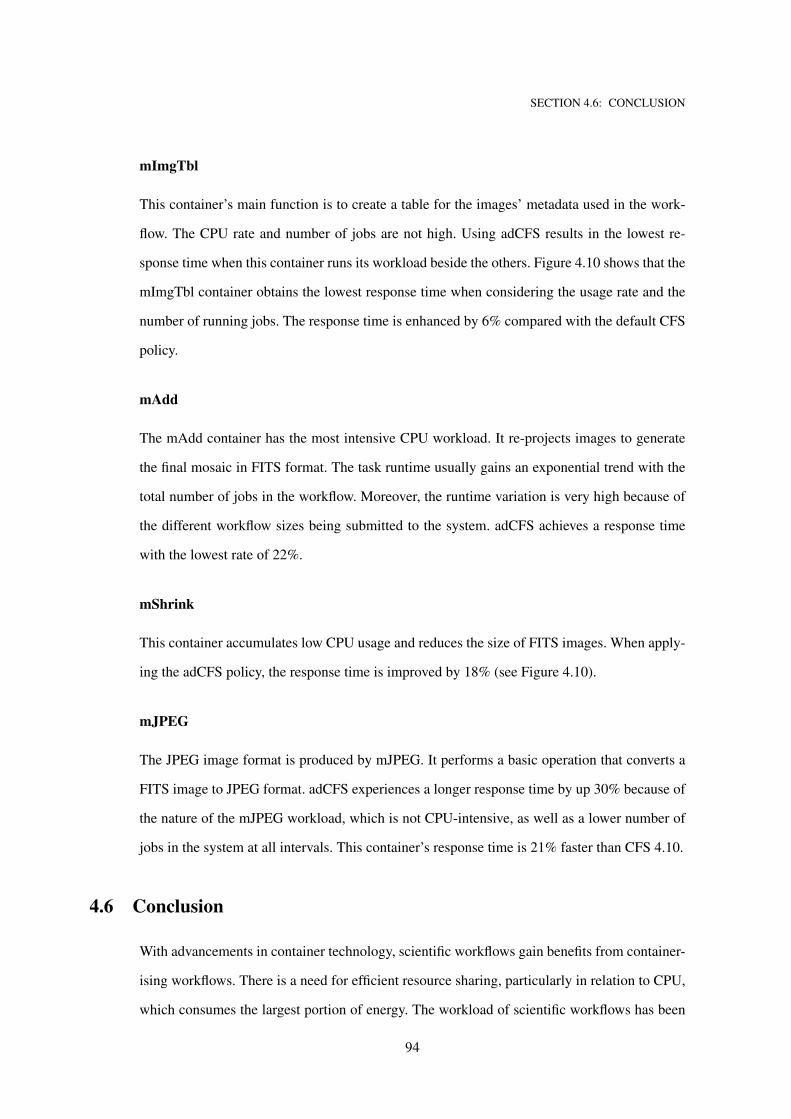
SECTION 4.6: CONCLUSION
mImgTbl
This container’s main function is to create a table for the images’ metadata used in the work-
flow. The CPU rate and number of jobs are not high. Using adCFS results in the lowest re-
sponse time when this container runs its workload beside the others. Figure 4.10 shows that the
mImgTbl container obtains the lowest response time when considering the usage rate and the
number of running jobs. The response time is enhanced by 6% compared with the default CFS
policy.
mAdd
The mAdd container has the most intensive CPU workload. It re-projects images to generate
the final mosaic in FITS format. The task runtime usually gains an exponential trend with the
total number of jobs in the workflow. Moreover, the runtime variation is very high because of
the different workflow sizes being submitted to the system. adCFS achieves a response time
with the lowest rate of 22%.
mShrink
This container accumulates low CPU usage and reduces the size of FITS images. When apply-
ing the adCFS policy, the response time is improved by 18% (see Figure 4.10).
mJPEG
The JPEG image format is produced by mJPEG. It performs a basic operation that converts a
FITS image to JPEG format. adCFS experiences a longer response time by up 30% because of
the nature of the mJPEG workload, which is not CPU-intensive, as well as a lower number of
jobs in the system at all intervals. This container’s response time is 21% faster than CFS 4.10.
4.6 Conclusion
With advancements in container technology, scientific workflows gain benefits from container-
ising workflows. There is a need for efficient resource sharing, particularly in relation to CPU,
which consumes the largest portion of energy. The workload of scientific workflows has been
94
SECTION 4.6: CONCLUSION
precisely characterised, which enables more effective CPU-sharing policies. In this work, we
propose architecture for building a Montage system by using multiple interrelated containers.
The jobs are assigned to containers based on the functionalities of their components. The pro-
posed adCFS fair-sharing policy is developed and applied to different CPU states. A Markov
chain model is used to dynamically derive and assign the appropriate CPU weight for contain-
ers. adCFS is an advance CPU scheduling feature that prioritises containers workloads, and the
main limitation of adCFS is the intolerance of incorrect values CPU portions. Setting incorrect
values for CPU portions would cause severe performance impact on hosted systems, and they
would likely experience instability phases. Experimental results show an enhanced container
response time of 12% compared with the default CFS policy.
95
CHAPTER 5A CPU Interference Detection Approach for
Containerised Scientific Workflow Systems
Container engines often do not consider CPU interferences, which can greatly impact other
neighboring containers’ CPU performance. Existing CPU interference detection methods ei-
ther require access rights to hardware-based metrics (e.g., LLC-miss, cache-miss), which are
usually not accessible in virtualised environments, or software-based metrics (e.g., query re-
sponse time, resource usage), which often suffer from undesirable high latency and low re-
source efficiency. Previously, Chapter 4 addressed the issue of unfair CPU sharing between
containers when the host CPU is fully utilised. A sharing policy called adCFS was introduced,
which considers the future state of CPU usage and proactively shares CPU cycles between var-
ious containers based on their corresponding workload metrics (e.g., CPU usage, task runtime,
#tasks). adCFS estimates the weight of workload characteristics and redistributes the CPU
based on the corresponding weights. The Markov chain model is used to predict CPU state
use, and the adCFS policy is triggered to dynamically allocate containers to the proper CPU
portions. The proposed CPU sharing policy will be used in this chapter to divide CPU resources
fairly between containers. However, containers performance can be further optimised by reduc-
ing CPU interferences that are generated by co-existing applications that share the CPU. This
chapter proposes a novel CPU-based metric called weiMetric which uses the built-in kernel
counters in an OS to detect CPU interference occurring during task execution. Our new metric
96
SECTION 5.0:
offers multiple advantages compared to existing metrics in the literature. First, it requires no
hardware metrics and hence, works for both virtualised and non-virtualised resources. Second,
it requires no extra probes as in a typical software-based method and hence does not incur
additional overheads for CPU resources. On top of that, it can be used by Cloud subscribers
without assistance from Cloud providers. More specifically, a set of weiMetric time series is
created to monitor the CPU contention during task execution. Outliers in the weiMetric time
series are detected when the weiMetric values are not within the confidence intervals. Exten-
sive experiments carried out on realistic containerised workloads showed that our proposed
weiMetric outperforms the state-of-the-art metrics in the literature and can detect CPU inter-
ference with less than 1.03% false positive rate. Note that although we mainly discuss our work
in the context of batch job systems, the proposed method extends in a straightforward way to
online service systems as well.
97
SECTION 5.1: INTRODUCTION
5.1 Introduction
In resource virtualisation, the service provider may overcommit resources in order to maximise
their utilisation and profit [175]. When CPU overcommitment is enabled, resources are shared
between containers/virtual machines in a fair-share manner [71]. Sharing CPU resources in
this way will likely cause interference, which may severely compromise the reliability of the
system and potentially violate Service Level Agreements (SLAs). CPU interference can also
degrade the performance of the whole system when multiple CPU-intensive applications run
simultaneously.
Recently, many scientific workflow systems have been containerised and executed on
Cloud infrastructures [68]. Containers share resources according to specific policies (e.g.,
Complete Fair Scheduling (CFS) [71]); therefore, the system can potentially suffer a denial
of service caused by CPU contention generated by co-located containers (a.k.a. noisy neigh-
bors) [96]. Experimentally, the study in [90] showed that containers can utilise more CPU
resources than originally allocated by the respective cgroup because the current cgroup mecha-
nisms do not count the computational burden of processing network traffic. As a consequence,
this may create CPU interference to co-located containers.
Several approaches [73, 74, 75, 76, 77, 78, 79, 80, 81] have been proposed in the literature
to detect CPU interference, most of which do not work well for containerised scientific work-
flow systems running in virtual machines (VMs). More specifically, the hardware-based ap-
proaches, e.g., [74, 75, 82, 64], often require elevated access to physical resource metrics (e.g.,
LLC-miss, cache-miss), which are usually not available. For instance, Google researchers [75]
proposed a combination of hardware performance metrics (CPU cycles and instructions) to
estimate the deviation of existing jobs. However, this set of metrics requires access to host in-
formation and hence is not accessible to the subscribers of Cloud services. On the other hand,
software-based approaches, e.g., [77, 79, 83, 73, 80, 81], must perform customised software
probes to execute a set of benchmarks to detect resource contention, which accumulates addi-
tional resource overheads. For instance, the probes may require up to 3.2% of the CPU shared
cache [80] as well as increasing the application response time up to 7% [81]. Furthermore, these
benchmarks are often designed to fit specific domains and therefore may not accurately model
98
SECTION 5.1: INTRODUCTION
real workloads of scientific workflow systems. For example, using the task response time as
in [73, 78] is not relevant to the context of scientific workflow because workflow tasks often
have highly deviated response times (its deviation may reach 128% of the mean’s value [84]),
which may lead to high false positive rates.
We propose a novel approach to detect CPU interference specifically designed for the con-
tainerised scientific workflow systems in virtualised environments by introducing a new metric
called weiMetric. weiMetric leverages the CPU-related events monitored by an OS built-in tool
called perf event [176], which is readily available in popular Linux distributions. Perf event
has been developed and used as a powerful tool for performance analysis in Linux since 2009.
However, to the best of our knowledge, we are the first to employ this tool to detect CPU inter-
ference in containerised scientific workflow systems running on virtualised resources. Among
the many events monitored by perf event that are available to cloud subscribers, we observed
that Task-Clock, Switch-Context, and CPU-Migrations are highly correlated to CPU interfer-
ence (see Figure 5.4). Therefore, weiMetric is defined as the weighted average of the standard
deviations of the counters of these three specific events. We first measure weiMetric over the
running time of the containerised application to obtain a weiMetric time series. Next, we em-
ploy the R package tsoutliers [177], which has been known to be effective in finding outliers
with lower false positive rates (FPR), to detect outliers corresponding to CPU interference. Fi-
nally, we check against the actual CPU demand to determine whether the interference is from
an internal or external source.
In the context of containerised scientific workflow systems, our proposed weiMetric has
significant advantages compared to the existing hardware-based and the software-based met-
rics. First, it detects CPU interference without the need to use hardware metrics, which makes it
applicable to both virtualised and non-virtualised resources. Second, our metric doesn’t require
additional customised probes as in software-based methods and hence incurs no extra over-
heads for CPU resources. Moreover, the metric is also available to Cloud subscribers without
assistance from Cloud providers. We have carried out extensive experiments on multiple con-
tainers of the popular workflow system Montage [150] as well as a well-known non-workflow
system Data Caching (memcached) [134]. In both cases, our proposed weiMetric outperforms
the state-of-the-art metrics in the literature and for a certain system configuration, can detect
99
SECTION 5.2: RELATED WORK
CPU interference with less than 1.03% false positive rate.
The chapter is organised as follows. Section 5.2 summarises existing solutions and high-
lights the limitations of the existing metrics when detecting CPU interference in containerised
workflow systems. Section 5.3 provides details of the proposed approach, namely (a) explains
the basic metrics used to define weiMetric, (b) elaborates on how the weiMetric time series
are built, (c) shows how interferences are detected and (d) provides details of our proposed
solution to alleviate interferences. Experimental results are discussed in Section 5.4, and con-
cluding remarks are provided in Section 5.5.
5.2 Related work
Many measurements metrics have been used in the literature to detect CPU interferences
e.g. [178, 75, 179, 78]. They quantitatively measure the selected metrics in relation to the
quality of service (QoS). They are classified into hardware and software-based metrics. The
hardware metrics are concerned with the direct measurement of the hardware registers that
are included with most modern processors. For example, the LLC-load-misses [74], cycle per
instruction (CPI) [75, 180] or instruction per cycle (IPC) [179] are used to monitor CPU per-
formance and observe the deviations that may point out an interference. The software-based
metrics monitor performance of applications on the host resources for partial/whole software
functions. These metrics are mainly used in virtualised environments where the underlying
non-partitioned resources (e.g., last level cache and memory controller) cannot be isolated
without additional hardware.
While much effort has been made to detect and mitigate the interference in virtualised
environments using preconfigured benchmarks, there has been little research into using the
Linux internal probes, such as[181], which are built-in functions initially developed to moni-
tor performance. Related work from the literature on detecting and mitigating interference is
presented here in terms of the following contexts. First, when the workflow system owner has
privileges to access hardware counters (non-virtualised), and, second, when the workflow sys-
tem is hosted on VMs, and the hardware metrics are inaccessible with no access to underlying
resources. Software metrics, designed probes, and benchmarks are used to detect the inter-
100
SECTION 5.2: RELATED WORK
ference in this second context. Both contexts represent the different hosting environments for
scientific workflow systems, which creates the difference in interference detection approaches.
Hardware-based Metrics
Working in a virtualisation environment makes the existing hardware metrics, such as CPI and
LLC-load-misses, inefficient in halting CPU interferences for containers running workflows in-
side VMs. The CPI metric is about the actual CPU cycles and instructions that are carried out
to run application workloads. Using CPI can be useful when running applications directly on
the physical resources (e.g., Google clusters [75]), but this won’t be appropriate when running
applications on VMs. A VM’s CPU cycles technically could be matched with the actual CPU
cycles; however, this would require a large effort in order to match the instructions. This limi-
tation is driven by the inability of the state-of-art profiling tools such as perf event [176] and
PAPI [182] to distinguish the actual application’s instructions running inside a VM. Moreover,
the current performance monitoring tools such as top, htop see VM threads only as anony-
mous processes with variable process IDs (PID). So, interference detection models that use
CPI cannot appropriately work with containerised scientific workflows running in VMs.
The Stay-Away approach [178] uses the dynamic reconfiguration technique to re-provision
resources for batch applications to alleviate the performance interference when co-located, with
best effort applications. This approach requires administrators to know neighbouring VM con-
tent for allocating batch applications with sensitive application VMs. In the context of having
workflows where all tasks have sensitive deadlines, this approach does not work efficiently as
all tasks have the same sensitivity level. Current public cloud business models would not allow
for the reclassification of VMs based on sensitivity as most leased VMs run highly-sensitive
applications, and ensuring SLA satisfaction is crucial to avoid loss of revenue. The cycles per
instruction (CPI2) metric introduced by [75] checks for significant differences in task perfor-
mance. It aggregates data for jobs executed in multiple tasks to detect normal and anomalous
behaviours for these jobs. While this approach shows the symptom of the interference, it still
requires additional analysis models to detect the root cause. CPI2 is preferred as a cloud met-
ric, but for applications inside VMs, it still remains inaccessible to the Cloud subscriber. This
metric can be incorporated with the tsoutliers model to investigate outliers in the CPI2 as it
101
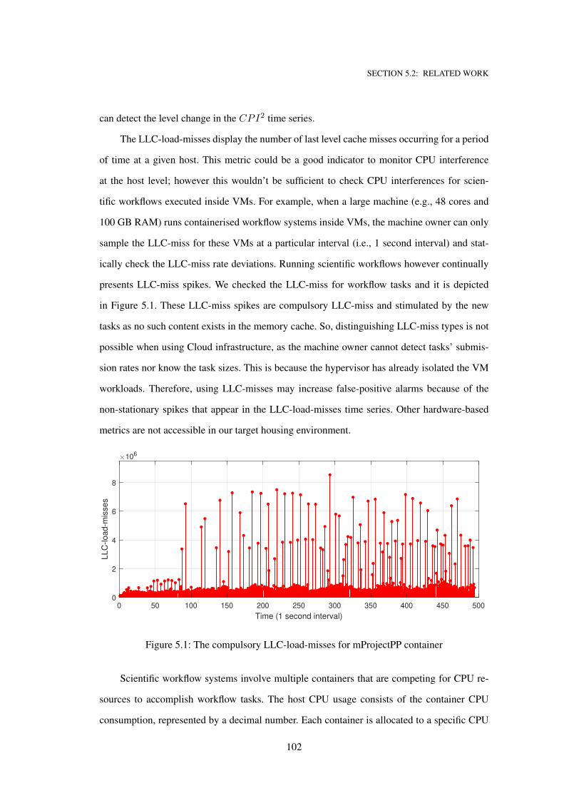
SECTION 5.2: RELATED WORK
can detect the level change in the CPI2 time series.
The LLC-load-misses display the number of last level cache misses occurring for a period
of time at a given host. This metric could be a good indicator to monitor CPU interference
at the host level; however this wouldn’t be sufficient to check CPU interferences for scien-
tific workflows executed inside VMs. For example, when a large machine (e.g., 48 cores and
100 GB RAM) runs containerised workflow systems inside VMs, the machine owner can only
sample the LLC-miss for these VMs at a particular interval (i.e., 1 second interval) and stat-
ically check the LLC-miss rate deviations. Running scientific workflows however continually
presents LLC-miss spikes. We checked the LLC-miss for workflow tasks and it is depicted
in Figure 5.1. These LLC-miss spikes are compulsory LLC-miss and stimulated by the new
tasks as no such content exists in the memory cache. So, distinguishing LLC-miss types is not
possible when using Cloud infrastructure, as the machine owner cannot detect tasks’ submis-
sion rates nor know the task sizes. This is because the hypervisor has already isolated the VM
workloads. Therefore, using LLC-misses may increase false-positive alarms because of the
non-stationary spikes that appear in the LLC-load-misses time series. Other hardware-based
metrics are not accessible in our target housing environment.
0 50 100 150 200 250 300 350 400 450 500
Time (1 second interval)
0
2
4
6
8
LLC
-load-m
isses
106
Figure 5.1: The compulsory LLC-load-misses for mProjectPP container
Scientific workflow systems involve multiple containers that are competing for CPU re-
sources to accomplish workflow tasks. The host CPU usage consists of the container CPU
consumption, represented by a decimal number. Each container is allocated to a specific CPU
102
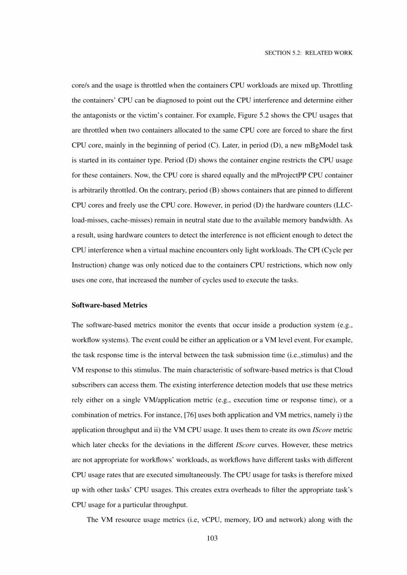
SECTION 5.2: RELATED WORK
core/s and the usage is throttled when the containers CPU workloads are mixed up. Throttling
the containers’ CPU can be diagnosed to point out the CPU interference and determine either
the antagonists or the victim’s container. For example, Figure 5.2 shows the CPU usages that
are throttled when two containers allocated to the same CPU core are forced to share the first
CPU core, mainly in the beginning of period (C). Later, in period (D), a new mBgModel task
is started in its container type. Period (D) shows the container engine restricts the CPU usage
for these containers. Now, the CPU core is shared equally and the mProjectPP CPU container
is arbitrarily throttled. On the contrary, period (B) shows containers that are pinned to different
CPU cores and freely use the CPU core. However, in period (D) the hardware counters (LLC-
load-misses, cache-misses) remain in neutral state due to the available memory bandwidth. As
a result, using hardware counters to detect the interference is not efficient enough to detect the
CPU interference when a virtual machine encounters only light workloads. The CPI (Cycle per
Instruction) change was only noticed due to the containers CPU restrictions, which now only
uses one core, that increased the number of cycles used to execute the tasks.
Software-based Metrics
The software-based metrics monitor the events that occur inside a production system (e.g.,
workflow systems). The event could be either an application or a VM level event. For example,
the task response time is the interval between the task submission time (i.e.,stimulus) and the
VM response to this stimulus. The main characteristic of software-based metrics is that Cloud
subscribers can access them. The existing interference detection models that use these metrics
rely either on a single VM/application metric (e.g., execution time or response time), or a
combination of metrics. For instance, [76] uses both application and VM metrics, namely i) the
application throughput and ii) the VM CPU usage. It uses them to create its own IScore metric
which later checks for the deviations in the different IScore curves. However, these metrics
are not appropriate for workflows’ workloads, as workflows have different tasks with different
CPU usage rates that are executed simultaneously. The CPU usage for tasks is therefore mixed
up with other tasks’ CPU usages. This creates extra overheads to filter the appropriate task’s
CPU usage for a particular throughput.
The VM resource usage metrics (i.e, vCPU, memory, I/O and network) along with the
103
SECTION 5.2: RELATED WORK
0 200 400 1000 1200 1400600 800 Time (Seconds)
0
50
100
Rel
evan
t C
PU
U
sage
%
mProjectPP
mBgModel
5
10
104
LLC-load-misses
0 100 200 300 600 700 800 900
1
2
3
105
cache-misses
0.5
1
1.5CPI
(B)(A) (C)
--cpuset-cpus=0
(D)
mProjectPP (tasks)
400 500
(D)
Figure 5.2: Cache misses, LLC-load-misses and CPI and for mProjectPP container
QoS violations are used in [178]. The approach learns the appropriate VM properties based on
previous QoS violations, and it uses Multi-Dimensional Scaling (MDS) to provision resources
with the hope to mitigate the resource contention effects. Indeed, using QoS won’t allow the
detection of CPU interferences in some cases. This is because, the QoS violations might be
caused by external factors that are not bound to CPU resources shortage or a CPU contention.
The execution and response time metrics were employed to detect the performance in-
terferences. For instance, the execution time is used to detect the contention on the memory
hierarchy. A special software probe is designed to contrast the execution time differences with
the pre-executed run in sandbox environment. The software probe runs continually on top of
the VMs, and when such differences are detected, an alarm is triggered. Such a mechanism
would accumulate practical limitations to design and deploy extra software probes that could
cause interference itself as well as consume additional resources. In a multi-tenant environ-
ment, the response time is employed to detect outlier tasks. Such detection models need an
104
SECTION 5.3: weiMetric AS A SYSTEM DESIGN
awareness model to check whether a certain task has been affected by interference. For exam-
ple, Yasaman et al [183] uses a machine learning-based model to detect the interference. The
proposed model uses a collaborative filtering model to explore whether a task has encountered
interference or not. The proposed approach in [183] does not rely on the hardware performance
counters that enable Cloud subscribers to detect contention. However, the response time is not
accurate enough to detect interferences for workflows systems as this is variable for the same
type of tasks. A workflow’s task response time, which normally margins lower than the mean
might be after the interference, remains within the standard deviations confidence intervals.
Mukerjee et al. [78] uses the designed probe that executes micro-benchmark code. The
deviation in the response time is continuously recorded and compared against the execution
time during an isolated run. The process raises a flag when a deviation is detected. An ex-
tra layer between the VMs and underlying resources is required to be installed, which is not
reachable when hiring resources from the public cloud. Moreover, this approach accumulates
an extra overhead on resources [78]. The weiMetric works in both scenarios (i.e., public and
private clouds) as the metrics are accessible. Also, the weiMetric does not need additional
software as it only uses the workflow tasks to construct the relevant time series. Finally, exist-
ing techniques to detect performance interference in applications are either expensive in terms
of profiling or only applicable from the perspective of the infrastructure owner.
5.3 weiMetric as a System Design
We introduce in this section weiMetric as a CPU interference monitoring metric that works in
both virtualised and non-virtualised environments. In Section 5.3.1, we discuss the three kernel
counters and explain why we use them to create weiMetric. In Section 5.3.2, we formally define
weiMetric as well as the weiMetric time series. We then describe in Section 5.3.3 the interfer-
ence detection process using weiMetric and the corresponding time series. As weiMetric is
sensitive to variations in CPU working conditions, such as contention, we included a queueing-
based CPU demand modeler to determine whether an internal/external noise causes weiMetric
outliers. Lastly, in Section 5.3.4, we discuss a technique to alleviate CPU interference by dy-
namically auto-scaling and isolating the CPU resources for containers, which is done after the
105
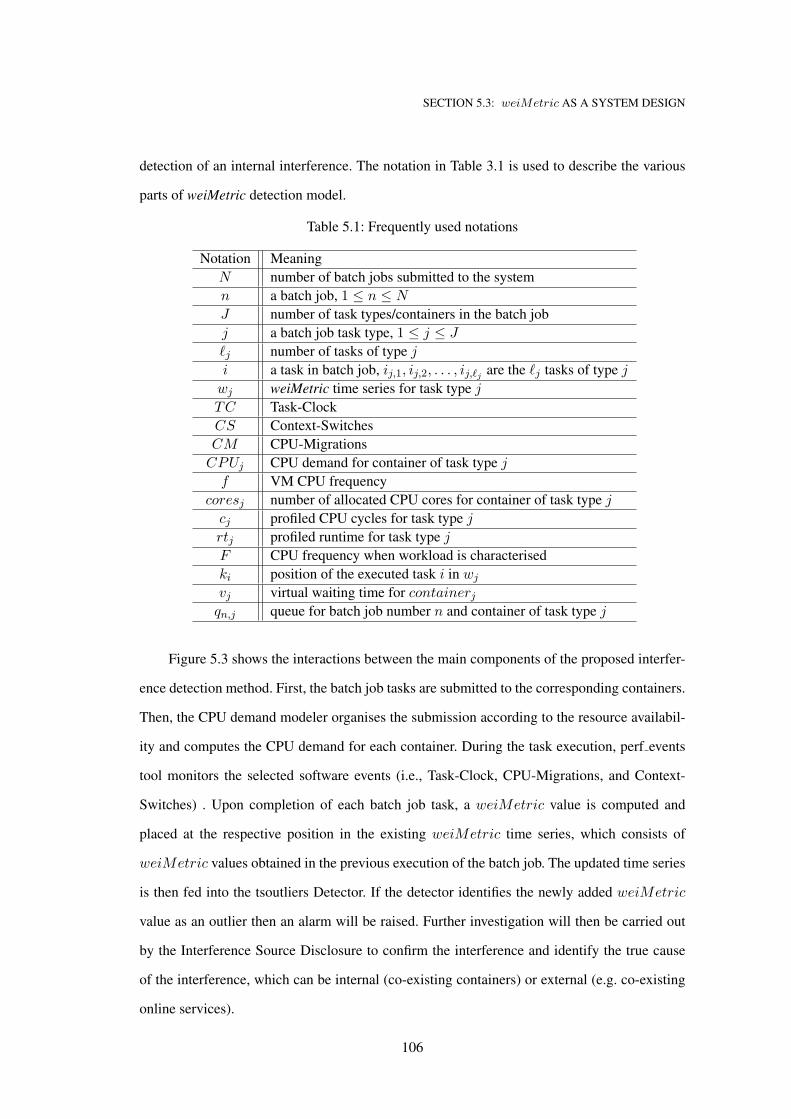
SECTION 5.3: weiMetric AS A SYSTEM DESIGN
detection of an internal interference. The notation in Table 3.1 is used to describe the various
parts of weiMetric detection model.
Table 5.1: Frequently used notations
Notation Meaning
N number of batch jobs submitted to the system
n a batch job, 1 ≤ n ≤ N
J number of task types/containers in the batch job
j a batch job task type, 1 ≤ j ≤ J
ℓj number of tasks of type j
i a task in batch job, ij,1, ij,2, . . . , ij,ℓj are the ℓj tasks of type j
wj weiMetric time series for task type j
TC Task-Clock
CS Context-Switches
CM CPU-Migrations
CPUj CPU demand for container of task type j
f VM CPU frequency
coresj number of allocated CPU cores for container of task type j
cj profiled CPU cycles for task type j
rtj profiled runtime for task type j
F CPU frequency when workload is characterised
ki position of the executed task i in wj
vj virtual waiting time for containerjqn,j queue for batch job number n and container of task type j
Figure 5.3 shows the interactions between the main components of the proposed interfer-
ence detection method. First, the batch job tasks are submitted to the corresponding containers.
Then, the CPU demand modeler organises the submission according to the resource availabil-
ity and computes the CPU demand for each container. During the task execution, perf events
tool monitors the selected software events (i.e., Task-Clock, CPU-Migrations, and Context-
Switches) . Upon completion of each batch job task, a weiMetric value is computed and
placed at the respective position in the existing weiMetric time series, which consists of
weiMetric values obtained in the previous execution of the batch job. The updated time series
is then fed into the tsoutliers Detector. If the detector identifies the newly added weiMetric
value as an outlier then an alarm will be raised. Further investigation will then be carried out
by the Interference Source Disclosure to confirm the interference and identify the true cause
of the interference, which can be internal (co-existing containers) or external (e.g. co-existing
online services).
106
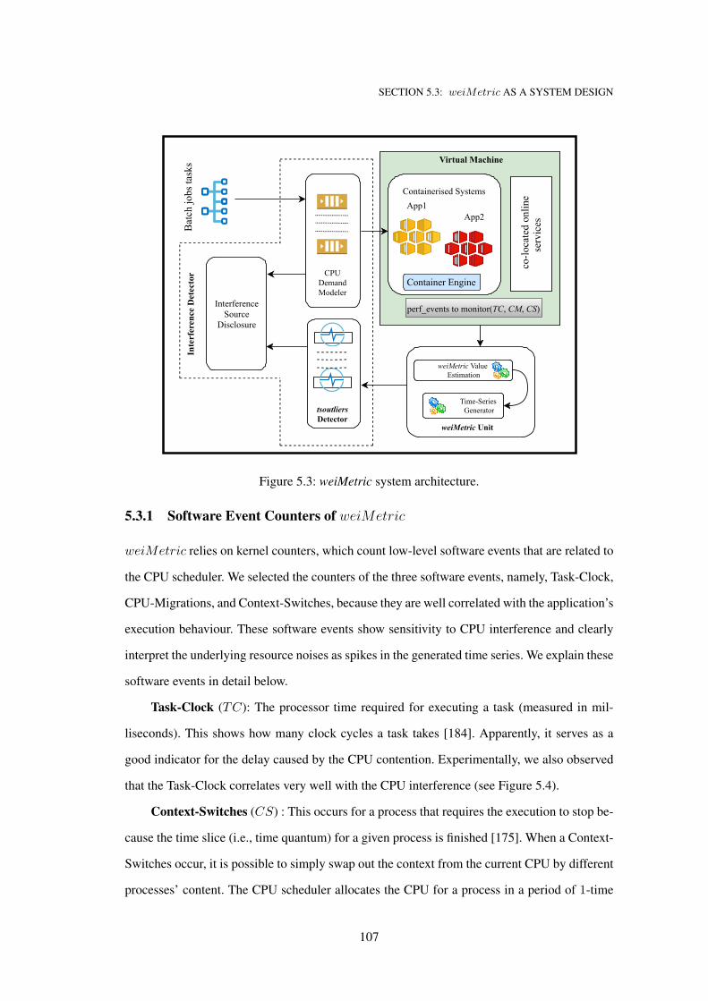
SECTION 5.3: weiMetric AS A SYSTEM DESIGN
InterferenceSource
Disclosure
tsoutliersDetector
CPUDemandModeler
App1
Batchjobstasks
weiMetricValueEstimation
Time-SeriesGenerator
weiMetricUnit
InterferenceDetector
VirtualMachine
ContainerEngine
perf_eventstomonitor(TC,CM,CS)
ContainerisedSystems
App2
co-locatedonline
services
Figure 5.3: weiMetric system architecture.
5.3.1 Software Event Counters of weiMetric
weiMetric relies on kernel counters, which count low-level software events that are related to
the CPU scheduler. We selected the counters of the three software events, namely, Task-Clock,
CPU-Migrations, and Context-Switches, because they are well correlated with the application’s
execution behaviour. These software events show sensitivity to CPU interference and clearly
interpret the underlying resource noises as spikes in the generated time series. We explain these
software events in detail below.
Task-Clock (TC): The processor time required for executing a task (measured in mil-
liseconds). This shows how many clock cycles a task takes [184]. Apparently, it serves as a
good indicator for the delay caused by the CPU contention. Experimentally, we also observed
that the Task-Clock correlates very well with the CPU interference (see Figure 5.4).
Context-Switches (CS) : This occurs for a process that requires the execution to stop be-
cause the time slice (i.e., time quantum) for a given process is finished [175]. When a Context-
Switches occur, it is possible to simply swap out the context from the current CPU by different
processes’ content. The CPU scheduler allocates the CPU for a process in a period of 1-time
107
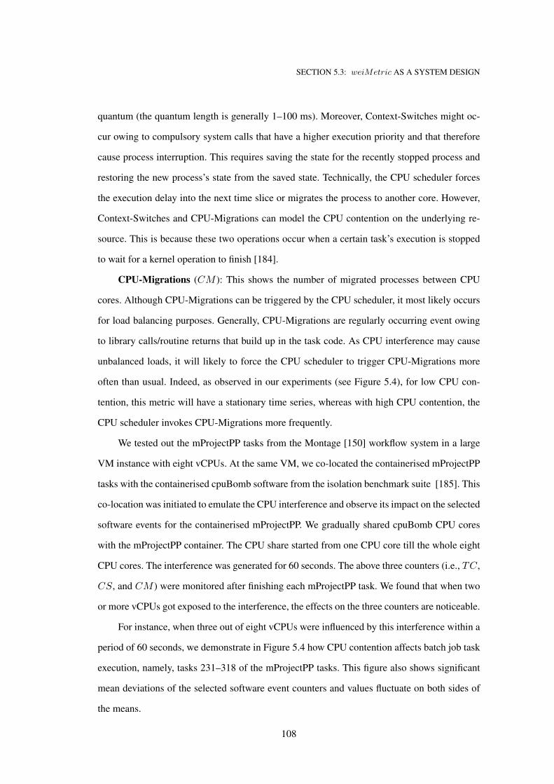
SECTION 5.3: weiMetric AS A SYSTEM DESIGN
quantum (the quantum length is generally 1–100 ms). Moreover, Context-Switches might oc-
cur owing to compulsory system calls that have a higher execution priority and that therefore
cause process interruption. This requires saving the state for the recently stopped process and
restoring the new process’s state from the saved state. Technically, the CPU scheduler forces
the execution delay into the next time slice or migrates the process to another core. However,
Context-Switches and CPU-Migrations can model the CPU contention on the underlying re-
source. This is because these two operations occur when a certain task’s execution is stopped
to wait for a kernel operation to finish [184].
CPU-Migrations (CM ): This shows the number of migrated processes between CPU
cores. Although CPU-Migrations can be triggered by the CPU scheduler, it most likely occurs
for load balancing purposes. Generally, CPU-Migrations are regularly occurring event owing
to library calls/routine returns that build up in the task code. As CPU interference may cause
unbalanced loads, it will likely to force the CPU scheduler to trigger CPU-Migrations more
often than usual. Indeed, as observed in our experiments (see Figure 5.4), for low CPU con-
tention, this metric will have a stationary time series, whereas with high CPU contention, the
CPU scheduler invokes CPU-Migrations more frequently.
We tested out the mProjectPP tasks from the Montage [150] workflow system in a large
VM instance with eight vCPUs. At the same VM, we co-located the containerised mProjectPP
tasks with the containerised cpuBomb software from the isolation benchmark suite [185]. This
co-location was initiated to emulate the CPU interference and observe its impact on the selected
software events for the containerised mProjectPP. We gradually shared cpuBomb CPU cores
with the mProjectPP container. The CPU share started from one CPU core till the whole eight
CPU cores. The interference was generated for 60 seconds. The above three counters (i.e., TC,
CS, and CM ) were monitored after finishing each mProjectPP task. We found that when two
or more vCPUs got exposed to the interference, the effects on the three counters are noticeable.
For instance, when three out of eight vCPUs were influenced by this interference within a
period of 60 seconds, we demonstrate in Figure 5.4 how CPU contention affects batch job task
execution, namely, tasks 231–318 of the mProjectPP tasks. This figure also shows significant
mean deviations of the selected software event counters and values fluctuate on both sides of
the means.
108
SECTION 5.3: weiMetric AS A SYSTEM DESIGN
50 100 150 200 250 300 350 4006000
8000
10000
12000task-clock
50 100 150 200 250 300 350 4001000
2000
3000
4000 context-switches
50 100 150 250 300 350 40050
100
150CPU migrations
200
Figure 5.4: Reaction of the software event counters to interference. The x-axis represents mPro-
jectPP task indices and the y-axis represents the event counters (Task-Clock, Context-Switches,
and CPU-Migrations) during the execution of mProjectPP tasks. The container CPU resource
was artificially exposed to CPU-bound workload (i.e., cpuBomb workload) within tasks 231–
318 of the mProjectPP tasks and the counters demonstrated outliers (spikes) accordingly.
The above software event counters are used to obtain a weiMetric value to properly
model the behaviour of CPU resources. This new metric is suitable for batch job tasks, where
the order of these tasks form time-series data that model the task execution data. Technically,
tasks are executed in subsequent steps in which part of the batch job tasks are executed in
parallel. Therefore, an execution occurs over time and creates a time series that shows what is
occurring within the CPU.
5.3.2 weiMetric Construction Unit
A weiMetric construction unit transforms the software event counters to the time series do-
main. This enables us to study the abnormal behaviour of CPU resources from a fine-grained
perspective. We assume that there are N batch jobs, and every batch job n ∈ {1, 2, . . . , N}
has J task types. We create a single container, denoted containerj , for each task type j. More-
over, each task type j ∈ {1, 2, . . . , J} has ℓj tasks ij,1, ij,2, . . . , ij,ℓj . For each task type j in the
batch job, we construct a separate sequence of weiMetric time series data, which are denoted
109
SECTION 5.3: weiMetric AS A SYSTEM DESIGN
as
wj = {weiMetricij,1 , . . . , weiMetricij,ℓj }.
Note that weiMetricij,1 refers to the weiMetric value of the first task of type j, and so forth.
In what follows, we will show how to generate the corresponding weiMetric value that
represents the behaviour of CPU resources during task execution. Mathematically speaking,
the weighted averages’ standard deviations for the three selected software event counters (i.e.,
TC, CS, and CM ) are used to estimate the corresponding weiMetric value. Then, the corre-
sponding time series is generated to check for outliers that might indicate CPU interference.
weiMetric Value Estimation
The data scales of the selected counters, namely, TC, CS, and CM , are different. Therefore,
we need to normalise the values so that they have the same scale. For this purpose, the weighted
average of the standard deviation is estimated for each value of the three selected software event
counter. The standard deviation is used to show the mean deviations for TC, CS, and CM .
The deviations indicate the instability in the CPU short-term scheduler which fires process
interruptions and switches the context. Experimentally, the execution data shows stationary
behaviour when the container has nothing interferes (see Figure 5.4 tasks 1–230). Therefore,
most of the execution data will be close to the mean with slight deviations.
The server could run several batch jobs n = 1, 2, . . . , N , where each batch job has J
task types and each task type j = 1, 2, . . . , J has ℓj tasks. Let TCn,j,i denote the Task-Clock
value for the task i of type j in batch job n. For a given type j and a given task i of type j,
let σ({TCj,i}) denote the standard deviation of TCn,j,i across N batch jobs. Similar notations
can be defined for the Context-Switches and CPU-Migrations counters. More specifically, we
have
σ({TCj,i}) =
√
√
√
√
1
N
N∑
n=1
(
TCn,j,i −
∑Nn=1 TCn,j,i
N
)2,
σ({CSj,i}) =
√
√
√
√
1
N
N∑
n=1
(
CSn,j,i −
∑Nn=1CSn,j,i
N
)2,
σ({CMj,i}) =
√
√
√
√
1
N
N∑
n=1
(
CMn,j,i −
∑Nn=1CMn,j,i
N
)2
.
110
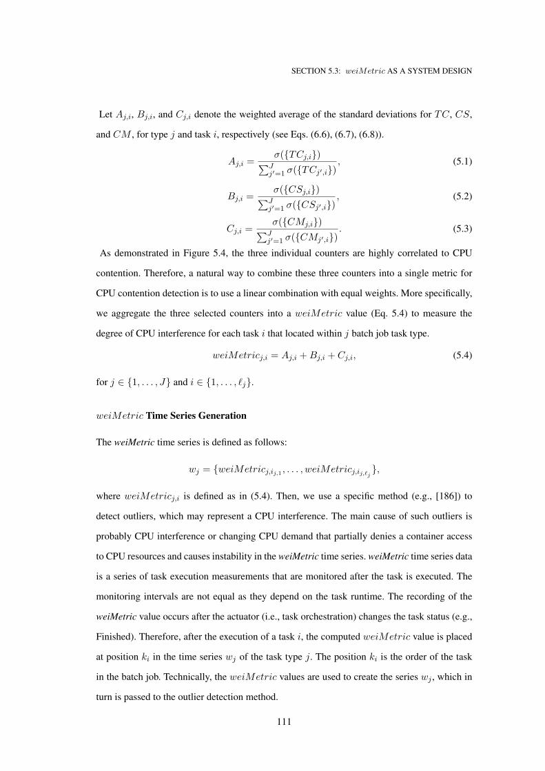
SECTION 5.3: weiMetric AS A SYSTEM DESIGN
Let Aj,i, Bj,i, and Cj,i denote the weighted average of the standard deviations for TC, CS,
and CM , for type j and task i, respectively (see Eqs. (6.6), (6.7), (6.8)).
Aj,i =σ({TCj,i})
∑Jj′=1 σ({TCj′,i})
, (5.1)
Bj,i =σ({CSj,i})
∑Jj′=1 σ({CSj′,i})
, (5.2)
Cj,i =σ({CMj,i})
∑Jj′=1 σ({CMj′,i})
. (5.3)
As demonstrated in Figure 5.4, the three individual counters are highly correlated to CPU
contention. Therefore, a natural way to combine these three counters into a single metric for
CPU contention detection is to use a linear combination with equal weights. More specifically,
we aggregate the three selected counters into a weiMetric value (Eq. 5.4) to measure the
degree of CPU interference for each task i that located within j batch job task type.
weiMetricj,i = Aj,i +Bj,i + Cj,i, (5.4)
for j ∈ {1, . . . , J} and i ∈ {1, . . . , ℓj}.
weiMetric Time Series Generation
The weiMetric time series is defined as follows:
wj = {weiMetricj,ij,1 , . . . , weiMetricj,ij,ℓj },
where weiMetricj,i is defined as in (5.4). Then, we use a specific method (e.g., [186]) to
detect outliers, which may represent a CPU interference. The main cause of such outliers is
probably CPU interference or changing CPU demand that partially denies a container access
to CPU resources and causes instability in the weiMetric time series. weiMetric time series data
is a series of task execution measurements that are monitored after the task is executed. The
monitoring intervals are not equal as they depend on the task runtime. The recording of the
weiMetric value occurs after the actuator (i.e., task orchestration) changes the task status (e.g.,
Finished). Therefore, after the execution of a task i, the computed weiMetric value is placed
at position ki in the time series wj of the task type j. The position ki is the order of the task
in the batch job. Technically, the weiMetric values are used to create the series wj , which in
turn is passed to the outlier detection method.
111
SECTION 5.3: weiMetric AS A SYSTEM DESIGN
5.3.3 Interference Detector
Our proposed CPU interference detector has two components: the outlier detection component
and the CPU demand modeler, the latter refines the output from the former.
The outlier detection component checks for outliers in the newly created time series wj :
wj appears to have stationary data when CPU resources encounter stable contention, whereas
outliers appear under high contention. For this end, the R package tsoutliers is used to detect
outliers in the task execution data. This model was originally introduced in [186] and recently
implemented in R [177]. This package detects values that are very different from the majority
of those in a time series. These anomaly values point out are potential data acquired from
an interference caused by usual behaviour that appears in the weiMetric series. The detected
anomalies in the CPU behaviour might be due to the actual CPU interference or the change
in CPU demands that causes the unstability in the weiMetric series. That is why we need to
employ the CPU demand modeler to confirm if the outliers signifies an actual CPU interference
and moreover, to disclose the source of the interference in the case of a true interference.
weiMetric Time Series Outlier Detection
The tsoutliers model examines the weiMetric values to identify outliers. Interference in the
CPU resources creates deviations in the batch job tasks’ time series (i.e., weiMetric time se-
ries). Therefore, the constructed time series of the weiMetric values describes the CPU con-
ditions during task execution. The primary function for tsoutliers is to check the significance
of the different outlier types for all time series values. The basic functions of the tsoutliers
package are as follows:
1. Locating outliers in the time series by fitting the time series using the auto.arima
function that is included in the forecast package . This process yields a new time
series called adjusted time series. The residuals of the adjusted time series are used to
examine τ -statistics for all potential outliers.
2. Remove insignificant outliers.
3. Repeat steps 1 and 2 until the minimal residuals are acquired.
112
SECTION 5.3: weiMetric AS A SYSTEM DESIGN
The tsoutliers model examines the weiMetric values to discover outliers. Interference in
the CPU resources creates significant residuals in the batch job tasks’ time series, as shown
in Figure 5.4. The constructed time series of weiMetric values describes the CPU conditions
during task executions.
The primary function of tsoutliers is to predict the original weiMetric values using well-
known time series models, such as ARIMA(p,d,q), to check for abnormal residuals in the
time series. ARIMA(p,d,q) predicts the completion of time series data by fitting the data and
acquiring p, d, and q parameters.
The estimated weiMetric value is checked against the actual one in the wj time series.
Predefined t-statistic estimations are used to confirm the outlier type in the time series. How-
ever, we used the tsoutliers model to check the status of the last entered weiMetric observation
considered an outlier. If so, an alert is triggered to take further steps to confirm the interference
by investigating CPU demand.
CPU Demand Model
This section presents a queuing model to compute the CPU demand, which is obviously needed
both to confirm the outlier in the wj time series as well as to identify whether the source of
interference is internal or external. A G/G/1 queuing model [187] is used to express the CPU
demand CPUj . We chose this model to cope with the task arrival and service times as a general
distribution, where each task type is serviced by a single container. Each queue represents the
dependent batch job tasks. The different batch job tasks are not mixed, and each queue relates
to a specific batch job. Many queues are created for each container. The queues are classified
based on the task type (e.g., j). For each batch job n and a task type j, we create a unique
job’s queue that can be expressed as qn,j and the queue follows the First-In-First-Out (FIFO)
queuing principle.
The CPU demand CPUj is expressed in terms of the time length needed to complete
various tasks. It is defined as the amount of queued jobs that placed on hold and waiting for
available resources. Jobs are placed into queues according to the job’s type. For instance, there
are eleven task types in large Montage workflows [84] and hence eleven queues are created
accordingly. This time, denoted as RT j , can be estimated from the task’s runtime, which is
113
SECTION 5.3: weiMetric AS A SYSTEM DESIGN
used to estimate the virtual waiting time vj (Eq. 5.5) for the last task in the queue qn,j that
assigned to container n and job type j. As we have long running tasks in the batch job, we
consider the remaining time for current running tasks rj (Eq. 5.6). The remaining tasks are
estimated by subtracting the task elapsed time ET from the recorded time length to complete
the task RT j . The CPU demand CPUj is estimated by adding the virtual waiting time (vj) to
remaining tasks rj (Eq. 5.7).vj =
w∑
1
qn,j ×RT j (5.5)
rj = RT j − ET (5.6)
CPUj = vj + rj (5.7)
Interference Source Disclosure
The interference source disclosure model is used to check whether the detected outlier is caused
by an internal or external interference stimulator. An increase in CPU demand indicates an
internal interference, whereas an external interference is reflected by the CPU demand having
stationary vj virtual waiting time for containers.
The internal CPU interference caused by the neighbouring containers that have just re-
ceived new tasks and their workload are queued in the CPU ready queue. Therefore, the con-
tainers’ CPU resources are throttled, causing the CPU to rethink the CPU resources for the
containers. In such cases, CPU resource sharing will trigger the CFS [71] to share the CPU
resources (i.e., cores) fairly. For example, when a container shares a CPU core with an idle
container, the active container will use most of the shared core (e.g., 80% of the CPU). How-
ever, once the idle container has a workload and becomes active, the CFS will divide the CPU
core equally between containers. Each container will gain equal access (50% each).
5.3.4 Interference Remedy Planning
After the interference is detected and confirmed as internal (caused by co-located containers),
we reschedule CPU cores among containers to alleviate the impact of interference, using our
approach that proposed in Chapter 4. We discuss this approach in detail below, considering the
different cases of low and high CPU contention.
114
SECTION 5.4: EXPERIMENTAL EVALUATION
Low CPU contention
In this scenario, there are enough resources for all the containers. Therefore, we can assign
different containers to disjoint sets of CPU cores and there will be no internal interference. The
number of CPU cores for the container j is computed by using the following equation:
coresj =cj × F × rtj × nj
f2, (5.8)
where cj is the profiled CPU cycles for task type j, F is the CPU frequency when the task j is
characterised, rtj is the profiled runtime, nj is the number of tasks of type j, and f is the VM’s
CPU core frequency, which can be found in the SLA or in the CPU information provided by
the manufacturer (i.e., /proc/cpuinfo).
High CPU contention
In this scenario, containers are obligated to share CPU cores, and the CPU scheduler should
be aware of interference and allocate adequate CPU portions to each container to minimise the
impact of interference. The CPU sharing technique for containerised applications in Chapter 4
proposes a policy that fairly allocates appropriate CPU portions to containers. It recalculates the
CPU isolation metrics and allocates the relevant CPU cores when the CPU is experiencing high
contention. The main idea of this sharing policy is to also take into account the characteristics
of the batch job tasks (i.e., CPU usage, task runtime, and #tasks) when defining the CPU
sharing metrics. Here, in our implementation of weiMetric, we adjust the policy proposed
in Chapter 4 by including the CPU demand CPUj as an additional metric, apart from the CPU
usage, task runtime, and #tasks. These four metrics are then used to dynamically auto-scale
and isolate the CPU resources for the running containers, which will reduce the interference
among the containers.
5.4 Experimental evaluation
Experiments were conducted on two bare metal servers hosted in the VX-Lab data centre [91],
which represent the different container hosting environments. Servers are almost identical,
differing in the number of CPU cores (i.e., server A has 16 cores while server B has 32 cores).
115
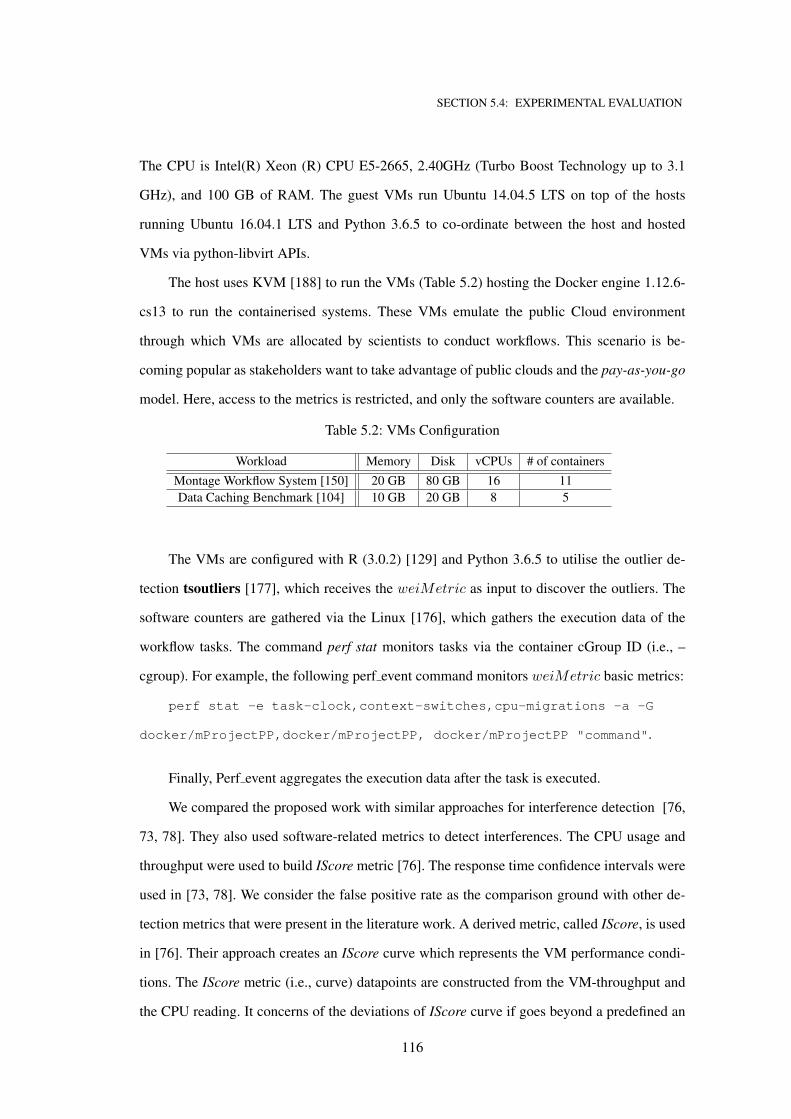
SECTION 5.4: EXPERIMENTAL EVALUATION
The CPU is Intel(R) Xeon (R) CPU E5-2665, 2.40GHz (Turbo Boost Technology up to 3.1
GHz), and 100 GB of RAM. The guest VMs run Ubuntu 14.04.5 LTS on top of the hosts
running Ubuntu 16.04.1 LTS and Python 3.6.5 to co-ordinate between the host and hosted
VMs via python-libvirt APIs.
The host uses KVM [188] to run the VMs (Table 5.2) hosting the Docker engine 1.12.6-
cs13 to run the containerised systems. These VMs emulate the public Cloud environment
through which VMs are allocated by scientists to conduct workflows. This scenario is be-
coming popular as stakeholders want to take advantage of public clouds and the pay-as-you-go
model. Here, access to the metrics is restricted, and only the software counters are available.
Table 5.2: VMs Configuration
Workload Memory Disk vCPUs # of containers
Montage Workflow System [150] 20 GB 80 GB 16 11
Data Caching Benchmark [104] 10 GB 20 GB 8 5
The VMs are configured with R (3.0.2) [129] and Python 3.6.5 to utilise the outlier de-
tection tsoutliers [177], which receives the weiMetric as input to discover the outliers. The
software counters are gathered via the Linux [176], which gathers the execution data of the
workflow tasks. The command perf stat monitors tasks via the container cGroup ID (i.e., –
cgroup). For example, the following perf event command monitors weiMetric basic metrics:
perf stat -e task-clock,context-switches,cpu-migrations -a -G
docker/mProjectPP,docker/mProjectPP, docker/mProjectPP "command".
Finally, Perf event aggregates the execution data after the task is executed.
We compared the proposed work with similar approaches for interference detection [76,
73, 78]. They also used software-related metrics to detect interferences. The CPU usage and
throughput were used to build IScore metric [76]. The response time confidence intervals were
used in [73, 78]. We consider the false positive rate as the comparison ground with other de-
tection metrics that were present in the literature work. A derived metric, called IScore, is used
in [76]. Their approach creates an IScore curve which represents the VM performance condi-
tions. The IScore metric (i.e., curve) datapoints are constructed from the VM-throughput and
the CPU reading. It concerns of the deviations of IScore curve if goes beyond a predefined an
116
SECTION 5.4: EXPERIMENTAL EVALUATION
interference threshold curve. The other approaches [73, 78] use the response time to detect in-
terference. The mean intervals of the response time are checked regularly seeking any response
time extension or overlapping between the response time mean confidence intervals.
5.4.1 Benchmarks
To test the designed metric, we compared it with the following two metrics:
• The work in [78] uses the workload’s mean response time of a pre-designed probe ap-
plication. The probe application is used to monitor the resources contentions. The probe
periodically executes CPU-intensive PHP scripts with a specific rate and concurrent con-
nection intensity. The probe encapsulates with httperf [189] to create concurrent HTTP
connections to targeted hosts. A back-end agent (i.e., controller) sends a concurrent
HTTP connection to monitor the mean response time and alert if any major response
time variation is detected. The 95% of mean probe response time is used in [78] to detect
any significant measurement with the baseline no-interference response time. However,
we observed in the experiments that the 95% confidence interval (CI) is not enough to
detect minor interference cases, therefore we use the 90% of mean probe response time
as a secondary metric.
• The combination of the container CPU usage and web service throughput value is used
in [76] to derive a new metric called IScore. This metric models the interference as a
deviation in the Cartesian square from the normal operation that executed earlier in an
isolated environment. The proposed approach in [76] requires prior profiling of the con-
tainerised application to compare it with the actual run on the cloud resources. However,
we used CPU usage with the containerised application throughput. For the workflow
system, we used containers that encounter a high volume of tasks such as mProjectPP,
mDiffFit and mBackground containers while for a non-workflow system we used the
memcached server containers to construct the IScore values to create the product set of
the Cartesian square.
117
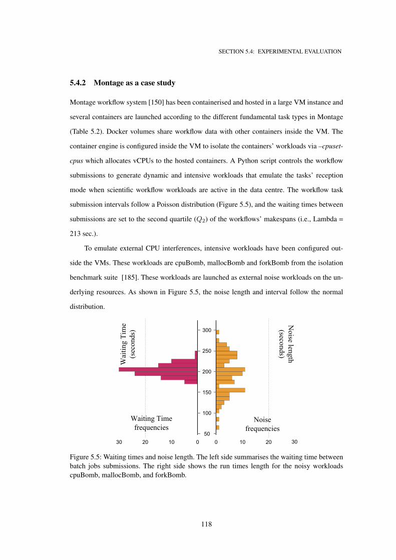
SECTION 5.4: EXPERIMENTAL EVALUATION
5.4.2 Montage as a case study
Montage workflow system [150] has been containerised and hosted in a large VM instance and
several containers are launched according to the different fundamental task types in Montage
(Table 5.2). Docker volumes share workflow data with other containers inside the VM. The
container engine is configured inside the VM to isolate the containers’ workloads via –cpuset-
cpus which allocates vCPUs to the hosted containers. A Python script controls the workflow
submissions to generate dynamic and intensive workloads that emulate the tasks’ reception
mode when scientific workflow workloads are active in the data centre. The workflow task
submission intervals follow a Poisson distribution (Figure 5.5), and the waiting times between
submissions are set to the second quartile (Q2) of the workflows’ makespans (i.e., Lambda =
213 sec.).
To emulate external CPU interferences, intensive workloads have been configured out-
side the VMs. These workloads are cpuBomb, mallocBomb and forkBomb from the isolation
benchmark suite [185]. These workloads are launched as external noise workloads on the un-
derlying resources. As shown in Figure 5.5, the noise length and interval follow the normal
distribution.
Noise length (seconds)
Wai
ting
Tim
e (s
econ
ds)
0102030 0 10 20 3050
100
150
200
250
300
Waiting Time frequencies
Noise frequencies
Figure 5.5: Waiting times and noise length. The left side summarises the waiting time between
batch jobs submissions. The right side shows the run times length for the noisy workloads
cpuBomb, mallocBomb, and forkBomb.
118
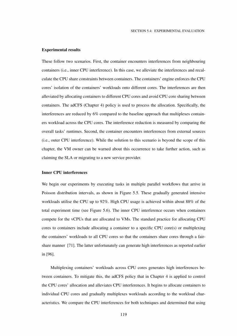
SECTION 5.4: EXPERIMENTAL EVALUATION
Experimental results
These follow two scenarios. First, the container encounters interferences from neighbouring
containers (i.e., inner CPU interference). In this case, we alleviate the interferences and recal-
culate the CPU share constraints between containers. The containers’ engine enforces the CPU
cores’ isolation of the containers’ workloads onto different cores. The interferences are then
alleviated by allocating containers to different CPU cores and avoid CPU core sharing between
containers. The adCFS (Chapter 4) policy is used to process the allocation. Specifically, the
interferences are reduced by 6% compared to the baseline approach that multiplexes contain-
ers workload across the CPU cores. The interference reduction is measured by comparing the
overall tasks’ runtimes. Second, the container encounters interferences from external sources
(i.e., outer CPU interference). While the solution to this scenario is beyond the scope of this
chapter, the VM owner can be warned about this occurrence to take further action, such as
claiming the SLA or migrating to a new service provider.
Inner CPU interferences
We begin our experiments by executing tasks in multiple parallel workflows that arrive in
Poisson distribution intervals, as shown in Figure 5.5. These gradually generated intensive
workloads utilise the CPU up to 92%. High CPU usage is achieved within about 88% of the
total experiment time (see Figure 5.6). The inner CPU interference occurs when containers
compete for the vCPUs that are allocated to VMs. The standard practice for allocating CPU
cores to containers include allocating a container to a specific CPU core(s) or multiplexing
the containers’ workloads to all CPU cores so that the containers share cores through a fair-
share manner [71]. The latter unfortunately can generate high interferences as reported earlier
in [96].
Multiplexing containers’ workloads across CPU cores generates high interferences be-
tween containers. To mitigate this, the adCFS policy that in Chapter 4 is applied to control
the CPU cores’ allocation and alleviates CPU interferences. It begins to allocate containers to
individual CPU cores and gradually multiplexes workloads according to the workload char-
acteristics. We compare the CPU interferences for both techniques and determined that using
119
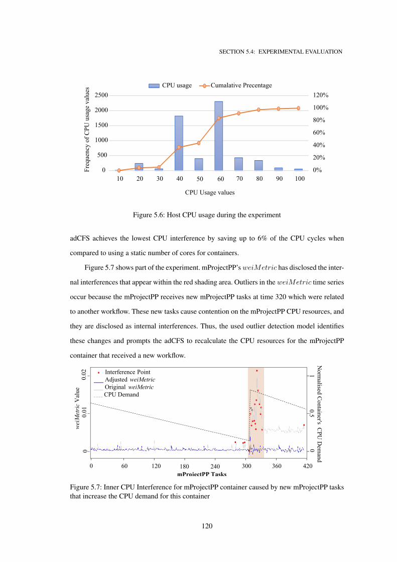
SECTION 5.4: EXPERIMENTAL EVALUATION
0%
20%
40%
60%
80%
100%
120%
0
500
1000
1500
2000
2500
10 20 30 40 70 80 90 100
Freq
uenc
y of
CPU
usa
ge v
alue
s
50 60
CPU Usage values
CPU usage Cumalative Precentage
Figure 5.6: Host CPU usage during the experiment
adCFS achieves the lowest CPU interference by saving up to 6% of the CPU cycles when
compared to using a static number of cores for containers.
Figure 5.7 shows part of the experiment. mProjectPP’s weiMetric has disclosed the inter-
nal interferences that appear within the red shading area. Outliers in the weiMetric time series
occur because the mProjectPP receives new mProjectPP tasks at time 320 which were related
to another workflow. These new tasks cause contention on the mProjectPP CPU resources, and
they are disclosed as internal interferences. Thus, the used outlier detection model identifies
these changes and prompts the adCFS to recalculate the CPU resources for the mProjectPP
container that received a new workflow.
0 60 120 mProjectPP Tasks
300 360 420
180 240 mBackground Tasks
wei
Met
ric
Val
ue
0.02
0.
01
0 0
1 0.5
Norm
alised Container's CPU D
emand
Interference Point ___ Adjusted weiMetric ___ Original weiMetric _ _ _ _ CPU Demand
0 60 120 300 360 420
0 0.
025
180 240
wei
Met
ric
Val
ue
0.02
0.
015
Interference Point ___ Adjusted weiMetric ___ Original weiMetric_ _ _ _ CPU Demand
0
1 0.5
Norm
alised Container's CPU D
emand
Figure 5.7: Inner CPU Interference for mProjectPP container caused by new mProjectPP tasks
that increase the CPU demand for this container
120
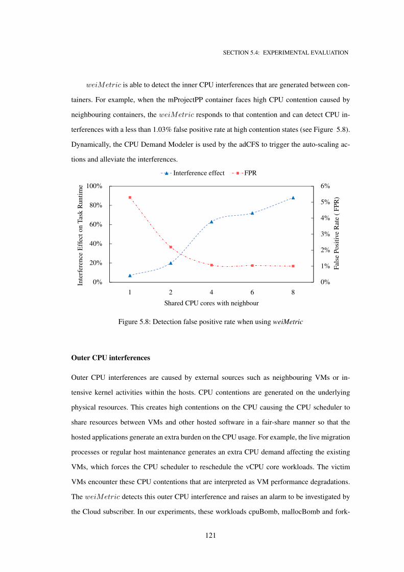
SECTION 5.4: EXPERIMENTAL EVALUATION
weiMetric is able to detect the inner CPU interferences that are generated between con-
tainers. For example, when the mProjectPP container faces high CPU contention caused by
neighbouring containers, the weiMetric responds to that contention and can detect CPU in-
terferences with a less than 1.03% false positive rate at high contention states (see Figure 5.8).
Dynamically, the CPU Demand Modeler is used by the adCFS to trigger the auto-scaling ac-
tions and alleviate the interferences.
0%
1%
2%
3%
4%
5%
6%
0%
20%
40%
60%
80%
100%
1 2 4 6 8
Fal
se P
osi
tive
Rat
e (
FP
R)
Inte
rfer
ence
Eff
ect
on T
ask R
unti
me
Shared CPU cores with neighbour
Interference effect FPR
Figure 5.8: Detection false positive rate when using weiMetric
Outer CPU interferences
Outer CPU interferences are caused by external sources such as neighbouring VMs or in-
tensive kernel activities within the hosts. CPU contentions are generated on the underlying
physical resources. This creates high contentions on the CPU causing the CPU scheduler to
share resources between VMs and other hosted software in a fair-share manner so that the
hosted applications generate an extra burden on the CPU usage. For example, the live migration
processes or regular host maintenance generates an extra CPU demand affecting the existing
VMs, which forces the CPU scheduler to reschedule the vCPU core workloads. The victim
VMs encounter these CPU contentions that are interpreted as VM performance degradations.
The weiMetric detects this outer CPU interference and raises an alarm to be investigated by
the Cloud subscriber. In our experiments, these workloads cpuBomb, mallocBomb and fork-
121
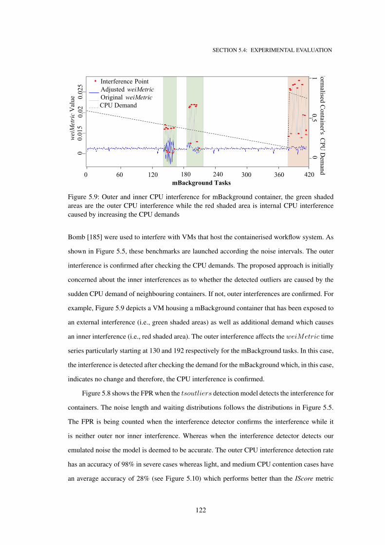
SECTION 5.4: EXPERIMENTAL EVALUATION
0 60 120 mProjectPP Tasks
300 360 420
180 240 mBackground Tasks
wei
Met
ric
Val
ue
0.02
0.
01
0 0
1 0.5
Norm
alised Container's CPU D
emand
Interference Point ___ Adjusted weiMetric ___ Original weiMetric _ _ _ _ CPU Demand
0 60 120 300 360 420
0 0.
025
180 240
wei
Met
ric
Val
ue
0.02
0.
015
Interference Point ___ Adjusted weiMetric ___ Original weiMetric_ _ _ _ CPU Demand
0
1 0.5
Norm
alised Container's CPU D
emand
Figure 5.9: Outer and inner CPU interference for mBackground container, the green shaded
areas are the outer CPU interference while the red shaded area is internal CPU interference
caused by increasing the CPU demands
Bomb [185] were used to interfere with VMs that host the containerised workflow system. As
shown in Figure 5.5, these benchmarks are launched according the noise intervals. The outer
interference is confirmed after checking the CPU demands. The proposed approach is initially
concerned about the inner interferences as to whether the detected outliers are caused by the
sudden CPU demand of neighbouring containers. If not, outer interferences are confirmed. For
example, Figure 5.9 depicts a VM housing a mBackground container that has been exposed to
an external interference (i.e., green shaded areas) as well as additional demand which causes
an inner interference (i.e., red shaded area). The outer interference affects the weiMetric time
series particularly starting at 130 and 192 respectively for the mBackground tasks. In this case,
the interference is detected after checking the demand for the mBackground which, in this case,
indicates no change and therefore, the CPU interference is confirmed.
Figure 5.8 shows the FPR when the tsoutliers detection model detects the interference for
containers. The noise length and waiting distributions follows the distributions in Figure 5.5.
The FPR is being counted when the interference detector confirms the interference while it
is neither outer nor inner interference. Whereas when the interference detector detects our
emulated noise the model is deemed to be accurate. The outer CPU interference detection rate
has an accuracy of 98% in severe cases whereas light, and medium CPU contention cases have
an average accuracy of 28% (see Figure 5.10) which performs better than the IScore metric
122
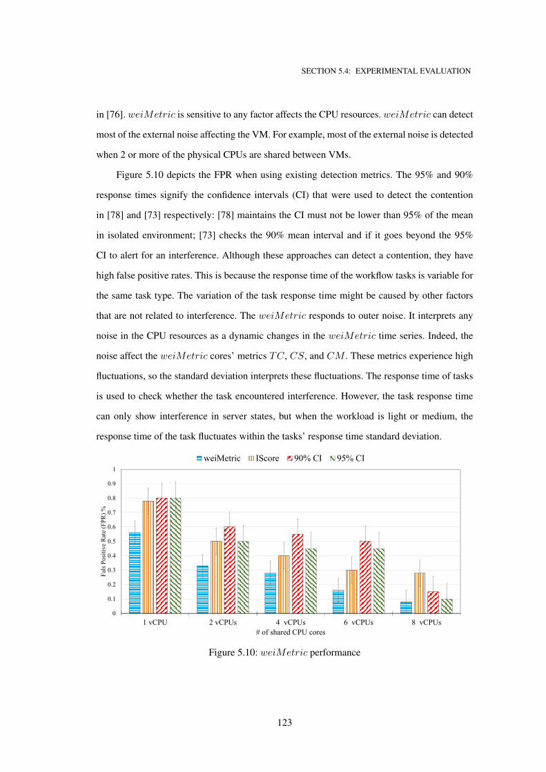
SECTION 5.4: EXPERIMENTAL EVALUATION
in [76]. weiMetric is sensitive to any factor affects the CPU resources. weiMetric can detect
most of the external noise affecting the VM. For example, most of the external noise is detected
when 2 or more of the physical CPUs are shared between VMs.
Figure 5.10 depicts the FPR when using existing detection metrics. The 95% and 90%
response times signify the confidence intervals (CI) that were used to detect the contention
in [78] and [73] respectively: [78] maintains the CI must not be lower than 95% of the mean
in isolated environment; [73] checks the 90% mean interval and if it goes beyond the 95%
CI to alert for an interference. Although these approaches can detect a contention, they have
high false positive rates. This is because the response time of the workflow tasks is variable for
the same task type. The variation of the task response time might be caused by other factors
that are not related to interference. The weiMetric responds to outer noise. It interprets any
noise in the CPU resources as a dynamic changes in the weiMetric time series. Indeed, the
noise affect the weiMetric cores’ metrics TC, CS, and CM . These metrics experience high
fluctuations, so the standard deviation interprets these fluctuations. The response time of tasks
is used to check whether the task encountered interference. However, the task response time
can only show interference in server states, but when the workload is light or medium, the
response time of the task fluctuates within the tasks’ response time standard deviation.
0
0.1
0.2
0.3
0.4
0.5
0.6
0.7
0.8
0.9
1
1 vCPU 2 vCPUs 4 vCPUs 6 vCPUs 8 vCPUs
Fals
Posit
ive
Rate
(FPR
) %
# of shared CPU cores
weiMetric IScore 90% CI 95% CI
Figure 5.10: weiMetric performance
123
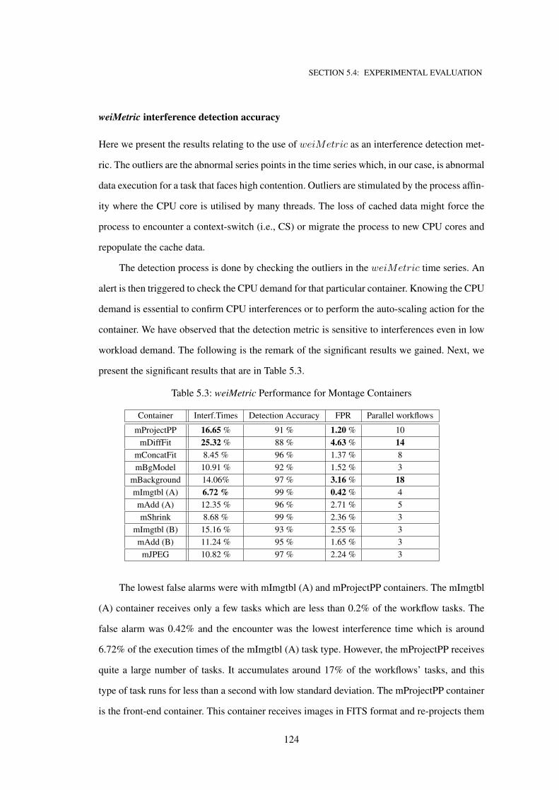
SECTION 5.4: EXPERIMENTAL EVALUATION
weiMetric interference detection accuracy
Here we present the results relating to the use of weiMetric as an interference detection met-
ric. The outliers are the abnormal series points in the time series which, in our case, is abnormal
data execution for a task that faces high contention. Outliers are stimulated by the process affin-
ity where the CPU core is utilised by many threads. The loss of cached data might force the
process to encounter a context-switch (i.e., CS) or migrate the process to new CPU cores and
repopulate the cache data.
The detection process is done by checking the outliers in the weiMetric time series. An
alert is then triggered to check the CPU demand for that particular container. Knowing the CPU
demand is essential to confirm CPU interferences or to perform the auto-scaling action for the
container. We have observed that the detection metric is sensitive to interferences even in low
workload demand. The following is the remark of the significant results we gained. Next, we
present the significant results that are in Table 5.3.
Table 5.3: weiMetric Performance for Montage Containers
Container Interf.Times Detection Accuracy FPR Parallel workflows
mProjectPP 16.65 % 91 % 1.20 % 10
mDiffFit 25.32 % 88 % 4.63 % 14
mConcatFit 8.45 % 96 % 1.37 % 8
mBgModel 10.91 % 92 % 1.52 % 3
mBackground 14.06% 97 % 3.16 % 18
mImgtbl (A) 6.72 % 99 % 0.42 % 4
mAdd (A) 12.35 % 96 % 2.71 % 5
mShrink 8.68 % 99 % 2.36 % 3
mImgtbl (B) 15.16 % 93 % 2.55 % 3
mAdd (B) 11.24 % 95 % 1.65 % 3
mJPEG 10.82 % 97 % 2.24 % 3
The lowest false alarms were with mImgtbl (A) and mProjectPP containers. The mImgtbl
(A) container receives only a few tasks which are less than 0.2% of the workflow tasks. The
false alarm was 0.42% and the encounter was the lowest interference time which is around
6.72% of the execution times of the mImgtbl (A) task type. However, the mProjectPP receives
quite a large number of tasks. It accumulates around 17% of the workflows’ tasks, and this
type of task runs for less than a second with low standard deviation. The mProjectPP container
is the front-end container. This container receives images in FITS format and re-projects them
124
SECTION 5.4: EXPERIMENTAL EVALUATION
according to the predefined scale in the FITS header template. They are CPU-bound tasks, and
are executed in subsequent steps. This container encountered an external noise that was around
16.65% and ten different parallel workflows were executed at the same time. Our proposed in-
terference detection technique has detected 91% of the external interference for this container.
Around 9% is missed, as 2% from the 9% is missed due to some unknown error (exceptions)
with the package tsoutliers. The designed script encountered some exceptional errors when
the tsoutliers model could not fit the weiMetric time series. The FPR was 1.20% and this
can refer to the deviations in the execution data in mProjectPP tasks. Unfortunately, these false
alarms are unavoidable as they would be too costly to diagnose and remove them.
The highest FPR was with mDiffFit and mBackground containers at 4.63% and 3.16%
respectively. These containers receive around 82% of the workflow tasks. These containers
accumulated around 14 and 18 parallel workflow executions respectively. They accumulated
this number of workflows because the workflow tasks are executed in subsequent steps which
create longer waiting time queues. The mDiffFit container encountered the most substantial
interference time in which around of 88% interference cases were detected. However, around
4.63% were false alarms due to the high deviation in the Task-clock metric which influenced
the weiMetric time series.
5.4.3 Memcached servers workloads as a case study
The proposed method was also tested for non-workflow workloads. We chose the data caching
benchmark, which is a distributed memory caching system [134]. This benchmark was con-
tainerised in [104] to simulate the behaviour of Twitter caching servers. The benchmark con-
sists of two tiers. The first is the server container(s) which run the Memcached workload. The
second is the client(s) who requests data cached on the Memcached containers. The service
quality of the Memcached servers is measured by the # of requests served per second rps.
The weiMetric time series is measured at each second interval as the perf event tool
allows monitoring the selected metrics (i.e., TC, CM and CS) per-second. The length of the
weiMetric time series is set to 20 points. This length is a user preference and depends on the
length of time of the detection phases. Unfortunately, a long weiMetric time series will delay
125
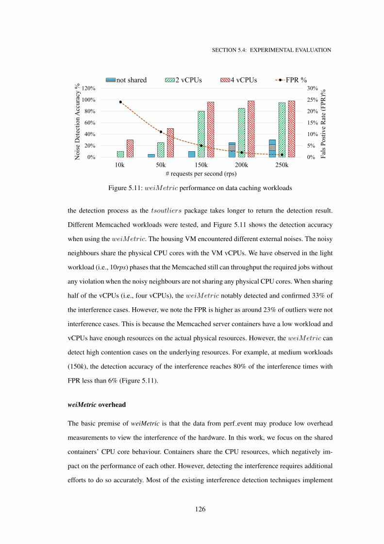
SECTION 5.4: EXPERIMENTAL EVALUATION
0%
5%
10%
15%
20%
25%
30%
0%
20%
40%
60%
80%
100%
120%
10k 50k 150k 200k 250k
Fals
Posti
ve R
ate
(FPR
)%
Noi
se D
etec
tion
Acc
urac
y %
# requests per second (rps)
not shared 2 vCPUs 4 vCPUs FPR %
Figure 5.11: weiMetric performance on data caching workloads
the detection process as the tsoutliers package takes longer to return the detection result.
Different Memcached workloads were tested, and Figure 5.11 shows the detection accuracy
when using the weiMetric. The housing VM encountered different external noises. The noisy
neighbours share the physical CPU cores with the VM vCPUs. We have observed in the light
workload (i.e., 10rps) phases that the Memcached still can throughput the required jobs without
any violation when the noisy neighbours are not sharing any physical CPU cores. When sharing
half of the vCPUs (i.e., four vCPUs), the weiMetric notably detected and confirmed 33% of
the interference cases. However, we note the FPR is higher as around 23% of outliers were not
interference cases. This is because the Memcached server containers have a low workload and
vCPUs have enough resources on the actual physical resources. However, the weiMetric can
detect high contention cases on the underlying resources. For example, at medium workloads
(150k), the detection accuracy of the interference reaches 80% of the interference times with
FPR less than 6% (Figure 5.11).
weiMetric overhead
The basic premise of weiMetric is that the data from perf event may produce low overhead
measurements to view the interference of the hardware. In this work, we focus on the shared
containers’ CPU core behaviour. Containers share the CPU resources, which negatively im-
pact on the performance of each other. However, detecting the interference requires additional
efforts to do so accurately. Most of the existing interference detection techniques implement
126
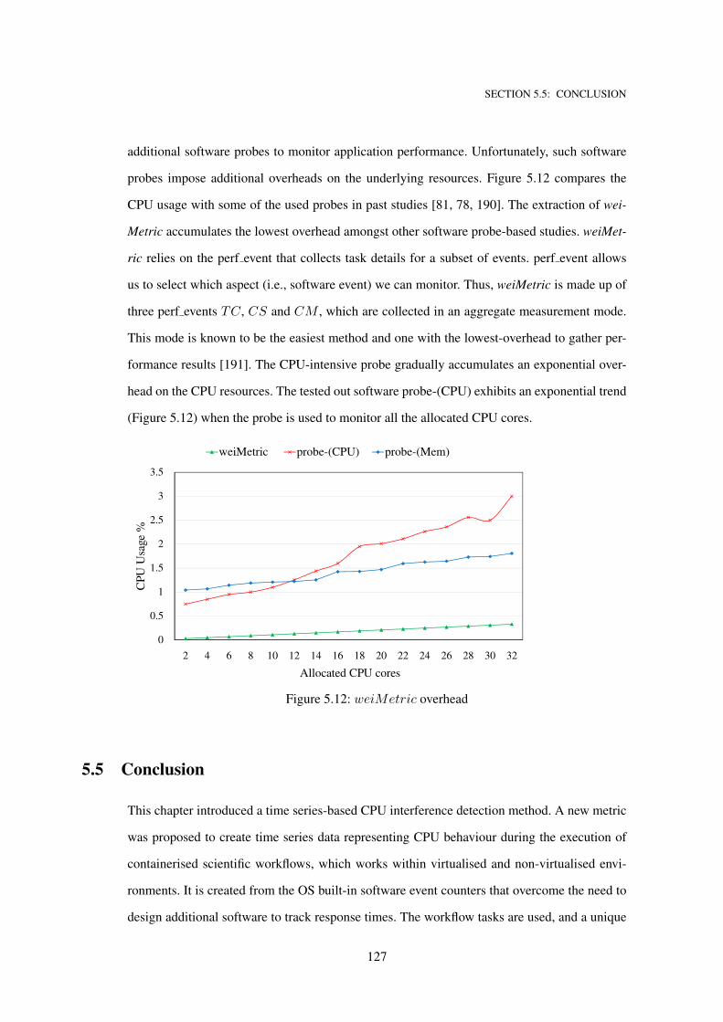
SECTION 5.5: CONCLUSION
additional software probes to monitor application performance. Unfortunately, such software
probes impose additional overheads on the underlying resources. Figure 5.12 compares the
CPU usage with some of the used probes in past studies [81, 78, 190]. The extraction of wei-
Metric accumulates the lowest overhead amongst other software probe-based studies. weiMet-
ric relies on the perf event that collects task details for a subset of events. perf event allows
us to select which aspect (i.e., software event) we can monitor. Thus, weiMetric is made up of
three perf events TC, CS and CM , which are collected in an aggregate measurement mode.
This mode is known to be the easiest method and one with the lowest-overhead to gather per-
formance results [191]. The CPU-intensive probe gradually accumulates an exponential over-
head on the CPU resources. The tested out software probe-(CPU) exhibits an exponential trend
(Figure 5.12) when the probe is used to monitor all the allocated CPU cores.
0
0.5
1
1.5
2
2.5
3
3.5
2 4 6 8 10 12 14 16 18 20 22 24 26 28 30 32
CP
U U
sage
%
Allocated CPU cores
weiMetric probe-(CPU) probe-(Mem)
Figure 5.12: weiMetric overhead
5.5 Conclusion
This chapter introduced a time series-based CPU interference detection method. A new metric
was proposed to create time series data representing CPU behaviour during the execution of
containerised scientific workflows, which works within virtualised and non-virtualised envi-
ronments. It is created from the OS built-in software event counters that overcome the need to
design additional software to track response times. The workflow tasks are used, and a unique
127
SECTION 5.5: CONCLUSION
time series is created for every task type. The limitation with weiMetric is noticed when a new
task type is entered into execution. There are no previous weiMetric values for this new type.
We are required to wait to build the appropriate time-series values that would be eligible to be
examined, by the outliers detection model. We must take precautions with this model to ensure
there are enough resources for this new task type. The proposed method is incorporated into the
adCFS policy [93] to fairly share CPU and alleviate inner CPU interferences between contain-
ers. The experiment results show that the proposed metric can detect CPU interferences with
98% accuracy in high contention states as well as save CPU cycles up to 6% when executing
intensive workloads.
128
CHAPTER 6Predictive Co-location Technique to Maximise
CPU Workloads of Data Centre Servers
Servers cause most energy wastage in data centres with low average utilisation. Modern data
centre providers cannot fully utilise servers, because the hosted applications’ workloads fluc-
tuate and executing additional workloads would cause failures in providing the agreed Qual-
ity of Service (QoS). Recently, data centre operators make application co-location powerful
mechanisms to increase their server utilisations though using predictive co-location technique.
However, existing predictive co-location algorithms suffer severe constraint violations, high
latencies, and long prediction control intervals. Parts of the previous chapters concepts have
been used in this chapter to address workloads co-location. We have provided in Chapter 3 a
proactive auto-scale technique manages the containers CPU resources for sensitive container-
ised applications. Also, in Chapter 4, we addressed the issue of unfair CPU sharing between
containers that run batch jobs. To co-locate workload safely, Chapter 5 introduced CPU metric,
called weiMetric to detect interferences occurring during tasks’ execution. This chapter intro-
duces an interference-aware automatic workload orchestration technique called M2-AutScale,
that proactively allocates batch jobs on sensitive application resources to maximise servers’
utilisation. The proposed technique prevents SLA violations that are generally caused by the
CPU interference of neighbouring applications. A hybrid nested Markovian time series predic-
tion model is carefully designed to predict containers’ CPU demands accurately. Then, CPU
129
SECTION 6.1: INTRODUCTION
interference is measured to dynamically reorganise appropriate CPU portions for the predicted
containers workloads as well as for batch jobs. Extensive experiments on CPU utilisation ob-
tained from Alibaba’s production cluster trace are used to fit and evaluate the proposed math-
ematical prediction model. This model outperformed several existing time series prediction
models that were used in the literature and improved the prediction accuracy for auto-regressive
integrated moving average (ARIMA) models by up to 16%. Then, this prediction model is in-
tegrated with several technical components so that batch job containers can safely co-exist
with multiple sensitive containerised applications. A realistic experimental environment is de-
signed to evaluate (M2-AutScale) for containerised applications. (M2-AutScale) can reduce
SLA violations by as much as 12% compared with AWS predictive scaling models. Further, it
improves resource utilisation by 30% compared with AWS scheduled scaling actions.
6.1 Introduction
Low resource usage in current data centres results in massive wastage of infrastructure invest-
ment and hardware resources. In early 2012, the mean CPU utilisation accruing to Google’s
production cluster was around 20% [15]. Recently, a careful study by [13] showed that around
60% of Microsoft Azure servers had CPU utilisations less than 20%. Similarly, the analysis
of Alibaba data center trace shows the CPU average of 4022 servers is 38.11% for a period
of consecutive 8 days [1]. The massive investment cost linked to low resource usage has un-
doubtedly become a key concern for cloud providers. To alleviate the issue, co-locating various
workloads on the same resources has been suggested to enhance resource utilisation by real-
ising high resource efficiency. This approach, however, often generates higher resource con-
tention [192, 151] and the contention results in unknown performance variability and greatly
reduces the QoS accruing to end user-facing services [193]. Clearly, workload co-location re-
sults in more unpredictable performance because of the interferences of shared resources. The
probability of interference occurring amongst all workloads increases with the number of co-
located workloads on the same servers [194, 195]. Once applications of high-priority jobs
suffer from interferences, they get high priority access to computing resources to fulfil the Ser-
vice Level Agreement (SLA) and the resource schedulers perform a reactive co-scheduling on
130
SECTION 6.1: INTRODUCTION
best-effort resources [196]. Additionally, the performance accruing to low-priority job work-
loads can undergo runtime sacrifice to prevent performance degradation of services linked to
high-priority jobs.
To address the issue of interference in the co-location approach, a plausible fix is to co-
locate distinct forms of cloud workloads on allocated resources for large-scale clusters to en-
hance resource utilisation [14]. Indeed, current major cloud providers, e.g. Alibaba [14] and
Google [197]), already co-allocate batch jobs with Internet services (i.e. sensitive applications)
on the same clusters to increase server utilisation and save energy. This management of work-
load co-location needs to be coordinated using scheduling tools/methods. Each cloud provider
tends to build its own cluster management tool/method to enable batch jobs to coexist with
latency-critical services. For instance, Sigma and Fuxi [198] are two schedulers used to co-
ordinate coexisting latency-critical applications and batch jobs in Alibaba data centers [194].
Even though cloud providers use their own sophisticated cluster management schedulers, their
CPU resources usage has not been optimised and their data centre CPU utilisation remains low
as discussed in the beginning of this section.
Apart from efficient resource utilisation, scalability of virtual resources is another major
concern when co-locating workloads in cloud environment. Many studies showed that con-
tainers are highly scalable and can achieve higher system utilisation than VMs [199, 200,
201]. Container-based cluster management systems such as Alibaba’s Fuxi [198] and Google’s
borg [151] are designed to employ residual resources to increase resource usages and pro-
vide cloud operators a marginal expense as the operating resource cost decreases. These data
centres operators (e.g., Google and Alibaba) built container-based architectures to easily co-
ordinate batch jobs with sensitive applications. This is because containers are highly resilient
and can flexibly undergo rapid resizing, whereas approaches such as rapid VM resizing can
hardly be executed following consumers’ busty resource usage patterns. Both of Fuxi [198]
and borg [151] exercise a conservative reactive consolidation of workloads which apparently
over-provision resources and leave substantial quantities of residual resources.
Thus, it is desirable to develop new resource allocation methods that not only achieve
efficient resource utilisation but also meet the scalability service level objective. From the
above discussion, a plausible approach is to incorporate (i) a forecasting model, which dynam-
131
SECTION 6.1: INTRODUCTION
ically estimates the resource demand, and hence provides scalability, and (ii) an interference-
aware model, which detects/stops interference caused by batch workloads and hence allows
co-locations of batch jobs and sensitive applications and as a result, guarantees high resource
utilisation.
This paper describes the M2-AutScale, an interference-aware nested-Markovian-level auto-
scaling method, which enables batch-based workloads to safely co-exist alongside sensitive
application workloads. A realistic environment is used to test the co-location method. Sev-
eral sensitive application containers [104] (i.e., data caching server, data analytics, and web
services) are safely co-located with batch job containers (i.e., Montage workflow). Workload
coexistence is controlled by hybrid prediction model that estimates the demand of the sensitive
application. Then, the residual resources are used to execute a regulated number of batch jobs
seeking high resource efficiency. The interferences generated by the batch jobs are carefully
studied and are considered when utilising the residual resources. The two main contributions
made here can be summarised as follows:
• A hybrid time-series prediction model. This utilises different prediction methods to pre-
cisely predict the CPU usage of sensitive-application containers. This model extends the
ARIMA models to make them aware of future time series level states by combining
them with nested Markovian models that can detect future state changes in the time se-
ries. A two-level Markovian structure is used, where a fine level structure is embedded
within a coarse one to better capture state transitions in CPU usage time series. Nested
Markov chains can detect the temporal characteristics of the time series [202] and con-
sidered in our work to detect the temporal changes in the CPU utilisation. The CPU
usage is partitioned into several percentile ranges to define Markov states at fine levels.
The coarse levels in the prediction model are referred to as a ‘state’, and the fine levels
as ‘substates’. A discrete-time Markov chain has stationary or homogeneous transition
probabilities that represent the transitions of the CPU usage values between the limited
number of states and substates.
• An interference-aware proactive auto-scaling method (M2-AutScale), which enables
batch-based workloads to safely co-exist with sensitive application workloads. Batch
132
SECTION 6.2: RELATED WORK
jobs would likely cause interferences in existing running applications; therefore, a safety
margin is strictly imposed to restrict the interference effects as well as unpredictable traf-
fic spikes. A monitoring tool reads (1) sensitive applications’ CPU usages and (2) CPU
contention metrics for CPU-related events using existing perf event events (e.g., Task-
Clock, Switch-Context, and CPU-Migrations). The CPU demand is then estimated after
considering the interferences that may be caused by neighbouring batch job containers.
This will maintain adequate QoS for sensitive applications and efficiently utilise residual
resources in the server. M2-AutScale scarifies batch jobs’ execution and throttles their
CPU resources to assure enough CPU resources for sensitive application containers.
This chapter is organised as follows. Existing scalability solutions are reviewed in Sec-
tion 6.2 and the proposed M2-AutScale method is described in Section 6.3 and evaluated in
Section 6.4. We conclude the paper in Section 6.5.
6.2 Related work
There has been a continuous increase in the volume and number of data centres that provide re-
sources on-demand to deploy different latency-sensitive systems. These resources are allocated
based on the promise that resources will be made available to execute application workloads.
However, this promise may stress the capabilities of Cloud providers when co-locating batch
jobs to improve resource efficiency. To solve this problem, the scale of data centres has been in-
creased; unfortunately, the energy consumption of data centres has also increased correspond-
ingly. This increasing trend of energy usage cannot continue as it will become economically
unfeasible. Therefore, resource optimisation is crucial to improve energy efficiency and reduce
power consumption; this is achievable by optimising the way servers can sustain a good quality
of service (QoS) when co-locating different workloads.
Increasing resource utilisation by sharing computing resources between compartments
may lead to reduced system performance and expose systems to security issues. Data cen-
tre management systems are designed to reduce unnecessary interference by not allowing co-
located jobs to be in excessive contention for the same computing resources in the absence of
an acceptable isolation mechanism. For example, Bubble-Flux [179] was created to evaluate
133
SECTION 6.2: RELATED WORK
how the memory affectability of applications changes with time and to learn how to prevent
memory-intensive services from reaching a similar state. Nathuji et al. [203] created a QoS-
aware model named Q-Clouds that powerfully modifies resource allocation to lighten the inter-
ference impacts on virtualised computing resources. Paragon [166] and Quasar [204] are group
leaders that use many online data mining techniques to determine the resource requirements of
cloud applications and to schedule them in a manner that limits resource interference. Deep-
Dive [205],another interference-aware system, uses a set of collaborative models to detect the
performance interference of co-located virtual machines (VMs).
Resource isolation is the recommended solution for avoiding interference impacts. For
example, Lo et al. [64] introduced the Heracles isolation system that co-locates sensitive ap-
plications with batch-based jobs while meeting the service-level agreement (SLA) requirement
for sensitive applications. They studied and analysed interference in sensitive Google applica-
tions that lacked robust consolidated equipment to preserve the QoS of sensitive applications
running alongside batch-based jobs. However, these co-location systems are utilised by Cloud
providers and information related to systems allocation is maintained by Cloud providers; end-
users cannot organise their workload in their own preferred manner. To overcome this issue,
our study proposes an approach that utilises user-friendly metrics that can be used by different
parties.
Kasture et al. [206] utilised a resource partitioning technique to improve cache utilisation.
Specifically, they performed fine-grained cache partitioning on servers that host best-effort
services with interactive applications. With regard to the interference impact on latency-critical
applications, Lo et al. [64] explored how sensitive Google applications can be isolated from
batch and low-priority workloads. They dynamically isolated multiple resources to co-locate
best-effort tasks with latency-sensitive jobs. Isolation was triggered from the cloud provider
side as most isolation mechanisms use hardware isolation systems that are inaccessible by
cloud subscribers. By contrast, our approach utilises user-related metrics to detect and mitigate
interference when co-locating batch jobs with sensitive applications.
Prediction models are used not only for scaling purposes but also for detecting perfor-
mance interference. Govindan et al. [207] predicted the interference for consolidated work-
loads. The probe performance was characterised under different conditions, and accordingly,
134
SECTION 6.2: RELATED WORK
a searching function matched the recorded performance in earlier degradation data. Inter-
ference was detected by continually analysing the VM behaviors on shared caches. Ahn et
al. [208] designed a contention-aware scheduling technique to detect workload conflicts in the
cache by gathering and analysing last-level cache (LLC) miss rates. They suggested search-
ing for a better machine to replace the VM. They migrated the VM if the existing allocation
case showed excessive shared cache conflicts or wrong non-uniform memory access (NUMA)
affinity. Interference among VMs was mitigated by designing special software that isolated
the VMs’ workloads. Kocoloski et al. [209] addressed the interference between VMs hosting
high-performance computing (HPC) applications. They created a special architecture to par-
tition nodes and to isolate HPC application workloads. Novakovic et al. [205] developed the
DeepDive system for identifying interference. This system used low-level hardware metrics to
identify the source of interference. The cycles per instruction (CPI) metric was used as a core
metric alongside VM-based metrics. Different components collaborate initially to determine
whether interference has occurred and accordingly create a logical warning alert. A VM that
causes interference is migrated and placed in a new machine that has been tested to be suitable
for this purpose. A synthetic benchmark is run to identify the optimal machine to place the VM
on, following which this VM will no longer cause interference.
[210] studied container scalability and proposed a self-adaptive controller to dynami-
cally manage VMs and container resources. They focused on recent emerging architectures
that use VMs to host different containerised applications. They introduced an auto-scaling re-
source controller, based on a discrete-time controller for VMs and containers according to the
given feedback. They investigated horizontal and vertical auto-scaling techniques. For verti-
cal scaling, they used structure permits resizing containers within the VM size. Containers
are monitored by a designed agent that monitors the container usage data. The agent controls
containers by horizontally scaling containers (i.e., creating or removing containers) or verti-
cally updating the resource allocation for containers (i.e., CPU/memory resources). However,
the interference is considered when pinning containerised applications to the same CPU cores.
Moreover, the VM agent accumulates additional overheads which may limit its performance
under burst workloads and thereby violate SLAs. [211] aimed to reduce the unpredictability
of resource provisioning for scientific applications via the automated distribution of design
135
SECTION 6.2: RELATED WORK
parameters and resources and limiting the acquired infrastructure cost. They aimed to antici-
pate the performance based on historical execution time data. Chen et al. [212] developed an
adaptive multi-learner to model the QoS and interference. The accuracies of the used method
are followed persistently at runtime in consideration of QoS obstruction. Usually, the most ap-
propriate model for estimating given information, as indicated by both local and global errors,
is utilised to make a forecast. However, their adaptive multi-learner is more likely to cause
additional resource overheads when working with dynamic workloads that require retesting
primitives and reselecting the most appropriate one.
Many researchers have implemented traditional resource allocation approaches such as
bin-packing and greedy algorithms. [204] examined the multi-dimensional bin-packing (MDBP)
problem and the related vector bin-packing (VBP) problem. [213] dealt with the MDBP for re-
source allocation issues in virtualised environments. They simulated using different greedy
algorithms such as first fit (FF), best fit (BF), permutation pack (PP), and choose pack (CP)
to solve resource allocation problems for shared resources that run non-scalable instances. By
contrast, our approach is designed to co-locate distributed workloads as the applications are
scalable and run over different machines.
Google designed the Omega shared-state architecture as a cluster scheduler to co-ordinate
different workloads on Google infrastructure [214]. This cluster scheduler [214] aimed to use
global cluster utilisation to dynamically scale resources and accelerate MapReduce jobs. In
Mercury, jobs can pick ensured and queueable containers with the goal that their execution is
non-preemptable/preemptable and resource apportioning is midway/disseminated [215]. [216]
scheduled long- and short-term jobs independently. A centralised scheduler was used for long-
term jobs, and short-term jobs were scheduled randomly in a manner comparable to Sparrow.
Data centre resource management systems perform an important role in resource distri-
bution. [217] surveyed various resource management systems aimed at optimising resource
utilisation in data centres. Tan et al. [218] studied resource usage patterns, and Mazumdar and
Kumar [219] suggested different strategies for analysing resource usage patterns to improve the
prediction performance. To ensure a high level of resource efficiency, the CPUs and memory
can adopt new designations of resources [220]. Warneke and Leng [221] investigated static re-
source partitioning and proposed a dynamic scheme to improve memory use in cluster resource
136
SECTION 6.2: RELATED WORK
management systems. Their new dynamic memory scheme enables big data applications to
utilise unused memory and thereby improve the processing efficiency for I/O processes. Bari
et al. [222] studied the networking energy efficiency in detail. Shojafar et al. [223] proposed
an adaptive approach to cope with dynamic workloads. Their approach proactively manages
networking resources for jobs. It considers end-to-end connections while maintaining the strict
QoS objectives for latency-sensitive services. [15] analysed the first published Google trace
and discussed how Google schedulers uses task information to improve resource utilisation.
Their study called for better resource management systems to improve data centre resource
efficiency. Toward this end, the present study introduces a new proactive system to improve
CPU resource utilisation.
Several researchers have investigated the prediction of resource usage [224, 225]. [224]
utilised repeated resource patterns to anticipate the resource usage for the same group of VMs.
They classified VMs into several groups based on time-series-based correlated workload pat-
terns. Numerous techniques have been proposed to estimate the resource usage for incoming
workloads. These techniques reserve resources for these future workloads and discharge them
once they are not required. Nonetheless, it is insufficient to guarantee a productive data cen-
tre because certain servers may still fail. Other studies used prediction models to anticipate
failures. For example, [226] used the auto-regressive moving average (ARMA) time series pre-
diction model with fault tree analysis to analyze resource availability and to anticipate system
failures. citeSedaghat2016 presented a scheduling algorithm that plans tasks in advance with
the main objective of minimising task failures. A stochastic model was used to analyse the
reliability and to quantify the impacts of correlated failures.
Many studies also identified tasks related to the management of resource capacities [227,
13, 59, 228, 229, 230], which usually utilise prediction models and workload modelling to
manage computing resources efficiently. For instance, Bobroff et al. [228] used regression
models to classify VM workloads and to predict resource demands. They used the prediction
to determine the periodic patterns and planned resources accordingly. Server consolidation
management provides significant potential for saving energy. Verma et al. [231] showed that
the correlation between applications can be modelled to dynamically consolidate workloads.
They introduced a peak-clustering-based placement method and experimentally demonstrated
137
SECTION 6.2: RELATED WORK
its power saving potential. [227] introduced a trace-based capacity manager. Their methodol-
ogy relies upon measurements of an individual server’s or application’s outstanding tasks at
hand to forecast future limit requests.
[18] introduced a predictive fine-grained resource scaling technique called CloudScale.
CloudScale employs dynamic voltage and frequency scaling (DVFS) to reduce the energy con-
sumption of servers. It uses a time-series-based prediction model to resolve scaling conflicts
with minimum SLA violations on applications. The recognition of an under-estimation er-
ror indicates that a service-level objective (SLO) infringement has just occurred. A proactive
cushioning is added to maintain a strategic distance from such infringements. [232] also used a
time-series-based approach, specifically, a seasonal auto-regressive integrated moving average
(ARIMA) model, for forecasting server workloads. They set a short term for the prediction
horizon to predict the number of requests for a pool of computing resources. The trace they
used showed that seasonal trending and seasonal ARIMA could be the best options for such
workloads. Moreover, using a short time series is necessary to make the response of the pre-
diction model very fast; therefore, they tested several seasonal ARIMA models. By contrast, in
our study, we used AUTO-ARIMA that dynamically sets the prediction model parameters and
uses an additional prediction layer to fix the inability of ARIMA to detect sudden variations in
the time series.
[233] developed a predictive auto-scaling technique for connection-oriented services. They
designed a long-lived-connection-based algorithm to proactively manage server provision-
ing and workload dispatching. The prediction model they used was designed based on auto-
regression to predict login rates. The dynamic provisioning approach performed well for pe-
riodic requests (i.e., login rates) that could be classified as a seasonal time series with daily
observations. [25] developed a model-predictive algorithm for forecasting the number of cus-
tomers visiting a system. This algorithm was supported by a performance model that estimated
response times and planned resources over the prediction horizon. Their auto-scaling tech-
nique aimed to minimise the cost for applications. They dealt with different cost metrics such
as SLA violations, resource charging, and configuration change costs. However, they used a
fixed prediction model (i.e., a second-order ARMA model) that may be limited when con-
sidering non-seasonal and highly variable workloads. [234] dealt with bursty workloads by
138
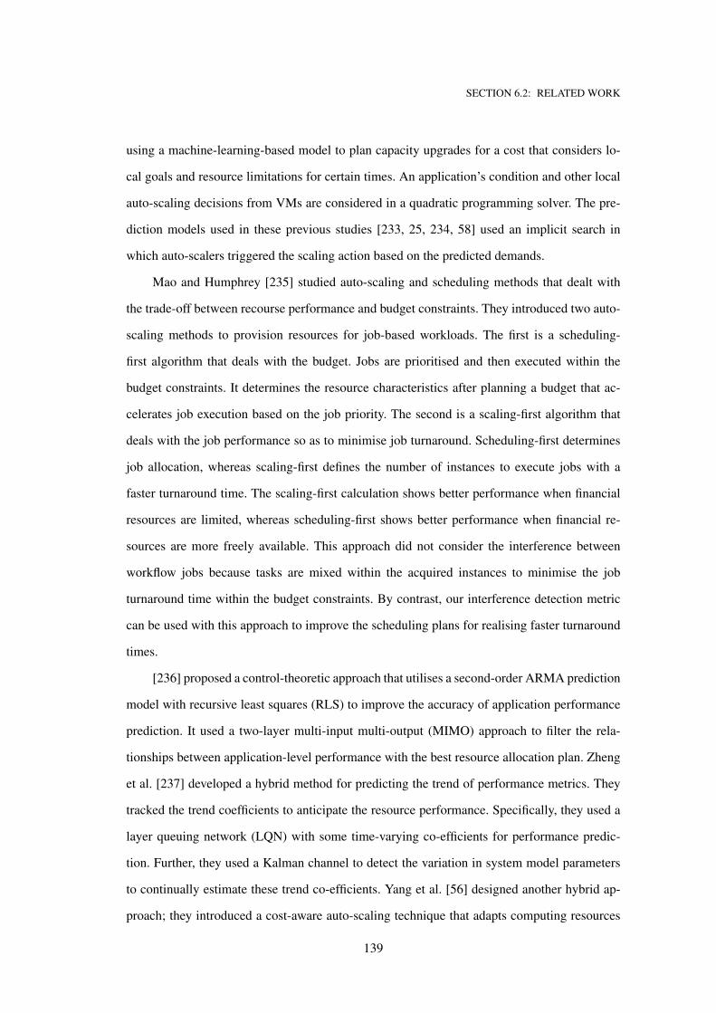
SECTION 6.2: RELATED WORK
using a machine-learning-based model to plan capacity upgrades for a cost that considers lo-
cal goals and resource limitations for certain times. An application’s condition and other local
auto-scaling decisions from VMs are considered in a quadratic programming solver. The pre-
diction models used in these previous studies [233, 25, 234, 58] used an implicit search in
which auto-scalers triggered the scaling action based on the predicted demands.
Mao and Humphrey [235] studied auto-scaling and scheduling methods that dealt with
the trade-off between recourse performance and budget constraints. They introduced two auto-
scaling methods to provision resources for job-based workloads. The first is a scheduling-
first algorithm that deals with the budget. Jobs are prioritised and then executed within the
budget constraints. It determines the resource characteristics after planning a budget that ac-
celerates job execution based on the job priority. The second is a scaling-first algorithm that
deals with the job performance so as to minimise job turnaround. Scheduling-first determines
job allocation, whereas scaling-first defines the number of instances to execute jobs with a
faster turnaround time. The scaling-first calculation shows better performance when financial
resources are limited, whereas scheduling-first shows better performance when financial re-
sources are more freely available. This approach did not consider the interference between
workflow jobs because tasks are mixed within the acquired instances to minimise the job
turnaround time within the budget constraints. By contrast, our interference detection metric
can be used with this approach to improve the scheduling plans for realising faster turnaround
times.
[236] proposed a control-theoretic approach that utilises a second-order ARMA prediction
model with recursive least squares (RLS) to improve the accuracy of application performance
prediction. It used a two-layer multi-input multi-output (MIMO) approach to filter the rela-
tionships between application-level performance with the best resource allocation plan. Zheng
et al. [237] developed a hybrid method for predicting the trend of performance metrics. They
tracked the trend coefficients to anticipate the resource performance. Specifically, they used a
layer queuing network (LQN) with some time-varying co-efficients for performance predic-
tion. Further, they used a Kalman channel to detect the variation in system model parameters
to continually estimate these trend co-efficients. Yang et al. [56] designed another hybrid ap-
proach; they introduced a cost-aware auto-scaling technique that adapts computing resources
139
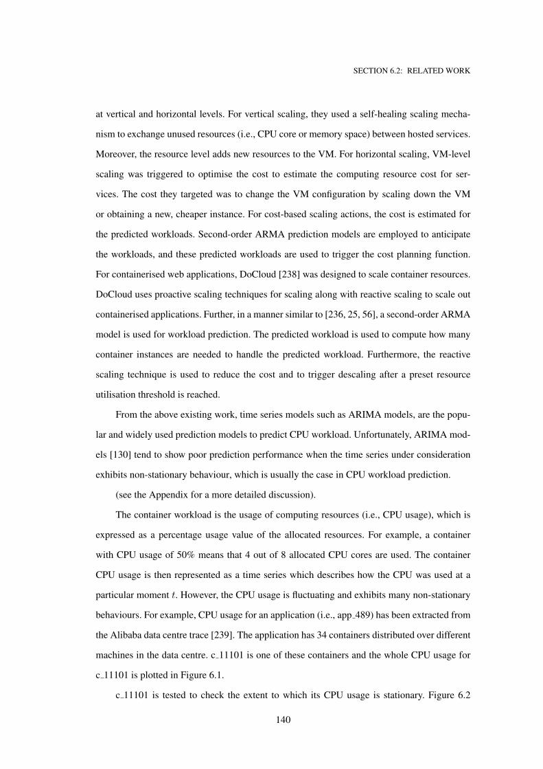
SECTION 6.2: RELATED WORK
at vertical and horizontal levels. For vertical scaling, they used a self-healing scaling mecha-
nism to exchange unused resources (i.e., CPU core or memory space) between hosted services.
Moreover, the resource level adds new resources to the VM. For horizontal scaling, VM-level
scaling was triggered to optimise the cost to estimate the computing resource cost for ser-
vices. The cost they targeted was to change the VM configuration by scaling down the VM
or obtaining a new, cheaper instance. For cost-based scaling actions, the cost is estimated for
the predicted workloads. Second-order ARMA prediction models are employed to anticipate
the workloads, and these predicted workloads are used to trigger the cost planning function.
For containerised web applications, DoCloud [238] was designed to scale container resources.
DoCloud uses proactive scaling techniques for scaling along with reactive scaling to scale out
containerised applications. Further, in a manner similar to [236, 25, 56], a second-order ARMA
model is used for workload prediction. The predicted workload is used to compute how many
container instances are needed to handle the predicted workload. Furthermore, the reactive
scaling technique is used to reduce the cost and to trigger descaling after a preset resource
utilisation threshold is reached.
From the above existing work, time series models such as ARIMA models, are the popu-
lar and widely used prediction models to predict CPU workload. Unfortunately, ARIMA mod-
els [130] tend to show poor prediction performance when the time series under consideration
exhibits non-stationary behaviour, which is usually the case in CPU workload prediction.
(see the Appendix for a more detailed discussion).
The container workload is the usage of computing resources (i.e., CPU usage), which is
expressed as a percentage usage value of the allocated resources. For example, a container
with CPU usage of 50% means that 4 out of 8 allocated CPU cores are used. The container
CPU usage is then represented as a time series which describes how the CPU was used at a
particular moment t. However, the CPU usage is fluctuating and exhibits many non-stationary
behaviours. For example, CPU usage for an application (i.e., app 489) has been extracted from
the Alibaba data centre trace [239]. The application has 34 containers distributed over different
machines in the data centre. c 11101 is one of these containers and the whole CPU usage for
c 11101 is plotted in Figure 6.1.
c 11101 is tested to check the extent to which its CPU usage is stationary. Figure 6.2
140
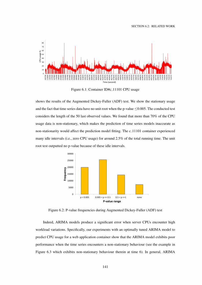
SECTION 6.2: RELATED WORK
0
10
20
30
40
50
60
70
80
90
1037
3011
5030
1263
3013
7630
1679
6017
9260
1905
6020
1860
2131
6022
4460
2357
6024
7060
2583
6026
9660
2809
6029
2260
3035
7031
4870
3261
7033
7470
3487
7036
0070
3713
7038
2670
3939
7040
5270
4165
7042
7870
4391
7045
0470
4617
7047
3070
4843
7049
5670
5069
7051
8270
5295
7054
0870
5521
7056
3470
5747
7058
6070
5973
7060
8670
6199
7063
1270
6425
7065
3870
6651
7067
6470
6877
7069
9070
7103
7072
1670
7329
7074
4270
7555
7076
6870
CPU usage %
Time (second)
Figure 6.1: Container ID#c 11101 CPU usage
shows the results of the Augmented Dickey-Fuller (ADF) test. We show the stationary usage
and the fact that time series data have no unit root when the p-value≤0.005. The conducted test
considers the length of the 50 last observed values. We found that more than 70% of the CPU
usage data is non-stationary, which makes the prediction of time series models inaccurate as
non-stationarity would affect the prediction model fitting. The c 11101 container experienced
many idle intervals (i.e., zero CPU usage) for around 2.5% of the total running time. The unit
root test outputted no p-value because of these idle intervals.
0
5000
10000
15000
20000
25000
30000
p < 0.005 0.005 < p <= 0.5 0.5 < p <=1 none
Freq
uenc
y
P-value range
Figure 6.2: P-value frequencies during Augmented Dickey-Fuller (ADF) test
Indeed, ARIMA models produce a significant error when server CPUs encounter high
workload variations. Specifically, our experiments with an optimally tuned ARIMA model to
predict CPU usage for a web application container show that the ARIMA model exhibits poor
performance when the time series encounters a non-stationary behaviour (see the example in
Figure 6.3 which exhibits non-stationary behaviour therein at time 6). In general, ARIMA
141
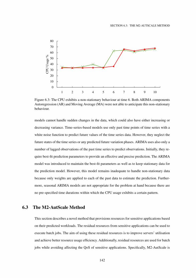
SECTION 6.3: THE M2-AUTSCALE METHOD
0
10
20
30
40
50
60
70
80
1 2 3 4 5 6 7 8 9 10
CPU
Usa
ge %
Time (seconds)
CPU usage time series ARIMA's Prediction
Figure 6.3: The CPU exhibits a non-stationary behaviour at time 6. Both ARIMA components
Autoregression (AR) and Moving Average (MA) were not able to anticipate this non-stationary
behaviour.
models cannot handle sudden changes in the data, which could also have either increasing or
decreasing variance. Time-series-based models use only past time points of time series with a
white noise function to predict future values of the time series data. However, they neglect the
future states of the time series or any predicted future variation phases. ARIMA uses also only a
number of lagged observations of the past time series to predict observations. Initially, they re-
quire best-fit prediction parameters to provide an effective and precise prediction. The ARIMA
model was introduced to maintain the best-fit parameters as well as to keep stationary data for
the prediction model. However, this model remains inadequate to handle non-stationary data
because only weights are applied to each of the past data to estimate the prediction. Further-
more, seasonal ARIMA models are not appropriate for the problem at hand because there are
no pre-specified time durations within which the CPU usage exhibits a certain pattern.
6.3 The M2-AutScale Method
This section describes a novel method that provisions resources for sensitive applications based
on their predicted workloads. The residual resources from sensitive applications can be used to
execute batch jobs. The aim of using these residual resources is to improve servers’ utilisation
and achieve better resource usage efficiency. Additionally, residual resources are used for batch
jobs while avoiding affecting the QoS of sensitive applications. Specifically, M2-AutScale is
142
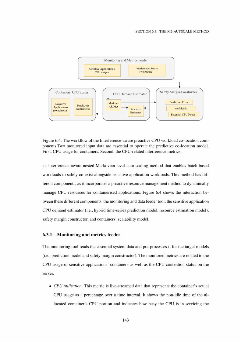
SECTION 6.3: THE M2-AUTSCALE METHOD
SafetyMarginConstructor
PredictionError
weiMetric
EssentialCPUNeeds
CPUDemandEstimator
ResourceEstimator
Markov-ARIMA
MonitoringandMetricsFeeder
SensitiveApplicationsCPUusages
Interference-Aware(weiMetric)
Containers'CPUScaler
SensitiveApplications(containers)
BatchJobs(containers)
Figure 6.4: The workflow of the Interference-aware proactive CPU workload co-location com-
ponents.Two monitored input data are essential to operate the predictive co-location model.
First, CPU usage for containers. Second, the CPU-related interference metrics.
an interference-aware nested-Markovian-level auto-scaling method that enables batch-based
workloads to safely co-exist alongside sensitive application workloads. This method has dif-
ferent components, as it incorporates a proactive resource management method to dynamically
manage CPU resources for containerised applications. Figure 6.4 shows the interaction be-
tween these different components: the monitoring and data feeder tool, the sensitive application
CPU demand estimator (i.e., hybrid time-series prediction model, resource estimation model),
safety margin constructor, and containers’ scalability model.
6.3.1 Monitoring and metrics feeder
The monitoring tool reads the essential system data and pre-processes it for the target models
(i.e., prediction model and safety margin constructor). The monitored metrics are related to the
CPU usage of sensitive applications’ containers as well as the CPU contention status on the
server.
• CPU utilisation. This metric is live-streamed data that represents the container’s actual
CPU usage as a percentage over a time interval. It shows the non-idle time of the al-
located container’s CPU portion and indicates how busy the CPU is in servicing the
143
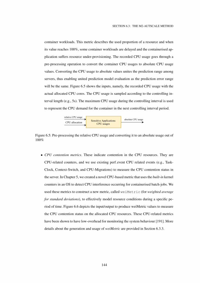
SECTION 6.3: THE M2-AUTSCALE METHOD
container workloads. This metric describes the used proportion of a resource and when
its value reaches 100%, some container workloads are delayed and the containerised ap-
plication suffers resource under-provisioning. The recorded CPU usage goes through a
pre-processing operation to convert the container CPU usages to absolute CPU usage
values. Converting the CPU usage to absolute values unites the prediction range among
servers, thus enabling united prediction model evaluation as the prediction error range
will be the same. Figure 6.5 shows the inputs, namely, the recorded CPU usage with the
actual allocated CPU cores. The CPU usage is sampled according to the controlling in-
terval length (e.g., 5s). The maximum CPU usage during the controlling interval is used
to represent the CPU demand for the container in the next controlling interval period.
absoluteCPUusagerelativeCPUusage
CPUallocation SensitiveApplicationsCPUusages
TCCS
CMweiMetricInterference-Aware
(weiMetric)
predictedCPUusage
CPUcoressafetymargin
requestedCPUCPUshare
ResourceEstimator
absoluteCPUusage
timeserieslevel
predictedCPUusagePredictionmodel
predictionerrorweiMetric
essentialCPUneeds
safetymarginSafetyMarginConstructor
Figure 6.5: Pre-processing the relative CPU usage and converting it to an absolute usage out of
100%
• CPU contention metrics. These indicate contention in the CPU resources. They are
CPU-related counters, and we use existing perf event CPU related events (e.g., Task-
Clock, Context-Switch, and CPU-Migrations) to measure the CPU contention status in
the server. In Chapter 5, we created a novel CPU-based metric that uses the built-in kernel
counters in an OS to detect CPU interference occurring for containerised batch-jobs. We
used these metrics to construct a new metric, called weiMetric (for weighted average
for standard deviations), to effectively model resource conditions during a specific pe-
riod of time. Figure 6.6 depicts the input/output to produce weiMetric values to measure
the CPU contention status on the allocated CPU resources. These CPU-related metrics
have been shown to have low-overhead for monitoring the system behaviour [191]. More
details about the generation and usage of weiMetric are provided in Section 6.3.3.
144
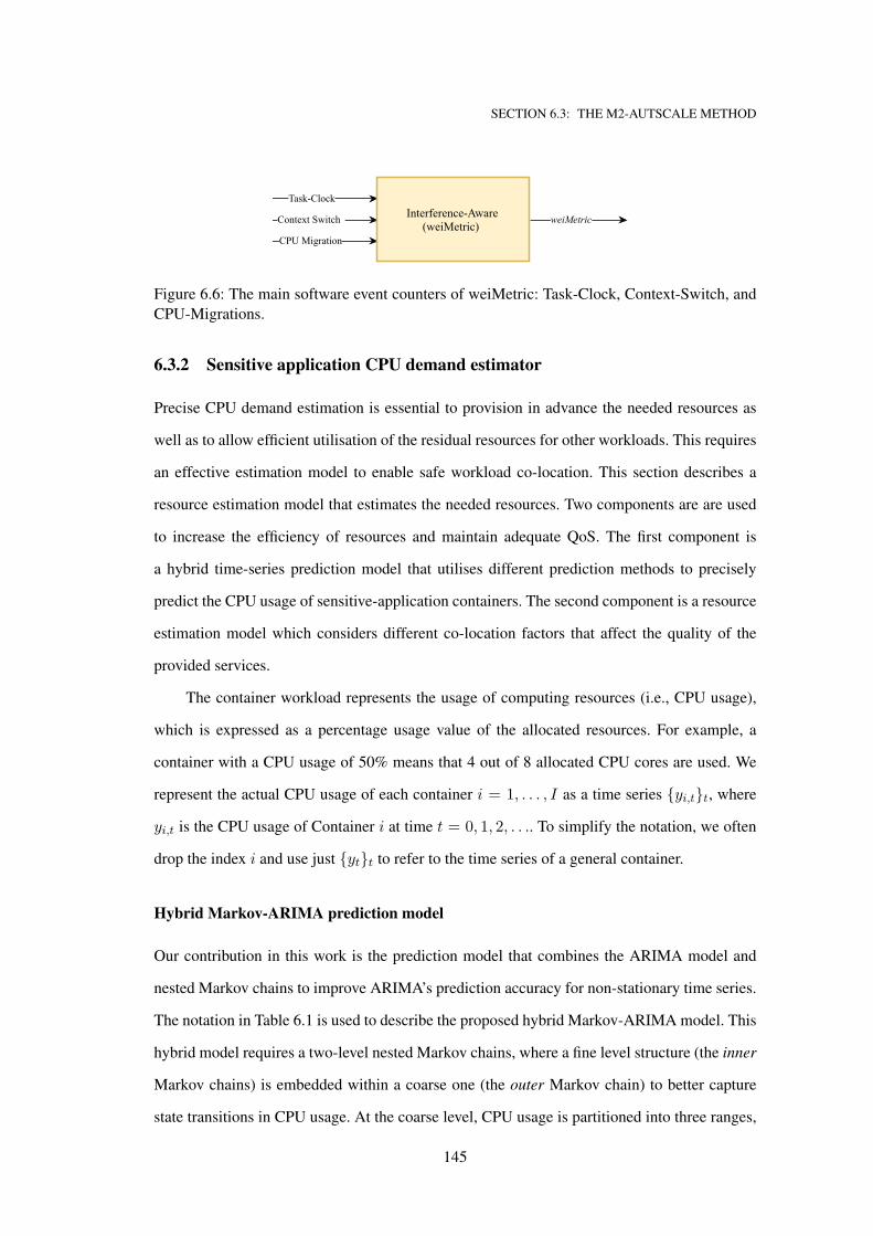
SECTION 6.3: THE M2-AUTSCALE METHODabsoluteCPUusage
relativeCPUusage
CPUallocation SensitiveApplicationsCPUusages
Task-Clock
ContextSwitch
CPUMigration
weiMetricInterference-Aware(weiMetric)
predictedCPUusage
CPUcoressafetymargin
requestedCPUCPUshare
ResourceEstimator
absoluteCPUusage
timeserieslevel
predictedCPUusagePredictionmodel
predictionerrorweiMetric
essentialCPUneeds
safetymarginSafetyMarginConstructor
Figure 6.6: The main software event counters of weiMetric: Task-Clock, Context-Switch, and
CPU-Migrations.
6.3.2 Sensitive application CPU demand estimator
Precise CPU demand estimation is essential to provision in advance the needed resources as
well as to allow efficient utilisation of the residual resources for other workloads. This requires
an effective estimation model to enable safe workload co-location. This section describes a
resource estimation model that estimates the needed resources. Two components are are used
to increase the efficiency of resources and maintain adequate QoS. The first component is
a hybrid time-series prediction model that utilises different prediction methods to precisely
predict the CPU usage of sensitive-application containers. The second component is a resource
estimation model which considers different co-location factors that affect the quality of the
provided services.
The container workload represents the usage of computing resources (i.e., CPU usage),
which is expressed as a percentage usage value of the allocated resources. For example, a
container with a CPU usage of 50% means that 4 out of 8 allocated CPU cores are used. We
represent the actual CPU usage of each container i = 1, . . . , I as a time series {yi,t}t, where
yi,t is the CPU usage of Container i at time t = 0, 1, 2, . . .. To simplify the notation, we often
drop the index i and use just {yt}t to refer to the time series of a general container.
Hybrid Markov-ARIMA prediction model
Our contribution in this work is the prediction model that combines the ARIMA model and
nested Markov chains to improve ARIMA’s prediction accuracy for non-stationary time series.
The notation in Table 6.1 is used to describe the proposed hybrid Markov-ARIMA model. This
hybrid model requires a two-level nested Markov chains, where a fine level structure (the inner
Markov chains) is embedded within a coarse one (the outer Markov chain) to better capture
state transitions in CPU usage. At the coarse level, CPU usage is partitioned into three ranges,
145
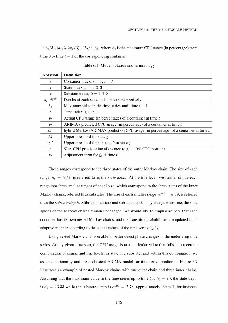
SECTION 6.3: THE M2-AUTSCALE METHOD
[0, ht/3), [ht/3, 2ht/3), [2ht/3, ht], where ht is the maximum CPU usage (in percentage) from
time 0 to time t− 1 of the corresponding container.
Table 6.1: Model notation and terminology
Notation Definition
i Container index, i = 1, . . . , I
j State index, j = 1, 2, 3
k Substate index, k = 1, 2, 3
dt, dsubt Depths of each state and substate, respectively
ht Maximum value in the time series until time t− 1
t Time index 0, 1, 2, . . .
yt Actual CPU usage (in percentage) of a container at time t
yt ARIMA’s predicted CPU usage (in percentage) of a container at time t
mt hybrid Markov-ARIMA’s prediction CPU usage (in percentage) of a container at time t
hjt Upper threshold for state j
rj,kt Upper threshold for substate k in state j
p SLA CPU provisioning allowance (e.g, ±10% CPU portion)
νt Adjustment term for yt at time t
These ranges correspond to the three states of the outer Markov chain. The size of each
range, dt = ht/3, is referred to as the state depth. At the fine level, we further divide each
range into three smaller ranges of equal size, which correspond to the three states of the inner
Markov chains, referred to as substates. The size of each smaller range, dsubt = ht/9, is referred
to as the substate depth. Although the state and substate depths may change over time, the state
spaces of the Markov chains remain unchanged. We would like to emphasise here that each
container has its own nested Markov chains, and the transition probabilities are updated in an
adaptive manner according to the actual values of the time series {yt}t.
Using nested Markov chains enable to better detect phase changes in the underlying time
series. At any given time step, the CPU usage is at a particular value that falls into a certain
combination of coarse and fine levels, or state and substate; and within this combination, we
assume stationarity and use a classical ARIMA model for time series prediction. Figure 6.7
illustrates an example of nested Markov chains with one outer chain and three inner chains.
Assuming that the maximum value in the time series up to time t is ht = 70, the state depth
is dt = 23.33 while the substate depth is dsubt = 7.78, approximately. State 1, for instance,
146
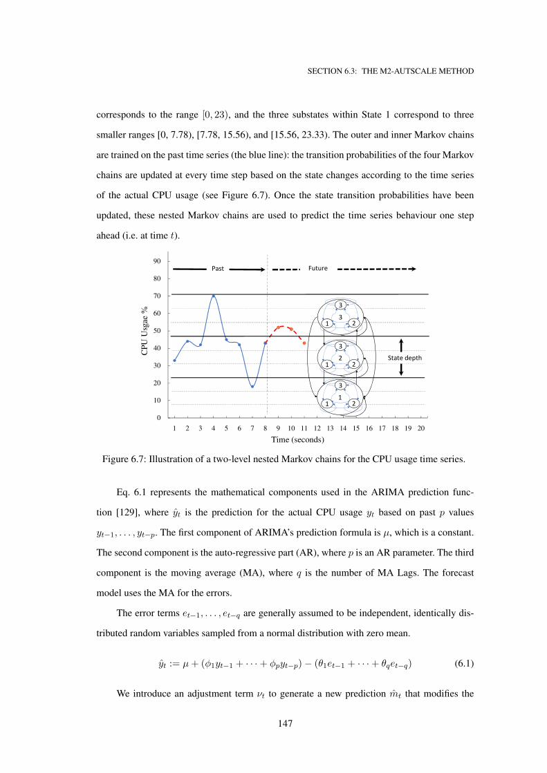
SECTION 6.3: THE M2-AUTSCALE METHOD
corresponds to the range [0, 23), and the three substates within State 1 correspond to three
smaller ranges [0, 7.78), [7.78, 15.56), and [15.56, 23.33). The outer and inner Markov chains
are trained on the past time series (the blue line): the transition probabilities of the four Markov
chains are updated at every time step based on the state changes according to the time series
of the actual CPU usage (see Figure 6.7). Once the state transition probabilities have been
updated, these nested Markov chains are used to predict the time series behaviour one step
ahead (i.e. at time t).
0
10
20
30
40
50
60
70
80
90
100
1 2 3 4 5 6 7 8 9 10 11 12 13 14 15 16 17 18 19 20
CPU
Usg
ae %
Time (seconds)
3
2
1
1 2
3
1 2
3
1 2
3
State depth
Past Future
Figure 6.7: Illustration of a two-level nested Markov chains for the CPU usage time series.
Eq. 6.1 represents the mathematical components used in the ARIMA prediction func-
tion [129], where yt is the prediction for the actual CPU usage yt based on past p values
yt−1, . . . , yt−p. The first component of ARIMA’s prediction formula is µ, which is a constant.
The second component is the auto-regressive part (AR), where p is an AR parameter. The third
component is the moving average (MA), where q is the number of MA Lags. The forecast
model uses the MA for the errors.
The error terms et−1, . . . , et−q are generally assumed to be independent, identically dis-
tributed random variables sampled from a normal distribution with zero mean.
yt := µ+ (φ1yt−1 + · · ·+ φpyt−p)− (θ1et−1 + · · ·+ θqet−q) (6.1)
We introduce an adjustment term νt to generate a new prediction mt that modifies the
147
SECTION 6.3: THE M2-AUTSCALE METHOD
original prediction of ARIMA as in Eq. 6.2. This modification makes ARIMA capable of de-
tecting the state transition of the time series.
mt := (1 + νt)yt. (6.2)
We discuss below the computation of νt based on the nested Markov chains. First, the
nested Markov chains predict the next state jt and substate kt for the time series at time t.
Then, the value of νt is computed as the numerical difference between the quantile of the
upper threshold rjt−1,kt−1= (jt−1−1)ht/3+kt−1ht/9 of the latest substate kt−1 in state jt−1
at time t − 1 and the quantile of the upper threshold rjt,kt
= (jt − 1)ht/3 + ktht/9 of the
predicted substate kt in state jt.
νt := Q(rjt,kt
)−Q(rjt−1,kt−1) =
rjt,kt
ht−
rjt−1,kt−1
ht. (6.3)
We now explain the meaning of Eq. 6.3. There are two scenarios.
• Scenario 1. The predicted state and substate at time t are the same as the true state and
substate at time t− 1, that is (jt, kt) = (jt−1, kt−1). This means that the nested Markov
chains predict that the time series {yt} remains stable from time t − 1 to time t. In this
case, rjt,kt
= rjt−1,kt−1, which implies that νt = 0, and hence, mt = yt. There is no
change to the ARIMA’s prediction.
• Scenario 2. The predicted state and substate at time t are not the same as the true state
and substate at time t − 1, that is (jt, kt) 6= (jt−1, kt−1). This means that the nested
Markov chains predict that the time series {yt} experiences a non-stationary behaviour
from time t − 1 to time t. In this case, we need to adjust the ARIMA’s prediction yt by
an amount of νtyt. If rjt,kt
> rjt−1,kt−1, or νt > 0, which means that the nested Markov
chain predict an increase in the CPU usage yt compared to yt−1, and we need to scale up
ARIMA’s prediction to obtain mt = (1 + νt)yt > yt. If rjt,kt
< rjt−1,kt−1, i.e. νt < 0,
then we need to scale down yt using the same equation.
The different steps of the proposed hybrid Markov-ARIMA prediction model are shown
in Algorithm 5, and lets elaborate further on on this algorithm using Figure 6.8 and Table 6.2.
148
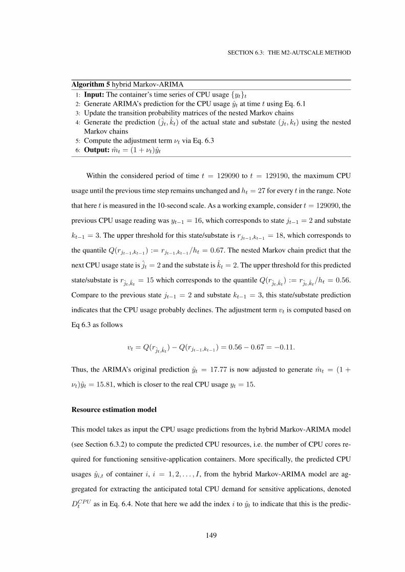
SECTION 6.3: THE M2-AUTSCALE METHOD
Algorithm 5 hybrid Markov-ARIMA
1: Input: The container’s time series of CPU usage {yt}t2: Generate ARIMA’s prediction for the CPU usage yt at time t using Eq. 6.1
3: Update the transition probability matrices of the nested Markov chains
4: Generate the prediction (jt, kt) of the actual state and substate (jt, kt) using the nested
Markov chains
5: Compute the adjustment term νt via Eq. 6.3
6: Output: mt = (1 + νt)yt
Within the considered period of time t = 129090 to t = 129190, the maximum CPU
usage until the previous time step remains unchanged and ht = 27 for every t in the range. Note
that here t is measured in the 10-second scale. As a working example, consider t = 129090, the
previous CPU usage reading was yt−1 = 16, which corresponds to state jt−1 = 2 and substate
kt−1 = 3. The upper threshold for this state/substate is rjt−1,kt−1= 18, which corresponds to
the quantile Q(rjt−1,kt−1) := rjt−1,kt−1
/ht = 0.67. The nested Markov chain predict that the
next CPU usage state is jt = 2 and the substate is kt = 2. The upper threshold for this predicted
state/substate is rjt,kt
= 15 which corresponds to the quantile Q(rjt,kt
) := rjt,kt
/ht = 0.56.
Compare to the previous state jt−1 = 2 and substate kt−1 = 3, this state/substate prediction
indicates that the CPU usage probably declines. The adjustment term vt is computed based on
Eq 6.3 as follows
vt = Q(rjt,kt
)−Q(rjt−1,kt−1) = 0.56− 0.67 = −0.11.
Thus, the ARIMA’s original prediction yt = 17.77 is now adjusted to generate mt = (1 +
νt)yt = 15.81, which is closer to the real CPU usage yt = 15.
Resource estimation model
This model takes as input the CPU usage predictions from the hybrid Markov-ARIMA model
(see Section 6.3.2) to compute the predicted CPU resources, i.e. the number of CPU cores re-
quired for functioning sensitive-application containers. More specifically, the predicted CPU
usages yi,t of container i, i = 1, 2, . . . , I , from the hybrid Markov-ARIMA model are ag-
gregated for extracting the anticipated total CPU demand for sensitive applications, denoted
DCPUt as in Eq. 6.4. Note that here we add the index i to yt to indicate that this is the predic-
149
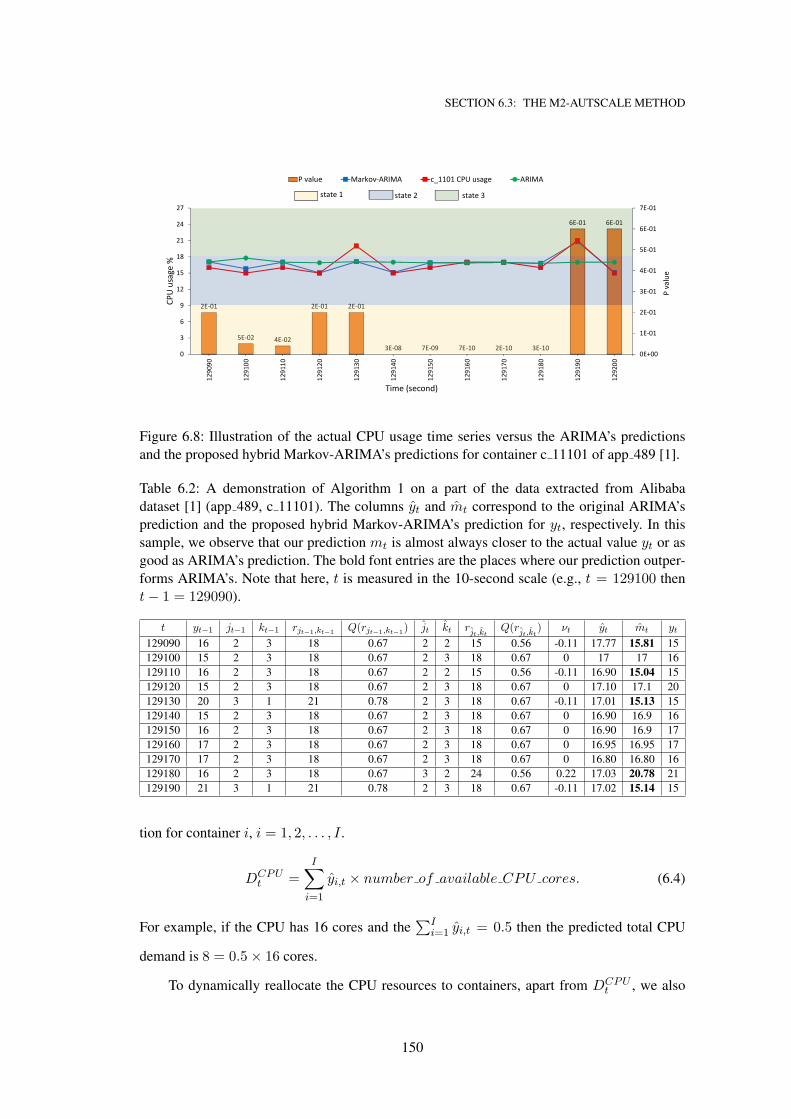
SECTION 6.3: THE M2-AUTSCALE METHOD
2E-01
5E-02 4E-02
2E-01 2E-01
3E-08 7E-09 7E-10 2E-10 3E-10
6E-01 6E-01
0E+00
1E-01
2E-01
3E-01
4E-01
5E-01
6E-01
7E-01
0
3
6
9
12
15
18
21
24
2712
9090
1291
00
1291
10
1291
20
1291
30
1291
40
1291
50
1291
60
1291
70
1291
80
1291
90
1292
00
CPU
usag
e %
Time (second)
P value Markov-ARIMA c_1101 CPU usage ARIMA
state 3state 2state 1
Pva
lue
Figure 6.8: Illustration of the actual CPU usage time series versus the ARIMA’s predictions
and the proposed hybrid Markov-ARIMA’s predictions for container c 11101 of app 489 [1].
Table 6.2: A demonstration of Algorithm 1 on a part of the data extracted from Alibaba
dataset [1] (app 489, c 11101). The columns yt and mt correspond to the original ARIMA’s
prediction and the proposed hybrid Markov-ARIMA’s prediction for yt, respectively. In this
sample, we observe that our prediction mt is almost always closer to the actual value yt or as
good as ARIMA’s prediction. The bold font entries are the places where our prediction outper-
forms ARIMA’s. Note that here, t is measured in the 10-second scale (e.g., t = 129100 then
t− 1 = 129090).
t yt−1 jt−1 kt−1 rjt−1,kt−1Q(rjt−1,kt−1
) jt kt rjt,kt
Q(rjt,kt
) νt yt mt yt
129090 16 2 3 18 0.67 2 2 15 0.56 -0.11 17.77 15.81 15
129100 15 2 3 18 0.67 2 3 18 0.67 0 17 17 16
129110 16 2 3 18 0.67 2 2 15 0.56 -0.11 16.90 15.04 15
129120 15 2 3 18 0.67 2 3 18 0.67 0 17.10 17.1 20
129130 20 3 1 21 0.78 2 3 18 0.67 -0.11 17.01 15.13 15
129140 15 2 3 18 0.67 2 3 18 0.67 0 16.90 16.9 16
129150 16 2 3 18 0.67 2 3 18 0.67 0 16.90 16.9 17
129160 17 2 3 18 0.67 2 3 18 0.67 0 16.95 16.95 17
129170 17 2 3 18 0.67 2 3 18 0.67 0 16.80 16.80 16
129180 16 2 3 18 0.67 3 2 24 0.56 0.22 17.03 20.78 21
129190 21 3 1 21 0.78 2 3 18 0.67 -0.11 17.02 15.14 15
tion for container i, i = 1, 2, . . . , I .
DCPUt =
I∑
i=1
yi,t × number of available CPU cores. (6.4)
For example, if the CPU has 16 cores and the∑I
i=1 yi,t = 0.5 then the predicted total CPU
demand is 8 = 0.5× 16 cores.
To dynamically reallocate the CPU resources to containers, apart from DCPUt , we also
150
SECTION 6.3: THE M2-AUTSCALE METHOD
need to compute the portion of CPU resources requested by each container as follows.
sharesi,t =reqi,t
∑Ii=1 reqi,t
, (6.5)
where reqi,t is the CPU resources requested at time t by container i. However, to avoid resource
under-provisioning, we also need to create backup resources (e.g., emergency resources) to
handle unpredictable workloads for sensitive applications. Therefore, we propose to create a
safety margin that helps to handle unpredictable workloads when such a sensitive-application
container begins consuming resources more than what it was predicted to.
6.3.3 Safety margin constructor
This section explais how to construct the safety margin using the weiMetric. We create safety
resources to reduce the impact of bursty workloads that occur occasionally. Different factors
impact the size of this safety margin. The first factor is the contention in the server. The
higher the contention in the CPU, the larger the margin will be. To measure the contention
in the CPU, we use the CPU interference metric weiMetric to sample the interference on the
server. We measure weiMetric at each time t by monitoring the server’s performance using
perf event [191]. This tool outputs the basic software event counters, i.e. Task-Clock (TC),
CPU-Migrations (CM), and Context-Switch (CS), which are used to compute weiMetric that
created in Chapter 5.
We now discuss in detail how to generate and use the weiMetric. Note that we create
different weiMetrics for different containers. Also, the sampling interval (e.g. five seconds) for
weiMetrics can be set by the user. For each container, let TCt denotes the job clock value at
time t = 0, 1, 2, . . .. For a sliding window of size W (e.g., W = 20), we use σTC([t−W+1, t])
to denote the standard deviation of the set {TCs : t−W + 1 ≤ s ≤ t}. Similar notations can
be defined for the context switch (CS) and CPU Migrations counters (CM). Let At, Bt, and Ct
denote the weighted average of the standard deviations for TC, CS, and CM, respectively (see
Eqs. (6.6), (6.7), (6.8)).
At =σTC([t−W + 1, t])
∑ts=t−W+1 σTC([s−W + 1, s])
, (6.6)
Bt =σCS([t−W + 1, t])
∑ts=t−W+1 σCS([s−W + 1, s])
, (6.7)
151
SECTION 6.3: THE M2-AUTSCALE METHOD
Ct =σCM ([t−W + 1, t])
∑ts=t−W+1 σCM ([s−W + 1, s])
. (6.8)
The weiMetric for the corresponding container is defined to be the average of these three quan-
tities
weiMetrict :=At +Bt + Ct
3.
The weiMetric is then linearly transformed into the normalised value f1 using the Min-Max
normalisation method as follows.
f1t =weiMetrict −min
max−min,
where max and min are the maximum and minimum values recorded for weiMetric when we
performed some test experiments to obtain some estimates for the metric. Note that f1t may
occasionally get larger than one.
The second factor is the prediction errors for CPU usage. The average root mean square
error (RMSE) is used to determine the size of the safety margin. Eq. 6.9 is used to compute the
average RMSE for each container in the server.
f2t =
√
√
√
√
(yt − yt)2∑t
t−W (ys−ys)2
W
(6.9)
The third factor is a constant value c that is estimated by the user. It shows the essential
workloads to operate the server operating system and the scalability model. The overheads of
these operations are estimated for adding this estimated value of c.
These three factors are averaged to create a safety margin for CPU resources that helps to
avoid SLA violations.
smt =f1t + f2t + c
3, (6.10)
The derived above smt ratio is used to compute the CPU emergency resources ERCPUt .
This emergency resources is added to the predicted CPU demand DCPUt which they are later
are used to be allocated for containers.
ERCPUt = smt × number of available CPU cores. (6.11)
152
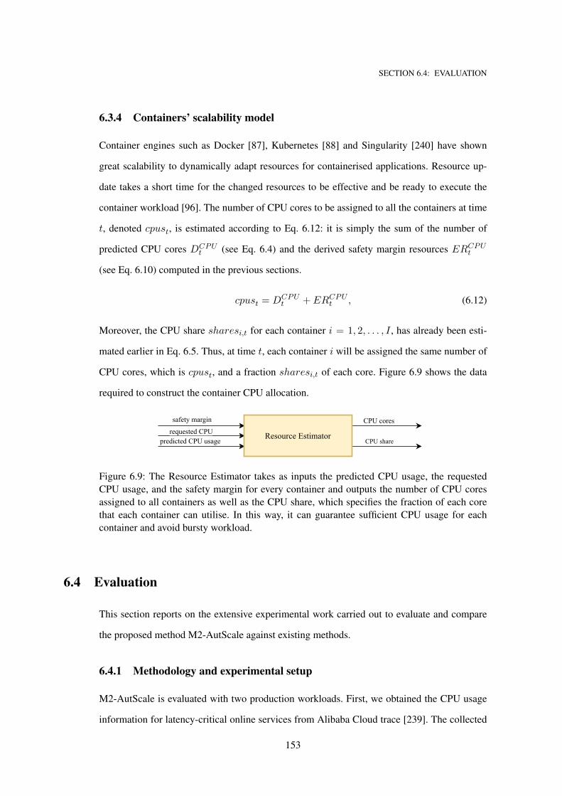
SECTION 6.4: EVALUATION
6.3.4 Containers’ scalability model
Container engines such as Docker [87], Kubernetes [88] and Singularity [240] have shown
great scalability to dynamically adapt resources for containerised applications. Resource up-
date takes a short time for the changed resources to be effective and be ready to execute the
container workload [96]. The number of CPU cores to be assigned to all the containers at time
t, denoted cpust, is estimated according to Eq. 6.12: it is simply the sum of the number of
predicted CPU cores DCPUt (see Eq. 6.4) and the derived safety margin resources ERCPU
t
(see Eq. 6.10) computed in the previous sections.
cpust = DCPUt + ERCPU
t , (6.12)
Moreover, the CPU share sharesi,t for each container i = 1, 2, . . . , I , has already been esti-
mated earlier in Eq. 6.5. Thus, at time t, each container i will be assigned the same number of
CPU cores, which is cpust, and a fraction sharesi,t of each core. Figure 6.9 shows the data
required to construct the container CPU allocation.
absoluteCPUusagerelativeCPUusage
CPUallocation SensitiveApplicationsCPUusages
TCCS
CMweiMetricInterference-Aware
(weiMetric)
predictedCPUusage
CPUcoressafetymargin
requestedCPUCPUshare
ResourceEstimator
absoluteCPUusage
timeserieslevel
predictedCPUusagePredictionmodel
predictionerrorweiMetric
essentialCPUneeds
safetymarginSafetyMarginConstructor
Figure 6.9: The Resource Estimator takes as inputs the predicted CPU usage, the requested
CPU usage, and the safety margin for every container and outputs the number of CPU cores
assigned to all containers as well as the CPU share, which specifies the fraction of each core
that each container can utilise. In this way, it can guarantee sufficient CPU usage for each
container and avoid bursty workload.
6.4 Evaluation
This section reports on the extensive experimental work carried out to evaluate and compare
the proposed method M2-AutScale against existing methods.
6.4.1 Methodology and experimental setup
M2-AutScale is evaluated with two production workloads. First, we obtained the CPU usage
information for latency-critical online services from Alibaba Cloud trace [239]. The collected
153
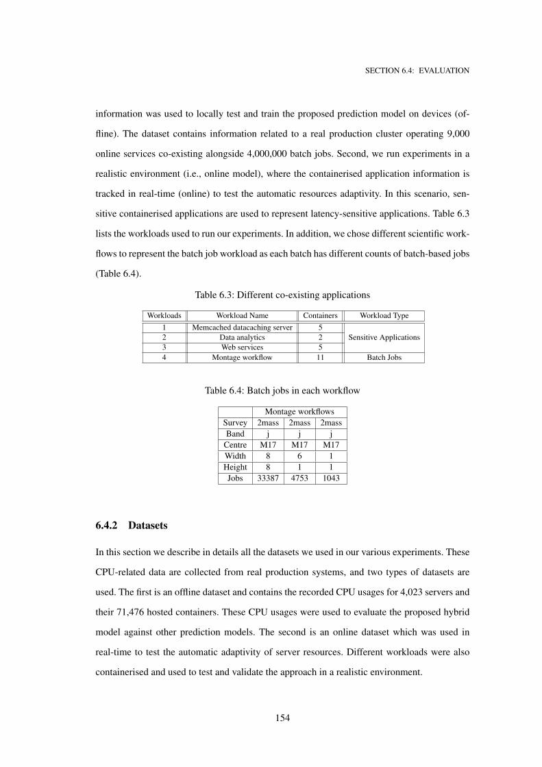
SECTION 6.4: EVALUATION
information was used to locally test and train the proposed prediction model on devices (of-
fline). The dataset contains information related to a real production cluster operating 9,000
online services co-existing alongside 4,000,000 batch jobs. Second, we run experiments in a
realistic environment (i.e., online model), where the containerised application information is
tracked in real-time (online) to test the automatic resources adaptivity. In this scenario, sen-
sitive containerised applications are used to represent latency-sensitive applications. Table 6.3
lists the workloads used to run our experiments. In addition, we chose different scientific work-
flows to represent the batch job workload as each batch has different counts of batch-based jobs
(Table 6.4).
Table 6.3: Different co-existing applications
Workloads Workload Name Containers Workload Type
1 Memcached datacaching server 5
Sensitive Applications2 Data analytics 2
3 Web services 5
4 Montage workflow 11 Batch Jobs
Table 6.4: Batch jobs in each workflow
Montage workflows
Survey 2mass 2mass 2mass
Band j j j
Centre M17 M17 M17
Width 8 6 1
Height 8 1 1
Jobs 33387 4753 1043
6.4.2 Datasets
In this section we describe in details all the datasets we used in our various experiments. These
CPU-related data are collected from real production systems, and two types of datasets are
used. The first is an offline dataset and contains the recorded CPU usages for 4,023 servers and
their 71,476 hosted containers. These CPU usages were used to evaluate the proposed hybrid
model against other prediction models. The second is an online dataset which was used in
real-time to test the automatic adaptivity of server resources. Different workloads were also
containerised and used to test and validate the approach in a realistic environment.
154
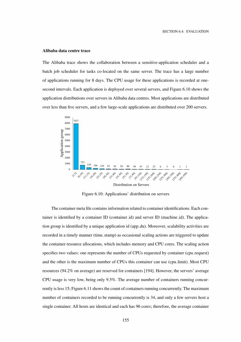
SECTION 6.4: EVALUATION
Alibaba data centre trace
The Alibaba trace shows the collaboration between a sensitive-application scheduler and a
batch job scheduler for tasks co-located on the same server. The trace has a large number
of applications running for 8 days. The CPU usage for these applications is recorded at one-
second intervals. Each application is deployed over several servers, and Figure 6.10 shows the
application distributions over servers in Alibaba data centres. Most applications are distributed
over less than five servers, and a few large-scale applications are distributed over 200 servers.
7927
752335 194 129 93 81 59 80 44 41 21 23 6 3 0 1 1
0
1000
2000
3000
4000
5000
6000
7000
8000
9000
App
licat
ion-
grou
p
Distribution on Servers
Figure 6.10: Applications’ distribution on servers
The container meta file contains information related to container identifications. Each con-
tainer is identified by a container ID (container id) and server ID (machine id). The applica-
tion group is identified by a unique application id (app du). Moreover, scalability activities are
recorded in a timely manner (time stamp) as occasional scaling actions are triggered to update
the container resource allocations, which includes memory and CPU cores. The scaling action
specifies two values: one represents the number of CPUs requested by container (cpu request)
and the other is the maximum number of CPUs this container can use (cpu limit). Most CPU
resources (94.2% on average) are reserved for containers [194]. However, the servers’ average
CPU usage is very low, being only 9.5%. The average number of containers running concur-
rently is less 15; Figure 6.11 shows the count of containers running concurrently. The maximum
number of containers recorded to be running concurrently is 34, and only a few servers host a
single container. All hosts are identical and each has 96 cores; therefore, the average container
155
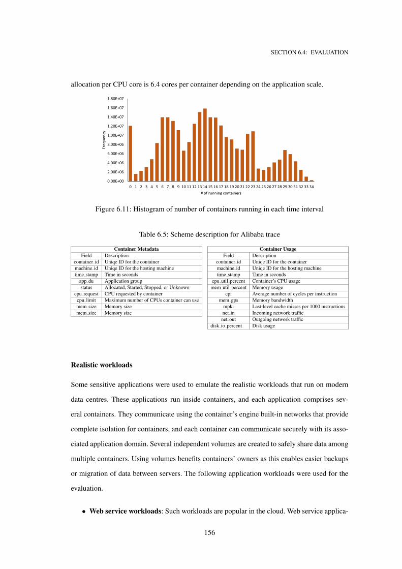
SECTION 6.4: EVALUATION
allocation per CPU core is 6.4 cores per container depending on the application scale.
0.00E+00
2.00E+06
4.00E+06
6.00E+06
8.00E+06
1.00E+07
1.20E+07
1.40E+07
1.60E+07
1.80E+07
0 1 2 3 4 5 6 7 8 9 10 11 12 13 14 15 16 17 18 19 20 21 22 23 24 25 26 27 28 29 30 31 32 33 34
Freq
uenc
y
# of running containers
Figure 6.11: Histogram of number of containers running in each time interval
Table 6.5: Scheme description for Alibaba trace
Container Metadata Container Usage
Field Description Field Description
container id Uniqe ID for the container container id Uniqe ID for the container
machine id Uniqe ID for the hosting machine machine id Uniqe ID for the hosting machine
time stamp Time in seconds time stamp Time in seconds
app du Application group cpu util percent Container’s CPU usage
status Allocated, Started, Stopped, or Unknown mem util percent Memory usage
cpu request CPU requested by container cpi Average number of cycles per instruction
cpu limit Maximum number of CPUs container can use mem gps Memory bandwidth
mem size Memory size mpki Last-level cache misses per 1000 instructions
mem size Memory size net in Incoming network traffic
net out Outgoing network traffic
disk io percent Disk usage
Realistic workloads
Some sensitive applications were used to emulate the realistic workloads that run on modern
data centres. These applications run inside containers, and each application comprises sev-
eral containers. They communicate using the container’s engine built-in networks that provide
complete isolation for containers, and each container can communicate securely with its asso-
ciated application domain. Several independent volumes are created to safely share data among
multiple containers. Using volumes benefits containers’ owners as this enables easier backups
or migration of data between servers. The following application workloads were used for the
evaluation.
• Web service workloads: Such workloads are popular in the cloud. Web service applica-
156
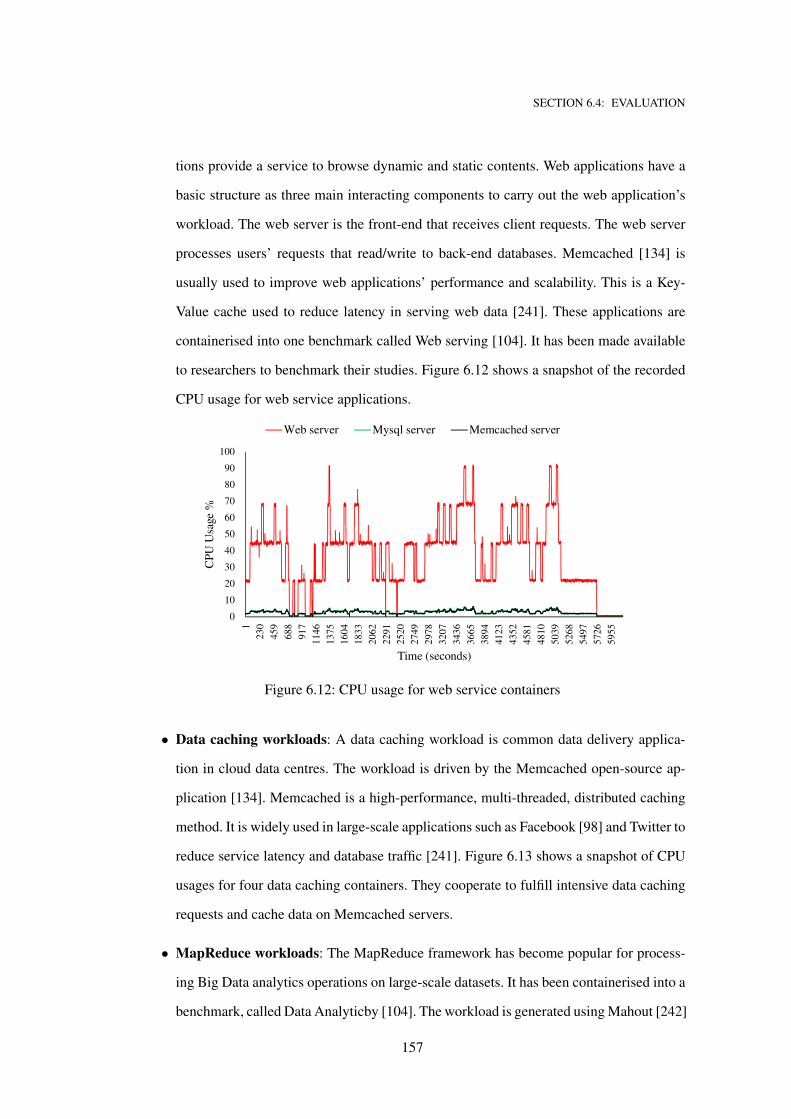
SECTION 6.4: EVALUATION
tions provide a service to browse dynamic and static contents. Web applications have a
basic structure as three main interacting components to carry out the web application’s
workload. The web server is the front-end that receives client requests. The web server
processes users’ requests that read/write to back-end databases. Memcached [134] is
usually used to improve web applications’ performance and scalability. This is a Key-
Value cache used to reduce latency in serving web data [241]. These applications are
containerised into one benchmark called Web serving [104]. It has been made available
to researchers to benchmark their studies. Figure 6.12 shows a snapshot of the recorded
CPU usage for web service applications.
0102030405060708090
100
123
045
968
891
711
4613
7516
0418
3320
6222
9125
2027
4929
7832
0734
3636
6538
9441
2343
5245
8148
1050
3952
6854
9757
2659
55
CPU
Usa
ge %
Time (seconds)
Web server Mysql server Memcached server
Figure 6.12: CPU usage for web service containers
• Data caching workloads: A data caching workload is common data delivery applica-
tion in cloud data centres. The workload is driven by the Memcached open-source ap-
plication [134]. Memcached is a high-performance, multi-threaded, distributed caching
method. It is widely used in large-scale applications such as Facebook [98] and Twitter to
reduce service latency and database traffic [241]. Figure 6.13 shows a snapshot of CPU
usages for four data caching containers. They cooperate to fulfill intensive data caching
requests and cache data on Memcached servers.
• MapReduce workloads: The MapReduce framework has become popular for process-
ing Big Data analytics operations on large-scale datasets. It has been containerised into a
benchmark, called Data Analyticby [104]. The workload is generated using Mahout [242]
157
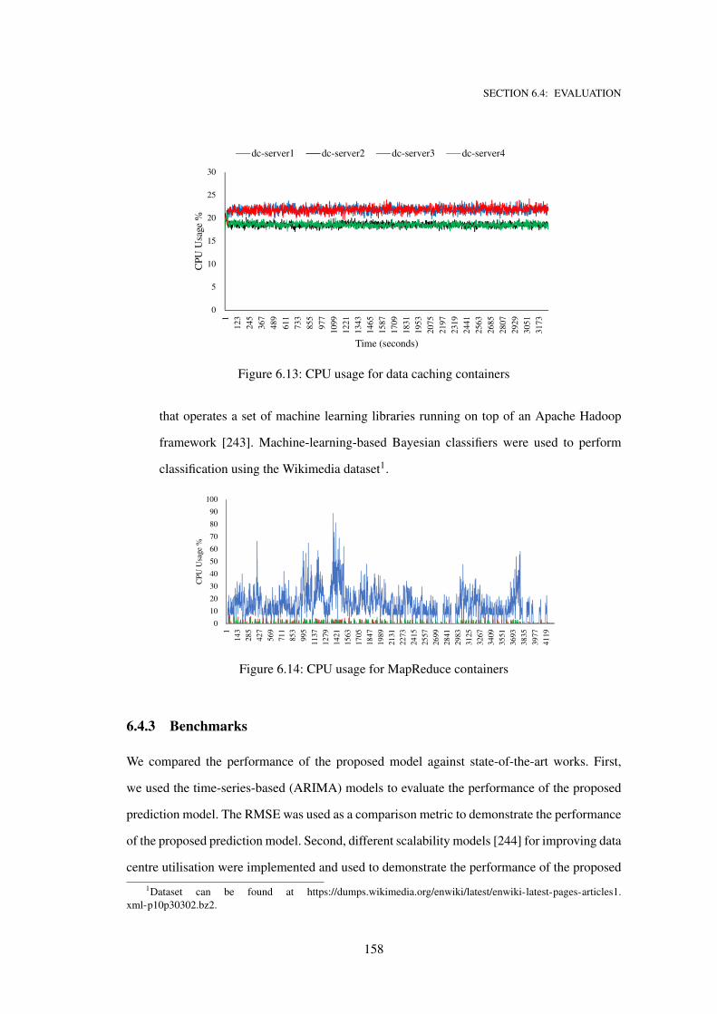
SECTION 6.4: EVALUATION
0
5
10
15
20
25
30
112
324
536
748
961
173
385
597
710
9912
2113
4314
6515
8717
0918
3119
5320
7521
9723
1924
4125
6326
8528
0729
2930
5131
73
CPU
Usa
ge %
Time (seconds)
dc-server1 dc-server2 dc-server3 dc-server4
Figure 6.13: CPU usage for data caching containers
that operates a set of machine learning libraries running on top of an Apache Hadoop
framework [243]. Machine-learning-based Bayesian classifiers were used to perform
classification using the Wikimedia dataset1.
0102030405060708090
100
114
328
542
756
971
185
399
511
3712
7914
2115
6317
0518
4719
8921
3122
7324
1525
5726
9928
4129
8331
2532
6734
0935
5136
9338
3539
7741
19
CPU
Usa
ge %
Time (seconds)
master slave01 slave02
Figure 6.14: CPU usage for MapReduce containers
6.4.3 Benchmarks
We compared the performance of the proposed model against state-of-the-art works. First,
we used the time-series-based (ARIMA) models to evaluate the performance of the proposed
prediction model. The RMSE was used as a comparison metric to demonstrate the performance
of the proposed prediction model. Second, different scalability models [244] for improving data
centre utilisation were implemented and used to demonstrate the performance of the proposed
1Dataset can be found at https://dumps.wikimedia.org/enwiki/latest/enwiki-latest-pages-articles1.
xml-p10p30302.bz2.
158
SECTION 6.4: EVALUATION
scalability model.
Bechmarked prediction models
The following prediction models were implemented and used to evaluate the proposed predic-
tion model using Alibaba’s dataset [239]:
• Random walk
• Linear trend estimation
• Quadratic trend
• Exponential smoothing
• Brown’s linear exponential smoothing
• Holt’s linear exponential smoothing
• Brown’s quadratic exponential smoothing
• ARIMA models
Benchmarked scalablity models
State-of-the-art predictive scaling has recently been made available in EC2 AWS data centres.
The data centre user (i.e., customer) can initiate auto-scaling plans and use at least one-day
historical data to predict demands. The basic principle of AWS EC2 predictive scaling is to
optimise resource usage at a specific value (e.g., 30% CPU usage). It adjusts the amount of
resources according to the dynamic resource usage prediction. It provisions enough resources
to maintain usage at the target user-specified value [244]. Different strategies are provided by
AWS, and we selected those related to cost and resource availability.
• Optimise for availability: The CPU average is kept under 40% and the auto-scaler opti-
mises it by proactively provisioning resources to maintain high availability and tackles
periodic traffic spikes [244].
159
SECTION 6.4: EVALUATION
• Optimise for cost (60% and 70%): Cost is a major concern in this strategy. It is related to
reducing the resource cost. It aims to boost the usage of shared servers while tolerating
some loss in application quality [244].
6.4.4 Experimental results
The conducted experiments are designed (1) to show the prediction accuracy of the proposed
prediction model, and (2) to evaluate the scalability of the proposed co-location method.
Results for the prediction models
We ran all listed prediction models together with our proposed one on the Alibaba dataset and
compare their performance with respect to the RSME. The hybrid Markov-ARIMA model pro-
duced the lowest RSME in all experiments. The improvement against the state-of-the-art (i.e.,
auto-ARIMA) was 4%–16%. The highest improvement, as expected, was recorded when the
time series presents high fluctuations. The web service (Figure 6.12) shows the highest fluc-
tuations among all workloads. The hybrid Markov-ARIMA model can detect the fluctuations
in the time series and imposes enhancements in the prediction. Figures 6.12, 6.15 and 6.16
show the RSME for different time series prediction models. The mean-based models produce
poor predictions, and the highest RSME was receded when using the constant estimation and
linear trend models. Note that in these figures, the depicted RSME are normalised against the
maximum RSME.
Results for the scalablity models
Figure 6.18 shows the aggregated CPU usages for sensitive applications and batch jobs when
using the M2-AutScale method. It also shows how this method interacts with sensitive-application
resources. It proactively throttles batch job containers’ CPU resources to let sensitive-application
containers use the CPU. The CPU usage for sensitive applications increases at second (159),
which creates an opportunity for using residual resources for batch jobs. However, as the batch
jobs would cause interference on existing running applications, a safety margin is strictly im-
posed to avoid unpredictable traffic spikes. Generally, the server’s CPU usage increases (up to
65%) as more batch jobs are pushed for execution. The safety margin is considered carefully
160
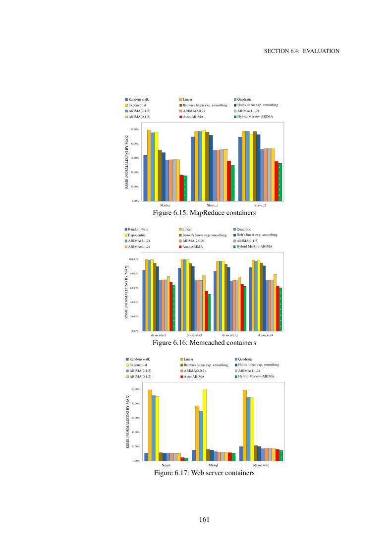
SECTION 6.4: EVALUATION
0.00%
20.00%
40.00%
60.00%
80.00%
100.00%
Master Slave_1 Slave_2
RS
ME
(N
OR
MA
LIZ
ING
BY
MA
X)
Random walk Linear
Exponential Brown's linear exp. smoothing
ARIMA(2,1,2) ARIMA(2,0,2)
ARIMA(0,1,2) Auto-ARIMA
Quadratic
Holt's linear exp. smoothing ARIMA(1,1,2)
Hybrid Markov-ARIMA
Figure 6.15: MapReduce containers
0.00%
20.00%
40.00%
60.00%
80.00%
100.00%
dc-server1 dc-server3 dc-server3 dc-server4
RS
ME
(N
OR
MA
LIZ
ING
BY
MA
X)
Random walk Linear
Exponential Brown's linear exp. smoothing
ARIMA(2,1,2) ARIMA(2,0,2)
ARIMA(0,1,2) Auto-ARIMA
Quadratic
Holt's linear exp. smoothing
ARIMA(1,1,2)
Hybrid Markov-ARIMA
Figure 6.16: Memcached containers
0.00%
20.00%
40.00%
60.00%
80.00%
100.00%
Nginx Mysql Memcache
RS
ME
(N
OR
MA
LIZ
ING
BY
MA
X)
Random walk Linear
Exponential Brown's linear exp. smoothing
ARIMA(2,1,2) ARIMA(2,0,2)
ARIMA(0,1,2) Auto-ARIMA
Quadratic
Holt's linear exp. smoothing ARIMA(1,1,2)
Hybrid Markov-ARIMA
Figure 6.17: Web server containers
161
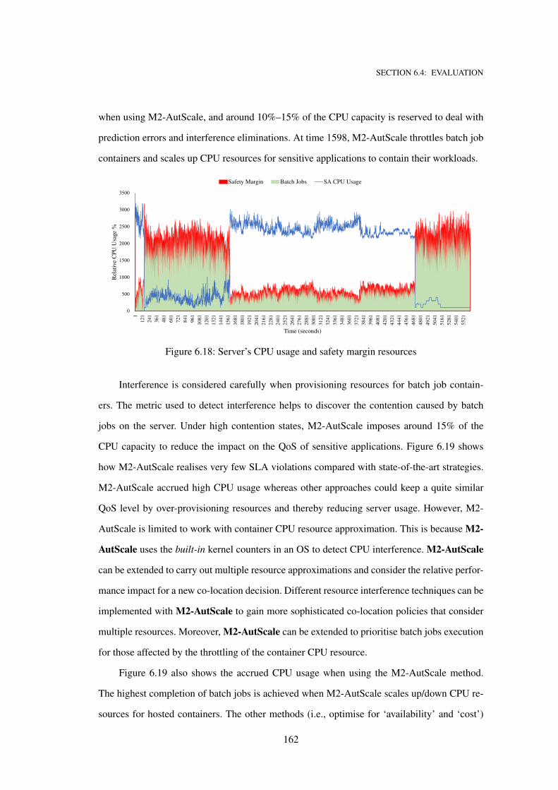
SECTION 6.4: EVALUATION
when using M2-AutScale, and around 10%–15% of the CPU capacity is reserved to deal with
prediction errors and interference eliminations. At time 1598, M2-AutScale throttles batch job
containers and scales up CPU resources for sensitive applications to contain their workloads.
0
500
1000
1500
2000
2500
3000
3500
112
124
136
148
160
172
184
196
110
8112
0113
2114
4115
6116
8118
0119
2120
4121
6122
8124
0125
2126
4127
6128
8130
0131
2132
4133
6134
8136
0137
2138
4139
6140
8142
0143
2144
4145
6146
8148
0149
2150
4151
6152
8154
0155
21
Rela
tive C
PU U
sage
%
Time (seconds)
Safety Margin Batch Jobs SA CPU Usage
Figure 6.18: Server’s CPU usage and safety margin resources
Interference is considered carefully when provisioning resources for batch job contain-
ers. The metric used to detect interference helps to discover the contention caused by batch
jobs on the server. Under high contention states, M2-AutScale imposes around 15% of the
CPU capacity to reduce the impact on the QoS of sensitive applications. Figure 6.19 shows
how M2-AutScale realises very few SLA violations compared with state-of-the-art strategies.
M2-AutScale accrued high CPU usage whereas other approaches could keep a quite similar
QoS level by over-provisioning resources and thereby reducing server usage. However, M2-
AutScale is limited to work with container CPU resource approximation. This is because M2-
AutScale uses the built-in kernel counters in an OS to detect CPU interference. M2-AutScale
can be extended to carry out multiple resource approximations and consider the relative perfor-
mance impact for a new co-location decision. Different resource interference techniques can be
implemented with M2-AutScale to gain more sophisticated co-location policies that consider
multiple resources. Moreover, M2-AutScale can be extended to prioritise batch jobs execution
for those affected by the throttling of the container CPU resource.
Figure 6.19 also shows the accrued CPU usage when using the M2-AutScale method.
The highest completion of batch jobs is achieved when M2-AutScale scales up/down CPU re-
sources for hosted containers. The other methods (i.e., optimise for ‘availability’ and ‘cost’)
162
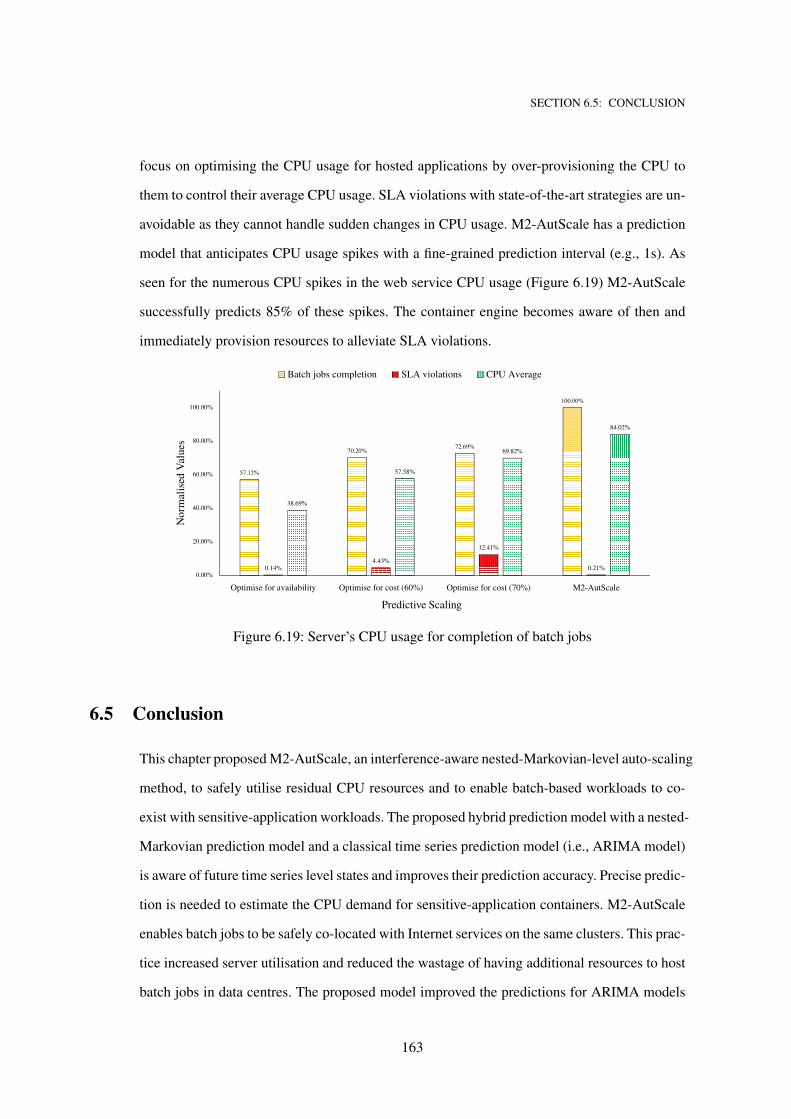
SECTION 6.5: CONCLUSION
focus on optimising the CPU usage for hosted applications by over-provisioning the CPU to
them to control their average CPU usage. SLA violations with state-of-the-art strategies are un-
avoidable as they cannot handle sudden changes in CPU usage. M2-AutScale has a prediction
model that anticipates CPU usage spikes with a fine-grained prediction interval (e.g., 1s). As
seen for the numerous CPU spikes in the web service CPU usage (Figure 6.19) M2-AutScale
successfully predicts 85% of these spikes. The container engine becomes aware of then and
immediately provision resources to alleviate SLA violations.
57.12%
70.20% 72.69%
100.00%
0.14%4.43%
12.41%
0.21%
38.69%
57.58%
69.82%
84.02%
0.00%
20.00%
40.00%
60.00%
80.00%
100.00%
Optimise for availability Optimise for cost (60%) Optimise for cost (70%) M2-AutScale
Nor
mal
ised
Valu
es
Predictive Scaling
Batch jobs completion SLA violations CPU Average
Figure 6.19: Server’s CPU usage for completion of batch jobs
6.5 Conclusion
This chapter proposed M2-AutScale, an interference-aware nested-Markovian-level auto-scaling
method, to safely utilise residual CPU resources and to enable batch-based workloads to co-
exist with sensitive-application workloads. The proposed hybrid prediction model with a nested-
Markovian prediction model and a classical time series prediction model (i.e., ARIMA model)
is aware of future time series level states and improves their prediction accuracy. Precise predic-
tion is needed to estimate the CPU demand for sensitive-application containers. M2-AutScale
enables batch jobs to be safely co-located with Internet services on the same clusters. This prac-
tice increased server utilisation and reduced the wastage of having additional resources to host
batch jobs in data centres. The proposed model improved the predictions for ARIMA models
163
SECTION 6.5: CONCLUSION
via the use of the nested-Markovian-level model. It achieved improved prediction accuracy and
reduced the RSME for the state-of-the-art (i.e., auto-ARIMA) to 4%–16%. The extensive ex-
periments carried out in this project showed that CPU resource usage can be improved by 30%
by proactively co-locating batch jobs in data centres compared with current predictive methods
used in AWS data centres.
164
CHAPTER 7Conclusion
This chapter summarises this study’s contributions to CPU resource management for container-
ised applications and identifies some future research directions to extend the proposed proactive
scalability techniques for different computing resources such as memory and I/O.
7.1 Summary
This thesis developed two novel hybrid prediction models and adopted a Markovian predic-
tion model to proactively manage the CPU provisioning for the hosted containers. Technically,
these prediction models administer the supplying of container CPU resources, with CPU re-
source managers enabled to make dynamic and proactive-sighted scaling decisions. The scal-
ing decision is generated regularly at short intervals (i.e., in the order of seconds) to dynami-
cally change the container CPU resources with negligible performance disruptions. According
to the required performance and SLA constraints, containerised applications in a data centre
were classified as follows: (1) Sensitive containerised applications. This often includes inter-
active applications such as social networking services. This type of application has strict QoS
and scalability requirements; Chapter 3 addresses these concerns. (2) Batch-based container-
ised applications. This includes workflows, which usually have constant workload patterns and
no direct interaction with users. Notably, such applications are less demanding than sensitive
containerised applications in terms of QoS. Therefore, the main concern considered for this
category is how to distribute the CPU computing power fairly between different containers;
165
SECTION 7.2: OVERALL CONTRIBUTIONS
Chapter 4 addresses this concern. As CPU interference is a major concern when dealing with
containers, Chapter 5 proposes weiMetric, a novel metric, that detects CPU interference and
supports the CPU scheduler. This allows the CPU manager to be aware of interference and
allocate adequate CPU portions to each container to minimise the effects of interference. In
Chapter 6, this metric is applied to maximise CPU utilisation in the data centre and to make
the CPU scheduler aware of CPU interference, thereby helping to avoid SLA violations and
increase the efficiency of the server by co-locating different containerised applications on the
same server.
7.2 Overall Contributions
This thesis focused on the problem of fine-grained CPU provisioning and sharing across mul-
tiple containerised applications. It developed several auto-scaling techniques, each of which
is suitable for a particular server workload co-location status. As mentioned in Section 1.4,
three co-location statuses were considered to deal with concerns over workload co-location.
Specifically, the following four research questions were addressed in this thesis:
1. How to efficiently estimate the CPU demand and proactively scale up/down only the
required CPU cores and frequency in an energy-efficient manner?
2. How is the CPU portion estimated and scaled up/down fairly between containers when
executing containerised scientific workflows?
3. How can CPU interference for virtualised resources be detected in the presence of noisy
neighbouring containers?
4. How can workload prediction be used by cloud providers to increase efficiency of CPU
resources and maximise CPU utilisation?
To efficiently estimate the CPU demand for sensitive containerised applications, Chapter 3
proposes an SLA-aware resource scaling approach. Chapter 3 experimentally investigates the
DVFS technique, which is commonly used by cloud providers to optimise both performance
166

SECTION 7.2: OVERALL CONTRIBUTIONS
and energy consumption for servers. The experiments conducted for testing the DVFS speci-
ficity on-demand governor found that this governor is aware of neither the predefined service
level objective (i.e., requests per second rps) nor the future workload. Further, it is a reactive
approach which over-provisions the CPU cores’ frequencies and wastes energy. To overcome
this issue, Chapter 3 proposes a novel hybrid workload prediction model based on ARIMA
time-series models and spectral fast Fourier transform (FFT) smoothing that co-operates to
anticipate CPU utilisation. The proposed prediction model dynamically adjusts the prediction
control horizon by smoothing the CPU utilisation time series and triggers the prediction func-
tion (i.e., ARIMA model) to estimate the near-future workload. Accordingly, a suitable plan
proactively manages the CPU resources (i.e., cores, frequency) to execute that predicted work-
load. The experimental results show that the proposed EBAS technique can successfully save
up to 14% energy on average compared with an on-demand Linux governor.
To estimate the fairer CPU portion for containerised scientific workflows, Chapter 4 devel-
ops the novel adCFS CPU sharing policy. This policy considers the future state of CPU usage
and proactively shares CPU cycles between various containers based on their corresponding
workload metrics (e.g., CPU usage, task runtime, #tasks). In the adCFS policy, the CPU utilisa-
tion is partitioned into three states, in which the transition between these states can be modelled
as a Markovian process. Therefore, a Markov chain prediction model is used to dynamically
derive and assign the appropriate CPU weight for containers. This prediction model can detect
the transition between the workflow tasks. It also predicts the CPU state occurrences, which
enables us to estimate the CPU state contention time. The Markov chain model can detect the
transition between the workflow tasks. Moreover, it predicts the occurrence and length of high
CPU contention states with 95%, 89%, and 79% accuracy rates for severe, cautious, and sta-
ble, respectively. Overall, the experimental results show a 12% enhancement in the container
response time compared to that of the default CFS policy.
To detect the CPU interference for virtualised resources, Chapter 5 proposes a time-series-
based method to detect the CPU interference. This method is based on weiMetric, a novel
CPU-based metric, that uses the built-in kernel counters in an OS to detect CPU interference
occurring during task execution. The proposed weiMetric works for both virtualised and non-
virtualised resources. weiMetric is designed to avoid the need to design additional software
167
SECTION 7.3: FUTURE RESEARCH DIRECTION
probes to track response times. Batch-based jobs (i.e., workflow tasks) are used, and a unique
time series is created for each task type. The proposed method in Chapter 5 is incorporated into
the adCFS policy designed previously in Chapter 4 to fairly share the CPU and alleviate internal
CPU interference between containers. Experiments on a real workflow system (i.e., Montage
workflow system) demonstrate the efficiency and accuracy of our method in detecting CPU
interference compared to existing works reported in literature. The experimental results show
that the proposed metric can detect CPU interferences with 98% accuracy in high-contention
states and save up to 6% CPU cycles when executing intensive workloads.
To increase the efficiency of CPU resources and maximise CPU utilisation, Chapter 6 pro-
poses M2-AutScale, a comprehensive new interference-aware, nested-Markovian-level auto-
scaling technique. This technique can safely utilise the residual CPU capacity that is left over
from sensitive containerised applications to proactively co-locate batch-based jobs. The proac-
tive CPU scaling decision is made by a novel hybrid prediction model that is made aware of
future time-series level states. Then, the proposed prediction model is used to precisely esti-
mate the CPU demand for sensitive-application containers. Overall, it achieves better predic-
tion accuracy. In particular, the RSME is 4%–16% lower on average compared with those of
state-of-the-art models (i.e., auto-ARIMA models). The extensive experiments conducted for
co-locating batch-based jobs with sensitive containerised applications show 30% improvement
in CPU resource usage compared with current predictive techniques used in AWS data centres.
7.3 Future Research Direction
We believe that the contributions of this thesis provide many future research directions for
achieving optimal integration and balance of energy usage in data centres.
7.3.1 Proactive auto-scaling for different computing resources
In this thesis, various proactive auto-scaling techniques were designed to manage the CPU re-
sources for containerised applications. However, they are limited to only working with CPU
resource (i.e., cores, frequency) scaling. We envision extending these proactive scaling tech-
niques to handle other types of cloud computing resources that consume a significant amount
168
SECTION 7.3: FUTURE RESEARCH DIRECTION
of energy. Specifically, memory and I/O resources consume a considerable portion of energy
in data centres [16]. Therefore, the future work aims to integrate the auto-scaling techniques
developed in this thesis to support memory and I/O resources scalability for containerised ap-
plications. This dynamic scalability would further optimise the energy consumption of cloud
data centres.
A comprehensive proactive auto-scaling technique that combines CPU, memory, and I/O
auto-scaling techniques into a holistic scaling model could achieve optimal energy efficiency
in cloud data centres. A holistic auto-scaling technique is needed because the hosted applica-
tion characteristic may change during the lifetime of the application owing to changes in the
workload characteristics. For example, some social media applications such as instant message
(IM) applications may need to provide push notifications to a client when such a message ar-
rives. These push notifications increase the number of connections to the server, which results
in memory demand. On the contrary, the application may have a search function to search
through the message history; in this case, the application uses the CPU to perform the search
function. This application requires the vertical scaling of all the computing resources asso-
ciated with the hosted VM (i.e., memory, CPU, I/O). Comprehensive scaling techniques are
needed to maintain minimal energy consumption in cloud data centres.
7.3.2 CPU sharing and interference categorisation
Chapter 5 introduced a new interference detection metric that can identify CPU interference
in a virtualised environment. The CPU interference between co-located containers is known to
impact both the QoS and the SLA objectives significantly. Therefore, further investigations can
be done in this area by using more advanced estimation techniques such as decision trees, sta-
tistical clustering, and machine learning to perform efficient interference-aware CPU workload
scheduling and container placement in data centres.
7.3.3 Harvest more types of computing resources
The workload co-location technique proposed in Chapter 6 proactively harvests residual CPU
resources from a sensitive application. These resources are eventually used to run batch-based
169

SECTION 7.3: FUTURE RESEARCH DIRECTION
jobs. Our technique provides a remarkable research direction to build different proactive har-
vest techniques to deal with different types of computing resources such as memory, disk,
and network bandwidth. For example, the harvesting technique may temporarily use a specific
disk space of a computing node to store data for batch-based jobs while the actual jobs might
be run on different computing nodes. Therefore, we need a co-ordination model to harvest
different computing resources (i.e., disk, network bandwidth, and CPU). The harvesting tech-
nique should be a well-designed technique that considers system reliability, energy efficiency,
and performance interference to efficiently utilise resources. This could be solved by utilising
deep-learning applications to deal with the complexity and heterogeneity of resources in the
cloud.
170
Bibliography
[1] Q. Liu and Z. Yu, “The elasticity and plasticity in semi-containerized co-locating cloud
workload: a view from alibaba trace,” in Proceedings of the 9th ACM Symposium on
Cloud Computing (SoCC), pp. 347–360, 2018.
[2] Y. Al-Dhuraibi, F. Paraiso, N. Djarallah, and P. Merle, “Elasticity in Cloud Computing:
State of the Art and Research Challenges,” IEEE Transactions on Services Computing
(TSC), vol. 11, no. 2, pp. 430–447, 2018.
[3] R. Buyya, S. N. Srirama, G. Casale, R. Calheiros, Y. Simmhan, B. Varghese, E. Gelenbe,
B. Javadi, L. M. Vaquero, M. A. Netto, A. N. Toosi, M. A. Rodriguez, I. M. Llorente,
S. De Capitani Di Vimercati, P. Samarati, D. Milojicic, C. Varela, R. Bahsoon, M. Dias
De Assuncao, O. Rana, W. Zhou, H. Jin, W. Gentzsch, A. Y. Zomaya, and H. Shen,
“A manifesto for future generation cloud computing: Research directions for the next
decade,” ACM Computing Surveys, vol. 51, no. 5, 2019.
[4] L. Duan, D. Zhan, and J. Hohnerlein, “Optimizing cloud data center energy efficiency
via dynamic prediction of cpu idle intervals,” in Proceedings of the 8th IEEE Interna-
tional Conference on Cloud Computing (CLOUD), pp. 985–988, 2015.
[5] S. Singh and I. Chana, “A survey on resource scheduling in cloud computing: Issues and
challenges,” Journal of Grid Computing, vol. 14, pp. 217–264, 2015.
[6] M. Mao and M. Humphrey, “A performance study on the vm startup time in the
cloud,” in Proceedings of the 5th IEEE International Conference on Cloud Computing
(CLOUD), pp. 423–430, 2012.
[7] “Aws auto scaling.” https://aws.amazon.com/autoscaling/. (Accessed on 12/01/2019).
171
SECTION 7.3: BIBLIOGRAPHY
[8] A. Fox, R. Griffith, A. Joseph, R. Katz, A. Konwinski, G. Lee, D. Patterson, A. Rabkin,
and I. Stoica, “Above the clouds: A berkeley view of cloud computing,” Dept. Electri-
cal Eng. and Comput. Sciences, University of California, Berkeley, Rep. UCB/EECS,
vol. 28, p. 13, 2009.
[9] P. Delforge, “America’s data centers consuming and wasting grow-
ing amounts of energy — nrdc.” https://www.nrdc.org/resources/
americas-data-centers-consuming-and-wasting-growing-amounts-energy, 2015.
(Accessed on 12/01/2019).
[10] P. Johnson and T. Marker, “Data centre energy efficiency product profile,” Pitt & Sherry,
report to equipment energy efficiency committee (E3) of The Australian Government
Department of the Environment, Water, Heritage and the Arts (DEWHA), 2009.
[11] A. Andrae and T. Edler, “On global electricity usage of communication technology:
trends to 2030,” Challenges, vol. 6, no. 1, pp. 117–157, 2015.
[12] J. Wilkes, “More Google cluster data.” Google research blog, 2011. Posted at http:
//googleresearch.blogspot.com/2011/11/more-google-cluster-data.html.
[13] E. Cortez, M. Russinovich, A. Bonde, M. Fontoura, A. Muzio, and R. Bianchini, “Re-
source Central: Understanding and Predicting Workloads for Improved Resource Man-
agement in Large Cloud Platforms?,” in Proceedings of the 26th ACM Symposium on
Operating Systems Principles (SOSP), 2017.
[14] C. Jiang, G. Han, J. Lin, G. Jia, W. Shi, and J. Wan, “Characteristics of Co-Allocated
Online Services and Batch Jobs in Internet Data Centers: A Case Study From Alibaba
Cloud,” IEEE Access, vol. 7, pp. 22495–22508, 2019.
[15] C. Reiss, A. Tumanov, G. R. Ganger, R. H. Katz, and M. A. Kozuch, “Heterogeneity and
dynamicity of clouds at scale: Google trace analysis,” in Proceedings of the 3rd ACM
Symposium on Cloud Computing (SOCC), p. 7, 2012.
[16] M. Dayarathna, Y. Wen, and R. Fan, “Data center energy consumption modeling: A
survey,” IEEE Communications Surveys and Tutorials, vol. 18, no. 1, pp. 732–794, 2016.
172
SECTION 7.3: BIBLIOGRAPHY
[17] L. Minas and B. Ellison, Energy efficiency for information technology: How to reduce
power consumption in servers and data centers. Intel Press, 2009.
[18] Z. Shen, S. Subbiah, X. Gu, and J. Wilkes, “Cloudscale: Elastic resource scaling for
multi-tenant cloud systems,” in Proceedings of the 2nd ACM Symposium on Cloud Com-
puting (SoCC), pp. 1–14, 2011.
[19] A. Ashraf, B. Byholm, and I. Porres, “Cramp: Cost-efficient resource allocation for mul-
tiple web applications with proactive scaling,” in Proceedings of the 4th IEEE Interna-
tional Conference on Cloud Computing Technology and Science (CloudCom), pp. 581–
586, 2012.
[20] R. Han, L. Guo, M. Ghanem, and Y. Guo, “Lightweight resource scaling for cloud ap-
plications,” in Proceedings of the 12th IEEE/ACM International Symposium on Cluster
Cloud and Grid Computing (CCGrid), pp. 644–651, 2012.
[21] H. Mi, H. Wang, G. Yin, Y. Zhou, D. Shi, and L. Yuan, “Online self-reconfiguration with
performance guarantee for energy-efficient large-scale cloud computing data centers,” in
IEEE International Conference on Services Computing (SCC), pp. 514–521, 2010.
[22] H. Engelbrecht and M. van Greunen, “Forecasting methods for cloud hosted resources,
a comparison,” in Proceedings of the 11th International Conference on Network and
Service Management (CNSM), pp. 29–35, 2015.
[23] J. J. Prevost, K. Nagothu, B. Kelley, and M. Jamshidi, “Prediction of cloud data center
networks loads using stochastic and neural models,” in Proceedings of the 6th Interna-
tional Conference on System of Systems Engineering (SoSE), pp. 276–281, 2011.
[24] M. Hadji and D. Zeghlache, “Minimum cost maximum flow algorithm for dynamic re-
source allocation in clouds,” in Proceedings of the 5th IEEE International Conference
on Cloud Computing (CLOUD), pp. 876–882, 2012.
[25] N. Roy, A. Dubey, and A. Gokhale, “Efficient autoscaling in the cloud using predictive
models for workload forecasting,” in Proceedings of the 4th IEEE International Confer-
ence on Cloud Computing (CLOUD), pp. 500–507, 2011.
173
SECTION 7.3: BIBLIOGRAPHY
[26] F. Wei, L. ZhiHui, W. Jie, and C. ZhenYin, “RPPS: A Novel Resource Prediction and
Provisioning Scheme in Cloud Data Center,” in Proceedings of the 9th IEEE Interna-
tional Conference on Services Computing (SCC), pp. 609–616, 2012.
[27] Z. Gong, X. Gu, and J. Wilkes, “Press: Predictive elastic resource scaling for cloud
systems,” in Proceedings of the International Conference on Network and Service Man-
agement (CNSM), pp. 9–16, 2010.
[28] M. Hasan, E. Magana, A. Clemm, L. Tucker, and S. Gudreddi, “Integrated and auto-
nomic cloud resource scaling,” in Proceedings of the IEEE Network Operations and
Management Symposium (NOMS), pp. 1327–1334, 2012.
[29] X. Dutreilh, N. Rivierre, A. Moreau, J. Malenfant, and I. Truck, “From data center re-
source allocation to control theory and back,” in Proceedings of the 3rd IEEE Interna-
tional Conference on Cloud Computing (CLOUD), pp. 410–417, 2010.
[30] X. Dutreilh, S. Kirgizov, O. Melekhova, J. Malenfant, N. Rivierre, and I. Truck, “Using
reinforcement learning for autonomic resource allocation in clouds: Towards a fully
automated workflow,” in Proceedings of the 7th International Conference on Autonomic
and Autonomous Systems (ICAS), pp. 67–74, 2011.
[31] J. Rao, X. Bu, C.-Z. Xu, L. Wang, and G. Yin, “Vconf: a reinforcement learning ap-
proach to virtual machines auto-configuration,” in Proceedings of the 6th international
conference on Autonomic computing, pp. 137–146, 2009.
[32] C.-Z. Xu, J. Rao, and X. Bu, “Url: A unified reinforcement learning approach for au-
tonomic cloud management,” Journal of Parallel and Distributed Computing, vol. 72,
no. 2, pp. 95 – 105, 2012.
[33] T. Lorido-Botran, J. Miguel-Alonso, and J. Lozano, “A review of auto-scaling tech-
niques for elastic applications in cloud environments,” Journal of Grid Computing,
vol. 12, no. 4, pp. 559–592, 2014.
174
SECTION 7.3: BIBLIOGRAPHY
[34] M. K. M. Murthy, H. A. Sanjay, and J. Anand, “Threshold based auto scaling of virtual
machines in cloud environment,” in Proceedings of the 11th International Conference
on Network and Parallel Computing (NPC), pp. 247–256, 2014.
[35] ASW, “Amazon cloudwatch - application and infrastructure monitoring.” https://aws.
amazon.com/cloudwatch/, 2019. (Accessed on 12/02/2019).
[36] A. Computing et al., “An architectural blueprint for autonomic computing,” IBM White
Paper, vol. 31, pp. 1–6, 2006.
[37] P. Koperek and W. Funika, “Dynamic business metrics-driven resource provisioning in
cloud environments,” in Proceedings of the 9th International Conference on Parallel
Processing and Applied Mathematics (PPAM), pp. 171–180, 2011.
[38] L. P. Kaelbling, M. L. Littman, and A. W. Moore, “Reinforcement learning: A survey,”
Journal of artificial intelligence research, pp. 237–285, 1996.
[39] J. Rao, X. Bu, C.-Z. Xu, and K. Wang, “A distributed self-learning approach for elastic
provisioning of virtualized cloud resources,” in Proceedings of the 19th IEEE Interna-
tional Symposium on Modeling and Analysis Simulation of Computer and Telecommu-
nication Systems (MASCOTS), pp. 45–54, 2011.
[40] J. Dilley, R. Friedrich, T. Jin, and J. Rolia, “Web server performance measurement and
modeling techniques,” Performance evaluation, vol. 33, no. 1, pp. 5–26, 1998.
[41] P. Pradhan, R. Tewari, S. Sahu, A. Chandra, and P. Shenoy, “An observation-based ap-
proach towards self-managing web servers,” in Proceedings of the 10th IEEE Interna-
tional Workshop on Quality of Service, pp. 13–22, 2002.
[42] T. S. Sowjanya, D. Praveen, K. Satish, and A. Rahiman, “The queueing theory in cloud
computing to reduce the waiting time.,” International Journal of Computer Science En-
gineering & Technology, vol. 1, no. 3, 2011.
[43] P. Suresh Varma, A. Satyanarayana, and R. Sundari, “Performance analysis of cloud
computing using queuing models,” in IEEE International Conference on Cloud Com-
puting Technologies Applications and Management, ICCCTAM, pp. 12–15, 2012.
175
SECTION 7.3: BIBLIOGRAPHY
[44] J. Vilaplana, F. Solsona, I. Teixido, J. Mateo, F. Abella, and J. Rius, “A queuing theory
model for cloud computing,” The Journal of Supercomputing, vol. 69, no. 1, pp. 492–
507, 2014.
[45] H. Khazaei, J. V. Misic, and V. B. Misic, “Performance analysis of cloud computing cen-
ters using m/g/m/m+r queuing systems,” IEEE Transactions on Parallel and Distributed
Systems (TPDS), vol. 23, pp. 936–943, 2012.
[46] Y. Hu, J. Wong, G. Iszlai, and M. Litoiu, “Resource provisioning for cloud computing,”
in Proceedings of the ACM Conference of the Center for Advanced Studies on Col-
laborative Research Conference of the Center for Advanced Studies on Collaborative
Research (CASCON), pp. 101–111, 2009.
[47] D. Xu, X. Liu, and Z. Niu, “Joint resource provisioning for internet datacenters with
diverse and dynamic traffic,” IEEE Transactions on, Cloud Computing, vol. PP, no. 99,
pp. 1–1, 2015.
[48] Q. Wang, Y. Kanemasa, M. Kawaba, and C. Pu, “When average is not average: large
response time fluctuations in n-tier systems,” in Proceedings of the 9th international
conference on Autonomic computing, pp. 33–42, 2012.
[49] M. Lemmon, “Towards a passivity framework for power control and response time man-
agement in cloud computing,” in Proceedings of 7th International Workshop on Feed-
back Computing, 2012.
[50] B. Urgaonkar, P. Shenoy, A. Chandra, P. Goyal, and T. Wood, “Agile dynamic provision-
ing of multi-tier internet applications,” ACM Transactions on Autonomous and Adaptive
Systems (TAAS), vol. 3, no. 1, pp. 1–39, 2008.
[51] D. Villela, P. Pradhan, and D. Rubenstein, “Provisioning servers in the application tier
for e-commerce systems,” ACM Transactions on Internet Technology (TOIT), vol. 7,
no. 1, p. 7, 2007.
176
SECTION 7.3: BIBLIOGRAPHY
[52] J. Hellerstein, S. Singhal, and Q. Wang, “Research challenges in control engineering of
computing systems,” IEEE Transactions on Network and Service Management, vol. 6,
no. 4, pp. 206–211, 2009.
[53] S. Farokhi, P. Jamshidi, D. Lucanin, and I. Brandic, “Performance-based vertical mem-
ory elasticity,” in Proceedings of the IEEE International Conference on Autonomic Com-
puting (ICAC), pp. 151–152, 2015.
[54] S. Dutta, S. Gera, A. Verma, and B. Viswanathan, “Smartscale: Automatic application
scaling in enterprise clouds,” in Proceedings of the 5th IEEE International Conference
on Cloud Computing (CLOUD), 2012.
[55] J. Jiang, J. Lu, G. Zhang, and G. Long, “Optimal cloud resource auto-scaling for web ap-
plications,” in Proceedings of the 13th IEEE/ACM International Symposium on Cluster
Cloud and Grid Computing (CCGrid), 2013.
[56] J. Yang, C. Liu, Y. Shang, Z. Mao, and J. Chen, “Workload Predicting-Based Automatic
Scaling in Service Clouds,” 2014.
[57] V. R. Messias, J. C. Estrella, R. Ehlers, M. J. Santana, R. C. Santana, and S. Reiff-
Marganiec, “Combining time series prediction models using genetic algorithm to au-
toscaling Web applications hosted in the cloud infrastructure,” Neural Computing and
Applications, 2016.
[58] R. S. Shariffdeen, D. T. Munasinghe, H. S. Bhathiya, U. K. Bandara, and H. M. Bandara,
“Adaptive workload prediction for proactive auto scaling in PaaS systems,” in Interna-
tional Conference on Cloud Computing Technologies and Applications (CloudTech),
pp. 22–29, 2016.
[59] H. Zhang, G. Jiang, K. Yoshihira, and H. Chen, “Proactive workload management in
hybrid cloud computing,” IEEE Transactions on Network and Service Management,
vol. 11, no. 1, pp. 90–100, 2014.
[60] Kihwan Choi, R. Soma, and M. Pedram, “Fine-grained dynamic voltage and frequency
scaling for precise energy and performance tradeoff based on the ratio of off-chip ac-
177
SECTION 7.3: BIBLIOGRAPHY
cess to on-chip computation times,” IEEE Transactions on Computer-Aided Design of
Integrated Circuits and Systems, vol. 24, no. 1, pp. 18–28, 2005.
[61] S. Yassa, R. Chelouah, H. Kadima, and B. Granado, “Multi-objective approach for
energy-aware workflow scheduling in cloud computing environments,” The Scientific
World Journal, 2013.
[62] C.-M. Wu, R.-S. Chang, and H.-Y. Chan, “A green energy-efficient scheduling algorithm
using the dvfs technique for cloud datacenters,” Future Generation Computer Systems
(FGCS), vol. 37, pp. 141–147, 2014.
[63] Z. Tang, L. Qi, Z. Cheng, K. Li, S. U. Khan, and K. Li, “An energy-efficient task schedul-
ing algorithm in dvfs-enabled cloud environment,” Journal of Grid Computing, vol. 14,
pp. 55–74, 2015.
[64] D. Lo, L. Cheng, R. Govindaraju, P. Ranganathan, and C. Kozyrakis, “Heracles: Im-
proving resource efficiency at scale,” in Proceedings of the 42nd ACM/IEEE Annual
International Symposium on Computer Architecture (ISCA), pp. 450–462, 2015.
[65] V. Pallipadi and A. Starikovskiy, “The Ondemand Governor Past, Present, and Future,”
in Linux Symposium, pp. 215–230, 2006.
[66] M. A. Rodriguez and R. Buyya, “A taxonomy and survey on scheduling algorithms for
scientific workflows in iaas cloud computing environments,” Concurrency and Compu-
tation: Practice and Experience, vol. 29, no. 8, pp. 1–23, 2017.
[67] A.-L. Lamprecht and K. J. Turner, “Scientific workflows,” International Journal on Soft-
ware Tools for Technology Transfer, vol. 18, no. 6, pp. 575–580, 2016.
[68] E. Afgan, D. Baker, B. Batut, M. Van Den Beek, D. Bouvier, M. Cech, J. Chilton,
D. Clements, N. Coraor, B. A. Gruning, et al., “The galaxy platform for accessible, re-
producible and collaborative biomedical analyses: 2018 update,” Nucleic acids research,
vol. 46, no. 1, pp. 537–544, 2018.
178
SECTION 7.3: BIBLIOGRAPHY
[69] F. da Veiga Leprevost, B. A. Gruning, S. Alves Aflitos, H. L. Rost, J. Uszkoreit,
H. Barsnes, M. Vaudel, P. Moreno, L. Gatto, J. Weber, M. Bai, R. C. Jimenez, T. Sach-
senberg, J. Pfeuffer, R. Vera Alvarez, J. Griss, A. I. Nesvizhskii, and Y. Perez-Riverol,
“BioContainers: an open-source and community-driven framework for software stan-
dardization,” Bioinformatics, vol. 33, no. 16, pp. 2580–2582, 2017.
[70] C. Anderson and K. Griffin, Windows Server 2008 R2 Remote Desktop Services Re-
source Kit. Pearson Education, 2010.
[71] C. S. Pabla, “Completely fair scheduler,” Linux J., no. 184, 2009.
[72] J. Leverich and C. Kozyrakis, “Reconciling high server utilization and sub-millisecond
quality-of-service,” in Proceedings of the 9th ACM European Conference on Computer
Systems (EuroSys), pp. 1–14, 2014.
[73] S. A. Javadi and A. Gandhi, “Dial: Reducing tail latencies for cloud applications via
dynamic interference-aware load balancing,” in IEEE International Conference on Au-
tonomic Computing, ICAC, pp. 135–144, 2017.
[74] S. Wang, W. Zhang, T. Wang, C. Ye, and T. Huang, “Vmon: Monitoring and quanti-
fying virtual machine interference via hardware performance counter,” 39th IEEE An-
nual Computer Software and Applications Conference, COMPSAC, vol. 2, pp. 399–408,
2015.
[75] X. Zhang, E. Tune, R. Hagmann, R. Jnagal, V. Gokhale, and J. Wilkes, “Cpi2: Cpu
performance isolation for shared compute clusters,” in Proceedings of the 8th ACM Eu-
ropean Conference on Computer Systems, EuroSys, pp. 379–391, 2013.
[76] K. Joshi, A. Raj, and D. J. Ram, “Sherlock: Lightweight detection of performance inter-
ference in containerized cloud services,” 19th IEEE International Conference on High
Performance Computing and Communications, HPCC, pp. 522–530, 2017.
[77] R. C. Chiang and H. H. Huang, “Tracon: Interference-aware scheduling for data-
intensive applications in virtualized environments,” in International Conference for
179
SECTION 7.3: BIBLIOGRAPHY
High Performance Computing ,Networking, Storage and Analysis, SC, pp. 1349–1358,
2011.
[78] J. Mukherjee, D. Krishnamurthy, and M. Wang, “Subscriber-driven interference detec-
tion for cloud-based web services,” IEEE Transactions on Network and Service Man-
agement, vol. 14, no. 1, pp. 48–62, 2017.
[79] S. A. Javadi, S. Mehra, B. K. R. Vangoor, and A. Gandhi, “Uie: User-centric interference
estimation for cloud applications,” IEEE International Conference on Cloud Engineer-
ing (IC2E), pp. 119–122, 2016.
[80] L. Subramanian, V. Seshadri, A. Ghosh, S. Khan, and O. Mutlu, “The application slow-
down model: Quantifying and controlling the impact of inter-application interference at
shared caches and main memory,” in Proceedings of the 48th ACM International Sym-
posium on Microarchitecture, MICRO, pp. 62–75, 2015.
[81] J. Mukherjee, D. Krishnamurthy, and J. A. Rolia, “Resource contention detection in
virtualized environments,” IEEE Transactions on Network and Service Management,
vol. 12, pp. 217–231, 2015.
[82] S. Eyerman and L. Eeckhout, “System-level performance metrics for multiprogram
workloads,” IEEE Micro, vol. 28, no. 3, pp. 42–53, 2008.
[83] A. K. Maji, S. Mitra, B. Zhou, S. Bagchi, and A. Verma, “Mitigating interference in
cloud services by middleware reconfiguration,” in Proceedings of the 15th ACM Inter-
national Middleware Conference (Middleware), pp. 277–288, 2014.
[84] G. Juve, A. L. Chervenak, E. Deelman, S. Bharathi, G. Mehta, and K. Vahi, “Character-
izing and profiling scientific workflows,” Future Generation Computer Systems (FGCS),
vol. Vol 29, no. 3, pp. 682–692, 2013.
[85] R. Rosen, “Resource management: Linux kernel namespaces and cgroups,” Haifux.
[86] P. Koutoupis, “Everything you need to know about linux containers, part i: Linux control
groups and process isolation,” Linux Journal, August, vol. 21, 2018.
180
SECTION 7.3: BIBLIOGRAPHY
[87] D. Merkel, “Docker: Lightweight linux containers for consistent development and de-
ployment,” Linux journal, vol. 2014, no. 239, 2014.
[88] C. N. C. Foundation, “kubernetes: Production-grade container scheduling and manage-
ment.” https://github.com/kubernetes/kubernetes, 2019. (Accessed on 12/02/2019).
[89] Docker-Inc, “Docker engine api and sdks.” https://docker-py.readthedocs.io/en/stable/
client.html, 2017.
[90] J. Khalid, E. Rozner, W. Felter, C. Xu, K. Rajamani, A. Ferreira, and A. Akella,
“Iron: Isolating network-based CPU in container environments,” in Proceedings of the
15th USENIX Symposium on Networked Systems Design and Implementation (NSDI),
pp. 313–328, 2018.
[91] I. D. Peake, J. O. Blech, I. E. Thomas, N. R. May, H. W. Schmidt, L. Fer-
nando, and R. Sreenivasamurthy, “The virtual experiences lab - a platform for
global collaborative engineering and beyond,” Computing Research Repository (CoRR),
vol. abs/1510.09077, 2015.
[92] E. J. Alzahrani, Z. Tari, P. Zeephongsekul, Y. C. Lee, D. Alsadie, and A. Y. Zomaya,
“Sla-aware resource scaling for energy efficiency,” in Proceedings of the 18th IEEE In-
ternational Conference on High Performance Computing and Communications, HPCC,
pp. 852–859, 2016.
[93] E. J. Alzahrani, Z. Tari, Y. C. Lee, D. Alsadie, and A. Y. Zomaya, “adcfs: Adaptive
completely fair scheduling policy for containerised workflows systems,” in Proceedings
of the 16th IEEE International Symposium on Network Computing and Applications
(NCA), pp. 1–8, 2017.
[94] A. More and S. Tapaswi, “Virtual machine introspection: towards bridging the semantic
gap,” Journal of Cloud Computing, vol. 3, no. 1, pp. 1–14, 2014.
[95] J. McGee, “The 6 steps of the container lifecycle - cloud computing news.” https://www.
ibm.com/blogs/cloud-computing/2016/02/08/the-6-steps-of-the-container-lifecycle/,
2016. (Accessed on 12/02/2019).
181
SECTION 7.3: BIBLIOGRAPHY
[96] P. Sharma, L. Chaufournier, P. Shenoy, and Y. C. Tay, “Containers and virtual machines
at scale: A comparative study,” in Proceedings of the 17th ACM International Middle-
ware Conference (Middleware), pp. 1–13, 2016.
[97] D. Griffin, T. K. Phan, E. Maini, M. Rio, and P. Simoens, “On the feasibility of using
current data centre infrastructure for latency-sensitive applications,” IEEE Transactions
on Cloud Computing, pp. 1–14, 2018.
[98] R. Nishtala, H. Fugal, S. Grimm, M. Kwiatkowski, H. Lee, H. C. Li, R. McElroy,
M. Paleczny, D. Peek, P. Saab, D. Stafford, T. Tung, and V. Venkataramani, “Scaling
memcache at facebook,” in Proceedings of the 10th USENIX Symposium on Networked
Systems Design and Implementation (NSDI), pp. 385–398, 2013.
[99] N. Grozev and R. Buyya, “Inter-cloud architectures and application brokering: taxon-
omy and survey,” Software: Practice and Experience, vol. 44, no. 3, pp. 369–390, 2014.
[100] L. M. Vaquero, L. Rodero-Merino, and R. Buyya, “Dynamically scaling applications in
the cloud,” ACM SIGCOMM Computer Communication Review, vol. 41, no. 1, pp. 45–
52, 2011.
[101] A. Basu, J. Vaidya, T. Dimitrakos, and H. Kikuchi, “Feasibility of a privacy preserving
collaborative filtering scheme on the google app engine: A performance case study,”
in Proceedings of the 27th Annual ACM Symposium on Applied Computing (SAC),
pp. 447–452, 2012.
[102] Y. Al-Dhuraibi, F. Paraiso, N. Djarallah, and P. Merle, “Autonomic Vertical Elasticity of
Docker Containers with ELASTICDOCKER,” in Proceedings of the 10th IEEE Inter-
national Conference on Cloud Computing (CLOUD), pp. 472–479, 2017.
[103] P. J. Brockwell and R. A. Davis, Introduction to time series and forecasting. Springer
Science & Business Media, 2006.
[104] M. Ferdman, A. Adileh, O. Kocberber, S. Volos, M. Alisafaee, D. Jevdjic, C. Kaynak,
A. D. Popescu, A. Ailamaki, and B. Falsafi, “Clearing the clouds: A study of emerg-
ing scale-out workloads on modern hardware,” in Proceedings of the 17th International
182
SECTION 7.3: BIBLIOGRAPHY
Conference on Architectural Support for Programming Languages and Operating Sys-
tems, ASPLOS, pp. 37–48, 2012.
[105] P. Dettori, X. Meng, S. R. Seelam, and P. H. Westerink, “Autoscaling applications in
shared cloud resources,” 2017. US Patent 9,547,534.
[106] G. B. Dasgupta, S. Gera, A. Verma, and B. Viswanathan, “Dynamically scaling multi-
tier applications vertically and horizontally in a cloud environment,” 2014. US Patent
8,756,610.
[107] D. A. Bacigalupo, J. I. van Hemert, A. Usmani, D. N. Dillenberger, G. B. Wills, and
S. A. Jarvis, “Resource management of enterprise cloud systems using layered queu-
ing and historical performance models,” in Proceedings of the 24th IEEE International
Symposium on Parallel and Distributed Processing (IPDPS), pp. 1–8, 2010.
[108] P. Bodık, R. Griffith, C. A. Sutton, A. Fox, M. I. Jordan, and D. A. Patterson, “Sta-
tistical machine learning makes automatic control practical for internet datacenters,” in
Workshop on Hot Topics in Cloud Computing (HotCloud), 2009.
[109] Q. Zhu and G. Agrawal, “Resource provisioning with budget constraints for adaptive
applications in cloud environments,” IEEE Transactions on Services Computing, vol. 5,
pp. 497–511, 2012.
[110] N. Pinski, D. S. Pai, A. U. Khalid, E. S. Stone, and M.-l. T. Bukovec, “Vertical scaling
of computing instances,” 2019. US Patent App. 10/355,934.
[111] W. Roetzheim, “System and method to estimate resource usage for a software develop-
ment project,” 2003. US Patent App. 09/904,644.
[112] K. Vaidyanathan and K. S. Trivedi, “A measurement-based model for estimation of re-
source exhaustion in operational software systems,” in Proceedings of the 10th Interna-
tional Symposium on Software Reliability Engineering (ISSRE), pp. 84–93, 1999.
[113] D. M. Bui, Y. I. Yoon, E. N. Huh, S. I. Jun, and S. Lee, “Energy efficiency for cloud
computing system based on predictive optimization,” Journal of Parallel and Distributed
Computing, vol. 102, pp. 103–114, 2017.
183
SECTION 7.3: BIBLIOGRAPHY
[114] H. Ghanbari, M. Litoiu, P. Pawluk, and C. Barna, “Replica placement in cloud through
simple stochastic model predictive control,” in Proceedings of the 7th IEEE Interna-
tional Conference on Cloud Computing (CLOUD), pp. 80–87, 2014.
[115] L. R. Moore, K. Bean, and T. Ellahi, “Transforming reactive auto-scaling into proactive
auto-scaling,” in Proceedings of the 3rd ACM International Workshop on Cloud Data
and Platforms (CloudDP@EuroSys), pp. 7–12, 2013.
[116] H. Fernandez, G. Pierre, and T. Kielmann, “Autoscaling web applications in heteroge-
neous cloud infrastructures,” in Proceedings of the IEEE International Conference on
Cloud Engineering (IC2E), pp. 195–204, 2014.
[117] M. Amiri and L. Mohammad-Khanli, “Survey on prediction models of applications
for resources provisioning in cloud,” Journal of Network and Computer Applications,
vol. 82, pp. 93–113, 2017.
[118] Q. Zhang, Q. Zhu, M. F. Zhani, R. Boutaba, and J. L. Hellerstein, “Dynamic service
placement in geographically distributed clouds,” IEEE Journal on Selected Areas in
Communications, vol. 31, no. 12, pp. 762–772, 2013.
[119] E. F. Coutinho, F. R. de Carvalho Sousa, P. A. L. Rego, D. G. Gomes, and J. N. de Souza,
“Elasticity in cloud computing: a survey,” Annales des Telecommunications, vol. 70,
no. 7-8, pp. 289–309, 2015.
[120] S. He, L. Guo, Y. Guo, C. Wu, M. Ghanem, and R. Han, “Elastic application container:
A lightweight approach for cloud resource provisioning,” in Proceedings of the 26th
IEEE International Conference on Advanced Information Networking and Applications
(AINA), pp. 15–22, 2012.
[121] I. Pietri and R. Sakellariou, “Energy-aware workflow scheduling using frequency scal-
ing,” in Proceedings of the 43rd International Conference on Parallel Processing Work-
shops (ICPPW), pp. 104–113, 2014.
184
SECTION 7.3: BIBLIOGRAPHY
[122] R. N. Calheiros and R. Buyya, “Energy-efficient scheduling of urgent bag-of-tasks ap-
plications in clouds through DVFS,” in Proceedings of the 6th IEEE International Con-
ference on Cloud Computing Technology and Science (CloudCom), pp. 342–349, 2014.
[123] Y. Hu, C. Liu, K. Li, X. Chen, and K. Li, “Slack allocation algorithm for energy min-
imization in cluster systems,” Future Generation Computer Systems (FGCS), vol. 74,
pp. 119–131, 2017.
[124] D. Didona, P. Romano, S. Peluso, and F. Quaglia, “Transactional auto scaler: Elastic
scaling of replicated in-memory transactional data grids,” ACM Transactions on Au-
tonomous and Adaptive Systems (TAAS), no. 2, pp. 1–32, 2014.
[125] J. Bi, H. Yuan, Y. Fan, W. Tan, and J. Zhang, “Dynamic fine-grained resource provision-
ing for heterogeneous applications in virtualized cloud data center,” in Proceedings of
the 8th IEEE International Conference on Cloud Computing (CLOUD), pp. 429–436,
2015.
[126] S. Farokhi, E. B. Lakew, C. Klein, I. Brandic, and E. Elmroth, “Coordinating CPU and
memory elasticity controllers to meet service response time constraints,” in Proceedings
of the International Conference on Cloud and Autonomic Computing (ICCAC), pp. 69–
80, 2015.
[127] W. Dawoud, I. Takouna, and C. Meinel, “Elastic virtual machine for fine-grained cloud
resource provisioning,” in Proceedings of the International Conference on Computing
and Communication Systems (ObCom), pp. 11–25, 2012.
[128] R. Appuswamy, C. Gkantsidis, D. Narayanan, O. Hodson, and A. I. T. Rowstron, “Scale-
up vs scale-out for hadoop: time to rethink?,” in Proceedings of the 4th ACM Symposium
on Cloud Computing (SOCC), pp. 1–13, 2013.
[129] R. J. Hyndman, Y. Khandakar, et al., “Automatic time series for forecasting: the forecast
package for r,” tech. rep., Monash University, Department of Econometrics and Business
Statistics, 2007.
185
SECTION 7.3: BIBLIOGRAPHY
[130] S. MAKRIDAKIS and M. HIBON, “Arma models and the box–jenkins methodology,”
Journal of Forecasting, vol. 16, no. 3, pp. 147–163, 1997.
[131] H. Zhang and Y. Sun, “An information theoretic approach to performance limits in linear
time invariant control systems,” in Proceedings of the 2nd IEEE Region 10 Conference
on Computers, Communications, Control and Power Engineering (TENCON), vol. 3,
pp. 1424–1427, 2002.
[132] C.-C. Hsu and B. A. Sandford, “The delphi technique: making sense of consensus,”
Practical assessment, research & evaluation, vol. 12, no. 10, pp. 1–8, 2007.
[133] A. Beloglazov, J. Abawajy, and R. Buyya, “Energy-aware resource allocation heuris-
tics for efficient management of data centers for cloud computing,” Future Generation
Computer Systems (FGCS), vol. 28, no. 5, pp. 755–768, 2012.
[134] B. Fitzpatrick, “Distributed caching with memcached,” Linux Journal, vol. 2004,
no. 124, 2004.
[135] T. Palit, Y. Shen, and M. Ferdman, “Demystifying cloud benchmarking,” in Proceedings
of the IEEE International Symposium on Performance Analysis of Systems and Software
(ISPASS), pp. 122–132, 2016.
[136] N. Rameshan, On the Role of Performance Interference in Consolidated Environments.
PhD thesis, 2016.
[137] P. S. Foundation, “psutil.” https://pypi.python.org/pypi/psutil, 2017. Accessed: 2017-5-
10.
[138] R. J. W. V. K. Dominik Brodowski, Nico Golde, “Cpu frequency and voltage scal-
ing code in the linux(tm) kernel.” https://www.kernel.org/doc/Documentation/cpu-freq/
governors.txt, 2015. (Accessed on 12/02/2019).
[139] K. Cacciatore, P. Czarkowski, S. Dake, J. Garbutt, B. Hemphill, J. Jainschigg,
A. Moruga, A. Otto, C. Peters, and B. E. Whitaker, “Exploring opportunities: Containers
and openstack,” OpenStack White Paper, vol. 19, 2015.
186
SECTION 7.3: BIBLIOGRAPHY
[140] A. CloudStack, “Apache cloudstack: Open source cloud computing,” Acessado em,
vol. 18, no. 06, 2014.
[141] N. Totla, “Docker and kubernetes container orchestration — docker.” https://github.com/
docker/swarm/wiki, 2017. (Accessed on 12/02/2019).
[142] L. Wang, D. Chen, and F. Huang, “Virtual workflow system for distributed collaborative
scientific applications on grids,” Computers & Electrical Engineering, vol. 37, no. 3,
pp. 300–310, 2011.
[143] B. Burns, B. Grant, D. Oppenheimer, E. Brewer, and J. Wilkes, “Borg, omega, and ku-
bernetes,” ACM Queue, vol. 14, no. 1, pp. 70–93, 2016.
[144] J. Bhimani, J. Yang, Z. Yang, N. Mi, Q. Xu, M. Awasthi, R. Pandurangan, and V. Bal-
akrishnan, “Understanding performance of I/O intensive containerized applications for
nvme ssds,” in Proceedings of the 35th IEEE International Performance Computing and
Communications Conference (IPCCC), pp. 1–8, 2016.
[145] W. Gerlach, W. Tang, K. P. Keegan, T. Harrison, A. Wilke, J. Bischof, M. D’Souza,
S. Devoid, D. Murphy-Olson, N. Desai, and F. Meyer, “Skyport: container-based exe-
cution environment management for multi-cloud scientific workflows,” in Proceedings
of the 5th International Workshop on Data-Intensive Computing in the Clouds (Data-
Cloud), pp. 25–32, 2014.
[146] C. Zheng, B. Tovar, and D. Thain, “Deploying high throughput scientific workflows on
container schedulers with makeflow and mesos,” in Proceedings of the 17th IEEE/ACM
International Symposium on Cluster, Cloud and Grid Computing (CCGRID), pp. 130–
139, 2017.
[147] R. K. Barik, R. K. Lenka, K. R. Rao, and D. Ghose, “Performance analysis of vir-
tual machines and containers in cloud computing,” in Proceedings of the International
Conference on Computing, Communication and Automation (ICCCA), pp. 1204–1210,
2016.
187
SECTION 7.3: BIBLIOGRAPHY
[148] C. Zheng and D. Thain, “Integrating containers into workflows: A case study using
makeflow, work queue, and docker,” in Proceedings of the 8th International Workshop
on Virtualization Technologies in Distributed Computing (VTDC@HPDC), pp. 31–38,
2015.
[149] D. Blankenberg, G. Von Kuster, E. Bouvier, D. Baker, E. Afgan, N. Stoler, J. Taylor, and
A. Nekrutenko, “Dissemination of scientific software with galaxy toolshed,” Genome
biology, vol. 15, no. 2, p. 403, 2014.
[150] J. C. Jacob, D. S. Katz, G. B. Berriman, J. Good, A. C. Laity, E. Deelman, C. Kessel-
man, G. Singh, M.-H. Su, T. A. Prince, and R. Williams, “Montage: a grid portal and
software toolkit for science-grade astronomical image mosaicking,” Int. J. Comput. Sci.
Eng (IJCSE), vol. Vol 4, no. 2, pp. 73–87, 2009.
[151] A. Verma, L. Pedrosa, M. Korupolu, D. Oppenheimer, E. Tune, and J. Wilkes, “Large-
scale cluster management at google with borg,” in Proceedings of the 10th European
Conference on Computer Systems (EuroSys), pp. 1–17, 2015.
[152] J. Corbet, “Per-entity load tracking [lwn.net].” https://lwn.net/Articles/531853/, 2013.
(Accessed on 23/05/2017).
[153] P. Lu, Y. C. Lee, V. Gramoli, L. M. Leslie, and A. Y. Zomaya, “Local resource shaper
for mapreduce,” 6th IEEE International Conference on Cloud Computing Technology
and Science (CloudCom), pp. 483–490, 2014.
[154] A. B. Yoo, M. A. Jette, and M. Grondona, “SLURM: simple linux utility for resource
management,” in Job Scheduling Strategies for Parallel Processing, 9th International
Workshop (JSSPP), pp. 44–60, 2003.
[155] W. Gerlach, W. Tang, A. Wilke, D. Olson, and F. Meyer, “Container orchestration for
scientific workflows,” in Proceedings of the IEEE International Conference on Cloud
Engineering (IC2E), pp. 377–378, 2015.
188
SECTION 7.3: BIBLIOGRAPHY
[156] L.-H. Hung, J. Hu, T. Meiss, A. Ingersoll, W. Lloyd, D. Kristiyanto, Y. Xiong, E. So-
bie, and K. Y. Yeung, “Building containerized workflows using the biodepot-workflow-
builder,” Cell systems, 2019.
[157] A. Beloglazov and R. Buyya, “Managing overloaded hosts for dynamic consolidation
of virtual machines in cloud data centers under quality of service constraints,” IEEE
Transactions on Parallel and Distributed Systems (TPDS), vol. 24, no. 7, pp. 1366–
1379, 2013.
[158] T. Groves and E. Schulte, “bfs-v-cfs groves-knockel-schulte.pdf.” https://www.cs.unm.
edu/∼eschulte/classes/cs587/data/bfs-v-cfs groves-knockel-schulte.pdf, 2009. (Ac-
cessed on 12/02/2019).
[159] J. Jose, O. Sujisha, M. Gilesh, and T. Bindima, “On the fairness of linux o (1) scheduler,”
in Proceedings of the 5th International Conference on Intelligent Systems, Modelling
and Simulation, pp. 668–674, 2014.
[160] A. Josh, “Understanding the linux 2.6. 8.1 cpu scheduler.” http://citeseerx.ist.psu.edu/
viewdoc/download?doi=10.1.1.671.7397&rep=rep1&type=pdf, 2005. (Accessed on
12/02/2019).
[161] C. Wong, I. Tan, R. Kumari, J. Lam, and W. Fun, “Fairness and interactive performance
of o (1) and cfs linux kernel schedulers,” in IEEE International Symposium on Informa-
tion Technology, vol. 4, pp. 1–8, 2008.
[162] P. Turner, B. B. Rao, and N. Rao, “Cpu bandwidth control for cfs,” in Proceedings of
the Linux Symposium, pp. 245–254, 2010.
[163] W. Wu and M. Crawford, “Interactivity vs. fairness in networked linux systems,” Com-
puter Networks, vol. 51, no. 14, pp. 4050–4069, 2007.
[164] D. Kang, W. Lee, and C. Park, “Kernel thread scheduling in real-time linux for wearable
computers,” ETRI journal, vol. 29, no. 3, pp. 270–280, 2007.
189
SECTION 7.3: BIBLIOGRAPHY
[165] K. Salah, A. Manea, S. Zeadally, and J. M. A. Calero, “Mitigating starvation of linux
cpu-bound processes in the presence of network i/o,” Journal of Systems and Software,
vol. 85, pp. 1899–1914, 2012.
[166] C. Delimitrou and C. Kozyrakis, “Paragon: Qos-aware scheduling for heterogeneous
datacenters,” in Architectural Support for Programming Languages and Operating Sys-
tems (ASPLOS), pp. 77–88, 2013.
[167] S. Srikantaiah, A. Kansal, and F. Zhao, “Energy aware consolidation for cloud comput-
ing,” in CLUSTER 2008, 2008.
[168] D. Makovoz and F. R. Marleau, “Point-source extraction with mopex,” Publications of
Astronomical Society of the Pacific (PASP), pp. 1113–1128, 2005.
[169] A. Bjorck, Numerical Methods for Least Squares Problems. Society for Industrial and
Applied Mathematics, 1996.
[170] G. John C., “Caltech ipac montage.” https://github.com/Caltech-IPAC/Montage, 2015.
(Accessed on 12/02/2019).
[171] J. C. Saez, A. Pousa, F. Castro, D. Chaver, and M. Prieto-Matias, “Towards completely
fair scheduling on asymmetric single-ISA multicore processors,” Journal of Parallel and
Distributed Computing, vol. 102, pp. 115 – 131, 2017.
[172] K. V. Craeynest, S. Akram, W. Heirman, A. Jaleel, and L. Eeckhout, “Fairness-aware
scheduling on single-isa heterogeneous multi-cores,” in Proceedings of the 22nd In-
ternational Conference on Parallel Architectures and Compilation Techniques (PACT),
pp. 177–187, 2013.
[173] A. Garg, “Real-time linux kernel scheduler,” Linux Journal, vol. 2009, no. 184, p. 2,
2009.
[174] J. Corbet, “Fair user scheduling and other scheduler patches [lwn.net].” https://lwn.net/
Articles/254711/, 2007. (Accessed on 12/02/2019).
[175] A. Silberschatz, G. Gagne, and P. B. Galvin, Operating system concepts. Wiley, 2018.
190
SECTION 7.3: BIBLIOGRAPHY
[176] A. C. De Melo, “The new linux’ perf’tools,” in Slides from Linux Kongress, vol. 18,
2010.
[177] J. Lopez-de Lacalle, “tsoutliers r package for detection of outliers in time series,” 2017.
[178] N. Rameshan, L. Navarro, E. Monte, and V. Vlassov, “Stay-away, protecting sensitive
applications from performance interference,” in Proceedings of the 15th ACM Interna-
tional Middleware Conference (Middleware), pp. 301–312, 2014.
[179] H. Yang, A. Breslow, J. Mars, and L. Tang, “Bubble-flux: Precise online qos manage-
ment for increased utilization in warehouse scale computers,” in Proceedings of the 40th
Annual International Symposium on Computer Architecture, ISCA, pp. 607–618, 2013.
[180] A. K. Maji, S. Mitra, and S. Bagchi, “ICE: an integrated configuration engine for inter-
ference mitigation in cloud services,” in IEEE International Conference on Autonomic
Computing (ICAC), pp. 91–100, 2015.
[181] R. Krishnakumar, “Kernel korner: kprobes-a kernel debugger,” Linux Journal, vol. 2005,
no. 133, p. 11, 2005.
[182] S. Moore, D. Terpstra, K. London, P. Mucci, P. Teller, L. Salayandia, A. Bayona, and
M. Nieto, “Papi deployment, evaluation, and extensions,” in Proceedings of User Group
Conference, pp. 349–353, 2003.
[183] Y. Amannejad, D. Krishnamurthy, and B. H. Far, “Detecting performance interference in
cloud-based web services,” IFIP/IEEE International Symposium on Integrated Network
Management (IM), pp. 423–431, 2015.
[184] M. Gorelick and I. Ozsvald, High Performance Python: Practical Performant Program-
ming for Humans. ” O’Reilly Media, Inc.”, 2014.
[185] J. N. Matthews, W. Hu, M. Hapuarachchi, T. Deshane, D. Dimatos, G. Hamilton, M. Mc-
Cabe, and J. Owens, “Quantifying the performance isolation properties of virtualization
systems,” in Proceedings of the Workshop on Experimental Computer Science (ExpCS),
pp. 1–9, 2007.
191
SECTION 7.3: BIBLIOGRAPHY
[186] C. Chen and L.-M. Liu, “Joint estimation of model parameters and outlier effects in time
series,” Journal of the American Statistical Association, vol. 88, no. 421, pp. 284–297,
1993.
[187] M. Haviv, “Queues-a course in queueing theory,” The Hebrew University, Jerusalem,
vol. 91905, 2009.
[188] A. Kivity and A. Liguori, “kvm : the linux virtual machine monitor,” in Proceedings of
the Linux Symposium, 2010.
[189] D. Mosberger and T. Jin, “httperf - a tool for measuring Web server performance,” Tech.
Rep. 98-61, 1998.
[190] L. Cherkasova and R. Gardner, “Measuring cpu overhead for i/o processing in the xen
virtual machine monitor,” in Proceedings of the USENIX Annual Technical Conference
(USENIX ATC), 2005.
[191] V. M. Weaver, “Linux perf event features and overhead,” in Proceedings of the 2nd Inter-
national Workshop on Performance Analysis of Workload Optimized Systems (FastPath),
vol. 13, 2013.
[192] J. Mars, L. Tang, R. Hundt, K. Skadron, and M. L. Soffa, “Bubble-up: Increasing utiliza-
tion in modern warehouse scale computers via sensible co-locations,” in Proceedings of
the 44th Annual IEEE/ACM International Symposium on Microarchitecture, MICRO-
44, pp. 248––259, 2011.
[193] W. Zhang, W. Cui, K. Fu, Q. Chen, D. E. Mawhirter, B. Wu, C. Li, and M. Guo, “Laius:
TOwards LAtency AWareness and IMproved UTilization of SPatial Multitasking Accel-
erators in Datacenters,” in Proceedings of the ACM International Conference on Super-
computing, ICS ’19, pp. 58––68.
[194] J. Guo, Z. Chang, S. Wang, H. Ding, Y. Feng, L. Mao, and Y. Bao, “Who limits the
resource efficiency of my datacenter: an analysis of alibaba datacenter traces,” in Pro-
ceedings of the International Symposium on Quality of Service (IWQoS), pp. 1–39, 2019.
192
SECTION 7.3: BIBLIOGRAPHY
[195] G. Amvrosiadis, J. W. Park, G. R. Ganger, G. A. Gibson, E. Baseman, and N. De-
Bardeleben, “On the diversity of cluster workloads and its impact on research results,” in
Proceedings of the USENIX Annual Technical Conference (USENIX ATC), pp. 533–546,
2018.
[196] O. Sonmez, N. Yigitbasi, S. Abrishami, A. Iosup, and D. Epema, “Performance analy-
sis of dynamic workflow scheduling in multicluster grids,” in Proceedings of the 19th
ACM International Symposium on High Performance Distributed Computing (HPDC),
pp. 49–60, 2010.
[197] J. L. Hellerstein, “Google cluster data.” Google research blog, 2010. Posted at http:
//googleresearch.blogspot.com/2010/01/google-cluster-data.html.
[198] Z. Zhang, C. Li, Y. Tao, R. Yang, H. Tang, and J. Xu, “Fuxi: A fault-tolerant resource
management and job scheduling system at internet scale,” Proc. VLDB Endow., vol. 7,
no. 13, p. 1393–1404, 2014.
[199] J. Bhimani, Z. Yang, M. Leeser, and N. Mi, “Accelerating big data applications using
lightweight virtualization framework on enterprise cloud,” in IEEE High Performance
Extreme Computing Conference, HPEC, pp. 1–7, 2017.
[200] P. Xu, S. Shi, and X. Chu, “Performance evaluation of deep learning tools in docker con-
tainers,” in 3rd International Conference on Big Data Computing and Communications
BIGCOM, pp. 395–403, 2017.
[201] K. Ye and Y. Ji, “Performance tuning and modeling for big data applications in docker
containers,” in International Conference on Networking, Architecture, and Storage NAS,
pp. 1–6, 2017.
[202] F. Tagliaferri, B. P. Hayes, I. M. Viola, and S. Z. Djokic, “Wind modelling with nested
markov chains,” Journal of Wind Engineering and Industrial Aerodynamics, vol. 157,
pp. 118–124, 2016.
193
SECTION 7.3: BIBLIOGRAPHY
[203] R. Nathuji, A. Kansal, and A. Ghaffarkhah, “Q-clouds: managing performance interfer-
ence effects for qos-aware clouds,” in Proceedings of the 5th European conference on
Computer systems (EuroSys), pp. 237–250, 2010.
[204] C. Delimitrou and C. Kozyrakis, “Quasar: Resource-efficient and QoS-aware cluster
management,” in Proceedings of the 19th International Conference on Architectural
Support for Programming Languages and Operating Systems (ASPLOS), pp. 127–144,
2014.
[205] D. M. Novakovic, N. Vasic, S. Novakovic, D. Kostic, and R. Bianchini, “Deepdive:
Transparently identifying and managing performance interference in virtualized envi-
ronments,” in Proceedings of the USENIX Annual Technical Conference (USENIX ATC),
pp. 219–230, 2013.
[206] H. Kasture and D. Sanchez, “Ubik: Efficient cache sharing with strict QoS for latency-
critical workloads,” in International Conference on Architectural Support for Program-
ming Languages and Operating Systems (ASPLOS), pp. 729–742, 2014.
[207] S. Govindan, J. Liu, A. Kansal, and A. Sivasubramaniam, “Cuanta: quantifying effects
of shared on-chip resource interference for consolidated virtual machines,” in Proceed-
ings of the 2nd ACM Symposium on Cloud Computing (SCC), pp. 1–22, 2011.
[208] J. Ahn, C. Kim, J. Han, Y. Choi, and J. Huh, “Dynamic virtual machine scheduling in
clouds for architectural shared resources,” in Proceedings of the 4th USENIX Workshop
on Hot Topics in Cloud Computing (HotCloud), 2012.
[209] B. Kocoloski, J. Ouyang, and J. Lange, “A case for dual stack virtualization: consoli-
dating HPC and commodity applications in the cloud,” in Proceedings of the 3rd ACM
Symposium on Cloud Computing (SOCC), 2012.
[210] L. Baresi, S. Guinea, A. Leva, and G. Quattrocchi, “A discrete-time feedback controller
for containerized cloud applications,” in Proceedings of the 24th ACM International
Symposium on Foundations of Software Engineering (FSE), pp. 217–228, 2016.
194
SECTION 7.3: BIBLIOGRAPHY
[211] M. Koehler, “An adaptive framework for utility-based optimization of scientific appli-
cations in the cloud,” Journal of Cloud Computing, vol. 3, pp. 1–12, 2014.
[212] T. Chen, R. Bahsoon, and X. Yao, “Online qos modeling in the cloud: A hybrid and
adaptive multi-learners approach,” in Proceedings of the 7th IEEE/ACM International
Conference on Utility and Cloud Computing (UCC), pp. 327–336, 2014.
[213] R. Nathuji, C. Isci, and E. Gorbatov, “Exploiting platform heterogeneity for power ef-
ficient data centers,” in Proceedings of the 4th International Conference on Autonomic
Computing (ICAC), pp. 1–5, 2007.
[214] M. Schwarzkopf, A. Konwinski, M. Abd-El-Malek, and J. Wilkes, “Omega: Flexible,
scalable schedulers for large compute clusters,” in Proceedings of the 8th ACM Euro-
pean Conference on Computer Systems (EuroSys), pp. 351–364, 2013.
[215] K. Karanasos, S. Rao, C. Curino, C. Douglas, K. Chaliparambil, G. M. Fumarola,
S. Heddaya, R. Ramakrishnan, and S. Sakalanaga, “Mercury: Hybrid Centralized and
Distributed Scheduling in Large Shared Clusters,” in Proceedings of the USENIX An-
nual Technical Conference (USENIX ATC), pp. 485–497, 2015.
[216] P. Delgado, F. Dinu, A.-M. Kermarrec, and W. Zwaenepoel, “Hawk: Hybrid datacen-
ter scheduling,” in Proceedings of the USENIX Annual Technical Conference (USENIX
ATC), pp. 499–510, 2015.
[217] X. Sun, N. Ansari, and R. Wang, “Optimizing resource utilization of a data center,” IEEE
Communications Surveys and Tutorials, vol. 18, no. 4, pp. 2822–2846, 2016.
[218] J. Tan, P. Dube, X. Meng, and L. Zhang, “Exploiting resource usage patterns for better
utilization prediction,” in Proceedings of the 31st IEEE International Conference on
Distributed Computing Systems Workshops (ICDCSW), pp. 14–19, 2011.
[219] S. Mazumdar and A. S. Kumar, “Statistical analysis of a data centre resource usage pat-
terns: A case study,” in Proceedings of the 2nd International Conference on Computing
and Communication Systems (I3CS), pp. 767–779, 2018.
195
SECTION 7.3: BIBLIOGRAPHY
[220] A. Wolke, B. Tsend-Ayush, C. Pfeiffer, and M. Bichler, “More than bin packing: Dy-
namic resource allocation strategies in cloud data centers,” Information Systems, vol. 52,
pp. 83–95, 2015.
[221] D. Warneke and C. Leng, “A case for dynamic memory partitioning in data centers,” in
Proceedings of the 2nd Workshop on Data Analytics in the Cloud (DanaC)- In Conjunc-
tion with ACM SIGMOD/PODS Conference, pp. 41–45, 2013.
[222] M. F. Bari, R. Boutaba, R. Esteves, L. Z. Granville, M. Podlesny, M. G. Rabbani,
Q. Zhang, and M. F. Zhani, “Data center network virtualization: A survey,” IEEE Com-
munications Surveys and Tutorials, pp. 909 – 928, 2013.
[223] M. Shojafar, N. Cordeschi, D. Amendola, and E. Baccarelli, “Energy-saving adaptive
computing and traffic engineering for real-time-service data centers,” in Proceedings
of theIEEE International Conference on Communication Workshop (ICCW), pp. 1800–
1806, 2015.
[224] A. Khan, X. Yan, S. Tao, and N. Anerousis, “Workload characterization and prediction
in the cloud: A multiple time series approach,” in Proceedings of the IEEE Network
Operations and Management Symposium, (NOMS), pp. 1287–1294, 2012.
[225] R. N. Calheiros, E. Masoumi, R. Ranjan, and R. Buyya, “Workload prediction using
ARIMA model and its impact on cloud applications’ QoS,” IEEE Transactions on Cloud
Computing (TCC), vol. 3, no. 4, pp. 449–458, 2015.
[226] T. Chalermarrewong, T. Achalakul, and S. C. W. See, “Failure prediction of data centers
using time series and Fault Tree Analysis,” in Proceedings of the 18th International
Conference on Parallel and Distributed Systems (ICPADS), pp. 794–799, 2012.
[227] J. Rolia, L. Cherkasova, M. Arlitt, and A. Andrzejak, “A capacity management service
for resource pools,” in Proceedings of the 5th International Workshop on Software and
Performance (WOSP), pp. 229–237, 2005.
196
SECTION 7.3: BIBLIOGRAPHY
[228] N. Bobroff, A. Kochut, and K. Beaty, “Dynamic placement of virtual machines for man-
aging SLA violations,” in Proceedings of the 10th IFIP/IEEE International Symposium
on Integrated Network Management (INM), pp. 119–128, 2007.
[229] M. C. Calzarossa, M. L. Della Vedova, L. Massari, D. Petcu, M. I. Tabash, and
D. Tessera, “Workloads in the clouds,” in Principles of Performance and Reliability
Modeling and Evaluation, pp. 525–550, Springer, 2016.
[230] H. Wang, C. Isci, L. Subramanian, J. Choi, D. Qian, and O. Mutlu, “A-DRM:
Architecture-Aware distributed resource management of virtualized clusters,” in VEE
2015 - Proceedings of the 11th ACM SIGPLAN/SIGOPS International Conference on
Virtual Execution Environments, 2015.
[231] A. Verma, G. Dasgupta, T. K. Nayak, P. De, and R. Kothari, “Server workload analysis
for power minimization using consolidation,” in Proceedings of the USENIX Annual
Technical Conference (USENIX ATC), pp. 28–28, 2009.
[232] V. G. Tran, V. Debusschere, and S. Bacha, “Hourly server workload forecasting up to 168
hours ahead using Seasonal ARIMA model,” in Proceedings of the IEEE International
Conference on Industrial Technology (ICIT), pp. 1127–1131, 2012.
[233] C. Gong, H. Wenbo, L. Jie, N. Suman, R. Leonidas, X. Lin, and Z. Feng, “Energy-
Aware Server Provisioning and Load Dispatching for Connection-Intensive Internet Ser-
vices,” USENIX Symposium on Networked Systems Design and Implementation (NSDI),
pp. 337–350, 2008.
[234] P. Lama, Y. Guo, and X. Zhou, “Autonomic performance and power control for co-
located Web applications on virtualized servers,” in Proceedings of the 21st IEEE Inter-
national Workshop on Quality of Service (IWQoS), pp. 63–72, 2013.
[235] M. Mao and M. Humphrey, “Scaling and scheduling to maximize application per-
formance within budget constraints in cloud workflows,” in Proceedings of the 27th
IEEE International Parallel and Distributed Processing Symposium (IPDPS), pp. 67–
78, 2013.
197
SECTION 7.3: BIBLIOGRAPHY
[236] P. Padala, K. Hou, K. G. Shin, X. Zhu, M. Uysal, Z. Wang, S. Singhal, and A. Mer-
chant, “Automated control of multiple virtualized resources,” in Proceedings of the 4th
European conference on Computer systems (EuroSys), pp. 13–26, 2009.
[237] T. Zheng, M. Litoiu, and C. M. Woodside, “Integrated estimation and tracking of per-
formance model parameters with autoregressive trends,” in Proceedings of the 2nd Joint
WOSP/SIPEW International Conference on Performance Engineering (ICPE), pp. 157–
166, 2011.
[238] C. Kan, “DoCloud: An elastic cloud platform for Web applications based on Docker,” in
Proceedings of the 18th International Conference on Advanced Communication Tech-
nology (ICACT), pp. 478–483, 2016.
[239] A. C. T. Program, “cluster data collected from production clusters in alibaba for clus-
ter management research.” https://github.com/alibaba/clusterdata, 2018. (Accessed on
12/03/2019).
[240] G. M. Kurtzer, V. Sochat, and M. W. Bauer, “Singularity: Scientific containers for mo-
bility of compute,” Public Library of Science (PLOS), vol. 12, no. 5, pp. 1–20, 2017.
[241] “Enhancing the scalability of memcached — intel R© software.” https://software.intel.
com/en-us/articles/enhancing-the-scalability-of-memcached, August 2012. (Accessed
on 12/10/2018).
[242] T. A. S. Foundation, “Apache mahout.” https://mahout.apache.org/, 2019. (Accessed on
12/03/2019).
[243] Apache.org, “Apache hadoop.” https://hadoop.apache.org/, 2019. (Accessed on
12/03/2019).
[244] J. Barr, “New–predictive scaling for ec2, powered by machine
learning — aws news blog.” https://aws.amazon.com/blogs/aws/
new-predictive-scaling-for-ec2-powered-by-machine-learning/, 2019. (Accessed
on 12/03/2019).
198
Related Documents