Efficient stochastic simulation of chemical kinetics networks using a weighted ensemble of trajectories

THE JOURNAL OF CHEMICAL PHYSICS 139, 115105 (2013)

Efficient stochastic simulation of chemical kinetics networksusing a weighted ensemble of trajectories

Rory M. Donovan, Andrew J. Sedgewick, James R. Faeder,a) and Daniel M. Zuckermanb)

Department of Computational and Systems Biology, University of Pittsburgh, Pittsburgh,Pennsylvania 15260, USA

(Received 21 March 2013; accepted 29 August 2013; published online 20 September 2013)

We apply the “weighted ensemble” (WE) simulation strategy, previously employed in the context ofmolecular dynamics simulations, to a series of systems-biology models that range in complexity froma one-dimensional system to a system with 354 species and 3680 reactions. WE is relatively easy toimplement, does not require extensive hand-tuning of parameters, does not depend on the details ofthe simulation algorithm, and can facilitate the simulation of extremely rare events. For the coupledstochastic reaction systems we study, WE is able to produce accurate and efficient approximations ofthe joint probability distribution for all chemical species for all time t. WE is also able to efficientlyextract mean first passage times for the systems, via the construction of a steady-state condition withfeedback. In all cases studied here, WE results agree with independent “brute-force” calculations, butsignificantly enhance the precision with which rare or slow processes can be characterized. Speedupsover “brute-force” in sampling rare events via the Gillespie direct Stochastic Simulation Algorithmrange from !1012 to !1018 for characterizing rare states in a distribution, and !102 to !104 forfinding mean first passage times. © 2013 AIP Publishing LLC. [http://dx.doi.org/10.1063/1.4821167]

I. INTRODUCTION

Stochastic behavior is an essential facet of biology, forinstance in gene expression, protein expression, and epi-genetic processes.1–14 Stochastic chemical kinetics simula-tions are often used to study systems biology models ofsuch processes.15–17 One of the more common stochasticapproaches, the one employed in the present study, is thestochastic simulation algorithm (SSA), also known as theGillespie algorithm.15, 18, 19

As stochastic systems biology models approach the truecomplexity of the systems being modeled, it quickly be-comes intractable to investigate rare behaviors using naïve(“brute-force”) simulation approaches. By their very nature,rare events occur infrequently; confoundingly, rare eventsare often those of most interest. For example, the switch-ing of a bistable system from one state to another may hap-pen so infrequently that running a stochastic simulation longenough to see transitions would be (extremely) computa-tionally prohibitive.20 This impediment only grows as modelcomplexity increases, and as such it poses a serious hurdle forsystems models as they grow more intricate.

Several approaches to speeding up the simulation ofrare events in stochastic chemical kinetic systems exist.A variety of “leaping” methods can, by taking advan-tage of approximate time-scale separation, accelerate theSSA itself.21–28 Kuwahara and Mura’s weighted stochas-tic simulation (wSSA) method29 was refined by Gillespieand co-workers,30–33 and is based on importance sam-pling. The forward flux sampling method of ten Wolde andco-workers20, 34–38 uses a series of interfaces in state-space to

a)[email protected]. URL: http://www.csb.pitt.edu/Faculty/Faeder/.b)[email protected]. URL: http://www.csb.pitt.edu/Faculty/zuckerman.

reduce computational effort, as does the non-equilibrium um-brella sampling approach.39, 40

Rare event sampling is also an active topic in the fieldof molecular dynamics simulations, and many approacheshave been proposed. Of the approaches that do not irre-versibly modify the free energy landscape of the system, somenotable methods include dynamic importance sampling,41

milestoning,42 transition path sampling,43 transition interfacesampling,44 forward flux sampling,36 non-equilibrium um-brella sampling,40 and weighted ensemble sampling.45–52 Fora summary of these methods, see Ref. 53. Many of theideas behind these techniques are not exclusive to molec-ular dynamics simulations, and can be adapted to study-ing stochastic chemical kinetic models. For example, dy-namic importance sampling seems to be closely relatedto wSSA.

Because of its relative simplicity and potential efficiencyin sampling rare events, we apply one of these methods, theweighted ensemble algorithm (WE) to well-established modelsystems of stochastic kinetic chemical reactions. These mod-els range in complexity from one species and two reactionsto 354 species and 3680 reactions. For the systems studied,WE proves many orders of magnitude faster than SSA sim-ulation alone, offers linear parallel scaling, returns full dis-tributions of desired species at arbitrary times, and can yieldmean first passage times (MFPTs) via the setup of a feedbacksteady-state.

II. METHODOLOGY

The methods employed are described immediately below,while the models are specified in Sec. III.

0021-9606/2013/139(11)/115105/12/$30.00 © 2013 AIP Publishing LLC139, 115105-1

Downloaded 01 Oct 2013 to 150.212.15.101. This article is copyrighted as indicated in the abstract. Reuse of AIP content is subject to the terms at: http://jcp.aip.org/about/rights_and_permissions

115105-2 Donovan et al. J. Chem. Phys. 139, 115105 (2013)

A. Stochastic chemical kinetics and BioNetGen

Stochastic chemical kinetics occupies a middle-groundin the realm of chemical simulation, between very explicit,and costly, molecular dynamics (MD) simulations and thedeterministic formalism of reaction rate equations (RREs).Stochastic chemical kinetics attempts to account for the ran-domness inherent in chemical reactions, without trying to ex-plicitly model the spatial structure of the reacting species. Itis many orders of magnitude faster than MD simulations, butmuch slower than the RRE approach. Stochastic chemical ki-netics is ideal to use for modeling the effects of low concentra-tions (or copy numbers) of chemical reactants, while ignoringthe effects of specific spatial distribution.

Stochastic chemical kinetics models can be solved ex-actly for sufficiently simple systems using the ChemicalMaster Equation (CME), and approximately (for all sys-tems) using Gillespie’s direct stochastic simulation algorithm(SSA).15, 18, 19 The SSA samples the CME exact solutionby modeling stochastic chemical kinetics in a straightfor-ward manner, and yields trajectories of species concentra-tions that converge to the RRE method in the limit of largeamounts of reactants. In brief, the SSA iteratively and stochas-tically determines which reaction fires at what time by sam-pling from the exponential distribution of waiting times be-tween reactions. For a detailed explanation of the SSA, seeRef. 15.

We employ the rule-based modeling and simulationpackage BioNetGen54 to simulate both our toy and com-plex models. Rule-based modeling languages allow thespecification of biochemical networks based on molecular in-teractions. Rules that describe those interactions can be usedto generate a reaction network that can be simulated eitheras RREs or using the SSA, or the rules can be used directly

to drive stochastic chemical kinetics simulations. BioNetGenhas been applied to a variety of systems, such as the aggre-gation of membrane proteins by cytosolic cross-linkers in theLAT-Grb2-SOS1 system,55 the single-cell quantification ofIL-2 response by effector and regulatory T cells,56 the anal-ysis and verification of the HMGB1 signaling pathway,57 therole of scaffold number in yeast signaling systems,58 and theanalysis of the roles of Lyn and Fyn in early events in B cellantigen receptor signaling.59 We employ BioNetGen’s imple-mentation of the direct SSA to propagate the dynamics in oursystems.

B. Weighted ensemble

WE is a general-purpose protocol used in molecular dy-namics simulations46–48, 50–52 that we adapt here to the effi-cient sampling of dynamics generated by chemical kineticmodels. In brief, WE employs a strategy of “statistical nat-ural selection” using quasi-independent parallel simulationswhich are coupled by the intermittent exchange of informa-tion. The intermittency leads directly to linear parallel scal-ing. Importantly, the simulations are coupled via configura-tion space (essentially the “phase space” of the system inphysics language or the “state-space” in cell and popula-tion modeling). This type of coupling permits both efficiencyand a large degree of scale independence. The efficiencyresults from distributing trajectories to typically under-sampled parts of the space, while scale independence is af-forded because every type of system has a configuration orstate-space.

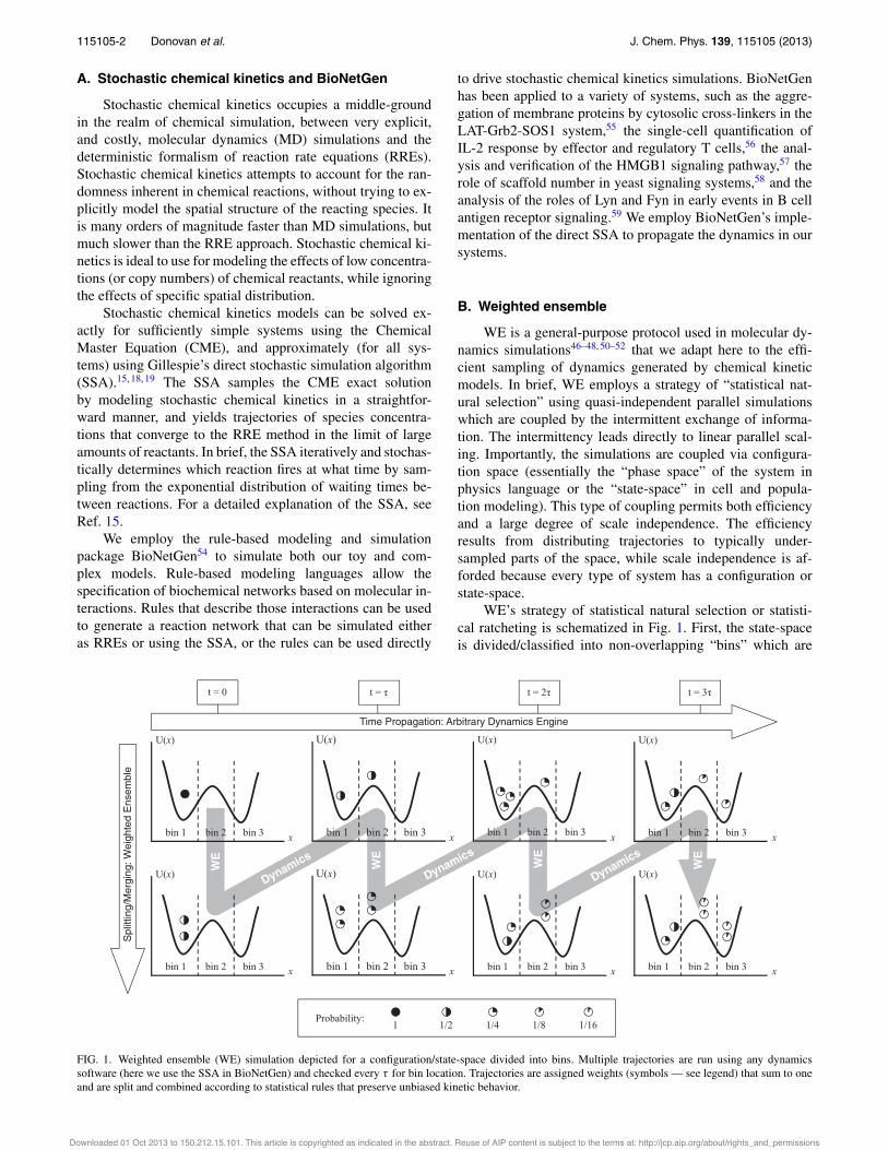
WE’s strategy of statistical natural selection or statisti-cal ratcheting is schematized in Fig. 1. First, the state-spaceis divided/classified into non-overlapping “bins” which are

t = 0 t = t = 2 t = 3

U(x)

bin 1 bin 2 bin 3

U(x)

bin 1 bin 2 bin 3

U(x)

bin 1 bin 2 bin 3

U(x)

bin 1 bin 2 bin 3

U(x)

bin 1 bin 2 bin 3

U(x)

bin 1 bin 2 bin 3

U(x)

bin 1 bin 2 bin 3

U(x)

bin 1 bin 2 bin 3

Probability:1/2 1/4 1/81 1/16

WE

Dynamics

WE

Dynamics

WE

Dynamics

WE

x x x x

x x x x

Time Propagation: Arbitrary Dynamics Engine

Spl

ittin

g/M

ergi

ng: W

eigh

ted

Ens

embl

e

FIG. 1. Weighted ensemble (WE) simulation depicted for a configuration/state-space divided into bins. Multiple trajectories are run using any dynamicssoftware (here we use the SSA in BioNetGen) and checked every ! for bin location. Trajectories are assigned weights (symbols — see legend) that sum to oneand are split and combined according to statistical rules that preserve unbiased kinetic behavior.

Downloaded 01 Oct 2013 to 150.212.15.101. This article is copyrighted as indicated in the abstract. Reuse of AIP content is subject to the terms at: http://jcp.aip.org/about/rights_and_permissions

115105-3 Donovan et al. J. Chem. Phys. 139, 115105 (2013)

typically static, although dynamic and adaptive tessellationsare possible.47 A target number of trajectories, Mtarg, is setfor each bin. Multiple trajectories are initiated from the de-sired initial condition and each is assigned a weight (proba-bility) so that the sum of weights is one. Trajectories are thensimulated independently according to the desired dynamics(e.g., molecular dynamics or SSA) and checked intermittently(every ! units of time) for their location. If a trajectory isfound to occupy a previously unoccupied bin, that trajectoryis split and replicated to obtain the target number of copies,Mtarg, for the bin. The sum of these newly spawned trajec-tories’ weights must sum to the weight of the parent trajec-tory, so in a splitting event, if the original parent trajectory hasweight w, the weight of each daughter is set to w/Mtarg. If abin is occupied by more than the target number, trajectoriesmust be pruned in a statistical fashion maintaining the sumof weights. Specifically, the two lowest weight trajectoriesare “merged” by randomly selecting one of them to survive,with probability proportional to their weights, and the sur-viving trajectory absorbs the weight of the pruned one. Thisresampling process is repeated as needed, and maintains anexact statistical representation of the evolving distribution oftrajectories.47

Setting up a WE simulation requires selection of state-space binning, trajectory multiplicity, and timing parame-ters. In our simulations, we chose to divide the state-spaceof an N-dimensional system into one- or two-dimensionalregular grids of non-overlapping bins. It is possible to usenon-Cartesian bins, and to adaptively change the bins duringsimulation,47, 50 but for simplicity we did not pursue any suchoptimization. Specific parameter choices for each model aregiven in Sec. III.

The weighted ensemble can be outlined fairly concisely.Let Mtarg be the target number of segments in each bin, Nbins

the number of bins, whose geometry are defined by the gridGgrid, ! the time-step of an iteration of WE, and Niters the totalnumber of iterations of WE. The WE procedure also requiresan initial state of the system, x0, which in our case is a list ofthe concentrations of all the chemical species in the system.Given these parameters, the WE algorithm is then:

procedure WE(Niters, !,Ggrid, Mtarg, x0)for i = 1 . . . Niters do

for each populated bin in Ggrid dopropagate dynamics for all trajectoriesupdate bin populations

for each bin in Ggrid doif bin population = 0 or Mtarg then

do nothingelse if bin population < Mtarg then

replicate trajectories until bin pop. = Mtarg

maintain sum of weights in each binelse if bin population > Mtarg then

merge trajectories until bin pop. = Mtarg

maintain sum of weights in each binsave coordinates and weights of each trajectory

return trajectory coordinates & weights for each iter.

The replicating and merging of trajectories in the above al-gorithm are done randomly, according to the weight of eachtrajectory segment in a given bin, which has been shown notto bias the dynamics of the ensemble.45, 48

When WE is used to manage an ensemble of trajectories,there are two time-scales of immediate concern: the periodat which trajectory coordinates are saved, and the period ! atwhich ensemble operations are performed. These two time-scales can be different, but for simplicity we set them to bethe same, and select ! such that it is greater than the inverseof the average event firing rate for the SSA. When we refer tothe time-step, or iteration of a process, we are referring to the! of Fig. 1.

WE can be employed in a variety of modes to ad-dress different questions. Originally developed to monitor thetime evolution of arbitrary initial probability distributions,45

i.e., non-stationary non-equilibrium systems, WE was gen-eralized to efficiently simulate both equilibrium and non-equilibrium steady-states.48 In steady-state mode, mean firstpassage times (MFPTs) can be estimated rapidly based onsimulations much shorter than the MFPT using a simple rigor-ous relation between the flux and MFPT.48 Steady-states canbe attained rapidly, avoiding long relaxation times, by usingthe inter-bin rates computed during a simulation to estimatebin probabilities appropriate to the desired steady-state; tra-jectories are then reweighted to conform to the steady-statebin probabilities.48 Both of these methods are described inmore detail below.

1. Basic WE: Probability distribution evolving in time

Perhaps the simplest use of a weighted ensemble of tra-jectories is to better sample rare states as a system evolvesin time, specifically the states corresponding to extreme val-ues of the binning coordinate. The SSA itself samples theexact distribution, but its sampling is concentrated about themode(s) of the distribution. The SSA naturally — and cor-rectly — samples rare states infrequently. By using WE tosplit up the state-space, however, one can resample the distri-bution at every time step ! , selecting those trajectories that ad-vance along a progress coordinate for more detailed study, butdoing so without applying any forces or biasing the trajecto-ries or the distribution. Essentially, WE appropriates much ofthe effort that brute-force SSA devotes to sampling the centralcomponent of the distribution, repurposing it to obtain betterestimates of the tails.

This basic use of WE requires none of the “tricks” weapply in later sections, such as using reweighting techniquesto accelerate obtaining a steady-state. We apply basic WE tosome of our systems — particularly, but not exclusively, tothose that are not bistable.

2. Steady-state

The mean first passage time (MFPT) from state A tostate B is a key observable. It is equal to the inverse ofthe flux (of probability density) from state A to state B in

Downloaded 01 Oct 2013 to 150.212.15.101. This article is copyrighted as indicated in the abstract. Reuse of AIP content is subject to the terms at: http://jcp.aip.org/about/rights_and_permissions

115105-4 Donovan et al. J. Chem. Phys. 139, 115105 (2013)

steady-state,60

MFPTA!B = 1Fluxss(A ! B)

. (1)

This relation provides the weighted ensemble approach theability to calculate MFPTs in a straightforward manner. Dur-ing a WE run, when any trajectories (and their associatedweights) reach a designated target area of state-space (or“state B”), they are removed and placed back in the initialstate (“state A”). Eventually, such a process will result in asteady-state flow of probability from state A to state B thatdoes not change in time (other than with stochastic noise).

Reweighting. The waiting time to obtain a steady-stateconstrains the efficiency of obtaining a MFPT by measuringfluxes via equation (1). This waiting time can vary from therelatively short time scale of intra-state equilibration for sim-ple systems, to much longer time-scales, on the order of theMFPT itself for more complicated systems. To reduce thiswaiting time, we use the steady-state reweighting procedureof Bhatt et al.48 This method measures the fluxes betweenbins to obtain a rate-matrix for transitions between bins, anduses a Markov formulation to infer a steady-state distributionfrom the (noisy) data available.

For instance, let {wi} be the set of bin weights (i.e., thesum of the weights of the trajectories in each bin), and let{wss

i } be the set of steady-state values of the bin weights. If fijis the flux of weight into bin i from bin j, then in steady-state,the flux out of a bin is equal to the flux into it,

dwssi

dt=

!

j

"f ss

ij " f ssji

#=

!

j

"kijw

ssj " kjiw

ssi

#= 0. (2)

Since the flux of weight into bin i from bin j is the productof a (constant) rate and the (current) weight in a bin, i.e.,fij = kijwj (true for both steady state and not), we can useEq. (2) to find the inter-bin rates. By measuring the inter-bin fluxes and the bin weights, we can approximately inferthe transition rates, and then find a set of weights that satisfyEq. (2). Once the set of bin weights is found, the weights ofthe individual trajectories in the bins are rescaled commensu-rately. This reweighting process should not be confused with aresampling process (such as basic WE splitting and merging)which does not change the distribution.

The steady-state distribution of weights thus inferred isnot necessarily the true steady-state of the system, but tends tobe closer to it than the distribution was prior to reweighting,and an iterative application of this procedure can convergeto the true distribution fairly rapidly. In practice, it has beenshown to accelerate the system’s evolution to a true steady-state by orders of magnitude in some cases.48

C. Estimation of computational efficiency

Since it is important to assess new approaches quanti-tatively, we compare the speedup in computing time fromweighted ensemble to a brute-force simulation (i.e., SSA).For a given observable (e.g., the fraction of probability in aspecified tail of the distribution) and a desired precision, we

estimate the efficiency using the ratio:

E := dynamics time in brute-force SSAdynamics time in WE-SSA

. (3)

Since both WE and brute-force use the same dynamicsengine/software, we can estimate the speedup of WE overbrute-force by just keeping track of how much total “dynam-ics time” was simulated in each. We employ this measurewhen estimating the advantage of using WE to investigate thetails of probability distributions, as well as for finding MFPTsin bistable systems.

Another measure of efficiency we employ for MFPT es-timation gauges how fast WE attains a result that is within50% of the true result (determined from exact or extensivebrute-force calculation):

E50%

:= dynamics time in brute-force SSA to get ± 50% exactdynamics time in WE-SSA to get ± 50% exact

.

(4)

This is an assessment of how well WE can extract rough es-timates of long time-scale behavior from simulations that aremuch shorter than those timescales.

Brute-force SSA simulations can be run for long timeswithout seeing a transition from one macro-state to another.To take account of the brute-force simulations where no tran-sitions occurred we use a maximum likelihood estimator forthe transition time, based on an exponential distribution ofwaiting times,61 which is a valid approximation for the one-dimensional and two-state systems studied below:

µMLE =$

1 " n

N

%T + 1

n

n!

i=1

ti ,

!µ = µMLE#n

,

(5)

where T is the length of the brute-force simulations, N is thenumber of these simulations performed, n is the number ofthese simulations in which a transition from one state to an-other is observed, and ti are the times at which the transitionis observed.

D. Limitations of our implementation

We used two different implementations of the weightedensemble framework: WESTPA, written in Python, isthe most feature-rich and stable,52 and is available athttp://chong.chem.pitt.edu/WESTPA. Another, written byZhang et al.46 and modified by us, is written in C,and is faster though less robust; it is available athttp://donovanr.github.com/WE_git_code.

Weighted ensemble (WE), as a scripting-level approach,inherently adds some overhead to the runtime of the dy-namics. This overhead, in theory, is quite minimal: stopping,starting, merging, and splitting trajectories are not computa-tionally costly operations. A key issue in practical implemen-tations, though, is how long the algorithm actually takes to

Downloaded 01 Oct 2013 to 150.212.15.101. This article is copyrighted as indicated in the abstract. Reuse of AIP content is subject to the terms at: http://jcp.aip.org/about/rights_and_permissions

115105-5 Donovan et al. J. Chem. Phys. 139, 115105 (2013)

run, i.e., the wall-clock running-time for dynamics (here, theSSA).

In practice, overhead can be significant for very simplesystems, for the sole reason that reading and writing to disktakes so much time compared to how long it takes to run thedynamics of small models. In our implementation, data arepassed from the dynamics engine to WE by reading and writ-ing files to disk. This handicap is an artifact of our interface,which could, with minimal work, be modified to somethingmore efficient. As a proof-of-principle, the version of WEwritten in C was modified, for the Schlögl reactions and thefutile cycle, to contain hard-coded versions of the Gillespiedirect algorithm for those systems, so as to obviate the I/Obetween WE and BNG. With these modifications, it was diffi-cult to ascertain any significant overhead costs at all, and ourruns completed in a matter of seconds. We also note that asmodel complexity increases and more time is devoted to dy-namics, the overhead problem becomes negligible. Practicalapplications of WE will, by nature, target models where dy-namics are expensive, rather than toy models, where they arecheap.

III. MODELS & RESULTS

We study four different models, ranging in complexityfrom two chemical reactions governing one chemical speciesto 3680 reactions governing 354 species. The models em-ploy coupled stochastic chemical reactions, which we imple-ment and simulate in BioNetGen using the SSA.15, 18, 19 Asdepicted in Fig. 1, these simulations are, in turn, managed bya weighted ensemble procedure.

A. Enzymatic futile cycle

1. Model

The enzymatic futile cycle is a simple and robust modelthat can, in certain parameter regimes, exhibit qualitativelydifferent behavior due to stochastic noise.62, 63 This signalingmotif can be seen in biological systems including GTPase cy-cles, MAPK cascades, and glucose mobilization.62, 64, 65

The enzymatic futile cycle studied here is modeled by

E1 + S1kf!!"!kf

B1ks!" E1 + S2,

E2 + S2kf!!"!kf

B2ks!" E2 + S1,

(6)

where kf = 1.0 and ks = 0.1. Here S1 can bind to its en-zyme E1, and in the bound form, B1, (i.e., B1 = E1 · S1), itcan be converted to S2, and then dissociate (and similarly forS2 !" S1). The total amount of substrate, S1 + S2, is con-served, as are the amounts of the different enzymes E1 andE2, of which is supplied only one of each kind, thus (S1

+ B1) + (S2 + B2) = 100. Following Kuwahara andMura,29 in the specific system we look at, we set S1 + S2

= 100 and E1 + B1 = E2 + B2 = 1.Thus constrained, the above system of reactions can be

solved by an approximately 400-state chemical master equa-

tion (CME), to obtain an exact probability density for all timeswhen initialized from an arbitrary starting point. We start thesystem at S1 = S2 = 50 and E1 = E2 = 1, and are interestedin the probability distribution of S1 after 100 s, that is, P(S1

= x, t = 100).

2. WE parameters

The WE data were generated using 101 bins of unit widthon the coordinate S1. We employed 100 trajectory segmentsper bin that were run for 100 iterations of a # = 1 s time-step,with no reweighting events. The brute-force data are from10,200 100-s runs, which is an equivalent amount of dynam-ics to compute as the single WE run, if all the bins were fullall the time. However, since the bins take some time to fillup, the WE run employed only 840,000 1-s segments, whichmakes the comparison to brute-force SSA more than fair.

3. Results

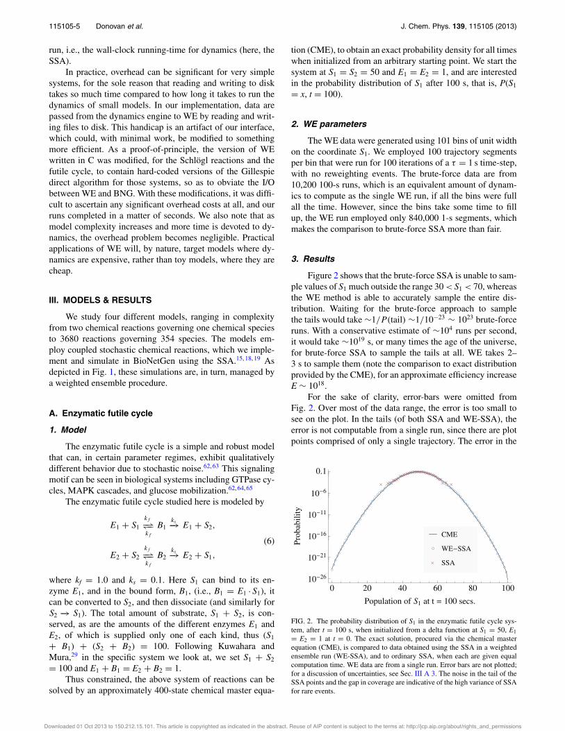
Figure 2 shows that the brute-force SSA is unable to sam-ple values of S1 much outside the range 30 < S1 < 70, whereasthe WE method is able to accurately sample the entire dis-tribution. Waiting for the brute-force approach to samplethe tails would take #1/P (tail) #1/10!23 # 1023 brute-forceruns. With a conservative estimate of #104 runs per second,it would take #1019 s, or many times the age of the universe,for brute-force SSA to sample the tails at all. WE takes 2–3 s to sample them (note the comparison to exact distributionprovided by the CME), for an approximate efficiency increaseE # 1018.

For the sake of clarity, error-bars were omitted fromFig. 2. Over most of the data range, the error is too small tosee on the plot. In the tails (of both SSA and WE-SSA), theerror is not computable from a single run, since there are plotpoints comprised of only a single trajectory. The error in the

! !!!!!!!

!!!!!!!!!!!!!!!!!!!!!!!!

! ! !

CME

WE!SSA

! SSA

0 20 40 60 80 10010!26

10!21

10!16

10!11

10!6

0.1

Population of S1 at t " 100 secs.

Prob

abili

ty

FIG. 2. The probability distribution of S1 in the enzymatic futile cycle sys-tem, after t = 100 s, when initialized from a delta function at S1 = 50, E1= E2 = 1 at t = 0. The exact solution, procured via the chemical masterequation (CME), is compared to data obtained using the SSA in a weightedensemble run (WE-SSA), and to ordinary SSA, when each are given equalcomputation time. WE data are from a single run. Error bars are not plotted;for a discussion of uncertainties, see Sec. III A 3. The noise in the tail of theSSA points and the gap in coverage are indicative of the high variance of SSAfor rare events.

Downloaded 01 Oct 2013 to 150.212.15.101. This article is copyrighted as indicated in the abstract. Reuse of AIP content is subject to the terms at: http://jcp.aip.org/about/rights_and_permissions

115105-6 Donovan et al. J. Chem. Phys. 139, 115105 (2013)

estimate of the distribution can be inferred visually from thedata’s departure form the CME exact solution. For SSA, how-ever, generating uncertainties far all values is essentially im-possible. When computing quantitative observables reportedbelow, we employ multiple independent runs to procure stan-dard errors in our estimate.

From the distribution, we are able to read off usefulstatistics. For instance, in the spirit of Kuwahara and Mura,29

and Gillespie et al.,30 one might desire to know the proba-bility of the futile cycle to have a value of S1 > 90 at !t= 100, which we will denote as p>90. Since WE gives anaccurate estimate of P(x, t) on an arbitrarily precise spatio-temporal grid, all that is required to find p>90 is to sum upthe area under the state of interest: we find p>90 = 2.47! 10"18 ± 3.4 ! 10"19 at one standard error, as computedfrom ten replicates of the single WE run plotted in Fig.2. The CME gives an exact value of 2.72 ! 10"18. Fol-lowing Gillespie et al.,30 the approximate number of nor-mal SSA runs needed to estimate this observable with com-parable error is nSSA

p>90= p>90/("p>90 )2 = 2.72 ! 10"18/(3.4

! 10"19)2 = 2.4 ! 1019 SSA runs. Using ten replicate runs,WE is able to sample it using a total of 8,317,000 trajec-tory segments, which is computationally equivalent to 83,170brute-force trajectories, resulting in an increase in samplingefficiency by a factor of E # 2.4 ! 1019/83,170 # 3 ! 1014

for this observable at this level of accuracy. Since WE givesthe full distribution, from the same data we can also find otherrare event statistics. For example, we might also wish to com-pute the probability that S1 $ 25 at !t = 100, which wewill call p$25. From the same data described in the preced-ing paragraph, we can find p$25 = 1.35 ! 10"7 ± 1.5 ! 10"8

at one standard error. The CME gives an exact value of 1.26! 10"7. Again, estimating the number of SSA runs necessaryto determine the same observable with similar accuracy asin Ref. 30, we find nSSA

p$25= p$25/("p$25 )2 = 1.26 ! 10"7/(1.5

! 10"8)2 = 6.0 ! 108 SSA runs. Our weighted ensemble cal-culation used the computational equivalent of 83,170 brute-force trajectories, resulting in an increase in sampling effi-ciency by a factor of E # 6.0 ! 108/83,170 # 7 ! 103 for thisobservable at this level of accuracy.

Kuwahara and Mura29 and Gillespie et al.30 define aquantity closely related to those computed above: the prob-ability of a system to pass from one state to another in a cer-tain time: P(xi % xf|!t).29–33 This is subtly different than justmeasuring areas under a distribution, since a trajectory is ter-minated, and removed from the ensemble, if it successfullyreaches the target. To make a direct comparison to this statis-tic, we implemented in WE an absorbing boundary conditionat the target state S1 = 25. Using ten WE runs, we find thatthe probability of reaching the S1 = 25 within 100 s, whichwe call pabs(25), is 1.61 ! 10"7 ± 1.93 ! 10"8 at one stan-dard error. The CME with an absorbing boundary conditionat S1 = 25 gives an exact value of 1.738 ! 10"7. As above,we estimate the number of brute-force SSA runs needed toattain a comparable estimate as nSSA

pabs(25)= pabs(25)/("pabs(25) )

2

= 1.738 ! 10"7/(1.93 ! 10"8)2 = 4.66 ! 108 SSA runs. Intotal, the ten WE runs used 6,342,600 trajectory segments,which is computationally equivalent to 63,426 brute-force tra-

jectories. This yields an increase in efficiency of E # 4.66! 108/63,426 # 7 ! 103 for this observable at this level ofaccuracy.

For the above statistic, Gillespie et al. report an efficiencygain of 7.76 ! 105 over brute-force SSA.30 Direct compar-isons of efficiency gain between wSSA and WE are diffi-cult, even when focussing on the same observable in the samesystem. Many factors contribute to this, notably that WE isnot optimized in a target-specific manner, as wSSA histori-cally has been. Further, in its simplest form, WE yields a fullspace/time distribution of trajectories, from which it is possi-ble to calculate rare event statistics for arbitrary states, whichneed not be specified in advance.

B. Schlögl reactions

1. Model

The Schlögl reactions are a classic toy-model for bench-marking stochastic simulations of bistable systems.66–68 Theyare two coupled reactions with one dynamic species, X:

A + 2Xk1"#$"k2

3X,

Bk3"#$"k4

X,

(7)

where k1 = 3 ! 10"7, k2 = 10"4, k3 = 10"3, k4 = 3.5,A = 105, and B = 2 ! 105. The species A and B are assumedto be in abundance, and are held constant. Both the mean firstpassage times and the time-evolution of arbitrary probabilitydistributions can be computed exactly.67

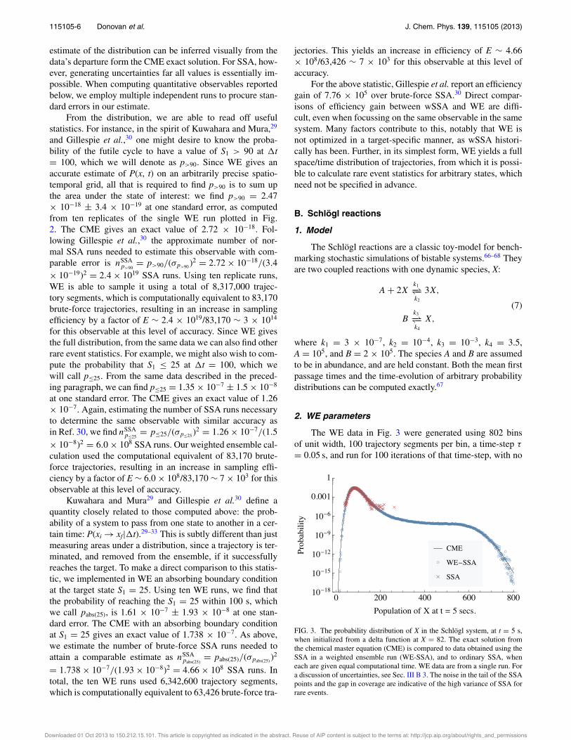
2. WE parameters

The WE data in Fig. 3 were generated using 802 binsof unit width, 100 trajectory segments per bin, a time-step %

= 0.05 s, and run for 100 iterations of that time-step, with no

FIG. 3. The probability distribution of X in the Schlögl system, at t = 5 s,when initialized from a delta function at X = 82. The exact solution fromthe chemical master equation (CME) is compared to data obtained using theSSA in a weighted ensemble run (WE-SSA), and to ordinary SSA, wheneach are given equal computational time. WE data are from a single run. Fora discussion of uncertainties, see Sec. III B 3. The noise in the tail of the SSApoints and the gap in coverage are indicative of the high variance of SSA forrare events.

Downloaded 01 Oct 2013 to 150.212.15.101. This article is copyrighted as indicated in the abstract. Reuse of AIP content is subject to the terms at: http://jcp.aip.org/about/rights_and_permissions

115105-7 Donovan et al. J. Chem. Phys. 139, 115105 (2013)

WE!SSA, RW!100

WE!SSA, RW!5

WE!SSA, RW!2

Exact

0 100 200 300 400 50010!12

10!10

10!8

10!6

10!4

0.01

1

Iteration

Flux

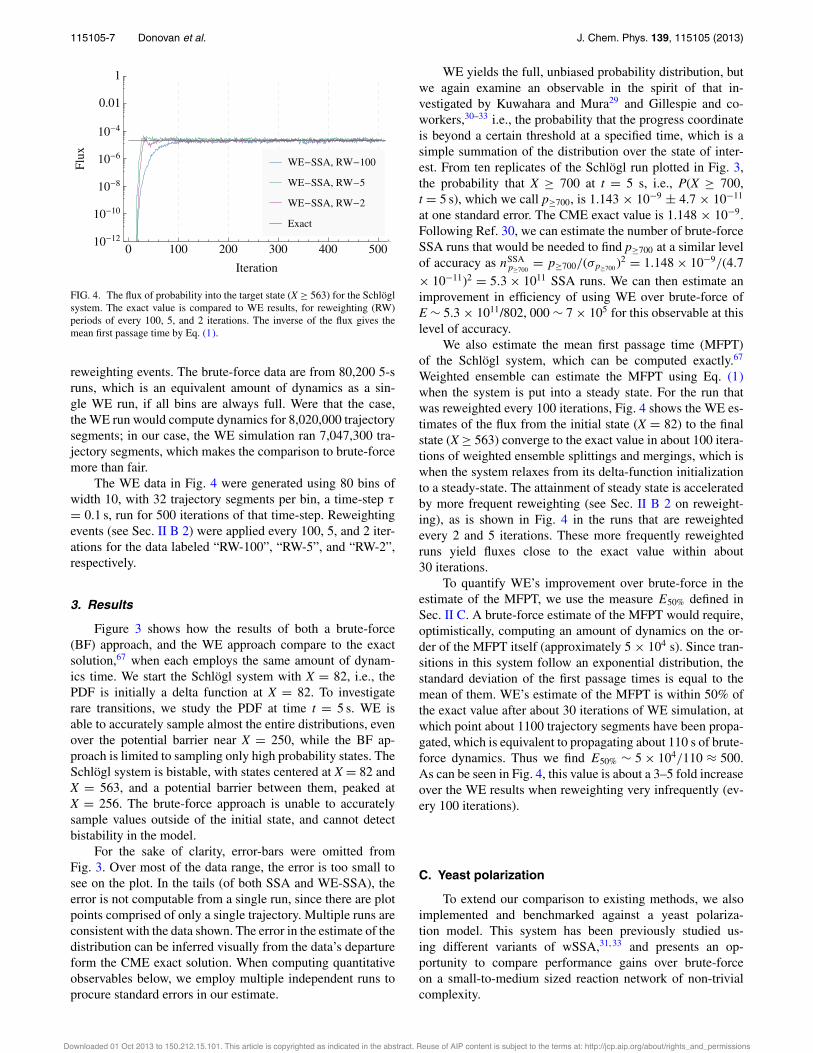
FIG. 4. The flux of probability into the target state (X ! 563) for the Schlöglsystem. The exact value is compared to WE results, for reweighting (RW)periods of every 100, 5, and 2 iterations. The inverse of the flux gives themean first passage time by Eq. (1).

reweighting events. The brute-force data are from 80,200 5-sruns, which is an equivalent amount of dynamics as a sin-gle WE run, if all bins are always full. Were that the case,the WE run would compute dynamics for 8,020,000 trajectorysegments; in our case, the WE simulation ran 7,047,300 tra-jectory segments, which makes the comparison to brute-forcemore than fair.

The WE data in Fig. 4 were generated using 80 bins ofwidth 10, with 32 trajectory segments per bin, a time-step !

= 0.1 s, run for 500 iterations of that time-step. Reweightingevents (see Sec. II B 2) were applied every 100, 5, and 2 iter-ations for the data labeled “RW-100”, “RW-5”, and “RW-2”,respectively.

3. Results

Figure 3 shows how the results of both a brute-force(BF) approach, and the WE approach compare to the exactsolution,67 when each employs the same amount of dynam-ics time. We start the Schlögl system with X = 82, i.e., thePDF is initially a delta function at X = 82. To investigaterare transitions, we study the PDF at time t = 5 s. WE isable to accurately sample almost the entire distributions, evenover the potential barrier near X = 250, while the BF ap-proach is limited to sampling only high probability states. TheSchlögl system is bistable, with states centered at X = 82 andX = 563, and a potential barrier between them, peaked atX = 256. The brute-force approach is unable to accuratelysample values outside of the initial state, and cannot detectbistability in the model.

For the sake of clarity, error-bars were omitted fromFig. 3. Over most of the data range, the error is too small tosee on the plot. In the tails (of both SSA and WE-SSA), theerror is not computable from a single run, since there are plotpoints comprised of only a single trajectory. Multiple runs areconsistent with the data shown. The error in the estimate of thedistribution can be inferred visually from the data’s departureform the CME exact solution. When computing quantitativeobservables below, we employ multiple independent runs toprocure standard errors in our estimate.

WE yields the full, unbiased probability distribution, butwe again examine an observable in the spirit of that in-vestigated by Kuwahara and Mura29 and Gillespie and co-workers,30–33 i.e., the probability that the progress coordinateis beyond a certain threshold at a specified time, which is asimple summation of the distribution over the state of inter-est. From ten replicates of the Schlögl run plotted in Fig. 3,the probability that X ! 700 at t = 5 s, i.e., P(X ! 700,t = 5 s), which we call p!700, is 1.143 " 10#9 ± 4.7 " 10#11

at one standard error. The CME exact value is 1.148 " 10#9.Following Ref. 30, we can estimate the number of brute-forceSSA runs that would be needed to find p!700 at a similar levelof accuracy as nSSA

p!700= p!700/("p!700 )2 = 1.148 " 10#9/(4.7

" 10#11)2 = 5.3 " 1011 SSA runs. We can then estimate animprovement in efficiency of using WE over brute-force ofE $ 5.3 " 1011/802, 000 $ 7 " 105 for this observable at thislevel of accuracy.

We also estimate the mean first passage time (MFPT)of the Schlögl system, which can be computed exactly.67

Weighted ensemble can estimate the MFPT using Eq. (1)when the system is put into a steady state. For the run thatwas reweighted every 100 iterations, Fig. 4 shows the WE es-timates of the flux from the initial state (X = 82) to the finalstate (X ! 563) converge to the exact value in about 100 itera-tions of weighted ensemble splittings and mergings, which iswhen the system relaxes from its delta-function initializationto a steady-state. The attainment of steady state is acceleratedby more frequent reweighting (see Sec. II B 2 on reweight-ing), as is shown in Fig. 4 in the runs that are reweightedevery 2 and 5 iterations. These more frequently reweightedruns yield fluxes close to the exact value within about30 iterations.

To quantify WE’s improvement over brute-force in theestimate of the MFPT, we use the measure E50% defined inSec. II C. A brute-force estimate of the MFPT would require,optimistically, computing an amount of dynamics on the or-der of the MFPT itself (approximately 5 " 104 s). Since tran-sitions in this system follow an exponential distribution, thestandard deviation of the first passage times is equal to themean of them. WE’s estimate of the MFPT is within 50% ofthe exact value after about 30 iterations of WE simulation, atwhich point about 1100 trajectory segments have been propa-gated, which is equivalent to propagating about 110 s of brute-force dynamics. Thus we find E50% $ 5 " 104/110 % 500.As can be seen in Fig. 4, this value is about a 3–5 fold increaseover the WE results when reweighting very infrequently (ev-ery 100 iterations).

C. Yeast polarization

To extend our comparison to existing methods, we alsoimplemented and benchmarked against a yeast polariza-tion model. This system has been previously studied us-ing different variants of wSSA,31, 33 and presents an op-portunity to compare performance gains over brute-forceon a small-to-medium sized reaction network of non-trivialcomplexity.

Downloaded 01 Oct 2013 to 150.212.15.101. This article is copyrighted as indicated in the abstract. Reuse of AIP content is subject to the terms at: http://jcp.aip.org/about/rights_and_permissions

115105-8 Donovan et al. J. Chem. Phys. 139, 115105 (2013)

1. Model

This yeast polarization model31 consists of six dynamicalspecies (note that in the reactions below, the concentration ofL never changes) and eight reactions:

R1 : ! k1!" R, k1 = 0.0038,

R2 : Rk2!" !, k2 = 0.0004,

R3 : R + Lk3!" RL + L, k3 = 0.042,

R4 : RLk4!" R, k4 = 0.010,

R5 : RL + Gk5!" Ga + Gbg, k5 = 0.011,

R6 : Gak6!" Gd, k6 = 0.100,

R7 : Gbg + Gdk7!" G, k7 = 1050,

R8 : ! k8!" RL, k8 = 3.21.

(8)

All reaction propensities are in numbers of particles per sec-ond. The system is initialized at t = 0 with species counts [R,L, RL, G, Ga, Gbg, Gd] = [50, 2, 0, 50, 0, 0, 0]. That is, westart with 50 molecules each of R and G, and 2 of L, and noothers.

By design, this system does not reach equilibrium;31 ad-ditionally, the rare event measured has no well-defined states,but is merely a measure of an unusually fast accumulation ofGbg.

2. WE parameters

The rare event statistics presented below were measuredusing 50 bins on the interval [0, 49], with an absorbing bound-ary condition at 50. We used 100 trajectory segments per bin,a time-step ! = 0.125 s, and we run for 160 iterations of thattime-step. We note that in situations like these the measure-ment of rare events with an absorbing boundary condition canbe somewhat sensitive to trajectory “bounce-out” from the tar-get state as the time-step is varied. This effect is intrinsic toSSA and not particular to weighted ensemble or other sam-pling methods.

3. Results

Our measurement of P(Gbg " 50 | 20s), i.e., the proba-bility of the population of Gbg reaching 50 within 20 s, was1.20 # 10!6 ± 0.04 # 10!6 at one standard error. We used100 replicate weighted ensemble runs to estimate the uncer-tainty.

To check these results, we also performed 80 millionbrute-force SSA trajectories, which yielded 108 trajectoriesthat successfully reached a Gbg population of 50 within 20 s.This brute-force data give an estimate for the rare event prob-ability of 1.35 # 10!6 ± 0.13 # 10!6 at one standard error,which corroborates the weighted ensemble result.

To estimate WE efficiency, again following Gillespieet al.,30 we can estimate the number of brute-force SSA

runs that would be needed to find P(Gbg " 50 | 20s) at asimilar level of accuracy as the weighted ensemble resultabove: NBF = P (Gbg " 50 | 20s)/" 2

P (Gbg"50|20s) = 1.20# 10!6/(0.04 # 10!6)2 = 7.3 # 108. In total, the 100 repli-cate WE runs in our measurement used 7.205 # 107 trajectorysegments, which is equivalent to running 7.205 # 107/160= 4.5 # 105 brute force trajectories. This yields a speed-upof WE over brute-force SSA of E $ (7.3 # 108)/(4.5 # 105)$ 1.6 # 103.

Gillespie and co-workers report values for this same rareevent of 1.23 # 106 ± 0.05 # 106 and 1.202 # 106 ± 0.014# 106 at two standard errors using two variants of wSSA,31

with speed-ups over brute-force of 20 and 250, respectively.

D. Epigenetic switch

1. Model

This model consists of two genes that repress each other’sexpression. Once expressed, each protein can bind particularDNA sites upstream of the gene which codes for the otherprotein, thereby repressing its transcription.69 If we denotethe ith protein concentration by gi, the deterministic systemis described by the equations:

dg1

dt= a1

1 + (g2/K2)n! g1

!,

dg2

dt= a2

1 + (g1/K1)m! g2

!,

(9)

where a1 = 156, a2 = 30, n = 3, m = 1, K1 = 1, K2 = 1, and! = 1. In our stochastic model, our chemical reactions takethe form of a birth-death process, the propensity functions ofwhich are taken from the above differential equations:

! k1(g2)!!!" g1k0!" !,

! k2(g1)!!!" g2k0!" !,

(10)

where k0 = 1/! , k1(g2) = a1/[1 + (g2/K2)n], k2(g1) = a2/[1 + (g1/K1)m].

For this system, we define a target state and an initialconfiguration. The system is initially set to have g1 = 30 andg2 = 0, and we look for transitions to a target state, which wedefine as having both g1 % 20 and g2 & 3. This target statedefinition was chosen so that the rate was insensitive to smallperturbations in the threshold values chosen for g1 and g2.

2. WE parameters

For this system, we implemented 2-dimensional bins: 15along g1 and 31 along g2, for a total of 465 bins. The binsalong the g1 coordinate were of unit width on the interval [0,10], and then of width 10 on the interval [10, 50], with oneadditional bin on [50, ']. The bins along the g2 coordinatewere of unit width on the interval [0, 30], with one additionalbin on [30, '].

The WE data in Fig. 5 were generated using 16 tra-jectory segments per bin, a time-step ! = 0.1 s, and runfor 500 iterations of that time-step, with reweighting events

Downloaded 01 Oct 2013 to 150.212.15.101. This article is copyrighted as indicated in the abstract. Reuse of AIP content is subject to the terms at: http://jcp.aip.org/about/rights_and_permissions

115105-9 Donovan et al. J. Chem. Phys. 139, 115105 (2013)

WE!SSA 1 WE!SSA 2 WE!SSA 3

WE!SSA 4 WE!SSA 5 WE!SSA 6

SSA !" 3#"0 100 200 300 400 500

10!12

10!10

10!8

10!6

10!4

Iteration

Flux

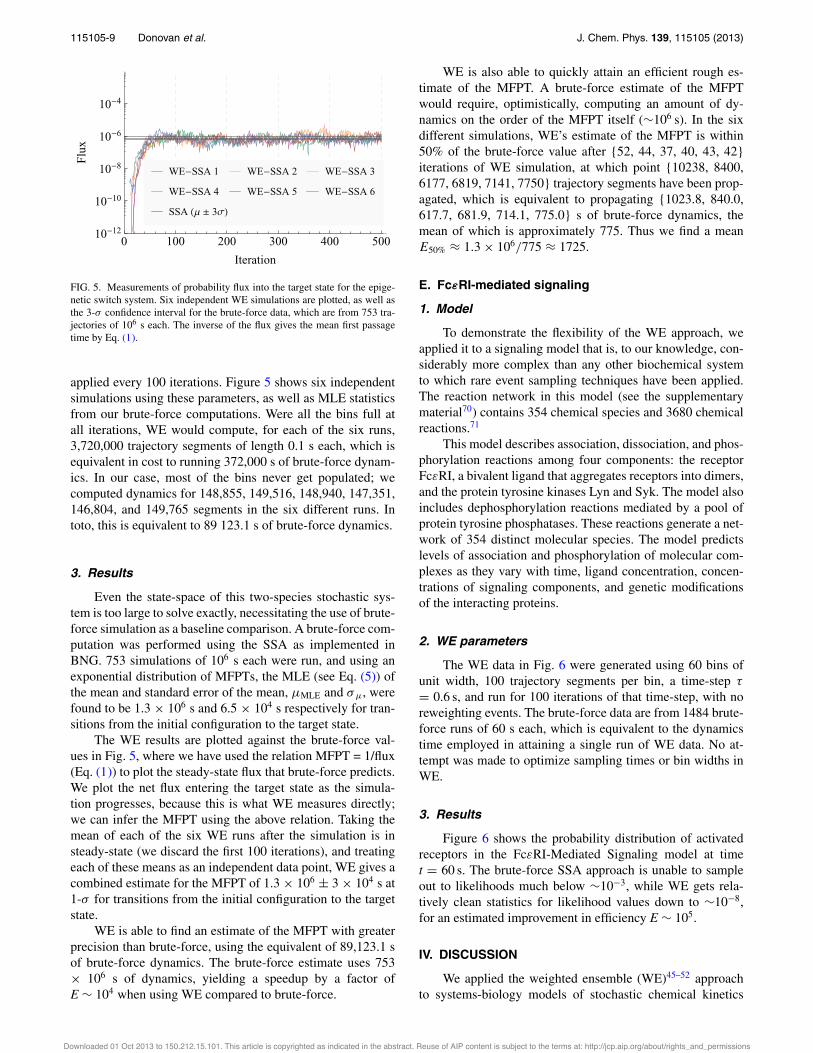
FIG. 5. Measurements of probability flux into the target state for the epige-netic switch system. Six independent WE simulations are plotted, as well asthe 3-! confidence interval for the brute-force data, which are from 753 tra-jectories of 106 s each. The inverse of the flux gives the mean first passagetime by Eq. (1).

applied every 100 iterations. Figure 5 shows six independentsimulations using these parameters, as well as MLE statisticsfrom our brute-force computations. Were all the bins full atall iterations, WE would compute, for each of the six runs,3,720,000 trajectory segments of length 0.1 s each, which isequivalent in cost to running 372,000 s of brute-force dynam-ics. In our case, most of the bins never get populated; wecomputed dynamics for 148,855, 149,516, 148,940, 147,351,146,804, and 149,765 segments in the six different runs. Intoto, this is equivalent to 89 123.1 s of brute-force dynamics.

3. Results

Even the state-space of this two-species stochastic sys-tem is too large to solve exactly, necessitating the use of brute-force simulation as a baseline comparison. A brute-force com-putation was performed using the SSA as implemented inBNG. 753 simulations of 106 s each were run, and using anexponential distribution of MFPTs, the MLE (see Eq. (5)) ofthe mean and standard error of the mean, µMLE and !µ, werefound to be 1.3 ! 106 s and 6.5 ! 104 s respectively for tran-sitions from the initial configuration to the target state.

The WE results are plotted against the brute-force val-ues in Fig. 5, where we have used the relation MFPT = 1/flux(Eq. (1)) to plot the steady-state flux that brute-force predicts.We plot the net flux entering the target state as the simula-tion progresses, because this is what WE measures directly;we can infer the MFPT using the above relation. Taking themean of each of the six WE runs after the simulation is insteady-state (we discard the first 100 iterations), and treatingeach of these means as an independent data point, WE gives acombined estimate for the MFPT of 1.3 ! 106 ± 3 ! 104 s at1-! for transitions from the initial configuration to the targetstate.

WE is able to find an estimate of the MFPT with greaterprecision than brute-force, using the equivalent of 89,123.1 sof brute-force dynamics. The brute-force estimate uses 753! 106 s of dynamics, yielding a speedup by a factor ofE " 104 when using WE compared to brute-force.

WE is also able to quickly attain an efficient rough es-timate of the MFPT. A brute-force estimate of the MFPTwould require, optimistically, computing an amount of dy-namics on the order of the MFPT itself ("106 s). In the sixdifferent simulations, WE’s estimate of the MFPT is within50% of the brute-force value after {52, 44, 37, 40, 43, 42}iterations of WE simulation, at which point {10238, 8400,6177, 6819, 7141, 7750} trajectory segments have been prop-agated, which is equivalent to propagating {1023.8, 840.0,617.7, 681.9, 714.1, 775.0} s of brute-force dynamics, themean of which is approximately 775. Thus we find a meanE50% # 1.3 ! 106/775 # 1725.

E. Fc!RI-mediated signaling

1. Model

To demonstrate the flexibility of the WE approach, weapplied it to a signaling model that is, to our knowledge, con-siderably more complex than any other biochemical systemto which rare event sampling techniques have been applied.The reaction network in this model (see the supplementarymaterial70) contains 354 chemical species and 3680 chemicalreactions.71

This model describes association, dissociation, and phos-phorylation reactions among four components: the receptorFc"RI, a bivalent ligand that aggregates receptors into dimers,and the protein tyrosine kinases Lyn and Syk. The model alsoincludes dephosphorylation reactions mediated by a pool ofprotein tyrosine phosphatases. These reactions generate a net-work of 354 distinct molecular species. The model predictslevels of association and phosphorylation of molecular com-plexes as they vary with time, ligand concentration, concen-trations of signaling components, and genetic modificationsof the interacting proteins.

2. WE parameters

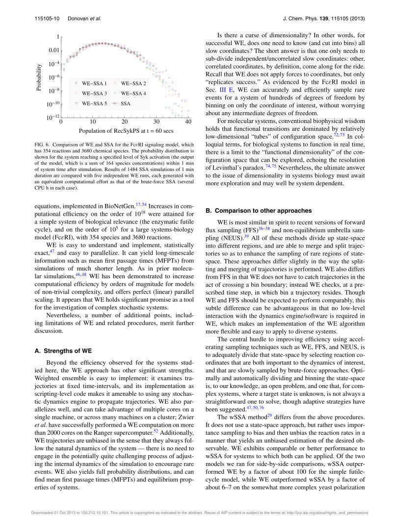
The WE data in Fig. 6 were generated using 60 bins ofunit width, 100 trajectory segments per bin, a time-step #

= 0.6 s, and run for 100 iterations of that time-step, with noreweighting events. The brute-force data are from 1484 brute-force runs of 60 s each, which is equivalent to the dynamicstime employed in attaining a single run of WE data. No at-tempt was made to optimize sampling times or bin widths inWE.

3. Results

Figure 6 shows the probability distribution of activatedreceptors in the Fc"RI-Mediated Signaling model at timet = 60 s. The brute-force SSA approach is unable to sampleout to likelihoods much below "10$3, while WE gets rela-tively clean statistics for likelihood values down to "10$8,for an estimated improvement in efficiency E " 105.

IV. DISCUSSION

We applied the weighted ensemble (WE)45–52 approachto systems-biology models of stochastic chemical kinetics

Downloaded 01 Oct 2013 to 150.212.15.101. This article is copyrighted as indicated in the abstract. Reuse of AIP content is subject to the terms at: http://jcp.aip.org/about/rights_and_permissions

115105-10 Donovan et al. J. Chem. Phys. 139, 115105 (2013)

! ! !! ! ! ! ! ! ! ! ! ! ! ! ! ! !

! ! !! !

WE!SSA 1 WE!SSA 2

WE!SSA 3 WE!SSA 4

WE!SSA 5 ! SSA

0 10 20 30 4010!12

10!10

10!8

10!6

10!4

0.01

1

Population of RecSykPS at t " 60 secs

Prob

abili

ty

FIG. 6. Comparison of WE and SSA for the Fc!RI signaling model, whichhas 354 reactions and 3680 chemical species. The probability distribution isshown for the system reaching a specified level of Syk activation (the outputof the model, which is a sum of 164 species concentrations) within 1 minof system time after stimulation. Results of 1484 SSA simulations of 1 minduration are compared with five independent WE runs, each generated withan equivalent computational effort as that of the brute-force SSA (severalCPU h in each case).

equations, implemented in BioNetGen.17, 54 Increases in com-putational efficiency on the order of 1018 were attained fora simple system of biological relevance (the enzymatic futilecycle), and on the order of 105 for a large systems-biologymodel (Fc!RI), with 354 species and 3680 reactions.

WE is easy to understand and implement, statisticallyexact,47 and easy to parallelize. It can yield long-timescaleinformation such as mean first passage times (MFPTs) fromsimulations of much shorter length. As in prior molecu-lar simulations,46, 48 WE has been demonstrated to increasecomputational efficiency by orders of magnitude for modelsof non-trivial complexity, and offers perfect (linear) parallelscaling. It appears that WE holds significant promise as a toolfor the investigation of complex stochastic systems.

Nevertheless, a number of additional points, includ-ing limitations of WE and related procedures, merit furtherdiscussion.

A. Strengths of WE

Beyond the efficiency observed for the systems stud-ied here, the WE approach has other significant strengths.Weighted ensemble is easy to implement: it examines tra-jectories at fixed time-intervals, and its implementation asscripting-level code makes it amenable to using any stochas-tic dynamics engine to propagate trajectories. WE also par-allelizes well, and can take advantage of multiple cores on asingle machine, or across many machines on a cluster; Zwieret al. have successfully performed a WE computation on morethan 2000 cores on the Ranger supercomputer.52 Additionally,WE trajectories are unbiased in the sense that they always fol-low the natural dynamics of the system — there is no need toengage in the potentially quite challenging process of adjust-ing the internal dynamics of the simulation to encourage rareevents. WE also yields full probability distributions, and canfind mean first passage times (MFPTs) and equilibrium prop-erties of systems.

Is there a curse of dimensionality? In other words, forsuccessful WE, does one need to know (and cut into bins) allslow coordinates? The short answer is that one only needs tosub-divide independent/uncorrelated slow coordinates: other,correlated coordinates, by definition, come along for the ride.Recall that WE does not apply forces to coordinates, but only“replicates success.” As evidenced by the Fc!RI model inSec. III E, WE can accurately and efficiently sample rareevents for a system of hundreds of degrees of freedom bybinning on only the coordinate of interest, without worryingabout any intermediate degrees of freedom.

For molecular systems, conventional biophysical wisdomholds that functional transitions are dominated by relativelylow-dimensional “tubes” of configuration space.72, 73 In col-loquial terms, for biological systems to function in real time,there is a limit to the “functional dimensionality” of the con-figuration space that can be explored, echoing the resolutionof Levinthal’s paradox.74, 75 Nevertheless, the ultimate answerto the issue of dimensionality in systems biology must awaitmore exploration and may well be system dependent.

B. Comparison to other approaches

WE is most similar in spirit to recent versions of forwardflux sampling (FFS)36–38 and non-equilibrium umbrella sam-pling (NEUS).39 All of these methods divide up state-spaceinto different regions, and are able to merge and split trajec-tories so as to enhance the sampling of rare regions of state-space. These approaches differ slightly in the way the split-ting and merging of trajectories is performed. WE also differsfrom FFS in that WE does not have to catch trajectories in theact of crossing a bin boundary; instead WE checks, at a pre-scribed time step, in which bin a trajectory resides. ThoughWE and FFS should be expected to perform comparably, thissubtle difference can be advantageous in that no low-levelinteraction with the dynamics engine/software is required inWE, which makes an implementation of the WE algorithmmore flexible and easy to apply to diverse systems.

The central hurdle to improving efficiency using accel-erating sampling techniques such as WE, FFS, and NEUS, isto adequately divide that state-space by selecting reaction co-ordinates that are both important to the dynamics of interest,and that are slowly sampled by brute-force approaches. Opti-mally and automatically dividing and binning the state-spaceis, to our knowledge, an open problem, and one that, for com-plex systems, where a target state is unknown, is not always astraightforward one to solve, though adaptive strategies havebeen suggested.47, 50, 76

The wSSA method29 differs from the above procedures.It does not use a state-space approach, but rather uses impor-tance sampling to bias and then unbias the reaction rates in amanner that yields an unbiased estimation of the desired ob-servable. WE exhibits comparable or better performance towSSA for systems to which both can be applied. Of the twomodels we ran for side-by-side comparisons, wSSA outper-formed WE by a factor of about 100 for the simple futile-cycle model, while WE outperformed wSSA by a factor ofabout 6–7 on the somewhat more complex yeast polarization

Downloaded 01 Oct 2013 to 150.212.15.101. This article is copyrighted as indicated in the abstract. Reuse of AIP content is subject to the terms at: http://jcp.aip.org/about/rights_and_permissions

115105-11 Donovan et al. J. Chem. Phys. 139, 115105 (2013)

model. Since wSSA biases/unbiases reaction rates, while WEdivides state-space, the advantage of one over the other maybe situation-dependent. For instance, as noted by the wSSAauthors,30 when a reaction network is finely tuned and ex-hibits qualitatively different behavior outside a narrow rangeof parameter space (e.g., the Schlögl reactions), employing astrategy that changes the rates of reactions can be very chal-lenging. The ease of implementation of the WE framework,which does not require the potentially challenging task ofbiasing and reweighting multi-dimensional dynamics, wouldappear to scale better with model complexity than current ver-sions of wSSA; however, for very small models such as thefutile cycle, wSSA may outperform WE in measuring selectobservables.

A limitation which would appear to be common to ac-celerated sampling techniques employed to estimate non-equilibrium observables is the system-intrinsic timescale:“tb”, or the “event duration” time.77, 78 This timescale repre-sents the time it takes for realistic (unbiased) trajectories to“walk” from one state to another, excluding the waiting timeprior to the event. The event duration is often only a fractionof the MFPT, since it is the likelihood of walking this paththat is low; the time to actually walk the path is often quitemoderate. WE excels at overcoming the low likelihood of atransition, but it would appear difficult if not impossible forany technique which generates transition trajectories to over-come tb, which is the intrinsic timescale of transition events.

Finally, it should be noted that all state-space methodsthat branch trajectories, including WE, typically produce cor-related trajectories, due to the splitting/merging events. Forexample, the presence of 10 trajectories in a bin does not im-ply 10 statistically independent samples. While such correla-tions do not appear to have impeded the application of WE tothe systems investigated here, future work will aim to quan-tify their effects and reduce their potential impact. The presentwork accounted for correlations by analyzing multiple fullyindependent WE runs.

C. Future applications

Beyond potential applications to more complex stochas-tic chemical kinetics models, the weighted ensemble formal-ism could be applied to spatially heterogeneous systems. WEshould be able to accelerate the sampling of models such asthose generated by MCell79–81 or Smoldyn,82 perhaps usingthree-dimensional spatial bins.

It may be possible to integrate WE with other methods.We note that the state-space dividing approaches of a num-ber of methods (forward flux,20, 34–36 non-equilibrium um-brella sampling,39, 40 and weighted ensemble45–52), since theyare dynamics-agnostic, could be combined with other meth-ods that accelerate the dynamics engine itself, such as the ! -leaping modification of Gillespie’s SSA and its many vari-ants and improvements,83–86 to yield multiplicative increasesin runtime speedup.

More speculatively, WE could be combined with paral-lel tempering methods.87–89 WE accelerates the explorationof the free-energy landscape at a given temperature, and since

it does not bias dynamics, the trajectories it propagates couldbe suitable for replica exchange schemes.

For complex models where exploring the state-spacevia brute-force is prohibitively expensive, WE could also beemployed to search for bistability, or in a model-checkingcapacity90–92 to search for pathological states.

ACKNOWLEDGMENTS

We gratefully acknowledge funding from NSF Grant No.MCB-1119091, NIH Grant No. P41 GM103712, NIH GrantNo. T32 EB009403, and NSF Expeditions in ComputingGrant (Award No. 0926181). We thank Steve Lettieri, ErnestoSuarez, and Justin Hogg for helpful discussions.

1M. Esteller, N. Engl. J. Med. 358, 1148 (2008).2H. H. McAdams and A. Arkin, Proc. Natl. Acad. Sci. U.S.A. 94, 814(1997).

3A. Arkin, J. Ross, and H. H. McAdams, Genetics 149, 1633 (1998).4W. J. Blake, M. Kaern, C. R. Cantor, and J. J. Collins, Nature (London)422, 633 (2003).

5 J. M. Raser and E. K. O’Shea, Science 304, 1811 (2004).6L. S. Weinberger, J. C. Burnett, J. E. Toettcher, A. P. Arkin, and D. V.Schaffer, Cell 122, 169 (2005).

7M. Acar, J. T. Mettetal, and A. van Oudenaarden, Nat. Genet. 40, 471(2008).

8L. Cai, N. Friedman, and X. S. Xie, Nature (London) 440, 358 (2006).9M. B. Elowitz, A. J. Levine, E. D. Siggia, and P. S. Swain, Science 297,1183 (2002).

10A. Raj and A. van Oudenaarden, Cell 135, 216 (2008).11N. Maheshri and E. K. O’Shea, Annu. Rev. Biophys. Biomol. Struct. 36,

413 (2007).12B. B. Kaufmann and A. van Oudenaarden, Curr. Opin. Genet. Dev. 17, 107

(2007).13V. Shahrezaei and P. S. Swain, Curr. Opin. Biotechnol. 19, 369 (2008).14A. Raj and A. van Oudenaarden, Annu. Rev. Biophys. 38, 255 (2009).15D. T. Gillespie, Annu. Rev. Phys. Chem. 58, 35 (2007).16D. J. Wilkinson, Stochastic Modelling for Systems Biology, 2nd ed. (CRC

Press, 2011), p. 335.17M. L. Blinov, J. R. Faeder, B. Goldstein, and W. S. Hlavacek, Bioinformat-

ics 20, 3289 (2004).18D. T. Gillespie, J. Comput. Phys. 22, 403 (1976).19D. T. Gillespie, J. Phys. Chem. 81, 2340 (1977).20R. Allen, P. Warren, and P. ten Wolde, Phys. Rev. Lett. 94, 018104 (2005).21W. Zhou, X. Peng, Z. Yan, and Y. Wang, Comput. Biol. Chem. 32, 240

(2008).22E. Mjolsness, D. Orendorff, P. Chatelain, and P. Koumoutsakos, J. Chem.

Phys. 130, 144110 (2009).23D. D. Jenkins and G. D. Peterson, Comput. Phys. Commun. 182, 2580

(2011).24A. Chatterjee, K. Mayawala, J. S. Edwards, and D. G. Vlachos, Bioinfor-

matics 21, 2136 (2005).25B. Bayati, P. Chatelain, and P. Koumoutsakos, J. Comput. Phys. 228, 5908

(2009).26D. T. Gillespie and L. R. Petzold, J. Chem. Phys. 119, 8229 (2003).27H. Lu and P. Li, Comput. Phys. Commun. 183, 1427 (2012).28M. A. Gibson and J. Bruck, J. Phys. Chem. A 104, 1876 (2000).29H. Kuwahara and I. Mura, J. Chem. Phys. 129, 165101 (2008).30D. T. Gillespie, M. Roh, and L. R. Petzold, J. Chem. Phys. 130, 174103

(2009).31M. K. Roh, D. T. Gillespie, and L. R. Petzold, J. Chem. Phys. 133, 174106

(2010).32B. J. Daigle, M. K. Roh, D. T. Gillespie, and L. R. Petzold, J. Chem. Phys.

134, 044110 (2011).33M. K. Roh, B. J. Daigle, D. T. Gillespie, and L. R. Petzold, J. Chem. Phys.

135, 234108 (2011).34R. J. Allen, D. Frenkel, and P. R. ten Wolde, J. Chem. Phys. 124, 024102

(2006).

Downloaded 01 Oct 2013 to 150.212.15.101. This article is copyrighted as indicated in the abstract. Reuse of AIP content is subject to the terms at: http://jcp.aip.org/about/rights_and_permissions

115105-12 Donovan et al. J. Chem. Phys. 139, 115105 (2013)

35R. J. Allen, D. Frenkel, and P. R. ten Wolde, J. Chem. Phys. 124, 194111(2006).

36R. J. Allen, C. Valeriani, and P. R. ten Wolde, J. Phys.: Condens. Matter 21,463102 (2009).

37N. B. Becker, R. J. Allen, and P. R. ten Wolde, J. Chem. Phys. 136, 174118(2012).

38N. B. Becker and P. R. ten Wolde, J. Chem. Phys. 136, 174119 (2012).39A. Dickson, A. Warmflash, and A. R. Dinner, J. Chem. Phys. 130, 074104

(2009).40A. Warmflash, P. Bhimalapuram, and A. R. Dinner, J. Chem. Phys. 127,

154112 (2007).41D. M. Zuckerman and T. B. Woolf, J. Chem. Phys. 111, 9475 (1999).42A. K. Faradjian and R. Elber, J. Chem. Phys. 120, 10880 (2004).43C. Dellago, P. G. Bolhuis, F. S. Csajka, and D. Chandler, J. Chem. Phys.

108, 1964 (1998).44T. S. van Erp, D. Moroni, and P. G. Bolhuis, J. Chem. Phys. 118, 7762

(2003).45G. A. Huber and S. Kim, Biophys. J. 70, 97 (1996).46B. W. Zhang, D. Jasnow, and D. M. Zuckerman, Proc. Natl. Acad. Sci.

U.S.A. 104, 18043 (2007).47B. W. Zhang, D. Jasnow, and D. M. Zuckerman, J. Chem. Phys. 132,

054107 (2010).48D. Bhatt, B. W. Zhang, and D. M. Zuckerman, J. Chem. Phys. 133, 014110

(2010).49M. C. Zwier, J. W. Kaus, and L. T. Chong, J. Chem. Theory Comput. 7,

1189 (2011).50J. L. Adelman and M. Grabe, J. Chem. Phys. 138, 044105 (2013).51S. Lettieri, M. C. Zwier, C. A. Stringer, E. Suarez, L. T. Chong, and

D. M. Zuckerman, “Simultaneous computation of dynamical and equi-librium information using a weighted ensemble of trajectories,” e-printarXiv:1210.3094.

52M. Zwier, J. Adelman, J. Kaus, S. Lettieri, E. Suarez, D. Wang, D. Zuck-erman, M. Grabe, and L. Chong, “WESTPA: A portable, highly scalablesoftware package for weighted ensemble simulation and analysis, (unpub-lished).

53M. C. Zwier and L. T. Chong, Curr. Opin. Pharmacol. 10, 745 (2010).54J. R. Faeder, M. L. Blinov, and W. S. Hlavacek, Methods Mol. Biol. 500,

113 (2009).55A. Nag, M. I. Monine, J. R. Faeder, and B. Goldstein, Biophys. J. 96, 2604

(2009).56O. Feinerman, G. Jentsch, K. E. Tkach, J. W. Coward, M. M. Hathorn, M.

W. Sneddon, T. Emonet, K. A. Smith, and G. Altan-Bonnet, Mol. Syst.Biol. 6, 437 (2010).

57H. Gong, P. Zuliani, A. Komuravelli, J. R. Faeder, and E. M. Clarke, BMCBioinf. 11(Suppl. 7), S10 (2010).

58T. M. Thomson, K. R. Benjamin, A. Bush, T. Love, D. Pincus, O.Resnekov, R. C. Yu, A. Gordon, A. Colman-Lerner, D. Endy, and R. Brent,Proc. Natl. Acad. Sci. U.S.A. 108, 20265 (2011).

59D. Barua, W. S. Hlavacek, and T. Lipniacki, J. Immunol. 189, 646 (2012).60T. L. Hill, Free Energy Transduction and Biochemical Cycle Kinetics

(Dover Publications, 2004), p. 119.61B. Zagrovic and V. Pande, J. Comput. Chem. 24, 1432 (2003).62M. Samoilov, S. Plyasunov, and A. P. Arkin, Proc. Natl. Acad. Sci. U.S.A.

102, 2310 (2005).

63A. Warmflash, D. N. Adamson, and A. R. Dinner, J. Chem. Phys. 128,225101 (2008).

64B. N. Kholodenko, Nat. Rev. Mol. Cell Biol. 7, 165 (2006).65L. Wang and E. D. Sontag, J. Math. Biol. 57, 29 (2008).66F. Schlögl, Z. Phys. 253, 147 (1972).67D. T. Gillespie, Markov Processes: An Introduction for Physical Scientists

(Gulf Professional Publishing, 1992), p. 565.68M. Vellela and H. Qian, J. R. Soc., Interface 6, 925 (2009).69D. Roma, R. O’Flanagan, A. Ruckenstein, A. Sengupta, and R. Mukhopad-

hyay, Phys. Rev. E 71, 011902 (2005).70See supplementary material at http://dx.doi.org/10.1063/1.4821167 for de-

tails of the model.71J. R. Faeder, W. S. Hlavacek, I. Reischl, M. L. Blinov, H. Metzger, A.

Redondo, C. Wofsy, and B. Goldstein, J. Immunol. 170, 3769 (2003).72W. E, W. Ren, and E. Vanden-Eijnden, Chem. Phys. Lett. 413, 242

(2005).73P. G. Bolhuis, D. Chandler, C. Dellago, and P. L. Geissler, Annu. Rev. Phys.

Chem. 53, 291 (2002).74A. Sali, E. Shakhnovich, and M. Karplus, Nature (London) 369, 248

(1994).75K. A. Dill and H. S. Chan, Nat. Struct. Biol. 4, 10 (1997).76D. Bhatt and I. Bahar, J. Chem. Phys. 137, 104101 (2012).77D. M. Zuckerman and T. B. Woolf, J. Chem. Phys. 116, 2586

(2002).78B. W. Zhang, D. Jasnow, and D. M. Zuckerman, J. Chem. Phys. 126,

074504 (2007).79J. Stiles, and T. Bartol, in Computational Neuroscience: Realistic Modeling

for Experimentalists, edited by E. De Schutter (CRC Press, Boca Raton,2001), pp. 87–127.

80R. A. Kerr, T. M. Bartol, B. Kaminsky, M. Dittrich, J.-C. J. Chang, S. B.Baden, T. J. Sejnowski, and J. R. Stiles, SIAM J. Sci. Comput. (USA) 30,3126 (2008).

81J. R. Stiles, D. Van Helden, T. M. Bartol, E. E. Salpeter, and M. M. Salpeter,Proc. Natl. Acad. Sci. U.S.A. 93, 5747 (1996).

82S. S. Andrews, Methods Mol. Biol. 804, 519 (2012).83L. A. Harris and P. Clancy, J. Chem. Phys. 125, 144107 (2006).84T. Tian and K. Burrage, J. Chem. Phys. 121, 10356 (2004).85Y. Cao, D. T. Gillespie, and L. R. Petzold, J. Chem. Phys. 124, 044109

(2006).86D. T. Gillespie, J. Chem. Phys. 115, 1716 (2001).87U. H. Hansmann, Chem. Phys. Lett. 281, 140 (1997).88Y. Sugita and Y. Okamoto, Chem. Phys. Lett. 314, 141 (1999).89D. J. Earl and M. W. Deem, Phys. Chem. Chem. Phys. 7, 3910

(2005).90E. M. Clarke, O. Grumberg, and D. A. Peled, Model Cheking (MIT Press,

1999), p. 314.91E. M. Clarke, J. R. Faeder, C. J. Langmead, L. A. Harris, S. K. Jha, and

A. Legay, Proceedings of the 6th Annual Conference on ComputationalMethods in Systems Biology, Lecture Notes in Computer Science (Bioin-formatics) Vol. 5307 (Springer-Verlag, 2008), pp. 231–250.

92S. K. Jha, E. M. Clarke, C. J. Langmead, A. Legay, A. Platzer, and P. Zu-liani, Proceedings of the 7th Annual Conference on Computational Meth-ods in Systems Biology, Lecture Notes in Computer Science (Bioinformat-ics) Vol. 5688 (Springer-Verlag, 2009), pp. 218–234.

Downloaded 01 Oct 2013 to 150.212.15.101. This article is copyrighted as indicated in the abstract. Reuse of AIP content is subject to the terms at: http://jcp.aip.org/about/rights_and_permissions