Universidade Federal da Bahia Instituto de Matem´ atica Programa de P´ os-Gradua¸c˜ ao em Ciˆ encia da Computa¸c˜ ao EFFICIENT SHADOW ANTI-ALIASING TECHNIQUES USING SILHOUETTE REVECTORIZATION M´ arcio Cerqueira de Farias Macedo TESE DE DOUTORADO Salvador 28 de Maio de 2018

Welcome message from author
This document is posted to help you gain knowledge. Please leave a comment to let me know what you think about it! Share it to your friends and learn new things together.
Transcript
Universidade Federal da BahiaInstituto de Matematica
Programa de Pos-Graduacao em Ciencia da Computacao
EFFICIENT SHADOW ANTI-ALIASINGTECHNIQUES USING SILHOUETTE
REVECTORIZATION
Marcio Cerqueira de Farias Macedo
TESE DE DOUTORADO
Salvador28 de Maio de 2018


MARCIO CERQUEIRA DE FARIAS MACEDO
EFFICIENT SHADOW ANTI-ALIASING TECHNIQUES USINGSILHOUETTE REVECTORIZATION
Esta Tese de Doutorado foi apresen-tada ao Programa de Pos-Graduacaoem Ciencia da Computacao da Uni-versidade Federal da Bahia, comorequisito parcial para obtencao dograu de Doutor em Ciencia da Com-putacao.
Orientador: Prof. Dr. Antonio Lopes Apolinario Junior
Salvador28 de Maio de 2018

TERMO DE APROVACAO
MARCIO CERQUEIRA DE FARIAS MACEDO
EFFICIENT SHADOW ANTI-ALIASINGTECHNIQUES USING SILHOUETTE
REVECTORIZATION
Esta Tese de Doutorado foi julgada ade-quada a obtencao do tıtulo de Doutor emCiencia da Computacao e aprovada em suaforma final pelo Programa de Pos-Graduacaoem Ciencia da Computacao da UniversidadeFederal da Bahia.
Salvador, 28 de Maio de 2018
Prof. Dr. Antonio Lopes Apolinario JuniorUniversidade Federal da Bahia
Prof. Dr. Karl Philips Apaza AgueroUniversidade Federal da Bahia
Prof. Dr. Vinicius Moreira MelloUniversidade Federal da Bahia
Prof. Dr. Esteban Walter Gonzalez CluaUniversidade Federal Fluminense
Prof. Dr. Ricardo Guerra MarroquimUniversidade Federal do Rio de Janeiro

ACKNOWLEDGEMENTS
Here, I would like to express my gratitude to everyone who has directly supported meduring my Ph.D. studies.
First, I would like to thank my advisor Prof. Dr. Antonio Lopes Apolinario Juniorfor his enthusiasm, guidance and patience throughout my time at the Federal Universityof Bahia, supporting my ideas and providing insightful suggestions that greatly helpedme in these last years.
Next, I owe a special thanks to Prof. Dr. Karl Apaza Aguero for being a reviewer ofsome papers related to this project, sharing his opinions with respect to the work beingdeveloped. Also, I wish to express my gratitude to my former advisor and also good friendProf. Dr. Antonio Carlos dos Santos Souza, for introducing me to the field of ComputerGraphics and initiating my passion in all the aspects related to real-time rendering.
I am grateful to all my colleagues from the Computer Graphics Laboratory at theFederal University of Bahia and the Labrasoft at the Federal Institute of Bahia for theirhelp and discussion. Special thanks go to Rafaela Souza Alcantara, always ready toexchange ideas about my work, and Almir Vinicius Teixeira, who helped me to implementa shadow algorithm in a well-known game engine.
I am thankful to Vladimir Bondarev for helping me to understand the theoreticalprinciples of the shadow silhouette revectorization in the beginning of my Ph.D. work.
With respect to the financial support, I would like to thank Coordenacao de Aper-feicoamento de Pessoal do Nıvel Superior (CAPES) for the scholarship program. Fur-thermore, I would like to thank the NVIDIA Corporation, who provided the hardwareused in the experimental setup through the GPU Education Center Program.
Finally, I would like to dedicate this work to my friends and my family. In special,I would like to thank my mother Vilma for the good advices that help me to keep thefocus to achieve my goals. Next, I would like to thank my grandmother Lucidalva andmy father Edson for always estimulating me to study. I would like to thank my brotherDanilo, for sharing the fun times with me during these last years. Last, but not least, Iwould like to thank my girlfriend Veronica, for her love, support and patience with meand my long hours of study and dedication. Looking at me with her beautiful smile, shewas always ready to share her optimistic view of the life with me, mainly when I gotfrustrated or confused about my work.
Thank you very much!
v


RESUMO
A renderizacao em tempo real de sombras de alta qualidade e um problema desafiador naarea de computacao grafica. A tecnica de mapeamento de sombras e a mais adotada pararesolver tal problema, porem ela introduz artefatos de serrilhamento ao longo da silhuetadas sombras e nao e capaz de simular o efeito de penumbra. As tecnicas capazes desimular penumbra sao computacionalmente muito custosas, provendo desempenho muitomais lento do que o necessario para o tempo real. Nesta tese, e apresentada a tecnica demapeamento de sombras baseada em revetorizacao, uma tecnica que leva em consideracaoa resolucao do ponto de vista da camera e a forma da silhueta da sombra para prover anti-serrilhamento com um baixo custo adicional de processamento. Levando em consideracaoa melhoria na qualidade visual obtida com a tecnica de revetorizacao de sombras, a funcaode visibilidade baseada em revetorizacao e estendida para a proposicao de um conjuntode tecnicas que proveem anti-serrilhamento de alta qualidade para sombras com ou sempenumbra. A transformada de distancia Euclidiana tambem e integrada com a funcao devisibilidade baseada em revetorizacao para prover escalabilidade e desempenho em temporeal para a simulacao de penumbras. Os resultados, avaliados em termos de qualidadevisual e tempo de renderizacao, mostram que as tecnicas propostas produzem menosartefatos visuais do que os trabalhos relacionados, enquanto mantem o desempenho emtempo real, principalmente para o calculo de sombras sem penumbra.
Palavras-chave: Renderizacao, Tempo Real, Anti-Serrilhamento, Sombras, Revetor-izacao, Transformada de Distancia.
vii


ABSTRACT
Real-time rendering of high-quality shadows is a challenging problem in computer graph-ics. Shadow mapping is widely adopted for real-time shadow rendering, but introducesaliasing artifacts along the shadow silhouette and is not able to simulate the penumbraeffect. Techniques that simulate penumbra are computationally expensive, providing per-formance far from real time. In this thesis, we present the revectorization-based shadowmapping, a technique that takes advantage of the camera-view resolution and the shadowsilhouette shape to suppress shadow aliasing artifacts at little additional cost. Inspiredby the superior visual quality obtained with the shadow silhouette revectorization, weextend the revectorization-based visibility function to propose a set of techniques thatprovide high-quality anti-aliasing for both shadow rendering and penumbra simulation.We further integrate the Euclidean distance transform into the revectorization-basedvisibility function to provide scalability and real-time performance for the penumbrasimulation. The results, evaluated in terms of visual quality and rendering time, showthat the proposed techniques produce less visual artifacts than related work, while keep-ing the real-time performance, mainly for the shadow rendering without the penumbrasimulation.
Keywords: Rendering, Real Time, Anti-Aliasing, Shadows, Revectorization, DistanceTransform.
ix


CONTENTS
Chapter 1—Introduction 1
1.1 Motivation . . . . . . . . . . . . . . . . . . . . . . . . . . . . . . . . . . . 11.2 Hypothesis . . . . . . . . . . . . . . . . . . . . . . . . . . . . . . . . . . . 61.3 Contributions . . . . . . . . . . . . . . . . . . . . . . . . . . . . . . . . . 61.4 Organization . . . . . . . . . . . . . . . . . . . . . . . . . . . . . . . . . 7
Chapter 2—Background and State-of-the-Art Review 9
2.1 Rendering Equation . . . . . . . . . . . . . . . . . . . . . . . . . . . . . . 92.2 Shadow Rendering . . . . . . . . . . . . . . . . . . . . . . . . . . . . . . 122.3 Hard Shadows . . . . . . . . . . . . . . . . . . . . . . . . . . . . . . . . . 16
2.3.1 Warping . . . . . . . . . . . . . . . . . . . . . . . . . . . . . . . . 162.3.2 Partitioning . . . . . . . . . . . . . . . . . . . . . . . . . . . . . . 172.3.3 Silhouette Recovery . . . . . . . . . . . . . . . . . . . . . . . . . . 18
2.4 Filtered Hard Shadows . . . . . . . . . . . . . . . . . . . . . . . . . . . . 202.5 Visually Plausible Soft Shadows . . . . . . . . . . . . . . . . . . . . . . . 22
2.5.1 Percentage-Closer Soft Shadows . . . . . . . . . . . . . . . . . . . 222.5.2 Back-Projection . . . . . . . . . . . . . . . . . . . . . . . . . . . . 242.5.3 Pre-Filtering . . . . . . . . . . . . . . . . . . . . . . . . . . . . . . 252.5.4 Screen-Space Filtering . . . . . . . . . . . . . . . . . . . . . . . . 26
2.6 Accurate Soft Shadows . . . . . . . . . . . . . . . . . . . . . . . . . . . . 272.7 Discussion . . . . . . . . . . . . . . . . . . . . . . . . . . . . . . . . . . . 292.8 Summary . . . . . . . . . . . . . . . . . . . . . . . . . . . . . . . . . . . 30
Chapter 3—Revectorization-Based Shadow Mapping 31
3.1 Revectorization-Based Conservative Shadow Silhouette Recovery . . . . . 323.1.1 Overview . . . . . . . . . . . . . . . . . . . . . . . . . . . . . . . 323.1.2 Shadow Silhouette Locatization . . . . . . . . . . . . . . . . . . . 333.1.3 Shadow Silhouette Traversal . . . . . . . . . . . . . . . . . . . . . 353.1.4 Shadow Silhouette Normalization . . . . . . . . . . . . . . . . . . 373.1.5 Hard Shadow Anti-Aliasing Visibility Function . . . . . . . . . . . 38
3.2 Revectorization-Based Non-Conservative Shadow Silhouette Recovery . . 393.2.1 Overview . . . . . . . . . . . . . . . . . . . . . . . . . . . . . . . 403.2.2 Shadow Silhouette Locatization . . . . . . . . . . . . . . . . . . . 403.2.3 Shadow Silhouette Traversal . . . . . . . . . . . . . . . . . . . . . 413.2.4 Shadow Silhouette Normalization . . . . . . . . . . . . . . . . . . 42
xi

xii CONTENTS
3.2.5 Hard Shadow Anti-Aliasing Visibility Function . . . . . . . . . . . 433.3 Results and Discussion . . . . . . . . . . . . . . . . . . . . . . . . . . . . 44
3.3.1 Experimental Setup . . . . . . . . . . . . . . . . . . . . . . . . . . 443.3.2 Visual Quality Evaluation . . . . . . . . . . . . . . . . . . . . . . 453.3.3 Rendering Time Evaluation . . . . . . . . . . . . . . . . . . . . . 533.3.4 Limitations . . . . . . . . . . . . . . . . . . . . . . . . . . . . . . 55
3.4 Summary . . . . . . . . . . . . . . . . . . . . . . . . . . . . . . . . . . . 55
Chapter 4—Revectorization-Based Filtered Shadow Mapping 57
4.1 Revectorization-based Percentage-Closer Filtering . . . . . . . . . . . . . 574.1.1 Filtered Hard Shadow Anti-Aliasing Visibility Function . . . . . . 584.1.2 Revectorization-Based Filtering . . . . . . . . . . . . . . . . . . . 59
4.2 Euclidean Distance Transform Shadow Mapping . . . . . . . . . . . . . . 634.2.1 Overview . . . . . . . . . . . . . . . . . . . . . . . . . . . . . . . 634.2.2 Euclidean Distance Transform Shadowing . . . . . . . . . . . . . 634.2.3 Euclidean Distance Transform Filtering . . . . . . . . . . . . . . . 65
4.3 Results and Discussion . . . . . . . . . . . . . . . . . . . . . . . . . . . . 664.3.1 Experimental Setup . . . . . . . . . . . . . . . . . . . . . . . . . . 674.3.2 Visual Quality Evaluation . . . . . . . . . . . . . . . . . . . . . . 674.3.3 Rendering Time Evaluation . . . . . . . . . . . . . . . . . . . . . 704.3.4 Limitations . . . . . . . . . . . . . . . . . . . . . . . . . . . . . . 74
4.4 Summary . . . . . . . . . . . . . . . . . . . . . . . . . . . . . . . . . . . 75
Chapter 5—Revectorization-Based Soft Shadow Mapping 77
5.1 Variable-Size Penumbra Estimation . . . . . . . . . . . . . . . . . . . . . 775.2 Euclidean Distance Transform Soft Shadow Mapping . . . . . . . . . . . 785.3 Revectorization-Based Soft Shadow Mapping . . . . . . . . . . . . . . . . 805.4 Screen-Space Revectorization-Based Soft Shadow Mapping . . . . . . . . 825.5 Results and Discussion . . . . . . . . . . . . . . . . . . . . . . . . . . . . 83
5.5.1 Experimental Setup . . . . . . . . . . . . . . . . . . . . . . . . . . 835.5.2 Visual Quality Evaluation . . . . . . . . . . . . . . . . . . . . . . 835.5.3 Rendering Time Evaluation . . . . . . . . . . . . . . . . . . . . . 875.5.4 Discussion . . . . . . . . . . . . . . . . . . . . . . . . . . . . . . . 885.5.5 Limitations . . . . . . . . . . . . . . . . . . . . . . . . . . . . . . 90
5.6 Summary . . . . . . . . . . . . . . . . . . . . . . . . . . . . . . . . . . . 91
Chapter 6—Revectorization-Based Accurate Soft Shadow Mapping 93
6.1 Revectorization-Based Accurate Soft Shadow Rendering . . . . . . . . . . 936.1.1 Adaptive Light Source Sampling . . . . . . . . . . . . . . . . . . . 936.1.2 Final Rendering . . . . . . . . . . . . . . . . . . . . . . . . . . . . 976.1.3 Temporally Coherent Soft Shadow Computation . . . . . . . . . . 98
6.2 Results and Discussion . . . . . . . . . . . . . . . . . . . . . . . . . . . . 99
CONTENTS xiii
6.2.1 Experimental Setup . . . . . . . . . . . . . . . . . . . . . . . . . . 996.2.2 Visual Quality Evaluation . . . . . . . . . . . . . . . . . . . . . . 1006.2.3 Rendering Time Evaluation . . . . . . . . . . . . . . . . . . . . . 1026.2.4 Limitations . . . . . . . . . . . . . . . . . . . . . . . . . . . . . . 105
6.3 Summary . . . . . . . . . . . . . . . . . . . . . . . . . . . . . . . . . . . 108
Chapter 7—Concluding Remarks 109
7.1 Conclusion . . . . . . . . . . . . . . . . . . . . . . . . . . . . . . . . . . . 1097.2 Future Work . . . . . . . . . . . . . . . . . . . . . . . . . . . . . . . . . . 110
Appendix A—Revectorization-Based Shadow Mapping Source Code for GLSL 125
A.1 Overview . . . . . . . . . . . . . . . . . . . . . . . . . . . . . . . . . . . . 125A.2 Shadow Silhouette Localization . . . . . . . . . . . . . . . . . . . . . . . 126A.3 Shadow Silhouette Traversal . . . . . . . . . . . . . . . . . . . . . . . . . 126A.4 Shadow Silhouette Normalization . . . . . . . . . . . . . . . . . . . . . . 128A.5 Conservative Revectorization-based Shadow Mapping (RBSM) Visibility
Function . . . . . . . . . . . . . . . . . . . . . . . . . . . . . . . . . . . . 128A.6 Summary . . . . . . . . . . . . . . . . . . . . . . . . . . . . . . . . . . . 128
Appendix B—Revectorization-Based Shadow Mapping Source Code for Unity 131
B.1 Shadows in Game Engines . . . . . . . . . . . . . . . . . . . . . . . . . . 131B.2 Shadows in Unity . . . . . . . . . . . . . . . . . . . . . . . . . . . . . . . 132B.3 Revectorization-Based Shadow Mapping in Unity . . . . . . . . . . . . . 134B.4 Summary . . . . . . . . . . . . . . . . . . . . . . . . . . . . . . . . . . . 137


LIST OF FIGURES
1.1 An illustration of umbra, penumbra and lit effects. . . . . . . . . . . . . . 11.2 Shadows enhancing the visual understanding of the scene. . . . . . . . . 21.3 Examples of applications that make use of shadows. . . . . . . . . . . . . 31.4 Factors that influence the size of a penumbra. . . . . . . . . . . . . . . . 41.5 Shadows produced with aliasing artifacts in different game titles. . . . . . 51.6 Shadows in Tom Clancy’s The Division. . . . . . . . . . . . . . . . . . . 6
2.1 An overview of ray tracing. . . . . . . . . . . . . . . . . . . . . . . . . . . 122.2 An overview of shadow volume. . . . . . . . . . . . . . . . . . . . . . . . 132.3 An overview of shadow mapping. . . . . . . . . . . . . . . . . . . . . . . 142.4 Aliasing artifacts produced by shadow mapping. . . . . . . . . . . . . . . 152.5 False self-shadowing produced by shadow mapping. . . . . . . . . . . . . 152.6 Shadow anti-aliasing by warping. . . . . . . . . . . . . . . . . . . . . . . 162.7 Shadow anti-aliasing by partitioning. . . . . . . . . . . . . . . . . . . . . 172.8 Shadow anti-aliasing by silhouette recovery. . . . . . . . . . . . . . . . . 192.9 Shadow anti-aliasing by hard shadow filtering. . . . . . . . . . . . . . . . 202.10 Visually plausible soft shadow rendering with PCSS. . . . . . . . . . . . 232.11 Visually plausible soft shadow rendering with back-projection. . . . . . . 242.12 Visually plausible soft shadow rendering with screen-space filtering. . . . 262.13 Accurate soft shadows produced by different techniques. . . . . . . . . . 28
3.1 Normalized relative position of a pixel in a shadow map texel. . . . . . . 323.2 An overview of RBSM for conservative hard shadow anti-aliasing. . . . . 333.3 Orientation of a lit fragment inside an aliased shadow silhouette. . . . . . 353.4 Artifacts generated by RBSM in the shadows produced by sloped surfaces. 363.5 Shadow silhouette shapes handled by conservative RBSM. . . . . . . . . 373.6 RBSM conservative anti-aliasing for three different shadow silhouette shapes. 393.7 An overview of RBSM for non-conservative hard shadow anti-aliasing. . . 403.8 Orientation of a shadowed fragment inside an aliased shadow silhouette. . 413.9 Additional shadow silhouette shapes handled by non-conservative RBSM. 423.10 RBSM non-conservative anti-aliasing for distinct shadow silhouette shapes. 433.11 Visual comparison of hard shadow techniques for a 10242 shadow map. . 453.12 Visual comparison of hard shadow techniques for a 20482 shadow map. . 463.13 Visual comparison of hard shadow techniques for a 40962 shadow map. . 473.14 Visual comparison of shadow mapping and RBSM for simple scenarios. . 483.15 Visual comparison of shadow mapping and RBSM for a 10242 shadow map. 493.16 Visual comparison of shadow mapping and RBSM for a 20482 shadow map. 49
xv

xvi LIST OF FIGURES
3.17 Visual comparison of shadow mapping and RBSM for a 20482 shadow map. 503.18 Visual comparison of shadow mapping and RBSM for a 20482 shadow map. 513.19 Visual comparison of hard shadow techniques for a 5122 shadow map. . . 54
4.1 An overview of RBSM for filtered hard shadow anti-aliasing. . . . . . . . 584.2 Filtered hard shadow rendering of RBSM for a U-shaped shadow silhouette. 594.3 The penumbra effect produced by RPCF for different penumbra sizes. . . 594.4 An overview of the optimized implementation of RPCF. . . . . . . . . . . 604.5 An overview of Euclidean Distance Transform Shadow Mapping (EDTSM). 624.6 A more in-depth overview of EDTSM. . . . . . . . . . . . . . . . . . . . 644.7 Skeleton artifacts generated by EDT and their suppression by mean filtering. 654.8 Visual comparison of filtered hard shadow techniques for YeahRight. . . . 684.9 Visual comparison of filtered hard shadow techniques for Bunny. . . . . . 694.10 Visual comparison of filtered hard shadow techniques for SanMiguel. . . . 704.11 Visual comparison of filtered hard shadow techniques for a noisy surface. 714.12 Visual comparison between EDTSM and ground-truth. . . . . . . . . . . 74
5.1 An overview of Euclidean Distance Transform Soft Shadow Mapping (EDTSSM). 785.2 An overview of Revectorization-based Soft Shadow Mapping (RBSSM). . 805.3 Visual comparison of soft shadow techniques for YeahRight. . . . . . . . 845.4 Visual comparison of soft shadow techniques for SanMiguel. . . . . . . . 855.5 Visual comparison between soft shadow techniques for SanMiguel. . . . . 865.6 Time usage of soft shadow techniques for YeahRight. . . . . . . . . . . . 875.7 Time usage of soft shadow techniques for SanMiguel. . . . . . . . . . . . 885.8 Time usage of soft shadow techniques for YeahRight. . . . . . . . . . . . 895.9 Time usage of soft shadow techniques for SanMiguel. . . . . . . . . . . . 895.10 Visual comparison between soft shadow techniques for a large penumbra. 91
6.1 An overview of the revectorization-based accurate soft shadow mapping. 946.2 Accurate soft shadow rendering by RBSM and RPCF. . . . . . . . . . . 986.3 Accurate soft shadows produced by different techniques for Armadillo. . . 1006.4 Accurate soft shadows produced by different techniques for YeahRight. . 1016.5 Accurate soft shadows produced by different techniques for QuadBot. . . 1026.6 Comparison between soft shadow techniques under distinct penumbra sizes.1036.7 Temporal coherency provided by accurate adaptive sampling approaches. 1046.8 Limitation of the proposed approach. . . . . . . . . . . . . . . . . . . . . 108

LIST OF TABLES
2.1 A brief comparison between filtered hard shadow mapping techniques. . . 222.2 A brief comparison between visually plausible soft shadow techniques. . . 27
3.1 Processing time of hard shadow techniques for a 720p window size. . . . . 503.2 Processing time of hard shadow techniques for a 10242 shadow map. . . . 513.3 Processing time of shadow mapping and RBSM for an 1080p window size. 523.4 Processing time of shadow mapping and RBSM for a 10242 shadow map. 53
4.1 Processing time of filtered hard shadow techniques for a 720p window size. 714.2 Processing time of filtered hard shadow techniques for a 10242 shadow map. 724.3 Processing time of filtered hard shadow techniques for a 720p window size. 724.4 Processing time of each individual step of EDTSM for a 10242 shadow map. 73
6.1 Processing time of different sampling strategies for a 720p window size. . 1046.2 Processing time of different sampling strategies for a 10242 shadow map. 1056.3 Processing time per step of the proposed approach for a 720p window size. 1066.4 Processing time per step of the proposed approach for a 10242 shadow map.107
B.1 List of variables available in Unity for shadow mapping with spot lights. 132B.2 List of functions available in Unity for shadow mapping with spot lights. 133
xvii


LIST OF ACRONYMS
PCSS Percentage Closer Soft Shadows
PCF Percentage-Closer Filtering
VSM Variance Shadow Mapping
CSM Convolution Shadow Mapping
ESM Exponential Shadow Mapping
EVSM Exponential Variance Shadow Mapping
GSM Gaussian Shadow Mapping
MSM Moment Shadow Mapping
SAVSM Summed-Area Variance Shadow Mapping
CSSM Convolution Soft Shadow Mapping
VSSM Variance Soft Shadow Mapping
ESSM Exponential Soft Shadow Mapping
MSSM Moment Soft Shadow Mapping
SAT Summed-Area Tables
SSPCSS Screen-Space Percentage-Closer Soft Shadows
SSABSS Screen-Space Anisotropic Blurred Soft Shadows
SSSM Separable Soft Shadow Mapping
RBSM Revectorization-based Shadow Mapping
GLSL OpenGL Shading Language
RPCF Revectorization-based Percentage-Closer Filtering
EDTSM Euclidean Distance Transform Shadow Mapping
EDT Euclidean Distance Transform
xix

xx LIST OF ACRONYMS
PBA Parallel Banding Algorithm
CUDA Compute Unified Device Architecture
EDTSSM Euclidean Distance Transform Soft Shadow Mapping
RBSSM Revectorization-based Soft Shadow Mapping
SSRBSSM Screen-Space Revectorization-based Soft Shadow Mapping

Chapter
1In this chapter, we present the motivation of this work, as well as the main question of research and the
achieved contributions. Finally, we briefly show how the rest of this thesis is organized.
INTRODUCTION
1.1 MOTIVATION
According to the level of visibility with respect to the light source, a point can be classifiedas being lit, in penumbra or in umbra. To understand this classification, let us visualizethe scenario shown in Figure 1.1. In this scenario, the blue point (Figure 1.1-(a)) is litbecause it is totally visible by the light source (white circle located at the top-left cornerof Figure 1.1), the green point (Figure 1.1-(b)) is in penumbra because it is partiallyvisible to the light source, and the red point (Figure 1.1-(c)) is in umbra because it isnot visible to the light source, since all the light rays emitted by the light source in thedirection of the red point are blocked by the cube. On the basis of this classification,we can define a shadow as a composition of umbra and penumbra points, or, in otherwords, as a composition of points that are partially or not visible by the light source.
Figure 1.1 A scene illuminated by an area light source. According to the level of occlusion ofthe light source, a point can be located in a lit (a), penumbra (b), or (c) umbra region. Imageis courtesy of (EISEMANN et al., 2011).
1

2 INTRODUCTION
Figure 1.2 (Left) Our visual perception of the scene changes according to the disposition ofthe shadows cast by the virtual spheres. (Right) Shadows provide information about the shapeof the objects even if they are not visible in the scene. Left image is in the public domain. Rightimage is courtesy of ©IdeaLuz Photography.
In the real world, shadows are important because they enhance our understandingof the surrounding scene. As shown on the left of Figure 1.2, the presence of shadowsimproves our visual perception because they enhance our comprehension with respectto the spatial disposition of light blocker and shadow receiver objects. Moreover, asexemplified on the right of Figure 1.2, shadow silhouettes can provide information aboutthe shape of the objects even if those objects cannot be visualized in the scene.
In computer graphics, shadows enhance the realism of the images rendered from vir-tual scenes. As shown in Figure 1.3, shadow rendering can be useful for a variety ofapplications, being able to:
Enhance the visual quality of virtual animations generated during movie produc-tion, as illustrated by the movie picture shown in Figure 1.3-(a). Hence, shadowrendering is desirable for the industry of film and visual effects (CHRISTENSENet al., 2006);
Improve the realism of virtual players and scenarios, as well as the immersion of theuser in the virtual world. Specially for games (STORY; WYMAN, 2016), whoseexample is shown in Figure 1.3-(b), user interactivity is the key factor that motivatesthe real-time rendering of shadows, with support to the presence of dynamic lightsources, light blocker and shadow receiver objects;
Simulate the influence of indoor and outdoor illumination in the interior appear-ance of rooms and buildings (SCHMIDT et al., 2016). This aspect is useful forarchitectural walk-throughs and ergonomic design of offices. An example of suchan application can be seen in Figure 1.3-(c);

1.1 MOTIVATION 3
(a) (b) (c)
(d) (e) (f)
Figure 1.3 Shadows are desirable in several applications, such as: (a) movies (©Rovio En-tertainment), (b) games (©Blizzard Entertainment), (c) interior design (©3DPower), (d) sim-ulation (CERQUEIRA et al., 2017), (e) art (WON; LEE, 2016), and (f) augmented reality(NOWROUZEZAHRAI et al., 2011).
Increase the visual understanding, allowing the modelling of virtual scenarios to bedone as accurately as possible. This feature is specially important for simulatorsand computer vision applications that need to establish a spatial relationship be-tween the rendered objects and require high-quality shadow rendering (LAWSON;SALANITRI; WATERFIELD, 2016). An example of such an application is thesonar simulator shown in Figure 1.3-(d);
Fool the audience about the shape of the shadow caster. Figure 1.3-(e), for instance,shows the shadow of an elephant, although the shadow casters are just actors withdifferent poses. In this sense, art and sculpture can make use of shadows as a partof the work of art (MITRA; PAULY, 2009; CHEN et al., 2017) or the performanceart (WON; LEE, 2016), enabling new levels of creativity for the artist and newlevels of immersion for the audience;
Allow the real-time, seamlessly integration of virtual content into an augmentedreality application (FRANKE, 2014). From Figure 1.3-(f), for example, we can seethat the shadow cast by the virtual warrior into the real scene enhances the realismof the scene visualization;
Specifically for games and augmented reality applications, a successful shadow ren-

4 INTRODUCTION
(a) (b)
Figure 1.4 The penumbra size varies according to (a) the size of the light source and (b) thedistance between light blocker and shadow receiver objects. Image (a) courtesy of (EISEMANNet al., 2011). Image (b) courtesy of (SCHWARZLER et al., 2012).
dering algorithm must fulfill two essential requirements:
High Visual Quality - To improve the user’s perception of the virtual scene, shadowsmust be accurate, temporally coherent, and free from artifacts.
Real-Time Performance - For applications where virtual scenes change dynami-cally, shadows should ideally be computed in real time, enabling the user to interact withthe application and receive fast feedback (i.e., without too much delay). As pointed byrelated work (YANG et al., 2010), shadows should ideally be computed faster than 100frames per second, saving time for other operations of the application (e.g., geometryrendering, morphing, collision detection, shading).
These requirements are also desirable for offline applications (e.g., movies) that requirea preview of the shadow effect before running a more costly, non-interactive accurateshadow rendering solution.
Unfortunately, the methods that compute highly accurate shadows take too muchprocessing time to be used interactively for dynamic scenes. That happens because a real-world shadow contains the penumbra effect, that is characterized by the smooth transitionlocated between lit and umbra regions. The main problem to simulate the penumbra effectlies in the determination of its size, that varies according to two factors: the size of thelight source, where the larger is the light source, the larger is the penumbra size (Figure1.4-(a)); the distance of the light source to both light blocker and shadow receiver objects,where a slight deformation on the receiver surface can cause the penumbra to grow insize (Figure 1.4-(b)).
The task of computing both umbra and penumbra components of the shadow makesthe shadow rendering algorithm computationally expensive. In this case, the algorithmneeds to perform an accurate visibility evaluation over the light source on the basis of thegeometric information available in the scene. To simplify the shadow rendering problem,some methods restrict the shadow evaluation only for the fragments visible in the scene.Also, only the umbra component of the shadow is computed on the basis of an image-based representation of the light source view. These simplifications make the methods

1.1 MOTIVATION 5
(a) (b)
(c) (d)
Figure 1.5 Shadows produced with perspective aliasing artifacts in different game titles:(a) The Amazing Spider Man, 2012 (©Activision); (b) Monster Hunter 4 Ultimate, 2013(©Capcom Co., Ltd.); (c) Besiege, 2015 (©Spiderling Studios); (d) Fallout 4, 2015 (©BethesdaGame Studios).
feasible for real-time applications, but prone to artifacts that lower the shadow visualquality. Examples of shadow artifacts are visible in the silhouette of the shadows shownin Figure 1.5 and in the close up shown in Figure 1.6.
In practice, shadows can be computed from object- or image-based approaches. Object-based approaches aim to compute accurate shadows by forming a single polygon mesh,called shadow volume, composed of all the projections between a ray emitted from a pointlight source and each vertex located at the object’s silhouette (CROW, 1977). Becausethe resolution of the shadow volume is viewpoint independent, artifacts are effectivelysuppressed in this solution. Unfortunately, object-based approaches tend to be slowerand less scalable than image-based approaches.
Image-based approaches typically store the depth buffer of the scene rendered from thelight’s viewpoint in a shadow map and use this information to determine, in the cameraview, whether a fragment is in shadow (WILLIAMS, 1978). Despite the advantages of
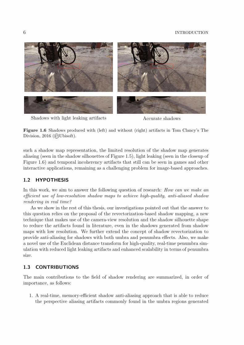
6 INTRODUCTION
Shadows with light leaking artifacts Accurate shadows
Shadows with light leaking artifacts Accurate shadowsShadows with light leaking artifacts Accurate shadows
Figure 1.6 Shadows produced with (left) and without (right) artifacts in Tom Clancy’s TheDivision, 2016 (©Ubisoft).
such a shadow map representation, the limited resolution of the shadow map generatesaliasing (seen in the shadow silhouettes of Figure 1.5), light leaking (seen in the closeup ofFigure 1.6) and temporal incoherency artifacts that still can be seen in games and otherinteractive applications, remaining as a challenging problem for image-based approaches.
1.2 HYPOTHESIS
In this work, we aim to answer the following question of research: How can we make anefficient use of low-resolution shadow maps to achieve high-quality, anti-aliased shadowrendering in real time?
As we show in the rest of this thesis, our investigations pointed out that the answer tothis question relies on the proposal of the revectorization-based shadow mapping, a newtechnique that makes use of the camera-view resolution and the shadow silhouette shapeto reduce the artifacts found in literature, even in the shadows generated from shadowmaps with low resolution. We further extend the concept of shadow revectorization toprovide anti-aliasing for shadows with both umbra and penumbra effects. Also, we makea novel use of the Euclidean distance transform for high-quality, real-time penumbra sim-ulation with reduced light leaking artifacts and enhanced scalability in terms of penumbrasize.
1.3 CONTRIBUTIONS
The main contributions to the field of shadow rendering are summarized, in order ofimportance, as follows:
1. A real-time, memory-efficient shadow anti-aliasing approach that is able to reducethe perspective aliasing artifacts commonly found in the umbra regions generated
1.4 ORGANIZATION 7
on the basis of an image-based approach;
2. A set of shadow rendering techniques that are able to produce real-time, high-quality shadows with fixed-, variable-size penumbra and less artifacts than relatedwork;
3. An anti-aliasing, screen-space shadow mapping technique that generates shadowsfaster than the techniques commonly found in the literature, at the cost of slightlyreduced visual quality;
4. An adaptive light source sampling approach that is able to generate temporally co-herent, accurate shadows from a few light source samples, speeding up the accurateshadow computation;
5. A practical implementation of the memory-efficient shadow anti-aliasing techniquein a well-known game engine. This contribution not only shows that the proposedtechnique is easy to be implemented and integrated into an application, but alsoallows the evaluation of the proposed technique in the context of more complexenvironments typically found in games.
1.4 ORGANIZATION
The remainder of this work is organized as follows:Chapter 2, Background and State-of-the-Art Review. This chapter gives an
overview of relevant work in the field of shadow rendering. The basic concepts of shadowrendering as well as a review of recent related work are presented.
Chapter 3, Revectorization-Based Shadow Mapping. This chapter presentsthe technique proposed to solve the problem of real-time shadow anti-aliasing using theconcept of shadow silhouette revectorization.
Chapter 4, Revectorization-Based Filtered Shadow Mapping. This chap-ter focuses on the description and evaluation of two techniques that simulate fixed-sizepenumbra from revectorized shadows.
Chapter 5, Revectorization-Based Soft Shadow Mapping. This chapter presentsthree techniques able to compute anti-aliased variable-size penumbra on the basis of thetechniques shown in Chapters 3 and 4.
Chapter 6, Revectorization-Based Accurate Soft Shadow Mapping. In thischapter, we introduce the proposed technique able to compute accurate shadows inter-actively. The concept of shadow silhouette revectorization is used to guide a temporallycoherent adaptive sampling of the area light source.
Chapter 7, Concluding Remarks. This chapter concludes this thesis, showing thefinal considerations about this work, and suggesting potential future directions.


Chapter
2In this chapter, we present the theoretical background behind the field of shadow rendering and review
the most relevant and recent works proposed in the literature.
BACKGROUND AND STATE-OF-THE-ART REVIEW
For the rest of this manuscript, we use the following mathematical notation: boldfacefor points and vectors, italics for scalars and non-standard functions, normal font fortraditional mathematical functions (e.g., cos, sin), calligraphic mathematical symbol forsets (e.g., A), and sans serif for matrices (e.g., S). For convenience, we assume thatscalars and functions are defined in R, points and vectors are defined in R3, unless statedotherwise. The subscripts x, y and z are used to refer to the positions of the variables inthe 3D space.
2.1 RENDERING EQUATION
The problem of shadow computation can be understood as a part of the global illumi-nation problem, which is the reproduction of the photorealistic appearance of an objectlocated inside a 3D scene and illuminated by an area light source. The quantity thatcaptures the appearance of an object in a 3D scene is called radiance. Radiance ex-presses how much power arrives at (or leaves from) a certain point on a surface in a givendirection (DUTRE et al., 2006). We refer to radiance by the function L(p,Θ), where pis the surface point and Θ is the radiance direction. Also, we use the terms L(p → Θ)and L(p← Θ) to define the radiance leaving and arriving at the point p in the directionΘ, respectively.
The photorealistic appearance of an object is typically computed by the equilibriumdistribution of light energy inside the scene. However, the light emitted by an arealight source may interact in many ways with the objects in the scene and to modelall the possible behaviours and interactions of the light in the scene is computationallyimpracticable. To ease this computation, global illumination methods commonly assumethat light is emitted, reflected, or transmitted from a surface point. Moreover, theyassume that light travels instantaneously in straight lines, without influence of externalfactors (DUTRE et al., 2006).
9

10 BACKGROUND AND STATE-OF-THE-ART REVIEW
The formulation of the global illumination rendering equation relies on the principleof energy conservation. Let us define Le(p → Θ) as the radiance emitted by the pointp in the direction Θ, and L(p → Θ) as the total exitant radiance leaving the point pin the direction Θ. L(p → Θ) is equivalent to the sum of the emitted and reflectedradiance at the point p in the direction Θ. The reflected radiance is the result of aninteraction between the incoming radiance L(p ← Ψ) and the bidirectional reflectancedistribution function fr(p,Ψ → Θ), which defines how the light is reflected at the pointp according to the radiance incident in direction Ψ and reflected in direction Θ. Hence,we can formalize the global illumination rendering equation as (KAJIYA, 1986; IMMEL;COHEN; GREENBERG, 1986)
L(p→ Θ) = Le(p→ Θ) +
∫Ω+
fr(p,Ψ→ Θ)L(p← Ψ)cos(np,Ψ)dωΨ, (2.1)
where the integral term denotes the total reflected radiance over the hemisphere Ω+
above p and cos(np,Ψ) is the cosine of the angle formed by the normal vector np of thepoint p and the ingoing direction Ψ. The bouncing behaviour of the reflected light isrepresented by the incoming radiance L(p← Ψ), which depends on the outgoing radianceL(q→ −Ψ) at a different point q.
An alternative, simpler formulation of the rendering equation replaces the integrationover the hemisphere around the surface point by an integration over all the surfaces visibleto the surface point. In this case, a ray casting operation is used to find the closest pointq visible to the point p at direction Ψ. Using the ray casting operation, we can define abinary visibility function Vray(p,q) ∈ 0, 1
Vray(p,q) =
0 if p and q are not mutually visible,
1 otherwise.(2.2)
Using these definitions, we can reformulate the rendering equation as
L(p→ Θ) = Le(p→ Θ) +
∫Afr(p,Ψ→ Θ)L(q→ −Ψ)Vray(p,q)G(p,q)dAq, (2.3)
where the set A represents all the surfaces present in the scene and
G(p,q) =cos(np,Ψ)cos(nq,−Ψ)
||p− q||2. (2.4)
As the focus of our proposal relies on the shadow computation only, we are moreinterested in the computation of the direct illumination that arrives at the surface comingdirectly from the area light source. In this sense, we can assume that the integration mustbe calculated over all the area light source samples l visible to the point p. Then, therendering equation is simplified to
L(p→ Θ) =
∫Lfr(p,
−→pl → Θ)Le(l→
−→lp)Vray(p, l)G(p, l)dLl, (2.5)

2.1 RENDERING EQUATION 11
where the set L represents the surface area of the area light sources present in the scene,
and Le(l →−→lp) is the emitted radiance of the area light source sample l visible to the
point p along the direction−→lp. We have omitted the emitted radiance term Le(p → Θ)
in (2.5) because we assume that the term is different from zero for light sources only. Inthis case, the term is only added to the sum when a light source is visible in the finalrendered image.
If we separate the shading term from the shadow term, we obtain an alternative formof the direct lighting equation
L(p→ Θ) =
∫Lfr(p,
−→pl → Θ)G(p, l)dLl ·
1
|L|
∫LLe(l→
−→lp)Vray(p, l)dLl (2.6)
If we assume that the area light source has homogeneous directional radiation overits surface and that the area light source is uniformly colored (EISEMANN et al., 2011),
we can reduce the emitted radiance Le(l →−→lp) to a constant value L∗e, which is taken
out from the integral. This results in the equation
L(p→ Θ) = L∗e
∫Lfr(p,
−→pl → Θ)G(p, l)dLl ·
1
|L|
∫LVray(p, l)dLl (2.7)
Although (2.7) is an approximation of the physically correct solution (2.5), this equa-tion allows the reproduction of realistic shadows. To solve the integral (2.7) numerically,we can sample the area light source uniformly
L(p→ Θ) = L∗e
n−1∑i=0
fr(p,−→pli → Θ)G(p, li)Vray(p, li), (2.8)
where n ∈ N is the number of point light source samples.In practice, by solving (2.8), we are able to produce accurate soft shadows that
simulate both umbra and penumbra effects. However, as pointed by related work (EISE-MANN et al., 2011), hundreds or thousands of area light source samples are typicallyrequired to allow the estimation of accurate soft shadows from (2.8), making this equa-tion computationally expensive to be solved in real time.
One alternative to simplify (2.8) relies on the computation of hard shadows thatsimulate only the umbra effect. Hard shadows are extremely suitable for real-time appli-cations because, to compute them, one just needs to replace the visibility sum over then light source samples (2.8) to a visibility evaluation over a single point light source l
′.
Then, the shadow term of the direct-lighting equation becomes just Vray(p, l′) in
L(p→ Θ) = L∗efr(p,−→pl
′ → Θ)G(p, l′)Vray(p, l
′). (2.9)
Obviously, this alternative equation presents a trade-off between visual quality andrendering performance, since hard shadows can be easily computed in real time, but arenot as accurate as soft shadows due to the lack of the penumbra simulation. A commonalternative to remedy this situation is to treat Vray(p, l
′) as a real-valued, continuous

12 BACKGROUND AND STATE-OF-THE-ART REVIEW
Figure 2.1 In ray tracing, the camera sends several view rays into the scene. When theserays hit an object, they send shadow rays in the direction of the light source. Then, a point isdetermined to be in shadow if its corresponding shadow ray hits another point before reachingthe light source. The original image is in the public domain.
visibility function. Therefore, l′
is considered as an approximation of the area lightsource, so that it could enable Vray to estimate how much of the area light source isvisible from a given surface point in the scene. Techniques that use this strategy typicallyproduce visually plausible soft shadows, since they simulate the variable-size penumbraeffect without sampling the entire area light source. Another alternative to improve theaccuracy of hard shadows is to simply blur the resulting shadows with a fixed-size filter,generating filtered hard shadows with fixed-size penumbra.
In the next section, we present the most traditional techniques able to compute Vray
and solve (2.9). Next, we review the existing methods that extend these traditionaltechniques to compute hard and soft shadows efficiently.
2.2 SHADOW RENDERING
One of the main issues to solve the simplified rendering equation (2.8, 2.9) is how tocompute the binary visibility function Vray(p, l) (2.2), regardless of whether l is a sampleof an area light source (2.8) or just a single point light source (2.9). The most traditionaltechniques able to accomplish this task are: ray tracing, shadow volume and shadowmapping.
Ray tracing (WHITTED, 1980) is a well-known object-based shadow algorithm ableto compute accurate hard shadows. In this technique, a view ray (red arrows in Figure2.1) is traced from the camera viewpoint to the virtual scene through each pixel in theimage plane (gray grid in Figure 2.1). If the view ray hits a surface point in the scene,a new shadow ray is traced from the hit point to the light source. If the shadow rayhits an opaque object before reaching the light source, the surface point hit by the viewray is in shadow (see the point hit by the lower view ray in Figure 2.1). Otherwise, the

2.2 SHADOW RENDERING 13
Figure 2.2 In shadow volume, a point is in shadow if it is located inside the shadow volumeformed by the extrusion of the vertices located at the silhouette of the shadow caster in thedirection of the rays emitted by the light source. Image is courtesy of (MCGUIRE, 2004).
surface point is directly visible by the light source and is lit (see the point hit by theupper view ray in Figure 2.1). Ray tracing is not only able to simulate shadows, but alsomany other effects (e.g., reflection, refraction), a property that makes this technique apowerful tool for computing some global illumination effects. Unfortunately, even withthe recent advances in literature (WALD et al., 2014; FUETTERLING et al., 2015;PERARD-GAYOT; KALOJANOV; SLUSALLEK, 2017), ray tracing does not providereal-time performance for dynamic scenes. Therefore, it is mostly used for applicationsthat use offline rendering (e.g., movie production) or for the rendering of precomputedeffects for static or dynamic scenes (MORGAN; PRANCKEVICIUS, 2014).
A faster alternative to ray tracing is shadow volume (CROW, 1977). A shadowvolume consists of a set of polygons formed by an extrusion (dotted lines in Figure 2.2) ofthe vertices located at the silhouette of the objects presented in the scene (green caster inFigure 2.2) in the direction of the rays emitted by the light source (light in Figure 2.2). Asurface point is in shadow (black rectangle in Figure 2.2) if it is located inside the shadowvolume, and is lit otherwise. Shadow volume is an object-based algorithm faster thanray tracing and generates accurate hard shadows. However, despite the recent advancestowards adapting the use of shadow volume to compute real-time shadows (GERHARDSet al., 2015; MORA et al., 2016), shadow volume does not provide stable frame rates,since the shadow rendering time greatly depends on the number of polygons of the shadowvolume seen in the camera view. Moreover, shadow volume still demands higher memoryfootprints, because one needs to store the many polygons that form the shadow volume.Finally, the recent shadow volume techniques are still slow for real-time applications.
A faster, less accurate alternative than both ray tracing and shadow volume is shadowmapping (WILLIAMS, 1978). Shadow mapping is an image-based shadow algorithmcomposed of two passes, whose pipeline is depicted in Figure 2.3. In the first pass, thetechnique samples the 3D space viewed from the light source (an example is shown inthe top-middle of Figure 2.3) and rasterizes the distance of the light source to the closestsurface points of the scene into a depth texture called shadow map, as shown in thetop-right of Figure 2.3. In the second pass, each surface point visible in the camera view

14 BACKGROUND AND STATE-OF-THE-ART REVIEW
Figure 2.3 In shadow mapping, the scene (top-left) is rendered from the viewpoint of the lightsource (top-middle), and its depth buffer is stored in a shadow map (top-right). Then, a pointis in shadow if its distance to the light source is greater to the one stored in the shadow map(bottom). Image is courtesy of (EISEMANN et al., 2011).
is projected into the light source view and its distance to the light source is compared tothe one stored in the shadow map (i.e., shadow test). If the surface point is farther fromthe light source than its light blocker as stored in the shadow map, the surface point is inshadow. Otherwise, the surface point is lit and must be shaded accordingly. An exampleof the final result produced by shadow mapping is shown on the bottom of Figure 2.3.
The shadow mapping solution has several advantages, such as: simplicity, flexibility,scalability, hardware support and real-time performance. However, the finite resolutionof the shadow map introduces some problems:
1. Pixels of the shadow map do not correspond to pixels in screen space, as can beseen in Figure 2.4-(a). This insufficient resolution of the shadow map (gray grid inFigure 2.4-(a)) generates aliasing artifacts, mainly along the shadow silhouette, ascan be seen in the silhouette of the shadows shown in Figure 2.4-(b);
2. Due to numerical precision issues, pixels of the screen space may lie between pixelsof the shadow map, generating false self-shadowing. In Figure 2.5-(a), false self-

2.2 SHADOW RENDERING 15
(a) (b)
Figure 2.4 Due to the (a) limited resolution of the shadow map (gray grid projected into thecamera view), shadow mapping generates hard shadows with (b) perspective aliasing artifacts.Images are courtesy of ©Vladimir Bondarev.
(a) (b)
Figure 2.5 Hard shadows (a) with false self-shadowing. (b) Accurate hard shadows.
shadowing is visible by the striped umbra artifacts present in both plane and teapotobjects;
3. Because of the previous artifacts, whenever the camera or the light source moves inthe scene, the shadow’s shape may change in a temporally incoherent, unrealisticway (EISEMANN et al., 2011). This effect is mainly seen in videos and animations.
While false self-shadowing can be easily solved by adding a fixed (WILLIAMS, 1978)or adaptive depth bias (DOU et al., 2014) to influence the shadow test, aliasing artifactsand temporal incoherence are two of the major problems of image-based approaches,hampering the generation of accurate hard shadows, as exemplified by Figure 2.5-(b).

16 BACKGROUND AND STATE-OF-THE-ART REVIEW
Uniform distribution Non-uniform distribution
Figure 2.6 (Left) A uniform distribution of depth values in the shadow map produces aliasedartifacts along the shadow silhouette. (Right) A non-uniform, perspective distribution of depthvalues improves shadow visual quality. Images courtesy of (STAMMINGER; DRETTAKIS,2002).
In the following sections, we present the different types of shadows that can be sim-ulated on the basis of shadow mapping and we also discuss many strategies proposed toalleviate the aliasing problem of shadow mapping. We refer the reader to reference books(EISEMANN et al., 2011) (WOO; POULIN, 2012) for a more complete review of theexisting shadow rendering algorithms.
2.3 HARD SHADOWS
Hard shadows represent only the umbra component of the shadow, in other words, thetotal absence of light. Shadow mapping is the most traditional technique able to solve(2.9) in real time, at the cost of generating aliased hard shadows. In this section, wediscuss the different strategies that have been proposed to generate anti-aliased hardshadows in real time with shadow mapping.
2.3.1 Warping
Aliasing artifacts can be reduced by changing the parametrization of the shadow mapgeneration. In other words, by changing the warping function that transforms world-space coordinates to shadow map texture coordinates, one can improve the shadow mapresolution in the region near the viewpoint, while lowering the sampling density in theregions far from the viewpoint. This warping effect can be seen in Figure 2.6. In Figure2.6-left, the shadow map generation wastes space of the shadow map due to the uniformdistribution of the depth values. Then, as can be seen in Figure 2.6-right, by warpingthe shadow map generation with a non-uniform perspective projection, one can make abetter use of the available shadow map resolution, improving the sampling density forthe objects visible in the current camera viewpoint.
Different from the approaches that aim to distribute the depth values uniformly in theshadow map texture (BRABEC; ANNEN; SEIDEL, 2002), perspective shadow mapping(STAMMINGER; DRETTAKIS, 2002) is the first technique proposed to warp the shadow

2.3 HARD SHADOWS 17
(a) (b)
Figure 2.7 For a large scene, the use of an insufficient shadow map resolution may generatealiasing artifacts along the shadow silhouette (a). The efficient distribution of several high-resolution shadow maps per sub-units of the 3D space helps on reducing these aliasing artifacts(b). Images courtesy of (LAURITZEN; SALVI; LEFOHN, 2011).
map using non-uniform perspective projection instead of the orthographic one. Whilethis simple changing of parametrization has hardware support and greatly improves thequality of the shadow rendering, the algorithm does not handle several special cases andrestrictions, reducing the quality of the shadow map parametrization.
Approaches such as light-space perspective shadow mapping (WIMMER; SCHERZER;PURGATHOFER, 2004), trapezoidal shadow mapping (MARTIN; TAN, 2004), and per-spective optimal shadow mapping (CHONG; GORTLER, 2004; CHONG; GORTLER,2007) try to generalize the use of perspective shadow maps for different scenarios andlight sources, and distribute the error equally among objects located near and far fromthe viewer. Logarithmic parametrization (LLOYD et al., 2008) is an alternative approachto obtain a higher accurate warping algorithm at the cost of lower frame rate.
Warping techniques minimize aliasing artifacts efficiently, but flickering artifacts stillcan be seen when the camera or the light source moves in the scene. These flickeringartifacts are caused by the use of the non-uniform sampling strategy, that may changethe warping function per frame, in a temporally incoherent way. Also, even if the warpingstrategies make better use of the shadow map resolution, aliasing artifacts are still gen-erated by such techniques because the shadow map resolution, the source of the aliasing,remains finite and limited.
2.3.2 Partitioning
An alternative to reduce aliasing artifacts is to make use of several shadow maps generatedfrom different locations to better sample the depth of the objects located near and farthe camera viewpoint. Figure 2.7 shows shadows generated without and with partitionedshadow maps.

18 BACKGROUND AND STATE-OF-THE-ART REVIEW
Approaches based on z-partitioning split the 3D space inside the view frustum intoseveral sub-units along the z-axis and associate a separate shadow map for each sub-unit (ENGEL, 2006; ZHANG et al., 2006; ZHANG; SUN; NYMAN, 2008; LAURITZEN;SALVI; LEFOHN, 2011).
Another set of techniques evaluates the error produced by the use of a single low-resolution shadow map and try to adapt the shadow map configuration, either by gener-ating more shadow maps or increasing the shadow map resolutions, in order to reduce thealiasing artifacts caused by the insufficient shadow map resolution (FERNANDO et al.,2001; ARVO, 2004; GIEGL; WIMMER, 2007b; GIEGL; WIMMER, 2007a; LEFOHN;SENGUPTA; OWENS, 2007).
Partitioning techniques are useful to reduce aliasing artifacts caused mainly by theuse of a single shadow map in a large-scale virtual environment. To further improvethe accuracy of the solution, these techniques are commonly associated with warpingtechniques. Thus, the several shadow maps generated from partitioning approaches arebuilt using an improved parametrization approach. While this combination may work insome situations, for simpler scenarios in which high-quality shadows could be renderedwith a single shadow map of high resolution, the use of partitioned shadow maps may onlyincrease memory usage (although recent works, such as (SINTORN et al., 2014; KAMPEet al., 2016; SCANDOLO; BAUSZAT; EISEMANN, 2016a; SCANDOLO; BAUSZAT;EISEMANN, 2016b), have focused on the efficient compression of shadow maps) andprocessing time.
2.3.3 Silhouette Recovery
Some techniques aim to compute accurate hard shadows by minimizing the jagged shadowsilhouettes produced by shadow mapping.
Hybrid approaches based on shadow mapping, shadow volume (MCCOOL, 2000;CHAN; DURAND, 2004), and ray tracing (HERTEL; HORMANN; WESTERMANN,2009) have been proposed in the literature. As can be seen in the comparison betweenFigures 2.8-(a) and 2.8-(b), these methods are able to estimate accurate hard shadows.However, as shown in Figure 2.8-(c), they compute shadows faster than the referencesolutions, but still much slower than shadow mapping.
To reconstruct accurate shadow silhouettes, some techniques rely on the storage ofadditional geometric information. In shadow silhouette mapping (SEN; CAMMARANO;HANRAHAN, 2003), the vertex that lies on the geometry silhouette is stored in theshadow map. Fast sub-pixel anti-aliased shadow mapping (PAN et al., 2009) uses pixel’sposition and associated face normal in addition to the shadow map. Sub-pixel shadowmapping (LECOCQ et al., 2014) stores triangle information (i.e., 3D vertex coordinatesand depth derivatives) with the shadow map. Each one of these techniques has a differentvisibility function that uses this augmented information to reconstruct accurate shadowsilhouettes. However, they also increase memory consumption and processing time toachieve such a goal.
To solve the mismatch problem of shadow mapping, the mapping of each pixel in thecamera view into an exclusive texel in the shadow map, other approaches, such as (AILA;

2.3 HARD SHADOWS 19
(a) (b) (c)
Figure 2.8 Silhouette recovery techniques solve aliasing artifacts (a) by recovering accurateshadow silhouettes (b). These techniques guarantee high-quality anti-aliasing, however, theyadd a high computational overhead for shadow mapping (c). SM - Shadow mapping. H -Silhouette recovery technique. SV - Shadow volume. Images courtesy of (CHAN; DURAND,2004).
LAINE, 2004; JOHNSON et al., 2005; WYMAN; HOETZLEIN; LEFOHN, 2015), treatthe shadow map as an irregular data structure to correct the insufficient shadow mapsampling. Unfortunately, the building and management of such data structures demandadditional processing time to the shadow rendering algorithm.
To perform shadow anti-aliasing, shadow map silhouette revectorization (BONDAREV,2014) embeds shadow silhouettes into a discontinuity space and revectorizes them accord-ing to their discontinuity directions. While the technique indeed alleviates aliasing, themethod consists of two passes in the shader, increases memory consumption and does notwork well for sloped surfaces, generating artifacts during revectorization. By adaptingthis technique to work in a single pass in the shader, revising its theory to reduce memoryconsumption, adding support for shadow anti-aliasing in sloped surfaces, and extendingit to support penumbra simulation, we show that we can take advantage of this shadowrevectorization effect to provide high-quality shadow anti-aliasing.
Techniques for reconstructing shadow silhouettes are useful because they can solve thealiasing problem in an accurate way. However, as exemplified by the performance resultsshown in Figure 2.8-(c), most of these techniques add a high computational overheadto shadow mapping. Also, by incorporating additional geometric information into theshadow map, these techniques typically add a large memory footprint to the hard shadowrendering.
Warping and partitioning strategies seem to be well established in industry, sincethe state-of-the-art techniques satisfy the requirements of games and other interactiveapplications (LAURITZEN; SALVI; LEFOHN, 2011). In this scenario, these strategiesare typically integrated with other strategies, such as silhouette recovery and hard shadowfiltering, to improve the accuracy of the latter ones. On the other hand, shadow silhouetterecovery techniques solve the aliasing problem accurately, but they are not as fast and

20 BACKGROUND AND STATE-OF-THE-ART REVIEW
(a) Shadow Mapping (b) PCF (c) VSM
(a) Shadow Mapping (b) PCF (c) VSM(a) Shadow Mapping (b) PCF (c) VSM(a) Shadow Mapping (b) PCF (c) VSM
Figure 2.9 Hard shadow filtering techniques minimize the shadow aliasing problem of shadowmapping (a) by simulating fixed-size penumbra. Unfortunately, (b) banding or (c) light leakingartifacts may affect the visual quality of the penumbra rendering.
lightweight as shadow mapping.While the simplification of (2.9) guarantees real-time performance, hard shadows tech-
niques are not realistic because they do not generate penumbra natively and produceshadows with visual quality far from the physically accurate solution. In the next sec-tion, we discuss alternative solutions that simulate the penumbra effect on the basis ofthe filtering of hard shadows.
2.4 FILTERED HARD SHADOWS
To simulate the penumbra effect on the basis of the hard shadows generated by shadowmapping, some techniques perform filtering over the hard shadows, or over the shadowmap itself, to produce filtered hard shadows with fixed-size penumbra. This effect canbe seen in Figure 2.9. By blurring the hard shadows shown in Figure 2.9-(a), we canproduce fixed-size penumbra, as seen in Figures 2.9-(b) and 2.9-(c).
The most traditional algorithm for fixed-size penumbra simulation is Percentage-Closer Filtering (PCF) (REEVES; SALESIN; COOK, 1987). As an extension of shadowmapping, PCF takes the shadow test results performed over a filter region and averagesthem to determine the final shadow intensity. By filtering the shadow test results, ratherthan the shadow map itself, PCF is not prone to light leaking artifacts, and providesreal-time performance, while keeping low memory consumption for the penumbra simu-lation. However, PCF does not support texture pre-filtering, does not provide scalabilityin terms of filter size, and requires a high number of samples to solve banding artifacts.An example of banding artifacts produced by PCF can be seen in Figure 2.9-(b).
To make the shadow filtering scalable, Variance Shadow Mapping (VSM) (DON-NELLY; LAURITZEN, 2006) uses Chebyshev’s inequality, depth and squared depthstored in the shadow map to determine the shadow intensity of a surface point by meansof a probability of whether the point is in shadow. VSM supports shadow map pre-

2.4 FILTERED HARD SHADOWS 21
filtering and is scalable for the filter size, but generates light leaking artifacts in shadows.An example of light leaking artifacts produced by VSM is shown in Figure 2.9-(c).
To reduce the light leaking artifacts of VSM, Convolution Shadow Mapping (CSM)(ANNEN et al., 2007) uses Fourier series to approximate and linearize the shadow test. InCSM, the shadow map is converted into filtered basis textures that are used to determinethe final shadow intensity as a weighted sum of basis functions stored in basis textures.CSM supports pre-filtering and reduces light leaking artifacts as compared to VSM, atthe cost of more memory consumption and processing time than VSM.
To minimize the processing time required by CSM, Exponential Shadow Mapping(ESM) (ANNEN et al., 2008; SALVI, 2008) approximates the shadow test by an ex-ponential function, rather than Fourier series. ESM stores exponent-transformed depthvalues into the shadow map, which are later used for penumbra simulation. ESM is fasterand requires less memory footprint than CSM, while generating visual results similar tothe ones obtained with VSM.
To improve the visual quality of both VSM and ESM, Exponential Variance ShadowMapping (EVSM) (LAURITZEN; MCCOOL, 2008) merges both ESM and VSM theoriesto produce high-quality fixed-size penumbra simulation. In EVSM, light leaking onlyoccurs at places where both ESM and VSM techniques generate such an artifact.
As an alternative to both VSM and ESM techniques, Gaussian Shadow Mapping(GSM) (GUMBAU et al., 2011; GUMBAU et al., 2013) replaces Chebyshev’s inequalityby a Gaussian cumulative distribution function to minimize light leaking. Also, inspiredby EVSM, GSM warps its visibility function to take advantage of the exponential functionproposed in ESM to further reduce light leaking.
Moment Shadow Mapping (MSM) (PETERS; KLEIN, 2015; PETERS, 2017) im-proves VSM by storing four powers of depth in the shadow map and treating the penum-bra simulation as a Hamburger or Hausdorff moment problem. MSM reduces the lightleaking artifacts of VSM, generates results similar to EVSM, while keeping nearly thesame rendering time of both techniques, but consuming more memory requirements thanVSM.
Filtering techniques are an efficient alternative to shadow mapping, producing shad-ows that mimic the appearance of the penumbra effect. In Table 2.1, we show a generalclassification of the filtered hard shadow techniques presented in this section with respectto the relevant attributes discussed so far.
VSM, CSM, ESM, EVSM, GSM, and MSM techniques filter the shadow map bywarping the depth stored in the shadow map into another basis function, making thepenumbra simulation scalable in terms of filter size. However, as shown in Figure 2.9-(c),these shadow map filtering techniques introduce noticeable light leaking artifacts thatreduce the shadow visual quality. On the other hand, PCF filters the hard shadowsproduced with shadow mapping to avoid light leaking. However, PCF is not scalablewith respect to the filter size.
Despite requiring low processing time to minimize the aliasing artifacts produced byshadow mapping, none of the filtered hard shadow techniques presented in this sectioncan remove the aliasing artifacts caused by the use of low-resolution shadow maps, sincethey work over jagged shadow silhouettes (Figure 2.9-(b)). Increasing the resolution of

22 BACKGROUND AND STATE-OF-THE-ART REVIEW
PropertyMethod Anti-aliasing Reduced Leaking Scalability Memory Footprint
PCF 6 4 6 LowVSM 6 6 4 MediumCSM 6 6 4 HighESM 6 6 4 Medium
EVSM 6 6 4 MediumGSM 6 6 4 MediumMSM 6 6 4 Medium
Table 2.1 Classification of filtered hard shadow mapping techniques proposed in the literatureaccording to the following attributes: anti-aliasing for shadows produced with low-resolutionshadow maps, reduced light leaking artifact generation, scalability with respect to the filtersize and memory consumption (low if the algorithm uses only the shadow map, medium ifthe algorithm uses two or more channels of the shadow map and high if the algorithm usesadditional textures for penumbra simulation).
the shadow map may overcome this issue, at the cost of higher memory consumption andprocessing time. But, even in this case, any closeup on the shadow could reveal the alias-ing artifacts. Larger kernel sizes may also remove the aliasing of the shadows, however,they severely blur out the shadows, losing too much detail of the shadow silhouette.
As we further state in the next section, filtered hard shadows are more realistic thanhard shadows, but they also lack realism because they are able to simulate only fixed-sizepenumbra, meanwhile real-world shadows mostly contain variable-size penumbra.
2.5 VISUALLY PLAUSIBLE SOFT SHADOWS
Differently from the techniques that compute fixed-size penumbra, visually plausible softshadow techniques take into consideration the fact that the size of the penumbra variesaccording to the distance of the surface point to both light source and other light blockersurface points. Shadows that are computed on the basis of a single point light sourceand that can simulate variable-size penumbra are called visually plausible soft shadows.Soft shadows because they simulate the variable-size penumbra effect. Visually plausibleshadows because they resemble the visual quality of accurate shadows. An example of avisually plausible soft shadow is shown in Figure 2.10.
Here, we review the existing soft shadow methods that have been proposed to extendthe concept of hard shadow mapping to compute soft shadows in real time.
2.5.1 Percentage-Closer Soft Shadows
Area light sources produce soft shadows in which the penumbra size varies along theshadow silhouette, as visible in Figure 2.10. The task of estimating this penumbra sizein a general configuration is non-trivial (EISEMANN et al., 2011).
To ease the task of variable penumbra size estimation, the Percentage Closer SoftShadows (PCSS) technique uses an assumption that both light source, light blocker and
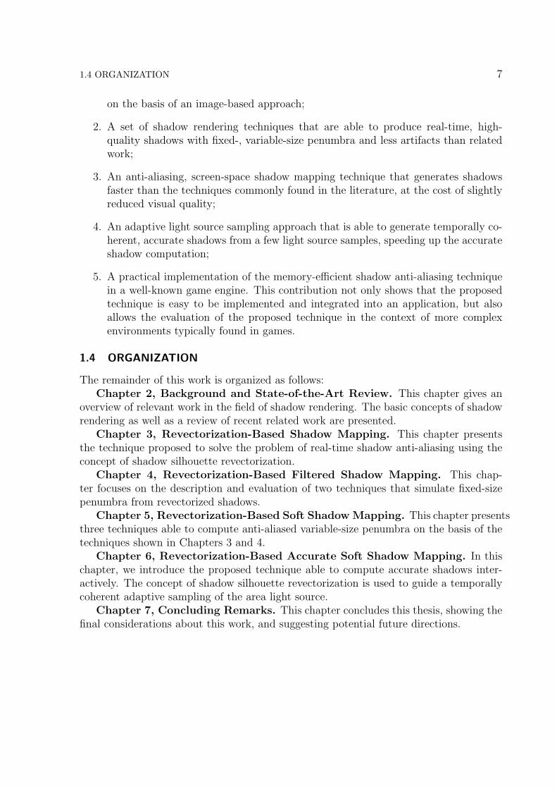
2.5 VISUALLY PLAUSIBLE SOFT SHADOWS 23
Figure 2.10 Visually plausible soft shadows have penumbra whose size varies according to thedistance of each surface point to both light source and light blocker objects. Image courtesy of(FERNANDO, 2005).
shadow receiver objects are all planar and parallel to each other (SOLER; SILLION,1998). Hence, by the use of similar triangles, the penumbra size can be easily estimated(FERNANDO, 2005).
The PCSS framework consists of three main steps: the average blocker depth com-putation, the penumbra size estimation and the soft shadow filtering. First, the shadowmap is searched in a given region and the average distance of the blocker to the lightsource is computed. Then, this average distance is used in addition to the light sourcesize and the receiver depth for the penumbra size estimation. Finally, the PCF is appliedover the penumbra size of the soft shadow filtering. PCSS is easy to implement, providesanti-aliasing, uses only one shadow map, and requires neither pre-processing nor addi-tional geometric information. However, PCSS produces aliased shadows for large arealight sources (EISEMANN et al., 2011). Also, this technique scales poorly for large filtersizes because a large amount of texture lookups for both average blocker depth estimationand soft shadow filtering steps is required.
Temporal coherence has already been exploited to generate visually plausible softshadows on the basis of the PCSS framework (SCHERZER et al., 2009; SCHERZER;SCHWARZLER; MATTAUSCH, 2011; SCHWARZLER et al., 2013). While these tech-

24 BACKGROUND AND STATE-OF-THE-ART REVIEW
(a) BP (b) VSSM (c) Reference
Figure 2.11 While providing a plausible visual quality for the soft shadow rendering, back-projection (BP) approaches (such as (GUENNEBAUD; BARTHE; PAULIN, 2007) (a)) are toomuch slower than pre-filtering techniques (such as VSSM (b)). Images courtesy of (YANG etal., 2010).
niques are able to provide realistic soft shadows in real time, they require several framesto converge to a correct solution. Also, the frame rate may change considerably betweenframes for dynamic scenes with moving objects, cameras or light sources, being inade-quate for applications that demand constant frame rates. Shen et al. (SHEN et al., 2011)propose an analytical filtering solution to improve the image quality of PCSS, but thealgorithm is inefficient in terms of performance for large filter sizes.
To improve the performance of PCSS, Klein et al. (KLEIN; NISCHWITZ; OBER-MEIER, 2012) compute the average blocker depth and estimate the penumbra size onlyfor the fragments located at the hard shadow silhouette. Then, for each fragment outsidethe shadow silhouette, a gathering approach and an erosion operation are used to locatethe shadow silhouette and estimate the penumbra intensity of the soft shadows. Thisapproach is slightly faster than PCSS for large kernel sizes, but is still prone to aliasingartifacts at the penumbra location.
2.5.2 Back-Projection
Rather than using the PCSS framework to compute soft shadows, back-projection tech-niques aim to provide an accurate soft shadow solution by unprojecting a micropatchfor each shadow map texel and then using this geometric representation to compute theamount of the light source occluded by the blocker objects (ATTY et al., 2006; AS-ZODI; SZIRMAY-KALOS, 2006; GUENNEBAUD; BARTHE; PAULIN, 2006; BAVOIL;CALLAHAN; SILVA, 2008). Micropatches are approximations of the blocker geometry.Thus, they may cause shadow overestimation and light leaking. To solve such problems,the authors of (SCHWARZ; STAMMINGER, 2007) propose the use of an occlusion bit-mask. In fact, they place sample points on the area light source and use a simple bitrepresentation to track which of the samples are occluded. Unfortunately, this approachsuffers from performance issues, especially for high-resolution shadow maps. Hierarchi-cal solutions and techniques based on efficient contour detection are commonly used to

2.5 VISUALLY PLAUSIBLE SOFT SHADOWS 25
reduce the computational cost of the soft shadow mapping (GUENNEBAUD; BARTHE;PAULIN, 2007; YANG et al., 2009).
Back-projection techniques generate high-quality soft shadows using a single shadowmap, as shown in Figure 2.11-(a). However, these methods are still prone to artifactsand achieve only interactive performance due to the usage and computation of multipleshadow maps required to properly track the micropatches into the area light source.
2.5.3 Pre-Filtering
To solve both problems of aliasing and scalability of the PCSS, pre-filtering techniquescommonly use a filterable function to approximate either the average blocker depth esti-mation, the shadow test or both of them.
Summed-Area Variance Shadow Mapping (SAVSM) (LAURITZEN, 2008) replacesthe PCF step of PCSS by VSM (DONNELLY; LAURITZEN, 2006), which makes thesoft shadow filtering scalable with respect to the filter size. Unfortunately, the averageblocker depth estimation remains costly and the use of VSM for shadow filtering makesSAVSM more prone to light leaking artifacts than PCSS.
Convolution Soft Shadow Mapping (CSSM) (ANNEN et al., 2008) proposes a constant-time average blocker depth estimation on the basis of a pre-filtered shadow map andpre-filtered Fourier series basis images. CSM (ANNEN et al., 2008) is used to performsoft shadow filtering over the penumbra area. Indeed, CSSM brings scalability to PCSS,however, suffers from light leaking artifacts and high memory consumption.
Variance Soft Shadow Mapping (VSSM) (DONG; YANG, 2010; YANG et al., 2010)estimates the average blocker depth efficiently on the basis of a pre-filtered shadow mapand the Chebyshev’s Inequality. VSSM provides performance compatible with relatedwork, makes use of the VSM theory to estimate the average blocker depth, and generatessoft shadows with reduced light leaking artifacts.
Exponential Soft Shadow Mapping (ESSM) (SHEN; FENG; YANG, 2013) uses theESM (ANNEN et al., 2008; SALVI, 2008) theory to estimate the average blocker depthand compute the final soft shadow intensity in constant time on the basis of a pre-filtered exponential shadow map. A number of improvements are proposed to alleviatelight leaking artifacts, improve the accuracy of the pre-filtering, and keep the real-timeperformance of the approach.
Similarly to VSSM, Moment Soft Shadow Mapping (MSSM) (PETERS et al., 2016;PETERS et al., 2017) generates a pre-filtered moment shadow map (PETERS; KLEIN,2015), and use it to estimate the average blocker depth and perform the soft shadowfiltering by solving the Hamburger moment problem. Some schemes to optimize theapproach, as well as to handle numerical precision issues, are presented as well.
Different from the previous approaches, the work proposed by related work (SEL-GRAD et al., 2015) uses a new pre-filtering method in which a per-texel fragment list ofall blockers is stored in a multi-layer shadow map (XIE; TABELLION; PEARCE, 2007).Depth and opacity of all the blocker fragments are stored in a hierarchical representa-tion, where each level stores the average depth and the accumulated opacity of the texelsinvolved. This shadow map representation is then used to perform shadow filtering.

26 BACKGROUND AND STATE-OF-THE-ART REVIEW
(a) Screen-space filtering (b) PCSS (c) Reference
Figure 2.12 Screen-space filtering (a) is able to generate soft shadows visually similar to theones generated by PCSS (b) and the reference solution (c). Images courtesy of (BUADES;GUMBAU; CHOVER, 2015).
Stochastic soft shadow mapping (LIKTOR et al., 2015) samples a 4D shadow lightfield using a stochastic soft shadow map and converts such samples to a pre-filterablebasis. The authors use EVSM to represent the visibility function, but any other pre-filterable basis could be used.
Pre-filtering techniques are a good alternative to produce real-time visually plausiblesoft shadows (an example is shown in Figure 2.11-(b)) with constant-time filtering. Mostof them make use of Summed-Area Tables (SAT) (CROW, 1984) as their pre-filteringfunction to avoid the brute-force sampling proposed by the PCSS technique. However, thetime to build the SAT structure increases according to the shadow map resolution used.So, pre-filtering techniques are typically scalable with respect to the average blocker depthestimation and soft shadow filtering, but do not provide scalability for high shadow mapresolutions. Furthermore, the drawback shared by the pre-filtering techniques is that theyare prone to light leaking or incorrect shadow computation at contact borders, makingtheir use unsuitable for complex scenarios.
2.5.4 Screen-Space Filtering
An alternative to improve the performance of the soft shadow computation is to performsome or all the soft shadow filtering in the screen space. The basic idea behind thisstrategy is to generate hard shadows in the camera viewpoint with traditional shadowmapping, adapt the PCSS theory to estimate a screen-space penumbra size, and blur thehard shadows by the application of a separable filter over the penumbra region.
Screen-Space Percentage-Closer Soft Shadows (SSPCSS) (MOHAMMADBAGHER etal., 2010) proposes that the PCSS framework must be fully computed in screen space.Blocker search and shadow filtering steps are filtered in screen space by the use of aseparable cross bilateral filter (PHAM; VLIET, 2005). Screen-Space Anisotropic BlurredSoft Shadows (SSABSS) (ZHENG; SAITO, 2011) computes the average blocker depthin light space and performs screen-space anisotropic Gaussian blur over the penumbrasize to improve the visual quality of SSPCSS. Separable Soft Shadow Mapping (SSSM)(BUADES; GUMBAU; CHOVER, 2015) proposes a separable algorithm to estimate the

2.6 ACCURATE SOFT SHADOWS 27
PropertyMethod Anti-aliasing Reduced Leaking Scalability (BD/SF) Working space
PCSS 6 4 6/6 Light spaceSAVSM 6 6 6/4 Light spaceVSSM 6 6 4/4 Light spaceESSM 6 6 4/4 Light spaceMSSM 6 6 4/4 Light space
SSPCSS 6 4 4/4 Screen spaceSSABSS 6 4 6/4 Screen spaceSSSM 6 4 4/4 Screen space
Table 2.2 Classification of the main visually plausible soft shadow techniques proposed in theliterature according to the following attributes: anti-aliasing for shadows produced with low-resolution shadow maps, reduced light leaking artifact generation, scalability with respect tothe average blocker depth (BD) estimation and soft shadow filtering (SF), and working space.
average blocker depth and uses the Gaussian filtering to filter the shadows in screen space.
The main advantage of screen-space approaches over related work is that, by theuse of separable filtering techniques, the soft shadow computation can be done faster.However, while this strategy may work well in scenarios such as the one shown in Figure2.12, screen-space filtering provides just an approximation of the effect obtained by thefiltering of perspectively deformed kernels in the shadow map (light) space. That is whythe screen-space filtering strategy is not as accurate as the previous strategies.
In Table 2.2, we evaluate the properties of the main techniques proposed for visuallyplausible soft shadow rendering. Similar to the filtered hard shadow techniques, none ofthe visually plausible soft shadow rendering techniques is able to minimize aliasing arti-facts for low-resolution shadow maps. Also, only PCSS and the screen-space techniquesare able to reduce light leaking artifacts. Similar to PCF, PCSS uses a solution that doesnot provide scalability. In this sense, only the screen-space techniques sacrifice accuracyto achieve higher performance and scalability for the soft shadow rendering.
Visually plausible soft shadows are more accurate than hard and filtered hard shadows,but still lack realism because these shadows are computed on the basis of a single pointlight source. In the next section, we show the proposed techniques dedicated to solve thesimplified rendering equation (2.8) by means of area light source sampling.
2.6 ACCURATE SOFT SHADOWS
Differently from the other techniques presented in the previous sections, accurate softshadow techniques do not work with single point light sources. In order to evaluate thesimplified rendering equation (2.8) correctly, they sample the area light source so thatthey can evaluate the binary visibility function Vray correctly.
The most traditional version of ray tracing (WHITTED, 1980) can only reproducehard shadows because only one shadow ray is sent to evaluate the visibility conditionof the surface point. By distributing several shadow rays per area light source and
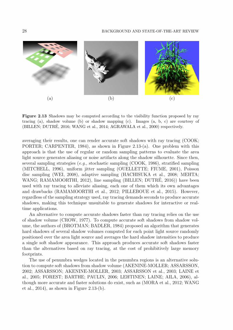
28 BACKGROUND AND STATE-OF-THE-ART REVIEW
(a) (b) (c)
Figure 2.13 Shadows may be computed according to the visibility function proposed by raytracing (a), shadow volume (b) or shadow mapping (c). Images (a, b, c) are courtesy of(BILLEN; DUTRE, 2016; WANG et al., 2014; AGRAWALA et al., 2000) respectively.
averaging their results, one can render accurate soft shadows with ray tracing (COOK;PORTER; CARPENTER, 1984), as shown in Figure 2.13-(a). One problem with thisapproach is that the use of regular or random sampling patterns to evaluate the arealight source generates aliasing or noise artifacts along the shadow silhouette. Since then,several sampling strategies (e.g., stochastic sampling (COOK, 1986), stratified sampling(MITCHELL, 1996), uniform jitter sampling (OUELLETTE; FIUME, 2001), Poissondisc sampling (WEI, 2008), adaptive sampling (HACHISUKA et al., 2008; MEHTA;WANG; RAMAMOORTHI, 2012), line sampling (BILLEN; DUTRE, 2016)) have beenused with ray tracing to alleviate aliasing, each one of them which its own advantagesand drawbacks (RAMAMOORTHI et al., 2012; PILLEBOUE et al., 2015). However,regardless of the sampling strategy used, ray tracing demands seconds to produce accurateshadows, making this technique unsuitable to generate shadows for interactive or real-time applications.
An alternative to compute accurate shadows faster than ray tracing relies on the useof shadow volume (CROW, 1977). To compute accurate soft shadows from shadow vol-ume, the authors of (BROTMAN; BADLER, 1984) proposed an algorithm that generateshard shadows of several shadow volumes computed for each point light source randomlypositioned over the area light source and averages the hard shadow intensities to producea single soft shadow appearance. This approach produces accurate soft shadows fasterthan the alternatives based on ray tracing, at the cost of prohibitively large memoryfootprints.
The use of penumbra wedges located in the penumbra regions is an alternative solu-tion to compute soft shadows from shadow volume (AKENINE-MOLLER; ASSARSSON,2002; ASSARSSON; AKENINE-MOLLER, 2003; ASSARSSON et al., 2003; LAINE etal., 2005; FOREST; BARTHE; PAULIN, 2006; LEHTINEN; LAINE; AILA, 2006), al-though more accurate and faster solutions do exist, such as (MORA et al., 2012; WANGet al., 2014), as shown in Figure 2.13-(b).

2.7 DISCUSSION 29
Since the development of the accumulation buffer (HAEBERLI; AKELEY, 1990),many algorithms have been proposed to use shadow mapping to generate hard shadowsin real time and average them using the accumulation buffer.
For a linear light source, the 2D version of an area light source, only two shadowmaps placed at the vertices of the linear light source are required to produce accurate softshadows using a two-channel shadow map which stores depth and visibility (HEIDRICH;BRABEC; SEIDEL, 2000).
For static scenes, visibility precomputation is allowed and some algorithms makeuse of this strategy to compute interactive or real-time accurate soft shadows (HERF;HECKBERT, 1996; HECKBERT; HERF, 1997; HERF, 1997; AGRAWALA et al., 2000;ST-AMOUR; PAQUETTE; POULIN, 2005), as can be seen in Figure 2.13-(c). The cleardrawback of precomputation is that, for dynamic scenes, the precomputed structuresmust be recalculated for every frame, decreasing the efficiency of the solution.
For dynamic scenes, alias-free shadow maps (SINTORN; EISEMANN; ASSARSSON,2008) have been used for hard shadow estimation per light source sample. In that work,the authors could generate high-quality, accurate soft shadows at interactive frame rates,because the alias-free shadow map generation is considerably costly when compared toalternative shadow mapping approaches. The adaptive sampling solution proposed in(SCHWARZLER et al., 2012) uses a screen-space subdivision criteria to determine howmany light source samples are needed to generate accurate soft shadows. Although thistechnique works well when the camera is far away from the scene, because a few lightsource samples are needed to provide visually accurate soft shadows, the subdivision stepconsumes too much processing time to determine the number of samples, making thisapproach inefficient when the camera is relatively close to penumbra regions, where alarge number of light source samples are required to provide accurate soft shadows.
While the evaluation of (2.8) provides high-quality visual results, the estimationof the visibility function for several light source samples is computationally expensive(SCHWARZLER et al., 2012), preventing its use for interactive applications, such asgames and augmented reality.
2.7 DISCUSSION
In this thesis, we aim to propose shadow rendering algorithms for real-time anti-aliasingof hard and soft shadows on the basis of the concept of shadow revectorization. Todo so, we improve the theory initially proposed by related work (BONDAREV, 2014)to perform shadow anti-aliasing of higher quality, with a memory footprint as small asthe one required by shadow mapping. Also, we extend the original work on shadowrevectorization to support anti-aliasing of filtered hard shadows, visually plausible softshadows, and the rendering of accurate soft shadows.
As shown in Section 2.3, shadow silhouette recovery techniques generally produceaccurate hard shadows, but are inefficient in terms of processing time and memory con-sumption. In this thesis, we propose a new technique for efficient, accurate shadow anti-aliasing that works well for both low- and high-resolution shadow maps, while keepingperformance and memory footprint as low as the ones obtained with shadow mapping.
30 BACKGROUND AND STATE-OF-THE-ART REVIEW
Taking advantage of our proposed technique for silhouette recovery, we aim to presenta novel technique that is able to generate anti-aliased filtered hard shadows for both low-and high-resolution shadow maps, without as much light leaking artifacts as relatedwork, because we do not rely on shadow map pre-filtering for penumbra simulation. Toachieve the desired scalability for the penumbra simulation, at the cost of higher memoryconsumption, we make use of Euclidean distance transform to filter the hard shadows.
On the basis of the developed filtered hard shadow techniques, we propose differenttechniques that take advantage of the improved hard shadow silhouette recovery strategyobtained with shadow revectorization to achieve anti-aliased soft shadow rendering. Themain technique uses a screen-space approach that improves the accuracy of the existingscreen-space soft shadow techniques, while providing real-time performance through thescalability for the soft shadow filtering.
Finally, our main focus of research in this thesis is the proposition of real-time tech-niques for efficient shadow artifact minimization. The faster existing strategy to computeaccurate soft shadows relies on the evaluation of the shadow mapping visibility functionover a discrete representation of the area light source. Such a discretization may occur bythe uniform or adaptive sampling of the area light source. While the uniform samplingmay generate several, unnecessary light source samples, which further increases the com-putational cost of the visibility evaluation over the area light source, the current solutionfor adaptive sampling is prone to aliasing, banding artifacts (due to the undersamplingof the penumbra region) and consequent temporal incoherence (SCHWARZLER et al.,2012).
To improve the performance of the accurate soft shadow generation, while keepingthe high visual accuracy of the solution, we propose an alternative adaptive solutionstrategy to generate a few, consistent light source samples to represent the area lightsource. By replacing the shadow mapping visibility function by a revectorization-basedvisibility function that already provides shadow anti-aliasing, we target to further reducethe number of light source samples required to generate accurate soft shadows.
2.8 SUMMARY
In this chapter, we have presented the theoretical background for shadow rendering.Moreover, we have discussed the advantages and drawbacks of the existing shadow ren-dering techniques with respect to the simulation of hard and soft shadows.
As we show in the next chapters, we propose a set of techniques to solve the mainproblem still found in both hard and soft shadow mapping techniques proposed in theliterature: the aliasing artifacts. For hard shadows, we make use of the shadow revector-ization to achieve the desired high visual quality of the shadow rendering. For filteredhard shadows and visually plausible soft shadows, we make use of the Euclidean distancetransform to simulate penumbra with high performance and visual quality. Finally, sincethe main problem of the existing techniques for accurate soft shadow rendering relies onits high computational cost, we propose an adaptive solution that uses a revectorization-based visibility function to speed up the computation of accurate soft shadows.

Chapter
3In this chapter, we present and evaluate our proposed technique that uses the concept of shadow revector-
ization for real-time hard shadow anti-aliasing. To further state the practical contribution of this work,
we show the results of the proposed technique in the context of a game engine.
REVECTORIZATION-BASED SHADOW MAPPING
Image revectorization may be defined as an anti-aliasing approach that uses the availableimage resolution to reduce the jagged pattern of an aliased region by the recovering ofits approximate original color. The main advantage of such an approach is the ability togenerate images of higher visual quality in real time.
In the field of real-time shadows, techniques based on shadow mapping generate alias-ing artifacts along the shadow silhouette mainly when using low-resolution shadow mapsfor the shadow computation. In this case, the revectorization of the aliased shadow is auseful alternative to improve the shadow visual quality and its temporal coherence, whilekeeping the low memory consumption and real-time performance of the rendering. Thefirst attempt for such a shadow revectorization technique (BONDAREV, 2014) consid-ered only the aliasing present in hard shadows, required two passes on the shader, didnot handle the artifacts produced by the revectorization on sloped surfaces, and requiredan additional texture for shadow anti-aliasing.
In this chapter, we present the Revectorization-based Shadow Mapping (RBSM), ourproposed technique for hard shadow anti-aliasing that alleviates the aforementioned prob-lems of the shadow revectorization proposed in (BONDAREV, 2014). We show how thistechnique can be used for conservative (Section 3.1) and non-conservative anti-aliasing(Section 3.2). This chapter covers the discussion and results mainly presented in fourauthored publications (MACEDO; APOLINARIO, 2016; MACEDO; APOLINARIO;AGUERO, 2017; MACEDO et al., 2017; MACEDO; APOLINARIO, 2018).
To ease the explanation of the proposed approach, let us assume that each camera-view fragment (or pixel) is visually represented by a red square (as can be seen in the redgrid shown in Figure 3.1-(a)), that is projected in a shadow map texel represented by ayellow square (as can be seen in the yellow grid shown in Figure 3.1-(a)). The normalizedrelative position (or sub-coordinates) c ∈ R2 of the camera-view fragment in the shadowmap texel (Figure 3.1-(b)) is estimated by
31

32 REVECTORIZATION-BASED SHADOW MAPPING
(a) (b)
cx = 0.6
cy
=0.6
Figure 3.1 Shadow mapping estimates shadow intensities per projected shadow map texel(each yellow square in the yellow grid) rather than per camera-view fragment (or pixel, repre-sented by each red square inside the red grid) (a). To help on the minimization of these aliasingartifacts, we estimate the normalized relative position c of each camera-view fragment (bluesquare in (b)) inside the projected shadow map texel.
cx = pxn− bpxnccy = pym−
⌊pym
⌋,
(3.1)
where p represents a surface point transformed to the light source viewpoint, n and mare the shadow map width and height.
From the subtraction with the floor function in (3.1), we know that cx and cy lie inthe closed unit interval [0, 1].
3.1 REVECTORIZATION-BASED CONSERVATIVE SHADOW SILHOUETTE RE-COVERY
3.1.1 Overview
RBSM is an algorithm that aims to locate shadow silhouette patterns in the scene andto use the available screen-space resolution provided by the camera view to performshadow anti-aliasing through the revectorization of the shadow. To do that efficiently,the algorithm operates only over the lit side of the shadow silhouette, achieving what wecall a conservative shadow anti-aliasing. An overview of RBSM can be seen in Figure3.2. A pseudocode of RBSM is shown in Algorithm 1.
To minimize the shadow aliasing, RBSM defines a visibility function that works perfragment in the camera view. Much like an extension of the morphological anti-aliasing(JIMENEZ et al., 2011) for hard shadows, RBSM takes as input the shadow map (Line 2of Algorithm 1) and the scene rendered from the camera viewpoint, with the aliased hard

3.1 REVECTORIZATION-BASED CONSERVATIVE SHADOW SILHOUETTE RECOVERY 33
(a) (g)
(b) (c) (d) (e) (f)
Figure 3.2 An overview of the RBSM pipeline for conservative hard shadow anti-aliasing.Given the aliased shadow silhouettes generated by shadow mapping (a), a neighbourhood eval-uation (green arrows in (b)) is conducted to detect aliased lit fragments (b) and also the direc-tions (green arrows in (c)) of where the shadow silhouette is located (c). Then, the algorithmtraverses (blue arrows in (d)) the light space (yellow grid) to determine the normalized relativedistance (gray shades in (e)) of each camera-view lit fragment (each red square in the red grid)to the shadow silhouette (e). Finally, the algorithm uses a linear comparison (green line in (f))to revectorize the shadow silhouette (f, g) in the camera space.
shadows estimated by the shadow test (Figures 3.2-(a, b) and Lines 4-5 of Algorithm1). After the evaluation of the spatial coherency between neighbours in the shadow map(Figure 3.2-(b)), the algorithm proceeds by detecting the directions of where aliasingartifacts are located (Figure 3.2-(c), Line 6 of Algorithm 1). In RBSM, these directions(green arrows in Figure 3.2-(c)) are represented as discontinuities in the shadowing pro-cess. On the basis of the discontinuity representation, the next step of RBSM consistsin the traversal of the lit side of the shadow silhouette (Figure 3.2-(d)). This traversal isperformed with the goal of computing not only the size of the aliased silhouette wherethe fragment is located, but also the relative position of the fragment in this aliasedsilhouette (Line 7 of Algorithm 1). After the traversal is ended for all directions, RBSMcomputes the size of the aliased silhouette and the distance of each fragment to the endsof the shadow silhouette. This distance is normalized to the origin of the local coordinatesystem of the aliased silhouette, as shown in Figure 3.2-(e). Finally, a linear comparisonbetween vertical and horizontal normalized distances is computed to determine whethera fragment must be revectorized (put in shadow) by the algorithm (Figure 3.2-(f) andLine 8 of Algorithm 1).
3.1.2 Shadow Silhouette Locatization
The first step of RBSM consists in the generation of the aliased hard shadows as proposedby shadow mapping. Hence, let us assume p as a surface point in the camera view and
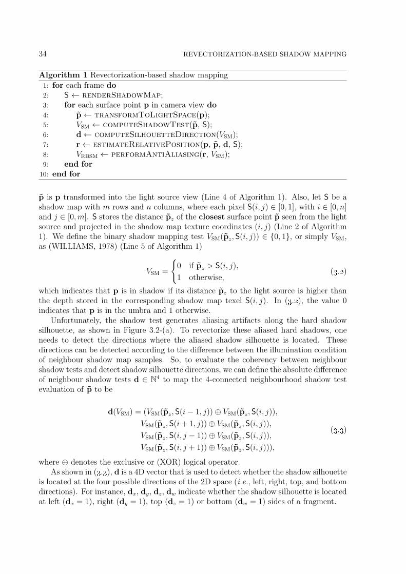
34 REVECTORIZATION-BASED SHADOW MAPPING
Algorithm 1 Revectorization-based shadow mapping
1: for each frame do2: S ← renderShadowMap;3: for each surface point p in camera view do4: p← transformToLightSpace(p);5: VSM ← computeShadowTest(p, S);6: d← computeSilhouetteDirection(VSM);7: r← estimateRelativePosition(p, p, d, S);8: VRBSM ← performAntiAliasing(r, VSM);9: end for
10: end for
p is p transformed into the light source view (Line 4 of Algorithm 1). Also, let S be ashadow map with m rows and n columns, where each pixel S(i, j) ∈ [0, 1], with i ∈ [0, n]and j ∈ [0,m]. S stores the distance pz of the closest surface point p seen from the lightsource and projected in the shadow map texture coordinates (i, j) (Line 2 of Algorithm1). We define the binary shadow mapping test VSM(pz, S(i, j)) ∈ 0, 1, or simply VSM,as (WILLIAMS, 1978) (Line 5 of Algorithm 1)
VSM =
0 if pz > S(i, j),
1 otherwise,(3.2)
which indicates that p is in shadow if its distance pz to the light source is higher thanthe depth stored in the corresponding shadow map texel S(i, j). In (3.2), the value 0indicates that p is in the umbra and 1 otherwise.
Unfortunately, the shadow test generates aliasing artifacts along the hard shadowsilhouette, as shown in Figure 3.2-(a). To revectorize these aliased hard shadows, oneneeds to detect the directions where the aliased shadow silhouette is located. Thesedirections can be detected according to the difference between the illumination conditionof neighbour shadow map samples. So, to evaluate the coherency between neighbourshadow tests and detect shadow silhouette directions, we can define the absolute differenceof neighbour shadow tests d ∈ N4 to map the 4-connected neighbourhood shadow testevaluation of p to be
d(VSM) = (VSM(pz, S(i− 1, j))⊕ VSM(pz, S(i, j)),
VSM(pz, S(i+ 1, j))⊕ VSM(pz, S(i, j)),
VSM(pz, S(i, j − 1))⊕ VSM(pz, S(i, j)),
VSM(pz, S(i, j + 1))⊕ VSM(pz, S(i, j))),
(3.3)
where ⊕ denotes the exclusive or (XOR) logical operator.As shown in (3.3), d is a 4D vector that is used to detect whether the shadow silhouette
is located at the four possible directions of the 2D space (i.e., left, right, top, and bottomdirections). For instance, dx, dy, dz, dw indicate whether the shadow silhouette is locatedat left (dx = 1), right (dy = 1), top (dz = 1) or bottom (dw = 1) sides of a fragment.
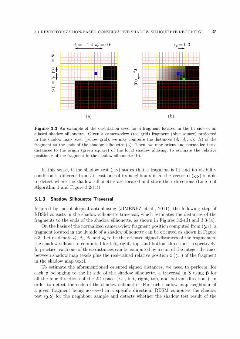
3.1 REVECTORIZATION-BASED CONSERVATIVE SHADOW SILHOUETTE RECOVERY 35
(a)
dl = −1.4 dr = 0.6
db
=0.6
dt
=−
0.4
(b)
rx = 0.3
ry
=0.6
Figure 3.3 An example of the orientation used for a fragment located in the lit side of analiased shadow silhouette. Given a camera-view (red grid) fragment (blue square) projectedin the shadow map texel (yellow grid), we may compute the distances (d l, dr, d t, d b) of thefragment to the ends of the shadow silhouette (a). Then, we may orient and normalize thesedistances to the origin (green square) of the local shadow aliasing, to estimate the relativeposition r of the fragment in the shadow silhouette (b).
In this sense, if the shadow test (3.2) states that a fragment is lit and its visibilitycondition is different from at least one of its neighbours in S, the vector d (3.3) is ableto detect where the shadow silhouettes are located and store their directions (Line 6 ofAlgorithm 1 and Figure 3.2-(c)).
3.1.3 Shadow Silhouette Traversal
Inspired by morphological anti-aliasing (JIMENEZ et al., 2011), the following step ofRBSM consists in the shadow silhouette traversal, which estimates the distances of thefragments to the ends of the shadow silhouette, as shown in Figures 3.2-(d) and 3.3-(a).
On the basis of the normalized camera-view fragment position computed from (3.1), afragment located in the lit side of a shadow silhouette can be oriented as shown in Figure3.3. Let us denote dl, dr, dt, and db to be the oriented signed distances of the fragment tothe shadow silhouette computed for left, right, top, and bottom directions, respectively.In practice, each one of those distances can be computed by a sum of the integer distancebetween shadow map texels plus the real-valued relative position c (3.1) of the fragmentin the shadow map texel.
To estimate the aforementioned oriented signed distances, we need to perform, foreach p belonging to the lit side of the shadow silhouette, a traversal in S using p forall the four directions of the 2D space (i.e., left, right, top, and bottom directions), inorder to detect the ends of the shadow silhouette. For each shadow map neighbour ofa given fragment being accessed in a specific direction, RBSM computes the shadowtest (3.2) for the neighbour sample and detects whether the shadow test result of the

36 REVECTORIZATION-BASED SHADOW MAPPING
(a) (b) (c)
Figure 3.4 Jagged shadow silhouettes (a) are revectorized with RBSM (b). However, artifacts(pointed by red arrows) may arise for sloped surfaces due to the depth change that affects theshadow test (b). By using our solution, we can reduce this problem (c).
neighbour is different from the one estimated for the given fragment. In this case, sincethe conservative RBSM operates only over lit fragments, a shadowed fragment has beendetected. Therefore, we have detected the end of the shadow silhouette and we need toend the traversal in that particular direction. On the other hand, if the shadow test is thesame between neighbour shadow map texels, we need to check if the neighbours share atleast one discontinuity direction in common (3.3). If that is not the case, the neighbourshadow map texel accessed during traversal does not belong to the same shadow silhouetteand the shadow traversal must be ended.
To better understand the shadow silhouette traversal, let us visualize the scenarioshown in Figure 3.2-(d). Only for the lit fragments inside the shadow silhouette, weperform the shadow silhouette traversal (resulting in the blue arrows depicted in Figure3.2-(d)). To the right of these fragments, there are shadowed fragments that mark theend of the shadow silhouette. To the left of these fragments, there are other lit fragments.However, since these neighbour lit fragments do not have discontinuity directions, theydo not belong to the same shadow silhouette. One important note with respect to thistraversal is that, while the rotation of the light source influences the visual aspect ofthe shadow aliasing seen from the camera viewpoint, the generated shadow map is stillaligned with the light source coordinate system. Therefore, the traversal provided byRBSM over X and Y axis of the shadow map works well regardless of the orientation ofthe light source.
For sloped surfaces, the depth of the shadow map sample being accessed may changein relation to the depth accessed in the initial shadow map texel. If we use the samedepth retrieved from pz for shadow test during traversal, artifacts may arise in the caseswhere the depth change in S(i, j) affects the shadow test result (Figure 3.4-(b)). Tosolve this problem, we use the shadow mapping assumption that pz ≥ S(i, j) holds forevery shadow map texel. Thus, to detect this depth change during traversal, we checkwhether |pz − S(i, j)| < ε holds. If the condition is true, we update pz before the shadowtest: pz = pz − ε. In fact, we use an approach that ensures for fragments in shadow,pz > S(i, j). Conversely, for lit fragments, pz < S(i, j). As shown in Figure 3.4-(c), this
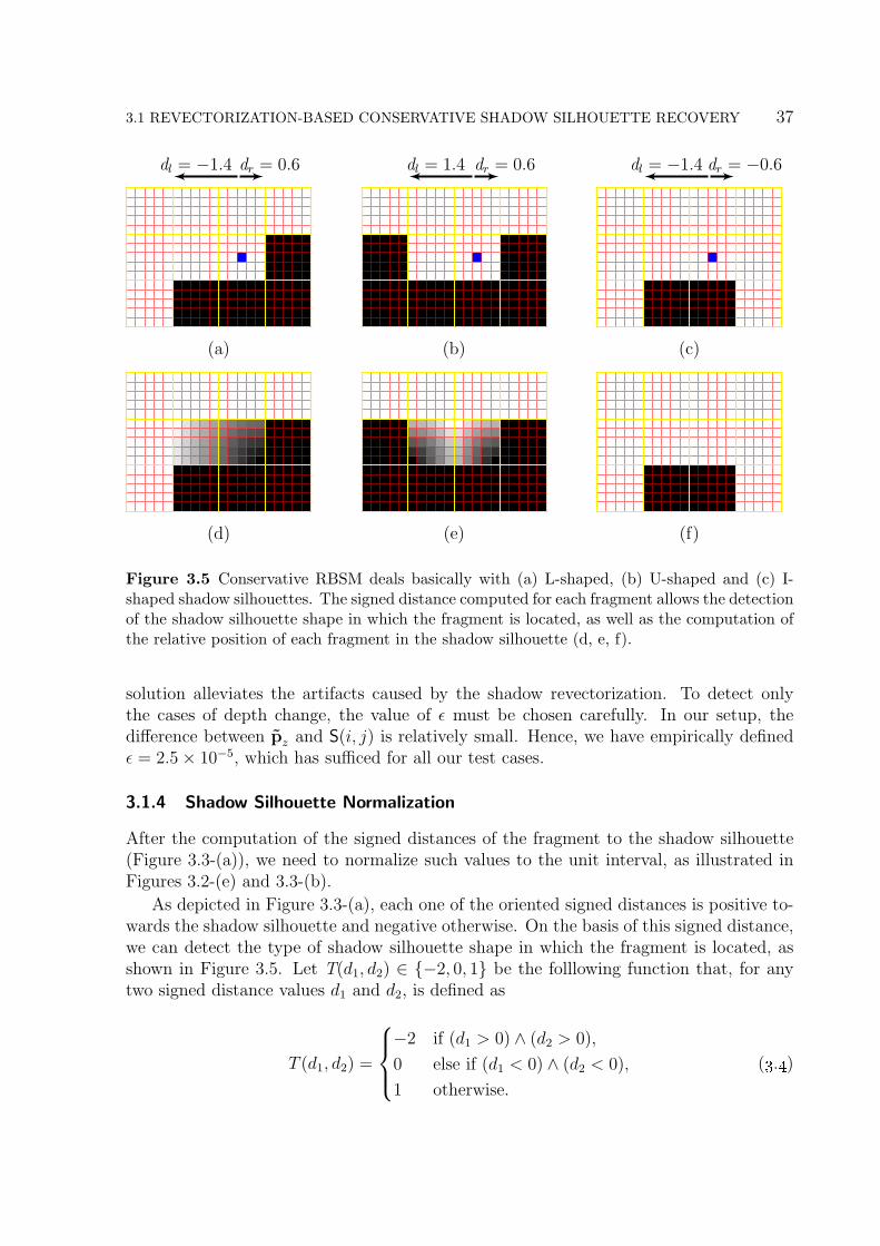
3.1 REVECTORIZATION-BASED CONSERVATIVE SHADOW SILHOUETTE RECOVERY 37
dl = −1.4 dr = 0.6
(a)
dl = 1.4 dr = 0.6
(b)
dl = −1.4 dr = −0.6
(c)
(d) (e) (f)
Figure 3.5 Conservative RBSM deals basically with (a) L-shaped, (b) U-shaped and (c) I-shaped shadow silhouettes. The signed distance computed for each fragment allows the detectionof the shadow silhouette shape in which the fragment is located, as well as the computation ofthe relative position of each fragment in the shadow silhouette (d, e, f).
solution alleviates the artifacts caused by the shadow revectorization. To detect onlythe cases of depth change, the value of ε must be chosen carefully. In our setup, thedifference between pz and S(i, j) is relatively small. Hence, we have empirically definedε = 2.5× 10⁻⁵, which has sufficed for all our test cases.
3.1.4 Shadow Silhouette Normalization
After the computation of the signed distances of the fragment to the shadow silhouette(Figure 3.3-(a)), we need to normalize such values to the unit interval, as illustrated inFigures 3.2-(e) and 3.3-(b).
As depicted in Figure 3.3-(a), each one of the oriented signed distances is positive to-wards the shadow silhouette and negative otherwise. On the basis of this signed distance,we can detect the type of shadow silhouette shape in which the fragment is located, asshown in Figure 3.5. Let T(d1, d2) ∈ −2, 0, 1 be the folllowing function that, for anytwo signed distance values d1 and d2, is defined as
T (d1, d2) =
−2 if (d1 > 0) ∧ (d2 > 0),
0 else if (d1 < 0) ∧ (d2 < 0),
1 otherwise.
(3.4)

38 REVECTORIZATION-BASED SHADOW MAPPING
As shown in Figure 3.5-(a) and Equation (3.4), an L-shaped shadow silhouette hasT (d1, d2) = 1 because both positive and negative distance values are computed for thefragment located in the shadow silhouette. As seen in Figure 3.5-(b), a lit fragment in aU-shaped shadow silhouette has T (d1, d2) = −2 for a specific axis, because both signeddistances are positive. Likewise, a lit fragment in an I-shaped shadow silhouette hasT (d1, d2) = 0 for a specific axis because both signed distances are negative, as can beseen in Figures 3.5-(c).
Assuming that r ∈ R2, illustrated in Figure 3.3-(b), is the relative position of thefragment in the shadow silhouette, r can be computed as follows
rx = max(T (dl, dr), 2VSM − 1)|max(T (dl, dr)dl, T (dl, dr)dr)|
|dl|+ |dr|
ry = max(T (dt, db), 2VSM − 1)|max(T (dt, db)dt, T (dt, db)db)|
|dt|+ |db|.
(3.5)
For L-shaped shadow silhouettes (T (d1, d2) = 1), as illustrated in Figure 3.5-(d),Equation (3.5) computes the relative position on the basis of the positive distance valuespreviously estimated, since they are the output of the right-handed max function. Forfragments on the lit side of U-shaped shadow silhouettes, the function T (d1, d2) changesthe sign of the distances computed, such that r is calculated on the basis of the minimumdistance value, closest to the end of the shadow silhouette, as shown in Figure 3.5-(e).Also, since T (d1, d2) = −2, the scale by factor 2 is used to normalize r to the interval[0, 1]. For fragments located on the lit side of I-shaped shadow silhouettes, the functionT (d1, d2) makes the relative position to be 0 since T (d1, d2) for any two negative distancevalues d1 and d2 is 0. This is illustrated in Figure 3.5-(f).
3.1.5 Hard Shadow Anti-Aliasing Visibility Function
To produce anti-aliased hard shadows, as depicted in Figures 3.2-(f, g), we need to takethree facts into consideration: the result of the shadow test VSM (3.2), the type of theshadow silhouette shape in which the fragment is located (Figure 3.6), and the normalizedrelative position r of the fragment in the shadow silhouette (Figure 3.3).
Figure 3.6 shows the visual effect that we aim to achieve using RBSM. As shownin this figure, fragments that were estimated to be in shadow (VSM = 0) by the shadowtest must remain in shadow after the shadow revectorization. On the other hand, thealgorithm must not perform anti-aliasing for I-shaped shadow silhouettes (Figures 3.6-(c,f)), since the revectorization effect is best suited for L- and U-shaped shadow silhouettes(Figures 3.6-(a, b, d, e)). Fragments located at I-shaped shadow silhouettes can be easilydetected by checking whether rxry = 0, following (3.5). For lit fragments located in theL- and U-shaped shadow silhouettes, a simple linear comparison using r (1− rx > ry) isable to determine whether the fragment must be shadowed or remain lit.
Given those circumstances, the RBSM hard shadow anti-aliasing visibility functionVRBSM(VSM, r) ∈ 0, 1 is defined as follows
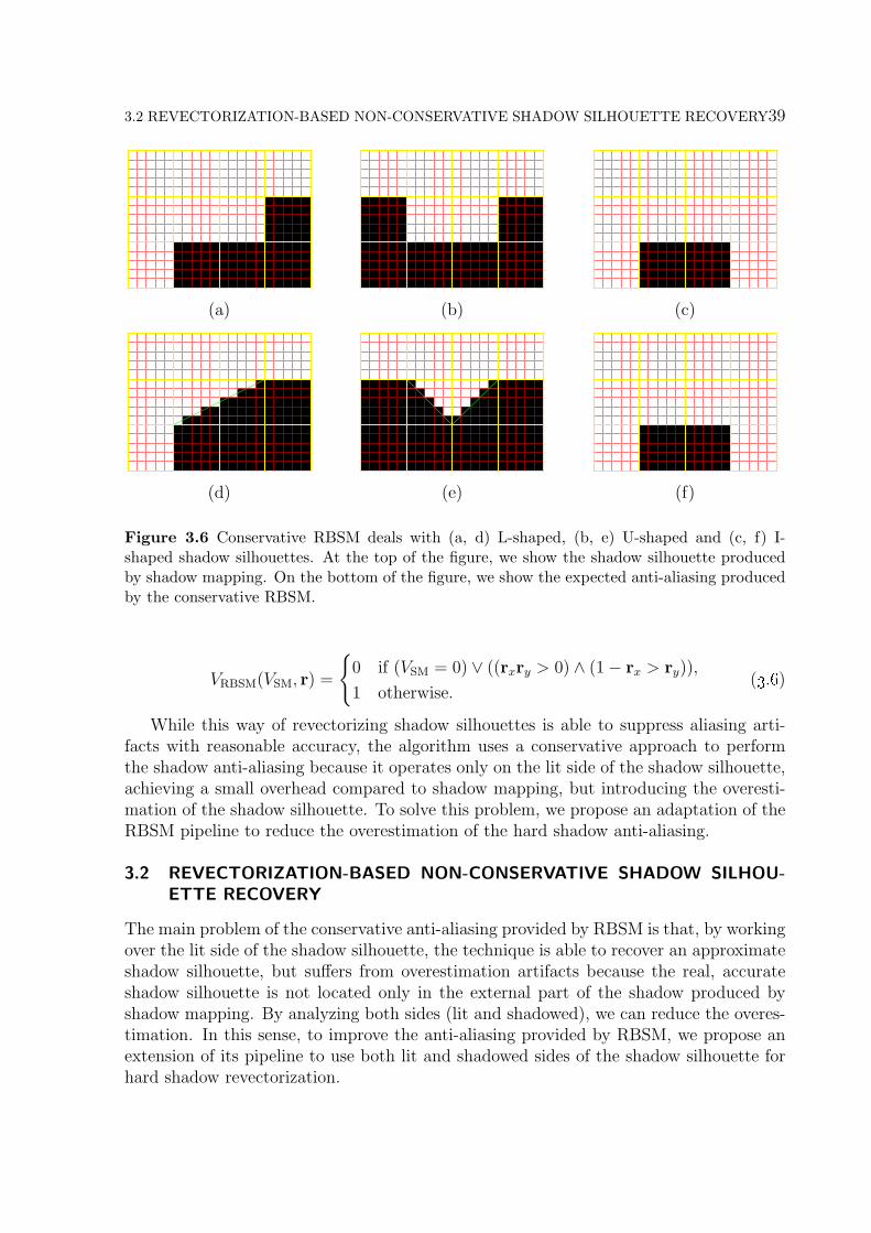
3.2 REVECTORIZATION-BASED NON-CONSERVATIVE SHADOW SILHOUETTE RECOVERY39
(a) (b) (c)
(d) (e) (f)
Figure 3.6 Conservative RBSM deals with (a, d) L-shaped, (b, e) U-shaped and (c, f) I-shaped shadow silhouettes. At the top of the figure, we show the shadow silhouette producedby shadow mapping. On the bottom of the figure, we show the expected anti-aliasing producedby the conservative RBSM.
VRBSM(VSM, r) =
0 if (VSM = 0) ∨ ((rxry > 0) ∧ (1− rx > ry)),
1 otherwise.(3.6)
While this way of revectorizing shadow silhouettes is able to suppress aliasing arti-facts with reasonable accuracy, the algorithm uses a conservative approach to performthe shadow anti-aliasing because it operates only on the lit side of the shadow silhouette,achieving a small overhead compared to shadow mapping, but introducing the overesti-mation of the shadow silhouette. To solve this problem, we propose an adaptation of theRBSM pipeline to reduce the overestimation of the hard shadow anti-aliasing.
3.2 REVECTORIZATION-BASED NON-CONSERVATIVE SHADOW SILHOU-ETTE RECOVERY
The main problem of the conservative anti-aliasing provided by RBSM is that, by workingover the lit side of the shadow silhouette, the technique is able to recover an approximateshadow silhouette, but suffers from overestimation artifacts because the real, accurateshadow silhouette is not located only in the external part of the shadow produced byshadow mapping. By analyzing both sides (lit and shadowed), we can reduce the overes-timation. In this sense, to improve the anti-aliasing provided by RBSM, we propose anextension of its pipeline to use both lit and shadowed sides of the shadow silhouette forhard shadow revectorization.

40 REVECTORIZATION-BASED SHADOW MAPPING
(a) (g)
(b) (c) (d) (e) (f)
Figure 3.7 An overview of the RBSM pipeline for non-conservative hard shadow anti-aliasing.Given the aliased shadow silhouettes generated by shadow mapping (a), a neighbourhood eval-uation (green arrows in (b)) is conducted to detect aliased fragments (b) and also the directions(green arrows in (c)) of where the shadow silhouette is located (c), regardless of whether thefragment is located in the inner- or the outer-side of the shadow silhouette. Then, the algo-rithm traverses the light space (blue arrows in (d)) to determine the normalized relative distance(gray shades in (e)) of the camera-view fragments (red grid) located on both sides of the shadowsilhouette to the shadow silhouette itself (e). Finally, taking advantage of this normalized rel-ative distance, the algorithm computes a dilated version of the revectorized shadow, with lessoverestimation artifacts than the conservative approach (f, g).
3.2.1 Overview
An overview of the non-conservative RBSM pipeline is shown in Figure 3.7. Also, thisnon-conservative RBSM uses the same pseudocode shown in Algorithm 1. As can beseen in Figure 3.7-(b), after the shadow map generation, both shadow test (3.2) andneighbourhood evaluation are computed for all lit and now also shadowed fragmentsvisible in the camera view. Then, on the basis of the neighbourhood evaluation previouslycomputed, the algorithm detects all the fragments located in the shadow silhouette usingthe discontinuity representation of (3.3) for both sides of the shadow silhouette (Figure3.7-(c)). For each fragment in the aliased shadow silhouette, a traversal is performed forboth sides of the shadow silhouette (Figure 3.7-(d)) to estimate the aliasing size and thenormalized relative distance of each fragment to the shadow silhouette (Figure 3.7-(e)).Then, a new visibility function is used to determine the new location of the revectorizedshadow silhouette (Figures 3.7-(f, g)).
3.2.2 Shadow Silhouette Locatization
For non-conservative anti-aliasing, we need to detect the directions where the shadowsilhouette is located in both inner- and outer-sides of the shadow silhouette, because the

3.2 REVECTORIZATION-BASED NON-CONSERVATIVE SHADOW SILHOUETTE RECOVERY41
(a)
dl = 1.6 dr = −0.4
db
=−
0.4dt
=0.6
(b)
rx = 0.8
ry
=0.6
Figure 3.8 An example of the orientation used for a fragment located in the shadowed side ofan aliased shadow silhouette. Given a camera-view (red grid) fragment (blue square) projectedin the shadow map texel (yellow grid), we may compute the distances (d l, dr, d t, d b) of thefragment to the ends of the shadow silhouette (a). Then, we may orient and normalize thesedistances to the origin (green square) of the local shadow aliasing, to estimate the relativeposition r of the fragment in the shadow silhouette (b).
shadow anti-aliasing will cover both parts of the silhouette, as shown in Figure 3.7-(f).
For every fragment in the camera view, we compute the shadow test (3.2) and thedirections of where the shadow silhouette is located (3.3). As a result of this step, we havethe directions of where the shadow silhouette is located for all the fragments situated inthe aliased shadow silhouette (Figure 3.7-(c)).
3.2.3 Shadow Silhouette Traversal
Similarly to the conservative RBSM, during the traversal of the shadow silhouette (Figure3.7-(d)), regardless of whether the fragment is located in the lit or shadowed side of theshadow silhouette, we still need to perform the shadow test (3.2) for each neighbourshadow map texel being accessed. To detect the end of the shadow silhouette, we check ifthe neighbour fragment has a different visibility condition than the one estimated by theinitial fragment of the traversal. In this sense, for lit fragments, the shadow silhouette endsin a shadowed fragment (Figure 3.3-(a)). On the counterpart, for shadowed fragments,the shadow silhouette ends in a lit fragment (Figure 3.8-(a)). If the visibility conditionbetween neighbours is the same, we still compute the discontinuity directions (3.3) andcheck whether neighbour fragments share at least one discontinuity direction. If that isnot the case, the traversal has stepped out of the lit/shadowed side of the aliased shadowsilhouette.
The result of this step is the estimation of the oriented signed distance for both lit(Figure 3.3-(a)) and shadowed (Figure 3.8-(a)) fragments located in the aliased silhouette.

42 REVECTORIZATION-BASED SHADOW MAPPING
dl = 1.4 dr = −0.6
(a)
dl = −1.4 dr = −0.6
(b)
dl = 1.4 dr = 0.6
(c)
(d) (e) (f)
Figure 3.9 Fragments in the shadowed side of the aliasing can be located in (a) L-shaped,(b) U-shaped and (c) I-shaped shadow silhouettes. The behaviour of the normalized relativeposition computation (d, e, f) is different from the one computed for lit fragments.
3.2.4 Shadow Silhouette Normalization
Once the shadow silhouette traversal has ended, we proceed with the computation of thenormalized distance r of each fragment to the corner of the aliased shadow silhouette(Figure 3.7-(e)). Depending on whether the fragment is located inside or outside theshadowed part of the silhouette, the origin of this local coordinate system (representedby the green square in Figures 3.3-(b) and 3.8-(b)) is changed. Nevertheless, the originis still located at the corner of the aliasing.
To compute the normalized relative position of the fragment in the shadow silhouette,we use (3.4) and (3.5), following the orientation shown in Figure 3.9.
As seen in Figure 3.9-(a), an L-shaped shadow silhouette has T (d1, d2) = 1 because wecan measure positive and negative distance values for the fragment located in the shad-owed part of the aliased silhouette. As depicted in Figure 3.9-(b), a shadowed fragmentin a U-shaped shadow silhouette has T (d1, d2) = 0 for a specific axis because both signeddistances are negative. Finally, as shown in Figure 3.9-(c), a shadowed fragment in anI-shaped shadow silhouette has T (d1, d2) = −2 for a specific axis, because both signeddistances are positive.
For a shadow fragment located in an L-shaped shadow silhouette, Equation (3.5) com-putes the relative position r making use of the positive distance values estimated duringthe shadow silhoeutte traversal. For fragments located on the shadowed side of both U-

3.2 REVECTORIZATION-BASED NON-CONSERVATIVE SHADOW SILHOUETTE RECOVERY43
(a) (b) (c)
(d) (e) (f)
Figure 3.10 Non-conservative RBSM for three distinct scenarios. At the top of the figure, weshow the shadow silhouette produced by shadow mapping. On the bottom of the figure, weshow the expected anti-aliasing produced by the non-conservative RBSM.
and I-shaped shadow silhouettes, since VSM = 0, the left-handed max function outputs0 for U-shaped shadow silhouettes (see Figure 3.9-(e)) and −1 for I-shaped shadow sil-houettes (see Figure 3.9-(f)). That scale factor makes the estimated relative positions tolook like the ones illustrated in Figures 3.9-(e, f).
3.2.5 Hard Shadow Anti-Aliasing Visibility Function
Before proposing the non-conservative anti-aliasing, as depicted in Figures 3.7-(f, g), wefirst need to analyze the proposed improved visibility function V ∗RBSM(VSM, r) ∈ 0, 1 forthe separate cases when the fragment is lit (VSM = 1) or is in shadow (VSM = 0)
V ∗RBSM(0, r) =
0 if (rxry = 0) ∨ (|rx|+ |ry| > 1
2),
1 otherwise.(3.7)
V ∗RBSM(1, r) =
0 if (rxry > 0) ∧ (rx + ry <
12),
1 otherwise.(3.8)
As shown in Figure 3.10, for the originally shadowed part of the shadow silhouette,whenever the fragment is distant to the corner of the shadow silhouette by more thana value of 1
2(see Figure 3.9 for a reference of the relative position computed for every
shadow silhouette shape), the shadowed part is changed to be lit in (3.7). Since r canbe negative for shadowed fragments, according to (3.5), we use the max function to putthis value to 0. Likewise, for the originally lit part of the shadow silhouette, whenever

44 REVECTORIZATION-BASED SHADOW MAPPING
the fragment is distant to the origin of the shadow silhouette by less than a value of 12,
the lit part is put in shadow, as shown in (3.8).
As can be seen in (3.7) and (3.8), the visibility functions are, in some way, comple-mentary to each other. So, we can define the non-conservative visibility function as
V ∗RBSM(VSM, r) =
0 if (rxry = 2VSM) ∨ ((|rx||ry| > 0) ∧ ((1− VSM)
+(2VSM − 1)(|rx|+ |ry|) < 12)),
1 otherwise.
(3.9)
In the next section, we show a comparison between both implementations of RBSM,discussing in more details the advantages and drawbacks of each approach.
3.3 RESULTS AND DISCUSSION
In this section, we evaluate different hard shadow techniques in terms of visual quality andrendering performance. We follow related work (SEN; CAMMARANO; HANRAHAN,2003; CHAN; DURAND, 2004) and compare both conservative and non-conservativeRBSM with the traditional shadow mapping technique, as well as the stencil shadowvolume (HEIDMANN, 1991) for generating ground-truth hard shadows.
We have tested our RBSM in different scenarios. For the models of Figures 3.11,3.14 and 3.15, we evaluate how RBSM handles the aliasing artifacts generated by low-resolution shadow maps in models with low geometric complexity. In Figures 3.12 and3.16, we evaluate how well RBSM performs anti-aliasing for shadow silhouettes thatcontain several intersections and fine details of the object. In Figure 3.13, we showhow RBSM reduces the aliasing of the shadows generated by a complex model with finedetails along its silhouette. In Figure 3.17, we test the anti-aliasing provided by RBSMin a complex scenario with trees and several overlapping objects that produce holes andaliased shadows even for high-resolution shadow maps. Finally, in Figure 3.18, we showan example of the RBSM anti-aliasing for a game-like, outdoor scenario.
3.3.1 Experimental Setup
For all the tests contained in this thesis, a computer equipped with an Intel CoreTM
i7-3770K CPU (3.50 GHz), 8GB RAM, and an NVIDIA GeForce GTX Titan X graphicscard was used to run the experimental tests. For some scenarios, OpenGL (SHREINERet al., 2013) and OpenGL Shading Language (GLSL) (ROST et al., 2009) were used toimplement RBSM, shadow mapping and shadow volume. For the other scenarios, wehave used the Unity Pro version 5.6.0.f3 and the Cg language (FERNANDO; KILGARD,2003) to evaluate the performance of the conservative RBSM for distinct, game-like sce-narios, typical of a game engine. Most of the figures shown in this section do not containscenes with high-frequency textures because they could potentially mask shadow render-ing irregularities. That is why we have chosen to use white textures in the ground planesand in some of the other objects.

3.3 RESULTS AND DISCUSSION 45
(a) Shadow Mapping (b) Conservative RBSM
(c) Non-Conservative RBSM (d) Shadow Volume
(a) Shadow Mapping (b) Conservative RBSM
(c) Non-Conservative RBSM (d) Shadow Volume
(a) Shadow Mapping (b) Conservative RBSM
(c) Non-Conservative RBSM (d) Shadow Volume
(a) Shadow Mapping (b) Conservative RBSM
(c) Non-Conservative RBSM (d) Shadow Volume
(a) Shadow Mapping (b) Conservative RBSM
(c) Non-Conservative RBSM (d) Shadow Volume
Figure 3.11 A visual comparison between (a) shadow mapping, (b) conservative, (c) non-conservative RBSM and (d) shadow volume for the Armadillo model using a 10242 shadowmap resolution. False color visualizations show the difference between the shadows generatedby different hard shadow techniques (a, b, c) and the ones obtained by the reference shadowvolume solution (d).
3.3.2 Visual Quality Evaluation
In Figures 3.11, 3.12 and 3.13, we compare both shadow mapping, RBSM and shadowvolume for scenarios with different shadow map resolutions. In all the figures, it is visible

46 REVECTORIZATION-BASED SHADOW MAPPING
(a) Shadow Mapping (b) Conservative RBSM
(c) Non-Conservative RBSM (d) Shadow Volume
(a) Shadow Mapping (b) Conservative RBSM
(c) Non-Conservative RBSM (d) Shadow Volume
(a) Shadow Mapping (b) Conservative RBSM
(c) Non-Conservative RBSM (d) Shadow Volume
(a) Shadow Mapping (b) Conservative RBSM
(c) Non-Conservative RBSM (d) Shadow Volume
(a) Shadow Mapping (b) Conservative RBSM
(c) Non-Conservative RBSM (d) Shadow Volume
Figure 3.12 A visual comparison between (a) shadow mapping, (b) conservative, (c) non-conservative RBSM and (d) shadow volume for the Fence model using a 20482 shadow mapresolution. False color visualizations show the difference between the shadows generated bydifferent hard shadow techniques (a, b, c) and the ones obtained by the reference shadowvolume solution (d).
that RBSM improves the visual quality of the shadows generated by shadow mapping byremoving the aliasing artifacts along the shadow silhouette. In all those figures, the falsecolor visualizations also show that the non-conservative RBSM produces shadows thatresemble the ones generated by shadow volume. Meanwhile, the conservative RBSM isable to successfully reduce the aliasing artifacts of shadow mapping, but causing a slight

3.3 RESULTS AND DISCUSSION 47
(a) Shadow Mapping (b) Conservative RBSM
(c) Non-Conservative RBSM (d) Shadow Volume
(a) Shadow Mapping (b) Conservative RBSM
(c) Non-Conservative RBSM (d) Shadow Volume
(a) Shadow Mapping (b) Conservative RBSM
(c) Non-Conservative RBSM (d) Shadow Volume
(a) Shadow Mapping (b) Conservative RBSM
(c) Non-Conservative RBSM (d) Shadow Volume
(a) Shadow Mapping (b) Conservative RBSM
(c) Non-Conservative RBSM (d) Shadow Volume
Figure 3.13 A visual comparison between (a) shadow mapping, (b) conservative, (c) non-conservative RBSM and (d) shadow volume for the YeahRight model using a 40962 shadowmap resolution. False color visualizations show the difference between the shadows generatedby different hard shadow techniques (a, b, c) and the ones obtained by the reference shadowvolume solution (d).
overestimation in the shadow.
In Figures 3.14, 3.15 and 3.16, we show a visual comparison between shadow mappingand conservative RBSM for different models and shadow map resolutions. We can see

48 REVECTORIZATION-BASED SHADOW MAPPING
Figure 3.14 A visual comparison between shadow mapping (left) and conservative RBSM(right) for the Chris, Coconut and Dragon models using 2562, 5122 and 10242 shadow mapresolutions.
that, regardless of the shadow map resolution used, shadow mapping generates aliasing

3.3 RESULTS AND DISCUSSION 49
Figure 3.15 A visual comparison between shadow mapping (left) and conservative RBSM(right) for the Robot model using a 10242 shadow map resolution.
Figure 3.16 A visual comparison between shadow mapping (left) and conservative RBSM(right) for the Gate model using a 20482 shadow map resolution.
artifacts along the shadow silhouette because the shadow map resolution is finite anddoes not match the pixel resolution of the camera view. Then, by traversing the shadowaliasing silhouette, RBSM is able to minimize the artifacts and improve the shadow visualquality.
The quality of the shadow revectorization is dependent on the shadow map resolutionused and the quality of the aliased silhouette. RBSM works well for the scenarios shown inFigures 3.12 and 3.14 despite the use of low (2562) and medium (5122 and 10242) shadowmap resolutions. In these cases, the objects and their shadows are relatively simple,since there is not much intersection between shadow silhouettes and a few fine detailsto be captured by the shadow map. Hence, the aliasing is the most noticeable artifactthat prevents an accurate shadow rendering. So, by the use of RBSM, we can minimizethese artifacts and improve the shadow visual quality efficiently. On the other hand, the

50 REVECTORIZATION-BASED SHADOW MAPPING
Figure 3.17 A visual comparison between shadow mapping (top) and conservative RBSM(bottom) for the complex San Miguel model using a 20482 shadow map resolution.
Shadow Map ResolutionScene Method 5122 10242 20482 40962
Figure 3.11
Shadow Mapping 3.28 ms 3.31 ms 3.36 ms 3.68 msConservative RBSM 3.48 ms 3.63 ms 3.82 ms 4.43 ms
Non-conservative RBSM 3.58 ms 3.66 ms 3.86 ms 4.48 msShadow Volume 145.9 ms 145.9 ms 145.9 ms 145.9 ms
Figure 3.12
Shadow Mapping 3.02 ms 3.03 ms 3.10 ms 3.34 msConservative RBSM 3.28 ms 3.38 ms 3.52 ms 4.28 ms
Non-conservative RBSM 3.34 ms 3.41 ms 3.62 ms 4.39 msShadow Volume 153.8 ms 153.8 ms 153.8 ms 153.8 ms
Figure 3.13
Shadow Mapping 9.14 ms 9.25 ms 9.31 ms 9.58 msConservative RBSM 9.44 ms 9.51 ms 9.64 ms 10.27 ms
Non-conservative RBSM 9.52 ms 9.56 ms 9.72 ms 10.39 msShadow Volume 338.9 ms 338.9 ms 338.9 ms 338.9 ms
Table 3.1 Rendering performance for different hard shadow techniques for varying shadowmap resolution. Scenes were rendered at an output 720p resolution.
shadows shown in the red closeups of Figures 3.13, 3.15 and in the green closeup of Figure3.16 have a more complex shape, with several intersections in the shadow silhouette andfine details captured by the shadow map, respectively. In these cases, RBSM minimizes

3.3 RESULTS AND DISCUSSION 51
Figure 3.18 A visual comparison between shadow mapping (top) and conservative RBSM(bottom) for the exterior environment of the Unity’s Adam model using a 20482 shadow mapresolution.
Output ResolutionScene Method 480p 720p 1080p
Figure 3.11
Shadow Mapping 2.92 ms 3.31 ms 4.00 msConservative RBSM 3.17 ms 3.63 ms 4.39 ms
Non-conservative RBSM 3.19 ms 3.66 ms 4.45 msShadow Volume 80.31 ms 145.9 ms 307.6 ms
Figure 3.12
Shadow Mapping 2.70 ms 3.03 ms 3.69 msConservative RBSM 2.95 ms 3.38 ms 4.01 ms
Non-conservative RBSM 3.01 ms 3.41 ms 4.24 msShadow Volume 81.43 ms 153.8 ms 333.3 ms
Figure 3.13
Shadow Mapping 8.91 ms 9.25 ms 9.94 msConservative RBSM 9.15 ms 9.51 ms 10.2 ms
Non-conservative RBSM 9.19 ms 9.56 ms 10.3 msShadow Volume 190.1 ms 338.9 ms 713.9 ms
Table 3.2 Rendering performance for different hard shadow techniques for varying outputresolution. Scenes were rendered at a 10242 shadow map resolution.
the aliasing artifacts at the cost of causing a shadow overestimation, suppressing somedetails of the original shadow silhouette.

52 REVECTORIZATION-BASED SHADOW MAPPING
Shadow Map Resolution
Scene MethodLow
(2562)Medium(5122)
High(10242)
Very High(20482)
Figure 3.14-topShadow Mapping 4.96 ms 4.99 ms 5.01 ms 5.03 ms
RBSM5.03 ms(1.41%)
5.07 ms(1.60%)
5.10 ms(1.79%)
5.12 ms(1.78%)
Figure 3.14-mediumShadow Mapping 5.14 ms 5.16 ms 5.17 ms 5.20 ms
RBSM5.14 ms(0.00%)
5.19 ms(0.58%)
5.20 ms(0.58%)
5.21 ms(0.19%)
Figure 3.14-bottomShadow Mapping 5.06 ms 5.09 ms 5.11 ms 5.12 ms
RBSM5.14 ms(1.58%)
5.16 ms(1.37%)
5.20 ms(1.76%)
5.22 ms(1.95%)
Figure 3.15Shadow Mapping 5.08 ms 5.11 ms 5.12 ms 5.14 ms
RBSM5.14 ms(1.18%)
5.16 ms(0.97%)
5.18 ms(1.17%)
5.22 ms(1.55%)
Figure 3.16Shadow Mapping 5.07 ms 5.08 ms 5.14 ms 5.16 ms
RBSM5.12 ms(0.98%)
5.14 ms(1.18%)
5.15 ms(0.19%)
5.18 ms(0.38%)
Figure 3.17Shadow Mapping 5.02 ms 5.03 ms 5.04 ms 5.04 ms
RBSM5.08 ms(1.19%)
5.10 ms(1.39%)
5.11 ms(1.38%)
5.13 ms(1.78%)
Figure 3.18Shadow Mapping 7.43 ms 7.46 ms 7.48 ms 7.69 ms
RBSM7.46 ms(0.40%)
7.51 ms(0.67%)
7.57 ms(1.20%)
7.74 ms(0.65%)
Table 3.3 Rendering performance (including percentual of overhead) for shadow mapping andRBSM for varying shadow map resolution. Scenes were rendered at an output 1080p resolution.
In Figure 3.17, we show a more complex scenario that contains many structures withfine details (trees), non-planar shadow receivers (chairs on the floor) and multiple objectsthat overlap each other. In this case, shadow mapping not only generates the aliasingartifacts, but is also not able to capture the fine details of the light blocker objects, causingthe appearance of holes along the shadow silhouette (see the blue rectangles in Figure3.17). RBSM helps on the minimization of shadow aliasing artifacts (see the closeupsof Figure 3.17), but is not able to solve the problem of the shadow holes caused by theinsufficient shadow map resolution used.
In Figure 3.18, we show that our shadow anti-aliasing implementation works notonly for indoor environments, but also for large outdoor environments with high-detailedstructures, such as vegetations, streets and buildings. The closeups in Figure 3.18 showthat a shadow map with insufficient resolution for outdoor scenes clearly generates shadowaliasing artifacts that can be effectively suppressed by RBSM. Hence, we can see thatRBSM is an algorithm able to provide shadow anti-aliasing for planar (e.g., shadowsseen in the white ground planes of Figures 3.11, 3.12 and 3.13) and non-planar shadowreceivers (Figure 3.17), simple (Figures 3.11, 3.14 and 3.15) and complex scenarios in

3.3 RESULTS AND DISCUSSION 53
Output ResolutionScene Method 720p 1080p 2160p
Figure 3.14-topShadow Mapping 5.01 ms 5.03 ms 5.04 ms
RBSM5.11 ms(1.99%)
5.12 ms(1.78%)
5.12 ms(1.58%)
Figure 3.14-mediumShadow Mapping 5.19 ms 5.20 ms 5.20 ms
RBSM5.19 ms(0.00%)
5.21 ms(0.19%)
5.22 ms(0.38%)
Figure 3.14-bottomShadow Mapping 5.11 ms 5.12 ms 5.14 ms
RBSM5.16 ms(0.97%)
5.22 ms(1.95%)
5.34 ms(3.89%)
Figure 3.15Shadow Mapping 5.02 ms 5.14 ms 5.21 ms
RBSM5.18 ms(3.18%)
5.22 ms(1.55%)
5.24 ms(0.57%)
Figure 3.16Shadow Mapping 5.05 ms 5.16 ms 5.17 ms
RBSM5.10 ms(0.99%)
5.18 ms(0.38%)
5.25 ms(1.54%)
Figure 3.17Shadow Mapping 4.99 ms 5.04 ms 5.07 ms
RBSM5.03 ms(0.80%)
5.13 ms(1.78%)
5.14 ms(1.38%)
Figure 3.18Shadow Mapping 7.49 ms 7.69 ms 15.08 ms
RBSM7.63 ms(1.86%)
7.74 ms(0.65%)
15.55 ms(3.11%)
Table 3.4 Rendering performance (including percentual of overhead) for shadow mapping andRBSM for varying output resolution. Scenes were rendered at a 10242 shadow map resolution.
small (Figure 3.13), medium (Figure 3.17) and large (Figure 3.18) scale.
3.3.3 Rendering Time Evaluation
Tables 3.1 and 3.2 show timing results obtained from different hard shadow techniques inour developed application. Shadow mapping and RBSM techniques are almost two ordersof magnitude faster than shadow volume, generating shadows in real time, regardless ofthe shadow map or output resolution used. It is worthy to note that RBSM is less than 1millissecond slower than shadow mapping, while providing an improved visual quality forthe hard shadow rendering. Meanwhile, to reduce the overestimation of the conservativeRBSM, non-conservative RBSM demands an overhead of less than 0.3 millisseconds toprovide an improved hard shadow anti-aliasing.
To corroborate the results shown in Tables 3.1 and 3.2, we measured the averageprocessing time obtained in the Unity game engine to run the scenarios shown in Figures3.14, 3.15, 3.16, 3.17 and 3.18. The results were reported in Tables 3.3 and 3.4, forvarying shadow map and output resolutions. Similarly to the shadow mapping technique,RBSM becomes slower as long as both shadow map (Table 3.3) and output resolutions

54 REVECTORIZATION-BASED SHADOW MAPPING
(a) Shadow Mapping (b) Conservative RBSM
(c) Non-Conservative RBSM (d) Shadow Volume
(a) Shadow Mapping (b) Conservative RBSM
(c) Non-Conservative RBSM (d) Shadow Volume
(a) Shadow Mapping (b) Conservative RBSM
(c) Non-Conservative RBSM (d) Shadow Volume
(a) Shadow Mapping (b) Conservative RBSM
(c) Non-Conservative RBSM (d) Shadow Volume
(a) Shadow Mapping (b) Conservative RBSM
(c) Non-Conservative RBSM (d) Shadow Volume
Figure 3.19 A visual comparison between (a) shadow mapping, (b) conservative, (c) non-conservative RBSM and (d) shadow volume for the Fence model using a 5122 shadow mapresolution.
(Table 3.4) are increased. Fortunately, the percentage of overhead added by RBSM keepssmall regardless of the shadow map or output resolution used, proving that the RBSMtechnique is scalable with respect to these changes in resolution and adds a small overheadof processing time to shadow mapping.
Both Table 3.3 and Table 3.4 show that the RBSM technique is about 0.01 to 0.5milliseconds (or between 0.1% and 3.9%) slower than shadow mapping for the hardwaresetup used. Meanwhile, we can see from all the figures shown in this paper that RBSMgreatly improves the visual quality of the shadow. Hence, we believe that RBSM provedto be an efficient hard shadow anti-aliasing technique, because it can leverage the shadowvisual quality, while adding a pretty small overhead of ∼1.2%, in average, in the totalframe time of a popular game engine.

3.4 SUMMARY 55
3.3.4 Limitations
Similar to other image-based hard shadow techniques, the main limitation of the anti-aliasing provided by RBSM relies on its accuracy, that is highly dependent on the shadowmap resolution used. For instance, as can be seen in Figure 3.19, for a low-resolutionshadow map, RBSM minimizes the aliasing problem, but does not recover an accurateshadow silhouette at the shadowed region, introducing shadow overestimation (Figure3.19-(b)) or producing shadowed shapes (Figure 3.19-(c)) that deviate from the onesobtained by accurate hard shadow techniques (Figure 3.19-(d)). By comparing Figures3.12 and 3.19, we can see that just by increasing the shadow map resolution, we canminimize such a problem.
Because the technique does not rely on additional geometric details to perform theanti-aliasing, RBSM does not handle holes caused by the use of an insufficient shadow mapresolution. Moreover, for models with fine details, the revectorization does not performwell for low-resolution shadow maps, since the shadow map is not able to capture thefine geometric details of the model.
The visibility functions of both conservative and non-conservative RBSM may intro-duce some small artifacts along the anti-aliased shadow silhouette due to the shadowsilhouette traversal step, that may compute the oriented signed distances incorrectly dueto small depth changes in the geometry. The solution proposed in Section 3.1.3 helpsminimizing these artifacts.
3.4 SUMMARY
In this chapter, we have presented the RBSM, a hard shadow mapping technique thatdoes not rely on an additional texture or geometric information to perform real-timehard shadow anti-aliasing. By traversing the shadow silhouette, RBSM is able to mini-mize aliasing by the definition of a visibility function that closes the aliased silhouette,recovering an approximate hard shadow silhouette.
Two ways to perform the shadow revectorization were presented. The first, calledconservative RBSM, operates only over the lit side of the shadow silhouette, achievingreal-time hard shadow anti-aliasing, but promoting shadow overestimation. The second,called non-conservative RBSM, operates over both lit and shadowed sides of the shadowsilhouette to produce an anti-aliasing with higher accuracy than the one provided byconservative RBSM, at the cost of slightly increased processing time.
Compared to shadow mapping, RBSM reduces shadow aliasing in real time. Com-pared to shadow volume, RBSM produces high-quality shadows that resemble the onesobtained by such an accurate hard shadow technique, but RBSM is pretty much fasterthan shadow volume, being more adequate for real-time applications.
To show that RBSM is easy to implement, meanwhile providing a practical contribu-tion for this thesis, an integration of RBSM into the popular Unity game engine has beendone. In the Unity game engine, we could compare both shadow mapping and RBSMtechniques for different scenarios, ranging from the simplest to the most complex, game-like ones. In this case, the visual quality and performance obtained by RBSM reinforced

56 REVECTORIZATION-BASED SHADOW MAPPING
the idea that the shadow revectorization is ready to be used for practical applicationsthat make use of hard shadow rendering.
To further expand the theory of RBSM, in the next chapters we show how RBSM canbe used to enhance the visual quality of shadows that simulate the penumbra effect.
Chapter
4In this chapter, we present the extension of RBSM to produce filtered hard shadows, or fixed-size penum-
bra, in real time. To do so efficiently, we make a novel use of the concept of Euclidean distance transform
to generate the penumbra effect with high quality.
REVECTORIZATION-BASED FILTERED SHADOWMAPPING
As discussed in the previous chapter, both conservative and non-conservative versions ofRevectorization-based Shadow Mapping (RBSM) were originally designed to provide anti-aliasing for hard shadows. In this chapter, we present two new techniques that extend theRBSM theory to provide anti-aliasing for filtered hard shadows, or fixed-size penumbra.The first technique, called Revectorization-based Percentage-Closer Filtering (RPCF), isa direct extension of RBSM for filtered hard shadow rendering. RPCF generates fixed-size penumbra with higher quality than Percentage-Closer Filtering (PCF) at the cost ofbeing slower than PCF because of the use of the shadow revectorization as a basis forthe hard shadow filtering. To minimize the overhead of RPCF, keeping its high visualquality results, we developed another technique, called Euclidean Distance TransformShadow Mapping (EDTSM). In this chapter, we present and evaluate both techniqueswith respect to the state-of-the-art. This chapter covers the discussion and results mainlypresented in the four following authored publications (MACEDO; APOLINARIO, 2016;MACEDO; APOLINARIO; AGUERO, 2017; MACEDO; APOLINARIO JR., 2017a;MACEDO; APOLINARIO, 2018).
4.1 REVECTORIZATION-BASED PERCENTAGE-CLOSER FILTERING
An overview of the pipeline to produce filtered hard shadows can be seen in Figure4.1. While the pipeline is pretty much similar to the one proposed for non-conservativeRBSM (see Section 3.2), to introduce filtering for the anti-aliased hard shadows, weneed to change the RBSM visibility function such that the algorithm outputs penumbraintensities, rather than whether a fragment is in shadow.
57
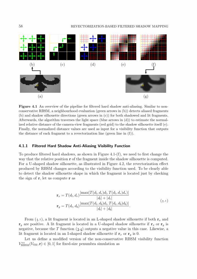
58 REVECTORIZATION-BASED FILTERED SHADOW MAPPING
(a) (g)
(b) (c) (d) (e) (f)
Figure 4.1 An overview of the pipeline for filtered hard shadow anti-aliasing. Similar to non-conservative RBSM, a neighbourhood evaluation (green arrows in (b)) detects aliased fragments(b) and shadow silhouette directions (green arrows in (c)) for both shadowed and lit fragments.Afterwards, the algorithm traverses the light space (blue arrows in (d)) to estimate the normal-ized relative distance of the camera-view fragments (red grid) to the shadow silhouette itself (e).Finally, the normalized distance values are used as input for a visibility function that outputsthe distance of each fragment to a revectorization line (green line in (f)).
4.1.1 Filtered Hard Shadow Anti-Aliasing Visibility Function
To produce filtered hard shadows, as shown in Figure 4.1-(f), we need to first change theway that the relative position r of the fragment inside the shadow silhouette is computed.For a U-shaped shadow silhouette, as illustrated in Figure 4.2, the revectorization effectproduced by RBSM changes according to the visibility function used. To be clearly ableto detect the shadow silhouette shape in which the fragment is located just by checkingthe sign of r, let us compute r as
rx = T (dl, dr)|max(T (dl, dr)dl, T (dl, dr)dr)|
|dl|+ |dr|
ry = T (dt, db)|max(T (dt, db)dt, T (dt, db)db)|
|dt|+ |db|.
(4.1)
From (4.1), a lit fragment is located in an L-shaped shadow silhouette if both rx andry are positive. A lit fragment is located in a U-shaped shadow silhouette if rx or ry isnegative, because the T function (3.4) outputs a negative value in this case. Likewise, alit fragment is located in an I-shaped shadow silhouette if rx or ry is 0.
Let us define a modified version of the non-conservative RBSM visibility functionV ∗∗RBSM(VSM, r) ∈ [0, 1] for fixed-size penumbra simulation as

4.1 REVECTORIZATION-BASED PERCENTAGE-CLOSER FILTERING 59
(a) (b) (c)
Figure 4.2 For a U-shaped shadow silhouette (a), the revectorization effect provided by non-conservative RBSM (b) is different from the one produced by RBSM when aiming filtered hardshadow rendering (c).
(a) (b) (c)
Figure 4.3 The penumbra effect produced by RPCF for different penumbra sizes.
V ∗∗RBSM(VSM, r) =
1− VSM + (2VSM − 1)max(rx, ry) if rxry < 0,
VSM else if rxry = 0,
min(max(1− VSM + (2VSM − 1)(rx + ry), 0), 1) otherwise.
(4.2)
In (4.2), we basically modified Equation (3.9), such that, rather than clamping V ∗RBSM
to be 0 or 1, we use the addition and subtraction operations over r and VSM to determinethe smooth transition that characterizes the filtered hard shadow intensities. With sucha modification, we are able to produce fixed-size penumbra such as the one shown inFigure 4.1-(g).
4.1.2 Revectorization-Based Filtering
One problem with the use of (4.2) is that the penumbra size is fixed and limited, propor-tional to the size of the shadow silhouette, which depends on the shadow map resolution.To enable control over the filter size, we simply incorporate PCF into the revectorizationpipeline, giving name to the RPCF technique (Figure 4.3). For each sample of RPCF,we set its visibility condition to be the shadow test (3.2) if the sample is located in aplace outside the shadow silhouette. Otherwise, if the sample is located in the lit orshadowed side of the shadow silhouette, we assume its visibility as the result of Equation(4.2). Then, the final intensity of a given fragment is computed by the average of shadow

60 REVECTORIZATION-BASED FILTERED SHADOW MAPPING
0
(a)
0
(b)
0
(c)
0 0
(d)
0
(e)
0 0
(f)
0 0 1
0 0 0
0 0 0
(g)
Figure 4.4 An illustration of the optimized implementation of RPCF listed in Algorithm 2.For each shadow map sample (blue rectangle) inside the filter kernel (orange grid) we computeits shadow intensity and locate the direction of the shadow silhouette (a). Then, we estimatethe shadow silhouette size (b) and perform the shadow revectorization in the camera-space (redgrid) sample (yellow rectangle) (c). For the next sample (d), the algorithm checks whethersilhouette is located at the same direction of the previous sample (red arrows in (e)), to reusethe relative position previously estimated for the shadow revectorization (f). In (g), we showthe filter result. This figure shows the filter kernel aligned with the light space, and each shadowmap texel equivalent to a 4× 4 grid in the camera space only for visualization purposes.
intensities computed for every sample located in the RPCF kernel.
In terms of performance, the RBSM step with the most computational cost is theshadow silhouette size estimation. In a naıve implementation, one would need to traversethe shadow map several times to locate the ends of the shadow silhouette for everyshadow map sample inside the RPCF kernel. To reduce the computational cost of therevectorization, we take advantage of the fact that, once we have computed the shadowsilhouette size, we may reuse such an information to define the visibility of neighborshadow map samples. This prevents the algorithm from a new traversal over the shadowmap, saving costly shadow map texture lookups. The steps of this revectorization aregiven in Algorithm 2 and shown in Figure 4.4.
Given the kernel size for shadow filtering wfilter ∈ N (Line 2 of Algorithm 2), wesample the neighbourhood of size P of each fragment p projected in the shadow mapS (Line 10 of Algorithm 2, Figure 4.4-(a)). Then, for each sample s, we proceed asproposed in the RBSM algorithm (Algorithm 1), by computing the shadow test (3.2),the silhouette directions (3.3) (Lines 11-12 of Algorithm 2), estimating the relative po-sition of s in the aliased silhouette (Lines 16-17 of Algorithm 2 and Figure 4.4-(b)) and

4.1 REVECTORIZATION-BASED PERCENTAGE-CLOSER FILTERING 61
Algorithm 2 Revectorization-based shadow filtering
1: P ← penumbra size;2: wfilter ← shadow filter size;3: V ∗∗RBSSM ← 0;4: dprev ← null;5: rprev ← null;6: for each frame do7: S ← renderShadowMap;8: for each surface point p in camera view do9: p← transformToLightSpace(p);
10: for each sample s of S in wfilter, neighbour of p in P do11: VSM ← computeShadowTest(s, S);12: d← computeSilhouetteDirection(VSM);13: if hasSameDirection(d,dprev) then14: r← updateRelativePosition(rprev);15: else16: s← transformToCameraSpace(s);17: r← estimateRelativePosition(s, s, d, S);18: end if19: V ∗∗RBSSM ← V ∗∗RBSSM + performAntiAliasing(r, VSM);20: end for21: dprev ← d;22: rprev ← r;23: end for24: return V ∗∗RBSSM/wfilter;25: end for26:
27: procedure hasSameDirection(d,dprev)28: for each coordinate c of d do29: if dc == dprev
c and dc == 1 then30: return true;31: end if32: end for33: return false;34: end procedure
performing the revectorization of the fragment using (4.2) (Line 19 of Algorithm 2 andFigure 4.4-(c)). If the next sample inside the RPCF kernel (Figure 4.4-(d)) is located inthe same silhouette of the previous sample (Line 13 of Algorithm 2 and Figure 4.4-(e)),we update the relative position previously computed (Line 14 of Algorithm 2) by takinginto consideration the distance between previous and current samples. Then, we use theupdated relative position to perform the revectorization of the current sample (Line 19 ofAlgorithm 2 and Figure 4.4-(f)). To detect whether the current sample is located in the

62 REVECTORIZATION-BASED FILTERED SHADOW MAPPING
(a) Shadow Mapping (b) Non-Conservative RBSM
(c) EDT Normalization (d) EDT Filtering
(a) Shadow Mapping (b) Non-Conservative RBSM
(c) EDT Normalization (d) EDT Filtering
(a) Shadow Mapping (b) Non-Conservative RBSM
(c) EDT Normalization (d) EDT Filtering
(a) Shadow Mapping (b) Non-Conservative RBSM
(c) EDT Normalization (d) EDT Filtering
(a) Shadow Mapping (b) Non-Conservative RBSM
(c) EDT Normalization (d) EDT FilteringFigure 4.5 An overview of EDTSM. Given the aliased hard shadows obtained with the tra-ditional shadow mapping (a), non-conservative RBSM is applied to generate anti-aliased hardshadows (b). Then, penumbra intensities are computed on the basis of a normalized EDT overthe penumbra region (c). Finally, a mean filter (d) is applied over the normalized EDT toreduce skeleton artifacts generated by the EDT computation.
same silhouette of the previous sample, we check whether the current sample is locatedin a shadow silhouette (i.e., if a single coordinate of d is equal to 1) and whether bothsamples share, at least, a single silhouette direction in common (i.e., if both samples havethe same coordinate of d equals to 1) (Lines 27-34 of Algorithm 2). Finally, the finalpenumbra intensity of p is computed as an average of the shadow intensities computedinside the RPCF kernel (Line 24 of Algorithm 2 and Figure 4.4-(g)).
While RPCF is able to suppress the aliasing artifacts commonly generated by PCF,the technique inherits one of the problems of PCF: non-scalability with respect to thefilter size. To minimize such a problem, we propose another technique that computesshadows on the basis of separable Euclidean Distance Transform (EDT).

4.2 EUCLIDEAN DISTANCE TRANSFORM SHADOW MAPPING 63
Algorithm 3 Euclidean distance transform shadow mapping
1: P ← penumbra size;2: wfilter ← mean filter size;3: for each frame do4: S ← renderShadowMap;5: G ← renderGBuffer;6: R ← revectorizeShadow(S, G);7: EDT ← performEDTShadowing(R, G, P );8: F ← filterShadow(EDT, G, wfilter);9: renderShadowedScene(F, G);
10: end for
4.2 EUCLIDEAN DISTANCE TRANSFORM SHADOW MAPPING
4.2.1 Overview
EDTSM is a technique that uses EDT to simulate the penumbra effect over anti-aliasedhard shadows. In Figure 4.5, we show the steps that are required to simulate fixed-sizepenumbra using EDT on the basis of the hard shadows generated by shadow mapping.The full process is listed in Algorithm 3.
The main assumption of EDTSM is that the penumbra intensity of a fragment can beapproximated by the Euclidean distance of the fragment to the nearest fragment located inthe hard shadow silhouette. Therefore, the first step of EDTSM consists in the generationof the shadow map texture (Line 4 of Algorithm 3) for real-time hard shadow rendering.To avoid shadow aliasing (Figure 4.5-(a)), this technique requires the use of a hard shadowanti-aliasing technique before the fixed-size penumbra simulation. Hence, we make useof non-conservative RBSM (Figure 4.5-(b) and Line 6 of Algorithm 3) to generate anti-aliased hard shadows in real time. Also, to restrict shadow and shading computationsto the fragments visible to the camera, as suggested by the deferred rendering pipeline,we use a G-buffer G (SAITO; TAKAHASHI, 1990) of viewport width w and height hthat stores, for each pixel G(i, j) ∈ R6, the world-space position p and normal n of thevisible surface points in the camera viewpoint. (Line 5 of Algorithm 3). Afterward,to simulate the penumbra effect, the EDT is computed over the image with the hardshadows previously estimated. Then, the Euclidean distance is normalized (Figure 4.5-(c) and Line 7 of Algorithm 3) and filtered (Figure 4.5-(d) and Line 8 of Algorithm 3)inside a user-defined fixed-size penumbra region, because the penumbra intensity of afragment must lie in the interval of intensities between the umbra and lit regions.
4.2.2 Euclidean Distance Transform Shadowing
Let us call seed a fragment that lies in the hard shadow silhouette (green rectangles inFigure 4.6) and that will be used as a basis for the EDT computation. Even if it islocated in a thin aliased shadow, a seed fragment can be easily located in the screenspace of the camera view by the application of a 3× 3 rectangular filter over the shadows

64 REVECTORIZATION-BASED FILTERED SHADOW MAPPING
(a)
D D
(b)
P
(c)
D ≤ P2
(d)
12− D
P12
+ DP
(e)
Figure 4.6 A more in-depth overview of EDTSM. First, non-conservative RBSM is used (a)to generate anti-aliased shadow silhouettes (green rectangles) in the camera view (red grid).Then, for every fragment in the screen space, the world-space position is retrieved from the G-buffer, and the world-space distance D to closest fragment located in the shadow silhouette iscomputed (b). Given a user-defined penumbra size P (c), the algorithm restricts the penumbracomputation for fragments located in the penumbra region (d). Finally, the EDT previouslycomputed is normalized to simulate the smooth transition between lit and umbra regions thatcharacterize the penumbra effect (e).
produced with non-conservative RBSM. In this case, a fragment is a seed if the hardshadow intensity of the fragment differs from the hard shadow intensity of one of itsneighbours located in the 8-connected neighbourhood of the fragment in the screen space(Figure 4.6-(a)).
Once the seed fragments have been detected in the image, the EDT can be computed.So, for each non-seed fragment, the world-space Euclidean distance D of the fragmentto the nearest seed located in the shadow silhouette is computed (Figure 4.6-(b)), Dbeing a world-space distance computed on the basis of the world-space position retrievedfrom a G-buffer (SAITO; TAKAHASHI, 1990) previously computed. Just by applyingthe EDT in the world space, the user does not have control over the desired penumbrasize. To solve this problem, let us assume P as a user-defined parameter which controlsthe size of the penumbra that will be simulated. As shown in Figure 4.6-(c), each halfof the penumbra size belongs to one side of the shadow silhouette. Therefore, one caneasily detect whether a fragment belongs to the desired penumbra region by checking ifthe distance of the fragment to the shadow silhouette is lower or equal than half of thepenumbra size (i.e., D ≤ P/2) (Figure 4.6-(d)). For the fragments located outside of thepenumbra region, the shadow intensity is given by the shadow test (umbra and lit regionsin Figure 4.6-(d)). Meanwhile, for fragments in the penumbra region, we keep the resultof the EDT as shadow intensity.
As can be seen in Figure 4.6-(d), EDT does not resemble a penumbra mostly because itis not normalized. The transition between umbra and lit regions in the desired penumbrais not smooth as it should be to characterize a penumbra. To solve this problem, theEuclidean distance is normalized to the closed unit interval [0, 1], assuming that umbraand lit fragments have intensities 0 and 1, respectively. Hence, the final intensity I ∈ [0, 1]of the fragments located in the penumbra region is

4.2 EUCLIDEAN DISTANCE TRANSFORM SHADOW MAPPING 65
(a) (b)
(a) (b)(a) (b)
(a) (b)(a) (b)
Figure 4.7 After the EDT computation, skeleton artifacts may arise along gradient disconti-nuities (green closeup of (a)). Also, aliasing artifacts may still remain even after the shadowrevectorization (blue closeup of (a)). By applying a simple mean filter, those artifacts can besuppressed (b).
I =
12− D
Pif the fragment was in shadow,
12
+ DP
otherwise.(4.3)
As shown in (4.3), the final intensity of each fragment depends on the previous visibil-ity condition given by RBSM. For instance, knowing that the maximum distance of eachfragment belonging to the penumbra region to the nearest seed is P/2 (Figure 4.6-(d)), ifthe fragment was in shadow, as computed by RBSM, the new penumbra intensity of thefragment must lie in the interval [0, 1
2], because 0 is the intensity of the fragments located
in shadow and 12
is the intensity of the fragments located in the middle of the penumbraregion. Accordingly, lit fragments, as computed by RBSM, must have their penumbraintensities lying in the interval [1
2, 1]. By the use of (4.3), EDTSM is able to satisfy these
constraints and simulate the penumbra effect (Figure 4.6-(e)).
4.2.3 Euclidean Distance Transform Filtering
A well-known feature of EDT is the generation of skeletons along gradient discontinuities(WRIGHT; CIPOLLA; GIBLIN, 1995). This property of EDT is desirable in several

66 REVECTORIZATION-BASED FILTERED SHADOW MAPPING
applications, such as integer medial axis estimation (HESSELINK; ROERDINK, 2008).However, these skeletons generated by EDT, when visualized inside a penumbra, consti-tute an artifact because a penumbra does not have skeletons along its silhouette (greencloseup of Figure 4.7-(a)). Moreover, RBSM is able to minimize aliasing artifacts gener-ated by shadow mapping, but is not able to remove all of them (blue closeup of Figure4.7-(a)). To minimize both skeleton and aliasing artifacts simultaneously, a simple screen-space separable mean filter is applied over the shadow silhouette (Figure 4.7-(b)). Themean filtering was chosen to solve these problems because of its simplicity, low processingtime, separability and effectiveness to suppress the skeleton artifacts even for low-orderfilter sizes.
The EDT algorithm is performed in screen space, taking as input the image of theshadowed scene rendered from the camera viewpoint. In this sense, special care mustbe taken to make this process edge aware and viewpoint invariant. Edge awarenessis important because different objects cannot influence on the penumbra computationof each other. Viewpoint invariance is desirable because the penumbra size must bekept constant, regardless of the distance of the viewer to the shadowed region. EDTSMsolves both problems by the use of the depth value and world-space position storedin the G-buffer. Depth information is used to detect edges, which separate differentobjects in the scene. In this sense, for instance, a fragment is only considered to be inpenumbra if the depth difference between the fragment and its nearest seed is below auser-defined threshold (empirically, we have set this depth threshold as 2.5×10⁻³). Also,only neighbours with similar depth difference are taken into account for mean filtering.In counterpart, to make the EDT viewpoint invariant, world-space position is used tocompute the Euclidean distance values D in the EDT. Inspired by screen-space softshadow algorithms, the viewpoint invariance of the mean filtering is solved by estimatingthe mean filter size wscreen
filter that varies according to the distance of the camera to thescene. Here, wscreen
filter is measured as (MOHAMMADBAGHER et al., 2010)
wscreenfilter =
wfilterzscreen
pzeye, (4.4)
zscreen =1
2tanfovy2
, (4.5)
where wfilter is the mean filter size defined by the user, pzeye is the distance of the fragmentp to the center of the camera, fovy specifies the vertical field of view angle and zscreen isthe inverse of the viewport scale, in terms of field of view.
4.3 RESULTS AND DISCUSSION
In this section, we compare our EDTSM and RPCF techniques with traditional filteredhard shadow mapping techniques, such as PCF (REEVES; SALESIN; COOK, 1987),Variance Shadow Mapping (VSM) (DONNELLY; LAURITZEN, 2006), and ExponentialVariance Shadow Mapping (EVSM) (LAURITZEN; MCCOOL, 2008), as well as thestate-of-the-art fixed-size penumbra simulation technique, Moment Shadow Mapping(MSM) (PETERS; KLEIN, 2015). These techniques were chosen for evaluation because
4.3 RESULTS AND DISCUSSION 67
they produce fixed-size penumbra, lying in the scope of this chapter. Therefore, tech-niques that simulate variable-size penumbra (i.e., soft shadows) on the basis of point orarea light sources are not evaluated in this section.
We have tested different penumbra simulation techniques in three distinct scenarios.Figure 4.8 shows a model with fine detailed structures along its silhouette. Figure 4.9shows shadows cast on a non-planar model. Figure 4.10 shows a scenario with severallight blocker and shadow receiver objects positioned over each other.
4.3.1 Experimental Setup
For EDT computation, we have used the open-source implementation of the ParallelBanding Algorithm (PBA) (CAO et al., 2010) implemented in Compute Unified DeviceArchitecture (CUDA) (KIRK; HWU, 2013). Although many other works have attemptedto compute EDT efficiently (RONG; TAN, 2006; SCHNEIDER; KRAUS; WESTER-MANN, 2009; WANG; TAN, 2013), in our tests, PBA delivered the fastest and mostaccurate EDT computation.
CUDA/OpenGL interoperability was used to optimize resource management and pro-cessing time. A filter of order 15 × 15 was applied to suppress skeleton and bandingartifacts. Specifically for RPCF, we have used a filter of order 7× 7, since the techniquedemands less samples to suppress banding artifacts. In the results, we have tested filtersof higher orders only to determine whether the techniques are scalable in terms of thefilter size.
4.3.2 Visual Quality Evaluation
In the blue closeups of Figures 4.8 and 4.9, we show whether the different shadowingtechniques are able to suppress aliasing artifacts. For small penumbra sizes, the blurprovided by PCF is insufficient to suppress aliasing artifacts (Figures 4.8-(a) and 4.9-(a)). The same effect is visible for the shadow map filtering techniques (Figures 4.8-(b, c,d) and 4.9-(b, c, d)), which simulate penumbra with blurred jagged silhouettes along theshadow. Techniques that use shadow revectorization as basis for penumbra simulation(RPCF and EDTSM) are able to minimize this artifact efficiently (Figures 4.8-(e, f) and4.9-(e, f)).
In the red closeups of Figures 4.8, 4.9 and 4.10, we show whether each techniquegenerates light leaking artifacts inside the shadow. All shadow map filtering techniquesare prone to light leaking artifacts. In this sense, VSM (Figures 4.8-(b), 4.9-(b) and4.10-(b)) is more susceptible to light leaking than EVSM (Figures 4.8-(c), 4.9-(c) and4.10-(c)). In terms of visual quality, MSM is better than both VSM and EVSM, greatlyreducing the light leaking artifacts (the effectiveness of MSM is mainly visible in Figure4.9-(d)). The techniques that filter shadows to simulate penumbra (PCF, RPCF andEDTSM) are not prone to light leaking artifacts (Figures 4.8-(a, e, f), 4.9-(a, e, f) and4.10-(a, e, f)).
RPCF and EDTSM support shadow rendering for planar (Figures 4.8-(e, f)) andnon-planar receivers (Figures 4.9-(e, f)). Moreover, both techniques support penumbrasimulation not only for simple scenarios, but also for more complex, game-like scenarios,

68 REVECTORIZATION-BASED FILTERED SHADOW MAPPING
(a) PCF (b) VSM (c) EVSM
(d) MSM (e) RPCF (f) EDTSM
(a) PCF (b) VSM (c) EVSM
(d) MSM (e) RPCF (f) EDTSM
(a) PCF (b) VSM (c) EVSM
(d) MSM (e) RPCF (f) EDTSM
(a) PCF (b) VSM (c) EVSM
(d) MSM (e) RPCF (f) EDTSM
(a) PCF (b) VSM (c) EVSM
(d) MSM (e) RPCF (f) EDTSM
(a) PCF (b) VSM (c) EVSM
(d) MSM (e) RPCF (f) EDTSM
(a) PCF (b) VSM (c) EVSM
(d) MSM (e) RPCF (f) EDTSM
(a) PCF (b) VSM (c) EVSM
(d) MSM (e) RPCF (f) EDTSM
(a) PCF (b) VSM (c) EVSM
(d) MSM (e) RPCF (f) EDTSM
(a) PCF (b) VSM (c) EVSM
(d) MSM (e) RPCF (f) EDTSM
(a) PCF (b) VSM (c) EVSM
(d) MSM (e) RPCF (f) EDTSM
(a) PCF (b) VSM (c) EVSM
(d) MSM (e) RPCF (f) EDTSM
(a) PCF (b) VSM (c) EVSM
(d) MSM (e) RPCF (f) EDTSM
Figure 4.8 Fixed-size penumbra produced by different techniques. Each closeup shows whetherthe technique handles light leaking (red) and aliasing (blue) artifacts. Images were generatedfor the YeahRight model using a 10242 shadow map resolution.
such as the one shown in Figures 4.10-(e, f), where several light blocker and shadowreceiver objects with fine detailed structures (e.g., trees) are located in the same scene.

4.3 RESULTS AND DISCUSSION 69
(a) PCF (b) VSM (c) EVSM
(d) MSM (e) RPCF (f) EDTSM
(a) PCF (b) VSM (c) EVSM
(d) MSM (e) RPCF (f) EDTSM
(a) PCF (b) VSM (c) EVSM
(d) MSM (e) RPCF (f) EDTSM(a) PCF (b) VSM (c) EVSM
(d) MSM (e) RPCF (f) EDTSM
(a) PCF (b) VSM (c) EVSM
(d) MSM (e) RPCF (f) EDTSM(a) PCF (b) VSM (c) EVSM
(d) MSM (e) RPCF (f) EDTSM
(a) PCF (b) VSM (c) EVSM
(d) MSM (e) RPCF (f) EDTSM
(a) PCF (b) VSM (c) EVSM
(d) MSM (e) RPCF (f) EDTSM
(a) PCF (b) VSM (c) EVSM
(d) MSM (e) RPCF (f) EDTSM
(a) PCF (b) VSM (c) EVSM
(d) MSM (e) RPCF (f) EDTSM
(a) PCF (b) VSM (c) EVSM
(d) MSM (e) RPCF (f) EDTSM
(a) PCF (b) VSM (c) EVSM
(d) MSM (e) RPCF (f) EDTSM
(a) PCF (b) VSM (c) EVSM
(d) MSM (e) RPCF (f) EDTSM
Figure 4.9 Fixed-size penumbra produced by different techniques. Each closeup shows whetherthe technique light leaking (red) and aliasing (blue) artifacts. Images were generated for theBunny model using a 10242 shadow map resolution.

70 REVECTORIZATION-BASED FILTERED SHADOW MAPPING
(a) PCF (b) VSM (c) EVSM
(d) MSM (e) RPCF (f) EDTSM
(a) PCF (b) VSM (c) EVSM
(d) MSM (e) RPCF (f) EDTSM
(a) PCF (b) VSM (c) EVSM
(d) MSM (e) RPCF (f) EDTSM
(a) PCF (b) VSM (c) EVSM
(d) MSM (e) RPCF (f) EDTSM
(a) PCF (b) VSM (c) EVSM
(d) MSM (e) RPCF (f) EDTSM
(a) PCF (b) VSM (c) EVSM
(d) MSM (e) RPCF (f) EDTSM
(a) PCF (b) VSM (c) EVSM
(d) MSM (e) RPCF (f) EDTSM
Figure 4.10 Fixed-size penumbra produced by different techniques. Each closeup showswhether the technique handles light leaking artifacts. Images were generated for the SanMiguelmodel using a 10242 shadow map resolution.
Also, despite being an image-based technique, EDTSM supports penumbra simulationon noisy surfaces with high-frequency details, as shown in Figure 4.11. In this figure,we reinforce that EDTSM is able to separate penumbra simulation from self-shadowing,while properly handling the noisy depth differences distributed over the surface. Hence,the gamut of scenes shown in this section reveals that both EDTSM and RPCF are ableto generate fixed-size penumbra, with less aliasing and light leaking than related work.
4.3.3 Rendering Time Evaluation
As shown in Tables 4.1 and 4.2, shadow map filtering is an efficient way to simulatepenumbra, being relatively scalable with respect to the shadow map (Table 4.1), view-

4.3 RESULTS AND DISCUSSION 71
Figure 4.11 Fixed-size penumbra simulation on a noisy surface with laterally increasing fre-quency. Image was generated for the YeahRight model using a 10242 shadow map resolution.
Shadow Map Resolution (ms)Scene Method 5122 10242 20482 40962
Figure 4.8
PF 10.5 10.6 10.8 12.0PCF 11.3 11.4 11.4 11.7
EDTSM 12.9 13.0 13.2 13.8RPCF 26.2 27.3 27.8 30.0
Figure 4.9
PF 1.9 2.1 2.4 3.6PCF 2.9 3.0 3.1 3.5
EDTSM 4.5 4.6 4.8 5.7RPCF 10.4 11.0 11.5 12.0
Figure 4.10
PF 126.9 128.2 129.8 133.8PCF 126.7 129.0 130.3 133.5
EDTSM 129.5 130.9 132.8 136.3RPCF 138.8 141.2 145.7 148.1
Table 4.1 Processing time for several hard shadow filtering techniques and different scenesrendered at an output 720p resolution. Measurements include varying shadow map resolution.PF - Pre-filtering techniques that produce nearly the same processing time results (namelyVSM, EVSM and MSM).
port (Table 4.2) and kernel resolutions (Table 4.3). Moreover, the different shadow mapfiltering techniques that we have tested in this chapter provide nearly the same low ren-dering times, that is why they are refereed by a single row in each table. However, all thisefficiency comes at the price of light leaking artifacts generation inside shadows (Figures

72 REVECTORIZATION-BASED FILTERED SHADOW MAPPING
Output Resolution (ms)Scene Method 480p 720p 1080p
Figure 4.8
PF 9.9 10.6 11.3PCF 9.8 11.4 11.9
EDTSM 10.8 13.0 14.9RPCF 16.4 27.3 30.3
Figure 4.9
PF 0.9 2.1 3.1PCF 0.9 3.0 4.0
EDTSM 2.3 4.6 6.9RPCF 4.3 11.0 12.5
Figure 4.10
PF 127.8 128.2 128.8PCF 127.8 129.0 129.5
EDTSM 129.3 130.9 133.5RPCF 132.9 141.2 143.7
Table 4.2 Processing time for several hard shadow filtering techniques and different scenesrendered at a 10242 shadow map resolution. Measurements include varying output image res-olution. PF - Pre-filtering techniques that produce nearly the same processing time results(namely VSM, EVSM and MSM).
Kernel Size (ms)Scene Method 72 152 232 312
Figure 4.8
PF 10.3 10.6 10.8 11.1PCF 9.8 11.4 13.5 17.0
EDTSM 12.4 13.0 13.5 14.3RPCF 27.3 77.5 166.6 285.7
Figure 4.9
PF 1.8 2.1 2.4 2.7PCF 1.2 3.0 5.6 9.3
EDTSM 4.1 4.6 5.3 6.1RPCF 11.0 65.7 145.3 255.7
Figure 4.10
PF 127.9 128.2 128.4 128.6PCF 128.3 129.0 130.2 133.5
EDTSM 130.3 130.9 131.6 132.6RPCF 141.2 200.2 366.3 552.2
Table 4.3 Processing time for several hard shadow filtering techniques and different scenesrendered at an output 1280 × 720 resolution and using a 10242 shadow map resolution. Mea-surements include varying kernel size. PF - Pre-filtering techniques that produce nearly thesame processing time results (namely VSM, EVSM and MSM).
4.8-(b, c, d), 4.9-(b, c, d) and 4.10-(b, c, d)). PCF is more scalable to the shadow mapresolution than the shadow map filtering techniques (Table 4.1), but is one of the slowesttechniques for high-order filter sizes (Table 4.3) and is prone to aliasing artifacts alongthe shadow silhouette (Figures 4.8-(a) and 4.9-(a)). RPCF is able to suppress aliasingartifacts (Figures 4.8-(e), 4.9-(e) and 4.10-(e)), but is the slowest penumbra simulation

4.3 RESULTS AND DISCUSSION 73
Output Resolution (ms)Scene Step 480p 720p 1080p
Figure 4.8
G-buffer 4.1 4.5 4.7Shadow Map 4.3 4.3 4.3
RBSM 0.2 0.4 0.6EDT 1.3 2.3 2.9
Mean Filter 0.7 1.2 2.0Shading 0.2 0.3 0.4Total 10.8 13.0 14.9
Figure 4.9
G-buffer 0.1 0.3 0.4Shadow Map 0.2 0.2 0.2
RBSM 0.1 0.4 0.7EDT 1.1 2.3 3.1
Mean Filter 0.7 1.2 2.2Shading 0.1 0.2 0.3Total 2.3 4.6 6.9
Figure 4.10
G-buffer 63.4 63.5 63.6Shadow Map 63.0 63.0 63.0
RBSM 0.6 0.7 1.0EDT 1.3 2.3 3.3
Mean Filter 0.7 1.1 2.2Shading 0.3 0.3 0.4Total 129.3 130.9 133.5
Table 4.4 Processing time of each individual step of the proposed EDTSM (including G-bufferand shadow map rendering) for different scenes rendered using a 10242 shadow map resolution.Measurements include varying output image resolution.
technique, regardless of shadow map (Table 4.1), viewport (Table 4.2) and kernel reso-lution (Table 4.3). EDTSM is slightly slower than the majority of previous work (Table4.1) and is not scalable with respect to the output image resolution (Table 4.2), becauseEDT is an image-based operation. Finally, EDTSM is more scalable to the filter sizethan PCF and RPCF techniques, becoming even faster than these two related work forhigh-order filter sizes (Table 4.3).
In Table 4.4, we show the processing time obtained for each step of EDTSM forvarying output resolution. We have not conducted the same analysis for other parametersbecause a variation in the shadow map resolution (Table 4.1) affects mainly the shadowmap rendering and RBSM computation steps. Meanwhile, the variation of the kernel size(Table 4.3) affects only the mean filtering step.
From Table 4.4, we can see that, as expected, the processing times demanded byG-buffer and shadow map rendering steps vary according to the number of trianglespresent in the scene. With respect to the shadowing step of the algorithm, the EDTcomputation is the bottleneck of EDTSM. We recall that, to the best of our knowledge,the algorithm that we use to compute the EDT in real time, the PBA (CAO et al., 2010),
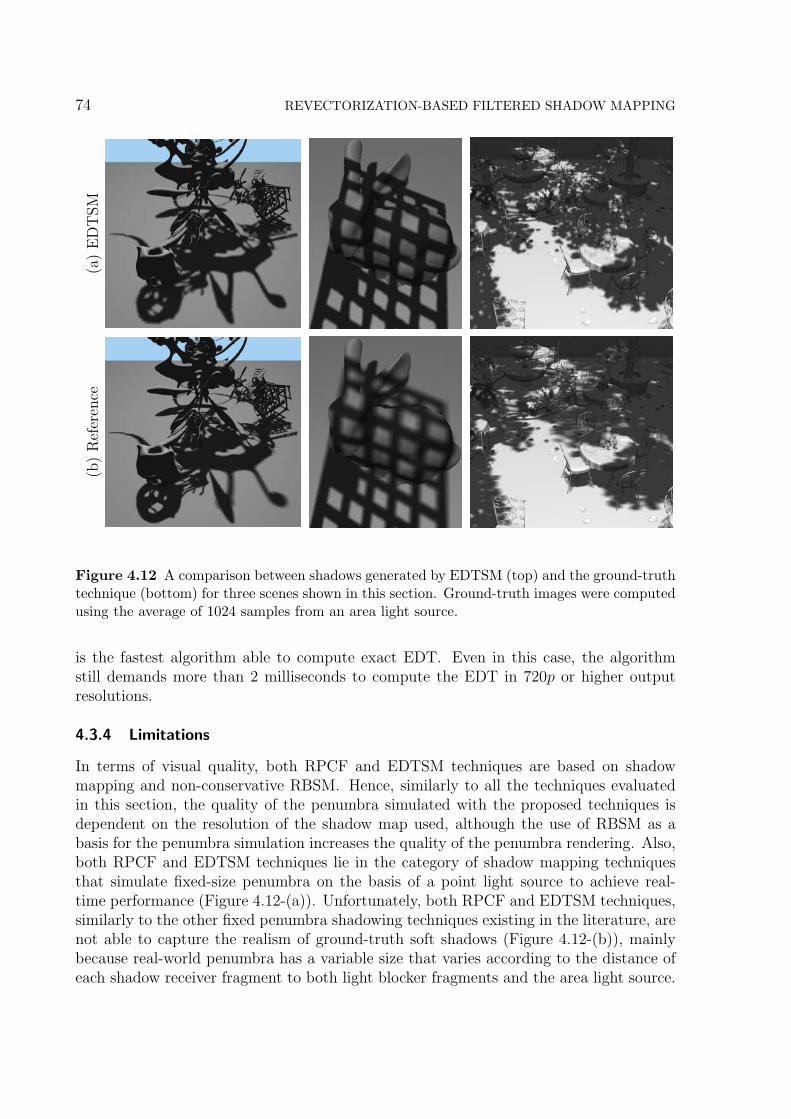
74 REVECTORIZATION-BASED FILTERED SHADOW MAPPING(a
)E
DT
SM
(b)
Ref
eren
ce
Figure 4.12 A comparison between shadows generated by EDTSM (top) and the ground-truthtechnique (bottom) for three scenes shown in this section. Ground-truth images were computedusing the average of 1024 samples from an area light source.
is the fastest algorithm able to compute exact EDT. Even in this case, the algorithmstill demands more than 2 milliseconds to compute the EDT in 720p or higher outputresolutions.
4.3.4 Limitations
In terms of visual quality, both RPCF and EDTSM techniques are based on shadowmapping and non-conservative RBSM. Hence, similarly to all the techniques evaluatedin this section, the quality of the penumbra simulated with the proposed techniques isdependent on the resolution of the shadow map used, although the use of RBSM as abasis for the penumbra simulation increases the quality of the penumbra rendering. Also,both RPCF and EDTSM techniques lie in the category of shadow mapping techniquesthat simulate fixed-size penumbra on the basis of a point light source to achieve real-time performance (Figure 4.12-(a)). Unfortunately, both RPCF and EDTSM techniques,similarly to the other fixed penumbra shadowing techniques existing in the literature, arenot able to capture the realism of ground-truth soft shadows (Figure 4.12-(b)), mainlybecause real-world penumbra has a variable size that varies according to the distance ofeach shadow receiver fragment to both light blocker fragments and the area light source.

4.4 SUMMARY 75
In terms of rendering performance, RPCF is not scalable to the kernel size, similarlyto PCF, although the technique requires a small kernel size to generate penumbra freefrom banding artifacts. As for EDTSM, the costly step of the technique is the EDTcomputation, making EDTSM slightly slower than the majority of related work for thesame scene configurations. Despite these facts, the quality of the penumbra simulatedstimulates the use of EDTSM for anti-aliased fixed-size penumbra rendering.
4.4 SUMMARY
In this chapter, we have presented two techniques for fixed-size penumbra simulation:RPCF, a filtered hard shadow mapping technique that extends the non-conservativeRBSM to output penumbra intensities rather than hard shadow intensities; EDTSM,a technique that simulates penumbra by computing a normalized EDT over the hardshadows generated by non-conservative RBSM.
Compared to other filtered hard shadow techniques, both RPCF and EDTSM tech-nique are able to reduce shadow aliasing and light leaking, keeping real-time frame ratesand high-quality penumbra simulation for planar and non-planar receivers, simple andcomplex scenarios. By performing the filtering over the light space, RPCF is slightlymore accurate than EDTSM, meanwhile EDTSM is faster than RPCF due to the use ofa separable implementation of EDT to speed up the hard shadow filtering.
Both RPCF and EDTSM share the same limitation of other fixed-size penumbrasimulation techniques that are based on shadow mapping: the quality of the simulationdepends on the accuracy of the shadow map rendered, and fixed-size penumbra is notmuch realistic, because real-world penumbra has a variable size along its silhouette.
In the next chapters, we show how to extend both RPCF and EDTSM techniques tosimulate variable-size penumbra on the basis of a single point light source, enhancing thequality of the shadow rendering, at the cost of a lower frame rate.


Chapter
5In this chapter, we present the extension of RBSM to provide anti-aliasing for visually plausible soft
shadow rendering. A novel solution that computes soft shadows almost entirely on the screen space is
designed to keep high-quality anti-aliasing, while improving the performance of the revectorization-based
soft shadow rendering.
REVECTORIZATION-BASED SOFT SHADOWMAPPING
As shown in the previous chapter, Revectorization-based Shadow Mapping (RBSM)can be adapted for fixed-size penumbra simulation, but this kind of shadow render-ing lacks realism because real-world shadows contain variable-size penumbra along itssilhouette. In this chapter, we present three new techniques that use the concepts ofshadow revectorization and Euclidean distance transform to provide visually plausible softshadow rendering. The first technique, named Euclidean Distance Transform Soft ShadowMapping (EDTSSM), is an extension of Euclidean Distance Transform Shadow Map-ping (EDTSM) for soft shadow rendering. The second technique, named Revectorization-based Soft Shadow Mapping (RBSSM), improves the accuracy of EDTSSM, at the cost ofloss in performance. The third technique, called Screen-Space Revectorization-based SoftShadow Mapping (SSRBSSM), provides a balance between accuracy and performance,keeping visual quality as accurate as RBSSM, while generating soft shadows faster thanEDTSSM. In this chapter, we present and evaluate all these techniques with respect tothe state-of-the-art in the field of visually plausible soft shadow mapping. This chaptercovers the discussion and results mainly presented in an authored publication (MACEDO;APOLINARIO, 2017).
5.1 VARIABLE-SIZE PENUMBRA ESTIMATION
To estimate the penumbra size of a given region, Percentage Closer Soft Shadows (PCSS)proposes that one needs to first approximate the scene by objects that are planar andparallel to each other. The depth of such a planar approximation is given by the averageblocker depth zavg(wavg
k , pz, S), or simply zavg, for a kernel with size wavgk ∈ N (FER-
NANDO, 2005)
77

78 REVECTORIZATION-BASED SOFT SHADOW MAPPING
(a) Anti-aliasedShadow
(b) Penumbra Size (c) EDT Shadowing (d) EDT Filtering
Figure 5.1 An overview of EDTSSM. We estimate anti-aliased hard shadows in the cameraview with non-conservative RBSM (a). On the basis of PCSS, we estimate the penumbra size ofthe fragments located at the hard shadow silhouette (b), and use it to normalize the EDT thatis computed to measure the distance of each fragment to the closest hard shadow silhouette,simulating the penumbra effect (c). To suppress the skeleton artifacts generated by the EDT,an edge-aware viewpoint-invariant filtering algorithm is applied over the shadow (d).
zavg =
∑wavgk
i=0
∑wavgk
j=0 (1− VSM)S(i, j)
ε+∑wavg
ki=0
∑wavgk
j=0 (1− VSM), (5.1)
where ε = 0.001 is a small constant value to avoid the division by zero.
Then, on the basis of the parallel-planar assumption of PCSS, the variable penumbrasize wp(wl, zavg, pz), or simply wp, can be estimated according to the light source size wl
as (FERNANDO, 2005)
wp = wlpz − zavg
zavg
(5.2)
In the next sections, we show each one of the proposed techniques make use of thoseequations to generate visually plausible soft shadows.
5.2 EUCLIDEAN DISTANCE TRANSFORM SOFT SHADOW MAPPING
In Algorithm 4, we present a high-level overview of the proposed approach to computesoft shadows on the basis of a normalized EDT. The steps of this approach are depictedin Figure 5.1. We render the scene from the light source and camera viewpoints (Lines3 and 4 of Algorithm 4) to produce anti-aliased hard shadows with non-conservativeRBSM (Figure 5.1-(a), Line 5 of Algorithm 4). Then, we estimate the penumbra size ofthe fragments located in the hard shadow silhouette (Figure 5.1-(b), Line 6 of Algorithm4), such that we can apply the normalized EDT to compute the soft shadow (Figure

5.2 EUCLIDEAN DISTANCE TRANSFORM SOFT SHADOW MAPPING 79
Algorithm 4 Euclidean distance transform soft shadow mapping
1: wfilter ← soft shadow filter size;2: for each frame do3: S ← renderShadowMap;4: G ← renderGBuffer;5: R ← revectorizeShadow(S, G);6: P ← estimatePenumbraSize(R, S);7: EDT ← performEDTShadowing(R, G, P);8: F ← filterShadow(EDT, G, wfilter);9: renderShadowedScene(F, G);
10: end for
5.1-(c), Line 7 of Algorithm 4) and filter it to suppress the skeleton artifacts generatedby the application of the EDT (Figure 5.1-(d), Line 8 of Algorithm 4).
The key difference between EDTSM and EDTSSM is that the penumbra size is nolonger fixed, determined by the user. Now, for each fragment in the camera view, wemust determine whether the fragment is located in a penumbra region, and what is theentire variable-sized penumbra region in the world space, such that we can compute thesoft shadows on the basis of an EDT. The PCSS framework proposes that the penumbrasize must be computed for every fragment in the camera view, since this size determinesthe area of the shadow map that must be filtered by the algorithm (FERNANDO, 2005).Similarly to (KLEIN; NISCHWITZ; OBERMEIER, 2012), we optimize such approachby computing the penumbra size only for the fragments located at the hard shadowsilhouette and propagating such a data for the remaining fragments outside the shadowsilhouette. Differently from (KLEIN; NISCHWITZ; OBERMEIER, 2012), we computethe penumbra size of the fragments located at the revectorized, anti-aliased hard shadowsilhouette. Also, we propagate the penumbra size in real time using the nearest neighboursearch provided by the EDT algorithm.
Similarly to EDTSM, to determine whether a fragment is located in the shadowsilhouette in the image with the revectorized hard shadows (Figure 5.1-(a)), we checkwhether the visibility condition of the current fragment is different from at least oneof the neighbours located inside a 3 × 3 rectangular filter. Then, for each fragment inthe shadow silhouette, we take advantage of the planar-parallel assumption of PCSS toestimate the penumbra size in real time (Figure 5.1-(b)), following Equations (5.1) and(5.2).
Once we have the penumbra size wp computed for every fragment located in therevectorized hard shadow silhouette, we need to propagate this data for the fragmentslocated outside the shadow silhouette. To do so, for each fragment outside the hardshadow silhouette, we compute the EDT, that returns exactly the location of the closestfragment located in the hard shadow silhouette. In this case, since wp was estimated withrespect to the light space, it cannot be directly used to define the size of the penumbrain the world space, since this task is non-trivial (FERNANDO et al., 2001). Hence,we multiply wp by a user-defined parameter β, which helps with the definition of the

80 REVECTORIZATION-BASED SOFT SHADOW MAPPING
HSM
Visibility Classification
(a)
Blocker Search Area
zavg
p
(b)
wl
zavg
pzwp
(c)
RBSM Filter Area
Soft Shadow(d)
Figure 5.2 An overview of RBSSM. After shadow map and G-buffer rendering, a hierarchicalshadow map (HSM) is built to locate potential penumbra fragments in the camera view (a).For these fragments, the average blocker depth (zavg in (b)) is computed, then the penumbrasize (wp in (c)) is estimated and filtered using RBSM to generate the soft shadows (d).
penumbra size in the world space. In our experimental tests, we have verified thatβ = 750 keeps the penumbra size similar to the one found in the most common softshadow mapping algorithm, such as PCSS.
Then, to compute the penumbra intensity of each fragment located in wp, we haveslightly changed (4.3) to take into account the variable-size penumbra
I =
12− D
βwpif the fragment was in the hard shadow,
12
+ Dβwp
otherwise.(5.3)
With (5.3), we are able to compute soft shadows such as the one shown in Figure5.1-(c). To suppress the skeleton artifacts commonly produced by the use of EDT, weapply the same mean filtering step shown in Section 4.2.3, using (4.4).
5.3 REVECTORIZATION-BASED SOFT SHADOW MAPPING
Another alternative to compute anti-aliased soft shadows in real time consists in thedirect integration of RBSM into the PCSS pipeline. Hence, RBSSM computes anti-aliased shadows based on PCSS and RBSM frameworks. Two steps are added into RBSMto perform penumbra size estimation and soft shadow filtering. To identify potentialfragments located in the penumbra, improving the performance of the approach, we makeuse of a hierarchical shadow map (HSM) (GUENNEBAUD; BARTHE; PAULIN, 2006)H. In this case, H is a two-channel pyramidal-like min-max texture, that, at level l, hasm2l
rows and n2l
columns. Each pixel in the first level (l = 0) of H is defined by the shadowmap itself. Then, the subsequent levels of H can be iteratively built by computing bothminimal and maximal values of the depths stored in a 2× 2 region of the previous level.

5.3 REVECTORIZATION-BASED SOFT SHADOW MAPPING 81
Algorithm 5 Revectorization-based soft shadow mapping
1: wl ← light source size;2: wavg
k ← kernel size for average blocker depth estimation;3: for each frame do4: S ← renderShadowMap;5: G ← renderGBuffer;6: H ← buildHierarchicalShadowMap;7: for each surface point p visible in camera view from G do8: p← transformToLightSpace(p);9: VHSM ← estimateVisibilityFromHSM(p, H);
10: if VHSM = umbra or VHSM = lit then11: VRBSSM ← computeShadowTest(p, S);12: else13: zavg ← computeAvgBlockDepth(wavg
k , p, S);14: wp ← estimatePenumbraSize(wl, zavg, pz);15: VRBSSM ← computeSoftShadow(wp, p, S);16: end if17: end for18: end for
Indeed, the process of computing H works like mip-mapping, but we compute minimaland maximal values over a region rather than the average of the depth values.
With the map H, given the shadow map region intersected by the frustum formedby the light source area and the surface point p, the depth values zmin ∈ [0, 1] andzmax ∈ [0, 1] of the corresponding hierarchical shadow map level must be retrieved toallow the evaluation of the illumination condition of the surface point by the visibilityfunction VHSM(pz, zmin, zmax)
VHSM(pz, zmin, zmax) =
lit if pz ≤ zmin,
in umbra else if pz ≥ zmax,
in penumbra otherwise.
(5.4)
An overview of RBSSM is shown in Figure 5.2 and is listed in Algorithm 5. First, wegenerate the shadow map S from the light source viewpoint (WILLIAMS, 1978) (Line4 of Algorithm 5), the G-buffer G to avoid calculations on hidden fragments, evaluatingthe illumination only for the fragments visible to the camera (Line 5 of Algorithm 5),and the hierarchical shadow map H, to quickly classify the penumbra surface points inthe scene and discard the non-penumbra surface points from the soft shadow calculation(Line 6 of Algorithm 5 and Figure 5.2-(a)).
Afterwards, we transform each visible surface point p to the light source viewpoint(Lines 7 and 8 of Algorithm 5) and use H to identify the potential fragments locatedin the penumbra using (5.4) (Line 9 of Algorithm 5, Figure 5.2-(a)). The visibility ofthe surface points located outside the penumbra is given by the shadow test (3.2) (Lines10-11 of Algorithm 5). Meanwhile, for the surface points located in the penumbra, we
82 REVECTORIZATION-BASED SOFT SHADOW MAPPING
proceed as proposed in the PCSS, computing average blocker depth (5.1) and penumbrasize (5.2) (Lines 13-14 of Algorithm 5).
Rather than using the typical Percentage-Closer Filtering (PCF) for soft shadow fil-tering in the penumbra size wp, we replace the PCF technique by Revectorization-basedPercentage-Closer Filtering (RPCF) (Line 15 of Algorithm 5 and Figure 5.2-(d)).
RBSSM is able to generate soft shadows with high visual quality and real-time perfor-mance. An alternative to reduce its visual quality and improve its rendering performanceconsists on the realization of the soft shadow filtering in the screen space, as we show inthe next section.
5.4 SCREEN-SPACE REVECTORIZATION-BASED SOFT SHADOW MAPPING
SSRBSSM is an alternative approach to compute soft shadows on the basis of RBSMand PCSS frameworks that favors rendering performance rather than visual quality. Thealgorithm is much similar to RBSSM, except for the soft shadow filtering step, that iscomputed in the screen space.
SSRBSSM computes a shadow map and a G-buffer (Figure 5.2-(a)). Then, the averageblocker depth and penumbra size are estimated in the shadow map space as well (Figures5.2-(b, c)). However, the penumbra size estimated by RBSSM works well for filtering inthe shadow map space. Since we aim to filter the soft shadows in the screen space, weestimate a screen-space penumbra size using (4.4).
To produce anti-aliased screen-space soft shadows, we must obtain the informationabout the anti-aliased hard shadows in the screen space. To do so, we produce filteredhard shadows in the screen-space using the RBSM technique (4.2) and save the filteredhard shadow intensity of each visible fragment. Next, we separate the soft shadow filteringin two steps: horizontal and vertical filtering in the screen space. In the horizontal pass,filtering is performed over the filtered hard shadow on the screen-sized penumbra area.In the vertical pass, filtering is done over the horizontally filtered hard shadows. In thisstep, the filtering must be edge-aware, since we lose information about the edge locationin screen space. Hence, we use the separable cross-bilateral filter technique proposed in(PHAM; VLIET, 2005) for this purpose. Because the bilateral filter is not separablein essence, striped artifacts may appear during the filtering. We reduce such artifactsby increasing the bilateral filter sampling rate. Even in this case, since the number ofincreased samples is still smaller than the number of samples required for a non-separableimplementation of the bilateral filter, separable bilateral filter is better suited, in terms ofperformance requirements, to our solution than the non-separable version of the bilateralfilter.
As we show in the next section, the computation of the screen-space soft shadowfiltering together with the high-quality revectorization-effect makes SSRBSSM an efficientalternative for simpler scenarios, where high performance is desirable for soft shadowrendering.

5.5 RESULTS AND DISCUSSION 83
5.5 RESULTS AND DISCUSSION
In this section, we evaluate the techniques in terms of visual quality and performance.We compare the proposed approaches (EDTSSM, RBSSM and SSRBSSM) with the mosttraditional real-time soft shadow technique (PCSS), well-known shadow map pre-filteringtechniques (Variance Soft Shadow Mapping (VSSM) and Moment Soft Shadow Mapping(MSSM)) and one of the most recent screen-space soft shadow techniques (Screen-SpaceAnisotropic Blurred Soft Shadows (SSABSS)). The visual quality is evaluated for thesame shadow map and viewport resolutions and for different scenarios. Performance isevaluated for different shadow map and viewport resolutions and for different scenarios.Hard shadow techniques are not evaluated in this section because they are out of thescope of this chapter.
5.5.1 Experimental Setup
Following related work (PETERS et al., 2016), we fixed the filter size of 9 × 9 for theblocker search step, and 15×15 for the soft shadow filtering step of PCSS, VSSM, MSSMand EDTSSM techniques. For RBSSM, we have used a kernel size of 7 × 7 since thefiltering variant (Equation (4.2)) of RBSM requires less samples to effectively minimizebanding artifacts. For the screen-space techniques, namely SSABSS and SSRBSSM, wehave used a kernel size of 31 × 31, similarly to related work (BUADES; GUMBAU;CHOVER, 2015).
5.5.2 Visual Quality Evaluation
In Figures 5.3, 5.4 and 5.5, we show a comparison between the proposed approachesfor different scenarios. In Figure 5.3, we evaluate the techniques for a complex object,with fine, detailed structures along its silhouette. In Figures 5.4 and 5.5, we show howdifferent techniques handle the soft shadow computation for a more complex scenario,with multiple objects in different scales distributed all over the scene. Not only thescalability of the methods are evaluated for such a scenario with increased geometrycomplexity, but also the accuracy of the methods are evaluated due to the presence ofmultiple overlapping objects affecting the appearance of the shadow.
An equal low shadow map resolution comparison between different soft shadow tech-niques is depicted in Figure 5.3. For the limited 10242 shadow map resolution, PCSSgenerates aliasing artifacts along the soft shadow silhouette (Figure 5.3-(a)). VSSM andMSSM suffer from aliasing and light leaking artifacts (Figures 5.3-(b, d)). SSABSS pro-vides similar visual quality than PCSS in this scenario (Figure 5.3-(c)). EDTSSM isnot prone to aliasing artifacts, but promotes an overblurring of the shadow (Figure 5.3-(e)). Both RBSSM and SSRBSSM are able to effectively minimize the aliasing artifactswithout the shadow overblurring (Figures 5.3-(f, g)), producing anti-aliased soft shadowscomparable with ground-truth shadows (Figure 5.3-(h)).
A comparison between different soft shadow techniques for a more complex (game-like) scenario, due to the presence of several overlapping objects distributed along thescene and with different geometry complexity, is shown in Figures 5.4 and 5.5. As pointed

84 REVECTORIZATION-BASED SOFT SHADOW MAPPING
(a) PCSS (10.8 ms) (b) VSSM (13.1 ms) (c) SSABSS (10.7 ms)
(d) MSSM (12.5 ms) (e) EDTSSM (13.2 ms) (f) RBSSM (15.4 ms)
(g) SSRBSSM (10.8 ms) (h) Ground-Truth (1.14 s)
(a) PCSS (10.8 ms) (b) VSSM (13.1 ms) (c) SSABSS (10.7 ms)
(d) MSSM (12.5 ms) (e) EDTSSM (13.2 ms) (f) RBSSM (15.4 ms)
(g) SSRBSSM (10.8 ms) (h) Ground-Truth (1.14 s)
(a) PCSS (10.8 ms) (b) VSSM (13.1 ms) (c) SSABSS (10.7 ms)
(d) MSSM (12.5 ms) (e) EDTSSM (13.2 ms) (f) RBSSM (15.4 ms)
(g) SSRBSSM (10.8 ms) (h) Ground-Truth (1.14 s)
(a) PCSS (10.8 ms) (b) VSSM (13.1 ms) (c) SSABSS (10.7 ms)
(d) MSSM (12.5 ms) (e) EDTSSM (13.2 ms) (f) RBSSM (15.4 ms)
(g) SSRBSSM (10.8 ms) (h) Ground-Truth (1.14 s)
(a) PCSS (10.8 ms) (b) VSSM (13.1 ms) (c) SSABSS (10.7 ms)
(d) MSSM (12.5 ms) (e) EDTSSM (13.2 ms) (f) RBSSM (15.4 ms)
(g) SSRBSSM (10.8 ms) (h) Ground-Truth (1.14 s)
(a) PCSS (10.8 ms) (b) VSSM (13.1 ms) (c) SSABSS (10.7 ms)
(d) MSSM (12.5 ms) (e) EDTSSM (13.2 ms) (f) RBSSM (15.4 ms)
(g) SSRBSSM (10.8 ms) (h) Ground-Truth (1.14 s)
(a) PCSS (10.8 ms) (b) VSSM (13.1 ms) (c) SSABSS (10.7 ms)
(d) MSSM (12.5 ms) (e) EDTSSM (13.2 ms) (f) RBSSM (15.4 ms)
(g) SSRBSSM (10.8 ms) (h) Ground-Truth (1.14 s)
(a) PCSS (10.8 ms) (b) VSSM (13.1 ms) (c) SSABSS (10.7 ms)
(d) MSSM (12.5 ms) (e) EDTSSM (13.2 ms) (f) RBSSM (15.4 ms)
(g) SSRBSSM (10.8 ms) (h) Ground-Truth (1.14 s)
(a) PCSS (10.8 ms) (b) VSSM (13.1 ms) (c) SSABSS (10.7 ms)
(d) MSSM (12.5 ms) (e) EDTSSM (13.2 ms) (f) RBSSM (15.4 ms)
(g) SSRBSSM (10.8 ms) (h) Ground-Truth (1.14 s)
Figure 5.3 A visual comparison between distinct soft shadow techniques. Shadow map pre-filtering techniques produce soft shadows with light leaking artifacts (pointed by red arrows).Images were generated for the YeahRight model using a 10242 shadow map resolution. Theground-truth image was computed using the average of 1024 area light source samples.
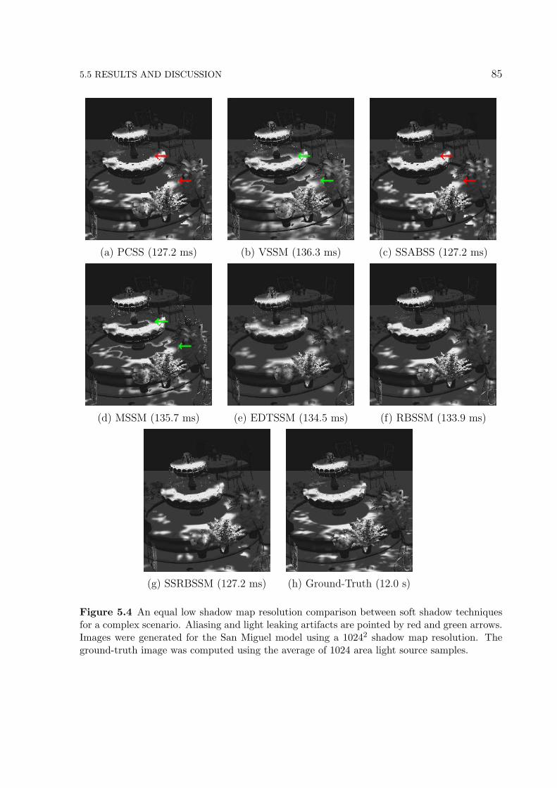
5.5 RESULTS AND DISCUSSION 85
(a) PCSS (127.2 ms) (b) VSSM (136.3 ms) (c) SSABSS (127.2 ms)
(d) MSSM (135.7 ms) (e) EDTSSM (134.5 ms) (f) RBSSM (133.9 ms)
(g) SSRBSSM (127.2 ms) (h) Ground-Truth (12.0 s)
Figure 5.4 An equal low shadow map resolution comparison between soft shadow techniquesfor a complex scenario. Aliasing and light leaking artifacts are pointed by red and green arrows.Images were generated for the San Miguel model using a 10242 shadow map resolution. Theground-truth image was computed using the average of 1024 area light source samples.

86 REVECTORIZATION-BASED SOFT SHADOW MAPPING
(a) PCSS (127.2 ms) (b) VSSM (136.3 ms) (c) SSABSS (127.2 ms)
(d) MSSM (135.7 ms) (e) EDTSSM (134.5 ms) (f) RBSSM (133.9 ms)
(g) SSRBSSM (127.2 ms) (h) Ground-Truth (12.0 s)
Figure 5.5 An equal low shadow map resolution comparison between soft shadow techniquesfor a complex scenario. Aliasing and light leaking artifacts are pointed by red and green arrows.Images were generated for the San Miguel model using a 10242 shadow map resolution. Theground-truth image was computed using the average of 1024 area light source samples.
by red arrows, PCSS and SSABSS suffer from aliasing artifacts (Figures 5.4-(a, c) and5.5-(a, c)). VSSM and MSSM suffer from light leaking artifacts (Figures 5.4-(b, d) and5.5-(b, d)). Again, we can see that EDTSSM does not suffer from aliasing artifacts, but

5.5 RESULTS AND DISCUSSION 87
overblurs the shadow (Figures 5.4-(e) and 5.5-(e)). RBSSM and SSRBSSM producesshadows that are more similar to the ground-truth than the other evaluated techniques(Figures 5.4-(f, g) and 5.5-(f, g)). Unfortunately, screen-space techniques are prone tolight leaking artifacts near the silhouette of the objects if the depth difference of distinctobjects in the scene is too small (see the region pointed by green arrows in Figures 5.5-(c,g)). In this sense, SSRBSSM is better than related work because it minimizes the aliasingartifacts (Figure 5.4-(g)).
5.5.3 Rendering Time Evaluation
In Figures 5.6, 5.7, 5.8 and 5.9, we show the performance of the several soft shadowtechniques evaluated in this section under varying shadow map and output resolutionsfor the different scenarios evaluated in the previous subsection.
PCSS, SSABSS and SSRBSSM are generally the fastest techniques, regardless of thescene configuration. PCSS is relatively scalable with respect to the shadow map resolution(Figures 5.6 and 5.7) and is not scalable in terms of output resolution (Figures 5.8 and5.9). RBSSM has the same performance characteristics of PCSS, but the additional costdemanded by the shadow revectorization makes RBSSM slower than PCSS. In this case,PCSS is faster than RBSSM, meanwhile RBSSM provides better visual quality thanPCSS. On the other hand, VSSM and MSSM techniques handle well varying outputresolution (Figures 5.8 and 5.9), but are not scalable with respect to the shadow mapresolution, becoming two of the slowest techniques for higher shadow map resolutions(Figures 5.6 and 5.7). This happens because of the time needed to compute the summed-area table, required for the shadow map pre-filtering, increases as much as the shadow mapresolution is increased. EDTSSM is scalable with respect to the shadow map resolution
5122 10242 20482 4096210
12
14
16
18
20
Shadow Map Resolution
Per
form
ance
[ms] PCSS
VSSMSSABSSMSSM
EDTSSMRBSSM
SSRBSSM
Figure 5.6 Time usage (in milliseconds) for several soft shadow techniques. Rendering timeswere measured for the YeahRight model shown in Figure 5.3 at an output 1280×720 resolution.Measurements include varying shadow map resolution.

88 REVECTORIZATION-BASED SOFT SHADOW MAPPING
(Figures 5.6 and 5.7), but is not scalable in terms of viewport resolution (Figures 5.8 and5.9), because the Euclidean Distance Transform, the costly step of EDTSSM, is computedin the screen space. The screen-space techniques (SSABSS and SSRBSSM) are not thatscalable in terms of viewport resolution (Figures 5.8 and 5.9), but they are generallyfaster than related work regardless of scene configuration.
5.5.4 Discussion
Comparing solely the results obtained with EDTSSM, RBSSM and SSRBSSM, the screen-space variant is able to successfully compute soft shadows visually similar to the onesobtained with RBSSM, while being faster than EDTSSM. This fact can be mainly seenin Figures 5.3 and 5.4. The greatest advantage of SSRBSSM is that, by performing mostof the computation in the screen space, the technique is faster than both revectorization-based techniques in all the scenes tested in this chapter. In this sense, RBSSM is suitablefor applications that demand high quality shadow rendering, EDTSSM is desirablefor applications that demand a balance between quality and performance, meanwhileSSRBSSM is desirable for applications that demand visually plausible soft shadow ren-dering with high performance.
Compared to related work, all the revectorization-based techniques provide the bestvisual quality results and are able to minimize aliasing and light leaking artifacts even forlow-resolution shadow maps (Figures 5.3-(f, g), 5.4-(f, g) and 5.5-(f, g)). Also, RBSSMis the technique that produces shadows most similar to the ones generated by a denseuniform sampling of the area light source. In terms of performance, as can be seen inFigures 5.6, 5.7, 5.8 and 5.9, we clearly have three distinct groups that represent differentbehaviours of the soft shadow techniques. The first group composed of the screen-space
5122 10242 20482 40962125
130
135
140
145
150
Shadow Map Resolution
Per
form
ance
[ms] PCSS
VSSMSSABSSMSSM
EDTSSMRBSSM
SSRBSSM
Figure 5.7 Time usage (in milliseconds) for several soft shadow techniques. Rendering timeswere measured for the San Miguel model shown in Figures 5.4 and 5.5 at an output 1280× 720resolution. Measurements include varying shadow map resolution.
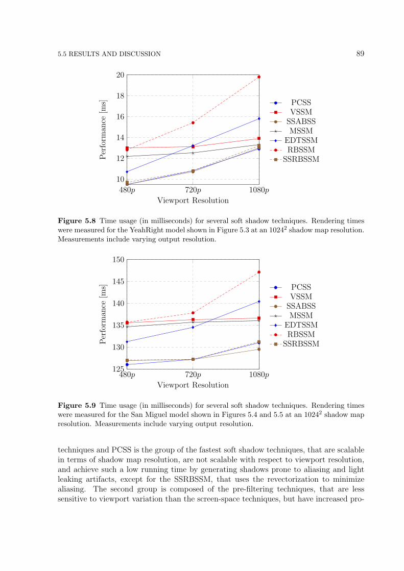
5.5 RESULTS AND DISCUSSION 89
480p 720p 1080p
10
12
14
16
18
20
Viewport Resolution
Per
form
ance
[ms] PCSS
VSSMSSABSSMSSM
EDTSSMRBSSM
SSRBSSM
Figure 5.8 Time usage (in milliseconds) for several soft shadow techniques. Rendering timeswere measured for the YeahRight model shown in Figure 5.3 at an 10242 shadow map resolution.Measurements include varying output resolution.
480p 720p 1080p125
130
135
140
145
150
Viewport Resolution
Per
form
ance
[ms] PCSS
VSSMSSABSSMSSM
EDTSSMRBSSM
SSRBSSM
Figure 5.9 Time usage (in milliseconds) for several soft shadow techniques. Rendering timeswere measured for the San Miguel model shown in Figures 5.4 and 5.5 at an 10242 shadow mapresolution. Measurements include varying output resolution.
techniques and PCSS is the group of the fastest soft shadow techniques, that are scalablein terms of shadow map resolution, are not scalable with respect to viewport resolution,and achieve such a low running time by generating shadows prone to aliasing and lightleaking artifacts, except for the SSRBSSM, that uses the revectorization to minimizealiasing. The second group is composed of the pre-filtering techniques, that are lesssensitive to viewport variation than the screen-space techniques, but have increased pro-

90 REVECTORIZATION-BASED SOFT SHADOW MAPPING
cessing time and generates light leaking artifacts for simple and complex scenarios. Thethird group is composed of the other revectorization-based techniques, namely EDTSSMand RBSSM, whose cost increases according to both shadow map and viewport resolu-tions. It is worthy to note that the rate of increase in the processing time of RBSSMfor higher viewport resolution is similar to the rate produced by PCSS and EDTSSM.Moreover, although RBSSM is, in average, 20% slower than the pre-filtering techniquesand 50% slower than the screen-space techniques for the scenario shown in Figure 5.3, fora more complex scenario (Figures 5.4 and 5.5), in which the overall processing time of thesolution is dominated by the geometry rendering, the technique becomes less than ≈ 5%more costly than the pre-filtering techniques and less than ≈ 10% more costly than thescreen-space techniques. Given these facts, we can state that SSRBSSM is desirable forsimple scenarios, since the technique is less prone to aliasing and light leaking artifactsthan related work and provides one of the fastest processing times. RBSSM is desirablefor complex scenarios, since even SSRBSSM suffers from light leaking artifacts (Figure5.5-(g)) and RBSSM is able to provide an improved visual quality with less than 10%of processing time overhead, as compared to related work. Finally, EDTSSM providesa balance between SSRBSSM and RBSSM, obtaining competitive performance for bothsimple and complex scenarios.
5.5.5 Limitations
One of the limitations shared by all techniques evaluated in this chapter is that the qualityof the generated soft shadow is highly dependent on the resolution of the shadow map.In this sense, we reinforce that the revectorization-based soft shadow techniques are ableto minimize such a problem efficiently.
As a screen-space technique, SSRBSSM suffers from the same problem of the otherscreen-space soft shadow techniques: the screen-space filtering does not approximate thefiltering produced from perspectively deformed kernels used for soft shadow filtering inthe light space, nor takes into account the shadows located outside the view, while it isstill prone to light leaking artifacts if the depth difference between different objects istoo small (Figure 5.5-(g)). That is why the RBSSM technique, by performing the softshadow filtering in the light space, has higher accuracy than SSRBSSM.
By using the mean filtering step as an alternative to minimize the skeleton artifactsgenerated by EDT, EDTSSM promotes an overblurring of the soft shadows that decreasesthe visual quality of the shadow rendering.
In terms of performance, RBSSM generates shadows with higher accuracy than relatedwork, but is one of the slowest soft shadow mapping techniques.
Finally, all the techniques compared in this chapter compute soft shadows using onlyone shadow map, located at the center of the area light source, and assuming that bothlight source and blocker objects are planar and parallel to each other. This simplifyingassumption makes the algorithms fast enough to run in real time and to generate visuallyplausible soft shadows. However, physical accuracy is lost because that assumption bringsincorrect penumbra size and visibility estimations (EISEMANN et al., 2011). An exampleof such a problem is visible in Figure 5.10, where the PCSS algorithm fails to estimate

5.6 SUMMARY 91
(a) PCSS (b) Accurate Shadows
Figure 5.10 For complex, large penumbra sizes, common real-time soft shadow techniques(a) fail to produce near accurate soft shadows (b) (see the region pointed by the red arrows).Images were generated for the YeahRight model using 10242 shadow map resolution.
the large penumbra size correctly.
5.6 SUMMARY
In this chapter, we have shown three techniques for visually plausible soft shadow ren-dering: EDTSSM, a technique that computes soft shadows on the basis of a normalizedEDT, RBSSM, a technique that extends the RBSM approach to compute soft shadows,and SSRBSSM, a technique that computes soft shadows in the screen space, on the basisof the filtered hard shadow visibility function of RBSM.
Due to the revectorization effect provided by RBSM, all the proposed techniques areable to provide anti-aliasing for the soft shadow rendering. EDTSSM and RBSSM reducethe light leaking artifacts commonly generated by shadow map pre-filtering techniques, atthe cost of more processing time for the shadow rendering. On the other hand, despite thelimitations caused by performing the shadow filtering in the screen space, the SSRBSSMtechnique has shown promising results with respect to visual quality, while being one ofthe fastest soft shadow techniques compared to the other evaluated works.
None of the techniques proposed for visually plausible soft shadow rendering cancompute accurate soft shadows because they approximate an area light source by a singlepoint light source in order to simplify the shadow rendering problem. In the next chapter,we show how the revectorization effect can benefit the reproduction of accurate softshadows computed on the basis of an adaptive area light source sampling.


Chapter
6In this chapter, we present an algorithm that takes advantage of the improved accuracy obtained with
RBSM to generate accurate soft shadows from a few light source samples, while producing temporally
coherent soft shadows at interactive frame rates.
REVECTORIZATION-BASED ACCURATE SOFTSHADOW MAPPING
The problem of the techniques discussed in the previous chapter is that they are computedon the basis of a single point light source, typically located at the center of an area lightsource. Such an approximation decreases the quality of the shadow rendering, but makesthe shadowing process real time. In this chapter, we present a new technique that usesthe concepts of shadow revectorization and adaptive sampling to speed up the accuraterendering of soft shadows. The content of this chapter is based on an authored publication(MACEDO; APOLINARIO JR., 2017b).
6.1 REVECTORIZATION-BASED ACCURATE SOFT SHADOW RENDERING
An overview of the proposed algorithm is presented in Figure 6.1 and a high-level pseu-docode is listed in Algorithm 6. Similarly to the solution proposed by related work(SCHWARZLER et al., 2012), we adaptively sample quads of four point light sourcesfrom the area light source (Figure 6.1-(a), Line 3 of Algorithm 6) and use them to evalu-ate whether banding artifacts are generated by the algorithm (Figures 6.1-(b, c, d, e, f),Lines 4-9 and 11 of Algorithm 6). In this case, we take advantage of the improved accu-racy provided by the Revectorization-based Shadow Mapping (RBSM) visibility functionto select less light source samples than related work (SCHWARZLER et al., 2012), whilekeeping its same visual quality. We further present a novel strategy to speedup the ac-curate soft shadow rendering on the basis of a visibility map (Figure 6.1-(g), Line 10 ofAlgorithm 6).
6.1.1 Adaptive Light Source Sampling
Let us define the area light source L as an adaptive structure where each node consistsof a quad Q formed by four neighbour point light sources. The main goal of the adap-
93
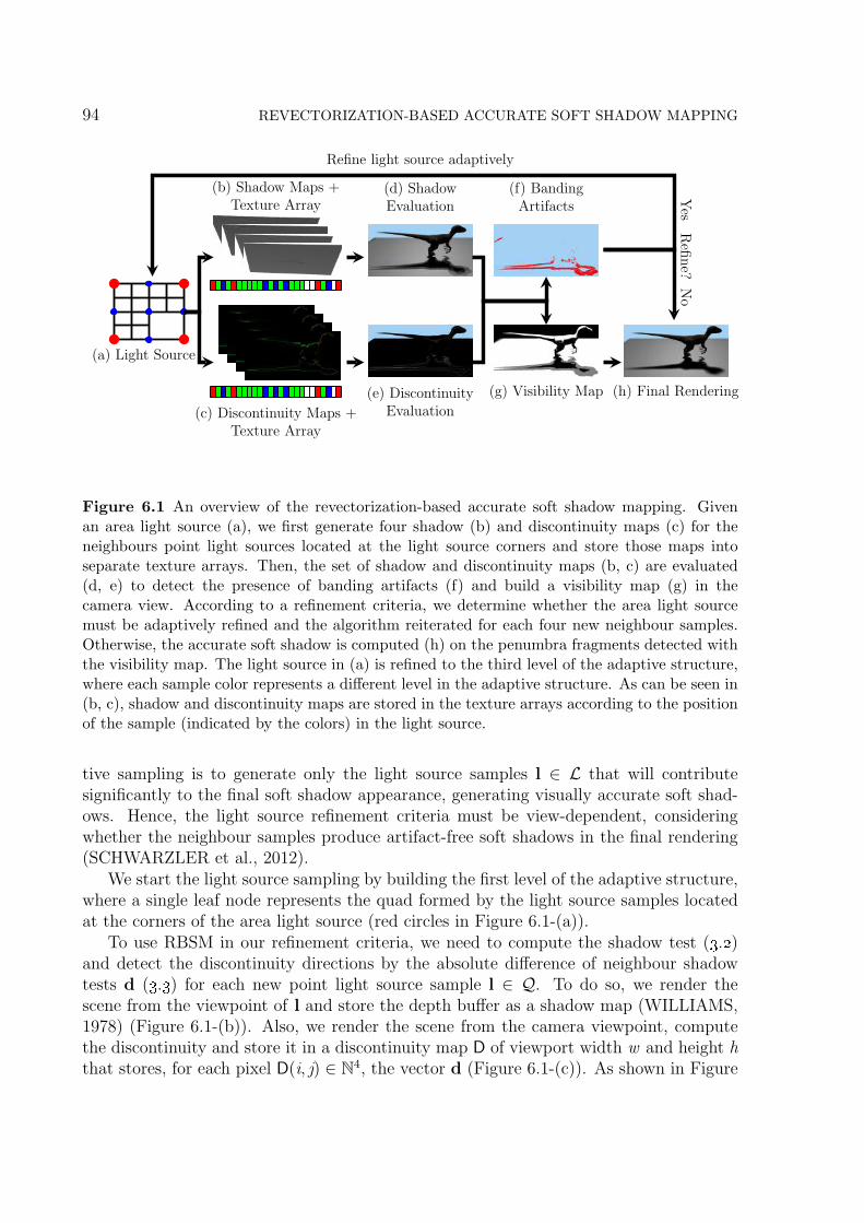
94 REVECTORIZATION-BASED ACCURATE SOFT SHADOW MAPPING
(a) Light Source
(b) Shadow Maps +Texture Array
(c) Discontinuity Maps +Texture Array
(d) ShadowEvaluation
(e) DiscontinuityEvaluation
(f) BandingArtifacts
(g) Visibility Map (h) Final Rendering
Refine light source adaptivelyR
efin
e?N
oY
es
Figure 6.1 An overview of the revectorization-based accurate soft shadow mapping. Givenan area light source (a), we first generate four shadow (b) and discontinuity maps (c) for theneighbours point light sources located at the light source corners and store those maps intoseparate texture arrays. Then, the set of shadow and discontinuity maps (b, c) are evaluated(d, e) to detect the presence of banding artifacts (f) and build a visibility map (g) in thecamera view. According to a refinement criteria, we determine whether the area light sourcemust be adaptively refined and the algorithm reiterated for each four new neighbour samples.Otherwise, the accurate soft shadow is computed (h) on the penumbra fragments detected withthe visibility map. The light source in (a) is refined to the third level of the adaptive structure,where each sample color represents a different level in the adaptive structure. As can be seen in(b, c), shadow and discontinuity maps are stored in the texture arrays according to the positionof the sample (indicated by the colors) in the light source.
tive sampling is to generate only the light source samples l ∈ L that will contributesignificantly to the final soft shadow appearance, generating visually accurate soft shad-ows. Hence, the light source refinement criteria must be view-dependent, consideringwhether the neighbour samples produce artifact-free soft shadows in the final rendering(SCHWARZLER et al., 2012).
We start the light source sampling by building the first level of the adaptive structure,where a single leaf node represents the quad formed by the light source samples locatedat the corners of the area light source (red circles in Figure 6.1-(a)).
To use RBSM in our refinement criteria, we need to compute the shadow test (3.2)and detect the discontinuity directions by the absolute difference of neighbour shadowtests d (3.3) for each new point light source sample l ∈ Q. To do so, we render thescene from the viewpoint of l and store the depth buffer as a shadow map (WILLIAMS,1978) (Figure 6.1-(b)). Also, we render the scene from the camera viewpoint, computethe discontinuity and store it in a discontinuity map D of viewport width w and height hthat stores, for each pixel D(i, j) ∈ N4, the vector d (Figure 6.1-(c)). As shown in Figure

6.1 REVECTORIZATION-BASED ACCURATE SOFT SHADOW RENDERING 95
Algorithm 6 Revectorization-based accurate soft shadowing
1: for each frame do2: G ← renderGBuffer;3: for each new quad Q of light source L with index q do4: for each new light source sample li of Q do5: Si ← renderShadowMap(li);6: Di ← renderDiscontinuityMap(Si, G);7: end for8: ss← computeShadowSum(S, G);9: sd← isSoftDiscontinuity(D, G);
10: VMq ← updateVisibilityMap(ss, sd, VMq−1, G);11: if hasBandingArtifact(ss, sd, G) then12: refineAdaptiveStructure(L);13: end if14: end for15: renderAccurateSoftShadow(S, D, VM, L, G);16: end for
6.1, both maps are stored in separate texture arrays, whose sizes are equivalent to themaximum number of samples that can be selected from L (Lines 3-7 of Algorithm 6).To optimize the discontinuity map rendering, we use a G-buffer (SAITO; TAKAHASHI,1990) to guarantee that (3.3) is computed for visible fragments only (Lines 2 and 6 ofAlgorithm 6).
After the shadow and discontinuity map rendering, we need to determine whether thesamples located in the same quad are sufficient for accurate soft shadow rendering. Todo so, we project both shadow and discontinuity maps of the four neighbour samples intothe same camera view and compare them (Figure 6.1-(d, e)) to detect whether bandingartifacts are produced by the use of those samples (Figure 6.1-(f)). This comparison isdone in a two-pass strategy with the scene rendered from the camera viewpoint.
In the first pass, for each fragment p projected in a pixel with coordinates (i, j) inthe camera view, we estimate the shadow sum ss(VSM,Q, i, j) ∈ [0, 4], or simply ss, thatis the sum of the four shadow test values of p computed from the neighbour four shadowmaps in the light quad Q (Figure 6.1-(d) and Line 8 of Algorithm 6)
ss(VSM,Q, i, j) =4∑
k=1, Sk∈Q
VSM(pz, Sk(i, j)). (6.1)
Additionally, we label a fragment as soft discontinuity if the fragment is in the shadowsilhouette (i.e., d 6= 0) for at least sd point light source samples (Figure 6.1-(e) and Line9 of Algorithm 6). Considering sd ∈ [0, 4], sd = 1 generates a really small number ofsamples for rendering, making the approach susceptible to banding artifacts. On theother hand, sd = 4 generates several samples, as a few fragments are classified as lyingin the shadow silhouette for all the four neighbour light source samples. sd = 2 or 3generates a moderate number of samples. We have used sd = 2 for all the scenarios

96 REVECTORIZATION-BASED ACCURATE SOFT SHADOW MAPPING
shown in this chapter because this value generates less samples than sd = 3, while beingmuch less susceptible to banding artifacts than sd = 1.
In the next pass, both shadow sum and fragment classification (Figure 6.1-(d, e)) areused to locate the fragments that potentially produce banding artifacts in the cameraview (Figure 6.1-(f), Line 11 of Algorithm 6). Based on the previously computed shadowsum (6.1), fully lit (i.e., ss = 4) and fully shadowed fragments (i.e., ss = 0) are discardedfrom rendering because they are not located in the penumbra and cannot cause bandingartifacts. Fragments classified as soft discontinuity are discarded from rendering as well,because RBSM will guarantee high-quality anti-aliasing for them. The remaining frag-ments (whose shadow sum lies between 1 and 3) are compared against their 8-connectedneighbour fragments in the camera view. If the fragment has at least one neighbourfragment that has a different shadow sum or that is a soft discontinuity, the fragment isdiscarded. The only fragments rendered in the scene are the ones whose shadow sumsstate that the fragments are in the penumbra and the shadow sums are the same forall the 8-connected neighbours. That is the case of the fragments located in penumbraregions that are not sufficiently smooth, due to the high distance between light sourcesamples (and their shadow maps). As shown in Figure 6.1-(f), those fragments producebanding artifacts in the final rendering, rather than a single, smooth penumbra region(SCHWARZLER et al., 2012).
Hardware occlusion query (BARTZ; MEIBNER; HUTTNER, 1998) is used to checkif a single pixel was rendered on the screen. If this condition is true, the area light sourceis further refined according to the adaptive structure (Line 12 of Algorithm 6). Then,the algorithm is iterated for the new light quads (Figure 6.1).
To optimize the performance of our solution, while we perform the light source sam-pling, we build and update a visibility map VM. This map is a texture that stores thefinal illumination condition of each fragment (i.e., whether the fragment is lit, penumbraor umbra) (Figure 6.1-(g)). With such a map, we are able to restrict the costly accuratesoft shadow rendering for penumbra fragments only.
The algorithm to compute the visibility map is fairly simple, yet effective. First, weclear VM, indicating that no classification has been assigned to any visible fragment.Then, we use the estimated shadow sum to update the stored visibility condition of thefragment. Let us redefine the shadow sum as ssq and the visibility map as VMq, whereq refers to a index of Q. For the first quad of the adaptive structure, the visibilityclassification VM0(i, j ) of the fragment p located at the pixel (i, j ) is computed on thebasis of the shadow sum estimated at that pixel ss0(i, j )
VM0(i, j) =
umbra if ss0(i, j) = 0,
penumbra else if 1 ≤ ss0(i, j) ≤ 3,
lit otherwise.
(6.2)
Additionally, we define VM0 as penumbra for the fragments classified as soft discontinuity.
For the next quad, assuming that the adaptive structure has more than one level, weupdate the visibility map by classifying the fragment as penumbra if there is a differencebetween the illumination condition previously estimated in the visibility map and the one

6.1 REVECTORIZATION-BASED ACCURATE SOFT SHADOW RENDERING 97
given by the current shadow sum. In other words
VMq(i, j) =
penumbra if VMq−1(i, j) = lit and ssq(i, j) = 0,
or VMq−1(i, j) = umbra and ssq(i, j) = 4.(6.3)
Finally, in the final rendering step (Figure 6.1-(h)), after the refinement criteria hasbeen satisfied, we access the visibility map to determine the visibility condition of thefragment in the camera view. Lit and umbra fragments are illuminated accordingly, andfor penumbra fragments only, we proceed with the computation of the final soft shadowintensity.
6.1.2 Final Rendering
Given the n light source samples l distributed over the surface of the area light source L,the final soft shadow intensity of a point p (Figure 6.1-(h), Line 15 of Algorithm 6) canbe computed according to the visibility function V ∈ [0, 1]
V =
∑ni=1 ωiV
∗∗RBSM(li)∑n
i=1 ωi. (6.4)
where V∗∗RBSM(li) denotes the visibility function of the filtered version of the RBSM tech-nique (4.2) with respect to the point light source li, and V estimates how much of thearea light source is visible to the point p. Therefore, V = 0 indicates that the entire arealight source is not visible to a given surface point p, and V = 1 indicates the full visibilityof the area light source to p. ωi is the weight assigned to the point light source li thatcompensates for the irregular distribution of samples, computed as (SCHWARZLER etal., 2012)
ω =1
(2α + 1)2, (6.5)
where α is the level of the adaptive structure.
RBSM is the basis of three distinct techniques that produce different shadow outputs:conservative, non-conservative and filtered RBSM. In (6.4), we use the filtered version ofRBSM because the use of filtering for shadow revectorization is efficient to solve bandingartifacts.
We could compute (6.4) in n shader passes, evaluating V per sample in each pass, andusing the accumulation buffer (HAEBERLI; AKELEY, 1990) to store the accumulatedsoft shadow intensity. Since we store the n shadow and discontinuity maps into twotexture arrays (Figure 6.1-(b, c)), we are able to compute (6.4) and evaluate the filteredRBSM visibility function for all the light source samples in a single pass on the shader,further saving many read/write operations that would be needed by the accumulationbuffer.
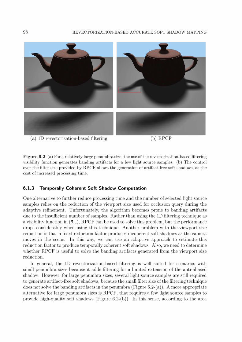
98 REVECTORIZATION-BASED ACCURATE SOFT SHADOW MAPPING
(a) 1D revectorization-based filtering (b) RPCF
(a) 1D revectorization-based filtering (b) RPCF(a) 1D revectorization-based filtering (b) RPCF
Figure 6.2 (a) For a relatively large penumbra size, the use of the revectorization-based filteringvisibility function generates banding artifacts for a few light source samples. (b) The controlover the filter size provided by RPCF allows the generation of artifact-free soft shadows, at thecost of increased processing time.
6.1.3 Temporally Coherent Soft Shadow Computation
One alternative to further reduce processing time and the number of selected light sourcesamples relies on the reduction of the viewport size used for occlusion query during theadaptive refinement. Unfortunately, the algorithm becomes prone to banding artifactsdue to the insufficient number of samples. Rather than using the 1D filtering technique asa visibility function in (6.4), RPCF can be used to solve this problem, but the performancedrops considerably when using this technique. Another problem with the viewport sizereduction is that a fixed reduction factor produces incoherent soft shadows as the cameramoves in the scene. In this way, we can use an adaptive approach to estimate thisreduction factor to produce temporally coherent soft shadows. Also, we need to determinewhether RPCF is useful to solve the banding artifacts generated from the viewport sizereduction.
In general, the 1D revectorization-based filtering is well suited for scenarios withsmall penumbra sizes because it adds filtering for a limited extension of the anti-aliasedshadow. However, for large penumbra sizes, several light source samples are still requiredto generate artifact-free soft shadows, because the small filter size of the filtering techniquedoes not solve the banding artifacts in the penumbra (Figure 6.2-(a)). A more appropriatealternative for large penumbra sizes is RPCF, that requires a few light source samples toprovide high-quality soft shadows (Figure 6.2-(b)). In this sense, according to the area

6.2 RESULTS AND DISCUSSION 99
light source and the penumbra size, each one of the revectorization-based techniques ismore adequate for accurate soft shadow rendering.
To compute the appropriate window size for occlusion query automatically, we es-timate such value according to the RBSM technique used and the current level of theadaptive structure. We draw this approach from the observation that the window sizereduction may change from adaptive structure level because, as long as the structureis refined, we can relax the criteria to guarantee that a small number of samples willbe used for rendering. Let us assume ws the original window size, wsRBSM(ws, α) andwsRPCF(ws, α) the window sizes used for the 1D revectorization-based filtering and RPCFtechniques, respectively. In this work, we have used the following window sizes
wsRBSM(ws, α) =
ws if 0 ≤ α ≤ 1,ws2
else if 2 ≤ α ≤ 3,ws4
otherwise.
(6.6)
wsRPCF(ws, α) =
ws4
if 0 ≤ α ≤ 1,ws6
else if 2 ≤ α ≤ 3,ws8
otherwise.
(6.7)
As we aim to generate a few light source samples, the idea of keeping the adaptivestructure built from the previous frame and refining or condensing it in the next framedid not improve the performance of the algorithm.
6.2 RESULTS AND DISCUSSION
In this section, we evaluate the soft shadow techniques in terms of visual quality andperformance. We compare our revectorization-based (RB) adaptive sampling with othersampling strategies, namely the uniform sampling of the area light source (using 289samples, as suggested in (SCHWARZLER et al., 2012)) and the adaptive sampling solu-tion proposed in (SCHWARZLER et al., 2012). Also, we compare our approach with atraditional technique from the field of real-time soft shadow mapping: Percentage CloserSoft Shadows (PCSS) (FERNANDO, 2005).
6.2.1 Experimental Setup
To provide a fair comparison between the adaptive sampling of (SCHWARZLER etal., 2012) and ours, we have used their solution with a reduction over the window sizefor occlusion query by a factor of 4 and Percentage-Closer Filtering (PCF) (REEVES;SALESIN; COOK, 1987) to compensate the banding artifacts. Their solution is alwaysslower than ours when using the same window size for both occlusion query (during adap-tive sampling) and output resolution (during final rendering). All images were generatedby a rectangular area light source. Both PCF and RPCF techniques use the same kernelsize of 2× 2.

100 REVECTORIZATION-BASED ACCURATE SOFT SHADOW MAPPING
(a) UniformSampling
(b) AdaptiveSampling
(c) RB AdaptiveSampling
(d) PCSS
0 18
14
38
12
(a) UniformSampling
(b) AdaptiveSampling
(c) RB AdaptiveSampling
(d) PCSS
0 18
14
38
12
(a) UniformSampling
(b) AdaptiveSampling
(c) RB AdaptiveSampling
(d) PCSS
0 18
14
38
12
(a) UniformSampling
(b) AdaptiveSampling
(c) RB AdaptiveSampling
(d) PCSS
0 18
14
38
12
Figure 6.3 Accurate soft shadows produced by different techniques. In this scenario, 289light source samples were used for uniform sampling (a), 47 light source samples were usedfor adaptive sampling (b), and only 25 light source samples were used for our RB adaptivesampling (c). PCSS (d) uses a single point light source sample. False color visualizations showthe difference between the normalized shadow intensities generated by uniform sampling, whichuses the largest number of samples, and the other techniques. Images were generated for theArmadillo model using a 10242 shadow map resolution.
6.2.2 Visual Quality Evaluation
As shown in Figures 6.3, 6.4, 6.5, our revectorization-based adaptive sampling provideshigh-quality, accurate soft shadows (Figures 6.3-(c), 6.4-(c), 6.5-(c)), needing a few lightsource samples to achieve such a visual quality. We require about 4-11 times less samplesthan the uniform sampling approach (Figures 6.3-(a), 6.4-(a), 6.5-(a)) and 2-4 times lesssamples than the adaptive sampling approach proposed in (SCHWARZLER et al., 2012)(Figures 6.3-(b), 6.4-(b), 6.5-(b)) to achieve high visual quality. Although the real-timesoft shadow technique (Figures 6.3-(d), 6.4-(d), 6.5-(d))) generates visually plausible softshadows, the penumbra size is estimated incorrectly and some details of the shadow arelost due to the approximation of the area light source by a single point light source.
An analysis of the influence of the penumbra size over the proposed adaptive samplingalgorithm can be seen in Figure 6.6. For small penumbra sizes (Figure 6.6-(a)), ourapproach is faster than the uniform sampling approach, while generating accurate softshadows from a few light source samples. Real-time soft shadow algorithms, in this case,tend to produce visually plausible soft shadows (Figure 6.6-(a)). As the penumbra sizeincreases (Figures 6.6-(b, c)), more light source samples are needed to effectively suppressbanding artifacts. In this scenario, while being able to generate accurate soft shadows,

6.2 RESULTS AND DISCUSSION 101
(a) UniformSampling
(b) AdaptiveSampling
(c) RB AdaptiveSampling
(d) PCSS
0 18
14
38
12
(a) UniformSampling
(b) AdaptiveSampling
(c) RB AdaptiveSampling
(d) PCSS
0 18
14
38
12
(a) UniformSampling
(b) AdaptiveSampling
(c) RB AdaptiveSampling
(d) PCSS
0 18
14
38
12
(a) UniformSampling
(b) AdaptiveSampling
(c) RB AdaptiveSampling
(d) PCSS
0 18
14
38
12
Figure 6.4 Accurate soft shadows produced by different techniques. In this scenario, 289light source samples were used for uniform sampling (a), 134 light source samples were usedfor adaptive sampling (b), and only 62 light source samples were used for our RB adaptivesampling (c). PCSS (d) uses a single point light source sample. False color visualizations showthe difference between the normalized shadow intensities generated by uniform sampling, whichuses the largest number of samples, and the other techniques. Images were generated for theYeahRight model using a 10242 shadow map resolution.
our approach may be slower than the uniform sampling approach mainly because of threefactors: 1. RBSM is slower than the traditional shadow mapping, although it providesimproved visual quality, 2. the adaptive refinement provides an additional cost to thefinal rendering time, while the uniform approach does not have such a step, 3. in thecase where the penumbra fills much of the screen-space available, the use of the visibilitymap does not discard a high number of fragments from the final rendering evaluation.As shown in Figure 6.6-(b, c), for large penumbra sizes, real-time soft shadow algorithmsare able to generate soft shadows with low processing time, but cannot generate accuratesoft shadows (as pointed by the red arrows in Figure 6.6-(b, c)). Indeed, such a differenceis mainly visible for situations such as the one shown in Figure 5.10, where the umbraregion disappears entirely in penumbra. In these cases, the approximation of the arealight source by a single point light source does not provide enough information for thesampling and rendering of those fine details of the penumbra.
The improved temporal coherency obtained with our solution can be seen in Figure6.7. The adaptive sampling approach of (SCHWARZLER et al., 2012) greatly varies thenumber of selected light source samples according to the distance of the camera to thepenumbra region. While a high number of samples is selected when a large amount of thescreen space is occupied by the penumbra, a really small number of samples are selectedwhen the camera is far away. In this case, one can see the shadows as a composition

102 REVECTORIZATION-BASED ACCURATE SOFT SHADOW MAPPING
(a) UniformSampling
(b) AdaptiveSampling
(c) RB AdaptiveSampling
(d) PCSS
0 18
14
38
12
(a) UniformSampling
(b) AdaptiveSampling
(c) RB AdaptiveSampling
(d) PCSS
0 18
14
38
12
(a) UniformSampling
(b) AdaptiveSampling
(c) RB AdaptiveSampling
(d) PCSS
0 18
14
38
12
(a) UniformSampling
(b) AdaptiveSampling
(c) RB AdaptiveSampling
(d) PCSS
0 18
14
38
12
Figure 6.5 Accurate soft shadows produced by different techniques. In this scenario, 289light source samples were used for uniform sampling (a), 246 light source samples were usedfor adaptive sampling (b), and only 63 light source samples were used for our RB adaptivesampling (c). PCSS (d) uses a single point light source sample. False color visualizations showthe difference between the normalized shadow intensities generated by uniform sampling, whichuses the largest number of samples, and the other techniques. Images were generated for theQuadBot model using a 10242 shadow map resolution.
of several hard shadows rather than a single soft shadow (SCHWARZLER et al., 2012).Our approach keeps the number of samples selected from the area light source consistent,generating high-quality soft shadows regardless of the distance from the viewer to thepenumbra region.
6.2.3 Rendering Time Evaluation
A performance comparison between the techniques evaluated in this section can be seenin Tables 6.1 and 6.2. The uniform sampling of the area light source provides stableframe rates under different parameters, but provides the worst performance, due to thelarge number of samples used for every frame. The adaptive sampling strategy proposedin (SCHWARZLER et al., 2012) becomes faster as long as the shadow map resolutionincreases, because less samples are required to generate high-quality accurate soft shadowswhen high resolution shadow maps are used. On the other hand, such a sampling strategyis sensitive to high output resolutions due to the use of a screen-space criteria. For a 1080poutput resolution, the adaptive sampling strategy provides performance similar to uniformsampling. Our revectorization-based sampling strategy provides the best performanceamong the evaluated accurate soft shadow techniques, regardless of the shadow map andoutput resolutions used. Obviously, PCSS obtains better performance since the techniqueuses only one sample of the light source to compute the soft shadows. However, as shown

6.2 RESULTS AND DISCUSSION 103
Unif
orm
Sam
pling
RB
Sam
pling
PC
SS
50 ms 50 ms 50 ms
45 ms (30 samples) 100 ms (50 samples) 300 ms (215 samples)
3.03 ms 3.12 ms 3.33 ms
(a) (b) (c)
Figure 6.6 A performance/visual quality comparison between different soft shadow techniquesunder distinct penumbra sizes. For small penumbra sizes (a), our approach is generally fasterthan the uniform sampling approach. The opposite occurs for large penumbra sizes (b, c), whichdemands an increased number of samples to minimize the banding artifacts. A real-time softshadow approach is able to render visually plausible soft shadows for small penumbra sizes (a),but deviates from the accurate soft shadow under large penumbra sizes (see the region pointedby the red arrows in b, c). Images were generated for the Teapot model using a 10242 shadowmap resolution.
in Figures 6.3, 6.4 and 6.5, PCSS also provides the worst soft shadows in terms of visualquality.
An in-depth evaluation of the rendering times obtained for each step of our algorithmis shown in Tables 6.3 and 6.4. It is visible that the bottlenecks of our approach arethe shadow map rendering and the accurate soft shadow rendering. The shadow maprendering is costly because, different from the discontinuity map rendering and othersteps, this one cannot take advantage of a G-buffer rendering to optimize the performanceof the scene rendering. So, the entire scene must be rendered several times, accordingto the number of samples selected from the area light source. On the other hand, theaccurate soft shadow rendering is costly because of the shadow revectorization visibilityfunction that must be computed for every light source sample. The other steps of our

104 REVECTORIZATION-BASED ACCURATE SOFT SHADOW MAPPING
25 samples 14 samples 4 samples
25 samples 25 samples 25 samples
Adap
tive
Sam
pling
RB
Sam
pling
25 samples 14 samples 4 samples
25 samples 25 samples 25 samples
Adap
tive
Sam
pling
RB
Sam
pling
25 samples 14 samples 4 samples
25 samples 25 samples 25 samples
Adap
tive
Sam
pling
RB
Sam
pling
25 samples 14 samples 4 samples
25 samples 25 samples 25 samples
Ad
apti
veS
amp
lin
gR
BS
amp
lin
g
25 samples 14 samples 4 samples
25 samples 25 samples 25 samples
Adap
tive
Sam
pling
RB
Sam
pling
25 samples 14 samples 4 samples
25 samples 25 samples 25 samples
Adap
tive
Sam
pling
RB
Sam
pling
25 samples 14 samples 4 samples
25 samples 25 samples 25 samples
Ad
apti
veS
amp
lin
gR
BS
amp
lin
g
Figure 6.7 The temporal coherency provided by both adaptive sampling and revectorization-based (RB) adaptive sampling approaches. Our approach works well independently of thecamera position, while keeping consistent the number of samples selected from the area lightsource. Images were generated for the Raptor model using a 10242 shadow map resolution.
Shadow Map ResolutionModel Method 5122 10242 20482
Armadillo(Figure 6.3)
Uniform Sampling 350 ms 360 ms 380 msAdaptive Sampling 175 ms 100 ms 95 ms
RB Adaptive Sampling 95 ms 80 ms 80 msPCSS 5.3 ms 5.4 ms 5.5 ms
YeahRight(Figure 6.4)
Uniform Sampling 1.4s 1.4 s 1.4 sAdaptive Sampling 1.5 s 770 ms 950 ms
RB Adaptive Sampling 340 ms 495 ms 620 msPCSS 11.2 ms 11.3 ms 11.7 ms
QuadBot(Figure 6.5)
Uniform Sampling 800 ms 820 ms 830 msAdaptive Sampling 950 ms 840 ms 610 ms
RB Adaptive Sampling 380 ms 385 ms 400 msPCSS 7.4 ms 7.5 ms 7.6 ms
Table 6.1 Rendering times for different sampling strategies measured for different scenes ren-dered at an output 720p resolution. Measurements include varying shadow map resolution.

6.2 RESULTS AND DISCUSSION 105
Output ResolutionModel Method 480p 720p 1080p
Armadillo(Figure 6.3)
Uniform Sampling 360 ms 360 ms 360 msAdaptive Sampling 50 ms 100 ms 270 ms
RB Adaptive Sampling 70 ms 80 ms 250 msPCSS 3.7 ms 5.4 ms 8.1 ms
YeahRight(Figure 6.4)
Uniform Sampling 1.4 s 1.4 s 1.4 sAdaptive Sampling 280 ms 770 ms 1.6 s
RB Adaptive Sampling 180 ms 495 ms 850 msPCSS 10 ms 11.3 ms 14.4 ms
QuadBot(Figure 6.5)
Uniform Sampling 800 ms 820 ms 830 msAdaptive Sampling 220 ms 840 ms 1 s
RB Adaptive Sampling 130 ms 385 ms 680 msPCSS 6 ms 7.5 ms 10.2 ms
Table 6.2 Rendering times for different sampling strategies measured for different scenes ren-dered at an 10242 shadow map resolution. Measurements include varying output resolution.
approach (e.g., discontinuity map rendering, light source refinement) are more sensitiveto output resolution changes, since the calculations are done for even more fragments inthe camera view.
6.2.4 Limitations
Since we compute accurate soft shadows on the basis of shadow maps, we may suffer fromsubsampling artifacts if a low-resolution shadow map is used to generate the soft shadows.An example of those artifacts can be seen in Figure 6.8-(a), in the region pointed by thered arrows. As shown in Figure 6.8-(b), these artifacts can be minimized by increasingthe shadow map resolution.
Subsampling artifacts may be caused not only because of the shadow map resolution,but also because of the light source sampling itself. If a few samples have inadequatelybeen selected from the light source, fine details of the shadow silhouette may be lostbecause of the shadow overestimation caused by the blurring of the shadow silhouette.This kind of blurring happens when RPCF (Figure 6.2-(b)) is used as a visibility functionto compute the soft shadows. As we discuss in Section 6.1.1, we reduce this problem bydefining a refinement criteria that generate the appropriate number of samples accordingto the presence of banding artifacts in the final rendering.
The proposed adaptive approach can be extended for colored textured area lightsources as well. Rather than using the samples located at the corners of the area lightsource, one must rearrange the samples to the center of the sub-quads, and use thosesamples to access the colored texture. Also, since an adaptive, sparse representation ofthe area light source may be sampled by the algorithm, one must take this fact intoconsideration when sampling the colored information of the light source. Indeed, insteadof retrieving the actual color of the texture for the sample position, the level of the

106 REVECTORIZATION-BASED ACCURATE SOFT SHADOW MAPPING
Shadow Map ResolutionModel Step 5122 10242 20482
Armadillo(Figure 6.3)
G-Buffer Rendering 2.9 ms 2.9 ms 2.9 msShadow Map Rendering 49.6 ms 42.2 ms 42.5 ms
Discontinuity Map Rendering 8.3 ms 6.1 ms 6.1 msLight Source Refinement (First Pass) 7.7 ms 7.0 ms 7.0 ms
Light Source Refinement (Second Pass) 2.5 ms 1.9 ms 1.6 msFinal Rendering 24.0 ms 19.9 ms 19.9 ms
Total 95 ms 80 ms 80 ms
YeahRight(Figure 6.4)
G-Buffer Rendering 5.9 ms 5.9 ms 5.9 msShadow Map Rendering 243 ms 351 ms 443 ms
Discontinuity Map Rendering 12.3 ms 17.9 ms 21.0 msLight Source Refinement (First Pass) 12.3 ms 18.9 ms 21.0 ms
Light Source Refinement (Second Pass) 3.4 ms 5.7 ms 6.5 msFinal Rendering 63.1 ms 95.6 ms 122.6 ms
Total 340 ms 495 ms 620 ms
QuadBot(Figure 6.5)
G-Buffer Rendering 4.5 ms 4.5 ms 4.5 msShadow Map Rendering 234 ms 243 ms 256 ms
Discontinuity Map Rendering 17.8 ms 18.8 ms 18.2 msLight Source Refinement (First Pass) 18.4 ms 18.8 ms 19.9 ms
Light Source Refinement (Second Pass) 5.0 ms 6.0 ms 5.1 msFinal Rendering 100.3 ms 93.9 ms 96.3 ms
Total 380 ms 385 ms 400 ms
Table 6.3 Rendering times for each step of the proposed approach, namely G-buffer, shadowmap and discontinuity map rendering, first and second passes of the light source refinement, andthe final accurate soft shadow rendering. Times were measured for some scenes shown in thechapter rendered at a 720p output resolution. Times include varying shadow map resolution.
sample in the adaptive structure can be used as an index to access the appropriate levelof a mip-mapped version of the texture. Unfortunately, since the light source refinementcriteria do not take into account the color information of the light source to generate newsamples, one can lose the details of the texture if a few samples are selected from thelight source.
In this work, we have proposed an adaptive sampling approach assuming that the arealight source consists of a rectangular, planar shape. Therefore, the use of an adaptivestructure where the light source is subdivided into quads is well suited for our purposes.To use our approach for more complex, non-rectangular, planar area light source shapes,one would need to fit a bounding box over the area of the light source, and then proceedwith the light source refinement, testing whether the select samples are in the area lightsource surface.
As already stated in Section 6.2.2, our approach is slower than the uniform samplingstrategy when using the same number of light source samples for accurate shadow ren-dering. Since our approach is view dependent, this scenario may occur if a large part of

6.2 RESULTS AND DISCUSSION 107
Output ResolutionModel Step 480p 720p 1080p
Armadillo(Figure 6.3)
G-Buffer Rendering 2.1 ms 2.9 ms 3 msShadow Map Rendering 41.4 ms 42.2 ms 141.1 ms
Discontinuity Map Rendering 4.7 ms 6.1 ms 34.5 msLight Source Refinement (First Pass) 4.2 ms 7.0 ms 36.6 ms
Light Source Refinement (Second Pass) 1.5 ms 1.9 ms 9.6 msFinal Rendering 16.1 ms 19.9 ms 25.2 ms
Total 70 ms 80 ms 250 ms
YeahRight(Figure 6.4)
G-Buffer Rendering 5.9 ms 5.9 ms 5.9 msShadow Map Rendering 136.5 ms 351 ms 460 ms
Discontinuity Map Rendering 5.6 ms 17.9 ms 35.6 msLight Source Refinement (First Pass) 4.6 ms 18.9 ms 46.2 ms
Light Source Refinement (Second Pass) 1.8 ms 5.7 ms 9.1 msFinal Rendering 25.6 ms 95.6 ms 293.2 ms
Total 180 ms 495 ms 850 ms
QuadBot(Figure 6.5)
G-Buffer Rendering 4.1 ms 4.5 ms 5.1 msShadow Map Rendering 86.6 ms 243 ms 311.5 ms
Discontinuity Map Rendering 5.3 ms 18.8 ms 36.8 msLight Source Refinement (First Pass) 4.5 ms 18.8 ms 44.2 ms
Light Source Refinement (Second Pass) 1.6 ms 6.0 ms 9.4 msFinal Rendering 27.9 ms 93.9 ms 273 ms
Total 130 ms 385 ms 680 ms
Table 6.4 Rendering times for each step of the proposed approach, namely G-buffer, shadowmap and discontinuity map rendering, first and second passes of the light source refinement, andthe final accurate soft shadow rendering. Times were measured for some scenes shown in thechapter rendered at an 10242 shadow map resolution. Times include varying output resolution.
the penumbra fills the camera view. On the other hand, as we show in Section 6.2.3, ourapproach is able to generate shadows visually similar to the ones obtained by uniformsampling, using much less samples if the camera is relatively distant to the penumbraregion.
In terms of performance, although we have proposed a temporally coherent solutionfor adaptive sampling, we still cannot guarantee constant, stable frame rate because thenumber of samples may vary between frames, according to camera and light source move-ments. Such a limitation is common for adaptive sampling strategies (SCHWARZLER etal., 2012). Even in this case, as shown in Figure 6.7, we provide results more stable thanrelated work. Also, we could not achieve real-time frame rates with our adaptive samplingapproach, obtaining at least interactive frame rates for most of the scene configurationsevaluated.

108 REVECTORIZATION-BASED ACCURATE SOFT SHADOW MAPPING
(a) 5122 (b) 10242
Figure 6.8 For a low-resolution shadow map (a), fine details (pointed by red arrows) of theshadow silhouette (b) may not be captured by our algorithm. Images were generated for theYeahRight model using 5122 (a) and 10242 (b) shadow map resolutions.
6.3 SUMMARY
In this chapter, we have presented a new soft shadow technique that uses the theorybehind RBSM to guide the adaptive sampling of an area light source. By computingshadow and discontinuity maps for every point light source sampled from the area lightsource, we could define a view-dependent refinement criteria that detect whether theselected samples are sufficient for the generation of visually accurate soft shadows, freefrom banding artifacts. Also, we could define an optimization strategy by means of avisibility map to restrict the costly shadow computation for penumbra fragments only.
By using dozens or hundreds of point light sources for shadow rendering, we pro-duced accurate soft shadows at interactive frame rates, being generally faster than othersampling strategies.
Nevertheless, to simplify the validation of the proposed technique, we have restrictedour experimental setup to handle rectangular, single-colored area light sources. We believethat the theory shown in this chapter can be extended for non-rectangular, multi-coloredarea light sources as well.

Chapter
7In this chapter, we present our final considerations about the developed work.
CONCLUDING REMARKS
7.1 CONCLUSION
In this thesis, we have extensively shown the practical uses of the concept of shadowrevectorization to provide anti-aliasing for four types of shadows, namely hard shadows,filtered hard shadows, visually plausible soft shadows, and accurate soft shadows.
The main advantage that makes the shadow revectorization highly attractive for gamesand other interactive applications is that it adds a really small overhead (of less than onemillisecond for the hardware setup used) to the shadow mapping technique, while provid-ing a superior visual quality by the reduction of the aliasing artifacts. Another practicaladvantage that may increase the interest of developers in this technique relies on itseasiness of implementation. We could see that in practice, when implementing it onthe Unity 3D, a game engine that provides a limited source code access for developers.Without relying on the use of additional textures or modified shadow map representa-tions, Revectorization-based Shadow Mapping (RBSM) requires the very same inputs asshadow mapping, being easier to be integrated into existing game engines and industrialapplications than related work.
Another practical outcome of this thesis is the proposition of shadow rendering tech-niques that simulate the penumbra effect on the basis of an Euclidean Distance Trans-form (EDT). Although real-world, accurate soft shadows cannot be easy modelled interms of EDT, we have shown that the integration of this kind of distance transform intothe shadow revectorization pipeline allows the simulation of the smooth intensity transi-tion present in fixed- and variable-size penumbra, while providing scalability in terms ofshadow filtering and achieving processing time compatible with previous work.
Not only hard and filtered hard shadows, but also visually plausible soft shadowsare prone to aliasing artifacts, mainly at contact borders and low-sized penumbra. Inthis case, by integrating the shadow revectorization into the popular framework of thePercentage Closer Soft Shadows (PCSS) technique, we could minimize this problem effi-ciently. Moreover, to further improve the performance of the proposed solution, we have
109

110 CONCLUDING REMARKS
shown that this technique can take advantage of the screen space to achieve scalabilityin terms of shadow filtering, while keeping almost the same visual quality of the originalapproach. In this sense, we have proposed novel techniques that can replace the widelyused PCSS, generating shadows with improved performance, reduced aliasing and lightleaking artifacts.
Finally, we showed that even the field of accurate soft shadow rendering can benefitfrom the use of the shadow revectorization to guide the adaptive sampling of the arealight source. We could see that, since the shadow revectorization technique providesimproved accuracy than shadow mapping, one could select about two times less pointlight source samples of the area light source to produce a soft shadow that resembles theone obtained with shadow mapping. The use of a visibility map allowed us to furtherimprove the performance of our proposal by restricting the hard shadow revectorization tothe fragments located in penumbra, hence generating accurate soft shadows at interactivespeed.
We have shown that the shadow revectorization provides high-quality anti-aliasingin real time, reducing light leaking artifacts and producing shadows that outperformstate-of-the-art methods in terms of visual quality and/or processing time mainly forlow-resolution shadow maps. By providing consistent, real-time frame rates, we believethat shadow revectorization is useful for every application in which perspective aliasingis still visible due to the use of insufficient shadow map resolution or inadequate kernelsizes for filtering.
7.2 FUTURE WORK
In terms of hard shadow rendering, hybrid approaches that incorporate the use of addi-tional geometric information (such as (LECOCQ et al., 2014)) into the shadow revector-ization visibility function may be useful to improve the robustness of both techniques, atthe cost of more memory consumption for the final solution. Also, we have not tested ourapproach with partitioning strategies, such as cascaded shadow mapping (ENGEL, 2006).We believe that the integration and evaluation of the shadow revectorization pipeline intoa partitioning technique is useful to further leverage the benefits and drawbacks of theanti-aliasing provided by shadow revectorization for large-scale scenarios.
With respect to filtered hard shadow rendering, Euclidean Distance Transform ShadowMapping (EDTSM) is faster than Revectorization-based Percentage-Closer Filtering (RPCF),but is slightly slower than previous work because the EDT computation is the costly stepof EDTSM, even though we make use of the fastest solution proposed so far for EDTcomputation. Hence, a suggestion for future work is the proposition of a faster, less ac-curate EDT computation to speed up EDTSM. Another option for future work is theextension of EDTSM to compute accurate soft shadows.
In the field of visually plausible soft shadow rendering, inspired by the solutionproposed in (SCHWARZLER et al., 2013), temporal coherence could be exploited toreuse some soft shadow calculations per frame, further improving the performance of therevectorization-based soft shadow techniques. Another possibility for future work is theproposition of a hybrid approach that uses Revectorization-based Soft Shadow Mapping
7.2 FUTURE WORK 111
(RBSSM) whenever visual quality is the priority for the scene rendering, and EuclideanDistance Transform Soft Shadow Mapping (EDTSSM) or Screen-Space Revectorization-based Soft Shadow Mapping (SSRBSSM) whenever performance is a priority or RBSSMwould be too costly to perform soft shadow rendering. Finally, the integration of the pro-posed soft shadow techniques in the context of a game engine would allow the evaluationof all revectorization-based approaches in industrial applications, such as games.
For accurate soft shadow rendering, one could investigate more efficient ways to solvethe problem of accurate soft shadow computation for textured and non-planar area lightsources. Also, inspired by the solution proposed in (MARRS; WATSON; HEALEY,2017), one could propose a hybrid approach that uses optimized multi-view renderingto reduce the computational cost of the shadow map rendering and adaptive area lightsource sampling to reduce the cost of the soft shadow rendering.
We have not tested the accuracy of the proposed techniques for a scenario with mul-tiple light sources. In this topic, one could investigate, for instance, whether the use ofEuclidean distance transform produces visually plausible results when simulating penum-bra regions generated by multiple light sources.


BIBLIOGRAPHY
AGRAWALA, M. et al. Efficient Image-based Methods for Rendering Soft Shadows. In:Proceedings of the ACM SIGGRAPH. New York, NY, USA: ACM Press/Addison-WesleyPublishing Co., 2000. p. 375–384. ISBN 1-58113-208-5.
AILA, T.; LAINE, S. Alias-Free Shadow Maps. In: Proceedings of the EGSR. Aire-la-Ville, Switzerland, Switzerland: Eurographics Association, 2004. p. 161–166. ISBN3-905673-12-6.
AKENINE-MOLLER, T.; ASSARSSON, U. Approximate Soft Shadows on ArbitrarySurfaces Using Penumbra Wedges. In: Proceedings of the EGRW. Aire-la-Ville, Switzer-land, Switzerland: Eurographics Association, 2002. p. 297–306. ISBN 1-58113-534-3.
ANNEN, T. et al. Real-time, All-frequency Shadows in Dynamic Scenes. ACM Trans.Graph., ACM, New York, NY, USA, v. 27, n. 3, p. 1–8, ago. 2008. ISSN 0730-0301.
ANNEN, T. et al. Convolution Shadow Maps. In: KAUTZ, J.; PATTANAIK, S. (Ed.).Proceedings of the EGSR. Aire-la-Ville, Switzerland: The Eurographics Association, 2007.p. 51–60. ISBN 978-3-905673-52-4. ISSN 1727-3463.
ANNEN, T. et al. Exponential Shadow Maps. In: Proceedings of GI. Toronto, Ont.,Canada: Canadian Information Processing Society, 2008. p. 155–161. ISBN 978-1-56881-423-0.
ARVO, J. Tiled Shadow Maps. In: Proceedings of the CGI. Washington, DC, USA: IEEEComputer Society, 2004. p. 240–247. ISBN 0-7695-2171-1.
ASSARSSON, U.; AKENINE-MOLLER, T. A Geometry-based Soft Shadow VolumeAlgorithm Using Graphics Hardware. ACM Trans. Graph., ACM, New York, NY, USA,v. 22, n. 3, p. 511–520, jul. 2003. ISSN 0730-0301.
ASSARSSON, U. et al. An Optimized Soft Shadow Volume Algorithm with Real-timePerformance. In: Proceedings of the ACM HWWS. Aire-la-Ville, Switzerland, Switzer-land: Eurographics Association, 2003. p. 33–40. ISBN 1-58113-739-7.
ASZODI, B.; SZIRMAY-KALOS, L. Real-time Soft Shadows with Shadow Accumula-tion. In: FELLNER, D.; HANSEN, C. (Ed.). Eurographics Short Papers. Aire-la-Ville,Switzerland: The Eurographics Association, 2006. p. 53–56.
ATTY, L. et al. Soft Shadow Maps: Efficient Sampling of Light Source Visibility. Com-puter Graphics Forum, v. 25, n. 4, p. 725–741, dec 2006.
113

114 BIBLIOGRAPHY
BARTZ, D.; MEIBNER, M.; HUTTNER, T. Extending Graphics Hardware For Occlu-sion Queries In OpenGL. In: SPENCER, S. N. (Ed.). Proceedings of the EGGH. Aire-la-Ville, Switzerland: The Eurographics Association, 1998. ISBN 0-89791-097-X. ISSN1727-3471.
BAVOIL, L.; CALLAHAN, S. P.; SILVA, C. T. Robust Soft Shadow Mapping withBackprojection and Depth Peeling. J. Graphics Tools, v. 13, n. 1, p. 19–30, 2008.
BILLEN, N.; DUTRE, P. Line Sampling for Direct Illumination. Computer GraphicsForum, Wiley-Blackwell, v. 35, n. 4, July 2016.
BONDAREV, V. Shadow Map Silhouette Revectorization. In: Proceedings of the ACMI3D. New York, NY, USA: ACM, 2014. p. 162–162.
BRABEC, S.; ANNEN, T.; SEIDEL, H.-P. Practical Shadow Mapping. Journal of Graph-ics Tools, v. 7, n. 4, p. 9–18, 2002.
BROTMAN, L. S.; BADLER, N. I. Generating Soft Shadows with a Depth Buffer Algo-rithm. IEEE Computer Graphics and Applications, v. 4, n. 10, p. 5–14, Oct 1984. ISSN0272-1716.
BUADES, J. M.; GUMBAU, J.; CHOVER, M. Separable Soft Shadow Mapping. TheVisual Computer, v. 32, n. 2, p. 167–178, 2015. ISSN 1432-2315.
CAO, T.-T. et al. Parallel Banding Algorithm to Compute Exact Distance Transformwith the GPU. In: Proceedings of the ACM I3D. New York, NY, USA: ACM, 2010. p.83–90. ISBN 978-1-60558-939-8.
CERQUEIRA, R. et al. A Novel GPU-based Sonar Simulator for Real-time Applications.Computers & Graphics, v. 68, n. Supplement C, p. 66 – 76, 2017. ISSN 0097-8493.
CHAN, E.; DURAND, F. An Efficient Hybrid Shadow Rendering Algorithm. In: Pro-ceedings of the EGSR. Aire-la-Ville, Switzerland: Eurographics Association, 2004. p.185–195.
CHEN, X. et al. Ballistic Shadow Art. In: Proceedings of the GI. Waterloo, Ontario,Canada: Canadian Human-Computer Communications Society, 2017. p. 190–198. ISBN978-0-9947868-2-1.
CHI, J.; SUN, T. Development drivers: Third-party engines and mobile gaming. McKin-sey & Company, February 2015.
CHONG, H. Y.; GORTLER, S. J. A Lixel for Every Pixel. In: Proceedings of the EGSR.Aire-la-Ville, Switzerland: Eurographics Association, 2004. p. 167–172. ISBN 3-905673-12-6.
CHONG, H. Y.; GORTLER, S. J. Scene Optimized Shadow Mapping. Harvard ComputerScience Technical Report: TR-07-07. Cambridge, MA, USA, 2007. 1-8 p.
BIBLIOGRAPHY 115
CHRISTENSEN, P. H. et al. Ray Tracing for the Movie ‘Cars’. In: Proceedings of theIEEE Symposium on Interactive Ray Tracing. [S.l.: s.n.], 2006. p. 1–6.
COOK, R. L. Stochastic Sampling in Computer Graphics. ACM Trans. Graph., ACM,New York, NY, USA, v. 5, n. 1, p. 51–72, jan. 1986. ISSN 0730-0301.
COOK, R. L.; PORTER, T.; CARPENTER, L. Distributed Ray Tracing. In: Proceedingsof the ACM SIGGRAPH. New York, NY, USA: ACM, 1984. p. 137–145. ISBN 0-89791-138-5.
CROW, F. C. Shadow Algorithms for Computer Graphics. In: Proceedings of the ACMSIGGRAPH. New York, NY, USA: ACM, 1977. p. 242–248.
CROW, F. C. Summed-area Tables for Texture Mapping. In: Proceedings of the ACMSIGGRAPH. New York, NY, USA: ACM, 1984. p. 207–212. ISBN 0-89791-138-5.
DONG, Z.; YANG, B. Variance Soft Shadow Mapping. In: Proceedings of the ACM I3D.New York, NY, USA: ACM, 2010. p. 1–1. ISBN 978-1-60558-939-8.
DONNELLY, W.; LAURITZEN, A. Variance Shadow Maps. In: Proceedings of the ACMI3D. New York, NY, USA: ACM, 2006. p. 161–165. ISBN 1-59593-295-X.
DOU, H. et al. Adaptive Depth Bias for Shadow Maps. In: Proceedings of the ACM I3D.New York, NY, USA: ACM, 2014. p. 97–102. ISBN 978-1-4503-2717-6.
DUTRE, P. et al. Advanced Global Illumination. Natick, MA, USA: AK Peters Ltd, 2006.ISBN 1568813074.
EISEMANN, E. et al. Real-Time Shadows. Natick, MA, USA: A.K. Peters, 2011. 398 p.ISBN 978-1568814384.
ENGEL, W. Cascaded Shadow Maps. In: ShaderX 5.0 Advanced Rendering Techniques.Hingham (Mass.): Charles River Media, 2006. p. 197–206.
FERNANDO, R. Percentage-closer Soft Shadows. In: ACM SIGGRAPH 2005 Sketches.New York, NY, USA: ACM, 2005.
FERNANDO, R. et al. Adaptive Shadow Maps. In: Proceedings of the ACM SIGGRAPH.New York, NY, USA: ACM, 2001. p. 387–390. ISBN 1-58113-374-X.
FERNANDO, R.; KILGARD, M. J. The Cg Tutorial: The Definitive Guide to Pro-grammable Real-Time Graphics. Boston, MA, USA: Addison-Wesley Longman PublishingCo., Inc., 2003. ISBN 0321194969.
FOREST, V.; BARTHE, L.; PAULIN, M. Realistic Soft Shadows by Penumbra-wedgesBlending. In: Proceedings of the ACM Symposium on Graphics Hardware. New York, NY,USA: ACM, 2006. p. 39–46. ISBN 3-905673-37-1.

116 BIBLIOGRAPHY
FRANKE, T. A. Delta Voxel Cone Tracing. In: Proceedings of the IEEE ISMAR. [S.l.:s.n.], 2014. p. 39–44.
FRENCH, M. et al. The tech list. Develop 100, 2014.
FUETTERLING, V. et al. Efficient Ray Tracing Kernels for Modern CPU Architectures.Journal of Computer Graphics Techniques (JCGT), v. 4, n. 5, p. 90–111, December 2015.ISSN 2331-7418.
GERHARDS, J. et al. Partitioned Shadow Volumes. Computer Graphics Forum, Black-well Publishing Ltd, v. 34, n. 2, p. 549–559, 2015. ISSN 1467-8659.
GIEGL, M.; WIMMER, M. Fitted Virtual Shadow Maps. In: Proceedings of the GI. NewYork, NY, USA: ACM, 2007. p. 159–168. ISBN 978-1-56881-337-0.
GIEGL, M.; WIMMER, M. Queried Virtual Shadow Maps. In: Proceedings of the ACMI3D. New York, NY, USA: ACM, 2007. p. 65–72. ISBN 978-1-59593-628-8.
GUENNEBAUD, G.; BARTHE, L.; PAULIN, M. Real-time Soft Shadow Mapping byBackprojection. In: Proceedings of the EGSR. Aire-la-Ville, Switzerland: EurographicsAssociation, 2006. p. 227–234. ISBN 3-905673-35-5.
GUENNEBAUD, G.; BARTHE, L.; PAULIN, M. High-Quality Adaptive Soft ShadowMapping. Computer Graphics Forum, Blackwell Publishing Ltd, v. 26, n. 3, p. 525–533,2007. ISSN 1467-8659.
GUMBAU, J. et al. Shadow Map Filtering with Gaussian Shadow Maps. In: Proceedingsof the ACM VRCAI. New York, NY, USA: ACM, 2011. p. 75–82. ISBN 978-1-4503-1060-4.
GUMBAU, J. et al. Smooth Shadow Boundaries with Exponentially Warped GaussianFiltering. Computers & Graphics, v. 37, n. 3, p. 214 – 224, 2013. ISSN 0097-8493.
HACHISUKA, T. et al. Multidimensional Adaptive Sampling and Reconstruction for RayTracing. ACM Trans. Graph., ACM, New York, NY, USA, v. 27, n. 3, p. 33:1–33:10, ago.2008. ISSN 0730-0301.
HAEBERLI, P.; AKELEY, K. The Accumulation Buffer: Hardware Support for High-quality Rendering. In: Proceedings of the ACM SIGGRAPH. New York, NY, USA: ACM,1990. p. 309–318. ISBN 0-89791-344-2.
HECKBERT, P. S.; HERF, M. Simulating Soft Shadows with Graphics Hardware. Pitts-burgh, PA, USA, 1997.
HEIDMANN, T. Real shadows, real time. Iris Universe, v. 18, p. 28–31, 1991.
HEIDRICH, W.; BRABEC, S.; SEIDEL, H.-P. Soft Shadow Maps for Linear Lights.In: PEROCHE, B.; RUSHMEIER, H. (Ed.). Proceedings of the Workshop on RenderingTechniques. Vienna: Springer Vienna, 2000. p. 269–280. ISBN 978-3-7091-6303-0.

BIBLIOGRAPHY 117
HERF, M. Efficient Generation of Soft Shadow Textures. Pittsburgh, PA, USA, 1997.
HERF, M.; HECKBERT, P. S. Fast Soft Shadows. In: Proceedings of the ACM SIG-GRAPH. New York, NY, USA: ACM, 1996. p. 145.
HERTEL, S.; HORMANN, K.; WESTERMANN, R. A Hybrid GPU Rendering Pipelinefor Alias-Free Hard Shadows. In: Proceedings of Eurographics. Munchen, Germany: Eu-rographics Association, 2009. p. 59–66.
HESSELINK, W. H.; ROERDINK, J. B. T. M. Euclidean Skeletons of Digital Image andVolume Data in Linear Time by the Integer Medial Axis Transform. IEEE Transactionson Pattern Analysis and Machine Intelligence, v. 30, n. 12, p. 2204–2217, 2008.
IMMEL, D. S.; COHEN, M. F.; GREENBERG, D. P. A Radiosity Method for Non-diffuse Environments. In: Proceedings of the ACM SIGGRAPH. New York, NY, USA:ACM, 1986. p. 133–142. ISBN 0-89791-196-2.
JIMENEZ, J. et al. Practical morphological anti-aliasing. In: ENGEL, W. (Ed.). GPUPro 2. Natick, MA, USA: AK Peters Ltd., 2011. p. 95–113.
JOHNSON, G. S. et al. The Irregular Z-buffer: Hardware Acceleration for IIrregular DataStructures. ACM Trans. Graph., v. 24, n. 4, p. 1462–1482, 2005.
KAJIYA, J. T. The Rendering Equation. In: Proceedings of the ACM SIGGRAPH. NewYork, NY, USA: ACM, 1986. p. 143–150. ISBN 0-89791-196-2.
KAMPE, V. et al. Fast, Memory-Efficient Construction of Voxelized Shadows. IEEETransactions on Visualization and Computer Graphics, v. 22, n. 10, p. 2239–2248, 2016.
KIRK, D. B.; HWU, W.-m. W. Programming Massively Parallel Processors: A Hands-on Approach. 2. ed. San Francisco, CA, USA: Morgan Kaufmann Publishers Inc., 2013.ISBN 9780123914187.
KLEIN, A.; NISCHWITZ, A.; OBERMEIER, P. Contact Hardening Soft Shadows usingErosion. In: Proceedings of the WSCG. Pilsen: [s.n.], 2012.
LAINE, S. et al. Soft Shadow Volumes for Ray Tracing. ACM Transactions on Graphics,ACM, New York, NY, USA, v. 24, n. 3, 2005.
LAURITZEN, A. Summed-Area Variance Shadow Maps. In: NGUYEN, H. (Ed.). GPUGems 3. [S.l.]: Addison-Wesley, 2008. p. 157–182.
LAURITZEN, A.; MCCOOL, M. Layered Variance Shadow Maps. In: Proceedings of theGI. Toronto, Ont., Canada: Canadian Information Processing Society, 2008. p. 139–146.ISBN 978-1-56881-423-0.
LAURITZEN, A.; SALVI, M.; LEFOHN, A. Sample Distribution Shadow Maps. In:Proceedings of the ACM I3D. New York, NY, USA: ACM, 2011. p. 97–102. ISBN 978-1-4503-0565-5.

118 BIBLIOGRAPHY
LAWSON, G.; SALANITRI, D.; WATERFIELD, B. Future directions for the develop-ment of virtual reality within an automotive manufacturer. Applied Ergonomics, v. 53,Part B, p. 323 – 330, 2016. ISSN 0003-6870.
LECOCQ, P. et al. Sub-pixel Shadow Mapping. In: Proceedings of the ACM I3D. NewYork, NY, USA: ACM, 2014. p. 103–110. ISBN 978-1-4503-2717-6.
LEFOHN, A. E.; SENGUPTA, S.; OWENS, J. D. Resolution-matched Shadow Maps.ACM Trans. Graph., ACM, New York, NY, USA, v. 26, n. 4, out. 2007. ISSN 0730-0301.
LEHTINEN, J.; LAINE, S.; AILA, T. An Improved Physically-Based Soft Shadow Vol-ume Algorithm. Computer Graphics Forum, Blackwell Publishing, Inc, v. 25, n. 3, p.303–312, 2006.
LIKTOR, G. et al. Stochastic Soft Shadow Mapping. In: Proceedings of the EGSR. Aire-la-Ville, Switzerland: Eurographics Association, 2015. p. 1–11.
LLOYD, D. B. et al. Logarithmic Perspective Shadow Maps. ACM Trans. Graph., ACM,New York, NY, USA, v. 27, n. 4, p. 106:1–106:32, nov. 2008. ISSN 0730-0301.
MACEDO, M.; APOLINARIO, A. Revectorization-Based Shadow Mapping. In: Proceed-ings of the GI. School of Computer Science, University of Waterloo, Waterloo, Ontario,Canada: Canadian Human-Computer Communications Society, 2016. p. 75–83. ISBN978-0-9947868-1-4.
MACEDO, M.; APOLINARIO, A. Improved anti-aliasing for euclidean distance trans-form shadow mapping. Computers & Graphics, v. 71, p. 166 – 179, 2018. ISSN 0097-8493.
MACEDO, M. C. F.; APOLINARIO, A. L. Euclidean Distance Transform Soft ShadowMapping. In: Proceedings of the SIBGRAPI. [S.l.: s.n.], 2017. p. 238–245.
MACEDO, M. C. F.; APOLINARIO, A. L.; AGUERO, K. A. Optimized Visibility Func-tions for Revectorization-Based Shadow Mapping. ArXiv e-prints, nov. 2017.
MACEDO, M. C. F.; APOLINARIO JR., A. L. Euclidean Distance Transform ShadowMapping. In: Proceedings of the GI. School of Computer Science, University of Waterloo,Waterloo, Ontario, Canada: Canadian Human-Computer Communications Society, 2017.p. 171–180. ISBN 978-0-9947868-2-1.
MACEDO, M. C. F.; APOLINARIO JR., A. L. Revectorization-Based Accurate SoftShadow Using Adaptive Area Light Source Sampling. In: Proceedings of the GI. Schoolof Computer Science, University of Waterloo, Waterloo, Ontario, Canada: CanadianHuman-Computer Communications Society, 2017. p. 181–189. ISBN 978-0-9947868-2-1.
MACEDO, M. C. F. et al. Hard Shadow Anti-Aliasing for Spot Lights in a Game Engine.In: Proceedings of the SBGAMES. [S.l.: s.n.], 2017.

BIBLIOGRAPHY 119
MARRS, A.; WATSON, B.; HEALEY, C. G. Real-Time View Independent Rasteriza-tion for Multi-View Rendering. In: Proceedings of the EUROGRAPHICS. Lyon, France:Eurographics Association, 2017. v. 36, n. 2, p. 17–20.
MARTIN, T.; TAN, T.-S. Anti-aliasing and Continuity with Trapezoidal Shadow Maps.In: Proceedings of the EGSR. Aire-la-Ville, Switzerland: Eurographics Association, 2004.p. 153–160. ISBN 3-905673-12-6.
MCCOOL, M. D. Shadow Volume Reconstruction from Depth Maps. ACM Trans. Graph.,ACM, New York, NY, USA, v. 19, n. 1, p. 1–26, jan. 2000. ISSN 0730-0301.
MCGUIRE, M. Efficient Shadow Volume Rendering. In: FERNANDO, R. (Ed.). GPUGems. [S.l.]: Addison-Wesley, 2004. p. 137–166.
MEHTA, S. U.; WANG, B.; RAMAMOORTHI, R. Axis-aligned Filtering for InteractiveSampled Soft Shadows. ACM Trans. Graph., ACM, New York, NY, USA, v. 31, n. 6, p.163:1–163:10, nov. 2012. ISSN 0730-0301.
MITCHELL, D. P. Consequences of Stratified Sampling in Graphics. In: Proceedings ofthe ACM SIGGRAPH. New York, NY, USA: ACM, 1996. p. 277–280. ISBN 0-89791-746-4.
MITRA, N. J.; PAULY, M. Shadow Art. ACM Trans. Graph., ACM, New York, NY,USA, v. 28, n. 5, p. 156:1–156:7, dez. 2009. ISSN 0730-0301.
MOHAMMADBAGHER, M. et al. Screen-space Percentage-Closer Soft Shadows. In:ACM SIGGRAPH 2010 Posters. New York, NY, USA: ACM, 2010. p. 133–133. ISBN978-1-4503-0393-4.
MORA, F. et al. Lazy Visibility Evaluation for Exact Soft Shadows. Computer GraphicsForum, Blackwell Publishing Ltd, v. 31, n. 1, p. 132–145, 2012. ISSN 1467-8659.
MORA, F. et al. Deep Partitioned Shadow Volumes using Stackless and Hybrid Traver-sals. In: Proceedings of the EGSR. Goslar Germany, Germany: The Eurographics Asso-ciation, 2016. p. 73–83. ISBN 978-3-03868-019-2.
MORGAN, G.; PRANCKEVICIUS, A. Practical Techniques for Ray Tracing in Games.In: GDC Vault. [S.l.: s.n.], 2014.
NOWROUZEZAHRAI, D. et al. Light Factorization for Mixed-frequency Shadows inAugmented Reality. In: Proceedings of the IEEE ISMAR. [S.l.: s.n.], 2011. p. 173–179.
OUELLETTE, M. J.; FIUME, E. On Numerical Solutions to One-dimensional IntegrationProblems with Applications to Linear Light Sources. ACM Trans. Graph., ACM, NewYork, NY, USA, v. 20, n. 4, p. 232–279, out. 2001. ISSN 0730-0301.
PAN, M. et al. Fast, Sub-pixel Antialiased Shadow Maps. Computer Graphics Forum,Blackwell Publishing Ltd, v. 28, n. 7, p. 1927–1934, 2009. ISSN 1467-8659.

120 BIBLIOGRAPHY
PARKER, S. G. et al. OptiX: A General Purpose Ray Tracing Engine. ACM Trans.Graph., ACM, New York, NY, USA, v. 29, n. 4, p. 66:1–66:13, jul. 2010. ISSN 0730-0301.
PERARD-GAYOT, A.; KALOJANOV, J.; SLUSALLEK, P. GPU Ray Tracing usingIrregular Grids. Computer Graphics Forum, The Eurographics Association and JohnWiley & Sons Ltd., v. 36, n. 2, 2017. ISSN 1467-8659.
PETERS, C. Non-linearly Quantized Moment Shadow Maps. In: Proceedings of the HPG.New York, NY, USA: ACM, 2017. p. 15:1–15:11. ISBN 978-1-4503-5101-0.
PETERS, C.; KLEIN, R. Moment Shadow Mapping. In: Proceedings of the ACM I3D.New York, NY, USA: ACM, 2015. p. 7–14. ISBN 978-1-4503-3392-4.
PETERS, C. et al. Beyond Hard Shadows: Moment Shadow Maps for Single Scattering,Soft Shadows and Translucent Occluders. In: Proceedings of the ACM I3D. New York,NY, USA: ACM, 2016. p. 159–170. ISBN 978-1-4503-4043-4/16/03.
PETERS, C. et al. Improved Moment Shadow Maps for Translucent Occluders, SoftShadows and Single Scattering. Journal of Computer Graphics Techniques (JCGT), v. 6,n. 1, p. 17–67, March 2017.
PHAM, T.; VLIET, L. van. Separable Bilateral Filtering for Fast Video Preprocessing.In: Proceedings of the IEEE ICME. [S.l.: s.n.], 2005.
PILLEBOUE, A. et al. Variance Analysis for Monte Carlo Integration. ACM Trans.Graph., ACM, New York, NY, USA, v. 34, n. 4, p. 124:1–124:14, 2015.
RAMAMOORTHI, R. et al. A Theory of Monte Carlo Visibility Sampling. ACM Trans.Graph., ACM, New York, NY, USA, v. 31, n. 5, p. 121:1–121:16, set. 2012. ISSN 0730-0301.
REEVES, W. T.; SALESIN, D. H.; COOK, R. L. Rendering Antialiased Shadows withDepth Maps. In: Proceedings of the ACM SIGGRAPH. New York, NY, USA: ACM, 1987.p. 283–291. ISBN 0-89791-227-6.
RONG, G.; TAN, T.-S. Jump Flooding in GPU with Applications to Voronoi Diagramand Distance Transform. In: Proceedings of the ACM I3D. New York, NY, USA: ACM,2006. p. 109–116. ISBN 1-59593-295-X.
ROST, R. J. et al. OpenGL Shading Language. 3rd. ed. [S.l.]: Addison-Wesley Profes-sional, 2009. ISBN 0321637631, 9780321637635.
SAITO, T.; TAKAHASHI, T. Comprehensible Rendering of 3-D Shapes. In: Proceedingsof the ACM SIGGRAPH. New York, NY, USA: ACM, 1990. p. 197–206. ISBN 0-89791-344-2.
SALVI, M. Rendering Filtered Shadows With Exponential Shadow Maps. In: ShaderX6.0 Advanced Rendering Techniques. Hingham (Mass.): Charles River Media, 2008. p.257–274.

BIBLIOGRAPHY 121
SCANDOLO, L.; BAUSZAT, P.; EISEMANN, E. Compressed Multiresolution Hierar-chies for High-quality Precomputed Shadows. In: Proceedings of the EUROGRAPHICS.Goslar Germany, Germany: Eurographics Association, 2016. p. 331–340.
SCANDOLO, L.; BAUSZAT, P.; EISEMANN, E. Merged Multiresolution Hierarchies forShadow Map Compression. Computer Graphics Forum, v. 35, n. 7, p. 383–390, 2016.
SCHERZER, D.; SCHWARZLER, M.; MATTAUSCH, O. Fast Soft Shadows with Tem-poral Coherence. In: ENGEL, W. (Ed.). GPU Pro 2. [S.l.]: A.K. Peters, 2011. ISBN978-1568817187.
SCHERZER, D. et al. Real-Time Soft Shadows Using Temporal Coherence. In: Proceed-ings of the ISVC. [S.l.: s.n.], 2009. (Lecture Notes in Computer Science), p. 13–24.
SCHMIDT, T.-W. et al. State of the Art in Artistic Editing of Appearance, Lighting andMaterial. Computer Graphics Forum, v. 35, n. 1, p. 216–233, 2016. ISSN 1467-8659.
SCHNEIDER, J.; KRAUS, M.; WESTERMANN, R. GPU-based real-time discrete eu-clidean distance transforms with precise error bounds. In: Proceedings of the VISAPP.[S.l.: s.n.], 2009. p. 435–442.
SCHWARZ, M.; STAMMINGER, M. Bitmask Soft Shadows. Computer Graphics Forum,Blackwell Publishing Ltd, v. 26, n. 3, p. 515–524, 2007. ISSN 1467-8659.
SCHWARZLER, M. et al. Fast Percentage Closer Soft Shadows Using Temporal Coher-ence. In: Proceedings of the ACM I3D. New York, NY, USA: ACM, 2013. p. 79–86. ISBN978-1-4503-1956-0.
SCHWARZLER, M. et al. Fast Accurate Soft Shadows with Adaptive Light Source Sam-pling. In: Proceedings of the VMV. Aire-la-Ville, Switzerland: Eurographics Association,2012. p. 39–46. ISBN 978-3-905673-95-1.
SELGRAD, K. et al. Filtering Multi-Layer Shadow Maps for Accurate Soft Shadows.Computer Graphics Forum, v. 34, n. 1, p. 205–215, 2015. ISSN 1467-8659.
SEN, P.; CAMMARANO, M.; HANRAHAN, P. Shadow Silhouette Maps. ACM Trans.Graph., v. 22, n. 3, p. 521–526, jul. 2003.
SHEN, L.; FENG, J.; YANG, B. Exponential Soft Shadow Mapping. Computer GraphicsForum, Blackwell Publishing Ltd, v. 32, n. 4, p. 107–116, 2013. ISSN 1467-8659.
SHEN, L. et al. Predicted Virtual Soft Shadow Maps with High Quality Filtering. Com-puter Graphics Forum, Blackwell Publishing Ltd, v. 30, n. 2, p. 493–502, 2011. ISSN1467-8659.
SHREINER, D. et al. OpenGL Programming Guide: The Official Guide to Learn-ing OpenGL, Version 4.3. 8th. ed. [S.l.]: Addison-Wesley Professional, 2013. ISBN0321773039, 9780321773036.

122 BIBLIOGRAPHY
SINTORN, E.; EISEMANN, E.; ASSARSSON, U. Sample Based Visibility for Soft Shad-ows Using Alias-free Shadow Maps. In: Proceedings of the EGSR. Aire-la-Ville, Switzer-land, Switzerland: Eurographics Association, 2008. p. 1285–1292.
SINTORN, E. et al. Compact Precomputed Voxelized Shadows. ACM Trans. Graph.,v. 33, n. 4, p. 150:1–150:8, 2014.
SOLER, C.; SILLION, F. X. Fast Calculation of Soft Shadow Textures Using Convolution.In: Proceedings of the ACM SIGGRAPH. New York, NY, USA: ACM, 1998. p. 321–332.ISBN 0-89791-999-8.
ST-AMOUR, J.-F.; PAQUETTE, E.; POULIN, P. Soft Shadows from Extended LightSources with Penumbra Deep Shadow Maps. In: Proceedings of the GI. Toronto, Ont.,Canada: Canadian Information Processing Society, 2005. p. 105–112.
STAMMINGER, M.; DRETTAKIS, G. Perspective Shadow Maps. ACM Trans. Graph.,ACM, New York, NY, USA, v. 21, n. 3, p. 557–562, jul. 2002. ISSN 0730-0301.
STORY, J.; WYMAN, C. HFTS: Hybrid Frustum-traced Shadows in ”the Division”.In: Proceedings of the ACM SIGGRAPH Talks. New York, NY, USA: ACM, 2016. p.13:1–13:2. ISBN 978-1-4503-4282-7.
WALD, I. et al. Embree: A Kernel Framework for Efficient CPU Ray Tracing. ACMTrans. Graph., ACM, New York, NY, USA, v. 33, n. 4, p. 143:1–143:8, jul. 2014. ISSN0730-0301.
WANG, J.; TAN, Y. Efficient euclidean distance transform algorithm of binary imagesin arbitrary dimensions. Pattern Recognition, v. 46, n. 1, p. 230 – 242, 2013.
WANG, L. et al. GEARS: A General and Efficient Algorithm for Rendering Shadows.Computer Graphics Forum, v. 33, n. 6, p. 264–275, 2014. ISSN 1467-8659.
WEI, L.-Y. Parallel Poisson Disk Sampling. ACM Trans. Graph., ACM, New York, NY,USA, v. 27, n. 3, p. 1–9, ago. 2008. ISSN 0730-0301.
WHITTED, T. An Improved Illumination Model for Shaded Display. Commun. ACM,ACM, New York, NY, USA, v. 23, n. 6, p. 343–349, jun. 1980. ISSN 0001-0782.
WILLIAMS, L. Casting Curved Shadows on Curved Surfaces. In: Proceedings of the ACMSIGGRAPH. New York, NY, USA: ACM, 1978. p. 270–274.
WIMMER, M.; SCHERZER, D.; PURGATHOFER, W. Light Space Perspective ShadowMaps. In: KELLER, A.; JENSEN, H. W. (Ed.). Proceedings of the EGSR. Aire-la-Ville,Switzerland: Eurographics Association, 2004. p. 143–151. ISBN 3-905673-12-6.
WON, J.; LEE, J. Shadow Theatre: Discovering Human Motion from a Sequence ofSilhouettes. ACM Trans. Graph., ACM, New York, NY, USA, 2016.

BIBLIOGRAPHY 123
WOO, A.; POULIN, P. Shadow Algorithms Data Miner. Natick, MA, USA: CRC Press,2012. 268 p. ISBN 978-1439880234.
WRIGHT, M. W.; CIPOLLA, R.; GIBLIN, P. J. Skeletonization using an extendedEuclidean distance transform. Image and Vision Computing, v. 13, n. 5, p. 367 – 375,1995.
WYMAN, C.; HOETZLEIN, R.; LEFOHN, A. Frustum-traced Raster Shadows: Revis-iting Irregular Z-buffers. In: Proceedings of the ACM I3D. New York, NY, USA: ACM,2015. p. 15–23. ISBN 978-1-4503-3392-4.
XIE, F.; TABELLION, E.; PEARCE, A. Soft Shadows by Ray Tracing Multilayer Trans-parent Shadow Maps. In: Proceedings of the EGSR. Aire-la-Ville, Switzerland: Euro-graphics Association, 2007. p. 265–276. ISBN 978-3-905673-52-4.
YANG, B. et al. Variance Soft Shadow Mapping. Computer Graphics Forum, BlackwellPublishing Ltd, v. 29, n. 7, p. 2127–2134, 2010.
YANG, B. et al. Packet-based Hierarchal Soft Shadow Mapping. In: Proceedings of theEGSR. Aire-la-Ville, Switzerland: Eurographics Association, 2009. p. 1121–1130.
ZHANG, F.; SUN, H.; NYMAN, O. Parallel-Split Shadow Maps on Programmable GPUs.In: NGUYEN, H. (Ed.). GPU Gems 3. [S.l.]: Addison-Wesley, 2008. p. 203–237.
ZHANG, F. et al. Parallel-split Shadow Maps for Large-scale Virtual Environments. In:Proceedings of the ACM VRCIA. New York, NY, USA: ACM, 2006. p. 311–318. ISBN1-59593-324-7.
ZHENG, Z.; SAITO, S. Screen Space Anisotropic Blurred Soft Shadows. In: ACM SIG-GRAPH 2011 Posters. New York, NY, USA: ACM, 2011. p. 75–75. ISBN 978-1-4503-0971-4.


Appendix
AIn this appendix, an implementation of the conservative RBSM for OpenGL Shading Language (GLSL)
is shown.
REVECTORIZATION-BASED SHADOW MAPPINGSOURCE CODE FOR GLSL
A.1 OVERVIEW
Conservative Revectorization-based Shadow Mapping (RBSM) aims to locate shadowsilhouette patterns in the scene and to use the available screen-space resolution providedby the camera view to perform shadow anti-aliasing through the revectorization effect.
The first step of RBSM consists in an evaluation of the shadow test (3.2) (Lines 9-12of Listing A.1) for each fragment p projected in the light space. Then, the techniqueevaluates the difference of shadow test results between neighbour shadow map texels (3.3)(Lines 16-17 of Listing A.1). The goal of this step is to detect where the shadow aliasingis located. This step is performed only for lit fragments (Lines 13-14 of Listing A.1)because the conservative RBSM aims to minimize shadow aliasing by working over thelit-side of the shadow silhouette. Hence, since shadowed fragments will remain in shadowafter the revectorization, they are discarded from the additional computation required byRBSM. After the evaluation of the spatial coherency between neighbour shadow tests,the algorithm is able to detect the directions of where the shadow aliasing is located.
For each fragment inside a shadow silhouette (Lines 18-19 of Listing A.1), the algo-rithm performs a traversal over the shadow silhouette in order to compute the size of theshadow silhouette, as well as the relative distance and position of each fragment withrespect to the end of the shadow silhouette (Lines 23-24 of Listing A.1). To do so, thesub-coordinates of each fragment in the corresponding shadow map texels (3.1) must becomputed beforehand (Lines 21-22 of Listing A.1). Next, the algorithm normalizes therelative distance of each fragment to the shadow silhouette (3.5) (Lines 25-26 of ListingA.1) and determines whether a fragment must be shadowed by RBSM (3.6) (Lines 27-28of Listing A.1).
125
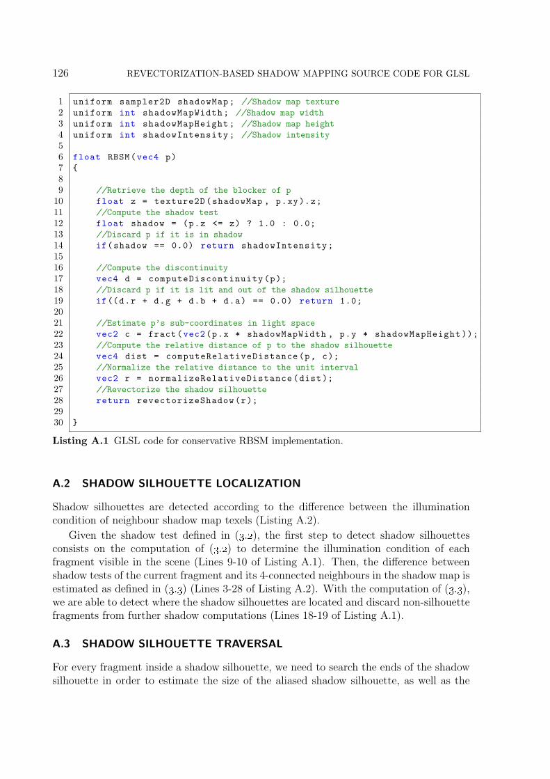
126 REVECTORIZATION-BASED SHADOW MAPPING SOURCE CODE FOR GLSL
1 uniform sampler2D shadowMap; //Shadow map texture
2 uniform int shadowMapWidth; //Shadow map width
3 uniform int shadowMapHeight; //Shadow map height
4 uniform int shadowIntensity; //Shadow intensity
56 float RBSM(vec4 p)
7
89 //Retrieve the depth of the blocker of p
10 float z = texture2D(shadowMap , p.xy).z;
11 //Compute the shadow test
12 float shadow = (p.z <= z) ? 1.0 : 0.0;
13 //Discard p if it is in shadow
14 if(shadow == 0.0) return shadowIntensity;
1516 //Compute the discontinuity
17 vec4 d = computeDiscontinuity(p);
18 //Discard p if it is lit and out of the shadow silhouette
19 if((d.r + d.g + d.b + d.a) == 0.0) return 1.0;
2021 //Estimate p’s sub-coordinates in light space
22 vec2 c = fract(vec2(p.x * shadowMapWidth , p.y * shadowMapHeight ));
23 //Compute the relative distance of p to the shadow silhouette
24 vec4 dist = computeRelativeDistance(p, c);
25 //Normalize the relative distance to the unit interval
26 vec2 r = normalizeRelativeDistance(dist);
27 //Revectorize the shadow silhouette
28 return revectorizeShadow(r);
2930
Listing A.1 GLSL code for conservative RBSM implementation.
A.2 SHADOW SILHOUETTE LOCALIZATION
Shadow silhouettes are detected according to the difference between the illuminationcondition of neighbour shadow map texels (Listing A.2).
Given the shadow test defined in (3.2), the first step to detect shadow silhouettesconsists on the computation of (3.2) to determine the illumination condition of eachfragment visible in the scene (Lines 9-10 of Listing A.1). Then, the difference betweenshadow tests of the current fragment and its 4-connected neighbours in the shadow map isestimated as defined in (3.3) (Lines 3-28 of Listing A.2). With the computation of (3.3),we are able to detect where the shadow silhouettes are located and discard non-silhouettefragments from further shadow computations (Lines 18-19 of Listing A.1).
A.3 SHADOW SILHOUETTE TRAVERSAL
For every fragment inside a shadow silhouette, we need to search the ends of the shadowsilhouette in order to estimate the size of the aliased shadow silhouette, as well as the

A.3 SHADOW SILHOUETTE TRAVERSAL 127
1 uniform vec2 shadowMapStep; //Shadow map step size
23 vec4 computeDiscontinuity(vec4 p)
4
56 vec4 dir = vec4 (0.0, 0.0, 0.0, 0.0);
7 //x = left; y = right; z = bottom; w = top
89 //Perform the shadow test for the 4-connected neighbourhood
10 p.x -= shadowMapStep.x;
11 float z = texture2D(shadowMap , p.xy).z;
12 dir.x = (p.z <= z) ? 1.0 : 0.0;
1314 p.x += 2.0 * shadowMapStep.x;
15 z = texture2D(shadowMap , p.xy).z;
16 dir.y = (p.z <= z) ? 1.0 : 0.0;
1718 p.x -= shadowMapStep.x;
19 p.y += shadowMapStep.y;
20 z = texture2D(shadowMap , p.xy).z;
21 dir.z = (p.z <= z) ? 1.0 : 0.0;
2223 p.y -= 2.0 * shadowMapStep.y;
24 z = texture2D(shadowMap , p.xy).z;
25 dir.w = (p.z <= z) ? 1.0 : 0.0;
2627 //Return the absolute difference of neighbour shadow tests
28 return abs(dir - 1.0);
2930
Listing A.2 GLSL code for discontinuity computation.
relative distance of the fragment to the end of the shadow silhouette. This search is donein all the four directions of the 2D space (i.e., left, right, top and bottom directions), suchthat we can estimate the 2D relative position of the fragment in the shadow silhouette(Lines 3-12 of Listing A.3). The shadow silhouette traversal algorithm for each directionof the 2D space is implemented in Lines 14-54 of Listing A.3.
For each shadow map neighbour of a given fragment (Lines 17, 26-27 of Listing A.3),RBSM computes the shadow test for the neighbour (Lines 28-32 of Listing A.3) anddetects whether the shadow test result of the neighbour is different from the one estimatedfor the given fragment (Lines 33-34 of Listing A.3). In this case, since conservative RBSMoperates over lit fragments, a shadowed fragment has been detected. Therefore, we havedetected the end of the shadow silhouette and we end the traversal in the particulardirection (Lines 35-37 of Listing A.3). On the other hand, if the shadow test is the samebetween neighbour shadow map texels (Lines 38-39 of Listing A.3), we need to check ifthe neighbour shadow map texel is still located in the shadow silhouette (Lines 40-41 ofListing A.3). If that is not the case, the traversal must be ended (Lines 42-44 of Listing

128 REVECTORIZATION-BASED SHADOW MAPPING SOURCE CODE FOR GLSL
A.3).To limit the extent of the shadow silhouette traversal, we define a variable maxSize
that defines the maximum size of the shadow silhouette (Line 1 of Listing A.3). This vari-able is only used to improve the temporal consistency of the algorithm. Using maxSize= 16 was sufficient for our tests.
As a result of the shadow silhouette traversal, the algorithm returns the distance ofthe fragment to the end of the shadow silhouette (Lines 50-54 of Listing A.3).
A.4 SHADOW SILHOUETTE NORMALIZATION
After the computation of the distance of each fragment to the shadow silhouette, we needto normalize such value to the unit interval, as already described in Chapter 3.
As can be seen in Listing A.4, we compute both (3.4) and (3.5) in the functioncomputeRelativeDistance (Lines 1-10 of Listing A.4).
A.5 CONSERVATIVE RBSM VISIBILITY FUNCTION
As we show in Listing A.5, a few lines of GLSL are required to implement the visibilityfunction proposed for conservative RBSM.
In practice, the function takes as input the normalized relative position previouslyestimated and performs two linear comparisons to determine whether a fragment mustbe put in the shadowed region of the new revectorized shadow.
A.6 SUMMARY
In this appendix, we have shown a practical implementation of conservative RBSM usingthe popular GLSL. By providing the implementation details of conservative RBSM, webelieve that one can easily implement the other techniques shown in this thesis, such asnon-conservative RBSM, Revectorization-based Percentage-Closer Filtering (RPCF) andthe others. The reference full implementation of RBSM for GLSL is available in a publicrepository1
1https://github.com/MarcioCerqueira/GlobalIllumination/tree/master/ShadowMapping

A.6 SUMMARY 129
1 uniform int maxSize; //Maximum shadow silhouette size
23 vec4 computeRelativeDistance(vec4 p, vec2 c)
4
56 float dl = computeRelativeDistance(p, vec2(-1, 0), (1.0 - c.x));
7 float dr = computeRelativeDistance(p, vec2(1, 0), c.x);
8 float db = computeRelativeDistance(p, vec2(0, -1), (1.0 - c.y));
9 float dt = computeRelativeDistance(p, vec2(0, 1), c.y);
10 return vec4(dl , dr , db , dt);
1112
1314 float computeRelativeDistance(vec4 p, vec2 dir , float c)
15
1617 vec4 np = p;
18 float foundSilhouetteEnd = 0.0;
19 float distance = 0.0;
20 //Compute the step of traversal for current direction
21 vec2 step = dir * shadowMapStep;
2223 //Iteratively traverse the shadow silhouette
24 for(int it = 0; it < maxSize; it++)
2526 //Access the neighbour of p
27 np.xy += step;
28 //Retrieve the depth of the blocker of np
29 float z = texture2D(shadowMap , np.xy).z;
30 //Determine the visibility of np
31 float center = (np.z <= z) ? 1.0 : 0.0;
32 bool isCenterUmbra = !bool(center );
33 //When the visibility of p and np is different
34 if(isCenterUmbra)
35 //End the traversal
36 foundSilhouetteEnd = 1.0;
37 break;
38 //When the visibility of p and np is equal
39 else
40 //Check if np has any discontinuity direction
41 vec4 d = computeDiscontinuity(np);
42 //Else, end the traversal
43 if((d.r + d.g + d.b + d.a) == 0.0) break;
44
45 //Increase the distance
46 distance ++;
4748
4950 //Take into account p’s sub-coordinates for distance estimation
51 distance = distance + (1.0 - c);
52 return mix(-distance , distance , foundSilhouetteEnd );
5354
Listing A.3 GLSL code for shadow silhouette traversal.

130 REVECTORIZATION-BASED SHADOW MAPPING SOURCE CODE FOR GLSL
1 float normalizeRelativeDistance(vec2 dist)
23 float T = 1;
4 if(dist.x < 0.0 && dist.y < 0.0) T = 0;
5 if(dist.x > 0.0 && dist.y > 0.0) T = -2;
67 float length = min(abs(dist.x) + abs(dist.y), float(maxSize ));
8 return abs(max(T * dist.x, T * dist.y))/ length;
910
1112 vec2 normalizeRelativeDistance(vec4 dist)
13
1415 vec2 r;
16 r.x = normalizeRelativeDistance(vec2(dist.x, dist.y));
17 r.y = normalizeRelativeDistance(vec2(dist.z, dist.w));
18 return r;
1920
Listing A.4 GLSL code for relative position normalization.
1 float revectorizeShadow(vec2 r)
2
34 if((r.x * r.y > 0) && (1.0 - r.x > r.y)) return shadowIntensity;
5 else return 1.0;
67
Listing A.5 GLSL code for conservative revectorization.

Appendix
BIn this appendix, we discuss how popular game engines give support to shadow rendering and present a
practical implementation of conservative RBSM into one of them.
REVECTORIZATION-BASED SHADOW MAPPINGSOURCE CODE FOR UNITY
Real-time shadow rendering is desirable in several computer graphics applications, suchas games. The most popular game engines typically provide support to this featurethrough the traditional shadow mapping algorithm. Unfortunately, shadow mapping iswell known to generate aliasing artifacts along the shadow silhouette, decreasing therealism of the rendered virtual scenes. In this appendix, we present an implementationof the most basic conservative Revectorization-based Shadow Mapping (RBSM) for hardshadow anti-aliasing in a game engine. Even with the limited source code access providedby some game engines, we demonstrate how to implement an improvement of the shadowmapping technique for shadow anti-aliasing. We have chosen to implement our approachfor spot lights in a commercial and popular game engine, the Unity 3D.
B.1 SHADOWS IN GAME ENGINES
Unity 3D Engine1 uses shadow mapping to generate shadows for spot and point lightsources. For directional light sources, cascaded shadow maps (ENGEL, 2006) take ad-vantage of the partitioning strategy (Section 2.3.2) to reduce aliasing artifacts. Area lightsources are supported for the Unity Pro version and require precomputed lighting condi-tions of the scene. Although not natively supported, shadow volumes are available as afree plugin for older versions of Unity in the Unity Asset Store2. While these techniquesmay work well for some scenarios, the main problem with Unity is that both free andprofessional versions of the engine give limited source code access for developers (the en-tire source code is available through an additional payment for Unity Pro users). Hence,it is difficult for one to implement its own improvements in the shadow algorithms usingthe available source code.
1https://unity3d.com2https://www.assetstore.unity3d.com/en/content/1861
131

132 REVECTORIZATION-BASED SHADOW MAPPING SOURCE CODE FOR UNITY
Name Type DescriptionShadowMapTexture internal Shadow map
ShadowMapTexture TexelSize float4Shadow map texel size /Shadow map resolution
shadowCoord float4Coordinates to access the
shadow map for a given fragment
LightShadowData float4Shadow intensity
(or shadow strength, in Unity)
Table B.1 List of variables available in Unity for shadow mapping with spot lights.
Similarly to Unity, CryEngine3 and Unreal Engine4 support shadow mapping forpoint and spot light sources, cascaded shadow maps for directional lights and ray tracingfor static scenes. Additionally, Unreal Engine supports an original technique called raytraced distance field soft shadows, which improves the visual quality of the cascadedshadow maps, further reducing the aliasing artifacts, but increasing processing time.
Although it is not formally defined as a game engine, NVIDIA GameWorks5 is asample development kit that provides support for several real-time shadow techniquesinto the NVIDIA ShadowWorks6 and advanced ray tracing solutions via NVIDIA OptiX(PARKER et al., 2010). NVIDIA GameWorks is open-source, has already been integratedinto the Unreal Engine7 and is extensible to work with Unity Pro8.
Unity is the most used game engine for mobile gaming (CHI; SUN, 2015), is thesecond game engine most recommended by industry experts (FRENCH et al., 2014) andis also one the most popular game engines for general game production, having more than770 millions of users over the world9. However, even with this huge popularity, Unitystill produces shadows with aliasing artifacts that are mostly visible in shadows renderedfrom point or spot light sources. Therefore, we present an implementation of conservativeRBSM that uses the available source code access in the popular Unity game engine toimprove the visual quality of the hard shadows generated from spot lights.
B.2 SHADOWS IN UNITY
Unity uses the shadow mapping as a basis to compute shadows generated from directional,point and spot light sources.
Directional light sources try to mimic the behaviour of distant light sources (e.g., thesun) by emitting parallel light rays in a single, dominant direction to illuminate largeoutdoor scenes. Since these light sources are defined by their directions, rather than theirpositions, a shadow map is rendered using orthographic projection to keep the light rays
3https://www.cryengine.com/4https://www.unrealengine.com/5https://developer.nvidia.com/gameworks6https://developer.nvidia.com/shadowworks7https://developer.nvidia.com/nvidia-gameworks-and-ue48https://developer.nvidia.com/content/gameworks-unity9https://unity3d.com/pt/public-relations
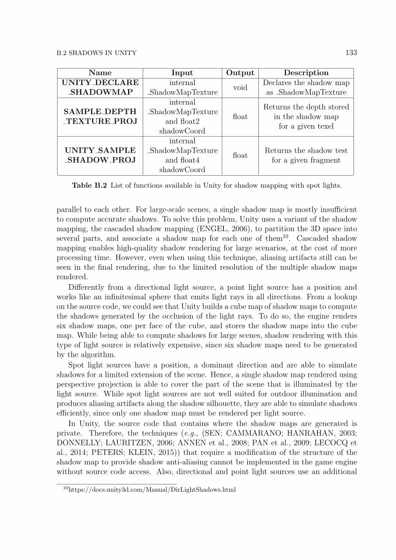
B.2 SHADOWS IN UNITY 133
Name Input Output DescriptionUNITY DECLARE
SHADOWMAPinternal
ShadowMapTexturevoid
Declares the shadow mapas ShadowMapTexture
SAMPLE DEPTHTEXTURE PROJ
internalShadowMapTexture
and float2shadowCoord
floatReturns the depth stored
in the shadow mapfor a given texel
UNITY SAMPLESHADOW PROJ
internalShadowMapTexture
and float4shadowCoord
floatReturns the shadow test
for a given fragment
Table B.2 List of functions available in Unity for shadow mapping with spot lights.
parallel to each other. For large-scale scenes, a single shadow map is mostly insufficientto compute accurate shadows. To solve this problem, Unity uses a variant of the shadowmapping, the cascaded shadow mapping (ENGEL, 2006), to partition the 3D space intoseveral parts, and associate a shadow map for each one of them10. Cascaded shadowmapping enables high-quality shadow rendering for large scenarios, at the cost of moreprocessing time. However, even when using this technique, aliasing artifacts still can beseen in the final rendering, due to the limited resolution of the multiple shadow mapsrendered.
Differently from a directional light source, a point light source has a position andworks like an infinitesimal sphere that emits light rays in all directions. From a lookupon the source code, we could see that Unity builds a cube map of shadow maps to computethe shadows generated by the occlusion of the light rays. To do so, the engine renderssix shadow maps, one per face of the cube, and stores the shadow maps into the cubemap. While being able to compute shadows for large scenes, shadow rendering with thistype of light source is relatively expensive, since six shadow maps need to be generatedby the algorithm.
Spot light sources have a position, a dominant direction and are able to simulateshadows for a limited extension of the scene. Hence, a single shadow map rendered usingperspective projection is able to cover the part of the scene that is illuminated by thelight source. While spot light sources are not well suited for outdoor illumination andproduces aliasing artifacts along the shadow silhouette, they are able to simulate shadowsefficiently, since only one shadow map must be rendered per light source.
In Unity, the source code that contains where the shadow maps are generated isprivate. Therefore, the techniques (e.g., (SEN; CAMMARANO; HANRAHAN, 2003;DONNELLY; LAURITZEN, 2006; ANNEN et al., 2008; PAN et al., 2009; LECOCQ etal., 2014; PETERS; KLEIN, 2015)) that require a modification of the structure of theshadow map to provide shadow anti-aliasing cannot be implemented in the game enginewithout source code access. Also, directional and point light sources use an additional
10https://docs.unity3d.com/Manual/DirLightShadows.html
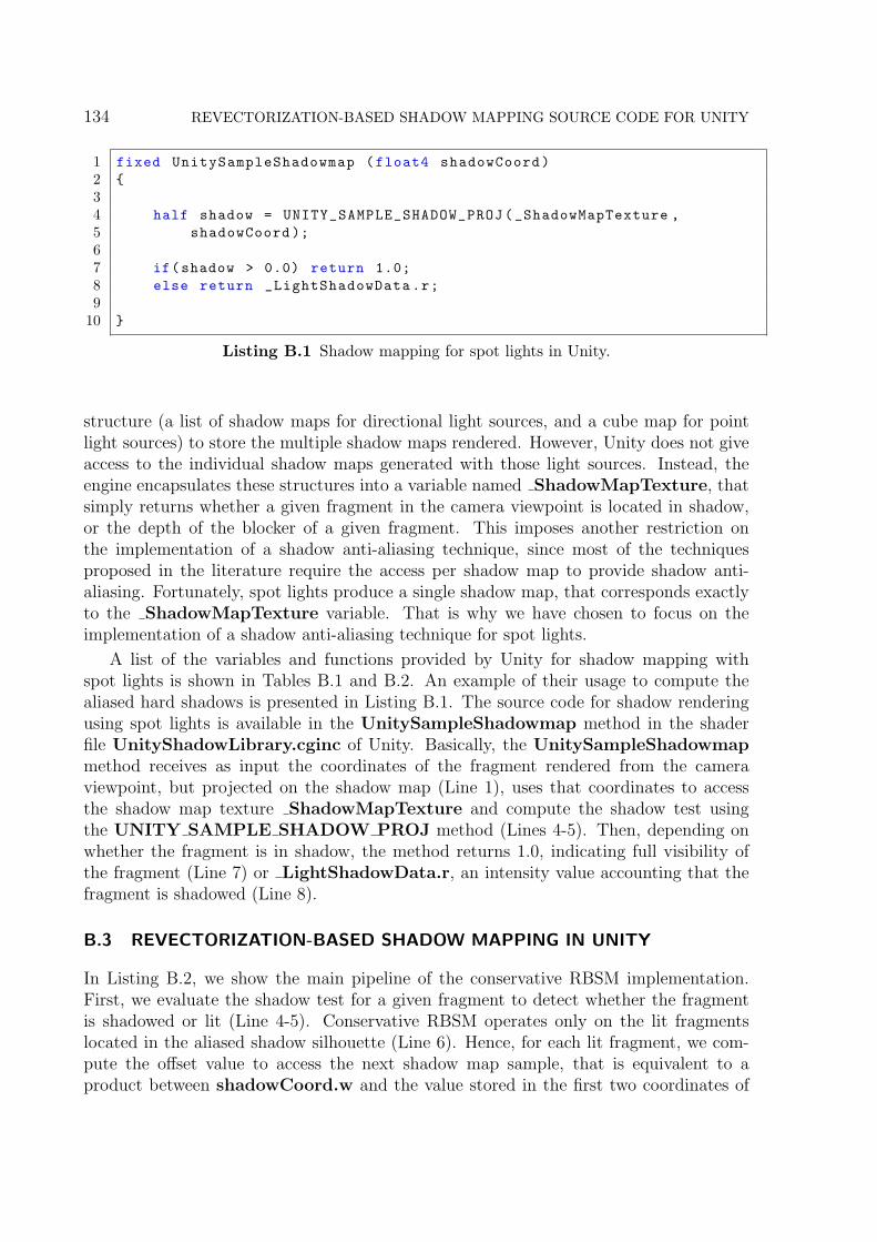
134 REVECTORIZATION-BASED SHADOW MAPPING SOURCE CODE FOR UNITY
1 fixed UnitySampleShadowmap (float4 shadowCoord)
2
34 half shadow = UNITY_SAMPLE_SHADOW_PROJ(_ShadowMapTexture ,
5 shadowCoord );
67 if(shadow > 0.0) return 1.0;
8 else return _LightShadowData.r;
910
Listing B.1 Shadow mapping for spot lights in Unity.
structure (a list of shadow maps for directional light sources, and a cube map for pointlight sources) to store the multiple shadow maps rendered. However, Unity does not giveaccess to the individual shadow maps generated with those light sources. Instead, theengine encapsulates these structures into a variable named ShadowMapTexture, thatsimply returns whether a given fragment in the camera viewpoint is located in shadow,or the depth of the blocker of a given fragment. This imposes another restriction onthe implementation of a shadow anti-aliasing technique, since most of the techniquesproposed in the literature require the access per shadow map to provide shadow anti-aliasing. Fortunately, spot lights produce a single shadow map, that corresponds exactlyto the ShadowMapTexture variable. That is why we have chosen to focus on theimplementation of a shadow anti-aliasing technique for spot lights.
A list of the variables and functions provided by Unity for shadow mapping withspot lights is shown in Tables B.1 and B.2. An example of their usage to compute thealiased hard shadows is presented in Listing B.1. The source code for shadow renderingusing spot lights is available in the UnitySampleShadowmap method in the shaderfile UnityShadowLibrary.cginc of Unity. Basically, the UnitySampleShadowmapmethod receives as input the coordinates of the fragment rendered from the cameraviewpoint, but projected on the shadow map (Line 1), uses that coordinates to accessthe shadow map texture ShadowMapTexture and compute the shadow test usingthe UNITY SAMPLE SHADOW PROJ method (Lines 4-5). Then, depending onwhether the fragment is in shadow, the method returns 1.0, indicating full visibility ofthe fragment (Line 7) or LightShadowData.r, an intensity value accounting that thefragment is shadowed (Line 8).
B.3 REVECTORIZATION-BASED SHADOW MAPPING IN UNITY
In Listing B.2, we show the main pipeline of the conservative RBSM implementation.First, we evaluate the shadow test for a given fragment to detect whether the fragmentis shadowed or lit (Line 4-5). Conservative RBSM operates only on the lit fragmentslocated in the aliased shadow silhouette (Line 6). Hence, for each lit fragment, we com-pute the offset value to access the next shadow map sample, that is equivalent to aproduct between shadowCoord.w and the value stored in the first two coordinates of
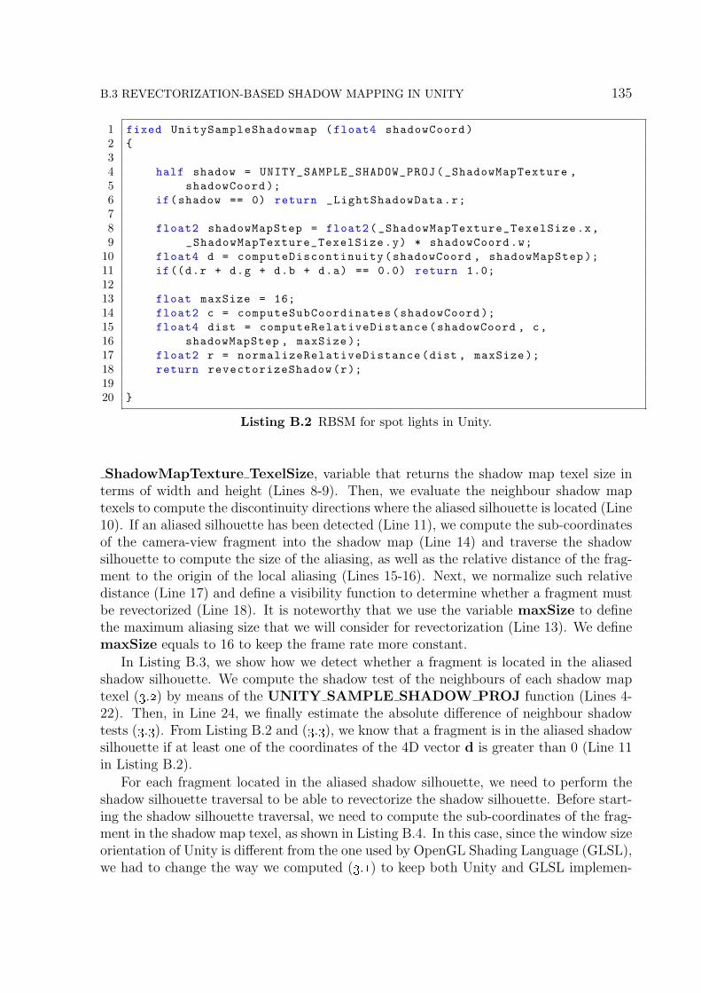
B.3 REVECTORIZATION-BASED SHADOW MAPPING IN UNITY 135
1 fixed UnitySampleShadowmap (float4 shadowCoord)
2
34 half shadow = UNITY_SAMPLE_SHADOW_PROJ(_ShadowMapTexture ,
5 shadowCoord );
6 if(shadow == 0) return _LightShadowData.r;
78 float2 shadowMapStep = float2(_ShadowMapTexture_TexelSize.x,
9 _ShadowMapTexture_TexelSize.y) * shadowCoord.w;
10 float4 d = computeDiscontinuity(shadowCoord , shadowMapStep );
11 if((d.r + d.g + d.b + d.a) == 0.0) return 1.0;
1213 float maxSize = 16;
14 float2 c = computeSubCoordinates(shadowCoord );
15 float4 dist = computeRelativeDistance(shadowCoord , c,
16 shadowMapStep , maxSize );
17 float2 r = normalizeRelativeDistance(dist , maxSize );
18 return revectorizeShadow(r);
1920
Listing B.2 RBSM for spot lights in Unity.
ShadowMapTexture TexelSize, variable that returns the shadow map texel size interms of width and height (Lines 8-9). Then, we evaluate the neighbour shadow maptexels to compute the discontinuity directions where the aliased silhouette is located (Line10). If an aliased silhouette has been detected (Line 11), we compute the sub-coordinatesof the camera-view fragment into the shadow map (Line 14) and traverse the shadowsilhouette to compute the size of the aliasing, as well as the relative distance of the frag-ment to the origin of the local aliasing (Lines 15-16). Next, we normalize such relativedistance (Line 17) and define a visibility function to determine whether a fragment mustbe revectorized (Line 18). It is noteworthy that we use the variable maxSize to definethe maximum aliasing size that we will consider for revectorization (Line 13). We definemaxSize equals to 16 to keep the frame rate more constant.
In Listing B.3, we show how we detect whether a fragment is located in the aliasedshadow silhouette. We compute the shadow test of the neighbours of each shadow maptexel (3.2) by means of the UNITY SAMPLE SHADOW PROJ function (Lines 4-22). Then, in Line 24, we finally estimate the absolute difference of neighbour shadowtests (3.3). From Listing B.2 and (3.3), we know that a fragment is in the aliased shadowsilhouette if at least one of the coordinates of the 4D vector d is greater than 0 (Line 11in Listing B.2).
For each fragment located in the aliased shadow silhouette, we need to perform theshadow silhouette traversal to be able to revectorize the shadow silhouette. Before start-ing the shadow silhouette traversal, we need to compute the sub-coordinates of the frag-ment in the shadow map texel, as shown in Listing B.4. In this case, since the window sizeorientation of Unity is different from the one used by OpenGL Shading Language (GLSL),we had to change the way we computed (3.1) to keep both Unity and GLSL implemen-

136 REVECTORIZATION-BASED SHADOW MAPPING SOURCE CODE FOR UNITY
1 float4 computeDiscontinuity(float4 shadowCoord , float2 shadowMapStep)
2
34 float4 dir = float4 (0.0, 0.0, 0.0, 0.0);
5 //x = left; y = right; z = bottom; w = top
67 shadowCoord.x += shadowMapStep.x;
8 dir.x = UNITY_SAMPLE_SHADOW_PROJ(_ShadowMapTexture , shadowCoord );
9 dir.x = (dir.x > 0.0) ? 1.0 : 0.0;
1011 shadowCoord.x -= 2.0 * shadowMapStep.x;
12 dir.y = UNITY_SAMPLE_SHADOW_PROJ(_ShadowMapTexture , shadowCoord );
13 dir.y = (dir.y > 0.0) ? 1.0 : 0.0;
1415 shadowCoord.x += shadowMapStep.x;
16 shadowCoord.y -= shadowMapStep.y;
17 dir.z = UNITY_SAMPLE_SHADOW_PROJ(_ShadowMapTexture , shadowCoord );
18 dir.z = (dir.z > 0.0) ? 1.0 : 0.0;
1920 shadowCoord.y += 2.0 * shadowMapStep.y;
21 dir.w = UNITY_SAMPLE_SHADOW_PROJ(_ShadowMapTexture , shadowCoord );
22 dir.w = (dir.w > 0.0) ? 1.0 : 0.0;
2324 return abs(dir - 1.0);
2526
Listing B.3 Discontinuity direction estimation in Unity.

B.4 SUMMARY 137
1 float2 computeSubCoordinates(float4 shadowCoord)
2
34 float2 c = float2(frac ((1.0 - shadowCoord.x/shadowCoord.w) *
5 _ShadowMapTexture_TexelSize.z),
6 frac ((1.0 - shadowCoord.y/shadowCoord.w) *
7 _ShadowMapTexture_TexelSize.w));
8 c.x = 1.0 - lerp (0.5 - c.x, (0.5 - c.x) + 1.0, step (0.5, c.x));
9 c.y = 1.0 - lerp (0.5 - c.y, (0.5 - c.y) + 1.0, step (0.5, c.y));
10 return c;
1112
Listing B.4 An algorithm to compute the sub-coordinates of a camera-view fragment in thelight space in Unity.
tations using the same value.
The algorithm to compute the relative distances of the fragment to the ends of theshadow silhouette is shown in Listing B.5. RBSM computes the relative distance of thefragment with respect to the shadow silhouette to the four directions of the 2D space. Foreach direction (Lines 5-12), we perform the traversal over the shadow silhouette (Line 28).Then, for each shadow map texel being accessed, we check whether we step out of the litside of the aliased silhouette. This condition is fulfilled whenever we step into an umbratexel (Lines 33-35) or step into a lit texel that does not have any discontinuity directions(i.e., the texel is not neighbour of an umbra texel) (Lines 36-40). Otherwise, we incrementthe variable distance (Line 42) that represents the size of the aliasing. In Line 47, we addthe sub-coordinates of the fragment into the distance previously computed to improvethe accuracy of the distance computation. In Line 48, we use a linear interpolation tomake the distance value signed, as already presented in Chapter 3.
To estimate the relative position r in Listing B.6, we basically implement the equations(3.4) and (3.5). The same statement is held for the implementation of the conservativeRBSM visibility function, that is implemented as shown in Listing B.7, following (3.6).
B.4 SUMMARY
In this appendix, we have presented an implementation of conservative RBSM, for theUnity game engine. Since Unity uses the shadow mapping for shadow rendering, aliasingartifacts are generated along the shadow silhouette. As shown in Section 3.3, by theuse of the proposed implementation of RBSM, we are able to minimize these aliasingartifacts, generating high-quality shadows at minimal additional cost.
Due to the limited source code access provided by Unity, we were not able to imple-ment RBSM for other types of light source, such as point and directional light sources.Moreover, we could not implement RBSM for soft shadows that simulate the penumbraeffect. The implementation of RBSM using the entire Unity source code, or the imple-mentation in other game engines, may enable one to adapt the technique to support hardand soft shadow rendering for any light source. Finally, since NVIDIA GameWorks may

138 REVECTORIZATION-BASED SHADOW MAPPING SOURCE CODE FOR UNITY
1 float4 computeRelativeDistance(float4 shadowCoord , float2 c,
2 float2 shadowMapStep , int maxSize)
3
45 float dl = computeRelativeDistance(shadowCoord , float2(1, 0),
6 (1.0 - c.x), shadowMapStep , maxSize );
7 float dr = computeRelativeDistance(shadowCoord , float2(-1, 0),
8 c.x, shadowMapStep , maxSize );
9 float db = computeRelativeDistance(shadowCoord , float2(0, 1),
10 (1.0 - c.y), shadowMapStep , maxSize );
11 float dt = computeRelativeDistance(shadowCoord , float2(0, -1),
12 c.y, shadowMapStep , maxSize );
13 if(db > 0 && dt > 0) dt = -dt;
14 return float4(dl , dr , db , dt);
1516
1718 float computeRelativeDistance(float4 shadowCoord , float2 dir , float c,
19 float2 shadowMapStep , int maxSize)
20
2122 float4 tempShadowCoord = shadowCoord;
23 float foundSilhouetteEnd = 0.0;
24 float distance = 0.0;
25 float2 shadowMapDiscontinuityStep = dir * shadowMapStep;
26 tempShadowCoord.xy += shadowMapDiscontinuityStep;
2728 for(int it = 0; it < maxSize; it++)
2930 float shadow = UNITY_SAMPLE_SHADOW_PROJ(_ShadowMapTexture ,
31 tempShadowCoord );
3233 if(shadow == 0.0)
34 foundSilhouetteEnd = 1.0;
35 break;
36 else
37 float4 d = computeDiscontinuity(tempShadowCoord ,
38 shadowMapStep );
39 if((d.r + d.g + d.b + d.a) == 0.0) break;
40
4142 distance ++;
43 tempShadowCoord.xy += shadowMapDiscontinuityStep;
4445
4647 distance = distance + (1.0 - c);
48 return lerp(-distance , distance , foundSilhouetteEnd );
4950
Listing B.5 Computation of the relative position of a fragment inside a shadow silhouette inUnity.

B.4 SUMMARY 139
1 float2 normalizeRelativeDistance(float4 dist , int maxSize)
2
34 float2 r = float2 (0.0, 0.0);
5 r.x = normalizeRelativeDistance(float2(dist.x, dist.y), maxSize );
6 r.y = normalizeRelativeDistance(float2(dist.z, dist.w), maxSize );
7 return r;
89
1011 float normalizeRelativeDistance(float2 dist , int maxSize)
1213 float T = 1;
14 if(dist.x < 0.0 && dist.y < 0.0) T = 0;
15 if(dist.x > 0.0 && dist.y > 0.0) T = -2;
1617 float length = min(abs(dist.x) + abs(dist.y), float(maxSize ));
18 return abs(max(T * dist.x, T * dist.y))/ length;
1920
Listing B.6 Normalization of the relative position of a fragment inside a shadow silhouette inUnity.
1 float revectorizeShadow(float2 r)
2
34 if((r.x * r.y > 0) && (1.0 - r.x > r.y)) return _LightShadowData.r;
5 else return 1.0;
67
Listing B.7 Conservative RBSM visibility function in Unity.
be used with Unity Pro, the field of shadows in game engines still needs a gentle intro-duction on how to integrate NVIDIA ShadowWorks with Unity Pro and an evaluationof the shadow techniques of NVIDIA ShadowWorks in the context of the Unity gameengine.
The reference full implementation of RBSM for Unity is available in a public reposi-tory11
11https://github.com/MarcioCerqueira/GlobalIllumination/tree/master/RBSMinUnity
Related Documents