Efficient Scheduling Algorithms for Quality-of-Service Guarantees in the Internet by Anthony Chi-Kong Kam Submitted to the Department of Electrical Engineering and Computer Science in partial fulfillment of the requirements for the degree of Doctor of Philosophy at the MASSACHUSETTS INSTITUTE OF TECHNOLOGY @ Massachusetts April 2000 Institute of Technology 2000. All rights reserved. A uthor ....................... t ... Department of Electrical Engineering and Computer Science April 28, 2000 Certified by ........... . ... Kai-Yeung Siu Associate Professor Thesis Supervisor Accepted by........ .............. ....... ..... ............ Arthur C. Smith Chairman, Department Committee on Graduate Students MASSACHUSETTS INSTITUTE OF TECHNOLOGY --- JUN 22 2000 LIBRARIES

Welcome message from author
This document is posted to help you gain knowledge. Please leave a comment to let me know what you think about it! Share it to your friends and learn new things together.
Transcript

Efficient Scheduling Algorithms for
Quality-of-Service Guarantees in the Internet
by
Anthony Chi-Kong Kam
Submitted to the Department of Electrical Engineering and ComputerScience
in partial fulfillment of the requirements for the degree of
Doctor of Philosophy
at the
MASSACHUSETTS INSTITUTE OF TECHNOLOGY
@ Massachusetts
April 2000
Institute of Technology 2000. All rights reserved.
A uthor ....................... t ...Department of Electrical Engineering and Computer Science
April 28, 2000
Certified by ........... . ...Kai-Yeung Siu
Associate ProfessorThesis Supervisor
Accepted by........ .............. ....... ..... ............
Arthur C. SmithChairman, Department Committee on Graduate Students
MASSACHUSETTS INSTITUTEOF TECHNOLOGY
---JUN 22 2000
LIBRARIES

Efficient Scheduling Algorithms for Quality-of-Service
Guarantees in the Internet
by
Anthony Chi-Kong Kam
Submitted to the Department of Electrical Engineering and Computer Scienceon April 28, 2000, in partial fulfillment of the
requirements for the degree ofDoctor of Philosophy
Abstract
The unifying theme of this thesis is the design of packet schedulers to provide quality-of-service (QoS) guarantees for various networking problem settings. There is a dualemphasis on both theoretical justification and simulation evaluation. We have workedon several widely different problem settings - optical networks, input-queued crossbarswitches, and CDMA wireless networks - and we found that the same set of schedulingtechniques can be applied successfully in all these cases to provide per-flow bandwidth,delay and max-min fairness guarantees.
We formulated the abstract scheduling problems as a sum of two aspects. First,the particular problem setting imposes constraints which dictate what kinds of trans-mission patterns are allowed by the physical hardware resources, i.e., what are thefeasible solutions. Second, the users require some form of QoS guarantees, whichtranslate into optimality criteria judging the feasible solutions. The abstract problemis how to design an algorithm that finds an optimal (or near-optimal) solution amongthe feasible ones.
Our schedulers are based on a credit scheme. Specifically, flows receive creditsat their guaranteed rate, and the arrival stream is compared to the credit streamacting as a reference. From this comparison, we derive various parameters such asthe amount of unspent credits of a flow and the waiting time of a packet since itscorresponding credit arrived. We then design algorithms which prioritize flows basedon these parameters. We demonstrate, both by rigorous theoretical proofs and bysimulations, that these parameters can be bounded. By bounding these parameters,our schedulers provide various per-flow QoS guarantees on average rate, packet delay,queue length and fairness.
Thesis Supervisor: Kai-Yeung SiuTitle: Associate Professor
2

Acknowledgments
First, I want to thank my supervisor Sunny Siu. I will always cherish the informal,
frank, and fun-filled atmosphere of our collaboration. He allowed me almost complete
freedom, and gave me an endless array of interesting problems to work on. Sunny's
skill of mental association truly amazes me - from any one networking problem he
would easily think of seven others which are similar in some way, and more than
half of those would open up substantive research issues. Our joint work branches out
from optical networks to terabit switches to wireless communication - a variety that
is reflected in the contents of this thesis - and problems which we have no time to
pursue we wrote up as proposals and attracted other students to work on. I spent the
past four years on a wonderful journey of exploration through problem space, with
him applying a light guiding touch when my theoretical research became too esoteric.
He also set a great example for all his students by working harder than any two of us
combined, and despite his 110% booked schedule, he always has time to be helpful
and resourceful.
I also want to thank Rick Barry and Eric Swanson, who co-supervised the early
part of this thesis (chapter three) and co-authored the related papers. Since I was
new to the field of networking, they were very generous in sharing their wealth of
technical knownledge and insights. More importantly, I also want to thank them
for their infectious enthusiasm for our joint project. Other colleagues at Lincoln
Laboratory, especially Eytan Modiano and Steve Finn, also helped immensely in my
initiation into this field.
My thesis committee, Professors John Tsitsiklis and Hari Balakrishnan (in ad-
dition to Sunny), also helped with their critiques into both the theoretical and the
practical issues of my research, and their insightful comments led to my own clearer
understanding of chapters five and six.
My officemates maintained a fun work space for all to enjoy and also helped with
their special expertise in other subfields of networking. Of special mention is Thit
Minn, who knew everything about wireless communications, and by teaching me a
3
mere drop of what he knew, enabled me to achieve the results in chapter six of this
thesis, which is joint work with him. (Not to mention that he fed me some very tasty
home-made noodles!) Another special mention goes to Paolo Narvaez, who did the
coolest research among us (in my opinion), and with whom I had extremely enjoyable
discussions and friendly arguments about all aspects of networking. Paolo and David
Lecumberri also helped in my stressful job hunt, by providing contacts and by sharing
their experience as we try to graduate together.
In addition to those above who directly helped with my research, a big "thank
you" also goes to all my friends who made these past four years the happiest time
of my life, especially Amanda Lee, Alaine Young, Celine Fung, John Wong, Linda
Chin, and Gregorboo, for the wonderful company, and the fabulous meals. Special
thanks to all my boardgame friends, especially Otto Ho and Tony Wu, who pulled
all-nighters with me playing TITAN and bridge and other games - and if I may add,
who are always graceful in defeat!
DEDICATION
Finally, and most important of all, this thesis is dedicated to my wife and best
friend Elaine Chen. This thesis would not be possible without her love, support,
patience, and understanding. Thank you for sharing every moment of our lives!
4

Contents
1 Introduction and Problem Formulation
1.1 Overview ..... ........................
1.2 Problem Formulation ....................
1.2.1 General Description and Assumptions . . . .
1.2.2 Abstract Problem . . . . . . . . . . . . . . .
1.2.3 Optimality Criteria . . . . . . . . . . . . . .
1.3 Chapter Summary and Preview . . . . . . . . . . .
2 Quality-of-Service Contracts
2.1 Rate Guarantees . . . . . . . . . . . . . . . . . . .
2.1.1 Contract based on Credits . . . . . . . . . .
2.1.2 Bucket Size Restrictions . . . . . . . . . . .
2.1.3 Contract based on Validated Queue Lengths
2.2 Delay Guarantees . . . . . . . . . . . . . . . . . . .
2.2.1 Validation viewed as virtual traffic shaping
2.2.2 Contract based on Validated Waiting Times
2.2.3 Credits vs Validated delays . . . . . . . . .
2.3 Fairness Guarantees . . . . . . . . . . . . . . . . . .
2.4 Theoretical Results on Bounded Credits . . . . . .
2.4.1 Definitions . . . . . . . . . . . . . . . . . . .
2.4.2 Statements of Theorems . . . . . . . . . . .
2.4.3 Proof of Theorem 2.2 . . . . . . . . . . . . .
2.4.4 Proof of Theorem 2.3 . . . . . . . . . . . . .
5
13
. . . 13
. . . 14
. . . 14
. . . 15
. . . 17
. . . 18
19
. . . . . . . . 19
. . . . . . . . 21
. . . . . . . . 22
. . . . . . . . 23
. . . . . . . . 25
. . . . . . . . 26
. . . . . . . . 26
. . . . . . . . 27
. . . . . . . . 28
. . . . . . . . 29
. . . . . . . . 29
. . . . . . . . 30
. . . . . . . . 31
. . . . . . . . 34

2.5 Chapter Summary and Preview . . . . . . . . . . . . . . . . . . . . .
3 Input-Queued Crossbar Switches
3.1 Background and Motivation . . . . . . . . . . . .
3.2 Problem M odel . . . . . . . . . . . . . . . . . . .
3.3 Previous W ork . . . . . . . . . . . . . . . . . . .
3.3.1 Previous theoretical work with no speedup
3.3.2 Previous theoretical work with speedup . .
3.3.3 Previous simulation studies . . . . . . . .
3.4 General Description of our Schedulers . . . . . . .
3.4.1 Stable marriage matching algorithm . . . .
3.5 Choice of Edge Weights . . . . . . . . . . . . . .
3.5.1 Simulation Methods . . . . . . . . . . . .
3.5.2 Using credits as edge weights . . . . . . .
3.5.3 Using LC as edge weights . . . . . . . . .
3.5.4 Using VW as Edge Weights . . . . . . . .
3.5.5 Rescaling and mixing weights . . . . . . .
3.6 Other Issues . . . . . . . . . . . . . . . . . . . . .
3.6.1 Multiple flows per input-output pair . . .
35
36
37
39
. . . . . . . . . . . 4 0
. . . . . . . . . . . 4 1
. . . . . . . . . . . 4 2
. . . . . . . . . . . 4 3
. . . . . . . . . . . 4 3
. . . . . . . . . . . 4 4
. . . . . . . . . . . 4 7
. . . . . . . . . . . 4 7
. . . . . . . . . . . 4 9
. . . . . . . . . . . 53
. . . . . . . . . . . 54
. . . . . . . . . . . 5 5
. . . . . . . . . . . 58
. . . . . . . . . . . 58
3.6.2 Traffic Shaping Effects and Minimum Output Buffer Require-
m ents . . . . . . . . . . . . . . . . . . . . . . . . .
3.6.3 Effects of other simulation parameters . . . . . . .
3.7 Fair Sharing of Unreserved Switch Capacity . . . . . . . .
3.7.1 Two phase Usage Weighted Algorithm . . . . . . .
3.7.2 Allowing negative credits . . . . . . . . . . . . . . .
3.8 Chapter Summary . . . . . . . . . . . . . . . . . . . . . .
3.9 Details of Simulation Settings . . . . . . . . . . . . . . . .
3.9.1 Admission Control of flows' Bandwidth Reservation
3.9.2 Random Cell Arrival Process . . . . . . . . . . . .
3.9.3 Measured Parameters . . . . . . . . . . . . . . . . .
. . . . . . 59
. . . . . . 63
. . . . . . 63
. . . . . . 65
. . . . . . 66
. . . . . . 67
. . . . . . 68
Requests . 68
. . . . . . 69
. . . . . . 70
6

3.9.4 Fairness Simulations . . . . . . . . . . .
4 All-Optical Metro- and Local-Area Networks
4.1 Background and Motivation . . . . . . . . . . .
4.2 Problem Model . . . . . . . . . . . . . . . . . .
4.3 Related W ork . . . . . . . . . . . . . . . . . . .
4.4 LAN Schedulers - Theoretical Properties . . . .
4.4.1 Description of Algorithms . . . . . . . .
4.4.2 Statements of Theorems . . . . . . . . .
4.4.3 Proofs . . . . . . . . . . . . . . . . . . .
4.5 LAN Schedulers - Simulation Evaluation . . . .
4.5.1 Using C as edge weights . . . . . . . . .
4.5.2 Using LC as edge weights . . . . . . . .
4.5.3 CU-weighted fairness algorithm . . . . .
4.6 Extensions to Multiple Transceivers . . . . . . .
4.7 Distributed Scheduling for Metro-Area Network
4.7.1 Network Model . . . . . . . . . . . . . .
4.7.2 Distributed master-slave schedulers . . .
4.7.3 LAN scheduler . . . . . . . . . . . . . .
4.7.4 MAN scheduler . . . . . . . . . . . . . .
4.7.5 Simulations Summary . . . . . . . . . .
4.8 Chapter Summary . . . . . . . . . . . . . . . .
4.9 Simulation Settings . . . . . . . . . . . . . . . .
4.9.1 Outline of a control protocol . . . . . . .
4.9.2 Stochastic models for flow and traffic generation
5 Optical Distribution Tree
5.1 Background and Motivation . . . . . . . . . . . . . . .
5.2 Problem M odel . . . . . . . . . . . . . . . . . . . . . .
5.2.1 Distribution Tree Architecture and Hardware .
5.2.2 Problem Statements . . . . . . . . . . . . . . .
100
104
. . . . . . 104
. . . . . . 106
. . . . . . 106
. . . . . . 108
7
71
72
. . . . . . . . . . . . 73
. . . . . . . . . . . . 74
. . . . . . . . . . . . 77
. . . . . . . . . . . . 80
. . . . . . . . . . . . 80
. . . . . . . . . . . . 80
. . . . . . . . . . . . 82
. . . . . . . . . . . . 85
. . . . . . . . . . . . 85
. . . . . . . . . . . . 86
. . . . . . . . . . . . 88
. . . . . . . . . . . . 89
. . . . . . . . . . . . 90
. . . . . . . . . . . . 90
. . . . . . . . . . . . 94
. . . . . . . . . . . . 95
. . . . . . . . . . . . 96
. . . . . . . . . . . . 98
. . . . . . . . . . . . 98
. . . . . . . . . . . . 99
. . . . . . . . . . . . 99
5.3 Related W ork . . . . . . . . . . . . . . . . . . . . .
5.4 Feasibility Constraints . . . . . . . . . . . . . . . .
5.4.1 Reservation Factor . . . . . . . . . . . . . .
5.5 Scheduling Algorithms . . . . . . . . . . . . . . . .
5.5.1 The CQ' Algorithm .................
5.5.2 Exact Feasibility Test . . . . . . . . . . . . .
5.5.3 Approximate Feasibility Test . . . . . . . . .
5.5.4 Theoretical Results - Statement of Theorems
5.5.5 Proofs . . . . . . . . . . . . . . . . . . . . .
5.6 Choice of Wavelength Subsets . . . . . . . . . . . .
5.6.1 The One-or-All Design Strategy . . . . . . .
5.6.2 The Hierarchical Design Strategy . . . . . .
5.7 Simulation Evaluation of the Algorithms . . . . . .
5.7.1 Simulation Settings . . . . . . . . . . . . . .
5.7.2 Comparing exact and approximate feasibility
5.7.3 Using LC and VW as weights . . . . . . . .
5.7.4 Fairness . . . . . . . . . . . . . . . . . . . .
5.8 Chapter Summary . . . . . . . . . . . . . . . . . . . . . . . . . . . . 1 3 1
6 CDMA Wireless Network
6.1 Background and Motivation . . . . . . . . . .
6.1.1 Overview of our contributions . . . . .
6.2 Problem Model . . . . . . . . . . . . . . . . .
6.2.1 Base station transmitter . . . . . . . .
6.2.2 OVSF codes . . . . . . . . . . . . . . .
6.2.3 Control protocol . . . . . . . . . . . .
6.2.4 Feasibility Constraints and Reservation
6.3 Initial leaf assignment . . . . . . . . . . . . .
6.4 Scheduling algorithm . . . . . . . . . . . . . .
6.4.1 Algorithm description . . . . . . . . .
8
tests
109
111
113
114
114
116
118
119
120
123
124
124
127
127
129
130
130
133
134
135
137
137
137
139
141
142
144
144
Factor
6.4.2 Theoretical Guarantee . . . . . . . . . . . . . . . . . . . . . . 146
6.4.3 Stress-Test algorithm . . . . . . . . . . . . . . . . . . . . . . . 147
6.4.4 P roofs . . . . . . . . . . . . . . . . . . . . . . . . . . . . . . . 148
6.4.5 Modified bucket size restriction . . . . . . . . . . . . . . . . . 154
6.4.6 Variation: Timeslot-based leaf re-assignment . . . . . . . . . . 154
6.5 Sim ulations . . . . . . . . . . . . . . . . . . . . . . . . . . . . . . . . 156
6.5.1 Simulation Settings . . . . . . . . . . . . . . . . . . . . . . . . 156
6.5.2 Credit bounds on stress-test scheduler . . . . . . . . . . . . . 158
6.5.3 Non-stress-test scheduler and fair sharing . . . . . . . . . . . . 160
6.6 Chapter Summary and Further Discussions . . . . . . . . . . . . . . . 161
7 Summary 163
7.1 Problem Formulation . . . . . . . . . . . . . . . . . . . . . . . . . . . 163
7.2 A lgorithm s. . . . . . . . . . . . . . . . . . . . . . . . . . . . . . . . . 165
7.3 R esults . . . . . . . . . . . . . . . . . . . . . . . . . . . . . . . . . . . 165
7.4 Issues specific to each problem setting . . . . . . . . . . . . . . . . . . 166
9

List of Figures
3-1 Max-min fairness with rate guarantees. . . . . . . . . . . . . . . . . . 65
4-1 WDM broadcast LAN with central scheduler and dedicated control
channel. . . . . . . . . . . . . . . . . . . . . . . . . . . . . . . . . . . 74
4-2 Max-min fairness with rate guarantees. Top example m = 3; bottom
exam ple m = 2. . . . . . . . . . . . . . . . . . . . . . . . . . . . . . . 88
4-3 Wavelength routed network . . . . . . . . . . . . . . . . . . . . . . . 91
5-1 ONRAMP architecture for a regional access network. . . . . . . . . . 105
5-2 Upstream/downstream traffic in a distribution tree. . . . . . . . . . . 107
6-1 Transmitter at the base station. . . . . . . . . . . . . . . . . . . . . . 137
6-2 16-leaf OVSF code tree. . . . . . . . . . . . . . . . . . . . . . . . . . 138
6-3 Timeslotted transmissions showing the header structure for 3G W-
C D M A . . . . . . . . . . . . . . . . . . . . . . . . . . . . . . . . . . . 139
6-4 Over-populating a subtree-of-4-leaves. The dark nodes represent the 4
assigned leaves. . . . . . . . . . . . . . . . . . . . . . . . . . . . . . . 143
6-5 Maintaining the under-population condition at the top 3 levels. The
dark nodes represent the 4 assigned leaves. . . . . . . . . . . . . . . . 143
10

List of Tables
3.1 Performance of the C-weighted algorithm. . . . . . . . . . . . . . . . 51
3.2 Performance of the LC-weighted algorithm. . . . . . . . . . . . . . . 53
3.3 Performance of the VW-weighted algorithm. . . . . . . . . . . . . . . 55
3.4 Performance of a mixed weight algorithm . . . . . . . . . . . . . . . . 57
3.5 Effect of switch size N on C-weighted algorithm . . . . . . . . . . . . 63
3.6 Effect of burst size on LC-weighted algorithm (N = 32, 2-state traffic) 63
3.7 Effect of burst size on VW-weighted algorithm (N = 32, 2-state traffic) 64
3.8 Performance of the CU-weighted algorithm. . . . . . . . . . . . . . . 67
4.1 Performance of the C-weighted algorithm for constantly backlogged
traffic. Control parameters are N, m, max gf; others are measured pa-
ram eters . . . . . . . . . . . . . . . . . . . . . . . . . . . . . . . . . . 86
4.2 Performance of the C-weighted algorithm, for backlogged and bursty
traffic. Control parameters are N, m, max gf and traffic type; others
are measured parameters. . . . . . . . . . . . . . . . . . . . . . . . . 87
4.3 Performance of the LC-weighted algorithm for bursty traffic. Control
parameters are N, m, max gf and traffic type. Other parameters are
m easured. . . . . . . . . . . . . . . . . . . . . . . . . . . . . . . . . . 87
4.4 Performance of the CU-weighted algorithm for constantly backlogged
traffic. Control parameters are N, m, max gYf and total no. of flows.
Other parameters are measured. . . . . . . . . . . . . . . . . . . . . . 89
5.1 Performance of the C-weighted algorithm, with exact and approximate
feasibility tests. . . . . . . . . . . . . . . . . . . . . . . . . . . . . . . 130
11

5.2 Performance of the LC- and VW-weighted algorithms, with exact and
approximate feasibility tests. . . . . . . . . . . . . . . . . . . . . . . . 131
6.1 Credit bounds for constantly backlogged traffic with "stress test" sched-
uler. First four columns show control parameters; last two columns
show measurements. . . . . . . . . . . . . . . . . . . . . . . . . . . . 159
6.2 Credit bounds for constantly backlogged traffic with "stress test" sched-
uler with leaf re-assignment. First four columns show control parame-
ters; last two columns show measurements. . . . . . . . . . . . . . . . 159
6.3 Credit bounds for bursty traffic with "stress test" scheduler. First five
columns show control parameters; last two columns show measurements. 160
7.1 Feasibility constraints of the four problem settings. . . . . . . . . . . 164
7.2 Theoretical results on bounded credits. . . . . . . . . . . . . . . . . . 166
12

Chapter 1
Introduction and Problem
Formulation
1.1 Overview
Future networks will need to support a large variety of applications with varying
quality-of-service (QoS) requirements, such as bandwidth, delay and fairness guar-
antees. In particular, they must simultaneously support low-rate delay-insensitive
messages (e.g. e-mail) and high-rate bandwidth and delay sensitive sessions (e.g.
high quality video) as well as a large variety of anticipated and unanticipated hetero-
geneous services and applications in between.
The unifying theme of this thesis is the design of packet schedulers to provide
quality-of-service (QoS) guarantees for various networking problem settings. There
is a dual emphasis on both theoretical justification and simulation evaluation. We
have worked on several widely different problem settings - optical networks, input-
queued switches, and wireless networks - and we found that the same set of scheduling
techniques can be applied successfully in all these cases.
This thesis is organized as follows: The rest of this chapter will formulate a com-
mon abstract problem that underlies all the different problem settings. Chapter two
will describe some basic theoretical results on the common abstract problem and also
describe more precisely the exact QoS guarantees that our algorithms provide. Then
13

each of the next four chapters will apply the theory to a different problem setting,
and discusses problem-specific simulation results. Chapter three will deal with input-
queued switches. Chapter four will deal with an all-optical metro- and local-area
network. Chapter five will deal with an optical distribution tree. Chapter six will
deal with a CDMA wireless network. Because each problem setting is different, we
will leave the discussions of background, motivation and prior work until each respec-
tive chapter. Finally, chapter seven contains concluding remarks and discussions for
future work.
1.2 Problem Formulation
We now describe a common abstract problem formulation that encompasses all four
problem settings to be discussed in detail later.
1.2.1 General Description and Assumptions
Flows and QoS. This thesis is concerned with providing QoS guarantees to indi-
vidual flows. In this thesis, a flow is defined as the basic unit or entity which enjoys
individual QoS guarantees. For example, in an input-queued switch a flow can be an
IP flow or an ATM virtual circuit, in optical networks a flow can be a session, and in
a wireless networks a flow can be a call from a single user. We assume each flow has
a unique ID.
Each flow requires service from the system (network or switch) in the form of data
transmissions. Data corresponding to a particular flow arrives at one point of the
system, the source of the flow, and stays in a queue until it is transmitted to another
point, the destination of the flow. The QoS parameters take the form of rate, delay
and fairness guarantees of the data transmissions enjoyed by each individual flow. In
this thesis we will assume that each flow has its own queue (per-flow queueing), and
that any flow can be serviced at any time. (The only exception is that in the context
of input-queued switches (chapter three) an alternative queueing structure will be
discussed.)
14

Feasibility Constraints. The system as a whole (network or switch) can be
considered a kind of server providing service to the flows. Unlike well-studied single-
server systems which can only service a single flow at any given time, however, we
consider systems which can simultaneously service several flows, and in fact service
them by different amounts (at different rates). Not any arbitrary set of flows can
be serviced simultaneously. The particular system imposes feasibility constraints on
which subset of flows can be serviced simultaneously and which subset of flows can-
not. The constraints are problem-specific and are derived from respective hardware
constraints - the number and type of transmitters and receivers, or input and output
ports, the number of wavelengths, the number and structure of orthogonal codes in
CDMA wireless networks, etc.
Time-slotting and cell-based transmissions. All four problem settings we
studied are time-slotted systems. In some settings, time-slotting is natural and stan-
dard within the industry (e.g., input-queued switch, wireless networks). In others,
time-slotting is a design choice made to simplify QoS provisioning. We further assume
that data are transmitted (services are rendered) in fixed-sized chunks called cells. If
the original data packets arriving at the system are of variable sizes, they are broken
down into cells and then re-assembled at the destinations.
Centralized Algorithm. In most of this thesis we will also assume there is a
centralized algorithm, called a scheduler, that decides in each timeslot which (feasible)
subset of flows to service. In systems which are physically distributed (optical and
wireless networks) there is a need for a control channel and also pipelining; these will
be discussed in the respective chapters on those problem settings. We also considered
a distributed algorithm for a metro-area optical network in chapter three.
1.2.2 Abstract Problem
With the above description and assumptions in mind, we can now formulate the
abstract problem as follows: Let F denote the set of of all flows and let f E F be
a typical flow. The most basic variables associated with a flow are these which deal
with the arrivals and departures to its queue:
15

1. Af(t) denotes the number of cells belonging to f that arrived at timeslot t.
(Arrivals to the queue.)
2. Sf(t) denotes the number of cells belonging to f that are scheduled for service
at timeslot t. (Departures from the queue.)
3. Lf(t) denotes the queue length, i.e., the number of queued cells of f waiting to
be scheduled at the beginning of timeslot t. Thus we have
Lf(t +1) = Lf(t) + Af(t) - Sf(t). (1.1)
Obviously, queue lengths cannot become negative, and a flow can only receive
service up to the number of cells waiting to be serviced. This means that S1 (t) Lf (t)
(if new arrivals cannot be immediately serviced for hardware reasons) or Sf (t) <
Lf(t) + Af(t) (if arrivals can be immediately serviced). We will say a flow is idle at
time t if it has no cells waiting for service, otherwise the flow is backlogged.
The feasibility constraints of the system is described by a feasibility function:
Feasible([S(t)]) -+ {True, False} (1.2)
The notation [S 1(t)], called the service vector, denotes an |FI-dimensional vector list-
ing all the Sf (t) values for all flows f E F, listed in ID order. Basically, the Feasible()
function is a "test" function that decides whether the simutaneous services of each
flow f by an amount Sf(t) is possible or not. The feasibility function is problem-
specific and derived from underlying hardware constraints, and will be different for
each of our four problem settings.
Note that service vectors are vectors of non-negative integers. To avoid certain
theoretical difficulties, we will assume that Sf (t) is bounded whenever we consider
only feasible vectors. Because of finite system capacities, such an assumption is
trivially true in almost any networking problem setting one can imagine.
Given this formulation, the scheduling problem can be described thus:
16

Abstract Problem: At each timeslot t, what feasible service vector
[Sf(t)] should be chosen?
1.2.3 Optimality Criteria
Among the many feasible vectors, picking a "good" solution depends on the optimality
criteria being used. Ultimately, these optimality criteria are derived from users' QoS
requirements, which we will now describe. The next chapter will discuss how these
QoS requirements can be translated into formal mathematical statements.
1. Throughput: The total throughput of the system (switch or network) should
be close to 100%.
2. Bandwidth Reservations: We want to provide bandwidth reservations to
individual flows, so each flow can enjoy its own reserved bandwidth even when
the rest of the system is heavily loaded (perhaps with a lot of best-effort traffic).
3. Cell Delay Guarantees: For some traffic types such as voice and video, cell
delay guarantees are as important as bandwidth guarantees because cells that
arrive too late are useless.
4. Fairness: The unreserved portion of the system capacity should be shared
fairly. This is particularly important in systems with a lot of legacy best-effort
traffic. The particular problem setting will decide whether fairness means every
flow should have the same share, or there should be a kind of max-min fair
pattern (or weighted versions of either).
5. Algorithm Efficiency: In an input-queued switch and in the optical networks
that we considered (chapters three, four and five), timeslots are a few microsec-
onds to sub-microsecond. The algorithm has to choose a feasible service vector
every timeslot, and therefore it must be a simple, efficient algorithm, with possi-
ble hardware implementation (in input-queued switches). In wireless networks,
timeslots are of the order of 1 millisecond and algorithm speed is less critical.
17

1.3 Chapter Summary and Preview
We have formulated the abstract scheduling problems as a sum of two aspects. First,
the particular problem setting imposes constraints which dictate what kinds of trans-
mission patterns are allowed by the physical hardware, i.e., what are the feasible
solutions. Second, the flows (users) require some form of QoS guarantees, which
translate into optimality criteria judging the feasible solutions. The abstract problem
is how to design an algorithm that finds an optimal (or near-optimal) solution among
the feasible ones.
Because the QoS requirements are common to all four problem settings, the next
chapter will first provide more precise mathematical statements (and proofs) on the
QoS guarantees that we provide with our schedulers. Then in chapters three to six
we will delve into each problem setting and its unique feasibility constraint.
18
Chapter 2
Quality-of-Service Contracts
This chapter describes, in precise mathematical terms, the QoS guarantees that our
schedulers make to the individual flows. The guarantees include rate, delay and
fairness guarantees, and they form part of the optimality criteria with which we judge
the merit of our schedulers. We also judge our schedulers by their total throughput
and their algorithm speed, but since these two issues are not QoS promises that the
schedulers make to individual flows, they are not discussed in this chapter.
Our schedulers will provide per-flow QoS guarantees in the form of contracts which
are bounds on certain parameters. The actual size of the bounds depend on the
specific problem setting, and will be evaluated when each problem setting is discussed.
The aim of this chapter is two-fold. First, sections 2.1-2.3 explain the meaning of our
QoS contracts on rate, delay and fairness in more practical and intuitive terms. Then,
section 2.4 provides some theoretical results common to all four problem settings
investigated in the next four chapters.
2.1 Rate Guarantees
Before we can discuss precise mathematical statements, there are several questions
that must be answered for a more precise understanding of the meaning of rate
guarantees.
The first question is how bandwidth reservations can be made. We envision a
19

scheme where, at setup time, each flow negotiates during an admission control process
about its guaranteed rate. The network decides to grant or deny or modify the
requests based on external factors such as priority, billing, etc., in addition to current
congestion level. In this thesis we do not consider how admission control makes this
decision. Once agreed, a flow's guaranteed rate typically does not change (although
our algorithms do not assume this fact).
The second question is what it means to have bandwidth "reserved" for a flow.
Two extreme cases are clear: First, if the flow sends a smooth stream of cells below its
guaranteed rate, then the cells should be transmitted with very little delay. Second, if
the flow is extremely busy and constantly has a large backlog of cells queued up, then
its average transmission rate should be at least its guarantee rate. Unfortunately, it is
less clear what should happen when the flow is very bursty and sometimes transmits
at a very high peak rate and sometimes becomes idle, even though its average rate is
comparable to its guaranteed rate.
Specifically, if a flow is idle for a long time and then a large burst of cells arrives,
should the flow enjoy extra service, possibly hogging some resources and starving
other flows for an extended duration, to make up for the time it was idle? Abstractly
speaking, rates are not very meaningful unless the duration over which the rate is cal-
culated is agreed or understood. The question is: what is the time-scale, or duration
of interest, over which reservations must be respected? If the time-scale is long, then
the algorithm must tolerate highly bursty flows (with very long idle periods followed
by large bursts) by giving preference to long-idle flows, and therefore potentially hurt
other flows by allowing hogging behavior. However, if the time-scale is short - and
this is the approach in most frame-based schemes - then an idle flow simply forfeits
its chance, and when it becomes busy again, another frame may have already begun
and the past will be forgotten, so that, over the long term, bursty flows will transmit
below its guaranteed rate because of missed opportunities. Fundamentally, then, this
is a question of tolerance for burstiness, and a question of balancing the dual goals of
long-term throughput guarantees and short-term steady service.
As in services supported over ATM, we propose to clarify these issues by providing
20
contracts with our algorithms. Each flow (or user) can understand exactly what
service it can expect from our algorithms. Moreover, to allow network designers
flexibility in answering these questions, we will introduce another degree-of-freedom
which corresponds to the amount of burstiness / prolonged idleness that the system
will tolerate from a flow.
2.1.1 Contract based on Credits
Let gf denote the guaranteed rate (guaranteed bandwidth, GBW) of a flow f, mea-
sured in units of cells/timeslot. Also, let T = 1 denote the GBW in units of times-
lots/cell. (One way to understand Tf is that if rf > 1, it is what the inter-service
interval should be in number of timeslots.)
Our rate guarantees are expressed in terms of a per-flow credit variable. The
outstanding credit or simply credit of a flow f at time t is denoted Cf(t), and is
defined by the following equation:
Cf(t + 1) = C1(t) + G5(t) - Sf(t). (2.1)
where the term Gf(t) = gf most of the time (the exception is described in the next
section). Credits are initialized to zero. Intuitively, a flow gains (possibly fractional)
credits at a steady rate equal to its guaranteed rate gf, and spends one credit whenever
it transmits a cell. Thus at any time t, the flow is sending above, below, or exactly at
its guaranteed rate depending on whether Cf(t) is negative, positive, or zero. Some
of our schedulers provide a rate guarantee in the form of bounded credits:
Contract based on Credits C:
There exists a constant upperbound Cmax, such that for any flow f, its
credit Cf(t) <; Cmax for all time t. In other words, at any time t, a flow's
total number of transmissions will lag behind its reserved rate by at most
a constant number of cells, equal to Cmax.
The usefulness of such a contract of course depends mainly on the size of the
21

bound Cma,. We will later demonstrate, in each specific problem setting, that the
bounds are small (tight) and therefore practically useful.
This contract only provides an upperbound, but not a lowerbound. We view it
as another design choice (again to be made by network designers) whether to allow
a flow to transmit above its GBW (i.e. whether credits can become negative), and if
so, whether such "excess" transmissions using unreserved system capacity should be
handled by a separate fairness mechanism.
Finally, note that the contract establishes a bound for all time. This means not
only that time-average rate is guaranteed, but the sequence of transmissions is also
guaranteed to be smooth in some sense. One way to look at this is that a flow accrues
one integral credit every Ty timeslots. Therefore, if Cf(t) is close to zero at all times,
then the sequence of transmissions closely follow the sequence of credit "arrivals" of
one every Tf timeslots.
2.1.2 Bucket Size Restrictions
As discussed previously, a design choice must be made as to the "time-scale" over
which rate reservations are guaranteed, i.e., the network must decide how much bursti-
ness / prolonged idleness to tolerate from each flow.
In our credit-based framework, this discussion takes the following form: If Gf(t)
gf always, then a bursty flow which is temporarily idle will have Sf(t) = 0 (since no
service is possible) and thus it will accumulate a lot of credits without bound. When
this flow becomes backlogged again, a design choice has to be made as to how to
deal with its high credit level. Should it immediately obtain a lot of service, possibly
starving other well-behaving flows in the mean time? Or should its high credit level
be discounted somehow, representing a network design choice not to tolerate such
prolonged idleness?
To allow network designers flexibility in answering these questions, we adopt the
following exception handling based on a "bucket-size" idea: each flow is associated
with a bucket size Bf (negotiated on setup together with gf) and at any time t, if
the flow is idle and its credit is already at least its bucket size (Cf (t) > Bf), then
22

Gf(t) = 0, and therefore credit will stay the same (Cf(t + 1) = Cf(t)) because the
credit is not incremented further and there is no service. In other words,
Gf(t) 0 if Cf(t) > Bf and f is idle (2.2)
Gf (t) gf otherwise (2.3)
In this scheme, flows which are idle for prolonged periods of time will lose credit
increments, and the bucket size represents a maximum amount of idleness that the
network will tolerate before penalizing a flow. Flows which are known to be very
bursty can ask for a larger bucket size on setup.
The idea of a bucket size has been used before in many networking scenarios (e.g.,
[52, 55]) but unlike most such proposals, our bucket size restriction only applies to idle
flows. We made this choice because a busy flow with a credit exceeding its bucket size
possibly represents a poor job done by our scheduler (not servicing the flow frequently
enough), and therefore the flow should not be penalized to forfeit credit increments.
With a bucket size restriction in place, the QoS contract of bounded credits has
a slightly different interpretation. A flow is still guaranteed to lag behind its credit
accrual process by at most Cma, cells. However, its credit accrual process may no
longer correspond to a time-average rate of gf because of forfeited credit increments.
Thus, an individual flow must understand that it is guaranteed transmissions at its
reserved rate, up to a lag of Cmax cells plus whatever credits it loses due to its own
fault.
2.1.3 Contract based on Validated Queue Lengths
A different rate guarantee we provide is based on a parameter called the validate
queue length, defined as
LCf(t) = min(Lf(t),Cf(t)). (2.4)
23

Intuitively, this is the number of cells of flow f that have existing corresponding credits
"earmarked" for them already. We will use the term validated cells to describe them.
These cells are a sort of priority customers: they are not waiting for transmission due
to lack of credit - they already have credits and are waiting for transmission simply
because of scheduling conflicts.
Some of our schedulers provide a rate guarantee in the form of bounded LC:
Contract based on Validated Queue Lengths LC: There exists a
constant upperbound LCmax, such that for any flow f, its LCf (t) LCmax
for all time t. In more practical and intuitive terms, this means:
1. If the flow has a large queue (Lf(t) > LCmax) then its credits must
be bounded (Cf(t) LCmax). In other words its total number of
transmissions lags behind its reserved rate by at most a small con-
stant number of cells LCmax; the flow is already transmitting at very
close to full reserved rate. Such a flow can be considered to be "over-
loading" since Lf(t) > Cf (t).
2. On the other hand, if the flow has a lot of credits (Cf(t) > LCmax)
then its queue size is guaranteed to be small (Lf (t) LCmax). So, its
total number of transmissions lags behind its total number of arrived
cells (which is, of course, the maximum number of transmissions
possible) by at most a small constant LCmax. Such a flow can be
considered to be "underloading" since Lf(t) < Cf(t).
In short, "overloading" flows have few unspent credits, and "underloading" flows
have short bounded queues. Both of these cases represent practical, useful guarantees.
Mathematically speaking, since LCf(t) 5 Cf(t) by definition, an upperbound
on C is also an upperbound on LC, but not vice versa. It may seem therefore an
LC-based contract is weaker than a C-based contract. However, the usefulness of
a bound depends a lot on the size of the bound, and our schedulers in many cases
turn out to provide a smaller (tighter) LCmax bound than the corresponding Cmax
24

bound. This is one advantage of using an LC-based contract. Another advantage is
that, in simulations, we observed that LCma, bounds can be established without the
need for bucket size restrictions. (The intuitive reason is that idle flows already have
LCf(t) = 0.)
2.2 Delay Guarantees
Again, before we can discuss precise mathematical statements, we must first make
a design choice as to the meaning of delay guarantees. If a flow's arrival process is
not restricted or policed/shaped in some way, it is not possible for the system to
provide per-cell delay guarantees, simply because there might be too many arrivals
to be serviced within the system capacity and therefore both queue lengths and cell
delays must grow unbounded.
Therefore, in this work we provide a form of delay guarantee with reference to
the credit accrual process. Remember that a validated cell is a queued cell with
a matching credit. Taking this concept one small step further, we can define the
validation time of a cell to be the time when it obtains a matching credit. (We will
assume cells are matched with credits in order of arrival.) That is, if a flow has
Cf(t) > Lf(t), then the next cell to arrive will be validated immediately at arrival,
whereas if a flow has Cf(t) < Lf(t), the next cell to arrive will be validated only
when the flow obtains a matching credit for this cell. For instance, cell c arrives at
time ta and finds that there are 2 credits and 10 cells ahead of it. Of these 10 cells,
the oldest 2 are validated (since there are 2 existing credits) while the remaining 8
are not. Cell c would have to wait until the flow accrues the next 9 credits before
it can be validated - the first 8 of these go to validate cells ahead of c, and the 9th
one validates c. (Depending on the exact arrival time in relation to the "arrival" of
credits, the validation time will fall between ta + 8 Tf and ta + 9Tf.)
Now, we can define the validated waiting time (validated delay) of a cell as the
time it has waited since its validation, and define the validated waiting time VWf (t)
25

of a flow as
VWf(t) = validated waiting time of the oldest validated cell flow f. (2.5)
If the flow has no validated cells, i.e., no queued cells or no positive credits, we define
VWf (t) = 0 by convention.
2.2.1 Validation viewed as virtual traffic shaping
An alternative view of validation is to imagine that each cell has to go through a
kind of traffic shaping module [47, 18] before it will be considered by the scheduler.
The traffic shaper keeps track of credits. A cell first arrives at the shaper and if
there is a credit for it then it is validated and goes on to the the scheduler's queues
immediately. However, if there is no credit for it, then the cell is detained by the traffic
shaper until a credit arrives for its validation. (Again, we assume cells belonging to
the same flow are validated in order.) Given this traffic shaping pre-processing step,
the actual arrival process at the scheduler will be distorted and different from the
actual arrival process at the filter - e.g., if the arrival process at the filter is Bernoulli
then the arrival process at the scheduler is a sort of "capped" or "truncated" version
of Bernoulli. However, the resulting number of cells being considered by the scheduler
is exactly the number of validated cells LCf (t) and the time of arrival at the scheduler
is exactly the validation time. Thus the bookkeeping tricks which we call validation
can simply be viewed as (virtual) traffic shaping which distorts the actual arrival to
better suit our scheduling algorithms for providing QoS guarantees.
2.2.2 Contract based on Validated Waiting Times
Some of our algorithms provide a delay guaranteed based on bounded VWf (t):
Contract based on Validated Waiting Times VW: There exists a
constant upperbound VWma, such that for any flow f, its VWf(t) <
VWmax for all time t. In more practical and intuitive terms, consider time
26
t and flow f and consider the oldest cell c still waiting to be served.
1. If cell c arrived at the same timeslot as its corresponding credit, or
later, then c will be validated at arrival and will have its actual delay
bounded by VWmax timeslots. (The flow is "underloading" in this
case.)
2. On the other hand, if cell c arrived before its corresponding credit, it
will have to wait (say, for a duration of T timeslots) before validation.
Its actual delay VWmax + T but T is not bounded. However, in
this case c's matching credit will be spent within VWmax timeslots,
i.e., the actual transmissions lags behind the accrual of credits by at
most VWmax timeslots (or equivalently, at most VWmax X g cells).
So the flow is transmitting at very close to full reserved bandwidth
already. (The flow is "overloading" in this case.)
In short, "underloading" flows have bounds on actual cell delays, and "overload-
ing" flows have each credit spent very soon and thereby follow closely a smooth trans-
mission pattern at their guaranteed rates. Both of these cases represent practical,
useful guarantees.
2.2.3 Credits vs Validated delays
We now show that an upperbound on C implies that VW is also upperbounded.
Lemma 2.1: Bounded C implies bounded VW.
Any (theoretical or experimental) credit bound Cmax provided by our algo-
rithms implies a (theoretical or experimental, respectively) bound on val-
idated delay: each cell of flow f will have its validated delay < [CmaxTf -
Proof: Assume a cell of flow f is not serviced within this time. Then, another Cmax
credits would have been accrued. These, together with the cell's matching credit (not
yet spent because the cell is not yet served), would exceed the Cmax bound, which is
a contradiction. Q.E.D.
27

Note that this lemma regardless of whether the flow has a finite bucket size or
not. This is because, as long as the cell under consideration has not been served, the
queue is non-empty and the credit bucket restriction is not in effect.
Even though an upperbound on C implies an upperbound on VW, but not vice
versa, this does not mean a VW-based contract is weaker, because the size of the
bounds matter. Also, as phrased above, the VWma, bound applies to all flows uni-
formly. However, a Cma bound, which also applies to all flows uniformly, implies
different VW bounds for different flows. Specifically, a flow with a smaller rate gf
will have an (inversely) proportionally larger bound < [Cma.Tfl. This, of course,
represents a slightly different kind of QoS guarantees that the network can support.
2.3 Fairness Guarantees
The meaning of fairness guarantees may be subject to even more design choices than
rate and delay guarantees. In this thesis, we investigated only rate-based fairness
guarantees, specifically, guarantees on the number of excess/unreserved transmissions
beyond a flow's GBW. In our credit-based framework, this means guarantees on the
value of Cf(t) in the negative region.
The main question for rate-based fairness is: how should the unreserved capacity
of the system be shared? The first answer that comes to mind may be: the excess
capacity should be divided equally. Indeed, this is our approach in dealing with a
wireless network (chapter six) - in that case we prove that the difference between the
credits of two flows at any point in time, Cf, (t) - Cf2 (t), is bounded. In particular
this means that if both flows receive excess transmissions then they receive roughly
equal amounts, up to a bounded difference.
Equal sharing, however, is not the appropriate answer for the optical networks
and input-queued switches that we consider in chapters three to five. This is because
in these settings, different flows use different hardware resources, and so they may
have different bottlenecks. If several flows use a highly contended resource (e.g., some
transmitter in an optical network), they may be collectively restricted to a low total
28
rate, and it is not appropriate that other flows should be restricted to the same low
rates if other flows do not have this resource as a bottleneck. In these cases, therefore,
we adopt a notion of max-min fairness, which means each flow should have its total
rate maximized as long as this does not penalize another flow which is at a lower rate.
Our schedulers try to provide the max-min fair rate to the flows. Because the max-
min fair pattern of capacity allocation is different for each specific problem setting,
we will defer further discussion until the respective chapters.
2.4 Theoretical Results on Bounded Credits
We now list some theoretical results on bounded credits that apply to all problem
settings.
2.4.1 Definitions
First, we define the weight of a feasible service vector to be:
W([Sf(t)]) = E Sf(t)Cf(t) (2.6)fEF
Next, we define the reservation factor a of the system. The value of a captures
what fraction of the system capacity has been reserved by the guaranteed rates gf.
Consider the vector [gf], which denotes an IFI-dimensional vector listing all the gf
values for all flows f E F, listed in ID order. Let {I[S] : k = 1, 2, ...K} index the
finite set of all possible feasible service vectors. Note that by assumption (chapter
one), Sf (t) is bounded if we consider only feasible vectors. Since each feasible vector
is a vector of non-negative integers, the fact that each entry Sf(t) is bounded implies
there are only a finite number of feasible vectors.
The reservation factor is defined as the minimum value of a for which the following
is true:
Main property of a:
There exists non-negative constants (coefficients) {N : k = 1, 2, ..., K}
29

such that
[gf = 1 k[S], and (2.7)1<k<K
Z k =ca (2.8)1<k<K
In other words, the vector of guaranteed rates [gf] is a weighted sum of feasible
vectors, where the weights (coefficients) sum to a. To gain an intuitive understanding
of a, imagine the following scenario. Assuming a < 1, if in the long run, the system
chooses service vector [Sk] during a fraction k of the time, then the guaranteed rate
of any flow equals its long-term time-average transmission rate (i.e., total number of
transmissions divided by total time). Further, if a < 1, then the system can afford to
shut down with no service (Sf(t) = OVf E F) for a fraction 1 - a of the time. This is
why we call a the reservation factor - satisfying the reserved rates [gf] only requires
the system to be in service a fraction a of the time. Finally, if a > 1, then it is not
possible to express [gf] as a weighted sum of feasible vectors where the weights sum
to 1, and so no matter how the system chooses service vectors for each timeslot, it is
impossible for the guaranteed rates to equal the time-average transmission rates.
2.4.2 Statements of Theorems
Theorem 2.2: Bounded C for constantly backlogged traffic.
Assume traffic is constantly backlogged, i.e., every flow has enough queued
cells for however many cells Sf (t) the scheduler may choose to send. At
time t, let W*(t) denote the maximum possible weight of a feasible service
vector, and suppose the algorithm chooses set [Sf(t)] of weight W([Sf (t)]).
Let a denote the system's reservation factor. If for some constants a and
K1, where a > a, we have
Vt, W([Sf (t)]) > a x W*(t) - K1 (2.9)
then all credits will be bounded, i.e., there exists a constant Cmax such
30

that
Vt, Vf, Cf (t) < Cmax (2.10)
This theorem is a generalization of a result of [51], which assumes K1 = 0 and
a = 1 (thus a < 1), and which deals with weights based on queue lengths (weight of
[Sf (t)] defined as EfEF Sf (t)Lf (t)) and proves a notion of stability. In contrast, our
theorem allows arbitrary a and K and proves a hard, non-probabilistic bound. We
are able to achieve a hard non-probabilistic bound because we are bounding credits,
which "arrive" in a fixed stream, as opposed to randomly-arriving data cells. In fact,
the result of [51] assumes i.i.d. arrival processes. We made the following important
generalization to arbitrary traffic arrivals:
Theorem 2.3: Bounded C for finite bucket sizes.
Theorem 1 remains true for arbitrary traffic arrival pattern (Af (t)), in-
cluding but not limited to constantly backlogged traffic (and i.i.d. arrival-
s), if every flow has a finite bucket size Bf.
Remember that our bucket sizes only restrict credit increments for flows which
are idle. The importance of theorem 2.3 is to show that while temporarily idle flows
have credits bounded by buckets, the remaining busy flows (with no bucket size
restrictions) also have their credits bounded because they are serviced frequently
enough. Moreover, flows can switch between busy and idle states arbitrarily, and
this includes flows which are constantly backlogged, flows which have extremely large
bursts, flows with a slow and smooth arrival stream, flows which are "malicious" or
"adversarial" in any sense, and any mixture thereof.
2.4.3 Proof of Theorem 2.2
We will prove that the quantity V(t) = EfEF Cf (t) 2 is bounded, which would imply
all Cf(t) are bounded. The proof here is adapted from [51] which proves a notion
31

of stability on (expected) queue lengths. In contrast, we will prove a hard, non-
probabilistic bound on credits. For notational clarity, we will write Ef to denote
EfeF, i.e. summation over all flows, and we will also write Ek to denote E1<k<K,
summation over all feasible vectors.
Cf(t + 1) = Cf(t) + Gf(t) - Sf(t) (2.11)
= C (t) + gf - Sf (t) (constantly backlogged flows) (2.12)
V(t + 1) - V(t) = Z[Cf (t + 1)2 - Cf (t)2] (2.13)f
= ([2Cj'(t)(gf - S1 (t)) + (gf - S 1 (t)) 2] (2.14)f
<2 1:[Cf (t) (gf - Sf (t))]I + K2 (2.15)I
where the term Ef(gf - S1 (t))2 has been bounded by some constant K 2 in the last in-
equality. This is possible because gf are given constants and S1 (t) values are bounded
by the system capacity.
Now, at time t, let [S*(t)] be a feasible service vector that achieves the maxi-
mum weight W*(t) for that timeslot. By the pre-condition of theorem 2.2, we have
W([Sf (t)j) ; a x W*(t) - K 1 , and so:
E[Cf (t)f - Sf (t))] (2.16)f
< K1 + E [Cf(t)(gf - aS*(t))] (2.17)f
= K1 + Z[C (t)(((3kSj) - aS*(t))] (2.18)f k
= K 1 + Z[Cf (t)(E /k(S - S*,(t)) - (a - a)S*,(t))] (2.19)f k
= K1 +E Z k[Z C1 (t)Sk - E C(t)S*(t)] - (a - a) E C1(t)S* (t) (2.20)k f f f
Consider the last equation. The term Ef Cf(t)S*(t) is the weight of a maximum
weighted feasible vector. It is larger than or equal to each g Cf(t)Sk term, which
32

is the weight of some fixed feasible vector. This, together with the fact that each
A3 ;> 0, implies each term inside the Ek summation is < 0. In the last term, denote
a - a by 7. Note that - > 0 by definition of a. We have:
Z[Cf(t )(gf - S(t))] < K1 + 0 - - E C(t )S* (t) (2.21)f f
= K1 - -y x W*(t) (2.22)
Substituting this back into equation (2.15), we have
V (t + 1) - V (t) < 2 E[C (t )(gf - Sf(t))] + K 2 (2.23)f
< K1 + K 2 - 2y x W*(t) (2.24)
We can finally prove that V(t) = Ef Cf(t) 2 is bounded. The logic has two parts:
First, since V(t + 1) - V(t) < K1 + K 2 , the V(t) value can only increase by a finite
amount each timeslot. Second, the largest credit value at time t, i.e., maxfEF Cf(t),
is at least /V(t)/IFI, and a maximum weighted feasible vector weighs at least as
much as the largest credit value (corresponding to the weight of a feasible vector with
1 at a single entry and 0 everywhere else). Therefore, for large enough V(t), we have
W*(t) ;> K+K 2 , so that V(t+ 1) - V(t) < 0, i.e., V will decrease in the next timeslot.
Thus the value of V can increase by at most K1 + K 2 each timeslot, until it becomes
too large and must decrease. Therefore V(t) is bounded for all time, and so is Cf(t)
for any flow.
For an evaluation of the value of this bound, note that if V(t) > Viticai =F x
(Kl+K 2 )2, then V must decrease in the next timeslot. Therefore the bound is V(t)
Veriticat + K1 + K 2Vt. This gives a bound of Cmax = /Vcriticai + K1 + K 2 . Q.E.D.
33
2.4.4 Proof of Theorem 2.3
We will briefly outline how the previous proof can be adapted. First, equation (2.12)
becomes
Cf(t + 1) = Cf(t) + Gf(t) - Sf(t) (2.25)
and equations (2.13)-(2.15) still hold after replacing gj with Gf(t).
Let Fb(t) be the subset of flows that are not idle at time t, and let F(t) be the
set of idle flows. The crucial observation is this: the weight of service vector [Sf (t)] is
given by Ef EFb(t) Cf (t)Sf (t), where the summation only includes busy flows, but not
idle flows. This is because Sf(t) = 0 for idle flows. Based on this observation, we can
rewrite the left hand side of equation (2.17) as
Z[Cf (t)(Gf (t) - Sf (t)) (2.26)f
Z [Cf (t)(Gf(t) - Sf(t))] + j [Cf (t) (Gf(t) - Sf(t))] (2.27)fE Fb(t) fcFi (t)
= [Cf(t)(Gf(t) -Sf(t))]+ 5 [Cf(t)Gf(t)] - 5 [Cf(t)Sf(t)J2.28)f EFbMt fEFi (t) fEFi (t)
= [Cf(t)(Gf(t) - Sf(t))] + (K 3 - 0) (2.29)fEFb(t)
where the term EfEFi(t)[Cf(t)Sf(t)] = 0 (Sf(t) = 0 for idle flows), and the term
EfEFi(t)[Cf(t)Gf(t)] has been bounded by some positive constant K 3 , because idle
flows either have Cf(t) < Bf (bucket size restriction) or Gf(t) = 0 (no credit in-
crement). The remaining term EfEFb(t)[Cf(t)Gf(t)] can now be treated just like
Ef[Cf(t)gf] of equations (2.17)-(2.22). In particular, at any time t, the vector [Gf(t)]
can still be written as a weighted sum of service vectors. Thus equations (2.22) and
(2.24) simply become
34

E [Cf(t)(Gf(t) - Sj(t))1 < K1 + K3 - 'Y x W*(t) (2.30)
f V(t + 1) - V(t) < K, + K2 + K3 -f W(M (2.31)
and the rest of the proof follows without change. Q.E.D.
2.5 Chapter Summary and Preview
This chapter described the QoS guarantees that our schedulers make to the individual
flows. In mathematical terms, our guarantees are bounds on certain parameters -
credits C, validated queue lengths LC and validated waiting times VW. In more
practical and intuitive terms, our guarantees can be explained as contracts in the
form of bounded delays, bounded queue lengths, and bounded difference between the
actual transmissions and the guaranteed rates.
We also presented a few basic theoretical results that can be used to prove bound-
edness of credits (theorems 2.2 and 2.3). These in turn also imply boundedness of
LC and VW (lemma 2.1).
These theoretical results will be applied to different problem settings in the next
four chapters. Moreover, in each problem setting, we will also experimentally evaluate
some algorithms which have no theoretical guarantees (in the sense of theorems 2.2
and 2.3) but which exhibit boundedness in simulations. The actual size of all bounds,
whether theoretically proven or observed in simulation, will also be evaluated in each
specific problem setting.
35
Chapter 3
Input-Queued Crossbar Switches
This chapter presents several fast, practical scheduling algorithms that enable provi-
sion of rate and delay guarantees (in the style of chapter two), in an input-queued
switch with no speedup. Our schedulers also provide approximate max-min-fair shar-
ing of unreserved switch capacity.
The novelties of our schedulers derive from judicious choices of edge weights in
a bipartite matching problem. The edge weights are C, LC and VW, and certain
simple functions of them. We show that stable marriage matchings can be used in
conjunction with theorems 2.2 and 2.3 to ensure bounded credits when the reservation
factor is less than 50% (a < -). Two different algorithms to compute such matchings
will be discussed, the well-known Gale-Shapley algorithm and another one of our own
invention.
Although a few "hard" guarantees can be proved using theorems 2.2 and 2.3, most
of this chapter is devoted to the study of "soft" guarantees observed in simulations. As
can be expected, the provable guarantees are weaker than the observed performance
bounds in simulations. Variations of our schedulers which are based on LC and VW,
as opposed to C, will also be studied and discussed as tradeoffs between complexity
and performance (as measured by the usefulness of each contract and the size of
bounds).
We will conclude this chapter by addressing two problem-specific issues. First,
although our algorithms are designed for switches with no speedup, we will derive
36
upper bounds on the minimal buffer requirement in the output queues necessary to
prevent buffer overflow when our algorithms are used in switches with speedup larger
than one. Second, we will discuss a practical variation of the queueing structure used
in a switch.
As mentioned in the overview of chapter one, because this thesis deals with four
disparate problem settings, we have deferred the background motivation and survey
of previous works in each problem setting until the start of the corresponding chapter.
3.1 Background and Motivation
Traditional switches and routers usually employ output-queueing - when packets ar-
rive at an input port, they are immediately transferred by a high-speed switching
fabric to the correct output port. Data are then stored in output queues, and various
queue management policies have been considered, e.g., virtual clock algorithms [56],
deficit round robin [48], weighted fair queueing or generalized processor sharing [43],
and many variations (see [54] for an excellent survey). These output-queue man-
agement policies aim at controlling more precisely the time of departure of packets
belonging to different flows, thus providing various QoS guarantees.
However, for this pure output-queueing scheme to work, the speed of the switching
fabric and output buffer memory is required to be N times the input line speed (or
sum of the line speeds if they are not equal), where N is the number of input lines.
This is because all input lines could have incoming data at the same time and they all
need to be transferred, potentially to the same output port. As line speeds increase
to the Gb/s range and as routers have more input ports, the required fabric speed
becomes infeasible unless very expensive technologies are used. For a discussion of
the technology trends in relation to this problem, see e.g., [29, 3].
To overcome this problem, switches that employ input-queueing are being consid-
ered (e.g., [3, 33, 35, 28]). In this scheme, incoming data are first stored in queues
at the input side. Then a slower fabric would transfer some of them to the output
side, where they might be sent along an output line immediately, or queued again for
37
further resource management 1 . The decision of which packets to transfer across the
fabric is made by a scheduling algorithm. The ratio of the fabric speed to the input
speed is called the "speedup." An output queued switch essentially has a speedup of
N (whereupon input queues become unnecessary), whereas an input-queued switch
typically has a much lower speedup, as low as the minimum value of 1 (i.e., no
speedup). The main advantage of input queueing with low speedup is that the slow-
er fabric speed makes such a switch more feasible and scalable, in terms of current
technology and cost. For this reason there are also recent interest in switches with
multiple slow crossbars acting in parallel, e.g., [11, 41].
The main disadvantage of input-queueing is that packets will be temporarily de-
layed in the input queues, especially by other packets at the same input but destined
to different outputs - in contrast, with output-queueing a packet is never affected by
others going to different outputs. This additional input-side queueing delay must be
understood or quantified in order for an input-queued switch to provide similar kinds
of QoS guarantees as an output-queued switch.
This chapter aims at studying the effect of this additional input-side delay, con-
centrating on its impact on three QoS features - rate and delay guarantees, and fair
sharing of unreserved switch capacity. We will present scheduling algorithms that
achieve very good results with respect to these QoS requirements with no speedup.
The rest of this chapter is organized as follows: Section 3.2 states our problem
model. Section 3.3 reviews some relevant previous works and explains the specific
contributions of this chapter in that context. Section 3.4 presents our algorithms
for rate and delay guarantees, and also includes several theoretical results. These
algorithms are evaluated in section 3.5. Some issues specific to input-queued switches
are discussed in section 3.6, including traffic shaping effects and special queueing
structures. Section 3.7 introduces max-min fairness and evaluate the performance
of some fairness schedulers. Concluding remarks are given in section 3.8 and finally,
1Some authors [34, 36] have employed the term "combined input output queueing" to describesystems which have queues at both sides. Most of this chapter (except section 3.6.2) only considersthe problem from the viewpoint of designing an efficient scheduling algorithm to manage inputqueues, so whether there are also output queues is irrelevant.
38

detailed simulation settings are listed in section 3.9.
3.2 Problem Model
No Speedup. We will assume the switch has the minimum speedup of 1, i.e., the
fabric speed is equal to the input speed. The motivation is that lower speedup makes
the switch more feasible and scalable in terms of current technology and costs. An
alternative view (which is also more realistic economically) is that, given whatever
fabric speed is technologically feasible, a low speedup provides more aggregate band-
width. A speedup of 1 also provides the most stringent testing condition for our
algorithms in simulations.
Note that at a speedup of 1, output buffers become unnecessary. In section 3.6.2
we will briefly consider using our algorithms in switches with speedup > 1, where
output buffers are necessary; we will mainly study the problem of providing bounds
on the output queue length in that scenario.
Feasibility Constraints. The switch fabric studied here is a timeslotted crossbar
(or any functional equivalent). Abstractly, a crossbar is completely characterized
by its feasibility constraints - that at any given time, any input port can only be
transmitting to one output port (or none at all), and any output port can only be
receiving from one input port (or none at all). The usual abstract picture of a crossbar
depicts it as a bipartite graph G = (U, V, E). The input ports are nodes U and output
ports are nodes V, and the edges E represent possible transmissions. The crossbar
feasibility constraints specify that a set of cells can be transmitted simultaneously if
and only if it corresponds to a matching - a subset of edges M C E such that each
node has at most one connecting edge in M. In other words, a feasible service vector
[Sf(t)] is a 0-1 vector which, when viewed as a subset of edges, form a matching.
Reservation Factor. In practice it is likely that several flows have the same
input-output pair; in this case each flow will have its own guaranteed rate and its
own set of parameters Cf (t), VWf (t), etc. However, for the sake of simplicity we will
temporarily assume that each flow has a distinct input-output pair. This restriction
39

will be lifted in section 3.6.1. Given this assumption, we can write gij, Lij (t), etc.,
when we mean gf, Lf(t) where f is the unique flow that goes from input i to output
3.
The total guaranteed rate using input port i (respectively, output port j) is Ej gij
(respectively, EZ gij). Since an input or output port can handle only 1 cell per timeslot,
admission control should avoid overbooking and make sure that:
Vi, gi3 1 (3.1)
Vj, gij 1 (3.2)
The reservation factor a of the switch is defined as
a = max(max gigmax gi) (3.3)3
that is, the highest reserved load of all input and output ports. It is easy to show
(e.g., [34]) that this definition is equivalent to the one in section 2.4.1.
3.3 Previous Work
Most scheduling algorithms, including ours, associate a priority or weight w(e) to the
each edge e E E; thus most scheduling algorithms are characterized by two separate
choices -
" deciding what to use as edge weights/priorities w(e), and
" computing a matching given the weighted graph (G, w).
Since matchings have been studied for a long time as combinatorial algorithm
problems, it is not surprising that most previous work utilize existing matching al-
gorithms or simple modifications. Our main contributions derive from our choices of
edge weights, and what performance can be proved (theoretically) or demonstrated
(in simulations).
40

3.3.1 Previous theoretical work with no speedup
In [51], an early theoretical result, the scheduling algorithm uses queue lengths Lf(t)
as edge weights and chooses the matching with the maximum total weight at each time
slot (i.e., W([Sf(t)]) = W*(t) and a = 1, K1 = 0 in theorem 2.2). It is proved that
with i.i.d. traffic streams, the expected queue lengths E[Lf (t)] are bounded, assuming
of course that no input or output port is overbooked (a < 1). This is true even if the
traffic pattern is non-uniform, and even if any or all ports are loaded arbitrarily close
to 100%. Hence, this maximum weighted matching algorithm (with queue lengths
as weights) achieves 100% throughput. This result is later independently discovered
by [34]. No speedup is required for this result. The main drawback preventing the
immediate practical application of this theoretical result is that maximum weighted
matching algorithms are complex and slow, not suitable for implementation in high-
speed switches. (For an overview of the maximum weighted matching problem, see
e.g., [2]. Most algorithms have 0(N3 ) or comparable complexity, and large overhead.)
To overcome this problem, recently faster algorithms [50, 37] have also been proved
to achieve the same result of bounding expected queue lengths. [37] still uses maxi-
mum weighted matchings, but the weights are "port occupancies" defined by w(eij) =
sum of queue lengths of all flows at input port i and all flows destined to output port j.
The novelty is that using these as edge weights, a faster O(N 25 ) complexity algorithm
can be used to find maximum weighted matchings. [50] goes one step further and
shows that, with the original queue lengths as edge weights, expected queue lengths
can be bounded by a large class of randomized algorithms. Moreover, some of these
algorithms have O(N 2 ) complexity. [50] calls these algorithms "linear complexity" -
linear in the number of edges (i.e., linear in input size).
In other generalizations, [36] and [32] both use a maximum weighted matching
algorithm on edge weights which are, respectively, waiting times (i.e., the waiting
time of the oldest cell in each queue), and queue lengths normalized by the arrival
rates. Both prove that expected edge weights are bounded (which implies bounded
expected queue lengths) and both can be considered solutions that provide better
41

delay or fairness properties than the original algorithm [51, 34] based on queue length
alone.
All of these results are based on Lyapunov (potential function) analysis in the style
of section 2.4.3, and consequently, all the theoretically established bounds are very
loose. While the algorithm of [51, 34] exhibits relatively small bounds in simulations
(see [33]), the sample randomized algorithm given in [50], which is the only "linear-
complexity" algorithm above, still exhibits very large bounds in simulations. To the
best of our knowledge, no linear-complexity algorithm has been shown to have small
bounds in simulations and also provide some kind of theoretical guarantee.
3.3.2 Previous theoretical work with speedup
Very recently, there are several results dealing with QoS guarantees with speedup
[45, 7, 30, 49, 12]. The earliest of these, [45], provides an algorithm that, with a
speedup of 4 (or more), allows an input-queued switch to exactly emulate an output-
queued switch with FIFO queues. In other words, given any cell arrival pattern,
the output patterns in the two switches are identical. [49, 12] strengthen this result
in two ways: first, their algorithms require only a speedup of 2, and second, their
algorithms allow emulation of other output-queueing disciplines besides FIFO (e.g.,
[49] can emulate any monotonic, work-conserving output queueing discipline). These
results can therefore be used with many of the common output fair queueing schemes
that have known QoS guarantees (see [54] for survey). All these emulation-based
algorithms use edge weights which are based on the reference model being emulated,
e.g., the service time of the cell in the reference model. In contrast, [7, 30] present
several new algorithms that are not emulation-based but provide QoS guarantees
that are comparable to those achievable in well-known output-queueing schemes, e.g.,
delay bounds independent of switch size N are obtained with speedup of 6, delay
bounds dependent on N are obtained with speedup of 4, and 100% throughput can
be guaranteed with speedup of 2. These algorithms use edge weights similar to our
credits and validated delays.
Unlike the results cited in the previous section which are based on maximum
42

weighted matchings and Lyapunov analysis, the results cited in this section are based
on stable marriage matchings or maximal matchings (or variations) and combina-
torial analysis. Consequently, they typically have lower complexity (many of these
algorithms have linear complexity) and much tighter theoretical bounds. However,
they all require speedup of 2 or more.
3.3.3 Previous simulation studies
While theoretical studies have concentrated on the goals of bounding expected queue
lengths and waiting times, various simulation studies [33, 3, 22, 20, 40, 8] have been
carried out to investigate other aspects as well, such as average delay, packet loss or
blocking probabilities, etc. Some of these studies also investigated the advantage of
having a small speedup of about 2-5 (much smaller than N). As in the theoretical
works cited above, the scheduling algorithms used are based on matching algorithms
which are not completely new, including: maximum weighted matching, maximum
size (unweighted) matching, stable marriage matchings, randomized matchings, etc..
3.4 General Description of our Schedulers
Our schedulers are designed according to the same general principle - some edge
weights are chosen, and we hope that a matching algorithm will make them bounded.
Our edge weights are the parameters C, LC, VW and simple functions of them. As de-
scribed in chapter two, bounding these parameters correspond to useful QoS contracts
which have practical and intuitive meanings. Our contribution, compared to the pre-
vious works, is that we present several fast and practical scheduling algorithms that,
in simulations, support large amounts of bandwidth reservation (a ~ 90% of switch
capacity) with low delay, facilitate approximate max-min-fair sharing of unreserved
capacity, and achieve close to 100% throughput, all at no speedup. We also present
some algorithms that use a mixture of C, LC and VW to provide heterogeneous QoS
guarantees to different traffic classes.
Instead of using slow maximum weighted matching algorithms, we use fast stable
43

marriage matching algorithms (and variations). Because such algorithms run faster
and are suboptimal for our task, we are only able to establish theorems 2.2 and 2.3
for the case of a = j, i.e., we can prove that C is bounded only when a < 50%. This
is much weaker than the observed performance of bounded C (and other parameters)
at a ~ 90%.
The rest of this section will describe the common matching algorithms used by all
our schedulers, and also present some theoretical results. Then, different choices of
edge weights will be evaluated in simulations in the next section.
3.4.1 Stable marriage matching algorithm
The combinatorial problem of stable marriage matchings have been studied for several
decades [15]. In this original context, there are N men and N women, and each person
has a preference list ranking all persons of the opposite sex in order of preference for
marriage. A stable marriage is a complete pairing of all men and all women, such
that one cannot find a man and a woman, not married to each other, who would
prefer each other to his or her current mate. The idea is that if such a pair exists,
they would "run away" and the marriages would not be "stable".
In the context of input-queued switch scheduling, stable marriage matchings have
been considered before, e.g., [33, 45, 7, 30, 49]. In this context, each input i ranks
all outputs according to the weights w(eij) for all j, and similarly each output ranks
all inputs. These constitute the preference lists.2 Ties in edge weights can be broken
by lexicographical order or left unbroken (as a slight generalization of the original
problem setting).
In this context, the following definition of stable marriage matching can be used:
Definition 3.1 - stable marriage matchings: Given a weighted bipar-
tite graph (U, V, E, w), a matching M C E is a stable marriage matching
2Note that while it is possible to transform N2 edge weights into preference lists in this way, thereverse is not always possible - i.e., some sets of preference lists may not correspond to any set ofedge weights.
44
if: for any edge E V M, there is an edge em E M such that they share a
common node and w(eM) w(E). 3
As defined, stable marriage matchings seem to have not much in common with
the maximum weighted matchings used in the theoretical results of [51, 34, 36, 37]
in no-speedup scenarios - indeed, a stable marriage matching may or may not have
the maximum weight, and a maximum weight matching may or may not be a stable
marriage. The two types of matchings are linked by the following lemma, a more
general version of which will be proved in the next chapter:
Lemma 3.1: Stable marriage matchings have at least half maxi-
mum weight.
Given a weighted bipartite graph with non-negative weights, any stable
marriage matching has at least half (j) the total weight of a maximum
weighted matching.
There are several algorithms for computing stable marriage matchings. In the
original algorithm of [15], each man (input) proposes to his most preferred woman
(output). Each woman accepts her most preferred proposal so far, and the two are
now "engaged". Each unmatched man goes on to propose to his next most preferred
woman, etc. A woman always accepts her most preferred proposal so far, breaking a
previous engagement if necessary (in which case her previous man becomes unmatched
again). This is known as "back-tracking." [15] shows that the algorithm terminates
with a stable marriage.
For our simulations we designed a new, slightly faster algorithm which works on
all edge weights together, instead of treating them as preference lists. This Central
Queue (CQ) algorithm starts from an empty matching M, and examines each edge in
decreasing order of weight. On examining an edge e, it is added to M if possible, i.e.,
3 This definition is similar to an unweighted maximal matching, i.e., a matching for which it isnot possible to add another edge. More precisely, in such a matching, Ve V M, 3eM E M such thatthey share a common node. Thus our definition of a stable marriage matching merely adds therequirement that w(eM) > W(O.
45

if M U e is still a matching, otherwise e is discarded. The algorithm stops when M
has reached its maximum possible size of N edges, or when all the edges have been
examined. The CQ algorithm is thus a greedy algorithm with no back-tracking. A
correctness proof of a more general version of CQ is given in the next chapter.
Algorithm complexity: The complexity of both algorithms is the same and
equal to O(N 2 ) (i.e., linear in the number of edges) once the edge weights are sorted
/ preference lists are prepared. In general, sorting would increase the complexity to
O(N 2 log N). However, there are two significant opportunities for lowering the sorting
complexity.
1. When edge weights are C or LC, they have an additional property that, from
one timeslot to the next, they change by at most a small constant amount (in
the case of C they change by at most 1). With this property we can maintain the
edges in sorted order and use a linear, one-pass process to update the sorting
from one timeslot to the next. More precisely, we keep a doubly-linked list
of "bags," where each "bag" holds all edges of the same weight. Increasing an
edge weight by 1 simply means taking the edge from its current bag (eliminating
the bag if this is the last edge) and putting it in the next bag with a weight
which is 1 higher (creating this bag and inserting it into the doubly-linked list
if necessary). Increasing or decreasing an edge weight by any small constant
amount therefore takes only small constant time, and sorting can be maintained
in linear O(N 2) time.
2. In our simulations, edge weights are found to be bounded by small integer
constants. While we cannot give a theoretical proof of boundedness for all
algorithms4 this nevertherless suggests using bin-sorting in all cases, with an
array of as many bins as the bound (or twice the bound, to be safe). Edge
weights which exceed the number of bins must still be sorted by a general
4Even previous theoretical proofs [51, 50, 34, 36, 371 only bound expected values of edge weights.Absolute, worst-case edge weight bounds for random traffic are likely either impossible or too looseto be meaningful.
46

sorting and so worst-case complexity is still 0(N2 log N), but actual complexity
will usually be linear O(N 2 ).
Note that for the original algorithm of [15], each input/output can maintain its own
sorted doubly-linked list of bags or its own array of bins. In simulations we found
that the central queue algorithm is slightly faster than the algorithm of [15], proba-
bly because the former operates in one pass while the latter requires back-tracking.
However, the algorithm of [15] may be more easily parallelizable in hardware.
Optimization: The update rule. Following [50], we also implemented a very
simple optimization in our algorithms. At each timeslot, a stable marriage matching
M is computed. Then it is compared to the matching M' used in the previous timeslot,
and whichever one has the larger total edge weight is the one actually used in the
current timeslot. Thus it is possible that when a particularly high-weight matching
is found in one timeslot (say, due to lucky tie-breaking when choosing equal weighted
edges) then it will be used in several subsequent timeslots if the edge weights change
only slowly over time. In simulations we found that this optimization improved
performance slightly.
3.5 Choice of Edge Weights
This section will present different choices of edge weights and evaluate them in sim-
ulations. A brief description of our simulation methods will be presented first.
3.5.1 Simulation Methods
As a design choice, in our simulations a flow is not allowed to transmit if its credit
is zero (i.e., zero-weight edges are dropped from the stable marriage matching), even
if some resources (switch fabric bandwidth) are not used as a result. In other words,
the simulated algorithms are not "work-conserving" in the usual sense. In real life
such a choice would be unnecessarily wasteful. However, we make this choice in
our simulator for two reasons: First, this represents a more stringent test on our
47
algorithms - if they perform well in this scenario, they must perform even better in
the non-wasteful scenario. Second, in some sense a flow without credit has already
used up its reserved share of the bandwidth; therefore, allowing zero-credit flows to
transmit amounts to letting them use unreserved bandwidth. We consider the sharing
of unreserved bandwidth as a fairness issue and will give a more careful treatment in
section 3.7.
Nevertheless, it is reasonable to ask whether our algorithms can exhibit high total
throughput. The answer is yes - when augmented with option to allow zero-credit
flows to transmit, all our algorithms have a total throughput of at least 92% (in one
or two cases) and usually 97-100% (in the vast majority of cases) in simulations. Now
that the throughput question is settled, in all the simulations reported in this section,
zero-credit flows are not allowed to transmit and excess bandwidth is simply wasted
in order to create a more stringent test condition.
In our simulations, we use a 32x32 switch (i.e., N = 32). To control the amount
and distribution of guaranteed rates gi3 , we used two simulation parameters - max-
imum guaranteed rate gmax and loading factor a (i.e., the highest load of any input
or output). Random generation of flows and their guaranteed rates is described in
the last section in more details. Our simulator loads every input-output (i, j) com-
bination with a guaranteed rate from 0 to gmax. The loading is highly non-uniform
among different input-output pairs, and the total reserved rate of the entire switch is
close to the upper limit of a x N.
Our simulations use three kinds of stochastic traffic models:
1. Constantly backlogged traffic - all flows are assumed to have queued cells at all
times.
2. Bernoulli traffic - the stream of arriving cells is a memoryless, i.i.d. stream of
0-or-1 arrival per timeslot.
3. 2-state traffic - each flow is regulated by a 2-state Markov chain that represents
"bursting" and "resting" states of the underlying flow; this type of traffic is
more bursty than Bernoulli traffic. The average burst length is 5 cells.
48

Further descriptions are given in the last section. In both non-backlogged cases,
the average arrival rate is chosen to equal the guaranteed rate, for these reasons:
if the arrival rate were higher, the flow will eventually become almost constantly
backlogged, whereas if the arrival rate were lower, this represents over-reservation or
under-utilization and therefore may not be a very stringent test case for our algo-
rithms. All traffic streams are independent.
While most of our simulations concentrate on the effects of varying gmax, load oz
and the traffic type, section 3.6.3 will discuss the effect of varying other simulation
parameters such as average burst length and switch size.
3.5.2 Using credits as edge weights
The credit-weighted algorithm simply uses credits as edge weights w = Cf (t) and
computes a stable marriage matching for transmission in each timeslot. Edge weights
do not depend on other factors such as queue lengths - except that flows with empty
queues must be ignored by the algorithm. This explains the very simple algorithm
completely.
We verified the suspicion that the algorithm suffered from a hogging problem when
used by non-backlogged traffic with no bucket size restrictions (Bf = oc). When a
flow becomes temporarily idle (by entering the idle state in 2-state traffic or by chance
in Bernoulli traffic), it simply collects credits, increasing Cf (t) as long as it stays idle,
without limit. As long as it is idle (and ignored by the algorithm), it does not actually
hurt other flows. However, when cells arrive at this flow it suddenly will have a much
higher edge weight w(ef) = Cf(t) compared to others, and thus it will hog its input
and output ports for a long time, transmitting every timeslot until its credit drops to
a lower level comparable to other flows.
We also verified that this hogging problem can be solved by using finite buckets,
as stated in theorem 2.3.
For simplicity, in our simulations every flow has the same bucket size. The algo-
rithm obviously does not require this and indeed, we envision both gf and Bf to be
negotiable parameters during each flow's setup - if a flow can negotiate a larger Bf,
49

the scheduling algorithm will tolerate a higher degree of burstiness from this flow.
Our simulation results are shown in table 3.1 for various values of gmax and a. The
quantity of interest is Cmax, the maximum Cf (t) value achieved during the simulation,
for any flow f, and for any timeslot (our simulations run for 100000 timeslots). 5 This
value can be practically treated as a "soft" bound for Cf (t). The fact that edge weights
are bounded enable the implementation of the algorithm in fixed size memory and
hardware.
In most cases of our simulations (and all cases reported here) Cmax = Bf. However,
note that Cmax bounds credits for both temporarily idle flows and busy flows. While
idle flows have credits bounded explicitly by Bf bucket size restrictions, the table
shows that busy flows also have their credits bounded because the algorithm serves
these flows frequently enough. We also measured the observed maximum value of
LCf(t) and reports it as LCmax in the table. This bound can be interpreted as the
credit bound for busy flows, specifically, those which have a long queue (Lf(t) >
Cf (t) = LCf (t)), and therefore this provides additional evidence that busy flows
typically have their credits bounded by a smaller (i.e., tighter) value.
The usefulness of this scheduler depends entirely on the bounds Cmax and LCmax
- the smaller the bounds, the stronger and more useful the contract. The practicality
of this credit-weighted algorithm derives from the fact that the bounds are very small
constants.
Algorithm complexity: Since the edge weights change by at most 1 (increment
or decrement) every timeslot, the sort order can be maintained from one timeslot to
the next with a one-pass linear updating procedure. Complexity is therefore O(N 2 ).
Theoretical results: First of all, lemma 3.1 allows the application of theorems
2.2 and 2.3 with a = j, K 1 = 0, thus proving that
Theorem 3.2
When a < 50%, the credit-weighted algorithm bounds credits in the style
5For each different choice of simulation parameters we run the experiment 10 times and reportthe overall upperbound figure. The 10 different bounds measured from the 10 trials are typicallywithin about 20% of the overall upperbound reported here. The measured values already exhibitalmost no change (about 1-5%) after 50000 timeslots.
50
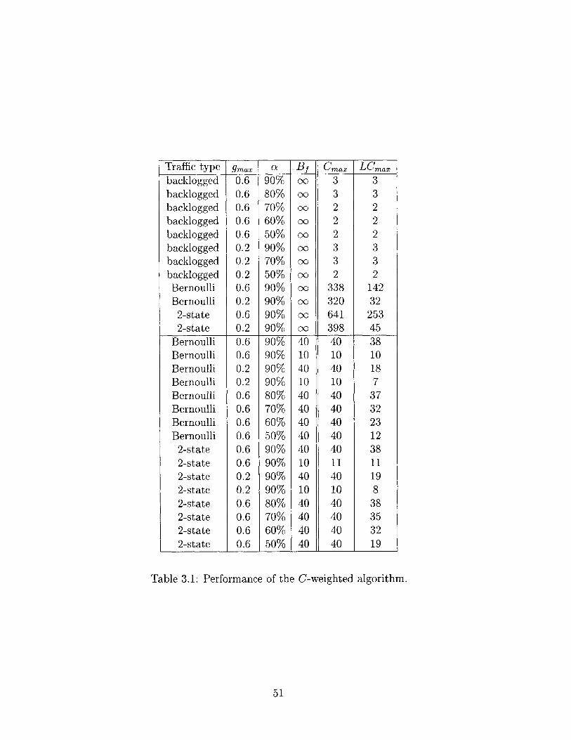
Traffic type gmax Oz Bf Cmax LCmaxbacklogged 0.6 90% o 3 3backlogged 0.6 80% o0 3 3backlogged 0.6 70% o0 2 2backlogged 0.6 60% o0 2 2backlogged 0.6 50% o0 2 2backlogged 0.2 90% 00 3 3backlogged 0.2 70% o 3 3backlogged 0.2 50% 00 2 2Bernoulli 0.6 90% 00 338 142Bernoulli 0.2 90% o 320 322-state 0.6 90% o 641 2532-state 0.2 90% o 398 45
Bernoulli 0.6 90% 40 40 38Bernoulli 0.6 90% 10 10 10Bernoulli 0.2 90% 40 40 18Bernoulli 0.2 90% 10 10 7Bernoulli 0.6 80% 40 40 37Bernoulli 0.6 70% 40 40 32Bernoulli 0.6 60% 40 40 23Bernoulli 0.6 50% 40 40 12
2-state 0.6 90% 40 40 382-state 0.6 90% 10 11 112-state 0.2 90% 40 40 192-state 0.2 90% 10 10 82-state 0.6 80% 40 40 382-state 0.6 70% 40 40 352-state 0.6 60% 40 40 322-state 0.6 50% 40 40 19
Table 3.1: Performance of the C-weighted algorithm.
51
of theorems 2.2 and 2.3.
To evaluate the size of the theoretical bound, we have K1 = 0, K 2 = N, K 3 =
aNBf. At a = 0.4(- = 0.1) and Bf = 40, this leads to a theoretical bound of
Cmlry = / +K1 K 2 +K 3 ~ N x Kl+ +K ~ 6000. As -y -+ 0 (a -+ 0.5)
the bound increases inversely. It is obvious that the theoretically provable hard
bound is very loose compared to typically observed Cmax values. Thus, the theory
- loose bounds at 50% loading - is much weaker than the observed performance,
which exhibits tight bounds even at a = 90% switch capacity. This discrepancy is
most likely due to the inherent "looseness" of the Lyapunov proof technique, and the
unavailability of combinatorial proof techniques for our no-speedup scenario.
Important Footnote to any QoS Contract - soft versus hard bounds:
The bound Cmax is obtained by simulation, and is not a theoretical bound. One may
have reservations about using such a bound in a "contract" or for flow admission
control. However, for no-speedup scenarios, Lyapunov analysis often yields loose
bounds and no useful combinatorial proof technique is known yet.6 Therefore, a soft
bound obtained by simulations can be considered good enough for practical purposes,
especially if the flow/user recognizes the bound is obtained by simulations. Also, in
today's networks there is a large proportion of legacy, best-effort traffic that requires
no bandwidth reservation. Therefore a < - might be a realistic assumption. In that
case "stability" in the sense of bounded edge weights is guaranteed by theory, and
the fact that observed bounds are much smaller than the theoretical bounds can be
considered a fortunate bonus.
6Indeed, the previous works which use Lyapunov analysis in no-speedup scenarios ([51, 50, 34, 36,37]) only bound expected values of queue lengths, waiting times, etc. anyway; our Cmax bound is a de-terministic bound (because the credit stream is deterministic) and therefore already an improvementover bounds on expected values.
52

Table 3.2: Performance of the LC-weighted algorithm.
3.5.3 Using LC as edge weights
In this section we consider using the number of validated cells LCf (t) as the edge
weight. We do not use any bucket sizes in this section.7 One reason for using LC as
edge weights is that bounded LC translates into a meaningful contract (chapter two).
Another reason for using LCf (t) as edge weights is that the LC-weighted algorithm
is observed to reduce hogging behavior for bursty traffic without the use of buckets.
With this algorithm, a long-idle flow can still exhibit some hogging behavior, but this
only happens when a large burst arrives in a very short duration right after a long
idle period, so that both Cf(t) and Lf(t) are large (resulting in a high edge weight).
In simulations, hogging behavior occurs much less often and to a much less severe
extent, compared to the C-weighted algorithm without buckets. Table 3.2 shows the
simulation results.
Table 3.2 also lists the maximum queue size Lmax and maximum credit size Cmax.
Even though Lmax is relatively large, scenario 1 of the LC-based contract implies
these flows are already transmitting at full reserved speed. Also, even though Cmax
7Bucket sizes can still be added to the LC-weighted algorithm since how to manage credits andwhat to use as edge weights are two independent issues. However, based on the simulation resultsfor the LC-weighted algorithm with no bucket size, the utility of adding bucket sizes seem doubtful.
53
Traffic type gmax a Cmax LCmax LmaxBernoulli 0.6 90% 369 13 404Bernoulli 0.6 80% 373 11 360Bernoulli 0.6 70% 369 6 307Bernoulli 0.6 60% 370 6 289Bernoulli 0.6 50% 350 4 242Bernoulli 0.2 90% 314 7 333
2-state 0.6 90% 616 31 6712-state 0.6 80% 588 29 6652-state 0.6 70% 702 21 7012-state 0.6 60% 645 15 6432-state 0.6 50% 736 6 6192-state 0.2 90% 418 10 423

is relatively large, such flows must have very short queues by scenario 2 of the LC-
based contract. Note that in the original credit-weighted algorithm without credits,
such flows are the ones that hog input/output ports and create trouble. In the LC-
weighted algorithm, they still have small edge weights (because of small Lf(t)) and
do not cause any trouble at all.
Algorithm complexity: Since the edge weights change by at most 1 (increment
or decrement) every timeslot, the sort order can be maintained from one timeslot to
the next with a one-pass linear updating procedure. Complexity is therefore O(N 2 ).
We conjecture that, if a < j, then bounded LC can be guaranteed theoretically.
One supporting reason is that if a flow's arrival rate Af > gf, then in the long term
it becomes constantly backlogged with LCf(t) -+ Cf(t), whereas if Af < gf, then
in the long term LCf(t) -+ Lf(t) and this becomes the scenario of [51, 34]. Again,
simulation results exceed the conjectured performance.
A starvation problem for edge weights based on queue lengths: The LC-
weighted algorithm, and other algorithms based on queue lengths including [51, 50,
34], all suffer from an undesirable starvation problem. Suppose a flow has no arrivals
during a prolonged period between t = T1 and t = T2 . The last cell that arrive right
before t = T will experience long delay because eventually it will become the only
queued cell for this flow and so the edge weight will be stuck at the low value of 1.
In actual implementations, a possible fix is to have an exception handling mechanism
kick in when the waiting time is too large. Another implementational trick might be
to have "phantom" cells arrive to flush out the real cells during long idle periods - i.e.,
to increment Lf (t) even though there are no real arrivals. One last way is not to use
queue lengths at all, and instead use waiting times explicitly. This is the approach of
our next algorithm.
3.5.4 Using VW as Edge Weights
We now consider using validated waiting time VWf as the edge weight. Note that
this algorithm requires more bookkeeping than the credit- or LC-weighted algorithms,
since we now have to keep track of the individual timestamps for each cell in the queue.
54

Traffic type gmax ' Cmax VWmax (timeslots) Wmax (timeslots)Bernoulli 0.6 90% 397 45 1830Bernoulli 0.6 80% 378 23 1795Bernoulli 0.6 70% 383 11 1766Bernoulli 0.6 60% 364 5 1803Bernoulli 0.6 50% 322 5 1740Bernoulli 0.2 90% 292 35 3520
2-state 0.6 90% 739 77 47502-state 0.6 80% 646 6 33232-state 0.6 70% 515 6 20322-state 0.6 60% 530 6 17872-state 0.6 50% 480 6 10502-state 0.2 90% 389 48 3330
Table 3.3: Performance of the VW-weighted algorithm.
The simulation results are shown in table 3.3. VWmax is the largest VWf(t) for all f
and all t and again it acts as a practical "soft" bound in our VW-based contract.
Table 3.3 also lists the maximum actual waiting time (actual cell delay) Wmax,
and maximum credit size Cmax. Even though Wmax is relatively large, scenario 2 of
the contract implies these flows are already transmitting at full reserved speed. Also,
even though Cmax is relatively large, cells of such flows must experience small delay
according to scenario 1 of the contract.
Algorithm complexity: If a cell is not transmitted, its edge weight will increase
by 1 in the next timeslot. If a cell is transmitted, however, the next cell's waiting
time can be arbitrarily smaller (depending on the inter-arrival duration). Thus, edge
weights can change by arbitrary amounts every timeslot. The stable marriage match-
ing algorithms will require a sorting pre-processing step and complexity is therefore
O(N 2 log N).
3.5.5 Rescaling and mixing weights
In the algorithms presented so far, each flow on startup negotiate only a guaranteed
rate gf, and possibly a bucket size Bf. Typically, however, flows also have differing
tolerances for delay. In the most general case, some flows (e.g., priority file transfer,
55
leased line) might have only rate guarantees, while other flows (e.g. voice, video)
might have rate and delay guarantees which are independent or decoupled. None of the
above algorithms are flexible enough in this respect - the credit-weighted algorithm
guarantees a bound on VWf(t) equal to Cmax and therefore couples each flow's delaygf
bound to its rate, whereas the VW-weighted algorithm bounds every flow's VWf (t)
by the same bound VWmax.
One way to handle such heterogeneous traffic is to use some kind of weighted
round-robin on the different classes. Similar approaches are used in many curren-
t (input-queued and output-queued) switches, e.g., for different ATM classes. Our
fabric scheduler algorithm, however, can be modified to handle all classes together
without additional round-robin or other forms of prioritizing. The simple observa-
tion is that each flow can choose different methods to determine its weight, and the
matching algorithm simply treats all weights as numbers and find a stable matching.
Since the weights are in essentially different "units" and yet the matching algorith-
m treats them all as numbers, we decided to rescale the weights into similar "units."
Intuitively, as credits arrive in a smooth stream, measuring validated waiting time in
multiples of credit intervals (Ty = -I) is in some sense similar to measuring number
of outstanding credits. We used this as the basic rescaling between the two classes of
flows and use NVWf= -- f - VWfgf to denote a "normalized" validated waiting
time. In addition to normalization, each flow may have its weight rescaled by a pri-
ority level Pf. flows with a given delay requirement should count its delay bound in
units of Tf and set the priority Pf accordingly. To summarize,
1. flows with credit based weights have w = Pf Cf or PfLCf.
2. flows with waiting-time based weights have w = Pf VW = Pf VWfgf = Pf NVWf.
For credit-weighted flows, those with higher Pf will have proportionally fewer
unspent credits or shorter queues (for LC-weighted "underloading" flows), and for
VW-weighted flows, those with higher Pf will have proportionally shorter actual
delay (for "underloading" flows) or each credit will be spent proportionally sooner
56
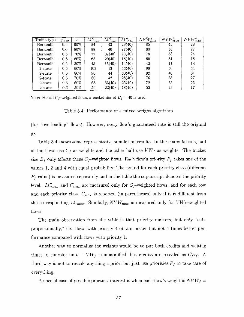
Traffic type gmax a LC LC2 x LC4 x NVWmIY NVWax NVh7xBernoulli 0.6 90% 84 43 29(40) 85 45 28Bernoulli 0.6 80% 88 40 27(40) 80 38 27Bernoulli 0.6 70% 77 37(40) 23(40) 78 38 24Bernoulli 0.6 60% 65 29(40) 18(40) 60 31 18Bernoulli 0.6 50% 43 15(40) 14(40) 42 17 132-state 0.6 90% 103 53 33(40) 98 50 342-state 0.6 80% 90 44 30(40) 92 40 312-state 0.6 70% 80 42 28(40) 76 38 272-state 0.6 60% 68 33(40) 23(40) 72 33 232-state 0.6 50% 50 22(40) 18(40) 52 23 17
Note: For all Cf-weighted flows, a bucket size of Bf = 40 is used.
Table 3.4: Performance of a mixed weight algorithm
(for "overloading" flows). However, every flow's guaranteed rate is still the original
9f-
Table 3.4 shows some representative simulation results. In these simulations, half
of the flows use Cf as weights and the other half use VWf as weights. The bucket
size Bf only affects those Cf-weighted flows. Each flow's priority Pf takes one of the
values 1, 2 and 4 with equal probability. The bound for each priority class (different
Pf value) is measured separately and in the table the superscript denotes the priority
level. LCmax and Cmax are measured only for Cf-weighted flows, and for each row
and each priority class, Cmax is reported (in parentheses) only if it is different from
the corresponding LCmax. Similarly, NVWmax is measured only for VWf-weighted
flows.
The main observation from the table is that priority matters, but only "sub-
proportionally," i.e., flows with priority 4 obtain better but not 4 times better per-
formance compared with flows with priority 1.
Another way to normalize the weights would be to put both credits and waiting
times in timeslot units - VWf is unmodified, but credits are rescaled as CfTf. A
third way is not to rescale anything a-priori but just use priorities Pf to take care of
everything.
A special case of possible practical interest is when each flow's weight is NVWf =
57

vWf - VWfgf, i.e., the network management does not negotiate rate and delayTrf
guarantees separately but instead mandates that slower flows (small gf) must tol-
erate proportionally larger delay. Simulations show that an algorithm using these
weights performs similarly to the LC-weighted algorithm, in terms of observed bounds
Cmax, L max, flOWmax, etc. However, using VWfgf confers an important advantage
- it does not suffer from the starvation problem of the LC-weighted algorithm (or
any queue length based algorithm) mentioned in section 3.5.3. The tradeoff is that
waiting-time based algorithms run slower by a factor of logN because of the sorting
required.
3.6 Other Issues
3.6.1 Multiple flows per input-output pair
In reality it is likely that many flows have the same input-output pair. In order to pro-
vide per-flow QoS guarantees, many switch designers are now implementing per-flow
queueing. A simple way to handle many flows with our algorithms comes from the
realization that any input port can send at most one cell per timeslot anyway. There-
fore, for any input-output pair, the CQ algorithm simply considers the highest-weight
(C, LC, VW, CU, etc.) flow with non-empty queue, and ignores all other flows of the
same input-output pair. Thus the CQ algorithm still runs in O(N 2 ) or O(N 2 log N)
time. Of course, this means the ports need to perform a preprocessing step to find
the highest-weight flow. Depending on the implementation details, this preprocessing
step may require O(IFI) time, which is higher than O(N 2 log N). However, this pre-
processing step is likely to be very fast in practice, especially if a port also maintains
a sort order of its flows based on weight, similar to the sort order maintained from
one timeslot to the next by the scheduler.
We have performed additional simulations where multiple flows are allowed per
input-output pair. In these simulations, the total number of flows (counting only those
with positive gf) is approximately equal to that of previous reported simulations. The
58

most "crowded" input-output pair typically has about 3-10 flows. We found very little
change (about 5-10%) in the simulation results in terms of various measured bounds.
Depending on the exact hardware arrangement, it may be the case that the cross-
bar fabric can only access a much smaller number of queues. Specifically, the input
port has N virtual output queues (VOQs) connected to the crossbar fabric, and any
cells in the matching must come from these VOQs. Each VOQ corresponds to a
different output, thus we have per-input-output-pair queueing. Now, if the arrivals
are allowed into these VOQs without restriction and assuming these VOQs are FIFO,
then it is impossible to provide per-flow QoS guarantees, as a misbehaving flow can
hog its VOQ to the detriment of other flows with the same input-output pair. So,
entry to the VOQs must also be restricted, and this means per-flow queueing is still
needed to store cells before they enter VOQs. The new idea here, and a natural
one, is to have a simple traffic policing unit which releases validated cells from the
per-flow queues into their VOQs. Once inside the VOQs, the scheduler treats all
cells of the same VOQ as if they belong to the same "super" flow, with a combined
guaranteed rate. The essential difference between this new method and that of the
previous paragraph is that in the previous method a pre-processing step to find the
highest-weight flow (for each input-output pair) is necessary, whereas the new method
does not require such a search. In preliminary simulations, the new method also keeps
weights bounded, although the the bounds are usually larger by a factor of 2-5 (under
our simulation settings), probably due to the coarse-grained nature of the scheduling
which only operates on "super" flows but not on individual flows.
3.6.2 Traffic Shaping Effects and Minimum Output Buffer
Requirements
In this section we will show that the credit-weighted algorithm (with or without
buckets), in addition to providing provable bandwidth and (validated) waiting time
guarantees, also acts as a traffic shaping mechanism.
Consider a particular flow f, with guaranteed rate gf, being served by the credit-
59
weighted algorithm. Let Sf"u"(t) be the flow's total number of transmissions (across
the switch fabric) up to time t (inclusive), and let Cfcur(t) be the total number
of credits received up to time t (inclusive), i.e., C "r"'m (t) = t x gf - total credits
forfeited due to bucket limitations. By definition, the unspent credit (i.e., edge weight)
is Cf(t) = CYCCUr"(t) - Sccum"(t).
By choice, cells without credits will not be transmitted and therefore Cf(t) > 0.
This, combined with any edge weight bound Cmax, theoretical or simulation-based,
translates directly into the following:
0 < Cf(t) = Cfcum"(t) - Saccur"(t) Cmax (3.4)
Using the above relation on two different times t1 and t2 (> ti), we have:
number of transmitted cells during the interval(ti, t 2] (3.5)
- S "ccu"(t2 ) - Sccur"(ti) (3.6)
K Cmax + cyccurn(t 2 ) - C "ccurn(ti) (3.7)
= Cmax + number of credits received during the interval (3.8)
K Cmax + (t2 - t1) X gf (3.9)
In other words, during the interval, the flow can only transmit at most Cmax cells
more than its reserved share of (t2 - tl) x gf cells. Using a common traffic-description
terminology [54], the stream of transmitted cells is (p, -)-regulated with rate p = gf
and burst size- = Cmax. Thus the scheduler also acts as a traffic shaper. Note that
the burst size o is different from the flow's bucket size Bf, although the two quantities
are correlated.
What are the consequences of this traffic shaping? In the conceptually simplest
case, there is no output buffer in the switch, and cells transferred across the fabric
exit via an output line immediately. In this case, the downstream node now faces
60
shaped traffic. Each flow is individually shaped (which implies the aggregate is also
shaped). This has various consequences for the performance bounds of the down-
stream scheduler [54].
In actual switches, there may be output buffers for various reasons. For example,
if the switch speedup is larger than 1 (unlike the assumption used in most of this
paper), then the output line speed is slower than the fabric speed and output buffers
are mandatory. For another example, buffering may be required for re-assembly of
variable-length packets which have been broken up into fixed sized cells during the
switch fabric crossbar scheduling.
Consider a particular output buffer and let {Vk}k=1,2,...K be the set of flows destined
for it. The fact that each flow is shaped implies a bound on the queue length in
the output buffer, under a simple assumption - the output buffer must be "work-
conserving" in the sense that cells are being released at a constant rate of Rst cells
per timeslot as long as the output buffer is non-empty, and Rt > Eg gVk, the total
rate entering the output buffer. Under this assumption, the output buffer length
is bounded by the sum of all burst sizes EK .vk, which equals K x Cma, in our
scenario.' This provides a minimum output buffer length requirement which will
prevent any buffer overflow. Note that this result is essentially a simple observation
on (p, -)-shaped traffic, which happens to be the output traffic pattern of the credit
weighted algorithm.
As an interesting and practical example, suppose the speedup is 2, in which case a
modified proof of theorems 2.2 and 2.3 show that the credit-weighted algorithm guar-
antees that credits are bounded even at 100% reservation. Now, by the assumption
that network management does not overbook any resource, the total guaranteed rate
into any output port is at most equal to the output line speed. If we further assume
that the output queue is work conserving at the output line speed, then the above
8 A simple proof: Consider any time t 2 and let t1 be the most recent time (ti < t2 ) at whichthe output buffer is empty. During the interval (ti, t 2], the total number of cells "arriving" at theoutput buffer is bounded by k=1 gVk X (t2 - ti) + K x Cma, and because the output buffer isnon-empty during the entire interval, the total number of cells released from the buffer is at leastRout x (t2 - ti). Since Ruot E i I9, the difference, which is the queue length at the arbitrarilychosen time t2 , is at most K X Cmax.
61
discussion gives a bound on the output queue length.
Since the input traffic entering the switch is not pre-regulated but the output
is regulated, this means the crossbar scheduler has pushed any possible congestion
to the input queues. Therefore, it is probably a good idea to implement any packet
discarding algorithms (if applicable) at the input side while allocating enough memory
for the output queues to prevent any overflow.
The above observations are only valid for the credit-weighted algorithm. Even
though the LC- and VW-weighted algorithms exhibit edge weight bounds at up
to 90% loading in simulations, these bounds do not translate into (p, a)-shaping of
output traffic. The chief reason is that we mainly employ the concept of validation
without bucket size restrictions. As such, validation emulates a pure rate-based,
(p = gf, a = oc) traffic shaper which pre-regulates per-flow traffic prior to their
arrival at the input ports of the switch. These algorithms indeed allow a flow to be
idle for a long time and collect a lot of credits.
However, suppose instead the algorithms are modified to emulate a per-flow (p =
gf, 0f) traffic shaper, where the parameter u7f is negotiated during flow setup and
serves a similar function to Bf of the credit-weighted algorithm. Implementationally,
this means the algorithm is modified to stop giving credits to a flow once the flow's
unmatched credit, Cf(t) - Lf(t), which equals the unused credits in the traffic shaper
being emulated, exceeds a'". Alternatively, suppose the input traffic is in fact pre-
regulated by the source or by an upstream node. In such cases, the validated arrivals
will be (p = gf, af")-shaped. This, together with an (experimentally observed) edge
weight bound, implies the output traffic will be (p = gf, afut)-shaped. For example,
calculations similar to those of equations (3.6)-(3.9) show that for the modified LC-
weighted algorithm with an observed edge weight bound of LCmax, we have aU'" =
ai" + LCmax. Here, the output rate and input rate are both equal to gf, but the
output burst size will be larger than the input burst size. Once the output traffic can
be proved to be shaped, output queue lengths can be bounded as before.
62

N Traffic type g9rax a Bf Cmax LCmax32 Bernoulli 0.2 90% 40 40 1864 Bernoulli 0.2 90% 40 40 23128 Bernoulli 0.2 90% 40 40 3332 Bernoulli 0.2 90% 10 10 764 Bernoulli 0.2 90% 10 10 7
128 Bernoulli 0.2 90% 10 10 1132 2-state 0.2 90% 40 40 1964 2-state 0.2 90% 40 40 35
128 2-state 0.2 90% 40 40 4032 2-state 0.2 90% 10 10 864 2-state 0.2 90% 10 10 10128 2-state 0.2 90% 10 10 10
Table 3.5: Effect of switch size N on C-weighted algorithm.
burst size gmax a Cmax LCmax Lmax
5 0.6 90% 616 31 67110 0.6 80% 642 38 73320 0.6 70% 638 50 72540 0.6 60% 667 77 790
Table 3.6: Effect of burst size on LC-weighted algorithm (N = 32, 2-state traffic)
3.6.3 Effects of other simulation parameters
In the simulations reported so far, the switch size is fixed at N = 32 and the average
burst size is fixed at 5 timeslots. Tables 3.5-3.7 briefly investigate the effects of
changing these parameters. We have chosen a different algorithm for each table;
however, the resulting trends are similar for other algorithms not represented here.
3.7 Fair Sharing of Unreserved Switch Capacity
By design choice, our schedulers only serve a flow when it can pay the required credit.
Since reserved bandwidth usually does not make up 100% of switch capacity (a < 1),
the algorithms are not "work-conserving" and will lead to under-utilization. We
argued that this represents a more stringent test condition when evaluating provision
63

burst size gmax a Cmax VWmax (timeslots) Wmax (timeslots)5 0.6 90% 739 77 4750
10 0.6 90% 1023 102 589820 0.6 90% 2330 133 630240 0.6 90% 4207 178 6799
Table 3.7: Effect of burst size on VW-weighted algorithm (N = 32, 2-state traffic)
of rate and delay guarantees. For the sake of completeness we now investigate the
remaining question: how should the unreserved capacity of the network be used? This
section presents algorithms which achieve near-maximum utilization and fair sharing
of the unreserved capacity.
In this paper we apply the notion of max-min fairness (see e.g., [4] p.527) to
the unreserved capacity of the network resources. The resources required to support
bandwidth reservations are exempted from fairness considerations, but the leftover
resources must be shared fairly by all flows. Max-min fairness is a rate-based notion,
and does not take into account individual cell delays. We will use the term "excess
rate" to denote a flow's transmission rate in excess of its guaranteed rate (if any).
Definition 3.2 - Max-min fairness: A set of flow excess rates (mea-
sured in cells/timeslot) is max-min fair if and only if every flow has one
(or more) bottleneck resource. A resource is a bottleneck resource for a
particular flow if (a) that resource is fully utilized, and (b) that flow has
at least as high an excess rate as any other flow using that resource.
As an example, figure 3-1 shows five flows in an N = 3 switch. Each flow has
a different input-output combination, corresponding to its row (input) and column
(output) in each matrix. All numbers are transmission rates in cells/timeslot. The
first matrix shows the guaranteed rates granted to the flows. Two of the five flows
have gf = 0 and they represent best-effort traffic. Input port 1 (row 1), which can
support a maximum rate of 1 cell/timeslot, must use 0.4 of that capacity to support
the guaranteed transmissions of the two 1st row flows, and therefore only has an
excess rate of 0.6 cells/timeslot available for fair sharing. Similarly, output port 2
64

0.3 0.1 0.4 0.2 0.7 0.30.3 + 0.2 = 0.50.0 0.0 0.2 0.8 0.2 0.8
9f + fair shares of excess bandwidth total rate
Figure 3-1: Max-min fairness with rate guarantees.
(column 2) must use 0.4 of its rate of 1 cell/timeslot to support guaranteed traffic,
leaving only 0.6 for sharing. Using these excess rates, the max-min fair shares of the
excess rates are shown in the second matrix - the flows in the 2nd column have an
output bottleneck and are limited to an excess rate of O 3= 0.2 each, while the other
two flows are limited by their respective inputs as bottlenecks. The total rate of each
flow is its guaranteed rate plus its fair share of excess bandwidth, shown in the third
matrix.
3.7.1 Two phase Usage Weighted Algorithm
We now present an algorithm that operates in two phases in each timeslot. In the first
phase, the algorithm runs any of the bandwidth reservation algorithms of the previous
sections to produce a matching X. The flows in X have their credits decremented
as usual. Then, if JXI < N, i.e., if there could be more transmissions, the algorithm
runs a second phase to choose some flows to fill up the transmission schedule. These
flows have their Usage variable U1 incremented by 1. (Uf are initialized to zeros.)
Thus each Uf counts the number of cells a flow has sent without paying credits for
them, i.e., the number of "excess" or unpaid transmissions. (Note that by design, our
greedy reservation algorithms will never miss a busy flow which has a credit to spend.
Therefore, all the flows chosen during the second phase have no credit, Cf = 0.)
The intuitive idea is that to be fair, flows which have few previous excess trans-
missions (small Uf) should be considered first in the sharing of excess resources. Our
second phase Usage Weighted Algorithm implements this intuition directly as fol-
lows: the algorithm considers each flow in increasing U1 order, trying to add it to the
matching X if possible, skipping it otherwise with no backtracking. This is identical
to the central queue (CQ) algorithm except the weights U1 are sorted in increasing
65
order, and the initial matching is computed by the first phase (instead of an empty
matching).
3.7.2 Allowing negative credits
Another approach to use the unreserved switch capacity is simply to allow credits to
become negative. In the sorting of CQ, the flow with lowest (i.e., most negative) credit
is still sorted first. An equivalent view is that flows are now sorted (in decreasing
order) by CUf = Cf - Uf (and Cf is maintained at non-negative levels, as before).
This view is equivalent because, intuitively, as credits arrive they may be considered
to "retroactively" pay for previous excess transmissions, which are now accounted for
as guaranteed transmissions.
With this approach, the algorithm again operates in one phase, i.e., all transmis-
sions (reserved or unreserved) are assigned during one loop through a single sorted list.
A slightly modified proof of theorems 2.2 and 2.3 (omitted for length consideration)
shows that the new algorithm still bounds credits for 50% loading.
Table 3.8 shows the performance of the CU-weighted algorithm. The total number
of flows shown in the table include those with positive bandwidth guarantee, and those
with no bandwidth guarantee. The latter represents best-effort traffic. A detailed
description of the simulation can be found in last section. Backlogged traffic represents
an overloading scenario where all flows are constantly backlogged. In our simulations,
when Bernoulli traffic is used the total arrival rate of all flows (with or without GBW)
equals N cells/timeslot, which is the highest possible throughput of the switch. This
represents an exact loading scenario.
The table shows that total switch throughput is usually very high. (For Bernoul-
li traffic at exact loading, the throughput is affected by the arrival processes and
therefore not very meaningful.) The algorithm's performance regarding fairness is
measured by the parameter 6f, defined as the ratio of a flow's excess transmission
rate over its max-min fair excess rate (computed offline). flows getting less than its
fair share will have 6 f < 1 and flows getting more will have 6 f > 1. The table shows
the distribution of all 67 values and also the minimum value. It shows that many
66

no. of total % of flows with f in these ranges:Traffic gmax flows with no. of 0 min 6f min 6f 0.7 0.85 0.95 Total switch
type non-zero GBW flows value to 0.7 to 0.85 to 0.95 or more throughputbacklogged 0.6 160 2048 90% 0.171 1.5% 2.0% 3.1% 93.4% 98.5%backlogged 0.6 155 1024 90% 0.159 4.0% 4.3% 5.8% 85.9% 92.5%backlogged 0.2 204 1024 50% 0.413 1.0% 2.2% 2.3% 94.5% 97.3%backlogged 0.2 201 2048 50% 0.161 0.4% 1.0% 1.7% 96.9% 99.0%Bernoulli 0.2 204 1024 50% 0.672 0.04% 0.4% 1.5% 98.1% -
Bernoulli 0.2 201 2048 50% 0.614 0.1% 0.8% 1.6% 97.5% -
Table 3.8: Performance of the CU-weighted algorithm.
flows (at least 85% of them) obtain at least 95% of their fair shares. However, a small
fraction of flows might be treated very unfairly (small 6f) under some settings. The
simulation results are similar for the two phase algorithm. In practice, the one-phase
CU-weighted algorihtm might be preferable to the two phase algorithm because of
its simpler implementation and slightly faster running time.
3.8 Chapter Summary
This chapter described several fast, practical algorithms for bandwidth reservations
and cell delay guarantees, in an input-queued switch with no speedup. Our schedulers
also provide approximate max-min-fair sharing of unreserved switch capacity, and
achieve close too 100% total throughput.
All our schedulers use stable marriage matchings and only differ by what they use
as edge weights w. They all try to bound edge weights, which lead to various QoS
contracts. The edge weights we investigated include C, LC, VW and scaled versions
and mixtures of them. By applying theorems 2.2 and 2.3, we proved that the credit-
weighted algorithm can guarantee bounded credits at a < 50%. In simulations all
the algorithms exhibit small edge weight bounds at reservation levels of a = 90%.
The choice of edge weights depends on which resulting contract is suitable for
the applications at hand. No one algorithm is strictly better than another. For
example, comparing the credit-weighted algorithm and the LC-weighted algorithm,
the former provides a tighter Cmax bound while the latter provides a tighter LCmax
67

for the same experimental settings. For another example, if the design goal is to have
each flow experience similar (validated) delay, then the VW-weighted algorithm is
suitable, since the credit-weighted algorithm provides delays which depend on each
flow's guaranteed rate. More generally, each flow might have different methods of
determining edge weights depending on what type of traffic it is, and each flow's edge
weight might be rescaled by a priority factor, as discussed in section 3.5.5. In this
case each flow will have a different contract corresponding to its choice of edge weight.
As a future work, the same principle of choosing appropriate edge weights and
bounding them might be more widely applicable to achieve other kinds of QoS con-
tracts, e.g., delay variation guarantees, fairness based on waiting times (unlike rate-
based max-min fairness), etc.
3.9 Details of Simulation Settings
3.9.1 Admission Control of flows' Bandwidth Reservation
Requests
In our simulations, we use a 32x32 switch (i.e., N - 32). To control the amount
and distribution of guaranteed rates gij , we used two simulation parameters - loading
factor a, and maximum guaranteed rate gmax. As a reminder, the loading factor is
defined as
a = max(max gi3 , max Egij) (3.10)
that is, the highest load of all input and output ports.
Random generation of flows and their guaranteed rates is done as follows: the
simulator considers each different (i, j) pair (V1 < i, j < N) in random order. Each
(i, J) pair is considered exactly once and when it is being considered, the simulator
generates gij as a uniform random variable between 0.01 and gmax. If the gij so
generated (in conjunction with other gi'y already generated) will increase the loading
68
factor beyond a, then it is decreased as much as necessary to keep the loading factor
exactly a. (Some flows therefore might have gf = 0.) This method can be viewed as a
very simple admission control - flows arrive at random and request a random amount
of bandwidth guarantee, while the admission control maintains each input/output
port's loading to a or less.
In most of our simulations, we found that this method usually loads every input
and output port evenly and close to the loading factor, i.e., Ei, gijj ~ E, gij' ~ a.
Consequently,
the total reserved rate of the switch ~ a x N. (3.11)
Note that although each port is almost uniformly loaded, this is very different from
"uniform loading" which means each input-output combination is uniformly loaded,
i.e., each gij = -. Our simulations in fact load each (i, j) pair very non-uniformly.
We have done additional simulations (not reported here) where the load on each
input (or output) port also vary significantly from almost 0 to a. (Note that the total
throughput is necessarily much smaller than a x N in such cases.) Our algorithms
seem to perform a little better at this uneven, but on average lower loading.
3.9.2 Random Cell Arrival Process
We use two kinds of non-backlogged traffic: Bernoulli (memoryless) traffic and 2-
state traffic. These two kinds of traffic share several common features: different
flows are completely probabilistically independent; the number of arrivals Af(t) is
always either 0 or 1; and the average arrival rate Af is exactly the guaranteed rate
gY. We choose Af = gf for two reasons: if the average arrival rate were higher, the
flow would eventually accumulate a large backlog (a situation already studied in the
previous section), whereas if the average arrival rate were lower, the reservations will
be larger than the actual traffic that needs to be transmitted and the algorithm's job
is correspondingly easier. Therefore, Af = gf represents the most stringent test case
for non-backlogged traffic.
69

In Bernoulli traffic, Vt, Prob(Af (t) = 1) = gYf (and so Prob(Af (t) = 0) = 1 - gf).
2-state traffic is more bursty: at each t the flow can be in busy or idle state. In busy
state Prob(Af(t) = 1busy) = 2gf whereas in idle state Prob(Af(t) = 1idle) = 0.9
State transition (toggling between the busy and idle states) happen with probability
0.2 in each timeslot; thus lengths of busy or idle periods are exponentially distributed
with an average length of 5 timeslots.
3.9.3 Measured Parameters
Here is a list of parameters measured during our simulations:
1. Lf(t), queue length,
2. Cf(t), credit,
3. LCf(t) = min(L1 (t), Cf (t)), number of validated cells,
4. Wj(t), actual waiting time of the oldest cell,
5. VWf (t), validated waiting time of the oldest cell.
Each of these parameters is defined for any flow f at any time t. However, we
are only interested in soft upper bounds on these parameters, i.e., the largest value
attained, by any flow and at any time during the length of the simulation. For
instance, Cmax = maxf maxt C (t) and similarly for LCmax, etc.
For a given algorithm, and a given choice of gmax, Ce, traffic type, bucket size (if
applicable), the simulation is run at least 10 times. Each of these 10 or more runs
typically consists of 10000-100000 timeslots, and the bounds of interest are recorded.
Then overall upperbound figures are reported.
9 1n some of our simulations some gf can be larger than I. For such flows, Prob(Af (t) = 1 busy) =1, Prob(Af (t) = 1lidle) = 2gf - 1. This maintains the average arrival rate at gf .
70

3.9.4 Fairness Simulations
Flow generation is handled slightly differently for fairness simulations, because of the
need to generate best-effort flows with no bandwidth guarantee. A total number of
flows is chosen before hand. Each flow is considered in sequence and given random
input and output ports, both chosen uniformly among the N = 32 ports. The gen-
eration of each flow's guaranteed rate is done as before, subject to the same simple
"admission control" of not loading any input or output beyond a. By choosing a
large total number of flows and using this generation method, we ensure that those
flows considered earlier will have their bandwidth reservation requests granted while
those considered later will have no guarantee, i.e., they act as best-effort traffic in our
simulation.
Cell arrival for non-backlogged traffic is handled exactly as before, with one ex-
ception: each flow's arrival rate equals its guaranteed rate (possibly zero) plus a small
constant. In each test case the small constant is adjusted so that the total arrival
rate of all flows equals N cells/timeslot, which is the highest possible throughput of
the switch. This represents an exact loading scenario.
The algorithm's performance regarding fairness is measured by the parameter
6f, defined as the ratio of a flow's excess transmission rate over its fair excess rate
(computed offline). When non-backlogged traffic is used, the fair excess rate used
in this calculation must upperbounded by the actual total number of cell arrivals.
flows getting less than its fair share will have 6f < 1 and flows getting more will have
6f > 1. We report both the distribution of all 6f values (among all flows, aggregating
all 10 or more runs) and also the minimum 6f value (minimized over all flows and
over all 10 or more runs).
71

Chapter 4
All-Optical Metro- and Local-Area
Networks
This chapter applies our theory and algorithmic ideas to an all-optical metro- and
local-area network, providing rate, delay and fairness guarantees.
The feasibility constraints of the LAN portion of the optical network are very
similar to those of the input-queued switch of the previous chapter. The algorithms
and results are also similar - small C, LC, VW bounds are observed in simulations
at a = 90%, while boundedness of C is proved for a < 50%. This chapter also
proves a generalized version of lemma 3.1 and also prove correctness for a variant of
the CQ algorithm. A main novelty of this chapter is the discussion of a distributed
master-slave scheduler for the metro-area optical network, in section 4.7.
72
4.1 Background and Motivation
Most existing all-optical network activities, including the DARPA AON, ONTC,
MONET, and Rainbow programs, provide only circuit switched services. In other
words, at the optical layer the optical signals provide only fixed or very slowly vary-
ing point-to-point connections. It is expected that future users will demand integrated
services, with ATM being a prime example; these networks may not be appropriate
for reaching all end-users but rather will mainly be used as backbone networks which
interconnect network switches.
We have been investigating optical LANs and MANs in the All-Optical Network
(AON) consortium [27] for direct optical interconnection of bursty end-users and/or
switches with bursty connections. The AON Consortium has developed an all-optical
LAN/MAN testbed which provides time-slotted WDM service [27]. In a more recent
DARPA Next Generation Internet (NGI) consortium project, we explore extensions
of this service to achieve fine-grained statistical multiplexing with different virtual
circuits time-sharing the wavelengths in a fair manner, using fast-tunable transceivers.
An important goal of the NGI project is to support bandwidth-on-demand (BoD)
services with quality of service (QoS) guarantee over WDM networks.
BoD services can be directly supported over WDM using a multi-access protocol.
A variety of WDM multi-access protocols for LANs and MANs have been proposed
and studied in the literature. For a survey, see for example [39]. However, most
of these protocols provide only best-effort service (the few exceptions to this pro-
vide mechanisms for integrating best-effort and circuit switched services) or real-time
service without any hard QoS guarantee (see for example [21]).
Unlike these other proposed algorithms for WDM multi-access networks, this chap-
ter describes schedulers which are unique in that it supports delay and bandwidth
guarantees, fairness is considered, and the algorithms are fast enough to run in real
time.
The rest of the chapter is organized as follows: Section 4.2 describes the local-area
network in more detail and derives the feasibility constraints based on the network
73

passivebcast
*Traffic Demand
I Schedules
Control ChannelScheduler
Figure 4-1:nel.
WDM broadcast LAN with central scheduler and dedicated control chan-
hardware. Section 4.3 discusses some related work. Section 4.4 presents our LAN
algorithms and proves some theoretical results regarding credit bounds. Section 4.5
then evaluates the algorithms in simulations, in terms of rate guarantees and also
fairness. Section 4.6 discusses briefly extensions of the algorithms to handle different
number of transceivers per node. Section 4.7 discusses the metro-area network and
presents a distributed scheduler for use in such networks. Concluding remarks are
given in section 4.8 and finally, detailed simulation settings are listed in section 4.9.
4.2 Problem Model
This chapter deals with both a local-area broadcast star network (LAN), and a metro-
area network (MAN) formed by connecting several LANs together with a wavelength
router. We will defer all discussions of the MAN and its distributed scheduler until
section 4.7. This section now describes the LAN problem setting in detail and justifies
our choice of a centralized scheduler for LANs.
LAN architecture. The LAN we studied is the one used in the B-service of
the DARPA AON [27]. It is a time-slotted broadcast network connecting N nodes
(figure 4-1). A node may be a workstation, a server, or a router connecting to another
network.
74
Transceivers. For most of this chapter, we assume each node has one transmitter
and one receiver for data transmission. In section 4.6 our algorithms will be general-
ized to handle the case where different nodes have different numbers of transmitters
and/or receivers, e.g., a router or server node might have several transceivers while
a workstation might have only one. Each transmitter and receiver can be indepen-
dently tuned to one of a finite set of m wavelengths {A, ,A2 ..., Am}, where in general
m < N. Data are transmitted in fixed-size cells, where one cell can be sent on one
wavelength in one timeslot. Following the existing B-service of the DARPA AON
[27], we assume that all tuning latencies are negligible compared to the length of a
timeslot.
Sychronization and pipelined transmissions. We also assume that each
transmitter and each receiver is individually synchronized so that cells arrive at the
central broadcast star at timeslot boundaries. All propagation delays are assumed to
be known and transmissions are pipelined. For instance, if the delay between node i
and the broadcast star is /. (which may or may not be an integral multiple of the
timeslot length T) and timeslots at the broadcaster start at times t, t + T, t + 2T,
etc., then the transmitter at node i may start to send a cell at times t - Aj, t + T -
Aj, t + 2T - Aj, etc. and the receiver at node i may start to receive a cell at times
t + i, t + T + Ai, t + 2T + i, etc.
Centralized scheduler and control channel To deal with bursty traffic, we
chose to use a centralized collision-free scheduler to dynamically decide which flows
should transmit at which timeslot, on a slot by slot basis. The scheduler communi-
cates with the stations via a dedicated control channel.' Because of control channel
delays, a newly arrived cell must wait until its presence is reported to the scheduler
before it can possibly be scheduled and transmitted. All our schedulers simply use
whatever delayed queue lengths knowledge it currently has. Such an access delay is
unavoidable in any scheduling scheme, as opposed to collide-and-retry schemes (e.g.,
'This chapter will not study the problem of designing an optimal control channel protocol; instead
we point out that [27] has one already in place, and in the appendix of [25] we outlined one particular
control protocol and the associated timing issues as a proof of concept.
75
Aloha and variations) which reduce access delays at the expense of throughput loss
due to collisions. We decide to favor a collision-free scheduler over a collide-and-retry
protocol because we want to achieve higher throughput, and also because even in
collide-and-retry schemes the destination receiver needs to be notified of the incom-
ing wavelength in advance anyway. Finally there is a legacy reason: the B-service
of DARPA AON already uses a centralized scheduling scheme. Also note that the
computed schedules must be disseminated to the sources and destinations in advance
of actual data transmissions, in a pipelined fashion.
Feasibility Constraints. Given a control protocol and pipelining in both the
data transmissions and the control channel, the problem conforms to the abstraction
defined in chapter one, where a feasible service vector must be chosen every timeslot.
The main constraint of a broadcast star network is that, to avoid collision, two cells
transmitted on the same wavelength cannot arrive at the broadcast star at the same
time. We model the broadcast LAN as a bipartite graph (U, V, E), where U represents
the source nodes U and V destination nodes, and each edge e E E represents a possible
transmission from u G U to some v E V. (In reality, both U and V represent the
same set of N routers/workstations.) The feasibility constraints can then be stated
as: a feasible service vector must be a 0-1 vector which represents an m-matching -
Definition 4.1: rn-matching.
A matching is a subset of edges X C E such that: (i) Vu E U, X contains
zero or one edge connecting to u, and similarly (ii) Vv E V, X contains
zero or one edge connecting to v. An m-matching is a matching with m
or fewer edges (i.e., lXi < im).
The three conditions correspond directly to the three hardware constraints - (i)
transmitter constraint: each u can only transmit one cell per slot, (ii) receiver con-
straint: each v can only receive one cell per slot, and (iii) wavelength constraint:
there are only m total wavelengths. Note that propagation delays do not change the
transmitter and receiver constraints, because of pipelining.
76
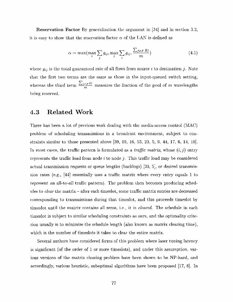
Reservation Factor By generalization the argument in [34] and in section 3.2,
it is easy to show that the reservation factor a of the LAN is defined as
a = max(max gij, max g1,) (4.1)2 3
where gij is the total guaranteed rate of all flows from source i to destination j. Note
that the first two terms are the same as those in the input-queued switch setting,
whereas the third term MfEF measures the fraction of the pool of m wavelengths
being reserved.
4.3 Related Work
There has been a lot of previous work dealing with the media-access control (MAC)
problem of scheduling transmissions in a broadcast environment, subject to con-
straints similar to those presented above [39, 19, 16, 53, 23, 5, 9, 44, 17, 6, 14, 10].
In most cases, the traffic pattern is formulated as a traffic matrix, whose (i, j) entry
represents the traffic load from node i to node j. This traffic load may be considered
actual transmission requests or queue lengths (backlogs) [23, 5], or desired transmis-
sion rates (e.g., [44] essentially uses a traffic matrix where every entry equals 1 to
represent an all-to-all traffic pattern). The problem then becomes producing sched-
ules to clear the matrix - after each timeslot, some traffic matrix entries are decreased
corresponding to transmissions during that timeslot, and this proceeds timeslot by
timeslot until the matrix contains all zeros, i.e., it is cleared. The schedule in each
timeslot is subject to similar scheduling constraints as ours, and the optimality crite-
rion usually is to minimize the schedule length (also known as matrix clearing time),
which is the number of timeslots it takes to clear the entire matrix.
Several authors have considered forms of this problem where laser tuning latency
is significant (of the order of 1 or more timeslots), and under this assumption, var-
ious versions of the matrix clearing problem have been shown to be NP-hard, and
accordingly, various heuristic, suboptimal algorithms have been proposed [17, 6]. In
77

this paper, tuning latencies are assumed insignificant, and under such assumption-
s, the matrix-clearing problem is actually solvable by a polynomial-time algorithm.
The main idea of the matrix-clearing algorithm involves solving many instances of
bipartite matching problems. Such an approach was originally proposed in a satellite
switching (SS/TDMA) context [23, 5 and has been adopted for WDM broadcast star
situations in various ways [19, 16, 531.
If the matrix-clearing algorithm is used in a simple poll-schedule-transmit ap-
proach, then the system may suffer from low throughput, unfairness and long access
delay. In this approach, the scheduler polls all stations and obtains a traffic matrix
D, whose entries Dij are actual number of data cells to be transmitted from node i to
node j. Then the scheduler uses the matrix-clearing algorithm to generate a schedule.
In the simplest case, this schedule is then executed, and when it is completed, the
scheduler polls again and the cycle repeats.2 It is easy to see that without additional
(presumably high-layer) traffic control, busy sessions/flows can hog the resources, by
making large requests each time. Moreover, if some Dij is large, then the schedule
length might be large. This causes two problems: first, this lengthens the polling
interval and hence the network access time, and second, the schedule might be s-
parse (low throughput) because the schedule length might become very long in order
to accommodate a few large Dij values even though the rest of the traffic matrix
has already been cleared. One obvious way to alleviate some of these problems is
to limit the schedule length in some way, but the matrix-clearing algorithm cannot
be adapted easily to a limited schedule length except by a simple truncation of the
minimum-length schedule, which can in turn introduce further unfairness. Another
alternative is to limit the size of the requests that can be submitted, but this can
still lead to low throughput and unfairness as non-congested resources (transmitters
or receivers) are under-utilized because the requests are artificially constrained.
A more sophisticated way to use the matrix-clearing algorithm is to have a pre-
2This is the approach used in the original satellite switching context [23, 5]. In that context, itmight be a valid approach since the round-trip delay is so long, making frequent contacts betweenscheduler and node stations impractical.
78
scheduler or network management / traffic regulator module, which reads all the
traffic requests (e.g., actual queue lengths Dij as above) and then decides how many
transmissions each session is entitled or permitted to send. This decision can be made
based on fairness, priority, billing and other network management concerns. Then,
the permitted (regulated) transmissions are assembled into a traffic matrix D, and
it is this matrix which is then sent to the matrix-clearing algorithm for scheduling.
By limiting the sizes of the entries of b, the schedule length can also be limited. (In
other words, the problem of large schedule lengths is circumvented by feeding the
algorithm a matrix with smaller entries to begin with.) This is a good approach in
the sense that it allows for fairness and priority considerations, and it can also limit
the schedule length (hence polling interval). However, it still faces two problems. The
first problem is the need for a pre-scheduler, which simply pushes the fairness and
priority issues one step away (and perhaps into a higher layer). The second problem,
and a more difficult one, is that the matrix-clearing algorithm itself runs relatively
slowly, and becomes a bottleneck lengthening the polling interval, so the whole system
again cannot respond fast enough to dynamic traffic conditions.
In preliminary simulations, we found that calculating the schedule for one times-
lot takes a few milliseconds, using the matrix-clearing algorithm of [5] and employing
the bipartite matching algorithm of [42] as a subroutine. (This simulation is per-
formed with N = 100 nodes, m = 20 wavelengths, about 2000 flows, and various
other assumptions.) In contrast, the timeslotted WDM service of DARPA AON [27]
has a timeslot of 2 microseconds. Clearly, even if the software code is substantial-
ly optimized and even if we change some simulation assumptions, the running time
will not improve 1000 times from the milliseconds range to approach the order of
2 microseconds, without radical changes to the algorithm itself. Moreover, even if
matrix-clearing can be performed much faster, we are still left with the need to de-
sign a separate pre-scheduler to deal with bandwidth reservations, fairness and other
issues.
In short, the work described in this chapter grew out of the realization that
bipartite-matching based matrix-clearing algorithms are generally too slow, and may
79

be good only for static or slowly varying traffic conditions. Therefore this chap-
ter proposes alternative scheduling algorithms similar to those used in input-queued
switches, which run very fast and which provide rate, delay and fairness guarantees.
(thereby eliminating the need for a pre-scheduler or higher-layer traffic control).
While our bandwidth reservation algorithms have theoretical guarantees, our fair-
ness algorithms are approximate algorithms, i.e., they often, but not always, achieve
fairness. There have been other algorithms that trade optimality for speed in the
past (e.g., [9]); however, to the best of our knowledge, this is the first work that uses
very fast (albeit approximate) scheduling algorithms to handle fairness and minimum
bandwidth guarantees all within the optical layer, as a first step toward supporting
integrated services at the optical layer in WDM networks.
4.4 LAN Schedulers - Theoretical Properties
4.4.1 Description of Algorithms
Our LAN schedulers are basically the same as the CQ algorithm used in chapter
three for input-queued switches. The only difference is that now the matchings are
restricted to m or fewer edges. To re-iterate, an edge weight is chosen (which can
be C, LC, VW or simple functions of these parameters), and then the CQ algorithm
starts from an empty matching M, and examines each edge in decreasing order of
weight. On examining an edge e, it is added to M if possible, i.e., if M U e is still an
m-matching, otherwise e is discarded. The algorithm stops when M has reached its
maximum possible size of m edges, or when all the edges have been examined.
These schedulers will be evaluated in simulations in the next section. For now,
we prove some theoretical properties.
4.4.2 Statements of Theorems
All theoretical properties hinge on the following definition, which generalizes the
concept of stable marriage matchings. This definition is chosen because (i) it char-
80

acterizes the output of the CQ algorithm in the LAN setting (lemma 4.1) and (ii) it
provides a nice theoretical property (theorem 4.2) which allows theorems 2.2 and 2.3
to be applied.
Definition 4.2 - stable marriage m-matchings: Given a weighted
bipartite graph (U, V, E, w), an m-matching M C E is a stable marriage
m-matching if: for any edge a ( M, at least one of these conditions is true
1. There is an edge eM E M such that they share a common node and
w(eM) > w(E). (This is the same condition as in the definition of
stable marriage matchings. We will say eM blocks e in this case)
2. |M| = rn and w(i) < w(eM) VeM G M.
Note that the second condition is in effect only when MI = rn. In other words, if
IMI < m, then M is a stable marriage m-matching if and only if it is a stable marriage
matching. Based on this observation, and the fact that any matching can have at
most N edges, it is easy to see that definition 3.1 for stable marriage matchings and
definition 4.2 for stable marriage m-matchings are equivalent when rn = N.
Lemma 4.1: Correctness of CQ
When the CQ algorithm terminates, M is a stable marriage m-matching.
Not only does the definition characterizes the output of CQ, it also guarantees
that stable marriage m-matchings have at least half the maximum possible weight
among all m-matchings. (The weight of a matching M is defined as the sum of its
edge weights, W(M) = EeEM W(e)-)
Lemma 4.2: Stable marriage rn-matchings have at least half max-
imum weight.
Given a weighted bipartite graph with non-negative weights, any stable
marriage m-matching has at least half (1) the total weight of a maximum
weighted m-matching.
81
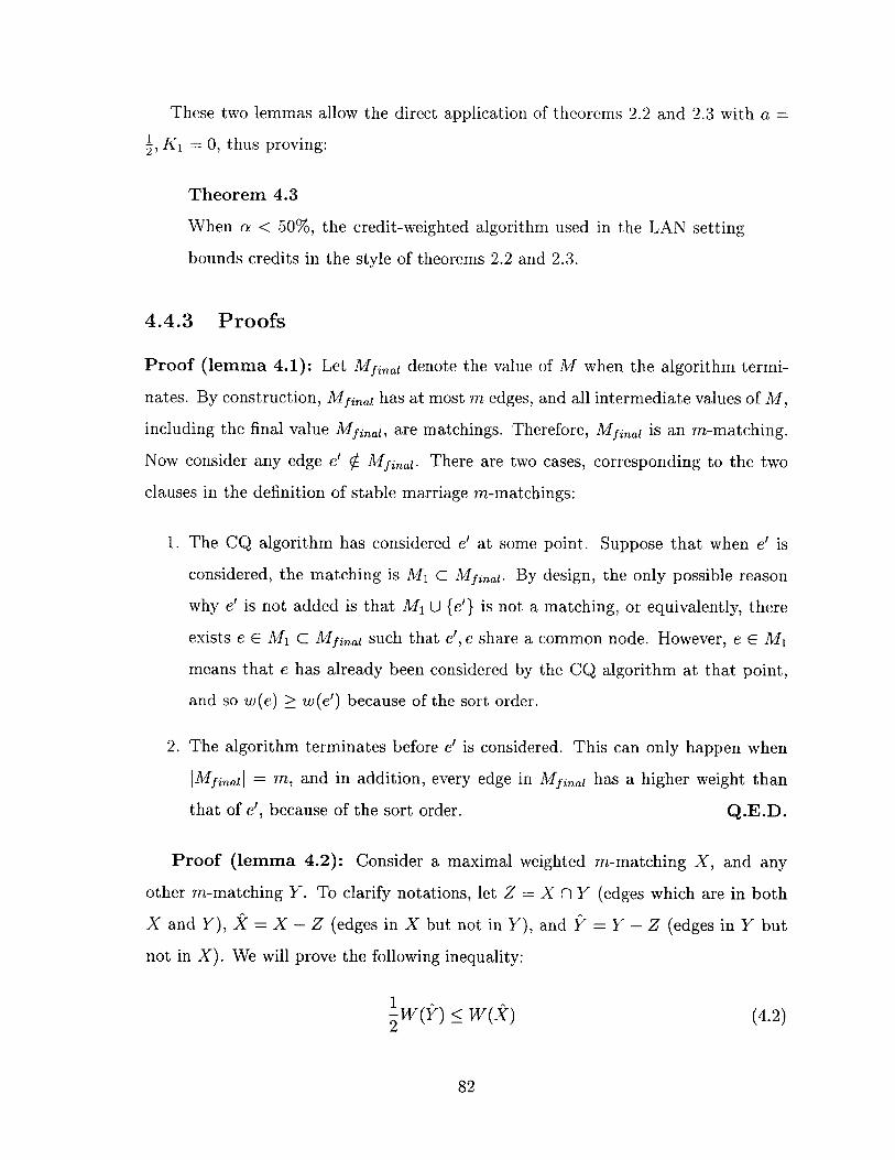
These two lemmas allow the direct application of theorems 2.2 and 2.3 with a =
, K 1 = 0, thus proving:
Theorem 4.3
When a < 50%, the credit-weighted algorithm used in the LAN setting
bounds credits in the style of theorems 2.2 and 2.3.
4.4.3 Proofs
Proof (lemma 4.1): Let Mfinal denote the value of M when the algorithm termi-
nates. By construction, Mfinal has at most m edges, and all intermediate values of M,
including the final value Mfinal, are matchings. Therefore, Mfinal is an m-matching.
Now consider any edge e' Mfinal. There are two cases, corresponding to the two
clauses in the definition of stable marriage m-matchings:
1. The CQ algorithm has considered e' at some point. Suppose that when e' is
considered, the matching is M, C Mfinal. By design, the only possible reason
why e' is not added is that M1 U {e'} is not a matching, or equivalently, there
exists e E Mi C Mfinal such that e', e share a common node. However, e E M
means that e has already been considered by the CQ algorithm at that point,
and so w(e) > w(e') because of the sort order.
2. The algorithm terminates before e' is considered. This can only happen when
IMfinall = rn, and in addition, every edge in Mfinal has a higher weight than
that of e', because of the sort order. Q.E.D.
Proof (lemma 4.2): Consider a maximal weighted m-matching X, and any
other m-matching Y. To clarify notations, let Z = X n Y (edges which are in both
X and Y), Z = X - Z (edges in X but not in Y), and Y = Y - Z (edges in Y but
not in X). We will prove the following inequality:
-W(Y) < W(X) (4.2)
82

Once the inequality is proven, we have
W(X) W()-+W(Z) (4.3)1-W(Y)+W(Z) (4.4)
1 1> -W(Y) + -W(Z) (non-negative edge weights) (4.5)
2 2_W(Y)+W(Z) 1
W -W(Y). (4.6)2 2
and we obtain the lemma by considering Y to be a maximum weighted m-matching.
To prove inequality 4.2, we have:
Case I: assume JXj < m. Then every edge eg e Y has a blocking edge in X
with weight greater than or equal to w(eg). Denote this blocking edge by block(eg).
Note: In case eg has two blocking edges both of equal or higher weight, we can
assume (without loss of generality) that each edge has a numeric unique identifier
(assigned arbitrarily, e.g., flow ID) and let block(eg) denote the one with a smaller
unique identifier.
Here are some simple properties of edges eg E $ and their blocking edges:
1. block(ef") E X and w(block(eg)) > w(eg), by definition.
2. block(eg) Y, because Y, being a matching, cannot contain both eg and
its blocking edge. Combining block(eg) E X and block(eg) V Y, we have
block(eg) E X - X n Y .
3. Any ek = (u, v) E X can only block at most two different edges in Y. This
is because Y is an rn-matching and contains at most one edge connecting to u
and at most one edge connecting to v.
Now let the edges of Y be explicitly listed as {ei, e2, ...ek}. We have:
w(ei) < w(block(ei))
w(e 2) < w(block(e 2))
w(ek) w(block(ek))
83

Summing up all equations, the sum of the left sides = w(ej)+...+w(e") = W(Y).
On the right sides, every block(ei) C X, and any edge in X can appear at most twice,
thus the sum of the right sides < 2 x W(X). (Note that this uses the assumption
that edge weights are non-negative.) This proves the required W(Y) 2W(X) for
the case of JXJ < m.
Case II: assume IX I = m. Let emin be the minimum weight edge in X (breaking
ties arbitrarily). Now every eg E Y either has a blocking edge block(eg) C X with
greater or equal weight (as in case I), or else w(eg) w(emin). Among the k edges of
Y, without loss of generality assume the first 1 edges have blocking edges with greater
or equal weights, and the remaining k - I edges do not. Then we have:
w(ei) < w(block(ei)), for i = 1, ..., 1.
w(ej) < w(emin), for j = 1 + 1, ... , k.
Let R denote the summation of the right sides, E w(block(ei))+i _g+ w(emin).
Compare it to the quantity 2 x W(X), written as an explicit summation of individual
edge weights containing 2|Z terms (each edge weight appearing twice because of the
factor of 2). We have:
1. Reasoning as in case I, every w(block(ei)) term in R appears as a term in
2 x W(X), since every block(e) E X and every edge in X can appear as
block(ei) at most twice.
2. By definition of emin as the minimum weight edge in X, any w(emin) term in R
is smaller than or equal to any term in 2 x W(X).
3. There are k terms in R, and 21Xi terms in 2 x W(X). We also have k = -Y
|Y| - |Z| m - |Zj (because Y is an m-matching) = IX| - IZI = |k| < 21±1.
In conclusion, there are more terms in 2 x W(X) than in R, and the terms are
correspondingly larger or equal. (Moreover, all terms are non-negative.) Thus R <
2 x W(±). Summing all inequalities then imply: sum of left sides = W(Y) < R <
2 x W(X) as required. Q.E.D.
84

4.5 LAN Schedulers - Simulation Evaluation
This section will evaluate the performance of our LAN schedulers in simulations.
Detailed description of our simulation methods are given in the last section of this
chapter. In brief, they are similar to those used in the last chapter on input-queued
switches, and in particular, in our simulations a flow is not allowed to transmit if its
credit is zero (i.e., zero-weight edges are dropped from the stable marriage matching),
even if some network capacity is wasted as a result. As in the previous chapter, this
choice is made because it represents a more stringent test on our schedulers.
4.5.1 Using C as edge weights
Table 4.1 shows the simulation results for the credit-weighted algorithm for constantly
backlogged traffic. As the table shows, although theorem 4.3 only guarantees Cf val-
ues are bounded when a < j, in simulations Cf are bounded even for a = 90%. Also,
although the theoretical bound is rather loose, in simulations the actual bounds are
very small. For a detailed explanation of our simulation methods, settings, stochastic
models, and exact meanings of all parameters, refer to the last section of this chapter.
Actual Running Time: In our simulations, the algorithm requires about 5-30
microseconds to compute each m-matching in software.3 One can reasonably expect a
hardware implementation to be several times faster, which would bring the algorithm
speed in line with the timeslot length of 2 microseconds in the B-service of DARPA
AON [27]. The running time is similar for all our algorithms reported in subsequent
sections.
Figure 4.2 shows some simulation results using the credit-weighted algorithm for
both backlogged and bursty traffic. For constantly backlogged traffic, the two algo-
rithms behave identically since bucket size restrictions only apply to idle flows. For
bursty traffic, our simulations use the same bucket size Bf for all flows (although
the algorithm allows different flows to have different bucket sizes). An entry with
3 The simulation is written as a stand-alone C program, compiled with the gcc compiler, and rununder Linux on a 500MHz processor.
85
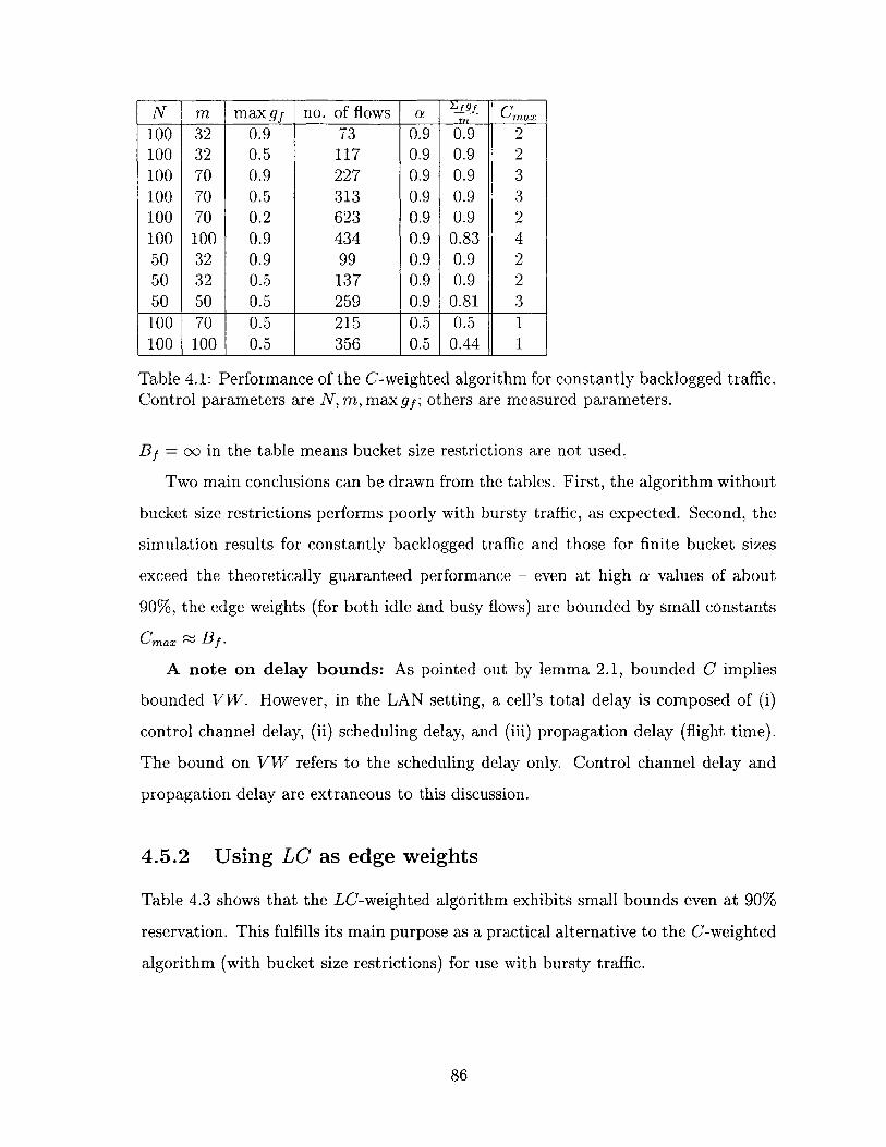
N m maxgf no. of flows a 'J9J Cmax100 32 0.9 73 0.9 0.9 2100 32 0.5 117 0.9 0.9 2100 70 0.9 227 0.9 0.9 3100 70 0.5 313 0.9 0.9 3100 70 0.2 623 0.9 0.9 2100 100 0.9 434 0.9 0.83 450 32 0.9 99 0.9 0.9 250 32 0.5 137 0.9 0.9 250 50 0.5 259 0.9 0.81 3
100 70 0.5 215 0.5 0.5 1100 100 0.5 356 0.5 0.44 1
Table 4.1: Performance of the C-weighted algorithm for constantly backlogged traffic.Control parameters are N, m, max g1 ; others are measured parameters.
Bf = oo in the table means bucket size restrictions are not used.
Two main conclusions can be drawn from the tables. First, the algorithm without
bucket size restrictions performs poorly with bursty traffic, as expected. Second, the
simulation results for constantly backlogged traffic and those for finite bucket sizes
exceed the theoretically guaranteed performance - even at high a values of about
90%, the edge weights (for both idle and busy flows) are bounded by small constants
Cmax x Bf.
A note on delay bounds: As pointed out by lemma 2.1, bounded C implies
bounded VW. However, in the LAN setting, a cell's total delay is composed of (i)
control channel delay, (ii) scheduling delay, and (iii) propagation delay (flight time).
The bound on VW refers to the scheduling delay only. Control channel delay and
propagation delay are extraneous to this discussion.
4.5.2 Using LC as edge weights
Table 4.3 shows that the LC-weighted algorithm exhibits small bounds even at 90%
reservation. This fulfills its main purpose as a practical alternative to the C-weighted
algorithm (with bucket size restrictions) for use with bursty traffic.
86

N m max gf no. of flows a f Traffic Bf Cmax LCmax100 70 0.9 227 0.9 0.9 backlogged irrelevant 3 3100 70 0.9 227 0.9 0.9 Bernoulli CWA 212 98100 70 0.9 227 0.9 0.9 Bernoulli 30 30 26100 70 0.9 227 0.9 0.9 Bernoulli 5 6 5100 70 0.9 227 0.9 0.9 Bernoulli 1 2 2100 70 0.9 227 0.9 0.9 2-state CWA 763 312100 70 0.9 227 0.9 0.9 2-state 30 30 28100 70 0.9 227 0.9 0.9 2-state 5 6 6100 70 0.9 227 0.9 0.9 2-state 1 3 3100 70 0.5 313 0.9 0.9 backlogged irrelevant 3 3100 70 0.5 313 0.9 0.9 Bernoulli 1 3 2100 70 0.5 313 0.9 0.9 2-state 1 3 3100 70 0.2 623 0.9 0.9 backlogged irrelevant 2 2100 70 0.2 623 0.9 0.9 2-state 30 30 12100 70 0.2 623 0.9 0.9 2-state 5 6 3100 70 0.2 623 0.9 0.9 2-state 1 3 2
50 32 0.9 99 0.9 0.9 backlogged irrelevant 2 250 32 0.9 99 0.9 0.9 2-state CWA 828 39850 32 0.9 99 0.9 0.9 2-state 5 6 5
Table 4.2: Performance of the C-weighted algorithm, for backlogged and bursty traf-fic. Control parameters are N, m, max gf and traffic type; others are measured pa-
rameters.
Table 4.3: Performance of the LC-weightedparameters are N, m, max gf and traffic type.
algorithm for burstyOther parameters are
traffic. Controlmeasured.
87
N m maxgf no. of flows a L Traffic LCmax
100 70 0.9 227 0.9 0.9 Bernoulli 12100 70 0.9 227 0.9 0.9 2-state 30100 70 0.5 313 0.9 0.9 Bernoulli 10100 70 0.5 313 0.9 0.9 2-state 22100 70 0.2 623 0.9 0.9 2-state 850 32 0.9 99 0.9 0.9 2-state 15100 70 0.5 215 0.5 0.5 2-state 5100 100 0.5 356 0.5 0.44 2-state 7
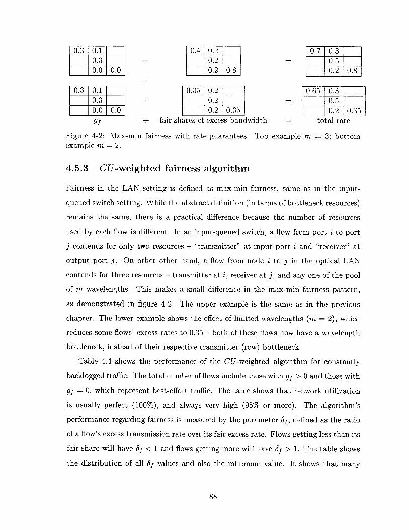
0.3 0.1 0.4 0.2 0.7 0.30.3 + 0.2 = 0.50.0 0.0 0.2 0.8 0.2 0.8
0.3 0.1 0.35 0.2 0.65 0.30.3 + 0.2 = 0.50.0 0.0 0.2 0.35 0.2 0.359f + fair shares of excess bandwidth total rate
Figure 4-2: Max-min fairness with rate guarantees. Top example m = 3; bottomexample m = 2.
4.5.3 CU-weighted fairness algorithm
Fairness in the LAN setting is defined as max-min fairness, same as in the input-
queued switch setting. While the abstract definition (in terms of bottleneck resources)
remains the same, there is a practical difference because the number of resources
used by each flow is different. In an input-queued switch, a flow from port i to port
j contends for only two resources - "transmitter" at input port i and "receiver" at
output port j. On other other hand, a flow from node i to j in the optical LAN
contends for three resources - transmitter at i, receiver at j, and any one of the pool
of m wavelengths. This makes a small difference in the max-min fairness pattern,
as demonstrated in figure 4-2. The upper example is the same as in the previous
chapter. The lower example shows the effect of limited wavelengths (m = 2), which
reduces some flows' excess rates to 0.35 - both of these flows now have a wavelength
bottleneck, instead of their respective transmitter (row) bottleneck.
Table 4.4 shows the performance of the CU-weighted algorithm for constantly
backlogged traffic. The total number of flows include those with gf > 0 and those with
gYf = 0, which represent best-effort traffic. The table shows that network utilization
is usually perfect (100%), and always very high (95% or more). The algorithm's
performance regarding fairness is measured by the parameter 6f, defined as the ratio
of a flow's excess transmission rate over its fair excess rate. Flows getting less than its
fair share will have 6f < 1 and flows getting more will have 6f > 1. The table shows
the distribution of all 6f values and also the minimum value. It shows that many
88

no. of total % of flows with f in these ranges:m max gj flows with no. of a Ef gf /m min 6f min 6f 0.7 0.85 0.95 Network
gj > 0 flows value to 0.7 to 0.85 to 0.95 or more Util.32 0.9 73 5000 0.9 0.9 0.984 100.0% 100.0%70 0.9 227 5000 0.9 0.9 0.857 1.9% 98.1% 100.0%70 0.5 313 5000 0.9 0.9 0.857 2.0% 98.0% 100.0%70 0.5 313 1000 0.9 0.9 0.975 100.0% 100.0%70 0.2 623 5000 0.9 0.9 0.888 3.8% 96.2% 100.0%70 0.5 213 5000 0.5 0.5 0.986 100.0% 100.0%
100 0.9 434 5000 0.9 0.83 0.168 1.7% 2.3% 2.7% 93.3% 95.1%100 0.5 356 5000 0.5 0.44 0.241 0.6% 1.2% 2.0% 96.2% 97.9%
Note: In all cases reported in this table, N = 100.
Table 4.4: Performance of the CU-weighted algorithm for constantly backlogged traf-fic. Control parameters are N, m, max gf and total no. of flows. Other parametersare measured.
flows (at least 93% of them) obtain at least 95% of their fair shares. However, a small
fraction of flows are treated very unfairly (small 6f) under some settings, because of
the greedy and heuristic nature of the algorithm.
4.6 Extensions to Multiple Transceivers
So far we have assumed that each node has only one transmitter and one receiver.
If some nodes have more than one transceiver, the transmission constraints will no
longer be an m-matching. For instance, a node with three transmitters and five
receivers can simultaneously transmit three cells and receive five cells.
The CQ algorithm can easily be generalized to handle any arbitrary transmission
constraints. Again all flows are sorted by weight (C, LC, VW, CU, etc.) and the
algorithm goes through all flows in one pass, choosing greedily without backtracking.
The set X begins empty, and a flow f is added to it if the new set X U {f} will not
violate any transmission constraints. We conjecture that the set X calculated by CQ
will still have at least 1 the maximum weight of any set of flows which obeys the2
constraints. If this conjecture is true, it can be applied to prove theorems 2.2 and 2.3.
With multiple transceivers per node, it may be possible for a flow to transmit two
or more cells in one timeslot, depending on the exact implementation and queuing
discipline employed at the nodes. If this is possible, the set X must allow repeated
occurrences of the same flow i.e., X must be a multi-set and the feasible service vector
89

can contain entries Sf(t) > 1. Also, the CQ algorithm must be slightly modified in
one of two ways. The first way is that after a flow is added to X, the flow must have
its new priority calculated and then reinserted at the correct place in the sort order,
so that it is possible to consider it again later in the scan through the flows. The
second way is that each flow is still considered only once, but when it is considered
it is added to X as many times as possible.
4.7 Distributed Scheduling for Metro-Area Net-
work
We will now briefly outline a distributed scheduler for an optical metro-area network
(MAN). This section will mainly be concerned with the description of the problem
and the schedulers, showing how our algorithmic ideas can be adapted to a distributed
setting. Simulation results from our previous works [26, 24] will also be presented in
a summary form.
4.7.1 Network Model
Architecture. Let N denote the overall number of end nodes as before. The N
nodes are grouped into K LANs and each node is connected to its LAN hub. The K
LAN hubs are then connected to a metro area network (MAN) hub. The nodes are not
connected to each other or to the MAN hub directly. Each connection employs a pair
of fibers so that communication can proceed in both directions without interfering
with each other. All propagation delays are assumed to be known integral number
of timeslots, and we will use Aj to denote the delay (in number of timeslots) from
node i (1 < i < N) to its LAN hub, and A' (1 < k < K) to denote the delay
from LAN hub k to the MAN hub. This connection architecture is similar to the
LAN/MAN connections in the existing AON testbed [27]. The connections are all-
optical; there are no opto-electric conversions and no buffering/queueing inside the
network. Queues only exist at the nodes in the LAN, i.e., at the network boundaries.
90

wavelength routerA1 A2 A3
Al
A2
A3
Wavelength routing by classfrom one LAN to others
(There are K=4 LANs, and thereforeK-1=3 routed wavelength classes.)
wavelength router
A, A2 A3 A, A2 A3destined to coming from
other LANs other LANs
AO AI A2 A3 ----- ~- one
CD CDOTs LAN
Data flow in a routed network(Control flow not shown)
Figure 4-3: Wavelength routed network
For simplicity we assume each node has 1 transmitter and 1 receiver; extensions to
more transmitters or receivers can be handled as described in section 4.6.
Various devices can be used in each hub, such as broadcast stars, wavelength
routers or switches. This chapter considers a specific network with splitters and
broadcast stars at the LAN hubs, and a single K-port wavelength router at the MAN
hub. Each port of the router is connected to a different LAN.
Wavelength Classes. The wavelengths supported by the entire system are par-
titioned into one local class, AO, plus K - 1 routed or remote classes A1 , A2 , ... , AK-1-
Local wavelengths (Ao) are only used inside each LAN; they are not present at the
MAN hub or along the LAN-MAN links. Remote wavelengths are routed by the MAN
hub as follows: any AP wavelength (1 < p K - 1) entering port k (i.e., coming
from LAN k) will be routed through port 1 to LAN 1 where 1 = k + p mod K. A
more intuitive description is that A1 wavelengths will be routed down 1 port (e.g.,
port 1 to port 2, port 4 to port 5) and A2 wavelengths will be routed down 2 ports,
etc., with wrap-around at the Kth port. See figure 4-3. If a certain A E AP is re-
ceived at two ports ki, k2 at the same time, the two transmissions are routed to ports
11 = k, + p mod K and 12 = k2 + p mod K simultaneously without any interference.
We assume the wavelength classes are constants, i.e., we do not consider the
problem of re-configuring wavelengths based on very slowly-changing traffic patterns,
91
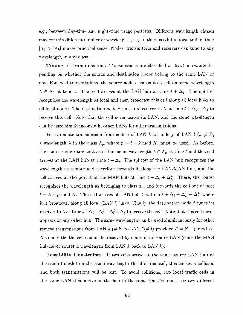
e.g., between day-time and night-time usage patterns. Different wavelength classes
may contain different number of wavelengths, e.g., if there is a lot of local traffic, then
IAol > jAki makes practical sense. Nodes' transmitters and receivers can tune to any
wavelength in any class.
Timing of transmissions. Transmissions are classified as local or remote de-
pending on whether the source and destination nodes belong to the same LAN or
not. For local transmissions, the source node i transmits a cell on some wavelength
A c AO at time t. This cell arrives at the LAN hub at time t + Aj. The splitter
recognizes the wavelength as local and then broadcast this cell along all local links to
all local nodes. The destination node j tunes its receiver to A at time t + A + Aj to
receive this cell. Note that the cell never leaves its LAN, and the same wavelength
can be used simultaneously in other LANs for other transmissions.
For a remote transmission from node i of LAN k to node j of LAN 1 (k : 1),
a wavelength A in the class AP, where p = 1 - k mod K, must be used. As before,
the source node i transmits a cell on some wavelength A E AP at time t and this cell
arrives at the LAN hub at time t + Aj. The splitter of the LAN hub recognizes the
wavelength as remote and therefore forwards it along the LAN-MAN link, and the
cell arrives at the port k of the MAN hub at time t + Aj + A'. There, the router
recognizes the wavelength as belonging to class AP, and forwards the cell out of port
1 = k + p mod K. The cell arrives at LAN hub 1 at time t + Aj + A' + A' where
it is broadcast along all local (LAN 1) links. Finally, the destination node j tunes its
receiver to A at time t+A,+A +Af + A to receive the cell. Note that this cell never
appears at any other hub. The same wavelength can be used simultaneously for other
remote transmissions from LAN k'( k) to LAN l'(A 1) provided ' = k' + p mod K.
Also note the the cell cannot be received by nodes in its source LAN (since the MAN
hub never routes a wavelength from LAN k back to LAN k).
Feasibility Constraints. If two cells arrive at the same source LAN hub at
the same timeslot on the same wavelength (local or remote), this causes a collision
and both transmissions will be lost. To avoid collisions, two local traffic cells in
the same LAN that arrive at the hub in the same timeslot must use two different
92

wavelengths A', A2 c A0 . This is the same wavelength constraint as in previous
sections. Additionally, two remote traffic cells from the same LAN k destined to the
same LAN 1 and which arrive at the source LAN hub k in the same timeslot must
use two different wavelengths A', A2 E Ap. (Note that two such remote cells will be
simultaneous at the MAN hub and the destination LAN 1 hub also, since they face
the same LAN-MAN delays of Al + Af'.)
Consequently, the wavelength constraint of the overall network is that: at any
given timeslot, for any given LANs k and 1, there can be at most JAol local cells
passing through hub k, and at most JAp| remote cells passing through hub k destined
to hub l(= k + p mod K). This, together with the usual transmitter and receiver
constraints, constitute the feasibility constraints of this network.
Two cells arriving at their source LAN hubs at different times will never collide.
In this way, cells transmissions are pipelined along each link, and a link (between
node and LAN hub, or a LAN-MAN link) carries many in-flight cells staggered by
timeslots and multiplexed by different wavelengths (for each timeslot).
Control Channel. We assume a separate control channel where each LAN sched-
uler receives queue lengths information from all nodes and broadcasts schedules back
to all nodes, and where the MAN scheduler receives queue lengths information from
the LAN schedulers and broadcasts schedules back to them. Because of propagation
delays and also because of capacity limits on the control channel, schedulers cannot
have up to date information about the queue lengths at the nodes. Nevertheless,
our schedulers just use whatever delayed queue length information they have. To
reduce the information flow on the control channel, we follow the guiding principle of
minimum information sharing (or "need-to-know" basis). Each LAN scheduler only
knows the queue lengths of (local and remote) flows originating from the LAN, and
the MAN scheduler only knows the queues lengths of remote flows. Thus, no sched-
uler has a global picture of changing traffic conditions. However, we do assume the
MAN scheduler knows the existence of every flow (local or remote) and each flow's
gf, if any; both of these are "static" information available during flow setup.
93

4.7.2 Distributed master-slave schedulers
We will employ one scheduler at each LAN hub, plus a master scheduler at the
MAN hub. Together, they will compute feasible schedules in a distributed fashion.
Although local and remote flows use different wavelength classes, they share the same
transmitters and receivers, e.g., a remote cell and a local cell cannot be scheduled to
arrive at a destination node at the same timeslot because the single receiver at the
node cannot receive both cells. Therefore, a method must be found to ensure that
the remote transmissions scheduled by the MAN scheduler do not conflict with the
local transmissions scheduled by the LAN schedulers.
Our approach is to use the schedulers in a master-slave arrangement. Conceptu-
ally, in a first phase, the MAN scheduler chooses a set of remote cells that will pass
through the MAN hub at time t. This will be called the remote traffic set RTS(t).
The MAN scheduler then notifies each LAN scheduler k of the subset of RTS(t) cells
whose source or destination node is in LAN k. Obviously, all this must occur at a
time much earlier than t so that the information can propagate back to the nodes in
time for transmission allowing the cells to arrive at the MAN hub at time t. The exact
timing will be discussed shortly. Because of the 1-transmitter-per-node constraint, at
most 1 cell of RTS(t) can originate from each node, and similarly, at most 1 cell of
RTS(t) can be destined to each node because of the receiver constraint. Moreover,
between any source LAN k and destination LAN 1, at most IAl-k mod K' cells can be
in RTS(t) due to the wavelength constraint.
In a conceptual second phase, each LAN scheduler k chooses a set of local cells
that will pass through its LAN hub at time t'. This will be called the local traffic
set LTSk(t'). By design of our algorithm, this computation is made only after the
MAN scheduler has notified LAN scheduler k of all remote cells that may conflict
with LTSk(t') cells. More precisely, due to the transmitter constraint, if a remote cell
in RTS(t'+AL) comes from node i in LAN k, it means transmitter i will used for this
remote cell at time t' - AZX, and consequently, this remote cell is the only cell from i
that can arrive at the LAN k hub at time t'. In other words, if cell c E RTS(t'+ Ak)
94

comes from node i of LAN k, then LTSk(t') cannot contain any local cell from node
i. Similarly, if cell c E RTS(t' - A') is destined for node j of LAN k, then LTSk(t)
cannot contain any local cell destined to node j - otherwise a remote cell and a local
cell would arrive at the destination node j at the same time t'+ Aj (on two different
wavelengths, one local and one remote) and the single receiver cannot receive both.
In addition to these constraints from RTS(t' ± AL) cells, the LTSk(t') cells must
also satisfy its own transmitter, receiver and wavelength constraints: at most 1 cell
from each node, at most 1 cell destined to each node, and the number of local cells
ILTSk(t')| cannot exceed the number of local wavelengths |Ao|.By this design, the MAN scheduler chooses RTS cells without regard to local
traffic. Each LAN scheduler chooses LTS cells after learning the RTS cells that
might affect its choice. A LAN scheduler is not allowed to override decisions made
by the MAN scheduler. The exact timing of these RTS and LTS computations
is flexible so long as (1) the RTS and LTS are computed early enough to enable
in-time schedule dissemination to nodes on the control channel, and (2) each LTS
computation is only made after relevant RTS schedules have been received by the
LAN scheduler. In particular, the two conceptual phases do not happen consecutively
in real time, and for a given value of t', the K computations of LTSk(t') of different
LANs can occur at different times. When computing RTS and LTS, each scheduler
uses whatever delayed queue lengths information it has at its disposal, so the queue
lengths information is only slightly delayed at the LAN schedulers, but considerably
more delayed at the MAN scheduler. Thus local traffic does not suffer the long access
delay caused by remote scheduling. 4
4.7.3 LAN scheduler
The LAN scheduler obtains delayed queue lengths information from all the nodes
within the LAN about all flows (local and remote) that originate inside the LAN.
4Preliminary simulations show that for small networks, a centralized scheduler, e.g., at the MANhub, performs slightly better in terms of fairness. However, in this case even local transmissionsmust be scheduled by a remote scheduler, thereby increasing local cells' access delay considerably.That is why we do not pursue centralized schedulers in MANs in this study.
95

It reports queue lengths of remote flows to the MAN hub. It also keeps track of
credits (or LC or VW or whatever weight is being used) for all local flows. However
it does not track credits for remote flows originating at its LAN, nor does it know the
existence of flows in other LANs.
The LAN scheduling algorithm is basically the same as before: a CQ algorithm
is used and local flows are sorted by weights, and the scheduler tries to add each
flow to the service vector in a greedy (non-back-tracking) fashion, while maintaining
the feasibility constraints. The only difference is that, the CQ algorithm cannot
cannot start with an empty matching, but instead it must start with the knowledge
that certain transmitters and receivers are already booked by the MAN scheduler's
respective RTS.
4.7.4 MAN scheduler
The MAN scheduler obtains delayed queue lengths information about all remote flows
from their respective source LANs and also keeps track of credits for all the remote
flows. However it does not know the queue lengths nor track credits of any local flows.
The MAN scheduling algorithm is essentially the CQ algorithm with a simple
rate matching mechanism added. For the moment, suppose the MAN scheduler
knows the exact max-min-fair rates of each flow, and therefore knows what frac-
tion of each transmitter and receiver should be used by local traffic if perfect fairness
were achieved. It then imposes that fraction as a constraint on itself. More specifi-
cally, suppose transmitter i should be used by local traffic a fraction Oi of the time
when all flows achieve their max-min fair rates. Then the MAN scheduler tracks a
variable TransmitterPermiti, which is incremented by 1 - Oi every timeslot. Simi-
larly, if receiver j should be used by local traffic a fraction #f of the time, then the
ReceiverPermit variable is incremented by 1- q$ every timeslot. The key step of the
algorithm is still greedy: all remote flows are sorted by weights and chosen greedily
in one pass. However when a flow is considered, in addition to checking the avail-
ability of the transmitter, receiver, and a wavelength (in the appropriate class), the
algorithm also checks whether TransmitterPermiti > 1 and ReceiverPermit, > 1.
96

If so the flow is scheduled and TransmitterPermiti and ReceiverPermit, are both
decremented by 1, otherwise the flow is skipped as if it violates some constraints.
Note that TransmitterPermit can be spent (decremented) by any remote flow that
uses transmitter i, i.e., Transmitter Permits are not earmarked for particular flows,
instead they are simply a rate-matching device. (In contrast, credits are per-flow
variables and can only be spent by the flow that owns them.)
It can be easily seen that with this rate-matching scheme, in the long run, the
fraction of transmitter i devoted to remote traffic is at most 1 - Oi, and so local traffic
gets at least a fraction of 02 as deserved. In other words, the MAN scheduler exercises
self-imposed rate-based constraints when computing its schedule, so that the LAN
schedulers can have their fair share. Such a rate-control mechanism is necessary in
the MAN scheduler because no scheduler ever compares remote flows' weights to local
flows' weights. (Indeed no scheduler tracks credits for both local and remote flows.)
Therefore, in the absence of a rate-control scheme, remote flows (which are scheduled
first by the MAN scheduler) will simply have absolute priority over local flows and
hog the transceivers that they share, regardless of relative credits between remote
and local flows.
Ideally, 0, and Oj values are computed from max-min-fair rates, which require an
iterative algorithm. We have found that a simple approximation does quite well in
simulations. Our algorithms estimates a local flow's fair excess rate as the smallest of
excess transmitter bandwidth excess receiver bandwidth and excess wavelength bandwidth in its LAN
#flows sharing transmitter ' #flows sharing receiver #f lows in its LAN
(By excess bandwidths we mean the portion after guaranteed rates are accounted
for.) Each 0; then equals the sum of fair excess rates of all local flows from node i,
and similarly each Oj equals the sum of fair excess rates of all local flows destined
to node j. Note that the MAN scheduler can make these calculations with only the
"static" knowledge of flows' existence and their gf.
As preliminary simulations show, however, the distributed scheme as described
is not perfect, and credits can become unbounded. To fix this problem, we added
exception handling as follows: If a local flow finds itself going substantially below
its guarantee (large Cf), then it can raise a flag (including its Cf value) on the next
97

report to the MAN scheduler, which will then preemptively reserve the required trans-
mitter/receiver for the LAN. Similarly, if a remote flow finds itself going substantially
below its guarantee, then the scheduler will schedule it regardless of whether there are
Transmitter and Receiver Permits available - in this case, TransmitterPermiti and
Receiver Permitj are still decremented even if they are less than 1, so that negative
values will be achieved. Admittedly this exception handling is an ad hoc improve-
ment, but in simulations it improves both credit bounds and fairness.
4.7.5 Simulations Summary
In [26, 24] we published some simulations results for the distributed scheduler. For
length reasons we will only summarize them here. In our simulations, there are
K = 3 LANs and the LAN-to-MAN propagation delays are 30, 50 and 70 timeslots
respectively, while the node-to-LAN-hub delays are all equal to 4 timeslots. Each
LAN has 50 nodes, for a total of N = 150. The local wavelength class has |Aol 20
wavelengths and each of the two remote wavelength classes has |A1| = 1A21 = 10
wavelengths. We tried various settings of 2000-3000 flows, distributed between local
and remote flows in different ways, with both backlogged and bursty traffic, and with
various random distributions of gf. The main results are that the credit bounds are
only slightly larger than those reported in section 4.5 for the LAN-only scenario,
total system throughput is 97-100%, and an approximate max-min fair pattern is
again established. We also measured our algorithm's actual running time at about
5-30 microseconds for each LTS calculation (i.e., same as in the LAN-only scenario)
and about 10-50 microseconds for each RTS calculation. Hardware optimizations
will likely bring them in line with timeslot lengths of a few microseconds.
4.8 Chapter Summary
In this chapter, we described several LAN schedulers based on the CQ algorithm and
with various choices of edge weights. We introduced a definition of stable marriage
m-matchings and proved that the C-weighted algorithm bounds credits at a < 50%
98
in the style of theorems 2.2 and 2.3. We also evaluated the LC-weighted and CU-
weighted LAN schedulers in simulations, and showed that our algorithms work well
at reservation levels of 90% of capacity, with small credit and delay bounds, even for
bursty traffic.
Finally, we also described how our algorithmic ideas can be used in a distributed
fashion in a wavelength-routed LAN/MAN network. The key idea in that case is
that the MAN scheduler (master) computes its part of the schedule first and then
tells the LANs of its decisions, and the LAN schedulers (slaves) cannot override the
MAN scheduler. To prevent the MAN scheduler from hogging resources, it exercises
self-imposed rate-matching constraints. Aside from these rate-matching mechanisms,
both schedulers are greedy algorithms similar to those used in the LAN-only scenario.
4.9 Simulation Settings
4.9.1 Outline of a control protocol
Due to length considerations, we only give a very brief outline of a sample control
protocol here, as a proof of feasibility.
Our control protocol is based on round-robin polling/reporting. Suppose the
scheduler resides at the central broadcaster. We assume a separate control wave-
length, with associated fixed-tuned inexpensive transceivers, for nodes to report their
queue length or arrival information to the scheduler. The N nodes report in fixed
round-robin fashion, and each node's report contains all the queue lengths of all flows
originating at that node. Suppose a cell contains 1000 bits (slightly more than two
ATM cells). If each node is the source of about 50-100 flows, it can include all these
flows' queue lengths in a single "report cell," listing all queue lengths without includ-
ing flow IDs since the IDs are known to the scheduler on flow setup. So, each node
can send one report cell every N timeslots. Therefore, a data cell's control protocol
delay may range from 1 to N timeslots (plus node-scheduler flight time) depending
on when it arrives compared to the next queue length report from its source.
99
The controller disseminates the schedules by broadcasting each m-matching in a
second control wavelength. In a typical case of 16-bit flow IDs, and m = 30 data
wavelengths, an m-matching can be specified using 480 bits or just one 1000-bit
"schedule cell." By convention, the first listed flow uses wavelength A,, the second
flow uses A2 , etc.
Assuming the broadcast network is installed in a LAN with physical dimension of
about a kilometer, the flight time is about 5 microseconds. With a timeslot of about
1 microsecond (1000 bits at 1 Gbit/second), the flight time is about 5 timeslots.
In simulations we used propagation delays of 0 to 20 timeslots, and different nodes
may have different propagation delays. We have disregarded small buffer zones used
around timeslots for synchronization and transceiver-tuning purposes, see [27] for a
similar example.
4.9.2 Stochastic models for flow and traffic generation
Parameters used in our simulations are divided into two categories - control pa-
rameters which are chosen manually, and measured parameters which measure the
algorithms' performance under the chosen setting. The following are the control
parameters in each simulation:
" N, the number of nodes.
" m, the number of wavelengths (for data transmissions, excluding control wave-
lengths).
" Total duration of simulation (not reported). Typically this is 10000 to 100000
timeslots.
* The number of flows that request rate guarantees (not reported). Each flow's
source and destination nodes are chosen randomly, independently and uniform-
ly among the N nodes. There may be several flows with the same source-
destination pair. A flow's rate gB is generated as explained in the next two
100
items. flows which are denied any rate guarantee (i.e., gf = 0) are not reported
in bandwidth reservation simulations.
* max gf, the maximum guaranteed rate. Each flow's guaranteed rate gf is gener-
ated independently and uniformly distributed in the range [-, max gj]. (How-
ever, see the next item.)
* Omax, the maximum reservation factor (not reported). The simulations generate
gf values one by one, considering the flows one by one in some random order.
When a flow is considered, if its (newly-generated) guaranteed rate, when added
to other guaranteed rates already generated, will exceed reservation factor amax,
then its guaranteed rate is set to zero instead. In bandwidth reservation simula-
tions, this flow has essentially disappeared, and therefore they are not reported
in the "no. of flows" column in those simulations. In fairness simulations, this
flow now represents best-effort traffic with no reservations. In our simulations
we set amax at 50% or 90%. The actual reservation factor a(< armax), and
the actual number of flows with non-zero rate guarantees are measured (and
reported) when all gf values have been generated in this manner.
* Traffic type. We used three different types of traffic:
1. Constantly backlogged traffic.
2. Bernoulli traffic (also known as I.I.D. or memoryless traffic): In each times-
lot (independently) one cell arrives with probability af, otherwise no cell
arrives. Each flow's arrival rate af is chosen to equal its guaranteed rate
g1 . The flows' arrival processes are independent of each other.
3. 2-state traffic: Each flow is described by a 2-state Markov chain. The two
states are called bursting and resting. While in the bursting state one cell
arrives every timeslot, and while in the resting state no cell arrives. Each
flow has its own state and changes states independently of other flows. In
this model, each flow's state transition probabilities are determined by its
arrival rate af (chosen to equal its gf) and the average burst length. In
101
our simulations, all 2-state flows have an average burst length of 20 cells
regardless of arrival rates. (In contrast, a Bernoulli process of rate af has
an average burst length of 1, which is typically one to a few cells in
most of our simulations.)
In any simulation, all flows have the same traffic type. We did not choose any
scenario where the arrival rate exceeds the guaranteed rate because, in such a
scenario, all flows will simply become constantly backlogged in the long term.
Also we did not choose any scenario where the arrival rate is less than the
guaranteed rate, because that does not represent a stringent test condition for
our algorithms.
* Node-to-broadcaster propagation delay (not reported). Our simulations use
propagation delays of 0-20 timeslots, with different nodes having different de-
lays. We found that propagation delays of this magnitude have negligible effect
on the performance of our algorithms in simulations. Therefore, we did not
include the propagation delay parameters explicitly in the figures.
For any choice of control parameter values, the whole simulation is repeated many
times - typically 30-100 times. Then various parameters are measured. The following
are the measured parameters in our bandwidth reservation simulations. (Unless oth-
erwise stated, all measured parameters are averaged over the 30-100 repeated runs.)
" a, the reservation factor. Note that a < amax by our method of generating
flows and their guaranteed rates. Typically, however, we use a large enough
number of flows that we observe a = amax-
" Mf , the wavelength reservation factor. This measures the fraction of the
network's "nominal" total bandwidth of m cells/timeslot that has been reserved.
(Note that Zg is one component of a by definition.)
* Cmax, the observed bound on unspent credits Cf (t). This bound is the maximum
value across all flows, all timeslots, and all repeated runs.
102

" LCmax, the observed bound on LCf(t) = min(Cf(t), Qf(t)). This bound is the
maximum value across all flows, all timeslots, and all repeated runs.
" The number of flows with non-zero rate guarantees.
The following additional parameters are used in our fairness simulations:
* 6f, the ratio of a flow's excess transmission rate (measured over the simulation
duration) divided by its fair excess rate (computed off-line using an algorithm
described in [4]). Flows getting less than its fair share will have 6f < 1 and
flows getting more will have 6f > 1. We measure the distribution of all 6f values
of all flows (over all repeated runs). We also measure the minimum 6f value
among all flows in all repeated runs.
" Total network utilization. This is the total number of transmissions (guaranteed
or not) divided by the total possible, which is mx duration of simulation. (To-
tal utilization is only measured in fairness simulations because our bandwidth
reservation algorithms are designed to only serve guaranteed traffic.)
" The total number of flows (control parameter), including those with non-zero
rate guarantees, and those with zero rate guarantees (i.e., best-effort flows).
103

Chapter 5
Optical Distribution Tree
This chapter considers another optical network which has fundamentally different
feasibility constraints compared to the previous two chapters.
The optical LAN and MAN of chapter four use fast tuneable transceivers and are
designed for all-to-all traffic. In contrast, this chapter studies an aggregation/distribution
network which has all-to-one and one-to-all traffic, where some nodes use fixed-tuned
(i.e., non-tuneable) transceivers. These differences in hardware and in traffic assump-
tions lead to different feasibility constraints. Consequently, the algorithms used will
be different, and so are the theoretical results. In particular we are able to prove that
up to 100% reservation level can be supported (a < 1). However, this result requires
a slower algorithm. We therefore also investigated several faster algorithms which
either works for certain special tree networks, or works for a general tree network but
only supports up to 50% reservation (a < }).
5.1 Background and Motivation
A DARPA sponsored research consortium (called ONRAMP 1 ) comprising the Mas-
sachusetts Institute of Technology, AT&T, Nortel, Cabletron, and JDS Fitel was
formed in 1998 to develop new architectures and technologies for the Next Gener-
'Next Generation Internet - Optical Network for Regional Access with Multiwavelength ProtocolsConsortium.
104
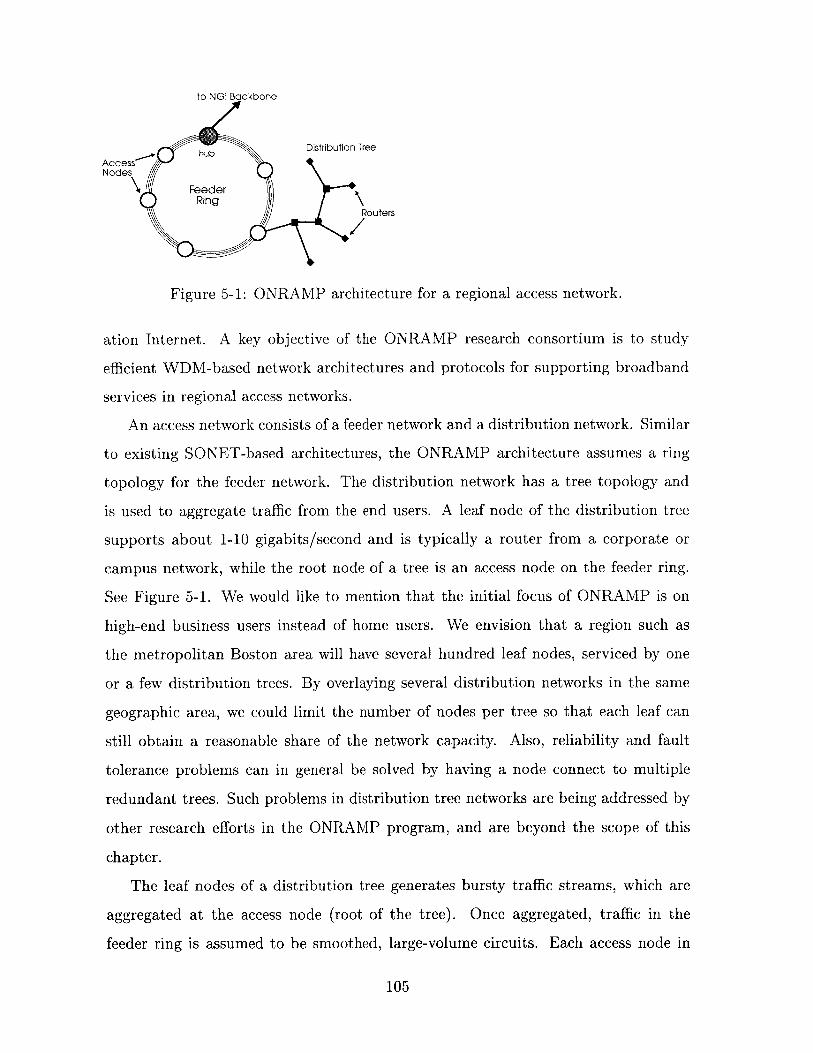
to NGI Backbone
Access hub Distribution Tree
Nodes
FeederRing
Routers
Figure 5-1: ONRAMP architecture for a regional access network.
ation Internet. A key objective of the ONRAMP research consortium is to study
efficient WDM-based network architectures and protocols for supporting broadband
services in regional access networks.
An access network consists of a feeder network and a distribution network. Similar
to existing SONET-based architectures, the ONRAMP architecture assumes a ring
topology for the feeder network. The distribution network has a tree topology and
is used to aggregate traffic from the end users. A leaf node of the distribution tree
supports about 1-10 gigabits/second and is typically a router from a corporate or
campus network, while the root node of a tree is an access node on the feeder ring.
See Figure 5-1. We would like to mention that the initial focus of ONRAMP is on
high-end business users instead of home users. We envision that a region such as
the metropolitan Boston area will have several hundred leaf nodes, serviced by one
or a few distribution trees. By overlaying several distribution networks in the same
geographic area, we could limit the number of nodes per tree so that each leaf can
still obtain a reasonable share of the network capacity. Also, reliability and fault
tolerance problems can in general be solved by having a node connect to multiple
redundant trees. Such problems in distribution tree networks are being addressed by
other research efforts in the ONRAMP program, and are beyond the scope of this
chapter.
The leaf nodes of a distribution tree generates bursty traffic streams, which are
aggregated at the access node (root of the tree). Once aggregated, traffic in the
feeder ring is assumed to be smoothed, large-volume circuits. Each access node in
105

the feeder ring has both WDM wavelength routing and electronic switching capabili-
ties. The ONRAMP access network architecture is designed such that the aggregated
bandwidth can scale to multi-terabit/second.
A distribution tree typically has many more leaf nodes (e.g., 200) than wave-
lengths (e.g., 32-64), and different leaves may have widely different traffic volumes
which change dynamically. The ONRAMP architecture is designed to support users
with heterogeneous bandwidth and bursty traffic requirements, where the traffic de-
mand between different users can differ by several order of magnitudes. Specifically,
our model allows a leaf node to use one or more fixed-tuned or tunable transceiver;
moreover, different leaf nodes can support different subsets of wavelengths depending
on their expected traffic volumes. The purpose of our schedulers is to enable the
leaves of a distribution tree to share the available wavelengths dynamically based on
changing traffic demands.
5.2 Problem Model
5.2.1 Distribution Tree Architecture and Hardware
The distribution network has a tree topology and is used to aggregate traffic from the
end users. The root of the tree is an access node connecting the tree to the feeder
network, and each leaf is typically a router from a corporate or campus network
supporting several gigabits/second.
An advantage offered by a tree topology is that there is exactly one path from
any node to any other node; in other words there is no routing issue. In future
metropolitan-area distribution networks, we believe there will be much more inter-
network traffic than intra-network traffic. Thus in this paper we will assume the
following "hubbed traffic" model - that all traffic either goes from a leaf to the root
(upstream) or from the root to a leaf (downstream). See Figure 5-2. If two leaf nodes
in a tree want to communicate with each other, they must go through the root as if
they belong to different distribution networks. This assumption simplifies the data
106

UPSTREAM_
FEEDERRING
DOWNSTREAM
N Internal Node = Broadcaster/Combiner/Amplifier
]I Leaf = Corporate/Campus Router
Root = Access Node
Figure 5-2: Upstream/downstream traffic in a distribution tree.
transmission protocols considerably and, as we will explain shortly, also reduces the
transceiver component costs. (Note that this assumption does not affect traffic that
stays within the same campus, for example. Such traffic never enters the distribution
tree in the first place because the entire campus may be represented by just one leaf.)
In a distribution tree, each link represents a pair of unidirectional optical fibers,
one upstream and one downstream. The fibers support a set of m wavelengths as
parallel channels. Two data transmissions on the same wavelength along the same
section of fiber result in a collision, and both transmissions will be lost. The root has
an array of m fixed-tuned transmitters each tuned to a different wavelength, and a
similar array of m fixed-tuned receivers.
Each leaf is equipped with one or more transmitters, and each transmitter may be
either fixed-tuned to a particular wavelength, or it may be fully-tuneable to all wave-
lengths (with negligible tuning latency). Different leaves can transmit on different
subsets of wavelengths (of different cardinality) depending on their expected traffic
volumes. For example, a low-traffic router might be equipped to support (transmit
on) only one wavelength, i.e., it has one fixed-tuned transmitter, while a busy web
server might support multiple wavelengths - by having several fixed-tuned transmit-
ters or even fully-tuneable transmitters
Each leaf is also equipped with receivers, and these can be fixed-tuned or fully-
107

tunable just like the transmitters. A leaf can transmit on one wavelength subset
and receive on a different wavelength subset. Differentiating leaves based on traffic
volumes allow us to reduce the transceiver component costs by equipping low-traffic
leaves with one or a few cheap fixed-tuned transceivers. Note that all this flexibility
is enabled by the hubbed traffic assumption, since leaves do not have to communicate
directly with each other and so two leaves do not need to have common wavelengths.
The intermediate nodes of a distribution tree are simple optical devices that (i)
broadcast the signal downstream, (ii) combine signals upstream, and (iii) amplify the
signals as necessary.
Time-slotting and Pipelining. To simplify scheduling, we assume time is
slotted and data are sent in fixed-sized cells. In a typical scenario, each wavelength
carries 10 Gbit/sec, and a cell contains 4 Kbytes (32 Kbits, 3.2 microseconds). In
practice, small guard times must be added between cell transmissions, so a time slot
is about 4-5 microseconds. In a metropolitan-area distribution network, the distance
between a leaf node and the root (access node) is about 10 kilometers, corresponding
to a propagation delay of about 50 microseconds. Thus, about 10 cells can be in flight
in a pipelined fashion, on any single wavelength at any given time. As transmitters
are located at the various leaves at various distances from the root, they must be
synchronized so that transmitted cells arrive at the root respecting the root's time-slot
boundaries. Different leaves will thus be time-shifted by different amounts compared
to the root and one another.
5.2.2 Problem Statements
Given the above setting, downstream traffic is a simple broadcast, with the proper
leaf receiving at the correct wavelength at the correct time. So there is no contention
issue in receiving traffic, and we will not discuss downstream traffic any further in this
chapter. Upstream traffic, however, faces possible contention and must be coordinated
to avoid (or recover from) collisions.
Problem 1 - Wavelength Contention. The main problem addressed in this
chapter is: How to coordinate upstream traffic as traffic contends for the network's
108
wavelengths? This is a dynamic, media access control (MAC) problem.
Two main approaches to solving MAC problems are (i) collision-free scheduling,
and (ii) collide-and-retry strategies (such as ALOHA). Scheduling introduces an ad-
ditional leaf-to-root round-trip delay and a scheduling (queueing) delay even for light
traffic, but works very well and can achieve 100% network utilization for heavy traf-
fic. A random collide-and-retry strategy on the other hand works well for light traffic
because of low access delay, but does not work for high-latency environment and for
heavy traffic it has very high delay (many retries) and low throughput. Moreover, a
random strategy cannot provide any QoS.
Since the ONRAMP distribution network has high latency and we want to support
QoS, it is natural for us to consider collision-free scheduling schemes. We will assume
a separate control channel where leaves make traffic requests to the root, and the
root sends transmission schedules that it has computed. The control channel can
be implemented as another wavelength, or as a time-slice of some data wavelength,
etc. A more detailed discussion of the control channel can be found in the previous
chapter which uses collision-free scheduling on a star network.
Problem 2 - Choice of Wavelength Subsets. The second problem addressed
in this chapter is: What wavelength subsets should each leaf support? This is a stat-
ic, equipment design problem. Having different leaves support different wavelength
subsets can differentiate heavy and light users in a cost-effective manner. An addi-
tional goal is that careful choice of wavelength subsets can alleviate the wavelength
contention problem as well.
5.3 Related Work
There has been a lot of work on the problem of wavelength contention in a metropolitan-
area or local-area optical network. Most of them, like our work, employ scheduling-
based MAC protocols [39, 10, 19, 16, 53, 9, 17, 6, 44]. Typically, the input traffic is
abstracted as a traffic matrix and various bi-partite matching algorithms have been
investigated. Some works also investigate the effect of high tuning latencies and show
109

that the scheduling problems can become NP-complete and therefore approximate al-
gorithms must be used [17, 6]. Often the abstract optimality criterion is minimizing
the time to transmit all input traffic; this does not directly translate to any per-flow
QoS guarantees. Some more recent results have concentrated on the more practical
problem of directly providing per-flow QoS guarantees, e.g., [31] and the previous
chapter.
Comparison between this chapter and previous chapter: The previous
chapter and this chapter are similar in several aspects - both assume a centralized
scheduler and a control channel; both use similar algorithms based on sorting of
weights; and both use "credits" to provide bandwidth guarantees. The main differ-
ences are in the problem setting and the strength of theoretical results. Previously
we considered only fully-tunable transceivers used in broadcast star LANs or LANs
coupled by a wavelength router to form a metropolitan-area network, and we were
only able to prove that the algorithm will respect bandwidth reservations of 50%
network capacity. The main contributions of this chapter are that (i) we improve
upon the practicality of the problem by allowing the use of much cheaper fixed-tuned
transceivers, and (ii) we improve the theoretical result by proving that the algorithm
will respect bandwidth reservations of 100% network capacity. These improvements
are possible because of the new problem setting of distribution trees with hubbed
traffic.
Another contribution of this chapter is the introduction and solution of the second
problem, that of choosing wavelength subsets both to differentiate users on traffic
volumes and to facilitate scheduling. We are not aware of any previous work that
poses a similar problem. (There are previous works that investigate different nodes
supporting different wavelength subsets, e.g., in the form of multi-hop broadcast
networks, but the problems there are substantially different.)
110

5.4 Feasibility Constraints
Given all assumptions on the control channel, time-slotting and pipelining, the up-
stream wavelength contention problem becomes: at each timeslot, which cells should
arrive at the root, and what wavelengths should each cell use? The set of cells, plus
their assigned wavelengths, comprise the "schedule" for that timeslot. Obviously, cells
scheduled for the same timeslot (i.e., they arrive at the root at that timeslot) may
have different actual start transmission times due to different leaf-to-root propagation
delays.
We now make the following observation: A set of cells scheduled for the same
timeslot to arrive at the root will have no collision along the tree if and only if they
all use different wavelengths. This is because if they do not collide at the root, they
cannot collide somewhere else along the way because the network is a tree and all paths
converge towards the root. This observation leads to the following characterization
of the feasibility constraints of the network.
Definition 5.1: Feasibility constraints (original version).
A service vector [Sf (t)] is a non-negative integral vector that corresponds
to a set of cells. It is feasible if and only if each cell c can be assigned a
wavelength A(c) and a transmitter tr(c) (at the origin of c) such that (i)
all wavelengths are different, and (ii) for each cell, the transmitter tr(c)
is capable of transmitting at wavelength A(c).
In this chapter, we assume a transmitter is either fully-tuneable to all m wave-
lengths (with no tuning latency) or it is fixed-tuned to one of the m wavelength.
(In other words, we do not consider transmitters that can be tuned to more than
1 but fewer than all m wavelengths.) Such an assumption is valid in the majority
of real-life networks. We allow a leaf to have a set of transmitters and each can be
fully-tuneable or fixed-tuned, but we make a further realistic assumption that if a leaf
has two or more fixed-tuned transmitters, then each of these transmits on a different
wavelength. (After all, two transmitters fixed-tuned to the same wavelength at the
111

same leaf is redundant!) Under these assumptions, we define the following notations
characterizing a leaf node l -
1. T(l) = number of fully-tuneable transmitters.
2. T(l) = number of fixed-tuned transmitters.
3. A(l) C {A, A, ... , Am} = the subset of wavelengths which the fixed-tuned trans-
mitters of I can use. Note that T (1) = IA(l) , and if leaf 1 has only fully-tuneable
transmitters but no fixed-tuned ones, then A(1) = 0.
4. T(l) = T(l) + Tf (l) = total number of transmitters.
Note that a leaf node's transmission capability is completely defined by T(l) and A(1).
Definition 5.1 is phrased in terms of actually assigning each cell to a wavelength
and a transmitter. We now make some simple derivations. Let c(l) denote the number
of cells from leaf l in a service vector being considered. The first observation is that,
without loss of generality, in each leaf the fully-tuneable transmitters can be used
before the fixed-tuned ones, because a fully-tuneable transmitter can do whatever
a fixed-tuned transmitter can. Therefore, if c(l) 5 T(l), then these cells can all
use fully-tuneable transmitters and so, there is no need to keep track of individual
wavelength assignments for these c(l) cells so long as the total number of cells in
the service vector is at most m. Further, even if c(l) > T(l), the first T(l) cells
can be assigned to fully-tuneable transmitters and we only have to keep track of the
c(l) - T(l) cells which are assigned to fixed-tuned transmitters.
Let cf(l) = max(c(l) - T(l), 0) denote the number of cells assigned to fixed-tuned
transmitters. For an assignment to exist, we must have cf(l) 5 Tf(l), obviously.
Indeed, consider any two leaves 11,12 and we must have cf(ll) +c1 (l2 ) IA(1 1) U A(1 2 )1
- e.g., if A(l 1 ) = {A, A2 , A3 , A4} and A(12 ) = {A, A2 , A3 , A5 }, then together they can
only support 5 cells in their fixed-tuned transmitters because those transmitters over
in wavelengths. This argument can be generalized to any subset of leaves. Perhaps
surprisingly, when generalized to all subset of leaves, the necessary condition also
becomes sufficient, as stated in the following well-known theorem:
112

SDR Theorem: System of Distinct Representatives
Consider a finite collection of finite sets X {X , X 2, ... , X}. An SDR
of X is a function f such that f(Xi) E XiVi, and f(Xi) # f(Xj) where
i / j. The SDR theorem states that: an SDR exists if and only if for any
sub-collection Y C X, the following inequality holds:
I U Xi ;> lf (5-1)xi eV
(We use the term "collection" loosely, and allow the possibility that some
Xi = Xj where i j, i.e., multiple copies of the same set.)
Proof: This is a well-known theorem. A sample proof can be found in [13]. Q.E.D.
To apply the SDR theorem to our current setting, construct an Xi to represent
each cell c being transmitted on a fixed-tuned transmitter, and let the set contents
be Xi = A(origir(c)). (If cf(1) > 1 then multiple copies of the same set exists in the
collection.) Then f(Xi) becomes the wavelength assigned to the cell Xi.
Based on this discussion, we can rewrite the feasibility constraint as follows:
Definition 5.2: Feasibility constraints.
A service vector [Sf (t)] is a non-negative integral vector that corresponds
to a set of cells. It is feasible if and only if (i) the total number of cells
< m, and (ii) for any leaf, c(l) < T(l), and (iii) for any subset of leaves
V, we have ZIEL Cf (l) 5 1UIeL A() I
5.4.1 Reservation Factor
Part of the purpose of rewriting definition 5.1 into definition 5.2 is that it allows
the derivation of the reservation factor o. Basically, each of the three conditions in
definition 5.2 must be checked. Since all flows have the same destination (the root
of the tree), as far as reservation factor is concerned we can lump together all the
flows from the same origin leaf. Let g(l) denote the sum of all rate guarantees (gf)
for flows originating at leaf 1. Let L denote the set of all leaves. We have
113
1. by condition (i), a ,
2. by condition (ii), a < g(I) for any leaf 1,-T(1)
3. by condition (iii), the part of the guaranteed rate which needs to be carried
by fixed-tuned transmitters must satisfy a condition similar to SDR. For ex-
ample, if four leaves share 3 wavelengths between them and yet each one has
a total reserved rate of g(l) = 0.9, then the reservations cannot possibly be re-
spected because together they have reserved 3.6 cells/timeslot and yet there are
only 3 wavelengths available to them. Specifically, any leaf will have to carry
max(g(l) - T(l), 0) of its total guaranteed rate g(l) on fixed-tuned transceivers,
and so, for any subset of leaves L' c L,
aEL' max(0, g(l) - T(l)) (5.2)- |UEL, A(1)|I
This leads to the definition of a below:
le L g(i) g(l) ZleL max(0, g(l) - T~)a = max( , max ,max Tt(1)) (5.3)m leL T(l) 'LcL I UEL, A(l)I
Using an argument based on linear-programming and convex hulls, and modified
from [34], it can be shown that the above definition is equivalent to the one in section
2.4.1.
5.5 Scheduling Algorithms
5.5.1 The CQ' Algorithm
Our schedulers in this chapter all use a variation of the CQ algorithm, which we will
call CQ'. Both algorithms start by ignore flows with empty queues or credits less
than 1. (In other words, we consider the "stress-test" versions of schedulers here.)
Both algorithms then sort all flows by a priority number or weight, which may be
114
C, LC, VW, etc. Then both start with an empty set X and examines each flow in
decreasing order of priority. The main difference between the two algorithms is the
feasibility checks that happen to a flow f when it is examined.
1. In CQ, f is added to X if XUf still satisfies the feasibility constraint. Otherwise
the flow is skipped and CQ examines the next flow in the sorted list.
2. In CQ', the flow f is added to X as many times as possible, because in this chap-
ter a feasible vector can contain multiple cells from the same flow (Sf(t) > 1).
More precisely, the variable Sf (t) is incremented as much as possible while main-
taining feasibility of the the service vector [Sf(t)]. Obviously, Sf(t) still cannot
exceed the number of queued cells waiting for service. Then CQ' examines the
next flow.
Another main difference between CQ' (as used in this chapter) and CQ (as used
in previous chapters), is that in previous chapters the feasibility constraint is easy to
check - by keeping bit-arrays indexed by input i and output j to denote whether X
already contains an edge from i (or to j), the feasibility check simply means checking
if the source and destination of f are already in X. This clearly takes small constant
time, and is a main reason why CQ (as used in previous chapters) can run in O(Q)
or 0(Q log Q) time where Q = min(N 2 ,I F) bounds the number of iterations.
However it turns out that the feasibility check of CQ' (as used in this chapter) is
quite complicated. In fact, in the next section we show a feasibility check that takes
0(m2 ) time per test. The number of tests performed can be bounded as follows:
First, from each leaf, a pre-processing step can discard all but the T(l) flows with
highest priority (since the leaf cannot transmit more than T(l) cells anyway). This
bounds the number of flows to ZIEL T(l), which is the total number of trasmitters in
the network2 . Each flow may be tested once or more, but it will be tested more than
2Since the total bandwidth in a distribution tree is limited, the number of leaves is also limitedby practical concerns of how much bandwidth each leaf should get. This is why a metropolitan areawith too many leaves should be serviced by multiple trees. Therefore, we envision the number ofleaves per tree to be about 200-500 and need not worry too much about the algorithm's scalabilityas the number of leaves tends to infinity. With 32 wavelengths at 10 Gbit/sec and 200-500 leaves,each would get about 1 Gbit/sec on average, consistent with the design goal of ONRAMP.
115

once only if it is added to X after previous tests, and IX is limited by the number of
wavelengths m. So, the total number of tests Q < m + min( F|, ZICL T(l)), and the
overall CQ' algorithm runs in (m 2Q) or (m2Q log Q) time
Such a running time is substantially slower than those in previous chapters, be-
cause of the m 2 factor. We investigated two approaches to reduce the running time.
In section 5.5.3 we designed an approximate feasibility test which runs much faster. In
section 5.6 we looked at specific network designs (choice of wavelength subsets A(l))
which make the correct feasibility test (not the approximate version) runs faster.
Note that any discussion of running time must be compared to what computation
can be performed (perhaps by dedicated hardware) in one timeslot, because the algo-
rithm needs to be run for each timeslot. Thus, there is a tradeoff between algorithm
speed and length of timeslot (size of cell), which in turn corresponds to the traffic
granularity.
5.5.2 Exact Feasibility Test
We now show a feasibility test. As a reminder, the problem is that given X which
is feasible, to test whether adding one cell from f would maintain feasibility. (In the
CQ' algorithm, this test is repeated for as many cells from f as long as feasibility is
maintained.) Let 1 denote the source leaf of f.
The test first checks conditions (i) and (ii) of definition 5.2. If by adding f to
X, the total number of wavelengths would exceed m, or if the total number of cells
from 1, c(l), would exceed the the number of transmitters, T(l), then the test returns
FALSE at once.
If conditions (i) and (ii) are not violated, and if I has a fully-tuneable transmitter
not yet scheduled - i.e., if c(l) < Tt(l) - then the test returns TRUE at once.
The main portion of the test checks condition (iii) for flows being sent on fixed-
tuned transmitters, and this portion is based on a novel application of bi-partite
matchings. Construct a bi-partite graph G = (X', A, E) where the left-side consists
of those cells (already scheduled) in X which need to be transmitted on fixed-tuned
transmitters, where there are m right-side nodes A representing the m wavelengths,
116

and there is an edge (x', A') c E if and only if the source leaf of x', denoted ', has a
fixed-tuned transmitter of wavelength A', i.e., A' C A(l').
A matching M is a subset of edges so that no node (in X' or A) has two edges
connected to it. In our context, the matchings are exactly the feasible wavelength
assignments, where (x', A') c M means cell x' is transmitted by a fixed-tuned trans-
mitter on wavelength A'.
In the CQ' algorithm's loop, the bi-partite graph and a matching (wavelength
assignment) M are constructed one flow at a time. Initially the graph has only m
right-side nodes, but no left-side nodes nor edges. When the first flow is added (the
first flow that has to be transmitted on some fixed-tuned transmitter) a left-side node
and associated edges representing it are added and one of the edges is arbitrarily
chosen and marked. Throughout the algorithm, the set of marked edges will form
the matching (wavelength assignment) M. When a new cell of a flow is considered, a
corresponding new node xne, is added, and new edges are also added corresponding
to those wavelengths which the source of xne supports on fixed-tuned transmitters.
Then the algorithm tries to find an "augmenting" path p defined as a path with the
following properties:
1. p starts from the new node xe, and ends at some node in A; since the graph is
bi-partite, this implies p has an odd number of edges (denoted as el, e2 , ...e2q+1)
where the odd-numbered edges go from X' to A and the even-numbered edges
go from A to X'.
2. p ends at a node Aend c A that corresponds to an unassigned wavelength, i.e.,
there are no currently marked edges connected to Aend.
3. p contains no loops.
4. all the odd-numbered edges are unmarked (V M), and all the even-numbered
edges are marked (E M).
If such a path is found, then the algorithm flips the marked/unmarked status of
every edge on p, i.e. all odd-numbered edges are now marked and all even-numbered
117

edges are now unmarked. It is easy to see that the new set of marked edges form a
matching, and that it includes all the old X' nodes plus also the new node xnew. In
our context, what happened is that each old X' node (i.e., each previously scheduled
cell) that lies along the chosen path p have just switched to another edge (wavelength)
in order to accommodate the new node (flow).
It is also easy to prove that if no "augmenting" path exists, then there can be
no matching including all the old flows and the new one, i.e., the new flow and the
old flows together are not feasible. Therefore, this search for an "augmenting" path
constitutes the feasibility test, and also maintains a wavelength assignment for those
scheduled flows. If a flow is not scheduled, its new node and associated edges are
removed from the graph.
Note that this feasibility test produces not just a feasible service vector, but an
actual wavelength assignment. This is useful in real-life applications of our schedulers.
Running time (per test): The search can be done by a depth-first search or
a breadth-first search, both running in O(jEJ) time. Since there are m wavelengths
and at most m scheduled flows, both sides of the graph have at most m nodes and so
Et < m2.
5.5.3 Approximate Feasibility Test
The exact feasibility test above allows a form of backtracking. At any point in time,
there is a (temporary) assignment of wavelengths to scheduled cells (in X), and a new
cell might be added which would require re-assigning some wavelengths. In optical
networking literature this form of backtracking is also sometimes called "wavelength
re-arrangement."
The approximate feasibility test eliminates this backtracking. More precisely, the
approximate test still first checks conditions (i) and (ii) of definition 5.2, and returns
FALSE if adding the new cell would violate either condition. Also, if conditions (i)
and (ii) are satisfied and the source leaf of the flow has a fully-tuneable transmitter
left, the test returns TRUE at once.
The difference is in what happens when the test finds out that a cell requires
118

the use of a fixed-tuned transmitter. When the first such cell is tested, it is added
to X and assigned any of the wavelengths its source supports (on a fixed-tuned
transmitter). When a subsequent such cell is tested, the algorithm checks if any of
its source 1's fixed-tuned transmitters can be used (i.e., some wavelength e A(l) is
not yet assigned). If so, the cell is added and assigned one of the as-yet-unassigned
wavelengths of A(l). However, if all wavelengths in A(l) are currently assigned, then
the cell is discarded. In terms of graph theory, this is equivalent to tryng to find an
augmenting path of one edge (one hop) only.
Running time (per test): The test simply has to check if some wavelength in
A(l) is unassigned; the running time is therefore O(IA(l)I). In practice, this is a very
fast bit-testing operation.
5.5.4 Theoretical Results - Statement of Theorems
As before, the weight of a service vector is defined as EfEF Sf (t)Cf (t). The differences
between the performance of the two feasibility tests are described by the following
results:
Definition 5.3: Correct Feasibility Tests
A feasibility test is correct if it satisfies the following condition: it adds a
cell c to X if and only if {c} U X is still feasible.
Lemma 5.1: Exact Feasibility Test is correct
The exact feasibility test is correct in the sense of definition 5.3.
Proof: A cell is added if and only if an augmenting path is found. It is a standard,
basic result in graph theory that an augmenting path can be found if and only if that
a matching can be increased in size (number of edges) - which in our context means
maintaining the feasibility of X. Q.E.D.
Lemma 5.2: Approximate Feasibility Test is over-conservative
The approximate feasibility test will add a cell c to set X only if {c} U X
119
is still feasible. However, it may not add c even if {c} U X is still feasible.
(I.e., it is not correct in the sense of definition 5.3.)
Proof: Since the algorithm makes an explicit wavelength assignment when adding
a cell, obviously {c} U X is feasible. To show the second statement of the lemma,
consider this example: A(la) ={1, 2} and A(lb) = {1}. If a cell from la has higher
credit, the algorithm will add it first, and may assign it to wavelength 1, which would
preclude a cell from lb (of lower credit) to be added later. However, the two cells
together are feasible since the cell from 1a could use wavelength 2 instead. Q.E.D.
Theorem 5.1: Exact Feasibility Test leads to Maximum Weight
If CQ' uses credits as priorities, and uses a correct feasibility test, then the
output service vector has the maximum possible weight (among feasible
vectors).
Corollary 5.1: In this case, credits would be bounded in the style of
theorems 2.2 and 2.3 for any a < 1.
Theorem 5.2: Approximate Feasibility Test leads to Half Maxi-
mum Weight
If CQ' uses the approximate feasibility test and credits as priorities, then
the output service vector has at least half the maximum possible weight
(among feasible vectors).
Corollary 5.2: In this case, credits would be bounded in the style of
theorems 2.2 and 2.3 for any a < 50%.
5.5.5 Proofs
Proof (theorem 5.1): Since the test is correct in the sense of definition 5.3, the
final set of cells, call it Xfina, is feasible.
Now, let Y($ Xfina) be any other fesible set. We want to prove that W(Xfinai) >
W(Y). Note that we can ignore flows with Cf(t) = 0 since they do not contribute to
the weights.
120

We will first prove that Xfinal is not a subset of Y. Assume for later contradiction
that Xfinal C Y (and Xfinal # Y). Then -y E Y - Xfinal (i.e., y E Y, y V Xfinal).
At the time y is considered by the CQ' algorithm, X C Xjinai, and so {y} U X c Y.
However, any subset of a feasible set is still feasible, and since Y is feasible, this
means {y} U X is also, and the algorithm should have added y to X and so y would
appear in the Xfinal. This is a contradiction.
Since Xfinal is not a subset of Y, SO Xfinal - Y is non-empty. Let x be a cell
in Xfinal - Y with largest weight (Cf), breaking ties arbitrarily. We will denote the
credit of a cell x as C, i.e., Cx = Cf where x is a cell of flow f.Now, fix a particular wavelength assignment for Xfinal and one for Y, and let Ax (x)
(respectively, Ay(x)) denote the wavelength assigned to cell x in each assignment.
The main technique of the proof consists of constructing a wavelength assignment
for a set Yi, which contains x together with all or all but one members of Y, where
W(Y) > W(Y). The construction works as follows. Consider wavelength A0
Ax(x). There are three cases:
1. Suppose A0 is unassigned in Y. Then Y = Y U {x} can be assigned by assigning
every flow in Y as before (according to Ay()) and assigning x to A0.
2. Suppose Ao is assigned to some z E Y (i.e., Ay(z) = Ao) and Cx > Cz. Then
Y = Y U {x} - {z} where every flow in Y - {z} is assigned as before (according
to Ayo) and the wavelength A0 is now assigned to x instead of z.
3. Suppose A0 is assigned to some y E Y (i.e., Ay(y) = Ao) and C, > Cx. We
now prove that y E X n Y. By construction, x has the highest weight among
Xfinai - Y, and so C, > Cx implies C, > Cx' V x' E Xfnal - Y, and so by the
algorithm's sorting, y is considered before every x' E Xfinal - Y. Therefore, at
the time y is considered, X c Xfina, n Y. Therefore, {y} U X is a subset of Y
and is therefore also feasible, and so y would be added by the algorithm. This
proves that y E Xfinal n Y.
We are now ready to construct Y and its wavelength assignment for this third
case. Starting with Y and its assignment, x and A0 are added. This creates
121

a conflict as x and y both use A0 , so we re-assign y to A1 = Ax(y) - i.e., to
accommodate x, we switch y from its wavelength in Ay() to its wavelength in
Ax(. If A1 is unassigned or assigned to some z in Ay() where Cz 5 Cx, we
stop (and remove z if appropriate). Otherwise, A1 is assigned to Y2 in Ay() and
CY2 > Cx. By the same argument we have Y2 6 Xfinal n Y and so we can again
switch it to Ax (y2) = A2 , and re-iterate. Since Xfinal n Y is a finite set of cells,
and one of them is re-assigned from the wavelength specified by Ay() to the
wavelength specified by Ax() every iteration, the process must stop when the
conflict can finally be resolved either because the new wavelength is unassigned
in Ay(), or assigned to some z where C, < C.
In all three cases, we have constructed a wavelength assignment for Y, where
Y = Y U {x} or Y1 = Y U {x} - {z} and C2 5 Cx. Therefore, W(Y) > W(Y). Note
that IXfinal n Y11 = IXfinal n Yj + 1. We can now repeat the whole proof for Xfinal
and Y 1. By induction, we can construct a sequence of wavelength assignments and
feasible sets {Y, Y1, Y 2 , ... , Yq} such that IXjinal n Yj+iI = IX n Y I+1 with the final set
Yq- X, where W(Y) W(Y 1 ) W(Y 2) < ... < W(Yq) = W(Xfinal). Thus we have
proved that W(Xfinal) W(Y) for arbitrary feasible set Y, i.e., the Xfinal calculated
by our algorithm has the maximum weight. Q.E.D.
Proof (theorem 5.2): Let X be the set computed by the algorithm and let Y
be a maximum-weight feasible set. Since the algorithm makes an explicit wavelength
assignment, obviously X is feasible. Pick a particular wavelength assignment for Y.
Consider any y E Y - X and suppose it is assigned wavelength AY. Since y V X,
at the time y is considered by the algorithm, AY is already in use by some x E X,
and by the sorting, C, Cy. We will say that x blocks y or block(y) = x. Note
that for two different cells Y1, Y2 E Y - X, they have different wavelengths and
therefore are blocked by different x. Let Y - X = {yi, Y2, ... , yq} and we can write
W(Y - X) = E<i-<q Cyi EZ<i<q Cbloctk(y) W(X), the final inequality derived
from the fact that every block(yi) is different and they are all in X. Finally, W(Y) =
W(Y n X) + W(Y - X) 2W(X) as required. Q.E.D.
122

5.6 Choice of Wavelength Subsets
Given current technologies, it is very expensive to equip hundreds of leaf nodes all
with fast, fully-tunable transmitters, or full sets of fixed-tuned transmitters. Such
implementation costs are particularly wasteful for those leaves which only use a tiny
portion of the aggregate bandwidth of all wavelengths. Therefore, the primary reason
for limiting some leaves to subsets of wavelengths is cost effectiveness.
The equipment design problem of what wavelength subset a given leaf should
support is a multi-faceted question, and many interesting and useful abstract problems
can be formulated. The following problems are good examples. Suppose we are
designing a distribution tree where every leaf has an aggregate guaranteed bandwidth
g(l) it needs to support (to be divided among flows of that leaf). For a real-life
example, a leaf node might buy a leased-line connection of bandwidth g(l) from the
access network service provider. The feasibility question is: given all the g(l) values,
how can we determine A(l) and T(l) to maintain a < 1? (Or a < 1 if the approximate
feasibility test is used.) And among the many feasible choices of A(l) and T(l), which
ones might minimize the hardware cost in some sense? The "incremental" version of
these problems are even more interesting: given a current network and the A(l) and
T(l) values of its already-deployed leaf nodes which cannot be changed, when a new
leaf 1' must be added what A(l') and T(l') should it have, so that both old and new
guaranteed bandwidths can be respected? And if this is not possible, what minimal
changes/upgrades should be made to the old leaf nodes' equipment?
While these feasibility, cost-reduction, and scalability problems are very interest-
ing and practical, they are all equipment design problems. As such, they are "off-line"
problems that can and perhaps should be solved optimally, even at the expense of
some time-consuming exhaustive search analysis if necessary, before the equipment
is assembled. In the rest of this chapter we concentrate on the "on-line" aspects of
choosing wavelength subsets. Specifically, certain strategies of choosing wavelength
subsets will enable much faster feasibility tests to be used, while still maintaining
100% reservation level as in theorem 5.1. We will now propose some strategies that -
123

in addition to algorithm speed improvement - also correspond to realistic, practical
ideas about equipping leaves differently according to their different traffic level.
5.6.1 The One-or-All Design Strategy
The very basic yet practical One-or-All design strategy is very simple. Conceptually
leaves are simply classified as "high-end" or "low-end". Each "high-end" node has
one or more expensive fully-tunable transmitters but no fixed-tuned transmitters -
T(l) > 0 and A(l) = <$. On the other hand, each "low-end" node has a single cheap
fixed-tuned transmitter - T(l) = 0 and Tf (l) = IA(l)1 = 1.
Under this strategy, it is obvious that a selected set of flows is feasible if and only
if (i) all the "low-end" flows have different wavelengths, and (ii) the total number of
flows < m. To check condition (i) in constant time, the algorithm can keep an m-bit
array to denote whether each wavelength has been used by a "low-end" flow already
scheduled. Thus a correct feasibility test can be performed in small constant time. At
the end of the loop, each "low-end" flow is assigned its only supported wavelength, and
the remaining wavelengths can be assigned arbitrarily to the remaining "high-end"
flows.
5.6.2 The Hierarchical Design Strategy
The One-or-All strategy only differentiates leaves into two classes. The Hierarchical
design strategy is a generalization. A leaf is allowed to have both fully-tuneable and
fixed-tuned transmitters. However, we restrict the format of the subsets of wave-
lengths used on the fixed-tuned transmitters of the nodes, i.e., A(l). We will call
these subsets the supported wavelength subsets, even though if a node also has a fully-
tuneable transmitter than it in fact can "support" transmissions on all wavelengths.
We will illustrate with an example where there are m = 32 wavelengths which
are numbered 1,2,3,.. .,32. Each leaf's supported wavelength subset A(l) has the form
{k2'+1, ..., (k+1)2'} for some integers k and i in range. Leaves with lowest traffic each
supports only 1 wavelength (i = 0). Leaves with slightly more traffic each supports
124
2 wavelengths {2k + 1, 2k}(i = 1). Leaves with even more traffic each supports 4
wavelengths {4k + 1, 4k + 2, 4k + 3, 4k + 4}. Then come the leaves supporting 8
wavelengths {8k + 1, ... , 8k + 8} and 16 wavelengths {16k +1, ... , 16k + 16} and finally
leaves supporting all 32 wavelengths. The important property here, which we call the
"inclusion" property, is that for any two different wavelength subsets, either they do
not overlap (intersect) at all, or one is a subset of the other.
We now demonstrate a new feasibility test procedure, which we call the Hierar-
chical Test Procedure (HTP).
Under the Hierarchical strategy, there are m wavelength subsets of 1 wavelength,
subsets of 2 wavelengths, m subsets of 4 wavelengths, etc.. The total number of
wavelength subsets is m + M + + ... +1 = 2m - 1. HTP keeps a variable usage for
each of the 2m - 1 wavelength subsets. Each usage is initialized to zero. When a cell
of source leaf 1 is considered, HTP checks all wavelength sets A' which are supersets
of A(l) - i.e., A(l) C A' and also A' = A(l) - to see if for each A', its usage is less than
its number of wavelengths (which is JA'J).
For instance, if A(l) = {5, 6} then the algorithm checks the sets {5, 6}, {5, 6, 7, 8},
{1,2, ..., 7, 8}, {1, 2, ..., 16} and {1,2, ..., 32}. If indeed usage(A') < A'j for every A',
the cell is added to X and all usage(A') variables are incremented by 1; otherwise,
the flow is skipped and usage variables are unchanged.
The idea is that usage(A') counts how many flows already scheduled (in X) would
be using wavelengths from A'. Clearly, for the set X to remain feasible, it is necessary
to maintain usage(A') < fA'j for every wavelength set A'. Lemma 5.3 below will show
that, checking all such sets also imply that the condition is sufficient for feasibility.
Because of the structure of the wavelength sets, there are at most 1 + log m
supersets to be checked at each iteration, thus the running time of HTP is a very fast
o(log m). Finally, although we illustrate the Hierarchical strategy with an m = 32
example, the same idea holds for values of m not powers-of-2. Indeed, the only
requirement is that the wavelength sets have the "inclusion" property, and the running
time is simply the maximum number of supersets to be checked.
It remains to be shown how the scheduled cells in the final X can be assigned to
125
wavelengths. A simple idea works best: first, assign each flow with only 1 wavelength
to that wavelength. Then, assign flows with 2 wavelengths to one of their wavelengths,
choosing only from previously unassigned wavelengths and choosing arbitrarily if both
wavelengths are not yet assigned. This procedure repeats for flows with 4, 8, 16, and
finally all 32 wavelengths. Using the "inclusion" property of wavelength subsets, it is
easy to show that this procedure results in a valid wavelength assignment.
Lemma 5.3: HTP is correct in the sense of definition 5.3
HTP adds a cell c to set X if and only if {c} U X is still feasible.
Corollary 5.3: Theorem 5.1 can be applied to show that, if the net-
work is constructed according to the hierarchical design strategy, and if a
scheduler uses credits as weights and HTP in CQ', then credits would be
bounded in the style of theorems 2.2 and 2.3 for any o < 1.
Proof: Since usage(A') JA'I for every wavelength set A' is a necessary condition for
feasibility, when HTP rejects a cell it is because {c} U X is not feasible. This proves
half of the lemma. For the other half, we need to prove that when the algorithm
decides to add a cell to X, the resulting set would still be feasible. We will prove this
by using the SDR theorem.
Consider any subset of cells Y = {ci, c2 , ... cq} C X. Consider the collection
of their wavelength sets {A(ci) : 1 < i < q} and let Z denote their union: Z =
bigcupi<i<qA(ci). Now, from the collection remove every duplicate and every set which
is a strict (i.e., proper) subset of another. Without loss of generality assume we are
left with the subcollection {A(ci) : 1 < i < k}. It is easy to prove the following -
1. By the "inclusion" property, and since all strict subsets and duplicates have
been removed, the remaining sets must be non-overlapping, i.e., A(ci) n A(cj) is
empty for all 1 < i < j k.
2. Z = U1<i<k A(ci).
3. In other words, the subcollection {A(vi) : 1 < i < k} partitions Z.
126

For i = 1, 2, ...k, define Y = {c E Y : A(c) C A(ci)}. We say that Y is the set of
cells "represented" by ci in the subcollection/partition. It is easy to show that the
sets {Y: 1 i < k} partitions the set Y.
Finally we have
IYd = -{c fY : A(c) C A(cj)}j (5.4)
< 1{c c X A(c) c A(cj)}| (5.5)
= usage(A(ci)) (by definition of usage). (5.6)
z = I U A(c)1 (5.7)cE
E I A(c)I (5.8)1<i<k
> E usage(A(ci)) (feasibility) (5.9)1<i<k
> E I Yi| (5.10)1<i<k
114 Y(5.11)
Since this is true for any Y C X, the SDR theorem states that a wavelength
assignment exists, i.e., X is feasible. Q.E.D.
5.7 Simulation Evaluation of the Algorithms
This section evaluates the performance of our algorithms in simulations. We first
describe the simulation settings and random network and traffic generation, before
we describe the simulation results.
5.7.1 Simulation Settings
Generating a Random Network. The first step in a simulation is the random
generation of the network itself. The simulated network corresponds to the one-or-all
design strategy. There are Nm leaves which support all m wavelengths, and N1 leaves
which support one wavelength each. Of the latter group, the wavelengths are assigned
127
as evenly as possible, e.g., if there are m = 20 wavelengths and N, = 100 such leaves
then each wavelength would be used by 5 leaves, whereas if there are N1 = 107 such
leaves then 7 of the wavelengths (randomly chosen) would be used by an extra 6th
leaf.
Admission control. After generating a random network, the second step in our
simulation is the random generation of per-flow bandwidth guarantees gf. There are
Nflow flows, and each one is assigned to a random leaf in proportion to the leaf's
number of supported wavelengths JAJ, i.e., a leaf with m wavelengths is m times as
likely to be assigned a flow compared to a leaf with a single wavelength. (Note that
this random generation method does not guarantee that every leaf has at least one
flow.) Each flow also makes a bandwidth request gf which is uniformly chosen between
0.1 and 1. If the request would not raise the network loading a above a pre-set value
of ama, it is accepted. Otherwise, the request is reduced to the maximum value
which would not raise loading above clmax. If a flow ends up with a guaranteed rate
of zero, it is discarded from the simulation - this is because every transmission must
be accompanied by a credit and zero-gf flows never gain any credits and therefore
can never transmit. The number of accepted flows (i.e., those with positive gf) is
reported as Nacc. Where applicable, all flows have the same bucket size B1 .
Traffic Generation. The third step in our simulation is the random traffic
generation and the running of the scheduling algorithms. In our simulations, a flow's
traffic arrival rate af is either exactly gf (50% probability) or 2 x gf (25% probability,
representing flows that underbooked) or 1 x gf (25% probability, representing flows
that overbooked). Each flow toggles between a bursting state (where 1 cell arrives
per timeslot) and an idle state (where no cell arrives) using a 2-state Markov model
where the average burst length is 5 cells and the transition probabilities are adjusted
to reflect the chosen average arrival rate af. The scheduling algorithms are those
already described, plus some variations discussed in the next sections.
Measuring and reporting results. The final step in our simulation is the re-
porting of results. Every line of the every table corresponds to a different choice of
algorithms and/or simulation parameters (e.g., m, Nm, N 1). For every such line, the
128
experiment is repeated at least 10 times, each time running for 100000 or more times-
lots. Where bounds are concerned (e.g., credit bound Cmax in bandwidth reservation
algorithms) the overall observed maximum value is reported, i.e., the maximum credit
level achieved by any flow, at any timeslot, during any of the 10 or more runs. This
can practically be treated as a soft bound (as opposed to a theoretically determined
hard bound).
5.7.2 Comparing exact and approximate feasibility tests
Our first simulation goal is to evaluate the approximate feasibility test. Theoreti-
cally speaking, the Approximate Algorithm only guarantees to support bandwidth
guarantees when the reservation level a < 50%. In simulations, its performance is
much better. The simulation results shown in table 5.1 indicate that up to a = 90%
reservations can be supported with a tight credit bound C"ax. For comparison, we
also simulated the exact feasibility test, and show its (slightly better, i.e., tighter)
bounds Cnax. To put the bounds into perspective, note that a typical bound is ap-
proximately 20 credits, and in the simulation duration of 100000 timeslots, this means
the flows are lagging behind their guaranteed rate by an approximate rate of 0.0002
cells/timeslot. Alternatively, since each flow's gf is between 0.1 and 1, a credit of
20 means a flow lags behind its guaranteed transmissions by about 20-200 timeslots.
We would like to point out that all observed bounds are much tighter than their
theoretically calculated values.
We have tried several variations on the simulation setup, e.g., having each flow's
af = gf exactly (instead of 25% overbooking flows and 25% underbooking flows), or,
having smaller gf distributed in the 0.05 to 0.5 range (and using roughly twice as
many flows). The observed credit bounds remain small integers and change by less
than 30% (usually much less).
We have also performed some simulations on two other networks, one designed
according to the hierarchical design strategy, and one with arbitrary wavelength sub-
sets. Preliminary results are similar to those shown for the one-or-all network, with
both algorithms exhibiting similar sized credit bounds when a, Bf, m, Nacc and the
129

Table 5.1: Performance of the C-weighted algorithm, with exact and approximatefeasibility tests.
number of leaves are similar to those shown in the table. Note that the approximate
feasibility test is most useful in the unrestricted network where the exact feasibility
test may be too slow, whereas in the one-or-all network and the hierarchical network,
a fast correct feasibility test can be used and there is little incentive to use the ap-
proximate test. Still it is comforting to see both algorithms behave similarly in all
cases.
5.7.3 Using LC and VW as weights
We also investigated using LC or VW as the sorting criterion instead of unspent
credit. The observed bounds LCmax and VWmax are reported in table 5.2. (We do
not use a bucket size restriction with these sorting criteria, and so the tables do not
include Bf.)
5.7.4 Fairness
Max-min fairness can be used in the optical distribution tree, just as it is used in
optical broadcast LANs and input-queued switches. Basically, the 3 conditions of
definition 5.2 (which are also the 3 cases of the definition of a) list all the possible
bottlenecks. In particular, a wavelength subset can be a bottleneck. To investi-
gate how our algorithms handle fair sharing of unreserved bandwidth, we performed
some preliminary simulations on a CU-weighted CQ' algorithm, with flows usual-
130
m Nm N1 Nfiow Nacc a IB Cnax Cmax20 10 40 50 20-32 50 20 20 2020 10 40 50 20-32 50 10 12 1020 10 40 50 20-32 50 5 9 920 10 40 50 35-50 90 20 28 2520 10 40 50 35-50 90 10 21 1920 10 40 50 35-50 90 5 19 1740 100 100 100 38-57 50 5 8 540 100 100 100 75-117 90 5 23 18

m N. N1 N 1 ow Nacc m LCa - LCnax20 10 40 50 20-32 50 12 920 10 40 50 35-50 90 28 2340 100 100 100 38-57 50 8 640 100 100 100 75-117 90 22 22
(a) LC Bounds for both Algorithms.
m Nm N1 Ni1 ow Nacc a VWmaax VW ax20 10 40 50 20-32 50 63 5020 10 40 50 35-50 90 160 9740 100 100 100 38-57 50 32 2240 100 100 100 75-117 90 110 84
(b) VW Bounds (measured in timeslots) for both Algorithms.
Table 5.2: Performance of the LC- and VW-weighted algorithms, with exact andapproximate feasibility tests.
ly overloading their guaranteed rates. The preliminary results support two broad
conclusions:
1. Regardless of reservation level (we tried a = 50% - 90%), the total throughput
(i.e., reserved plus unpaid transmissions) is at least 95% in all examples and
usually 98-100%.
2. Each flow's excess rate (i.e., its time-average transmission rate above its gf) is at
least 70% (and usually more than 95%) of its max-min fair rate. For a further
discussion of excess rates and max-min fairness, please refer to our previous
works.
5.8 Chapter Summary
This chapter considered an optical aggregation/distribution tree network (part of the
ONRAMP architecture) under the "hubbed" traffic assumption. Each end node can
employ fully-tuneable or fixed-tuned transceivers, depending on its expected traffic
volume. We presented several scheduling algorithms, all based on using CQ' with
different weights, which provide bounds on C, LC, VW and fairness in simulations.
In terms of theory, the C-weighted algorithm used with exact feasibility test can
131

guarantee bounded C at any a < 1. Because the exact feasibility test may be slow in
practice, we also investigated two approaches to speed up the scheduler. First, a fast
approximate feasibility test is presented and shown to bound C at any a < 1. Second,
we presented two network design strategies which classify users by traffic volumes in
an intuitive manner, and these design strategies enable the use of fast feasibility tests
that still guarantee bounded C at any a < 1.
132

Chapter 6
CDMA Wireless Network
This chapter applies our theory and algorithmic ideas to schedule bursty data traffic in
the forward (base-to-mobile) link of a wireless wideband-CDMA (W-CDMA) system
using orthogonal variable-spreading-factor (OVSF) codes. The feasibility constraints
are substantially different from previous chapters, and are derived mainly from the
structure of the OVSF CDMA scheme used. The problem setting we choose - in-
cluding both the control scheme and the coding scheme - conforms to the proposed
third-generation (3G) W-CDMA standards.
This chapter presents an entirely new theoretical result about fairness: we prove
that with constantly backlogged traffic ("greedy sources"), all flows receive the same
share of the unreserved network capacity, up to a constant difference. This is proved
using a combinatorial technique completely different from the proofs of theorems 2.2
and 2.3. In addition, we also prove (again using a combinatorial technique) that cred-
its can be bounded for any a ; 1 for backlogged traffic. Simulation evaluations are
also performed to evaluate the size of credit and fairness bounds and to demonstrate
good performance in bursty traffic.
A final note on terminology before we start: In wireless networks, what we call a
flow in the other chapters is usually called a connection or call instead. We will follow
this practice here. Also, in wireless networks a cell usually refers to the geographic
area served by a base station. However this chapter only deals with the transmissions
of one base station within one such geographic area, so we will follow the rest of
133

this thesis and still use the word cell to mean a fixed-sized unit of data that can be
transmitted on one (lowest-rate) channel in one timeslot.
6.1 Background and Motivation
Recent work in wireless communications has focused on the support of multimedia
applications such as video, web surfing, image and data file transfer. It is expected
that in next-generation wireless systems, many applications will require different levels
of quality of service (QoS) in terms of data rate, bit error rate and delay. The
required data rate must also be specified in terms of peak and average rates since
some applications are bursty in nature. This view leads to very different design
strategies in implementing next-generation wireless systems compared to those that
exist today. Current second-generation systems, such as IS-95 CDMA and GSM
TDMA, are circuit-switched for voice communication, and fall short of meeting the
different QoS needs for future multimedia applications.
Recent proposals for third-generation (3G) wireless systems have paved the way
for the support of various wireless multimedia applications. They offer variable data
rates (as high as 2 Mbps) to mobile users by using either circuit- or packet-switching.
In the proposed 3G Wideband Code Division Multiple Access (W-CDMA) scheme,
a mobile user receives variable data rates by decoding a single Orthogonal Variable-
Spreading- Factor (OVSF) code or a multiple of Orthogonal Maximum-Spreading-
Factor (OMSF) codes. These multi-rate CDMA transmission schemes are classified
as OVSF-CDMA and multi-code CDMA (MCD-CDMA), respectively. In terms of
hardware complexity, OVSF-CDMA is preferred since it requires a single decoder
at the mobile terminal regardless of the rate transmitted from a base station. In
the forward (base-to-mobile) link communication, each traffic channel is time-slotted.
Both control information and user data bits are time-multiplexed in each time slot.
In OVSF-CDMA, a user's (instantaneous) data rate can be varied every time slot
since the rate field (indicating the transmitted data rate) is embedded in the con-
trol information. However, the standard does not specifically address the procedure
134
of resource allocation, i.e., OVSF code assignment for rate adaptation and packet
switching on a time-slot basis. While code (re)assignment for the purpose of average
rate guarantees has been studied before, e.g., [38], it has mainly been considered on a
per-call basis, i.e., when a new call comes into existence the codes of all existing calls
may be re-assigned to facilitate the provision of rate guarantees. Obviously, any code
re-assignment done on a per-call timescale cannot (and is not intended to) handle
traffic burstiness on a shorter timescale. The novelty of our work is that we utilize
existing header fields in the proposed 3G standards to perform timeslot-based code
re-assignment to handle bursty traffic.
6.1.1 Overview of our contributions
In this chapter, we propose a forward link scheduling scheme for W-CDMA that
dynamically assigns OVSF codes to mobile users on a time-slot basis such that (i) the
total throughput of the system is maximized while (ii) supporting per-flow guaranteed
rates and (iii) sharing any unreserved network capacity fairly. This is achieved in the
presence of bursty traffic without the need for a mobile user to overbook its required
rate, thereby maximizing the system throughput. Since the required control signalling
to implement our scheme is based on the 3G W-CDMA standard, our results are
directly applicable to systems using this standard.
Our proposed scheme actually consists of two separate algorithms. Using an initial
code assignment algorithm, we assign an incoming call to a CDMA code on call setup.
Our initial code assignment algorithm is heuristic in nature. Then every timeslot we
use a scheduling algorithm to dynamically decide the instantaneous rates of each
call. Due to the special feasibility constraints of the problem setting, our scheduling
algorithm is modified from and more complicated than those of previous chapters.
Our proposed scheme is designed for use only in the forward link communication of a
CDMA system using OVSF codes. However, it is also applicable, and in fact simpler,
in an MCD-CDMA system.
We have focused on the forward link (base station to handsets), rather than the
reverse link (handsets to base station), for the following reason: It is foreseen that
135
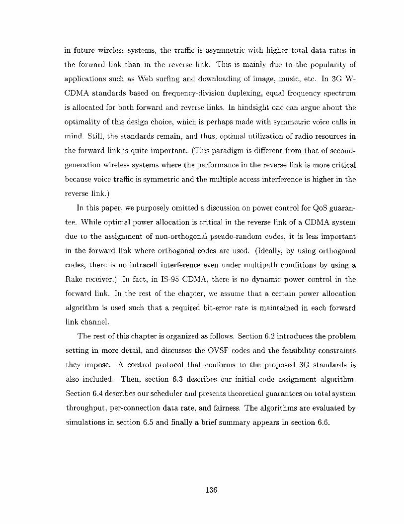
in future wireless systems, the traffic is asymmetric with higher total data rates in
the forward link than in the reverse link. This is mainly due to the popularity of
applications such as Web surfing and downloading of image, music, etc. In 3G W-
CDMA standards based on frequency-division duplexing, equal frequency spectrum
is allocated for both forward and reverse links. In hindsight one can argue about the
optimality of this design choice, which is perhaps made with symmetric voice calls in
mind. Still, the standards remain, and thus, optimal utilization of radio resources in
the forward link is quite important. (This paradigm is different from that of second-
generation wireless systems where the performance in the reverse link is more critical
because voice traffic is symmetric and the multiple access interference is higher in the
reverse link.)
In this paper, we purposely omitted a discussion on power control for QoS guaran-
tee. While optimal power allocation is critical in the reverse link of a CDMA system
due to the assignment of non-orthogonal pseudo-random codes, it is less important
in the forward link where orthogonal codes are used. (Ideally, by using orthogonal
codes, there is no intracell interference even under multipath conditions by using a
Rake receiver.) In fact, in IS-95 CDMA, there is no dynamic power control in the
forward link. In the rest of the chapter, we assume that a certain power allocation
algorithm is used such that a required bit-error rate is maintained in each forward
link channel.
The rest of this chapter is organized as follows. Section 6.2 introduces the problem
setting in more detail, and discusses the OVSF codes and the feasibility constraints
they impose. A control protocol that conforms to the proposed 3G standards is
also included. Then, section 6.3 describes our initial code assignment algorithm.
Section 6.4 describes our scheduler and presents theoretical guarantees on total system
throughput, per-connection data rate, and fairness. The algorithms are evaluated by
simulations in section 6.5 and finally a brief summary appears in section 6.6.
136

Cl
NotationC
2b data sequence of
user jb2
ci code sequence of
mod-2 addition to carrier modulator
CN
bN
Figure 6-1: Transmitter at the base station.
6.2 Problem Model
6.2.1 Base station transmitter
Figure 6-1 illustrates a block diagram of a CDMA base station transmitter capable of
supporting N forward link channels; i.e. it can support a maximum of N simultaneous
forward link connections. In each channel, a user's data sequence of rate R bps is
spread by an assigned orthogonal code sequence of rate R, bps, meaning each data bit
is mapped into a code of length RC/R. The length RC/R is also called the spreading
factor [46]. The encoded sequences from all forward channels are then summed before
broadcast. At the receiving end, each mobile user decodes the data sequence by De-
spreading (i.e. extracting) only its encoded sequence from the broadcast, a step made
possible by the use of orthogonal codes to eliminate inter-channel interference.
6.2.2 OVSF codes
In OVSF-CDMA, the codes are of different lengths (i.e., spreading factors) so that
a code with a smaller length can be used to transmit more information bits per
unit time. It is well known [1] that a binary code sequence C of length 1 can be
used to generate two orthogonal binary code sequences of length 21, C1 = [CC] and
C2 = [CC], where C is the inverted sequence of C. Using this procedure recursively,
137

C
1 2 C1 10 2
1 2 L 4 C41 110 1010 10011 2 3 F4 6 7 8 C8
2 3 4 5 6 7 10 11 12 13 14 15 16 C16
Figure 6-2: 16-leaf OVSF code tree.
OVSF codes can be generated and represented as nodes in a balanced binary tree. An
example is shown in Figure 6-2. Each node in the tree corresponds to a code, and all
codes in the same level have identical code length and are mutually orthogonal. The
top level code, called the root code, has a code length of 1 by convention. The two
codes directly beneath the root have length 2, and the four codes between them have
length 4, etc. The bottom level codes are called leaf codes or simply leaves, and in the
example shown in Figure 6-2, each leaf has length 16. A code X is called the parent
of another code Y if X is directly above Y in the code tree, in which case Y is also
referred to one of the two children of X. For any particular code, its ancestors include
itself, its parent and the parent's ancestors (recursively). Equivalently, the ancestors
are the nodes within the shortest path from a code to the root code inclusively. Thus,
the root code is an ancestor of every other code in a tree. As noted before, a forward
link channel using a code with a longer length transmits proportionally less data
(information bits) per unit time. For convenience, we normalize the data rates such
that a channel using a leaf (length 16 in the example shown) supports rate 1, a leaf's
parent (length 8) at rate 2, etc., up to the root code at rate 16 (in the example shown).
The root code rate will be denoted R,..
An important property of OVSF codes is that two codes are orthogonal if and
only if none is an ancestor of the other. In the forward link of OVSF-CDMA, only
a mutually orthogonal set of codes can be used for simultaneous transmissions -
otherwise data sequences spread by a code and its ancestors are corrupted because
138
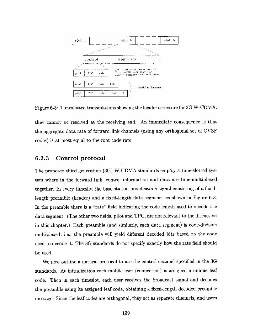
sloslot lot k slot N
control user data
TPC - transmit power control
pilot TPC rate ID - mobile user identifierI CLEAF - assigned OVSF leaf code
pilot TPC rate LEAFmodified headers
pilot TPC rate LEAF ID
Figure 6-3: Timeslotted transmissions showing the header structure for 3G W-CDMA.
they cannot be resolved at the receiving end. An immediate consequence is that
the aggregate data rate of forward link channels (using any orthogonal set of OVSF
codes) is at most equal to the root code rate.
6.2.3 Control protocol
The proposed third generation (3G) W-CDMA standards employ a time-slotted sys-
tem where in the forward link, control information and data are time-multiplexed
together. In every timeslot the base station broadcasts a signal consisting of a fixed-
length preamble (header) and a fixed-length data segment, as shown in Figure 6-3.
In the preamble there is a "rate" field indicating the code length used to decode the
data segment. (The other two fields, pilot and TPC, are not relevant to the discussion
in this chapter.) Each preamble (and similarly, each data segment) is code-division
multiplexed, i.e., the preamble will yield different decoded bits based on the code
used to decode it. The 3G standards do not specify exactly how the rate field should
be used.
We now outline a natural protocol to use the control channel specified in the 3G
standards. At initialization each mobile user (connection) is assigned a unique leaf
code. Then in each timeslot, each user receives the broadcast signal and decodes
the preamble using its assigned leaf code, obtaining a fixed-length decoded preamble
message. Since the leaf codes are orthogonal, they act as separate channels, and users
139
using different leaves will receive different decoded preambles.
A decoded preamble contains the rate field, specifying the code used to decode
the data segment of this timeslot. This code (for decoding the data segment) will
be called the data code. A rate of 1 specifies the use of the leaf code as the data
code, a rate of 2 means the parent of the leaf, a rate of 4 means the grandparent of
the leaf, etc., up to the root code rate which specifies the use of the root code. A
rate of 0 means the connection will not receive data this timeslot. For a code tree
of L leaves, the rate can take one of the values in the set {0, 1, 2, 4, 8, ..., L}. There
are 2 + log2 L different choices in this set, and so the rate field itself requires only
[log 2 (2 + log 2 L)] bits, e.g., 4 bits for a 256-leaf code. As explained before, using a
higher-rate (shorter length) data code will generate more decoded information bits
from the fixed length data segment. Thus the base station can communicate the
chosen service vector [Sf (t)] to each connection.
As a consequence of this choice of control protocol, two main algorithms are used
at the base station. First, when a connection starts, an initial leaf assignment must be
made. Second, service vectors [Sf (t)] must be chosen and data transmissions must be
scheduled (i.e., preamble rate fields and data segments must be filled) on a timeslot-
by-timeslot basis. Both algorithms will turn out to have a significant impact on the
size of the performance bounds.
Note that the above description specifies that each connection must have a differ-
ent leaf code, i.e., the leaf code also acts as the unique connection ID. This is a design
choice of the 3G standards. It is a simple matter to augment the standards to allow
several connections to share the same leaf code - each connection needs a unique ID
(which is not the leaf code alone) and the header also needs an additional "ID" field
to specify which (if any) of the connections sharing a leaf should decode the following
data segment at the specified rate. We will not explore this simple modification any
further here.
140
6.2.4 Feasibility Constraints and Reservation Factor
A connection's gf will be normalized by the leaf code rate. In a typical example,
if a timeslot is one millisecond long, and decoding a data segment using a leaf code
yields 10 information bits, then the leaf code rate equals 1Obits/millisecond or 10kbps,
and a connection that is granted a 20kbps reserved rate has gf = 2. (In a constant
rate circuit or "bit pipe" system without dynamic scheduling, a rate of 2 would be
provisioned by using a code which is a parent of a leaf code to decode 20 bits from
the data segment every timeslot). Data are transmitted in fixed-sized cells, where
each cell equals the amount of information bits decoded from a data segment using
a leaf code (10 bits in the previous example) - this is the minimum number of bits
received, and the leaf rate can also be considered as 1 cell/timeslot. We allow gf
values to be any non-negative numbers, not necessarily integers.
The feasibility constraints on the integral service vector [Sf (t)] are that, when
viewed as data codes in the code tree, the codes must be mutually orthogonal, i.e.,
no code is an ancestor of another. Note that given a connection's leaf code, the
instantenous rate specified in the header uniquely specifies the data code. Also, we
allow Sf(t) values which are not powers-of-2 (in which case the control protocol uses
the next higher power-of-2 in the header rate field).
Since it is possible for the data code to be the root code, it is easy to show that in
accordance to the definition in section 2.4.1, the reservation factor of this network is
a = fEF 9(61)Rr
One may wonder that the definition of a simply depends on the sum of all rates,
but not on how the rates are distributed inside the code tree. This independence is
because of the possibility of using the root code rate in a TDM/round-robin fashion,
an issue which will be explored fully in the next section. Indeed, an "uneven" distri-
bution of concentrating high-rate calls in one part of the code tree will lead to worse
performance such as higher (looser) credit and fairness bounds, however, it turns out
to have no effect on the boundedness result itself, which is the main application of
141

the definition of a.
6.3 Initial leaf assignment
The initial leaf assignment algorithm is invoked only on call setup. Our choice is a
heuristic algorithm that assigns a leaf to a new connection based on its gf. The the
main intuition is that all the gf values should be spread as evenly across the code
tree as possible. More specifically, consider any subtree (i.e., the part of the code
tree beneath some internal node) containing I leaves, and consider the connections
assigned to those leaves. It is desirable that the total gf of these connections be
less than 1, a condition we will refer to as under-populating the subtree. If several
assignment choices (i.e., several possible leaf codes) would all maintain this desirable
condition, one of them is chosen randomly. As the code tree fills up it may become
impossible to maintain this condition, in which case our heuristic algorithm tries
to violate this condition (i.e. over-populate the subtrees) by as small an amount
as possible (minimizing the fraction total 9g i Stubtre as it exceeds 1) and at as few
subtrees as possible.
To understand why it might be undesirable to over-populate subtrees, consider
the following extreme example. In a 16-leaf code tree, there are 4 connections, each
having gf of 4. In an extreme over-population scenario, they are assigned to the same
subtree of 4 leaves (Figure 6-4), and because their leaves have a common grandparent,
two (or more) of them can receive in the same timeslot only if each receives at very
low rates of 1 (leaf) or 2 (parent). If such low rates are sustained for a long time,
they will not be able to obtain their guaranteed rate of 4. In fact, the only way to
provision gf of 4 for each of them is to let each one receive at the root code rate
16 for one-fourth of the time, e.g., once every 4 timeslots, resulting in an essentially
TDM system. In the other extreme (the under-population scenario, Figure 6-5), since
the 16-leaf code tree has 4 different subtrees of 4 leaves each, our algorithm would
assign each of the 4 connections into a different such subtree, thus maintaining the
under-population condition as much as possible. Each connection can therefore enjoy
142
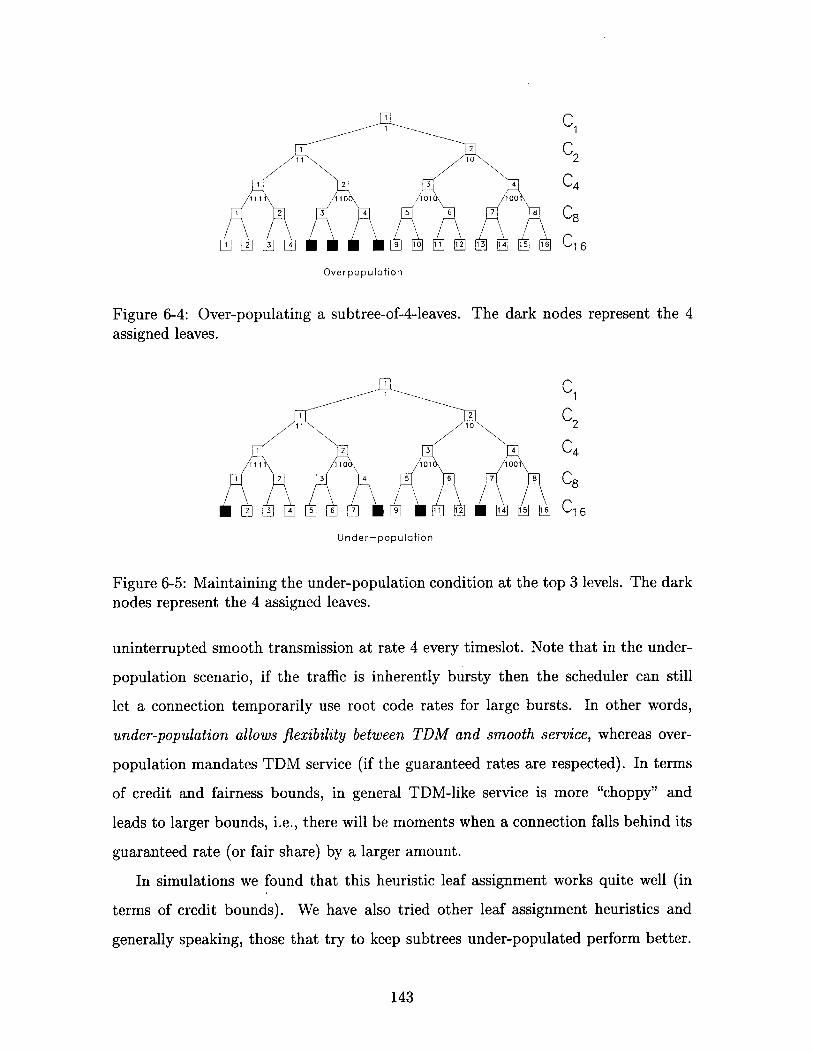
C
1 11 2 13 1 5 1 1
2 C
1 2 3 4 C1111 1106 101 100
2 3 4 5 6 7 8 6
31429314 11 12 13 14 15 16 C 1
Overpopulation
Figure 6-4: Over-populating a subtree-of-4-leaves. The dark nodes represent the 4
nd assigned leaves.
C1
2 C
1 2 3 4 C41111 110 101 100
1 2 3 4 5 6 7 8 C
2 3 4 5 6 7 9 11 12 14 15 116 C
Under-popu lotion
Figure 6-5: Maintaining the under-population condition at the top 3 levels. The darknodes represent the 4 assigned leaves.
uninterrupted smooth transmission at rate 4 every timeslot. Note that in the under-
population scenario, if the traffic is inherently bursty then the scheduler can still
let a connection temporarily use root code rates for large bursts. In other words,
under-population allows flexibility between TDM and smooth service, whereas over-
population mandates TDM service (if the guaranteed rates are respected). In terms
of credit and fairness bounds, in general TDM-like service is more "choppy" and
leads to larger bounds, i.e., there will be moments when a connection falls behind its
guaranteed rate (or fair share) by a larger amount.
In simulations we found that this heuristic leaf assignment works quite well (in
terms of credit bounds). We have also tried other leaf assignment heuristics and
generally speaking, those that try to keep subtrees under-populated perform better.
143

There are several heuristics of this sort besides the one presented, e.g., trying to min-
imize the number of over-populated subtrees first, trying to minimize the difference
between total gf in subtree and number of leaves in subtree, as opposed to the frac-
tion, etc. In the next section we will prove that for whatever leaf assignment used,
the credit will be bounded by some constant (although the size of this bound will
depend on the particular heuristic).
6.4 Scheduling algorithm
6.4.1 Algorithm description
The job of the scheduling algorithm is, given a leaf assignment, to decide which
connections can receive and at what rates in each timeslot, i.e., to choose a feasible
service vector [Sf(t)]. The main intuitive idea of the algorithm is the same as the
CQ and CQ' algorithms - simply sort the connections in order of credits, and then
go through the sorted list and schedule connections with more credits to receive
more cells (i.e. at a higher instantaneous rate). However, we found that a simple
adaptation of CQ' performs very poorly in simulations, and therefore we designed the
following algorithm which introduces some "back-tracking" into CQ'. In the following
description, the word "rate" refers to the instantaneous rate, i.e., the rate field in the
header.
1. (a) Initialize all connections to have (instantaneous) rate = 0, and all codes in
the tree to have the status "unassigned." (b) Ignore all connections with empty
queues.
2. Sort all remaining connections by decreasing credits (breaking ties arbitrarily)
into a sorted list.
3. Let X be a connection with the maximum credit in the sorted list. (a) If X's
rate = 0 and its leaf has an ancestor which is already assigned, then ignore X
144

for this timeslot. (b) Otherwise, define the "new rate" of X as follows: if X's
rate = 0, then new rate = 1, else new rate = double X's rate.
4. IF X has at least as many queued cells as its new rate, THEN
* (a) Increase X's rate to the new rate.
* (b) Decrease X's credit by the amount its rate has been increased.
* (c) Mark the code A that will be used by X at its new rate as "assigned" (A
will be X's leaf code or its ancestor). Back-tracking: If A is an ancestor
of some already assigned code B, used by connection Y, then reset Y's
rate to zero, re-issue any credit paid by Y, reset B to "unassigned", and
ignore Y for this timeslot. Do this to all such assigned descendents of A.
e (d) If the total of all assigned rates now equals the root code rate, the
algorithm stops. Otherwise, go to step 2 (i.e., re-sort). Note that, imple-
mentationally speaking, there is no need to re-sort the entire list, as the
algorithm just needs to re-insert X at the right place.
5. ELSE (comment: X has fewer queued cells than its new rate) (a) do not increase
its rate, (b) drop X from the sorted list, and (c) go to step 3.
Roughly speaking, the algorithm works in a loop, and every iteration, it finds the
maximum-credit connection and increases its rate one level up the code tree, while
maintaining an invariant that the assigned codes are always mutually orthogonal.
(To maintain this invariant, it sometimes have to back-track and cancel previously
made assignments, via step (4c).) The algorithm terminates when the total rates
assigned equal the root code rate (i.e., the network capacity), or when all connections
are dropped from consideration via steps (3a), (4c) or (5b). Note that a connection
ignored via steps (3a) or (4c) will take no further part in the algorithm (for this
timeslot). In contrast, a connection dropped from the sorted list via step (5b) will
not have another rate increase but may take part in the algorithm again, if a future
step (4c) finds it necessary to reset its rate to zero and re-issue credits. Once the
algorithm terminates, the rates are filled in the header.
145
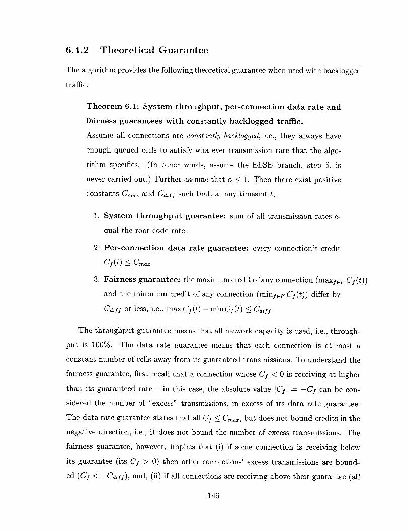
6.4.2 Theoretical Guarantee
The algorithm provides the following theoretical guarantee when used with backlogged
traffic.
Theorem 6.1: System throughput, per-connection data rate and
fairness guarantees with constantly backlogged traffic.
Assume all connections are constantly backlogged, i.e., they always have
enough queued cells to satisfy whatever transmission rate that the algo-
rithm specifies. (In other words, assume the ELSE branch, step 5, is
never carried out.) Further assume that a < 1. Then there exist positive
constants Cma, and Cdif f such that, at any timeslot t,
1. System throughput guarantee: sum of all transmission rates e-
qual the root code rate.
2. Per-connection data rate guarantee: every connection's credit
Cf(t) Cmax.
3. Fairness guarantee: the maximum credit of any connection (maxfEF Cf )
and the minimum credit of any connection (minfEF Cf (t)) differ by
Cdi f or less, i.e., max Cf(t) - min Cf(t) Cdif.
The throughput guarantee means that all network capacity is used, i.e., through-
put is 100%. The data rate guarantee means that each connection is at most a
constant number of cells away from its guaranteed transmissions. To understand the
fairness guarantee, first recall that a connection whose Cf < 0 is receiving at higher
than its guaranteed rate - in this case, the absolute value ICf I = -Cf can be con-
sidered the number of "excess" transmissions, in excess of its data rate guarantee.
The data rate guarantee states that all Cf 5 Cmax, but does not bound credits in the
negative direction, i.e., it does not bound the number of excess transmissions. The
fairness guarantee, however, implies that (i) if some connection is receiving below
its guarantee (its Cf > 0) then other connections' excess transmissions are bound-
ed (Cf < -Cdiff), and, (ii) if all connections are receiving above their guarantee (all
146
Cf > 0) then although the number of excess transmissions is not bounded, all connec-
tions have approximately the same number of excess transmissions, up to a difference
of Cdiff. This represents "fair sharing" of the unreserved portion of network capacity.
The usefulness of the algorithm will depend on how small (tight) the bounds are.
Although the theoretically provable bounds are large, in simulations the bounds are
small. Note that the theorem applies as long as o < 1. It does not matter how leaves
are assigned and how subtrees are over- or under-populated - those factors affect
the size of the bounds (both in theory and in simulations), but the theoretical result
of boundedness still stands.
Since Theorem 6.1 requires all connections to be constantly backlogged, it can be
interpreted in two ways. First, the theorem means that rate reservations are respected
when the network is congested and every connection is constantly backlogged. Second,
the theorem acts as a kind of "legacy" guarantee for non-bursty traffic.
6.4.3 Stress-Test algorithm
The algorithm as stated above allows credits to become negative, i.e., connections
can receive at higher than their guaranteed rates.
Another variation of this algorithm is called the "stress-test" variation, where
connections are not allowed to spend more credits than they have. Step (1b) of
the algorithm is modified so that connections with less than 1 credit (C < 1) are
also ignored, and the IF condition of step (4) is modified so that steps (4a-4d) will
be performed only if the connection has enough credit to handle the rate increase
and still keep the resulting credit non-negative. An equivalent description is that a
connection with not enough credits is treated exactly as if it has not enough queued
cells - in both cases, step (5) is executed instead of step (4). With these modifications,
the algorithm maintains C > 0 for all connections all the time.
An immediate consequence is that each connection's time-average rate will never
exceed its guarantee, and therefore, if the total gf is less than the network capacity
(root code rate), some capacity will simply be wasted. Therefore, by choice, the
throughput guarantee of theorem 6.1 no longer holds. Also, since there are no excess
147

transmissions, the fairness guarantee is meaningless. However, we still have the rate
guarantee:
Theorem 6.2: Stress-test scheduler provides rate guarantees with
constantly backlogged traffic.
As in theorem 6.1, assume all connections are constantly backlogged and
that a < 1. If the stress-test scheduler is used, then there exist a posi-
tive constant Cmax such that, at any timeslot t, every connection's credit
Cf(t) Cmax.
As discussed in previous chapters, we study this "wasteful" stress-test algorithm
for two reasons. First, it acts as a more stringent test condition for our simulations
in evaluating credit bounds. Second, and especially important in the problem set-
ting of this chapter, the stress-test algorithm separates the problem of providing rate
guarantees and the problem of fair sharing of unreserved capacity. While the original
(non-stress-test) algorithm couples rate guarantee and fairness and in fact dictates
a notion of approximately-equal sharing, as in Theorem 1, the stress-test algorithm
uses only the reserved capacity of the network and services only the guaranteed trans-
missions - thus allowing network management to design another fair-sharing method
to allocate the unreserved capacity if desired.
6.4.4 Proofs
Throughout this presentation of proofs, we will assume traffic is constantly back-
logged. Consequently, Cf (t + 1) = C1 (t) + gf - Sf (t). Unless otherwise specified,
the proofs apply to both the non-stress-test and stress-test versions of the algorithm.
These boundedness proofs are based on combinatorial techniques and are substan-
tially different from the techniques used in proving theorems 2.2 and 2.3.
Let R, denote the root code rate (network capacity) and let G = EfZEF gf. Finally,
define Cm(t) = max Cf(t), the maximum credit value at the beginning of time t. We
will prove theorem 6.1 by a sequence of lemmas 6.1-6.4:
148

Lemma 6.1: System Throughput Guarantee
At any timeslot t when step (5) of the algorithm is not executed, EfEF Sf M
R,. As a corollary, for the non-stress-test algorithm Vt EfEF Sf(t) -Rr
Proof: if step (5) is not executed, then the algorithm maintains at least one connec-
tion in the sorted list (the connection whose rate has just increased). Therefore the
algorithm will not terminate due to all connections being dropped from consideration.
After step (4c), the set of codes is always orthogonal, and so EfCF Sf(t) Rr. If
EfEF Sf t < Rr at this point, the algorithm will execute another loop. Therefore,
the algorithm only terminates when the orthogonal set of codes after (4c) satisfy
EfEF Sf t) Rr. To show that the algorithm terminates, note that with each iter-
ation, some Sf (t) increases, and so the total EfEF Sf () would also increase unless
some connection was dropped from consideration by step (4c). Since both the number
of connections and the total rate are bounded, the algorithm must terminate. For
the corollary, note that for the non-stress-test algorithm, step (5) is never executed
in any timeslot (for backlogged traffic). Q.E.D.
Lemma 6.2: Only high-credit connections are serviced
At any timeslot t when step (5) of the algorithm is not executed, if Sf (t) >
0 then Cf (t) Cm(t)-Rr. I.e., the algorithm will not assign transmissions
to a connection whose credit differs from the maximum credit Cm(t) by
more than Rr.
Proof: the key observation is that in the sorted list there will always be a connection
whose Cf(t) = Cm(t). To prove this, note that connections are only dropped from
consideration by step (4c) (since step (5) is not executed, by assumption). Consider
step (4c) and let RA, RB denote the rates of codes A and B. Since B is a descendent
of A, we have RB < RA/2 since rates decrease by half every level down the code tree.
Before the rate increase of X, its rate is RA/2 and its current credit in the sort order
is Cx(t) -RA/2. Similar, the current credit of Y in the sort order is Cy(t) -RB. Since
X is chosen over Y in step (3), we have Cx(t) - RA/2 > Cy(t) - RB, which implies
Cx(t) Cy(t). In other words, if a connection with Cy(t) = Cm(t) is dropped, it is
149
because another connection with CX(t) = Cm(t) has a rate increase. Therefore, there
will always be at least one connection in the sorted list whose Cf(t) = C.(t). Now,
such a connection will not have its credit drop below Cm(t) - R, during the running
of the algorithm, since the maximum rate that can be assigned is R,. Therefore, the
algorithm will not choose connections whose Cf(t) < Cm(t) - R, in step (3) and such
connections will not be assigned any (positive) transmission rate. Q.E.D.
Lemma 6.3: Per-Connection Data Rate Guarantee
For the non-stress-test algorithm, if G < R, then there exist a (positive)
constant Cmax such that Vt, Vf, Cf(t) _ Cmax.
Proof: For the non-stress-test algorithm, at any timeslot, some connections' credits
may be positive, some may be zero, and some may be negative. We consider the
summation of all the positive credits,
P(t) = 1: max(O, Cf (t)) (6.2)fEF
We will prove that Vt, P(t) 5 (2|FI + 1)R,, where IFI denotes the number of con-
nections. Since P(t) is the sum of non-negative terms, this implies each term cannot
exceed P(t) and therefore Vt, Vf, Cf(t) < (21F I+ 1)R., thus proving the lemma with
a constant Cmax = (21FI+ 1)R,.
To prove that P(t) is bounded we track its evolution from one timeslot to the
next:
AP = P(t + 1) - P(t) = Z [max(O, Cf (t + 1)) - max(0, Cf (t))] (6.3)fEF
Consider the term 6 = max(O, Cf(t + 1)) - max(O, Cf(t)), we have these cases:
1. If Cf(t+ 1) > 0 then 6 = Cf(t+ 1)- max(0,Cf(t+ 1)) 5 Cf(t+ 1)- Cf(t),
since max(0, Cf(t)) ;> Cf(t).
2. If Cf(t + 1) < 0 and Cf (t) < 0 then 6 = 0.
150
3. If C5(t + 1) < 0 and Cf(t) > 0 then 6 = -Cf(t) < 0.
Therefore,
AP < Ef CF|Cf (t+1)>C
f EFICf (t+1)>C
(6.4)
(6.5)[gf - Sf (t)]
We now show, by induction, that VtP(t) < (21FI + 1)Rr. At t = 0 we have the
base case of Cf(0) = 0 and P(0) = 0. For the induction step, there are two cases:
1. P(t) < 2IFIR,. We have AP EfeF|Cf(t+1)>olgf -Sf(t) f EFICf(t+1)>O 9f <
EfEFgf 5 Rr, so that P(t + 1) 5 P(t) + R, < (21F| + 1)R, as required.
2. 2F IRr < P(t) 5 (2IFI +1)R,. Since P(t) = EfEF max(0, Cf (t)) is a summation
of JFl non-negative terms, we know the maximum term Cm(t) > - > 2 Rr.
Applying lemma 2 for timeslot t, we have:
Sf(t) > 0 > Cf (t) > Cm(t) - Rr > Rr (6.6)
(6.7)> Cf (t + 1) > 0
since a connection's credit can drop by at most R, in one timeslot. Using this,
we have:
E Sft Wf EFCf (t+1)>O
P(t + 1) - P(t)
= Z'Sf (t)SE SfWfeF
=R, (Lemma 1)
K E [gf - S (t)]f EFICf (t+1)>O
( gf) - RRf EFCf (t+1)>O
< G-R 0
Therefore, P(t + 1) < P(t) (21F| + 1)Rr as required.
(6.8)
(6.9)
(6.10)
(6.11)
(6.12)
151
[Cf (t + 1) - Cf (01]

In both cases, P(t + 1) < (21FI + 1)R, and so inductively we have Vt, P(t) <
(21FI + 1)R,. This further implies all credits are bounded above. Q.E.D.
Lemma 6.4: Fairness Guarantee
For the non-stress-test algorithm, if G < R, then there exist a (positive)
constant Cdiff such that Vt, maxfEF Cf (t) - minf EF Cf (t) Cdif f -
Proof: First we observe that the sum of all credits is a linear function of time:
ECf(t+l) = [Cf (t) + gf - S(t)1 (6.13)fEF fEF
= Z Cf (t) + G - R, by Lemma 1 (6.14)fEF
= E C (0) + (t + 1)(G - R,) by induction (6.15)feE
= (t + 1)(G - R,) since Cf (0) = 0. (6.16)
Case (i): When G = Rr, this means the sum of all credits is always zero. Now,
lemma 3 implies credits are upper-bounded in this case. Since the sum of credits is
zero and all credits are upper-bounded, this means credits are lower-bounded as well.
In fact, the proof of lemma 3 shows that Vt, P(t) 5 (21FI+1)Rr, and therefore the sum
of negative credits N(t) = EfEF min(O, Cf(t)) > -(21FI-+1)R,, since P(t)+N(t) = 0.
Therefore Vt, maxf F Cf(t) - minfE F f Cdif 2Cmax = 2(2|F| + 1)Rr.
Case (ii): When G < Rr the above shows that the sum of credits decreases (i.e.,
grows more and more negative) linearly in time, and therefore there is no hope of a
hard lower-bound. We now proceed to prove that all credits will grow negative at an
approximately equal "speed" resulting in the difference in credits being bounded by
Cdiff.
The key observation is that the algorithm chooses transmissions based on the
relative ranking of credits, but never based on the actual credit values themselves.
(In other words, the algorithm never compares a credit value to anything other than
another credit value.) Therefore, the algorithm's output - the service vector [Sf (t)]
- would be exactly the same if every credit of every connection is increased by the
152
same value. This further means that we can uniformly increase every connection's gf
by the same amount and the algorithm's outputs (in every timeslot) would remain
the same.
In particular, consideration a scenario where every connection's guaranteed data
rate is g' = gf + R--G (instead of gf), and let C'(t) (instead of C (t)) denote the
credits in this scenario. Then we have EfEF 9f = G + F| R--G = Rr, and by Case
1, there exists Cdiff such that Vt, maxfEF C'(0- minfEF C'(t) < Cdiff. By the key
observation, it is easy to see that C'(t) = Cf(t) + Rr-Gt and so the same constant
also satisfies Vt, maxfEF Cf (t) - minfEF Cf ) Cdif f . Q.E.D.
Proof (theorem 6.2): The entire proof of lemma 3 can be repeated. In fact the
algebra is somewhat simplified - since all Cf(t) > 0, we have AP = EF 9f - Sf(t)1-
The exact same proof by induction can be used to show that P(t) < (21FI + 1)R, as
before and every line of algebraic manipulation is still valid. It only remains to show
that lemmas 1 and 2 are still valid in the situation where they are used in the proof
of lemma 3, i.e., in case 2 of the induction step.
Case 2 of the induction step occurs for those timeslots when P(t) > 2 FIR,, which
implies Cm(t) > 2 Rr. However, as long as Cm(t) > R,, no connection will run out
of credit because the maximum number of transmitted cells is Rr. In other words,
step (5) of the algorithm is not executed in these timeslots and so lemmas 1 and 2
are applicable. Q.E.D.
Note on size of theoretical bounds: The bounds established above - Cmax =
(2|FI + 1)Rr, Cdiff = 2(2|F + 1)Rr - are quite loose. E.g., in the case of |Fl = 2
and each gf = Rr/2, one can construct an example where Cm(t) = Rr/ 2 for some
timeslots. Our value of Cmax = 5Rr therefore overestimates by a factor of 10. For
larger values of jF| the over-estimation is even greater. More careful analysis can
reduce the value of Cmax and Cdiff but we will not include these for length concerns.
The "soft bounds" obtained from simulations are much smaller (tighter) anyway.
153

6.4.5 Modified bucket size restriction
When we first studied the wireless network of this chapter, we used the exact bucket
size restrictions as in previous chapters - only idle flows (whose Cf > Bf) are penal-
ized to forfeit credit increments. However, early simulations show that this does not
work well. Upon further investigation, we find that this is because the instanteous
rates can only take on values which are powers-of-2. This means that if a connection
has 5 cells (or 5 validated cells, if the stress-test or LC-weighted version is used),
either the rate must be held back at 4, or the rate may be increased to 8 in which
case 3/8 of the data rate is wasted. (In contrast, in previous chapters either Sf(t) is
restricted to 0 or 1, or it can be any non-negative integers with no "gaps" in between
up to the number of transmitters of the source.) After some experimentation, we
designed a modified rule for bucket size restriction:
1. During step 5 of the algorithm, i.e., if a connection does not have as many
queued cells as the new rate, then the connection is flagged as "delinquent" for
the next timeslot (only).
2. At the beginning of every timeslot, every connection receives a credit increment
equal to its gf (as before), with the following exception: if a connection's Cf (t) >
Bf, and it has an empty queue or it was flagged as "delinquent" in the previous
timeslot, then it forfeits its credit increment.
As before, the modified bucket size restriction penalizes connections that under-
utilize their reserved rates for extended periods of time. Such a connection may
eventually have a large enough credit (Cf > Bf) and a small enough queue (becoming
idle or delinquent) that it no longer gets credits at its guaranteed rate.
6.4.6 Variation: Timeslot-based leaf re-assignment
As mentioned, some previous work [38] investigated code reassigment on a per-call
basis, where a call can be moved from any code to any other code. Meanwhile, this
chapter investigates instantaneous rate assignment on a timeslot basis, i.e., data code
154

re-assignments which are limited to the leaf code (permanently assigned on setup)
and its ancestors up to the root code. This section now briefly describes a variation
which combines both ideas and allows the datacode to be re-assigned to any code in
the tree on a timeslot basis.
First of all, this involves changing the header in the 3G standards. For example, a
new "newleaf" field can be used (log L bits where L = number of leaves) in addition
to the existing "rate" field. Then the data segment immediately following the header
will be decoded using an appropriate ancestor of the newleaf (as specified by the
instantaneous rate). Alternatively, a new "datacode" field can be used instead of
the "rate" field, and the new datacode directly specifies which datacode to use for
the following data segment. (Since a tree with L leaves has 2L - 1 codes overall,
the datacode can be specified by 1 + log L bits.) In both cases, the control protocol
may specify that the next header (in the next timeslot) be decoded using the original
leaf assigned on call setup, or using the newleaf (or the leaf descendent of the new
datacode). Obviously, with these changes, the initial leaf assignment algorithm does
not affect performance any more.
The scheduler can then be modified as follows to take advantage of the new free-
dom in the choice of datacodes:
1. There is no need to keep track of individual data codes (i.e., their "assigned/unassigned"
status). Instead, the algorithm simply keeps track of each connection's assigned
instantaneous rate.
2. Step (4c) becomes: If the total assigned rate is larger than the root code rate,
say by an amount A(> 0), then choose any subset of connections whose assigned
rates sum to exactly A, reset those connections' rates to zero and re-issue them
credits, then finally stop the algorithm (because the total assigned rate is now
exactly the root code rate). Note that such a subset (with rates summing to
A) must exist because all rates are powers-of-2 (this is a simple property of sets
of numbers which are powers-of-2). In fact there might be many such subsets,
and we found in simulations that the exact choice makes little difference in
155

performance.
3. When the algorithm stops, connections have been assigned rates but have not
yet been assigned data codes. A simple post-processing step similar to con-
structing a Huffman code tree is now used: the two smallest rates are combined
recursively and in this way the a set of mutually orthogonal codes can be as-
signed.
With these changes, the theorems hold as stated.
6.5 Simulations
6.5.1 Simulation Settings
The main goal of our simulations is to experimentally evaluate the size of the cred-
it and fairness bounds. The theorems guarantee boundedness, but only in case of
constantly backlogged traffic, and even then the bounds are large (loose). Our sim-
ulations will show that credits remain at much lower, practically useful level than
theoretically provable, for both backlogged and bursty traffic.
In our simulations, the number of leaves L is fixed at 256. Three different network
loading patterns are used:
1. Many small connections: each connection has a gf uniformly chosen between 0
and 2. Connections are added one by one until the total gf reaches a pre-set
value.
2. A few large connections: each connection has a gf uniformly chosen between 16
and 48. Connections are added one by one until the total gf reaches a pre-set
value.
3. Mixed connections: each connection is a small connection (gf 0-2) with proba-
bility s and a large connection (gf 16-48) with probability 1 - s. Connections
are added one by one until the total gf reaches a pre-set value.
156

When the number of connections exceeds L, which happens sometimes in the
"many small connections" loading pattern, we augment the 3G standards with an ID
field, as described in the last paragraph of section 6.2.3. Besides varying the loading
pattern, we also simulated two different models of traffic arrival processes.
1. In the constantly backlogged model, each connection is assumed to always have
at least as many queued cells as the algorithm wants to schedule.
2. In the bursty traffic model, for each connection, traffic arrives at the base station
in bursts. Each connection's arrival process is controlled by a 2-state Markov
chain. While in the "idle" state, a connection has no arrivals (i.e., no new cells
are added to the queue). While in the "bursting" stage, a "packet" of P cells
arrives per timeslot, where P is uniformly distributed from 0 to 10 xgf, for an
average pack size of 5 x gf cells. The Markov chain transition probabilities are
chosen so that a connection is in the idle state 1 of the time and in the bursting55
state } of the time, and once in the bursting state, the connection spends an
average of 10 timeslots there. Thus an average burst consists of 10 packets,
each of an average of 5 x gf cells.
Note that in the bursty traffic case, the average arrival rate equals gf exactly. We
made this design choice because (i) if the arrival rate were higher, the connection may
become backlogged, reverting to the constantly backlogged case, and (ii) if the arrival
rate were smaller, this represents a less stringent test condition for the algorithms.
The performance measures taken during the simulations consist of various ob-
served bounds, and we separately report the bounds on large connections C'a and
on small connections Cmax. All measurements are taken at the end of timeslots, i.e.,
after the current set of transmissions and credit decrements (payments). For each
measurement, the simulation is run 10 or more times (using the same settings), each
time for a duration of 10000 timeslots, and the overall bound is reported.
157

6.5.2 Credit bounds on stress-test scheduler
Table 6.1 shows the results of the stress-test version of the scheduling algorithm with
the constantly backlogged traffic model. (The non-stress-test version will be discussed
later.) Although the credit bounds are somewhat larger than in previous chapters,
remember that a credit bound of approximately 200 cells in a duration of 10000
timeslots equals a data rate of 0.02 cell/timeslot, i.e., 2% of the leaf code rate, which
is a tiny fraction of the guarantee. Moreover, in longer simulations (not reported
here), the bounds stay roughly constant.
Another way to evaluate a credit bound is to count how many timeslots would be
needed to gain that amount of credit. For instance, for a large call, the average gf is
32, and so a credit bound of 200 corresponds to 200 7 timeslots, i.e., it is (at most)
lagging behind its guaranteed rate by 7 timeslots. This leads to an interesting obser-
vation: Small calls have much lower gf than large calls, and yet C'ax is comparable
to Cax in size, meaning that small calls lag behind their guaranteed rate by a much
larger number of timeslots. This happens because the algorithm sorts connections by
their credits regardless of their g . Following ideas in previous chapters, we performed
other preliminary simulations (not included here) which show that if the algorithm
sorts connections by i, then the connections have widely different credit bounds,
but each connection would lag behind its own guaranteed rate by approximately the
same number of timeslots.
Table 6.2 shows the results of the stress-test scheduler in constantly backlogged
traffic, but this time with the addition of the "newleaf" field in the control header
thereby allowing leaf code re-assignment every timeslot. The results show a dramatic
improvement over those of table 6.1. In most cases reported here, the credit bound
corresponds to a lag of 1-3 timeslots only. These results show that the additional
freedom introduced by leaf re-assignment indeed facilitates the scheduling task.
Table 6.3 shows the results of the stress-test scheduler on bursty traffic (with
no leaf re-assignment). For simplicity, in these simulations every connection has a
finite bucket size of Bf = gf x b, for a chosen constant B. In other words, each
158

Loading pattern s =Prob(small connection) total gf tota mx m
Many small 1 128 50% - 17Many small 1 192 75% - 19Many small 1 230 90% - 66Many small 1 256 100% - 266
Few large 0 128 50% 75 -Few large 0 192 75% 158 -Few large 0 230 90% 266 -Few large 0 256 100% 260 -
Mixed 0.8 128 50% 130 101Mixed 0.8 192 75% 130 103Mixed 0.8 230 90% 170 125Mixed 0.8 256 100% 265 223Mixed 0.5 128 50% 120 97Mixed 0.5 192 75% 160 102Mixed 0.5 230 90% 235 172Mixed 0.5 256 100% 312 239
Table 6.1: Credit bounds for constantly backlogged traffic with "stress test" scheduler.First four columns show control parameters; last two columns show measurements.
Loading pattern s =Prob(small connection) total gf total Cx CMaMany small 1 128 50% - 3Many small 1 192 75% - 3Many small 1 230 90% - 4
Many small 1 256 100% - 9Few large 0 128 50% 32 -Few large 0 192 75% 32 -Few large 0 230 90% 34 -Few large 0 256 100% 35 -
Mixed 0.8 128 50% 32 2Mixed 0.8 192 75% 32 3Mixed 0.8 230 90% 39 4Mixed 0.8 256 100% 37 9Mixed 0.5 128 50% 32 2Mixed 0.5 192 75% 32 2Mixed 0.5 230 90% 33 2Mixed 0.5 256 100% 39 24
Table 6.2: Credit bounds for constantly backlogged traffic with "stress test" schedulerwith leaf re-assignment. First four columns show control parameters; last two columnsshow measurements.
159

Loading pattern s =Prob(small connection) total gYf CoBama CfnBMany small 1 128 50% 5 - 27Many small 1 192 75% 5 - 43Many small 1 230 90% 5 - 69Many small 1 256 100% 5 - 124Many small 1 128 50% 50 - 40Many small 1 192 75% 50 - 74Many small 1 230 90% 50 - 101Many small 1 256 100% 50 - 255
Mixed 0.8 128 50% 5 150 120Mixed 0.8 192 75% 5 169 130Mixed 0.8 230 90% 5 204 188Mixed 0.8 256 100% 5 220 240Mixed 0.8 128 50% 50 165 101Mixed 0.8 192 75% 50 169 130Mixed 0.8 230 90% 50 210 188Mixed 0.8 256 100% 50 302 258
Table 6.3: Credit bounds for bursty traffic with "stresscolumns show control parameters; last two columns show
test" scheduler. First fivemeasurements.
bucket size equals the credit that would have been gained in $ timeslots. (This is
only a choice made for our simulations. In practice, our scheduler allows arbitrary
bucket sizes.) The credit bounds are similar to the constantly backlogged case of
table 6.1, showing that the bucket size restriction is doing a reasonably good job of
controlling "misbehaving" connections. Also, the credit bounds increase slightly as
the bucket size increases - intuitively, larger buckets mean less control. We have also
performed some simulations (not reported here) with bursty traffic but no bucket size
restriction. As suspected, credits grow unbounded, i.e., they do not seem to converge
for the simulation duration of 10000 timeslots.
6.5.3 Non-stress-test scheduler and fair sharing
All the simulation results reported so far (tables 6.1-6.3) are obtained using the stress-
test scheduler, where a connection cannot receive more cells than it has (positive)
credits. Therefore, any unreserved network capacity (i.e., root code rate minus total
160

gj) will simply be wasted, and the total network utilization is bounded by the the
total gf.
We also simulated the non-stress-test version of the scheduler, where a connection's
credit can become negative. In this case, theorem 1 guarantees that, for constantly
backlogged traffic, the throughput is 100% and the unreserved capacity (if any) is
shared approximately equally among connections (up to a difference of Cdiff). Again,
the purpose of simulations is to observe the size of the bounds and to try the algorithm
with bursty traffic. We make the following observations:
1. If 100% of the network is reserved (a = 1, ECfEF 9f = R,), there is no substantial
difference between the performances of the stress-test scheduler and the non-
stress-test scheduler, for both backlogged and bursty traffic.
2. For both backlogged and bursty traffic, the Cdiff bound is approximately the
same size as the Cma bound for the stress-test scheduler.
3. For bursty traffic, by our choice of simulation settings, the total arrival rate
equals the total gf in our simulations. Therefore, the maximum throughput is
the total gf. In simulations, we observe that the queue lengths remain small
and bounded, showing that the network achieves maximum possible throughput
- every arrived cell is transmitted except for a small number in the queues.
In other preliminary simulations where connections are sorted not by credits but
by C , we observed that connections with larger gf obtain proportionally more excess
transmissions so that the difference between the smallest and largest C values remaingf
bounded. (This boundedness can also be proved using a slightly modified proof of
theorem 6.1.) Whether this proportional sharing represents a more fair approach than
the (approximately) equal sharing of theorem 1 is really a matter of design choice.
6.6 Chapter Summary and Further Discussions
Existing wireless networks provide the same constant-rate "circuit switching" or "bit
pipe" service to each user. This is inappropriate for supporting future multimedia and
161

data traffic, which is bursty and can have QoS requirements that differ from one user
to another by several orders of magnitude. This chapter proposes a scheme (based on
the proposed 3G W-CDMA standards) which provides per-connection rate guarantee
to bursty users in the forward link of an OVSF-CDMA system. The scheme consists
of a heuristic initial leaf assignment, invoked on call setup, followed by a timeslot-
based scheduler which uses a variation of CQ with additional back-tracking. We prove
that 100% throughput, bounded credit and in addition approximately equal sharing of
unreserved capacity can all be guaranteed by theory, if traffic is constantly backlogged.
Simulation evaluation of the credit and fairness bounds are also performed, for both
backlogged and bursty traffic.
We also investigated a change to the 3G W-CDMA control channel standard
by adding the "newleaf" fields to the control header, in order to allow timeslot-
based leaf code re-assignment. Simulations show that this improves the credit bounds
substantially. Enlarging the control header, however, effectively reduces the useable
network capacity. In practice, a reasonable compromise is perhaps to not use the
"newleaf" field, but to allow leaf code re-assignments on a per-call basis (as suggested
in [38]) just to ease over-population of subtrees occasionally, and to use only the "rate"
field on a timeslot basis.
Obviously the algorithm of this chapter can be used with sorting criteria (weights)
based on LC and VW and scaled and mixed versions of them as well. Preliminary
simulations in these areas do not demonstrate any unexpected behavior and are not
included here.
162
Chapter 7
Summary
7.1 Problem Formulation
This thesis investigated QoS-provisioning in four different networking problem set-
tings - an input-queued crossbar switch, two kinds of optical networks, and a CDMA
wireless network. There is a dual emphasis on both theoretical justification and sim-
ulation evaluation.
A common setting for all problems is the use of a centralized scheduler to con-
trol time-slotted transmissions1 . The main goal of the scheduler is to provide, on a
per-flow basis, guarantees on average rate, cell delay and fair access to unreserved
system capacity. A secondary but still important goal of the scheduler is to maximize
total system throughput. In the input-queued switch and the optical networks, it is
also important that the scheduler has a fast running time in the range of a few mi-
croseconds to sub-microsecond, corresponding to the timeslot lengths of the problem
setting.
We formulated the abstract scheduling problems as a sum of two aspects. First,
the particular problem setting imposes hardware constraints which translate into
feasibility constraints on what set of cells can be transmitted in each timeslot. Each
problem setting provides its own unique feasibility constraints, which are summarized
'As an exception, section 4.7 describes a distributed scheduler for a metro-area optical network.
163
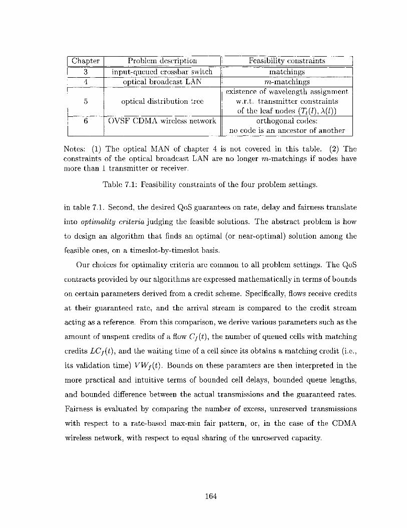
Chapter Problem description Feasibility constraints3 input-queued crossbar switch matchings4 optical broadcast LAN m-matchings
existence of wavelength assignment5 optical distribution tree w.r.t. transmitter constraints
of the leaf nodes (T(l), A(l))6 OVSF CDMA wireless network orthogonal codes:
no code is an ancestor of another
Notes: (1) The optical MAN of chapter 4 is not covered in this table. (2) Theconstraints of the optical broadcast LAN are no longer m-matchings if nodes havemore than 1 transmitter or receiver.
Table 7.1: Feasibility constraints of the four problem settings.
in table 7.1. Second, the desired QoS guarantees on rate, delay and fairness translate
into optimality criteria judging the feasible solutions. The abstract problem is how
to design an algorithm that finds an optimal (or near-optimal) solution among the
feasible ones, on a timeslot-by-timeslot basis.
Our choices for optimality criteria are common to all problem settings. The QoS
contracts provided by our algorithms are expressed mathematically in terms of bounds
on certain parameters derived from a credit scheme. Specifically, flows receive credits
at their guaranteed rate, and the arrival stream is compared to the credit stream
acting as a reference. From this comparison, we derive various parameters such as the
amount of unspent credits of a flow Cf (t), the number of queued cells with matching
credits LCf(t), and the waiting time of a cell since its obtains a matching credit (i.e.,
its validation time) VWf (t). Bounds on these paramters are then interpreted in the
more practical and intuitive terms of bounded cell delays, bounded queue lengths,
and bounded difference between the actual transmissions and the guaranteed rates.
Fairness is evaluated by comparing the number of excess, unreserved transmissions
with respect to a rate-based max-min fair pattern, or, in the case of the CDMA
wireless network, with respect to equal sharing of the unreserved capacity.
164
7.2 Algorithms
In each problem setting, our schedulers follow the same general principle. First, a
priority or weight is chosen - our choices include Cf(t), LCf(t), VWf(t) and scaled
versions and mixtures of them. Second, a feasible set of cells is found which has
high total weight. Third, we prove rigorously, or demonstrate in simulations, that
the schedulers lead to bounded weights, which correspond to our QoS contracts. In
practice, the choice of weights is a design decision, and depends on which resulting
contract is more suitable for the application at hand. Mixtures of weights can be used
to provide heterogeneous QoS guarantees to different types of flows.
The algorithms that actually find a feasible set of cells (with high total weight)
differ from problem to problem, based on the peculiarities of the feasibility constraints.
Most algorithms are based on sorting the flows by weights, then considering the flows
in sorted order with the highest-weight flow first, and trying to include one (or more)
cells from each considered flow. Our algorithms for input-queued switches and optical
networks are greedy in nature, whereas our algorithm for the wireless network includes
limited back-tracking. In the case of optical distribution trees, we also designed
variations on our schedulers with improved running speeds which trade off either
optimality (one variation calculates only approximate solutions) or generality (some
variations work only on special network designs).
7.3 Results
One abstract theoretical result of this thesis is characterizing some general condi-
tions (theorems 2.2 and 2.3) under which a scheduler can guarantee bounded credit
(which also implies bounded LCf(t) and VWf(t)). Then, in each problem setting,
we apply the general result to prove that using credits Cf (t) as weights, our sched-
ulers can guarantee bounded credits when the reservation factor is below a certain
problem-specific threshold; these theoretical boundedness results are summarized in
table 7.2. Other theoretical results not included in the table are the guarantees on
165
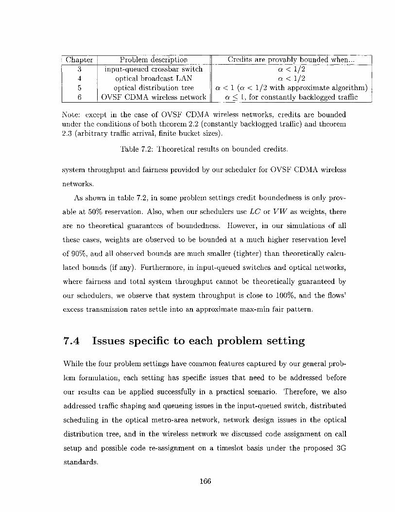
Chapter Problem description Credits are provably bounded when...3 input-queued crossbar switch a < 1/24 optical broadcast LAN a < 1/25 optical distribution tree a < 1 (a < 1/2 with approximate algorithm)6 OVSF CDMA wireless network a < 1, for constantly backlogged traffic
Note: except in the case of OVSF CDMA wireless networks, credits are boundedunder the conditions of both theorem 2.2 (constantly backlogged traffic) and theorem2.3 (arbitrary traffic arrival, finite bucket sizes).
Table 7.2: Theoretical results on bounded credits.
system throughput and fairness provided by our scheduler for OVSF CDMA wireless
networks.
As shown in table 7.2, in some problem settings credit boundedness is only prov-
able at 50% reservation. Also, when our schedulers use LC or VW as weights, there
are no theoretical guarantees of boundedness. However, in our simulations of all
these cases, weights are observed to be bounded at a much higher reservation level
of 90%, and all observed bounds are much smaller (tighter) than theoretically calcu-
lated bounds (if any). Furthermore, in input-queued switches and optical networks,
where fairness and total system throughput cannot be theoretically guaranteed by
our schedulers, we observe that system throughput is close to 100%, and the flows'
excess transmission rates settle into an approximate max-min fair pattern.
7.4 Issues specific to each problem setting
While the four problem settings have common features captured by our general prob-
lem formulation, each setting has specific issues that need to be addressed before
our results can be applied successfully in a practical scenario. Therefore, we also
addressed traffic shaping and queueing issues in the input-queued switch, distributed
scheduling in the optical metro-area network, network design issues in the optical
distribution tree, and in the wireless network we discussed code assignment on call
setup and possible code re-assignment on a timeslot basis under the proposed 3G
standards.
166
Bibliography
[1] F. Adachi et al. Tree-structured generation of orthogonal spreading codes with
different lengths for forward link of DS-CDMA mobile radio. Electronics Letters,
33(1):27-8, January 1997.
[2] Ravindra K. Ahuja, Thomas L. Magnanti, and James B. Orlin. Network flows:
theory, algorithms, and applications. Prentice Hall, Englewood Cliffs NJ, 1993.
[3] T. Anderson, S. Owicki, J. Saxe, and C. Thacker. High-speed switch schedul-
ing for local-area networks. ACM Trans. on Computer Systems, 11(4):319-352,
November 1993.
[4] Dimitri Bertsekas and Robert Gallager. Data Networks, 2nd ed. Prentice Hall,
1992.
[5] G. Bongiovanni, D. T. Tang, and C. K. Wong. A general multibean satellite
switching algorithm. IEEE Trans. on Communications, 29(7):1025-36, July
1981.
[6] Michael S. Borella and Biswanath Mukherjee. Efficient scheduling of nonuniform
packet traffic in a WDM/TDM local lightwave network with arbitrary transceiver
tuning latencies. In Proc. IEEE INFOCOM 95, Boston MA, pages 129-137, 1995.
[7] Anna Charny, P. Krishna, Naimish Patel, and Robert Simcoe. Algorithms
for providing bandwidth and delay guarantees in input-buffered crossbars with
speedup. In IWQoS 98, 1998.
167
[8] J.S.-C. Chen and T.E.Stern. Throughput analysis, optimal buffer allocation, and
traffic imbalance study of a generic nonblocking packet switch. IEEE J. Selected
Areas in Communications, 9(3):439-49, April 1991.
[9] Ming Chen and Tak-Shing Yum. A conflict-free protocol for optical WDMA
networks. In Proc. IEEE Globecom 91, Phoenix AZ, volume 2, pages 1276-1281,
December 1991.
[10] Mon-Song Chen, Nicholas R. Dono, and Rajiv Ramaswami. A media-access
protocol for packet-switched wavelength division multiaccess metropolitan area
networks. IEEE J. Selected Areas in Communications, 8(6):1048-1057, August
1990.
[11] F. Chiussi, J. Kneuer, and V. P. Kumar. Low-cost scalable switching solutions
for broadband networking: the atlanta architecture and chipset. IEEE Commu-
nications Magazine, 35(12):44-53, December 1997.
[12] S.T. Chuang, A. Goel, Nick McKeown, and Balaji Prabhakar. Matching output
queueing with a combined input output queued switch. Technical Report CSL-
TR-98-758, Computer Science Laboratory, Stanford University, April 1998.
[13] Thomas H. Cormen, Charles E. Leiserson, and Ronald L. Rivest. Introduction
to Algorithms. MIT Press, Cambridge MA, 1990.
[14] K. Y. Eng and A. S. Acampora. Fundamental conditions governing TDM switch-
ing assignments in terrestrial and satellite networks. IEEE Trans. on Commu-
nications, 35(7):755-761, July 1987.
[15] D. Gale and L.S. Shapley. College admissions and the stability of marriage.
American Mathematical Monthly, 69:9-15, 1962.
[16] A. Ganz and Y. Gao. A time-wavelength assignment algorithm for a WDM star
network. In Proc. IEEE INFOCOM 92, Florence, Italy, pages 2144-2150, May
1992.
168

[17] Vijay Sivaraman George N. Rouskas. On the design of optimal TDM schedules
for broadcast WDM networks with arbitrary transceiver tuning latencies. In
Proc. IEEE INFOCOM 96, San Francisco CA, pages 1217-1224, March 1996.
[18] L. Georgiadis, R. Guerin, V. Peris, and K. Sivarajan. Efficient network QoS pro-
visioning based on per node traffic shaping. IEEE/A CM Trans. on Networking,
4(4), August 1996.
[19] D. Guo, Y. Yemini, and Z. Zhang. Scalable high-speed protocols for WDM
optical star networks. In Proc. IEEE INFOCOM 94, Toronto, Canada, pages
1544-1551, June 1994.
[20] A.L. Gupta and N.D. Georganas. Analysis of a packet switch with input and
output buffers and speed constraints. In Proc. IEEE INFOCOM 91, Bal Harbour
FL, pages 694-700, 1991.
[21] R. T. Hofmeister, L. G. Kazovsky, C. L. Lu, and P. Poggiolini. CORD: optical
packet-switched network testbed. Fiber and Integrated Optics, 16(2):199-219,
1997.
[22] I. Iliadis and W.E. Denzel. Performance of packet switches with input and output
queueing. In Proc. ICC 90, Atlanta GA, pages 747-53, 1990.
[23] Thomas Inukai. An efficient SS/TDMA time slot assignment algorithm. IEEE
Trans. on Communications, 27(10):1449-55, October 1979.
[24] Anthony C. Kam and Kai-Yeung Siu. A real-time distributed scheduling algo-
rithm for supporting QoS over WDM networks. In Proc. SPIE: Conference on
All-Optical Networking: Architecture, Control and Management Issues, Boston,
MA, volume 3531, November 1998.
[25] Anthony C. Kam, Kai-Yeung Siu, Richard A. Barry, and Eric Swanson. A
cell switching WDM broadcast LAN with bandwidth guarantee and fair access.
IEEE/OSA J. of Lightwave Technology, 16(12):2265-80, December 1998.
169

[26] Anthony C. Kam, Kai-Yeung Siu, Richard A. Barry, and Eric Swanson. Toward
best-effort services over WDM networks with fair access and minimum band-
width guarantee. IEEE J. Selected Areas in Communications, 16(7):1024-39,
September 1998.
[27] I. P. Kaminow et al. A wideband all-optical WDM network. IEEE J. Selected
Areas in Communications, 14(5):780-799, June 1996.
[28] M. Karol and M. Hluchyj. Queueing in high-performance packet-switching. IEEE
J. Selected Areas in Communications, 6:1587-1597, December 1998.
[29] S. Keshav and Rosen Sharma. Issues and trends in router design. IEEE Com-
munications Magazine, pages 144-151, May 1998.
[30] P. Krishna, Naimish Patel, Anna Charny, and Robert Simcoe. On the speedup
required for work-conserving crossbar switches. In IWQoS 98, 1998.
[31] B. Li and Y. Qin. Traffic scheduling in a photonic packet switching system
with QoS guarantee. IEEE/OSA J. of Lightwave Technology, 16(12):2281-2295,
December 1998.
[32] S. Li and N. Ansari. Provisioning QoS features for input-queued ATM switches.
Electronics Letters, 34(19), September 1998.
[33] Nick McKeown. Scheduling Algorithms for Input-Queued Cell Switches. PhD
thesis, University of California at Berkeley, May 1995.
[34] Nick McKeown, Venkat Anantharam, and Jean Walrand. Achieving 100%
throughput in an input-queued switch. In Proc. IEEE INFOCOM 96, San Fran-
cisco CA, pages 296-302, March 1996.
[35] Nick McKeown, M. Izzard, A. Mekkittikul, W. Ellersick, and M. Horowitz. The
Tiny Tera: a packet switch core. IEEE Micro, 17(1):27-33, January 1997.
[36] Adisak Mekkittikul and Nick McKeown. A starvation-free algorithm for achiev-
ing 100% throughput in an input-queued switch. In ICCCN 96, 1996.
170

[37] Adisak Mekkittikul and Nick McKeown. A practical scheduling algorithm to
achieve 100% throughput in input-queued switches. In Proc. IEEE INFOCOM
98, San Francisco CA, pages 792-9, April 1998.
[38] Thit Minn and Kai-Yeung Siu. Dynamic assignment of orthogonal variable
spreading factor codes in W-CDMA. Technical report, Laboratory for Infor-
mation and Decision Systems, MIT, 1999.
[39] Biswanath Mukherjee. WDM-based local lightwave networks part I: Single-hop
systems. IEEE Networks, 6(3):12-27, May 1992.
[40] Y. Oie, M. Murara, K. Kubota, and H. Miyahara. Effect of speedup in non-
blocking packet switch. In Proc. ICC 89, Boston MA, pages 410-14, 1989.
[41] E. Oki and N. Yamanaka. Tandem-crosspoint ATM switch with input and output
buffers. IEEE Communications Letters, 2(7), July 1998.
[42] Christo H. Papadimitriou and Kenneth Steiglitz. Combinatorial Optimization:
Algorithms and Complexity. Prentice Hall, 1982.
[43] A. Parekh and R. Gallager. A generalized processor sharing approach to flow
control - the single node case. In Proc. IEEE INFOCOM 92, Florence, Italy,
pages 915-24, 1992.
[44] Gerard R. Pieris and Galen H. Sasaki. Scheduling transmissions in WDM
broadcast-and-select networks. IEEE/ACM Trans. on Networking, 2(2):105-110,
April 1994.
[45] Balaji Prabhakar and Nick McKeown. On the speedup required for combined
input and output queued switching. Technical report, Computer Science Labo-
ratory, Stanford University, 1997.
[46] J.G. Proakis. Digital Communications. McGraw-Hill, 1995.
[47] H. Sariowan. A Service Curve Approach to Performance Guarantees in Integrated
Service Networks. PhD thesis, University of California, San Diego, 1996.
171

[48] M. Shreedhar and G. Varghese. Efficient fair queuing using deficit round robin.
IEEE/A CM Trans. on Networking, 4(3):375-85, June 1996.
[49] Ion Stoica and Hui Zhang. Exact emulation of an output queueing switch by a
combined input output queueing switch. In IWQoS 98, 1998.
[50] L. Tassiulas. Linear complexity algorithms for maximum throughput in radio
networks and input queued switchs. In Proc. IEEE INFOCOM 98, San Francisco
CA, pages 533-9, April 1998.
[51] L. Tassiulas and A. Ephremides. Stability properties of constrained queueing
systems and scheduling policies for maximum throughput in multihop radio net-
works. IEEE Trans. Automatic Control, 37(12):1936-1948, December 1992.
[52] J. Turner. New directions in communications (or which way to the information
age). IEEE Communications Magazine, 24:8-15, 1986.
[53] T. Weller and B. Hajek. Scheduling nonuniform traffic in a packet switching
system with small propagation delay. In Proc. IEEE INFOCOM 94, Toronto,
Canada, pages 1344-1351, June 1994.
[54] Hui Zhang. Service disciplines for guaranteed performance service in packet-
switching networks. Proc. IEEE, 83(10):1374-96, October 1995.
[55] L. Zhang. A New Architecture for Packet Switching Network Protocols. PhD
thesis, Massachusetts Institute of Technology, Cambridge MA, 1989.
[56] L. Zhang. Virtual clock: A new traffic control algorithm for packet switching
networks. In Proc. A CM SIGCOMM 90, pages 19-29, 1990.
172
Related Documents