Efficient mixing and unpredictability in an experimental game

Efficient mixing and unpredictability in an

experimental game

Charles Noussair and Marc Willinger*

November 2003

Abstract

We report experimental data from a two-player, two-action game with a unique mixed strategy equilibrium. In contrast to most previous experiments, our design allows subjects to explicitly choose mixed strategies. Our results strongly reject standard predictions (mixed strategy equilibrium and the maxmin strategy profile), both when measured as subjects’ choices of probability distributions over actions, and as the resulting actions played. The Quantal Response Equilibrium (QRE) concept is a good predictor of the subjects' average choices. While achieving unpredictability is the main intuition justifying mixed strategy play, our data suggest that few subjects choose their strategies with the intent of achieving unpredictability. Rather, the observed patterns of mixing appear to be based on the expected payoff differences between agents’ two possible actions. Keywords: Mixed strategy equilibrium, maxmin, quantal response equilibrium, experimental economics. JEL Classification : C9, C91, C72.

* Noussair: Department of Economics, Emory University, Altanta, GA 30322, USA. E-mail: [email protected]. Willinger: Faculté des Sciences Economiques, Université de Montpellier I, Avenue de la Mer, BP 9606, 34054 Montpellier Cedex 1, France. E-mail: [email protected]. We thank Kene Boun My for development of the computer program used in the experiment. We would like to thank Tom Palfrey, Paul Pezanis-Christou, Jason Shachat and Gisèle Umbauer for their valuable comments that have improved the paper considerably. We also thank participants in the Summer 2003 Economic Science Association Meetings in Boston, MA, USA, for helpful comments.

1

1. Introduction In games where the only Nash equilibrium is in mixed strategies, it constitutes the unique

prediction of classical game theory. However, there are theoretical reasons to question the ability

of mixed strategy equilibrium (hereafter MSE) to predict behavior. Unlike equilibria in pure

strategies, mixed strategy equilibria are generically unstable. The choice of a mixed strategy on

the part of a rational player requires a belief that all other players play each of their actions with

precisely their equilibrium probabilities. The slightest deviation from equilibrium behavior on the

part of any player generally causes a pure strategy to become a unique best response for other

players. Furthermore, even if all others use their equilibrium strategies, a player is indifferent

between the equilibrium strategy and any other mixture over the actions that comprise his

equilibrium strategy, and thus there exist individual deviations from equilibrium that are costless

to the individual. However, despite the rather unconvincing theoretical foundation for equilibrium

play, classical non-cooperative game theory makes no other prediction in games with a unique

equilibrium in mixed strategies.

The concept of MSE seems intuitively more appealing if it is interpreted as a long run

frequency of action choices in a repeated game, because in principle any systematic deviation on

the part of a player from his equilibrium mixing probabilities can eventually be detected and

exploited by other players to his detriment.1 Thus, the empirical research in the area has generally

been focused on the issue of convergence of strategy choices to equilibrium with repeated play

(see Camerer, 2003, for a survey). Because of the ability to precisely specify the structure of the

game, most of the research has involved experimental methods. However, experimental studies

have reached various conclusions about the power of mixed strategy equilibrium to predict

behavior when it is the unique equilibrium of a game. Experiments that O’Neill (1989, 1991) and

Binmore et al. (2001) report indicate that overall choice frequencies are close to the equilibrium

predictions. A field study of data from Wimbledon tennis matches (Walker and Wooders, 2001)

also finds support for the use of equilibrium mixed strategies on the part of professional tennis

players. When the mixed strategy equilibrium involves each player choosing each of two actions

with equal probability, as in the matching pennies game, behavior is typically consistent with the

equiprobable MSE (Mookherjee and Sopher, 1997, Ochs, 1995).

On the other hand, in many games, substantial deviations from the MSE frequencies are

observed (Lieberman, 1961; Rapoport and Boebel, 1992; Ochs, 1995; Goeree and Holt, 2000;

1 Shachat and Swarthout (2003) report evidence that humans readily detect and exploit systematic deviations from equilibrium play in games with a unique Nash equilibrium in mixed strategies.

2

Shachat, 2002). Furthermore, Brown and Rosenthal’s (1990) reexamination of the data of O’Neill

(1989) noted that although overall average choices were close to the equilibrium frequencies,

there were a number of serious discrepancies with MSE at the level of the individual decision.

Ochs (1995) and Goeree and Holt (2001) among others, illustrate that choice frequencies of

players depend on their own payoffs, and not only on other players’ payoffs, as would be the case

in a mixed strategy equilibrium.

To provide a unified explanation of the discrepancies between experimental data and

Nash equilibrium in strategy choices in games, the Quantal Response Equilibrium (QRE) model

has been proposed (McKelvey and Palfrey, 1995). The model assumes that each player has an

estimate of his expected payoff from each of his actions that is unbiased but contains an unbiased

error. Players then choose the action that they believe yields the highest expected payoff, given

the strategies other players choose. Thus, QRE is a generalization of Nash equilibrium. The

model has the intuitively appealing and empirically relevant properties that a strategy is more

likely to be chosen the higher its expected payoff, yet no strategy is chosen with probability one.

This guarantees the own payoff effects and the heterogeneity of decisions typically observed in

laboratory experiments. Several studies have observed that the direction of deviations from

equilibrium in games with a unique MSE is consistent with the predictions of QRE (McKelvey et

al., 2000; Goeree et al., 2003).

In this paper, we report the results from an experiment with a previously unstudied two-

player, two-action game with a unique mixed strategy equilibrium. Our game belongs to the class

of "unprofitable games", which have the property that the Nash equilibrium payoff is not greater

than that under the Maxmin solution for any player.2 The unprofitable game that we consider has

a distinct Nash equilibrium and Maxmin solution, both of which are in mixed strategies. Since we

are interested in subjects' mixing behavior, we use a protocol in which participants play the mixed

extension of the game. This allows us to observe explicit mixing on the part of subjects. Rather

than choosing their actions directly, subjects are asked to choose probability distributions over

their possible actions. After the probabilities are chosen, an exogenous random device chooses

the action of each player. While the protocol allows “explicit mixing”, it does not preclude the

possibility of “internal” randomization before the choice of probability distribution is made.

However, in cases where explicit mixing occurs, the researcher can observe actual randomization,

rather than having to infer the existence of randomization from observing a sequence of actions

2 Morgan and Sefton (2002) studied subjects’ choices in particular unprofitable games, where the unique Nash equilibrium and Maxmin solutions are distinct. They found that neither the Nash solution nor the Maxmin solution offered a good description of their data, while QRE was consistent with most of their observations.

3

and making the assumption that the actions are drawn from a stationary distribution. In contrast to

traditional protocols, it allows for more refined testing of the hypothesis that mixed strategies are

used, because it provides additional data: the distributions selected as well as the outcomes of the

randomization process.

There is reason to believe that our protocol would enhance the ability of the mixed

strategy equilibrium to describe the data. The protocol facilitates randomization because to

generate the appropriate probabilities, subjects do not have to construct random sequences, which

are difficult to do in an independent and identically distributed manner.3 It may also make

subjects aware of the potential optimality of mixing. The design also facilitates a focus on the

behavioral assumption that underlies the notion of Quantal Response Equilibrium. Because

actions with greater expected payoff are played with greater probability, it predicts that behavior

in the mixed extension would exhibit the following two properties. Agents would be most likely

to play a mixed strategy consisting of placing probability one on the action with the highest

expected payoff. The second is that if one of the two pure strategies maximizes expected payoff, a

given mixed strategy would be more likely to be observed, the higher the probability it places on

the optimal action.

The results of the paper indicate the following. Mixing is widely observed. However, the

observed choices and outcomes are inconsistent with the use of equilibrium mixed strategies,

minimax strategies, and cooperative behavior. The outcomes are consistent with the Quantal

Response Equilibrium at the aggregate level. The mixing that is observed does not appear to

reflect a desire to be unpredictable but rather primarily a consequence of payoff differences

between actions. In section 2 we present the theoretical predictions and the experimental

procedures. Section 3 presents our results and section 4 concludes with a short discussion.

2. The Experiment 2.1. The Game and Theoretical Models

The game studied is the two-by-two normal form game shown in figure 1. Let p equal the

probability that row player chooses the action U and q equal the probability that column player

chooses L. The game has a unique mixed strategy equilibrium at p* = .05 and q* = .05. We will

refer to this strategy profile as the prediction of the MSE. In the MSE, the probability of

outcomes UL (Up, Left), UR, DL, and DR (Down, Right) are 1/400, 19/400, 19/400, and 361/400.

The expected payoffs in the mixed strategy equilibrium are 9.5 for each player.

3 Shachat (2002) reports that the availability of an explicit mixing device reduces the autocorrelation in subjects’ decisions from one period to the next.

4

Figure 1: Normal Form of the Game

Outcome of Column

Player's Choice

LEFT RIGHT

UP 190 , 0 0 , 190

Outcome of Row

Player's Choice DOWN 0, 10 10, 0

The maxmin solution, at which each player chooses the action where his expected payoff

is maximized under the assumption that the other player attempts to minimize his payoff, is at pm

= .05 and qm = .95. We will refer to this strategy profile as the prediction of the MM solution. If

both players follow their maxmin strategy, which are not mutual best responses for this game, the

probabilities of the four outcomes are 19/400, 1/400, 361/400, and 19/400 for UL, UR, DL and

DR respectively. The expected payoff is 9.5 for each player in the maxmin strategy profile, equal

to that in the MSE for all players.

It is clear from figure 1 that there are opportunities to attain total welfare considerably

greater than in the MSE or the MM. In the game, the choice of the Row player determines the

overall payoff. If U is played, total earnings are 190, but if D is played, they are 10. One simple

strategy profile that yields payoffs along the frontier as well as identical expected earnings for the

two players is for Row player to choose U and Column player to choose L with probability 0.5.

This strategy profile, which we call the Cooperative (CO) solution, yields each player an expected

payoff of 95. In a repeated game, the CO outcome can be achieved if Row player plays U in

every period, and Column player alternates between L and R. The cooperative outcome also

corresponds to the Nash Bargaining Solution for the game. The feasible average per-period

payoffs of the game for the two players correspond to a region with vertices at (10,0), (0, 10),

(190, 0), and (0, 190). The maxmin payoff vector is (9.5, 9.5). The payoff vector that maximizes

5

the product of the two players’ earnings relative to the maxmin, occurs at (95, 95), the payoff at

the cooperative outcome.

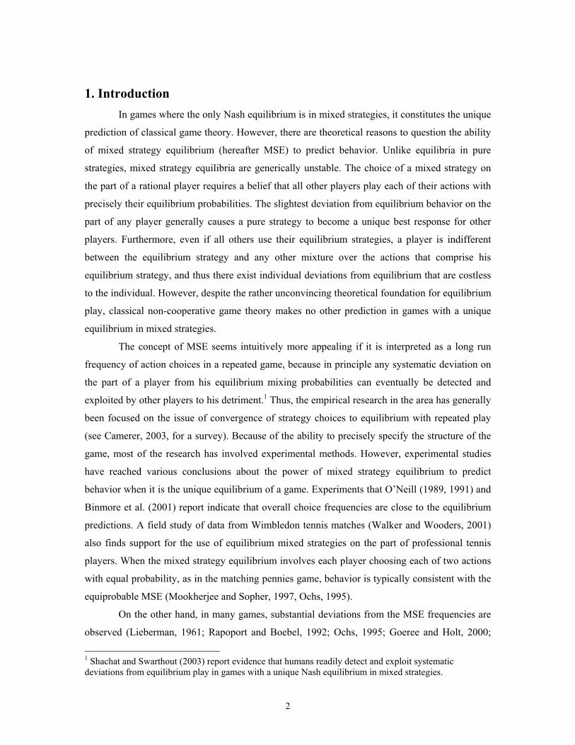
A Quantal Response Equilibrium to the game is shown in figure 2. The QRE illustrated in

the figure assumes the commonly employed logit specification of the relationship between the

probability an action is chosen and the error in the estimation of payoffs. The vertical axis

indicates the probability that row player chooses U and that column player chooses L. The

horizontal axis is the level of error, λ, which corresponds to the probability that U is chosen. The

graph for Row player is the solution to )ee(

e)(P )D(u)U(u

)U(u

U λλ

λ

+=λ , where )(λUP is

the probability that action U is chosen under error parameter lambda, and is the expected

utility of action U. The other series is analogous, indicating the probability that action L is chosen

on the part of Column player. The figure shows that any probability of Row playing action U

between .05 and .5988 and any probability of Column playing L between .0064 and .5 is

consistent with a QRE. Although a strict interpretation of QRE requires that the strategies of

paired Row and Column players correspond to a common λ, we will require only each player

makes his decision as if the two players have a common λ, although the actual value of the

parameter might be different between the two players.

)U(u^

4 Thus, we will say that any observed

values of p and q such that any p ∈ [.05, .5988] and any q ∈ [.0064, .5] will be classified as

consistent with the QRE solution. Thus the predictions of the QRE solution cover approximately

27.09 percent of the strategy space. If the percentage of outcomes consistent with QRE is

significantly greater than 27.09, we will say that the data support the model. The predictions of

the four models are summarized in table 1.

Table 1: Predictions of the MSE, MM, CO, QRE Solutions Solution Prediction

MSE (Mixed Strategy Equilibrium) p* = .05, q* = .05

MM (Maxmin Profile) pm = .05, qm = .95

CO (Cooperative Model) pc = 1, qc = .5

QRE (Quantal Response Equilibium) pQRE ∈ [.05, .5988], qQRE ∈ [.0064, .5]

6

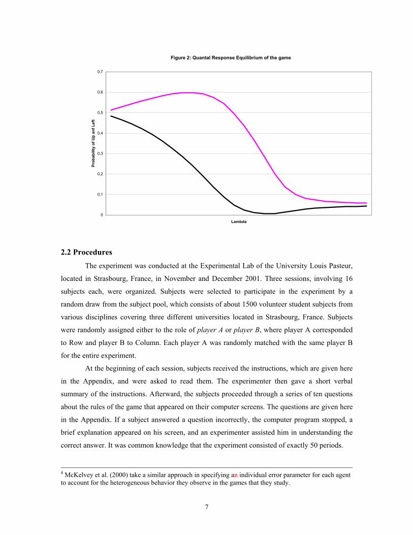
Figure 2: Quantal Response Equilibrium of the game

0

0,1

0,2

0,3

0,4

0,5

0,6

0,7

Lambda

Prob

abili

ty o

f Up

anf L

eft

2.2 Procedures

The experiment was conducted at the Experimental Lab of the University Louis Pasteur,

located in Strasbourg, France, in November and December 2001. Three sessions, involving 16

subjects each, were organized. Subjects were selected to participate in the experiment by a

random draw from the subject pool, which consists of about 1500 volunteer student subjects from

various disciplines covering three different universities located in Strasbourg, France. Subjects

were randomly assigned either to the role of player A or player B, where player A corresponded

to Row and player B to Column. Each player A was randomly matched with the same player B

for the entire experiment.

At the beginning of each session, subjects received the instructions, which are given here

in the Appendix, and were asked to read them. The experimenter then gave a short verbal

summary of the instructions. Afterward, the subjects proceeded through a series of ten questions

about the rules of the game that appeared on their computer screens. The questions are given here

in the Appendix. If a subject answered a question incorrectly, the computer program stopped, a

brief explanation appeared on his screen, and an experimenter assisted him in understanding the

correct answer. It was common knowledge that the experiment consisted of exactly 50 periods.

4 McKelvey et al. (2000) take a similar approach in specifying an individual error parameter for each agent to account for the heterogeneous behavior they observe in the games that they study.

7

To enhance subjects’ ability to form independent sequences of action choices should they

wish to do so, a mechanism was used whereby they could choose probability distributions over

their set of actions. The instructions indicated to subjects that they were endowed with 100

tokens, and that any integer portion of the 100 tokens could be assigned to each of the actions. In

other words, in each period participants were required to specify an allocation of 100 tokens

between two available actions. The actions were called W and X for Row player and Y and Z for

Column player during the experiment. A subject moved a bar on her computer screen to make her

choice. Subjects were explicitly reminded in the instructions that they could assign all of the

tokens to either one of their actions if they wished to be certain that a particular action would be

chosen for them. A random device then chose the actual action played by the subject, where the

probability of each action choice was equal to the percentage of the 100 tokens the player had

placed on the action. For example, if Row player decided to allocate proportion p of his tokens to

action W, that action would be chosen with probability p. This procedure allows explicit choice of

the mixing probability, since subjects knew that the allocation in any given period determined

their chances of playing each of their two actions. Explicit mixing allows us to compare the

predicted probability of each action with the observed probability choice directly. In contrast, in

experiments that elicit action choices, implicit probabilities must be inferred from observed

outcomes.5

The game was simultaneous so that a player did not know the other player’s decision for

the current period until after making his own choice. After subjects had decided on an allocation

of their tokens, the outcome was selected at random according to the probability distributions

induced by the subjects’ choices. The outcome was announced by displaying on the screen the

option selected for each player and the resulting payoff for both. The payoff matrix, as displayed

in the instructions presented to the subjects, is summarized in figure 1. The current period

earnings of both players and own accumulated earnings until the current point of the experiment

were displayed at all times. Subjects could also review the history of play since the beginning of

the experiment by hitting a history key. At the end of the experiment, the total amount of Yens

5 Ochs (1995) uses a different technique for eliciting a probability distribution over actions. A player participates in a game with two possible actions, A and B. In each period, each player has three options, to play action A, to play action B, or to form a sequence of ten choices of A and B. He is then matched with an opponent in ten identical games, played simultaneously. If he chose action A, he plays A in all ten games. If he chose B, he plays B in all ten games. If he chose to form a list consisting of As and Bs, he plays A in a percentage of the ten games equal to the percentage on his list that were As.

Shachat (2002) uses a system of strategy elicitation similar to ours. In a game with four actions, he allows subjects to place cards of four different colors in a “shoe” in any desired proportion. Each color represented one of the four actions available to the individual. The deck of cards is shuffled and one card is drawn. The color of the card that is drawn determines the action chosen.

8

earned by a subject in the experiment was converted into French Francs at the rate 1 Franc = 20

Yens. Subjects were paid privately one by one, and were invited to write down short comments

while waiting their turn to receive payment.

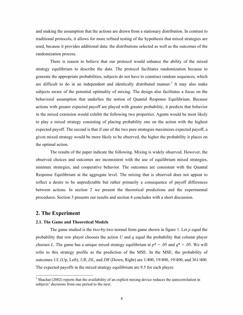
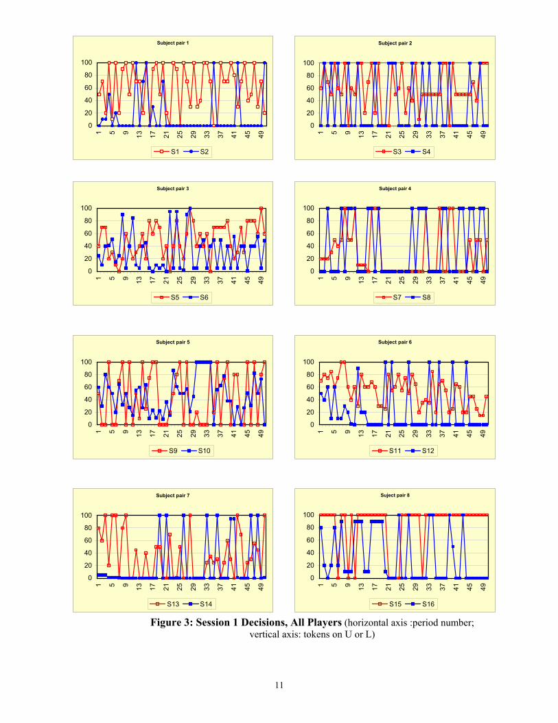
3. Results The time series of the decisions of each pair of subjects are shown in figures 3-5 below. The

figures indicate the number of tokens Row player subjects placed on the upper row, U, and the

number of tokens Column player subjects placed on L, by period, for each of the 24 pairs of

subjects. In the figures, Sj denotes subject j and odd-numbered j correspond to row players while

the even numbers correspond to column players. Players 1 and 2 are paired with each other, as are

3 and 4, etc… The horizontal axes in the figures denote the period number of the session, ranging

from 1 to 50. The vertical axes indicate the number of tokens, out of the maximum possible

number of 100, that row player placed on U and column player placed on L. Several initial

impressions can be gained from inspection of the figures and comparison of the data to the

predictions of the MSE, MM, and CO solutions. Recall that the MSE predicts an average choice

of 5 (5% of all tokens) for both Row and Column player, the MM solution predicts average

choices of 5 for Row player and 95 for Column player, and the CO solution predicts a choice of

100 for Row player and an average of 50 for Column player. The average can be attained in

several ways. For example, the randomizing device could be used to specify exactly the predicted

percentage on each action in any period. Alternatively, a combination of 0 and 100 could be

chosen with a frequency that corresponds to the appropriate mixing probability. If randomization

occurs before the actual choice of action, identical numbers describe the expected proportion of

instances in which each action is chosen. Table 2 illustrates the percentage of instances in which

the realized action of each player was U for Row players and L for Column players.

The figures illustrate considerable discrepancies between the data and the solution

concepts. Overall, the average choice is 45 for Row players and 28.3 for Column players. The

average choice of each of the 24 individual Row players as well as each of the 24 Column players

is greater than the equilibrium prediction of 5. The average choice of every Row player is greater

than the maxmin prediction of 5, and the average choice of every Column player less than the

maxmin prediction of 95. There are two pairs of subjects, players 15 and 16 in session 1, and

players 31 and 32 in session 2, that exhibit patterns of behavior that are consistent with the CO

for sustained episodes. In particular, the latter pair follows the CO strategy profile perfectly for

the first 20 periods. However, overall, it is clear that none of the three solutions provides a

9

satisfactory explanation for the observed data. Furthermore, there appears to be no tendency for

decisions to converge in the direction of the predictions of any of the solution concepts with

repetition of the game. Thus our first result is that none of these three predictions receive

substantial support in our data.

Result 1: Observed choices are highly inconsistent with the Mixed Strategy Equilibrium, the

Minimax, and the Cooperative Solutions.

Support for Result 1: A t-test rejects the hypothesis that the average choice of Row players

(pooling all the choices of all Row players) is equal to 5 (t = 12.44, p < .001), indicating

inconsistency with the MSE and the MM models. A sign-test rejects the hypothesis that the

median (across all Row players) of the average strategy choice of Row players is equal to 5, at p

< .001, since 24 of 24 players choose an average action greater than 5. The same tests also reject

the hypotheses that the mean and median strategies are equal to 100, the prediction of the CO

model, at similar significance levels. For Column players, the hypotheses that the average and

median strategies chosen are equal to 5, the MSE prediction, and 95, the MM prediction, can all

be rejected at the p <.001 level.

We can also consider whether the proportion of instances in which each outcome, the

actual action resulting from a player’s decision, is observed is consistent with the predictions of

the solution concepts. Using a t-test, we reject the hypothesis that the percentage of instances in

which Row’s action is U is equal to 5%, the prediction of the MSE and MM models (t = 12.33, p

< .001). We also reject the hypothesis that the percentage is equal to the CO prediction of 100

with t = 16.93, yielding a similar level of significance. We reject the hypothesis that the

percentage of action L outcomes is equal to the MSE prediction (t = 10.98, p < .001), as well as

equal to the MM prediction (t = 26.43, p < .001). A Χ2 test of goodness of fit rejects the

hypothesis that the distribution of the frequency of the four possible outcomes is equal to the

MSE prediction (Χ2 = 10.26, p < .05), and the MM prediction (Χ2 = 37.44, p < .001). □

10

Subject pair 7

0

20

40

60

80

100

1 5 9 13 17 21 25 29 33 37 41 45 49

S13 S14

Subject pair 5

0

20

40

60

80

100

1 5 9 13 17 21 25 29 33 37 41 45 49

S9 S10

Subject pair 2

0

20

40

60

80

100

1 5 9 13 17 21 25 29 33 37 41 45 49

S3 S4

Subject pair 6

0

20

40

60

80

100

1 5 9 13 17 21 25 29 33 37 41 45 49

S11 S12

Subject pair 1

0

20

40

60

80

100

1 5 9 13 17 21 25 29 33 37 41 45 49

S1 S2

Suject pair 8

0

20

40

60

80

100

1 5 9 13 17 21 25 29 33 37 41 45 49

S15 S16

Subject pair 3

0

20

40

60

80

100

1 5 9 13 17 21 25 29 33 37 41 45 49

S5 S6

Subject pair 4

0

20

40

60

80

100

1 5 9 13 17 21 25 29 33 37 41 45 49

S7 S8

Figure 3: Session 1 Decisions, All Players (horizontal axis :period number; vertical axis: tokens on U or L)

11

Subject pair 7

0

20

40

60

80

100

1 5 9 13 17 21 25 29 33 37 41 45 49

S13 S14

Subject pair 1

0

20

40

60

80

1001 5 9 13 17 21 25 29 33 37 41 45 49

S1 S2

Subject pair 5

0

20

40

60

80

100

1 5 9 13 17 21 25 29 33 37 41 45 49

S9 S10

Subject pair 3

0

20

40

60

80

100

1 5 9 13 17 21 25 29 33 37 41 45 49

S5 S6

Subject pair 2

0

20

40

60

80

100

1 5 9 13 17 21 25 29 33 37 41 45 49

S3 S4

Subject pair 8

020406080

100

1 5 9 13 17 21 25 29 33 37 41 45 49

S15 S16

Subject pair 6

0

20

40

60

80

100

1 5 9 13 17 21 25 29 33 37 41 45 49

S11 S12

Subject pair 4

0

20

40

60

80

100

1 5 9 13 17 21 25 29 33 37 41 45 49

S7 S8

Figure 4: Session 2 Decisions, All Players

12

Player pair 7

0

20

40

60

80

100

1 5 9 13 17 21 25 29 33 37 41 45 49

S13 S14

Player pair 1

0

20

40

60

80

100

1 5 9 13 17 21 25 29 33 37 41 45 49

S1 S2

Player pair 5

0

20

40

60

80

100

1 5 9 13 17 21 25 29 33 37 41 45 49

S9 S10

Player pair 3

0

20

40

60

80

100

1 5 9 13 17 21 25 29 33 37 41 45 49

S5 S6

Player pair 2

0

20

40

60

80

100

1 5 9 13 17 21 25 29 33 37 41 45 49

S3 S4

Player pair 8

0

20

40

60

80

100

1 5 9 13 17 21 25 29 33 37 41 45 49

S15 S16

Player pair 6

0

20

40

60

80

100

1 5 9 13 17 21 25 29 33 37 41 45 49S11 S12

Player pair 4

0

20

40

60

80

100

1 5 9 13 17 21 25 29 33 37 41 45 49

S7 S8

Figure 5: Session 3 Decisions, All Players

13

Table 2: Percentage of choices of U for Row and L for Column

Player pair Session 1 Session 2 Session 3 Row Column Row Column Row Column

1 0.58 0.18 0.38 0.24 0.58 0.38 2 0.66 0.32 0.34 0.22 0.34 0.52 3 0.48 0.32 0.30 0.28 0.42 0.24 4 0.32 0.40 0.24 0.18 0.50 0.60 5 0.34 0.42 0.36 0.28 0.54 0.50 6 0.50 0.24 0.36 0.32 0.48 0.26 7 0.32 0.20 0.24 0.34 0.58 0.08 8 0.84 0.34 0.78 0.36 0.42 0.32

Average 0.51 0.30 0.38 0.28 0.48 0.36

The figures also illustrate a tendency for players to increasingly forego the use of the

randomizing device over time and to instead make choices of 0 and 100 tokens more often as the

game is repeated. Figure 6 illustrates this dynamic over time. Of course, observing a choice of 0

or 100 does not rule out the possibility that randomization occurs mentally (implicit mixing)

before the actual choices are made, and that the pure strategies that we observe reflect the use of

mixed strategies. Indeed, the frequent choice of both 0 and 100 on the part of individuals in

adjacent periods suggests that some subjects do randomize mentally before making their choice.

It is possible that over time, agents become more comfortable making randomizations on their

own instead of relying on the device.

Result 2: Use of the explicit randomizing device is widespread but declines over time.

Support for result 2: Figure 6 reveals that 75% of row players and 45% of column players use

the explicit randomizing device in period 1. These are therefore lower bounds on the percentage

of players that use a mixed strategy, since players may mix without using the device. The figure

indicates a tendency for the percentage to decrease over time for the average player. By the last

period, the percentages have decreased to 45% and 38% for Row and Column players

respectively. □

14

0,00 0,10 0,20 0,30 0,40 0,50 0,60 0,70 0,80 0,90

1 3 5 7 9 11 13 15 17 19 21 23 25 27 29 31 33 35 37 39 41 43 45 47 49 51

period

% of tokens on U and

row column

Figure 6: Frequency of choice of pure strategies over time (average

percentage of tokens on U and L)

It is clear that most players change their choices frequently over the course of the game

and often employ the explicit mixing device. This suggests that players recognize the need to be

unpredictable at least to some extent. To consider the level of predictability of decisions, we

estimate the following probit model for each player.

tDDDP DLt

URt

ULtt

41

31

21

101 βββββ ++++= −−− (1)

1tP denotes the number of tokens placed on the player’s first action, U in the case of the

Row player, and L in the case of the Column player, in period t. The variable is a dummy

variable that equals 1 if the outcome in period t-1 is UL (which yields a payoff of 190 for Row

and 0 for Column), and zero otherwise. and are analogous. The estimation is

conducted separately for each player in recognition of the obvious heterogeneity in behavior

between different individuals. Significant values of

ULtD 1−

URtD 1−

DLtD 1−

1β , 2β , or 3β would indicate a dependence of

decisions on the realized outcome of the previous period. Finally, if 4β is significant, there is a

general tendency over time for the number of tokens placed on the first action, which is U for row

players and L for column players, to either increase or decrease, depending on the sign of the

coefficient.

15

The variables included in the estimation equation are those that might be thought to

render the player’s decisions predictable from the point of view of the other player.6 We will

interpret the adjusted pseudo-R2 values resulting from estimating the equation for an individual as

a measure of the individual’s predictability. The results of the estimation are given in table 3. The

table indicates the average and range of adjusted pseudo-R2 values for the 24 players in each of

the two roles. It also indicates the number of players for whom the coefficient was significant at p

< .05 and whether the significance was positive or negative. For example (1+, 4-) indicates that

the coefficient on the variable was significantly positive for one of the 24 players in the role

indicated, significantly negative for four of the players, and insignificant for the remaining 19

players.

Table 3: Statistics for Estimates of Equation (1)

Row Players Column Players

Average adjusted R2 .148 .157

Standard Deviation .135 .145

Range of R2 [min,max] [006,.600] [.035,.558]

DUL 1+,4- 1+,8-

DUR 2+ 5-

DDL 4+,1- 1+,5-

Period 2+,4- 2+,9-

Several observations are clear from the data in the table. The first is that the average

adjusted R2 for Column players is roughly the same as for Row players, indicting that on average

Row and Column players are equally predictable. The second observation is the lack of any

variable that is significantly explanatory for more than six of the 24 Row players. The third is the 6 In addition to the specification presented here, we also considered other specifications. In particular, we considered as a dependent variable the effect of the variable Rt-1, which equals the number of times during the t-1 periods already played that the opponent used his first strategy, that is, U for Row players and L for column players. We also considered Et-1, the relative earnings of the two players between periods 1 and t-1. This takes the form of the sum of the earnings for the opposing player over the t-1 periods, divided by the sum of the player’s own earnings for the t-1 periods. We also considered u , the difference in the average payoff that the player has received from periods 1 through t-1 between actions 1 and 2, calculated for a Row player by averaging his earnings in every period in which action U was chosen from periods 1 to t-1, performing the same calculation for the periods in which action D was chosen, and taking the difference between the two averages. For Column players it is the difference between the historical average payoff between actions L and R. None of these variables added to the adjusted R2 of most players

21

11 −− − tt u

16

lack of a variable that is explanatory for more than eleven Column players. The most pronounced

relationship is that nine of the 24 Column players did exhibit a general tendency to play R more

frequently over time that was independent of the previous period’s outcome. Some overall

patterns are summarized in result 3, which also contains results on the correlation between

predictability and earnings.

Result 3: Players’ actions are unpredictable. Row and Column players are equally

unpredictable on average. Row player predictability is associated with higher average

earnings for both players. The level of predictability between an individual and the player

with whom he is matched is correlated.

Support for Result 3: We cannot reject the hypothesis, using a t-test, that the average R2 value

over either Row of Column players is equal to zero. We also cannot reject the hypothesis, using a

pooled variance t-test, that the average R2 is the same between Row and Column players at p <

.05 (t = .19). Taking each player as an observation, there is a correlation of .212 between R2

(predictability) and own earnings for Row players, which is significant at the 5% level. The

correlation between predictability and own earnings for Column players was .036, insignificant at

the 5% level. For Row players, the correlation between own earnings and the predictability of

partner was -.031. Between Column players’ earnings and Row player predictability, the

correlation was .296. The latter is significant at the 5% level. Earnings were significantly higher

for Row players who had a predictable partner, but not for Column players. The predictability of

Row players and their partners exhibited a positive correlation of .401, significant at p < .001, so

that the more predictable a player was, the more predictable was his partner. □

The positive relationship between Row player predictability and higher earnings for both

players is related to a greater incidence of play of U on the part of Row players, which increases

expected total earnings. The fact that Column players choose L more often than in a non-

cooperative equilibrium raises the expected return of playing U and attracts Row players to

choose U more frequently. These earnings are not related to the predictability of Column, because

Row can be induced to choose U with a predictable strategy of alternating between L and R, or an

unpredictable mixture that puts sufficient probability on L.

and they were therefore left out in the results reported here. Their inclusion would not change the conclusions we give below.

17

Indeed, predictability of Row players appears to be positively correlated with the

perceived expected payoff of playing U compared to D. In a game with a unique mixed strategy

equilibrium such as ours, a player has an incentive to be unpredictable in order to equalize the

expected payoff between the actions of the other player, so that the other player is unable to use a

pure strategy best response to a predictable strategy. However inspection of the relationship

between a player’s predictability and the difference in the average historical payoff of her two

actions suggests a different rationale for the unpredictability we observe. Unpredictability is more

likely when the expected payoffs of a player’s own two actions are close to each other. A player

is more predictable the larger the difference in the historical average payoff of the two strategies.

Let be the difference in the average payoff that the player has received from periods

1 through t-1 between actions 1 and 2. It is calculated for a Row player by averaging his earnings

in every period in which action U was chosen from periods 1 to t-1, performing the same

calculation for the periods in which action D was chosen, and taking the difference between the

two averages. The variable is calculated in an analogous manner for Column players as the

difference between the historical average payoff between L and R. It seems reasonable to suppose

that a player views the historical average payoff of an action as a good predictor of the expected

payoff of the action at time t. The pattern suggests the following conjecture.

21

11 −− − tt uu

Conjecture: Unpredictability on the part of a player i is a result of indifference between i’s

own two actions, rather than an attempt to make the other player j indifferent between his

two actions.

Support for conjecture: The predictability of player i is negatively correlated with the difference

in the expected payoff of i’s two actions. The average value over the 49 periods, beginning in

period 2, of the variable for Row players is 26.24, while the average value of

for Column players is 57.96. Both and u are greater than

zero, when averaged over an entire session, for every pair of players in the study. In an expected

payoff sense, every Row player would have been better off playing U more often and every

Column player would have been better off playing R more often, provided that their partner did

not change strategy in response. Among Row players, there is a positive correlation between

and predictability as captured in the R

Dt

Ut uu 11 −− −

Lt

Rt uu 11 −− −

Dt

Ut uu 11 −− −

Dt

Ut uu 11 −− − L

tR

t u 11 −− −

Lt

Rt u 11 −− −

2 term of .482, which is significant at p <

.001. For column players, there is a positive correlation between and predictability

of .234, which is significant at the p < .05 level. □

u

18

One intuition for why a player would be more unpredictable when the expected payoffs

of her two actions are close together is that the expected payoffs are estimated with error. The

smaller the difference in expected payoff, the more likely the subject to choose a suboptimal

action and therefore to appear unpredictable. Such estimation error is the underlying behavioral

assumption of Quantal Response Equilibrium. Under QRE, each player’s estimate of the expected

payoff of each of his actions is subject to an unbiased error, and the player chooses the action

leading to the higher estimated expected payoff. The probability a suboptimal strategy is chosen

is therefore decreasing in the difference between its true expected payoff and that of the optimal

strategy. This suggests that QRE may be a good predictor of the patterns we observe in the data.

Indeed, as we report in result 4, at the aggregate level, the QRE is quite informative in describing

the range of aggregate frequencies typically observed.

Result 4: Aggregate frequencies of action choices are in a range consistent with the Quantal

Response Equilibrium Model.

Support for Result 4: The QRE model allows choices of the Row player, the number of tokens

placed on U, to be between 5 and 59.88 and those of Column player, the number of tokens

assigned to L, to be between 0.64 and 50. Although this region covers only 27.09 percent of the

space of possible actions, 21 of 24 (87.5%) pairs have average frequencies of outcomes within

this range. 7 □

It is instructive to study the three pairs of subjects whose average choices are inconsistent

with the QRE. These are pairs 2 and 8 in session 1, and pair 16 in session 2. The source of the

failure of QRE in all of these cases is that the Row player played U more frequently that the QRE

model allows. These three pairs were also the three pairs who had the highest total payoffs of the

24 pairs in the study. This suggests that group level considerations cause the departure from QRE

observed in these groups, and that the assumption of non-cooperative behavior is not fully valid

for these groups. This is not surprising given the potential gains from strategy profiles such as the

CO solution.

7 Therefore, according to Selten's (1991) measure of predictive success, S = h – a, where h measures the hit rate of paired choices falling into the predicted area, and a is the predicted rate, only 87.5% of player pairs have a net positive hit rate.

19

0,000,050,100,150,200,250,300,350,400,450,50

0 4 8 12 16 20 24 28 32 36 40 44 48 52 56 60 64 68 72 76 80 84 88 92 96 100

# of tokens on U, L

fre

qu

en

cy

row player column player

Figure 7: Distribution of Choices of All Row and Column Players

Figure 7 illustrates the percentage of instances in which each of the 101 possible

decisions in the mixed extension, pooled across the players in each role, was played. The vertical

column is the percentage of total observations during which the particular number of tokens was

placed on U or L. It shows that 0 and 100 are the most frequent choices, and that there is a

tendency to choose strategies that are divisible by 10 (corresponding to 10% increments), and in

particular 50%. There are no choices of action that are not divisible by 5. This is inconsistent with

the notion of QRE in the mixed extension, since the probability of the observation of a choice

should be increasing in the expected payoff of the choice. Since an action of 0 or 100 always

yields the greatest expected payoff, choices of 0 should be more common than 1, which in turn

should be more frequent than 2, etc., when 0 is the optimal decision. When a choice of 100 is

optimal, 100 should be the most frequent choice, followed by 99, then by 98, etc. In fact,

although the strategy with the highest expected payoff is the most common choice, the strategy

with the lowest expected payoff, the other (suboptimal) pure strategy, is the second most

common. This suggests that in games with a large number of strategies, the QRE model might be

supplemented with rules of thumb to narrow down the set of possible choices.

The Nash equilibrium can be calculated for a game close to the mixed extension.

Consider a game with 21 actions for Row player and 21 actions for column player. The 21 actions

for Row player consist of placing 0, 5, 10, etc… tokens on action U. The 21 actions for Column

player consist of placing 0, 5, 10, etc… tokens on action L. This provides a reasonable

20

approximation to our game since no strategy that was not divisible by 5 was ever chosen in the

experiment. The unique Nash equilibrium of the game is the following mixed strategy

equilibrium. Row player places x tokens on U with probability )

55(

21)( += xxP . In other words,

he places 0 tokens on U with probability .5, 5 tokens on U with probability .25, 10 tokens with

probability .125, etc… Similarly, Column player places x tokens on U with probability

)5

5(2

1)( += xxP . The QRE for this 21 action version of the mixed extension also has the

property that action 0 is the most frequently chosen action for each player, for any value of λ > 0.

Also for any λ > 0, the action 5 is the second most frequently chosen, 10 is the third most frequent

etc. The data show that 0 is the most common strategy employed for both players, which is

consistent with the QRE of the mixed extension. However, as mentioned previously, the data do

not show the pattern of monotonic decline in the incidence of play of strategies that involve

greater placement of tokens on D and R.

4. Discussion The data exhibit the following characteristics. In a manner consistent with some of the

previous studies, we find large and qualitative differences between the observed decisions of

agents and the mixed strategy equilibrium. Observed decisions are also very different from two

competing predictions, the maxmin strategy profile, and the outcome that would result from the

maximization of total group earnings. The failure of mixed strategy equilibrium appears to stem

from several sources. The first is its reliance on purely non-cooperative assumptions about

individual behavior. The second is its instability: an equilibrium mixed strategy is only a best

response if the other player uses his equilibrium mixture, but whenever it is a best response, there

are infinitely many other best responses.

The data have the feature that the aggregate outcomes are typically in the range consistent

with a Quantal Response Equilibrium. Although QRE effectively describes the overall data,

inspection of individual decisions reveals two patterns of behavior inconsistent with the

assumptions of a formulation of Quantal Response Equilibrium that assumes purely self-

interested players. The first is the existence of cooperative behavior on the part of some subject

pairs that is consistent with the maximization of group level gains. The second is that the

distribution of strategy choices in the mixed extension does not have the feature that less costly

deviations from optimal behavior are more likely to be observed than other actions. In particular,

21

the most common choices observed are the pure strategies, which always have the feature that

they have the highest and the lowest expected payoffs among the available strategies. Thus the

strategy with the lowest expected payoff in the mixed extension is typically one of the two most

likely choices. Suboptimal strategies are often chosen in our game because they satisfy particular

rules of thumb as well as the fact that they are not very costly relative to optimal behavior. A

paradox exists in that the QRE is successful in predicting the range of aggregate frequencies of

observed actions but not at the level of the mixed extension. This may be due to framing and if

the mixed extension of the game was presented to subjects as a normal form, the QRE model may

perform substantially better.

We also observe a relationship between unpredictability, player roles, and earnings.

Unpredictability appears to indicate indifference between the available actions in addition to

intent to be unpredictable. Unpredictability is not necessarily profitable in that for Row players, it

was negatively correlated with earnings.

References

Binmore K., J. Swierzbinski, and C. Proulx (2001) “Does Minimax Work: An Experimental

Study?” Economic Journal, 111, 445-464.

Camerer, C. (2003), Behavioral Game Theory, Princeton University Press, Princeton, NJ, USA.

Brown J., and R. Rosenthal (1990), "Testing the Minimax Hypothesis: a Re-examination of

O'Neill's Game Experiment", Econometrica, 38, 1065-1081.

Goeree J. and C. Holt, (2001), “Ten Little Treasures of Game Theory and Ten Intuitive

Contradictions”, American Economic Review, 91, 1402-1422.

Goeree J., C. Holt, and T. Palfrey (2003), “Risk averse behavior in generalized matching pennies

games”, Games and Economic Behavior, forthcoming.

Lieberman B. (1962), "Experimental studies of conflict in some two-person and three person

games", in J. Criswell, H. Solomon & P. Suppes (eds), Mathematical modes in small group

processes, Standord University Press, 203-220.

22

McKelvey, R., Palfrey T., (1995), "Quantal response equilibria for normal-form games", Games

and Economic Behavior, 10, 6-38.

McKelvey, R., T. Palfrey, and R. Weber (2000), “The effects of payoff magnitude and

heterogeneity on behavior in 2x2 games with unique mixed strategy equilibria”, Journal of

Economic Behavior and Organization, 42, 523-548.

Mookherjee D., Sopher B., (1997), "Learning and Decision Costs in Experimental Constant-sum

Games", Games and Economic Behavior, 19, 97-132

Morgan, J., Sefton M., (2002), "An experimental investigation of unprofitable games", Games

and Economic Behavior, 40, 123-146.

Ochs, J. (1995), "Games with a unique, mixed strategy equilibria : an experimental study",

Games and Economic Behavior, 10, 202-217.

O'Neill, B. (1987), "Nonmetric test of the minimax theory of two-person zerosum games",

Proceedings of the National Academy of Sciences, 84, 2106-2109.

O’Neill (1991), "Comment on Brown and Rosenthal's reexamination", Econometrica, 59, 503-

507.

Rapoport A., Boebel R. (1992), "Mixed strategies in striclty competitive games : a further test of

the minimax hypothesis", Games and Economic Behavior, 4, 261-283.

Shachat J. (2002), "Mixed strategy play and the minimax hypothesis", Journal of Economic

Theory, 104, 189-226.

Selten, R. (1991) “Properties of a Measure of Predictive Success”, Mathematical Social Sciences,

21, 153-167.

Walker M., Wooders J., (2001), "Minimax play at Wimbledon", American Economic Review, 91,

1521-1538.

23

Appendix This appendix contains a translation from the original French of the instructions given to subjects

in the experiment and of the computerized quiz that subjects were required to complete at the

beginning of the experiment. The quiz questions are included here for Row Players. Column

players were required to complete nearly identical questions, with the terms “player A” and

“player B” interchanged and some changes in the earnings figures in the questions to reflect the

two different roles.

IINNSSTTRRUUCCTTIIOONNSS

Welcome

The experiment in which you are about to participate is a study of decision making. The instructions are simple. If you follow them carefully and make good decisions, you might earn a considerable amount of money. Your earnings depend on your decisions as well as the decisions of the other subjects in the experiment. All of your decisions will be anonymous and will be transmitted over a computer network. You will indicate your choice at a computer that you will be sitting in front of and your computer will indicate your earnings during the course of the experiment.

Your total earnings for the experiment will be given to you in cash at the end of the

experiment. As soon as all subjects have read though the instructions, one person will proceed to give a

summary of the instructions out loud.

Overview of the Experiment

At the beginning of the experiment, you will be matched at random with another subject in this room. For the entire experiment, you will interact only with him or her. The experiment consists of a sequence of periods during each of which you must make a decision. The player you are matched with must also make a decision. During each period, you can earn an amount of money that depends on your choice and the choice of another player. Earnings are expressed in terms of “yen” during the experiment, but your earnings in yen will be converted to francs at the end of the experiment (the procedure for converting yen to francs will be explained at the end of the instructions). There are two types of roles in this experiment, which we will call player A and player B. By a random draw you have been assigned the role of a player ____ and the subject you will interact with has been assigned the role of a player ____.

24

How the experiment proceeds

The experiment consists of 50 periods. In each period, you must make a choice. To make this choice, you have 100 tokens at the beginning of the period, that you must assign among two options. For player A, the two options are called W and X, and for player B, they are called Y and Z. You must assign all 100 tokens each period. You can choose to assign all of your tokens to one of the two options, or you can assign part of your tokens to one option and the rest to the other option. For example, player A can decide to assign 30 tokens to option W and 70 tokens to option X. Similarly, player B can decide for example to assign 30 tokens to option Y and 70 tokens to option Z.

For player A, the assignment of tokens determines the chance that option W or option X will be realized, according to the following rule: If player A decides to assign N tokens to option W and 100 – N tokens to option X, option W will be selected by the computer with a N in 100 chance and option X will be selected by the computer with a (100 – N) in 100 chance. For example, if player A decides to assign 30 tokens to option W and 70 tokens to option X, there is a 30 in 100 chance that the computer will select option W and a 70 in 100 chance that the computer will select option X. An identical rule applies to the choice of player B. If player B chooses to assign N tokens to option Y and 100 – N tokens to option Z, the chance that the computer will select option Y is N in 100 and the chance that the computer selects option Z is (100 – N) in 100. For example, if player B decides to assign 30 tokens to option Y and 70 tokens to option Z, there is a 30 in 100 chance that the computer will select option Y and a 70 in 100 chance that the computer will select option Z. If a player assigns all of his tokens to one option, it is certain that this option will be selected (because the chance that is selected is 100 in 100).

In each period, the option selected for player A will be matched with the option selected for player B. If the option selected for player A is option W and the option selected for player B is option Y, player A earns 190 yen and player B earns 0 yen. If the option selected for player A is option W and the option selected for player B is option Z, player A earns 0 yen and player B earns 190 yen. If the option selected for player A is option X and the option selected for player B is option Y, player A earns 0 yen and player B earns 10 yen. If the option selected for player A is option X and the option selected for player B is option Z, player A earns 10 yen and player B earns 0 yen.

Table 1 summarizes the possible earnings that players A and B can obtain during a period.

25

Result of Player B’s Choice

Option Y

Selected

Option Z

Selected

Option W

Selected

A earns 190 yen

B earns 0 yen

A earns 0 yen

B earns 190 yen

Result of Player A’s Choice

Option X

Selected

A earns 0 yen

B earns 10 yen

A earns 10 yen

B earns 0 yen

Table 1. Earnings of Player A and Player B

At the time that you make your choice, you do not know the choice made by the other player (that is, his assignment of his or her 100 tokens among his or her two options). Similarly, at the moment the other player makes his or her choice, he or she does not know your choice. After the two players have made their choices for the period, two simultaneous random draws will determine the options selected for the two players: the random draw for player A will determine whether the option selected will be W or X, and the random draw for player B will determine if the option selected will be Y or Z. These two random draws are independent. That is, for player A, the chance that option W or X is the outcome does not depend on the choice of player B, it depends only on the assignment of tokens decided upon by player A. Similarly for player B, the chance that option Y or Z is the outcome does not depend on the choice of player A, it depends only on the assignment of tokens decided upon by player B.

At the end of each period, the computer will inform you of the option that was selected for you, the option that was selected for the other player, your earnings, and the earnings of the other player. All periods will proceed in the same manner.

The total number of yen that you have earned during the 50 periods will be converted to Francs, according to the following conversion rate: 1 franc is equivalent to 20 yen.

Before the experiment begins, you must answer a questionnaire that will be given on your computer, in order to verify your understanding of the instructions.

At the end of the experiment, the experimenter will come to you individually to give you your earnings. While you are waiting for your earnings, you may fill out the comment sheet.

You are asked not to communicate with any other participant during the experiment. If you have a question, raise your hand, and an experimenter will answer your question individually.

26

Quiz

Questions for Row Players.

True or False?

1. You are matched with the same player in every period.

2. The option selected for a player is determined by a random draw.

3. You cannot be certain whether the option W will be selected by the random draw during

a period.

4. If you assign 70 tokens to option W, option X will have a chance of 70 in 100 of being

selected.

5. If during a period, the option selected for you is option X and the option selected for

player B is option Y, you earn 190 yen and player B earns 190 yen.

6. If during a period, the option selected for you is option W and the option selected for

player B is option Y, you earn 0 yen and player B earns 190 yen.

7. At the end of each period, the computer will indicate to you the number of tokens that

player B assigned to option Y and Z.

8. At the end of the experiment, if you have obtained accumulated earnings of 1500 yen,

your earnings in francs will be equal to 1500*____ francs.

9. The experiment will consist of exactly 50 periods.

10. The decision of the other player in a period will influence the option chosen for you in

the period.

27