Efficient Decompositional Rule Extraction for Deep Neural ...

Efficient Decompositional Rule Extraction for DeepNeural Networks

Mateo Espinosa Zarlenga†University of Cambridge

Cambridge, [email protected]

Zohreh Shams†University of Cambridge

Cambridge, [email protected]

Mateja Jamnik†University of Cambridge

Cambridge, [email protected]

Abstract

In recent years, there has been significant work on increasing both interpretabilityand debuggability of a Deep Neural Network (DNN) by extracting a rule-basedmodel that approximates its decision boundary. Nevertheless, current DNN ruleextraction methods that consider a DNN’s latent space when extracting rules,known as decompositional algorithms, are either restricted to single-layer DNNs orintractable as the size of the DNN or data grows. In this paper, we address theselimitations by introducing ECLAIRE, a novel polynomial-time rule extractionalgorithm capable of scaling to both large DNN architectures and large trainingdatasets. We evaluate ECLAIRE on a wide variety of tasks, ranging from breastcancer prognosis to particle detection, and show that it consistently extracts moreaccurate and comprehensible rule sets than the current state-of-the-art methodswhile using orders of magnitude less computational resources. We make all ofour methods available, including a rule set visualisation interface, through theopen-source REMIX library (https://github.com/mateoespinosa/remix).

1 Introduction

As the field of Artificial Intelligence (AI) transitions from traditional symbolic methods into opaquemodels like Deep Neural Networks (DNNs) [1], there has been a great amount of concern over thepotential consequences of using these methods in safety-critical environments [2, 3]. The use ofsuch “black-box” models in practice can not only lead to uncertainty and delays when debuggingand root-causing mistakes in a model’s behaviour (as in Uber’s infamous accident [4, 5]), but it alsogoes against the long-held conventions of using transparent, interpretable models for life threateningdecisions [6, 7]. Furthermore, the lack of transparency in DNNs has been shown to lead to usermistrust [8] and to models that misleadingly show promising results for the wrong reasons [9]. Suchopacity perpetuates a barrier for the practical use of DNNs despite their celebrated success in tasksranging from computer vision [10] and language modelling [11] to diagnosis [12].

As a reaction to these concerns, a new line of work in the field of eXplainable AI (XAI) has beendeveloped to explore ways of demystifying a DNN’s decision boundary and to facilitate debugging anddeployment of these models. A promising proposal in this direction is to make use of the latent spacelearnt by a DNN to construct a rule-based model (a set or list of IF-THEN rules) that approximatesits decision boundary [13, 14]. Such approaches complement a DNN’s high performance by offeringtransparency and debuggability in the form of both “local” interpretability (i.e., understanding howa single prediction was made) as well as “global” interpretability (i.e., discovering global patternsin the data that explain how the DNN acts). This is in contrast to existing XAI alternatives, suchas feature importance methods [15, 16], sample importance methods [17, 18] and counterfactualexplanations [19, 20], where a method only provides either local or global interpretability in their

†Department of Computer Science and Technology

1st Workshop on eXplainable AI approaches for debugging and diagnosis (XAI4Debugging@NeurIPS2021).

arX

iv:2

111.

1262

8v1

[cs

.LG

] 2

4 N

ov 2

021

basic form. Moreover, aided by publicly available rule set visualisation tools [21, 22], as well as thepossibility of injecting expert hand-crafted rules into rule sets (e.g., as suggested in [23]), existingwork and open-source frameworks for deploying rule-based models can significantly assist modeldevelopers, legal moderators, and model users with debugging and deploying a DNN by analysing itsapproximating rule-based model.

Nevertheless, previous rule extraction methods that consider the inner workings of a DNN to constructtheir rules, commonly referred to as “decompositional” methods [24], tend to have severe limitations.First, with very few exceptions, most decompositional algorithms have been designed to work onlyon shallow architectures [14, 13]. Second, to the best of our knowledge, all of the approaches that areable to operate on non-trivial DNNs suffer from intractability issues and, therefore, are impracticalfor tasks that require very deep architectures or have a large training dataset [25, 23]. Both of theseare in stark contrast with the current direction in DNN architecture design where deep models trainedon large datasets dominate over shallow models trained with small datasets [26].

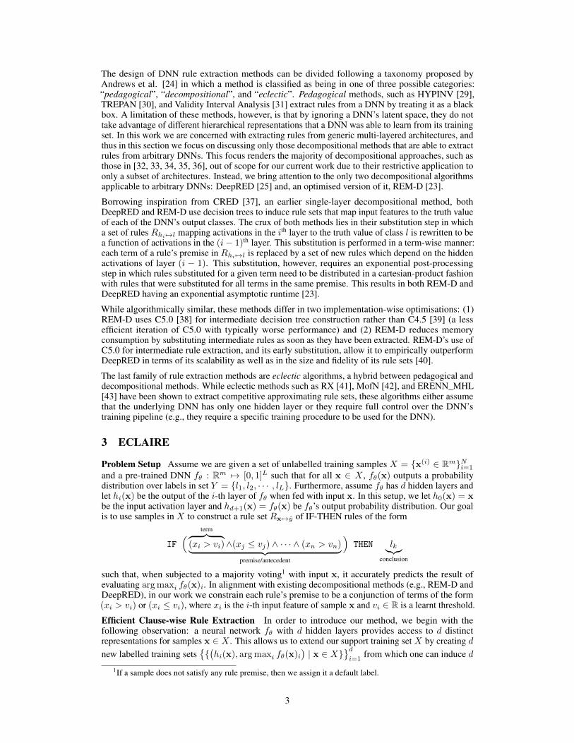
In this paper we address these limitations by proposing ECLAIRE, a novel decompositional ruleextraction algorithm for DNNs. Our method, depicted in Figure 1, avoids the intractability commonto other decompositional methods by making use of a two-step process that efficiently uses a DNN’slatent space to guide its rule extraction. Our main contributions can be summarised as follows:

• We introduce ECLAIRE, a novel decompositional rule extraction algorithm which, to thebest of our knowledge, is the first polynomial-time decompositional method applicable toarbitrary DNNs.

• We show that ECLAIRE’s rule sets outperform those extracted by current state-of-the-artdecompositional methods in both predictive performance and comprehensibility (measuredas the number and length of extracted rules). Furthermore, we show that ECLAIRE is able toachieve this while using significantly less computational resources than competing methods.

• We open-source our methods, together with a rule visualisation and interaction library, aspart of the REMIX package (https://github.com/mateoespinosa/remix).

Figure 1: Representation of how ECLAIRE extracts rules from a DNN that outputs a probabilitydistribution over classes {l1, l2, l3}. ECLAIRE uses a 2-step process in which it (i) extracts rulesmapping intermediate (layer-wise) activations to the DNN’s predictions and then (ii) performs aclause-wise substitution to produce a rule set Rx7→y mapping input activations to output predictions.

2 Related Work

Previous work on explaining a DNN’s prediction using rule-based explanations can be divided intotwo lines of work: (i) rule-based model-agnostic local explainability methods and (2) DNN ruleextraction methods. While members of the former family of methods, which include algorithms suchas LORE [27] and Anchors [28], are able to generate rule-based explanations for the behaviour of aDNN in a point’s local neighbourhood, they are unable to provide insights on any global patternscaptured by the DNN’s decision boundary. Hence, given that we are interested in extracting rule-basedmodels that provide both local and global interpretability in a DNN, in this section we focus on DNNrule extraction methods.

2

The design of DNN rule extraction methods can be divided following a taxonomy proposed byAndrews et al. [24] in which a method is classified as being in one of three possible categories:“pedagogical”, “decompositional”, and “eclectic”. Pedagogical methods, such as HYPINV [29],TREPAN [30], and Validity Interval Analysis [31] extract rules from a DNN by treating it as a blackbox. A limitation of these methods, however, is that by ignoring a DNN’s latent space, they do nottake advantage of different hierarchical representations that a DNN was able to learn from its trainingset. In this work we are concerned with extracting rules from generic multi-layered architectures, andthus in this section we focus on discussing only those decompositional methods that are able to extractrules from arbitrary DNNs. This focus renders the majority of decompositional approaches, such asthose in [32, 33, 34, 35, 36], out of scope for our current work due to their restrictive application toonly a subset of architectures. Instead, we bring attention to the only two decompositional algorithmsapplicable to arbitrary DNNs: DeepRED [25] and, an optimised version of it, REM-D [23].

Borrowing inspiration from CRED [37], an earlier single-layer decompositional method, bothDeepRED and REM-D use decision trees to induce rule sets that map input features to the truth valueof each of the DNN’s output classes. The crux of both methods lies in their substitution step in whicha set of rules Rhi 7→l mapping activations in the ith layer to the truth value of class l is rewritten to bea function of activations in the (i− 1)th layer. This substitution is performed in a term-wise manner:each term of a rule’s premise in Rhi 7→l is replaced by a set of new rules which depend on the hiddenactivations of layer (i − 1). This substitution, however, requires an exponential post-processingstep in which rules substituted for a given term need to be distributed in a cartesian-product fashionwith rules that were substituted for all terms in the same premise. This results in both REM-D andDeepRED having an exponential asymptotic runtime [23].

While algorithmically similar, these methods differ in two implementation-wise optimisations: (1)REM-D uses C5.0 [38] for intermediate decision tree construction rather than C4.5 [39] (a lessefficient iteration of C5.0 with typically worse performance) and (2) REM-D reduces memoryconsumption by substituting intermediate rules as soon as they have been extracted. REM-D’s use ofC5.0 for intermediate rule extraction, and its early substitution, allow it to empirically outperformDeepRED in terms of its scalability as well as in the size and fidelity of its rule sets [40].

The last family of rule extraction methods are eclectic algorithms, a hybrid between pedagogical anddecompositional methods. While eclectic methods such as RX [41], MofN [42], and ERENN_MHL[43] have been shown to extract competitive approximating rule sets, these algorithms either assumethat the underlying DNN has only one hidden layer or they require full control over the DNN’straining pipeline (e.g., they require a specific training procedure to be used for the DNN).

3 ECLAIRE

Problem Setup Assume we are given a set of unlabelled training samples X = {x(i) ∈ Rm}Ni=1

and a pre-trained DNN fθ : Rm 7→ [0, 1]L such that for all x ∈ X , fθ(x) outputs a probabilitydistribution over labels in set Y = {l1, l2, · · · , lL}. Furthermore, assume fθ has d hidden layers andlet hi(x) be the output of the i-th layer of fθ when fed with input x. In this setup, we let h0(x) = xbe the input activation layer and hd+1(x) = fθ(x) be fθ’s output probability distribution. Our goalis to use samples in X to construct a rule set Rx7→y of IF-THEN rules of the form

IF( term︷ ︸︸ ︷(xi > vi)∧(xj ≤ vj) ∧ · · · ∧ (xn > vn)︸ ︷︷ ︸

premise/antecedent

)THEN lk︸︷︷︸

conclusion

such that, when subjected to a majority voting1 with input x, it accurately predicts the result ofevaluating argmaxi fθ(x)i. In alignment with existing decompositional methods (e.g., REM-D andDeepRED), in our work we constrain each rule’s premise to be a conjunction of terms of the form(xi > vi) or (xi ≤ vi), where xi is the i-th input feature of sample x and vi ∈ R is a learnt threshold.

Efficient Clause-wise Rule Extraction In order to introduce our method, we begin with thefollowing observation: a neural network fθ with d hidden layers provides access to d distinctrepresentations for samples x ∈ X . This allows us to extend our support training set X by creating dnew labelled training sets

{{(hi(x), argmaxi fθ(x)i

)| x ∈ X}

}di=1

from which one can induce d

1If a sample does not satisfy any rule premise, then we assign it a default label.

3

rule sets Rhi 7→y that map each hidden layer’s output to fθ’s label predictions y = argmaxi fθ(x)i.The crux of our method consists of efficiently unifying all d rule sets {Rh1 7→y, · · · , Rhd 7→y} intoa single rule set Rx7→y that maps input samples x ∈ X to fθ’s predicted labels. In the same waythat bagging and feature subsampling are key to the ability of random forests to reduce variance andoverfitting [44], making use of d different representations of the same dataset to construct Rx 7→y cansignificantly help reducing the variance and overfitting that would otherwise be present in vanilla ruleinduction algorithms.

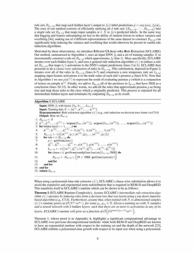
Motivated by these observations, we introduce Efficient CLAuse-wIse Rule Extraction (ECLAIRE).Our method, summarised in Algorithm 1, uses an input DNN fθ and a set of training samples X toincrementally construct a rule setRx7→y which approximates fθ (line 1). More specifically, ECLAIREiterates over each hidden layer hi and uses a general rule induction algorithm ψ(·) to induce a ruleset Rhi 7→y that maps hi’s activations to the DNN’s output predictions (lines 2 to 5). ECLAIRE thenproceeds to do a clause-wise substitution of rules in Rhi 7→y. This substitution, depicted in Figure 2,iterates over all of the rules in Rhi 7→y (lines 6-7) and constructs a new temporary rule set Ix7→pmapping input feature activations x to the truth value of each rule’s premise p (lines 8-9). Note thatin Algorithm 1 we use p(x(i)) to represent the result of evaluating premise p (which is a conjunctionof terms) on sample x(i). Finally, we add to Rx 7→y all of the premises in Ix7→p that have TRUE as aconclusion (lines 10-12). In other words, we add all the rules that approximate premise p as beingtrue and map those rules to the class which p originally predicted. This process is repeated for allintermediate hidden layers and terminates by outputting Rx 7→y as its result.

Algorithm 1 ECLAIREInput: DNN fθ with layers {h0, h1, ..., hd+1}Input: Training data X = {x(1),x(2), . . . ,x(N)}Hyperparameter: Rule extraction algorithm ψ(·) (e.g., rule induction on decision trees learnt via C5.0)Output: Rule set Rx 7→y

1: Rx 7→y ← ∅2: y(1), y(2), . . . , y(N) ← argmax

(hd+1(x

(1))), argmax

(hd+1(x

(2))), . . . , argmax

(hd+1(x

(N)))

3: for hidden layer i = 1, . . . , d do4: x′(1), x′(2), . . . , x′(N) ← hi(x

(1)), hi(x(2)), . . . , hi(x

(N))

5: Rhi 7→y ← ψ({(x′(1), y1), (x

′(2), y2), ..., (x′(N)

, yN )})

6: for rule r ∈ Rhi 7→y do7: p← getPremise(r)8: y

(1)p , y

(2)p , . . . , y

(N)p ← p

(x′(1)), p(x′(2)), . . . , p(x′(N))

9: Ih0→p ← ψ({(x(1), y

(1)p ), (x(2), y

(2)p ), ..., (x(N), y

(N)p )}

)10: for clause c ∈ getPremisesByConclusion

(Ih0→p, TRUE

)do

11: Rx 7→y ← Rx7→y ∪{IF c THEN getConclusion(r)

}12: end for13: end for14: end for15: return Rx7→y

When using a polynomial-time rule extractor ψ(·), ECLAIRE’s clause-wise substitution allows it toavoid the expensive and exponential term redistribution that is required in REM-D and DeepRED.This manifests itself in ECLAIRE’s runtime which can be shown to be as follows:Theorem 1 (ECLAIRE Runtime Complexity). Assume ECLAIRE’s intermediate rule extraction algo-rithm ψ(·) operates by inducing rules from a decision tree that was learnt using a top-down impurity-based algorithm (e.g., C5.0). Furthermore, assume that, when trained withN m-dimensional samples,ψ(·)’s runtime grows as O(Npnmpm), for some pn, pm ∈ N. Given a training set with N samplesand a neural network with d hidden layers, such that there are at most m activations in any of itslayers, ECLAIRE’s runtime will grow as a function of O

(dNmax(3,pn+1)mpm

).

Theorem 1, whose proof is in Appendix A, highlights a significant computational advantage inECLAIRE over previous decompositional methods: while both REM-D and DeepRED are knownto have an exponential runtime with respect to the training set and the depth of the network [23],ECLAIRE exhibits a polynomial-time growth with respect to its input size when using a polynomial-

4

time rule induction method for ψ(·). Furthermore, ECLAIRE’s use of a DNN’s intermediate repre-sentations independently of their topological order in the network implies that, in stark contrast toREM-D and DeepRED, it is agnostic to the DNN’s network topology and it can be easily parallelised,something we take advantage of in practice by distributing the work in the main loop (lines 3-15)across nthreads threads. Notice that this is not possible in both REM-D and DeepRED as they extractrules in a sequential manner, processing the DNN’s layers in reverse topological order.

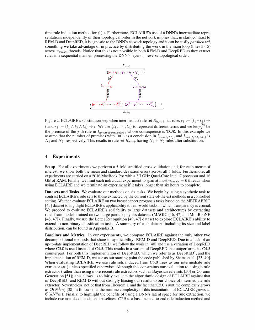
Figure 2: ECLAIRE’s substitution step when intermediate rule setRhi 7→y has rules r1 := (t1∧ t2)⇒l and r2 := (t1 ∧ t3 ∧ t4)⇒ l. We use {t1, · · · , t4} to represent different terms and we let p(k)j bethe premise of the j-th rule in Ix7→getPremise(rk) whose consequence is TRUE. In this example weassume that the number of premises with TRUE as a conclusion in Ix7→(t1∧t2) and Ix 7→(t1∧t3∧t4) isN1 and N2, respectively. This results in rule set Rx7→y having N1 +N2 rules after substitution.

4 Experiments

Setup For all experiments we perform a 5-fold stratified cross-validation and, for each metric ofinterest, we show both the mean and standard deviation errors across all 5 folds. Furthermore, allexperiments are carried on a 2016 MacBook Pro with a 2.7 GHz Quad-Core Intel i7 processor and 16GB of RAM. Finally, we limit each individual experiment to span at most nthreads = 6 threads whenusing ECLAIRE and we terminate an experiment if it takes longer than six hours to complete.

Datasets and Tasks We evaluate our methods on six tasks. We begin by using a synthetic task tocontrast ECLAIRE’s rule sets to those extracted by the current state-of-the-art methods in a controlledsetting. We then evaluate ECLAIRE on two breast cancer prognosis tasks based on the METRABRIC[45] dataset to highlight ECLAIRE’s applicability to real-world tasks in which transparency is crucial.We proceed to evaluate ECLAIRE’s scalability to large datasets and architectures by extractingrules from models trained on two large particle physics datasets (MAGIC [46, 47] and MiniBooNE[48, 47]). Finally, we use the Letter Recognition [49, 47] dataset to explore ECLAIRE’s ability toextend to non-binary classification tasks. A summary of each dataset, including its size and labeldistribution, can be found in Appendix B.

Baselines and Metrics In our experiments, we compare ECLAIRE against the only other twodecompositional methods that share its applicability: REM-D and DeepRED. Due to a lack of anup-to-date implementation of DeepRED, we follow the work in [40] and use a variation of DeepREDwhere C5.0 is used instead of C4.5. This results in a variant of DeepRED that outperforms its C4.5counterpart. For both this implementation of DeepRED, which we refer to as DeepRED*, and theimplementation of REM-D, we use as our starting point the code published by Shams et al. [23, 40].When evaluating ECLAIRE, we use rule sets induced from C5.0 trees as our intermediate ruleextractor ψ(·) unless specified otherwise. Although this constraints our evaluation to a single ruleextractor (rather than using more recent rule extractors such as Bayesian rule sets [50] or ColumnGeneration [51]), this allows us to fairly evaluate the algorithmic design of ECLAIRE against thatof DeepRED* and REM-D without strongly biasing our results to our choice of intermediate ruleextractor. Nevertheless, notice that from Theorem 1, and the fact that C5.0’s runtime complexity growsas O(N2m) [38], it follows that the runtime complexity of this instantiation of ECLAIRE grows asO(dN3m). Finally, to highlight the benefits of using a DNN’s latent space for rule extraction, weinclude two non-decompositional baselines: C5.0 as a baseline end-to-end rule induction method and

5

PedC5.0 [23, 40] as a baseline pedagogical algorithm. The latter method uses C5.0 to induce a ruleset from a training set where each sample is labelled using the DNN’s prediction for that sample.

When comparing any two methods, we evaluate the fidelity of the extracted rule sets with respectto the input DNN (defined as the predictive accuracy when sample x(i) is assigned label y(i) =argmaxj fθ(x

(i))j) and their comprehensibility as measured by their number of rules and theiraverage rule length. Furthermore, as a way to evaluate the tractability of our methods, we keep trackof the resources utilised by each method in terms of both wall-clock time and memory. Finally, giventhat there may be a direct benefit from using the rule sets extracted from the DNN as standaloneinterpretable models (e.g., as a form of model distillation that generates stronger rule-based models),we include each rule set’s accuracy and AUC as part of our evaluation.

Model and Hyperparameter Selection Although ECLAIRE is applicable to arbitrary DNN archi-tectures, in order for us to simplify architecture selection during evaluation, in our experiments wefocus on extracting rule sets from multilayer perceptrons (MLPs). Moreover, in order to simulateECLAIRE’s use case, we maintain a strict separation between fine-tuning the DNN we train for atask and fine-tuning the rule extraction algorithm we apply to that model. More specifically, wetrain several MLP architectures for each task and extract rules only from the best performing model.During rule extraction, we control the growth of intermediate rule sets induced via C5.0 by varyingonly the minimum number of samples µ that we require C5.0 to have before splitting a node. Becauseµ requires different fine-tuning strategies across different tasks2, in this section we report only thehighest performing rule set we obtain after varying µ across a task-and-method-specific spectrum.Unless specified otherwise, all other C5.0’s hyperparameters, with the exception of winnowing whichis always set to true, are left as their default values. We include all details of each task’s architectureand hyperparameter selection, including the search spectrum used for µ for each task, in Appendix C.

4.1 XOR: Evaluating Rule Set Interpretability in Controlled Setup

In this section, we use a synthetic dataset to evaluate the performance of ECLAIRE and our baselinesin a controlled environment known to be challenging for vanilla rule induction algorithms andpedagogical rule extraction methods. For this, we make use of a variant of the XOR classificationtask, in a form commonly used for studying feature selection methods [7, 52, 53], in which wegenerate a dataset {(x(i), yi)}1000i=1 with 1000 10-dimensional samples such that every data pointx(i) ∈ [0, 1]10 is constructed by independently sampling each dimension from a uniform distributionin [0, 1]. In this dataset, we assign a binary label yi ∈ {0, 1} to each point x(i) by XOR-ing the resultof rounding its first two dimensions as yi = round

(x(i)1

)⊕ round

(x(i)2

).

In order for a classifier to be able to achieve a high performance in this task, it must learn that only thefirst two dimensions are meaningful for predicting the output label. This property makes this datasetan illustrative example of a task in which decision trees are unable to obtain a high performancewithout a large training dataset [54, 25]. In this section, we hypothesise that decompositionalmethods will outperform both vanilla rule induction algorithms and pedagogical rule extractionmethods as their use of a DNN’s latent representations during training results in an implicit dataaugmentation process. Furthermore, we hypothesise that within our decompositional baselines,ECLAIRE will outperform other methods given that its two-step process avoids the need of nestingmultiple sequential approximations when merging rule sets as done in both REM-D and DeepRED*.To test both hypothesises, we extract rules from an MLP with hidden layer sizes {64, 32, 16} trainedon this dataset and report our findings in the XOR rows of Table 1. The MLP’s test accuracy is96.6%± 1.9% and its AUC is 96.6%± 1.9%.

As hypothesised, Table 1 shows that ECLAIRE outperforms all other decompositional methods in theXOR task in terms of both accuracy and fidelity. We further observe that ECLAIRE uses significantlyless resources than REM-D and DeepRED* while generating significantly fewer rules than both.Moreover, note that, as expected, we also observe that both C5.0 and PedC5.0 are unable to captureany meaningful rules and instead generate an empty rule set that acts as a random classifier. Finally,we observe that the standard deviation of ECLAIRE’s rule set sizes is relatively small compared to itsmean. This is in stark contrast with the observed standard deviations of rule set sizes in both REM-Dand DeepRED*, which tend to be even greater than their means. Such behaviour indicates that

2This is particularly important in REM-D and DeepRED* as low values of µ can easily lead to intractability.

6

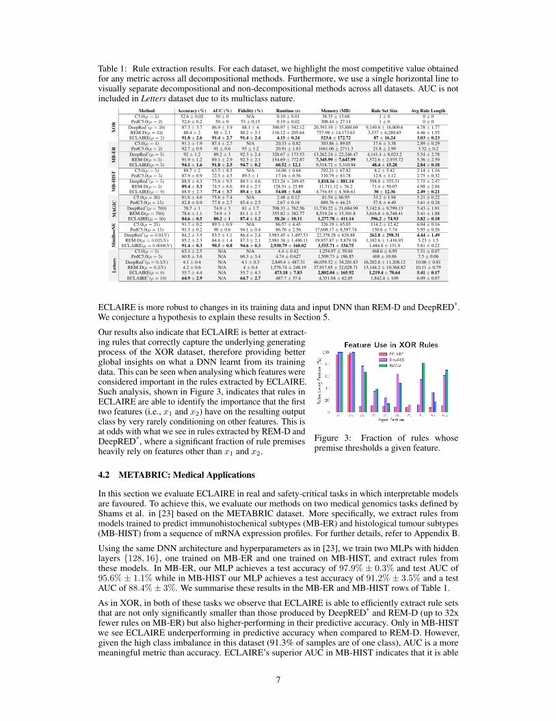
Table 1: Rule extraction results. For each dataset, we highlight the most competitive value obtainedfor any metric across all decompositional methods. Furthermore, we use a single horizontal line tovisually separate decompositional and non-decompositional methods across all datasets. AUC is notincluded in Letters dataset due to its multiclass nature.

Method Accuracy (%) AUC (%) Fidelity (%) Runtime (s) Memory (MB) Rule Set Size Avg Rule LengthX

OR

C5.0(µ = 2) 52.6 ± 0.02 50 ± 0 N/A 0.10 ± 0.01 38.35 ± 13.68 1 ± 0 0 ± 0PedC5.0(µ = 2) 52.6 ± 0.2 50 ± 0 53 ± 0.15 0.19 ± 0.02 308.44 ± 27.14 1 ± 0 0 ± 0

DeepRed*(µ = 30) 87.3 ± 3.7 86.9 ± 3.9 88.1 ± 4 390.97 ± 542.12 20,393.19 ± 35,889.69 9,149.8 ± 16,009.6 4.78 ± 1.77REM-D(µ = 33) 88.4 ± 2 88 ± 2.1 88.2 ± 3.1 116.12 ± 205.64 757.98 ± 14,173.63 3,337 ± 6,280.65 4.46 ± 1.55

ECLAIRE(µ = 2) 91.8 ± 2.6 91.4 ± 2.7 91.4 ± 2.4 4.15 ± 0.24 523.6 ± 172.72 87 ± 16.24 3.03 ± 0.23C5.0(µ = 4) 91.1 ± 1.9 87.4 ± 2.7 N/A 20.33 ± 0.82 303.86 ± 89.05 17.6 ± 3.38 2.89 ± 0.29

PedC5.0(µ = 2) 92.7 ± 0.9 91 ± 0.6 93 ± 1.2 20.91 ± 1.83 1661.06 ± 2711.3 21.8 ± 2.99 3.32 ± 0.2DeepRed*(µ = 5) 92 ± 1.2 89.2 ± 3 92.3 ± 2.4 328.67 ± 173.53 13,262.24 ± 22,246.47 4,141.4 ± 8,023.2 5.54 ± 2.78REM-D(µ = 5) 91.9 ± 1.2 89.1 ± 2.9 92.3 ± 2.1 154.69 ± 772.87 7,345.99 ± 7,647.99 1,572.6 ± 2,935.72 5.36 ± 2.59M

B-E

R

ECLAIRE(µ = 5) 94.1 ± 1.6 91.8 ± 2.5 94.7 ± 0.2 60.52 ± 12.1 9,518.72 ± 5,310.94 48.4 ± 15.28 2.84 ± 0.18

MB

-HIS

T C5.0(µ = 5) 89.7 ± 2 63.5 ± 8.5 N/A 16.06 ± 0.64 292.21 ± 67.82 8.2 ± 5.42 2.14 ± 1.16PedC5.0(µ = 5) 87.9 ± 0.9 72.5 ± 4.5 89.3 ± 1 17.16 ± 0.56 310.79 ± 83.78 12.8 ± 3.12 2.75 ± 0.32

DeepRed*(µ = 5) 88.9 ± 4.3 73.6 ± 9.5 89.3 ± 4.6 523.24 ± 249.45 1,818.16 ± 881.14 598.8 ± 355.31 7.75 ± 2.47REM-D(µ = 5) 89.4 ± 3.3 74.5 ± 6.6 89.4 ± 2.7 128.51 ± 25.89 11,711.12 ± 76.2 71.4 ± 50.07 4.98 ± 2.04

ECLAIRE(µ = 9) 88.9 ± 2.3 77.4 ± 3.7 89.4 ± 1.8 54.08 ± 5.68 4,754.45 ± 4,306.61 30 ± 12.36 2.49 ± 0.21C5.0(µ = 30) 81.6 ± 4.6 75.6 ± 7.4 N/A 2.48 ± 0.12 81.54 ± 66.95 33.2 ± 1.94 3.21 ± 0.22

PedC5.0(µ = 15) 82.8 ± 0.9 77.8 ± 2.7 85.4 ± 2.5 2.67 ± 0.18 889.76 ± 44.23 57.8 ± 4.49 3.61 ± 0.28DeepRed*(µ = 700) 78.7 ± 1 74.9 ± 3 81 ± 1.7 708.33 ± 762.56 11,730.22 ± 21,684.99 5,142.6 ± 9,799.13 5.43 ± 1.91REM-D(µ = 700) 78.6 ± 1.1 74.9 ± 3 81.1 ± 1.7 355.82 ± 382.77 8,519.24 ± 15,301.8 3,616.8 ± 6,748.41 5.41 ± 1.88M

AG

IC

ECLAIRE(µ = 50) 84.6 ± 0.5 80.2 ± 1 87.4 ± 1.2 58.26 ± 10.11 1,277.78 ± 411.14 396.2 ± 74.93 3.82 ± 0.18

Min

iBoo

NE C5.0(µ = 25) 91.7 ± 0.2 89.3 ± 0.9 N/A 86.57 ± 4.45 326.19 ± 65.03 114.2 ± 12.42 6.04 ± 0.16

PedC5.0(µ = 15) 91.5 ± 0.2 90 ± 0.6 94.1 ± 0.4 86.76 ± 2.56 17,608.17 ± 8,597.74 150.6 ± 7.74 5.95 ± 0.26DeepRed*(µ = 0.03N ) 84.2 ± 3.5 83.5 ± 1.1 86.4 ± 2.4 3,983.45 ± 1,497.53 22,378.28 ± 620.88 262.8 ± 298.31 4.44 ± 1.49REM-D(µ = 0.025N ) 85.2 ± 2.3 84.6 ± 1.4 87.3 ± 2.1 2,981.38 ± 1,496.11 19,957.87 ± 5,879.18 1,182.6 ± 1,416.93 5.23 ± 1.5

ECLAIRE(µ = 0.0008N ) 91.4 ± 0.3 90.5 ± 0.8 94.6 ± 0.3 2,930.79 ± 160.02 3,555.71 ± 334.75 1,484.8 ± 131.9 5.81 ± 0.22C5.0(µ = 5) 63.1 ± 2.5 N/A N/A 4.4 ± 0.42 1,254.97 ± 39.04 468.6 ± 6.95 7.51 ± 0.07

PedC5.0(µ = 5) 60.8 ± 3.6 N/A 60.3 ± 3.4 4.74 ± 0.627 1,509.73 ± 186.85 468 ± 10.06 7.5 ± 0.06DeepRed*(µ = 0.3N ) 4.1 ± 0.4 N/A 4.1 ± 0.3 2,849.4 ± 487.31 46,059.52 ± 34,201.83 16,202.8 ± 11,208.12 10.06 ± 0.81REM-D(µ = 0.3N ) 4.2 ± 0.6 N/A 4 ± 0.4 1,576.74 ± 248.19 37,917.65 ± 32,028.71 13,144.2 ± 10,368.82 10.11 ± 0.79ECLAIRE(µ = 8) 55.7 ± 4.4 N/A 55.7 ± 4.3 473.18 ± 7.83 2,802.04 ± 165.92 1,219.4 ± 70.64 5.41 ± 0.17L

ette

rs

ECLAIRE*(µ = 10) 64.9 ± 2.9 N/A 64.7 ± 2.7 487.7 ± 37.4 4,351.04 ± 62.05 1,842.4 ± 109 6.09 ± 0.07

ECLAIRE is more robust to changes in its training data and input DNN than REM-D and DeepRED*.We conjecture a hypothesis to explain these results in Section 5.

Figure 3: Fraction of rules whosepremise thresholds a given feature.

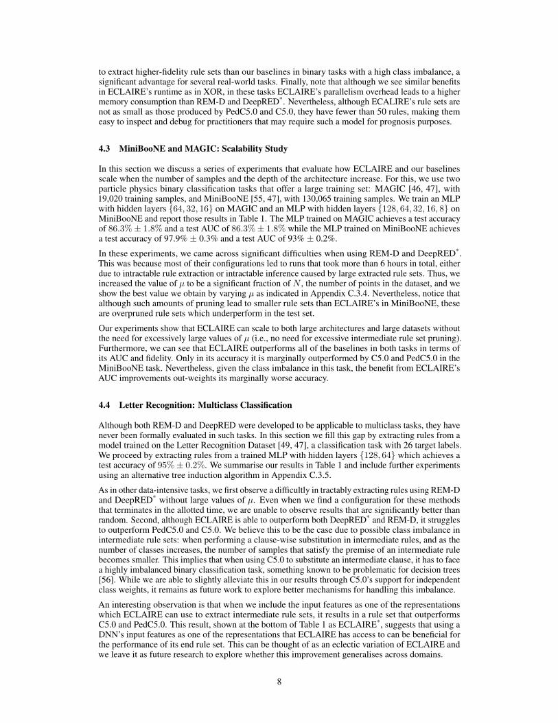
Our results also indicate that ECLAIRE is better at extract-ing rules that correctly capture the underlying generatingprocess of the XOR dataset, therefore providing betterglobal insights on what a DNN learnt from its trainingdata. This can be seen when analysing which features wereconsidered important in the rules extracted by ECLAIRE.Such analysis, shown in Figure 3, indicates that rules inECLAIRE are able to identify the importance that the firsttwo features (i.e., x1 and x2) have on the resulting outputclass by very rarely conditioning on other features. This isat odds with what we see in rules extracted by REM-D andDeepRED*, where a significant fraction of rule premisesheavily rely on features other than x1 and x2.

4.2 METABRIC: Medical Applications

In this section we evaluate ECLAIRE in real and safety-critical tasks in which interpretable modelsare favoured. To achieve this, we evaluate our methods on two medical genomics tasks defined byShams et al. in [23] based on the METABRIC dataset. More specifically, we extract rules frommodels trained to predict immunohistochenical subtypes (MB-ER) and histological tumour subtypes(MB-HIST) from a sequence of mRNA expression profiles. For further details, refer to Appendix B.

Using the same DNN architecture and hyperparameters as in [23], we train two MLPs with hiddenlayers {128, 16}, one trained on MB-ER and one trained on MB-HIST, and extract rules fromthese models. In MB-ER, our MLP achieves a test accuracy of 97.9% ± 0.3% and test AUC of95.6% ± 1.1% while in MB-HIST our MLP achieves a test accuracy of 91.2% ± 3.5% and a testAUC of 88.4%± 3%. We summarise these results in the MB-ER and MB-HIST rows of Table 1.

As in XOR, in both of these tasks we observe that ECLAIRE is able to efficiently extract rule setsthat are not only significantly smaller than those produced by DeepRED* and REM-D (up to 32xfewer rules on MB-ER) but also higher-performing in their predictive accuracy. Only in MB-HISTwe see ECLAIRE underperforming in predictive accuracy when compared to REM-D. However,given the high class imbalance in this dataset (91.3% of samples are of one class), AUC is a moremeaningful metric than accuracy. ECLAIRE’s superior AUC in MB-HIST indicates that it is able

7

to extract higher-fidelity rule sets than our baselines in binary tasks with a high class imbalance, asignificant advantage for several real-world tasks. Finally, note that although we see similar benefitsin ECLAIRE’s runtime as in XOR, in these tasks ECLAIRE’s parallelism overhead leads to a highermemory consumption than REM-D and DeepRED*. Nevertheless, although ECALIRE’s rule sets arenot as small as those produced by PedC5.0 and C5.0, they have fewer than 50 rules, making themeasy to inspect and debug for practitioners that may require such a model for prognosis purposes.

4.3 MiniBooNE and MAGIC: Scalability Study

In this section we discuss a series of experiments that evaluate how ECLAIRE and our baselinesscale when the number of samples and the depth of the architecture increase. For this, we use twoparticle physics binary classification tasks that offer a large training set: MAGIC [46, 47], with19,020 training samples, and MiniBooNE [55, 47], with 130,065 training samples. We train an MLPwith hidden layers {64, 32, 16} on MAGIC and an MLP with hidden layers {128, 64, 32, 16, 8} onMiniBooNE and report those results in Table 1. The MLP trained on MAGIC achieves a test accuracyof 86.3%± 1.8% and a test AUC of 86.3%± 1.8% while the MLP trained on MiniBooNE achievesa test accuracy of 97.9% ± 0.3% and a test AUC of 93% ± 0.2%.

In these experiments, we came across significant difficulties when using REM-D and DeepRED*.This was because most of their configurations led to runs that took more than 6 hours in total, eitherdue to intractable rule extraction or intractable inference caused by large extracted rule sets. Thus, weincreased the value of µ to be a significant fraction of N , the number of points in the dataset, and weshow the best value we obtain by varying µ as indicated in Appendix C.3.4. Nevertheless, notice thatalthough such amounts of pruning lead to smaller rule sets than ECLAIRE’s in MiniBooNE, theseare overpruned rule sets which underperform in the test set.

Our experiments show that ECLAIRE can scale to both large architectures and large datasets withoutthe need for excessively large values of µ (i.e., no need for excessive intermediate rule set pruning).Furthermore, we can see that ECLAIRE outperforms all of the baselines in both tasks in terms ofits AUC and fidelity. Only in its accuracy it is marginally outperformed by C5.0 and PedC5.0 in theMiniBooNE task. Nevertheless, given the class imbalance in this task, the benefit from ECLAIRE’sAUC improvements out-weights its marginally worse accuracy.

4.4 Letter Recognition: Multiclass Classification

Although both REM-D and DeepRED were developed to be applicable to multiclass tasks, they havenever been formally evaluated in such tasks. In this section we fill this gap by extracting rules from amodel trained on the Letter Recognition Dataset [49, 47], a classification task with 26 target labels.We proceed by extracting rules from a trained MLP with hidden layers {128, 64} which achieves atest accuracy of 95%± 0.2%. We summarise our results in Table 1 and include further experimentsusing an alternative tree induction algorithm in Appendix C.3.5.

As in other data-intensive tasks, we first observe a difficultly in tractably extracting rules using REM-Dand DeepRED* without large values of µ. Even when we find a configuration for these methodsthat terminates in the allotted time, we are unable to observe results that are significantly better thanrandom. Second, although ECLAIRE is able to outperform both DeepRED* and REM-D, it strugglesto outperform PedC5.0 and C5.0. We believe this to be the case due to possible class imbalance inintermediate rule sets: when performing a clause-wise substitution in intermediate rules, and as thenumber of classes increases, the number of samples that satisfy the premise of an intermediate rulebecomes smaller. This implies that when using C5.0 to substitute an intermediate clause, it has to facea highly imbalanced binary classification task, something known to be problematic for decision trees[56]. While we are able to slightly alleviate this in our results through C5.0’s support for independentclass weights, it remains as future work to explore better mechanisms for handling this imbalance.

An interesting observation is that when we include the input features as one of the representationswhich ECLAIRE can use to extract intermediate rule sets, it results in a rule set that outperformsC5.0 and PedC5.0. This result, shown at the bottom of Table 1 as ECLAIRE*, suggests that using aDNN’s input features as one of the representations that ECLAIRE has access to can be beneficial forthe performance of its end rule set. This can be thought of as an eclectic variation of ECLAIRE andwe leave it as future research to explore whether this improvement generalises across domains.

8

5 Discussion

Variance Reduction in ECLAIRE In [23], Shams et al. observe a very high variance in thesize of rule sets extracted with REM-D and postulate that this is due to different neural networkinitialisations leading to latent spaces that vary in interpretability properties. Nevertheless, our resultsin Table 1 suggest that this may not be the case, as ECLAIRE’s variance is significantly smallerthan that observed in both REM-D and DeepRED*. Inspired by results on convergence learning[57, 58], in this paper we challenge this hypothesis by arguing that the variance observed in REM-D,and therefore in DeepRED, is not the result of different initialisations leading to different levels ofinterpretability in a DNN’s latent space, but it is rather the result of a crucial design factor in REM-D:REM-D uses rule sets induced from decision trees to substitute terms in its intermediate rule sets,forcing the need of a cartesian-product redistribution of terms afterwards. Decision trees, being high-variance classifiers [59], are highly sensitive to their training sets. This implies that when REM-Dsubstitutes the same term in an intermediate rule using two different datasets (as it would happenacross two different training folds), it can generate vastly different rule sets. Hence, because during itsterm-wise substitution REM-D replaces each term in an intermediate rule’s premise with a set of rulesextracted from a decision tree, the variance in the number of rules after one substitution grows in amultiplicative fashion. This is because all newly substituted terms in a clause need to be redistributedin a cartesian-product (a visual representation of this process can be found in Appendix D). Therefore,we argue that the significant reduction in variance we observe in our evaluation of ECLAIRE is dueto the fact that ECLAIRE performs a clause-wise substitution rather than a term-wise substitution,hence avoiding a multiplicative growth in the number of rules. This hypothesis explains the results inTable 1 and highlights a significant advantage of ECLAIRE over other decompositional methods.

Growth Coping Mechanisms Despite ECLAIRE’s superior performance compared to our baselines,Table 1 shows that ECLAIRE can still take a considerable amount of time to extract high-performingrule sets in large datasets and architectures. Furthermore, we observe a growth in the number of rulesextracted by ECLAIRE as the amount of data and the model size increase. As a way to alleviate thisgrowth, we explore four different coping mechanisms: (1) intermediate rule pruning, where, as in[23], we increase the value of µ to generate smaller intermediate rule sets, (2) hidden representationsubsampling, where we generate intermediate rule sets only from a subset of the DNN’s intermediaterepresentations, (3) training set subsampling, where, as in [25], only a fraction of the DNN’s trainingset is used for rule extraction, and (4) intermediate rule ranking, where the lowest p% of rulesin intermediate rule sets, as ranked by their confidence levels, are dropped. We summarise theseexperiments in Appendix E.

Our results indicate that the performance of ECLAIRE’s rule sets is robust to heavy training datasubsampling as well as significant intermediate representation subsampling and intermediate rulepruning via confidence ranking. Specifically, we observe that ECLAIRE is very data efficient: one cansubsample up to 50% of the training set during rule extraction, causing a ∼ 50% drop in extractiontime and rule set size, without observing an absolute loss of more than 0.5% in the resulting rule setfidelity. Similar results are observed when one subsamples every other two hidden representationswhen generating intermediate rule sets or drops the lowest 25% of rules in intermediate rule sets.Nevertheless, our experiments also highlight a clear limitation in ECLAIRE: for achieving optimalperformance, ECLAIRE requires significant task-specific fine tuning of its µ hyperparameter. Whilein practice we observe that selecting µ from [10−5N, 10−4N ] yields good results, we leave theexploration of more systematic strategies for selecting µ to future work.

6 Conclusion

With the ubiquitous use of DNNs, it has become increasingly important to be able to explain, aswell as debug, the decisions made by production-sized DNNs. In this work we aim to fill this gapby proposing ECLAIRE, a novel decompositional rule extraction algorithm, which, to the best ofour knowledge, is the first polynomial-time decompositional algorithm able to scale to both largetraining sets and deep architectures. In contrast to previous work which focuses on using intermediaterepresentations in a sequential manner, ECLAIRE exploits these representations in parallel to buildan ensemble of classifiers that can then be efficiently combined into a single rule set. We evaluateECLAIRE on six different tasks and show that it consistently outperforms the previous state-of-the-artdecompositional methods and vanilla rule induction methods in terms of the accuracy and fidelity of

9

its output rule set. At the same time, ECLAIRE uses orders of magnitude less resources and producesfewer rules than current state-of-the-art decompositional methods. Excited with the prospects that canarise from this work, and to encourage the use of our algorithms in both industry and research, wemake all of our methods, together with an extensive set of visualisation and inspection tools, publiclyavailable as part of the REMIX library. Follow up research could explore generalising ECLAIRE toregression tasks, as well as to RNN architectures, and could include work on alleviating the effects ofclass imbalance in multiclass settings.

Acknowledgements

MEZ acknowledges support from the Gates Cambridge Trust via the Gates Cambridge Scholarship.

References[1] Artificial Intelligence Index. The Artificial Intelligence Index: 2017 Annual Report. Technical report,

Technical report, 2017.

[2] Ashraf Abdul, Jo Vermeulen, Danding Wang, Brian Y Lim, and Mohan Kankanhalli. Trends and trajectoriesfor explainable, accountable and intelligible systems: An hci research agenda. In Proceedings of the 2018CHI conference on human factors in computing systems, pages 1–18, 2018.

[3] Nadia Burkart and Marco F Huber. A survey on the explainability of supervised machine learning. Journalof Artificial Intelligence Research, 70:245–317, 2021.

[4] Joan Claybrook and Shaun Kildare. Autonomous vehicles: No driver. . . no regulation? Science,361(6397):36–37, 2018.

[5] Aarian Marshall. The uber crash won’t be the last shocking self-driving death. Transportation, Wired,Available at: https://www. wired. com/story/uber-self-driving-crash-explanation-lidar-sensors/, Retrieved,6(24):18, 2018.

[6] Michael W Kattan, Kenneth R Hess, Mahul B Amin, Ying Lu, Karl GM Moons, Jeffrey E Gershenwald,Phyllis A Gimotty, Justin H Guinney, Susan Halabi, Alexander J Lazar, et al. American joint committeeon cancer acceptance criteria for inclusion of risk models for individualized prognosis in the practice ofprecision medicine. CA: a cancer journal for clinicians, 66(5):370–374, 2016.

[7] Ahmed M Alaa and Mihaela van der Schaar. Demystifying black-box models with symbolic metamodels.In NeurIPS, pages 11301–11311, 2019.

[8] Todd Kulesza, Simone Stumpf, Margaret Burnett, Sherry Yang, Irwin Kwan, and Weng-Keen Wong.Too much, too little, or just right? ways explanations impact end users’ mental models. In 2013 IEEESymposium on visual languages and human centric computing, pages 3–10. IEEE, 2013.

[9] Shachar Kaufman, Saharon Rosset, Claudia Perlich, and Ori Stitelman. Leakage in data mining: Formula-tion, detection, and avoidance. ACM Transactions on Knowledge Discovery from Data (TKDD), 6(4):1–21,2012.

[10] Kaiming He, Xiangyu Zhang, Shaoqing Ren, and Jian Sun. Deep residual learning for image recognition.In Proceedings of the IEEE conference on computer vision and pattern recognition, pages 770–778, 2016.

[11] Jacob Devlin, Ming-Wei Chang, Kenton Lee, and Kristina Toutanova. Bert: Pre-training of deep bidirec-tional transformers for language understanding. arXiv preprint arXiv:1810.04805, 2018.

[12] Jeffrey De Fauw, Joseph R Ledsam, Bernardino Romera-Paredes, Stanislav Nikolov, Nenad Tomasev,Sam Blackwell, Harry Askham, Xavier Glorot, Brendan O’Donoghue, Daniel Visentin, et al. Clinicallyapplicable deep learning for diagnosis and referral in retinal disease. Nature medicine, 24(9):1342–1350,2018.

[13] Congjie He, Meng Ma, and Ping Wang. Extract interpretability-accuracy balanced rules from artificialneural networks: A review. Neurocomputing, 387:346–358, 2020.

[14] Tameru Hailesilassie. Rule extraction algorithm for deep neural networks: A review. arXiv preprintarXiv:1610.05267, 2016.

[15] Ramprasaath R Selvaraju, Michael Cogswell, Abhishek Das, Ramakrishna Vedantam, Devi Parikh, andDhruv Batra. Grad-cam: Visual explanations from deep networks via gradient-based localization. InProceedings of the IEEE international conference on computer vision, pages 618–626, 2017.

[16] Scott Lundberg and Su-In Lee. A unified approach to interpreting model predictions. arXiv preprintarXiv:1705.07874, 2017.

[17] Been Kim, Oluwasanmi Koyejo, Rajiv Khanna, et al. Examples are not enough, learn to criticize! criticismfor interpretability. In NIPS, pages 2280–2288, 2016.

10

[18] Pang Wei Koh and Percy Liang. Understanding black-box predictions via influence functions. In DoinaPrecup and Yee Whye Teh, editors, Proceedings of the 34th International Conference on Machine Learning,volume 70 of Proceedings of Machine Learning Research, pages 1885–1894, International ConventionCentre, Sydney, Australia, 06–11 Aug 2017. PMLR.

[19] Sandra Wachter, Brent Mittelstadt, and Chris Russell. Counterfactual explanations without opening theblack box: Automated decisions and the gdpr. Harv. JL & Tech., 31:841, 2017.

[20] Susanne Dandl, Christoph Molnar, Martin Binder, and Bernd Bischl. Multi-objective counterfactualexplanations. In International Conference on Parallel Problem Solving from Nature, pages 448–469.Springer, 2020.

[21] Adam M Smith, Wen Xu, Yao Sun, James R Faeder, and G Elisabeta Marai. RuleBender: integratedmodeling, simulation and visualization for rule-based intracellular biochemistry. BMC bioinformatics,13(8):1–16, 2012.

[22] Yao Ming, Huamin Qu, and Enrico Bertini. RuleMatrix: Visualizing and understanding classifiers withrules. IEEE transactions on visualization and computer graphics, 25(1):342–352, 2018.

[23] Zohreh Shams, Botty Dimanov, Sumaiyah Kola, Nikola Simidjievski, Helena Andres Terre, Paul Scherer,Urska Matjasec, Jean Abraham, Mateja Jamnik, and Pietro Lio. REM: An Integrative Rule ExtractionMethodology for Explainable Data Analysis in Healthcare. bioRxiv, 2021.

[24] Robert Andrews, Joachim Diederich, and Alan B Tickle. Survey and critique of techniques for extractingrules from trained artificial neural networks. Knowledge-based systems, 8(6):373–389, 1995.

[25] Jan Ruben Zilke, Eneldo Loza Mencía, and Frederik Janssen. Deepred–rule extraction from deep neuralnetworks. In International Conference on Discovery Science, pages 457–473. Springer, 2016.

[26] Weibo Liu, Zidong Wang, Xiaohui Liu, Nianyin Zeng, Yurong Liu, and Fuad E Alsaadi. A survey of deepneural network architectures and their applications. Neurocomputing, 234:11–26, 2017.

[27] Riccardo Guidotti, Anna Monreale, Salvatore Ruggieri, Dino Pedreschi, Franco Turini, and Fosca Giannotti.Local rule-based explanations of black box decision systems. arXiv preprint arXiv:1805.10820, 2018.

[28] Marco Tulio Ribeiro, Sameer Singh, and Carlos Guestrin. Anchors: High-precision model-agnosticexplanations. In Proceedings of the AAAI conference on artificial intelligence, volume 32, 2018.

[29] Emad W Saad and Donald C Wunsch II. Neural network explanation using inversion. Neural networks,20(1):78–93, 2007.

[30] Mark W Craven. Extracting comprehensible models from trained neural networks. Technical report,University of Wisconsin-Madison Department of Computer Sciences, 1996.

[31] Sebastian Thrun. Extracting rules from artificial neural networks with distributed representations. Advancesin neural information processing systems, pages 505–512, 1995.

[32] LiMin Fu. Rule learning by searching on adapted nets. In AAAI, volume 91, pages 590–595, 1991.

[33] LiMin Fu. Rule generation from neural networks. IEEE Transactions on Systems, Man, and Cybernetics,24(8):1114–1124, 1994.

[34] Geoffrey G Towell and Jude W Shavlik. Extracting refined rules from knowledge-based neural networks.Machine learning, 13(1):71–101, 1993.

[35] Robert Andrews and Shlomo Geva. Rule extraction from a constrained error back propagation mlp. InAustralian Conference on Neural Networks, Brisbane, Queensland, pages 9–12, 1994.

[36] Robert Andrews. Inserting and extracting knowledge from constrained error back-propagation networks.In Proceedings of the 6th Australian Conference on Neural Networks. NSW, 1995.

[37] Makoto Sato and Hiroshi Tsukimoto. Rule extraction from neural networks via decision tree induction.In IJCNN’01. International Joint Conference on Neural Networks. Proceedings (Cat. No. 01CH37222),volume 3, pages 1870–1875. IEEE, 2001.

[38] J Ross Quinlan. Data mining tools see5 and c5.0. https://www.rulequest.com/see5-info.html, 2020.

[39] J Ross Quinlan. C4. 5: programs for machine learning. Elsevier, 2014.

[40] Sumaiyah Kola. Optimising rule extraction for deep neural networks. Master’s thesis, University ofCambridge, 11 2020. Computer Science Tripos - Part II Dissertation.

[41] Eduardo R Hruschka and Nelson FF Ebecken. Extracting rules from multilayer perceptrons in classificationproblems: A clustering-based approach. Neurocomputing, 70(1-3):384–397, 2006.

[42] Geoffrey G Towell and Jude W Shavlik. Extracting refined rules from knowledge-based neural networks.Machine learning, 13(1):71–101, 1993.

[43] Manomita Chakraborty, Saroj Kumar Biswas, and Biswajit Purkayastha. Rule extraction from neuralnetwork trained using deep belief network and back propagation. Knowledge and Information Systems,62:3753–3781, 2020.

11

[44] Tin Kam Ho. Random decision forests. In Proceedings of 3rd international conference on documentanalysis and recognition, volume 1, pages 278–282. IEEE, 1995.

[45] Bernard Pereira, Suet-Feung Chin, Oscar M Rueda, Hans-Kristian Moen Vollan, Elena Provenzano,Helen A Bardwell, Michelle Pugh, Linda Jones, Roslin Russell, Stephen-John Sammut, et al. The somaticmutation profiles of 2,433 breast cancers refine their genomic and transcriptomic landscapes. Naturecommunications, 7(1):1–16, 2016.

[46] RK Bock. Major Atmospheric Gamma Imaging Cherenkov Telescope project (MAGIC). URL:https://archive. ics. uci. edu/ml/datasets/magic+ gamma+ telescope, 2007.

[47] Arthur Asuncion and David Newman. UCI machine learning repository, 2007.[48] A Aguilar, LB Auerbach, RL Burman, DO Caldwell, ED Church, AK Cochran, JB Donahue, A Fazely,

GT Garvey, RM Gunasingha, et al. Evidence for neutrino oscillations from the observation of ν eappearance in a ν µ beam. Physical Review D, 64(11):112007, 2001.

[49] Peter W Frey and David J Slate. Letter recognition using Holland-style adaptive classifiers. Machinelearning, 6(2):161–182, 1991.

[50] Tong Wang, Cynthia Rudin, Finale Doshi-Velez, Yimin Liu, Erica Klampfl, and Perry MacNeille. Abayesian framework for learning rule sets for interpretable classification. The Journal of Machine LearningResearch, 18(1):2357–2393, 2017.

[51] Sanjeeb Dash, Oktay Günlük, and Dennis Wei. Boolean decision rules via column generation. arXivpreprint arXiv:1805.09901, 2018.

[52] Jianbo Chen, Le Song, Martin Wainwright, and Michael Jordan. Learning to explain: An information-theoretic perspective on model interpretation. In International Conference on Machine Learning, pages883–892. PMLR, 2018.

[53] Jianbo Chen, Mitchell Stern, Martin J Wainwright, and Michael I Jordan. Kernel feature selection viaconditional covariance minimization. arXiv preprint arXiv:1707.01164, 2017.

[54] Guy Blanc, Jane Lange, and Li-Yang Tan. Top-down induction of decision trees: rigorous guarantees andinherent limitations. arXiv preprint arXiv:1911.07375, 2019.

[55] AA Aguilar-Arevalo, CE Anderson, LM Bartoszek, AO Bazarko, SJ Brice, BC Brown, L Bugel, J Cao,L Coney, JM Conrad, et al. The MiniBooNE detector. Nuclear instruments and methods in physicsresearch section a: accelerators, spectrometers, detectors and associated equipment, 599(1):28–46, 2009.

[56] Philippe Lenca, Stéphane Lallich, Thanh-Nghi Do, and Nguyen-Khang Pham. A comparison of differentoff-centered entropies to deal with class imbalance for decision trees. In Pacific-Asia Conference onKnowledge Discovery and Data Mining, pages 634–643. Springer, 2008.

[57] Yixuan Li, Jason Yosinski, Jeff Clune, Hod Lipson, and John E Hopcroft. Convergent learning: Dodifferent neural networks learn the same representations? In FE@ NIPS, pages 196–212, 2015.

[58] David Bau, Bolei Zhou, Aditya Khosla, Aude Oliva, and Antonio Torralba. Network dissection: Quantify-ing interpretability of deep visual representations. In Proceedings of the IEEE conference on computervision and pattern recognition, pages 6541–6549, 2017.

[59] Thomas G Dietterich and Eun Bae Kong. Machine learning bias, statistical bias, and statistical variance ofdecision tree algorithms. Technical report, Citeseer, 1995.

[60] Jack Kiefer, Jacob Wolfowitz, et al. Stochastic estimation of the maximum of a regression function. TheAnnals of Mathematical Statistics, 23(3):462–466, 1952.

[61] Diederik P Kingma and Jimmy Ba. Adam: A method for stochastic optimization. arXiv preprintarXiv:1412.6980, 2014.

[62] Carla E Brodley and Paul E Utgoff. Multivariate versus univariate decision trees. Citeseer, 1992.[63] Wei-Yin Loh. Classification and regression trees. Wiley interdisciplinary reviews: data mining and

knowledge discovery, 1(1):14–23, 2011.[64] Leo Breiman, Jerome H Friedman, Richard A Olshen, and Charles J Stone. Classification and regression

trees. Routledge, 2017.[65] Morteza Mashayekhi and Robin Gras. Rule extraction from random forest: the rf+ hc methods. In

Canadian Conference on Artificial Intelligence, pages 223–237. Springer, 2015.

A ECLAIRE’s Asymptotic Bounds

A.1 Notation

Throughout this section, we let |R| be the number of rules in a rule set R, T (R) be the set of allunique terms in rules in R, and Tmax(R) be the set of terms in the longest rule in R.

12

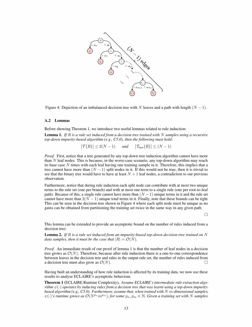
Figure 4: Depiction of an imbalanced decision tree with N leaves and a path with length (N − 1).

A.2 Lemmas

Before showing Theorem 1, we introduce two useful lemmas related to rule induction:Lemma 1. If R is a rule set induced from a decision tree trained with N samples using a recursivetop-down impurity-based algorithm (e.g., C5.0), then the following must hold:∣∣T (R)∣∣ ≤ 2(N − 1) and

∣∣Tmax(R)∣∣ ≤ (N − 1)

Proof. First, notice that a tree generated by any top-down tree induction algorithm cannot have morethan N leaf nodes. This is because, in the worst-case scenario, any top-down algorithm may reachits base case N times with each leaf having one training sample in it. Therefore, this implies that atree cannot have more than (N − 1) split nodes in it. If this would not be true, then it is trivial tosee that the binary tree would have to have at least N + 1 leaf nodes, a contradiction to our previousobservation.

Furthermore, notice that during rule induction each split node can contribute with at most two uniqueterms to the rule set (one per branch) and with at most one term to a single rule (one per root-to-leafpath). Because of this, a single rule cannot have more than (N − 1) unique terms in it and the rule setcannot have more than 2(N − 1) unique total terms in it. Finally, note that these bounds can be tight.This can be seen in the decision tree shown in Figure 4 where each split node must be unique as nogains can be obtained from partitioning the training set twice in the same way in any given path.

This lemma can be extended to provide an asymptotic bound on the number of rules induced from adecision tree:Lemma 2. If R is a rule set induced from an impurity-based top-down decision tree trained on Ndata samples, then it must be the case that |R| = O(N).

Proof. An immediate result of our proof of lemma 1 is that the number of leaf nodes in a decisiontree grows as O(N). Therefore, because after rule induction there is a one-to-one correspondencebetween leaves in the decision tree and rules in the output rule set, the number of rules induced froma decision tree must also grow as O(N).

Having built an understanding of how rule induction is affected by its training data, we now use theseresults to analyse ECLAIRE’s asymptotic behaviour.Theorem 1 (ECLAIRE Runtime Complexity). Assume ECLAIRE’s intermediate rule extraction algo-rithm ψ(·) operates by inducing rules from a decision tree that was learnt using a top-down impurity-based algorithm (e.g., C5.0). Furthermore, assume that, when trained withN m-dimensional samples,ψ(·)’s runtime grows as O(Npnmpm), for some pn, pm ∈ N. Given a training set with N samples

13

and a neural network with d hidden layers, such that there are at most m activations in any of itslayers, ECLAIRE’s runtime will grow as a function of O

(dNmax(3,pn+1)mpm

).

Proof. We begin our proof with a high-level summary of ECLAIRE’s approach: for each layer i in ournetwork, ECLAIRE extracts an intermediate rule set Rhi 7→y using rule extractor ψ(·) on intermediateactivations hi and the labels predicted by the input DNN. It then iterates over all premises in Rhi 7→y ,extracts a rule set mapping input activations x to each premise’s truth value, and adds the relevantrules into the output set. This procedure implies that the total amount of work done by ECLAIRE toprocess hidden layer i grows asymptotically as

O

((complexity of ψ(·) when trained with N samples and m features)

+ (number of rules in Rhi 7→y)× (complexity of evaluating a rule in Rhi 7→y N times)+ (number of rules in Rhi 7→y)× (complexity of ψ(·) when trained with N samples and m features)

+ (number of rules in Rhi 7→y)× (complexity of post-processing and adding new rules)

)Which can be rewritten as:

O

((Npnmpm) +

∣∣Rhi 7→y∣∣× (∣∣Tmax(Rhi 7→y

)∣∣N + (Npnmpm) +∣∣Tmax

(I(t)x 7→p

)∣∣∣∣I(r)x7→p′∣∣))

where we define I(t)x7→p to be the temporary rule set (approximating premise p) with the longest ruleand we define I(r)x 7→p′ as the temporary extracted rule set with the largest number of rules in it. Notethat we used the fact that, by assumption, ψ(·)’s worst case runtime grows asO(Npnmpm). Applyinglemmas 1 and 2 to this expression gives us

O

((Npnmpm) +N ×

((N − 1)N + (Npnmpm) + (N − 1)N

))Finally, using the fact that (N − 1) = O(N) and (N3) = O(Nmax(3,pn+1)mpm) as both pn and pmare natural numbers, and recalling that ECLAIRE performs this much work for each hidden layer, weget that ECLAIRE’s total runtime grows as a function of

O

(d((Npnmpm) + 2(N3) + (Npn+1mpm)

))= O

(dNmax(3,pn+1)mpm

)

B Dataset Details

In this section we include a brief description of all the non-synthetic datasets used for the tasksdescribed in Section 4.

METABRIC [45] This dataset consists of a collection of anonymized features extracted from breastcancer tumours in a cohort of 1, 980 patients. It includes clinical traits, gene expression patterns,tumour characteristics, and survival rates for a period of 4 years. The specific tasks we consider inMETABRIC, taken from [23], are:

• Immunohistochemical subtype prediction (MB-ER): for this task we predict immunohis-tochemical subtypes in breast cancer patients using 1000 mRNA expression patterns. Eachsample can be classified as one of two types, ER+ or ER-, which are crucial for determininga patient’s treatment.

• Histological tumour subtype prediction (MB-HIST): for this task we predict histologicalsubtypes of breast cancer tumours using 1004 mRNA expression profiles. Each samplecan be classified as either Invasive Lobular Carcinoma (ILC) or Invasive Ductal Carcinoma(IDC), two most common breast cancer histological subtypes [23].

14

MAGIC [46, 47] This is a particle physics dataset in which a signal needs to be classified as being ahigh-energy gamma ray or some background hadron cosmic radiation. Each of the 19,020 trainingsamples consists of 10 real-valued features that are generated via a Monte Carlo program and a binarylabel indicating whether the observation corresponds as a high-energy gamma ray (signal) or somebackground hadron radiation.

MiniBooNE [55, 47] This is a particle physics dataset in which one is interested in discriminatingelectron neutrino events from background events in interactions collected in the MiniBooNE experi-ment. Each of the 130,065 training samples consists of 50 real-valued features empirically collectedin the MiniBooNE experiment and a binary label indicating whether the sample represents a electronneutrino event (signal) or a background event.

Letter Recognition [49, 47] This dataset consists of 20, 000 representations of black-and-whiteEnglish capital letters labelled with one of 26 classes (A to Z). Each sample is generated by extracting16 statistical features from the images of each letter.

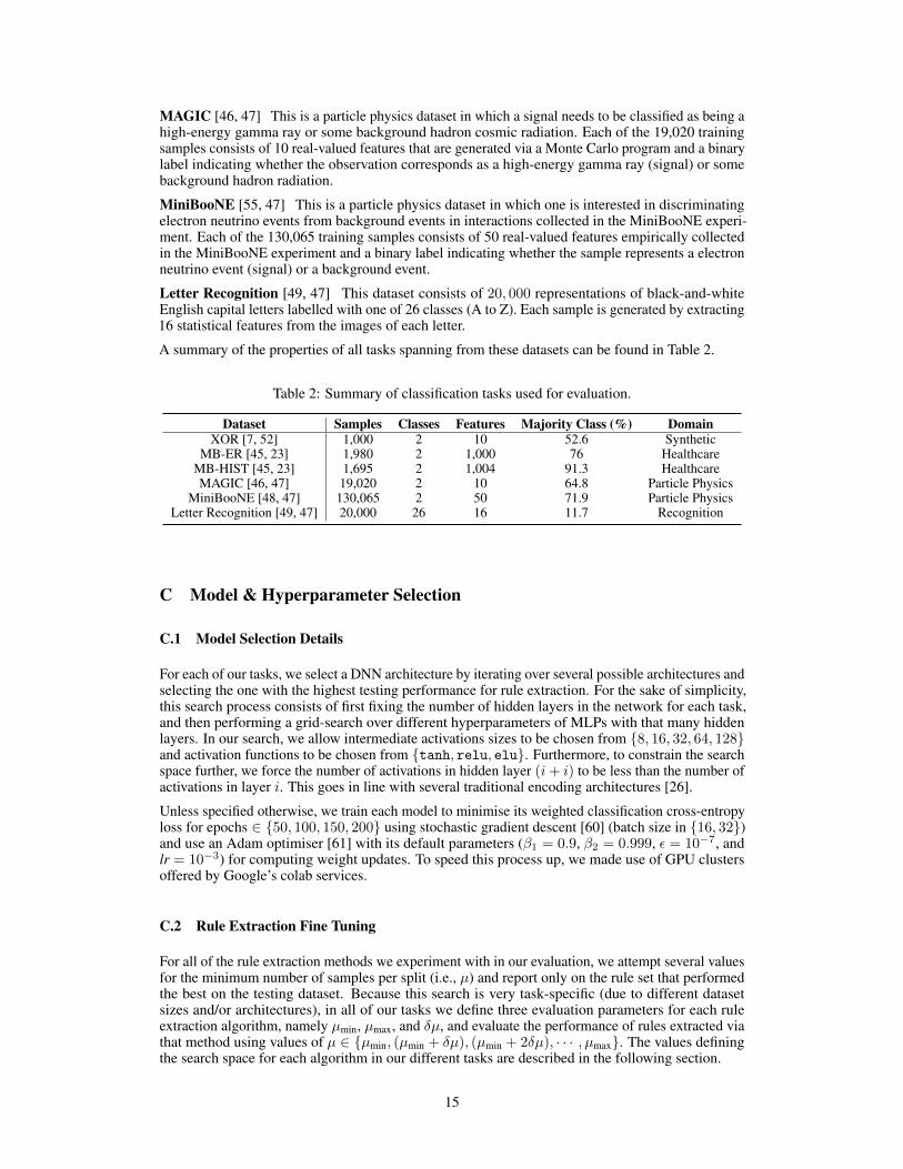
A summary of the properties of all tasks spanning from these datasets can be found in Table 2.

Table 2: Summary of classification tasks used for evaluation.

Dataset Samples Classes Features Majority Class (%) DomainXOR [7, 52] 1,000 2 10 52.6 Synthetic

MB-ER [45, 23] 1,980 2 1,000 76 HealthcareMB-HIST [45, 23] 1,695 2 1,004 91.3 HealthcareMAGIC [46, 47] 19,020 2 10 64.8 Particle Physics

MiniBooNE [48, 47] 130,065 2 50 71.9 Particle PhysicsLetter Recognition [49, 47] 20,000 26 16 11.7 Recognition

C Model & Hyperparameter Selection

C.1 Model Selection Details

For each of our tasks, we select a DNN architecture by iterating over several possible architectures andselecting the one with the highest testing performance for rule extraction. For the sake of simplicity,this search process consists of first fixing the number of hidden layers in the network for each task,and then performing a grid-search over different hyperparameters of MLPs with that many hiddenlayers. In our search, we allow intermediate activations sizes to be chosen from {8, 16, 32, 64, 128}and activation functions to be chosen from {tanh, relu, elu}. Furthermore, to constrain the searchspace further, we force the number of activations in hidden layer (i+ i) to be less than the number ofactivations in layer i. This goes in line with several traditional encoding architectures [26].

Unless specified otherwise, we train each model to minimise its weighted classification cross-entropyloss for epochs ∈ {50, 100, 150, 200} using stochastic gradient descent [60] (batch size in {16, 32})and use an Adam optimiser [61] with its default parameters (β1 = 0.9, β2 = 0.999, ε = 10−7, andlr = 10−3) for computing weight updates. To speed this process up, we made use of GPU clustersoffered by Google’s colab services.

C.2 Rule Extraction Fine Tuning

For all of the rule extraction methods we experiment with in our evaluation, we attempt several valuesfor the minimum number of samples per split (i.e., µ) and report only on the rule set that performedthe best on the testing dataset. Because this search is very task-specific (due to different datasetsizes and/or architectures), in all of our tasks we define three evaluation parameters for each ruleextraction algorithm, namely µmin, µmax, and δµ, and evaluate the performance of rules extracted viathat method using values of µ ∈ {µmin, (µmin + δµ), (µmin + 2δµ), · · · , µmax}. The values definingthe search space for each algorithm in our different tasks are described in the following section.

15

C.3 Task-specific Configurations

In this section we describe the configuration that our grid search produces for each of the tasks wediscuss in Section 4. We also include a description of the search space used for µ when evaluatingdifferent rule extraction methods.

C.3.1 XOR

Given the simplicity of the XOR task, we constrain the architecture search space to be only overMLPs using 3 hidden layers. This results in the best performing model having hidden layers withsizes {64, 32, 16} and tanh activation between them. This model is then trained for 150 epochsusing a batch size of 16.

When fine-tuning the different rule extractors, we use µmin = 2, µmax = 15, and δµ = 1 forECLAIRE, C5.0, and PedC5.0 as they all terminate relatively quickly and obtain good performancewithout much pruning. REM-D and DeepRED*, however, fail to terminate before their allotted timeswhen using values of µ below 25. Because of this, we evaluate them using values of µ in the rangedefined by µmin = 25, µmax = 35, and δµ = 1.

C.3.2 METABRIC

For both METABRIC tasks described in Section 4.2, we use the exact same architecture and trainingprocess used by Shams et al. in [23], which was determined through a similar grid search process.This architecture consists of an MLP with hidden layers with sizes {128, 16} and tanh activations inbetween them. For both tasks we train the model for 150 epochs using a batch size of 16.

In our rule extraction fine-tuning, we use µmin = 2, µmax = 15, and δµ = 1 for C5.0, PedC5.0, andECLAIRE. As suggested by [23], and due to their longer run times, we use µmin = 5, µmax = 15, andδµ = 5 for REM-D and DeepRED*.

C.3.3 MAGIC

In the MAGIC dataset results reported in Section 4.3, we search over architectures with 3 hiddenlayers and our grid-search results in the best model having layers of size {64, 32, 16} with ReLUactivations in between them. The best training configuration found is then trained for 200 epochswith a batch size of 32.

In our rule extraction fine-tuning, for ECLAIRE we use µmin = 50, µmax = 200, and δµ = 25 whilefor both REM-D and DeepRED* we use µmin = 500, µmax = 1000, and δµ = 50. Note that weuse large values of µ for REM-D and DeepRED* as we found it extremely hard to get reasonableextraction times when using less than 500 samples for µ. Finally, for C5.0 and PedC5.0 we searchover all µ values defined by µmin = 5, µmax = 50, and δµ = 5.

C.3.4 MiniBooNE

We found the MiniBooNE task to require the most capacity to obtain good results compared toothers experiments in this paper. We force our model architecture to use 5 hidden layers and searchfor models trained with epochs ∈ {20, 30, 40} given the large training size. This gives us a bestperforming architecture that uses hidden units {128, 64, 32, 16, 8} with an ELU activation in betweenthem which is trained for 30 epochs with a batch size of 16.

In our rule extraction fine-tuning, this task proved to be more complicated than the rest given itstraining size. For ECLAIRE we use µmin = 0.0005N , µmax = 0.0015N , and δµ = 0.0001N (whereN is the number of training samples) as values below 0.0005N result extraction times longer than 6hours. For both REM-D and DeepRED*, we increase the minimum value of µ significantly to getruns that terminate in their allotted times and use µmin = 0.02N , µmax = 0.1N , and δµ = 0.005N .Finally, given their fast extraction times, for C5.0 and PedC5.0 we search over all µ values defined byµmin = 5, µmax = 50, and δµ = 5.

16

C.3.5 Letter Recognition

For the results we report on the Letter Recognition dataset in Section 4.4, we search over architectureswith 2 hidden layers and obtain a best performing model that has layers of size {128, 64} with ELUactivations in between them. The best training configuration is trained for 150 epochs with a batchsize of 32.

In our rule extraction fine-tuning, we use µmin = 5, µmax = 15, and δµ = 1 for ECLAIRE, C5.0,and PedC5.0. As in the physics datasets, both DeepRED* and REM-D struggle to terminate in areasonable amount of time unless µ is significantly high. This is exacerbated by the large number ofclasses in this task. Because of this, we use µmin = 0.25N , µmax = 0.5N , and δµ = 0.05N duringtheir fine-tuning process.

CART as Intermediate Rule Extractor in Letters While in all of our binary tasks we are ableto construct high-performing rule sets with C5.0, we fail to observe this same trend in the Lettersdataset, our task of choice for multi-class evaluation. More specifically, Table 1 shows that end-to-endC5.0 rule sets are unable to achieve a high performance compared to that previously reported forother induction algorithms [62]. Therefore, in this section we explore the use of CART [63] treesfor intermediate rule induction and show these results in Table 3. In these experiments, we comparethe performance of rule sets induced from end-to-end CART trees, as well as rule sets induced fromCART trees learnt from data that was labelled using the DNN’s predictions (which we refer to asPedCART), against that of rule sets extracted with ECLAIRE when CART is used as its intermediaterule extractor. Furthermore, for the sake of obtaining a fair comparison between our baselines that isunbiased with respect to the choice of rule extraction algorithm, we also compare ECLAIRE againstversions of both REM-D and DeepRED that use CART as an intermediate rule extractor. For clarity,we refer to these versions of our baselines as ECLAIRECART, REM-DCART, and DeepREDCART,respectively.

In all of these experiments, we control the growth of CART-generated trees using Cost ComplexityPruning (CCP) [64] and by varying the number of minimum samples per split µ as in our previoustasks. For CART, PedCART, and ECLAIRECART we search over the spectrum defined by µmin =0.0001N , µmax = 0.0051N , and δµ = 0.0005N . As it was the case when using C5.0 as anintermediate rule extractor, for both DeepREDCART and REM-DCART we require significantly highervalues of µ to terminate in the allotted time. Because of this, we limit our search over µ to be over thespectrum defined by µmin = 0.1N , µmax = 0.3N , and δµ = 0.05N . This results in overpruned rulesets in DeepREDCART which, although small in size, take orders of magnitude more time to extractthan those generated by ECLAIRE.

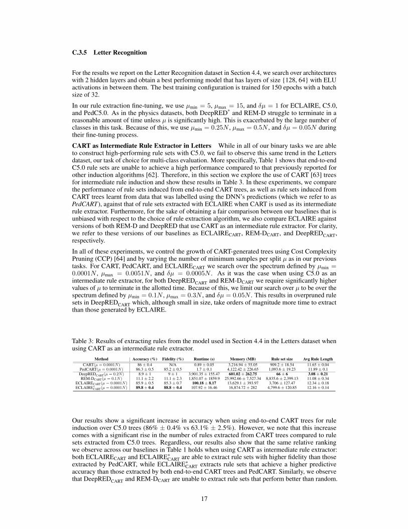
Table 3: Results of extracting rules from the model used in Section 4.4 in the Letters dataset whenusing CART as an intermediate rule extractor.

Method Accuracy (%) Fidelity (%) Runtime (s) Memory (MB) Rule set size Avg Rule LengthCART(µ = 0.0001N ) 86 ± 0.4 N/A 0.89 ± 0.05 3,216.94 ± 55.05 909.2 ± 18.54 11.65 ± 0.04

PedCART(µ = 0.0001N) 86.3 ± 0.5 85.2 ± 0.5 1.7 ± 0.1 4,122.42 ± 226.65 1,093.6 ± 19.23 11.89 ± 0.1DeepREDCART(µ = 0.2N) 8.9 ± 1 9 ± 1 3,901.35 ± 155.47 601.02 ± 262.75 66 ± 6 3.08 ± 0.21REM-DCART(µ = 0.1N) 11.1 ± 2.2 11.1 ± 2.3 1,851.07 ± 1859.9 25,992.66 ± 7,527.34 8,835.6 ± 2,399.13 11.08 ± 0.34

ECLAIRECART(µ = 0.0001N) 85.9 ± 0.5 85.3 ± 0.7 100.18 ± 8.17 13,629.1 ± 393.97 3,706 ± 127.47 12.34 ± 0.18ECLAIRE∗CART(µ = 0.0001N) 89.8 ± 0.4 88.8 ± 0.4 107.92 ± 16.46 16,874.72 ± 282 4,799.6 ± 120.85 12.16 ± 0.14

Our results show a significant increase in accuracy when using end-to-end CART trees for ruleinduction over C5.0 trees (86% ± 0.4% vs 63.1% ± 2.5%). However, we note that this increasecomes with a significant rise in the number of rules extracted from CART trees compared to rulesets extracted from C5.0 trees. Regardless, our results also show that the same relative rankingwe observe across our baselines in Table 1 holds when using CART as intermediate rule extractor:both ECLAIRECART and ECLAIRE∗CART are able to extract rule sets with higher fidelity than thoseextracted by PedCART, while ECLAIRE∗CART extracts rule sets that achieve a higher predictiveaccuracy than those extracted by both end-to-end CART trees and PedCART. Similarly, we observethat DeepREDCART and REM-DCART are unable to extract rule sets that perform better than random.

17

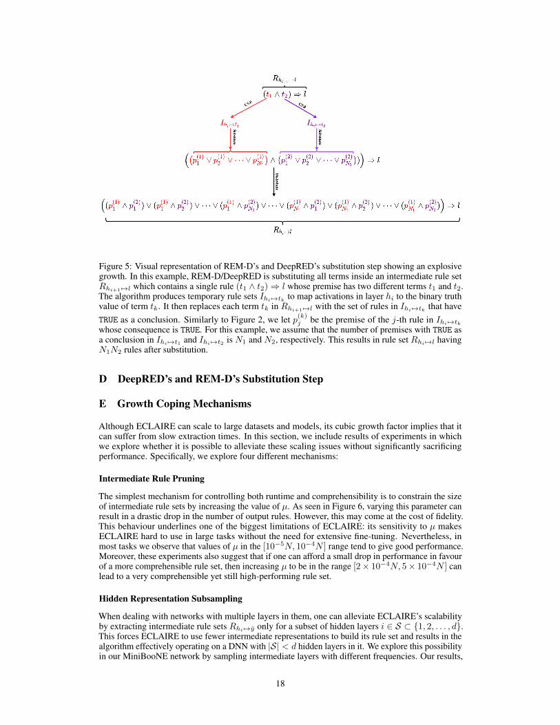
Figure 5: Visual representation of REM-D’s and DeepRED’s substitution step showing an explosivegrowth. In this example, REM-D/DeepRED is substituting all terms inside an intermediate rule setRhi+1 7→l which contains a single rule (t1 ∧ t2)⇒ l whose premise has two different terms t1 and t2.The algorithm produces temporary rule sets Ihi 7→tk to map activations in layer hi to the binary truthvalue of term tk. It then replaces each term tk in Rhi+1 7→l with the set of rules in Ihi 7→tk that haveTRUE as a conclusion. Similarly to Figure 2, we let p(k)j be the premise of the j-th rule in Ihi 7→tkwhose consequence is TRUE. For this example, we assume that the number of premises with TRUE asa conclusion in Ihi 7→t1 and Ihi 7→t2 is N1 and N2, respectively. This results in rule set Rhi 7→l havingN1N2 rules after substitution.

D DeepRED’s and REM-D’s Substitution Step

E Growth Coping Mechanisms

Although ECLAIRE can scale to large datasets and models, its cubic growth factor implies that itcan suffer from slow extraction times. In this section, we include results of experiments in whichwe explore whether it is possible to alleviate these scaling issues without significantly sacrificingperformance. Specifically, we explore four different mechanisms:

Intermediate Rule Pruning

The simplest mechanism for controlling both runtime and comprehensibility is to constrain the sizeof intermediate rule sets by increasing the value of µ. As seen in Figure 6, varying this parameter canresult in a drastic drop in the number of output rules. However, this may come at the cost of fidelity.This behaviour underlines one of the biggest limitations of ECLAIRE: its sensitivity to µ makesECLAIRE hard to use in large tasks without the need for extensive fine-tuning. Nevertheless, inmost tasks we observe that values of µ in the [10−5N, 10−4N ] range tend to give good performance.Moreover, these experiments also suggest that if one can afford a small drop in performance in favourof a more comprehensible rule set, then increasing µ to be in the range [2× 10−4N, 5× 10−4N ] canlead to a very comprehensible yet still high-performing rule set.

Hidden Representation Subsampling

When dealing with networks with multiple layers in them, one can alleviate ECLAIRE’s scalabilityby extracting intermediate rule sets Rhi 7→y only for a subset of hidden layers i ∈ S ⊂ {1, 2, . . . , d}.This forces ECLAIRE to use fewer intermediate representations to build its rule set and results in thealgorithm effectively operating on a DNN with |S| < d hidden layers in it. We explore this possibilityin our MiniBooNE network by sampling intermediate layers with different frequencies. Our results,

18

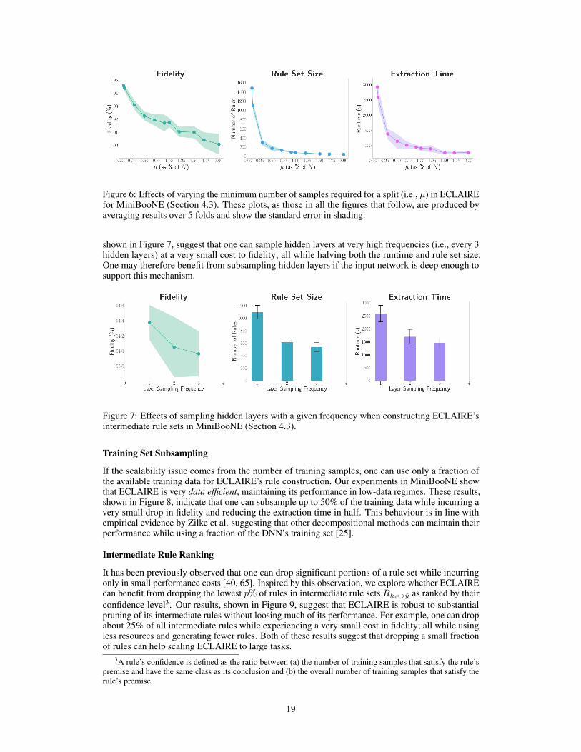
Figure 6: Effects of varying the minimum number of samples required for a split (i.e., µ) in ECLAIREfor MiniBooNE (Section 4.3). These plots, as those in all the figures that follow, are produced byaveraging results over 5 folds and show the standard error in shading.

shown in Figure 7, suggest that one can sample hidden layers at very high frequencies (i.e., every 3hidden layers) at a very small cost to fidelity; all while halving both the runtime and rule set size.One may therefore benefit from subsampling hidden layers if the input network is deep enough tosupport this mechanism.

Figure 7: Effects of sampling hidden layers with a given frequency when constructing ECLAIRE’sintermediate rule sets in MiniBooNE (Section 4.3).

Training Set Subsampling

If the scalability issue comes from the number of training samples, one can use only a fraction ofthe available training data for ECLAIRE’s rule construction. Our experiments in MiniBooNE showthat ECLAIRE is very data efficient, maintaining its performance in low-data regimes. These results,shown in Figure 8, indicate that one can subsample up to 50% of the training data while incurring avery small drop in fidelity and reducing the extraction time in half. This behaviour is in line withempirical evidence by Zilke et al. suggesting that other decompositional methods can maintain theirperformance while using a fraction of the DNN’s training set [25].

Intermediate Rule Ranking

It has been previously observed that one can drop significant portions of a rule set while incurringonly in small performance costs [40, 65]. Inspired by this observation, we explore whether ECLAIREcan benefit from dropping the lowest p% of rules in intermediate rule sets Rhi 7→y as ranked by theirconfidence level3. Our results, shown in Figure 9, suggest that ECLAIRE is robust to substantialpruning of its intermediate rules without loosing much of its performance. For example, one can dropabout 25% of all intermediate rules while experiencing a very small cost in fidelity; all while usingless resources and generating fewer rules. Both of these results suggest that dropping a small fractionof rules can help scaling ECLAIRE to large tasks.

3A rule’s confidence is defined as the ratio between (a) the number of training samples that satisfy the rule’spremise and have the same class as its conclusion and (b) the overall number of training samples that satisfy therule’s premise.

19

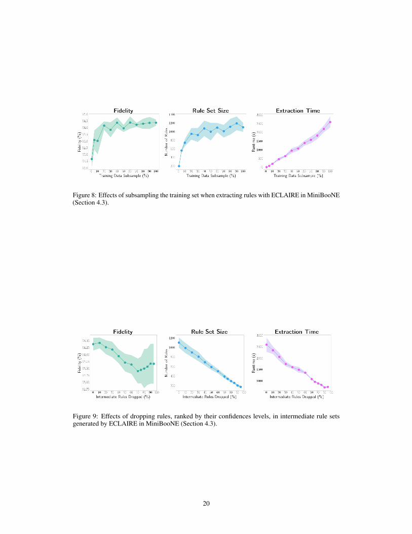
Figure 8: Effects of subsampling the training set when extracting rules with ECLAIRE in MiniBooNE(Section 4.3).

Figure 9: Effects of dropping rules, ranked by their confidences levels, in intermediate rule setsgenerated by ECLAIRE in MiniBooNE (Section 4.3).

20