Efficient Content-based Retrieval in Parallel Databases of ...

HAL Id: tel-00465943https://tel.archives-ouvertes.fr/tel-00465943

Submitted on 22 Mar 2010

HAL is a multi-disciplinary open accessarchive for the deposit and dissemination of sci-entific research documents, whether they are pub-lished or not. The documents may come fromteaching and research institutions in France orabroad, or from public or private research centers.

L’archive ouverte pluridisciplinaire HAL, estdestinée au dépôt et à la diffusion de documentsscientifiques de niveau recherche, publiés ou non,émanant des établissements d’enseignement et derecherche français ou étrangers, des laboratoirespublics ou privés.

Efficient Content-based Retrieval in Parallel Databasesof Images

Jorge Roberto Manjarrez Sanchez

To cite this version:Jorge Roberto Manjarrez Sanchez. Efficient Content-based Retrieval in Parallel Databases of Images.Réseaux et télécommunications [cs.NI]. Université de Nantes, 2009. Français. �tel-00465943�

https://tel.archives-ouvertes.fr/tel-00465943

https://hal.archives-ouvertes.fr

École Centrale de Nantes Université de Nantes École des Mines de Nantes

ÉCOLE DOCTORALE STIM

« SCIENCES ET TECHNOLOGIES DE L’INFORMATION ET DES MATÉRIAUX »

ANNÉE 2009

No attribué par la bibliothèque

Efficient Content-Based Retrieval in Parallel

Databases of Images

THÈSE DE DOCTORAT DE L’UNIVERSITÉ DE NANTES

Discipline : INFORMATIQUE

Spécialité : Bases de Données

Présentée

Et soutenue publiquement par

Jorge Roberto MANJARREZ SANCHEZ

Le 26 Octobre 2009

à l’UFR Sciences & Techniques, Université de Nantes,

devant le jury ci-dessous

Président: Anne Doucet, Professeur des universités, Université Paris VI

Rapporteurs: Patrick Gros, Directeur de Recherche, INRIA Rennes

Examinateur : Florent Autrusseau, Ingénieur de recherche, École polytechnique de l'université de

Nantes

Directeur de thèse : Patrick Valduriez, Directeur de recherche, INRIA Montpellier

Co-directeur : José Martinez, Professeur des universités, École polytechnique de l'université de

Nantes

Laboratoire: LABORATOIRE D’INFORMATIQUE DE NANTES ATLANTIQUE.

CNRS FRE 2729. 2, rue de la Houssinière, BP 92 208 –44 322 Nantes, CEDEX 3.

Recherche par Contenu dans les

Bases Parallèles d’Images

Abstract. In this thesis, we address the performance problem when searching in large databases of

images. The processing of similarity queries is a computational challenge because of the

dimensionality of the abstract representation for the images and size of the databases. We

present two data organization methods that account for performance improvement. The first one

is based on the clustering of the database in centralized settings. We derive an optimal range of

values for the number of clusters to obtain from a database, which in conjunction with a searching

algorithm allows to efficiently process nearest neighbor queries. However as the dimensionality

and size of the database increase, a single computer is overwhelmed. The second method is based

on data partitioning over a shared nothing machine. Based on the results of the first method, this

method maximizes parallelism. We also derive the optimal number of processing nodes to

maximize resource utilization.

We performed extensive experiments with synthetic and real databases. They validate the

proposals and show that the performance level is superior to existing approaches which beyond a

certain dimensionality or database size become inefficient.

Keywords: Multimedia data management, Multidimensional data, Databases, Data clustering,

Cluster and parallel computing, Data partitioning.

Résumé. Cette thèse porte sur le traitement des requêtes par similarité sur les données de haute

dimensionnalité, notamment multimédias, et, parmi elles, les images plus particulièrement. Ces

requêtes, notamment celles des k plus proches voisins (kNN), posent des problèmes de calcul de

par la nature des données elles-mêmes et de la taille de la base des données.

Nous avons étudié leurs performances quand une méthode de partitionnement est appliquée sur

la base de données pour obtenir et exploiter des classes. Nous avons proposé une taille et un

nombre optimaux de ces classes pour que la requête puisse être traitée en temps optimal et avec

une haute précision. Nous avons utilisé la recherche séquentielle comme base de référence.

Ensuite nous avons proposé des méthodes de traitement de requêtes parallèles sur une grappe de

machines. Pour cela, nous avons proposé des méthodes d’allocation des données pour la

recherche efficace des kNN en parallèle. Nous proposons de même, un nombre réduit de nœuds

sur la grappe de machines permettant néanmoins des temps de recherche sous-linéaires et

optimaux vis-à-vis des classes déterminées précédemment.

Nous avons utilisé des donnés synthétiques et réelles pour les validations pratiques. Dans les deux

cas, nous avons pu constater des temps de réponse et une qualité des résultats supérieurs aux

méthodes existantes, lesquelles, au-delà d'un faible nombre des dimensions, deviennent

inefficaces.

Mots-clés: Gestion de données multimédias, données multidimensionnelles, bases de données,

classification, parallélisme dans des grappes de machines, partitionnement de données.

Acknowledgements I am grateful with the CONACYT and the National Polytechnic Institute of Mexico as well

as with INRIA France.

I am also very thankful with my advisor Dr. Patrick Valduriez, who received me at the

INRIA ATLAS Research Team and gave me all I needed to carry out my research and helped

me to improve my scientific skills. This acknowledge is also for my co-advisor Dr. Jose

Martinez, I am deeply thankful with him for all the invaluable knowledge he shared with

me and for his unconditional support that made possible this thesis.

I thank also the members of my evaluation committee for their insightful comments on

my proposal.

The conclusion of this thesis is the result of many aspects, among them the love of my

petite princesse Valeria, my mom and my brothers. I cannot forget also all the rest of my

family who in spite of being far away they were always close to me. I dedicate this thesis

to them.

I want to greet all my friends, among them: Quiane, Reza, David, Alvaro, Erwan, Aga,

Noemi, Malika, Wence, Eduardo, Thomas, Cedric…and all the lab mates and amies with

whom I share unforgettable soirées amusantes. Also to all my good friends in Mexico who

were near all this journey: Vero, Claudia, Raquel, José, Miguel, Raul … too many to name

them all here, je ne vous oublie pas!.

Finally, to the people who helped me in administrative tasks and I don’t forget: Elodie

Chahbani, Virginie Desroches, Christine Brunet…merci.

Nantes, October 2009

Table of Contents

Table of figures .............................................................................................................. XI

Résumé Étendu ..................................................................................................................... 1

1 Introduction ............................................................................................... 19

1.1 Motivation ......................................................................................................... 19

1.2 Statement of the problem ................................................................................. 21

1.3 Contributions ..................................................................................................... 22

1.4 Overview ............................................................................................................ 23

2 Background on content-based retrieval ...................................................... 25

2.1 Visual feature descriptors.................................................................................. 28

2.2 High-dimensional data model ........................................................................... 31

2.3 Distances ............................................................................................................ 32

2.4 Similarity queries ............................................................................................... 33

2.5 Geometry of queries .......................................................................................... 34

2.6 Feature transformation ..................................................................................... 35

2.7 Intrinsic dimensions ........................................................................................... 36

2.8 Improving performances of queries .................................................................. 36

2.8.1 Full and approximate searches .......................................................................... 37

2.8.2 High-dimensional geometry .............................................................................. 37

2.8.3 Indexing ............................................................................................................. 39

2.8.4 Clustering ........................................................................................................... 41

2.8.5 Parallel search ................................................................................................... 44

2.9 Performance evaluation .................................................................................... 49

3 Optimal Clustering for Efficient Retrieval .................................................... 55

3.1 Some complexity considerations ....................................................................... 56

3.2 CBIR using clustering ......................................................................................... 58

3.3 Optimal database clustering.............................................................................. 60

3.4 Experiments ....................................................................................................... 63

3.4.1 Data sets ............................................................................................................ 63

3.4.2 Experiments baseline ......................................................................................... 67

3.4.3 Searching process .............................................................................................. 67

3.4.4 Performance evaluation .................................................................................... 68

3.5 Summary ............................................................................................................ 72

4 Parallel nearest neighbor queries ............................................................... 75

4.1 Data allocation scheme ..................................................................................... 76

4.1.1 Data partitioning ............................................................................................... 76

4.1.2 Data placement (data layout) ........................................................................... 76

4.2 Validation ........................................................................................................... 78

4.2.1 Data sets ............................................................................................................ 79

4.2.2 kNN searching process....................................................................................... 79

4.2.3 Performance evaluation .................................................................................... 80

4.2.4 Effect of the size of k .......................................................................................... 83

4.2.5 Effect of data placement ................................................................................... 84

4.3 Summary ............................................................................................................ 85

5 Conclusions ................................................................................................ 87

5.1 Further work. Query processing ........................................................................ 87

5.2 Further work. Multiuser .................................................................................... 88

6 References ................................................................................................. 89

Table of figures

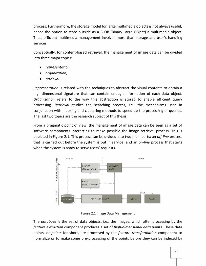
Figure 2.1 Image Data Management .................................................................................... 27

Figure 2.2 Distance induced shape ....................................................................................... 34

Figure 2.3 The effect of data transformation ....................................................................... 35

Figure 2.4 Illustration of MINDIST and MINMAXDIST .......................................................... 41

Figure 2.5 Synopsis of hierarchical clustering....................................................................... 42

Figure 2.6 Two images from the Flickr database with VisualDescriptor

type="ScalableColorType" numOfBitplanesDiscarded="0" numOfCoeff="64", having

exactly the same feature vector. .......................................................................................... 52

Figure 3.1 Histogram of distances of the data sets used in the experiments ...................... 65

Figure 3.2 Distribution of points in clusters obtained from FSC and FCS datasets, n=100,

d=64. ..................................................................................................................................... 66

Figure 3.3 Distribution of points in clusters generated with MMV, n=100, d=128, 256,500.

.............................................................................................................................................. 67

Figure 3.4 Analysis of processing time for kNN(10), 100% precision ................................... 69

Figure 3.5 Fraction of the clusters read to solve kNN(10) queries ....................................... 70

Figure 3.6 Fraction of the clusters read to solve kNN(50) queries ....................................... 70

Figure 3.7 Performance of 50NN queries, for 64-dimensional data. ................................... 72

Figure 4.1 Execution times for 1000 kNN(50) queries for n=107 non uniform databases of

different data dimensionalities............................................................................................. 81





Figure 4.4 Disk I/O count for the kNN(50) query processing over databases of different

dimensionalities. ................................................................................................................... 82

Figure 4.5 Distance computations count for the kNN(50) query processing over databases

of different dimensionalities. ............................................................................................... 83

Figure 4.6 Nodes activated simultaneously to process a query in 256 dimensions............. 84

1

RÉSUMÉ ÉTENDU 1. INTRODUCTION

Nous assistons aujourd’hui à l'impact croissant des développements technologiques,

notamment ceux de la miniaturisation des composants électroniques, des réseaux de

communication et la puissance de calcul des processeurs, dans le domaine de la gestion

d'information. En particulier, les données images sont produites à un taux explosif, avec

toutes sortes d’outils et d’appareils. Par conséquent, la gestion de grandes collections

d’images est devenue un grand défi pour la recherche en informatique.

Donnons quelques exemples de motivation et les approches technologiques générales

afin d'aborder ce problème. Partout dans le monde, les utilisateurs exigent des méthodes

pour la recherche efficace d’images dans des bases volumineuses. Des propositions de

systèmes à l’échelle du Web pour la recherche d’images, telles que Yahoo et Google,

notamment, s’appuient sur le texte environnant dans les pages Web pour gérer les images

elles-mêmes. Par conséquent, les utilisateurs interrogent la base de données à l’aide de

texte, avec l'espoir que ce texte rapproche la description des images requis. Les

inconvénients de cette approche sont que le texte qui entoure les images n’est pas

nécessairement en relation ni avec le contenu d'image ni sa sémantique. En outre, une

fois qu'une image est récupérée, elle est séparée de son contexte et toute l'information

utilisée pour son indexation est perdue. Parfois même, la plupart des résultats sont

inutiles.

De plus, pas toutes les images existantes sont hébergées dans des pages web. Flickr est

l'exemple le plus notable avec une base de millions d'images. Toutefois, ces images sont

également recherchées en utilisant du texte, appelé des métadonnées, puisqu’il comporte

des informations tel que le nom donné par le propriétaire, la taille, la date...et des mots

clés. Ainsi, la récupération se sert des étiquettes et des annotations du propriétaire,

évidemment reflétant les émotions et les intérêts du propriétaire.

Un autre facteur limitant ces systèmes, est leur incapacité à rechercher des images

basées sur les propriétés visuelles, utiles lorsqu'il est difficile d'exprimer en mots les

conditions requises pour résoudre les requêtes. Dans ce cas, il est nécessaire de

rechercher les images semblables basées sur leur contenu, par exemple, des couleurs, des

textures et des formes

2

La recherche d'images par le contenu (RIPC) a été un problème de recherche très étudié

durant plusieurs années. Malgré tout, il semble que cette problématique soit de plus en

plus intéressante, car les développements technologiques facilitent la génération de bases

d'images de grands volumes. Or pour rendre leur exploitation performante, des méthodes

de navigation et de recherche efficaces sont nécessaires.

Classiquement, la mise en œuvre d'un système pour la recherche d'images RIPC,

comprend une étape d'extraction des vecteurs caractéristiques et une autre pour

l'organisation de ces vecteurs, le tout dans une étape de pre-processing avant la mis en

ligne du système. La première sert à obtenir la représentation abstraite en utilisant une

technique d'analyse d'images pour transformer chaque image en un point

multidimensionnel: chaque dimension est une caractéristique de description pertinente,

qui permet d'identifier le contenu de l'image. Elle peut être une plage bin d'un

histogramme de couleurs. Ensuite, tous les points multidimensionnels ainsi obtenus

doivent être organisés pour permettre le traitement de requêtes de façon efficace.

Le traitement de requêtes par le contenu fonctionne par l’exemple. À la différence des

bases de données traditionnelles, ici l'utilisateur dirige le processus de recherche en

utilisant une image exemple qui ressemble à celles qu'il veut trouver dans la base.

D’abord, l’image fournie est transformée en un point dans le même espace

multidimensionnel, puis la distance (Euclidienne, par exemple) entre le point requête et

les points de la base est calculée pour déterminer leur similarité. Comme résultat de la

recherche, un ensemble limité aux k meilleures réponses est présenté à l’utilisateur. Ce

type de requête s'appelle "k plus proches voisins" ou tout simplement kNN, et elle est

l'une des plus utiles pour la récupération d’images par le contenu. Pour les bases

volumineuses la recherche séquentielle est prohibitive, puisque le coût algorithmique du

calcul de la similarité est élevé.

Pour accélérer la recherche, plusieurs techniques d'indexation ont été développées [17].

Soit par le partitionnement des données, soit par le partitionnement de l'espace,

l’indexation permet de trouver rapidement les régions intéressantes et ainsi réduire le

temps d’exécution des requêtes. L’arbre X-tree [11] et l’arbre R-tree [45] et ses dérivés

sont des exemples notables de techniques qui partitionnent les données en utilisant des

régions. Ces méthodes et les méthodes de partitionnement de l’espace sont implémentés

dans un modèle d'espace vectoriel, et prennent en compte les caractéristiques

topologiques de l’espace des donnés. Mais pour les hautes dimensionnalités, ils doivent

parcourir quasiment la totalité des nœuds pour faire une élimination des régions qui ne

contiennent pas des points-réponse: leur performance devient alors comparable à celle

d’une recherche séquentielle. Dans les techniques qui partitionnent les données, on

3

retrouve celles qui utilisent un espace métrique [31][46] pour la représentation des points

multidimensionnels. La seule caractéristique prise en compte entre les images est leur

distance, et on profite de l'inégalité triangulaire pour éliminer les régions qui ne sont pas

intéressantes. L’arbre M-tree [35] et l’index iDistance [49] en sont quelques exemples. La

méthode M-Tree utilise un arbre balancé qui optimise les opérations d’entrée-sortie du

disque et le nombre d'évaluation des distances de similarité. L'index iDistance trie les

points selon leur distance puis utilise un arbre B+Tree pour le traitement des requêtes.

Cette méthode implique un coût élevé pour les requêtes, qui croît exponentiellement avec

la dimensionnalité.

Les méthodes de réduction de la dimensionnalité peuvent être utilisées, mais ajoutent un

niveau d'imprécision aux données qui doivent subir une nouvelle transformation et

potentiellement une perte de précision dans la description, qui finalement influence la

qualité des résultats.

Alternativement, quand on utilise une méthode de regroupement (clustering), il semble

que l'on peut atteindre de bons résultats [31]. Le regroupement est une méthode qui

permet de diviser la base en groupes de données selon leur ressemblance, ainsi la

recherche peut être orientée vers un ensemble réduit de la base avec de fortes

probabilités de contenir les points recherchés. Bien qu'il existe plusieurs propositions

suivant cette approche, il y a encore quelques problèmes à résoudre, parmi ceux-ci,

déterminer le nombre optimal de clusters ou partitions et par conséquent leur taille. Cette

question est importante, car même si pendant une première recherche on élimine des

clusters qui ne sont pas d'intérêt pour une requête, la recherche dans les clusters restants

peut s'avérer une tâche lourde. Il faut également considérer le cas où l'utilisateur ne

possède pas une image d'exemple pour démarrer la requête, dans ce cas le regroupement

peut permettre de feuilleter rapidement la base.

Néanmoins, la taille de la base d’images peu être très large et la puissance de calcul d’un

seul processeur devient incapable de fournir les temps de réponse corrects. De plus, la

capacité d’accès aux données stockées sur disque devient aussi un goulot d’étranglement

et ainsi un point de réduction des performances. Dans un tel contexte l’utilisation des

architectures parallèles nous paraît une solution naturelle.

Les architecture parallèles, notamment celles composées de nœuds indépendants, chacun

possédant ses propres processeurs, disques et mémoire vive, appelé Shared-Nothing (SN)

sont les mieux adaptées au passage à l’échelle en termes de taille de base ou de nombres

d’utilisateurs, ceci avec un rapport performance/coût optimal lors que les nœuds sont des

PC standards en grappe.

4

Pour mieux exploiter toute la puissance offerte par les architectures SN, la base de donnés

doit être correctement stockée sur les différents nœuds. Puisque le coût de traitement

d’une requête est proportionnel au temps de réponse plus large parmi les nœuds, alors il

faut repartir également la charge de travail parmi eux. Pour cela il faut d’abord

partitionner la base de donnés puis distribuer les partitions d’une telle manière que pour

évaluer une requête nécessitant b partitions, chaque nœud travaille au plus sur

partitions, où m est le nombre de nœuds disponibles sur la machine SN. Cette méthode

appelée dégroupement (declustering) a été démontrée comme étant NP-complète [2] ; il

faut alors essayer d’obtenir des heuristiques pour résoudre ce problème autant qu’il se

peut et aboutir à un équilibrage de charge.

De plus, une caractéristique souhaitée est celle d’avoir un nombre correct des nœuds de

calcul. En effet, pour maximiser l’utilisation des ressources, pour une taille de la base de

données, il faut un nombre optimal des nœuds de calcul et ainsi, le temps de traitement

des requêtes est le plus efficace.

Dans cette thèse, nous traitons le problème des performances des requêtes parallèles

basées sur le contenu dans les bases d’images. Il s’agit d’un problème ouvert car la

recherche dans des bases d’images de plus en plus grandes reste un grand défi

informatique en raison de la représentation multidimensionnelle utilisée pour décrire,

stocker et rechercher les images avec des très nombreuses dimensions. La base de notre

recherche est le travail pionnier de José Martinez et Patrick Valduriez [64] qui montre les

limites d'une approche centralisée en raison de la complexité du processus de recherche

multidimentionnelle dans les bases d’images. Motivé par ce résultat, nous analysons les

aspects algorithmiques de la recherche lorsqu'est utilisée une méthode de

partitionnement, telle que le regroupement, sur la base de données.

Dans cette thèse, nous proposons une solution au problème de l'exécution efficace des

requêtes basées sur le contenu dans de grandes bases de données images en exploitant

efficacement le parallélisme fourni par une grappe SN de machines. Nous accomplissons

ce but en deux étapes :

Dans un premier temps, nous proposons la pré-structuration optimale de la base

de données images pour améliorer le temps de réponse. Notre proposition est

basée sur une analyse de la complexité de la recherche d’images par le contenu

quand une méthode quelconque est utilisée pour partitionner la base de

donnés. Nous montrons alors qu'il est possible d'accomplir des performances sous-

linéaires, en utilisant un nouvel algorithme de recherche que nous proposons.

Ensuite, pour résoudre le problème lié à la taille des données et améliorer les

performances, nous avons développé un modèle analytique pour déterminer le

5

nombre optimal des nœuds requis pour traiter efficacement les requêtes. Nous

proposons une méthode d’allocation des données (dégroupement) sur cette

machine SN, qui est développée en exploitant les résultats obtenus dans la

première partie et en combinaison avec des stratégies de placement. Ainsi, nous

proposons un algorithme pour le traitement parallèle des requêtes qui tire le

meilleur de la puissance fournie par cette configuration.

Pour éviter toute dispersion dans notre travail, nous avons volontairement concentré

notre présentation sur le problème de la récupération des images dans le cadre de la RIPC.

Mais puisque notre proposition est basée sur le paradigme général de la recherche par

similarité dans un espace métrique, elle peut être tout aussi utile dans les applications de

la recherche des données multimédias en général, mais aussi dans d’autres domaines

comme la biologie ou la finance.

Le reste de ce résumé étendu de notre thèse est organisé comme suit. Dans la section 2

nous discutons la complexité de la recherche en utilisant le regroupement et nous

présentons notre proposition pour le partitionnement de la base et sa validation

analytique. Nous offrons aussi quelques résultats expérimentaux. Dans la section 3, nous

présentons la proposition pour le traitement parallèle des requêtes ainsi que sa validation

expérimentale. Finalement, dans la section 4, nous formulons quelques conclusions et

donnons quelques pistes de recherche futures.

2. RIPC EN UTILISANT LE REGROUPEMENT

Comme expliqué ci-dessus, pour éviter les problèmes de performances des méthodes

d’indexation causés par les hautes dimensionnalités qu’on utilise pour la description des

images, il est possible soit de réduire les dimensions, soit de faire un regroupement des

descripteurs.

La réduction de la dimensionnalité est un processus qui transforme l'espace de donnés en

un autre moins complexe. Mais pour que cette transformation soit utile il faut prendre en

considération autant que possible les caractéristiques de l'espace initial, de façon à les

préserver dans celui d'arrivée. Pour cette raison, une faiblesse de la réduction des

dimensions est la perte de précision potentielle dans la description des données. Nous

n'approfondirons pas ce sujet ici.

A priori, le regroupement peut se voir affecté du même problème que les méthodes

d'indexation. Néanmoins on peut espérer l'économie d'un très grande nombre de calcul

de distances de similarité, car le but est de regrouper un ensemble de points similaires les

uns avec les autres, sous forme de clusters, et ainsi faire une récupération plus rapide.

Même si le processus pour obtenir les clusters est coûteux, il peut être réalisé en mode

6

hors-ligne, c'est-à-dire, avant la mise en ouvre du système, dans une phase préliminaire.

Dans cette thèse nous ne suggérons pas une méthode de regroupement spécifique. La

méthode k-means, comme utilisée dans [34] ou le processus décrit dans [30] sont deux

processus pour l'obtention des clusters qui peuvent être utilisés en conjonction avec notre

proposition, car ils acceptent le nombre de clusters désirés comme paramètre. Ici nous

nous concentrons sur l'exploitation efficace du regroupement pour rendre la RIPC

performante.

Supposons le cas de la recherche via une méthode de regroupement quelconque, alors

nous pouvons écrire la complexité générale comme:

[1]

Où:

est le nombre des clusters produits par la méthode de clusterisation ;

est la complexité de la recherche parmi les clusters;

est le nombre de clusters susceptibles d'avoir suffisamment d'images

similaires;

est la complexité de la recherché parmi les clusters de points

multidimensionnels.

Si l’on fait le calcul des complexités standard pour et pour la recherche

séquentielle dans clusters, on peut observer que le parcours logarithmique d'une base

clustérisée, soit en est supposé d’être hiérarchique et bien balancée, et

présente peu d'importance. En fait, il pose une limite faible pour le nombre de clusters qui

peuvent contenir des images pertinentes: .

Rappelons que nous sommes intéressés en résoudre des requêtes du type k plus proches

voisins. Plus avec précision, nous sommes intéressés par les voisins les plus proches.

La complexité en , i.e., linéal, est actuellement la ligne de base pour tous les

algorithmes de recherche dans les espaces de haute dimensionnalité. Plus précisément,

nous dévons considérer si le résultat doit être trié. Comme k est

indépendant de n et petit, la recherche séquentielle prédomine la complexité et

s’applique au problème en question. Un autre paramètre qui doit être considéré est la

taille des descripteurs. Alors, dans un espace d-dimensionnel, le calcul de la distance est

au moins en . Alors, la complexité est plus précisément exprimée en disant qu’elle

appartient à . Encore, comme d est indépendant de la taille de la base n

et petite en relation à elle, de manière asymptotique, d peut-être considéré une

constante. Notons que quelques distances peuvent avoir une complexité plus grande. Par

7

exemple, comme indique par son nom, la distance quadratique à une complexité en

, laquelle est plus contraignante dans la pratique.

Au-dessus du la ligne de base en , le pire de cas que nous envisageons est celui de la

recherché sequentielle suivi d’un tri de toute la base de donnés. Dans ce cas, la limite

supérieure de tout algorithme pour RIPC est en . Une fois encore, cette

complexité tiens malgré le paramètre constant d. Cette limite supérieure est aussi

indépendante de k. Ce scenario correspond à le cas où il est utilisé un tri en lieu d’une

procédure du type top-k.

Au contraire, sous cette ligne de base , les recherches indépendantes de la taille de la

base mais lies à celui du résultat, semblent difficiles voir impossibles d’achever sans

l’addition de quelques hypothèses. Néanmoins, nous allons démontrer qu’il est possible

d’obtenir des complexités en , en utilisant clustering et parallélisme, et pas une

base sans structure et un seul processeur. Même si trouver un algorithme en est

le but idéal, mais ce n’est pas possible.

2.1 Partitionnement optimal

La complexité générique de l'équation 1 introduit un problème d'optimisation, lequel doit

satisfaire les contraintes suivantes pour être optimal :

minimiser comme une fonction du nombre de cluster candidats,

i.e., , et le nombre de clusters sélectionnés;

s'assurer que ;

s'assurer que .

Voyons le pire des cas avec:

une sélection linéaire des clusters;

une recherche séquentielle dans chaque cluster sélectionné;

un tri complet basé sur la fusion des résultats dérivés de chaque cluster

sélectionné.

Alors, nous pouvons formuler les propositions suivantes :

Lemme 1.(Limite supérieure pour la recherche en utilisant la clusterisation).

Sous les conditions mentionnées ci-dessus, la complexité générale de [1] devient [2]:

[2]

8

Ainsi, l'algorithme de recherche basé sur le regroupement des données est optimal en

, sous les conditions:

; et clusters de cardinalité similaire.

Démonstration.

Tout d'abord simplifions avec C'=1. Proposons . En le substituant dans l'équation

[2] nous obtenons la complexité en:

Ensuite, avec une constante multiplicative égale à ½ qui est la relation entre l’ensemble

des descripteurs m et la taille de la base de donnés n, de sorte que m=λ·n. Proposons

aussi , alors l'équation [2] devient:

La deuxième proposition rend asymptotiquement égaux les deux termes, c'est-à-dire

l'algorithme optimal.

Notons que les deux propositions définissent un intervalle de validité pour le nombre de

clusters. Leurs complexités sont égales.

En substituant ces cardinalités , la complexité de l'équation [2]

devient:

Cela peut être simplifié en:

9

Qui est certainement en

Notons aussi que de cette preuve, nous pouvons dériver des variations algorithmiques,

d'optimal à suboptimal en , sous les conditions moins restrictives

et

Le cas optimal peut être obtenu avec une constante multiplicative , car C' est petit et

indépendant de n.

Ce lemme est important car, grâce à l'hypothèse de regroupement, il permet la

conception d'un algorithme pour la recherche par contenu sous-linéaire en utilisant des

algorithmes basiques qui ne le sont pas, même s'il est plus lent que l’algorithme

théoriquement meilleur qui est en . De plus, ce lemme nous donne le nombre

(asymptotiquement) optimal pour le nombre de clusters d'un algorithme quelconque de

regroupement.

Nous montrons dans le tableau 3.3 (de la thèse), quelques valeurs analytiques calculées

pour différentes tailles de n par colonne. Cinf et Csup sont les valeurs qui définissent

l'intervalle pour le nombre de clusters selon notre proposition (c.f. lemme 1), et leurs

cardinalités respectives sont n’inf et n’sup . On peut observer que le facteur de sélectivité

baisse rapidement avec la taille de la base, pour n=1024 elle est 3.13% mais pour un

million d’images, elle est à peine 0,10%. La ligne de l’accélération montre que, comme la

proposition pour Csup s’exécute par rapport à une simple recherche séquentielle, nous

obtenons un gain considérable. Nous verrons dans la section suivante les résultats

pratiques de l’application de notre proposition.

2.2 Validation expérimentale

Dans cette section nous présentons des expériences qui ont pour but : évaluer les

implications du nombre des clusters proposé sur les performances et comparer l’efficacité

des stratégies de recherche en combinaison avec le paramètre retenu lors des expériences

de la première étape.

Dans cette section nous présentons les jeux de données utilisés pour valider notre

proposition, l’algorithme de recherche et les résultats pour différentes tailles de la base de

donnés.

2.2.1 Plateforme de validation

10

Pour valider l'efficacité de notre proposition, nous avons développé une plateforme

expérimentale. Elle est écrite en Java 1.6 sur un processeur Pentium cadencé à 3 GHz avec

1 Go de mémoire principale. Dans cette section, nous décrivons les ensembles de données

utilisés, le processus de recherche des k plus proches voisins et les temps de réponse.

2.2.2 Expérimentations avec des ensembles de données non uniformes

Nous avons développé un générateur de clusters synthétiques : MMV (pour Manjarrez

Martinez Valduriez). Les données générées simulent des clusters hypersphériques de

points multidimensionnels. Une telle approche a été utilisée notamment dans [30] et [90].

Nous allons plus loin en faisant varier les conditions à l'intérieur de chaque cluster pour

produire une charge de travail réaliste.

D'abord, |C| centres de dimensionnalité d sont générés au hasard pour positionner les

clusters dans l'espace multidimensionnel. Chaque ensemble de données est caractérisé

par n, d, |C| , le nombre de points, la taille de l'espace multidimensionnel et le nombre

de clusters respectivement. Pour chacun de ces paramètres, l'intervalle de valeurs est

, , .

Ensuite, chaque cluster c est rempli avec une population nc de d-points gaussiens. Ainsi un

cluster est caractérisé par r, , . Le rayon r définit l'espace utilisé par le cluster; est la

densité, i.e. le nombre de points par unité de volume. La population est le nombre de d-

points dans le cluster. Ces paramètres ont les valeurs suivantes: r {1,[1,3]} la première

valeur indique des rayons uniformes tandis que la deuxième est le rapport entre les

rayons mineur et majeur, car les rayons ne sont pas uniformes et sont générés au hasard

en utilisant ces valeurs pour la valeur analytique des clusters. De la même façon, la

population est générée avec . Pour un traitement équitable des requêtes,

tous les clusters ont été normalisés dans [0,1]d en divisant les composants de chaque

point par la plus haute valeur. On retient, comme représentant de chaque cluster le point

moyen, appelé centroïde.

Pour estimer la difficulté de recherche dans un tel espace défini pour les clusters générés

par MMV, nous avons construit l’histogramme de distances pour 100 000 points de 64

dimensions. Nous avons pu constater que l’histogramme est concentré à droite : il

s’éloigne de l’origine, alors les données sont plus proche du bord de l’espace. En

conclusion, puisque l’histogramme est fortement concentré, alors la recherche dans

l’espace représenté par ces données n’est pas facile.

2.2.3 Ligne de base des performances

11

Afin d'évaluer l'efficacité dans nos expériences, nous avons effectué une recherche

séquentielle en utilisant un algorithme rapide pour trouver les vrais plus proches voisins

pour tous les ensembles de données. Les requêtes kNN sont les plus utiles et difficiles

dans les systèmes RIPC. Les recherches linéaires visent à établir les 10 et 50 voisins les plus

proches, kNN(10) et kNN(50), pour chacun des 1.000 points-requêtes et déterminer le

temps de réponse moyen. Ces points-requêtes sont sélectionnés aléatoirement dans

l'ensemble de données.

2.2.4 Traitement des requêtes

Dans une situation réelle, un processus de regroupement s’applique en mode offline sur la

base de donnés, et la partitionne en autant de clusters conformément à notre proposition.

La base de donnés M =n est ainsi organisée en C clusters. Les images sont transformées

en un ensemble de points M={m1, m2, …mn} où chacun est mi={m1, m2,…md}, et chaque

requête a la forme q={q1,q2…qd}. La RIBC a lieu dans un espace métrique (D, L), où L est la

fonction de distance et M D, et D: RN. La distance utilisée pour déterminer la similarité

entre le point requête q et tous les m contenus dans la base est L2 ou distance

Euclidienne, qui est calculée avec:

Le processus de recherche est constitué de deux étapes : sélection des clusters (cluster

ranking) et sélection des points. La première fait un parcours des centroïdes pour

déterminer ∆, la limite inferieure des distances du cluster au point requête. Nous

n'utilisons pas de structure d'index: les centroïdes sont stockés en mémoire vive, tandis

que les points de chaque cluster sont sur le disque dur. Dans une deuxième étape, les

clusters sont analysés en ordre ascendant pour trouver les k plus proches voisins. Nous

utilisons les requêtes du type kNN car ce sont les plus intéressantes (mais aussi les plus

difficiles) dans la recherche par le contenu.

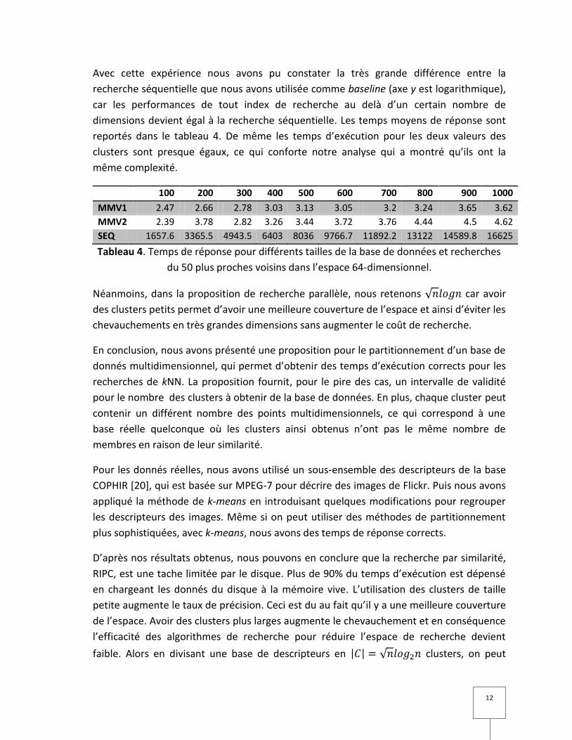
Nous avons mesuré les temps d’exécution des requêtes pour trouver les 50 plus proches

voisins dans un espace à 64 dimensions. Pour ce cas, les donnés utilisées sont appelées

MMV1 et MMV2 qui correspondent au nombre des clusters et

respectivement, pour un ensemble n des données indiqué par les nombres de l’axe x

multiplié par 100 000, ce qui correspond de 100 000 à 1 million.

12

Avec cette expérience nous avons pu constater la très grande différence entre la

recherche séquentielle que nous avons utilisée comme baseline (axe y est logarithmique),

car les performances de tout index de recherche au delà d’un certain nombre de

dimensions devient égal à la recherche séquentielle. Les temps moyens de réponse sont

reportés dans le tableau 4. De même les temps d’exécution pour les deux valeurs des

clusters sont presque égaux, ce qui conforte notre analyse qui a montré qu’ils ont la

même complexité.

100 200 300 400 500 600 700 800 900 1000

MMV1 2.47 2.66 2.78 3.03 3.13 3.05 3.2 3.24 3.65 3.62

MMV2 2.39 3.78 2.82 3.26 3.44 3.72 3.76 4.44 4.5 4.62

SEQ 1657.6 3365.5 4943.5 6403 8036 9766.7 11892.2 13122 14589.8 16625

Tableau 4. Temps de réponse pour différents tailles de la base de données et recherches

du 50 plus proches voisins dans l’espace 64-dimensionnel.

Néanmoins, dans la proposition de recherche parallèle, nous retenons car avoir

des clusters petits permet d’avoir une meilleure couverture de l’espace et ainsi d’éviter les

chevauchements en très grandes dimensions sans augmenter le coût de recherche.

En conclusion, nous avons présenté une proposition pour le partitionnement d’un base de

donnés multidimensionnel, qui permet d’obtenir des temps d’exécution corrects pour les

recherches de kNN. La proposition fournit, pour le pire des cas, un intervalle de validité

pour le nombre des clusters à obtenir de la base de données. En plus, chaque cluster peut

contenir un différent nombre des points multidimensionnels, ce qui correspond à une

base réelle quelconque où les clusters ainsi obtenus n’ont pas le même nombre de

membres en raison de leur similarité.

Pour les donnés réelles, nous avons utilisé un sous-ensemble des descripteurs de la base

COPHIR [20], qui est basée sur MPEG-7 pour décrire des images de Flickr. Puis nous avons

appliqué la méthode de k-means en introduisant quelques modifications pour regrouper

les descripteurs des images. Même si on peut utiliser des méthodes de partitionnement

plus sophistiquées, avec k-means, nous avons des temps de réponse corrects.

D’après nos résultats obtenus, nous pouvons en conclure que la recherche par similarité,

RIPC, est une tache limitée par le disque. Plus de 90% du temps d’exécution est dépensé

en chargeant les donnés du disque à la mémoire vive. L’utilisation des clusters de taille

petite augmente le taux de précision. Ceci est du au fait qu’il y a une meilleure couverture

de l’espace. Avoir des clusters plus larges augmente le chevauchement et en conséquence

l’efficacité des algorithmes de recherche pour réduire l’espace de recherche devient

faible. Alors en divisant une base de descripteurs en clusters, on peut

13

espérer que l’algorithme de recherche soit plus performant. La stratégie de recherche SS2

proposée, permet d’avoir les meilleurs temps de réponse et la meilleure précision.

3. TRAITEMENT PARALLÈLE DES REQUÊTES

Dans l’article [64] il a été démontré la limite des bases de données centralisées pour la

recherche efficace des images. Dans cette section nous profitons des résultats de la

section antérieure quand au nombre optimal des clusters à obtenir à partir des

descripteurs d’images et l’utilisons en conjonction d’une machine parallèle SN de type

grappe de PCs pour améliorer les temps de réponse. De même nous proposons le nombre

optimal des nœuds en fonction de la taille de la base d’images pour achever une telle

amélioration, tout en maximisant l’utilisation des ressources.

A notre connaissance, il s’agit de la première solution au problème des performances pour

le traitement des requêtes kNN avec une machine parallèle SN, qui en même temps

maximise l’utilisation des nœuds de calcul pour une taille donnée de la base.

3.1 L’Allocation des données

Ici nous présentons notre proposition pour partitionner et placer les données sur la

machine parallèle, ce procédure est appelé data allocation ou dégroupement.

La première étape, le partitionnement, est réalisée en appliquant une méthode

quelconque sur la base des descripteurs d’images comme proposé dans la section 3.

La deuxième étape consiste à placer les partitions ainsi obtenues sur la machine de tel

manière, que la charge de travail pour résoudre une requête, soit également répartie

entre les nœuds et en même temps les ressources soient correctement exploitées. De

manière intuitive, on peut supposer que les clusters plus similaires doivent être placés sur

des nœuds différents pour ainsi maximiser le parallélisme. Cette observation basique va

motiver notre approche pour le placement.

Pour cela, nous proposons le théorème suivant

Théorème 1. Supposons une machine parallèle SN d’au moins nœuds, alors la

complexité d’une requête est en .

Démonstration. Voir la démonstration détaillée dans le chapitre 4 de la thèse. Cette

démonstration exploite le Lemme 1 de la section 3, en supposant une distribution plus ou

moins équilibrée des clusters.■

14

Notons que le temps d’exécution logarithmique est possible dans un environnement

parallèle. Effectivement, du fait que l’algorithme le plus simple est une recherche

séquentielle suivi d’un tri général, alors le meilleur temps de réponse est en .

Néanmoins, le nombre de processeurs nécessaire est en et avec une optimisation

standard en ; dans les deux cas le nombre de processeurs n’est pas réel, car

pour une base de taille 107, il faudrait avoir plus de 400,000 processeurs! Ceci dit, si l’on

considère des cœurs dans des processeurs multi-cœurs, ceci deviendra bientôt réaliste.

Nous pouvons dire que, en utilisant regroupement, cette limite n’est pas si large.

Néanmoins, il y a toujours un trade-off entre le temps réponse et l’espace de stockage, ou

bien, entre le temps de réponse et le nombre de processeurs. Donc, il faut quand même

processeurs pour avoir la possibilité d’atteindre une complexité logarithmique,

c'est-à-dire, plus de 3,000 processeurs pour notre base de 107 objets. De plus, les clusters

deviennent extrêmement petits, plus précisément logarithmiques, sinon la recherche

séquentielle dans un cluster plus large dominerait le temps d’exécution. Dans notre base

de 107 objets, cela signifie que chaque cluster contient moins de 23 objets…

En résumé, ce théorème fourni une réponse théorique positive et alternative aux

méthodes d’indexation actuelles. Cependant, il ne faut pas exclure que l’indexation et une

amélioration algorithmique peuvent être combinées avec le regroupement et le

parallélisme que nous présentons ici.

3.2 Validation Expérimentale

Pour valider l'efficacité de notre proposition, nous avons développé une plate-forme

expérimentale. Elle est développée en Java 1.5 courant sur une machine parallèle SN avec

des nœuds Intel Xeon IA32 2.4GHz avec 2GB de mémoire centrale chacun. Le nombre de

nœuds dépend de la taille de la base de données. Dans cette section, nous décrivons les

ensembles de données utilisés, le processus de recherche des k plus proches voisins et les

résultats d'exécution obtenus.

3.2.1 Traitement des requêtes

Nous décrivons maintenant notre algorithme simple mais efficace pour permettre de

traiter rapidement les requêtes kNN [79] en parallèle. Nous soulignons que le processus

décrit, suit les paramètres donnés dans la section précédente et il est basé sur disque:

toutes les donnés sont stockées en mémoire secondaire.

Étape 1, Distribution de données. L'algorithme de placement prend en considération la

proximité entre les clusters pour distribuer les plus proches sur des nœuds différents.

Cependant, comme nous l’avons montré, c'est une différence incertaine : investir pour

15

atteindre un gain minimal au coût d'un certain (peut-être) processus cher. Par conséquent

dans ces expériences, les clusters sont distribués sur les nœuds de log2n d'une manière

circulaire, Round-robin. Par conséquent, tous les nœuds ont presque le même nombre de

clusters (qui ont approximativement le même nombre de points).

Étape 2, Sélection des clusters. Pour trouver l'ensemble d'objets de kNN pour une requête

q, un nombre suffisant de clusters doit être choisi afin de s'assurer de renvoyer les k

meilleurs d-points. Premièrement, une recherche séquentielle sur disque est exécutée

pour comparer q à tous les centroïdes en utilisant la distance euclidienne et employer les

rayons afin de trouver les trier de plus proche au plus éloigné. Les premiers log2n sont

considérés. Pour chaque cluster correspondant au centroïde choisi, nous savons le nœud

sur lequel il a été placé pendant l'étape 1.

Avec cette simple heuristique, nous visons à trouver tous les kNN qui sont équivalents à

faire une recherche séquentielle. En effet, dans plusieurs travaux sur l'analyse de

traitement des requêtes de kNN [14, 58] il a été proposé un seuil qui garantit la

récupération de tous ou un pourcentage élevé du NN. Ici, la prise des premiers log2n

clusters rangés est un seuil assez grand pour obtenir la pleine précision.

Étape 3, Parcours des clusters. Une fois connu le nœud pour chaque cluster d'intérêt, une

recherche parallèle est exécutée sur eux pour obtenir jusqu'aux k objets. Sur chaque

nœud, le balayage local des clusters choisi a lieu sous forme d’une recherche séquentielle

et de l’utilisation d'une file à priorité afin de garder les meilleures réponses de k. Par

conséquent, chaque nœud renvoie un ensemble d'éléments triés au nœud principal.

Étape 4, Fusion des résultats. Le nœud maître fusionne les différents résultats arrivant des

nœuds, et obtient la liste des k meilleures réponses globales, et finalement, la renvoie à

l'utilisateur ou à l'application.

3.2.2. Évaluation des performances

Dans cette section nous validons le théorème 1 en utilisant des donnés générées par

MMV et réparties en clusters, ce qui correspond à 20 000 et 73534 clusters

pour 1 million et 10 million respectivement, réparties en log2n nœuds, c'est-à-dire, en 20

et 23.

Nous avons traité 1000 requêtes kNN pour les ensembles de données décrites. On a

mesuré le temps moyen de réponse pour des requêtes traitées sur disque, le nombre de

calcul de distances et les entrées sorties. Les valeurs de k sont 50, 100. Nos résultats

montrent que le comportement du temps de réponse est sous-linéaire.

16

D’autres résultats qui montrent une variation du nombre de clusters dans l’intervalle de

validité sont omis dans ce résumé. Même si le temps a tendance à augmenter avec la

dimensionnalité (logiquement, puisqu'il grandit avec la taille des descripteurs), cette

augmentation n'est pas exponentielle, c'est-à-dire qu'il n'y a pas de problème rédhibitoire

de la dimensionnalité. Ceci est dû à la sélection réduite de l'espace de recherche, même si

on fait une recherche séquentielle pour faire une sélection des clusters pertinents en

cherchant parmi les centroïdes. De plus, il n y a pas besoin de faire une recherche à

l'intérieur des clusters sélectionnés, il suffit de les rapporter pour l'étape finale de fusion

et de tri.

Ces expériences ont été réalisées en utilisant un placement de type round robin que nous

avons démontré avoir une performance acceptable par comparaison à des techniques de

placement plus sophistiquées. Pour des données de 500 dimensions, il y a en moyenne 16

nœuds activés en parallèle et le temps de réponse est de 0.3 secondes.

4. CONCLUSION

Dans cette section finale, nous résumons les contributions de cette thèse, qui ont fait

l’objet de trois publications dans des conférences internationales. De même, nous

discutons quelques travaux futurs et prometteurs pour aller plus loin dans la RIPC.

Dans un premier temps, nous avons présenté une proposition pour le partitionnement de

la base de données en un nombre prédéterminé de clusters [61]. Cette proposition

permet d'améliorer les temps de réponse de la recherche par le contenu des k plus

proches voisins en bases d'images.

La proposition consiste en un intervalle de valeurs pour le nombre de clusters, et dans

cette thèse, nous avons présenté dans un premier temps une validation analytique puis

expérimentale pour le pire des cas, c'est-à-dire pour une sélection séquentielle des

centroïdes afin d'obtenir les clusters pertinents qui sont stockés sur disque, pour des

ensembles de descripteurs de différentes tailles et dimensionnalités. Ensuite, nous avons

proposé un algorithme de recherche qui fait un parcours des clusters d’intérêt de tel

manière qu’il es possible de déterminer plus rapidement les kNN et nous avons démontré

qu’il est possible d’obtenir des performances sous linéaires.

Ensuite nous avons proposé une architecture parallèle avec le nombre optimal des nœuds

de calcul en fonction de la taille de la base d’images à traiter. La méthode de placement

plus simple round-robin est plus performante que des autres plus sophistiqués [62]. Cette

méthode de declustering est exploitée pour le traitement en parallèle des requêtes kNN

avec un taux de précision égal à celle des recherches séquentielles mais avec un cout très

17

minimal. Cette méthode passe à l’échelle pour gérer des bases d’images volumineuses

[63].

4.1 Travaux futurs

Le support multiutilisateur. Ce sujet et en relation avec la mise en ouvre d’un vrai système,

lequel doit garantir un niveau de service aux utilisateurs, notamment éviter les retards

dans l’attention des requêtes. Le planning de la capacité des serveurs est une activité pour

déterminer la quantité maximale de charge que le system est capable de traiter

correctement. Pour cela, le système doit être soumis à des conditions sévères de

fonctionnement et analyser le comportement.

Un autre axe de recherche consiste à exploiter les architectures P2P, qui permettent

d’exploiter une puissance de calcul que peut passer à l’échelle avec une forte dynamicité.

Un autre axe de recherche est travailler sur les architectures multi-cœur et les disques

d’état solide (SSD). Les premiers même si permettent d’augmenter la puissance de calcul

d’une seule machine l’implémentation des algorithmes introduise des problèmes lies à

l’exécution simultanée sur les cœurs. Les disques SSD peuvent améliorer le coût des

transferts des données et réduire le temps de recherche.

18

19

1 INTRODUCTION

The work presented in this thesis is related to the efficiency of queries in image databases.

Firstly, we introduce the motivation for this work, ranging from the need to manage

constantly increasing masses of information, especially visual ones, to the peculiarities

and specific challenges that image data poses. Then, the problem at hand is stated more

precisely and some state-of-the art solutions rapidly surveyed in order to contrast or align

them with our approach. Next, the benefits of our proposal are roughly drawn; it consists

of two steps: a theoretical analysis leading to asymptotic guarantees, then experiments

that confirm the previous study both on realistic and actual data sets. This chapter ends

up with an outline of the following chapters.

1.1 MOTIVATION

Recently, we have witnessed the impact of rapid technological developments in

information technologies. Image data, as well as other media, is generated at an explosive

rate. Therefore, management of large image data sets has become a challenge. Let us

introduce some motivating examples and the general technological approaches that

dominate in order to address this problem.

Around the world, users demand for efficient searching of image data from voluminous

databases.

Currently, web-scale image searching proposals, such as Yahoo and Google, among others,

rely on the surrounding text found in the web pages to manage the images themselves.

Hence, users query the database using text, with the hope that this text approximates the

description of the required images.

The drawbacks of this approach are that the surrounding text does not necessarily have to

do neither with the image contents nor its semantics. Also, once an image is retrieved, it is

separated from its context and all the information used for its indexing is lost. Sometimes

most of the results are useless.

Furthermore, not all existing images are hosted inside web pages. Flickr is the most

notable example with a database of millions of images. However, these images are also

searched by typing text. Retrieval makes use of user’s tags and annotations, evidently

reflecting the owner’s emotions and interests.

20

An additional limiting factor is their inability to search for images based on the visual

properties, useful when it is hard to express in words the requirements to solve queries. In

such case, queries can be formulated with the help of another image, some examples of

this situation occurs when answering the following questions:

Where is this architectural material/detail being used?

Where can I buy an electronic appliance like this?

Do we have a medical treatment for a skin disease like this?

This kind of queries, which aim at object detection or image matching, requires searching

for similar images based on their contents, e.g., colors, textures and shapes.

Generally speaking, Content-Based Image Retrieval (CBIR) relies on image processing

techniques and uses a Query-by-Example paradigm to search for images. Proposals in CBIR

transform the query and the images in the database into a high-dimensional space by

extracting low-level feature descriptors from them.

This high-dimensional abstract representation for the database of images altogether with

a distance function, allows executing the searching process in a metric space. A metric

space is defined by a set of points and a distance function. The fundamental concept in

metric spaces is that similarity between points is quantified in terms of a distance. CBIR is

implemented by the similarity search paradigm: retrieval of images by determining

feature similarity. An exact match, as occurs in relational databases does not have sense.

The aim of similarity searches is to found a set of the most similar images in a database to

a given query image. This set can be obtained by a range approach or a best match

approach.

In the range approach, a threshold value is used to indicate the accepted level of similarity

(or dissimilarity) of any image in the database from the query image, all images qualifying

within this range are presented to the user. The similarity between the query and each

image in the database is estimated by computing their distance, e.g., the Euclidean

distance.

For the best match approach, the winning set is usually restricted to the k most similar

images, i.e., the k-Nearest Neighbors (kNN), which turns out to be, generally speaking, the

most useful kind of query in CBIR. Conceptually, kNN query processing requires computing

the distance from every feature descriptor in the database to the feature descriptor of the

example image in order to determine the k most similar. Obviously, performing a

sequential search can be very inefficient for large databases.

21

1.2 STATEMENT OF THE PROBLEM

In this research, we address the performance problem when searching on large high-

dimensional databases. Effectively, image retrieval poses a computational challenge due

to the high-dimensional abstract representation used to describe, store and retrieve the

images. Let us describe some directions that have been investigated to address this issue,

namely indexing techniques, clustering algorithms, parallel architectures.

The most computationally expensive operations of this searching process are mainly the

distance evaluations and the disk I/O’s (for large databases which don’t fit in main

memory), which bound the overall processing time. Assuming a general metric space,

several research directions have been proposed aiming to efficiently perform CBIR.

In order to avoid as much as possible the traversal of the database and hence reducing the

processing time, indexing methods have been developed [17][46]. However, their

efficiency is not appropriate above a number of dimensions of the high-dimensional data

representation and is even worse when facing large databases. They are affected by the

so-called curse of dimensionality and their performance deteriorates drastically [53][88].

Furthermore the size of the database influences their efficiency because they do not fit

into main memory and consequently disk accesses largely increment the retrieval costs or

their construction increments the storage costs.

Alternatively, clustering methods [31], which main goal is to partition the database into

groups of similar objects appear to be useful provided an adequate searching algorithm.

When clustering is used, the searching process can rapidly discard irrelevant clusters to

then concentrate the search in a small subset to retrieve the desired images. Though a

wealth of research has been done based on this idea, there still remain open issues such

as determining the optimal number of clusters to obtain from the database and the

efficient handling of large databases. The importance of these issues is that even if the

pruning process can reject uninteresting clusters, the search within the remaining clusters

is still a time-consuming task. This is exacerbated when the database becomes larger,

which not only strains the I/O subsystem but demands more storage space and more

computing power.

The use of parallel databases seems to be a natural option within this context. However,

an affordable parallel solution should be as simple as possible. Contrary to big

supercomputers, we believe that servers constructed with many low-cost processing units

with their own attached disks offers the required aggregated computing power and

flexibility. This provides the I/O parallelism, the sharing of the processing load among the

available processors and the flexibility to scale-up in order to cope with larger databases.

These are some of the advantages of the shared-nothing architecture, its excellent

22

cost/performance ratio and scalability. Thoughts in this direction are shared by other

authors [44]. Also, Google [7] uses this same kind of idea, to serve millions of users and to

store petabytes of information. However, to efficiently take advantage of such

architecture, some issues must be solved.

Thus, let us assume a shared-nothing architecture. Firstly the layout of the data must be

carefully planned because it has a direct effect in performance, scalability and load-

balancing. For these reasons, it is important to retrieve the same amount of data from

each node. This goal has been defined as declustering optimality (DO) [1], which aim is to

distribute the data in a way that the retrieval load is uniformly distributed among the

nodes. However this is a hard to achieve goal; it has been proved to be an NP-complete

problem; no optimal declustering scheme is possible in general [1][57].

Secondly, in order to maximize resource utilization and to avoid unnecessary system

overhead, the appropriate number of nodes for processing a database of a given size must

be determined, where each node comprises its own processor, main memory and

attached disk.

1.3 CONTRIBUTIONS

The background of our research is the work done by Prof. Martinez and Prof. Valduriez

[64]. Their results show the limits of a centralized database due to the computational

complexity of the retrieval process. Motivated by this, we analyze the algorithmic aspects

of the searching problem when it uses a partitioning method, such as clustering, on the

database. In this research, we propose a solution to the problem of content-based

retrieval performance in large databases of images by efficiently exploiting the parallelism

provided by a parallel shared nothing database system. We accomplish this goal in two

steps:

Firstly, we study the complexity of a general search when using a method to partition

the database. We derived an upper bound of this problem and proposed a range of

values to the number of partitions or clusters to impose on the database in order to

yield efficient CBIR. This upper bound is used by an improved searching algorithm that

can perform several times above the sequential scan with the same precision.

Secondly, as we are mainly interested in large image databases, we have developed an

analytical model useful to determine the optimal number of nodes to efficiently

process similarity queries in a parallel database. We develop a declustering method

based on the results of the first step combined with several placement strategies and

two query processing algorithms that make use of such architecture to efficiently

23

process nearest neighbor queries, it means, maximizing resource utilization with high

results quality.

Experiments with realistic databases test the performance improvement over sequential

search which is the baseline to indexing algorithms. In contrast with previously proposed

approaches, the optimal number of nodes is not an empirically defined parameter. Our

work sets the theoretical guarantees for the achievable performance by using the

proposed number of processing nodes for a given database in combination with different

searching strategies. In this way, by using a fraction of the hardware used by previous

approaches we may provide enough computing power to efficiently search large-scale

multidimensional databases. This may be useful to solve several issues: performance,

storage capabilities, capacity planning and several costs including energy saving [8].

Additionally, even if we have oriented our presentation to the problem of image retrieval,

as our proposal is based in the similarity search paradigm in a metric space, it is not only

useful within the context of CBIR, but also has applications in general multimedia retrieval,

biology and finance to name a few. Thus our results may be applied successfully to other

domains.

1.4 OVERVIEW

This thesis is divided into two parts: the first one provides the background and review of

the related literature, whilst the second part is devoted to the development of our

proposals together with their validation tests and their analysis. Part one consists of

chapters 2, whereas part two consist of chapters 3 and 4.

In Chapter 2, we provide enough background material necessary to ensure a self-

contained exposition of our study and to set the context of our contributions. We discuss

some concepts of high-dimensional spaces from the point of view of query processing, the

same goes for metric spaces.

In the same chapter, then we present some state-of-the-art CBIR proposals based on

indexing and/or clustering for centralized settings. Then we introduce parallel

architectures, followed by a discussion of related literature on the declustering problem

and proposals for parallel similarity search.

In Chapter 3, we analyze the complexity of searching in a clustered database and derive

the number of clusters. This range of values is evaluated experimentally, and is an

intermediate result towards our declustering method.

24

In Chapter 4, we propose a declustering method, which is analyzed for several placement

options and data sets. This proposal accounts for improving CBIR performance in parallel

settings.

Finally, in Chapter 5, we state some conclusions about our results and outline future

research directions.

25

2 BACKGROUND ON CONTENT-BASED

RETRIEVAL

In this chapter, we first introduce the reader to the need for content-based retrieval. We

then provide the general architecture common to the systems that try to achieve this goal.

We discuss in some details the elements that make this task so difficult, mainly the high-

dimensionality of the metadata extracted from the images and major differences with

respect to traditional database queries.

This chapter is also important because, herein, we discuss the groundwork concepts that

support the reasons that make us consider and opt for a given approach in the rest of the

chapters.

Retrieval of images, and multimedia data in general, could rely to some extent in text

based approaches. However, one limitation of text-based models is the difficulty to

describe in terms of a human language the contents of a data object, as it is sometimes

subjective and influenced by appreciation, cultural issues and other aspects. One solution

has been to develop a kind of thesaurus to limit and standardize the words that can be

used in the description. However there is another problem facing text based systems

which is that the manual annotation results impractical in terms of time and effort for

huge databases. Automatic annotation [36][87][59], in some specific domains, can come

up with acceptable results in terms of description accuracy. Some commercial systems

such as Google use HTML tags to identify multimedia objects, especially images, then with

the aid of the surrounding text indexes them.

Instead of this text-based management model research efforts are oriented towards visual

storage and retrieval. This is called Content-Based Image Retrieval (CBIR).

Visual search, an application case of CBIR, based on the whole image or regions can ease

the searching for hardware, tools, fabric, furnishing and shopping in general. The case of

like.com, a vendor of clothing in general, is perhaps a good example of visual shopping,

one real application of CBIR useful in several domains.

Visually shopping in www.like.com, allows searching based on regions of picture of

objects, using color, shape or both, through categories of brands, colors and styles.

Although there is no information about the architecture, it is somewhat easy to

understand its internals by playing with it. It has a relatively small-sized database, thus

images can be manually or semi-automatically classified at population-time, with the aid

26

of the categories defined by tags. This class-based structure is used to guide the search to

specific categories, in this way the search space is narrowed down. Additionally, a user can

upload a photo to find similar products, but the user steers the search in several ways: by

selecting a product category and a style of the product, by selecting a region of interest,

by selecting characteristic of interest (color, pattern, shape), brand and optionally

describing words and giving an email…This makes us presume that the search is

completed or refined manually, it is not an on-line matching process. Whether it is CBIR or

not it is far beyond satisfying real visual searching needs, since an advisory message is

displayed at the end of the search: “Searching hundreds of thousands of images takes

time, we’ll email you when your visual search has completed (usually within one day).”

This important drawback enforces the need to devise efficient image searching

techniques.

What is also important to note from this case is that the different techniques used for

image retrieval, rather than being exclusive, should be complementary. Recently Google

Lab’s Similar Images project, added the option to refine and search by dominant color

additionally to the traditional keyword search.

The CBIR paradigm also challenges current Relational Data Base Management Systems

(RDBMS), which traditionally deal with alphanumeric data types. For each item or record

in a RDBMS one or more of the columns are used as searching keys, while in multimedia

databases it is the whole object that is used to find the relevant objects for a query. In an

RDBMS queries look for records satisfying a criterion and they simply match or do not

match it, i.e., an exact match approach is performed, whereas in CBIR this concept does

not have too much sense. Indeed, CBIR aims for searching the most similar, not identical,

objects in a database for a given query.

The insufficiency of the traditional RDBMS approach to provide efficient multimedia data

management has lead to several proposals:

Multimedia Flat File based,

Multimedia DBMS extensions,

Specialized Multimedia DBMS.

Flat File Systems are simply those based on storing directly the images in the file system of

the hosting operating system. Beyond Flat File Systems are DBMS, which provide support

for concurrent user access, database integrity, fault tolerance and security among other

desirable features in a production or commercial system, such as the possibility to be

integrated with other company’s systems and business processes. However, commercial

or generic DBMS come with a plethora of unnecessary features that burden the retrieval

27

process. Furthermore, the storage model for large multimedia objects is not always useful,

hence the option to store outside as a BLOB (Binary Large OBject) a multimedia object.

Thus, efficient multimedia management involves more than storage and user’s handling

services.

Conceptually, for content-based retrieval, the management of image data can be divided

into three major topics:

representation,

organization,

retrieval.

Representation is related with the techniques to abstract the visual contents to obtain a

high-dimensional signature that can contain enough information of each data object.

Organization refers to the way this abstraction is stored to enable efficient query

processing. Retrieval studies the searching process, i.e., the mechanisms used in

conjunction with indexing and clustering methods to speed up the processing of queries.

The last two topics are the research subject of this thesis.

From a pragmatic point of view, the management of image data can be seen as a set of

software components interacting to make possible the image retrieval process. This is

depicted in Figure 2.1. This process can be divided into two main parts: an off-line process

that is carried out before the system is put in service; and an on-line process that starts

when the system is ready to serve users’ requests.

Figure 2.1 Image Data Management

The database is the set of data objects, i.e., the images, which after processing by the

feature extraction component produces a set of high-dimensional data points. These data

points, or points for short, are processed by the feature transformation component to

normalize or to make some pre-processing of the points before they can be indexed by

28

the feature organization component. This step concludes the off-line process. The system

is ready to be on-line and accept queries in the form of an image which is also processed

to extract its feature descriptors, by the same methods used to process the database. This

descriptor is sent to the similarity search component which performs a somewhat

intelligent traversal of the indexed features, to finally retrieve and return back the results

of the most similar images to the user.

Let us observe that the abstracted term for an image description used henceforth in this

thesis, is feature vector, data point or simply point, which refer to the visual feature

descriptors as used in the high-dimensional data model explained below.

The remainder of the chapter presents some elementary concepts for understanding CBIR

internals and problems. The discussion follows the retrieval process depicted in Figure 2.1.

We first describe the nature, type and properties of the feature descriptors. Next, we

define the high-dimensional data model for CBIR, followed by some pre-processing of the

features vectors such as normalization. After that, we introduce the concept of distances

and metric spaces followed by some considerations on the kind of queries. It follows up by

the implications in the design and performance of the different data organization

techniques, both in centralized and parallel settings.

2.1 VISUAL FEATURE DESCRIPTORS

To facilitate the retrieval of images, a suitable computer-friendly representation is

obtained by applying a feature extraction process on the database. The output of this

process, which quantifies some visual properties such as the colors, textures or shapes, is

an abstraction of the visual contents called visual feature descriptor.

This abstraction must represent with fidelity the images; this means it should be

descriptive and discriminative. It must characterize an image in such a way that it is

possible to distinguish if it is different or similar to any other. The retrieval of images

based on their contents relies on these properties.

The descriptors should be robust; this means it should be invariant to image

transformations, i.e., an image which has suffered any operation such as rotation,

translation, scaling, variations in illumination and point of view, must still be identified as

the original one.

The quality of a descriptor is also proportional to its size. Large descriptors entail more

fidelity in the characterization of the contents. However, they require more storage space

and, what is quite important; it takes more time to compute similarity. A compact

representation with high discriminative power is the ideal, however in practice they are

above 64 dimensions. One research direction is to find a good balance between size and

29

quality of descriptors. Another research direction is how to organize and query them,

which is the subject of this thesis.

In order to recognize the features that best describe images, two approaches have been

followed: global and local descriptions. Global descriptions are coarse grain as they

consider the whole image for their analysis. For example a global histogram computes the

scale of gray or the colors using some color space (RGB, HSV) [84].

A histogram descriptor characterizes an image by its color distribution. This descriptor is

the result of counting the number of pixels of each color and each dimension of the

descriptor corresponds to one bin of the color histogram. Two common choices to

represent an image color are: the RGB model (based on the Red, Green, Blue

decomposition) and the HSV model (Hue, Saturation, Value). As the histogram is

computed by counting the number of pixels of each color an image quantized into an 8 x 8

x 8 RGB color space has 512 bins, i.e., a descriptor with 512 dimensions. Similarly,

quantization in the HSV space with respectively 18, 3 and 3 levels, results into 162

dimensional descriptors.

A histogram being a global statistic about the image, different distributions of the same

levels of colors may arise to the same descriptors even if the involved images are not

related at all. Inversely, it is somewhat counter-intuitive that too precise histograms can

defeat the similarity comparison. There are several approaches for this shortcoming: one

is to preprocess the image using color quantization, hence a 224-bin histogram can be

quantized to a 15-bin histogram, with an improvement in recognition accuracy in two

times, from 37% to 78% [78]. This can be considered as a dimensionality reduction

method which is known to improve recognition accuracy [85]. Another way to alleviate

this issue is by splitting the image in regions and computing the color histogram for each

one. This is near the concept used in local descriptors.

Instead of considering the image at large, some regions or points of interest are

determined. The focus of local descriptors is to detect local points of interest from which

to extract the energy used to describe the contents. A local feature is a small region or

point of the image different to all around it. Hence they can be seen as anchors for the

matching process. The drawback with these local descriptors is that, from a single image,

hundreds if not thousands of such called points of interest can be extracted, thus

increasing the dimensionality of the descriptor. On the counterpart, their main advantages

are that: they are robust to occlusions, rotations, scaling, etc, and that they give very

effective results. (Also, they are sometimes easier to compute as they are restricted to

some portion of the image.)

30

Prior to local feature extraction there is a point detection step. A good feature descriptor

represents the meaningful aspects of an image. The definition of meaningful or interesting

aspects is domain dependent and requires having knowledge of the goal application to get

the best. Consider a human picture, for someone it would be interesting to recognize

faces, for someone else to recognize skin texture to possibly determine epidermal health,

someone else would be interested only in general features such as color, lastly someone

would be interested in the conveyed emotion. We have a large scale of needs, some easy

to attain with the current technology, some not yet reached.

A robust local descriptor is the Scale Invariant Feature Transformation, SIFT [60], which is

acceptable in face of variants in illumination, rotation and scaling, it is the best according

to several criteria [65]. However some recent proposal improves on some of its

weaknesses. In fact, SIFT is only invariant with respect zoom and rotation, thus Affine SIFT

[68] adds capabilities to handle translation of the angles defining the camera axis

orientation, useful also in video retrieval. Speeded-Up Robust Features, SURF[9] is also a

recent robust interest-point detector which also provides repeatability, meaning it finds

the same points of interest for an image independently of the rotation.

Feature extraction can be automatic or semi-automatic. Automatic techniques with no

human intervention allow working in a general domain. Semi-automatic feature extraction

is required when there are complex contents meaningful only to humans or hard to

capture by a computer system. For example, in a picture, by using techniques of pattern

recognition a system can identify a car but it can hardly determine if it is a sports car. In

face recognition systems, emotions are also hard to recognize. Sometimes domain

dependent intelligent techniques, based on machine learning, are developed but they are

constrained to identify only those objects for which they have been trained. Indeed, for

general purposes, it is impossible to extract all the features needed or desirable.

The complicated nature of the visual information contained in an image and the variety of

techniques to describe the contents, has motivated the creation of the MPEG-7 standard.

It defines a set of low level descriptors, e.g., color, texture and shape descriptors, as well

as high-level metadata, e.g., copyright, author, semanticals: user’s tags, etc.

In our experiments, we test our system with a database processed to obtain 64-

dimensional Scalable Color and Color Structure descriptors. The Scalable Color descriptor

is computed with the 1-D Haar Transform in the HSV space. The Color Structure descriptor

is also a histogram with spatial color distribution [20].

Finally, to the desired properties of a feature descriptor: descriptive and discriminative

power, and low dimensionality, we add a third one: fast processing. Because feature

31

extraction is a pre-processing step to enable CBIR and also to process the query.

Therefore, near real time is required not only for pre-processing the database but also to

avoid delaying the processing of queries.

2.2 HIGH-DIMENSIONAL DATA MODEL

As pointed out, in this thesis we are going to work with a high-dimensional representation

of the images. This representation corresponds to the description of the visual features

obtained by a process of image recognition and pattern analysis techniques. The set of

feature descriptors obtained allow finding images that are visually similar to a given one.

We describe the high-dimensional data model used to represent the image objects in the

database and the query object, and how it is used for searching.

Let us have a given collection, or database, of size n of image objects. In order to enable

retrieval, they are processed and from each one it is obtained a vector m of features in a

d-dimensional space. The choice of both, the process for generating the set M of feature

vectors m and the dimensionality d, are domain dependent. The idea is that the obtained

feature vector describe as much as possible the object’s contents and d varies commonly

from 10 to 256 [40], and in some cases up to 500 and 1000.

After this process, the database of actual images is transformed into a set:

M={m1, m2, …mn}

of high-dimensional feature vectors, or points, where each one is:

mi={m1, m2,…md}.

Within this data model, after obtaining M, an image example is given as a query of what it

is desired to be retrieved. The content-based retrieval takes place in the metric space:

where L is a distance function:

and:

with , the real valued d-dimensional data space. In this metric space, the only way to

perform retrieval is by computing the distance between objects.

32

Generally, the distance is one in the Minkowski family such as L2 or Euclidean distance. So,

the provided query example is also transformed into an instance of , obtaining:

q={q1,q2…qd}.

To determine whether any two points q and m are similar or not, the proximity between

them, e.g., using the L2 distance, is evaluated, the smaller the proximity the more similar

the objects are. This is going to be further analyzed in the next section.

2.3 DISTANCES

In the general architecture, when descriptors have been extracted from the objects in the

database and from the query in the form of image examples, similarities have to be

computed in order to retrieve the closest objects. Let us introduce the necessary

background on this subject.

Proximity, a general term to indicate similarity, is generally quantified by means of a

distance function.

A distance L in a metric space is a two argument function:

from a couple of objects to a positive real value, which has the following properties:

1. Symmetry. The distance from point x to y is the same as the distance from y to x.

2. Positivity. This property encompasses reflexivity and non-negativity, i.e., distance

between identical objects is zero and for any two different objects there must be a

positive distance.

3. Triangle inequality. The distance between two points x and y must be shorter or

equal to the sum of their distances to a third point z. If point z is on the line

between x and y, equality holds.

If a distance satisfies 1 and 2 it is called a semi-metric. A distance which complies with all

three properties is called a metric.

33

From definition d(x,x)=0, thus, a zero distance means the two compared objects are

exactly the same. If the distance is normalized, then one means they are far away from

each other, i.e., the smaller the distance between objects means the more similar they

are. Hence similarity can be expressed as s(x,y)=1-d(x,y). A similarity of 1 means

completely similar while 0 means completely different.

Let us now introduce some commonly used distances.

2.3.1.1 Euclidean

Also known as L2, the Euclidean distance is defined as:

It is influenced by the biggest components of the involved points. Hence it is necessary to

do some data transformation that we shall introduce below.

2.3.1.2 Manhattan

Also known as city-block or L1, the Manhattan distance is evaluated in movements

parallels to the x and y axes. It slightly emphasizes the outliers of the data set, i.e., points

located far from other points/clusters will appear effectively further away.

It is defined as:

2.3.1.3 Chebychev

The Chebychev distance, also known as the chessboard distance or L∞ returns the largest

difference between any pair of corresponding coordinates. It is not easy to identify

outliers as it favors only at one dimension.

Its definition is:

2.4 SIMILARITY QUERIES

Distances by themselves, let them be the ones introduce above or more complex ones,

are insufficient. They only provide the basic ground of allowing us to compare two objects.

Similarity queries in a database use quite a lot of binary distance computations.

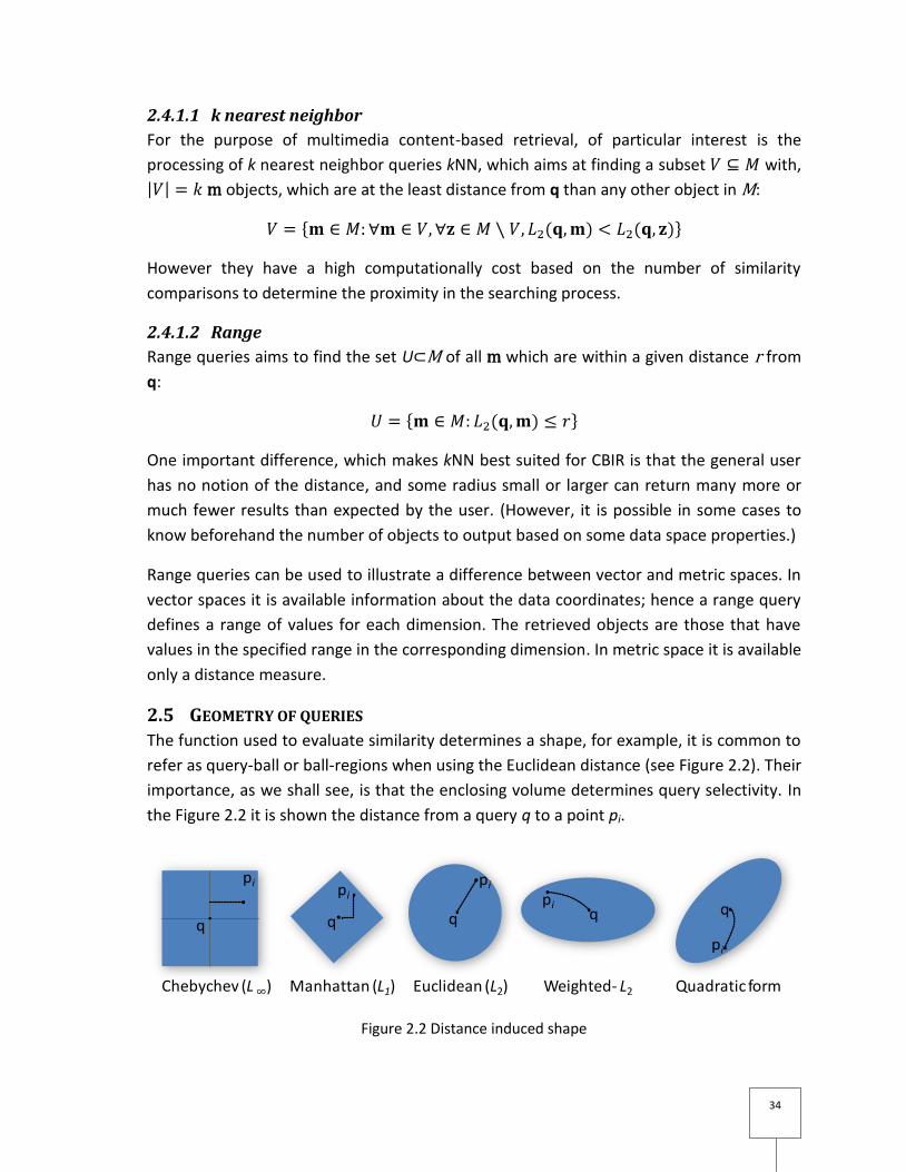
34

2.4.1.1 k nearest neighbor

For the purpose of multimedia content-based retrieval, of particular interest is the

processing of k nearest neighbor queries kNN, which aims at finding a subset with,

m objects, which are at the least distance from q than any other object in M:

However they have a high computationally cost based on the number of similarity

comparisons to determine the proximity in the searching process.

2.4.1.2 Range

Range queries aims to find the set U⊂M of all m which are within a given distance r from

q:

One important difference, which makes kNN best suited for CBIR is that the general user

has no notion of the distance, and some radius small or larger can return many more or

much fewer results than expected by the user. (However, it is possible in some cases to

know beforehand the number of objects to output based on some data space properties.)

Range queries can be used to illustrate a difference between vector and metric spaces. In

vector spaces it is available information about the data coordinates; hence a range query

defines a range of values for each dimension. The retrieved objects are those that have

values in the specified range in the corresponding dimension. In metric space it is available

only a distance measure.

2.5 GEOMETRY OF QUERIES

The function used to evaluate similarity determines a shape, for example, it is common to

refer as query-ball or ball-regions when using the Euclidean distance (see Figure 2.2). Their

importance, as we shall see, is that the enclosing volume determines query selectivity. In

the Figure 2.2 it is shown the distance from a query q to a point pi.

Figure 2.2 Distance induced shape

Euclidean (L2)Manhattan (L1) Weighted- L2 Quadratic formChebychev (L ∞)

q

pi

q q q qpi

pi

pi

pi

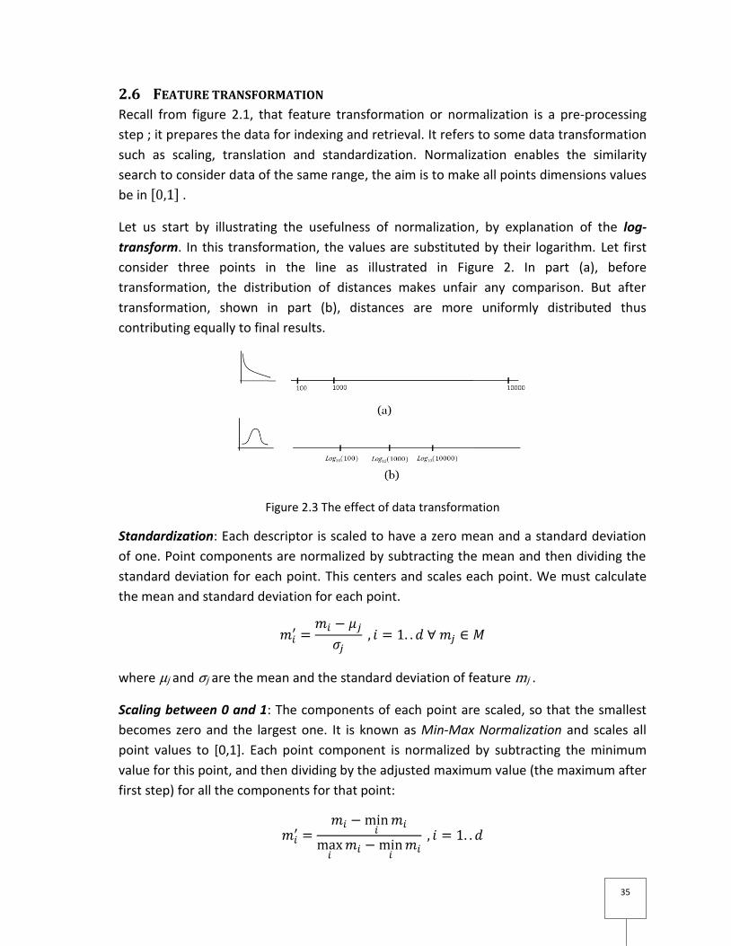
35

2.6 FEATURE TRANSFORMATION

Recall from figure 2.1, that feature transformation or normalization is a pre-processing

step ; it prepares the data for indexing and retrieval. It refers to some data transformation

such as scaling, translation and standardization. Normalization enables the similarity

search to consider data of the same range, the aim is to make all points dimensions values

be in .

Let us start by illustrating the usefulness of normalization, by explanation of the log-

transform. In this transformation, the values are substituted by their logarithm. Let first

consider three points in the line as illustrated in Figure 2. In part (a), before

transformation, the distribution of distances makes unfair any comparison. But after

transformation, shown in part (b), distances are more uniformly distributed thus

contributing equally to final results.

Figure 2.3 The effect of data transformation

Standardization: Each descriptor is scaled to have a zero mean and a standard deviation

of one. Point components are normalized by subtracting the mean and then dividing the

standard deviation for each point. This centers and scales each point. We must calculate

the mean and standard deviation for each point.

where µj and σj are the mean and the standard deviation of feature mj .

Scaling between 0 and 1: The components of each point are scaled, so that the smallest

becomes zero and the largest one. It is known as Min-Max Normalization and scales all

point values to [0,1]. Each point component is normalized by subtracting the minimum

value for this point, and then dividing by the adjusted maximum value (the maximum after

first step) for all the components for that point:

36

where:

then

Of course, this transformation requires at least two distinct points to be possible.

2.7 INTRINSIC DIMENSIONS

In contrast with the dimensions used to represent data objects, hence apparent

dimensions, the intrinsic dimensions of a data set are the real dimensions, i.e., the ones

with which it is possible to embed all the data set objects while preserving their distance.

It can be estimated by:

where μ and σ2 are the mean and variance of the histogram of distances [25].

A data set with high intrinsic dimensions has a concentrated histogram of distances with a

high mean µ and a small variance σ2. It means that the distance between any pair of

objects is very small, hence data is roughly equidistant. This makes this kind of data space

hard to search in as it is required to compare every object to determine relevance [31].

Furthermore, what means relevance when all objects are almost equidistant to any other?

This is a modeling problem that we do not address.

We are going to evaluate our data sets by computing the histogram of distances to

measure their searching complexity and the implications in search performances. It is

desirable also, to determine the intrinsic dimensionality and evaluate again how it

influences retrieval performances.

2.8 IMPROVING PERFORMANCES OF QUERIES

This section contains a review of some of the most recent and relevant methods in CBIR,

from centralized to parallel settings. We first review sequential scan as the basic searching

method, we move then to more refined searching methods: indexing and clustering. We

end up by presenting the parallel approach for CBIR.

Having pre-processed and processed the database, the obtained high-dimensional points

must be structured to enable fast similarity search. Effectively, any of the previously

introduced distances has a computational cost which is proportional to the dimensions d

of the descriptors. With respect to an application, this is probably a constant but it can be

37

quite large. More importantly, it is unthinkable to compare the query image to all the

objects in the database.

2.8.1 Full and approximate searches

The simplest method to answer similarity queries is the sequential search of the whole

database, it is also known as naive or brute force algorithm. The cost is proportional to the

database size and thus is applicable only to small databases. Its importance arises from

the fact that more complex searching structures cannot perform better than it beyond a

certain dimensionality threshold. Thus it can be used as a baseline for both time and

precision performance. Sequential search takes time proportional to the database size

O(n), but zero pre-processing time and zero storage overhead.

Alternatively, a user is sometimes willing to trade-off some processing time for better

results quality, or will exchange storage for an increase in speed, or a combination of

these tradeoffs [89][81].

Approximate search, ε-search, is the choice when it is not possible to get the full results as

returned by a sequential search, but this little loss in precision will be compensated by

blasting processing times. Initial parameters for the ε-search, such as the processing time

or the accepted level of precision, are required as a stop condition for the searching

process, and all qualifying objects within that range of precision will be returned to the

user.

Even for ε-search, faster solutions are required for large databases. However there are

several issues related to the inherent properties of the high-dimensional space, some of

them are discussed in the next section. Among the possibilities to structure a data set are

indexing and clustering methods. An index partitions the data space or the data and

constructs a hierarchy of nested bounding regions or data bounding regions respectively.

On the other hand, clustering methods make groups of data objects based on their

similarity. A cluster contains most similar objects, so the searching process has a criterion

to discard uninteresting clusters with respect to a query, hence only the selected ones are

searched to obtain the result set. The idea with both, indexing and clustering, is to reduce

query execution time by decreasing the search space.

2.8.2 High-dimensional geometry

One main problem is that high-dimensional spaces come with new, often counter-

intuitive, difficulties. The empty space phenomenon, is one of them.

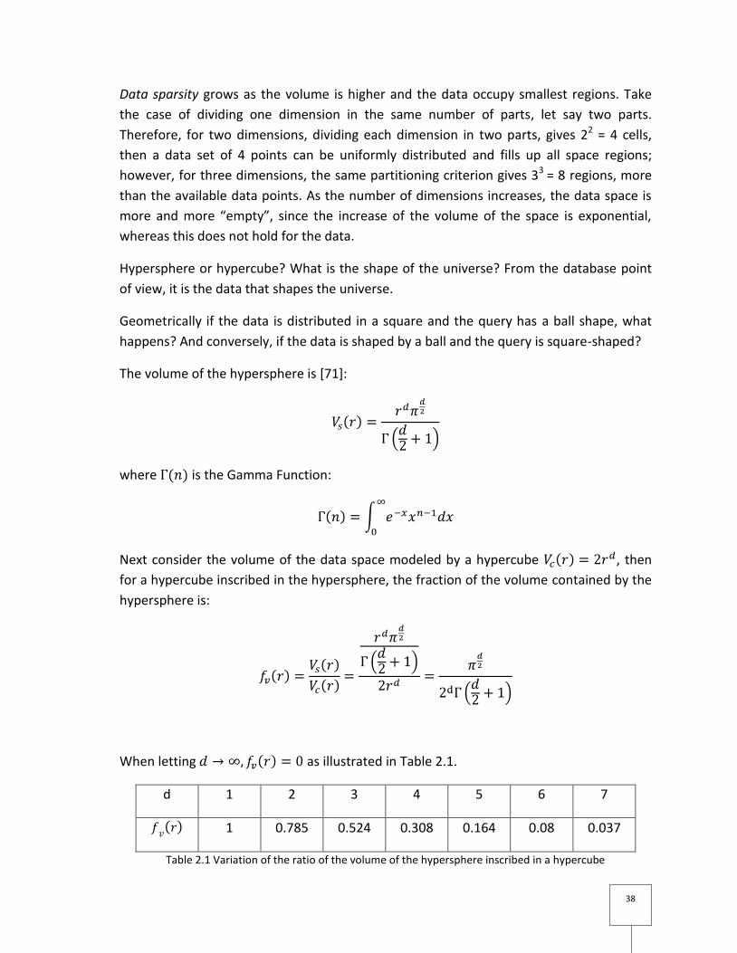
38

Data sparsity grows as the volume is higher and the data occupy smallest regions. Take

the case of dividing one dimension in the same number of parts, let say two parts.

Therefore, for two dimensions, dividing each dimension in two parts, gives 22 = 4 cells,

then a data set of 4 points can be uniformly distributed and fills up all space regions;

however, for three dimensions, the same partitioning criterion gives 33 = 8 regions, more

than the available data points. As the number of dimensions increases, the data space is

more and more “empty”, since the increase of the volume of the space is exponential,

whereas this does not hold for the data.

Hypersphere or hypercube? What is the shape of the universe? From the database point

of view, it is the data that shapes the universe.

Geometrically if the data is distributed in a square and the query has a ball shape, what

happens? And conversely, if the data is shaped by a ball and the query is square-shaped?

The volume of the hypersphere is [71]:

where is the Gamma Function:

Next consider the volume of the data space modeled by a hypercube , then

for a hypercube inscribed in the hypersphere, the fraction of the volume contained by the

hypersphere is:

When letting as illustrated in Table 2.1.

d 1 2 3 4 5 6 7

1 0.785 0.524 0.308 0.164 0.08 0.037

Table 2.1 Variation of the ratio of the volume of the hypersphere inscribed in a hypercube

39

This means that for higher dimensions the space retained by hypersphere and hypercube

inclusion is almost empty and hence all indexing structures relying in this, will eventually

fail. Also, the number of points enclosed in the hypershpere approaches 0 as dimensions

grows.

Another interesting property is that for higher dimensions the volume of the hypersphere

is concentrated near the surface [54], which makes almost equidistant all points and hard

to determine dissimilarity.

Fortunately, and as is theoretically demonstrated in [15] some databases can be still

useful, in the sense that it is possible to distinguish between objects in higher dimensions,

e.g., a database which does not follow a uniform distribution; which is indeed the case for

most real databases. Additionally, working with the intrinsic dimensionality of a data set is

an alternative to these problems.

2.8.3 Indexing

Indexing of the feature vectors helps to speed up the search process. Using a data space

or space partitioning approach [8], the feature vectors are indexed so that uninteresting

regions can be pruned. However, because of the properties of the multidimensional data

representation (time complexity is exponential with the number of dimensions), the best

recent results show that only queries up to 30 dimensions can be handled [18][19]. Above

this limit, the search performance of indexing becomes comparable to sequential scan

[24]. Other works propose to map the multidimensional data representation to another

space with reduced dimensions. This allows dealing with a more manageable space at the

expense of some loss of precision [2][3].

Nevertheless, in order to improve access efficiency, data has been organized into indexing

structures. There are two approaches:

partitioning the data,

partitioning the space.

Data partitioning consider in some way the distribution of the data in the space, this

means that more densely populated zones should require to be partitioned further to

arise to partitions more or less equally populated. Metric indexing which takes into

consideration the distance between data can be seen as member of this category. The

covering shapes enclosing the data can overlap.

Space partitioning splits the space into nested regions enclosing a number of points. Each

region is a Minimum Bounding Rectangle (MBR) which approximates an axis-oriented

rectangle. They were the first geometrical representation of space partitions, but due to

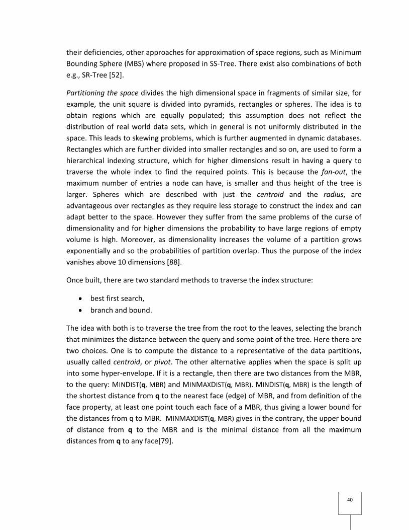
40

their deficiencies, other approaches for approximation of space regions, such as Minimum

Bounding Sphere (MBS) where proposed in SS-Tree. There exist also combinations of both

e.g., SR-Tree [52].

Partitioning the space divides the high dimensional space in fragments of similar size, for

example, the unit square is divided into pyramids, rectangles or spheres. The idea is to

obtain regions which are equally populated; this assumption does not reflect the

distribution of real world data sets, which in general is not uniformly distributed in the

space. This leads to skewing problems, which is further augmented in dynamic databases.

Rectangles which are further divided into smaller rectangles and so on, are used to form a

hierarchical indexing structure, which for higher dimensions result in having a query to

traverse the whole index to find the required points. This is because the fan-out, the

maximum number of entries a node can have, is smaller and thus height of the tree is

larger. Spheres which are described with just the centroid and the radius, are

advantageous over rectangles as they require less storage to construct the index and can

adapt better to the space. However they suffer from the same problems of the curse of

dimensionality and for higher dimensions the probability to have large regions of empty

volume is high. Moreover, as dimensionality increases the volume of a partition grows

exponentially and so the probabilities of partition overlap. Thus the purpose of the index

vanishes above 10 dimensions [88].

Once built, there are two standard methods to traverse the index structure:

best first search,

branch and bound.

The idea with both is to traverse the tree from the root to the leaves, selecting the branch

that minimizes the distance between the query and some point of the tree. Here there are

two choices. One is to compute the distance to a representative of the data partitions,

usually called centroid, or pivot. The other alternative applies when the space is split up

into some hyper-envelope. If it is a rectangle, then there are two distances from the MBR,

to the query: MINDIST(q, MBR) and MINMAXDIST(q, MBR). MINDIST(q, MBR) is the length of

the shortest distance from q to the nearest face (edge) of MBR, and from definition of the

face property, at least one point touch each face of a MBR, thus giving a lower bound for

the distances from q to MBR. MINMAXDIST(q, MBR) gives in the contrary, the upper bound

of distance from q to the MBR and is the minimal distance from all the maximum

distances from q to any face[79].

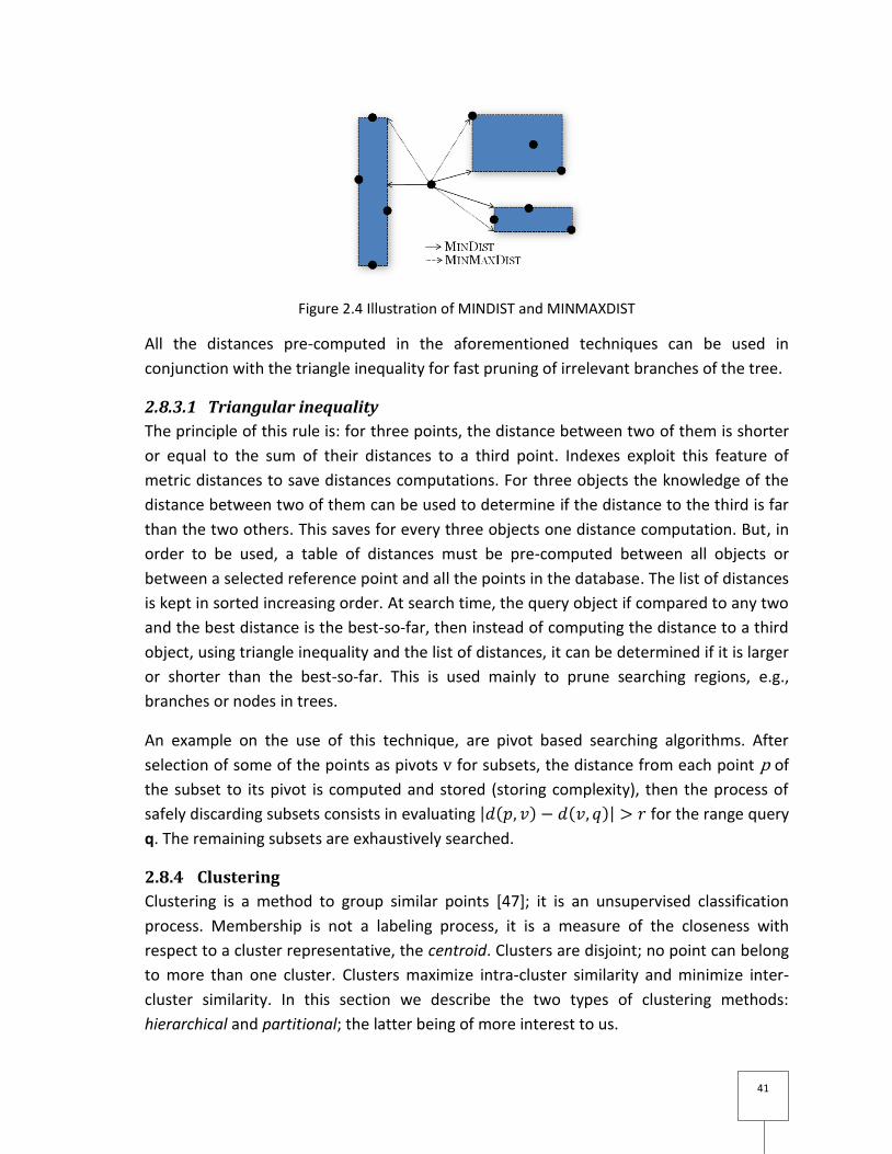
41

Figure 2.4 Illustration of MINDIST and MINMAXDIST

All the distances pre-computed in the aforementioned techniques can be used in

conjunction with the triangle inequality for fast pruning of irrelevant branches of the tree.

2.8.3.1 Triangular inequality

The principle of this rule is: for three points, the distance between two of them is shorter

or equal to the sum of their distances to a third point. Indexes exploit this feature of

metric distances to save distances computations. For three objects the knowledge of the

distance between two of them can be used to determine if the distance to the third is far

than the two others. This saves for every three objects one distance computation. But, in

order to be used, a table of distances must be pre-computed between all objects or

between a selected reference point and all the points in the database. The list of distances

is kept in sorted increasing order. At search time, the query object if compared to any two

and the best distance is the best-so-far, then instead of computing the distance to a third

object, using triangle inequality and the list of distances, it can be determined if it is larger

or shorter than the best-so-far. This is used mainly to prune searching regions, e.g.,

branches or nodes in trees.

An example on the use of this technique, are pivot based searching algorithms. After

selection of some of the points as pivots v for subsets, the distance from each point p of

the subset to its pivot is computed and stored (storing complexity), then the process of

safely discarding subsets consists in evaluating for the range query

q. The remaining subsets are exhaustively searched.

2.8.4 Clustering

Clustering is a method to group similar points [47]; it is an unsupervised classification

process. Membership is not a labeling process, it is a measure of the closeness with

respect to a cluster representative, the centroid. Clusters are disjoint; no point can belong

to more than one cluster. Clusters maximize intra-cluster similarity and minimize inter-

cluster similarity. In this section we describe the two types of clustering methods:

hierarchical and partitional; the latter being of more interest to us.

42

Hierarchical Clustering is a deterministic group forming process. It can be agglomerative

(each point is a cluster, then combine) or divisive (all data set is a cluster, then split) and,

respectively bottom up, or top-down. Figure 2 shows a synopsis of this hierarchical

clustering.

Bottom-up starts with n clusters, each has a single point. A table of inter-cluster distances

is constructed with a high cost. Iteratively, we merge the two closest clusters into a

single super-cluster until the tree is constructed. The overall complexity of this process is

known to be in in the worst case, though a direct algorithm fitted to our data set

case is only in thanks to the use of triangular inequality in metric spaces.

Top-down starts with one big cluster, i.e., all the database. It then applies a non-

hierarchical algorithm (e.g., k-means) to divide the set into two clusters. It repeats this

process until each cluster contains one point (or a sufficiently small number of points).

Figure 2.5 Synopsis of hierarchical clustering

Partitional clustering, single or flat level clustering, is as its name suggests, a clustering

method which splits a data set into a predefined number of groups or clusters. The most

popular partitional method is the k-means [48], where k stands for the number of clusters

which are iteratively refined. The clustering consists in: 1) starts by selecting initial k

centroids, 2) then assign each point to the nearest centroid, 3) for each obtained group

recomputed the centroid. The partitioning criterion of the k-means is to minimize the

average squared distance for each point to the centroid.

The complexity of k-means can be derived approximately, as the number of required

iterations i to converge to an optimization criterion is not deterministic: it is dependent to

the selection of the initial centroids and the number of clusters. Its cost can be estimated

based on the d dimensionality of the data points, the number k of clusters and the

iterations i to converge for a database of size n: . Observe that the step to

determine the best centroid for each point is itself a nearest neighbor search and is

in for the whole data set.

As can be observed, top-down is faster than bottom-up.

Hierarchical clustering

Top-down -divisive

split a large cluster to form small clusters

Bottom-up -agglomerative

join smaller clusters to form

bigger ones

43

One characteristic of partitioning methods is the overlap. Overlap does not mean that a

point belongs to more than one cluster, but that the space defined by the enclosing ball

for a cluster of points overlap portions of the space delimited by another enclosing ball.

Remember that the distance used shapes the space. Thus assuming the L2 distance, hyper-

spherical shapes wrap the data points, i.e., is a ball partitioning approach.

Searching using clustering is a two-step approach: pruning and refinement. Firstly, a

search at a coarse level to select interesting clusters is executed by computing the

distance from the query to the cluster centroid, taking into account the radius and making

used of the triangle inequality. Then, a refinement step, searches within the selected

clusters the desired kNN of the query.

For each cluster a representative called centroid is computed to perform searching. The

centroid summarizes the cluster properties. This group has points more similar between

them than across clusters.

Most of the clustering schemes [30][31] construct a hierarchical structure of similar

clusters or make use of an index structure to access rapidly some kind of cluster

representative, such as the centroid, which typically is the mean vector of features for

each cluster. In the searching process, this hierarchy or index is traversed by comparing

the query object with the cluster representatives in order to find the clusters of interest.

In both index and cluster-based strategies, the cost of computing the distances to

determine similarity can be very high for large multimedia databases.

We are interested more in the partitioning properties of k-means than in grouping, i.e, we

use it as a method to partition the database in a determined number of clusters. Indeed,

selecting the appropriate number of clusters has been a subject of interesting research.

Some empirical results showed that around is an ideal number of clusters [82][37]

within the context of specific searching algorithms. More recently Berrani [13] stated that

it is not possible to establish a relation between the number of clusters and the query

time. His observations are made based on his searching techniques and experiments.

However we argue that it is possible to estimate the cost of the searching steps according

to their complexity and analytically propose an optimal range of values for the

number of clusters, using general searching algorithms.

The same as the curve is more and more approximated by smaller line segments so that

the space can be covered by smaller and thus more compact clusters. It is thus desirable

to have many small clusters than a few large ones to better group the data points and

hence improve the filtering techniques.

44

2.8.5 Parallel search

In multimedia databases, where the efficient processing of similarity queries due to the

size of the database results in significant storage and performance requirements, it seems

mandatory to use a parallel machine, which allows for: sharing among multiple processors

the distance computing workload; reducing the I/O cost by using parallel I/O devices

simultaneously (this also improves throughput, as contention is reduced by reading and

scanning the different database partitions at the node where each one resides).

Disk accesses for large databases become a performance problem. Efficient storage

techniques aims to reduce this disk I/O bottleneck by minimizing the operations required

to retrieve information. They achieve this by clustering related information therefore the

number of disk accesses are reduced by retrieving data from a small number of disk

blocks. These are intra-disk placement schemes, which even if they optimize retrieval

within a disk, sooner or later the volume of the database and the high retrieval rate will

exceed its capacity [75]. The idea is to minimize the disk I/O bottleneck by trying to access

in the less possible operations the required data. Placing in contiguous disk blocks similar

data can help to achieve this, and a single sequential read operation does better the work

than several random ones. However it is impossible to anticipate the optimal placement

for every possible query. Part of this overhead is due to the mechanical parts of the

device. Solid State Disks (SSD) [22], which do not have them, may provide the required

efficiency levels, even though their price seems yet prohibitive to most applications. Inter-

disk placement which allows retrieving data in parallel from several devices cope more

efficiently with these limits [39].

Sometimes disks are needed not for their storage space, but for performance. When it is a

priority to eliminate the I/O bottleneck due to intensive users’ requests, storage capacity

is a second term concern. Due to excessive data requests, the data transfer bus becomes

saturated decreasing the overall system throughput, hence the need for parallel I/O’s to

avoid disk contention problems and speed up query processing. Thus the number of

required disks is a performance-driven selection issue to enable parallelism.

This is the purpose of partitioning: allowing databases to exploit the added I/O bandwidth

to speed up data operations, and more precisely declustering aim to balance the amount

of data fetched from each node to reduce the overall processing time.

2.8.5.1 Database architectures: choice is shared-nothing

In order to get the required computing power for the strident processing of similarity

searches, there are mainly three types of architectures [14]:

45

shared memory,

shared disk,

shared nothing.

This taxonomy is based on the type of resources accessible to the processing unit (or

processor for short). The shared resources are disk and main memory. They are presented

from less to more flexible, meaning they are easy to scale, i.e., add more resources to

cope with bigger workloads. The sharing of the data containers (disk and main memory)

reduces the complexity of programming.

In shared memory or shared everything, each CPU has access to any memory or disk unit.

Hence, it is possible to achieve load balancing at the price of little extensibility and low

availability. In shared disk, each CPU has exclusive access to main memory but access to

any disk. This increase extensibility but is still limited due to the shared resources.

Zero sharing is implemented by the shared-nothing architecture. In this type of machines

each node has its own processing unit, main memory and disk. A high speed

interconnection network allows to exchange messages between nodes.

Big servers are expensive, hard to scale and as they concentrate all processing units in a

single frame they introduce a new failure point. Shared-nothing architectures, provide

scalability using commodity hardware [5].

2.8.5.2 Query execution strategies

There are mainly to approaches to control the execution of queries in parallel search:

control flow,

data flow.

In the control flow approach, there is a single node controlling all processes related to a

query; it is a master-slave paradigm. The master starts and synchronizes all the queries.

On the other hand, the data flow approach, has no centralized control; nodes interchange

messages to synchronize and the availability of a query triggers a searching process [74].

Based on these considerations, we can identify three parallel query (PQ) execution

strategies:

PQ1.- A single node controls the flow of a query. Data is distributed equally and randomly

across all machines. A query is sent to all nodes which compute the result from local data.

Results are merged in a central node. Drawback: a node processes a query even if its local

data do not contribute to the final result. This result in waste of processing time.

46

PQ2.- Data is range partitioned. Each node is responsible of a fraction of the data space. A

central node computes the data interval satisfying the query and sends it to the

corresponding node. The main drawback is that a node does the work of a single server.

Although each node will evaluate a query, but due to data “hot-spots”, a node will

eventually become saturated degrading system performance. This strategy is an example

of inter-query parallelism, where each node solves a different query.

PQ3. In this strategy, the data is also partitioned, but the processing load is shared among

available nodes, thus the more evenly it is distributed the less the processing time. This is

a case of intra-query parallelism: the goal is to reduce the processing time of a complex

query, as is the case of a similarity query.

2.8.5.3 Forms of parallelism

Our aim is to maximize system performance by dividing the total amount of the work

required to solve a query between available nodes, thus minimizing the time to solve a

query (divide and conquer). Query parallelism can be of two types:

interquery parallelism. Several queries execute in parallel and independently. The

aim is to increase system throughput by processing multiple queries at the same

time

intraquery parallelism. A query is split over available processors, each one

executing independently its operators. Data must be partitioned to enable

independence in processing. The aim is to decrease processing time by processing

the operators of a query simultaneously by different processors (inter-operator

parallelism) and by processing the same operator by all the processors each one

working in a subset of the database (intra-operator parallelism)

Intra-query parallelism allows to speed up the processing of queries by sharing the

processing of a single query by several processing units. This way, the time required to

process a complex query is reduced approximately by the number of processors used

more the merging cost.

Similarity query processing can benefit from parallel processing; exact kNN queries require

scanning a large fraction of the database while returning a small result set. High scalability

is achieved by the shared-nothing architecture; performance can be improved by adding

processing nodes, to some extent.

The ignored component in the proposed architectures is the computing infrastructure

where search is actually performed. Generally it is assumed to be centralized, so scaling is

not possible. When it is explicitly parallel or distributed, to our knowledge, the

maximization of resource utilization is ignored even for a single query/user. To exploit this

47

parallel architecture, data allocation is an issue. The layout of the database must be

planned such that it is possible to maximize parallelism and achieve load balancing.

The key advantage of declustering or data allocation is to reduce the total amount of work

to be processed by a node and consequently reducing the overall response time, which is

dependent on the longest time taken by a node to accomplish its task. Thus is desirable

that the nodes process the same amount of data and contribute equally to the final result.

Though optimality in data allocation in parallel databases has been proved to be NP-

complete near optimal solutions can be obtained [1][2][57].

2.8.5.4 Literature review

This section review relevant research in parallel CBIR. Despite that declustering has been a

subject of research in RDBMS and spatial databases, we concentrate the presentation to

multidimensional approaches.

Gao et al [42], present a multi-disk environment to process kNN queries in up to 5-

dimensional data. The works is based on the Parallel R-tree [50]. The tree is stripped on M

disks, where M is the node fan out. Thus the main objective is to avoid disk bottleneck. For

each disk is constructed an in-memory priority queue, the best nearest neighbor from all

of them is the updatable upper bound to prune leaf nodes, the best answers are kept also

in a separate queue. For 5 disk their best proposal takes 0.65 seconds approximately for

60 thousand 3-dimensional object for k=100 with 5 disks, which is only reduced to 0.4

seconds with 30 disks.

In [50], Kamel et al. presents an architecture of one processor-multiple disks to process

range queries using an interesting concept called proximity index allocation which

measures the similarity between nodes to later place them on the disks, avoiding to put

similar nodes together, this allows a near optimal allocation process. A shared-nothing-

based implementation is presented by [76], however they are based on the R-Tree which

is used to index spatial data, i.e. two-dimensional datasets. To our purposes, one of their

conclusions is that, the choice of the declustering algorhtm (placement of data over the

nodes) has not significance in the overall response time. We will see that using round

robin placement we achieve near optimal declustering.

In [10] Berchthold et al. proposed an allocation method for the X-Tree using a graph

coloring algorithm. It has been reported that the Pyramid tree outperforms the X-Tree by

a factor of 800 in response time in centralized settings [90].

In [75], Prabhakar et al, presents a four disk architecture concerned mainly with the

placement within each disk, i.e., a very low level placement scheme of wavelet

48

coefficients. This architecture is used for browsing image thumbnails by exploiting

parallelism (they use parallelism to retrieve the coefficients) but the final selected images

must be reconstructed in the clients’ side from the wavelet coefficients (kind of feature

vector).

The Parallel M-Tree [91] of Zezula et al, and one extension [3] address the problem of

distributing the nodes of the M-Tree in the parallel system by computing the distance of

each newly object placed in a node with all the objects already available, it is achieved by

performing a range query with a radius equal to the distance from the object to its parent.

The proposal of Zezula et al achieved approximately 15 speed up for 10000 45-

dimensional data with 20 disks.

In [18][19], the authors propose an hybrid architecture of redundant multidisc and shared-

nothing, to improve disk I/O based in the Parallel R-Tree. However, they provide results

for 100, 000 data of up to 80 dimensions which, as we will demonstrate, are

outperformed by our proposal with much less resources.

Recently, Liu et al [58] propose a clustering based parallel spill tree altogether with a

search method, in their study, they begin with an initial 1.5 billion images which after

“cleaning” remains in around 200 million, a large enough image database but the

dimensionality of the data set is 100 and their proposal needs 200 machines. In the

contrary, according to our proposal presented in chapter 4, we use 1000 descriptors and

nodes, which in order to process the whole 200 millions images database would

require only 27 nodes.

Also, Gil-Acosta et al [43], experiment with a parallel proposal of List of Clusters [33].

Several datasets are used to evaluate performance for main-memory searching for range

and kNN queries. Their argument is that using secondary storage (hard disks) facing large

amounts of query loads will eventually accelerate the failure rate of them. Among their

results are that the best cluster sizes are 10 to 50 and that retrieving the top three clusters

is possible to achieve 90% of exact results. Their best parallel processing proposal achieves

a 50% of the optimal performance.

Novak et al [70] built a P2P system based on M-Chord [69] and Pivoting M-Tree [77] for

image similarity search. M-Chord is a distributed data structure based on iDistance [49]

and Chord. The idea of iDistance for one-dimensional mapping is combined with Chord to

partition the data among peers. Data is partitioned in Voronoi regions and a number of

pivots are one-dimensional mapped with iDistance, then the partitions are distributed

among the peers and index with Chord. Using this system, the authors propose to

evaluate range and kNN queries. The range intersecting the mapping is used to determine

49

peers relevance and hence query routing. For kNN queries, a set of empirically tuned

parameters to determine the most promised peers is used. The peer originating the query

is responsible to gather the results. As this system make use of the COPHIR database [], it

uses MPEG-7 descriptors and the corresponding distance function. But as it also makes a

combination of the descriptors to form a single one, it assigns relevance to the individual

descriptors with an experimentally tuned weight parameter. All data and index structures

are kept in main-memory. Their search heuristics show that visiting 40% of the clusters

achieve a 90% recall with almost the same levels from one to ten millions images equally

distributed among 500 peers. A precise search visits in average 253 peers.

Lastly, Bosque et al [21] describes a load balancing algorithm for heterogeneous

processing nodes. Their results over a database of 12.5 millions images reports a

decreasing speed up from 1.8 for 5 nodes to 1.6 for 25. They perform a linear search of all

images signatures in all nodes.

2.9 PERFORMANCE EVALUATION

Measuring as always. The usual metrics to evaluate effectiveness and efficiency (both

known under the generic term of “performance”) are:

accuracy (precision and recall),

response time.

The former stands for how good are the retrieved results and the latter for how long takes

the retrieval process (i.e., how long does it take to answer a query).

Precision is the ability of the system to retrieve only relevant objects (or to reject

irrelevant ones). Recall is the ability to retrieve the relevant objects. The ideal is achieved

when every object retrieved is relevant (precision 100%) and every relevant object is

retrieved (recall 100%). Here relevance is in comparison with the results obtained with a

full sequential search. From the fact that for higher dimensions there is no indexing

proposal better than it. So the results obtained with a proposed searching strategy are

compared with those obtained with sequential search. This does not imply results are the

best from a point of view of visual quality, which is a subjective measure dependent on

the evaluator’s criterion. Additionally, quality of visual description is much related to

descriptors performance. In this thesis, we assume a good descriptor is provided and the

quality of our proposals are 100% (full precision) when the results produced by our

searching strategies are the same of those of a full sequential search.

50

To evaluate accuracy, a known database, the ground truth, and a set of queries are

established. Precision can be evaluated by comparison of the retrieved objects with

respect to an experts’ selection. Recall is not so easy to determine and it becomes harder

and harder for large databases. Hence, the use of synthetic data sets, where the data

space is somehow known, so it is possible to execute controlled experiments. Another

option is to execute a sequential search to obtain a baseline of relevant objects. Or embed

a number of known good objects in a large unknown or bad database of objects.

Evaluating an algorithm by its execution time can be misleading. Wall-clock time

measurements are hardware dependent; certainly using a system with a faster CPU and a

wider data transfer bus with a high speed disk, improve the overall processing time

compared to a slower one. Although it is important to time an algorithm in order to give

to the user an idea of the expected quality of service, it is better to use platform

independent measures; counting the number of disk transfers, counting the number of

distances evaluated and comparing its improvement over a well known baseline (e.g.,

sequential scan) may be more useful. These measures can be used as a reference even

when more powerful machines will be available.

As seen above, there are some trade-offs in high-dimensional similarity search. When

conceiving a searching algorithm, some issues are of main interest to solve. For a

combination of design objectives, the question is: “how fair is it to assess and judge the

quality of a searching algorithm when they tackle different problems?”.

Which algorithm is the best baseline? In some papers it is stated that 15 dimensions is

the efficiency limit to most index structures [88]. Some other says that VA-file is not

affected by the curse of dimensionality [23][24]. In practice, when a sequential search

overcomes any algorithm in higher dimensions, the curse of dimensionality takes place.

From these claims, it is evident that results are influenced by an algorithm design goals

and the testing databases. It happens that it is overlooked that two comparing structures

where designed and hence optimized for different constraints making unfair the

comparison. Moreover, some data spaces are easy in the sense that data points are well

distributed in the space, leading to non empty space regions and have low intrinsic

dimensionality; hence similarity can be easily determined.

However there is an additional issue affecting an algorithm performance: the quality of

the implementation. In fact, a good programmer can come up with a very efficient

implementation of a not so good algorithm and, conversely, good algorithms can be

ruined by a misunderstanding of its building concepts or an unoptimized implementation.

51

On the other hand, it is also evident that at some extent, nothing performs better than

sequential search. Thus to evaluate our proposal we come up with a very fast sequential

search implementation used as a baseline to compare improvements.

Which database to test with? With respect to benchmark databases, we have synthetic

and real ones, the most notable by its size being COPHIR [20] which currently contains

millions of images downloaded from Flickr, well actually only the Scalable Color (FSC) and

Color Structure (FCS) MPEG-7 descriptors.

For synthetic data sets a uniform distribution has been used many times by randomly

generating d-points, but it has been proved that this kind of data is far from being real and

also useless for similarity search [80].

Thus for our experiments we used real and synthetic data sets, with the observation that

our synthetic data sets are far from being uniform, they follow different data distributions

and thus are realistic in the sense that the distribution of clusters and cluster’s

populations are not uniform.

How to establish the ground truth? The importance of the query object used to test is

also important, whether it is a randomly taken object from the database or is a new one.

For real databases it can be “injected” manually some known and small set of images to

compare the usual measures recall and precision, but this is not practical as having such a

known ground truth implies transforming an image to generate several others close to it.

Hence, we suggest also to run a sequential search for every randomly selected query from

the database, or new ones, in order to determine the actual nearest neighbors.

The importance of descriptors. Multimedia objects are retrieved based on their similarity

by means of a similarity metric. The similarity metric is hard to determine as it should

reflect with accuracy the human judgment. Sometimes what is returned by the system is

rejected by the user. The groups of images obtained by using clustering of feature vectors

or indexing, do not necessarily correspond to semantically related images. This is not a

problem of clustering methods, it is an issue of the feature extraction methods, which

maps images with different meanings, into a nearby location in the representation space.

In fact this problem is called the semantic gap [83]. To illustrate this problem consider the

pair of images of figure 6, which have the similar descriptors but are not identical and

possibly from a certain point of view neither the same meaning. This example emphasizes

the importance of an adequate feature extraction method to describe an image which

needs to be applied by considering the domain when pre-processing the database.

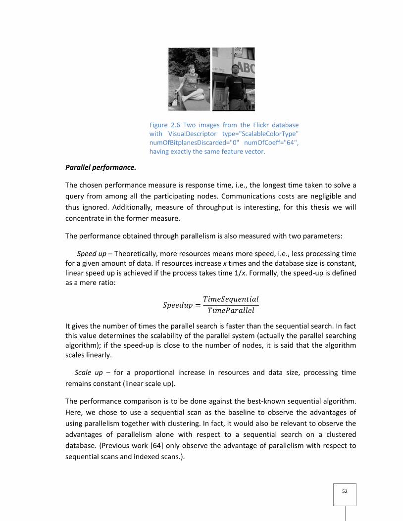
52

Figure 2.6 Two images from the Flickr database with VisualDescriptor type="ScalableColorType" numOfBitplanesDiscarded="0" numOfCoeff="64", having exactly the same feature vector.

Parallel performance.

The chosen performance measure is response time, i.e., the longest time taken to solve a

query from among all the participating nodes. Communications costs are negligible and

thus ignored. Additionally, measure of throughput is interesting, for this thesis we will

concentrate in the former measure.

The performance obtained through parallelism is also measured with two parameters:

Speed up – Theoretically, more resources means more speed, i.e., less processing time for a given amount of data. If resources increase x times and the database size is constant, linear speed up is achieved if the process takes time 1/x. Formally, the speed-up is defined as a mere ratio:

It gives the number of times the parallel search is faster than the sequential search. In fact this value determines the scalability of the parallel system (actually the parallel searching algorithm); if the speed-up is close to the number of nodes, it is said that the algorithm scales linearly.

Scale up – for a proportional increase in resources and data size, processing time

remains constant (linear scale up).

The performance comparison is to be done against the best-known sequential algorithm.

Here, we chose to use a sequential scan as the baseline to observe the advantages of

using parallelism together with clustering. In fact, it would also be relevant to observe the

advantages of parallelism alone with respect to a sequential search on a clustered

database. (Previous work [64] only observe the advantage of parallelism with respect to

sequential scans and indexed scans.).

53

Amdahl stated [4] that the gain of using parallelism is limited by the unparallelizable

portion of a process. The good news is that our process is disk-bounded so, parallel disks

operations reduce the overall processing time. Furthermore, distances are computed on

local data, i.e., on a reduced fraction of the database. So in the overall, speedup is the

expected gain of a parallel over a sequential search.

54

55

3 OPTIMAL CLUSTERING FOR

EFFICIENT RETRIEVAL

The idea of the partitioning method is to cluster the database to form homogeneous

groups of most similar data points. The aim is to organize the database in small compact

groups of data points, so that a searching process can rapidly prune uninteresting clusters

to then concentrate the search in the more likely ones to contain the desired images. As

noted in the last chapter, though there is a wealth of proposals based on this idea, there

still remain open issues such as determining the optimal number of clusters or partitions

and consequently their size. The importance of this issue is that even if the pruning

process can discard uninteresting clusters, the search within the remaining clusters can be

a time consuming task. Also, having too many clusters shall impact the I/O subsystem.

Also, as a database becomes larger, the processing capacity of a single machine is

overwhelmed. To overcome this shortcoming, the results obtained in this chapter are the

foundation to the parallel proposal studied in the next chapter, which implements a

declustering method in a shared-nothing parallel architecture.

The motivation for this chapter is to analyze the problem of efficient content based image

retrieval from a computational complexity point of view. The approach is to design a high-

level scenario under reasonable and simple hypotheses.

A first hypothesis is that the solution should use some kind of clustering. However, the

exact algorithm remains an open issue at this stage. In contrast, we shall derive a specific

number of clusters to organize the database.

Next, we decided to avoid the use of any indexing technique, since the literature showed

us that they present limitations that avoid them to be useful in high-dimensional data

spaces. We were willing to reach tenths and hundreds of dimensions. In contrast, we rely

on simple search algorithm, i.e., sequential scans with some ordering of the results,

including a mere general sort procedure.

Therefore, to achieve some speed-up, we had to take advantage of parallelism. However,

we chose to limit “drastically” the number of machines used for answering a query. A

56

logarithmic increase of the number of machine with respect to the number of images

seems to use a practical scenario.

Under these conditions, we show hereafter that it is possible to achieve sub-linear

response time.

The rest of the chapter is structured as follows. In section 3.1 we review some theoretical

complexities for conducting a search over an unorganized data set of points. In section 3.2

we discuss the complexity of searching by using clustering. In section 3.3 we present the

actual proposal for database clustering and its analytical validation. In section 3.4 we show

experimental results. Finally, in section 3.5 we state some concluding remarks and

additional discussions.

3.1 SOME COMPLEXITY CONSIDERATIONS

Recall that one of the main problems that CBIR faces is the curse of dimensionality. This

means that it is not possible to index efficiently points in high dimensions. In general it

was reported that indexing methods can deal with up to 10 dimensional spaces in the

average [88]; above that limit, their performance is comparable with mere sequential

scan. Some recent proposals, such as the iDistance [49], reports performance up to 30

dimensions but its limits have not been formally proved.

Considering these limitations, we decide to avoid using such indexing techniques in our

search for an efficient a general solution to multimedia retrieval.

constant

logarithmic

Square root

linear

sorted

Table 3.1 Some complexities for searching in a database of n images, eventually the k best with .

Let us remind that we are interested in searching the k nearest neighbors. More precisely,

we are interested in the exact nearest neighbors. The table 3.1 gives some possible

complexities for the retrieval of k images in a database of size n, where k is expected to be

a constant independent of, and much smaller than n. They correspond to common

complexities for various algorithms.

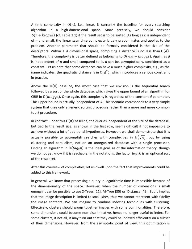
57

A time complexity in , i.e., linear, is currently the baseline for every searching

algorithm in a high-dimensional space. More precisely, we should consider

(cf. Table 3.1) if the result set is to be sorted. As long as k is independent

of n and small, the linear scan time complexity largely predominates and applies to the

problem. Another parameter that should be formally considered is the size of the

descriptors. Within a d dimensional space, computing a distance is no less than .

Therefore, the complexity is better defined as belonging to . Again, as d

is independent of n and small compared to it, d can be, asymptotically, considered as a

constant. Let us note that some distances can have a much higher complexity, e.g., as the

name indicates, the quadratic distance is in , which introduces a serious constraint

in practice.

Above the baseline, the worst case that we envision is the sequential search

followed by a sort of the whole database, which gives the upper bound of an algorithm for

CBIR in . Once again, this complexity is regardless of the constant d parameter.

This upper bound is actually independent of k. This scenario corresponds to a very simple

system that uses only a generic sorting procedure rather than a more and more common

top-k procedure.

In contrast, under this baseline, the queries independent of the size of the database,

but tied to the result size, as shown in the first row, seems difficult if not impossible to

achieve without a lot of additional hypotheses. However, we shall demonstrate that it is

actually possible to accomplish searches with complexities in , but by using

clustering and parallelism, not on an unorganized database with a single processor.

Finding an algorithm in is the ideal goal, as of the information theory, though

we do not yet know if it is reachable. In the notations, the factor is an optional sort

of the result set.

After this overview of complexities, let us dwell upon the fact that improvements could be

added to this framework.

In general, we know that processing a query in logarithmic time is impossible because of

the dimensionality of the space. However, when the number of dimensions is small

enough it can be possible to use X-Trees [11], M-Tree [35] or iDistance [49]. But it implies

that the image description is limited to small sizes, thus we cannot represent with fidelity

the image contents. We can imagine to combine indexing techniques with clustering.

Effectively, clusters should group together images with some commonalities. Therefore,

some dimensions could become non-discriminative, hence no longer useful to index. For

some clusters, if not all, it may turn out that they could be indexed efficiently on a subset

of their dimensions. However, from the asymptotic point of view, this optimization is

58

insufficient as long as at least one cluster has to be scanned sequentially. In practice, it can

make a big difference, especially in a multiuser environment. We do not consider this

issue in this work.

To avoid the performance deterioration exhibited by indexing methods, it is possible to

proceed with a reduction of dimensions. Dimensionality reduction is a process that

transforms one data space into another less complex but, to be worth for CBIR, this

transformation process must take into consideration as much as possible the

characteristics of the initial space, to preserve them to that of arrival. For this reason, the

weakness of dimensionality reduction approaches is an additional loss of precision. We

are not going to discuss further about them, it was the subject of the preceding chapter.

Let us note that in practice, especially during the experiments that we conducted, we

must take into consideration not only the number of images n, but also the size of their

abstract representation m. The relation between them is a constant , i.e., the

actual size of the database is directly related to the number of images, λ being the size of

the descriptor of one image. Naturally the bigger λ, the more important are the

repercussions on the performances. Effectively, we will see that the search is disk I/O's

bounded.

In summary, using a single machine, and without clustering and/or indexing, we cannot

expect a better time complexity than . This can even degrade to if the

wanted results are sorted with a general-purpose sort rather than a best-fitted procedure.

3.2 CBIR USING CLUSTERING

Due to the relatively “poor” results achieved by the indexing approaches, we analyze, as

an alternative to indexing, the case of a CBIR that relies on:

• a clustering of the database at pre-processing-time,

• parallel scans with a small-sized parallel architecture at run-time.

It has been demonstrated and experimented in previous work [64] that parallelism alone

is insufficient.

To avoid the efficiency deterioration exhibited by indexing methods, as well as to avoid

the effectiveness deterioration with a reduction of dimensions, we add a clustering

process to the parallel approach.

Clustering suffers a priori of the same general problem as indexing methods [31]. Indeed,

multidimensional points are used as abstract representation of actual images and the

searching process cannot avoid distance calculations. But the intention is to compute as

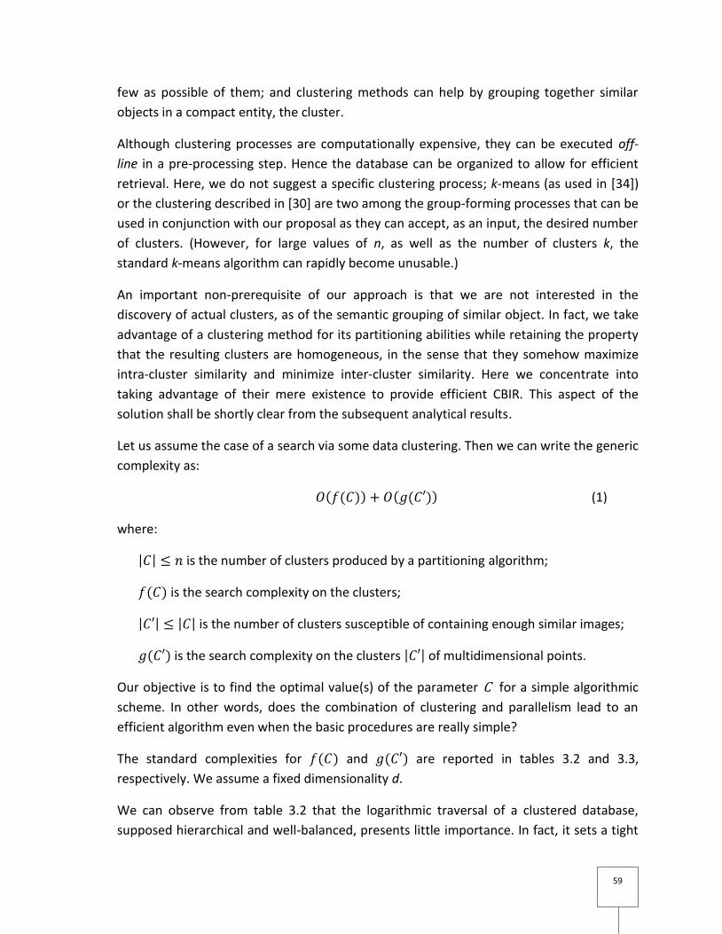
59

few as possible of them; and clustering methods can help by grouping together similar

objects in a compact entity, the cluster.

Although clustering processes are computationally expensive, they can be executed off-

line in a pre-processing step. Hence the database can be organized to allow for efficient

retrieval. Here, we do not suggest a specific clustering process; k-means (as used in [34])

or the clustering described in [30] are two among the group-forming processes that can be

used in conjunction with our proposal as they can accept, as an input, the desired number

of clusters. (However, for large values of n, as well as the number of clusters k, the

standard k-means algorithm can rapidly become unusable.)

An important non-prerequisite of our approach is that we are not interested in the

discovery of actual clusters, as of the semantic grouping of similar object. In fact, we take

advantage of a clustering method for its partitioning abilities while retaining the property

that the resulting clusters are homogeneous, in the sense that they somehow maximize

intra-cluster similarity and minimize inter-cluster similarity. Here we concentrate into

taking advantage of their mere existence to provide efficient CBIR. This aspect of the

solution shall be shortly clear from the subsequent analytical results.

Let us assume the case of a search via some data clustering. Then we can write the generic

complexity as:

(1)

where:

is the number of clusters produced by a partitioning algorithm;

is the search complexity on the clusters;

is the number of clusters susceptible of containing enough similar images;

is the search complexity on the clusters of multidimensional points.

Our objective is to find the optimal value(s) of the parameter C for a simple algorithmic

scheme. In other words, does the combination of clustering and parallelism lead to an

efficient algorithm even when the basic procedures are really simple?

The standard complexities for and are reported in tables 3.2 and 3.3,

respectively. We assume a fixed dimensionality d.

We can observe from table 3.2 that the logarithmic traversal of a clustered database,

supposed hierarchical and well-balanced, presents little importance. In fact, it sets a tight

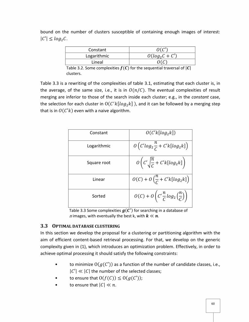
60

bound on the number of clusters susceptible of containing enough images of interest:

.

Constant

Logarithmic

Lineal Table 3.2. Some complexities for the sequential traversal of clusters.

Table 3.3 is a rewriting of the complexities of table 3.1, estimating that each cluster is, in

the average, of the same size, i.e., it is in . The eventual complexities of result

merging are inferior to those of the search inside each cluster; e.g., in the constant case,

the selection for each cluster in , and it can be followed by a merging step

that is in even with a naive algorithm.

Constant

Logarithmic

Square root

Linear

Sorted

Table 3.3 Some complexities for searching in a database of n images, with eventually the best k, with .

3.3 OPTIMAL DATABASE CLUSTERING

In this section we develop the proposal for a clustering or partitioning algorithm with the

aim of efficient content-based retrieval processing. For that, we develop on the generic

complexity given in (1), which introduces an optimization problem. Effectively, in order to

achieve optimal processing it should satisfy the following constraints:

• to minimize as a function of the number of candidate classes, i.e.,

the number of the selected classes;

• to ensure that ;

• to ensure that .

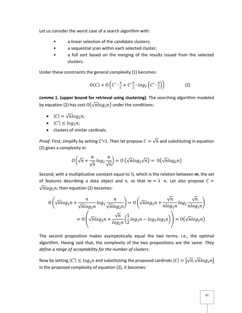
61

Let us consider the worst case of a search algorithm with:

• a linear selection of the candidate clusters;

• a sequential scan within each selected cluster;

• a full sort based on the merging of the results issued from the selected

clusters.

Under these constraints the general complexity (1) becomes:

(2)

Lemma 1. (upper bound for retrieval using clustering). The searching algorithm modeled

by equation (2) has cost under the conditions:

;

;

clusters of similar cardinals.

Proof. First, simplify by setting C’=1. Then let propose and substituting in equation

(2) gives a complexity in:

Second, with a multiplicative constant equal to ½, which is the relation between m, the set

of features describing a data object and n, so that . Let also propose

, then equation (2) becomes:

The second proposition makes asymptotically equal the two terms, i.e., the optimal

algorithm. Having said that, the complexity of the two propositions are the same. They

define a range of acceptability for the number of clusters.

Now by setting and substituting the proposed cardinals

in the proposed complexity of equation (2), it becomes:

62

This can be simplified to:

which is certainly in

Notice that, from the proof, it can be derived some algorithmic variations, from optimal to

suboptimal in under less restrictive conditions.

Our proposal for partitioning the database is then , the optimal case

can be obtained with a near multiplicative factor , since C’ is small and independent of n.

This lemma is important since, thanks to the clustering hypothesis, it allows the design of

a sub-linear content-based retrieval algorithm, using basic algorithms which are not. The

proposed algorithm is order of magnitudes under the sequential scan, though it is still

much slower than the best theoretical achievement which could be in .

Additionally, this lemma gives us the (asymptotic) optimal number of clusters (i.e., it

accepts small variations), which can be used as a parameter by the clustering algorithm.

Table 3.4 shows analytical values computed for different database sizes n in each column.

Cinf and Csup are the values that define the interval for the number of clusters in our

proposal, and their respective cardinals are n’inf and n’sup It can be observed that the

selectivity factor decreases rapidly as the database grows, for n=1024 it is 3.13% but for

one million images it is 0,10%. The speed-up row shows how the proposal for Csup

performs compared with a naive sequential search process, which is a considerable gain.

n 1, 024 8,192 32,768 1,048,576 33,554,432

Cinf : 32 91 181 1,024 5,793

Csup : 320 1,177 2,715 20,480 144,815

n’inf : 32 91 181 1,024 5,793

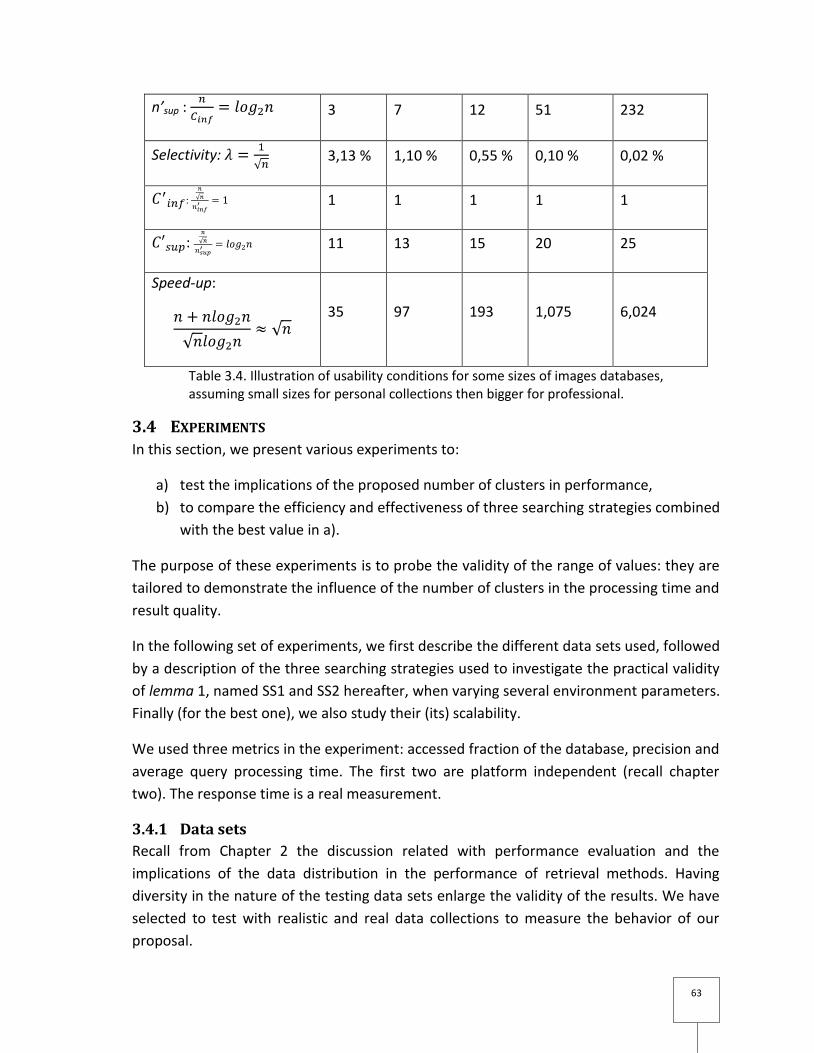
63

n’sup : 3 7 12 51 232

Selectivity: 3,13 % 1,10 % 0,55 % 0,10 % 0,02 %

: 1 1 1 1 1

: 11 13 15 20 25

Speed-up:

35 97 193 1,075 6,024

Table 3.4. Illustration of usability conditions for some sizes of images databases, assuming small sizes for personal collections then bigger for professional.

3.4 EXPERIMENTS

In this section, we present various experiments to:

a) test the implications of the proposed number of clusters in performance,

b) to compare the efficiency and effectiveness of three searching strategies combined

with the best value in a).

The purpose of these experiments is to probe the validity of the range of values: they are

tailored to demonstrate the influence of the number of clusters in the processing time and

result quality.

In the following set of experiments, we first describe the different data sets used, followed

by a description of the three searching strategies used to investigate the practical validity

of lemma 1, named SS1 and SS2 hereafter, when varying several environment parameters.

Finally (for the best one), we also study their (its) scalability.

We used three metrics in the experiment: accessed fraction of the database, precision and

average query processing time. The first two are platform independent (recall chapter

two). The response time is a real measurement.

3.4.1 Data sets

Recall from Chapter 2 the discussion related with performance evaluation and the

implications of the data distribution in the performance of retrieval methods. Having

diversity in the nature of the testing data sets enlarge the validity of the results. We have

selected to test with realistic and real data collections to measure the behavior of our

proposal.

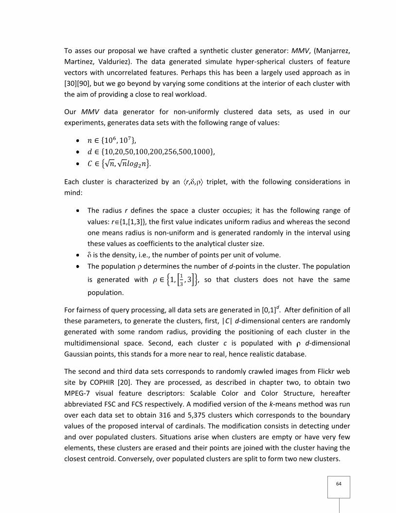
64

To asses our proposal we have crafted a synthetic cluster generator: MMV, (Manjarrez,

Martinez, Valduriez). The data generated simulate hyper-spherical clusters of feature

vectors with uncorrelated features. Perhaps this has been a largely used approach as in

[30][90], but we go beyond by varying some conditions at the interior of each cluster with

the aim of providing a close to real workload.

Our MMV data generator for non-uniformly clustered data sets, as used in our

experiments, generates data sets with the following range of values:

,

,

.

Each cluster is characterized by an r, , triplet, with the following considerations in

mind:

The radius r defines the space a cluster occupies; it has the following range of

values: r {1,[1,3]}, the first value indicates uniform radius and whereas the second

one means radius is non-uniform and is generated randomly in the interval using

these values as coefficients to the analytical cluster size.

is the density, i.e., the number of points per unit of volume.

The population determines the number of d-points in the cluster. The population

is generated with , so that clusters does not have the same

population.

For fairness of query processing, all data sets are generated in [0,1]d. After definition of all

these parameters, to generate the clusters, first, |C| d-dimensional centers are randomly

generated with some random radius, providing the positioning of each cluster in the

multidimensional space. Second, each cluster c is populated with d-dimensional

Gaussian points, this stands for a more near to real, hence realistic database.

The second and third data sets corresponds to randomly crawled images from Flickr web

site by COPHIR [20]. They are processed, as described in chapter two, to obtain two

MPEG-7 visual feature descriptors: Scalable Color and Color Structure, hereafter

abbreviated FSC and FCS respectively. A modified version of the k-means method was run

over each data set to obtain 316 and 5,375 clusters which corresponds to the boundary

values of the proposed interval of cardinals. The modification consists in detecting under

and over populated clusters. Situations arise when clusters are empty or have very few

elements, these clusters are erased and their points are joined with the cluster having the

closest centroid. Conversely, over populated clusters are split to form two new clusters.

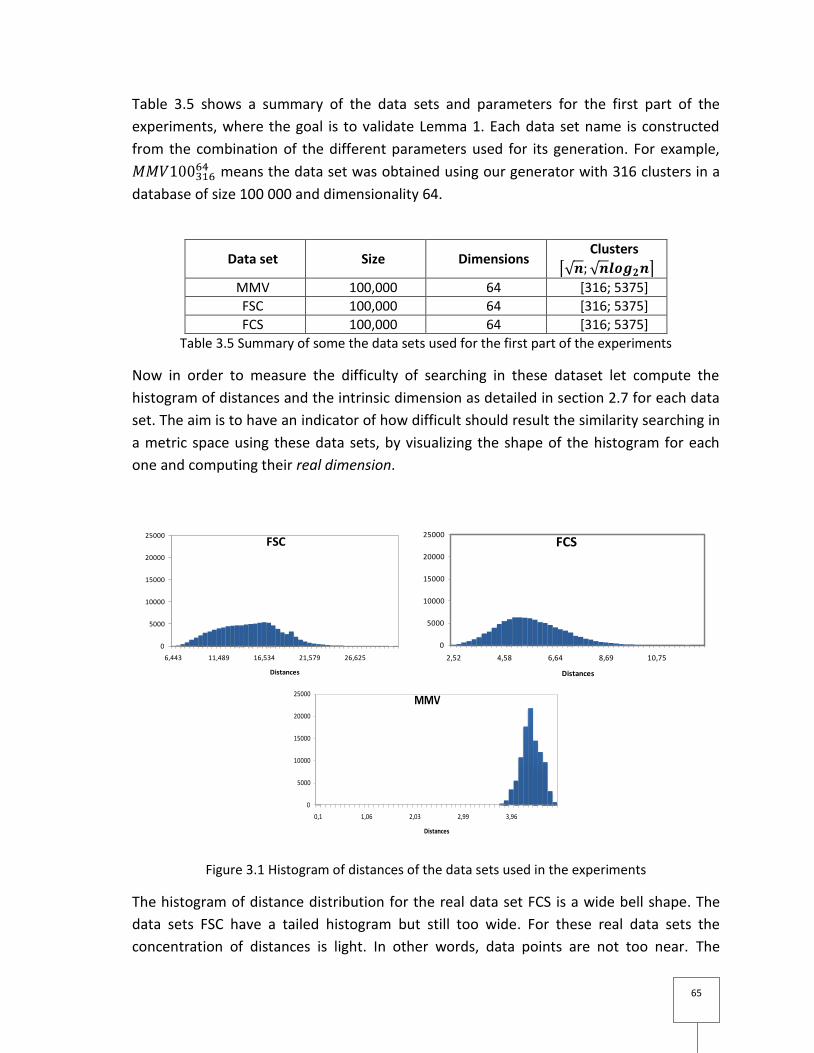
65

Table 3.5 shows a summary of the data sets and parameters for the first part of the

experiments, where the goal is to validate Lemma 1. Each data set name is constructed

from the combination of the different parameters used for its generation. For example,

means the data set was obtained using our generator with 316 clusters in a

database of size 100 000 and dimensionality 64.

Data set Size Dimensions Clusters

MMV 100,000 64 [316; 5375]

FSC 100,000 64 [316; 5375]

FCS 100,000 64 [316; 5375]

Table 3.5 Summary of some the data sets used for the first part of the experiments

Now in order to measure the difficulty of searching in these dataset let compute the

histogram of distances and the intrinsic dimension as detailed in section 2.7 for each data

set. The aim is to have an indicator of how difficult should result the similarity searching in

a metric space using these data sets, by visualizing the shape of the histogram for each

one and computing their real dimension.

Figure 3.1 Histogram of distances of the data sets used in the experiments

The histogram of distance distribution for the real data set FCS is a wide bell shape. The

data sets FSC have a tailed histogram but still too wide. For these real data sets the

concentration of distances is light. In other words, data points are not too near. The

0

5000

10000

15000

20000

25000

6,443 11,489 16,534 21,579 26,625

Distances

FSC

0

5000

10000

15000

20000

25000

2,52 4,58 6,64 8,69 10,75

Distances

FCS

0

5000

10000

15000

20000

25000

0,1 1,06 2,03 2,99 3,96

Distances

MMV

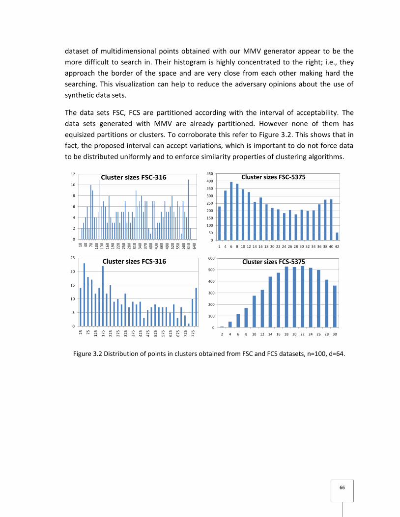
66

dataset of multidimensional points obtained with our MMV generator appear to be the

more difficult to search in. Their histogram is highly concentrated to the right; i.e., they

approach the border of the space and are very close from each other making hard the

searching. This visualization can help to reduce the adversary opinions about the use of

synthetic data sets.

The data sets FSC, FCS are partitioned according with the interval of acceptability. The

data sets generated with MMV are already partitioned. However none of them has

equisized partitions or clusters. To corroborate this refer to Figure 3.2. This shows that in

fact, the proposed interval can accept variations, which is important to do not force data

to be distributed uniformly and to enforce similarity properties of clustering algorithms.

Figure 3.2 Distribution of points in clusters obtained from FSC and FCS datasets, n=100, d=64.

0

2

4

6

8

10

12

10 40 7010

013

016

019

022

025

028

031

034

037

040

043

046

049

052

055

058

061

064

0

Cluster sizes FSC-316

0

50

100

150

200

250

300

350

400

450

2 4 6 8 10 12 14 16 18 20 22 24 26 28 30 32 34 36 38 40 42

Cluster sizes FSC-5375

0

5

10

15

20

25

25

75

12

5

17

5

22

5

27

5

32

5

37

5

42

5

47

5

52

5

57

5

62

5

67

5

72

5

77

5

Cluster sizes FCS-316

0

100

200

300

400

500

600

2 4 6 8 10 12 14 16 18 20 22 24 26 28 30

Cluster sizes FCS-5375

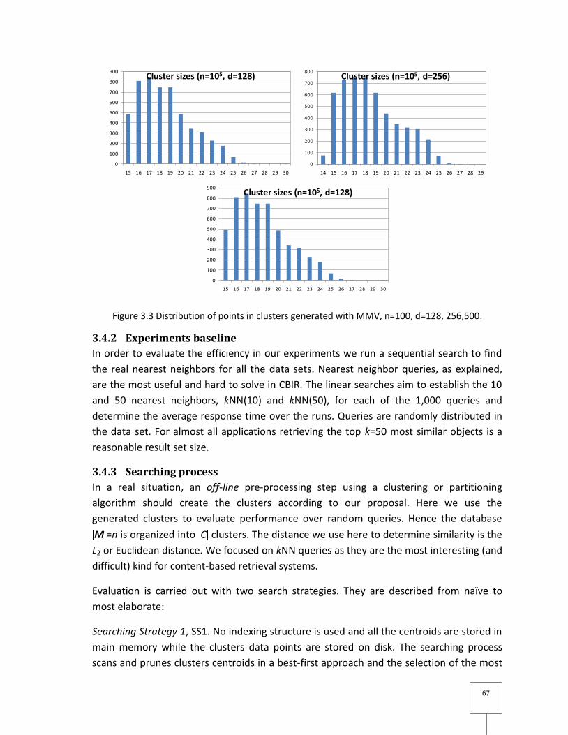
67

Figure 3.3 Distribution of points in clusters generated with MMV, n=100, d=128, 256,500.

3.4.2 Experiments baseline

In order to evaluate the efficiency in our experiments we run a sequential search to find

the real nearest neighbors for all the data sets. Nearest neighbor queries, as explained,

are the most useful and hard to solve in CBIR. The linear searches aim to establish the 10

and 50 nearest neighbors, kNN(10) and kNN(50), for each of the 1,000 queries and

determine the average response time over the runs. Queries are randomly distributed in

the data set. For almost all applications retrieving the top k=50 most similar objects is a

reasonable result set size.

3.4.3 Searching process

In a real situation, an off-line pre-processing step using a clustering or partitioning

algorithm should create the clusters according to our proposal. Here we use the

generated clusters to evaluate performance over random queries. Hence the database

M =n is organized into C clusters. The distance we use here to determine similarity is the

L2 or Euclidean distance. We focused on kNN queries as they are the most interesting (and

difficult) kind for content-based retrieval systems.

Evaluation is carried out with two search strategies. They are described from naïve to

most elaborate:

Searching Strategy 1, SS1. No indexing structure is used and all the centroids are stored in

main memory while the clusters data points are stored on disk. The searching process

scans and prunes clusters centroids in a best-first approach and the selection of the most

0

100

200

300

400

500

600

700

800

900

15 16 17 18 19 20 21 22 23 24 25 26 27 28 29 30

Cluster sizes (n=105, d=128)

0

100

200

300

400

500

600

700

800

14 15 16 17 18 19 20 21 22 23 24 25 26 27 28 29


0

100

200

300

400

500

600

700

800

900

15 16 17 18 19 20 21 22 23 24 25 26 27 28 29 30


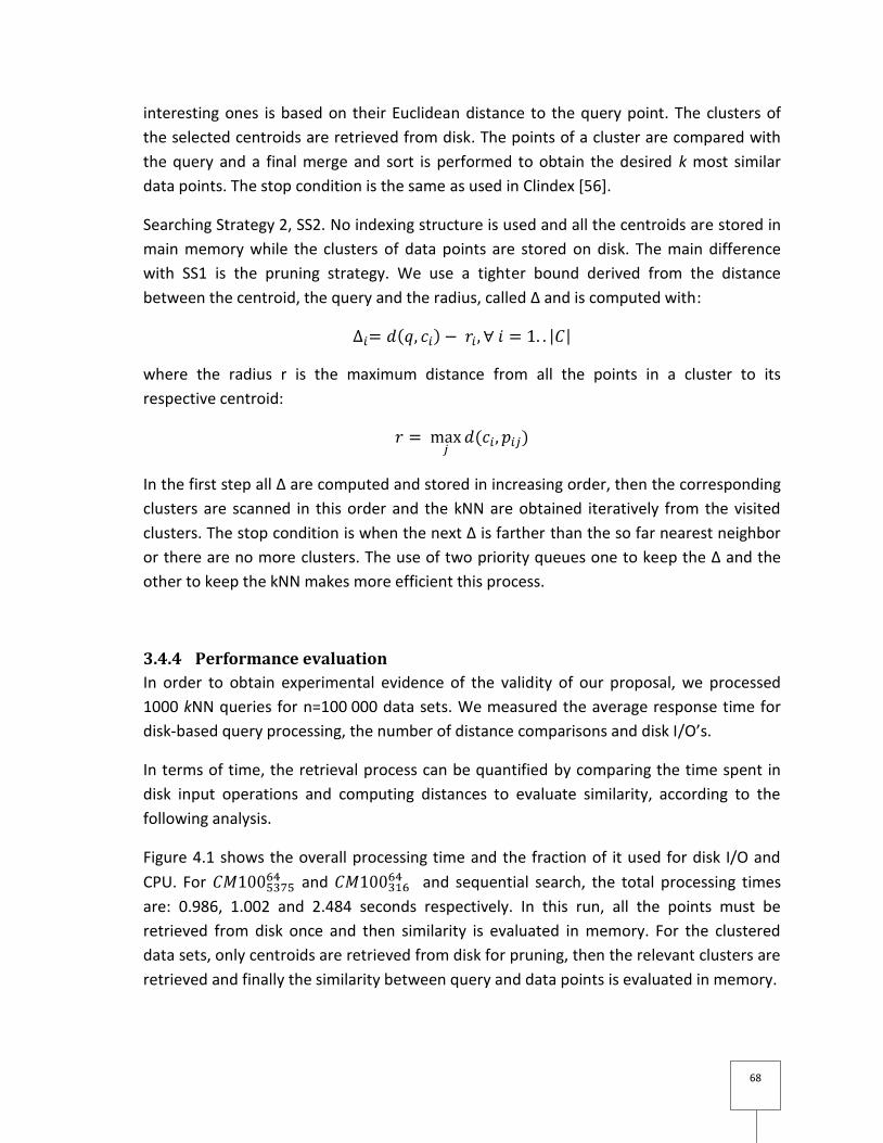
68

interesting ones is based on their Euclidean distance to the query point. The clusters of

the selected centroids are retrieved from disk. The points of a cluster are compared with

the query and a final merge and sort is performed to obtain the desired k most similar

data points. The stop condition is the same as used in Clindex [56].

Searching Strategy 2, SS2. No indexing structure is used and all the centroids are stored in

main memory while the clusters of data points are stored on disk. The main difference

with SS1 is the pruning strategy. We use a tighter bound derived from the distance

between the centroid, the query and the radius, called ∆ and is computed with:

where the radius r is the maximum distance from all the points in a cluster to its

respective centroid:

In the first step all ∆ are computed and stored in increasing order, then the corresponding

clusters are scanned in this order and the kNN are obtained iteratively from the visited

clusters. The stop condition is when the next ∆ is farther than the so far nearest neighbor

or there are no more clusters. The use of two priority queues one to keep the ∆ and the

other to keep the kNN makes more efficient this process.

3.4.4 Performance evaluation

In order to obtain experimental evidence of the validity of our proposal, we processed

1000 kNN queries for n=100 000 data sets. We measured the average response time for

disk-based query processing, the number of distance comparisons and disk I/O’s.

In terms of time, the retrieval process can be quantified by comparing the time spent in

disk input operations and computing distances to evaluate similarity, according to the

following analysis.

Figure 4.1 shows the overall processing time and the fraction of it used for disk I/O and

CPU. For and and sequential search, the total processing times

are: 0.986, 1.002 and 2.484 seconds respectively. In this run, all the points must be

retrieved from disk once and then similarity is evaluated in memory. For the clustered

data sets, only centroids are retrieved from disk for pruning, then the relevant clusters are

retrieved and finally the similarity between query and data points is evaluated in memory.

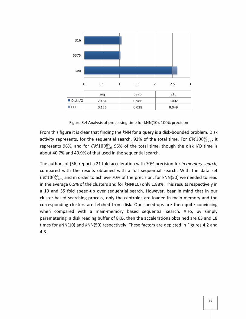
69

Figure 3.4 Analysis of processing time for kNN(10), 100% precision

From this figure it is clear that finding the kNN for a query is a disk-bounded problem. Disk

activity represents, for the sequential search, 93% of the total time. For , it

represents 96%, and for 95% of the total time, though the disk I/O time is

about 40.7% and 40.9% of that used in the sequential search.

The authors of [56] report a 21 fold acceleration with 70% precision for in memory search,

compared with the results obtained with a full sequential search. With the data set

and in order to achieve 70% of the precision, for kNN(50) we needed to read

in the average 6.5% of the clusters and for kNN(10) only 1.88%. This results respectively in

a 10 and 35 fold speed-up over sequential search. However, bear in mind that in our

cluster-based searching process, only the centroids are loaded in main memory and the

corresponding clusters are fetched from disk. Our speed-ups are then quite convincing

when compared with a main-memory based sequential search. Also, by simply

parametering a disk reading buffer of 8KB, then the accelerations obtained are 63 and 18

times for kNN(10) and kNN(50) respectively. These factors are depicted in Figures 4.2 and

4.3.

0 0.5 1 1.5 2 2.5 3

seq

5375

316

seq 5375 316

Disk I/O 2.484 0.986 1.002

CPU 0.156 0.038 0.049

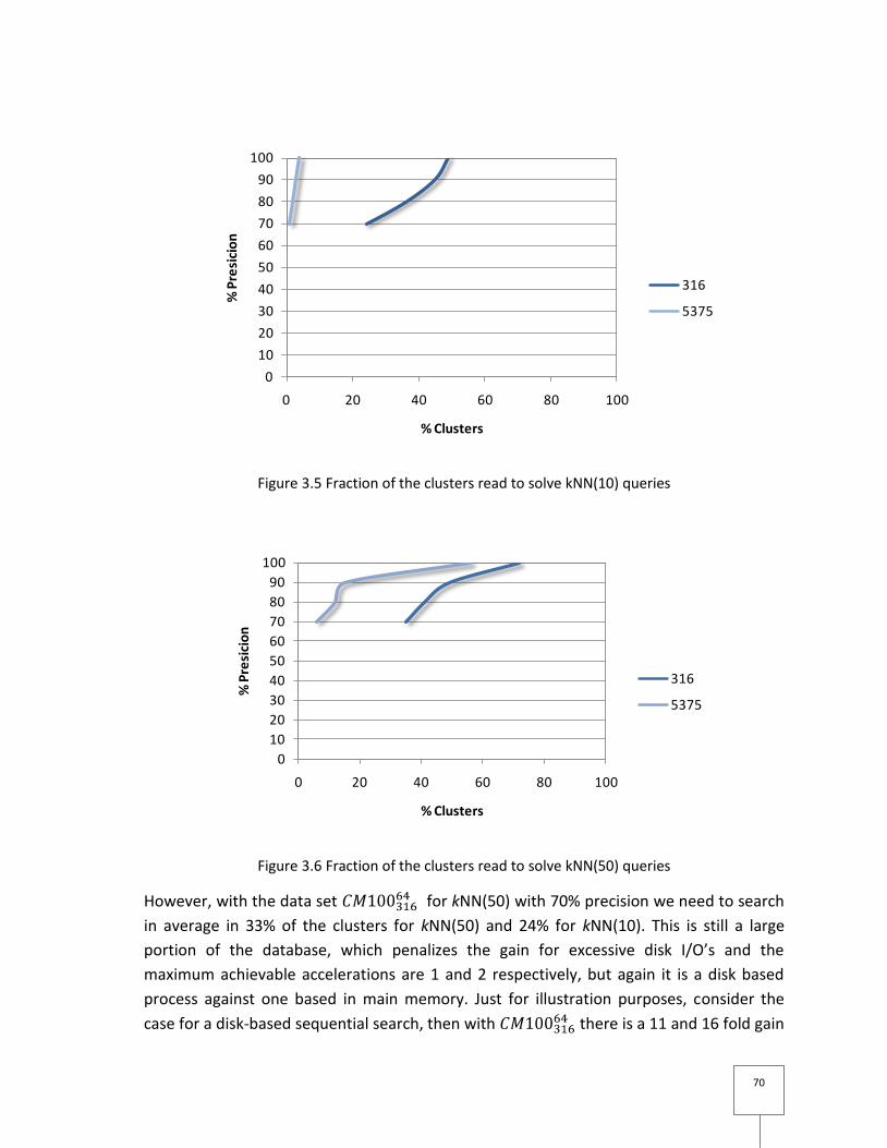
70

Figure 3.5 Fraction of the clusters read to solve kNN(10) queries

Figure 3.6 Fraction of the clusters read to solve kNN(50) queries

However, with the data set for kNN(50) with 70% precision we need to search

in average in 33% of the clusters for kNN(50) and 24% for kNN(10). This is still a large

portion of the database, which penalizes the gain for excessive disk I/O’s and the

maximum achievable accelerations are 1 and 2 respectively, but again it is a disk based

process against one based in main memory. Just for illustration purposes, consider the

case for a disk-based sequential search, then with there is a 11 and 16 fold gain

0

10

20

30

40

50

60

70

80

90

100

0 20 40 60 80 100

% P

resi

cio

n

% Clusters

316

5375

0

10

20

30

40

50

60

70

80

90

100

0 20 40 60 80 100

% P

resi

cio

n

% Clusters

316

5375

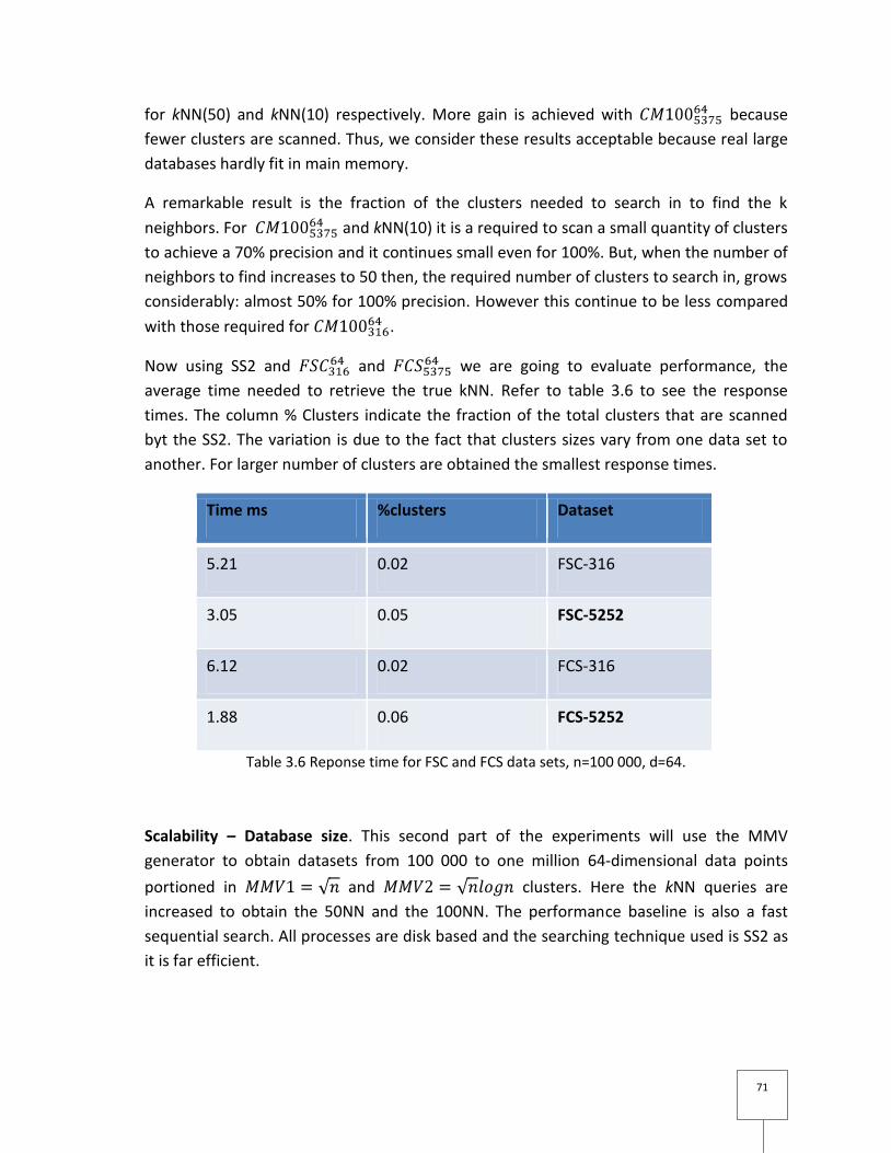
71

for kNN(50) and kNN(10) respectively. More gain is achieved with because

fewer clusters are scanned. Thus, we consider these results acceptable because real large

databases hardly fit in main memory.

A remarkable result is the fraction of the clusters needed to search in to find the k

neighbors. For and kNN(10) it is a required to scan a small quantity of clusters

to achieve a 70% precision and it continues small even for 100%. But, when the number of

neighbors to find increases to 50 then, the required number of clusters to search in, grows

considerably: almost 50% for 100% precision. However this continue to be less compared

with those required for .

Now using SS2 and and we are going to evaluate performance, the

average time needed to retrieve the true kNN. Refer to table 3.6 to see the response

times. The column % Clusters indicate the fraction of the total clusters that are scanned

byt the SS2. The variation is due to the fact that clusters sizes vary from one data set to

another. For larger number of clusters are obtained the smallest response times.

Time ms %clusters Dataset

5.21 0.02 FSC-316

3.05 0.05 FSC-5252

6.12 0.02 FCS-316

1.88 0.06 FCS-5252

Table 3.6 Reponse time for FSC and FCS data sets, n=100 000, d=64.

Scalability – Database size. This second part of the experiments will use the MMV

generator to obtain datasets from 100 000 to one million 64-dimensional data points

portioned in and clusters. Here the kNN queries are

increased to obtain the 50NN and the 100NN. The performance baseline is also a fast

sequential search. All processes are disk based and the searching technique used is SS2 as

it is far efficient.

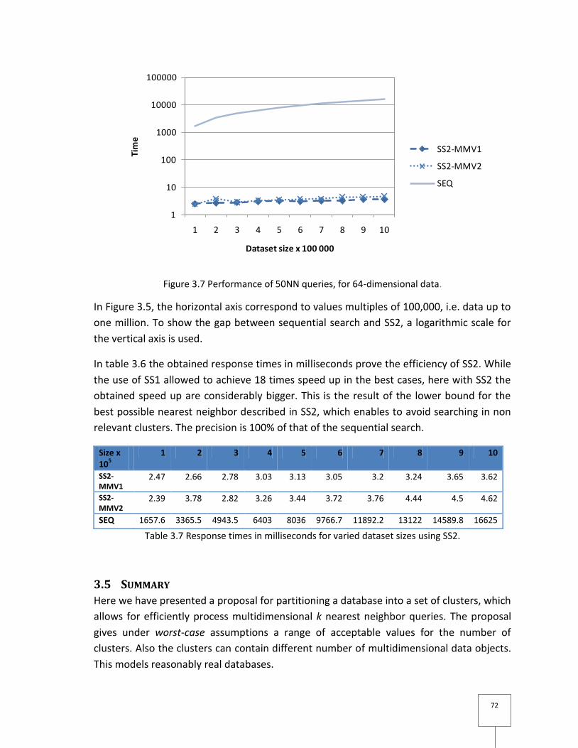
72

Figure 3.7 Performance of 50NN queries, for 64-dimensional data.

In Figure 3.5, the horizontal axis correspond to values multiples of 100,000, i.e. data up to

one million. To show the gap between sequential search and SS2, a logarithmic scale for

the vertical axis is used.

In table 3.6 the obtained response times in milliseconds prove the efficiency of SS2. While

the use of SS1 allowed to achieve 18 times speed up in the best cases, here with SS2 the

obtained speed up are considerably bigger. This is the result of the lower bound for the

best possible nearest neighbor described in SS2, which enables to avoid searching in non

relevant clusters. The precision is 100% of that of the sequential search.

Size x 10

5 1 2 3 4 5 6 7 8 9 10

SS2-MMV1

2.47 2.66 2.78 3.03 3.13 3.05 3.2 3.24 3.65 3.62

SS2-MMV2

2.39 3.78 2.82 3.26 3.44 3.72 3.76 4.44 4.5 4.62

SEQ 1657.6 3365.5 4943.5 6403 8036 9766.7 11892.2 13122 14589.8 16625

Table 3.7 Response times in milliseconds for varied dataset sizes using SS2.

3.5 SUMMARY

Here we have presented a proposal for partitioning a database into a set of clusters, which

allows for efficiently process multidimensional k nearest neighbor queries. The proposal

gives under worst-case assumptions a range of acceptable values for the number of

clusters. Also the clusters can contain different number of multidimensional data objects.

This models reasonably real databases.

1

10

100

1000

10000

100000

1 2 3 4 5 6 7 8 9 10

Tim

e

Dataset size x 100 000

SS2-MMV1

SS2-MMV2

SEQ

73

We used the grouping properties of the k-means method to partition the database to

speed up retrieval. More elaborated or efficient partitioning algorithms can be used to

improve clustering accuracy. For us, it is important to avoid very small and very large

clusters.

From the results obtained in the experiments, we can conclude that:

The search is a disk-bounded process. More than 90% of the searching time is

spent by loading data from disk to RAM.

Smaller cluster sizes increase precision. This is due to the fact the there is a better

coverage of the data space. Having large clusters means more overlapping

between them, and this misleads pruning algorithms and the number of retained

clusters remains large. Figures 2 and 3 corroborate this statement. Hence, dividing

a data set in clusters shall enable a searching algorithm to reach

the most efficient levels of performance.

SS2 which provides a better lower bound for the distances from the clusters to the

query speed up the searching process.

These results were published in [61].

74

75

4 PARALLEL NEAREST NEIGHBOR

QUERIES

Based on previous results [64], we hereafter address the scalability issue of answering

efficiently similarity queries by exploring a combination of data partitioning, i.e.,

clustering, as a pre-processing step together with small-sized parallelism at run-time.

This chapter exploits the popular parallel shared-nothing architecture to provide fast CBIR

to large databases with high-dimensional data descriptions. Assuming that a partitioning

process has been applied on the database and based on the optimal number of clusters

derived in Chapter 3, this chapter proposes a data allocation scheme which leads to an

optimal number of clusters and nodes. The method is validated through experiments with

different high-dimensional databases and implemented a query processing algorithm for

full kNN which performs orders of magnitude above the sequential search.

The sub-goals of this chapter are numerous: We want to verify and determine the optimal

number of nodes for a given database in order to achieve the best speed-up. Secondly, we

propose a query processing algorithm capable to produce results of high-precision levels.

Then, we want to determine the best placement (declustering) algorithm to maximize

parallelism. We also look for flexibility of scaling up in order to cope with bigger and bigger

databases. Of course, we aim at obtaining the shortest response time, by maximizing

throughput and minimizing resource utilization.

To our knowledge, this is the first proposal to address the performance problem to solve

nearest neighbor queries for high-dimensional data on a shared-nothing architecture,

which is optimal in minimizing the number of processing nodes for a given database. In

other words, our proposal accounts for efficient kNN query processing by maximizing

resource utilization.

The rest of the chapter is as follows: in section 4.1, we introduce the data allocation

scheme which takes into consideration the database and the parallel platform. Then in

section 4.2, we present various experiments to test the implications on performance of

the proposed number of clusters in combination with the parallel shared-nothing

machine. Finally in section 4.2, we present some concluding remarks.

76

4.1 DATA ALLOCATION SCHEME

Our data allocation or desclustering scheme proceeds in two steps:

1) data partitioning which produces a set of clusters;

2) data placement which places the clusters on the available nodes.

This aims to reduce the time required to perform full search by distributing the database

among the nodes of the SN parallel system.

4.1.1 Data partitioning

To overcome the problem introduced by the dimensionality of the data objects, which

eventually deteriorates a search into a sequential, or even worst, one possibility is to rely

on a clustering of the database. Although this process is computationally expensive, it can

be done off-line, in a pre-processing step before query execution. The goal is to minimize

the number of inter-point distances to compute per query, by grouping them together

based on their similarity. We do not suggest the use of any specific clustering or

partitioning process. This has been the focus of several works [47][51] and better yet, to

take advantage of the available parallel power and make this pre-processing faster [6].

Thus, we assume that a given database of size n, can be partitioned by using some

partitioning process, which produces a set C of clusters of data objects.

Based on the partitioning of the database, when executing a query, the set of clusters C

can be pruned to a subset of candidate clusters C’ containing the most similar objects.

In the previous chapter we studied and developed on this idea. Our proposal for

partitioning the database is then . Additionally, it can be derived some

algorithmic variations, from optimal to suboptimal in , under less restrictive

conditions, and , the optimal case can be obtained with

a near multiplicative factor λ, since C’ is small and independent of n.

4.1.2 Data placement (data layout)

Two objectives drive this section:

minimizing the number of data objects which reside on disk and are requested

simultaneously,

maximizing the utilization of the processing resources.

The first objective is achieved by an efficient data layout mechanism whereas the latter is

reached by an algorithmic approach described in Theorem 1.

Intuitively similar objects should be placed in different nodes hence parallel retrieval takes

place, thus in can be enhanced the probability that a query has equally distributed the

77

required clusters over the nodes. This is the basic observation that motivates our data

layout proposal. Recall from chapter 1 and 2 that the optimal method aims to have no

more than clusters processed at each node, this balancing the workload and

reducing the processing time by improving parallelism.

Once the database is partitioned into clusters according to our proposal depicted in

lemma 1 (previous chapter), we need to place these clusters onto the nodes of the

parallel system. Our solution for the placement of the clusters is to determine the number

of nodes which yields the best (asymptotically) achievable performance.

In order to avoid system overhead, there must be a balance between the size of the

database and the number of nodes.

Thus we state the following theorem:

Theorem 1. Assume a shared nothing parallel system of at least nodes, then the

average complexity of any query is in .

Proof: The proof can be achieved as a result of Lemma 1 and of by a simple round robin

placement of the clusters over the available nodes. That is, distributing clusters

over log2n nodes, each node will have clusters each one containing in average

objects. With clusters selected, in the worst case the average

number of selected classes on each node is only one. The local complexities, executed in

parallel over all the participating nodes, are then:

Since the last product factor is very small, we can ignore it. Thus we get the approximation

Consolidation of results must be carried out by merging the local results, which are limited

to the best k found data objects. In the worst case, each node returns as many results as

there are objects in the treated class, that is , and all the nodes participate in

the merging of the results, and the parallel complexity of the process is in:

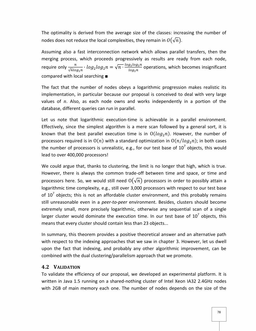
78

The optimality is derived from the average size of the classes: increasing the number of

nodes does not reduce the local complexities, they remain in .

Assuming also a fast interconnection network which allows parallel transfers, then the

merging process, which proceeds progressively as results are ready from each node,

require only operations, which becomes insignificant

compared with local searching ■

The fact that the number of nodes obeys a logarithmic progression makes realistic its

implementation, in particular because our proposal is conceived to deal with very large

values of n. Also, as each node owns and works independently in a portion of the

database, different queries can run in parallel.

Let us note that logarithmic execution-time is achievable in a parallel environment.

Effectively, since the simplest algorithm is a mere scan followed by a general sort, it is

known that the best parallel execution time is in . However, the number of

processors required is in with a standard optimization in ; in both cases

the number of processors is unrealistic, e.g., for our test base of 107 objects, this would

lead to over 400,000 processors!

We could argue that, thanks to clustering, the limit is no longer that high, which is true.

However, there is always the common trade-off between time and space, or time and

processors here. So, we would still need processors in order to possibly attain a

logarithmic time complexity, e.g., still over 3,000 processors with respect to our test base

of 107 objects; this is not an affordable cluster environment, and this probably remains

still unreasonable even in a peer-to-peer environment. Besides, clusters should become

extremely small, more precisely logarithmic, otherwise any sequential scan of a single

larger cluster would dominate the execution time. In our test base of 107 objects, this

means that every cluster should contain less than 23 objects...

In summary, this theorem provides a positive theoretical answer and an alternative path

with respect to the indexing approaches that we saw in chapter 3. However, let us dwell

upon the fact that indexing, and probably any other algorithmic improvement, can be

combined with the dual clustering/parallelism approach that we promote.

4.2 VALIDATION

To validate the efficiency of our proposal, we developed an experimental platform. It is

written in Java 1.5 running on a shared-nothing cluster of Intel Xeon IA32 2.4GHz nodes

with 2GB of main memory each one. The number of nodes depends on the size of the

79

database. In this section, we describe the data sets used, the k nearest neighbor searching

process and the performance results obtained.

4.2.1 Data sets

The same generators for realistic data sets and the COPHIR [20] database are used for

evaluating the efficiency and scalability of our declustering method.

4.2.2 kNN searching process

We now describe our simple but effective algorithm to enable fast processing of kNN

queries [79] in the parallel system. Keep in mind that the process follows the parameters

given in section 4.1.1 which are indeed the result from last chapter and the process is disk

based, i.e., all data is stored in disk while performing the searching process.

Step 1. Data Distribution

We did not try yet to develop a heuristic algorithm for optimizing the placement of the

clusters. Nevertheless, the placement algorithm could take into consideration closeness

between classes to distribute the nearest ones over different nodes. However, as we have

shown, this is a questionable trade-off: investing to reach a minimal gain at the cost of

some (maybe) expensive process. Therefore in these experiments, the clusters are

distributed on the log2n machines in a round-robin way. Therefore, all the nodes have

almost the same number of clusters (which have approximately the same number of

objects).

Step 2. Cluster Selection.

Query points are generated randomly under the same assumptions than the generated

data sets. To find the set of kNN objects for a query q, a sufficient number of classes must

be selected in order to ensure to return the best k d-points. Firstly, a sequential disk-

based search is executed to compare q with all the centroids, using the common Euclidean

distance, and using the radiuses in order to find the nearest clusters1. The first log2n

clusters are considered. For each selected cluster, we know the node on which it has been

placed during step 1.

With this simple heuristic, we aim at retrieving all the kNN which is equivalent to a full

search. Indeed, in several research works on kNN query processing analysis [12,56]

propose a threshold which guarantees the retrieval of all or a high percentage of the NN.

1 Let us note that even though the centroids of the clusters could fit into main memory, if

we consider that the data is actually stored in a database and our aim is to validate our

proposal for worst case conditions, then the process is disk-based.

80

Here, taking the first ranked log2n clusters is a threshold large enough to achieve full

precision.

Step 3. Sequential Scans of the Selected Clusters

Once known the node for each cluster of interest, a parallel search is executed on them to

retrieve up to k objects. On each node, the scan of the locally selected class(es) takes

place in the form of a mere sequential search and the use of a bounded priority queue to

keep the best k responses. Therefore, each node returns a set of k sorted elements to the

master node.

Step 4. Merging

The master node merges the various results arriving from the nodes, prunes the list to the

best k global answers, and returns it to the user or the application.

4.2.3 Performance evaluation

In order to obtain experimental evidence of how well our data allocation method

improves the processing of nearest neighbor queries, we processed 1000 kNN queries

from the same data space for the above mentioned data sets. We measured:

the average response time,

the number of distance comparisons,

the number of disk I/O’s.

The results presented here are for databases of 107 data objects. The sizes of k for the

queries are 50, 100 and 150. The data generator used is MMV.

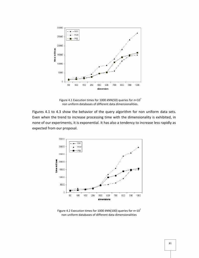
81

Figure 4.1 Execution times for 1000 kNN(50) queries for n=107

non uniform databases of different data dimensionalities.

Figures 4.1 to 4.3 show the behavior of the query algorithm for non uniform data sets.

Even when the trend to increase processing time with the dimensionality is exhibited, in

none of our experiments, it is exponential. It has also a tendency to increase less rapidly as

expected from our proposal.

Figure 4.2 Execution times for 1000 kNN(100) queries for n=107

non uniform databases of different data dimensionalities

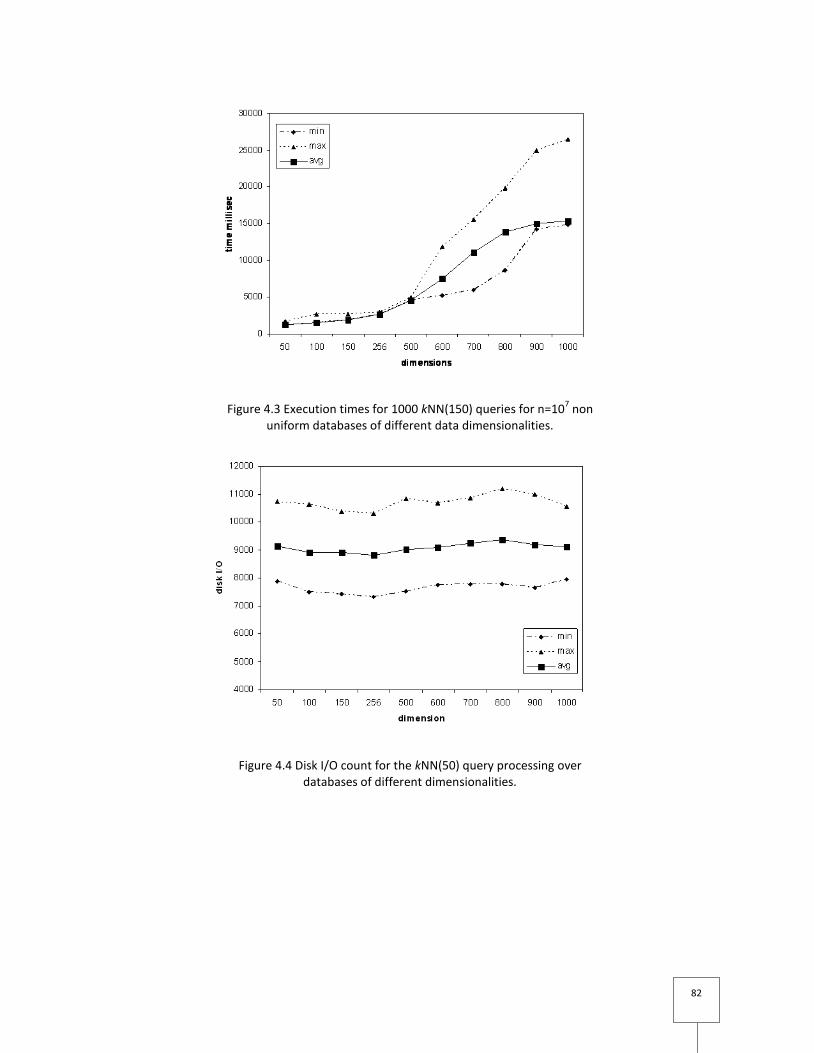
82

Figure 4.3 Execution times for 1000 kNN(150) queries for n=107 non

uniform databases of different data dimensionalities.

Figure 4.4 Disk I/O count for the kNN(50) query processing over databases of different dimensionalities.

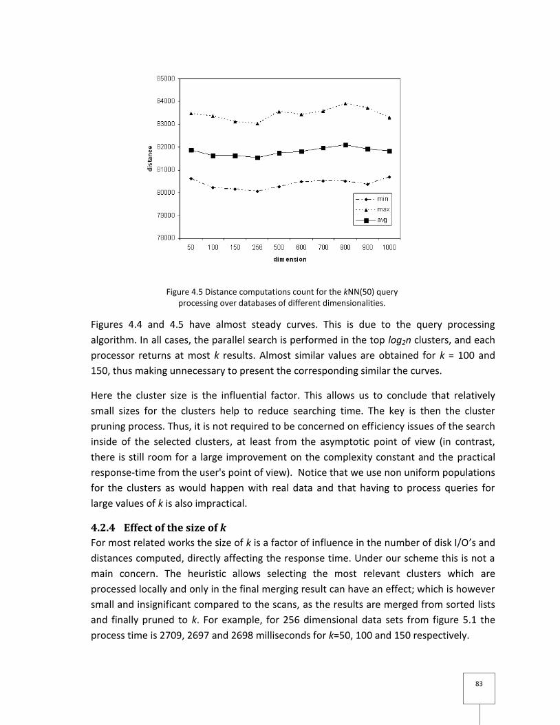
83

Figure 4.5 Distance computations count for the kNN(50) query processing over databases of different dimensionalities.

Figures 4.4 and 4.5 have almost steady curves. This is due to the query processing

algorithm. In all cases, the parallel search is performed in the top log2n clusters, and each

processor returns at most k results. Almost similar values are obtained for k = 100 and

150, thus making unnecessary to present the corresponding similar the curves.

Here the cluster size is the influential factor. This allows us to conclude that relatively

small sizes for the clusters help to reduce searching time. The key is then the cluster

pruning process. Thus, it is not required to be concerned on efficiency issues of the search

inside of the selected clusters, at least from the asymptotic point of view (in contrast,

there is still room for a large improvement on the complexity constant and the practical

response-time from the user's point of view). Notice that we use non uniform populations

for the clusters as would happen with real data and that having to process queries for

large values of k is also impractical.

4.2.4 Effect of the size of k

For most related works the size of k is a factor of influence in the number of disk I/O’s and

distances computed, directly affecting the response time. Under our scheme this is not a

main concern. The heuristic allows selecting the most relevant clusters which are

processed locally and only in the final merging result can have an effect; which is however

small and insignificant compared to the scans, as the results are merged from sorted lists

and finally pruned to k. For example, for 256 dimensional data sets from figure 5.1 the

process time is 2709, 2697 and 2698 milliseconds for k=50, 100 and 150 respectively.

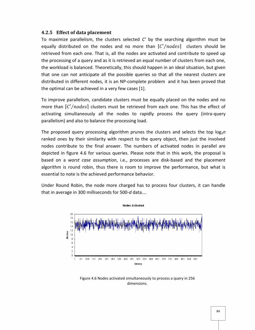
84

4.2.5 Effect of data placement

To maximize parallelism, the clusters selected C’ by the searching algorithm must be

equally distributed on the nodes and no more than clusters should be

retrieved from each one. That is, all the nodes are activated and contribute to speed up

the processing of a query and as it is retrieved an equal number of clusters from each one,

the workload is balanced. Theoretically, this should happen in an ideal situation, but given

that one can not anticipate all the possible queries so that all the nearest clusters are

distributed in different nodes, it is an NP-complete problem and it has been proved that

the optimal can be achieved in a very few cases [1].

To improve parallelism, candidate clusters must be equally placed on the nodes and no

more than clusters must be retrieved from each one. This has the effect of

activating simultaneously all the nodes to rapidly process the query (intra-query

parallelism) and also to balance the processing load.

The proposed query processing algorithm prunes the clusters and selects the top log2n

ranked ones by their similarity with respect to the query object, then just the involved

nodes contribute to the final answer. The numbers of activated nodes in parallel are

depicted in figure 4.6 for various queries. Please note that in this work, the proposal is

based on a worst case assumption, i.e., processes are disk-based and the placement

algorithm is round robin, thus there is room to improve the performance, but what is

essential to note is the achieved performance behavior.

Under Round Robin, the node more charged has to process four clusters, it can handle

that in average in 300 milliseconds for 500-d data.…

Figure 4.6 Nodes activated simultaneously to process a query in 256 dimensions.

85

4.3 SUMMARY

In this chapter we proposed a data allocation scheme for efficient kNN query processing

on multimedia databases in a shared-nothing architecture [62]. Our proposal can be

summarized to the following contribution: an upper and a lower bound on the number of

fragments or clusters that can be obtained from the database and the number of nodes

required to maximize resources utilization and to achieve optimal parallel kNN searching

[63]. The number of clusters is based on the complexity analysis of the general search

problem for CBR and the number of nodes in the parallel architecture is proposed on the

same principle but taking into consideration that it must be feasible to implement the

architecture. We validated our method for different non uniform data sets under worst-

case hypothesis. Any improvements such as: a better placement scheme and putting into

main memory the centroids must signify a performance improvement. Here we showed

that our proposal stands for the derived algorithmic complexities.

86

87

5 CONCLUSIONS

In this final chapter we summarize the contributions of this thesis. We also discuss further

and promising improvements and research directions.

Our proposals are around the potential of data clustering techniques as a preprocessing

step for scaling CBIR to large databases more efficiently than simple sequential search.

These results were published into three international conferences.

Firstly, we have analyzed the complexity of searching using clustering, we have used a

modified k-means as the underlying clustering process and provided a range of values for

k which allows to bound the running time several times in average over sequential search

[61]. This result can be seen as:

A way to provide the value of k for the k-means clustering algorithm, using a query

efficiency approach

A framework for similarity search based on clustering, as it is provided the size of

cluster to yield efficient retrieval

A database partitioning step in a declustering method for parallel retrieval.

Secondly, we have presented a declustering technique for image databases in parallel

shared nothing architectures in chapter 4. Our proposal uses the results for database

partitioning obtained in chapter 3 complemented with a placement strategy. We have

presented a simple random round robin placement strategy [62]. We have shown that

declustering optimality is difficult to achieve and the results obtained with naive round

robin are comparable to the ones obtained by more sophisticated placement strategies.

This corroborates previous research done in the context of parallel spatial and RDBMS .

Additionally we have presented algorithms to efficiently process kNN [63]. The results

show a great improvement over sequential search and maintains the theoretical

expected running time which is better than previous research, performing at best in

.

5.1 FURTHER WORK. QUERY PROCESSING

In this work we have concentrated in kNN queries and the use of global descriptors, of

further relevance is the processing of range and orthogonal range queries, the use of local

descriptors and related similarity distances. This proposal is aimed to enhance perceptual

precision of results. It is known that visual similarity is improved by the use of local

descriptors which are obtained in large quantities from images and the Euclidean

88

distances is not precisely the most suitable. This context increases the computational cost

of similarity search, hence the interest of using the computational power of our proposal

to solve these kinds of problems.

5.2 FURTHER WORK. MULTIUSER

This topic is related with a production system which has to guarantee the required service

level to users (QoS), i.e., to avoid users experience delays. It is by itself a complete

research subject. Capacity planning is an analysis step aiming at determining first the

maximum amount of load that a system is capable of handle correctly with a set of

resources. The system must be stressed (load testing at unusual/peak conditions) to

determine its capacity (to understand its behavior). In general capacity is increased by

increasing the number of machines. However there is a latency overhead introduced by

resource synchronization, communication, manageability and additionally increased price.

This is also a matter of QoS issues.

89

6 REFERENCES

1 Abdel-Ghaffar, K. A. and Abbadi, A. E. 1997. Optimal Allocation of Two-Dimensional

Data. In Proceedings of the 6th international Conference on Database theory (January

08 - 10, 1997). F. N. Afrati and P. G. Kolaitis, Eds. Lecture Notes In Computer Science,

vol. 1186. Springer-Verlag, London, 409-418.

2 Abdel-Ghaffar, K. A. and Abbadi, A. E. 2006. The Optimality of Allocation Methods for

Bounded Disagreement Search Queries: The Possible and the Impossible. IEEE Trans.

on Knowl. and Data Eng. 18, 9 (Sep. 2006), 1194-1206.

3 Alpkocak, A. Danisman, T, Ulker, T. 2002. A Parallel Similarity Search in High

Dimensional Metric Space Using M-Tree. In: Advanced Environments, Tools, and

Applications for Cluster Computing: NATO Advanced Research Workshop, IWCC 2001.

Lecture Notes in Computer Science Vol. 2326. Springer (2002) 166-171.

4 Amdhal, G.M. 1967. Validity of a single processor approach to achieving large scale

computing capabilities. In proceedings of the AFIPS Conference (1967) 483-485.

5 Anderson, T. E., Culler, D. E., Patterson, D. A., and the NOW team 1995. A Case for

NOW (Networks of Workstations). IEEE Micro 15, 1 (Feb. 1995), 54-64.

6 Attila Gürsoy, E.E.: Data Decomposition for Parallel K-means Clustering. In: PPAM ‘03:

Lecture Notes in Computer Science Vol. 3019. Springer. (2004) 241-248

7 Barroso, L. A., Dean, J., and Hölzle, U. 2003. Web Search for a Planet: The Google

Cluster Architecture. IEEE Micro 23, 2 (Mar. 2003), 22-28.

8 Barroso, L. A. 2005. The price of performance. Queue 3, 7 (Sep. 2005), 48-53.

9 Bay, H., Ess, A., Tuytelaars, T., and Van Gool, L. 2008. Speeded-Up Robust Features

(SURF). Comput. Vis. Image Underst. 110, 3 (Jun. 2008), 346-359.

10 Berchtold, S., Böhm, C., Braunmüller, B., Keim, D.A., Kriegel, H.: Fast parallel similarity

search in multimedia databases. In: SIGMOD Rec. 26, 2 (1997) 1-12.

11 Berchtold, S., Keim, D.A., Kriegel, H.P.. The X-tree: An Index Structure for High-

Dimensional Data, In Proceedings of the 22nd international Conference on Very Large

Data Bases (September 03-06,1996). 28-39.

12 Berrani, S.-A., Amsaleg, L., Gros, P.: Approximate Searches: k-Neighbors + Precision.

In: CIKM ‘03: Proceedings of the 12th ACM International Conference on Information

and Knowledge. (2003) 24-31.

13 Berrani, S.-A. Recherche approximative de plus proches voisins avec contrôle

probabiliste de la précision ; application la recherche d'images par le contenu. Ph.D.

thesis - University of Rennes 1, February 2004

14 Bergsten, B., Couprie, M., and Valduriez, P., Overview of Parallel Architectures for

Databases, Comput. J., 1993, vol. 36, no. 8, pp. 734-740.

90

15 Beyer,K., Goldstein,J., Ramakrishnan,R. and Shaft,U. When Is 'Nearest Neighbor'

Meaningful? Proc. Int'l Conf. Database Theory (ICDT '99), pp. 217-235, Jan. 1999.

16 Bhatia, R., Sinha, R. K., and Chen, C. 2000. Hierarchical Declustering Schemes for

Range Queries. In Proceedings of the 7th international Conference on Extending

Database Technology: Advances in Database Technology (March 27 - 31, 2000). C.

Zaniolo, P. C. Lockemann, M. H. Scholl, and T. Grust, Eds. Extending Database

Technology, vol. 1777. Springer-Verlag, London, 525-537.

17 Böhm, C., Berchtold, S., and Keim, D. A. 2001. Searching in high-dimensional spaces:

Index structures for improving the performance of multimedia databases. ACM

Comput. Surv. 33, 3 (Sep. 2001), 322-373.

18 Bok, K. S., Seo, D. M., Song, S. I., Kim, M.H., Yoo, J.S.: An Index Structure for Parallel

Processing of Multidimensional Data. In: WAIM ‘05: Advances in Web-Age

Information Management, 6th International Conference. Lecture Notes in Computer

Science Vol. 3739. Springer (2005) 589-600

19 Bok, K.S., Song, S.I., Yoo, J.S.: Efficient k-Nearest Neighbor Searches for Parallel

Multidimensional Index Structures. In: DASFAA ‘06: Database Systems for Advanced

Applications, 11th International Conference, Lecture Notes in Computer Science

Vol.3882. Springer (2006). 870-879

20 Bolettieri, P., Esuli, A., Falchi,F., Lucchese, C., Perego, R., Piccioli, T. and Rabitti, F.

2009 CoPhIR: a Test Collection for Content-Based Image Retrieval. CoRR

abs/0905.4627: (2009)

21 Bosque, J. L., Robles, O. D., Pastor, L., and Rodríguez, A. 2006. Parallel CBIR

implementations with load balancing algorithms. J. Parallel Distrib. Comput. 66, 8

(Aug. 2006), 1062-1075.

22 Bouganim, L., Jónsson, B.P., and Bonnet, P. 2009. uFLIP: Understanding Flash IO

Patterns. In 4th biennial conference on innovative data systems (CIDR'09), January 4-

7, 2009

23 Bouteldja,N, Gouet-Brunet, V., and Scholl, M. 2006. Back to the curse of

dimensionality with local image descriptors, Technical Report, CNAM, Paris, 2006.

24 Bouteldja, N., Gouet-Brunet, V., and Scholl, M. 2009. Approximate Retrieval with

HiPeR: Application to VA-Hierarchies. In Proceedings of the 15th international

Multimedia Modeling Conference on Advances in Multimedia Modeling (Sophia-

Antipolis, France, January 07 - 09, 2009). B. Huet, A. Smeaton, K. Mayer-Patel, and Y.

Avrithis, Eds. Lecture Notes In Computer Science, vol. 5371. Springer-Verlag, Berlin,

Heidelberg, 344-355.

25 Bozkaya, T. and Ozsoyoglu, M. Indexing large metric spaces for similarity search

queries. ACM Transactions on Database Systems, 24(3):361–404, 1999.

91

26 Brin, S. 1995. Near Neighbor Search in Large Metric Spaces. In Proceedings of the 21th

international Conference on Very Large Data Bases (September 11 - 15, 1995). U.

Dayal, P. M. Gray, and S. Nishio, Eds. Very Large Data Bases. Morgan Kaufmann

Publishers, San Francisco, CA, 574-584.

27 Cantone, D., Ferro, A., Pulvirenti, A., Recupero, D. R., and Shasha, D. 2005. Antipole

Tree Indexing to Support Range Search and K-Nearest Neighbor Search in Metric

Spaces. IEEE Trans. on Knowl. and Data Eng. 17, 4 (Apr. 2005), 535-550.

28 Cha, G.H. and Chung, C.W. 2002. The GC-Tree: A High-Dimensional Index Structure for

Similarity Search in Image Databases. In IEEE Trans. on Multimedia, Vol. 4, No. 2, pp.

235--247, June 2002.

29 Chakrabarti, K. and Mehrotra, S. 2000. Local Dimensionality Reduction: A New

Approach to Indexing High Dimensional Spaces. In Proceedings of the 26th

international Conference on Very Large Data Bases (September 10 - 14, 2000). 89-100.

30 Chavez, E. and Navarro, G.. An Effective Clustering Algorithm to Index High

Dimensional Metric Spaces. In Proceedings of the Seventh international Symposium on

String Processing information Retrieval (Spire'00) (September 27 - 29, 2000). SPIRE.

IEEE Computer Society, Washington, DC, 75.

31 Chávez, E., Navarro, G., Baeza-Yates, R., and Marroquín, J. L. 2001. Searching in metric

spaces. ACM Comput. Surv. 33, 3 (Sep. 2001), 273-321.

32 Chavez, E., Navarro, G. 2003 Probabilistic proximity search: Fighting the curse of

dimensionality in metric spaces. In: Information Processing Letters, Volume 85, Issue

1, 16 (2003) 39-46

33 Chávez, E. and Navarro, G. 2005. A compact space decomposition for effective metric

indexing. Pattern Recogn. Lett. 26, 9 (Jul. 2005), 1363-1376.

34 Choupo, A. K., Berti-Équille, L., and Morin, A.. Optimizing progressive query-by-

example over pre-clustered large image databases. In Proceedings of the 2nd

international Workshop on Computer Vision Meets Databases (Baltimore, MD, June

17 - 17, 2005). CVDB '05, vol. 160, 13-20.

35 Ciaccia, P., Patella, M., and Zezula, P.. M-tree: An Efficient Access Method for

Similarity Search in Metric Spaces. In Proceedings of the 23rd international Conference

on Very Large Data Bases (August 25 - 29, 1997). 426-435.

36 Duygulu, P., Barnard, K., Freitas, J. F., and Forsyth, D. A. 2002. Object Recognition as

Machine Translation: Learning a Lexicon for a Fixed Image Vocabulary. In Proceedings

of the 7th European Conference on Computer Vision-Part IV (May 28 - 31, 2002). A.

Heyden, G. Sparr, M. Nielsen, and P. Johansen, Eds. Lecture Notes In Computer

Science, vol. 2353. Springer-Verlag, London, 97-112.

92

37 Einarsson, Í. S., Erlingsson, B., Valgeirsson, Á. G., Jónsson, B. Þ. and Amsaleg, L.

2003. Using clustering to index image descriptors: A performance evaluation.

Technical Report, Reykjavík University, 2003.

38 Fang, M. T., Lee, R. C., and Chang, C. C. 1986. The Idea of De-Clustering and its

Applications. In Proceedings of the 12th international Conference on Very Large Data

Bases (August 25 - 28, 1986). W. W. Chu, G. Gardarin, S. Ohsuga, and Y. Kambayashi,

Eds. Very Large Data Bases. Morgan Kaufmann Publishers, San Francisco, CA, 181-188.

39 Ferhatosmanoglu,H., Ramachandran, A., Agrawal, D. and Abbadi, A.E. 2007. Data

space mapping for efficient IO in large multi-dimensional databases. Information

Systems 32 (2007) 83–103

40 Flickner, M., Sawhney, H., Niblack, W., Ashley, J., Huang, Q., Dom, B., Gorkani, M.,

Hafner, J., Lee, D., Petkovic, D., Steele, D., and Yanker, P. 1995. Query by Image and

Video Content: The QBIC System. Computer 28, 9 (Sep. 1995), 23-32.

41 Fukunage, K. and Narendra, P. M. 1975. A Branch and Bound Algorithm for Computing

k-Nearest Neighbors. IEEE Trans. Comput. 24, 7 (Jul. 1975), 750-753.

42 Gao Y.J., Chen G.C ., Chen L., Chen C. Best-first based parallel nearest neighbor

queries. In Proc. of International Conference on Management of Data (COMAD), 2005.

43 Gil-Costa, V., Marin, M., and Reyes, N. 2009. Parallel query processing on distributed

clustering indexes. J. of Discrete Algorithms 7, 1 (Mar. 2009), 3-17

44 Gray,J., Shenoy, P. Rules of Thumb in Data Engineering. In Proceedings of the 16th

international Conference on Data Engineering ICDE 2000. IEEE Computer Society,

Washington, DC, 3-10.

45 Guttman, A..R-trees: a dynamic index structure for spatial searching, Proceedings of

the 1984 ACM SIGMOD international conference on Management of data (June 18-21,

1984).

46 Hjaltason, G. R. and Samet, H.. Index-driven similarity search in metric spaces (Survey

Article). ACM Trans. Database Syst. 28, 4 (Dec. 2003), 517-580.

47 Jain, A.K., Dubes, R.C.: Algorithms for Clustering Data. Prentice Hall. 1988

48 Jain, A. K. 2008. Data Clustering: 50 Years Beyond K-means. In Proceedings of the 2008

European Conference on Machine Learning and Knowledge Discovery in Databases -

Part I (Antwerp, Belgium, September 15 - 19, 2008). W. Daelemans, B. Goethals, and

K. Morik, Eds. Lecture Notes In Artificial Intelligence, vol. 5211. Springer-Verlag,

Berlin, Heidelberg, 3-4.

49 Jagadish, H. V., Ooi, B. C., Tan, K., Yu, C., and Zhang, R. . iDistance: An adaptive B+-tree

based indexing method for nearest neighbor search. ACM Trans. Database Syst. 30, 2

(Jun. 2005), 364-397.

50 Kamel, I., Faloutsos, C.: Parallel R-trees. In: SIGMOD ’92: Proceedings of the ACM

international Conference on Management of Data (1992) 195-204

93

51 Kanungo, T., Mount, D. M., Netanyahu, N., Piatko, C., Silverman, R., Wu, A. Y.: An

efficient k-means clustering algorithm: Analysis and implementation. In: IEEE Trans.

Pattern Analysis and Machine Intelligence, 24 (2002) 881-892.

52 Katayama, N. and Satoh, S. 1997. The SR-tree: An Index Structure for High-

Dimensional Nearest Neighbor Queries. In Proc. Intl. Conf. on Management of Data,

ACM SIGMOD, pp. 369-380. 1997.

53 Kleinberg, J. M. 1997. Two algorithms for nearest-neighbor search in high dimensions.

In Proceedings of the Twenty-Ninth Annual ACM Symposium on theory of Computing

(El Paso, Texas, United States, May 04 - 06, 1997). STOC '97. ACM, New York, NY, 599-

608.

54 Korn,F., Pagel, B.U. and Faloutsos, C. 2001. On the dimensionality curse and the self-

similarity blessing. IEEE Trans. on Knowl. and Data Eng. 13, 1 (Jan. 2001).

55 Lejsek, H., Ásmundsson, F. H., Jónsson, B. ó. and Amsaleg, L. 2008. NV-tree: An

Efficient Disk-Based Index for Approximate Search in Very Large High-Dimensional

Collections. IEEE Transactions on Pattern Analysis and Machine Intelligence, preprint

(May 20, 2008). PAMI(31), No. 5, May 2009, pp. 869-883.

56 Li, C., Chang, E., Garcia-Molina, H., and Wiederhold, G. 2002. Clustering for

Approximate Similarity Search in High-Dimensional Spaces. IEEE Trans. on Knowl. and

Data Eng. 14, 4 (Jul. 2002), 792-808

57 Liu, D. and Shekhar, S. 1996. Partitioning similarity graphs: a framework for

declustering problems. Inf. Syst. 21, 6 (Sep. 1996), 475-496.

58 Liu, T., Rosenberg C.R., Rowley, H.A.: Clustering Billions of Images with Large Scale

Nearest Neighbor Search. 8th IEEE Workshop on Applications of Computer Vision

(WACV 2007). 28

59 Liu, Y., Zhang, D., Lu, G., and Ma, W. 2007. A survey of content-based image retrieval

with high-level semantics. Pattern Recogn. 40, 1 (Jan. 2007), 262-282.

60 Lowe, D. G. 2004. Distinctive Image Features from Scale-Invariant Keypoints. Int. J.

Comput. Vision 60, 2 (Nov. 2004), 91-110.

61 Manjarrez-Sanchez, J., Martinez, J., and Valduriez, P. 2007. On the Usage of Clustering

for Content Based Image Retrieval. In Computer Science - Theory and Applications,

Second International Symposium on Computer Science in Russia, CSR 2007, Lecture

Notes In Computer Science, vol. 4649. Springer-Verlag, Berlin, Heidelberg, 281-289

62 Manjarrez-Sanchez, J., Martinez, J., and Valduriez, P. 2007. A Data Allocation Method

for Efficient Content-Based Retrieval in Parallel Multimedia Databases. In Proceedings

of The Second International Workshop on Parallel and Distributed Multimedia

Computing (ParDMCom 2007) ISPA Workshops 2007. Lecture Notes in Computer

Science 4743, Springer-Verlag, Berlin, Heidelberg, 285-294

94

63 Manjarrez-Sanchez, J., Martinez, J., and Valduriez, P. 2008. Efficient Processing of

Nearest Neighbor Queries in Parallel Multimedia Databases. In Proceedings of the

19th international Conference on Database and Expert Systems Applications (Turin,

Italy, September 01 - 05, 2008). S. S. Bhowmick, J. Küng, and R. Wagner, Eds. Lecture

Notes In Computer Science, vol. 5181. Springer-Verlag, Berlin, Heidelberg, 326-339.

64 Martinez, J. and Valduriez, P. 2004. Vers un passage à l'échelle pour un SGBD

d'images. Conférence en Recherche Information et Applications (mars 2004) CORIA

2004, 347-362.

65 Mikolajczyk, K. and Schmid, C. 2005. A Performance Evaluation of Local Descriptors.

IEEE Trans. Pattern Anal. Mach. Intell. 27, 10 (Oct. 2005), 1615-1630.

66 Moon, B., Acharya, A., and Saltz, J. H. 1996. Study of Scalable Declustering Algorithms

for Parallel Grid Files. In Proceedings of the 10th international Parallel Processing

Symposium (April 15 - 19, 1996). IPPS. IEEE Computer Society, Washington, DC, 434-

440.

67 Moon, B. and Saltz, J. H. 1998. Scalability Analysis of Declustering Methods for

Multidimensional Range Queries. IEEE Trans. on Knowl. and Data Eng. 10, 2 (Mar.

1998), 310-327.

68 Morel, J.M. and Yu, G. 2009. ASIFT: A New Framework for Fully Affine Invariant Image

Comparison. SIAM Journal on Imaging Sciences. 2, 2 (2009) 438-469.

69 Novak, D. and Zezula, P. 2006. M-Chord: a scalable distributed similarity search

structure. In Proceedings of the 1st international Conference on Scalable information

Systems (Hong Kong, May 30 - June 01, 2006). InfoScale '06, vol. 152. ACM, New York,

NY, 19.

70 Novak, D., Batko, M. and Zezula, P. 2008. Web-scale system for image similarity

search: When the dreams are coming true. In Proc. of CBMI '08, IEEE, 2008. 446-453

71 Ospino-Portillo, J.E. Volúmenes de hiperesferas. Technical Report. Departamento de

Matemática, Estadística y Física, Universidad del Norte 2005.

72 Ooi, B. C., Tan, K. L., Yu, C., Zhang, R.: Indexing the Distance: An Efficient Method to

KNN Processing. In: VLDB ‘01: Proceedings of the 27th International Conference on

Very Large Data Bases, (2001) 421-430

73 Ooi, B. C., Tan, K. L., Yu, C., Zhang, R.: iDistance: An adaptive B+-tree based indexing

method for nearest neighbor search. In: Journal of the ACM Transactions on Database

Systems, Vol 30-2, (2005) 364-397

74 Özsu, M. T. and Valduriez, P. 1999. Principles of Distributed Database Systems (2nd

Ed.). Prentice-Hall, Inc.

75 Prabhakar, S., Agrawal, D., El Abbadi, A., Singh, A., Smith, T.: Browsing and placement

of multi-resolution images on parallel disks. In: Multimedia Systems. Volume 8-6.

Springer (2003) 459-469

95

76 Schnitzer, B., Leutenegger, S.T.: Master-Client R-Trees: A New Parallel R-Tree

Architecture. In: SSDBM ‘99: Proceedings of the 11th International Conference on

Scientific and Statistical Database Management (1999).

77 Skopal, T., Pokorný, J., and Snásel, V. 2004. PM-tree: Pivoting metric tree for similarity

search in multimedia databases. In ADBIS (Local Proceedings).

78 Redfield, S. and Harris, J. G. 2000. The role of massive color quantization in object

recognition. In International Conference on Image Processing (ICIP), pages 137–186,

Vancouver, Canada, September 2000.

79 Roussopoulos, N., Kelley, S., Vincent, F.: Nearest Neighbor Queries. In: SIGMOD ‘95:

Proceedings of the International Conference on Management of Data, San Jose,

California, May 22-25. 71-79

80 Shaft, U. and Ramakrishnan, R. 2006. Theory of nearest neighbors indexability. ACM

Trans. Database Syst. 31, 3 (Sep. 2006), 814-838.

81 Siguroardottir, R., Por Jonsson, B., Hauksson, H., and Amsaleg, L. 2005. The Quality vs.

Time Trade-off for Approximate Image Descriptor Search. In Proceedings of the 21st

international Conference on Data Engineering Workshops (April 05 - 08, 2005).

ICDEW. IEEE Computer Society, Washington, DC, 1175.

82 Siguroardottir, R., Por Jonsson, B., Hauksson, H., and Amsaleg, L. 2004. The Effect of

Cluster Size on Image Descriptor Retrieval Performance. Technical Report, Reykjavík

University, august 2004.

83 Smeulders, A. W., Worring, M., Santini, S., Gupta, A., and Jain, R. 2000. Content-Based

Image Retrieval at the End of the Early Years. IEEE Trans. Pattern Anal. Mach. Intell.

22, 12 (Dec. 2000), 1349-1380.

84 Swain, M. J. and Ballard, D. H. 1991. Color indexing. Int. J. Comput. Vision 7, 1 (Nov.

1991), 11-32

85 Theodoridis and Koutroumbas, K.. 2003. Pattern Recognition (2nd Ed.). Academic

Press.

86 Thomasian, A. and Zhang, L. 2008. Persistent clustered main memory index for

accelerating k-NN queries on high dimensional datasets. Multimedia Tools Appl. 38, 2

(Jun. 2008), 253-270.

87 Vasconcelos, N. 2007. From Pixels to Semantic Spaces: Advances in Content-Based

Image Retrieval. Computer 40, 7 (Jul. 2007), 20-26.

88 Weber, R., Schek, H., and Blott, S.. A Quantitative Analysis and Performance Study for

Similarity-Search Methods in High-Dimensional Spaces. In Proceedings of the 24rd

international Conference on Very Large Data Bases (August 24 - 27, 1998). 194-205.

89 Weber, R. and Böhm, K. 2000. Trading Quality for Time with Nearest Neighbor Search.

In Proceedings of the 7th international Conference on Extending Database

Technology: Advances in Database Technology (March 27 - 31, 2000). C. Zaniolo, P. C.

96

Lockemann, M. H. Scholl, and T. Grust, Eds. Extending Database Technology, vol.

1777. Springer-Verlag, London, 21-35.

90 Yu, D. and Zhang, A. 2003 ClusterTree: Integration of Cluster Representation and

Nearest-Neighbor Search for Large Data Sets with High Dimensions. IEEE Trans. on

Knowl. and Data Eng. vol. 15, no. 5, pp.1316-1337. 2003.

91 Zezula, P., Savino, P., Rabitti, F., Amato, G., Ciaccia, P.: Processing M-trees with

parallel resources. In: Research Issues In Data Engineering. Eighth International

Workshop on Continuous-Media Databases and Applications (1998) 147-154

97

Recherche par le contenu parallèle dans les bases de données images

Résumé. Cette thèse porte sur le traitement des requêtes par similarité sur les données de haute

dimensionnalité, notamment multimédias, et, parmi elles, les images plus particulièrement. Ces requêtes,

notamment celles des k plus proches voisins (kNN), posent des problèmes de calcul de par la nature des

données elles-mêmes et de la taille de la base des données.

Nous avons étudié leurs performances quand une méthode de partitionnement est appliquée sur la base de

données pour obtenir et exploiter des classes. Nous avons proposé une taille et un nombre optimaux de ces

classes pour que la requête puisse être traitée en temps optimal et avec une haute précision. Nous avons

utilisé la recherche séquentielle comme base de référence.

Ensuite nous avons proposé des méthodes de traitement de requêtes parallèles sur une grappe de

machines. Pour cela, nous avons proposé des méthodes d’allocation des données pour la recherche efficace

des kNN en parallèle. Nous proposons de même, un nombre réduit de noeuds sur la grappe de machines

permettant néanmoins des temps de recherche sous-linéaires et optimaux vis-à-vis des classes déterminées

précédemment.

Nous avons utilisé des donnés synthétiques et réelles pour les validations pratiques. Dans les deux cas, nous

avons pu constater des temps de réponse et une qualité des résultats supérieurs aux méthodes existantes,

lesquelles, au-delà d'un faible nombre des dimensions, deviennent inefficaces.

Mots-clés: Gestion de données multimédias, données multidimensionnelles, bases de données,

classification, parallélisme dans des grappes de machines, partitionnement de données.

Parallel Content-based Retrieval in Image Databases

Abstract. In this thesis, we address the performance problem when searching in large databases of images.

The processing of similarity queries is a computational challenge because of the dimensionality of the

abstract representation for the images and size of the databases. We present two data organization

methods that account for performance improvement. The first one is based on the clustering of the

database in centralized settings. We derive an optimal range of values for the number of clusters to obtain

from a database, which in conjunction with a searching algorithm allows to efficiently process nearest

neighbor queries. However as the dimensionality and size of the database increase, a single computer is

overwhelmed. The second method is based on data partitioning over a shared nothing machine. Based on

the results of the first method, this method maximizes parallelism. We also derive the optimal number of

processing nodes to maximize resource utilization.

We performed extensive experiments with synthetic and real databases. They validate the proposals and

show that the performance level is superior to existing approaches which beyond a certain dimensionality or

database size become inefficient.

Keywords: Multimedia data management, Multidimensional data, Databases, Data clustering, Cluster and

parallel computing, Data partitioning.

Efficient Content-based Retrieval in Parallel Databases of ...

Documents