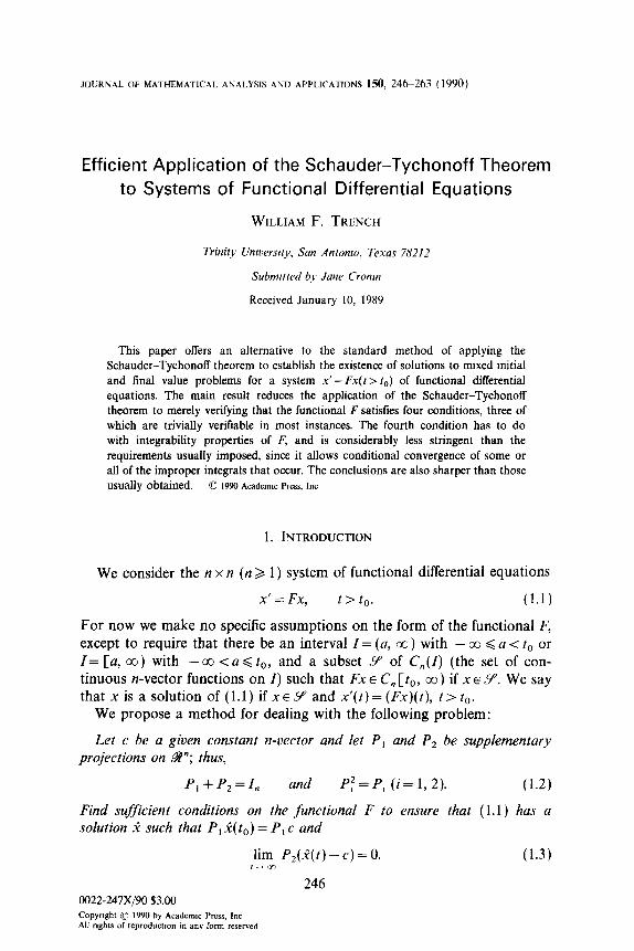
JOURNAL OF MATHEMATICAL ANALYSIS AND APPLICATIONS 150, 246263 ( 1990) Efficient Application of the Schauder-Tychonoff Theorem to Systems of Functional Differential Equations WILLIAM F. TRENCH Trinity Unmemly, San Antonlo, Texas 78212 Subrmtted by Jane Cromn Received January 10, 1989 This paper offers an alternative to the standard method of applying the Schauder-Tychonoff theorem to establish the existence of solutions to mtxed initial and final value problems for a system x’=Fx(f > to) of functional differential equations. The main result reduces the application of the Schauder-Tychonoff theorem to merely verifying that the functional F satisfies four conditions, three of which are trivially verifiable in most instances. The fourth condition has to do with integrability properties of F, and is considerably less stringent than the requirements usually imposed, since it allows conditional convergence of some or all of the improper integrals that occur. The conclusions are also sharper than those usually obtained. 0 1990 Acadenuc Press, Inc 1. INTRODUCTION We consider the n x n (n 2 1) system of functional differential equations x’ = Fx, t> t,. (1.1) For now we make no specific assumptions on the form of the functional F, except to require that there be an interval I= (a, co) with - cc 6 a < t, or I= [a, co) with --co <a< t,, and a subset Y of C,,(Z) (the set of con- tinuous n-vector functions on I) such that Fx E Cn[tO, 00) if x E Y. We say that x is a solution of (1.1) if XEY and x’(t)=(Fx)(t), t>tO. We propose a method for dealing with the following problem: Let c be a given constant n-vector and let P, and P, be supplementary projections on %?‘; thus, P,+P,=Z, and Pf = P, (i= 1,2). (1.2) Find sufficient conditions on the functional F to ensure that (1.1) has a solution 2 such that P, .?(to) = P, c and lim Pz(a( t) - c) = 0. l + ,K 246 (1.3) 0022-247X/90 $3.00 CopyrIght 0 1990 by Academic Press, Inc All nghls of reproduclmn in any form reserved

Welcome message from author
This document is posted to help you gain knowledge. Please leave a comment to let me know what you think about it! Share it to your friends and learn new things together.
Transcript
JOURNAL OF MATHEMATICAL ANALYSIS AND APPLICATIONS 150, 246263 ( 1990)
Efficient Application of the Schauder-Tychonoff Theorem to Systems of Functional Differential Equations
WILLIAM F. TRENCH
Trinity Unmemly, San Antonlo, Texas 78212
Subrmtted by Jane Cromn
Received January 10, 1989
This paper offers an alternative to the standard method of applying the Schauder-Tychonoff theorem to establish the existence of solutions to mtxed initial and final value problems for a system x’=Fx(f > to) of functional differential equations. The main result reduces the application of the Schauder-Tychonoff theorem to merely verifying that the functional F satisfies four conditions, three of which are trivially verifiable in most instances. The fourth condition has to do with integrability properties of F, and is considerably less stringent than the requirements usually imposed, since it allows conditional convergence of some or all of the improper integrals that occur. The conclusions are also sharper than those usually obtained. 0 1990 Acadenuc Press, Inc
1. INTRODUCTION
We consider the n x n (n 2 1) system of functional differential equations
x’ = Fx, t> t,. (1.1)
For now we make no specific assumptions on the form of the functional F, except to require that there be an interval I= (a, co) with - cc 6 a < t, or I= [a, co) with --co <a< t,, and a subset Y of C,,(Z) (the set of con- tinuous n-vector functions on I) such that Fx E Cn[tO, 00) if x E Y. We say that x is a solution of (1.1) if XEY and x’(t)=(Fx)(t), t>tO.
We propose a method for dealing with the following problem:
Let c be a given constant n-vector and let P, and P, be supplementary projections on %?‘; thus,
P,+P,=Z, and Pf = P, (i= 1,2). (1.2)
Find sufficient conditions on the functional F to ensure that (1.1) has a solution 2 such that P, .?( to) = P, c and
lim Pz(a( t) - c) = 0. l + ,K
246
(1.3)
0022-247X/90 $3.00 CopyrIght 0 1990 by Academic Press, Inc All nghls of reproduclmn in any form reserved
BOUNDS FOR DISTANCE OF A MANIFOLD 241
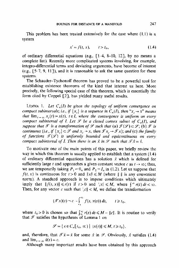
This problem has been treated extensively for the case where (1.1) is a system
x’ =f(t, xl, t> to, (1.4)
of ordinary differential equations (e.g., [l-4, 8-10, 121, by no means a complete list). Recently more complicated systems involving, for example, integro-differential terms and deviating arguments, have become of interest (e.g., [5-7, 9, 11 I), and it is reasonable to ask the same question for these systems.
The Schauder-Tychonoff theorem has proved to be a powerful tool for establishing existence theorems of the kind that interest us here. More precisely, the following special case of this theorem, which is essentially the form cited by Coppel [2], has yielded many useful results.
LEMMA 1. Let C,,(I) be given the topology of uniform convergence on compact subintervab; i.e., if {x,} is a sequence in C,,(I), then “x, -+ x” means that lim, _ ~ x,(t) = x(t), t E I, where the convergence is uniform on every compact subinterval of I. Let Y be a closed convex subset of C,(I), and suppose that F is a transformation of9 such that (a) F(Y) c Y; (b) f is continuous (i.e., if {x,} c Y and xj + x, then F-xl -+ F-x); and (c) the family of functions F(Y) is uniformly bounded and equicontinuous on every compact subinterval of I. Then there is an ,? in Y such that F-1 = 2.
To motivate one of the main points of this paper, we briefly review the way in which this theorem is usually applied to establish that a system (1.4) of ordinary differential equations has a solution 2 which is defined for sufficiently large t and approaches a given constant vector c as t -+ co; thus, we are temporarily taking P1 = 0, and P, = 1, in (1.2). Let us suppose that f (t, x) is continuous for t > 0 and /(x1( < M (where 11 )I is any convenient norm). A standard approach is to impose conditions which ultimately imply that Ilf(t, x)11 <r(t) if t >O and llxlj GM, where j” r(t) dt < co. Then, for any vector c such that j(c(I <M, we define the transformation
(5x)(t) = ~-j-~ f(s, x(s)) ds, tk to, ,
where to> 0 is chosen so that j: r(s) ds 6 M- lIcI\. It is routine to verify that F satisfies the hypotheses of Lemma 1 on
Y= {xd,[to, co) 1 Ilx(t)ll GM, mt,},
and, therefore, that SZ = ,i! for some 2 in Y. Obviously, i satisfies (1.4) and lim,,,@t)=c.
Although many important results have been obtained by this approach
248 WILLIAM F. TRENCH
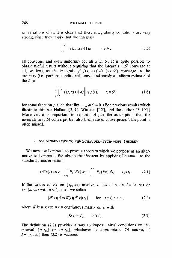
or variations of it, it is clear that these integrability condittons are very strong, since they imply that the integrals
all converge, and even uniformly for all .Y in Y. It is quite possible to obtain useful results without requiring that the integrals (1.5) converge at all, so long as the integrals f” f(s, X(S)) ds (XE 9) converge in the ordinary (i.e., perhaps conditional) sense, and satisfy a uniform estimate of the form
IIJ ‘X,
XEY, I (1.6)
for some function p such that lim, _ Ix, p(t) = 0. (For previous results which illustrate this, see Hallam [3,4]. Wintner [12], and the author [S-lo].) Moreover, it is important to exploit not just the assumption that the integrals in (1.6) converge, but also their rate of convergence. This point is often missed.
2. AN ALTERNATIVE TO THE SCHAUDER-TYCHONOFF THEOREM
We now use Lemma 1 to prove a theorem which we propose as an alter- native to Lemma 1. We obtain the theorem by applying Lemma 1 to the standard transformation
(Y-x)(t) = c + J’ P,(Fx) ds - j-l P,(Fx) ds, tg t,. (2.1) kl I
If the values of Fx on [to, co) involve values of ,Y on I= [a, co) or I= (a, co) with a < t,, then we define
(Y-x)(t) = K(t)(Y-x)(t,) for tEI, t<to, (2.2)
where K is a given n x n continuous matrix on Z, with
Nt)=J,, t> t,. (2.3)
The defmition (2.2) provides a way to impose initial conditions on the interval [a, to] or (a, to], whichever is appropriate. Of course, if Z= [to, co) then (2.2) is vacuous.
FUNCTIONAL DIFFERENTIAL EQUATIONS 249
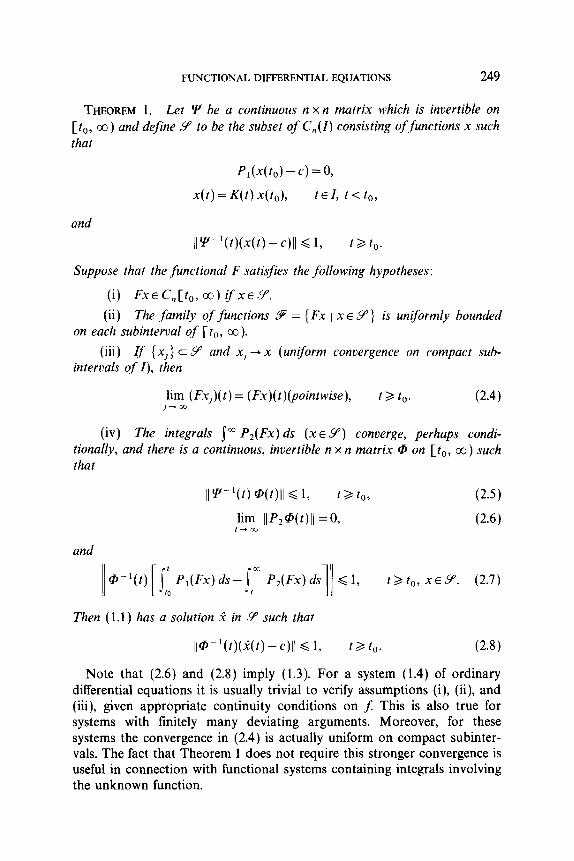
THEOREM 1. Let !P be a continuous n x n matrix which is invertible on [to, co) and define Y to be the subset of C,(Z) consisting of functions x such that
P,(x(to) -cl = 0,
x(t) = K(t) x(t,), tEI, t<to,
and
II y-‘(t)tx(t) - c)ll d 1, t> to.
Suppose that the functional F satisfies the following hypotheses:
(i) FxE Cn[tO, co) ifx~Y.
(ii) The family of functions 9 = {Fx ) x E Y) is uniformly bounded on each subinterval of [to, CO).
(iii) rf {x,} CY d an x,+x (uniform convergence on compact sub- intervals of I), then
lim (Fx,)(t) = (Fx)(t)(pointwise), t> to. (2.4) /-m
(iv) The integrals f” P,(Fx) ds (x E 9’) converge, perhaps condi- tionally, and there is a continuous, invertible n x n matrix 0 on [to, co) such that
II !J- l(t) @(t)ll < 1, t> to, (2.5)
lim IIP2@(t)ll =O, (2.6) t-m
and
’ P,(Fx)ds-I=’ P,(Fx)ds <l, t> to, ~~940. (2.7) 10 I
Then (1.1) has a solution x in Y such that
Il@-‘w@(+4ll G 1, t> to. (2.8)
Note that (2.6) and (2.8) imply (1.3). For a system (1.4) of ordinary differential equations it is usually trivial to verify assumptions (i), (ii), and (iii), given appropriate continuity conditions on f: This is also true for systems with finitely many deviating arguments. Moreover, for these systems the convergence in (2.4) is actually uniform on compact subinter- vals. The fact that Theorem 1 does not require this stronger convergence is useful in connection with functional systems containing integrals involving the unknown function.
250 WILLIAM F. TRENCH
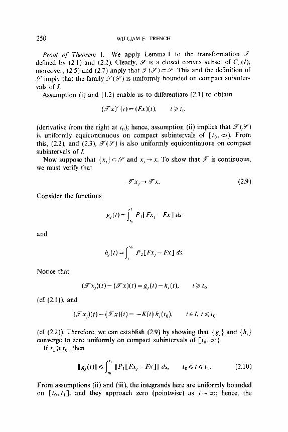
Proof’ of Theorem 1. We apply Lemma I to the transformation .F defined by (2.1) and (2.2). Clearly, Y is a closed convex subset of C,,(Z); moreover, (2.5) and (2.7) imply that y--(y) c ,Y. This and the definition of .Y imply that the family y(Y) is uniformly bounded on compact subinter- vals of I.
Assumption (i) and (1.2) enable us to differentiate (2.1) to obtain
(Fx)’ (t)= (Fx)(t), t 2 t,
(derivative from the right at t,); hence, assumption (ii) implies that y(Y) is uniformly equicontinuous on compact subintervals of [to, co). From this, (2.2), and (2.3), y(?Y) is also uniformly equicontinuous on compact subintervals of I.
Now suppose that {x,} c Y and x, +x. To show that y is continuous, we must verify that
TX] + Y-x. (2.9)
Consider the functions
g,+jr P,[Fx,-Fx] ds 10
and
Notice that
(cf. (2.1)), and
h,(t) = J, fm P2 [ Fx, - Fx] ds.
(q)(f) - (Fx)( d=g,O-h,(t), t b to
V-x,)(t) - (TX)(~) = -K(t) h,Oo), tEz, t,<to
(cf. (2.2)). Therefore, we can establish (2.9) by showing that (g,> and {h,} converge to zero uniformly on compact subintervals of [to, 03).
If f, 2 to, then
Ils,(f)ll Gs” llf’,CFx,-Fxlll 4 t,<t<t1. (2.10) ro
From assumptions (ii) and (iii), the integrands here are uniformly bounded on [to, ti], and they approach zero (pointwise) as j-+ co; hence, the
FUNCTIONAL DIFFERENTIAL EQUATIONS 251
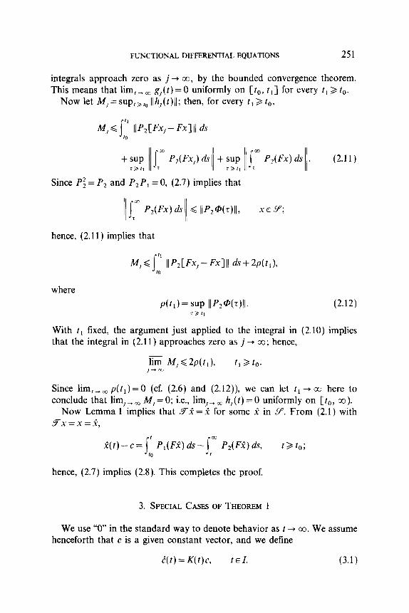
integrals approach zero as j + co, by the bounded convergence theorem. This means that lim, _ ‘*, g,(t) =0 uniformly on [to, tr] for every t, Z to.
Now let M, = sup, a ,0 Ilh,(t)l\; then, for every tr > t,,,
P,(Fx,)ds + sup Ir P,(Fx)ds . II 1 il
(2.11) rat, 7
Since Pz = P, and P,P, = 0, (2.7) implies that
hence, (2.11) implies that
M,6 s ” ll&Cf’x,-Fx]Il ds+@(tl), 10 where
P(lI) = sup llP*@(~)ll. T 2 I,
(2.12)
With tI fixed, the argument just applied to the integral in (2.10) implies that the integral in (2.11) approaches zero as j -+ co; hence,
lim M, d 2p(tl), fl > to. , - a!
Since lim, _ o. p(tr) =0 (cf. (2.6) and (2.12)), we can let t, + cc here to conclude that lim,,, M, = 0; i.e., lim,, oj h,(t) = 0 uniformly on [to, co).
Now Lemma 1 implies that 3i = J? for some f in 9’. From (2.1) with Fx=x=i,
i(t) - c = j’ P,(Fi) ds - Cm P2(Fi) ds, t>to; 10 f
hence, (2.7) implies (2.8). This completes the proof.
3. SPECIAL CASESOF THEOREM 1
We use “0” in the standard way to denote behavior as t -+ co. We assume henceforth that c is a given constant vector, and we define
e(t) = K(t)c, t E I. (3.1)
252 WILLIAM F. TRENCH
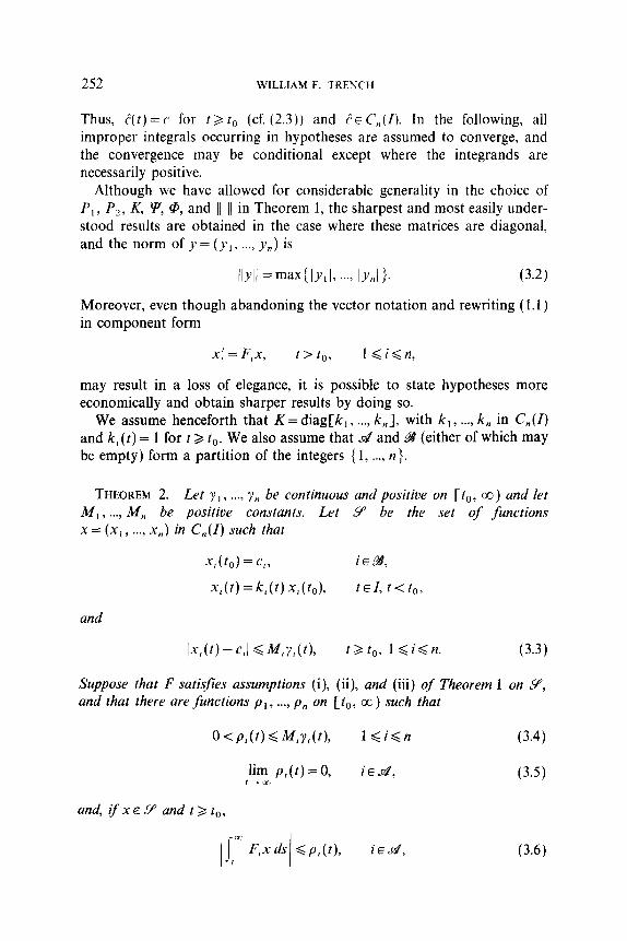
Thus, t(t) = c for t 3 to (cf. (2.3)) and ? E C,(I). In the following, all improper integrals occurring in hypotheses are assumed to converge, and the convergence may be conditional except where the integrands are necessarily positive.
Although we have allowed for considerable generality in the choice of P,, P?, K. Y, @, and II 1) in Theorem 1, the sharpest and most easily under- stood results are obtained in the case where these matrices are diagonal, and the norm of y = ( )‘r, . . . . y,) is
/lull = max: ly3)113 -., bnl>. (3.2)
Moreover, even though abandoning the vector notation and rewriting (1.1) in component form
x: = F,x, t> to, l<iin,
may result in a loss of elegance, it is possible to state hypotheses more economically and obtain sharper results by doing so.
We assume henceforth that K= diag[k,, . . . . k,], with kr, . . . . k, in C,(Z) and k,(t) = 1 for t 2 to. We also assume that d and g (either of which may be empty) form a partition of the integers { 1, . . . . H}.
THEOREM 2. Let yl, . . . . y,, be continuous and positive on [to, co ) and let M,, . . . . M, be positive constants. Let Y be the set of functions x = (x1, . . . . x,) in C,(Z) such that
-x,(to) = Cl, iE&?,
xi(t) =kt(t) xz(to)t tEI, t<to,
and
Ix,(t) - c,I 6 M,?,(t), tat,, 1 <i<n. (3.3)
Suppose that F satisfies assumptions (i), (ii), and (iii) of Theorem 1 on 9, and that there are functions pl, . . . . pn on [to, co) such that
0 <p,(t) G M,lJ,(t), 1 <i<n (3.4)
lim p,(t) = 0, iE&, (3.5 t-cc )
and, $XEY and t> to,
/I,“’ F,sml <p,(t), ied, (3.6
FUNCTIONAL DIFFERENTIAL EQUATIONS 253
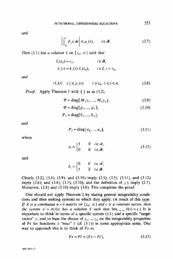
and
Then (1.1) has a solution ,? on [to, CO) such that
a,(t,) = Cl, iEL49,
az(t)=k,(t)~i(tO), tEz, t< t,,
and
F,(t) - c,I G P,(t), t>tO, ldi<n.
Proof. Apply Theorem 1 with I( 11 as in (3.2),
y=diagCM,~,, . . . . M,IJ,I,
@ = diagb,, . . . . ~1,
P, = diag[b,, . . . . b,],
and
where
P, = diag[a,, . . . . a,],
i
1 if iE&, a, =
0 if iEB,
(3.7)
(3.8)
(3.9)
(3.10)
(3.11)
(3.12)
and if iEd, if iE99.
Clearly (3.2), (3.4), (3.9), and (3.10) imply (2.5); (3.5), (3.11), and (3.12) imply (2.6); and (3.6), (3.7), (3.10), and the definition of (1 (1 imply (2.7). Moreover, (2.8) and (3.10) imply (3.8). This completes the proof.
One should not apply Theorem 2 by stating general integrability condi- tions and then seeking systems to which they apply. (A result of this type: If A is a continuous n x n matrix on [to, co) and c is a constant vector, then the system x’ = A(t)x has a solution 1 such that lim,, 7. i(t) = c.) It is important to think in terms of a specific system ( 1.1) and a specific “target vector” c, and to base the choice of yl, . . . . y,, on the integrability properties of Fx for functions x “near” i? (cf. (3.1)) in some appropriate sense. One way to approach this is to think of Fx as
Fx=F?+(Fx-F?), (3.13)
40!3/150/1-17
254 WILLIAM F. TRENCH
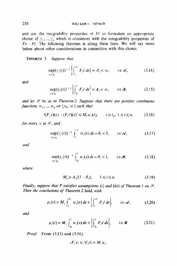
and use the integrability properties of F? to formulate an appropriate choice of y1 , . . . . ;I,, which is consistent with the integrability properties of Fx - Ft. The following theorem is along these lines. We will say more below about other considerations in connection with this choice.
THEOREM 3. Suppose that
iEd’, (3.14)
and
iEZ8, (3.15)
and let 9 be as in Theorem 2. Suppose that there are positive continuous functions w, , . . . . w, on [t,, CC ) such that
l(F,.y)(t) - (F,Ut)l d M,w,(t), tBto, l<i<n, (3.16)
for every .Y in Y, and
;;~(Y,w-’ Jl‘ w,(s)ds=~,<l, iE&, (3.17)
and
sup(y,(t))-’ J’ w,(s)ds=e,<l, iE@), (3.18) I 2 10 10
where
M,BA,l(l -elk 1 <i,<n. (3.19)
Finally, suppose that F satisfies assumptions (i) and (iii) of Theorem 1 on Y. Then the conclusions of Theorem 2 hold, with
P,(t)=M, Ja w,(s)ds+ j- F,tds, I I
iEd, (3.20) f I
and
P,(t)=M, J’ w,(s)ds+ J’ F,Sds, I I
iEW. (3.21) to 4l
Proof From (3.13) and (3.16),
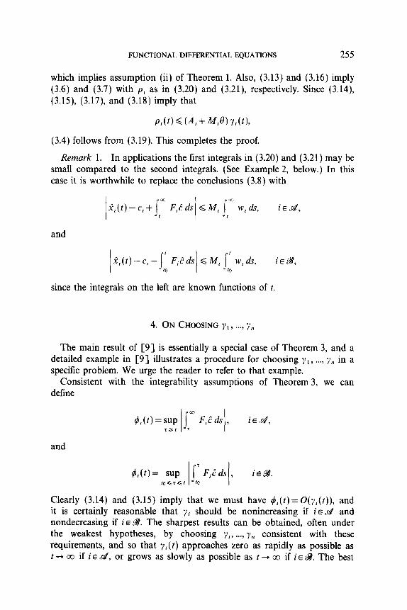
FUNCTIONAL DIFFERENTIAL EQUATIONS 255
which implies assumption (ii) of Theorem 1. Also, (3.13) and (3.16) imply (3.6) and (3.7) with p, as in (3.20) and (3.21) respectively. Since (3.14) (3.15), (3.17), and (3.18) imply that
p,(t) 6 (A, + M,@ Y,(t),
(3.4) follows from (3.19). This completes the proof.
Remark 1. In applications the first integrals in (3.20) and (3.21) may be small compared to the second integrals. (See Example 2, below.) In this case it is worthwhile to replace the conclusions (3.8) with
and
since the integrals on the left are known functions of t.
4. ON CHOOSING yl, . . . . y,
The main result of [9] is essentially a special case of Theorem 3, and a detailed example in [9] illustrates a procedure for choosing yl, . . . . yn in a specific problem. We urge the reader to refer to that example.
Consistent with the integrability assumptions of Theorem 3, we can define
and
q&(t)= sup 1’ FiCds , I I
iE9Y. 10 s f 6 I 10
Clearly (3.14) and (3.15) imply that we must have di(t)= O(yJt)), and it is certainly reasonable that yi should be nonincreasing if ie d and nondecreasing if ie .B. The sharpest results can be obtained, often under the weakest hypotheses, by choosing y,, . . . . yn consistent with these requirements, and so that ri(t) approaches zero as rapidly as possible as t --) cc if i E d, or grows as slowly as possible as t + a3 if i E W. The best
256 WILLIAM F. TRENCH
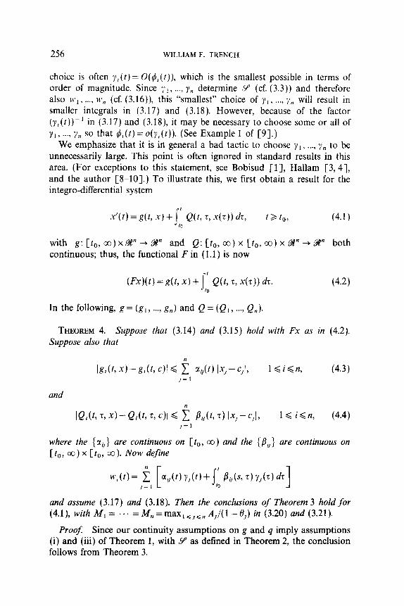
choice is often r,(r) = 0($,(r)), which is the smallest possible in terms of order of magnitude. Since y,, . . . . yn determine ,Y (cf. (3.3)) and therefore also 11’~. . . . . M’, (cf. (3.16)), this “smallest” choice of yl, . . . . y,, will result in smaller integrals in (3.17) and (3.18). However, because of the factor (y,(t))-’ in (3.17) and (3.18), it may be necessary to choose some or all of Yl > ..‘3 yn so that $,(t)=o(y,(t)). (See Example 1 of [9].)
We emphasize that it is in general a bad tactic to choose y, , . . . . y,, to be unnecessarily large. This point is often ignored in standard results in this area. (For exceptions to this statement, see Bobisud [l], Hallam [3,4], and the author [S-lo].) To illustrate this, we first obtain a result for the integro-differential system
x’(t) = cd4 xl + J,; Q(f, ~,.-dz)) 4 t> t,, (4.1)
with g: [to, co)xW” -+ 5e” and Q: [to, co) x [to, co) x R” + W” both continuous; thus, the functional F in (1.1) is now
(Fx)(t) = s(l, xl + j-L Q<t, ~z, 4~)) dz. (4.2)
In the following, g = (g,, . . . . g,) and Q = (Q,, . . . . Q,).
THEOREM 4. Suppose that (3.14) and (3.15) hold with FX as in (4.2). Suppose also that
Ig,(t, xl - gt(& c)l Q i ai/(Q lx,- CJl, l<i<n, (4.3) ,=I
and
where the {ai, > are continuous on [t,, co) and the (a,,} are continuous on [to, co) x [to, 03). Now define
w,(t)= i ,=l
[‘,,(‘) y,(l)+ j’ &(h z, ?Jb) dT]
m
and assume (3.17) and (3.18). Then the conclusions of Theorem 3 hold for (4.1), with M, = ... =~V,=rnax,~,,, A,/(1 -0,) in (3.20) and (3.21).
Proof: Since our continuity assumptions on g and q imply assumptions (i) and (iii) of Theorem 1, with Y as defined in Theorem 2, the conclusion follows from Theorem 3.
FUNCTIONAL DIFFERENTIAL EQUATIONS 257
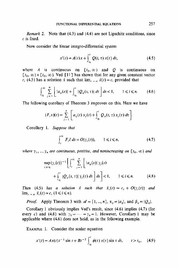
Remark 2. Note that (4.3) and (4.4) are not Lipschitz conditions, since c is fixed.
Now consider the linear integro-differential system
x'(t) = A(t)x + jr Q(t, T) X(T) dz, (45) 10
where A is continuous on [t,,, co) and Q is continuous on [to, cc ) x [to, co). Ved [ 111 has shown that for any given constant vector c, (4.5) has a solution f such that lim,, 3. i(t)=c, provided that
jm i [ la,(s)1 +j’ lQ,(s, z)l do] ds< 1, 1 ~i~n. (4.6) f0 J=l 10
The following corollary of Theorem 3 improves on this. Here we have
(Fix)(t) = i [a,(t) x,(t) + j’ Q,(t, T) x,(T) dT]. j=1 f0
Corollary 1. Suppose that
F m F,e ds= O(y,(t)), l<i<n, (4.7)
where yI, . . . . y,, are continuous, positive, and nonincreasing on [to, co) and
+ j’ IQ& ~11 y,(TW ds < 1, II 1 <i<n. (4.8) f0
Then (4.5) has a solution .? such that Z,(t) = ci + O(yi(t)) and lim,,, a,(t)=ci (16i6n).
Prooj Apply Theorem 3 with d = { 1, . . . . n}, c1,, = laOI, and /?, = IQ,\.
Corollary 1 obviously implies Ved’s result, since (4.6) implies (4.7) (for every c) and (4.8) with y, = . . = yn = 1. However, Corollary 1 may be applicable where (4.6) does not hold, as in the following example.
EXAMPLE 1. Consider the scalar equation
x’(t)=Ax(t)t-‘sin t+ Bte2 I t 4(z) X(T) sin t dq t>to, (4.9) 10
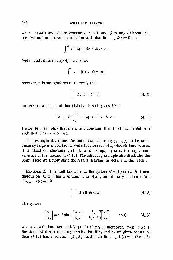
258 WILLIAM F. TRENCH
where A( #O) and B are constants, t, > 0, and 4 is any differentiable, positive, and nonincreasing function such that lim, t ,;c, b(t) = 0 and
c x
rr’&t) (sin tI dr< ~1.
Ved’s result does not apply here, since
s K’ tr’ lsin t( dr = co;
however, it is straightforward to verify that
s OrJ Feds=O(l/t) I
(4.10)
for any constant c, and that (4.8) holds with y(t) = l/t if
Ml + IBI J,: T -l&z) Jsin r( dz c 1. (4.11)
Hence, (4.11) implies that if c is any constant, then (4.9) has a solution i such that a(t) = c + 0( l/t).
This example illustrates the point that choosing yi, . . . . yn to be unne- cessarily large is a bad tactic. Ved’s theorem is not applicable here because it is based on choosing y(t) = 1, which simply ignores the rapid con- vergence of the integral in (4.10). The following example also illustrates this point. Here we simply state the results, leaving the details to the reader.
EXAMPLE 2. It is well known that the system x’=A(r)x (with A con- tinuous on (0, co)) has a solution CZ satisfying an arbitrary final condition lim f+m i(t)=c if
s O” IIA(t)ll dt < oz. (4.12)
The system
where 6, #O does not satisfy (4.12) if c1< 1; moreover, even if ~1> 1, the standard theorem merely implies that if c, and c2 are given constants, then (4.13) has a solution (ai, a,) such that lim,,, Z,(t)= c, (i= 1, 2).
FUNCTIONALDIFFERENTIALEQUATIONS 259
However, Corollary 1 (with Q =0) and Remark 1 imply that if a > 0 and (c,, c2) is arbitrary, then (4.13) has a solution (a,, a,) such that
~-l(t)=C1(1-a,S,+,(t))--b,c,S,(t)+O(t-2")
and
c&(f)= -a*c,S,+2(f)+C~(1-6~S,+,(t))+O(t-21-1),
where
S,(t) = lrn s-p sinsds=O(t-B), /?>O. ,
This conclusion is obtained by letting y,(t) = t-’ and y2(f) = tBa- ‘. A sharper result is available if c2 = 0; i.e., for every constant c, , (4.13 ) has a solution (a,, 2,) such that
and i,(t)= -u2c,S,+2(t)+O(t-2~-2).
This is obtained by letting yi(t) = t-“-l and y2(t) = t-‘-I.
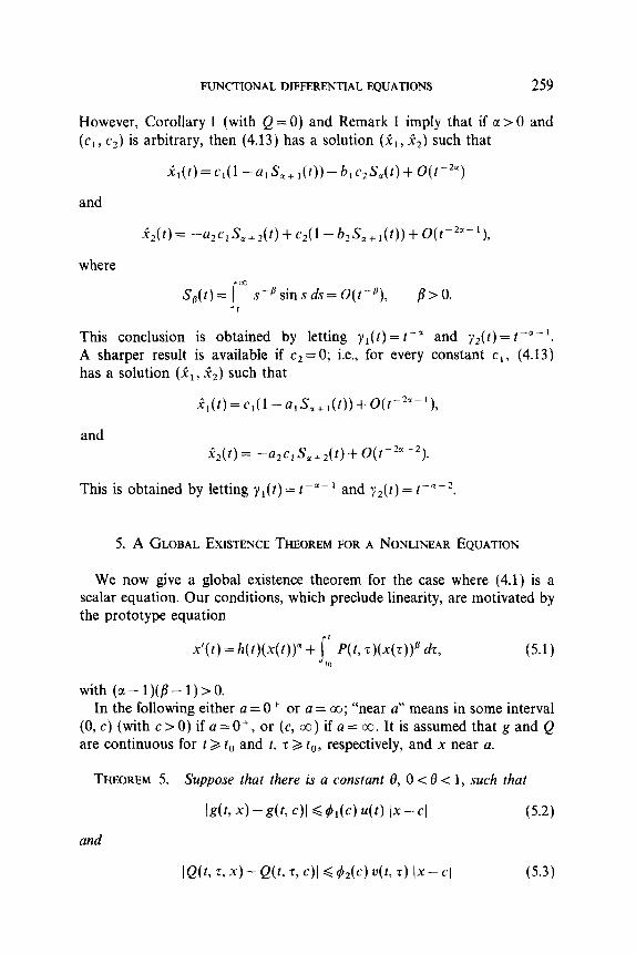
5. A GLOBAL EXISTENCE THEOREM FOR A NONLINEAR EQUATION
We now give a global existence theorem for the case where (4.1) is a scalar equation. Our conditions, which preclude linearity, are motivated by the prototype equation
x’(t) = h( t)(x( t))* + j’ P(t, T)(X(T))B dz, (5.1) m
with (a- l)(fl- l)>O. In the following either a = 0 + or a = co; “near u” means in some interval
(0, c) (with c>O) if u=O+, or (c, co) if a= co. It is assumed that g and Q are continuous for t Z t, and t, z 2 to, respectively, and x near u.
THEOREM 5. Suppose that there is a constant 8, 0 < 8 < 1, such that
Ig(t, x) - g(c c)l G #l(C) u(t) lx - cl (5.2)
and
lQ(c T, xl - Q(h 7, cl< 42(c) u(f, 7) lx - cl (5.3)
260 WILLIAM F. TRENCH
I~C is near a and
Ix - L-1 d Hc, (5.4)
where u and v are continuous on [to, CC ) and [t,, CC ) x [t,, x ), respective(y, and
lim +,(c)=O, i= 1, 2. (5.5) (‘(1
Suppose also that, for c near a, j: F? ds (cf (4.2)) converges, perhaps condi- tionally, and that there is a positive, nonincreasing, and continuous function y on [to, GO) such that
where
s = 4s) Y(S) ds = W(t)), , and
(5.6)
(5.7)
(5.8)
I s m ds -) v(s, T) y(z) dz = O(y(t)). I kl
Then the scalar equation (4.1) has a solution JZ such that
F(t) - cl d w4kJ) - ’ r(t), tatto,
and
(5.9)
(5.10)
lim a(t) = c, (5.11) t-00
provided that c is sufficiently near a.
Proof. We apply Theorem 2 with n = 1 and d = { 1 }. Let
9 = {XE CCto, co 1 I Ix(t) - cl d MY(4d) -’ y(t)), (5.12)
where c is any constant sufficiently near a so that our hypotheses hold. Assumptions (i) and (iii) of Theorem 1 hold for reasons like those given in
FUNCTIONAL DIFFERENTIAL EQUATIONS 261
the proof of Theorem 4. From (3.13), (5.2) (5.3) (5.4) (5.12), and the monotonicity of y,
and this implies (ii) of Theorem 1. Also, (3.13), (5.2), and (5.3) imply that if xELf and tat,, then
m
IJ I
Fx ds < p(t; c), *
where
x 4,(c) j- 4s) Y(S) ds+ MC) j- ds js u(s, z) Y(T) dr . , I kl 1 Obviously lim, _ o. p(t; c) = 0 for every c. From (5.6), (5.8), and (5.9)
P(4 cl G [H(c) + WY(toW’ C&4(c) + W*(c)11 r(t), t 2 to,
where A and B are constants independent of c. Therefore, because of (5.5) and (5.7),
dt; c) < K(c) wJ(to))-’ Y(t), t>to,
where lim, _ (I K(c) = 0. Theorem 2 now implies the stated conclusion for any c such that K(c) 6 1.
This theorem has the following corollary for the prototype equation (5.1).
COROLLARY 2. Suppose that h: C[to, 00) -+B and P: [to, co) x [to, co) + B are continuous and satisfy the integrability conditions
J cc h(s) ds = WY(~)), (5.13) *
J J ads ’ PO, z) dz = W(t)), , hl
(5.14)
J “O Ih(s)I 14s) ds = W(t)), I
262
und
WILLIAM F. TRENCH
I
i 1 ds ’ IP(s,z)(l’(t)dz=O(y(t)),
r * 1,)
with y as in Theorem 5. Let 8 be an)! number in (0, 1). Then (5.1) has a solution 2 which satisfies (5.10) and (5.1 I), provided that c is sufficientl} large if r. /I < 1, or c is sufficiently small ij” a, p > 1.
Proof: Comparing (5.1) with (4. l), we see that here
g(t, x) = h(t).? and Q(t, z, x) = P(t, z).xB;
therefore, (5.13) and (5.14) imply (5.6), with H(c)=@+vcP for some constants p and v independent of c. The mean value theorem and (5.4) imply that
1x6-CbJ < 161 [(1+8)c]fi-’ Is-CCJ,
where the “k” is “t” if 6> 1, or “-” if 6~ 1; hence, (5.4) implies (5.2) and (5.3), with u(t) = /h(t)/, v(t, z) = IP(t, z)l,
41(c) = I4 cc1 f WI”-‘,
and
42(c) = WI Cl1 IL WI”- ‘.
Since (5.5) and (5.7) obviously hold with a = 0’ if a, /? > 1 or with a = co if a, /? < 1, Theorem 5 implies the conclusion.
REFERENCES
1. L. E. BOBNJD, Asymptotic behavior of solutions of perturbed linear systems, Proc. Amer. Math. Sot. 35 (1972), 457463.
2. W. B. COPPEL, “Stability and Asymptotic Behavior of Differential Equations,” Heath, Boston (1965).
3. T. G. HALLAM, Asymptotic integration of second order differential equations with integrable coeficients, SIAM J. Appt. Math. 19 (1970), 43Ck439.
4. T. G. HALLAM, Asymptotic integration of a nonhomogeneous differential equation with integrable coefiicients, Czechoslooak Mad J. 21 (1971), 661-671.
5. Y. KITAMURA AND T. KUSANO, On the oscillation of a class of nonlinear differential systems with deviating argument, J. Math. Anal. Appl. 66 (1978), 20-36.
6. Y. KITAMURA AND T. KUSANO, Oscdlation and a class of nonlinear systems with general deviating arguments, Nonlinear Anal. 2 (1978), 537-551.
7. Y. KITAMURA AND T. KUSANO, Oscillation of first-order nonlinear differential equations with deviating arguments, Proc. Amer. Math. Sot. 78 (1980), 64-68.
FUNCTIONAL DIFFERENTIAL EQUATIONS 263
8. W. F. TRENCH, Systems of differential equations subject to mild integral conditions, Proc. Amer. Math. Sot. 87 (1983), 263-270.
9. W. F. TRENCH, Asymptotics of differential systems with deviating arguments, Proc. Amer. Math. Sot. 92 (1984) 219-224.
10. W. F. TRENCH, Extensions of a theorem of Wintner on systems with asymptotically constant solutions, Trans. Amer. Math. Sot. 293 (1986). 477483.
11. Y. A. VED AND S. S. BAYALIEVA, Asymptotic relations between solutions of linear homogeneous drfferential and integrodifferential equations, Differenftal’nye Urauneniya 6 (1970) 335-342 [in Russian].
12. A. WINTNER, On a theorem of B&her in the theory of ordinary linear differential equations, Amer. J. Math. 76 (1954), 183-190.
Related Documents