Efficient Algorithms for Determining 3-D Bi-Plane Imaging Geometry

Efficient Algorithms for Determining 3-D Bi-Plane ImagingGeometry*

Jinhui Xu†, Guang Xu†, Zhenming Chen†, and Vikas Singh†Department of Computer Science and Engineering, State University of New York at Buffalo, 201Bell Hall, Buffalo, NY 14260, USA, [email protected], [email protected],[email protected], [email protected]

Kenneth R. HoffmannDepartment of Neurosurgery, State University of New York at Buffalo, 445 Biomedical ResearchBuilding, 3435 Main St., Buffalo, NY 14214, USA, [email protected]

AbstractBiplane projection imaging is one of the primary methods for imaging and visualizing thecardiovascular system in medicine. A key problem in such a technique is to determine the imaginggeometry (i.e., the relative rotation and translation) of two projections so that the interested 3-Dstructures can be accurately reconstructed. Based on interesting observations and efficient geometrictechniques, we present in this paper new algorithmic solutions for this problem. Comparing withexisting optimization-based approaches, our techniques yield better accuracy, have boundedexecution time, and thus are more suitable for on-line applications. Our techniques can easily detectoutliers to further improve the accuracy.

1 IntroductionCardiovascular diseases (such as vessel blockage and narrowing) have been major causes ofdeath in the United States for a long time. Effective treatment and diagnosis procedures forthis type of diseases heavily rely on accurate 3-D images of the interested vessel structure.Tomographic techniques, such as magnetic resonance imaging (MRI) and computedtomography (CT), although generate 3-D data sets for visualization and analysis (e.g.,rendering), cannot yet provide the time resolution necessary for interventions and for dynamicevaluations of rapidly moving structures such as heart. Thus, projection imaging generated byimage intensifier-TV (II-TV) systems is still the dominant form of imaging in this area, mainlydue to its rapid image acquisition and relatively larger field of view.

In projection imaging, 3-D structures are reconstructed from one or more 2-D projections. Akey problem in such reconstructions is to determine the relative translation and rotation, calledimaging geometry, of the coordinate system associated with one projection with respect tothose associated with other projections. Since the size of vessels in a vascular system is verysmall, inaccurate imaging geometry may cause the reconstructed 3-D vessels located in totallydifferent positions.

As a promising approach, bi-plane imaging (in which each 3-D image is reconstructed fromtwo projections) has received considerable attention in recent years and a number of techniqueshave been developed for its imaging geometry determination and 3-D reconstruction [5,6,11,

*This research was supported in part by NIH under USPHS grant HL52567.†The research of this author was supported in part by an IBM faculty partnership award, and an award from NYSTAR (New York stateoffice of science, technology, and academic research) through MDC (Microelectronics Design Center).

NIH Public AccessAuthor ManuscriptJ Comb Optim. Author manuscript; available in PMC 2006 April 17.

Published in final edited form as:J Comb Optim. 2005 September ; 10(2): 113–132.

NIH

-PA Author Manuscript

NIH

-PA Author Manuscript

NIH

-PA Author Manuscript

12,16,21]. A common approach for determining image geometry in these techniques is to firstidentify a set of corresponding pairs of points in the two projections, then convert the problemto a certain non-linear optimization problem, and find a feasible solution by using greedyalgorithms or general optimization packages. Due to their heuristic nature, these approachesguarantee neither the quality of solutions nor the time efficiency, and thus may not be suitablefor online applications.

We notice that in the field of Computer Vision, a similar problem, called Epipolar GeometryDetermination (or EGD), has been studied extensively [14,18,19,22]. The Epipolar GeometryDetermination problem tries to determine the epipolar geometry relating two images of a singlescene and plays an important role in many applications, such as scene modeling and vehiclenavigation. Quite a few interesting approaches were previously proposed for solving thisproblem. (Excellent surveys on existing techniques can be found in articles [23,1,13].)However, almost all of them are based on iterative numerical computation which in generalcan not guarantee the converging speed and therefore are not suitable for online cardiovascularapplications. Further, the EGD problem is slightly more general than our problem. In the EGDproblem, the relative orientation of the two images could be arbitrary and unknown in advance.But in our problem, rough estimation of the imaging geometry of the two projections can beobtained from the imaging system. Consequently, algorithms for the EGD problem cannotfully exploit the special geometric structures of cardiovascular images.

To provide better solutions, we reduce the imaging geometry determination problem to thefollowing geometric search problem: Given two sets of 2-D points A = {a1, a2, ···, an} and B= {b1, b2, ···, bn} on two image screens (or planes) respectively with each pair of points ai andbi (called a corresponding pair) being the approximate projections of an unknown 3-D pointpi, also given the 3-D coordinate system of A, find the most likely position of the origin oB andthe orientation of the 3-D coordinate system of B in the coordinate system of A. It is easy tosee that in an ideal situation where ai and bi are exact projections of pi, it is sufficient to consideronly a constant number of corresponding pairs. In practice, however, it is often difficult to findthe exact corresponding pairs as the correspondence is established manually. Thus, a numberof corresponding pairs are often considered in practice to ensure the accuracy.

In this paper, we present an efficient geometric approach to solve the above problem. Ourapproach first reduces the imaging geometry determination problem to an optimal cell searchproblem in an arrangement of surfaces in E6. Based on interesting observations, we thensimplify the rather complicated surfaces, which can not be analytically expressed, so that eachof them can be implicitly expressed by an equation. The simplified surfaces are in general non-algebraic, indicating that directly computing the arrangement could be very challenging. Toovercome this difficulty, we study the error sensitivity of each variable in the imaging geometryand use it to partition the feasible domain into smaller regions so that the topological structureof the arrangement in each region can be effectively captured by some lower dimensional (e.g.,2 or 3-D) arrangements. The curves and surfaces in these lower dimensional arrangements,although are still non-algebraic, have “nice” properties and can be used to efficiently find theoptimal cell. Comparing with existing approaches, our techniques achieve better accuracy (assuggested by our experimental results) and have bounded running time. Our techniques caneasily recognize outliers in A and B to further improve the accuracy.

The rest of this paper is organized as follows. Section 2 gives some preliminaries of theproblem. Section 3 shows that the imaging geometry problem can be reduced to solving anarrangement search problem in E6 space. In Section 4, we discuss the major difficulties of thearrangement search approach and our main ideas for overcoming them. In Section 5, we presentour algorithms for finding the maximum point in lower dimensional arrangements.Experimental results and comparison with existing approach are given in Section 6.

Xu et al. Page 2

J Comb Optim. Author manuscript; available in PMC 2006 April 17.

NIH

-PA Author Manuscript

NIH

-PA Author Manuscript

NIH

-PA Author Manuscript

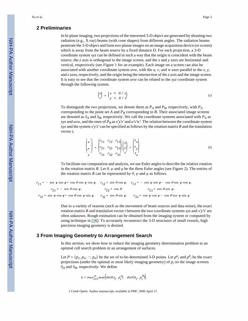
2 PreliminariesIn bi-plane imaging, two projections of the interested 3-D object are generated by shooting tworadiation (e.g., X-ray) beams (with cone shapes) from different angles. The radiation beamspenetrate the 3-D object and form two planar images on an image acquisition device (or screen)which is away from the beam source by a fixed distance D. For each projection, a 3-Dcoordinate system xyz can be defined in such a way that the origin is coincident with the beamsource, the z axis is orthogonal to the image screen, and the x and y axes are horizontal andvertical, respectively (see Figure 1 for an example). Each image on a screen can also beassociated with another coordinate system uvw, with the u, v, and w axes parallel to the x, y,and z axes, respectively, and the origin being the intersection of the z axis and the image screen.It is easy to see that the coordinate system uvw can be related to the xyz coordinate systemthrough the following system.

(uv) = (x × D / zy × D / z) (1)

To distinguish the two projections, we denote them as PA and PB, respectively, with PAcorresponding to the point set A and PB corresponding to B. Their associated image screensare denoted as SA and SB, respectively. We call the coordinate systems associated with PA asxyz and uvw, and the ones of PB as x′y′z′ and u′v′w′. The relation between the coordinate systemxyz and the system x′y′z′ can be specified as follows by the rotation matrix R and the translationvector t,

(x ′

y ′

z ′) = (r11 r12 r13

r21 r22 r23r31 r32 r33

) (xyz) + (txty

tz) (2)

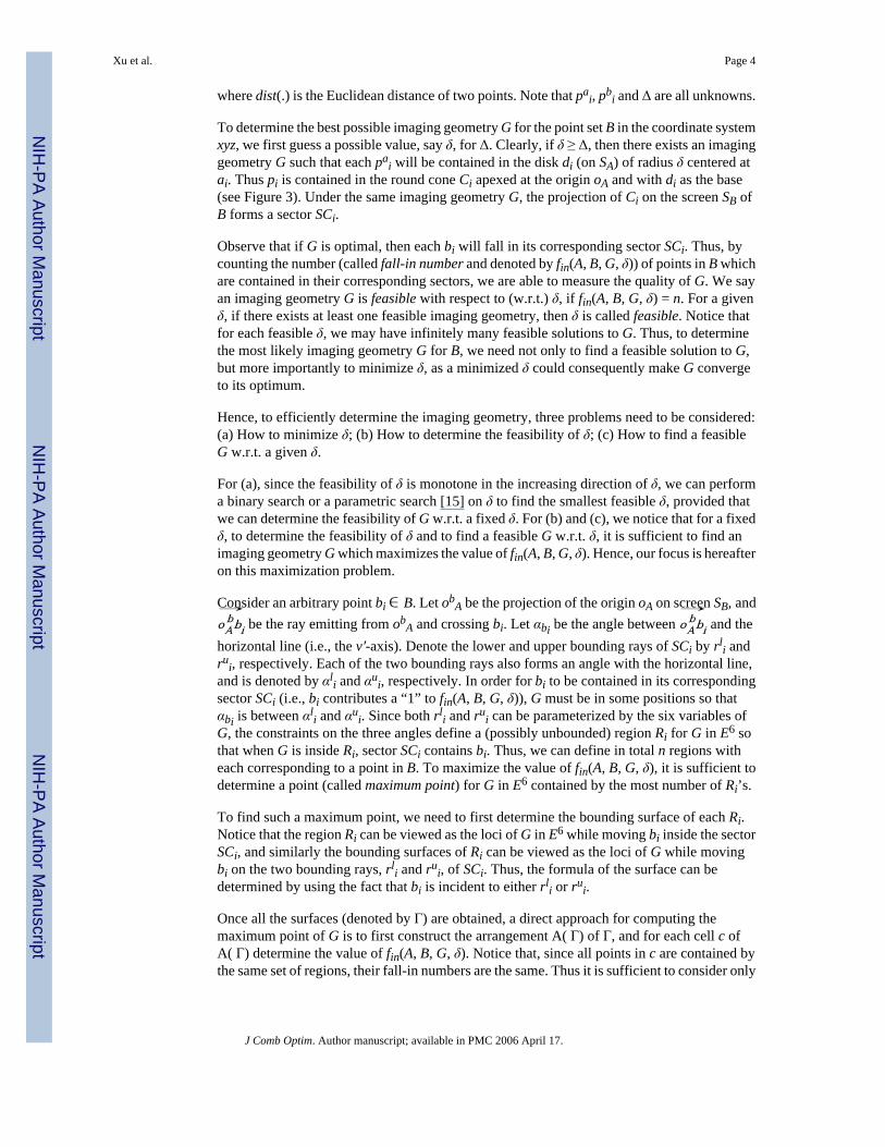
To facilitate our computation and analysis, we use Euler angles to describe the relative rotationin the rotation matrix R. Let θ, ψ and φ be the three Euler angles (see Figure 2). The entries ofthe rotation matrix R can be represented by θ, ψ and φ as follows.

r11 = − sin ψ sin φ + cos θ cos ψ cos φ, r12 = sin θ cos φ, r13 = − cos ψ sin φ − cos θ sin ψ cos φ,

r21 = − sin θ cos ψ, r22 = cos θ, r23 = sin θ sin ψ,

r31 = sin ψ cos φ + cos θ cos ψ sin φ, r32 = sin θ sin φ, r33 = cos ψ cos φ − cos θ sin ψ sin φ.

Due to a variety of reasons (such as the movement of beam sources and data noise), the exactrotation matrix R and translation vector t between the two coordinate systems xyz and x′y′z′ areoften unknown. Rough estimation can be obtained from the imaging system or computed byusing technique in [16]. To accurately reconstruct the 3-D structures of small vessels, highprecision imaging geometry is desired.

3 From Imaging Geometry to Arrangement SearchIn this section, we show how to reduce the imaging geometry determination problem to anoptimal cell search problem in an arrangement of surfaces.

Let P = {p1, p2, ···, pn} be the set of to-be-determined 3-D points. Let pai and pb

i be the exactprojections (under the optimal or most likely imaging geometry) of pi on the image screensSA and SB, respectively. We define

Δ = maxi=1n max{dist(ai, pi

a), dist(bi, pib)},

Xu et al. Page 3

J Comb Optim. Author manuscript; available in PMC 2006 April 17.

NIH

-PA Author Manuscript

NIH

-PA Author Manuscript

NIH

-PA Author Manuscript

where dist(.) is the Euclidean distance of two points. Note that pai, pb

i and Δ are all unknowns.

To determine the best possible imaging geometry G for the point set B in the coordinate systemxyz, we first guess a possible value, say δ, for Δ. Clearly, if δ ≥ Δ, then there exists an imaginggeometry G such that each pa

i will be contained in the disk di (on SA) of radius δ centered atai. Thus pi is contained in the round cone Ci apexed at the origin oA and with di as the base(see Figure 3). Under the same imaging geometry G, the projection of Ci on the screen SB ofB forms a sector SCi.

Observe that if G is optimal, then each bi will fall in its corresponding sector SCi. Thus, bycounting the number (called fall-in number and denoted by fin(A, B, G, δ)) of points in B whichare contained in their corresponding sectors, we are able to measure the quality of G. We sayan imaging geometry G is feasible with respect to (w.r.t.) δ, if fin(A, B, G, δ) = n. For a givenδ, if there exists at least one feasible imaging geometry, then δ is called feasible. Notice thatfor each feasible δ, we may have infinitely many feasible solutions to G. Thus, to determinethe most likely imaging geometry G for B, we need not only to find a feasible solution to G,but more importantly to minimize δ, as a minimized δ could consequently make G convergeto its optimum.

Hence, to efficiently determine the imaging geometry, three problems need to be considered:(a) How to minimize δ; (b) How to determine the feasibility of δ; (c) How to find a feasibleG w.r.t. a given δ.

For (a), since the feasibility of δ is monotone in the increasing direction of δ, we can performa binary search or a parametric search [15] on δ to find the smallest feasible δ, provided thatwe can determine the feasibility of G w.r.t. a fixed δ. For (b) and (c), we notice that for a fixedδ, to determine the feasibility of δ and to find a feasible G w.r.t. δ, it is sufficient to find animaging geometry G which maximizes the value of fin(A, B, G, δ). Hence, our focus is hereafteron this maximization problem.

Consider an arbitrary point bi ∈ B. Let obA be the projection of the origin oA on screen SB, and

oAbbi

→ be the ray emitting from ob

A and crossing bi. Let αbi be the angle between oAbbi

→ and the

horizontal line (i.e., the v′-axis). Denote the lower and upper bounding rays of SCi by rli and

rui, respectively. Each of the two bounding rays also forms an angle with the horizontal line,

and is denoted by αli and αu

i, respectively. In order for bi to be contained in its correspondingsector SCi (i.e., bi contributes a “1” to fin(A, B, G, δ)), G must be in some positions so thatαbi is between αl

i and αui. Since both rl

i and rui can be parameterized by the six variables of

G, the constraints on the three angles define a (possibly unbounded) region Ri for G in E6 sothat when G is inside Ri, sector SCi contains bi. Thus, we can define in total n regions witheach corresponding to a point in B. To maximize the value of fin(A, B, G, δ), it is sufficient todetermine a point (called maximum point) for G in E6 contained by the most number of Ri’s.

To find such a maximum point, we need to first determine the bounding surface of each Ri.Notice that the region Ri can be viewed as the loci of G in E6 while moving bi inside the sectorSCi, and similarly the bounding surfaces of Ri can be viewed as the loci of G while movingbi on the two bounding rays, rl

i and rui, of SCi. Thus, the formula of the surface can be

determined by using the fact that bi is incident to either rli or ru

i.

Once all the surfaces (denoted by Γ) are obtained, a direct approach for computing themaximum point of G is to first construct the arrangement A( Γ) of Γ, and for each cell c ofA( Γ) determine the value of fin(A, B, G, δ). Notice that, since all points in c are contained bythe same set of regions, their fall-in numbers are the same. Thus it is sufficient to consider only

Xu et al. Page 4

J Comb Optim. Author manuscript; available in PMC 2006 April 17.

NIH

-PA Author Manuscript

NIH

-PA Author Manuscript

NIH

-PA Author Manuscript

one point from each cell. The maximum point of G can then be determined by finding the cellwith the maximum fall-in number.

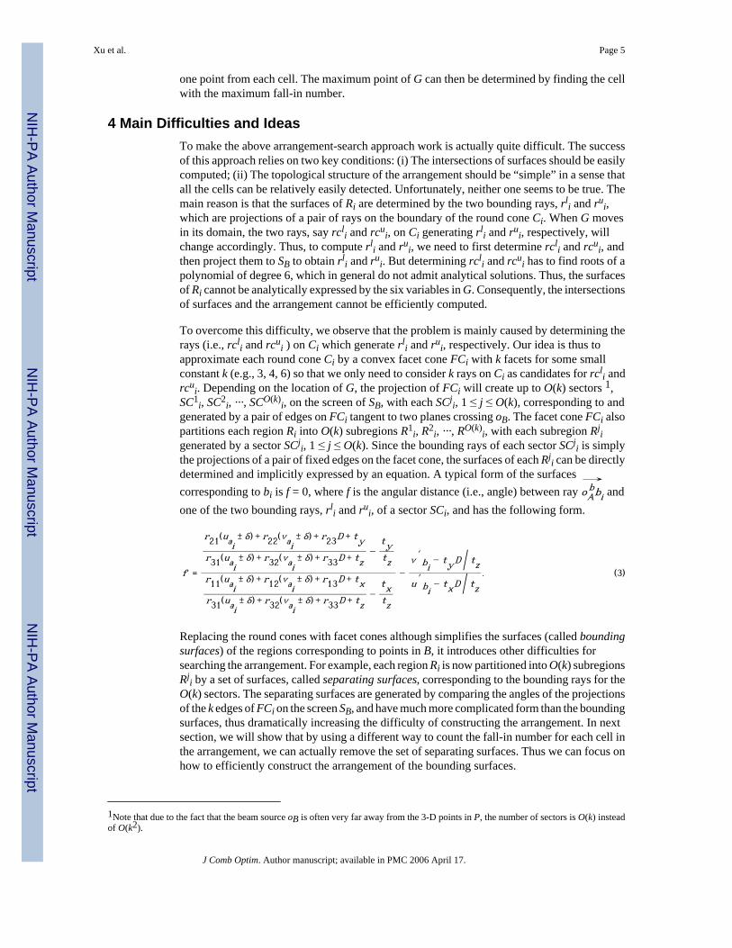
4 Main Difficulties and IdeasTo make the above arrangement-search approach work is actually quite difficult. The successof this approach relies on two key conditions: (i) The intersections of surfaces should be easilycomputed; (ii) The topological structure of the arrangement should be “simple” in a sense thatall the cells can be relatively easily detected. Unfortunately, neither one seems to be true. Themain reason is that the surfaces of Ri are determined by the two bounding rays, rl

i and rui,

which are projections of a pair of rays on the boundary of the round cone Ci. When G movesin its domain, the two rays, say rcl

i and rcui, on Ci generating rl

i and rui, respectively, will

change accordingly. Thus, to compute rli and ru

i, we need to first determine rcli and rcu

i, andthen project them to SB to obtain rl

i and rui. But determining rcl

i and rcui has to find roots of a

polynomial of degree 6, which in general do not admit analytical solutions. Thus, the surfacesof Ri cannot be analytically expressed by the six variables in G. Consequently, the intersectionsof surfaces and the arrangement cannot be efficiently computed.

To overcome this difficulty, we observe that the problem is mainly caused by determining therays (i.e., rcl

i and rcui ) on Ci which generate rl

i and rui, respectively. Our idea is thus to

approximate each round cone Ci by a convex facet cone FCi with k facets for some smallconstant k (e.g., 3, 4, 6) so that we only need to consider k rays on Ci as candidates for rcl

i andrcu

i. Depending on the location of G, the projection of FCi will create up to O(k) sectors 1,SC1

i, SC2i, ···, SCO(k)

i, on the screen of SB, with each SCji, 1 ≤ j ≤ O(k), corresponding to and

generated by a pair of edges on FCi tangent to two planes crossing oB. The facet cone FCi alsopartitions each region Ri into O(k) subregions R1

i, R2i, ···, RO(k)

i, with each subregion Rji

generated by a sector SCji, 1 ≤ j ≤ O(k). Since the bounding rays of each sector SCj

i is simplythe projections of a pair of fixed edges on the facet cone, the surfaces of each Rj

i can be directlydetermined and implicitly expressed by an equation. A typical form of the surfacescorresponding to bi is f = 0, where f is the angular distance (i.e., angle) between ray oA

bbi

→ and

one of the two bounding rays, rli and ru

i, of a sector SCi, and has the following form.

f =

r21(uai± δ) + r22(vai

± δ) + r23D + ty

r31(uai± δ) + r32(vai

± δ) + r33D + tz−

tytz

r11(uai± δ) + r12(vai

± δ) + r13D + tx

r31(uai± δ) + r32(vai

± δ) + r33D + tz−

txtz

−v ′

bi− tyD / tz

u ′bi

− txD / tz. (3)

Replacing the round cones with facet cones although simplifies the surfaces (called boundingsurfaces) of the regions corresponding to points in B, it introduces other difficulties forsearching the arrangement. For example, each region Ri is now partitioned into O(k) subregionsRj

i by a set of surfaces, called separating surfaces, corresponding to the bounding rays for theO(k) sectors. The separating surfaces are generated by comparing the angles of the projectionsof the k edges of FCi on the screen SB, and have much more complicated form than the boundingsurfaces, thus dramatically increasing the difficulty of constructing the arrangement. In nextsection, we will show that by using a different way to count the fall-in number for each cell inthe arrangement, we can actually remove the set of separating surfaces. Thus we can focus onhow to efficiently construct the arrangement of the bounding surfaces.

1Note that due to the fact that the beam source oB is often very far away from the 3-D points in P, the number of sectors is O(k) insteadof O(k2).

Xu et al. Page 5

J Comb Optim. Author manuscript; available in PMC 2006 April 17.

NIH

-PA Author Manuscript

NIH

-PA Author Manuscript

NIH

-PA Author Manuscript

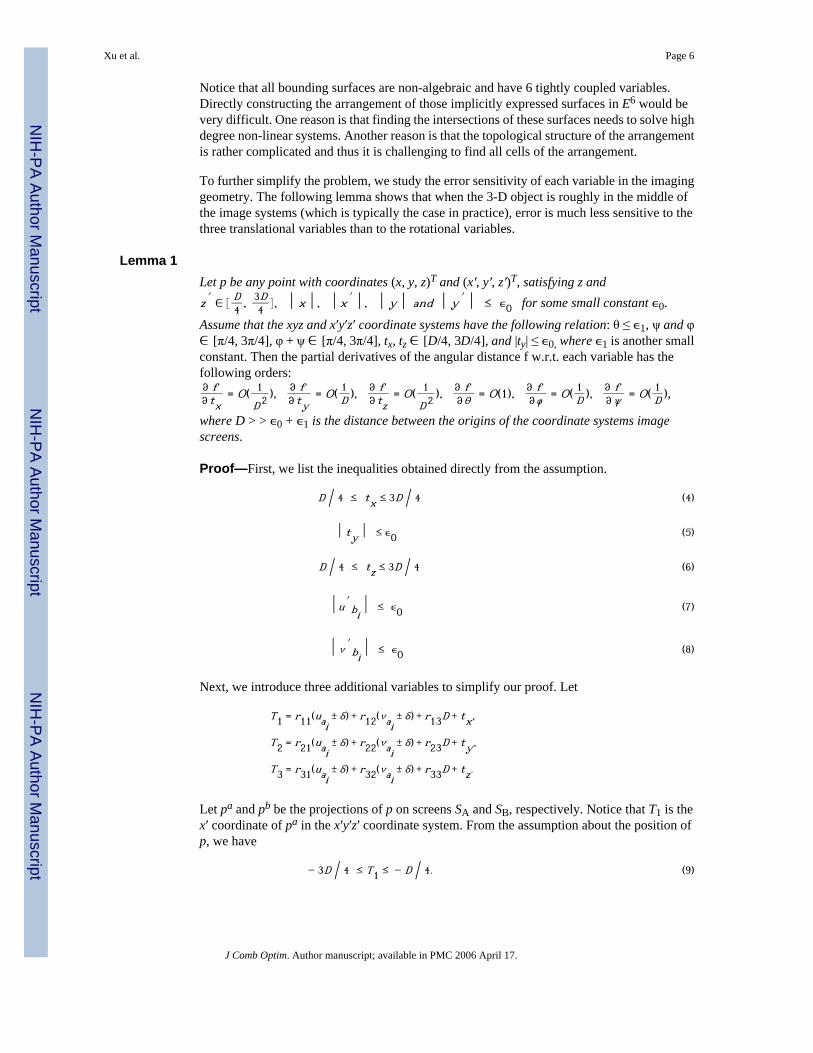
Notice that all bounding surfaces are non-algebraic and have 6 tightly coupled variables.Directly constructing the arrangement of those implicitly expressed surfaces in E6 would bevery difficult. One reason is that finding the intersections of these surfaces needs to solve highdegree non-linear systems. Another reason is that the topological structure of the arrangementis rather complicated and thus it is challenging to find all cells of the arrangement.

To further simplify the problem, we study the error sensitivity of each variable in the imaginggeometry. The following lemma shows that when the 3-D object is roughly in the middle ofthe image systems (which is typically the case in practice), error is much less sensitive to thethree translational variables than to the rotational variables.

Lemma 1Let p be any point with coordinates (x, y, z)T and (x′, y′, z′)T, satisfying z andz ′ ∈ D

4 , 3D4 , | x | , | x ′ | , | y | and | y ′ | ≤ ∊0 for some small constant ∊0.

Assume that the xyz and x′y′z′ coordinate systems have the following relation: θ ≤ ∊1, ψ and φ∈ [π/4, 3π/4], φ + ψ ∈ [π/4, 3π/4], tx, tz ∈ [D/4, 3D/4], and |ty| ≤ ∊0, where ∊1 is another smallconstant. Then the partial derivatives of the angular distance f w.r.t. each variable has thefollowing orders:∂ f∂tx

= O( 1

D 2 ), ∂ f∂ty

= O( 1D ), ∂ f

∂tz= O( 1

D 2 ), ∂ f∂θ = O(1), ∂ f

∂φ = O( 1D ), ∂ f

∂ψ = O( 1D ),

where D > > ∊0 + ∊1 is the distance between the origins of the coordinate systems imagescreens.

Proof—First, we list the inequalities obtained directly from the assumption.

D / 4 ≤ tx ≤ 3D / 4 (4)

| ty | ≤ ∊0 (5)

D / 4 ≤ tz ≤ 3D / 4 (6)

| u ′bi | ≤ ∊0 (7)

| v ′bi | ≤ ∊0 (8)

Next, we introduce three additional variables to simplify our proof. Let

T1 = r11(uai± δ) + r12(vai

± δ) + r13D + tx,

T2 = r21(uai± δ) + r22(vai

± δ) + r23D + ty,

T3 = r31(uai± δ) + r32(vai

± δ) + r33D + tz.

Let pa and pb be the projections of p on screens SA and SB, respectively. Notice that T1 is thex′ coordinate of pa in the x′y′z′ coordinate system. From the assumption about the position ofp, we have

− 3D / 4 ≤ T1 ≤ − D / 4. (9)

Xu et al. Page 6

J Comb Optim. Author manuscript; available in PMC 2006 April 17.

NIH

-PA Author Manuscript

NIH

-PA Author Manuscript

NIH

-PA Author Manuscript

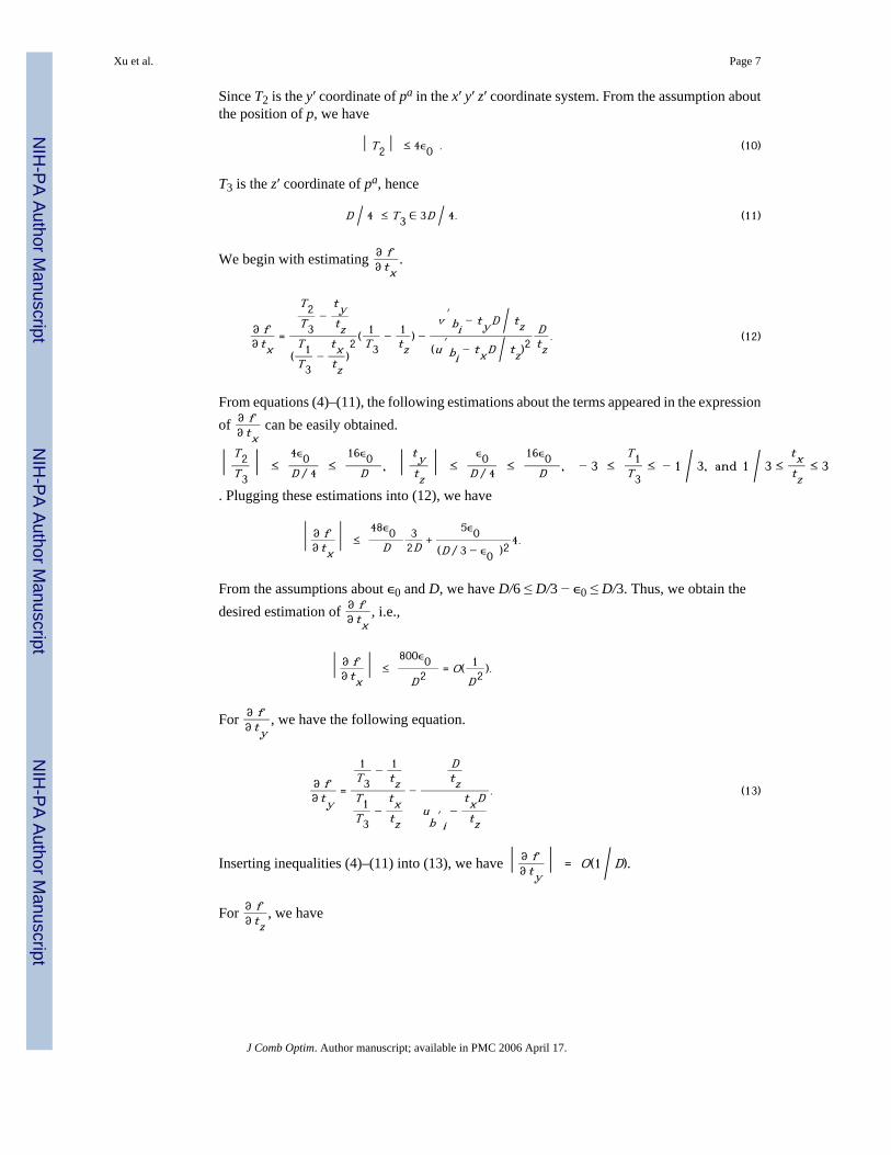
Since T2 is the y′ coordinate of pa in the x′ y′ z′ coordinate system. From the assumption aboutthe position of p, we have

| T2 | ≤ 4∊0 . (10)

T3 is the z′ coordinate of pa, hence

D / 4 ≤ T3 ∈ 3D / 4. (11)

We begin with estimating ∂ f∂tx

.

∂ f∂tx

=

T2T3

−tytz

(T1T3

−txtz

)2 ( 1

T3− 1

tz) −

v ′bi

− tyD / tz

(u ′bi

− txD / tz)2

Dtz

. (12)

From equations (4)–(11), the following estimations about the terms appeared in the expressionof ∂ f

∂tx can be easily obtained.

| T2T3

| ≤4∊0D / 4 ≤

16∊0D , | ty

tz| ≤

∊0D / 4 ≤

16∊0D , − 3 ≤

T1T3

≤ − 1 / 3, and 1 / 3 ≤txtz

≤ 3

. Plugging these estimations into (12), we have

| ∂ f∂tx | ≤

48∊0D

32D +

5∊0(D / 3 − ∊0 )2

4.

From the assumptions about ∊0 and D, we have D/6 ≤ D/3 − ∊0 ≤ D/3. Thus, we obtain thedesired estimation of ∂ f

∂tx, i.e.,

| ∂ f∂tx

| ≤800∊0

D2 = O( 1

D2 ).

For ∂ f∂ty

, we have the following equation.

∂ f∂ty

=

1T3

− 1tz

T1T3

−txtz

−

Dtz

ub′

i−

txD

tz

. (13)

Inserting inequalities (4)–(11) into (13), we have | ∂ f∂ty

| = O(1 / D).

For ∂ f∂tz

, we have

Xu et al. Page 7

J Comb Optim. Author manuscript; available in PMC 2006 April 17.

NIH

-PA Author Manuscript

NIH

-PA Author Manuscript

NIH

-PA Author Manuscript

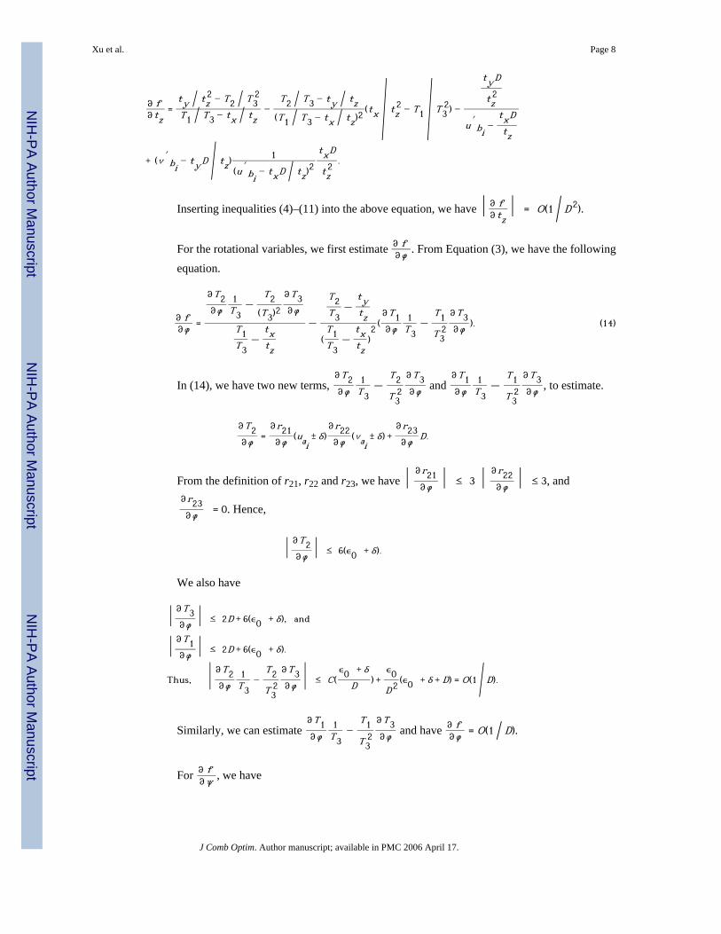
∂ f∂tz

=ty / tz

2 − T2 / T32

T1 / T3 − tx / tz−

T2 / T3 − ty / tz(T1 / T3 − tx / tz)

2 (tx / tz2 − T1 / T3

2) −

tyD

tz2

u ′bi

−txD

tz

+ (v ′bi

− tyD / tz)1

(u ′bi

− txD / tz)2

txD

tz2 .

Inserting inequalities (4)–(11) into the above equation, we have | ∂ f∂tz

| = O(1 / D 2).

For the rotational variables, we first estimate ∂ f∂φ . From Equation (3), we have the following

equation.

∂ f∂φ =

∂T2∂φ

1T3

–T2

(T3)2

∂T3∂φ

T1T3

–txtz

–

T2T3

–tytz

(T1T3

–txtz

)2 (

∂T1∂φ

1T3

–T1

T32

∂T3∂φ ). (14)

In (14), we have two new terms, ∂T2∂φ

1T3

–T2

T32

∂T3∂φ and

∂T1∂φ

1T3

–T1

T32

∂T3∂φ , to estimate.

∂T2∂φ =

∂r21∂φ (uai

± δ)∂r22∂φ (vai

± δ) +∂r23∂φ D.

From the definition of r21, r22 and r23, we have | ∂r21∂φ | ≤ 3 | ∂r22

∂φ | ≤ 3, and∂r23∂φ = 0. Hence,

| ∂T2∂φ | ≤ 6(∊0 + δ).

We also have

| ∂T3∂φ | ≤ 2D + 6(∊0 + δ), and

| ∂T1∂φ | ≤ 2D + 6(∊0 + δ).

Thus, | ∂T2∂φ

1T3

−T2

T32

∂T3∂φ | ≤ C(

∊0 + δ

D ) +∊0

D2 (∊0 + δ + D) = O(1 / D).

Similarly, we can estimate ∂T1∂φ

1T3

−T1

T32

∂T3∂φ and have ∂ f

∂φ = O(1 / D).

For ∂ f∂ψ , we have

Xu et al. Page 8

J Comb Optim. Author manuscript; available in PMC 2006 April 17.

NIH

-PA Author Manuscript

NIH

-PA Author Manuscript

NIH

-PA Author Manuscript

∂ f∂ψ =

∂T2∂ψ

1T3

−T2

T32

∂T3∂ψ

T1T3

−txtz

−

T2T3

−tytz

(T1T3

−txtz

)2 (

∂T1∂ψ

1T3

−T1

T32

∂T3∂ψ ).

We get

∂ f∂ψ = O(1 / D).

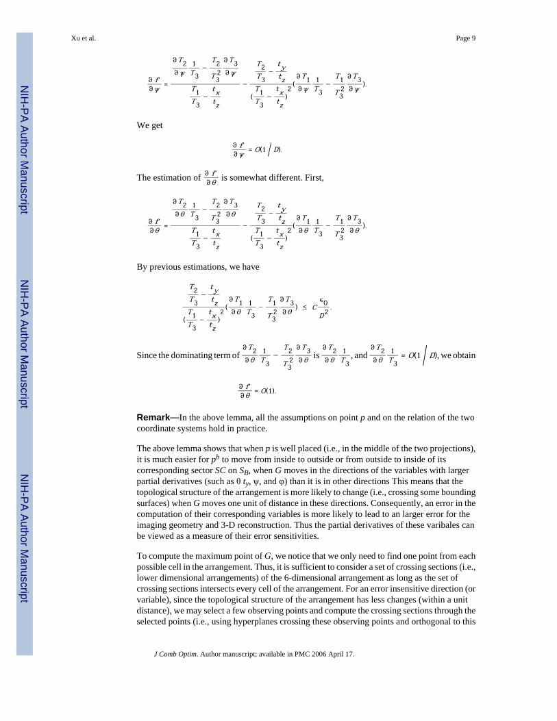
The estimation of ∂ f∂θ is somewhat different. First,

∂ f∂θ =

∂T2∂θ

1T3

−T2

T32

∂T3∂θ

T1T3

−txtz

−

T2T3

−tytz

(T1T3

−txtz

)2 (

∂T1∂θ

1T3

−T1

T32

∂T3∂θ ).

By previous estimations, we have

T2T3

−tytz

(T1T3

−txtz

)2 (

∂T1∂θ

1T3

−T1

T32

∂T3∂θ ) ≤ C

∊0

D2 .

Since the dominating term of ∂T2∂θ

1T3

−T2

T32

∂T3∂θ is

∂T2∂θ

1T3

, and ∂T2∂θ

1T3

= O(1 / D), we obtain

∂ f∂θ = O(1).

Remark—In the above lemma, all the assumptions on point p and on the relation of the twocoordinate systems hold in practice.

The above lemma shows that when p is well placed (i.e., in the middle of the two projections),it is much easier for pb to move from inside to outside or from outside to inside of itscorresponding sector SC on SB, when G moves in the directions of the variables with largerpartial derivatives (such as θ ty, ψ, and φ) than it is in other directions This means that thetopological structure of the arrangement is more likely to change (i.e., crossing some boundingsurfaces) when G moves one unit of distance in these directions. Consequently, an error in thecomputation of their corresponding variables is more likely to lead to an larger error for theimaging geometry and 3-D reconstruction. Thus the partial derivatives of these varibales canbe viewed as a measure of their error sensitivities.

To compute the maximum point of G, we notice that we only need to find one point from eachpossible cell in the arrangement. Thus, it is sufficient to consider a set of crossing sections (i.e.,lower dimensional arrangements) of the 6-dimensional arrangement as long as the set ofcrossing sections intersects every cell of the arrangement. For an error insensitive direction (orvariable), since the topological structure of the arrangement has less changes (within a unitdistance), we may select a few observing points and compute the crossing sections through theselected points (i.e., using hyperplanes crossing these observing points and orthogonal to this

Xu et al. Page 9

J Comb Optim. Author manuscript; available in PMC 2006 April 17.

NIH

-PA Author Manuscript

NIH

-PA Author Manuscript

NIH

-PA Author Manuscript

direction to cut the arrangement). In this way, we may avoid considering this directioncontinuously, and hence reduce the dimensions of the arrangement.

To implement this idea, we can select a few “good” variables with larger partial derivatives asthe variables of the arrangement, and place a grid in the subspace of the domain induced bythose unselected variables. We say a set of variables are good if the bounding surfaces inducedby setting other variables to constants has simple forms or nice structures. Notice that in theimaging geometry determination problem, the domain can be assumed to be a small hyperboxas a rough estimation of the optimal solution can be obtained by using some previous techniques[16] or from the imaging system. The sizes of the grid may vary in different directions,consistent with their partial derivatives.

Hence it is possible to compute the maximum point through traversing a set of lowerdimensional arrangements. Following is the main steps of our algorithm for computing themaximum point.

1. Select 2 or 3 good variables, and place a grid in the subspace of the domain inducedby other variables.

2. For each grid point,

a. determine the expression of each bounding surface in the subspace inducedby the selected variables;

b. compute the maximum point in the arrangements of the set of lowerdimensional surfaces.

3. Return the maximum point found among all grid points.

5 Finding the Maximum Point in a Lower Dimensional ArrangementTo solve the maximum point problem, we need to first select the set of variables. By Lemma1, we know that θ is the most error-sensitive variable, and thus should be chosen. Three othervariables, ty, ψ, and φ has the same order. Since ty is loosely coupled with θ, we pick ty overthe other two rotational variables.

To select other possible variables, we first observe that if two rotational variables are selected

simultaneously, the surfaces will be of the form g1(α1, α2)

g2(α1, α2)+ c = 0, where, α1 and α2 are the

two rotational variables, and g1(), g2() are two functions containing products of trigonometricfunctions of α1 and α 2. The surfaces will be rather complicated, and more importantly, theirintersections will not be easily computed. Hence, in our algorithm, we only select one rotationalvariable.

Since our approach needs to traverse an arrangement on each grid point, the more variableswe select, the less grid points we need to consider. Thus on one hand, it is better to select morevariables to ensure time efficiency as long as the associated arrangements can still be easilytraversed. On the other hand, selecting more variables will complicate the surfaces and makeit harder to traverse the arrangement. Nevertheless, our analysis shows that it is possible toselect another translational variable tx and still obtain relatively simple surfaces.

With the selected variables, at each grid point the bounding surfaces have the following form.

Xu et al. Page 10

J Comb Optim. Author manuscript; available in PMC 2006 April 17.

NIH

-PA Author Manuscript

NIH

-PA Author Manuscript

NIH

-PA Author Manuscript

tx{v ′bi

(r31(uai± δ) + r32(vai

± δ) + r33D) − D(r21(uai± δ) + r22(vai

± δ) + r23D)} +

ty{D(r11(uai± δ) + r12(vai

± δ) + r13D) − u ′bi

(r21(uai± δ) + r22(vai

± δ) + r23D)} =

tz{v ′bi

(r11(uai± δ) + r12(vai

± δ) + r13D) − u ′bi

(r31(uai± δ) + r32(vai

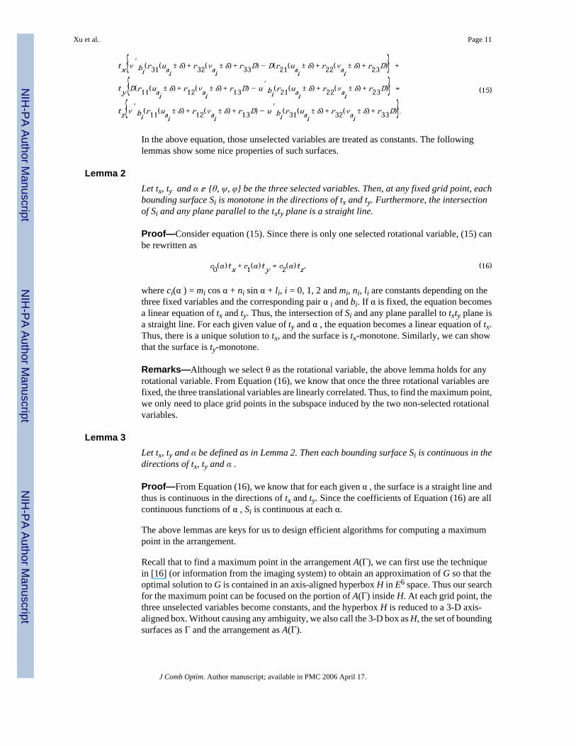
± δ) + r33D)}.(15)

In the above equation, those unselected variables are treated as constants. The followinglemmas show some nice properties of such surfaces.

Lemma 2Let tx, ty and α ɛ {θ, ψ, φ} be the three selected variables. Then, at any fixed grid point, eachbounding surface Si is monotone in the directions of tx and ty. Furthermore, the intersectionof Si and any plane parallel to the txty plane is a straight line.

Proof—Consider equation (15). Since there is only one selected rotational variable, (15) canbe rewritten as

c0(α)tx + c1(α)ty = c2(α)tz, (16)

where ci(α ) = mi cos α + ni sin α + li, i = 0, 1, 2 and mi, ni, li are constants depending on thethree fixed variables and the corresponding pair α i and bi. If α is fixed, the equation becomesa linear equation of tx and ty. Thus, the intersection of Si and any plane parallel to txty plane isa straight line. For each given value of ty and α , the equation becomes a linear equation of tx.Thus, there is a unique solution to tx, and the surface is tx-monotone. Similarly, we can showthat the surface is ty-monotone.

Remarks—Although we select θ as the rotational variable, the above lemma holds for anyrotational variable. From Equation (16), we know that once the three rotational variables arefixed, the three translational variables are linearly correlated. Thus, to find the maximum point,we only need to place grid points in the subspace induced by the two non-selected rotationalvariables.

Lemma 3Let tx, ty and α be defined as in Lemma 2. Then each bounding surface Si is continuous in thedirections of tx, ty and α .

Proof—From Equation (16), we know that for each given α , the surface is a straight line andthus is continuous in the directions of tx and ty. Since the coefficients of Equation (16) are allcontinuous functions of α , Si is continuous at each α.

The above lemmas are keys for us to design efficient algorithms for computing a maximumpoint in the arrangement.

Recall that to find a maximum point in the arrangement A(Γ), we can first use the techniquein [16] (or information from the imaging system) to obtain an approximation of G so that theoptimal solution to G is contained in an axis-aligned hyperbox H in E6 space. Thus our searchfor the maximum point can be focused on the portion of A(Γ) inside H. At each grid point, thethree unselected variables become constants, and the hyperbox H is reduced to a 3-D axis-aligned box. Without causing any ambiguity, we also call the 3-D box as H, the set of boundingsurfaces as Γ and the arrangement as A(Γ).

Xu et al. Page 11

J Comb Optim. Author manuscript; available in PMC 2006 April 17.

NIH

-PA Author Manuscript

NIH

-PA Author Manuscript

NIH

-PA Author Manuscript

Hence our task is to find the maximum point in A(Γ) ∩ H. As mentioned previously, all pointsin each cell of A(Γ) share the same fall-in number. For two neighboring cells c1 and c2 separatedby a bounding surface Si, the two sets of fall-in points (i.e., the points of B contained in theircorresponding sectors) in the two cells differ only by one point bi, since crossing the surfaceSi means turning bi from a fall-in point to a non-fall-in point (or vice versa). Hence thedifference of the fall-in numbers of the two cells is 1. To find the cell with the maximum fall-in number, our main idea is to design a plane sweep algorithm which extracts one or morepoints from each cell and efficiently determine their fall-in numbers.

To better illustrate our plane sweep algorithm, we first assume that there are only two boundingsurfaces generated from each facet cone FCi with each Si corresponding to a bounding ray ofthe sector SCi. (Later on we will show how to remove this assumption.) Thus in the arrangementA(Γ), when G crosses Si, its fall-in number either increases or decreases by 1. Equivalently,each surface Si can be viewed as an oriented surface. When G crosses Si in the direction of itsorientation, the fall-in number of G increases by 1.

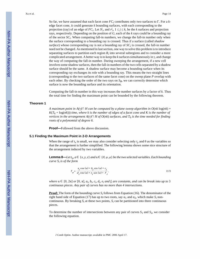
To efficiently search all cells in A(Γ) ∩ H, we sweep a plane P parallel to the txty-plane throughH. P starts from the bottom of H and moves in the increasing direction of θ (see Figure 5). Let[θ0, θ1] be the range of θ in H, and let P θ be the intersection of P and A(Γ) n H when P movesto the position of θ. By Lemma 2, we know that the intersections of Γ and P are a set of lines.Hence Pθ is the portion of an arrangement of lines inside a rectangle. The following lemmashows that the fall-in number of each cell in Pθ0 can be efficiently computed.

Lemma 4The fall-in number of each cell in Pθ0 can be computed in O(n log n + K0) time, where K0 isthe number of cells in Pθ0.

Proof—Since Pθ0 is the portion of an arrangement of lines inside a convex polygon (e.g.,rectangle), we can use topological peeling [4] (or topological walk [3]) to generate the set ofcells as well as the intersections of Pθ0 in O(n log n + K0) time. The fall-in number of the firstcell c encountered by topological peeling can be computed by first selecting an arbitrary pointin c as (a fixed) G and then checking whether each point in B is contained in its correspondingsector. The time needed for checking each point is O(1) once G is fixed. Thus the total timefor computing the fall-in number of the first cell is O(n). For each later encountered cell (bytopological peeling), we can compute its fall-in number from its neighboring cell in O(1) time,since topological peeling generates cells in a wave propagation fashion. Thus the total timeneeded for computing all fall-in numbers is O(n + K0). Thus the lemma follows.

To compute the fall-in numbers for those cells in A(Γ) ∩ H which have not yet intersected byP, we detect all the events in which P encounters a cell or finishes a cell while moving frombottom to top. Notice that there are several types of events which could change the topologicalstructure of Pθ: (a) A surface which is previously outside of H enters H and generates a lineon P ∩ H; (b) A surface leaves H, and hence its corresponding line on P ∩ H moves outsideof H; (c) A new cell is encountered by P; (d) A cell is finished by P.

For type (a) and (b) events, we can compute for each surface Si ∈ Γ its intersections with theboundary of H, and insert the events into an event queue (such as priority queue) for the planesweep. Since the intersections can be computed in constant time for each surface, and insertingeach event into an event queue takes O(log n) time, the total time for type (a) and (b) events isO(n log n) time.

For type (c) and (d) events, we have the following lemma.

Xu et al. Page 12

J Comb Optim. Author manuscript; available in PMC 2006 April 17.

NIH

-PA Author Manuscript

NIH

-PA Author Manuscript

NIH

-PA Author Manuscript

Lemma 5For each cell which is not discovered by a type (a) or (b) event, and does not intersect Pθ0, itsfirst intersection with P occurs at a vertex generated by three bounding surfaces or theboundary of H.

Proof—By Lemma 2, we know that all surfaces in γ are monotone in tx and ty directions.Suppose there is such a cell c which is first intersected by P at an interior point on one of itsbounding surfaces Si. By Lemma 3, we know Si is continuous. Thus if move P up slightly, sayby a sufficient small constant ∊, then Si will generate a closed curve on P, contradicting Lemma2.

To efficiently detect all type (c) and (d) events, we consider a type (c) event (type (d) eventscan be similarly handled). Let c be the cell encountered by P. By Lemma 5, the first encounteredpoint is a vertex v of c. Let S1, S2 and S3 be the three surfaces generating v. Consider the momentjust before P meets v. By Lemma 3, all the three surfaces S1, S2 and S3 are continuous. Thuseach of them produces a line on P. The three lines generate at least two vertices on P, say v1and v2, which are neighboring to each other on one of three lines and converge to v when Pmoves to v. Thus to detect this event, it is sufficient to compute v at the time when v1 and v2becomes neighbors to each other at their first time.

To detect all such events, we can start from Pθ0 and compute for each pair of neighboringvertices in Pθ0 the time when they converge (or merge) (if they do), and store such time in theevent queue if it is in the range of H. Then we use the event queue to sweep the arrangement.When a new vertex is generated on P or two vertices become neighbors to each other at theirfirst time, we check whether there is a possible event. In this way, we can capture all the eventsand thus detect all the cells in A(Γ)∩ H.

The following lemma shows that each type (c) or (d) event can be detected efficiently.

Lemma 6The intersection of three bounding surfaces can be computed by solving a polynomial ofdegree 6.

Proof—Followed from Equation (16) and Lemma 2.

The following lemma bounds the total time used for detecting all events.

Lemma 7All events can be detected in O(n log n + K(T6 + log n)) time, where K is the total number ofvertices in A(Γ)∩ H, and T6 is the time needed for finding roots of a polynomial of degree 6.

Proof—From Lemma 4, we know that the total time for constructing the arrangement Pθ0 isO(n log n+K0). In Pθ0, there are O(K0) pairs of neighboring vertices. Each pair of neighboringvertices takes O(T6) time (by Lemma 6) to find the possible event and O(log n) time to insertthe event into the event queue. For each new vertex in A(Γ)∩ H, the plane sweep algorithmtakes O(T6 + log n) time to find the event, to insert into, and to delete from the event queue.Thus the total time for generating all vertices is O(n log n + K(T6 + log n)), and the lemmafollows.

The fall-in number of each cell c can be computed in O(1) time at the moment when P intersectsc at the first time by using the already computed fall-in numbers of its neighboring cells.

Xu et al. Page 13

J Comb Optim. Author manuscript; available in PMC 2006 April 17.

NIH

-PA Author Manuscript

NIH

-PA Author Manuscript

NIH

-PA Author Manuscript

So far, we have assumed that each facet cone FCi contributes only two surfaces to Γ. For a k-edge facet cone, it could generate k bounding surfaces, with each corresponding to theprojection (ray) of an edge of FCi. Let Sj

i, and rji, 1 ≤ j ≤ k, be the k surfaces and projection

rays, respectively. Depending on the position of G, each of the k rays could be a bounding rayof the sector SCi. When computing fall-in numbers, we change the fall-in number only whenthe surface corresponding to a bounding ray is crossed. Thus if a surface (called shadowsurface) whose corresponding ray is not a bounding ray of SCi is crossed, the fall-in numberneed not be changed. As mentioned in last section, one way to solve this problem is to introduceseparating surfaces to partition each region Ri into several subregions and to consider a morecomplicated arrangement. A better way is to keep the k surfaces simultaneously in γ, and changethe way of computing the fall-in number. During sweeping the arrangement, if a new cellinvolves some shadow surfaces, then the fall-in numbers of the two cells separated by a shadowsurface should be the same. A shadow surface may become a bounding surface when itscorresponding ray exchanges its role with a bounding ray. This means the two straight lines(corresponding to the two surfaces of the same facet cone) on the sweep plane P overlap witheach other. By checking the order of the two rays on SB, we can correctly determine whichsurface is now the bounding surface and its orientation.

Computing the fall-in number in this way increases the number surfaces by a factor of k. Thusthe total time for finding the maximum point can be bounded by the following theorem.

Theorem 1A maximum point in A(γ)∩ H can be computed by a plane sweep algorithm in O(nk log(nk) +K(T6 + log(nk))) time, where k is the number of edges of a facet cone and K is the number ofvertices in the arrangement A(γ)∩ H of O(nk) surfaces, and T6 is the time needed for findingroots of a polynomial of degree 6.

Proof—Followed from the above discussion.

5.1 Finding the Maximum Point in 2-D ArrangementsWhen the range of tx is small, we may also consider selecting only ty and θ as the variables sothat the arrangement is further simplified. The following lemma shows some nice structure ofthe arrangement induced by two variables.

Lemma 8—Let ta, a ∈ {x, y, z} and α ∈ {θ, ψ, φ} be the two selected variables. Each boundingcurve Si is of the form

Ta =ai cos (α) + bi sin (α) + cidi cos (α) + ei sin (α) + f i

, (17)

where α ∈ [0, 2π] or [0, π], ai, bi, ci, di, ei and fi are constants, and can be break into up to 3continuous pieces. Any pair of curves has no more than 4 intersections.

Proof: The form of the bounding curve Si follows from Equation (16). The denominator of theright hand side of Equation (17) has up to two roots, say α1 and α2, which make Si non-continuous. By breaking Si at these two points, Si can be partitioned into three continuouspieces.

To determine the number of intersections between any pair of curves S1 and S2, we considerthe following equation.

Xu et al. Page 14

J Comb Optim. Author manuscript; available in PMC 2006 April 17.

NIH

-PA Author Manuscript

NIH

-PA Author Manuscript

NIH

-PA Author Manuscript

a1 cos (α) + b1 sin (α) + c1d1 cos (α) + e1 sin (α) + f 1

=a2 cos (α) + b2 sin (α) + c2d2 cos (α) + e2 sin (α) + f 2

.

Replacing cos(α) by z and sin(α) by ± 1 − z 2, we can convert the above equation into apolynomial equation of degree 4. Thus the number of intersections between S1 and S2 is atmost 4.

Lemma 8 enables us to find a maximum point at each grid point by using some 2-D arrangementtraversal algorithms [2]. The following lemma bounds the running time.

Lemma 9—The maximum point of a 2-D arrangement can be found in O(n log n + K) time,where K is the number of vertices in the 2-D arrangement inside H.

Proof: By Lemma 8, we know that the pairwise intersections are no more than 4. Thus by usingthe algorithm in [2], we can traverse the whole arrangement in O(n log n + K) time.

To find the “global” maximum in the 2-D or 3-D arrangements, we determine a maximumpoint for each grid point and return the best as our solution.

5.2 Removing OutliersAfter the binary search on δ has finished, the accuracy can be further improved by removinga few outliers from the point sets A and B. Notice that the correspondence between A and Bare often established manually, and may not be consistent with each other. By removing a fewoutliers, we could further reduce δ and consequently reduce the error of G. The main idea isas follows. Once δ is reduced to be infeasible, we can find a maximum point for G, and checkwhich points in B are not contained in their corresponding sectors. If the number of such pointsis small, we can just discard those non-fall-in points from A and B. By doing so, δ becomesfeasible again and therefore may be further reduced. Hence, the error of G could be decreased.

6 Experimental ResultsTo evaluate the performance of our technique, we implemented our algorithm using C++ andLEDA 4.4 on a DELL OPTIPLEX GX260 PC with 2.26GHz running Redhat Linux 8.0, andcompare it with a well-recognized algorithm [11] in Cardiovascular community. We conductour experiment with the same configuration as those in [11]. Our experiment randomlygenerates a biplane imaging geometry in a small neighborhood of the following settings: ψ =π/2, θ = 0, φ = 0, |tx| = |tz| = 0.5D, ty = 0, D = 140cm; and the input noise (or image errors) forimage data are up to 0.15cm. A set of 3-D object points are placed close to the center of thetwo coordinate systems. The object points are projected onto the screen SA and SB, respectively.A and B are then chosen by adding random noise to the projections of P.

Our experiment shows that the absolute errors for the translational variables and the Eulerangles are either much smaller than or comparable with those in [11]. For instance, in most ofour examples, errors are as small as 0.05cm for the translational variables and 0.5° for the Eulerangles while the errors in [11] could be as much as 0.15cm for the translational variables and3° for the rotational variables. Our experiments indicate that the errors are consistent with thesensitivity analysis stated in Lemma 1. As expected, Figure 6(a) shows that the errors of ty tendto decrease when there are more corresponding pairs. Figure 6(b) shows that the errors of tyslowly increase with an increase in the input image errors.

Xu et al. Page 15

J Comb Optim. Author manuscript; available in PMC 2006 April 17.

NIH

-PA Author Manuscript

NIH

-PA Author Manuscript

NIH

-PA Author Manuscript

References1. Aggarwal J, Nandhakumar N. “On the computation of motion from sequences of images-A review,”.

Proc IEEE 1988;76(8):917–935.2. Amato NM, Goodrich MT, Ramos EA. “Computing the arrangement of curve segments: Divide-and-

conquer algorithms via sampling,”. Proc 11th Annual ACM-SIAM Symposium on DiscreteAlgorithms 2000:705–706.

3. Asano T, Guibas LJ, Tokuyama T. “Walking in an arrangement topologically,”. International Journalof Computational Geometry and Applications 1994;4(2):123–151.

4. D.Z. Chen, S. Luan, and J. Xu,“Topological Peeling and Implementation,” Proc. 12th AnnualInternational Symposium on Algorithms And Computation (ISAAC), Lecture Notes in ComputerScience, Vol. 2223, Springer Verlag, 2001, pp.454–466.

5. Chen SYJ, Metz CE. “Improved determination of biplane imaging geometry from two projectionimages and its application to three-dimensional reconstruction of coronary arterial trees,”. Med Phys1997;24:633–654. [PubMed: 9167155]

6. Esthappan J, harauchi H, Hoffmann K. “Evaulation of imaging geometries c alculated from biplaneimages,”. Med Phys 1998;25(6):965–975. [PubMed: 9650187]

7. Fusiello A. “Uncalibrated Euclidean reconstruction: a review,”. Image and Vision Computing2000;18:555–563.

8. Grondin CM, Dyrda I, Pasternac A, Campeau L, Bourassa MG, Lesperance J. “Discrepancies betweencineangiographic and postmortem findings in patients with coronary artery disease and recentmyocardial revascularization,”. Circulation 1974;49:703–708. [PubMed: 4544728]

9. Hoffmann KR, Doi K, Chan HP, Chua KG. “Computer reproduction of the vasculature using anautomated tracking method,”. Proc SPIE 1987;767:449–453.

10. Hoffmann KR, Doi K, Chan HP, Takamiya M. “Three dimensional reproduction of coronary vasculartrees using the double-squre-box method of trackings,”. Proc SPIE 1988;914:375–378.

11. Hoffmann KR, Metz CE, Chen Y. “Determination of 3D imaging geometry and object configurationsfrom two biplane views: An enhancement of the Metz-Fencil technique,”. Med Phys 1995;22:1219–1227. [PubMed: 7476707]

12. Hoffmann KR, Sen A, Lan L, Kok-Gee Chua, Esthappan J, Mazzucco M. “A system for determinationof 3D vessel tree centerlines from biplane images,”. The International Journal of Cardiac Imaging2000;16:315–330.

13. Huang T, Netravali A. “Motion and structure from feature correspondences: A review,”. Proc IEEE1994;82(2):252–268.

14. Luong QT, Faugeras OD. “The fundamental matrix: Theory, algorithms and stability analysis,”. TheInternational Journal of Computer Vision 1996;1(17):43–76.

15. Megiddo N. “Applying parallel computation algorithms in the design of serial algorithms,”. Journalof ACM 1983;30(4):852–865.

16. Metz CE, Fencil LE. “Determination of three-dimensional structure in biplane radiography withoutprior knowledge of the relationship between the two views,”. Med Phys 1989;16:45–51. [PubMed:2921979]

17. D. P. Nazareth, K. R. Hoffmann, A. Walczak, J. Dmochowski, L. Guterman, S. Rudin, D. R. Bednarek,“Determination of biplane geometry and centerline curvature in vascular imaging,” Manuscript,2002.

18. Quan L. “Invariants of six points and projective reconstruction from three uncalibrated images,”.IEEE Transaction on Pattern Analysis and Machine Intelligence 1995;17(1)

19. Torr P, Zisserman A, Maybank S. “Robust detection of degenerate configurations for the fundamentalmatrix,”. Proc of the 5th Int Conf on computer Vision 1995:1037–1042.

20. Vlodaver Z, Frech R, Van Tassel RA, Edwards JE. “Correlation of the antemortem coronaryangiogram and the postmortem specimen,”. Circulation 1973;47:162–169. [PubMed: 4686593]

21. Wahle A, Wellnhofer E, Mugaragu I, Sauer HU, Oswald H, Fleck E. “Assessment of diffuse coronaryartery disease by quantitative analysis of coronary morphology based upon 3-D reconstruction frombiplane angiograms,”. IEEE Transactions on Medical Imaging 1995;14:230–241.

Xu et al. Page 16

J Comb Optim. Author manuscript; available in PMC 2006 April 17.

NIH

-PA Author Manuscript

NIH

-PA Author Manuscript

NIH

-PA Author Manuscript

22. Zhang Z, Luong QT, Faugeras O. “Motion of an uncalibrated stereo rig: Self-calibration and metricreconstruction,”. IEEE Trans Robotics and Automation 1996;12(1):103–113.

23. Zhang Z. “Determining the Epipolar Geometry and its Uncertainty: A Review,”. International Journalof Computer Vision 27(2):161–195.

Xu et al. Page 17

J Comb Optim. Author manuscript; available in PMC 2006 April 17.

NIH

-PA Author Manuscript

NIH

-PA Author Manuscript

NIH

-PA Author Manuscript

Figure 1.Coordinate systems of bi-plane imaging.

Xu et al. Page 18

J Comb Optim. Author manuscript; available in PMC 2006 April 17.

NIH

-PA Author Manuscript

NIH

-PA Author Manuscript

NIH

-PA Author Manuscript

Figure 2.The three Euler angles.

Xu et al. Page 19

J Comb Optim. Author manuscript; available in PMC 2006 April 17.

NIH

-PA Author Manuscript

NIH

-PA Author Manuscript

NIH

-PA Author Manuscript

Figure 3.A corresponding pair, ai and bi, and the associated round cone.

Xu et al. Page 20

J Comb Optim. Author manuscript; available in PMC 2006 April 17.

NIH

-PA Author Manuscript

NIH

-PA Author Manuscript

NIH

-PA Author Manuscript

Figure 4.Facet cone.

Xu et al. Page 21

J Comb Optim. Author manuscript; available in PMC 2006 April 17.

NIH

-PA Author Manuscript

NIH

-PA Author Manuscript

NIH

-PA Author Manuscript

Figure 5.Sweep the arrangement A(Γ) ∩ H.

Xu et al. Page 22

J Comb Optim. Author manuscript; available in PMC 2006 April 17.

NIH

-PA Author Manuscript

NIH

-PA Author Manuscript

NIH

-PA Author Manuscript

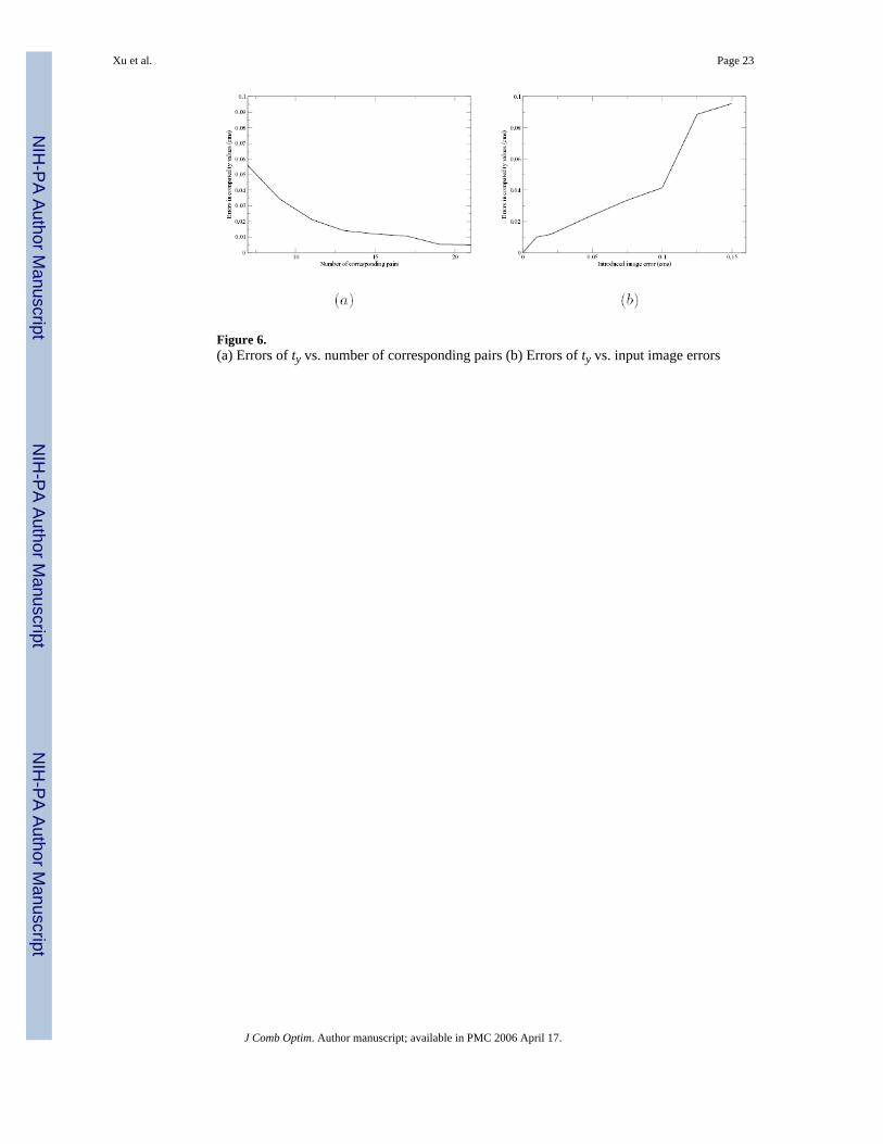
Figure 6.(a) Errors of ty vs. number of corresponding pairs (b) Errors of ty vs. input image errors

Xu et al. Page 23

J Comb Optim. Author manuscript; available in PMC 2006 April 17.

NIH

-PA Author Manuscript

NIH

-PA Author Manuscript

NIH

-PA Author Manuscript