Efficient adaptive step size control for exponential integrators

arX

iv:2

102.

0252

4v1

[m

ath.

NA

] 4

Feb

202

1

Efficient adaptive step size control for exponential integrators

Pranab Jyoti Deka, Lukas Einkemmer

Department of Mathematics, University of Innsbruck, A-6020 Innsbruck, Austria

Abstract

Traditional step size controllers make the tacit assumption that the cost of a time step is independent of the stepsize. This is reasonable for explicit and implicit integrators that use direct solvers. In the context of exponentialintegrators, however, an iterative approach, such as Krylov methods or polynomial interpolation, to compute theaction of the required matrix functions is usually employed. In this case the assumption of constant cost is not valid.This is, in particular, a problem for higher-order exponential integrators, which are able to take relatively large timesteps based on accuracy considerations. In this paper, we consider an adaptive step size controller for exponentialRosenbrock methods that determines the step size based on the premise of minimizing computational cost. Thelargest allowed step size, given by accuracy considerations, merely acts as a constraint. We test this approach ona range of nonlinear partial differential equations. Our results show significant improvements (up to a factor of 4reduction in the computational cost) over the traditional step size controller for a wide range of tolerances.

Keywords: automatic step size selection, adaptive step size controller, exponential integrators, exponentialRosenbrock methods, Leja interpolation

1. Introduction

Solving time dependent partial differential equations (PDEs) numerically is an important task in many fields ofscience and engineering. Consequently, improvements in numerical algorithms have contributed greatly to betterunderstand a range of natural phenomena and such methods are essential in many industrial settings. Fasternumerical methods, in this context, allow us to perform simulations with increased fidelity, e.g. increasing thenumber of grid points, including more physical effects, etc.

While explicit numerical methods are suitable for some problems, for many PDEs a large efficiency improvementcan be attained by using implicit time integrators. Consequently, such methods have attained much interest andmany software packages have been written to facilitate the use of such methods by practitioners, see e.g. [16, 17].More recently, so-called exponential Rosenbrock integrators have been introduced [21]. We refer to the reviewarticle [20] for more details. This class of methods linearizes the partial differential equation and then treats amatrix function representing the linear part using Krylov iteration, Leja interpolation, or Taylor methods. Similarto implicit integrators, exponential Rosenbrock methods can take much larger time steps than explicit methods.However, the fact that such methods do not approximate the linear part of the equation (except for the error in theiterative scheme) allows them, in many situations, to take even larger time steps. Moreover, these methods do notsuffer from the dichotomy between good behavior on the negative real axis (where the stability function is expectedto decay) and on the imaginary axis (where the stability function should have unit magnitude) that afflicts implicitintegrators. Because of this, exponential integrators have been used extensively and demonstrated to be superiorcompared to implicit methods in several situations, see e.g. [18, 22, 5, 11, 9, 8].

To facilitate the use of software packages based on these integrators by practitioners, it is desirable to freethe user from explicitly choosing the time step size. Ideally, the user would only prescribe a tolerance and thenumerical algorithm would then select an appropriate step size. To accomplish this, so-called (automatic) stepsize controllers are used in conjunction with an error estimator. Ideally, this also frees the user from verifying theaccuracy of the simulations (by numerical convergence studies or similar means). Step size controllers can increasethe computational efficiency by allowing the software to adaptively increase and/or decrease the step size during thecourse of the simulation.

Almost all step size controllers are predicated on the assumption that the largest possible step size should beselected. Thus, the step size is chosen such that the error committed exactly matches the tolerance specified by

Email addresses: [email protected] (Pranab Jyoti Deka), [email protected] (Lukas Einkemmer)

Preprint submitted to Journal of LATEX Templates February 5, 2021

the user (in practical implementations often a safety factor is imposed to avoid frequent step size rejection). Thisis a reasonable assumption for explicit Runge–Kutta methods, where the computational cost is independent of thestep size. However, this approach is also used in many implicit and exponential software packages. For example,the implicit RADAU5 code [16, Chap. IV.8] and the implicit multistep based CVODE code [17] use this approach.These implicit (or exponential) methods require an iterative solution of a linear system or the iterative computationof the action of certain matrix functions. This is commonly done by iterative methods. However, the number ofiterations required is quite sensitive to the properties of the matrix. Smaller time step sizes reduce the magnitudeof the largest eigenvalue of the matrix, which in turn reduces the number of iterations required per time step. Thismeans that reducing the time step size below what is dictated by the specified tolerance can actually result in anincrease in performance, thereby invalidating the assumption that the cost of a time step is independent of the stepsize.

None of the widely employed step size controllers are able to exploit this fact. This is problematic for two reasons.First, it reduces the computational efficiency by taking time steps size that do not yield optimal performance. Second,such step size controllers often do not show a monotonous increase in cost as the tolerance decreases. Thus decreasingthe tolerance can actually (sometimes drastically) reduce the run-time required for the simulations. Such behaviouris observed in a range of test problems [22, 23, 18] as well as for problems that stem from more realistic physicalmodels [11, 2, 26]. The problem with this behaviour is that the user of the software is once again tasked with tuningthe parameters of the method (i.e. decreasing the tolerance until the run-time is minimized). Thus, this largelynegates the utility of an automatic step size controller. This behaviour can be observed for exponential integratorsas well as implicit Runge–Kutta methods, BDF methods, and implicit-explicit (IMEX) methods.

While all of the considerations made above are valid for implicit schemes just as well as for exponential integra-tors, the issues raised become even more important for exponential integrators. The reason being that exponentialintegrators, especially for problems where nonlinear effects are relatively weak, are often able to take even largertime steps than implicit integrators. Thus, exponential integrators when used in conjunction with a traditional stepsize controller are more likely to operate in a regime that is problematic.

In the context of ordinary differential equations, the importance of considering variations in cost (as a function ofthe time step size) has been recognized in [15]. There analytically derived estimates of the cost are used. Obtaininga good a priori estimate of the cost is often extremely difficult for (especially nonlinear) PDEs. In the context ofapproximating matrix exponentials by polynomial interpolation at Leja points (a precursor for exponential integra-tors), a procedure to determine the optimal step size based on a backward error analysis has been proposed [4]. Thisapproach can be very effective but requires certain information on the spectrum of the matrix under consideration.This information is not easily obtained in a matrix free implementation and, for nonlinear PDEs, can change fromone time step to the next. In addition, it is well known that for such an approach, the number of iterations isoverestimated and early truncation criteria have to be used to obtain optimal performance.

In [12], an adaptive step size controller has been introduced that explores the space of admissible step sizes(i.e. step sizes that satisfy the tolerance) dynamically during the simulation and adapts the step size based on themeasured cost. This has the advantage that no prior estimates of the cost are needed. In fact, no information of theiterative scheme used or the hardware where the simulation is run, enters the algorithm. Only the computationalcost of the previously conducted time steps is used. It was shown in [12] that, for a number of implicit Runge–Kuttamethods, this approach reduces the overall computational cost significantly and results in a monotonic relation ofthe computational effort with the run time.

The goal of the this paper is to consider an adaptive step size controller for exponential integrators and toinvestigate its performance. This controller is an extension of the method described in [12] to exponential integrators.As mentioned above, using adaptive step size control is particularly important in the case of exponential integrators.We demonstrate that the developed controller performs well, that is, it increases computational efficiency and removesthe non-monotonous behaviour observed in the traditional approach to step size control. We also compare theperformance of the adaptive step size controller to the implicit approach proposed in [12] and find that the presentapproach can yield improvements in performance of up to an order of magnitude.

The paper is structured as follows. An introduction to exponential integrators and our implementation is presentedin section 2. In section 3, the principle of the proposed step size controller is presented. The performance of thisstep size controller is then analyzed for some nonlinear problems in section 4. We conclude our study in section 5.

2. Exponential Integrators

In this section, we provide an introduction to exponential integrators and Leja interpolation that we use tocompute the action of the resulting matrix-vector products. We refer the reader to [20] for more details. Let us

2

consider the initial value problem

∂u

∂t= f(u), u(t = 0) = u0, (1)

where u = u(x, t) in 1D, u = u(x, y, t) in 2D, and f(u) is some nonlinear function of u (usually depends on spatialderivatives of u). Linearizing Eq. 1 about un, the starting point for a given time step, we get

∂u

∂t= J (un)u+ F(u),

where J (u) is the Jacobian of the nonlinear function f(u) and F(u) = f(u) − J (u)u is the nonlinear remainder.We use exponential Rosenbrock (EXPRB) methods [19] to solve equations of this form. The simplest of the EXPRBmethods, known as the exponential Rosenbrock–Euler method, is given by

un+1 = un +∆tϕ1(J (un)∆t)f(un), (2)

where the superscripts n and n+1 indicate the time steps. The ϕl(z) functions are defined by the recursive relation

ϕl+1(z) =1

z

(

ϕl(z)−1

l!

)

, l ≥ 1

withϕ0(z) = ez

which corresponds to the matrix exponential. The exponential Rosenbrock–Euler method is second-order accurateand only needs the action of one matrix function per time step. Moreover, an error estimator for Eq. 2 has beendeveloped by [7]. For the second order accuracy to hold, it is crucial that the Jacobian is used. In fact, integratorsthat replace the Jacobian by an arbitrary linear operator, require more stages to obtain a given order. These methodsare referred to as either exponential Runge–Kutta methods or exponential time differencing methods. We will onlyconsider exponential Rosenbrock methods in this paper. Many higher order variants of this idea are available in theliterature, see e.g. [20, 25, 24]. Of particular interest in this work are higher order embedded schemes that, similarto embedded Runge–Kutta methods, are a pair of exponential integrators with same internal stages but differentorder. The difference between these two methods is then used to cheaply obtain an error estimate for adaptive stepsize control.

In this work, we use the fourth-order (EXPRB43) scheme with a third-order error estimator, presented in [21]and the Butcher tableau of which can be found in [20]. The two internal stages are given by an and bn, and the thirdand fourth-order solutions are given by Eq. 3 and 4 respectively. The difference between these two solutions givesan error estimate of order three.

an = un + ϕ1

(

1

2J (un)∆t

)

f(un)1

2∆t

bn = un + ϕ1 (J (un)∆t) f(un)∆t

+ ϕ1 (J (un)∆t) (F(an)−F(un))∆t

un+1 = un + ϕ1 (J (un)∆t) f(un)∆t

+ ϕ3(J (un)∆t)(−14F(un) + 16F(an)− 2F(bn))∆t (3)

un+1 = un + ϕ1 (J (un)∆t) f(un)∆t

+ ϕ3(J (un)∆t)(−14F(un) + 16F(an)− 2F(bn))∆t

+ ϕ4(J (un)∆t)(36F(un)− 48F(an) + 12F(bn))∆t (4)

3

2.1. Leja interpolation

The main computational effort required in an exponential integrator is to evaluate the action of the matrixfunctions ϕk. Similar to the treatment of linear solves in implicit schemes, iterative methods are commonly used totreat the large matrices resulting from the spatial discretization of PDEs. Krylov subspace methods, methods basedon polynomial interpolation, and Taylor methods are the most common options. A comparison of many of thesemethods has been conducted in [1, 3]. In this work we will exclusively use interpolation at Leja points. However, thedeveloped adaptive step size controller is expected to work equally well for other strategies.

An effective way of computing the action the matrix exponential and the ϕk functions is interpolation at Lejapoints [6]. Here, we present a synopsis of the algorithm that we use in our implementation (following [3]). Ap-propriately placing the interpolation points requires the spectral properties of the matrix. Let us suppose that theeigenvalues of the matrix A satisfy

α ≤ Re σ(A) ≤ ν ≤ 0, −β ≤ Im σ(A) ≤ β,

where σ(A) denotes the spectrum of A; α and ν are the smallest and largest real eigenvalues respectively, and β

is the largest, in modulus, imaginary eigenvalue. The values of α, ν, and β can be obtained by Gershgorin’s disktheorem.

One can then construct an ellipse, with semi-major axis a and semi-minor axis b, consisting of all the eigenvaluesof the matrix A. For real eigenvalues, let c be the midpoint of the ellipse and γ be one-fourth the distance betweenthe two foci of the ellipse. For the matrix exponential, we interpolate the function exp(c+ γξ) on pre-computed Lejapoints (ξ) in the interval [−2, 2].

The nth term of the interpolation polynomial p(z) is defined as

pn(z) = pn−1(z) + dn yn−1(z),

yn(z) = yn−1(z)×

(

z − c

γ− ξm

)

,

where the di correspond to the divided differences of the function exp(c + γξ). For imaginary eigenvalues, one caninterpolate the function exp(c + γξ) on the interval i[−2, 2]. To interpolate ϕk functions on Leja points, one cansimply replace exp(c+ γξ) with ϕk(c+ γξ).

In this study, we approximate the action of the ϕk functions by interpolating them as a polynomial on Lejapoints. The preference for Leja points over the well-known Chebyshev points can be attributed to the fact thatthe interpolation of a polynomial at m + 1 Chebyshev nodes necessitates the re-computation of the matrix-vectorproducts at the previously computed m nodes. However, Leja points can be generated in a sequence: using m + 1Leja points needs only one extra computation, and the computation at the previous m nodes can be reused.

3. Adaptive Step Size Controller

To conduct automatic step size control, an error estimate is essential to ensure that the local error is belowthe user-specified tolerance. Embedded schemes, which share the internal stages, can be efficiently used as errorestimators (with only a small increase in computation cost). Richardson extrapolation is one of the other commonlyused error estimator.

The widely used traditional step size controller uses the largest step size (with a safety factor) that satisfies theprescribed tolerance. This implicitly assumes that the cost of each step size is independent of the step size ∆t. This istrue for explicit methods or implicit methods that that solve the corresponding linear systems using direct methods.Let us suppose that the error incurred in the nth time step is en = D(∆tn)(p+1), where p is the order of the methodused and D is some constant. The tolerance specified by the user is tol. The optimal step size, for (n + 1)th timestep, is given by tol = D(∆tn+1)(p+1). Eliminating D, we get

∆tn+1 = ∆tn ×

(

tol

en

)1/(p+1)

This simple formula can be interpreted as a P controller. The mathematical analysis is, in fact, based on thisobservation (see, for example, [14, 13, 27, 28]). A PI controller has also been proposed in [14]. These local step sizecontrollers form the backbone of most time integration packages. For example, the RADAU5 code [16, Chap. IV.8]employs a variant of the PI controller, while the multistep based CVODE code [17] and [10] uses a variant of the Pcontroller.

4

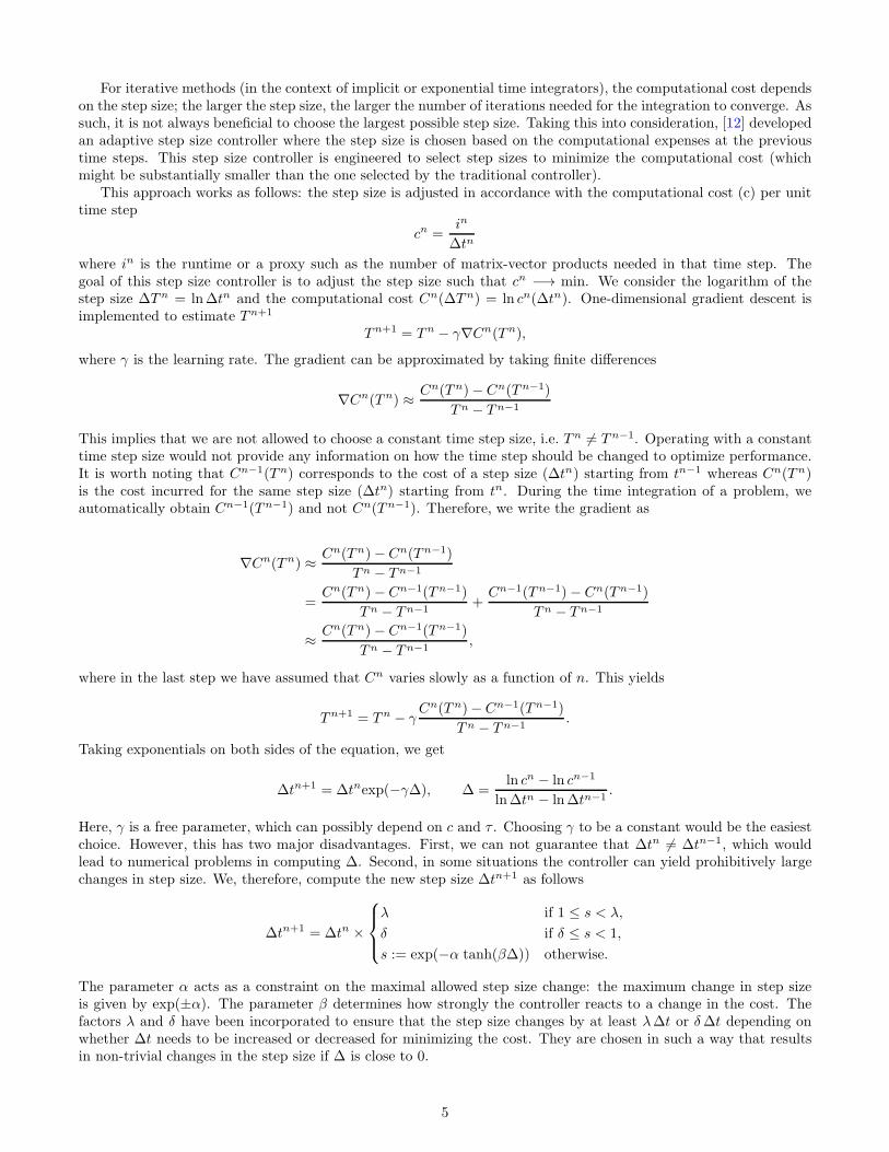
For iterative methods (in the context of implicit or exponential time integrators), the computational cost dependson the step size; the larger the step size, the larger the number of iterations needed for the integration to converge. Assuch, it is not always beneficial to choose the largest possible step size. Taking this into consideration, [12] developedan adaptive step size controller where the step size is chosen based on the computational expenses at the previoustime steps. This step size controller is engineered to select step sizes to minimize the computational cost (whichmight be substantially smaller than the one selected by the traditional controller).

This approach works as follows: the step size is adjusted in accordance with the computational cost (c) per unittime step

cn =in

∆tn

where in is the runtime or a proxy such as the number of matrix-vector products needed in that time step. Thegoal of this step size controller is to adjust the step size such that cn −→ min. We consider the logarithm of thestep size ∆T n = ln∆tn and the computational cost Cn(∆T n) = ln cn(∆tn). One-dimensional gradient descent isimplemented to estimate T n+1

T n+1 = T n − γ∇Cn(T n),

where γ is the learning rate. The gradient can be approximated by taking finite differences

∇Cn(T n) ≈Cn(T n)− Cn(T n−1)

T n − T n−1

This implies that we are not allowed to choose a constant time step size, i.e. T n 6= T n−1. Operating with a constanttime step size would not provide any information on how the time step should be changed to optimize performance.It is worth noting that Cn−1(T n) corresponds to the cost of a step size (∆tn) starting from tn−1 whereas Cn(T n)is the cost incurred for the same step size (∆tn) starting from tn. During the time integration of a problem, weautomatically obtain Cn−1(T n−1) and not Cn(T n−1). Therefore, we write the gradient as

∇Cn(T n) ≈Cn(T n)− Cn(T n−1)

T n − T n−1

=Cn(T n)− Cn−1(T n−1)

T n − T n−1+

Cn−1(T n−1)− Cn(T n−1)

T n − T n−1

≈Cn(T n)− Cn−1(T n−1)

T n − T n−1,

where in the last step we have assumed that Cn varies slowly as a function of n. This yields

T n+1 = T n − γCn(T n)− Cn−1(T n−1)

T n − T n−1.

Taking exponentials on both sides of the equation, we get

∆tn+1 = ∆tnexp(−γ∆), ∆ =ln cn − ln cn−1

ln∆tn − ln∆tn−1.

Here, γ is a free parameter, which can possibly depend on c and τ . Choosing γ to be a constant would be the easiestchoice. However, this has two major disadvantages. First, we can not guarantee that ∆tn 6= ∆tn−1, which wouldlead to numerical problems in computing ∆. Second, in some situations the controller can yield prohibitively largechanges in step size. We, therefore, compute the new step size ∆tn+1 as follows

∆tn+1 = ∆tn ×

λ if 1 ≤ s < λ,

δ if δ ≤ s < 1,

s := exp(−α tanh(β∆)) otherwise.

The parameter α acts as a constraint on the maximal allowed step size change: the maximum change in step sizeis given by exp(±α). The parameter β determines how strongly the controller reacts to a change in the cost. Thefactors λ and δ have been incorporated to ensure that the step size changes by at least λ∆t or δ∆t depending onwhether ∆t needs to be increased or decreased for minimizing the cost. They are chosen in such a way that resultsin non-trivial changes in the step size if ∆ is close to 0.

5

These parameters, (α, β, λ, and δ) have been numerically optimized for the linear diffusion-advection equationand an implicit Runge–Kutta scheme for a range of values of N , η, and tol. This step size controller has been designedwith two variants: (i) Non-penalized variant: the aforementioned parameters have been chosen to incur the minimumpossible cost, (ii) Penalized variant: if the traditional controller performs better than the non-penalized variant, apenalty is charged on the proposed controller. This penalty has been imposed to trade off the enhanced performanceof the proposed controller (where it performs better) with an acceptable amount of diminished performance (whereit performs worse than the traditional controller). The numerical optimization yields the following set of parameters

Non-penalized α = 0.65241444 β = 0.26862269 λ = 1.37412002 δ = 0.64446017

Penalized α = 1.19735982 β = 0.44611854 λ = 1.38440318 δ = 0.73715227

The improved performance of this controller for both implicit schemes [12] and exponential integrators (as we willsee in this paper) further shows the generality of the approach. In particular, this is emphasized as the parametersthat have been obtained for a linear PDE generalize well to nonlinear problems for a variety of numerical methods.

It is worth noting that the proposed step size controller is designed solely to minimize the computational cost anddoes not take into account the error incurred during the time integration. As such, we need to take the minimum ofthe step sizes given by the traditional and the proposed step size controller

∆tn+1 = min(

∆tn+1proposed, ∆tn+1

traditional

)

This ensures that, in addition to satisfying the accuracy requirements set by the user, the controller minimizes thecomputational cost (by choosing a smaller time step size) whenever possible.

In the context of exponential integrators, there is an additional detail that needs to be taken care of: thecomputation of the Leja interpolation to the prescribed tolerance. In some situations, especially if relatively largestep sizes are chosen, the polynomial interpolation might fail to converge within a reasonable number of iterations.If this is the case for any of the internal stages of the exponential Rosenbrock scheme, we reject the step and use thetraditional controller to determine a smaller step size.

4. Numerical results

In this section, we investigate the performance of the proposed step size controller and compare it with thetraditional controller using the embedded EXPRB43 scheme for a number of nonlinear problems. We present adetailed explanation of how the step size controller can improve the performance of exponential Rosenbrock methodsin practice.

4.1. Viscous Burgers’ Equation

The one-dimensional viscous Burgers’ equation (conservative form) reads

∂u

∂t=

1

2η∂u2

∂x+

∂2u

∂x2,

where periodic boundary conditions are imposed in [0, 1]. The Peclet number (η) is a measure of the relative strengthof advection to diffusion. Higher values of η indicate advection-dominated scenarios whereas lower values of η implydiffusion-dominated cases. Periodic boundary conditions are imposed on [0, 1]. The initial condition is

u(x, t = 0) = 1 + exp

(

1−1

1− (2x− 1)2

)

+1

2exp

(

−(x− x0)

2

2σ2

)

with x0 = 0.9 and σ = 0.02.We wish to test our step size controller in diffusion as well as advection dominated cases. If η is small (diffusion

dominated), then the Gaussian part is dynamically smeared out, and u(x, t) is slowly advected over a significantamount of time. If η is large (advection dominated), the solution experiences rapid advection and the Gaussian issmeared out after a long time. We choose the final time of the integration to be t = 10−2. This means that forany value of η, a fixed amount of diffusion is inherently introduced in the simulations. For the space discretization,we consider a third-order upwind scheme for advection and the second-order centered difference scheme for diffusion(see 5).

The work-precision diagram is shown in Fig. 1. The computational cost incurred, in our case, measured by thenumber of matrix-vector products, is plotted as a function of the user-specified tolerance. The blue curves correspond

6

2 3 41e3

10−4

10−6

10−80.50 0.75 1.00 1.25

1e41.0 1.5 2.0 2.5

1e42 4

1e4

0.5 1.0 1.51e4

10−4

10−6

10−82 4 6

1e40.25 0.50 0.75 1.00

1e50.5 1.0 1.5

1e5

1 2 3 41e4

10−4

10−6

10−84 6 8

1e40.5 1.0 1.5

1e51 2 3

1e5

N=100 N=300 N=500 N=700η=10

η=50

η=100

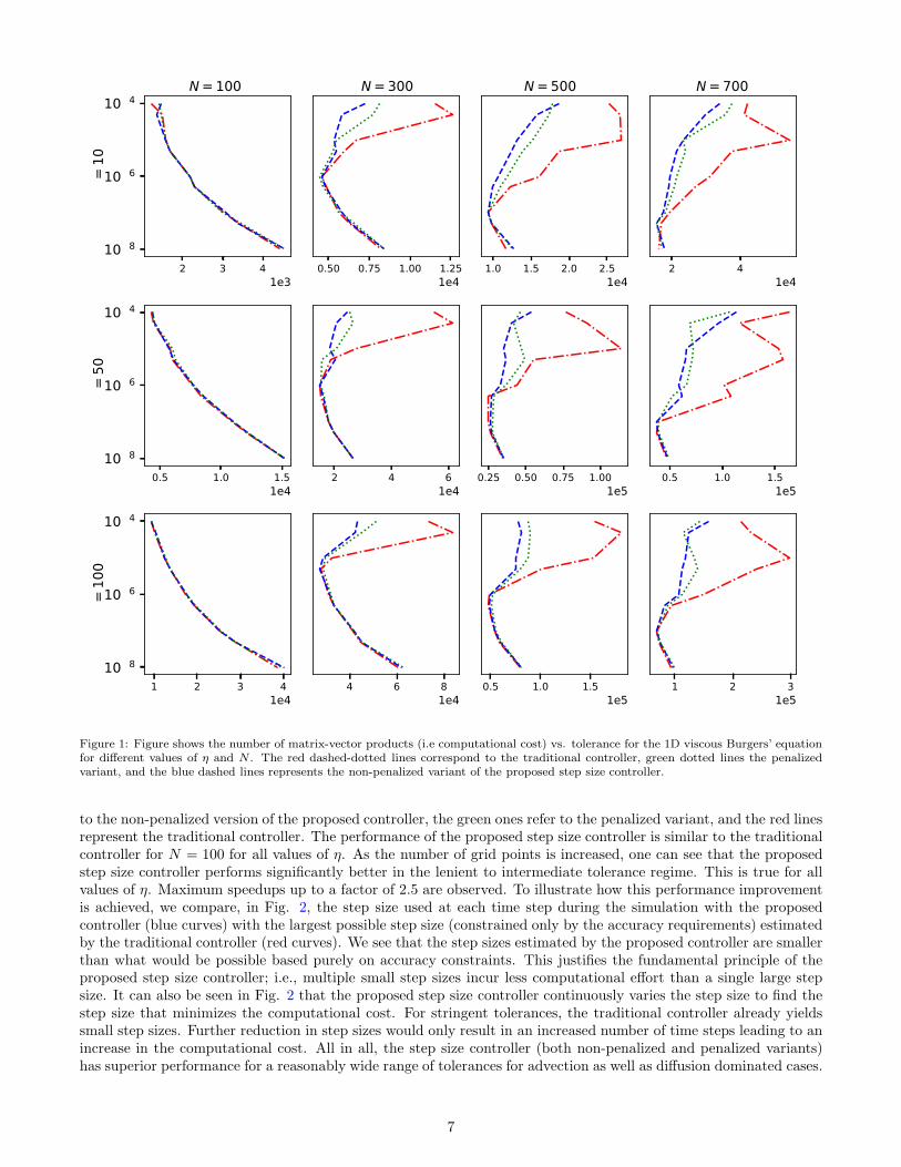
Figure 1: Figure shows the number of matrix-vector products (i.e computational cost) vs. tolerance for the 1D viscous Burgers’ equationfor different values of η and N . The red dashed-dotted lines correspond to the traditional controller, green dotted lines the penalizedvariant, and the blue dashed lines represents the non-penalized variant of the proposed step size controller.

to the non-penalized version of the proposed controller, the green ones refer to the penalized variant, and the red linesrepresent the traditional controller. The performance of the proposed step size controller is similar to the traditionalcontroller for N = 100 for all values of η. As the number of grid points is increased, one can see that the proposedstep size controller performs significantly better in the lenient to intermediate tolerance regime. This is true for allvalues of η. Maximum speedups up to a factor of 2.5 are observed. To illustrate how this performance improvementis achieved, we compare, in Fig. 2, the step size used at each time step during the simulation with the proposedcontroller (blue curves) with the largest possible step size (constrained only by the accuracy requirements) estimatedby the traditional controller (red curves). We see that the step sizes estimated by the proposed controller are smallerthan what would be possible based purely on accuracy constraints. This justifies the fundamental principle of theproposed step size controller; i.e., multiple small step sizes incur less computational effort than a single large stepsize. It can also be seen in Fig. 2 that the proposed step size controller continuously varies the step size to find thestep size that minimizes the computational cost. For stringent tolerances, the traditional controller already yieldssmall step sizes. Further reduction in step sizes would only result in an increased number of time steps leading to anincrease in the computational cost. All in all, the step size controller (both non-penalized and penalized variants)has superior performance for a reasonably wide range of tolerances for advection as well as diffusion dominated cases.

7

0.000 0.005 0.010Time

100

101

dt/dt C

FL

N=300 η=50

0.000 0.005 0.010Time

100

101

102

N=500 η=50

0.000 0.005 0.010Time

100

101

102

N=700 η=100

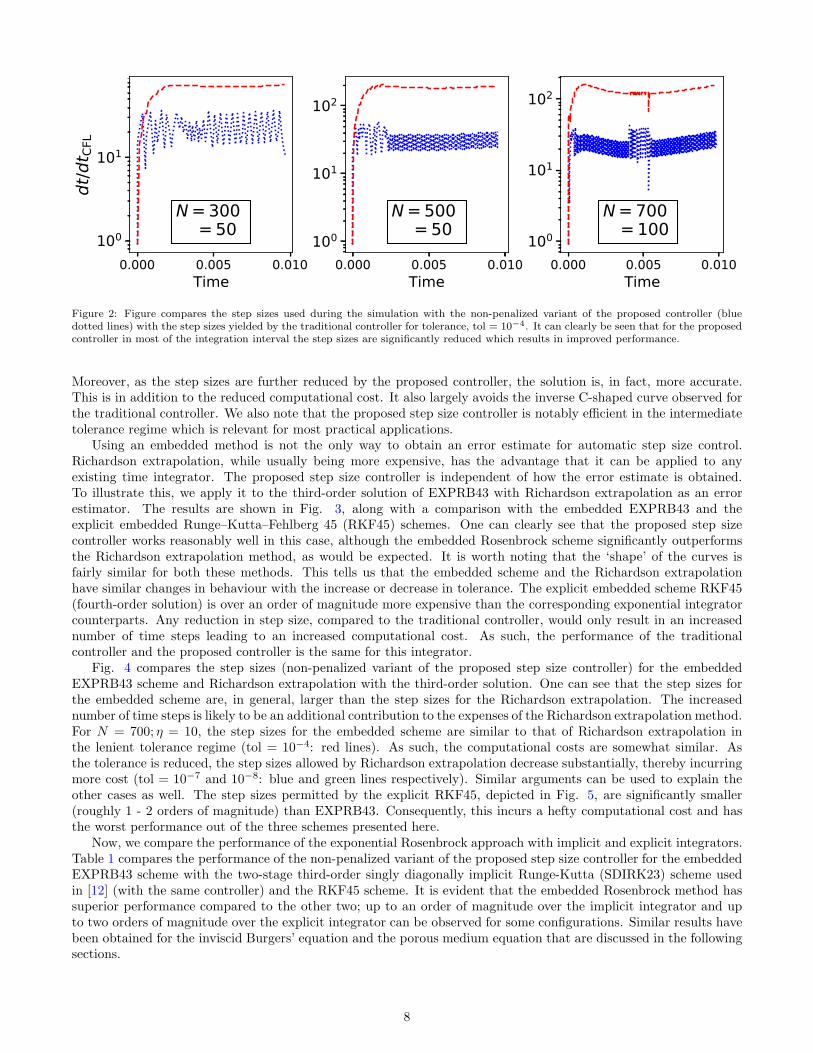
Figure 2: Figure compares the step sizes used during the simulation with the non-penalized variant of the proposed controller (bluedotted lines) with the step sizes yielded by the traditional controller for tolerance, tol = 10−4. It can clearly be seen that for the proposedcontroller in most of the integration interval the step sizes are significantly reduced which results in improved performance.

Moreover, as the step sizes are further reduced by the proposed controller, the solution is, in fact, more accurate.This is in addition to the reduced computational cost. It also largely avoids the inverse C-shaped curve observed forthe traditional controller. We also note that the proposed step size controller is notably efficient in the intermediatetolerance regime which is relevant for most practical applications.

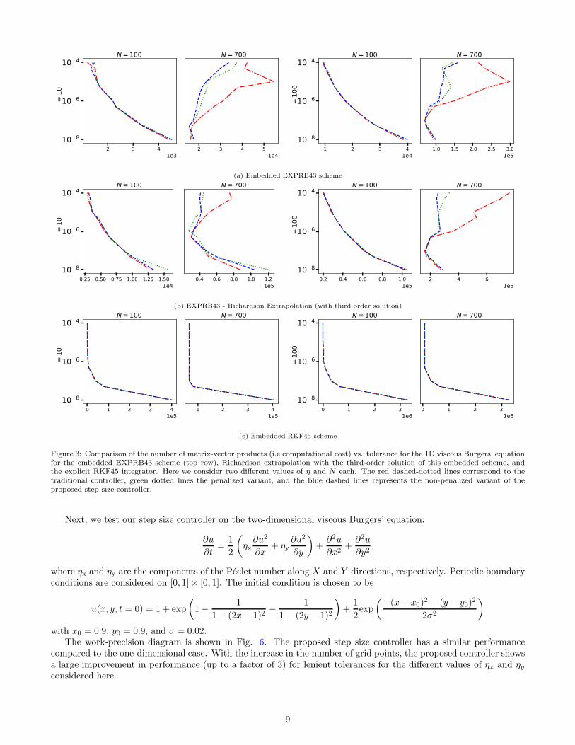
Using an embedded method is not the only way to obtain an error estimate for automatic step size control.Richardson extrapolation, while usually being more expensive, has the advantage that it can be applied to anyexisting time integrator. The proposed step size controller is independent of how the error estimate is obtained.To illustrate this, we apply it to the third-order solution of EXPRB43 with Richardson extrapolation as an errorestimator. The results are shown in Fig. 3, along with a comparison with the embedded EXPRB43 and theexplicit embedded Runge–Kutta–Fehlberg 45 (RKF45) schemes. One can clearly see that the proposed step sizecontroller works reasonably well in this case, although the embedded Rosenbrock scheme significantly outperformsthe Richardson extrapolation method, as would be expected. It is worth noting that the ‘shape’ of the curves isfairly similar for both these methods. This tells us that the embedded scheme and the Richardson extrapolationhave similar changes in behaviour with the increase or decrease in tolerance. The explicit embedded scheme RKF45(fourth-order solution) is over an order of magnitude more expensive than the corresponding exponential integratorcounterparts. Any reduction in step size, compared to the traditional controller, would only result in an increasednumber of time steps leading to an increased computational cost. As such, the performance of the traditionalcontroller and the proposed controller is the same for this integrator.

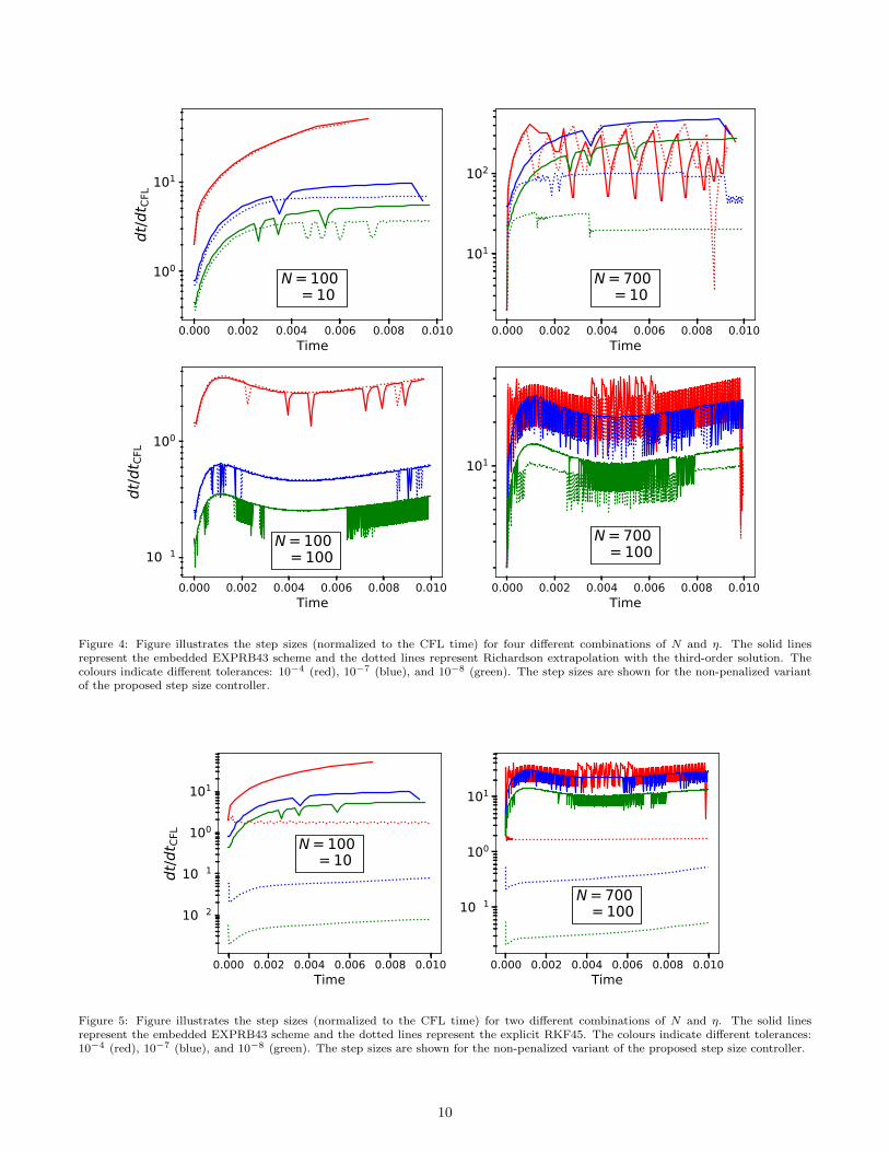
Fig. 4 compares the step sizes (non-penalized variant of the proposed step size controller) for the embeddedEXPRB43 scheme and Richardson extrapolation with the third-order solution. One can see that the step sizes forthe embedded scheme are, in general, larger than the step sizes for the Richardson extrapolation. The increasednumber of time steps is likely to be an additional contribution to the expenses of the Richardson extrapolation method.For N = 700; η = 10, the step sizes for the embedded scheme are similar to that of Richardson extrapolation inthe lenient tolerance regime (tol = 10−4: red lines). As such, the computational costs are somewhat similar. Asthe tolerance is reduced, the step sizes allowed by Richardson extrapolation decrease substantially, thereby incurringmore cost (tol = 10−7 and 10−8: blue and green lines respectively). Similar arguments can be used to explain theother cases as well. The step sizes permitted by the explicit RKF45, depicted in Fig. 5, are significantly smaller(roughly 1 - 2 orders of magnitude) than EXPRB43. Consequently, this incurs a hefty computational cost and hasthe worst performance out of the three schemes presented here.

Now, we compare the performance of the exponential Rosenbrock approach with implicit and explicit integrators.Table 1 compares the performance of the non-penalized variant of the proposed step size controller for the embeddedEXPRB43 scheme with the two-stage third-order singly diagonally implicit Runge-Kutta (SDIRK23) scheme usedin [12] (with the same controller) and the RKF45 scheme. It is evident that the embedded Rosenbrock method hassuperior performance compared to the other two; up to an order of magnitude over the implicit integrator and upto two orders of magnitude over the explicit integrator can be observed for some configurations. Similar results havebeen obtained for the inviscid Burgers’ equation and the porous medium equation that are discussed in the followingsections.

8

2 3 41e3

10−4

10−6

10−82 3 4 5

1e4

N=100 N=700η=10

1 2 3 41e4

10−4

10−6

10−81.0 1.5 2.0 2.5 3.0

1e5

N=100 N=700

η=100

(a) Embedded EXPRB43 scheme

0.25 0.50 0.75 1.00 1.25 1.501e4

10−4

10−6

10−80.4 0.6 0.8 1.0 1.2

1e5

N=100 N=700

η=10

0.2 0.4 0.6 0.8 1.01e5

10−4

10−6

10−82 4 6

1e5

N=100 N=700

η=100

(b) EXPRB43 - Richardson Extrapolation (with third order solution)

0 1 2 3 41e5

10−4

10−6

10−81 2 3 4

1e5

N=100 N=700

η=10

0 1 2 31e6

10−4

10−6

10−80 1 2 3

1e6

N=100 N=700

η=100

(c) Embedded RKF45 scheme

Figure 3: Comparison of the number of matrix-vector products (i.e computational cost) vs. tolerance for the 1D viscous Burgers’ equationfor the embedded EXPRB43 scheme (top row), Richardson extrapolation with the third-order solution of this embedded scheme, andthe explicit RKF45 integrator. Here we consider two different values of η and N each. The red dashed-dotted lines correspond to thetraditional controller, green dotted lines the penalized variant, and the blue dashed lines represents the non-penalized variant of theproposed step size controller.

Next, we test our step size controller on the two-dimensional viscous Burgers’ equation:

∂u

∂t=

1

2

(

ηx∂u2

∂x+ ηy

∂u2

∂y

)

+∂2u

∂x2+

∂2u

∂y2,

where ηx and ηy are the components of the Peclet number along X and Y directions, respectively. Periodic boundaryconditions are considered on [0, 1]× [0, 1]. The initial condition is chosen to be

u(x, y, t = 0) = 1 + exp

(

1−1

1− (2x− 1)2−

1

1− (2y − 1)2

)

+1

2exp

(

−(x− x0)2 − (y − y0)

2

2σ2

)

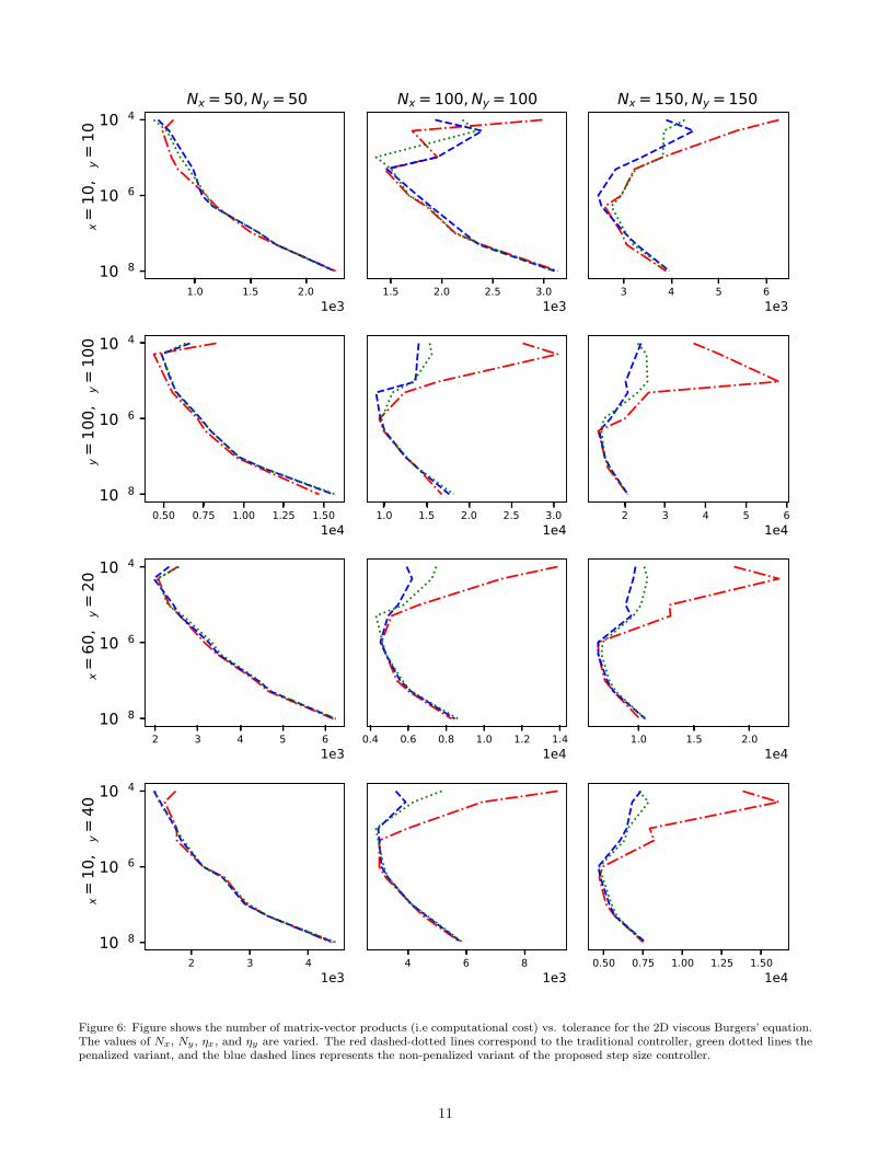
with x0 = 0.9, y0 = 0.9, and σ = 0.02.The work-precision diagram is shown in Fig. 6. The proposed step size controller has a similar performance

compared to the one-dimensional case. With the increase in the number of grid points, the proposed controller showsa large improvement in performance (up to a factor of 3) for lenient tolerances for the different values of ηx and ηyconsidered here.

9

0.000 0.002 0.004 0.006 0.008 0.010Time

100

101

dt/dt C

FL

N=100 η=10

0.000 0.002 0.004 0.006 0.008 0.010Time

101

102

N=700 η=10

0.000 0.002 0.004 0.006 0.008 0.010Time

10−1

100

dt/dt C

FL

N=100 η=100

0.000 0.002 0.004 0.006 0.008 0.010Time

101

N=700 η=100

Figure 4: Figure illustrates the step sizes (normalized to the CFL time) for four different combinations of N and η. The solid linesrepresent the embedded EXPRB43 scheme and the dotted lines represent Richardson extrapolation with the third-order solution. Thecolours indicate different tolerances: 10−4 (red), 10−7 (blue), and 10−8 (green). The step sizes are shown for the non-penalized variantof the proposed step size controller.

0.000 0.002 0.004 0.006 0.008 0.010Time

10−2

10−1

100

101

dt/dt C

FL N=100 η=10

0.000 0.002 0.004 0.006 0.008 0.010Time

10−1

100

101

N=700 η=100

Figure 5: Figure illustrates the step sizes (normalized to the CFL time) for two different combinations of N and η. The solid linesrepresent the embedded EXPRB43 scheme and the dotted lines represent the explicit RKF45. The colours indicate different tolerances:10−4 (red), 10−7 (blue), and 10−8 (green). The step sizes are shown for the non-penalized variant of the proposed step size controller.

10

1.0 1.5 2.01e3

10−4

10−6

10−81.5 2.0 2.5 3.0

1e33 4 5 6

1e3

0.50 0.75 1.00 1.25 1.501e4

10−4

10−6

10−81.0 1.5 2.0 2.5 3.0

1e42 3 4 5 6

1e4

2 3 4 5 61e3

10−4

10−6

10−80.4 0.6 0.8 1.0 1.2 1.4

1e41.0 1.5 2.0

1e4

2 3 41e3

10−4

10−6

10−84 6 8

1e30.50 0.75 1.00 1.25 1.50

1e4

Nx=50,Ny=50 Nx=100,Ny=100 Nx=150,Ny=150η x

=10

,ηy=10

η y=10

0,η y

=10

0η x

=60

,ηy=20

η x=10

,ηy=40

Figure 6: Figure shows the number of matrix-vector products (i.e computational cost) vs. tolerance for the 2D viscous Burgers’ equation.The values of Nx, Ny, ηx, and ηy are varied. The red dashed-dotted lines correspond to the traditional controller, green dotted lines thepenalized variant, and the blue dashed lines represents the non-penalized variant of the proposed step size controller.

11

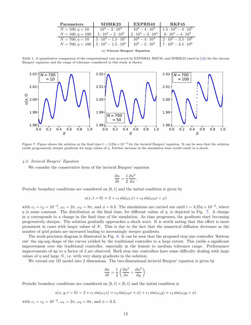
Parameters SDIRK23 EXPRB43 RKF45

N = 100, η = 10 104 − 3 · 104 103 − 4 · 103 1.5 · 103 − 4 · 105

N = 100, η = 100 5 · 104 − 2 · 105 2 · 104 − 3 · 104 6 · 104 − 4 · 105

N = 700, η = 10 5 · 104 − 1.5 · 105 104 − 4 · 104 2 · 103 − 3.5 · 106

N = 700, η = 100 5 · 105 − 1.5 · 106 105 − 2 · 105 7 · 104 − 3.5 · 106

(a) Viscous Burgers’ Equation

Table 1: A quantitative comparison of the computational cost incurred by EXPRB43, RKF45, and SDIRK23 (used in [12]) for the viscousBurgers’ equation and the range of tolerance considered in this study is shown.

0.0 0.2 0.4 0.6 0.8 1.0X

1.98

1.99

2.00

2.01

2.02

u(x,t)

N=700 η=10

0.0 0.2 0.4 0.6 0.8 1.0X

1.98

1.99

2.00

2.01

2.02

N=700 η=50

0.0 0.2 0.4 0.6 0.8 1.0X

1.98

1.99

2.00

2.01

2.02 N=700 η=100

Figure 7: Figure shows the solution at the final time t = 3.25η× 10−2 for the inviscid Burgers’ equation. It can be seen that the solutionyields progressively steeper gradients for large values of η. Further increase in the simulation time would result in a shock.

4.2. Inviscid Burgers’ Equation

We consider the conservative form of the inviscid Burgers’ equation

∂u

∂t=

1

2

∂u2

∂x.

Periodic boundary conditions are considered on [0, 1] and the initial condition is given by

u(x, t = 0) = 2 + ǫ1 sin(ω1x) + ǫ2 sin(ω2x+ ϕ)

with ǫ1 = ǫ2 = 10−2, ω1 = 2π, ω2 = 8π, and φ = 0.3. The simulations are carried out until t = 3.25η × 10−2, whereη is some constant. The distribution at the final time, for different values of η, is depicted in Fig. 7. A changein η corresponds to a change in the final time of the simulation. As time progresses, the gradients start becomingprogressively sharper. The solution gradually approaches a shock wave. It is worth noting that this effect is moreprominent in cases with larger values of N . This is due to the fact that the numerical diffusion decreases as thenumber of grid points are increased leading to increasingly steeper gradients.

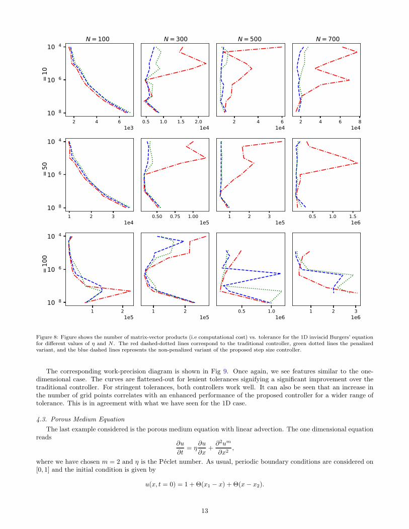
The work-precision diagram is illustrated in Fig. 8. It can be seen that the proposed step size controller ‘flattensout’ the zig-zag shape of the curves yielded by the traditional controller to a large extent. This yields a significantimprovement over the traditional controller, especially in the lenient to medium tolerance range. Performanceimprovements of up to a factor of 4 are observed. Both step size controllers have some difficulty dealing with largevalues of η and large N , i.e. with very sharp gradients in the solution.

We extend our 1D model into 2 dimensions. The two-dimensional inviscid Burgers’ equation is given by

∂u

∂t=

1

2

(

∂u2

∂x+

∂u2

∂y

)

.

Periodic boundary conditions are considered on [0, 1]× [0, 1] and the initial condition is

u(x, y, t = 0) = 2 + ǫ1 sin(ω1x) + ǫ2 sin(ω2x+ φ) + ǫ1 sin(ω1y) + ǫ2 sin(ω2y + φ)

with ǫ1 = ǫ2 = 10−2, ω1 = 2π, ω2 = 8π, and φ = 0.3.

12

2 4 61e3

10−4

10−6

10−80.5 1.0 1.5 2.0

1e42 4 6

1e42 4 6 8

1e4

1 2 31e4

10−4

10−6

10−80.50 0.75 1.00

1e51 2 3

1e50.5 1.0 1.5

1e6

1 21e5

10−4

10−6

10−81 2

1e50.5 1.0

1e61 2 3

1e6

N=100 N=300 N=500 N=700η=10

η=50

η=100

Figure 8: Figure shows the number of matrix-vector products (i.e computational cost) vs. tolerance for the 1D inviscid Burgers’ equationfor different values of η and N . The red dashed-dotted lines correspond to the traditional controller, green dotted lines the penalizedvariant, and the blue dashed lines represents the non-penalized variant of the proposed step size controller.

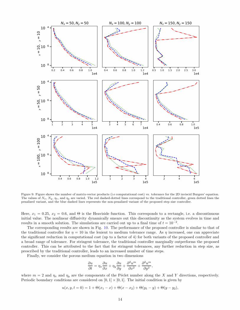
The corresponding work-precision diagram is shown in Fig 9. Once again, we see features similar to the one-dimensional case. The curves are flattened-out for lenient tolerances signifying a significant improvement over thetraditional controller. For stringent tolerances, both controllers work well. It can also be seen that an increase inthe number of grid points correlates with an enhanced performance of the proposed controller for a wider range oftolerance. This is in agreement with what we have seen for the 1D case.

4.3. Porous Medium Equation

The last example considered is the porous medium equation with linear advection. The one dimensional equationreads

∂u

∂t= η

∂u

∂x+

∂2um

∂x2,

where we have chosen m = 2 and η is the Peclet number. As usual, periodic boundary conditions are considered on[0, 1] and the initial condition is given by

u(x, t = 0) = 1 + Θ(x1 − x) + Θ(x− x2).

13

0.2 0.4 0.6 0.8 1.01e4

10−4

10−6

10−80.4 0.6 0.8 1.0 1.2

1e40.5 1.0 1.5 2.0 2.5 3.0

1e4

1 2 3 4 51e4

10−4

10−6

10−83 4 5 6 7

1e40.4 0.6 0.8 1.0

1e5

0.4 0.6 0.8 1.0 1.21e5

10−4

10−6

10−81 2 3 4

1e52 4 6

1e5

Nx=50,Ny=50 Nx=100,Ny=100 Nx=150,Ny=150

η x=10

,ηy=10

η y=50

,ηy=50

η x=10

0,η y

=10

0

Figure 9: Figure shows the number of matrix-vector products (i.e computational cost) vs. tolerance for the 2D inviscid Burgers’ equation.The values of Nx, Ny, ηx, and ηy are varied. The red dashed-dotted lines correspond to the traditional controller, green dotted lines thepenalized variant, and the blue dashed lines represents the non-penalized variant of the proposed step size controller.

Here, x1 = 0.25, x2 = 0.6, and Θ is the Heaviside function. This corresponds to a rectangle, i.e. a discontinuousinitial value. The nonlinear diffusivity dynamically smears out this discontinuity as the system evolves in time andresults in a smooth solution. The simulations are carried out up to a final time of t = 10−2.

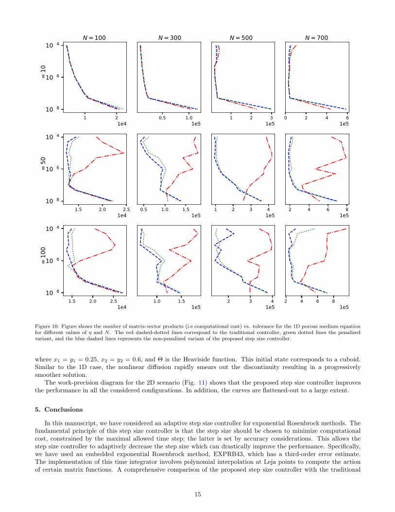
The corresponding results are shown in Fig. 10. The performance of the proposed controller is similar to that ofthe traditional controller for η = 10 in the lenient to medium tolerance range. As η increased, one can appreciatethe significant reduction in computational cost (up to a factor of 4) for both variants of the proposed controller anda broad range of tolerance. For stringent tolerance, the traditional controller marginally outperforms the proposedcontroller. This can be attributed to the fact that for stringent tolerances, any further reduction in step size, asprescribed by the traditional controller, leads to an increased number of time steps.

Finally, we consider the porous medium equation in two dimensions

∂u

∂t= ηx

∂u

∂x+ ηy

∂u

∂y+

∂2um

∂x2+

∂2um

∂y2,

where m = 2 and ηx and ηy are the components of the Peclet number along the X and Y directions, respectively.Periodic boundary conditions are considered on [0, 1]× [0, 1]. The initial condition is given by

u(x, y, t = 0) = 1 + Θ(x1 − x) + Θ(x− x2) + Θ(y1 − y) + Θ(y − y2),

14

1 21e4

10−4

10−6

10−80.5 1.0

1e51 2 3

1e50 2 4 6

1e5

1.5 2.0 2.51e4

10−4

10−6

10−80.5 1.0 1.5

1e51 2 3 4

1e52 4 6 8

1e5

1.5 2.0 2.51e4

10−4

10−6

10−81.0 1.5

1e52 3 4

1e52 4 6 8

1e5

N=100 N=300 N=500 N=700η=10

η=50

η=100

Figure 10: Figure shows the number of matrix-vector products (i.e computational cost) vs. tolerance for the 1D porous medium equationfor different values of η and N . The red dashed-dotted lines correspond to the traditional controller, green dotted lines the penalizedvariant, and the blue dashed lines represents the non-penalized variant of the proposed step size controller.

where x1 = y1 = 0.25, x2 = y2 = 0.6, and Θ is the Heaviside function. This initial state corresponds to a cuboid.Similar to the 1D case, the nonlinear diffusion rapidly smears out the discontinuity resulting in a progressivelysmoother solution.

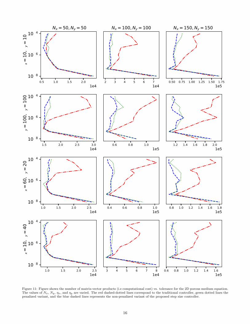
The work-precision diagram for the 2D scenario (Fig. 11) shows that the proposed step size controller improvesthe performance in all the considered configurations. In addition, the curves are flattened-out to a large extent.

5. Conclusions

In this manuscript, we have considered an adaptive step size controller for exponential Rosenbrock methods. Thefundamental principle of this step size controller is that the step size should be chosen to minimize computationalcost, constrained by the maximal allowed time step; the latter is set by accuracy considerations. This allows thestep size controller to adaptively decrease the step size which can drastically improve the performance. Specifically,we have used an embedded exponential Rosenbrock method, EXPRB43, which has a third-order error estimate.The implementation of this time integrator involves polynomial interpolation at Leja points to compute the actionof certain matrix functions. A comprehensive comparison of the proposed step size controller with the traditional

15

0.5 1.0 1.5 2.01e4

10−4

10−6

10−82 3 4 5 6 7

1e40.50 0.75 1.00 1.25 1.50 1.75

1e5

1.5 2.0 2.5 3.01e4

10−4

10−6

10−80.6 0.8 1.0

1e51.2 1.4 1.6 1.8 2.0

1e5

1.0 1.5 2.0 2.51e4

10−4

10−6

10−80.4 0.6 0.8 1.0

1e50.8 1.0 1.2 1.4 1.6 1.8

1e5

1.0 1.5 2.0 2.51e4

10−4

10−6

10−83 4 5 6 7 8

1e40.6 0.8 1.0 1.2 1.4 1.6

1e5

Nx=50,Ny=50 Nx=100,Ny=100 Nx=150,Ny=150η x

=10

,ηy=10

η y=10

0,η y

=10

0η x

=60

,ηy=20

η x=10

,ηy=40

Figure 11: Figure shows the number of matrix-vector products (i.e computational cost) vs. tolerance for the 2D porous medium equation.The values of Nx, Ny, ηx, and ηy are varied. The red dashed-dotted lines correspond to the traditional controller, green dotted lines thepenalized variant, and the blue dashed lines represents the non-penalized variant of the proposed step size controller.

16

controller has been presented for different values of the Peclet number, the number of the grid points, and theuser-specified tolerance for the various equations under consideration. We summarize our results as follows:

• The proposed step size controller has superior performance (compared to the traditional controller) for almostall configurations considered here. This is particularly true in the lenient to medium tolerance regime. Arguably,equations in physics and astrophysics are solved up to accuracy within this range of tolerances. The zig-zagcurves, yielded by the traditional controller, are flattened out. This exemplifies the use of such a step sizecontroller in practice.

• Multiple small step sizes, in many situations, do indeed incur less computational effort than a single large stepsize and we have seen that the proposed step size controller can effectively exploit this fact.

• It has been observed that the curves for the work-precision diagrams have similar ‘shapes’ in 1D and 2D. Thisindicates the reliability and effectiveness of the proposed controller.

• Comparisons with explicit (RKF45) and implicit (SDIRK23) schemes have shown that the exponential Rosen-brock method outperforms both these classes of integrators by a significant margin.

• We recommend the non-penalized variant of the step size controller as it shows improved performance in almostall configurations considered.

This study has been performed for a set of representative but relatively simple problems. In future work, we willimplement this step size controller as part of a software package and test it for more realistic scenarios. A typicalexample would be the propagation of fluids or particles in the interstellar or intergalactic medium in 3D. This mayinclude a combination of linear and/or nonlinear advection and diffusion coupled to other physical processes likedispersion, collisions, etc.

Acknowledgements

This work is supported by the Austrian Science Fund (FWF)—project id: P32143-N32.

Spatial Discretization

We use the third order upwind scheme to discretize the advective term which is given by

∂u

∂x≈

−ui+2 + 6ui+1 − 3ui − 2ui−1

6∆x(.1)

The primary advantage of this scheme is that it introduces less numerical diffusion. The structure or features of thephysical parameter under consideration is preserved to a large extent. The diffusive term is discretized using thesecond-order centered difference scheme

∂2u

∂x2≈

ui+1 − 2ui + ui−1

∆x2(.2)

References

[1] L. Bergamaschi, M. Caliari, A. Martinez, and M. Vianello. Comparing Leja and Krylov approximations of largescale matrix exponentials. In Proc. ICCS 2006, pages 685–692. Springer, 2006.

[2] D. S. Blom, P. Birken, H. Bijl, F. Kessels, A. Meister, and A. H. van Zuijlen. A comparison of Rosenbrockand ESDIRK methods combined with iterative solvers for unsteady compressible flows. Adv. Comput. Math.,42(6):1401–1426, 2016.

[3] M. Caliari, P. Kandolf, A. Ostermann, and S. Rainer. Comparison of software for computing the action of thematrix exponential. BIT Numer. Math., 54:113 – 128, 2014.

[4] M. Caliari, P. Kandolf, A. Ostermann, and S. Rainer. The Leja method revisited: Backward error analysis forthe matrix exponential. SIAM J. Sci. Comput., 38(3):A1639–A1661, 2016.

[5] M. Caliari and A. Ostermann. Implementation of exponential Rosenbrock-type integrators. Appl. Numer. Math.,59(3-4):568–581, 2009.

17

[6] M. Caliari, M. Vianello, and L. Bergamaschi. Interpolating discrete advection–diffusion propagators at lejasequences. J. Comput. Appl. Math., 172(1):79 – 99, 2004.

[7] Marco Caliari and Alexander Ostermann. Implementation of exponential rosenbrock-type integrators. Appl.

Numer. Math., 59(3):568 – 581, 2009.

[8] N. Crouseilles, L. Einkemmer, and J. Massot. Exponential methods for solving hyperbolic problems withapplication to collisionless kinetic equations. J. Comput. Phys., 420:109688, 2020.

[9] N. Crouseilles, L. Einkemmer, and M. Prugger. An exponential integrator for the drift-kinetic model. Comput.

Phys. Commun., 224:144–153, 2018.

[10] S. Eckert, H. Baaser, D. Gross, and O. Scherf. A BDF2 integration method with step size control for elasto-plasticity. Comput. Mech, 34(5):377–386, 2004.

[11] L. Einkemmer, M. Tokman, and J. Loffeld. On the performance of exponential integrators for problems inmagnetohydrodynamics. J. Comput. Phys., 330:550–565, 2017.

[12] Lukas Einkemmer. An adaptive step size controller for iterative implicit methods. Appl. Numer. Math., 132:182– 204, 2018.

[13] K. Gustafsson. Control-theoretic techniques for stepsize selection in implicit Runge-Kutta methods. ACM Trans.

Math. Software, 20(4):496–517, 1994.

[14] K. Gustafsson, M. Lundh, and G. Soderlind. A PI stepsize control for the numerical solution of ordinarydifferential equations. BIT Numer. Math., 28(2):270–287, 1988.

[15] K. Gustafsson and G. Soderlind. Control strategies for the iterative solution of nonlinear equations in ODEsolvers. SIAM J. Sci. Comput., 18(1):23–40, 1997.

[16] E. Hairer and G. Wanner. Solving Ordinary Differential Equations II, Stiff and Differential-Algebraic Problems.Springer Berlin Heidelberg, 1996.

[17] A. C. Hindmarsh and R. Serban. User Documentation for cvode v2.9.0.https://computation.llnl.gov/sites/default/files/public/cv_guide.pdf, 2016.

[18] M. Hochbruck, C. Lubich, and H. Selhofer. Exponential integrators for large systems of differential equations.SIAM J. Sci. Comput., 19(5):1552–1574, 1998.

[19] M. Hochbruck and A. Ostermann. Explicit integrators of rosenbrock-type. Oberwolfach Rep., 3:1107 – 1110,2006.

[20] M. Hochbruck and A. Ostermann. Exponential integrators. Acta Numer., 19:209 – 286, 2010.

[21] M. Hochbruck, A. Ostermann, and J. Schweitzer. Exponential Rosenbrock-type methods. SIAM J. on Numer.

Anal., 47(1):786–803, 2009.

[22] J. Loffeld and M. Tokman. Comparative performance of exponential, implicit, and explicit integrators for stiffsystems of ODEs. J. Comput. Appl. Math., 241:45–67, 2013.

[23] V. T. Luan, M. Tokman, and G. Rainwater. Preconditioned implicit-exponential integrators (IMEXP) for stiffPDEs. J. Comput. Phys., 335:846–864, 2017.

[24] Vu Thai Luan and D. Michels. Explicit exponential rosenbrock methods and their application in visual com-puting. arXiv:1805.08337, 2018.

[25] Vu Thai Luan and Alexander Ostermann. Parallel exponential rosenbrock methods. Comput. Math. with Appl.,71(5):1137 – 1150, 2016.

[26] M. Narayanamurthi, P. Tranquilli, A. Sandu, and M. Tokman. EPIRK-W and EPIRK-K time discretizationmethods. arXiv:1701.06528, 2017.

[27] G. Soderlind. Automatic control and adaptive time-stepping. Numer. Algorithms, 31(1-4):281–310, 2002.

[28] G. Soderlind. Time-step selection algorithms: Adaptivity, control, and signal processing. Appl. Numer. Math.,56(3-4):488–502, 2006.

18