Efficiency and administrative costs in primary care

Discussion Papers in Economics

No. 2000/62

Dynamics of Output Growth, Consumption and Physical Capital in Two-Sector Models of Endogenous Growth

by

Farhad Nili

Department of Economics and Related Studies University of York

Heslington York, YO10 5DD

No. 1999/27

Efficiency and Administrative Costs in Primary Care

by

Antonio Giuffrida, Hugh Gravelle and Matthew Sutton

Efficiency and Administrative Costs in Primary Care

Antonio Giuffrida, Hugh Gravelle, Matthew Sutton*

July 1999

Abstract

We construct a simple model of the determinants of administrativemanagerial effort and apply it explain the doubling of the cost ofadministering primary care in England in real terms between 1989/90 and1994/5 following the introduction of the internal market. We find that themain cost driver was the number of GPs, that there are economies of scalebut not economies of scope in administration, and that fundholding appearedto increase administrative costs. Most the increase in administrative cost overthe period could not be explained by the change in the cost drivers orfundholding, suggesting that the recent abolition of fundholding may do littleto reduce primary care administrative costs.

Keywords: primary care; administrative costs; efficiency measurement;performance indicators.

JEL codes: I18, I11, L31

* National Primary Care Research and Development Centre, Centre for Health Economics, University of York,York, YO1 5DD, UK; emails: [email protected], [email protected] and [email protected]. Support from theDepartment of Health to the NPCRDC is acknowledged. The views expressed are those of the authors and notnecessarily those of the Department of Health.

2

1. Introduction

This paper estimates a cost function for primary care administration using a panel of data for

Family Health Service Authorities (FHSAs) in England. It makes a number of methodological

and substantive contributions.

First, we set out a simple model of the determinants of administrative costs. We use the model

to examine the implications of endogenous managerial effort for what is meant by inefficiency

and for the estimation of the cost function. The econometric approach to the estimation of the

cost administrative cost function which we use has been advocated in previous discussions of

the measurement of efficiency (Schmidt and Sicklets, 1984). Our modelling approach is

therefore of wider interest for the estimation of efficiency in health care. In particular it

complements the debate in the Symposium on Frontier Estimation in the Journal of Health

Economics1 which focused on alternative methods for estimating efficiency, rather than on the

welfare implications of the estimates.

Second, we examine how far the doubling of administrative expenditure between 1989/90 and

1994/5 is due to shifts in the cost function and changes in administrative tasks. Our analysis is

relevant to the debate about the effect of the introduction of the internal market in the British

National Health Services (NHS) and the changes to the contract between the NHS and the

general practitioners who act as gatekeepers to the system. One of the justifications for the

current sweeping changes in the organisation of the NHS is that the introduction of the internal

market and the changes to the general practitioners contract from 1989/90 onward led,

amongst other things, to an increase in administration costs (Department of Health, 1997). By

estimating an administrative cost function for primary care services we provide some evidence

of the possible effect of the internal market, in particular of the spread of fundholding

practices, on administrative costs in primary care.

Third, the cost function enables us to examine the extent of economies of scale and scope in

primary care administration. The recent reorganisation of the NHS has led to a devolution of

some administrative responsibilities for primary care from health authorities to more numerous

1 See the papers in the Journal of Health Economics, 13(3), 1994, pages 255-346.

3

lower level units (Primary Care Groups). It also expected that the reforms will lead health

authorities to merge (Department of Health, 1997).

Fourth, the estimated cost function is relevant for the current policy focus on explicit

measurement of performance and initiatives to reduce administrative cost (Department of

Health, 1997; NHS Executive, 1998). We use the estimated cost function to examine

differences in administrative expenditure across health authorities and the potential gains

achievable if such differences can be attributed to differences in efficiency.

Section 2 presents a simple model of the determinants of administrative costs and discusses

whether differences in costs imply differences in efficiency. Section 3 gives the institutional

background and outlines the data. Section 4 describes the regression model and estimation

methods. Section 5 presents and discusses the results. Section 6 concludes.

2. Modelling inefficiency

In this section we set out a simple model of the determinants of administrative costs. We

suppose that endogenous managerial effort affects administrative cost so that what is usually

measured as exogenous inefficiency is in fact endogenous. This has implications both for the

welfare interpretation of the empirical results and for the estimation of the administrative cost

function. Our approach is similar to Gaynor and Pauly (1990) in that we allow for endogenous

effort but do so in a rather different institutional setting with different property rights.

2.1 Managerial effort and administrative costs

The manager in the primary health care authority controls a vector of administrative inputs

L1,…,Ln (clerks, office space, computers, etc.) with parametric input prices w1,..,wn. The

manager receives a salary w0. Defining L = (L1,…,Ln) total administrative expenditure is w0 +

wL. The authority’s main task is administering payments to primary care practitioners and

service providers (GPs, dentists, opticians, pharmacies). (We give a fuller account of the role

of the health authority in section 4).

4

There is an administrative technology defined by2

g a q L x( , , ; ) ≥ 0 ga > 0, gq < 0, g L < 0, g x < 0, (1)

where a is the effort of the manager, q is a vector of endogenous variables which can be

influenced by health authority managers, and x is a vector of exogenous variables.

To fix ideas we think of q as measuring some aspects of the quality of care provided in the

authority, for example the proportion of women aged 25-64 who receive a cervical smear.

Managers can increase this proportion by providing information and advice to general

practitioners. Increases in the proportion can trigger additional payments to GPs and hence

additional processing by the FSHA, so that an increase in q may be costly.

The components of x include the primary care workers (GPs, dentists, opticians, etc.) in the

authority: the more such workers the greater the administrative services required in connection

with payments, budget setting and monitoring. x also includes population characteristics (such

as morbidity) and characteristics of the authority, such as its area and transport facilities. We

assume for the purposes of this section that the primary care work force to be serviced by the

authority is exogenous.3 We test for the endogeneity of the quality and primary care worker

variables in section 5.

Suppose that the managerial utility function is 4

m m a r x w b q x wL a w= = − − +( , ; , ) ( ; )β β β β0 1 22

3 0 (2)

where βi > 0, i =0,...,3. Managers prefer higher salaries and dislike effort. In equation (2),

b(q;x) is the net social benefit from the health care provided with given numbers of primary

care staff supplying primary care services of quality q to a given population. Note that b is net

of the costs of GPs, other primary care staff, pharmaceuticals prescribed etc. Managers are

concerned both about the health of the population and the costs of providing primary care.

This may be because of altruism or because they care about the judgement of their professional

2 gq, gL, gx are (vectors of) partial derivatives with respect to the components of q,L,y. We define thecomponents of x so that increases in x tighten the technology constraint.3 The remuneration of primary care staff was nationally negotiated.4 Many of our points would be valid with a more general function but this simple form enables sharperconclusions to be drawn.

5

expertise which is based on the performance of their authority and its administrative

expenditure.

If we define a as effective effort, the parameter β2 can capture the tastes and the productivity

of the manager. For example, suppose that managers care about the number of hours they

work and that h hours input by a manager of calibre ϕ yields effective effort a = hϕ. Then

β'2h2 is the cost of h hours and β2a

2 = (β'2/ϕ2)a2 is the cost of effective effort where β2 reflects

both the manager's preferences and his productivity.

We examine the decisions by the manager in three stages.5 At stage 1, for given a,q,x, and w,

the manager’s chooses L subject to the technological constraint g(a,q,L;x) ≥ 0. Even if

managerial salary w0 is an increasing function of administrative expenditure we assume that the

manager’s preference parameters and the relationship between salary and administrative

expenditures are such that, for given a,q,x, and w, managerial utility is a monotonically

decreasing function of administrative expenditure.6 Hence the manager’s decision is equivalent

to choosing L to minimise the cost of the non-managerial inputs. The preference parameters β

have no effect on the stage 1 decision since they merely scale the input prices. The optimal

input vector L(a,q;x,w) gives the administrative cost function conditional on effort:

LCCCCCwxqaCwxqawLwC waxqa =<>><=+= ,0 ,0 ,0 ,0 ),,;,(),;,(0 (3)

The manager’s stage 2 decision is to choose managerial effort, for given q, to maximise

m b q x C a q x w a w= − − + +β β β β β0 1 22

3 1 0( ; ) ( , ; , ) ( ) (4)

The first order condition is

β β1 22 0C a q x w aa ( , ; , ) − = (5)

yielding the optimal effort decision a a q x wo o= ( ; , , )β and the administrative cost function

5 We assume that b is concave in q and that the feasible set defined by the administrative production technologyg(.) is convex so that the optimisation problems at each stage are well behaved and first order conditionsidentify unique global solutions.6 The effect on managerial utility of an increase in non-managerial administrative expenditure is − β1 +β3w0'(wL) so that provided that w0'(wL) is sufficiently small, utility declines with expenditure.

6

C C a q x w q x w C q x wo o o= =( ( ; , , ), ; , ) ( ; , , )β β (6)

The comparative static properties are straightforward. Effort is increasing in β1 and

decreasing in β2. Increases in quality q and the exogenous variables x increase effort if and

only if they increase the productivity of effort (Caq < 0, Cax < 0).

Unsurprisingly, managers supply more effort, at a given q, if they place greater weight on the

administration cost relative to their effort cost. More productive managers, who therefore

have smaller marginal costs of effective effort, also supply a greater amount of effective effort,

though they may put in fewer nominal hours. Although increases in q or x increase

administration costs, their effect on effort depends on whether they increase the cost by

reducing the effects of additional effort. Alternatively, since Caq = Cqa, Cax = Cxa effort

increases with these variables if it reduces their marginal cost.7

The stage three decision is to choose quality, taking account of its effect on the net benefits b

and on administrative costs Co. The first order condition is, remembering that ao is chosen

optimally,

β β β β β β0 1 1 2 0 12 0b C C a a b q x C a q x wq q ao

qo

p qo− − + = − =( ) ( , ) ( , ; , ) (7)

The optimal q q x woo oo= ( , , )β and a a q x w a x woo o oo oo= =( ; , , ) ( , , )β β give the observed

level of administrative costs in the authority

C C a x w q x w x w C x woo oo oo oo= =( ( , , ), ( , , ), , ) ( , , )β β β (8)

Using the first order conditions (7) and (5) we see that quality is increasing in β0 but that the

effects of the other preference parameters depend on Caq because they will also induce changes

in effort, and therefore in the marginal cost of quality. Thus

[ ]sgn sgn∂∂β

β β

qC C a

oo

q aqo

11 1

= − − (9)

[ ]sgn sgn∂∂β

β β

qC a

oo

aqo

21 2

= − (10)

7

Since a oβ1

0> and aoβ2

0< we see that if additional effort reduces the marginal cost of quality

then quality decreases with β2 but may increase or fall with β1. Increases in the effort

parameter β2 reduce effort and this increases the marginal cost of quality, thereby reducing its

optimal level. However, although increases in the value of cost reductions β1 increase effort

and reduce the marginal cost of quality, this effect is counteracted by the fact that increases in

quality are costly and a greater weight is attached to such increases.

2.2 Policy implications

In section 5 we estimate an administrative cost function from data on administrative

expenditure and its determinants. If their preference parameters differ, managers will supply

different amounts of effort, conditional on the other determinants of administrative

expenditure. Those with lower effort levels will have higher administrative costs. What is the

policy significance of such cost differences? Suppose that the welfare function is

S b q x wL a= − −γ γ γ0 1 22( ; ) (11)

Welfare is identical to the manager’s objective function except for the possibly different

weights on the net benefits, the costs of the non-managerial administrative inputs and the

manager’s effort costs. We assume that the input prices w measure the social opportunity

costs of the inputs and that the social cost of managerial effort is γ2a2. The salary of the

manager is a transfer payment.

The divergence between the socially optimal decisions and those taken by the manager arises

from the differences in the welfare and managerial objectives. Given the simple form of the

manager’s utility function and the welfare function, what matters are the relative weights

assigned to net benefits b, administrative costs C and managerial effort a. These weights

depend on managerial preferences and on property rights.

Without loss of generality, we can set γ2 = β2, so that the welfare function takes full account of

the manager’s private effort cost.8 Although distributional concerns about the relative merits

7 Equality of cross partials of the cost function requires that the technology is smooth enough in the sense of ghaving continuous second derivatives.8 With more than one health authority we must allow for the fact that there will possibly be different vectors( β β β β0 1 2 3

i i i i, , , ) of managerial preference parameters across the health authorities. There is no reason why the

8

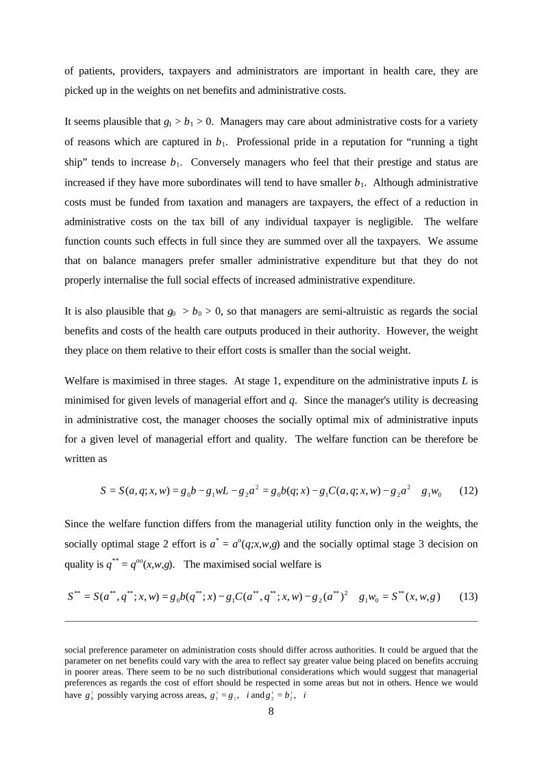
of patients, providers, taxpayers and administrators are important in health care, they are

picked up in the weights on net benefits and administrative costs.

It seems plausible that γ1 > β1 > 0. Managers may care about administrative costs for a variety

of reasons which are captured in β1. Professional pride in a reputation for “running a tight

ship” tends to increase β1. Conversely managers who feel that their prestige and status are

increased if they have more subordinates will tend to have smaller β1. Although administrative

costs must be funded from taxation and managers are taxpayers, the effect of a reduction in

administrative costs on the tax bill of any individual taxpayer is negligible. The welfare

function counts such effects in full since they are summed over all the taxpayers. We assume

that on balance managers prefer smaller administrative expenditure but that they do not

properly internalise the full social effects of increased administrative expenditure.

It is also plausible that γ0 > β0 > 0, so that managers are semi-altruistic as regards the social

benefits and costs of the health care outputs produced in their authority. However, the weight

they place on them relative to their effort costs is smaller than the social weight.

Welfare is maximised in three stages. At stage 1, expenditure on the administrative inputs L is

minimised for given levels of managerial effort and q. Since the manager's utility is decreasing

in administrative cost, the manager chooses the socially optimal mix of administrative inputs

for a given level of managerial effort and quality. The welfare function can be therefore be

written as

012

2102

210 ),;,();(),;,( wawxqaCxqbawLbwxqaSS γγγγγγγ +−−=−−== (12)

Since the welfare function differs from the managerial utility function only in the weights, the

socially optimal stage 2 effort is a* = ao(q;x,w,γ) and the socially optimal stage 3 decision on

quality is q** = qoo(x,w,γ). The maximised social welfare is

),,()(),;,();(),;,( 012

210 γγγγγ wxSwawxqaCxqbwxqaSS ∗∗∗∗∗∗∗∗∗∗∗∗∗∗∗∗ =+−−== (13)

social preference parameter on administration costs should differ across authorities. It could be argued that theparameter on net benefits could vary with the area to reflect say greater value being placed on benefits accruingin poorer areas. There seem to be no such distributional considerations which would suggest that managerialpreferences as regards the cost of effort should be respected in some areas but not in others. Hence we wouldhave γ 0

i possibly varying across areas, γ γ1 1i i= ∀, and γ β2 2

i i i= ∀,

9

where a a x w a q x woo o∗∗ ∗∗= =( , , ) ( ; , , )γ γ .

The cost function Co(q;x,w,γ) = C(ao(q;x,w,γ),q;x,w,γ) shows the administrative costs for a

given quality when the administrative inputs and managerial effort are chosen to maximise

welfare. Call Co(q;x,w,γ) the first best cost function and suppose for the moment that

Co(q;x,w,γ) is known. Given the assumptions about managerial and social preference weights,

it is obvious from the first order condition on effort choice (5) that the manager chooses too

little effort.9 Consequently the authority will lie above the first best function:

Co(q;x,w,β) − Co(q;x,w,γ) > 0 (14)

However, comparison of the welfare and managerial utility maximising decisions shows that

some care is required in drawing welfare implications from the fact that an authority lies above

the first best cost function. The welfare loss

),);,,(),,,((),);,,(),,,((

),;,(),;,(

wxwxqwxaSwxwxqwxaS

wxqaSwxqaSoooooooo

oooo

ββγγ −=

−∗∗∗∗

(15)

arises because the manager is incompletely altruistic: she chooses the wrong effort and

endogenous quality. The excess administrative expenditure (14) fails to reflect the welfare loss

for two reasons. First, it does not allow for the fact that quality as well as effort diverge from

the social optimum cost. If q is in fact endogenous in the sense that it is under the control of

the manager, we have to take account of the first type of error in using (14) as a measure of

(15). We test for endogeneity of quality in the cost function in section 5.

Second, even if quality is exogenous, so that only managerial effort is at issue, (14) ignores the

cost of the manager's effort. Since ao(q;x,w,γ) minimises C(a,q;x,w) + γ2a2/γ1 the welfare loss

at given quality is proportional to10

)],,;(),,;([

]),,;(),,;()[/()],,;(),,;([ 2212

γβ

γβγγγβ

wxqCwxqC

wxqawxqawxqCwxqCoo

oooo

−<

−+−(16)

9 The effect of the preference parameter on effort is ∂ao/∂β1 = − Ca/ (β1Caa+β2) > 0 and we have assumed thatβ1 < γ1.

10

The importance of the over-estimation of the welfare loss depends on the relative magnitudes

of the difference between managerial effort costs at the private and social optimum and the

difference between administrative costs at these points. It is plausible that the difference

between the true welfare loss (the left hand side of (16)) and the measured difference in

administrative costs (the right hand side) is not large. Managerial effort cost is likely to be

negligible compared with the cost of the other administrative inputs, so that the difference

between the cost of privately and socially optimal managerial effort is also negligible and so the

difference in administrative costs in (14) may be a reasonable measure of the welfare loss from

the manager’s suboptimal effort.

Low managerial effort leads to a welfare loss relative to the first best situation achievable if the

regulator can observe and control managerial effort. Managerial effort is also likely to be

second best inefficient in the sense that managers can be made better off and administrative

cost reduced even when managerial effort and preferences are not observed. Since

administrative cost is observable it is possible to design an incentive scheme which makes the

manager better off and reduces administrative costs.11 The scheme would be equivalent to

increasing the manager’s preference parameter β1, so that she supplies more effort and reduces

administrative expenditure.

In general managerial incentive schemes will not lead to a first best effort level. Not only are

the manager’s preferences not fully known, account would also have to be taken of the

unobserved random factors affecting costs and of managerial risk aversion. Further, if we also

allow for the fact that some aspects of the quality of care may be both endogenous and

observed with error, the optimal second best scheme may be very low power to avoid giving

managers too large an incentive to reduce cost by reducing quality (Holmstrom and Milgrom,

1991) .

10 Although the manager’s salary cost w0 is not a social cost of producing administrative services (the socialcost of managerial effort is γ2a

2) and is included in C = w0 + wL, it drops out of the difference betweenCo(q;x,w,β) and Co(q;x,w,γ), which is just the difference between the costs of vectors of non-managerial inputs.11 For example, with w0 = κ0 − κ1C (κ1 > 0), the marginal value of additional effort to the manager is − [β1 +(β1 + β3)κ1]Ca − 2β2a, so that the manager is induced to supply additional effort and κ0 can be set to ensure heis better off. Since the marginal social value of w0 is zero suitable choice of the incentive scheme parametersalso increases welfare.

11

The administrative cost function which can be estimated is not the first best cost function

Co(q;x,w,γ) but the function corresponding to the effort level of the area with the greatest

effort level: Co(q;x,w,βmax) where βmax < γ1 is the maximum value of the preference parameter

β1 across the areas. Since even the manager with the highest marginal valuation of

administration cost reductions undervalues cost reductions, comparison of the administration

cost Co(qi;xi,wi,βi) in area i with the estimated function Co(qi;xi,wi,βmax) will underestimate the

administrative cost reduction which could be achieved by supplying the first best amount of

effort.

However, even in these circumstances there is value in estimating the cost function. The

differences in costs between areas can be used to identify those where there is apparently poor

performance which merits further more detailed investigation. The differences in costs which

remain after such investigation provide some guidance as the potential welfare gains from

introducing incentive schemes and other mechanisms for improving performance.

2.3 Implications for estimation results

The second reason for introducing a simple formal model of managerial decisions is to guide

the estimation of the cost function and the interpretation of the results. We have assumed that

additional effort by managers can reduce expenditure on inputs required to administer the

primary care system. Assume for the moment that managerial effort is the only endogenous

variable in the cost function. Effort will be a function of all the other variables in the cost

function and managerial preferences. To illustrate the implications, suppose that, after suitable

transformation, the true cost function in area i at time t is

c x x ait it it it it= + + +δ δ δ ε1 1 2 2 3 (17)

where cit is the (transformed) administrative cost, x1it is an observable exogenous variable and

x2it is also exogenous but unobserved. εit is a zero mean i.i.d error term reflecting unobservable

exogenous factors which do not influence managerial effort and are uncorrelated with the x1it,

x2it. Assume that the unobserved variable is correlated with the observed:

x x rit i it it2 0 1 1= + +φ φ (18)

and rit a zero mean i.i.d. error. Managerial effort is

12

a x x vit i it it it= + + +α α α0 1 1 2 2 (19)

where α0i reflects authority specific factors and vit is a zero mean i.i.d. error term.

Because the unobserved managerial effort and the unobserved x2it have area specific

components OLS would yield biased estimates and panel data techniques should be used.

Random effects estimation requires that the area effects are not correlated with x1it (Baltagi,

1995). But the omitted x2it are correlated with x1it by assumption and the omitted managerial

effort variable is correlated with x1it (directly and indirectly via x2it) from the manager’s

optimisation problem. Thus the endogeneity of managerial effort indicates that we should use

fixed effects procedures to estimate the cost function.

The coefficients in the estimated cost equation

c d d D d xit j jj

it= + +=∑0 0

21 1 (20)

where the Dj are area dummies, satisfy

plim d0 = δ0 + (δ2 + δ3α2)φ0 (21)

plim d0i = (δ2 + δ3α2)φ0i + δ3α0i (22)

plim d1 = δ1 + (δ2 + δ3α2)φ1 + δ3α1 (23)

It has been suggested (Schmidt and Sickles, 1984; Skinner, 1994) that the estimated area

specific effects d0i can be used to make inferences about the relative efficiency of the areas.

We argued in the previous section that a better interpretation of the differences in cost

remaining after allowing for the non-effort variables is as an indication of the possible scope for

welfare improvements from changing incentives.

As the first term in (22) makes clear, the estimated area specific effects can also reflect the

impact of unobserved variables (x2it) (Dor, 1994; Newhouse, 1994). The area effects measure

differences in managerial effort and therefore potential welfare gains only if the unobserved

variables (a) do not vary systematically across areas (φ0 0i i= ∀, ) or (b) do not affect the cost

function, either directly (δ2 = 0) or indirectly through managerial effort (α2 = 0).

13

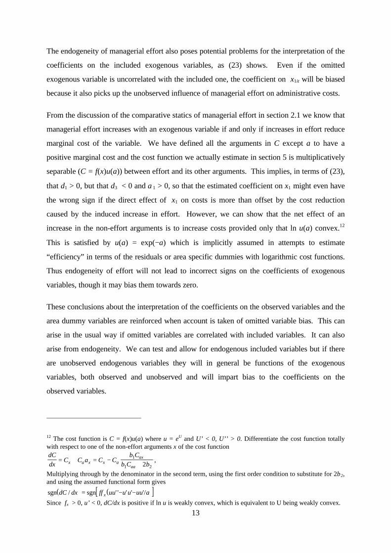
The endogeneity of managerial effort also poses potential problems for the interpretation of the

coefficients on the included exogenous variables, as (23) shows. Even if the omitted

exogenous variable is uncorrelated with the included one, the coefficient on x1it will be biased

because it also picks up the unobserved influence of managerial effort on administrative costs.

From the discussion of the comparative statics of managerial effort in section 2.1 we know that

managerial effort increases with an exogenous variable if and only if increases in effort reduce

marginal cost of the variable. We have defined all the arguments in C except a to have a

positive marginal cost and the cost function we actually estimate in section 5 is multiplicatively

separable (C = f(x)u(a)) between effort and its other arguments. This implies, in terms of (23),

that δ1 > 0, but that δ3 < 0 and α1 > 0, so that the estimated coefficient on x1 might even have

the wrong sign if the direct effect of x1 on costs is more than offset by the cost reduction

caused by the induced increase in effort. However, we can show that the net effect of an

increase in the non-effort arguments is to increase costs provided only that ln u(a) convex.12

This is satisfied by u(a) = exp(−a) which is implicitly assumed in attempts to estimate

“efficiency” in terms of the residuals or area specific dummies with logarithmic cost functions.

Thus endogeneity of effort will not lead to incorrect signs on the coefficients of exogenous

variables, though it may bias them towards zero.

These conclusions about the interpretation of the coefficients on the observed variables and the

area dummy variables are reinforced when account is taken of omitted variable bias. This can

arise in the usual way if omitted variables are correlated with included variables. It can also

arise from endogeneity. We can test and allow for endogenous included variables but if there

are unobserved endogenous variables they will in general be functions of the exogenous

variables, both observed and unobserved and will impart bias to the coefficients on the

observed variables.

12 The cost function is C = f(x)u(a) where u = eU and U’ < 0, U’’ > 0. Differentiate the cost function totallywith respect to one of the non-effort arguments x of the cost functiondC

dxC C a C C

C

Cx a x x aax

aa= + = −

+β

β β1

1 22,

Multiplying through by the denominator in the second term, using the first order condition to substitute for 2β2,and using the assumed functional form gives

( ) ( )[ ]sgn / sgn ' ' ' ' '/dC dx ff uu u u uu ax= − −

Since fx > 0, u’ < 0, dC/dx is positive if ln u is weakly convex, which is equivalent to U being weakly convex.

14

We interpret the simple model of administrative costs as warning that care is required in

drawing strong conclusions from empirical estimates of cost functions and of inefficiency.

Such warnings always in order given the imperfections of health service data sets. A formal

model at least cautions us as the likely sources of bias and possibly their directions.

3. Data and institutional background

During the period of our analysis (1989/90 to 1994/513) primary care in England was

administrated by 90 Family Health Service Authorities (FHSAs) covering geographically

defined populations of about 500,000.14 Prior to April 1990 FHSAs were mainly responsible

for administering payments to general practitioners, practice nurses, dentists, opticians, and

pharmacies providing primary care services. The new GP contract in 1990 expanded the tasks

of FHSAs and increased the range of activities for which GPs could claim payment. FHSAs

also increased their monitoring role and were expected to improve the quality of primary care

by feeding back information to GPs and encouraging peer review. From April 1991 practices

were permitted to hold budgets to spend on certain types of secondary care and on

pharmaceuticals. The budgets were negotiated with FHSAs and administered by them.

The data are annual observations from the Health Service Indicators (HSI), a database

collected by the NHS Executive (NHS Executive, several years). Table 1 contains definitions

and descriptive statistics of the variables used in the analysis. The dependent variable is the

total revenue expenditure on FHSAs administration in £ 000’ in current prices.15

The variables we consider to be the main drivers of FHSA administrative expenditure are the

numbers of general practitioners, practice nurses, ophthalmic medical practitioners, dentists

and community pharmacies in the FHSA.

13 These are financial years running from April 1 to March 31.14 Before April 1990 FHSAs were called Family Practitioner Committees. In April 1996 FHSAs werereorganised into 100 new Health Authorities which combined responsibility for secondary and primary care.15 Expenditure on administration includes: authority member’s remuneration; honoraria, fees etc for FHSAadvisers; medical audit teams fees etc; other salaries and wages; computer supplies and services; other suppliesand services; establishment expenses; bank charges; hire purchase and lease charges; transport and moveableplant; premises and fixed plant; agency services; recharges from other FHSAs/HAs and NHS Trusts; auditorsremuneration; miscellaneous.

15

FHSA accounts do not provide information on prices of administrative inputs. We therefore

used the New Earnings Survey (Department of Employment, several years) to construct an

index of administrative labour input prices as the regional average gross weekly earnings for

full-time non-manual workers on adult rates in public administration.16 To allow for other

sources of variation in input prices we also included dummies variables for three types of area,

relative to inner London: outer London, metropolitan areas (roughly other large city areas) and

shire counties (non urban areas).

The obvious major change in the organisation of primary care in the period under consideration

was the introduction of general practitioners fundholding in April 1991. Fundholding practices

held budgets to cover the costs of referring their patients for certain categories of non

emergency secondary care. The scheme increased FHSAs' administrative burden as they had

to negotiate the budget for fundholders each year, to monitor financial outcomes and to check

on the use to which fundholders put any budget surplus. We measure the burden of

fundholding in a year as the proportion of practices which were fundholders in the following

year to allow for the fact that fundholder budgets were negotiated in the previous year.

The quality of the primary health care provided in the FHSAs is proxied by the success of

cervical cytology screening. Before the 1st April 1990 GPs were rewarded for the number of

tests given, while for subsequent years they received target payments if they screened at least a

specified proportion of women aged 25-64 on their list. Since information on cytology

screening is generated only in connection with payments to GPs we ensure longitudinal

comparability by measuring the quality of screening by the FHSA's z-score (Armitage and

Berry, 1994).17

To control for FHSAs characteristics that may affect the costs of administering a given number

of primary care practitioners delivering care a given quality, we used the health of the

16 In their analysis of hospital cost functions Scott and Parkin (1995) argued that because wages are set bynational bargaining, it is reasonable to assume that labour input prices are the same across units andconsequently, can be dropped from the estimation. However, in order to account for longitudinal variation ininput prices we decided to keep labour input prices in the analysis.17 The primary care quality index is calculated as z x xit it t t= −( ) / σ , where xit represents the number of cervicalcytology tests per eligible population or the proportion of GPs reaching the target of 90% screening for theeligible population in area i in year t, xt is its mean value in year t and σt is its standard deviation in year t.

16

population as measured by its standardised mortality rate and the population density per

hectare.

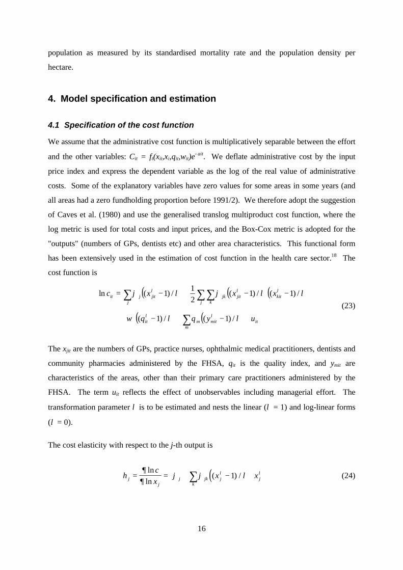
4. Model specification and estimation

4.1 Specification of the cost function

We assume that the administrative cost function is multiplicatively separable between the effort

and the other variables: Cit = ft(xit,xi,qit,wit)e−ait. We deflate administrative cost by the input

price index and express the dependent variable as the log of the real value of administrative

costs. Some of the explanatory variables have zero values for some areas in some years (and

all areas had a zero fundholding proportion before 1991/2). We therefore adopt the suggestion

of Caves et al. (1980) and use the generalised translog multiproduct cost function, where the

log metric is used for total costs and input prices, and the Box-Cox metric is adopted for the

"outputs" (numbers of GPs, dentists etc) and other area characteristics. This functional form

has been extensively used in the estimation of cost function in the health care sector.18 The

cost function is

( ) ( )( )

( ) ( ) itm

mitmit

kitj

jitk

jkj

jitjit

uyq

xxxc

+−+−+

−−+−=

∑

∑∑∑

λθλω

λλϕλϕ

λλ

λλλ

/)1(/)1(

/)1(/)1(21

/)1(ln

(23)

The xjit are the numbers of GPs, practice nurses, ophthalmic medical practitioners, dentists and

community pharmacies administered by the FHSA, qit is the quality index, and ymit are

characteristics of the areas, other than their primary care practitioners administered by the

FHSA. The term uit reflects the effect of unobservables including managerial effort. The

transformation parameter λ is to be estimated and nests the linear (λ = 1) and log-linear forms

(λ = 0).

The cost elasticity with respect to the j-th output is

( )η∂

∂ϕ ϕ λλ λ

jj

j jk jk

j

c

xx x= = + −

∑ln

ln( ) /1 (24)

17

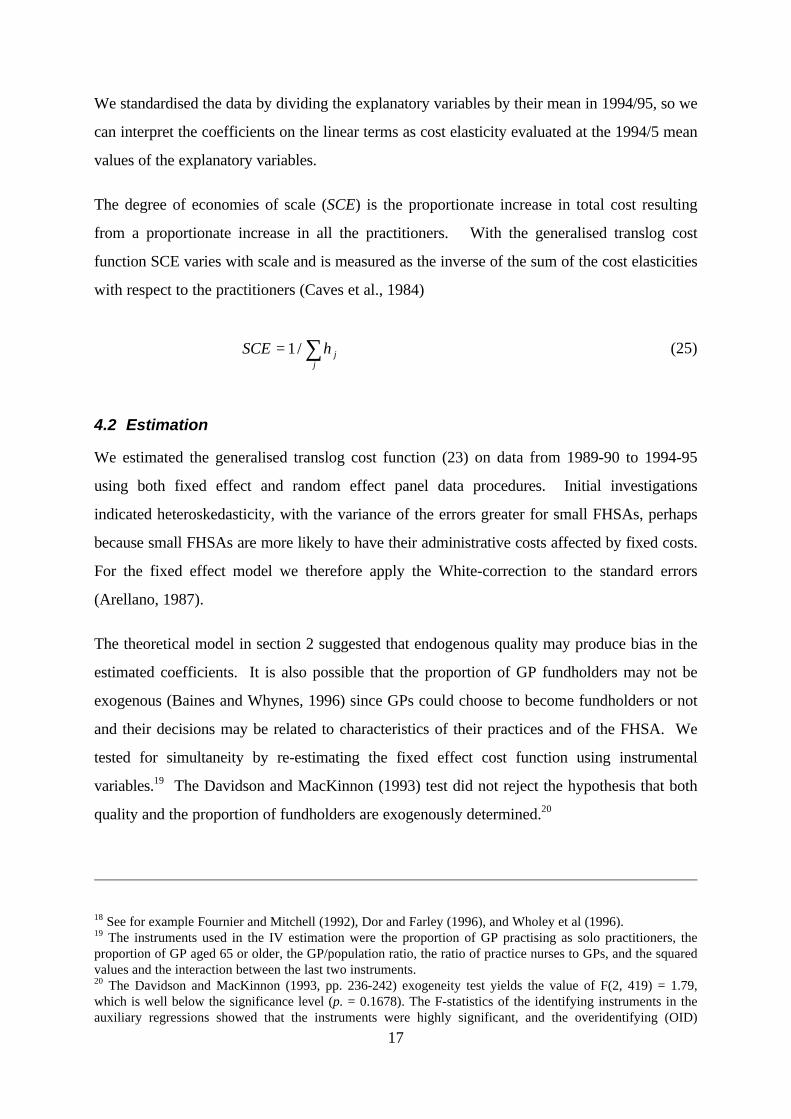
We standardised the data by dividing the explanatory variables by their mean in 1994/95, so we

can interpret the coefficients on the linear terms as cost elasticity evaluated at the 1994/5 mean

values of the explanatory variables.

The degree of economies of scale (SCE) is the proportionate increase in total cost resulting

from a proportionate increase in all the practitioners. With the generalised translog cost

function SCE varies with scale and is measured as the inverse of the sum of the cost elasticities

with respect to the practitioners (Caves et al., 1984)

SCE jj

= ∑1/ η (25)

4.2 Estimation

We estimated the generalised translog cost function (23) on data from 1989-90 to 1994-95

using both fixed effect and random effect panel data procedures. Initial investigations

indicated heteroskedasticity, with the variance of the errors greater for small FHSAs, perhaps

because small FHSAs are more likely to have their administrative costs affected by fixed costs.

For the fixed effect model we therefore apply the White-correction to the standard errors

(Arellano, 1987).

The theoretical model in section 2 suggested that endogenous quality may produce bias in the

estimated coefficients. It is also possible that the proportion of GP fundholders may not be

exogenous (Baines and Whynes, 1996) since GPs could choose to become fundholders or not

and their decisions may be related to characteristics of their practices and of the FHSA. We

tested for simultaneity by re-estimating the fixed effect cost function using instrumental

variables.19 The Davidson and MacKinnon (1993) test did not reject the hypothesis that both

quality and the proportion of fundholders are exogenously determined.20

18 See for example Fournier and Mitchell (1992), Dor and Farley (1996), and Wholey et al (1996).19 The instruments used in the IV estimation were the proportion of GP practising as solo practitioners, theproportion of GP aged 65 or older, the GP/population ratio, the ratio of practice nurses to GPs, and the squaredvalues and the interaction between the last two instruments.20 The Davidson and MacKinnon (1993, pp. 236-242) exogeneity test yields the value of F(2, 419) = 1.79,which is well below the significance level (p. = 0.1678). The F-statistics of the identifying instruments in theauxiliary regressions showed that the instruments were highly significant, and the overidentifying (OID)

18

5. Results

Table 2 reports the estimates of the cost function (23) including the linear, quadratic and cross

product terms.21 The estimated economies of scale factor (SCE) is evaluated at the 1994/5

means of the explanatory variables and since the variables are standardised at their 1994/5

means the estimated linear terms on the primary care practitioners are the elasticities of

administrative cost with respect to the numbers of GPs, dentists etc. The fixed effects model is

reported in the first two columns and has positive and significant linear terms for general

practitioners and practice nurses, the linear term for opticians is positive but not statistically

significant and those for dentists and pharmacies are negative, though not significant. The last

two columns in Table 2 present the estimates of the random effects model. We argued in

section 2.3 that endogenous managerial effort implied that the random effects specification was

likely to be misspecified. The Hausman (1978) test indicates that the assumption that area

effects are not correlated with the other regressors cannot be rejected22 and so the random

effects model is appropriate.

The model of managerial effort in section 2.1 implies that effort will be correlated with the

number of practitioners if the marginal cost of practitioners is reduced by managerial effort

(Caq <0) and if the manager cares about administrative costs (β1 > 0). The assumed cost

function is of the form C=f(x,q)h(a) which implies Caq < 0. Since β1 reflects both managerial

preferences and the incentive structure in primary care administration, the fact that the

Hausman test indicates that area effects are not correlated with practitioners suggests that

incentives to reduce primary care administration costs are negligible.

The random effects model yields economically more sensible results since all the linear cost

terms on the primary care practitioners are positive. Further, the random effects model

produces much modest prediction errors because, unlike the fixed effects model, it does not

restrictions test (Godfrey and Hutton, 1994) suggested that the instruments were valid and the model was notmisspecified (χ2(5) = 9.612; p. = 0.103).21 The value of λ was chosen to maximise the log-likelihood of the regression and was determined using a gridsearch as suggested by Dor and Farley (1996). The search range was -2.0 and +2.0, with intervals of 0.01.22 The Hausman procedure tests the assumption that the disturbances do not contain individual invariant effectswhich are unobserved and correlated with the independent variables by comparing the coefficients provided bythe fixed and by the random effects models. If the assumption is correct, the coefficients estimated by the twomodels are not systematically different and the random effects model is more efficient.

19

have to sacrifice a large number of degrees of freedom in estimating area effects. This is

important when assessing economies of scale or scope.

Both models indicate that the number of general practitioners has the largest proportionate

effect on costs. This is plausible since the remuneration system for GPs is much more

complicated than for other practitioners. Density of population is significantly positively

associated with administrative costs in the random effects model. Since the variable shows

relatively little change over time it may be picking up area effects. One possibility is that more

densely populated areas have greater turnover of patients on GP lists and so generate more

administration. The regional dummies are also of the expected sign, indicating that Inner

London areas have significantly higher administrative costs than more rural areas and also than

other urban areas, probably because of differences in property rents.

5.1 Economies of scale

Both models suggest that that there are economies of scale exist in the administration of

primary care. The fixed effects model estimates that the SCE is equal to 1.543 but this is not

significantly different from unity. The random effects model estimate indicates a more modest

SCE, 1.209 which is statistically different from unity because the random effects estimates are

more precise. The random effects model suggests that there are economies of scale to be

exploited at the mean 1994/5 size of FHSA.

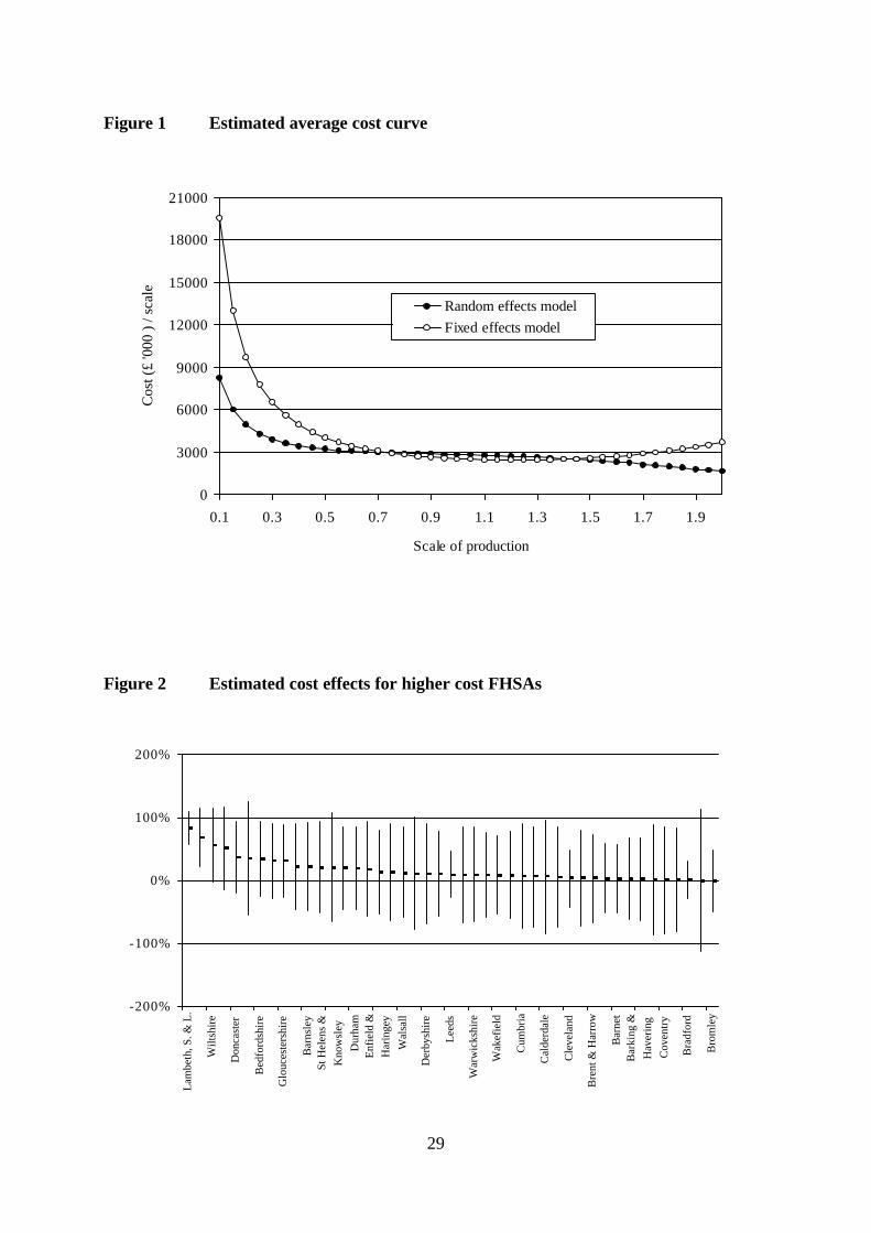
Figure 1 illustrates the impact of scale on costs for non local variations in scale. It is derived

by calculating the administrative cost of an FHSA from the fixed and random effects models

when the primary care practitioner variables are increased or decreased proportionately from

their mean 1994/5 values and the values of all other explanatory variables are held constant at

their 1994/5 means. The curves plot the resulting total costs divided by the scale factor for the

primary care practitioner variables and can be regarded as the multi-"output" analogue of

single output average cost function.

The curve derived from the fixed effect model is “U” shape and indicates the presence of

economies of scale for small and medium-sized FHSAs. Economies of scale are exhausted at a

level 20% larger than the average FHSA

20

The average cost curve estimated by the random effects model is similar to the fixed effects

model for scales of production near to the mean. Economies of scale are much less for small

FHSAs. The random effects model suggests that there are economies of scale at all level of

production.

The fact that both models suggest marked economies of scale for small FHSAs may have some

implications for possible future developments in the administration of primary care in England.

The NHS was reorganised around Primary Care Groups (PCGs) April 1999. PCGs consist of

around 50 general practitioners with total lists of about 100,000 patients - they are about one

fifth the size of Health Authorities, some of whose functions they have taken over. Our

estimates suggest that there could be adverse consequences for administrative costs if PCGs

take over all of the primary care administrative tasks previously carried out by FHSAs.

5.2 Economies of scope

There are economies of scope if the cost of administering a given set of primary care

practitioners is less than sum of the costs of administering them separately (Baumol et al,

1982). One way to measure economies of scope is as the proportionate change in costs from

partitioning the practitioner types into two groups (Fournier and Michell, 1992):

C x C x C x x

C x x

( , , ) ( , , ) ( , , )( , , )

1 2 1 2

1 2

0 0⋅ + ⋅ − ⋅⋅

(26)

where x1, x2 is a partition of the practitioner vector.

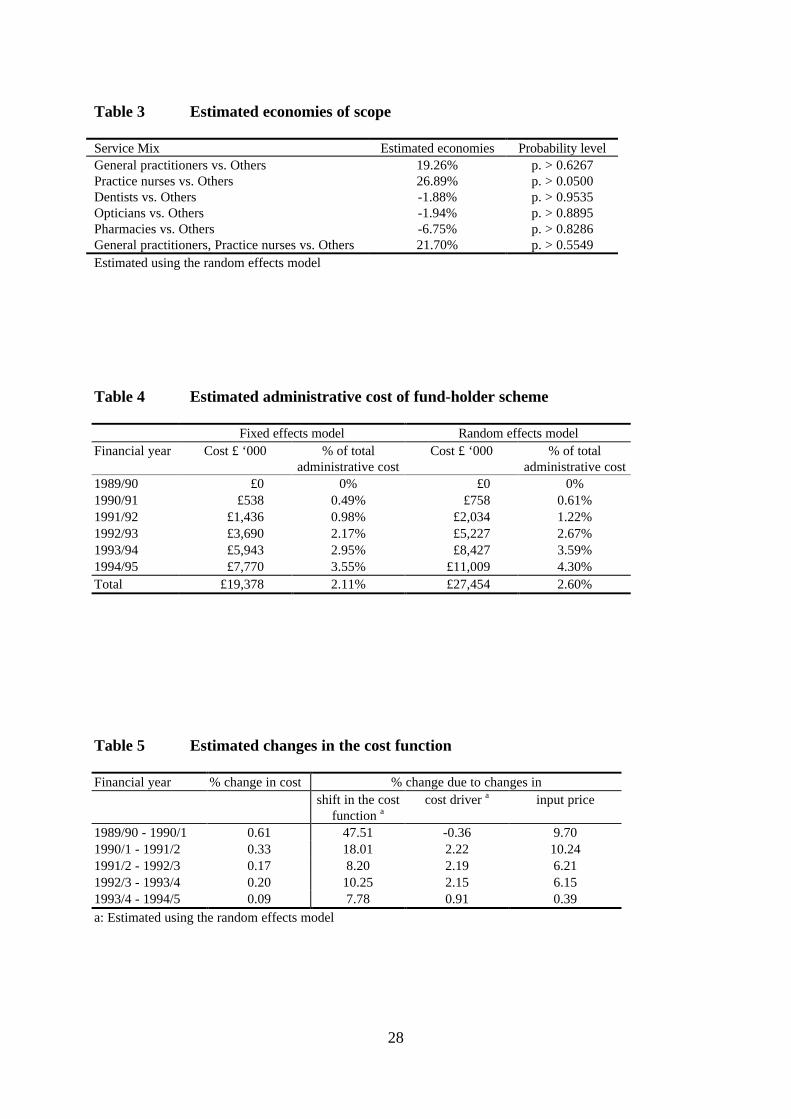
Table 3 reports estimated economies of scope for six possible partitions: each practitioner type

separately administered from the rest and practice nurses and GPs administered separately from

all other practitioners.23 The cost changes are calculated at the 1994/5 means. Whilst some of

the cost differences are large, only that for separate administration of practice nurses is

significant.

23 The economies of scope estimated by the fixed effects model are similar but not significant.

21

5.3 Fundholding and administration costs

The introduction of fundholding in April 1991 increased the tasks which FHSAs were expected

to carry out. We included the proportion of fundholding practices to reflect this change in

function. The regression indicates that fundholding had a significant positive effect on costs,

though its magnitude is small. Table 4 presents the estimated administrative costs of the

associated with fundholding both in absolute terms and as a proportion of total administrative

costs. Fundholding accounts for 3.5-4.3% (as depending on whether the fixed and random

effects estimates are used) of the expenditure in administration in the financial year 1994/95

which is between £7.7M - £11M.

5.4 Changes in administration cost over time

Administration cost changes over time for three reasons: changes in the cost drivers (outputs,

quality and control variables); changes in the price of inputs; and shifts in the cost function

across all FHSAs (reflected in the year dummies in Table 2). The first column in Table 5

shows the proportionate change in the cost each year. The second column is the change in

costs which would have occurred due solely to the shift in the cost function with the drivers

and input prices held constant. The third and fourth columns give the proportionate changes in

costs which would be attributable solely to changes in the drivers and in the input prices

respectively. It is apparent that the changes in the number of practitioners, quality levels etc

have had relatively little effect on total cost over the period. The effect of input price inflation

is greater but still minor compared with the shifts in the cost function.

The shift of the cost function over time could be the reflection of a number of factors:

(i) there may have been “negative technical progress”: the technology altered to make it more

costly to administer primary care. This seems implausible.

(ii) Factor price changes may have not been fully allowed for in our deflation of administrative

costs by input price indices. Our input price index is imperfect but it is difficult to believe that

there were increases in the prices of inputs used in administering primary care which are

capable of explaining the more than doubling of administrative costs over the period.

(iii) An increase in the administrative tasks performed by FHSAs. The fundholding variable is

a direct measure of some of the new administrative tasks associated with the internal market

22

and is included in the cost drivers. Since other additional administrative tasks were not

associated with fundholding, the fundholding variable may be an inadequate proxy for all the

increased tasks resulting from the internal market reforms of the early 1990ies.

Total administrative costs of FHSA were £215M in 1994/5 (current prices) and we estimate

that cost increased between 1989/90 and 1994/5 by 123% as a result of shift in the cost

function, rather than to changes in its arguments. If the year dummies are picking up the effect

of the increase in administrative tasks, we have identified a further large cost of the 1990

reforms.

5.5 Relative efficiency

The estimated cost function can be used to derive an estimate of the difference in costs due to

unobserved area effects, using the estimated fixed effects or, in the case of the random effects

model, from the area residuals. We calculate the cost effect as the percentage difference

between the cost of the area given its estimated fixed effect and the cost it would have with the

area average fixed effect: exp{ }F Fi − − 1where Fi is the estimated area fixed effect and F is

the mean fixed effect. Figure 2 presents a “league table” for the areas with above average

fixed effects and plots the estimated area cost effects and their confidence intervals.

Such area effects have been interpreted as an indicator of efficiency (Schmidt and Sickles,

1984) but we argued in section 2.2 that necessary conditions for this interpretation are that the

number of primary care practitioners and the quality of primary care are exogenous as far as

managers are concerned and the effort of managers has negligible social cost. Even if these

conditions are satisfied we showed in section 2.3 that the area effects would yield biased

estimates of the differences in managerial effort.

The size of the confidence intervals also indicates that one should be extremely cautious in

using these results to label areas as more or less efficient in terms of their administrative costs.

Figure 2 shows that only a few of the “inefficient” or high cost FHSAs have a cost effect which

is significantly above the mean. The analysis may however be useful as an initial filter to select

areas for further investigation after allowing for differences in costs associated with routinely

observable factors such as the number of practitioners.

23

6. Conclusion

A simple theoretical model of managerial effort to reduce administrative costs reinforces

previous cautions about the interpretation of the results of studies of inefficiency in health care.

Estimated differences in costs measure welfare differences across units only if relevant decision

makers cannot control outputs or quality and if the unobserved effort costs have negligible

social significance. Further, estimates of cost differences as area fixed effects or as residuals

from random effects models are unlikely to be unbiased if managerial effort is endogenous.

The lesson is that empirical investigation of cost functions needs to rest on careful specification

of the decision generating those cost functions.

Our investigation of the costs of administering primary care in the NHS suggests:

• numbers of general practitioners had the greatest effect on administration costs;

• there were unexploited economies of scale in primary care administration;

• the introduction of fundholding had a significant but relatively small positively impact on

costs;

• most of the doubling of costs over the period 1989/90 - 1994/5 is attributable to shifts in

the cost function, most likely reflecting unmeasured increases in administrative tasks,

including those following the changes to the GP contract in 1990;

• regression based comparison of administrative costs across FHSAs shows that only a

small number can be said to be significantly more costly ceteris paribus than average.

Policy to reduce administration costs may be best directed at improving the performance

of all areas, perhaps by introduction of incentive schemes, rather than by concentrating

attention on the few obviously high cost areas.

24

References

Armitage P, and Berry G. (1994) Statistical Methods in Medical Research. Oxford: BlackwellScience.

Arellano M. (1987) Computing robust standard errors for within-group estimators. OxfordBulletin of Economics and Statistics, 49, 431- 434.

Baltagi B.H.. Econometric Analysis of Panel Data. Chichester: John Wiley & sons, 1995

Baines DL, Whynes DK. (1996) Selection bias in GP fundholding. Health Economics, 5, 129-140

Baumol W, Panzar I, Willig R. (1982) Contestable Markets and the Theory of IndustryStructure. San Diego, CA: Harcourt Brace Janovich.

Caves DW, Christensen LR, Tretheway MW. (1980) Flexible cost functions for multiproductsfirms. Review of Economics and Statistics, 62, 477-481.

Caves DW, Christensen LR, Tretheway MW. (1984) Economies of density versus economiesof scale. Why trunk or local service airline costs differ. Rand Journal of Economics, 15,471-489.

Davidson R, and MacKinnon JG. (1993) Estimation and Inference in Econometrics. NewYork: Oxford University Press.

Department of Employment. New Earnings Survey. London: HMSO, several years.

Department of Health. The New NHS Modern and Dependable. London: The StationeryOffice, 1997

Dor A. (1994) Non-minimum cost functions and the stochastic frontier: On applications tohealth care providers. Journal of Health Economics, 13, 329-334.

Dor A, Farley DE. (1996) Payment source and the cost of hospital care: Evidence from amultiproduct cost function with multiple payers. Journal of Health Economics, 15, 1-21.

Fournier GM, Mitchell JM. (1992) Hospital costs and competition for services: A multiproductanalysis. Review of Economics and Statistics, 72, 627-634.

Gaynor M, Pauly MV. (1990) Compensation and productive efficiency in partnerships:evidence from medical group practice, Journal of Political Economy, 98, 544-573.

Godfrey LG, Hutton JP. (1994) Discriminating between errors-in-variables, simultaneity andmisspecification in linear regression models. Economics Letters;44:359-64.

Hausman JA. (1978) Specification tests in econometrics. Econometrica, 46, 1251-1271.

Holmstrom B, Milgrom P. (1991) Multitask principal-agent analyses: incentive contracts,asset ownership, and job design. Journal of Law, Economics and Organization, 7,Special Issue, 24-52.

Newhouse JP. (1994) Frontier estimation: how useful a tool for health economics? Journal ofHealth Economics, 13, 317-322.

NHS Executive. The new NHS Modern and Dependable: A National Framework forAssessing Performance. London: Department of Health, 1998.

NHS Executive. Health Service Indicators Handbook. Leeds, 1996.

25

Schmidt P, Sickles R. (1984) Production frontiers and panel data. Journal of Business andEconomic Statistics, 2, 367-374.

Scott A, Parkin D. (1995) Investigating hospital efficiency in the new NHS: The role of thetranslog cost function. Health Economics, 4, 467-478.

Skinner J. (1994) What do stochastic frontier cost functions tell us about inefficiency? Journalof Health Economics, 13, 323-328.

Wholey D, Feldman R, Christianson JB, Enberg J. (1996) Scale and scope economies amonghealth maintenance organizations. Journal of Health Economics, 15, 657-684.

26

Table 1 Description of the variables

Variable Mean Std. Dev. Min MaxAdministrative costs in '000 £Financial year 1989/90 741.39 371.01 257.1 1916.83Financial year 1990/91 1154.64 505.51 502.04 2618.17Financial year 1991/92 1514.80 609.08 706.03 3181.71Financial year 1992/93 1798.67 787.46 822.47 5287.41Financial year 1993/94 2160.38 995.72 731.23 6533.2Financial year 1994/95 2391.20 1168.82 902.35 7293.67Descriptive statistics for the entire sampleAdministrative costs in '000 £ 1626.85 968.56 257.1 7293No. of General medical practitioners (GPs) 287.16 174.02 69 900No. of Practice nurses 89.77 64.89 0 396No. of Dentists having contract with theFHSA

172.87 109.20 38 540

No. of Ophthalmic opticians having contractwith the FHSA

137.93 83.39 15 523

No. of Community pharmacies 108.22 62.51 28 305% of Fundholders 11.06 11.30 0 58.04Population density (population per hectares) 17.80 20.19 0.61 100.76Quality of cervical cytology tests (z-values) 10.00 1.00 6.36 12.27Standardised mortality rate (SMR) 102.10 10.44 76.7 136.5

27

Table 2 Parameter estimates of the cost function

Fixed effects model Random effects modelVariable Coefficients Standard

ErrorCoefficients Standard

ErrorGeneral practitioners (x1) 0.603** 0.286 0.650*** 0.102Practice nurses (x2) 0.063* 0.033 0.066* 0.034Dentists (x3) -0.035 0.165 0.009 0.069Opticians (x4) 0.045 0.048 0.084*** 0.032Pharmacies (x5) -0.027 0.346 0.019 0.082% of Fundholders 0.036** 0.017 0.046*** 0.016Quality of cervical cytology test 0.188* 0.098 0.057 0.097Population density 0.296 0.473 0.055*** 0.019SMR 0.043 0.065 0.061 0.073x1 × x1 1.364* 0.708 -0.033 0.340x2 × x2 0.083 0.054 0.065 0.066x3 × x3 0.972 0.629 -0.296 0.349x4 × x4 -0.143* 0.075 -0.312*** 0.075x5 × x5 -0.326 0.639 -0.351 0.365x1 × x2 0.058 0.148 -0.052 0.124x1 × x3 -0.531 0.413 -0.008 0.284x1 × x4 0.028 0.161 -0.248* 0.139x1 × x5 -1.096 0.710 -0.096 0.289x2 × x3 -0.179* 0.095 -0.090 0.086x2 × x4 0.023 0.051 0.045 0.055x2 × x5 -0.044 0.089 -0.029 0.085x3 × x4 -0.316** 0.143 0.145 0.125x3 × x5 0.105 0.450 0.322 0.250x4 × x5 0.409** 0.178 0.259** 0.127Outer London a - - -0.106* 0.054Metropolitan areas a - - -0.172*** 0.057Shire counties a - - -0.261*** 0.0711990/91 0.389*** 0.018 0.388*** 0.0191991/92 0.554*** 0.021 0.556*** 0.0221992/93 0.633*** 0.024 0.632*** 0.0251993/94 0.731*** 0.026 0.726*** 0.0251994/95 0.806*** 0.027 0.797*** 0.026Intercept 7.026 0.238 7.156*** 0.063λ 1.04 1.04Estimated SCE 1.543 1.209Hausman test [χ2 (29)] 6.26R2 0.929 0.925RESET [F(3, 418)] 0.96 0.10F-test that all ui = 0 [F(89, 421)] 4.80*** -Breush-Pagan test [χ2 (1)] b - 96.31***

Test that SCE =1 [F(1, 421)] 0.27 22.69***

*** indicates p ≤ 0.01; ** indicates 0.01 < p ≤ 0.05; * indicates 0.05 < p ≤ 0.1a: These variables are not included in the fixed effects model as they are time invariant.b: The Breush and Pagan test that Var (ui) = 0.

28

Table 3 Estimated economies of scope

Service Mix Estimated economies Probability levelGeneral practitioners vs. Others 19.26% p. > 0.6267Practice nurses vs. Others 26.89% p. > 0.0500Dentists vs. Others -1.88% p. > 0.9535Opticians vs. Others -1.94% p. > 0.8895Pharmacies vs. Others -6.75% p. > 0.8286General practitioners, Practice nurses vs. Others 21.70% p. > 0.5549Estimated using the random effects model

Table 4 Estimated administrative cost of fund-holder scheme

Fixed effects model Random effects modelFinancial year Cost £ ‘000 % of total

administrative costCost £ ‘000 % of total

administrative cost1989/90 £0 0% £0 0%1990/91 £538 0.49% £758 0.61%1991/92 £1,436 0.98% £2,034 1.22%1992/93 £3,690 2.17% £5,227 2.67%1993/94 £5,943 2.95% £8,427 3.59%1994/95 £7,770 3.55% £11,009 4.30%Total £19,378 2.11% £27,454 2.60%

Table 5 Estimated changes in the cost function

Financial year % change in cost % change due to changes inshift in the cost

function acost driver a input price

1989/90 - 1990/1 0.61 47.51 -0.36 9.701990/1 - 1991/2 0.33 18.01 2.22 10.241991/2 - 1992/3 0.17 8.20 2.19 6.211992/3 - 1993/4 0.20 10.25 2.15 6.151993/4 - 1994/5 0.09 7.78 0.91 0.39a: Estimated using the random effects model

29

Figure 1 Estimated average cost curve

0

3000

6000

9000

12000

15000

18000

21000

0.1 0.3 0.5 0.7 0.9 1.1 1.3 1.5 1.7 1.9

Scale of production

Cos

t (£

'000

) / s

cale

Random effects modelFixed effects model

Figure 2 Estimated cost effects for higher cost FHSAs

-200%

-100%

0%

100%

200%

Lam

beth

, S. &

L.

Wilt

shir

e

Don

cast

er

Bed

ford

shir

e

Glo

uces

ters

hire

Bar

nsle

ySt

Hel

ens

&K

now

sley

Dur

ham

Enf

ield

&H

arin

gey

Wal

sall

Der

bysh

ire

Lee

ds

War

wic

kshi

re

Wak

efie

ld

Cum

bria

Cal

derd

ale

Cle

vela

nd

Bre

nt &

Har

row

Bar

net

Bar

king

&H

aver

ing

Cov

entr

y

Bra

dfor

d

Bro

mle

y