Effects of the attractive interactions in the thermodynamic, dynamic, and structural anomalies of a two length scale potential

arX

iv:1

006.

0033

v1 [

cond

-mat

.sta

t-m

ech]

31

May

201

0PREPRINT

Effects of the attractive interactions in the thermodynamic,

dynamic and structural anomalies of a two length scale potential

Jonathas Nunes da Silva,1 Evy Salcedo,2 Alan Barros de Oliveira,3 and Marcia C. Barbosa1

1Instituto de Fısica, Universidade Federal do Rio Grande do Sul,

Caixa Postal 15051, 91501-970, Porto Alegre, RS, Brazil∗

2Departamento de Fısica, Universidade Federal de Santa Catarina,

Florianopolis, SC, 88010-970, Brazil†

3Departamento de Fısica, Universidade Federal de Ouro Preto,

Ouro Preto, MG, 35400-000, Brazil‡

(Dated: June 2, 2010)

Abstract

Using molecular dynamic simulations we study a system of particles interacting through a con-

tinuous core-softened potentials consisting of a hard core, a shoulder at closest distances and an

attractive well at further distance. We obtain the pressure-temperature phase diagram of of this

system for various depths of the tunable attractive well. Since this is a two length scales potential,

density, diffusion and structural anomalies are expected. We show that the effect of increasing

the attractive interaction between the molecules is to shrink the region in pressure in which the

density and the diffusion anomalies are present. If the attractive forces are too strong, particle will

be predominantly in one of the two length scales and no density of diffusion anomaly is observed.

The structural anomalous region is present for all the cases.

PACS numbers:

∗Electronic address: [email protected]†Electronic address: [email protected]‡Electronic address: [email protected]

1

I. INTRODUCTION

The phase behavior of single component systems as particles interacting via the so-called

core-softened (CS) potentials are receiving a lot of attention recently. These potentials

exhibit a repulsive core with a softening region with a shoulder or a ramp [1–12]. These

models were motivated by the aim of construct a simple two-body isotropic potential capable

of describing the complicated features of systems interacting via anisotropic potentials. This

approach generates models analytically [13–16] and computationally [1–9] tractable still

capable to retain the qualitative features of the real complex systems.

The physical motivation behind these studies is the recently acknowledged possibility

that some single component systems display coexistence between two different liquid phases

[17–19], a low density liquid phase (LDL) and a high density liquid phase (HDL), ending

at a LDL-HDL critical point. This opened the discussion about the relation between the

presence of two liquid phases, the existence of thermodynamic anomalies in liquids and the

form of the potential. The case of water is probably the most intensively studied. A liquid

where the specific volume at ambient pressure starts to increase when cooled below T ≈ 4oC

[20, 21]. Besides, in a certain range of pressures, water also exhibits an anomalous increase

of compressibility and specific heat upon cooling from experiments [22, 23]. Experiments

for Te, [24] Ga, Bi, [25] S, [26, 27] and Ge15Te85, [28] and simulations for silica, [29–31]

silicon [32] and BeF2, [29] show that these materials present also density anomaly.

Besides the anomalies discussed above, water has dynamic anomalies as well. Experiments

show that the diffusion constant, D, increases on compression at low temperature, T , up to

a maximum Dmax(T ) at P = PDmax(T ). The behavior of normal liquids, with D decreasing

on compression, is restored in water only at high P , e.g. for P > PDmax ≈ 1.1 kbar at

10oC [21, 22]. Computational simulations for the Simple Point Charge/Extended (SPC/E)

water model [33] recover the experimental results and show that the anomalous behavior

of D extends to the metastable liquid phase of water at negative pressures – a region that

is difficult to access for experiments [34–36]. In this region the diffusivity D decreases for

decreasing p until it reaches a minimum value Dmin(T ) at some pressure pDmin(T ), and

the normal behavior, with D increasing for decreasing p, is reestablished only for P <

PDmin(T ) [34–38]. Besides water, silica [31, 39] and silicon [40] also exhibit a diffusion

anomalous region.

2

Acknowledging that CS potentials might engender density and diffusion anomalies, de

Oliveira et al. [7, 41–45] proposed a simple CS model. It has a repulsive core that exhibits

a region of softening where the slope changes drastically. This model exhibits density,

diffusion and structural anomalies like the anomalies present in experiments [21, 22] and

simulations [34–36] for water. This simple system has no attraction between the particles

and, therefore, no liquid-gas or liquid-liquid critical points are present. Realistic models

should have attractive interactions since most molecules attract each other either due to van

der Waals interactions or to more sophisticated electrostatic forces.

Which effect in the pressure-temperature phase diagram one might expect from the addi-

tion of a larger attractive part in the potential? For one length scale potentials, the increase

of the attractive well leads to an increase in the temperature of the liquid-gas critical point.

In the case of the continuous two length scale potential the same behavior might be expected

for the liquid-gas critical point but it is not clear which effect the depth of the well has in

the location in the pressure-temperature phase diagram of the liquid-liquid critical point.

Moreover, it is also not clear which effect the attraction has in the location in the pressure-

temperature phase diagram of the density, diffusion and structural anomalous regions.

In this paper we address these two questions by studying the pressure-temperature phase

diagram of a potential with a repulsive core followed by a tunable attractive well. We check

if the introduction of the attraction between particles affects the liquid-liquid critical point

and the density, diffusion and structural anomalies.

The remaining of this paper goes as follows. In Sec. II the model is introduced and the

methods are presented. Details of simulations are given Sec. III. In Sec. IV the results are

discussed and, finally, the conclusion are made in Sec. V.

II. THE MODEL

The model consists of a system of N particles of diameter σ, inside a cubic box with

volume V , resulting in a number density ρ = N/V . The interacting effective potential

between particles is given by

U∗(r) = 4

[

(

σ

r

)12

−(

σ

r

)6]

+ a exp

[

−1

c2

(

r − r0σ

)2]

+ b exp

[

−1

d2

(

r − r1σ

)2]

, (1)

3

where U∗(r) = U(r)/ε. The first term of Eq. (1) is a Lennard-Jones potential of well depth

ε. The second and third terms are Gaussians centered on radius r = r0 and r = r1, with

heights a and b, and widths c and d respectively. This potential can represent a whole family

of two length scales intermolecular interactions, from a deep double wells potential [46, 47]

to a repulsive shoulder [5], depending on the choice of the values of the parameters.

For b = 0 the attractive part vanishes and the potential becomes purely repulsive. This

case was previously studied for determining the pressure-temperature phase diagram as well

as the regions where water-like anomalies occur [7, 41].

How the addition of an attractive part in the potential affects the overall pressure-

temperature phase diagram? In order to answer to this question we obtain the pressure

temperature phase diagram of the potentials illustrated in Fig. 1 where the attractive part

is increased systematically without changing the core-softened part of the potential. This is

done by setting the potential given by Eq. (1) with fixed parameters: a = 5.0, r0/σ = 0.7,

c = 1.0, r1/σ = 3.0, d = 0.5 for the five cases studied in this work. The parameter b for

each case is shown in Table I.

TABLE I: Parameter b in the potential Eq. (1) for each case studied in this work. The other

parameters are a = 5.0, r0/σ = 0.7, c = 1.0, r1/σ = 3.0, and d = 0.5 for the five cases.

b

Case A 0

Case B −0.25

Case C −0.50

Case D −0.75

Case E −1.00

The potential shown in Fig. 1 has two length scales within a repulsive shoulder followed

by a attractive well. The addition of an attractive part to the ramp-like format gives rise

to a liquid-liquid first order phase transition and to a first order liquid-gas phase transition

ending at critical points. The liquid-liquid phase transition is located in the vicinity of the

anomalous region.

4

1 2 3 4 5r* = r/σ

0

2

4

6

U*(r)

Case A (b=0)B (b = -0.25)C (b = -0.50)D (b = -0.75)E (b = -1.00)

FIG. 1: Interaction potential Eq. (1) with parameters a = 5.0, r0/σ = 0.7, c = 1.0, r1/σ = 3.0 and

d = 0.5 for all cases. b is shown in Table I for each case.

III. DETAILS OF SIMULATIONS

For the case in which b = 0 the results shown in this paper were adapted from Refs.

[7, 41]. For the other cases (b 6= 0) the details of simulations are as follows.

The quantities of interest were obtained by NV T -constant molecular dynamics using

the LAMMPS package [48]. N = 1372 particles were used into a cubic box with periodic

boundary conditions in all directions. The interaction through particles, Eq. (1), had a cutoff

of 4.5σ and the Nose-Hoover heat-bath was used in order to keep fixed the temperature.

All simulations were initialized in a liquid phase previously equilibrated over 5×105 steps

at T ∗ = 0.6. The time step used was 0.001 in reduced units and the runs were carried out for

a total of 3 × 106 steps, dumping instantaneous configurations for every 2000 steps, giving

then a total of 1500 independent configurations. The first 200 configuration were discarded

for equilibration purposes, thus 1300 configurations were used for sampling averages.

Temperature, pressure, density and diffusion are shown in dimensionless units,

T ∗ ≡kBT

ǫ

ρ∗ ≡ ρσ3

P ∗ ≡Pσ3

ǫ

5

D∗ ≡D(m/ǫ)1/2

σ. (2)

The pressure of the system is calculated by means of the the virial theorem,

P = ρkBT +1

3V

⟨

∑

i<j

f (rij) rij

⟩

, (3)

where rij is the vector that it connects particle i with particle j, f(r) =-∇U(r). The symbol

〈...〉 indicates ensemble average.

The mobility of particles is evaluated by the mean square displacement, given by

⟨

∆r(τ)2⟩

=⟨

[r(τ0 + τ)− r(τ0)]2⟩

. (4)

The diffusion coefficient is then obtained from the expression above by taking the infinite

time limit, namely

D = limτ→∞

∆r (τ)2

6τ. (5)

For normal fluids the diffusion at constant temperature grows with decreasing density.

Actually in most cases it is expected that it would follows the Stokes-Einstein relation, i.e.,

D ∝ T .

The structure of the system studied by using the translational order parameter, defined

as [31, 36, 49]

t =∫ ξc

0|g(ξ)− 1| dξ, (6)

where ξ = rρ1/3 is the inter-particle distance divided by the average separation between pairs

of particles ρ−1/3. g (ξ) is the distribution function of pairs. ξc is the distance cutoff, where

we use half of the length of the simulation box, rc, multiplied by ρ1/3. Another alternative to

rc would be the first or the second peak in the g (r). Our choice is preferable, first, because it

is the maximum distance allowed for the calculation of g (r) [50] giving us a better approach

allowed for t. Second, the peaks of g (r) change place according to density and temperature

of the system. Thus additional work would be necessary to find such positions.

For the ideal gas, g = 1 thus t = 0. As the system becomes more structured a long range

order (g 6= 1) appears and t assumes large values. The translational order parameter has its

maximum value in the crystal phase . Therefore, t gives a measurement of how close is the

fluid close to the crystallization. For a fixed temperature normal fluids present a monotonic

t(ρ) curve, increasing with density.

6

IV. RESULTS

Phase Diagram

Fig. 2 illustrates the pressure-temperature phase diagram for the cases A-E obtained

through simulations using the potential shown in Fig. 1. As the attractive well becomes

deeper, the liquid-gas critical point appears and goes to higher temperatures what can be

easily understood as follows. At low densities the liquid-gas transition is observed by cluster

expansion namely

βP

ρ= 1− 2πρ

∫

f(r)r2dr −8π2ρ2

3

∫ ∫ ∫

f(r)f(r′)f(|r − r′|) sin θr2r′2drdr′dθ (7)

where f(r) = e−βU(r) − 1. The critical point is located at

∂P

∂ρ= 0

∂2P

∂ρ2= 0 . (8)

The low density behavior obtained using the cluster expansion is illustrated in

Fig. 3. For T ∗ = 0.60 Fig. 3 shows the pressure-density phase diagram for b =

0.0,−0.25,−0.50,−0.75,−1.00 using the second and the third virial. For b = −1.00

the unstable region of the pressure-density phase diagram is large and the system at

this temperature is deep in the liquid-gas coexistence region of the pressure-temperature

phase diagram. For b = −0.75 the unstable region is present but is rather small. For

b = 0.0,−0.25, and −0.50 no unstable region in the pressure-density phase diagram is ob-

served indicating that the system is above the liquid-gas transition and that T = 0.60

is larger than the critical point temperature. The comparison between the cases with

b = 0.0,−0.25, and −0.50 suggests that since the slope of the pressure-density phase di-

agram increases as b increases, the liquid-gas critical temperature decreases as b increases,

T ∗c (b = −0.25) < T ∗

c (b = −0.50) < T ∗c (b = −0.75) < T ∗

c (b = −1.00). Consequently the

attractive part favors the liquid phase to exists for higher temperatures what is also ob-

served in discontinuous potentials [51, 52]. Fig. 4 obtained from the simulations illustrated

in Fig. ?? summarizes the effect of the attractive part in the location of the critical points

in the pressure-temperature diagram.

At high densities where the liquid-liquid phase transition is present the cluster expansion

with second and third virial is not appropriated. Simulations show that as b decreases

7

0 0.1 0.2 0.3 0.4 0.5 0.6

T*

0

0.5

1

1.5

2

P*

(a)

0 0.2 0.4 0.6 0.8

T*

0

0.2

0.4

0.6

0.8

P*

(b)

0.2 0.4 0.6 0.8

T*

0

0.2

0.4

0.6

P*

(c)

0.3 0.4 0.5 0.6 0.7 0.8

T*

0

0.05

0.1

0.15

0.2

0.25

P*

(d)

1 1.2 1.4 1.6T*

0

0.04

0.08

P*

(e)

FIG. 2: Pressure-temperature phase diagram for the five cases studied in this work. The gray lines

are the isochores. (a) Case A (b = 0): ρ∗ = 0.04, 0.06, 0.07, 0.08, 0.09, 0.10, 0.107, 0.11, 0.115,

0.120, 0.125, 0.130, 0.134, 0.140, 0.144, 0.148, 0.154, 0.158, 0.160, 0.168, 0.174, 0.180, 0.188, 0.194,

and 0.20 from bottom to top. (b) Case B (b = −0.25): ρ∗ = 0.01, 0.015, . . ., and 0.165 from bottom

to top. (c) Case C (b = −0.50): same as panel (b), (d) Case D (b = −0.75): same as panel (b).

(e) Case E (b = −1.00): ρ∗ = 0.02, 0.025, . . ., and 0.2 from bottom to top. The solid, bold line

is the TMD line, the dashed line mark the maxima and minima in the diffusion and the dotted

line bounds the region of structural anomaly. The filled and open circles are the liquid-liquid and

liquid-gas critical points respectively.

8

0.015 0.02 0.025 0.03 0.035 0.04 0.045 0.05 0.055

ρ∗

-0.4

-0.2

0

0.2

P*

b=0.0b=-0.25b=-0.50b=-0.75b=-1.00

FIG. 3: Pressure versus density for T ∗ = 0.60 for the cases b = 0.0,−0.25,−0.5,−0.75,−1.00 from

top to bottom.

the pressure needed to form the high density liquid phase, decreases. This reflects that

the attractive part favors the high density liquid phase over the low density liquid phase.

The attraction leads in this case to a more compact liquid phase what is also observed in

discontinuous potentials [51, 52].

Density anomaly

The density anomalous region in the pressure temperature phase-diagram can be found

as follows. From the Maxwell relation,

(

∂V

∂T

)

P

= −

(

∂P

∂T

)

V

(

∂V

∂P

)

T

, (9)

the condition for density anomaly at fixed pressure, i.e., a maximum in ρ(T ) curve given by

(∂ρ/∂T )P = 0, is equivalent to the condition (∂P/∂T )ρ = 0, corresponding to a minimum in

the P (T ) function. While the former is suitable for NPT -constant experiments/simulations

the latter is more convenient for our NV T -ensemble study, thus adopted in this work.

In this sense, the minima at the isochores mean that the system has density anomaly.

These extrema points in the pressure-temperature phase diagram are named as temperature

of maximum density (TMD) points, which connected form the TMD line. Fig. 2 shows

the TMD line as a solid, bold line in panels (a)-(d), corresponding to the cases in which

9

0 0.4 0.8 1.2

T*

0

0.04

0.08

0.12

P*

C

E

BE

FIG. 4: Location of the critical points for the cases B-E considered in this work. The Case A does

not present any fluid-fluid critical point whereas the Case B has a liquid-gas but no liquid-liquid

critical point. The symbols have the same meaning as in Fig. 2, i.e., filled and open circles mark

the liquid-liquid and liquid-gas critical points respectively. The arrows indicate the direction of

increasing the attractive interaction.

b = 0.0,−0.25,−0.50, and −0.75 respectively. As the attractive well becomes deeper, the

region in the pressure temperature phase-diagram occupied by the density anomalous region

shrinks and moves to lower pressures and higher temperatures until to the limiting case

(b = −1.00) in which no density anomaly is present [note that there are no local minima in

the P (T ) curves of Fig. 2(e)].

The link between the depth of the attractive region and the presence or not of the

TMD goes as follows. The TMD is related to the presence of large regions in the system

in which particles are in two preferential distances represented by the first scale and the

second scale in our potential [12, 53–55]. While for normal liquids as the temperature is

increased the percentage of particles at closest scales decreases [see the case (e) in Fig. 5],

for anomalous liquids [see cases (a), (b), (c) and (d) in the Fig. 5] there is a region in the

pressure-temperature phase diagram where as the temperature is increased the percentage

of particles at the closest distance increases while the percentage of particles in the second

scale decreases. This increasing in the percentage is only possible if particles move from the

second to the first scale.

In Fig. 5(e), the decrease of particles in the first scale leads to a decrease of density with

10

0 1 2 3 4 5r/ σ

0

0.5

1

1.5

2

g(r)

(a)

0 1 2 3 4 5 6 7r/σ

0

0.5

1

1.5

2

g(r)

(b)

0 2 4 6 8 10r/σ

0

0.5

1

1.5

2

g(r)

(c)

0 2 4 6 8 10r/σ

0

0.5

1

1.5

2

2.5

g(r)

(d)

0 2 4 6 8 10r/σ

1

2

3

g(r)

(e)

FIG. 5: Radial distribution function versus distance for (a) the Case A (b = 0.0) with ρ∗ = 0.14

and T ∗ = 0.25, 0.35, 0.45, 0.55, 1.0, 2.0, 3.0, and 4.0; (b) Case B (b = −0.25) with ρ∗ = 0.085

and T ∗ = 0.32, 0.36, 0.44, 0.56, 0.68, and 0.80; (c) Case C (b = −0.50) with ρ∗ = 0.06 and

T ∗ = 0.44, 0.48, 0.60, 0.72, 1.0, 1.6, 2.0, and 3.5; (d) Case D (b = −0.75) with ρ∗ = 0.06 and

T ∗ = 0.40, 0.44, 0.48, 0.56, 0.60, 0.68, 0.72, 0.80, and 1.0; and (e) Case E (b = −1.00) with ρ∗ = 0.07

and T ∗ = 0.45, 0.50, 0.55, 0.60, 0.65, 0.70, 0.75, and 0.80. The arrows indicate the direction of in-

creasing temperature.

11

an increasing temperature: behavior expected for normal liquids. In the Fig. 5(a)-(d), the

increase of particles in the first scale leads to an increase of density with temperature what

characterizes the anomalous region. The anomaly is, therefore, related to the increase of

the probability of particles to be in the first scale when the temperature is increased while

the percentage of particles in the second scale decreases. As the potential becomes highly

attractive this “mobility” between scales disappears, i.e., the high density liquid becomes

dominant and no anomalous region is observed.

Diffusion anomaly

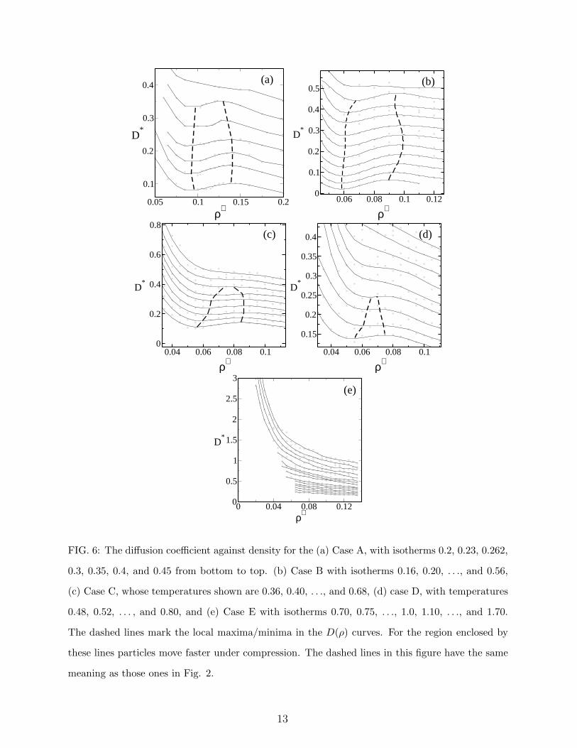
The mobility of any liquid is given by the diffusion constant. Figure 6 shows the behavior

of the dimensionless translational diffusion coefficient, D∗, as function of the dimensionless

density, ρ∗, at constant temperature for b = 0.0, −0.25, −0.50, −0.75, and b = −1.00. The

solid lines are polynomial fits to the data obtained through simulation (dots in Fig. 6). For

normal liquids, the diffusion coefficient at constant temperature decreases with density. For

the cases A-D [shown in Fig. 6(a)-(d)] D∗ anomalously increases with density in a certain

range of pressures and temperatures instead. From Figure 6 we see that for very small and

very high densities D∗ decreases with increasing density as expected for a normal liquid.

For intermediate values of density, ρDmax > ρ > ρDmin, D∗ increases with increasing density

what leads to local maxima at ρDmax and a local minima at ρDmin. These local extrema

in the diffusion versus density plots bound the region inside which the diffusion behaves

anomalously (dashed lines in Fig. 6). This region is mapped into the pressure-temperature

diagram illustrated in Fig. 2 as dashed lines in (a)-(d). As the attractive well becomes

deeper, the diffusion anomalous region in the pressure-temperature phase diagram shrinks

and it goes to lower pressures. In the case in which b = −1.00, shown in Figure 6(e), the

diffusion constant behaves as in a normal liquid. This result again is consistent with the

idea that a deeper attractive term favors the high density liquid phase.

Structural anomaly

Besides the density and the diffusion anomalies an structural anomalous region might be

present. Figure 7 shows the translational order parameter as a function of density for fixed

12

0.05 0.1 0.15 0.2

ρ∗

0.1

0.2

0.3

0.4

D*

(a)

0.06 0.08 0.1 0.12

ρ∗

0

0.1

0.2

0.3

0.4

0.5

D*

(b)

0.04 0.06 0.08 0.1

ρ∗

0

0.2

0.4

0.6

0.8

D*

(c)

0.04 0.06 0.08 0.1

ρ∗

0.15

0.2

0.25

0.3

0.35

0.4

D*

(d)

0 0.04 0.08 0.12ρ∗

0

0.5

1

1.5

2

2.5

3

D*

(e)

FIG. 6: The diffusion coefficient against density for the (a) Case A, with isotherms 0.2, 0.23, 0.262,

0.3, 0.35, 0.4, and 0.45 from bottom to top. (b) Case B with isotherms 0.16, 0.20, . . ., and 0.56,

(c) Case C, whose temperatures shown are 0.36, 0.40, . . ., and 0.68, (d) case D, with temperatures

0.48, 0.52, . . . , and 0.80, and (e) Case E with isotherms 0.70, 0.75, . . ., 1.0, 1.10, . . ., and 1.70.

The dashed lines mark the local maxima/minima in the D(ρ) curves. For the region enclosed by

these lines particles move faster under compression. The dashed lines in this figure have the same

meaning as those ones in Fig. 2.

13

temperatures for the potential we are studying for b = 0.0,−0.25,−0.50,−0.75, and −1.00.

The dots represent the simulation data and the solid lines are polynomial fit to the data.

The non-monotonic behaviour of these curves indicate that there is a region in which t

decreases with density. This means that the system becomes less structured for increasing

density. Dotted lines determine the local maxima and minima of t, bounding the structural

anomalous region. This region was mapped into the pressure-temperature phase diagram

(dotted lines), as can be seen in Figure 2. The comparison between the behavior for different

b values indicates that as the attractive well becomes deeper the structural anomalous region

in the pressure-temperature phase diagram shrinks and moves to lower pressures and it is

still present even in the deepest case, b = −1.00. According to these results we believe that

for b < −1.00, i.e., cases in which the attractive part is more intense than one showed in

Case E, the structural anomalous region will also vanish. This result again is consistent

with the idea that a deeper attractive term favors the high density liquid phase.

Figure 8 gives an overview of the density, diffusion, and structural anomaly locations in

the pressure-temperature phase diagram.

V. CONCLUSIONS

In this paper we have explored the effect of the addition of an attractive part in a two

length scales potential. Particularly we analyze if the depth of the attractive part changes

the position (and the presence of not) in the pressure-temperature phase diagram of the

two liquid-gas and liquid-liquid critical points and of the density, diffusion and structural

anomalous regions.

For sufficiently intense attraction between particles both the liquid-liquid and the liquid-

gas critical points are present. These two critical points are observed even for a very at-

tractive potential. For a small attractive interaction, only the liquid-gas critical point was

found what indicates that for the coexistence of two liquid phases the attractive well have

to be deeper than a certain threshold.

Since the attraction favors the liquid phase (particularly the high density liquid phase), as

the b decreases the liquid-gas critical point moves to higher temperatures (shown in Fig. 4)

and the liquid-liquid critical point to lower pressures.

The density, diffusion and structural anomalous regions are present even in the absence of

14

0.05 0.1 0.15 0.2 0.25

ρ∗

0.6

0.8

1

1.2

t

(a)

0.05 0.1 0.15 0.2 0.25

ρ*

0.6

0.8

1

1.2

1.4

t

(b)

0.05 0.1 0.15 0.2

ρ*

0.6

0.8

1

1.2

t

(c)

0.05 0.1 0.15 0.2 0.25 0.3

ρ*

0.6

0.7

0.8

0.9

1

1.1

1.2

t

(d)

0.05 0.1 0.15 0.2ρ∗

0.4

0.5

0.6

0.7

0.8

0.9

1

1.1

t

(e)

FIG. 7: Translational order parameter against density for (a) Case A, where each line correspond

to an isotherm. The isotherms are: 0.25, 0.30, . . ., 0.55, 0.7, 1.0, 1.5, 2.0, and 2.5 from top to

bottom. (b) Case B, with isotherms 0.20, 0.28, . . ., 0.68, 0.80, 1.0, 1.2, 1.6, 2.0, and 2.5 from top

to bottom. (c) Case C whose temperatures are 0.36, 0.40, . . ., 0.80, 1.0, 1.2, 1.6, 2.0, 2.5, and 3.0

from top to bottom. (d) case D with T ∗ = 0.52, 0.56, . . . , 0.80, 1.0, 1.2, 1.6, 2.0, 2.5, 3.0, and 3.5

from top to bottom. Finally, (e) case E with T ∗ = 0.70, 0.75, . . ., 1.0, 1.10, . . .,1.70, 2.0, 2.5, and

3.0 from top to bottom. The dotted lines bound the region of structural anomalies, i.e., the region

where the parameter t decreases upon increasing density.

15

0 0.3 0.60

0.2

0.4

0.6

0.8

1

P*

0.3 0.6

T*

0

0.2

0.4

0.6

0.8

1

1 2 30

0.5

1

1.5

2

2.5(a) (b) (c)

A

B

DC

A

BCD

A

B

CD

E

FIG. 8: (a) TMD line for the cases considered in this paper. Note that there is no density anomaly

in the Case E (see Fig. 2). (b) The diffusion anomaly region for the Case A-D. No diffusion

anomaly was found for the Case E (see fig. 6). The shadowed regions correspond to the region

between the dashed lines in Fig. 2. In (c) is shown the structural anomalous region for Case A-E.

Here, the shadowed region corresponds to the region between the dotted lines in Fig. 2. See the

text for discussion.

attraction. As b decreases, the high density liquid structure is favored and so the anomalous

regions in the pressure-temperature phase diagram ( shown in Fig. 8) shrinks, moves to

lower pressures and disappears for very attractive potentials.

In resume density and diffusion anomalous regions are present in two length scales po-

tential if the attractive interaction is not too strong.

ACKNOWLEDGMENTS

We thank for financial support from the Brazilian science agencies CNPq, CAPES and

FAPEMIG. This work is also partially supported by the CNPq through the INCT-FCx.

[1] S. V. Buldyrev and H. E. Stanley, Physica A 330, 124 (2003).

[2] A. Skibinsky, S. V. Buldyrev, G. Franzese, G. Malescio, and H. E. Stanley, Phys. Rev. E 69,

061206 (2005).

16

[3] V. B. Henriques, N. Guissoni, M. A. Barbosa, M. Thielo, and M. C. Barbosa, Mol. Phys.

103, 3001 (2005).

[4] P. C. Hemmer and G. Stell, Phys. Rev. Lett. 24, 1284 (1970).

[5] E. A. Jagla, Phys. Rev. E 58, 1478 (1998).

[6] N. B. Wilding and J. E. Magee, Phys. Rev. E 66, 031509 (2002).

[7] A. B. de Oliveira, P. A. Netz, T. Colla, and M. C. Barbosa, J. Chem. Phys. 124, 084505

(2006).

[8] N. G. Almarza, J. A. Capitan, J. A. Cuesta, and E. Lomba, J. Chem. Phys 131, 124506

(2009).

[9] D. Y. Fomin, , N. V. Gribova, V. N. Ryzhov, S. M. Stishov, and D. Frenkel, J. Chem. Phys

129, 064512 (2008).

[10] G. Franzese, J. Mol. Liq. 136, 267 (2007).

[11] A. B. de Oliveira, G. Franzese, P. A. Netz, and M. C. Barbosa, J. Chem. Phys. 128, 064901

(2008).

[12] A. B. de Oliveira, P. A. Netz, and M. C. Barbosa, Europhys. Lett. 85, 36001 (2009).

[13] S. Zhou, Phys. Rev. E 74, 031119 (2006).

[14] S. Zhou, Phys. Rev. E 77, 041110 (2008).

[15] S. Zhou, J. Chem. Phys. 130, 054103 (2009).

[16] S. A. Egorov, J. Chem. Phys. 128, 174503 (2008).

[17] G. Franzese, G. Malescio, A. Skibinsky, S. V. Buldyrev, and H. E. Stanley, Nature (London)

409, 692 (2001).

[18] P. H. Poole, F. Sciortino, U. Essmann, and H. E. Stanley, Nature (London) 360, 324 (1992).

[19] J. N. Glosli and F. H. Ree, Phys. Rev. Lett. . 82, 4659 (1999).

[20] R. Waler, Essays of natural experiments, Johnson Reprint, New York, 1964.

[21] C. A. Angell, E. D. Finch, and P. Bach, J. Chem. Phys. 65, 3063 (1976).

[22] F. X. Prielmeier, E. W. Lang, R. J. Speedy, and H.-D. Ludemann, Phys. Rev. Lett. 59, 1128

(1987).

[23] L. Haar, J. S. Gallangher, and G. Kell, NBS/NRC Steam Tables. Thermodyanic and Trans-

port Properties and Computer Programs for Vapor and Liquid States of Water in SI Units.,

Hemisphere Publishing Co., Washington D. C., 1st ed., 1984.

[24] H. Thurn and J. Ruska, J. Non-Cryst. Solids 22, 331 (1976).

17

[25] Periodic table of the elements, http://periodic.lanl.gov/default.htm, 2007.

[26] G. E. Sauer and L. B. Borst, Science 158, 1567 (1967).

[27] S. J. Kennedy and J. C. Wheeler, J. Chem. Phys. 78, 1523 (1983).

[28] T. Tsuchiya, J. Phys. Soc. Jpn. 60, 227 (1991).

[29] C. A. Angell, R. D. Bressel, M. Hemmatti, E. J. Sare, and J. C. Tucker, Phys. Chem. Chem.

Phys. 2, 1559 (2000).

[30] R. Sharma, S. N. Chakraborty, and C. Chakravarty, J. Chem. Phys. 125, 204501 (2006).

[31] M. S. Shell, P. G. Debenedetti, and A. Z. Panagiotopoulos, Phys. Rev. E 66, 011202 (2002).

[32] S. Sastry and C. A. Angell, Nature Mater. 2, 739 (2003).

[33] H. J. C. Berendsen, J. R. Grigera, and T. P. Straatsma, J. Phys. Chem. 91, 6269 (1987).

[34] P. A. Netz, F. W. Starr, H. E. Stanley, and M. C. Barbosa, J. Chem. Phys. 115, 344 (2001).

[35] P. A. Netz, F. W. Starr, M. C. Barbosa, and H. E. Stanley, J. Mol. Phys. 101, 159 (2002).

[36] J. R. Errington and P. G. Debenedetti, Nature (London) 409, 318 (2001).

[37] J. Mittal, J. R. Errington, and T. M. Truskett, J. Phys. Chem. B 110, 18147 (2006).

[38] A. Mudi, C. Chakravarty, and R. Ramaswamy, J. Chem. Phys. 122, 104507 (2005).

[39] S. H. Chen, F. Mallamace, C. Y. Mou, M. Broccio, C. Corsaro, A. Faraone, and L. Liu,

Proceedings of the National Academy of Science of United States of America 103, 12974

(2006).

[40] T. Morishita, Phys. Rev. E 72, 021201 (2005).

[41] A. B. de Oliveira, P. A. Netz, T. Colla, and M. C. Barbosa, J. Chem. Phys. 125, 124503

(2006).

[42] A. B. de Oliveira, M. C. Barbosa, and P. A. Netz, Physica A 386, 744 (2007).

[43] A. B. de Oliveira, P. A. Netz, and M. C. Barbosa, Euro. Phys. J. B 64, 48 (2008).

[44] A. B. de Oliveira, E. B. Neves, C. Gavazzoni, J. Z. Paukowski, P. A. Netz, and M. C. Barbosa,

J. Chem. Phys. 132, 164505 (2010).

[45] A. B. de Oliveira, E. Salcedo, C. Chakravarty, and M. C. Barbosa, J. Chem. Phys. (in press)

(2010).

[46] C. H. Cho, S. Singh, and G. W. Robinson, Faraday Discuss. 103, 19 (1996).

[47] P. A. Netz, J. F. Raymundi, A. S. Camera, and M. C. Barbosa, Physica A 342, 48 (2004).

[48] S. J. Plimpton, J. Comp. Phys. 117, 1 (1995).

[49] J. E. Errington, P. G. Debenedetti, and S. Torquato, J. Chem. Phys. 118, 2256 (2003).

18

[50] D. Frenkel and B. Smit, Understanding Molecular Simulation, Academic Press, San Diego,

1st ed., 1996.

[51] G. Malescio, F. G., G. Pellicane, A. Skibinsky, S. V. Buldyrev, and H. E. Stanley, J. Phys.:

Condens. Matter 14, 2193 (2002).

[52] G. Malescio, G. Franzese, A. Skibinsky, S. V. Buldyrev, and H. E. Stanley, Phys. Rev. E 71,

061504 (2005).

[53] H. E. Stanley, S. V. Buldyrev, M. Canpolat, M. Meyer, O. Mishima, M. R. Sadr-Lahijany,

A. Scala, and F. W. Starr, Physica A 257, 213 (1998).

[54] H. E. Stanley, [Proceedings of the 1998 International Conference on Complex Fluids], Pramana

[A Journal of the Indian Academy of Sciences, founded by C. V. Raman] 53, 53 (1999).

[55] H. E. Stanley, S. V. Buldyrev, M. Canpolat, O. Mishima, A. Sadr-Lahijany, M. R. Scala, and

F. W. Starr, Physical Chemistry and Chemical Physics 2, 1551 (2000).

19