Effects of Pavement Roughness on Vehicle Speeds

Effects of Pavement Roughness on Vehicle Speeds

M. A. Karan and Ralph Haas, Department of Civil Engineering, University of Waterloo

Ramesh Kher, Ontario Ministry of Transportation and Communications

Vehicle speeds on highways as affected by a variety of factors, such as geometric characteristics of the roadway and traffic conditions, have been extensively studied. One factor that has received little attention is that of pavement condition. This report describes a study conducted in the summer of 1974 to develop relationships between average ve­hicle speed and pavement condition for two-lane highways. The con­dition factor chosen was roughness, and 72 sites covering a wide range of roughness were selected. Measurements included speed, roughness, geometric characteristics, and traffic counts. Capacities and volume­capacity ratios of the sections were calculated. A regression model re­lating average speed to roughness in terms of riding comfort index, volume-capacity ratio, and speed limit was developed. The model is simple and plausible and has a reasonable multiple correlation coeffi­cient (0.77) .

The operating speed of a highway is one of the major in­dicators of the level of service provided to the user and one of the major factors to be used in the analysis and justification of highway projects. A number of studies have been conducted to establish vehicle speed charac­teristics for different highways and conditions. These have shown that operating speeds are affected mainly by the following five groups of variables:

1. Driver characteristics, 2. Vehicle characteristics, 3. Roadway characteristics, 4. Traffic conditions, and 5. Environmental conditions.

Driver characteristics include age, occupation, sex, and experience as well as trip length, trip purpose, and presence or absence of passengers. Vehicle character­istics include engine size and power, type, age, weight, and maximum speed.

Roadway characteristics such as geographic location, sight distance, lateral clearance, frequency of intersec­tions, gradient length and magnitude, and type of surface

Publication of this paper sponsored by Committee on Theory of Pave­ment Design.

122

have been shown to be important in speed analysis. Traffic volume and density, composition, access con­

trol, and passing maneuvers are the most important variables related to traffic.

Time of day and climatic conditions are the major environmental factors. Although the effects of time and weather on speed have not yet been well established, ex­perience has shown that they cannot be neglected.

One of the major unknowns in speed studies is the ef­fect of pavement condition or roughness on operating speed. Recent improvements in the economic evaluation component of pavement design and management suggest that all agency and user costs need to be included ( 1). As a consequence, an existing pavement condition that significantly affects operating speeds can have significant economic implications in terms of extra user time and vehicle operating costs and potential extra accident and discomfort costs.

SCOPE AND OBJECTIVES OF STUDY

The basic purpose of this study was to establish initial relationships of speed and roughness for rural highways through a field study of a range of representative high­way sections. Riding comfort index (RCI) was chosen as the indicator of roughness. [RCI is the Canadian equivalent of present serviceability index (PSI) except that a scale of 0 to 10 is used instead of a scale of 0 to 5 as for PSI values.]

Highways with both 80-km/ h (50-mph) and 96-km/h (60-mph) speed limits were chosen for the study. These represent speed limits for many highway sections in Canada, and they encompass the current, common 88-km/ h (55-mph) speed limit in the United States.

The followirig sections describe the scope and re­sults of the field study, the analysis of the data, and the potential use of the relationships developed in pavement design and management systems.

FIELD STUDY

Selection of Study Sites

In selecting the location of the sites, we made an attempt

F3

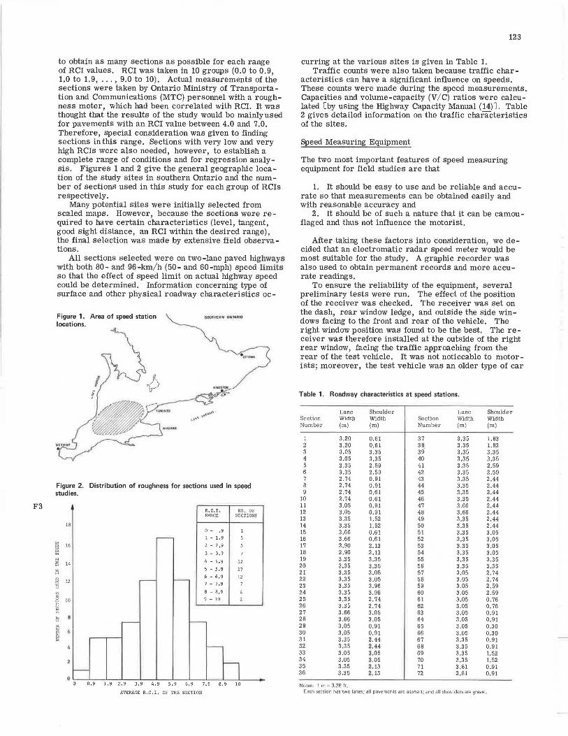
to obtain as many sections as possible for each range of RCI values. RCI was taken in 10 groups (0.0 to 0.9, 1.0 to 1.9, ... , 9.0 to 10). Actual measurements of the sections were taken by Ontario Ministry of Transporta­tion and Communications (MTC) personnel with a rough­ness meter, which had been correlated with RCI. It was thought that the results of the study would be mainly used for pavements with an RCI value between 4.0 and 7.0. Therefore, special consideration was given to finding sections in this range. Sections with very low and very high RCis were also needed, however, to establish a complete range of conditions and for regression analy­sis. Figures 1 and 2 give the general geographic loca­tion of the study sites in southern Ontario and the num­ber of sections used in this study for each group of RCis respectively.

Many potential sites were initially selected from scaled maps. However, because the sections were re­quired to have certain characteristics (level, tangent, good sight distance, an RCI within the desired range), the final selection was made by extensive field observa­tions.

All sections selected were on two-lane paved highways with both 80- and 96-km/h (50- and 60-mph) speed limits so that the effect of speed limit on actual highway speed could be determined. Information concerning type of surface and other physical roadway characteristics oc-

Figure 1. Area of speed station locations.

Figure 2. Distribution of roughness for sections used in speed studies.

18

§ 16

~

~ 14

~

~ 12

" "' s 10

~ ~ ::l l!l

~

0

R.C.I. NO, OF RANCE SECTIONS

0 - .9 1

- 1 - 1.9 5

2 - 2,9 5

3 - 3 . 9 7

4 - 4 . 9 12

5 - 5,9 17

I----6 - 6 ,9 12 - 7 - 7. 9 7

8 - 8,9 4

9 - 10 2

- ~

,__

- n 0 0 . 9 1.9 2.9 3 . 9 4.9 5.9 6.9 7 . 9 8.9 10

AVERAGE R. C . I, OF THE SECTION

123

curring at the various sites is given in Table 1. Traffic counts were also taken because traffic char­

acteristics can have a significant influence on speeds . These counts were made during the speed measurements. Capacities and volume-capacity (V/C) ratios were calcu­lated [by using the Highway Capacity Manual ( 14) J. Table 2 gives detailed information on the traffic characteristics of the sites.

Speed Measuring Equipment

The two most important features of speed measuring equipment for field studies are that

1. It should be easy to use and be reliable and accu­rate so that measurements can be obtained easily and with reasonable accuracy and

2. It should be of such a nature that it can be camou­flaged and thus not influence the motorist.

After taking these factors into consideration, we de­cided that an electromatic radar speed meter would be most suitable for the study. A graphic recorder was also used to obtain permanent records and more accu­rate readings.

To ensure the reliability of the equipment, several preliminary tests were run. The effect of the position of the receiver was checked. The receiver was set on the dash, rear window ledge, and outside the side win­dows facing to the front and rear of the vehicle. The right window position was found to be the best. The re -ceiver was therefore installed at the outside of the right rear window, facing the traffic approaching from the rear of the test vehicle. It was not noticeable to motor­ists; moreover, the test vehicle was an older type of car

Table 1. Roadway characteristics at speed stations.

Lane Shoulder Lane Shoulder Section Width Width Section Width Width Number (m) (m) Number (m) (m)

1 3.20 0.61 37 3 .35 1.83 2 3.20 0.61 38 3.35 1.83 3 3.05 3.35 3g 3.35 3.35 4 3.05 3.35 40 3.35 3.35 5 3.3 5 2.59 41 3.3 5 2.59 6 3.3 5 2.59 42 3.35 2.59 7 2. 74 0.91 43 3 .35 2.44 8 2.74 0 .91 44 3.35 2.44 9 2.74 0.61 45 3.35 2.44

10 2.74 0 .61 46 3.35 2.44 11 3.05 0.91 47 3.66 2.44 12 3.05 0.91 48 3.66 2.44 13 3.35 1.52 49 3.35 2 .44 14 3.35 1.52 50 3.35 2.44 15 3.66 0.61 51 3 .35 3.05 16 3.66 0.61 52 3 .35 3.05 17 2 .90 2.13 53 3.35 3.05 18 2. 90 2. 13 54 3.35 3.05 19 3.3 5 3.35 55 3.35 3.35 20 3.35 3.35 56 3.35 3.35 21 3.35 3 .05 57 3.05 2. 74 22 3.35 3.05 58 3.05 2.74 23 3.3 5 3.96 59 3.05 2 . 59 24 3.35 3. 96 60 3.05 2 .59 25 3.35 2. 74 61 3.05 0.76 26 3.35 2.74 62 3 .05 o. 76 27 3.66 3.05 63 3.05 0.91 28 3.66 3 .05 64 3.05 0.9 1 29 3.05 0.91 65 3.05 0 .30 30 3.05 0.9 1 66 3 .05 0.30 31 3.35 :?-.44 67 3.35 0.9 1 32 3 .35 2.44 68 3.35 0.91 33 3.05 3.05 69 3.35 1.52 34 3.05 3.05 70 3.35 1.52 35 3.35 2.13 71 3.81 0.91 36 3.35 2. 13 72 3.81 0.9 1

Notes: 1m=3.28 ft , Each section has two lanes; all pavements are asphalt; and all shoulders are gravel .

124

with no resemblance to police vehicles, After several test runs, it was found that traffic in

both directions could be observed from the single posi­tion. As a consequence, speeds in both directions were measured at the same time, at each study site. Traffic volumes did not create any difficulty because they were relatively low (free-flow conditions). In the case of two vehicles passing the station at the same time, the data were canceled by the observer sitting on the front seat of the test vehicle simply by putting a mark on the rec­ords.

As a check on the reliability of the radar during the field study, tuning forks were used to simulate speeds of 48, 80, and 112 km/h (30, 50, and 70 mph). Adjust­ments were made before the actual speed measurements.

Field Measurements

After the selection of speed stations for the study, rough­ness was measured at each station on a 0.4-km (0.25-mile) section. The measurements were taken with a BPR roughometer, and the readings were converted to RCI from a previously established correlation with mean panel ratings. Table 3 gives roughness readings and RCI values for each study station.

The next step consisted of speed measurements. For these, the test vehicle was parked on the far edge of the shoulder at each station. In the case of inadequate shoulder widths, private driveways were used. The ra­dar and recorder were set, and the receiver was placed in position. Standard field sheets were used to record traffic and roadway data. The following information was obtained from each station:

1. Speeds of vehicles by type and direction; 2. Hourly traffic volumes by type and direction; and 3. Roadway characteristics (land and shoulder widths,

type of pavement, and the like).

It should be noted that all observations were made during daytime but not in a specific time period. Rush hours, when traffic volumes are very heavy, were avoided. The speed measurements were generally made under free -flow conditions so that the effect of slow-moving vehicles or congestion could be minimized.

Motorcycles were excluded from the study. Similarly, "unusual" drivers (such as very slow-moving, elderly drivers) were not taken into account. When a vehicle was felt to be influenced by such a slow-moving vehicle or opposing traffic, the measurement was omitted.

The sample size was calculated by the formula given in the Manual of Traffic Engineering Studies (2). An at­tempt was made to observe 60 vehicles at each station; however, at some stations (especially those on secon­dary county roads), this number could not be obtained in a reasonable length of time because of the very low traffic volumes.

ANALYSIS OF FIELD DATA

A total of 4105 vehicle speeds were measured during the field studies. Although measurements were made by type of vehicle, the data were combined for the final analysis and an overall average speed for each station was calculated. Because the objective of the study was to determine the relationship between average highway speed and roughness of the pavement, this approach was considered reasonable. The calculated mean speeds and standard deviation of the speed distributions at each station are given in Table 4.

Figure 3, which was obtained from the information given in Table 4, shows the speed measurements deter-

mined by the field studies. It shows that, on county roads with a speed limit of 80 km/h (50 mph), a high proportion of the motorists usually drive somewhat too fast, even on very rough pavements. This situation may be partially explained by the lack of speed limit enforce­ment on these facilities. On main highways, most drivers tend to obey the speed limit.

The data given in Table 5 and plotted in Figure 3 were first analyzed separately for each group of speed limits and capacity levels. Various regression models were tested. Because of the data limitations, however, a gen­erally acceptable model could not be developed.

The data for 80- and 90-km/h (50- and 60-mph) speed limits were then combined, and one general regression model was tested. Several different forms of models were checked. The final four equations considered are as follows:

y = 34.4 718 + 0.0l99x1 X4 + 0.0044xi

Y = 32.9584 + 0.0J 83X1X4 + 0.0055xi - 0.0Q75x2X3

y = 2.596x10.0928 X X3 -0.0275 X X4 0.704

y = 30.7368 + l .0375x1 - l l .2421x3 + 0.0062xl

where

(I)

(2)

(3)

(4)

y = average highway speed in kilometers per hour, X1 = RCI, x2 = total capacity of roadway in vehicles per hour, X3 = V /C ratio, and X4 = speed limit in kilometers per hour.

Statistical characteristics of these models, as indi­cated by the data given in Table 5, are similar. All co­efficients are statistically significant; constant terms are alike; and all of them have similar multiple corre­lation coefficients. Mean, absolute mean, and standard deviation of residuals were calculated for further analy­sis. However, the results were not particularly helpful for selecting the best model.

Subjective, logical tests were then applied. Model 3 was eliminated because of the production nature of the equation. It would give zero speeds for zero RCI value, which means no vehicle movement on very rough sec­tions. This is unrealistic.

The remaining models were then studied thoroughly. Model 4 was finally selected mainly because of its sim­plicity. Caution should, however, be exercised in use of the x3 term in the model. The reason for this is that field measurements were conducted mostly under free­flow conditions. The effect of V /C ratio in speed, there­fore, is perhaps not accurately represented by the model over the whole range of possible V / C ratios (from 0.0 to 1.0). Thus the recommended model should not be used for highway sections with very high traffic volumes. Similarly, the model is not too accurate for RCI values of less than 2 .0.

COMPARISON OF RESULTS

Figure 4 compares the data of this investigation with those of previously presented relationships.

The relationships used by the Ontario MTC in their pavement management system OPAC (1) are represented by heavy solid lines for various speed limits between 80 aud 112 km/ h (50 and 70 mph). Also shown are the linear regressions (model 4) for data from the 80-km/h (50-mph) speed limit roads and the 96-km/ h (60-mph) speed limit roads.

The MTC relationship for the 80-km/h (50-mph) speed limit roads compares reasonably well with the observed

125

Table 2. Traffic characteristics at speed stations.

Total Directional Volume- Speed Total Directional Volume- Speed Section Capacity Volume Capacity Limit Section Capacity Volume Capacity Limit Number (vehicles/ h) (vehicles/ h) Ratio (km/ h) Number (vehicles/ h) (vehicles/ h) Ratio (km/h)

1 1253 7 0 .01 BO 37 1531 51 0 .07 BO 2 1253 12 0.02 80 38 1531 63 0.08 80 3 1409 17 0 .02 80 39 1531 120 0 . 16 96 4 1409 16 0 .02 80 40 1531 108 0.14 96 5 1531 35 0.05 96 41 1531 108 0 . 14 96 6 1531 49 0.06 96 42 1531 72 0.09 96 7 1183 33 0 .06 80 43 1531 96 0.13 96 B 1183 34 0.06 80 44 1531 96 0 . 13 96 9 1131 25 0.04 80 45 1531 72 0.09 96

10 1131 24 0 .04 80 46 1531 84 0 . 11 96 11 1262 28 0 .04 80 47 1740 84 0 .10 96 12 1262 111 0 .18 80 48 1740 96 0.11 96 13 1496 69 0.09 80 49 1531 96 0.13 96 14 1496 78 0. 10 80 50 1531 120 0 . 16 96 15 1479 203 0 .27 80 51 1531 156 0 .20 96 16 1479 225 0 .30 80 52 1531 144 0.1 8 96 17 1357 94 0 . 13 96 53 1531 96 0 . 12 96 18 1357 69 0.10 96 54 1531 192 0 .25 96 19 1531 336 0.43 96 55 1531 156 0.20 96 20 1531 252 0 .33 96 56 1531 228 0.29 96 21 1531 108 0. 14 96 57 1409 216 0 .31 96 22 1531 144 0.19 96 58 1409 156 0.22 96 23 1531 131 0.17 96 59 1409 156 0 .22 96 24 1531 125 0 . 16 96 60 1409 144 0.20 96 25 1531 69 0 .09 80 61 1253 48 0.06 80 26 1531 63 0.08 80 62 1253 48 0.06 80 27 1740 70 0.08 96 63 1262 36 0.06 80 28 1740 88 0 . 10 96 64 1262 48 0.08 80 29 1262 42 0 .07 80 65 1140 33 0.06 80 30, 1262 37 0.06 80 66 1140 39 0.07 80 31 1531 156 0 .20 96 67 1375 47 0.07 96 32 1531 120 0 . 16 96 68 1375 61 0.09 96 33 1409 96 0 . 14 96 69 1496 58 0.08 80 34 1409 132 0 .19 96 70 1496 40 0,05 80 35 1531 132 0 .17 96 71 1557 156 0 .20 80 36 1531 132 0 . 17 96 72 1557 144 0 . 18 80

Note: 1 km/h = 0.621 mph,

Table 3. Roughness data for speed stations. Table 4. Speed data for speed stations.

Roughness Roughness Mean Standard M ean Standard

Section Index Se ction Index Section Speed Devia tion Section Speed Deviation

Number (mm/km) RC!' Number (mm/ km) RC!' Number (km/ h) (km/ h) Number (km/h) (km/ h)

1 4762 0.5 37 1080 6.9 1 67 8.79 37 82 10.06

2 3493 1.8 38 1016 7.2 2 67 9.10 38 83 8. 72

3 3.4 39 762 8.4 3 86 14.76 39 98 10.90

4 3.6 40 826 8.1 4 85 10,32 40 101 12 .08

5 572 9.7 41 953 7.5 5 96 9.24 41 94 12.49

6 699 8.8 42 1016 7.2 6 96 9.34 42 99 12.17

7 2858 2.7 43 1080 6.9 7 77 8.52 43 91 15.39

8 3175 2.2 44 1651 5. 1 8 78 8.97 44 94 12.99

9 3556 1. 7 45 1397 5.8 9 78 10.34 45 94 11.95

10 3874 1.4 46 1524 5.4 10 78 14.04 46 96 11.56

11 3747 1.5 47 1461 5.6 11 62 4.59 47 94 10.59

12 3175 2.2 48 1143 6.7 12 61 7.65 48 98 12. 70

13 2032 4.2 49 1016 7.2 13 78 17.23 49 98 10. 77

14 1588 5.2 50 889 7.8 14 78 11.59 50 94 10.21

15 4064 1.2 51 1080 6.9 15 69 11.51 51 93 14.52

16 3366 2.0 52 1080 6.9 16 72 8.77 52 94 11.09

17 2032 4.2 53 1080 6.9 17 91 17 .36 53 91 11.85

18 2223 3.8 54 1461 5.6 18 90 11.90 54 86 9.26

19 1016 7.2 55 2 159 4.0 19 93 10.21 55 85 9.74

20 1016 7.2 56 2096 4.0 20 91 8.65 56 83 9.35

21 2032 4.2 57 1524 5.4 21 99 9.27 57 90 9.19

22 2096 4.0 58 1461 5.6 22 93 10.21 58 88 12 . 77

23 2413 3.4 59 1588 5.2 23 88 10.42 59 91 9.68

24 2159 3.9 60 1651 5.1 24 93 10.18 60 88 9.97

25 1080 6.9 61 1715 4.9 25 91 11.11 61 83 12.48

26 1143 6. 7 62 1524 5.4 26 88 10.79 62 77 10.79 27 635 9.2 63 1651 5.1 27 96 14.81 63 86 11.79

28 699 8. 8 64 1461 5.6 28 93 12.30 64 82 11. 74

29 1715 4.9 65 1651 5.1 29 78 10.90 65 85 13 .09

30 1905 4.4 66 2032 4.2 30 86 14.57 66 85 13 . 15

31 1588 5.2 67 1778 4.7 31 91 12.06 67 93 12.99

32 1334 6.0 68 1270 6.2 32 91 11.33 68 91 14.31

33 1651 5.0 69 1842 4.6 33 86 11.22 69 72 12.59

34 1461 5.6 70 2223 3 .8 34 86 12.08 70 72 10. 13

35 1270 6.2 71 2667 3.0 35 85 10.14 71 75 11. 16

36 1270 6.2 72 3302 2 .1 36 90 11.22 72 74 10 .92

Notes: 1 mm/km= 15.78 mm/mile. Note: 1 km/h = 0.621 mph.

The length of each section is 0 .40 km (0.25 mile ). 01 RCI = 25.25 - 10.0093 log R where R = roughness index.

126

data although its slope could be adjusted. For the 96-km/ h (60-mph) speed llmit roads, it also compares l'ea­sonably well with the data, but again the slope could be adjusted. The MTC relationship also appears to reduce speed too severely for the lower RC! values (vehicles travel somewhat faster 011 very i·ough roads under free­flow conditions than originally postulated).

Finally, McFarland 's Q1'igioal postulated relationship .for 96-km/ h (60-mph) speed limit roads (.!.!) is also shown in Figure 4. It agrees i·easonably well with the observed data for high RCI values (greater than about 7), but it reduces speed too severely for the lower RCI values.

Figure 3. Distribution of mean vehicle speeds.

Note : 1 km/h c 0.621 mph.

10 -

60KPH

I I I I

' I I ' ' I I I

• SEC:TONS WITH BO KPH SPEED LIMIT

+ SECTIONS WITH 96 KPH SPEED LIMIT

96KPH

. . . • i

I I • •

• I

ITTamn~nn~oonee~~oo~nM%%•Dm SPEED (kph)

Table 5. Statistical characteristics of regression equations.

Multiple Standard Model Correlation Student's Error of Goodness Number Coefficient t-Values• Estimate of Fit

1 0.73 t, = 5.87 2.67 96.78

2 0.77 l1 = 5.56 2.56 72. 77 t, = 6.41 t, = 2.67

0.79 t, = 7.40 0 .05 85.16 t, = 2.90 t, = 8.54

0.77 t1 = 5.74 2.52 60.41 t, = 2.67 t, = 8.25

aTheoretical t = 2.32.

Figure 4. Speed-riding comfort index data and relationships. .. .. 000

Note: 1 km/h = 0.621 mph. . .., x ... ~ 60

... "' i?

~~ • fllfA fOll M ~ ..... 51<f::C.0 LNftt n~

2 >( " .. 96•pll " e --- LINEAR flEGflESSION P'Ofl 600ph DATA

• 'lGkph " .., % Q to ;;: .•i .

I : - #u..AINmS~ .. 'U)fO IJI w,r.c - MtFARL4N0 1S OfllGINAL POSTULATED

RELATIONSHIP FDA 96;.ph LIMIT

0 '2 128

SPEED , kph

USE OF SPEED-ROUGHNESS RELATIONSHIPS IN PAVEMENT MANAGEMENT

General Implications

The pavement design and management concept that has been used recently for developing real working systems within various highway agenci R (~, 4, ~ ~. '.!_, 8, ~ .!.Q.) in­cludes the generation and analysis o1 alternative design strategies. In the analysis procedure, the performance output of each strategy is predicted. Then the cost and benefit implications of these performance outputs are determined and compared for selecting the optimal strat­egy.

Today many pavement authorities have agreed that both agency costs (initial capital, resurfacing, and main­tenance costs) and user costs (traffic delay, vehicle op­eration, travel time, accident, and discomfort) need to be considered in the economic evaluation of alternative pavement design strategies. Recent studies (1, 11) have quantitatively illustrated the importance of the user costs component.

User costs vary significantly with pavement perfor­mance. This variation is a function of roughness, which affects vehicle speeds and operating costs. As the pave­ment deteriorates, the lower speeds result in higher user costs. Therefore, a pavement strategy that pro­vides a low level of serviceability over a longer period of time causes higher user costs than a strategy that serves the traffic on a smoother surface for most of the time.

Figure 5 . Speed profiles for two example strategies.

11~T1

10 " 20 " TIME (YEARS)

Note: 1 km/h • 0.621 mph. /~JI•'"'"''' '"''l'<""'"'M iµn·Jo n"'' bo ""' ' ~"nl"'l" • •llld•· """'"WT4th....i ,,.,,.

TIME(VEARS)

Figure 6. Unit costs (excluding taxes} of speed reductions at different RCI levels on a rolling tangent in Ontario.

~ r CARI - -

~ / ~ / ~ I'.... .,,,_:.,¥ . / • ~ ,..,_ .u.•!Y

= -- ""''"·~ '~ 1 ............... ""'•71) .;;;,

1 -

3 (i40 ~s 64 n ao ee gs J04

SPEED, KPH

EXAMPLE• EXTRA UNIT COST BETW£EN POINTS --A(FIC1 : 7!1,SPEED•ll21<PH}AND

11lflCl•!ID,SPEED•941<PHFORCARS AN0781<PHFOFITRUCl<S!IS • CARS• ID9 CENTS/KM SIN(;lE IJNITTRUCl<S • 186CENTS/l<M TRACTOR TRAILERS• 2)4 CENTS/KM

Note: 1 cent/km = 1.609 cents/mile_ 1 km/h • 0.621 mph.

=~~<!--~!l!!.!'-"!"~;:::2..J.-1--~

~IS«il-'~-.!:i~~-1--l ~llBl-+-~~~~;;;;,;;,,,i_.J-....j

b~-t--!~f-'~~~~-1--1

§·~--+---<f--+---t---t-+--+-~•

jlOO 4'-B---'56-6.L.4--'72-B..l.O-B'-B ---'96_K)..._4_,ll 2

SPEED. KPH

56 Go! 72 00 88 96 104 112

SPEED, KPH

As a consequence, determination of speed profiles during the life of a pavement becomes extremely impor­tant because it provides a means for relating user costs to pavement performance.

When the performance history of a pavement design strategy is determined, as shown in the upper portion of Figure 5, the speed profile of the strategy can then be easily found by the types of relationships shown in Fig­ure 4. An example is shown in the lower portion of Fig­ure 5, which is patterned after Kher, Phang, and Haas (1). The corresponding user costs can be calculated from data available in the literature (12, 13) or from re­lationships such as those shown in Figure6, also pat­terned after Kher, Phang, and Haas (1). (In Figure 6, unit costs =vehicle operation and travel time.)

The effect of the traffic volume on vehicle speeds should also be considered in the analysis for more ac­curate results because speed reductions may occur as a result of increased traffic volumes as well as low pavement serviceability levels. Therefore, speed ver­sus roughness and traffic (combined) relationships should be the object of future research for more comprehensive user cost analysis.

Example

A simple example can serve to illustrate the economic implications of speed-roughness variations.

Suppose that a two-lane highway with an annual aver­age daily traffic (AADT) of 5000 and a 96-km/ h (60-mph) speed limit has reached a terminal serviceability (i.e., RCI) level of 4.5. The extra user costs involved in delaying the resurfacing (which is expected to raise the RCI level to 8.0) by 1 year should be calculated.

If we assume that the 5000 AADT represents all pas­senger cars, then Figure 4 indicates an 88-lan/ h (55-mph) average speed for an RCI of 4. 5 and a 96-km/ h (60-mph) average speed for an RCI of 8.0. Figure 6 then indicates user costs of 8.8 and 6.9 cents/ km (14.1 and 11.2 cents/mile) respectively for the befo1·e and after resurfacing conditions.

For a 1.6-km (1-mile) section and 350 days, the ex­tra user costs of delaying resurfacing are 5000 x 350 x (0.141 - 0.112), which is $50 750. This would be re­duced slightly by the delay in the extra user costs due to resurfacing (using present worth of costs analysis), but it still represents quite a significant extra cost. Of course budget restrictions of the agency involved might require many such resurfacing delays despite the extra user costs. Nevertheiess, these extra user costs should be determined and used as a factor in determining in­vestment priorities.

The foregoing example has been chosen to cover a fairly narrow range and conditions in which the observed data of Figure 4 agree quite closely with the relationship that the Ontario MTC uses in its pavement management system. Allowing the serviceability to drop to lower levels than those of the example would result in higher extra user costs as well as possible extra capital costs for resurfacing (i.e., extra thickness).

CONCLUSIONS

Three major points of this paper can be summarized.

1. Speeds of motor vehicles on highways are signifi­cantly affected by pavement condition. Neglecting this effect may result in major errors in the economic eval­uation of alternative pavement design strategies.

2. Field observations were made at 72 selected sta­tions in southern Ontario. Vehicle speeds were mea­sured for various roughness levels (which were trans-

127

formed into RCI values). Geometric characteristics of the roadway section at each station were also determined. Traffic counts were conducted and V / C ratios were cal­culated.

3. A regression equation was developed for two-lane rural highways to express vehicle speeds in te1·ms of RCI, V/ C ratio, and speed limit. The relationship has potential application to individual pavement projects or to a series of projects within a network. It compares reasonably well with previously postulated relationships over a certain range of conditions.

ACKNOWLEDGMENT

The study on which this paper is based was supported by the Ontario Ministry of Transportation and Communica­tions.

REFERENCES

1. R. K. Kher, W. A. Phang, and R. C. G. Haas. Economic Analysis of Elements in Pavement De­sign. TRB, Transportation Research Record 572, 1976, pp. 1-14.

2. D. E. Cleveland. Manual of Traffic Engineering Studies. ITE, Arlington, Va., 1964.

3. W. R. Hudson and others. A Systems Approach Applied to Pavement Design and Research. Texas Highway Department, Center for Highway Research, and Texas Transportation Institute, Research Rept. 123-1, March 1970.

4. W. R. Hudson, R. K. Kher, and B. F. McCullough. Automation in Pavement Design and Management Systems. HRB, Special Rept. 128, 1972, pp. 40-53.

5. J. L. Brown. Texas Highway Department Pave­ment Management System. TRB, Transportation Research Record 512, 1974, pp. 16-20.

6. W. A. Phang and R. Slocum. Pavement Investment Decision Making and Management System. Ontario Ministry of Transportation and Communications, Rept. RRl 74, Oct. 1971.

7. W. A. Phang. Flexible Pavement Design in Ontario. TRB, Transportation Research Record 512, 1974, pp. 28-43.

8. D. E. Peterson. Utah's Pavement Design and Eval­uation System. TRB, Transportation Research Record 512, 1974, pp. 21-27.

9. W. T. Kenis and T. F. McMahon. Pavement Analy­sis System: VESYS II. AASHO Design Committee Meeting, Oct. 1972.

10. R. L. Lytton and W. F. McFarland. Implementa­tion of a Systems Approach to Pavement Design. TRB, Transportation Research Record 512, 1974, pp. 58-62.

11. W. F. McFarland. Benefit Analysis for Pavement Design Systems. Texas Highway Department, Cen­ter for Highway Research, and Texas Transporta­tion Institute, Research Rept. 123-13, April 1972.

12. P. J. Claffey. Running Costs of Motor Vehicles as Affected by Road Design and Traffic. NCHRP, Rept. 111, 1971.

13. R. Winfrey. Economic Analysis for Highways. IEP, New York (formerly International Textbook Com­pany, Scranton), 1969.

14. Highway Capacity Manual-1965. HRB, Special Rept. 87, 1965.