Effects of models with finite loci, selection, dominance, epistasis and linkage on inbreeding coefficients based on pedigree and genotypic information

1Animal Science Department, Faculty of Agriculture, University of Zagreb, Zagreb, Croatia and2Department of Livestock Science, University of Agricultural Sciences Vienna, Vienna, Austria

Effects of models with finite loci, selection, dominance, epistasisand linkage on inbreeding coefficients based on pedigree and

genotypic information

By INO CURIK1, JOHANN SOLKNER

2 and NIKOLA STIPIC1

SummaryConsidering the effects of selection, dominance, epistasis and linkage, a stochastic computer simulationwas performed to study how well inbreeding coefficients calculated from pedigree (fped) and genotypicfrequencies (fhet) correspond to the inbreeding coefficient that is defined as the proportion ofautozygous loci in the modelled genome (i.e. the level of autozygosity, faut). Although in randommating populations all three inbreeding coefficients show almost (with slight deviations in models withtwo loci) the same expectation, they represent three separate variables. First, faut, fped and fhet

responded differently to selection, dominance, epistasis and linkage. Second, they did not have thesame standard deviations, which means that the effects of random drift, especially in models underselection, were not affecting all three coefficients in the same way. Finally, they were not alwaysdefined in the same domain. With selection as the most important factor responsible for the observeddiscrepancies, the bias (discrepancy) was present in both directions, thus leading to overestimation orunderestimation of the observed level of autozygosity depending on the genetic model, linkage andinitial gene frequency. Variation of the autozygosity level (between replicates) was increased notably inmodels with additive inheritance under selection and was an additional potential source of bias. Thus,when the trait is, to a large extent, controlled by a finite number of loci and when selection is present,the bias in the estimation of the autozygosity is likely to occur and caution is necessary wheneverconclusions are based on inbreeding coefficients estimated from the pedigree or decrease inheterozygosity.

Zusammenfassung

Effekt von Modellen mit finiten Loci, Selektion, Dominanz, Epistasie und Kopplung auf anhand vonPedigrees und Genotypenfrequenzen ermittelte Inzuchtkoeffizienten

Mit einer Simulationsstudie wurde uberpruft, wie gut Inzuchtkoeffizienten, welche anhand vonPedigreeinformationen (fped) bzw. uber Genotypenfrequenzen (fhet) geschatzt werden, mit demtatsachlichen Autozygotiegrad (faut) des modellierten Genoms ubereinstimmen. Modelle mit finitenLoci (2 bzw. 100), Dominanz, Epistasie und Kopplung wurden untersucht und Zufallspaarung bzw.Selektion nach dem Phanotyp betrieben. Obwohl die drei Inzuchtkoeffizienten bei Zufallspaarungbeinahe identische Erwartungswerte zeigten (mit leichten Abweichungen bei Modellen mit 2 Loci),reprasentieren sie unterschiedliche Variablen. Es zeigten sich unterschiedliche Wirkungen vonSelektion, Dominanz, Epistasie und Kopplung auf faut, fped und fhet. Weiterhin waren dieStandardabweichungen verschieden, was bedeutet, dass Drift sich vor allem in Modellen mit Selektionunterschiedlich stark auswirkte. Zudem erstreckt sich die Definition der drei Koeffizienten nicht aufden gleichen Parameterraum. Unter Selektion, als wichtigstem Faktor fur Verzerrungen in derSchatzung der Inzuchtkoeffizienten, ergaben sich positive und negative Abweichungen vom wahrenAutozygotiegrad in Abhangigkeit vom genetischen Modell, Grad der Kopplung und Ausgangsallel-frequenz. Die Variation im Autozygotiergrad (zwischen Wiederholungen) war in Modellen mitadditiver Genwirkung und Selektion deutlich erhoht und fuhrte ebenfalls zu Verzerrungen. Wenn alsoein die Variation eines Merkmals zu einem großen Teil von einer begrenzten Anzahl von Locikontrolliert wird und Selektion wirkt, ist Vorsicht bei der Interpretation von Ergebnissen angebracht,bei denen Autozygotie uber Pedigree-Inzuchtkoeffizienten oder Genotypenfrequenzen abgeleitetwurde.

J. Anim. Breed. Genet. 119 (2002), 101–115� 2002 Blackwell Verlag, BerlinISSN 0931–2668

Ms. received: 13.06.2001Ms accepted: 26.11.2001

U.S. Copyright Clearance Center Code Statement: 0931–2668/2002/1902–0101 $15.00/0 www.blackwell.de/synergy

Introduction

The main effect of inbreeding is to render the population homozygous at the cost ofdecrease in heterozygosity. Redistribution of genetic variances, change in the populationmean (mostly negative), higher incidence of defects caused by recessive genes in thehomozygous state and decreased homeostasis are potential consequences of such change(FALCONER and MACKAY 1996). All these are the reasons why inbreeding is a subject ofinterest in such diverse areas of biological research as evolutionary genetics (TEMPLETON

1980; CHARLESWORTH and CHARLESWORTH 1987), forensic science (WEIR 1994), plantbreeding (HALLAUER and MIRANDA 1981), animal breeding (VAN ARENDONK et al. 1999),biomedical research (FESTING 1979), human welfare and genetics (CAVALLI-SFORZA andBODMER 1971) and conservation biology (SOULE 1986).

The inbreeding coefficient is a quantitative measure of inbreeding defined by WRIGHT

(1922) as the correlation between arbitrary values assigned to the uniting gametes and itscalculation is based on the path-coefficients technique. MALECOT (1948), in terms ofprobability, gave another definition of the inbreeding coefficient. Following MALECOT

(1948), the inbreeding coefficient is the probability that two homologue genes in anindividual are identical by descent (autozygous). In both concepts, the inbreedingcoefficient can be extended to a population level by taking the average of individualvalues.

To estimate the average inbreeding coefficient of a large population from pedigrees,WRIGHT and MCPHEE (1925) used the method based on a random sample of individualswith tracing their single random lines in order to find whether or not they had a commonancestor. CRUDEN (1949) and EMIK and TERRILL (1949) derived the so-called tabularmethod where they calculated inbreeding coefficient successively in terms of previouslycomputed values in ancestral populations. With invention of ‘Henderson–Quaas’algorithms (HENDERSON 1976; QUAAS 1976) and development of computing power, nowthere are several algorithms (TIER 1990; GOLDEN et al. 1991; MEUWISSEN and LUO 1992)that are able to calculate inbreeding coefficients for all members of a large population in arelatively short time.

When estimated from the pedigree, inbreeding coefficient refers to the expected value,and is related to the whole genome, i.e. on average for all loci or, equivalently, to arandomly sampled locus out of the population of all loci in the genome (SIMIANER 1994). Inaddition, it is assumed that systematic changes in gene frequency due to selection are notpresent (WRIGHT 1951, 1965). Pedigree inbreeding coefficient is appropriate for traitscontrolled by a number of loci that are close to infinity. First, in the infinitesimal modelthere is no sampling variation in the inbreeding level for individuals with the same pedigree(for example, all full sibs have the same level of inbreeding). Second, as stated by WRAY

et al. (1990): ‘if the selected trait is assumed to be controlled by many unlinked loci, each ofsmall additive effect (the infinitesimal model), then the rate of inbreeding at selected loci isexpected to be the same as at neutral loci’.

To study the effects of selection and inbreeding, BERESKIN et al. (1969) definedinbreeding coefficient in the broad sense of reflecting changes in heterozygosity. In thefollowing paper, BERESKIN et al. (1970) showed, by a Monte Carlo simulation, thatinbreeding coefficients estimated from pedigree do not correspond to the inbreedingcoefficient derived from the heterozygosity when selection is affecting a trait controlled bya finite number of loci. Discrepancies between those two estimates under a finite locusmodel with the presence of selection were confirmed in a more recent and detailedsimulation study by GROEN et al. (1995). In both studies, inbreeding coefficients estimatedfrom the pedigree reflected only the extra decrease in the heterozygosity arising becausethe parents were related, while the inbreeding coefficient estimated from the genotypicfrequencies, in addition, reflected the change in the heterozygosity caused by directionalselection.

102 I. Curik et al.

The aim of the present work was to study the reliability of the estimation of inbreedingfor traits that are controlled by a finite number of loci. To reach this aim, we usedcomputer modelling (Monte Carlo simulations) and compared the calculations ofinbreeding coefficients from traditional pedigree assessment and genotypic frequencieswith the observed level of autozygosity in the modelled genome. The major emphasis wasgiven to situations where the basic assumption (concerning the estimates of inbreedingfrom pedigree information or genotypic frequencies) that genes are neutral with respect toselection does not hold. In addition, the effects of epistasis and linkage and their interactionwith selection on the estimation of inbreeding were also studied. For that purpose we usedthe concept of identity disequilibrium as a function with two components, one for thecorrelated effects of sampling and union of gametes in finite populations, and one for theeffects of linkage, as defined by WEIR and COCKERHAM (1969a).

Simulation model and methods

Genetic model

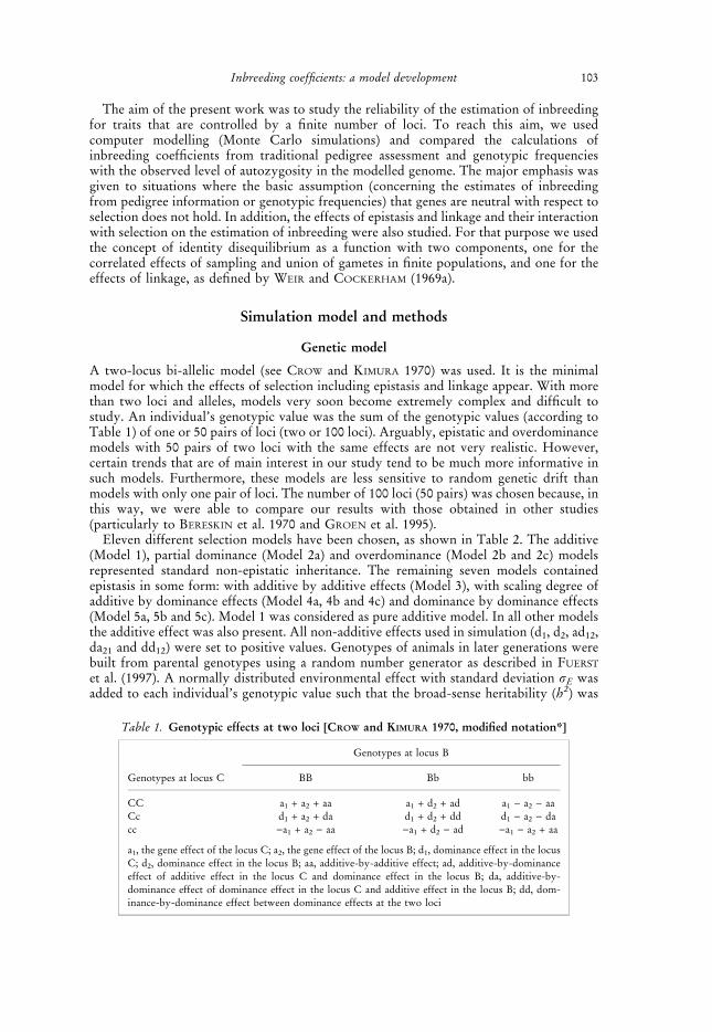
A two-locus bi-allelic model (see CROW and KIMURA 1970) was used. It is the minimalmodel for which the effects of selection including epistasis and linkage appear. With morethan two loci and alleles, models very soon become extremely complex and difficult tostudy. An individual’s genotypic value was the sum of the genotypic values (according toTable 1) of one or 50 pairs of loci (two or 100 loci). Arguably, epistatic and overdominancemodels with 50 pairs of two loci with the same effects are not very realistic. However,certain trends that are of main interest in our study tend to be much more informative insuch models. Furthermore, these models are less sensitive to random genetic drift thanmodels with only one pair of loci. The number of 100 loci (50 pairs) was chosen because, inthis way, we were able to compare our results with those obtained in other studies(particularly to BERESKIN et al. 1970 and GROEN et al. 1995).

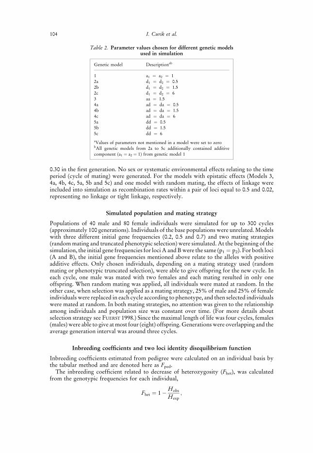
Eleven different selection models have been chosen, as shown in Table 2. The additive(Model 1), partial dominance (Model 2a) and overdominance (Model 2b and 2c) modelsrepresented standard non-epistatic inheritance. The remaining seven models containedepistasis in some form: with additive by additive effects (Model 3), with scaling degree ofadditive by dominance effects (Model 4a, 4b and 4c) and dominance by dominance effects(Model 5a, 5b and 5c). Model 1 was considered as pure additive model. In all other modelsthe additive effect was also present. All non-additive effects used in simulation (d1, d2, ad12,da21 and dd12) were set to positive values. Genotypes of animals in later generations werebuilt from parental genotypes using a random number generator as described in FUERST

et al. (1997). A normally distributed environmental effect with standard deviation rE wasadded to each individual’s genotypic value such that the broad-sense heritability (h2) was

Table 1. Genotypic effects at two loci [CROW and KIMURA 1970, modified notation*]

Genotypes at locus B

Genotypes at locus C BB Bb bb

CC a1 + a2 + aa a1 + d2 + ad a1 ) a2 ) aaCc d1 + a2 + da d1 + d2 + dd d1 ) a2 ) dacc )a1 + a2 ) aa )a1 + d2 ) ad )a1 ) a2 + aa

a1, the gene effect of the locus C; a2, the gene effect of the locus B; d1, dominance effect in the locusC; d2, dominance effect in the locus B; aa, additive-by-additive effect; ad, additive-by-dominanceeffect of additive effect in the locus C and dominance effect in the locus B; da, additive-by-dominance effect of dominance effect in the locus C and additive effect in the locus B; dd, dom-inance-by-dominance effect between dominance effects at the two loci

103Inbreeding coefficients: a model development

0.30 in the first generation. No sex or systematic environmental effects relating to the timeperiod (cycle of mating) were generated. For the models with epistatic effects (Models 3,4a, 4b, 4c, 5a, 5b and 5c) and one model with random mating, the effects of linkage wereincluded into simulation as recombination rates within a pair of loci equal to 0.5 and 0.02,representing no linkage or tight linkage, respectively.

Simulated population and mating strategy

Populations of 40 male and 80 female individuals were simulated for up to 300 cycles(approximately 100 generations). Individuals of the base populations were unrelated. Modelswith three different initial gene frequencies (0.2, 0.5 and 0.7) and two mating strategies(random mating and truncated phenotypic selection) were simulated. At the beginning of thesimulation, the initial gene frequencies for loci A and B were the same (p1 ¼ p2). For both loci(A and B), the initial gene frequencies mentioned above relate to the alleles with positiveadditive effects. Only chosen individuals, depending on a mating strategy used (randommating or phenotypic truncated selection), were able to give offspring for the new cycle. Ineach cycle, one male was mated with two females and each mating resulted in only oneoffspring. When random mating was applied, all individuals were mated at random. In theother case, when selection was applied as a mating strategy, 25% of male and 25% of femaleindividuals were replaced in each cycle according to phenotype, and then selected individualswere mated at random. In both mating strategies, no attention was given to the relationshipamong individuals and population size was constant over time. (For more details aboutselection strategy see FUERST 1998.) Since the maximal length of life was four cycles, females(males) were able to give at most four (eight) offspring. Generations were overlapping and theaverage generation interval was around three cycles.

Inbreeding coefficients and two loci identity disequilibrium function

Inbreeding coefficients estimated from pedigree were calculated on an individual basis bythe tabular method and are denoted here as Fped.

The inbreeding coefficient related to decrease of heterozygosity (Fhet), was calculatedfrom the genotypic frequencies for each individual,

Fhet ¼ 1 � Hobs

Hexp;

Table 2. Parameter values chosen for different genetic modelsused in simulation

Genetic model Descriptionab

1 a1 ¼ a2 ¼ 12a d1 ¼ d2 ¼ 0.52b d1 ¼ d2 ¼ 1.52c d1 ¼ d2 ¼ 63 aa ¼ 1.54a ad ¼ da ¼ 0.54b ad ¼ da ¼ 1.54c ad ¼ da ¼ 65a dd ¼ 0.55b dd ¼ 1.55c dd ¼ 6

aValues of parameters not mentioned in a model were set to zerobAll genetic models from 2a to 5c additionally contained additivecomponent (a1 ¼ a2 ¼ 1) from genetic model 1

104 I. Curik et al.

where Hobs is observed heterozygosity of an individual and Hexp is expectedheterozygosity under Hardy–Weinberg equilibrium and is obtained here as observedheterozygosity in the first cycle. The same approach was used in the papers by BERESKIN

et al. (1969, 1970), SATHER et al. (1977) and DAVIS and BRINKS (1983, 1984).The inbreeding coefficient related to the proportion of autozygous loci (identical by

descent) in the modelled genome was denoted as autozygosity inbreeding coefficient.Faut was calculated for each individual according to the following formula:

Faut ¼number of autozygous loci

total number of loci

To obtain Faut, for each locus all individual alleles in the base population were labelledwith unique identification and then followed through the segregation. Recently, the samedefinition of the individual inbreeding coefficient was also used by BIERNE et al. (2000).Levels of inbreeding in the populations were expressed as the averages of the individualcoefficients and were denoted as faut for the autozygosity inbreeding coefficient, fped for thepedigree inbreeding coefficient, and fhet for the inbreeding coefficient related to decrease ofheterozygosity. Heterozygosity inbreeding coefficient (fhet) is the same parameter as usedin the simulation of GROEN et al. (1995).

For models with two loci, we also calculated the autozygosity inbreeding coefficientsfor the first (f1) and second (f2) locus as well as for both loci (f12). With thosecoefficients, we were able to define two loci identity disequilibrium (gaut) by thefollowing formula:

gaut ¼ f12 � f1f2:

The two loci identity disequilibrium (gaut) is, according to the concept presented inCOCKERHAM and WEIR (1968) and WEIR and COCKERHAM (1969a, 1969b), a function thatexpresses the effects of linkage on the inbreeding level.

Simulation software and procedure

The simulation was performed by a combination of FORTRAN90 and SAS programs.A FORTRAN program DOMEPI 2.1 (see FUERST 1998) was adapted for the purposeof this study. To calculate pedigree inbreeding coefficient for each individual, thealgorithm of TIER (1997) was included. Taking into account all possible combinations,initial gene frequencies, mating strategies, recombination rates, number of loci andgenetic models, there were 120 different runs, each with 100 replicates. The data filesgenerated by the FORTRAN simulation contained the following information for eachmember of a population: animal, sire, dam, birth cycle, sex, pedigree inbreedingcoefficient, heterozygosity, autozygosity inbreeding coefficients and genotypic frequen-cies. Information about gene frequencies, heterozygosity inbreeding coefficient, identitydisequilibrium and generation interval was added by SAS programs (SAS Institute,Cary, NC, USA).

Results and discussion

Inbreeding coefficients (faut, fped and fhet) under random mating

When random mating was practiced as a mating strategy, there were no differencesbetween expectations of all three inbreeding coefficients and neither initial genefrequencies nor linkage within pairs of loci influenced the expected inbreedingcoefficients.


Heterozygosity inbreeding coefficient (fhet) under selection

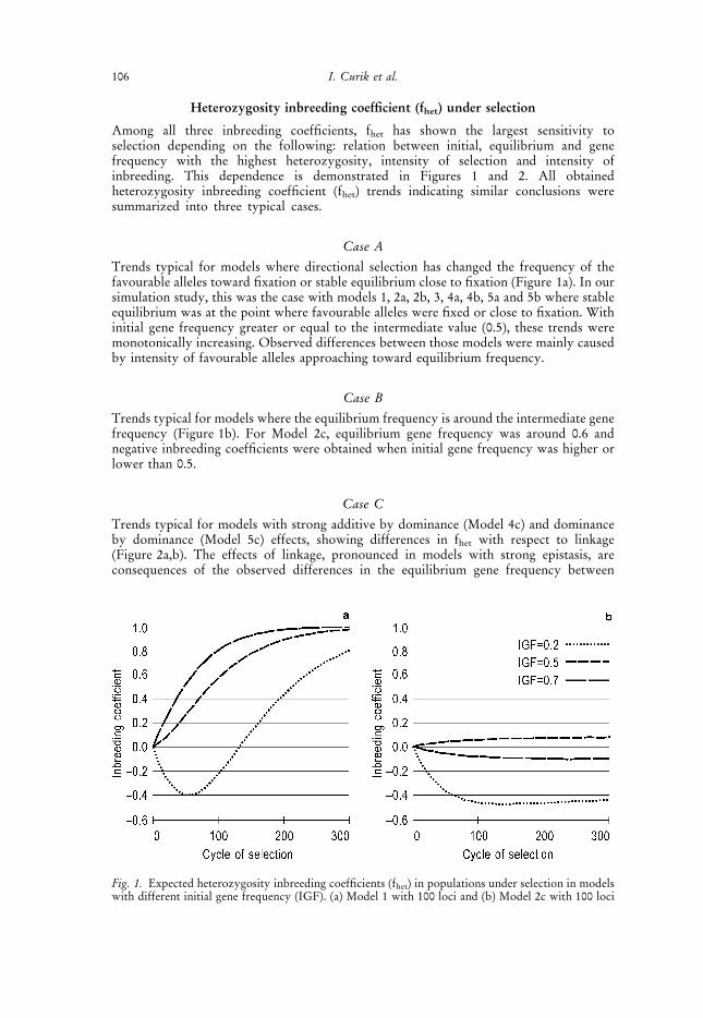
Among all three inbreeding coefficients, fhet has shown the largest sensitivity toselection depending on the following: relation between initial, equilibrium and genefrequency with the highest heterozygosity, intensity of selection and intensity ofinbreeding. This dependence is demonstrated in Figures 1 and 2. All obtainedheterozygosity inbreeding coefficient (fhet) trends indicating similar conclusions weresummarized into three typical cases.

Case A

Trends typical for models where directional selection has changed the frequency of thefavourable alleles toward fixation or stable equilibrium close to fixation (Figure 1a). In oursimulation study, this was the case with models 1, 2a, 2b, 3, 4a, 4b, 5a and 5b where stableequilibrium was at the point where favourable alleles were fixed or close to fixation. Withinitial gene frequency greater or equal to the intermediate value (0.5), these trends weremonotonically increasing. Observed differences between those models were mainly causedby intensity of favourable alleles approaching toward equilibrium frequency.

Case B

Trends typical for models where the equilibrium frequency is around the intermediate genefrequency (Figure 1b). For Model 2c, equilibrium gene frequency was around 0.6 andnegative inbreeding coefficients were obtained when initial gene frequency was higher orlower than 0.5.

Case C

Trends typical for models with strong additive by dominance (Model 4c) and dominanceby dominance (Model 5c) effects, showing differences in fhet with respect to linkage(Figure 2a,b). The effects of linkage, pronounced in models with strong epistasis, areconsequences of the observed differences in the equilibrium gene frequency between

Fig. 1. Expected heterozygosity inbreeding coefficients (fhet) in populations under selection in modelswith different initial gene frequency (IGF). (a) Model 1 with 100 loci and (b) Model 2c with 100 loci

106 I. Curik et al.

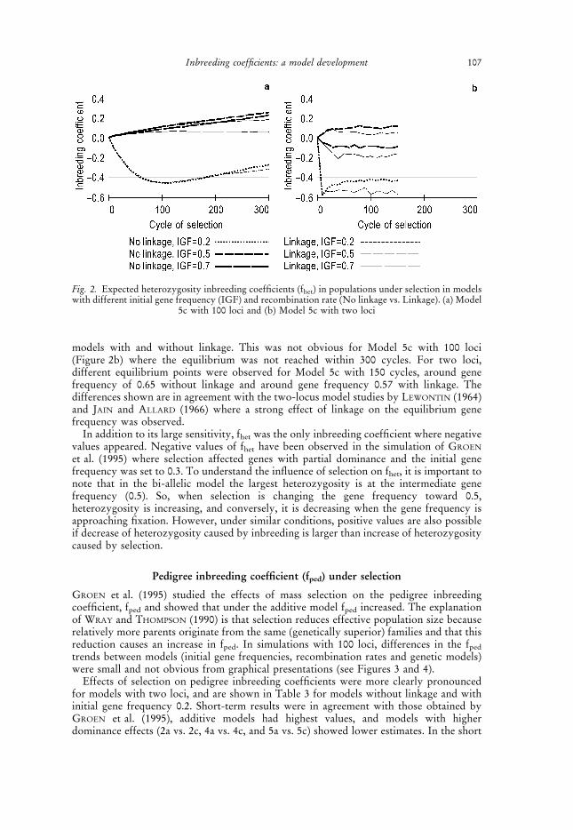
models with and without linkage. This was not obvious for Model 5c with 100 loci(Figure 2b) where the equilibrium was not reached within 300 cycles. For two loci,different equilibrium points were observed for Model 5c with 150 cycles, around genefrequency of 0.65 without linkage and around gene frequency 0.57 with linkage. Thedifferences shown are in agreement with the two-locus model studies by LEWONTIN (1964)and JAIN and ALLARD (1966) where a strong effect of linkage on the equilibrium genefrequency was observed.

In addition to its large sensitivity, fhet was the only inbreeding coefficient where negativevalues appeared. Negative values of fhet have been observed in the simulation of GROEN

et al. (1995) where selection affected genes with partial dominance and the initial genefrequency was set to 0.3. To understand the influence of selection on fhet, it is important tonote that in the bi-allelic model the largest heterozygosity is at the intermediate genefrequency (0.5). So, when selection is changing the gene frequency toward 0.5,heterozygosity is increasing, and conversely, it is decreasing when the gene frequency isapproaching fixation. However, under similar conditions, positive values are also possibleif decrease of heterozygosity caused by inbreeding is larger than increase of heterozygositycaused by selection.

Pedigree inbreeding coefficient (fped) under selection

GROEN et al. (1995) studied the effects of mass selection on the pedigree inbreedingcoefficient, fped and showed that under the additive model fped increased. The explanationof WRAY and THOMPSON (1990) is that selection reduces effective population size becauserelatively more parents originate from the same (genetically superior) families and that thisreduction causes an increase in fped. In simulations with 100 loci, differences in the fped

trends between models (initial gene frequencies, recombination rates and genetic models)were small and not obvious from graphical presentations (see Figures 3 and 4).

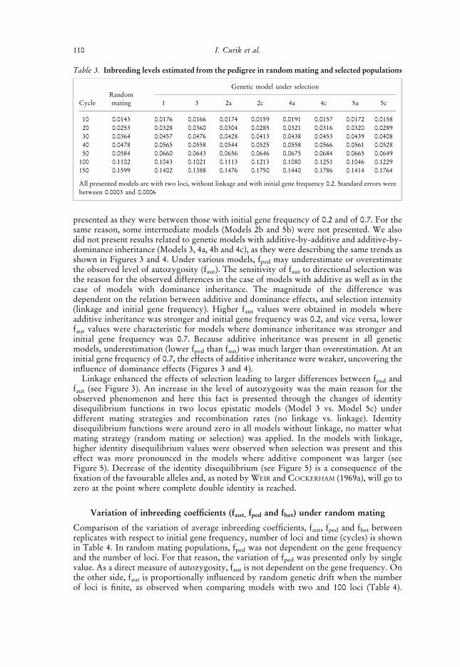
Effects of selection on pedigree inbreeding coefficients were more clearly pronouncedfor models with two loci, and are shown in Table 3 for models without linkage and withinitial gene frequency 0.2. Short-term results were in agreement with those obtained byGROEN et al. (1995), additive models had highest values, and models with higherdominance effects (2a vs. 2c, 4a vs. 4c, and 5a vs. 5c) showed lower estimates. In the short

Fig. 2. Expected heterozygosity inbreeding coefficients (fhet) in populations under selection in modelswith different initial gene frequency (IGF) and recombination rate (No linkage vs. Linkage). (a) Model

5c with 100 loci and (b) Model 5c with two loci


term, all populations that were under selection reached a higher inbreeding level (fped) thanpopulations where mating was at random. The results were reversed in the long term,where models with additive effects had lower fped values and models with higherdominance effects (2a vs. 2c, 4a vs. 4c, and 5a vs. 5c) provided higher estimates. When thetrait is controlled by a small number of loci, selection forces favourable alleles to fixationquickly and after that the population is mated at random. In this paper it is shown that theeffect of selection prior to fixation on the population structure was probably the reasonwhy fped estimates for additive models were, in the long term, even lower than estimates

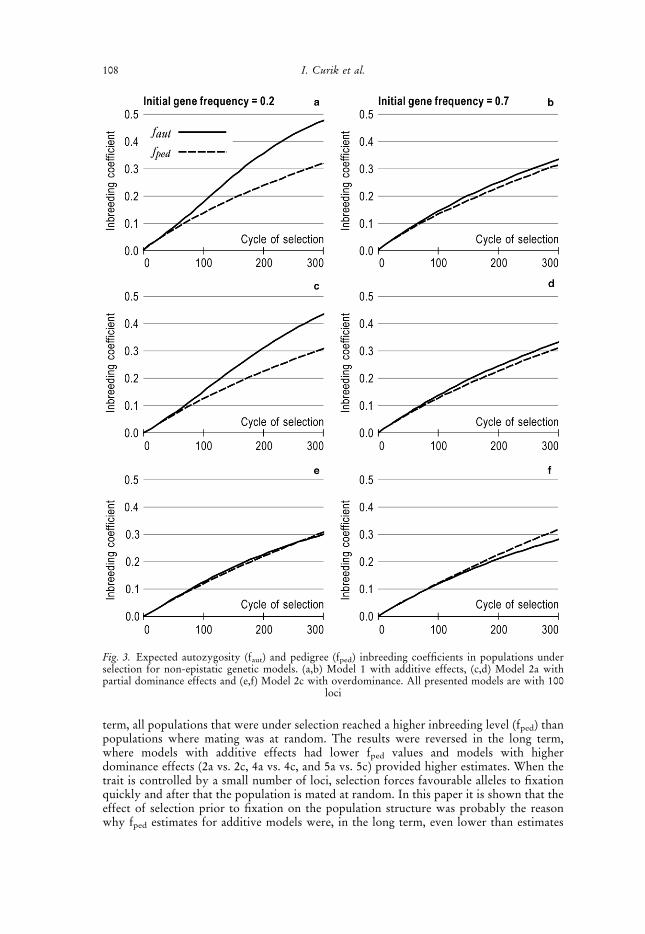
Fig. 3. Expected autozygosity (faut) and pedigree (fped) inbreeding coefficients in populations underselection for non-epistatic genetic models. (a,b) Model 1 with additive effects, (c,d) Model 2a withpartial dominance effects and (e,f) Model 2c with overdominance. All presented models are with 100

loci

108 I. Curik et al.

obtained for random mating populations (Table 3). The highest long-term fped estimateswere obtained for models where the combination of additive and dominance effects wassuch that the additive effect led to higher inbreeding coefficients and dominance effectsprolonged the duration of selection. KIMURA and CROW (1963) found that maximumavoidance of inbreeding would not result in the lowest level of inbreeding in the long term.To some extent, their statement is consistent with our results where mating favouring thehighest level of inbreeding in the short term did not result in the highest inbreeding in thelong term. The effects of linkage and different initial gene frequencies were small.

Autozygosity inbreeding coefficient (faut) under selection

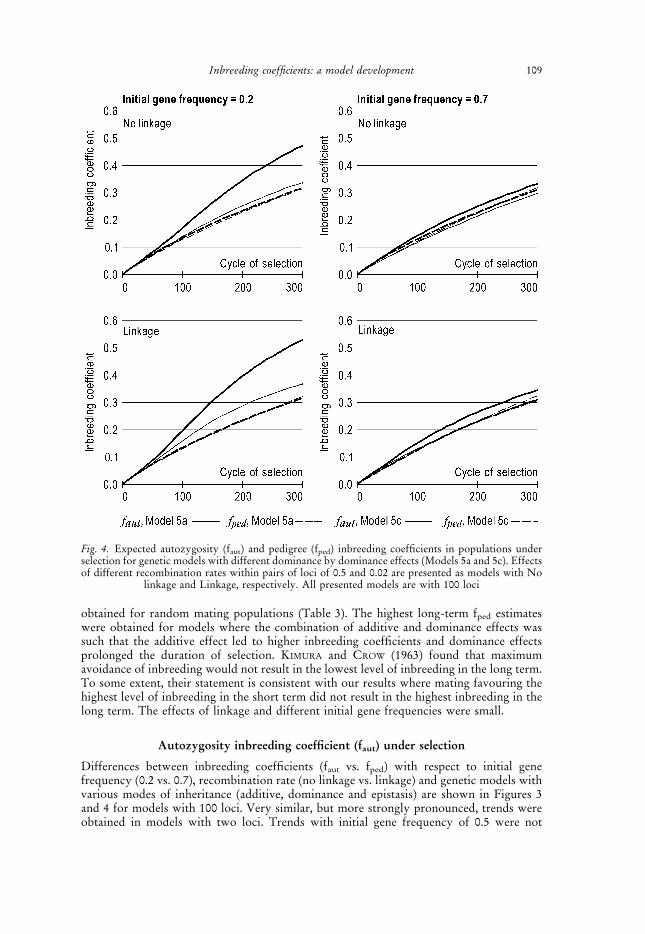
Differences between inbreeding coefficients (faut vs. fped) with respect to initial genefrequency (0.2 vs. 0.7), recombination rate (no linkage vs. linkage) and genetic models withvarious modes of inheritance (additive, dominance and epistasis) are shown in Figures 3and 4 for models with 100 loci. Very similar, but more strongly pronounced, trends wereobtained in models with two loci. Trends with initial gene frequency of 0.5 were not

Fig. 4. Expected autozygosity (faut) and pedigree (fped) inbreeding coefficients in populations underselection for genetic models with different dominance by dominance effects (Models 5a and 5c). Effectsof different recombination rates within pairs of loci of 0.5 and 0.02 are presented as models with No

linkage and Linkage, respectively. All presented models are with 100 loci


presented as they were between those with initial gene frequency of 0.2 and of 0.7. For thesame reason, some intermediate models (Models 2b and 5b) were not presented. We alsodid not present results related to genetic models with additive-by-additive and additive-by-dominance inheritance (Models 3, 4a, 4b and 4c), as they were describing the same trends asshown in Figures 3 and 4. Under various models, fped may underestimate or overestimatethe observed level of autozygosity (faut). The sensitivity of faut to directional selection wasthe reason for the observed differences in the case of models with additive as well as in thecase of models with dominance inheritance. The magnitude of the difference wasdependent on the relation between additive and dominance effects, and selection intensity(linkage and initial gene frequency). Higher faut values were obtained in models whereadditive inheritance was stronger and initial gene frequency was 0.2, and vice versa, lowerfaut values were characteristic for models where dominance inheritance was stronger andinitial gene frequency was 0.7. Because additive inheritance was present in all geneticmodels, underestimation (lower fped than faut) was much larger than overestimation. At aninitial gene frequency of 0.7, the effects of additive inheritance were weaker, uncovering theinfluence of dominance effects (Figures 3 and 4).

Linkage enhanced the effects of selection leading to larger differences between fped andfaut (see Figure 3). An increase in the level of autozygosity was the main reason for theobserved phenomenon and here this fact is presented through the changes of identitydisequilibrium functions in two locus epistatic models (Model 3 vs. Model 5c) underdifferent mating strategies and recombination rates (no linkage vs. linkage). Identitydisequilibrium functions were around zero in all models without linkage, no matter whatmating strategy (random mating or selection) was applied. In the models with linkage,higher identity disequilibrium values were observed when selection was present and thiseffect was more pronounced in the models where additive component was larger (seeFigure 5). Decrease of the identity disequilibrium (see Figure 5) is a consequence of thefixation of the favourable alleles and, as noted by WEIR and COCKERHAM (1969a), will go tozero at the point where complete double identity is reached.

Variation of inbreeding coefficients (faut, fped and fhet) under random mating

Comparison of the variation of average inbreeding coefficients, faut, fped and fhet betweenreplicates with respect to initial gene frequency, number of loci and time (cycles) is shownin Table 4. In random mating populations, fped was not dependent on the gene frequencyand the number of loci. For that reason, the variation of fped was presented only by singlevalue. As a direct measure of autozygosity, faut is not dependent on the gene frequency. Onthe other side, faut is proportionally influenced by random genetic drift when the numberof loci is finite, as observed when comparing models with two and 100 loci (Table 4).

Table 3. Inbreeding levels estimated from the pedigree in random mating and selected populations

RandomGenetic model under selection

Cycle mating 1 3 2a 2c 4a 4c 5a 5c

10 0.0143 0.0176 0.0166 0.0174 0.0159 0.0191 0.0157 0.0172 0.015820 0.0253 0.0328 0.0360 0.0304 0.0285 0.0321 0.0316 0.0320 0.028930 0.0364 0.0457 0.0476 0.0428 0.0413 0.0438 0.0453 0.0439 0.040840 0.0478 0.0565 0.0558 0.0544 0.0525 0.0558 0.0566 0.0561 0.052850 0.0584 0.0660 0.0643 0.0656 0.0646 0.0675 0.0684 0.0665 0.0649

100 0.1102 0.1043 0.1021 0.1113 0.1213 0.1080 0.1251 0.1046 0.1229150 0.1599 0.1402 0.1388 0.1476 0.1750 0.1440 0.1786 0.1414 0.1764

All presented models are with two loci, without linkage and with initial gene frequency 0.2. Standard errors werebetween 0.0003 and 0.0006

110 I. Curik et al.

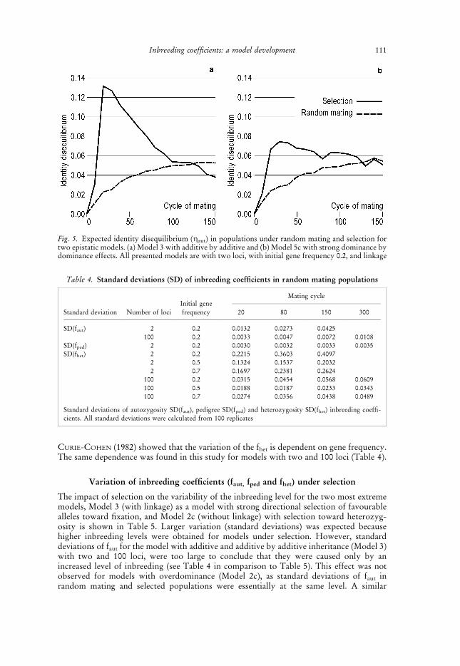
CURIE-COHEN (1982) showed that the variation of the fhet is dependent on gene frequency.The same dependence was found in this study for models with two and 100 loci (Table 4).

Variation of inbreeding coefficients (faut, fped and fhet) under selection

The impact of selection on the variability of the inbreeding level for the two most extrememodels, Model 3 (with linkage) as a model with strong directional selection of favourablealleles toward fixation, and Model 2c (without linkage) with selection toward heterozyg-osity is shown in Table 5. Larger variation (standard deviations) was expected becausehigher inbreeding levels were obtained for models under selection. However, standarddeviations of faut for the model with additive and additive by additive inheritance (Model 3)with two and 100 loci, were too large to conclude that they were caused only by anincreased level of inbreeding (see Table 4 in comparison to Table 5). This effect was notobserved for models with overdominance (Model 2c), as standard deviations of faut inrandom mating and selected populations were essentially at the same level. A similar

Fig. 5. Expected identity disequilibrium (gaut) in populations under random mating and selection fortwo epistatic models. (a) Model 3 with additive by additive and (b) Model 5c with strong dominance bydominance effects. All presented models are with two loci, with initial gene frequency 0.2, and linkage

Table 4. Standard deviations (SD) of inbreeding coefficients in random mating populations

Initial geneMating cycle

Standard deviation Number of loci frequency 20 80 150 300

SD(faut) 2 0.2 0.0132 0.0273 0.0425100 0.2 0.0033 0.0047 0.0072 0.0108

SD(fped) 2 0.2 0.0030 0.0032 0.0033 0.0035SD(fhet) 2 0.2 0.2215 0.3603 0.4097

2 0.5 0.1324 0.1537 0.20322 0.7 0.1697 0.2381 0.2624

100 0.2 0.0315 0.0454 0.0568 0.0609100 0.5 0.0188 0.0187 0.0233 0.0343100 0.7 0.0274 0.0356 0.0438 0.0489

Standard deviations of autozygosity SD(faut), pedigree SD(fped) and heterozygosity SD(fhet) inbreeding coeffi-cients. All standard deviations were calculated from 100 replicates


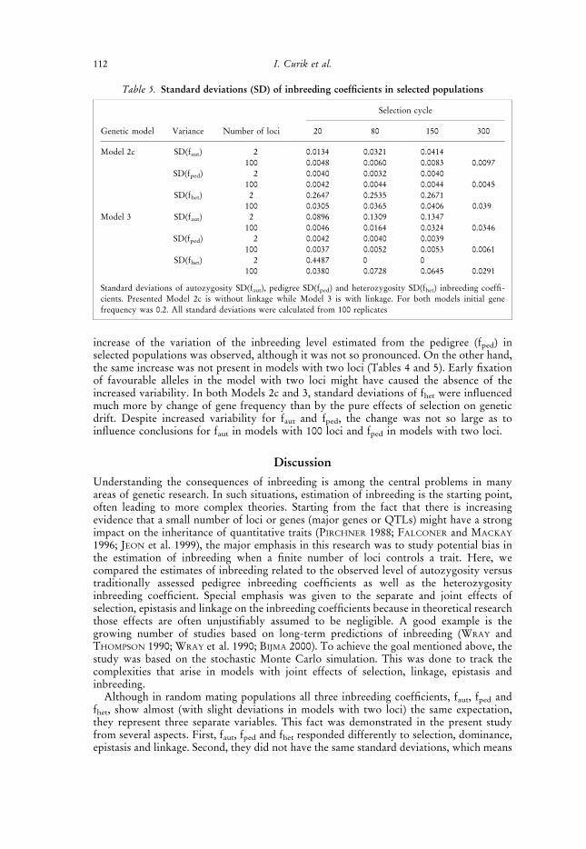
increase of the variation of the inbreeding level estimated from the pedigree (fped) inselected populations was observed, although it was not so pronounced. On the other hand,the same increase was not present in models with two loci (Tables 4 and 5). Early fixationof favourable alleles in the model with two loci might have caused the absence of theincreased variability. In both Models 2c and 3, standard deviations of fhet were influencedmuch more by change of gene frequency than by the pure effects of selection on geneticdrift. Despite increased variability for faut and fped, the change was not so large as toinfluence conclusions for faut in models with 100 loci and fped in models with two loci.

Discussion

Understanding the consequences of inbreeding is among the central problems in manyareas of genetic research. In such situations, estimation of inbreeding is the starting point,often leading to more complex theories. Starting from the fact that there is increasingevidence that a small number of loci or genes (major genes or QTLs) might have a strongimpact on the inheritance of quantitative traits (PIRCHNER 1988; FALCONER and MACKAY

1996; JEON et al. 1999), the major emphasis in this research was to study potential bias inthe estimation of inbreeding when a finite number of loci controls a trait. Here, wecompared the estimates of inbreeding related to the observed level of autozygosity versustraditionally assessed pedigree inbreeding coefficients as well as the heterozygosityinbreeding coefficient. Special emphasis was given to the separate and joint effects ofselection, epistasis and linkage on the inbreeding coefficients because in theoretical researchthose effects are often unjustifiably assumed to be negligible. A good example is thegrowing number of studies based on long-term predictions of inbreeding (WRAY andTHOMPSON 1990; WRAY et al. 1990; BIJMA 2000). To achieve the goal mentioned above, thestudy was based on the stochastic Monte Carlo simulation. This was done to track thecomplexities that arise in models with joint effects of selection, linkage, epistasis andinbreeding.

Although in random mating populations all three inbreeding coefficients, faut, fped andfhet, show almost (with slight deviations in models with two loci) the same expectation,they represent three separate variables. This fact was demonstrated in the present studyfrom several aspects. First, faut, fped and fhet responded differently to selection, dominance,epistasis and linkage. Second, they did not have the same standard deviations, which means

Table 5. Standard deviations (SD) of inbreeding coefficients in selected populations

Selection cycle

Genetic model Variance Number of loci 20 80 150 300

Model 2c SD(faut) 2 0.0134 0.0321 0.0414100 0.0048 0.0060 0.0083 0.0097

SD(fped) 2 0.0040 0.0032 0.0040100 0.0042 0.0044 0.0044 0.0045

SD(fhet) 2 0.2647 0.2535 0.2671100 0.0305 0.0365 0.0406 0.039

Model 3 SD(faut) 2 0.0896 0.1309 0.1347100 0.0046 0.0164 0.0324 0.0346

SD(fped) 2 0.0042 0.0040 0.0039100 0.0037 0.0052 0.0053 0.0061

SD(fhet) 2 0.4487 0 0100 0.0380 0.0728 0.0645 0.0291

Standard deviations of autozygosity SD(faut), pedigree SD(fped) and heterozygosity SD(fhet) inbreeding coeffi-cients. Presented Model 2c is without linkage while Model 3 is with linkage. For both models initial genefrequency was 0.2. All standard deviations were calculated from 100 replicates

112 I. Curik et al.

that the effects of random drift, especially in models under selection, were not affecting allthree coefficients in the same way. Finally, they were not always defined in the samedomain; for example fhet was not always positive.

In this study, the most important factor responsible for the observed discrepanciesbetween inbreeding coefficients (faut, fped and fhet) was selection. In the models withselection, the bias (discrepancy) was present in both directions, thus leading tooverestimation or underestimation of the observed level of autozygosity depending onthe genetic model, linkage and initial gene frequency. Variation of the autozygosity level(between replicates) was increased notably in models with additive inheritance underselection and was an additional potential source of bias. The number of loci affecting thetrait was also important as in our models it was proportional to the effects of genes, andselection was stronger when the number of loci was small. Also, the small number of lociwas responsible for the larger random genetic drift leading to larger variation and potentialdiscrepancies between inbreeding coefficients even when selection was absent. Inconclusion, estimates of inbreeding coefficients are unreliable, especially for the smallnumber of linked genes with large additive effects under selection. Giving recommenda-tions on how to measure the real magnitude of the bias is beyond the scope of this studyand should be a topic of further research. Here, the exact values of the parameters used inthe model-building were not intended to describe particular biological populations. Ourmain focus was on observing trends and relations between above-mentioned factors(selection, dominance, epistasis, linkage and number of loci).

Limitations of the model applied

Estimation of inbreeding is not only affected by factors analysed in this paper and wewould like to mention some other factors and their potential influence on the inbreedinglevel and its estimation. Mutation of a gene that is identical by descent would lead to alower level of autozygosity in the population. At the same time, mutation would increasethe number of polymorphic alleles, thus leading to higher heterozygosity. Lethal anddetrimental recessive genes would be the reason for exclusion of individuals with higherautozygosity from the population and thus also for the lower autozygosity level in thepopulation. Both factors (mutation and exclusion of individuals with higher autozygosity)would lead to overestimation of autozygosity when it is estimated from the pedigree. If weconsider that mutation is a rare phenomenon, the potential bias will be negligible in theshort term, but in contrast, a high mutation rate in the long-term might lead to severe bias.When there are more than two alleles per locus, which is realistic but not analysed in thisstudy, some important genetic parameters of the population like equilibrium genefrequency and gene frequency with highest heterozygosity as well as genetic models andselection intensity could change to some extent. Apparently, fhet would be stronglyaffected, being functionally dependent on the relation between equilibrium and genefrequency with highest heterozygosity. However, if selection is moving favourable allelestoward fixation or close to fixation, the number of alleles might be reduced fairly quicklyto two alleles and thus to models presented in this study. With experimental data,researchers are faced with additional sources of bias. Good examples are problems withincomplete pedigree information (MACCLUER et al. 1983; VAN RADEN 1992) and molecularmarkers that do not correspond completely to genotypes (CURIE-COHEN 1982).

Conclusions

When the trait is, to a large extent, controlled by a finite number of loci and when selectionis present, the bias in the estimation of the autozygosity is likely to occur and caution isnecessary whenever conclusions are based on inbreeding coefficients estimated from thepedigree or decrease in heterozygosity. For example, the potential bias might appear in the


estimation of inbreeding depression, in the estimation of genetic parameters that depend onthe accuracy of relationship matrices (additive as well as dominance, additive-by-additive,additive-by-dominance and dominance-by-dominance) and in the IBD mapping forquantitative traits. Development of more efficient molecular techniques (for exampleDNA-chips, multiplex PCR reactions) is fast and, at the same time, the capacities ofmolecular devices are growing. Thus, with additional knowledge about modes ofinheritance, in the near future, better and more specific (with respect to certainchromosomal regions) estimates of autozygosity will be possible.

AcknowledgementsThe authors wish to thank Christian Fuerst for supplying the base version of the simulation program(DOMEPI 2.1) and for the help in upgrading the program when it was necessary. We are also gratefulto Bruce Tier for providing the algorithm to compute pedigree-inbreeding coefficients, to Alois Essland Aleksandar Pekec for helpful comments and suggestions, as well as to Dragan Tupajic for thegraphic design of the figures. This project was financially supported by Croatian Ministry of Scienceand Technology under code 178007 (a part of the project 178831).

References

BERESKIN, B.; SHELBY, C. E.; HAZEL, L. N., 1969: Monte Carlo studies of selection and inbreeding inswine. I. Genetic and phenotypic trends. J. Anim. Sci. 29: 678–686.

BERESKIN, B.; SHELBY, C. E.; HAZEL, L. N., 1970: Monte Carlo studies of selection and inbreeding inswine. II. Inbreeding coefficients. J. Anim. Sci. 30: 681–689.

BIERNE, N.; TSITRONE, A.; DAVID, P., 2000: An inbreeding model of associative overdominance duringa population bottleneck. Genetics 155: 1981–1990.

BIJMA, P., 2000: Long-term genetic contributions: prediction of rates of inbreeding and genetic gain inselected populations. PhD Thesis. Wageningen University, The Netherlands.

CAVALLI-SFORZA, L. L.; BODMER, W. F., 1971: The Genetics of Human Populations. WH Freeman,San Francisco, CA

CHARLESWORTH, D.; CHARLESWORTH, B., 1987: Inbreeding depression and its evolutionary conse-quences. Annu. Rev. Ecol. Syst. 18: 237–268.

COCKERHAM, C. C.; WEIR, B. S., 1968: Sib mating with two linked loci. Genetics 60: 629–640.CROW, J. F.; KIMURA, M., 1970: An Introduction to Population Genetics Theory. Harper & Row, New

York, NYCRUDEN, D., 1949: The computation of inbreeding coefficients for closed populations. J. Hered. 40:

248–251.CURIE-COHEN, M., 1982: Estimates of inbreeding in a natural population: a comparison of sampling

properties. Genetics 100: 339–358.DAVIS, M. E.; BRINKS, J. S., 1983: Selection and concurrent inbreeding in simulated beef herds. J. Anim

Sci. 56: 40–51.DAVIS, M. E.; BRINKS, J. S., 1984: Selection and concurrent inbreeding in simulated beef herds: model

development. J. Anim Sci. 59: 1488–1500.EMIK, L. O.; TERRILL, C. E., 1949: Systematic procedures for calculating inbreeding coefficients.

J. Hered. 40: 51–55.FALCONER, D. S.; MACKAY, T. F. C., 1996: Introduction to Quantitative Genetics. Longman , London,

UK.FESTING, M., 1979: Inbred Strains in Biomedical Research. Oxford University Press, New York, NYFUERST, C., 1998: Domepi 2.1 Manuel. Institut fur Nutztierwissenschaften, Universitat fur

Bodenkultur, Wien, Austria.FUERST, C.; JAMES, J. W.; SOLKNER, J.; ESSL, A., 1997: Impact of dominance and epistasis on the genetic

make-up of simulated populations under selection: a model development. J. Anim. Breed. Genet.114: 163–175.

GOLDEN, B. L.; BRINKS, J. S.; BOURDON, R. M., 1991: A performance programmed method forcomputing inbreeding coefficients from large data sets for use in mixed-model analysis. J. Anim.Sci. 69: 3564–3573.

GROEN, A. B.; KENNEDY, B. W.; EISSEN, J. J., 1995: Potential bias in inbreeding depression estimateswhen using pedigree relationships to assess the degree of homozygosity for loci under selection.Theor. Appl. Genet. 91: 665–671.

HALLAUER, A. R.; MIRANDA, J. B., 1981: Quantitative Genetics in Maize Breeding. Iowa StateUniversity, Ames, IO.

114 I. Curik et al.

HENDERSON, C. R., 1976: A simple method for the inverse of a numerator relationship matrix used inprediction of breeding values. Biometrics 32: 69–83.

JAIN, S. K.; ALLARD, R. W., 1966: The effects of linkage, epistasis, and inbreeding on populationchanges under selection. Genetics 53: 633–659.

JEON, J.-T.; CARLBORG, O.; TORNSTEN, A.; GIUFFRA, E.; AMARGER, V.; CHARDON, P.; ANDERSSON-EKLUND, L.; ANDERSSON, K.; HANSSON, I.; LUNDSTROM, K.; ANDERSSON, L., 1999: A paternallyexpressed QTL affecting skeletal and cardiac muscle mass in pig maps to the IGF2 locus. Nat.Genet 21: 157–158.

KIMURA, M.; CROW, J. F., 1963: On the maximum avoidance of inbreeding. Genet. Res. 4: 399–415.LEWONTIN, R. C., 1964: The interaction of selection and linkage. I. General considerations; heterotic

models. Genetics 49: 49–67.MACCLUER, J. W.; BOYCE, A. J.; DYKE, B.; WEITKAMP, L. R.; PFENNIG, D. W.; PARSONS, C. J., 1983:

Inbreeding and pedigree structure in Standardbred horses. J. Hered. 74: 394–399.MALECOT, G., 1948: Les Mathematiques de L’heredite. Masson et Cie, Paris, France.MEUWISSEN, T. H. E.; LUO, Z., 1992: Computing inbreeding coefficients in large populations. Genet.

Sel. Evol. 24: 305–309.PIRCHNER, F., 1988: Finding genes affecting quantitative traits in domestic animals. In: WEIR, B. S.;

EISEN, E. J.; GOODMAN, M. M.; NAMKOONG, G. (eds), Proceedings of the Second InternationalConference on Quantitative Genetics, Sinauer Associates, Sunderland, MA.

QUAAS, R. L.; 1976: Computing the diagonal elements and inverse of a large numerator relationshipmatrix. Biometrics 32: 949–953.

SATHER, A. P.; SWIGIR, L. A.; HARVEY, W. R., 1977: Genetic drift and response to selection in simulatedpopulations: The simulation model and gene and genotype responses. J. Anim Sci. 44: 343–351.

SIMIANER, H., 1994: Derivation of single-locus relationship coefficients conditional on markerinformation. Theor. Appl. Genet. 88: 548–556.

SOULE, M., 1986: Conservation Biology. Sinauer Associates, Sunderland, MA.TEMPLETON, A. R,; 1980: The theory of speciation via the founder principle. Genetics 94: 1011–1038.TIER, B., 1990: Computing inbreeding coefficients quickly. Genet. Sel. Evol. 22: 419–430.TIER, B., 1997: Useful Algorithms for the Genetic Evaluation of Livestock. PhD Thesis, The

University of New England, Armidale, Australia.VAN ARENDONK, J. A. M.; BINK, M. C. A. M.; BIJMA, P.; BOVENHUIS, H.; DE KONING, D.-J.;

BRASCAMP, E. W., 1999: Use of phenotypic and molecular data for genetic evaluation of livestock.In: DEKKERS, J. C. M.; LAMONT, S. J.; ROTHSCHILD, M. F. (eds), From Jay Lush to Genomics:Visions for Animal Breeding and Genetics, May 16–18, Iowa State University, Ames, IO.

VAN RADEN, P. M., 1992: Accounting for inbreeding and crossbreeding in genetic evaluations of largepopulations. J. Dairy Sci. 75: 3136–3144.

WEIR, B., 1994: The effects of inbreeding on forensic calculations. Annu. Rev. Genet. 28: 597–621.WEIR, B. S.; COCKERHAM, C. C., 1969a: Pedigree mating with two linked loci. Genetics 61: 923–940.WEIR, B. S.; COCKERHAM, C. C., 1969b: Group inbreeding with two linked loci. Genetics 63: 711–742.WRAY, N. R.; THOMPSON, R., 1990: Prediction of rates of inbreeding in selected populations. Genet.

Res. 55: 41–54.WRAY, N. R.; WOOLLIAMS, J. A.; THOMPSON, R., 1990: Methods for predicting rates of inbreeding in

selected populations. Theor. Appl. Genet. 80: 503–512.WRIGHT, S., 1922: Inbreeding coefficients and relationship. Am. Nat. 56: 330–338.WRIGHT, S., 1951: The genetical structure of populations. Ann. Eugen. 15: 323–354.WRIGHT, S., 1965: The interpretation of population structure by F-statistics with special regard to

systems of mating. Evolution 19: 395–420.WRIGHT, S.; MCPHEE, H. C., 1925: An approximate method of calculating inbreeding coefficients and

relationship from livestock pedigrees. J. Agric. Res. 31: 377–383.

Author’s address: INO CURIK, Animal Science Department, Faculty of Agriculture University ofZagreb, Svetosimunska 25, 10 000 Zagreb, Croatia. E-mail: [email protected]


Effects of models with finite loci, selection, dominance, epistasis and linkage on inbreeding coefficients based on pedigree and genotypic information

Documents