Effects of Increasing Surface Reflectivity on Urban Climate, Air Quality and Heat-Related Mortality Zahra Jandaghian A Thesis in The Department of Building, Civil and Environmental Engineering Presented in the Partial Fulfillment of the Requirements For the Degree of Doctor of Philosophy (Building Engineering) at Concordia University Montreal, Quebec, Canada September 2018 © Zahra Jandaghian, 2018

Welcome message from author
This document is posted to help you gain knowledge. Please leave a comment to let me know what you think about it! Share it to your friends and learn new things together.
Transcript

Effects of Increasing Surface Reflectivity on Urban Climate, Air Quality and Heat-Related Mortality
Zahra Jandaghian
A Thesis in
The Department of Building, Civil and Environmental Engineering
Presented in the Partial Fulfillment of the Requirements For the Degree of
Doctor of Philosophy (Building Engineering) at Concordia University
Montreal, Quebec, Canada
September 2018
© Zahra Jandaghian, 2018
CONCORDIA UNIVERSITY SCHOOL OF GRADUATE STUDIES
This is to certify that thesis prepared
By: Zahra Jandaghian Entitled: Effects of Increasing Surface Reflectivity on Urban Climate, Air Quality and Heat-Related Mortality
and submitted in partial fulfillment of the requirements for the degree of Doctor of Philosophy (Building Engineering)
complies with the regulations of the University and meets the accepted standards with respect to originality and quality.
Signed by the final examining committee:
Chair Dr. Adam Krzyzak
External Examiner Dr. David J. Sailor
External to Program Dr. Damon H. Matthews
Examiner Dr. Fariborz Haghighat
Examiner Dr. Fuzhan Nasiri
Thesis Supervisor Dr. Hashem Akbari
Approved by
Dr. Fariborz Haghighat
Chair of Department of Graduate Program Director
25 October 2018 Date of Defense
Dr. Amir Asif Dean, Gina Cody School of Engineering and Computer Science
III
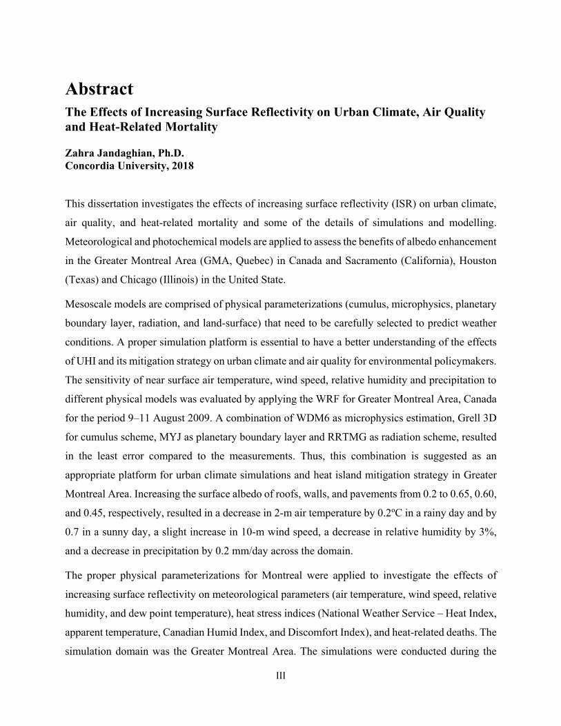
Abstract The Effects of Increasing Surface Reflectivity on Urban Climate, Air Quality and Heat-Related Mortality Zahra Jandaghian, Ph.D. Concordia University, 2018 This dissertation investigates the effects of increasing surface reflectivity (ISR) on urban climate,
air quality, and heat-related mortality and some of the details of simulations and modelling.
Meteorological and photochemical models are applied to assess the benefits of albedo enhancement
in the Greater Montreal Area (GMA, Quebec) in Canada and Sacramento (California), Houston
(Texas) and Chicago (Illinois) in the United State.
Mesoscale models are comprised of physical parameterizations (cumulus, microphysics, planetary
boundary layer, radiation, and land-surface) that need to be carefully selected to predict weather
conditions. A proper simulation platform is essential to have a better understanding of the effects
of UHI and its mitigation strategy on urban climate and air quality for environmental policymakers.
The sensitivity of near surface air temperature, wind speed, relative humidity and precipitation to
different physical models was evaluated by applying the WRF for Greater Montreal Area, Canada
for the period 9–11 August 2009. A combination of WDM6 as microphysics estimation, Grell 3D
for cumulus scheme, MYJ as planetary boundary layer and RRTMG as radiation scheme, resulted
in the least error compared to the measurements. Thus, this combination is suggested as an
appropriate platform for urban climate simulations and heat island mitigation strategy in Greater
Montreal Area. Increasing the surface albedo of roofs, walls, and pavements from 0.2 to 0.65, 0.60,
and 0.45, respectively, resulted in a decrease in 2-m air temperature by 0.2oC in a rainy day and by
0.7 in a sunny day, a slight increase in 10-m wind speed, a decrease in relative humidity by 3%,
and a decrease in precipitation by 0.2 mm/day across the domain.
The proper physical parameterizations for Montreal were applied to investigate the effects of
increasing surface reflectivity on meteorological parameters (air temperature, wind speed, relative
humidity, and dew point temperature), heat stress indices (National Weather Service – Heat Index,
apparent temperature, Canadian Humid Index, and Discomfort Index), and heat-related deaths. The
simulation domain was the Greater Montreal Area. The simulations were conducted during the

IV
2005 and 2011 heat wave periods. Heat-related mortality correlations were developed for Montreal.
The beneficial contributions of albedo enhancement were a decrease in temperature by 0.8oC, an
increase in relative humidity by 2%, an increase in dew point temperature by 0.4oC, a slight increase
in wind speed, and a decrease in heat-related mortality by 3.2%. Increasing surface reflectivity
could save seven lives and improve the level of comfort for urban dwellers.
To assess the effects of increasing surface reflectivity on mitigating urban heat islands and
improving air quality, simulations were carried out over a larger geographical area (North America
with horizontal resolution of 12km) within nested domains as urban areas (Sacramento in
California, Houston in Texas, and Chicago in Illinois with horizontal resolution of 2.4km) in a two-
way nested approach by online coupling of chemistry package with the solver of WRF (WRF-
Chem). The 2-way nested approach provided an integrated simulation setup to capture the full
impacts of meteorological and photochemical reactions and decrease the uncertainties associated
with scale separation and grid resolution. The Lin, Goddard, Rapid Radiative Transfer Model,
Mellor-Yamada-Janjic and Grell-Devenyi ensemble schemes are respectively selected for
microphysics, shortwave radiation, longwave radiation, planetary boundary layer and cumulus
parameterization. For anthropogenic and biogenic emission estimations, the models of the United
States National Emission Inventory for 2011 (US-NEI11) and Model of Emissions of Gases and
Aerosols from Nature (MEGAN) are respectively simulated for the inner domains. The Modal
Aerosol Dynamics Model for Europe and Regional Atmospheric Chemistry Mechanism (RACM)
are applied to estimate the effects of aerosols on radiation processes and hydrological cycles in the
atmosphere and to estimate the gas-phase reactions. Photolysis frequencies are calculated by the
Fast_J model scheme. Increasing surface albedo resulted a decrease in air temperature by 2-3oC in
urban areas of these three cities. Albedo enhancement resulted in a slight increase in wind speed;
an increase in relative humidity (3%) and dew point temperature (0.3oC) during simulation period.
Increasing urban reflectivity led to a decrease in PM2.5 and O3 concentrations by 2-4μg/m3 and 4-
8 ppb in urban areas of these three cities based on their locations. Sacramento showed a larger
reduction in ozone concentration as a result of larger decrease in air temperature because of the
heat island mitigation strategy.
The two-way nested approach was employed to investigate the effects of albedo enhancement on
aerosol-radiation-cloud (ARC) interactions over the Greater Montreal Area during the 2011 heat
wave period. The third domain of simulation covers the GMA with the horizontal resolution of

V
800m. Four sets of simulations with and without aerosol estimations and convective
parameterizations were carried out to explore the direct, semi-direct and indirect effects of aerosols.
The physical and chemical parameterizations are modified to be coupled with the Model for
Simulating Aerosol Interactions with Chemistry (MOSAIC) aerosol scheme and the Carbon Bond
Mechanism (CBM-Z) gas phase chemistry scheme. The Morrison double-moment scheme and the
Mellor-Yamada-Janjic scheme are selected as microphysics and planetary boundary layer options,
respectively. The Grell-Devenyi ensemble scheme and the rapid radiative transfer model are
respectively used for cumulus parameterization and shortwave and longwave radiations. The US-
NEI11 and MEGAN are applied to calculate the anthropogenic and biogenic emission estimation,
respectively. The Fast-J is used for the photolysis scheme in WRF-Chem. Aerosols cause a
decrease in shortwave radiation reaching to the ground (20 Wm-2) and thus reduces the radiation
budget (25 Wm-2). The albedo enhancement induced a decrease in air temperature by nearly 0.5oC
in Montreal during heat wave period. The relative humidity and water mixing ratio also decreased
by 0.5 g/kg and 3%, respectively. Increasing surface reflectivity led to a decrease of 8-h ozone
concentrations by 2ppb across the GMA. Reducing temperature induced a reduction in planetary
boundary layer height, which reduced the advection and diffusion of pollutants. Hence, reducing
planetary boundary layer height increases the pollutant concentrations and assists the O3 and NO
reaction rates to produce NO2. The fine particulate matter also decreased by nearly 3 µg/m3 in GMA
during simulation period. An increase of albedo led to a net decrease of radiative flux into the
ground and therefore a decrease of convective cloud formation.
The comparisons between simulated air temperature using WRF and WRF-Chem with
measurements indicated that both models predict the temperature reasonably well. The modeling
results indicated that each of these four cities (Montreal, Sacramento, Houston, Chicago) across
North America can benefit from increasing surface reflectivity. But, the extent to which surface
modification can improve urban climate and air quality effectively depends on meteorology,
geography, scale, topography, morphology, land use patterns, the emission rates and mixture of
biogenic and anthropogenic pollutants, baseline albedo fraction distribution, and the potential for
surface modification in that specific city.

VI
Acknowledgements First and foremost, I would like to express my sincere gratitude and heartful appreciation to my supervisor, Professor Hashem Akbari, for his continuous guidance, wisdom, and great support. His breadth of experience helped me through countless challenges. This research is owed to his intellectual inputs, moral encouragement and selfless commitment to conveying his knowledge to a fare-thee-well. I am, and will always be, grateful for the invaluable advices, knowledge and time he devoted during this research. The legacy of his excellent work as an advisor will shape my professional career for years to come.
I would also like to sincerely thank my dissertation committee, Prof. Fariborz Haghighat, Prof. Damon Matthews, Prof. Fuzhan Nasiri and Prof. David Sailor (Arizona State University) for their interest in my work and their valuable inputs, insightful comments and precious time.
When I first joined the Heat Island Group at Concordia, there were a number of students whose assistance, guidance, and mentorship were essential to setting my scientific groundwork. I appreciate their time and most importantly, their friendship. Special thanks to Dr. Ali G. Touchaei for his valuable discussions.
There are several collaborators and support staff to whom I extend my biggest thanks. I thank Mr. Sylvain Belanger for his computational maintenance at Concordia. I would also like to thank the staff at Calculquebec, especially Dr. Daniel Stubbs for providing computational facilities for my simulations.
I acknowledge the funding for this research provided by the Natural Science and Engineering Research Council of Canada (NSERC) to Prof. Hashem Akbari under the discovery program.
Second to the last, I wish to express my warmest appreciation and love to my family. I wholeheartedly thank my parents -Effat Javadi and Mohammad Jandaghian- who have contributed the most to my life and made many sacrifices. Thank you for serving as role models and giving me perspective and constant reminders to maintain life balance. Big thanks to my wonderful brothers -Taha and Mojtaba- by playing in childhood, we learnt how to always have fun and be happy and support each other to pursue our dreams. Big thanks to my lovely sisters-in-low -Mahdiyeh and Elaheh- you bring more joy and beauty to our lives. Here, I would also wish to thank the loveliest and compassionate grandma in the world, Akram. Your legacy as being kind, motivated, thankful, hardworking throughout life will always remain with us. You are so much missed.
Last, but the most, I am deeply thankful to my loving husband and best friend, Ehsan Saadatfar. Your patience, continuous encouragement and kindness have always upheld me. Thank you for your love, immense support and thoughtful advices. I am very grateful for all you have provided me over these years. I cannot express my feelings and gratitude into words.

VII
Dedication
To my beloved parents, Effat and Mohammad
To my lovely husband and best friend, Ehsan

VIII
Contribution
Article Title: Sensitivity Analysis of Physical Parameterizations in WRF for Urban Climate Simulations and Heat Island Mitigation in Montreal Authors: Zahra Jandaghian, Ali G. Touchaei, Hashem Akbari Article Status: Published in Urban Climate. doi:10.1016/j.uclim.2017.10.004 The content of this paper is used in chapter 4.
Article Title: The Effects of Increasing Surface Reflectivity on Heat-Related Mortality in Greater Montreal Area Authors: Zahra Jandaghian, Hashem Akbari Article Status: Published in Urban Climate. doi.org/10.1016/j.uclim.2018.06.002 The content of this paper is used in chapter 5.
Article Title: Effects of Increasing Surface Reflectivity on Urban Climate and Air Quality: A Detailed Study for Sacramento, Houston, and Chicago Authors: Zahra Jandaghian, Hashem Akbari Article Status: Published in Climate. doi:10.3390/cli6020019 The content of this paper is used in chapter 6.
Article Title: Effects of Increasing Surface Reflectivity on Aerosol-radiation-cloud Interactions Authors: Zahra Jandaghian, Hashem Akbari Article Status: To be submitted The content of this paper is used in chapter 7.
Conference presentations:
- Zahra Jandaghian, Hashem Akbari. “Effects of Increasing Surface Reflectivity on Urban Climate and Air Quality over North America”, 4th International Conference on Building, Energy, Environment, 4-5 February 2018, Melbourne, Australia - Zahra Jandaghian, Hashem Akbari. “The Effects of Aerosol-radiation-cloud Interactions on Air Quality over North America during Heatwave Period” 6th International Conference on Climate Change Adaptation, 16-17 September 2017, University of Toronto, Canada - Zahra Jandaghian, Hashem Akbari. “Urban Heat Island and Human Health”, 4th International Conference on Countermeasures to Urban Heat Island, 30-31 May and 1 June 2016, National University of Singapore, Singapore

IX
Table of Contents List of Figures ................................................................................................................................................................................ XII List of Tables ............................................................................................................................................................................. XVIII List of Symbols & Abbreviations ............................................................................................................................................... XXIII Chapter 1 .......................................................................................................................................................................................... 1 Introduction ...................................................................................................................................................................................... 1
1.1. Problem Statement ............................................................................................................................................................... 3 1.2. Research Objectives ............................................................................................................................................................. 4 1.3. Limitations and Assumptions .............................................................................................................................................. 6 1.4. Research Significance .......................................................................................................................................................... 6 1.5. Thesis Structure ................................................................................................................................................................... 7
Chapter 2 .......................................................................................................................................................................................... 2 Literature Review............................................................................................................................................................................. 2
2.1. Effects of Urban Heat Island and Its Mitigation Strategy on Heat-Related Deaths ....................................................... 3 2.2. Effects of Urban Heat Island and Increasing Surface Reflectivity on Urban Climate and Air Quality ....................... 7 2.3. Meteorological and Photochemical Models to Investigate the Effects of UHI and ISR on Heat-Related Mortality, Urban Climate and Air Quality ................................................................................................................................................. 9 2.4. Concluding Statement of Literature Review: Effects of Increasing Surface Reflectivity on Heat-Related Mortality, Urban Climate and Air Quality ............................................................................................................................................... 11
Chapter 3 ........................................................................................................................................................................................ 13 Methodology ................................................................................................................................................................................... 13
3.1. Meteorological and Photochemical Simulations .............................................................................................................. 14 3.1.1. Simulation Models: WRF, WRF-Chem, ML-UCM ..................................................................................................... 14 3.1.2. Preparation of Simulation Models and Requirements .................................................................................................. 16 3.1.3. Simulations Scenarios and Evaluation of Model Performance .................................................................................... 24
3.2. Develop a Platform for Urban Climate Simulation and Heat Island Mitigation Strategy ........................................... 26 3.2.1. Defining Simulation Domain and Period ..................................................................................................................... 27 3.2.2. Preparation of Input Data for Simulations ................................................................................................................... 28 3.2.3. Collection of Local Meteorological Data to Evaluate Model Performance.................................................................. 28 3.2.4. Parametric Simulations of Physical Options ................................................................................................................ 29 3.2.5. Analyses of Physical Parameterizations in WRF ......................................................................................................... 36
3.3. Heat-Related Mortality Estimation .................................................................................................................................. 37 3.3.1. Defining Simulation Domain and Period ..................................................................................................................... 37 3.3.2. Preparation of Input Data for Simulations ................................................................................................................... 40 3.3.3. Collection of Local Meteorological Data to Evaluate Model Performance.................................................................. 40 3.3.4. Analyses of Meteorological and Heat Stress Indices Parameters ................................................................................. 40 3.3.5. Considering Air Mass Classification ........................................................................................................................... 41 3.3.6. Estimation of Heat- Related Mortality ......................................................................................................................... 43
3.4. Simulations of Urban Climate and Air Quality within a Two-way Nested Approach ................................................. 48 3.4.1. Defining Simulation Domain and Period ..................................................................................................................... 49 3.4.2. Preparation of Input Data for Physical and Chemical Parameterizations ..................................................................... 50 3.4.3. Simulation Scenarios for Urban Climate and Air Quality Assessment ........................................................................ 51 3.4.4. Collection of Local Meteorological and Air Quality Data to Evaluate Model Performance ........................................ 52 3.4.5. Analyses of Meteorological and Photochemical Parameters ........................................................................................ 53
3.5. Effects of Increasing Surface Albedo on Aerosol-Radiation-Cloud Interactions in Urban Atmosphere .................... 53 3.5.1. Defining Simulation Domain and Period ..................................................................................................................... 54 3.5.2. Preparation of Input Data for Physical and Chemical Parameterizations ..................................................................... 55 3.5.3. Simulation Scenarios to Estimate the Effects of Increasing Surface Reflectivity on Aerosol, Radiation and Cloud Interactions ............................................................................................................................................................................ 56 3.5.4. Collection of Measurements to Evaluate Model Performance ..................................................................................... 57 3.5.5. Analyses of Meteorological and Photochemical Parameters ........................................................................................ 58 3.5.6. Estimation of Aerosol-Radiation, Aerosol-Cloud and Aerosol-Radiation-Cloud Interactions ..................................... 58
3.6. Summary of Methodology ................................................................................................................................................. 60

X
Chapter 4 ........................................................................................................................................................................................ 63 Sensitivity Analysis of Physical parameterizations in WRF for Urban Climate and Heat Island Mitigation Strategy ......... 63
4.1. Defining Simulation Domain and Period ......................................................................................................................... 64 4.2. Analysis of Physical Parameterizations in WRF and Effects of Increasing Surface Reflectivity on Urban Climate . 65
4.2.1. Air Temperature ........................................................................................................................................................... 66 4.2.2. Wind Speed .................................................................................................................................................................. 73 4.2.3. Relative Humidity ........................................................................................................................................................ 81 4.2.4. Precipitation ................................................................................................................................................................. 87
4.3. Discussion and Conclusion of Physical Parameterizations in WRF and Effects of Increasing Surface Reflectivity . 93 4.4. Applications of the Developed Platform for Urban Climate Simulation and Heat Island Mitigation Strategy ......... 95
Chapter 5 ........................................................................................................................................................................................ 97 Effects of Increasing Surface Reflectivity on Heat-Related Mortality ....................................................................................... 97
5.1. Defining Simulation Domain and Period ......................................................................................................................... 98 5.2. Evaluation of Meteorological Model Performance .......................................................................................................... 99 5.3. Effects of Increasing Surface Reflectivity on Meteorological Parameters and Heat Stress Indices .......................... 105 5.4. Reduction in Heat-Related Mortality (HRM) by Increasing Urban Albedo ............................................................... 110 5.5. Discussion and Limitation of Heat-Related Mortality Estimation ............................................................................... 112 5.6. Summary of the Effects of Increasing Surface Reflectivity on Heat-Related Mortality ............................................. 114 5.7. Applications of Heat-Related Mortality Estimation ...................................................................................................... 116
Chapter 6 ...................................................................................................................................................................................... 118 Effects of Increasing Surface Albedo on Urban Climate and Air Quality over a Large Geographical Area within Nested
Domains as Urban Areas ............................................................................................................................................................. 118 6.1. Defining Simulation Domain and Period ....................................................................................................................... 119 6.2. Simulation Scenarios for Urban Climate and Air Quality Assessment ....................................................................... 121 6.3. Evaluation of Meteorological and Photochemical Model Performance ....................................................................... 121 6.4. Effects of Increasing Surface Reflectivity on Urban Climate and Air Quality ........................................................... 127 6.5. Discussion and Limitations of Urban Climate and Air Quality Studies ...................................................................... 135 6.6. Summary of the Effects of Increasing Surface Albedo on Urban Climate and Air Quality within a Two-Way Nested Simulation Approach .............................................................................................................................................................. 136 6.7. Applications of a Two-Way Nested Simulation Approach in Urban Climate and Air Quality Studies .................... 137
Chapter 7 ...................................................................................................................................................................................... 138 Effects of Increasing Surface Reflectivity on Aerosol-Radiation-Cloud Interactions in the Urban Atmosphere ................ 138
7.1. Defining Simulation Domain and Period ....................................................................................................................... 140 7.2. Preparation of Input Data for Physical and Chemical Parameterizations .................................................................. 140 7.3. Simulation Scenarios to Estimate the Effects of Increasing Surface Reflectivity on Aerosol, Radiation and Cloud Interactions .............................................................................................................................................................................. 141 7.4. Estimation of Aerosol-Radiation, Aerosol-Cloud and Aerosol-Radiation-Cloud Interactions .................................. 142 7.5. Evaluation of Meteorological and Photochemical Model Performance ....................................................................... 143 7.6. Effects of Heat Island on Aerosol-Radiation-Cloud Interactions ................................................................................. 148 7.7. Effects of Increasing Surface Reflectivity (ISR) on Urban Climate, Air Quality and Aerosol, Radiation and Cloud Interactions .............................................................................................................................................................................. 155 7.8. Discussion and Limitations of Aerosol, Radiation and Cloud Interactions Assessment ............................................ 158 7.9. Effects of Albedo Enhancement on Urban Climate, Air Quality and Aerosol, Radiation and Cloud Interactions in the Urban Atmosphere ........................................................................................................................................................... 159 7.10. Summary of Simulation Results in terms of Air Temperature Predictions and its Correlation with Albedo Enhancements ......................................................................................................................................................................... 161
7.10.1. Air Temperature Prediction in WRF and WRF-Chem ............................................................................................. 161 7.10.2. The Correlation Between Surface Albedo Enhancement and Temperature Reduction ............................................ 163
Chapter 8 ...................................................................................................................................................................................... 176 Conclusion and Remarks ............................................................................................................................................................. 176
8.1. Summary of Conclusions ................................................................................................................................................. 177 8.2. Remarks ............................................................................................................................................................................ 180 8.3. Future Work ..................................................................................................................................................................... 180
References ...................................................................................................................................................................................... 182 Appendices ..................................................................................................................................................................................... 200 Appendix A .................................................................................................................................................................................... 201

XI
A.1. The 1st Task WRF namelist.input .................................................................................................................................. 201 A.2. The 2nd Task WRF namelist.input ................................................................................................................................. 204 A.3. The 3rd Task WRF-Chem namelist.input ...................................................................................................................... 207 A.4. The 4th Task WRF-Chem namelist.input ...................................................................................................................... 211
Appendix B .................................................................................................................................................................................... 215 B.1. Theory of the Aerosol Interactions in the Atmosphere ................................................................................................ 215
B.1.1. Formation of Hydrometeors in the Atmosphere ........................................................................................................ 215 B.1.2. Diffusional Growth of Aerosol Particles ................................................................................................................... 216 B.1.3. Nucleation of Ice Crystals ......................................................................................................................................... 216
B.2. Aerosol impact on cloud properties ............................................................................................................................... 217 B.3. Numerical Description of Aerosol Particles .................................................................................................................. 218 B.4. Aerosol Schemes in WRF-Chem .................................................................................................................................... 220 B.4.1. The MOSAIC aerosol mechanism ............................................................................................................................... 221 B.4.2. The MADE Aerosol Mechanism .................................................................................................................................. 223
Appendix C .................................................................................................................................................................................... 225 National Weather Service – Heat Index (NWS-HI) .............................................................................................................. 225

XII
List of Figures
Figure 2.1. The effect of an increase in average annual temperature on temperature-related deaths (After McMichael et al., 2006) ................................................................................................................................ 5
Figure 3.1. Meteorological and photochemical models’ interactions (LULC= Land Use/Land Cover) .... 14
Figure 3.2. Flowchart of WRF coupled with chemistry package (green color) and urban canopy model (brown color) (T= air temperature, P= pressure, RH=relative humidity, WS=wind speed, WPS=weather pre-processing system, UCM=urban canopy model, WRF=weather research & forecasting model, ARW=advanced research WRF) .......................................................................... 15
Figure 3.3. Simulation approaches: preparation, processes and achievements (WPS=weather pre-processing system, WRF=weather research & forecasting model, WRF with chemistry=WRF-Chem, UCM=urban canopy model, US-NEI11=United States National Emission Inventory 2011, MEGAN= Model of Emissions of Gases and Aerosols from Nature, CTRL=control case, ALBEDO= albedo enhancement, ISR=increasing surface reflectivity) ............................................................................ 16
Figure 3.4. Steps to compile and run the WPS and WRF models .............................................................. 18
Figure 3.5. The US-NEI11 simulation approach to estimate anthropogenic emissions ............................. 22
Figure 3.6. The MEGAN simulation approach to estimate biogenic emission .......................................... 23
Figure 3.7. Model treatment of aerosol estimations and interactions with other physical and chemical options in WRF-Chem ........................................................................................................................ 24
Figure 3.8. The simulation approach to prepare an appropriate platform for urban climate assessment (ISR=increasing surface reflectivity, HRM= heat-related mortality, CTRL= base case simulations, ALBEDO= increasing urban albedo) ................................................................................................. 27
Figure 3.9. Simulation domains (grid sizes of domain 1: 9 km × km, domain 2: 3 km × km, domain 3: 1 km × km, domain 4: 0.333 km × km). Black refers to urban and build-up and cropland/woodland, the blue and purple refer to water bodies ................................................................................................. 28
Figure 3.10. The location of weather stations in Greater Area of Montreal .............................................. 29
Figure 3.11. Simulation approach to estimate the effects of increasing surface reflectivity on heat-related mortality (ISR=increasing surface reflectivity, HRM= heat-related mortality, CTRL= base case simulations, ALBEDO= increasing urban albedo) ............................................................................. 38
Figure 3.12. Simulation domain and Land Use Land Cover (LULC) of GMA ......................................... 38
Figure 3.13. Maximum and minimum temperatures for the summer (June, July, August (JJA)) for GMA in 2005 and 2011 .................................................................................................................................... 39
Figure 3.14. The number of deaths corresponding to each synoptic weather type during summer time (JJA). Dry Moderate (DM): mild and dry air; Dry Tropical (DT): the hottest and driest conditions; Moist Moderate (MM): warmer and more humid conditions; Moist Tropical (MT): warm and very humid; Moist Tropical Plus (MT+): hotter and more humid subset of MT; Transition (TR): days in which one weather type yields to another (Source: Sheridan, 2002) ................................................................... 42
Figure 3.15. Steps to calculate heat-related mortality ................................................................................ 45
XIII
Figure 3.16. HRM-algorithm to find the constant value (a) for HRM corresponding to the MT/MT+ air mass classification for each day of simulations (the number 4.51 is the sum of MT/MT+ frequency in JJA in GMA) ...................................................................................................................................... 46
Figure 3.17. HRM-algorithm to find the constant value (a) for HRM corresponding to the DT air mass classification (the number 2.27 is the DT frequency in JJA in GMA ................................................. 47
Figure 3.18. Simulation approach to investigate the effects of UHI and ISR on urban climate and air quality with a two-way nested method (ISR=increasing surface reflectivity, CTRL= base case simulation, ALBEDO= increasing urban albedo, ARC=aerosol-radiation-cloud) ................................................ 49
Figure 3.19. Simulation domains and land use/land cover over North America (mother domain, horizontal resolution: 12km) Sacramento, Houston, and Chicago (inner domains, horizontal resolution: 2.4km). ............................................................................................................................................................ 50
Figure 3.20. Simulation approaches for the 4th objective (AR=aerosol-radiation, AC=aerosol-cloud, ARC=aerosol-radiation-cloud interactions, ISR=increasing surface reflectivity) .............................. 54
Figure 3.21. The land use/ land cover of the 1st domain over North America (grid size: 12km × 12km), the 2nd domain over Ontario and Quebec provinces (grid size: 4km × 4km) and 3rd domain over Greater Montreal Area (grid size: 800m × 800m) ........................................................................................... 55
Figure 3.22. The location of weather (shown by triangles) and air quality (shown by circles) monitoring stations in GMA .................................................................................................................................. 58
Figure 4.1. Simulation domains (grid sizes of domain 1: 9 km × km, domain 2: 3 km × km, domain 3: 1 km × km, domain 4: 0.333 km × km). Black refers to urban and build-up and cropland/woodland, the blue and purple refer to water bodies ................................................................................................. 64
Figure 4.2. The hourly 2-m air temperature of the simulated of the S06 model ensemble (solid line) vs. measurements (dashed line) from seven weather stations for a period of 09-11 Aug-2009 across GMA (McTavish (MT), Pierre Elliott Trudeau Intl (PET), St-Hubert (SH), Ste-Anne-de-Bellevue (SAB), VArennes (VA), MIrabel (MI), Ste-Clothide (SC)) ........................................................................... 68
Figure 4.3. Root mean square error in predicted 2-m air temperature (°C) with different WRF settings .. 71
Figure 4.4. Root mean square error in predicted 2-m air temperature (°C) in weather station over the domain (McTavish (MT), Pierre Elliott Trudeau Intl (PET), St-Hubert (SH), Ste-Anne-de-Bellevue (SAB), VArennes (VA), MIrabel (MI), Ste-Clothide (SC)) ........................................................................... 71
Figure 4.5. 2-m air temperature (°C) differences (CTRL- ALBEDO) in different physical parameterization ............................................................................................................................................................ 73
Figure 4.6. 2-m air temperature (°C) differences (CTRL- ALBEDO) in weather station over the domain (McTavish (MT), Pierre Elliott Trudeau Intl (PET), St-Hubert (SH), Ste-Anne-de-Bellevue (SAB), VArennes (VA), MIrabel (MI), Ste-Clothide (SC)) ........................................................................... 73
Figure 4.7. The hourly 10-m wind speed of the simulated (solid line) vs. measurements (dashed line) from seven weather stations for a period of 09-11 Aug-2009 across GMA (McTavish (MT), Pierre Elliott Trudeau Intl (PET), St-Hubert (SH), Ste-Anne-de-Bellevue (SAB), VArennes (VA), MIrabel (MI), Ste-Clothide (SC)) .............................................................................................................................. 75
Figure 4.8. Root mean square error in predicted wind speed (m/s) with different WRF settings .............. 79

XIV
Figure 4.9. Root mean square error in predicted wind speed (m/s) in weather station over the domain (McTavish (MT), Pierre Elliott Trudeau Intl (PET), St-Hubert (SH), Ste-Anne-de-Bellevue (SAB), VArennes (VA), MIrabel (MI), Ste-Clothide (SC)) ........................................................................... 79
Figure 4.10. 10-m Wind speed (m/s) differences (CTRL- ALBEDO) in different physical parameterizations ............................................................................................................................................................ 81
Figure 4.11. 10-m Wind speed (m/s) differences (CTRL- ALBEDO) in weather station over the domain (McTavish (MT), Pierre Elliott Trudeau Intl (PET), St-Hubert (SH), Ste-Anne-de-Bellevue (SAB), VArennes (VA), MIrabel (MI), Ste-Clothide (SC)) ........................................................................... 81
Figure 4.12. Root mean square error in predicted relative humidity (%) at 2-m height with different WRF settings ................................................................................................................................................ 85
Figure 4.13. Root mean square error in predicted relative humidity (%) at 2-m height in weather station over domain (McTavish (MT), Pierre Elliott Trudeau Intl (PET), St-Hubert (SH), Ste-Anne-de-Bellevue (SAB), VArennes (VA), MIrabel (MI), Ste-Clothide (SC)) ................................................ 85
Figure 4.14. 2-m Relative humidity (%) differences (CTRL- ALBEDO) in different physical parameterizations ................................................................................................................................ 87
Figure 4.15. 2-m Relative humidity (%) (CTRL- ALBEDO) in weather station over the domain (McTavish (MT), Pierre Elliott Trudeau Intl (PET), St-Hubert (SH), Ste-Anne-de-Bellevue (SAB), VArennes (VA), MIrabel (MI), Ste-Clothide (SC)) ............................................................................................ 87
Figure 4.16. Root mean square error in predicted precipitation (mm) with different WRF setting ........... 91
Figure 4.17. Root mean square error in predicted precipitation (mm) in weather station over the domain (McTavish (MT), Pierre Elliott Trudeau Intl (PET), St-Hubert (SH), Ste-Anne-de-Bellevue (SAB), VArennes (VA), MIrabel (MI), Ste-Clothide (SC)) ........................................................................... 91
Figure 4.18. Precipitation (mm) differences (CTRL- ALBEDO) with different physical parameterizations ............................................................................................................................................................ 93
Figure 4.19. Precipitation (mm) differences (CTRL- ALBEDO) in weather stations over the domain (McTavish (MT), Pierre Elliott Trudeau Intl (PET), St-Hubert (SH), Ste-Anne-de-Bellevue (SAB), VArennes (VA), MIrabel (MI), Ste-Clothide (SC)) ........................................................................... 93
Figure 5.1. Simulation domain and Land Use Land Cover (LULC) of GMA ........................................... 98
Figure 5.2. Simulated averaged 3-day cycle of 2-m air temperature (oC) in CTRL [solid line] vs. measurements [dashed line] from four weather stations over GAM during 2005 [left] and 2011 [right] heat wave periods (McTavish (MT), Pierre Elliott Trudeau Intl (PET), St-Hubert (SH), Ste-Anne-de-Bellevue (SAB)) ............................................................................................................................... 102
Figure 5.3. Simulated averaged 3-day cycle of 10-m wind speed (m/s) in CTRL [solid line] vs. measurements [dashed line] from four weather stations over GAM during 2005 [left] and 2011 [right] heat wave periods (McTavish (MT), Pierre Elliott Trudeau Intl (PET), St-Hubert (SH), Ste-Anne-de-Bellevue (SAB)) ............................................................................................................................... 103
Figure 5.4. Simulated averaged 3-day cycle of dew point temperature (oC) in CTRL [solid line] vs. measurements [dashed line] from four weather stations over GAM during 2005 [left] and 2011 [right] heat wave periods (McTavish (MT), Pierre Elliott Trudeau Intl (PET), St-Hubert (SH), Ste-Anne-de-Bellevue (SAB)) ............................................................................................................................... 104

XV
Figure 5.5. Simulated averaged 3-day cycle of 2-m relative humidity (%) in CTRL [solid line] vs. measurements [dashed line] in urban and rural areas over GAM during 2005 [left] and 2011 [right] heat wave periods ............................................................................................................................. 105
Figure 5.6. Simulated averaged diurnal (3-day) cycle of National Weather Service – Heat Index (oC), Apparent Temperature (oC), Canadian Humid Index (oC), Discomfort Index (Units) in CTRL scenarios in 2011 [left] and 2005 [right] shown in urban areas [solid line] and rural areas [dashed line] ....... 107
Figure 5.7. Daily averaged 2-m air temperature (oC), 10-m wind speed (km/s), dew point temperature (oC), and 2-m relative humidity (%) and differences between CTRL and ALBEDO in GAM during 2005 & 2011 heat wave period. Spatially averaged values for urban (solid line) and rural (dashed line) areas are shown with solid and dashed line, respectively. ......................................................................... 109
Figure 5.8. Daily averaged discomfort index (Units) and apparent temperature (oC) shown in CTRL [dashed line] and ALBEDO [solid line] scenarios during 2005 & 2011 heat wave period ........................... 110
Figure 6.1. Simulation domains and land use/land cover over North America (mother domain, horizontal resolution: 12km) Sacramento, Houston, and Chicago (inner domains, horizontal resolution: 2.4km). .......................................................................................................................................................... 120
Figure 6.2. The time series (hourly) of the simulated (solid line) vs. measurements (dashed line) T2 (°C), WS10 (m/s), and RH2 (%) at urban monitoring stations across Sacramento, Houston, and Chicago. .......................................................................................................................................................... 125
Figure 6.3. The time series (averaged 24-h) of simulated (black bar chart) vs. measurements (patterned downward diagonal bar chart) of PM2.5 (µg/m3) and O3 (ppb) concentrations at urban monitoring stations across Sacramento, Houston, and Chicago. ......................................................................... 126
Figure 6.4. The overall mean bias error (MBE), mean absolute error (MAE), and root mean square error (RMSA) of T2 (°C), WS10 (m/s), Td (°C), RH2 (%), O3 (ppb), PM2.5 (µg/m3), SO42.5 (µg/m3), NO32.5 (µg/m3), OC2.5 (µg/m3), and NO2 (ppb) during the 2011 heat wave period. ..................................... 127
Figure 6.5. The average differences between CTRL and ALBEDO scenarios in T2 (°C), WS10 (m/s), RH2 (%), O3 (ppb), PM2.5 (µg/m3), SO42.5 (µg/m3), NO32.5 (µg/m3), OC2.5 (µg/m3), and NO2 (ppb) during the 2011 heat wave period. ............................................................................................................... 132
Figure 6.6. The average differences between CTRL and ALBEDO scenarios of T2 (°C) and O3 (ppb) during the 2011 heat wave period in suburb and urban areas of Sacramento, Chicago, and Houston. ....... 132
Figure 6.7. The differences between CTRL (solid line and black bar chart) and ALBEDO (red dashed line and patterned downward diagonal bar chart) scenarios in hourly T2 (°C) and 24-h avg. PM2.5 (µg/m3) and O3 (ppb) concentrations during the 2011 heat wave period across the urban areas of Sacramento, Houston, and Chicago ....................................................................................................................... 133
Figure 6.8. The maximum 2-m air temperature (°C), PM2.5 (µg/m3) and O3 (ppb) concentrations in CTRL and ALBEDO scenarios across Sacramento, Houston, and Chicago during the 2011 heat wave period. .......................................................................................................................................................... 134
Figure 7.1. The land use/ land cover of the 1st domain over North America (grid size: 12km × 12km), the 2nd domain over Ontario and Quebec provinces (grid size: 4km × 4km) and 3rd domain over Greater Montreal Area (grid size: 800m × 800m) ......................................................................................... 140
Figure 7.3. Hourly comparison of simulation with measurements of T2 (oC), WS10 (m/s), RH2(%) from McTavish weather station (MT) and O3(ppb), PM2.5(µg/m3), and NO2(ppb) from Decarie Interchange

XVI
(DI) air quality monitoring station over GMA during the 2011 heat wave period (21st to 23rd of July)[The black solid line shows simulations and the red dashed line shows measurements] ......... 147
Figure 7.4. Hourly comparison of aerosol-radiation (AR-DE) simulation with base case (BASE) simulation and measurements of T2 (oC), RH2(%), O3(ppb), PM2.5(µg/m3). Hourly comparison of aerosol-radiation (AR-DE) simulation with base case (BASE) simulation of planetary boundary layer height (PBLH, m) and radiative balance (RB, W m-2) over GMA during the 2011 heat wave period (21st to 23rd of July) [The black and yellow solid lines respectively represent the BASE and AR-DE simulations. The red dashed line shows measurements] .................................................................. 152
Figure 7.5. Hourly comparison of aerosol-cloud (AC-SDE) simulation with base case (BASE) simulation and measurements of T2 (oC), RH2(%), O3(ppb), PM2.5(µg/m3). Hourly comparison of aerosol-cloud (AC-SDE) simulation with base case (BASE) simulation of planetary boundary layer height (PBLH, m) and radiative balance (RB, W m-2) over GMA during the 2011 heat wave period (21st to 23rd of July) [The black and blue solid lines respectively represent the BASE and AC-DE simulations. The red dashed line shows measurements] .............................................................................................. 153
Figure 7.6. Hourly comparison of aerosol-radiation-cloud (ARC-IDE) simulation with base case (BASE) simulation and measurements of T2 (oC), RH2(%), O3(ppb), PM2.5(µg/m3). Hourly comparison of aerosol-radiation-cloud (ARC-IDE) simulation with base case (BASE) simulation of planetary boundary layer height (PBLH, m) and radiative balance (RB, W m-2) over GMA during the 2011 heat wave period (21st to 23rd of July) [The black and purple solid lines respectively represent the BASE and ARC-IDE simulations. The red dashed line shows measurements] .......................................... 154
Figure 7.7. The comparison between direct (AR-DE), semi-direct (AC-SDE), indirect (ARC-IDE), and base (BASE) case scenarios of T2(oC), RH2(%), O3(ppb), PM2.5(µg/m3) with measurements in McTavish station near the center of the GMA. The AR, AC, ARC, BASE is presented with yellow, blue, purple, black solid lines, respectively and the measurements is presented with dashed red line. ................ 155
Figure 7.8. The hourly 2-m air temperature (T2, °C) comparisons of WRF results (solid black line) vs. WRF-Chem results (dashed red line) vs. measurements (dashed black line) from four weather stations across the GMA during the 2011 heat wave period (McTavish (MT), Pierre Elliott Trudeau Intl (PET), St-Hubert (SH), Ste-Anne-de-Bellevue (SAB)) ............................................................................... 162
Figure 7.9. The correlation between maximum and minimum temperature reductions and maximum albedo changes in Sacramento, Houston, Chicago with the horizontal resolution of 2.4km and Greater Montreal Area (GMA) with the horizontal resolution of 800m. ...................................................... 166
Figure 7.10. The land use/ land cover of the inner domains of the 3rd and 4th objectives: Sacramento, Houston, Chicago and Greater Montreal Area and the google map of high intensity residential (HIR), low intensity residential (LIR) and industrial/commercial (I/C) areas. The black, green and yellow boxes refer to HIR, LIR and I/C areas, respectively. ........................................................................ 169
Figure 7.11. The average of minimum and maximum changes of albedo (Fraction, black bars), 2-m air temperature reduction (oC, red bars) and ozone concentration reduction (ppb, blue bars) in each UCM categories (low intensity (LIR) and high intensity residential (HIR), commercial/industrial (I/C) areas) in each city (Sacramento, Houston, Chicago, Greater Montreal Area). The left Y-axis shows the air temperature in oC and the right Y-axis shows the ozone concentration in ppb. ............................... 171
Figure 7.12. The albedo changes (light colors) and 2-m air temperature reduction (oC-dark colors) in each UCM categories: low intensity (LIR-blue bars), high intensity residential (HIR-red bars) and commercial/industrial (I/C-green bars) areas) ones in each city: Sacramento, Houston, Chicago, and Greater Montreal Area ...................................................................................................................... 172

XVII
Figure 7.13. The temperature reduction (oC- light colors) and ozone concentration reduction (ppb-dark colors) in each UCM categories: low intensity (LIR-blue bar), high intensity residential (HIR-red bars), and commercial/industrial (I/C, green bars) areas) ones in each city: Sacramento, Houston, Chicago, and Greater Montreal Area ............................................................................................................... 172
Figure 7.14. The correlation between temperature reduction and albedo changes in (a) Sacramento area (36 × 31 grids), Houston area (41 × 31 grids), and Chicago area (36 × 31 grids) with the horizontal resolution of 2.4km. (b) Greater Montreal Area (GMA) (101 × 71 grids) with the horizontal resolution of 800m. ............................................................................................................................................ 173
Figure 7.15. The correlation between ozone concentration reduction and temperature reduction in (a) Sacramento area (36 × 31 grids), Houston area (41 × 31 grids), and Chicago area (36 × 31 grids) with the horizontal resolution of 2.4km. (b) Greater Montreal Area (GMA) (101 × 71 grids) with the horizontal resolution of 800m. .......................................................................................................... 174
Figure 7.16. The correlation between ozone concentration reduction and albedo changes in (a) Sacramento area (36 × 31 grids), Houston area (41 × 31 grids), and Chicago area (36 × 31 grids) with the horizontal resolution of 2.4km. (b) Greater Montreal Area (GMA) (101 × 71 grids) with the horizontal resolution of 800m. ............................................................................................................................................ 175
Figure C.1. Köhler Curves (After Jerome Fast, 2014) ............................................................................. 222

XVIII
List of Tables
Table 1.1. UHI mitigation strategies and their impacts ................................................................................ 2
Table 2.1. Summary of the effects of increasing surface reflectivity on urban climate from previous studies .............................................................................................................................................................. 3
Table 3.1. Description of the steps to compile and run the WPS and WRF models .................................. 18
Table 3.2. urban canopy parameters in URBPARM.TBL in WRFV3.6.1 ................................................. 25
Table 3.3. Weather stations in Greater Montreal Area with their locations (Latitude, Longitude, and Elevation)............................................................................................................................................ 29
Table 3.4. Simulation set-ups with different options on parameterization of microphysics, cumulus, PBL, and radiation ....................................................................................................................................... 30
Table 3.5. Parameterization schemes of microphysics model in WRF ...................................................... 31
Table 3.6. Parameterization schemes of cumulus model in WRF .............................................................. 33
Table 3.7. Parameterization schemes of planetary boundary layer models in WRF .................................. 35
Table 3.8. WRF output parameters and calculations to obtain other parameters ....................................... 37
Table 3.9. Maximum air temperature measured in four weather stations over GMA in 2005 and 2011heat wave periods ....................................................................................................................................... 39
(McTavish (MT), Pierre Elliott Trudeau Intl (PET), St-Hubert (SH), St-Anne-de-Bellevue (SAB)) ......... 39
Table 3.10. WRF output variables and calculation to obtain other parameters .......................................... 41
Table 3.11. Air mass types in the Spatial Synoptic Classifications (Sheridan, 2002) ................................ 42
Table 3.12. Summertime mortality rate for GMA within five weather types (1981–2000): weather type frequency for JJA and relative mortality (the averaged anomalous number of heat-related death above baseline value for mean daily mortality). The standard deviation is presented. [Mortality rate per 100,000 people, calculated based on Statistics Canada 2011 Census as 3,824,221 people in GMA] (Source: Vanos et al., 2014) ............................................................................................................... 42
Table 3.13. Mortality calculation for summer time in various locations per 100,000 population (DT=dry tropical, MT= moist tropical, MT+= moist tropical plus, DIS = day in sequence during for an offensive weather type (day 1= 1 and day 3= 3), TOS= time of season (1 = 1st of June and 32 = 1st of July, and so on until the end of August), AT=apparent temperature) ................................................................ 43
Table 3.14. The parameters to estimate HRM in GMA during the 2005 and 2011 heat wave period (DT=dry tropical, MT= moist tropical, MT+= moist tropical plus, DIS= day in sequence, TOS= time of season, AT=apparent temperature) ................................................................................................................. 44
Table 3.15. Physical and chemical parameterizations applied in WRF_Chem .......................................... 51
Table 3.16. Urban fabric of three cities in NA (Source: Rose et al., 2003) ................................................ 52

XIX
Table 3.17. WRF-Chem output variables and calculation to obtain other parameters ............................... 53
Table 3.18. Selected physical and chemical parameterizations applied in WRF-Chem ............................. 56
Table 3.19. Two sets of simulation: CTRL Cases and ALBEDO Cases. Four sets of scenarios for each case: control simulation with no ARC interactions (BASE), aerosol and radiation interactions as direct effect (AR-DE), aerosol and cloud interactions as semi-direct effect (AC-SDE) and the aerosol-radiation-cloud interactions as indirect effect (ARC-IDE). In ALBEDO cases, each scenario is repeated with regard to Increasing Surface Reflectivity (ISR). ................................................................................ 57
Table 3.20. Weather and air quality stations in GMA with their locations (Latitude and Longitude) ....... 58
Table 4.1. Simulation set-ups with different options on parameterization of microphysics, cumulus, PBL, and radiation ....................................................................................................................................... 65
Table 4.2. Mean Bias Error (MBE) in predicted 2-m air temperature (°C) with different WRF settings (McTavish (MT), Pierre Elliott Trudeau Intl (PET), St-Hubert (SH), Ste-Anne-de-Bellevue (SAB), VArennes (VA), MIrabel (MI), Ste-Clothide (SC)) ........................................................................... 68
Table 4.4. Root Mean Square Error (RMSE) in predicted 2-m air temperature (°C) with different WRF settings (McTavish (MT), Pierre Elliott Trudeau Intl (PET), St-Hubert (SH), Ste-Anne-de-Bellevue (SAB), VArennes (VA), MIrabel (MI), Ste-Clothide (SC)) ............................................................... 70
Table 4.5. 2-m air temperature (°C) differences between CTRL & ALBEDO scenarios (McTavish (MT), Pierre Elliott Trudeau Intl (PET), St-Hubert (SH), Ste-Anne-de-Bellevue (SAB), VArennes (VA), MIrabel (MI), Ste-Clothide (SC)) ....................................................................................................... 72
Table 4.6. Mean Bias Error (MBE) in predicted wind speed (m/s) with different WRF settings (McTavish (MT), Pierre Elliott Trudeau Intl (PET), St-Hubert (SH), Ste-Anne-de-Bellevue (SAB), VArennes (VA), MIrabel (MI), Ste-Clothide (SC)) ............................................................................................ 76
Table 4.7. Mean Absolute Error (MAE) in predicted wind speed (m/s) with different WRF settings (McTavish (MT), Pierre Elliott Trudeau Intl (PET), St-Hubert (SH), Ste-Anne-de-Bellevue (SAB), VArennes (VA), MIrabel (MI), Ste-Clothide (SC)) ........................................................................... 77
Table 4.8. Root Mean Square Error (RMSE) in predicted wind speed (m/s) with different WRF settings (McTavish (MT), Pierre Elliott Trudeau Intl (PET), St-Hubert (SH), Ste-Anne-de-Bellevue (SAB), VArennes (VA), MIrabel (MI), Ste-Clothide (SC)) ........................................................................... 78
Table 4.9. 10-m wind speed (m/s) differences between CTRL & ALBEDO scenarios (McTavish (MT), Pierre Elliott Trudeau Intl (PET), St-Hubert (SH), Ste-Anne-de-Bellevue (SAB), VArennes (VA), MIrabel (MI), Ste-Clothide (SC)) ....................................................................................................... 80
Table 4.10. Mean Bias Error (MBE) in predicted relative humidity (%) at 2-m height with different WRF settings (McTavish (MT), Pierre Elliott Trudeau Intl (PET), St-Hubert (SH), Ste-Anne-de-Bellevue (SAB), VArennes (VA), MIrabel (MI), Ste-Clothide (SC)) ............................................................... 82
Table 4.11. Mean Absolute Error (MAE) in predicted relative humidity (%) at 2-m height with different WRF settings (McTavish (MT), Pierre Elliott Trudeau Intl (PET), St-Hubert (SH), Ste-Anne-de-Bellevue (SAB), VArennes (VA), MIrabel (MI), Ste-Clothide (SC)) ................................................ 83
Table 4.12. Root Mean Square Error (RMSE) in predicted relative humidity (%) at 2-m height with different WRF settings (McTavish (MT), Pierre Elliott Trudeau Intl (PET), St-Hubert (SH), Ste-Anne-de-Bellevue (SAB), VArennes (VA), MIrabel (MI), Ste-Clothide (SC)) ................................................ 84

XX
Table 4.13. Relative humidity (%) at 2-m height differences between CTRL & ALBEDO scenario (McTavish (MT), Pierre Elliott Trudeau Intl (PET), St-Hubert (SH), Ste-Anne-de-Bellevue (SAB), VArennes (VA), MIrabel (MI), Ste-Clothide (SC)) ........................................................................... 86
Table 4.14. Mean Bias Error (MBE) in predicted precipitation (mm) with different WRF settings (McTavish (MT), Pierre Elliott Trudeau Intl (PET), St-Hubert (SH), Ste-Anne-de-Bellevue (SAB), VArennes (VA), MIrabel (MI), Ste-Clothide (SC)) ............................................................................................ 88
Table 4.15. Mean Absolute Error (MAE) in predicted precipitation (mm) with different WRF settings (McTavish (MT), Pierre Elliott Trudeau Intl (PET), St-Hubert (SH), Ste-Anne-de-Bellevue (SAB), VArennes (VA), MIrabel (MI), Ste-Clothide (SC)) ........................................................................... 89
Table 4.16. Root Mean Square Error (RMSE) in predicted precipitation (mm) with different WRF settings (McTavish (MT), Pierre Elliott Trudeau Intl (PET), St-Hubert (SH), Ste-Anne-de-Bellevue (SAB), VArennes (VA), MIrabel (MI), Ste-Clothide (SC)) ........................................................................... 90
Table 4.17. Precipitation (mm) differences between CTRL & ALBEDO scenarios (McTavish (MT), Pierre Elliott Trudeau Intl (PET), St-Hubert (SH), Ste-Anne-de-Bellevue (SAB), VArennes (VA), MIrabel (MI), Ste-Clothide (SC)) ..................................................................................................................... 92
Table 4.18. Comparisons of 2-m air temperature results of S06 with other studies with different physical parameterizations ................................................................................................................................ 94
Table 5.1. Max air temperature measured in four weather stations over GMA in 2005 and 2011heat wave periods (McTavish (MT), Pierre Elliott Trudeau Intl (PET), St-Hubert (SH), Ste-Anne-de-Bellevue (SAB)) .............................................................................................................................................. 100
Table 5.2. MBE (Mean Bia Error), MAE (Mean Absolute Error), and RSME (Root Mean Square Error) of 2-m air temperature (oC), 10-m wind speed (km/h) and dew point temperature (oC) simulation results in CTRL case vs. measurements obtained from weather stations over the domain in 2005 and 2011 .......................................................................................................................................................... 101
(McTavish (MT), Pierre Elliott Trudeau Intl (PET), St-Hubert (SH), Ste-Anne-de-Bellevue (SAB)) ..... 101
Table 5.3. Averaged 3-day differences of 2-m air temperature (oC), 10-m wind speed (m/s), dew point temperature (oC), and 2-m relative humidity (%) between CTRL and ALBEDO scenarios in GAM during 2005 and 2011 heat wave periods ......................................................................................... 108
Table 5.4. 2-m air temperature (T2, (oC)), dew point temperature (DPT, (oC)), and apparent temperature (AT, (oC)) at 1600h, in CTRL and ALBEDO scenarios during 2005 & 2011 heat wave events in GAM .......................................................................................................................................................... 111
Table 5.5. Air mass classifications on each day during 2005 & 2011 heat wave periods in GAM, the bold entries show changes in air mass type resulted in increasing surface albedo ................................... 111
Table 5.6. Daily heat-related mortality estimation per 100,000 population based on above calculations for DT, MT and MT+ ............................................................................................................................. 112
during 2005 & 2011 heat wave periods. For human lives, the numbers are shown with 1 decimal ......... 112
Table 6.1. Physical and chemical parameterizations applied in WRF_Chem .......................................... 120
Table 6.2. Urban fabric of three cities in NA (Source: Rose et al., 2003) ................................................ 121
XXI
Table 6.3. Mean bias error (MBE) of T2 (°C), WS10 (m/s), Td (°C), RH2 (%), O3 (ppb), PM2.5 (µg/m3), SO42.5 (µg/m3), NO32.5 (µg/m3), OC2.5 (µg/m3), and NO2 (ppb) at selected monitoring stations across Sacramento, Houston, and Chicago. ................................................................................................. 124
Table 6.4. Mean absolute error (MAE) of T2 (°C), WS10 (m/s), Td (°C), RH2 (%), O3 (ppb), PM2.5 (µg/m3), SO42.5 (µg/m3), NO32.5 (µg/m3), OC2.5 (µg/m3), and NO2 (ppb) at selected monitoring stations across Sacramento, Houston, and Chicago. ................................................................................................. 124
Table 6.5. Root mean square error (RMSE) of T2 (°C), WS10 (m/s), Td (°C), RH2 (%), O3 (ppb), PM2.5 (µg/m3), SO42.5 (µg/m3), NO32.5 (µg/m3), OC2.5 (µg/m3), and NO2 (ppb) at selected monitoring stations across Sacramento, Houston, and Chicago. ...................................................................................... 124
Table 6.6. The differences between CTRL and ALBEDO scenarios of T2 (°C), WS10 (m/s), RH2 (%), O3 (ppb), PM2.5 (µg/m3), SO42.5 (µg/m3), NO32.5 (µg/m3), OC2.5 (µg/m3), and NO2 (ppb) during the 2011 heat wave period across Sacramento, Houston, and Chicago. ................................................. 131
Table 7.1. Selected physical and chemical parameterizations applied in WRF-Chem ............................. 141
Table 7.2. Two sets of simulation: CTRL Cases and ALBEDO Cases. Four sets of scenarios for each case: control simulation with no ARC interactions (BASE), aerosol and radiation interactions as direct effect (AR-DE), aerosol and cloud interactions as semi-direct effect (AC-SDE) and the aerosol-radiation-cloud interactions as indirect effect (ARC-IDE). In ALBEDO cases, each scenario is repeated with regard to Increasing Surface Reflectivity (ISR). .............................................................................. 142
Table 7.3. Mean Bias Error (MBE) of T2 (oC), WS10 (m/s), RH2(%) from 4 weather stations: McTavish (MT), Pierre Elliott Trudeau Intl (PET), St-Hubert (SH), Ste-Anne-de-Bellevue (SAB); O3(ppb), PM2.5(µg/m3), and NO2(ppb) from 4 air quality stations (Decarie Interchange (DI), Montreal Airport (MA), St-Jean-Baptiste (SJB), Ste-Anne-de-Bellevue (SAB) over GMA during the 2011 heat wave period (21st to 23rd of July) ............................................................................................................... 145
Table 7.4. Mean Absolute Error (MAE) of T2 (oC), WS10 (m/s), RH2(%) from 4 weather stations: McTavish (MT), Pierre Elliott Trudeau Intl (PET), St-Hubert (SH), Ste-Anne-de-Bellevue (SAB); O3(ppb), PM2.5(µg/m3), and NO2(ppb) from 4 air quality stations (Decarie Interchange (DI), Montreal Airport (MA), St-Jean-Baptiste (SJB), Ste-Anne-de-Bellevue (SAB)over GMA during the 2011 heat wave period (21st to 23rd of July) ...................................................................................................... 145
Table 7.5. Root mean square error (RMSE) of T2 (oC), WS10 (m/s), RH2(%) from 4 weather stations: McTavish (MT), Pierre Elliott Trudeau Intl (PET), St-Hubert (SH), Ste-Anne-de-Bellevue (SAB); O3(ppb), PM2.5(µg/m3), and NO2(ppb) from 4 air quality stations (Decarie Interchange (DI), Montreal Airport (MA), St-Jean-Baptiste (SJB), Ste-Anne-de-Bellevue (SAB) over GMA during the 2011 heat wave period (21st to 23rd of July) ...................................................................................................... 145
Table 7.6. Summary of meteorological and chemical variable statistics on the 21st of July 2011 heat wave period: radiative balance (RB, W m-2), down-welling shortwave radiation at surface (SW↓, W m-2), T2 (oC), PBLH (m), water mixing ratio (WMR, kg/kg), PM2.5(µg/m3), O3(ppb) concentrations averaged and disaggregated by regions: North, Center, South over the Greater Montreal Area. Uncertainties (±) show standard deviation across domain. .......................................................................................... 151
Table 8. The differences between CTRL and ALBEDO scenarios of T2 (oC), RH2(%), O3 (ppb), PM2.5
(µg/m3), NO2 (ppb), NO (ppb) over North, Center and South part of GMA during the 2011 heat wave period ................................................................................................................................................ 157

XXII
Table 7.8. Mean Bias Error (MBE), Mean Absolute Error (MAE) and Root Mean Square Error (RMSE) of T2 (oC) from WRF and WRF-Chem results compared with measurements (McTavish (MT), Pierre Elliott Trudeau Intl (PET), St-Hubert (SH), Ste-Anne-de-Bellevue (SAB)) over GMA during the 2011 heat wave period ............................................................................................................................... 162
Table 7.9. Summary of the WRF and WRF-Chem key features .............................................................. 163
Table 7.10. The comparisons between our simulation results and the previous one ................................ 164
Table 7.11. The average (daily average of simulation period (3 days)) changes of albedo (Fraction), 2-m air temperature reduction (oC), ozone concentration reduction (ppb) in each UCM categories (low intensity (LIR) and high intensity residential (HIR), commercial/industrial (C/I) areas) in each city (Sacramento, Houston, Chicago, Greater Montreal Area) ................................................................ 170
Table 8.1. Comparisons of 2-m air temperature results (Root Mean Square Error (RMSE)) of the current tasks with previous studies using WRF and WRF-Chem ................................................................. 179
Table C.1. Available aerosol schemes to be coupled with chemistry package ........................................ 221
in WRF to evaluate the ARC interactions ................................................................................................. 221

XXIII
List of Symbols & Abbreviations English Symbols
𝐶𝑅 Heat Capacity of Roof (J m-3 K-1)
𝐶𝑊 Heat Capacity of Wall (J m-3 K-1)
𝐶𝐺 Heat Capacity of Ground (J m-3 K-1)
CM The value of each parameter from simulations
CO Observations from weather or air quality stations
𝑓𝑢𝑟𝑏 Urban fraction (Fraction)
g Gravitational Acceleration (m/s)
GFX Ground Heat Flux (Wm-2)
HFX Sensible Heat Flux (Wm-2)
LH Latent Heat Flux (Wm-2)
mb millibar 𝑃𝑠𝑢𝑟𝑓 dry hydrostatic surface pressure (millibar)
𝑃𝑡𝑜𝑝 dry hydrostatic pressure at model top (millibar)
Pstation station pressure (millibar)
ppb part per billion Q2 Actual mixing ratio (%)
QWMR water mixing ratio (g water /kg dry air)
QCWMR cloud water mixing ratio (g water /kg dry air)
QRWMR rain water mixing ratio (g water /kg dry air)
QVWMR water vapor mixing ratio (g water /kg dry air)
RB Radiative Balance (Wm-2)
Greek Symbols
𝛼𝑅 Surface Albedo of Roof (Fraction)
𝛼𝑊 Surface Albedo of Wall (Fraction)
𝛼𝐺 Surface Albedo of Ground (Fraction)
𝛼𝑖 Constant value in heat-related mortality calculations
𝜀𝑅 Surface Emissivity of Roof
𝜀𝑊 Surface Emissivity of Wall
𝜀𝐺 Surface Emissivity of Ground
XXIV
𝜆𝑅 Thermal Conductivity of Roof (J m-1s-1 K-1)
𝜆𝑊 Thermal Conductivity of Wall (J m-1s-1 K-1)
𝜆𝐺 Thermal Conductivity of Ground (J m-1s-1 K-1)
𝑍0𝑅 Roughness Length for momentum over Roof (m)
𝑍0𝐺 Roughness Length for momentum over Ground (m)
𝑍0𝑊 Roughness Length for momentum- Wall (m)
Abbreviations
AC-SDE Aerosol-Cloud Semi-Direct Effect
AGL Above Ground Level
ALA American Lung Association
AH Absorbed Heat (Wm-2)
ALBEDO Albedo scenario
AOD Aerosol Optical Depth
AQS Air Quality System
ARC Aerosol-Radiation-Cloud
ARC-IDE Aerosol-Radiation-Cloud Indirect Effect
AR-DE Aerosol-Radiation Direct Effect
AT Apparent Temperature (oC)
AC Air Conditioning
AVHRR Advanced Very High-Resolution Radiometer
BASE Base case scenario
BEM Building Energy Model
BEP Building Effect Parameterization BETA Thermal efficiency of heat exchanger
BouLac Bougeault- Lacarrere
CASTNET Clean Air Status and Trend Network
CBM Carbon Bond Mechanism
CCN Cloud Condensation Nuclei
CD Consecutive Days
CFC Chlorofluorocarbon
CFD Computational Fluid Dynamic
XXV
CAM Compliance Assurance Monitoring Model
CMAQ Community Multiscale Air Quality Modeling System CHI Canadian Humid Index
CEHA Canadian Environmental Health Atlas
CSUMM Colorado State Urban Meteorological Model
CASTNET Clean Air Status and Trend Network
CTRL Control scenario
COP Coefficient of performance of AC conditioning
DI Discomfort Index
DPT Dew Point Temperature (oC)
DIS Day In Sequences
DT Dry Tropical
DP Dry Polar
DM Dry Moderate
EPA Environmental Protection Agency
GMA Greater Montreal Area
GFS Global Forecast System
GAPTEM Comfort range of indoor temperature (k) GAPHUM Comfort humidity of AC systems (kg/kg)
HRM Heat-Related Mortality
HI heat indices HSEQUIP_SCALE_FACTOR Peak Heat Generated by Equipment (Wm-2)
IPCC Intergovernmental Panel on Climate Change
ISR Increasing Surface Reflectivity
JJA June, July, August
LBNL Lawrence Berkeley National Laboratory
LSM Land-Surface Model
LST Local Standard Time (hr)
LULC Land Use/Land Cover
LW Long Wave Radiation (Wm-2)
MADE Modal Aerosol Dynamics Model for Europe
MAE Mean Absolute Error
MB Mean Bias
MAE Mean Absolute Error

XXVI
MBE Mean Bias Error
ME Mean Error
MP Moist Polar
MM Moist Moderate
MT Moist Tropical
MT+ Moist Tropical+
MEGAN Model of Emissions of Gases and Aerosols from Nature
ML-UCM Multi-Layer of the Urban Canopy Model
MM5 Fifth-generation NCAR/Penn State Mesoscale Model
MOSAIC Model for Simulating Aerosol Interactions with Chemistry
MT Moist Tropical
MT+ Moist Tropical Plus
MYJ Mellor-Yamada-Janjic
NARR North American Regional Reanalysis
NBE Normalized Bias Error
NCAR National Center for Atmospheric Research
NCEP National Center for Environmental Prediction
NOAA National Oceanic and Atmospheric Administration
NOAH-LSM NOAH- Land Surface Model
NSSL National Severe Storm Laboratory
NWP Numerical Weather Prediction
NWS-HI National Weather Service – Heat Index
NMA Mean Absolute Error
NMB Normalized Mean Bias
NME Normalized Mean Error
PBLH Planetary Boundary Layer Height (m)
P Pressure (millibar) PWIN Coverage area fraction of windows in the walls of the buildings
RADM2 Regional Acid Deposition Model Version 2
RACM Regional Atmospheric Chemistry Mechanism
RRTMG Rapid Radiative Transfer Model
RANS Reynolds Averaged Navier-Stokes equations
RB Radiative Budget (Wm-2)
RH2 2-m Relative Humidity (%)

XXVII
RMSE Root Mean Square Error
RRTM Rapid Radiative Transfer Model
SIA Secondary Inorganic Aerosol
SYN Synergistic
SL-UCM Single Layer Urban Canopy Model
SOA Secondary Organic Aerosols
SORGAM Secondary ORGanic Aerosol Model
SSA Single Scattering Albedo
SSC Spatial Synoptic Classification
SVP Saturated Vapor Pressure
SMR saturated mixing ratio
SW Short Wave Radiation (Wm-2)
SWDOWN Downward Shortwave Radiation (Wm-2)
T2 2-m air temperature (oC)
TR Transition
TOS Time of Season
TKE Turbulent Kinetic Energy TARGHUM Target Humidity of AC systems (kg/kg)
TARGTEMP Target Temperature of AC systems (K)
UBL Urban Boundary Layer
UCM Urban Canopy Model
USCB United States Census Bureau
UHI Urban Heat Island
US-NEI11 US National Emission Inventory-2011
UAM Urban Airshed Model
UMM Urbanized Mesoscale Model
UTC Universal Time Coordinate
USGS US Geographical System
VOC Volatile Organic Compound
WBGT Wet Bulb Global Temperature (K)
WPS WRF Pre-processing System
WRF Weather Research Forecasting
WRF-Chem Weather Research and Forecasting model with Chemistry
WS10 10-m Wind Speed (m/s)

XXVIII
WHO World Health Organization WSM6 WRF Single-Moment 6-class
WDM6 WRF Double-Moment 6-class Scheme WMR Water Mixing Ratio (g water /kg dry air) YSU Yonsei University scheme

XXIX
Definitions of the terminologies used in the thesis
Terminology Definition Albedo The portion of the incident radiation that is reflected by a surface ALBEDO Scenario The albedo of roofs, walls, and roads are assumed to be 0.65, 0.60, and 0.45,
respectively in this scenario Aerosol-Radiation-Cloud interactions The direct, semi-direct and indirect effects of aerosols and the interaction of aerosols
with radiation and cloud in the atmosphere CTRL Scenario The albedo of roofs, walls, and roads are assumed to be 0.2 Cumulus Model Considers the cloud convection in the domain Dry Polar (DP) of air mass classification
From polar regions. Associated with the lowest temperatures and clear, dry conditions
Dry Moderate (DM) of air mass classification
Includes mild and dry air
Dry Tropical (DT) of air mass classification
Represents the hottest and driest conditions at any location with sunny, clear skies
Day In Sequence (DIS) for heat-related mortality calculation
It is a day during heat wave period for an offensive weather type (day 1= 1 and day 3= 3)
High-intensity residential areas (class 32) of the Urban Canopy Model
An urban area with vegetation coverage under 20%
Industrial/commercial areas (class 33) of the Urban Canopy Model
includes infrastructure and highly developed areas not classified as residential
Low-intensity residential (class 31) of the Urban Canopy Model
includes areas with a mixture of built-up structures and vegetation (for 20–70% of land cover)
Land-surface Model Estimates the physical processes as heat & moisture on the land Multi-layered Urban Canopy Model (ML-UCM)
The ML-UCM is a part of the land-surface parameterization to predict the heat and moisture fluxes from canopies to atmosphere
Microphysics Model Estimates the processes of transforming water in the atmosphere Model of Emissions of Gases and Aerosols from Nature (MEGAN)
MEGAN estimates the time resolved gridded BVOC emission estimation in mole/km2/hr. It is designed for regional and global emission modeling and has a base resolution of 1 km
Mean Bias Error (MBE) MBE is an indication of underestimation or overestimation of a parameter. MBE =
1
N∑ (CM − CO),N
1 CO are modeled and observed concentrations, respectively and N is the total number of model and observation pairs.
Mean Absolute Error (MAE) MAE is a natural metric to evaluate the performance of the model (absolute differences between measurement and simulations). MAE =
1
N∑ |CM − CO| N
1 CM and CO are modeled and observed concentrations, respectively and N is the total number of model and observation pairs.
Moist Polar (MP) of air mass classification
Typically, cool, humid, and cloudy conditions
Moist Moderate (MM) of air mass classification
Warmer and more humid than MP
Moist Tropical (MT) of air mass classification
Represent hottest and most humid weather type. Skies are partly cloudy in the summer because of instability and convection
Moist Tropical+ (MT+) of air mass classification
Extreme subset of MT, in which morning and afternoon apparent temperature are above the MT
Planetary boundary layer model Accounts for the change in near surface wind distribution & determine vertical exchanges of heat, moisture & momentum
Root Mean Square Error (RMSE) RMSE is a standard deviation of the residuals. Residuals are a measure of how far from the regression line data points are. RMSE is a measure of how spread out these residuals are.
RMSE = [1
N∑ (CM − CO)2N
1 ]1/2
CM and CO are modeled and observed concentrations, respectively and N is the total number of model and observation pairs.
Radiation Model Determines different radiation processes in the atmosphere and at surface Transition (TR) of air mass classification
Days in which one weather type yields to another
Time Of Season (TOS) for heat-related mortality calculation
The day of simulation during summertime (June, July and August) (1 = 1st of June and 32 = 1st of July, and so on until the end of August)

XXX
Two-way nested approach Online coupling of the chemistry package with the solver of the meteorological model and simulating over a larger geographical area within a nested domain as an urban area
Urban Canopy Models (UCMs) Provides more accurate feedbacks on urban areas for surface layer and planetary boundary layer schemes
1
Chapter 1 Introduction Cities cover about 2% of the Earth`s land and account for 60–80% of energy use (Akbari et al.,
2015). Half of the world`s population live in urban areas and this number is expected to increase
to 70% by 2050 (IPCC, 2014). The growth of urbanization leads to changes in land use/land cover.
In urban areas, human activities consume energy and release anthropogenic heat. Thus, the
temperatures in urban areas are typically higher than in their surroundings. This phenomenon is
called urban heat island (UHI). UHI causes an increase in cooling energy consumption (Akbari and
Konopacki, 2005), and in air pollutants emissions (Akbari et al., 2001). UHI deteriorates air quality,
endangers human health, increases mortality (Kosatsky et al., 2005) and changes the urban
ecosystem (Kayleigh et al., 2013).
To reduce the adverse effects of UHI, various adaptation and mitigation strategies are
considered. Adaptation requires the adjustment of urban inhabitants to modify their way of living.
Mitigation implies direct intervention into the system to identify problems and to reduce negative
aspects. The mitigation strategies of the UHI include but are not limited to: increasing surface
reflectivity (ISR) (roofs, walls and pavements), increasing greenery spaces (shade trees), and
decreasing anthropogenic heat emissions. These strategies lead to a decrease in air temperature and
temperature-dependent atmospheric chemistry that controls photochemical reaction rate of
production and destruction of ozone. The consequences of applying these methods result in a
decrease in cooling energy demand in summertime (Akbari et al., 2001) with partially offsetting
increases in heating demand in winter (Touchaei et al., 2016). In addition, surface modifications
will improve urban climate and air quality. Table 1.1 presents the potential effects of these
mitigation strategies.

2
Table 1.1. UHI mitigation strategies and their impacts
Impacts Mitigation strategies
- Decrease surface, air and apparent temperature - Decrease anthropogenic and biogenic emissions rate - Decrease temperature-dependent photochemical reaction rate - Decrease planetary boundary layer height
Increasing surface reflectivity
- Decrease surface, air and radiant temperature - Decrease biogenic emissions rate - Increase deposition of pollutants - Increase evapotranspiration, cooling and shading - Increase volatile organic compounds (VOCs)
Increasing greenery spaces
- Decrease air and apparent temperatures - Decrease the rate of anthropogenic emission
Decreasing anthropogenic heat emissions
Increasing surface reflectivity (ISR) is a verifiable, measurable and repeatable heat island
mitigation strategy. ISR decreases urban temperatures and photochemical reaction rates and
enhances human health and comfort (Akbari and Kolokotsa, 2016; Taha, 2008). The albedo in
urban areas ranges from 0.1 to 0.2. It can be increased to 0.6 by the use of high-reflective materials
on roofs, walls, and pavements (Akbari et al., 2001; Akbari and Kolokotsa, 2016). The effects of
surface modifications on urban climate and atmospheric conditions have been investigated in
various regions and episodes (Salamanca and Martilli, 2012; Fallmann et al., 2014; Touchaei et al.,
2016). More detail is presented in Chapter 2.
Meteorological and photochemical models have been developed to predict urban climate and
air quality. The interaction between meteorology and atmospheric chemistry is complicated.
Meteorology has its effects on atmospheric chemistry through temperature, cloud formation,
precipitation, radiation, wind speed and direction, and planetary boundary layer (PBL) height.
Chemical interactions in the atmosphere influence meteorology through aerosol, ozone, NOx, CO
and VOCs. Land surface properties also affect natural emission and dry deposition (Seinfeld and
Pandis, 2012). A model is required to capture the full impacts of meteorological processes and
photochemical interactions in the atmosphere and at the surface.
The online Weather Research and Forecasting Model (WRF) (Skamarock et al., 2005) is
applied to simulate the meteorological processes in the atmosphere. The WRF is a non-hydrostatic
mesoscale numerical weather prediction (NWP) system. Mesoscale models are comprised of many
physical parameterizations to predict the weather condition. The WRF can be coupled with the
urban canopy models (UCMs). The UCM is a part of the land-surface parameterization to predict
3
the heat and moisture fluxes from canopies to atmosphere. In addition, the WRF can be coupled
with a chemistry package (WRF-Chem) to simulate meteorological quantities and air pollution
concentrations simultaneously (Grell et al., 2005). The components of air quality are consistent
with the meteorological components within the same transport scheme, grid and physics schemes
and time steps. Chapter 3 explains these models.
1.1. Problem Statement
High temperatures increase the rate of heat-related mortality in urban areas and cause 12,000
deaths worldwide annually (McMichaeland et al., 2004). UHI intensity and duration cause an
increase in morbidity and mortality (Nitschke et al., 2011; Wang et al., 2012; Jenkins et al., 2014;
Horton et al., 2014; Hajat et al., 2010; Harlan et al., 2006; Harlan and Ruddell 2011). Yet the effects
of UHI mitigation strategies have not been investigated in relation to the rate of heat-related deaths
in urban areas. Here, the effects of increasing surface reflectivity are investigated on heat-related
mortality during heat wave periods.
The UHI impact on urban climate and air quality is typically studied through a one-way
approach at local, regional and global scales (Arnfield, 2003; Ban-Weiss et al., 2015; Taha 2008
and 2009; Salamanca et al., 2012; Li and Bou-Zeid 2014; Bhati and Mohan 2016). The
meteorological processes and photochemical reactions in the urban atmosphere magnify the UHI
effects. These interactions in the urban environment cause changes in regional climate. The
changes in the regional atmosphere affect local pollution. Thus, a two-way nested simulation
approach is required to capture the full impacts of these processes, from the regional scale through
the local scale. Here, the effects of increasing surface reflectivity on urban climate and air quality
are investigated over a larger geographical area within nested domains as urban areas in a two-way
nested simulation approach.
Atmospheric aerosols affect the radiative balance of the Earth-Atmosphere system by scattering
and absorbing the incoming solar radiation directly and by influencing cloud formation and
precipitation indirectly (IPCC 2013; Zhang et al., 2014 and 2008). The atmospheric aerosols have
been closely linked with modification of radiation budgets and cloud systems (Fan et al., 2013).
The effects of albedo enhancement have not been investigated on aerosol direct (aerosol-radiation),
semi-direct (aerosol-cloud), and indirect (aerosol-radiation-cloud) interactions in the atmosphere.
This dissertation investigates the effects of heat island and increasing surface reflectivity on the

4
interactions of aerosols, radiation and clouds in the atmosphere in urban area.
The Weather Research and Forecasting Model (WRF) (Skamarock et al., 2005) is used. The
WRF includes parameterizations for microphysics, cumulus, planetary boundary layer, radiation,
and land surface model. Analyzing the sensitivity of meteorological parameters (e.g., air
temperature, wind speed and relative humidity) to a different set of parameterizations enables
researchers to select the most accurate model platform for urban climate simulations. In previous
studies the effects of UHI and its mitigation strategies have been investigated applying the WRF
model (Salamanca et al., 2012; Li and Bou-Zeid, 2014; Bhati and Mohan, 2016). Previous efforts
are mostly performed using coarse grid cells, because of limitation in computational resources.
But, the fine-resolution grid spacing provides more detailed information on the spatial variation of
the air temperature in urban areas. In this study, sensitivity analyses of physical parameterizations
in WRF are also performed to develop a proper platform for urban climate simulations.
1.2. Research Objectives
The main aim is to investigate the effects of increasing surface reflectivity on heat-related
mortality, urban climate and air quality. For these purposes, four objectives are defined. The
research objectives and a brief explanation to accomplish them are stated as follows.
1st objective: Develop a platform for urban climate simulation and heat island mitigation
strategy
Mesoscale models are comprised of physical parameterizations (cumulus, microphysics,
planetary boundary layer, radiation, and land-surface) that need to be carefully selected to predict
weather conditions. The physical processes can be selected based on a set of sensitivity analyses.
A proper simulation platform is essential to have a better understanding of the effects of UHI and
its mitigations strategy on urban climate and air quality for environmental policymakers. Twenty
sets of simulations are conducted. A variety of WRF options are used to investigate the sensitivity
of air temperature, wind speed, relative humidity and precipitation to the choice of the model
ensemble. The simulation domain is the Greater Montreal Area. The simulation period includes
sunny and rainy conditions in summer 2009.
2nd objective: Investigate the effects of urban heat island and its mitigation strategy on heat-
related mortality

5
The proper physical parameterizations are applied to achieve the second goal. The effects of
extreme heat events and increasing surface reflectivity are investigated on meteorological
parameters (air temperature, wind speed, relative humidity, and dew point temperature), heat stress
indices (National Weather Service – Heat Index, apparent temperature, Canadian Humid Index,
and Discomfort Index) and heat-related deaths. The non-accidental mortality data is used for the
period of June, July, and August from Canadian Vital Statistics data bases at Statistics Canada.
Heat-related mortality correlations are developed. The simulation domain is the Greater Montreal
Area. The simulation period includes two heat wave events in 2005 and 2011.
3rd objective: Develop a two-way nested simulation approach to assess the effects of urban
heat island and its mitigation strategy on urban climate and air quality
A two-way nested simulation approach is developed and applied over a larger geographical
area through local scales such as urban areas. This approach provides an integrated simulation
setup to capture the full impacts of meteorological processes and photochemical interactions in the
atmosphere. The effects of surface modification are investigated on meteorological parameters (air
temperature, wind speed, dew point temperature and relative humidity) and air quality components
(ozone, fine particulate matters, nitrogen dioxide and PM2.5 subspecies). The simulation domain is
over North America with a focus on three cities: Sacramento, California; Houston, Texas; and
Chicago, Illinois. The simulations cover the 2011 heat wave period.
4th objective: Investigate the effects of heat island mitigation strategy on aerosol-radiation-
cloud interactions in the urban atmosphere
Increasing surface reflectivity affects the aerosol-radiation, aerosol-cloud and aerosol-
radiation-cloud interactions. An approach is developed to calculate the radiation budget and water
mixing ratio in the atmosphere and at the surface. Four scenarios are defined to separate the impacts
of aerosol-radiation from aerosol-cloud interactions. The two-way nested simulation approach is
applied to analyze the direct, semi-direct and indirect effects of aerosols on urban climate and air
quality. These simulations predict the interaction of aerosols, meteorology, chemistry and radiation
in a fully interactive manner. The simulation domain covers North America through the Greater
Montreal Area, during the 2011 heat wave period.

6
1.3. Limitations and Assumptions
At the heart of this research, there are several limitations and assumptions. Limitations include
data processing and computer resources. Data processing includes collecting, categorizing,
validating, and extracting reliable data. Computer resources are required with sufficient memory
capacity and fast processing in order to compile, couple and carry on various simulations in a timely
manner.
Assumptions include urban characteristics and simulations approaches. Urban areas are
categorized in three groups: 1) low intensity residential, 2) high intensity residential and 3)
industrial and commercial ones. In each category, building properties are considered to be similar.
Proportions of roofs, pavements, and vegetation in each grid cell are assumed to be constant and
the same as other grids in the same urban category. The simulations and analyses are based on the
assumptions that the population density and urban structure over the domain is homogenous. The
simulations are conducted to cover heat wave periods. Simulation of the entire year can reveal more
detailed information on the annual effects of the mitigation strategy. In addition, the atmospheric
layer is assumed to be heterogeneous in these modeling. The results of this dissertation are region-
specific.
1.4. Research Significance
The effects of heat island and its mitigation strategies have already been reported in previous
studies on specific locations and episodes (Arnfield, 2003; Ban-Weiss et al., 2015; Taha, 2008 and
2009; Salamanca et al., 2012; Li and Bou-Zeid, 2014; Bhati and Mohan, 2016). But, there are many
aspects of these strategies that need attention. For example, the effects of heat island mitigation
strategies on heat-related mortality have not been investigated. Here, an algorithm is defined to
estimate the effects of increasing surface reflectivity on heat-related deaths.
The other contribution is to provide a two-way nested approach to enable the researcher to
analyze the effects of surface modifications on urban climate and air quality over a larger
geographical area through regional and local scales such as urban areas. Another contribution is to
prepare an approach to investigate the effects of increasing surface albedo on aerosols interactions,
radiative budgets and the hydrological cycle in the atmosphere and at the surface.

7
1.5. Thesis Structure
Chapter 2 presents a literature review of the current state of knowledge and its shortcomings.
Chapter 3 provides a description of the simulation tools and methodologies. Chapter 4, 5, 6 and 7,
respectively discuss the results of the four objectives: sensitivity analysis of physical
parameterizations in WRF for urban climate simulations and heat island mitigation strategy, the
effects of increasing surface reflectivity on heat-related mortality, effects of increasing surface
albedo on urban climate and air quality over a large geographical area within nested domain as
urban areas, and effects of increasing surface reflectivity on aerosol-radiation-cloud interactions in
the atmosphere and at the surface. Chapter 8 addresses the research conclusions, contributions, and
future work. Appendix A presents the “namelist.input” of each task of this dissertation. The theory
of the aerosol interactions in the atmosphere is presented in Appendix B. Appendix C shows the
National Weather Service – Heat Index chart.

2
Chapter 2 Literature Review
Surface and air temperatures are typically higher in urban areas compared to their surroundings
and cause the formation of urban heat island (UHI) (Akbari et al., 2016; Taha 1997; Oke, 1987;
Roth et al., 1989). The UHI depends upon urban characteristics (the type of urban materials), heat
emissions from anthropogenic sources (such as buildings, transportations, industrial processes and
human metabolism), and population density (Akbari et al., 2015; Akbari et al., 2016; Taha, 2008;
Wilby, 2007). Summertime UHI reduces indoor-outdoor thermal comfort and increases cooling
energy demand. UHI increases the temperature-sensitive emissions from biogenic and
anthropogenic sources. High temperature accelerates the photochemical reaction rates and
increases the formation and concentrations of tropospheric ozone.
Mitigation strategies are applied to reduce the effects of UHI in urban areas. These strategies
include but are not limited to: increasing surface reflectivity (roofs, walls and pavements),
increasing greenery spaces, and controlling the source of anthropogenic heat in urban areas (Akbari
et al., 2016; Akbari, 1992; Taha, 2008). Increasing surface reflectivity (ISR) is a verifiable,
measurable, and repeatable strategy to mitigate the impacts of UHI on regional, urban and global
scales (Akbari et al., 2001 and 2009; Arnfield, 2003; Ban-Weiss et al., 2015; Taha, 2008 and 2009;
Taha et al., 1997). Meteorological and photochemical models are applied to investigate the effects
of heat island and its mitigation strategy on urban climate and air quality. Table 2.1 summarizes
some of these studies.
The present chapter aims to prepare a brief background of the existing literature to investigate
the effects of UHI and increasing surface reflectivity on urban climate, air quality and heat-related
mortality. Section 2.1 presents the effects of UHI and its mitigation strategy on heat-related
mortality (HRM) and human health. Section 2.2 explains the effects of UHI and ISR on urban
climate and air quality. Section 2.3 summarizes the meteorological and photochemical simulations

3
applied in this research. A concluding statement regarding the objectives of this thesis is addressed
in Section 2.4.
Table 2.1. Summary of the effects of increasing surface reflectivity on urban climate from previous studies Reference Model Used Albedo changes Effects of increasing surface reflectivity Taha (2008) MM5 & CAM roof, wall, pavement albedo
increased by 0.1, 0.25, 0.08, respectively
surface and air temperature decreased by up to 10oC and 3oC in Sacramento during summer time
Santamouris et al., 2012
CFD surface albedo in a park increased by 0.12
surface temperature decreased by up to 12oC during a typical summer day in Athens
Millstein D. & Menon S., 2011
WRFV3.2 roof & pavement albedo increased by 0.25 & 0.15 over US
summer afternoon temperature in urban locations reduced by 0.11-0.53oC
Georgescu et al., 2012 WRFV3.2 surface albedo increased to 0.88 under maximum expansion scenario in Sun Corridor
average air temperature decreased by 0.83, 0.77 & 0.7oC in Spring, Summer, & Fall, respectively
Georgescu et al., 2014 WRFV3.2 cool roofs in urban areas over the US under urban expansion scenario increased by 0.8
average air temperature decreased in all urban areas by up to 2oC in Mid-Atlantic & California
Zhou Y. et al., 2010 WRFV3.3 urban albedo is doubled and tripled
air temperature decreased by 2.5oC in Atlanta
Oleson et al., 2010 CAM roof albedo increased by 0.58 air temperature decreased by 0.6 Fallmann et al., 2014 WRFV3.6 surface albedo increased by
0.7 2-m air temperature and ozone concentrations decreased by nearly 0.5 °C and 5–8% in urban areas of Stuttgart during the 2003 heat wave period
Salamanca & Martilli, 2012
WRFV3.2 roof and road albedo increased by 0.45 & 0.35
urban temperature decreased by 1.5–2 °C during hot summer days in Madrid
Taha et al., 2015 WRF & CMAQ roof, wall, and pavement albedo increased by 0.4, 0.1, and 0.2, respectively
surface and air temperature decreased by up to 7 °C and 2–3 °C, respectively, ozone decreased by up to 5–11 ppb during the daytime
Touchaei et al., 2016 WRF-Chem roof, wall and road albedo increased by 0.45, 0.40, and 0.25, respectively
air temperature, ozone & fine particulate matters concentrations decreased by up to 0.7 °C, 0.2 ppb, and 1.8 µg/m3, respectively during the 2005 heat wave period in Greater Montreal Area, Canada
MM5: fifth-generation of Mesoscale Model; CAM: Compliance Assurance Monitoring Model; CFD: Computational Fluid Dynamic; CMAQ: Community Multiscale Air Quality Modeling System
2.1. Effects of Urban Heat Island and Its Mitigation Strategy on Heat-Related Deaths
Heat-related mortality can be magnified in urban areas because of the urban heat island effects.
Climate change can also exacerbate extreme heat events and the duration of high temperature
(IPCC, 2014). High temperature intensity and duration cause an increase in morbidity and mortality
(Nitschke et al., 2011; Wang et al., 2012; Jenkins et al., 2014; Horton et al., 2014; Hajat et al.,
2010; Harlan et al., 2006 and 2011).
Health impacts range from heat exhaustion to heat stress, kidney failure and heart attacks
(WHO, 2010; Matzarakis and Nastos, 2011). Heat-related mortality occurs mostly in vulnerable
sections of the society such as elderly, homeless, and socially disadvantaged people (Vandentorren

4
et al., 2006; Vaneckova et al., 2010; Peng et al., 2011, Cusack et al., 2011; Yardley et al., 2011;
Buchina et al., 2015). Much of the excess mortality is related to cardiovascular, cerebrovascular
and respiratory causes and is concentrated in the elderly (Åström et al., 2011; Bunker et al., 2016).
The combination of climate change, urban heat island and heat wave leads to higher daytime
temperatures, causing heat stress for urban dwellers. The extreme heat event analyses indicate that
urban heat island plays an important role in premature urban mortality (Conti et al., 2005). Heat
island effects air temperature, humidity, wind speed, radiation, and air pollution (Fischer et al.,
2012). Epidemiological and statistical studies indicate a positive correlation between extreme
ambient temperature and mortality during summer, particularly among elderly and women
(McGeehin et al., 2001; Diaz et al., 2002; O’Neill et al., 2003, 2005 and 2009).
People living in urban environments are at greater risk than those in rural areas (Diaz et al.,
2002). Inner urban environments, with high thermal mass and low ventilation, absorb and retain
heat and can amplify the rise in temperature. Mortality is related to daytime temperature, humidity,
heat wave duration, and nighttime low temperatures. Anderson and Bell (2009) estimate an
increment in death by 4.5% per degree Celsius in heat wave intensity and 0.4% per day in heat
wave duration. Zanobetti et al. (2008 and 2014) used mortality data across the United States and
found that mortality increases by 3.6% per °C increase in temperature. Basu (2009) and Basu and
Samet (2002) evaluated the relationship between mortality rate and temperature and found that
mortality rate increased 4.6% per °C rise in apparent temperature (representing the combined
effects of air temperature and relative humidity).
McMichael et al. (2006) presented the results of an investigation on the relation between
temperature and mortality in eleven cities of the eastern United States. They defined a U-shaped
relationship between the number of daily deaths and daily temperature. The study illustrates that
mortality rates rise as temperatures reach beyond the upper and lower thresholds of human comfort.
Figure 2.1 shows that by 2050, the number of heat-related deaths will increase more compared to
cold-related deaths.
The indirect impacts of the UHI on human health occur through its effects on increasing
photochemical reaction rates, which produce more ozone, thus worsening air quality. Air pollution
affects the respiratory, circulatory, and olfactory systems. The effect is to aggravate pre-existing
diseases or to degrade health status. The CO, NO2 and O3 effects on health are well documented
(Conti et al., 2005). In high temperature, the ability of the circulatory system to transport O2 will
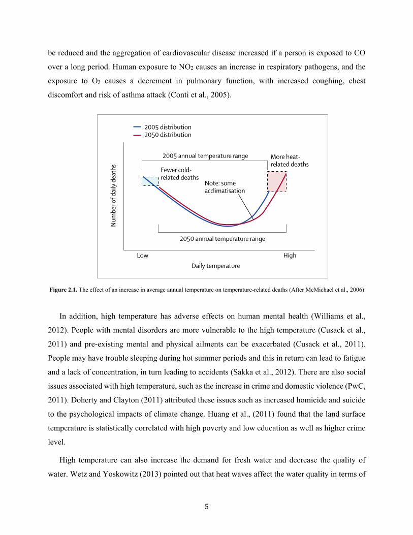
5
be reduced and the aggregation of cardiovascular disease increased if a person is exposed to CO
over a long period. Human exposure to NO2 causes an increase in respiratory pathogens, and the
exposure to O3 causes a decrement in pulmonary function, with increased coughing, chest
discomfort and risk of asthma attack (Conti et al., 2005).
Figure 2.1. The effect of an increase in average annual temperature on temperature-related deaths (After McMichael et al., 2006)
In addition, high temperature has adverse effects on human mental health (Williams et al.,
2012). People with mental disorders are more vulnerable to the high temperature (Cusack et al.,
2011) and pre-existing mental and physical ailments can be exacerbated (Cusack et al., 2011).
People may have trouble sleeping during hot summer periods and this in return can lead to fatigue
and a lack of concentration, in turn leading to accidents (Sakka et al., 2012). There are also social
issues associated with high temperature, such as the increase in crime and domestic violence (PwC,
2011). Doherty and Clayton (2011) attributed these issues such as increased homicide and suicide
to the psychological impacts of climate change. Huang et al., (2011) found that the land surface
temperature is statistically correlated with high poverty and low education as well as higher crime
level.
High temperature can also increase the demand for fresh water and decrease the quality of
water. Wetz and Yoskowitz (2013) pointed out that heat waves affect the water quality in terms of

6
nutrients and organic matter. The degraded water quality will consequently affect human health.
In addition, access to reliable water service presents one of the social risks associated with heat
wave events (Yardley et al., 2011). Extreme heat can lead to damage the urban water infrastructure
such as pipelines, which can interrupt water services. The quality of water, especially drinking
water, affects the health condition of human beings significantly.
The heat–health relationship has been investigated using a wide range of weather metrics such
as temperature, relative humidity, solar radiation, barometric pressure, and wind speed (Barnett et
al., 2010; Zhang et al., 2014). But there is still no universal standard metric for heat exposure.
Furthermore, the impacts of high temperature on human health may vary according to geographical
location (Zhang et al., 2014). Another important factor deserving attention is the consideration of
high temperature in relation to age, gender, education, social, economic and cultural aspects.
The effects of high temperature on mortality is based on data collection and statistical analysis.
Applying the statistical data alone cannot reflect the effects of any adaptation or mitigation
strategies on heat-related health and deaths. Thus, developing a proper approach to estimate the
effects of high temperature and its mitigation strategies will assist the estimation of heat-related
mortality rates. Therefore, to have a proper understanding of the effects of heat wave events and
heat island mitigation strategy on heat-related deaths, a meteorological simulation needs to be
applied. Meteorological simulation deals with complex interactions between the meteorological
parameters (e.g., temperature, wind, moisture, etc.) and urban morphology. Results can be used by
decision-makers to make policies to improve lives of urban dwellers.
The effects of increased surface reflectivity on heat-related mortality has been investigated in a
few studies. Kalkstein et al. (2013) showed that the UHI mitigation strategies in the District of
Columbia contribute to a 7% reduction in the total number of heat-related mortality. The effects of
UHI mitigation strategies were investigated in health-debilitating air masses in four cities across
the US (Detroit, Los Angeles, New Orleans and Philadelphia). The heat-related deaths decreased
by an average of 5 to 10% in these cities (Kalkstein and Sheridan, 2003). The results of another
study by Kalkstein (1999) showed that a 1-2 oC reduction in outdoor temperature could reduce
mortality by 10–20% in Washington.

7
One objective of this dissertation is to investigate the effects of urban heat island and increasing
surface reflectivity on heat-related mortality in the Greater Montreal Area, Canada. The intention
is to apply meteorological simulations to define heat-related mortality correlations.
2.2. Effects of Urban Heat Island and Increasing Surface Reflectivity on Urban
Climate and Air Quality
The urban heat island phenomenon intensifies the effects of meteorological and chemical
parameters in the urban atmosphere. UHI increases the photochemical reaction rates and pollutant
emissions from biogenic and anthropogenic sources. UHI causes an increase in cooling energy
demands, thus producing more pollutants from fossil fuel combustion. In addition, high
temperature leads to smog formation and increased ozone concentrations in urban areas. Ozone has
a close interaction with meteorological parameters (temperature, cloud, radiation, wind speed) as
well as chemical parameters (NOx, CO, VOCs). Ozone is a photochemical pollutant. O3 reactions
take place in the presence of sunlight and involve volatile organic compounds (VOC) and oxides
of nitrogen (NOx). It is formed during daytime and destroyed during the night within complex
chemical reaction chains. The ozone concentration increases during periods with hot, sunny and
calm conditions and thus negatively affects the air quality in urban areas (Seinfeld & Pandis, 2012).
The heat island also intensifies the processes of ozone formation in the urban environment. Thus,
the effects of UHI mitigation strategies on temperature and ozone concentrations need to be
investigated.
The UHI impacts on urban climate and air quality are typically studied through a one-way
approach at local, regional and global scales (Arnfield, 2003; Ban-Weiss et al., 2015; Taha, 2008
and 2009; Salamanca et al., 2012; Li and Bou-Zeid, 2014; Bhati and Mohan, 2016). In these studies,
the interaction between regional atmosphere and local climate is neglected. The one-way approach
cannot simulate the complete interactions between urban climate and air quality. The
meteorological processes and photochemical reactions in the urban atmosphere magnify the UHI
effects. These interactions in the urban environment cause changes in regional climate. The
changes in regional atmosphere affect local pollution. A two-way nested approach provides an
integrated simulation setup to capture the full impacts of meteorological processes and
photochemical interactions in the atmosphere. This approach decreases the uncertainties associated

8
with scale separation and grid resolution. In addition, this method reveals more details of the effects
of surface modifications on urban climate and regional air quality.
Another important factor that affects air quality in urban areas is aerosols. Aerosols affect the
radiative balance of the Earth-Atmosphere system by scattering and absorbing the incoming solar
radiation directly and by influencing cloud formation and precipitation indirectly (IPCC 2013;
Zhang et al., 2014 and 2008). The aerosols impact cloud properties by convective potential energy
such as radiation, relative humidity and wind shear (Fan et al., 2013). The evaporative cooling of
water bodies during daytime is recognized to modulate the influence of aerosols on the processes
of convective systems (Tao et al., 2011). Aerosols also act as cloud condensation nuclei (CCN) and
may impact the life-time, albedo, and precipitation of cloud systems, through a complex interaction
between cloud micro-physics and dynamics (Chen et al., 2011; Archer-Nicholls et al., 2015). There
are two opposite effects of aerosol on cloud formation and precipitation because of aerosol radiative
properties and CCN potentials: aerosols reduce the downward solar radiation to the ground,
decreasing sensible heat fluxes to evaporate water and thus lessening precipitation; or absorbing
solar radiation and gain heat and enhancing the convective clouds formation, thus increasing
precipitation (Kluser et al., 2008; Levin and Brenguier, 2009; Koren et al., 2005; Fan et al., 2013).
But current understanding of aerosol effects on the radiative budget and hydrological cycle of the
climate system is still inadequate at the fundamental level. Some uncertainties also exist in aerosol
estimation because of their heterogeneous distribution and complex interactions with radiation and
clouds in the atmosphere (IPCC AR5, 2013).
Increasing surface albedo results in reflecting more short wave radiation and decreasing air
temperature and photochemical reaction rates (Akbari et al., 2001 and 2009; Arnfield, 2003; Ban-
Weiss et al., 2015; Taha, 2008 and 2009; Taha et al., 2000; Salamanca et al., 2012; Li and Bou-
Zeid., 2014; Bhati and Mohan., 2016). By increasing surface reflectivity (ISR), Taha (2008) found
2 oC decrease in maximum air temperature in urban areas in California. Similar results were found
in Greece (Synnefa et al., 2008) and New York City (Lynn et al., 2009). Taha (2015) found 3 oC
and 5–10 ppb decreases in air temperature and ozone concentrations respectively in Sacramento.
Salamanca and Martilli (2012) have shown that a higher albedo decreases urban temperature by
1.5–2 oC during hot summer days in Madrid. Fallmann et al. (2013 and 2014) showed that
increasing surface albedo led to a decrease in 2-m air temperature and ozone concentrations, by 0.5 oC and 5–8 % respectively, in urban areas of Stuttgart during the 2003 heat wave period. Taha et

9
al. (2015) found that by increasing surface albedo, the air temperature was reduced by 2–3°C in
Sacramento and the ozone concentrations decreased by up to 5–11 ppb during the daytime. The
results of increasing albedo in Houston showed a reduction in temperature by up to 3.5 °C (Taha,
2008).
Few studies have also addressed the effects of albedo enhancement on a global scale. Akbari et
al. (2012) found that by increasing roofs’ (0.25) and pavements’ (0.15) albedos, the total radiative
forcing will decrease by 0.044 Wm-2. Menon et al. (2010) found an increase of 0.5 Wm-2 in total
outgoing radiation over global land area with albedo enhancement in urban areas (0.1). Oleson et
al. (2010) found a decrease of 0.8 to 1.2 oC of urban heat island by increasing roof albedo (0.9).
Most previous studies have used a one-way simulation (climate simulations first, followed by
air quality simulations). This approach does not provide a feedback of the atmospheric pollutants
on the climate. One objective of this dissertation is to develop a two-way nested approach to
simulate the full impacts of meteorological processes and photochemical reactions on urban
climate and air quality. This approach provides an integrated simulation setup to investigate the
effects of UHI and its mitigation strategy over a larger geographical area through urban areas.
Increasing surface albedo may induce impacts on the hydrological cycle and radiative budget in
the atmosphere. Yet, the effect of surface modification on aerosol-radiation-cloud interactions has
not been investigated. Thus, it is necessary to illustrate the effects of heat island mitigation strategy
on aerosols through case studies at different scales with a proper simulation tool. The model is
required to combine the nonlinear effects of aerosols and simulate the interaction of aerosols,
meteorology, chemistry and radiation in a fully interactive manner. Another objective of this
dissertation is to develop an approach to investigate the effects of UHI and albedo enhancement
on aerosols’ direct, semi-direct and indirect effects in the atmosphere and at the surface.
2.3. Meteorological and Photochemical Models to Investigate the Effects of UHI and
ISR on Heat-Related Mortality, Urban Climate and Air Quality
The meteorological and photochemical prediction models have been developed in response to
the increased concerns regarding the effects of urban climate and air quality on human health. To
investigate the effects of urban heat island and increasing surface reflectivity on urban climate, the
NCAR Weather Research and Forecasting Model (WRF) (Skamarock et al., 2005) is applied to
simulate the meteorological processes in the atmosphere. The online WRF is a non-hydrostatic
10
mesoscale numerical weather prediction (NWP) system. Mesoscale models are comprised of many
physical parameterizations (cumulus, microphysics, planetary boundary layer, radiation, and land-
surface) that have been used to predict the weather condition (WRF User Guide, 2014). In addition,
the urban canopy models (UCMs) are used to represent the urban areas for more accurate
estimation of air temperature, wind speed, relative humidity, surface temperature, and shortwave
and longwave radiation. Urban areas are considered as a part of the land-surface parameterization
to predict the heat and moisture fluxes from land to atmosphere.
Analyzing the sensitivity of meteorological parameters (e.g., air temperature, wind speed and
relative humidity) to a different set of parameterizations (i.e., model ensemble) enables researchers
to select the most accurate model platform for urban climate simulations. In previous studies the
effects of UHI and its mitigation strategies have also been investigated applying the WRF model
(Salamanca et al., 2012; Li and Bou-Zeid, 2014; Bhati and Mohan, 2016). Previous efforts in urban
climate simulations are mostly performed using coarse grid cells, because of limitation in
computational resources. In recent years, with further advancement of supercomputers and parallel
processing, an approach with fine-resolution (sub-kilometer) grid cells has become a new trend
(Marta-Almeida et al., 2016; Zheng et al., 2016; Touchaei et al., 2016). The fine-resolution grid
spacing provides more detailed information on the spatial variation of the air temperature; hence,
the selected model ensemble should be compatible with the selected technique. The results of these
simulations are compared with the measurements obtained from weather stations and aircraft
observations. The sensitivity analyses of physical parameters are based on the comparison between
a predicted variable and the observed value from weather stations. The other objective of this
dissertation is to develop an appropriate platform for urban climate simulations and heat island
mitigation strategy.
To investigate the effects of UHI and ISR on air quality, the WRF model needs to be coupled
with a chemistry package (WRF-Chem) to simulate meteorological quantities and air quality
simultaneously (Grell et al., 2005). WRF-Chem has several physical and chemical
parameterizations (Skamarock et al., 2008). The component of air quality is consistent with the
meteorological ones within the same transport scheme, grid and physics schemes, and time steps.
The spatial and temporal aspects of the WRF-Chem application have been analysed in many studies
through one-way approaches, in local, regional or global scales (Ahmadov et al., 2012; Chuang et
al., 2011; Misenis and Zhang, 2010; Zhang et al., 2012; Yahya et al., 2014; Tessum et al., 2015).

11
Another intention is to apply a two-way nested approach in WRF-Chem over a larger geographical
area through regional and local scales such as urban areas. The morphological, thermal, and
micro-scale properties of the urban canopy are considered by coupling WRF-Chem with a multi-
layer of the Urban Canopy Model (ML-UCM) (Martilli et al., 2002).
The WRF-Chem model considers a variety of coupled physical and chemical processes such as
transport, deposition, emission, chemical transformation, aerosol interactions, photolysis and
radiation. Thus, to investigate the effects of UHI and ISR on aerosol-radiation-cloud (ARC)
interactions in the atmosphere, the online-coupled WRF-Chem is applied to provide such
interactive opportunities (Grell et al., 2005, 2013 and 2014). WRF-Chem has been employed in a
wide range of studies and is capable of simulating the interactions among various atmospheric
processes and meteorological components and air quality (Grell and Baklanov, 2011; Baklanov et
al., 2014; Fast et al., 2012; Gao et al., 2011; Qian et al., 2009; Zhang et al., 2010). Saide et al.
(2012) and Yang et al. (2011) evaluated the WRF-Chem simulations of aerosol-cloud-precipitation
interactions over the Southeast Pacific for one month. The comparisons with measurements and
satellite data indicated that the model performed reasonably well in predicting aerosols and clouds.
Fast et al. (2006) investigated the treatment of aerosol optical properties in WRF-Chem and
evaluated the simulation results using data collected during clear sky periods in the 2000 Texas Air
Quality Study. Zhang (2008) applied WRF-Chem over eastern Texas in August 2000 to show that
the presence of aerosols causes a decrease in temperature by up to 0.18 oC near the surface and an
increase by up to 0.16 oC at the top of planetary boundary layer (~30 km). Zhang et al. (2014)
represented a decrease of 0.22–0.59 mm/day in domain-wide mean precipitation over eastern
Texas. Aerosols have a significant impact on climate state (Jacobson, 2002; Chung and Seinfeld,
2005; H. Liao et al., 2009) and future climate changes with regard to mitigation strategies
employment (Brasseur and Roeckner, 2005). The other goal of this dissertation is to investigate
the effects of UHI and ISR on aerosols’ direct (aerosol-radiation), semi-direct (aerosol-cloud), and
indirect (aerosol-radiation-cloud) interactions in the atmosphere.
2.4. Concluding Statement of Literature Review: Effects of Increasing Surface
Reflectivity on Heat-Related Mortality, Urban Climate and Air Quality
This chapter reviewed the literature in several areas that pertain to the topic of the present
research. The research gaps are identified here and addressed further in the following chapters. The
12
conclusions of the literature review with respect to investigations of the effects of increasing
surface reflectivity on heat-related mortality, urban climate and air quality are summarized in the
following statements:
▪ The urban heat island phenomenon has adverse effects on urban climate and air quality. UHI
increases photochemical reaction rates, increases cooling energy demands, endangers human
health and increases heat-related mortality.
▪ Increasing surface reflectivity (ISR) decreases urban temperatures, decreases photochemical
reaction rates, decreases cooling energy demands in buildings during summertime, and
improves air quality and human health and comfort.
▪ The impacts of high temperature on mortality are significant. Yet, there is no correlation
between the effects of heat island and its mitigation strategy on heat-related deaths.
▪ There is a close relation between UHI, urban morphology and atmospheric science. To have a
better understanding of the UHI effects on urban climate and air quality for environmental
policymakers, a proper simulation platform is essential for further simulations and analyses.
▪ Most analyses regarding the effects of UHI and its mitigation strategy have focused on a one-
way simulation approach. Instead, a two-way nested approach is required to capture the full
impacts of meteorological processes and photochemical reactions on urban climate and air
quality.
▪ The effects of urban heat island and increasing surface albedo have not been investigated on
aerosol interactions, radiative budget and hydrological cycle of the climate system. Thus, a
simulation approach is required to combine these nonlinear effects of aerosols and to simulate
the aerosols-radiation-cloud interactions in the atmosphere in a fully interactive manner.
The applied methodology and simulation approaches to address the objectives of this thesis are
presented in Chapter 3.

13
Chapter 3 Methodology
The main objectives of this dissertation are to investigate the effects of increasing surface
reflectivity on urban climate, air quality and heat-related mortality. These objectives are
accomplished by the following tasks:
• developing a platform for urban climate simulation and heat island mitigation
strategy;
• investigating the effects of urban heat island and its mitigation strategy on heat-
related mortality;
• developing a two-way nested simulation approach to assess the effects of urban heat
island and increasing surface reflectivity on urban climate and air quality; and
• investigating the effects of heat island and increasing surface albedo on aerosol-
radiation-cloud interactions.
Section 3.1 introduces the simulation approaches to achieve these tasks including: meteorological
and photochemical models, a setup procedure, preparation to perform simulations, and evaluation
of model performance. Section 3.2 explains applied methodology to develop an appropriate
platform for urban climate simulation and heat island mitigation strategy. Section 3.3. addresses
the approaches to estimate the effects of increasing urban albedo on heat-related mortality. Section
3.4. describes the methods to investigate the effects of increasing solar reflectance on urban climate
and air quality within a two-way nested simulation approach. Section 3.5 provides the procedure
to estimate the effects of increasing surface albedo on aerosol-radiation-cloud interactions in the
atmosphere.

14
3.1. Meteorological and Photochemical Simulations
Meteorological models use surface characteristics (land use / land cover) and initial and
boundary conditions to solve a set of conservation equations, simulate the advection and diffusion
of pollutants, and predict meteorological conditions (namely air temperature, moisture, wind speed,
etc.). Photochemical models use the meteorological conditions and air pollutants’ emission
estimations (from biogenic and anthropogenic sources) to simulate emission, transformation and
dispersion of pollutants and predict air quality conditions (namely ozone, nitrogen dioxide, carbon
monoxide, etc.). Figure 3.1. shows the meteorological and photochemical models’ interactions.
Figure 3.1. Meteorological and photochemical models’ interactions (LULC= Land Use/Land Cover)
3.1.1. Simulation Models: WRF, WRF-Chem, ML-UCM The online Weather Research and Forecasting model (WRF) considers a variety of
meteorological and physical parameterizations (cumulus, microphysics, planetary boundary layer,
radiation, and land-surface) to predict weather conditions. The WRF is a mesoscale numerical
weather prediction (NWP) system which is fully compressible (deals with flows having significant
changes in fluid density) and non-hydrostatic (the vertical momentum equation is solved). WRF
can be coupled with chemical parameterizations (Chem) to simulate the meteorological quantities
and air pollution concentrations simultaneously (Grell et al., 2005). Coupling the WRF with a
chemistry package enables researchers to simulate chemical processes (transport, deposition,
emission, chemical transformation, aerosol interactions, photolysis and radiation) to predict air
quality conditions. The component of air quality is consistent with the meteorological components
within the same transport scheme, grid and physics schemes, and time steps. In addition, the multi-
layered Urban Canopy Model (ML-UCM) can be coupled with the meteorological and
photochemical models. The ML-UCM is a part of the land-surface parameterization to predict the
Surface characteristics (LULC, moisture, ...)
Initial and boundary conditions
Emission inventories (anthropogenic & biogenic sources)
Meteorological model (simulate advection & diffusion)
Predict meteorological conditions
Photochemical model (simulate emission, transformation & dispersion)
Predict air quality conditions
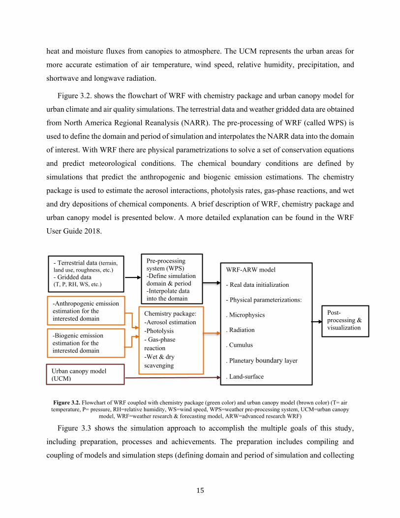
15
heat and moisture fluxes from canopies to atmosphere. The UCM represents the urban areas for
more accurate estimation of air temperature, wind speed, relative humidity, precipitation, and
shortwave and longwave radiation.
Figure 3.2. shows the flowchart of WRF with chemistry package and urban canopy model for
urban climate and air quality simulations. The terrestrial data and weather gridded data are obtained
from North America Regional Reanalysis (NARR). The pre-processing of WRF (called WPS) is
used to define the domain and period of simulation and interpolates the NARR data into the domain
of interest. With WRF there are physical parametrizations to solve a set of conservation equations
and predict meteorological conditions. The chemical boundary conditions are defined by
simulations that predict the anthropogenic and biogenic emission estimations. The chemistry
package is used to estimate the aerosol interactions, photolysis rates, gas-phase reactions, and wet
and dry depositions of chemical components. A brief description of WRF, chemistry package and
urban canopy model is presented below. A more detailed explanation can be found in the WRF
User Guide 2018.
Figure 3.2. Flowchart of WRF coupled with chemistry package (green color) and urban canopy model (brown color) (T= air temperature, P= pressure, RH=relative humidity, WS=wind speed, WPS=weather pre-processing system, UCM=urban canopy
model, WRF=weather research & forecasting model, ARW=advanced research WRF)
Figure 3.3 shows the simulation approach to accomplish the multiple goals of this study,
including preparation, processes and achievements. The preparation includes compiling and
coupling of models and simulation steps (defining domain and period of simulation and collecting
- Terrestrial data (terrain, land use, roughness, etc.) - Gridded data (T, P, RH, WS, etc.)
Pre-processing system (WPS) -Define simulation domain & period -Interpolate data into the domain
WRF-ARW model
- Real data initialization
- Physical parameterizations:
. Microphysics
. Radiation
. Cumulus
. Planetary boundary layer
. Land-surface
Post-processing & visualization
-Anthropogenic emission estimation for the interested domain
Urban canopy model (UCM)
Chemistry package: -Aerosol estimation -Photolysis - Gas-phase reaction -Wet & dry scavenging
-Biogenic emission estimation for the interested domain

16
input data and measurements data). The processes refer to WRF, WRF-Chem, UCM simulations,
and anthropogenic and biogenic emission estimations. In addition, data analysis is a main part of
the process, including comparing the simulation results with measurements and comparing
different scenarios. The consequences of these approaches are to: 1) develop a platform for urban
climate simulations and heat island mitigation strategy; 2) develop an algorithm to estimate heat-
related mortality; 3) provide a two-way nested approach to simulate urban climate and air quality;
4) define an approach to estimate the effects of surface modification on aerosol-radiation-cloud
interactions in the atmosphere. These procedures are explained in the following figure.
Figure 3.3. Simulation approaches: preparation, processes and achievements (WPS=weather pre-processing system, WRF=weather research & forecasting model, WRF with chemistry=WRF-Chem, UCM=urban canopy model, US-NEI11=United
States National Emission Inventory 2011, MEGAN= Model of Emissions of Gases and Aerosols from Nature, CTRL=control case, ALBEDO= albedo enhancement, ISR=increasing surface reflectivity)
3.1.2. Preparation of Simulation Models and Requirements 3.1.2.1. Compiling and Coupling of Simulation Models
WRF simulations require significant preparation and computer resources. At the onset, one
should make sure that the computer has sufficient memory capacity and a fast processing system
Achievements
Simulation models: Compiling & coupling WPS, WRF, Chem, UCM, US-NEI11, MEGAN
Simulation requirements: - Define simulation domain and period - Collect input data for each simulation - Collect measured data from weather and air quality monitoring stations for each simulation
Preparation
- Simulate base case scenario - Simulate ISR scenario
- Extract the simulations` data - Compare simulations with measurements - Compare CTRL & ALBEDO results
Processes
- Choice of proper physical options - Choice of proper chemical options -Simulation of US-NEI11 -Simulation of MEGAN
Simulation Data analysis
Develop
specific
approach
for each
objective
Develop a platform for urban climate simulations and heat island mitigation strategy (1st Objective)
Develop an algorithm to estimate heat-related mortality (2nd Objective)
Provide a two-way nested approach to simulate urban climate & air quality (3rd Objective)
Define an approach to estimate the interaction of aerosol-radiation-cloud (4th Objective)

17
in order to compile, couple and carry out various simulations in a timely manner. Here, the North
America-caluculquebec cluster is used to perform each simulation. The first step to start
simulations is to compile and couple the WRF Preprocessing System (WPS), WRF Data
Assimilation (WRF-DA) and Advanced Research WRF Solver (ARW-WRF).
➢ WRF Preprocessing System (WPS)
This program is used primarily for real-data simulations. Its functions include: 1) defining
simulation domains; 2) interpolating terrestrial data (such as terrain, land use, and soil types) to the
simulation domain; and 3) interpolating meteorological data to the simulation domain.
➢ WRF Data Assimilation (WRF-DA)
This program is used to inject observations into the interpolated analyses created by WPS. It can
also be used to update the WRF model's initial conditions when the model is run in cycling mode.
It is based on an incremental variational data assimilation technique and has both 3D-Var and 4D-
Var capabilities.
➢ Advanced Research WRF Solver (ARW-WRF)
This is the key component of the modeling system, which is composed of several initialization
programs for real-data simulations. The key features of the WRF model include: fully
compressible, nonhydrostatic equations with hydrostatic option; 2) regional and global
applications; 3) mass-based terrain-following coordinates; 4) vertical grid-spacing which can vary
with height; 5) Runge-Kutta 2nd and 3rd order time integration options; 6) scalar-conserving flux
form for prognostic variables; 7) 2nd to 6th order advection options (horizontal and vertical); 8)
monotonic transport and positive-definite advection option for moisture, scalar, tracer, and TKE
(Turbulent Kinetic Energy); and 9) full physics options for land-surface, planetary boundary layer,
atmospheric and surface radiation, microphysics and cumulus convection. Figure 3.4 shows the
steps to compile and run WPS and WRF. Table 3.1 summarizes the description of these steps.

18
Figure 3.4. Steps to compile and run the WPS and WRF models
Table 3.1. Description of the steps to compile and run the WPS and WRF models
Steps to compile & run WPS & WRF models Description System environment tests It is important to have required compiler as gfortran. The WRF build system
has scripts as the top level for the user interface as well. Building libraries
There are various libraries that should be installed for example netcdf and Jasper. These libraries must be installed with the same compilers as will be used to install WRF and WPS.
Library compatibility tests These tests are essential to verify that the libraries are able to work with the compilers that are to be used for the WPS and WRF builds.
Building WRFV3 After ensuring that all libraries are compatible with the compilers, one can now prepare to build WRFV3. First, the tar file should be downloaded from verified source and unpacked in the preferred directory. Then, a configuration file should be created to compile. The compiler is selected to be serially or in parallel.
Building WPS
After building the WRF model, WPS program needs to be built. A tar file containing the WPS source code, is downloaded and unpacked. Then the WPS is compiled to be compatible with WRF. If the compilation is successful, there should be three executables in the WPS top-level directory, that are linked to their corresponding directories.
Static geography data
To initiate a real-data case, the domain's physical location on the globe and the static information for that location must be created. This requires a data set that includes such fields as topography and land use categories. These data need to be downloaded and un-compressed.
Real-Time data
For real-data cases, the WRF model requires up-to-date meteorological information for both an initial condition and lateral boundary conditions. This meteorological data is traditionally a file that is provided by a previously run external model or analysis. For a semi-operational set-up, the meteorological data is usually sourced from a global model, which permits locating the WRF model's domains anywhere on the globe. The National Centers for Environmental Prediction (NCEP) run the Global Forecast System (GFS) model four times daily.
Run WPS & WRFV3
First, the WPS is executed by modifying its name-list to reflect information that is required for the particular simulation. The geogrid will match the geographical data and define the simulation domain. The ungird unpack necessary data regarding the simulation period. The met-gird interpolate the weather and terrestrial data on the domain of interest. To simulate the WRF, the name-list needs to be modified. The data provided by WPS, should be connected and linked to the run directory.
System environment tests
Building libraries
Library compatibility tests
Static geography data
Real-time data Building WPS
Building WRF
Run WPS & WRFV3
19
➢ System Environment Tests
It is important to have “gfortran”, “gcc” and “cpp” compilers. In addition to the compilers required
to manufacture the WRF executables, the WRF build system has scripts as the top level for the user
interface—namely, “csh”, “perl”, and “sh”.
➢ Building Libraries
There are various libraries that should be installed including: “mpich”, “netcdf”, “Jasper”, “libpng”,
and “zlib”. These libraries must be installed with the same compilers as will be used to install WRF
and WPS.
➢ Library Compatibility Tests
Once the target machine is able to make “Fortran” and “C” executables, after the “NetCDF” and
“MPI” libraries are constructed, two additional small tests are required to emulate the WRF code's
behavior. It is essential to verify that the libraries are able to work with the compilers that are to be
used for the WPS and WRF builds. These tests are for “Fortran+ C+ NetCDF” and “Fortran + C +
NetCDF + MPI”.
➢ Building WRFV3
After ensuring that all libraries are compatible with the compilers, one can now prepare to build
WRFV3. First, the tar file should be downloaded from a verified source (NCAR) and unpacked in
the preferred directory. Then, a configuration file should be created to compile. The compiler is
selected to be serial or in parallel. For parallel, which is for real case simulations, there are three
options: “smpar”, “dmpar” and “dm+sm”. The “dmpar” is the best option; it has fewer errors and
is more compatible with other programming languages. To check whether it was successful, the
executable files—namely, “wrf.exe”, “real.exe”, “ndown.exe”, and “tc.exe”—need to be checked.
➢ Building WPS
After building the WRF model, WPS program needs to be built. A tar file containing the WPS
source code is downloaded and unpacked. Then the WPS is compiled to be compatible with WRF.
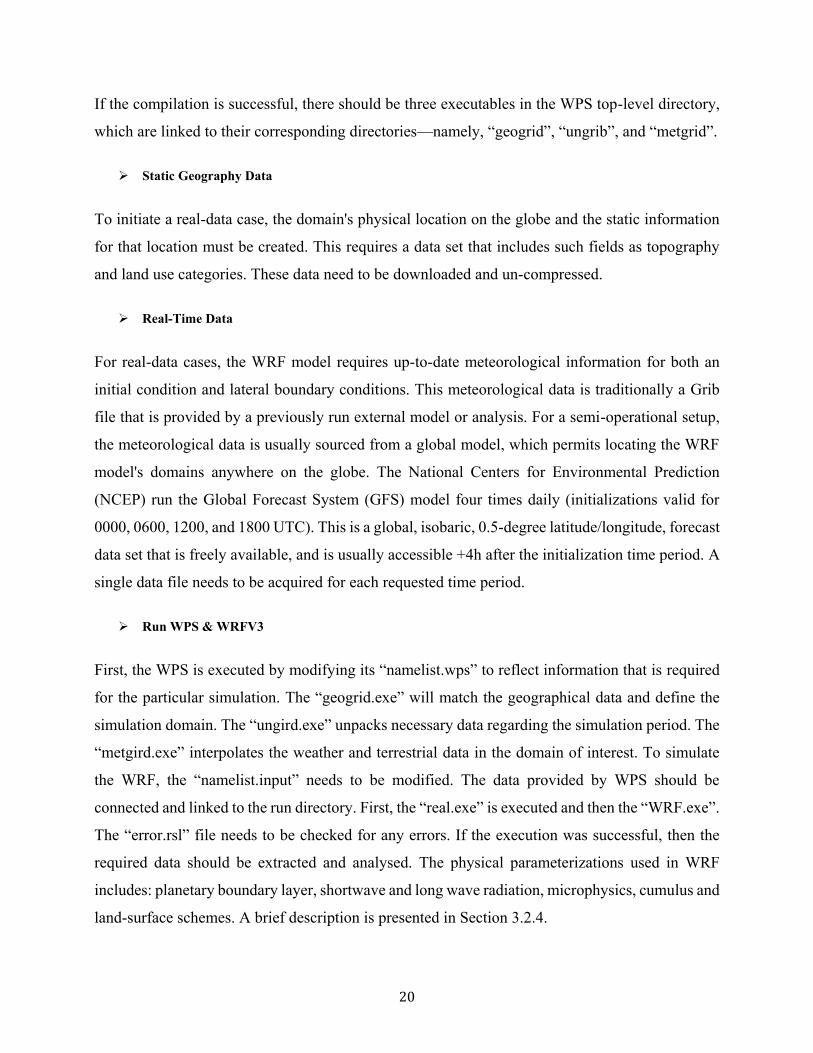
20
If the compilation is successful, there should be three executables in the WPS top-level directory,
which are linked to their corresponding directories—namely, “geogrid”, “ungrib”, and “metgrid”.
➢ Static Geography Data
To initiate a real-data case, the domain's physical location on the globe and the static information
for that location must be created. This requires a data set that includes such fields as topography
and land use categories. These data need to be downloaded and un-compressed.
➢ Real-Time Data
For real-data cases, the WRF model requires up-to-date meteorological information for both an
initial condition and lateral boundary conditions. This meteorological data is traditionally a Grib
file that is provided by a previously run external model or analysis. For a semi-operational setup,
the meteorological data is usually sourced from a global model, which permits locating the WRF
model's domains anywhere on the globe. The National Centers for Environmental Prediction
(NCEP) run the Global Forecast System (GFS) model four times daily (initializations valid for
0000, 0600, 1200, and 1800 UTC). This is a global, isobaric, 0.5-degree latitude/longitude, forecast
data set that is freely available, and is usually accessible +4h after the initialization time period. A
single data file needs to be acquired for each requested time period.
➢ Run WPS & WRFV3
First, the WPS is executed by modifying its “namelist.wps” to reflect information that is required
for the particular simulation. The “geogrid.exe” will match the geographical data and define the
simulation domain. The “ungird.exe” unpacks necessary data regarding the simulation period. The
“metgird.exe” interpolates the weather and terrestrial data in the domain of interest. To simulate
the WRF, the “namelist.input” needs to be modified. The data provided by WPS should be
connected and linked to the run directory. First, the “real.exe” is executed and then the “WRF.exe”.
The “error.rsl” file needs to be checked for any errors. If the execution was successful, then the
required data should be extracted and analysed. The physical parameterizations used in WRF
includes: planetary boundary layer, shortwave and long wave radiation, microphysics, cumulus and
land-surface schemes. A brief description is presented in Section 3.2.4.

21
➢ Run WPS & WRFV3
First, the WPS is executed by modifying its “namelist.wps” to reflect information that is required
for the particular simulation. The “geogrid.exe” will match the geographical data and define the
simulation domain. The “ungird.exe”, unpack necessary data regarding the simulation period. The
“metgird.exe”, interpolate the weather and terrestrial data on the domain of interest. To simulate
the WRF, the “namelist.input” needs to be modified. The data provided by WPS, should be
connected and linked to the run directory. First, the “real.exe” is executed and then the “WRF.exe”.
The “error.rsl” file needs to be checked for any errors. If the execution was successful, then the
required data should be extracted and analysed. The physical parameterizations used in WRF
includes: planetary boundary layer, shortwave and long wave radiation, microphysics, cumulus and
land-surface schemes. A brief description is presented in section 3.2.4.
3.1.2.2. Coupling the WRF with the Urban Canopy Model (UCM)
Urban Canopy Models (UCMs) can provide more accurate feedbacks on urban areas for surface
layer and planetary boundary layer schemes. There are three types of UCMs within WRF: slab
(bulk), single-layer (SL), and multi-layer (ML). The urban canopy model consists of sensible heat
fluxes from roofs, walls and roads and aggregates them into the exchange of momentum and energy
between the urban surface and atmosphere. Surface temperatures are calculated from the upward
long wave radiation. Wind shear calculations allow for increased roughness, shadowing from
buildings and characteristic radioactive properties within street canyons. Thermal properties of
building materials and anthropogenic heat generated by human activities are considered as well
(Chen et al., 2011).
A multi-layer of the urban canopy model (ML-UCM) represents the 3-dimentional nature of
urban surfaces and interacts with the planetary boundary layer. In the ML-UCM, the effects of
walls (as vertical surfaces) and roofs and roads (as horizontal surfaces) are considered in terms of
momentum, turbulent kinetic energy and potential temperature.
3.1.2.3. Compiling and Coupling the Chemistry Package with WRF
The chemistry package is downloaded from NCAR and unpacked in the “run” directory of
WRF. The “GFortran”, “C” and “NetCDF” programming languages are used to compile the
chemistry package with the solver of the WRF. The air quality component of the model is fully
consistent with the meteorological component, having the same transport, grid, and physics

22
schemes with the same time steps. WRF-Chem considers a variety of chemical processes including
dry deposition, aerosol and photolysis estimations. Dry deposition is defined based on the surface
of the soil and the plants’ resistances and is simulated within suitable schemes in WRF-Chem. The
surface resistance depends on the diffusion coefficient, the reactivity, and water solubility of the
reactively trace gas. By changing the land use input data, these schemes have to be adapted
accordingly. To estimate the photolysis rate, the Fast-J model in the chemistry package is an
accurate and fast algorithm to evaluate the effect of cloud, aerosol and ozone on photolysis rate
(Wild et al., 2000). The model solves the multi-reflection in the atmosphere using exact scattering
phase function and optical depths to predict the photolytic intensities. For model stability, wet
scavenging, cloud chemistry, sub-grid aqueous chemistry, and aerosols radiation feedback need to
be activated in the solver of WRF-Chem.
➢ Emission Estimations
Modeling of the chemical composition of the atmosphere requires preliminary information
about initial emissions of chemical compounds within the modeling domain. Emission inventories
describe the amount of pollutants discharged into the atmosphere. For anthropogenic emission
estimation, the United States National Emission Inventory for 2011 (US-NEI-11) is used. The US-
NEI-11 is installed. The simulation domain and episode are defined by modifying its name-list file.
The US-NEI contains the anthropogenic emission for the contiguous 48 states of the US, southern
Canada and northern Mexico in 4-km spatial resolution. This inventory is designed for regional
scale and photochemical models that require emission data for NOx, VOC, CO, SO2, NH3, PM2.5,
and PM10. Emissions have been split into point and area sources. The model results are then
transferred to the programming language that can be read by the solver of the WRF-Chem. Figure
3.5 shows the steps to estimate the anthropogenic emissions with NEI-2011.
Figure 3.5. The US-NEI11 simulation approach to estimate anthropogenic emissions
NEI-2011 data
Emiss-v04.F Convert-emiss.exe WRF-Chem
Define simulation domain and period
(Zipped ASCII files) (Binary files) WRF NETCDF files
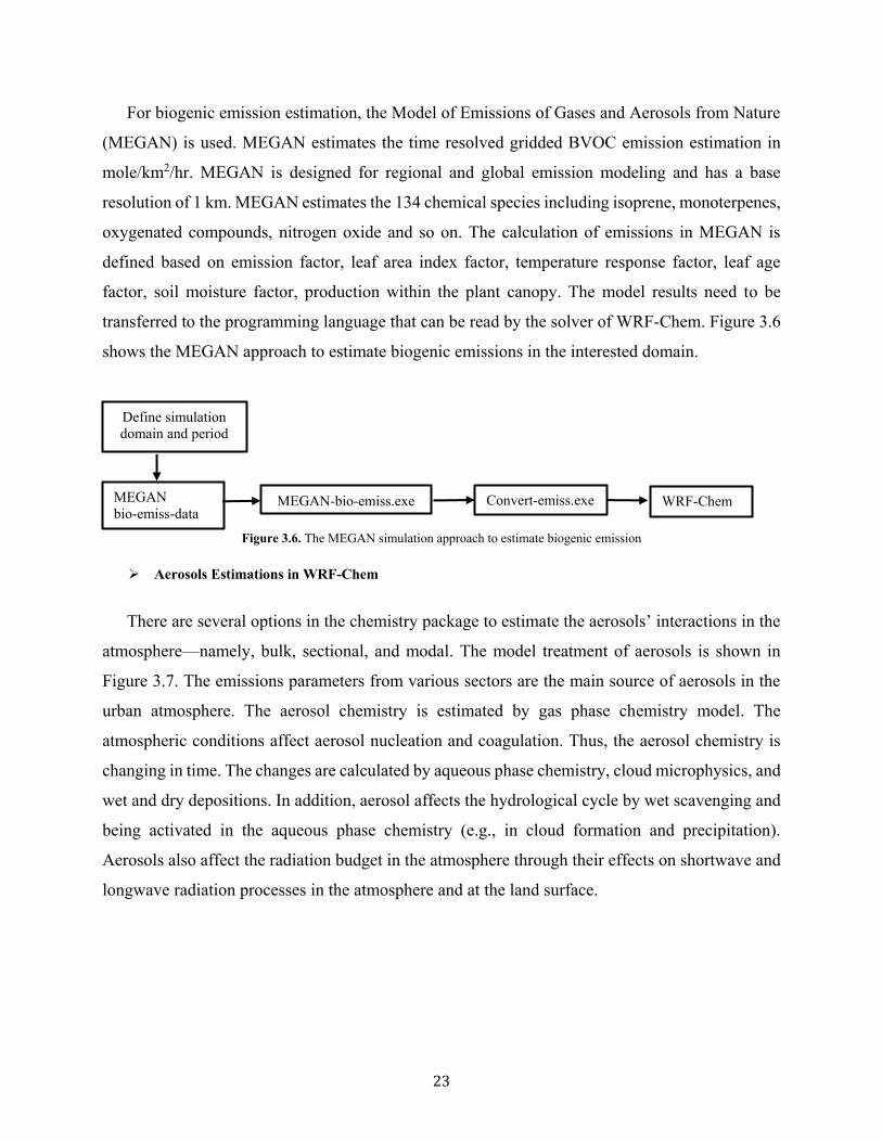
23
For biogenic emission estimation, the Model of Emissions of Gases and Aerosols from Nature
(MEGAN) is used. MEGAN estimates the time resolved gridded BVOC emission estimation in
mole/km2/hr. MEGAN is designed for regional and global emission modeling and has a base
resolution of 1 km. MEGAN estimates the 134 chemical species including isoprene, monoterpenes,
oxygenated compounds, nitrogen oxide and so on. The calculation of emissions in MEGAN is
defined based on emission factor, leaf area index factor, temperature response factor, leaf age
factor, soil moisture factor, production within the plant canopy. The model results need to be
transferred to the programming language that can be read by the solver of WRF-Chem. Figure 3.6
shows the MEGAN approach to estimate biogenic emissions in the interested domain.
Figure 3.6. The MEGAN simulation approach to estimate biogenic emission
➢ Aerosols Estimations in WRF-Chem
There are several options in the chemistry package to estimate the aerosols’ interactions in the
atmosphere—namely, bulk, sectional, and modal. The model treatment of aerosols is shown in
Figure 3.7. The emissions parameters from various sectors are the main source of aerosols in the
urban atmosphere. The aerosol chemistry is estimated by gas phase chemistry model. The
atmospheric conditions affect aerosol nucleation and coagulation. Thus, the aerosol chemistry is
changing in time. The changes are calculated by aqueous phase chemistry, cloud microphysics, and
wet and dry depositions. In addition, aerosol affects the hydrological cycle by wet scavenging and
being activated in the aqueous phase chemistry (e.g., in cloud formation and precipitation).
Aerosols also affect the radiation budget in the atmosphere through their effects on shortwave and
longwave radiation processes in the atmosphere and at the land surface.
MEGAN bio-emiss-data
MEGAN-bio-emiss.exe Convert-emiss.exe WRF-Chem
Define simulation domain and period

24
Figure 3.7. Model treatment of aerosol estimations and interactions with other physical and chemical options in WRF-Chem
3.1.2.5. Preparation of Simulation Requirements
For each objective, the simulation domain and period are different, thus the input data differ
also. The simulations are conducted with the initial and boundary conditions obtained from the
North American Regional Reanalysis (NARR) for the specific domain and episode. These data are
then interpolated to the domain of interest by simulating WPS. The evaluation of the model
performance is conducted by comparing the simulation results with measurements obtained from
weather and air-quality monitoring stations across the domain. A more detailed explanation
regarding each objective follows.
3.1.3. Simulations Scenarios and Evaluation of Model Performance 3.1.3.1. Simulations of Control Case and Increasing Surface Reflectivity
Two sets of simulations are conducted with different scenarios for each objective: the base case
condition that the albedo of roofs, walls, and roads are assumed to be 0.2 (hereafter referred to as
CTRL); and the increasing surface reflectivity scenario where the albedo of roofs, walls, and roads
is increased (hereafter referred to as ALBEDO). The changes to gridded ALBEDO can be
calculated as: surface albedo enhancement (roofs, walls, and roads) × fraction of urban area per
grid cell.
Three different urban categories are defined within WRF urban canopy models. Low-intensity
residential (class 31) includes areas with a mixture of built-up structures and vegetation (for 20–
70% of land cover). High-intensity residential areas (class 32) have vegetation coverage under
Gas Phase Chemistry Aerosol microphysics
Dry deposition Emissions
Aerosol nucleation
Aerosol chemistry
Aqueous phase chemistry
Cloud microphysics, wet deposition
Radiative transfer

25
20%. Industrial/commercial areas (class 33) include infrastructure and highly developed areas not
classified as residential (USGS 2014). To investigate the effects of albedo enhancement, the albedo
of roofs, walls, and roads are increased from 0.2 to 0.65, 0.60, and 0.45, respectively. The αR, αW
and αG represent surface albedo of roofs, walls, and roads, respectively, and are modified in the
URBPARM.TBL. Table 3.2 is located in the “run” directory of the WRF and represents urban
canopy parameters. The changes are shown in bold. With these modifications, the effects of
increasing surface reflectivity are investigated on urban climate and air quality in a specific domain
and period of simulation by comparing the ALBEDO results with the CTRL results.
Table 3.2. urban canopy parameters in URBPARM.TBL in WRFV3.6.1
Parameters
Unit
Specific value for Low-intensity residential
High-intensity residential
Industrial /commercial
𝐹𝑢𝑟𝑏(Urban Fraction) Fraction 0.5 0.9 0.95 𝐶𝑅 & 𝐶𝑊 (Heat Capacity of Roof & Wall) J m-3 K-1 1.0E6 1.0E6 1.0E6 𝐶𝐺 (Heat Capacity of Ground) J m-3 K-1 1.4E6 1.4E6 1.4E6 𝜆𝑅 & 𝜆𝑊 (Thermal Conductivity of Roof & Wall) J m-1s-1 K-1 0.67 0.67 0.67 𝜆𝐺 (Thermal Conductivity of Ground) J m-1s-1 K-1 0.4004 0.4004 0.4004 𝜶𝑹 (Surface Albedo of Roof) Fraction 0.65 0.65 0.65 𝜶𝑾 (Surface Albedo of Wall) Fraction 0.60 0.60 0.60 𝜶𝑮 (Surface Albedo of Ground) Fraction 0.45 0.45 0.45 𝜀𝑅 & 𝜀𝑊(Surface Emissivity of Roof & Wall) - 0.90 0.90 0.90 𝜀𝐺 (Surface Emissivity of Ground) - 0.95 0.95 0.95 𝑍0𝑅 & 𝑍0𝐺 (Roughness Length for momentum over Roof & Ground)
m 0.01 0.01 0.01
𝑍0𝑊 (Roughness Length for momentum- Wall) m 0.0001 0.0001 0.0001 PWIN (Coverage area fraction of windows in the walls of the buildings)
- 0.2 0.2 0.2
BETA (Thermal efficiency of heat exchanger) - 0.75 0.75 0.75 Air Conditioning Switch (On=1) 1 1 1 COP (Coefficient of performance of AC conditioning) - 3.5 3.5 3.5 TARGTEMP (Target T of AC systems) K 297 298 298 GAPTEM (Comfort range of indoor temperature) K 0.5 0.5 0.5 TARGHUM & GAPHUM (Target & Comfort humidity of AC systems)
kg/kg 0.005 0.005 0.005
HSEQUIP_SCALE_FACTOR (Peak Heat Generated by Equipment)
W/m2 36 20 16
3.1.3.2. Evaluation of Model Performance
The performance and accuracy of the simulation results are quantitatively based on a series of
metrics estimations (Boylan and Russell, 2006). The mean bias error (MBE), mean absolute error
(MAE), and the root mean square error (RMSE) of the meteorological parameters are calculated.
Mean bias error (MBE) is the indication of underestimation (negative value) or overestimation
(positive value) of the predicted meteorological variables compared to the measurements (Eq. 1).

26
Mean absolute error (MAE) represents the absolute error in simulation and is known as a natural
metric to evaluate the performance of a model (Walcott, 2005) (Eq. 2). Root mean square error
(RMSE) is a more rigorous indicator for model assessment (Eq. 3).
𝑀𝐵𝐸 = 1
𝑁∑(𝐶𝑀 − 𝐶𝑂)
𝑁
1
(Eq. 1)
𝑀𝐴𝐸 = 1
𝑁∑ |𝐶𝑀 − 𝐶𝑂|𝑁
1
(Eq. 2)
𝑅𝑀𝑆𝐸 = √∑ (𝐶𝑀 − 𝐶𝑂)2𝑁
1
𝑁
(Eq. 3)
Where CM and CO are modelled and observed data, and N is the number of model and observation
pairs in hours.
3.2. Develop a Platform for Urban Climate Simulation and Heat Island Mitigation
Strategy
Parameterization is a simple way of representing physical processes such as cloud formation
and precipitation. Mesoscale models are comprised of many parameterizations that are used for
predicting the weather condition. The model ensemble for urban climate simulation includes
parameterizations for microphysics, cumulus, planetary boundary layer (PBL), radiation, land
surface, and urban canopy. Characterizing the meteorological parameters (e.g., air temperature,
wind speed, relative humidity and precipitation) to a different set of parameterizations (i.e., model
ensemble) enables researchers to select the proper model platform for urban climate simulations.
Figure 3.8 shows the simulation approach to accomplish this objective. A brief description is
presented for each step in the following sections. Box A refers to explanations in Section 3.1.2, and
box B shows the accomplishments and endpoints of this objective.

27
Figure 3.8. The simulation approach to prepare an appropriate platform for urban climate assessment (ISR=increasing surface reflectivity, HRM= heat-related mortality, CTRL= base case simulations, ALBEDO= increasing urban albedo)
3.2.1. Defining Simulation Domain and Period The simulation domain is the Greater Montreal Area (GMA) that is centered at the ~45.5ºN and
~73.6ºW. The horizontal domain of the simulations is composed of four two-way nested domains
with 37×22, 43×34, 91×61, and 145×91 grid points, and a grid sizes of 9, 3, 1 and 0.333 km × km,
respectively. The vertical coordinate eta is calculated by ((P − Ptop)/ (Psurf − Ptop); where P is the dry
hydrostatic pressure at each corresponding level, Psurf is dry hydrostatic surface pressure, and Ptop
is a constant dry hydrostatic pressure at model top). The vertical resolution includes 51 vertical
layers from the surface to a fixed pressure of ~100 mb (~16 km AGL). The selected simulation
period starts with a clear sky condition (9th of August) and ends with a rainy condition (11th of
August). The summer days are selected because results are used to evaluate the effect of urban heat
island mitigation strategy (increasing surface reflectivity). Figure 3.9 shows the simulation
domains based on USGS land use categories.
B
B
A - Compiling the WPS, WRF, UCM - Coupling ML-UCM with WRF
Parametric simulations of physical options (CTRL scenario)
Investigate the effects of ISR on urban climate
Collect field data form weather stations for verification
Define simulation domain and period Prepare input data
Parametric simulations of physical options (ALBEDO scenario)
Compare the simulation results with measurements
Develop an appropriate platform for urban climate simulations
Applying this platform to investigate the effects of ISR on HRM
Outcome Preparation Processes
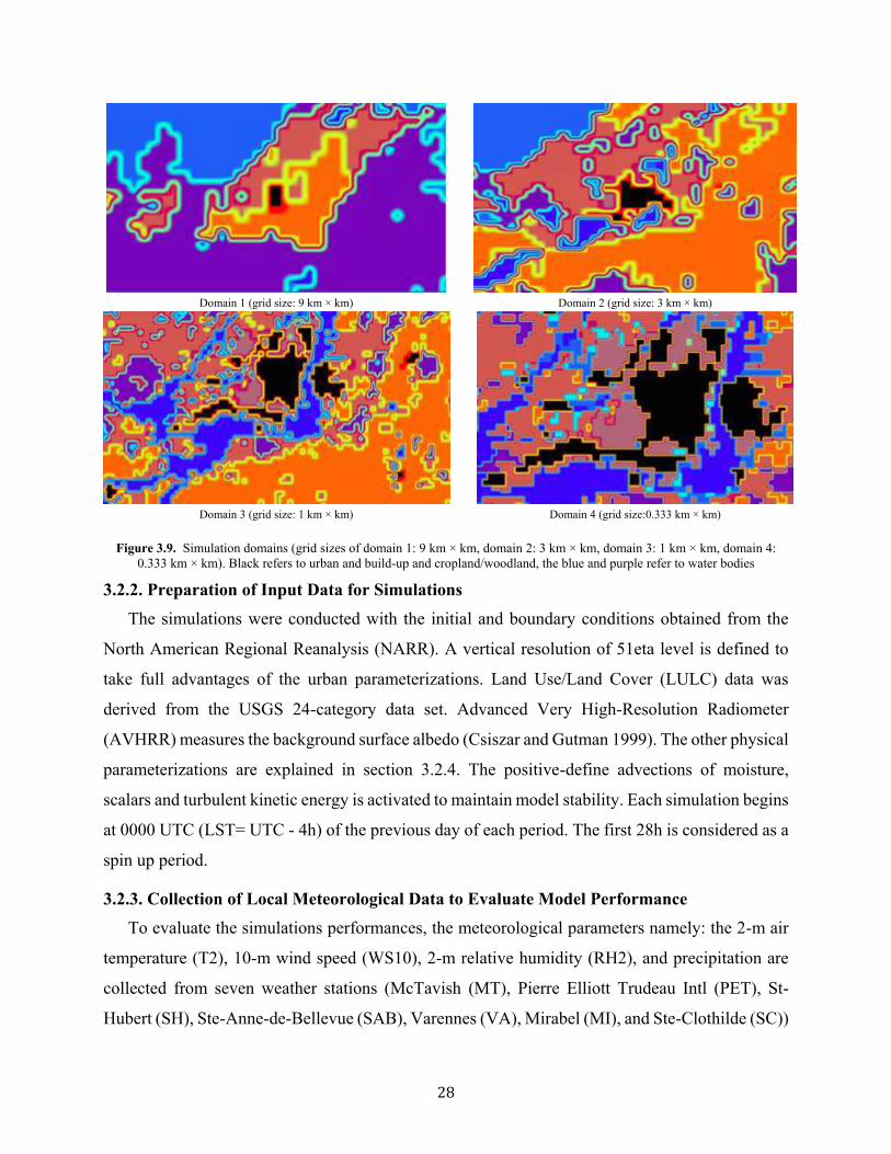
28
Domain 1 (grid size: 9 km × km) Domain 2 (grid size: 3 km × km)
Domain 3 (grid size: 1 km × km) Domain 4 (grid size:0.333 km × km)
Figure 3.9. Simulation domains (grid sizes of domain 1: 9 km × km, domain 2: 3 km × km, domain 3: 1 km × km, domain 4:
0.333 km × km). Black refers to urban and build-up and cropland/woodland, the blue and purple refer to water bodies
3.2.2. Preparation of Input Data for Simulations The simulations were conducted with the initial and boundary conditions obtained from the
North American Regional Reanalysis (NARR). A vertical resolution of 51eta level is defined to
take full advantages of the urban parameterizations. Land Use/Land Cover (LULC) data was
derived from the USGS 24-category data set. Advanced Very High-Resolution Radiometer
(AVHRR) measures the background surface albedo (Csiszar and Gutman 1999). The other physical
parameterizations are explained in section 3.2.4. The positive-define advections of moisture,
scalars and turbulent kinetic energy is activated to maintain model stability. Each simulation begins
at 0000 UTC (LST= UTC - 4h) of the previous day of each period. The first 28h is considered as a
spin up period.
3.2.3. Collection of Local Meteorological Data to Evaluate Model Performance To evaluate the simulations performances, the meteorological parameters namely: the 2-m air
temperature (T2), 10-m wind speed (WS10), 2-m relative humidity (RH2), and precipitation are
collected from seven weather stations (McTavish (MT), Pierre Elliott Trudeau Intl (PET), St-
Hubert (SH), Ste-Anne-de-Bellevue (SAB), Varennes (VA), Mirabel (MI), and Ste-Clothilde (SC))

29
across the Greater Montreal Area for the 9th to 11th of August 2009. Figure 3.10 and Table 3.3
present their geographical locations.
Figure 3.10. The location of weather stations in Greater Area of Montreal
Table 3.3. Weather stations in Greater Montreal Area with their locations (Latitude, Longitude, and Elevation) Signs Station Name Station Code Latitude (N) Longitude (W) Elevation (m)
McTavish MT 45.50 -73.58 73 Pierre Elliott Trudeau PET 45.47 -73.75 36
St-Hubert SH 45.52 -73.42 27
Ste-Anne-de-Bellevue SAB 45.42 -73.92 39
Varennes VA 45.72 -73.38 18
Mirabel MI 45.67 -74.03 82
Ste-Clothilde SC 45.17 -73.68 53
3.2.4. Parametric Simulations of Physical Options The physical parameterizations need to be carefully selected to predict weather conditions. The
physical processes can be selected based on a set of sensitivity analysis. A proper simulation
platform is essential to have a better understanding of the effects of UHI and its mitigations strategy
on urban climate and air quality for environmental policy makers. Table 3.4 presents the simulation
set-ups with different options on parametrizations. The options that are used for each physical
model are presented in the parenthesis. The options for all domains are the same, except the
cumulus model that is not activated for the 4th domain and the ML-UCM that is only activated for
the 4th domain. A land surface model (LSM) is used for all these model ensembles. LSM provides
information on momentum, heat and moisture fluxes on land points by using atmospheric feedback
of other schemes in a simulation. LSM updates surface variables (e.g., the ground temperature, soil
temperature profile, soil moisture profile, snow cover, and canopy properties) in each iteration step
as independent variables. A brief description of other physical parameterizations is provided in the

30
following. Table 3.4. Simulation set-ups with different options on parameterization of microphysics, cumulus, PBL, and radiation
Microphysics Cumulus PBL Radiation S01 WDM (16)1 Simplified Arakawa-Schubert (4)2 MYJ (2)3 RRTMG (4) S02 WDM (16) Betts-Miller-Janjic (2)5 MYJ (2) RRTMG (4) S03 WDM (16) Grell 3D (5)6 BouLac PBL (8)7 RRTMG (4) S04 WDM (16) Grell 3D (5) MYJ (2) Dudhia (1)8 S05 Eta (5)9 Grell 3D (5) MYJ (2) RRTMG (4) S06 WDM (16) Grell 3D (5) MYJ (2) RRTMG (4) S07 WDM (16) Grell-Freitas (3)10 MYJ (2) RRTMG (4) S08 Goddard (7)11 Grell 3D (5) MYJ (2) RRTMG (4) S09 WDM (16) Kain-Fritsch (1)12 MYJ (2) RRTMG (4) S10 Lin (2)13 Grell 3D (5) MYJ (2) RRTMG (4) S11 Milbrandt-Yau (9)14 Grell 3D (5) MYJ (2) RRTMG (4) S12 Morrison (10)15 Grell 3D (5) MYJ (2) RRTMG (4) S13 NSSL (17)16 Grell 3D (5) MYJ (2) RRTMG (4) S14 NSSL with CCN (18) Grell 3D (5) MYJ (2) RRTMG (4) S15 WDM (16) New Simplified Arakawa-Schubert (14)17 MYJ (2) RRTMG (4) S16 SBU-YLin (13)18 Grell 3D (5) MYJ (2) RRTMG (4) S17 Thompson (8)19 Grell 3D (5) MYJ (2) RRTMG (4) S18 WDM (16) Tiedtke (6)20 MYJ (2) RRTMG (4) S19 WSM (6)21 Grell 3D (5) MYJ (2) RRTMG (4) S20 WDM (16) Zhang-McFarlane (7)22 MYJ (2) RRTMG (4) 1 Lim and Hong, (2010), 2 Pan and Wu., (1995), 3 Janjic (1994), 4 Iacono et al. (2008),5 Janjic (1990), 6 Grell (1993), and Grell and Devenyi (2002), 7 Bougeault and Lacarrere, (1989), 8 Dudhia (1989), and Mlawer et al. (1997), 9 NOAA, (2001), 10 Grell and Freitas (2014), 11 Tao et al. (1989), 12 Kain (2004), 13 Lin (1983), 14 Milbrandt and Yau, (2005a), and Milbrandt and Yau, (2005b), 15 Morrison et al. (2009), 16 Mansellet al. (2010), 17 Han and Pan (2011), 18 Lin and Colle (2011), 19 Thompson et al. (2008), 20 Tiedtke (1989), and Zhang et al. (2011), 21 Hong and Lim, (2006), 22 Zhang and McFarlane, (1995) 3.2.4.1. Selection of Appropriate Microphysics Options
Microphysics models determine the process of transforming water from one form (rain, snow,
graupel, vapor) to another. In general, water vapor creates cloud water and cloud ice to shape snow,
graupel (soft hail or snow pellets) and rain. The main equations governing the processes are
conservation of momentum, energy, and mass of water in the cloud, rain, snow, and other forms of
precipitation. Table 3.5 presents a brief description of different schemes of microphysics in WRF.
Detailed explanation follows.
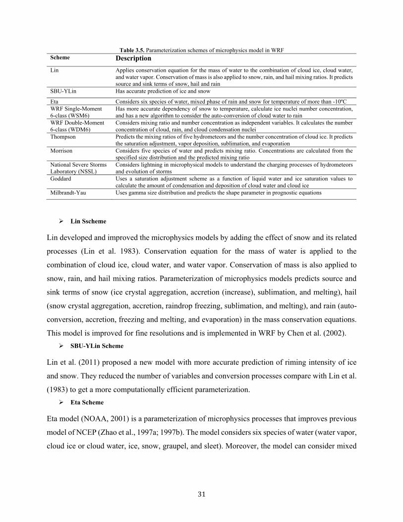
31
Table 3.5. Parameterization schemes of microphysics model in WRF Scheme Description Lin Applies conservation equation for the mass of water to the combination of cloud ice, cloud water,
and water vapor. Conservation of mass is also applied to snow, rain, and hail mixing ratios. It predicts source and sink terms of snow, hail and rain
SBU-YLin Has accurate prediction of ice and snow
Eta Considers six species of water, mixed phase of rain and snow for temperature of more than -10ºC WRF Single-Moment 6-class (WSM6)
Has more accurate dependency of snow to temperature, calculate ice nuclei number concentration, and has a new algorithm to consider the auto-conversion of cloud water to rain
WRF Double-Moment 6-class (WDM6)
Considers mixing ratio and number concentration as independent variables. It calculates the number concentration of cloud, rain, and cloud condensation nuclei
Thompson Predicts the mixing ratios of five hydrometeors and the number concentration of cloud ice. It predicts the saturation adjustment, vapor deposition, sublimation, and evaporation
Morrison Considers five species of water and predicts mixing ratio. Concentrations are calculated from the specified size distribution and the predicted mixing ratio
National Severe Storms Laboratory (NSSL)
Considers lightning in microphysical models to understand the charging processes of hydrometeors and evolution of storms
Goddard Uses a saturation adjustment scheme as a function of liquid water and ice saturation values to calculate the amount of condensation and deposition of cloud water and cloud ice
Milbrandt-Yau Uses gamma size distribution and predicts the shape parameter in prognostic equations
➢ Lin Sscheme
Lin developed and improved the microphysics models by adding the effect of snow and its related
processes (Lin et al. 1983). Conservation equation for the mass of water is applied to the
combination of cloud ice, cloud water, and water vapor. Conservation of mass is also applied to
snow, rain, and hail mixing ratios. Parameterization of microphysics models predicts source and
sink terms of snow (ice crystal aggregation, accretion (increase), sublimation, and melting), hail
(snow crystal aggregation, accretion, raindrop freezing, sublimation, and melting), and rain (auto-
conversion, accretion, freezing and melting, and evaporation) in the mass conservation equations.
This model is improved for fine resolutions and is implemented in WRF by Chen et al. (2002). ➢ SBU-YLin Scheme
Lin et al. (2011) proposed a new model with more accurate prediction of riming intensity of ice
and snow. They reduced the number of variables and conversion processes compare with Lin et al.
(1983) to get a more computationally efficient parameterization. ➢ Eta Scheme
Eta model (NOAA, 2001) is a parameterization of microphysics processes that improves previous
model of NCEP (Zhao et al., 1997a; 1997b). The model considers six species of water (water vapor,
cloud ice or cloud water, ice, snow, graupel, and sleet). Moreover, the model can consider mixed
32
phase of rain and snow for temperature of more than -10ºC. Temperature range specifies the
presence of cloud water (>0 ºC), cloud ice (< -15ºC), or the chance for either of them. ➢ WRF Single-Moment 6-class (WSM6) Scheme
WRF Single-Moment 6-class (WSM6) scheme (Hong and Lim, 2006) is the improved version of
previous parameterizations proposed by Hong et al. (2004). Many modifications were performed
to have a realistic model: 1) more accurate dependence of snow to temperature, 2) advanced model
for calculating ice nuclei number concentration, and 3) new algorithm for auto-conversion of cloud
water to rain. ➢ WRF Double-Moment 6-class (WDM6) Scheme
WDM6 (Lim and Hong, 2010) is the double-moment version of WSM6 (Hong and Lim, 2006). In
the double-moment scheme both mixing ratio and number concentration are considered as
independent variables. This model calculates the number concentration of cloud, rain, and cloud
condensation nuclei. Numbers of cloud and rain drops are an exponential function of their size.
The interception is a function of mixing ratio and temperature. This assumption significantly
changes the number of small size raindrops. ➢ Thompson Scheme
Thompson scheme predicts the mixing ratios of five hydrometeors (cloud water, rain, cloud ice,
snow, and graupel) and the number concentration of cloud ice (Thompson et al., 2008). The model
predicts the saturation adjustment, vapor deposition, sublimation, and evaporation. ➢ Morrison Scheme
Morrison double-moment scheme (Morrison 2009) considers five species (cloud droplets, cloud
ice, snow, rain, and graupel). The velocity components and the perturbation of potential
temperature, geopotential, and surface pressure of dry air, along with water vapor mixing ratio, and
the different cloud microphysics variables are used in a set of prognostic equations to predict the
mixing ratio. The number concentrations are calculated from the specified size distribution and the
predicted mixing ratio. ➢ National Severe Storms Laboratory (NSSL) Scheme
The NSSL scheme has the capability of considering lightning in microphysical models (Mansell et
al., 2010) to understand the charging processes of hydrometeors and evolution of storms. Two
independent moments, mass mixing ratio and number concentration of cloud droplets, rain, ice
crystals, snow, and graupel is predicted by the model.

33
➢ Goddard Scheme
Tao et al. (1989) proposed a saturation adjustment scheme as a function of liquid water and ice
saturation values to calculate the amount of condensation and deposition of cloud water and cloud
ice. The scheme is a single-moment microphysical model that can predict the mixing ratio of
different hydrometeors. ➢ Milbrandt-Yau Scheme
Milbrandt-Yau scheme uses gamma size distribution (Milbrandt and Yau, 2005a; 2005b) and the
radar reflectivity is added to predict the shape parameter in prognostic equations.
3.2.4.2. Selection of Appropriate Cumulus Options
Cumulus parameterizations consider the effect of convective air movement outside clouds on
up drafting and down drafting of clouds (Grell and Devenyi, 2002). Inclusion of the cumulus model
affects the vertical heat and moisture fluxes in a column of air above individual grids. In addition,
some models are able to predict the cloud and precipitation tendencies. All WRF options estimate
the convective component of surface rainfall. In general, the models have three parts; 1) trigger
function to identify the convection, 2) flux equations for mass and/or momentum and/or energy, 3)
the closure assumptions. Table 3.6 presents a brief description of different schemes of cumulus in
WRF. Detailed explanation follows. Table 3.6. Parameterization schemes of cumulus model in WRF
Scheme Description Simplified Arakawa-Schubert
Considers the mass and energy balance in clouds. Surface rainfall is parameterized in the moisture balance equation
Betts-Miller-Janjic Considers convective mixing and keeps the total enthalpy unchanged in the deep convection profile. Predicts the shallow clouds to consider the effect of atmospheric stability on the temperature profile
Grell 3D
Divides parameterizations into dynamic control and feedback. It accounts for both entrainment rate and detrainment rate in the steady state plume equation
Grell-Freitas Predicts the cloud convection in high-resolution grid size simulations Kain-Fritsch Uses the vertical momentum conservation equation to capture instabilities New Simplified Arakawa-Schubert
Uses turbulent diffusion-based approach and considers the convection-induced pressure gradient forcing in momentum equation
Tiedtke Considers the eddy transport of energy in prognostic equations Zhang-McFarlane Modifies the cumulus parameterization in the Canadian Climate Center General Circulation Model
by considering the exchange of unstable air change with adjacent layers
➢ Simplified Arakawa-Schubert Scheme
A simple set of equations considers the mass and energy balance in clouds (Pan and Wu., 1995).
High energy parcels are assumed to move upward to reach a level of free convection. The
percentage of the parcels at a point below the cloud is specified to determine the entrainment rate

34
and it was assumed that the parcel will lose the energy in the cloud. In this model surface rainfall
is also parameterized in the moisture balance equation. ➢ Betts-Miller-Janjic Scheme
Janjic (1994) modified the earlier version of a cumulus parameterization by adding convective
mixing to the thermodynamically driven process and keeping the total enthalpy unchanged in the
deep convection profile. Additionally, for shallow clouds, which are identified by a jump in relative
humidity, a positive change in entropy change is conditionally added to the equations. To predict
the shallow clouds, the humidity profile plays an important role and it was modified to consider
the effect of atmospheric stability on the temperature profile. ➢ Grell 3D Scheme
This model divides parameterizations into dynamic control and feedback (Grell, 1993; Grell and
Devenyi, 2002). The dynamic control governs the effect of convection by the environment. The
feedback parameterization determines the adjustment of the environment by the convection. Grell
3D Scheme accounts for both entrainment rate and detrainment rate in the steady state plume
equation. The model uses the updraft and downdraft mass flux to calculate normalized mass flux,
normalized condensation and evaporation profiles, moist static energy, and liquid water content. ➢ Grell-Freitas Scheme
The Grell-Freitas scheme predicts the cloud convection in high-resolution grid size simulations
(Grell and Freitas, 2014). The model limited the number of ensembles in Grell 3D scheme to
optimize the calculation time in numerical weather prediction simulations. ➢ Kain-Fritsch Scheme
Kain-Fritsch scheme is a new version based on the Lagrange approach mass flux parameterization.
It uses the vertical momentum conservation equation to capture instabilities (Kain, 2004). The
model calculates the decay of the convective available potential energy of cloud convection. The
outputs are temperature, water vapor mixing ratio, and cloud water mixing ratio tendencies. The
model also estimates the surface rainfall. ➢ New Simplified Arakawa-Schubert Scheme
Han and Pan (2011) developed the New Simplified Arakawa-Schubert scheme using turbulent
diffusion-based approach and considering the convection-induced pressure gradient forcing in
momentum equation. A finite entrainment and detrainment rates for heat, moisture, and momentum

35
was specified. To avoid excessive grid-scale precipitation by depleting more instability in deep
convection, cumulus convection was modified to be stronger and deeper. ➢ Tiedtke Scheme
Tiedtke (1989) proposed a mass flux-based model that considers the eddy transport of energy in
prognostic equations. In addition to updraft and downdraft of clouds, a penetrative convection
closure was parameterized for deep convection. Shallow convection is governed by the same
turbulent moisture flux as of penetrative convection for near surface layers. ➢ Zhang-McFarlane Scheme
This model modifies the cumulus parameterization in the Canadian Climate Center General
Circulation Model by considering the exchange of unstable air change with adjacent layers (Zhang
and McFarlane, 1995). The formulation is based on the mass flux of hydrometeors along with their
energy conservation.
3.2.4.3. Selection of Appropriate Planetary Boundary Layer (PBL) Options
Planetary boundary layer (PBL) is responsible for vertical flux exchange in the whole column
of air in a grid cell (Pielke, 2002). PBL quantifies the influence of momentum, heat and moisture
fluxes in the vertical sub-grid terms. In mesoscale models, PBL is divided into three sub-layers.
The viscous layer goes from the ground to the height of surface roughness where fluxes of heat,
moisture, and other constituents are experimentally estimated based on the von Karman constant
and friction velocity. The surface layer and transition layer are the two other parts of PBL and they
can be estimated as a function of height (Pielke, 2002). Urban surfaces are heterogeneous surfaces
and the parameterization is based on more complex methods. Table 3.7 presents a brief description
of different schemes of PBL in WRF. Detailed explanation follows. Table 3.7. Parameterization schemes of planetary boundary layer models in WRF
Scheme Description Mellor-Yamada-Janjic (MYJ) Considers the viscous sublayer above water bodies and a turbulent layer above the water
sublayer and lands Bougeault- Lacarrere (BouLac) Calculates the TKE in a prognostic equation as a function of vertical molecular dissipation,
mass flux, horizontal velocity, and heat
➢ Mellor-Yamada-Janjic (MYJ) Scheme
Janjic (1994) considers the viscous sublayer above water bodies and a turbulent layer above the
water sublayer and lands. In addition, the model calculates TKE (Turbulent Kinetic Energy) above
turbulent layer to reduce the spin up time for the model (Janjic, 2002). MYJ (Mellor-Yamada-
36
Janjic) has the minimum bias for different urban categories, about 0˚C for industrial category and
high-density residential category and about 1˚C for low-density residential category. Thermal
roughness length affects the surface temperature during the day, and the surface temperature during
the night is strongly related to the choice of PBL. ➢ Bougeault- Lacarrere (BouLac) Scheme
This model calculates the TKE (Turbulent Kinetic Energy) in a prognostic equation as a function
of vertical molecular dissipation, mass flux, horizontal velocity, and heat (Bougeault and Lacarrere,
1989).
3.2.4.4. Selection of Appropriate Radiation Options
Radiation parameterization determines the energy balance of the domain. The surface of the
domain (e.g., urban surface) can receive shortwave energy from the sun or longwave energy from
the sky. Urban surfaces absorb part of the energy and reflect the rest, while emitting longwave
radiation. The amount of energy that strikes the surface is a function of sky condition and solar
zenith angle. The energy exchange on the surface is well discussed by Liou (1980), and a different
algorithm with a different level of complexity has been developed to quantify it (ASHRAE, 2007;
Duffie and Beckman, 2006; Iqbal, 1983). Incoming solar radiation and emitted longwave radiation
from the ground varies through different mechanisms in the atmosphere. In a clear sky, part of the
sunlight energy on top of the atmosphere is absorbed by different tracer gases (e.g., ozone, water
vapor, etc.) and the rest reaches the ground. However, cloudy and polluted sky increases the
absorption by increasing the normal optical thickness of the air layer (Liou, 1980). The part of the
radiation reflected from the ground goes through the same process. The longwave radiation that is
emitted from the surface of the earth and gases are absorbed by the atmosphere or transmitted.
3.2.5. Analyses of Physical Parameterizations in WRF Data analysis are comprised of two parts: compare the simulation results with measurements
(model performance evaluation) and compare the results of two simulations (CTRL scenario with
ALBEDO scenario). The parameters that are directly extracted from the simulation results are 2-m
air temperature (T2, K), precipitation (RAINNC, mm), horizontal and vertical wind speed (U10,
V10, m/s), and mixing ratio (amount of water vapor in the air) (Q2, %). Other parameters are
calculated as presented in Table 3.8 namely 10-m wind speed (WS10, m/s) and 2-m relative
humidity (RH2, %).

37
Table 3.8. WRF output parameters and calculations to obtain other parameters Parameters to be calculated Calculations 10-m wind speed (m/s) (U10, V10)
√(𝑈10)2 + (𝑉10)2 = WS(m/s) U10 = horizontal wind speed V10 = vertical wind speed
Mixing ratio (Q2) to estimate the 2-m relative humidity (%)
SVP = 6.11 × 10(
7.5×T2237.3+T2
)
SMR = 621.97 SVP
(Pstation − SVP)
RH = Q2
SMR × 100
SVP = saturated vapor pressure SMR = saturated mixing ratio Pstation= station pressure (millibar) T2 = 2-m air temperature (oC)
The physical parameterizations in the solver of WRF need to be carefully selected to predict
weather conditions. Proper physical options for meteorological simulations enable environmental
policy makers to have a better understanding of the effects of heat island and its mitigations strategy
on urban climate and air quality. For Greater Montreal Area (GMA), an appropriate platform is
developed based on the city`s specific location and weather conditions. This platform is verified
by comparing the simulations results with measurements and thus further is applied to perform
other objectives such as assessing the effects of heat island and increasing surface reflectivity on
heat-related mortality in Greater Montreal Area. In addition, it provides a good understanding of
each physical parametrizations in WRF and their impacts on meteorological parameters in cold
climate.
3.3. Heat-Related Mortality Estimation
Heat-related mortality (HRM) can be magnified in urban areas because of the urban heat island
(UHI) effects. UHI intensity and duration cause an increase in mortality. To fight the heat island
effects, increasing urban albedo is applied. To investigate the effects of increasing surface
reflectivity (ISR) on heat-related deaths, a meteorological simulation is used. An algorithm is
defined to estimate the effects of high temperature on HRM. Figure 3.11 shows the simulation
approach to estimate the effects of urban heat island and increasing surface reflectivity on heat-
related mortality. Box A refers to explanations in Section 3.1.2, and box B shows the
accomplishments of this objective.
3.3.1. Defining Simulation Domain and Period The simulation domain is Greater Montreal Area centered at the ~45.5º N and ~73.6º W. The
horizontal domain of the simulations is composed of four two-way nested domains with 37×22,
43×34, 91×61, and 145×91 grid points, and a grid spacing of 9, 3, 1 and 0.333 km x km,

38
respectively. Figure 3.12 shows the simulation domain and land use/ land cover of domain 4. The
simulations are conducted during the 2005 (10th -12th July) and the 2011 (20th – 23rd July) heat wave
events. Table 3.9 presents the maximum air temperature recorded on each day of the simulation.
Figure 3.13 shows the maximum and minimum temperatures for the summer (June, July, August
(JJA)) for GMA in 2005 and 2011.
Figure 3.11. Simulation approach to estimate the effects of increasing surface reflectivity on heat-related mortality
(ISR=increasing surface reflectivity, HRM= heat-related mortality, CTRL= base case simulations, ALBEDO= increasing urban albedo)
Figure 3.12. Simulation domain and Land Use Land Cover (LULC) of GMA
B
B
Develop an algorithm to estimate HRM
- Compiling the WPS, WRF, UCM - Coupling ML-UCM with WRF
Simulate the 2005 & 2011 heat wave period (CTRL scenario)
Investigate the effects of ISR on urban climate
Collect filed data form weather stations for verification
Define simulation domain and period
Prepare Input data
Simulate with ALBEDO scenario for 2005 & 2011 heat wave period
Compare the simulation results with measurements
Determine an air mass classification for each day of simulations
Estimate the effects of ISR on heat-related mortality
Outcome Preparation Processes
A

39
Table 3.9. Maximum air temperature measured in four weather stations over GMA in 2005 and 2011heat wave periods (McTavish (MT), Pierre Elliott Trudeau Intl (PET), St-Hubert (SH), St-Anne-de-Bellevue (SAB))
Heat wave periods July 2005 Max temperature (oC)
MT PET SH SAB
July 2005 10th 31.6 31.5 31.1 30.8 11th 32.3 32.8 31.5 32.2 12th 30.6 30.6 30.7 30.3
July Average T (oC) 26.9 27.3 27.0 27.1
July 2011 21th 34.9 35.6 36.0 34.7 22nd 31.3 31.9 32.6 32.2 23rd 31.6 32.6 32.6 31.9
July Average T (oC) 28.3 28.5 29.0 28.5
Figure 3.13. Maximum and minimum temperatures for the summer (June, July, August (JJA)) for GMA in 2005 and 2011
0
5
10
15
20
25
30
35
Tem
pera
ture
(o C)
Date
0
5
10
15
20
25
30
35
40
Tem
pera
ture
(o C)
Date
High T2 Normal low T2 Normal high T2 Low T2

40
3.3.2. Preparation of Input Data for Simulations
The simulations were conducted with the initial and boundary conditions obtained from the
North American Regional Reanalysis (NARR). A vertical resolution of 51eta level is defined to
take full advantages of the urban parameterizations. The proper physical parameterizations of the
1st objective is used to simulate the CTRL and ALBEDO cases of the 2005 and 2011 heat wave
period over Greater Montreal Area. The positive-define advections of moisture, scalars and
turbulent kinetic energy is activated to maintain model stability. Each simulation begins at 1200
UTC (LST= UTC - 4h) of the previous day of each period. The first 24h is considered as a spin up
period.
3.3.3. Collection of Local Meteorological Data to Evaluate Model Performance To evaluate the simulations performances, the meteorological parameters namely: 2-m air
temperature (T2), 10-m wind speed (WS10), relative humidity (RH), and dew point temperature
(DPT) are collected from four weather stations (McTavish (MT), Pierre Elliott Trudeau Intl (PET),
St-Hubert (SH), Ste-Anne-de-Bellevue (SAB)) across the Greater Montreal Area for two heat wave
period in 2005 and 2011. Table 3.3 presents their geographical locations.
3.3.4. Analyses of Meteorological and Heat Stress Indices Parameters The parameters that are directly extracted from the simulation results are the 2-m air
temperature (T2, K), dew point temperature (DPT, K), horizontal and vertical wind speed (U10,
V10, m/s), and water mixing ratio (Q2, %). Other parameters are calculated as presented in Table
3.10—namely, 10-m wind speed (WS10), 2-m relative humidity (RH2), and three heat stress
indices: apparent temperature (AT), Canadian Humid Index (CHI), and Discomfort Index (DI).
The parameters that are analysed for the two heat wave periods are T2, WS10, RH2, DPT, AP,
CHI, DI, and the National Weather Service Heat Index (NWS-HI). The NWS-HI is a measurement
to show how hot it feels when RH2 is factored in with the actual T2. The NWS-HI is extracted
from the Heat Index Chart (Appendix C).

41
Table 3.10. WRF output variables and calculation to obtain other parameters WRF output variables Calculations 2-m air temperature (K) [T2] T2(K) – 273.15 = T2(oC)
CHI = T2 + (0.55 × (VP − 10)) Canadian Humid Index VP = vapor pressure (millibar)
DI = T2 − (0.55 × (1 − 0.01RH)) × (T2 − 14.5) Discomfort Index
10-m wind speed (m/s) [U10, V10]
√(𝑈10)2 + (𝑉10)2 = WS(m/s) U10 = horizontal wind speed V10 = vertical wind speed
Actual mixing ratio [Q2] to estimate the 2-m relative humidity (%)
SVP = 6.11 × 10(
7.5×T2237.3+T2
)
SMR = 621.97 SVP
(Pstation − SVP)
RH = Q2
SMR × 100
SVP = saturated vapor pressure SMR = saturated mixing ratio Pstation= station pressure (millibar)
Dew point temperature (K) (TH2) TH2(K) – 273.15 = TH2(oC)
AT = 23.2 + 0.55T2 + 0.003DPT2 − 0.2DPT Apparent temperature DPT=dew point temperature (oC)
3.3.5. Considering Air Mass Classification
Three indicators are applied to translate the effects of extreme heat events and the potential of
increasing surface reflectivity on heat-related mortality rates: air mass type, air temperature, and
apparent temperature changes for each day during heat wave periods. The air temperature and
apparent temperature are calculated based on simulation results. As this research focuses on heat,
the summer period of June, July and August (JJA) in the Greater Montreal Area (GMA) is being
analysed. In another study, Vanos et al. (2014) classified weather types into Spatial Synoptic
Classification (SSC) (Sheridan, 2002) for 12 cities in Canada. The air mass classifications are
presented in Table 3.11. The meteorological data applied to classify weather types into SSC was
collected from airport weather stations maintained by the Meteorological Service of Canada. They
estimated the heat-related mortality based on daily non-accidental mortality data that were
collected across the city’s metropolitan area from the Canadian Vital Statistics databases at
Statistics Canada over 20 years (1981–2000). Table 3.12 represents the GMA specific air mass
classification, the summertime frequencies (JJA, %), and heat-related mortality (Vanos et al., 2014;
Martel B et al., 2010). The number of deaths related to each air mass classification is estimated
based on the rate above the mean anomalous daily mortality in Montreal per 100,000 people. The
Statistics Canada Census estimated the population of Montreal as 3,824,221 people in 2011. The
Dry Moderate (DM) weather type, that includes mild and dry air in the summer season, is the most
common type in the Greater Montreal Area. The highest rate of mortality in the GMA during
summer periods corresponds to the hotter and more humid air mass type (MT+), while the dry
tropical condition (DT) places second (Vanos et al., 2014). Figure 3.14 shows the number of deaths

42
corresponding to each synoptic weather type during summertime (JJA). The Canadian
Environment Health Atlas (CEHA) estimates that in Montreal 121 people die each year because of
high temperature. This number is subject to a number of limitations: 1) it is not categorized on a
daily basis; 2) it does not reflect people’s age, sex, or economic, social or education status, or
whether they had any health issues before; 3) it does not show whether summer death is only
because of heat or is a combination of intense heat and air quality degradation. Table 3.11. Air mass types in the Spatial Synoptic Classifications (Sheridan, 2002)
Table 3.12. Summertime mortality rate for GMA within five weather types (1981–2000): weather type frequency for JJA and relative mortality (the averaged anomalous number of heat-related death above baseline value for mean daily mortality). The
standard deviation is presented. [Mortality rate per 100,000 people, calculated based on Statistics Canada 2011 Census as 3,824,221 people in GMA] (Source: Vanos et al., 2014)
Synoptic weather category
Frequency (%) Deaths SD ~ Number of deaths based on 2011 Census
DM 32.2 1.96 ±0.36 75 DT 1.30 2.27 ±0.53 87 MM 24.0 1.95 ±0.36 75 MT 22.0 2.13 ±0.42 81
MT+ 4.40 2.38 ±0.59 91 TR 16.1 0 0 0
Dry Moderate (DM): mild and dry air; Dry Tropical (DT): the hottest and driest conditions; Moist Moderate (MM): warmer and more humid conditions; Moist Tropical (MT): warm and very humid; Moist Tropical Plus (MT+): hotter and more humid subset of MT; Transition (TR): days in which one weather type yields to another (Source: Sheridan, 2002)
Figure 3.14. The number of deaths corresponding to each synoptic weather type during summer time (JJA). Dry Moderate (DM):
mild and dry air; Dry Tropical (DT): the hottest and driest conditions; Moist Moderate (MM): warmer and more humid conditions; Moist Tropical (MT): warm and very humid; Moist Tropical Plus (MT+): hotter and more humid subset of MT;
Transition (TR): days in which one weather type yields to another (Source: Sheridan, 2002)
DM32%
DT1%MM
24%
MT22%
MT+5%
TR16%
DM DT MM MT MT+ TR
Air Mass Definition
Dry Polar (DP) From polar regions. Associated with the lowest temperatures and clear, dry conditions Dry Moderate (DM) Includes mild and dry air Moist Polar (MP) Typically, cool, humid, and cloudy conditions Moist Moderate (MM) Warmer and more humid than MP Transition (TR) Days in which one weather type yields to another Moist Tropical (MT) Represent hottest and most humid weather type. Skies are partly cloudy in the summer
because of instability and convection Moist Tropical+ (MT+) Extreme subset of MT, in which morning and afternoon apparent temperature are above
the MT Dry Tropical (DT) Represents the hottest and driest conditions at any location with sunny, clear skies
2.27 deaths/day (87 deaths)
2.13 death/day (81 deaths)
2.38 deaths/day (91 deaths)

43
3.3.6. Estimation of Heat- Related Mortality
Air mass type, air temperature and apparent temperature changes for each day are applied to
translate the effects of extreme heat events and the potential of increasing surface reflectivity on
heat-related mortality during heat wave periods. The steps to estimate heat-related mortality are
presented in Figure 3.15. To estimate the heat-related mortality for the domain of interest during
the 2005 and 2011 heat wave periods, first the previous correlations (as presented in Table 3.13)
are analysed. Three of these correlations, in the cities with the same air mass classifications as the
Greater Montreal Area (New York and the District of Columbia) are selected. Table 3.13. Mortality calculation for summer time in various locations per 100,000 population (DT=dry tropical, MT= moist
tropical, MT+= moist tropical plus, DIS = day in sequence during for an offensive weather type (day 1= 1 and day 3= 3), TOS= time of season (1 = 1st of June and 32 = 1st of July, and so on until the end of August), AT=apparent temperature)
No. City Air mass classifications Heat-related mortality correlations (HRMd) 1 New York
For all air mass classifications (Kalkstein et al., 2007)
–4.394 + 8.343 DIS – 0.082 TOS + 0.33 AT (1) 2 Philadelphia –1.625 + 0.835 DIS – 0.018 TOS + 0.086 AT (2) 3 St. Louis 0.023 – 0.012 TOS + 0.13 AT (3) 4 Detroit –0.653 + 3.183 DIS (4) 5 Washington, D.C. 1.538 + 0.281 DIS – 0.006 TOS + 0.065 AT (5) 6 District of Columbia
(Kalkstein et al., 2013) DT air mass -13.197 + 1.07 DIS - 0.066 TOS + 0.612 AT (6)
7 MT & MT+ air masses 8.168 - 0.016 TOS + 0.301 AT (7) 8 Chicago
(Hayhoe et al., 2009) DT & MT air masses − 26.74 + 4.62 DIS + 0.777 AT (8)
9 For other air mass types − 7.8 + 0.266 AT (9)
Two categories are considered regarding the air mass classifications for heat-related mortality
estimation: dry tropical (DT) and moist tropical / moist tropical plus (MT/MT+). Since the heat-
related deaths corresponding to the frequency of DT are significant, the positive weighting factor
for the day in sequences (DIS) is only defined for this air mass category. The DIS factor means
that for each consecutive day within the DT area, the estimated mortality increases by 1.07. Another
weighting factor in this calculation is apparent temperature, 0.339, derived from the effects of
temperature (T2) and dew point temperature (DPR). The other factor is time of season (TOS),
derived from Kalkstein et al.’s (2013) HRM correlations for DT and MT/MT+ in the District of
Columbia. Accordingly, the daily heat-related mortality calculation for Dry Tropical (DT) that
represents the hottest and driest condition is Equation 4:
HRMD = −4.32 + 1.07DIS − 0.066TOS + 0.339 AT (Eq. 4)
and for Moist Tropical (MT) and Moist Tropical Plus (MT+) that represent very warm and humid condition is Equation 5:
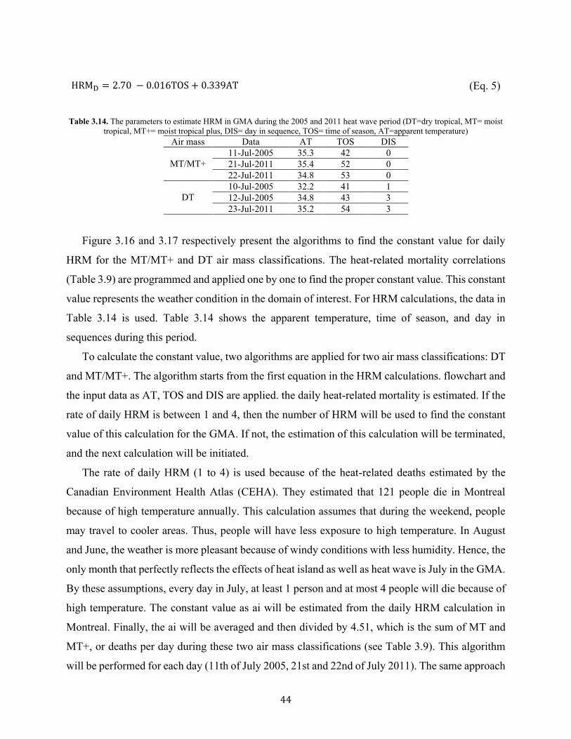
44
HRMD = 2.70 − 0.016TOS + 0.339AT (Eq. 5)
Table 3.14. The parameters to estimate HRM in GMA during the 2005 and 2011 heat wave period (DT=dry tropical, MT= moist
tropical, MT+= moist tropical plus, DIS= day in sequence, TOS= time of season, AT=apparent temperature) Air mass Data AT TOS DIS
MT/MT+
11-Jul-2005 35.3 42 0 21-Jul-2011 35.4 52 0 22-Jul-2011 34.8 53 0
DT
10-Jul-2005 32.2 41 1 12-Jul-2005 34.8 43 3 23-Jul-2011 35.2 54 3
Figure 3.16 and 3.17 respectively present the algorithms to find the constant value for daily
HRM for the MT/MT+ and DT air mass classifications. The heat-related mortality correlations
(Table 3.9) are programmed and applied one by one to find the proper constant value. This constant
value represents the weather condition in the domain of interest. For HRM calculations, the data in
Table 3.14 is used. Table 3.14 shows the apparent temperature, time of season, and day in
sequences during this period.
To calculate the constant value, two algorithms are applied for two air mass classifications: DT
and MT/MT+. The algorithm starts from the first equation in the HRM calculations. flowchart and
the input data as AT, TOS and DIS are applied. the daily heat-related mortality is estimated. If the
rate of daily HRM is between 1 and 4, then the number of HRM will be used to find the constant
value of this calculation for the GMA. If not, the estimation of this calculation will be terminated,
and the next calculation will be initiated.
The rate of daily HRM (1 to 4) is used because of the heat-related deaths estimated by the
Canadian Environment Health Atlas (CEHA). They estimated that 121 people die in Montreal
because of high temperature annually. This calculation assumes that during the weekend, people
may travel to cooler areas. Thus, people will have less exposure to high temperature. In August
and June, the weather is more pleasant because of windy conditions with less humidity. Hence, the
only month that perfectly reflects the effects of heat island as well as heat wave is July in the GMA.
By these assumptions, every day in July, at least 1 person and at most 4 people will die because of
high temperature. The constant value as ai will be estimated from the daily HRM calculation in
Montreal. Finally, the ai will be averaged and then divided by 4.51, which is the sum of MT and
MT+, or deaths per day during these two air mass classifications (see Table 3.9). This algorithm
will be performed for each day (11th of July 2005, 21st and 22nd of July 2011). The same approach

45
is performed to estimate the HRM for DT air mass condition. The differences are in the input data,
in the HRM correlation, and in that the average number is divided by 2.27 (see Table 3.9).
Figure 3.15. Steps to calculate heat-related mortality
Collecting measured data from weather stations (T2, WS10, RH, DPT, AP) regarding the 2005 & 2011heatwave events in the domain of interest
Collecting the verified heat-related mortality data from previous studies
Identifying air mass classification for the summer period (JJA) from previous studies
Simulating the meteorological model for the 2005 & 2011 heatwave events
Categorizing each day during heatwave period into an air mass classification based on simulation results (T2, WS10, RH, DPT, AP). The focus is on two air mass classifications: DT & MT/MT+
Estimating the heat-related correlations from previous studies (Table 3.9) and select the three calculationthat has the
The heat-related calculation is: HRMd = C1 + C2DIS + C3TOS + C4AT
HRMD = heat-induced mortality on daily basis DIS = day in sequence during for an offensive weather type (day 1= 1 and day 3= 3) TOS = time of season (1 = 1st of June and 32 = 1st of July, and so on until the end of August) AT = apparent temperature at a specific time of the day in that location The constant C1 to C4 are city specific and air mass type specific
Defining an algorithm to derive the constant values from other correlations in previous studies
Employing simulation results (AT), time of season and day in sequence to find constant parameters for two air mass classifications (DT & MT/MT+)
Estimating the HRM in GMA during the 2005 and 2011 heat waves periods

46
Figure 3.16. HRM-algorithm to find the constant value (a) for HRM corresponding to the MT/MT+ air mass classification for
each day of simulations (the number 4.51 is the sum of MT/MT+ frequency in JJA in GMA)
NO
YES
YES
Print 𝑎𝑖, i= 1, I
𝐴𝑣𝑔 𝑎 = − (∑ 𝑎𝑖
𝐼)/4.51
Stop
𝑎𝑖 = HRM𝑖 + 0.016TOS − 0.339 AT
NO
If 1< HRMi <4
Print HRMi (I)
i= i+1
Save 𝑎𝑖
Start
Select Equation n
n=0, i =0
n= n+1
Calculate HRMi
Print a
HRM equations from Table 3.13
If n<N
Select TOS, DIS, AT from Table 3.14
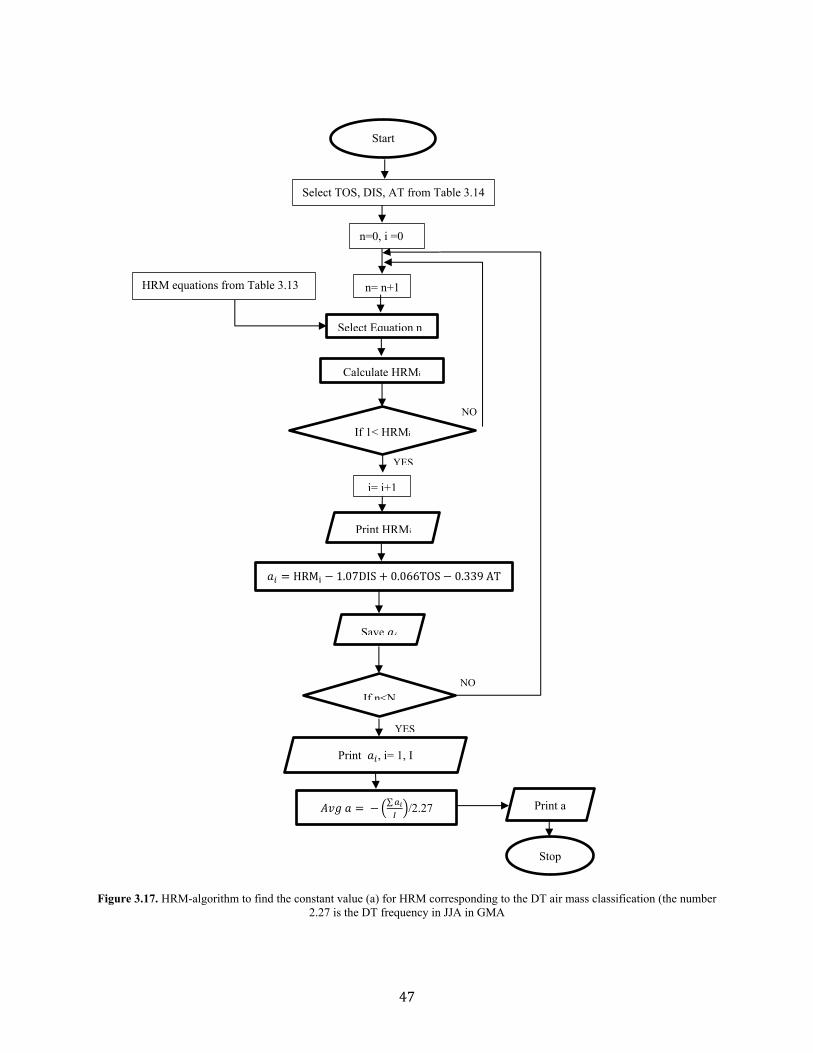
47
Figure 3.17. HRM-algorithm to find the constant value (a) for HRM corresponding to the DT air mass classification (the number
2.27 is the DT frequency in JJA in GMA
NO
YES
YES
Print 𝑎𝑖, i= 1, I
𝐴𝑣𝑔 𝑎 = − (∑ 𝑎𝑖
𝐼)/2.27
Stop
𝑎𝑖 = HRMi − 1.07DIS + 0.066TOS − 0.339 AT
NO
If 1< HRMi <4
Print HRMi (I)
i= i+1
Save 𝑎𝑖
Start
Select Equation n
n=0, i =0
n= n+1
Calculate HRMi
Print a
HRM equations from Table 3.13
If n<N
Select TOS, DIS, AT from Table 3.14

48
There are a number of HRM correlations that have been developed to estimate the effects of
high temperature on the rate of deaths in several cities across the globe, except in cold climate cities
such as the Greater Montreal Area. In addition, the effects of increasing surface reflectivity on
reducing heat mortality rate has not been investigated in the GMA. Thus, the meteorological
simulations are performed to investigate the effects of heat island and its mitigation strategy on
meteorological parameters and heat stress indices during two heat wave periods. The achievements
of this study are not limited to only comparing the effects of increasing surface reflectivity on the
aforementioned parameters, but they are also extended further and lead to defining algorithms to
develop HRM correlations for two main air mass classifications in the GMA. The developed HRM
algorithms can assist other researchers and policymakers to estimate the effects of any other
mitigation strategies for heat-related deaths in the GMA. The study illuminates the essential steps
to take before modifying these correlations or defining new ones. The air quality degradation can
also be a cause of heat-related death because of increasing the temperature-dependent
photochemical reaction rates and increasing emissions from pollutant sources in the urban area.
Thus, further analysis of the effects of high temperature on air quality needs to be carried out by
photochemical models such as WRF-Chem.
3.4. Simulations of Urban Climate and Air Quality within a Two-way Nested
Approach
Previous studies focused on a one-way simulation approach to investigate the effects of UHI
and its mitigation strategy on urban climate and air quality. But a two-way nested approach
provides an integrated simulation setup and captures the full impacts of meteorological processes
and photochemical reactions. This method can be applied over a larger geographical area through
regional and local scales such as urban areas. Thus, it reduces the uncertainties associated with
scale separation and grid resolution to investigate the effects of UHI and surface modifications on
urban climate and air quality. The WRF-Chem is used to consider a variety of coupled physical
and chemical processes such as transport, deposition, emission, chemical transformation, aerosol
interactions, photolysis and radiation. The morphological, thermal, and micro-scale properties of
the urban canopy are considered by coupling of a multi-layer of the Urban Canopy Model (ML-
UCM) within WRF-Chem. The aspect of the model that relates to the chemical parameterization
is briefly explained in the following figure. The simulation approach for the third objective is

49
presented in Figure 3.18. Box A refers to explanations in Section 3.1.2 and box B shows the
accomplishments and endpoints of this objective.
Figure 3.18. Simulation approach to investigate the effects of UHI and ISR on urban climate and air quality with a two-way
nested method (ISR=increasing surface reflectivity, CTRL= base case simulation, ALBEDO= increasing urban albedo, ARC=aerosol-radiation-cloud)
3.4.1. Defining Simulation Domain and Period
The first domain covers North America (NA) including Canada, the United States of America,
and the Northern part of Mexico with 445 grids in west–east direction and 338 grids in south–north
direction. The horizontal resolution is 12km. The second, third, and fourth domains cover the
Sacramento area (36 × 31 grids), Houston area (41 × 31 grids), and Chicago area (36 × 31 grids)
with the horizontal resolution of 2.4km. The vertical resolution includes 35 vertical layers from the
surface to a fixed pressure of ~100 mb (~16 km AGL). Figure 3.19 shows the simulation domains
and land use/land cover. The simulation period extended seven consecutive hottest days in 2011,
from the 17th to 23rd of July. The first 72h of the simulation is disregarded as a spin-up period. The
reason for the 72hrs spin-up is because of the chemistry package and photochemical reactions that
- Compiling the WPS, WRF-Chem, UCM - Coupling ML-UCM with WRF-Chem - Anthropogenic & biogenic emission estimation simulations
Select proper physical & chemical options for a two-way nested approach (CTRL scenario)
Investigate the effects of ISR on urban climate & air quality
Collect field data form weather and air quality stations to evaluate model performance
Define simulation domain and period Prepare input data
Simulate the ALBEDO scenario
Compare the simulation results with measurements
Design a two-way nested simulation approach to investigate the effects of UHI & ISR on urban climate and air quality
Outcome Preparation Processes
The 2-way nested approach is applied to investigate the effects of ARC interactions
B
B
A

50
are coupled with the meteorological processes. Hence, the spin up time for WRF-Chem simulations
usually took longer than WRF simulations.
Figure 3.19. Simulation domains and land use/land cover over North America (mother domain, horizontal resolution: 12km)
Sacramento, Houston, and Chicago (inner domains, horizontal resolution: 2.4km).
3.4.2. Preparation of Input Data for Physical and Chemical Parameterizations The simulation is conducted with the initial and boundary conditions obtained from the North
American Regional Reanalysis (NARR) (Mesinger et al, 2006). Land use was derived from the
USGS 24-category data set. The Lin scheme is used as microphysics model to evaluate six classes
of hydrometeors (Lin, Farley, and Orville 1983). Goddard scheme (Janjic Z.I., 1994) and Rapid
Radiative Transfer Model (RRTMG; Iacono et al., 2008) are respectively selected for shortwave
and longwave radiations. The planetary boundary layer (PBL) is simulated by the Mellor-Yamada-

51
Janjic scheme using Eta similarity theory (Janjic 2002). The unified NOAH land surface model is
applied. For cumulus parameterization, the Grell-Devenyi ensemble scheme (Grell and Devenyi
2002) is used. The positive-define advections of moisture, scalars and turbulent kinetic energy are
activated for model stability.
For anthropogenic and biogenic emission estimations, the models of the United States National
Emission Inventory for 2011 (US-NEI11) and Model of Emissions of Gases and Aerosols from
Nature (MEGAN) are respectively simulated for the inner domains. The results are applied in the
solver of WRF-Chem (see section 3.1.2). The Modal Aerosol Dynamics Model for Europe
(MADE) (Ackermann et al., 1998) is coupled with the chemistry package to estimate the effects of
aerosols on radiation processes and hydrological cycles in the atmosphere. The Regional
Atmospheric Chemistry Mechanism (RACM) (Stockwell et al., 1997) is used to estimate the gas-
phase reactions. The secondary organic aerosols (SOA) have also been incorporated into MADE
by means of the Secondary ORGanic Aerosol Model (SORGAM). Photolysis frequencies are
calculated by the Fast_J model scheme (Fast et al, 2006; Grell et al. 2005 and 2014). Wet
scavenging, cloud chemistry, sub-grid aqueous chemistry, and aerosols radiation feedback need to
be activated in the solver of WRF-Chem for model stability. Table 3.15 presents the physical and
chemical parameterizations applied in WRF-Chem.
Table 3.15. Physical and chemical parameterizations applied in WRF_Chem
Category Option Used Microphysics Lin scheme
Shortwave radiation Goddard Longwave radiation RRTMG Land surface model NOAH Planetary boundary layer scheme Mellor–Yamada–Janjic Scheme Cumulus parameterization Grell Devenyi Chemistry option RACM Photolysis scheme Fast_J Aerosol option MADE/SORGAM Advection scheme Runge–Kutta third order LULC data USGS 24-class Anthropogenic emissions US-NEI11 Biogenic emissions MEGAN Urban canopy model ML-UCM
3.4.3. Simulation Scenarios for Urban Climate and Air Quality Assessment
Three cities are selected for detail analyses: Sacramento (California), Houston (Texas), and
Chicago (Illinois) based on Akbari et al., (2001, 2003 and 2008) and Rose et al., (2003) findings
on the urban fabric of these cities. Using high-resolution orthophotography, they found that roofs

52
cover 20–25% and pavements cover 30–40% of urban surfaces. Table 3.16 presents the urban
fabric of Sacramento, Chicago, and Houston (Rose et al., 2003). Table 3.16. Urban fabric of three cities in NA (Source: Rose et al., 2003)
Metropolitan Areas Roofs (%) Pavements (%) Sacramento 20 45 Chicago 25 37 Houston 22 30
Two sets of simulations are conducted: CTRL case (UHI effects) and ALBEDO case
(increasing surface reflectivity (ISR) effects) during the 2011 heat wave period over the simulation
domains. The fraction of urban fabric of these three cities and the changes because of increasing
surface reflectivity are applied to calculate the albedo changes over the domains. The changes of
surface albedo modification from the CTRL case as 0.2 to full adoption of roofs and pavements
can be calculated as: (fraction of roofs in Sacramento) 0.20 × 0.65 (the increase of albedo for
roofs) + 0.45 (fraction of pavements in Sacramento) × 0.45 (the increase of albedo for pavements)
= 0.33 (as an example for Sacramento; the surface albedo (of roofs and pavements) increased from
0.13 to 0.33 (as a full adaptation of albedo enhancement)). The change to gridded ALBEDO can
be calculated as: (Surface albedo enhancement (roofs, walls, and pavements) × Fraction of urban
areas per grid cell).
The effects of increasing surface reflectivity are investigated on meteorological (hourly 2-m air
temperature (T2, oC), 10-m wind speed (WS10, m/s), 2-m relative humidity (RH2, %), and dew
point temperature (DPT, oC)) and photochemical parameters (daily particular matters (PM2.5,
µg/m3), ozone (O3, ppb), nitrogen dioxide (NO2, ppb), PM2.5 subspecies (particulate sulfate (SO42.5,
µg/m3), particulate nitrate (NO32.5, µg/m3), and organic carbon (OC2.5, µg/m3)) by comparing the
ALBEDO results with the CTRL results.
3.4.4. Collection of Local Meteorological and Air Quality Data to Evaluate Model Performance
The evaluation of the model performance is conducted by comparing the simulation results with
measurements obtained from weather and air-quality stations in Sacramento, Houston, and
Chicago. The weather and air quality monitoring stations were chosen based on their locations
close to the downtown of the selected cities (hereafter referred to as urban) and their surroundings
(hereafter referred to as suburb). The hourly 2-m air temperature (T2,oC), 10-m wind speed (WS10,
m/s), 2-m relative humidity (RH2, %), and dew point temperature (DPT, oC) simulation results (as

53
estimated in Table 3.2) are compared with the measurements obtained from the U.S. Environmental
Protection Agency (EPA) Clean Air Status and Trend Network (CASTNET). The daily averaged
modelled fine particular matters (PM2.5, µg/m3), ozone (O3, ppb), nitrogen dioxide (NO2, ppb),
PM2.5 subspecies (particulate sulfate (SO42.5, µg/m3), particulate nitrate (NO32.5, µg/m3), and
organic carbon (OC2.5, µg/m3)) concentrations are compared with the EPA Air Quality System
(AQS) observations using 24-h average data. The time series of simulation results changed to the
local time for each specific location: Sacramento: LST= UTC – 7h; Houston and Chicago:
LST=UTC – 5h.
3.4.5. Analyses of Meteorological and Photochemical Parameters The chemical components of WRF-Chem simulation results that are applied to investigate the
effects of ISR on urban climate and air quality are: fine particular matters (PM2.5, µg/m3), ozone
(O3, ppb), nitrogen dioxide (NO2, ppb), PM2.5 subspecies (particulate sulfate (SO42.5, µg/m3),
particulate nitrate (NO32.5, µg/m3), and organic carbon (OC2.5, µg/m3)). The meteorological
components are: 2-m air temperature (T2,oC), 10-m wind speed (WS10, m/s), 2-m relative
humidity (RH2, %), and dew point temperature (DPT, oC). Table 3.17 presents the calculations of
wind speed and relative humidity. Other parameters are the output of WRF-Chem. Table 3.17. WRF-Chem output variables and calculation to obtain other parameters
Parameters to be calculated Calculations 10-m wind speed (m/s) (U10, V10)
√(𝑈10)2 + (𝑉10)2 = WS(m/s) U10 = horizontal wind speed V10 = vertical wind speed
Mixing ratio (Q2) to estimate the 2-m relative humidity (%)
SVP = 6.11 × 10(
7.5×T2237.3+T2
)
SMR = 621.97 SVP
(Pstation − SVP)
RH = Q2
SMR × 100
SVP = saturated vapor pressure SMR = saturated mixing ratio Pstation= station pressure (millibar) T2 = 2-m air temperature (oC)
3.5. Effects of Increasing Surface Albedo on Aerosol-Radiation-Cloud Interactions in
Urban Atmosphere
To understand the effects of increasing surface reflectivity (ISR) on urban climate, air quality
and aerosol-radiation-cloud interactions in the atmosphere, the chemistry package and aerosol
scheme are compiled and coupled with the WRF and UCM. Figure 3.21 shows the simulation
approaches for the fourth objective. The effects of ISR are separately investigated as aerosol-
radiation (AR), aerosol-cloud (AC) and aerosol-radiation-cloud (ARC) interactions. A brief

54
description is presented for each step. Box A refers to explanations in Section 3.1.2, and box B
shows the accomplishments of this objective.
Figure 3.20. Simulation approaches for the 4th objective (AR=aerosol-radiation, AC=aerosol-cloud, ARC=aerosol-radiation-cloud interactions, ISR=increasing surface reflectivity)
3.5.1. Defining Simulation Domain and Period The horizontal domain of the simulation is composed of three two-way nested domains
covering North America (445 × 338 grids), part of Ontario and Quebec provinces (139 × 124 grids),
and the Greater Montreal Area (GMA) (101 × 71 grids) with the horizontal resolution of 12km,
4km and 800m, respectively. The vertical resolution includes 35 vertical layers. Figure 3.22 shows
the simulation domains and land use/land cover. The simulation period extended over seven
consecutive hottest days during the 2011 heat wave period, from the 17th to 23rd of July. The first
48h of the simulation is disregarded as the spin-up period. The reason for the 48h spin-up time is
that after this period, the results are stable enough to be extracted and analysed. Here, the
simulations are conducted on three paralleled nodes on cluster.
B
B
Define an approach to separate the effects of AR, AC and ARC estimations
- Compiling the WPS, WRF-Chem, UCM - Coupling ML-UCM with WRF-Chem - Anthropogenic & biogenic emission estimation simulations
Select proper physical & chemical options to simulate Base case, AR, AC and ARC interactions (Table 3.15)
Investigate the effects of ISR on AR, AC and ARC interactions
Collect field data form weather and air quality stations to evaluate model performance
Define simulation domain and period
Prepare input file
Simulate the Base, AR, AC and ARC interactions with ALBEDO scenario
Compare the simulation results with measurements
Develop equations to estimate the effects of AR, AC and ARC interactions
Outcome Preparation Processes
A
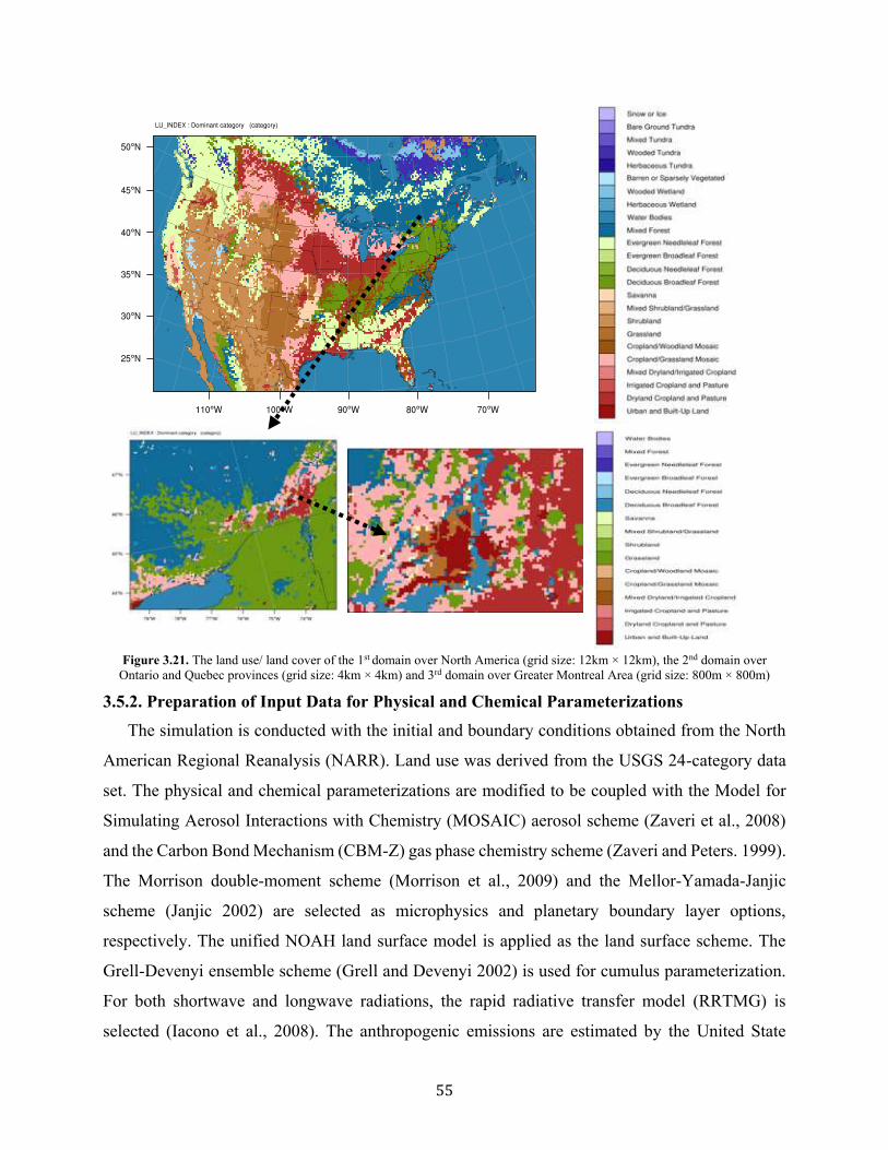
55
Figure 3.21. The land use/ land cover of the 1st domain over North America (grid size: 12km × 12km), the 2nd domain over
Ontario and Quebec provinces (grid size: 4km × 4km) and 3rd domain over Greater Montreal Area (grid size: 800m × 800m)
3.5.2. Preparation of Input Data for Physical and Chemical Parameterizations The simulation is conducted with the initial and boundary conditions obtained from the North
American Regional Reanalysis (NARR). Land use was derived from the USGS 24-category data
set. The physical and chemical parameterizations are modified to be coupled with the Model for
Simulating Aerosol Interactions with Chemistry (MOSAIC) aerosol scheme (Zaveri et al., 2008)
and the Carbon Bond Mechanism (CBM-Z) gas phase chemistry scheme (Zaveri and Peters. 1999).
The Morrison double-moment scheme (Morrison et al., 2009) and the Mellor-Yamada-Janjic
scheme (Janjic 2002) are selected as microphysics and planetary boundary layer options,
respectively. The unified NOAH land surface model is applied as the land surface scheme. The
Grell-Devenyi ensemble scheme (Grell and Devenyi 2002) is used for cumulus parameterization.
For both shortwave and longwave radiations, the rapid radiative transfer model (RRTMG) is
selected (Iacono et al., 2008). The anthropogenic emissions are estimated by the United State

56
National Emission Inventory (US-NEI11). The Model of Emissions of Gases and Aerosols from
Nature (MEGAN, Guenther et al., 2006) is used to calculate the biogenic emissions. The
anthropogenic and biogenic emissions are estimated only for the inner domain of the simulation.
Then the emission estimations from anthropogenic and biogenic sources are transferred to the
solver of WRF-Chem (see Section 3.1.2). The Fast-J is used for the photolysis scheme in WRF-
Chem (Fast et al., 2006). For dynamic options, the positive definite advections of chemistry,
moisture, scalars and turbulent kinetic energy have been activated. Table 3.18 summarizes the
physical and chemical parameterizations in WRF-Chem. Table 3.18. Selected physical and chemical parameterizations applied in WRF-Chem Category Option Used Microphysics Morrison double-moment scheme Radiation Schemes (shortwave & longwave) RRTMG Land Surface NOAH LSM
Planetary Boundary Layer Mellor-Yamada-Janjic Scheme
Cumulus clouds Grell3D
Gas-phase Chemistry CBM-Z
Photolysis Fast_J Anthropogenic emissions US-NEI11
Biogenic emissions MEGAN Aerosol scheme MOSAIC 8-bin Advection Scheme Runge–Kutta 3rd order
3.5.3. Simulation Scenarios to Estimate the Effects of Increasing Surface Reflectivity on Aerosol, Radiation and Cloud Interactions
Four scenarios are defined to separate the impacts of aerosol-radiation interactions from
aerosol-cloud interactions. The base scenario represents the processes of meteorological and
chemical interactions without considering the aerosol interaction with radiation and cloud, wet
scavenging and convective parameterizations (hereafter referred to BASE). In the second, third and
fourth simulations, model treatments remain the same as the BASE scenario, but the parameters
are activated regarding the aerosol-radiation (as direct effect; hereafter referred to AD-DE),
aerosol-cloud (as semi-direct effect; hereafter referred to AC-SDE), and aerosol-radiation-cloud
interactions (as indirect effect; hereafter referred to ARC-IDE). In addition, the effects of
increasing surface reflectivity are investigated on aerosol-radiation-cloud interactions in the
atmosphere. Two sets of simulations, each set consisting of the four aforementioned scenarios, are
conducted: CTRL case (UHI effects) and ALBEDO case (increasing surface reflectivity (ISR)

57
effects). Each scenario with albedo enhancement is referred to as ISR. Table 3.19 summarizes these
scenarios. The changes are in bold. Table 3.19. Two sets of simulation: CTRL Cases and ALBEDO Cases. Four sets of scenarios for each case: control simulation with no ARC interactions (BASE), aerosol and radiation interactions as direct effect (AR-DE), aerosol and cloud interactions as semi-direct effect (AC-SDE) and the aerosol-radiation-cloud interactions as indirect effect (ARC-IDE). In ALBEDO cases, each
scenario is repeated with regard to Increasing Surface Reflectivity (ISR).
simulations Scenario Aerosol-radiative feedback Aerosol-cloud feedback Convective parameterization
CTRL Cases
BASE Off Off Off
AR-DE On Off Off
AC-SDE Off On On
ARC-IDE On On On
ALBEDO Cases
ISR-BASE Off Off Off
ISR-AR-DE On Off Off
ISR-AC-SDE Off On On
ISR-ARC-IDE On On On
3.5.4. Collection of Measurements to Evaluate Model Performance
To evaluate the model performance, the ARC-IDE simulation results are compared with
measurements obtained from weather and air quality monitoring stations across the Greater
Montreal Area. The hourly 2-m air temperature (T2, oC), 10-m wind speed (WS10, m/s), and 2-m
relative humidity (RH2, %) are compared to measurements from four weather stations (McTavish
(MT), Pierre Elliott Trudeau Intl (PET), St-Hubert (SH), Ste-Anne-de-Bellevue (SAB)). The
hourly modelled fine (diameter less than 2.5 micrometers) particulate matter (PM2.5, µg/m3), ozone
(O3, ppb) and nitrogen dioxide (NO2, ppb) are compared with measurements from four air quality
monitoring stations (St-Jean-Baptiste (3), Decarie Interchange (28), Montreal Airport (66), and
Ste-Anne-de-Bellevue (99)). Figure 3.23 and Table 3.20 present their geographical locations. The
time series of simulation results are changed to the local time (LST = UTC – 4h).
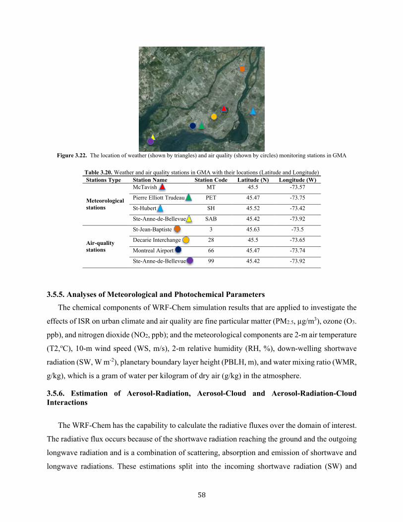
58
Figure 3.22. The location of weather (shown by triangles) and air quality (shown by circles) monitoring stations in GMA
Table 3.20. Weather and air quality stations in GMA with their locations (Latitude and Longitude) Stations Type Station Name Station Code Latitude (N) Longitude (W)
Meteorological stations
McTavish MT 45.5 -73.57
Pierre Elliott Trudeau PET 45.47 -73.75
St-Hubert SH 45.52 -73.42
Ste-Anne-de-Bellevue SAB 45.42 -73.92
Air-quality stations
St-Jean-Baptiste 3 45.63 -73.5
Decarie Interchange 28 45.5 -73.65
Montreal Airport 66 45.47 -73.74
Ste-Anne-de-Bellevue 99 45.42 -73.92
3.5.5. Analyses of Meteorological and Photochemical Parameters The chemical components of WRF-Chem simulation results that are applied to investigate the
effects of ISR on urban climate and air quality are fine particular matter (PM2.5, µg/m3), ozone (O3.
ppb), and nitrogen dioxide (NO2, ppb); and the meteorological components are 2-m air temperature
(T2,oC), 10-m wind speed (WS, m/s), 2-m relative humidity (RH, %), down-welling shortwave
radiation (SW, W m-2), planetary boundary layer height (PBLH, m), and water mixing ratio (WMR,
g/kg), which is a gram of water per kilogram of dry air (g/kg) in the atmosphere.
3.5.6. Estimation of Aerosol-Radiation, Aerosol-Cloud and Aerosol-Radiation-Cloud Interactions
The WRF-Chem has the capability to calculate the radiative fluxes over the domain of interest.
The radiative flux occurs because of the shortwave radiation reaching the ground and the outgoing
longwave radiation and is a combination of scattering, absorption and emission of shortwave and
longwave radiations. These estimations split into the incoming shortwave radiation (SW) and

59
outgoing longwave radiation (LW) balance. A set of calculations are defined to estimate the
radiative budget (RB) over the simulation domain as the difference between the radiation going
into the system and the out-going radiation (Eq. 5):
RB = SW↓ + LW↓
− SW↑ − LW↑ (Eq. 5)
For the two scenarios (CTRL and ALBEDO), the radiative balance (ΔRB) is defined based on
the differences between their simulation results. As the incoming radiation is the same for all
scenarios, the ΔRB is estimated to be equal to the differences in outgoing radiation (Eq. 6):
ΔRB = RBCTRL− RBALBEDO = (SW↑ + LW↑) |CTRL − (SW↑
+LW↑) |ALBEDO (Eq. 6)
The direct, semi-direct and indirect effects of aerosol on the radiation budget is also calculated.
The aerosol characteristics are assumed to be the same and the sky is assumed to be clear over the
domain during the simulation. The direct SW radiation is calculated based on the differences in
upwelling SW radiation in BASE and aerosol-radiation (AR-DE) simulation results (Eq. 7):
SWDirect = SW↑BASE − SW↑
AR-DE (Eq. 7)
The semi-direct effect, with regard to cloud formation, can be calculated based upon the
differences between BASE and AC-SDE simulation results (Eq. 8):
SWSemi-direct = SW↑BASE – SW↑
AC-SDE (Eq. 8)
The indirect effects are estimated with the comparison between BASE results and the aerosol-
radiation-cloud interaction (ARC-IDE) simulation results (Eq. 9):
SWIndirect = SW↑BASE− SW↑
ARC-IDE (Eq. 9)
Here, the effects of aerosols on the hydrological cycle, cloud formation and atmospheric
stability is minimal, because of the choice of simulation period. It is estimated as the water mixing
ratio (QWMR) (which is a gram of water per kilogram of dry air (g/kg) in the atmosphere). The
QWMR is calculated as a combination of the cloud water mixing ratio ( QCWMR), rain water mixing
ratio (QRWMR) and water vapor mixing ratio (QVWMR
) in the atmosphere (g/kg) (Eq. 10).

60
QWMR = QCWMR+ QRWMR
+ QVWMR (Eq. 10)
These ARC interactions are nonlinear and thus very complicated to be investigated. It means
that the sum of changes because of aerosol-radiation interactions and aerosol-cloud interactions is
not necessarily equal to the overall changes in ARC interactions. In a nonlinear system, the total
effect of one parameter can be decomposed into the contribution from pure impact and synergistic
impact (resulting from the synergy between that parameter and others). Thus, the impact of each
individual factor (f)—namely, temperature, ozone, fine particular matters, radiative budget and
water mixing ratio—can be derived as the following:
Direct effects: AR-DE = f AR f BASE
Semi-direct effects: AC-SDE = f AC f BASE
Indirect effect: ARC: ARC-IDE= f ARC f BASE
Synergistic impact: SYN= f ARC + f BASE f AC f AR
The aerosols affect the radiation budget and hydrological cycles in the atmosphere. By
increasing surface albedo to mitigate the urban heat island impacts, the aerosol-radiation, aerosol-
cloud and aerosol-radiation-cloud interactions will be affected as well. To estimate these nonlinear
effects, an approach is developed to calculate the radiation budget and water mixing ratio in the
atmosphere. In addition, a set of calculations are developed to investigate the separate effects of
AR, AC and ARC simulations on urban climate and air quality. These developed approaches can
further be applied to find the full impacts of UHI mitigation strategies on urban climate, air quality
and ARC interactions in the atmosphere.
3.6. Summary of Methodology
An appropriate platform is developed to simulate urban climate and heat island mitigation
strategy. The Weather Research and Forecasting Model (WRF) is used. WRF is comprised of many
physical parameterizations that are applied to predict weather conditions. The model ensemble for
urban climate simulation includes parameterizations for microphysics, cumulus, planetary
boundary layer (PBL), radiation, land surface, and urban canopy. Characterizing the
meteorological parameters (e.g., air temperature, wind speed, relative humidity and precipitation)
to a different set of parameterizations (i.e., model ensemble) enables researchers to select the proper

61
model platform for urban climate simulations. The physical processes can be selected based on a
set of sensitivity analyses. Thus, 20 sets of simulations with different physical parameterizations
are conducted. The model that has the least error compared to the measurements is proposed as the
proper platform for further analysis of heat island mitigation strategy.
Heat wave intensity and duration cause an increase in mortality. The developed platform for
urban climate simulations is applied to investigate the effects of increasing surface reflectivity
(ISR) on heat-related mortality (HRM). An algorithm is defined to estimate the effects of ISR on
HRM. Three indicators are applied to translate the effects of extreme heat events and the potential
impact of ISR on HRM rates: air mass type, air temperature and apparent temperature changes for
each day during heat wave periods. The air temperature and apparent temperature are calculated
based on WRF simulation results. Two air mass categories are considered to estimate HRM: dry
tropical (DT) and moist tropical / moist tropical plus (MT/MT+). Figure 3.16 and 3.17 show the
applied algorithms to calculate the HRM in MT/MT+ and DT air mass types.
A two-way nested approach is developed. It provides an integrated simulation setup to capture
the full impacts of meteorological processes and photochemical reactions. This approach reduces
the uncertainties associated with scale separation and grid resolution. The WRF is coupled with the
chemistry package (WRF-Chem) and a multi-layer of the Urban Canopy Model (ML-UCM) to
predict the morphological, thermal, and micro-scale properties of the urban canopy. The model
considers a variety of coupled physical and chemical processes such as transport, deposition,
emission, chemical transformation, aerosol interactions, photolysis and radiation. This approach is
further used to investigate the effects of heat island mitigation strategy on aerosol interactions in
the atmosphere.
Increasing surface reflectivity affects the aerosol-radiation (AR), aerosol-cloud (AC) and
aerosol-radiation-cloud (ARC) interactions. To estimate these nonlinear effects, an approach is
developed to calculate the radiation budget and water mixing ratio in the atmosphere and at the
surface. Four scenarios are defined to separate the impacts of aerosol-radiation interactions from
aerosol-cloud interactions. The base scenario represents the processes of meteorological and
chemical interactions without considering the aerosol interaction with radiation and cloud, wet
scavenging and convective parameterizations. In the second, third and fourth simulations, model
treatments remain the same as the base case scenario, but the parameters are activated regarding

62
the aerosol-radiation (as direct effect), aerosol-cloud (as semi-direct effect), and aerosol-radiation-
cloud interactions (as indirect effect). These ARC interactions are nonlinear; that is, the sum of
changes because of aerosol-radiation interactions and aerosol-cloud interactions is not necessarily
equal to the effects of each one. In a nonlinear system, the total effect of one parameter can be
decomposed into the contributions from pure impact and synergistic impact.
The results of these objectives lead to the post-processing analyses of WRF and WRF-Chem
simulations. The 2-m air temperature results of these simulations are compared with measurements.
The WRF results from the second objective (effects of ISR on HRM in the GMA) are compared
with the WRF-Chem results from the fourth objective (effects of ISR on ARC in the GMA). These
analyses indicate the separate effects of meteorological processes on predicting air temperature
distinguished from the combination effects of meteorological and photochemical reactions on air
temperature. Three factors are considered in these comparisons: the initial time and effort to
simulate each model, computational resources, and the accuracy of these models in predicting 2-m
air temperature by comparing with measurements.
The other post-processing analysis is to assess the correlation between surface albedo
enhancement and temperature reduction. The results of the second objective (effects of ISR on
HRM in the GMA), third objective (effects of ISR on Sacramento, Houston and Chicago in a two-
way nested approach), and fourth objective (effects of ISR on ARC interactions in the GMA) are
considered. The size of the inner grid for the second objective is 0.3km × 0.3km; for the third
objective it is 2.4km × 2.4km; and for the fourth objective it is 0.8km × 0.8km. The average albedo
enhancement in each grid in urban areas is compared with its corresponding temperature reduction.

63
Chapter 4 Sensitivity Analysis of Physical parameterizations in WRF for Urban Climate and Heat Island Mitigation Strategy
Mesoscale models are comprised of many parameterizations that are used to predict weather
conditions. The model ensemble for urban climate simulation includes parameterizations for
microphysics, cumulus, planetary boundary layer (PBL), radiation, land surface, and urban canopy.
Characterizing the meteorological parameters (e.g., air temperature, wind speed, etc.) in relation to
a different set of parameterizations (i.e., model ensemble) enables researchers to select the proper
model platform for urban climate simulations and heat island mitigation strategies. The WRF is
applied to assess the sensitivity of physical parameterizations on air temperature, wind speed,
relative humidity and precipitation over the Greater Montreal Area, Canada for the period of 9–11
August 2009. A multi-layer of urban canopy model is used to consider the turbulence between
buildings in urban areas (Chen et al., 2011).
The results of the base case simulations are compared with measurements for the period of 9–
11 August 2009, from seven weather stations (McTavish (MT), Pierre Elliott Trudeau Intl (PET),
St-Hubert (SH), Ste-Anne-de-Bellevue (SAB), Varennes (VA), Mirabel (MI), and Ste-Clothilde
(SC)). A set of metrics calculations are applied to evaluate model performance (mean bias error
(MBE), mean absolute error (MAE) and root mean square error (RMSE)). The model ensemble
with the least error is presented as an appropriate platform for urban climate simulations to study
Urban Heat Island (UHI) mitigation strategies. Increasing surface reflectivity was applied to
mitigate the UHI intensity over the domain. The albedo of roofs, walls, and roads increased from
0.2 to 0.65, 0.6, and 0.45, respectively. The physical parameterizations in WRF are explained in
detail in Chapter 3, Section 3.2. Here, the results of this study are presented. The research presented
in this chapter is summarized in the article by Z. Jandaghian, A. G. Touchaei, and H. Akbari (2017),

64
“Sensitivity analysis of physical parameterizations in WRF for urban climate simulations and heat
island mitigation in Montreal” (doi:10.1016/j.uclim.2017.10.004).
4.1. Defining Simulation Domain and Period
The simulation domain is the Greater Montreal Area (GMA) that is centered at the ~45.5ºN and
~73.6ºW. The horizontal domain of the simulations is composed of four two-way nested domains
with 37×22, 43×34, 91×61, and 145×91 grid points, and a grid sizes of 9, 3, 1 and 0.333 km × km,
respectively. The vertical resolution includes 51 vertical layers from the surface to a fixed pressure
of ~100 mb (~16 km AGL). The selected simulation period starts with a clear sky condition (9th of
August) and ends with a rainy condition (11th of August). The summer days are selected because
results are used to evaluate the effect of urban heat island mitigation strategy (increasing surface
reflectivity). Figure 4.1 shows the simulation domains based on USGS land use categories.
Domain 1 (grid size: 9 km × km) Domain 2 (grid size: 3 km × km)
Domain 3 (grid size: 1 km × km) Domain 4 (grid size:0.333 km × km)
Figure 4.1. Simulation domains (grid sizes of domain 1: 9 km × km, domain 2: 3 km × km, domain 3: 1 km × km, domain 4:
0.333 km × km). Black refers to urban and build-up and cropland/woodland, the blue and purple refer to water bodies
The simulations were conducted with the initial and boundary conditions obtained from the
North American Regional Reanalysis (NARR). Land Use/Land Cover (LULC) data was derived
from the USGS 24-category data set. Advanced Very High-Resolution Radiometer (AVHRR)

65
measures the background surface albedo (Csiszar and Gutman 1999). The other physical
parameterizations are explained in section 3.2.4. The positive-define advections of moisture,
scalars and turbulent kinetic energy is activated to maintain model stability. Each simulation begins
at 0000 UTC (LST= UTC - 4h) of the previous day of each period. The first 28h is considered as a
spin up period.
4.2. Analysis of Physical Parameterizations in WRF and Effects of Increasing Surface
Reflectivity on Urban Climate
The physical parameterizations need to be selected to predict weather conditions. A set of
sensitivity analysis are carried. A proper simulation platform provides a better understanding of
the effects of UHI and its mitigations strategy on urban climate. The model ensemble for urban
climate simulation includes parameterizations for microphysics, cumulus, planetary boundary layer
(PBL), radiation, land surface, and urban canopy. Characterizing the meteorological parameters
(e.g., air temperature, wind speed, relative humidity and precipitation) to a different set of
parameterizations (i.e., model ensemble) enables researchers to select the proper model platform
for urban climate simulations. Table 4.1 presents the simulation set-ups with different options on
parametrizations. A brief description of these parameterizations has been presented in Chapter 3. Table 4.1. Simulation set-ups with different options on parameterization of microphysics, cumulus, PBL, and radiation
Microphysics Cumulus PBL Radiation S01 WDM (16)1 Simplified Arakawa-Schubert (4)2 MYJ (2)3 RRTMG (4) S02 WDM (16) Betts-Miller-Janjic (2)5 MYJ (2) RRTMG (4) S03 WDM (16) Grell 3D (5)6 BouLac PBL (8)7 RRTMG (4) S04 WDM (16) Grell 3D (5) MYJ (2) Dudhia (1)8 S05 Eta (5)9 Grell 3D (5) MYJ (2) RRTMG (4) S06 WDM (16) Grell 3D (5) MYJ (2) RRTMG (4) S07 WDM (16) Grell-Freitas (3)10 MYJ (2) RRTMG (4) S08 Goddard (7)11 Grell 3D (5) MYJ (2) RRTMG (4) S09 WDM (16) Kain-Fritsch (1)12 MYJ (2) RRTMG (4) S10 Lin (2)13 Grell 3D (5) MYJ (2) RRTMG (4) S11 Milbrandt-Yau (9)14 Grell 3D (5) MYJ (2) RRTMG (4) S12 Morrison (10)15 Grell 3D (5) MYJ (2) RRTMG (4) S13 NSSL (17)16 Grell 3D (5) MYJ (2) RRTMG (4) S14 NSSL with CCN (18) Grell 3D (5) MYJ (2) RRTMG (4) S15 WDM (16) New Simplified Arakawa-Schubert (14)17 MYJ (2) RRTMG (4) S16 SBU-YLin (13)18 Grell 3D (5) MYJ (2) RRTMG (4) S17 Thompson (8)19 Grell 3D (5) MYJ (2) RRTMG (4) S18 WDM (16) Tiedtke (6)20 MYJ (2) RRTMG (4) S19 WSM (6)21 Grell 3D (5) MYJ (2) RRTMG (4) S20 WDM (16) Zhang-McFarlane (7)22 MYJ (2) RRTMG (4) 1 Lim and Hong, (2010), 2 Pan and Wu., (1995), 3 Janjic (1994), 4 Iacono et al. (2008),5 Janjic (1990), 6 Grell (1993), and Grell and Devenyi (2002), 7 Bougeault and Lacarrere, (1989), 8 Dudhia (1989), and Mlawer et al. (1997), 9 NOAA, (2001), 10 Grell and Freitas (2014), 11 Tao et al. (1989), 12 Kain (2004), 13 Lin (1983), 14 Milbrandt and Yau, (2005a), and Milbrandt and Yau, (2005b), 15 Morrison et al. (2009), 16 Mansellet al. (2010), 17 Han and Pan (2011), 18 Lin and Colle (2011), 19 Thompson et al. (2008), 20 Tiedtke (1989), and Zhang et al. (2011), 21 Hong and Lim, (2006), 22 Zhang and McFarlane, (1995)

66
4.2.1. Air Temperature
The 2-m air temperature of simulations’ results are compared with measurements. Figure 4.2
shows the hourly 2-m air temperature of the simulated results of the S06 model ensemble (solid
line) vs. measurements (dashed line) from seven weather stations for a period of 09-11 Aug-2009
across GMA (McTavish (MT), Pierre Elliott Trudeau Intl (PET), St-Hubert (SH), Ste-Anne-de-
Bellevue (SAB), VArennes (VA), MIrabel (MI), Ste-Clothide (SC)). Table 4.2, 4.3 and 4.4 present
the MBE, MAE and RMSA, respectively. For these simulations, the average MBEs (-1.5 oC)
indicates that the model on average underestimates the 2-m air temperature. The main reason for
this underestimation is the exclusion of anthropogenic heat emission in WRF solver. The
anthropogenic heat emission as traffic and human activities can significantly contribute to an
increase in the air temperature of urban areas by up to 2°C (Salamanca et al., 2014). The MAE is
the highest in S04 that the Dudhia model is used for the radiation estimation. Skin temperature is
sensitive to shortwave radiation; consequently, the 2-m air temperature is sensitive to the selected
options for radiation parameterization. The RRTMG parameterization is more accurate than the
combination of the Dudhia scheme for shortwave and RRTM scheme for longwave radiation. The
least MAE (1.6 °C) is in WDM (WRF Double-Moment 6-class Scheme) coupled with Grell 3D
(S06) and with New Simplified Arakawa-Schubert (S01) as microphysics and cumulus scheme,
respectively (Table 4.3). In the urban weather station, the MAE is minimized (1.4 °C). by using the
WDM as microphysics scheme coupled with the choice of MYJ as PBL and RRTMG as the
radiation scheme. The choices of PBL (MYJ and BouLac; coupled to ML-UCM) show a good
agreement in predicting the 2-m air temperature in the urban area. In rural areas, the MAE of the
model ensemble using the MYJ scheme was 0.2 °C less than the MAE of S03 using the BouLac
scheme. Table 4.4 and Figure 4.3 present the RMSE of the simulations and accuracy of models.
S06, S01, S16 and S07 have the least RMSE of about 2 °C. Figure 4.4 indicates that the least RMSE
belongs to the urban area (McTavish weather station). Thus, the RMSE is higher in rural areas than
urban ones. The combination of WDM6 (Lim and Hong, 2010) for microphysics, MYJ (Janjic,
1994) for planetary boundary layer, and RRTMG (Iacono et al., 2008) for radiation schemes
provided better results compared with measurements.
The temperature differences between CTRL and ALBEDO scenario presents in Table 4.5. The
results of S10, S12, S07 and S01 simulations indicate a higher temperature reduction (Figure 4.5).

67
However, the average calculated temperature differences of these simulations are 0.2oC. Figure 4.6
indicates that the urban areas` temperature is decreased more compared to their surroundings by
increasing surface albedo.
0
10
20
30
0 6 12 18 0 6 12 18 0 6 12 18
Tem
pera
ture
(oC
)
Hour
MT
0
10
20
30
40
0 6 12 18 0 6 12 18 0 6 12 18
Tem
pera
ture
(oC
)
Hour
PET
0
10
20
30
0 6 12 18 0 6 12 18 0 6 12 18
Tem
pera
ture
(oC
)
Hour
SAB
0
10
20
30
0 6 12 18 0 6 12 18 0 6 12 18
Tem
pera
ture
(oC
)
Hour
SH
0
10
20
30
0 6 12 18 0 6 12 18 0 6 12 18
Tem
pera
ture
(oC
)
Hour
MI
0
5
10
15
20
25
30
0 6 12 18 0 6 12 18 0 6 12 18
Tem
pera
ture
(oC
)
Hour
VA
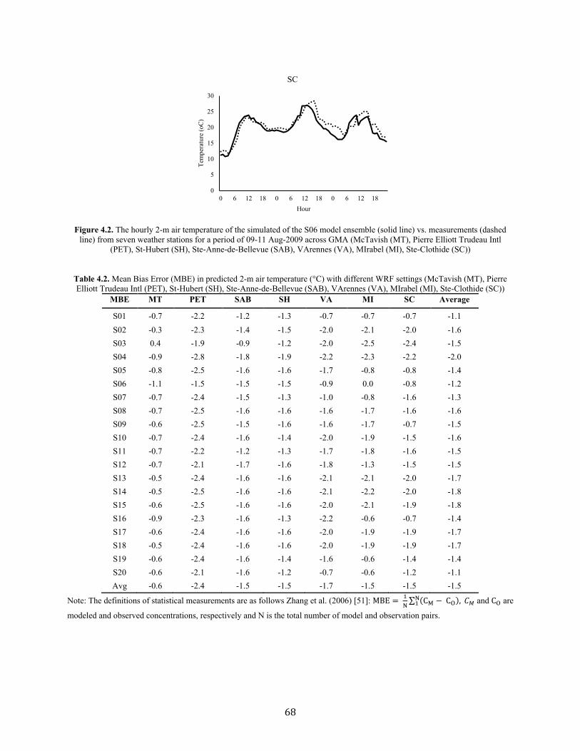
68
Figure 4.2. The hourly 2-m air temperature of the simulated of the S06 model ensemble (solid line) vs. measurements (dashed
line) from seven weather stations for a period of 09-11 Aug-2009 across GMA (McTavish (MT), Pierre Elliott Trudeau Intl (PET), St-Hubert (SH), Ste-Anne-de-Bellevue (SAB), VArennes (VA), MIrabel (MI), Ste-Clothide (SC))
Table 4.2. Mean Bias Error (MBE) in predicted 2-m air temperature (°C) with different WRF settings (McTavish (MT), Pierre Elliott Trudeau Intl (PET), St-Hubert (SH), Ste-Anne-de-Bellevue (SAB), VArennes (VA), MIrabel (MI), Ste-Clothide (SC))
MBE MT PET SAB SH VA MI SC Average S01 -0.7 -2.2 -1.2 -1.3 -0.7 -0.7 -0.7 -1.1 S02 -0.3 -2.3 -1.4 -1.5 -2.0 -2.1 -2.0 -1.6 S03 0.4 -1.9 -0.9 -1.2 -2.0 -2.5 -2.4 -1.5 S04 -0.9 -2.8 -1.8 -1.9 -2.2 -2.3 -2.2 -2.0 S05 -0.8 -2.5 -1.6 -1.6 -1.7 -0.8 -0.8 -1.4 S06 -1.1 -1.5 -1.5 -1.5 -0.9 0.0 -0.8 -1.2 S07 -0.7 -2.4 -1.5 -1.3 -1.0 -0.8 -1.6 -1.3 S08 -0.7 -2.5 -1.6 -1.6 -1.6 -1.7 -1.6 -1.6 S09 -0.6 -2.5 -1.5 -1.6 -1.6 -1.7 -0.7 -1.5 S10 -0.7 -2.4 -1.6 -1.4 -2.0 -1.9 -1.5 -1.6 S11 -0.7 -2.2 -1.2 -1.3 -1.7 -1.8 -1.6 -1.5 S12 -0.7 -2.1 -1.7 -1.6 -1.8 -1.3 -1.5 -1.5 S13 -0.5 -2.4 -1.6 -1.6 -2.1 -2.1 -2.0 -1.7 S14 -0.5 -2.5 -1.6 -1.6 -2.1 -2.2 -2.0 -1.8 S15 -0.6 -2.5 -1.6 -1.6 -2.0 -2.1 -1.9 -1.8 S16 -0.9 -2.3 -1.6 -1.3 -2.2 -0.6 -0.7 -1.4 S17 -0.6 -2.4 -1.6 -1.6 -2.0 -1.9 -1.9 -1.7 S18 -0.5 -2.4 -1.6 -1.6 -2.0 -1.9 -1.9 -1.7 S19 -0.6 -2.4 -1.6 -1.4 -1.6 -0.6 -1.4 -1.4 S20 -0.6 -2.1 -1.6 -1.2 -0.7 -0.6 -1.2 -1.1 Avg -0.6 -2.4 -1.5 -1.5 -1.7 -1.5 -1.5 -1.5
Note: The definitions of statistical measurements are as follows Zhang et al. (2006) [51]: MBE = 1
N∑ (CM − CO),N
1 𝐶𝑀 and CO are
modeled and observed concentrations, respectively and N is the total number of model and observation pairs.
0
5
10
15
20
25
30
0 6 12 18 0 6 12 18 0 6 12 18Te
mpe
ratu
re (o
C)
Hour
SC

69
Table 4.3. Mean Absolute Error (MAE) in predicted 2-m air temperature (°C) with different WRF settings (McTavish (MT), Pierre Elliott Trudeau Intl (PET), St-Hubert (SH), Ste-Anne-de-Bellevue (SAB), VArennes (VA), MIrabel (MI), Ste-Clothide
(SC)) MAE MT PET SAB SH VA MI SC Average S01 1.3 2.3 1.9 1.6 1.6 2.1 1.4 1.7 S02 1.4 2.4 2.2 1.9 2.8 3.1 2.7 2.4 S03 1.3 1.9 2.1 1.7 3.8 3.6 4.2 2.7 S04 1.6 2.8 2.3 2.2 3.3 3.6 3.3 2.7 S05 1.5 2.6 2.3 1.9 4.3 3.4 1.6 2.5 S06 1.5 2.6 2.3 1.9 1.7 0.0 1.5 1.6 S07 1.5 2.5 2.3 1.7 1.9 2.2 3.2 2.2 S08 1.5 2.5 2.2 1.8 5.0 4.6 4.9 3.2 S09 1.5 2.5 2.3 1.8 4.3 4.2 1.4 2.6 S10 1.4 2.4 2.2 1.7 3.2 3.2 2.7 2.4 S11 1.3 2.3 1.9 1.6 3.0 4.2 3.2 2.5 S12 1.5 2.3 2.3 1.9 4.3 3.9 2.7 2.7 S13 1.4 2.5 2.3 1.9 3.0 3.4 3.0 2.5 S14 1.3 2.6 2.3 1.9 3.0 3.4 3.1 2.5 S15 1.4 2.6 2.3 1.8 3.3 3.7 3.2 2.6 S16 1.4 2.4 2.2 1.6 3.5 1.9 1.4 2.1 S17 1.4 2.5 2.3 1.8 3.3 3.8 3.3 2.6 S18 1.3 2.5 2.3 1.8 3.9 3.9 3.4 2.7 S19 1.4 2.5 2.2 1.7 5.1 1.9 5.0 2.8 S20 1.4 2.3 2.2 1.5 1.6 1.9 5.1 2.3 Avg 1.4 2.4 2.2 1.8 3.3 3.1 3.0 2.5
Note: The definitions of statistical measurements are as follows Zhang et al. (2006) [51]: MAE =1
N∑ |CM − CO| N
1 CM and CO are
modeled and observed concentrations, respectively and N is the total number of model and observation pairs.

70
Table 4.4. Root Mean Square Error (RMSE) in predicted 2-m air temperature (°C) with different WRF settings (McTavish (MT), Pierre Elliott Trudeau Intl (PET), St-Hubert (SH), Ste-Anne-de-Bellevue (SAB), VArennes (VA), MIrabel (MI), Ste-Clothide
(SC)) RMSE MT PET SAB SH VA MI SC Average
S01 1.6 2.7 2.3 1.9 2.1 2.5 1.7 2.1 S02 1.7 2.8 2.6 2.4 3.5 3.8 3.5 2.9 S03 1.6 2.4 2.5 2.2 5.0 4.8 5.5 3.4 S04 1.9 2.8 2.8 2.9 4.1 4.3 4.1 3.3 S05 1.8 2.9 2.6 2.3 5.0 4.0 1.9 2.9 S06 1.8 2.9 2.7 2.3 2.1 0.0 1.8 1.9 S07 1.8 2.8 2.6 2.0 2.4 2.6 4.0 2.6 S08 1.8 2.9 2.6 2.1 5.7 5.3 5.8 3.7 S09 1.7 2.9 2.6 2.3 4.9 4.9 1.7 3.0 S10 1.7 2.7 2.6 2.0 3.9 3.8 3.4 2.9 S11 1.6 2.7 2.3 1.9 3.7 4.9 4.0 3.0 S12 1.8 2.7 2.7 2.3 5.0 4.5 3.4 3.2 S13 1.6 2.8 2.7 2.3 3.7 4.1 3.8 3.0 S14 1.6 2.9 2.7 2.3 3.7 4.1 3.9 3.0 S15 1.7 2.9 2.7 2.3 4.0 4.3 4.0 3.1 S16 1.7 2.7 2.6 1.9 4.3 2.3 1.7 2.5 S17 1.6 2.9 2.7 2.3 4.0 4.4 4.1 3.1 S18 1.6 3.0 2.7 2.4 4.6 4.6 4.2 3.3 S19 1.7 2.8 2.6 2.0 5.8 2.3 5.8 3.3 S20 1.7 2.7 2.6 1.9 2.1 2.3 5.8 2.7 Avg 1.7 2.8 2.6 2.2 4.0 3.7 3.7 3.0
RMSE = [1
N∑ (CM − CO)2N
1 ]1/2
CM and CO are modeled and observed concentrations, respectively and N is the total number of model and observation pairs.
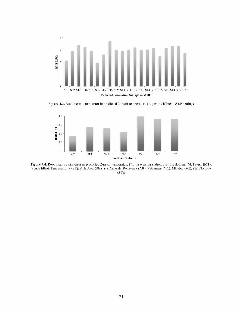
71
Figure 4.3. Root mean square error in predicted 2-m air temperature (°C) with different WRF settings
Figure 4.4. Root mean square error in predicted 2-m air temperature (°C) in weather station over the domain (McTavish (MT), Pierre Elliott Trudeau Intl (PET), St-Hubert (SH), Ste-Anne-de-Bellevue (SAB), VArennes (VA), MIrabel (MI), Ste-Clothide
(SC))
0
1
2
3
4
S01 S02 S03 S04 S05 S06 S07 S08 S09 S10 S11 S12 S13 S14 S15 S16 S17 S18 S19 S20
RM
SE(0 C
)
Different Simulation Set-ups in WRF
0.0
1.0
2.0
3.0
4.0
MT PET SAB SH VA MI SC
RM
SE (o C
)
Weather Stations

72
Table 4.5. 2-m air temperature (°C) differences between CTRL & ALBEDO scenarios (McTavish (MT), Pierre Elliott Trudeau Intl (PET), St-Hubert (SH), Ste-Anne-de-Bellevue (SAB), VArennes (VA), MIrabel (MI), Ste-Clothide (SC))
ΔT MT PET SAB SH VA MI SC Average S01 0.2 0.1 0.1 0.1 0.3 0.3 0.1 0.2 S02 0.2 0.1 0.1 0.1 0.1 0.1 0.1 0.1 S03 0.2 0.1 0.2 0.1 0.2 0.1 0.1 0.1 S04 0.2 0.1 0.2 0.1 0.2 0.1 0.1 0.1 S05 0.3 0.1 0.2 0.1 0.2 0.2 0.0 0.1 S06 0.2 0.1 0.2 0.2 0.1 0.0 0.1 0.1 S07 0.2 0.1 0.2 0.2 0.7 0.1 0.0 0.2 S08 0.2 0.1 0.1 0.1 0.1 0.1 0.1 0.1 S09 0.2 0.2 0.2 0.1 0.2 0.2 0.1 0.2 S10 0.2 0.2 0.1 0.1 0.0 0.4 0.7 0.2 S11 0.2 0.1 0.2 0.1 0.2 0.5 0.2 0.2 S12 0.2 0.5 0.1 0.1 0.1 0.5 0.2 0.2 S13 0.2 0.1 0.0 0.0 0.0 0.1 0.3 0.1 S14 0.2 0.1 0.1 0.0 0.1 0.1 0.2 0.1 S15 0.2 0.2 0.1 0.1 0.1 0.2 0.1 0.1 S16 0.1 0.1 0.1 0.1 -0.5 0.2 0.6 0.1 S17 0.2 0.2 0.1 0.1 0.1 0.2 0.1 0.1 S18 0.2 0.2 0.1 0.1 0.0 0.2 0.1 0.1 S19 0.4 0.1 0.1 0.1 0.1 0.2 0.1 0.2 S20 0.3 0.4 0.1 -0.5 0.4 0.2 0.3 0.2 Avg 0.2 0.2 0.1 0.1 0.1 0.2 0.2 0.2

73
Figure 4.5. 2-m air temperature (°C) differences (CTRL- ALBEDO) in different physical parameterization
Figure 4.6. 2-m air temperature (°C) differences (CTRL- ALBEDO) in weather station over the domain (McTavish (MT), Pierre
Elliott Trudeau Intl (PET), St-Hubert (SH), Ste-Anne-de-Bellevue (SAB), VArennes (VA), MIrabel (MI), Ste-Clothide (SC)) 4.2.2. Wind Speed
Wind speed plays an important role in calculating air temperature from skin temperature in
land surface model. The transient effect of wind speed on air temperature is complicated. An
increase in wind speed increases the convection heat transfer that reduces the skin temperature,
which simultaneously causes a decrease in convection heat transfer. The wind speed is typically
measured at a 10-m height from the ground; so, the 10-m wind speed is compared for current
analysis. All model ensembles underestimate the wind speed in rural and urban areas. The
underestimation of 2-m air temperature is probably because of the underestimation in 10-m wind
speed. The main justification for underestimation of 2-m air temperature is inaccuracy of predicting
0.0
0.1
0.1
0.2
0.2
0.3
S01 S02 S03 S04 S05 S06 S07 S08 S09 S10 S11 S12 S13 S14 S15 S16 S17 S18 S19 S20
ΔT(o C
)
Different Simulation Set-ups in WRF
0.0
0.1
0.1
0.2
0.2
0.3
MT PET SAB SH VA MI SC
ΔT(o C
)
Weather Stations

74
wind speed by PBL options. PBL options with the coupling capability to UCMs are not well
designed for very fine-resolution grids.
Figure 4.7 shows the hourly 10-m wind speed of the simulated results of the S06 model
ensemble (solid line) vs. measurements (dashed line) from seven weather stations for a period of
09-11 Aug-2009 across GMA (McTavish (MT), Pierre Elliott Trudeau Intl (PET), St-Hubert (SH),
Ste-Anne-de-Bellevue (SAB), VArennes (VA), MIrabel (MI), Ste-Clothide (SC)). The MBE and
MAE for wind speed calculations is fairly large (Table 4.6 and Table 4.7). Microphysics and
cumulus parameterizations that introduce higher inaccuracies in predicting 2-m air temperature
have high MBE, which shows the high dependency of the calculated air temperature on wind speed.
The predicted wind speed in the urban area has a MAE of about 1 m/s. The average performance
of model ensembles through the simulation domain based on MAE is almost the same (about 1 to
2 m/s). Table 4.8, Figure 4.8 and 4.9 provide the resulting RMSE for the weather stations and the
selected model ensembles. The highest RMSE belong to S03 and S16. The combination of WDM6
(Lim and Hong, 2010) for microphysics, MYJ (Janjic, 1994) for planetary boundary layer, and
RRTMG (Iacono et al., 2008) for radiation schemes provided better results compared with
measurements.
Table 4.9 and Figure 4.10 present the wind speed differences between CTRL and ALBEDO
scenario. The results show a slight increase in wind speed (an average of 0.1 m/s) when the surface
albedo increases. The highest increase in wind speed is for S02 and S17, while the lowest belongs
to S03, S13 and S14. Figure 4.11 indicates the results in weather stations over the domain. The
wind speed increases in urban areas (McTavish) more than rural parts. The result demonstrates that
an increase in surface albedo will slightly increase the wind speed, which will assist the decrease
in air temperature eventually.
-1
0
1
2
3
4
5
0 6 12 18 0 6 12 18 0 6 12 18
Win
d Sp
eed
(m/s
)
Hour
MT
-1012345678
0 6 12 18 0 6 12 18 0 6 12 18
Win
d Sp
eed
(m/s
)
Hour
PET

75
Figure 4.7. The hourly 10-m wind speed of the simulated (solid line) vs. measurements (dashed line) from seven weather stations for a period of 09-11 Aug-2009 across GMA (McTavish (MT), Pierre Elliott Trudeau Intl (PET), St-Hubert (SH), Ste-Anne-de-
Bellevue (SAB), VArennes (VA), MIrabel (MI), Ste-Clothide (SC))
-1
0
1
2
3
4
5
6
0 6 12 18 0 6 12 18 0 6 12 18
Win
d Sp
eed
(m/s
)
Hour
SAB
-1
0
1
2
3
4
5
6
7
8
0 6 12 18 0 6 12 18 0 6 12 18
Win
d Sp
eed
(m/s
)
Hour
SH
-1
0
1
2
3
4
5
6
7
8
0 6 12 18 0 6 12 18 0 6 12 18
Win
d Sp
eed
(m/s
)
Hour
MI
-1
0
1
2
3
4
5
6
0 6 12 18 0 6 12 18 0 6 12 18
Win
d Sp
eed
(m/s
)
Hour
VA
-1
0
1
2
3
4
5
6
7
8
0 6 12 18 0 6 12 18 0 6 12 18
Win
d Sp
eed
(m/s
)
Hour
SC

76
Table 4.6. Mean Bias Error (MBE) in predicted wind speed (m/s) with different WRF settings (McTavish (MT), Pierre Elliott Trudeau Intl (PET), St-Hubert (SH), Ste-Anne-de-Bellevue (SAB), VArennes (VA), MIrabel (MI), Ste-Clothide (SC))
MBE MT PET SAB SH VA MI SC Average S01 0.6 0.2 0.5 0.0 0.0 1.8 1.1 0.6
S02 0.3 -0.5 0.3 -0.7 -0.2 1.4 -0.7 0.0
S03 0.9 -0.1 0.8 -0.4 -0.1 1.9 1.1 0.6
S04 0.3 -0.4 0.2 -0.7 -0.2 1.5 0.7 0.2
S05 0.3 -0.4 0.3 -0.7 -0.1 1.5 0.9 0.3
S06 0.3 -0.4 0.3 -0.6 0.0 1.5 0.9 0.3
S07 0.3 -0.5 0.3 -0.7 -0.1 1.5 0.9 0.2
S08 0.3 -0.4 0.2 -0.7 -0.1 1.6 0.9 0.2
S09 0.4 -0.4 0.4 -0.5 0.0 1.6 1.0 0.4
S10 0.3 -0.4 0.3 -0.7 -0.1 1.5 0.9 0.2
S11 0.4 -0.2 0.5 -0.5 0.0 1.7 1.0 0.4
S12 0.4 -1.5 0.3 -0.7 -0.1 0.5 0.9 0.0
S13 0.4 -0.2 0.4 -0.4 0.0 1.7 1.0 0.4
S14 0.4 -0.2 0.5 -0.5 0.0 1.7 1.0 0.4
S15 0.3 -0.3 0.3 -0.7 -0.1 1.6 0.8 0.3
S16 1.2 -0.4 0.5 -0.8 0.0 1.5 0.8 0.4
S17 0.4 0.0 0.0 -0.6 0.5 1.4 0.9 0.4
S18 0.3 -0.5 0.9 -0.5 0.5 1.4 0.9 0.4
S19 0.3 -0.5 0.3 -0.8 -0.1 1.5 0.8 0.2
S20 0.3 -0.6 0.3 -0.7 -0.1 1.4 0.9 0.2
Avg 0.4 -0.4 0.4 -0.6 0.0 1.5 0.8 0.3
Note: The definitions of statistical measurements are as follows Zhang et al. (2006) [51]: MBE = 1
N∑ (CM − CO),N
1 𝐶𝑀 and CO are
modeled and observed concentrations, respectively and N is the total number of model and observation pairs.

77
Table 4.7. Mean Absolute Error (MAE) in predicted wind speed (m/s) with different WRF settings (McTavish (MT), Pierre
Elliott Trudeau Intl (PET), St-Hubert (SH), Ste-Anne-de-Bellevue (SAB), VArennes (VA), MIrabel (MI), Ste-Clothide (SC)) MAE MT PET SAB SH VA MI SC Average S01 1.0 1.2 0.9 1.3 1.1 1.8 1.2 1.2 S02 0.8 1.4 0.7 1.4 1.1 1.5 1.4 1.2 S03 1.3 1.5 1.0 1.4 1.4 2.0 1.6 1.5 S04 0.9 1.2 0.7 1.5 1.2 1.6 1.3 1.2 S05 0.9 1.2 0.7 1.4 1.4 1.8 1.8 1.3 S06 1.0 1.3 0.7 1.4 1.1 1.7 1.6 1.2 S07 0.9 1.3 0.7 1.4 1.4 1.8 1.8 1.3 S08 0.9 1.3 0.6 1.3 1.4 1.9 1.7 1.3 S09 0.9 1.3 0.8 1.4 1.5 1.8 1.9 1.4 S10 0.8 1.3 0.7 1.4 1.2 1.8 1.8 1.3 S11 0.8 1.3 0.8 1.4 1.3 1.8 1.5 1.3 S12 0.9 1.6 0.7 1.4 1.4 1.0 1.7 1.2 S13 0.8 1.3 0.8 1.3 1.3 1.8 1.5 1.3 S14 0.8 1.3 0.8 1.4 1.3 1.8 1.5 1.3 S15 0.8 1.2 0.7 1.4 1.3 1.7 1.5 1.2 S16 1.6 1.3 0.8 1.4 1.3 1.9 1.9 1.4 S17 0.9 0.0 0.0 1.4 1.5 1.6 1.8 1.0 S18 0.8 1.3 1.1 1.4 1.3 1.6 1.4 1.3 S19 0.9 1.3 0.8 1.4 1.3 1.9 1.8 1.3 S20 0.9 1.3 0.8 1.3 1.4 1.8 1.7 1.3 Avg 0.9 1.2 0.7 1.4 1.3 1.7 1.6 1.3
Note: The definitions of statistical measurements are as follows Zhang et al. (2006) [51]: MAE =1
N∑ |CM − CO| N
1 CM and CO are
modeled and observed concentrations, respectively and N is the total number of model and observation pairs.

78
Table 4.8. Root Mean Square Error (RMSE) in predicted wind speed (m/s) with different WRF settings (McTavish (MT), Pierre Elliott Trudeau Intl (PET), St-Hubert (SH), Ste-Anne-de-Bellevue (SAB), VArennes (VA), MIrabel (MI), Ste-Clothide (SC))
RMSE MT PET SAB SH VA MI SC Average S01 1.3 1.5 1.1 1.6 1.3 2.1 1.4 1.5 S02 1.0 1.8 0.9 1.7 1.5 1.9 1.7 1.5 S03 1.7 1.9 1.4 1.8 1.8 2.6 2.1 1.9 S04 1.1 1.6 0.8 1.8 1.6 2.1 1.6 1.5 S05 1.1 1.6 0.9 1.8 1.8 2.2 2.2 1.6 S06 1.3 1.6 0.9 1.8 1.3 2.2 1.9 1.6 S07 1.1 1.6 0.9 1.8 1.7 2.3 2.3 1.7 S08 1.1 1.6 0.8 1.7 1.8 2.3 2.2 1.6 S09 1.1 1.6 1.0 1.8 1.9 2.2 2.2 1.7 S10 1.0 1.6 0.9 1.8 1.7 2.3 2.3 1.7 S11 1.0 1.6 1.0 1.8 1.7 2.2 1.9 1.6 S12 1.1 1.9 0.9 1.8 1.8 1.4 2.1 1.6 S13 1.0 1.5 1.0 1.7 1.7 2.2 1.8 1.6 S14 1.0 1.6 1.0 1.8 1.7 2.2 1.9 1.6 S15 1.0 1.5 0.9 1.8 1.7 2.1 1.8 1.5 S16 2.0 1.6 1.0 1.8 1.7 2.4 2.4 1.8 S17 1.1 0.4 0.4 1.8 1.9 2.0 2.2 1.4 S18 1.0 1.5 1.4 1.6 1.7 1.9 1.8 1.6 S19 1.1 1.7 0.9 1.8 1.7 2.3 2.2 1.7 S20 1.0 1.5 1.0 1.7 1.8 2.2 2.2 1.6 Avg 1.1 1.6 1.0 1.8 1.7 2.2 2.0 1.6
Note: The definitions of statistical measurements are as follows Zhang et al. (2006) [51]: RMSE = [1
N∑ (CM − CO)2N
1 ]1/2
CM and CO are modeled and observed concentrations, respectively and N is the total number of model and observation pairs.

79
Figure 4.8. Root mean square error in predicted wind speed (m/s) with different WRF settings
Figure 4.9. Root mean square error in predicted wind speed (m/s) in weather station over the domain (McTavish (MT), Pierre Elliott Trudeau Intl (PET), St-Hubert (SH), Ste-Anne-de-Bellevue (SAB), VArennes (VA), MIrabel (MI), Ste-Clothide (SC))
0
1
1
2
2
S01 S02 S03 S04 S05 S06 S07 S08 S09 S10 S11 S12 S13 S14 S15 S16 S17 S18 S19 S20
RM
SE W
ind
Spee
d (m
/s)
Different Simulation Set-ups in WRF
0.0
0.5
1.0
1.5
2.0
2.5
MT PET SAB SH VA MI SC
RM
SE W
ind
Spee
d (m
/s)
Weather Stations

80
Table 4.9. 10-m wind speed (m/s) differences between CTRL & ALBEDO scenarios (McTavish (MT), Pierre Elliott Trudeau Intl (PET), St-Hubert (SH), Ste-Anne-de-Bellevue (SAB), VArennes (VA), MIrabel (MI), Ste-Clothide (SC)) ΔWS MT PET SAB SH VA MI SC Average S01 0.2 0.2 0.2 0.1 0.2 0.2 0.1 0.1 S02 0.2 0.2 0.1 -0.1 0.1 0.2 0.8 0.2 S03 0.1 -0.2 0.1 0.0 -0.1 0.1 0.0 0.0 S04 0.2 0.1 0.1 0.1 0.1 0.1 0.1 0.1 S05 0.1 0.1 0.1 0.0 0.1 0.1 0.0 0.1 S06 0.1 0.0 0.2 0.0 0.3 0.0 0.0 0.1 S07 0.1 0.0 0.1 0.0 0.1 0.0 0.0 0.0 S08 0.2 0.1 0.0 0.0 0.1 0.1 0.0 0.0 S09 0.2 0.1 0.1 0.0 0.1 0.1 0.0 0.1 S10 0.1 0.1 0.1 0.0 0.1 0.1 0.0 0.1 S11 0.2 0.1 0.0 0.1 0.0 0.1 0.1 0.1 S12 0.1 -0.2 0.1 0.6 0.1 -0.2 -0.1 0.1 S13 0.1 -0.1 0.1 0.0 0.1 -0.1 0.0 0.0 S14 0.0 0.1 0.1 0.0 0.1 0.1 0.0 0.0 S15 0.1 0.1 0.1 0.0 0.1 0.1 0.0 0.1 S16 1.0 0.0 0.1 -0.1 0.1 0.0 -0.1 0.2 S17 0.1 0.4 0.7 0.0 0.2 0.3 0.0 0.2 S18 0.1 0.0 0.7 0.0 0.7 0.0 0.0 0.2 S19 0.1 0.0 0.1 0.0 0.1 0.0 0.0 0.0 S20 0.1 0.0 0.1 0.0 0.1 0.0 0.0 0.0 Avg 0.2 0.0 0.2 0.0 0.1 0.1 0.0 0.1

81
Figure 4.10. 10-m Wind speed (m/s) differences (CTRL- ALBEDO) in different physical parameterizations
Figure 4.11. 10-m Wind speed (m/s) differences (CTRL- ALBEDO) in weather station over the domain (McTavish (MT), Pierre
Elliott Trudeau Intl (PET), St-Hubert (SH), Ste-Anne-de-Bellevue (SAB), VArennes (VA), MIrabel (MI), Ste-Clothide (SC))
4.2.3. Relative Humidity
Relative humidity is a function of moisture content, air temperature, and surface pressure.
Therefore, it carries part of the error from the inaccuracy in predicting the air temperature. The
RH calculations are explained in Chapter 3. The relative humidity at 2-m height is underestimated
by all model ensembles and the average MBE is -2.8% (Table 4.10). The least MAE (Table 4.11)
is observed in the urban areas. The average MAE is 14.4% (varied from 13% to 17%). The model
ensembles have the same performance by means of their RMSE (Table 4.12) with the average of
17.7%. However, the predicted relative humidity in the urban areas is more accurate compared to
rural areas because of the lack of moisture in urban regions. In urban areas, both moisture content
of the air and moisture flux from the ground are low. Figure 4.12 and 4.13 present the RMSE
0.00
0.10
0.20
S01 S02 S03 S04 S05 S06 S07 S08 S09 S10 S11 S12 S13 S14 S15 S16 S17 S18 S19 S20
ΔW
S (
m/
s)
Different Simulation Set-ups in WRF
0.0
0.1
0.2
MT PET SAB SH VA MI SC
ΔWS
(m/s
)
Weather Stations

82
relative humidity (%) at 2-m height with different WRF settings and within various weather
stations, respectively. The combination of WDM6 (Lim and Hong, 2010) for microphysics, MYJ
(Janjic, 1994) for planetary boundary layer, and RRTMG (Iacono et al., 2008) for radiation
schemes provided better results compared with measurements.
The relative humidity differences between CTRL and ALBEDO scenario are presented in
Table 4.13 and Figures 4.14. The results show a decrease in relative humidity as an average of
3.2% as the surface reflectivity of roofs, walls and grounds increases. The highest decrease in RH
is in S03, S04, S05 and S18 simulations. The two WRF setting that the differences are positive and
indicate a slight increase in RH are S06 and S07, where the Grell-Freitas and Grell-3D used as the
cumulus model. Figure 4.15 indicates the results in various weather stations over the domain. The
relative humidity decreases less in rural areas compared to the urban areas because of the more
greening spaces that exist in rural parts.
Table 4.10. Mean Bias Error (MBE) in predicted relative humidity (%) at 2-m height with different WRF settings (McTavish (MT), Pierre Elliott Trudeau Intl (PET), St-Hubert (SH), Ste-Anne-de-Bellevue (SAB), VArennes (VA), MIrabel (MI), Ste-
Clothide (SC)) MBE MT PET SAB SH VA MI SC Average S01 -0.4 9.7 -0.3 0.5 -1.4 4.2 -5.7 1.0 S02 -9.2 2.0 -7.7 -7.2 -7.6 -2.6 -6.7 -5.6 S03 -11.1 0.9 -10.6 -7.0 -10.5 -3.6 -6.5 -6.9 S04 -5.5 4.4 -5.4 -3.7 -5.3 -0.2 -3.2 -2.7 S05 -6.1 4.2 -5.8 -3.8 -5.7 -3.9 -4.8 -3.7 S06 -0.8 4.3 -5.9 -4.4 -0.2 7.8 -1.0 0.0 S07 -5.7 4.7 -5.2 -4.1 -6.3 -1.3 -0.9 -2.7 S08 -6.1 4.8 -5.3 -3.9 -5.2 0.3 -3.4 -2.7 S09 -7.1 3.5 -6.1 -5.0 -6.0 -1.1 -6.7 -4.1 S10 -5.3 5.3 -4.1 -3.0 -1.3 4.6 0.4 -0.5 S11 -7.6 3.2 -7.7 -5.0 -4.1 1.2 -1.4 -3.0 S12 -6.2 -1.0 -1.1 0.3 -1.0 -5.5 1.2 -1.9 S13 -7.1 2.8 -2.6 -1.6 -2.6 -1.7 -1.1 -2.0 S14 -7.0 3.3 -6.9 -4.6 -6.8 -1.3 -4.1 -3.9 S15 -7.1 3.0 -6.4 -5.6 -6.4 -1.5 -5.1 -4.2 S16 -1.2 4.9 -3.7 -4.1 0.1 -1.4 -3.6 -1.3 S17 -6.3 3.8 -2.8 -4.4 -2.8 -0.7 -4.0 -2.5 S18 -7.4 2.6 -4.2 -5.7 -4.0 -2.0 -5.2 -3.7 S19 -6.1 5.1 -4.6 -3.6 -4.5 -1.8 -3.2 -2.7 S20 -6.2 3.8 -4.2 -4.4 -7.2 -1.2 -3.9 -3.3 Avg -6.0 3.8 -5.0 -4.0 -4.4 -0.6 -3.4 -2.8
Note: The definitions of statistical measurements are as follows Zhang et al. (2006) [51]: MBE = 1
N∑ (CM − CO),N
1 𝐶𝑀 and CO are
modeled and observed concentrations, respectively and N is the total number of model and observation pairs.
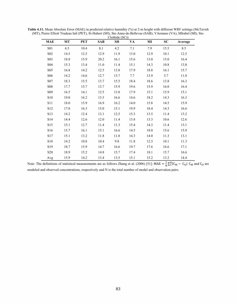
83
Table 4.11. Mean Absolute Error (MAE) in predicted relative humidity (%) at 2-m height with different WRF settings (McTavish (MT), Pierre Elliott Trudeau Intl (PET), St-Hubert (SH), Ste-Anne-de-Bellevue (SAB), VArennes (VA), MIrabel (MI), Ste-
Clothide (SC)) MAE MT PET SAB SH VA MI SC Average S01 6.5 10.4 8.1 4.2 7.1 7.9 15.5 8.5 S02 14.5 12.5 12.9 11.9 13.0 12.9 10.1 12.5 S03 18.8 15.9 20.2 16.1 15.6 13.0 15.0 16.4 S04 15.3 13.4 11.0 11.4 15.1 14.3 10.8 13.0 S05 16.8 14.2 12.5 13.8 17.9 18.8 16.1 15.7 S06 14.2 14.6 12.7 13.7 7.7 13.9 5.7 11.8 S07 18.3 15.5 13.7 15.5 18.4 18.6 13.8 16.3 S08 17.7 15.7 13.7 15.9 19.6 15.9 16.0 16.4 S09 16.5 14.1 12.5 13.8 17.9 15.1 15.9 15.1 S10 19.0 16.2 15.5 16.6 14.6 18.2 14.3 16.3 S11 18.0 15.9 16.9 16.2 14.0 15.8 14.5 15.9 S12 17.0 16.3 15.0 15.1 19.9 18.4 14.3 16.6 S13 14.2 12.4 13.1 12.5 15.3 13.5 11.4 13.2 S14 14.4 12.6 12.0 11.4 13.8 13.3 10.6 12.6 S15 15.1 12.7 11.4 11.3 15.4 14.3 11.4 13.1 S16 15.7 16.1 15.1 16.6 14.5 18.0 15.6 15.9 S17 15.1 13.2 11.8 11.8 14.3 14.0 11.3 13.1 S18 14.2 10.8 10.4 9.8 11.8 12.3 10.1 11.3 S19 18.7 15.9 14.7 16.6 19.7 17.6 16.6 17.1 S20 18.9 15.2 14.8 15.7 17.4 18.1 15.7 16.6 Avg 15.9 14.2 13.4 13.5 15.1 15.2 13.2 14.4
Note: The definitions of statistical measurements are as follows Zhang et al. (2006) [51]: MAE =1
N∑ |CM − CO| N
1 CM and CO are
modeled and observed concentrations, respectively and N is the total number of model and observation pairs.

84
Table 4.12. Root Mean Square Error (RMSE) in predicted relative humidity (%) at 2-m height with different WRF settings (McTavish (MT), Pierre Elliott Trudeau Intl (PET), St-Hubert (SH), Ste-Anne-de-Bellevue (SAB), VArennes (VA), MIrabel
(MI), Ste-Clothide (SC)) RMSE MT PET SAB SH VA MI SC Average
S01 8.7 12.8 10.1 5.4 10.3 10.1 20.2 11.1 S02 19.6 15.4 17.4 16.1 16.7 15.3 14.1 16.4 S03 23.9 19.1 24.4 20.2 20.8 17.3 19.0 20.7 S04 18.2 15.6 15.3 14.8 17.9 16.2 14.0 16.0 S05 19.7 17.0 15.9 16.7 20.6 22.2 20.2 18.9 S06 16.5 17.2 15.9 16.5 10.4 27.8 8.1 16.1 S07 21.2 18.5 16.8 18.4 21.5 23.1 17.7 19.6 S08 21.3 18.6 16.9 19.1 22.8 18.9 19.9 19.6 S09 19.7 17.0 15.9 16.5 20.7 17.8 20.3 18.3 S10 22.2 19.2 18.3 19.7 17.2 22.2 18.5 19.6 S11 22.6 21.7 21.3 21.8 18.7 18.6 18.5 20.5 S12 19.8 18.6 17.5 17.8 22.8 21.4 18.5 19.5 S13 18.1 15.0 16.7 15.4 18.6 15.6 14.1 16.2 S14 18.4 15.2 16.5 14.9 17.2 15.5 13.6 15.9 S15 18.4 15.3 15.9 14.9 18.4 16.4 14.1 16.2 S16 18.4 19.1 17.8 19.3 17.3 24.1 20.4 19.5 S17 18.2 15.5 15.1 15.1 16.2 16.1 14.3 15.8 S18 17.3 13.4 13.6 12.9 14.4 14.4 12.4 14.0 S19 21.8 19.0 17.5 19.5 23.1 23.5 20.3 20.7 S20 22.0 17.9 17.5 18.7 21.0 23.5 19.5 20.0 Avg 19.3 17.1 16.8 16.7 18.3 19.0 16.9 17.7
Note: The definitions of statistical measurements are as follows Zhang et al. (2006) [51]: RMSE = [1
N∑ (CM − CO)2N
1 ]1/2
CM and CO are modeled and observed concentrations, respectively and N is the total number of model and observation pairs.

85
Figure 4.12. Root mean square error in predicted relative humidity (%) at 2-m height with different WRF settings
Figure 4.13. Root mean square error in predicted relative humidity (%) at 2-m height in weather station over domain (McTavish
(MT), Pierre Elliott Trudeau Intl (PET), St-Hubert (SH), Ste-Anne-de-Bellevue (SAB), VArennes (VA), MIrabel (MI), Ste-Clothide (SC))
0.0
5.0
10.0
15.0
20.0
MT PET SAB SH VA MI SC
RM
SE(%
)
Weather Station
0
5
10
15
20
25
S01 S02 S03 S04 S05 S06 S07 S08 S09 S10 S11 S12 S13 S14 S15 S16 S17 S18 S19 S20
RM
SE(%
)
Different Simulation Set-ups in WRF

86
Table 4.13. Relative humidity (%) at 2-m height differences between CTRL & ALBEDO scenario (McTavish (MT), Pierre Elliott Trudeau Intl (PET), St-Hubert (SH), Ste-Anne-de-Bellevue (SAB), VArennes (VA), MIrabel (MI), Ste-Clothide (SC))
ΔRH MT PET SAB SH VA MI SC Average S01 -0.8 -0.5 -0.8 -0.5 -1.9 -1.5 -7.2 -1.9 S02 -3.6 -5.1 -3.6 12.7 -3.6 -5.1 -6.0 -2.0 S03 -7.2 -9.2 -7.2 -9.5 -7.2 -9.2 -9.5 -8.4 S04 -7.2 -9.6 -7.9 -9.3 -7.9 -9.6 -9.3 -8.7 S05 -7.7 -8.1 -7.1 -8.9 -7.1 -6.0 -5.1 -7.2 S06 1.6 -2.0 -1.7 -1.3 5.7 6.5 3.0 1.7 S07 0.1 0.6 0.8 1.1 -0.4 1.9 3.9 1.1 S08 -1.4 -1.0 -1.1 -0.9 -1.1 -1.0 -0.9 -1.0 S09 -1.8 -2.8 -2.2 -1.9 -2.7 -2.8 -2.0 -2.3 S10 -2.8 -3.4 -2.1 -2.6 -1.6 -5.0 -6.3 -3.4 S11 0.7 -0.8 -3.1 -4.0 -2.8 -8.1 -5.7 -3.4 S12 -1.9 -6.7 -1.4 -1.4 -1.4 -6.7 -1.0 -2.9 S13 -1.5 -1.3 -0.6 -1.1 -0.6 -1.3 -2.3 -1.2 S14 -0.7 -0.5 -0.3 1.2 -0.3 -0.5 0.4 -0.1 S15 -2.4 -4.1 -2.1 -3.3 -2.1 -4.1 -3.3 -3.1 S16 -1.8 -6.8 -4.9 -6.7 -1.1 -3.9 -6.7 -4.6 S17 -3.8 -5.4 -1.0 -4.8 -1.0 -5.4 -4.8 -3.7 S18 -6.0 -8.4 -3.9 -7.9 -3.7 -8.4 -7.9 -6.6 S19 -5.0 -4.5 -3.9 -5.3 -3.9 -3.1 -5.3 -4.4 S20 -3.0 -3.1 -1.7 -1.0 -2.7 -1.6 -2.6 -2.2 Avg -2.8 -4.1 -2.8 -2.8 -2.4 -3.7 -3.9 -3.2

87
Figure 4.14. 2-m Relative humidity (%) differences (CTRL- ALBEDO) in different physical parameterizations
Figure 4.15. 2-m Relative humidity (%) (CTRL- ALBEDO) in weather station over the domain (McTavish (MT), Pierre Elliott Trudeau Intl (PET), St-Hubert (SH), Ste-Anne-de-Bellevue (SAB), VArennes (VA), MIrabel (MI), Ste-Clothide (SC))
4.2.4. Precipitation
The numerical weather prediction models cannot fully capture the hydrological cycles and the
effects of clouds and water processes in the atmosphere. The assessment of the precipitation by
WRF is in a cumulative form meaning that even when the hourly precipitation for 5-h event is 1.0,
0.0, 0.3, 0.0, 3.0, the model still gets this magnitude correct for the total daily and or total episode.
The comparisons of precipitation can provide a qualitative assessment of the prediction of water
cycle by these models’ ensembles. The average MBA (Table 4.14) of all model ensembles are
almost the same except the S02 with Betts-Miller-Janjic cumulus scheme which is 0 mm. It
indicates that this cumulus model performs well in predicting precipitation using fine resolution
grid size. In the urban area, MAE (Table 4.15) of the predicted precipitation by other model
ensembles was almost the same. The MAE of all models is less than 3 mm. Table 4.16 and Figures
-10
-8
-6
-4
-2
0
2
4
S01 S02 S03 S04 S05 S06 S07 S08 S09 S10 S11 S12 S13 S14 S15 S16 S17 S18 S19 S20ΔR
H (%
)
Different Simulation Set-ups in WRF
-5.0
-4.0
-3.0
-2.0
-1.0
0.0MT PET SAB SH VA MI SC
ΔRH
(%)
Weather Station

88
4.16 and 4.17 provide the calculated RMSE of the model ensemble in predicting the rainfall episode
during the simulation period with different WRF settings.
Table 4.14. Mean Bias Error (MBE) in predicted precipitation (mm) with different WRF settings (McTavish (MT), Pierre Elliott
Trudeau Intl (PET), St-Hubert (SH), Ste-Anne-de-Bellevue (SAB), VArennes (VA), MIrabel (MI), Ste-Clothide (SC)) MBA MT PET SAB SH VA MI SC Average S01 -0.2 -0.3 -0.3 -0.3 -0.3 -0.3 -0.3 -0.3 S02 -0.3 -0.2 -0.2 1.5 -0.2 -0.2 -0.2 0.0 S03 -0.3 -0.3 -0.3 -0.3 -0.3 -0.3 -0.3 -0.3 S04 -0.3 -0.3 -0.3 -0.3 -0.3 -0.3 -0.3 -0.3 S05 -0.2 -0.3 -0.3 -0.2 -0.3 -0.3 -0.3 -0.3 S06 -0.2 -0.3 -0.3 -0.3 -0.3 -0.3 -0.3 -0.3 S07 -0.3 -0.3 -0.3 -0.3 -0.3 -0.3 -0.3 -0.3 S08 -0.2 -0.2 -0.2 -0.1 -0.2 -0.2 -0.1 -0.2 S09 -0.3 -0.3 -0.3 -0.3 -0.3 -0.3 -0.3 -0.3 S10 -0.2 -0.2 -0.3 -0.1 -0.2 -0.2 -0.1 -0.2 S11 -0.2 -0.2 -0.2 -0.1 -0.2 -0.2 -0.1 -0.2 S12 -0.2 -0.2 -0.2 -0.1 -0.2 -0.2 -0.1 -0.2 S13 -0.1 -0.3 -0.2 0.2 -0.2 -0.3 0.2 -0.1 S14 -0.2 -0.3 -0.2 0.1 0.0 -0.1 0.3 0.0 S15 -0.2 -0.3 -0.3 -0.3 -0.3 -0.3 -0.3 -0.3 S16 -0.2 -0.1 -0.1 -0.2 -0.1 -0.1 -0.2 -0.1 S17 -0.2 -0.2 -0.1 -0.1 -0.1 -0.2 -0.2 -0.2 S18 -0.2 -0.3 -0.3 -0.3 -0.2 -0.3 -0.2 -0.3 S19 -0.2 -0.2 -0.3 -0.2 -0.2 -0.2 -0.2 -0.2 S20 -0.2 -0.3 -0.3 -0.3 -0.3 -0.3 -0.3 -0.3 Avg -0.2 -0.3 -0.2 -0.1 -0.2 -0.3 -0.2 -0.2
Note: The definitions of statistical measurements are as follows Zhang et al. (2006) [51]: MBE = 1
N∑ (CM − CO),N
1 𝐶𝑀 and CO are
modeled and observed concentrations, respectively and N is the total number of model and observation pairs.

89
Table 4.15. Mean Absolute Error (MAE) in predicted precipitation (mm) with different WRF settings (McTavish (MT), Pierre Elliott Trudeau Intl (PET), St-Hubert (SH), Ste-Anne-de-Bellevue (SAB), VArennes (VA), MIrabel (MI), Ste-Clothide (SC))
MAE MT PET SAB SH VA MI SC Average S01 0.2 0.3 0.3 0.3 0.3 0.3 0.3 0.3 S02 0.3 0.2 0.2 0.0 0.2 0.2 0.2 0.2 S03 0.3 0.3 0.3 0.3 0.3 0.3 0.3 0.3 S04 0.3 0.3 0.3 0.3 0.3 0.3 0.3 0.3 S05 0.2 0.3 0.3 0.2 0.3 0.3 0.3 0.3 S06 0.2 0.3 0.3 0.3 0.3 0.3 0.3 0.3 S07 0.3 0.3 0.3 0.3 0.3 0.3 0.3 0.3 S08 0.2 0.2 0.2 0.1 0.2 0.2 0.1 0.2 S09 0.3 0.3 0.3 0.3 0.3 0.3 0.3 0.3 S10 0.2 0.2 0.3 0.1 0.2 0.2 0.1 0.2 S11 0.2 0.2 0.2 0.1 0.2 0.2 0.1 0.2 S12 0.2 0.2 0.2 0.1 0.2 0.2 0.1 0.2 S13 0.1 0.3 0.2 0.2 0.2 0.3 0.2 0.2 S14 0.2 0.3 0.2 0.1 0.2 0.1 0.3 0.2 S15 0.2 0.3 0.3 0.3 0.3 0.3 0.3 0.3 S16 0.2 0.1 0.1 0.2 0.1 0.1 0.2 0.2 S17 0.2 0.2 0.1 0.1 0.1 0.2 0.2 0.2 S18 0.2 0.3 0.3 0.3 0.2 0.3 0.2 0.3 S19 0.2 0.2 0.3 0.2 0.2 0.2 0.2 0.2 S20 0.2 0.3 0.3 0.3 0.3 0.3 0.3 0.3 Avg 0.2 0.3 0.2 0.2 0.2 0.3 0.2 0.2
Note: The definitions of statistical measurements are as follows Zhang et al. (2006) [51]: MAE =1
N∑ |CM − CO| N
1 CM and CO are
modeled and observed concentrations, respectively and N is the total number of model and observation pairs.

90
Table 4.16. Root Mean Square Error (RMSE) in predicted precipitation (mm) with different WRF settings (McTavish (MT), Pierre Elliott Trudeau Intl (PET), St-Hubert (SH), Ste-Anne-de-Bellevue (SAB), VArennes (VA), MIrabel (MI), Ste-Clothide
(SC)) RMSE MT PET SAB SH VA MI SC Average
S01 1.4 2.0 1.8 1.7 1.7 2.0 1.8 1.8 S02 1.6 1.5 1.4 0.0 1.4 1.5 1.2 1.2 S03 1.7 2.0 1.8 1.8 1.9 2.0 1.9 1.9 S04 1.7 2.0 1.8 1.8 1.9 2.0 1.9 1.9 S05 1.5 1.8 1.6 1.1 1.9 1.7 1.9 1.6 S06 1.2 0.0 1.8 1.8 1.7 2.0 1.9 1.5 S07 2.0 1.8 1.8 2.0 1.7 2.0 1.9 1.9 S08 1.3 1.3 1.1 0.5 1.0 1.0 0.7 1.0 S09 1.7 2.0 1.8 1.8 1.7 1.7 1.9 1.8 S10 1.2 1.3 1.5 0.7 1.5 1.3 0.8 1.2 S11 1.3 1.3 1.1 0.5 1.0 1.3 0.7 1.0 S12 1.2 1.3 1.3 0.6 1.2 1.3 0.7 1.1 S13 0.8 1.9 1.3 1.0 1.2 2.0 1.0 1.3 S14 1.4 1.6 1.1 0.6 1.1 0.8 2.1 1.2 S15 1.4 2.0 1.8 1.8 1.7 2.0 1.9 1.8 S16 1.4 0.9 0.9 1.2 0.7 0.9 1.3 1.1 S17 1.4 1.1 0.9 0.9 0.9 1.1 1.1 1.0 S18 1.4 2.0 1.8 1.8 1.4 2.0 1.4 1.7 S19 1.4 1.3 1.5 1.1 1.5 1.4 1.2 1.4 S20 1.4 2.0 1.8 1.8 1.7 2.0 1.9 1.8 Avg 1.4 1.5 1.5 1.2 1.5 1.6 1.5 1.5
Note: The definitions of statistical measurements are as follows Zhang et al. (2006) [51]: RMSE = [1
N∑ (CM − CO)2N
1 ]1/2
CM and CO are modeled and observed concentrations, respectively and N is the total number of model and observation pairs.

91
Figure 4.16. Root mean square error in predicted precipitation (mm) with different WRF setting
Figure 4.17. Root mean square error in predicted precipitation (mm) in weather station over the domain (McTavish (MT), Pierre
Elliott Trudeau Intl (PET), St-Hubert (SH), Ste-Anne-de-Bellevue (SAB), VArennes (VA), MIrabel (MI), Ste-Clothide (SC))
The precipitation differences between CTRL and ALBEDO scenario are presented in Table
4.17 and Figure 4.18. In general, an increase of albedo reduces the absorption of solar radiation
and the transfer of sensible and latent heat into the atmosphere. The convective clouds reduce the
downward flux of long wave radiation and thus the net absorption of radiation is decreased.
Therefore, an increase in albedo leads to a net decrease of radiative flux into the ground and a net
decrease of convective cloud and precipitation. But, in these simulations, the results show a slight
increase in precipitation in S02, S06, and S08 and not a significant change in S11, S12, S13 and
S14, and a decrease in other model ensembles. In general precipitation decreases as 0.2 mm if the
surface reflectivity of roofs, walls and grounds increases. Figure 4.19 shows the precipitation
differences between CTRL and ALBEDO for different weather stations over the domain.
0.0
0.5
1.0
1.5
2.0
S01 S02 S03 S04 S05 S06 S07 S08 S09 S10 S11 S12 S13 S14 S15 S16 S17 S18 S19 S20
RM
SE p
reci
pita
tion
(mm
)
Different Simulation Set-ups in WRF
0.0
0.5
1.0
1.5
MT PET SAB SH VA MI SC
RM
SE p
reci
pita
tion
(mm
)
Weather Station

92
Table 4.17. Precipitation (mm) differences between CTRL & ALBEDO scenarios (McTavish (MT), Pierre Elliott Trudeau Intl (PET), St-Hubert (SH), Ste-Anne-de-Bellevue (SAB), VArennes (VA), MIrabel (MI), Ste-Clothide (SC)) ΔRain MT PET SAB SH VA MI SC Average
S01 0.5 -0.1 0.0 -2.0 -0.3 -0.1 -1.0 -0.5 S02 -0.4 -0.1 0.3 0.0 0.3 -0.1 0.5 0.1 S03 -0.5 -0.5 -0.6 -0.6 -0.3 -0.5 -0.5 -0.5 S04 -0.4 -0.6 -0.4 -1.3 -0.3 -0.4 -0.4 -0.5 S05 -1.1 0.1 -0.2 -0.5 0.1 0.1 -0.6 -0.3 S06 2.2 0.5 -0.5 -0.4 -0.2 -0.1 -0.2 0.2 S07 -0.8 -0.8 -0.8 -0.9 -1.1 -0.7 -0.7 -0.8 S08 -0.4 1.3 1.8 1.7 0.1 0.5 -0.5 0.6 S09 -0.5 -0.9 -0.9 -0.5 -0.4 -0.6 -1.2 -0.7 S10 -0.2 -1.7 -1.5 0.6 -1.8 0.4 -0.3 -0.7 S11 0.1 0.1 2.5 -3.0 -0.1 0.1 0.4 0.0 S12 -0.7 0.5 -0.6 -0.8 0.3 1.5 0.0 0.0 S13 0.0 -0.1 0.1 -0.9 1.0 -0.2 0.0 0.0 S14 -0.2 -2.2 0.4 1.8 1.4 -0.2 -0.7 0.0 S15 0.2 -0.4 -0.3 -0.3 -0.2 -0.4 -0.3 -0.2 S16 -0.2 -1.1 -0.9 -0.2 -0.9 -1.1 -0.7 -0.7 S17 -0.9 -0.1 2.3 -1.4 1.9 -0.1 0.1 0.3 S18 -0.2 -0.4 -0.6 -0.3 -0.2 -0.2 -0.2 -0.3 S19 0.1 0.1 -1.4 -0.7 -1.0 0.1 -0.1 -0.4 S20 -0.2 -0.2 -0.2 -0.4 -0.6 -0.2 -0.6 -0.4 Avg -0.2 -0.3 -0.1 -0.5 -0.1 -0.1 -0.3 -0.2

93
Figure 4.18. Precipitation (mm) differences (CTRL- ALBEDO) with different physical parameterizations
Figure 4.19. Precipitation (mm) differences (CTRL- ALBEDO) in weather stations over the domain (McTavish (MT), Pierre Elliott Trudeau Intl (PET), St-Hubert (SH), Ste-Anne-de-Bellevue (SAB), VArennes (VA), MIrabel (MI), Ste-Clothide (SC))
4.3. Discussion and Conclusion of Physical Parameterizations in WRF and Effects of
Increasing Surface Reflectivity
A sensitivity analysis of physical parametrizations in WRF are conducted (for a total of 20
model ensembles) to evaluate their performance on predicting urban climate (2-m air temperature,
10-m wind speed, 2-m relative humidity, and precipitation). A period of three days in August (09-
Aug-2009 to 11-Aug-2009) is selected. The simulation starts from a sunny day and ends with a
rainy condition. Four domains are telescopically nested to cover the Greater Montreal Area with
the resolution of 333 m. The hourly data of the aforementioned parameters are estimated. This
specific time frame shows the close combination of sunny and rainy conditions over the interested
domain. To see the results of choice of parameterizations change under different weather patterns,
more simulations need to be carried out during sunny, rainy and very warm episodes to indicate
the choice of parameterizations. However, the results from these simulations are episode-specific
-1.1
-0.6
-0.1
0.4
S01 S02 S03 S04 S05 S06 S07 S08 S09 S10 S11 S12 S13 S14 S15 S16 S17 S18 S19 S20
ΔPre
cipi
tatio
n(m
m)
Different Simulation Set-ups in WRF
-0.6
-0.3
0.0MT PET SAB SH VA MI SC
ΔPre
cipi
tatio
n(m
m)
Weather Station

94
and might not be transferrable to other locations and conditions. The anthropogenic heat emission
estimation needs to be available to achieve more accurate and reliable results in the future.
The S06 simulation setup (Table 4.1) shows the reasonable results compared with
measurements. The combination of WDM6 (Lim and Hong, 2010), Grell 3D (Grell, 1993; Grell
and Devenyi, 2002), MYJ (Janjic, 1994), and RRTMG (Iacono et al., 2008) as microphysics,
cumulus, planetary boundary layer, and radiation schemes, respectively, resulted in the least error
in 2-m air temperature (RMSE = 1.9 oC) compared to the measurements (Table 4.4 and Figure 4.2).
The combination of S01 and S20 that used the same microphysics, planetary boundary layer height
and radiation provides the least error comparing to other model ensembles, as well. The
comparisons of wind speed indicated that S06 results are close to S02, S04 and S17. But these
models could not predict the 2-m air temperature as accurately as S06. The relative humidity results
indicated that S06 has the least error compared to measurements except in the S01 simulation. The
reason is that the S01 uses the Simplified Arakawa-Schubert scheme for cumulus modelling and
thus predicts the rainy condition better. But this scheme cannot accurately predict the T2 on a sunny
day (Table 4.12 and Figure 4.11). The precipitation results are better in S08, S11, S16 and S17
compared to S06, but again, these simulation setups cannot predict the T2 and WS accurately
(Table 4.16 and Figure 4.15). Since the prediction of T2 is more important in terms of heat island
mitigation strategy, the S06 model ensemble is selected. The other reason for S06 selection is its
computational time, which is 10% less compared to other simulation setups. The result of model
performance in terms of T2 (S06) is compared with other studies with different physical
parametrizations (Table 4.18). The results of T2 in estimates of S06 simulation setup are in good
agreement with other studies, considering different episodes and periods of simulations (rainy
conditions for this study). Table 4.18. Comparisons of 2-m air temperature results of S06 with other studies with different physical parameterizations
Study Microphysics Cumulus PBL Radiation T2 evaluation results S06 (the present study), rainy episode in GMA, 2009
WDM6 Grell 3D MYI RRTMG RMSE= 1.9
Fallmann et al., 2014 Stuttgart, heat wave 2003
WSM06 Kain-Fritch
MYJ Shortwave: Goddard Longwave: RRTM
R2 = 0.71
Salamanca et al., 2012, Madrid, two separate hottest day in summer 2008
WSM03 _ MYJ Shortwave: Dudhia Longwave: RRTM
RMSE = 1.5
Vahmani & Ban-Weiss. 2016, LA, 6-11 July 2012
Lin Kain-Fritch
YSU Shortwave: Dudhia Longwave: RRTM
RMSE = 3.8

95
Chen et al., 2013, Hangzhou, China, July 2009
WSM06 Betts–Miller–Janjic
YSU Shortwave: Dudhia Longwave: RRTM
RMSE = 1.61
YSU: Yonsei University scheme; WDM06: WRF Double-Moment 6-class; WSM06: WRF Single-Moment 6-class; MYJ: Mellor-Yamada-Janjic; RMSE: Root Mean Square Error; RRTMG: Rapid Radiative Transfer Model
All models on average slightly underestimate the meteorological parameters. One of the main
reasons is that the WRF cannot estimate the anthropogenic heat emissions. Human activities are
the main source of heat emission in urban areas—for example, the use of transportation and air
conditioning in summer time. Another important issue is the possible impact of other micro-scale
effects that are not captured by the model resolution. The exact characteristics, height and direction
of buildings cannot be simulated in the model, while these parameters affect the results of
measurements in weather stations.
As the surface reflectivity of roofs, walls and roads increased, the results indicated that the
averaged 2-m air temperature decreased by 0.2 °C, the 10-m wind speed slightly increased, the
relative humidity decreased by an average of 3.2%, and the precipitation decreased by 0.2 mm.
However, the results from these simulations are episode-specific and might not be transmissible to
other locations and conditions. The anthropogenic heat emission estimation needs to be available
to achieve more accurate and reliable results in the future.
4.4. Applications of the Developed Platform for Urban Climate Simulation and Heat
Island Mitigation Strategy
The developed model is an appropriate platform for urban climate simulations. This
meteorological platform (with proper physical options for microphysics, cumulus, PBL and
radiation models) enable environmental policymakers to have a better understanding of the effects
of heat island and mitigations strategies on urban areas in cold climates. This platform is verified
by comparing the simulation results with measurements and thus further is applied to perform other
objectives. The same physical parameterizations and simulation approach is used to assess the
effects of heat island and increasing surface reflectivity on heat-related mortality in the Greater
Montreal Area during the 2005 and 2011 heat wave periods. The results of this study are presented
in Chapter 5. In addition, the developed platform provides a good understanding of each physical
parametrization in WRF and their impacts on meteorological parameters in a cold climate.

96

97
Chapter 5 Effects of Increasing Surface Reflectivity on Heat-Related Mortality Heat-related mortality is increasing as a result of climate change and extreme heat events. Climate
change can exacerbate extreme heat events and the duration of high temperatures (IPCC, 2014).
High temperature intensity and duration cause an increase in morbidity and mortality. According
to the Canadian Environmental Health Atlas (CEHA 2018), 121 people die every year in Montreal
because of heat-related issues. In another study, the number of heat-related deaths was estimated
to be 209 people during the July 2010 heat wave period in Montreal (Bustinza et al., 2013).
Increasing surface reflectivity is applied to mitigate the effects of heat island and high temperature
in urban areas. ISR decreases heat-related mortality by 3 to 16% in different locations (Kalkstein
and Sheridan, 2003; Kalkstein et al., 2011 and 2013). In addition, increasing surface albedo can
shift days to less oppressive air mass conditions by 50% (Kalkstein et al., 2011 and 2013), and thus
provide a more pleasant environment for urban dwellers.
The Weather Research and Forecasting model (WRF) is coupled with a multi-layer of the Urban
Canopy Model (ML-UCM) to investigate the effects of urban heat island intensity during the 2005
and 2011 heat wave periods in the Greater Montreal Area (GMA), Canada. Each day of simulation
is categorized into an air mass type using the Spatial Synoptic Classification (SSC). The non-
accidental mortality data during the summer period is employed and the number of deaths above
the expected mean anomalous daily mortality is calculated for each air mass classification. Results
indicate that moist tropical plus (hotter and more humid conditions than the moist tropical) and dry
tropical (the hottest and driest conditions) weather have the highest rank in heat-related deaths. The
effects of increasing surface reflectivity (ISR) is assessed using four meteorological parameters: 2-
m air temperature (T2), 10-m wind speed (WS10), 2-m relative humidity (RH2), and dew point
temperature (DPT), and four heat stress indices: National Weather Service – Heat Index (NWS-
HI), Apparent Temperature (AT), Canadian Humid Index (CHI), and Discomfort Index (DI).

98
The meteorological parameters of the CTRL scenario (where the albedo of roofs, walls, and
roads are assumed to be 0.2) are compared with the measurements obtained from urban (McTavish
(MT) and Pierre Elliott Trudeau Intl (PET)) and rural (Montreal/St-Hubert (SH) and Ste-Anne-de-
Bellevue (SAB)) weather stations across the domain. A set of metrics calculations are applied to
evaluate model performance (mean bias error (MBE), mean absolute error (MAE) and root mean
square error (RMSE)). In the ALBEDO scenario, the albedo of roofs, walls, and roads are increased
from 0.2 to 0.65, 0.60, and 0.45, respectively. The effects of ISR are investigated on urban climate,
heat stress indices and heat-related mortality by comparing the CTRL and ALBEDO results.
Air mass type, air temperature and apparent temperature changes for each day are applied to
translate the effects of extreme heat events and the potential of increasing surface reflectivity on
heat-related mortality during the 2005 and 2011 heat wave periods. The daily heat-related mortality
(HRM) is estimated for two air mass classifications in the GMA: DT (dry tropical) and MT/MT+
(moist tropical and moist tropical plus). The algorithms to estimate heat-related mortality are
explained in detail in Chapter 3, Section 3.3. Here, the results of this study are presented. The
research addressed in this chapter is summarized in the article by Z. Jandaghian and H. Akbari
(2018), “The effects of increasing surface reflectivity on heat-related mortality in the Greater
Montreal Area, Canada” (https://doi.org/10.1016/j.uclim.2018.06.002).
5.1. Defining Simulation Domain and Period
The simulation domain is Greater Montreal Area. Figure 5.1 shows the simulation domain and
land use, land cover. The simulations are conducted during the 2005 (10th -12th July) and the 2011
(20th – 23rd July) heat wave events.
Figure 5.1. Simulation domain and Land Use Land Cover (LULC) of GMA

99
The simulations were conducted with the initial and boundary conditions obtained from the
North American Regional Reanalysis (NARR). A vertical resolution of 51eta level is defined to
take full advantages of the urban parameterizations. The proper physical parameterizations of the
previous task (1st objective) is used to simulate the CTRL and ALBEDO cases of the 2005 and
2011 heat wave period over Greater Montreal Area.
5.2. Evaluation of Meteorological Model Performance
To evaluate the simulations performances, the meteorological parameters namely: 2-m air
temperature (T2), 10-m wind speed (WS10), relative humidity (RH), and dew point temperature
(DPT) are collected from four weather stations (McTavish (MT), Pierre Elliott Trudeau Intl (PET),
St-Hubert (SH), Ste-Anne-de-Bellevue (SAB)) across the Greater Montreal Area for two heat wave
period in 2005 and 2011. Table 3.3 presents their geographical locations.
The parameters that are directly extracted from the simulation results are the 2-m air
temperature (T2, K), dew point temperature (DPT, K), horizontal and vertical wind speed (U10,
V10, m/s), and water mixing ratio (Q2, %). Other parameters are calculated as presented in Table
3.10 namely 10-m wind speed (WS10), 2-m relative humidity (RH2), and 3 heat stress indices:
apparent temperature (AT), Canadian Humid Index (CHI), and Discomfort Index (DI). The
parameters that are analysed for the two heat wave periods are T2, WS10, RH2, DPT, AP, CHI,
DI, and the National Weather Service – Heat Index (NWS-HI). The NWS-HI is a measurement to
show how hot it feels when RH2 is factored in with the actual T2.
Table 5.1 presents the maximum air temperature measured in weather stations for the 2005 and
2011 heat wave periods during three consecutive days in July. The hourly data obtained from
weather stations are compared with the hourly simulated values for CTRL case simulations. Table
5.2 presents the MBE, MAE and RSME of aforementioned parameters. Figure 5.2, Figure 5.3,
Figure 5.4, Figure 5.6 respectively show comparisons between simulated averaged 3-day cycle and
observed 2-m air temperature, 10-m wind speed, and dew point temperature in four weather stations
and 2-m relative humidity for urban and rural areas.
The model, on average, slightly overestimates the air temperature, wind speed and dew point
temperature in the 2005 simulation. The model slightly underestimates the air temperature and
wind speed in the 2011 simulation. One of the reasons is that the effects of micro scale parameters

100
cannot be captured in mesoscale models precisely. The heat emission from buildings and the
transportation sectors cannot be estimated in the model solver. The relative humidity at the 2-m
height is estimated based on a calculation from National Oceanic and Atmospheric Administration
(NOAA) weather services and is addressed in Chapter 3. The measurements of heat stress indices
are also presented in Chapter 3. In other studies, the comparison of thermal components of WRF
and the Fifth-Generation NCAR/Penn State Mesoscale Model (MM5) indicated that both models
have the MBE of T2 as almost -3.8oC to 0.2oC during a year (Gilliam et al., 2006; Wu et al., 2008;
Wang et al., 2009; Liu et al., 2010). Thus, the performance of WRF is generally consistent with the
measurements and the results are well reliable for further investigations. Table 5.1. Max air temperature measured in four weather stations over GMA in 2005 and 2011heat wave periods (McTavish
(MT), Pierre Elliott Trudeau Intl (PET), St-Hubert (SH), Ste-Anne-de-Bellevue (SAB))
Heat wave periods July 2005 Max Temperature (oC)
MT PET SH SAB
July 2005 10th 31.6 31.5 311 30.8 11th 32.3 32.8 31.5 32.2 12th 30.6 30.6 30.7 30.3
July Average T (oC) 26.9 27.3 27.0 27.1
July 2011 21th 34.9 35.6 36.0 34.7 22nd 31.3 31.9 32.6 32.2 23rd 31.6 32.6 32.6 31.9
July Average T (oC) 28.3 28.5 29.0 28.5
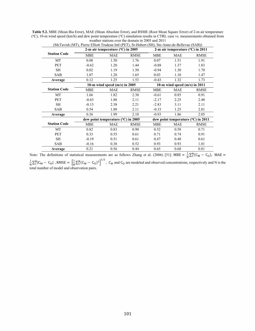
101
Table 5.2. MBE (Mean Bia Error), MAE (Mean Absolute Error), and RSME (Root Mean Square Error) of 2-m air temperature (oC), 10-m wind speed (km/h) and dew point temperature (oC) simulation results in CTRL case vs. measurements obtained from
weather stations over the domain in 2005 and 2011 (McTavish (MT), Pierre Elliott Trudeau Intl (PET), St-Hubert (SH), Ste-Anne-de-Bellevue (SAB))
Station Code
2-m air temperature (oC) in 2005 2-m air temperature (oC) in 2011 MBE MAE RMSE MBE MAE RMSE
MT 0.08 1.50 1.76 0.07 1.51 1.91 PET -0.62 1.20 1.44 -0.88 1.37 1.83 SH 0.02 1.19 1.50 -0.94 1.30 1.70
SAB 1.07 1.28 1.65 0.03 1.10 1.47 Average 0.12 1.25 1.53 -0.43 1.32 1.73
Station Code
10-m wind speed (m/s) in 2005 10-m wind speed (m/s) in 2011 MBE MAE RMSE MBE MAE RMSE
MT 1.66 1.82 2.30 -0.61 0.85 0.91 PET -0.63 1.88 2.11 -2.17 2.25 2.40 SH -0.13 2.38 2.21 -2.83 3.11 2.11
SAB 0.54 1.88 2.11 -0.33 1.25 2.81 Average 0.36 1.99 2.18 -0.93 1.86 2.05
Station Code
dew point temperature (oC) in 2005 dew point temperature (oC) in 2011 MBE MAE RMSE MBE MAE RMSE
MT 0.82 0.83 0.90 0.52 0.58 0.71 PET 0.33 0.55 0.61 0.71 0.74 0.91 SH -0.19 0.51 0.61 0.47 0.48 0.61
SAB -0.16 0.38 0.52 0.93 0.93 1.01 Average 0.21 0.56 0.44 0.65 0.68 0.81
Note: The definitions of statistical measurements are as follows Zhang et al. (2006) [51]: MBE = 1
N∑ (CM − CO),N
1 MAE =
1
N∑ |CM − CO| N
1 , RMSE = [1
N∑ (CM − CO)2N
1 ]1/2
, 𝐶𝑀 and CO are modeled and observed concentrations, respectively and N is the total number of model and observation pairs.

102
Figure 5.2. Simulated averaged 3-day cycle of 2-m air temperature (oC) in CTRL [solid line] vs. measurements [dashed line] from four weather stations over GAM during 2005 [left] and 2011 [right] heat wave periods (McTavish (MT), Pierre Elliott
Trudeau Intl (PET), St-Hubert (SH), Ste-Anne-de-Bellevue (SAB))
20
26
32
38
0 6 12 18 24
T2(
o C)
MT
20
26
32
38
0 6 12 18 24
T2(
o C)
MT
18
24
30
36
0 6 12 18 24
T2(
o C)
PET
20
26
32
38
0 6 12 18 24
T2(
o C)
PET
18
24
30
36
0 6 12 18 24
T2(
o C)
SH
20
26
32
38
0 6 12 18 24
T2(
o C)
SH
18
24
30
36
0 6 12 18 24
T2(
o C)
SAB
18
24
30
36
0 6 12 18 24
T2(
o C)
SAB

103
Figure 5.3. Simulated averaged 3-day cycle of 10-m wind speed (m/s) in CTRL [solid line] vs. measurements [dashed line] from four weather stations over GAM during 2005 [left] and 2011 [right] heat wave periods (McTavish (MT), Pierre Elliott Trudeau
Intl (PET), St-Hubert (SH), Ste-Anne-de-Bellevue (SAB))
0
5
10
15
20
0 6 12 18 24
WS
(m/s
)MT
0
5
10
15
0 6 12 18 24
WS
(m/s
)
MT
0
10
20
0 6 12 18 24
WS
(m/s
)
PET
0
20
40
0 6 12 18 24W
S (m
/s)
PET
0
10
20
0 6 12 18 24
WS
(m/s
)
SH
0
20
40
0 6 12 18 24
WS
(m/s
)
SH
0
5
10
15
20
25
0 8 16 24
WS
(m/s
)
SAB
0
10
20
30
0 6 12 18 24
WS
(m/s
)
SAB

104
Figure 5.4. Simulated averaged 3-day cycle of dew point temperature (oC) in CTRL [solid line] vs. measurements [dashed line] from four weather stations over GAM during 2005 [left] and 2011 [right] heat wave periods (McTavish (MT), Pierre Elliott
Trudeau Intl (PET), St-Hubert (SH), Ste-Anne-de-Bellevue (SAB))
10
15
20
25
30
0 6 12 18 24
DPT
(o C)
MT
10
15
20
25
30
0 6 12 18 24
DPT
(o C)
MT
10
15
20
25
30
0 6 12 18 24
DPT
(o C)
PET
10
15
20
25
30
0 6 12 18 24D
PT (o C
)
PET
10
15
20
25
30
0 6 12 18 24
DPT
(o C)
SH
10
15
20
25
30
0 6 12 18 24
DPT
(o C)
SH
10
15
20
25
30
0 6 12 18 24
DPT
(o C)
SAB
10
15
20
25
30
0 6 12 18 24
DPT
(o C)
SAB
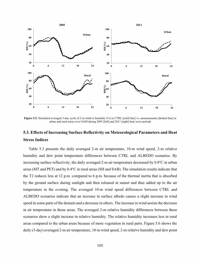
105
2005 2011
Figure 5.5. Simulated averaged 3-day cycle of 2-m relative humidity (%) in CTRL [solid line] vs. measurements [dashed line] in
urban and rural areas over GAM during 2005 [left] and 2011 [right] heat wave periods
5.3. Effects of Increasing Surface Reflectivity on Meteorological Parameters and Heat
Stress Indices
Table 5.3 presents the daily averaged 2-m air temperature, 10-m wind speed, 2-m relative
humidity and dew point temperature differences between CTRL and ALBEDO scenarios. By
increasing surface reflectivity, the daily averaged 2-m air temperature decreased by 0.8oC in urban
areas (MT and PET) and by 0.4oC in rural areas (SH and SAB). The simulation results indicate that
the T2 reduces less at 12 p.m. compared to 6 p.m. because of the thermal inertia that is absorbed
by the ground surface during sunlight and then released at sunset and thus added up to the air
temperature in the evening. The averaged 10-m wind speed differences between CTRL and
ALBEDO scenarios indicate that an increase in surface albedo causes a slight increase in wind
speed in some parts of the domain and a decrease in others. The increase in wind assists the decrease
in air temperature in those areas. The averaged 2-m relative humidity differences between these
scenarios show a slight increase in relative humidity. The relative humidity increases less in rural
areas compared to the urban areas because of more vegetation in rural parts. Figure 5.6 shows the
daily (3-day) averaged 2-m air temperature, 10-m wind speed, 2-m relative humidity and dew point
20
40
60
80
100
0 6 12 18 24
RH
(%)
Urban
20
40
60
80
100
0 6 12 18 24
RH
(%)
Urban
20
40
60
80
100
0 6 12 18 24
RH
(%)
Rural
20
40
60
80
100
0 6 12 18 24R
H(%
)
Rural

106
temperature differences between CTRL and ALBEDO scenarios during these two heat wave
periods. Spatially averaged values for urban and rural areas are shown with solid and dashed lines,
respectively.
Figure 5.7 shows the daily averaged discomfort index (DI) and apparent temperature (AT) for
CTRL and ALBEDO scenarios. The results indicate that an increase in surface albedo causes a
decrease in apparent temperature and discomfort indices that makes the environment more
preferable and suitable for human beings during summer time. Thus, it reduces the risk of heat-
related morbidity and mortality. Two indicators are applied (2-m air temperature and 2-m relative
humidity) that are also extracted from ALBEDO simulation results in these estimations. Because
of albedo enhancement, the DI improved by nearly 3% and 1.7% in urban and rural areas. The AT
decreased by nearly 2.6oC and 1.8oC in urban and rural areas, respectively (Figure 5.8). In general,
the urban diurnal range of heat indices (HI) is higher than the rural ones; thus, the consequences of
increasing surface reflectivity in urban areas are more measurable.

107
2005 2011
Figure 5.6. Simulated averaged diurnal (3-day) cycle of National Weather Service – Heat Index (oC), Apparent Temperature (oC),
Canadian Humid Index (oC), Discomfort Index (Units) in CTRL scenarios in 2011 [left] and 2005 [right] shown in urban areas [solid line] and rural areas [dashed line]
20
25
30
35
0 6 12 18 24
NW
S -
HI(
oC
)
20
30
40
0 6 12 18 24
NW
S -
HI(
oC
)
27
32
37
42
47
0 6 12 18 24
AT
(oC
)
40
50
60
70
0 6 12 18 24
AT
(oC
)
25
30
35
40
0 6 12 18 24
Ca
na
dia
n H
um
id I
nd
ex
(o
C)
25
35
45
0 6 12 18 24
Ca
na
dia
n H
um
id I
nd
ex
(o
C)
20
25
30
0 6 12 18 24
DI
(Un
its)
20
25
30
0 6 12 18 24
DI
(Un
its)

108
Table 5.3. Averaged 3-day differences of 2-m air temperature (oC), 10-m wind speed (m/s), dew point temperature (oC), and 2-m
relative humidity (%) between CTRL and ALBEDO scenarios in GAM during 2005 and 2011 heat wave periods CTRL-ALBEDO
Heat-wave MT PET SH SAB
∆T2 (oC)
2005 0.7 0. 5 0.2 0.7 2011 0.8 0.7 0.2 0.6
∆WS10 (m/s)
2005 0.2 -0.05 -0.01 0.01 2011 0.3 -0.09 -0.02 0.01
∆DPT (oC) 2005 -0.19 -0.27 -0.18 -0.25 2011 -0.28 -0.38 -0.13 -0.29
∆RH2 (%)
2005 -0.4 -0.2 -0.09 -0.13 2011 -0.3 -0.4 -0.17 -0.11
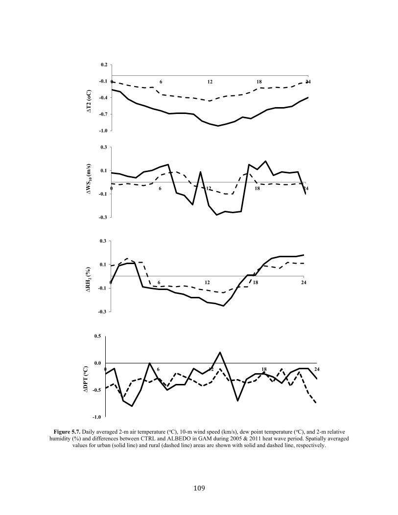
109
Figure 5.7. Daily averaged 2-m air temperature (oC), 10-m wind speed (km/s), dew point temperature (oC), and 2-m relative
humidity (%) and differences between CTRL and ALBEDO in GAM during 2005 & 2011 heat wave period. Spatially averaged values for urban (solid line) and rural (dashed line) areas are shown with solid and dashed line, respectively.
-1.0
-0.7
-0.4
-0.1
0.2
0 6 12 18 24∆T
2 (o
C)
-0.3
-0.1
0.1
0.3
0 6 12 18 24
∆WS 1
0 (m
/s)
-0.3
-0.1
0.1
0.3
0 6 12 18 24
∆RH
2 (%
)
-1.0
-0.5
0.0
0.5
0 6 12 18 24
∆DPT
(o C)

110
Figure 5.8. Daily averaged discomfort index (Units) and apparent temperature (oC) shown in CTRL [dashed line] and ALBEDO
[solid line] scenarios during 2005 & 2011 heat wave period
5.4. Reduction in Heat-Related Mortality (HRM) by Increasing Urban Albedo
The algorithms to estimate the heat-related mortality is explained in Chapter 3. Here, the results
address the effects of UHI mitigation strategy on modifying air mass classifications and decreasing
heat-related death. Increasing surface reflectivity leads to a decrease in air temperature, an increase
in relative humidity and dew point temperature, and a slight increase in wind speed. Table 5.4
presents the 2-m air temperature (T2, (oC)), dew point temperature (DPT, (oC)) and apparent
temperature (AT, (oC)) at 1600h (because this hour is a good representer of the changes in
temperature, apparent temperature and relative humidity), in CTRL and ALBEDO scenarios. These
changes can lead to a significant improvement in human health and comfort and thus reduces heat-
related mortality during heat wave events.
15
20
25
30
0 6 12 18 24
Dis
com
fort
Inde
x (U
nits
)
15
20
25
30
35
0 6 12 18 24
App
aren
t tem
pera
ture
(oC
)
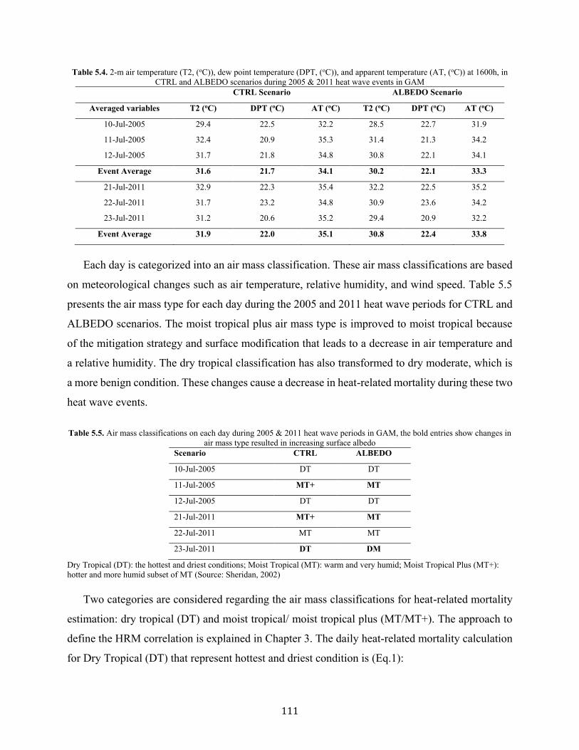
111
Table 5.4. 2-m air temperature (T2, (oC)), dew point temperature (DPT, (oC)), and apparent temperature (AT, (oC)) at 1600h, in CTRL and ALBEDO scenarios during 2005 & 2011 heat wave events in GAM
CTRL Scenario ALBEDO Scenario
Averaged variables T2 (oC) DPT (oC) AT (oC) T2 (oC) DPT (oC) AT (oC)
10-Jul-2005 29.4 22.5 32.2 28.5 22.7 31.9
11-Jul-2005 32.4 20.9 35.3 31.4 21.3 34.2
12-Jul-2005 31.7 21.8 34.8 30.8 22.1 34.1
Event Average 31.6 21.7 34.1 30.2 22.1 33.3
21-Jul-2011 32.9 22.3 35.4 32.2 22.5 35.2
22-Jul-2011 31.7 23.2 34.8 30.9 23.6 34.2
23-Jul-2011 31.2 20.6 35.2 29.4 20.9 32.2
Event Average 31.9 22.0 35.1 30.8 22.4 33.8
Each day is categorized into an air mass classification. These air mass classifications are based
on meteorological changes such as air temperature, relative humidity, and wind speed. Table 5.5
presents the air mass type for each day during the 2005 and 2011 heat wave periods for CTRL and
ALBEDO scenarios. The moist tropical plus air mass type is improved to moist tropical because
of the mitigation strategy and surface modification that leads to a decrease in air temperature and
a relative humidity. The dry tropical classification has also transformed to dry moderate, which is
a more benign condition. These changes cause a decrease in heat-related mortality during these two
heat wave events.
Table 5.5. Air mass classifications on each day during 2005 & 2011 heat wave periods in GAM, the bold entries show changes in
air mass type resulted in increasing surface albedo Scenario CTRL ALBEDO
10-Jul-2005 DT DT
11-Jul-2005 MT+ MT
12-Jul-2005 DT DT
21-Jul-2011 MT+ MT
22-Jul-2011 MT MT
23-Jul-2011 DT DM
Dry Tropical (DT): the hottest and driest conditions; Moist Tropical (MT): warm and very humid; Moist Tropical Plus (MT+): hotter and more humid subset of MT (Source: Sheridan, 2002)
Two categories are considered regarding the air mass classifications for heat-related mortality
estimation: dry tropical (DT) and moist tropical/ moist tropical plus (MT/MT+). The approach to
define the HRM correlation is explained in Chapter 3. The daily heat-related mortality calculation
for Dry Tropical (DT) that represent hottest and driest condition is (Eq.1):

112
HRMD = −4.32 + 1.07DIS − 0.066TOS + 0.339 AT (Eq. 5.1)
and for Moist Tropical (MT) and Moist Tropical Plus (MT+) that represent very warm and humid condition is (Eq. 2):
HRMD = 2.70 − 0.016TOS + 0.339AT (Eq. 5.2)
Table 5.6 represents the results of heat-related mortality estimation in CTRL and ALBEDO
scenarios. The consequences of surface modifications in urban areas indicate that in the 2005 and
2011 heat wave, there would be 2.7% and 3.7% reduction in heat-related mortality. As the air mass
classification shifted from oppressive condition (e.g., DT) to a benign situation (e.g., DM), a
reduction in HRM is more noticeable.
Table 5.6. Daily heat-related mortality estimation per 100,000 population based on above calculations for DT, MT and MT+
during 2005 & 2011 heat wave periods. For human lives, the numbers are shown with 1 decimal Mortality Estimations
Scenario CTRL ALBEDO
10-Jul-2005 4.9 4.8
11-Jul-2005 13.9 13.6
12-Jul-2005 7.8 7.6
Total HRM ~ 27 ~ 26
Average Mortality 8.9 8.7
Averaged Reduction (%) 2.7%
21-Jul-2011 13.9 13.8
22-Jul-2011 13.6 13.4
23-Jul-2011 7.3 6.2
Total HRM ~ 35 ~ 33
Average Mortality 11.6 11.2
Averaged Reduction (%) 3.7%
5.5. Discussion and Limitation of Heat-Related Mortality Estimation
The simulations show that increasing surface reflectivity decreases urban ambient temperature.
The positive impacts of lower temperatures are: (1) improving human health and comfort and (2)
decreasing heat-related mortality during heat-wave periods. Decreasing air temperature also has
the following positive effects on air quality: (1) a decrease in temperature-dependent rates of certain
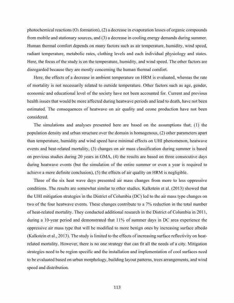
113
photochemical reactions (O3 formation), (2) a decrease in evaporation losses of organic compounds
from mobile and stationary sources, and (3) a decrease in cooling energy demands during summer.
Human thermal comfort depends on many factors such as air temperature, humidity, wind speed,
radiant temperature, metabolic rates, clothing levels and each individual physiology and states.
Here, the focus of the study is on the temperature, humidity, and wind speed. The other factors are
disregarded because they are mostly concerning the human thermal comfort.
Here, the effects of a decrease in ambient temperature on HRM is evaluated, whereas the rate
of mortality is not necessarily related to outside temperature. Other factors such as age, gender,
economic and educational level of the society have not been accounted for. Current and previous
health issues that would be more affected during heatwave periods and lead to death, have not been
estimated. The consequences of heatwave on air quality and ozone production have not been
considered.
The simulations and analyses presented here are based on the assumptions that; (1) the
population density and urban structure over the domain is homogenous, (2) other parameters apart
than temperature, humidity and wind speed have minimal effects on UHI phenomenon, heatwave
events and heat-related mortality, (3) changes on air mass classification during summer is based
on previous studies during 20 years in GMA, (4) the results are based on three consecutive days
during heatwave events (but the simulation of the entire summer or even a year is required to
achieve a more definite conclusion), (5) the effects of air quality on HRM is negligible.
Three of the six heat wave days presented air mass changes from more to less oppressive
conditions. The results are somewhat similar to other studies. Kalkstein et al. (2013) showed that
the UHI mitigation strategies in the District of Columbia (DC) led to the air mass type changes on
two of the four heatwave events. These changes contribute to a 7% reduction in the total number
of heat-related mortality. They conducted additional research in the District of Columbia in 2011,
during a 10-year period and demonstrated that 11% of summer days in DC area experience the
oppressive air mass type that will be modified to more benign ones by increasing surface albedo
(Kalkstein et al., 2013). The study is limited to the effects of increasing surface reflectivity on heat-
related mortality. However, there is no one strategy that can fit all the needs of a city. Mitigation
strategies need to be region specific and the installation and implementation of cool surfaces need
to be evaluated based on urban morphology, building layout patterns, trees arrangements, and wind
speed and distribution.

114
Kalkstein et al. (2013) also investigated the effects of UHI mitigation strategies on health-
debilitation air masses in four cities across the US. The results of increasing albedo and vegetation
indicated that the air mass type changed by an average of 7%, 16%, 3% and 4% in Detroit, Los
Angeles, New Orleans and Philadelphia, respectively. The heat-related death decreased by an
average of 5 to 10% in these cities. The results of another study by Kalkstein (1999) showed that a
1-2 °C reduction in outdoor temperature, along with some other meteorological changes, could
reduce mortality by 10–20%. Here, the ratio of 50% positive modification in air mass
classifications is similar to EPA study (Kalkstein and Sheridan, 2003). Results indicate an average
of 3.2% reduction in heat- related mortality during the 2005 and 2011 heat wave period in GMA
(a 2.7% reduction in HRM in the 2005 heat wave period and a 3.7% reduction in the 2011 heat
wave period), corroborate with EPA-sponsored studies on cool cities (Kalkstein and Sheridan,
2003; Vanos et al., 2013, 2014; Sheridan and Kalkstein, 2004; Sheridan et al., 2009). According to
Canadian Environmental Health Atlas (CEHA 2018), 121 people die every year in Montreal
because of heat related issues; a 3.2% reduction because of albedo increase in GMA, could save 4
lives per year. In another study carried out by Bustinza et al. (2013), the number of heat- related
death in GMA (including Montreal, Laval, Monteregie, and Lanaudiere with the total population
of 4,221,002) was estimated to be 209 people during July 2010 heat wave period alone. A 3.2%
reduction in HRM would results in savings life of 6 people during that period.
5.6. Summary of the Effects of Increasing Surface Reflectivity on Heat-Related
Mortality
The main objective of this study was to investigate the effects of increasing surface reflectivity
on heat-related mortality in the Greater Montreal Area during the 2005 and 2011 heat wave periods.
Numerical simulations were conducted using the online Weather Research and Forecasting model
(WRFV3.6.1) coupled with a multi-layer of the Urban Canopy Model (ML-UCM). The simulation
results were analysed in terms of four meteorological parameters: 2-m air temperature, 10-m wind
speed, 2-m relative humidity, dew point temperature and four heat stress indices: National Weather
Service – Heat Index, apparent temperature, Canadian Humid Index, and Discomfort Index. A
series of metrics calculations were employed to evaluate model performance and to compare the
simulation results with the measurements obtained from four weather stations over the domain.

115
The comparisons of the base case simulations indicated that the model on average slightly
overestimates the meteorological variables.
The albedo of roofs, walls and grounds were increased from 0.2 in CTRL scenarios to 0.65,
0.60, and 0.45 in ALBEDO scenarios, respectively. The results showed that the differences
between the meteorological parameters (T2, WS10, RH2, DPT) in CTRL and ALBEDO scenarios
are more significant in urban areas than in surrounding areas. The average daily 2-m air temperature
reduced by 0.8 °C in the urban area during both heat wave events, whereas this amount in rural
areas was around 0.4 °C. The albedo enhancement caused a slight increase in wind speed in urban
areas that increased the convection heat transfer and thus decreased the skin temperature. A higher
wind speed reduces the effects of heat and ambient temperature and produces a more pleasant
condition for urban dwellers. The results show an increase in relative humidity and dew point
temperature by nearly 2%. The relative humidity changes are less obvious in rural areas compared
to the urban area because of the existence of more vegetation spaces, and thus moisture in the
region. In addition, albedo enhancement causes a decrease in boundary-layer height that reduces
the chance of advection and diffusion of pollutants and hence increases the pollutants
concentrations. The effects of increasing albedo have also been investigated by means of four
indices of heat stress. The results showed that since surface albedo modifications reduced
temperature and increased relative humidity, these indices were also modified and improved to
some extent. Increasing surface albedo is a verifiable strategy to mitigate the UHI effects. It should
be noted that this strategy is region-specific and needs to be evaluated for any area of interest
because it depends on the particular urban characteristics and morphology.
Here, three indicators are applied to translate the effects of extreme heat events and the potential
of increasing surface reflectivity on heat-related mortality rates: air mass type, air temperature, and
apparent temperature changes for each day during heat wave periods. As a consequence of ISR,
the moist tropical plus and dry tropical air mass types are shifted to moist tropical and dry moderate,
respectively. These changes cause a decrease in heat-related mortality during these two heat wave
events. Three of the six heat wave days showed air mass changes from more to less oppressive
conditions. The beneficial outcome is a reduction in heat- related deaths by approximately 3.2%
during heat wave periods, meaning that 4–6 lives per year could be saved. It should be noted that
by reducing ambient temperature, the pollutant emission from biogenic and anthropogenic sources
and thus photochemical reaction rates will reduce. So, the deaths related to air quality will also be

116
reduced. In addition, increasing surface reflectivity shifts days into less oppressive air masses by
50% (3 of 6 days during heat wave periods).
The heat-related mortality estimation is based upon some assumptions and limitations. One
limitation is that the HRM algorithms are rather simplistic. Epidemiologists tend to focus on
ambient conditions even though most individuals spend 85% of their time indoors and indoor
exposure is implicated in a large fraction of heat-related deaths. But, here the focus of this study is
on the effects of albedo enhancement only on ambient temperature and then its effects on heat-
related mortality. The details of how people losing their lives and how their bodies react to extreme
heat events are still not known. However, here the effort is made by using other correlations and
modifying them for Greater Montreal Area based on its specific air mass condition. The effects of
ozone concentrations because of elevated heat is neglected. The impacts of wind speed and
radiation budget changes since meteorological parameters and human physical characteristics, such
as age, gender, economic and educational status, have not been considered. Hence, the cumulative
effects of these factors need to be considered in future studies. While it appears unlikely that
increasing surface reflectivity contributes to large reductions in ambient temperature in urban areas
(as 2 °C or greater), the study shows that cooling temperature even by less than a degree can lead
to air mass category changes and reduce the adverse effects of elevated temperature in urban areas,
thus improving human comfort and decreasing heat-related mortality to a noticeable extent.
5.7. Applications of Heat-Related Mortality Estimation
The developed correlations to estimate the effects of high temperature on mortality can be used
to investigate the effects of other heat island mitigation strategies (e.g., increasing surface
vegetation and controlling anthropogenic heat) on the rate of heat deaths in the Greater Montreal
Area. Results could be used by decision-makers to make policies to improve lives of urban dwellers
in the GMA. In addition, these analyses indicated that increasing surface reflectivity can facilitate
a positive change in air mass classifications. Albedo enhancement shifts days into less oppressive
air masses, which in turn improves human health and comfort.
With the heat-related mortality correlations and region-specific algorithm provided, the
approach used here illuminates the essential steps for developing HRM equations for other
locations and episodes. It should be noted that the HRM is a result of air quality degradation as
well. The reason is because of an increase in temperature-dependent photochemical reactions rates

117
and an increase in emissions from pollutant sources in urban areas. Thus, further analysis of the
effects of high temperature on air quality needs to be carried out. The indirect effects of high
temperature on HRM are required be estimated by photochemical models such as WRF-Chem.
Hence, the WRF-Chem is applied to investigate the effects of heat island mitigation strategy on
urban climate as well as air quality for other objectives in the following chapters.

118
Chapter 6 Effects of Increasing Surface Albedo on Urban Climate and Air Quality over a Large Geographical Area within Nested Domains as Urban Areas
Most previous studies have used a one-way simulation (climate simulations first, followed by air
quality simulations). This approach does not provide feedback on the effect of atmospheric
pollutants on the climate. Previous simulations are used to estimate the effects of surface
modifications and changes in surface albedo on urban climate and air quality through a one-way
simulation approach at local, regional and global scales (Arnfield, 2003; Ban-Weiss et al., 2015;
Taha 2008 and 2009; Salamanca et al., 2012; Li and Bou-Zeid 2014; Bhati and Mohan 2016). Thus,
the interaction between regional atmosphere and local climate is disregarded. The one-way
approach does not simulate the complete interactions between urban climate and air quality. The
meteorological processes and photochemical reactions in the urban atmosphere magnify the UHI
effects. These interactions in the urban environment cause changes in regional climate. The
changes in regional atmosphere affect local pollution. Thus, a two-way nested simulation approach
is required to capture the full impacts of these processes from the regional to the local scale. A two-
way nested approach provides an integrated simulation setup to simulate the full impacts of
meteorological and photochemical interactions. This approach decreases the uncertainties
associated with scale separation and grid resolution. In addition, this method reveals more details
of the effects of surface modifications on urban climate and regional air quality.
The Weather Research and Forecasting Model (WRF) is coupled with the chemistry package
(WRF-Chem) and a multi-layer of the urban canopy model (ML-UCM). The model investigates
the effects of increasing surface reflectivity on urban climate and air quality over North America
focusing on three populated cities: Sacramento (in California), Houston (in Texas), and Chicago
(in Illinois) during the 2011 heat wave period. The methodology and simulation approaches are

119
explained in Chapter 3. Here, the results of these simulations are presented. This research is
summarized in the article by Z. Jandaghian and H. Akbari (2018), “The Effects of Increasing
Surface Albedo on Urban Climate and Air Quality: A Detailed Study for Sacramento, Houston,
and Chicago” (Climate 2018, 6, 19; doi:10.3390/cli6020019).
6.1. Defining Simulation Domain and Period
The first domain covers North America (NA) including Canada, the United States of America,
and the Northern part of Mexico with 445 grids in west–east direction and 338 grids in south–north
direction. The horizontal resolution is 12km. The second, third, and fourth domains cover the
Sacramento area (36 × 31 grids), Houston area (41 × 31 grids), and Chicago area (36 × 31 grids)
with the horizontal resolution of 2.4km. The vertical resolution includes 35 vertical layers from the
surface to a fixed pressure of ~100 mb (~16 km AGL). Figure 6.1 shows the simulation domains
and land use/land cover. The simulation period extended seven consecutive hottest days in 2011,
from the 17th to 23rd of July. The first 72h of the simulation is disregarded as a spin-up period.

120
Figure 6.1. Simulation domains and land use/land cover over North America (mother domain, horizontal resolution: 12km)
Sacramento, Houston, and Chicago (inner domains, horizontal resolution: 2.4km).
Table 6.1 presents the physical and chemical parameterizations applied in WRF-Chem.
Table 6.1. Physical and chemical parameterizations applied in WRF_Chem
Category Option Used Microphysics Lin scheme
Shortwave radiation Goddard Longwave radiation RRTMG Land surface model NOAH Planetary boundary layer scheme Mellor–Yamada–Janjic Scheme Cumulus parameterization Grell Devenyi Chemistry option RACM Photolysis scheme Fast_J Aerosol option MADE/SORGAM Advection scheme Runge–Kutta third order LULC data USGS 24-class Anthropogenic emissions US-NEI11 Biogenic emissions MEGAN Urban canopy model ML-UCM

121
6.2. Simulation Scenarios for Urban Climate and Air Quality Assessment
Three cities are selected for detail analyses: Sacramento (California), Houston (Texas), and
Chicago (Illinois) based on Akbari et al., (2001, 2003 and 2008) and Rose et al., (2003) findings
on the urban fabric of these cities. Using high-resolution orthophotography, they found that roofs
cover 20–25% and pavements cover 30–40% of urban surfaces. Table 6.2 presents the urban fabric
of Sacramento, Chicago, and Houston (Rose et al., 2003). Table 6.2. Urban fabric of three cities in NA (Source: Rose et al., 2003)
Metropolitan Areas Roofs (%) Pavements (%) Sacramento 20 45 Chicago 25 37 Houston 22 30
Two sets of simulations are conducted: CTRL case (UHI effects) and ALBEDO case
(increasing surface reflectivity (ISR) effects) during the 2011 heat wave period over the simulation
domains. The fraction of urban fabric of these three cities and the changes because of increasing
surface reflectivity are applied to calculate the albedo changes over the domains. The changes of
surface albedo modification from the CTRL case as 0.2 to full adoption of roofs and pavements
can be calculated as: (fraction of roofs in Sacramento) 0.20 × 0.65 (the increase of albedo for
roofs) + 0.45 (fraction of pavements in Sacramento) × 0.45 (the increase of albedo for pavements)
= 0.33 (as an example for Sacramento; the surface albedo (of roofs and pavements) increased from
0.13 to 0.33 (as a full adaptation of albedo enhancement)). The change to gridded ALBEDO can
be calculated as: (Surface albedo enhancement (roofs, walls, and pavements) × Fraction of urban
areas per grid cell).
6.3. Evaluation of Meteorological and Photochemical Model Performance
The model performance of WRF-Chem is evaluated by comparing the simulation results with
observations obtained from weather and air-quality stations in Sacramento, Houston, and Chicago.
The weather and air quality monitoring stations were chosen based on their locations close to the
downtown of the selected cities (hereafter referred to as urban) and their surroundings (hereafter
referred to as suburb). The hourly 2-m air temperature (T2), 10-m wind speed (WS10), 2-m relative
humidity (RH2), and dew point temperature (TD) simulation results are compared with the
measurements obtained from the U.S. Environmental Protection Agency (EPA) Clean Air Status

122
and Trend Network (CASTNET). Since the measurements from air quality stations were averaged
24-h, the daily averaged modelled chemical components are extracted and evaluated to have the
same temporal basis. Thus, the daily averaged modelled fine particular matters (PM2.5), ozone (O3),
nitrogen dioxide (NO2), PM2.5 subspecies (particulate sulfate (SO42.5), particulate nitrate (NO32.5),
and organic carbon (OC2.5)) concentrations are compared with the EPA Air Quality System (AQS)
observations using 24-h average data.
Here, the time series of simulation results changed to the local time for each specific location:
Sacramento: LST = UTC – 7 h; Houston and Chicago: LST = UTC – 5 h. The performance and
accuracy of the simulation results are quantitatively based on a series of metrics estimations
(Boylan and Russell, 2006). The Zhang et al. (2006) approach is followed and the mean bias error
(MBE), mean absolute error (MAE), and the root mean square error (RMSE) are calculated for
meteorological and chemical parameters.
In terms of meteorological components of the model, the WRF-Chem effectively captures the
diurnal variations of 2-m air temperature, overpredicts 10-m wind speed, overpredicts dew point
temperature, and under-predicts 2-m relative humidity. The MBA of T2 (−0.07 °C) shows that the
model is capable in predicting air temperature. A small underprediction can be seen in urban areas
(~−0.3 °C) that indicates the model deficiency in calculating the heat emission from anthropogenic
sources in urban areas accurately. The MAE and RMSE of T2 are approximately 1 °C.
Wind speed plays an important role in calculation of air temperature from skin temperature in
the land surface model. The 10-m wind speed comparisons show small to large overpredictions
(0.3 to 3.15 m/s). The MBA is 1.65 m/s, that shows the model is unable to capture the effects of
micro scales and wind patterns. The MAE and RMSE of WS10 are almost 2 m/s.
Relative humidity is a function of moisture content, air temperature, and surface pressure. The
spatial distribution of RH2 represents an underestimation with the MBE of −1.42%. This
underestimation shows that the microphysics scheme does not accurately account for the processes
of transforming water (rain, vapor, cloud, etc.) and moisture fluxes. It also shows the model
limitation in capturing the sea surface temperature, wind speed, and their impacts on water mixing
ratio and water content of the air properly. The MAE and RMSE of RH2 are nearly 10% and 13%,
respectively. Figure 6.2 shows the time series (hourly) of the observed vs. simulated T2 (°C), WS10
(m/s), and RH2 (%) in the urban areas of Sacramento, Houston, and Chicago. The dew point
temperature is also calculated. The MBA, MAE, and RMSE of dew point temperature (0.39, 0.53,

123
and 0.65 °C, respectively) show that the model overpredicts the moisture content in the atmosphere
especially in urban areas (~0.5 °C).
In terms of the chemical component of the model, the WRF_ChemV3.6.1, as configured here,
tends to under-predict 24-h fine particular matters (PM2.5) and over-predict the 24-h O3
concentrations during the 2011 heat wave period. The MBE of the 24-h avg. PM2.5 is −1.42 µg/m3.
The MAE and RMSE of PM2.5 are approximately 4 µg/m3. This is because the accuracy in fine
particular matters concentrations is to some extent a function of its subspecies estimations as
particulate sulfate, particulate nitrate, and organic carbons. Thus, the simulation results of SO42.5
(µg/m3), NO32.5 (µg/m3), and OC2.5 (µg/m3) are compared with observations at urban areas of
aforementioned cities.
The performance of PM2.5 subspecies is a combination of overprediction of particulate sulfate
(MBE ~ 5 µg/m3) and underprediction of particulate nitrate (MBE ~ −4 µg/m3) and organic carbon
(MBE ~ −3 µg/m3). The MAE and RMSE of SO42.5, NO32.5, and OC2.5 are approximately 5, 4, and
3 µg/m3, respectively. The comparison between simulated ozone and measurements indicated an
overestimation of O3 across the domains (MBE ~ 5 ppb). The O3 concentrations is overestimated
due to the NOx and VOCs overestimation in emission inventories and their calculations in
chemistry packages (US-NEI11 and MEGAN). The average MAE and RMSE of O3 are around 7
ppb and 8 ppb, respectively. In addition, the NO2 concentrations is calculated as one of the
precursors in ozone formation. The MBE of NO2 in urban areas (~2.5 ppb) show that the model
tends to overpredict the nitrogen dioxide. The MAE and RMSE of NO2 is around 4 ppb.
Figure 6.3 shows the observed vs. simulated PM2.5 (µg/m3) and O3 (ppb) concentrations in the
urban areas of Sacramento, Houston, and Chicago. Tables 6.3, 6.4, and 6.5 respectively represent
the mean bias error (MBE), mean absolute error (MAE), and the root mean square error (RMSE)
of T2 (°C), WS10 (m/s), RH2 (%), PM2.5 (µg/m3), and O3 (ppb) for the three cities. There are
several limitations and assumptions in these comparisons. The simulation results are extracted
hourly for all variables, whereas the observation in terms of PM2.5 and O3 are reported as a 24-h
average. Figure 6.4 shows the overall comparison between observed vs. simulated aforementioned
parameters in terms of MBA, MAE, and RMSE. Despite the model biases in simulating
meteorological and chemical variables, the performance of WRF-Chem is generally consistent with
most air quality models (Gilliam et al., 2006; Wu et al., 2008; Wang et al., 2009; Liu et al., 2010;
Appel et al., 2012). Thus, the WRF-Chem is mostly suited for application of simulating and

124
investigating the effects of urban heat island and its mitigation strategies on urban climate and air
quality in a two-way nested simulation approach.
Table 6.3. Mean bias error (MBE) of T2 (°C), WS10 (m/s), Td (°C), RH2 (%), O3 (ppb), PM2.5 (µg/m3), SO42.5 (µg/m3), NO32.5
(µg/m3), OC2.5 (µg/m3), and NO2 (ppb) at selected monitoring stations across Sacramento, Houston, and Chicago.
Variables Mean Bias Error (MBE)
Average Sacramento Houston Chicago Suburb Urban Suburb Urban Suburb Urban
T2 (°C) 0.15 −0.34 0.22 −0.34 −0.30 0.19 −0.07 WS10 (m/s) 1.90 3.15 0.87 0.34 1.28 1.05 1.43 Td (°C) 0.21 0.61 0.24 0.47 0.33 0.47 0.39 RH2 (%) −5.43 −5.63 −1.03 8.16 1.88 −6.45 −1.42 24-h avg. O3 (ppb) 9.72 4.68 3.17 3.85 2.31 4.38 4.68 24-h avg. PM2.5 (µg/m3) −5.94 2.30 −3.26 2.07 −3.86 −2.33 −1.84 24-h avg. SO42.5 (µg/m3) - 4.20 - 5.30 - 3.89 4.46 24-h avg. NO32.5 (µg/m3) - −3.75 - −4.40 - −3.52 −3.91 24-h avg. OC2.5 (µg/m3) - −1.80 - −2.33 - −3.68 −2.60 24-h avg. NO2 (ppb) - 2.61 - 3.40 - 1.25 2.42
Note: The definitions of statistical measurements are as follows Zhang et al. (2006) [51]: MBE = 1
N∑ (CM − CO),N
1 𝐶𝑀 and CO are
modeled and observed concentrations, respectively and N is the total number of model and observation pairs.
Table 6.4. Mean absolute error (MAE) of T2 (°C), WS10 (m/s), Td (°C), RH2 (%), O3 (ppb), PM2.5 (µg/m3), SO42.5 (µg/m3),
NO32.5 (µg/m3), OC2.5 (µg/m3), and NO2 (ppb) at selected monitoring stations across Sacramento, Houston, and Chicago.
Variables Mean Absolute Error (MAE)
Average Sacramento Houston Chicago Suburb Urban Suburb Urban Suburb Urban
T2 (°C) 1.05 0.88 1.20 0.88 0.77 1.12 0.99 WS10 (m/s) 1.96 3.33 1.26 1.20 2.31 1.79 1.97 Td (°C) 0.56 0.30 0.49 0.63 0.56 0.66 0.53 RH2 (%) 15.32 9.45 5.38 9.54 8.98 10.11 9.80 24-h avg. O3 (ppb) 9.72 9.90 6.92 6.01 2.56 5.88 6.83 24-h avg. PM2.5 (µg/m3) 6.24 3.05 3.26 3.70 3.86 2.33 3.74 24-h avg. SO42.5 (µg/m3) - 4.20 - 5.30 - 3.89 4.46 24-h avg. NO32.5 (µg/m3) - 3.75 - 4.45 - 3.52 3.91 24-h avg. OC2.5 (µg/m3) - 1.80 - 2.33 - 3.68 2.60 24-h avg. NO2 (ppb) - 4.71 - 3.40 - 2.54 3.55
Note: The definitions of statistical measurements are as follows Zhang et al. (2006) [51]: MAE =1
N∑ |CM − CO| N
1 CM and CO are
modeled and observed concentrations, respectively and N is the total number of model and observation pairs. Table 6.5. Root mean square error (RMSE) of T2 (°C), WS10 (m/s), Td (°C), RH2 (%), O3 (ppb), PM2.5 (µg/m3), SO42.5 (µg/m3),
NO32.5 (µg/m3), OC2.5 (µg/m3), and NO2 (ppb) at selected monitoring stations across Sacramento, Houston, and Chicago.
Variables Root Mean Square Error (RMSE)
Average Sacramento Houston Chicago Suburb Urban Suburb Urban Suburb Urban
T2 (°C) 1.35 1.13 1.44 1.13 1.01 1.32 1.23 WS10 (m/s) 2.29 3.68 1.58 1.47 2.86 2.22 2.35 Td (°C) 0.68 0.37 0.58 0.77 0.67 0.80 0.65 RH2 (%) 18.94 12.32 7.52 12.26 11.36 13.48 12.65 24-h avg. O3 (ppb) 10.51 14.21 7.89 6.71 3.09 8.21 8.44 24-h avg. PM2.5 (µg/m3) 7.74 3.25 4.04 4.30 4.82 2.81 4.49 24-h avg. SO42.5 (µg/m3) - 4.44 - 6.24 - 3.93 4.87 24-h avg. NO32.5 (µg/m3) - 3.96 - 4.87 - 4.28 4.37 24-h avg. OC2.5 (µg/m3) - 1.93 - 2.39 - 3.76 2.69 24-h avg. NO2 (ppb) - 5.74 - 4.10 - 2.89 4.24

125
Note: The definitions of statistical measurements are as follows Zhang et al. (2006) [51]: RMSE = [1
N∑ (CM − CO)2N
1 ]1/2
CM and CO are modeled and observed concentrations, respectively and N is the total number of model and observation pairs.
Sacramento Houston Chicago
T2
(°C
)
WS
10 (
m/s
)
RH
2 (%
)
Figure 6.2. The time series (hourly) of the simulated (solid line) vs. measurements (dashed line) T2 (°C), WS10 (m/s), and RH2
(%) at urban monitoring stations across Sacramento, Houston, and Chicago.
25
30
35
40
0 12 0 12 0 12 0 1225
30
35
40
0 12 0 12 0 12 0 1220
25
30
35
40
0 12 0 12 0 12 0 12
0
5
10
0 12 0 12 0 12 0 120
5
10
0 12 0 12 0 12 0 120
5
10
0 12 0 12 0 12 0 12
20
40
60
80
100
0 12 0 12 0 12 0 1220
40
60
80
100
0 12 0 12 0 12 0 1220
40
60
80
100
0 12 0 12 0 12 0 12

126
Sacramento Houston Chicago
PM
2.5 (µ
g/m
3 )
O3 (p
pb
)
Figure 6.3. The time series (averaged 24-h) of simulated (black bar chart) vs. measurements (patterned downward diagonal bar chart) of PM2.5 (µg/m3) and O3 (ppb) concentrations at urban monitoring stations across Sacramento, Houston, and Chicago.
Mean Bias Error (MBE) of parameters
Mean Absolute Error (MAE) of parameters
0
5
10
15
20
25
2011-07-20. 2011-07-21. 2011-07-22. 2011-07-23.0
5
10
15
20
25
2011-07-20. 2011-07-21. 2011-07-22. 2011-07-23.0
5
10
15
20
25
2011-07-20. 2011-07-21. 2011-07-22. 2011-07-23.
0
20
40
60
80
2011-07-20. 2011-07-21. 2011-07-22. 2011-07-23.0
20
40
60
80
2011-07-20. 2011-07-21. 2011-07-22. 2011-07-23.0
20
40
60
80
2011-07-20. 2011-07-21. 2011-07-22. 2011-07-23.
-5
-3
-1
1
3
5

127
Root Mean Square Error (RMSA) of parameters
Figure 6.4. The overall mean bias error (MBE), mean absolute error (MAE), and root mean square error (RMSA) of T2 (°C),
WS10 (m/s), Td (°C), RH2 (%), O3 (ppb), PM2.5 (µg/m3), SO42.5 (µg/m3), NO32.5 (µg/m3), OC2.5 (µg/m3), and NO2 (ppb) during the 2011 heat wave period.
6.4. Effects of Increasing Surface Reflectivity on Urban Climate and Air Quality
Results discussed here are based on the comparison between the ALBEDO and CTRL scenarios
for each city. Table 6.6 and Figure 6.5 represent the average differences in T2 (°C), WS10 (m/s),
Td (°C), RH2 (%), PM2.5 (µg/m3), O3 (ppb), SO42.5 (µg/m3), NO32.5 (µg/m3), OC2.5 (µg/m3), and
NO2 (ppb) during the 2011 heat wave period across the second, third, and fourth domains:
Sacramento (CA), Houston (TX), and Chicago (IL). Figure 6.6 shows the averaged differences of
T2 (°C) and O3 (ppb) concentrations in suburb and urban areas of the aforementioned cities.
Sacramento, California is located in the central valley near the Sierra foothills. It is at the
confluence of the Sacramento River and the American River and is known as the Sacramento Valley.
The city has a population of approximately 500,000 people and covers over 253 km2 (United States
Census Bureau, 2011). Its climate is characterized by mild year-round temperature. It has a hot-dry-
0
5
10
0
5
10
15

128
summer Mediterranean climate with little humidity and an abundance of sunshine. Based on the
National Oceanic and Atmospheric Administration (NOAA) Online Weather Data (2017),
Sacramento has the summer temperature exceeding 32 °C on 73 days and 38 °C on 15 days. The
State of the Air 2017 report, by American Lung Association (2017), ranks the USA metropolitan
areas based on ozone and some particular pollutions during 2013, 2014, and 2015 period. They used
the official data from the U.S. Environmental Protection Agency (EPA). Sacramento ranks fifth
because of its high ozone concentration.
In a study performed at the Lawrence Berkeley National Laboratory (LBNL), Taha et al. (2000)
applied the Colorado State Urban Meteorological Model (CSUMM) and the Urban Airshed Model
(UAM-IV) to estimate the impacts of heat island mitigation strategies in Sacramento on the area’s
local meteorology and ozone air quality in 2000. The albedo level and vegetative cover increased
by approximately 0.11 and 0.14, respectively. Using 11–13 July 1990 as the modeling period, the
average daily ozone and temperature decreased by up to 10 ppb and 1.6 °C, respectively. In a more
recent study, Taha et al. (2015) applied WRF with CMAQ in Sacramento Valley with the inner
domain of 1 km resolution. The albedo of roofs, walls, and pavements increased by 0.4, 0.1, and
0.2, respectively. The surface temperature and air temperature were reduced by up to 7 °C and 2–
3 °C, respectively. The ozone concentrations also decreased by up to 5–11 ppb during the daytime.
The simulation results for Sacramento show that albedo enhancement leads to a net decrease in
2-m air temperature by up to 2.5 °C and 0.7 °C in urban and suburban areas, respectively. Most of
the decreases occur between 1200 and 1600 LST as shown in Figure 6.7. Figure 6.8-Sa (CTRL)
shows the maximum air temperature across the simulation domain in the heat wave period. By
increasing surface reflectivity, the maximum temperature reduction is around 3 °C almost in all
parts of the city (Figure 6.8-Sb-ALBEDO) and this reduction is more obvious in the western part
of the domain. The wind speed slightly decreased over the entire domain. The relative humidity
increased by 7% and 3% in urban and suburban areas, respectively. Increasing surface reflectivity
affords a decrease of nearly 2.4 µg/m3 in PM2.5 concentrations in urban area (Figure 6.7) and 1
µg/m3 in suburb. Figure 6.7-Sc shows the maximum PM2.5 concentrations across the domain. The
maximum is around 12 µg/m3 in urban area that decreases by 2–3 µg/m3 as the results of albedo
enhancement (Figure 6.8-Sd). The heat island mitigation strategy causes a decline in O3 by almost
8 ppb in urban (Figure 6.7) and 3 ppb in suburb of the Sacramento area. Figure 6.8-Se shows the
maximum O3 concentrations as nearly 80 ppb across the simulation domain that decreases to nearly

129
70 ppb by UHI mitigation strategy (Figure 6.8-Sf). The results resemble those of previous studies
(Taha et al., 2008, 2013 and 2015). In addition, the particulate sulfate, particulate nitrate, organic
carbon, and nitrogen dioxide are compared in CTRL and ALBEDO simulations results. Albedo
enhancement causes no changes to minimal changes to particular matters subspecies but decreases
the NO2 concentration by ~1 ppb.
Houston is the fourth most populous city in the U.S. with a population of 2.3 million within a
land area of 1700 km2 (United States Census Bureau, 2017). It is located in the Southeast Texas
near the Gulf of Mexico. Houston’s climate is classified as humid subtropical. During the summer,
the temperature commonly reaches 34 °C, and some days it reaches to even 40 °C. The wind comes
from the south and southeast and brings heat and moisture from the Gulf of Mexico. The highest
temperature recorded in Houston is 43 °C, which occurred during the 2011 heat wave period
(NOAA Online Weather Data). Houston also suffers from excessive ozone levels and the American
Lung Association (2017) named the city as the 12th most polluted city in the U.S., based on EPA
2013, 2014, and 2015 data base.
Taha (2008) used MM5 to evaluate the model’s episode performance and its response to
increasing surface albedo and vegetation in Houston during several days in August 2000. In
ALBEDO scenario, the roof albedo was increased from an average of 0.1 to an average of 0.3; wall
albedo was increased from an average of 0.25 to an average of 0.3; pavement albedo was increased
from an average of 0.08 to 0.2. The results indicated a reduction in temperature by up to 3.5 °C, and
also caused warming in some areas by up to 1.5 °C. Results indicated that cooling usually occurs
during daytime, while heating occurs at night. The other simulations show the same results (Taha
2003 and 2005).
The simulation results for Houston show that albedo enhancement leads to a net decrease in 2-
m air temperature by up to 3 °C and 0.8 °C in urban (Figure 6.7) and suburban areas, respectively.
Unlike previous studies, no heating effect is witnessed in these simulations. The reason is because
of the sea breeze consideration in the solver of WRF-Chem. Figure 6.8-Ha illustrates the maximum
air temperature across the Houston in the heat wave period. The maximum temperature reduction
is above 3 °C almost in all parts of the city (Figure 6.8-Hb). The model tends to perform relatively
better in urban rather than in suburb areas. With albedo enhancement, the wind speed slightly
decreased, and the relative humidity increased by up to 7% in urban and 3% in suburb. Increasing
surface reflectivity affords a decrease of PM2.5 concentrations by up to 3.5 µg/m3 and 2.6 µg/m3 in

130
urban and suburban areas, respectively. Figure 6.8-Hc shows the maximum PM2.5 concentrations
across Houston. The maximum is above 20 µg/m3 in urban area that decreases to 16 µg/m3 as the
results of albedo enhancement (Figure 6.8-Hd). The O3 concentrations also decrease by up to 7.2
ppb and 3 ppb in urban and suburban areas, respectively. Figure 6.8-He shows the maximum O3
concentrations as above 80 ppb across the simulation domain that decreases to nearly 70 ppb all
over the domain (Figure 6.8-Hf). Here, the results resemble to previous studies (Taha 2003, 2005
and 2008). Increasing surface albedo in the urban area of Houston causes no changes in particular
matters subspecies and a decrease of 1.2 ppb in NO2 concentration.
Chicago is the third most populous city in the U.S. with over 2.7 million residents. The city
area is 606 km2 (United State Census Bureau). The city lies on the southwestern shores of Lake
Michigan and has two rivers: the Chicago River and the Calumet River. Chicago has a humid
continental climate. Summer temperatures can reach up to 32 °C. Taha et al., (1998) used a three-
dimensional, Eulerian, mesoscale meteorological model (CSUMM) to simulate the effects of large
scale surface modifications on meteorological conditions in 10 cities across the U.S. Surface
modifications included increasing albedo by 0.03 ± 0.05 and increasing vegetative fraction by 0.03
± 0.04. The results indicated that the air temperature was reduced by up to 1 °C in the Chicago
area.
The simulation results for Chicago show that albedo enhancement leads to a net decrease in 2-m
air temperature by up to nearly 2 °C and 0.8 °C in urban (Figure 6.7) and suburban areas, respectively.
Figure 6.8-Ca shows the maximum air temperature across the simulation domain. With albedo
enhancement, the air temperature reduced over the domain (Figure 6.8-Cb). The wind speed slightly
reduces in suburbs, with no changes in urban areas. The results show a slight decrease in relative
humidity by up to 0.2% in Chicago’s urban areas. The reason is because of the wind speed direction
that is north to west (passing the bodies of water) and the city’s location that is along one of the Great
Lakes, Lake Michigan, and has the Mississippi River Watershed and the Chicago River. The other
reason is due to the increasing surface reflectivity that reduces the skin temperature and thus air
temperature that might also decrease the chance of evaporation and thus decreases moisture content
above the ground. This strategy also affords a decrease of PM2.5 concentrations by up to 2.5 µg/m3
and 0.6 µg/m3 in urban and suburban areas, respectively. The maximum PM2.5 concentrations across
Chicago is nearly 12 µg/m3, that decreases to nearly 9 µg/m3 as the results of albedo enhancement
(Figure 6.8-Cc and 4.27-Cd). The O3 concentrations decrease by up to 4.2 ppb in urban area and 1.7

131
ppb in suburb. Figure 6.7-Ce shows the maximum O3 concentrations as nearly 70 ppb across the
simulation domain that decreases to almost 65 ppb all over the domain (Figure 6.8-Cf). Increasing
urban albedo in Chicago leads to an increase of particulate nitrate by 3 ppb and a decrease of NO2
concentration by ~ 1ppb.
Overall, the results indicate that with albedo enhancement, the air temperature drops (~1.5 °C)
and thus causes a decrease in ozone concentrations (~5 ppb) and nitrogen dioxide (~1 ppb).
Increasing surface solar reflectance lead to a minimal decrease in particular matters (~2 µg/m3) and
no significant changes in its subspecies. The SO42.5 and NO32.5 concentrations reduced slightly in
urban areas (~0.1 µg/m3) because of the decrease in air temperature and thus photochemical reaction
rates, but there is no change in OC2.5 (µg/m3). The UHI mitigation strategy increased the relative
humidity and dew point temperature. The results show that there are no significant changes in the
wind speed over the domain and the differences between two scenarios is 0.05 m/s. This minimal
change is because of the WRF-Chem configurations and it does not reflect any changes in momentum
transport from the shallow boundary layer. Table 6.6. The differences between CTRL and ALBEDO scenarios of T2 (°C), WS10 (m/s), RH2 (%), O3 (ppb), PM2.5 (µg/m3),
SO42.5 (µg/m3), NO32.5 (µg/m3), OC2.5 (µg/m3), and NO2 (ppb) during the 2011 heat wave period across Sacramento, Houston, and Chicago.
Δ ALBEDO
CTRL-ALBEDO Sacramento Houston Chicago Average Suburb Urban Suburb Urban Suburb Urban Δ T2 (°C) 0.72 2.37 0.81 2.68 0.75 1.76 1.52 Δ WS10 (m/s) 0.03 0.02 0.33 0.02 −0.08 0.00 0.05 Δ Td (°C) −0.26 −0.39 −0.27 −0.46 −0.21 −0.34 −0.32 Δ RH2 (%) −2.99 −6.88 −2.44 −6.89 −0.81 0.21 −3.30 24-h avg. O3 (ppb) 2.98 7.52 2.85 7.23 1.77 4.23 4.43 24-h avg. PM2.5 (µg/m3) 0.98 2.36 2.59 3.49 0.61 2.48 2.08 24-h avg. SO42.5 (µg/m3) - 0.02 - 0.01 - 0.06 0.03 24-h avg. NO32.5 (µg/m3) - 0.01 - 0.05 - 0.23 0.09 24-h avg. OC2.5 (µg/m3) - 0.00 - 0.00 - 0.00 0.00 24-h avg. NO2 (ppb) - 0.82 - 1.21 - 0.91 0.98

132
Figure 6.5. The average differences between CTRL and ALBEDO scenarios in T2 (°C), WS10 (m/s), RH2 (%), O3 (ppb), PM2.5
(µg/m3), SO42.5 (µg/m3), NO32.5 (µg/m3), OC2.5 (µg/m3), and NO2 (ppb) during the 2011 heat wave period.
Figure 6.6. The average differences between CTRL and ALBEDO scenarios of T2 (°C) and O3 (ppb) during the 2011 heat wave
period in suburb and urban areas of Sacramento, Chicago, and Houston.
-4
-3
-2
-1
0
1
2
3
4
5 ΔParameters= CTRL-ALBEDO
0
1
1
2
2
3
3
Suburb Urban Suburb Urban Suburb Urban
ΔT (o C
)
ΔT = CTRL-ALBEDO (oC)
Sacramento Chicago Houston
0
2
4
6
8
10
Suburb Urban Suburb Urban Suburb Urban
ΔO3
(ppm
)
ΔO3 = CTRL-ALBEDO (ppm)
Sacramento Chicago Houston
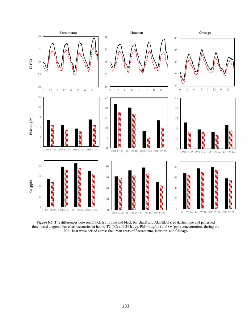
133
Sacramento Houston Chicago T
2 (°
C)
PM
2.5 (
µg
/m3 )
O3
(pp
b)
Figure 6.7. The differences between CTRL (solid line and black bar chart) and ALBEDO (red dashed line and patterned
downward diagonal bar chart) scenarios in hourly T2 (°C) and 24-h avg. PM2.5 (µg/m3) and O3 (ppb) concentrations during the 2011 heat wave period across the urban areas of Sacramento, Houston, and Chicago
20
25
30
35
40
0 12 0 12 0 12 0 1220
25
30
35
40
0 12 0 12 0 12 0 1220
25
30
35
40
0 12 0 12 0 12 0 12
0
5
10
15
20
25
2011-07-20. 2011-07-21. 2011-07-22. 2011-07-23. 0
5
10
15
20
25
2011-07-20. 2011-07-21. 2011-07-22. 2011-07-23.0
5
10
15
20
25
2011-07-20. 2011-07-21. 2011-07-22. 2011-07-23.
0
20
40
60
80
2011-07-20. 2011-07-21. 2011-07-22. 2011-07-23. 0
20
40
60
80
2011-07-20. 2011-07-21. 2011-07-22. 2011-07-23.0
20
40
60
80
2011-07-20. 2011-07-21. 2011-07-22. 2011-07-23.

134
Sacramento Houston Chicago
T2-
CT
RL
-a
T2-
AL
BE
DO
-b
O3-
CT
RL
-c
O3-
AL
BE
DO
-d
PM
2.5-
CT
RL
-e
PM
2.5-
AL
BE
DO
-f
Figure 6.8. The maximum 2-m air temperature (°C), PM2.5 (µg/m3) and O3 (ppb) concentrations in CTRL and ALBEDO
scenarios across Sacramento, Houston, and Chicago during the 2011 heat wave period.

135
6.5. Discussion and Limitations of Urban Climate and Air Quality Studies
Comparing the simulation results with measurements indicates that the WRF-Chem generally
reproduces well the hourly variations of meteorological variables, but overpredicts or underpredicts
the air pollutant concentrations during the 2011 heat wave period. One of the reasons is that the
simulation results are extracted at the start of each hour, whereas the measurements are reported as
hourly or daily averages. This means that the comparisons are not made exactly at the same time.
Another reason concerns the anthropogenic and biogenic estimations by US-NEI11 (spatial
resolution of 1 km) and MEGAN (spatial resolution of 4 km): the spatial resolution of these models
cannot accurately account for the actual emissions of anthropogenic and biogenic pollutions into
the atmosphere.
The 2011 heat wave period is selected for these simulations to investigate the effects of
increasing albedo during the heat wave period in each city. However, in order to specify the effects
of increasing albedo, another simulation should be carried out in normal conditions during summer.
Then the results need to be compared with the heat wave period to see the typical effects of albedo
enhancement in each location. A study to assess the effects of increasing surface albedo for a whole
year is also suggested to see its effects during the winter season and during a year as well.
Simulation of the entire year can reveal more information on the annual effects of the mitigation
strategy. In addition, it is recommended to assesses the effects of other UHI mitigation strategies
(such as increasing the fraction of vegetative cover) on urban climate and air quality within a two-
way nested approach.
To gain better results of the effectiveness of high-albedo strategy in improving the regional
ozone air quality, other episodes and locations with more reliable emission inventories should be
further investigated, modeled, and analysed in a more detailed modeling approach. The information
on an area’s local climate can help to focus on heat island mitigation strategies that best suit their
region. For example, cities with dry climates may achieve greater benefits from increasing the
vegetative fraction of urban areas (yielding more evapotranspiration) than would cities in humid
climates. However, dry-climate cities also need to consider the availability of water to maintain
vegetation. A more detailed analysis of simulation results is suggested to investigate the effects of
surface modifications on decreasing the temperature-dependent photochemical reaction rates, as

136
well as decreasing evaporation losses of organic compounds from industrial sectors, and mobile
and stationary sources.
6.6. Summary of the Effects of Increasing Surface Albedo on Urban Climate and Air
Quality within a Two-Way Nested Simulation Approach
A two-way nested simulation approach is applied to evaluate the surface modification
consequences on meteorological processes (air temperature, wind speed, relative humidity, dew
point temperature) and chemical reactions (ozone, nitrogen dioxide, fine particulate matters, PM2.5
subspecies (particulate sulfate (SO42.5), particulate nitrate (NO32.5) and organic carbon (OC2.5)) in
a unified continental scale through regional scales. The simulations are conducted over North
America through Sacramento, Houston, and Chicago during the 2011 heat wave period. The two-
way nested approach with fine-resolution modelling framework can equip researchers with an
integrated simulation setup to capture the full impacts of meteorological and photochemical
reactions. The applied method would serve as a basis for future model improvements and
parameterization development, fine-resolution dispersion, and photochemical modelling for other
geographical locations.
The model performance is evaluated by comparing the simulation results with the observations.
Despite the model biases in simulating meteorological and chemical variables, the performance of
WRF-Chem is generally consistent with most air quality models (Gilliam et al., 2006; Wu et al.,
2008; Wang et al., 2009; Liu et al., 2010; Appel et al., 2012), thus is mostly suited for application
of simulating and investigating the effects of urban heat island and its mitigation strategies. The
MBA, MAE, and RMSE estimations confirmed the model capabilities. For meteorological
components, the WRF-ChemV3.6.1, as configured here, captures well the diurnal variations of 2-
m air temperature (MBA ~−0.07 ◦C), overpredicts 10-m wind speed (MBA ~1.65 m/s),
overpredicts dew point temperature (MBA ~0.4 ◦C), and underpredicts 2-m relative humidity
(MBA ~−1.4%). For chemical component, the model underpredicts the daily fine particular matters
(PM2.5) (MBA ~−1.5 μg/m3) and overpredicts the O3 concentrations (MBA ~5 ppb). The model
underpredicts the NO2 (~2.5 ppb) and overpredicts particulate sulfate (MBE ~5 μg/m3) and
underpredicts particulate nitrate (MBE ~−4 μg/m3) and organic carbon (MBE ~−3 μg/m3) in urban
areas of aforementioned cities during the 2011 heat wave period. The model tends to perform
relatively better in urban, rather than in suburban areas.

137
Two sets of simulations are conducted with regard to surface modifications: the CTRL scenario
and the ALBEDO scenario. With albedo enhancement, the results indicated:
- a decrease in air temperature by 2.3◦C in urban areas and 0.7◦C in suburban areas - a slight increase in wind speed across the domain - an increase in relative humidity (3%) and dew point temperature (0.3◦C) in urban areas - a decrease of PM2.5 concentrations by 2.7μg/m3 in urban areas and 1.4μg/m3 in suburban
areas - a decrease of O3 concentrations by 6.3ppb in urban areas and 2.5ppb in suburban areas - minimal changes in PM2.5 subspecies - a decrease of nitrogen dioxide to 1 ppb in urban areas The results presented here are episode- and region-specific and thus may not provide a suitable
basis for generalization to other circumstances. Overall, the results confirm that for Sacramento in
California, Houston in Texas, and Chicago in Illinois, the albedo enhancement is an effective
mitigation strategy to reduce the air temperature and improve air quality. The results show that
Sacramento and Houston benefit more from increasing surface solar reflectance. These findings
are an asset for policymakers and urban planning designers. However, the suggestion is to
investigate the effects of other UHI mitigation strategies on urban climate and air quality before
making decisions or applying any surface modifications. Another suggestion is to simulate the
models with more accurate emission inventories. In addition, a simulation for the entire year is
recommended that can reveal more information of the mitigation strategy impacts.
6.7. Applications of a Two-Way Nested Simulation Approach in Urban Climate and
Air Quality Studies
A two-way nested approach provides an integrated simulation setup to capture the full impacts
of meteorological processes and photochemical reactions in the atmosphere. This approach reduces
the uncertainties associated with scale separation and grid resolution. It provides a good
understanding of the effects of surface modification strategies on urban climate and air quality. The
prepared modeling setup here can assist other researches to investigate the effects of any mitigation
strategies in other locations and episodes. In addition, it can be applied to investigate the effects of
increasing surface reflectivity on aerosol-radiation-cloud interactions in the atmosphere, which is
the other objective of this dissertation. The results of this assessment are presented in the following
chapter (Chapter 7). The other application is to estimate the albedo fraction of urban areas and its
correlation with air temperature and ozone concentrations. The results of these analyses are
presented in Chapter 8.

138
Chapter 7 Effects of Increasing Surface Reflectivity on Aerosol-Radiation-Cloud Interactions in the Urban Atmosphere The primary pollutants emitted from natural and anthropogenic sources turn into secondary
compounds by photochemical reactions and atmospheric meteorological factors. Aerosols affect
the radiative balance of the Earth-Atmosphere system by scattering and absorbing the incoming
solar radiation directly and by influencing cloud formation and precipitations indirectly (IPCC
2013; Zhang et al., 2014 and 2008). The aerosols impact cloud properties by convective potential
energy such as radiation, relative humidity and wind shear (Fan et al., 2013). The evaporative
cooling of water bodies during daytime is recognized to modulate the influence of aerosols on the
processes of convective systems (Tao et al., 2011). Aerosols also act as cloud condensation nuclei
(CCN) and may impact the life-time, albedo, and precipitation of cloud systems, through a
complex interaction between cloud micro-physics and dynamics (Chen et al., 2011; Archer-
Nicholls et al., 2015). There are two opposite effects of aerosols on cloud formation and
precipitation, due to aerosol radiative properties and CCN potentials: aerosols reduce the
downward solar radiation to the ground, decreasing sensible heat fluxes to evaporate water and
thus lessening precipitation; or they absorb solar radiation, gain heat, and enhance the formation
of convective clouds, thus increasing precipitation (Kluser et al., 2008; Levin and Brenguier, 2009;
Koren et al., 2005; Fan et al., 2013). Current understanding of aerosol effects on the radiative
budget and hydrological cycle of the climate system is still inadequate at the fundamental level.

139
Some uncertainties also exist in aerosol estimation because of their heterogeneous distribution and
complex interactions with radiation and clouds in the atmosphere (IPCC AR5, 2013).
Aerosols have a significant impact on climate state (Jacobson, 2002; Chung and Seinfeld, 2005;
H. Liao et al., 2009) and future climate changes with regard to employment of mitigation strategies
(Brasseur and Roeckner, 2005). WRF-Chem is used to combine the nonlinear effects of aerosols
and simulate the interaction of aerosols, meteorology, chemistry and radiation in a fully interactive
manner (Grell et al., 2005, 2013 and 2014). WRF_Chem has been employed in a wide range of
studies and is capable of simulating the feedbacks among various atmospheric processes and
meteorological components, air quality and atmospheric interactions (Grell and Baklanov, 2011;
Baklanov et al., 2014; Fast et al., 2012; Gao et al., 2011; Qian et al., 2009; Zhang et al., 2010).
Saide et al. (2012) and Yang et al. (2011) evaluated the WRF-Chem simulations of aerosol-cloud-
precipitation interactions over the Southeast Pacific (SEP) for one month. The comparisons with
measurements and satellite data indicated that the model performed reasonably well in predicting
aerosols and clouds. Zhang (2008) applied WRF-Chem over eastern Texas in August 2000 to show
that the presence of aerosols causes a decrease in temperature by up to 0.18 oC near the surface
and an increase by up to 0.16 oC at the top of planetary boundary layer (~30 km). Zhang et al.
(2014) represented a decrease of 0.22–0.59 mm/day in domain-wide mean precipitation over
eastern Texas.
Accordingly, radiation parametrization determines the energy balance of the domain. The
urban surfaces receive shortwave energy from the sun. Urban surfaces absorb part of the energy,
heat the surface and local atmosphere, reflect the rest, and emit longwave radiation. Surface
modification will affect the energy balance of the domain. Increasing surface albedo enhances the
reflectivity of the urban area and affects the radiation budget, local temperature and cloud
formation. But as important as the topic is, the effects of any surface modifications have not been
investigated on the aerosol, radiation and cloud interactions in urban areas. Here, the effects of
heat island mitigation strategy are investigated on aerosol-radiation-cloud interactions over the
Greater Montreal Area. The research presented in this chapter is summarized in the article, “Effects
of Increasing Surface Albedo on Aerosol-Radiation-Cloud Interactions in Greater Montreal Area,
Canada,” submitted to a journal.
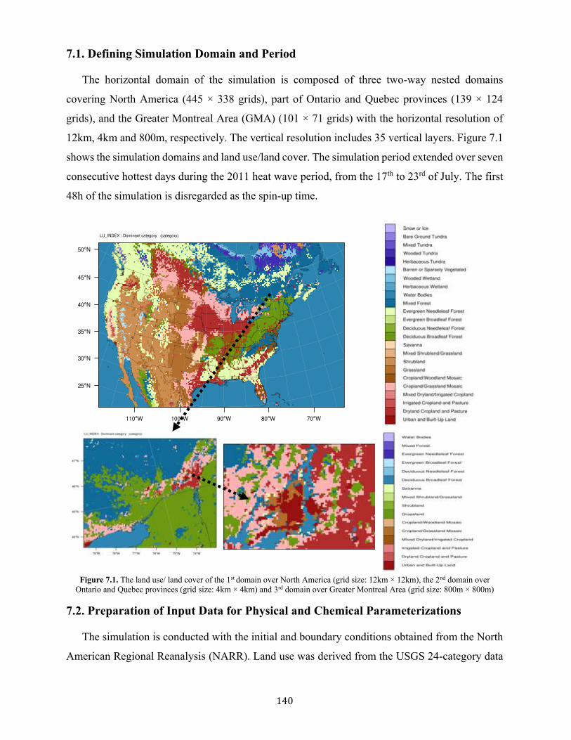
140
7.1. Defining Simulation Domain and Period
The horizontal domain of the simulation is composed of three two-way nested domains
covering North America (445 × 338 grids), part of Ontario and Quebec provinces (139 × 124
grids), and the Greater Montreal Area (GMA) (101 × 71 grids) with the horizontal resolution of
12km, 4km and 800m, respectively. The vertical resolution includes 35 vertical layers. Figure 7.1
shows the simulation domains and land use/land cover. The simulation period extended over seven
consecutive hottest days during the 2011 heat wave period, from the 17th to 23rd of July. The first
48h of the simulation is disregarded as the spin-up time.
Figure 7.1. The land use/ land cover of the 1st domain over North America (grid size: 12km × 12km), the 2nd domain over
Ontario and Quebec provinces (grid size: 4km × 4km) and 3rd domain over Greater Montreal Area (grid size: 800m × 800m)
7.2. Preparation of Input Data for Physical and Chemical Parameterizations
The simulation is conducted with the initial and boundary conditions obtained from the North
American Regional Reanalysis (NARR). Land use was derived from the USGS 24-category data
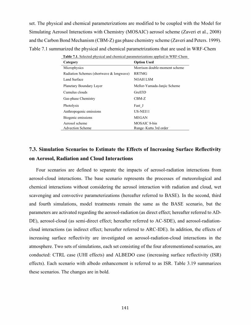
141
set. The physical and chemical parameterizations are modified to be coupled with the Model for
Simulating Aerosol Interactions with Chemistry (MOSAIC) aerosol scheme (Zaveri et al., 2008)
and the Carbon Bond Mechanism (CBM-Z) gas phase chemistry scheme (Zaveri and Peters. 1999).
Table 7.1 summarized the physical and chemical parametrizations that are used in WRF-Chem Table 7.1. Selected physical and chemical parameterizations applied in WRF-Chem Category Option Used Microphysics Morrison double-moment scheme Radiation Schemes (shortwave & longwave) RRTMG Land Surface NOAH LSM
Planetary Boundary Layer Mellor-Yamada-Janjic Scheme
Cumulus clouds Grell3D
Gas-phase Chemistry CBM-Z
Photolysis Fast_J Anthropogenic emissions US-NEI11
Biogenic emissions MEGAN Aerosol scheme MOSAIC 8-bin Advection Scheme Runge–Kutta 3rd order
7.3. Simulation Scenarios to Estimate the Effects of Increasing Surface Reflectivity
on Aerosol, Radiation and Cloud Interactions
Four scenarios are defined to separate the impacts of aerosol-radiation interactions from
aerosol-cloud interactions. The base scenario represents the processes of meteorological and
chemical interactions without considering the aerosol interaction with radiation and cloud, wet
scavenging and convective parameterizations (hereafter referred to BASE). In the second, third
and fourth simulations, model treatments remain the same as the BASE scenario, but the
parameters are activated regarding the aerosol-radiation (as direct effect; hereafter referred to AD-
DE), aerosol-cloud (as semi-direct effect; hereafter referred to AC-SDE), and aerosol-radiation-
cloud interactions (as indirect effect; hereafter referred to ARC-IDE). In addition, the effects of
increasing surface reflectivity are investigated on aerosol-radiation-cloud interactions in the
atmosphere. Two sets of simulations, each set consisting of the four aforementioned scenarios, are
conducted: CTRL case (UHI effects) and ALBEDO case (increasing surface reflectivity (ISR)
effects). Each scenario with albedo enhancement is referred to as ISR. Table 3.19 summarizes
these scenarios. The changes are in bold.
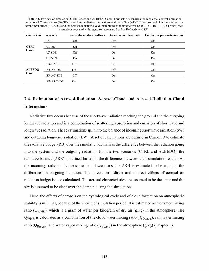
142
Table 7.2. Two sets of simulation: CTRL Cases and ALBEDO Cases. Four sets of scenarios for each case: control simulation with no ARC interactions (BASE), aerosol and radiation interactions as direct effect (AR-DE), aerosol and cloud interactions as semi-direct effect (AC-SDE) and the aerosol-radiation-cloud interactions as indirect effect (ARC-IDE). In ALBEDO cases, each
scenario is repeated with regard to Increasing Surface Reflectivity (ISR).
simulations Scenario Aerosol-radiative feedback Aerosol-cloud feedback Convective parameterization
CTRL Cases
BASE Off Off Off
AR-DE On Off Off
AC-SDE Off On On
ARC-IDE On On On
ALBEDO Cases
ISR-BASE Off Off Off
ISR-AR-DE On Off Off
ISR-AC-SDE Off On On
ISR-ARC-IDE On On On
7.4. Estimation of Aerosol-Radiation, Aerosol-Cloud and Aerosol-Radiation-Cloud
Interactions
Radiative flux occurs because of the shortwave radiation reaching the ground and the outgoing
longwave radiation and is a combination of scattering, absorption and emission of shortwave and
longwave radiation. These estimations split into the balance of incoming shortwave radiation (SW)
and outgoing longwave radiation (LW). A set of calculations are defined in Chapter 3 to estimate
the radiative budget (RB) over the simulation domain as the difference between the radiation going
into the system and the outgoing radiation. For the two scenarios (CTRL and ALBEDO), the
radiative balance (ΔRB) is defined based on the differences between their simulation results. As
the incoming radiation is the same for all scenarios, the ΔRB is estimated to be equal to the
differences in outgoing radiation. The direct, semi-direct and indirect effects of aerosol on
radiation budget is also calculated. The aerosol characteristics are assumed to be the same and the
sky is assumed to be clear over the domain during the simulation.
Here, the effects of aerosols on the hydrological cycle and of cloud formation on atmospheric
stability is minimal, because of the choice of simulation period. It is estimated as the water mixing
ratio (QWMR), which is a gram of water per kilogram of dry air (g/kg) in the atmosphere. The
QWMR is calculated as a combination of the cloud water mixing ratio ( QCWMR), rain water mixing
ratio (QRWMR) and water vapor mixing ratio (QVWMR
) in the atmosphere (g/kg) (Chapter 3).

143
7.5. Evaluation of Meteorological and Photochemical Model Performance
To evaluate the model performance, the ARC-IDE simulation results are compared with
measurements obtained from weather and air quality stations across the GMA during the 2011
heat wave period (21st to 23rd of July). The hourly 2-m air temperature (T2, oC), 10-m wind speed
(WS10, m/s) and 2-m relative humidity (RH2, %) are compared with measurements from four
weather stations (McTavish (MT), Pierre Elliott Trudeau Intl (PET), St-Hubert (SH), Ste-Anne-
de-Bellevue (SAB)). The hourly modelled fine particulate matter (PM2.5, µg/m3), ozone (O3, ppb)
and nitrogen dioxide (NO2, ppb) concentrations are compared with measurements from four air
quality stations (Decarie Interchange (28), Montreal Airport (66), St-Jean-Baptiste (3), Ste-Anne-
de-Bellevue (99)). The mean bias error (MBE), mean absolute error (MAE) and root mean square
error (RMSE) of the hourly meteorological parameters (T2 (oC), WS10 (m/s), RH (%)) and
chemical components (O3(ppb), PM2.5(µg/m3), NO2(ppb)) are presented in Tables 7.3, 7.4 and 7.5,
respectively. Figure 7.2 shows scatterplots of simulated vs. actual measurements of meteorological
and chemical variables. The correlation coefficient (R2) of a linear regression between simulated
and measured values are also presented in these figures.
The meteorological performance of the model indicates that the WRF-Chem slightly
underpredicts the spatial distribution of 2-m air temperature (MBE= -0.3oC, MAE and RMSE
~1oC), slightly overpredicts 10-m wind speed (MBE= 0.4 m/s, MAE and RMSE ~1m/s), and
underpredicts 2-m relative humidity (MBE= -4.3%, MAE= 7% and RMSE=9%). The 2-m air
temperature results show a strong correlation (0.85 < R2 <0.93) with measurements. They show
that the model is capable of predicting T2 and the spatial distribution of temperature in urban and
rural areas (Figure 7.2-T2). The wind speed is well predicted in urban areas (R2 = 60) compared to
rural areas (R2 = 40) (Figure 7.2-WS). But the model underpredicts the spatial distribution of
relative humidity. This underestimation shows that the microphysics scheme and cloud scheme do
not precisely account for the processes of transforming water (rain, vapor, cloud, etc.) and moisture
fluxes in the atmosphere. It also shows the model limitation in properly capturing wind speed
impacts on water mixing ratio and water content of the air. Figure 7.2-RH shows the correlations
between measured and simulated RH range from 0.6 to 0.8.
The chemical component of the model indicates that the WRF-Chem tends to underpredict fine
particulate matter (PM2.5) (MBE = −0.6 µg/m3, MAE = 5 µg/m3 and RMSE = 6.5 µg/m3),
overpredict ozone (O3) (MBE= 3.2 ppb, MAE= 10 ppb, and RMSE=13 ppb), and overpredict the
nitrogen dioxide (NO2) (MBE= 1.3 ppb, MAE= 5 ppb, and RMSE=6.3 ppb) concentrations. The

144
correlation between measured and simulated value shows that the model is capable of predicting
air quality parameters reasonably well in urban areas compared to their surroundings. The R2 of
fine particulate matter ranges from 0.5 to 0.7 (Figure 7.2-PM2.5). Figure 7.2- O3 shows the
comparison between measurements and simulations of ozone concentrations and indicates a good
correlation range from 0.6 to 0.8. The overestimation of O3 concentrations is due to the NOx and
VOCs calculations in emission inventories (US-NEI11 for NOx estimation and MEGAN for VOCs
estimation) in the chemistry packages. The NO2 concentrations are also estimated as one of the
precursors in ozone formation. The results show that the model tends to overpredict the nitrogen
dioxide and has a poor correlation between measured and simulated value range from 0.4 to 0.5.
Figure 7.3 shows the results of T2, WS10, RH2, PM2.5, O3 and NO2 comparisons with a weather
station (McTavish) and an air quality monitoring station (Decarie Interchange) located near the
downtown of the GMA for three days. The model on average slightly underpredicts the particulate
matter concentration at night and moderately overpredicts it during the day, but it well captures
the morning and evening peaks of PM2.5. As for ozone prediction, the model overpredicts its
concentrations during the day, but the model accurately captures the peak ozone concentrations.
Thus, it shows that the model prediction for ozone is well suited to be compared with the 8-h peak
concentration of National Ambient Air Quality Standard (NAAQS), which is also correlated with
human health effects. Overall, the performance of WRF-Chem, as configured here, is consistent
with most air quality models such as the fifth-generation NCAR/Penn State Mesoscale Model
(MM5) and the CMAQ model (Gilliam et al., 2006; Wu et al., 2008; Wang et al., 2009; Liu et al.,
2010) in simulating meteorological and chemical variables. Thus, it is well suited for application
of simulating and investigating the effects of heat island, and for mitigation strategy regarding
aerosols’ direct, semi-direct and indirect effects.

145
Table 7.3. Mean Bias Error (MBE) of T2 (oC), WS10 (m/s), RH2(%) from 4 weather stations: McTavish (MT), Pierre Elliott Trudeau Intl (PET), St-Hubert (SH), Ste-Anne-de-Bellevue (SAB); O3(ppb), PM2.5(µg/m3), and NO2(ppb) from 4 air quality stations (Decarie Interchange (DI), Montreal Airport (MA), St-Jean-Baptiste (SJB), Ste-Anne-de-Bellevue (SAB) over GMA
during the 2011 heat wave period (21st to 23rd of July)
Variables Mean Bias Error (MBE)
Average MT PET SH SAB
T2 (oC) -0.41 -0.34 -0.48 0.10 -0.28
WS10 (m/s) 0.40 0.23 0.70 0.29 0.40
RH2 (%) -2.83 -6.09 -4.32 -3.81 -4.26
DI MA SJB SAB
24-h avg. O3(ppb) 8.53 -4.04 3.17 5.13 3.19
24-h avg. PM2.5(µg/m3) 0.69 4.90 -1.87 -6.18 -0.62
24-h avg. NO2(ppb) 0.84 1.11 -5.92 9.43 1.36 Note: The definitions of statistical measurements are as follows Zhang et al. (2006): MBE =
1
N∑ (CM − CO),N
1 𝐶𝑀 and CO are modeled and observed concentrations, respectively and N is the total number of model and observation pairs.
Table 7.4. Mean Absolute Error (MAE) of T2 (oC), WS10 (m/s), RH2(%) from 4 weather stations: McTavish (MT), Pierre Elliott Trudeau Intl (PET), St-Hubert (SH), Ste-Anne-de-Bellevue (SAB); O3(ppb), PM2.5(µg/m3), and NO2(ppb) from 4 air
quality stations (Decarie Interchange (DI), Montreal Airport (MA), St-Jean-Baptiste (SJB), Ste-Anne-de-Bellevue (SAB)over GMA during the 2011 heat wave period (21st to 23rd of July)
Variables Mean Absolute Error (MAE)
Average MT PET SH SAB
T2 (oC) 0.84 0.88 0.78 1.03 0.88
WS10 (m/s) 0.68 1.02 1.44 0.66 0.95
RH2 (%) 6.79 7.81 5.59 6.47 6.66
DI MA SJB SAB
24-h avg. O3(ppb) 8.85 12.57 7.91 10.12 9.86
24-h avg. PM2.5(µg/m3) 2.84 5.23 5.04 6.33 4.86
24-h avg. NO2(ppb) 2.16 2.29 6.02 9.44 4.97 Note: The definitions of statistical measurements are as follows Zhang et al. (2006): MAE =
1
N∑ |CM − CO| N
1 CM and CO are modeled and observed concentrations, respectively and N is the total number of model and observation pairs.
Table 7.5. Root mean square error (RMSE) of T2 (oC), WS10 (m/s), RH2(%) from 4 weather stations: McTavish (MT), Pierre Elliott Trudeau Intl (PET), St-Hubert (SH), Ste-Anne-de-Bellevue (SAB); O3(ppb), PM2.5(µg/m3), and NO2(ppb) from 4 air
quality stations (Decarie Interchange (DI), Montreal Airport (MA), St-Jean-Baptiste (SJB), Ste-Anne-de-Bellevue (SAB) over GMA during the 2011 heat wave period (21st to 23rd of July)
Variables Root Mean Square Error (RMSE)
Average MT PET SH SAB
T2 (oC) 1.08 1.13 1.10 1.24 1.13
WS10 (m/s) 1.07 1.39 1.90 0.87 1.30
RH2 (%) 9.60 10.16 7.74 8.42 8.98
DI MA SJB SAB
24-h avg. O3(ppb) 10.96 14.48 11.45 14.74 12.91
24-h avg. PM2.5(µg/m3) 3.79 6.59 7.81 7.98 6.54
24-h avg. NO2(ppb) 3.10 3.33 8.08 11.04 6.38
Note: The definitions of statistical measurements are as follows Zhang et al. (2006): RMSE = [1
N∑ (CM − CO)2N
1 ]1/2
CM and CO are modeled and observed concentrations, respectively and N is the total number of model and observation pairs

146
Figure 7.2. Comparison of simulation with measurements of T2 (oC), WS10 (m/s), RH2(%) from 4 weather stations: McTavish (MT), Pierre Elliott Trudeau Intl (PET), St-Hubert (SH), Ste-Anne-de-Bellevue (SAB); and O3(ppb), PM2.5(µg/m3), NO2(ppb) from 4 air quality stations (Decarie Interchange (DI), Montreal Airport (MA), St-Jean-Baptiste (SJB), Ste-Anne-de-Bellevue (SAB) over the Greater Montreal Area during the 2011 heat wave period (21st to 23rd of July) [the blue dots are measurements and simulations. The dashed blue line indicates the correlation between measurements and simulations (trendline)]
McTavish-Urban Pierre Elliott Trudeau Intl-Urban St-Hubert-Rural Ste-Anne-de-Bellevue-Rural
T2 (o C
)
WS
(m/s
)
RH
(%)
Decarie Interchange Montreal Airport St-Jean-Baptiste Ste-Anne-de-Bellevue
PM2.
5 (µ
g/m
3 )
O3 (
ppb)
NO
2(pp
b)
R² = 0.93
26
30
34
26 30 34
Sim
ulat
ion
Measurment
R² = 0.92
26
30
34
26 30 34
Sim
ulat
ions
Measurments
R² = 0.88
22
26
30
34
22 26 30 34
Sim
ulat
ions
Measurments
R² = 0.85
22
26
30
34
22 26 30 34
Sim
ulat
ion
Measurment
R² = 0.60
0
2
4
6
8
10
1 3 5 7
Sim
ulat
ions
Measurments
R² = 0.58
0
2
4
6
8
10
1 3 5 7 9
Sim
ulat
ions
Measurments
R² = 0.41
0
2
4
6
8
10
1 3 5 7 9
Sim
ulat
ions
Measurments
R² = 0.38
0
2
4
6
0 2 4 6
Sim
ulat
ions
Measurments
R² = 0.63
35
55
75
95
35 55 75 95
Sim
ulat
ions
Measurments
R² = 0.68
35
55
75
95
35 55 75 95
Sim
ulat
ions
Measurments
R² = 0.85
35
55
75
95
35 55 75 95
Sim
ulat
ions
Measurments
R² = 0.76
35
55
75
95
35 55 75 95
Sim
ulat
ion
Measurment
R² = 0.73
0
10
20
30
0 10 20 30
Sim
ulat
ion
Measurment
R² = 0.64
0
10
20
30
0 10 20 30
Sim
ulat
ions
Measurements
R² = 0.50
0
10
20
30
0 10 20 30
Sim
ulat
ion
Measurment
R² = 0.56
0
10
20
30
0 10 20 30Si
mul
atio
nMeasurment
R² = 0.79
0
20
40
60
0 20 40 60
Sim
ulat
ions
Measurments
R² = 0.56
0
20
40
60
0 20 40 60
Sim
ulat
ions
Measurements
R² = 0.57
0
20
40
60
0 20 40 60
Sim
ulat
ions
Measurements
R² = 0.56
0
20
40
60
80
0 20 40 60 80
Sim
ulat
ions
Measurements
R² = 0.54
0
5
10
15
0 10 20
Sim
ulat
ions
Measurments
R² = 0.47
0
5
10
15
0 10 20
Sim
ulat
ions
Measurments
R² = 0.50
0
5
10
0 10 20
Sim
ulat
ions
Measurments
R² = 0.46
5
15
25
0 10 20
Sim
ulat
ions
Measurments

147
Figure 7.3. Hourly comparison of simulation with measurements of T2 (oC), WS10 (m/s), RH2(%) from McTavish weather station (MT) and O3(ppb), PM2.5(µg/m3), and NO2(ppb) from Decarie Interchange (DI) air quality monitoring station over GMA
during the 2011 heat wave period (21st to 23rd of July)[The black solid line shows simulations and the red dashed line shows measurements]
20
25
30
35
40
0 12 0 12 0 12
Tem
pera
ture
(oC
)
Time (hr)
0
2
4
6
8
10
0 12 0 12 0 12
Win
d sp
eed
(m/s
)
Time (hr)
0
20
40
60
80
100
0 12 0 12 0 12
RH
(%)
Time (hr)
0
20
40
60
80
0 12 0 12 0 12
O3
(ppb
)
Time (hr)
0
5
10
15
20
25
30
0 12 0 12 0 12
PM2.
5 (µ
g/m
3 )
Time (hr)
0
4
8
12
16
0 12 0 12 0 12
NO
2(p
pb)
Time (hr)

148
7.6. Effects of Heat Island on Aerosol-Radiation-Cloud Interactions
The simulations are performed during the 2011 heat wave period in the Greater Montreal Area.
The effects of heat island are investigated on aerosol, radiation and cloud interactions. The results
of four CTRL case simulations including BASE, AR-DE, AC-SDE, and ARC-IDE are analyzed
spatially. The radiative balance (RB) and down-welling shortwave radiation at the surface (SW↓)
are estimated based on calculations in Chapter 3. The water mixing ratio (WMR) is also calculated
as a combination of the cloud water mixing ratio, rain water mixing ratio and water vapor mixing
ratio in the atmosphere as grams per kg of dry air (g/kg).
The 2-m air temperature responses vary according to the aerosols’ direct and indirect effects.
The PBL height changes are closely related to the air temperature change spatially. Table 7.6
summarizes the averaged radiative balance (RB, W m-2), down-welling shortwave radiation at the
surface (SW↓, Wm-2), 2-m air temperature (T2, oC), water mixing ratio (WMR, g/kg), fine
particulate matter (PM2.5, µg/m3), and ozone concentrations (O3, ppb) disaggregated as three
regions—the North, Center, and South parts of the Greater Montreal Area.
• Aerosol-Radiation Interactions: Direct Effects
In general, the direct effects of aerosols are a decrease in radiative balance and thus reduction
in the heat absorbed by the surfaces. Aerosol concentrations cause a decrease in shortwave
radiation reaching to the ground, whether by scattering or absorbing the incoming solar radiation.
Here, the SW↓ reduces by 30Wm-2 and thus the RB reduces by almost 15Wm-2 across the entire
domain. The radiative balance is positive during the daytime and negative at night. The effect of
aerosol-radiation indicates that the radiative balance reduces in day and at night in the AR-DE
simulation compared to the BASE case simulation.
The 2-m air temperature increases by 0.2oC in the Center of the domain. The increase of air
temperature indicates that the aerosols are mostly absorbent because of their sizes (e.g., coarse
particulate matters) or compositions (e.g., black carbon). A minimal change in T2 and radiation
variables is seen in the Southern part of the GMA. In the North of the domain, a decrease in T2
occurs by 0.4oC. The reduction in T2 indicates that aerosols scatter the solar radiation more and
thus cool urban atmosphere. The planetary boundary layer height follows the same changes in
temperature: as temperature increases, the PBLH increases and thus the concentration of pollutants
across the domain slightly decreases. Here, the PBLH increases by 20m in the Center and decrease
by 30m in the Northern parts and decreases slightly in the South region. The water mixing ratio

149
increases by 0.3g/kg in the Center, whereas it decreases by 0.5g/kg in the North part. The increase
in WMR shows that the high temperature causes more evaporation from water bodies in the
domains.
In terms of air quality, the aerosol-radiation interactions cause a slight decrease in fine
particulate matter concentrations in the South, but reductions by 5 and 3µg/m3 over the Center and
North regions. This reduction owes to an increase in the PBLH. Ozone is a temperature-dependent
component, but at most a slight increase is observed across the domains. Figure 5 shows hourly
comparisons of air temperature (T2, oC), relative humidity (RH, %), fine particulate matter (PM2.5,
µg/m3) and ozone (O3, ppb) concentrations with measurements and base case simulations. The
hourly comparison of planetary boundary layer height (PBLH, m) and radiative balance (RB, W
m-2) of AR-DE and BASE simulations are also presented in Figure 5. The black and yellow solid
lines respectively represent the BASE and AR-DE simulations. The red dashed line shows
measurements.
• Aerosol-Cloud Interactions: Semi-Direct Effects
Considering the effects of clouds and humidity, during the daytime, more incoming solar
radiation is absorbed by clouds and water droplets in the atmosphere. The absorption causes
changes in radiation balance at the surface. The RB is less during the day and less during the night
compared to the base case simulation results. The sky was mostly clear during the simulation
period (the 2011 heat wave). Clear sky condition implies slight to minimal changes to radiative
budget and downwelling short-wave radiation at the surface. The RB reduces by 10Wm-2 over the
domain.
The daily 2-m air temperature decreases by 0.2oC and the PBLH shows slight changes. The
water mixing ratio also indicates minimal changes. The daily particulate matter concentrations
decrease by 3µg/m3 and the daily ozone concentrations decrease by 2ppb over the entire region,
which can be the result of a decrease in temperature. Figure 6 shows the effects of aerosol-cloud
interactions on air temperature (T2, oC), relative humidity (RH, %), fine particulate matter (PM2.5,
µg/m3) and ozone (O3, ppb) concentrations, planetary boundary layer height (PBLH, m) and
radiative balance (RB, Wm-2) during the 2011 heat wave period. The black and blue solid lines
respectively represent the BASE and AC-SDE simulations. The red dashed line shows
measurements.
• Aerosol-Radiation-Cloud Interactions: Indirect Effects

150
To simulate the indirect effects of aerosols, the aerosol-radiation feedbacks, the aerosol-cloud
feedbacks and the convective parameterizations are activated. Therefore, the combination of
aerosols that scatter solar radiation is estimated with the aerosols that can absorb the solar radiation
and emit infrared radiation, thus increasing air temperature, increasing convective
parameterization, and increasing latent heat fluxes and cloud formation in the area. Because of the
effects of aerosols, water droplets and clouds, less solar radiation (~20Wm-2) approaches the
surface and more longwave radiation is absorbed by particulate matter. Hence, the radiative
balance decreases by 25Wm-2. The 2-m air temperature increases over the Center and North part
of the domain by up to 0.5oC and 0.3oC, respectively. A minimal increase in T2 is also seen in the
South area by up to 0.1oC. The PBLH increases by up to 40m in the Center and North and increases
by 10m in the South part of the domain. The water mixing ratio slightly increases in the Center
and decreases in other part of the Greater Montreal Area.
The aforementioned changes in meteorological parameters impose impacts on every aspect of
air quality. They alter photolysis rates and kinetics that lead to changes in chemical transformation.
They also change transport and deposition processes. Meanwhile, the changes in solar radiation
and temperature affect the NO2 photolysis rates and hence the formation of O3 and PM2.5 in the
atmosphere. This complex interaction also decreases pollutant formation, as expected, because of
a reduction in photochemical reactions and temperature caused by ARC interactions. But since the
photolysis rate depends on other factors such as albedo and clouds, a dual behavior of pollutant
transformation and concentration is seen in the simulations. On the other hand, an increase in
planetary boundary layer height leads to a better advection and diffusion of pollutants and
decreases their concentrations. The PM2.5 shows smaller concentrations by 2µg/m3, whereas the
ozone shows a larger concentration by nearly 2ppb compared to the base case scenario across the
entire domain. These conclusions confirm the nonlinear effects of ARC interactions and the effects
that aerosols introduce into the atmosphere and weather patterns. Figure 7 shows the effects of
aerosol-radiation-could interactions on air temperature (T2, oC), relative humidity (RH, %), fine
particulate matter (PM2.5, µg/m3) and ozone (O3, ppb) concentrations, planetary boundary layer
height (PBLH, m) and radiative balance (RB, Wm-2) during the 2011 heat wave period. The black
and purple solid lines respectively represent the BASE and ARC-IDE simulations. The red dashed
line shows measurements.
The results of direct, semi-direct, indirect effects and BASE case simulations are compared
with measurements from weather and air quality stations in the GMA during the weekdays
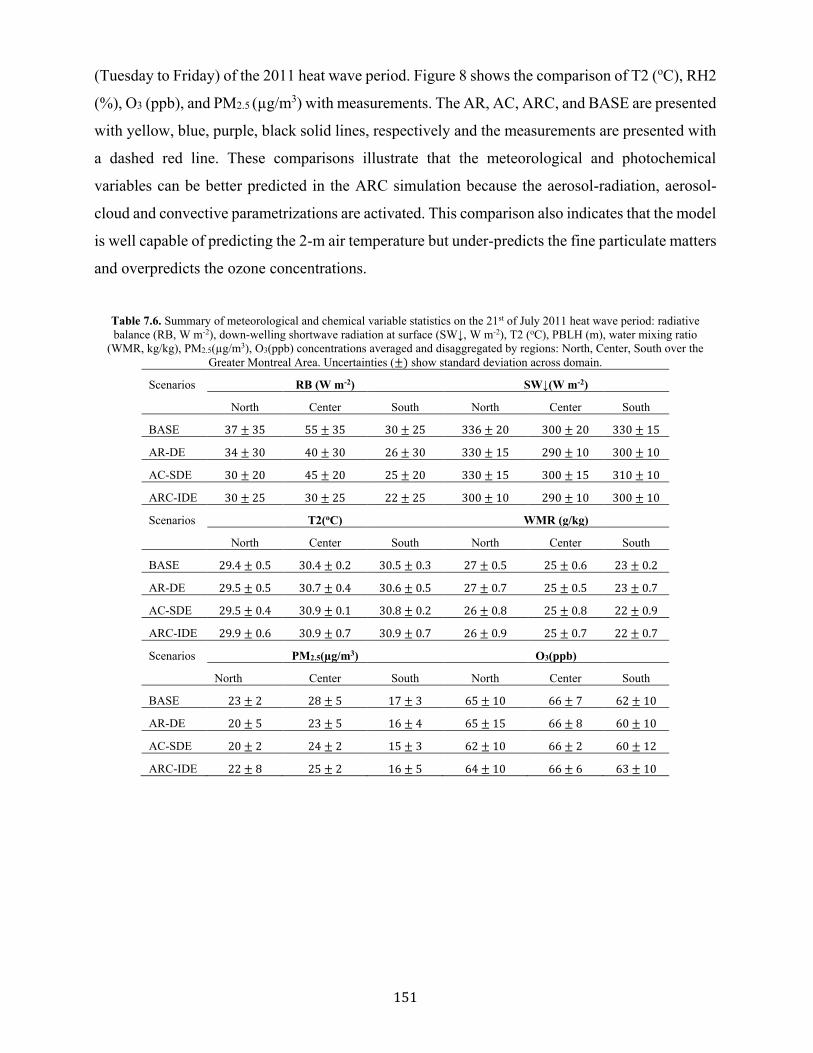
151
(Tuesday to Friday) of the 2011 heat wave period. Figure 8 shows the comparison of T2 (oC), RH2
(%), O3 (ppb), and PM2.5 (µg/m3) with measurements. The AR, AC, ARC, and BASE are presented
with yellow, blue, purple, black solid lines, respectively and the measurements are presented with
a dashed red line. These comparisons illustrate that the meteorological and photochemical
variables can be better predicted in the ARC simulation because the aerosol-radiation, aerosol-
cloud and convective parametrizations are activated. This comparison also indicates that the model
is well capable of predicting the 2-m air temperature but under-predicts the fine particulate matters
and overpredicts the ozone concentrations.
Table 7.6. Summary of meteorological and chemical variable statistics on the 21st of July 2011 heat wave period: radiative balance (RB, W m-2), down-welling shortwave radiation at surface (SW↓, W m-2), T2 (oC), PBLH (m), water mixing ratio
(WMR, kg/kg), PM2.5(µg/m3), O3(ppb) concentrations averaged and disaggregated by regions: North, Center, South over the Greater Montreal Area. Uncertainties (±) show standard deviation across domain.
Scenarios RB (W m-2) SW↓(W m-2)
North Center South North Center South
BASE 37 ± 35 55 ± 35 30 ± 25 336 ± 20 300 ± 20 330 ± 15
AR-DE 34 ± 30 40 ± 30 26 ± 30 330 ± 15 290 ± 10 300 ± 10
AC-SDE 30 ± 20 45 ± 20 25 ± 20 330 ± 15 300 ± 15 310 ± 10
ARC-IDE 30 ± 25 30 ± 25 22 ± 25 300 ± 10 290 ± 10 300 ± 10
Scenarios T2(oC) WMR (g/kg)
North Center South North Center South
BASE 29.4 ± 0.5 30.4 ± 0.2 30.5 ± 0.3 27 ± 0.5 25 ± 0.6 23 ± 0.2
AR-DE 29.5 ± 0.5 30.7 ± 0.4 30.6 ± 0.5 27 ± 0.7 25 ± 0.5 23 ± 0.7
AC-SDE 29.5 ± 0.4 30.9 ± 0.1 30.8 ± 0.2 26 ± 0.8 25 ± 0.8 22 ± 0.9
ARC-IDE 29.9 ± 0.6 30.9 ± 0.7 30.9 ± 0.7 26 ± 0.9 25 ± 0.7 22 ± 0.7
Scenarios PM2.5(µg/m3) O3(ppb)
North Center South North Center South
BASE 23 ± 2 28 ± 5 17 ± 3 65 ± 10 66 ± 7 62 ± 10
AR-DE 20 ± 5 23 ± 5 16 ± 4 65 ± 15 66 ± 8 60 ± 10
AC-SDE 20 ± 2 24 ± 2 15 ± 3 62 ± 10 66 ± 2 60 ± 12
ARC-IDE 22 ± 8 25 ± 2 16 ± 5 64 ± 10 66 ± 6 63 ± 10
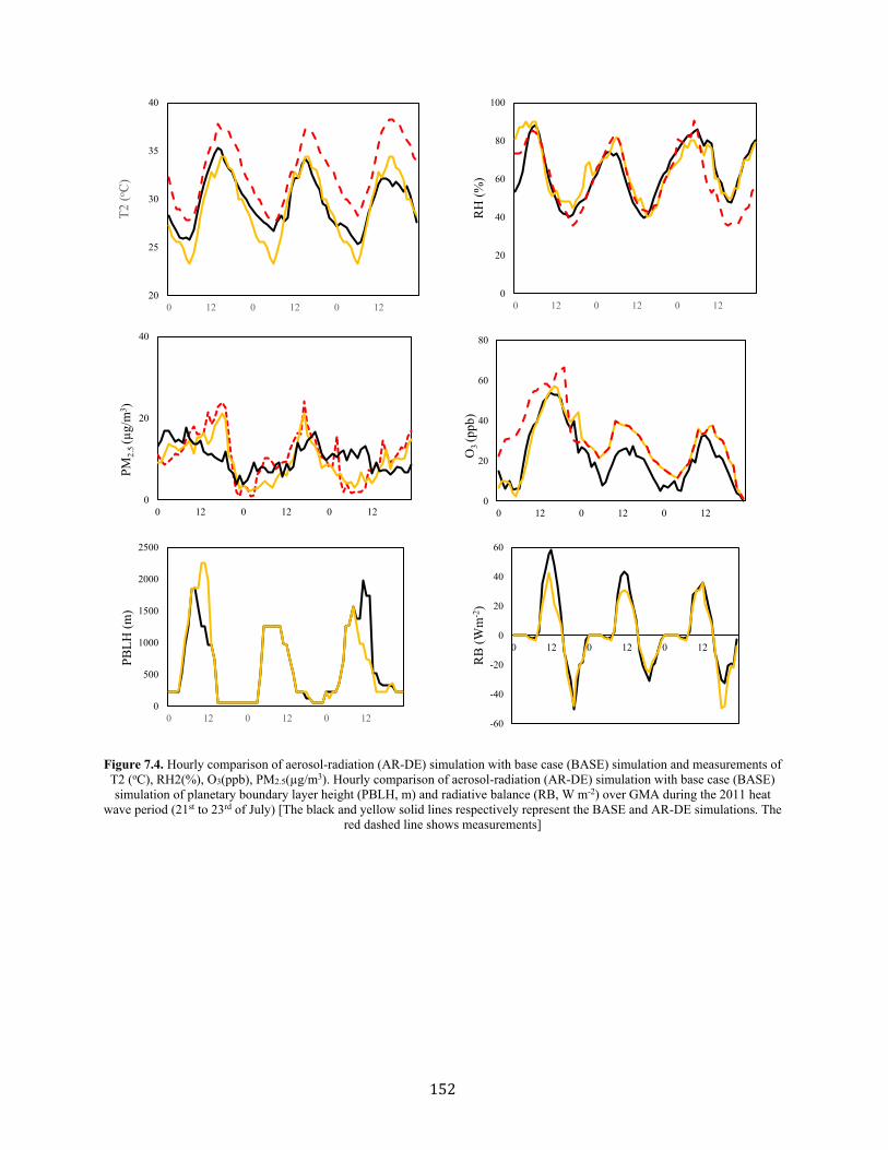
152
Figure 7.4. Hourly comparison of aerosol-radiation (AR-DE) simulation with base case (BASE) simulation and measurements of T2 (oC), RH2(%), O3(ppb), PM2.5(µg/m3). Hourly comparison of aerosol-radiation (AR-DE) simulation with base case (BASE) simulation of planetary boundary layer height (PBLH, m) and radiative balance (RB, W m-2) over GMA during the 2011 heat
wave period (21st to 23rd of July) [The black and yellow solid lines respectively represent the BASE and AR-DE simulations. The red dashed line shows measurements]
20
25
30
35
40
0 12 0 12 0 12
T2 (o C
)
0
20
40
60
80
100
0 12 0 12 0 12
RH
(%)
0
20
40
0 12 0 12 0 12
PM2.
5 (µ
g/m
3 )
0
20
40
60
80
0 12 0 12 0 12
O3 (p
pb)
0
500
1000
1500
2000
2500
0 12 0 12 0 12
PBLH
(m)
-60
-40
-20
0
20
40
60
0 12 0 12 0 12
RB
(Wm
-2)
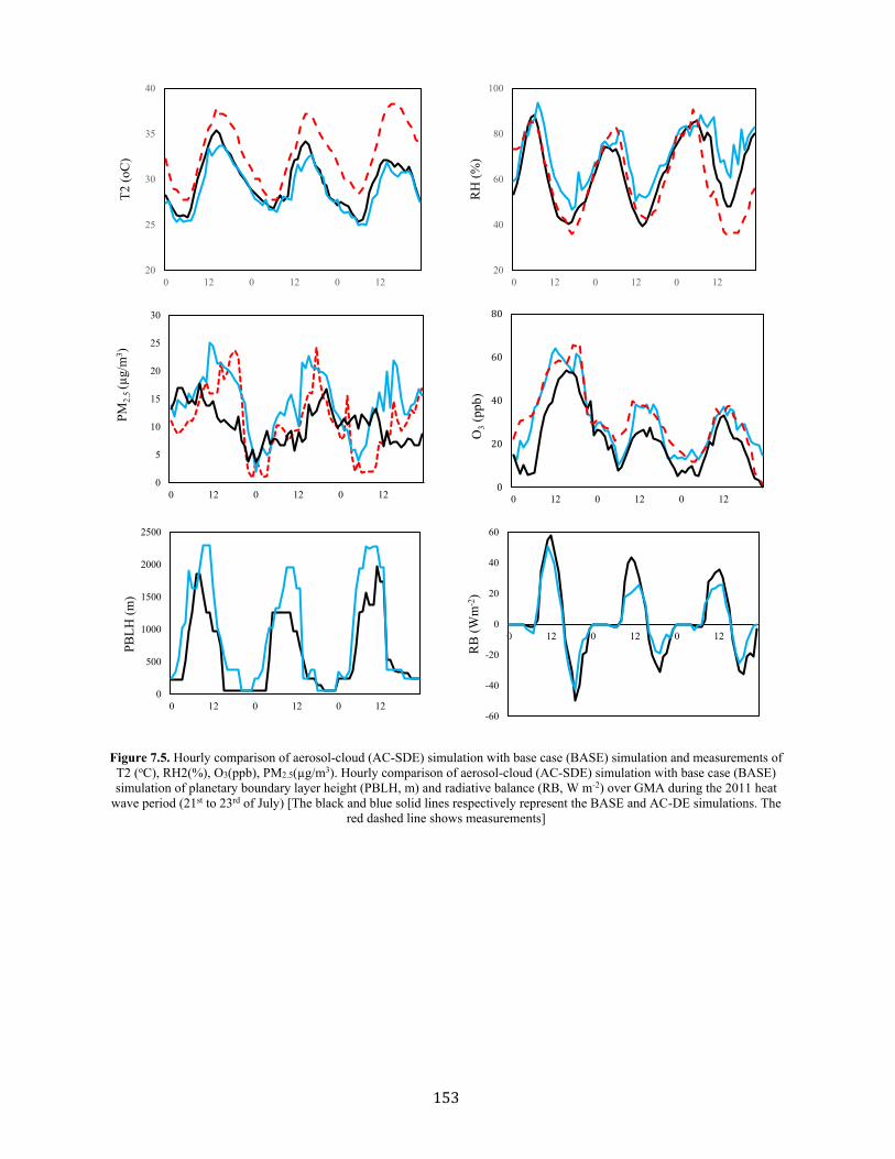
153
Figure 7.5. Hourly comparison of aerosol-cloud (AC-SDE) simulation with base case (BASE) simulation and measurements of T2 (oC), RH2(%), O3(ppb), PM2.5(µg/m3). Hourly comparison of aerosol-cloud (AC-SDE) simulation with base case (BASE) simulation of planetary boundary layer height (PBLH, m) and radiative balance (RB, W m-2) over GMA during the 2011 heat
wave period (21st to 23rd of July) [The black and blue solid lines respectively represent the BASE and AC-DE simulations. The red dashed line shows measurements]
20
25
30
35
40
0 12 0 12 0 12
T2 (o
C)
20
40
60
80
100
0 12 0 12 0 12
RH
(%)
0
5
10
15
20
25
30
0 12 0 12 0 12
PM2.
5 (µ
g/m
3 )
0
20
40
60
80
0 12 0 12 0 12
O3
(ppb
)
0
500
1000
1500
2000
2500
0 12 0 12 0 12
PBLH
(m)
-60
-40
-20
0
20
40
60
0 12 0 12 0 12
RB
(Wm
-2)

154
Figure 7.6. Hourly comparison of aerosol-radiation-cloud (ARC-IDE) simulation with base case (BASE) simulation and measurements of T2 (oC), RH2(%), O3(ppb), PM2.5(µg/m3). Hourly comparison of aerosol-radiation-cloud (ARC-IDE) simulation with base case (BASE) simulation of planetary boundary layer height (PBLH, m) and radiative balance (RB, W m-2) over GMA
during the 2011 heat wave period (21st to 23rd of July) [The black and purple solid lines respectively represent the BASE and ARC-IDE simulations. The red dashed line shows measurements]
20
25
30
35
40
0 12 0 12 0 12
T2 (o
C)
20
40
60
80
100
0 12 0 12 0 12
RH
(%)
0
5
10
15
20
25
30
0 12 0 12 0 12
PM2.
5 (µ
g/m
3 )
0
20
40
60
80
0 12 0 12 0 12
O3 (p
pb)
0
500
1000
1500
2000
2500
0 12 0 12 0 12
PBLH
(m)
-60
-40
-20
0
20
40
60
80
0 12 0 12 0 12RB
(Wm
-2)

155
Figure 7.7. The comparison between direct (AR-DE), semi-direct (AC-SDE), indirect (ARC-IDE), and base (BASE) case scenarios of T2(oC), RH2(%), O3(ppb), PM2.5(µg/m3) with measurements in McTavish station near the center of the GMA. The AR, AC, ARC, BASE is presented with yellow, blue, purple, black solid lines, respectively and the measurements is presented
with dashed red line.
7.7. Effects of Increasing Surface Reflectivity (ISR) on Urban Climate, Air Quality
and Aerosol, Radiation and Cloud Interactions
The effects of albedo enhancement is analysed on the radiation balance at solar noon (RB, Wm-
2), cloud coverage (CC, %), water mixing ratio (WMR, gwater/kgdry air), 2-m air temperature (T2, oC), planetary boundary layer height (PBLH, m), ozone (O3, ppb), fine particulate matters (PM2.5,
µg/m3) and nitrogen dioxide (NO2, ppb) concentrations. Table 8 presents the differences between
CTRL and ALBEDO (CTRL−ALBEDO) scenarios in four cases (ISR-BASE, ISR-AR-DE, ISR-
AC-SDE, ISR-ARC-IDE) over the North, Center and South part of the Greater Montreal Area
during the 2011 heat wave period.
7.7.1. Effects of ISR on Meteorological and Chemical Components
20
25
30
35
40
0 12 0 12 0 12
T2 (o
C)
0
20
40
60
80
100
0 12 0 12 0 12
RH
(%)
0
5
10
15
20
25
30
0 12 0 12 0 12
PM2.
5(µg
/m3 )
0
20
40
60
80
0 12 0 12 0 12
O3
(ppb
)
156
Here, the effects of increasing solar reflectivity are presented in the ISR-BASE case simulation,
where the radiation and cloud feedbacks are not considered, and convective parameterization is
not activated. The simulation results show that albedo enhancement leads to a net decrease in daily
2-m air temperature by up to 0.7°C in the Center and 0.5°C in other parts of the domain during the
2011 heat wave period. The water mixing ratio reduces by 0.2g/kg across Montreal and cloud
coverage indicates no change because of albedo increment. The heat island mitigation strategy
causes a decline in solar noon radiative balance by almost 20Wm-2. The planetary boundary layer
height lower by 28m in the Center and 20m in the North and South part of Montreal. Decreasing
temperature leads to a decrease in planetary boundary layer height, which reduces the advection
and diffusion of pollutants. Hence, this phenomenon increases the pollutant concentrations and
also assists the O3 and NO reaction rates to produce NO2. This is the reason that the ozone
concentration is higher in some parts of the domain. On the other hand, by decreasing air
temperature, the rate of temperature-sensitive photochemical reaction rates reduces and thus
affords a decrease in daily ozone concentrations by nearly 4ppb in the Greater Montreal Area
during the heat wave period. Albedo enhancement causes a decline in fine particulate matter by
4µg/m3 and minimal changes to nitrogen dioxide concentrations.
7.7.2. Effects of ISR on Aerosol, Radiation and Cloud Interactions in the Urban Atmosphere
The effects of albedo enhancement on aerosol and radiation interactions show a slight increase
in air temperature by ~ 0.2oC in the Center area and a decrease by the same amount in the other
parts of the domain. The reason for these changes is because of the simulation configuration that
only the radiation feedback is considered, and the convective parametrization and cloud formation
has not been activated. Thus, the results indicate that because of the absorbent components in the
Center part of the GMA, although the albedo is increased, but the outgoing longwave radiation
from the surface is trapped by atmospheric aerosols. Therefore, without considering the convective
parametrizations, the air temperature increases and heats the local atmosphere. An increase in
temperature lead to a rise in water mixing ratio by nearly 0.2g/kg in the Center and a decline by
the same amount in other part of the domain, but no changes in cloud coverage. Increasing surface
reflectivity causes a decrease in radiative balance at solar noon by around 15Wm-2 across Montreal.
Heat island mitigation strategy reduces the planetary boundary layer height across the domain by
10m. Surface albedo modifications cause a decrease in the temperature-dependent photochemical
reaction rates in the atmosphere, even though it is minimal. The O3 (ppb), PM2.5 (µg/m3), and NO2

157
(ppb) concentrations decrease slightly as a consequence of increasing surface reflectivity on
aerosol and radiation interactions.
The aerosol and cloud interactions show that albedo enhancement leads to a slight decrease in
2-m air temperature. This occurs because the aerosol-radiation interactions have not been
estimated in these simulations. As temperature reduces, the evaporation from water bodies
reduces, and thus a decrease in water mixing ratio is expected. But the results show that water
mixing ratio behaves differently and increases slightly across the domain. The cloud coverage also
rises by 3% across the entire domain. Increasing solar reflectance causes a decrease in radiative
balance at solar noon by around 20Wm-2. Albedo enhancement causes a decrease in PBLH in a
range of 20m in the GMA. The fine particulate matters and ozone concentrations decrease by
1µg/m3 and 1ppb in aerosol-cloud (ISR-AC-SDE) simulation, respectively.
Considering the nonlinear and complex interaction of aerosol-radiation-cloud in the
atmosphere, the 2-m air temperature decreases by 0.5oC in the Center and North parts of the
domain and 0.3oC in the Southern area. The water mixing ratio decreases to 0.5 g/kg in the Center
and 0.3g/kg in the North and South regions. The cloud coverage declined by 3-5% across the
Greater Montreal Area. Albedo enhancement leads to a net decrease in radiative balance at solar
noon by 25Wm-2 in the Center and 22Wm-2 in the Northern and Southern regions. Increasing solar
reflectivity imposes a decrease in planetary boundary layer height to 25m and 20m in the Center
and other parts of Montreal, respectively. Heat island mitigation strategy affords a decrease in
temperature and thus ozone concentrations to almost 3ppb across the entire domain. The fine
particulate matter also reduces to about 3µg/m3 in the Center and 2µg/m3 in other areas during the
2011 heat wave period. The NO2 concentrations reduces slightly compared to PM2.5 and O3
concentrations across the domain of interest.
Table 8. The differences between CTRL and ALBEDO scenarios of T2 (oC), RH2(%), O3 (ppb), PM2.5 (µg/m3), NO2 (ppb), NO
(ppb) over North, Center and South part of GMA during the 2011 heat wave period CTRL−ALBEDO Region ISR-BASE ISR-AR-DE ISR-AC-SDE ISR-ARC-IDE
Δ RB at noon (Wm-2) North 18 15 20 22 Center 20 16 21 25 South 17 17 21 23
Δ Cloud coverage (%) North No change No change 3 3 Center No change No change 3 5 South No change No change 3 3
ΔWMR (g/kg)
North 0.2 0.2 -0.2 0.3 Center 0.2 -0.2 -0.2 0.5 South 0.2 0.2 -0.2 0.3
Δ daily T2 (°C) North 0.47 0.19 0.25 0.33 Center 0.67 -0.23 0.25 0.55

158
South 0.54 0.21 0.25 0.51 Δ PBLH(m)
North 22 10 20 22 Center 28 8 23 25 South 20 10 20 18
24-h avg. O3(ppb)
North 3.67 0.59 0.74 2.66 Center 4.41 0.56 0.68 2.76 South 3.55 0.51 0.57 2.09
24-h avg. PM2.5(µg/m3)
North 3.11 0.98 1.03 2.88 Center 3.67 0.78 0.54 2.59 South 3.21 0.60 0.67 1.91
24-h avg. NO2(ppb)
North 0.19 0.27 0.25 0.28 Center 0.36 0.18 0.31 0.35 South 0.13 0.16 0.24 0.23
7.8. Discussion and Limitations of Aerosol, Radiation and Cloud Interactions
Assessment
Current understanding of aerosol impacts on the radiative budget and hydrological cycle of the
climate system is still inadequate at the fundamental level. Some uncertainties exist in aerosol
estimation because of their heterogeneous distribution and complex interactions with radiation and
clouds in the atmosphere. Here, a two-way nested approach is applied over the Greater Montreal
Area during the 2011 heat wave period. The simulation period is restricted to seven consecutive
days during the heat wave event, and hence the short-term response of increasing surface
reflectivity is considered. To have a better understanding of aerosol interactions in the atmosphere,
it is suggested to perform a simulation over a year to see the seasonal effects as well as rainy and
cloudy conditions of these complex nonlinear interactions.
The results of the WRF-Chem simulations, with the meteorological and chemical settings
configured here, are in good agreement with measurements, but different settings can also be
applied. As with any modeling approaches, there are some issues and caveats to remember when
evaluating the simulation outcomes. Some of these concerns relate to the assumptions and
fundamental issues during the course of this study—for example, the choice of aerosol scheme,
the selection of physical and chemical parametrizations, emission inventories data, and so on. On
the other hand, when applying finer resolution grids, the effects of cloud formations and
hydrological cycles cannot be captured accurately.
While the simulations illustrate the importance of aerosol-radiation-cloud estimations and the
effects of heat island mitigation strategy on these complex interactions, the current study is still
subject to a number of limitations. Several issues in model treatments and configurations available
for aerosol feedback studies will introduce inaccuracies and uncertainties in model performance.

159
For example, the MOSAIC aerosol module cannot calculate the estimation of secondary organic
aerosols (SOA) accurately and the Fast-J photolysis algorithm disregards the feedbacks of all
photochemically-active gases to photolysis. These missing treatments will surely affect the
accuracy of aerosol concentrations. In addition, aerosol effects on cloud dynamic feedbacks,
hydrological cycle (as precipitation), and convective clouds cannot be fully captured in WRF-
Chem, which may cause an underestimation in the indirect effects of aerosols. As mentioned
before, seven consecutive days during the 2011 heat wave period is still too short to characterize
the long-term variation trend. Nevertheless, this work demonstrates the effects of increasing
surface reflectivity on aerosol, radiation and cloud interactions through direct, semi-direct, and
indirect effects of aerosols over the Greater Montreal Area and will thus provide a useful
foundation upon which future improvements can be identified and focused.
7.9. Effects of Albedo Enhancement on Urban Climate, Air Quality and Aerosol,
Radiation and Cloud Interactions in the Urban Atmosphere
The effects of increasing surface reflectivity are investigated on urban climate, air quality and
aerosol-radiation and cloud interactions over Greater Montreal Area during the 2011 heat wave
period. A two-way nested approach is applied by online coupling of the chemistry package within
the solver of the Weather Research and Forecasting model (WRF-Chem). In addition, the WRF-
Chem is coupled with a multi-layer of the Urban Canopy Model (ML-UCM) to provide more detail
of the effects of surface modifications. This approach simulates the emission, transport, deposition,
chemical transformation, and aerosol interactions in the atmosphere. The two-way nested method
captures more detailed treatments of urban morphology and responses to heat island mitigation
strategies. Therefore, the method estimates the feedbacks between chemistry and meteorological
interactions as cloud formation and radiation budget.
The direct, semi-direct and indirect effects of aerosols are analysed. These simulations are
conducted with and without convective parameterizations and are performed only with regard to
radiation schemes, to separate the instantaneous radiative effects of the aerosol-radiation from
aerosol-cloud interactions. The ARC simulation is compared with measurements from weather
and air quality monitoring stations. To mitigate the urban heat island impacts, the surface albedo
of roofs, walls and grounds increased from 0.2 in CTRL scenario to 0.65, 0.60 and 0.45,
respectively, in ALBEDO scenario. The consequences of increasing surface reflectivity are
disaggregated spatially for data presentation into three regional subdomains: North, Center, and

160
South regions of the Greater Montreal Area. The outcomes indicate a decrease in 2-m air
temperature, a minimal to slight decrease in water mixing ratio, a decrease in planetary boundary
layer height, a decline in radiative budget at solar noon, a decrease in cloud coverage and minimal
to slight reductions in ozone, fine particulate matter and nitrogen dioxide concentrations.
Albedo enhancement led to a net decrease in radiative balance at solar noon by 25Wm-2 in the
Center and by nearly 22Wm-2 in the Northern and Southern regions of the Greater Montreal Area
during the 2011 heat wave period. The consequences of increasing solar reflectivity on aerosol-
radiation-cloud interactions indicated a decrease in 2-m air temperature by 0.5oC in the Center and
North parts of the domain and by 0.3oC in the Southern area. The water mixing ratio decreased to
0.5g/kg in the Center and 0.3g/kg in the North and South regions. The cloud coverage declined by
3-5% across the Greater Montreal Area. Increasing urban albedo imposes a decrease in planetary
boundary layer height to 25m and 20m in the Center and other parts of Montreal, respectively.
Heat island mitigation strategy afforded a decrease in temperature and thus ozone concentrations
to 3ppb across the entire domain. The fine particulate matter reduced to about 3µg/m3 in the Center
and 2µg/m3 in other areas during the 2011 heat wave period. Albedo enhancement causes a
decrease in boundary-layer height that reduces the chance of advection and diffusion of pollutants
and hence increases the pollutants concentrations. In addition, shallow boundary layer can impose
an increase in pollutants reaction rates. Decreasing the contaminates dispersion as well as
increasing the chance of chemical reactions result in growing pollutants concentration in some part
of the domain. The consequences discussed here are episode and domain specific and may not be
applied in generalizing and extrapolating the findings to other times, seasons, or geographical
locations.
The effects of increasing surface reflectivity have been investigated on urban climate and air
quality. A two-way nested approach is applied in WRF-Chem. This approach simulates the
emission, transport, deposition, chemical transformation, and aerosol interactions in the
atmosphere. The two-way nested method captures more detailed treatments of urban morphology
and responses to heat island mitigation strategies. In addition, the method estimates the feedbacks
between chemistry and meteorological interactions as cloud formation, precipitation and radiation
budget. However, to what extent the WRF and WRF-Chem results are closer with measurements,
a comparison between the meteorological model and photochemical model is required. This
comparison indicates the capability of each model in predicting air temperature. In addition,
assessing the correlation between albedo enhancement and air temperature illuminates the effects
161
of this heat island mitigation strategy on urban climate and air quality. These comparisons are
presented in the following section with more detail.
7.10. Summary of Simulation Results in terms of Air Temperature Predictions and
its Correlation with Albedo Enhancements
The temperature changes because of albedo enhancement are of an interest to urban climate
and air quality policymakers. Thus, the performance of WRF and WRF-Chem simulations are also
evaluated regarding 2-m air temperature. The WRF and WRF-Chem simulations are compared
with measurements. The conclusion of these comparisons is presented in Section 7.10.1. In
addition, the correlation between changes in albedo enhancement that impose changes in
temperature and ozone concentrations are estimated for three different urban categories (high
intensity residential, low intensity residential, and industrial and commercial) in the urban canopy
model (UCM). The results of the present study are applied to the Greater Montreal Area (GMA)
in Canada. The consequences of increasing surface albedo in three cities—namely, Sacramento
(California), Houston (Texas), and Chicago (Illinois) in the USA—are also estimated. These
analyses are illustrated in Section 7.10.2.
7.10.1. Air Temperature Prediction in WRF and WRF-Chem Here, the WRF and WRF-Chem simulations of 2-m air temperature (T2) are compared with
measurements (four weather stations (McTavish (MT), Pierre Elliott Trudeau Intl (PET), St-
Hubert (SH), Ste-Anne-de-Bellevue (SAB)) across the Greater Montreal Area during the 2011
heat wave period. The mean bias error (MBE), mean absolute error (MAE) and root mean square
error (RMSE) are estimated. Table 7.8 summarizes the outcomes. Figure 7.5 compares the T2 of
simulations with measurements. The outcomes of WRF-Chem, WRF and measurements are
presented by a dashed red line, solid black line and dashed black line, respectively. The
comparisons indicate that WRF and WRF-Chem slightly underpredict the 2-m air temperature;
though the WRF-Chem outcomes show less error compared to WRF. To perform the WRF-Chem,
more efforts are needed in order to select the proper physical parameterizations that can be coupled
with proper choice of chemistry packages. In addition, WRF-Chem needs more computational
resources to be performed. The estimation of anthropogenic and biogenic emissions is required to
be simulated. Table 7.9 summarizes the key features of WRF and WRF-Chem. More details can
be found in Chapter 3. Thus, for urban climate simulations, it is suggested to perform the WRF.

162
But, if the focus of interest is air quality, the WRF-Chem has to be carried out. The WRF-Chem
is able to predict the meteorological process and air quality conditions, simultaneously. This is the
reason that the WRF-Chem tends to reflect the real atmosphere, and the results have a good
agreement with measurements. Table 7.8. Mean Bias Error (MBE), Mean Absolute Error (MAE) and Root Mean Square Error (RMSE) of T2 (oC) from WRF and WRF-Chem results compared with measurements (McTavish (MT), Pierre Elliott Trudeau Intl (PET), St-Hubert (SH), Ste-
Anne-de-Bellevue (SAB)) over GMA during the 2011 heat wave period Model Performance MT PET SH SAB Average
WRF
MBE 0.07 -0.88 -0.94 0.03 -0.43
MAE 1.51 1.37 1.30 1.10 1.32
RMSE 1.91 1.83 1.70 1.47 1.73
WRF-Chem
MBE -0.41 -0.34 -0.48 0.10 -0.28
MAE 0.84 0.88 0.78 1.03 0.88
RMSE 1.08 1.13 1.10 1.24 1.13
The definitions of statistical measurements are as follows Zhang et al. (2006): MBE = 1
N∑ (CM − CO),N
1 MAE =1
N, RMSE =
[1
N∑ (CM − CO)2N
1 ]1/2
, 𝐶𝑀 and CO are modeled and observed concentrations, respectively and N is the total number of model and observation pairs.
Figure 7.8. The hourly 2-m air temperature (T2, °C) comparisons of WRF results (solid black line) vs. WRF-Chem results
(dashed red line) vs. measurements (dashed black line) from four weather stations across the GMA during the 2011 heat wave period (McTavish (MT), Pierre Elliott Trudeau Intl (PET), St-Hubert (SH), Ste-Anne-de-Bellevue (SAB))
25
30
35
40
0 12 0 12 0 12 0 12
T2(o C
)
Time (hr)
25
30
35
40
0 12 0 12 0 12 0 12
T2(o C
)
Time (hr)PET
20
25
30
35
0 12 0 12 0 12 0 12
T (o C
)
Time (hour)SH
20
25
30
35
0 12 0 12 0 12 0 12
T2 (o C
)
Time (hr)SAB
MT

163
Table 7.9. Summary of the WRF and WRF-Chem key features WRF WRF-Chem
WRF simulate the advection and diffusion of variables. It has sub-grid scale transport (WRF parameterizations, PBL, convection). WRF can be used for regional and global applications. It has the following capabilities: - Fully compressible nonhydrostatic equations - Complete Coriolis and curvature terms - One-way and Two-way nesting with multiple nests and nest levels - Mass-based terrain-following coordinate - Vertical grid-spacing can vary with height - Four different map-scale factors:polar stereographic;Lambert-conformal; Mercator; Latitude and longitude- Runge-Kutta 2nd and 3rd order time integration options - Scalar-conserving flux form for prognostic variables - 2nd to 6th order advection options - Monotonic transport and positive-definite advection option for moisture, scalar, tracer, and TKE - Time-split small step for acoustic and gravity-wave modes - Upper boundary absorption and Rayleigh damping lateral boundary conditions Full physics options for land-surface, planetary boundary layer, atmospheric and surface radiation, microphysics and cumulus convections
WRF-Chem can be coupled with the WRF. Coupling the WRF with chemistry package enables researchers to simulate chemical processes (transport, deposition, emission, chemical transformation, aerosol interactions, photolysis and radiation) to predict air quality conditions. The component of air quality is consistent with the meteorological ones within the same transport scheme, grid and physics schemes and time steps. It has the following capabilities: -Dry deposition soil/vegetation scheme - Wet scavenging -Biogenic emission estimation - Anthropogenic emission estimation - Gas-phase mechanism assessment - Photolysis estimation - Aerosol estimation - Treatment of chemical reactions, aqueous phase chemistry, gas phase species and aerosols
7.10.2. The Correlation Between Surface Albedo Enhancement and Temperature Reduction Here, the results of WRF-Chem is presented with more details. The WRF-Chem is coupled
with the urban canopy model (UCM), which has three urban categories: 1) low intensity residential
(LIR), 2) high intensity residential (HIR) and 3) industrial and commercial (I/C) areas. In each
category, building properties are considered to be similar. In addition, the fraction of roofs,
pavements, and vegetation in each grid cell is assumed to be constant and the same as other grids
in the same urban category. This limitation causes uncertainties in estimating the correlation
between the fraction of albedo enhancement and decreasing air temperature and ozone
concentrations. But, as the conclusions of these simulations and previous studies reveal, the
correlation between decreasing air temperature and increasing surface reflectivity is not because
of the size of the city or its population. For instance, Sacramento is nearly one third of Chicago in
terms of area and has nearly half the population density; but because of its specific synoptic
condition, weather pattern and geographical location the effects of albedo enhancement are
significant. Sacramento ranks fifth because of its high ozone concentration. Thus, the effects of
reducing air temperature on ozone concentrations are larger compared to other cities. It shows that

164
UHI mitigation strategies that reduce temperature will improve air quality to some extent. Table
7.10 presents these comparisons. Table 7.10. The comparisons between our simulation results and the previous one
City Studies Results
Sacramento Population= 500, 000 Area= 253 km2
Population density = 1900/km2
The simulations: Albedo of roofs, walls, pavements increased by 0.65, 0.6 and 0.45, respectively
T2 decreased by 2.5oC in urban and 0.7oC in rural areas O3 decreased by 8 ppb in urban and 3 ppb in rural areas
Taha (2008) Albedo increased by 0.11 Vegetation increased by 0.14
T2 decreased by 1.6oC O3 decreased by 10 ppb
Taha et al., (2015) Albedo of roofs, walls, pavements increased by 0.4, 0.1, and 0.2, respectively
T2 decreased by 2.3oC O3 decreased by 5-11 ppb
Houston Population= 2.3 million Area= 1700 km2
Population density = 1400/km2
The simulations: Albedo of roofs, walls, pavements increased by 0.65, 0.6 and 0.45, respectively
T2 decreased by 3oC in urban and 0.8oC in rural areas O3 decreased by 7.2 ppb in urban and 3 ppb in rural areas
Taha (2003) roof albedo was increased from an average of 0.1 to an average of 0.3; wall albedo was increased from an average of 0.25 to an average of 0.3; pavement albedo was increased from an average of 0.08 to 0.2
T2 decreased by 3.5oC
Chicago Population= 2.7 million Area= 606 km2
Population density = 4593/km2
The simulations: Albedo of roofs, walls, pavements increased by 0.65, 0.6 and 0.45, respectively
T2 decreased by 2oC in urban and 0.8oC in rural areas O3 decreased by 5 ppb in urban and 2 in rural areas
Taha et al., (1999) Roof albedo increased by 0.03 ± 0.05 and vegetative fraction increased by 0.03 ± 0.04.
T2 decreased by 1oC
In previous studies, researchers looked at a simple linear interpolation between the effects of
roofs and grounds albedo enhancement on air temperature reduction in urban areas. Linear
interpolation means that increasing albedo of roofs and grounds causes a decrease in air
temperature in urban areas. But, here in addition to the effects of albedo of roofs and grounds, the
effects of albedo of walls are investigated on air temperature. The effects of walls are accounted
for in different results and correlation between albedo enhancement and temperature reduction.
Because of these factors, the impacts of three urban categories in the urban canopy model are also
considered in the following.
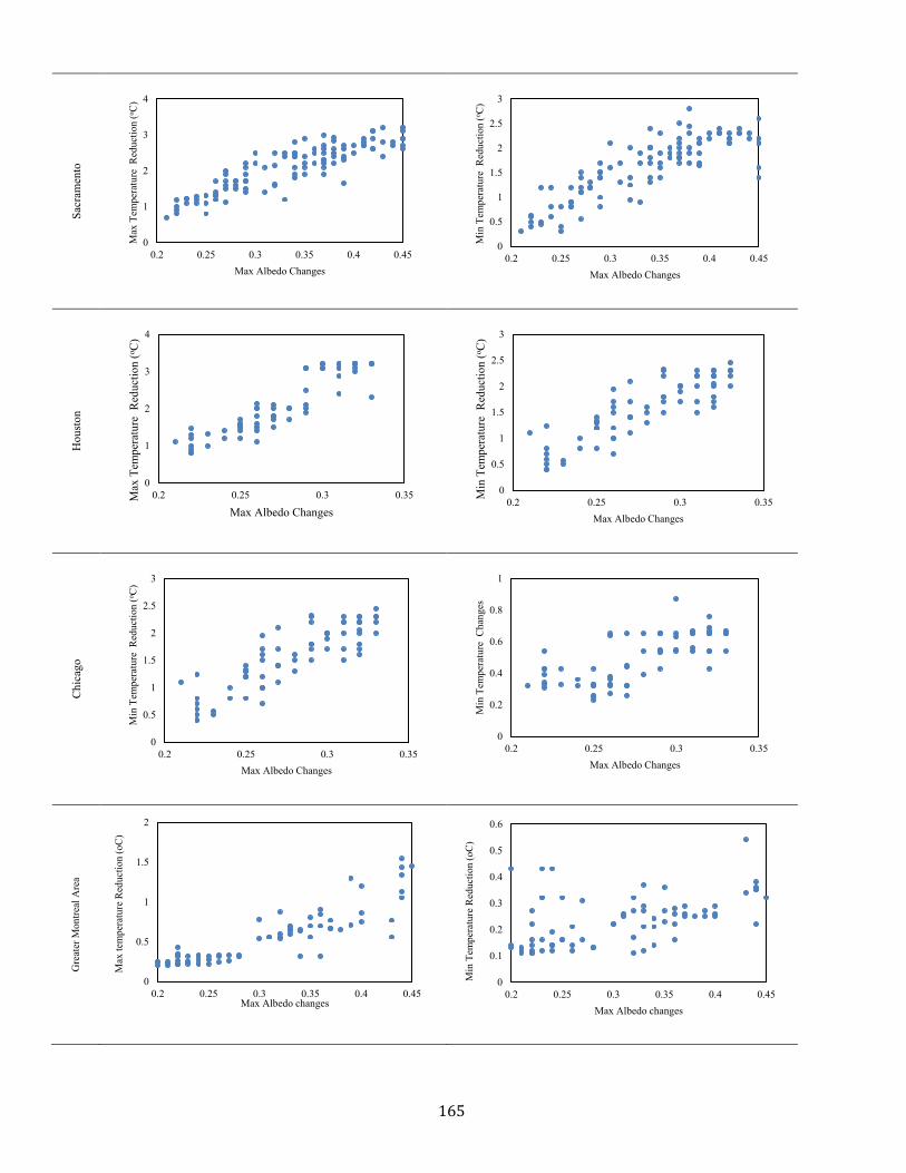
165
Sacr
amen
to
Hou
ston
Chi
cago
Gre
ater
Mon
treal
Are
a
0
1
2
3
4
0.2 0.25 0.3 0.35 0.4 0.45
Max
Tem
pera
ture
Red
uctio
n (o C
)
Max Albedo Changes
0
0.5
1
1.5
2
2.5
3
0.2 0.25 0.3 0.35 0.4 0.45
Min
Tem
pera
ture
Red
uctio
n (o C
)
Max Albedo Changes
0
1
2
3
4
0.2 0.25 0.3 0.35Max
Tem
pera
ture
Red
uctio
n (o C
)
Max Albedo Changes
0
0.5
1
1.5
2
2.5
3
0.2 0.25 0.3 0.35Min
Tem
pera
ture
Red
uctio
n (o C
)
Max Albedo Changes
0
0.5
1
1.5
2
2.5
3
0.2 0.25 0.3 0.35
Min
Tem
pera
ture
Red
uctio
n (o C
)
Max Albedo Changes
0
0.2
0.4
0.6
0.8
1
0.2 0.25 0.3 0.35
Min
Tem
pera
ture
Cha
nges
Max Albedo Changes
0
0.5
1
1.5
2
0.2 0.25 0.3 0.35 0.4 0.45
Max
tem
pera
ture
Red
uctio
n (o
C)
Max Albedo changes
0
0.1
0.2
0.3
0.4
0.5
0.6
0.2 0.25 0.3 0.35 0.4 0.45
Min
Tem
pera
ture
Red
uctio
n (o
C)
Max Albedo changes

166
Figure 7.9. The correlation between maximum and minimum temperature reductions and maximum albedo changes in Sacramento, Houston, Chicago with the horizontal resolution of 2.4km and Greater Montreal Area (GMA) with the horizontal
resolution of 800m.
Figure 7.10 shows the inner domains of the simulations. The Google maps of the three urban
categories are also presented. The downtown of each city is chosen as the high intensity residential
area. The low intensity residential area and industrial/commercial area are selected based on
Google map data and satellite pictures. Then the grid that covers each area is considered. Table
7.10 presents the results of the daily average of albedo changes, 2-m air temperature reduction and
ozone concentration reduction for Sacramento (36 × 31 grids), Houston (41 × 31 grids), Chicago
(36 × 31 grids) with a horizontal resolution of 2.4 km, and for the Greater Montreal Area (GMA)
(101 × 71 grids) with the horizontal resolution of 800 m.
Sacramento area is 36 in west-east direction and 31 in south-north direction, each grid is
2.4km×2.4km
Midtown Sacramento- High intensity residential
(black box) Mercy General Hospital- industrial /commercial
area (yellow box)
low intensity residential (green box)

167
Houston area is 41in west-east direction and 31 in south-north direction, each grid is 2.4km×2.4km
High intensity residential (black box) Downtwon -industrial/commercial area (yellow
box)
low intensity residential (green box)
Chicago area is 36 in west-east direction and 31 in south-north direction, each grid is 2.4km×2.4km
1 1

168
High intensity residential (black box) Industrial/commercial area (yellow box)
low intensity residential (green box)
Greater Montreal Area is 145 in west-east direction and 91 in south-north direction, each grid is
0.800km×0.800km
High intensity residential (black box) Industrial/commercial area (yellow box)
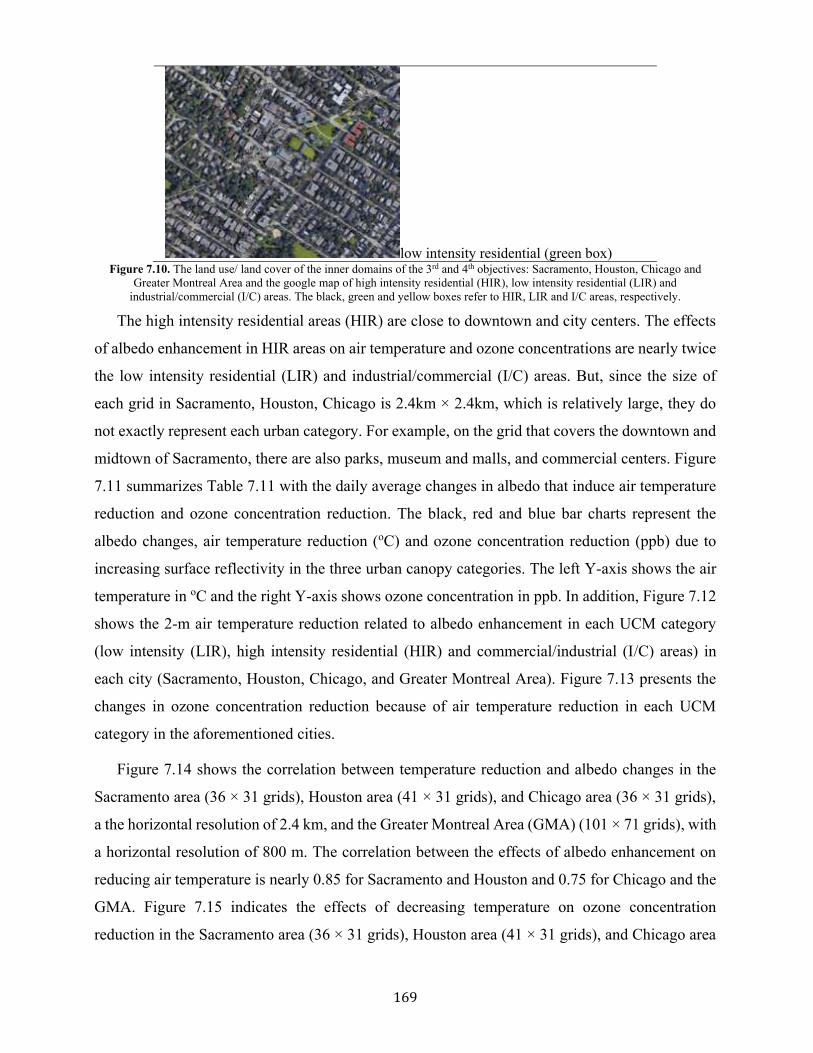
169
low intensity residential (green box) Figure 7.10. The land use/ land cover of the inner domains of the 3rd and 4th objectives: Sacramento, Houston, Chicago and
Greater Montreal Area and the google map of high intensity residential (HIR), low intensity residential (LIR) and industrial/commercial (I/C) areas. The black, green and yellow boxes refer to HIR, LIR and I/C areas, respectively.
The high intensity residential areas (HIR) are close to downtown and city centers. The effects
of albedo enhancement in HIR areas on air temperature and ozone concentrations are nearly twice
the low intensity residential (LIR) and industrial/commercial (I/C) areas. But, since the size of
each grid in Sacramento, Houston, Chicago is 2.4km × 2.4km, which is relatively large, they do
not exactly represent each urban category. For example, on the grid that covers the downtown and
midtown of Sacramento, there are also parks, museum and malls, and commercial centers. Figure
7.11 summarizes Table 7.11 with the daily average changes in albedo that induce air temperature
reduction and ozone concentration reduction. The black, red and blue bar charts represent the
albedo changes, air temperature reduction (oC) and ozone concentration reduction (ppb) due to
increasing surface reflectivity in the three urban canopy categories. The left Y-axis shows the air
temperature in oC and the right Y-axis shows ozone concentration in ppb. In addition, Figure 7.12
shows the 2-m air temperature reduction related to albedo enhancement in each UCM category
(low intensity (LIR), high intensity residential (HIR) and commercial/industrial (I/C) areas) in
each city (Sacramento, Houston, Chicago, and Greater Montreal Area). Figure 7.13 presents the
changes in ozone concentration reduction because of air temperature reduction in each UCM
category in the aforementioned cities.
Figure 7.14 shows the correlation between temperature reduction and albedo changes in the
Sacramento area (36 × 31 grids), Houston area (41 × 31 grids), and Chicago area (36 × 31 grids),
a the horizontal resolution of 2.4 km, and the Greater Montreal Area (GMA) (101 × 71 grids), with
a horizontal resolution of 800 m. The correlation between the effects of albedo enhancement on
reducing air temperature is nearly 0.85 for Sacramento and Houston and 0.75 for Chicago and the
GMA. Figure 7.15 indicates the effects of decreasing temperature on ozone concentration
reduction in the Sacramento area (36 × 31 grids), Houston area (41 × 31 grids), and Chicago area

170
(36 × 31 grids), with s horizontal resolution of 2.4 km, and the Greater Montreal Area (GMA) (101
× 71 grids) with s horizontal resolution of 800 m. Figure 7.15 reveals that ozone concentration
depends on temperature. The R2 is around 0.90 for Sacramento and Houston and 0.70 and 0.60 for
Chicago and the GMA, respectively. In addition, Figure 7.16 presents the correlation between
ozone concentration reduction and albedo changes in Sacramento, Houston, Chicago and the
GMA. The correlation between increasing albedo and decreasing ozone concentration is nearly
0.80, 0.62, 0.55 respectively for Sacramento, Houston and Chicago, with a horizontal resolution
of 2.4km, and 0.75 for the Greater Montreal Area, with a horizontal resolution of 800m.
Table 7.11. The average (daily average of simulation period (3 days)) changes of albedo (Fraction), 2-m air temperature
reduction (oC), ozone concentration reduction (ppb) in each UCM categories (low intensity (LIR) and high intensity residential (HIR), commercial/industrial (C/I) areas) in each city (Sacramento, Houston, Chicago, Greater Montreal Area)
Cities UCM categories Average albedo changes (Fraction)
Average temperature reduction (oC)
Average ozone concentration reduction (ppb)
Sacramento LIR 0.21 0.81 2.98 HIR 0.33 2.31 7.52 I/C 0.20 0.89 3.61
Houston LIR 0.19 0.81 2.85 HIR 0.27 2.51 7.23 I/C 0.19 0.80 3.98
Chicago LIR 0.23 0.75 1.77 HIR 0.32 1.53 4.23 I/C 0.19 0.78 2.87
Greater Montreal Area
LIR 0.16 0.82 2.82 HIR 0.32 1.85 4.81 I/C 0.15 1.10 1.11

171
Figure 7.11. The average of minimum and maximum changes of albedo (Fraction, black bars), 2-m air temperature reduction (oC, red bars) and ozone concentration reduction (ppb, blue bars) in each UCM categories (low intensity (LIR) and high intensity residential (HIR), commercial/industrial (I/C) areas) in each city (Sacramento, Houston, Chicago, Greater Montreal Area). The
left Y-axis shows the air temperature in oC and the right Y-axis shows the ozone concentration in ppb.
0
1
2
3
4
5
6
7
8
0
0.5
1
1.5
2
2.5
3
LIR HIR I/C LIR HIR I/C LIR HIR I/C LIR HIR I/C
O3
(ppb
)
T2 (o
C)
Sacramento Houston Chicago Greater Montreal Area

172
Figure 7.12. The albedo changes (light colors) and 2-m air temperature reduction (oC-dark colors) in each UCM categories: low intensity (LIR-blue bars), high intensity residential (HIR-red bars) and commercial/industrial (I/C-green bars) areas) ones in each
city: Sacramento, Houston, Chicago, and Greater Montreal Area
Figure 7.13. The temperature reduction (oC- light colors) and ozone concentration reduction (ppb-dark colors) in each UCM categories: low intensity (LIR-blue bar), high intensity residential (HIR-red bars), and commercial/industrial (I/C, green bars)
areas) ones in each city: Sacramento, Houston, Chicago, and Greater Montreal Area
Houston Sacramento Chicago Greater Montreal Area
HIR
LIR
I/C
Houston Sacramento Chicago Greater Montreal Area
HIR
LIR
I/C

173
Figure 7.14. The correlation between temperature reduction and albedo changes in (a) Sacramento area (36 × 31 grids), Houston area (41 × 31 grids), and Chicago area (36 × 31 grids) with the horizontal resolution of 2.4km. (b) Greater Montreal Area (GMA)
(101 × 71 grids) with the horizontal resolution of 800m.
0
0.5
1
1.5
2
2.5
3
3.5
0.13 0.17 0.21 0.25 0.29 0.33 0.37 0.41 0.45
Tem
pera
ture
Red
uctio
n (o C
)
Albedo Changes (Fraction)
a- Correlation between temperature reduction in Sacramento, Houston, and Chicago regarding to albedo changes
Sacramento
Houston
Chicago
0
0.5
1
1.5
2
2.5
0.1 0.15 0.2 0.25 0.3 0.35 0.4 0.45
Tem
pera
ture
Red
uctio
n (o C
)
Albedo Changes (Fraction)
b- Correlation between temperature reduction in Greater Montreal Area regarding to albedo changes
Greater Montreal Area

174
Figure 7.15. The correlation between ozone concentration reduction and temperature reduction in (a) Sacramento area (36 × 31
grids), Houston area (41 × 31 grids), and Chicago area (36 × 31 grids) with the horizontal resolution of 2.4km. (b) Greater Montreal Area (GMA) (101 × 71 grids) with the horizontal resolution of 800m.
0
1
2
3
4
5
6
7
8
9
10
0 0.5 1 1.5 2 2.5 3 3.5
ozon
e R
educ
tion
(ppb
)
Temperature Reduction (oC)
a- Correlation between ozone concentration reduction in Sacramento, Houston, and Chicago regarding to temperature reduction
Sacramento
Houston
Chicago
0
1
2
3
4
5
6
7
0 0.5 1 1.5 2 2.5
ozon
e R
educ
tion
(ppb
)
Temperature Reduction (oC)
b- Correlation between ozone concentration reduction in Greater Montreal Area regarding to temperature reduction
Greater Montreal Area

175
Figure 7.16. The correlation between ozone concentration reduction and albedo changes in (a) Sacramento area (36 × 31 grids),
Houston area (41 × 31 grids), and Chicago area (36 × 31 grids) with the horizontal resolution of 2.4km. (b) Greater Montreal Area (GMA) (101 × 71 grids) with the horizontal resolution of 800m.
0
2
4
6
8
10
12
0.13 0.18 0.23 0.28 0.33 0.38 0.43
ozon
e R
educ
tion
(ppb
)
Albedo Changes (Fraction)
a- Correlation between ozone concentration reduction in Sacramento, Houston, and Chicago regarding to albedo changes
Sacramento
Houston
Chicago
0
1
2
3
4
5
6
7
0.1 0.15 0.2 0.25 0.3 0.35 0.4 0.45
ozon
e R
educ
tion
(ppb
)
Albedo Changes (Fraction)
b- Correlation between ozone concentration reduction in Greater Montreal Area regarding to albedo changes
Greater Montreal Area

176
Chapter 8 Conclusion and Remarks
Surface and air temperatures are typically higher in urban areas compared to their surroundings
and form the urban heat island (UHI) phenomenon. UHI increases cooling energy demands,
deteriorates air quality, endangers human health, increases mortality and changes the urban
ecosystem. To fight the UHI effects, increasing surface reflectivity (ISR) is well-documented as a
measurable and repeatable heat island mitigation strategy.
The focus of this research was to investigate the effects of increasing surface reflectivity on
urban climate, air quality and heat-related mortality. The goals were accomplished by applying the
online numerical Weather Research and Forecasting model coupled with Chemistry (WRF-Chem).
WRF-Chem considers a variety of meteorological and physical parameterizations and chemical
processes to predict weather and air quality conditions. In addition, a multi-layer of the Urban
Canopy Model (ML-UCM) was coupled with the WRF-Chem to represent the urban areas. The
models were further modified to accommodate the specific needs of this study and related
sensitivity analysis.
A base case scenario (CTRL) was established for each of the objectives identified in the study.
The results are compared with measurements obtained from weather and air quality stations across
the interested domain. The consequences of ISR were deemed to be reasonable enough, within the
episode and scope of the study, to proceed in evaluating the potential impacts of surface
modification strategy. Then, the albedo of roofs, walls, and pavements was increased from 0.2 in
the CTRL scenario to 0.65, 0.60 and 0.45 in the ALBEDO scenario. The outcomes indicate that
albedo enhancement is effective in modifying air temperature, meteorology-sensitive and
temperature-sensitive photochemical reaction rates and reducing biogenic and anthropogenic
emissions in urban areas. Hence, the effects of increasing surface reflectivity on temperature has
significant positive impacts on the rates of production and accumulation of ozone in the polluted
boundary layer in urban areas. Albedo enhancement also affects other meteorological and

177
photochemical fields, modifies weather patterns, and improves air quality and human comfort and
health. These effects may vary spatially and temporally.
8.1. Summary of Conclusions
This numerical modeling study was carried out to evaluate the potential meteorological and
photochemical impacts of surface modification on urban climate, air quality and heat-related death.
The conclusive outcomes of this research regarding the effects of increasing surface reflectivity
are summarized in the following:
1st Task: Develop a platform for urban climate simulation and heat island mitigation strategy.
Mesoscale models are comprised of physical parameterizations (cumulus, microphysics, planetary
boundary layer, radiation, and land-surface) that need to be carefully selected to predict weather
conditions. The physical processes can be selected based on the twenty sets of sensitivity analysis.
A proper simulation platform is essential to have a better understanding of the effects of UHI and
its mitigation strategy on urban climate and air quality for environmental policymakers. The
sensitivity of near surface air temperature, wind speed, relative humidity and precipitation to
different physical models was evaluated by applying the WRF for Montreal, Canada for the period
9–11 August 2009. The combination of WDM6 (Lim and Hong, 2010), Grell 3D (Grell, 1993;
Grell and Devenyi, 2002), MYJ (Janjic, 1994), and RRTMG (Iacono et al., 2008) as microphysics,
cumulus, planetary boundary layer, and radiation schemes, respectively, resulted in the least error
compared to measurements and thus is suggested as an appropriate platform for urban climate
simulations and UHI mitigation strategy. Increasing surface reflectivity was applied and the results
indicate a decrease in 2-m air temperature by 0.2 oC, a slight increase in 10-m wind speed, a
decrease in relative humidity by 3%, and a decrease in precipitation by 0.2 mm/day across the
domain.
2nd Task: Investigate the effects of urban heat island and its mitigation strategy on heat-related mortality.
The proper physical parameterizations were applied to achieve the second goal. The effects of
extreme heat events and increasing surface reflectivity were investigated on meteorological
parameters (air temperature, wind speed, relative humidity, and dew point temperature), heat stress
indices (National Weather Service – Heat Index, apparent temperature, Canadian Humid Index,
and Discomfort Index) and heat-related deaths. Heat-related mortality correlations were

178
developed. The simulation domain was the Greater Montreal Area. The simulation period included
two heat wave events in 2005 and 2011. The beneficial contributions of ISR were a decrease in
temperature by 0.6 oC, an increase in relative humidity by 2%, an increase in dew point temperature
by 0.4 oC, a slight increase in wind speed, and a decrease in heat-related mortality by 3.2%,
meaning that nearly seven lives could be saved.
3rd Task: Develop a two-way nested simulation approach to assess the effects of urban heat
island and its mitigation strategy on urban climate and air quality.
The effects of increasing surface reflectivity were investigated over a larger geographical area
(North America) within a nested domain of urban areas (Sacramento in California, Houston in
Texas, and Chicago in Illinois) in a two-way nested approach to decrease the uncertainties
associated with scale separation and grid resolution. The developed approach provided an
integrated simulation setup to capture the full impacts of meteorological and photochemical
reactions. WRF-Chem simulated the diurnal variation of air temperature reasonably well,
overpredicted wind speed and dew point temperature, underpredicted relative humidity,
overpredicted ozone and nitrogen dioxide concentrations, and underpredicted fine particulate
matter (PM2.5). The performance of PM2.5 was a combination of overprediction of particulate
sulfate and underprediction of particulate nitrate and organic carbon. Increasing the surface albedo
of roofs, walls, and pavements from 0.2 to 0.65, 0.60, and 0.45, respectively, resulted in a decrease
in air temperature by 2.3oC in urban areas and 0.7oC in suburban areas; a slight increase in wind
speed; an increase in relative humidity (3%) and dew point temperature (0.3oC); a decrease of
PM2.5 and O3 concentrations by 2.7μg/m3 and 6.3 ppb in urban areas and 1.4μg/m3 and 2.5ppb in
suburban areas, respectively; minimal changes in PM2.5 subspecies; and a decrease of nitrogen
dioxide (1 ppb) in urban areas. Sacramento enjoyed larger reductions in ozone concentration as a
result of larger decrease in air temperature because of the heat island mitigation strategy.
4th Task: Investigate the effects of heat island mitigation strategy on aerosol-radiation-cloud
interactions in the atmosphere.
The effects of albedo enhancement were investigated on aerosol-radiation-cloud (ARC)
interactions in a two-way nested simulation approach over the Greater Montreal Area during the
2011 heat wave period. Four sets of simulations with and without aerosol estimations and

179
convective parameterizations were carried out to explore the direct, semi-direct and indirect effects
of aerosols. The albedo enhancement induced a decrease in 2-m air temperature by nearly 0.5 oC
in the Center and North part of the domain and a decrease by nearly 0.3 oC in the South part. The
relative humidity and water mixing ratio also decreased by 0.5 g/kg and 3%, respectively. Albedo
enhancement led to a decrease in ozone concentrations by 2 ppb across the entire domain.
Reducing temperature led to a reduction in planetary boundary layer height, which reduced the
advection and diffusion of pollutants. Hence, this phenomenon increased the pollutant
concentrations and also assisted the O3 and NO reaction rates to produce NO2. The fine particulate
matter also decreased by nearly 3 µg/m3 in the Center and by nearly 2 µg/m3 in the other parts of
the GMA during the 2011 heat wave period. The NO2 and SO2 reductions were much less
compared to PM2.5 and O3. An increase of albedo led to a net decrease of radiative flux into the
ground and therefore a decrease of convective cloud formation and precipitation.
In addition, here the results of 2-m air temperature in these four tasks are compared with other
studies that applied the WRF and WRF-Chem. Table 8.1. shows the root mean square error of
these four tasks and previous research. The comparisons indicate that the WRF and WRF-Chem
results are generally consistent with the measurements and thus are well reliable to be applied for
further investigations. Table 8.1. Comparisons of 2-m air temperature results (Root Mean Square Error (RMSE)) of the current tasks with previous
studies using WRF and WRF-Chem Study RMSE of T2 Fallmann et al., 2014 1.7 Salamanca et al., 2012, 1.5 Vahmani & Ban-Weiss. 2016, 3.8 Chen et al., 2013, 1.61 Millstein D. & Menon S., 2011 2.8 Georgescu et al., 2012 1.9 Georgescu et al., 2014 2.5 Zhou Y. et al., 2010 1.1 Fallmann et al., 2014 1.6 Salamanca & Martilli, 2012 1.6 Taha et al., 2015 1.1 Touchaei et al., 2016 1.8 1st task: develop a proper platform for urban climate simulation 1.9 2nd task: effects of albedo enhancement on heat-related mortality 1.6 3rd task: develop a two-way nested simulation approach 1.3 4th task: effects of increasing albedo on aerosol-radiation-cloud interactions 1.1
180
8.2. Remarks
To conclude, this research demonstrates the potential capacity of the increasing surface
reflectivity to mitigate the UHI effects. The consequences of albedo enhancement indicate a
decrease in air temperature, a decrease in temperature-dependent photochemical reaction rates and
a decrease in heat-related mortality. Accordingly, there are four scientific contributions regarding
the effects of urban heat island and its mitigation strategy: 1) a platform is developed for urban
climate simulations and heat island mitigation strategy; 2) heat-related mortality calculations are
derived to estimate the effects of heat island and its mitigation strategy on human death rate; 3) a
two-way nested simulation approach is developed to investigate the effects of UHI and increasing
surface reflectivity on urban climate and air quality over a larger geographical area within nested
domains of urban areas; 4) the effects of albedo enhancement are investigated on aerosols
interactions, radiation budget and hydrological cycles in the atmosphere and at the surface.
The benefits and applications of this research are: developing a comprehensive basis for local
and regional climate and air quality simulations; assessing the effects of increasing surface
reflectivity on urban climate and air quality in various urban areas; investigating the aerosol
estimation in the chemistry package within WRF-Chem; providing more accurate and reliable
information for air quality policymakers to improve urban climate and air quality and reduce heat-
related mortality during heat wave periods.
The main drawback in investigating the potential impacts of surface modification is that the
meteorological and photochemical modeling carries inherent numerical issues, assumptions and
limitations that affect the results and hence should be acknowledged. There is a risk to implement
this strategy if one only seeks to reduce air temperature, whereas it may also reduce the planetary
boundary layer height, increase the ozone and particulate matter concentrations in some parts of
the domain, reducing cloud formation and precipitation. Thus, there are some caveats that
regulators need to carefully consider prior to albedo enhancement.
8.3. Future Work
Increasing surface reflectivity indicates a promising UHI mitigation strategy to reduce the air
temperature and temperature-dependent photochemical reaction rates, and thus to improve urban
climate and air quality and reduce heat-related death. However, this research can be even more
fruitful if the following recommendations will be considered for future studies:

181
- Here, the simulations were conducted during the heat wave periods. It is essential to
investigate the effects of UHI mitigation strategy over seasonal time spans and on an annual
basis. This would provide a more realistic assessment of the long-term effects of UHI and
increasing surface reflectivity.
- Comparing other mitigation strategies such as increasing surface vegetation in urban areas
with increasing surface albedo. This comparison provides a more beneficial assessments
for air quality regulators and policymakers.
- Improve the input data such as emission inventories in terms of biogenic and anthropogenic
emissions, and urban morphological data, for future analyses.
- Next, modeling efforts of the UHI and its mitigation strategies should evaluate scenarios
based on future-year emission inventories that account for increased urbanization. Future-
year controlled emissions should also be applied to scenarios of lower emissions.
- City-specific modeling is needed to account for actual urbanization trends and growth plans
that have impacts on local meteorology and air quality.
Modifications and improvements of models (such as photolysis rate estimations and aerosols
estimations) may be needed beyond what was achieved in this study to make the application
more specific to certain regions and conditions.

182
References Akbari H. and Kolokotsa D. 2016. Three decades of urban heat islands and mitigation technologies research. Enbuild. 133: 834-842.
Akbari H. and Touchaei A.G. 2014. Modeling and labeling heterogeneous directional reflective roofing materials. Sol. Energy Mater. Sol. Cells 124: 192-210.
Akbari, H., Bretz, S., Kurn, D.M. and Hanford, J. 1997. Peak power and cooling energy savings of high-albedo roofs. Energy and Buildings, 25, (2) 117-126
Akbari, H., Menon, S. and Rosenfeld, A. 2009. Global cooling: increasing world-wide urban albedos to offset CO2. Climatic Change, 94, (3-4) 275-286
Akbari, H., Pomerantz, M., and Taha, H. 2001. Cool surfaces and shade trees to reduce energy use and improve air quality in urban areas. Solar Energy, 70, (3) 295-310
Akbari, H. and Rose, L.S. Characterizing the Fabric of the Urban Environment: A Case Study of Metropolitan Chicago, Illinois; Report LBNL-49275; Lawrence Berkeley National Laboratory: Berkeley, CA, USA, 2001.
Akbari, H., Rose, L.S. and Taha, H. 2003. Analyzing the land cover of an urban environment using high-resolution orthophotos. Landsc. Urban Plan. 63, 1–14.
Abdul-Razzak, H. and Ghan, S. J. 2002. A parameterization of aerosol activation 3. sectional representation, J. Geophys. Res., 107, 3: 1029-2001
Ackermann, I.J., Hass, H., Memmesheimer, M., Ebel, A., Binkowski, F.S. and Shankar, U. 1998. Modal aerosol dynamics model for Europe: Development and first applications. Atmos. Environ. 32, 2981–2999.
Ahmad, S. and Hashim, N.M. 2007. Effects of soil moisture on urban heat island occurrences: case of Selangor, Malaysia. Humanity & Social Sciences Journal, 2, (2) 132- 138
Ahmadov, R., McKeen, S.A., Robinson, A.L., Bahreini, R., Middlebrook, A.M., de Gouw, J.A., Meagher, J., Hsie, E.-Y., Edgerton, E., and Shaw, S. A. 2012. volatility basis set model for summertime secondary organic aerosols over the eastern United States in 2006. J. Geophys. Res. 117, 06–31.
American Lung Association. 2017. Available online: http://www.lung.org/our-initiatives/healthy-air/ sota/city-rankings/most-polluted-cities.html (accessed on 28 January 2018).
Anderson B.G., and Bell M.L. 2009. Weather-related mortality: how heat, cold, and heat waves affect mortality in the United States. Epidemiology. 20(2): 205–213.
Appel, K.W., Chemel, C., Roselle, S.J., Francis, X.V., Hu, R.-M., Sokhi, R.S., Rao, S.T and Galmarini, S. 2012. Examination of the Community Multiscale Air Quality (CMAQ) model perfor-mance over the North American and European domains. Atmos. Environ. 53, 142–155.
Archer-Nicholls, S., Lowe, D. and Darbyshire, E. 2015. Characterizing Brazilian biomass burning emissions using WRF-Chem with MOSAIC sectional aerosol, Geosci. Model Dev., 8, 549–577
Arnfield, A.J. and Grimmond, C.S.B. 1998. An urban canyon energy budget model and its application to

183
urban storage heat flux modeling. Energy and Buildings, 27, (1) 61-68
Arnfield, A.J. 2003. Two decades of urban climate research: a review of turbulence, exchanges of energy and water, and the urban heat island. International Journal of Climatology, 23, (1) 1-26
ARW User Guide, 2017. ARW Version 3 Modeling System User’s Guide. National Center for Atmospheric Research, Boulder (CO), US.
Åström D.O, Forsberg B. and Rocklöv J. 2011. Heat wave impact on morbidity and mortality in the elderly population: A review of recent studies. Maturitas. 69(2): 99-105.
Baik J. J., Kim. Y. H., and Han J. Y. 2007. Effect of boundary-layer stability on urban heat island induced circulation, Theor. Appl. Climatol., 89, 73–81.
Baklanov, A., Schlünzen, K., Suppan, P. 2014. Online coupled regional meteorology chemistry models in Europe: current status and prospects, Atmos. Chem. Phys., 14, 317–398.
Ban-Weiss G.A., Woods J., Levinson R. 2014. Using remote sensing to quantify albedo of roofs in seven California cities, Part 1: Methods. Sol Energy. 115: 777-790.
Barnard, J. C., Fast, J. D., and Paredes-Miranda, G. 2010. Technical Note: Evaluation of the WRF-Chem “Aerosol Chemical to Aerosol Optical Properties” Module using data from the MILAGRO campaign, Atmos. Chem. Phys., 10, 7325–7340.
Barnett AG., Tong S., Clements AC. 2010. What measure of temperature is the best predictor of mortality? Environ. Res. 110 (6): 604-611.
Basu R, and Samet JM. 2002. Relation between elevated ambient temperature and mortality: a review of the epidemiologic evidence, Epidemiol. Rev. 24: 190–202.
Basu R. 2009. High ambient temperature and mortality: a review of the epidemiologic studies from 2001 to 2008. Enviro Health. 8: 40-48.
Berry R., Livesley S.J., Aye L. 2013. Tree canopy shade impacts on solar irradiance received by building walls and their surface temperature, Build. Environ. 69: 91–100.
Bhati, S. and Mohan, M., 2016. WRF model evaluation for the urban heat island assessment under varying land use/land cover and reference site conditions. Theor. Appl. 16: 94-101
Bianchini, F. and Hewage, K. 2012. How “green” are the green roofs? Lifecycle analysis of green roof materials. Build. Environ. 48, 57-65.
Blonquist, J. M., J. M. Norman, and B. Bugbee. 2009. Automated measurement of canopy stomatal conductance based on infrared temperature. Agricultural and Forest Meteorology 149:1931–1945.
Bond, T. C. and Bergstrom, R. W. 2006. Light absorption by carbonaceous particles: an investigative review, Aerosol Sci. Tech., 39, 1–41.
Bond, T. C., Doherty, S. J., Fahey, D. W. and Forster, P. M. 2013. Bounding the role of black carbon in the climate system: a scientific assessment, J. Geophys. Res.- Atmos., 11, 1–163.

184
Bornstein, R., and Lin, Q. 2000. Urban heat islands and summertime convective thunderstorms in Atlanta: Three cases studies, Atmos. Environ., 34, 507–516.
Bowler, D.E., Buyung-Ali. L., Knight, T.M., and Pullin, A.S. 2010. Urban greening to cool towns and cities: A systematic review of the empirical evidence. Landscape and Urban Planning, 97, (3) 147-155
Boylan, J. W. and Russell, A. G. 2006. PM and light extinction model performance metrics, goals, and criteria for three-dimensional air quality models, Atmos. Environ., 40, 4946–4959.
Britter, R.E. & Hanna, S.R. 2003. Flow and dispersion in urban areas. Annual Review of Fluid Mechanics, 35, 1: 469-496.
Bunker A., Wildenhain J., Vandenbergh A., Henschke N., Rocklöv J., Hajat S. and Sauerborn R. 2016. Effects of Air Temperature on Climate-Sensitive Mortality and Morbidity Outcomes in the Elderly; a Systematic Review and Meta-analysis of Epidemiological Evidence. EBioMedicine. 6: 258-268.
Bougeault, P., Lacarrere, P., 1989. Parameterization of orography-induced turbulence in a mesobeta-scale model. Mon. Weather Rev. 117, 1872–1890. Environment Canada, (2013).
Chapman, E. G., Gustafson Jr., W. I., Easter, R. C., Barnard, J. C., Ghan, S. J., Pekour, M. S., and Fast, J. D. 2009. Coupling aerosol- cloud-radiative processes in the WRF-Chem model: Investigating the radiative impact of elevated point sources, Atmos. Chem. Phys., 9: 945–964.
Chapman, L. and Thornes, J.E. 2004. Real-Time Sky-View Factor Calculation and Approximation. Journal of Atmospheric & Oceanic Technology, 21, 5: 730-741
Chen F. and Dudhia J. 2001. Coupling an advanced land surface–hydrology model with the Penn State–NCAR MM5 modeling system. Part I: model implementation and sensitivity. Monthly Weather Review, 129: 569-585.
Chen F., Kusaka H., Bornstein R., Ching J., Grimmond C. S. B., Grossman-Clarke S., Loridan T., Manning K.W., Martilli A., Miao S., Sailor D., Salamanca F.P., Taha H., Tewari M., Wang X., Wyszogrodzkia A.A. and Zhang C. 2011. The integrated WRF/urban modelling system: development, evaluation, and applications to urban environmental problems. Int. J. Climatol. 31: 273-288.
Chen H., Oak R., Huang H. and Tsuchiya T. 2009. Study on mitigation measures for outdoor thermal environment on present urban blocks in Tokyo using coupled simulation, Build. Environ. 44: 2290–2299.
Chen, F. and Dudhia, J. 2001. Coupling an advanced land surface–hydrology model with the Penn State–NCAR MM5 modeling system. Part I: model implementation and sensitivity. Mon. Weather Rev. 129, 569–585.
Chen, F. 2011. The integrated WRF/urban modeling system: Development, evaluation, and applications to urban environmental problems, Int. J. Climatol., 31(2), 273–288.
Chen, F., Yang, X. and Zhu, W. 2013. WRF simulations of urban heat island under hot-weather synoptic conditions: The case study of Hangzhou City, China. Atmos. Res. 138, 364–377.
Chen, S.H. and Sun, W.Y. 2002. A one-dimensional time dependent cloud model. J. Meteorol. Soc. Jpn. 80, 99–118.
185
Chen, Y., Jiang, W.M., Zhang, N., He, X.F., and Zhou, R.W. 2009. Numerical simulation of the anthropogenic heat effect on urban boundary layer structure. Theor Appl Climatol, 97, (1-2) 123-134
Chou, M.D. and Suarez, M.J. 1999. A Solar Radiation Parameterization (CLIRAD-SW) Developed at Goddard Climate and Radiation Branch for Atmospheric Studies; NASA Technical Memorandum NASA/Goddard Space Flight Center Greenbelt: Greenbelt, MD, USA.
Chuang, M.-T., Zhang, Y. and Kang, D. 2011. Application of WRF/Chem-MADRID for real-time air quality forecasting over the southeastern United States. Atmos. Environ. 45, 6241–6250.
Conti S., Meli P., Minelli G., Solimini R., Toccaceli V., Vichi M., Beltrano C. and Perini L. 2005. Epidemiologic study of mortality during the summer 2003 heat wave in Italy. Environ Res 98(3):390–399.
Coutts AM., Daly E., Beringer J. and Tapper NJ. 2013. Assessing practical measures to reduce urban heat: green and cool roofs, Build. Environ. 70: 266–276.
Crouse DL., Peters PA., van Donkelaar A., Goldberg MS., Villeneuve PJ., and Brion O. 2012. Risk of nonaccidental and cardiovascular mortality in relation to long-term exposure to low concern- tractions of fine particulate matter: a Canadian national-level cohort study. Environ Health Perspect 120:708–714.
Csiszar I. and Gutman G. 1999. Mapping global land surface albedo from NOAA AVHRR. Journal of Geophysical Research, 104: 6215–28.
Curriero FC, Heiner KS, Samet JM, Zeger SL, Strug L. and Patz JA. 2002. Temperature and mortality in 11 cities of the eastern United States. Am J Epidemiol. 155: 80–87.
Cusack L., de Crespigny C., Athanasos P. 2011. Heatwaves and their impact on people with alcohol, drug and mental health conditions: a discussion paper on clinical practice considerations. J. Adv. Nurs. 67 (4): 915-922.
Diaz J., Jordan A., García R., Lopez C., Alberdi J., Hernandez E., Otero A. 2002. Heat waves in Madrid 1986-1997: effects on the health of the elderly. Int. Arch. Occup. Environ. Health. 75 (3): 163-170.
Diffenbaugh N.S. and Ashfaq M. 2010. Intensification of hot extremes in the United States. Geophys Res Lett. 37(15): 157-185.
Dudhia, J., 1989. Numerical study of convection observed during the winter monsoon experiment using a mesoscale two-dimensional model. J. Atmos. Sci. 46, 3077–3107.
Duffie, J.A. and Beckman, W.A., 1991. Solar Engineering of Thermal Processes. Wiley and Sons, Inc., Hoboken (NJ), US.
Emeis, S. 2010. Surface-based remote sensing of the atmospheric boundary layer. Series: Atmospheric and Oceanographic Sciences Library, 40: 174pp.
Environment Canada, (2017). [Online: http://climate.weather.gc.ca/].
EPA. 2005. Available online: http://www.epa.gov/ttnchie1/net/2005inventory.html (accessed on 28 January 2017).
Epstein Y. and Moran D.S. 2006. Thermal comfort and heat stress indices. Ind Health. 44(3): 388-398.

186
Fallmann, J., Emeis, S. and Suppan, P. 2014. Mitigation of urban heat stress - a modelling case study for the area of Stuttgart. DIE ERDE - Journal of the Geographical Society of Berlin, 144, (3-4) 202-216
Fallmann, J., Emeis, S. and Suppan, P. 2013. Mitigation of urban heat stress—A modelling case study for the area of Stuttgart. J. Geogr. Soc. Berl. 144, 202–216.
Fallmann, J., Forkel, R. and Emeis, S. 2016. Secondary effects of urban heat island mitigation measures on air quality. Atmos Environ. 125, 199–211.
Fan, H. and Sailor, D.J. 2005. Modeling the impacts of anthropogenic heating on the urban climate of Philadelphia: a comparison of implementations in two PBL schemes. Atmospheric Environment, 39, (1) 73-84.
Fan, J., Leung, L. R., Rosenfeld, D., Chen, Q., Li, Z., Zhang, J., and Yan, H. 2013. Microphysical effects determine macro-physical response for aerosol impacts on deep convective clouds. P. Natl. Acad. Sci. USA, 110, E4581–E4590.
Fast, J. D., Allan, J., Bahreini, R., Craven, J. and Emmons, L. 2014. Modeling regional aerosol and aerosol precursor variability over California and its sensitivity to emissions and long-range transport during the 2010 CalNex and CARES campaigns, Atmos. Chem. Phys., 14, 10013–10060.
Fast, J. D., Gustafson, W. I., Easter, R. C., Zaveri, R. A., Barnard, J. C., Chapman, E. G., Grell, G. A., and Peck- ham, S. E. 2006. Evolution of ozone, particulates, and aerosol direct radiative forcing in the vicinity of Houston using a fully coupled meteorology-chemistry-aerosol model, J. Geophys. Res., 111, 1– 29.
Fast, J.D., Gustafson, W.I., Jr., Easter, R.C., Zaveri, R.A., Barnard, J.C., Chapman, E.G., Grell, G.A. and Peckham, S.E. 2006. Evolution of ozone, particulates, and aerosol direct radiative forcing in the vicinity of Houston using a fully coupled meteorology-chemistry-aerosol model. J. Geophys. Res. 111, 203–213.
Ferrari, C., Touchaei, A.G., Sleiman, M., Libbra, A., Muscio, A., Siligardi, C. and Akbari, H. 2013. Effect of aging processes on solar reflectivity of clay roof tiles. Adv. Build. Energy Res. 8 (1), 28–40.
Fischer E.M, Oleson K.W. and Lawrence D.M. 2012. Contrasting urban and rural heat stress responses to climate change. Geophy Res Lett 39(3).
Gao, Y., Zhao C., Liu X., Zhang M., and Leung L. R. 2014. WRF-Chem simulations of aerosols and anthropogenic aerosol radiative forcing in east Asia, Atmos. Environ., 92, 250–266.
Gilliam R.C., Hogrefe C. and Rao S.T. 2006. New methods for evaluating meteorological models used in air quality applications. Atmos. Environ. 40: 5073–5086.
Grell G.A. and Devenyi D. 2002. A generalized approach to parameterizing convection combining ensemble and data assimilation techniques. Geophysical Research Letters. 29 (14): 31-38.
Grell, G. A. and Freitas, S. R. 2014. A scale and aerosol aware stochastic convective parameterization for weather and air quality modeling, Atmos. Chem. Phys., 14, 5233–5250.
Grell, G. A., and S. Freitas. 2013. A scale and aerosol aware stochastic convective parameterization for weather and air quality modeling, Atmos. Chem. Phys. Discuss., 13, 23,846–23,893.
Grell, G. and Baklanov, A. 2011. Integrated modelling for forecasting weather and air quality: a call for

187
fully coupled approaches, Atmos. Environ., 45, 6845–6851.
Grell, G.A. 1993. Prognostic evaluation of assumptions used by cumulus parameterizations. Mon. Weather Rev. 121, 764–787.
Grell, G.A., Peckham, S.E., Schmitz, R., McKeen, S.A., Frost, G., Skamarock, W.C. and Eder, B. 2005. Fully coupled "online" chemistry within the WRF model. Atmospheric Environment, 39, (37) 6957-6975
Grimmond, C.S.B. 1992. The suburban energy balance: Methodological considerations and results for a mid-latitude west coast city under winter and spring conditions. International Journal of Climatology, 12, (5) 481-497
Guenther, A., Karl, T., Harley, P., Wiedinmyer, C., Palmer, P.I. and Geron, C. 2006. Estimates of global terrestrial isoprene emissions using MEGAN (Model of Emissions of Gases and Aerosols from Nature). Atmos. Chem. Phys. 6, 3181–3210.
Guenther, A.B., Jiang, X., Heald, C.L., Sakulyanontvittaya, T., Duhl, T., Emmons, L.K., and Wang, X. 2012. The Model of Emissions of Gases and Aerosols from Nature version 2.1 (MEGAN2.1): an extended and updated framework for modeling biogenic emissions. Geosci.Model Dev., 5, (6) 1471-1492
Guenther, A.B., Zimmerman, P.R., Harley, P.C., Monson, R.K., and Fall, R. 1993. Isoprene and monoterpene emission rate variability: Model evaluations and sensitivity analyses. Journal of Geophysical Research: Atmospheres, 98, (D7) 12609-12617
Guenther, A.B., Jiang, X., Heald, C.L., Sakulyanontvittaya, T.; Duhl, T.; Emmons, L.K.; Wang, X. The Model of Emissions of Gases and Aerosols from Nature Version 2.1 (MEGAN2.1): An extended and updated framework for modeling biogenic emissions. Geosci. Model. Dev. 2012, 5, 1471–1492.
Hajat S., O’Connor M. and Kosatsky T. 2010. Health effects of hot weather: from awareness of risk factors to effective health protection. Lancet. 375(9717): 856–863.
Han, J. and Pan, H., 2011. Revision of convection and vertical diffusion schemes in the NCEP Global Forecast System. Weather Forecast. 26, 520–533.
Hanna A.F., Yeatts K.B., Xiu A., Zhu Z. and Smith R.L. 2011. Associations between ozone and morbidity using the spatial synoptic classification system. Env Health 10 (1):1–15.
Harlan S.L., Brazel A.J., Prashad L., Stefanov W.L. and Larsen L. 2006. Neighborhood microclimates and vulnerability to heat stress. Soc. Sci. Med. 63 (11): 2847-2863.
Harlan S.L. and Ruddell D.M. 2011. Climate change and health in cities: impacts of heat and air pollution and potential co-benefits from mitigation and adaptation. Curr. Opin. Environ. Sustain. 3 (3): 126-134.
Hong B. and Lin B. 2014. Numerical study of the influences of different patterns of the building and green space on microscale outdoor thermal comfort and indoor natural ventilation. Building Simulation. 7: 525-536.
Hong, S., Lim, J.J. 2006. The WRF single-moment 6-class microphysics scheme (WSM6). J. Korean Meteorol. Soc. 42, 129–151.
Hong, S.Y., Dudhia, J., Chen, S.H. 2004. A revised approach to ice microphysical processes for the bulk

188
parameterization of clouds and precipitation. Mon. Weather Rev. 132, 103–120.
Hooshangi, H., Akbari, H., Touchaei, A.G. 2016. Measuring solar reflectance of variegated flat roofing materials using quasi-Monte Carlo method. Energ. Buildings. 10: 060-073.
Horton D.E., Skinner C.B., Singh D., Diffenbaugh N.S. 2014. Occurrence and persistence of future atmospheric stagnation events. Nat Clim Change Lett. 4: 698-703.
Iacono, M. J., Delamere, J. S., Mlawer, E. J., Shephard, M. W., Clough, S. A., and Collins, W. D. 2008. Radiative forcing by long–lived greenhouse gases: calculations with the AER radiative transfer models. Journal of Geophysical Research, 113, D13103,
IPCC (Intergovernmental Panel on Climate Change). Climate Change 2013: The Physical Science Basis. Contribution of Working Group I to the Fifth Assessment Report of the Intergovernmental Panel on Climate Change, Cambridge University Press, Cambridge, UK and New York, NY, USA, 1535 pp.
IPCC. 2014. Summary for policymakers. In: Climate Change 2014. Impacts, Adaptation, and Vulnerability. Part A: Global and Sectoral Aspects. Contribution of Working Group II to the Fifth Assessment Report of the Intergovernmental Panel on Climate Change. 1-32, New York (NY), USA.
Jacobson, M. Z. 2006. Effects of externally-through-internally-mixed soot inclusions within clouds and precipitation on global climate. The Journal of Physical Chemistry A, 110(21):6860–6873.
Jacobson, M.Z. and Ten Hoeve, J.E. 2011. Effects of Urban Surfaces and White Roofs on Global and Regional Climate. Journal of Climate, 25, (3) 1028-1044
Jandaghian Z., Akbari H. 2018. The Effects of Increasing Surface Albedo on Urban Climate and Air Quality: A Detailed Study for Sacramento, Houston, and Chicago. Climate. 6(2) 19.
Jandaghian Z., Touchaei G.A., Akbari H. 2017. Sensitivity analysis of physical parameterizations in WRF for urban climate simulations and heat island mitigation in Montreal. Uclim. 24: 577-599
Jandaghian, Z., and Akbari, H. 2018. The effects of increasing surface reflectivity on heat-related mortality in Greater Montreal Area, Canada. Uclim. 25: 135-15
Janjic Z. I. 1994. The step–mountain Eta Coordinate Model: Further developments of the convection, viscous sublayer, and turbulence closure schemes. Monthly Weather Review. 122: 927–945.
Janjic Z. I. 2002. Nonsingular implementation of the Mellor–Yamada Level 2.5 Scheme in the NCEP meso model. NCEP Office Note, No. 437.
Janjic, Z.I., 1990. The step-mountain coordinate: physical package. Mon. Weather Rev. 118, 1429–1443.
Janjic, Z.I., 1994. The step–mountain eta coordinate model: further developments of the convection, viscous sublayer, and turbulence closure schemes. Mon. Weather Rev. 122, 927–945.
Jenkins K., Hall J., Glenis V., Kilsby C., McCarthy C., Goodess D., Smith N., Malleson M. 2014. Probabilistic spatial risk assessment of heat impacts and adaptations for London, Clim. Change 124: 105–117.
Jerrett M, Burnett RT, Beckerman BS, Turner MC, Krewski D, Thurston G, et al. 2013. Spatial analysis of

189
air pollution and mortality in California. Am J Respir Crit Care Med 188(5):593–599.
Jerrett M, Burnett RT, Pope CA III, Ito K, Thurston G, Krewski D, et al. 2009. Long-term ozone exposure and mortality. N Engl J Med 360(11):1085–1095.
Kain, J.S., 2004. The Kain–Fritsch convective parameterization: an update. J. Appl. Meteorol. 43, 170–181.
Kalkstein L., Sailor D., Shickman K., Sherdian S. and Vanos J. 2013. Assessing the health impacts of urban heat island reduction strategies in the District of Columbia. Report DDOE ID#2013-10-OPS, Global Cool Cities Alliance.
Kalkstein L.S., Greene J.S., Mills D. and Samenow J. 2011. An Evaluation of the Progress in Reducing Heat- Related Human Mortality in Major U.S. cities. Natural Hazards 56:113-129.
Kalkstein L.S. and Sheridan S.C. 2003. The Impact of Heat Island Reduction Strategies on Health-Debilitating Oppressive Air Masses in Urban Areas. Phase 1. U.S. EPA Heat Island Reduction Initiative.
Kalkstein L.S. and Valimont K.M. 1986. An evaluation of summer discomfort in the United States using a relative climatological index. Bull. Am. Meteorol. Soc. 67, 842–848.
Kalkstein LS. 1999. A new approach to evaluate the impact of climate on human mortality. Environ Health Perspect 96:145-150.
Kalkstein, L.S. and Valimont, K.M., 1986. An evaluation of summer discomfort in the United States using a relative climatological index. Bull. Am. Meteorol. Soc. 67, 842–848.
Kalnay, E. and Cai, M. 2003. Impact of urbanization and land-use change on climate. Nature, 423, (6939) 528-531
Klüser, L., Rosenfeld, D., Macke, A. and Holzer-Popp, T., 2008. Observations of convective clouds generated by solar heating of dark smoke plumes. Atmospheric Chem- istry and Physics 8, 2833-2840.
Köhler, H. 1936. The nucleus in and the growth of hygroscopic droplets, T. Faraday Soc., 32, 1152–1161.
Koren, I., Kaufman Y. J, Remer L. A., and Martins J. V. 2004. Measurement of the effect of Amazon smoke on inhibition of cloud formation, Science, 303(5662), 1342–1345.
Krayenhoff E.S. and Voogt J.A. 2010. Impacts of urban albedo increase on local air temperature at daily-annual time scales: model results and synthesis of previous work, J. Appl. Meteorol. Climatol. 49: 1634–1648.
Kruger E.L., Minella F.O. and Rasia F. 2010. Impact of urban geometry on outdoor thermal comfort and air quality from field measurements in Curitiba, Brazil. Building & Environment. 46: 621-634.
Kusaka, H., Kondo, H., Kikegawa, Y., and Kimura, F. 2001. A Simple Single-Layer Urban Canopy Model for Atmospheric Models: Comparison With Multi-Layer And Slab Models. Boundary-Layer Meteorology, 101, (3) 329-358
Laden F, Schwartz J, Speizer FE and Dockery DW. 2006. Reduction in fine particulate air pollution and mortality: extended follow-up of the Harvard Six Cities study. Am J Respir Crit Care Med 173(6):667–

190
672.
Lai, L.W. and Cheng, W.L. 2009. Air quality influenced by urban heat island coupled with synoptic weather patterns. Science of The Total Environment, 407, (8) 2724-2733
Levin, Z. and Brenguier, J.-L. 2009. Effects of pollution and biomass aerosols on clouds and precipitation: observational studies, Chapter 6. In: Levin, Z., Cotton, W.R. (Eds.), Aerosol Pollution Impact on Precipitation: a Scientific Review. Springer, ISBN 978-1-4020-8689-2.
Li, D., Bou-Zeid, E., 2014. Quality and sensitivity of high-resolution numerical simulation of urban heat islands. Environ. Res. Lett. 9: 055-001.
Liao, J., Wang, T., Wang, X., Xie, M., Jiang, Z., Huang, X. and Zhu, J. 2014. Impacts of different urban canopy schemes in WRF/Chem on regional climate and air quality in Yangtze River Delta, China. Atmos. Res. 146, 226–243.
Lim, K.S., Hong, S., 2010. Development of an effective double-moment cloud microphysics scheme with prognostic Cloud Condensation Nuclei (CCN) for weather and climate models. Mon. Weather Rev. 138, 1587–1612.
Lin Y., Colle B. A. 2011. A new bulk microphysical scheme that includes riming intensity and temperature–dependent ice characteristics. Monthly Weather Review, 139: 1013–1035.
Lin Y., Farley R., Orville H. D. 1983. Bulk parameterization of the snow field in a cloud model. Climate and Applied Meteorology, 22:1065–1092.
Lin, Y., Colle, B.A., 2011. A new bulk microphysical scheme that includes riming intensity and temperature-dependent ice characteristics. Mon. Weather Rev. 139, 1013–1035.
Lin, Y., R. Farley, D., and Orville, H. D. 1983. Bulk parameterization of the snow field in a cloud model. J. Clim. Appl. Meteorol., 22, pp. 1065–1092.
Lin, Y., Farley, R. and Orville, H.D. Bulk parameterization of the snow field in a cloud model. J. Clim. Appl. Meteorol. 1983, 22, 1065–1092.
Liou, K.N., 1980. An Introduction to Atmospheric Radiation, 2nd ed. Academic Press, San Diego (CA), US.
Liu, X.-H., Zhang, Y., Olsen, K., Wang, W.-X., Do, B., and Bridgers, G. 2010. Responses of future air quality to emission controls over North Carolina, part I: model evaluation for current-year simulations. Atmospheric Environment 44 (23), 2443-2456.
Liu, Y., Chen, F., Warner, T., & Basara, J. 2006. Verification of a Mesoscale Data- Assimilation and Forecasting System for the Oklahoma City Area during the Joint Urban 2003 Field Project. Journal of Applied Meteorology and Climatology, 45, (7) 912-929
Lynn B H. 2009. A modification to the NOAH LSM to simulate heat mitigation strategies in the New York City metropolitan area J. Appl. Meteorol. Climatol. 48 199–216
Mansell, E.R., Ziegler, C.L. and Bruning, E.C., 2010. Simulated electrification of a small thunderstorm with two-moment bulk microphysics. J. Atmos. Sci. 67, 171–194.

191
Marta-Almeida, M., Teixeira, J.C., Carvalho, M.J., Melo-Gonçalves, P. and Rocha, M.A. 2016. High resolution WRF climatic simulations for the Iberian Peninsula: Model validation. Phys. Chem. Earth Parts 10: 03-010.
Martel B., Giroux J.X., Gosselin P., Chebana F., Ouarda T.B.M.J., Charron C. 2010. Indicateurs et seuils météorologiques pour les systèmes de veille-avertissement lors de vagues de chaleur au Québec. Québec: Institut national de santé publique du Québec. ISBN 978-2-550-59896-1.
Martilli, A. 2007. Current research and future challenges in urban mesoscale modelling. International Journal of Climatology, 27, (14) 1909-1918
Martilli, A., Clappier, A., and Rotach, M. 2002. An Urban Surface Exchange Parameterisation for Mesoscale Models. Boundary-Layer Meteorology, 104, (2) 261-304
Martilli, A., Grossman-Clarke, S., Tewari, M., and Manning, K. W. 2014. Description of the modifications made in WRF.3.1 and short user's manual of BEP. 24:05-014.
Matsui, H., Koike, M., Kondo, Y., Moteki, N., Fast, J. D., and Zaveri, R. A. 2013. Development and validation of a black carbon mixing state resolved three-dimensional model: aging processes and radiative impact, J. Geophys. Res.-Atmos., 118, 2304–2326
Matzarakis A. and Nastos P.T. 2011. Human-biometeorological assessment of heat waves in Athens. Theor. Appl. Climatol. 105, 99-106.
McGeehin M.A. and Mirabelli M. 2001. The potential impacts of climate variability and change on temperature-related morbidity and mortality in the United States. Environ Health Perspect 109(Suppl 2):185–189.
McMichael A. and Woodruff R.E, Hales S., 2006. Climate change and human health: present and future risks. 367(9513):859-69.
Mesinger F., Dimego G., Kalnay E., Mitchell K., Shafran P.C., Ebisuzaki W., Jovic D., Woollen J., Rogers E., Berbery E. H., EK M.B., Fan Y., Grumbine R., Higgins W., Li H., Lin Y., Manikin G., Parrish D., Shi W. 2006. North American Regional Reanalysis. Bulletin of American Meteorological Society, 87(3): 343–360.
Miao, S. G., Chen. F., Li. Q. C., and Fan S. Y. 2010. Impacts of urban processes and urbanization on summer precipitation: A case study of heavy rainfall in Beijing on 1 August 2006, J. Appl. Meteorol. Climatol., 50, 806–825.
Milbrandt, J.A., Yau, M.K., 2005a. A multimoment bulk microphysics parameterization. Part I: analysis of the role of the spectral shape parameter. J. Atmos. Sci. 62, 3051–3064.
Milbrandt, J.A., Yau, M.K., 2005b. A multimoment bulk microphysics parameterization. Part II: a proposed three-moment closure and scheme description. J. Atmos. Sci. 62, 3065–3081.
Millstein, D., Menon, S., 2011. Regional climate consequences of large-scale cool roof and photovoltaic array deployment. Environ. Res. Lett. 6 (034001).
Misenis, C. and Zhang, Y. 2010. An examination of sensitivity of WRF/Chem predictions to physical parameterizations, horizontal grid spacing, and nesting options. Atmos. Res. 2010, 97, 315–334.

192
Mlawer, E.J., Taubman, S.J., Brown, P.D., Iacono, M.J., Clough, S.A., 1997. Radiative transfer for inhomogeneous atmospheres: RRTM, a validated correlated-k model for the longwave. J. Geophys. Res. 102, 16663–16682.
Morakinyo. T.E, Balogun. A.A. and Adegun O.B. 2013. Comparing the effect of trees on thermal conditions of two typical urban buildings, Urban Clim. 3: 76–93
Morrison, H., Thompson, G., Tatarskii, V. 2009. Impact of cloud microphysics on the development of trailing stratiform precipitation in a simulated squall line: comparison of one- and two-moment schemes. Mon. Weather Rev. 137, 991–1007.
NCAR. WRF User’s Guide. 2016. Mesoscale and Microscale Meteorology Division; National Center for Atmospheric Research (NCAR): Boulder, CO, USA.
NCAR. WRF-CHEM Emission Guide. 2016. National Center for Atmospheric Research (NCAR) and The University Corporation for Atmospheric Research (UCAR): Boulder, CO, USA.
NCAR. WRF-CHEM User’s Guide. 2016. WRF-Chem Emissions Guide; National Center for Atmospheric Research (NCAR): Boulder, CO, USA.
Nitschke M., Tucker G.R., Hansen A., Williams S., Zhang Y. and Bi P. 2011. Impact of two recent extreme heat episodes on morbidity and mortality in Adelaide, South Australia: a case-series analysis. Environ. Health 10 (42): 10-42
NOAA. 2001. National oceanic and atmospheric administration changes to the NCEP Meso Eta analysis and forecast system: increase in resolution, new cloud microphysics, modified precipitation assimilation, modified 3DVAR analysis.
O’Neill M.S. and Ebi K.L. 2009. Temperature extremes and health: impacts of climate variability and change in the United States. J Occup Environ Med 51: 13–25.
O’Neill M.S. Zanobetti A. and Schwartz J. 2003. Modifiers of the temperature and mortality association in seven US cities, Am. J. Epidemiol. 157: 1074–1082.
O’Neill M.S., Zanobetti A. and Schwartz J. 2005. Disparities by race in heat-related mortality in four US cities: the role of air conditioning prevalence, J. Urban Health Bull. N. Y. Acad. Med. 82: 191–197.
Oke. TR. 1973. City size and the urban heat island. Atmos Environ 7:769–779
Oke, T.R. 1981. Canyon geometry and the nocturnal urban heat island: Comparison of scale model and field observations. Journal of Climatology, 1, (3) 237-254
Oke, T.R. 1982. The energetic basis of the urban heat island. Quarterly Journal of the Royal Meteorological Society, 108, (455) 1-24
Oke, T.R. 1987. Boundary layer climates, 5 ed. Psychology Press.Oleson, K.W., Bonan, G.B., & Feddema, J. 2010. Effects of white roofs on urban temperature in a global climate model. Geophysical Research Letters, 37, (3) L03701
Oke, T.R. 1997. Urban climates and global environmental change. Applied Climatology: Principles & Practices.New York, NY: Routledge 273-287

193
Oleson K.W., Bonan G.B. and Feddema J. 2010. The effects of white roofs on urban temperature in a global climate model, Geophys. Res. Lett., 37, 37: 03-21.
Oleson K.W., Bonan G.B., Feddema J. and Jackson T. 2011. An examination of urban heat island characteristics in a global climate model, Int. J. Climatol. 31(12): 02-22
Oliver B., Hoelscher M.T., Meier F., Nehls T., Ziegler F. 2015. Evaluation of the health-risk reduction potential of countermeasures to urban heat islands. Enbuild. 114: 27-37.
Onishi, A., Cao, X., Ito, T., Shi, F. and Imura, H. 2010. Evaluating the potential for urban heat-island mitigation by greening parking lots. Urban Forestry & Urban Greening, 9, (4) 323-332
Pan, H.L., Wu, W.S., 1995. Implementing a mass flux convective parameterization package for the NMC medium range forecast model. In: NMC Office Note, 409.40, pp. 20–233.
Peng R.D., Bobb J.F., Tebaldi C., McDaniel L., Bell M.L., Dominici F. 2011. Toward a quantitative estimate of future heatwave mortality under global climate change. Environ. Health Perspect. 119(5): 701-706.
Pielke, R.A.S., 2002. Mesoscale Meteorological Modeling, 2nd ed. Academic Press, San Diego (CA), US.
Qian, Y., D. Gong, J. Fan, L. R. Leung, R. Bennartz, D. Chen, and W. Wang. 2009. Heavy pollution suppresses light rain in China: Observations and modeling, J. Geophys. Res., 114, D00K02, doi:10.1029/2008JD011575.
Raaschou-Nielsen et al., 2013. Air pollution and lung cancer incidence in 17 European cohorts: prospective analyses from the European Study of Cohorts for Air Pollution Effects (ESCAPE). 10.1016/S1470-2045(13)70279-1.
Rizwan, A.M., Dennis, L.Y.C., and LIU, C. 2008. A review on the generation, determination and mitigation of Urban Heat Island. Journal of Environmental Sciences, 20, (1) 120-128
Rose, L.S., Akbari, H. and Taha, H. 2003. Characterizing the Fabric of the Urban Environment: A Case Study of Greater Houston, Texas; Report LBNL-51448; Lawrence Berkeley National Laboratory: Berkeley, CA, USA.
Rosenfeld, A.H., Akbari, H., Romm, J.J. and Pomerantz, M. 1998. Cool communities: strategies for heat island mitigation and smog reduction. Energy and Buildings, 28, (1) 51- 62
Rosenfeld, D. 2000. Suppression of rain and snow by urban and industrial air pollution, Science, 287(5459), 1793–1796.
Saide, P. E., Spak, S. N., Carmichael, G. R., Mena-Carrasco, M. A., Yang, Q., Howell, S., Leon, D. C., Snider, J. R., Bandy, A. R., Collett, J. L., Benedict, K. B., de Szoeke, S. P., Hawkins, L. N., Allen, G., Crawford, I., Crosier, J., and Springston, S. R. 2012. Evaluating WRF-Chem aerosol indirect effects in Southeast Pa- cific marine stratocumulus during VOCALS-REx, Atmos. Chem. Phys., 12, 3045–3064.
Sakka, A., Santamouris, M., Livada, I., Nicol, F. and Wilson, M. 2012. On the thermal performance of low-income housing during heat waves. Energy Build. 49, 69-77.

194
Salamanca, F. and Martilli, A. 2012. A numerical study of the Urban Heat Island over Madrid during the DESIREX (2008) campaign with WRF and an evaluation of simple mitigation strategies. International Journal of Climatology, 32, (15) 2372-2386
Salamanca, F. and Martilli, A. 2012. A numerical study of the Urban Heat Island over Madrid during the DESIREX (2008) campaign with WRF and an evaluation of simple mitigation strategies. International Journal of Climatology, 32, (15) 2372-2386
Salamanca, F., Georgescu, M., Mahalov, A., Moustaoui, M. and Wang, M. 2014. Anthropogenic heating of the urban environment due to air conditioning. J. Geophys. Res. Atmos. 119 (10), 5949–5965.
Salamanca, F., Martilli, A. and Yague, C. 2012. A numerical study of the Urban Heat Island over Madrid during the DESIREX (2008) campaign with WRF and an evaluation of simple mitigation strategies. Int. J. Climatol. 32, 2372–2386.
Santamouris M. 2014. Cooling the cities – a review of reflective and green roof mitigation technologies to fight heat island and improve comfort in urban environments, Sol. Energy 103: 682–703.
Santamouris M, Sfakianaki A, Pavlou K. 2010. On the efficiency of night ventilation techniques applied to residential buildings, Energy Build. 42: 1309–1313.
Santamouris M. 2013. Using cool pavements as a mitigation strategy to fight urban heat island – a review of the actual developments, Renew. Sustain. Energy Rev. 26: 224–240.
Savi T, Andri S. and Nardini A. 2013. Impact of different green roof layering on plant water status and drought survival, Ecol. Eng. 57: 188–196.
Schell, B., Ackermann, I.J., Hass, H., Binkowski, F.S. and Ebel, A. 2001. Modeling the formation of secondary organic aerosol within a comprehensive air quality model system. J. Geophys. Res. Atmos. 106: 28275–28293.
Schwarzenbach, R., Gschwend, P., and Imboden, D. 1993. Environmental Organic Chemistry. John Wiley & Sons Inc., New York.
Seinfeld, J.H. and Pandis, S.N. 2012. Atmospheric Chemistry and Physics: From Air Pollution to Climate Change, 2nd ed.; John Wiley & Sons, Inc.: Hoboken, NJ, USA.
Sheridan S. and Kalkstein A. 2009. Trends in heat-related mortality in the United States, 1975–2004. Nat Hazards. 50(1): 145–160.
Sheridan S.C, Kalkstein L.S. 2004. Progress in heat watch-warning system technology. Bull Am Meteorol Soc. 85:1931–1941.
Sheridan S.C. 2002. The redevelopment of a weather-type classification scheme for North America. Int J Climatol 22(1):51–68.
Sherwood S.C. and Huber M. 2010. An adaptability limit to climate change due to heat stress. Proc Nat Acad Sci 107:9552–9555.
Skamarock W.C., Klemp J.B., Dudhia J, Gill D.O., Barker D.M., Duha M.G., Huang X.Y., Wang W. and Powers J.G., 2008. A Description of the Advanced Research WRF Version 3. National Center for
195
Atmospheric Research: Boulder, CO, USA.
Skamarock, W. C., Klemp, J. B., Dudhia, J., Gill, D. O., Barker, D. M., Wang, W. and Powers, J. G. 2005. A Description of the Advanced Research WRF Version 2. National Center for Atmospheric Research Boulder CO Moseoscale and microscale meteorolgy division.
Skamarock, W.C., Klemp, J.B., Dudhia, J., Gill, D.O., Barker, D.M., Wang, W., Powers, J.G. 2008. A Description of the Advanced Research WRF Version 3; National Center for Atmospheric Research: Boulder, CO, USA.
Smoyer K.E, Rainham D.G. and Hewko J.N. 2000. Heat-stress-related mortality in five cities in Southern Ontario: 1980–1996. Int J Biometeorol. 44: 190–97.
Spanaki, A., Tsoutsos, T. and Kolokotsa, D. 2011. On the selection and design of the proper roof pond variant for passive cooling purposes. Renew. Sustain. Energy Rev. 15 (8), 3523-3533.
Stein, U. and Alpert, P. 1993. Factor separation in numerical simulations. J. Atmos. Sci. 50: 2107–2115.
Stocker, T.F., Dahe, Q., and Plattner, G.K. 2013. Climate Change 2013: The Physical Science Basis. Working Group I Contribution to the Fifth Assessment Report of the Intergovernmental Panel on Climate Change.Summary for Policymakers.
Stockwell, W.R., Kirchner, F., Kuhn, M., and Seefeld, S. 1997. A new mechanism for regional atmospheric chemistry modeling. Journal of Geophysical Research: Atmospheres, 102, (D22) 25847-25879
Stockwell, W.R., Middleton, P., Chang, J.S., and Tang, X. 1990. The second-generation regional acid deposition model chemical mechanism for regional air quality modeling. Journal of Geophysical Research: Atmospheres, 95, (D10) 16343-16367
Stockwell, W.R., Kirchner, F., Kuhn, M. and Seefeld, S. 1997. A new mechanism for regional atmospheric chemistry modeling. J. Geophys. Res. Atmos. 102, 25847–25879.
Synnefa A., Santamouris M. and Kolokotsa D. 2009. Promotion of cool roofs in the EU—The Cool Roofs Project Second Int. Conf. on Countermeasures to Urban Heat Islands (Berkeley, CA) (available at http://heatisland2009.lbl.gov/docs/ 231120-synnefa-doc.pdf)
Taha H., Akbari H. and Rosenfeld A. 1991. Heat island and oasis effects of vegetative canopies: micrometeorological field-measurements. Theor Appl Climatol. 44:123–38.
Taha H. 1997. Urban climates and heat islands: albedo, evapotranspiration, and anthropogenic heat. Energy Build Spec Issue Urban Heat Islands. 25: 99–103.
Taha H. 2008. Urban surface modification as a potential ozone air-quality improvement strategy in California: A mesoscale modeling study. Bound. Layer Meteorol. 127: 219–239.
Taha H. 2008. Meso-urban meteorological and photochemical modeling of heat island mitigation. Atmos Environ. 42:8795-809.
Taha H., 2009. In Mesoscale and Meso-urban Meteorological and Photochemical Modeling of Heat Island Mitigation in California: Results and Regulatory Aspects Conference on Countermeasures to UHI, Berkeley (CA) USA.

196
Taha, H. 1997a. Modeling the impacts of large-scale albedo changes on ozone air quality in the South Coast Air Basin. Atmospheric Environment, 31, (11) 1667-1676
Taha, H. 1999. Modifying a Mesoscale Meteorological Model to Better Incorporate Urban Heat Storage: A Bulk-Parameterization Approach. Journal of Applied Meteorology, 38, (4) 466-473
Taha, H. 2008. Episodic Performance and Sensitivity of the Urbanized MM5 (uMM5) to Perturbations in Surface Properties in Houston Texas. Bound. Layer Meteorol. 127, 193–218.
Taha, H. 2005. Evaluating Meteorological Impacts of Urban Forest and Albedo Changes in the Houston-Galveston Region: A Fine-Resolution (UCP) Meso-Urban Modeling Study of the August–September 2000 Episode; Report Prepared for the Houston Advanced Research Center by Altostratus Inc.; Altostratus Inc.: Martinez, CA, USA.
Taha, H. 2013. Meteorological, emissions, and air-quality modeling of heat-island mitigation: Recent findings for California, USA. Int. J. Low Carbon Technol. 10: 3–14.
Taha, H. 2003. Potential Meteorological and Air-Quality Implications of Heat-Island Reduction Strategies in the Houston-Galveston TX Region; Technical Note HIG-12-2002-01; Lawrence Berkeley National Laboratory: Berkeley, CA, USA.
Taha, H. 2013. Ranking and Prioritizing the Deployment of Community-Scale Energy Measures Based on Their Indirect Effects in California’s Climate Zones. Available online: http://www.energy.ca.gov/ 2011publications/CEC-500-2011-FS/CEC-500-2011-FS-021.pdf (accessed on 28 January 2018).
Taha, H., Chang, S. and Akbari, H., 2000. Meteorological and Air Quality Impacts of Heat Island Mitigation Measures in Three U.S. Cities. LBNL, Berkeley (CA) USA
Taha, H., Konopacki, S., and Gabersek, S. 1999. Impacts of Large-Scale Surface Modifications on Meteorological Conditions and Energy Use: A 10-Region Modeling Study. Theor. Appl. Climatol. 62: 175–185.
Taha, H., Wilkinson, J., Bornstein, R., Xiao, Q., McPherson, G., Simpson, J., Anderson, C., Lau, S., Lam, J. and Blain, C. 2015. An urban–forest control measure for ozone in the Sacramento, CA Federal Non-Attainment Area (SFNA). Sustain. Cities Soc. 21: 51–65.
Tao, W., Simpson, J. and McCumber, M., 1989. An ice–water saturation adjustment. Mon. Weather Rev. 117, 231–235.
Tao, W.-K., Shi, J.J., Chen, S.S., Lang, S., Lin, P.-L., Hong, S.-Y., Peters-Lidard, C., Hou, A. 2011. The impact of microphysical schemes on hurricane intensity and track. Asia-Pac. J. Atmos.
Tao, Z., Larson, S.M., Wuebbles, D.J., Williams, A. and Caughey, M. 2003. A summer simulation of biogenic contributions to ground-level ozone over the continental United States. J. Geophys. Res. 108- 4404.
Tessum, C.W., Hill, J.D. and Marshall, J.D. 2015. Twelve-month, 12 km resolution North American WRF-Chem v3.4 air quality simulation: Performance evaluation. Geosci. Model. Dev. 8: 957–973.
Tewari, M., Chen, F., Wang, W., Dudhia, J., LeMone, M.A., Mitchell, K., Ek, M., Gayno, G., Wegiel, J. and Cuenca, R.H. 2004. Implementation and verification of the unified NOAH land surface model in the
197
WRF model. In: 20th Conference on Weather Analysis and Forecasting/16th Conference on Numerical Weather Prediction, pp.11–15.
Thompson, G., Field, P.R., Rasmussen, R.M. and Hall, W.D. 2008. Explicit forecasts of winter precipitation using an improved bulk microphysics scheme. Part II: implementation of a new snow parameterization. Mon. Weather Rev. 136, 5095–5115.Tiedtke, M., 1989. A comprehensive mass flux scheme for cumulus parameterization in large-scale models. Mon. Weather Rev. 117, 1779–1800.
Thunis, P. and Cuvelier, C. 2000. Impact of biogenic emissions on ozone formation in the Mediterranean area—A BEMA modeling study. Atmos. Environ. 34: 467–481.
Tong, H., Walton, A., Sang, J., and Chan, J.C.L. 2005. Numerical simulation of the urban boundary layer over the complex terrain of Hong Kong. Atmospheric Environment, 39, (19) 3549-3563
Touchaei A.G. and Akbari H. 2013. The climate effects of increasing the albedo of roofs in a cold region. Adv. Build. Energy Res. 7: 186–191.
Touchaei A.G. and Akbari H. 2015. Evaluation of the seasonal effect of increasing albedo on urban climate and energy consumption of buildings in Montreal. Urban Clim. 14: 278–289.
Touchaei, A.G., Akbari, H. and Tessum, C.W. 2016. Effect of increasing urban albedo on meteorology and air quality of Montreal (Canada) - Episodic simulation of heat wave in 2005. Atmos. Environ. 132, 188e206.
Touchaei, A.G. and Wang, Y., 2015. Characterizing urban heat island in Montreal (Canada)—effect of urban morphology. Sustain. Cities Soc. 19, 395–402.
UCAR (University Corporation for Atmospheric Research). GCIP NCEP Eta Model Output. 2005. Available online: http://rda.ucar.edu/datasets/ds609.2/ (accessed on 15 January 2017).
US Census Bureau. Cartographic Boundary Shapefiles Regions. 2013. Available online: https://www. census.gov/geo/maps-data/data/cbf/cbf_region.html (accessed on 10 February 2017).
US Census Bureau. Year-2014 US Urban Areas and Clusters. 2014. Available online: ftp://ftp2.census.gov/ geo/tiger/TIGER2014/UAC/ (accessed on 10 February 2017).
US EPA (US Environmental Protection Agency). Air Quality Modeling Technical Support Document for the Regulatory Impact Analysis for the Revisions to the National Ambient Air Quality Standards for Particulate Matter, Research Triangle Park, NC 27711. 2012. Available online: http://www.regulations.gov/ (accessed on 28 January 2018).
US-National Climate Data Centre (NOAA). Available online: https://www.ncdc.noaa.gov (accessed on 28 January 2018).
Vandentorren, S., Bretin, P., Zeghnoun, A., Mandereau-Bruno, L., Croisier, A., Cochet, C., Riberon, J., Siberan, I., Declercq, B. and Ledrans, M., 2006. Heat-related mortality e August 2003 heat wave in France: risk factors for death of elderly people living at home. Eur. J. Public Health 16 (6), 583e591.
Vaneckova P., Beggs P.J. and Jacobson C.R., 2010. Spatial analysis of heat-related mortality among the elderly between 1993 and 2004 in Sydney, Australia. Soc. Sci. Med. 70 (2), 293-304.
Vanos J.K., Cakmak S., Bristow C., Brion V., Tremblay N., Martin S.L. and Sheridan S.S. 2013. Synoptic

198
weather typing applied to air pollution mortality among the elderly in 10 Canadian cities. Environ Res 126:66–75.
Vanos J.K., Hebbern C. and Cakmak S. 2014. Risk assessment for cardio- vascular and respiratory mortality due to air pollution and synoptic meteorology in 10 Canadian cities. Environ Pollut 185:322–332.
Wan, H. C., Z. Zhong, X. Q. Yang, and X. A. Li. 2013. Impact of city belt in Yangtze River Delta in China on a precipitation process in summer: A case study, Atmos. Res., 125–126, 63–75.
Wang K., Zhang, Y., Jang C.J., Phillips S. and Wang B.Y. 2009. Modelling study of Intercontinental air pollution transport over the Trans-Pacific region in 2001 using the community multiscale air quality (CMAQ) modelling system. J. Geophys. Res. 114, 43-07.
Wang X.Y., Barnett A.G., Yu W., FitzGerald G., Tippett V., Aitken P., Neville G., McRae D., Verrall K. and Tong S. 2012. The impact of heatwaves on mortality and emergency hospital admissions from non-external causes in Brisbane, Australia. Occup. Environ. Med. 69 (3), 163-169.
Williams, D., Elghali, L., Wheeler, R. and France, C. 2012. Climate change influence on building lifecycle greenhouse gas emissions: case study of a UK mixed-use development. Energy Build. 48, 112e126.
World Health Organization (WHO). 2010. International Classification of Diseases, 10th Revision (ICD-10).
WRF User’s Guide. 2016. Mesoscale & Microscale Meteorology Division, National Center for Atmospheric Research (NCAR).
Wu S.-Y., Krishnan S., Zhang Y. and Aneja V. 2008. Modelling atmospheric transport and fate of ammonia in North Carolina, part I. Evaluation of meteorological and chemical predictions. Atmos. Environ. 42, 3419–3436.
Wu, L., Su, H., and Jiang, J. H. 2011. Regional simulations of deep convection and biomass burning over South America: 2. biomass burning aerosol effects on clouds and precipitation, J. Geophys. Res., 116, D17209
Wu, S.-Y., Krishnan, S., Zhang, Y. and Aneja, V. 2008. Modelling atmospheric transport and fate of ammonia in North Carolina, part I. Evaluation of meteorological and chemical predictions. Atmospheric Environment 42, 3419-34
Yahya, K., Wang, K., Gudoshava, M., Glotfelty, T. and Zhang, Y. 2006. Application of WRF/Chem over North America under the AQMEII Phase 2: Part I. Comprehensive evaluation of 2006 simulation. Atmos. Environ. 2015, 155, 733–755.
Yardley J., Sigal R.J., Kenny G.P. 2011. Heat health planning: the importance of social and community factors. Glob. Environ. Change 21 (2), 670-679.
Zanobetti A., Luttmann-Gibson H., Horton E.S., Cohen A., Coull B.A., Hoffmann B., Schwartz J.D., Mittleman M.A., Li Y., Stone P.H., de Souza C., Lamparello B., Koutrakis P. and Gold D.R., 2014. Brachial artery responses to ambient pollution, temperature, and humidity in people with type 2 diabetes: a repeated- measures study. Environ. Health Perspect. 122 (3), 242.
Zanobetti A. and Schwartz J. 2008. Temperature and mortality in nine US cities. Epidemiology 19:563-70.

199
Zaveri, R. A., Easter, R. C., Fast, J. D., and Peters, L. K. 2008. Model for simulating aerosol interactions and chemistry (MOSAIC), J. Geophys. Res., 113, D132024
Zaveri, R. A. 2013. Development and validation of a black carbon mixing state resolved three-dimensional model: aging processes and radiative impact, J. Geophys. Res.-Atmos., 118, 2304–2326.
Zhang K., Li Y., Schwartz J.D. and O׳Neill M.S. 2014. What weather variables are important in predicting heat-related mortality? A new application of statistical learning methods. Environ. Res. 132, 350-359.
Zhang K., Chen Y.H., Schwartz J.D., Rood R.B. and O'Neill M.S. 2014. Using forecast and observed weather data to assess performance of forecast products in identifying heat waves and estimating heat wave effects on mortality. Environ. Health Perspect. 122, 912-918.
Zhang Y., Liu X.H., Olsen K. M., Wang W.X., Do B.A. and Bridgers G. M. 2010. Responses of future air quality to emission controls over North Carolina—Part I: Model evaluation for current-year simulations. Atmos. Environ. 44: 2443–2456.
Zhang, C., Wang, Y. and Hamilton, K. 2011. Improved representation of boundary layer clouds over the southeast pacific in ARW–WRF using a modified Tiedtke cumulus parameterization scheme. Mon. Weather Rev. 139, 3489–3513.
Zhang, F., Wang, J. and Ichoku, C. 2014. Sensitivity of mesoscale modelling of smoke direct radiative effect to the emission inventory: a case study in north- ern sub-Saharan African region, Environ. Res. Lett., 9, 075002.
Zhang, G.J. and McFarlane, N.A. 1995. Sensitivity of climate simulations to the parameterization of cumulus convection in the Canadian Climate Centre General Circulation Model. Atmosphere-Ocean 33, 407–446.
Zhang, Y., Dulière, V., Mote, P.W., Salathé, E.P. 2009. Evaluation of WRF and HadRM mesoscale climate simulations over the U.S. Pacific Northwest. J. Clim. 22, 5511–5526.
Zhang, Y., Fu, R., Yu, H., Dickinson, R. E., Juarez, R. N., Chin, M., and Wang, H. 2008. A regional climate model study of how biomass burning aerosol impacts land–atmosphere inter- actions over the Amazon, J. Geophys. Res., 113.
Zhang, Y., Chen, Y., Sarwar, G., Schere, K. 2012. Impact of gas-phase mechanisms on Weather Research Forecasting Model with Chemistry (WRF/Chem) predictions: Mechanism implementation and comparative evaluation. J. Geophys. Res.
Zhang, Y., Liu, P., Pun, B. and Seigneur, C. 2006. A comprehensive performance evaluation of MM5-CMANQ for the summer 1999 southern oxidant study episode—Part I. Evaluation protocols, databases and meteorological predictions. Atmos. Environ. 40: 4825–4838.
Zhao, Q., Black, T.L. and Baldwin, M.E., 1997. Implementation of the cloud prediction scheme in the eta model at NCEP. Weather Forecast. 12, 697–712.
Zheng, Y., Alapaty, K., Herwehe, J.A., Del Genio, A.D. and Niyogi, D. 2016. Improving high-resolution weather forecasts using the Weather Research and Forecasting (WRF) model with an updated Kain–Fritsch scheme. AMS Journal.

200
Appendices
Appendix A presents the “namelist.input” of each task of this dissertation. The theory of the
aerosol interactions in the atmosphere is presented in Appendix B. Appendix C shows the chart of
the National Weather Service – Heat Index (NWS-HI).
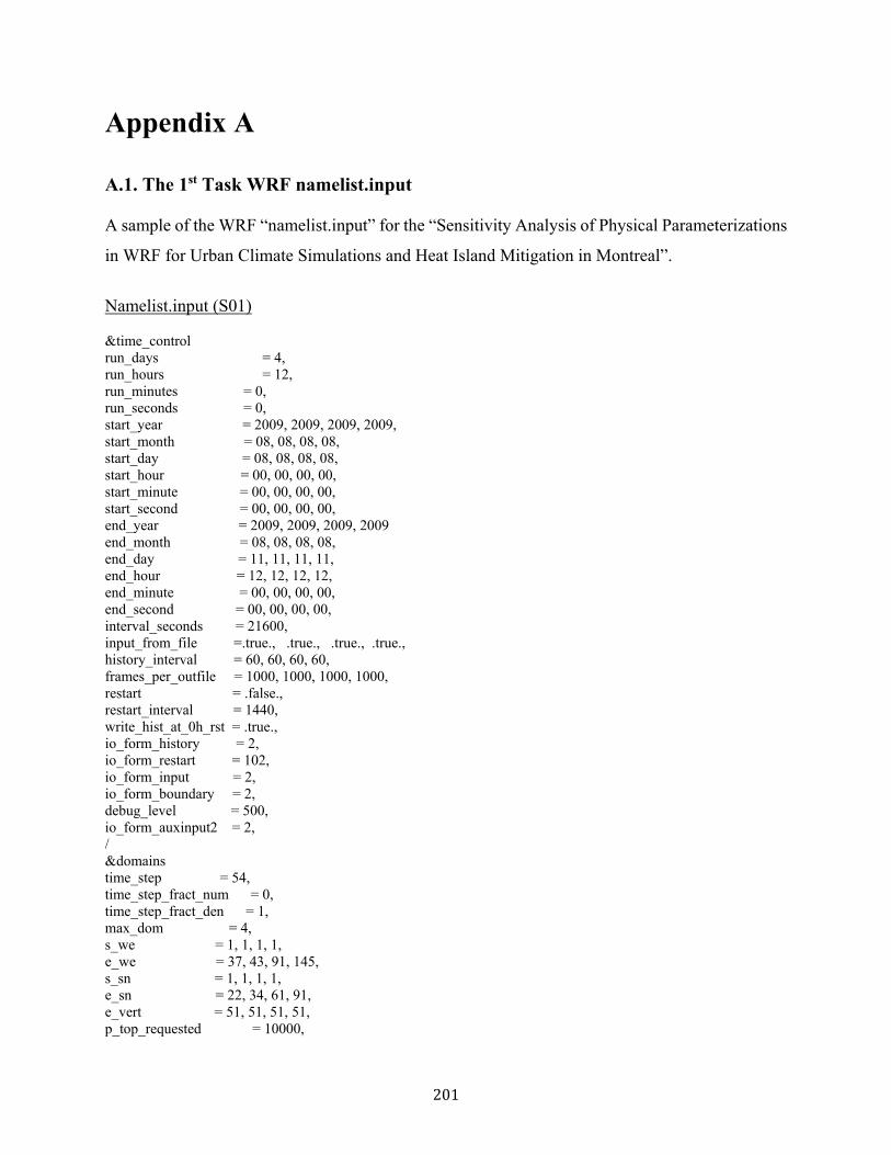
201
Appendix A
A.1. The 1st Task WRF namelist.input
A sample of the WRF “namelist.input” for the “Sensitivity Analysis of Physical Parameterizations
in WRF for Urban Climate Simulations and Heat Island Mitigation in Montreal”.
Namelist.input (S01) &time_control run_days = 4, run_hours = 12, run_minutes = 0, run_seconds = 0, start_year = 2009, 2009, 2009, 2009, start_month = 08, 08, 08, 08, start_day = 08, 08, 08, 08, start_hour = 00, 00, 00, 00, start_minute = 00, 00, 00, 00, start_second = 00, 00, 00, 00, end_year = 2009, 2009, 2009, 2009 end_month = 08, 08, 08, 08, end_day = 11, 11, 11, 11, end_hour = 12, 12, 12, 12, end_minute = 00, 00, 00, 00, end_second = 00, 00, 00, 00, interval_seconds = 21600, input_from_file =.true., .true., .true., .true., history_interval = 60, 60, 60, 60, frames_per_outfile = 1000, 1000, 1000, 1000, restart = .false., restart_interval = 1440, write_hist_at_0h_rst = .true., io_form_history = 2, io_form_restart = 102, io_form_input = 2, io_form_boundary = 2, debug_level = 500, io_form_auxinput2 = 2, / &domains time_step = 54, time_step_fract_num = 0, time_step_fract_den = 1, max_dom = 4, s_we = 1, 1, 1, 1, e_we = 37, 43, 91, 145, s_sn = 1, 1, 1, 1, e_sn = 22, 34, 61, 91, e_vert = 51, 51, 51, 51, p_top_requested = 10000,

202
num_metgrid_levels = 30, num_metgrid_soil_levels = 4, dx = 9000, 3000, 1000, 333.333, dy = 9000, 3000, 1000, 333.333, grid_id = 1, 2, 3, 4, parent_id = 1, 1, 2, 3, i_parent_start = 1, 12, 6, 19, j_parent_start = 1, 6, 6, 21, parent_grid_ratio = 1, 3, 3, 3, parent_time_step_ratio = 1, 3, 3, 3, feedback = 1, smooth_option = 2, eta_levels = 1.0000, 0.9968, 0.9953, 0.9937, 0.9921, 0.9905, 0.9886, 0.9864, 0.9837, 0.9805, 0.9766, 0.9720, 0.9664, 0.9599, 0.9520, 0.9427, 0.9315, 0.9184, 0.9028, 0.8753, 0.8407, 0.7752, 0.7142, 0.6574, 0.6046, 0.5553, 0.5095, 0.4668, 0.4271, 0.3901, 0.3557, 0.3236, 0.2937, 0.2659, 0.2401, 0.2160, 0.1935, 0.1726, 0.1532, 0.1351, 0.1182, 0.1025, 0.0879, 0.0743, 0.0616, 0.0498, 0.0338, 0.0286, 0.0191, 0.0033, 0.0000, / &physics mp_physics = 16, 16, 16, 16, ra_lw_physics = 4, 4, 4, 4, ra_sw_physics = 4, 4, 4, 4, radt = 10, 10, 10, 10, sf_sfclay_physics = 2, 2, 2, 2, sf_surface_physics = 2, 2, 2, 2, sf_urban_physics = 0, 0, 0, 3, bl_pbl_physics = 2, 2, 2, 2, bldt = 0, 0, 0, 0, cu_physics = 4, 4, 4, 0, cudt = 5, 5, 5, 5, icloud = 1, isfflx = 1, ifsnow = 1, surface_input_source = 1, maxiens = 1, maxens = 3, maxens2 = 3, maxens3 = 16, ensdim = 144, num_soil_layers = 4, num_urban_layers = 5400, / &dynamics w_damping = 1, diff_opt = 1, 1, 1, 1, km_opt = 1, 1, 1, 1, diff_6th_opt = 0, 0, 0, 0, diff_6th_factor = 0.12, 0.12, 0.12, 0.12, base_temp = 290., damp_opt = 0, zdamp = 5000., 5000., 5000., 5000., dampcoef = 0.2, 0.2, 0.2, 0.2, khdif = 0, 0, 0, 0, kvdif = 0, 0, 0, 0, non_hydrostatic = .true., .true., .true., .true., moist_adv_opt = 1, 1, 1, 1, scalar_adv_opt = 1, 1, 1, 1,
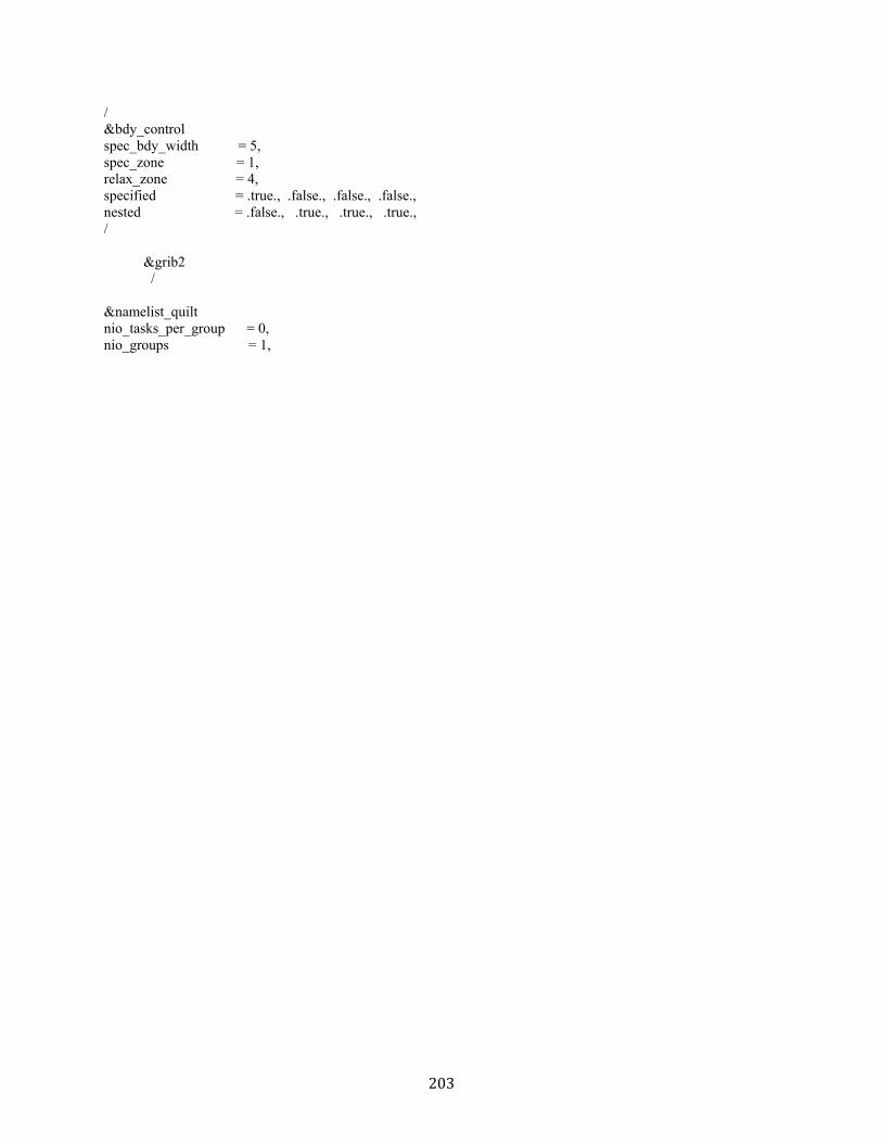
203
/ &bdy_control spec_bdy_width = 5, spec_zone = 1, relax_zone = 4, specified = .true., .false., .false., .false., nested = .false., .true., .true., .true., / &grib2 / &namelist_quilt nio_tasks_per_group = 0, nio_groups = 1,

204
A.2. The 2nd Task WRF namelist.input
Effects of Increasing Surface Reflectivity on Heat-Related Mortality in Greater Montreal Area,
Canada. The WRF name-list is for the 2005 heat wave period. For the 2011 heat wave, the
simulation configuration is the same, the date is different, thus the input data.
&time_control run_days = 0, run_hours = 0, run_minutes = 0, run_seconds = 0, start_year = 2005, 2005, 2005, 2005, start_month = 07, 07, 07, 07, start_day = 08, 08, 08, 08, start_hour = 12, 12, 12, 12, start_minute = 00, 00, 00, 0, start_second = 00, 00, 00, 0, end_year = 2005, 2005, 2005, 2005, end_month = 07, 07, 07, 07, end_day = 12, 12, 12, 12, end_hour = 12, 12, 12, 12, end_minute = 00, 00, 00, 0, end_second = 00, 00, 00, 0, interval_seconds = 10800, input_from_file = .true., .true., .true., .true., history_interval = 60, 60, 60, 60, frames_per_outfile = 1000, 1000, 1000, 1000, restart = .false., restart_interval = 1440, io_form_history = 2, io_form_restart = 2, io_form_input = 2, io_form_boundary = 2, debug_level = 500, io_form_auxinput2 = 2, / &domains time_step = 54, time_step_fract_num = 0, time_step_fract_den = 1, max_dom = 4, s_we = 1, 1, 1, 1, e_we = 37, 43, 91, 145, s_sn = 1, 1, 1, 1, e_sn = 22, 34, 61, 91, e_vert = 51, 51, 51, 51, p_top_requested = 10000, num_metgrid_levels = 30, num_metgrid_soil_levels = 4,

205
dx = 9000, 3000, 1000, 333.333, dy = 9000, 3000, 1000, 333.333, grid_id = 1, 2, 3, 4, parent_id = 1, 1, 2, 3, i_parent_start = 1, 12, 6, 19, j_parent_start = 1, 6, 6, 21, parent_grid_ratio = 1, 3, 3, 3, parent_time_step_ratio = 1, 3, 3, 3, feedback = 1, smooth_option = 2, eta_levels = 1.0000, 0.9968, 0.9953, 0.9937, 0.9921, 0.9905, 0.9886, 0.9864, 0.9837, 0.9805, 0.9766, 0.9720, 0.9664, 0.9599, 0.9520, 0.9427, 0.9315, 0.9184, 0.9028, 0.8753, 0.8407, 0.7752, 0.7142, 0.6574, 0.6046, 0.5553, 0.5095, 0.4668, 0.4271, 0.3901, 0.3557, 0.3236, 0.2937, 0.2659, 0.2401, 0.2160, 0.1935, 0.1726, 0.1532, 0.1351, 0.1182, 0.1025, 0.0879, 0.0743, 0.0616, 0.0498, 0.0338, 0.0286, 0.0191, 0.0033, 0.0000, / &physics mp_physics = 2, 2, 2, 2, ra_lw_physics = 4, 4, 4, 4, ra_sw_physics = 5, 5, 5, 5, radt = 9, 9, 9, 9, sf_sfclay_physics = 2, 2, 2, 2, sf_surface_physics = 2, 2, 2, 2, sf_urban_physics = 0, 0, 0, 1, bl_pbl_physics = 2, 2, 2, 2, bldt = 0, 0, 0, 0, cu_physics = 5, 0, 0, 0, cudt = 0, icloud = 1, surface_input_source = 1, maxiens = 1, maxens = 3, maxens2 = 3, maxens3 = 16, ensdim = 144, num_soil_layers = 4, / &fdda / &dynamics w_damping = 1, diff_opt = 1, 1, 1, 1, km_opt = 4, 4, 4, 4, diff_6th_opt = 0, 0, 0, 0, diff_6th_factor = 0.12, 0.12, 0.12, 0.12, base_temp = 290., damp_opt = 0, zdamp = 5000., 5000., 5000., 5000., dampcoef = 0.2, 0.2, 0.2, 0.2, khdif = 0, 0, 0, 0, kvdif = 0, 0, 0, 0, non_hydrostatic = .true., .true., .true., .true., moist_adv_opt = 1, 1, 1, 1,

206
scalar_adv_opt = 1, 1, 1, 1, / &bdy_control spec_bdy_width = 5, spec_zone = 1, relax_zone = 4, specified = .true., .false., .false., .false., nested = .false., .true., .true., .true., / &grib2 / &namelist_quilt nio_tasks_per_group = 0, nio_groups = 1, /

207
A.3. The 3rd Task WRF-Chem namelist.input
The Effect of Increasing Surface Albedo on Urban Climate and Air Quality: A Detailed Study for
Sacramento, Houston, and Chicago.
&time_control run_days = 0, run_hours = 0, run_minutes = 0, run_seconds = 0, start_year = 2011, 2011, 2011, 2011, start_month = 07, 07, 07, 07, start_day = 15, 15, 15, 15, start_hour = 00, 00, 00, 00, start_minute = 00, 00, 00, 00, start_second = 00, 00, 00, 00, end_year = 2011, 2011, 2011, 2011, end_month = 07, 07, 07, 07, end_day = 23, 23, 23, 23, end_hour = 00, 00, 00, 00, end_minute = 00, 00, 00, 00, end_second = 00, 00, 00, 00, interval_seconds = 21600, input_from_file = .true., .true., .true., .true., history_interval = 60, 60, 60, 60, frames_per_outfile = 1000, 1000, 1000, 1000, restart = .false., restart_interval = 1440, write_hist_at_0h_rst = .ture., io_form_history = 2, io_form_restart = 2, io_form_input = 2, io_form_boundary = 2, auxinput6_inname = 'wrfbiochemi_<domain> ', auxinput5_inname = 'wrfchemi_<domain> _<date>', auxinput5_interval_m = 60, 60, 60, 60, io_form_auxinput2 = 2, io_form_auxinput5 = 2, io_form_auxinput6 = 2, io_form_auxinput7 = 0, io_form_auxinput8 = 0, io_form_auxinput12 = 0, io_form_auxinput13 = 0, debug_level = 500, auxinput1_inname = "met_em.d<domain>.<date>", / &domains

208
time_step = 72, time_step_fract_num = 0, time_step_fract_den = 1, max_dom = 4, s_we = 1, 1, 1, 1, e_we = 445, 36, 41, 36, s_sn = 1, 1, 1, 1, e_sn = 338, 31, 31, 31, e_vert = 35, 35, 35, 35, p_top_requested = 10000, num_metgrid_levels = 30, num_metgrid_soil_levels = 4, dx = 12000, 2400, 2400, 2400, dy = 12000, 2400, 2400, 2400, grid_id = 1, 2, 3, 4, parent_id = 1, 1, 1, 1, i_parent_start = 1, 35, 272, 221, j_parent_start = 1, 181, 187, 71, parent_grid_ratio = 1, 5, 5, 5, parent_time_step_ratio = 1, 5, 5, 5, feedback = 1, smooth_option = 0, zap_close_levels = 50, interp_type = 1, t_extrap_type = 2, force_sfc_in_vinterp = 0, use_levels_below_ground = .true. use_surface = .true. lagrange_order = 2, / sfcp_to_sfcp = .true., / &physics mp_physics = 2, 2, 2, 2, progn = 1, 1, 1, 1, ra_lw_physics = 4, 4, 4, 4, swint_opt = 1, ra_sw_physics = 4, 4, 4, 4, radt = 21, 21, 21, 21, sf_sfclay_physics = 2, 2, 2, 2, sf_surface_physics = 2, 2, 2, 2, sf_urban_physics = 0, 3, 3, 3, bl_pbl_physics = 2, 2, 2, 2, bldt = 0, 0, 0, 0, cu_physics = 3, 3, 3, 3, icloud = 1, ifsnow = 1, isfflx = 1, surface_input_source = 1, cu_diag = 1, 1, 1, 1, cudt = 0, surface_input_source = 1, num_soil_layers = 4, num_urban_layers = 5400, mp_zero_out = 2,

209
mp_zero_out_thresh = 1.e-12, maxiens = 1, maxens = 3, maxens2 = 3, maxens3 = 16, ensdim = 144, cu_rad_feedback = .true., .true., .true., .true., / &fdda / &dynamics rk_ord = 3, w_damping = 1, diff_opt = 1, 1, 1, 1, km_opt = 4, 4, 4, 4, diff_6th_opt = 0, 0, 0, 0, diff_6th_factor = 0.12, 0.12, 0.12, 0.12, base_temp = 290.0, damp_opt = 0, zdamp = 5000.0, 5000.0, 5000.0, 5000.0, dampcoef = 0.2, 0.2, 0.2, 0.2, khdif = 0, 300, 300, 300, kvdif = 0, 300, 300, 300, non_hydrostatic = .true., .true., .true., .true., moist_adv_opt = 2, 2, 2, 2, scalar_adv_opt = 2, 2, 2, 2, chem_adv_opt = 2, 2, 2, 2, tke_adv_opt = 2, 2, 2, 2, time_step_sound = 4, 4, 4, 4, h_mom_adv_order = 5, 5, 5, 5, v_mom_adv_order = 3, 3, 3, 3, h_sca_adv_order = 5, 5, 5, 5, v_sca_adv_order = 3, 3, 3, 3, / &bdy_control spec_bdy_width = 5, spec_zone = 1, relax_zone = 4, specified = .true., .false., .false., .false., nested = .false., .true., .true., .true., / &grib2 / &namelist_quilt nio_tasks_per_group = 0, nio_groups = 1, / &chem kemit = 23,
210
chem_opt = 11, 11, 11, 11, bioemdt = 30, 30, 30, 30, photdt = 30, 30, 30, 30, chemdt = 0, 0, 0, 0, io_style_emissions = 2, emiss_opt = 3, 3, 3, 3, emiss_opt_vol = 0, 0, 0, 0, chem_in_opt = 0, 0, 0, 0, phot_opt = 2, 2, 2, 2, gas_drydep_opt = 1, 1, 1, 1, aer_drydep_opt = 1, 1, 1, 1, bio_emiss_opt = 2, 2, 2, 2, ne_area = 104, dust_opt = 2, dmsemis_opt = 0, seas_opt = 2, depo_fact = 0.25, gas_bc_opt = 1, 1, 1, 1, gas_ic_opt = 1, 1, 1, 1, aer_bc_opt = 1, 1, 1, 1, aer_ic_opt = 1, 1, 1, 1, gaschem_onoff = 1, 1, 1, 1, aerchem_onoff = 1, 1, 1, 1, wetscav_onoff = 1, 1, 1, 1, cldchem_onoff = 1, 1, 1, 1, vertmix_onoff = 1, 1, 1, 1, chem_conv_tr = 1, 1, 1, 1, conv_tr_wetscav = 1, 1, 1, 1, conv_tr_aqchem = 1, 1, 1, 1, biomass_burn_opt = 0, 0, 0, 0, plumerisefire_frq = 30, 30, 30, 30, have_bcs_chem = .true., .true.,.true.,.true., aer_ra_feedback = 1, aer_op_opt = 1, opt_pars_out = 1, diagnostic_chem = 0, chemdiag = 1, /

211
A.4. The 4th Task WRF-Chem namelist.input
Effects of increasing surface reflectivity on aerosol-radiation-cloud interaction over Greater
Montreal Area during the 2011 heat wave period. The namelist of the ARC simulation is presented.
Namelist. Input WRF-Chem (ARC) &time_control run_days = 0, run_hours = 0, run_minutes = 0, run_seconds = 0, start_year = 2011, 2011, 2011, start_month = 07, 07, 07, start_day = 15, 15, 15, start_hour = 00, 00, 00, start_minute = 00, 00, 00, start_second = 00, 00, 00, end_year = 2011, 2011, 2011, end_month = 07, 07, 07, end_day = 23, 23, 23, end_hour = 00, 00, 00, end_minute = 00, 00, 00, end_second = 00, 00, 00, interval_seconds = 21600, input_from_file = .true., .true., .true., history_interval = 60, 60, 60, 60, frames_per_outfile = 1000, 1000, 1000, 1000, restart = .false., restart_interval = 1440, write_hist_at_0h_rst = .ture., io_form_history = 2, io_form_restart = 2, io_form_input = 2, io_form_boundary = 2, auxinput6_inname = 'wrfbiochemi_<domain> ', auxinput5_inname = 'wrfchemi_<domain> _<date>', auxinput5_interval_m = 60, 60, 60, 60, io_form_auxinput2 = 2, io_form_auxinput5 = 2, io_form_auxinput6 = 2, io_form_auxinput7 = 0, io_form_auxinput8 = 0, io_form_auxinput12 = 0, io_form_auxinput13 = 0, debug_level = 500, auxinput1_inname = "met_em.d<domain>.<date>", /
212
&domains time_step = 72, time_step_fract_num = 0, time_step_fract_den = 1, max_dom = 3, s_we = 1, 1, 1, e_we = 445, 139, 101, s_sn = 1, 1, 1, e_sn = 338, 124, 71, e_vert = 35, 35, 35, p_top_requested = 10000, num_metgrid_levels = 30, num_metgrid_soil_levels = 4, dx = 12000, 4000, 800, dy = 12000, 4000, 800, grid_id = 1, 2, 3, parent_id = 1, 1, 2, i_parent_start = 1, 329, 98, j_parent_start = 1, 212, 74, parent_grid_ratio = 1, 3, 5, parent_time_step_ratio = 1, 3, 5, feedback = 1, smooth_option = 0, zap_close_levels = 50, interp_type = 1, t_extrap_type = 2, force_sfc_in_vinterp = 0, use_levels_below_ground = .true. use_surface = .true. lagrange_order = 1, / sfcp_to_sfcp = .true., / &physics mp_physics = 2, 2, 2, progn = 1, 1, 1, ra_lw_physics = 4, 4, 4, swint_opt = 1, ra_sw_physics = 4, 4, 4, radt = 21, 21, 21, sf_sfclay_physics = 2, 2, 2, sf_surface_physics = 2, 2, 2, sf_urban_physics = 0, 0, 3, bl_pbl_physics = 2, 2, 2, bldt = 0, 0, 0, cu_physics = 5, 5, 5, icloud = 1, ifsnow = 1, isfflx = 1, surface_input_source = 1, cu_diag = 1, 1, 1, 1, cudt = 0, surface_input_source = 1, num_soil_layers = 4,

213
sf_urban_physics = 0, 0, 0, 0, num_urban_layers = 5400, mp_zero_out = 2, mp_zero_out_thresh = 1.e-12, maxiens = 1, maxens = 3, maxens2 = 3, maxens3 = 16, ensdim = 144, cu_rad_feedback = .true.,.true.,.true.,.true., / &fdda / &dynamics rk_ord = 3, w_damping = 1, diff_opt = 1, 1, 1, 1, km_opt = 4, 4, 4, 4, diff_6th_opt = 0, 0, 0, 0, diff_6th_factor = 0.12, 0.12, 0.12, 0.12, base_temp = 290.0, damp_opt = 0, zdamp = 5000.0, 5000.0, 5000.0, 5000.0, dampcoef = 0.2, 0.2, 0.2, 0.2, khdif = 0, 0, 300, kvdif = 0, 0, 300, non_hydrostatic = .true., .true., .true., .true., moist_adv_opt = 2, 2, 2, 2, scalar_adv_opt = 2, 2, 2, 2, chem_adv_opt = 2, 2, 2, 2, tke_adv_opt = 2, 2, 2, 2, time_step_sound = 4, 4, 4, 4, h_mom_adv_order = 5, 5, 5, 5, v_mom_adv_order = 3, 3, 3, 3, h_sca_adv_order = 5, 5, 5, 5, v_sca_adv_order = 3, 3, 3, 3, / &bdy_control spec_bdy_width = 5, spec_zone = 1, relax_zone = 4, specified = .true., .false., .false., .false., nested = .false., .true., .true., .true., / &grib2 / &namelist_quilt

214
nio_tasks_per_group = 0, nio_groups = 1, / &chem kemit = 23, chem_opt = 10, 10, 10, bioemdt = 30, 30, 30, photdt = 30, 30, 30, chemdt = 0, 0, 0, io_style_emissions = 2, emiss_opt = 3, 3, 3, 3, emiss_opt_vol = 0, 0, 0, 0, chem_in_opt = 0, 0, 0, 0, phot_opt = 2, 2, 2, 2, gas_drydep_opt = 1, 1, 1, 1, aer_drydep_opt = 1, 1, 1, 1, bio_emiss_opt = 1, 1, 1, 1, ne_area = 104, dust_opt = 2, dmsemis_opt = 0, seas_opt = 2, depo_fact = 0.25, gas_bc_opt = 1, 1, 1, 1, gas_ic_opt = 1, 1, 1, 1, aer_bc_opt = 1, 1, 1, 1, aer_ic_opt = 1, 1, 1, 1, gaschem_onoff = 1, 1, 1, 1, aerchem_onoff = 1, 1, 1, 1, wetscav_onoff = 1, 1, 1, 1, cldchem_onoff = 1, 1, 1, 1, vertmix_onoff = 1, 1, 1, 1, chem_conv_tr = 1, 1, 1, 1, conv_tr_wetscav = 1, 1, 1, 1, conv_tr_aqchem = 1, 1, 1, 1, biomass_burn_opt = 0, 0, 0, 0, plumerisefire_frq = 30, 30, 30, 30, have_bcs_chem = .false., .false.,.false., aer_ra_feedback = 1, aer_op_opt = 1, opt_pars_out = 1, diagnostic_chem = 0, chemdiag = 1, /

215
Appendix B B.1. Theory of the Aerosol Interactions in the Atmosphere
The interaction of aerosol particles and clouds formation involve processes on multiple scales.
They range from the nucleation of liquid and solid particles on the scale of a few nanometer to the
growth of droplets to several micrometers up to the dynamics of cloud systems and the
hydrological cycle on the scale of several kilometers. Here, the aerosol interaction with cloud and
microphysics in the atmosphere is explained.
B.1.1. Formation of Hydrometeors in the Atmosphere The nucleation and growth of a liquid or solid particle in the atmosphere can be described by
thermodynamic theory. The thermodynamic state of a system can be defined by one of its
thermodynamic potentials. The Gibbs free energy G is commonly used to describe the
thermodynamics of phase changes. For a mixture of n components G is calculated by:
𝐺 = ∑ 𝜇𝑙𝑛𝑙
𝑛
𝑙=1
where 𝜇𝑙 is the chemical potential and 𝑛𝑙 is the number of moles of component l. The formation
of water droplet (wd), from water vapor (wv) is determined by the change in G:
∆𝐺 = 𝐺𝑤𝑑 − 𝐺𝑤𝑣 = 𝑛𝑤(𝜇𝑤 − 𝜇𝑣) + 𝜋𝐷2 𝜎𝑤𝑣
where 𝜎𝑤𝑣 is the surface tension of water vapor interface and represent the amount of energy
needed to increase the surface by one-unit area. Assuming water vapor is an ideal gas, 𝜇𝑣 can be
expressed as a function of water vapor pressure e (Seinfeld and Pandis, 2006).
𝜇𝑣 = 𝜇𝑣𝑜 + 𝑅𝑇𝑙𝑛
𝑒
𝑒𝑜
Where R is the universal Gas constant, T is the temperature and 𝜇𝑣𝑜 is the standard chemical
potential defined at 𝑒𝑜 = 1013.25hpa. The ratio 𝑒
𝑒𝑜 is saturation ratio as S. For S=1 the water
vapor is in chemical equilibrium. For S<1, the Gibbs free energy change is positive, but for S>1
a maximum G exists.
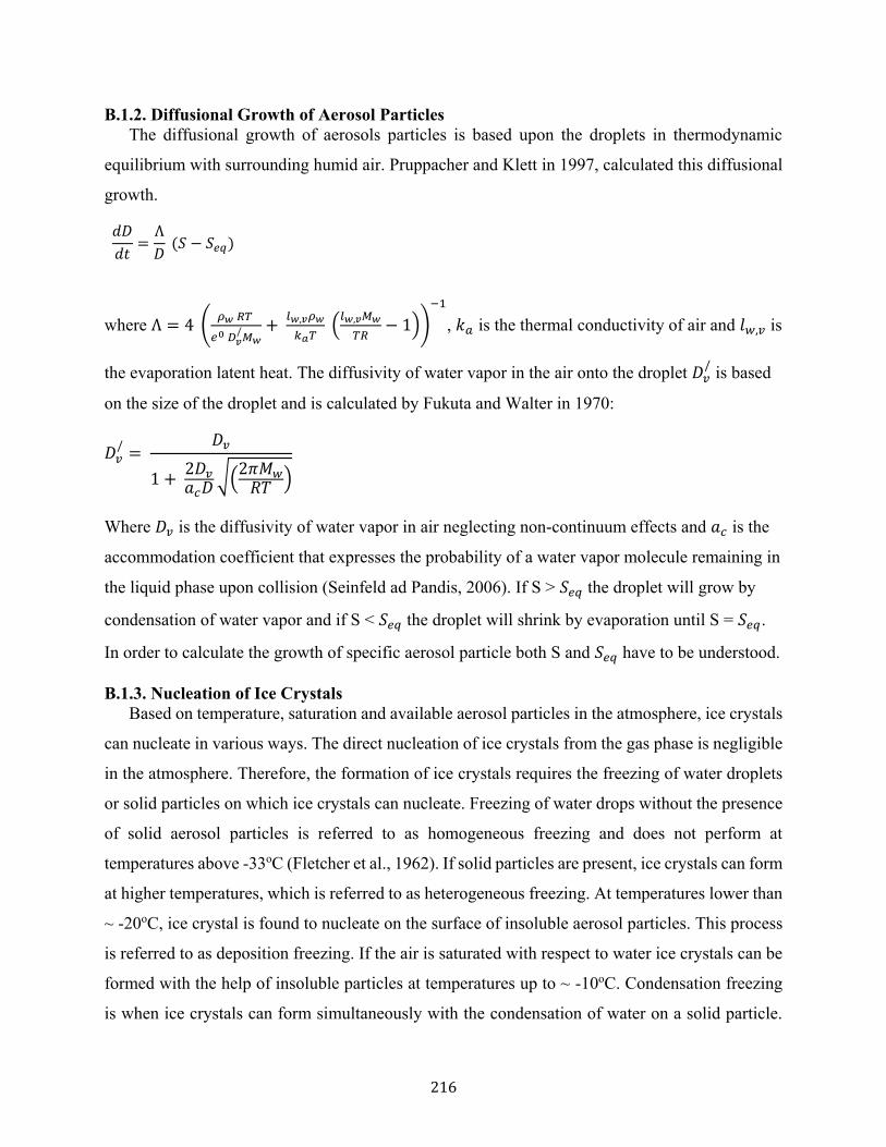
216
B.1.2. Diffusional Growth of Aerosol Particles The diffusional growth of aerosols particles is based upon the droplets in thermodynamic
equilibrium with surrounding humid air. Pruppacher and Klett in 1997, calculated this diffusional
growth.
𝑑𝐷
𝑑𝑡=
Λ
𝐷 (𝑆 − 𝑆𝑒𝑞)
where Λ = 4 (𝜌𝑤 𝑅𝑇
𝑒0 𝐷𝑣/
𝑀𝑤
+ 𝑙𝑤,𝑣𝜌𝑤
𝑘𝑎𝑇 (
𝑙𝑤,𝑣𝑀𝑤
𝑇𝑅− 1))
−1
, 𝑘𝑎 is the thermal conductivity of air and 𝑙𝑤,𝑣 is
the evaporation latent heat. The diffusivity of water vapor in the air onto the droplet 𝐷𝑣/ is based
on the size of the droplet and is calculated by Fukuta and Walter in 1970:
𝐷𝑣/
= 𝐷𝑣
1 + 2𝐷𝑣
𝑎𝑐𝐷√(
2𝜋𝑀𝑤
𝑅𝑇)
Where 𝐷𝑣 is the diffusivity of water vapor in air neglecting non-continuum effects and 𝑎𝑐 is the
accommodation coefficient that expresses the probability of a water vapor molecule remaining in
the liquid phase upon collision (Seinfeld ad Pandis, 2006). If S > 𝑆𝑒𝑞 the droplet will grow by
condensation of water vapor and if S < 𝑆𝑒𝑞 the droplet will shrink by evaporation until S = 𝑆𝑒𝑞.
In order to calculate the growth of specific aerosol particle both S and 𝑆𝑒𝑞 have to be understood.
B.1.3. Nucleation of Ice Crystals Based on temperature, saturation and available aerosol particles in the atmosphere, ice crystals
can nucleate in various ways. The direct nucleation of ice crystals from the gas phase is negligible
in the atmosphere. Therefore, the formation of ice crystals requires the freezing of water droplets
or solid particles on which ice crystals can nucleate. Freezing of water drops without the presence
of solid aerosol particles is referred to as homogeneous freezing and does not perform at
temperatures above -33oC (Fletcher et al., 1962). If solid particles are present, ice crystals can form
at higher temperatures, which is referred to as heterogeneous freezing. At temperatures lower than
~ -20oC, ice crystal is found to nucleate on the surface of insoluble aerosol particles. This process
is referred to as deposition freezing. If the air is saturated with respect to water ice crystals can be
formed with the help of insoluble particles at temperatures up to ~ -10oC. Condensation freezing
is when ice crystals can form simultaneously with the condensation of water on a solid particle.
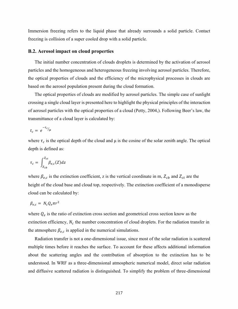
217
Immersion freezing refers to the liquid phase that already surrounds a solid particle. Contact
freezing is collision of a super cooled drop with a solid particle.
B.2. Aerosol impact on cloud properties
The initial number concentration of clouds droplets is determined by the activation of aerosol
particles and the homogeneous and heterogeneous freezing involving aerosol particles. Therefore,
the optical properties of clouds and the efficiency of the microphysical processes in clouds are
based on the aerosol population present during the cloud formation.
The optical properties of clouds are modified by aerosol particles. The simple case of sunlight
crossing a single cloud layer is presented here to highlight the physical principles of the interaction
of aerosol particles with the optical properties of a cloud (Petty, 2004,). Following Beer’s law, the
transmittance of a cloud layer is calculated by:
𝑡𝑐 = 𝑒−𝜏𝑐
𝜇⁄
where 𝜏𝑐 is the optical depth of the cloud and μ is the cosine of the solar zenith angle. The optical
depth is defined as:
𝜏𝑐 = ∫ 𝛽𝑒,𝑐(𝑍)𝑑𝑧𝑍𝑐𝑡
𝑍𝑐𝑏
where 𝛽𝑒,𝑐 is the extinction coefficient, z is the vertical coordinate in m, 𝑍𝑐𝑏 and 𝑍𝑐𝑡 are the
height of the cloud base and cloud top, respectively. The extinction coefficient of a monodisperse
cloud can be calculated by:
𝛽𝑒,𝑐 = 𝑁𝑐𝑄𝑒𝜋𝑟2
where 𝑄𝑒 is the ratio of extinction cross section and geometrical cross section know as the
extinction efficiency, 𝑁𝑐 the number concentration of cloud droplets. For the radiation transfer in
the atmosphere 𝛽𝑒,𝑐 is applied in the numerical simulations.
Radiation transfer is not a one-dimensional issue, since most of the solar radiation is scattered
multiple times before it reaches the surface. To account for these affects additional information
about the scattering angles and the contribution of absorption to the extinction has to be
understood. In WRF as a three-dimensional atmospheric numerical model, direct solar radiation
and diffusive scattered radiation is distinguished. To simplify the problem of three-dimensional

218
scattering, a two-stream approximation is usually used for the diffusive part of the atmospheric
radiation. Thereby, the upwelling and down welling part of the diffusive radiation in an
atmospheric column are assumed to be isotropic in each hemisphere. The radiation transfer in an
atmospheric column can then be treated as a one-dimensional problem and can be described by the
extinction coefficient, the single scattering albedo, which is defined as the scattering fraction of
the extinction coefficient, and the asymmetry parameter, which can be interpreted as the average
of the cosine of the scattering angle for a high number of scattering events (Petty, 2004). All
parameters are a function of wavelength and in case of clouds, they depend on the size distribution
of hydrometeors in the cloud.
On the other hand, the formation of rain is very complicated and cannot be explained by the
diffusional growth of cloud droplets to the size of rain drops, because it would need several hours
with a sufficient high supersaturation. Therefore, the growth of cloud droplets to the size of rain
drops is dominated by another process, namely the collision and coalescence of the droplets. The
increase in mass of a single cloud drop mc/ with diameter Dc , falling through a population of
smaller drops with diameter Dc/ and mass mc
/, can be calculated by the volume the drop is falling
through times the number concentration of smaller drops Nc/:
𝑑𝑚𝑐/
𝑑𝑡=
1
4 𝜋 (𝐷𝑐 + 𝐷𝑐
/)2(|𝑊𝑠𝑒𝑑 − 𝑊𝑠𝑒𝑑/ |)𝑚𝑐
/𝑁𝑐
/= 𝐾𝑐(𝐷𝑐 , 𝐷𝑐
/)𝑚𝑐
/𝑁𝑐
/
where 𝑊𝑠𝑒𝑑 and 𝑊𝑠𝑒𝑑/ are the fall velocities of the drops and 𝐾𝑐(𝐷𝑐 , 𝐷𝑐/) is the collection kernel
of two drops falling with different fall velocities and is calculated by:
𝐾𝑐 (𝐷𝑐 , 𝐷𝑐/) =
1
4 𝜋(𝐷𝑐 , 𝐷𝑐
/)2𝐸(𝐷𝑐 , 𝐷𝑐
/) |𝑊𝑠𝑒𝑑 − 𝑊𝑠𝑒𝑑/ |
Smaller cloud droplets will grow slower in comparison to larger particles and for droplets
smaller than 10μm the collision efficiency is negligible. Therefore, aerosol particles can strongly
modify the growth of cloud droplets to rain drops.
B.3. Numerical Description of Aerosol Particles
To investigate the aerosol-radiation-cloud interactions in the atmosphere, a numerical model
at a specific scale is required to evaluate the physical, chemical and aerosol dynamical processes

219
during a specific period of time. Aerosols are particles with various chemical compositions
suspended in the air and can be described by a continuous size distribution as a function of the
particle diameter:
𝑛𝑁(𝐷𝑝) = 𝑑𝑁
𝑑𝐷𝑝
To describe chemical and physical processes related with the atmospheric aerosol in numerical
model systems efficiently, the size distribution of the aerosol particles is separated in individual
overlapping modes, depending on the size and chemical composition of the particles (Whitby and
McMurry, 1997). Each mode is approximated by a log- normal size distribution function (Whitby,
1978) with constant chemical composition:
𝑛𝑁,𝑙(𝐷𝑝) = 1
𝐷𝑝
𝑁𝑙
𝑙𝑛𝜎𝑙√2𝜋 exp (−
𝑙𝑛2 (𝐷𝑝
𝐷𝑝,𝑙⁄ )
𝑙𝑛2𝜎𝑙)
Where n is the number concentration of particles in mode l, σl is the geometrical standard
deviation of mode l, and Dp,l the median diameter of the particles in mode l. The size distribution
function and the total number concentration of aerosol particles can be calculated by:
𝑛𝑁,𝑙(𝐷𝑝) = ∑ 𝑛𝑁,𝑙(𝐷𝑝)𝑙
To simulate the temporal evolution of nN,l(Dp) in the atmosphere, one has to simulate the
temporal evolution of nN,l, σl , and Dp,l . For processes like advection and diffusion the differential
equations for σl and Dp,l cannot be solved directly (Whitby and McMurry, 1997). Therefore, the
equations in the model are formulated for integral moments of nN,l(Dp). The k-th moment Mkx of
the size distribution of mode l is defined as:
𝑀𝑘𝑙 = ∫ 𝐷𝑘𝑛𝑁,𝑙(𝐷𝑝)d𝐷𝑝
∞
0
The moments are directly related to integral quantities of the aerosol population by:
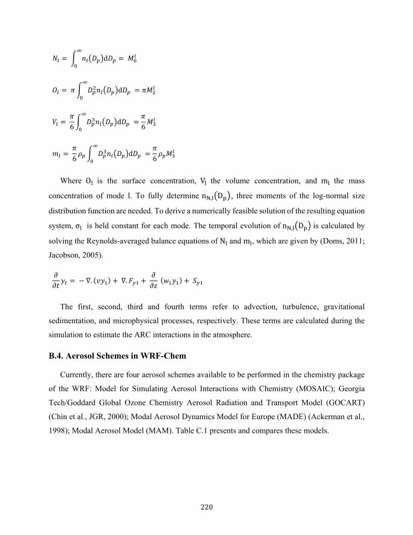
220
𝑁𝑙 = ∫ 𝑛𝑙(𝐷𝑝)d𝐷𝑝 = 𝑀0𝑙
∞
0
𝑂𝑙 = 𝜋 ∫ 𝐷𝑝2𝑛𝑙(𝐷𝑝)d𝐷𝑝
∞
0
= 𝜋𝑀2𝑙
𝑉𝑙 = 𝜋
6∫ 𝐷𝑝
3𝑛𝑙(𝐷𝑝)d𝐷𝑝 ∞
0
=𝜋
6𝑀3
𝑙
𝑚𝑙 = 𝜋
6𝜌𝑝 ∫ 𝐷𝑝
3𝑛𝑙(𝐷𝑝)d𝐷𝑝 ∞
0
=𝜋
6𝜌𝑝𝑀3
𝑙
Where Ol is the surface concentration, Vl the volume concentration, and ml the mass
concentration of mode l. To fully determine nN,l(Dp), three moments of the log-normal size
distribution function are needed. To derive a numerically feasible solution of the resulting equation
system, σl is held constant for each mode. The temporal evolution of nN,l(Dp) is calculated by
solving the Reynolds-averaged balance equations of Nl and ml, which are given by (Doms, 2011;
Jacobson, 2005).
𝜕
𝜕𝑡𝑦𝑡 = − ∇. (𝑣𝑦1) + ∇. 𝐹𝑦1 +
𝜕
𝜕𝑧 (𝑤1𝑦1) + 𝑆𝑦1
The first, second, third and fourth terms refer to advection, turbulence, gravitational
sedimentation, and microphysical processes, respectively. These terms are calculated during the
simulation to estimate the ARC interactions in the atmosphere.
B.4. Aerosol Schemes in WRF-Chem
Currently, there are four aerosol schemes available to be performed in the chemistry package
of the WRF: Model for Simulating Aerosol Interactions with Chemistry (MOSAIC); Georgia
Tech/Goddard Global Ozone Chemistry Aerosol Radiation and Transport Model (GOCART)
(Chin et al., JGR, 2000); Modal Aerosol Dynamics Model for Europe (MADE) (Ackerman et al.,
1998); Modal Aerosol Model (MAM). Table C.1 presents and compares these models.

221
Table C.1. Available aerosol schemes to be coupled with chemistry package in WRF to evaluate the ARC interactions
Categories MOSAIC GOCART MADE MAM Aerosol size distribution
Sectional Bulk Modal Modal
SO4 -- ✓ ✓ ✓ ✓
NH4-- ✓ ✓ ✓ ✓
NO3 ✓ ✓ ✓
Organics ✓ ✓
Soot ✓ ✓
Sea salt ✗ ✓ ✓
Mineral dust ✗ ✓ ✓
Interaction with radiation
✓ ✓ ✓ Only RRTMG
Interaction with clouds
✓ ✓ ✓ Only resolved
clouds (Sc) Gas phase chemistry MOZART3 RADM1 RADM1 CBMZ4
Aerosol chemistry VBS4 ✗ SORGAM2
✗ Highlights - Sectional
scheme for 4 or 8 bins - IA6, OA7 & SOA8
- Size information available only for dust & sea salt - No SOA
- 3 log-normal modes - IA, OA & SOA
- 3 or 7 log-normal modes - IA, OA, SOA
1. Regional Acid Deposition Model Version 2. Secondary Organic Aerosol Model 3. Model for Ozone & Related chem. Tracer 4. Volatility Basis Set 5. Carbon-Bond Mechanism Version Z) 6. Inorganic Aerosol 7. Organic Aerosol 8. Secondary Organic Aerosol
Accordingly, the MOSAIC as the sectional aerosol estimation and MADE as the modal one,
are the most proper aerosol models to be applied in these simulations. In the following section, a
brief description of these two aerosol schemes are pointed out.
B.4.1. The MOSAIC aerosol mechanism
The Model for Simulating Aerosol Interactions and Chemistry (MOSAIC) mechanism is a
sectional scheme, with 4 or 8 a set of discrete size bins (Zaveri et al., 2008). MOSAIC carries five
inorganic ions, with three organic matter and even secondary organic aerosols. All chemical
components within each size bin are assumed to be internally mixed (Zaveri et al., 2008). Some
uncertainties in the model representation have been recognized in previous studies as aerosol
composition, size distribution and optical properties that would probably affect the result in
radiative forcing predictions as well (Matsui et al., 2013; Kodros et al., 2015).

222
Within MOSAIC, each aerosol chemical component has its challenges in calculating refractive
index, especially in terms of the most absorbing particle, Black Carbon (BC) (Barnard et al., 2010).
The overall complex refractive index is calculated for each bin using a mixing rule (Maxwell-
Garnett mixing rule) to approximate the internal structure of the aerosol particles (Bond et al.,
2006; Bond and Bergstrom, 2006; Barnard et al., 2010; Matsui et al., 2013). Mie calculations are
used to calculate the intermediate optical properties for each bin, which are summed over size bins
to give the bulk extinction coefficient (BEC), scattering coefficient (SC), single scattering albedo
(SSA = SC /BEC) and asymmetry factor (g). Each of these variables are functions of the size
parameter (x = 2πr
λ) where λ is the light wavelength and r is the wet radius at the centre of the
aerosol bin (Fast et al., 2006). A full description of the optical property calculations is given by
Fast et al. (2006) and Barnard et al. (2010).
The activation of cloud condensation nuclei is the key process in simulating aerosol–cloud
interactions. Aerosols become activated as soon as the environmental supersaturation in the air
entering the cloud `s process and formation. The Köhler et al. (1936) theory describes the
equilibrium state of an aerosol particle, assumed to be an aqueous salt solution, with ambient water
vapour. Figure C.1 shows the Köhler Curve.
Figure C.1. Köhler Curves (After Jerome Fast, 2014)
When an aerosol particle becomes activated to form a cloud droplet termed as critical
supersaturation (SC). The activation fraction is calculated based on mass, number of each bin and
aerosol composition using the methodology of Abdul-Razzak and Ghan (2002). The primary driver
of cloud droplet activation is the vertical velocity (W): air parcels with higher W reach higher
maximum supersaturations (Smax). All particles with Sc < Smax will be activated, whereas those
with Sc > Smax remain un-activated within clouds and are known as interstitial aerosols (Chapman
223
et al., 2009). The number and mass fraction of activated CCN in each aerosol bin can be calculated
by comparing Smax with Sc at the sectional limits of each bin (Abdul-Razzak and Ghan, 2002).
WRF-Chem carries six diagnostic variables showing the concentration of particles that can
potentially activate at given supersaturations of 0.02, 0.05, 0.1, 0.2, 0.5 and 1% as CCN0.02,
CCN0.05, CCN0.1, CCN0.2, CCN0.5 and CCN1.0, respectively.
To investigate the indirect effects the cloud activation scheme needs to be coupled with a
double-moment microphysical parameterisation that involve both number and mass loadings for
hydrometeors. The double-moment Morrison et al. (2005, 2009) parameterisation has been
coupled with MOSAIC aerosol (Yang et al., 2011). One of the main sinks of particulate mass is
wet scavenging of interstitial and activated aerosol (Slinn, 1984). Wet removal causes the aerosol
particles to be deposited out of the atmosphere, without the possibility of resuspension and
evaporation (Yang et al., 2015).
In deep convective clouds, secondary activation of aerosol has been observed (Heymsfield et
al., 2009) and modelled (e.g. Segal et al., 2003; Yang et al., 2015), whereby further interstitial
aerosol particles are activated above cloud base due to supersaturation not being fully offset by
droplet growth, as hydrometeors are scavenged in the cloud column. This is a process
unrepresented in the current model setup, as the Abdul-Razzak and Ghan (2002) parameterisation
assumes all activation at cloud base. If secondary activation were included in the model, it would
primarily act to increase the efficiency with which aerosol is scavenged from cloud and reduce the
amount of aerosol transported to the mid and up- per troposphere (Yang et al., 2015). However,
representing this process is challenging on this scale of the model, without bin microphysics or
fully resolved updraft velocities. Use of the aerosol-aware Kain–Fritsch parameterisation (Berg et
al., 2015) could enable consideration of this process in parameterised clouds for future studies.
B.4.2. The MADE Aerosol Mechanism
The Modal Aerosol Dynamics Model for Europe (MADE; Ackermann et al. 1998) presents the
aerosol population by log-normal size distribution functions, so-called modes, and represent the
aerosol dynamic processes like the Brownian coagulation of small particles. Five modes represent
sub-micron particles consisting of sulphate, ammonium, nitrate, organic compounds, water, and
soot in a range of mixing states and sizes where interact with anthropogenic emissions of particles
and gases through coagulation where the size distributions overlap. These modes enable the

224
explicit simulation of soot aging in the atmosphere (Riemer et al., 2004, 2003). Sea salt and mineral
dust particles are represented by three modes for different size ranges in each case. The emissions
of sea salt and mineral dust particles are calculated online in the model as a function of atmospheric
state, e.g. 10 m-wind speed, and friction velocity, and surface properties, such as sea surface
temperature, soil type, and soil moisture (Lundgren, 2010; Stanelle et al., 2010).

225
Appendix C
National Weather Service – Heat Index (NWS-HI)
The heat index is a measure of how hot it feels when relative humidity is factored in with air
temperature. To find the heat index, one can check the air temperature first and then the relative
humidity. For example, is the air temperature is 96oF and the relative humidity is 65%, the heat
index is 121oF, meaning how hot it feels. The red area without numbers indicates extreme danger.
The National Weather Service will initiate alert procedures when the heat index is exceed 105-110
oF for at least two consecutive days.
Related Documents


![Biblioteche della Provincia di Reggio Emilia - …biblioteche.provincia.re.it/.../elenco_dvd_160916123336.pdf2400072610 Kamkari, Fariborz \I \\fiori di Kirkuk Medusa Film [distributore]](https://static.cupdf.com/doc/110x72/5e4fa5c67b310f45b410a4a0/biblioteche-della-provincia-di-reggio-emilia-2400072610-kamkari-fariborz-i-fiori.jpg)
