Effects of Environmental Variation at Multiple Scales on ...digitalassets.lib.berkeley.edu/.../LaBarbera_berkeley_0028E_16182.pdf · Effects of Environmental Variation at Multiple

Effects of Environmental Variation at Multiple Scales on the Dark-eyed Junco (Junco hyemalis) in California

By

Kathleen LaBarbera

A dissertation submitted in partial satisfaction of the

requirements for the degree of

Doctor of Philosophy

in

Integrative Biology

in the

Graduate Division

of the

University of California, Berkeley

Committee in charge:

Professor Eileen A. Lacey, Chair Professor Rauri Bowie Professor Damian Elias

Professor Steven Beissinger

Spring 2016

1

ABSTRACT

Effects of Environmental Variation at Multiple Scales on the Dark-eyed Junco (Junco hyemalis) in California

by

Kathleen LaBarbera

Doctor of Philosophy in Integrative Biology

University of California, Berkeley

Professor Eileen A. Lacey, Chair

The selective pressures acting on phenotypes are complex and can vary over space and time. To examine the effects of selection due to environmental conditions on avian bill morphology, we explored spatial and temporal variation in bill morphology in a common generalist songbird, the Dark-eyed Junco (Junco hyemalis). We measured bill length, width, and depth, and calculated surface area, for >800 museum specimens collected in the state of California from 1905-1980. We then examined which environmental variables (precipitation, temperature, and habitat type) at which temporal scales (seasonal, annual, hemi-decadal, and decadal) could explain variation in each measure of bill morphology. Although we predicted relationships consistent with selection on the bill for foraging utility and optimal thermoregulation, the patterns we found were more complex. The effects of the environmental factors examined varied with season and with the specific bill traits. Measures of habitat type were more strongly associated with bill morphology than were individual climate variables, and temperature was a more important predictor of bill morphology than precipitation. Bill surface area displayed stronger effects of environmental conditions than did linear measures of bill morphology. Of the climate variables identified as important in our analyses, support was strongest for the measure of decadal temperature variability. The strong relationship between vegetative community and bill surface area in our models, the support for longer-term temperature variables, and the support for the importance of temperature variability suggests that in complex natural systems, large-scale context—ecology and climate—plays a strong role that is not seen by looking at its component parts alone. Different environmental conditions produce different selective pressures. We explored patterns of life history variation along an elevation gradient to identify the factors contributing to this variation. We monitored breeding Dark-eyed Juncos in the Sierra Nevada mountains of California at sites from 1960 to 2660 m above sea level and compared breeding season length, temporal patterns of peak breeding activity, clutch size, brood size, nestling quality, and nest mortality among elevations. We also compared maximum and minimum daily temperature, daily snow depth, and monthly precipitation across the elevations to determine whether these abiotic factors could explain life history variation. We found small differences in breeding season length and in the pattern of reproductive timing among elevations. While breeding season at the intermediate elevation was intermediate in length, the pattern of peak breeding activity was not

2

intermediate between the patterns observed at low and high elevations. The life history differences across elevations could not be explained solely by abiotic factors, but may be related to the effects of those factors on the birds' prey base or nesting sites, potentially exacerbated at lower elevations by the ongoing drought. We found no differences among elevations in clutch size, brood size, or nestling quality. Higher elevations had greater nest mortality, possibly due to severe weather. A computer simulation constructed to mimic the field system suggests that these mortality differences, in combination with the differences in breeding season length, contribute to substantial differences among elevations in reproductive success which may be difficult to observe in a field setting. We then investigated whether variation in climatic conditions, breeding season length, and number of offspring produced per season in populations of junco breeding at different elevations led to variation in breeding synchrony, in extra-pair paternity, or in the use of a sexually-selected male signal, the amount of white in the tail. We also tested for genetic structure among the populations. Using 12 variable microsatellite loci, we found differences in extra-pair paternity rates among our populations, with a low extra-pair paternity rate (20% of nests) at high elevations, a high rate (57%) at middle elevations, and an intermediate rate (38%) at low elevations. We found no differences among elevations in mean values of tail white or tail white asymmetry, and no differences in a measure of the honesty of the signal (the strength of the correlation between tail white and either of two indices of male quality). Despite differences in the temporal patterns of breeding activity as well as in the length of the breeding season, we found no differences in breeding synchrony among elevations, and no assocation between the presence of extra-pair paternity and a brood's breeding synchrony. We detected no genetic differentiation among populations, indicating that consistent gene flow occurs between the populations. Persistent gene flow may explain the lack of differentiation in the tail white signal despite substantial differences in the potential strength of sexual selection among elevations.

i

DEDICATION For the birds: for the bravery of the broken-wing display; for the gamble of hard eggs hatching into soft chicks; for the fast-beating hearts and fluttering wings.

ii

INTRODUCTION What drives the variation we see in the natural world? From the assortment of bill sizes in Darwin's finches through the latitudinal gradients in body size and clutch size to the wide variety of mating systems—consider cooperative Acorn Woodpeckers, lekking birds of paradise, polyandrous Galápagos Hawks or the laissez faire variety of the Dunnock—biologists have sought to explain how variation in the environment could drive such incredible biological variation. That the environment affects biological phenotype may seem simple and intuitive: the drought hits and only the finches with bills big enough to crack the drought-resistant seeds survive (Grant and Grant 1993); industrialization turns white trees sooty and the camouflage-dependent moths follow suit (Kettlewell 1956). But these examples are iconic precisely because they are intuitive, and because that is rare. Most of the time, the environment is a collection of many factors all fluctuating slightly, not a single factor dramatically transforming. How, then, under these conditions of more moderate—but arguably more complex—variation, does the environment influence organisms?

I chose to tackle this question in the Dark-eyed Junco (Junco hyemalis), a small Emberizid songbird whose dark executioner's hood and ground-hopping habits are a familiar sight across most of North America. While most bird species have shifted their ranges in response to climate change, the junco has shown little or no change (Tingley et al. 2012). This, combined with the "move, adapt, or die" paradigm of possible responses to climate change—and the fact that juncos have definitely not died—implies that the junco has found a way to cope with varying environments. That the junco is numerous and builds easy-to-reach ground nests also made it an appealing study organism; but it was its apparent ability to thrive under many environmental regimes that most intrigued me about this small brown bird.

In this dissertation I address the issue of response to environmental variation from a number of angles. In the first chapter I approach it from a large-scale morphological perspective, asking: what about the environment affects the size of junco bills? On what scale(s) do these relationships occur? In the second and third chapters I take advantage of the pocket-size environmental gradient that occurs on mountains due to differing elevations to explore how life history traits and sexual selection vary under different environmental conditions. These systems are complex and the results are not all straightforward. Nevertheless, I believe this work reflects the reality of biological systems when not in a state of crisis: that environmental variation influences some, but not all, traits, in manners both predictable and unexpected.

iii

ACKNOWLEDGEMENTS This work was funded by a National Science Foundation Graduate Research Fellowship; a Berkeley Fellowship from the University of California, Berkeley; Museum of Vertebrate Zoology funds from the Louise Kellogg, Karl Koford and Martens Funds; grants from the Department of Integrative Biology; and research grants from the American Ornithologists' Union, the Animal Behavior Society, and Sigma Xi. My committee members spent untold hours discussing ideas and reading drafts. Damian Elias reminded me each week that the world contains many animals that dance and sing, only some of which have four or fewer legs. Rauri Bowie advised on everything from genetic techniques to ACUC requirements. Steve Beissinger let me be a Brown-headed Cowbird in his lab, allowing me to greedily gulp down ornithology and ecology each week as if I were one of his own. My committee chair Eileen Lacey let me be an ornithologist in a mammalogy lab and a behavioral ecologist in a museum; she reminded me to always keep one eye on the big ideas, even when the tricky details are jumping up and down, shouting "Worry about me!"; she worked transformative magic on my half-baked writing; and she showed me a piece of rhino hide when I really needed to see it. Specimen access was made possible by the generous help of Moe Flannery at the California Academy of Sciences and Carla Cicero at the Museum of Vertebrate Zoology, as well as the many collectors and curators behind both collections. My research assistants contributed to field data collection, genetic analyses, and historical data collection, not to mention problem-solving, hypothesis-proposing, campfire cuisine-inventing, and generally being inspiring people. These research assistants were: Jennifer Bates, Jolie Carlisle, Anthony Gilbert, Alison Greggor, Laurie Hall, Kia Hayes, Violet Kimzey, Kelley Langhans, Kelsey Lyberger, Aline M. Lee, Kyle Marsh, Sarah Maclean, Abhas Misraraj, Hillary Park, Natalie Pistole, Charles Post, Jeremy Spool, Joleen Tseng, and Josh Van Bourg. Josh Scullen at the San Francisco Bay Bird Observatory provided invaluable training to me and, indirectly, to the many field assistants I then trained. Lydia Smith advised on genetic work. I gratefully acknowledge the feedback and advice of Rachel Walsh, Tali Hammond, Andrew Rush, Laurie Hall, J. Patrick Kelly, Corey Tarwater, Mike Sheehan, Henry Streby, and Craig Moritz. The Behavior Lab Group, Beissinger Lab, and Museum of Vertebrate Zoology community provided the environment in which the ideas in this dissertation were hatched, nurtured, and fledged. Paulo Llambías, Irby Lovette, and the people in the Fuller Evolutionary Biology Lab introduced me to ornithology. My parents Michael and Maggie LaBarbera taught me that animals and writing are important and often beautiful. Quintin Stedman was there through everything—and "everything" was a lot. Limpet the cat was bad a lot, but she sat on me when I needed to be sat on.

1

Chapter 1: Unexpected environmental correlates of bill morphology in a generalist songbird INTRODUCTION The selective pressures acting on phenotypes are complex and can vary markedly over space and time. Most demonstrations of selection in natural populations of vertebrates have emphasized environmental conditions that impose strong selective pressures (Kingsolver et al. 2001). For example, classic studies of selection on bill size in Galápagos finches (Grant & Grant 2002) explored the effects of extremes in drought and precipitation while studies of variable coloration in guppies (Endler 1978) were based on comparisons of populations in pools characterized by significant differences in predation risk. Although these studies have confirmed that selection can generate substantial variation in naturally occurring phenotypes, it seems likely that many phenotypic traits are subject to selective pressures that are not as extreme. Because studies reporting the effects of weak selection are underrepresented in the literature (Kingsolver et al. 2001), the impacts of these types of selective pressures on organismal phenotypes—which are probably more common—are less thoroughly understood.

Analyses of avian bill morphology provide opportunities to explore interactions between less extreme selective pressures and phenotypic variation in greater detail. The bill is critical to multiple fundamental aspects of avian biology such as foraging, thermoregulation, and sound production (Grant and Grant 1996, Ballentine 2006, Greenberg et al. 2012). As a result, the bill is likely to be subject to a complex suite of selective forces, the effects of which may be evident over relatively short time periods (Grant and Grant 1993, 2002, Badyaev et al. 2008) as well as longer temporal frameworks (Symonds and Tattersall 2010). Variation in bill morphology is readily documented given that avian bills are typically preserved as part of museum specimens. Collectively, these attributes suggest that studies of avian bill morphology may shed light on the effects of multiple selective pressures acting on complex organismal phenotypes.

To examine the effects of selection on avian bill morphology, we explored spatial and temporal variation in bill morphology in a common, ecologically generalized songbird, the Dark-eyed Junco (Passeriformes: Emberizidae, Junco hyemalis). We focused our analyses on a geographically widespread generalist to capitalize on intraspecific variation in bill morphology as a measure of the outcomes of the selective pressures experienced by individuals. Dark-eyed Juncos are found throughout North America and feed on seeds and arthropods (Nolan et al. 2002). Ecologically, these birds range from highly seasonal boreal habitats to less seasonal semi-tropical regions. Elevationally, this species occurs from sea level to the sub-alpine tree line of montane regions. As a result, populations of Dark-eyed Juncos are expected to experience marked variation in environmental conditions that should be associated with considerable differences in the selective pressures acting on the bill morphology of members of this species.

We used data from museum specimens of Dark-eyed Juncos (hereafter “juncos”) to evaluate two hypotheses regarding the effects of environmental conditions on bill morphology. The foraging ecology hypothesis asserts that bill morphology is under strong selective pressure to optimize the acquisition and processing of food (Price 1987, Grant and Grant 1996). According to this hypothesis, bill structure should co-vary with the food resources consumed. In granivorous birds, the aspects of bill structure most likely to affect foraging efficacy are bill width and depth, both of which have been shown to be associated with bite force in several avian species (Herrel et al. 2005, Badyaey et al. 2008). In contrast, the heat dissipation hypothesis

2

asserts that bill morphology is subject to selective pressures associated with the necessity of regulating heat loss to the external environment as part of thermoregulation (Symonds and Tattersall 2010, Greenberg et al. 2012). According to this hypothesis, bill structure—in particular bill surface area (Greenberg and Danner 2012)—should co-vary with differences in thermal environments. These hypotheses are not exclusive and both may contribute to variation in bill structure, particularly in geographically widespread generalist species that are likely to encounter a variety of environmental conditions. Our analyses of bill morphology in juncos reveal unexpected environmental impacts on phenotypic variation in this species and generate new insights into the dynamic interplay of selective factors affecting this critical component of avian morphology.

METHODS Specimens examined We measured museum specimens of adult Junco hyemalis belonging to the Oregon Junco taxonomic group (J. h. thurberi, J. h. shufeldti, J. h. oreganus, J. h. pinosus, and J. h. montanus). The specimens examined had been captured in the state of California between 1905 and 1980, with the majority of individuals (92%) collected between 1905 and 1945. We chose to focus on juncos from California for two reasons: first, because the state contains a large diversity of biomes within a relatively small geographic area; and second, because the early collecting expeditions mounted by the Museum of Vertebrate Zoology (MVZ), which explicitly focused on California, provide an unusually extensive record of juncos from across the state. These efforts to document the biodiversity of California provide us with a specimen collection that, while not complete (as no collection is), is less likely to suffer from major gaps. All materials examined were held in the MVZ or the California Academy of Sciences (CAS); see Appendix for list of specimens. Although specimens held in the MVZ had been designated Junco oreganus instead of Junco hyemalis due to a historical difference in naming convention, the two taxa are considered synonymous (American Ornithologists' Union 1998). Metadata associated with each specimen (sex, subspecies, date and location of collection) were downloaded using the VertNet online search portal. Morphological measurements Bill length, width, and depth are standard avian morphological measures (Symonds and Tattersall 2010, Greenberg et al. 20120) that are expected to capture the aspects of variation in bill morphology most relevant to the hypotheses considered here. Bill length was measured as the length of the exposed culmen. Bill width was measured at the base of the bill, at the edge of the rhamphotheca immediately adjacent to flesh. Bill depth was measured at the deepest part of the bill, which typically corresponded to the area between the nares. Bill surface area was calculated from bill length, width, and depth following Greenberg et al. (2012) using the formula:

Surface area = ((width + depth)/4 * length * π). Wing chord length, a proxy for overall body size (McGlothlin et al. 2005), was measured

from the base of the carpometacarpus to the end of the longest primary feather. All measurements were performed by the same individual (KL) using digital calipers (bill and tarsus measures) or a wing rule (wing chord). Only undamaged bills were measured.

3

Temporal variation in bill morphology Bill morphology is known to vary over multiple temporal scales. An individual's bill morphology exhibits variation throughout the year and over the individual's lifetime (Matthysen 1989). Additionally, bill morphology shows high heritability across generations (Boag and Grant 1978), and environmental variation on the scale of years to decades—the equivalent of two-to-ten generations—has been demonstrated to drive large variation in bill morphology (Grant and Grant 2002). The generation time of the junco is approximately one-to-two years; juncos may breed at one year of age, and on average breed for fewer than three seasons during their lifetimes; i.e., surviving 3-4 years. (Nolan et al. 2002). Accordingly, to capture variation both within individuals' lifetimes and across multiple generations, we examined potential environmental correlates of bill morphology over the following temporal scales: (1) annual (most recent year), (2) hemi-decadal (most recent five years), and (3) decadal (most recent 10 years).

In addition to variation on the scale of years, the environment exhibits relatively predictable seasonal variation. In California, much of this variation resides in precipitation, with high precipitation in the winter and low precipitation in the summer. Seasonal temperature variation is less consistent across California, but the general pattern is of mild winters and warm summers. The selection pressures acting on birds likely differ among the seasons: the spring and summer months are dominated by breeding efforts, while fall and winter are not. These seasonal differences necessitated analyzing breeding and wintering birds separately, as relationships may not be consistent between them: for example, work on Song Sparrows (Melospiza melodia) found that different variables affect bill morphology under different climate regimes (Danner and Greenberg 2015). Additionally, because most Dark-eyed Juncos are migratory (Nolan et al. 2002), few experience the environmental conditions at a given location year-round. We allocated specimens to one of two seasonally-distinct analyses, "summer" or "winter," based on subspecies and date of collection: J.h. shufeldti, J. h. oreganus, and J. h. montanus, which only winter in California, were included in the winter analysis; J.h. thurberi and J.h. pinosus, which may winter and breed in California, were included in the summer analysis if they were collected between March 15 and September 30, inclusive, and were otherwise included in the winter analysis. These delimitations were based on our own field observations of junco migratory timing, as well as those of Nolan et al. (2002). The winter analysis includes only environmental data from the months of October through February, while the summer analysis includes only environmental data from the months of April through August. This approach ensured that each specimen was associated only with environmental data from the relevant time of year at their capture location (Fig. 1). Additionally, separating the summer and winter analyses provided an opportunity to compare the variables affecting bill morphology under two broadly different sets of circumstances.

Environmental correlates of bill morphology To examine the effects of variation in the abiotic environment on bill morphology, we obtained the following monthly climate variables from PRISM historical climate data (PRISM Climate Group): precipitation (pptn), minimum temperature (Tmin), maximum temperature (Tmax), and mean temperature (Tmean). Temperature and precipitation are standard measures of abiotic climate (Tingley et al. 2012). Maxima and minima of temperature were included, as even a brief spike or drop in temperature can have large effects on small birds (Graber and Graber 1979, McKechnie and Wolf 2010). Maxima and minima of precipitation were not included because in non-arid habitats, mean precipitation explains substantially (~10x) more variation in net primary

4

productivity than does variation in precipitation (Guo et al. 2012). The PRISM historical dataset provides GIS raster files containing the monthly means of the four climate variables ranging from 1895 to 1990 as measured over 4km-by-4km grid cells across California. The geospatial processing was performed with Python. A common Open Source library, GDAL, provided the "geo" capabilities of the script to generate geographic locations and query PRISM raster climate files.

To determine which environmental conditions were associated with a given specimen, we used the the latitude and longitude of the locality at which each specimen was collected to assign that individual to a specific raster cell. Because juncos are highly vagile birds whose ranges likely extend beyond a single raster cell (Nolan et al. 2002), a buffer code was used to convert mean environmental values for a single 4 km by 4 km cell to a those for a circle with a radius of 15 km centered on the collection locality for each specimen. For each calendar month, values for cells within this circle were averaged to generate a single mean value per environmental variable examined; raster cells that were only partially located within the 15 km radius were not included in these analyses. This procedure was repeated for each of the 10 years prior to the collection date of a specimen.

We used the PRISM monthly climate data to calculate three precipitation-derived and seven temperature-derived climate variables (Table 1). These variables were chosen to maximize coverage of climatic variation while accounting for the need to limit the number of variables to a quantity tractable with our sample sizes.

Habitat type

Because interactions among temperature and precipitation may be complex, and because the impacts of these interactions on juncos may be mediated by elements of the biotic environment such as vegetation, we also examined variation in bill morphology in relation to the Jepson eFlora regions of California (used with permission of the Jepson Herbarium [Jepson Flora Project 2013]). The Jepson eFlora geographic subdivisions of California capture broad patterns of habitat variation such as differences in substrate and vegetative community. We used ArcGIS v. 10.2.2 to to identify the corresponding Jepson region for each specimen in our dataset. All 10 Jepson regions of California were represented in our data; these regions consist of the Cascade Ranges Region (CaR), the Central Western California Region (CW), the Mojave Desert Region (DMoj), the Sonoran Desert Region (DSon), the Great Central Valley Region (GV), the Modoc Plateau Region (MP), the Northwestern California Region (NW), the Sierra Nevada Region (SN), the East of the Sierra Nevada Region (SNE), and the Southwestern California Region (SW).

Statistical analysis To examine relationships among environmental parameters, Jepson floral categories, and bill morphology, we ran generalized additive mixed models (package gamm4) in R v. 3.1.2 (R Core Team 2014). We ran separate models for summering and wintering birds. Each model had a single bill trait (length, width, depth, or surface area) as the dependent variable. For each bill trait, we began with a base model that included sex, subspecies, month of collection, and wing chord as linear terms, year of collection as a random effect, and the interaction term between latitude and longitude as a potentially non-linear smooth term to account for any spatial autocorrelation in bill morphology. These variables are basic parameters that may affect bill morphology, and were judged important to include in all analyses.

5

We then used AIC-based model selection ("dredge" in package MuMIn; Bartoń 2015) to determine the best-supported combination of the base model with any set of the following additional linear terms: Jepson region, pptn(1yr), pptn(10yrs), pptnsd(10yrs), Tmin(1yr), Tmax(1yr), Tmin(5yrs), Tmax(5yrs), Tmin(10yrs), Tmax(10yrs), and Tsd(10yrs). We constructed a confidence set of models that included any model with an Akaike weight ≥0.1wbest, where wbest is the Akaike weight of the best-supported model, as recommended by Burnham and Anderson (2002). We averaged the confidence set models and calculated relative importance values for each variable using "model.avg" in package MuMIn (Bartoń 2015).

In order to check for any functionally important bill parameters not captured in our primary bill measurements, we also performed a principal components analysis on the three bill measures (length, width, and depth) for each season, and repeated the generalized linear models described above using the resulting principal components of bill morphology as dependent variables. Model selection and averaging were performed as described above, as were estimates of the relative importance of the variables examined.

Note on terminology Given the two-step modeling strategy employed, the terminology used to report our results varies. With regard to construction of the base models, no model selection occurred (i.e. all models contained the same variables), and thus it was appropriate to assign estimates of statistical significance to the variables included in these analyses. In contrast, because model selection was employed in analyses of Jepson regions and environmental variables, we report the relative importance of each factor in these analyses. Relative importance (RI) is a quantitative measure of support for including a given variable in the averaged model, with 1.0 indicating complete support and 0.0 indicating no support. To facilitate comparisons of different variables, we designate RI = 0.0 as "no support," RI = 0.01 - 0.20 as "weak support," RI = 0.21 - 0.50 as "moderate support," and RI > 0.51 as "strong support." RESULTS Sample sizes Sample sizes were unevenly distributed among Jepson regions and subspecies in both the summer and winter analyses (Table 2). This limited our ability to compare categories in cases where sample sizes were small. Base model The bills of J. h. thurberi differed from those of other subspecies, and wing chord was positively related to bill size. Among summer birds, J. h. thurberi bills were significantly shorter and smaller in surface area than J. h. pinosus, and individuals with greater wing chord had significantly wider bills (Table 3a). Among winter birds, J. h. thurberi bills were shorter, shallower, wider, and smaller surface area than all other subspecies, and individuals with greater wing chord had bills with greater length and surface area (Table 3b). Month and sex were not significantly related to any bill measure in either season.

Results of analyses using PCs as dependent variables were similar, indicating that (1) in both seasons the bills of J. h. thurberi tended to be smaller than those of the other subspecies and (2) wing chord length and bill size were significantly (positively) correlated (Tables S2a and S2b).

6

The results of PC-based models differed from our previous analyses in that the former found evidence of significantly smaller bills in J. h. pinosus based on one principal component (PC3). In general, however, J. h. thurberi appeared to be the most morphologically distinct of the subspecies included in our analyses, with this differentiation being evident in both summer and winter.

Effects of Jepson habitat regions For summer and winter birds, the single top-supported model for each of the three linear bill measures examined (length, width, depth) was the base model, which did not include measures of either Jepson region or climate variables. In contrast, inclusion of Jepson region was strongly supported for models for bill surface area for both summer and winter birds (Tables 4 & 5). Similarly, analyses using PCs as dependent variables revealed that inclusion of Jepson region was strongly supported for one PC axis in each season. Specifically, inclusion of Jepson region was supported for PC2 in the summer dataset, and for PC1 in the winter dataset (Tables S3a and S3b). Thus, overall, Jepson habitat regions had limited ability to explain variation in linear measures of bill morphology, but were robustly associated with variation in bill surface area. Effects of climate variables We found no support for the inclusion of any precipitation variables in the models for any of the aspects of bill morphology examined. In contrast, inclusion of temperature variables was supported, although the specific variables identified and their relative importance varied with season and the specific measure of bill morphology examined (Tables 4 & 5). For example, among summer birds, there was only weak support for inclusion of a single temperature variable—Tsd(10yrs)—in our model for bill length. In contrast, for bill surface area, all temperature-related variables received weak or moderate support for inclusion in the confidence model set, with the shortest-term (1yr) variables receiving the least support. Finally, for bill width and bill depth, no temperature variables received support for inclusion in the models.

Among winter birds, we found only weak support for inclusion of Tsd(10yrs) in the models for bill length, width, and depth but strong support for this variable in the model for bill surface area. While the effect of Tsd(10yrs) on bill length in summer birds was positive, the effects of this environmental parameter on bill morphology in winter birds were consistently negative. Among winter birds, we found weak support for inclusion of several other temperature variables [Tmin(1yr), Tmin(5yrs), Tmin(10yrs), and Tmax(1yr)] in our model for bill length, but no support for models of bill width or bill depth. Of the morphological measures considered, bill surface area was most clearly associated with temperature, with all temperature variables appearing in the confidence model set for this aspect of bill morphology. While Tsd(10yrs) was strongly supported, all measures of temperature mimima were moderately supported, and measures of temperature maxima received only weak support. There was no clear pattern in the directions of their effects.

Analyses using PCs as dependent variables were generally similar, revealing weak to moderate support for most of the temperature variables considered (Tables S3a & S3b). While inclusion of precipitation variables was not supported in any analyses based on our primary measures of bill morphology, one precipitation variable—Pptn(10yrs)—was included in the confidence model set for PC2 for summer birds, although inclusion of this variable was only weakly supported. Thus, in general, temperature appeared to be more strongly associated with a bill morphology than precipitation.

7

DISCUSSION Our analyses provide evidence that the selective pressures acting on bill morphology in Dark-eyed Juncos are complex and temporally dynamic. The effects of the environmental factors examined varied with season and with the specific morphological traits considered. Measures of overall habitat type (i.e., Jepson regions) were more strongly associated with bill morphology than were individual climate variables, and temperature was a more important predictor of bill morphology than precipitation. In parallel, bill surface area—the most derived, integrative morphological measure considered—displayed stronger effects of environmental conditions than did linear measures of bill morphology. Of the climate variables identified as important in our analyses, support was strongest for the measure of long-term temperature variability, again implying a complex relationship between morphology and environmental conditions. Foraging vs. thermoregulation We had predicted that bill width and bill depth would be related to food-related environmental variables: namely preciptation, which affects the types of both seed and arthropod food available (Grant and Grant 1989). However, precipitation variables did not explain variation in any of the measures of bill morphology examined. We had predicted that bill surface area would be related to variation in temperature, and while there was greater support for a relationship of temperature with surface area than with the other morphological measures examined, most temperature variables were only weakly supported. In contrast, vegetative community was strongly supported, but only in models of bill surface area. Temporal variation The relationships among bill morphology and environmental parameters reported here clearly varied as a function of the temporal scale over which environmental conditions were measured. Differences in these relationships were evident across seasons as well as across years, with decadal environmental measures being the most consistently supported scale of temporal variation. The most consistently supported variable across models was the decadal measure of temperature variation. Seasonal variation in the factors influencing bill morphology is perhaps not surprising given that habitat conditions, including food resources, may vary substantially between the summer and winter and given that, due to the differences among subspecies in migratory habits, summer and winter birds in our analyses differed in their make-up of subspecies. Multiple selection pressures Bill measures did differ in which variables were supported in their models, but not in the patterns we predicted. Width and depth were not related to precipitation or vegetation in either season, but were related to one temperature variable in wintering birds. That bill width and bill depth showed similar patterns to each other in each season may be due to their functional linkage: both are known to be strongly predictive of bite force (Herrel et al. 2005, Badyaev et al. 2008). No precipitation variable was supported in any model, despite the predicted connection between precipitation and the foraging function of the bill. Temperature variables were generally not strongly supported. Models of bill surface area had the highest support for temperature variables among all bill measures, and also had complete support for the inclusion of Jepson region. This

8

is contrary to our prediction: we expected that surface area would be more affected by temperature variables than by vegetation, as surface area is closely linked to capacity for heat dissipation.

Our results clearly show that bill surface area, more than any of its component measurements (bill length, width, or depth), responds to the vegetative community and possibly to temperature. Bill surface area is a composite measure that integrates multiple linear bill dimensions (e.g., length, width, depth) and is thus likely to reflect the net outcome of the various selective pressures acting on this functionally important morphological feature. These distinct selective pressures may act in concert or in opposition. If critical environmental parameters vary independently, however, interactions between these factors and morphology may be more difficult to discern. As a result, integrative measures that capture multiple environmental factors (e.g., Jepson regions) and morphological traits (e.g., bill surface area) may be best suited to providing an overview of the selective pressures acting on morphological phenotypes. Use of such measures may not allow a clear evaluation of the effects of specific selective pressures but may provide an important starting point for evaluating the net effects of selection on bill morphology.

Conclusions Variation in bill morphology among Dark-eyed Juncos differed from patterns reported for Galápagos finches or Song Sparrows (Grant and Grant 1993, 2002, Greenberg and Danner 2012, Greenberg et al. 2012, Danner and Greenberg 2015) in that no single environmental variable was clearly associated with variation in bill morphology. Instead, our analyses indicated that juncos represent a more complex system in which multiple variables appear to contribute to morphological variation over multiple temporal scales. A critical difference between our analyses and those of Galápagos finches and Song Sparrows is that we did not focus on a specific selective event or abrupt, catastrophic change in environmental conditions. As a result, our findings may be more indicative of typical interactions between environment, selection, and bill morphology. In support of this interpretation, a study of bill morphological variation in several Australian psittacines over more than a century found that while climatic variables correlated with some changes in bill morphology, bill variation was best explained by models that included geographic location, suggesting that both climate and habitat affect bill morphology (Campbell-Tennant et al. 2015). This agrees with our findings and suggests that these relationships may exist across Aves. The strong relationship between vegetative community and bill surface area revealed here, together with the support for longer-term (decadal) environmental parameters provided by our analyses, suggests that in complex natural systems the effects of climatic and other factors may not be evident by examining individual selective pressures or phenotypic traits. Phenotypes are complex and thus understanding the sources of variation in phenotypic characters requires analyses of multiple environmental factors and their composite effects on organisms.

9

CHAPTER 1 TABLES AND FIGURES

Table 1. Climate variables used in our analyses include measures of both precipitation (pptn) and temperature (T) at multiple temporal scales. Variable name

Description Time span (yrs)

Calculated from

Pptn(1yr) Annual mean precipitation 1 monthly total pptn

Pptn(10yrs) Decadal mean precipitation 10 monthly total pptn

Pptnsd(10yrs) Decadal standard deviation of precipitation

10 monthly total pptn

Tmin(1yr) Annual minimum temperature 1 monthly Tmin Tmax(1yr) Annual maximum temperature 1 monthly Tmax Tmin(5yrs) Hemi-decadal minimum temperature 5 monthly Tmin Tmax(5yrs) Hemi-decadal maximum temperature 5 monthly Tmax Tmin(10yrs) Decadal minimum temperature 10 monthly Tmin Tmax(10yrs) Decadal maximum temperature 10 monthly Tmax Tsd(10yrs) Decadal standard deviation of mean

temperature 10 monthly Tmean

10

Table 2. Mean, standard deviation (SD), and sample size (n) of each bill measure for each sex, subspecies, and Jepson region. Sample sizes were unevenly distributed, and differed between the summer and winter analyses. The summer analysis did not include J. h. montanus, J. h. oreganus, or J. h. shufeldti because these subspecies do not inhabit the study area during the summer. Season Variable Bill Length

Mean±SD Bill Width Mean±SD

Bill Depth Mean±SD

Bill SA Mean±SD

n

Summer Sex Female 10.08±0.48 5.45±0.23 6.10±0.28 91.5±5.6 203 Male 10.18±0.53 5.52±0.25 6.14±0.26 93.3±5.8 309

Subspecies pinosus 10.46±0.43 5.43±0.17 6.11±0.24 94.8±5.5 90 thurberi 10.08±0.50 5.51±0.25 6.13±0.27 92.1±5.7 422

Jepson Region1 CaR 10.08±0.37 5.44±0.26 6.23±0.28 92.4±5.4 23 CW 10.38±0.46 5.43±0.17 6.12±0.24 94.2±5.7 108 DMoj 9.67±0.44 5.54±0.13 6.06±0.18 88.1±4.8 12 DSon 10.58±0.14 5.35±0.09 6.18±0.10 95.8±1.3 2 GV 9.54±0.43 5.44±0.23 6.23±0.23 87.5±5.5 6 MP 10.29±0.58 5.52±0.21 6.13±0.23 94.2±6.8 20 NW 10.16±0.46 5.52±0.24 6.14±0.28 93.0±5.4 183 SN 9.99±0.45 5.47±0.25 6.08±0.25 90.6±5.3 70 SNE 9.72±0.49 5.72±0.19 6.22±0.36 91.2±6.5 37 SW 10.24±0.56 5.43±0.34 6.03±0.23 92.2±6.1 51

Winter Sex Female 9.89±0.46 5.52±0.23 6.26±0.28 92.9±5.4 114 Male 10.07±0.50 5.54±0.23 6.34±0.28 94.0±6.4 187

Subspecies montanus 10.10±0.41 5.51±0.18 6.41±0.25 94.6±5.4 58 oreganus 10.32±0.44 5.54±0.12 6.49±0.27 97.6±6.2 25 pinosus 10.32±0.39 5.41±0.19 6.21±0.27 94.2±5.2 36 shufeldti 10.20±0.49 5.49±0.27 6.35±0.30 94.9±6.6 36 thurberi 9.82±0.47 5.59±0.24 6.26±0.27 91.4±5.9 146

Jepson Region1 CaR 9.71±0.51 5.60±0.27 6.41±0.29 91.7±6.5 8 CW 10.16±0.45 5.46±0.19 6.28±0.30 93.8±5.93 94 DMoj 9.96±0.52 5.46±0.15 6.42±0.19 93.0±5.7 28 DSon 10.07±0.46 5.46±0.16 6.20±0.28 92.1±3.9 8 GV 9.77±0.57 5.58±0.26 6.22±0.30 90.6±6.7 36 MP 9.84±0.42 5.66±0.24 6.29±0.18 92.4±4.5 30 NW 10.12±0.47 5.99±0.24 6.38±0.30 95.2±6.3 43 SN 10.04±0.45 5.55±0.24 6.33±0.27 93.7±6.4 42 SNE 10.35±0.31 5.72±0.16 6.56±0.28 99.9±3.6 5 SW 9.74±0.35 5.43±0.20 6.13±0.39 88.6±6.8 7

1CaR: Cascade Ranges; CW: Central Western California; DMoj: Mojave Desert; DSon: Sonoran Desert; GV: Great Central Valley; MP: Modoc Plateau; NW: Northwestern California; SN: Sierra Nevada; SNE: East of the Sierra Nevada; SW: Southwestern California.

11

Table 3a. Results from the base model of the summer analysis suggest that J. h. thurberi has shorter bills with smaller surface area than J. h. pinosus, and that wing chord is positively associated with bill width. Bill Variable Coeff SE z p Length thurberi -0.429 0.106 4.03 <0.001*

month 0.004 0.015 0.284 0.777 sex(M) 0.075 0.053 1.40 0.162 wing 0.010 0.009 1.14 0.254

Width thurberi -0.037 0.052 0.717 0.474 month -0.002 0.007 0.285 0.776 sex(M) 0.036 0.027 1.35 0.178 wing 0.009 0.005 2.05 0.040*

Depth thurberi 0.049 0.044 1.11 0.266 month 0.009 0.008 1.12 0.261 sex(M) 0.015 0.031 0.485 0.628 wing 0.007 0.005 1.40 0.163

SA thurberi -4.179 1.448 2.88 0.004* month -0.043 0.180 0.241 0.809 sex(M) 1.079 0.655 1.64 0.101 wing 0.194 0.110 1.75 0.080

12

Table 3b. Results from the base model of the winter analysis suggest that J. h. thurberi has shorter, shallower, wider bills with smaller surface area than J. h. montanus, J. h. oreganus, J. h. pinosus, and J. h. shufeldti, and that wing chord is positively associated with bill length and surface area. Bill Variable Coeff SE z p Length oreganus 0.088 0.124 0.706 0.480

pinosus 0.015 0.132 0.116 0.907 shufeldti 0.032 0.108 0.291 0.771 thurberi -0.324 0.088 3.65 <0.001* month -0.002 0.006 0.295 0.768 sex(M) 0.005 0.062 0.073 0.942 wing 0.021 0.010 2.12 0.034*

Width oreganus 0.070 0.059 1.19 0.234 pinosus 0.035 0.060 0.571 0.568 shufeldti 0.015 0.051 0.296 0.767 thurberi 0.117 0.040 2.93 0.003* month -0.003 0.003 0.949 0.343 sex(M) 0.007 0.030 0.226 0.821 wing 0.004 0.005 0.787 0.432

Depth oreganus 0.061 0.075 0.802 0.423 pinosus -0.137 0.080 1.72 0.858 shufeldti -0.042 0.066 0.634 0.526 thurberi -0.132 0.053 2.50 0.012* month -0.002 0.004 0.540 0.590 sex(M) 0.037 0.038 0.978 0.328 wing 0.008 0.006 1.34 0.179

SA oreganus 1.840 1.622 1.13 0.258 pinosus -0.476 1.711 0.277 0.782 shufeldti 0.280 1.426 0.195 0.845 thurberi -2.893 1.189 2.42 0.015* month -0.056 0.082 0.689 0.491 sex(M) 0.149 0.815 0.182 0.856 wing 0.306 0.131 2.33 0.020*

13

Table 4a. The confidence sets of models for each bill measure for the summer analysis. "Base" is the base set of variables included in all models (subspecies, month, sex, wing chord, and a smoothed latitude*longitude interaction term). Reg = Jepson habitat region; k = number of model parameters; w = Akaike weight of model.

Bill Model k AICC ΔAICC w Length Base 10 703.6 0 0.787

Base + Tsd(10yrs) 11 707.5 3.90 0.112 Width Base 10 8.9 0 0.924 Depth Base 10 149.5 0 0.940 SA Base + Reg 19 3201.1 0 0.171

Base + Reg + Tsd(10yrs) 20 3202.1 1.04 0.102 Base + Reg + Tmin(10yrs) + Tmin(5yrs) 21 3203.9 2.83 0.042 Base + Reg + Tmin(5yrs) 20 3204.0 2.87 0.041 Base + Reg + Tmax(5yrs) 20 3204.1 3.02 0.038 Base + Reg + Tmin(10yrs) 20 3204.1 3.02 0.038 Base + Reg + Tmax(10yrs) 20 3204.2 3.08 0.037 Base + Reg + Tmax(10yrs) + Tmax(5yrs) 21 3204.2 3.11 0.036 Base + Reg + Tmax(1yr) 20 3204.5 3.41 0.031 Base + Reg + Tmin(1yr) 20 3204.5 3.44 0.031 Base + Reg + Tsd(10yrs) + Tmin(5yrs) 21 3205.2 4.11 0.022 Base + Reg + Tsd(10yrs) + Tmin(10yrs) + Tmin(5yrs) 22 3205.3 4.17 0.021 Base + Reg + Tsd(10yrs) + Tmin(10yrs) 21 3205.3 4.22 0.021 Base + Reg + Tmin(10yrs) + Tmin(5yrs) + Tmin(1yr) 22 3205.4 4.35 0.019 Base + Reg + Tmin(5yrs) + Tmin(1yr) 21 3205.4 4.36 0.019

14

Table 4b. Model-averaged parameters for each variable in the summer analysis. The summer analysis strongly supported the inclusion of Jepson region in the model of bill surface area, and had moderate-to-weak support for all temperature variables in that model. In models of other bill traits, only Tsd(10yrs) in the model of bill length was supported at all. This table presents only variables that appeared in the confidence set of best-supported models. Reg(x) = Jepson region; specific region appears in parentheses. Bill Variable Rel. Importance Coeff SE Length Tsd(10yrs) 0.12 0.009 0.028 SA Reg(CW) 1.0 -0.526 2.327

Reg(DMoj) 1.0 -5.744 3.221 Reg(DSon) 1.0 0.632 5.336 Reg(GV) 1.0 -5.740 3.020 Reg(MP) 1.0 0.987 2.042 Reg(NW) 1.0 0.951 1.644 Reg(SN) 1.0 -2.178 1.750 Reg(SNE) 1.0 -1.965 2.204 Reg(SW) 1.0 -0.944 2.765 Tsd(10yrs) 0.25 0.102 0.281 Tmin(5yrs) 0.25 0.120 0.454 Tmin(10yrs) 0.21 -0.052 0.415 Tmax(5yrs) 0.11 0.028 0.271 Tmax(10yrs) 0.11 -0.006 0.265 Tmin(1yr) 0.10 -0.011 0.137 Tmax(1yr) 0.05 0.005 0.031

15

Table 5a. The confidence sets of models for each bill measure for the winter analysis. "Base" is the base set of variables included in all models (subspecies, month, sex, wing chord, and a smoothed latitude*longitude interaction term). Reg = Jepson habitat region; k = number of model parameters; w = Akaike weight of model. Bill Model k AICC ΔAICC w Length Base 13 425.8 0 0.457

Base + Tmin(1yr) 14 428.8 2.95 0.104 Base + Tmin(5yrs) 14 429.0 3.23 0.091 Base + Tmin(10yrs) 14 429.7 3.89 0.065 Base + Tsd(10yrs) 14 429.9 4.12 0.058 Base + Tmax(1yr) 14 430.1 4.30 0.053

Width Base 13 -7.9 0 0.783 Base + Tsd(10yrs) 14 -5.0 2.89 0.185

Depth Base 13 133.4 0 0.827 Base + Tsd(10yrs) 14 137.3 3.85 0.121

SA Base + Reg + Tsd(10yrs) 23 1882.9 0 0.104 Base + Reg + Tsd(10yrs) + Tmin(10yrs) + Tmin(5yrs) 25 1883.6 0.68 0.074 Base + Reg 22 1884.0 1.04 0.062 Base + Reg + Tmin(10yrs) + Tmin(5yrs) 24 1884.2 1.24 0.056 Base + Reg + Tsd(10yrs) + Tmin(1yr) 24 1884.8 1.90 0.040 Base + Reg + Tsd(10yrs) + Tmin(5yrs) 24 1884.9 1.94 0.039 Base + Reg + Tsd(10yrs) + Tmin(10yrs) 24 1885.3 2.36 0.032 Base + Reg + Tmin(5yrs) 23 1885.7 2.82 0.025 Base + Reg + Tmin(1yr) 23 1885.9 2.82 0.025 Base + Reg + Tmin(10yrs) + Tmin(5yrs) + Tmin(1yr) 25 1885.9 2.93 0.024 Base + Reg + Tsd(10yrs) + Tmax(10yrs) + Tmax(5yrs) 25 1886.0 2.99 0.023 Base + Reg + Tsd(10yrs) + Tmax(10yrs) 24 1886.1 3.11 0.022 Base + Reg + Tsd(10yrs) + Tmax(5yrs) 24 1886.1 3.18 0.021 Base + Reg + Tsd(10yrs) + Tmax(1yr) 24 1886.3 3.20 0.021 Base + Reg + Tmin(10yrs) 25 1886.4 3.34 0.020 Base + Reg + Tsd(10yrs) + Tmin(5yrs) + Tmin(1yr) 25 1886.5 3.46 0.018 Base + Reg + Tsd(10yrs) + Tmin(10yrs) + Tmin(1yr) 25 1886.7 3.59 0.017 Base + Reg + Tmin(10yrs) + Tmin(5yrs) + Tmax(5yrs) 24 1886.8 3.81 0.015 Base + Reg + Tmax(10yrs) + Tmax(5yrs) 23 1886.9 3.84 0.015 Base + Reg + Tmax(10yrs) 25 1886.9 3.96 0.014 Base + Reg + Tmin(10yrs) + Tmin(5yrs) + Tmax(10yrs) 23 1886.9 3.96 0.014 Base + Reg + Tmax(1yr) 23 1887.0 3.97 0.014 Base + Reg + Tmax(5yrs) 25 1887.0 4.06 0.014 Base + Reg + Tsd(10yrs) + Tmin(1yr) + Tmax(5yrs) 25 1887.1 4.09 0.013 Base + Reg + Tsd(10yrs) + Tmin(5yrs) + Tmax(5yrs) 25 1887.1 4.13 0.013 Base + Reg + Tsd(10yrs) + Tmin(5yrs) + Tmax(10yrs) 25 1887.2 4.21 0.013 Base + Reg + Tsd(10yrs) + Tmin(1yr) + Tmax(10yrs) 25 1887.3 4.26 0.012 Base + Reg + Tmin(5yrs) + Tmin(1yr) 24 1887.4 4.37 0.012 Base + Reg + Tmin(10yrs) + Tmin(1yr) 24 1887.5 4.48 0.011

16

Table 5b. Model-averaged parameters for each variable in the winter analysis. The winter analysis strongly supported the inclusion of Jepson region and Tsd(10yrs) in models of bill surface area, and showed moderate-to-weak support for a number of temperature variables in all models. This table presents only variables that appeared in the confidence set of best-supported models. Reg(x) = Jepson region; specific region appears in parentheses. Bill Variable Rel. Importance Coeff SE Length Tmin(1yr) 0.13 -0.005 0.013

Tmin(5yrs) 0.11 -0.004 0.013 Tmin(10yrs) 0.08 -0.003 0.011 Tsd(10yrs) 0.07 -0.007 0.037 Tmax(1yr) 0.06 -0.002 0.008

Width Tsd(10yrs) 0.19 -0.002 0.036 Depth Tsd(10yrs) 0.13 -0.011 0.035 SA Reg(CW) 1.0 5.458 3.493

Reg(DMoj) 1.0 6.308 5.283 Reg(DSon) 1.0 6.968 7.263 Reg(GV) 1.0 4.770 2.666 Reg(MP) 1.0 3.403 3.647 Reg(NW) 1.0 1.741 3.300 Reg(SN) 1.0 8.054 2.942 Reg(SNE) 1.0 13.98 4.462 Reg(SW) 1.0 6.515 5.043 Tsd(10yrs) 0.59 -0.725 1.262 Tmin(5yrs) 0.39 -0.461 0.987 Tmin(10yrs) 0.34 0.361 0.929 Tmin(1yr) 0.22 -0.066 0.225 Tmax(5yrs) 0.15 0.022 0.324 Tmax(10yrs) 0.15 -0.018 0.335 Tmax(1yr) 0.04 -0.007 0.054

17

Figure 1. Specimens collected in each season were approximately evenly distributed across the study area (California).

!!!!!!!!!!!!!!!!!!!!!!!!!

!!!!!!!!!!!

!!

!!!!!

!!!

!

!!!!!!!!

! ! !

!!!!!!!

!!!!!!!!!!

!!

!!!

!

!!!!

!!!!!!!!!

!!

!!!!!!!!!!!!!!!

!

!!!

!!

!

!

!

!

!!!

!

!!!!!!!

!!!!!!!

!!!!

!

!!!!!!!!!!!! !!!!!! !!!!

!!!!!!!!

!!!

!

!

!!!!

!

!

!!!!!!!!!

!!!!!

!!!!!!!

!!!!

!!

!!!!

!

!!!

!

!!!!!!!!!!!!!

!

!!!!

!!!!!!

!!!!!!!!!

!!!

!!

!

!

!!

!!

!!!

!!!!!!!!!!

!!!!!!!!!!!!!!

!!

!!!!

!!!!!!!!!!

!!

!

!!!!

!

!!!!!!!!!!!!!!!

!!!!!

!!!!!!!!!!!!

!!

!

!

!

!!!!!!!

!!

!

! !!!!

!!!!!!! !

!!!!!!!! !!!!

!!!

!

!

!!

!!!!

!

!!

!

!!

!

! !

!

!!!

!

!

!!

!!!!

!!

!!!

!

!

! !

!!

!

!

!! !

!!!!

!!!

!

!

!

!

!

!

!

!

!!!!!

!

!!

!

!

!

!!

!!

!!!

!!!!!!!!!!!!!!!!!!!!!!!!!!!!

!!!!!!!!!!!

!

!

!

!!

!!!!!!!!!!!!

!

!!!

!!!!!!!!!!!!!

!!!!

!

!!!!

!!!!!!!!!!!

!!!!!

!

!

!!

!!!!!!!!!!

!!!!!

!!!!!!!!!!!!!!!!!!!

!!!

!

!!

!

!

!

!!!!!!

!!

!!!

!

!!

!!!!!

!!!!!!

!!!

!!!!!!!

! !!!

!!!!!!!!!!!!!!!!!

!

!!!!!

!!

!!!

!

!

!

!!!!!

!

!

!

!!!!

!

!!!!!!

!

!

!

!

!!

!!

!

!

!

!!

!!!

!!

!!

!!

!

!

!

!

!!!

!!!

!

!

!

!!!

!

!!!!!

!!!!!!!!

!!!!!!!

(

(

(((((

((((((((((((((((((

(

(((((

((

(

((

(

( (

(

((

(

(

(

((

(

(((( ((((

(

(((((((

((((((

((

(

((((((((((

((

((

((((((((((

(((

(

(((

((((((

((((

(((

((

((

((

((

(

(((((

((

(

(((

(((((((((((((

(

(

(

((((

(((

(((((((((

(

(

(((((((((((( ((

((((((

((

((((((((

((((

(

((((((((((( (

(((

(

(

( ((

((((

((((((((((((((((((((((

(((

(

(

(

(

(

(

(

(

(

(

(

(

((

(((

(

(((

((((((((((((((((((

(

((( (

( (((((((

((

(

((

((

((

((((((

(

(

(

(

(

(

((

(

((

(

(

(

(

(

(

((

( (

(

(

(((

(((((

((((

(

(

(

((

((((((((((((((((((((((((

(((((((

(

(

(

((

((

(((

(((

(

(

((

(

(

((((((

(

(((((

((

((

((

(

(

((((((((((((((

(

(((

((

((

(

(

(

(

((

(

(

(

(

(

(

(((((((((((((((((((((((((((

(

(

(

((((((

(((

(

((((((

(

((

(

((

(

(

(

(((((((

((((((

(((((((

(

(((

((((((((

((((((((((

(

((((((((((((((((

(

((((

(

(

(

((

(

((

((((((

((

(((

(((((((

(((

(

(((

((

(

(((((((((((((

(((

(

(

(((

(((

(

(

(

((

(

((

(

(

((

(

(

(

(

(

((

(

(

(((

Ü0 200 400100 Miles

LegendSeason

! Summer

( Winter

18

Chapter 2: Nest mortality rate and breeding season length drive variation in life history along an elevation gradient INTRODUCTION Life history strategies are comprised of behavioral, physiological, and anatomical traits that directly influence survival and reproductive success (Ricklefs and Wikelski 2002). Correlated patterns of variation in life history traits have long been recognized, resulting initially in the classification of life history strategies as r- or K-selected (Reznick et al. 2002). More recently, life history strategies have been located along a "fast-slow continuum", with "fast" species reproducing younger, producing more offspring, investing less in each offspring, and experiencing greater mortality than "slow" species (Fisher et al. 2001).

Great effort has been devoted to explaining large-scale geographic patterns in the distribution of life history speed, particularly the gradient from slow to fast life histories with increasing latitude (Lack 1947; Robinson et al. 2010). However, several factors render such an explanation especially challenging. The variation in question occurs over a large area (Robinson et al. 2010), rendering study of the life history speed gradient difficult both logistically and statistically, as many variables are likely to be correlated over large scales. Additionally, most studies of latitudinal life history variation have occurred across multiple species, necessitating controls for phylogenetic relationships, which are not always possible (Bears et al. 2009; Jeschke and Kokko 2009). Finally, latitudinal gradients provide little opportunity for independent comparisons; in the New World, for example, there are at most two latitudinal gradients, if the Northern and Southern hemispheres are considered separately.

Elevation gradients provide a promising alternative for studying life history variation. Generally speaking, higher elevations experience shorter breeding seasons, leading to variation in life history speed across elevation (Bears et al. 2009; Altamirano et al. 2015; Boyle et al. 2015). Elevation-related life history variation may occur over a relatively tractable geographic scale, permitting more in-depth study of populations and allowing latitudinally-varying factors such as day length to be held constant. Elevation gradients also provide many opportunities for independent comparisons (e.g. Boyle et al. 2016). Several examples of elevational variation in life history speed have been described (Grant and Dunham 1990; Bears et al. 2009; Boyle et al. 2016). For example, Sceloporus lizards at different elevations exhibit differing growth rates and consequently different ages at first reproduction, which is attributed to elevational variation in temperature regimes and food availability (Grant and Dunham 1990). In birds, most studies support the idea that higher-elevation populations pursue slower life history strategies than low-elevation populations (Badyaev 1997; Bears et al. 2009; Boyle et al. 2016). Red-faced Warblers (Cardellina rubrifrons) lay smaller clutches at higher elevations (Dillon and Conway 2015), a pattern shared with Mountain Bluebirds (Sialia corrucoides; Johnson et al. 2006), Cardueline finches (Badyaev 1997), Thorn-tailed Rayaditos (Aphrastura spinicauda; Altamirano et al. 2015) and 26 of the 45 bird species reviewed by Krementz and Handford (1984). Cardueline finches also produce fewer broods per season at higher elevations (Badyaev 1997). Mountain Bluebirds provide more parental care, in form of provisioning, at high elevations (Johnson et al. 2007).

Most such studies have focused on a binary high-vs.-low elevation comparison. For example, Dark-eyed Juncos (Junco hyemalis) breeding in Alberta, Canada were found to have consistent brood size across elevations, but to produce fewer broods per season at high elevation, and have

19

higher offspring and adult survival at high elevation (Bears et al. 2009). Thus, while there is considerable support for these high-slow and low-fast endpoints, the transition between them remains poorly understood. Yet transitions present an important opportunity to tease apart the effects of contributors to variation—particularly as elevation can alter more than one environmental factor. When sites at different elevations can differ in multiple ways, it is necessary to examine more than two elevations in order to connect cause with effect.

In this study we sought to describe the pattern of life history speed variation over an elevation gradient and to discern the affects upon this pattern of weather and nest mortality. We monitored Dark-eyed Juncos breeding at elevations ranging from 1960 to 2660 m a.s.l. in the Sierra Nevada mountains of California, and compared the length of the breeding season, clutch size, brood size, and offspring quality among elevations. We sought to describe the transition between the two life history speeds observed by Bears et al. (2009) and to thereby investigate what factors contribute to this life history variation. In addition, we used values derived from our field observations to construct a simulation of birds breeding at different elevations, which allowed us to artificially vary individual parameters and observe their effects. This made it possible to test hypotheses that were not tractable in the field. METHODS Study system Study species The Dark-eyed Junco Junco hyemalis ("junco") is a common passerine bird found across North America from sea level to the subalpine tree line (Nolan et al. 2002). The broad geographic range of the junco means that juncos survive and reproduce under a variety of environmental conditions. Juncos may respond to environmental variation through plasticity, e.g. in seasonal changes to their thermal properties (Swanson 1991), or through evolution, as in the rapid loss of a sexually selected trait in an isolated population of juncos that colonized a novel environment (Price et al. 2008). Juncos primarily nest on the ground (Nolan et al. 2002), and do not build nests on snow (White 1973); hence the date of snowmelt directly influences the onset of breeding (Smith and Andersen 1985). Study location We performed field work at eight sites located in Stanislaus National Forest in the Sierra Nevada Mountains, CA. These sites ranged in elevation from 1960 to 2660 m a.s.l. All sites were located close to Highway 4 or Spicer Reservoir Road to enable rapid travel among sites, making simultaneous monitoring of the sites possible. These sites were periodically impacted by a variety of human activities, including camping, fishing, hunting, logging, and cattle grazing. The primary habitat types were conifer forest, open meadows dominated by grasses and corn lily Veratrum californicum, and at high elevations, rocky areas dominated by low scrub including big sagebrush Artemisia tridentata and manzanita Arctostaphylos spp.

In 2012-2014, California experienced low precipitation and record high temperatures that combined to effect a severe drought (Griffin and Anchukaitis 2014). This drought may have affected our study system, particularly at the lower elevations (Waring and Schwilk 2014; Staudinger et al. 2015). Field methods

20

We visited each field site every 1-10 days throughout the breeding season (May-September) in 2013 and 2014. In 2015 we performed an abbreviated field season during 12-14 May and 14-19 July only. We captured adults in mist nets using playback, measured wing chord length using a wing rule, measured tarsus length using digital calipers, measured mass to the nearest 0.1 g using an Ohaus HH120 digital pocket scale, collected approximately 50 µl of blood from the brachial vein for genetic analysis, photographed the tail, and banded them with unique combinations of one U.S. Fish and Wildlife aluminum band and either three (2013) or two (2014-2015) color bands of acetal or darvic.

To monitor reproductive timing and success, we searched extensively for nests throughout the field season. Directed nest searches were conducted by using a stick to gently disturb concealing vegetation at a height of ~10cm above the ground in order to provoke incubating females to flush from the nest. Observations of adult juncos carrying food in their bills, or making alarm "chip" vocalizations, also frequently led us to nest locations. Several additional nests were discovered incidental to other field activities, e.g. while mist netting adults. For each nest we recorded location information including habitat (either "meadow," a primarily open area with low vegetation, or "forest," as in White 1973); and clutch size and/or brood size whenever possible. To age nestlings, we created a photographic key of nestling appearance (primarily based on the extent of feather growth) by age using photographs of nestlings of known age; the age of these calibration nestlings was known because they were observed in the act of hatching.

When nestlings were 8-13 days post-hatch we banded them with one aluminum and three color bands (2013) or one aluminum band only (2014), photographed them to document feather development, collected blood from the brachial vein, and took morphological measurements. Nestlings were replaced in the nest afterward. Young fledglings, not yet capable of strong flight, were occasionally caught by hand and were processed in the same manner as nestlings.

We recorded all sightings of juncos, including their band combinations. Records of fledgling sightings included estimates of tail length relative to a full-grown adult tail (e.g. one-fourth adult tail length) and head plumage color (i.e. whether molt had begun, which darkens the head plumage) to aid in estimating fledgling age. We calibrated tail length-based age estimates using resightings of banded individuals of known age. Weather data

We downloaded publically available weather data from weather stations through the National Climatic Data Center of the National Oceanic and Atmospheric Administration (NOAA). We used data from 13 weather stations located above 1850 m a.s.l. in the Sierra Nevada mountains in Alpine, Amador, Calaveras, Mariposa, and Tuolumne Counties (Table S4). These weather stations were chosen for their proximity to our study area to help ensure that the associated data were representative of conditions at our study sites. We accessed the following daily weather measures: maximum temperature (Tmax), minimum temperature (Tmin), total precipitation, and snow depth. We divided the weather data into three elevation bins: "low" (1850–2100 m), "middle" (2240–2460 m), and "high" (2470–2660 m). These elevation bins were also employed in analysing the life history data and in constructing the simulation. Elevation bins, rather than a continuous measure of elevation, were used to maximize statistical power as the sample sizes at some sites were low. To test whether elevations differed, we ran generalized additive models (gam in package gamm4) in which the weather measure of interest was the response variable, date was a nonlinear smooth term, and elevation category was an independent variable.

21

Analysis of life history Statistical analyses were performed in R v. 3.1.2 (R Core Team 2014). To analyse elevational

patterns in clutch size and brood size, we ran generalized linear models with clutch size or brood size as the response variable, and nest hatch date (Julian date), elevation, and an interaction between nest initiation date and elevation as potential explanatory variables. We modeled the error as Poisson-distributed because clutch and brood size are integer counts.

To assess relationships between elevation and offspring quality, we used the residuals of a regression of individual chick body mass, divided by wing chord, against age, as a measure of condition (Ardia 2005; Schulte-Hostedde et al. 2005), and used those residuals as our response variable in a linear model that included hatchdate (Julian date), elevation, and an interaction between hatchdate and elevation as potential explanatory variables. Hatchdate was included in the model because nestling condition often declines over the course of the breeding season in altricial birds (Arnold et al. 2004; Bize et al. 2006; Verhulst and Nilsson 2008).

To compare the length of the breeding season across elevations, we divided nests into the same three elevation bins used for weather data (see above). We calculated potential breeding season length using weather data, while realized breeding season length was based on our observations of nesting activity. We calculated two measures of the potential breeding season length. The temperature-based potential breeding season length was the number of days between the first and last day of the year in which Tmin > 0 °C in each elevation bin, based on the generalized additive model (gam in package gamm4) of that elevation bin, in which Tmin was the response variable and date was a nonlinear smooth term. The additive model was employed to reduce the influence on our calculations of individual, outlying measurements; this is similar to using the mean of the data rather than the minimum. The snow-based potential breeding season length was the number of days between the last day where snow depth > 0 in the spring and the first day that snow depth >0 in the fall.

We considered the realized breeding season length to be the number of days between the 10th and 90th percentiles of first hatch dates in each elevation bin (Bears et al. 2009; Dillon and Conway 2015). We omitted 2015 nests from this analysis because our field work did not span the entire potential breeding season in 2015. Since this calculation is based on the distribution of hatch dates only, it is shorter than the period of time during which juncos are engaged in breeding activity. To estimate the total length of time during which juncos are engaged in breeding activity, the number of days to lay (4) and to incubate (13) eggs was added to the beginning of the realized breeding season, and the number of days caring for nestlings (11) and fledglings (14) was added to the end of the realized breeding season.

We used the Mayfield method (Mayfield 1975) to calculate daily nest survival rate for each elevation bin. This method weights observed nest failures by the number of observation days to account for the greater opportunity for successful nests to be observed, relative to unsuccessful nests. Simulation To explore the potential effects of variation in nest mortality rate and within-season variation in brood size on elevational patterns of reproductive success, we simulated a simplified version of our study system using the agent-based simulation program NetLogo (Wilensky 1999). In the base model, 1200 agents (each agent equivalent to one breeding pair) laid four eggs each, incubated them, cared for them, fledged them, and then repeated this cycle until the breeding season ended (Figure 1). The agents were distributed evenly among three elevations, with each

22

elevation differing in the length of the breeding season. The simulation reported the following results for each elevation: number of eggs laid, number of broods hatched, and number of independent offspring (i.e., the number of offspring still alive at the curtailment of parental care). The durations of laying, incubation, and care were derived from our field data and from Nolan et al. (2002), and were as follows: four days of laying (one egg laid per day); 13 days of incubation; 11 days of nestling care; and 14 days of postfledging care. The duration of the breeding season at each elevation was taken from our field data; see Results for specific values. We simulated daily brood mortality by randomly selecting broods to be lost each days; an agent that lost a brood began breeding again at the laying stage the day following brood loss. The base model daily mortality rate was 2.5% of broods, which was our overall (all elevations pooled) mean daily rate of nest loss (see Results).

We simulated a number of perturbations of this base model. "Staggered season onset" delayed the onset of breeding a random number (0-10) of days in all breeding pairs. "Variable mortality" adjusted the number of randomly-selected broods lost each day separately within each elevation. The "late clutch size reduction" set the clutch size to three instead of four when there were < 45 days remaining in the breeding season on the day that the third egg was laid, to simulate the late-season reduction in clutch size commonly observed in passerines (e.g. White 1973). The "late breeding penalty" reduced the number of fledglings by one in broods fledging when there were 20 days or fewer remaining in the breeding season, to simulate reduced fledgling survival late in the season (Arnold et al. 2004; Bize et al. 2006; Verhulst and Nilsson 2008).

RESULTS Weather differences among elevations Daily minimum temperature declined as elevation increased, with the difference being considerably smaller between middle and high elevations than between those and low elevations (Table 1; Fig. 2a & 2b). Daily maximum temperature decreased with increasing elevation (Fig. 3a & 3b). Precipitation did not differ among elevations (Fig. 4). Snow depth was significantly greater at middle and high elevations than at low elevations, and was greatest at middle elevations (Fig. 5).

Temperature-based potential breeding season length at low elevation was 261 days, at middle elevation was 171 days, and at high elevation was 169 days. Mean snow-based potential breeding season length was 208 days at low elevation, 161 days at middle elevation, and 159 days at high elevation. Sample sizes for life history measures Hatchdates were known or estimated for 156 breeding attempts in 2013-2014; these include nests with eggs or nestlings (100) and young fledglings aged based on tail length (56). We monitored a total of 109 nests over 2013-2015. Habitat was recorded for all nests. Depending on the timing of our observations, we knew the clutch size, the brood size, or both for any given nest (Table 2). Only nests which were visited at least twice were included in our analyses of nest survival. We were able to band and measure nestlings at only a subset of broods, due variously to nest mortality or to logistical challenges; a total of 187 nestlings in 67 broods were measured during the study.

23

Life history and elevation Realized breeding season length differed slightly among elevations. Realized breeding season lengths were as follows: at high elevations, 44 days; at mid elevations, 50 days; at low elevations, 58 days (Fig. 6). The number of days during which juncos were engaged in breeding activity of any kind were: at high elevations, 86 days; at mid elevations, 92 days; at low elevations, 100 days.

Temporal patterns of breeding activity also differed among elevations. While low and high elevations showed a bimodal distribution of nest hatch dates, at low elevations the earlier peak was approximately half the height of the later peak, while at high elevations the peaks were of the same height. Middle elevations showed little distinction between a small earlier and large later peak, such that the distribution approached unimodality.

Timing of breeding differed between habitats at the low elevations. Meadow nests were bimodally distributed, while forest nests lacked the earlier peak (Fig. S1a & b). The habitats showed no difference at middle elevations. At high elevations, breeding appeared to begin earlier in the forest than the meadow, but the sample size was very small (n=4 high elevation forest nests).

Daily nest survival rates were reduced as elevation increased: at high elevations, daily nest survival rate was 0.965; at middle elevations, 0.974; at low elevations, 0.980. Mean daily nest survival across all elevations was 0.974.

Neither clutch size nor brood size were significantly related to elevation or nest hatch date (Fig. 7a and 7b), or the interaction between the two. Offspring quality was not significantly related to elevation, hatchdate, or the interaction between them (Fig. 8). Simulation The base model of the simulation demonstrated that the relatively small differences in breeding season length observed among elevations, independent of any other variation, could nevertheless result in elevation differences in reproductive success (Table 3). The addition of other sources of variation (staggered season onset, late clutch size reduction, or late breeding penalty) generally increased these elevation differences in reproductive success only slightly. An exception was the addition of elevationally variable mortality, which did not affect the number of broods hatched, but led to an increase in the number of eggs laid with increasing elevation, and a decrease in the number of independent offspring produced with increasing elevation.

The "realistic" model, which incorporated the sources of variation observed in our study system (staggered season onset, late breeding penalty, and variable mortality), showed only small differences among elevations in the number of eggs laid and the number of broods hatched, but considerable differences in the number of independent offspring produced, with high elevation pairs producing 2.4 independent offspring while middle elevation pairs produced 3.5 and low elevation pairs produced 4.5. DISCUSSION Environment and reproductive timing Our results suggest that in this system, differences in the abiotic environment are insufficient to account for observed patterns in reproductive timing. Potential breeding season length, as calculated based on minimum daily temperature or snow depth, was >45 days longer at low elevation while differing by only two days between middle and high elevations. This does not

24

matched observed breeding activity, which differed by approximately even intervals between each elevation bin (eight days between low and middle elevations, six days between middle and high elevations). These weather data also do not explain the differences in peak breeding activity, where middle elevations appear more different from low and high elevations than low and high elevations are from each other. Precipitation showed no differences among elevations, and maximum daily temperature showed only small differences.

While temperature and snow depth may limit the onset of breeding (White 1973), the most important environmental influence on timing of breeding is probably the peak in arthropod food availability (Thomas et al. 2001; Verhulst and Nilsson 2008). Like most altricial passerines, nestling juncos are insectivores, and the degree of synchronization of peak nestling food demand with peak arthropod food availability is a key determinant of breeding success (Thomas et al. 2001). Additionally, because starvation is a major cause of mortality among newly independent juveniles (Sullivan 1989), and because adult juncos must undergo an energy-intensive molt immediately following breeding (White 1973; Wilson and Martin 2005), the cost of breeding later than the food peak extends beyond the nestling period.

These costs of breeding late render the late peaks in breeding activity observed in our low and middle elevation juncos especially perplexing. We saw no evidence that the small number of early breeders in these habitats preceded their food peak: nestlings in these nests achieved equal body mass to their later-hatched counterparts. However, it has been repeatedly shown that early breeders are of higher quality (Verhulst and Nilsson 2008), suggesting that early breeding is challenging. It may be that the food peaks at these elevations are sufficiently prolonged that juncos may delay breeding without a reduction in reproductive success, and that most juncos do so in order to avoid the elevated costs of early breeding. At high elevations the food peak is likely more compressed, accounting for the greater incidence of early breeding.

An alternative explanation for the late breeding peaks at low and middle elevations is that habitat structure changes dramatically over the course of the season, and juncos may delay breeding until optimal nest sites are created by the growth of sheltering plants. Juncos usually place nests under low, concealing cover: a leaf, grass, bush, low tree branch, or rock (White 1973; Nolan et al. 2002). Many of these cover types do not reach sufficient size until some time in to the growing season. For example, the corn lily, whose broad low leaves often shelter junco nests, begins growing only when the ground thaws and does not reach sufficient size to shelter nests until several weeks later (Fig. 9). As nests must be hidden from the first egg day to protect eggs from depredation, juncos might delay the onset of breeding until preferred nest sites are available. Comparisons with other systems Differences in breeding season length were smaller in this system than in the system studied by Bears et al. (2009): Bears et al. report a difference in breeding season length of 52-61 days between their high and low elevations, while the same difference in our system is just 14 days. Some of this difference is very likely due to the fact that the two elevations studied by Bears et al. (2009) had a greater altitudinal difference than our low and high sites (1000 m vs. 700 m) and were located at a higher latitude, which increases the environmental effect of any given elevation difference. Additionally, some variation is to be expected between geographically distinct systems. Nevertheless, the discrepancy between our system and that studied by Bears et al. is striking. One potential explanation is the drought which occurred in our study area. As drought effects are likely to be more severe at lower elevations than at higher elevations (Waring and

25

Schwilk 2014; Staudinger et al. 2015), the drought may have reduced the breeding season length at low elevations while having little effect at higher elevations, reducing the overall differences in breeding season length. However, a study of juncos breeding in the Sierra Nevada at 1950-2100 m (corresponding to our "low" elevation bin), but not during a drought, found a similar breeding season length (54 days, recalculated from Fig. 4 in White 1973 in the same manner as realized breeding season length was calculated for our own field data). This suggests that this breeding season length, while shorter than expected based on Bears et al.'s (2009) study, is normal for this location. Additionally, the drought does not appear to have shifted the breeding season substantially, as our observed breeding season largely matches that observed by White: Julian days 154–208 (White 1973) vs. Julian days 147–205 (this study).

White (1973) reports different patterns of breeding in forest vs. meadow habitat, with breeding in the meadows beginning earlier and being distributed in two peaks, while breeding in the forest began later and followed a single peak. We found the same difference in our low elevations, suggesting that this is a general pattern across the Sierras at 1950-2100 m. However, this does not appear to hold true across all elevations, as we do not observe this pattern at our middle or high elevation sites. Nest mortality Nest mortality rate increased with increasing elevation. This difference may be due to predation, human-related activity, or weather, all of which were observed to cause nest failure in our system. Commonly-observed potential nest predators in our system include chipmunks (Tamias spp.), American martens (Martes americana), black bears (Ursus americanus), garter snakes (Thamnophis sp.), and Steller's Jays (Cyanocitta stelleri), all of which are found across the studied elevation range. Only one predation event, of a garter snake on nestlings, was directly observed; however, numerous other nest mortalities were suspected predation events due to the disruption of nesting material (a signature of chipmunk depredation [White 1973]), including three in which a large number of adult feathers were found in the nest area, suggesting that the female was also depredated. Human-related activity was observed to cause nest mortality primarily through nest trampling by grazing cows, although one nest was killed due to logging, and another is suspected to have been killed by a pet dog from a campground. Like depredation, human-related mortality is a danger across all elevations.

Severe weather, however, does occur with greater frequency at higher elevations (Johnson et al. 2007), and is known to cause nest mortality in our system as well as others. Snowstorms and thunderstorms caused nest loss in high-elevation juncos breeding in Utah (Smith and Andersen 1982). Heavy rainfall leads to nest mortality in the Green-backed Tit (Parus monticolus), with survival further decreasing when cold temperatures accompany the rain (Shiao et al. 2015). A late spring snowstorm at high elevation drove abandonment of 68% of nests by Red-faced Warblers (Decker and Conway 2009). Furthermore, severe weather can reduce reproductive success indirectly through negatively impacting parental energy stores. Storms adversely affected the fat stores and stress levels of White-ruffed Manakins (Corapipo altera); moreover, this effect was greater in individuals at higher elevations (Boyle et al. 2010). Simulation

Our simulation of breeding juncos experiencing the same conditions as were observed in our field system demonstrated that even apparently small differences in realized breeding season length can have considerable effects on relative reproductive success. In the model that most

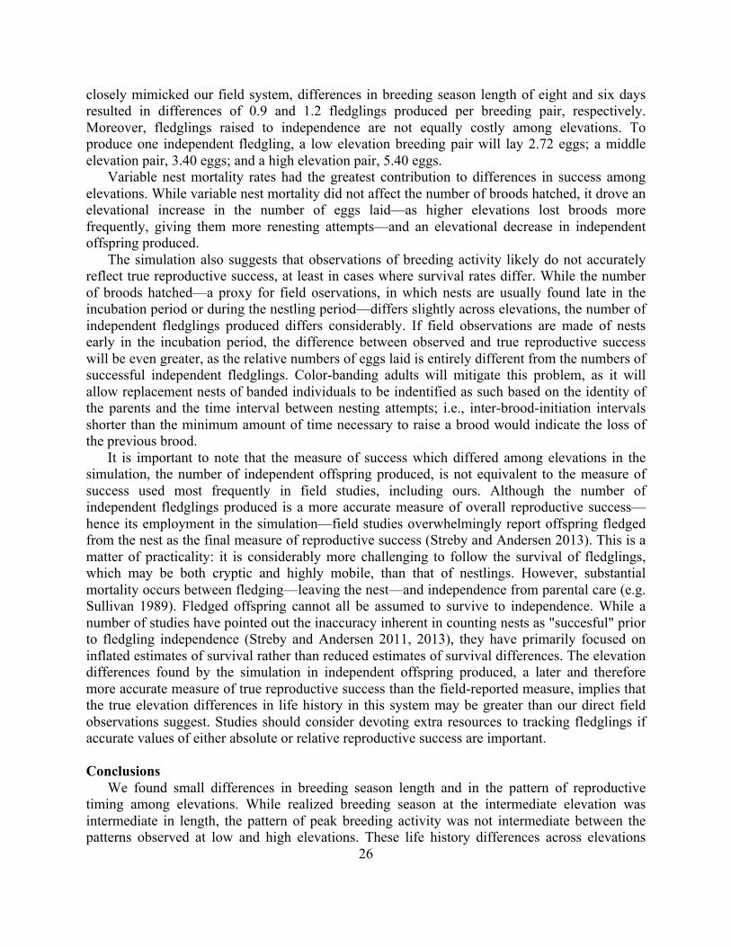
26

closely mimicked our field system, differences in breeding season length of eight and six days resulted in differences of 0.9 and 1.2 fledglings produced per breeding pair, respectively. Moreover, fledglings raised to independence are not equally costly among elevations. To produce one independent fledgling, a low elevation breeding pair will lay 2.72 eggs; a middle elevation pair, 3.40 eggs; and a high elevation pair, 5.40 eggs.

Variable nest mortality rates had the greatest contribution to differences in success among elevations. While variable nest mortality did not affect the number of broods hatched, it drove an elevational increase in the number of eggs laid—as higher elevations lost broods more frequently, giving them more renesting attempts—and an elevational decrease in independent offspring produced.

The simulation also suggests that observations of breeding activity likely do not accurately reflect true reproductive success, at least in cases where survival rates differ. While the number of broods hatched—a proxy for field oservations, in which nests are usually found late in the incubation period or during the nestling period—differs slightly across elevations, the number of independent fledglings produced differs considerably. If field observations are made of nests early in the incubation period, the difference between observed and true reproductive success will be even greater, as the relative numbers of eggs laid is entirely different from the numbers of successful independent fledglings. Color-banding adults will mitigate this problem, as it will allow replacement nests of banded individuals to be indentified as such based on the identity of the parents and the time interval between nesting attempts; i.e., inter-brood-initiation intervals shorter than the minimum amount of time necessary to raise a brood would indicate the loss of the previous brood.

It is important to note that the measure of success which differed among elevations in the simulation, the number of independent offspring produced, is not equivalent to the measure of success used most frequently in field studies, including ours. Although the number of independent fledglings produced is a more accurate measure of overall reproductive success—hence its employment in the simulation—field studies overwhelmingly report offspring fledged from the nest as the final measure of reproductive success (Streby and Andersen 2013). This is a matter of practicality: it is considerably more challenging to follow the survival of fledglings, which may be both cryptic and highly mobile, than that of nestlings. However, substantial mortality occurs between fledging—leaving the nest—and independence from parental care (e.g. Sullivan 1989). Fledged offspring cannot all be assumed to survive to independence. While a number of studies have pointed out the inaccuracy inherent in counting nests as "succesful" prior to fledgling independence (Streby and Andersen 2011, 2013), they have primarily focused on inflated estimates of survival rather than reduced estimates of survival differences. The elevation differences found by the simulation in independent offspring produced, a later and therefore more accurate measure of true reproductive success than the field-reported measure, implies that the true elevation differences in life history in this system may be greater than our direct field observations suggest. Studies should consider devoting extra resources to tracking fledglings if accurate values of either absolute or relative reproductive success are important.

Conclusions

We found small differences in breeding season length and in the pattern of reproductive timing among elevations. While realized breeding season at the intermediate elevation was intermediate in length, the pattern of peak breeding activity was not intermediate between the patterns observed at low and high elevations. These life history differences across elevations

27

could not be explained solely by abiotic factors, but may be related to the effects of those factors on the juncos' prey base, potentially exacerbated at lower elevations by the ongoing drought. We found no differences among elevations in clutch size, brood size, or nestling quality. Higher elevations had greater nest mortality, possibly due to severe weather. A simulation constructed to mimic the field system suggests that these mortality differences, in combination with the differences in breeding season length, contribute to substantial differences among elevations in reproductive success which may be difficult to observe in a field setting.

28

CHAPTER 2 TABLES AND FIGURES Table 1. High, middle, and low elevations differed significantly in maximum and minimum daily temperature and daily snow depth, but not in daily precipitation. 1Calculations are in comparison to high elevation. Variable Elevation1 Estimate±SE t-value p Min. temperature Middle 0.510±0.089 5.73 <0.001*

Low 5.70±0.097 58.6 <0.001* Max. temperature Middle 1.17±0.091 13.0 <0.001*

Low 3.84±0.099 38.8 <0.001* Precipitation Middle 0.227±0.140 1.63 0.103

Low 0.050±0.161 0.311 0.756 Snow depth Middle 0.028±0.006 4.43 <0.001*

Low -0.264±0.010 -27.79 <0.001* Table 2. Sample sizes of nests for each year or elevation range. Year or Elevation Clutch size

known Brood size known

Included in survival analysis

Total nests

2013 23 48 43 53 2014 25 38 35 46 2015 7 4 6 10 1960–2193 m 17 25 21 36 2194–2427 m 22 35 34 42 2428–2660 m 16 30 29 31 Total 55 90 84 109

29

Table 3. Mean ± SE reproductive success per agent at each of three elevations in simulation models with different attributes. Models were each run five times with 400 agents per elevation. The base model included different breeding season lengths at each elevation and a single nest mortality rate across elevations. Subsequent models add modifications: SSO = staggered season onset; LCR = late clutch size reduction; LBP = late breeding penalty; VM = variable daily nest mortality among elevations (high: 3.5%; middle: 2.5%; low: 2.0%). *This model was the most similar to the attributes observed in our field study system. Model Eggs laid Broods hatched Independent fledglings

Low Mid High Low Mid High Low Mid High Base 13.57±

0.03 12.52± 0.03

11.80± 0.02

2.47± 0.01

2.31±0.01 2.14±0.01 4.50±0.04 4.01±0.04 3.77±0.01

+ SSO 13.09± 0.03

11.99± 0.02

11.29± 0.02

2.38± 0.01

2.18±0.01 2.05±0.01 4.30±0.06 3.83±0.04 3.39±0.04

+ LCR

12.33± 0.05

11.09± 0.04

11.00± 0.04

2.47± 0.00

1.98±0.01 2.07±0.01 4.53±0.03 3.32±0.03 3.37±0.04

+ LBP

13.60± 0.03

12.56± 0.02

11.81± 0.04

2.48± 0.01

2.27±0.01 2.14±0.01 4.26±0.03 3.74±0.01 3.47±0.02

+ VM 12.63± 0.02

12.58± 0.02

13.30± 0.03

2.44± 0.01

2.27±0.01 2.13±0.00 5.10±0.03 4.16±0.04 2.87±0.02

+SSO, LBP, VM*

12.12± 0.03

11.96± 0.03

12.64± 0.03

2.36± 0.01

2.17±0.01 2.03±0.01 4.46±0.02 3.52±0.03 2.35±0.03

30

Figure 1. Decision tree depicting the process of simulating one agent, representing one breeding pair. At the beginning of the simulation, each agent is given a number of days (the length of its breeding season) based on its designated elevation. Each time a day passes, the number of days remaining to the agent is checked; if zero days remain, that agent stops. Additionally, each day, a certain number (determined by the mortality rate) of nests are lost; consequences of nest loss are shown in dashed arrows. SSO, staggered season onset; LCR, late clutch size reduction; LBP, late breeding penalty.

31

32

Figure 2. Daily minimum temperature decreased at higher elevations. Data shown with daily data points (a) and with best-fit lines only (b). a)

-30

-20

-10

0

10

20

-30

-20

-10

0

10

20

-30

-20

-10

0

10

20

1high2med

3low

2012-01 2012-07 2013-01 2013-07 2014-01 2014-07 2015-01time

Tmin

2000

2200

2400

2600

ELEVATION

0.20.2

33

b)

-10

-5

0

5

10

15

2012-01 2012-07 2013-01 2013-07 2014-01 2014-07 2015-01time

Tmin

Elev_cat1high

2med

3low

34

Figure 3. Daily maximum temperature decreased at higher elevations. Data shown with daily data points (a) and with best-fit lines only (b). a)

b)

-10

0

10

20

30

-10

0

10

20

30

-10

0

10

20

30

1high2med

3low

2012-01 2012-07 2013-01 2013-07 2014-01 2014-07 2015-01time

Tmax

2000

2200

2400

2600

ELEVATION

0.20.2

0

10

20

2012-01 2012-07 2013-01 2013-07 2014-01 2014-07 2015-01time

Tmax

Elev_cat1high

2med

3low

35

Figure 4. Patterns of monthly precipitation did not differ among elevations.

0

100

200

300

0

100

200

300

0

100

200

300

1high2med

3low

2012-01 2012-07 2013-01 2013-07 2014-01 2014-07 2015-01time

Precip_month

2000

2200

2400

2600

ELEVATION

0.80.8

36

Figure 5. Daily snow depth measures differed among elevations, with higher elevations experiencing greater snow depth.

0.0

0.5

1.0

1.5

2.0

0.0

0.5

1.0

1.5

2.0

0.0

0.5

1.0

1.5

2.0

1high2med

3low

2012-01 2012-07 2013-01 2013-07 2014-01 2014-07 2015-01time

(SNWD/1000)

2000

2200

2400

2600

ELEVATION

0.20.2

37

Figure 6. Kernel density plot of first hatch dates at low (blue dotted line), middle (green dashed line) and high (red solid line) elevations for the years 2013 and 2014.

120 140 160 180 200 220 240

0.000

0.005

0.010

0.015

0.020

Julian hatch date

Density

38

Figure 7. Clutch size (a) and brood size (b) were not significantly different among elevations. a)

b)

3.4

3.6

3.8

4.0

4.2

Means with 95% CI

Elevation

Clu

tch

size

1high 2mid 3low

n=16 n=22 n=17

3.0

3.2

3.4

3.6

3.8

4.0

Means with 95% CI

Elevation

Bro

od s

ize

1high 2mid 3low

n=30 n=35 n=25

39

Figure 8. Chick quality was not significantly related to elevation or hatchdate. Elevation is denoted by Hi (high), Mi (middle), or Lo (low); hatchdate by Ea (early) or La (late).

1HiEa 2HiLa 3MiEa 4MiLa 5LoEa 6LoLa

-0.05

0.00

0.05

Mass/Wing by Elevation & Hatchdate

Elevation

Mas

s/W

ing

resi

dual

s ag

ains

t age

40

Figure 9. Seasonal changes in habitat structure may affect junco nest site choices. Corn lilies early in the season (a) are too short to act as cover for nests. Later (b) they are a frequently-used cover for junco nests. (a)

(b)

41

Chapter 3: Extra-pair paternity and sexual selection in Dark-eyed Juncos (Junco hyemalis) breeding along an elevation gradient with substantial gene flow INTRODUCTION The selective forces operating on an individual depend upon the context. In the iconic example, a light-colored moth will experience different selective pressures in a forest of white-barked trees than it would in a forest of dark-barked trees (Kettlewell 1956). As environmental context changes, so does the strength and direction of the selective forces at work (e.g. density [Punzalan et al. 2010; Taff et al. 2013]; precipitation [Grant & Grant 1993]; female preferences [Chaine & Lyon 2008; Gosden & Svensson 2008]). The use of signals for communication among animals responds to variation in selective pressures (Badyaev & Qvarnström 2002). Geographic and temporal variation in the use of particular signals has been documented in several systems (e.g., House Sparrows [Solberg & Ringsby 1997]; Soay sheep [Robinson et al. 2008]; Lark Buntings [Chaine & Lyon 2008]), and this interpopulation variation in signal use is likely the result of a difference in contexts, with only some contexts producing selection favorable to signal use (Gosden & Svensson 2008; Elias et al. 2014). For example, the use of color signals in mate attraction varies with predation and environment in guppies (Endler 1995), and climate has been suggested to contribute to variation in the use of facial patterns in dominance signaling in the wasp Polistes dominulus (Tibbetts et al. 2011). In the case of sexually selected signals, the strength of sexual selection is expected to affect the use of the signals (Chaine & Lyon 2008).

Elevation gradients provide an opportunity to study the effects of environmental context while holding many other factors (e.g. latitude, species) constant. We utilized a series of sites at different elevations to explore the effects of environmental harshness, breeding synchrony, and number of offspring produced per season on two factors related to sexual selection: extra-pair paternity and the use of a male signal of quality. Extra-pair paternity, breeding synchrony, and sexual selection Extra-pair paternity, the siring of an offspring by a male other than the social mate of the offspring's mother, has the potential to increase the strength of sexual selection in socially monogamous birds by increasing the variance in male reproductive success (Webster et al. 2007; Balenger et al. 2009). Breeding synchrony—the degree of overlap of the fertile periods of females in a given population—is thought to potentially affect extra-pair paternity, although debate remains over whether greater breeding synchrony should lead to higher or lower frequencies of extra-pair paternity. Greater breeding synchrony might promote greater extra-pair paternity, and therefore stronger sexual selection, if the simultaneous displays of males facilitate female comparisons among them, enabling the females to more accurately select the best-quality genetic mates (Stutchbury and Morton 1995; Stutchbury 1998a, 1998b; but see Weatherhead and Yezerinac 1998). Alternatively, greater breeding synchrony might reduce extra-pair paternity, and weaken sexual selection, if males are constrained from seeking multiple mates by the need to guard their own mate during her fertile period (Birkhead and Biggins 1987; Westneat et al. 1990). Signals of quality and environmental conditions

One type of contextual variation that may affect signal use, particularly the use of signals of quality, is the degree to which the environment is challenging vs. hospitable (David et al. 2000;

42

Robinson et al. 2008). In a hospitable environment, most individuals may be able to afford the cost of producing or bearing a high-quality signal. Signal quality may therefore not be a highly accurate indicator of individual quality, receivers may not be willing to pay the costs of signal perception, and signal use will be disfavored (Guilford & Dawkins 1991; Candolin 2003). In contrast, as the environment becomes more challenging, more individuals will be limited in their investment in signals, and signal quality may become more strongly correlated with individual quality—i.e., more dependent upon the condition of the individual (David et al. 2000). As signals of quality become more reliable, the benefits to receivers of attending to them will increase (Guilford & Dawkins 1991; Candolin 2003). Increased receiver attention in turn increases the benefits of signaling for the sender (Candolin 2003). Therefore, one mechanism through which environmental conditions may have an effect on the use of signals of quality is if more challenging environments drive increased condition-dependence of signals of quality (David et al. 2000). METHODS Study species Overview The Dark-eyed Junco Junco hyemalis ("junco") is a common passerine bird found across North America from sea level to the subalpine tree line (Nolan et al. 2002). The broad geographic range of the junco means that juncos survive and reproduce under a variety of environmental conditions, making them well-suited to studies of environmental effects. During the spring and summer breeding season, male juncos defend territories and attract females. In the winter juncos form flocks with dominance hierarchies (Balph et al. 1979; Ketterson 1979). Thus, over the course of the year males experience selective pressures from both female choice (during breeding) and intrasexual competition (during breeding, over mates, and in winter over dominance rank). Tail white: a signal of quality Juncos possess dark grey tails with symmetrical white patches on the outer rectrices (Fig. 1a). Tail white is weakly sexually dimorphic, with males on average having larger areas of white on the tail (Balph et al. 1979; Ketterson 1979; Ferree 2013), and is highly variable among individuals (Holberton et al. 1989). Male courtship display includes tail-fanning, during which the white tail patches are especially visible (Enstrom et al. 1997). Tail white is sexually selected in males, with females preferring males with larger white patches (Hill et al. 1999; McGlothlin et al. 2005). Captive males fed a high-quality diet grew larger and brighter white patches than males fed a poor-quality diet, suggesting that tail white is a signal of male quality (McGlothlin et al. 2007).

Evidence suggests that the condition-dependence of tail white may be greater in more challenging environmental conditions. White patch size appeared to be more closely related to individual quality in poorly-fed captive males than in well-fed males (McGlothlin et al. 2007). A wild population that colonized a location with a milder climate experienced a reduction in both average tail white and in female preference for tail white after colonization (Price et al. 2008), as is predicted if the more hospitable environment caused the condition-dependence of the tail white signal to drop: as the benefits of attending to the signal decrease, females cease using the signal in mate choice, selective pressure for large tail white patches decreases, and other selective pressures (e.g. a cost of tail white [Price et al. 2008]) act unopposed.

43

Wing length: a correlate of quality Wing length has repeatedly been shown to be related to dominance in winter flocks, with longer-winged individuals achieving higher dominance ranks (Baker & Fox 1978; Balph et al. 1979; Ketterson 1979). Wing length is often used as a proxy for body size (Ketterson 1979; McGlothlin et al. 2005), but it is not simply reflective of mass (Helms et al. 1967). As tail white is a signal of quality and wing length is a proxy for quality, a correlation between tail white and wing length is expected. In a Virginia population of juncos, McGlothlin et al. (2005) showed that a combination of female choice and male-male competition create selective pressure for a correlation between tail white and wing length in males. Study location We performed field work at eight primary sites located in Stanislaus National Forest in the Sierra Nevada mountains, CA. These sites ranged in elevation from 1960 to 2660 m a.s.l. and exhibited marked elevational differences in climate, with higher elevations experiencing colder minimum and maximum daily temperatures, a longer period of time during which snow was present, and greater snow depth. Juncos breeding at higher elevations had shorter breeding seasons and, due to higher rates of nest mortality, produced fewer offspring per breeding season (Chapter 2).

In addition to our primary field sites, we also performed field work at several secondary sites (Table S5). These sites were selected to represent a variety of elevations as well as distances from our primary field sites.

Data collection Field work We visited each primary field site every 1-10 days throughout the breeding season (May-September) in 2013 and 2014. In 2015 we performed an abbreviated field season during 12-14 May and 14-19 July only. We visited secondary field sites opportunistically during spring and summer 2012 and spring 2016. We captured adults in mist nets using playback, took morphological measurements, collected approximately 50 µl of blood from the brachial vein for genetic analysis, photographed the tail (Fig. 1b), and banded them with unique combinations of one U.S. Fish and Wildlife aluminum band and either three (2013) or two (2014-2015) color bands of acetal or darvic.

We searched our primary field sites extensively for nests and recorded clutch size and/or brood size whenever possible. When nestlings were 8-13 days post-hatch we banded them with one aluminum and three color bands (2013) or one aluminum band only (2014), photographed them to document feather development, collected approximately 50 µl of blood from the brachial vein for genetic analysis, and took morphological measurements. Nestlings were replaced in the nest afterward. Young fledglings, not yet capable of strong flight, were occasionally caught by hand and were processed in the same manner as nestlings. Breeding synchrony index Our study system exhibits elevational differences in the temporal pattern of breeding activity (Chapter 2). To quantify these differences, we calculated a breeding synchrony index for each monitored nest in 2013–2014 following Kempenaers (1993); this synchrony index represents the proportion of all females in the population that were fertile during the focal female's fertile period. A synchrony index of zero indicates an asynchronous population with no overlap of

44

female fertile periods, while a synchrony index of one indicates a completely synchronous population. We assumed that females became fertile five days prior to the first egg date and remained fertile until they laid the penultimate egg, a common and well-supported assumption in passerine birds (Yezerinac and Weatherhead 1998). In cases where clutch size was unknown, we assumed it to be four (our mean observed clutch size). It is unlikely that we found all nests at each of our study locations; therefore our synchrony index is an approximation, since we cannot include all females in the system. However, assuming that the likelihood of our finding a nest is uncorrelated with the timing of the nest, the synchrony index should represent a valid relative measure of synchrony even if some nests were not found. Quantification of tail white Photographs of adult male tails were viewed and analysed in ImageJ64 (Schneider et al. 2012). The "select" tool was used to outline and measure the number of white pixels on a feather, which was divided by the total number of pixels on that feather to get the proportion of the feather surface that was white. Note that, as a proportion, this measure is independent of the absolute size of the image. These measurements were performed on the third, fourth, and fifth rectrices on both the left and right side of all individuals. An additional metric, tail white asymmetry, was calculated from these measurements as the absolute value of the difference between the proportions of white on the left and right fourth rectrices. Because the photos of the tails were taken while the researcher manually fanned the tail of the bird (rather than from feathers detached from the bird), the proportion of white visible in the photo is likely to be biologically relevant: portions of the feather that would not be visible in the normal course of display, such as the extreme base of the feather, were also not visible in our photographs. Genetic analyses We extracted DNA from whole blood using either Qiagen or Zymo DNA extraction kits. We amplified the DNA at 12 microsatellite loci (Table 1) using the following PCR protocol: 3 min at 94°C; then 30 cycles of 30 s at 94°C, 1 min at primer-specific annealing temperature Ta (see Table 1), and 90 s at 72°C; then 10 min at 72°C. We then genotyped the PCR products using an ABI 3730 DNA Analyzer (Applied Biosystems), estimating allele size with a GeneScan-500 LIZ size standard. We viewed the genotyping results on GeneMapper v. 3.7 (Applied Biosystems; see Table S6 for genetic data).

We performed paternity analysis in Cervus v. 3.0.3 (Kalinowski et al. 2007). We omitted data from one microsatellite locus (Mme7) because it was Z-linked, and Cervus does not recommend using sex-linked loci. We included known mothers in the analysis when possible, but in many cases we did not have genetic data for the mother. For broods for which the social father was known, we considered a brood to contain extra-pair paternity if Cervus assigned a male other than the social father to one or more of the offspring with 95% confidence. For broods for which the social father was not known, we considered a brood to contain extra-pair paternity if no single male genotype could have accounted for all broodmates' genotypes, assuming full siblingship, with two or fewer mismatches at two or fewer loci. This is a conservative measure, as broods with single paternity may also be extra-pair.

We used STRUCTURE v. 2.3.4 (Pritchard et al. 2000; Hubisz et al. 2009) to look for genetic structure among our populations using data from our 12 microsatellite loci. We included adults from both our primary and secondary field sites in our analysis. Our secondary field sites represented a variety of distances from our primary field sites, as well as elevational replicates of

45

several of our primary sites: this enabled us to look for isolation-by-distance and isolation-by-environment (Sexton et al. 2013). We assumed one, two, three, or four populations and ran admixture models with the following parameters: 25,000 burn-in period followed by 100,000 repetitions. We ran 10 replicates for each assumed number of populations and, within each set of 10 replicates, averaged the natural logarithm of the likelihood of our genetic data given the assumed population structure. Statistical analysis Statistical analyses were performed in R v. 3.2.4 (R Core Team 2016). To test for differences among elevations in amount of tail white and in the relationship between tail white and male quality, we ran linear models with elevation, male quality, tail length, and the elevation*male quality interaction as fixed effects, with either total tail white, mean fourth rectrix tail white, or tail white asymmetry as the response variable. We ran one set of analyses in which the proxy for male quality was wing chord, and a second set of analyses in which the proxy for male quality was the residuals from a linear regression of male mass against tarsus length. We included only males from our primary field sites in these analyses. RESULTS Breeding synchrony Synchrony indices did not significantly differ among elevations (Fig. 2a) or among broods with and without extra-pair paternity (Fig. 2b). Tail white Total tail white, mean fourth rectrix white, and tail white asymmetry were not significantly related to elevation, male quality, tail length, or the interaction between elevation and male quality (all p > 0.05). Sample size was 161 unique males measured (Table S7). Extra-pair paternity We were able to assign extra-pair or within-pair status to 51 broods containing 137 genotyped chicks. Of these broods, 21 (41%) contained at least one extra-pair chick. The proportion of extra-pair broods differed substantially among elevations (Table 2), with high elevations showing a significantly lower rate of extra-pair paternity than middle elevations (X-squared = 4.97, df = 1, p = 0.026). The rate of extra-pair paternity at low elevations was not significantly different from either high or middle elevations (p > 0.05). Genetic structure The single population models consistently had the highest probability, indicating that our genetic data do not exhibit spatial structure. Models assuming two, three, or four populations had lower probability and were unable to assign individuals to populations with any confidence (Fig. 3). DISCUSSION The frequency of extra-pair paternity (EPP) differed among elevations, with EPP being least common at high elevations and most common at middle elevations; low elevation sites were characterized by an intermediate rate of EPP that did not differ significantly from other elevations. In contrast, the size of white patches on males' tails did not differ with elevation, providing no evidence that sexual selection on this trait varied with rate of extra-pair paternity.

46

No genetic differentiation was evident among elevations, indicating that differences among EPP rates were not associated with significant differences in genetic substructure.

We found no evidence for genetic structure associated either with geographic distance or with elevation in our system, although both isolation by distance and isolation by environment are frequently found in vertebrates (Sexton et al. 2013) including birds (e.g. Foster et al. 2007; Caro et al. 2013; Habel et al. 2014; Ferrer et al. 2016). The lack of genetic structure in our study system implies the presence of substantial gene flow across elevations. It is therefore unlikely that differences among elevations in life history parameters and EPP reflect underlying differences in genotype in our system. Rather, differences among juncos breeding at different elevations are most likely due to local environmental conditions and their interactions with life history traits and reproductive biology (Boyle et al. 2016).

The finding that EPP rates were lowest at high elevations is consistent with a multi-species study of Emberizid sparrows (Bonier et al. 2014), although a study of Mountain Bluebirds Sialia corrucoides found no effect of elevation on EPP rates (Balenger et al. 2009). The expected general decrease in EPP with increasing elevation has been suggested to reflect either the greater breeding synchrony or the greater paternal care required at higher elevations (Badyaev and Ghalambor 2001; Bonier et al. 2014). In our system, differences in EPP rate cannot be attributed to differences in breeding synchrony, as breeding synchrony did not differ among elevations or among broods with and without extra-pair offspring. In our study system, offspring at higher elevations were not of higher quality (Chapter 2), suggesting that if male care is more extensive at higher elevations, this care is necessary to achieve offspring quality comparable to lower elevations. Clearly, however, more direct measures of male care are required to assess relationships among elevation and male care in juncos. More generally, support for the predicted relationship between paternity and paternal care (Winkler 1987) is inconsistent (reviewed in Alonzo 2010). Indeed, no consistent predictor of EPP rates has been found for passerines (Griffith et al. 2002; Westneat and Stewart 2003; Schmoll 2011), suggesting that the relationship between these variables is complex and is likely influenced by additional factors that may vary with elevation.

The significantly greater EPP rate at mid-elevation sites suggests that the strength of sexual selection on males may also be greater at middle elevations (Webster et al. 2007; Balenger et al. 2009). This is magnified by the differences between the elevations in reproductive success: the number of successful offspring per breeding pair is predicted to be > 30% greater at middle elevations than at high elevations (3.5 vs. 2.4; Chapter 2). The expected number of surviving extra-pair offspring should therefore also be greater at middle elevations, leading to greater potential variance in male reproductive success, and potentially stronger sexual selection.

Hwoever, our data on tail white do not support this predicted pattern of greater sexual selection at middle elevations. Although tail white is affected by diet quality (McGlothlin et al. 2007) and is displayed during courtship by males (Enstrom et al. 1997), and although female juncos have been repeatedly shown to prefer males with larger patches of tail white (Hill et al. 1999; McGlothlin et al. 2005), we found no evidence that tail white varied with elevation. It is possible that tail white does not function as a signal of quality in our system. The use of sexually-selected signals can vary even within a single species (Badyaev and Qvarnström 2002) and thus evidence indicating that tail white is sexually selected in other populations of juncos may not indicate that the same trait is used by members of our study system. Tail white is both sexually dimorphic and an indicator of age class in our study animals, with females having less tail white than males, and year-old males having less tail white than older males (K. LaBarbera,

47

pers. obs.). Boves et al. (2014) reported a similar age-specific pattern of tail white variation in the Cerulean Warbler Setophaga cerulea and suggested that signal honesty may be maintained by inherent physiological constraints during feather growth. This signal may therefore be maintained even in the absence of female preference for males with greater tail white. However, the rapid decrease in tail white in the San Diego juncos, and the fitness cost of large amounts of tail white reported there (Price et al. 2008), argues against tail white being a selectively neutral trait for male juncos.

This lack of clear evidence of elevational differences in sexual selection is perhaps not wholly surprising given the mobility of juncos. While breeding adults do exhibit philopatry, nestlings do not reliably return to their natal areas to breed (K. LaBarbera pers. obs.). Combined with the lack of genetic structure reported here, this vagility suggests that ongoing gene flow among elevations may be too great for differences in sexual selection pressures among elevations to generate phenotypic differences among males (Haldane 1930; Bolnick and Nosil 2007). The San Diego population of juncos that underwent rapid change in tail white due to novel environmental conditions (Price et al. 2008) is thought to have had little gene exchange with other junco populations (Yeh et al. 2004). Similarly, the collection of cardueline finch species in which reduced sexual dimorphism was found at higher elevations (Badyaev 1997b; Badyaev and Ghalambor 1998) were largely genetically isolated from one another. Collectively, these findings suggest that genetic isolation and the associated potential for genetic drift or strong local selection may be critical to the evolution of localized differences in sexually selected traits.

Conclusions

We report here that elevation differences in environment, several life history traits including number of offspring produced per year, and a sexual behavior (the frequency of extra-pair paternity) do not lead to differences in the strength of sexual selection as represented by a sexually-selected trait. We also find evidence for substantial gene flow among elevations. It may be that gene flow is too great in this system to permit divergence among elevations at the current strength of selection (Haldane 1930; Bolnick and Nosil 2007). Further research on the mechanisms of gene flow among differing environments in juncos might aid in illuminating why the junco thrives undifferentiated across a broad environmental range while other avian species show elevational divergence (Badyaev 1997b; Habel et al. 2014).

48

CHAPTER 3 TABLES AND FIGURES Table 1. Microsatellite loci used in the genetic analysis. Reverse primers were modified by the addition of a "pigtail" to the 5' end, as in Makarewich et al. (2009). Ta = annealing temperature during PCR. *This primer locus is Z-linked, so females have only one allele. This locus was used in population structure analysis but not in paternity analysis. Locus Forward 3' to 5' Reverse 5' to 3' Ta

(°C) Species of Origin

Reference

Cuµ28 GAGGCACAGA AATGTGAATT

TAAGTAGAAGGACTTG ATGGCT

55 Catharus ustulatus

Gibbs et al. 1999

Dpµ01 TGGATTCACA CCCCAAAATT

AGAAGTATATAGTGCC GCTTGC

55 Setophaga petechia

Dawson et al. 1997

Dpµ16 ACAGCAAGGT CAGAATTAAA

AACTGTTGTGTCTGAGCCT 63 Setophaga petechia

Dawson et al. 1997

Gf01b AGAGGAAAAA CTCCTGTGG

CTGCATGCAGACTGAA ATTCT

59 Geospiza fortis / Junco hyemalis

Petren 1998, Rasner et al. 2004

Gf05 AAACACTGGG AGTGAAGTCT

AACTATTCTGTGATCCTG TTACAC

56 Geospiza fortis

Petren 1998

Gf06 GCTATTGAGCTAAC TAAATAAACAACT

CACAAATAGTAATTAAAA GGAAGTACC

47 Geospiza fortis

Pentren 1998

Jh_mm4.1 TATCTGGTAA TGTCTCTTGTC

AATTCCTGGACATGAA TGAAG

58 Junco hyemalis

Price et al. 2008

Jh_mm4.2 GAATGAAAT TACTGGTGCATG

AGATAGGTAGAAGGCA GAAGC

60 Junco hyemalis

Price et al. 2008

Jh_mmA03 ATGCTCCCCG CTCTCTCCTGC

TGCATCAAGTCCTTGA AGCAC

63 Junco hyemalis

Gerlach et al. 2012

Jh_mmJu05 TGACCATGC CTTGGATATG

CATGGGAAACATGGA CACTG

63 Junco hyemalis

Gerlach et al. 2012

Mme7* TGCGAGCC TTTCCAAGTTTG

AACCCCACATGAAAC AGGTCAC

54 Melospiza melodia

Jeffery et al. 2001

Pdoµ3 CTGTTCATT AACTCACAGGT

AGTGAAACTTTAAT CAGTTG

44 Passer domesticus

Neumann & Wetton 1996

Table 2. Rates of extra-pair paternity differed among elevations. EP = extra-pair. Elevation Total broods EP broods % EP High 15 3 20% Mid 23 13 57% Low 13 5 38%

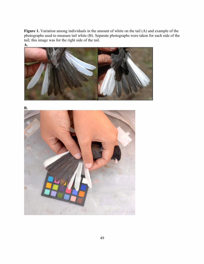
49

Figure 1. Variation among individuals in the amount of white on the tail (A) and example of the photographs used to measure tail white (B). Separate photographs were taken for each side of the tail; this image was for the right side of the tail. A.

B.

50

Figure 2. Breeding synchrony index did not significantly differ among elevations (A) or between broods with and without extra-pair offspring (B). A.

B.

1high 2mid 3low

0.00

0.05

0.10

0.15

0.20

0.25

0.30

Elevation

Bre

edin

g sy

nchr

ony

inde

x

N Y

0.00

0.05

0.10

0.15

0.20

0.25

0.30

EPP present?

Bre

edin

g sy

nchr

ony

inde

x

51

Figure 3. STRUCTURE plot showing the likelihood of each individual (one column per individual) belonging to either of two population groups, which are represented by red and green. The even probabilities indicate a lack of genetic structure. Population codes on the x-axis correspond to codes in Table S5.

52

REFERENCES Alcántara, J. M., and P. J. Rey. 2003. Conflicting selection pressures on seed size: evolutionary

ecology of fruit size in a bird-dispersed tree, Olea europaea. J Evol Biol 16:1168-1176. Alexander, H. J., J. S. Taylor, S. S. Wu, and F. Breden. 2006. Parallel evolution and vicariance in

the guppy (Poecilia reticulata) over multiple spatial and temporal scales. Evolution 60(11):2352-2369.

Alonzo, S. H. 2010. Social and coevolutionary feedbacks between mating and parental investment. Trends Ecol Evol 25:99-108.

Altamirano, T. A., J. T. Ibarra, M. de la Maza, S. A. Navarrete, and C. Bonacic. 2015. Reproductive life-history variation in a secondary cavity-nester across an elevational gradient in Andean temperate ecosystems. Auk 132(4):826-835.

American Ornithologists’ Union. 1998. Check-list of North American Birds, 7th ed. American Ornithologists’ Union, Washington, D.C.

Andersson, M. 1982. Sexual selection, natural selection and quality advertisement. Biol J Linn Soc 17:375-393.

Ardia, D. R. 2005. Super size me: An experimental test of the factors affecting lipid content and the ability of residual body mass to predict lipid stores in nestling European Starlings. Funct Ecol 19(3):414-420.

Arnold, J. M., J. J. Hatch, and I. C. T. Nisbet. 2004. Seasonal declines in reproductive success of the common tern Sterna hirundo: timing or parental quality? J Avian Biol 35(1):33-45.

Babin-Fenske, J., M. Anand, and Y. Alarie. 2008. Rapid morphological change in stream beetle museum specimens correlates with climate change. Ecol Entomol 33:646-651.

Badyaev, A. V. 1997a. Avian life history variation along altitudinal gradients: an example with cardueline finches. Oecologia 111(3):365-374.

Badyaev, A. V. 1997b. Altitudinal variation in sexual dimorphism: a new pattern and alternative hypotheses. Behav Ecol 8(6):675-690.

Badyaev, A. V., and C. K. Ghalambor. 1998. Does a trade-off exist between sexual ornamentation and ecological plasticity? Sexual dichromatism and occupied elevational range in finches. Oikos 82(2):319-324.

Badyaev, A. V., and C. K. Ghalambor. 2001. Evolution of life histories along elevational gradients: trade-off between parental care and fecundity. Ecology 82(10):2948-2960.

Badyaev, A. V., and A. Qvarnström. 2002. Putting sexual traits into the context of an organism: a life-history perspective in studies of sexual selection. Auk 19(2):301-310.

Badyaev, A. V., R. L. Young, K. P. Oh, and C. Addison. 2008. Evolution on a local scale: developmental, functional, and genetic bases of divergence in bill form and associated changes in song structure between adjacent habitats. Evolution 62(8):1951-1964.

Baker, C. M., and S. F. Fox. 1978. Dominance, survival, and enzyme polymorphism in Dark-eyed Juncos, Junco hyemalis. Evolution 32(4):697-711.

Balenger, S. L., L. S. Johnson, H. L. Mays Jr., and B. S. Masters. 2009. Extra-pair paternity in the socially monogamous mountain bluebird Sialia currucoides and its effect on the potential for sexual selection. J Avian Biol 40:173-180.

Ballentine, B. 2006. Morphological adaptation influences the evolution of a mating signal. Evolution 60(9):1936-1944.

Balmford, A. 1996. Extinction filters and current resilience: the significance of past selection pressures for conservation biology. Trends Ecol Evol 5347(5):193-196.

53

Balph, M. H., D. F. Balph, and H. C. Romesburg. 1979. Social status signaling in winter flocking birds: an examination of a current hypothesis. Auk 96(1):78-93.

Bartoń, K. 2015. MuMIn: Multi-Model Inference. R package version 1.13.4. http://CRAN.R-project.org/package=MuMIn

Bears, H., K. Martin, and G. C. White. 2009. Breeding in high-elevation habitat results in shift to slower life-history strategy within a single species. J Anim Ecol 78:365-375.

Birkhead, T. R., and J. D. Biggins. 1987. Reproductive synchrony and extra-pair copulation in birds. Ethology 74:320–334.

Bize, P., R. Piault, B. Moureau, and P. Heeb. 2006. A UV signal of offspring condition mediates context-dependent parental favouritism. Proc Roy Soc B Biol Sci 273(1597):2063-2068.

Boag, P. T., and P. R. Grant. 1978. Heritability of external morphology in Darwin's finches. Nature 274(24):793-794.

Bolnick, D. I., and P. Nosil. 2007. Natural selection in populations subject to a migration load. Evolution 61:2229–2243.

Bonier, F., C. Eikenaar, P. R. Martin, and I. T. Moore. 2014. Extrapair paternity rates vary with latitude and elevation in emberizid sparrows. Am Nat 183(1):54-61.

Boves, T. J., D. A. Buehler, P. B. Wood, A. D. Rodewald, J. L. Larkin, P. D. Keyser, and T. Ben Wigley. 2014. Multiple plumage traits convey information about age and within-age-class qualities of a canopy-dwelling songbird, the Cerulean Warbler. Auk 131:20-31.

Boyle, W. A., D. R. Norris, and C. G. Guglielmo. 2010. Storms drive altitudinal migration in a tropical bird. Proc R Soc B 277:2511-2519.

Boyle, W. A., B. K. Sandercock, and K. Martin. 2016. Patterns and drivers of intraspecific variation in avian life history along elevational gradients: A meta-analysis. Biol Rev 91:469-482.

Brooks, R., and J. A. Endler. 2001. Direct and indirect sexual selection and quantitative genetics of male traits in guppies (Poecilia reticulata). Evolution 55(5):1002-1015.

Burnham, K. P., and D. R. Anderson. 2002. Model selection and multimodal inference: a practical information—theoretic approach, 2nd edn. Springer-Verlag, New York.

Campbell-Tennant, D. J. E., J. L. Gardner, M. R. Kearney, and M. R. E. Symonds. 2015. Climate-related spatial and temporal variation in bill morphology over the past century in Australian parrots. J Biogeogr 42:1163-1175.

Candolin, U. 2003. The use of multiple cues in mate choice. Biol Rev 78(4):575-595. Caro, L. M., P. C. Caycedo-Rosales, R. C. K. Bowie, H. Slabbekoorn, and C. D. Cadena. 2013.

Ecological speciation along an elevational gradient in a tropical passerine bird? J Evol Biol 26(2):357-374.

Chaine, A. S., and B. E. Lyon. 2008. Adaptive plasticity in female mate choice dampens sexual selection on male ornaments in the lark bunting. Science 319(5862):459-462.

Danner, R. M., and R. Greenberg. 2015. A critical season approach to Allen's rule: bill size declines with winter temperature in a cold temperate environment. J Biogeogr 42(1):114-120.

David, P., T. Bjorksten, K. Fowler, and A. Pomiankowski. 2000. Condition-dependent signalling of genetic variation in stalk-eyed flies. Nature 406:186-188.

Dawson, R. J. G., H. L. Gibbs, K. A. Hobson, and S. M. Yezerinac. 1997. Isolation of microsatellite DNA markers from a passerine bird, Dendroica petechia (the yellow warbler), and their use in population studies. Heredity 79:506-514.

Decker, K. L., and C. J. Conway. 2009. Effects of an unseasonable snowstorm on Red-Faced Warbler nesting success. Condor 111(2):392-395.

54

Desrochers, A. 2010. Morphological response of songbirds to 100 years of landscape change in North America. Ecology 91(6):1577-1582.

Dillon, K. G., and C. J. Conway. 2015. Elevational gradient in clutch size of red-faced warblers. J Field Ornithol 86(2):163-172.

Elias, D. O., S. Sivalinghem, A. C. Mason, M. C. B. Andrade, and M. M. Kasumovic. 2014. Mate-guarding courtship behaviour: Tactics in a changing world. Anim Behav 97:25-33.

Endler, J. A. 1983. Natural and sexual selection on color patterns in poeciliid fishes. Environ Biol Fish 9(2):173-190.

Endler, J. 1995. Multiple-trait coevolution and environmental gradients in guppies. Trends Ecol Evol 10(1):22-29.

Enstrom, D. A., E. D. Ketterson, and V. Nolan. 1997. Testosterone and mate choice in the dark-eyed junco. Anim Behav 54:1135-1146.

Ferree, E. 2013. Geographic variation in morphology of Dark-eyed Juncos and implications for population divergence. Wilson J Ornithol 125(3):454-470.

Ferrer, E. S., V. García-Navas, J. Bueno-Enciso, R. Barrientos, E. Serrano-Davies, C. Cáliz-Campal, J. J. Sanz, and J. Ortego. 2016. The influence of landscape configuration and environment on population genetic structure in a sedentary passerine: Insights from loci located in different genomic regions. J Evol Biol 29:205-219.

Fisher, D. O., I. P. F. Owens, and C. N. Johnson. 2001. The ecological basis of life history variation in marsupials. Ecology 82(12):3531-3540.

Fleming, I. A., and M. R. Gross. 1994. Breeding competition in a Pacific salmon (Coho: Oncorhynchus kisutch): measures of natural and sexual selection. Evolution 48(3):637-657.

Foster, J. T., B. L. Woodworth, L. E. Eggert, P. J. Hart, D. Palmer, D. C. Duffy, and R. C. Fleischer. 2007. Genetic structure and evolved malaria resistance in Hawaiian honeycreepers. Mol Ecol 16:4738-4746.

Gerlach, N. M., J. W. McGlothlin, P. G. Parker, and E. D. Ketterson. 2012. Promiscuous mating produces offspring with higher lifetime fitness. Proc Roy Soc B: Biol Sci 279:860-866.

Gibbs, H. L., L. M. Tabak, and K. Hobson. 1999. Characterization of microsatellite DNA loci for a neotropical migrant songbird, the Swainson's thrush (Catharus ustulatus). Mol Ecol 8:1551-1561.

Gómez, J. M. 2004. Bigger is not always better: conflicting selective pressures on seed size in Quercus ilex. Evolution 58(1):71-80.

Goodman, K. R., J. P. Kelley, S. C. Welter, G. K. Roderick, and D. O. Elias. 2015. Rapid diversification of sexual signals in Hawaiian Nesosydne planthoppers (Hemiptera: Delphacidae): the relative role of neutral and selective forces. J Evol Biol 28:415-427.

Gosden, T. P., and E. I. Svensson. 2008. Spatial and temporal dynamics in a sexual selection mosaic. Evolution 62(4):845-856.

Grant, B. W., and A. E. Dunham. 1990. Elevational covariation in environmental constraints and life histories of the desert lizard Sceloporus merriami. Ecology 71(5):1765-1776.

Grant, B. R., and P. R. Grant. 1989. Natural selection in a population of Darwin's finches. Am Nat 133(3):377-393.

Grant, B. R., and P. R. Grant. 1993. Evolution of Darwin's finches caused by a rare climatic event. Proc R Soc Lond B Biol Sci 251(1331):111-117.

Grant, B. R., and P. R. Grant. 1996. High survival of Darwin's finch hybrids: effects of beak morphology and diets. Ecology 77(2):500-509.

55

Grant, P. R., and B. R. Grant. 2002. Unpredictable evolution in a 30-year study of Darwin's finches. Science 296:707-712.

Greenberg, R., V. Cadena, R. M. Danner, and G. Tattersall. 2012. Heat loss may explain bill size differences between birds occupying different habitats. PLoS ONE 7(7):e40933.

Greenberg, R., and R. M. Danner. 2012. The influence of the California marine layer on bill size in a generalist songbird. Evolution 66(12):3825-3835.

Griffin, D., and K. J. Anchukaitis. 2014. How unusual is the 2012 – 2014 California drought? Geophys Res Lett 41:9017-9023.

Griffith, S. C., I. P. F. Owens, and K. A. Thuman. 2002. Extra pair paternity in birds: a review of interspecific variation and adaptive function. Mol Ecol 11:2195-2212.

Guilford, T., and M. S. Dawkins. 1991. Receiver psychology and the evolution of animal signals. Anim Behav 42:1-14.

Guo, Q., Z. M. Hu, S. G. Li, X. R. Li, X. M. Li, and G. R. Yu. 2012. Spatial variations in aboveground net primary productivity along a climate gradient in Eurasian temperate grassland: Effects of mean annual precipitation and its seasonal distribution. Glob Change Biol 18:3624-3631.

Habel, J. C., W. Ulrich, G. Peters, M. Husemann, and L. Lens. 2014. Lowland panmixia versus highland disjunction: Genetic and bioacoustic differentiation in two species of East African White-eye birds. Conserv Genet 15:655-664.

Haldane, J. B. S. 1930. A mathematical theory of natural and artificial selection. (Part VI, Isolation.). Math Proc Cambridge 26:220–230.

Hansen, T. F., and S. H. Orzack. 2005. Assessing current adaptation and phylogenetic inertia as explanations of trait evolution: the need for controlled comparisons. Evolution 59(10):2063-2072.

Heinen-Kay, J. L., K. E. Morris, N. A. Ryan, S. L. Byerley, R. E. Venezia, M. N. Peterson, and R. B. Langerhans. 2015. A trade-off between natural and sexual selection underlies diversification of a sexual signal. Behav Ecol 26(2):533-542.

Helms, C. W., W. H. Aussiker, E. B. Bower, and S. D. Fretwell. 1967. A biometric study of major body components of the Slate-colored Junco, Junco hyemalis. Condor 69(6):560-578.

Herrel, A., J. Podos, S. K. Huber, and A. P. Hendry. 2005. F Bite performance and morphology in a population of Darwin's finches: implications for the evolution of beak shape. Funct Ecol 19(1):43-48.

Hill, J. A., D. A. Enstrom, E. D. Ketterson, V. Nolan, and C. Ziegenfus. 1999. Mate choice based on static versus dynamic secondary sexual traits in the dark-eyed junco. Behav Ecol 10(1):91-96.

Holberton, R. L., K. P. Able, J. C. Wingfield. 1989. Status signalling in dark-eyed juncos, Junco hyemalis: plumage manipulations and hormonal correlates of dominance. Anim Behav 37:681-689.

Hubisz, M. J., D. Falush, M. Stephens, and J. K. Pritchard. 2009. Inferring weak population structure with the assistance of sample group information. Mol Ecol Resources 9:1322-1332.

Jeffery, K. J., L. F. Keller, P. Arcese, and M. W. Bruford. 2001. The development of microsatellite loci in the song sparrow, Melospiza melodia (Aves) and genotyping errors associated with good quality DNA. Mol Ecol Notes 1:11-13.

Jepson Flora Project (eds.). 2013. Jepson eFlora, http://ucjeps.berkeley.edu/IJM.html. Accessed on December 11 2013.

56

Jeschke, J., and H. Kokko. 2009. The roles of body size and phylogeny in fast and slow life histories. Evol Ecol 23:867-878.

Johnson, L. S., J. L. Brubaker, E. Ostlind, and S. L. Balenger. 2007. Effect of altitude on male parental expenditure in Mountain Bluebirds (Sialia currucoides): are higher-altitude males more attentive fathers? J Ornithol 148:9-16.

Johnson, L. S., E. Ostlind, J. L. Brubaker, S. L. Balenger, B. G. P. Johnson, and H. Golden. 2006. Changes in egg size and clutch size with elevation in a Wyoming population of Mountain Bluebirds. Condor 108:591-600.

Kalinowski, S. T., M. L. Taper, and T. C. Marshall. 2007. Revising how the computer program CERVUS accommodates genotyping error increases success in paternity assignment. Mol Ecol 16:1099-1106.

Kempanaers, B. 1993. The use of a breeding synchrony index. Ornis Scandinavica 24(1):84. Ketterson, E. D. 1979. Aggressive behavior in wintering Dark-eyed Juncos: determinants of

dominance and their possible relation to geographic variation in sex ratio. Wilson Bull 91(3):371-383.

Ketterson, E. D., and V. Nolan Jr. 1982. The role of migration and winter mortality in the life history of a temperate-zone migrant, the Dark-eyed Junco, as determined from demographic analyses of winter populations. Auk 99(2):243-259.

Kettlewell, H. B. D. 1956. Further selection experiments on industrial melanism in the Lepidoptera. Heredity 10(3):287-301.

Krementz, D. G., and P. Handford. 1984. Does avian clutch size increase with altitude? Oikos 43(2):256-259.

Lack, D. 1947. The significance of clutch size. Ibis 89:302-352. Makarewich, C. A., L. M. Stenzler, V. Ferretti, D. W. Winkler, and I. J. Lovette. 2009. Isolation

and characterization of microsatellite markers from three species of swallows in the genus Tachycineta: T. albilinea, T. bicolor and T. leucorrhoa. Mol Ecol Resources 9:631-635.

Matthysen, E. 1989. Seasonal variation in bill morphology of nuthatches Sitta europaea: dietary adaptations or consequences? Ardea 77:117-125.

Mayfield, H. F. 1975. Suggestions for calculating nest success. Wilson Bull 87:456-466. McGlothlin, J. W., D. L. Duffy, J. L. Henry-Freeman, and E. D. Ketterson. 2007. Diet quality

affects an attractive white plumage pattern in dark-eyed juncos (Junco hyemalis). Behav Ecol and Sociobiol 61(9):1391-1399.

McGlothlin, J. W., P. G. Parker, V. Nolan, E. D. Ketterson. 2005. Correlational selection leads to genetic integration of body size and an attractive plumage trait in Dark-eyed Juncos. Evolution 59(3):658-671.

McKechnie, A. E., and B. O. Wolf. 2010. Climate change increases the likelihood of catastrophic avian mortality events during extreme heat waves. Biol Lett 6:253-256.

Neumann, K., and J. H. Wetton. 1996. Highly polymorphic microsatellites in the house sparrow Passer domesticus. Mol Ecol 5:307-309.

Nolan, Jr., V., E. D. Ketterson, D. A. Cristol, C. M. Rogers, E. D. Clotfelter, R. C. Titus, S. J. Schoech, and E. Snajdr. 2002. Dark-eyed Junco (Junco hyemalis), The Birds of North America Online (A. Poole, Ed.). Ithaca: Cornell Lab of Ornithology. Available at bna.birds.cornell.edu/bna/species/716. Accessed July 10, 2015.

Nudds, R. L., and S. A. Oswald. 2007. An interspecific test of Allen's Rule: evolutionary implications for endothermic species. Evolution 61(12):2839-2848.

57

Owens, I. P. F., and P. M. Bennett. 1994. Mortality costs of parental care and sexual dimorphism in birds. Proc R Soc Lond B Biol Sci 257:1-8.

Parmesan, C., and G. Yohe. 2003. A globally coherent fingerprint of climate change impacts across natural systems. Nature 421(6918):37-42.

Petren, K. 1998. Microsatellite primers from Geospiza fortis and cross-species amplification in Darwin's finches. Mol Ecol 7:1771-1788.

Price, T. 1987. Diet variation in a population of Darwin's finches. Ecology 68(4):1015-1028. Price, T. D., P. J. Yeh, and B. Harr. 2008. Phenotypic plasticity and the evolution of a socially

selected trait following colonization of a novel environment. American Naturalist 172(S1):S49-S62.

PRISM Climate Group. Oregon State University. Available at http://prism.oregonstate.edu. Accessed February 3, 2015.

Pritchard, J. K., M. Stephens, and P. Donnelly. 2000. Population structure using multilocus genotype data. Genetics 155:945-959.

Punzalan, D., F. H. Rodd, and L. Rowe. 2010. Temporally variable multivariate sexual selection on sexually dimorphic traits in a wild insect population. Am Nat 175(4):401-414.

R Core Team. 2016. R: A language and environment for statistical computing. R Foundation for Statistical Computing, Vienna, Austria. http://www.R-project.org/.

Rasner, C. A., P. Yeh, L. S. Eggert, K. E. Hunt, D. S. Woodruff, and T. D. Price. 2004. Genetic and morphological evolution following a founder event in the dark-eyed junco, Junco hyemalis thurberi. Mol Ecol 13:671-681.

Reznick, D., M. J. Bryant, and F. Bashey. 2002. r- and K-selection revisited: the role of population regulation in life-history evolution. Ecology 83(6):1509-1520.

Ricklefs, R. E., and M. Wikelski. 2002. The physiology/life-history nexus. Trends in Ecol Evol 17(10):462-468.

Robinson, W. D., M. Hau, K. C. Klasing, M. Wikelski, J. D. Brawn, S. H. Austin, C. E. Tarwater, R. E. Ricklefs. 2010. Diversification of life histories in New World birds. Auk 127(2):253-262.

Robinson, M. R., J. G. Pilkington, T. H. Clutton-Brock, J. M. Pemberton, and L. E. B. Kruuk. 2008. Environmental heterogeneity generates fluctuating selection on a secondary sexual trait. Curr Biol 18(10):751-757.

Rohr, J. R., D. M. Madison, and A. M. Sullivan. 2003. On temporal variation and conflicting selection pressures: a test of theory using newts. Ecology 84(7):1816-1826.

Schluter, D., T. D. Price, and L. Rowe. 1991. Conflicting selection pressures and life history trade-offs. Proc R Soc Lond B Biol Sci 246(1315):11-17.

Schmoll, T. 2011. A review and perspective on context-dependent genetic effects of extra-pair mating in birds. J Ornithol 152(S1):265-277.

Schneider, C.A., W. S. Rasband, and K. W. Eliceiri. 2012. NIH Image to ImageJ: 25 years of image analysis. Nature Methods 9: 671-675.

Schulte-Hostedde, A. I., B. Zinner, J. S. Millar, and G. J. Hickling. 2005. Restitution of mass-size residuals: validating body condition indices. Ecology 86(1):155-163.

Sexton, J. P., S. B. Hangartner, and A. A. Hoffman. 2013. Genetic isolation by environment or distance: Which pattern of gene flow is most common? Evolution 68:1-15.

Shiao, M., M. Chuang, H. Yuan, and Y. Wang. 2015. Effects of weather variation on the timing and success of breeding in two cavity-nesting species in a subtropical montane forest in Taiwan. Auk 132(3):671-684.

58

Sillett, T. S., and R. T. Holmes. 2002. Variation in survivorship of a migratory songbird throughout its annual cycle. J Anim Ecol 71(2):296-308.

Smith, K. G., and D. C. Andersen. 1982. Food, predation, and reproductive ecology of the Dark-eyed Junco in Northern Utah. Auk 99(4):650-661.

Smith, K. G., and D. C. Andersen. 1985. Snowpack and variation in reproductive ecology of a montane ground-nesting Passerine, Junco hyemalis. Ornis Scandinavica 16:8-13.

Solberg, E. J., and T. H. Ringsby. 1997. Does male badge size signal status in small island populations of House Sparrows, Passer domesticus? Ethology 103(3):177-186.

Staudinger, M., M. Weiler, and J. Seibert. 2015. Quantifying sensitivity to droughts – an experimental modeling approach. Hydrol Earth Syst Sci 19:1371-1384.

Streby, H. M., and D. E. Andersen. 2011. Seasonal productivity in a population of migratory songbirds: why nest data are not enough. Ecosphere 2(7):1-15.

Streby, H. M., and D. E. Andersen. 2013. Testing common assumptions in studies of songbird nest success. Ibis 155:327-337.

Stutchbury, B. J., and E. S. Morton. 1995. The effect of breeding synchrony on extra-pair mating systems in songbirds. Behaviour 132:675–690.

Stutchbury, B. J. M. 1998a. Breeding synchrony best explains variation in extra-pair mating system among avian species. Behav Ecol Sociobiol 43:221–222.

Stutchbury, B. J. M. 1998b. Female mate choice of extra-pair males: breeding synchrony is important. Behav Ecol Sociobiol 43: 213–215.

Sullivan, K. A. 1989. Predation and starvation: age-specific mortality in juvenile juncos (Junco phaenotus). J Anim Ecol 58:275-286.

Swanson, D. L. 1991. Seasonal adjustments in metabolism and insulation in the Dark-eyed Junco. Condor 93(3):538-545.

Symonds, M. R. E., and Tattersall G. J. 2010. Geographical variation in bill size across bird species provides evidence for Allen's rule. Am Nat 176(2):188-197.

Taff, C. C., C. R. Freeman-Gallant, P. O. Dunn, L. A. Whittingham. 2013. Spatial distribution of nests constrains the strength of sexual selection in a warbler. J Evol Biol 26(7):1392-1405.

Templeton, C. N., and W. M. Shriner. 2004. Multiple selection pressures influence Trinidadian guppy (Poecilia reticulata) antipredator behavior. Behav Ecol 15(4):673-678.

Tibbetts, E. A., O. Skaldina, V. Zhao, A. L. Toth, M. Skaldin, L. Beani, and J. Dale. 2011. Geographic variation in the status signals of Polistes dominulus paper wasps. PLoS ONE 6(12): e28173. doi:10.1371/journal.pone.0028173

Tingley, M. W., M. S. Koo, C. Moritz, A. C. Rush, and S. R. Beissinger. 2012. The push and pull of climate change causes heterogeneous shifts in avian elevational ranges. Global Change Biol 18:3279-3290.

Verhulst, S., and J. Nilsson. 2008. The timing of birds' breeding seasons: a review of experiments that manipulated timing of breeding. Phil Trans Roy Soc B 363:399-410.

Waring, E. F., and D. W. Schwilk. 2014. Plant dieback under exceptional drought driven by elevation, not by plant traits, in Big Bend National Park, Texas, USA. PeerJ 2:e477.

Weatherhead, P. J., and S. M. Yezerinac. 1998. Breeding synchrony and extra-pair mating in birds. Behav Ecol Sociobiol 43(3):217-219.

Webster, M. S., K. A. Tarvin, E. M. Tuttle, and S. Pruett-Jones. 2007. Promiscuity drives sexual selection in a socially monogamous bird. Evolution 61(9):2205-2211.

Westneat, D. F., P. W. Sherman, and M. L. Morton. 1990. The ecology and evolution of extra-pair copulations in birds. Curr Ornithol 7: 331–369.

59

Westneat, D. F, and I. R. K. Stewart. 2003. Extra-pair paternity in birds: causes, correlates, and conflict. Ann Rev Ecol Evol Syst 34(1):365-396.

White, J. M. 1973. Breeding biology and feeding patterns of the Oregon Junco in two Sierra Nevada habitats. Ph.D. dissertation, Univ of California, Berkeley.

Wilensky, U. 1999. NetLogo. http://ccl.northwestern.edu/netlogo/. Center for Connected Learning and Computer-Based Modeling, Northwestern University. Evanston, IL.

Wilson, S., and K. Martin. 2005. Songbird use of high-elevation habitat during the fall post-breeding and migratory periods. Ecoscience 12(4):561-568.

Winkler, D. W. 1987. A general model for parental care. Am Nat 130:526–543. Yeh, P. J., and T. D. Price. 2004. Adaptive phenotypic plasticity and the successful colonization

of a novel environment. American Naturalist 164(4):531-542.

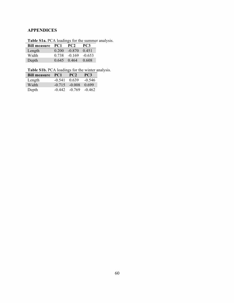
60

APPENDICES Table S1a. PCA loadings for the summer analysis. Bill measure PC1 PC2 PC3 Length 0.200 -0.870 0.451 Width 0.738 -0.169 -0.653 Depth 0.645 0.464 0.608 Table S1b. PCA loadings for the winter analysis. Bill measure PC1 PC2 PC3 Length -0.541 0.639 -0.546 Width -0.715 -0.008 0.699 Depth -0.442 -0.769 -0.462

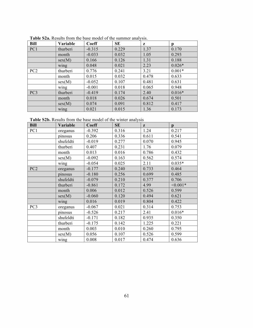
61

Table S2a. Results from the base model of the summer analysis. Bill Variable Coeff SE z p PC1 thurberi -0.315 0.229 1.37 0.170 month -0.033 0.032 1.05 0.293 sex(M) 0.166 0.126 1.31 0.188 wing 0.048 0.021 2.23 0.026* PC2 thurberi 0.776 0.241 3.21 0.001* month 0.015 0.032 0.478 0.633 sex(M) -0.052 0.107 0.481 0.631 wing -0.001 0.018 0.065 0.948 PC3 thurberi -0.419 0.174 2.40 0.016* month 0.018 0.026 0.674 0.501 sex(M) 0.074 0.091 0.812 0.417 wing 0.021 0.015 1.36 0.173 Table S2b. Results from the base model of the winter analysis Bill Variable Coeff SE z p PC1 oreganus -0.392 0.316 1.24 0.217 pinosus 0.206 0.336 0.611 0.541 shufeldti -0.019 0.277 0.070 0.945 thurberi 0.407 0.231 1.76 0.079 month 0.013 0.016 0.786 0.432 sex(M) -0.092 0.163 0.562 0.574 wing -0.054 0.025 2.11 0.035* PC2 oreganus -0.177 0.240 0.733 0.464 pinosus -0.180 0.256 0.699 0.485 shufeldti -0.079 0.210 0.377 0.706 thurberi -0.861 0.172 4.99 <0.001* month 0.006 0.012 0.526 0.599 sex(M) -0.060 0.120 0.494 0.621 wing 0.016 0.019 0.804 0.422 PC3 oreganus -0.067 0.021 0.314 0.753 pinosus -0.526 0.217 2.41 0.016* shufeldti -0.171 0.182 0.935 0.350 thurberi -0.175 0.142 1.225 0.221 month 0.003 0.010 0.260 0.795 sex(M) 0.056 0.107 0.526 0.599 wing 0.008 0.017 0.474 0.636

62

Table S3a. Relative importance of variables in the summer analysis. This table presents only variables that appeared in the confidence set of best-supported models. Bill Variable Rel. Importance Coeff SE PC1 — — — — PC2 CW 1.0 -0.047 0.485 DMoj 1.0 1.930 0.681 DSon 1.0 0.815 1.067 GV 1.0 0.835 0.594 MP 1.0 -0.018 0.515 NW 1.0 -0.478 0.368 SN 1.0 -0.134 0.429 SNE 1.0 0.681 0.534 SW 1.0 0.535 0.660 Tmax(10yrs) 0.34 -0.025 0.054 Tmax(5yrs) 0.30 -0.014 0.051 Tmax(1yr) 0.17 -0.010 0.023 Tsd(10yrs) 0.16 0.027 0.076 Tmin(5yrs) 0.05 -0.003 0.016 Pptn(10yrs) 0.04 0.001 0.003 Tmin(10yrs) 0.03 -0.002 0.013 Tmin(1yr) 0.03 -0.002 0.011 PC3 Tsd(10yrs) 0.10 0.008 0.032 Tmin(10yrs) 0.09 -0.003 0.012 Table S3b. Relative importance of variables in the winter analysis. This table presents only variables that appeared in the confidence set of best-supported models. Bill Variable Rel. Importance Coeff SE PC1 CW 0.55 -0.609 0.745 DMoj 0.55 -0.756 1.004 DSon 0.55 -0.662 1.128 GV 0.55 -0.434 0.547 MP 0.55 -0.191 0.537 NW 0.55 -0.222 0.515 SN 0.55 -0.766 0.809 SNE 0.55 -1.520 1.511 SW 0.55 -0.609 0.900 Tsd(10yrs) 0.51 0.232 0.291 PC2 Tsd(10yrs) 0.25 0.077 0.168 Tmax(1yr) 0.10 -0.006 0.019 Tmin(1yr) 0.10 -0.006 0.019 Tmin(10yrs) 0.09 -0.006 0.021 Tmin(5yrs) 0.08 -0.005 0.018 PC3 Tsd(10yrs) 0.13 0.014 0.064

63

Table S4. Weather stations from which data was used. Data provided courtesy of the National Climatic Data Center, part of the National Oceanic and Atmospheric Administration (NOAA). Elev. = elevation. Station name

Station ID Latitude Longitude Elevation (m)

Elev. bin

Spratt Creek GHCND:USS0019L39S 38.67 -119.82

1864 low

Yosemite Village 12 W

GHCND:USW00053150

37.7592 -119.8208

2018 low

Crane Flat Lookout

GHCND:USR0000CCRA 37.7617 -119.8247

2025 low

Poison Flat GHCND:USS0019L06S 38.51 -119.63

2358 med

Forestdale Creek

GHCND:USS0019L43S 38.68 -119.96

2444 med

White Wolf GHCND:USR0000CWWO 37.8511 -119.65

2446 med

Blue Lakes GHCND:USS0019L05S 38.61 -119.92

2456 med

Burnside Lake

GHCND:USS0019L41S 38.72 -119.89

2478 high

Monitor Pass

GHCND:USS0019L40S 38.67 -119.61

2533 high

Carson Pass GHCND:USS0019L45S 38.69 -119.99

2546 high

Horse Meadow

GHCND:USS0019L44S 38.84 -119.89

2608 high

Tuolumne Meadows Ranger Station

GHCND:USC00049063

37.8769 -119.3436

2650 high

Ebbetts Pass GHCND:USS0019L19S 38.55 -119.8

2672 high

64

Figure S1. Kernel density plot of first hatch dates at low (blue dotted line), middle (green dashed line) and high (red solid line) elevations for the years 2013 and 2014, separated by habitat: (a) meadow habitat; (b) forest habitat. High-elevation forest sample size is low; interpret this curve with caution. (a)

(b)

140 160 180 200 220 240

0.000

0.005

0.010

0.015

0.020

0.025

Julian hatch date

Density

140 160 180 200 220

0.000

0.005

0.010

0.015

0.020

0.025

Julian hatch date

Density

65

Table S5. Locations from which blood was collected from adult Dark-eyed Juncos for inclusion in the analysis of genetic structure. Locations marked with an asterisk (*) were primary field sites, at which substantial additional field work was conducted. Location codes correspond to codes used in Figure 3. Code Site name Latitude Longitude County Year(s) active 1 Berkeley N 32°52.309' W 122°15.783' Alameda 2016 2 Los Altos N 37°23.083' W 122°06.883' Santa Clara 2016 3 Pines N 37°49.163' W 120°05.677' Tuolumne 2012 4 Fraser Flat N 38°10.165' W 120°04.345' Tuolumne 2012 10 Sheep Ranch N 38°11.953' W 120°23.889' Calaveras 2013-2015 11 P10 N 38°19.543' W 120°14.673' Calaveras 2013 12 P7* N 38°22.541' W 120°11.625' Calaveras 2013-2015 13 Stanislaus River* N 38°25.325' W 120°02.907' Calaveras 2012-2015 14 Logged* N 38°24.434' W 120°02.297' Calaveras 2014-2015 15 Utica Reservoir* N 38°25.544' W 120°00.796' Calaveras 2012-2015 16 Lake Alpine* N 38°28.653' W 120°00.422' Alpine 2013-2015 17 P5* N 38°29.223' W 119°59.154' Alpine 2013-2015 18 Mosquito Lake* N 38°30.987' W 119°54.864' Alpine 2013-2015 19 P2 N 38°32.517' W 119°53.253' Alpine 2013 20 Ebbetts* N 38°32.667' W 119°48.717' Alpine 2013-2015 30 Tioga Lakes N 37°56.376' W 119°14.458' Mono 2012 31 Saddlebag N 37°57.351' W 119°16.023' Mono 2012 32 Rock Creek N 37°25.886' W 118°44.806' Mono 2012 33 Pack Station N 37°27.290' W 118°44.446' Mono 2012

66

Table S6. Microsatellite allele data. The site codes correspond to codes used in Figure 3 and Table S5. The table is broken into two parts: a) first six microsatellite loci, and b) remaining six microsatellite loci. *This primer locus is Z-linked, so females have only one allele. This locus was used in population structure analysis but not in paternity analysis. a) ID Site Sex Cuµ28 Dpµ01 Dpµ16 Gf01b Gf05 Gf06 16-001 1 M 172, 177 143, 143 161, 161 237, 238 198, 226 190, 190 16-002 1 M 174, 174 143, 143 163, 165 217, 231 215, 226 190, 190 16-003 2 M 171, 181 143, 143 161, 169 237, 240 213, 220 190, 190 16-004 2 F 172, 179 143, 156 161, 161 231, 252 220, 226 190, 190 12-016 3 M 172, 174 176, 180 161, 165 245, 251 213, 231 188, 205 12-017 3 M 172, 173 143, 143 163, 165 239, 242 206, 226 188, 190 12-018 3 M 187, 187 143, 143 163, 165 237, 250 218, 222 190, 200 12-019 3 M 187, 187 143, 154 161, 161 224, 237 NA, NA 198, 203 12-020 3 M 174, 185 143, 143 161, 161 237, 250 211, 218 188, 190 12-021 3 M 177, 189 143, 143 161, 163 242, 249 213, 220 190, 200 12-022 3 M 172, 174 143, 143 161, 169 237, 251 209, 215 190, 198 12-023 3 M 169, 177 143, 165 161, 161 249, 262 206, 209 190, 190 12-057 3 M 172, 174 143, 156 161, 165 237, 242 200, 224 190, 198 12-058 3 M 174, 181 143, 143 161, 161 235, 257 209, 231 190, 190 12-059 3 F 174, 187 152, 175 161, 163 231, 238 215, 218 190, 200 12-011 4 M 174, 174 143, 143 161, 161 235, 242 206, 231 190, 201 12-012 4 M 169, 174 143, 143 159, 165 235, 254 206, 215 190, 207 12-013 4 M 169, 170 165, 190 159, 163 239, 246 209, 231 190, 190 12-014 4 M 169, 169 139, 139 157, 159 245, 257 218, 237 190, 192 12-015 4 F 172, 172 162, 165 161, 169 232, 246 229, 237 196, 205 12-024 4 M 179, 181 143, 143 159, 161 237, 237 220, 233 190, 196 12-025 4 M 172, 207 143, 179 161, 175 238, 256 204, 222 190, 198 12-071 4 F 174, 187 143, 143 157, 161 232, 250 222, 229 190, 190 13-117 10 M 179, 181 139, 148 161, 163 235, 247 218, 222 190, 200 13-118 10 M 172, 176 143, 143 161, 161 229, 254 215, 222 192, 196 13-119 10 M 162, 169 142, 142 161, 165 237, 241 204, 235 190, 190 13-120 10 M 172, 172 143, 156 161, 165 237, 251 220, 231 190, 190 14-001 10 M 187, 187 143, 143 161, 161 231, 235 206, 209 190, 190 14-002 10 M 176, 187 177, 181 161, 161 224, 240 220, 229 190, 190 13-121 11 M 162, 177 141, 143 159, 163 242, 258 209, 220 190, 190 13-122 11 M 170, 185 143, 143 161, 163 235, 248 213, 224 190, 190 13-123 11 M 179, 185 143, 143 161, 163 232, 242 218, 237 190, 190 13-124 11 M 172, 174 143, 156 161, 163 240, 262 211, 222 190, 190 13-125 11 M 187, 197 143, 143 163, 165 229, 235 202, 224 190, 192

67

13-126 11 M 181, 203 167, 167 161, 165 241, 250 209, 218 188, 190 13-127 11 M 169, 172 171, 171 161, 173 238, 245 215, 237 190, 196 13-140 11 M 170, 176 143, 143 163, 167 250, 256 215, 229 190, 196 13-141 11 M 172, 172 139, 143 161, 165 231, 250 226, 229 190, 196 13-001 12 F 172, 172 143, 156 161, 163 235, 237 207, 229 190, 196 13-002 12 F 172, 179 NA, NA 165, 165 235, 237 204, 222 190, 190 13-041 12 M 175, 175 139, 143 161, 169 245, 249 211, 222 190, 190 13-042 12 M 172, 174 143, 143 159, 161 229, 235 211, 218 190, 190 13-043 12 M 175, 175 143, 148 161, 165 229, 235 218, 224 190, 200 13-044 12 M 181, 181 175, 175 161, 163 239, 251 204, 204 190, 190 13-045 12 M 177, 179 143, 156 159, 163 239, 241 204, 224 190, 190 13-046 12 M 183, 183 143, 143 161, 161 262, 267 207, 209 190, 190 13-047 12 M 174, 174 143, 143 165, 167 231, 252 211, 215 190, 190 13-048 12 M 169, 172 143, 143 159, 173 232, 237 220, 240 188, 188 13-049 12 M 169, 181 143, 143 161, 165 242, 272 213, 222 190, 192 13-050 12 M 172, 174 173, 181 161, 163 238, 248 213, 218 190, 190 13-051 12 M 172, 174 143, 143 163, 167 237, 250 202, 231 181, 190 13-052 12 M 172, 185 143, 143 154, 161 224, 254 200, 226 190, 198 13-053 12 M 177, 177 143, 143 159, 161 242, 251 221, 235 192, 200 14-003 12 F 177, 179 158, 162 159, 161 232, 237 200, 231 190, 190 14-009 12 M 177, 185 175, 181 161, 161 237, 242 226, 231 186, 209 14-013 12 M 170, 181 143, 143 161, 163 256, 256 211, 237 190, 190 14-014 12 M 172, 179 143, 143 161, 161 246, 246 209, 218 190, 198 12-001 13 M 170, 172 142, 142 159, 159 237, 249 222, 224 188, 190 12-002 13 M 179, 179 143, 143 165, 169 231, 245 206, 213 192, 205 12-003 13 M 170, 174 143, 143 161, 165 247, 252 211, 233 190, 190 12-004 13 M 173, 176 173, 173 161, 165 232, 242 209, 224 190, 192 12-005 13 M 183, 185 143, 162 161, 165 229, 242 204, 231 190, 190 12-006 13 M 170, 174 143, 143 159, 161 239, 239 222, 224 190, 190 12-007 13 M 177, 177 141, 183 165, 167 232, 239 213, 237 188, 190 13-097 13 M 177, 179 148, 148 167, 169 239, 245 206, 222 190, 190 13-098 13 M 172, 172 181, 181 161, 161 241, 242 224, 229 190, 190 13-099 13 M 172, 181 143, 143 159, 161 217, 239 206, 211 190, 196 13-100 13 M 172, 172 143, 156 161, 161 235, 256 209, 213 190, 198 13-101 13 M 176, 176 141, 143 163, 165 239, 241 218, 240 190, 190 13-102 13 M 172, 172 143, 175 161, 163 251, 258 200, 222 190, 200 13-103 13 M 172, 176 143, 165 161, 161 239, 245 215, 229 194, 198 13-104 13 M 172, 172 143, 143 161, 161 241, 264 202, 206 190, 203 13-105 13 M 174, 174 143, 181 161, 165 224, 276 204, 222 186, 190 13-106 13 M 168, 177 141, 160 163, 169 237, 248 220, 224 190, 190 13-107 13 M 174, 181 143, 143 159, 169 248, 250 211, 215 190, 190 13-108 13 F 172, 177 143, 185 161, 175 237, 256 237, 237 190, 190

68

14-004 13 M 187, 187 139, 139 161, 161 232, 256 206, 213 188, 190 14-005 13 M 181, 183 148, 148 161, 165 252, 257 218, 222 190, 190 14-006 13 M 179, 185 143, 143 165, 167 248, 257 215, 224 190, 192 14-007 13 M 169, 177 177, 186 159, 161 237, 250 198, 231 190, 190 14-008 13 M 177, 177 143, 143 157, 159 246, 272 213, 218 190, 198 14-010 13 M 176, 176 143, 160 161, 163 235, 242 204, 218 190, 192 14-011 13 M 170, 173 143, 143 159, 165 238, 248 211, 226 190, 190 14-012 13 M 170, 176 177, 177 161, 161 240, 248 211, 218 190, 190 14-068 13 M 176, 176 143, 143 161, 163 229, 232 207, 211 198, 198 14-023 14 M 172, 172 143, 160 161, 161 235, 246 204, 233 190, 192 14-024 14 F 172, 172 141, 141 159, 159 240, 242 206, 206 186, 190 14-025 14 M 174, 174 143, 143 161, 161 235, 245 226, 231 190, 194 14-026 14 M 170, 199 160, 160 161, 173 237, 242 198, 209 190, 190 14-033 14 M 169, 169 143, 143 161, 169 229, 238 226, 235 190, 190 14-037 14 M NA, NA 143, 143 161, 161 224, 238 206, 224 190, 190 12-008 15 M 177, 177 143, 143 161, 161 235, 252 218, 220 190, 190 12-009 15 M 176, 181 141, 162 161, 163 231, 237 202, 206 198, 203 12-010 15 M 172, 191 143, 143 161, 165 240, 240 209, 218 190, 190 12-039 15 M 170, 174 143, 167 161, 161 245, 245 204, 204 190, 205 12-041 15 M 170, 174 165, 165 161, 167 242, 250 213, 222 190, 190 13-111 15 M 177, 183 143, 143 161, 165 238, 242 222, 231 190, 205 13-112 15 M 174, 181 148, 148 161, 163 229, 246 222, 237 190, 200 13-113 15 M 170, 187 143, 143 163, 163 231, 235 206, 222 190, 190 13-114 15 M 174, 183 143, 143 163, 165 237, 254 235, 240 186, 190 14-018 15 M 177, 177 143, 152 161, 167 238, 242 226, 233 188, 205 14-019 15 M 172, 173 141, 167 161, 169 238, 238 218, 224 190, 190 14-020 15 F 172, 176 143, 143 161, 165 242, 252 211, 213 190, 198 13-011 16 M 174, 177 143, 169 161, 163 245, 256 204, 233 190, 190 13-012 16 F 172, 175 143, 164 159, 163 240, 242 206, 229 190, 190 13-013 16 M 172, 172 170, 182 157, 165 231, 252 211, 226 190, 190 13-018 16 M 179, 179 165, 165 163, 165 238, 246 211, 211 190, 190 13-019 16 M 172, 172 142, 146-2 161, 163 231, 252 213, 229 190, 190 13-020 16 M 185, 185 143, 148 161, 165 235, 250 211, 215 181, 190 13-021 16 M 172, 172 177, 177 157, 165 224, 238 209, 224 190, 198 13-022 16 F 175, 177 141, 141 159, 175 252, 252 206, 209 190, 203 13-024 16 F 172, 175 148, 167 161, 161 249, 259 209, 209 190, 198 13-073 16 F 175, 175 143, 179 167, 169 245, 249 211, 235 190, 203 13-074 16 F 166, 177 143, 156 157, 161 241, 242 209, 213 190, 190 13-075 16 M 168, 177 141, 143 161, 163 250, 252 198, 213 190, 200 13-076 16 M 172, 189 150, 150 161, 169 232, 250 218, 218 190, 190 13-077 16 M 172, 183 143, 143 167, 169 237, 241 211, 211 190, 200 13-078 16 M 168, 172 NA, NA 161, 163 237, 237 224, 231 188, 190

69

13-079 16 M 172, 187 143, 143 159, 161 224, 267 204, 241 190, 190 13-080 16 M 174, 183 143, 143 161, 165 249, 260 209, 226 184, 190 13-081 16 M 170, 174 142, 142 161, 165 235, 239 206, 211 190, 198 13-082 16 M 169, 175 143, 177 161, 163 245, 250 204, 213 190, 200 13-083 16 F 177, 177 143, 143 161, 161 248, 270 218, 220 190, 198 13-084 16 F 172, 174 143, 154 161, 161 248, 248 200, 206 190, 192 13-085 16 F 168, 172 152, 173 157, 161 237, 242 215, 231 190, 190 14-021 16 F 168, 187 181, 181 161, 163 235, 248 213, 226 190, 190 14-022 16 M 172, 185 148, 148 161, 161 226, 238 211, 222 190, 190 14-041 16 F 193, 193 160, 160 161, 163 226, 245 209, 213 188, 190 14-042 16 M 174, 179 142, 142 161, 163 235, 276 209, 229 190, 205 14-043 16 F 172, 172 143, 143 161, 161 232, 235 213, 220 190, 190 14-073 16 F 176, 181 143, 143 161, 161 239, 262 220, 231 186, 190 14-074 16 M 172, 179 177, 177 157, 163 231, 250 211, 220 190, 190 13-014 17 M 175, 175 141, 143 161, 165 246, 246 224, 226 190, 203 13-015 17 M 177, 177 143, 143 161, 165 238, 252 211, 215 190, 190 13-016 17 M 172, 191 143, 156 161, 165 240, 240 220, 224 185, 190 13-017 17 M 172, 179 149, 176 157, 161 238, 252 202, 226 190, 196 13-023 17 M 172, 189 143, 143 161, 165 231, 254 215, 222 190, 190 13-132 17 M 183, 183 143, 143 161, 161 232, 242 220, 226 190, 200 13-133 17 M 172, 181 143, 143 163, 165 247, 247 211, 235 190, 190 13-134 17 M 174, 176 143, 143 159, 163 249, 254 218, 233 190, 190 13-135 17 M 168, 174 148, 148 161, 163 242, 247 215, 222 186, 190 13-136 17 M 170, 205 173, 173 161, 163 250, 254 229, 233 190, 196 13-137 17 M 174, 183 143, 165 157, 159 240, 245 218, 231 190, 198 13-138 17 M 172, 172 154, 173 161, 167 238, 245 206, 218 190, 190 13-139 17 M 172, 174 143, 181 163, 165 242, 246 211, 222 190, 192 13-192 17 F 181, 181 148, 148 161, 161 226, 250 209, 213 192, 198 13-193 17 M 170, 172 143, 143 161, 167 224, 238 211, 226 190, 196 13-202 17 F 174, 189 143, 143 163, 165 232, 237 200, 218 190, 205 13-220 17 F 177, 181 143, 175 159, 165 239, 245 218, 229 190, 190 14-067 17 M 205, 205 141, 165 161, 161 235, 256 220, 224 190, 205 13-086 18 F 170, 179 141, 141 161, 161 238, 240 211, 220 190, 190 13-087 18 F 174, 183 160, 160 159, 167 224, 240 209, 237 190, 190 13-088 18 M 172, 172 143, 177 159, 177 223, 250 224, 231 190, 190 13-089 18 M 179, 187 143, 146 157, 161 235, 264 220, 226 185, 198 13-090 18 M 172, 183 143, 143 161, 161 223, 245 204, 229 190, 190 13-091 18 M 170, 175 143, 156 161, 163 235, 242 204, 224 190, 190 13-092 18 M 174, 177 152, 160 161, 165 237, 242 213, 215 198, 207 13-093 18 M 172, 177 143, 148 159, 161 224, 229 198, 213 190, 190 13-094 18 M 172, 177 142, 142 161, 165 224, 237 198, 231 190, 190 13-095 18 M 191, 191 141, 183 161, 165 250, 256 207, 231 190, 200

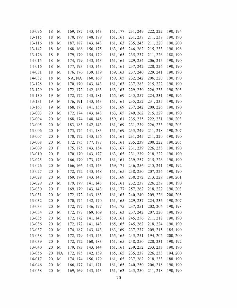
70

13-096 18 M 169, 187 143, 143 161, 177 231, 249 222, 222 190, 194 13-115 18 M 170, 179 148, 179 161, 161 231, 237 211, 237 190, 190 13-116 18 M 187, 187 143, 143 161, 163 235, 245 211, 220 190, 200 13-142 18 M 168, 168 156, 175 163, 165 246, 262 215, 233 190, 198 13-176 18 F 179, 179 154, 179 161, 165 235, 237 211, 226 188, 190 14-015 18 M 174, 179 143, 143 161, 161 229, 254 206, 215 190, 190 14-016 18 M 177, 193 143, 143 161, 161 237, 242 220, 226 190, 190 14-031 18 M 176, 176 139, 139 159, 163 237, 240 229, 241 190, 190 14-032 18 M NA, NA 160, 169 159, 165 232, 242 206, 220 190, 190 13-128 19 M 170, 170 143, 143 161, 163 237, 283 215, 222 190, 190 13-129 19 M 172, 172 142, 163 163, 163 229, 250 226, 233 190, 205 13-130 19 M 172, 172 143, 181 165, 169 245, 257 224, 231 190, 196 13-131 19 M 176, 191 143, 143 161, 161 235, 252 231, 235 190, 190 13-163 19 M 168, 177 141, 156 161, 169 237, 242 209, 226 190, 190 13-003 20 M 172, 174 143, 143 163, 165 249, 262 215, 229 190, 190 13-004 20 M 168, 174 148, 148 159, 161 235, 235 222, 231 190, 203 13-005 20 M 183, 183 142, 143 161, 169 231, 239 226, 233 198, 203 13-006 20 F 173, 174 141, 183 161, 169 235, 249 211, 218 190, 207 13-007 20 F 170, 172 143, 156 161, 161 231, 245 211, 220 190, 190 13-008 20 M 172, 175 177, 177 161, 161 235, 239 200, 222 190, 205 13-009 20 F 175, 175 143, 154 163, 167 231, 239 226, 233 190, 190 13-010 20 F 170, 170 143, 177 163, 165 231, 239 218, 222 190, 190 13-025 20 M 166, 179 173, 173 161, 161 239, 257 215, 226 190, 190 13-026 20 M 166, 166 143, 143 169, 171 246, 256 215, 241 190, 192 13-027 20 F 172, 172 143, 148 161, 165 238, 250 207, 226 190, 190 13-028 20 M 169, 174 143, 143 161, 169 238, 272 213, 229 190, 201 13-029 20 M 179, 179 141, 143 161, 161 232, 237 226, 237 190, 190 13-030 20 F 169, 179 143, 143 161, 177 257, 262 218, 222 190, 203 13-031 20 M 172, 172 143, 183 161, 163 240, 240 209, 226 200, 205 13-032 20 F 170, 174 142, 170 161, 165 229, 237 224, 235 190, 207 13-033 20 M 172, 177 146, 177 163, 175 237, 251 202, 206 190, 198 13-034 20 M 172, 177 169, 169 161, 163 237, 242 207, 220 190, 190 13-035 20 M 172, 172 141, 143 159, 161 245, 256 211, 218 190, 190 13-036 20 M 172, 172 141, 143 165, 165 245, 262 218, 224 190, 190 13-037 20 M 174, 187 143, 143 163, 169 237, 237 209, 215 185, 190 13-038 20 M 172, 179 143, 143 165, 165 245, 251 194, 202 200, 200 13-039 20 F 172, 172 160, 183 161, 165 248, 250 220, 231 190, 192 13-040 20 M 179, 183 143, 144 161, 161 239, 252 233, 233 190, 190 13-056 20 NA 172, 185 142, 159 165, 165 235, 237 226, 233 194, 200 14-017 20 M 174, 174 156, 179 161, 165 237, 262 218, 233 188, 190 14-046 20 M 166, 177 141, 171 161, 165 240, 250 206, 218 190, 190 14-058 20 M 169, 169 143, 143 161, 163 245, 250 211, 218 190, 190

71

14-059 20 M 181, 181 143, 143 161, 163 237, 259 202, 215 186, 190 14-062 20 M 172, 181 143, 156 161, 161 224, 237 215, 220 190, 200 14-063 20 F 162, 170 148, 148 161, 161 232, 239 209, 215 190, 205 14-083 20 M 185, 185 146, 146 161, 161 239, 250 209, 226 190, 198 14-085 20 M 176, 179 143, 143 161, 163 235, 237 211, 220 190, 190 14-086 20 M 172, 187 143, 143 159, 161 235, 242 213, 218 190, 190 12-030 30 M 170, 181 143, 143 161, 165 224, 238 218, 226 190, 190 12-033 30 M 172, 177 142, 147 161, 161 250, 270 220, 224 190, 190 12-034 30 M 166, 166 143, 175 161, 161 238, 246 213, 224 190, 198 12-046 30 M 166, 177 143, 167 161, 163 240, 262 220, 231 192, 200 12-063 30 M 181, 181 143, 143 161, 169 235, 263 213, 218 190, 205 12-064 30 M 166, 172 143, 143 161, 161 237, 242 215, 231 190, 190 12-065 30 M 174, 179 141, 141 161, 165 237, 239 211, 226 190, 190 12-031 31 F 171, 174 143, 143 161, 161 232, 240 211, 211 190, 203 12-032 31 M 176, 176 143, 171 161, 163 237, 248 198, 206 190, 190 12-035 31 M 174, 177 143, 177 161, 165 237, 245 220, 229 190, 190 12-036 31 M 168, 168 141, 156 161, 165 220, 231 202, 215 190, 190 12-037 31 M 177, 179 143, 143 159, 161 239, 249 224, 229 190, 205 12-042 31 M 172, 172 179, 179 161, 161 224, 231 218, 220 186, 190 12-043 31 M 176, 177 143, 143 161, 161 231, 239 215, 240 190, 198 12-045 31 M 168, 177 143, 143 161, 161 224, 239 206, 229 190, 198 12-048 31 M 176, 177 143, 143 159, 165 265, 277 222, 229 188, 190 12-049 31 M 174, 177 141, 141 163, 165 235, 259 235, 235 190, 190 12-051 31 M 172, 172 143, 154 161, 169 238, 248 209, 218 190, 198 12-052 31 M 176, 183 148, 148 157, 163 230, 257 206, 235 190, 190 12-053 31 M 172, 183 141, 141 161, 169 235, 239 218, 224 190, 190 12-054 31 M 172, 172 143, 148 157, 161 238, 265 209, 224 192, 198 12-066 31 F 172, 172 143, 148 161, 165 239, 241 207, 211 190, 192 12-067 31 F 174, 177 143, 143 161, 161 235, 239 204, 213 198, 198 12-079 31 M 176, 176 143, 143 161, 161 231, 262 209, 218 190, 190 12-026 32 M 169, 170 143, 143 165, 169 229, 238 218, 231 190, 190 12-028 32 M 174, 174 143, 143 161, 163 229, 240 224, 237 190, 192 12-047 32 M 169, 191 158, 181 159, 161 237, 245 209, 211 190, 192 12-055 32 M 172, 199 143, 143 157, 165 238, 246 202, 213 190, 190 12-072 32 M 168, 168 143, 143 161, 165 247, 247 213, 220 188, 190 12-050 33 M 172, 172 143, 143 161, 165 237, 240 220, 224 190, 190 12-056 33 M 181, 181 143, 143 161, 165 231, 240 209, 226 190, 190 12-068 33 M 176, 177 156, 156 161, 165 241, 241 222, 235 190, 190 12-069 33 M 177, 177 142, 142 161, 165 239, 241 226, 240 198, 200 12-073 33 M 174, 179 185, 185 161, 165 235, 245 222, 231 190, 196 12-081 33 M 174, 205 143, 179 161, 163 238, 238 218, 222 190, 200

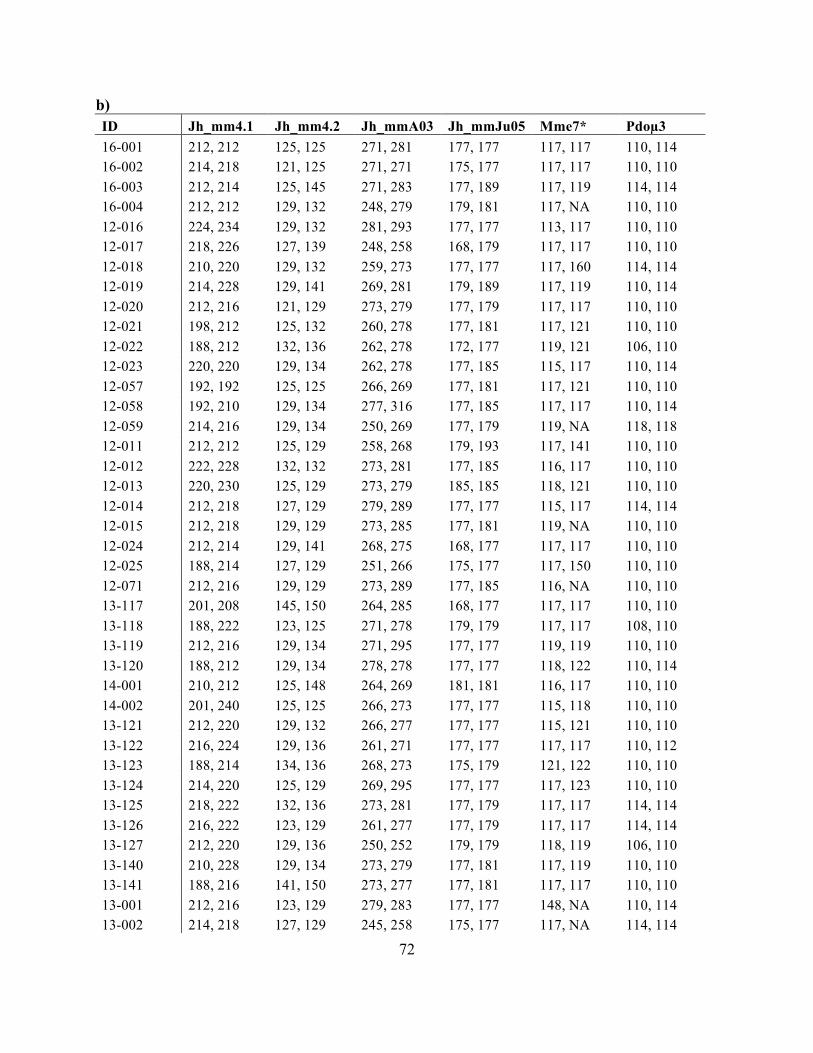
72

b) ID Jh_mm4.1 Jh_mm4.2 Jh_mmA03 Jh_mmJu05 Mme7* Pdoµ3 16-001 212, 212 125, 125 271, 281 177, 177 117, 117 110, 114 16-002 214, 218 121, 125 271, 271 175, 177 117, 117 110, 110 16-003 212, 214 125, 145 271, 283 177, 189 117, 119 114, 114 16-004 212, 212 129, 132 248, 279 179, 181 117, NA 110, 110 12-016 224, 234 129, 132 281, 293 177, 177 113, 117 110, 110 12-017 218, 226 127, 139 248, 258 168, 179 117, 117 110, 110 12-018 210, 220 129, 132 259, 273 177, 177 117, 160 114, 114 12-019 214, 228 129, 141 269, 281 179, 189 117, 119 110, 114 12-020 212, 216 121, 129 273, 279 177, 179 117, 117 110, 110 12-021 198, 212 125, 132 260, 278 177, 181 117, 121 110, 110 12-022 188, 212 132, 136 262, 278 172, 177 119, 121 106, 110 12-023 220, 220 129, 134 262, 278 177, 185 115, 117 110, 114 12-057 192, 192 125, 125 266, 269 177, 181 117, 121 110, 110 12-058 192, 210 129, 134 277, 316 177, 185 117, 117 110, 114 12-059 214, 216 129, 134 250, 269 177, 179 119, NA 118, 118 12-011 212, 212 125, 129 258, 268 179, 193 117, 141 110, 110 12-012 222, 228 132, 132 273, 281 177, 185 116, 117 110, 110 12-013 220, 230 125, 129 273, 279 185, 185 118, 121 110, 110 12-014 212, 218 127, 129 279, 289 177, 177 115, 117 114, 114 12-015 212, 218 129, 129 273, 285 177, 181 119, NA 110, 110 12-024 212, 214 129, 141 268, 275 168, 177 117, 117 110, 110 12-025 188, 214 127, 129 251, 266 175, 177 117, 150 110, 110 12-071 212, 216 129, 129 273, 289 177, 185 116, NA 110, 110 13-117 201, 208 145, 150 264, 285 168, 177 117, 117 110, 110 13-118 188, 222 123, 125 271, 278 179, 179 117, 117 108, 110 13-119 212, 216 129, 134 271, 295 177, 177 119, 119 110, 110 13-120 188, 212 129, 134 278, 278 177, 177 118, 122 110, 114 14-001 210, 212 125, 148 264, 269 181, 181 116, 117 110, 110 14-002 201, 240 125, 125 266, 273 177, 177 115, 118 110, 110 13-121 212, 220 129, 132 266, 277 177, 177 115, 121 110, 110 13-122 216, 224 129, 136 261, 271 177, 177 117, 117 110, 112 13-123 188, 214 134, 136 268, 273 175, 179 121, 122 110, 110 13-124 214, 220 125, 129 269, 295 177, 177 117, 123 110, 110 13-125 218, 222 132, 136 273, 281 177, 179 117, 117 114, 114 13-126 216, 222 123, 129 261, 277 177, 179 117, 117 114, 114 13-127 212, 220 129, 136 250, 252 179, 179 118, 119 106, 110 13-140 210, 228 129, 134 273, 279 177, 181 117, 119 110, 110 13-141 188, 216 141, 150 273, 277 177, 181 117, 117 110, 110 13-001 212, 216 123, 129 279, 283 177, 177 148, NA 110, 114 13-002 214, 218 127, 129 245, 258 175, 177 117, NA 114, 114

73

13-041 214, 224 140, 154 266, 281 179, 185 118, 119 110, 110 13-042 216, 238 134, 140 273, 285 177, 185 117, 121 110, 110 13-043 214, 222 125, 125 270, 275 179, 181 117, 117 110, 110 13-044 197, 209 123, 134 258, 316 168, 177 120, 122 110, 114 13-045 212, 218 127, 136 276, 278 179, 179 117, 117 110, 110 13-046 208, 230 129, 136 273, 281 177, 181 123, 156 110, 110 13-047 190, 212 125, 132 273, 278 177, 177 117, 125 114, 114 13-048 210, 230 129, 129 272, 278 177, 177 121, 125 114, 114 13-049 214, 214 132, 134 261, 275 179, 179 117, 121 110, 110 13-050 220, 224 125, 129 272, 277 181, 183 117, 122 110, 110 13-051 216, 220 125, 125 273, 279 177, 177 117, 117 110, 118 13-052 210, 224 123, 134 273, 331 177, 181 117, 117 114, 114 13-053 188, 210 134, 138 245, 285 177, 177 117, 117 110, 110 14-003 212, 214 129, 132 268, 271 177, 183 117, NA 110, 110 14-009 216, 230 129, 129 258, 275 177, 177 117, 121 108, 110 14-013 188, 220 125, 132 281, 281 177, 181 117, 123 110, 110 14-014 214, 216 129, 132 266, 277 179, 179 119, 119 82, 82 12-001 224, 238 127, 129 250, 307 177, 179 117, 117 110, 114 12-002 192, 216 129, 129 273, 275 175, 177 117, 123 110, 114 12-003 188, 226 127, 132 269, 273 177, 193 117, 117 110, 110 12-004 214, 240 136, 138 278, 281 177, 185 117, 117 110, 110 12-005 208, 218 129, 129 269, 275 175, 175 117, 125 110, 110 12-006 208, 220 129, 129 275, 279 175, 181 117, 117 110, 118 12-007 188, 224 127, 127 268, 275 177, 177 119, 119 110, 110 13-097 216, 238 134, 136 256, 273 177, 177 117, 117 110, 116 13-098 212, 218 129, 134 269, 279 172, 177 117, 117 114, 114 13-099 210, 220 125, 134 278, 289 168, 181 117, 120 110, 110 13-100 212, 212 125, 127 258, 281 170, 177 116, 121 110, 110 13-101 188, 216 132, 154 275, 278 177, 177 117, 119 110, 114 13-102 188, 216 123, 129 266, 275 177, 177 117, 119 110, 114 13-103 205, 212 129, 132 264, 277 177, 177 119, 122 114, 114 13-104 212, 222 125, 129 266, 303 177, 181 117, 119 110, 110 13-105 210, 212 127, 129 259, 291 177, 177 117, 120 114, 114 13-106 205, 214 123, 125 268, 281 181, 181 119, 121 110, 114 13-107 208, 222 134, 141 259, 275 177, 185 117, 117 114, 114 13-108 208, 214 129, 129 273, 277 177, 181 117, NA 110, 110 14-004 214, 230 127, 129 269, 277 NA, NA 119, 123 110, 114 14-005 188, 216 129, 134 277, 316 170, 181 126, 133 106, 106 14-006 212, 212 129, 136 279, 289 177, 177 117, 117 110, 110 14-007 236, 236 127, 132 258, 279 181, 183 115, 117 110, 110 14-008 190, 216 125, 129 273, 273 181, 181 121, 121 110, 110 14-010 214, 230 127, 138 279, 281 177, 179 117, 117 100, 100

74

14-011 214, 218 132, 150 266, 277 175, 185 NA, NA 110, 114 14-012 208, 218 129, 129 234, 279 177, 179 117, 117 110, 114 14-068 210, 214 132, 134 262, 273 177, 177 115, 117 110, 114 14-023 218, 218 129, 129 271, 277 177, 177 117, 117 110, 114 14-024 216, 220 125, 129 271, 279 177, 177 117, NA 110, 110 14-025 208, 216 132, 132 261, 261 175, 177 116, 119 110, 110 14-026 216, 218 129, 141 261, 277 179, 181 117, 118 110, 110 14-033 188, 188 132, 152 279, 279 177, 185 117, 117 110, 110 14-037 165, 214 129, 132 275, 277 177, 183 117, 117 114, 114 12-008 188, 224 127, 134 283, 316 177, 177 116, 116 110, 118 12-009 212, 212 132, 134 271, 271 177, 177 117, 122 114, 114 12-010 214, 240 132, 134 241, 264 177, 177 117, 121 110, 110 12-039 190, 212 129, 148 269, 283 177, 181 118, 150 110, 110 12-041 212, 216 129, 134 260, 278 179, 179 117, 121 110, 114 13-111 214, 222 125, 129 275, 277 179, 183 117, 117 110, 110 13-112 220, 244 123, 134 264, 271 177, 177 117, 121 110, 114 13-113 199, 218 129, 143 264, 271 177, 177 117, 121 110, 110 13-114 188, 244 129, 129 269, 279 177, 177 117, 121 110, 114 14-018 214, 214 129, 129 269, 279 177, 185 120, 150 110, 110 14-019 212, 216 129, 134 251, 275 177, 177 117, 117 110, 110 14-020 195, 220 127, 129 271, 275 175, 175 NA, NA 110, 110 13-011 212, 212 129, 143 279, 279 177, 179 117, 117 110, 114 13-012 212, 220 125, 132 272, 272 170, 185 117, NA 110, 110 13-013 196, 214 125, 134 281, 297 177, 181 117, 117 110, 110 13-018 212, 222 125, 129 273, 273 177, 179 117, 121 106, 110 13-019 188, 209 134, 134 273, 277 177, 177 117, 123 110, 118 13-020 216, 224 123, 127 273, 273 177, 177 117, 117 110, 110 13-021 216, 230 132, 134 273, 285 168, 177 117, 125 110, 110 13-022 190, 216 127, 129 272, 278 175, 177 117, NA 106, 110 13-024 214, 237 125, 125 272, 278 177, 177 117, NA 110, 114 13-073 165, 216 129, 134 270, 270 177, 177 117, NA 110, 114 13-074 188, 208 132, 140 254, 279 179, 179 117, NA 110, 110 13-075 188, 220 125, 136 272, 276 177, 177 115, 117 110, 110 13-076 216, 232 129, 129 254, 278 177, 177 117, 117 110, 110 13-077 212, 224 134, 134 281, 316 175, 177 117, 125 110, 118 13-078 216, 230 125, 129 278, 281 177, 179 121, 121 114, 114 13-079 216, 216 132, 132 270, 273 177, 179 116, 119 114, 114 13-080 206, 210 129, 129 256, 260 177, 179 115, 115 110, 110 13-081 218, 222 125, 132 272, 277 177, 177 115, 117 106, 114 13-082 190, 236 123, 129 277, 277 177, 179 117, 117 110, 118 13-083 218, 230 129, 132 272, 275 177, 177 122, NA 110, 110 13-084 212, 224 125, 129 273, 275 177, 181 125, NA 110, 110

75

13-085 188, 220 127, 132 279, 285 177, 179 119, NA 110, 110 14-021 210, 216 125, 136 266, 286 177, 181 121, NA 110, 110 14-022 212, 212 125, 129 273, 273 177, 181 113, 121 110, 114 14-041 212, 214 129, 129 271, 271 177, 177 121, NA 110, 114 14-042 220, 220 134, 136 258, 251 177, 185 117, 126 110, 110 14-043 212, 226 125, 129 254, 273 185, 185 114, NA 126, 126 14-073 210, 216 129, 132 248, 271 177, 177 121, NA 110, 110 14-074 212, 224 134, 136 273, 279 177, 177 117, 125 110, 110 13-014 216, 218 127, 132 254, 277 177, 177 117, 117 110, 110 13-015 214, 216 129, 132 259, 275 181, 181 120, 120 110, 110 13-016 220, 226 129, 140 268, 275 177, 177 122, 122 110, 114 13-017 218, 226 129, 129 291, 307 177, 179 117, 120 110, 110 13-023 216, 218 129, 140 261, 283 177, 179 117, 119 110, 110 13-132 216, 216 125, 129 273, 316 179, 185 117, 135 114, 118 13-133 226, 238 121, 129 278, 278 177, 179 117, 117 110, 110 13-134 212, 218 136, 136 250, 273 181, 181 116, 116 110, 126 13-135 210, 216 125, 129 273, 279 177, 179 117, 117 110, 110 13-136 212, 216 136, 141 262, 264 177, 177 117, 117 110, 110 13-137 188, 214 132, 134 261, 271 177, 177 115, 122 110, 110 13-138 208, 212 129, 129 264, 273 177, 177 118, 133 110, 114 13-139 210, 220 125, 134 264, 281 177, 177 117, 117 110, 110 13-192 188, 216 129, 136 271, 273 185, 185 117, NA 110, 110 13-193 216, 218 129, 136 253, 275 177, 177 119, 119 114, 114 13-202 198, 198 129, 129 279, 297 177, 177 151, NA 110, 110 13-220 216, 230 129, 136 261, 277 177, 181 117, NA 110, 110 14-067 190, 212 125, 132 271, 271 177, 179 117, 117 110, 110 13-086 188, 210 125, 134 270, 272 177, 177 121, NA 110, 114 13-087 210, 216 134, 143 272, 272 183, 183 122, NA 110, 110 13-088 214, 216 125, 134 261, 273 177, 177 117, 117 110, 110 13-089 212, 216 129, 136 262, 281 179, 179 117, 117 110, 110 13-090 216, 224 132, 154 276, 278 177, 183 117, 120 110, 110 13-091 212, 230 129, 132 262, 272 177, 177 117, 117 110, 110 13-092 212, 212 129, 140 278, 283 175, 181 117, 117 110, 114 13-093 165, 214 133, 139 276, 278 177, 181 115, 117 114, 114 13-094 216, 216 129, 136 272, 278 177, 179 117, 117 110, 110 13-095 216, 224 123, 129 264, 281 181, 181 117, 117 110, 110 13-096 212, 222 127, 138 261, 275 175, 177 117, 117 110, 110 13-115 224, 230 127, 129 275, 281 179, 181 117, 119 110, 118 13-116 212, 218 127, 132 278, 297 177, 177 118, 120 114, 114 13-142 188, 232 132, 143 250, 262 181, 189 117, 117 110, 110 13-176 216, 230 123, 127 281, 283 177, 181 119, NA 110, 118 14-015 216, 220 139, 139 273, 279 177, 177 117, 121 93, 100

76

14-016 212, 226 129, 129 271, 289 175, 177 117, 119 110, 114 14-031 210, 210 129, 132 258, 268 177, 177 119, 122 110, 110 14-032 212, 214 NA, NA 254, 269 177, 177 117, 122 114, 114 13-128 208, 224 127, 129 273, 275 179, 179 117, 117 110, 110 13-129 212, 214 125, 132 248, 268 177, 183 115, 135 110, 114 13-130 210, 216 129, 132 260, 278 177, 181 117, 117 114, 114 13-131 188, 214 129, 134 279, 281 175, 177 117, 119 110, 110 13-163 214, 224 134, 136 251, 277 177, 177 117, 117 110, 110 13-003 212, 216 129, 132 268, 278 177, 177 119, 119 110, 114 13-004 216, 216 132, 132 261, 273 177, 181 117, 123 114, 114 13-005 212, 214 129, 129 273, 285 177, 177 117, 154 110, 110 13-006 214, 234 125, 136 272, 273 179, 185 117, NA 110, 110 13-007 196, 237 129, 132 264, 270 179, 179 117, NA 114, 114 13-008 212, 218 125, 129 268, 273 177, 177 117, 117 110, 110 13-009 188, 218 125, 129 279, 297 177, 177 117, NA 110, 114 13-010 212, 218 129, 134 268, 277 177, 177 117, NA 110, 110 13-025 210, 220 129, 145 270, 270 179, 189 117, 121 106, 110 13-026 212, 214 129, 138 270, 272 177, 179 117, 121 110, 110 13-027 218, 218 125, 148 266, 268 177, 183 117, NA 110, 110 13-028 192, 212 129, 136 273, 277 177, 177 117, 121 110, 118 13-029 165, 216 129, 148 273, 278 177, 177 117, 125 110, 114 13-030 196, 208 134, 136 272, 279 177, 187 116, NA 110, 114 13-031 203, 218 125, 132 272, 273 177, 181 117, 141 114, 114 13-032 188, 212 132, 132 281, 285 179, 183 115, NA 110, 110 13-033 208, 216 132, 136 272, 273 177, 179 117, 125 114, 114 13-034 212, 216 127, 129 254, 278 175, 175 117, 119 110, 110 13-035 220, 226 129, 132 264, 275 177, 181 117, 117 114, 114 13-036 218, 218 134, 134 272, 272 179, 183 117, 117 110, 114 13-037 188, 210 125, 134 277, 277 177, 177 117, 117 110, 110 13-038 212, 212 129, 148 266, 285 177, 177 117, 117 110, 110 13-039 208, 238 123, 134 259, 261 177, 177 117, NA 110, 114 13-040 192, 210 132, 136 254, 256 177, 177 117, 121 110, 110 13-056 198, 212 127, 129 254, 285 177, 179 117, 117 110, 110 14-017 212, 220 129, 134 271, 273 177, 177 117, 117 110, 110 14-046 230, 234 123, 129 259, 271 179, 179 117, 121 110, 110 14-058 188, 226 129, 134 251, 275 179, 189 115, 118 110, 114 14-059 210, 236 132, 141 248, 259 177, 189 115, 115 110, 110 14-062 224, 236 125, 134 271, 275 177, 181 117, 117 110, 110 14-063 192, 222 127, 129 275, 275 177, 177 117, NA 110, 110 14-083 212, 212 125, 129 250, 273 177, 181 116, 117 110, 110 14-085 216, 224 129, 134 275, 291 168, 177 117, 117 110, 110 14-086 214, 214 129, 138 273, 279 179, 179 117, 117 110, 110

77

12-030 208, 216 129, 141 271, 281 177, 183 117, 118 110, 110 12-033 190, 212 121, 127 269, 271 177, 185 117, 119 110, 114 12-034 216, 244 127, 134 275, 275 177, 189 117, 117 110, 110 12-046 212, 212 136, 138 261, 281 177, 185 117, 117 110, 114 12-063 216, 220 132, 136 275, 277 177, 181 117, 117 110, 114 12-064 214, 238 121, 123 269, 279 177, 177 117, 117 110, 114 12-065 188, 224 130, 139 250, 279 175, 179 118, 121 110, 114 12-031 216, 218 129, 143 275, 286 177, 179 NA, NA 110, 114 12-032 210, 214 134, 136 275, 277 177, 183 117, 121 110, 110 12-035 214, 236 134, 141 271, 271 183, 183 121, 126 110, 110 12-036 212, 214 125, 129 271, 293 177, 179 117, 117 114, 114 12-037 216, 216 134, 136 278, 281 177, 179 119, 119 110, 110 12-042 232, 244 129, 132 256, 269 177, 177 117, 120 110, 110 12-043 201, 212 123, 125 273, 273 181, 181 117, 143 110, 110 12-045 212, 224 125, 132 273, 278 177, 177 117, 117 110, 110 12-048 214, 216 127, 136 268, 279 179, 179 117, 117 110, 110 12-049 195, 208 123, 129 281, 281 162, 179 117, 121 110, 110 12-051 216, 224 134, 136 277, 279 179, 179 117, 117 110, 110 12-052 212, 224 129, 154 273, 279 179, 181 117, 121 110, 110 12-053 208, 214 127, 132 281, 281 177, 177 117, 123 110, 110 12-054 188, 222 121, 132 277, 281 177, 185 117, 117 110, 110 12-066 216, 218 136, 143 275, 279 177, 177 117, NA 110, 114 12-067 224, 224 125, 129 271, 273 177, 177 117, NA 114, 114 12-079 214, 218 129, 136 264, 285 177, 183 117, 119 110, 110 12-026 216, 220 129, 129 266, 279 177, 177 117, 117 106, 114 12-028 216, 220 129, 129 273, 273 177, 177 117, 117 110, 110 12-047 218, 238 132, 134 264, 277 179, 179 115, 117 110, 110 12-055 188, 218 123, 125 273, 275 177, 181 117, 117 110, 114 12-072 199, 212 125, 129 271, 273 177, 179 117, 117 110, 114 12-050 188, 212 129, 129 250, 313 179, 189 117, 133 110, 110 12-056 214, 224 134, 152 241, 258 177, 177 117, 117 110, 110 12-068 203, 212 132, 141 266, 279 177, 177 117, 117 110, 110 12-069 210, 212 125, 145 278, 278 177, 177 117, 117 110, 110 12-073 208, 216 129, 129 250, 262 177, 183 117, 125 114, 114 12-081 195, 216 127, 134 271, 277 179, 179 117, 121 114, 114

78

Table S7. Tail white data for male juncos. All tail white values are values out of 1, where 0 is a completely non-white area and 1 is a completely white area. R4 = fourth rectrix; asym = asymmetry; elev = elevation.

ID Total White

Mean R4 White

R4 Asym Year

Julian Day

Elev (m)

Wing (mm)

Tarsus (mm)

Tail (mm)

Mass (g)

12-001 0.488 0.448 0.684 2012 139 1960 77 19.59 67 17.6 12-002 0.765 1.000 0.000 2012 139 1960 78 19.22 64 18.2 12-004 0.284 0.836 0.085 2012 140 1960 78 19.63 65 17 12-005 0.528 0.564 0.037 2012 140 1960 79 20.4 67 18.8 12-006 0.524 0.572 0.082 2012 147 1960 77 20.33 66 18.4 12-008 0.670 0.914 0.076 2012 141 2090 78 20.54 67 19.5 12-009 0.517 0.557 0.275 2012 142 2090 74 19.31 61 17.3 12-010 0.478 0.445 0.019 2012 142 2090 76 20.66 62 18.8 12-038 0.317 0.050 0.084 2012 161 1960 78 20.54 65 18.2 12-039 0.615 0.846 0.211 2012 162 2090 78 20.41 66 16.8 12-040 0.479 0.435 0.083 2012 221 2090 76 20.72 67 17.5 12-041 0.460 0.431 0.126 2012 162 2090 79 19.88 70 17.7 930-25752 0.307 0.023 0.014 2012 139 2090 76 20.25 61 17.6 930-25760 0.401 0.247 0.015 2012 158 2090 76 19.66 60 16.3 12-007 0.479 0.439 0.005 2013 140 1960 79 19.2 68 16.6 13-003 0.484 0.453 0.024 2013 146 2660 78 20.66 65 17.5 13-004 0.367 0.185 0.093 2013 158 2660 76 19.51 67 16.7 13-005 0.469 0.400 0.013 2013 165 2660 80 20.52 70 16.9 13-008 0.521 0.564 0.054 2013 148 2660 80 20.8 69 18.9 13-011 0.504 0.501 0.141 2013 166 2240 78 21.29 68 17.6 13-013 0.413 0.274 0.046 2013 165 2240 76 19.71 64 17.3 13-014 0.546 0.622 0.001 2013 196 2315 79 20.11 68 18.2 13-015 0.522 0.582 0.047 2013 165 2315 79 20.34 67 17.8 13-016 0.656 0.874 0.056 2013 165 2315 74 20.95 67 19 13-017 0.331 0.481 0.030 2013 135 2315 76 20.24 63 17.6 13-018 0.473 0.431 0.042 2013 167 2240 76 20.03 66 18.1 13-019 0.419 0.289 0.030 2013 172 2240 73 19.75 64 18 13-020 0.442 0.344 0.077 2013 188 2240 75 20.77 66 18.6 13-021 0.377 0.138 0.063 2013 220 2240 77 20.48 66 18.5 13-023 0.352 0.140 0.022 2013 183 2315 78 20.68 68 17.9 13-025 0.313 0.198 0.106 2013 166 2660 75 17.72 69 17.5 13-026 0.431 0.305 0.115 2013 112 2660 78 19.42 67 17.3 13-028 0.621 0.876 0.012 2013 228 2660 75 19.19 67 16.4 13-029 0.601 0.728 0.049 2013 223 2660 79 19.62 68 17.1

79

13-031 0.512 0.545 0.096 2013 157 2660 79 20.53 71 17.8 13-033 NA 0.175 0.091 2013 157 2660 77 20.38 66 17.1 13-034 0.564 0.637 0.066 2013 232 2660 79 20.03 67 18 13-035 0.524 0.564 0.058 2013 157 2660 76 19.77 67 17.3 13-036 0.595 0.723 0.190 2013 163 2660 78 21.15 69 19.3 13-037 0.610 0.809 0.135 2013 148 2660 81 20.85 73 18.8 13-038 0.449 0.450 0.013 2013 154 2660 78 19.53 68 16.8 13-040 0.601 0.728 0.145 2013 145 2660 77 19.71 68 18.1 13-041 0.613 0.755 0.085 2013 144 1965 76 20.66 65 18.5 13-042 0.356 0.261 0.263 2013 144 1965 76 18.51 68 17.2 13-043 0.323 0.482 0.053 2013 144 1965 80 19.54 67 19.1 13-044 0.640 0.855 0.063 2013 189 1965 79 20.45 69 17.9 13-045 0.476 0.429 0.052 2013 145 1965 75 19.94 66 18.3 13-046 0.532 0.588 0.141 2013 145 1965 79 19.53 71 17.7 13-047 0.486 0.465 0.080 2013 145 1965 75 20.26 65 18.4 13-049 0.602 0.757 0.014 2013 146 1965 81 19.88 70 17.4 13-050 0.478 0.453 0.028 2013 173 1965 73 20.85 65 17.7 13-051 0.296 0.383 0.030 2013 158 1965 76 19.73 69 18.1 13-052 0.523 0.583 0.020 2013 148 1965 79 20.31 69 18.9 13-053 0.509 0.534 0.211 2013 153 1965 79 19.24 68 17.5 13-075 0.458 0.370 0.086 2013 187 2240 79 19.43 68 17.5 13-076 0.469 0.434 0.178 2013 158 2240 75 19.98 63 18.3 13-077 0.439 0.316 0.018 2013 158 2240 76 20.66 67 18 13-078 0.507 0.554 0.024 2013 158 2240 78 20.96 67 18 13-079 NA 0.675 0.031 2013 191 2240 81 19.83 68 18.3 13-080 0.494 0.522 0.029 2013 164 2240 80 20.82 68 17.2 13-081 0.340 0.508 0.049 2013 141 2240 74 19.9 66 17.3 13-088 0.523 0.536 0.151 2013 168 2470 78 19.31 68 17.4 13-089 0.554 0.586 0.008 2013 148 2470 80 20.2 68 19 13-090 0.413 0.251 0.023 2013 228 2470 78 19.27 66 18.5 13-091 0.507 0.515 0.169 2013 133 2470 79 20.13 68 17.8 13-092 0.434 0.424 0.138 2013 146 2470 79 20.85 67 18.5 13-093 0.626 0.841 0.078 2013 168 2470 79 19.89 68 17.7 13-094 0.654 0.902 0.086 2013 156 2470 78 19.73 67 18.2 13-095 0.467 0.433 0.140 2013 156 2470 76 20.03 66 17.2 13-096 0.391 0.335 0.130 2013 156 2470 78 19.45 65 17.3 13-097 0.377 0.255 0.361 2013 173 2075 78 21.26 68 17.4 13-098 0.566 0.679 0.090 2013 155 2075 78 20.15 68 18.1 13-099 0.505 0.482 0.248 2013 173 2075 81 20.57 69 18 13-100 0.501 0.509 0.234 2013 165 2075 76 19.8 67 17.8 13-101 0.404 0.296 0.078 2013 172 1960 75 20.07 64 17.4 13-102 0.417 0.354 0.012 2013 220 1960 78 21.05 69 17.4

80

13-103 0.479 0.431 0.107 2013 166 1960 79 20.07 68 17.6 13-104 0.630 0.875 0.145 2013 142 1960 77 19.55 69 16.4 13-105 0.532 0.565 0.036 2013 143 1960 75 21.3 66 16.7 13-106 0.494 0.467 0.023 2013 223 1960 77 19.95 68 17.2 13-107 0.375 0.131 0.125 2013 156 1960 74 20.42 64 18 13-111 0.348 0.100 0.075 2013 163 2090 74 19.86 66 18.4 13-112 0.464 0.420 0.140 2013 166 2090 75 19.45 63 18.6 13-113 0.412 0.325 0.039 2013 166 2090 80 20.35 70 17.9 13-114 0.378 0.288 0.016 2013 223 2090 75 20.52 66 16.8 13-115 0.477 0.439 0.069 2013 189 2470 75 19 65 16.3 13-116 0.420 0.265 0.036 2013 159 2470 74 20.72 65 17.6 13-117 0.458 0.369 0.074 2013 196 1100 78 19.84 71 16.4 13-118 0.480 0.469 0.057 2013 144 1100 76 19.39 66 17.1 13-119 0.499 0.496 0.041 2013 144 1100 75 20.34 65 17.3 13-120 0.500 0.493 0.006 2013 164 1100 74 20.13 66 18.1 13-121 0.616 0.838 0.197 2013 145 1600 74 19.21 67 16.9 13-122 0.579 0.704 0.215 2013 232 1600 78 22.05 68 17.2 13-123 0.456 0.479 0.008 2013 187 1600 79 21.79 69 18.3 13-124 0.405 0.307 0.122 2013 165 1600 76 19.52 67 18.2 13-125 0.678 0.962 0.057 2013 146 1600 74 20.27 64 17.6 13-126 0.453 0.396 0.029 2013 156 1600 77 20.39 70 17.8 13-127 0.512 0.565 0.048 2013 155 1600 76 20.11 68 19.3 13-128 0.581 0.689 0.029 2013 154 2210 77 19.84 70 18.5 13-129 0.592 0.728 0.168 2013 148 2210 77 20.07 66 17.2 13-130 NA 0.917 0.101 2013 154 2210 76 19.95 67 17.5 13-131 0.538 0.600 0.070 2013 154 2210 79 19.55 67 17.5 13-132 0.546 0.624 0.065 2013 148 2315 81 20.7 70 19.3 13-133 0.518 0.555 0.114 2013 158 2315 73 20.5 66 17.7 13-134 0.306 0.094 0.019 2013 143 2315 72 18.88 65 16 13-135 0.539 0.582 0.065 2013 144 2315 79 20.03 70 18.2 13-136 0.438 0.375 0.012 2013 148 2315 80 21.34 68 18.8 13-137 0.415 0.415 0.143 2013 148 2315 76 19.52 66 17.7 13-138 0.394 0.175 0.221 2013 148 2315 74 19.05 64 17.7 13-139 0.390 0.300 0.239 2013 114 2315 76 20.49 63 18.7 13-140 0.637 0.871 0.082 2013 155 1645 78 20.3 69 18.3 13-141 0.586 0.734 0.337 2013 155 1645 75 19.85 65 16.9 13-142 0.555 0.636 0.068 2013 146 2470 76 19.5 64 17.9 13-163 0.439 0.406 0.163 2013 144 2380 74 19.62 62 17 12-003 0.458 0.403 0.118 2014 140 1960 79 20.54 69 18.9 14-001 0.465 0.395 0.055 2014 154 1100 77 20.03 66 17.6 14-002 0.520 0.548 0.065 2014 145 1100 81 19.52 70 17.3 14-004 0.236 0.010 0.021 2014 166 1960 77 20.3 66 15.8

81

14-005 0.465 0.427 0.010 2014 205 1960 75 19.51 65 16.9 14-006 0.517 0.561 0.073 2014 159 1960 79 19.88 68 17.5 14-007 0.284 0.101 0.035 2014 145 1960 79 19.33 70 18 14-008 0.464 0.416 0.007 2014 133 1960 79 20.53 65 18 14-009 0.457 0.397 0.012 2014 173 1965 76 19.44 66 18.1 14-010 0.639 0.707 0.278 2014 210 1960 78 20.2 70 16.3 14-011 0.512 0.540 0.043 2014 143 1960 77 21.67 67 17.7 14-012 0.432 0.296 0.073 2014 143 1960 77 20.84 63 16.4 14-013 0.533 0.590 0.124 2014 144 1965 76 21.16 65 18.3 14-014 0.391 0.241 0.012 2014 144 1965 77 20.81 65 18 14-015 0.548 0.649 0.060 2014 145 2470 76 19.73 67 16.8 14-016 0.458 0.394 0.017 2014 167 2470 78 20.96 68 18.4 14-017 0.394 0.264 0.110 2014 145 2660 76 20.78 68 17.2 14-018 0.306 0.004 0.004 2014 166 2090 79 20.03 67 16.9 14-019 0.731 0.934 0.040 2014 146 2090 79 19.64 68 18.5 14-022 0.447 0.355 0.092 2014 147 2240 76 20.53 66 16.1 14-023 0.419 0.289 0.026 2014 220 2090 75 20.57 64 17.5 14-025 0.481 0.445 0.007 2014 155 2090 80 NA 68 17.6 14-026 0.515 0.623 0.552 2014 155 2090 80 19.38 68 17.5 14-031 0.604 0.753 0.157 2014 154 2470 78 19.85 71 16.4 14-032 0.432 0.345 0.059 2014 157 2470 76 20.39 69 17.9 14-033 0.405 0.320 0.092 2014 158 2050 81 19.67 69 16.7 14-037 0.495 0.479 0.178 2014 156 2050 77 20.3 68 18.1 14-042 0.519 0.564 0.041 2014 148 2240 78 20.21 69 17.7 14-046 0.434 0.372 0.065 2014 169 2660 77 20.04 68 18.2 14-058 0.462 0.387 0.052 2014 178 2660 79 20.22 67 16.7 14-059 0.539 0.595 0.095 2014 178 2660 79 20.63 67 17.3 14-062 0.593 0.764 0.064 2014 223 2660 77 19.45 68 16.5 14-067 0.482 0.445 0.087 2014 133 2315 76 19.82 66 17.6 14-074 0.494 0.497 0.238 2014 134 2240 77 19.53 63 16.5 15-001 0.416 0.249 0.041 2015 132 1960 74 20.03 64 19.2 15-002 0.521 0.542 0.127 2015 134 1100 80 20.54 69 17.8 15-003 0.474 0.427 0.091 2015 134 1100 75 20.26 67 17.7 15-004 0.463 0.422 0.064 2015 134 1100 77 20.54 67 18.7 15-005 0.477 0.431 0.043 2015 195 1960 76 21.12 67 18.2 15-006 0.551 0.665 0.171 2015 195 1960 78 20.77 63 18 15-008 0.538 0.570 0.073 2015 196 2240 80 19.8 69 18.4 15-010 0.426 0.293 0.061 2015 196 2240 75 20.25 67 16.9 15-011 0.512 0.535 0.008 2015 196 2240 80 20.11 69 18.8 15-012 0.445 0.357 0.220 2015 197 2660 73 19.86 65 16.1 15-013 0.428 0.379 0.005 2015 197 2660 75 20.54 65 17.9 15-016 0.550 0.649 0.034 2015 198 1965 78 19.84 69 16.6

82

15-017 0.468 0.405 0.065 2015 199 2660 79 20.07 68 18.6

Effects of Environmental Variation at Multiple Scales on ...digitalassets.lib.berkeley.edu/.../LaBarbera_berkeley_0028E_16182.pdf · Effects of Environmental Variation at Multiple

Documents