Effects of contrast and size on orientation discrimination

Vision Research 44 (2004) 57–67

www.elsevier.com/locate/visres

Effects of contrast and size on orientation discrimination

Isabelle Mareschal a,b,*, Robert M. Shapley a

a Center for Neural Science, New York University, 4 Washington Place, New York, NY 10003, USAb Institute of Ophthalmology, University College London, 11-43 Bath Street, London EC1V 9EL, UK

Received 2 December 2002; received in revised form 27 May 2003

Abstract

Motivated by the recent physiological finding that a neuron’s receptive field can increase in size by a factor of 2–4-fold at low

contrast [Nat. Neurosci. 2 (1999) 733, Proc. Natl. Acad. Sci. USA 96 (1999) 12073], we sought to examine whether a psychophysical

task might reflect the contrast dependent changes in the size/structure of a receptive field. We postulate that since spatial summation

is not contrast invariant, a task that relies on the spatial structure of a receptive field, such as orientation discrimination, should also

be affected by changes in contrast. Previously, orientation discrimination thresholds have been reported to be roughly independent

of the contrast of a stimulus for most of the visible range of contrasts [i.e. J. Neurophysiol. 57 (1987) 773, J. Opt. Soc. Am. 6 (1989)

713, Vis. Res. 30 (1990) 449, Vis. Res. 39 (1999) 1631]. Here, we found large improvements in orientation discrimination with

contrast that were dependent on stimulus area. Furthermore, the apparent constancy of orientation discrimination for large area

stimuli is possibly a result of a floor effect on the threshold. Therefore we conclude that there is not strong evidence for contrast

invariant orientation discrimination. We interpret these results in the context of recent neurophysiological results about the ex-

pansion of cortical cells’ receptive fields at low contrast.

� 2003 Elsevier Ltd. All rights reserved.

1. Introduction

Recent neurophysiological experiments on neurons in

primary visual cortex (V1) suggest that the classical

notion of a fixed size receptive field is inadequate

(Kapadia, Westheimer, & Gilbert, 1999; Sceniak,

Ringach, Hawken, & Shapley, 1999). The main result of

these experiments is that the area of a neuron’s receptive

field, measured with an optimal stimulus at a low con-

trast, can be from two to fourfold larger than whenmeasured with the same stimulus at a high contrast. An

interpretation of this finding is that at low contrast there

is a physiological reorganization of the mechanisms

subserving the processing of spatial vision. Specifically,

there is an increased area of summation over which a

neuron pools information when tested with low contrast

stimuli. When the cell is tested with a high contrast

stimulus, the area of summation is reduced, presumablycausing an increase of the cell’s spatial resolution. More

recently, Sceniak, Hawken, and Shapley (2002) have

* Corresponding author. Address: Institute of Ophthalmology,

University College London, 11-43 Bath Street, London EC1V 9EL,

UK.

E-mail address: [email protected] (I. Mareschal).

0042-6989/$ - see front matter � 2003 Elsevier Ltd. All rights reserved.

doi:10.1016/j.visres.2003.07.009

examined neurons’ spatial frequency tuning and band

width at high and low contrast and have reportedchanges in neurons’ spatial frequency tuning curves

consistent with changes in the receptive field size. The

conclusion from the above studies is that receptive fields

undergo a spatial re-organization when probed with

stimuli going from high to low contrasts. This physio-

logical result, that receptive fields can vary in size de-

pending on the stimulus properties, suggests that the

notion of fixed visual receptive fields needs revision.Spatial integration has been examined previously in

psychophysics (i.e. Graham & Robson, 1987; Jamar &

Koenderink, 1983; Legge & Foley, 1980, 1981). How-

ever, these experiments were largely explored with the

underlying concept of a fixed size, hard wired receptive

field (i.e. Hubel & Wiesel, 1962). Given that the exper-

iments of Sceniak et al. (1999) and Kapadia et al. (1999)

have demonstrated that receptive fields in V1 cortex aremodified with stimulus contrast, we hypothesized that

psychophysical tasks which probe basic, low level visual

function might display similar contrast dependent

changes. There have been more recent reports that

contrast can affect observers’ judgments on many psy-

chophysical tasks, such as the perceived velocity of a

stimulus (i.e. Hawken, Gegenfurtner, & Tang, 1994;

58 I. Mareschal, R.M. Shapley / Vision Research 44 (2004) 57–67

Stone & Thompson, 1992), its perceived spatial fre-

quency (Gouled Smith & Thomas, 1989; Thomas &

Olzak, 1997), the perceived contrast of an embedded

stimulus (Polat & Sagi, 1993; Snowden & Hammett,

1998; Solomon & Morgan, 2000; Yu & Levi, 1998) as

well as other contextual effects (Mareschal, Henrie, &

Shapley, 2002). In this study we sought to examine

orientation discrimination as a function of the contrastand size of the test stimulus. We hypothesized that

under high contrast conditions, orientation thresholds

might not be as influenced by the size of the stimulus (no

increased area of pooling) as they would be under low

contrast conditions.

Previous experiments have measured orientation

discrimination as a function of contrast, but these were

carried out at a fixed stimulus size (Bowne, 1990; Reis-beck & Gegenfurtner, 1998; Skottun, Bradley, Sclar,

Ohzawa, & Freeman, 1987; Webster, De Valois, &

Switkes, 1990; Westheimer, Brincat, & Werhahn, 1999).

The general finding was that in the experiments where

the stimuli were small, increasing the contrast low-

ered the orientation thresholds (e.g. Regan & Beverley,

1985; Reisbeck & Gegenfurtner, 1998; McIlhagga &

Mullen, 1996), whereas in experiments using larger sizedstimuli, orientation discrimination thresholds were fairly

contrast invariant (e.g. Bowne, 1990; Skottun et al.,

1987). In addition, some experiments have also exam-

ined the effect of size on orientation thresholds, although

these were always carried out at a fixed contrast (i.e.

Heeley & Buchanon-Smith, 1990; Henrie & Shapley,

2001; Orban, Vandenbussche, & Vogels, 1984; Westhei-

mer et al., 1999). However, none of these experimentssystematically varied both contrast and size in order to

examine their joint influence on orientation thresholds.

We sought to examine the role that contrast and size

might exert on orientation discrimination thresholds to

test the prevailing notion of contrast invariance in ori-

entation discrimination and its theoretical consequences.

We consider our results in the context of the above

physiological framework of a variable sized receptivefield. However, we also consider the changes in signal

strength induced by both a reduction in stimulus size

and contrast and investigate what effects, if any, these

may have on our results.

2. Methods

2.1. Apparatus and stimuli

The stimuli were produced on-line using a Macintosh

G3 and displayed in the center of a Sony Trinitron

monitor. The monitor was viewed binocularly at varyingdistances (from 57 to 228 cm), had a mean luminance of

36 cd/m2, had a video attenuator connected and was

calibrated using a UDT photometer. The screen size was

36 cm · 27 cm, the resolution was 1024 · 768 pixels and

it was refreshed at 85 Hz. Stimulus generation, presen-

tation, and observers’ responses were all computer

controlled and stored on-line. Experiments were run

from within Matlab, using both Psychtoolbox (Brai-

nard, 1997) and Videotoolbox (Pelli, 1997) routines.

The stimulus consisted of a circular patch of grating

varying in size from 0.12� in diameter to 2� in diameter.In order to ensure that at least one cycle of the stimulus

was present within the circular aperture, observers var-

ied their viewing distance for the smaller sizes. This re-

sulted in the spatial frequency changing with the viewing

distance from 3 c/deg at vd¼ 57 cm to 12 c/deg at

vd¼ 228 cm. The phase of the gratings was randomized

except for the smallest size condition (0.12�) where we

ensured that the zero crossing was located in the centerof the aperture. Controls were performed to verify that

the changes in spatial frequency and band width pro-

duced by the changes in viewing distance or size were

not large enough to bias the orientation discrimination

thresholds. Several studies have examined orientation

discrimination thresholds as a function of spatial fre-

quency, and report spatial frequency dependency for the

extremes tested (i.e. very high and very low spatial fre-quencies). Over the mid-range of spatial frequencies

used here though, their data display relative invariance

with spatial frequency (i.e. Burr & Wijesundra, 1991;

Heeley & Buchanon-Smith, 1990; Phillips & Wilson,

1984).

2.2. Procedure

In each experiment, a two-alternative forced choice

stimulus procedure was employed. Observers were pre-

sented sequentially with two stationary stimuli and were

required to judge whether the orientation of the second

stimulus was shifted clockwise or counterclockwise rel-ative to the orientation of the first stimulus. The se-

quence was as follows: a fixation point was presented

(100 ms) followed by the first stimulus presentation (250

ms). A brief period (ranging from 500 to 750 ms) where

the screen returned to mean luminance ensued prior to

the presentation of the second stimulus (250 ms). The

observers’ task was to indicate by a keypress whether the

stimulus shift between the two presentations had beenclockwise or counterclockwise. Auditory negative feed-

back was provided on observers’ errors. The orientation

shifts that were tested varied between the different ob-

servers and were randomly chosen from a pre-deter-

mined set of test values. Thresholds were determined

using a method of constant stimuli to sample the psy-

chometric function.

Observers initially familiarized themselves with thetasks prior to threshold collection by practicing until the

thresholds collected reached a constant plateau. One of

the authors and three observers naive to the purpose of

I. Mareschal, R.M. Shapley / Vision Research 44 (2004) 57–67 59

the study served as subjects for these experiments. All

observers had normal or corrected to normal vision.

Observers’ data on a given condition were pooled

across the runs for a given stimulus configuration of size

and contrast, and a bootstrapping procedure was used

to fit a cumulative Gaussian function to the results

(Foster & Bischof, 1991). This procedure yielded the

75% correct point by interpolation as the measure oforientation discrimination thresholds. Error bars on the

plots represent the standard deviations of the thresholds

at the 75% criterion levels and were derived from the

bootstrapping procedure.

3. Results

3.1. Fovea

Orientation discrimination thresholds were measured

as a function of contrast for the different sized stimuli in

three observers. Stimuli in this experiment were pre-sented at the fixation point. The data for observers IM

and AS are plotted in the top panels (left and right,

respectively), and SS in the bottom left panel. The av-

eraged data from the three observers are plotted in the

bottom right panel. As is clearly captured in the aver-

aged data, all observers display a similar trend of results,

mainly that orientation discrimination thresholds are

not contrast invariant for the smaller sized stimuli.For all observers, the threshold curves for the small

sized stimuli are not flat. Rather threshold increases as

contrast is decreased for stimuli roughly smaller than

0.5�–0.8� in diameter. The data in these plots seem to

reveal two types of contrast dependent mechanisms: one

which is contrast invariant for large stimuli, and one

which is non-contrast invariant using small sized stimuli.

This result could reconcile previous experiments onorientation discrimination where some authors report

invariance with large sized stimuli only (i.e. Bowne,

1990; Skottun et al., 1987), whereas others report lack of

invariance but with, typically, smaller stimuli (McIl-

hagga & Mullen, 1996; Reisbeck & Gegenfurtner, 1998;

Westheimer et al., 1999). These graphs highlight that the

behavior of the mechanism underlying performance on

this task is dependent on both the size and the contrastof a stimulus. The dependence that is observed could be

explained by the following hypothesis. Suppose that the

area of spatial summation of neurons doing the task

increased with reduced contrast. If this were the case,

increasing the size of the stimulus would make it mat-

ched to the increased area of summation, possibly en-

abling a more accurate/better response with larger areas

at lower contrast.The data in Fig. 1 clearly reveal a co-dependency

between size and contrast in determining orientation

thresholds. In order to highlight this relationship, ori-

entation thresholds have been replotted in Fig. 2 as a

function of both the size and the contrast of the stimuli.

Examination of the three plots in Fig. 2 illustrates the

co-dependency of size and contrast in determining ori-

entation discrimination thresholds. The three dimen-

sional plots are not flat, but rather display a strong peak

in orientation thresholds for small sized, low contrast

stimuli.Figs. 1 and 2 both reveal that orientation thresholds

are dependent on the contrast of a stimulus for sizes

smaller than 0.5�–1� in diameter. At these sizes or

smaller, orientation thresholds increase as contrast is

reduced, and the area of pooling appears to shift as in-

dicated by the tuning curves becoming steeper. It would

be useful to obtain a measure of the breadth of spatial

summation of these curves for the different contrastsused. Examination of either Figs. 1 or 2 reveals that the

shapes of the curves vary with the different contrasts. In

particular, if one were to examine the size of stimulus at

which the orientation tuning for a given contrast had

reached half of its maximum value (likened to a measure

of the spatial summation), this measure would decrease

as contrast increased. In order to estimate this area

precisely, the midway point (corresponding to (maxi-mum threshold)minimum threshold)/2) of the different

contrast curves was interpolated for observers IM

and AS.

The data in Fig. 3 are reproduced from Fig. 1, but

with size as the abscissa. The data from observer SS

have not been included because, for this observer, we

were unable to obtain orientation thresholds at the two

smallest sizes and the data for the high contrast curveswere too shallow to obtain a meaningful measure of

spatial summation. For this reason we fit and interpo-

lated the halfway point for only the low contrast curves.

We wish to point out that this analysis makes no as-

sumptions about the data beyond that which is pre-

sented in the graphs. That is to say that how the curves

will diverge beyond the smallest size measured is not

addressed, although it is reasonable to assume that theywill increase exponentially. Also, it is clear by visual

inspection of the graphs that the slopes of the different

contrast curves are different. Particularly, the slopes of

the 4% and 6% curves are steeper than those of the

higher contrasts.

Table 1 reports the halfway threshold values as a

function of contrast for two observers. These values

decrease as contrast is increased, particularly between4% and 6%. We interpret this as a reduction in the area

of spatial summation with increasing contrast.

3.1.1. Detectability as a function of stimulus size

A clear concern here is how the detectability of thestimuli may affect our results, so in our experiments we

measured detection thresholds for the stimuli. This was

done using a two alternative forced choice paradigm

12

10

8

6

4

2

3 4 5 6 7 8 910

2

Contrast (%)

1deg0.5 deg0.25 deg0.12 deg

SS

14

12

10

8

6

4

23 4 5 6 7 8 9

102

Contrast (%)

1deg0.5deg0.25deg0.12deg

AS12

10

8

6

4

2

3 4 5 6 710

2 3 4 5 6 7

Contrast (%)

IM 2deg1 deg0.5 deg0.25 deg0.12 deg

1 deg0.5 deg0.25 deg0.12 deg

14

12

10

8

6

4

23 4 5 6 7 8 9 10 2

Contrast (%)

Ori

enta

tion

thre

shol

d (d

eg)

Ori

enta

tion

thre

shol

d (d

eg)

Ori

enta

tion

thre

shol

d (d

eg)

Ori

enta

tion

thre

shol

d (d

eg)

Fig. 1. Orientation discrimination thresholds for observer IM (top left), AS (top right), SS (bottom left) and the averaged data for the three observers

(bottom right) at different sizes as a function of the contrast of the stimulus. Spatial frequency¼ 3 cpd for stimuli sizes of 2�, 1� and 0.5�; spatialfrequency¼ 6 cpd for stimulus size of 0.25�; and spatial frequency¼ 12 cpd for stimulus size of 0.12�.

60 I. Mareschal, R.M. Shapley / Vision Research 44 (2004) 57–67

where observers had to indicate by a keypress whether

the stimulus had been presented in the first interval or

the second one. Contrast levels were tested using the

method of constant stimuli to sample the psychometric

function. The results are reported in Table 2 for subjects

IM and AS. There was a close correspondence between

these two observers for detection thresholds. For thesmallest size tested in the discrimination experiments

reported above, the stimulus was 2.4X its detection

threshold for IM and 2.8X for AS (note that for this size

the lowest contrast used in the experiment was 6%).

However, in order to ascertain that detectability was not

confounding our data, we measured orientation

thresholds for IM on the largest stimulus at 2.4X its

detection threshold (corresponding to 0.96% contrast).The orientation threshold measured for this stimulus

was 2.43�±0.2�. This is not significantly different from

the threshold measured at the higher contrasts for this

stimulus. This control experiment supports the conten-

tion that being a few multiples above detection thresh-

olds for our stimuli was not the limiting factor in

orientation thresholds measured in this task, and that

probability summation was not solely driving our re-sults. Indeed, for the large sized stimulus we observe

contrast invariance at the same multiple of detection

threshold as was used for the smaller sized stimulus, and

find no difference in orientation thresholds across the

contrast levels tested. This is in agreement with other

spatial vision tasks measured as a function of detect-

ability (e.g. Burbeck, 1987).

3.1.2. Control for changes in spatial frequency and band

width

In order to examine the effect of stimulus size on

orientation discrimination, we had to either change the

actual size of the stimulus (which would result in a

change in the number of cycles present in the stimulus),or change the viewing distance (which would result in a

change in the stimulus’ spatial frequency). In our ex-

periment, we decided to keep the number of cycles

constant and vary the viewing distance. However, we

tested for the effect of spatial frequency differences re-

sulting from the changes in viewing distance on our re-

sults. In the data plotted out in Fig. 1, the thresholds

measured for a stimulus size of 0.5� and larger weremeasured with a grating of 3 c/deg. Thresholds for a size

of 0.25� were measured with a grating of 6 c/deg, and for

a size of 0.12� were with a grating at 12 c/deg. Because

0

0.5

1

1.5

2

4 6 8 10 12 14 16 18 20

2

3

4

5

6

7

8

9

Contrast (%)

Size (deg)Ori

enta

tion

thr

esho

ld (

deg) IM

00.2

0.40.6

0.81

4 6 8 10 12 14 16 18 20

2

4

6

8

10

12

AS

Ori

enta

tion

thr

esho

ld (

deg)

Size (deg)

Contrast(%)

00.2

0.40.6

0.81

0

510

1520

2

4

6

8

10 SS

Ori

enta

tion

thr

esho

ld (

deg)

Size (deg)Contrast (%)

Fig. 2. Co-dependency of size and contrast in influencing orientation

thresholds. Orientation discrimination thresholds are plotted as a

function of the contrast (front axis) and size (right-hand axis) of the

stimuli for the three observers.

I. Mareschal, R.M. Shapley / Vision Research 44 (2004) 57–67 61

there might be some question about the effect of spatial

frequency on results measured under these stimulus

conditions, we re-measured orientation discrimination

thresholds for a size of 0.25� at both 3 c/deg and 12 c/

deg. It is impossible to measure thresholds at the

smallest size with a grating of 3 c/deg because therewould not be a full grating cycle in the stimulus. For this

reason, we measured orientation thresholds at different

spatial frequencies for the smallest size possible. In ad-

dition, we measured thresholds at 4% contrast for the 3

and 6 c/deg gratings (but not 12 c/deg because that

condition was not tested in the experiment plotted in

Fig. 1) and these were not significantly different (results

not on the graph).

Examination of Fig. 4 reveals that orientation dis-

crimination thresholds were not dependent on the spa-

tial frequencies that we used here. There is slightly more

variation at 6% than at 20%, but the data are within the

standard deviation limits. Also note that thresholds were

measured at 6% because for the smallest size stimulus

(with a grating of 12 c/deg) this was the lowest contrast

tested. This control confirmed previous studies (i.e. Burr& Wijesundra, 1991; Heeley & Buchanon-Smith, 1990;

Phillips & Wilson, 1984) that reported that over the

range of spatial frequencies used here, orientation dis-

crimination thresholds are constant.

Given that in our main experiment, we varied the

viewing distance without changing the spatial frequency

of the grating, this resulted in a change in the spatial

frequency being tested, but not a change in the numberof cycles being presented, except for at the two largest

sizes (1� and 2�). Only observer IM measured orienta-

tion thresholds using a 2� stimulus and obtained similar

values to those measured using a 1� stimulus even

though there were twice as many cycles of grating in the

2� stimulus.

3.2. Periphery

A possible concern with collecting thresholds in the

fovea is that performance may be plateauing due to

potential floor effects. We therefore carried out similarexperiments in the near periphery in order to compare

the rate of change in orientation discrimination as a

function of contrast in the periphery with that measured

in the fovea. This would highlight any differences in

contrast dependent spatial summation between the brain

representations of these two regions of the visual field.

In addition, we also sought to operate at a retinal ec-

centricity at which a potential floor effect would notoccur (‘‘floor effect’’ means the measured performance

of a mechanism plateaus before its maximum sensitivity

has been reached). For these reasons, we carried out the

same task as in the above experiment, but with the

stimuli presented 5� laterally from the central fixation

point.

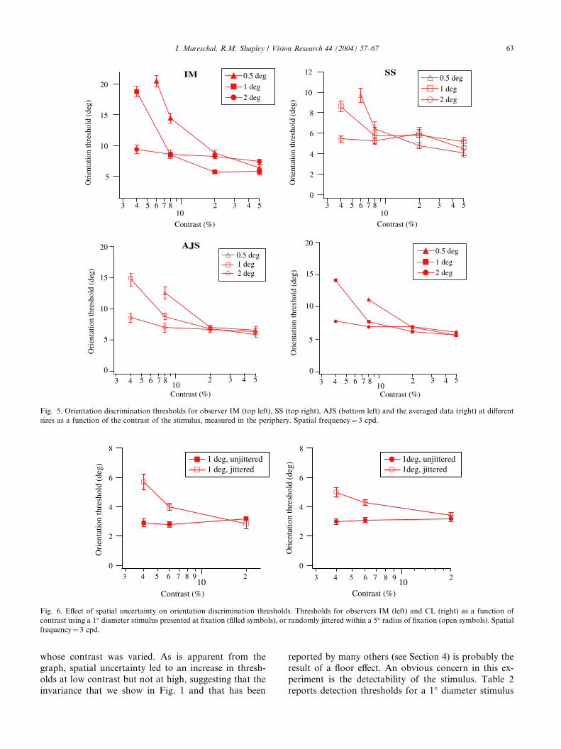
Fig. 5 plots the peripheral data measured for subject

IM (top left), SS (top right), AJS (bottom left) and theaveraged data (bottom right). The data are presented in

the same format as in Fig. 1. The absolute orientation

thresholds are higher in the periphery than in the fovea.

However, as with the foveal data, orientation discrimi-

nation thresholds are not contrast invariant. There is an

interaction between contrast and size in determining

orientation thresholds, with thresholds increasing as

contrast is decreased for stimuli smaller than 2�. Thisfinding is also consistent with a recent report by Sally

and Gurnsey using lines of different lengths in the fovea

and periphery (Sally & Gurnsey, 2003).

0 0.2 0.4 0.6 0.8 1 1.2 1.4 1.6 1.8 21

2

3

4

5

6

7

8

9

10

spatial extent (deg)0.1 0.2 0.3 0.4 0.5 0.6 0.7 0.8 0.9 1

2

3

4

5

6

7

8

9

10

11

12

spatial extent (deg)

Ori

enta

tion

thre

shol

d (d

eg)

Ori

enta

tion

thre

shol

d (d

eg)

4%

6%

8%

20%

80%

4%

6%

8%

20%

ASIM

Fig. 3. Orientation discrimination thresholds plotted as a function of size for two observers. Spatial frequency was 3 cpd for sizes of 0.5� and larger,

6 cpd for a size of 0.25� and 12 cpd for a size of 0.12�.

Table 1

Midway threshold values interpolated from the different contrast

curves in Fig. 3

4% contrast 6% contrast 8% contrast

IM 0.7� 0.56� 0.59�AS 0.5� 0.33� 0.38�

12

10

8

6

4

2

0

Ori

enta

tion

thre

shol

d (d

eg)

Spatial frequency (cpd)

6% 20%

3 6 12 3 6 12

Fig. 4. Orientation discrimination thresholds for observer IM at three

different spatial frequencies for a 0.25� diameter stimulus.

62 I. Mareschal, R.M. Shapley / Vision Research 44 (2004) 57–67

3.3. Contrast invariance or floor effect?

A question which might be raised from our data is

whether the invariance in the orientation thresholds

measured for large sized stimuli reflects contrast in-variance, per se, or is the result of a floor effect. That is

to say, does the measured threshold reflect the actual

size dependence or contrast dependence of the mecha-

nisms (filters) involved, or is some internal noise limiting

performance at high contrast and large size when neural

responses achieve a very high signal:noise ratio? In a

secondary experiment, we sought to address this by

measuring orientation thresholds for large sized stimulias a function of contrast for stimuli that were spatially

jittered. The stimulus could appear in a random spatial

location from the central fixation point within a radius

of 5� and was presented twice within the same spot (for

the two-flash orientation judgment to be made). This

procedure was performed on a large sized stimulus for

which orientation thresholds were found to be invariant

with contrast when there was no uncertainty. The ra-tionale was that by adding spatial uncertainty, we would

Table 2

Contrast detection thresholds for two subjects as a function of the size of th

Fovea

2� 1� 0.5� 0.25�

IM 0.4% 0.68% 1.01% 0.94%

AS 0.45% 0.55% 0.97% 1.2%

The first five columns are thresholds measured for stimuli presented in the f

raise the absolute orientation thresholds, akin to adding

noise. We hypothesized that by doing this while in-

creasing stimulus contrast, two possible outcomes could

arise: either orientation thresholds would remain con-

stant (supporting the notion of contrast invariance in

the sensory signals) or thresholds would decline withincreasing contrast (suggesting that internal, stimulus

independent noise might have been limiting perfor-

mance in the case where the stimuli did not have spatial

uncertainty added).

The results of this experiment are plotted out in Fig. 6

for two observers using a large 1� diameter stimulus

e stimulus

Periphery

0.12� 2� 1� 0.5�

2.5% 0.72% 1.13% 2.5%

2.12% 0.8% 1.2% 2.3%

ovea. The last three columns for stimuli presented 5� peripheral.

20

15

10

5

Ori

enta

tion

thre

shol

d (d

eg)

3 4 5 6 7 810

2 3 4 5

Contrast (%)

0.5 deg1 deg2 deg

12

10

8

6

4

2

0

Ori

enta

tion

thre

shol

d (d

eg)

3 4 5 6 7 810

2 3 4 5

Contrast (%)

0.5 deg1 deg2 deg

20

15

10

5

03 4 5 6 7 8

102 3 4 5

Ori

enta

tion

thre

shol

d (d

eg)

Contrast (%)

0.5 deg1 deg2 deg

Ori

enta

tion

thre

shol

d (d

eg)

Contrast (%)

20

15

10

5

03 4 5 6 7 8

102 3 4 5

0.5 deg1 deg2 deg

IM SS

AJS

Fig. 5. Orientation discrimination thresholds for observer IM (top left), SS (top right), AJS (bottom left) and the averaged data (right) at different

sizes as a function of the contrast of the stimulus, measured in the periphery. Spatial frequency¼ 3 cpd.

8

6

4

2

0

Ori

enta

tion

thre

shol

d (d

eg)

3 4 5 6 7 8 910

2

1deg, unjittered1deg, jittered

8

6

4

2

0

Ori

enta

tion

thre

shol

d (d

eg)

3 4 5 6 7 8 910

2

1 deg, unjittered1 deg, jittered

Contrast (%)Contrast (%)

Fig. 6. Effect of spatial uncertainty on orientation discrimination thresholds. Thresholds for observers IM (left) and CL (right) as a function of

contrast using a 1� diameter stimulus presented at fixation (filled symbols), or randomly jittered within a 5� radius of fixation (open symbols). Spatial

frequency¼ 3 cpd.

I. Mareschal, R.M. Shapley / Vision Research 44 (2004) 57–67 63

whose contrast was varied. As is apparent from the

graph, spatial uncertainty led to an increase in thresh-

olds at low contrast but not at high, suggesting that the

invariance that we show in Fig. 1 and that has been

reported by many others (see Section 4) is probably the

result of a floor effect. An obvious concern in this ex-

periment is the detectability of the stimulus. Table 2

reports detection thresholds for a 1� diameter stimulus

10

8

6

4

2

0

Ori

enta

tion

thre

shol

d (d

eg)

3 4 5 6 7 8 910

2

Contrast(%)

0.5 deg Combined0.5 deg Vertical

10

8

6

4

2

0

Ori

enta

tion

thre

shol

d (d

eg)

3 4 5 6 7 8 910

2

Contrast(%)

0.25 deg Combined0.25 deg Vertical

10

8

6

4

2

0

Ori

enta

tion

thre

shol

d (d

eg)

1 deg Combined 1 deg Vertical

sf=3cpd

sf=3cpd

sf=6cpd

64 I. Mareschal, R.M. Shapley / Vision Research 44 (2004) 57–67

measured at 5� eccentricity. However, although the

stimuli here were not presented that far peripherally,

spatial uncertainty had been added which could have

increased detection thresholds. For this reason we re-

measured the contrast detection threshold for a stimulus

of this size with spatial jitter added within a 3� radius

(as above). The contrast detection threshold was

1.05%±0.12% (IM) and 1.17%±0.2% (CL), so that thelowest contrast tested was roughly four times above

detection threshold. For this reason we feel that the

uncertainty result is not explained by reduced detect-

ability.

3.4. Special case for vertical orientations?

The oblique effect, that observers are more sensitive

to variations in orientation around vertical than around

oblique orientations, is a well documented phenomenon

(e.g. Campbell & Kulikowski, 1966; Heeley, Buchanon-

Smith, Cromwell, & Wright, 1997). We sought to in-

vestigate whether the contrast/size dependency that wereport might be limited to oblique orientations, by ex-

amining orientation discrimination thresholds measured

about the vertical (±3�) only.Fig. 7 plots the result of this experiment for observer

IM. The solid symbols are thresholds obtained using

only vertical orientations, the open symbols are thresh-

olds measured using all orientations between ±45�. Inthe panel on the left, the stimulus size was 0.25�, in themiddle panel the stimulus size was 0.5� and in the right-

hand panel the stimulus was 1�. For all three size con-

ditions, the two contrasts tested were 4% and 20%.

Clearly the contrast-size dependency reported in this

paper also applies to vertical orientations. For the three

different sizes used, the vertical data appear to be simply

a shifted version of the combined data. This indicates

that the dependence of orientation discrimination oncontrast is the same with verticals as with obliques for

each size. This suggests that there is no oblique effect for

contrast’s influence on spatial signal summation.

102

Contrast(%)

Fig. 7. Orientation discrimination thresholds for observer IM using

orientations around vertical only (open symbols) to measure thresh-

olds and combining orientations about vertical and obliques.

4. Discussion

We find that orientation discrimination thresholdsare not contrast invariant but rather depend on both the

contrast and the size of a stimulus. We suggest that the

area of summation (or, the area used to do the orien-

tation task) changes as a function of contrast. This is

reflected by the half height spatial extent varying de-

pending on the contrast of the stimulus used (see Fig. 3).

A similar trend of results was obtained for stimuli pre-

sented in the near periphery, although the absolutethresholds and summation areas differed. We suggest

that our results reflect a change in neural spatial sum-

mation that occurs for low contrast stimuli.

A concern that arises from this experiment is that our

data simply might reflect the fact that the statistical

properties of the stimuli vary at the different sizes and

contrasts used in our experiments. In order to investi-

gate this and to examine whether our results might beaccounted for by an extension of a model based on the

outputs of V1 filters, we modeled our data using con-

ventional models of orientation discrimination based on

population coding (i.e. Henrie & Shapley, 2001; Itti,

25

20

15

10

5

0

Ori

enta

tion

thre

shol

d (d

eg)

2.01.51.00.50.0Size (deg)

20% ave8% ave6% ave4% ave

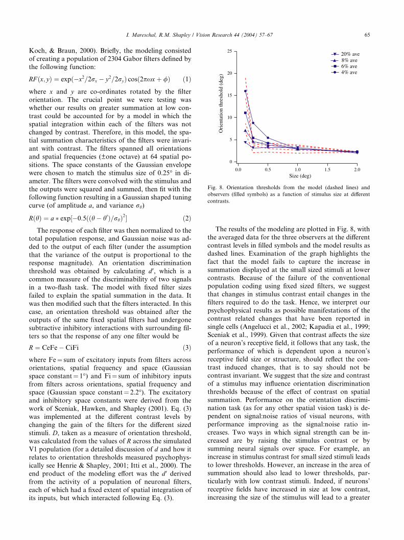
Fig. 8. Orientation thresholds from the model (dashed lines) and

observers (filled symbols) as a function of stimulus size at different

contrasts.

I. Mareschal, R.M. Shapley / Vision Research 44 (2004) 57–67 65

Koch, & Braun, 2000). Briefly, the modeling consisted

of creating a population of 2304 Gabor filters defined by

the following function:

RF ðx; yÞ ¼ expð�x2=2rx � y2=2ryÞ cosð2pxxþ /Þ ð1Þ

where x and y are co-ordinates rotated by the filter

orientation. The crucial point we were testing was

whether our results on greater summation at low con-

trast could be accounted for by a model in which thespatial integration within each of the filters was not

changed by contrast. Therefore, in this model, the spa-

tial summation characteristics of the filters were invari-

ant with contrast. The filters spanned all orientations

and spatial frequencies (±one octave) at 64 spatial po-

sitions. The space constants of the Gaussian envelope

were chosen to match the stimulus size of 0.25� in di-

ameter. The filters were convolved with the stimulus andthe outputs were squared and summed, then fit with the

following function resulting in a Gaussian shaped tuning

curve (of amplitude a, and variance rh)

RðhÞ ¼ a � exp½�0:5ððh� h0Þ=rhÞ2� ð2ÞThe response of each filter was then normalized to the

total population response, and Gaussian noise was ad-

ded to the output of each filter (under the assumptionthat the variance of the output is proportional to the

response magnitude). An orientation discrimination

threshold was obtained by calculating d 0, which is a

common measure of the discriminability of two signals

in a two-flash task. The model with fixed filter sizes

failed to explain the spatial summation in the data. It

was then modified such that the filters interacted. In this

case, an orientation threshold was obtained after theoutputs of the same fixed spatial filters had undergone

subtractive inhibitory interactions with surrounding fil-

ters so that the response of any one filter would be

R ¼ CeFe� CiFi ð3Þwhere Fe¼ sum of excitatory inputs from filters across

orientations, spatial frequency and space (Gaussian

space constant¼ 1�) and Fi¼ sum of inhibitory inputs

from filters across orientations, spatial frequency and

space (Gaussian space constant¼ 2.2�). The excitatory

and inhibitory space constants were derived from the

work of Sceniak, Hawken, and Shapley (2001). Eq. (3)was implemented at the different contrast levels by

changing the gain of the filters for the different sized

stimuli. D, taken as a measure of orientation threshold,

was calculated from the values of R across the simulated

V1 population (for a detailed discussion of d and how it

relates to orientation thresholds measured psychophys-

ically see Henrie & Shapley, 2001; Itti et al., 2000). The

end product of the modeling effort was the d 0 derivedfrom the activity of a population of neuronal filters,

each of which had a fixed extent of spatial integration of

its inputs, but which interacted following Eq. (3).

The results of the modeling are plotted in Fig. 8, with

the averaged data for the three observers at the different

contrast levels in filled symbols and the model results as

dashed lines. Examination of the graph highlights the

fact that the model fails to capture the increase in

summation displayed at the small sized stimuli at lowercontrasts. Because of the failure of the conventional

population coding using fixed sized filters, we suggest

that changes in stimulus contrast entail changes in the

filters required to do the task. Hence, we interpret our

psychophysical results as possible manifestations of the

contrast related changes that have been reported in

single cells (Angelucci et al., 2002; Kapadia et al., 1999;

Sceniak et al., 1999). Given that contrast affects the sizeof a neuron’s receptive field, it follows that any task, the

performance of which is dependent upon a neuron’s

receptive field size or structure, should reflect the con-

trast induced changes, that is to say should not be

contrast invariant. We suggest that the size and contrast

of a stimulus may influence orientation discrimination

thresholds because of the effect of contrast on spatial

summation. Performance on the orientation discrimi-nation task (as for any other spatial vision task) is de-

pendent on signal:noise ratios of visual neurons, with

performance improving as the signal:noise ratio in-

creases. Two ways in which signal strength can be in-

creased are by raising the stimulus contrast or by

summing neural signals over space. For example, an

increase in stimulus contrast for small sized stimuli leads

to lower thresholds. However, an increase in the area ofsummation should also lead to lower thresholds, par-

ticularly with low contrast stimuli. Indeed, if neurons’

receptive fields have increased in size at low contrast,

increasing the size of the stimulus will lead to a greater

66 I. Mareschal, R.M. Shapley / Vision Research 44 (2004) 57–67

increase of signal:noise ratio with area than it would at

high contrasts.

4.1. How does this fit in with contrast invariance?

Many researchers report contrast invariance of ori-

entation thresholds. However, most previous data werecollected along the lower end of our data plots of Fig. 2

and were not typically performed with the smaller sized

stimuli that we used (i.e. Bowne, 1990; Gouled Smith &

Thomas, 1989; Skottun et al., 1987; Westheimer et al.,

1999). Taken at face value, our data could suggest

contrast invariance with large stimuli. However we be-

lieve that this is a floor effect because measuring orien-

tation thresholds as a function of contrast with jitteredstimuli (Fig. 6) revealed that thresholds continue to

improve with increasing contrast for large stimuli.

Thresholds measured on any task result from sig-

nal:noise ratios. As a signal increases, the S:N ratios will

increase and thresholds will decline. In our experiments

using small sized stimuli at low contrast, the S:N ratios

are initially quite low because the signal is weak and

pooling is reduced to a small area (because the stimulusis small) and therefore threshold is high. As contrast is

increased, the strength of the signal will rise and S:N

ratio will increase, resulting in lower thresholds. How-

ever, as contrast is further increased, thresholds plateau.

This type of responsivity has been attributed to an hy-

pothetical non-monotonic increase in the strength of the

signal with contrast (Gouled Smith & Thomas, 1989).

However, we think the plateau might be a consequenceof a floor effect caused by internal noise. For large-sized

stimuli, the trend of results is different. With large

stimuli at low contrasts, S:N ratios are already quite

high because the stimulus more than sufficiently covers

the receptive fields involved in the task. Because of this,

increasing the contrast of the stimulus will not signifi-

cantly improve the S:N ratios.

4.2. Implications for contrast normalization theories

Contrast normalization models arose from the find-

ings that receptive field properties, such as for example

orientation and spatial frequency tuning, appeared to be

contrast invariant (i.e. Albrecht & Hamilton, 1982;Bradley, Skottun, Ohzawa, Sclar, & Freeman, 1987;

Sclar, Maunsell, & Lennie, 1990; Skottun et al., 1987).

Typically, invariance was suggested to occur via a con-

trast gain control mechanism that normalized the re-

sponse of a filter (receptive field) by the pooled

responses of surrounding filters (Carandini & Heeger,

1994; Carandini, Heeger, & Movshon, 1997). The end

result was that the absolute response magnitude of afilter might change as a function of contrast, but its

overall selectivity would not because the normalization

pool was commensurately affected by the changes in

contrast. Here, we find that invariance does not actually

exist in the domain of orientation. This lack of invari-

ance is expected based on the recent finding that re-

ceptive fields change in summation size with contrast.

This suggests a re-examination of theories pertaining to

contrasts’ effects on cortical responses. Previous reports

have found that contrast actually does affect spatial re-

ceptive field properties of V1 neurons (Angelucci et al.,2002; Kapadia et al., 1999; Sceniak et al., 1999), and we

confirm that at least in one domain, orientation, con-

trast can also have strong effects on psychophysically

measured discriminability.

Acknowledgements

This research was supported by National Eye Insti-

tute grant R01EY 01472 to Robert Shapley. We would

like to thank Samuel Solomon, Andrew J. Henrie,

Kukjin Kang, Peter Bex and Steven Dakin for helpful

comments.

References

Albrecht, D. G., & Hamilton, D. B. (1982). Striate cortex of monkey

and cat: contrast response function. Journal of Neurophysiology,

48, 217–237.

Angelucci, A., Levitt, J. B., Walton, E. J. S., Hupe, J.-M., Bullier, J., &

Lund, J. S. (2002). Circuits for local and global signal integration in

primary visual cortex. Journal of Neuroscience, 22, 8633–8646.

Bowne, S. F. (1990). Contrast discrimination cannot explain spatial

frequency, orientation or temporal frequency discrimination.

Vision Research, 30, 449–461.

Bradley, A., Skottun, B. C., Ohzawa, I., Sclar, G., & Freeman, R. D.

(1987). Visual orientation and spatial frequency discrimination: a

comparison of single neurons and behavior. Journal of Neurophy-

siology, 57, 755–772.

Brainard, D. H. (1997). The psychophysics toolbox. Spatial Vision, 10,

433–436.

Burbeck, C. A. (1987). Position and spatial frequency in large-scale

localization judgments. Journal of the Optical Society of America,

27, 417–427.

Burr, D. C., & Wijesundra, S. (1991). Orientation discrimination

depends on spatial frequency. Vision Research, 31, 1449–1452.

Campbell, F. W., & Kulikowski, J. J. (1966). Orientation selectivity of

the human visual system. Journal of Physiology, 187, 437–445.

Carandini, M., & Heeger, D. J. (1994). Summation and division by

neurons in primate visual cortex. Science, 1333–1336.

Carandini, M., Heeger, D. J., & Movshon, J. A. (1997). Linearity and

normalization in simple cells of the macaque primary visual cortex.

Journal of Neuroscience, 17, 8621–8644.

Foster, D. H., & Bischof, W. F. (1991). Thresholds from psychometric

functions: superiority of bootstrap to incremental and probit

variance estimators. Psychological Bulletin, 109, 152–159.

Gouled Smith, B., & Thomas, J. P. (1989). Why are some spatial

discriminations independent of contrast? Journal of the Optical

Society of America, 6, 713–724.

Graham, N., & Robson, J. G. (1987). Summation of very close spatial

frequencies: the importance of spatial probability summation.

Vision Research, 27, 1997–2007.

I. Mareschal, R.M. Shapley / Vision Research 44 (2004) 57–67 67

Hawken, M. J., Gegenfurtner, K. R., & Tang, C. (1994). Contrast

dependence of colour and luminance motion mechanisms in human

vision. Nature, 367, 268–270.

Heeley, D. W., & Buchanon-Smith, H. M. (1990). Recognition of

stimulus orientation. Vision Research, 30, 1429–1437.

Heeley, D. W., Buchanon-Smith, H. M, Cromwell, J. A., & Wright, J.

S. (1997). The oblique effect in orientation acuity. Vision Research,

37, 235–242.

Henrie, J. A., & Shapley, R. M. (2001). The relatively small decline in

orientation acuity as stimulus size decreases. Vision Research, 41,

1723–1733.

Hubel, D. H., & Wiesel, T. N. (1962). Receptive fields, binocular

interaction, and functional architecture in the cat’s visual cortex.

Journal of Physiology, 160, 106–154.

Itti, L., Koch, C., & Braun, J. (2000). Revisiting spatial vision: toward

a unifying model. Journal of the Optical Society of America, 17,

1899–1917.

Jamar, J. H. T., & Koenderink, J. J. (1983). Sine-wave gratings: scale-

invariance and spatial-integration at suprathreshold contrast.

Vision Research, 23, 805–810.

Kapadia, M. K., Westheimer, G., & Gilbert, C. D. (1999). Dynamics

of spatial summation in primary visual cortex of alert monkeys.

Proceedings of the National Academy of Science USA, 96, 12073–

12078.

Legge, G. E., & Foley, J. M. (1980). Contrast masking in human

vision. Journal of the Optical Society of America, 70, 1458–

1471.

Legge, G. E., & Foley, J. M. (1981). Contrast detection and near-

threshold discrimination in human vision. Vision Research, 7,

1041–1053.

Mareschal, I., Henrie, J. A., & Shapley, R. M. (2002). A psychophys-

ical correlate of contrast dependent changes in receptive field

properties. Vision Research, 42, 1879–1887.

McIlhagga, W. H., & Mullen, K. T. (1996). Contour integration with

colour and luminance contrast. Vision Research, 9, 1265–1280.

Orban, G. A., Vandenbussche, E., & Vogels, R. (1984). Human

orientation discrimination tested with long stimuli. Vision Re-

search, 24, 121–128.

Pelli, D. G. (1997). The Videotoolbox software for visual psychophys-

ics: transforming numbers into movies. Spatial Vision, 10, 437–442.

Phillips, G. C., & Wilson, H. W. (1984). Orientation bandwidths of

spatial mechanisms measured by masking. Journal of the Optical

Society of America A, 1, 226–232.

Polat, U., & Sagi, D. (1993). Lateral interactions between spatial

channels: supppression and facilitation revealed by lateral masking

experiments. Vision Research, 33, 993–999.

Regan, D., & Beverley, K. I. (1985). Postadaptation orientation

discrimination. Journal of the Optical Society of America, 2, 147–

155.

Reisbeck, T. E., & Gegenfurtner, K. R. (1998). Effects of contrast and

temporal frequency on orientation discrimination for luminance

and isoluminant stimuli. Vision Research, 38, 1105–1117.

Sally, S. L., & Gurnsey, R. (2003). Orientation discrimination in foveal

and extra-foveal vision: effects of stimulus bandwidth and contrast.

Vision Research, 43, 1375–1385.

Sceniak, M. P., Hawken, M. J., & Shapley, R. M. (2001). Visual spatial

characterization of macaque V1 neurons. Journal of Neurophysi-

ology, 85, 1873–1887.

Sceniak, M. P., Hawken, M. J., & Shapley, R. M. (2002). Contrast-

dependent changes in spatial frequency tuning of macaque V1

neurons: effects of a changing receptive field size. Journal of

Neurophysiology, 88, 1363–1373.

Sceniak, M. P., Ringach, D. L., Hawken, M. J., & Shapley, R. M.

(1999). Contrast’s effect on spatial summation by macaque V1

neurons. Nature Neuroscience, 2, 733–739.

Sclar, G., Maunsell, J. H., & Lennie, P. (1990). Coding of image

contrast in central visual pathways of the macaque monkey. Vision

Research, 30, 1–10.

Skottun, B. C., Bradley, A., Sclar, G., Ohzawa, I., & Freeman, R. D.

(1987). The effects of contrast on visual orientation and spatial

frequency discrimination: a comparison of single cells and behav-

iour. Journal of Neurophysiology, 57, 773–786.

Snowden, R. J., & Hammett, S. T. (1998). The effects of surround

contrast on contrast thresholds perceived, contrast and contrast

discrimination. Vision Research, 38, 1935–1945.

Solomon, J. A., & Morgan, M. J. (2000). Facilitation from collinear

flanks is cancelled by non-collinear flanks. Vision Research, 40,

279–286.

Stone, L. S., & Thompson, P. (1992). Human speed perception is

contrast dependent. Vision Research, 32, 1535–1549.

Thomas, J. P., & Olzak, L. A. (1997). Contrast gain control and fine

spatial discriminations. Journal of the Optical Society of America,

14, 2392–2405.

Webster, M. A., De Valois, K. K., & Switkes, E. (1990). Orientation

and spatial-frequency discrimination for luminance and chromatic

gratings. Journal of the Optical Society of America, 7, 1034–1049.

Westheimer, G., Brincat, S., & Werhahn, C. (1999). Contrast

dependency of foveal spatial functions: orientation, vernier, blur

and displacement discrimination and the tilt and Poggendorff

illusions. Vision Research, 39, 1631–1639.

Yu, C., & Levi, D. M. (1998). Spatial-frequency and orientation tuning

in psychophysical end-stopping. Visual Neuroscience, 15, 585–595.