Effectiveness of SOx, NOx, and Primary Particulate Matter ...

atmosphere

Article

Effectiveness of SOx, NOx, and Primary Particulate MatterControl Strategies in the Improvement of Ambient PMConcentration in Taiwan

Jiun-Horng Tsai 1,2, Ming-Ye Lee 1 and Hung-Lung Chiang 3,*

�����������������

Citation: Tsai, J.-H.; Lee, M.-Y.;

Chiang, H.-L. Effectiveness of SOx,

NOx, and Primary Particulate Matter

Control Strategies in the

Improvement of Ambient PM

Concentration in Taiwan. Atmosphere

2021, 12, 460. https://doi.org/

10.3390/atmos12040460

Academic Editors: Soontae Kim and

Rafael Borge

Received: 3 March 2021

Accepted: 31 March 2021

Published: 6 April 2021

Publisher’s Note: MDPI stays neutral

with regard to jurisdictional claims in

published maps and institutional affil-

iations.

Copyright: © 2021 by the authors.

Licensee MDPI, Basel, Switzerland.

This article is an open access article

distributed under the terms and

conditions of the Creative Commons

Attribution (CC BY) license (https://

creativecommons.org/licenses/by/

4.0/).

1 Department of Environmental Engineering, National Cheng Kung University, Tainan 701, Taiwan;[email protected] (J.-H.T.); [email protected] (M.-Y.L.)

2 Research Center for Climate Change and Environment Quality, National Cheng Kung University,Tainan 701, Taiwan

3 Department of Safety Health and Environmental Engineering, National Yunlin University of Science andTechnology, Yunlin 64002, Taiwan

* Correspondence: [email protected]; Tel.: +886-5-536-1489; Fax: +886-5-536-1353

Abstract: The Community Multiscale Air Quality (CMAQ) measurement was employed for eval-uating the effectiveness of fine particulate matter control strategies in Taiwan. There are threescenarios as follows: (I) the 2014 baseline year emission, (II) 2020 emissions reduced via the CleanAir Act (CAA), and (III) other emissions reduced stringently via the Clean Air Act. Based on theTaiwan Emission Data System (TEDs) 8.1, established in 2014, the emission of particulate matter2.5 (PM2.5) was 73.5 thousand tons y−1, that of SOx was 121.3 thousand tons y−1, and that of NOxwas 404.4 thousand tons y−1 in Taiwan. The CMAQ model simulation indicated that the PM2.5

concentration was 21.9 µg m−3. This could be underestimated by 24% in comparison with data fromthe ambient air quality monitoring stations of the Taiwan Environmental Protection Administration(TEPA). The results of the simulation of the PM2.5 concentration showed high PM2.5 concentrations incentral and southwestern Taiwan, especially in Taichung and Kaohsiung. Compared to scenario I, theaverage annual concentrations of PM2.5 for scenario II and scenario III showed reductions of 20.1%and 28.8%, respectively. From the results derived from the simulation, it can be seen that controlof NOx emissions may improve daily airborne PM2.5 concentrations in Taiwan significantly andcontrol of directly emitted PM2.5 emissions may improve airborne PM2.5 concentrations each month.Nevertheless, the results reveal that the preliminary control plan could not achievethe air qualitystandard. Therefore, the efficacy and effectiveness of the control measures must be considered tobetter reduce emissions in the future.

Keywords: Community Multiscale Air Quality (CMAQ); SOx; NOx; sulfate; nitrate; primary particu-late matter

1. Introduction

Air pollutants have a significant influence on global human health, quality of life,premature deaths and mortality rate, and the occurrence of different respiratory illnessesrelated to ambient air quality [1–6]. Each year, approximately seven million prematuredeaths are recorded across the world. Specifically, one-eighth of the total deaths in theworld are due to the combined effects of household and ambient air pollution [7]. Airpollution causes considerable economic impacts and also increases medical expenses,and the related loss of working days reduces economic productivity [8]. In Asia, it isestimated that about 7% of the gross domestic product (GDP) loss was attributed to localair pollution [9]. As far as the health risks associated with this particulate matter areconcerned, many epidemiological studies have been published to understand associatedcardiovascular diseases, respiratory diseases, cancer, and birth defects [10–17]. Moreover, afew studies have found a link between particles and inflammatory responses in sensitive

Atmosphere 2021, 12, 460. https://doi.org/10.3390/atmos12040460 https://www.mdpi.com/journal/atmosphere

Atmosphere 2021, 12, 460 2 of 16

people [18–20]. As discussed above, the influence of particulate matter (PM) on humanhealth is considered a crucial factor for air quality management.

Particulate matter (PM) pollution, which shortens the lives of humans significantly,contributes to a wide range of diseases [21,22]. Many epidemiological studies have iden-tified a positive correlation associating cardiovascular diseases, respiratory disease, andPM [10,23,24]. In addition, studies have indicated that PM is closely related to increasesin the mortality rates of lung cancer and other cardiopulmonary diseases [25–27]. Fineatmospheric aerosol mass concentrations are detrimental due to their influence on therespiratory system, their impact on visibility conditions, and their role in global climatechange [28,29]. In addition, to carbonaceous species, sulfate, nitrate, and ammonium arethe major species present in fine particulate matter in most situations [29]. In a study byDongarrà et al. [30], water-soluble ions consisted of a large fraction of PM10 and PM2.5 andammonium, sulfate, and nitrate particles accounted for 14–29% of the PM mass concen-tration. In the European population, the prevalence of the secondary inorganic aerosol(SIA) could be twice as high as that of the primary fine particulate matter [31]. In a Danishcohort study, the results indicated that long-term exposure to PM2.5, black carbon/organiccarbon (BC/OC), and secondary organic aerosols causes cardiovascular disease and mor-tality [32]. Therefore, the formation of the secondary aerosol fraction could be essentialfor understanding the source of fine PM contribution and set up PM control strategies.Furthermore, gas-phase reactions, such as SO2 and NO2, are precursors to the productionof H2SO4 and HNO3 via photochemical reactions, and this makes it possible for them totransfer into particulate matter [33]. Behera and Sharma [34] investigated the degradationof SO2, NO2, and NH3, and they found that these could form secondary inorganic aerosolsin an environmental chamber study. Secondary inorganic particulate matter, the domi-nant component of fine particles, is formed by homogeneous and heterogeneous reactionsamong gas species [35–37].

In addition, the effectiveness of air pollution control strategies is assessed to improveambient air quality, reduce exposure, and support human health. The US EnvironmentalProtection Agency (EPA) [38] is following the Clean Air Act (CAA) to use quality mod-els for the assessment of regulations, control strategies, and actions to not only reduceemissions but also improve ambient air quality. Air dispersion models are consideredimportant to inform a number of different regulatory assessments, e.g., the RegulatoryImpact Assessments, used to guide federal actions, and the National Ambient Air Qual-ity Standards (NAAQS), used to assess hazardous air pollutants and other health andecosystem measures. In Europe, the control of air pollutant emissions and related regula-tions were enacted with the intention to improve air quality across Europe [8]. In recentyears, the Community Multiscale Air Quality (CMAQ) model has been implemented withcomprehensive halogen sources and chemistry [39] to examine the overall influence ofhalogen species on air pollution over Europe, as the grid size can affect the predictionsof the CMAQ model [40]. Some research studies have been performed in northeasternU.S., including urban health impact studies using the Community Multiscale Air Quality(CMAQ) models to determine air pollution exposure. Results indicate that a larger domainis highly recommended for summer and weekends in eastern U.S. [41].

The observations at these stations can only monitor the level of pollutants aroundparticular locations. However, the emission, transport, and transformation of pollutionover the whole region can be shown by these models. Therefore, it is essential to harmonizethe criteria with capable and competent models to reproduce air quality features overa particular region in order to officially report national air pollution levels and examinecompliance with regulations [6].

In China, about one million deaths per year are attributed to air pollution [42]. TheAir Pollution Prevention and Control Action Plan (APPCAP) was implemented to reducePM2.5 concentration from 2013 to 2017, and the results indicated a 6.8% reduction rate inmortality attributable to PM2.5 pollution in 2017 compared to that in 2013. This supportsthe effectiveness of the APPCAP [42]. The question of how to validate the effectiveness

Atmosphere 2021, 12, 460 3 of 16

of air pollution control strategies could be an important focus for future works on airquality management.

In Taiwan, some studies have indicated that the CMAQ simulation is associated with adynamic NH3 emissions approach that could improve diurnal and seasonal variations andreduce simulation bias [43]. A real-time air quality forecasting (AQF) system was developedusing the Weather Research and Forecasting meteorological model and the CMAQ modelfor PM2.5 prediction, and the AQF system was able to reduce the PM2.5 forecast error andimprove the root-mean-square error (RMSE) and mean bias (MB) calculations [44]. Inaddition, local sources could be the most important emission sources and the emissionsof the power plants and iron/steel industries were under control. The management ofmotor vehicle emissions and construction/road dust should be taken into consideration toimprove PM2.5 levels in Taiwan [45].

Over the past decade, PM2.5 concentrations have presented a decreasing trend, asdetermined by the Taiwan EPA monitoring station network. The average concentrationwas 34 µg m−3 in 2007 and 30 µg m−3 in 2013. However, it still exceeds the level of15 µg m−3 (the annual average concentration) set by Taiwan’s National Ambient AirQuality Standard (NAAQS). Therefore, the effectiveness of air pollution control strategiesis important to enforce an emission reduction in gas precursors such as SOx and NOx andprimary particulate matter for improvement in ambient air quality.

The objective of this study was improvement in ambient PM2.5 concentrations usingvarious control measures under different scenarios. Emissions of primary PM2.5, SOx,and NOx were estimated, and an air quality model, CMAQ, was employed in simulatingthe ambient concentration of PM2.5. The simulated concentrations of each scenario werecompared to those generated from basic cases to demonstrate the effectiveness of the PM2.5control measures.

2. Materials and Methods2.1. Model Simulation

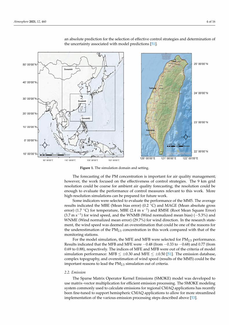
The US Environmental Protection Agency’s Community Multiscale Air Quality (CMAQ)modeling system version 4.7.1, associated with the fifth-generation Pennsylvania StateUniversity National Center for Atmospheric Research Mesoscale Model (MM5) version 3.7,was adopted to simulate ambient concentrations of PM2.5 in Taiwan. The modeling systemtook into account the chemistry and physics of pollutant transport, as presented in theguidelines suggested by Byun and Schere [46] and simultaneous frameworks proposed byWong et al. [47]. The system consists of three-level nested domains, as shown in Figure 1,where domain 1 (D1) covers east and south Asia (81 km × 81 km), domain 2 (D2) coversMainland China and east Asia (Japan and Korea) (27 km × 27 km), and domain 3 (D3)covers southeast China and Taiwan (9 km × 9 km).

Meteorology outputs were processed with the Meteorology–Chemistry Interface Pro-cessor (MCIP) [48] (version 4.3). The purpose was to build air-quality-model-ready meteo-rological input files.

CMAQ default profiles were used for the 81km outermost domain’s lateral boundaryconditions (BCs) and initial conditions (ICs). Boundary conditions for finer domains arenormally generated from coarser domains. Using ICON (Initial condition) and BCON(Boundary condition) modules, part of the preprocessing of the modules of CMAQ involvedthe preparation BCs and ICs. The CMAQ Chemistry-Transport Model (CCTM) with aEuler Backward Iterative (EBI) chemistry solver for photochemical mechanisms was used.The chemical mechanism used for the gaseous species was the carbon bond mechanism(CB05) [49].

There are many methods and performance indicators to validate the model simulation.Generally, the performance of a dispersion model simulation can be assessed by themean fractional error (MFE) (≤±50%) and the mean fractional bias (MFB) (≤±30%), andextended diagnostic evaluation and sensitivity tests can improve the performance of themodel simulation [50–52]. Results of the model simulation are used for a relative rather than

Atmosphere 2021, 12, 460 4 of 16

an absolute prediction for the selection of effective control strategies and determination ofthe uncertainty associated with model predictions [51].

Atmosphere 2021, 12, x FOR PEER REVIEW 4 of 17

Figure 1. The simulation domain and setting.

There are many methods and performance indicators to validate the model simula-tion. Generally, the performance of a dispersion model simulation can be assessed by the mean fractional error (MFE) (≤±50%) and the mean fractional bias (MFB) (≤ ±30%), and extended diagnostic evaluation and sensitivity tests can improve the performance of the model simulation [50–52]. Results of the model simulation are used for a relative rather than an absolute prediction for the selection of effective control strategies and determi-nation of the uncertainty associated with model predictions [51].

The forecasting of the PM concentration is important for air quality management; however, the work focused on the effectiveness of control strategies. The 9km grid reso-lution could be coarse for ambient air quality forecasting; the resolution could be enough to evaluate the performance of control measures relevant to this work. More high-resolution simulations can be prepared for future work.

Some indicators were selected to evaluate the performance of the MM5. The average results indicated the MBE (Mean bias error) (0.2 °C) and MAGE (Mean absolute gross error) (1.7 °C) for temperature, MBE (2.4 m s−1) and RMSE (Root Mean Square Error) (3.7 m s−1) for wind speed, and the WNMB (Wind normalized mean bias) (−5.3%) and WNME (Wind normalized mean error) (29.7%) for wind direction. In the research statement, the wind speed was deemed an overestimation that could be one of the reasons for the un-derestimation of the PM2.5 concentration in this work compared with that of the moni-toring stations.

For the model simulation, the MFE and MFB were selected for PM2.5performance. Results indicated that the MFB and MFE were −0.48 (from −0.33 to −0.68) and 0.77 (from 0.69 to 0.88), respectively. The indices of MFE and MFB were out of the criteria of model simulation performance: MFB ≤ ±0.30 and MFE ≤ ±0.50 [51]. The emission database, complex topography, and overestimation of wind speed (results of the MM5) could be the important reasons to lead the PM2.5 simulation out of criteria.

Figure 1. The simulation domain and setting.

The forecasting of the PM concentration is important for air quality management;however, the work focused on the effectiveness of control strategies. The 9 km gridresolution could be coarse for ambient air quality forecasting; the resolution could beenough to evaluate the performance of control measures relevant to this work. Morehigh-resolution simulations can be prepared for future work.

Some indicators were selected to evaluate the performance of the MM5. The averageresults indicated the MBE (Mean bias error) (0.2 ◦C) and MAGE (Mean absolute grosserror) (1.7 ◦C) for temperature, MBE (2.4 m s−1) and RMSE (Root Mean Square Error)(3.7 m s−1) for wind speed, and the WNMB (Wind normalized mean bias) (−5.3%) andWNME (Wind normalized mean error) (29.7%) for wind direction. In the research state-ment, the wind speed was deemed an overestimation that could be one of the reasons forthe underestimation of the PM2.5 concentration in this work compared with that of themonitoring stations.

For the model simulation, the MFE and MFB were selected for PM2.5 performance.Results indicated that the MFB and MFE were −0.48 (from −0.33 to −0.68) and 0.77 (from0.69 to 0.88), respectively. The indices of MFE and MFB were out of the criteria of modelsimulation performance: MFB ≤ ±0.30 and MFE ≤ ±0.50 [51]. The emission database,complex topography, and overestimation of wind speed (results of the MM5) could be theimportant reasons to lead the PM2.5 simulation out of criteria.

2.2. Emission

The Sparse Matrix Operator Kernel Emissions (SMOKE) model was developed touse matrix–vector multiplication for efficient emission processing. The SMOKE modelingsystem commonly used to calculate emissions for regional CMAQ applications has recentlybeen fine-tuned to support hemispheric CMAQ applications to allow for more streamlinedimplementation of the various emission processing steps described above [53].

Atmosphere 2021, 12, 460 5 of 16

The emission data used 1 km × 1 km data from the Taiwan Emission Data System(TEDs) v8.1 by referring to the format of SMOKE. The monitoring concentrations from theTaiwan Environmental Protection Administration (TEPA) air quality monitoring stationwere included here to evaluate model performance.

2.3. Scenarios

In this study, emission scenarios consisting of three parts were evaluated: a basiccase and two controlled cases. The basic case, scenario I, represented the emissions fromstationary sources and mobile sources and fugitive emissions in the base year (2014)following the emission standards of TEDs 8.1 developed and proven by TEPA. It focusedon permitted emissions from stationary sources, showing emission conditions in 2014. Theother scenarios were based on TEDs 8.1 and reduced the air pollution emissions followingthe control strategies of the different scenarios in 2020. According to the contents of thecontrol measures, the emissions of primary PM2.5, e.g., sulfur dioxide (SOx) and nitrogendioxide (NOx), under different scenarios were estimated. Scenario II was an adapted plan(Taiwan Clean Air Act Plan) designed to include more stringent emission standards forstationary sources (especial power plants) and on-road mobile sources, eliminate high-polluting aged vehicles, and promote electric vehicles. For scenario III, it was assumedthat more control measures could be conducted beyond scenario II. The measures involvedincluded the elimination of two-stroke motorcycles, the promotion of hybrid vehiclesand electric buses, and encouragement of the use of natural gas in power plants (shownin Table 1).

Table 1. The control strategies of the different scenarios.

Scenario Strategies

Scenario IYear–2014 Baseline year–2014

Scenario IITaiwan Clean Air

Act (TCAA)2020

• Allow emission growth by demand.• Power plant: replace the generation sector.• Conduct the state implement plan.• Make stringent the emission standards for power plants.• Identify mobile sources.• Replace two-stroke motorcycles.• Replace old buses.• Fugitive source: control river dust.

Scenario IIITCAA and

implement morecontrol strategies

Year–2020

• Follow the strategies of scenario II.• Implement more control strategies.• Make stringent the emission standards of existing sources (power

plants; basic iron and steel manufacturing; petroleum and coalproduct manufacturing; chemical material manufacturing;petrochemical manufacturing; pulp, paper, and paper productmanufacturing; and others).

• Phase out two-stroke motorcycles.• Promote clean fuels.

� Promote liquefied natural gas (LNG) for power plants.� Promote use of hybrid oil–electricity passenger cars.� Electrify buses.

3. Results and Discussion3.1. Baseline Conditions: Scenario I

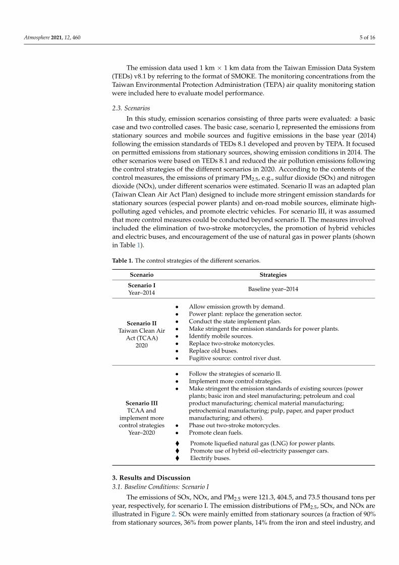
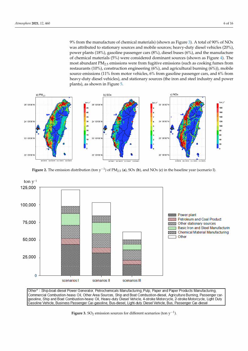
The emissions of SOx, NOx, and PM2.5 were 121.3, 404.5, and 73.5 thousand tons peryear, respectively, for scenario I. The emission distributions of PM2.5, SOx, and NOx areillustrated in Figure 2. SOx were mainly emitted from stationary sources (a fraction of 90%from stationary sources, 36% from power plants, 14% from the iron and steel industry, and

Atmosphere 2021, 12, 460 6 of 16

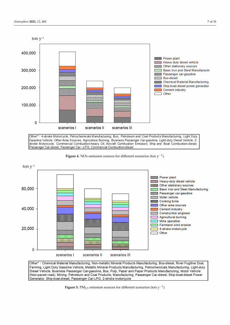
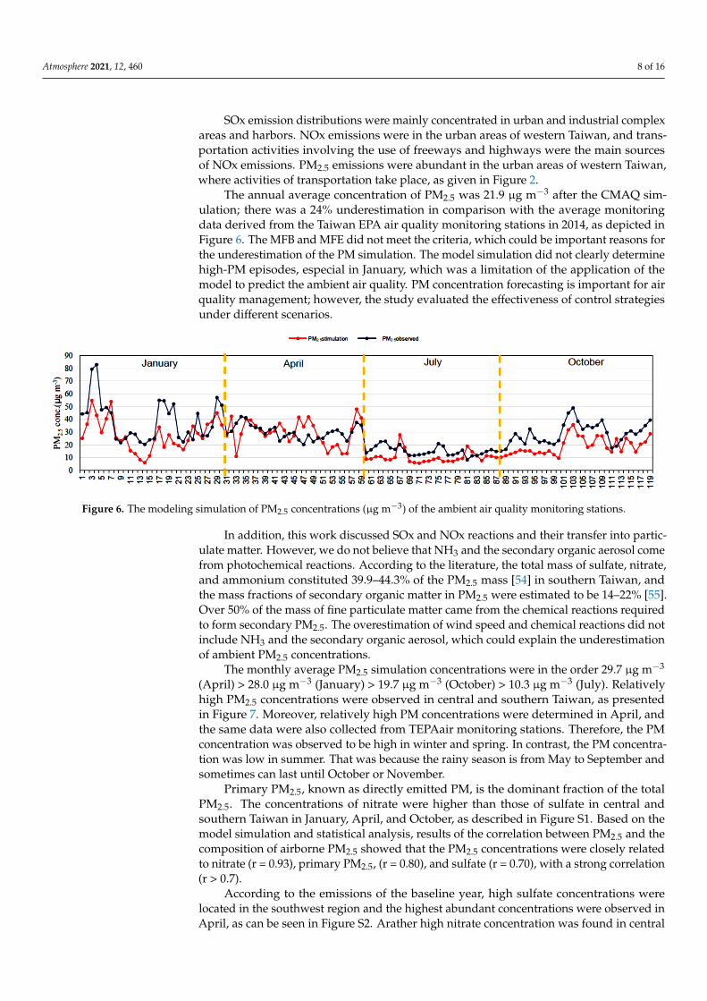
9% from the manufacture of chemical materials) (shown as Figure 3). A total of 90% of NOxwas attributed to stationary sources and mobile sources; heavy-duty diesel vehicles (20%),power plants (18%), gasoline passenger cars (8%), diesel buses (6%), and the manufactureof chemical materials (5%) were considered dominant sources (shown as Figure 4). Themost abundant PM2.5 emissions were from fugitive emissions (such as cooking fumes fromrestaurants (10%), construction engineering (6%), and agricultural burning (6%)), mobilesource emissions (11% from motor vehicles, 6% from gasoline passenger cars, and 6% fromheavy-duty diesel vehicles), and stationary sources (the iron and steel industry and powerplants), as shown in Figure 5.

Atmosphere 2021, 12, x FOR PEER REVIEW 6 of 17

3. Results and Discussion 3.1. Baseline Conditions: Scenario I

The emissions of SOx, NOx, and PM2.5 were 121.3, 404.5, and 73.5 thousand tons per year, respectively, for scenario I. The emission distributions of PM2.5, SOx, and NOx are illustrated in Figure 2. SOx were mainly emitted from stationary sources (a fraction of 90% from stationary sources, 36% from power plants, 14% from the iron and steel in-dustry, and 9% from the manufacture of chemical materials) (shown as Figure 3). A total of 90% of NOx was attributed to stationary sources and mobile sources; heavy-duty die-sel vehicles (20%), power plants (18%), gasoline passenger cars (8%), diesel buses (6%), and the manufacture of chemical materials (5%) were considered dominant sources (shown as Figure 4). The most abundant PM2.5 emissions were from fugitive emissions (such as cooking fumes from restaurants (10%), construction engineering (6%), and ag-ricultural burning (6%)), mobile source emissions (11% from motor vehicles, 6% from gasoline passenger cars, and 6% from heavy-duty diesel vehicles), and stationary sources (the iron and steel industry and power plants), as shown in Figure 5.

Figure 2. The emission distribution (ton y−1) of PM2.5 (a), SOx (b), and NOx (c) in the baseline year (scenario I). Figure 2. The emission distribution (ton y−1) of PM2.5 (a), SOx (b), and NOx (c) in the baseline year (scenario I).

Atmosphere 2021, 12, x FOR PEER REVIEW 7 of 17

Figure 3. SO2 emission sources for different scenarios (ton y−1).

Figure 4. NOx emission sources for different scenarios (ton y−1).

ton y−1

ton y−1

Figure 3. SO2 emission sources for different scenarios (ton y−1).

Atmosphere 2021, 12, 460 7 of 16

Atmosphere 2021, 12, x FOR PEER REVIEW 7 of 17

Figure 3. SO2 emission sources for different scenarios (ton y−1).

Figure 4. NOx emission sources for different scenarios (ton y−1).

ton y−1

ton y−1

Figure 4. NOx emission sources for different scenarios (ton y−1).

Atmosphere 2021, 12, x FOR PEER REVIEW 8 of 17

Figure 5. PM2.5emission sources for different scenarios (ton y−1).

SOx emission distributions were mainly concentrated in urban and industrial com-plex areas and harbors. NOx emissions were in the urban areas of western Taiwan, and transportation activities involving the use of freeways and highways were the main sources of NOx emissions. PM2.5 emissions were abundant in the urban areas of western Taiwan, where activities of transportation take place, as given in Figure 2.

The annual average concentration of PM2.5 was 21.9 μg m−3 after the CMAQ simula-tion; there was a 24% underestimation in comparison with the average monitoring data derived from the Taiwan EPA air quality monitoring stations in 2014, as depicted in Figure 6. The MFB and MFE did not meet the criteria, which could be important reasons for the underestimation of the PM simulation. The model simulation did not clearly de-termine high-PM episodes, especial in January, which was a limitation of the application of the model to predict the ambient air quality. PM concentration forecasting is important for air quality management; however, the study evaluated the effectiveness of control strategies under different scenarios.

Figure 6. The modeling simulation of PM2.5 concentrations (μg m−3) of the ambient air quality monitoring stations.

ton y−1

Figure 5. PM2.5 emission sources for different scenarios (ton y−1).

Atmosphere 2021, 12, 460 8 of 16

SOx emission distributions were mainly concentrated in urban and industrial complexareas and harbors. NOx emissions were in the urban areas of western Taiwan, and trans-portation activities involving the use of freeways and highways were the main sourcesof NOx emissions. PM2.5 emissions were abundant in the urban areas of western Taiwan,where activities of transportation take place, as given in Figure 2.

The annual average concentration of PM2.5 was 21.9 µg m−3 after the CMAQ sim-ulation; there was a 24% underestimation in comparison with the average monitoringdata derived from the Taiwan EPA air quality monitoring stations in 2014, as depicted inFigure 6. The MFB and MFE did not meet the criteria, which could be important reasons forthe underestimation of the PM simulation. The model simulation did not clearly determinehigh-PM episodes, especial in January, which was a limitation of the application of themodel to predict the ambient air quality. PM concentration forecasting is important for airquality management; however, the study evaluated the effectiveness of control strategiesunder different scenarios.

Atmosphere 2021, 12, x FOR PEER REVIEW 8 of 17

Figure 5. PM2.5emission sources for different scenarios (ton y−1).

SOx emission distributions were mainly concentrated in urban and industrial com-plex areas and harbors. NOx emissions were in the urban areas of western Taiwan, and transportation activities involving the use of freeways and highways were the main sources of NOx emissions. PM2.5 emissions were abundant in the urban areas of western Taiwan, where activities of transportation take place, as given in Figure 2.

The annual average concentration of PM2.5 was 21.9 μg m−3 after the CMAQ simula-tion; there was a 24% underestimation in comparison with the average monitoring data derived from the Taiwan EPA air quality monitoring stations in 2014, as depicted in Figure 6. The MFB and MFE did not meet the criteria, which could be important reasons for the underestimation of the PM simulation. The model simulation did not clearly de-termine high-PM episodes, especial in January, which was a limitation of the application of the model to predict the ambient air quality. PM concentration forecasting is important for air quality management; however, the study evaluated the effectiveness of control strategies under different scenarios.

Figure 6. The modeling simulation of PM2.5 concentrations (μg m−3) of the ambient air quality monitoring stations.

ton y−1

Figure 6. The modeling simulation of PM2.5 concentrations (µg m−3) of the ambient air quality monitoring stations.

In addition, this work discussed SOx and NOx reactions and their transfer into partic-ulate matter. However, we do not believe that NH3 and the secondary organic aerosol comefrom photochemical reactions. According to the literature, the total mass of sulfate, nitrate,and ammonium constituted 39.9–44.3% of the PM2.5 mass [54] in southern Taiwan, andthe mass fractions of secondary organic matter in PM2.5 were estimated to be 14–22% [55].Over 50% of the mass of fine particulate matter came from the chemical reactions requiredto form secondary PM2.5. The overestimation of wind speed and chemical reactions did notinclude NH3 and the secondary organic aerosol, which could explain the underestimationof ambient PM2.5 concentrations.

The monthly average PM2.5 simulation concentrations were in the order 29.7 µg m−3

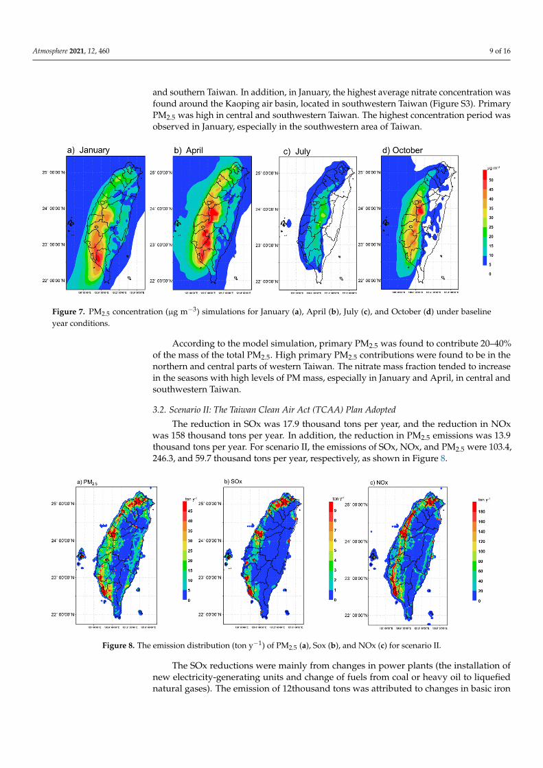
(April) > 28.0 µg m−3 (January) > 19.7 µg m−3 (October) > 10.3 µg m−3 (July). Relativelyhigh PM2.5 concentrations were observed in central and southern Taiwan, as presentedin Figure 7. Moreover, relatively high PM concentrations were determined in April, andthe same data were also collected from TEPAair monitoring stations. Therefore, the PMconcentration was observed to be high in winter and spring. In contrast, the PM concentra-tion was low in summer. That was because the rainy season is from May to September andsometimes can last until October or November.

Primary PM2.5, known as directly emitted PM, is the dominant fraction of the totalPM2.5. The concentrations of nitrate were higher than those of sulfate in central andsouthern Taiwan in January, April, and October, as described in Figure S1. Based on themodel simulation and statistical analysis, results of the correlation between PM2.5 and thecomposition of airborne PM2.5 showed that the PM2.5 concentrations were closely relatedto nitrate (r = 0.93), primary PM2.5, (r = 0.80), and sulfate (r = 0.70), with a strong correlation(r > 0.7).

According to the emissions of the baseline year, high sulfate concentrations werelocated in the southwest region and the highest abundant concentrations were observed inApril, as can be seen in Figure S2. Arather high nitrate concentration was found in central

Atmosphere 2021, 12, 460 9 of 16

and southern Taiwan. In addition, in January, the highest average nitrate concentration wasfound around the Kaoping air basin, located in southwestern Taiwan (Figure S3). PrimaryPM2.5 was high in central and southwestern Taiwan. The highest concentration period wasobserved in January, especially in the southwestern area of Taiwan.

Atmosphere 2021, 12, x FOR PEER REVIEW 9 of 17

In addition, this work discussed SOx and NOx reactions and their transfer into par-ticulate matter. However, we do not believe that NH3 and the secondary organic aerosol come from photochemical reactions. According to the literature, the total mass of sulfate, nitrate, and ammonium constituted 39.9–44.3% of the PM2.5 mass [54] in southern Tai-wan, and the mass fractions of secondary organic matter in PM2.5were estimated to be 14−22% [55]. Over 50% of the mass of fine particulate matter came from the chemical re-actions required to form secondary PM2.5. The overestimation of wind speed and chemi-cal reactions did not include NH3 and the secondary organic aerosol, which could explain the underestimation of ambient PM2.5 concentrations.

The monthly average PM2.5 simulation concentrations were in the order 29.7 μg m−3 (April) > 28.0 μg m−3 (January) > 19.7 μg m−3 (October) > 10.3 μg m−3 (July). Relatively high PM2.5 concentrations were observed in central and southern Taiwan, as presented in Figure 7. Moreover, relatively high PM concentrations were determined in April, and the same data were also collected from TEPAair monitoring stations. Therefore, the PM concentration was observed to be high in winter and spring. In contrast, the PM concen-tration was low in summer. That was because the rainy season is from May to September and sometimes can last until October or November.

Figure 7. PM2.5 concentration (μg m−3) simulations for January (a), April (b), July (c), and October (d) under baseline year conditions.

Primary PM2.5, known as directly emitted PM, is the dominant fraction of the total PM2.5. The concentrations of nitrate were higher than those of sulfate in central and southern Taiwan in January, April, and October, as described in Figure S1. Based on the model simulation and statistical analysis, results of the correlation between PM2.5 and the composition of airborne PM2.5 showed that the PM2.5 concentrations were closely related to nitrate (r = 0.93), primary PM2.5, (r = 0.80), and sulfate (r = 0.70), with a strong correlation (r > 0.7).

According to the emissions of the baseline year, high sulfate concentrations were located in the southwest region and the highest abundant concentrations were observed in April, as can be seen in Figure S2. Arather high nitrate concentration was found in central and southern Taiwan. In addition, in January, the highest average nitrate concentra-tion was found around the Kaoping air basin, located in southwestern Taiwan (Figure S3). Primary PM2.5 was high in central and southwestern Taiwan. The highest concentration pe-riod was observed in January, especially in the southwestern area of Taiwan.

According to the model simulation, primary PM2.5 was found to contribute 20−40% of the mass of the total PM2.5. High primary PM2.5 contributions were found to be in the northern and central parts of western Taiwan. The nitrate mass fraction tended to in-crease in the seasons with high levels of PM mass, especially in January and April, in central and southwestern Taiwan.

Figure 7. PM2.5 concentration (µg m−3) simulations for January (a), April (b), July (c), and October (d) under baselineyear conditions.

According to the model simulation, primary PM2.5 was found to contribute 20–40%of the mass of the total PM2.5. High primary PM2.5 contributions were found to be in thenorthern and central parts of western Taiwan. The nitrate mass fraction tended to increasein the seasons with high levels of PM mass, especially in January and April, in central andsouthwestern Taiwan.

3.2. Scenario II: The Taiwan Clean Air Act (TCAA) Plan Adopted

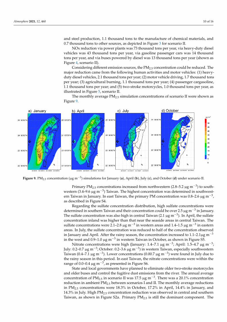
The reduction in SOx was 17.9 thousand tons per year, and the reduction in NOxwas 158 thousand tons per year. In addition, the reduction in PM2.5 emissions was 13.9thousand tons per year. For scenario II, the emissions of SOx, NOx, and PM2.5 were 103.4,246.3, and 59.7 thousand tons per year, respectively, as shown in Figure 8.

Atmosphere 2021, 12, x FOR PEER REVIEW 10 of 17

3.2. Scenario II: The Taiwan Clean Air Act (TCAA) Plan Adopted The reduction in SOx was 17.9 thousand tons per year, and the reduction in NOx

was 158 thousand tons per year. In addition, the reduction in PM2.5 emissions was 13.9 thousand tons per year. For scenario II, the emissions of SOx, NOx, and PM2.5 were 103.4, 246.3, and 59.7 thousand tons per year, respectively, as shown in Figure 8.

Figure 8. The emission distribution (ton y−1) of PM2.5 (a), Sox (b), and NOx (c) for scenario II.

The SOx reductions were mainly from changes in power plants (the installation of new electricity-generating units and change of fuels from coal or heavy oil to liquefied natural gases). The emission of 12thousand tons was attributed to changes in basic iron and steel production, 1.1 thousand tons to the manufacture of chemical materials, and 0.7 thousand tons to other sources, as depicted in Figure 3 for scenario II.

NOx reduction via power plants was 73 thousand tons per year, via heavy-duty diesel vehicles was 43 thousand tons per year, via gasoline passenger cars was 14 thou-sand tons per year, and via buses powered by diesel was 13 thousand tons per year (shown as Figure 4, scenario II).

Considering different emission sources, the PM2.5 concentration could be reduced. The major reduction came from the following human activities and motor vehicles: (1) heavy-duty diesel vehicles, 2.1 thousand tons per year; (2) motor vehicle driving, 1.7 thousand tons per year; (3) agricultural burning, 1.1 thousand tons per year; (4) passen-ger cargasoline, 1.1 thousand tons per year; and (5) two-stroke motorcycles, 1.0 thousand tons per year, as illustrated in Figure 5, scenario II.

The monthly average PM2.5 simulation concentrations of scenario II were shown as Figure 9.

Figure 8. The emission distribution (ton y−1) of PM2.5 (a), Sox (b), and NOx (c) for scenario II.

The SOx reductions were mainly from changes in power plants (the installation ofnew electricity-generating units and change of fuels from coal or heavy oil to liquefiednatural gases). The emission of 12thousand tons was attributed to changes in basic iron

Atmosphere 2021, 12, 460 10 of 16

and steel production, 1.1 thousand tons to the manufacture of chemical materials, and0.7 thousand tons to other sources, as depicted in Figure 3 for scenario II.

NOx reduction via power plants was 73 thousand tons per year, via heavy-duty dieselvehicles was 43 thousand tons per year, via gasoline passenger cars was 14 thousandtons per year, and via buses powered by diesel was 13 thousand tons per year (shown asFigure 4, scenario II).

Considering different emission sources, the PM2.5 concentration could be reduced. Themajor reduction came from the following human activities and motor vehicles: (1) heavy-duty diesel vehicles, 2.1 thousand tons per year; (2) motor vehicle driving, 1.7 thousand tonsper year; (3) agricultural burning, 1.1 thousand tons per year; (4) passenger cargasoline,1.1 thousand tons per year; and (5) two-stroke motorcycles, 1.0 thousand tons per year, asillustrated in Figure 5, scenario II.

The monthly average PM2.5 simulation concentrations of scenario II were shown asFigure 9.

Atmosphere 2021, 12, x FOR PEER REVIEW 10 of 17

3.2. Scenario II: The Taiwan Clean Air Act (TCAA) Plan Adopted The reduction in SOx was 17.9 thousand tons per year, and the reduction in NOx

was 158 thousand tons per year. In addition, the reduction in PM2.5 emissions was 13.9 thousand tons per year. For scenario II, the emissions of SOx, NOx, and PM2.5 were 103.4, 246.3, and 59.7 thousand tons per year, respectively, as shown in Figure 8.

Figure 8. The emission distribution (ton y−1) of PM2.5 (a), Sox (b), and NOx (c) for scenario II.

The SOx reductions were mainly from changes in power plants (the installation of new electricity-generating units and change of fuels from coal or heavy oil to liquefied natural gases). The emission of 12thousand tons was attributed to changes in basic iron and steel production, 1.1 thousand tons to the manufacture of chemical materials, and 0.7 thousand tons to other sources, as depicted in Figure 3 for scenario II.

NOx reduction via power plants was 73 thousand tons per year, via heavy-duty diesel vehicles was 43 thousand tons per year, via gasoline passenger cars was 14 thou-sand tons per year, and via buses powered by diesel was 13 thousand tons per year (shown as Figure 4, scenario II).

Considering different emission sources, the PM2.5 concentration could be reduced. The major reduction came from the following human activities and motor vehicles: (1) heavy-duty diesel vehicles, 2.1 thousand tons per year; (2) motor vehicle driving, 1.7 thousand tons per year; (3) agricultural burning, 1.1 thousand tons per year; (4) passen-ger cargasoline, 1.1 thousand tons per year; and (5) two-stroke motorcycles, 1.0 thousand tons per year, as illustrated in Figure 5, scenario II.

The monthly average PM2.5 simulation concentrations of scenario II were shown as Figure 9.

Figure 9. PM2.5 concentration (µg m−3) simulations for January (a), April (b), July (c), and October (d) under scenario II.

Primary PM2.5 concentrations increased from northwestern (2.8–5.2 µg m−3) to south-western (3.4–9.6 µg m−3) Taiwan. The highest concentration was determined in southwest-ern Taiwan in January. In east Taiwan, the primary PM concentration was 0.8–2.6 µg m−3,as described in Figure S4.

Regarding the sulfate concentration distribution, high sulfate concentrations weredetermined in southern Taiwan and their concentration could be over 2.5 µg m−3 in January.The sulfate concentration was also high in central Taiwan (2.1 µg m−3). In April, the sulfateconcentration inland was higher than that near the seaside areas in central Taiwan. Thesulfate concentrations were 2.1–2.8 µg m−3 in western areas and 1.4–1.5 µg m−3 in easternareas. In July, the sulfate concentration was reduced to half of the concentration observedin January and April. After the rainy season, the concentration increased to 1.1–2.1µg m−3

in the west and 0.9–1.0 µg m−3 in western Taiwan in October, as shown in Figure S5.Nitrate concentrations were high (January: 1.4–7.1 µg m−3; April: 1.5–4.7 µg m−3;

July: 0.2–0.7 µg m−3; October: 0.2–3.6 µg m−3) in western Taiwan, especially southwesternTaiwan (0.4–7.1 µg m−3). Lower concentrations (0.00.7 µg m−3) were found in July due tothe rainy season in this period. In east Taiwan, the nitrate concentrations were within therange of 0.0–0.4 µg m−3, as presented in Figure S6.

State and local governments have planned to eliminate older two-stroke motorcyclesand older buses and control the fugitive dust emissions from the river. The annual averageconcentration of PM2.5 in scenario II was 17.5 µg m−3. There was a 20.1% concentrationreduction in ambient PM2.5 between scenarios I and II. The monthly average reductionsin PM2.5 concentrations were 18.3% in October, 17.2% in April, 14.4% in January, and14.3% in July. High PM2.5 concentration reduction was observed in central and southernTaiwan, as shown in Figure S2a. Primary PM2.5 is still the dominant component. The

Atmosphere 2021, 12, 460 11 of 16

results of the correlation between PM2.5 and the composition of airborne PM2.5 proved thePM2.5 concentration to be related to nitrate (r = 0.92), primary PM2.5 (r = 0.82), and sulfate(r = 0.76).

In January, the primary PM2.5 mass fractions were 28–38% for different air basins. Thesulfate mass in PM2.5 fractions (9.1–24%) was higher than that observed in both northernand eastern Taiwan. High nitrate mass fractions were determined in central (16%) andsouthern (18%) Taiwan. In April, primary PM2.5 mass fractions were 22–32%, the sulfatefraction was 12–24%, and the nitrate fraction was 1.2–12%. A low PM mass was observedin July. The primary PM and sulfate mass fractions were found to be increasing, and adecrease in the nitrate fraction could be attributed to the rainy season in July, as nitratecompounds easily dissolve and react under high-moisture conditions. In October, the PMand sulfate fractions decreased and the nitrate fraction increased instead.

3.3. Scenario III: Conducted TCCA and More Control Strategies

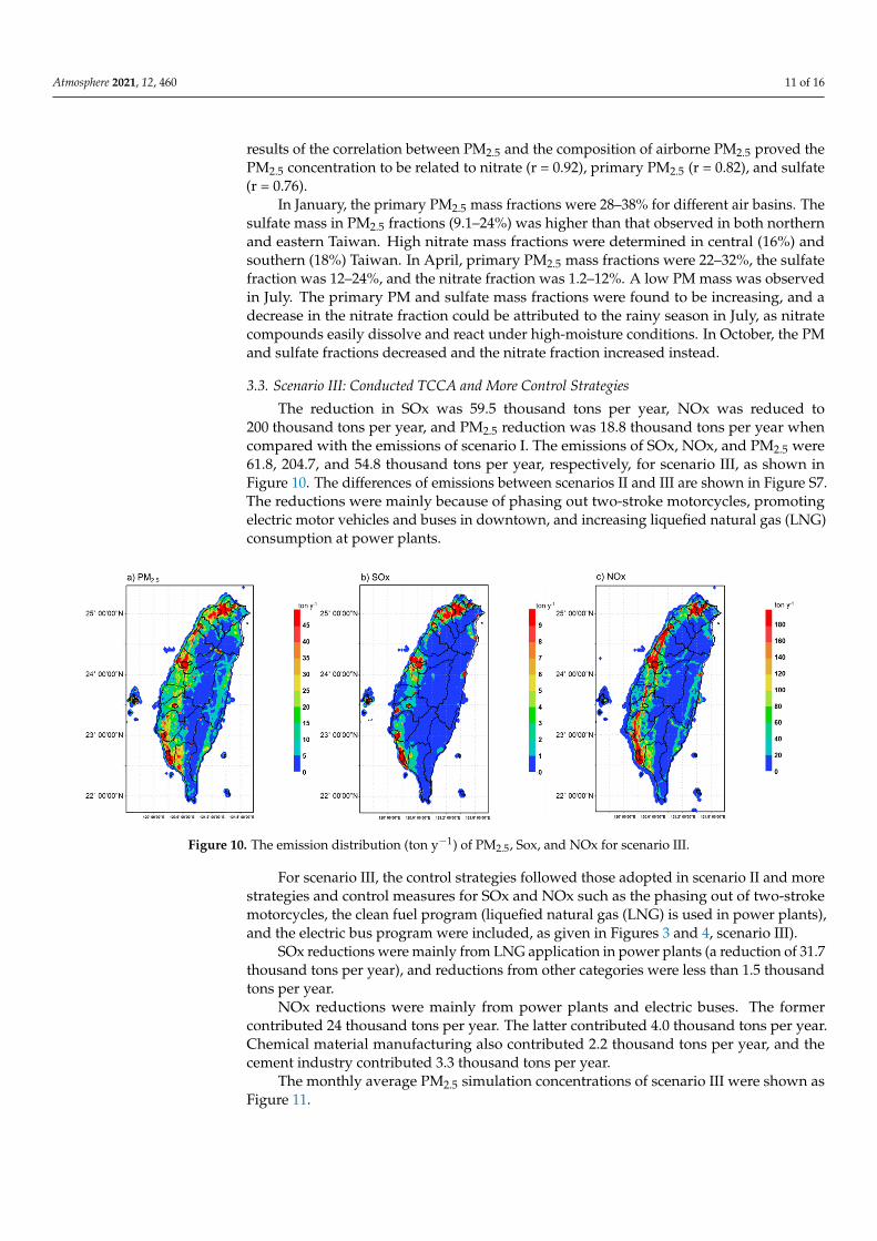
The reduction in SOx was 59.5 thousand tons per year, NOx was reduced to200 thousand tons per year, and PM2.5 reduction was 18.8 thousand tons per year whencompared with the emissions of scenario I. The emissions of SOx, NOx, and PM2.5 were61.8, 204.7, and 54.8 thousand tons per year, respectively, for scenario III, as shown inFigure 10. The differences of emissions between scenarios II and III are shown in Figure S7.The reductions were mainly because of phasing out two-stroke motorcycles, promotingelectric motor vehicles and buses in downtown, and increasing liquefied natural gas (LNG)consumption at power plants.

Atmosphere 2021, 12, x FOR PEER REVIEW 12 of 17

Figure 10. The emission distribution (ton y−1) of PM2.5, Sox, and NOx for scenario III.

For scenario III, the control strategies followed those adopted in scenario II and more strategies and control measures for SOx and NOx such as the phasing out of two-stroke motorcycles, the clean fuel program (liquefied natural gas (LNG) is used in power plants), and the electric bus program were included, as given in Figures 3 and 4, scenario III).

SOx reductions were mainly from LNG application in power plants (a reduction of 31.7 thousand tons per year), and reductions from other categories were less than 1.5 thousand tons per year.

NOx reductions were mainly from power plants and electric buses. The former contributed 24 thousand tons per year. The latter contributed 4.0 thousand tons per year. Chemical material manufacturing also contributed 2.2 thousand tons per year, and the cement industry contributed 3.3 thousand tons per year.

The monthly average PM2.5 simulation concentrations of scenario III were shown as Figure 11.

As to the primary PM2.5 distribution (0.8–9.2 μg m−3), the results indicated that high PM2.5 concentrations were observed in southern (3.2–9.2 μg m−3) and central (3.2–7.5 μg m−3) Taiwan. The highest primary PM2.5 concentration was about 10 μg m−3 in southern Taiwan in January. Low PM2.5 concentrations (0.8–3.2 μg m−3) were determined in July. (shown as Figure S8).

Figure 11. PM2.5 concentration (μg m−3) simulations for January (a), April (b), July (c), and October (d) under scenario III.

PM2.5 emissions were reduced via power plants (a reduction of 2.8 thousand tons per year), and the sulfate concentration distribution was 0.7–2.3 μg m−3. The results indicated

Figure 10. The emission distribution (ton y−1) of PM2.5, Sox, and NOx for scenario III.

For scenario III, the control strategies followed those adopted in scenario II and morestrategies and control measures for SOx and NOx such as the phasing out of two-strokemotorcycles, the clean fuel program (liquefied natural gas (LNG) is used in power plants),and the electric bus program were included, as given in Figures 3 and 4, scenario III).

SOx reductions were mainly from LNG application in power plants (a reduction of 31.7thousand tons per year), and reductions from other categories were less than 1.5 thousandtons per year.

NOx reductions were mainly from power plants and electric buses. The formercontributed 24 thousand tons per year. The latter contributed 4.0 thousand tons per year.Chemical material manufacturing also contributed 2.2 thousand tons per year, and thecement industry contributed 3.3 thousand tons per year.

The monthly average PM2.5 simulation concentrations of scenario III were shown asFigure 11.

Atmosphere 2021, 12, 460 12 of 16

Atmosphere 2021, 12, x FOR PEER REVIEW 12 of 17

Figure 10. The emission distribution (ton y−1) of PM2.5, Sox, and NOx for scenario III.

For scenario III, the control strategies followed those adopted in scenario II and more strategies and control measures for SOx and NOx such as the phasing out of two-stroke motorcycles, the clean fuel program (liquefied natural gas (LNG) is used in power plants), and the electric bus program were included, as given in Figures 3 and 4, scenario III).

SOx reductions were mainly from LNG application in power plants (a reduction of 31.7 thousand tons per year), and reductions from other categories were less than 1.5 thousand tons per year.

NOx reductions were mainly from power plants and electric buses. The former contributed 24 thousand tons per year. The latter contributed 4.0 thousand tons per year. Chemical material manufacturing also contributed 2.2 thousand tons per year, and the cement industry contributed 3.3 thousand tons per year.

The monthly average PM2.5 simulation concentrations of scenario III were shown as Figure 11.

As to the primary PM2.5 distribution (0.8–9.2 μg m−3), the results indicated that high PM2.5 concentrations were observed in southern (3.2–9.2 μg m−3) and central (3.2–7.5 μg m−3) Taiwan. The highest primary PM2.5 concentration was about 10 μg m−3 in southern Taiwan in January. Low PM2.5 concentrations (0.8–3.2 μg m−3) were determined in July. (shown as Figure S8).

Figure 11. PM2.5 concentration (μg m−3) simulations for January (a), April (b), July (c), and October (d) under scenario III.

PM2.5 emissions were reduced via power plants (a reduction of 2.8 thousand tons per year), and the sulfate concentration distribution was 0.7–2.3 μg m−3. The results indicated

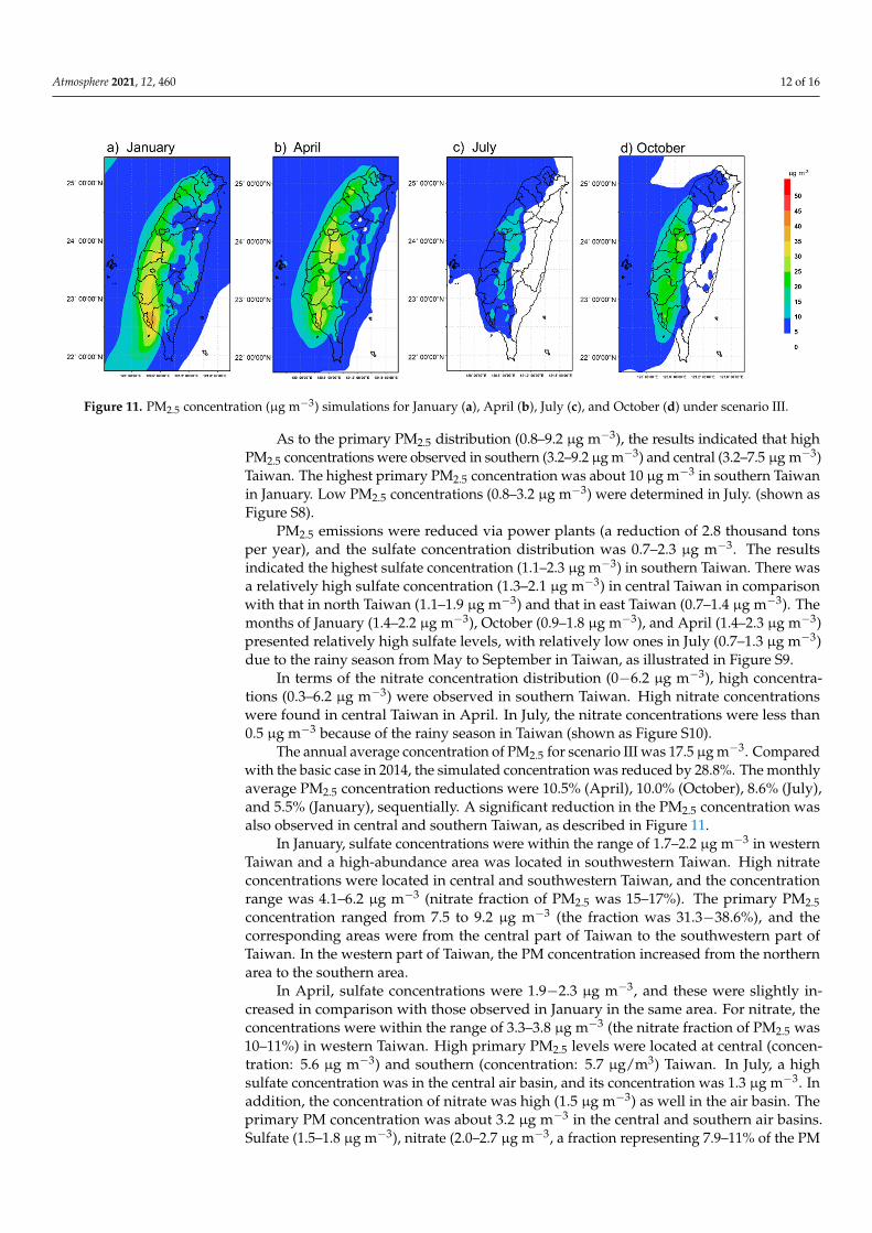
Figure 11. PM2.5 concentration (µg m−3) simulations for January (a), April (b), July (c), and October (d) under scenario III.

As to the primary PM2.5 distribution (0.8–9.2 µg m−3), the results indicated that highPM2.5 concentrations were observed in southern (3.2–9.2 µg m−3) and central (3.2–7.5 µg m−3)Taiwan. The highest primary PM2.5 concentration was about 10 µg m−3 in southern Taiwanin January. Low PM2.5 concentrations (0.8–3.2 µg m−3) were determined in July. (shown asFigure S8).

PM2.5 emissions were reduced via power plants (a reduction of 2.8 thousand tonsper year), and the sulfate concentration distribution was 0.7–2.3 µg m−3. The resultsindicated the highest sulfate concentration (1.1–2.3 µg m−3) in southern Taiwan. There wasa relatively high sulfate concentration (1.3–2.1 µg m−3) in central Taiwan in comparisonwith that in north Taiwan (1.1–1.9 µg m−3) and that in east Taiwan (0.7–1.4 µg m−3). Themonths of January (1.4–2.2 µg m−3), October (0.9–1.8 µg m−3), and April (1.4–2.3 µg m−3)presented relatively high sulfate levels, with relatively low ones in July (0.7–1.3 µg m−3)due to the rainy season from May to September in Taiwan, as illustrated in Figure S9.

In terms of the nitrate concentration distribution (0−6.2 µg m−3), high concentra-tions (0.3–6.2 µg m−3) were observed in southern Taiwan. High nitrate concentrationswere found in central Taiwan in April. In July, the nitrate concentrations were less than0.5 µg m−3 because of the rainy season in Taiwan (shown as Figure S10).

The annual average concentration of PM2.5 for scenario III was 17.5 µg m−3. Comparedwith the basic case in 2014, the simulated concentration was reduced by 28.8%. The monthlyaverage PM2.5 concentration reductions were 10.5% (April), 10.0% (October), 8.6% (July),and 5.5% (January), sequentially. A significant reduction in the PM2.5 concentration wasalso observed in central and southern Taiwan, as described in Figure 11.

In January, sulfate concentrations were within the range of 1.7–2.2 µg m−3 in westernTaiwan and a high-abundance area was located in southwestern Taiwan. High nitrateconcentrations were located in central and southwestern Taiwan, and the concentrationrange was 4.1–6.2 µg m−3 (nitrate fraction of PM2.5 was 15–17%). The primary PM2.5concentration ranged from 7.5 to 9.2 µg m−3 (the fraction was 31.3−38.6%), and thecorresponding areas were from the central part of Taiwan to the southwestern part ofTaiwan. In the western part of Taiwan, the PM concentration increased from the northernarea to the southern area.

In April, sulfate concentrations were 1.9−2.3 µg m−3, and these were slightly in-creased in comparison with those observed in January in the same area. For nitrate, theconcentrations were within the range of 3.3–3.8 µg m−3 (the nitrate fraction of PM2.5 was10–11%) in western Taiwan. High primary PM2.5 levels were located at central (concen-tration: 5.6 µg m−3) and southern (concentration: 5.7 µg/m3) Taiwan. In July, a highsulfate concentration was in the central air basin, and its concentration was 1.3 µg m−3. Inaddition, the concentration of nitrate was high (1.5 µg m−3) as well in the air basin. Theprimary PM concentration was about 3.2 µg m−3 in the central and southern air basins.Sulfate (1.5–1.8 µg m−3), nitrate (2.0–2.7 µg m−3, a fraction representing 7.9–11% of the PM

Atmosphere 2021, 12, 460 13 of 16

mass), and primary PM concentrations increased in October compared with those observedin July.

3.4. Effectiveness of Pollutant Reductions

Three major emission types consisting of NOx, SOx, and directly emitted PM2.5 weredetermined to contribute to the ambient PM2.5 aerosol mass. The implemented controlstrategies of the air quality management program (AQMP) help reduce SOx, NOx, anddirect PM2.5 emissions substantially. As presented earlier, the trends in SOx, NOx, andPM2.5 emissions suggest a direct relationship between lower emissions and improvementsin air quality.

In scenario II, it was shown that replacement of older power plants could be aneffective strategy for reducing directly emitted PM, SOx, and NOx. In addition, thereplacement of old heavy-duty diesel vehicles could reduce NOx and PM emissions, asshown in Figures 3–5.

In scenario III, SO2 emission reductions were mainly from the use of clean fuel (LNG)in power plants, basic iron and steel manufacturing, chemical material manufacturing, andpetroleum and coal product manufacturing. NOx reductions were from the use of LNG inpower plants, the phasing out of heavy-duty diesel vehicles, and the replacement of dieselbuses with electric buses. LNG power plants, vehicle phase-outs, exhaust control devices,and the retrofitting of old heavy-duty diesel vehicles could be relatively effective controlstrategies for reducing PM emissions in scenario III.

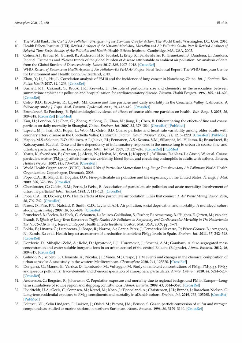
It is useful to evaluate the relative value of the ambient microgram per cubic meterimprovements in ambient PM2.5 under the per ton precursor emission reductions. Table 2presents the relative contributions of precursor emission reductions to ambient PM2.5concentrations in scenario II and scenario III. The analysis determines that SOx emissionreductions had the lowest return in terms of micrograms per cubic meter on the per tonemissions of PM2.5 reductions, about half that of NOx reductions. NOx emission reductionswere about twice as effective as SOx emission reductions for ambient PM2.5 concentrationreduction. However, the reductions in directly emitted PM2.5 emissions were approximately14−19 times more effective than SOx emission reductions. The results of scenarios II andIII indicated that the sequence of the effectiveness of PM2.5 concentration reduction wasprimary PM2.5 > NOx > SOx.

Table 2. Relative contributions of precursor emission reductions of the simulated PM2.5 concentration.

Precursor PM Fraction Scenario II Scenario III

SOx Sulfate 1 1NOx Nitrate 2.1 1.7PM2.5 Primary PM2.5 19 14

4. Conclusions

A simulated high PM2.5 concentration of the baseline scenario was observed in centraland southern Taiwan. The period with the higher PM level was found to range fromOctober to April of the following year. This was because the rainy season is from May toSeptember in Taiwan. Directly emitted PM2.5 was found to be the major component of totalPM2.5. Nitrate was considered a higher fraction of the PM2.5 mass than sulfate in high-PM2.5-concentration areas and periods. There was also a relatively high correlation betweensimulated PM2.5 concentration and nitrate during high-PM-concentration periods. Theemission reduction rates of scenario II and scenario III were 20.1% and 28.8%, respectively,in comparison with the rate of scenario I. The replacement of antiquated power plantsand the use of clean LNG fuel, the replacement of old motor vehicles, and stringentemission standards for stationary sources could be effective strategies for not only reducingemissions but also improving ambient air quality. However, the reduction in emissionsby enactment of the Taiwan Clean Air Act Plan and enhanced control measures is stillunable to achieve the annual average PM2.5 standard of 15 µg m−3. SO2 emission reduction

Atmosphere 2021, 12, 460 14 of 16

might help improve ambient air PM2.5. In addition, the relative contribution of precursoremission reductions to PM2.5 suggests that NOx emission control could lessen the problemof high PM2.5 concentrations and primary PM2.5 emission control might improve ambientPM2.5 concentrations in Taiwan, regardless of time and space. For the simulation in thiswork, the metrics of the MFE and MFB could not meet the criteria of model performance.The modeling system can be updated to more recent versions, which could be one of theroutes to improving its simulation performance benchmarks.

Supplementary Materials: The following are available online at https://www.mdpi.com/article/10.3390/atmos12040460/s1, Figure S1: The stimulation of primary PM2.5 concentrations for January (a),April (b), July (c) and October (d) under the baseline year condition, Figure S2: The stimulation ofsulfate concentrations for January (a), April (b), July (c) and October (d) under the baseline yearcondition, Figure S3: The stimulation of nitrate concentrations for January (a), April (b), July (c)and October (d) under the baseline year condition, Figure S4: The stimulation of primary PM2.5concentrations for January (a), April (b), July (c) and October (d) under Scenario II, Figure S5: Thestimulation of sulfate concentrations for January (a), April (b), July (c) and October (d) under thescenario II, Figure S6: The stimulation of nitrate concentrations for January (a), April (b), July (c)and October (d) under Scenario II, Figure S7: The stimulation of Primary PM2.5 concentrations forJanuary (a), April (b), July (c) and October (d)under the scenario III, Figure S8: The stimulation ofsulfate concentrations for January (a), April (b), July (c) and October (d) under the scenario III, FigureS9: The stimulation of Nitrate concentrations for January (a), April (b), July (c) and October (d) underthe scenario III, Figure S10: Comparison the differences of Scenario II (Figure 5) and III (Figure 6).(a) PM2.5; (b) Sox; (c) NOx.

Author Contributions: Conceived and designed the study, J.-H.T.; analyzed the data and modelstimulation, M.-Y.L., H.-L.C., and J.-H.T.; wrote and revised the paper, H.-L.C. and J.-H.T. All authorshave read and agreed to the published version of the manuscript.

Funding: This research was supported by the Ministry of Science and Technology, Taiwan.

Institutional Review Board Statement: Not applicable.

Informed Consent Statement: Not applicable.

Data Availability Statement: All the data are present in the manuscript.

Acknowledgments: The authors express their sincere thanks to the Ministry of Science and Technol-ogy, Executive Yuan, Republic of China (Taiwan), for research fund support (MOST 101-2221-E-006-160-MY3 and MOST 104-2221-E-006-020-MY3).

Conflicts of Interest: The authors declare no conflict of interest.

References1. Giannadaki, D.; Pozzer, A.; Lelieveld, J. Modeled global effects of airborne desert dust on air quality and premature mortality.

Atmos. Chem. Phys. 2014, 14, 957–968. [CrossRef]2. Lelieveld, J.; Hadjinicolaou, P.; Kostopoulou, E.; Giannakopoulos, C.; Tanarhte, M.; Tyrlis, E. Model projected heat extremes and

air pollution in the Eastern Mediterranean and Middle East in the twenty-first century. Reg. Environ. Chang. 2014, 14, 1937–1949.[CrossRef]

3. Abdo, N.; Khader, Y.S.; Abdelrahman, M.; Graboski-Bauer, A.; Malkawi, M.; Al-Sharif, M.; Elbetieha, A.M. Respiratory healthoutcomes and air pollution in the Eastern Mediterranean region: A systematic review. Rev. Environ. Health 2016, 31, 259–280.[CrossRef] [PubMed]

4. Khader, Y.S.; Abdo, N.; Abdelrahman, M.; Al-Sharif, M.; Bateiha, A.M.; Malkawi, M. The effect of air pollution on cancer in theEastern Mediterranean region: A systematic literature review. J. Environ. Pollut. Hum. Health 2016, 4, 66–71.

5. Dayan, U.; Ricaud, P.; Zinder, R.; Dulac, F. Atmospheric pollution over the eastern Mediterranean during summer—A review.Atmos. Chem. Phys. 2017, 17, 13233–13263. [CrossRef]

6. Kushta, J.; Georgiou, G.K.; Proestos, Y.; Christoudias, T.; Thunis, P.; Savvides, C.; Papadopoulos, C.; Lelieveld, J. Evaluation of EUair quality standards through modeling and the FAIRMODE benchmarking methodology. Air Qual. Atmos. Health 2019, 12, 73–86.[CrossRef]

7. WHO; Regional Office for Europe; OECD. EconomicCost of the Health Impact of Air Pollution in Europe: Clean Air, Health and Wealth;Regional Office for Europe: Copenhagen, Denmark; WHO: Geneva, Switzerland, 2015.

8. EEA (European Environmental Agency). Air Quality in Europe–2018 Report; 12/2018; EEA: Luxembourg, 2018; p. 83. [CrossRef]

Atmosphere 2021, 12, 460 15 of 16

9. The World Bank. The Cost of Air Pollution: Strengthening the Economic Case for Action; The World Bank: Washington, DC, USA, 2016.10. Health Effects Institute (HEI). Revised Analyses of the National Morbidity, Mortality and Air Pollution Study, Part II: Revised Analyses of

Selected Time-Series Studies of Air Pollution and Health; Health Effects Institute: Cambridge, MA, USA, 2003.11. Cohen, A.J.; Brauer, M.; Burnett, R.; Anderson, H.R.; Frostad, J.; Estep, K.; Balakrishnan, K.; Brunekreef, B.; Dandona, L.; Dandona,

R.; et al. Estimates and 25-year trends of the global burden of disease attributable to ambient air pollution: An analysis of datafrom the Global Burden of Diseases Study. Lancet 2017, 389, 1907–1918. [CrossRef]

12. WHO. Review of Evidence on Health Aspects of Air Pollution-REVIHAAP Project; Final Technical Report; The WHO European Centrefor Environment and Health: Bonn, Switzerland, 2013.

13. Zhou, Y.; Li, L.; Hu, L. Correlation analysis of PM10 and the incidence of lung cancer in Nanchang, China. Int. J. Environ. Res.Public Health 2017, 14, 1253. [CrossRef]

14. Burnett, R.T.; Cakmak, S.; Brook, J.R.; Krewski, D. The role of particulate size and chemistry in the association betweensummertime ambient air pollution and hospitalization for cardiorespiratory disease. Environ. Health Perspect. 1997, 105, 614–620.[CrossRef]

15. Ostro, B.D.; Broadwin, R.; Lipsett, M.J. Coarse and fine particles and daily mortality in the Coachella Valley, California: Afollow-up study. J. Expo. Anal. Environ. Epidemiol. 2000, 10, 412–419. [CrossRef]

16. Brunekreef, B.; Forsberg, B. Epidemiological evidence of effects of coarse airborne particles on health. Eur. Resp. J. 2005, 26,309–318. [CrossRef] [PubMed]

17. Kan, H.; London, S.J.; Chen, G.; Zhang, Y.; Song, G.; Zhao, N.; Jiang, L.; Chen, B. Differentiating the effects of fine and coarseparticles on daily mortality in Shanghai, China. Environ. Int. 2007, 33, 376–384. [CrossRef] [PubMed]

18. Lipsett, M.J.; Tsai, F.C.; Roger, L.; Woo, M.; Ostro, B.D. Coarse particles and heart rate variability among older adults withcoronary artery disease in the Coachella Valley, California. Environ. Health Perspect. 2006, 114, 1215–1220. [CrossRef] [PubMed]

19. Hapoo, M.S.; Salonen, R.O.; Hölinen, A.I.; Jalava, P.I.; Pennanen, A.S.; Kosma, V.M.; Sillanpää, M.; Hillamo, R.; Brunekreef, B.;Katsouyanni, K.; et al. Dose and time dependency of inflammatory responses in the mouse lung to urban air coarse, fine, andultrafine particles from six European cities. Inhal. Toxicol. 2007, 19, 227–246. [CrossRef] [PubMed]

20. Yeatts, K.; Svendsen, E.; Creason, J.; Alexis, N.; Herbst, M.; Scott, J.; Kupper, L.; Williams, R.; Neas, L.; Cascio, W.; et al. Coarseparticulate matter (PM2.5–10) affects heart rate variability, blood lipids, and circulating eosinophils in adults with asthma. Environ.Health Perspect. 2007, 115, 709–714. [CrossRef]

21. World Health Organization (WHO). Health Risks of Particulate Matter from Long-Range Transboundary Air Pollution; World HealthOrganization: Copenhagen, Denmark, 2006.

22. Pope, C.A., III; Majid, E.; Dogulas, D.W. Fine-particulate air pollution and life expectancy in the United States. N. Engl. J. Med.2009, 360, 376–386. [CrossRef]

23. Oberdorster, G.; Gelein, R.M.; Ferin, J.; Weiss, B. Association of particulate air pollution and acute mortality: Involvement ofultra-fine particles? Inhal. Toxicol. 1995, 7, 111–124. [CrossRef]

24. Pope, C.A., III; Dockery, D.W. Health effects of fine particulate air pollution: Lines that connect. J. Air Waste Manag. Assoc. 2006,56, 709–742. [CrossRef]

25. Naess, O.; Piro, F.N.; Nafstad, P.; Smith, G.D.; Leyland, A.H. Air pollution, social deprivation and mortality: A multilevel cohortstudy. Epidemiology 2007, 18, 686–694. [CrossRef]

26. Brunekreef, B.; Beelen, R.; Hoek, G.; Schouten, L.; Bausch-Goldbohm, S.; Fischer, P.; Armstrong, B.; Hughes, E.; Jerrett, M.; van denBrandt, P. Effects of Long-Term Exposure to Traffic-Related Air Pollution on Respiratory and Cardiovascular Mortality in The Netherlands:The NLCS-AIR Study; Research Report Health Effects Institute: Boston, MA, USA, 2009; pp. 5–71.

27. Boldo, E.; Linares, C.; Lumbreras, J.; Borge, R.; Narros, A.; Garcia-Pérez, J.; Fernández-Navarro, P.; Pérez-Gómez, B.; Aragonés,N.; Ramis, R.; et al. Health impact assessment of a reduction in ambient PM2.5 levels in Spain. Environ. Int. 2011, 37, 342–348.[CrossRef]

28. Ðordevic, D.; Mihajlidi-Zelic, A.; Relic, D.; Ignjatovic, L.J.; Huremovic, J.; Stortini, A.M.; Gambaro, A. Size-segregated massconcentration and water soluble inorganic ions in an urban aerosol of the central Balkans (Belgrade). Atmos. Environ. 2012, 46,309–317. [CrossRef]

29. Galindo, N.; Yubero, E.; Clemente, Á.; Nicolás, J.F.; Varea, M.; Crespo, J. PM events and changes in the chemical composition ofurban aerosols: A case study in the western Mediterranean. Chemosphere 2020, 244, 125520. [CrossRef]

30. Dongarrà, G.; Manno, E.; Varrica, D.; Lombardo, M.; Vultaggio, M. Study on ambient concentrations of PM10, PM10–2.5, PM2.5and gaseous pollutants. Trace elements and chemical speciation of atmospheric particulates. Atmos. Environ. 2010, 44, 5244–5257.[CrossRef]

31. Andersson, C.; Bergstro, R.; Johansson, C. Population exposure and mortality due to regional background PM in Europe—Long-term simulations of source region and shipping contributions. Atmos. Environ. 2009, 43, 3614–3620. [CrossRef]

32. Hvidtfeldt, U.A.; Geels, C.; Sorensen, M.; Ketzel, M.; Khan, J.; Tjonneland, A.; Christensen, J.H.; Brandt, J.; Raaschou-Nielsen, O.Long-term residential exposure to PM2.5 constituents and mortality in aDanish cohort. Environ. Int. 2019, 133, 105268. [CrossRef][PubMed]

33. Foltescu, V.L.; Selin Lindgern, E.; Isakson, J.; Öblad, M.; Pacyna, J.M.; Benson, S. Gas-to-particle conversion of sulfur and nitrogencompounds as studied at marine stations in northern European. Atmos. Environ. 1996, 30, 3129–3140. [CrossRef]

Atmosphere 2021, 12, 460 16 of 16

34. Behera, S.N.; Sharma, M. Degradation of SO2, NO2 and NH3 leading to formation of secondary inorganic aerosols: Anenvironmental chamber study. Atmos. Environ. 2011, 45, 4015–4024. [CrossRef]

35. Gen, M.; Zhang, R.; Huang, D.D.; Li, Y.; Chan, C.K. Heterogeneous SO2 oxidation in sulfate formation by photolysis of particulatenitrate. Environ. Sci. Technol. Lett. 2019, 6, 86–91. [CrossRef]

36. Meidan, D.; Holloway, J.S.; Edwards, P.M.; Dubé, W.P.; Middlebrook, A.M.; Liao, J.; Welti, A.; Graus, M.; Warneke, C.; Ryerson,T.B.; et al. Role of criegee intermediates in secondary sulfate aerosol formation in nocturnal power plant plumes in the SoutheastUS. ACS Earth Space Chem. 2019, 3, 748–759. [CrossRef]

37. Yang, J.; Li, L.; Wang, S.; Li, H.; Francisco, J.S.; Zeng, X.C.; Gao, Y. Unraveling a new chemical mechanism of missing sulfateformation in aerosol haze: Gaseous NO2 with aqueous HSO3

−/SO32−. J. Am. Chem. Soc. 2021. [CrossRef]

38. US EPA. Available online: https://www.epa.gov/cmaq/modeling-toxic-air-pollutants-cmaq (accessed on 5 April 2020).39. Sarwar, G.; Gantt, B.; Foley, K.; Fahey, K.; Spero, T.L.; Kang, D.; Mathur, R.; Hosein, F.; Xing, J.; Sherwin, T.; et al. Influence of

bromine and iodine chemistry on annual, seasonal, diurnal, and background ozone: CMAQ simulations over the NorthernHemisphere. Atmos. Environ. 2019, 213, 395–404. [CrossRef]

40. Sommariva, R.; Hollis, L.D.J.; Sherwen, T.; Baker, A.R.; Ball, S.M.; Bandy, B.J.; Bell, T.G.; Chowdhury, M.N.; Cordell, R.L.; Evans,M.J.; et al. Seasonal and geographical variability of nitryl chloride and its precursors in Northern Europe. Atmos. Sci. Lett. 2018,19, 844. [CrossRef]

41. Jang, X.; Yoo, E.H. evaluating the effect of domain size of the community multiscale air quality (cmaq) model on regional PM2.5simulations. In Global Perspectives on Health Geography; Lu, Y., Delmelle, E., Eds.; Springer Nature: Geneva, Switzerland, 2020.

42. Yue, H.; He, C.; Huang, Q.; Yin, D.; Bryan, B.A. Stronger policy required to substantially reduce deaths from PM2.5 pollution inChina. Nat. Commun. 2020, 11, 1462. [CrossRef]

43. Hsu, C.H.; Cheng, F.Y.; Chang, H.Y.; Lin, N.H. Implementation of a dynamical NH3 emissions parameterization in CMAQ forimproving PM2.5 simulation in Taiwan. Atmos. Environ. 2019, 218, 116923. [CrossRef]

44. Cheng, F.Y.; Feng, C.Y.; Yang, Z.M.; Hsu, C.H.; Chan, K.W.; Lee, C.Y.; Chang, S.C. Evaluation of real-time PM2.5 forecasts with theWRF-CMAQ modeling system and weather-pattern-dependent bias-adjusted PM2.5 forecasts in Taiwan. Atmos. Environ. 2021,244, 117909. [CrossRef]

45. Chen, T.F.; Chang, K.H.; Lee, C.H. Simulation and analysis of causes of a haze episode by combining CMAQ-IPR and brute forcesource sensitivity method. Atmos. Environ. 2019, 218, 117006. [CrossRef]

46. Byun, D.W.; Schere, K.L. Review of the governing equations, computational algorithms, and other components of the models-3Community Multiscale Air Quality (CMAQ) modeling system. Appl. Mech. Rev. 2006, 59, 51–77. [CrossRef]

47. Wong, D.C.; Pleim, J.; Mathur, R.; Binkowski, F.; Otte, T.; Gilliam, R. WRF-CMAQ two-way coupled system with aerosol feedback:Software development and preliminary results. Geosci. Model Dev. 2012, 5, 299–312. [CrossRef]

48. Otte, T.L.; Pleim, J.E. The Meteorology-Chemistry Interface Processor (MCIP) for the CMAQ modeling system: Updates throughMCIPv3.4.1. Geosci. Model Dev. 2010, 3, 243–256. [CrossRef]

49. Yarwood, G.; Rao, S.; Yocke, M.; Whitten, G. Updates to the CarbonBond Chemical Mechanism: CB05; Final Report to the US EPA,RT-0400675; US EPA: Washington, DC, USA, 2005; Available online: http://www.camx.com/publ/pdfs/CB05_Final_Report_120805.pdf (accessed on 2 March 2021).

50. Boylan, J.W.; Russell, A.G. PM and light extinction model performance metrics, goals, and criteria for three-dimensional airquality models. Atmos. Environ. 2006, 40, 4946–4959. [CrossRef]

51. United States Environmental Protection Agency (USEPA). Guidance on the Use of Models and Other Analyses for DemonstratingAttainment of Air Quality Goals for Ozone, PM2.5, and Regional Haze; Publication No. EPA-454/B-07-002 April; Office of Air QualityPlanning and Standards Air Quality Analysis Division: Research Triangle Park, NC, USA, 2007.

52. Henneman, L.R.F.; Liu, C.; Hu, Y.; Mulholland, J.A.; Russell, A.G. Air quality modeling for accountability research: Operational,dynamic, and diagnostic evaluation. Atmos. Environ. 2017, 166, 551–565. [CrossRef]

53. Eyth, A.; Pouliot, G.; Vukovich, J.; Strum, M.; Dolwick, P.; Allen, C.; Beidler, J.; Baek, B.H. Development of 2011 HemisphericEmissions for CMAQ. Presented at the 2016 CMAS Conference, Chapel Hill, NC, USA, 24–26 October 2016; Available online:https://www.cmascenter.org/conference//2016/slides/eyth_development_hemispheric_2016.pptx (accessed on 4 May 2020).

54. Tsai, Y.I.; Chen, C.L. Atmospheric aerosol composition and source apportionments to aerosol in southern Taiwan. Atmos. Environ.2006, 40, 4751–4763. [CrossRef]

55. Chou, C.C.K.; Lee, C.T.; Cheng, M.T.; Yuan, C.S.; Chen, S.J.; Wu, Y.L.; Hsu, W.C.; Lung, S.C.; Hsu, S.C.; Lin, C.Y.; et al. Seasonalvariation and spatial distribution of carbonaceous aerosols in Taiwan. Atmos. Chem. Phys. 2010, 10, 9563–9578. [CrossRef]