Effective computation of the multivariable Alexander polinomial of Lorenz links

Efective computation of the multivariable

Alexander polinomial of Lorenz links

Nuno Franco a,b,1,2 Luıs Silva a,c,1

aCIMA-UE and Department of Mathematics, University of Evora, Rua Romao

Ramalho, 59, 7000-671 Evora, Portugal

bemail: [email protected]

cemail: [email protected]

Abstract

Given two different representations of a Lorenz link, we compare how they affectthe computation of the multivariable Alexander polynomial. We also compare theAlexander polynomial with the trip number and genus. Our experimental resultslead us to conjecture that, for Lorenz knots, the Alexander polynomial is an equiv-alent invariant to the pair (trip number, genus). Finally we give a counterexamplein the case of Lorenz links.

Key words: Alexander Polynomial, genus, trip number, Lorenz kots

1 Introduction

We define a Lorenz flow as a semi-flow that has a singularity of saddle typewith a one-dimensional unstable manifold and an infinite set of hyperbolicperiodic orbits, whose closure contains the saddle point (see [7]). A Lorenz flow,together with an extra geometric assumption (see [11]) is called a GeometricLorenz flow. The dynamics of this type of flows can be described by first-return one-dimensional maps with one discontinuity, that are not necessarilysurjective in the continuity subintervals. This maps are called Lorenz maps,more precisely, we will adopt the following definition introduced in [7].

Definition 1 Let P < 0 < Q and r ≥ 1. A Cr Lorenz map f : [P, Q] → [P, Q]is a map described by a pair (f−, f+) where:

1 Author partially supported by FCT-Portugal2 The author is partially supported by FCT grant SFRH/BPD/26354/2006

Preprint submitted to Elsevier 4 June 2008

(1) f− : [P, 0] → [P, Q] and f+ : [0, Q] → [P, Q]are continuous and strictlyincreasing maps;

(2) f(P ) = P , f(Q) = Q and f has no other fixed points in [P, Q]\{0}.(3) There exists ρ > 0, the exponent of f , such that

f−(x) = f−(|x|ρ) and f+(x) = f+(|x|ρ)

where f− and f+, the coefficients of the Lorenz map, are Cr diffeomor-phisms defined on appropriate closed intervals.

Because of the ambiguity at the point 0, we consider the map undefined in 0.This Lorenz map is denoted by (P, Q, f−, f+) (if there is no ambiguity aboutthe interval of definition, we erase the corresponding symbols P, Q).

Let f j = f ◦ f j−1, f 0 = id, be the j-th iterate of the map f . We define theitinerary of a point x under a Lorenz map f as if (x) = (if(x))j , j = 0, 1, . . .,where

(if(x))j =

L if f j(x) < 0

0 if f j(x) = 0

R if f j(x) > 0

.

It is obvious that the itinerary of a point x will be a finite sequence in thesymbols L and R with 0 as its last symbol, if and only if x is a pre-imageof 0 and otherwise it is one infinite sequence in the symbols L and R. Soit is natural to consider the symbolic space Σ of sequences X0 · · ·Xn on thesymbols {L, 0, R}, such that Xi 6= 0 for all i < n and: n = ∞ or Xn = 0, withthe lexicographic order relation induced by L < 0 < R.

It is straightforward to verify that, for all x, y ∈ [−1, 1], we have

(1) If x < y then if (x) ≤ if(y), and(2) If if (x) < if(y) then x < y.

We define the kneading invariant associated to a Lorenz map f = (f−, f+), as

Kf = (K−f , K+

f ) = (Lif (f−(0)), Rif(f+(0))).

We say that a pair (X, Y ) ∈ Σ × Σ is admissible if (X, Y ) = Kf for someLorenz map f .

Consider the shift map s : Σ \ {0} → Σ, s(X0 · · ·Xn) = X1 · · ·Xn. The setof admissible pairs is characterized, combinatorially, in the following way (seefor example [6]).

2

Proposition 1 A pair (X, Y ) ∈ Σ × Σ is admissible if and only if X0 = L,Y0 = R and, for Z ∈ {X, Y } we have:(1) If Zi = L then si(Z) ≤ X;(2) If Zi = R then si(Z) ≥ Y ; with inequality (1) (resp. (2)) strict if X (resp.Y ) is finite.

2 Braids, Lorenz links and the Alexander polynomial

Let n > 0 be an integer. We denote by Bn the braid group on n strings givenby the following presentation (see [1]):

Bn =

⟨σ1, σ2, . . . , σn−1

∣∣∣∣∣∣∣

σiσj = σjσi (|i − j| ≥ 2)

σiσi+1σi = σi+1σiσi+1 (i = 1, . . . , n − 2)

⟩.

Where σi denotes a crossing between the strings occupying positions i and i+1,such that the string in position i crosses (in the up to down direction) overthe other, analogously σ−1

i , the algebraic inverse of σi, denotes the crossingbetween the same strings, but in the negative sense, i.e., the string in position i

crosses under the other. A positive braid is a braid with only positive crossings.A simple braid is a positive braid such that each two strings cross each otherat most once. So there is a canonical bijection between the permutation groupΣn and the set Sn, of simple braids with n strings, which associates to eachpermutation π, the braid bπ, where each point i is connected by a straight lineto π(i), keeping all the crossings positive.

Let X be a periodic sequence with least period k and let ϕ ∈ Σk be thepermutation that associates to each i the position occupied by si(X) in thelexicographic ordering of the k-tuple (s(X), . . . , sk(X)) (sk(X) = X). Defineπ ∈ Σk to be the permutation given by π(ϕ(i)) = ϕ(i mod k + 1), i.e.,π(i) = ϕ(ϕ−1(i) mod k+1). We associate to π the corresponding simple braidbπ ∈ Bk and call it the Lorenz braid associated to X. Since X is periodic, thisbraid represents a knot, and we call it the Lorenz knot associated to X. Thesame method is valid if we consider a pair of sequences. We obtain in this casea Lorenz braid which represents a Lorenz link. The Lorenz braid produced inthis way is just one possible representative for the respective Lorenz link.

Example: Let Z = (LRRLRRLRRLR)∞. Hence we have s11(Z) = Z,s(Z) = (RRLRRLRRLRL)∞, s2(Z) = (RLRRLRRLRLR)∞,s3(Z) = (LRRLRRLRLRR)∞, s4(Z) = (RRLRRLRLRRL)∞,· · · . Now af-ter lexicographic reordering the si(Z) we obtain s9(Z) < s6(Z) < s3(Z) <

3

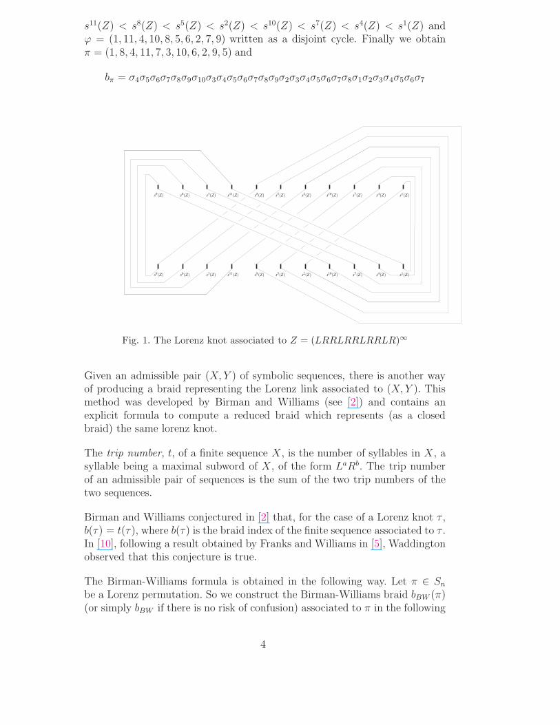
s11(Z) < s8(Z) < s5(Z) < s2(Z) < s10(Z) < s7(Z) < s4(Z) < s1(Z) andϕ = (1, 11, 4, 10, 8, 5, 6, 2, 7, 9) written as a disjoint cycle. Finally we obtainπ = (1, 8, 4, 11, 7, 3, 10, 6, 2, 9, 5) and

bπ = σ4σ5σ6σ7σ8σ9σ10σ3σ4σ5σ6σ7σ8σ9σ2σ3σ4σ5σ6σ7σ8σ1σ2σ3σ4σ5σ6σ7

Fig. 1. The Lorenz knot associated to Z = (LRRLRRLRRLR)∞

Given an admissible pair (X, Y ) of symbolic sequences, there is another wayof producing a braid representing the Lorenz link associated to (X, Y ). Thismethod was developed by Birman and Williams (see [2]) and contains anexplicit formula to compute a reduced braid which represents (as a closedbraid) the same lorenz knot.

The trip number, t, of a finite sequence X, is the number of syllables in X, asyllable being a maximal subword of X, of the form LaRb. The trip numberof an admissible pair of sequences is the sum of the two trip numbers of thetwo sequences.

Birman and Williams conjectured in [2] that, for the case of a Lorenz knot τ ,b(τ) = t(τ), where b(τ) is the braid index of the finite sequence associated to τ .In [10], following a result obtained by Franks and Williams in [5], Waddingtonobserved that this conjecture is true.

The Birman-Williams formula is obtained in the following way. Let π ∈ Sn

be a Lorenz permutation. So we construct the Birman-Williams braid bBW (π)(or simply bBW if there is no risk of confusion) associated to π in the following

4

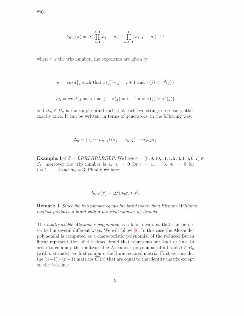
way:

bBW (π) = ∆2n

t−1∏

i=1

(σ1 · · ·σi)ni

1∏

i=t−1

(σt−1 · · ·σi)mt−i

where t is the trip number, the exponents are given by

ni = card{j such that π(j) − j = i + 1 and π(j) < π2(j)}

mi = card{j such that j − π(j) = i + 1 and π(j) > π2(j)}

and ∆n ∈ Bn is the simple braid such that each two strings cross each otherexactly once. It can be written, in terms of generators, in the following way:

∆n = (σ1 · · ·σn−1) (σ1 · · ·σn−2) · · ·σ1σ2σ1.

Example: Let Z = LRRLRRLRRLR. We have π = (8, 9, 10, 11, 1, 2, 3, 4, 5, 6, 7) ∈S11 moreover the trip number is 4, ni = 0 for i = 1, . . . , 3, mi = 0 fori = 1, . . . , 2 and m3 = 3. Finally we have

bBW (π) = ∆24(σ3σ2σ1)

3.

Remark 1 Since the trip number equals the braid index, then Birman-Williamsmethod produces a braid with a minimal number of strands.

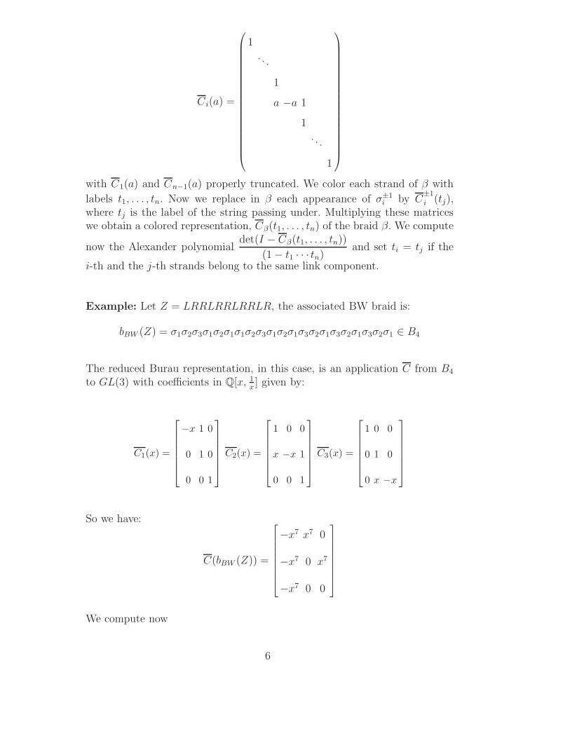
The multivariable Alexander polynomial is a knot invariant that can be de-scribed in several different ways. We will follow [8]. In this case the Alexanderpolynomial is computed as a characteristic polynomial of the reduced Buraulinear representation of the closed braid that represents our knot or link. Inorder to compute the multivariable Alexander polynomial of a braid β ∈ Bn

(with n strands), we first compute the Burau colored matrix. First we considerthe (n−1)×(n−1) matrices Ci(a) that are equal to the identity matrix excepton the i-th line:

5

Ci(a) =

1. . .

1

a −a 1

1. . .

1

with C1(a) and Cn−1(a) properly truncated. We color each strand of β with

labels t1, . . . , tn. Now we replace in β each appearance of σ±1i by C

±1i (tj),

where tj is the label of the string passing under. Multiplying these matriceswe obtain a colored representation, Cβ(t1, . . . , tn) of the braid β. We compute

now the Alexander polynomialdet(I − Cβ(t1, . . . , tn))

(1 − t1 · · · tn)and set ti = tj if the

i-th and the j-th strands belong to the same link component.

Example: Let Z = LRRLRRLRRLR, the associated BW braid is:

bBW (Z) = σ1σ2σ3σ1σ2σ1σ1σ2σ3σ1σ2σ1σ3σ2σ1σ3σ2σ1σ3σ2σ1 ∈ B4

The reduced Burau representation, in this case, is an application C from B4

to GL(3) with coefficients in Q[x, 1x] given by:

C1(x) =

−x 1 0

0 1 0

0 0 1

C2(x) =

1 0 0

x −x 1

0 0 1

C3(x) =

1 0 0

0 1 0

0 x −x

So we have:

C(bBW (Z)) =

−x7 x7 0

−x7 0 x7

−x7 0 0

We compute now

6

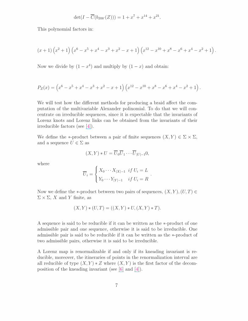
det(I − C(bBW (Z))) = 1 + x7 + x14 + x21.

This polynomial factors in:

(x + 1)(x2 + 1

) (x6 − x5 + x4 − x3 + x2 − x + 1

) (x12 − x10 + x8 − x6 + x4 − x2 + 1

).

Now we divide by (1 − x4) and multiply by (1 − x) and obtain:

PZ(x) =(x6 − x5 + x4 − x3 + x2 − x + 1

) (x12 − x10 + x8 − x6 + x4 − x2 + 1

).

We will test how the different methods for producing a braid affect the com-putation of the multivariable Alexander polinomial. To do that we will con-centrate on irreducible sequences, since it is expectable that the invariants ofLorenz knots and Lorenz links can be obtained from the invariants of theirirreducible factors (see [4]).

We define the ∗-product between a pair of finite sequences (X, Y ) ∈ Σ × Σ,and a sequence U ∈ Σ as

(X, Y ) ∗ U = U 0U 1 · · ·U |U |−10,

where

U i =

X0 · · ·X|X|−1 if Ui = L

Y0 · · ·Y|Y |−1 if Ui = R.

Now we define the ∗-product between two pairs of sequences, (X, Y ), (U, T ) ∈Σ × Σ, X and Y finite, as

(X, Y ) ∗ (U, T ) = ((X, Y ) ∗ U, (X, Y ) ∗ T ).

A sequence is said to be reducible if it can be written as the ∗-product of oneadmissible pair and one sequence, otherwise it is said to be irreducible. Oneadmissible pair is said to be reducible if it can be written as the ∗-product oftwo admissible pairs, otherwise it is said to be irreducible.

A Lorenz map is renormalizable if and only if its kneading invariant is re-ducible, moreover, the itineraries of points in the renormalization interval areall reducible of type (X, Y ) ∗ Z where (X, Y ) is the first factor of the decom-position of the kneading invariant (see [6] and [4]).

7

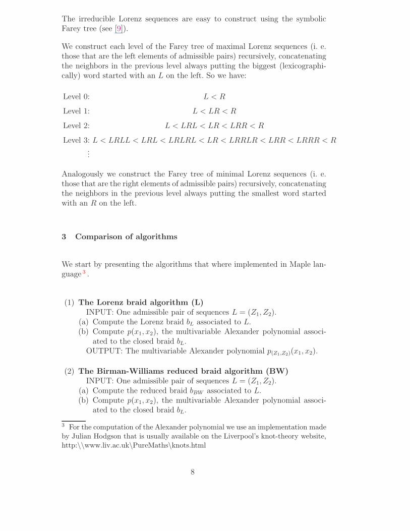
The irreducible Lorenz sequences are easy to construct using the symbolicFarey tree (see [9]).

We construct each level of the Farey tree of maximal Lorenz sequences (i. e.those that are the left elements of admissible pairs) recursively, concatenatingthe neighbors in the previous level always putting the biggest (lexicographi-cally) word started with an L on the left. So we have:

Level 0: L < R

Level 1: L < LR < R

Level 2: L < LRL < LR < LRR < R

Level 3: L < LRLL < LRL < LRLRL < LR < LRRLR < LRR < LRRR < R...

Analogously we construct the Farey tree of minimal Lorenz sequences (i. e.those that are the right elements of admissible pairs) recursively, concatenatingthe neighbors in the previous level always putting the smallest word startedwith an R on the left.

3 Comparison of algorithms

We start by presenting the algorithms that where implemented in Maple lan-guage 3 .

(1) The Lorenz braid algorithm (L)INPUT: One admissible pair of sequences L = (Z1, Z2).

(a) Compute the Lorenz braid bL associated to L.(b) Compute p(x1, x2), the multivariable Alexander polynomial associ-

ated to the closed braid bL.OUTPUT: The multivariable Alexander polynomial p(Z1,Z2)(x1, x2).

(2) The Birman-Williams reduced braid algorithm (BW)INPUT: One admissible pair of sequences L = (Z1, Z2).

(a) Compute the reduced braid bBW associated to L.(b) Compute p(x1, x2), the multivariable Alexander polynomial associ-

ated to the closed braid bL.

3 For the computation of the Alexander polynomial we use an implementation madeby Julian Hodgson that is usually available on the Liverpool’s knot-theory website,http:\\www.liv.ac.uk\PureMaths\knots.html

8

OUTPUT: The multivariable Alexander polynomial p(Z1,Z2)(x1, x2).

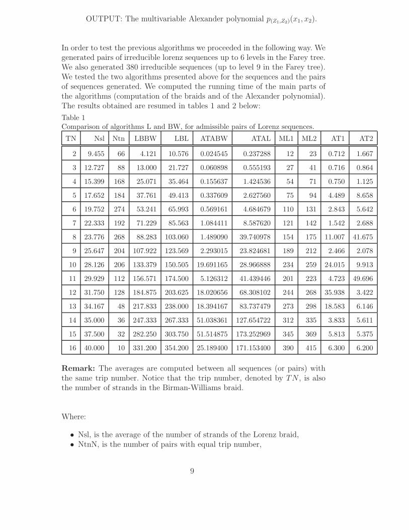
In order to test the previous algorithms we proceeded in the following way. Wegenerated pairs of irreducible lorenz sequences up to 6 levels in the Farey tree.We also generated 380 irreducible sequences (up to level 9 in the Farey tree).We tested the two algorithms presented above for the sequences and the pairsof sequences generated. We computed the running time of the main parts ofthe algorithms (computation of the braids and of the Alexander polynomial).The results obtained are resumed in tables 1 and 2 below:

Table 1Comparison of algorithms L and BW, for admissible pairs of Lorenz sequences.

TN Nsl Ntn LBBW LBL ATABW ATAL ML1 ML2 AT1 AT2

2 9.455 66 4.121 10.576 0.024545 0.237288 12 23 0.712 1.667

3 12.727 88 13.000 21.727 0.060898 0.555193 27 41 0.716 0.864

4 15.399 168 25.071 35.464 0.155637 1.424536 54 71 0.750 1.125

5 17.652 184 37.761 49.413 0.337609 2.627560 75 94 4.489 8.658

6 19.752 274 53.241 65.993 0.569161 4.684679 110 131 2.843 5.642

7 22.333 192 71.229 85.563 1.084411 8.587620 121 142 1.542 2.688

8 23.776 268 88.283 103.060 1.489090 39.740978 154 175 11.007 41.675

9 25.647 204 107.922 123.569 2.293015 23.824681 189 212 2.466 2.078

10 28.126 206 133.379 150.505 19.691165 28.966888 234 259 24.015 9.913

11 29.929 112 156.571 174.500 5.126312 41.439446 201 223 4.723 49.696

12 31.750 128 184.875 203.625 18.020656 68.308102 244 268 35.938 3.422

13 34.167 48 217.833 238.000 18.394167 83.737479 273 298 18.583 6.146

14 35.000 36 247.333 267.333 51.038361 127.654722 312 335 3.833 5.611

15 37.500 32 282.250 303.750 51.514875 173.252969 345 369 5.813 5.375

16 40.000 10 331.200 354.200 25.189400 171.153400 390 415 6.300 6.200

Remark: The averages are computed between all sequences (or pairs) withthe same trip number. Notice that the trip number, denoted by TN , is alsothe number of strands in the Birman-Williams braid.

Where:

• Nsl, is the average of the number of strands of the Lorenz braid,• NtnN, is the number of pairs with equal trip number,

9

• LBBW, is the average of lengths of the Birman-Williams braids for eachtrip number,

• LBL, is the average of lengths of the Lorenz braids for each trip number,• ATABW, is the average time, in seconds, for algorithm BW,• ATAL, is the average time, in seconds, for algorithm L,• ML1, is the maximal length found for the Birman-Williams braids for

each trip number,• ML2, is the maximal length found for the Lorenz braids for each trip

number,• AT1, is the average time, in miliseconds, for producing the Birman-

Williams braids for each trip number,• AT2, is the average time, in miliseconds, for producing the Lorenz braids

for each trip number,

As we can observe the average running times of both algorithms are very dif-ferent, showing that algorithm BW is faster than algorithm L. The averagelength of the braids is quite similar. So the difference in the number of strandsis a key factor to speed up the computation of the multivariable Alexanderpolynomials of Lorenz links. This is due to the fact that the algorithm we usedto compute the knot invariants lies on the construction of a matrix representa-tion of the braids. This representation is made in the matrix group GL(n−1),where n is the number of strands thus justifying the difference of performancewhen increasing the number of strands.

4 Comparison of invariants

Using the same set of sequences, we compared the behavior of knot and linkinvariants, namely the trip number, the genus (to be defined below) and theAlexander polynomial.

The genus g of a link L is the genus of M , where M is an orientable surfaceof minimal genus spanned by L.

From Theorem 1.1.18 of [3], given a link K and a braid representative bK ofthe link, we have

g(K) =C − N − u

2+ 1,

where C is the number of crossings in bK , N the string index and u the numberof link components.

The following table shows, for irreducible sequences up to level 9 in the Fareytree, as the trip number increases, how many different sequences with a giventrip number, and how many different genus and Alexander polynomials can

10

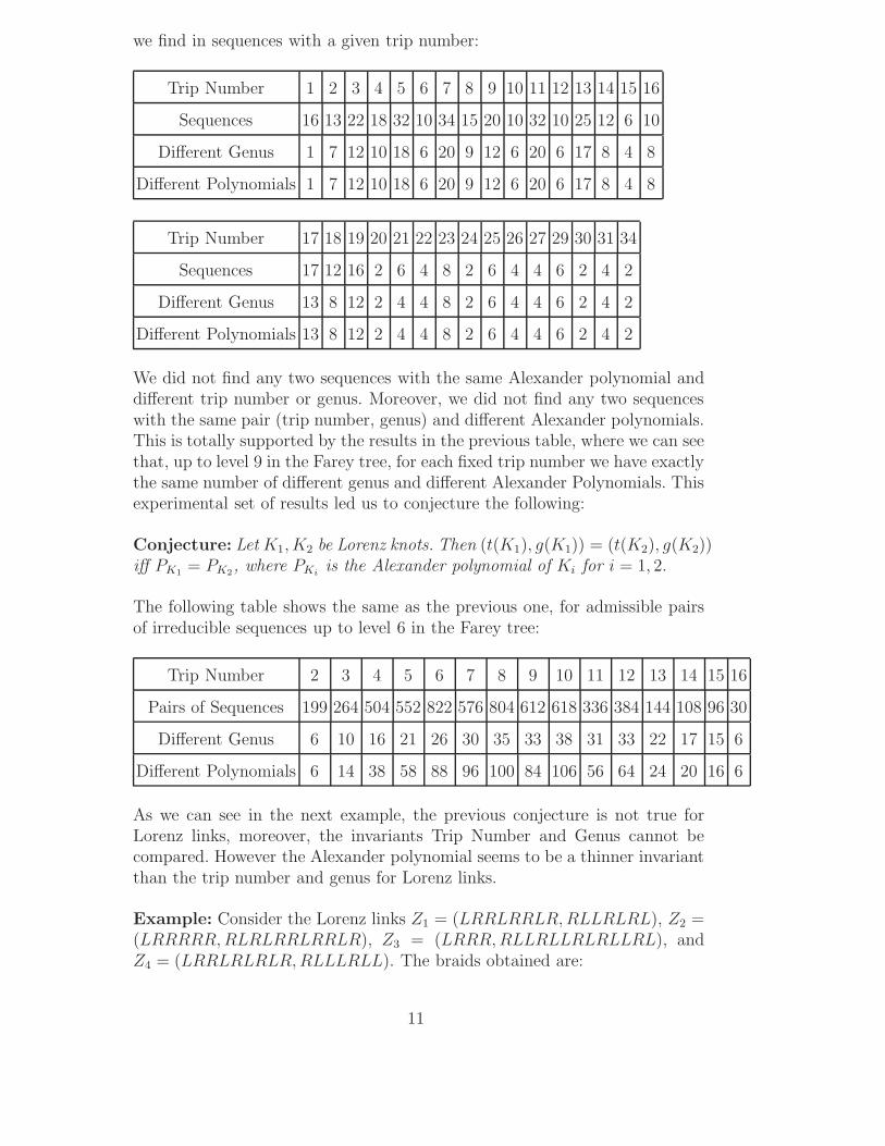
we find in sequences with a given trip number:

Trip Number 1 2 3 4 5 6 7 8 9 10 11 12 13 14 15 16

Sequences 16 13 22 18 32 10 34 15 20 10 32 10 25 12 6 10

Different Genus 1 7 12 10 18 6 20 9 12 6 20 6 17 8 4 8

Different Polynomials 1 7 12 10 18 6 20 9 12 6 20 6 17 8 4 8

Trip Number 17 18 19 20 21 22 23 24 25 26 27 29 30 31 34

Sequences 17 12 16 2 6 4 8 2 6 4 4 6 2 4 2

Different Genus 13 8 12 2 4 4 8 2 6 4 4 6 2 4 2

Different Polynomials 13 8 12 2 4 4 8 2 6 4 4 6 2 4 2

We did not find any two sequences with the same Alexander polynomial anddifferent trip number or genus. Moreover, we did not find any two sequenceswith the same pair (trip number, genus) and different Alexander polynomials.This is totally supported by the results in the previous table, where we can seethat, up to level 9 in the Farey tree, for each fixed trip number we have exactlythe same number of different genus and different Alexander Polynomials. Thisexperimental set of results led us to conjecture the following:

Conjecture: Let K1, K2 be Lorenz knots. Then (t(K1), g(K1)) = (t(K2), g(K2))iff PK1

= PK2, where PKi

is the Alexander polynomial of Ki for i = 1, 2.

The following table shows the same as the previous one, for admissible pairsof irreducible sequences up to level 6 in the Farey tree:

Trip Number 2 3 4 5 6 7 8 9 10 11 12 13 14 15 16

Pairs of Sequences 199 264 504 552 822 576 804 612 618 336 384 144 108 96 30

Different Genus 6 10 16 21 26 30 35 33 38 31 33 22 17 15 6

Different Polynomials 6 14 38 58 88 96 100 84 106 56 64 24 20 16 6

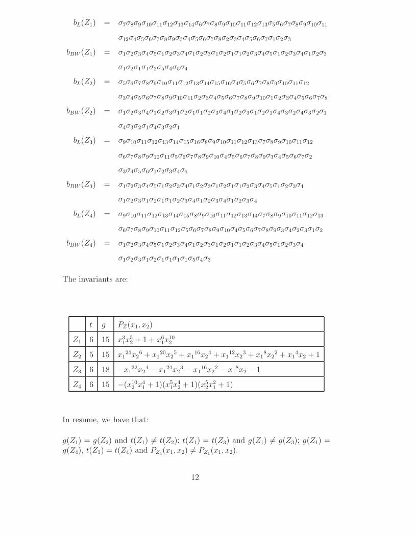
As we can see in the next example, the previous conjecture is not true forLorenz links, moreover, the invariants Trip Number and Genus cannot becompared. However the Alexander polynomial seems to be a thinner invariantthan the trip number and genus for Lorenz links.

Example: Consider the Lorenz links Z1 = (LRRLRRLR, RLLRLRL), Z2 =(LRRRRR, RLRLRRLRRLR), Z3 = (LRRR, RLLRLLRLRLLRL), andZ4 = (LRRLRLRLR, RLLLRLL). The braids obtained are:

11

bL(Z1) = σ7σ8σ9σ10σ11σ12σ13σ14σ6σ7σ8σ9σ10σ11σ12σ13σ5σ6σ7σ8σ9σ10σ11

σ12σ4σ5σ6σ7σ8σ9σ3σ4σ5σ6σ7σ8σ2σ3σ4σ5σ6σ7σ1σ2σ3

bBW (Z1) = σ1σ2σ3σ4σ5σ1σ2σ3σ4σ1σ2σ3σ1σ2σ1σ1σ2σ3σ4σ5σ1σ2σ3σ4σ1σ2σ3

σ1σ2σ1σ1σ2σ5σ4σ5σ4

bL(Z2) = σ5σ6σ7σ8σ9σ10σ11σ12σ13σ14σ15σ16σ4σ5σ6σ7σ8σ9σ10σ11σ12

σ3σ4σ5σ6σ7σ8σ9σ10σ11σ2σ3σ4σ5σ6σ7σ8σ9σ10σ1σ2σ3σ4σ5σ6σ7σ8

bBW (Z2) = σ1σ2σ3σ4σ1σ2σ3σ1σ2σ1σ1σ2σ3σ4σ1σ2σ3σ1σ2σ1σ4σ3σ2σ4σ3σ2σ1

σ4σ3σ2σ1σ4σ3σ2σ1

bL(Z3) = σ9σ10σ11σ12σ13σ14σ15σ16σ8σ9σ10σ11σ12σ13σ7σ8σ9σ10σ11σ12

σ6σ7σ8σ9σ10σ11σ5σ6σ7σ8σ9σ10σ4σ5σ6σ7σ8σ9σ3σ4σ5σ6σ7σ2

σ3σ4σ5σ6σ1σ2σ3σ4σ5

bBW (Z3) = σ1σ2σ3σ4σ5σ1σ2σ3σ4σ1σ2σ3σ1σ2σ1σ1σ2σ3σ4σ5σ1σ2σ3σ4

σ1σ2σ3σ1σ2σ1σ1σ2σ3σ4σ1σ2σ3σ4σ1σ2σ3σ4

bL(Z4) = σ9σ10σ11σ12σ13σ14σ15σ8σ9σ10σ11σ12σ13σ14σ7σ8σ9σ10σ11σ12σ13

σ6σ7σ8σ9σ10σ11σ12σ5σ6σ7σ8σ9σ10σ4σ5σ6σ7σ8σ9σ3σ4σ2σ3σ1σ2

bBW (Z4) = σ1σ2σ3σ4σ5σ1σ2σ3σ4σ1σ2σ3σ1σ2σ1σ1σ2σ3σ4σ5σ1σ2σ3σ4

σ1σ2σ3σ1σ2σ1σ1σ1σ1σ5σ4σ3

The invariants are:

t g PZ(x1, x2)

Z1 6 15 x31x

52 + 1 + x6

1x102

Z2 5 15 x124x2

6 + x120x2

5 + x116x2

4 + x112x2

3 + x18x2

2 + x14x2 + 1

Z3 6 18 −x132x2

4 − x124x2

3 − x116x2

2 − x18x2 − 1

Z4 6 15 −(x102 x4

1 + 1)(x51x

42 + 1)(x5

2x21 + 1)

In resume, we have that:

g(Z1) = g(Z2) and t(Z1) 6= t(Z2); t(Z1) = t(Z3) and g(Z1) 6= g(Z3); g(Z1) =g(Z4), t(Z1) = t(Z4) and PZ4

(x1, x2) 6= PZ1(x1, x2).

12

References

[1] E. Artin, Theory of braids, Ann. of Math. (2) 48 (1947) 101-126

[2] J. Birmann and R.F. Williams, Knotted periodic orbits in dynamical systems I:

Lorenz’s equations. Topology 22 (1983), 47–82.

[3] R. Ghrist, P. Holmes and M. Sullivan, Knots and Links in Three-Dimensional

Flows. Lecture Notes in Mathematics, Springer (1997).

[4] N. Franco, L. Silva, Genus and braid index associated to sequences of

renormalizable Lorenz maps.

[5] J. Franks, R. F. Williams, Braids and the Jones polynomial Trans. Am. Math.Soc 303, 97-108 (1987)

[6] L. Silva, J. Sousa Ramos, Topological invariants and renormalization of Lorenz

maps. Phys. D 162 (2002), no. 3-4, 233–243.

[7] W. de Melo, M. Martens, Universal models for Lorenz maps. Ergod. Th andDynam. Sys., 21 (2001), 833-860.

[8] H. R . Morton, The multivariable Alexander polynomial of a closed braid,Lowdimensional topology (H. Nencka, ed.), Contemporary Mathematics, vol.233, Amer. Math. Soc., 1999, pp. 251–256.”

[9] C. Tresser and R. Williams, Splitting words and Lorenz braids, Phys. D 62

(1993), 15–21.

[10] S. Waddington, Asymptotic formulae for Lorenz and horseshoe knots. Comm.Math. Phys. Volume 176, Number 2 (1996), 273–305.

[11] R. Williams, The structure of Lorenz attractors. Publ. Math. I.H.E.S., 50 (1979),73-99.

13

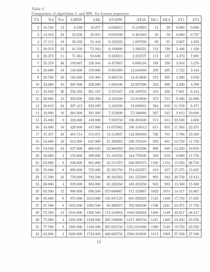
Table 2Comparison of algorithms L and BW, for Lorenz sequences

TN Nsl Ntn LBBW LBL ATABW ATAL ML1 ML2 AT1 AT2

2 10.538 13 8.539 16.077 0.033615 0.119923 15 29 0.000 0.000

3 14.318 22 22.636 32.955 0.052500 0.461682 40 59 0.000 0.727

4 17.111 18 39.333 51.444 0.102222 1.007056 69 91 2.667 4.333

5 20.313 32 61.250 75.563 0.193000 2.260531 112 139 2.406 1.438

6 20.273 11 71.364 84.636 0.233818 2.223727 115 137 4.273 7.091

7 25.278 36 109.667 126.944 0.477667 6.606194 198 230 3.944 5.278

8 28.000 18 140.000 159.000 0.985389 12.044889 259 295 1.722 3.444

9 29.700 20 165.600 185.300 0.865150 13.314600 272 305 2.300 3.850

10 33.000 10 207.000 229.000 1.638100 23.007200 333 369 3.200 4.700

11 34.833 36 238.333 261.167 2.275167 156.189722 410 450 7.861 6.444

12 39.600 10 303.600 330.200 3.435200 53.913800 473 515 9.400 24.800

13 38.618 34 307.412 332.029 5.165500 54.026941 564 610 11.559 6.471

14 42.000 16 364.000 391.000 7.252000 75.506688 507 545 3.813 10.688

15 45.000 8 420.000 449.000 7.959750 106.394500 574 614 23.500 4.000

16 44.000 16 420.000 447.000 14.077062 190.416812 615 655 11.563 22.375

17 47.357 28 485.714 515.071 13.512607 142.906393 736 781 7.786 10.500

18 54.000 16 612.000 647.000 21.292062 256.758188 833 881 12.750 11.750

19 53.833 24 627.000 660.833 23.868292 268.845208 900 949 12.250 10.958

20 50.000 4 570.000 599.000 21.185250 164.779500 589 619 8.000 11.750

21 63.000 8 840.000 881.000 45.511375 568.995875 1100 1154 15.250 36.750

22 55.000 8 693.000 725.000 35.591750 274.823375 819 857 27.375 15.625

23 57.500 16 759.000 792.500 46.562562 341.537688 902 942 20.750 12.813

24 60.000 4 828.000 863.000 65.220250 435.235250 943 983 15.500 15.500

25 62.500 12 900.000 936.500 373.666667 517.122667 1032 1074 14.417 24.667

26 65.000 8 975.000 1013.000 135.947125 685.922625 1125 1169 17.750 17.625

27 67.500 8 1053.000 1092.500 80.269875 762.926500 1196 1241 23.375 17.750

29 72.500 12 1218.000 1260.500 174.210083 1083.560333 1400 1449 42.917 46.417

30 75.000 4 1305.000 1349.000 205.528000 1317.400750 1421 1469 23.250 23.250

31 77.500 8 1395.000 1440.500 265.024750 1551.621000 1500 1549 19.750 23.250

34 85.000 4 1683.000 1733.000 468.665750 2560.310500 1815 1869 27.500 27.500

14