Effective barometric admittance and gravity residuals

E L S E V I E R Physics of the Earth and Planetary Interiors 90 (1995) 221-241

Pt tYSI( S O[ I I t [ : [ A R T t t

AN [) P l A N t . [AR~ I ~ , l t RIORS

Effective barometric admittance and gravity residuals

D.J. Crossley a,*, O.G. Jensen a, j. Hinderer b a Department of Earth and Planetary Sciences, McGill University, 3450 University Street, Montreal, Que. H3A 2A7, Canada

b Institute de Physique du Globe, 5, Rend Descartes, 67084 Strasbourg Cedex, France

Received 1 November 1993; accepted 22 April 1994

Abstract

In the analysis of surface gravity signals that may originate from the Earth's core, the step of correcting for the atmospheric pressure fluctuations is one that must be done carefully. We apply two techniques for determining the local, or effective, barometric admittance function between simultaneous observations of surface gravity and pressure. The first is a frequency domain fit that computes the admittance on a band-by-band basis. Using data from both the Canadian and French superconducting gravimeters we determined that the magnitude of the local, or background, admittance increases smoothly and monotonically from about 0.2 /xgal mbar 1 at long periods (> 10 days) to about 0.35/xgal mbar 1 at frequencies greater than 3 cycles per day (c.p.d.); the phase lag is within a few degrees of 180 ° . By comparison, the effective admittances of the large-scale harmonics of the solar heating tide (S1-S 7) are much smaller, between 0.1 and 0.3 /xgai mbar- l , for most of the harmonics of a day. In the second approach we fit a symmetrical time domain admittance function having lengths between 1 and 19 h using both a standard least-squares fit to a white noise residual and a new, and clearly superior, fit assuming a brown noise residual. Both time and frequency domain approaches give comparable results and contribute to a significant lowering of the residual level in non-tidal bands.

I. Introduct ion

It is clear that if gravity signals f rom the Ear th ' s core are ever going to be detected, it will require the careful stacking of data f rom a network of sensitive instruments such as the superconduct ing gravimeter (SG). Several recent analyses of SG records (e.g. Hindere r et al., 1993) permit the signal level in the intertidal f requency bands to be ' r educed ' to the level of a few ngal (10 -7 m s 2) which is the apparen t upper limit of de-

* Corresponding author.

tectability of seismically excited Slichter and core gravity modes (Crossley et al., 1991). As indicated in a companion paper in this volume (Jensen et al., 1995), techniques that aim to reduce this level have to be used with some care, lest the 'des i red signal' is removed along with the 'undes i red noise' . In that paper signal levels were reduced by the el imination of high slews (i.e. fast gravity gradients); in this paper we evaluate the reduction in residual signal level accompanying several models of the a tmospher ic admit tance function.

The effective barometr ic admit tance is the transfer function between gravity and pressure measurements at a single station. It is the local

0031-9201/95/$09.50 © 1995 Elsevier Science B.V. All rights reserved SSDI 0031-9201(95)05086-8

222 D.J. Crossley et al. / Physics of the Earth and Planetary Interiors 90 (1995) 221-241

part of an atmospheric correction that has long been recognised (e.g. Warburton and Goodkind, 1977) to include regional and global atmospheric effects. The effective admittance can be modelled as either a real or complex scalar function or one that is allowed to be time or frequency dependent. The use of some form of atmospheric admittance in surface gravity or seismic measurements is ubiquitous and very often performed by assuming a single scalar admittance. We will see that this practise is not only physically questionable, but its calculation using standard least squares techniques also involves a poor assumption.

The model for computing admittance is now recognised to require a spherical Earth model (e.g. Niebauer, 1988) and to include effects from regional and global pressure variations around a station and the vertical structure of the atmosphere (Merriam, 1992b). It has in some instances been assumed that the admittance is one sided in the time domain owing to a presumed require- ment of causality, i.e. that only past changes in air pressure at a station can affect the gravity at any instant of time. It will be demonstrated later that this is not the case when the pressure changes are associated, as they often are, with weather sys- tems moving horizontally across the gravimeter site.

We also emphasise that even though the SG is capable of detecting a 1 ngal signal, it is not necessary that pressure corrections be done to this level to reveal the presence of a harmonic (or quasi-harmonic) signal in the gravity record, un- less those signals are exactly at tidal periods or at the daily harmonics. In our experiments (e.g. Hinderer et al., 1993) a brown noise signal of amplitude say 40 ngal over a 2 year record gives a

residual gravity signal level of about 1 ngal in equivalent harmonic amplitude.

This paper is not intended to be an exhaustive study of the type undertaken by Merriam (1992b) who came to the conclusion that a global pressure correction is required at periods longer than a few days to correctly model gravity at the 1 /zgal level. Our intention is rather to demonstrate that a careful analysis of the local effective admittance can be beneficial if the desire is to reduce gravity residuals at periods shorter than 1 day.

2. Gravity data sets

There are three pairs of data sets in this study, identified as follows.

Data Set 1 (DS1). The residual gravity and pressure signals derived from the processing of two years of SG data from Cantley, Canada according to the methods used by the French SG processing group. The data and processing methods are fully described in Hinderer et al. (1993, 1995). For the purposes of this study no pressure correction was done during the tidal fitting process E T E R N A (Wenzel, 1994) in which we used the Tamura tidal potential. The mean value was removed from both the gravity residuals and the pressure; there was no other processing of the pressure data.

Data Set 2 (DS2). These data sets are for the exact same time period as DS1, but derive in- stead from the French SG instrument located near Strasbourg. Details can be found in Hin- derer et al. (1993).

Data Set 3 (DS3). These data is for the same 2 year period as for DS1 and DS2, but with differ-

Table 1 Frequency bands of interest Band (c.p.h.) (c.p.d.) (h) Comment

8 0.131-0.158 3.144-3.792 7.634-6.329 Quar diurnal 9 0.158-0.172 3.792-4.128 6.329-5.814

10 0.172-0.333 4.128-7.992 5.814-3.003

8-10 0.13-0.21 3.12-5.04 7.3-4.7 Preferred Slichter 10 0.21-0.30 5.04-7.2 4.7-3.3 Smylie Slichter

D.J. Crossrey et al, / Physics of the Earth and Planetary Interiors" 90 (1995) 221-241 223

ent processing. The data were decimated from 1 s to 1 rain and from 1 min to 1 h using filters designed especially for the CSGI (Canadian Su- perconducting Gravimeter Installation) data. For the gravity signal, a linear drift was removed and

a model tide subtracted using the programme GTIDE (Merriam, 1992a) for an elastic Earth with constant delta factors of 1.16 (i.e. the nominal station body tide). The pressure signal was the same as in DS1.

(a)

o

o

-i0.

CSGI gravity, uncorrected for pressure

POWER SPECTRAL DENSITY

NO 17520 NP 65536 CB I0 P Ii

- .

-6.o I - - -

- 8 . k

-12.0 k

0 1 2 3 4 5 6 7 8 9 i0 ii 12

cycles/day

(b)

4.0

2 . 0

u 0.0

n, -2.0 c~

~ -4.0 - - - - - -

~ - 6 . 0

-8.0

- i 0 . 0

CSGI pressure


~ ~ ' ~ '~'"~ ~,'~,,,d

-12.0

0 1 2 4 5 6 7

cycles/day

NO 17520 NP 65536 CB i0 P ii

9 i0 ii 12

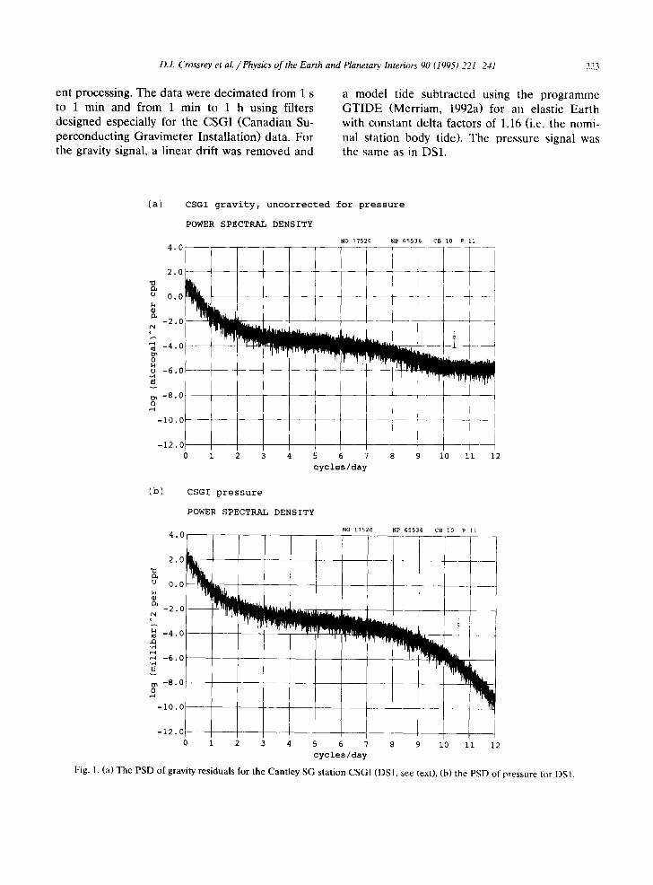
Fig. 1. (a) The PSD of gravity residuals for the Cantley SG station CSGI (DS1, see text), (b) the PSD of pressure for DSI.

224 D.J. Crossley et aL / Physics of the Earth and Planetary Interiors 90 (1995) 221-241

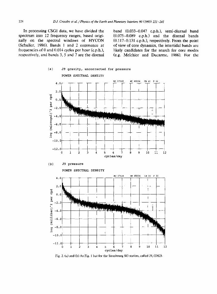
In processing CSGI data, we have divided the spectrum into 12 frequency ranges, based origi- nally on the spectral windows of HYCON (Schuller, 1986). Bands 1 and 2 commence at frequencies of 0 and 0.014 cycles per hour (c.p.h.), respectively, and bands 3, 5 and 7 are the diurnal

band (0.033-0.047 c.p.h.), semi-diurnal band (0.075-0.089 c.p.h.) and the diurnal bands (0.117-0.131 c.p.h.), respectively. From the point of view of core dynamics, the intertidal bands are likely candidates for the search for core modes (e.g. Melchior and Ducarme, 1986). For the

Ca)

4.0

J9 gravity, uncorrected for pressure


NO 17520 NP 65536 CB i0 P ii

2.0

u 0.0

-2.0

o M .u - 6 . 0

-8.0

- I 0 . 0

-12.C

~.L

1 2 4 5 6

cycles/day 8 9 I0 Ii 12

(b) J9 pressure


4 . 0

2 . 0

u 0.0 ~4 oJ

-2.0

~" - 4 . 0 Xl

,-t ,-4 - 6 . 0 . . . . . E v

-8.0 o

-i0.0

-12.0

NO 17520 NP 65536 CB i0 P 11

~111,.~..L

1 2 3 4 5 6 7 8 9 i0 ii

cycles/day

Fig. 2. (a) and (b) As Fig. 1 but for the Strasbourg SO station, called J9, (DS2).

12

D.J. Crossrey et al. /Physics of the Earth and Planetary Interiors 90 (1995) 221-241 225

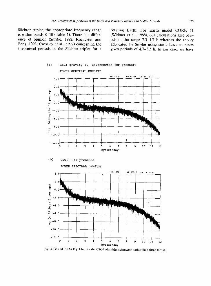
Slichter triplet, the appropriate frequency range is within bands 8-10 (Table 1). There is a difference of opinion (Smylie, 1992; Rochester and Peng, 1993; Crossley et al., 1992) concerning the theoretical periods of the Slichter triplet for a

rotating Earth. For Earth model CORE 11 (Widmer et al., 1988), our calculations give periods in the range 7.3-4.7 h whereas the theory advocated by Smylie using static Love numbers gives periods of 4.7-3.3 h. In any case, we have

(a)

4.0

2.0

o 0.0

-2 0

-4 0

0 u k -6 0------

v -8 0

o

-i0 O--

-12

CSGI gravity II, uncorrected for pressure


0 0

NO 17520 NP 65536 CB i0 P ii

I

2 3 5 6 7 8 9 i0 ii 12

cycles/day

(b) CSGI 1 hr pressure


4.C NO 17520 NP 65536 CB 10 P Ii

2.0

n.

u 0.0 k

-2.0

P ~ - 4 . 0

,~ - 6 . 0

-8.0

-i0.0

-12.0

u I 2 3 4 5 6 7 8 9 I0 ii 12

cycles/day

Fig. 3. (a) and (b) As Fig. 1 but for the CSGI with tides subtracted rather than fitted (DS3).


been using band 10 (5.8-3.0 h) as a candidate portion of the spectrum in which to assess the levels of residual gravity.

We use a standard spectral reconnaissance technique; a 10% cosine bell data taper, padding by a factor of 3.74, and a fast Fourier transform (FFT) smoothed by a frequency domain Parzen window (Jenkins and Watts, 1968) to produce the sample spectral estimate. As a measure of signal level, we use the equivalent time domain standard deviation (SD) in /zgal in the various frequency bands. This is the standard deviation of a pseudo-Gaussian white noise that would give the same signal level as that measured in the particular frequency band considered. As noted above, this level is considerably higher than that obtained from an amplitude spectrum normalised to give the true amplitude of a purely harmonic signal.

Fig. 1 shows the PSD (power spectral density) for (1) the uncorrected gravity residual and (2) the pressure for DS1. It can be seen that most of the tidal energy at 1 and 2 c.p.d, has been removed by ETERNA, and that harmonics of the solar atmospheric heating tide from S 1 - S 7, S 9

and S~1 are clearly visible. Both signals are af- fected at frequencies higher than 8 c.p.d, by the decimation filters used in the Strasbourg procedure (Hinderer et al., 1993).

Similar plots are shown in Fig. 2 for DS2 and in Fig. 3 for DS3. It can be seen that the Stras-

bourg spectra, based on DS2, are quite similar to those from the Canadian station. For DS3, it is evident that the tidal subtraction has left much more residual tidal energy in the 1, 2 and 3 c.p.d. bands than the fitting process used in DS1. More- over, the form of the decimation filter now closely matches that for the pressure, as can be seen in the similarity of the spectral roll-off beyond 8 c.p.d.

The PSD signal levels for the uncorrected gravity in DS1 are shown at the top of Table 2.

3. The effective barometric admittance

The barometric admittance is simply the transfer function between the residual gravity and atmospheric pressure signals at a single station. Ideally for this calculation these signals should be free of all effects not of atmospheric origin, i.e. no body or ocean tides, instrument drift or disturbances, and no hydrological signals. This is never satisfied in practise. In certain tidal processing packages such as H Y C O N and ETERNA, the pressure correction is performed along with the tidal fit. This is useful in terms of estimating the parameter covariance matrix, but undesirable if the pressure correction is too naive, which we will later argue is the case. Also, the modelling of hydrological and other signals such as the polar motion is often the final step in gravity interpre-

Table 2 Single coefficient solutions

Taper a Residual gravity (~gal)

Band 8 Band 9 Band 10 Full

Pressure admittance b

(/zgal mbar- 1) (deg)

Uncorrected gracity 1 0.1163 0.1139 0.0694 2.3362 2 0.1320 0.1251 0.0799 2.5083

Time domain solution a 1 0.0527 0.0468 0.0308 l. 1469 - 0.2569 2 0.0724 0.0629 0.0458 1.3314 - 0.2569

Frequency domain solution a 1 0.0533 0.0475 0.0312 1.1425 0.2550 2 0.0726 0.0634 0.0460 1.3261 0.2573

Ol R (~ - - 1 8 0

- - 0 . 2 5 4 7 - - 2 . 7 8

- - 0 . 2 5 6 9 - - 3 . 1 9

Data tapers: 1 = 10% cosine bell, 2 = boxcar. b Time domain solution a is real. Frequency domain solution a = l a te(itb)= o/R + i a I.

Prior to all FFTs the data mean was removed and the data was padded with zeros from 17520 to 65536 points.

D.J. Crossrey et al. / Physics of the Earth and Planetary Interiors 90 (1995) 221-241 227

tation and the presence of these signals when the pressure correction is performed will to some extent corrupt the barometric admittance.

For the gravity signal, it also makes a difference whether the body tides have been fitted or subtracted. In most tidal fitting procedures, atmospheric and ocean tides at the frequencies of the body tide potential are absorbed into the estimated tidal 6 and K factors, which is not the case when the body tides are subtracted.

A simple model is sufficient to give the basic physics of the correction. For a stationary column of air above a gravimeter station, the change in surface gravity due to a 1 mbar increase in atmospheric pressure (accompanying an increase in atmospheric density) can be written

Ag = Ag L + Ag2, (Ap = 1 mbar) (1)

where A g~ is due to the upwards attraction of the positive density contrast and Ag 2 is due to downwards loading of the ground. The latter is a combination of the gravity field owing to the deformation and the movement of the gravimeter through the ambient field gradient (Spratt, 1982). The relative sizes of the two terms in Eq. (1) depend on the size of the cell size considered. For a plane earth model Warburton and Good- kind (1977) showed the contributions to be approximately - 0.37/xgal mbar - 1 and + 0.02 /xgal mbar - [ , respectively, for a cell size which is 10 times the scale height (8.5-9.5 km depending on season, as quoted by Niebauer, 1988) of the standard atmosphere. This cell size is still much smaller than the horizontal scale of weather sys- tems. Treating a spherical Earth and the vertical structure of the atmosphere, Merriam (1992b) confirms that an admittance of -0 .35 tzgal mbar 1 is appropriate for local pressure disturbances from 0 to 0.5 °. We recover this value for both the Cantley and Strasbourg SG stations in the subtidal band.

4. Single time domain admittance

The most widely used pressure correction is a single, real, scalar admittance computed in the time domain. We minimise (in a least squares

sense) the difference between observed gravity residuals g(t) and the observed barometric pressure p(t) and solve for the real coefficient (which allows for no phase lag) to determine the corrected gravity residual

go(t) = g ( t ) -e~p( t ) (2)

Minimising I gc(t)[2 assumes that the errors in g(t) and the residuals gc(t) are uncorrelated. Applying Eq. (2) to DS1 in the time domain gives a = -0 .257/xga l mbar -~ for both forms of data taper (Table 2). For band 10, the use of a single admittance significantly reduces the SD from 69 to 31 ngal and from 80 to 46 ngal for the cosine bell and boxcar data tapers, respectively.

5. Single frequency domain admittance

We now transform Eq. (2) to the frequency domain

Gc( ,O) = G(o ) - ( 3 )

and allow a to be a complex scalar. Minimising IGc(w)[ 2 over the whole frequency range 0 < oJ < oN, where w N is Nyquist frequency, leads to

E [G*(w)P(o~)] a* = ~ ] P ( o ) [ : (4)

which is equivalent to the complex admittance defined by Warburton and Goodkind (1977) from the cross-spectrum of the gravity and pressure signals.

From Eq. (4) the real and imaginary solutions are

[PR(W)GR(~O) + PI(O~)GI(t.o)] (5)

~ IP(~o) l 2

and

[ PR(~O)G,(w) - P~(~O)GR(Oj)] oq = ~ [ p ( w ) 12 (6)

These can be combined into the admittance amplitude ~ and phase &. The results for DS1 are shown at the bottom of Table 2, where it can be seen that although the data taper slightly


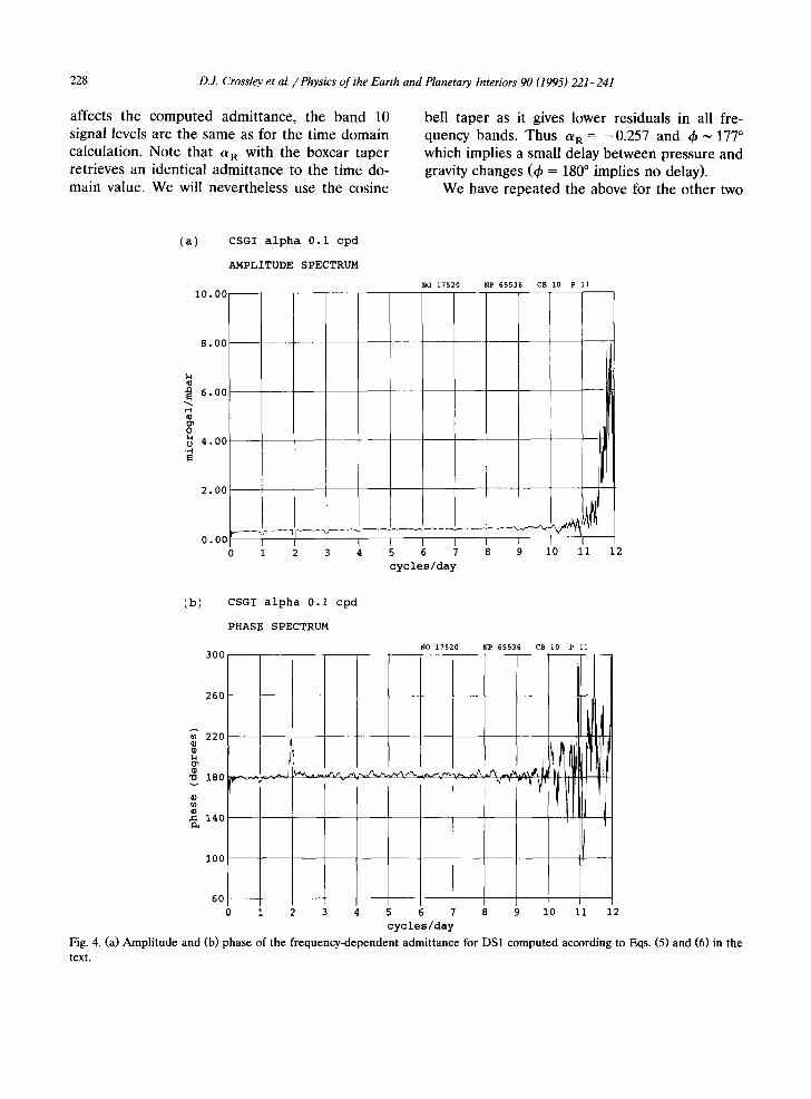
affects the computed admittance, the band 10 signal levels are the same as for the time domain calculation. Note that a R with the boxcar taper retrieves an identical admittance to the time domain value. We will nevertheless use the cosine

bell taper as it gives lower residuals in all frequency bands. Thus a R = - 0 . 2 5 7 and ~b ~ 177 ° which implies a small delay between pressure and gravity changes (~b = 180 ° implies no delay).

We have repeated the above for the other two

(a) CSGI alpha 0.i cpd

AMPLITUDE SPECTRUM

i0.00

8.00

6.00

t~ o u ~ 4.00

2.00

0.00 1 2 3 4

NO 17520 NP 65536 CB i0 P Ii

5 6 7 8 9 i0 ii

cycles/day

12

(b) CSGI alpha 0.i cpd

PHASE SPECTRUM

300

2601

220 ~

180 v

140

100

60

0 i

NO 17520

,.~ ~ . w ' ~ .-'x... ^ ~ ~,,.-,~. ^ A ./~, . . . . . . . . V v ~"l~ ~dr

[

4 5 8

cycles/day

NP 65536 CB 10 P ii

II IO, A

IV 't

9 i0 ii 12

Fig. 4. (a) Amplitude and (b) phase of the frequency-dependent admittance for DS1 computed according to Eqs. (5) and (6) in the text.


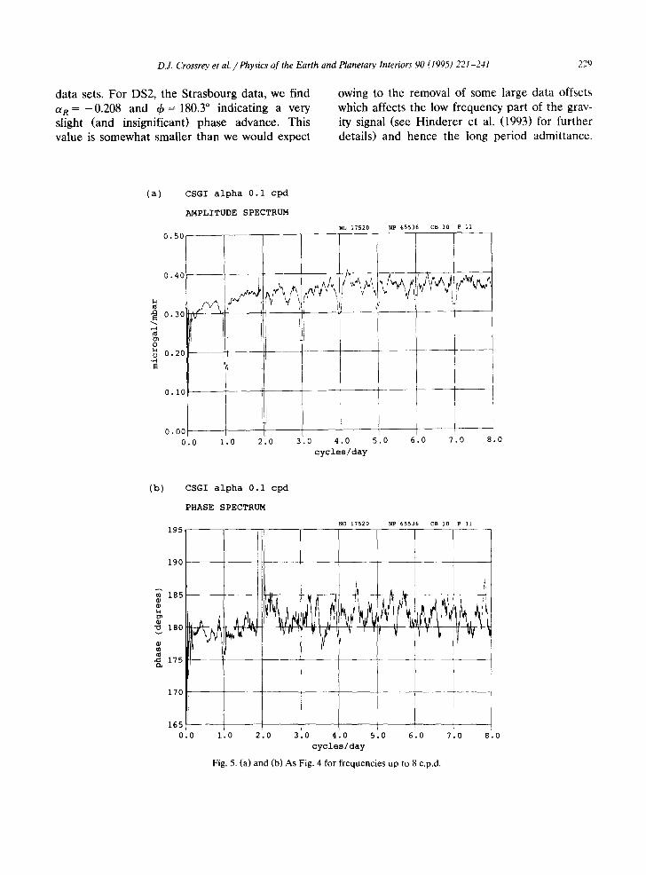
data sets. For DS2, the Strasbourg data, we find a R = - 0 . 2 0 8 and 4, = 180.3 ° indicating a very slight (and insignificant) phase advance. This value is somewhat smaller than we would expect

owing to the removal of some large data offsets which affects the low frequency part of the gravity signal (see Hinderer et al. (1993) for further details) and hence the long period admittance.

(a)

0.50

0.40

0.30

I;n o u ~ 0.20

0.I0

0.00

CSGI alpha 0.i cpd

AMPLITUDE SPECTRUM

-I .0 1.0

NO 17520 NP 65536 CB I0 P ii

2.0 3.0 4.0 5.0 .0 .0 8.0

cycles/day

(b)

195

190

185 @

D~

180 v

@ u)

175 C~

170

165

0.0

CSGI alpha 0.i cpd

PHASE SPECTRUM

1.0 2 .0 3.0 4 .0 5 .0 6.0 c y e l e s / clay

Fig, 5. (a) and (b) As Fig. 4 for frequencies up to 8 c.p.d.

NO 17520 NP 65536 CB i0 P li

7.0 8.0


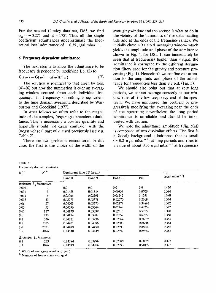
For the second Cantley data set, DS3, we find a R = - 0 . 2 7 5 and ~b = 175 °. Thus all the single coefficient admittances underest imate the theoretical local admittance of - 0 . 3 5 / x g a l mbar-1 .

6. Frequency-dependent admittance

The next step is to allow the admittance to be frequency dependent by modifying Eq. (3) to

Gc(to) = G(w) - ct( to)P(to) (7)

The solution is identical to that given by Eqs. (4)-(6) but now the summation is over an averaging window centred about each individual frequency. This frequency smoothing is equivalent to the time domain averaging described by War- burton and Goodkind (1977).

In what follows we often refer to the magnitude of the complex, frequency-dependent admittance. This is necessarily a positive quantity and hopefully should not cause confusion with the (negative) real part of a used previously (see e.g. Table 2).

There are two problems encountered in this case, the first is the choice of the width of the

averaging window and the second is what to do in the vicinity of the harmonics of the solar heating tide and at the ends of the frequency ranges. We initially chose a 0.1 c.p.d, averaging window which yields the amplitude and phase of the admittance shown in Fig. 4, for DS1. It can immediately be seen that at frequencies higher than 8 c.p.d, the admittance is corrupted by the different decimation filters used for the gravity and pressure processing (Fig. 1). Hencefor th we confine our atten- tion to the amplitude and phase of the admittance for frequencies less than 8 c.p.d. (Fig. 5).

We should also point out that at very long periods, we cannot average correctly as our window runs off the low frequency end of the spectrum. We have minimised this problem by pro- gressively modifying the averaging near the ends of the spectrum; nevertheless the long period admittance is unreliable and should be inter- preted with caution.

We note the admittance amplitude (Fig. 5(a)) is composed of two dissimilar effects. The first is a (focal) background admittance that is small ( ~ 0.2 izgal mbar -~) at long periods and rises to a value of about 0.35/xgal m b a r - 1 at frequencies

Table 3 Frequency domain solutions Af a N b Equivalent time SD (p, gal)


Otl0 (/zgal mbar -1)

Including S n harmonics 0.0001 1 0.0 0.0 0.0 0.0 0.450 0.001 3 0.01458 0.01318 0.00833 0.0700 0.394 0.002 5 0.03066 0.02591 0.01642 0.1581 0.380 0.005 15 0.03773 0.03378 0.02070 0.2619 0.374 0.01 27 0.04003 0.03576 0.02174 0.34863 0.372 0.02 55 0.04096 0.03664 0.02248 0.42259 0.372 0.05 137 0.04170 0.03799 0.02313 0.57550 0.370 0.1 273 0.04194 0.03902 0.02352 0.67250 0.368 0.2 546 0.04221 0.03936 0.02364 0.76675 0.367 0.5 1365 0.04421 0.04096 0.02383 0.86809 0.364 1.0 2731 0.04499 0.04150 0.02393 0.88242 0.362 1.5 4096 0.04540 0.04149 0.02397 0,89852 0.361

Excluding S n harmonics 0.1 273 0.04194 0.03996 0.02389 0,68227 0.373 1.5 4096 0.04243 0.04206 0.02393 0.90172 0.372

a Width of averaging window (c.p.d.). b Number of frequencies averaged.


between 4 and 8 c.p.d.. The small value at long periods simply means that large-scale pressure fluctuations are less well correlated with gravity than are local pressure fluctuations. The second is a line spectrum (broadened by the averaging window) at the harmonics of a day owing to the (global) effects of the solar heating tide. It is striking that the admittance associated with the diurnal harmonics is significantly smaller than that of the background and highly variable, with the S 2 admittance being the smallest, thus con- firming the results of Warburton and Goodkind (1977).

Recalling that the single coefficient time (or frequency) domain solution gives an (equivalent) admittance of 0.257 tzgal mbar -1 for this data set, it is clear that this value is influenced by the long period synoptic pressure fluctuations and is not representative of a local (background) admittance. Naturally, the noise reduction in the core mode bands could be improved upon by using this background value rather than the admittance computed from a global fit. The phase of the admittance is much less than 180 ° at long periods indicating a significant phase lag, whereas for

shorter periods it is close to 180 ° indicating that there is no significant departure from a purely elastic response of the Earth. The anomalous phase at a frequency of 2 c.p.d, is due to residual semi-diurnal tidal energy.

To explore the question of the appropriate averaging window for this calculation, we performed a number of tests with different averaging window widths and computed the admittance amplitude averaged over band 10 as well as the residual signal level SD for bands 8-10 (Table 3). The results are quite revealing. Obviously a single point-by-point admittance ( N = 1) reduces the residual signal to zero although this is not useful in practise. With more averaging (N increasing) the admittance averaged over band 10(al0) de- creases marginally from 0.372 to 0.362 /xgal mbar-t. There is little change in the SD for band 10 between windows with Af = 0.01 and 1.0 c.p.d., indicating the admittance is fairly robust to choice of A f; our initial estimate of 0.1 c.p.d, thus seems quite appropriate.

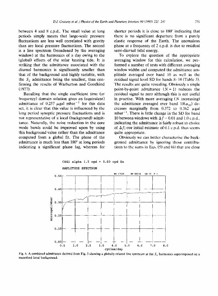
Obviously we can better characterise the background admittance by ignoring those contributions to the sums in Eqs. (5) and (6) that are close

CSGI alpha 1.5 cpd + 0.03 cpd Sn

AMPLITUDE SPECTRUM

0.50

0.40

k4 o.3o~ b~ 0

0.20

0.I0

NO 17520 NP 65536 CB I0 P 1

3.0 4.0

cycles/day

Fig. 6. A combined admittance derived from Fig. 5 showing a globally related line spectrum at the S~ harmonics superimposed on a smoothed local background.

0.00 I 0.0 1.0 2.0 5.0 6.0 7.0 8.0

to the S, harmonics. Here we chose to exclude contributions at frequencies closer than 0.015 c.p.d, to each daily harmonic and to further smooth the spectrum we use a wide averaging window of 1.5 c.p.d. In a separate step, we com-

(a)

puted the admittances obtained at the a n harmonics with a narrow window (0.03 c.p.d.) centred at each harmonic. The combined result (Fig. 6) illustrates clearly the difference between the local and global contributions to the admittance.

-6.01

%! 0.0

-z.c i~.~'~

(~ -2.o

~ - 3 . 0 - -

~ - 4 . 0 ~

- 5 . 0

(b)

n. o

D~ 0 ~4 o

1.0

CSGI uncorrected gravity



NO 17520 NP 65536 CB I0 P Ii

" I '11 I j' I'"

5.00 6.00 7.00 0.00 1.00 2.00 3.00 4.00

cycles/day

CSGI corrected gravity, single complex alpha


NO 17520 ~ 65536 CB 10 P 11 • ^

'flT!"~

8.00

0.0 1.0 2.0 3.0 4.0 5.0 6.0 7.0 8.0

cycles/day

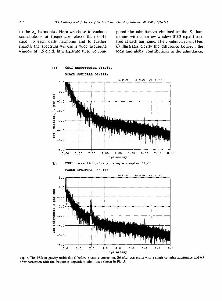
Fig. 7. The PSD of gravity residuals (a) before pressure correction, (b) after correction with a single complex admittance and (c) after correction with the frequency-dependent admittance shown in Fig. 5.


<c)

1.0

0.0

o

-i.0

P -2.0

t~ o -3.0

o .4

-4.0

0

-5.0

-6.0

.0

CSGI corrected gravity, alpha 0.i cpd


i. 2.0 3.0

NO 17520 NP 65536 CB i0 P Ii

I T

I - -

L

I

4.0 5.0

cycles/day

6 .0 7 . 0

Fig. 7 (continued).

8 .0

We now compare the gravity corrected by a single complex admittance with that obtained by using the admittance in Fig. 5. The uncorrected

gravity is shown in Fig. 7(a) and the two corrections shown in Figs. 7(b) and (c). It is evident that as the pressure correction is 'improved', the sig-

CSGI gravity, pressure corrected with/without S5, 0.1 cpd


-2.5

-3.1 O

O

-3.7

~n O

-4.3 O

v

~n ~ -4 .9

NO 17520 NP 65536 ii

-5.5

4.90 4.92 4.94 4.96 4.98 5.00 5.02 5.04 5.06 5.08 5.10

cycles/day

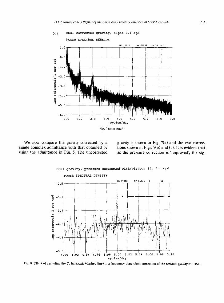
Fig. 8. Effect of excluding the S 5 harmonic (dashed line) in a frequency-dependent correction of the residual gravity for DS1.


nal level drops across the spectrum. The effect is most noticeable in the vicinity of the diurnal and semi-diurnal tidal bands where the residual tidal energy becomes quite apparent in Fig. 7(c). This suggests that a second fitting of the body tides (using for example ETERNA) could be usefully done to further reduce the tidal residuals.

The question of whether to include the S, harmonics in the pressure correction is tested in Fig. 8 which shows the corrected gravity around S 5 both with and without including the effect of the harmonic in the correction. The result clearly shows that one has to be extremely careful of peaks in the spectrum in the vicinity of these harmonics owing to the atmospheric tides. There is also a further complication at these harmonics owing to non-linear ocean tides, as shown for the semi-diurnal band by Merriam (1993).

Thus, even if there were no theoretical problems with the Slichter triplet identification of Smylie (1992), we would have to be very suspi- cious of his identification of a peak on the shoul- der of S 6 at 4 h. In general however, the S, harmonics have only a very small effect on the average residual signal levels in the Slichter bands,

as can be seen from the bottom section of Table 3.

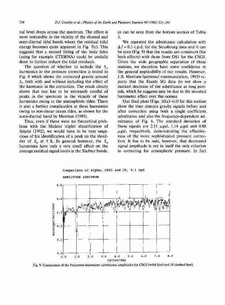
We repeated the admittance calculation with Af = 0.1 c.p.d, for the Strasbourg data and it can be seen (Fig. 9) that the results are consistent (for both effects) with those from DS1 for the CSGI. Given the wide geographic separation of these stations, we therefore have some confidence in the general applicability of our results. However, J.B. Merriam (personal communication, 1993) re- ports that the Esashi SG data do not show a marked decrease of the admittance at long periods, which he suggests may be due to the inverted barometer effect over the oceans.

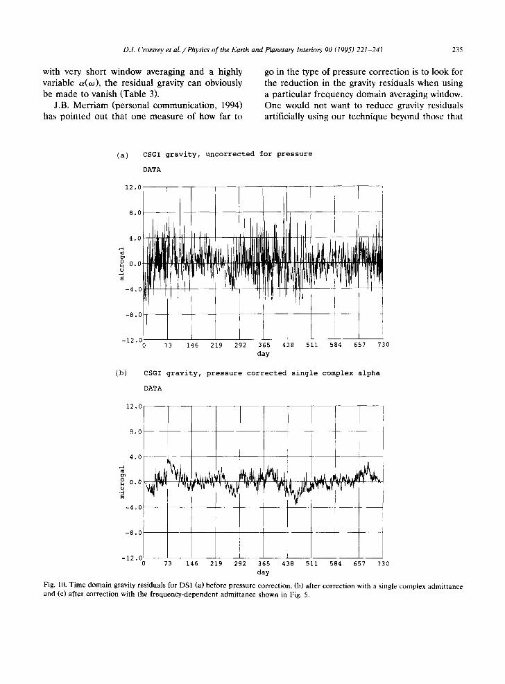
Our final plots (Figs. 10(a)-(c)) for this section show the time domain gravity signals before and after correction using both a single coefficient admittance and also the frequency-dependent admittance of Fig. 6. The standard deviation of these signals are 2.51 /zgal, 1.14 /zgal and 0.88 /zgal, respectively, demonstrating the effective- ness of the more sophisticated pressure correction. It has to be said, however, that decreased signal amplitude is not in itself the only criterion in correcting for atmospheric pressure. In fact

Comparison of alpha, CSGI and J9, 0.i cpd

AMPLITUDE SPECTRUM

0 .5

° ° II

0 0 .3

j 0 .2 J

o ~ . ,-I

0 .1 U

0 . 0 ¸ I I .0 1 .0 2 .0 3 .0 .0 5 .0 6 .0 7 .0 8 .0

c y c l e s / d a y

Fig. 9. Comparison of the frequency-dependent admittance amplitudes for CSGI (solid line) and J9 (dashed line).


with very short window averaging and a highly variable a(to), the residual gravity can obviously be made to vanish (Table 3).

J.B. Merriam (personal communication, 1994) has pointed out that one measure of how far to

go in the type of pressure correction is to look for the reduction in the gravity residuals when using a particular frequency domain averaging window. One would not want to reduce gravity residuals artificially using our technique beyond those that

(a) CSGI gravity, uncorrected for pressure

DATA

12. ̂

8.

4.1

c.

o 0.1

-4.

-8.

-12. - 0 73 146 219 292 365 438 511 584 657 730

day

(b) CSGI gravity, pressure corrected single complex alpha

DATA

12.0

8.0

4.0

° 0.0

-4.0

-8.0

-12.0

- - - - I I : I

73 146 219 292 365 438 511 584 657

day

730

Fig. 10. Time domain gravity residuals for DS1 (a) before pressure correction, (b) after correction with a single complex admittance and (c) after correction with the frequency-dependent admittance shown in Fig. 5.

236

(c)

D.Z Crossley et aL / Physics of ~e Earth and Planeta~ Interio~ 90 (1995) 221-241

CSGI gravity, pressure corrected, combined alpha (1.5+0.03)

DATA

12.0

8.0

4.0

o 0.0 o

-4.0

-8.0

-12.0 0 73 146 219 292 365 438 511 584 657 730

day

Fig. 10 (continued).

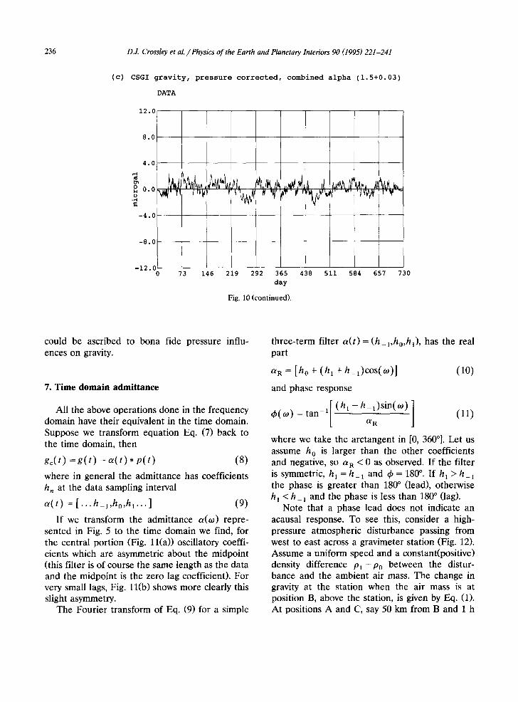
could be ascribed to bona fide pressure influ- ences on gravity.

7. Time domain admittance

All the above operations done in the frequency domain have their equivalent in the time domain. Suppose we transform equation Eq. (7) back to the time domain, then

gc( / ) = g ( / ) - a(t)* p(t) (8)

where in general the admittance has coefficients h , at the data sampling interval

a(t) = [. . .h_l,ho,hl. . . ] (9)

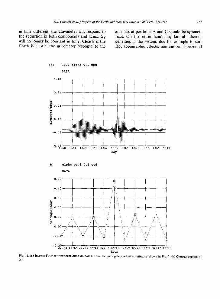
If we transform the admittance a(,o) repre- sented in Fig. 5 to the time domain we find, for the central portion (Fig. l l (a)) oscillatory coefficients which are asymmetric about the midpoint (this filter is of course the same length as the data and the midpoint is the zero lag coefficient). For very small lags, Fig. l l (b ) shows more clearly this slight asymmetry.

The Fourier transform of Eq. (9) for a simple

three-term filter a(t)= (h_l,ho,hO, has the real part

o/R = [h o q- (h 1 + h_l)COS(`o)] (10)

and phase response

tan_l [ (hi - h_l )s in( `o) 4,(,o) = [ (11) O~ R

where we take the arctangent in [0, 360°]. Let us assume h 0 is larger than the other coefficients and negative, so a R < 0 as observed. If the filter is symmetric, h I = h _ l and 4, = 180 °. If h 1 > h _ 1 the phase is greater than 180 ° (lead), otherwise h I < h _ 1 and the phase is less than 180 ° (lag).

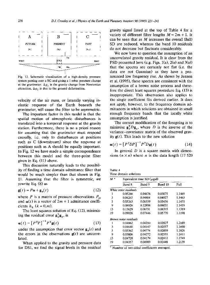
Note that a phase lead does not indicate an acausal response. To see this, consider a high- pressure atmospheric disturbance passing from west to east across a gravimeter station (Fig. 12). Assume a uniform speed and a constant(positive) density difference P l - P 0 between the disturbance and the ambient air mass. The change in gravity at the station when the air mass is at position B, above the station, is given by Eq. (1). At positions A and C, say 50 krn from B and 1 h


in time different, the gravimeter will respond to the reduction in both components and hence Ag will no longer be constant in time. Clearly if the Earth is elastic, the gravimeter response to the

air mass at positions A and C should be symmetrical. On the other hand, any lateral inhomo- geneities in the system, due for example to surface topographic effects, non-uniform horizontal

(a) CSGI alpha 0.1 cpd

DATA

0.48

0.35

~. 0.23

t~ o u ~ 0.i0 .,4

-0.03

-0.15 1360

m__

1361 1362 1363 1364 1365 1366 1367 1368 1369 1370 day

(b) alpha csgi 0.i cpd

DATA

0.50

0.40 / I I

0.30 /~

o 0.i0 o

0.00

-0.1~

-0.20 ]

i

I / ~,,/ \ I~/ ",

T i 32763 32764 32765 32766 32767 32768 32769 32770 32771 32772 32773

hour

Fig. 11. (a) Inverse Fourier transform (time domain) of the frequency-dependent admittance shown in Fig. 5. (b) Central portion of (a).

238 D.J. Crossley et at/Physics of the Earth and Planetary Interiors 90 (1995) 221-241

[- 7

I C I

PAST I I

(h_~) J r L J

A B

FUTURE PRESENT

(hi) (h,)

1 ~ Ag 1

WEST EAST

Ice'l A

Fig. 12. Schematic visualisation of a high-density pressure system passing over a SG and giving a 1 mbar pressure change at the gravimeter, z~g 1 is the gravity change from Newtonian attraction, Ag 2 is due to the ground deformation.

velocity of the air mass, or laterally varying in- elastic response of the Earth beneath the gravimeter, will cause the filter to be asymmetric.

The important factor in this model is that the spatial motion of atmospheric disturbances is translated into a temporal response at the gravity station. Furthermore, there is no a priori reason for assuming that the gravimeter must respond causally, i.e. only to disturbances at positions such as C (downstream) since the response at positions such as A should be equally important. In Fig. 12 we have made a simple correspondence between this model and the three-point filter given in Eq. (11) above.

This discussion naturally leads to the possibil- ity of finding a time domain admittance filter that would be much simpler than that shown in Fig. 11. Assuming that the filter is symmetric, we rewrite Eq. (8) as

g( t ) = e ~ + go(l) (12)

where P is a matrix of pressure observations P/k and ,~(t) is a vector of 2m + 1 admittance coefficients h k (k = O,m).

The least squares solution of Eq. (12), minimis- T ing the residual error g~g~, is

or(t) = [ PTP ]- ' pTg( t) (13)

under the assumption that error vector go(t) and the errors in the observations g(t) are uncorrelated.

When applied to the gravity and pressure data for DS1, we find the signal levels in the residual

gravity signal listed at the top of Table 4 for a variety of different filter lengths M = 2m + 1. It can be seen that as M increases the overall (full) SD are reduced, whereas the band 10 residuals do not decrease but fluctuate considerably.

We now have to question the assumption of an uncorrelated gravity residual. It is clear from the PSD presented here (e.g. Figs. l(a), 2(a) and 3(a)) that the spectra are certainly not flat (i.e. the data are not Gaussian) as they have a pro- nounced low frequency rise. As shown by Jensen et al. (1995), these spectra are consistent with the assumption of a brown noise process and therefore the direct least squares procedure Eq. (13) is inappropriate. This observation also applies to the single coefficient fits derived earlier. It does not apply, however, to the frequency domain admittances in which solutions are obtained in small enough frequency bands that the locally white assumption is justified.

The correct modification of the foregoing is to minimise T gcDgc, where D is the inverse of the variance-covariance matrix of the observed gravity g(t). This leads to the new solution

•(t) = [ p T D p ] - t p T D g ( t ) (14)

In general D is a square matrix with dimen- sions (n x n) where n is the data length (17 520

Table 4 Time domain solutions

M a Equiva len t t ime SD (~gal)


White no~e residua~ 1 0.05266 0.04676 0.03075 1.1469 3 0.04263 0.04884 0.04027 1.1463 5 0.05263 0.06559 0.03456 1.1455 9 0.08926 0.12898 0.08031 1.1419

13 0.15629 0.06731 0.08315 1.1319 19 0.09026 0.07446 0.05770 1.1198

Brown no~eresidua~ 1 0.04862 0.04350 0.02827 1.2189 3 0.04640 0.04147 0.02557 1.1690 5 0.05362 0.04774 0.02850 1.1826 9 0.05806 0.04272 0.02555 1.2411

13 0.04728 0.04179 0.02412 1.2749 19 0.04357 0.04989 0.02448 1.2139

a Number of two-sided coefficients averaged.

D.J. Crossrey et al. / Physics of the Earth and Planetary Interiors 90 (1995) 221-241 23t. )

for our data sets); it is quite inconvenient to use it directly in Eq. (14). Fortunately, we can find a reasonable approximation to D by recognising that as a positive definite matrix it can be fac- tored into the product EVE. By making the trans- formations g' = Eg,g ' c = Ege and P' = EP (e.g. Jackson, 1972), it can be seen that ,*(t) reduces to the original solution Eq. (13) (with primes added) by minimisation of g'cTg'c. We therefore seek a transformation E that restores P and g to a normally distributed form. This process is widely known as pre-whitening.

Elementary considerations suggest that a suit- able form is E T = [ . . . . 0 . . . . . 1 , - 1 . . . . . 0 . . . . ], i.e. a simple forward difference filter. The power response of this filter is 211 - c o s ( T r f ) ] between frequencies 0 and the Nyquist 0.5. Thus, the power spectrum a / f 2 of a brown noise process is modified by such a filter to 2 a [ l - cos(Trf )] / f ~ which is approximately flat across the frequency range.

The procedure is therefore to apply the above difference filter to both the gravity and pressure data sets before calculating the time domain solution using Eq. (13). The results are shown at the bottom of Table 4 where now we see that the

residuals in band 10 are not only significantly lower than those for the white noise solutions, but they are also bet ter behaved as M increases. However the improvement (taken as the lowering of signal level in band 10) is marginal, suggesting in practise that a short filter is sufficient.

We can compare the time and frequency domain solutions by recognising that a time domain filter of length M A t has a frequency resolution of A f = 1~(MAt) . The longest time domain filter considered here is 19 h, which is equivalent to a frequency averaging window of approximately 1.0 c.p.d. From Tables 3 and 4, we see that the band 10 SD for M = 19 is 0.024 /xgal, identical to the frequency domain solution for A f = 1.0.

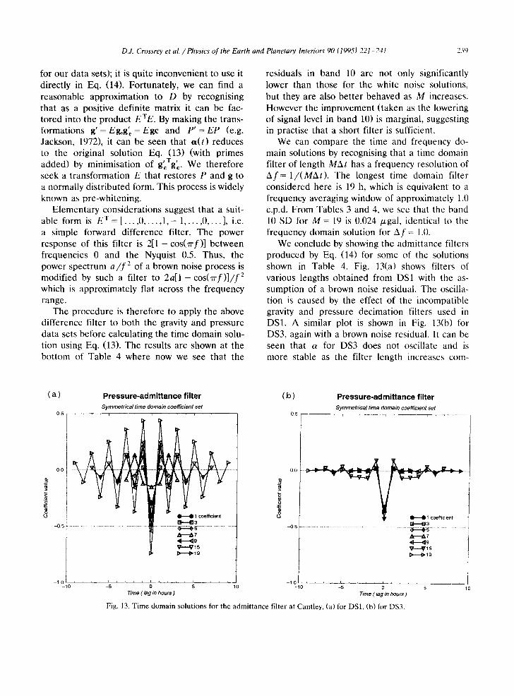
We conclude by showing the admittance filters produced by Eq. (14) for some of the solutions shown in Table 4. Fig. 13(a) shows filters of various lengths obtained from DS1 with the assumption of a brown noise residual. The oscilla- tion is caused by the effect of the incompatible gravity and pressure decimation filters used in DS1. A similar plot is shown in Fig. 13(b) for DS3, again with a brown noise residual. It can be seen that c~ for DS3 does not oscillate and is more stable as the filter length increases corn-

(a)

0 5

Pressure-admittance filter Symmetrical time domain coefficient set

(b)

0 ,0 - • , . .--

i -'- - - 7 ¢ ¢ 9 .";" .";'1 s I> ~: o 1 9

-1 .o f . . . . i . . . . i . . . . J . . . . . . - 1 0 - 5 0 5 10

Time ( lag in hours )

0 5

0 .0

- 0 . 5

Pressure-admittance filter Symmetrical time domain coefficient set

]

B - - ~ 3

2.. -'-7

1> 0 1 9

- I c . . . . i . . . . B - I 0 - 5 o

Time ( lag in hours )

Fig. 13. Time domain solutions for the admittance filter at Cantley, (a) for DS1, (b) for DS3.

5 10

240 D.J. Crossley et aL / Physics of the Earth and Planetary Interiors 90 (1995) 221-241

pared with DS1; we attribute this both to the similar decimation filters used in DS3 and, possi- bly, to the elimination of non-linear effects intro- duced into the tidal fitting process for DS1 (DS3 is for subtracted tides).

8. Summary and conclusions

Survey of Canada for maintenance of the CSGI at their site at Cantley. J. Hinderer acknowledges the support of CNRS-INSU for the Strasbourg SG facility. We thank Walter Ziirn for HYCON, George Wenzel for ETERNA and Jim Merriam for GTIDE. Finally, we have incorporated a number of useful comments suggested in a careful review by J. Merriam.

When doing the atmospheric correction of surface gravity data, the proper strategy will be determined by the available atmospheric data and the desired goal. In trying to lower the residual gravity levels in the search for weak signals from the core, it seems appropriate to use the type of pressure correction advocated here which takes into account both the local background admittance and that owing to the S n harmonics.

The correction can be done in either the time or the frequency domains with equal effective- ness, though the frequency domain correction permits selected frequencies, or frequency ranges, to be omitted more easily (if necessary). However for time domain admittance calculations, we rec- ommend that the gravity and pressure data be pre-whitened with a differencing filter before performing a least squares solution for the admittance filter coefficients.

Any type of nominal (e.g. a = -0.3) or single coefficient admittance correction that has been applied earlier to the gravity data must be re- versed prior to following the methods suggested here. Also the pressure correction should proba- bly be done in a separate step following drift modelling and tidal fitting or subtraction. If 'black box' procedures such as HYCON and ETERNA for tidal fitting are used, they should be implemented without a pressure channel.

Acknowledgements

This research was supported under grants (Operating, Infrastructure and International Fel- lowship) from the Natural Science and Engineer- ing Research Council of Canada variously to all three authors. We are grateful to The Geological

References

Crossley, D.J., Hinderer, J. and Legros, H., 1991. On the excitation, detection and damping of core modes. Phys. Earth Planet. Inter., 68: 97-116.

Crossley, D.J., Rochester, M.G. and Peng, Z.R., 1992. Slichter modes and Love numbers. Geophys. Res. Lett., 19: 1679- 1682.

Hinderer, J., Crossley, D. and Xu, H., 1993. A 2 year comparison between the French and Canadian superconducting gravimeter data. Geophys. J. Int., 116: 252-266.

Hinderer, J., Crossley, D. and Jensen, O., 1995. A search for the Slichter triplet in superconducting gravimeter data. Phys. Earth Planet. Inter., 90: 183-195.

Jackson, D.D., 1972. Interpretation of inaccurate, insufficient and inconsistent data. Geophys. J. R. Astron. Soc., 28: 97-109.

Jenkins, G.M. and Watts, D.G., 1968. Spectral Analysis and its Applications. Holden-Day, San Francisco, 525 pp.

Jensen, O., Hinderer, J. and Crossley, D.J., 1995. Noise limi- tations in the core-mode band of superconducting gravimeter data. Phys. Earth Planet. Inter., 90: 169-181.

Melchior, P. and Ducarme, B., 1986. Detection of inertial gravity oscillations in the Earth's core with a superconducting gravimeter at Brussels. Phys. Earth Planet. Inter., 42: 129-134.

Merriam, J.B., 1992a. An ephemeris for gravity tide predic- tions at the nanogal level. Geophys. J. Int., 108: 415-422.

Merriam, J.B., 1992b. Atmospheric pressure and gravity. Geo- phys. J. Int., 109: 488-500.

Merriam, J.B., 1993. Non-linear ocean tides observed with the Cantley superconducting gravimeter. In: 19th Annual CGU Meeting, Banff, Alberta, 9-11 May.

Niebauer, T.M., 1988. Correcting gravity measurements for the effect of local air pressure. J. Geophys. Res., 93: 7989-7991.

Rochester, M.G. and Peng, Z.R., 1993. The Slichter modes of the rotating Earth: a test of the subseismic approximation. Geophys. J. Int., 113: 575-585.

Schuller, K., 1986. Simultaneous tidal and multi-channel input analysis as implemented in the HYCON-method. In: R. Vierra (Editor), Proc. 10th Int. Symp. on Earth Tides. Consejo Superior de Investigaciones Cientific, Madrid, pp. 515-520.

D.J. Crossrey et aL / Physics of the Earth and Planetary Interiors 90 (1995) 221-241 241

Smylie, D.E., 1992. The inner core translational triplet and the density near Earth's center. Science, 255: 1678-1682.

Spratt, R.S., 1982. Modelling the effect of atmospheric pressure variations on gravity. Geophys. J. R. Astron. Soc., 71: 173-186.

Warburton, R.J. and Goodkind, J.M., 1977. The influence of

barometric-pressure variations on gravity. Geophys. J. R. Astron. Soc., 48: 281-292.

Wenzel, H.G., 1994. Earth tide analysis package--Eterna 3.20. Bull. Inf. Mattes Terrestres, 120: 91119-9022.

Widmer, R., Masters, G. and Gilbert, F., 1988. The spherical Earth revisited. EOS, Am. Geophys. Union, 69: 13111.

Effective barometric admittance and gravity residuals

Documents