1 Effect of unsampled populations on the estimation of 1 population sizes and migration rates between sampled 2 populations 3 4 Peter Beerli 5 Computer Science and Information Technology and Biological Sciences Department 6 Florida State University, Tallahassee FL 32306-4120 USA 7 8 Postal Address: CSIT, Dirac Science Library, Florida State University, Tallahassee FL 9 32306-4120 USA 10 Email: [email protected], 11 Phone: USA-(850) 645 1324, 12 Fax: USA-(850) 644 0098 13 14 Key words: migration rate, gene flow, maximum likelihood, finite migration model, 15 coalescence, population genetics, parallel execution, cluster 16 17 Running title: Effect of missing populations 18

Welcome message from author
This document is posted to help you gain knowledge. Please leave a comment to let me know what you think about it! Share it to your friends and learn new things together.
Transcript

1
Effect of unsampled populations on the estimation of1
population sizes and migration rates between sampled2
populations3
4
Peter Beerli5
Computer Science and Information Technology and Biological Sciences Department6
Florida State University, Tallahassee FL 32306-4120 USA7
8
Postal Address: CSIT, Dirac Science Library, Florida State University, Tallahassee FL9
32306-4120 USA10
Email: [email protected],11
Phone: USA-(850) 645 1324,12
Fax: USA-(850) 644 009813
14
Key words: migration rate, gene flow, maximum likelihood, finite migration model,15
coalescence, population genetics, parallel execution, cluster16
17
Running title: Effect of missing populations18
2
Abstract19
Current estimators of gene flow come in two flavors, those that estimate parameters20
assuming that the populations investigated are a small random sample of a large number21
of populations and those that assume that all populations were sampled. Maximum22
likelihood or Bayesian approaches that estimate the migration rates and population sizes23
directly using coalescent theory can easily accommodate datasets that contain a24
population that has no data, a so-called ghost population. This manipulation allows us to25
explore the effects of missing populations on the estimation of population sizes and26
migration rates between two specific populations. The biases of the inferred population27
parameters depend on the magnitude of the migration rate from the unknown populations.28
The effects on the population sizes are larger than the effects on the migration rates. The29
more immigrants from the unknown populations that are arriving in the sample30
populations the larger the estimated population sizes. Taking into account a ghost31
improves or at least does not harm the estimation of population sizes. Estimates of the32
scaled migration rate M (migration rate per generation divided by the mutation rate per33
generation) are fairly robust as long as migration rates from the unknown populations are34
not huge. The inclusion of a ghost does not improve the estimation of the migration rate35
M; when the migration rates are estimated as the number of immigrants Nm then a ghost36
improves the estimates because of its effect on population size estimation. It seems that37
for ‘real world’ analyses one should carefully choose which populations to sample, but38
there is no need to sample every population in the neighborhood of a population of39
interest.40

3
Introduction41
When we study organisms in their natural habitat, we almost always need to discuss the42
relationship of the populations studied to each other or to populations that were ignored.43
The magnitude of exchange of genetic material between the populations whether, in the44
long run, they remain separate or fuse into a single population. Researchers often use a45
measure of population divergence such as Sewall Wright’s fixation index, FST (Wright,46
1937; Wright, 1951), or similar statistics (Michalakis, Excoffier, 1996; Weir, Cockerham,47
1984) that partition the genetic variance among individuals in a population and between48
populations. Most researchers want not only to know whether there is structure among49
populations but also about the magnitude of the gene flow among them. In conservation50
biology, the estimation of a migration rate between populations of an endangered species51
might even be the goal of the study. Wright (1951) showed that there is a direct52
relationship between FST and the magnitude of gene flow between the populations for the53
n-island model. This approach, although widely used, is vulnerable to violations of its54
basic assumptions (Whitlock, McCauley, 1999). It provides only an overall average of55
the migration rate assuming that the number of populations is very large, whereas a more56
detailed view is often needed. Researchers, ignoring the problem that there might be57
interdependence of more than just two populations, have used, and often misused, FST-58
based approaches to estimate pairwise migration rates from multiple population data. Fu59
et al. (2003) showed that for finite numbers of populations, this interdependence can be60
substantial. Several methods have recently been developed to take such interdependence61
into account. Nicholson et al. (2002) and Weir and Hill (2002) developed statistics to62
estimate an FST-analog for each population, Wilson and Rannala (2003) and Pritchard et63
4
al. (2000) used allele frequencies to infer structure using Baysian approaches, whereas I64
and others (Bahlo, Griffiths, 2000; Beerli, Felsenstein, 1999; Nielsen, Wakeley, 2001)65
target the direct estimation of underlying population parameters, such as the migration66
rate, using coalescence theory with maximum likelihood or Bayesian approaches. In all67
these new approaches it is assumed the sampled populations represent all the populations,68
in stark contrast to methods that estimate a single migration parameter assuming that the69
sampled populations are a random sample from a large number of populations (Rousset,70
1996; Wakeley, Aliacar, 2001). Rarely, however, are all populations actually sampled.71
Are the individual-population estimators, by neglecting populations that are not part of72
the sample, giving a false impression of accuracy? Is it possible to estimate migration73
rates among arbitrarily chosen populations without the Herculean effort of sampling74
every population? This study explores the effect of missing data on gene flow analysis75
with my own maximum likelihood method MIGRATE (Beerli, 2003), which is based on the76
coalescent. I expect that findings in this study are also valid for similar approaches, such77
as GENETREE (Bahlo, Griffiths, 2000) and MDIV (Nielsen, Wakeley, 2001).78
79
5
Methods80
The Markov chain Monte Carlo based coalescent methods (Bahlo, Griffiths, 2000;81
Beaumont, 1999; Beerli, Felsenstein, 1999; Beerli, Felsenstein, 2001; Nielsen, Wakeley,82
2001; Wilson, Balding, 1998) allow for complicated population models, but it is83
commonly assumed that samples from all populations are in the dataset. This is rarely the84
case when researchers work with natural populations; some populations are not sampled85
because of logistic difficulties, or because one is not aware that additional populations86
exist. These statistical methods by themselves do not require that all sampled populations87
have data, but the effects of the unobserved populations on the results from these88
methods warrants exploration.89
Artificial datasets were created using a coalescent simulator similar in concept to90
Hudson’s (1983) simulator (the C source code for the coalescent tree generator simtree91
and the data simulator simdata can be obtained by request from PB). The simulation92
study was kept as simple as possible to reduce problems caused by having too many93
parameters. I simulated two main scenarios to explore the effect of missing populations:94
the effect of the magnitude of migration, and the effect of the number of missing95
populations.96
97
To explore the effect of the magnitude of the migration, a set of three interacting, equally98
sized populations was created of which only two are sampled (Fig. 1). I call the99
unsampled third population world. The immigration rate into the sampled populations100
from the world is called world-immigration to contrast it to the migration rates between101

6
the sampled populations (sample-immigration). Each dataset contains 20 individuals, 10102
in each sampled population, each individual was scored for 100 unlinked loci and each103
locus has a length of 1000 bp. The populations all have the same size Θ = 0.01, where Θ104
is 4 × effective population size Ne × mutation rate µ per generation and site; this is105
roughly equivalent to having 2500 individuals with a substitution rate µ of 10-6 per106
generation. For most of the simulations the migration rate between the sampled107
populations is kept at migration rate M = 100, where M is the immigration rate m scaled108
by µ. Using the above substitution rate, M = 100 translates into m = 0.0001 per109
generation. This is equivalent to 1 immigrant every 4 generations (4Ne(1)m = 4Ne
(2)m =1).110
The migration rate into population 1 from 2 is labeled M2-1 and the migration from world111
to 1 similarly is Mworld-1.112
The following scenarios were simulated:113
• No immigration from the world: (Fig. 2A) the two sampled populations do not114
receive migrants from the world population.115
• Unequal world-immigration (Fig. 2 B, C): (B) the world-immigration is of the116
same magnitude as the migration rate between the two populations, M = 100117
(4Ne(i)mworld-1= 1); (C) the immigration from the world is much bigger than the118
exchange between the samples, M = 1000 (4Ne(i)mworld-1=10). There is no migration119
from the sample to the world.120
• Symmetric immigration from the world (Fig. 2 D, E): All migration rates are the121
same as before except that all immigration from the world populations are122
matched with an immigration into the world population with the same magnitude.123
124
7
To check the variability of the outcome, I generated 10 additional datasets for the125
scenario with symmetric migration rates between all three populations (Fig. 2D), and two126
further datasets containing 50 and 100 individuals using the same scenario.127
128
For the analysis of the effect of the number of missing populations, datasets were created129
in which two sampled populations are part of a network of unobserved populations; sets130
of 3, 5, and 9 populations were simulated. For these simulations I kept the migration rate131
the same between all populations (Fig. 2D).132
133
Additionally, effects of the world populations when there is no migration between the134
sample populations (M = 0) were analyzed, using unequal and symmetric world-135
immigration scenarios.136
137
I analyzed these artificial datasets with MIGRATE (Beerli, Felsenstein, 1999; Beerli,138
Felsenstein, 2001). MIGRATE estimates migration rates and population sizes jointly using139
a maximum likelihood approach that is based on the coalescent (for an overview see140
Kingman, 2000). The program finds parameters by maximizing a relative likelihood141
using the Markov chain Monte Carlo sampling scheme devised by Metropolis et al.142
(1953) with modifications by Hastings (1970). For a set of n populations, n population143
sizes and n(n-1) immigration rates are estimated. The population sizes are reported as Θ144
(that is, 4Neµ for nuclear data). The immigration rates are estimated as M, which is m/µ.145
Each dataset was analyzed by assuming first that there are only two populations and146
second, that there is in addition a third unknown population, which I call a ghost147

8
population because the data do not indicate its presence or absence or how many such148
populations are present. For datasets with multiple unknown populations, only one ghost149
population was used. For each dataset , I performed two MIGRATE runs to get a rough150
estimate of the Markov chain Monte Carlo error. The design of the study allowed to151
employ an ANOVA analysis that checked the major effects of the variance introduced by152
having two datasets per scenario, the two replicates, the magnitude of the world-153
immigration, and the variance of the sample-immigration rates. The ANOVA analysis154
was done with MATHEMATICA 4.2 (Wolfram Research, 1999). Mean square errors (MSE)155
were calculated to explore the benefits of including the ghost in the analysis. The MSE156
measure is the expectation of the squared differences of the estimates and the expected157
values, MSE =
€
E(W −T)2 =Var(W ) +Bias2 , where W is the estimate and T is its158
expectation. Here, T is the values used to simulate the dataset (the truth), and the Bias is159
the difference from the mean estimate and the truth. The MSE incorporates two160
components, variance and bias. One seeks the method that minimizes MSE.161
The program version used was MIGRATE 1.7.3 (Beerli 2003) and all options were default162
except that a heating scheme (Markov Coupled Markov chain Monte Carlo: Geyer,163
Thompson, 1992) with 3 heated chains and one cold chain was in effect. The program164
was compiled for parallel execution using the Message Passing Interface (Gropp et al.,165
1999) and the analyses were done on an IBM eServer pSeries 690 cluster running AIX166
and using up to 101 processors concurrently. Details of the parallel implementation and167
its performance are described in the Appendix.168

9
Results169
Effects on the estimation of the population size: In Figure 3 results from the three170
scenarios each with two datasets generated with the same parameters are shown. The171
migration rate is unidirectional from the world to the sampled populations (Fig 3. A1 and172
A2). When there is no connection between the world and the samples, the two-population173
analysis estimates the sizes for the two populations well, with MSE = 0.088 × 10⁻⁶) with174
an expected value of Θ = 0.01. Both datasets recover the true value whereas the ghost-175
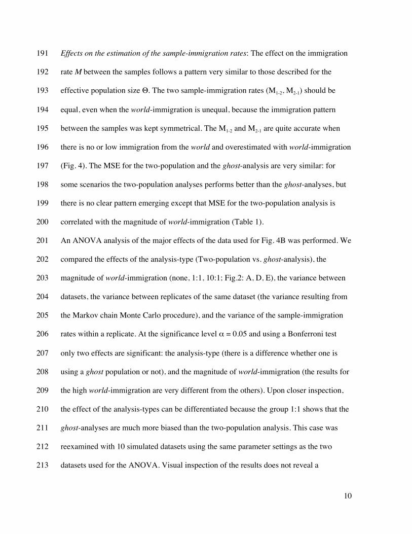
analysis tends to underestimate the population size (MSE = 1.73 × 10⁻⁶). With increased176
world-immigration, the two-population analysis overestimates the sizes considerably177
(MSE=8.2 × 10⁻⁶), whereas the ghost-analysis recovers the true values (MSE=0.15 × 10-178
6). The result for the high world-immigration is puzzling as one might expect that all the179
parameters might be overestimated, but the two-population analysis recovers the true180
values with an MSE of 0.33 × 10⁻⁶ . A summary of the MSEs for all parameters is shown181
in Table 1. The results for Θ from the simulations with symmetric immigration rates182
between sampled populations and world reveal s a similar pattern except for the high183
migration scenario (Fig. 3 B1 and B2). With low world-immigration, the two-population184
analysis overestimates and the ghost-analysis recovers the true values, but the high185
world-immigration simulations show over-estimation of the population sizes. There is a186
tight correlation with the magnitude of world-immigration rates: the MSE for all 3 two-187
population scenarios are 0.09 × 10⁻⁶, 9.0 × 10⁻⁶ , 15.6 × 10⁻⁶. The bias of the ghost-analysis188
is less well correlated with the magnitude of the immigration with MSEs of 1.7 × 10-6,189
0.01 × 10⁻⁶, and 0.86 × 10-6.190
10
Effects on the estimation of the sample-immigration rates: The effect on the immigration191
rate M between the samples follows a pattern very similar to those described for the192
effective population size Θ. The two sample-immigration rates (M1-2, M2-1) should be193
equal, even when the world-immigration is unequal, because the immigration pattern194
between the samples was kept symmetrical. The M1-2 and M2-1 are quite accurate when195
there is no or low immigration from the world and overestimated with world-immigration196
(Fig. 4). The MSE for the two-population and the ghost-analysis are very similar: for197
some scenarios the two-population analyses performs better than the ghost-analyses, but198
there is no clear pattern emerging except that MSE for the two-population analysis is199
correlated with the magnitude of world-immigration (Table 1).200
An ANOVA analysis of the major effects of the data used for Fig. 4B was performed. We201
compared the effects of the analysis-type (Two-population vs. ghost-analysis), the202
magnitude of world-immigration (none, 1:1, 10:1; Fig.2: A, D, E), the variance between203
datasets, the variance between replicates of the same dataset (the variance resulting from204
the Markov chain Monte Carlo procedure), and the variance of the sample-immigration205
rates within a replicate. At the significance level α = 0.05 and using a Bonferroni test206
only two effects are significant: the analysis-type (there is a difference whether one is207
using a ghost population or not), and the magnitude of world-immigration (the results for208
the high world-immigration are very different from the others). Upon closer inspection,209
the effect of the analysis-types can be differentiated because the group 1:1 shows that the210
ghost-analyses are much more biased than the two-population analysis. This case was211
reexamined with 10 simulated datasets using the same parameter settings as the two212
datasets used for the ANOVA. Visual inspection of the results does not reveal a213

11
consistent difference between the two-population and the ghost-analysis (Fig. 5).214
Averaging over the 10 different datasets gives parameter values that are very close to the215
truth (Table 2). The MSE of the immigration rate based on these 10 datasets for the two-216
population analysis is 125, and 144 for the ghost-analysis, somewhat better numbers than217
the crude MSE from two data sets of 320 and 517. The smaller the MSE, the more218
confidence we have that the method has a small bias and small variance. The variances219
for the sample immigration rates of the 10 replicates are 137.4 and 150.8, respectively.220
The ghost-analysis has higher variance because it estimates 9 parameters instead of just221
4; for low world-immigration rates both estimators seem to have small bias because the222
variance is of the same magnitude as the MSE.223
No direct migration between the sampled populations: Table 3 shows the MSEs for224
datasets where there is no migration between the sample populations. All gene flow225
between the samples is indirect through the world population. The two-population226
analyses have larger MSEs for Θ and M than the ghost-analyses, except for the227
unidirectional, large world-immigration where the two-population has a minimal MSE228
for Θ.229
Effects of the number of missed populations: The estimated sample-immigration rates M230
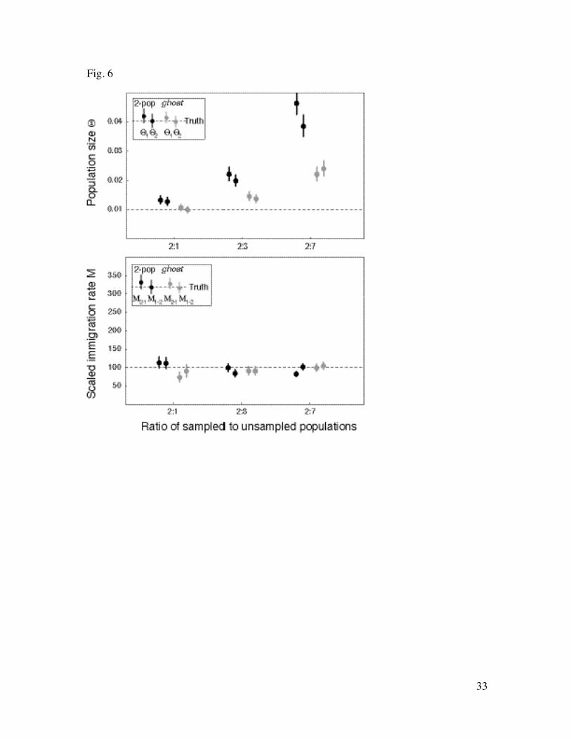
are astonishingly robust when we increase the number of unsampled populations (Fig. 6,231
bottom). The estimates for ratios of 2:1 between sampled and unsampled populations,232
2:3, and 2:7 are very similar for both types of analyses, both the two-population and the233
ghost-analysis seems to improve with more unsampled populations (Table 1). In contrast,234
the estimates of the population sizes are strongly affected by missed populations (Fig. 6,235
top). For the two-population analysis, the MSE increase about 9-fold between the ratios236

12
of sampled vs. missing populations of 2:1, 2:3, and 2:7. For the ghost-analysis, the values237
are smaller, but they show a similar, but weaker, trend as the two-population analysis238
(Table 1).239
Sample size: To make sure that the above comparisons are not an effect of small sample240
size (10 individual per population), additional datasets with 50 and 100 total individuals241
were analyzed. These datasets were simulated under the scenario that all migration rates242
are equal (Fig. 2D). The effect of small sample size on the estimates of the immigration243
rate is minimal (Fig. 7), except that the support intervals are somewhat larger with fewer244
individuals. The results for the population sizes are not shown but follow the same245
pattern; this is expected and has been found before (Pluzhnikov, Donnelly, 1996).246
Effects on the estimation of the number of immigrants into a sample population: The247
number of immigrants can be expressed as
€
4Nem =ΘΜ = 4Νeµ ×m µ . The biases that248
affect Θ and Μ will affect the 4Nem the same way. The biases of Θ for scenarios with249
medium and high world-immigration rates are large whereas the biases for M are much250
smaller for medium world-immigration than for large world-immigration, the biases for251
4Nem follow closely the biases for Θ.252
Discussion253
Results were partly expected and partly surprising. The estimates of the migration rate M254
between the samples are stable when there is no or low immigration from the world. The255
estimates deteriorate with large immigration rates from the world: the many alleles256
imported into the two sampled populations from the same source increase the estimates257
of M because the occurrence of the same allele in all the populations increases the chance258

13
that there was a migration. Surprisingly, with moderate world-immigration rates the259
number of missed populations does not affect the estimates of the migration rates260
between the samples. The local alleles are not swamped by alleles from world as in the261
large world-immigration scenarios and therefore allow to estimate successfully the262
migration rates between the samples. This confirms Hudson’s (1998) assertion that is263
possible to estimate a migration rate in a subgroup of populations in a n-island model264
based on a ‘local’ FST. Whether one uses a ghost in the analysis or not, is not that265
important because ignoring unknown populations or taking them into account provides266
very similar results for the migration rate estimates.267
The estimates of population sizes show more deviation from the true values than those for268
the migration rates. The quality of the estimates depends on the simulation scenario. With269
symmetric migration rates between the sample and the world a steady increase in270
population sizes was found and the deviation from the true value gets larger when the271
immigration rate increases or the number of missed population increases; having a272
migration rate M of 1000 from a single missed population is similar of having an M of273
100 from 10 missed populations. The ghost analysis improves the estimates of Θ274
somewhat with small immigration rates but the estimates are still biased upward when the275
gene flow from the unknown populations is large. There is a discrepancy between the276
source-sink and the symmetric migration scenario. In the source-sink scenario with large277
immigration rate the population sizes are estimated quite accurately. This is an artifact278
because the sample populations get swamped with alleles from the world and essentially279
become copies of the world population and therefore should have its size; instead of280
measuring the size of the samples under these conditions one is measuring the size of the281

14
unknown population. With symmetric and high migration rates all populations exchange282
many migrants through the world populations, so that the three populations essentially283
behave like one large population in which the coalescences are independent from the284
location of the sampling (Nagylaki, 2000).285
Fu et al. (2003) showed that many estimators using allele frequencies have difficulties286
estimating the degree of isolation for a finite number of small connected populations287
because the allele frequencies co-vary. This effect is more pronounced with small sizes288
because genetic drift acts on all populations and on the group as a whole. One might289
wonder how much approaches based on the limit of infinite number of populations (for290
example Wakeley, Aliacar, 2001; Wright, 1951) correctly estimate migration rates when291
the immigration rates deviate from an n-island model. I expect that for moderate and low292
migration rates the overall parameter estimates might be quite accurate because there was293
no strong deviation in simulations for these scenarios even with a large number of294
unsampled populations, but one would need to evaluate the behavior of these methods295
when the immigration rates from world populations to the sample populations are large.296
297
Migration rates might be expressed as genetic distances that take into account variances298
and covariances of allele frequencies (Wood, 1986, but see Fu, 2003). When there is no299
direct migration between the sample populations, variability still can be distributed300
through world and we would expect an upwards bias for the sample migration rates301
because with large world-immigration the sample populations are swamped with alleles302
from world. This results in a considerably biased sample-immigration rate for the303
scenario with unidirectional world-immigration where there is no exchange between the304

15
sample populations, the many similar world-alleles make it impossible to establish305
whether this is the result of sample-immigration or export of world-alleles into the306
samples. When there is more interest in historical processes than interest in variability307
patterns this distinction is relevant and migration rates cannot be replaced by pairwise308
genetic distances. Inclusion of a ghost population seems to improve the estimates of309
sample population sizes considerably, suggesting that a simple pairwise treatment of310
migration incorporates some of the variability imported from locations other than the pair311
under consideration and so will lead to overestimation of local variability.312
313
It seems unnecessary to add a ghost population to analyze migration rates M because in314
many comparisons the MSE do not strongly favor the ghost-analysis over a two-315
population approach although it seems that the two-population method is favored because316
of the larger variance of the ghost-analysis caused by the higher number of parameters to317
estimate. If the migration rate M from the unsampled population is known to be large or318
if the focus of the analysis is to estimate the population size Θ, or the number of319
immigrants 4Nem, which is the product of Θ and M, then the addition of a ghost does320
help to reduce the upwards bias. Bittner and King (2003) were using my ghost approach321
to estimate 4Nem between snake populations on islands in Lake Erie. They report that a322
ghost is useful only when few populations were sampled but when additional samples323
from more populations are available the inclusion of a ghost has no benefit for the324
estimation of 4Nem. We might extrapolate that when only two populations are sampled,325
the population sizes are most likely overestimated and the only hope for getting accurate326
numbers is to sample the dominating populations. Adding samples from other327

16
populations is fairly simple because one is not required to sample huge numbers of328
individuals to get decent results from a coalescent based analysis.329
330
Acknowledgement331
This study was supported by a grant from the National Science Foundation DEB-332
0108249 to Scott Edwards and the author; preliminary simulations were initiated while I333
was at the University of Washington supported by grants from National Science334
Foundation (DEB-9815650), the National Institute of Health (GM-51929 and HG-01989)335
to Joseph Felsenstein, whom I thank for many discussions on the topic. The simulations336
were supported by Florida State University School for Computational Science and337
Information Technology and utilized their IBM eServer pSeries 690 Power4-based338
supercomputer Eclipse. I also want to thank Thomas Uzzell, Laurent Excoffier, Mary339
Kuhner, Scott Edwards, Richard King, and an anonymous reviewer for helpful comments340
on the manuscript.341
Appendix342
The program MIGRATE-N summarizes over multiple unlinked loci calculating the343
likelihood344
€
L(Θ,M) = Pr(G |Θ,M)Pr(Dl |G)dGG∫
l=1
loci
∑345
(Beerli, Felsenstein, 1999). Each locus is independent from any other so that the346
integration over all possible genealogies for each locus can be run independently. This347
makes the problem embarrassingly parallel (for example see Rosenthal 1999). On348

17
multiple computers one can run all loci concurrently, and reduce the analysis time349
considerably. MIGRATE-N can be compiled for parallel machines utilizing MPI (Gropp et350
al., 1999). The current version uses a master-worker architecture. The flow of the351
analysis is as follows: the parameter file is read by the master-node. On interactive352
systems the menu can be displayed (all input/output related function are guided through353
the master). After the menu, the data are read and distributed to all worker nodes; the354
master orchestrates the workers, each of which gets a locus to work on. Once a locus is355
finished, the worker receives either a new locus or waits until all other workers are done356
with their work; the master then calculates the maximum likelihood estimate (MLE) by357
delegating the calculation of likelihoods and gradients to the workers. When the MLE is358
found, the first overview table is printed and the workers send all their locus summary359
data (sampled genealogies) to the master so that they can be redistributed to all other360
workers. After the redistribution of the data, the workers calculate the approximate361
support intervals for each parameter using the method of profile likelihood. The results362
are then forwarded to the master and printed in the outfile. The program needs to run on363
minimally 2 nodes and maximally as many as one can accommodate. A natural upper364
limit is the maximum number of loci or of parameters. A typical speedup is displayed in365
Fig. 8 and it shows that for a dataset with 100 loci and 9 parameters, 32 processors are366
very efficient and the use of more processors does not greatly improve the speed,367
although the 101 processor run is still 1.4 times faster than the 32-processor run. Even so368
the program is “embarrassingly parallel”; with more nodes more data need to be369
transferred on the network, which is much slower than the CPU. Another problem is that370
work on some loci is much faster than work on others; if all the k loci are distributed to k371

18
nodes then for further computation one needs to wait for that node that received the locus372
that was most time consuming to compute. When each node can take several loci then373
some loci will be calculated rapidly and others slowly, averaging the total waiting time.374
375
With the help of a computer-savvy person it is feasible for a lab group to set up a small376
cluster or group of connected workstations, and run batch jobs of MIGRATE-N without377
blocking individual researcher’s desktop computers and get a decent turn-around time for378
individual runs of the program.379

19
380
Literature381
382
Bahlo M, Griffiths RC (2000) Inference from gene trees in a subdivided population.383Theor Popul Biol 57, 79-95.384
Beaumont MA (1999) Detecting population expansion and decline using microsatellites.385Genetics 153, 2013-2029.386
Beerli P (2003) Migrate - a maximum likelihood program to estimate gene flow using the387coalescent, Tallahassee/Seattle.388
Beerli P, Felsenstein J (1999) Maximum-likelihood estimation of migration rates and389effective population numbers in two populations using a coalescent approach.390Genetics 152, 763-773.391
Beerli P, Felsenstein J (2001) Maximum likelihood estimation of a migration matrix and392effective population sizes in n subpopulations by using a coalescent approach.393Proc Natl Acad Sci U S A 98, 4563-4568.394
Bittner TD, King RB (2003) Gene flow and melanism in garter snakes revisited: a395comparison of molecular makers and island vs. coalescent models. Biological396Journal of the Linnean Society 79, 389–399.397
Fu R, Gelfand AE, Holsinger KE (2003) Exact moment calculations for genetic models398with migration, mutation, and drift. Theor Popul Biol 63, 231-243.399
Geyer CJ, Thompson EA (1992) Constrained Monte-Carlo Maximum-Likelihood for400Dependent Data. Journal of the Royal Statistical Society Series B-Methodological40154, 657-699.402
Gropp W, Lusk E, Skjellum A, NetLibrary Inc. (1999) Using MPI portable parallel403programming with the message-passing interface, 2nd edn. MIT Press,404Cambridge, Mass.405
Hastings WK (1970) Monte Carlo Sampling Methods using Markov Chains and their406Applications. Biometrika 57, 97-109.407
Hudson RR (1983) Properties of a neutral allele model with intragenic recombination.408Theor Popul Biol 23, 183-201.409

20
Hudson RR (1998) Island models and the coalescent process. Molecular Ecology 7, 413-410418.411
Kingman JF (2000) Origins of the coalescent. 1974-1982. Genetics 156, 1461-1463.412
Metropolis N, Rosenbluth AW, Rosenbluth N, Teller AH, Teller E (1953) Equation of413state calculation by fast computing machines. Journal of Chemical Physics 21,4141087-1092.415
Michalakis Y, Excoffier L (1996) A generic estimation of population subdivision using416distances between alleles with special reference for microsatellite loci. Genetics417142, 1061-1064.418
Nagylaki T (2000) Geographical invariance and the strong-migration limit in subdivided419populations. J Math Biol 41, 123-142.420
Nicholson G, Smith AV, Jonsson F, et al. (2002) Assessing population differentiation and421isolation from single-nucleotide polymorphism data. Journal of the Royal422Statistical Society Series B-Statistical Methodology 64, 695-715.423
Nielsen R, Wakeley J (2001) Distinguishing migration from isolation: a Markov chain424Monte Carlo approach. Genetics 158, 885-896.425
Pluzhnikov A, Donnelly P (1996) Optimal sequencing strategies for surveying molecular426genetic diversity. Genetics 144, 1247-1262.427
Pritchard JK, Stephens M, Donnelly P (2000) Inference of population structure using428multilocus genotype data. Genetics 155, 945-959.429
Rousset F (1996) Equilibrium values of measures of population subdivision for stepwise430mutation processes. Genetics 142, 1357-1362.431
Wakeley J, Aliacar N (2001) Gene genealogies in a metapopulation. Genetics 159, 893-432905.433
Weir BS, Cockerham CC (1984) Estimating F-Statistics for the Analysis of Population434Structure. Evolution Int J Org Evolution 38, 1358-1370.435
Weir BS, Hill WG (2002) Estimating f-statistics. Annu Rev Genet 36, 721-750.436
Whitlock MC, McCauley DE (1999) Indirect measures of gene flow and migration: FST437not equal to 1/(4Nm + 1). Heredity 82 ( Pt 2), 117-125.438
Wilson GA, Rannala B (2003) Bayesian inference of recent migration rates using439multilocus genotypes. Genetics 163, 1177-1191.440
Wilson IJ, Balding DJ (1998) Genealogical inference from microsatellite data. Genetics441150, 499-510.442

21
Wolfram Research I (1999) Mathematica. Wolfram Research, Inc., Champaign, Illinois.443
Wood JW (1986) Convergence of Genetic Distances in a Migration Matrix Model.444American Journal of Physical Anthropology 71, 209-219.445
Wright S (1937) The distribution of gene frequencies in populations. Proceedings of the446National Academy of Sciences of the United States of America 23, 307-320.447
Wright S (1951) The genetical structure of populations. Ann. Eugenics 15, 323-354.448
449

22
Tables450
Table 1. Mean square error (MSE) of the different scenarios (world population is source:451
B, C, and symmetric rates: D, E) used to analyze the simulated datasets. The MSE and its452
standard deviation is calculated based on the average of parameters over two replicates,453
(numbers in parantheses show the values for 10 replicates). The scenarios A-E are the454
same as in Figure 2. 2:3 and 2:7 are the ratios between sampled and unsampled455
populations. The true values for Θ and M are 0.01 and 100, respectively.456
457
Mean Square ErrorSimulated Scenario
Θ M
Two-population-analysis[x 10-6]
ghost-analysis[x 10-6]
Two-population-analysis ghost-analysis
A. No world-
immigration
0.088±0.022 1.73±0.26 115±105 286±325
B. Medium world-
immigration
8.2±0.30 0.15±0.05 190±2 4±5
C. High world-immigration
0.33±0.09 2.67±0.05 45041±12562 30637±7226
D. Medium world-immigration
9.02±0.94(9.46±2.89)
0.01±0.00(0.10±0.16)
320±101(125±144)
517±110(144±157)
E. High world-
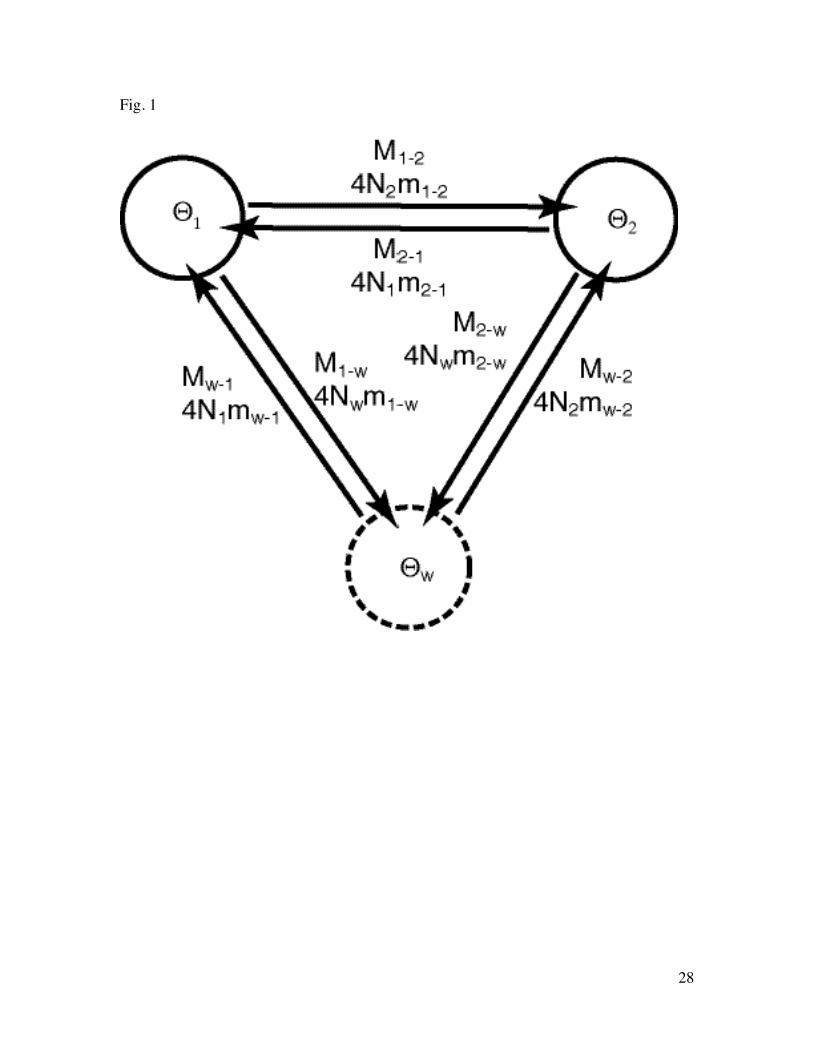
immigration
15.6±1.25 0.86±0.89 20862±5791 15068±7651
2:3 65.10±79.04 15.19±2.13 58±19 232±202
2:7 647.01±574.98 186.54±23.50 40±37 4±2

23
458Table 2. Averages of the migration rate M over 10 datasets. M is m/µ where m is the459
migration rate per generation and µ is the mutation rate per generation and site. The460
datasets were simulated with migration rates from population 2 into population 1 (M2-1)461
and from 1 into 2 (M1-2) of 100, the migration rate from and to the world population was462
also set to 100. The percentage values are the averages of the respective percentiles, MLE463
is the average of the maximum likelihood estimates.464
Immigration rate Two-population-analysis ghost-analysis
M2-1 1%
MLE
99%
86
100
116
85
100
117
M1-2 1%
MLE
99%
88
102
118
79
94
110
465

24
Table 3. Mean square error (MSE) when the migration between the samples is zero and466
migrants are only exchanged through the world population. The MSE and its standard467
deviation are calculated based on the average of parameters over two replicates. Letters468
B-E mark the scenarios B-E from Fig. 2, except that the true values for M between the469
samples are 0.470
471
472
473Mean Square ErrorSimulated
Scenario Θ M
Two-population-analysis
[x 10-6]
ghost-analysis
[x 10-6]
Two-population-analysis ghost-analysis
B. Medium world-immigration
8.42±0.78 0.37±0.02 1547±72 658±112
C. High world-immigration
0.18±0.02 2.87±0.58 83918±1982 65665±234
D. Medium world-
immigration
9.60±2.220 0.20±0.12 1154±142 828±106
E. High world-
immigration
21.39±1.77 1.87±0.52 38381±5404 39628±2881
25
474
Figures475
Fig. 1 Basic migration model used in the simulation study. Θ is 4 × effective population476
size Ne × mutation rate µ per generation and site; M is the scaled migration rate m/µ477
where m is the immigration rate per generation. 4Nm (ΘM) is the number of immigrants478
per generation. The subscripts indicate the population and the direction of the migration,479
the first letter is the donor and the second the recipient.480
481
Fig. 2 Migration models used to generate the simulated datasets: Unsampled world482
population are white, sampled populations, black. Thickness of arrows show the483
magnitude and direction of the immigration. Details are explained in the Methods484
section: (A) no immigration from world; (B, C) unidirectional immigration from world;485
(D, E) symmetric immigration.486
487
Fig. 3 Population size estimates with and without ghost-analysis. A1 and A2 are results488
from two simulated datasets using unequal migration rates between world and samples.489
B1 and B2are results from datasets using symmetric migration rates between world and490
samples. Dots mark the maximum likelihood estimate, the lines cover the range of the491
approximate 98% support interval. The box in the corner indicates the order of the492
parameters in the graph: each subblock consists of the sizes Θ1 and Θ2 using only the493
sampled populations (black), including a ghost (gray), respectively. The groups “none”,494
1:1, 10:1 indicate the strength of the immigration from the unsampled world population,495
26
where for example 10:1 means that the immigration from the world was ten times the496
immigration rate between the sampled populations.497
498
Fig. 4 Immigration rates estimates with and without ghost-analysis. A1 and A2 are results499
from two simulated datasets using unequal migration rates between world and samples.500
B1 and B2are results from datasets using equal migration rates between word and501
samples. Dots mark the maximum likelihood estimate of M, which is migration rate m502
over mutation rate µ, the lines cover the range of the approximate 98% support interval.503
The box in the corner indicates the order of the parameters in the graph: each subblock504
consists of the sizes Μ2-1 and Μ1-2 using only the sampled populations (black), including a505
ghost (gray), respectively. The groups “none”, 1:1, 10:1 indicate the strength of the506
immigration from the unsampled world population, where for example 10:1 means that507
the immigration from the world was ten times the immigration rate between the sampled508
populations.509
510
Fig. 5 Immigration rate estimates of ten independent datasets for 100 loci, simulated511
using a value of M=100 for all migration rates. Dots mark the maximum likelihood512
estimate, the lines cover the range of the approximate 98% support interval. The box in513
the corner indicates the order of the parameters in the graph: each subblock consists of514
the sizes Μ2-1 and Μ1-2 using only the sampled populations (black), including a ghost515
(gray), respectively.516
517

27
Fig. 6 Effect of the number of unsampled vs sampled populations. Dots mark the518
maximum likelihood estimate for population sizes (top) and the immigration rates519
(bottom), the lines cover the range of the approximate 98% support interval. The box in520
the corner indicates the order of the parameters in the graph: each subblock consists of521
the sizes Μ2-1 and Μ1-2 using only the sampled populations (black), including a ghost522
(gray), respectively. The groups 2:1, 2:3, 2:7 reflect the ratio of sampled to unsampled523
populations.524
525
Fig. 7 Comparison of the effect of sample size on the accuracy of the migration rate526
estimate. M is m/µ, where m is the immigration rate per generation and µ is the mutation527
rate per generation. Dots mark the maximum likelihood estimate, the lines cover the528
range of the approximate 98% support interval. The box in the corner indicates the order529
of the parameters in the graph: each subblock consists of the sizes Μ2-1 and Μ1-2 ignoring530
the world (black), taking world into account (gray), respectively.531
532
Fig. 8 Comparison of the run-time improvement of the parallel version of MIGRATE-N533
534
28
Fig. 1

29
Fig. 2

30
Fig.3

31
Fig. 4:

32
Fig. 5
33
Fig. 6

34
Fig 7.

35
Fig 8
Related Documents