effect of the tailpipe entry geometry on a two-stroke engine's ...

EFFECT OF THE TAILPIPE ENTRY GEOMETRY ON ATWO-STROKE ENGINE’S PERFORMANCE PREDICTION

By

Cornelius Gysbert Johannes van Niekerk

Presented in partial fulfilment of the requirements for the degree

MASTER OF ENGINEERINGIn the Faculty of Engineering,

University of Pretoria

Pretoria

December 2000

UUnniivveerrssiittyy ooff PPrreettoorriiaa eettdd,, VVaann NNiieekkeerrkk CC GG JJ ((22000022))

ii

ABSTRACT

Title: Effect of the Tailpipe Entry Geometry on a Two-Stroke Engine’sPerformance Prediction

Author: CGJ van NiekerkPromoters: Prof JA Visser, Mr DJ de KockDepartment: Department Mechanical and Aeronautical EngineeringDegree: Master in Engineering (Mechanical)

It is standard practice in one-dimensional gasdynamic simulations of high performance two-stroke engines to model the exhaust tail pipe entry as an area change using an algorithmsimilar to the area change of the reverse cone. In the reverse cone the area continually stepsdown while at the tail pipe entry it changes from stepping down to constant area. At this pointa vena contracta can form that effects the flow resistance of the tail pipe.

In an effort to improve the accuracy of the gasdynamic simulations the area change algorithmat the tail pipe entry was replaced with a restriction algorithm that incorporates a coefficient ofdischarge and allows an increase in entropy on the expansion side. The coefficient ofdischarge is defined as the actual measured mass flow divided by the mass flow predicted bythe restriction algorithm.

An experimental set up was designed and constructed to measure mass flows for a variety oftail pipe entry geometries at a range of pressures covering the pressure ratios encountered ina real engine. From the mass flow results the coefficients of discharge for a range ofpressure and area ratios and reverse cone angles could be calculated and arranged intomatrix form to define Cd-maps. The Cd-maps were incorporated into the simulation softwareand tested to ensure that it functioned correctly.

Finally, the simulation results with and without the Cd-maps were compared to measuredresults and it was shown that incorporating this refinement improves the accuracy of thesimulation results on the “over run” part of the power curve. This is the part of the powercurve after maximum power and very important in the development of high performance two-stroke engines. These maps can be used for all future simulations on any engine size thatuses the same tail pipe geometry.


iii

SAMEVATTING

Titel: Die Invloed van die Afbloeipyp se Geometrie op die Voorspelling vandie Werkverrigting van ‘n Tweeslagenjin

Outeur: CGJ van NiekerkPromotors: Prof JA Visser, Mnr DJ de KockDepartement: Departement Meganiese en Lugvaartkundige IngenieursweseGraad: Magister in Ingenieurswese (Meganies)

Dit is standaard praktyk in die een-dimensionele gasdinamiese simulasies van hoëwerkverrigting tweeslag enjins om die ingang van uitlaatstelsel se afbloeipyp as ‘n areaverandering te modelleer deur dieselfde algoritme te gebruik as wat vir die modellering vandie trukaatskegel gebruik word. In werklikheid verskil die twee deurdat die trukaats kegel sedeursnit oppervlakte kontinu verklein, terwyl die deursnit oppervlakte van die afbloeipyp seingang verander van ‘n afnemende waarde na ‘n konstante waarde. By dié punt kan ‘nvloeivernouing ontstaan wat die vloei weerstand kan beïnvloed.

In ‘n poging om die akkuraatheid van die gasdinamiese simulasies te verbeter, is dievarieërende oppervlak-algoritme by die afbloeipyp se inlaat vervang met ‘nweerstandsalgoritme wat ‘n vloeiweerstandskoeëfisiënt insluit en wat toelaat vir ‘n verhogingin entropie na die weerstand. Die vloeiweerstandskoeëfisiënt word gedefiniëer as dieverhouding tussen die gemete massavloei en die voorspelde massavloei soos voorspel deurdie weerstandsalgoritme.

‘n Eksperimentele opstelling is ontwerp en gebou om massavloeie by ‘n reeks afbloeipypingangsgeometrië te meet by ‘n reeks drukke wat die drukverhoudings, soos wat in werklikeenjins voorkom, te meet. Uit die massavloei resultate kan die vloeiweerstandskoeëfisiënt vir‘n reeks druk- en oppervlakverhoudings en trukaatskegel ingeslote hoeke, bereken word enin ‘n matriks gerangskik word om vloeiweerstandskoeëfisiënt-kontoerkaarte te vorm. Diekontoerkaarte is in die sagteware geïnkorporeer en getoets.

Ten slotte is die simulasie resultate met en sonder die kontoerkaarte met gemete resultatevergelyk en dit is gevind dat die verfyning die akkuraatheid van die simulasie verbeter by diegedeelte van die drywingskromme na maksimum drywing. Hierdie gedeelte van diedrywingskromme is baie belangrik by hoë werkverigting tweeslag enjins. Die kontoerkaartemaak nou deel uit van die simulasie sagteware en is van toepassing op alle enjins wat dietipe uitlaatstelsel gebruik.


iv

ACKNOWLEDGEMENTS

Boart Longyear Seco for the use of their rock drill test facility.

Mr Gavin Pemberton of Boart Longyear Seco for his help with the tests.

Vickers OMC for the loan of the pressure transducers, thermocouples and Budenburgcalibrator.

Desire van Niekerk, my loving wife, for the gentle but persistent pressure to complete thework and for the moral support.


v

TABLE OF CONTENTS

Abstract ............................................................................................................ ii

Acknowledgements ......................................................................................... iii

Table of Contents ............................................................................................ iv

List of Tables.................................................................................................... vii

List of Figures .................................................................................................. viii

Nomenclature................................................................................................... ix

CHAPTER 1: INTRODUCTION1.1 Background............................................................................................................... 11.2 Current level of knowledge ....................................................................................... 21.3 Motivation ................................................................................................................. 21.4 Scope........................................................................................................................ 2

CHAPTER 2: LITERATURE REVIEW2.1 Pre-amble ................................................................................................................. 42.2 General 1D methods – history .................................................................................. 42.3 GPB – Method .......................................................................................................... 62.4 Tailpipe entry geometric and flow modelling ............................................................. 72.5 Discharge coefficients............................................................................................... 82.6 Closing...................................................................................................................... 9

CHAPTER 3: THERMODYNAMIC AND COMPUTER MODEL OF RESTRICTION3.1 Pre-amble ................................................................................................................. 103.2 Thermodynamic model of constriction in pipe........................................................... 103.2.1 Subsonic Flow................................................................................................................. 113.2.2 Sonic Flow ...................................................................................................................... 153.3 Computer model of constriction ................................................................................ 163.3.1 Description of Subroutine RESTRICT................................................................................ 173.3.2 Testing of Subroutine RESTRICT ...................................................................................... 193.4 Closing...................................................................................................................... 20

CHAPTER 4: DETERMINATION OF DISCHARGE COEFFICIENTS4.1 Pre-amble ................................................................................................................. 21


vi

4.2 Description of experimental apparatus...................................................................... 214.3 Development of software to calculate the Coefficient of Discharge .......................... 224.4 Experimental Determination of the Coefficient of Discharge..................................... 234.4.1 Influence of Test Piece Length and Diameter on Results .................................................. 234.4.2 Description of Test Pieces ............................................................................................... 254.4.3 Experimental Procedure.................................................................................................. 264.4.4 Experimental Results ...................................................................................................... 264.5 Processed results ..................................................................................................... 284.5.1 Discussion of Processing Methodology............................................................................. 284.5.2 The Effect of the Reverse Cone Included Angle ................................................................ 304.5.3 The Effect of the Tail Pipe Diameter ................................................................................ 304.5.4 The Effect of the Restrictor Tailpipe Geometry ................................................................ 314.5.5 The Effect of the Venturi Tailpipe Geometry ....................................................................4.6 Discussion of Results................................................................................................ 344.7 Closing...................................................................................................................... 34

CHAPTER 5: SIMULATION STUDY5.1 Pre-amble ................................................................................................................. 355.2 Incorporation of Cd-Maps into EngMod2T ................................................................ 355.3 Simulated Engine Parameters .................................................................................. 355.4 Verification of RESTRICT in EngMod2T ................................................................... 365.5 The Effect of the Cd-Maps on the Simulation Results............................................... 375.6 Comparison of Simulated Results with Experimental Results................................... 395.6 Closing...................................................................................................................... 40

CHAPTER 6: SUMMARY, CONCLUSION AND RECOMMENDATIONS6.1 Summary .................................................................................................................. 416.2 Conclusions .............................................................................................................. 426.3 Recommendations… ................................................................................................ 42

APPENDICESA List of references` ..................................................................................................... 43B Listing of subroutine RESTRICT.FOR ...................................................................... 47C Test equipment, sensor calibration and BS1042 orifice dimensions......................... 56D Predicted mass flow through tailpipe ........................................................................ 61E Measured mass flow through test pieces.................................................................. 62F Coefficient of Discharge calculations ........................................................................ 73G Engine data............................................................................................................... 79H Dynamometer Results .............................................................................................. 82I Description of EngMod2T ......................................................................................... 83


vii

LIST OF TABLES

Table Number3.1 The initial values used to compare RESTRICT with CONTRACT,

EXPAND & TEMPDISC ............................................................................................ 193.2 Results of the comparison of RESTRICT with CONTRACT,

EXPAND and TEMPDISC......................................................................................... 204.1 Simulation test results for plain inlet with 25 degree included angle ......................... 244.2 Test piece dimensions .............................................................................................. 265.1 Major engine characteristics ..................................................................................... 36C.1 List of test instrumentation ........................................................................................ 56E.1 Atmospheric conditions............................................................................................. 62E.2 Test Piece 1 Results, 10 degree cone, 21.8mm tailpipe, plain entry ........................ 63E.3 Test Piece 2 Results, 20 degree cone, 21.8mm tailpipe, plain entry ........................ 64E.4 Test Piece 3 Results, 30 degree cone, 21.8mm tailpipe, plain entry ........................ 65E.5 Test Piece 4 Results, 40 degree cone, 21.8mm tailpipe, plain entry ........................ 66E.6 Test Piece 5 Results, 30 degree cone, 20.5 mm tailpipe, plain entry........................ 67E.7 Test Piece 6 Results, 30 degree cone, 23.5mm tailpipe, plain entry ........................ 68E.8 Test Piece 7 Results, 30 degree cone, 22.0mm tailpipe, 20.5mm restricted entry ... 69E.9 Test Piece 8 Results, 30 degree cone, 23.5mm tailpipe, 20.5mm restricted entry. .. 70E.10 Test Piece 9 Results, 30 degree cone, 22.0mm tailpipe, 20.5mm venturi entry ....... 71E.11 Test Piece 10 Results, 30 degree cone, 23.5mm tailpipe, 20.5mm venturi entry ..... 72F.1 Coefficient ai values .................................................................................................. 73F.2 Coefficient bi,j values................................................................................................. 74


viii

LIST OF FIGURES

Figure Number1.1 Schematic of Two-Stroke Engine.............................................................................. 12.1 Modelling of taper pipes as a series of parallel pipes................................................ 72.2 Current modelling of tailpipe entry flow ..................................................................... 72.3 Proposed modelling of tailpipe entry flow.................................................................. 83.1 Particle flow regimes at a restricted area change ..................................................... 103.2 Temperature / Entropy diagram for subsonic flow..................................................... 123.3 Temperature / Entropy diagram for sonic flow .......................................................... 153.4 Flow diagram of Subroutine RESTRICT ................................................................... 184.1 Experimental Apparatus............................................................................................ 214.2 Schematic drawing of experimental layout................................................................ 224.3 Schematic layout of test piece .................................................................................. 244.4 Photo of test pieces .................................................................................................. 264.5 Cd-map for 30 degree included angle reverse cone ................................................. 294.6 The effect of mesh length (area ratio) on Cd-values................................................. 294.7 The effect of included cone angle on the Cd-values ................................................. 304.8 The effect of tailpipe diameter on Cd-values............................................................. 314.9 Mass flow values for restricted tailpipe entries.......................................................... 324.10 Cd-values for the restricted tailpipe entries............................................................... 324.11 Mass flow results for the venturi type tailpipe entries................................................ 334.12 Cd-Values for the venturi type tailpipe entries .......................................................... 335.1 Comparison of the predicted power .......................................................................... 375.2 The influence of the Cd-Map on the Power Predicted............................................... 375.3 The Effect of the Cd-Map on the predicted Delivery Ratio ........................................ 385.4 The Effect of the Cd-Map on the Maximum Unburnt Air Temperature...................... 395.5 Comparison of Predicted and Measured Power ....................................................... 40C.1 Pressure Transducer Calibration Layout................................................................... 56I.1 A typical output screen of EngMod2T ....................................................................... 87I.2 Exhaust Pressure Trace at 9600 rpm ....................................................................... 88I.3 Exhaust Pressure Trace at 12000 rpm ..................................................................... 89I.4 Brake Mean Effective Pressure ................................................................................ 89I.5 Exhaust Centre Section Temperature....................................................................... 90


ix

NOMENCLATURE

List of SymbolsA AreaAr Area Ratioa Sonic VelocityCd Coefficient of DischargeCp Specific Heat at Constant Pressurec Particle Velocityd DiameterF Functionh Enthalpyl LengthM Mach Numberm! Mass Flow RateP PressurePr Pressure RatioR Gas ConstantT TemperatureEδ Change in Internal Energymδ Change in MassQδ Heat TransferredWδ Workγ Ratio of Specific Heatsθ Included Angle of the Reverse Coneρ Density

Subscripts

0 Reference Conditions1 Values for Pipe 12 Values for Pipe 2i Incidentm Meshr Reflectedt Throatteff Effective Value in Throat


x

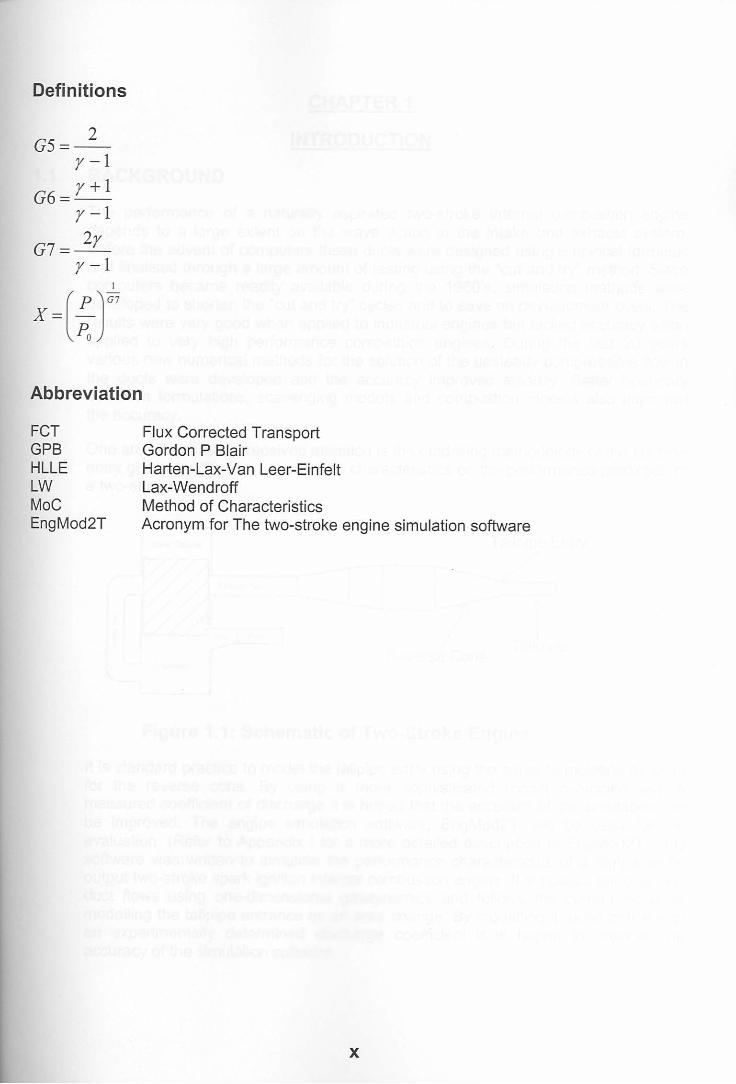
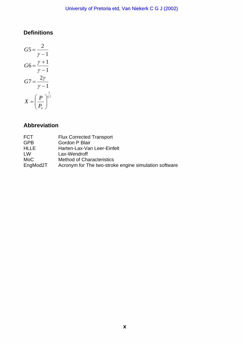
Definitions

125−

=γ

G

116

−+

=γγG

127−

=γγG

71

0

G

PPX

=

Abbreviation

FCT Flux Corrected TransportGPB Gordon P BlairHLLE Harten-Lax-Van Leer-EinfeltLW Lax-WendroffMoC Method of CharacteristicsEngMod2T Acronym for The two-stroke engine simulation software


1

CHAPTER 1

INTRODUCTION

1.1 BACKGROUND

The performance of a naturally aspirated two-stroke internal combustion enginedepends to a large extent on the wave action in the intake and exhaust system.Before the advent of computers these ducts were designed using empirical formulasand finalised through a large amount of testing using the “cut and try” method. Sincecomputers became readily available during the 1960’s, simulation methods weredeveloped to shorten the “cut and try” cycles and to save on development costs. Theresults were very good when applied to industrial engines but lacked accuracy whenapplied to very high performance competition engines. During the last 20 yearsvarious new numerical methods for the solution of the unsteady compressible flow inthe ducts were developed and the accuracy improved steadily. Better boundarycondition formulations, scavenging models and combustion models also improvedthe accuracy.

One area that has not received attention is the modelling methodology of the tail pipeentry geometry (Figure 1.1) and flow characteristics on the performance prediction ofa two-stroke engine.

Figure 1.1: Schematic of Tw

It is standard practice to model the tailpipefor the reverse cone. By using a mormeasured coefficient of discharge it is hopbe improved. The engine simulation soevaluation. (Refer to Appendix I for a mosoftware was written to simulate the perfoutput two-stroke spark ignition internal coduct flows using one-dimensional gasdymodelling the tailpipe entrance as an areaan experimentally determined dischargeaccuracy of the simulation software.

Tailpipe Entry

Tailpipe


Reverse Cone

o-Stroke Engine

entry using the same formulation as usede sophisticated model combined with aed that the accuracy of the simulation canftware, EngMod2T, will be used for there detailed description of EngMod2T) Thisormance characteristics of a high specificmbustion engine. It simulates the pipe andnamics and follows the current trend by change. By modelling it as an orifice with coefficient it is hoped to improve the

2

During the past 8 years some factory racing motorcycles started using restrictions orventuries at the tailpipe inlet. Other than for one brief reference (Irving, 1969:189) noexplanation or motivation for using it could be found. This study also aims to clarifythis point.

1.2 CURRENT LEVEL OF KNOWLEDGE

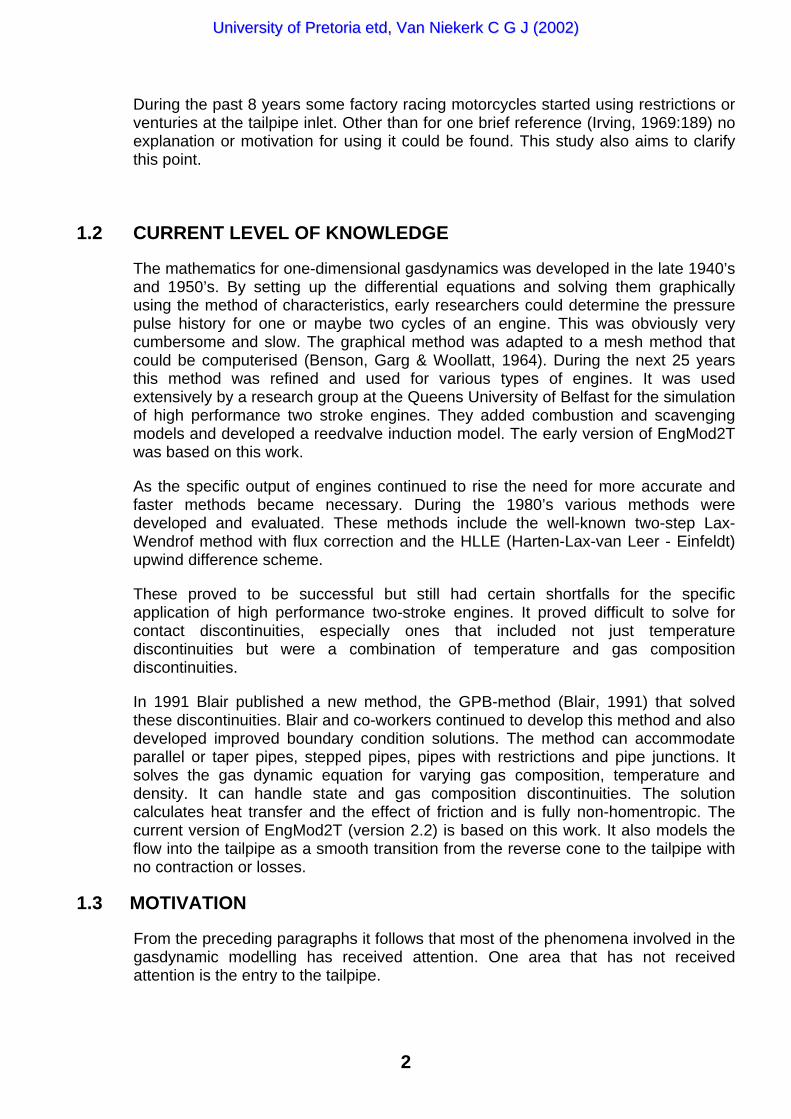
The mathematics for one-dimensional gasdynamics was developed in the late 1940’sand 1950’s. By setting up the differential equations and solving them graphicallyusing the method of characteristics, early researchers could determine the pressurepulse history for one or maybe two cycles of an engine. This was obviously verycumbersome and slow. The graphical method was adapted to a mesh method thatcould be computerised (Benson, Garg & Woollatt, 1964). During the next 25 yearsthis method was refined and used for various types of engines. It was usedextensively by a research group at the Queens University of Belfast for the simulationof high performance two stroke engines. They added combustion and scavengingmodels and developed a reedvalve induction model. The early version of EngMod2Twas based on this work.

As the specific output of engines continued to rise the need for more accurate andfaster methods became necessary. During the 1980’s various methods weredeveloped and evaluated. These methods include the well-known two-step Lax-Wendrof method with flux correction and the HLLE (Harten-Lax-van Leer - Einfeldt)upwind difference scheme.

These proved to be successful but still had certain shortfalls for the specificapplication of high performance two-stroke engines. It proved difficult to solve forcontact discontinuities, especially ones that included not just temperaturediscontinuities but were a combination of temperature and gas compositiondiscontinuities.

In 1991 Blair published a new method, the GPB-method (Blair, 1991) that solvedthese discontinuities. Blair and co-workers continued to develop this method and alsodeveloped improved boundary condition solutions. The method can accommodateparallel or taper pipes, stepped pipes, pipes with restrictions and pipe junctions. Itsolves the gas dynamic equation for varying gas composition, temperature anddensity. It can handle state and gas composition discontinuities. The solutioncalculates heat transfer and the effect of friction and is fully non-homentropic. Thecurrent version of EngMod2T (version 2.2) is based on this work. It also models theflow into the tailpipe as a smooth transition from the reverse cone to the tailpipe withno contraction or losses.

1.3 MOTIVATION

From the preceding paragraphs it follows that most of the phenomena involved in thegasdynamic modelling has received attention. One area that has not receivedattention is the entry to the tailpipe.


3

1.4 SCOPE

This work starts off with a literature survey of firstly the background and history ofone-dimensional gasdynamics followed by a description of the GPB method. Next, acloser look is taken at the modelling methodology of the tailpipe entry geometry. Theliterature survey finishes with a look at discharge coefficients and how to use them ina simulation method.

In chapter 3 the mathematical model for a restriction in a pipe, as used in the GPBmethod, is discussed. The equations are developed to a format that allows them tobe solved by the Newton-Raphson method for simultaneous non-linear equations.The software developed from this and its incorporation and testing into EngMod2T isdescribed.

In the following chapter, chapter 4, data necessary to determine the dischargecoefficients for the various combinations of tailpipe entry restrictions are determinedexperimentally on a flow bench. This is followed by a description of the method andsoftware developed to determine the discharge coefficients and the final processedresults in graphical form.

This is followed in chapter 5 with a simulation study to determine the influence of thetailpipe coefficient of discharge on the performance predicted by EngMod2T. Theresults are compared with experimental data.

The summary, conclusions and recommendations are given in chapter 6.


4

CHAPTER 2

LITERATURE REVIEW

2.1 PREAMBLE

This chapter is divided into four main categories. The first gives a brief description ofthe history and current state of the use of 1-Dimensional Gasdynamics to solve theunsteady compressible flow in the pipes and ducts of internal combustion engines.

The second part describes the GPB method of solving the 1-DimensionalGasdynamics equations; it’s comparison to other modern methods and the reasonsfor its choice above the others.

The third part describes the current methodology used in modelling the tailpipe entrygeometry and flow. It also points out where the approach used in this study differsfrom the conventional way.

Finally, the determination of discharge coefficients and its influence on the accuracyof the simulations are discussed. An alternative way of defining the coefficient ofdischarge is explained.

2.2 GENERAL 1-DIMENSIONAL METHODS - HISTORY

In the analysis of sound waves it is possible to use two approaches. If, in thederivation of the wave equation the assumption is made the wave amplitudes aresmall the second order terms can be neglected and the resulting equation is the well-known small wave equation. (Annand & Roe, 1974:31) These small amplitude soundwaves are linear waves, meaning that during superposition their amplitudes aresummed. They are the well-known acoustic waves. Acoustic waves do not changeshape as they travel through a gas.

If the amplitude is not small the second order terms cannot be neglected resulting innon-linear wave equations. Earnshaw (1910) developed these non-linear equationsfor sound waves. He showed that the pressure and velocity of the superpositionwave is related to that of the individual waves by a seventh power law. These largeamplitude sound waves are known as finite waves and they do change shape asthey travel through a gas.

The finite wave equations are hyperbolic differential equations and cannot be solvedanalytically. Riemann, in 1858 (Winterbone & Pearson, 2000) proposed the Methodof Characteristics (MoC) for solving them. This is a graphical method and verycumbersome and slow. Early researchers into the application of wave methods to themanifolds of internal combustion engines compared the results obtained withacoustic waves to those with finite waves to determine which one is correct for theapplication. Bannister and Mucklow (1948) studied the wave action following thesudden release of compressed gas from a cylinder. Wallace and Stuart-Mitchell(1953) included the effect of ports. Wallace and Nassif (1954) included the enginecylinder. Mucklow and Wilson (1955) studied the effect of friction and heat transferwhile Wallace and Boxer (1956) investigated wave action in diffusers. By this time


5

there was no more doubt that the finite wave theory was the correct one to apply tomanifolds of internal combustion engines. The theoretical derivation of the equationswas summarized by Bannister (1958) and this publication is still used as a referenceto date.

Benson, Garg and Woollatt (1964) developed a computerised version of the MoCusing a mesh method. This involved dividing the pipes and ducts into equal lengthmeshes and through interpolation the values of the left and right movingcharacteristics could be determined at each mesh boundary as a function of time.This landmark paper established the MoC as the method of choice for solving thegasdynamics in engine manifolds and ducts for the next 20 years. During this time alarge number of papers were published using the MoC as a base.

Of particular interest to this study are the papers published by a research group atthe Queen’s University of Belfast (QUB). Under the leadership of Professor Gordon PBlair they concentrated on the analysis and simulation of two-stroke engines. Theystarted by applying the MoC to a straight exhaust pipe (Blair & Goulburn, 1967)followed by a pipe with tapered sections (Blair & Johnson, 1968). Next they analysedthe flow in the induction system, (Blair & Arbuckle, 1970), and developed a moresophisticated treatment of boundary conditions (Blair & Cahoon, 1972). At this stagethey could analyse the open cycle of a two-stroke engine. By including thecalculation of the gas purity in each mesh (Blair & Ashe, 1976) and a rate of heatrelease combustion model (Blair, 1976) the power output of a two-stroke enginecould be predicted. As a further refinement a reed valve model was developed andincluded in the simulation software (Hinds & Blair, 1978; Blair, Hinds & Fleck, 1979;Fleck, Blair & Houston, 1987 and Fleck, Cartwright & Thornhill, 1997).

The original version of EngMod2T was based on the work by this group at QUB anda small sample program published by Blair (1990).

The MoC has several major drawbacks. Firstly, most of the time it was used in ahomentropic form. Solving the equations in the non-homentropic formulation requiresparticle pathline tracking (Benson et al. 1964) resulting in very long execution times.The homentropic solution ignores contact discontinuities (large jumps in temperatureand gas composition that occurs for instance when fresh charge short circuits out theexhaust port during the scavenging phase and comes into “contact” with the hotexhaust gas) resulting in inaccurate prediction of the wave action (Blair &Blair, 1987;McGinnity, Douglas & Blair, 1990 and Douglas, McGinnity & Blair, 1991).

Secondly, the MoC assumes constant values for the specific heats and gas constantfor each mesh in a pipe. Poloni, Winterbone and Nichols (1988) investigated thisassumption and showed that it can lead to inaccuracies.

Thirdly, the wave equations as solved by the MoC are in the non-conservative formmeaning that mass artificially lost or created between the ends of a pipe (Winterbone& Pearson, 2000:8, Van Howe & Sierens, 1991). This becomes particularly severewhen there are large entropy variations or changes of cross section in the pipe, as istypical for a two-stroke engine.

In an effort to overcome these defects finite difference methods were developed. It ispossible to write the solution algorithms based on the equations in the conservative


6

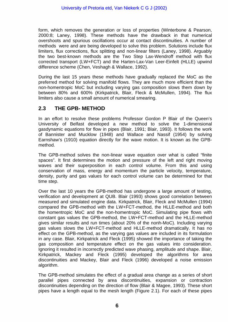
form, which removes the generation or loss of properties (Winterbone & Pearson,2000:8; Laney, 1998). These methods have the drawback in that numericalovershoots and spurious oscillations occur at contact discontinuities. A number ofmethods were and are being developed to solve this problem. Solutions include fluxlimiters, flux corrections, flux splitting and non-linear filters (Laney, 1998). Arguablythe two best-known methods are the Two Step Lax-Wendroff method with fluxcorrected transport (LW+FCT) and the Harten-Lax-Van Leer-Einfelt (HLLE) upwinddifference scheme (Chen, Veshagh & Wallace, 1992).

During the last 15 years these methods have gradually replaced the MoC as thepreferred method for solving manifold flows. They are much more efficient than thenon-homentropic MoC but including varying gas composition slows them down bybetween 80% and 600% (Kirkpatrick, Blair, Fleck & McMullen, 1994). The fluxlimiters also cause a small amount of numerical smearing.

2.3 THE GPB- METHOD

In an effort to resolve these problems Professor Gordon P Blair of the Queen’sUniversity of Belfast developed a new method to solve the 1-dimensionalgasdynamic equations for flow in pipes (Blair, 1991; Blair, 1993). It follows the workof Bannister and Mucklow (1948) and Wallace and Nassif (1954) by solvingEarnshaw’s (1910) equation directly for the wave motion. It is known as the GPB-method.

The GPB-method solves the non-linear wave equation over what is called “finitespaces”. It first determines the motion and pressure of the left and right movingwaves and their superposition in each control volume. From this and usingconservation of mass, energy and momentum the particle velocity, temperature,density, purity and gas values for each control volume can be determined for thattime step.

Over the last 10 years the GPB-method has undergone a large amount of testing,verification and development at QUB. Blair (1993) shows good correlation betweenmeasured and simulated engine data. Kirkpatrick, Blair, Fleck and McMullen (1994)compared the GPB-method with the LW+FCT-method, the HLLE-method and boththe homentropic MoC and the non-homentropic MoC. Simulating pipe flows withconstant gas values the GPB-method, the LW+FCT-method and the HLLE-methodgives similar results and run times (about 20% of the nonh-MoC). Including varyinggas values slows the LW+FCT-method and HLLE-method dramatically. It has noeffect on the GPB-method, as the varying gas values are included in its formulationin any case. Blair, Kirkpatrick and Fleck (1995) showed the importance of taking thegas composition and temperature effect on the gas values into consideration.Ignoring it resulted in incorrectly predicted wave phasing, amplitude and shape. Blair,Kirkpatrick, Mackey and Fleck (1995) developed the algorithms for areadiscontinuities and Mackey, Blair and Fleck (1996) developed a noise emissionalgorithm.

The GPB-method simulates the effect of a gradual area change as a series of shortparallel pipes connected by area discontinuities, expansion or contractiondiscontinuities depending on the direction of flow (Blair & Magee, 1993). These shortpipes have a length equal to the mesh length (Figure 2.1). For each of these pipes


the pressure loss through friction, the heat loss or gain through heat transfer, theheat generation from the friction and the mass, energy and momentum transportedacross the two boundaries are calculated.

Diffuser

Meshlength

Figure 2.1: Modelling

2.4 TAILPIPE ENTRY GE

It is standard practice to as for the area change inalgorithm is used (Blair &change is incorporated ischematic drawing of the

Figure 2.2: Current m

The area change algorimethods makes any prov

Calcu


ComputationalElement

flow

taper pip

OMETRIC

model the f the reverse Magee, 19n the sourc current met

odelling

thm in neitision for a f

Actua

lation Geometr

ActualGeometry

7

Reverse Cone

es as a series of parallel pipes.

AND FLOW MODELLING

low into tailpipe entry using the same algorithm cone. In the GPB-method the area contraction

93) and in the finite difference methods the areae terms of the equations. Figure 2.2 shows ahodology in the GPB-method.

of tailpipe entry flow.

her the GPB-method nor the finite differencelow contraction or flow breakaway at the tailpipe

Area Change Subroutine

Constant Area Subroutine

l Geometry

y

8

entry. Both assume a smooth transition from the reverse cone to the tailpipe. Blair,Kirkpatrick, Mackey and Fleck (1995) developed the algorithms for areadiscontinuities and particularly a contraction-expansion restriction that incorporates acoefficient of discharge. In this study the effect of replacing the area contractionalgorithm at the tailpipe entry with this restriction algorithm combined withexperimentally determined coefficients of discharge are investigated. The proposedcalculation layout is shown in Figure 2.3.

Figure 2.3: Proposed modelling of tailpipe entry flow.

Corberán, Royo, Pérez and Santiago (1994) simulated the performance of a 1993HONDA RS125R Grand Prix motorcycle that uses a venturi at the tailpipe entry.They do not state how the entry was modelled but do emphasise that they found thatits inclusion in the model had a small but important effect on the results. They founda better match between the measured and simulated results by including the effect ofthe venturi.

2.5 DISCHARGE COEFFICIENTS

An inherent part of a non-isentropic analysis of the cylinder to duct boundary, or aduct to atmosphere boundary, or a duct-to-duct boundary, includes the physicalgeometry of the aperture. This describes the geometry of the port, valve plus port orthe orifice and the area of the duct or ducts adjacent to the boundary. As all realflows contract in area as they pass through the eye of the aperture, it is normalpractice to describe this behaviour by a discharge coefficient.

The discharge coefficient is traditionally measured in a steady flow experiment andapplied to an unsteady flow simulation in a quasi-steady fashion (Benson, 1959). Anattempt was also made to determine the coefficient of discharge using theoreticalmeans (Benson & Pool, 1965a; Benson & Pool, 1965b; Decker, 1978).

Recently Blair, Lau, Cartwright, Raghanathan and Mackey (1995) pointed out thatthe traditional definition of discharge coefficient is the measured mass flow divided by

Area Change Subroutine

Constant Area Subroutine

Restriction Subroutine (Restriction can be physical

or a vena contracta) Actual Geometry

Calculation Geometry


9

the isentropically calculated mass flow through the area of the aperture. They definedthis coefficient of discharge as the “theoretical coefficient of discharge”. During asimulation it is more correct to use a discharge coefficient defined as the measuredmass flow divided by the calculated mass flow where the calculation was conductedusing the same theoretical model for that specific geometry as used in the simulationsoftware. They defined this as the “actual coefficient of discharge”. Blair and Drouin(1996) showed that using the actual coefficient of discharge greatly enhances theaccuracy of the simulations. This approach is used in EngMod2T and uses thedischarge coefficients for the ports, reed valves and pipe ends as determined byFleck and Cartwright (1996).

2.6 CLOSING

A brief investigation into the various methods used in one-dimensional gasdynamicswas conducted and some of their advantages and disadvantages were discussed.This was followed by a more in depth look at the GPB-method that is used in thesimulation software. The current practice of modelling the tailpipe entry as justanother gradual area change was investigated and a new methodology wasproposed. Finally a more realistic definition of the Coefficient of Discharge wasdiscussed.


10

CHAPTER 3

THERMODYNAMIC AND COMPUTER MODEL OF RESTRICTION

3.1 PREAMBLE

In this chapter a set of thermodynamic equations describing the 1-dimensional flowthrough a restriction is developed. These are then written in a suitable format forinclusion into the computer program. The subroutine that solves these equations arethen developed and tested.

3.2 THERMODYNAMIC MODEL OF RESTRICTION

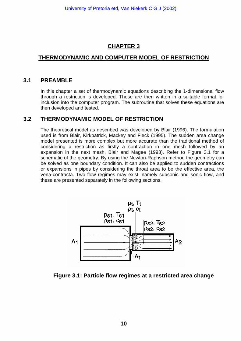
The theoretical model as described was developed by Blair (1996). The formulationused is from Blair, Kirkpatrick, Mackey and Fleck (1995). The sudden area changemodel presented is more complex but more accurate than the traditional method ofconsidering a restriction as firstly a contraction in one mesh followed by anexpansion in the next mesh, Blair and Magee (1993). Refer to Figure 3.1 for aschematic of the geometry. By using the Newton-Raphson method the geometry canbe solved as one boundary condition. It can also be applied to sudden contractionsor expansions in pipes by considering the throat area to be the effective area, thevena-contracta. Two flow regimes may exist, namely subsonic and sonic flow, andthese are presented separately in the following sections.

Figure 3.1: Particle flow regimes at a restricted area change


11

The following five equations has to be solved:

Mass flow (continuity) from pipe 1 to throat

1 tm m=! ! (3.1)

Mass flow (continuity) from throat to pipe 2

2tm m=! ! (3.2)

Conservation of energy (first law of thermodynamics) from pipe1 to throat

WchmEchmQ ttt δδδδδ +++=++ )

2()

2(

221

11 (3.3)

Conservation of energy (first law of thermodynamics) from throat to pipe 2

2 22

2 2( ) ( )2 2t

t tc cQ m h E m h Wδ δ δ δ δ+ + = + + + (3.4)

Conservation of momentum from throat to pipe 2

0)()( 222 =−+− ccmPPA tt ! (3.5)

These five equations has to be transformed into a suitable format to be solved insidethe application of the GPB-method.

3.2.1 Subsonic Flow

For subsonic flow the following assumptions are made:

- The contracting flow from pipe 1 to the throat is isentropic

- The expanding flow from the throat to pipe 2 is adiabatic but not isentropic,due to the “dead” zone between the jet surface and the wall.

A temperature/entropy diagram for the subsonic flow process is shown in Figure 3.2.In Figure 3.1 the expanding flow from the throat to the downstream superpositionpoint 2 is seen to leave turbulent vortices in the corners of that section. That thestreamlines of the flow give rise to particle flow separation implies a gain of entropyfrom the throat to area at point 2. This is summarised on the temperature/entropydiagram in Figure 3.2, where the gain in entropy for the flow rising from pressure Ptto P2 is clearly visible.


12

Figure 3.2: Temperature / Entropy diagram for subsonic flow

A further assumption is made in that it is assumed that the gas constant and thespecific heats are those of the gas at the upstream point. This lead to the followingreference state conditions:Density:

01

0001 RT

Pt == ρρ (3.6)

02

002 RT

P=ρ (3.7)

Acoustic velocity:

01001 RTaa t γ== (3.8)

0202 RTa γ= (3.9)

The continuity equation from pipe 1 to the throat may be stated as (Eq 3.1):

ttefft cAcA ρρ =111 (3.10)

Where teffA is the effective throat area, related to the geometric throat area tA , by:

tdteff ACA = (3.11)

From the gas-dynamic equations (Blair, 1996) it follows that5

0GXρρ = (3.12)

and by substituting in equation (3.10)

tGttefft

G cXAcXA 501

51101 ρρ = (3.13)


13

as the contraction process is assumed isentropic, using equation (3.6)

051

511 =− t

Gtteff

G cXAcXA (3.14)

The continuity equation from the throat to pipe 2 is (Eq 3.2)

222 cAcA ttefft ρρ = (3.15)

Using equation (3.12)

25

22025

0 cXAcXA Gt

Gttefft ρρ = (3.16)

and as

010 ρρ =t

and from (3.6) and (3.9)

201

001 a

Pγρ = (3.17)

and from (3.7) and (3.9)

202

002 a

Pγρ = (3.18)

substituting equations (3.17) and (3.18) into (3.16)

25

22201

5202 cXAacXAa G

tGtteff = (3.19)

The first law of thermodynamics from pipe 1 to the throat may be stated (Eq 3.3):

WchmEchmQ ttt δδδδδ +++=++ )

2()

2(

221

11 (3.20)

Assuming flow to be quasi-steady and steady state, the mass flow increments mustsatisfy the continuity equation and thus equation (3.20) reduces to:

22

221

1t

t

chch +=+ (3.21)

By definition

TCh p= (3.22)

and

1−=γγRCp (3.23)

and by substituting in equation (3.21)

2211 1

21

2tt cRTcRT +

−=+

− γγ

γγ (3.24)


14

Since XaRTa 0== γ (3.25)

And1

25−

=γ

G (3.26)

it follows that:

055 22201

21

21

201 =−−+ tt cXaGcXaG (3.27)

Using the same assumptions the first law of thermodynamics from throat to pipe 2may be stated as (Eq 3.4):

22

22

2

2 chch tt +=+ (3.28)

which becomes using the same logic:

055 22

22

202

22201 =−−+ cXaGcXaG tt (3.29)

The momentum equation from throat to pipe 2 may be stated as (Eq 3.5):

0)()( 222 =−+− ccmPPA tt ! (3.30)

by substituting 111 cAm ρ=! dividing by 0P and writing in terms of pressure amplitude:

0)()( 2110

172

72 =−+− cccA

PXXA t

GGt

ρ (3.31)

By using equation (3.12) this becomes:

0)()( 215

110

0172

72 =−+− cccXA

PXXA t

GGGt

ρ (3.32)

By using 0

00 ρ

γPa = and substituting it in equation (3.32):

0)()( 215

117

27

2201 =−+− cccXAXXAa t

GGGt γ (3.33)

Equations (3.14), (3.19), (3.27), (3.29) and (3.33) are the fundamental equationsgoverning the flow scenario as illustrated in Figure 3.1. By using the pressure ratiosas defined in the GPB method and the definitions of particle speed:

1111 −+= ir XXX

1222 −+= ir XXX

)(5 11011 ri XXaGc −=

)(5 22022 ir XXaGc −= (3.34)


15

and substituting them into these five equations, this results in the following equationswhere )(iF =0:

5 51 1 1 01 1 1(1) 0 ( 1) 5( )G G

r i i r teff t tF A X X a G X X A X c= = + − − − (3.35)

2 5 2 502 01 2 2 02 2 2 2(2) 0 ( 1) 5( )G G

teff t t r i r iF a A X c a X X a A G X X= = − + − − (3.36)

2 2 2 2 2 201 1 1 01 1 1 01(3) 0 5 ( 1) ( 5 ( )) 5r i i r t tF G a X X G a X X G a X c= = + − + − − − (3.37)2 2 2 2 2 201 02 2 2 02 2 2(4) 0 5 5 ( 1) ( 5 ( ))t t r i r iF G a X c G a X X G a X X= = + − + − − − (3.38)

2 7 7 501 2 2 2 1 1 1

01 1 1 02 2 2

(5) 0 ( ( 1) ) ( 1)5 ( )( 5 ( ))

G G Gt r i r i

i r t r i

F a A X X X A X XG a X X c G a X X

γ= = − + − + + − ×− − −

(3.39)

Equations (3.35) to (3.39) contain five unknowns, namely ttrr cXXX ,,, 21 and 02a .By using the Newton-Raphson method for multiple non-linear polynomials thesevalues are determined. A listing of the subroutine is included in Appendix B.

3.2.2 Sonic Flow

Figure 3.3: Temperature / Entropy diagram for sonic flow

The temperature / entropy diagram for the sonic flow process is shown in Figure 3.3.For sonic flow the Mach number in the throat is unity. This implies that:

101

==t

tt Xa

cM (3.40)


16

and thus:

tt Xac 01= (3.41)

Substituting this result into equation (3.14), the continuity equation from pipe 1 to thethroat is:

06011

511 =− G

tteffG XaAcXA (3.42)

And similarly, equation (3.19) becomes:

025

201262

02 =− cXaAXaA GGtteff (3.43)

The first law of thermodynamics from pipe 1 to the throat, equation (3.27) becomes:065 22

0121

21

201 =−+ tXaGcXaG (3.44)

and similarly, equation (3.29) becomes:

056 22

22

202

2201 =−− cXaGXaG t (3.45)

Equations (3.42) to (3.45) are the fundamental equations governing the flow scenario forsonic flow as illustrated in Figure 3.1.

By substituting the values as defined by equation (3.34) the four equations are in therequired format to be incorporated in the software. This results in the following equationswhere )(iF =0.0:

5 61 1 1 1 1(1) 0 ( 1) 5( )G G

r i r i teff tF A X X G X X A X= = + − − − (3.46)

6 502 01 2 2 2 2 2(2) 0 ( 1) 5( )G G

teff t r i r iF a A X a A X X G X X= = − + − − (3.47)

2 2 21 1 1 1(3) 0 5( 1) ( 5( )) 6i r i r tF G X X G X X G X= = + − + − − (3.48)

2 2 2 2 201 02 2 2 02 2 2(4) 0 6 5 ( 1) ( 5 ( ))t r i r iF G a X G a X X G a X X= = − + − − − (3.49)

Equations (3.46) to (3.49) contain four unknowns, namely trr XXX ,, 21 and 02a . By usingthe Newton-Raphson method for multiple non-linear simultaneous equations, thesevalues are determined. A listing of the subroutine is included in Appendix B.

3.3 COMPUTER MODEL OF AREA DISCONTINUITY WITH RESTRICTION

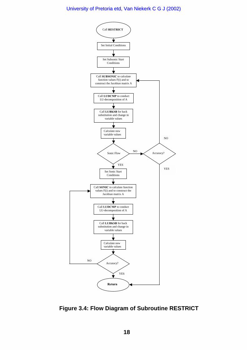
The subroutine, RESTRICT.FOR, was written to solve the two sets of non-linearsimultaneous equations, five for subsonic flow and four for sonic flow. (Refer toAppendix B for a listing of the subroutines). It is written in FORTRAN 77. It uses thesame methodology as the other boundary condition subroutines in EngMod2T. A flowdiagram for the subroutine is shown in Figure 3.4.


17

3.3.1 Description of RESTRICT

The subroutine starts of by setting the initial values. Using starting values close to thefinal result is required to allow the Newton-Raphson method to converge to theanswer. If it is the first time that the routine is called, it sets the initial values to defaultvalues based on the start up values in the exhaust pipe. Otherwise it uses the outputresults from the previous call to the subroutine from that specific restriction as thenew starting values.

This is followed by the subsonic loop. It calls the subroutine SUBSONIC whichcalculates the values of each function )(iF and the numerical partial derivatives ofeach function with respect to each unknown variable. This is done numerically andstored in the Jacobian matrix ),( jiA and returned to subroutine RESTRICT.Subroutine LUDCMP is called which firstly checks that matrix A is not singular afterwhich it does LU decomposition of A and determines the determinant D of matrix A .This is returned to RESTRICT which calls subroutine LUBKSB that does the backsubstitution of matrix A and stores the results in F and returns to RESTRICT. Thenew values for the unknown variables are calculated and the flow is checked forsonic condition. If the flow is subsonic the values are checked for convergence.

If the convergence criteria are met, these values are returned to the main program. Ifnot, the new values are used as the new initial conditions and the iteration isrepeated.

If sonic flow was reached the process jumps out of the subsonic loop to the sonicloop where new initial conditions are set (the particle velocity in the throat is set tothe sonic value) and subroutine SONIC is called which calculates the function )(iFand the Jacobian matrix ),( jiA for sonic conditions. After this the calculationproceeds the same way as for the subsonic case.


18

Figure 3.4: Flow Diagram of Subroutine RESTRICT

YES

YES

Call RESTRICT

Set Initial Conditions

Set Subsonic Start Conditions

Call SUBSONIC to calculate function values F(i) and to

construct the Jacobian matrix A

Call LUDCMP to conduct LU-decomposition of A

Call LUBKSB for back substitution and change in

variable values

Calculate new variable values

Sonic Flow Accuracy?

Set Sonic Start Conditions

Call SONIC to calculate function values F(i) and to construct the

Jacobian matrix A

Call LUDCMP to conduct LU-decomposition of A

Call LUBKSB for back substitution and change in

variable values

Calculate new variable values

Accuracy?

Return

NO

YES

NO

NO


19

3.3.2 Testing of RESTRICT

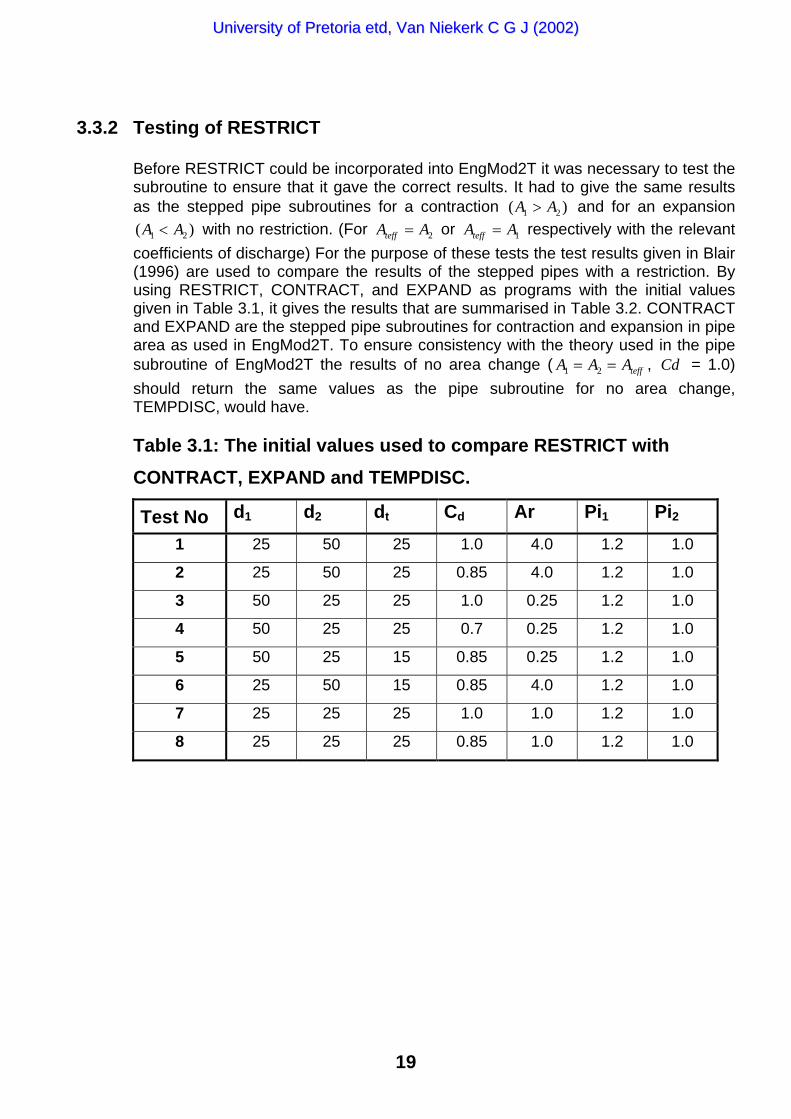
Before RESTRICT could be incorporated into EngMod2T it was necessary to test thesubroutine to ensure that it gave the correct results. It had to give the same resultsas the stepped pipe subroutines for a contraction )( 21 AA > and for an expansion

)( 21 AA < with no restriction. (For 2AAteff = or 1AAteff = respectively with the relevantcoefficients of discharge) For the purpose of these tests the test results given in Blair(1996) are used to compare the results of the stepped pipes with a restriction. Byusing RESTRICT, CONTRACT, and EXPAND as programs with the initial valuesgiven in Table 3.1, it gives the results that are summarised in Table 3.2. CONTRACTand EXPAND are the stepped pipe subroutines for contraction and expansion in pipearea as used in EngMod2T. To ensure consistency with the theory used in the pipesubroutine of EngMod2T the results of no area change ( teffAAA == 21 , Cd = 1.0)should return the same values as the pipe subroutine for no area change,TEMPDISC, would have.

Table 3.1: The initial values used to compare RESTRICT withCONTRACT, EXPAND and TEMPDISC.

Test No d1 d2 dt Cd Ar Pi1 Pi21 25 50 25 1.0 4.0 1.2 1.0

2 25 50 25 0.85 4.0 1.2 1.0

3 50 25 25 1.0 0.25 1.2 1.0

4 50 25 25 0.7 0.25 1.2 1.0

5 50 25 15 0.85 0.25 1.2 1.0

6 25 50 15 0.85 4.0 1.2 1.0

7 25 25 25 1.0 1.0 1.2 1.0

8 25 25 25 0.85 1.0 1.2 1.0


20

Table 3.2: Results of the comparison of RESTRICT withCONTRACT, EXPAND and TEMPDISC.

Expand Contract, Tempdisc orResults by Blair (1996)

Restrict

Test No Pr1 Pr2 Theory Pr1 Pr2

1 0.8850 1.0785 Expand 0.88501 1.07851

2 0.8931 1.0768 Blair 0.89307 1.07683

3 1.1227 1.3118 Contract 1.12270 1.31180

4 1.1239 1.3075 Blair 1.12389 1.30752

5 1.1436 1.2351 Blair 1.14363 1.23508

6 0.9967 1.0537 Blair 0.99669 1.05368

7 1.0000 1.2000 Tempdisc 1.00000 1.20000

8 1.0002 1.1998 Tempdisc 1.00022 1.19981

The test results as summarised in Table 3.2 indicates that it is acceptable to includesubroutine RESTRICT into the program EngMod2T. The results of the threesubroutines give identical results to RESTRICT. This is as expected as the sametheoretical approach is used as well as the same numerical solution scheme.

3.4 CLOSING

The thermodynamic equations for 1-dimensional compressible flow through arestriction as given by Blair (1996) was developed into a suitable format forprogramming and subroutine RESTRICT was developed and tested. It gaveacceptable test results and was included into the program EngMod2T.


CHAPTER 4

DETERMINATION OF DISCHARGE COEFFICIENTS

4.1 PRE-AMBLE

The chapter starts off by describing the experimental apparatus used to determinethe flow through the different tailpipe entry configurations. This is followed by thedevelopment of the equations and software necessary to determine the coefficient ofdischarge from the experimental results. Next, the results from the tests arepresented.

4.2 DESCRIPTION OF EXPERIMENTAL APPARATUS

The experimental apparatus for the measurement of the coefficients of discharge isshown in Figure 4.1. It was developed for these tests. The required range of pressureand mass flow ratios were determined by conducting a series of simulations with thetail pipe pressure ratio and mass flow as outputs. A sample of the results is shown inAppendix D. Originally the plan was to use the SuperFlow flow bench model SF110that is available in the engineering laboratory at the University of Pretoria.

Figur

Thiexecu

The crequircapabcomprto conof the

From orificecorne


Test Piece

e 4.1

s flowte the

ompreed mle of essortrol th test a

the d, chanr pres

Settling Tank

: Experimental Ap

bench is a small mo tests at the required p

ssor at the companass flows and pressa sustained flow of 1 is connected to a pree pressure in the settlpparatus.)

rier the air passes thrgeable in diameter tosure tappings design

BS1042 Orifice

21

paratus

del and does not have a sufficient flow capacity toressure ratios and mass flow values.

y Boart Longyear Seco was used to obtain theure ratios. This is a large industrial compressor00kg/s at a pressure of 800kPa. The outlet of thessure regulator and air drier. This regulator is useding tank. (Refer to Figure 4.2 for a schematic layout

ough the flow measurement section containing an measure more accurately differing flow rates, withed to conform to British Standard BS1042 (Anon)

22

and ending in the settling tank. The settling tank has pressure and temperaturesensors. On top of the settling tank is a pipe at the end of which the test pieces aremounted. The outlet of the test piece is to atmosphere, of which the temperature andpressure are recorded.

AIRINLET

TEST PIECE

OUTLET

dP

Pb

Tb

Tu

SETTLINGTANK

BS 1042ORIFICE

Figure 4.2: Schematic Drawing of Experimental Layout

A detailed description of the various sensors used and their calibration factors areincluded in Appendix C. Included as well are the detail drawings and the design limitsof the flow-measuring device according to British Standard BS1042.

4.3 DEVELOPMENT OF SOFTWARE TO CALCULATE THECOEFFICIENT OF DISCHARGE

The coefficient of discharge used in the subroutine RESTRICT is the actualcoefficient of discharge as described in by Blair et al (1995). Briefly, this means that ifthe orifice and ducts are modelled using the GPB method and the equations asderived in chapter 3, the calculated coefficient of discharge will, if used in thesimulation with the same boundary conditions, predict the same mass flow as themeasured mass flow.


23

To achieve this a program, FLOWPROG, was written using the pipe flow and thepipe boundary condition subroutines of EngMod2T combined with subroutineRESTRICT as developed in chapter 3. FLOWPROG simulates the actual flow bench,flow bench test pieces and boundary conditions. It uses the settling tank pressureand temperature as the inflow conditions to the test piece and the atmospherictemperature and pressure for the outflow boundary conditions. FLOWPROG uses asinput the following parameters:

i. Test piece geometry

ii. Test Pressure (Refer to Figure 4.2)

iii. Test Temperature

iv. Atmospheric temperature and pressure

v. Corrected measured mass flow.

The program starts off by assuming a coefficient of discharge of 1.0 and calculatesthe mass flow. It then decreases the coefficient of discharge and recalculates themass flow. This process is repeated until the measured and predicted mass flows arewithin 1% of each other.

4.4 EXPERIMENTAL DETERMINATION OF COEFFICIENT OFDISCHARGE.

It is not possible to test the restriction in isolation because of the physical constraints.The restriction is by its very nature the result of the flow through the joining of thereverse cone and tailpipe of the exhaust system. However, testing thetailpipe/reverse cone combination on the flow bench adds the complication to the testthat the inflow discharge coefficient at the test piece inlet diameter is a partialunknown. The effect of the friction factor (and thus the effect of the length of the testpiece) is also unclear at this stage. It is therefore necessary to evaluate these effectsfirst to ensure that their influence on the final test results are minimised before theactual testing to determine the coefficients of discharge commences.

4.4.1 Influence of test piece length and inlet diameter on results

In order to minimise the effect of the flow losses at the inlet of the reverse cone it isadvantages to use a sufficiently large diameter to reduce the entry speed of the air.This has however the adverse result of lengthening the reverse cone as the includedangle is one of the controlling parameters of the restriction that is being studied.

In order to study this effect, four test cases were modelled and tested usingFLOWPROG. The test piece dimensions and the test results at a range of testpressures are shown in Table 4.1. The coefficient of discharge at the test piece entryfrom the settling tank (which conforms to the definition by Blair and Drouin (1996) ofan open ended plain pipe) and is described by the following polynomial function:

1.0<Pr<1.4 Cd = -23.543+60.686Pr–51.04Pr2 +14.387Pr3 (4.1a)


24

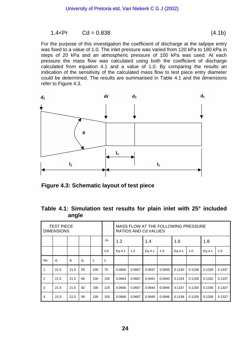
1.4<Pr Cd = 0.838 (4.1b)

For the purpose of this investigation the coefficient of discharge at the tailpipe entrywas fixed to a value of 1.0. The inlet pressure was varied from 120 kPa to 180 kPa insteps of 20 kPa and an atmospheric pressure of 100 kPa was used. At eachpressure the mass flow was calculated using both the coefficient of dischargecalculated from equation 4.1 and a value of 1.0. By comparing the results anindication of the sensitivity of the calculated mass flow to test piece entry diametercould be determined. The results are summarised in Table 4.1 and the dimensionsrefer to Figure 4.3.

l3

d2 dr d3 d1

l2 l1

θ

Figure 4.3: Schematic layout of test piece

Table 4.1: Simulation test results for plain inlet with 25° includedangle

TEST PIECEDIMENSIONS

MASS FLOW AT THE FOLLOWING PRESSURERATIOS AND Cd VALUES

Pr 1.2 1.4 1.6 1.8

Cd Eq 4.1 1.0 Eq 4.1 1.0 Eq 4.1 1.0 Eq 4.1 1.0

No d1 dt d2 l1 l2

1 21.5 21.5 55 100 75 0.0660 0.0667 0.0937 0.0945 0.1150 0.1158 0.1328 0.1337

2 21.5 21.5 66 100 100 0.0663 0.0667 0.0941 0.0945 0.1154 0.1158 0.1332 0.1337

3 21.5 21.5 82 100 125 0.0666 0.0667 0.0944 0.0946 0.1157 0.1159 0.1336 0.1337

4 21.5 21.5 99 100 150 0.0666 0.0667 0.0945 0.0946 0.1158 0.1159 0.1336 0.1337


25

The results show that the sensitivity of the tests on the test piece inlet conditions(coefficient of discharge and diameter) decreases as the diameter increases.However, the difference in mass flow for the 55mm diameter entrance using a Cdvalue of 1.0 versus the calculated Cd value using equation 4.1 is only 1.2 percent.Thus, even if the calculated Cd value incorporates an error, the effect on the resultswill be at maximum 1.2 percent, assuming the incorrect value will fall between 1.0and the correct value. Based on this fact, a test piece starting diameter of 63mm wasselected as this is a freely available hydraulic pipe diameter and therefor aconvenient size. The length for these sizes of test pieces has no effect.

4.4.2 Description of the test pieces

In order to create a coefficient of discharge map or to develop some mathematicalrelationship between the geometry, pressure ratio and coefficient of discharge for theconventional type of tail pipe entry four test pieces were constructed having thesame entry diameters and the same size tail pipes. The only value that was variedwas the included angle (and resulting from that, the cone length) in steps of 10degrees starting from 10 degrees and ending at 40 degrees. In tuned pipes theincluded angle varies typically from 15 degrees to 30 degrees depending on theapplication of the engine. The first four test pieces cover this spread of values. (Testpieces no 1 to 4)

The dimensions of the test pieces are shown in Table 4.2. The dimensions are asper Figure 4.3.

To investigate the size effect of the tailpipe a further two test pieces wereconstructed but with a bigger diameter and a smaller diameter tail pipe than usedwith the first four test pieces. The included angle was kept to 30 degrees. (Testpieces no 5 and no 6)

The next series of test pieces were variations of the type where the end of thereverse cone is smaller than the tail pipe. Two test pieces were constructed with thereverse cone end stepping up directly from its diameter to the tail pipe diameter. Thisis the layout used by the Aprillia Racing Team. (Test pieces no 7 and 8) This type oftail pipe geometry is known as the Restrictor type of tailpipe.

The final two test pieces were a further development on this theme. Instead ofstepping up directly from the reverse cone end diameter to the tail pipe diameter, agradual increase to the tail pipe diameter is used. This results in a venturi at the tailpipe entrance and is the layout as used by the Honda Racing Team. This is also thelayout that prompted this research project. (Test pieces no 9 and no 10) This type oftail pipe geometry is known as the Venturi type of tailpipe.


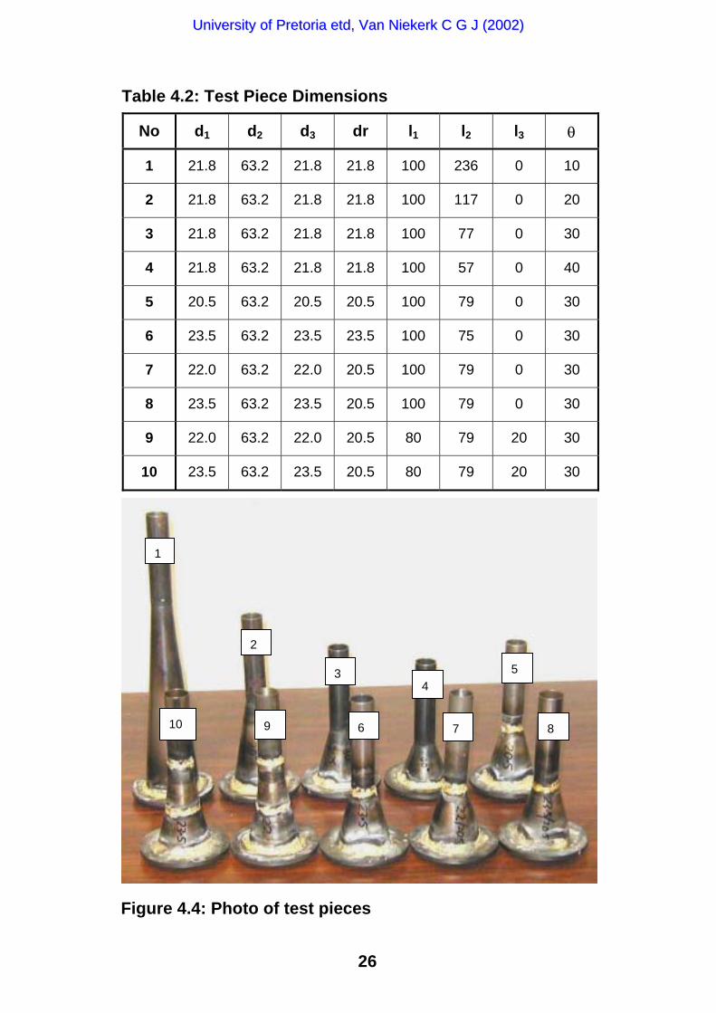
Table 4.2: Test Piece Dimensions

No d1 d2 d3 dr l1 l2 l3 θ

1 21.8 63.2 21.8 21.8 100 236 0 10

2 21.8 63.2 21.8 21.8 100 117 0 20

3 21.8 63.2 21.8 21.8 100 77 0 30

4 21.8 63.2 21.8 21.8 100 57 0 40

5 20.5 63.2 20.5 20.5 100 79 0 30

6 23.5 63.2 23.5 23.5 100 75 0 30

7 22.0 63.2 22.0 20.5 100 79 0 30

8 23.5 63.2 23.5 20.5 100 79 0 30

9 22.0 63.2 22.0 20.5 80 79 20 30

10 23.5 63.2 23.5 20.5 80 79 20 30

Figure 4.4: Phot


2

o of test p

3

26

ieces

4
5
10
9 6 7 8
1

27

4.4.3 Experimental Procedure

The test sequence is as follows:

i) The test apparatus is connected in the manner of Figure 4.2.

ii) The pressure transducers are calibrated using a Budenburg tester. This isdone with the transducer connected to the computer with the same connectingcables as used in the actual tests.

iii) With the pressure transducers in place and the test piece connected theregulator is opened and adjusted to obtain the required pressure in the settlingtank.

iv) Once the pressure values have stabilised the pressures and temperatures arerecorded.

v) The orifice pressures are used to calculate the pressure differential over theorifice to ensure that the orifice size falls inside the prescribed requirements ofBS1042. If not, the size must be changed and the results recorded again.

vi) If the pressure differential conforms to BS1042 the regulator is adjusted toobtain the next settling tank pressure and points iii to v are repeated.

vii) Once the results for required range of pressures for the test piece have beenrecorded the next test piece is installed and the process is repeated starting atpoint iii.

4.4.4 Experimental Results

The mass flow for each test piece for the range of test pressure ratios are calculatedfrom the test results. The calculations are done according to BS1042 for the orificeand uses the following inputs:

i) Upstream pressure

ii) Downstream pressure

iii) Upstream temperature

iv) Orifice and tube diameters

v) Atmospheric pressure.

A program was written using the methodology as described in BS1042: Part 1.4 tospeed up the calculation process. Firstly the measured pressures are averaged over asample period of 15 seconds to eliminate the effect of a small problem with noise, thencorrected using the calibration curves obtained from the Budenburg tester and thanfurther corrected according to the Wika calibration curve. The results are then used inthe BS1042 program to calculate the mass flow. The results are summarised inAppendix E.


28

4.5 PROCESSED RESULTS

4.5.1 Discussion of Processing Methodology

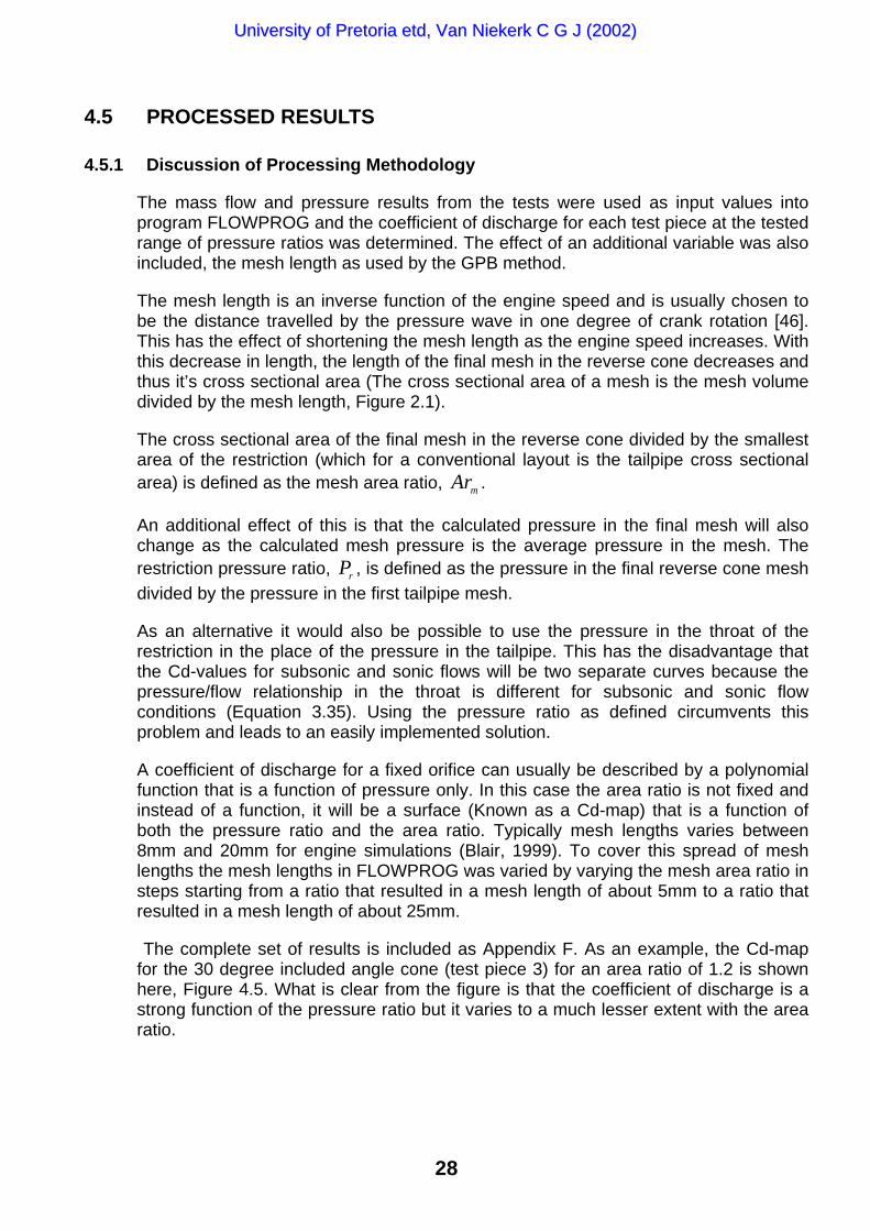
The mass flow and pressure results from the tests were used as input values intoprogram FLOWPROG and the coefficient of discharge for each test piece at the testedrange of pressure ratios was determined. The effect of an additional variable was alsoincluded, the mesh length as used by the GPB method.

The mesh length is an inverse function of the engine speed and is usually chosen tobe the distance travelled by the pressure wave in one degree of crank rotation [46].This has the effect of shortening the mesh length as the engine speed increases. Withthis decrease in length, the length of the final mesh in the reverse cone decreases andthus it’s cross sectional area (The cross sectional area of a mesh is the mesh volumedivided by the mesh length, Figure 2.1).

The cross sectional area of the final mesh in the reverse cone divided by the smallestarea of the restriction (which for a conventional layout is the tailpipe cross sectionalarea) is defined as the mesh area ratio, mAr .

An additional effect of this is that the calculated pressure in the final mesh will alsochange as the calculated mesh pressure is the average pressure in the mesh. Therestriction pressure ratio, rP , is defined as the pressure in the final reverse cone meshdivided by the pressure in the first tailpipe mesh.

As an alternative it would also be possible to use the pressure in the throat of therestriction in the place of the pressure in the tailpipe. This has the disadvantage thatthe Cd-values for subsonic and sonic flows will be two separate curves because thepressure/flow relationship in the throat is different for subsonic and sonic flowconditions (Equation 3.35). Using the pressure ratio as defined circumvents thisproblem and leads to an easily implemented solution.

A coefficient of discharge for a fixed orifice can usually be described by a polynomialfunction that is a function of pressure only. In this case the area ratio is not fixed andinstead of a function, it will be a surface (Known as a Cd-map) that is a function ofboth the pressure ratio and the area ratio. Typically mesh lengths varies between8mm and 20mm for engine simulations (Blair, 1999). To cover this spread of meshlengths the mesh lengths in FLOWPROG was varied by varying the mesh area ratio insteps starting from a ratio that resulted in a mesh length of about 5mm to a ratio thatresulted in a mesh length of about 25mm.

The complete set of results is included as Appendix F. As an example, the Cd-mapfor the 30 degree included angle cone (test piece 3) for an area ratio of 1.2 is shownhere, Figure 4.5. What is clear from the figure is that the coefficient of discharge is astrong function of the pressure ratio but it varies to a much lesser extent with the arearatio.


29

1.05

1.15

1.25

1.35

1.45

1.55 1

1.05 1.

11.

15 1.2

1.25 1.

31.

35

0.6

0.65

0.7

0.75

0.8

0.85

0.9

0.95

1

Cd

Area RatioPressure Ratio

Figure 4.5: Cd-map for a 30 degree included angl

In Figure 4.6 the results for the same 30 degree cone is shown1.15, 1.30, 1.45 and 1.60 on the same two-dimensional grapratio on the Cd-value can be up to 5 percent between the smratios.

0.7

0.75

0.8

0.85

0.9

0.95

1

1 1.1 1.2 1.3 1.4

Pressure Ratio

Cd-

valu

e

Figure 4.6: The effect of mesh length (area ratio)


Cd

0.95-10.9-0.950.85-0.90.8-0.850.75-0.80.7-0.750.65-0.70.6-0.65

e reverse cone

but for four area ratios,h. The effect of the area

allest and largest area

o

Ar

1.151.31.451.6

n Cd-values

30

4.5.2 The effect of reverse cone included angle.

The first four test pieces studied the effect of the reverse cone angle. The completeset of Cd-maps is included in Appendix F. For comparative purposes a graph wasconstructed by keeping the area ratio fixed at 1.2. This is shown in Figure 4.7.

0.7

0.75

0.8

0.85

0.9

0.95

1

1 1.1 1.2 1.3 1.4

Pressure Ratio

Cd-

Valu

e

Figure 4.7: The effect of included cone angle

The graph clearly shows that as the included angle destraight pipe, the Cd-values increases and vice versa.expected and the Cd-values should approach those of the cone angle approaches 180 degrees.

4.5.3 The effect of the tail pipe diameter

The tailpipe diameter should not have an influence on tthe choice of non-dimensional dependant variables weconfirmed by the comparison in Figure 4.8. The original with the trend lines fitted using a least squares fit. Thetogether with a maximum deviation of 1.3% from the meawhich has a maximum value of 2.8%.


ConeAngle

10deg

20deg

30deg

40deg

on the Cd-values

creases, thus approaching a This is in line with what isa plain open-ended pipe as

he coefficient of discharge ifre correctly chosen. This ismeasured points are shown trend lines are very close

n and inside the data scatter

31

0.7

0.75

0.8

0.85

0.9

0.95

1 1.1 1.2 1.3 1.4

Pressure Ratio

Cd-

Valu

e

Figure 4.8: The effect of tailpipe diameter on the

4.5.4 The effect of the Restrictor tail pipe geometry

This is one of the non-conventional tailpipe entry geometriconstructed by using a tailpipe that is larger than the end ofpieces were investigated with the same size reverse conebut with a 22.0mm and a 23.5mm tailpipe fitted respecticompared to those of the conventional tailpipes of 20.5mmflow results are shown in Figure 4.9 and the Cd-values in Fi

From Figure 4.9 it is clear that the mass flow increases tailpipe diameter for the same restriction size but it followstailpipe characteristic very closely, although with slightly 23.5mm tailpipe fitted the mass flow is close to that fortailpipe.

The coefficients of discharge increase with the size of Although it is the opposite to what is expected, it is indeed used is a function of the last reverse cone mesh pressurepressure and while this is not incorrect, it would probably mpressure in the vena contracta as well. This leads to addonly advantage being a more consistent graph. The igasdynamic calculations would yield the correct mass flodefinition of the pressure ratio used for both the test resusoftware is consistent.


TailpipeDiameter

20.5mm21.8mm23.5mm20.5mm21.8mm23.5mm

Cd-values

es under investigation. It is the reverse cone. Two test end diameter of 20.5mm

vely. The results are then and 23.5mm. The mass

gure 4.10.

slightly with an increase in the conventional 20.5mmmore flow. Even with the

the 20.5mm conventional

the tailpipe. (Figure 4.10)correct. The pressure ratio and the first tailpipe mesh

ore correct to include theitional complexity with themportant fact is that thew results as long as thelts and its inclusion in the

32

0

0.02

0.04

0.06

0.08

0.1

0.12

0.14

0.16

1 1.1 1.2 1.3 1.4Pressure Ratio

Mas

sflo

w (k

g/s)

20.5mmr22mmr23.5mm23.5mm20.5mmr22.0mmr23.5mm23.5mm

Figure 4.9: Mass flow values for restricted tailpipe entries

0.7

0.75

0.8

0.85

0.9

0.95

1

1 1.1 1.2 1.3 1.4Pressure Ratio

Cd-

Valu

e

20.5mm

r22mm

r23.5mm

23.5mm

20.5mm

r22.0mm

r23.5mm

23.5mm

Figure 4.10: Cd-Values for the restricted tailpipe configuration


33

4.5.5 The effect of the gradual area change restriction (venturi)

The results for the venturi type tailpipe entry geometry test pieces are shown inFigures 4.11 and 4.12.

0

0.02

0.04

0.06

0.08

0.1

0.12

1 1.05 1.1 1.15 1.2 1.25

Pressure Ratio

Mas

sflo

w (k

g/s)

20.5mmv22.0mmv23.5mm23.5mm20.5mmv22.0mmv23.5mm23.5mm

Figure 4.11: Mass flow results for the venturi type tailpipe entries

0.7

0.75

0.8

0.85

0.9

0.95

1 1.05 1.1 1.15 1.2 1.25

Pressure Ratio

Cd-

Valu

e

20.5mmv22.0mmv23.5mm23.5mm20.5mmv22.0mmv23.5mm23.5mm

Figure 4.12: Cd-Values for the venturi type tailpipe entries

For comparative purposes the results for the conventional 20.5mm and 23.5mmconventional tailpipes are included on the graphs. Both the venturi with the 22.0mmtailpipe and the one with the 23.5mm tailpipe show virtually the same mass flow as the


34

conventional 20.5mm tailpipe. This is an unexpected result. The Cd-values does differbut that is because they are also a function of the mesh cross sectional diameters.

4.6 DISCUSSION OF RESULTS

The results showing the influence of the reverse cone angle on the Cd-values indicateclearly that the Cd-values are a function of the angle; it decreases with an increase inangle and vice versa. What is interesting is the small values (large losses) at smallpressure ratios. This should have an effect on the simulation results and will beinvestigated in the next chapter. The effect of the tail pipe diameter was shown not toinfluence the Cd-values.

The restrictor tailpipe and the venturi tailpipe show unexpected results. The restrictortail pipe mass flow follows the mass flow curve of the conventional tail pipe with thesame diameter as the restrictor but with a small increase with an increase in tail pipediameter. With the venturi tail pipe the mass flow follows the mass flow curve of theconventional tailpipe even closer.

A possible explanation for its usage on a racing motorcycle lies in the fact that thecorrect resistance of the tail pipe is important to its performance. On a racingmotorcycle, because of its chassis and engine layout, it is not always possible to havethe same length and diameter tail pipe and/or silencer on the exhaust pipe of eachcylinder. Normally this would mean a large amount of testing and fine-tuning to matchthe resistances to the required value. Using a venturi of the correct size and a tail pipeand silencer of sufficient diameter will result in a pipe with the correct resistance. Theresistor tail pipe will have the same trend but with a higher sensitivity to the tailpipeand silencer length and diameter.

This ties in with observations on the racetrack. The use of the restrictor tailpipe wasfirst seen on the Aprillia RS250 racing motorcycle. It has one exhaust pipe fitted with a75mm long tail pipe and a 180mm long silencer. The other pipe has a 100mm long tailpipe and a 250mm long silencer. The restrictor tail pipe probably supplies sufficientcontrol over the resistances to match the two pipes.

The Honda NS250 racing motorcycle was the first motorcycle seen with the venturi tailpipes. It has the same length silencers on both pipes but the one exhaust has a120mm long tail pipe and the other a 370mm long tail pipe. This motorcycle is alsoleased to various teams that use silencers from a range of suppliers. A venturi tail pipewill supply the needed control to maintain the required resistance.

4.7 CLOSING

In this chapter it was shown from experimental results that the Cd-values of the tailpipe entry are a function of pressure and reverse cone angle. The numerical methodcauses it to be a function of mesh length (area ratio) as well. The characteristics of therestrictor and venturi tailpipes were investigated and an explanation for its use waspresented.


35

CHAPTER 5

SIMULATION STUDY

5.1 PRE-AMBLE

The effect of the experimentally determined coefficients of discharge on theperformance prediction of two-stroke engines are determined by including thecoefficient of discharge maps in the simulation software EngMod2T and conducting arange of simulations with and without the maps. The results are then compared to adynamometer test of the same engine.

5.2 THE INCORPORATION OF THE CD-MAPS IN ENGMOD2T

During each simulation time step, a new value for the coefficient of discharge as afunction of the pressure ratio, area ratio and the reverse cone angle is determined.This is done in the following manner:

i. During the start up of the main program a check is performed todetermine between which two maps the reverse cone angle falls.These two maps are then read by the start up section of the program.(If it falls exactly on one of the maps the procedure is simplified.)

ii. During the gasdynamic calculation a bi-linear interpolation betweenthe two area and the two pressure ratios that falls on either side of thepoint of interest on each map is performed. Thus a Cd-value isdetermined from each map.

iii. The final Cd-value is then determined by a linear interpolationbetween the two Cd-values.

iv. This value is then used for the next gasdynamic calculation.

v. For the next time step the procedure is repeated starting at point ii.

This process was coded into program EngMod2T and the four Cd-maps wereprepared in the correct matrix format, similar to the Cd-maps for the engine ports andpipe ends, to allow the program to read them into memory during the start upprocess.

5.3 SIMULATED ENGINE PARAMETERS

The engine chosen for the simulation study is from a commercially availableproduction motorcycle. Although it is meant for street use it is very popular as aracing motorcycle in modified form. The engine is twin cylinder engine in a 90degreeV layout. The intake and exhaust systems of the two cylinders are completelyindependent and the engine can thus be simulated as a 125cc single cylinder.


36

Table 5.1: Major engine characteristics

Description of characteristic Value

Engine type 90 deg V-2

Bore 54mm

Stroke 54mm

Capacity 125cc

Primary compression ratio 8.5:1

Secondary compression ratio 1.35:1

Type of exhaust port Bridged

Number of transfer ports 5

Type of intake system Reed valve

The complete set of input data used is listed in Appendix F. The exhaust pipedimensions listed are for a pipe developed for this type of racing and used withsuccess in racing application.

The physical data was obtained by measuring the engine. The values used in thecombustion model were obtained from the experimental results of a similar engine(Blair, 1996).

5.4 VERIFICATION OF RESTRICT IN ENGMOD2T

To ensure that subroutine RESTRICT functions correctly and does not induce falseresults because of a numerical error a comparison was made between resultsobtained from the original version of EngMod2T and the updated version but with aCd-value of 1.0. The new version but with a Cd-value of 1.0 should give the sameresults as the old version. The comparison of the power predicted by the two versionsis shown in Figure 5.1. For all practical purposes the results are identical, proving thatRESRICT gives the same results as CONTRACT for a Cd-value of 1.0. The smalldifferences can be attributed to the numerical accuracy of the non-linear solutionprocess. The influence of the coefficient of discharge can now be investigated.


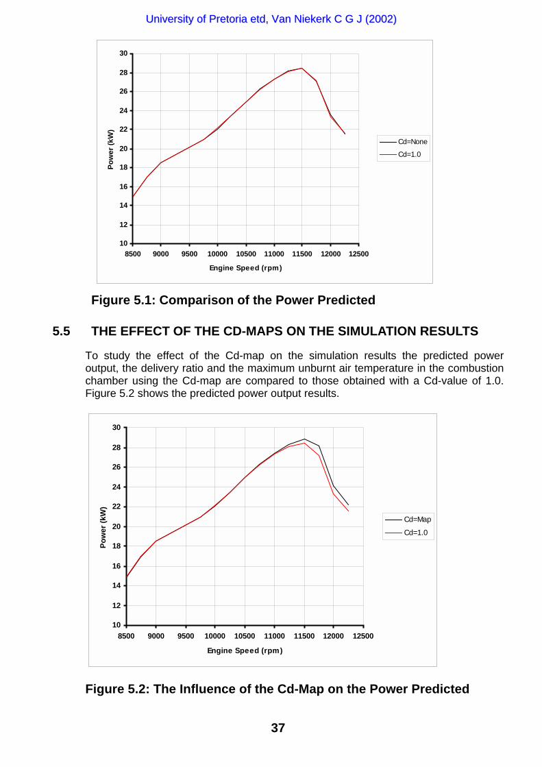
37

Figure 5.1: Comparison of the Power Predicted

5.5 THE EFFECT OF THE CD-MAPS ON THE SIMULATION RESULTS

To study the effect of the Cd-map on the simulation results the predicted poweroutput, the delivery ratio and the maximum unburnt air temperature in the combustionchamber using the Cd-map are compared to those obtained with a Cd-value of 1.0.Figure 5.2 shows the predicted power output results.

10

12

14

16

18

20

22

24

26

28

30

8500 9000 9500 10000 10500 11000 11500 12000 12500

Engine Speed (rpm)

Pow

er (k

W)

Cd=Map

Cd=1.0

Figure 5.2: The Influence of the Cd-Map on the Power Predicted

10

12

14

16

18

20

22

24

26

28

30

8500 9000 9500 10000 10500 11000 11500 12000 12500

Engine Speed (rpm)

Pow

er (k

W)

Cd=None

Cd=1.0


38

The inclusion of the Cd-map increases the predicted power an increasing but smallamount up to maximum power and has a large effect after maximum power. Theportion of the power curve after maximum power is known as the “over run” of theengine and is very important on a racing engine because of the lengthening effect ithas on the spread of useable power. (The so called “power band”) Accuratelypredicting the “over run” of an engine is an essential capability of a simulation programthat is used for the development of competition engines.

The delivery ratio comparison (Figure 5.3) indicates that the increased resistanceresulting from the Cd-map decreases the delivery ratio.

1.2

1.25

1.3

1.35

1.4

1.45

1.5

1.55

1.6

8500 9000 9500 10000 10500 11000 11500 12000 12500Engine Speed (rpm)

Del

iver

y R

atio

Cd=1.0Cd=Map

Figure 5.3: The Effect of the Cd-Map on the Delivery Ratio

The importance of this factor lays the effect the delivery ratio has on the temperatureof the unburnt air during combustion. Two identical engines but with different deliveryratios and the same charging efficiency will produce the same power but the one withthe lower delivery ratio will be more prone to detonation and pre-ignition. This is adirect result of less cool air flowing through the cylinder. The maximum temperature ofthe unburnt air before it becomes part of the combustion process indicates this. Figure5.4 compares the maximum unburnt air temperatures for the two simulations.


39

600

650

700

750

800

850

900

8500 9000 9500 10000 10500 11000 11500 12000 12500

Engine Speed (rpm)

Unb

urnt

Air

Tem

pera

ture

(C)

Cd=Map

Cd=1.0

Figure 5.4: The Effect of the Cd-Map on the Maximum UnburntAir Temperature

5.6 COMPARISON OF THE SIMULATED RESULTS WITH TEST RESULTS

To verify the improvement in the prediction of the power output of the software by theinclusion of the Cd-maps a comparison with measured results was made. Themeasured results are included as Appendix H. The tests were conducted on a HyperPower dynamometer and a correction factor of 1.2 was used. Unfortunately this is notthe correct factor but the tests had to fit in with other tests conducted on themotorcycle. The testing of a racing motorcycle is expensive (e.g. A set of pistons hasa life of around 250 racing kilometres) and as many tests as possible must beconducted in the available time. This test was part of a test where different sets ofexhaust pipes were compared.

The results in Appendix H show the power curves for the old and new version of theexhaust pipes. The results are in horsepower at the rear wheel. The results for thenew pipe was converted to kilowatts and halved, as it is a two-cylinder engine. Theresults are compared with the predictions by the old and new version of EngMod2T inFigure 5.5. The absolute values are not the same because of losses through the drivetrain, water pump, ignition and the wheel to roller interface. For comparative purposesthe measured results were “corrected” by multiplying it with a factor to have the samenumerical maximum power as the new simulation. This comparison shows that thetrend is correct for the new prediction. The inclusion of the Cd-maps improve the "overrun" prediction to a similar curve shape as the measured result.


40

10

12

14

16

18

20

22

24

26

28

30

8000 8500 9000 9500 10000 10500 11000 11500 12000

Engine Speed (rpm)

Pow

er (k

W) Sim-Old

Sim-NewDynoDyno-Corr

Figure 5.5: Comparisons of Predicted and Measured Power

5.7 CLOSING

The Cd-maps and subroutine RESTRICT were included in EngMod2T (version 2.3).It’s influence on the predicted power and the other simulation results were investigatedand compared to measured results. It was shown that the inclusion of the Cd-mapsimproves the accuracy of the simulation and is a necessary enhancement of thesoftware.


41

CHAPTER 6

SUMMARY, CONCLUSION AND RECOMMENDATIONS

6.1 SUMMARY

The effect of a more accurate way of modelling the tail pipe entry geometry of theexhaust pipe of a high performance two-stroke engine in one-dimensional gasdynamicsimulation software was investigated. Usually the entry to the tailpipe is modelledalong similar lines as the rest of the reverse cone, as a normal area change. Theeffect of modelling the entry along the lines of a restriction with a coefficient ofdischarge was proposed for investigation.

A thermodynamically more sophisticated model that includes an increase in entropyon the expansion side was developed from the formulation by Blair, Kirkpatrick,Mackey and Fleck (1995) into a suitable format for the inclusion into simulationsoftware. A Newton-Raphson method for solving a set of simultaneous non-linearequations was implemented to solve the equations for the restriction.

This implementation requires a coefficient of discharge value for the restriction.Apparatus for the experimental determination of the Cd-values for a range of reversecone angles, pressure ratios and area ratios was constructed. A range of tests thatcover the area and pressure ratios expected in an engine tailpipe was conducted andthe results were presented in a format suitable for its inclusion in the simulationsoftware.

The influence of the inclusion of this coding and Cd-maps in the software wasinvestigated and the power predicted was compared with measured results. It turnsout that using this approach improves the accuracy of the power output prediction atengine speeds higher than the speed at which maximum power occur.

At the same time the effect of special tailpipe entry geometry, the venturi inlet and therestriction inlet was investigated. It was concluded that their function is to control theexhaust outflow resistance to the required value and to remove its sensitivity to thegeometry of the tail pipe and silencer that follows, as long as the tailpipe and silenceris of sufficient size not to cause an additional restriction.


42

6.2 CONCLUSION

A theoretical model taking the effect of a restriction at the tailpipe into considerationtogether with an increase in entropy on the expansion side was shown to change theperformance predictions on a high specific power output two-stroke engine.

The size of the restriction was experimentally determined on a specially constructedtest apparatus. The results were post processed into a series of Cd-maps. The mapsshowed that there is definitely a restriction (probably in the form of a vena contracta)present in the tail pipe entry.

Using the experimentally determined Cd-maps together with the newly developedrestriction algorithm into the simulation model has a noticeable effect on the predictedperformance results, mostly in the “over run” part of the power delivery. It alsoinfluences the predicted maximum unburned air temperature and the delivery ratio.

Comparing the old and the new predicted power curves with a measured one showedclearly that the new curve follows the measured curve much more closely on the partof the curve after maximum power and as good as the old one up to maximum power.

It is concluded that it is necessary to model the tailpipe entry geometry and flowconditions of a high performance two-stroke engine more accurately using a moresophisticated model combined with measured Cd-maps, especially if the area ofinterest is the “over run” portion of the power curve. Failing to do so can result in faultydeductions, insights and engine design compromises.

Additionally, the function of specially designed tail pipe entries was investigated. It wasconcluded that the main function of these special entries was to render the exhaustsystem insensitive to the geometry of the tail pipe and silencer provided they were notmore restrictive than the tail pipe entry itself.

6.3 RECOMMENDATIONS AND FUTURE WORK

Comparing the predicted versus measured power characteristics the portion of thepower curve up to maximum power shows distinct humps that is not there on themeasured curve. This is probably resulting from the intake system resonant frequency.The shape of the delivery ratio curve, with humps corresponding to these in the powercurve, highlights this. It is possible that a further improvement in the accuracy of thepower prediction can be obtained by modelling the carburettor as a restriction similarto the tail pipe entry but with the cooling effect of the vaporising fuel taken intoaccount. This should be an area of further study.


43

Appendix A

REFERENCES

ANNAND W.J.D. & ROE G.E. 1974. Gas Flow in the Internal Combustion Engine 1st EditionISBN 0 85429 160 1 G T Foulis & Co Ltd

ANON. British Standard: BS1042: Section 1.1 and 1.4: 1984, Measurement of fluid flow inclosed conduits.

BANNISTER F.K., Mucklow G.F. 1948. Wave Action Following Sudden Release OfCompressed Gas From A Cylinder. Proc. I. Mech. E., Vol. 159.

BANNISTER F.K. 1958. Pressure Waves In Gasses In Pipes. Acroyd Stuart MemorialLectures, University Of Nottingham.

BENSON R.S. 1959. Experiments On Two Stroke Engine Exhaust Ports Under Steady AndUnsteady Flow Conditions. Proc. Inst Mech. E, Vol 173, No 19.

BENSON R.S., Garg R.D. & Woollatt D. 1964. A Numerical Solution Of Unsteady FlowProblems. Int. J. Mech. Sci, Pergamon Press, Vol 6.

BENSON R.S. & Pool D.E. 1965a. Compressible Flow Through A Two-Dimensional Slit. Int.J. Mech Sci, Vol 7.

BENSON R.S. & Pool D.E. 1965b. The Compressible Flow Discharge Coefficients For ATwo-Dimensional Slit. Int. J. Mech. Sci, Vol 7.

BLAIR A.J., Blair G.P. 1987. Gas Flow Modelling Of Valves And Manifolds In Car Engines.I. Mech. E. C11/87.

BLAIR G.P. 1976. Prediction Of Two-Cycle Engine Performance Characteristics. SAE760645.

BLAIR G.P. 1990. The Basic Design Of Two-Stroke Engines. ISBN 1-56091-008-9, SAE R-104.

BLAIR G.P. 1991. An Alternative Method For The Prediction Of Unsteady Gas Flow ThroughThe Internal Combustion Engine. SAE 911850.

BLAIR G.P. 1993. Correlation Of An Alternative Method For The Prediction Of EnginePerformance Characteristics With Measured Data. SAE 930501.

BLAIR G.P. 1996. The Design And Simulation Of Two-Stroke Engines. ISBN 1-56091-685-0,SAE R-161.

BLAIR G.P. 1999. The Design And Simulation Of For-Stroke Engines. ISBN 0-7680-0440-3.SAE R-1861.


44

BLAIR G.P., Arbuckle J.A. 1970. Unsteady Flow In The Induction System Of A ReciprocatingInternal Combustion Engine. SAE 700443.

BLAIR G.P., Ashe M.C. 1967. The Unsteady Gas Exchange Characteristics Of A Two-CycleEngine. SAE 760644.

BLAIR G.P., Cahoon W.L. 1972. A More Complete Analysis Of Unsteady Gas Flow ThroughA High-Specific-Output Two-Cycle Engine. SAE 720156.

BLAIR G.P. & Drouin F.M.M. 1996. Relationship Between Discharge Coefficients AndAccuracy Of Engine Simulations. SAE 962527.

BLAIR G.P., Goulburn J.R. 1967. The Pressure-Time History In The Exhaust System Of AHigh Speed Reciprocating Internal Combustion Engine. SAE 670477.

BLAIR G.P., Hinds E.T. & Fleck R. 1979. Predicting The Performance Characteristics OfTwo-Cycle Engines Fitted With Reed Induction Valves. SAE 790842.

BLAIR G.P., Johnston M.B. 1968.Unsteady Flow Effects In Exhaust Systems Of NaturallyAspirated, Crankcase Compression Two Cycle Internal Combustion Engines. SAE680594.

BLAIR G.P., Kirkpatrick S.J. & Fleck R. 1995. Experimental Validation Of A 1-D ModellingCode For A Pipe Containing Gas Of Varying Properties. SAE 950275.

BLAIR G.P., Kirkpatrick S.J., Mackey D.O. & Fleck R. 1995. Experimental Validation Of A 1-D Modelling Code For A Pipe System Containing Area Discontinuities. SAE 950276.

BLAIR G.P., Lau H.B., Cartwright A., Raghanathan B.D. & Mackey D.O. 1995. Coefficient OfDischarge At The Apertures Of Engines. SAE 952138.

BLAIR G.P., Magee S.J. 1993. Non-Isentropic Analysis of Varying Area Flow in EngineDucting. SAE 932399.

BURDEN R.L. & Faires J.D. 2993. Numerical Analysis. 5th Ed, PWS Publishing Company.

CARTWRIGHT A & FLECK R. 1994. A Detailed Investigation of Exhaust System Design inHigh Performance Two-Stroke Engines, SAE 942515.

CHEN C., Veshagh A. & Wallace F.J. 1992. A Comparison Between Alternative Methods ForGas Flow And Performance Prediction Of Internal Combustion Engines. SAE921734.

CORBERáN J.M., Royo R., Pérez A. & Santiago J. 1994. Optimisation of a 125 cc Racing 2-S Engine based on Modelling and Testing. SAE.

DECKER B.E.L. 1978. Compressible Flow Through Square Edge Rectangular Orifices. Proc.I. Mech. E., 1956, Vol 192.

DOUGLAS R., Mcginnity F.A. & Blair G.P. 1991. A Study Of Gas Temperature Effects OnThe Prediction Of Unsteady Flow. IMechE, C433/036.


45

EARNSHAW S. 1910. On The Mathematical Theory Of Sound, , Proc. Roy. Soc. 84.

FLECK R., Blair G.P. &, Houston R.A.R. 1987. An Improved Model For Predicting ReedValve Behaviour In Two-Stroke Cycle Engines. SAE 871654.

FLECK R. & Cartwright A. 1996. Coefficients Of Discharge In High Performance Two StrokeEngines. SAE 962534.

FLECK R., Cartwright A. & Thornhill D. 1997. Mathematical Modelling Of Reed ValveBehaviour In High Speed Two-Stroke Engines. SAE 972738.

HINDS E.T., Blair G.P. 1978. Unsteady Gas Flow Through Reed Valve Induction Systems,SAE 780766.

IRVING P.E. 1969. Tuning for Speed, 5th edition. London : Newnes Books.

KIRKPATRICK S.J., Blair G.P., Fleck R. & McMullen R.K. 1994. Experimental Evaluation Of1-D Computer Codes For The Simulation Of Unsteady Gas Flow Through Engines -A First Phase. SAE 941685.

LANEY C.B. 1998. Computational Gasdynamics. ISBN 0-521-57069-7. Cambridge UniversityPress.

MACKEY D.O., Blair G.P. & Fleck R. 1996. Correlation Of Simulated And Measured NoiseEmissions And Unsteady Gas Dynamic Flow From Engine Ducting. SAE 961806.

MCGINNITY F.A., Douglas R. & Blair G.P. 1990. Application Of An Entropy Analysis ToFour-Cycle Engine Simulation. SAE 900681.

MUCKLOW G.F., Wilson A.J. 1955. Wave-Action In Gasses: The Attenuation And ReflectionOf Compression Waves Propagated In Pipes. Proc. I. Mech. E. Vol 169.

ONORATI A., Winterbone D.E. & Pearson R.J. 1993. A Comparison Of The Lax-WendroffTechnique And The Method Of Characteristics For Engine Gas DynamicCalculations Using Fast Fourier Transform Spectral Analysis. SAE 930428.

POLONI M., Winterbone D.E. & Nichols J.R. 1988. Flow With Variable Specific Heats In TheExhaust Pipe System Of The Internal Combustion Engine. SAE 885094.

VAN HOVE W. & Sierens R. 1991 Calculation of the unsteady flow in exhaust pipe systems:new algorithm to fulfil the conservation law in pipes with gradual area changes. Proc.I. Mech. E., Vol 205

WALLACE F.J., Boxer G. 1956. Wave Action In Diffusers For Exhaust-Pipe Systems, WithSpecial Reference To The Scavenging Of Two-Stroke Engines. Proc. I. Mech. E.

WALLACE F.J., Nassif M.H. 1954. Air Flow In A Naturally Aspirated Two-Stroke Engine.Proc. I. Mech. E., Vol 168.

WALLACE F.J., Stuart-Mitchell R.W. 1953. Wave Action Following The Sudden Release OfAir Through An Engine Port System. Proc. I. Mech. E., Vol. 1b.


46

WINTERBONE D.E., Pearson R.J. 2000. Theory of Engine Manifold Design. 1st Edition.London. ISBN 1 86058 209 5 Professional Engineering Publishing Limited.

ZHANG H., Widener S.K. 1996. An Integrated Engine Cycle Simulation Model With SpeciesTracking In Piping System. SAE 960077.


47

Appendix BListing of subroutine RESTRICT.FOR

SUBROUTINE RESTRICT(XI1,XI2,A01,G1,R,FA1, # FA2,PA,XR1,XR2,A02,T02,D02,FAT,CD,CT,XT,SING,T2)CCC *******************************************************************C This subroutine calculates the temperature, pressure, mass flow and C entropy change through a restriction in a pipe. It was developed byC CGJ van Niekerk based on the theoretical work of Professor GP BlairC of the Queen's University of Belfast, Northern Ireland. The theoryC can be found in "Design and Simulation of Two-Stroke Engines”, by C GP Blair,SAE 1996.CC It solves the sets of non-linear equations using a Newton-RaphsonC scheme. The Jacobian is calculated numerically and the set of C equations are solved using LU-factorization using two subroutinesC from from "NUMERICAL RECIPIES". LUDCMP does the decomposition and C LUBKSB the back substitution.C *******************************************************************CC FA1 = Left hand mesh sectional areaC FA2 = Right hand mesh sectional areaC FAT = Throat areaC FEFF = Effective throat areaC CD = Coefficient of discharge in throatC XI1 = Left hand incidence wave pressure ratioC XI2 = Right hand incidence wave pressure ratioC XR1 = Left hand reflected wave pressure ratioC XR2 = Right hand reflected wave pressure ratioCCC IMPLICIT NONEC CHARACTER SING*4

REAL A(20,20),F(20) REAL D02,FA2,A02,XR2,XI2,G51,FA1,G71,A01,XI1,XR1,DELX,A02S,PA,T02 REAL XMX,T2,AR,R,D,G1,G41,G61,A01S,FAT,XT,CT,CD,XTS,MST,MS1,MS2 REAL FEFF,XR1S,XR2S,CTS

INTEGER ITER,ITMAX,N,I,J,INDX(20)CC SING ='NONE'

G71=2*G1/(G1-1) G51=2/(G1-1) G41=(3-G1)/(G1-1) G61=(G1+1)/(G1-1)

FEFF =FAT*CD


48

C Parallel pipe positive flow for no restriction - do not use the restrictedsubroutine

IF(FA1.EQ.FA2.AND.FA1.EQ.FAT.AND.CD.GT.0.999)THEN

CALL PARALLEL(XI1,XI2,A01,G1,G51,R,FA1,FA2,PA,XR1, # XR2,ITER,G41,G61,SING,T2,T02)

IF(SING.EQ.'SING')THEN WRITE(6,*)'PIPE PARALLEL IN RESTRICT SINGULAR ' STOP ENDIF

A02=SQRT(G1*R*T02) GOTO 400 ENDIF

! Initial starting values based on constant pressure

AR =FA2/FA1 XR1S=((1-AR)*XI1+2*XI2*AR)/(1+AR) XR2S=(2*XI1-XI2*(1-AR))/(1+AR) XR1 =XR1S XR2 =XR2S

IF(FA1.LE.FAT.AND.CD.GT.0.999)THEN XT =XI1+XR1-1 CT =G51*A01*(XI1-XR1) ENDIF

! Results from previous cycle used as starting values

CT =ABS(CT) CTS =CT XTS =XT A02S =A02 A01S =A01CC Subsonic restrictor flowC A02=A02/100 A01=A01/100 CT =CT/100

DELX = 0.001 ITER = 0 ITMAX= 15 N = 5100 ITER=ITER+1

DO I=1,N F(I)=0.0 DO J=1,N A(I,J)=0.0 ENDDO

ENDDO

! Call subroutine with subsonic flow equations

CALL SUBSONIC(DELX,XI1,XR1,XR2,XI2,FA1,FA2,FEFF,A01,A02, # G51,G71,XT,CT,F,A,G1)


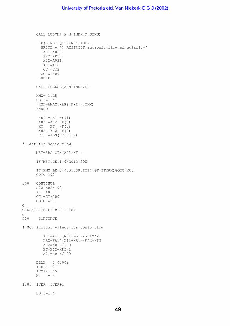
49

CALL LUDCMP(A,N,INDX,D,SING)

IF(SING.EQ.'SING')THEN WRITE(6,*)'RESTRICT subsonic flow singularity'

XR1=XR1S XR2=XR2S A02=A02S XT =XTS CT =CTS GOTO 400

ENDIF

CALL LUBKSB(A,N,INDX,F) XMX=-1.E5 DO I=1,N XMX=AMAX1(ABS(F(I)),XMX) ENDDO

XR1 =XR1 -F(1) A02 =A02 -F(2) XT =XT -F(3) XR2 =XR2 -F(4) CT =ABS(CT-F(5))

! Test for sonic flow MST=ABS(CT/(A01*XT))

IF(MST.GE.1.0)GOTO 300

IF(XMX.LE.0.0001.OR.ITER.GT.ITMAX)GOTO 200 GOTO 100

200 CONTINUE A02=A02*100 A01=A01S CT =CT*100 GOTO 400CC Sonic restrictor flowC300 CONTINUE

! Set initial values for sonic flow

XR1=XI1-(G61-G51)/G51**2 XR2=FA1*(XI1-XR1)/FA2+XI2 A02=A01S/100 XT=XI2+XR2-1 A01=A01S/100

DELX = 0.00002 ITER = 0 ITMAX= 45 N = 4

1200 ITER =ITER+1

DO I=1,N


50

F(I)=0.0 DO J=1,N A(I,J)=0.0 ENDDO

ENDDO

! Call subroutine with sonic flow equations

CALL SONIC(DELX,XI1,XR1,XR2,XI2,FA1,FA2,FEFF,A01, # A02,G51,G61,F,A,XT)

CALL LUDCMP(A,N,INDX,D,SING)

IF(SING.EQ.'SING')THEN WRITE(6,*)'RESTRICT sonic flow singularity' STOP ENDIF

CALL LUBKSB(A,N,INDX,F) XMX=-1.E5 DO I=1,N XMX=AMAX1(ABS(F(I)),XMX) ENDDO

XR1 =XR1 -F(1) XT =XT -F(2) XR2 =abs(XR2 -F(3)) A02 =abs(A02 -F(4))

IF(XMX.LE.0.0001.OR.ITER.GT.ITMAX)GOTO 220 GOTO 1200

220 CONTINUE

A02=A02*100 A01=A01S CT =XT*A01

400 T02=A02**2/(G1*R) T2 =T02*(XI2+XR2-1)**2 D02=PA/(R*T02)

RETURN ENDCC-------------------------------------------------------------------------C SUBROUTINE SUBSONIC(DELX,XI1,XR1,XR2,XI2,FA1,FA2,FAT,A01,A02, # G51,G71,XT,CT,F,A,G1)CC This subroutine contains the equations for the subsonic flow conditionsC IMPLICIT NONEC DIMENSION F(20),A(20,20) REAL FA2,A02,XR2,XI2,G51,FA1,G71,A01,XI1,XR1,F,A02S,A,G1 REAL DELX,F1S,F2S,F3S,F4S,F5S,XR1S,XR2S,FAT,CT,CTS,XT,XTSC F(1)=(XR1+XI1-1)**G51*A01*G51*(XI1-XR1)*FA1-FAT*XT**G51*CT


51

F(2)=A02**2*FAT*XT**G51*CT-A01**2*(XR2+XI2-1)**G51*A02*G51* # (XR2-XI2)*FA2

F(3)=G51*A01**2*(XR1+XI1-1)**2+(G51*A01*(XI1-XR1))**2-G51*A01**2* # XT**2-CT**2

F(4)=G51*A01**2*XT**2+CT**2-G51*A02**2*(XR2+XI2-1)**2-(G51*A02* # (XR2-XI2))**2

F(5)=A01**2*FA2*(XT**G71-(XR2+XI2-1)**G71)+G1*FA1*(XR1+XI1-1)**G51 # *G51*A01*(XI1-XR1)*(CT-G51*A02*(XR2-XI2))

F1S = F(1) F2S = F(2) F3S = F(3) F4S = F(4) F5S = F(5)

XR1S = XR1 XR2S = XR2 XTS = XT A02S = A02 CTS = CTC XR1 = XR1+DELX

F(1)=(XR1+XI1-1)**G51*A01*G51*(XI1-XR1)*FA1-FAT*XT**G51*CT





A(1,1) = (F(1)-F1S)/DELX A(2,1) = (F(2)-F2S)/DELX A(3,1) = (F(3)-F3S)/DELX A(4,1) = (F(4)-F4S)/DELX A(5,1) = (F(5)-F5S)/DELX XR1 = XR1SC A02 = A02+DELX






52


A(1,2) = (F(1)-F1S)/DELX A(2,2) = (F(2)-F2S)/DELX A(3,2) = (F(3)-F3S)/DELX A(4,2) = (F(4)-F4S)/DELX A(5,2) = (F(5)-F5S)/DELX A02 = A02SC XT = XT+DELX






A(1,3) = (F(1)-F1S)/DELX A(2,3) = (F(2)-F2S)/DELX A(3,3) = (F(3)-F3S)/DELX A(4,3) = (F(4)-F4S)/DELX A(5,3) = (F(5)-F5S)/DELX XT = XTSC XR2 = XR2+DELX






A(1,4) = (F(1)-F1S)/DELX A(2,4) = (F(2)-F2S)/DELX A(3,4) = (F(3)-F3S)/DELX A(4,4) = (F(4)-F4S)/DELX A(5,4) = (F(5)-F5S)/DELX XR2 = XR2SC CT = CT+DELX


53






A(1,5) = (F(1)-F1S)/DELX A(2,5) = (F(2)-F2S)/DELX A(3,5) = (F(3)-F3S)/DELX A(4,5) = (F(4)-F4S)/DELX A(5,5) = (F(5)-F5S)/DELX CT = CTSC F(1)=F1S F(2)=F2S F(3)=F3S F(4)=F4S F(5)=F5S

RETURN ENDCC-------------------------------------------------------------------------C SUBROUTINE SONIC(DELX,XI1,XR1,XR2,XI2,FA1,FA2,FAT,A01, # A02,G51,G61,F,A,XT)CC This subroutine contains the equations for the sonic flow conditionsC IMPLICIT NONEC DIMENSION F(20),A(20,20) REAL FA2,A02,XR2,XI2,G51,FA1,A01,XI1,XR1,F,A02S,A,XT,XTS,G61 REAL DELX,F1S,F2S,F3S,F4S,XR1S,XR2S,FATC F(1)=FA1*(XR1+XI1-1)**G51*G51*(XI1-XR1)-FAT*XT**G61

F(2)=A02*FAT*XT**G61-FA2*A01*(XR2+XI2-1)**G51* # G51*(XR2-XI2)

F(3)=G51*(XI1+XR1-1)**2+(G51*(XI1-XR1))**2-G61*XT**2

F(4)=G61*A01**2*XT**2-G51*A02**2*(XR2+XI2-1)**2-(G51*A02* # (XR2-XI2))**2

F1S = F(1) F2S = F(2) F3S = F(3) F4S = F(4)

XR1S = XR1 XR2S = XR2


54

XTS = XT A02S = A02C XR1 = XR1+DELX

F(1)=FA1*(XR1+XI1-1)**G51*G51*(XI1-XR1)-FAT*XT**G61


F(3)=G51*(XI1+XR1-1)**2+(G51*(XI1-XR1))**2-G61*XT**2


A(1,1) = (F(1)-F1S)/DELX A(2,1) = (F(2)-F2S)/DELX A(3,1) = (F(3)-F3S)/DELX A(4,1) = (F(4)-F4S)/DELX

XR1 = XR1SC XT = XT+DELX



F(3)=G51*(XI1+XR1-1)**2+(G51*(XI1-XR1))**2-G61*XT**2



XT = XTSC XR2 = XR2+DELX



F(3)=G51*(XI1+XR1-1)**2+(G51*(XI1-XR1))**2-G61*XT**2



XR2 = XR2SC A02 = A02+DELX


55



F(3)=G51*(XI1+XR1-1)**2+(G51*(XI1-XR1))**2-G61*XT**2



A02 = A02SC F(1)=F1S F(2)=F2S F(3)=F3S F(4)=F4S

RETURN END


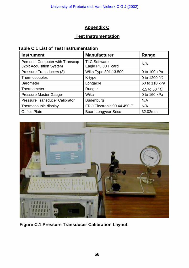
56

Appendix C

Test Instrumentation

Table C.1 List of Test InstrumentationInstrument Manufacturer RangePersonal Computer with Transcap32bit Acquisition System

TLC SoftwareEagle PC 30 F card N/A

Pressure Transducers (3) Wika Type 891.13.500 0 to 100 kPaThermocouples K-type 0 to 1200 Co

Barometer Longacre 60 to 110 kPaThermometer Rueger -15 to 60 Co

Pressure Master Gauge Wika 0 to 160 kPaPressure Transducer Calibrator Budenburg N/AThermocouple display ERO Electronic 90.44.450 E N/AOrifice Plate Boart Longyear Seco 32.02mm

Figure C.1 Pressure Transducer Calibration Layout.


57

Calibration of Pressure Transducers

Figure C.1 shows the personal computer with the sampling software and instrumentation.Next to it is the Budenburg calibrator with a pressure transducer fitted to the one port and theWika master gauge fitted to the other port.

Each pressure transducer connected to its cable and junction box was calibrated in turn. Thisconnection chain was not disturbed or swapped with other components during the testingphase in an effort to improve the accuracy of the results.

The transducers were calibrated against the master gauge at a range of pressures starting at0.0 kPa gauge pressure and finishing at 100 kPa gauge pressure. A polynomial function wasfitted to these values and used to correct the measured results after testing.


58

Master Gauge Calibration Certificate


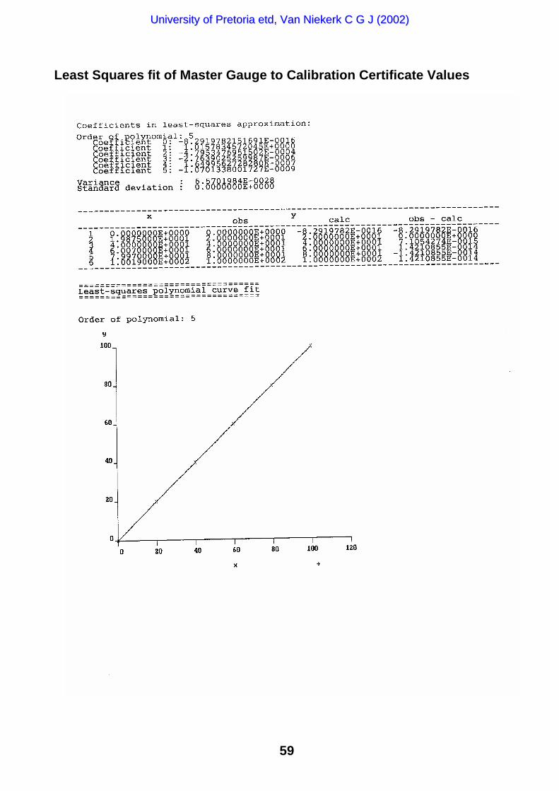
59

Least Squares fit of Master Gauge to Calibration Certificate Values


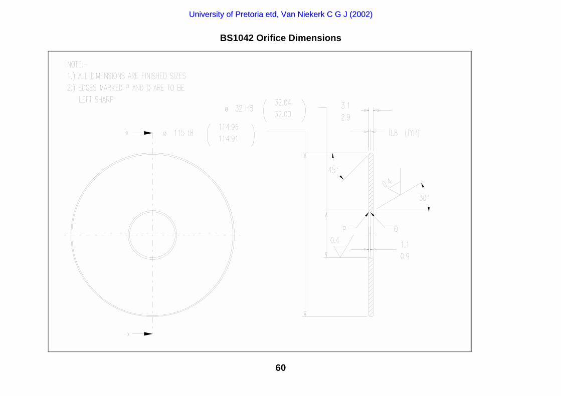
60

BS1042 Orifice Dimensions


61

Appendix D

Simulated Tailpipe Mass Flow and Pressure Ratio

Simulated Tailpipe Pressure Ratio

1

1.1

1.2

1.3

1.4

1.5

1.6

1.7

1.8

0 30 60 90 120 150 180 210 240 270 300 330 360

Crank Angle (Deg)

Pres

sure

Rat

io

Simulated Tailpipe Mass Flow

0

0.02

0.04

0.06

0.08

0.1

0.12

0.14

0.16

0 30 60 90 120 150 180 210 240 270 300 330 360

Crank Angle (Deg)

Mas

s Fl

ow (k

g/s)


62

Appendix E

Mass Flow Test Results

This Appendix contains the measured orifice test results, the corrected values for themeasured pressures and the calculated mass flow results for the 10 test pieces. Each testpiece was tested at 8 different reservoir pressures and three sets of measurements weretaken at each pressure. This resulted in 24 sets of results for each test piece and a totalnumber of 240 sets of test results.

The measured pressures were firstly corrected according to the pressure transducercalibration curves against the master gauge and then corrected according to the mastergauge calibration certificate. The calibrations are given in Appendix C.

The atmospheric conditions are given in Table E.1 and the test and mass flow resultsaccording to BS1042 in Table E.2 to Table E.11.

Table E.1 Atmospheric Conditions

Test piece Number Pressure (kPa) Temperature ( Co )

1 87.7 18.5

2 87.3 18.2

3 87.1 19.0

4 87.1 19.3

5 86.8 20.0

6 86.8 20.0

7 86.8 20.0

8 86.8 20.0

9 86.8 19.8

10 86.8 19.0


63

TABLE E.2 TEST PIECE 1, 10 DEGREE CONE, 21.8MM TAILPIPE, PLAIN TAILPIPE ENTRY

Test result file name Pum Pdm Prm Puc Pdc Prc Tu Tr m!ngd_10_051.ASC 8.2051 5.8399 5.1352 8.2805 6.0084 5.3468 21.3000 19.1000 0.03571ngd_10_052.ASC 8.1603 5.8028 5.1035 8.2351 5.9704 5.3140 21.3800 19.2000 0.03572ngd_10_053.ASC 8.1313 5.7796 5.0799 8.2057 5.9466 5.2895 21.4500 19.3000 0.03568ngd_10_101.ASC 15.5541 11.3168 10.0504 15.6975 11.5741 10.3593 20.9000 18.9000 0.05001ngd_10_102.ASC 15.5339 11.3037 10.0349 15.6772 11.5609 10.3437 21.0500 19.0000 0.04995ngd_10_103.ASC 15.5322 11.2945 10.0175 15.6755 11.5517 10.3262 21.2000 19.1000 0.04998ngd_10_151.ASC 22.1575 16.3739 14.6301 22.3149 16.6460 14.9320 20.0500 18.5000 0.06030ngd_10_152.ASC 22.0342 16.2829 14.5426 22.1917 16.5551 14.8452 20.3000 18.6500 0.06008ngd_10_153.ASC 22.0518 16.3005 14.5554 22.2093 16.5727 14.8579 20.5500 18.8000 0.06006ngd_10_201.ASC 29.9683 22.5614 20.2447 30.0968 22.8002 20.4665 19.5000 17.8000 0.07059ngd_10_202.ASC 29.9189 22.5035 20.1970 30.0477 22.7427 20.4197 19.7500 18.0000 0.07058ngd_10_203.ASC 29.8800 22.4637 20.1702 30.0091 22.7033 20.3934 20.0000 18.2000 0.07055ngd_10_301.ASC 42.9137 33.0355 29.8882 42.9372 33.1717 29.9219 18.4000 17.1000 0.08577ngd_10_302.ASC 42.7528 32.9034 29.7862 42.7778 33.0409 29.8218 18.9000 17.4000 0.08553ngd_10_303.ASC 42.6369 32.8086 29.6962 42.6629 32.9471 29.7334 19.4000 17.7000 0.08533ngd_10_401.ASC 55.4965 43.5552 39.7580 55.4267 43.6054 39.6568 16.9000 16.3000 0.09877ngd_10_402.ASC 55.0820 43.2588 39.4605 55.0144 43.3108 39.3618 17.4500 16.6300 0.09806ngd_10_403.ASC 54.8381 43.0620 39.2727 54.7718 43.1153 39.1757 18.0000 16.9500 0.09769ngd_10_501.ASC 67.4975 53.9069 49.5381 67.4017 53.9189 49.4059 15.2000 15.8000 0.10996ngd_10_502.ASC 67.0516 53.5550 49.2031 66.9555 53.5676 49.0704 15.8500 15.9300 0.10931ngd_10_503.ASC 66.7845 53.2883 48.9356 66.6882 53.3013 48.8026 16.5000 16.0500 0.10908ngd_10_601.ASC 80.3947 65.2991 60.3731 80.3327 65.3058 60.2891 14.5000 16.0000 0.12087ngd_10_602.ASC 80.4263 65.3135 60.4072 80.3644 65.3202 60.3234 14.7000 15.8500 0.12091ngd_10_603.ASC 80.5492 65.4364 60.5087 80.4877 65.4431 60.4255 14.9500 15.7000 0.12090

Pum = Upstream measured pressurePdm = Downstream measured pressurePrm = Measured reservoir pressurePuc = Upstream corrected pressurePdc = Downstream corrected pressurePrc = Corrected reservoir pressureTu = Upstream temperatureTr = Reservoir temperaturem! = Calculated mass flow


64





65





66





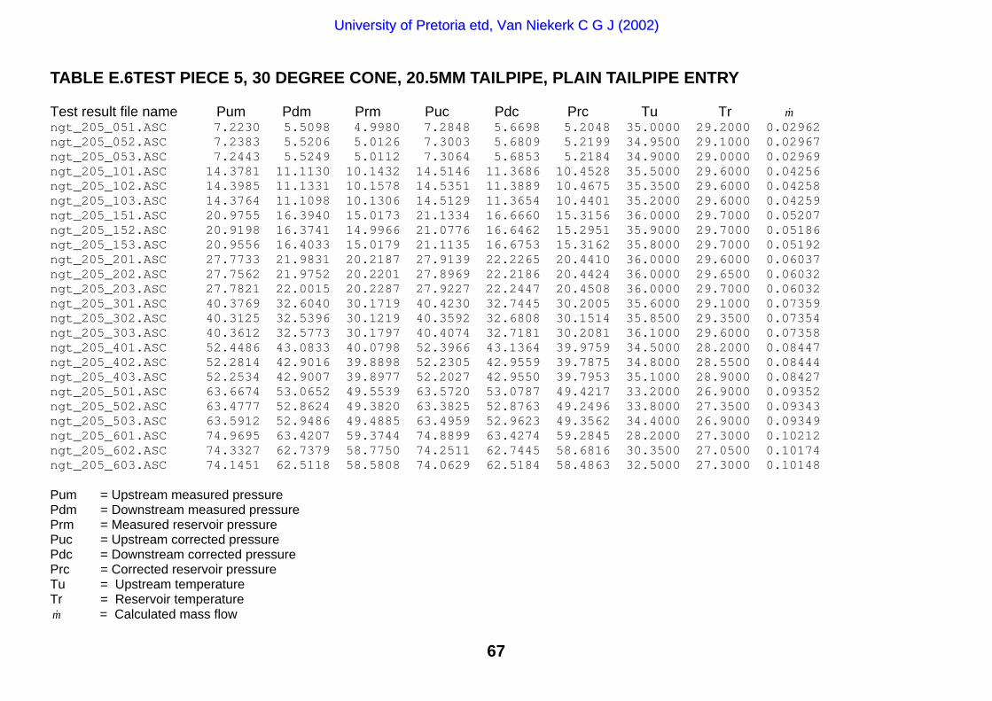
67

TABLE E.6TEST PIECE 5, 30 DEGREE CONE, 20.5MM TAILPIPE, PLAIN TAILPIPE ENTRY

Test result file name Pum Pdm Prm Puc Pdc Prc Tu Tr m!ngt_205_051.ASC 7.2230 5.5098 4.9980 7.2848 5.6698 5.2048 35.0000 29.2000 0.02962ngt_205_052.ASC 7.2383 5.5206 5.0126 7.3003 5.6809 5.2199 34.9500 29.1000 0.02967ngt_205_053.ASC 7.2443 5.5249 5.0112 7.3064 5.6853 5.2184 34.9000 29.0000 0.02969ngt_205_101.ASC 14.3781 11.1130 10.1432 14.5146 11.3686 10.4528 35.5000 29.6000 0.04256ngt_205_102.ASC 14.3985 11.1331 10.1578 14.5351 11.3889 10.4675 35.3500 29.6000 0.04258ngt_205_103.ASC 14.3764 11.1098 10.1306 14.5129 11.3654 10.4401 35.2000 29.6000 0.04259ngt_205_151.ASC 20.9755 16.3940 15.0173 21.1334 16.6660 15.3156 36.0000 29.7000 0.05207ngt_205_152.ASC 20.9198 16.3741 14.9966 21.0776 16.6462 15.2951 35.9000 29.7000 0.05186ngt_205_153.ASC 20.9556 16.4033 15.0179 21.1135 16.6753 15.3162 35.8000 29.7000 0.05192ngt_205_201.ASC 27.7733 21.9831 20.2187 27.9139 22.2265 20.4410 36.0000 29.6000 0.06037ngt_205_202.ASC 27.7562 21.9752 20.2201 27.8969 22.2186 20.4424 36.0000 29.6500 0.06032ngt_205_203.ASC 27.7821 22.0015 20.2287 27.9227 22.2447 20.4508 36.0000 29.7000 0.06032ngt_205_301.ASC 40.3769 32.6040 30.1719 40.4230 32.7445 30.2005 35.6000 29.1000 0.07359ngt_205_302.ASC 40.3125 32.5396 30.1219 40.3592 32.6808 30.1514 35.8500 29.3500 0.07354ngt_205_303.ASC 40.3612 32.5773 30.1797 40.4074 32.7181 30.2081 36.1000 29.6000 0.07358ngt_205_401.ASC 52.4486 43.0833 40.0798 52.3966 43.1364 39.9759 34.5000 28.2000 0.08447ngt_205_402.ASC 52.2814 42.9016 39.8898 52.2305 42.9559 39.7875 34.8000 28.5500 0.08444ngt_205_403.ASC 52.2534 42.9007 39.8977 52.2027 42.9550 39.7953 35.1000 28.9000 0.08427ngt_205_501.ASC 63.6674 53.0652 49.5539 63.5720 53.0787 49.4217 33.2000 26.9000 0.09352ngt_205_502.ASC 63.4777 52.8624 49.3820 63.3825 52.8763 49.2496 33.8000 27.3500 0.09343ngt_205_503.ASC 63.5912 52.9486 49.4885 63.4959 52.9623 49.3562 34.4000 26.9000 0.09349ngt_205_601.ASC 74.9695 63.4207 59.3744 74.8899 63.4274 59.2845 28.2000 27.3000 0.10212ngt_205_602.ASC 74.3327 62.7379 58.7750 74.2511 62.7445 58.6816 30.3500 27.0500 0.10174ngt_205_603.ASC 74.1451 62.5118 58.5808 74.0629 62.5184 58.4863 32.5000 27.3000 0.10148



68


Test result file name Pum Pdm Prm Puc Pdc Prc Tu Tr m!ngt_235_051.ASC 8.9227 5.9023 4.9898 9.0074 6.0724 5.1963 36.1000 29.1000 0.03996ngt_235_052.ASC 8.8595 5.8570 4.9431 8.9434 6.0260 5.1479 36.0000 29.0500 0.03984ngt_235_053.ASC 8.8206 5.8307 4.9342 8.9040 5.9990 5.1387 35.9000 29.0000 0.03975ngt_235_101.ASC 17.4241 11.7613 9.9847 17.5757 12.0221 10.2932 36.5000 29.3000 0.05681ngt_235_102.ASC 17.4528 11.7717 10.0015 17.6045 12.0326 10.3101 36.4000 29.3000 0.05692ngt_235_103.ASC 17.4750 11.7782 10.0179 17.6268 12.0391 10.3266 36.4000 29.3000 0.05700ngt_235_151.ASC 25.5092 17.5445 14.9808 25.6593 17.8136 15.2794 36.6000 28.9000 0.06964ngt_235_152.ASC 25.4498 17.4957 14.9421 25.6001 17.7650 15.2411 36.6000 29.0500 0.06958ngt_235_153.ASC 25.4796 17.5113 14.9673 25.6298 17.7805 15.2661 36.6000 29.2000 0.06965ngt_235_201.ASC 33.2814 23.2530 19.9681 33.3872 23.4859 20.1949 36.2000 28.3000 0.08055ngt_235_202.ASC 33.3765 23.3310 20.0382 33.4816 23.5633 20.2638 36.3500 28.5000 0.08063ngt_235_203.ASC 33.3138 23.2700 19.9842 33.4193 23.5028 20.2107 36.5000 28.7000 0.08058ngt_235_301.ASC 47.5287 34.1858 29.6451 47.5128 34.3108 29.6833 35.0000 27.2000 0.09795ngt_235_302.ASC 47.3863 34.0690 29.5257 47.3716 34.1951 29.5660 35.5000 27.5500 0.09773ngt_235_303.ASC 47.4617 34.1212 29.5895 47.4464 34.2468 29.6287 36.0000 27.7000 0.09776ngt_235_401.ASC 62.2014 46.0276 40.3349 62.1081 46.0645 40.2290 30.6000 25.5000 0.11410ngt_235_402.ASC 62.1100 45.9212 40.2313 62.0169 45.9586 40.1262 32.2000 25.9500 0.11382ngt_235_403.ASC 62.1368 45.9008 40.2281 62.0436 45.9383 40.1231 33.8000 26.4000 0.11369ngt_235_501.ASC 74.1609 56.1964 49.7293 74.0788 56.2054 49.5974 27.0000 25.1000 0.12575ngt_235_502.ASC 73.6332 55.5962 49.1127 73.5495 55.6058 48.9799 28.1000 25.3500 0.12553ngt_235_503.ASC 73.5620 55.5099 48.9991 73.4781 55.5196 48.8662 29.2000 25.6000 0.12532ngt_235_601.ASC 86.8294 67.2460 59.8879 86.7768 67.2526 59.8010 27.1000 26.1000 0.13640ngt_235_602.ASC 86.2691 66.8123 59.3452 86.2168 66.8189 59.2551 27.1500 25.8000 0.13575ngt_235_603.ASC 85.9102 66.5395 58.9911 85.8580 66.5462 58.8989 27.2000 25.5000 0.13531



69

TABLE E.8 TEST PIECE 7, 30 DEGREE CONE, 22.0MM TAILPIPE, 20.5MM RESTRICTED TAILPIPE ENTRY

Test result file name Pum Pdm Prm Puc Pdc Prc Tu Tr m!ngr_220_051.ASC 8.0256 5.8508 5.2077 8.0986 6.0196 5.4218 35.7000 30.8000 0.03363ngr_220_052.ASC 8.0595 5.8753 5.2348 8.1329 6.0447 5.4498 35.6000 30.7500 0.03372ngr_220_053.ASC 8.0683 5.8895 5.2435 8.1419 6.0593 5.4588 35.5000 30.7000 0.03368ngr_220_101.ASC 15.5265 11.5225 10.3126 15.6698 11.7815 10.6232 36.4000 31.5000 0.04738ngr_220_102.ASC 15.5175 11.5165 10.3003 15.6608 11.7755 10.6108 36.2000 31.4000 0.04738ngr_220_103.ASC 15.5291 11.5352 10.3170 15.6724 11.7943 10.6276 36.7000 31.8000 0.04730ngr_220_151.ASC 22.6430 17.0550 15.3465 22.7999 17.3256 15.6415 36.9000 31.8000 0.05781ngr_220_152.ASC 22.5758 16.9944 15.2752 22.7328 17.2651 15.5709 36.8000 31.8000 0.05777ngr_220_153.ASC 22.6087 17.0306 15.3200 22.7656 17.3012 15.6152 36.7000 31.8000 0.05777ngr_220_201.ASC 29.1438 22.2792 20.1420 29.2772 22.5202 20.3657 37.1000 31.8000 0.06586ngr_220_202.ASC 29.1315 22.2661 20.1374 29.2650 22.5073 20.3612 37.0500 31.9000 0.06587ngr_220_203.ASC 29.0964 22.2058 20.0726 29.2301 22.4474 20.2975 37.0000 32.0000 0.06598ngr_220_301.ASC 41.7554 32.7405 29.8845 41.7892 32.8797 29.9183 37.1000 31.8000 0.07926ngr_220_302.ASC 41.7454 32.7264 29.8817 41.7793 32.8657 29.9155 37.1500 31.9000 0.07926ngr_220_303.ASC 41.6899 32.6923 29.8334 41.7243 32.8319 29.8681 37.2000 32.0000 0.07915ngr_220_401.ASC 53.7598 43.1741 39.8017 53.6997 43.2267 39.7001 37.0000 31.6000 0.08964ngr_220_402.ASC 53.7028 43.1137 39.7518 53.6430 43.1666 39.6506 37.0500 31.7000 0.08963ngr_220_403.ASC 53.7187 43.1276 39.7575 53.6588 43.1804 39.6563 37.1000 31.8000 0.08964ngr_220_501.ASC 65.5006 53.7335 50.0310 65.4041 53.7458 49.8996 36.5000 31.0000 0.09842ngr_220_502.ASC 65.3469 53.6522 49.9550 65.2505 53.6646 49.8235 36.7500 31.2500 0.09804ngr_220_503.ASC 65.3930 53.6980 49.9962 65.2965 53.7103 49.8648 37.0000 31.5000 0.09801ngr_220_601.ASC 76.3447 63.7478 59.7434 76.2696 63.7545 59.6557 35.0000 29.6000 0.10577ngr_220_602.ASC 76.0320 63.4490 59.4812 75.9558 63.4557 59.3919 35.5500 30.1000 0.10551ngr_220_603.ASC 76.0034 63.3941 59.4548 75.9272 63.4008 59.3654 36.1000 30.6000 0.10551



70

TABLE E.9 TEST PIECE 8, 30 DEGREE CONE, 23.5MM TAILPIPE, 20.5MM RESTRICTED TAILPIPE ENTRY

Test result file name Pum Pdm Prm Puc Pdc Prc Tu Tr m!ngr_235_051.ASC 8.1824 5.6793 4.9370 8.2575 5.8437 5.1416 36.6000 32.0000 0.03616ngr_235_052.ASC 8.1443 5.6550 4.9092 8.2189 5.8188 5.1128 36.4500 31.9000 0.03606ngr_235_053.ASC 8.1677 5.6735 4.9239 8.2426 5.8378 5.1280 36.3000 31.8000 0.03611ngr_235_101.ASC 16.2459 11.5513 10.1031 16.3928 11.8105 10.4124 37.2000 32.6000 0.05142ngr_235_102.ASC 16.2475 11.5480 10.1083 16.3944 11.8072 10.4176 37.1000 32.5000 0.05146ngr_235_103.ASC 16.3209 11.6098 10.1626 16.4681 11.8695 10.4723 37.0000 32.4000 0.05155ngr_235_151.ASC 23.8995 17.3823 15.3392 24.0542 17.6519 15.6342 37.6000 32.9000 0.06263ngr_235_152.ASC 23.8927 17.3581 15.3165 24.0474 17.6278 15.6118 37.5500 32.9000 0.06271ngr_235_153.ASC 23.9805 17.4419 15.3864 24.1350 17.7113 15.6809 37.5000 32.9000 0.06276ngr_235_201.ASC 30.1369 22.3211 19.8299 30.2644 22.5618 20.0592 37.9000 33.0000 0.07034ngr_235_202.ASC 30.0472 22.2330 19.7490 30.1752 22.4744 19.9797 37.8500 33.0500 0.07031ngr_235_203.ASC 30.0938 22.2866 19.8001 30.2216 22.5276 20.0299 37.8000 33.1000 0.07030ngr_235_301.ASC 42.8806 32.9328 29.7246 42.9044 33.0701 29.7613 37.8000 32.9000 0.08335ngr_235_302.ASC 42.7629 32.8297 29.6218 42.7878 32.9680 29.6604 38.0000 33.0500 0.08322ngr_235_303.ASC 42.6459 32.7160 29.5033 42.6718 32.8554 29.5441 38.0000 33.2000 0.08317ngr_235_401.ASC 55.2009 43.9371 40.2580 55.1327 43.9851 40.1527 37.5000 32.8000 0.09275ngr_235_402.ASC 55.2475 43.9536 40.2952 55.1790 44.0015 40.1896 37.6000 32.9000 0.09287ngr_235_403.ASC 55.2054 43.9164 40.2554 55.1372 43.9645 40.1502 37.7000 33.0000 0.09282ngr_235_501.ASC 66.6399 54.3671 50.4083 66.5436 54.3783 50.2777 36.7000 32.2000 0.10078ngr_235_502.ASC 66.6034 54.3376 50.3754 66.5071 54.3489 50.2447 36.9500 32.3500 0.10070ngr_235_503.ASC 66.4918 54.2122 50.2583 66.3954 54.2237 50.1274 37.2000 32.5000 0.10068ngr_235_601.ASC 77.1695 64.0140 59.7918 77.0971 64.0207 59.7044 35.1000 31.3000 0.10826ngr_235_602.ASC 77.0941 63.9357 59.7110 77.0215 63.9424 59.6231 35.7000 31.5500 0.10814ngr_235_603.ASC 76.9227 63.7852 59.5590 76.8495 63.7919 59.4702 36.3000 31.8000 0.10789



71

TABLE E.10 TEST PIECE 9, 30 DEGREE CONE, 22.0MM TAILPIPE, 20.5MM VENTURI TAILPIPE ENTRY

Test result file name Pum Pdm Prm Puc Pdc Prc Tu Tr m!ngv_220_051.ASC 8.2181 5.9072 5.2140 8.2937 6.0774 5.4283 36.0000 31.0000 0.03472ngv_220_052.ASC 8.2448 5.9283 5.2349 8.3207 6.0991 5.4499 35.8000 30.8000 0.03478ngv_220_053.ASC 8.2634 5.9381 5.2477 8.3396 6.1091 5.4631 35.6000 30.6000 0.03486ngv_220_101.ASC 15.6250 11.4236 10.1306 15.7688 11.6818 10.4401 36.5000 31.5000 0.04856ngv_220_102.ASC 15.6041 11.3894 10.0934 15.7478 11.6473 10.4026 36.4000 31.4000 0.04864ngv_220_103.ASC 15.5755 11.3828 10.0936 15.7191 11.6407 10.4028 36.3000 31.0000 0.04851ngv_220_151.ASC 22.9209 17.0007 15.1486 23.0774 17.2714 15.4456 37.0000 31.7000 0.05954ngv_220_152.ASC 22.9060 16.9790 15.1342 23.0625 17.2498 15.4313 37.0000 31.7000 0.05957ngv_220_153.ASC 22.8276 16.9062 15.0665 22.9843 17.1772 15.3643 37.0000 31.7000 0.05952ngv_220_201.ASC 29.5871 22.2180 19.8965 29.7179 22.4595 20.1246 37.0000 31.7000 0.06830ngv_220_202.ASC 29.6158 22.2705 19.9331 29.7465 22.5116 20.1605 37.0000 31.7500 0.06821ngv_220_203.ASC 29.6285 22.2813 19.9537 29.7591 22.5223 20.1808 37.0000 31.8000 0.06822ngv_220_301.ASC 43.0193 33.1857 30.0081 43.0419 33.3204 30.0396 36.6000 31.3000 0.08310ngv_220_302.ASC 42.9573 33.1247 29.9679 42.9804 33.2601 30.0002 36.8000 31.5000 0.08304ngv_220_303.ASC 42.9472 33.1211 29.9646 42.9704 33.2565 29.9969 37.0000 31.7000 0.08299ngv_220_401.ASC 54.3755 43.4708 39.9419 54.3118 43.5215 39.8392 35.0000 30.4000 0.09142ngv_220_402.ASC 54.3006 43.4023 39.8699 54.2373 43.4535 39.7678 35.6000 29.6500 0.09128ngv_220_403.ASC 54.2766 43.3497 39.8433 54.2135 43.4012 39.7414 35.6000 30.9000 0.09139ngv_220_501.ASC 65.5254 53.7436 49.9340 65.4289 53.7558 49.8024 32.4000 29.3000 0.09914ngv_220_502.ASC 65.4294 53.6354 49.8348 65.3329 53.6478 49.7031 33.3000 29.0000 0.09901ngv_220_503.ASC 65.5519 53.7274 49.9223 65.4554 53.7397 49.7907 34.2000 30.0000 0.09903ngv_220_601.ASC 76.8598 64.2513 60.1565 76.7864 64.2580 60.0712 28.5000 28.4000 0.10713ngv_220_602.ASC 76.9190 64.2441 60.1580 76.8458 64.2508 60.0727 29.0000 28.5000 0.10733ngv_220_603.ASC 76.8634 64.1973 60.1006 76.7900 64.2040 60.0150 29.5000 28.6000 0.10719



72

TABLE E.11 TEST PIECE 10, 30 DEGREE CONE, 23.5MM TAILPIPE, 20.5MM VENTURI TAILPIPE ENTRY

Test result file name Pum Pdm Prm Puc Pdc Prc Tu Tr m!ngv_235_051.ASC 8.7412 5.8521 4.9717 8.8236 6.0210 5.1775 36.1000 31.5000 0.03904ngv_235_052.ASC 8.6854 5.8105 4.9424 8.7671 5.9783 5.1472 36.3500 31.3500 0.03892ngv_235_053.ASC 8.6852 5.8154 4.9473 8.7669 5.9833 5.1522 36.6000 31.2000 0.03886ngv_235_101.ASC 17.5578 11.9859 10.2339 17.7099 12.2483 10.5440 36.6000 32.0000 0.05638ngv_235_102.ASC 17.5621 11.9929 10.2478 17.7142 12.2553 10.5580 36.5500 31.9500 0.05638ngv_235_103.ASC 17.5447 11.9769 10.2285 17.6967 12.2392 10.5386 36.5000 31.9000 0.05637ngv_235_151.ASC 25.5866 17.8479 15.3406 25.7364 18.1159 15.6356 36.9000 32.1000 0.06867ngv_235_152.ASC 25.5802 17.8555 15.3412 25.7301 18.1235 15.6362 36.9000 32.1500 0.06861ngv_235_153.ASC 25.5359 17.7941 15.2884 25.6859 18.0623 15.5840 36.9000 32.2000 0.06867ngv_235_201.ASC 31.9698 22.9354 19.9947 32.0851 23.1711 20.2210 36.8000 32.0000 0.07614ngv_235_202.ASC 31.9753 22.9528 19.9966 32.0906 23.1883 20.2229 36.9000 32.1000 0.07608ngv_235_203.ASC 31.9501 22.9166 19.9757 32.0656 23.1524 20.2024 37.0000 32.2000 0.07611ngv_235_301.ASC 43.3577 33.3270 30.0643 43.3773 33.4604 30.0948 36.2000 31.8000 0.08405ngv_235_302.ASC 43.3598 33.3355 30.0778 43.3794 33.4688 30.1081 36.4000 31.9500 0.08400ngv_235_303.ASC 43.4334 33.4235 30.1510 43.4524 33.5559 30.1799 36.6000 32.1000 0.08394ngv_235_401.ASC 54.2550 43.3763 39.8441 54.1920 43.4276 39.7422 35.0000 31.2000 0.09127ngv_235_402.ASC 53.9865 43.1165 39.5847 53.9250 43.1694 39.4850 35.5000 31.3500 0.09107ngv_235_403.ASC 53.9302 43.0866 39.5483 53.8691 43.1397 39.4489 36.0000 31.5000 0.09088ngv_235_501.ASC 65.5752 53.8089 50.0037 65.4787 53.8210 49.8723 33.8000 30.8000 0.09887ngv_235_502.ASC 65.4238 53.6633 49.8536 65.3273 53.6757 49.7219 34.3000 30.9500 0.09871ngv_235_503.ASC 65.5476 53.7476 49.9538 65.4511 53.7598 49.8223 34.8000 31.1000 0.09884ngv_235_601.ASC 77.0565 64.3279 60.2122 76.9838 64.3346 60.1272 34.8000 31.1000 0.10658ngv_235_602.ASC 77.3522 64.6187 60.5033 77.2804 64.6254 60.4201 36.0500 31.0500 0.10649ngv_235_603.ASC 77.5739 64.8438 60.7464 77.5029 64.8505 60.6646 37.3000 31.0000 0.10635



73

Appendix F

Cd Calculations and Maps

Creation of Cd-Maps

The Cd-Values for the 24 test points for each test piece was calculated for 4 area ratiosspanning the mesh lengths from 5mm to 25 mm using program FLOWPROG.

For each area ratio a second order polynomial was fitted using a least squares fit. Thesefour polynomials represented four sections through the Cd-map at constant area ratios andas a function of pressure ratio. The 2R -values is given in Table F.1. A third orderpolynomial was fitted to each of the three coefficients of the four polynomials. This allowsthe construction of a polynomial for each area ratio required to create the Cd-map.

These polynomials were programmed into FORTRAN programs and the Cd-maps for thefirst four test pieces were an output in a text file in matrix format for each. It was notnecessary to create Cd-maps for the rest of the test pieces because the requiredinformation could be obtained from graphs at a fixed area ratio. (Refer to the discussions inparagraph 4.5.3 to paragraph 4.6)

The second order polynomial for the Cd-value is in the following format:2

210 xaxaaCd ++=And the third order polynomials for the coefficients:

33

2210 ybybybba iiiii +++=

The b coefficient values are given in Table F.2.

Table F.1: 2R -Values for ia - coefficients

10 Deg 20 Deg 30 Deg 40 Deg

Ar 2R Ar 2R Ar 2R Ar 2R

1.05 0.9950 1.10 0.9960 1.15 0.9900 1.20 0.9944

1.10 0.9944 1.20 0.9981 1.30 0.9933 1.45 0.9966

1.15 0.9941 1.30 0.9973 1.45 0.9944 1.70 0.9968

1.20 0.9933 1.40 0.9973 1.60 0.9952 1.95 0.9966


74

Table F.2 Coefficient ijb values

Test Piece0ib 1ib 2ib 3ib

0a -1052.3515 2651.5077 -2232.7000 627.7333

1a 2261.9171 -5684.1343 4775.7200 -1339.8667

1

10deg

2a -1212.9117 3043.6833 -2552.9000 715.0667

0a -208.7952 460.8358 -341.7900 84.8167

1a 466.4534 -1025.8242 759.4500 -188.1833

2

20deg

2a -255.2668 561.0048 -424.4700 102.5167

0a -84.4488 167.0196 -111.7022 25.0074

1a 194.2309 -382.3848 255.4837 -57.1605

3

30deg

2a -109.241 215.7780 -144.0881 32.2272

0a -26.7475 42.8133 -23.6664 4.3787

1a 62.7314 -99.1487 54.6626 -10.0896

4

40deg

2a -35.4456 56.6835 -31.2317 5.7621


75

Map and Data for 10 Degree Cone

1 1.05 1.1 1.15 1.2 1.25 1.3 1.35

1.05

1.1

1.15

1.2

0.6

0.65

0.7

0.75

0.8

0.85

0.9

0.95

1

Pressure Ratio

Cd-Map for 10 Degree Cone

0.95-1

0.9-0.95

0.85-0.9

0.8-0.85

0.75-0.8

0.7-0.75

0.65-0.7

0.6-0.65

Pressure Area Ratio

Ratio 1.05 1.1 1.15 1.2

1 0.767 0.766 0.765 0.764

1.05 0.832 0.819 0.81 0.806

1.1 0.882 0.862 0.849 0.844

1.15 0.916 0.897 0.883 0.877

1.2 0.934 0.923 0.911 0.906

1.25 0.949 0.941 0.933 0.93

1.3 0.959 0.953 0.949 0.949

1.35 0.964 0.964 0.964 0.964


76


1.05

1.15

1.25

1.35 1

1.05 1.

1

1.15 1.

2

1.25 1.

3

1.35

0.6

0.65

0.7

0.75

0.8

0.85

0.9

0.95

1

Cd



0.95-1

0.9-0.95

0.85-0.9

0.8-0.85

0.75-0.8

0.7-0.75

0.65-0.7

0.6-0.65

Pressure Area Ratio

Ratio 1.05 1.1 1.15 1.2 1.25 1.3 1.35 1.4

1 0.742 0.738 0.736 0.736 0.736 0.737 0.736 0.735

1.05 0.817 0.802 0.792 0.786 0.783 0.781 0.779 0.775

1.1 0.874 0.853 0.839 0.83 0.824 0.82 0.816 0.812

1.15 0.913 0.892 0.877 0.866 0.859 0.854 0.85 0.845

1.2 0.935 0.918 0.905 0.895 0.888 0.883 0.878 0.873

1.25 0.938 0.931 0.924 0.918 0.912 0.907 0.903 0.898

1.3 0.942 0.939 0.935 0.933 0.93 0.927 0.922 0.919

1.35 0.943 0.943 0.943 0.943 0.943 0.941 0.938 0.936


77


1.05

1.15

1.25

1.35

1.45

1.55 1

1.05 1.

11.

15 1.2

1.25 1.

31.

35

0.6

0.65

0.7

0.75

0.8

0.85

0.9

0.95

1

Cd



0.95-1

0.9-0.95

0.85-0.9

0.8-0.85

0.75-0.8

0.7-0.75

0.65-0.7

0.6-0.65

Pressure Area Ratio

Ratio 1.05 1.1 1.15 1.2 1.25 1.3 1.35 1.4 1.45 1.5 1.55 1.6

1 0.722 0.722 0.722 0.722 0.722 0.722 0.721 0.72 0.72 0.719 0.719 0.719

1.05 0.797 0.789 0.782 0.776 0.772 0.768 0.766 0.764 0.762 0.761 0.76 0.758

1.1 0.856 0.842 0.831 0.822 0.815 0.81 0.806 0.802 0.8 0.798 0.796 0.794

1.15 0.898 0.882 0.87 0.859 0.851 0.845 0.84 0.836 0.834 0.831 0.829 0.826

1.2 0.924 0.91 0.898 0.888 0.881 0.875 0.87 0.866 0.863 0.86 0.857 0.855

1.25 0.933 0.924 0.916 0.909 0.903 0.898 0.894 0.89 0.887 0.885 0.882 0.88

1.3 0.933 0.925 0.924 0.922 0.919 0.916 0.913 0.91 0.907 0.905 0.903 0.901

1.35 0.933 0.929 0.928 0.928 0.928 0.928 0.928 0.926 0.923 0.921 0.919 0.918


78


1.05

1.2

1.35

1.5

1.65

1.8 1 1.1 1.2 1.3

0.6

0.65

0.7

0.75

0.8

0.85

0.9

0.95

1

Cd

Area Ratio

Pressure Ratio


0.95-1

0.9-0.95

0.85-0.9

0.8-0.85

0.75-0.8

0.7-0.75

0.65-0.7

0.6-0.65

Pressure Area Ratio

Ratio 1.05 1.1 1.15 1.2 1.25 1.3 1.35 1.4 1.45 1.5 1.55 1.6 1.65 1.7 1.75 1.8 1.85

1 0.703 0.704 0.705 0.705 0.705 0.705 0.705 0.705 0.704 0.703 0.703 0.702 0.702 0.701 0.701 0.7 0.7

1.05 0.775 0.771 0.767 0.764 0.761 0.758 0.755 0.752 0.75 0.748 0.747 0.745 0.744 0.743 0.743 0.742 0.742

1.1 0.833 0.826 0.819 0.813 0.807 0.802 0.798 0.794 0.791 0.788 0.786 0.784 0.782 0.781 0.78 0.78 0.779

1.15 0.877 0.868 0.86 0.852 0.846 0.84 0.835 0.83 0.827 0.823 0.82 0.818 0.816 0.815 0.814 0.813 0.813

1.2 0.906 0.898 0.89 0.883 0.876 0.87 0.865 0.861 0.857 0.853 0.85 0.848 0.846 0.844 0.843 0.843 0.842

1.25 0.922 0.915 0.909 0.903 0.898 0.893 0.889 0.885 0.881 0.878 0.876 0.873 0.871 0.87 0.869 0.868 0.867

1.3 0.923 0.92 0.917 0.915 0.912 0.909 0.906 0.903 0.901 0.898 0.896 0.894 0.892 0.891 0.89 0.889 0.888

1.35 0.923 0.921 0.92 0.919 0.918 0.917 0.917 0.916 0.915 0.913 0.912 0.91 0.909 0.908 0.906 0.906 0.906


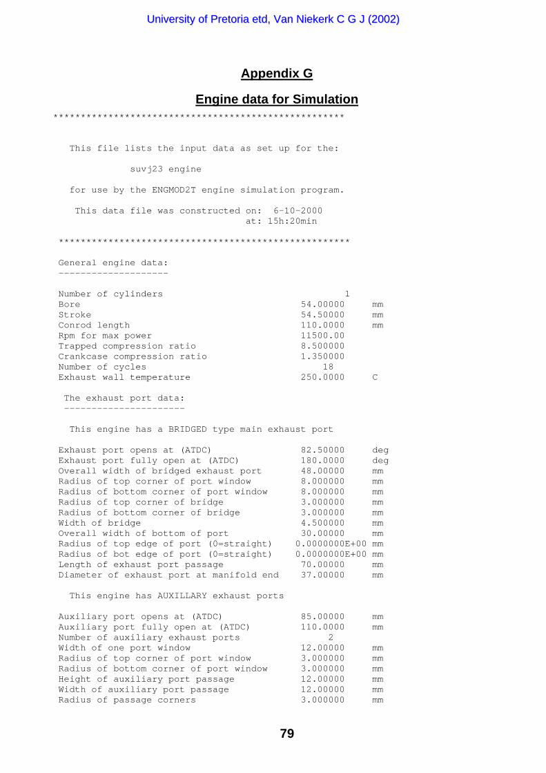
79

Appendix G

Engine data for Simulation***************************************************** This file lists the input data as set up for the: suvj23 engine for use by the ENGMOD2T engine simulation program. This data file was constructed on: 6-10-2000 at: 15h:20min ***************************************************** General engine data: -------------------- Number of cylinders 1 Bore 54.00000 mm Stroke 54.50000 mm Conrod length 110.0000 mm Rpm for max power 11500.00 Trapped compression ratio 8.500000 Crankcase compression ratio 1.350000 Number of cycles 18 Exhaust wall temperature 250.0000 C The exhaust port data: ---------------------- This engine has a BRIDGED type main exhaust port Exhaust port opens at (ATDC) 82.50000 deg Exhaust port fully open at (ATDC) 180.0000 deg Overall width of bridged exhaust port 48.00000 mm Radius of top corner of port window 8.000000 mm Radius of bottom corner of port window 8.000000 mm Radius of top corner of bridge 3.000000 mm Radius of bottom corner of bridge 3.000000 mm Width of bridge 4.500000 mm Overall width of bottom of port 30.00000 mm Radius of top edge of port (0=straight) 0.0000000E+00 mm Radius of bot edge of port (0=straight) 0.0000000E+00 mm Length of exhaust port passage 70.00000 mm Diameter of exhaust port at manifold end 37.00000 mm This engine has AUXILLARY exhaust ports Auxiliary port opens at (ATDC) 85.00000 mm Auxiliary port fully open at (ATDC) 110.0000 mm Number of auxiliary exhaust ports 2 Width of one port window 12.00000 mm Radius of top corner of port window 3.000000 mm Radius of bottom corner of port window 3.000000 mm Height of auxiliary port passage 12.00000 mm Width of auxiliary port passage 12.00000 mm Radius of passage corners 3.000000 mm


80

Transfer port data: ------------------- Transfer port opens at (ATDC) 114.0000 deg Transfer port is fully open at (ATDC) 180.0000 deg Number of transfer ports 5 Width of one port 19.00000 mm Radius of top corner of port window 2.000000 mm Radius of bottom corner of port window 2.000000 mm Type of scavenging model YAM12 Intake port type and data: -------------------------- This engine has a REED VALVE type intake port The reed petal material is GLASSFIBRE Number of reed valve petals 6 Thickness of petals 0.420000 mm Width of petals 22.70000 mm Free length of petals 37.00000 mm Young’s modulus 21.50000 MPa Density of petal material 1850.000 Kg/m^3 Damping factor for mode 1 0.2500000 Damping factor for mode 2 0.1500000 Included angle of reed valve block 47.00000 deg Diameter of port in reed valve block 34.00000 mm Maximum tip displacement 13.00000 mm Width of port in reed valve block 19.00000 mm Length of port in reed valve block 32.00000 mm Corner radius of port in reed valve block 2.000000 mm There is no curved stop plate The EXHAUST system has the following characteristics: ---------------------------------------------------- The exhaust system layout has: An individual pipe per cylinder and, a tuned pipe collector. The data for pipe no 1The length of pipe section 1 = 200.0 mmThe length of pipe section 2 = 235.0 mmThe length of pipe section 3 = 60.0 mmThe length of pipe section 4 = 90.0 mmThe length of pipe section 5 = 205.0 mmThe length of pipe section 6 = 200.0 mm The data for pipe no 1The diameter of pipe section 0 = 37.0 mmThe diameter of pipe section 1 = 48.0 mmThe diameter of pipe section 2 = 95.0 mmThe diameter of pipe section 3 = 118.0 mmThe diameter of pipe section 4 = 118.0 mmThe diameter of pipe section 5 = 22.2 mmThe diameter of pipe section 6 = 22.2 mm


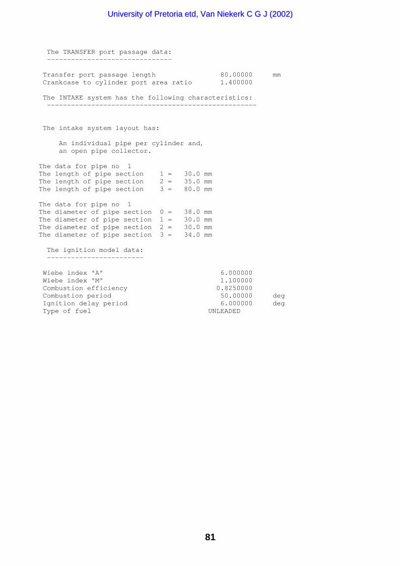
81

The TRANSFER port passage data: ------------------------------- Transfer port passage length 80.00000 mm Crankcase to cylinder port area ratio 1.400000 The INTAKE system has the following characteristics: ---------------------------------------------------- The intake system layout has: An individual pipe per cylinder and, an open pipe collector. The data for pipe no 1The length of pipe section 1 = 30.0 mmThe length of pipe section 2 = 35.0 mmThe length of pipe section 3 = 80.0 mm The data for pipe no 1The diameter of pipe section 0 = 38.0 mmThe diameter of pipe section 1 = 30.0 mmThe diameter of pipe section 2 = 30.0 mmThe diameter of pipe section 3 = 34.0 mm The ignition model data: ------------------------ Wiebe index "A" 6.000000 Wiebe index "M" 1.100000 Combustion efficiency 0.8250000 Combustion period 50.00000 deg Ignition delay period 6.000000 deg Type of fuel UNLEADED


82

Appendix H

Dynamometer Results


83

Appendix I

Description of Program EngMod2T

I.1 INTRODUCTION

Program EngMod2T is a one-dimensional gasdynamics based program thatsimulates the flow, combustion and scavenging in a two stroke engine to predict itspower output. It was created as an alternative to dynamometer testing of highperformance (motorcycle grand prix level) engines. Testing of these engines is acostly and expensive affair. Engine components seldom have a life of more than500 kilometres or 2 hours. Stabilizing the engine on the dynamometer at the correctexhaust pipe temperatures is a complex operation that uses a large portion of theactual testing time. Testing at the correct temperature is crucial because theresonant frequency of the exhaust system is dependant on the temperature.

As input it uses the engine physical characteristics for all the ducts, ports andplenums. It further uses model parameters based on test results for the combustionand scavenging models. The duct and plenum wall temperatures are also an input.From these inputs the pressures and temperatures in al the ducts and plenums arecalculated as a function of time.

I.2 HISTORY

EngMod2T started as a simple Method of Characteristics based program in 1985. Itcould simulate a single cylinder piston port engine using a simple heat release ratecombustion model and an empirical scavenging model. By 1990 a sophisticatedreed valve based intake system was added as an option and the port subroutineswere updated to accommodate most of the typical geometries used in modernengines. At this stage one of the biggest drawbacks was the fact that the exhaustpipe temperature was a user defined input.

Various newer methods like the Lax-Wendroff Two Step with Flux Correction andothers were investigated to get around this problem. In 1991 a new method waspublished by Professor Gordon P Blair of the Queen’s University of Belfast (Blair,1991) that not only calculated the temperature at each point in a duct but also itschemical composition as an inherent part of the method. (Professor Blair was theleader of a research group at that university that specialized in two-stroke enginegasdynamics and simulation starting in the mid 1960’s) EngMod2T was updated touse this new method, known as the GPB-method and has continually been updatedsince then as more sophisticated combustion, scavenging and boundary conditionmodels were developed.

In 1998 it was further expanded to allow the simulation of engines with up to fourcylinders and complex branch type intake and exhaust systems.


84

I.3 DESCRIPTION OF ENGMOD2T

To aid in the preparation of the input data a pre-processing program wasdeveloped. For a new project it prompts the user for the input data and it allowsediting of the data for an existing project. The data in Appendix G is a printout fromthis program.

Each pipe or duct in the intake or exhaust system can be divided into 20 segmentsof which each can be area expanding, contracting or constant. This allows theconstruction of multi-stage diffusers and reverse cones.

I.3.1 Exhaust System

Three configurations of exhaust manifold systems can be analysed:

• Individual pipes on each cylinder.

• Branch manifold type. This is a manifold where all the header pipes join in acommon junction followed by a common collector pipe.

• Log manifold type. This type has common collector pipe with each headerjoining it independently.

From the manifold outlet (or in the case of the individual pipe configuration from theexhaust port outlet) a further three options exists:

• Tuned pipes. This is the so called “expansion box” type of exhaust pipe asused on the high performance engines. It automatically applies the restrictionsubroutine to the tail pipe entrance. (This is the enhancement developedin this dissertation)

• Open pipe. This is a plain type outlet pipe although it can be configured to bethe same as the tuned pipe but with an important difference. It does notapply the restriction subroutine to the tail pipe entry.

• Box type. The collector pipe exits into a plenum or “box” with an additionalpipe exiting from the plenum. This is a typical system as used on industrialand outboard engines.

I.3.2 Intake System

The intake system is largely a mirror image of the exhaust system that also allowsthe same three manifold systems. Each of these systems can be open to theatmosphere or pass through a plenum. This plenum can be an air box or an air filterbox.


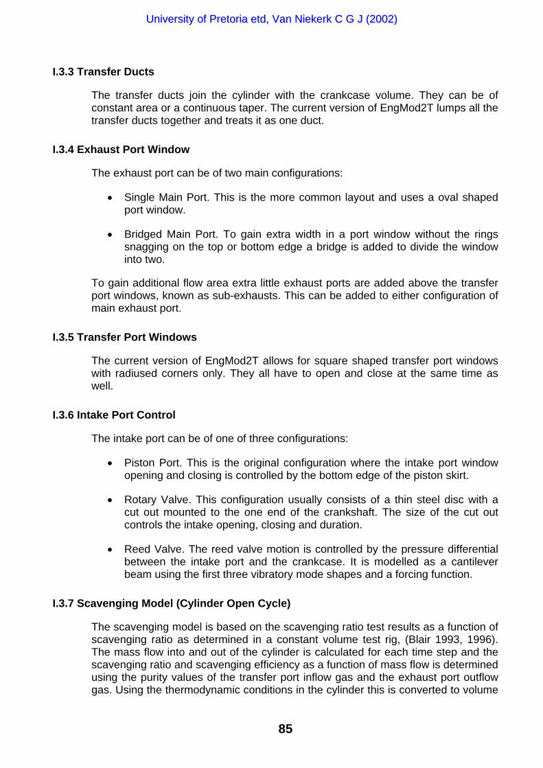
85

I.3.3 Transfer Ducts

The transfer ducts join the cylinder with the crankcase volume. They can be ofconstant area or a continuous taper. The current version of EngMod2T lumps all thetransfer ducts together and treats it as one duct.

I.3.4 Exhaust Port Window

The exhaust port can be of two main configurations:

• Single Main Port. This is the more common layout and uses a oval shapedport window.

• Bridged Main Port. To gain extra width in a port window without the ringssnagging on the top or bottom edge a bridge is added to divide the windowinto two.

To gain additional flow area extra little exhaust ports are added above the transferport windows, known as sub-exhausts. This can be added to either configuration ofmain exhaust port.

I.3.5 Transfer Port Windows

The current version of EngMod2T allows for square shaped transfer port windowswith radiused corners only. They all have to open and close at the same time aswell.

I.3.6 Intake Port Control

The intake port can be of one of three configurations:

• Piston Port. This is the original configuration where the intake port windowopening and closing is controlled by the bottom edge of the piston skirt.

• Rotary Valve. This configuration usually consists of a thin steel disc with acut out mounted to the one end of the crankshaft. The size of the cut outcontrols the intake opening, closing and duration.

• Reed Valve. The reed valve motion is controlled by the pressure differentialbetween the intake port and the crankcase. It is modelled as a cantileverbeam using the first three vibratory mode shapes and a forcing function.

I.3.7 Scavenging Model (Cylinder Open Cycle)

The scavenging model is based on the scavenging ratio test results as a function ofscavenging ratio as determined in a constant volume test rig, (Blair 1993, 1996).The mass flow into and out of the cylinder is calculated for each time step and thescavenging ratio and scavenging efficiency as a function of mass flow is determinedusing the purity values of the transfer port inflow gas and the exhaust port outflowgas. Using the thermodynamic conditions in the cylinder this is converted to volume


86

based values and from this the purity value at the exhaust port is determined fromthe curve fitted to the test results for the next time step. The new cylindertemperature, pressure and state variables are calculated from volume andthermodynamic values.

I.3.8 Combustion Model (Cylinder Closed Cycle)

During the compression phase the effect of cooling by the vaporisation of the fueldroplets are included in the energy equation. This is necessary because the coolingeffect plays a large role in high performance two-stroke engines.

The combustion model itself is a two zone model with one zone containing unburntmixture and the other the combustion products. A Wiebe function is fitted to theexperimentally determined mass fraction burnt as a function of crank angle. Thisfunction is used to transfer mass from the unburnt to the burnt zone in each timestep until combustion is complete (Blair, 1996).

The program uses the spark timing, delay period, the combustion duration, theWiebe function constants and combustion efficiency as input values.

I.3.9 Cd-Values and Cd-Maps

Cd-functions or Cd-maps are supplied for all the ports, pipe ends and pipe jointsbased on the work at The Queen’s University of Belfast. [34,35,46] The exception isthe tail pipe entry Cd-map as that was determined in this dissertation. These valuesare for the standard types of port and pipe configurations.

I.3.10 Chemical Equilibrium and Purity Values

As part of the GPB-method the purity in each mesh volume is calculated at eachtime step. The same is true for each plenum. From this the chemical specieconcentration is determined and using the gas composition, temperature andpressure the values for , ,p vC C R and γ for each control volume and plenum iscalculated.

I.3.11 Typical Outputs

Currently the outputs are: Power, BMEP, IMEP, FMEP, PMEP, Delivery ratio,Scavenging efficiency, Trapping efficiency, Charging efficiency, Maximum cylinderpressure and temperature, Maximum unburnt air temperature and the Exhaustcentre section temperature, all of which are written to a project file. The pressureand temperature traces at selected points in the ducts and for the cylinders andplenums are written to a separate file. During the analysis the user can also selectto have certain pressure traces displayed on the screen. Figure I.1 shows a typicalscreen output from the program.


87

Figure I.1: A typical output screen of EngMod2T

The screen plot shows the pressure ratio traces for the cylinder (limited to 3 in thegraphical output), the transfer port at the port window and the exhaust port at theport window. The crank angle is zero at the exhaust port opening. The exhaust blowdown pulse from exhaust open to transfer open (TPO), the suction pulse fromtransfer open (TPO) to transfer closing (TPC) and the plugging pulse from transferclosing (TPC) to exhaust closing (EPC) is clearly identifiable on the exhaustpressure trace.

I.4 VERFICATION

The verification of EngMod2T was done by comparing the results from the submodels with published results and by comparing the simulation results withmeasured results.

I.4.1 Sub Models

The sub models (port in and out flow, expanding and contracting duct flow, multiplepipe junctions, 2-zone combustion and scavenging) were based on the work of Blair(1996) and were compared to the results as published by Blair (1996, 1999).

I.4.2 Simulation Results

The second part of the verification consisted (and consists as refining it is anongoing process) of comparing the predicted results with measured results. Firstly,


88

the predicted duct pressure traces, in cylinder pressure traces and reed valve liftprofiles were compared with measured results. Next the predicted engineperformance characteristics were compared to measured results. The publicationby Cartwright and Fleck (1994) in which they measured the pressure traces in theexhaust as well as the engine performance of a high performance grand prixmotorcycle was used extensively to validate the software. Two samples from thispublication will be used here as examples.

I.4.2.1 Pressure Trace Comparison

The pressure traces from a high performance engine with a tuned pipe poses thebiggest problem to 1-dimensional gas dynamic simulation. Of utmost importance isto accurately predict the phasing of the pressure pulses as that determines thepositioning of maximum torque and the shape of the power curve. Figures I.2 andI.3 compares the measured and simulated results at 9600rpm and at 12000rpmrespectively.

0.4

0.6

0.8

1

1.2

1.4

1.6

1.8

2

0 60 120 180 240 300 360Crank Angle (Deg)

Pres

sure

Rat

io

Simulated

Measured

Figure I.2 Exhaust Pressure Trace at 9600rpm

The results show very good correspondence in phasing and good correspondencein amplitude. The simulation misses some of the high frequency content of themeasured traces, probably as a result of the finite length of the meshes and somenumerical smearing.


89

0.4

0.6

0.8

1

1.2

1.4

1.6

1.8

2

0 60 120 180 240 300 360

Crank Angle (Deg)

Pres

sure

Rat

io

Simulated

Measured

Figure I.3 Exhaust Pressure Trace at 12000rpm

I.4.2.2 Performance Prediction Validation

Cartwright and Fleck (1994) also measured the performance of this engine. FigureI.4 shows the comparison between the measured and predicted brake meaneffective pressure and Figure I.5 the comparison for the exhaust system centresection mean temperature.

7

7.5

8

8.5

9

9.5

10

10.5

11

8000 9000 10000 11000 12000 13000Engine Speed (RPM)

Bra

ke M

ean

Effe

ctiv

e Pr

essu

re (B

ar)

Simulated

Measured

Figure I.4 Brake Mean Effective pressure


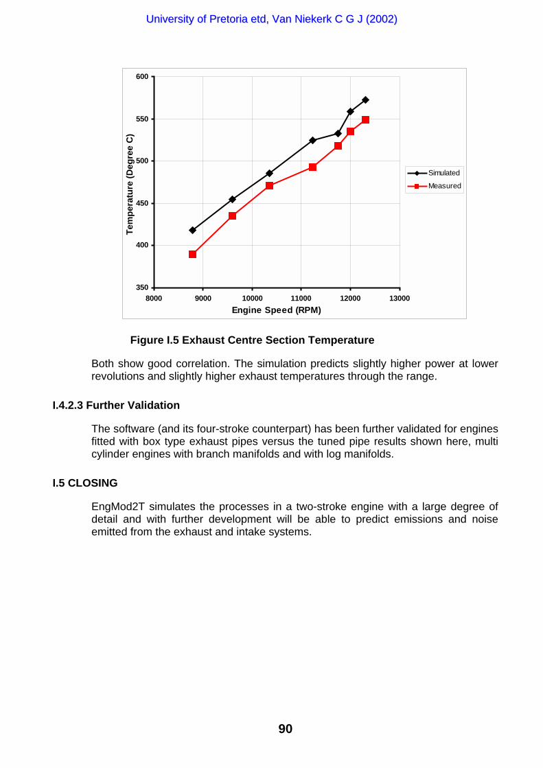
90

350

400

450

500

550

600

8000 9000 10000 11000 12000 13000Engine Speed (RPM)

Tem

pera

ture

(Deg

ree

C)

Simulated

Measured

Figure I.5 Exhaust Centre Section Temperature

Both show good correlation. The simulation predicts slightly higher power at lowerrevolutions and slightly higher exhaust temperatures through the range.

I.4.2.3 Further Validation

The software (and its four-stroke counterpart) has been further validated for enginesfitted with box type exhaust pipes versus the tuned pipe results shown here, multicylinder engines with branch manifolds and with log manifolds.

I.5 CLOSING

EngMod2T simulates the processes in a two-stroke engine with a large degree ofdetail and with further development will be able to predict emissions and noiseemitted from the exhaust and intake systems.


effect of the tailpipe entry geometry on a two-stroke engine's ...

Documents