EFFECT OF PAVEMENT TYPE ON FUEL CONSUMPTION by …

EFFECT OF PAVEMENT TYPE ON FUEL CONSUMPTION

IN CITY DRIVING

by

PALINEE SUMITSAWAN

Presented to the Faculty of the Graduate School of

The University of Texas at Arlington in Partial Fulfillment

of the Requirements

for the Degree of

DOCTOR OF PHILOSOPHY

THE UNIVERSITY OF TEXAS AT ARLINGTON

December 2011

Copyright © by Palinee Sumitsawan 2011

All Rights Reserved

DEDICATION

To my parents.

iv

ACKNOWLEDGEMENTS

I would like to acknowledge a number of people who have helped and supported

me to complete this research. The research in this dissertation has been supported by

the RMC Research and Education Foundation. Without their contribution, this

dissertation would not have been possible.

I would like to express my deepest gratitude to my research advisor, Dr. Siamak

A. Ardekani, for his friendship, support, advice, and counseling during my program of

study at the University of Texas at Arlington. I am thankful that he was always

available for assistance and advice. I have been fortunate that he provided me with

financial support by appointing me as a graduate research assistant. His invaluable

insight and expertise supervised me throughout this research. I also would like to

extend my appreciation to Dr. Stefan A. Romanoschi. His assistance and technical

counsel contributed through the development of this research. I would like to

acknowledge Dr. Stephen P. Mattingly for his guidance and necessary pieces of advice

concerning this research. The constructive comments and assistance of Dr. James C.

Williams during the conduct of this research is also greatly appreciated. I will always

be grateful to Dr. Chien-Pai Han for the superior vision, guidance, and assistance he

contributed during the statistical analysis.

I owe my gratitude to my parents, my relatives, and my husband, for their love,

help, support, and extraordinary courage. I also greatly appreciate the Royal Thai

v

Government for giving me the opportunity to pursue my degree at the University of

Texas at Arlington whose program provided a formative and important experience for

me.

My sincere thanks and appreciation go to former laboratory technician Mr. Jorge

Garcia Forteza for equipment installation and calibrations and to my fellow graduate

students for their assistance in data collection.

November 4, 2011

vi

ABSTRACT

EFFECT OF PAVEMENT TYPE ON FUEL CONSUMPTION

IN CITY DRIVING

Palinee Sumitsawan, PhD

The University of Texas at Arlington, 2011

Supervising Professor: Siamak A. Ardekani

Vehicular fuel consumption and emissions are two increasingly important

measures of effectiveness of sustainable transportation systems, particularly considering

that mobile sources in the U.S. account for the largest consumption of energy and

generation of air pollution. Improving the energy efficiency of the transportation sector

including improving vehicle shape, weight, engine size, and tire quality could play a

vital role in reducing fuel consumption and exhaust gas emissions. Pavement surface

type and other surface characteristics such as skid resistance and roughness affect

vehicular fuel consumption.

The main objective of this study has been to investigate any differences that

might exist in fuel consumption when operating an instrumented van on an Asphalt

Concrete (AC) versus on a Portland Cement Concrete (PCC) pavement under city

vii

driving conditions. The overall study goal has been to recommend consideration of

such user costs or savings in the life cycle analysis of alternative pavement designs for

city streets.

Fuel consumption measurements were made on multiple runs under two driving

modes: 30-mph constant speed and 3-mph/sec acceleration for 10 seconds. All factors

that could affect fuel consumption, other than the pavement surface were either

controlled or kept the same during the measurement runs. Those factors included

speed, ambient temperature, relative humidity, wind speed and direction, vehicle

weight, tire pressure, and use of auxiliary devices in the vehicle.

The results indicated that the differences in fuel consumption rates were

statistically significant at a 10% level of significance under both constant speed and

acceleration modes, with the fuel consumption rates on the PCC pavements being

lower. The extrapolated results also indicated that if all the annual vehicle miles of

travel in the Dallas-Fort Worth region took place at a constant speed of 30 mph on PCC

pavements, the statistically lower fuel rates could result in an annual savings of about

401 million gallons of fuel and an annual CO2 reduction of about 3.53 million metric

tons. Using an average gasoline price of about $3.29 per gallon and an average CO2

clean-up cost of about $18 per metric ton, these differences would amount to a savings

of about $1.38 billion per annum in the DFW region. The potential savings or costs in

fuel consumed and the CO2 emissions generated can be substantial over the design life

of a road project. It is therefore recommended that these savings or costs be considered

in the life cycle cost analysis of alternative road construction projects.

xi

TABLE OF CONTENTS

ACKNOWLEDGEMENTS ............................................................................................. iv

ABSTRACT .................................................................................................................... vi

LIST OF ILLUSTRATIONS ........................................................................................... xi

LIST OF TABLES ......................................................................................................... xiii

Chapter Page

1. INTRODUCTION ............................................................................................ 1

1.1 Problem Definition ............................................................................. 1

1.2 Study Objectives ................................................................................. 2

1.3 Dissertation Overview ........................................................................ 3

2. LITERATURE REVIEW ................................................................................. 5

2.1 Introduction ......................................................................................... 5

2.2 Background ......................................................................................... 5

2.3 Factors Affecting Fuel Consumption .................................................. 9

2.3.1 Vehicle Weight .................................................................... 9

2.3.2 Engine Oil .......................................................................... 10

2.3.3 Tires ................................................................................... 11

2.3.4 Aerodynamic Drag ............................................................. 16

2.3.5 Driving Practices and Techniques ..................................... 17

xii

2.4 Overview of Costs in Life-Cycle Cost Analysis............................... 19

2.4.1 Agency Costs ..................................................................... 21

2.4.2 User Costs .......................................................................... 22

2.4.3 Social Costs ....................................................................... 23

3. RESEARCH METHODOLOGY ................................................................... 25

3.1 Introduction ....................................................................................... 25

3.2 Selection of Road Sections ............................................................... 25

3.2.1 The First Test Sites ............................................................ 26

3.2.2 The Second Test Sites ........................................................ 28

3.3 The Test Vehicle ............................................................................... 31

3.4 Data Collection ................................................................................. 36

3.4.1 Experimental Design ......................................................... 36

3.4.2 Sample Sizes ...................................................................... 36

3.4.3 Measurements of Fuel Consumption ................................. 39

3.5 Data Analysis Approach ................................................................... 43

4. DATA ANALYSIS AND RESULTS ............................................................ 45

4.1 Introduction ....................................................................................... 45

4.2 Statistical Comparisons .................................................................... 48

4.2.1 Paired t-Test ....................................................................... 48

4.2.2 p-Value .............................................................................. 57

4.3 Estimation of Fuel Consumption and CO2 Emissions

including Cost Differences ..................................................................... 61

xiii

4.3.1 Estimation of Fuel Consumption and

CO2 Emissions ............................................................................ 61

4.3.2 Estimation of Fuel Saving and

Emissions Reductions ................................................................. 67

4.3.3 Estimation of CO2 Emissions of a Mile Section

of a Typical City Street ............................................................... 68

5. CONCLUSIONS AND RECOMMENDATIONS ......................................... 73

5.1 Conclusions....................................................................................... 73

5.2 Recommendations ............................................................................. 74

APPENDIX

A. INTERNATIONAL ROUGHNESS INDEX MEASUREMENTS ............... 77

B. SURVEYS OF LONGITUDINAL PROFILE ............................................... 97

C. FUEL MEASUREMENT RAW DATA ...................................................... 106

REFERENCES ............................................................................................................. 111

BIOGRAPHICAL INFORMATION............................................................................ 118

xi

LIST OF ILLUSTRATIONS

Figure Page

2.1 Tire Rolling Resistance............................................................................................. 12

2.2 Fuel Economy of Different Tire Makers .................................................................. 16

2.3 Energy Requirement for City Driving ...................................................................... 19

2.4 Costs in LCCA for Transportation Projects.............................................................. 21

2.5 Components of Vehicle Operating Costs ................................................................. 23

3.1 Abram Street (PCC) .................................................................................................. 27

3.2 Pecandale Drive (AC) ............................................................................................... 27

3.3 Road to Six Flags Street (PCC) ................................................................................ 29

3.4 Randol Mill Road (AC) ............................................................................................ 29

3.5 The Test Van and Data Collection Set-Up. (a) The Instrumented 2000

Chevy Astro Van and (b) The Inside Set-Up during Data Collection. ................... 33

3.6 On-Board Instruments. (a) Fuel Meter (b) Temperature Gauge and

(c) Data Acquisition System. .................................................................................. 34

3.7 Schematic Diagram of the Sensor and the Data Acquisition System. ...................... 34

4.1 Example of Raw Data Plot for PCC Pavement

under Constant Speed Mode ................................................................................... 47

4.2 Example of Raw Data Plot for PCC Pavement

under Acceleration Mode ....................................................................................... 47

4.3 Comparison Plot for Pecandale Drive (AC) vs. Abram Street (PCC)


xii

4.4 Comparison Plot for Pecandale Drive (AC) vs. Abram Street (PCC)


4.5 Comparison Plot for Randol Mill Road (AC) vs. Road to Six Flags (PCC)


4.6 Comparison Plot for Randol Mill Road (AC) vs. Road to Six Flags (PCC)


xiii

LIST OF TABLES

Table Page

3.1 Road Section Characteristics .................................................................................... 30

3.2 Gradations (% Passing by Weight or Volume) ......................................................... 31

3.3 Vehicle Classification by U.S. Environmental Protection Agency .......................... 35

3.4 The Four Factor-Level Combinations ...................................................................... 36

3.5 Sample-Size Determination ...................................................................................... 38

3.6 Sample-Size Determination Table ............................................................................ 39

3.7 Fuel-Consumption Measurement .............................................................................. 43

4.1 Average Fuel Consumption Rates for Pecandale Drive (AC) vs.

Abram Street (PCC) under Constant Speed Mode ................................................. 51

4.2 Average Fuel Consumption Rates for Pecandale Drive (AC) vs.

Abram Street (PCC) under Acceleration Mode ...................................................... 52

4.3 Hypothesis Test Results for Paired t-Test for Pecandale Drive (AC) vs.

Abram Street (PCC) at 10% Level of Significance ................................................ 53

4.4 Average Fuel Consumption Rates for Randol Mill Road (AC) vs.

Road to Six Flags (PCC) under Constant Speed Mode .......................................... 55

4.5 Average Fuel Consumption Rates for Randol Mill Road (AC) vs.

Road to Six Flags (PCC) under Acceleration Mode ............................................... 56

4.6 Hypothesis Test Results for Paired t-Test for Randol Mill Road (AC) vs.

Road to Six Flags (PCC) at 10% Level of Significance ......................................... 57

4.7 Test of p-Value for Pecandale Drive (AC) vs. Abram Street (PCC)

at 10% Level of Significance .................................................................................. 58

xiv

4.8 Test of p-Value for Randol Mill Road (AC) vs. Road to Six Flags (PCC)


4.9 Hypothesis Test Results for Paired t-Test for AC vs. PCC Pavements


4.10 Test of p-Value for AC vs. PCC Pavements


4.11 Standard Deviations and Sample Size after All Data Observed ............................. 60

4.12 Calculations of Annual Fuel Consumption for the Dallas-Fort Worth

Region of Texas under AC Pavement and Constant Speed Mode ......................... 63

4.13 Calculations of Annual Fuel Consumption for the Dallas-Fort Worth

Region of Texas under PCC Pavement and Constant Speed Mode ....................... 64

4.14 Total Annual CO2 Emissions for the Dallas-Fort Worth Region of Texas

under Constant Speed ............................................................................................. 66

4.15 Annual Fuel Savings and Emissions Reductions in Favor of

PCC Pavement for the Dallas-Fort Worth Region of Texas

under Constant Speed ............................................................................................. 67

4.16 Calculations of Daily Fuel Consumption on a One-Mile PCC Section

of a Typical City Street under Constant Speed Mode ............................................ 69

4.17 Calculations of Daily Fuel Consumption on a One-Mile AC Section

of a Typical City Street under Constant Speed Mode ............................................ 70

4.18 Daily CO2 Emissions on a One-Mile Section of a Typical City Street


4.19 Daily CO2 Emissions on a One-Mile AC vs. PCC Sections of a Typical

City Street under 30-mph Constant Speed from Pavement Production,

Construction, Maintenance, and Traffic ................................................................. 72

1

CHAPTER 1

INTRODUCTION

1.1 Problem Definition

Vehicular fuel consumption and emissions are two increasingly important

measures of effectiveness of sustainable transportation systems, particularly considering

that mobile sources in the U.S. account for the largest consumption of energy and

generation of air pollution. According to the U.S. Bureau of Transportation

Statistics(U.S. Bureau of Transportation Statistics, 2011), there were 255,917,664

registered vehicles in the U.S. in 2008. Gasoline, which is the main product from crude

oil refining, is one of the major fuels consumed by vehicles in the U.S. with a

consumption level of over 70 billion gallons in 2007. This is about half of the total

gasoline consumption for any purpose in the U.S. (TRB Special Report 285, 2006). As

such, the transportation sector is also the largest emitter of CO2 among all energy-use

sectors such as industrial, residential, and commercial sectors. Among three common

fossil fuels – petroleum, natural gas, and coal – 96% of the 2007 U.S. primary

transportation energy consumption relied on petroleum or crude oil (U.S. Department of

Energy, 2008). This trend continues despite the oil price increases which peaked at over

$140 a barrel in June 2008.

In motor vehicles, CO2 is the by-product of the combustion process and is

released to the atmosphere as a tailpipe emission. It is one of the greenhouse gases

2

contributing to global warming. Between 1990 and 2007, the CO2 emissions of the

transportation sector grew the most, a 26.8% increase over the 10-year period (1990 –

2000) and a 1.4% increase from 2006 to 2007 alone (U.S. Department of Energy, 2008).

As a result, improving the energy efficiency of the transportation sector including

improving vehicle shape, weight, engine size, and tire quality could play a vital role in

reducing fuel consumption and exhaust gas emissions. Pavement surface type and

surface characteristics such as skid resistance, roughness, and longitudinal slope also

affect vehicular fuel consumption.

1.2 Study Objectives

This study aims at investigating vehicular fuel consumption differences under two

different pavement surface types when operating a vehicle under urban driving speeds. It

follows an experimental design which aims at accounting for most factors affecting fuel

consumption in order to isolate the effect of pavement type on fuel consumption. The

main objective is to compare fuel consumption of an instrumented test vehicle as a

function of pavement surface material through direct field measurements. The study will

focus on paved city streets since urban driving accounts for a substantial share of the total

vehicular energy consumption and generated emissions. Two types of pavement

surfaces, namely Portland Cement Concrete (PCC) and Asphalt Concrete (AC), are

studied. Using known scaling factors documented in energy consumption literature

relating vehicle weight to fuel consumption, the study results for the test vehicle are

extrapolated to other vehicle types in the mix. This allows, as a second study objective,

to establish a procedure in a spreadsheet format for estimating the total fuel savings for

3

different pavement type scenarios. The latter would require, as an additional input

variable, data on vehicle mix and vehicle miles traveled within a city or region of interest.

Such data are published annually by the U.S. Bureau of Transportation Statistics (BTS).

The procedure developed will provide the necessary tool to achieve a third objective,

namely inclusion of potential fuel savings in the life-cycle cost analysis (LCCA) of

alternative pavement designs.

Based on the above objectives, the main outcomes of the study are anticipated to

be:

a. A statistical comparison of relative fuel economy differences for concrete and

asphalt pavement surfaces under urban driving conditions.

b. The development of a spreadsheet tool to estimate fuel consumption for

various pavement surfaces.

c. The development of a procedure to include fuel consumption cost in the

LCCA of different pavement design alternatives for a given pavement design

or re-surfacing project.

1.3 Dissertation Overview

The dissertation is divided into five chapters. Chapter 1 is the introduction and

problem definition. In chapter 2, the literature review discusses the background and

impacts of fuel consumption and the use of LCCA for pavement design alternatives.

Additionally, it reviews the factors that influence fuel consumption, followed by an

overview of costs to include in LCCA.

4

Chapter 3 presents the research methodology employed in the study. It describes

the criteria in selection of the test road sections and summarizes the characteristics of all

test road sections. It also describes the features of the test vehicle, including the fuel

meter equipment, temperature gauges, and an on-board data acquisition system.

Additionally, this chapter describes how the data are collected as well as the data analysis

approach. In chapter 4, the results are presented and discussed. Chapter 5 presents

conclusions and recommendations.

5

CHAPTER 2

LITERATURE REVIEW

2.1 Introduction

In this chapter, studies related to this research are reviewed. The review is on the

use of LCCA for pavement design alternatives, and the costs associated with LCCA. It

also presents the findings related to factors affecting fuel consumption.

2.2 Background

The Transportation Research Board (TRB) Special Report 285 states that

vehicular fuel consumption accounts for nearly half of the total energy consumption in

the U.S. (TRB Special Report 285, 2006). About half of that amount is estimated to be

due to urban city driving at speeds below 40 mph (Larson, 1992). As such, the oil crises

of 1970s led to numerous research studies on vehicular fuel consumption. This led to

advances in automotive design including lighter vehicles with more efficient engines,

more energy efficient tires, to smoother roadway alignments, and to traffic engineering

measures such as better timed traffic signals and national speed limit regulations.

The elemental fuel consumption model developed by scientists at the GM

Research Lab (Evans et al., 1976a; Evans et al., 1976b) was the widely accepted model

among the fuel consumption models developed in the 1970s. This model showed that the

fuel consumption in a single vehicle varies greatly depending on many factors including

speed, acceleration-deceleration cycle, vehicle weight, mechanical conditions of the

6

vehicle (e.g. tire pressure, wheel alignment, and state of its carburetion system), ambient

conditions such as wind and temperature, and pavement surface conditions. The model

speculated that about 70% of the variability in a vehicle’s fuel consumption is explained

by speed alone. Also an important factor influencing the fuel consumption rate is the

rolling pavement resistance, which is primarily a function of the pavement surface

condition and type. The fuel consumption differences due to rolling resistance were

expected to be particularly significant for trucks and other heavy vehicles.

Since the costs of road construction and maintenance constitute a large proportion

of the highway infrastructure projects, the World Bank, which provides financial and

technical assistance to developing countries, introduced the Highway Design and

Maintenance (HDM) Standards Model (Archondo-Callao and Faiz, 1994). This program

accounts for vehicle operating costs in addition to the construction, maintenance, and

rehabilitation costs of alternative pavement designs. It also incorporates the LCCA as a

basis for decision making in the selection of highway design alternatives.

The life-cycle cost in the HDM (Archondo-Callao and Faiz, 1994) included user

costs in addition to conventional construction, maintenance and rehabilitation costs. The

user costs were mainly the vehicle operating costs and exogenous costs such as the cost

the society incurs as the result of road usage. The vehicle operating cost model contained

variables related to vehicle characteristics such as engine size, speed, tire conditions, etc.,

and road characteristics such as smoothness and slope of the longitudinal profile. The

smoothness and slope of the longitudinal profile were the only pavement characteristics

used in the model for estimating the vehicle operating costs. The other pavement

7

characteristics such as the pavement type became statistically less significant since data

from both paved and unpaved roads were used. To enhance the Highway Design Model

work, a New Zealand study by Walls and Smith (1998) further suggested that the

smoothness of the longitudinal profile has little impact on the fuel consumption for paved

roads in good condition.

Papagiannakis and Delwa (Papagiannakis, 1999b; Papagiannakis and Delwar,

1999a; Papagiannakis and Delwar, 2001a) developed a software program which

highlighted the importance of incorporating vehicle operating costs in the life-cycle cost

analysis of pavement projects. Their findings were later implemented in the Pavement

Management System program of the Washington State Department of Transportation.

They also paid special attention to the effect of roughness on the vehicle operating costs

to illustrate the increase in these costs with the deterioration of the pavement.

In addition, many studies have attempted to systematically assess the effect of

pavement surface material type on fuel consumption (Jonsson and Hultqvist, 2009;

Taylor and Patten, 2006; Zaniewski, 1989; Zaniewski et al., 1982). Most of these studies

focused on fuel consumption of vehicles on highways under fairly high operating speeds.

A Canadian study (Taylor and Patten, 2006) performed measurement of fuel consumption

using heavy trucks, while a Swedish study (Jonsson and Hultqvist, 2009) was conducted

using passenger cars. Both study results indicated that there was potential fuel savings on

PCC over AC pavements. Additionally, the research by Zaniewski (Zaniewski, 1989;

Zaniewski et al., 1982), which was the earliest effort to investigate the effect of pavement

type on fuel consumption, also pointed out that fuel consumption of a truck when

8

travelling on PCC pavements is lower than when travelling on AC pavements. Because

their study was focused on fuel consumption of trucks on highways and also due to other

limitations of the methodology employed, this study has received substantial criticism

(Bein and Biggs, 1993). Partly due to these issues, Zaniewski’s findings have not been

widely adopted by the pavement engineering community. Zaniewski’s findings could

also allow incorporating fuel economy improvements and emissions reductions in the

life-cycle cost analysis of design alternatives for highway pavements. However, it is not

readily clear whether and to what extent they are applicable to city streets, where the

urban carbon footprint is becoming an increasingly important consideration in the

analysis of design alternatives.

A synthesis study by the Ontario Hot Mix Producers Association, for example,

cites that for every 1,000 kg of Portland cement, approximately 650 kg of carbon dioxide

is produced while the carbon in the asphalt cement will never be released into the

atmosphere (Brown, 2009). The Canadian study also compares two residential pavement

cross-sections, a PCC and an asphalt pavement in southern Ontario. The study then

proceeds to estimate the contributions of these two pavement materials to the carbon

footprint of a one-kilometer long section and concludes that the HMA pavement

generates only 22 percent of the carbon footprint of the PCC pavement, during pavement

construction process. The computations are based solely on estimated CO2 releases in the

materials production as well as construction phase of the projects. While the study

accounts for the CO2 releases from cement kilns in estimating the carbon footprint of

PCC projects, the portion of CO2 releases from oil refineries attributable to asphalt

9

production are not considered in making similar estimates for AC pavements. More

importantly, this and other similar studies (VicRoads, 2008) do not consider the

emissions resulting from the operation of motor vehicles over the design life of

pavements in these calculations. A key conclusion of the current study is that over the

design life of a pavement, the difference in the CO2 amounts resulting from operation of

motor vehicles on various pavement surfaces could be substantial and may in fact help

dwarf any such differences estimated for the production and construction phases.

2.3 Factors Affecting Fuel Consumption

The effect on fuel consumption depends on a number of factors as follows:

2.3.1 Vehicle Weight

Vehicle weight is a significant factor in fuel consumption. The emissions and fuel

consumption are greater for light trucks than those in the past. This indicates the

increasing trend toward the larger and heavier light trucks, which in the past had less

stringent emission standards and lower fuel efficiency (U.S. Environmental Protection

Agency, 2000). However, automobile manufacturers currently must develop vehicles in

accordance with the EPA emission standards as well as improving vehicle fleet gas

mileage. Newer cars and trucks will use less gasoline and emit less pollution. Carbon

dioxide, which is not classified as an emission, is the transportation sector's primary

contribution to climate change. Its emissions are directly proportional to fuel

consumption. A 1% decrease in fuel consumption results in a corresponding 1% decrease

in carbon dioxide emissions (U.S. Environmental Protection Agency, 2000). A European

10

study (Lubrizol, 2011) also shows that a 1% increase in fuel economy for one vehicle

could lower CO2 emissions by over 1.5 g/km.

Decreasing vehicle weight results in less energy required by the engine to

accelerate the vehicle and less rolling resistance from vehicles’ tires. A 1% weight

reduction results in 0.42% fuel economy gain (Casadei and Broda, 2008). One study (An

et al., 2002) also shows that when the car weight is decreased by 10%, the fuel economy

would increase 3 to 8%. Removing excess weight from the vehicle helps reduce fuel

consumption. It is shown that a reduction of 440 pounds (200 kg) can increase fuel

efficiency by 5% in a midsize car (Pagerit et al., 2006).

2.3.2 Engine Oil

Engine oil is used as the lubricant in internal combustion engines. It performs

many functions. The main function is to lubricate the moving components of the engine.

It, thus, primarily reduces friction between moving components. Other functions are to

clean, limit wear on the moving parts, inhibit corrosion, and cool the engine by carrying

away the heat generated by the frictional losses.

When engine components move against each other, this causes friction which

loses power by converting energy to heat. The contact between moving surfaces also

wears those parts which could lead to lower engine efficiency. Hence, it diminishes

power output and increases fuel consumption. The engine oil generates a separating film

between surfaces of moving parts to minimize direct contact. About 67% of friction

losses in the engine occur during this surface contact (Energy and Environmental

Analysis Inc., 2001).

11

The property of the engine oil which reduces friction is its viscosity. Viscosity is

a measure of oil’s resistance to flow. As temperature decreases, oil viscosity increases.

This accounts for increased fuel usage under low ambient temperatures and cold engine

operations. In order for the engine to perform at its peak fuel efficiency, the oil viscosity

must be high enough at high temperatures so that the oil film between moving parts does

not break down, and low enough at low temperatures to protect the engine from cranking.

Because friction loss between moving parts could affect from 10% to 40% of the energy

input to the engine (Transportation Energy Management Program, 1982), nowadays,

engine oil manufacturers develop their lubricant formulation to improve vehicles’ fuel

efficiency. Shell (2011) lubricant development program claims its engine oil yields 6.5%

fuel efficiency improvement. However, the engine oil grade and viscosity to be used in a

given vehicle is designated by the automobile manufacturers. The engine oil grade

requirement can vary from country to country when climatic conditions are considered.

2.3.3 Tires

Tires also have an impact on fuel consumption because about 12 to 20% of the

energy output is transmitted through the vehicle’s driveline as mechanical energy to

propel the wheels. Approximately 4 to 7% of the energy output is used by rolling

resistance (TRB Special Report 286, 2006). When the vehicle moves, it encounters

rolling resistance – the resistance that occurs when the vehicle tires rotate over the

contact surface. It acts in the direction opposite to the direction of travel (see Figure 2.1).

Basically, rolling resistance is the energy loss in rolling tires under the weight of the

vehicle. The primary cause of loss of energy is the deformation and recovery of the tire,

12

called hysteresis (Goodyear, 2008). The viscoelastic behavior of the rubber material of

tire generates the energy loss. The rubber has an elastic property where all energy that is

stored in the material during loading is returned when the load is removed, and the

material rapidly recovers its shape. Nevertheless, for viscous behavior of rubber, the

energy needed to deform the material is simultaneously transformed to heat.

Consequently, as for any viscoelastic material, some of energy is recovered during load

removal, while the remainder is transformed to heat (TRB Special Report 286, 2006).

Figure 2.1 Tire Rolling Resistance (Goodyear, 2008).

The TRB special report (2006) states that for most passenger vehicles, a 10%

reduction in rolling resistance produces a 1 to 2% increase in fuel economy and a

proportional reduction in fuel consumption. Additionally, in most passenger vehicles,

Society of Automotive Engineers (SAE) paper (Sovran and Bohn, 1981) indicates that a 5

to 7% decline in rolling resistance will lead to a 1% benefit in fuel economy. However,

tire rolling resistance measurement is usually performed as a laboratory test. The

13

measurement procedures used with different instruments under different circumstances

could generate variability of results.

Tire inflation pressure, tire diameter, tire tread, and tire construction have an

effect on rolling resistance. Motorists should be aware that the proper inflation pressure

is necessary for tire performance, safety and optimum fuel efficiency. Inflation pressure

affects tire deformation. Lower pressure causes the tire sidewalls to flex more and

generate higher rolling resistance. Keeping tires properly inflated is therefore important

to prevent excessive deformation and hysteresis, and achieving best gas mileage. Studies

indicate that for every 1 pound per square inch (psi) decline in tire pressure, fuel

economy lowers by 0.3 to 1% (Transportation Energy Management Program, 1982; U.S.

Department of Energy, 2010a). The figures are consistent to the U.S. EPA report (2006),

mentioning Aerospace Corp. and Goodyear studies. It is found that fuel economy

declines 1% for every 3.3 psi (Aerospace Corp) and 2.96 psi (Goodyear) decrease in tire

pressure.

A smaller tire has higher rolling resistance than a larger tire at the same tire

inflation pressure. According to Goodyear (2008), a smaller diameter drive axle tire

results in an increase in engine RPMs, thereby increasing fuel consumption. TRB special

report 286 (2006) indicates that tire or rim dimensions indeed have an influence on

rolling resistance as tires with rim diameters of 15 inches or lower result in a 10%

increase in rolling resistance compared to tires with a larger rim diameter.

Tire tread provides traction and makes contact with the road. The grooves of the

tire are designed to channel water underneath the tire and prevent hydroplaning.

14

Generally, smooth treads roll better than coarse treads. In other words, a tire with thicker

treads has a higher rolling resistance. Thicker tread tire can create more friction and

noise, but its tradeoff is to enhance safety.

Different tire construction or tire types, under similar driving conditions, could

result in different amounts of fuel consumed. The fuel economy improvement of radial

ply tires over bias ply tires is well documented. A tire with radial ply construction has

the advantage of relatively lower internal friction compared with that in a bias ply-

constructed tire. Radial ply tire reduces the deformation of the tread in the contact patch.

Therefore, these help decrease rolling resistance, tire wear, and energy consumption.

Radial ply tires could improve gas mileage by at least 5% (Thompson, 1979) or more

(Goodyear, 2008). A Canadian report exhibits that radial ply tires have a benefit in fuel

economy of 10% or more over bias ply tires. However, a conservative figure generally

accepted is that radial ply tires yield a 4 to 5% fuel economy benefit (Transportation

Energy Management Program, 1982).

Using low-rolling-resistance tires help minimize energy consumed. Low-rolling-

resistance tires are designed to enhance fuel economy by diminishing the amount of tire

friction and resistance while driving. U.S. Department of Energy (2010b) estimates that

about 5 to 15% of fuel consumed is used to overcome the rolling resistance for passenger

cars, while for heavy trucks, the amount is as high as 15 to 30%. A Californian study

(California Energy Commission, 2003) estimates that using low-rolling-resistance tires

reduce fuel consumption by 1.5 to 4.5%, but the tire data were not sufficient to compare

safety and other performance characteristics. New cars are generally equipped with low-

15

rolling-resistance tires. Auto manufacturers typically equip new vehicles with tires that

have low rolling resistance in order to satisfy Corporate Average Fuel Economy (CAFE)

standards. Nevertheless, when it comes to replacing the tires, there are no requirements

on adoption of low-rolling-resistance tires as the replacement tires.

The Daily Green (2009) provided interesting information on different low-rolling-

resistance tires available in the market. Seven different low-rolling-resistance tires from

Bridgestone, Goodyear, Michelin, and Yokohama were compared in terms of gas

mileage, using a set of Goodyear Integrity radials as the control tires. Figure 2.2

illustrates the results. Among all tires examined, the fuel-efficient leader was Michelin

Energy Saver A/S, which yielded 53.8 mpg. This is approximately a 4.7% improvement

over Goodyear Integrity. Goodyear Assurance ComforTred had the least fuel economy,

delivering only 50.0 mpg. Its fuel economy was worse than the control tires by 2.6%.

The article did not, however, discuss why the Goodyear Integrity had been picked as the

control tires. However, tire companies claimed the findings were different from their

own test results. This could be because the test conditions were under different

circumstances.

16

Figure 2.2 Fuel Economy of Different Tire Makers.

2.3.4 Aerodynamic Drag

Aerodynamic drag plays a part in fuel consumption due to the effect of wind and

driving speed. Wind influences fuel economy by essentially changing the load to the

vehicle. Side wind pushing the vehicle can affect rolling resistance. The driver must

compensate by turning the steering wheel to the wind. The variable that most affects

aerodynamic drag, however, is the vehicle speed. An aerodynamic drag loss mainly

occurs at highway speeds and is much higher at highway speeds than at city driving

speeds. At speeds of about 62 mph and above, over 50% of the fuel consumed to

mobilize the vehicle is used to overcome the aerodynamic drag (Transportation Energy

17

Management Program, 1982). The U.S. EPA (1980) reports, based on estimates made by

the Department of Transportation, that fuel consumed at a speed of 70 mph is 30% higher

than fuel consumed at a speed of 40 mph. It also indicates that wind reduced fuel

economy by 2 to 3% in most cars. However, the latter outcome is estimated based on a

constant speed of 55 mph, which is in the range of highway speeds, and there is an

implicit assumption that wind has no effect on fuel economy at vehicle speeds below 55

mph. The report indicates that the optimum fuel consumption is attained at the speed of

around 35 to 40 mph for most cars.

2.3.5 Driving Practices and Techniques

Aside from vehicle factors mentioned earlier, driver behavior or the manner in

which a vehicle is driven impacts fuel efficiency. While it is known that the factors

influencing fuel consumption are acceleration rate, deceleration rate, and time spent on

idling, the fuel economy information provided in some sources was limited to quantifying

their effects (Energy and Environmental Analysis Inc., 2001). Not much research has

been done on driving behavior. But it is reported that, by training drivers in fuel-efficient

driving techniques, the fuel consumption could be reduced by 10 to 15% (Transportation

Energy Management Program, 1982).

Aggressive driving is, among others, characterized by hard accelerations and

decelerations. Driving with high rates of acceleration and deceleration could be

represented as jackrabbits and tortoises, respectively. It is recommended that drivers

should apply steady pressure rather than sudden push on the accelerator pedal for safety

and fuel economy improvement (Transportation Energy Management Program, 1982).

18

Deceleration of vehicles is chiefly caused by slow moving traffic and traffic signals. The

braking technique to improve fuel economy is to minimize brake usage. For example,

when approaching slower moving traffic or traffic signals, begin to coast as soon as

possible (Transportation Energy Management Program, 1982).

An idling engine does not provide useful work. Transportation Energy

Management Program (1982) indicates that every 4 minutes of idling consumes enough

fuel to move a typical car about 0.63 miles (1 km). An idling time of 10 seconds uses

more fuel than the vehicle uses to restart and replace the electrical energy. Therefore,

trips being made should be planned in terms of route selection and other factors in order

to minimize the number of stops.

The effect on vehicular fuel consumption depends on several aspects as

mentioned earlier. It also includes usage of auxiliary devices, as energy is required to

power accessory loads. Figure 2.3 summarizes the major energy components in urban

driving.

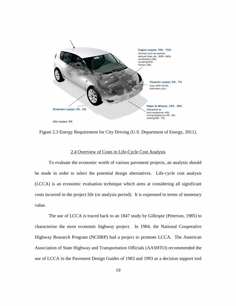
19

Figure 2.3 Energy Requirement for City Driving (U.S. Department of Energy, 2011).

2.4 Overview of Costs in Life-Cycle Cost Analysis

To evaluate the economic worth of various pavement projects, an analysis should

be made in order to select the potential design alternatives. Life-cycle cost analysis

(LCCA) is an economic evaluation technique which aims at considering all significant

costs incurred in the project life (or analysis period). It is expressed in terms of monetary

value.

The use of LCCA is traced back to an 1847 study by Gillespie (Peterson, 1985) to

characterize the most economic highway project. In 1984, the National Cooperative

Highway Research Program (NCHRP) had a project to promote LCCA. The American

Association of State Highway and Transportation Officials (AASHTO) recommended the

use of LCCA in the Pavement Design Guides of 1983 and 1993 as a decision support tool

20

for economic evaluation. The Intermodal Surface Transportation Efficiency Act (ISTEA)

of 1991 was the first act which called for “the use of LCCA in the design and engineering

of bridges, tunnels, and pavements” both for metropolitan and statewide planning.

Afterward, the National Highway System (NHS) Designation Act of 1995 mandated

States to perform LCCA on NHS projects costing $25 million or more. In 1996, the

Federal Highway Administration (FHWA) released LCCA guidance. Later, the

Transportation Equity Act for the 21st Century (TEA-21) of 1998 repealed the

requirement to perform LCCA on NHS projects. Guidance and recommendations on

practices in conducting LCCA was distributed by the FHWA in 1998 as Life-Cycle Cost

Analysis in Pavement Design. Recently, the FHWA’s Office of Asset Management has

developed an LCCA-based software package for pavements (Ozbay et al., 2003).

Life-cycle costs include all costs anticipated over the intended service life of a

project or a facility. The basic theory of LCCA is that all the impacts of the project can

be converted to monetary values so that the comparison between alternatives can be

conducted directly. The costs included in LCCA can be tangible and intangible and can

be generated by the agency, by the users of the facility, or by society (Ozbay et al., 2003).

The costs incorporated in LCCA are illustrated in Figure 2.4.

21

Figure 2.4 Costs in LCCA for Transportation Projects.

2.4.1 Agency Costs

Agency costs are the costs incurred directly by the agency in order to put the

project or the facility in service. Agency costs comprise initial construction cost, future

routine and preventive maintenance costs, resurfacing and rehabilitation cost, and costs

inherently associated with using personnel, for example, contract administration,

construction supervision, and administrative costs. The initial construction, periodic

maintenance, and rehabilitation costs include the costs of materials, labor, machinery, and

other contingencies. The salvage value is also considered as a part of agency costs. It is

the remaining value of the project at the end of the analysis period or service life.

Salvage value is a negative impact when calculating net present value, the discounted

Costs in LCCA

User

Costs

Social

Costs

Agency

Costs

Initial Construction

Periodic Maintenance

Future Rehabilitation

Others

Vehicle Operation Costs

Travel Delay

Others

Accidents

Environmental Impacts

Others

22

salvage is subtracted from the total costs. There is no general agreement on how to

estimate the salvage value since most infrastructure projects are not demolished at the

end of their service life or analysis period. Therefore, if the serviceability remains the

same among alternatives, the salvage value can be omitted from the calculations (Ozbay

et al., 2003).

2.4.2 User Costs

User costs are the costs incurred by the project users. These costs occur

throughout the service life of the project. According to Huang (2004), for a highway

facility, the user costs include both apparent and hidden costs incurred by the motoring

public. Most user costs are intangible. These costs include vehicle operating costs, user

travel delay, and other components such as discomfort from traffic flow interruptions and

traffic noise. Costs of travel delay are dependent on the demand and capacity of the

facility. During work zone operations and rehabilitation activities, travel delay costs

depend on a number of factors, such as traffic volume, number of days in operation, time

of day of operation, and number of lanes closed.

Vehicle operating costs depend on the facility’s serviceability, that is, mainly

pavement roughness. These costs consist of fuel consumption, lubricant consumption,

tire wear, parts and labor costs, vehicle maintenance, and depreciation or resale value.

Vehicle operating costs can be categorized into fixed and variable costs as depicted in

Figure 2.5 by the Victoria Transport Policy Institute. Roughness is a pavement

characteristic that could influence fuel consumption. There are significant operating cost

differences between a smooth and rough pavement. Vehicle operating costs, especially

23

fuel consumption, increase with an increase of pavement roughness (Peterson, 1985). A

recent research project that will be published in the near future by Auburn University also

presents the effect of pavement smoothness on fuel consumption (Christie, 2011). A

preview of the study shows that improvement in pavement smoothness could lower fuel

consumption by 1.8 to 2.7%. Consequently, the amount of fuel savings would be about

3.3 billion gallons a year.

Figure 2.5 Components of Vehicle Operating Costs.

2.4.3 Social Costs

Social costs are the costs encountered by society. The social costs include the

costs of crashes, accidents, property damage, and environmental impact. Accident costs

could be estimated as a dollar per unit length for different types of facilities, such as rural,

urban, and freeway. Generally, there is no research showing that accident rates can vary

Vehicle Operating Costs

Fixed Costs

Vehicle purchase

Registration fees

Insurance (partly variable)

Variable Costs

Fuel, oil, tire

Maintenance and repair

Parking and toll fees

Depreciation

24

among the alternatives with different serviceability. The environmental impacts can

encompass air, water, noise, and natural resources. Only the costs from air and noise

pollution could be monetized in transportation evaluation (Ozbay et al., 2003).

In summary, studies have shown that there are several important factors

influencing vehicular fuel consumption. Vehicle weight, engine oil, and tires are the

examples caused by the vehicle itself. Drivers’ behavior and techniques also have an

impact on fuel consumption.

LCCA is a technique that employs the principles of economic analysis to evaluate

long term performance between competing alternative investment options. Its purpose is

to estimate the overall costs of the project alternatives and to select the facility that

provides the lowest overall costs. LCCA is performed by adding up the discounted

monetary values of all benefits and costs that incur in each alternative. Costs considered

in the LCCA include the costs of owning and operating the facility over a period of time.

25

CHAPTER 3

RESEARCH METHODOLOGY

3.1 Introduction

In order to examine any differences that might exist in vehicular fuel consumption

on PCC versus AC pavements under city driving conditions, the study relies on operating

an instrumented motor vehicle on city streets. The fuel consumption of a test vehicle on

different surface types is then collected and compared. This chapter describes selection

of road sections, test vehicle, data collection, and data analysis approach.

3.2 Selection of Road Sections

Four street sections (two asphalt and two concrete sections) were selected for fuel

consumption studies. The selection criteria included surface material type, surface

roughness, longitudinal gradient, and location of the pavement sections. Two sets of

concrete pavement versus asphalt pavement sections with similar surface roughness and

longitudinal gradient were accordingly selected. Each pair of road sections (one AC and

one PCC) was approximately parallel so as to minimize the effect of wind direction and

velocity during measurement runs on the two road sections at a given time. Below is a

detailed description of each roadway section selected.

26

3.2.1 The First Test Sites

3.2.1.1 The PCC Section

A PCC section chosen was Abram Street (Figure 3.1). This is a Continuously

Reinforced Concrete Pavement (CRCP). The reinforced concrete slab is 8 inches deep

over 2-inch hot mix asphalt concrete type D on an 8-inch lime stabilized subgrade. The

roughness measurements were done by the Texas Department of Transportation resulting

in an average International Roughness Index (IRI) measurement of 174.6 in/mile. The

length of this section is approximately 3,500 feet. The longitudinal gradient was uphill

with the average value of 1.2% in the eastbound direction (direction of observations).

3.2.1.2 The AC Section

Approximately two blocks away and parallel to the PCC section, Pecandale Drive

(Figure 3.2) was selected as a test section for the asphalt pavement. Its layers includes a

7-inch deep hot mix asphalt concrete (1.5-inch Type D and 5.5-inch Type B) on a 6-inch

lime stabilized subgrade. The average IRI measurement was measured to be 180.6

in/mile. Comparing with the PCC section, the average IRI values are 3% higher.

However, they are both in the IRI range for new pavements (Sayers and Karamihas,

1998). The length of the section is approximately 1,900 feet. The average longitudinal

gradient was +1.2% in the direction of observations (eastbound), which was identical to

the gradient of the PCC section.

27

Figure 3.1 Abram Street (PCC).

Figure 3.2 Pecandale Drive (AC).

28

3.2.2 The Second Test Sites

Although asphalt pavements typically have high skid resistance, this study did not

have the skid resistance on the first two pavement sections measured due to lack of

testing devices. Therefore, statistical comparison of fuel consumption is needed to test

separately on other random selected sections to investigate whether or not the results are

consistent with the first sites.

3.2.2.1 The PCC Section

The second PCC section was the Road to Six Flags Street (Figure 3.3). This

section is a Jointed Plain Concrete Pavement (JPCP) with a 7-inch concrete slab on a 6-

inch lime stabilized subgrade. The spacing of the transverse joints was 20 feet. The

average IRI value was measured to be 323.3 in/mile. The length of the road section is

approximately 1,600 feet. The average longitudinal gradient was +0.4% in the direction

of observations (westbound).

3.2.2.2 The AC Section

The asphalt pavement section selected was the Randol Mill Road (Figure 3.4). It

consisted of an 8-inch deep layer of hot mix asphalt concrete (2-inch Type D and 6-inch

Type A) on a 6-inch lime stabilized subgrade. The average IRI value was 276.7 in/mile.

The IRI values of the last two sections have a difference of 16.8%, with the asphalt

section having a smaller IRI (smoother). The length of this section is approximately

1,400 feet. The average longitudinal gradient was uphill at the rate of 0.6% in the

direction of observations (westbound).

29

Figure 3.3 Road to Six Flags Street (PCC).

Figure 3.4 Randol Mill Road (AC).

30

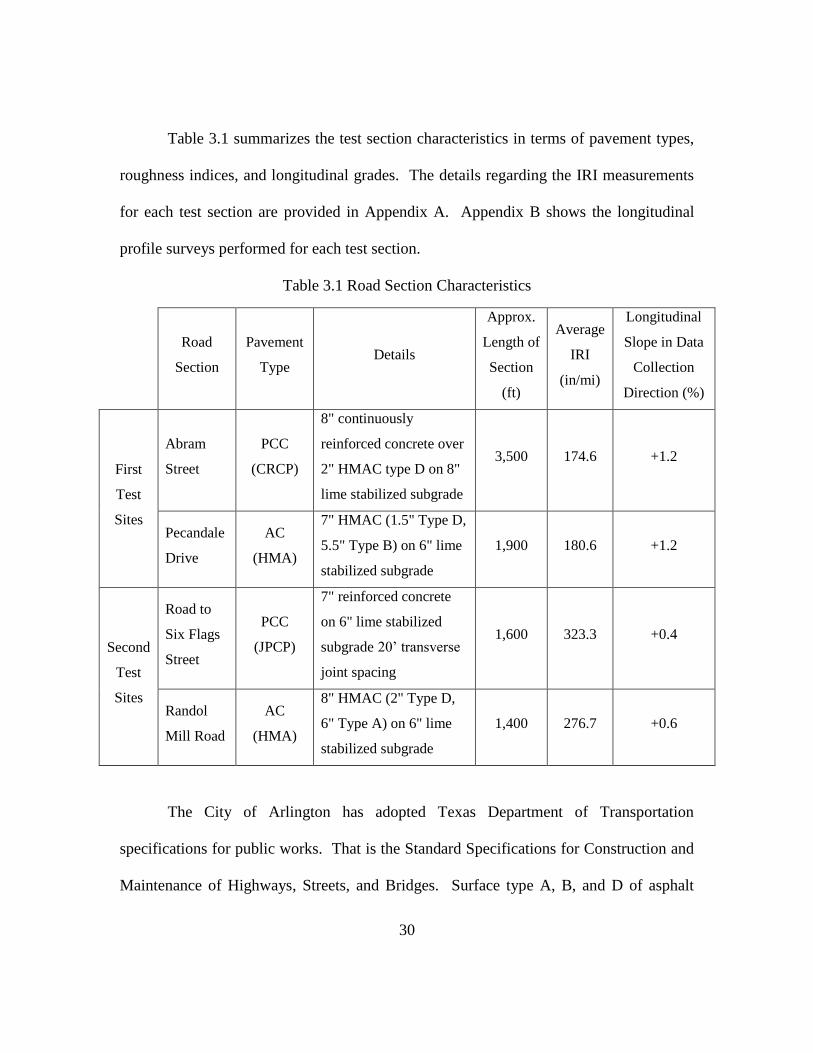
Table 3.1 summarizes the test section characteristics in terms of pavement types,

roughness indices, and longitudinal grades. The details regarding the IRI measurements

for each test section are provided in Appendix A. Appendix B shows the longitudinal

profile surveys performed for each test section.

Table 3.1 Road Section Characteristics

Road

Section

Pavement

Type Details

Approx.

Length of

Section

(ft)

Average

IRI

(in/mi)

Longitudinal

Slope in Data

Collection

Direction (%)

First

Test

Sites

Abram

Street

PCC

(CRCP)

8" continuously

reinforced concrete over

2" HMAC type D on 8"

lime stabilized subgrade

3,500 174.6 +1.2

Pecandale

Drive

AC

(HMA)

7" HMAC (1.5" Type D,

5.5" Type B) on 6" lime

stabilized subgrade

1,900 180.6 +1.2

Second

Test

Sites

Road to

Six Flags

Street

PCC

(JPCP)

7" reinforced concrete

on 6" lime stabilized

subgrade 20’ transverse

joint spacing

1,600 323.3 +0.4

Randol

Mill Road

AC

(HMA)

8" HMAC (2" Type D,

6" Type A) on 6" lime

stabilized subgrade

1,400 276.7 +0.6

The City of Arlington has adopted Texas Department of Transportation

specifications for public works. That is the Standard Specifications for Construction and

Maintenance of Highways, Streets, and Bridges. Surface type A, B, and D of asphalt

31

pavements conform to the gradations of materials shown in Table 3.2. The specifications

are outlined under 300 Items of Surface Courses and Pavement, located in Article 340.4

and Section A.1 (Texas Department of Transportation, 2004).

Table 3.2 Gradations (% Passing by Weight or Volume)

3.3 The Test Vehicle

An instrumented model 2000 Chevy Astro van (Figure 3.5) was utilized as the test

vehicle. Fuel consumption measurements in gallons per mile (gpm) were made with an

on-board data acquisition system. The fuel sensor, the temperature sensors, and the data

acquisition system (shown in Figure 3.6) were connected to the engine as shown

schematically in Figure 3.7. Two fuel sensors made instantaneous measurements of the

amount of fuel entering the engine and returning to the tank, with the difference between

the fuel intake and the amount returned to the tank being the instantaneous of fuel

consumed. The temperatures of the fuel entering the engine and returning to the tank

32

were also measured using two temperature gauges. The data acquisition system probes

could collect a sample from the sensors every 100 or 200 millisecond as setting by the

user. In addition to the fuel amounts and fuel temperature, the data acquisition system

also recorded the instantaneous vehicle speed. Vehicle speed is sampled at the rate of

one second driven by the transmission shaft.

The test vehicle has the curb weight of 4,397 lbs, which is the total weight of

vehicle with standard equipment. Its maximum allowable total vehicle weight, including

the weight of passengers and cargo (gross vehicle weight rating, GVWR) is 6,100 lbs.

According to the U.S. Environmental Protection Agency (EPA) vehicle classifications

(28 vehicle classes) listed in Table 3.3, the test vehicle is categorized into Light-Duty

Gasoline Truck 3 (LDGT3) as its GVWR was within this range. The LDGT3 class when

fully loaded has an average vehicle weight of 7,500 lbs. On the contrary, vehicle weight

is not a criterion for vehicle classification in the Federal Highway Administration

(FHWA). FHWA separates vehicle types into 13 categories based on whether the vehicle

carries passengers or cargo. Non-passenger vehicles are further divided by number of

axles and number of units, including both power and trailer units (Federal Highway

Administration, 2011).

33

(a)

(b)

Figure 3.5 The Test Van and Data Collection Set-Up. (a) The Instrumented 2000 Chevy

Astro Van and (b) The Inside Set-Up during Data Collection.

34

(a) (b)

(c)

Figure 3.6 On-Board Instruments. (a) Fuel Meter (b) Temperature Gauge and (c) Data

Acquisition System.

Figure 3.7 Schematic Diagram of the Sensor and the Data Acquisition System.

Fuel Sensor

1

ENGINE FUEL

TANK

Fuel Sensor

2

Temp 1

Temp 2

Data

Acquisition

System

Transmission

Shaft

Speed

35

Table 3.3 Vehicle Classification by U.S. Environmental Protection Agency (2003)

36

3.4 Data Collection

3.4.1 Experimental Design

The test vehicle equipped with the precision fuel meters and the speedometer was

driven over the experimental dry-surface road sections. Each PCC and AC section pair

had similar gradient and roughness indices. At this stage, the experimental design has

two factors (pavement type and driving mode) and two levels for each factor (PCC versus

AC; and constant speed of 30 mph versus a 3 mph/sec acceleration mode). The two

factors and two levels are varied together yielding four (22) treatment combinations or

responses on each pair of road sections, as shown in Table 3.4.

Table 3.4 The Four Factor-Level Combinations

Factor-Level

Combination

Pavement

Type Driving Mode

1 PCC Constant Speed

2 PCC Acceleration

3 AC Constant Speed

4 AC Acceleration

3.4.2 Sample Sizes

The main objective of this study is to investigate any differences that might exist

in fuel consumption when operating a motor vehicle on an AC versus a PCC pavement

under constant speed and acceleration driving conditions. Previously published studies

did not provide any evidence of the statistical parameters, for example, standard

37

deviations, in such fuel consumption studies. Therefore, some initial fuel measurements

were carried out on the experimental road sections and the preliminary data was

retrieved.

From the data collected, the sample sizes are calculated individually for constant

speed and acceleration scenarios as the fuel consumption observed between these driving

modes were different. Regardless of the pavement type, the fuel consumption operating

under acceleration was observed to be higher than under constant speed. Hence, this is

considered as a single-factor study.

In planning an experiment, the sample sizes that need to be taken on each

treatment are crucial. If the numbers of observations are too few, the experiment’s

outcome may be statistically indecisive. If there are too many observations taken, it is

time-consuming and costly. In sample-size determination with power approach, the

study uses a power of the test of 0.90, which can be interpreted as there is a probability of

90%, based on sample sizes employed, that the results will lead to the detection of

differences in fuel consumption.

From the preliminary data on Pecandale and Abram streets, the study has yielded

standard deviations of 5.8 x10-3

gpm under constant speed and 13.2 x10-3

gpm under

acceleration conditions, whereas on Randol Mill and Road to Six Flags streets, the

standard deviations are 5.3 x10-3

gpm under constant speed and 11.5 x10-3

gpm under

acceleration conditions, respectively. Table 3.5 depicts the specifications employed in

the study – 10% level of significance and 90% power. r is the number of factor levels

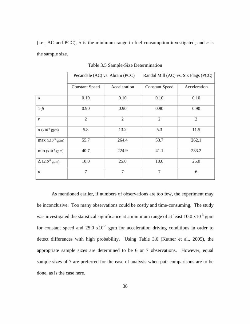
38

(i.e., AC and PCC), Δ is the minimum range in fuel consumption investigated, and n is

the sample size.

Table 3.5 Sample-Size Determination

Pecandale (AC) vs. Abram (PCC) Randol Mill (AC) vs. Six Flags (PCC)

Constant Speed Acceleration Constant Speed Acceleration

α 0.10 0.10 0.10 0.10

1-β 0.90 0.90 0.90 0.90

r 2 2 2 2

σ (x10-3 gpm) 5.8 13.2 5.3 11.5

max (x10-3 gpm) 55.7 264.4 53.7 262.1

min (x10-3 gpm) 40.7 224.9 41.1 233.2

Δ (x10-3 gpm) 10.0 25.0 10.0 25.0

n 7 7 7 6

As mentioned earlier, if numbers of observations are too few, the experiment may

be inconclusive. Too many observations could be costly and time-consuming. The study

was investigated the statistical significance at a minimum range of at least 10.0 x10-3

gpm

for constant speed and 25.0 x10-3

gpm for acceleration driving conditions in order to

detect differences with high probability. Using Table 3.6 (Kutner et al., 2005), the

appropriate sample sizes are determined to be 6 or 7 observations. However, equal

sample sizes of 7 are preferred for the ease of analysis when pair comparisons are to be

done, as is the case here.

39

Table 3.6 Sample-Size Determination Table

A day to be selected for data collection is mainly based on the surface condition

of the pavements. The surfaces must be dry. It would be on a dry day without rain. On

each dry day, other ambient conditions such as the direction and magnitude of wind

speed, air temperature, and humidity, were recorded. However, they did not influence the

analysis since pairwise data are collected under the same ambient conditions.

3.4.3 Measurements of Fuel Consumption

As mentioned earlier, fuel consumption measurements were made on four city

street sections: two PCC and two AC. Each PCC and AC section pairs had similar

gradient and roughness indices. In addition to pavement type, a number of other factors

could affect fuel consumption, including speed, acceleration, gradient, pavement

roughness, ambient temperature, atmospheric pressure, wind speed and direction, vehicle

weight, tire pressure, and use of auxiliary devices in the vehicle. In order to isolate the

40

effect of pavement type or fuel consumption, all the above factors were either controlled,

or assumed to be the same during the measurement runs.

The variables recorded for each measurement run included:

Ambient air temperature

Humidity

Wind speed and direction

Vehicle weight

Tire pressure

On/off status of auxiliary devices (A/C, radio, headlights, windows, etc.)

The last three factors were controlled and kept the same for all runs, during data

collection. The information on the first three factors was obtained from National Oceanic

and Atmospheric Administration (NOAA)’s National Weather Service website,

www.weather.gov, at the time of each study run. The weather station site is in Arlington

Municipal Airport. The radial distance from weather site to study sites is approximately

6 miles.

A 2000 Chevy Astro van with a six-cylinder 190-hp engine and automatic

transmission was used. For data collection, the vehicle is fitted with a data acquisition

system. The test vehicle, including a full tank of gasoline, all test equipment, and two

occupants, was approximately 4,700 lbs. The curb weight was 4,397 lbs.

41

Prior to the data collection on each study day, gasoline was at the full level in

order to control vehicle weight. The tire pressure was ascertained to be 50 psi, and the

vehicle was warmed up for about 15 minutes.

Prior to the commencement of a test run, the road section to drive on first was

randomly selected by tossing a coin (head for AC and tail for PCC). The next road

section would be its pair. For example, on a given day, a coin showed head, then the first

road section to perform fuel measurement would be on an asphalt section. Each of four

road sections was driven three consecutive runs at constant speed and then three

consecutive runs under acceleration. An observer, who rode with the driver, captured the

fuel data while the vehicle was operated at constant speed and under acceleration. Fuel

temperature, power cord, and instrument wires were periodically monitored to verify that

they worked properly.

During the performance of fuel measurement runs, obstacles occasionally

occurred and interrupted the driving conditions. Constant speed condition could not be

maintained and the acceleration driving condition could not be achieved. These caused

the driver to abandon these runs. Consequently, those runs had to be repeated. Apart

from unexpected traffic congestion and roadside maintenance, other data collection

interferences included previously parked vehicles pulling into the driving lane, mail

delivery vehicles stopping and going in the direction of observation, tailgating with

relatively low speed road users such as cyclists, pedestrians and lawn mowing near the

road curb, etc.

42

As discussed earlier, the fuel consumption data was collected for a total of seven

days. The fuel measurement data collection plan is depicted in Table 3.7. A and B

represent an average fuel consumption rate in gallons per mile under constant speed and

acceleration conditions for the first test sites, respectively. Likewise, C and D represent

an average fuel consumption rate in gallons per mile under constant speed and

acceleration conditions for the second test sites, respectively. Within each pair of test

sites, a statistical test to compare the means is employed on each pair of fuel consumption

under the same driving condition. For instance, considering the first test sites, fuel

consumption at constant speed on Abram Street (A1) is compared with fuel consumption

at constant speed on Pecandale Drive (A2). Again, under the acceleration driving

condition, fuel consumption B1 on Abram Street is compared with fuel consumption B2

on Pecandale Drive. The same approach is also adopted for the second test sites.

43

Table 3.7 Fuel-Consumption Measurement

Day

Fuel Consumption Measurement

The First Test Sites The Second Test Sites

Abram Street

(PCC)

Pecandale Drive

(AC)

Road to Six Flags

(PCC)

Randol Mill Road

(AC)

Constant

Speed Accel.

Constant

Speed Accel.

Constant

Speed Accel.

Constant

Speed Accel.

Day 1 A1 B1 A2 B2 C1 D1 C2 D2

Day 2 A1 B1 A2 B2 C1 D1 C2 D2

Day 3 A1 B1 A2 B2 C1 D1 C2 D2

Day 4 A1 B1 A2 B2 C1 D1 C2 D2

Day 5 A1 B1 A2 B2 C1 D1 C2 D2

Day 6 A1 B1 A2 B2 C1 D1 C2 D2

Day 7 A1 B1 A2 B2 C1 D1 C2 D2

3.5 Data Analysis Approach

As discussed, a sample size of seven is determined to be adequate for each factor–

level combination in order to obtain statistically meaningful conclusions at a 90% level of

confidence. A paired t-test is a pairwise comparison test used when comparing two sets

of measurements to assess whether the means are statistically different. As a result, it is

utilized as the statistical tool for hypothesis testing purposes in comparing fuel

consumption differences between the two pavement types in each driving mode.

44

Relating vehicle weight to fuel consumption, the test vehicle is extrapolated to

other vehicle classes in the mix. This enables the study to develop a spreadsheet format

to estimate the total fuel savings for different pavement types.

45

CHAPTER 4

DATA ANALYSIS AND RESULTS

4.1 Introduction

In the course of the fuel consumption measurements, every attempt was made to

either control all other factors that could affect fuel consumption or keep the factors that

cannot be controlled the same. These included 1) vehicle weight, 2) tire pressure, 3) fuel

type, 4) ambient temperature, 5) humidity, and 6) wind speed and direction. Among

these factors, the first three were kept the same for all runs. Factors 4-6 were recorded

for each run so that pairwise comparisons of fuel consumption on different pavements

would be made under similar conditions. For example, it would not be appropriate to

compare fuel consumption on the asphalt section when there is a 20 mph headwind to

that on the concrete pavement when there is a tailwind. Also, fuel consumption

characteristics of a vehicle could be different under different temperature or humidity

conditions.

Two different driving modes (cruise vs. acceleration) were used in the test runs.

Under the constant speed mode, a cruise speed of 30 mph was maintained throughout the

test run. In the acceleration mode, the fuel consumption data were collected while

accelerating from zero to 30 mph in 10 seconds, yielding an average acceleration rate of 3

mph/second.

46

Each data collection session included multiple runs in one or another driving

mode along two parallel test sites, one AC and one PCC. After each measurement

session, the fuel flow rate in gallons per minute and the cumulative fuel consumed in

each scenario were retrieved from the on-board data acquisition system. Two examples

of the raw data plots are shown in Figure 4.1 for PCC at constant speed and in Figure 4.2

for PCC under the acceleration mode. Vehicle speed is measured directly by the vehicle

speed sensor system mounted on the shaft. As the shaft rotates at various speeds,

magnetic field is induced by generating voltage pulse corresponding to those speeds. The

vehicle speed sensor generates an AC voltage signal output that increases or decreases

proportionally with the vehicle speed.

47

Figure 4.1 Example of Raw Data Plot for PCC Pavement under Constant Speed Mode

Figure 4.2 Example of Raw Data Plot for PCC Pavement under Acceleration Mode

0

1

2

3

4

5

6

7

8

9

10

11

12

13

14

0

5

10

15

20

25

30

35

0 2 4 6 8 10 12 14 16 18 20 22 24 26 28 30 32

Cu

m. F

ue

l C

on

su

me

d (

10

-3 g

als

)

Sp

ee

d (

mp

h)

Time (seconds)

Example of Raw Data Plot for Constant Speed

Speed

Fuel Consumed

0

1

2

3

4

5

6

7

8

9

10

11

12

0

5

10

15

20

25

30

35

0 1 2 3 4 5 6 7 8 9 10 Cu

m. F

ue

l C

on

su

me

d (

10

-3 g

als

)

Sp

ee

d (

mp

h)

Time (seconds)

Example of Raw Data Plot for Acceleration

Speed

Fuel Consumed

48

4.2 Statistical Comparisons

The data are tested at a 10% level of significance in order to obtain statistically

meaningful conclusions. To compare fuel consumption of an instrumented test vehicle as

a function of pavement surface types, a paired t-test is carried out. The p-value is also

considered when investigating.

4.2.1 Paired t-Test

As mentioned, a paired t-test is a pair test used when comparing two sets of

measurements to assess whether the means are statistically different. It is utilized as the

statistical tool for hypothesis testing purposes in comparing fuel consumption differences

between the two pavement types in each driving mode. Justification of a paired t-test can

be illustrated as follow.

Suppose there are p1 observations on street 1 on the jth

day and

there are p2 observations on street 2 on the jth

day

The average of the p1 observations is 1 j

x , and

The average of the p2 observations is 2 jx .

All observations are correlated, j = 1, 2, …, n

The p1 and p2 observations can be put in a vector. This vector has a multivariate

normal distribution.

1 11 121 1

2 21 222 2

1,

1

j

j

xN

x

; j = 1, 2, …, n

49

Where 1 j

x is a p1 x 1 vector consisting of street 1 observations, and

2 jx is a p2 x 1 vector consisting of street 2 observations.

1

1

1

11

1 ( 1)p

, 2

2

1

11

1 ( 1)p

Making a transformation by multiplying with the vector

' '

1 2

1 2

1 11 , 1A

p p

, 1 21 ( )p p

Then,

1 11 121 1

2 21 222 2

1, '

1

j

j

xA N A A A

x

1 1' ' ' '

1 2 1 1 1 2

2 21 2 1 2

1 1 1 11 , 1 1 1

j j

j j

j j

x xA x x

x xp p p p

1

1 22

j

j jj

xA x x

x

, a scalar

1 1 1 1' ' ' '

1 2 1 1 1 2 2 2

2 2 2 21 2 1 2

1 11 1 1 11 , 1 1 1 1 1

1 1A

p p p p

1 1

1 2

2 2

1

1A

11 12 2

21 22

' DA A

, a scalar

The components in 11 , 12 , 21 , and 22 are arbitrary.

50

Let 1 2

; 1,2, ,j j jD x x j n

1 2D

Then 2( , ); 1,2, ,j D DD N j n

Test 0 1 2:H is equivalent to test 0 : 0DH .

Hence, this is a paired t-test.

Given µ1 the average fuel consumption rates on a selected AC pavement and µ2

the average fuel consumption rates on a selected PCC pavement, the hypotheses for the

test would be:

H0: µ1 ≤ µ2

Ha: µ1 > µ2

4.2.1.1 The First Test Sites: Pecandale Drive (AC) vs. Abram Street (PCC)

The total fuel consumed was recorded and the corresponding consumption rates in

gallons per mile were calculated. The resulting data under constant speed mode and

acceleration mode were summarized in Table 4.1 and Table 4.2, respectively. The raw

data associated with these tables are provided in Appendix C. Figure 4.3 also shows a

comparison plot of fuel consumption between two pavement types under constant speed

mode, while Figure 4.4 illustrates the comparison plot under acceleration mode.

51

Table 4.1 Average Fuel Consumption Rates for Pecandale Drive (AC) vs. Abram Street

(PCC) under Constant Speed Mode

Date

Fuel Consumption (10-3

gpm)

AC PCC

November 7, 2008 43.7 39.8

January 16, 2009 53.2 46.8

April 21, 2011 54.1 51.3

April 23, 2011 52.6 48.7

April 28, 2011 53.8 49.7

May 3, 2011 58.6 53.4

May 5, 2011 55.1 51.0

Figure 4.3 Comparison Plot for Pecandale Drive (AC) vs. Abram Street (PCC) under

Constant Speed Mode

35.0

40.0

45.0

50.0

55.0

60.0

AC PCC

Fue

l Co

nsu

mp

tio

n (

x10

-3 g

pm

)

Pecandale Drive (AC) vs. Abram Street (PCC) under Constant Speed Mode

Nov 7

Jan 16

Apr 21

Apr 23

Apr 28

May 3

May 5

52

Table 4.2 Average Fuel Consumption Rates for Pecandale Drive (AC) vs. Abram Street

(PCC) under Acceleration Mode

Date


gpm)

AC PCC

November 7, 2008 239.0 232.5

January 16, 2009 260.5 234.6

April 21, 2011 281.0 257.7

April 23, 2011 293.6 271.6

April 28, 2011 281.5 273.7

May 3, 2011 273.2 290.6

May 5, 2011 274.2 271.9

Figure 4.4 Comparison Plot for Pecandale Drive (AC) vs. Abram Street (PCC) under

Acceleration Mode

230.0

240.0

250.0

260.0

270.0

280.0

290.0

300.0

AC PCC

Fue

l Co

nsu

mp

tio

n (

x10

-3 g

pm

)

Pecandale Drive (AC) vs. Abram Street (PCC) under Acceleration Mode

Nov 7

Jan 16

Apr 21

Apr 23

Apr 28

May 3

May 5

53

Utilizing a paired t-test, it can be observed from the Pecandale Drive (AC) vs.

Abram Street (PCC) that the calculated t-values based on fuel rate differences under all

conditions were greater than their respective tabulated (critical) t-values (see Table 4.3).

Consequently, all observed differences in fuel consumption rates were found to be

statistically significant. At a constant speed of 30 mph, the PCC section was associated

with lower consumption rate and the difference was statistically significant at a 10% level

of significance. This was also the case for the acceleration mode.

Table 4.3 Hypothesis Test Results for Paired t-Test for Pecandale Drive (AC) vs. Abram

Street (PCC) at 10% Level of Significance

Condition

t-statistics

DF Calculated t Tabulated t Results

Constant Speed of 30 mph 6 9.8220 1.4398 significant

Acceleration of 3 mph/sec 6 1.7380 1.4398 significant

According to Figure 4.4, the fuel data collected on May 3rd

under acceleration

happened to have more fuel consumption rate on PCC section. This data could be an

outlier as its trend was not consistent with the rest. However, when testing the hypothesis

under acceleration mode by excluding this data, the null hypothesis was rejected, so the

differences in fuel consumption rates were found to be statistically significant. Also, p-

value was less than α, the result was statistically significant.

54

4.2.1.2 The Second Test Sites: Randol Mill Road (AC) vs. Road to Six Flags

(PCC)

Fuel measurements were conducted on additional road sections, despite their

different conditions from the first road sections, to investigate whether or not AC

pavement has a higher vehicular fuel consumption rate than PCC pavement. Table 4.4

and Table 4.5 shows fuel consumption rates under constant speed mode and acceleration

mode, respectively. The associated raw data are provided in Appendix C. The

comparison plots of fuel consumption between Randol Mill Road (AC) and Road to Six

Flags (PCC) under constant speed mode and acceleration mode were also depicted in

Figure 4.5 and Figure 4.6 , respectively.

55

Table 4.4 Average Fuel Consumption Rates for Randol Mill Road (AC) vs. Road to Six

Flags (PCC) under Constant Speed Mode

Date


gpm)

AC PCC

July 3, 2009 47.7 41.1

July 23, 2009 52.8 45.4

July 24, 2009 51.7 42.1

April 21, 2011 47.8 42.0

April 23, 2011 48.9 39.7

April 28, 2011 49.3 42.3

May 3, 2011 47.2 42.0

Figure 4.5 Comparison Plot for Randol Mill Road (AC) vs. Road to Six Flags (PCC)

under Constant Speed Mode

35.0

40.0

45.0

50.0

55.0

AC PCC

Fue

l Co

nsu

mp

tio

n (

x10

-3 g

pm

)

Randol Mill Road (AC) vs. Road to Six Flags (PCC) under Constant Speed Mode

Jul 3

Jul 23

Jul 24

Apr 21

Apr 23

Apr 28

May 3

56

Table 4.5 Average Fuel Consumption Rates for Randol Mill Road (AC) vs. Road to Six

Flags (PCC) under Acceleration Mode

Date


gpm)

AC PCC

July 3, 2009 256.5 243.3

July 23, 2009 266.1 235.1

July 24, 2009 252.7 240.1

April 21, 2011 262.6 228.8

April 23, 2011 278.2 258.0

April 28, 2011 271.6 231.0

May 3, 2011 256.3 236.8

Figure 4.6 Comparison Plot for Randol Mill Road (AC) vs. Road to Six Flags (PCC)

under Acceleration Mode

220.0

230.0

240.0

250.0

260.0

270.0

280.0

AC PCC

Fue

l Co

nsu

mp

tio

n (

x10

-3 g

pm

)

Randol Mill Road (AC) vs. Road to Six Flags (PCC) under Acceleration Mode

Jul 3

Jul 23

Jul 24

Apr 21

Apr 23

Apr 28

May 3

57

For these two road sections, the observed fuel consumption rates were tested for

statistical significance at 10% level of significance. The fuel consumption rate for the

PCC pavement was observed to be lower than the rate for the AC pavement in both

driving modes. Table 4.6 summarizes the hypothesis test results.

Table 4.6 Hypothesis Test Results for Paired t-Test for Randol Mill Road (AC) vs. Road

to Six Flags (PCC) at 10% Level of Significance

Condition

t-statistics




4.2.2 p-Value

The p-value of a test is the smallest probability that would allow the null

hypothesis to be rejected. The smaller the p-value, the more strongly the test rejects the

null hypothesis. By comparing the p-value with selected value of α, the decision rule for

testing H0 against HA can be written as reject H0 if p < α.

Table 4.7 and Table 4.8 present the test of p-value at 10% level of significance for

the first test sites and the second test sites, respectively. On both test sites, it can be

observed that the p-values under all conditions were smaller than the value of α equal to

0.10. As a result, all null hypotheses were rejected, the results were statistically

significant. This supports the results from the previous paired t-test on both test sites. At

a constant speed of 30 mph, the PCC sections were associated with a lower consumption

58

rate and the differences were statistically significant at a 10% level of significance.

Under the acceleration mode at a 0.10 level, the differences were also statistically

significant with the PCC sections having lower fuel rates. It can be further observed from

Table 4.7 and Table 4.8 that if the significance level is 0.05, the fuel consumption rates

for the PCC pavements would be lower than the rates for the AC pavements at a constant

speed mode. However, it is not the case for the acceleration mode on Pecandale Drive

and Abram Street, because the differences are not statistically significant.

Table 4.7 Test of p-Value for Pecandale Drive (AC) vs. Abram Street (PCC) at 10%

Level of Significance

Condition

p-value test at α=0.10

p-value Results

Constant Speed of 30 mph 0.000032 significant

Acceleration of 3 mph/sec 0.066441 significant

Table 4.8 Test of p-Value for Randol Mill Road (AC) vs. Road to Six Flags (PCC) at

10% Level of Significance

Condition


p-value Results



59

The study further investigated the hypothesis tests in the case that all observed

data were merged for each driving mode. For asphalt sections, fuel consumption data

from Pecandale Drive were combined with data from Randol Mill Road, whereas for

concrete sections fuel data from Abram Street were combined with data from Road to Six

Flags. Those were based on the same driving conditions. That is, paired t-tests were

carried out for AC vs. PCC sections under constant speed and acceleration modes.

Table 4.9 summarizes the hypothesis test results. It can be observed that the

calculated t-values based on fuel rate differences under both driving conditions were

higher than their tabulated t-values. Thus, all differences in fuel consumption rates were

found to be statistically significant at a 10% level of significance with the fuel

consumption rates on AC sections being higher. p-values (see Table 4.10) also resulted

that all differences were significant as p-values were less than α, thereby null hypothesis

rejected.

Table 4.9 Hypothesis Test Results for Paired t-Test for AC vs. PCC Pavements at 10%

Level of Significance

Condition

t-statistics




60

Table 4.10 Test of p-Value for AC vs. PCC Pavements at 10% Level of Significance

Condition


p-value Results



To reconsider the standard deviations (σ) and sample size (n) after all fuel

measurement data were observed, Table 4.11 was generated as shown.

Table 4.11 Standard Deviations and Sample Size after All Data Observed

Pecandale (AC) vs. Abram (PCC) Randol Mill (AC) vs. Six Flags (PCC)

Constant Speed Acceleration Constant Speed Acceleration

α 0.10 0.10 0.10 0.10

1-β 0.90 0.90 0.90 0.90

r 2 2 2 2

σ (x10-3 gpm) 4.9 19.6 4.2 15.6

max (x10-3 gpm) 58.6 293.6 52.8 278.2

min (x10-3 gpm) 39.8 232.5 39.7 228.8

Δ (x10-3 gpm) 10.0 25.0 10.0 25.0

n 6 12 5 9

The standard deviations at constant speed mode on both pair of test sites (4.9 and

4.2 x10-3

gpm) were smaller than those used in determining sample size process (see

61

3.4.2), while the standard deviations under acceleration mode (19.6 and 15.6 x10-3

gpm)

were greater than those used in determining the sample size. Then, the new sample sizes

for each scenario were retrieved by using Table 3.6. The new sample sizes on both pair

of sections at constant speed were smaller than those calculated from the preliminary

study. The first test sites have 6 sample sizes, compared to previous sample sizes of 7,

while the second test sites have 5 sample sizes, compared to previous sample sizes of 7.

On the other hand, the new sample sizes under acceleration were larger than those from

the preliminary study. The new sample sizes of the first and second test sites are 12 and

9, respectively. The sample sizes under acceleration from preliminary study are 7 and 6

for the first and second test sites, respectively.

4.3 Estimation of Fuel Consumption and CO2 Emissions including Cost Differences

4.3.1 Estimation of Fuel Consumption and CO2 Emissions

This section is to quantify the fuel consumed by the test vehicle over two

pavement types as a basis for projecting potential costs or savings of one pavement type

versus another over a project design life. Fuel consumption rates are used to project fuel

consumption rate differences for other vehicles in the traffic mix using linear projections

based on respective vehicle weight ratios. The amounts of fuel consumption are also

used to estimate CO2 emissions.

The average fuel consumption rates are used as the basis for development of the

afore-mentioned spreadsheet tool (Chang et al., 1976; Wood et al., 1981). As discussed

earlier, under both driving modes, the fuel consumption rates for the PCC pavement was

62

found to be statistically (at α = 10%) lower than the corresponding rates for the AC

pavement. To illustrate the cumulative effect of these differences, the fuel rates for the

constant speed condition were applied to the annual vehicle miles of travel (VMT) in the

Dallas-Fort Worth (DFW) region of Texas. In 2007, for example, the total annual VMT

in the nine-county DFW region was estimated to be 62,697 million miles (North Central

Texas Council of Government, 2007). The fuel consumption rates used are the average

of 7-day fuel rates on Randol Mill and Road to Six Flags as Road to Six Flags could be a

representative of JPCP, the most common type of concrete pavement. It is the most

commonly used type of concrete pavement in the U.S since about 43 states use or have

JPCP design procedures (Delatte, 2008; Washington State Department of Transportation,

2003). The fuel rates then were applied to the VMT to obtain the total annual fuel

consumption estimates for a hypothetical mix of vehicles, as shown in Table 4.12 (for

AC) and Table 4.13 (for PCC).

63

Table 4.12 Calculations of Annual Fuel Consumption for the Dallas-Fort Worth Region

of Texas under AC Pavement and Constant Speed Mode

Vehicle

Type

Average

Vehicle

Weight

(lbs)

VMT

(million

miles/yr)

% in the

Mix

Fuel Rate

(gals/mi)

Fuel

Consumed

(million

gals/yr)

LDGV 3,000 42,273 67.425 0.0198 835.3

LDGT1 4,000 2,708 4.318 0.0263 71.3

LDGT2 4,000 9,013 14.376 0.0263 237.5

LDGT3 7,500 2,605 4.155 0.0494* 128.7

LDGT4 7,500 1,198 1.911 0.0494 59.2

HDGV2B 9,500 494 0.788 0.0626 30.9

HDGV3 12,000 141 0.225 0.0790 11.1

HDGV4 15,000 73 0.116 0.0988 7.2

HDGV5 18,000 40 0.063 0.1186 4.7

HDGV6 23,000 66 0.106 0.1515 10.1

HDGV7 29,500 16 0.026 0.1943 3.2

HDGV8A 47,000 16 0.025 0.3096 4.9

HDGV8B 80,000 2 0.003 0.5269 1.1

LDDV 3,000 42 0.068 0.0198 0.8

LDDT12 4,000 10 0.016 0.0263 0.3

HDDV2B 9,500 574 0.915 0.0626 35.9

HDDV3 12,000 163 0.259 0.0790 12.9

HDDV4 15,000 119 0.190 0.0988 11.8

HDDV5 18,000 80 0.128 0.1186 9.5

HDDV6 23,000 259 0.412 0.1515 39.2

HDDV7 29,500 92 0.147 0.1943 17.9

HDDV8A 47,000 155 0.247 0.3096 48.0

HDDV8B 80,000 2,075 3.310 0.5269 1,093.5

MC 700 46 0.074 0.0046 0.2

HDGB 15,000 14 0.022 0.0988 1.4

HDDBT 35,000 49 0.078 0.2305 11.2

HDDBS 22,500 80 0.128 0.1482 11.9

LDDT34 7,500 292 0.466 0.0494 14.4

∑ 62,697 100

2,714.1

* Measured in the field

64

Table 4.13 Calculations of Annual Fuel Consumption for the Dallas-Fort Worth Region

of Texas under PCC Pavement and Constant Speed Mode

Vehicle

Type

Average

Vehicle

Weight

(lbs)

VMT

(million

miles/yr)

% in the

Mix

Fuel Rate

(gals/mi)

Fuel

Consumed

(million

gals/yr)

LDGV 3,000 42,273 67.425 0.0168 711.9

LDGT1 4,000 2,708 4.318 0.0225 60.8

LDGT2 4,000 9,013 14.376 0.0225 202.4

LDGT3 7,500 2,605 4.155 0.0421* 109.7

LDGT4 7,500 1,198 1.911 0.0421 50.4

HDGV2B 9,500 494 0.788 0.0533 26.4

HDGV3 12,000 141 0.225 0.0674 9.5

HDGV4 15,000 73 0.116 0.0842 6.1

HDGV5 18,000 40 0.063 0.1010 4.0

HDGV6 23,000 66 0.106 0.1291 8.6

HDGV7 29,500 16 0.026 0.1656 2.7

HDGV8A 47,000 16 0.025 0.2638 4.2

HDGV8B 80,000 2 0.003 0.4491 1.0

LDDV 3,000 42 0.068 0.0168 0.7

LDDT12 4,000 10 0.016 0.0225 0.2

HDDV2B 9,500 574 0.915 0.0533 30.6

HDDV3 12,000 163 0.259 0.0674 11.0

HDDV4 15,000 119 0.190 0.0842 10.0

HDDV5 18,000 80 0.128 0.1010 8.1

HDDV6 23,000 259 0.412 0.1291 33.4

HDDV7 29,500 92 0.147 0.1656 15.2

HDDV8A 47,000 155 0.247 0.2638 40.9

HDDV8B 80,000 2,075 3.310 0.4491 931.9

MC 700 46 0.074 0.0039 0.2

HDGB 15,000 14 0.022 0.0842 1.2

HDDBT 35,000 49 0.078 0.1965 9.6

HDDBS 22,500 80 0.128 0.1263 10.2

LDDT34 7,500 292 0.466 0.0421 12.3

∑ 62,697 100

2,313.1


65

The field-measured fuel rates under the constant speed mode in Table 4.12 and

Table 4.13 correspond to the instrumented van, LDGT3 (7,500-lb weight). For the

purpose of calculations summarized in these tables, fuel consumption rates for all other

vehicle classes were estimated from the field-measured rate based on the weight ratio of

the two respective classes. For example, a 15,000-lb vehicle was estimated to have twice

as large a fuel consumption rate than the 7,500-lb test vehicle. As mentioned earlier, this

method of approximating fuel consumption rates was based on a number of fuel

consumption studies that have shown fuel consumption ratios to be approximately

proportional to vehicle weight ratios (Chang et al., 1976; Wood et al., 1981). The total

fuel consumption amounts per annum then were estimated using those rates and the total

VMT for each vehicle class. They resulted in an annual fuel consumption of 2,714

million gallons for AC pavement and 2,313 million gallons for PCC pavement.

The CO2 emissions from mobile sources may be calculated using emission fact

provided by EPA’s Office of Transportation and Air Quality (OTAQ). A gallon of

conventional gasoline generates 19.4 pounds (8.8 kg) of CO2 emissions (U.S.

Environmental Protection Agency, 2005). Therefore, the CO2 emissions per annum on

AC pavement is estimated to be 23.88 million metric tons, while CO2 emissions

estimation on PCC pavement is 20.36 million metric tons, summarized in Table 4.14. It

is noted that these estimates assume all the VMT occurs at a 30-mph constant speed.

66

Table 4.14 Total Annual CO2 Emissions for the Dallas-Fort Worth Region of Texas

under Constant Speed

Fuel Consumed

(million

gals/yr)

Total CO2

(million metric

tons/yr)

AC, Constant Speed (30 mph) 2,714 23.88

PCC, Constant Speed (30 mph) 2,313 20.35

The fuel consumption weight proportionality is a feasible approach for this

research study when there is no actual fuel consumption rates of all vehicle classes

provided. In lieu of testing on every vehicle class, the fuel consumption data were made

by the vehicle available at the time. The fuel consumption weight proportionality

assumption is reasonable to apply as weight resists movement. The more the vehicle

weight is, the more the energy is required by the engine to accelerate the vehicle and to

overcome rolling resistance. However, it should be noted that this method was

experimented under urban traffic condition at low speeds where weight and traffic

conditions have a direct impact on the fuel vehicle consumed (Wood et al., 1981).

Therefore, this approach could be a conservative assumption as numbers of acceleration

and deceleration, and stop-and-go can cause high fuel consumption rate. Using this

method for highway driving is doable to compare fuel consumption of vehicles that have

similar frontal areas. Because, in addition to vehicle weight, aerodynamic drag is a big

67

issue for a large frontal-area vehicle driving at highway speeds. A larger frontal area

creates higher drag force that acts on a moving vehicle.

4.3.2 Estimation of Fuel Saving and Emissions Reductions

As the overall results for the constant speed mode are summarized in Table 4.14,

if the annual vehicle miles of travel in the DFW region took place at a constant speed of

30 mph all on PCC pavements similar to the ones in the test sections, the statistically

lower fuel rate could result in an annual fuel savings of about 401 million gallons and an

annual CO2 reduction of about 3.53 million metric tons. Assuming an average gasoline

price of about $3.29 a gallon and an average CO2 clean-up cost of about $18 per metric

tons (EcoBusinessLinks, 2009), these differences (see Table 4.15) would amount to a

savings of about $1.38 billion per year in the DFW region, a cost savings which should

be considered in the life-cycle cost analysis of alternative city street pavement projects.

Table 4.15 Annual Fuel Savings and Emissions Reductions in Favor of PCC Pavement

for the Dallas-Fort Worth Region of Texas under Constant Speed

(million/yr)

Fuel Savings $1,319

Emissions Reductions $64

Total Savings $1,383

68

4.3.3 Estimation of CO2 Emissions of a Mile Section of a Typical City Street

Estimating CO2 emissions of a pavement involves many variable inputs. The

examples are carbon footprint from the material production, pavement construction, and

maintenance process of the pavement itself and carbon footprint produced by the vehicles

using that pavement section.

Abram Street is chosen for analysis as a typical city street. Abram Street has an

average daily traffic (ADT), which represents an estimate of the number of vehicles

traveling along this section of Abram Street, of 12,003 vehicles per day (City of

Arlington, 2011).

Table 4.16 presents fuel consumption on a one-mile long section of Abram Street.

The average fuel consumption rate on this section driven by the instrumented van is

0.0487 gpm. The fuel rate was projected to the other vehicle types in the mix by vehicle

weight ratio. The ADT was calculated based on % of vehicle mix. The fuel rates then

were multiplied to the ADT to obtain the total fuel consumption estimates for a mix of

vehicles. As a result, the total fuel consumed per day on a one-mile PCC section under

constant speed is estimated to be 512 gallons.

The same steps were applied to a one-mile AC section. AC section has an

average fuel consumption rate of 0.0530 gpm, from Pecandale Drive, but for comparison,

the study assumed that this section has the same ADT as PCC section. Table 4.17 show

the fuel consumption amounts per one mile per day in a hypothetical mix of vehicles,

which yielding to 558 gallons.

69

Table 4.16 Calculations of Daily Fuel Consumption on a One-Mile PCC Section of a

Typical City Street under Constant Speed Mode

Vehicle

Type

Average

Vehicle

Weight

(lbs)

% in the

Mix

ADT

(vpd)

Fuel Rate

(gals/mi)

Fuel

Consumed

(gals/mile/day)

LDGV 3,000 67.425 8,093 0.0195 157.7

LDGT1 4,000 4.318 518 0.0260 13.5

LDGT2 4,000 14.376 1,726 0.0260 44.8

LDGT3 7,500 4.155 499 0.0487 24.3

LDGT4 7,500 1.911 229 0.0487 11.2

HDGV2B 9,500 0.788 95 0.0617 5.8

HDGV3 12,000 0.225 27 0.0779 2.1

HDGV4 15,000 0.116 14 0.0974 1.4

HDGV5 18,000 0.063 8 0.1169 0.9

HDGV6 23,000 0.106 13 0.1493 1.9

HDGV7 29,500 0.026 3 0.1916 0.6

HDGV8A 47,000 0.025 3 0.3052 0.9

HDGV8B 80,000 0.003 0 0.5195 0.2

LDDV 3,000 0.068 8 0.0195 0.2

LDDT12 4,000 0.016 2 0.0260 0.1

HDDV2B 9,500 0.915 110 0.0617 6.8

HDDV3 12,000 0.259 31 0.0779 2.4

HDDV4 15,000 0.190 23 0.0974 2.2

HDDV5 18,000 0.128 15 0.1169 1.8

HDDV6 23,000 0.412 49 0.1493 7.4

HDDV7 29,500 0.147 18 0.1916 3.4

HDDV8A 47,000 0.247 30 0.3052 9.1

HDDV8B 80,000 3.310 397 0.5195 206.4

MC 700 0.074 9 0.0045 0.0

HDGB 15,000 0.022 3 0.0974 0.3

HDDBT 35,000 0.078 9 0.2273 2.1

HDDBS 22,500 0.128 15 0.1461 2.3

LDDT34 7,500 0.466 56 0.0487 2.7

∑ 100 12,003

512.2


70

Table 4.17 Calculations of Daily Fuel Consumption on a One-Mile AC Section of a

Typical City Street under Constant Speed Mode

Vehicle

Type

Average

Vehicle

Weight

(lbs)

% in the

Mix

ADT

(vpd)

Fuel Rate

(gals/mi)

Fuel

Consumed

(gals/mile/day)

LDGV 3,000 67.425 8,093 0.0212 171.6

LDGT1 4,000 4.318 518 0.0283 14.7

LDGT2 4,000 14.376 1,726 0.0283 48.8

LDGT3 7,500 4.155 499 0.0530 26.4

LDGT4 7,500 1.911 229 0.0530 12.2

HDGV2B 9,500 0.788 95 0.0671 6.4

HDGV3 12,000 0.225 27 0.0848 2.3

HDGV4 15,000 0.116 14 0.1060 1.5

HDGV5 18,000 0.063 8 0.1272 1.0

HDGV6 23,000 0.106 13 0.1625 2.1

HDGV7 29,500 0.026 3 0.2085 0.7

HDGV8A 47,000 0.025 3 0.3321 1.0

HDGV8B 80,000 0.003 0 0.5653 0.2

LDDV 3,000 0.068 8 0.0212 0.2

LDDT12 4,000 0.016 2 0.0283 0.1

HDDV2B 9,500 0.915 110 0.0671 7.4

HDDV3 12,000 0.259 31 0.0848 2.6

HDDV4 15,000 0.190 23 0.1060 2.4

HDDV5 18,000 0.128 15 0.1272 1.9

HDDV6 23,000 0.412 49 0.1625 8.0

HDDV7 29,500 0.147 18 0.2085 3.7

HDDV8A 47,000 0.247 30 0.3321 9.9

HDDV8B 80,000 3.310 397 0.5653 224.6

MC 700 0.074 9 0.0049 0.0

HDGB 15,000 0.022 3 0.1060 0.3

HDDBT 35,000 0.078 9 0.2473 2.3

HDDBS 22,500 0.128 15 0.1590 2.4

LDDT34 7,500 0.466 56 0.0530 3.0

∑ 100 12,003 557.5


71

According to Nair and Bhat (2000), many metropolitan planning organizations

(MPOs) typically calculate the VMT on city streets as about 10% of the VMT on all other

streets. A fraction of 0.10 of the total VMT in DFW nine-county region is on city streets

and is then multiplied to the fuel consumption in the region. Therefore, the amounts of

fuel consumed per day on a one-mile section of AC vs. PCC were about 55.8 and 51.2

gallons, respectively. As a gallon of conventional gasoline produces 19.4 pounds (8.8

kg) of CO2 emissions, the CO2 emissions on AC are estimated to be 0.491 metric tons,

while CO2 emissions estimation on PCC pavement is 0.450 metric tons. Table 4.18

presents this study’s estimate of the carbon footprint released by the mix of vehicles

under 30-mph constant speed on a one-mile long AC and PCC city streets per day.

Table 4.18 Daily CO2 Emissions on a One-Mile Section of a Typical City Street under

Constant Speed Mode

Fuel Consumed

(gals/mi/day)

Total CO2

(metric

tons/mi/day)

AC, Constant Speed (30 mph) 55.75 0.491

PCC, Constant Speed (30 mph) 51.22 0.450

As mentioned earlier that a Canadian study (Brown, 2009) compares two typical

residential pavement cross-sections, an AC and a PCC pavement section in southern

Ontario. The study estimates the contributions of these two pavement materials to the

carbon footprint of a one-kilometer long section. The calculation is based on the CO2

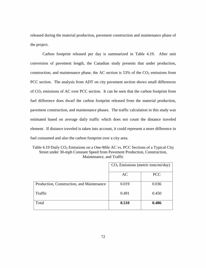
72

released during the material production, pavement construction and maintenance phase of

the project.

Carbon footprint released per day is summarized in Table 4.19. After unit

conversion of pavement length, the Canadian study presents that under production,

construction, and maintenance phase, the AC section is 53% of the CO2 emissions from

PCC section. The analysis from ADT on city pavement section shows small differences

of CO2 emissions of AC over PCC section. It can be seen that the carbon footprint from

fuel difference does dwarf the carbon footprint released from the material production,

pavement construction, and maintenance phases. The traffic calculation in this study was

estimated based on average daily traffic which does not count the distance traveled

element. If distance traveled is taken into account, it could represent a more difference in

fuel consumed and also the carbon footprint over a city area.

Table 4.19 Daily CO2 Emissions on a One-Mile AC vs. PCC Sections of a Typical City

Street under 30-mph Constant Speed from Pavement Production, Construction,

Maintenance, and Traffic

CO2 Emissions (metric tons/mi/day)

AC PCC

Production, Construction, and Maintenance 0.019 0.036

Traffic 0.491 0.450

Total 0.510 0.486

73

CHAPTER 5

CONCLUSIONS AND RECOMMENDATIONS

5.1 Conclusions

The goal of this study was to investigate any statistically significant differences

which might exist in fuel consumption rates on typical concrete versus asphalt city

streets. The study was conducted through field data collections using an instrumented

van.

It was observed that under urban driving speeds of 30 mph, the fuel consumption

per unit distance is lower on concrete pavements compared to asphalt pavements. These

findings were based on test runs on two sets of typical Portland Cement Concrete and

Asphalt Concrete street sections in Arlington, Texas, with each pair of study sites having

similar gradient and roughness index values. All observed differences were found to be

statistically significant at a 10% level of significance.

The annual potential costs or savings in fuel consumed and CO2 emissions

generated were shown to be substantial over the Dallas-Fort Worth region. As a result, it

is recommended that these costs or savings be considered in the life cycle cost analysis of

alternative projects. Differences in CO2 emissions should also be considered in life cycle

analysis when estimating the carbon footprint of particular pavement materials to be

used.

74

Estimation of carbon footprint is an important step in assessing the sustainability

of city development projects and the overall life cycle analysis of projects. In pavement

projects, specifically, the focus has been on estimating the carbon footprint of the

production cycle of various pavement materials as well as the initial construction phase.

A key finding of this study is that any such sustainability assessment must also consider

the emissions differences based on operations of motor vehicles on various pavement

surfaces. When considering a 20-50 year design life that is typical for city streets and the

annual vehicle miles of travel, such differences could help dwarf carbon footprint

estimations from the material production or pavement construction phases.

5.2 Recommendations

Critics of this study might argue that the numbers presented herein are not

accurate estimates of the actual costs and savings realized in the Dallas-Fort Worth or any

other urban region. This is because the examples presented are based on the mixes of

vehicles, all driven at a constant speed of 30 mph. Furthermore, the fuel consumption

rates per unit distance are developed based on a fairly limited sample of population of

asphalt and concrete pavement types and typical pavement cross-sections in a city.

Indeed it can be argued that to have accurate numbers, a more comprehensive study must

be conducted, which includes the variety of asphalt and concrete mix designs used in city

pavements as well as a broader sample of cross-section thicknesses of crown layers and

base materials. Such a study should also include direct fuel rate measurements for a

variety of vehicle types driven under a range of drive cycles as opposed to extrapolating

the fuel consumption characteristics of one vehicle driven at a constant speed to other

75

vehicle types and speed regimes. Thirdly, to better control exogenous factors such as

wind speed and direction, temperature, and humidity perhaps the tests should be

conducted using pavement sections constructed indoors where the ambient environment

is controlled. In addition to IRI values, direct measurements of the skid resistance would

be needed for each pavement section being tested. Last but not least, the measurements

should be made under a much wider range of ambient humidity and temperatures than

typically experienced in the Dallas-Fort Worth region.

Of course, if all these factors are to be considered it could be possible to show

beyond doubt that one type of pavement results in better fuel efficiency than another and

by how much. This would also substantially improve the accuracy of estimates of user

costs and savings. But it is important to note that the numerical examples in this research

are intended to illustrate how significant minute differences in fuel consumption and

emissions could be over the design life of a project. However, these results are at best

applicable to the specific pavement types studied and the test vehicle used. In fact, it

would not be feasible to develop, based on these specific results, very accurate estimation

algorithms that cover the entire spectrum of vehicle classes and pavement mix designs

and cross-sections.

In accounting for user costs or savings for specific design alternatives, a more

sensible approach could be to conduct similar tests of differences in fuel consumption

rates over pavement sections already constructed to the intended specifications and using

a representative vehicle with the highest proportion in the vehicle mix. In this vein, the

study results presented used a typical minivan driven over typical HMA and PCC

76

pavement cross-sections in the study region to illustrate that there could be statistically

significant differences in fuel consumption and emissions for one pavement type versus

another. Furthermore, numerical examples showed that such differences, while small on

a per mile basis, could be very large over the design life of a project and should therefore

be considered in any life cycle cost analysis or life cycle analysis of carbon footprints of

alternative pavement designs.

77

APPENDIX A

INTERNATIONAL ROUGHNESS INDEX MEASUREMENTS

78

Ride Quality Analysis Rel 2008.11.11 TxDOT Smoothness Specification 5880 Pay Schedule 3 Report run on Friday Feb 27 2009 3:03:50PM Input profile data file created Friday Feb 27 2009 10:25:48AM District 2 Highway PECANDALE_DR Area Office FT worth Beg RM 0000 +00.000 County 220 Beg Station 0000+00.0 CSJ JEFF HOWDES Lane roadbed K1 Phone FM2122E Name Input file t:\dalpme\uta project with profiler\cty220_pecandale_st_20090227_1624.pro *** eastbound outside lane *** Beg Station 0000+00.0 No Bump penalties assessed. Bonus paid for average IRIs of 30($600) to 60($0) No penalties assessed for high IRIs. Bonus NOT paid in sections with bump. Profile Length(Miles) 0.3612 Length(Station Units) 0019+07.1ft. Distance Station Type Width(feet) Elev(inches) 00.0009 0000+04.5 Bump .7 .19 00.0019 0000+09.8 Dip 4.0 -.25 00.0033 0000+17.6 Bump 2.2 .18 00.0039 0000+20.3 Bump 1.3 .17 00.0050 0000+26.5 Dip 3.4 -.23 00.0074 0000+39.2 Dip .5 -.16 00.0076 0000+39.9 Dip .2 -.15 00.0078 0000+41.2 Dip .2 -.15 00.0079 0000+41.7 Dip 4.0 -.22 00.0112 0000+59.2 Bump 4.7 .25 00.0138 0000+72.8 Dip 4.2 -.24 00.0167 0000+88.0 Bump 7.4 .22 00.0188 0000+99.5 Dip 8.3 -.30 00.0321 0001+69.7 Bump 3.1 .17 00.0350 0001+84.8 Dip .4 -.16 00.0489 0002+58.3 Bump .2 .15 00.0490 0002+58.6 Bump 1.6 .18 00.0506 0002+67.3 Dip 3.6 -.20 00.0603 0003+18.4 Dip .2 -.15 00.0604 0003+18.7 Dip .7 -.17 00.0942 0004+97.1 Bump .5 .16 00.0957 0005+05.1 Dip 5.4 -.25 00.1192 0006+29.4 Dip 2.9 -.23 00.1643 0008+67.8 Dip 4.2 -.27 00.1672 0008+82.8 Bump 2.0 .19 00.1703 0008+99.0 Dip 2.9 -.17 00.1922 0010+14.6 Bump .2 .15 00.1923 0010+15.5 Bump .2 .15 00.1932 0010+20.2 Dip 5.1 -.44 00.1954 0010+31.6 Bump .7 .18 00.1956 0010+32.6 Bump 2.4 .21 00.2027 0010+70.3 Bump .2 .16 00.2028 0010+71.0 Bump 1.3 .18 00.2034 0010+73.8 Bump .4 .16 00.2533 0013+37.7 Dip .9 -.16 00.2541 0013+41.5 Dip .9 -.18

79

Distance Station Type Width(feet) Elev(inches) 00.2550 0013+46.5 Dip 3.3 -.20 00.2577 0013+60.9 Bump 7.1 .27 00.2592 0013+68.3 Bump 4.0 .21 00.2608 0013+77.2 Dip 6.7 -.51 00.2626 0013+86.7 Bump 2.7 .20 00.2642 0013+95.2 Bump 2.9 .22 00.2795 0014+75.6 Bump 2.9 .22 00.2810 0014+83.8 Dip .2 -.15 00.2812 0014+84.5 Dip .4 -.15 00.2915 0015+39.3 Dip .2 -.15 00.2916 0015+39.8 Dip .5 -.17 00.3080 0016+26.4 Dip .7 -.18 00.3093 0016+33.0 Bump 8.3 .20 00.3160 0016+68.3 Dip 1.1 -.16 00.3564 0018+81.8 Dip .2 -.17 00.3565 0018+82.2 Dip .2 -.15 00.3565 0018+82.5 Dip 4.4 -.22 00.3583 0018+91.6 Bump 1.6 .17 00.3586 0018+93.6 Bump .5 .16 00.3588 0018+94.5 Bump .5 .16 Bumps/dips detected 56 Distance Station PSI IRI(L) IRI(R) Avg IRI Pay*SectLen Pay 00.1000 5+28.0 2.33 153.45 230.29 192.00 $ 0*(0.1000/0.10) $0 00.2000 10+56.0 2.53 114.39 237.37 176.00 $ 0*(0.1000/0.10) $0 00.3000 15+84.0 2.55 120.08 227.13 174.00 $ 0*(0.1000/0.10) $0 00.3612 19+07.1 2.46 125.35 236.88 181.00 $ 0*(0.0612/0.10) $0

Pay Adjustment Subtotal $0 Ave Left IRI 128.6 Ave Right IRI 232.5 Ave IRI 180.55 Total IRI adjustments $ 0 Total Bump adjustments $ 0 Total adjustments $ 0

80

Ride Quality Analysis Rel 2008.11.11 TxDOT Smoothness Specification 5880 Pay Schedule 3 Report run on Friday Feb 27 2009 2:59:30PM Input profile data file created Friday Feb 27 2009 10:30:14AM District 2 Highway ABRAM_ST Area Office Ft worth Beg RM 0000 +00.000 County 220 Beg Station 0000+00.0 CSJ JEFF HOWDES Lane roadbed K1 Phone FM2122E Name Input file t:\dalpme\uta project with profiler\cty220_abram_st_20090227_1628.pro *** eastbound outside lane *** Beg Station 0000+00.0 No Bump penalties assessed. Bonus paid for average IRIs of 30($600) to 60($0) No penalties assessed for high IRIs. Bonus NOT paid in sections with bump. Profile Length(Miles) 0.7276 Length(Station Units) 0038+41.7ft. Distance Station Type Width(feet) Elev(inches) 00.0129 0000+68.1 Dip .5 -.17 00.0132 0000+69.9 Dip .4 -.16 00.0262 0001+38.5 Dip 2.5 -.17 00.0382 0002+01.8 Bump .2 .15 00.0670 0003+53.9 Bump .2 .15 00.0993 0005+24.5 Bump 2.0 .20 00.0998 0005+26.7 Bump 2.5 .20 00.1003 0005+29.4 Bump .4 .16 00.1051 0005+54.8 Bump .2 .15 00.1052 0005+55.4 Bump 1.3 .20 00.1313 0006+93.5 Dip 2.9 -.23 00.1457 0007+69.2 Dip .4 -.16 00.1461 0007+71.2 Dip .4 -.15 00.2070 0010+93.2 Dip 4.2 -.25 00.2079 0010+97.5 Dip .2 -.15 00.2080 0010+98.1 Dip .4 -.16 00.2081 0010+98.8 Dip .9 -.17 00.2094 0011+05.7 Bump .2 .15 00.2095 0011+06.1 Bump 2.2 .18 00.2102 0011+09.7 Bump .2 .15 00.2391 0012+62.5 Dip 5.8 -.28 00.2416 0012+75.6 Bump 2.4 .19 00.2615 0013+80.7 Bump .2 .15 00.2873 0015+17.2 Dip .9 -.17 00.2875 0015+18.2 Dip .4 -.16 00.2877 0015+19.0 Dip .5 -.16 00.2878 0015+19.7 Dip .4 -.16 00.2906 0015+34.2 Bump .2 .16 00.2907 0015+34.8 Bump .4 .15 00.3441 0018+16.6 Bump .2 .15 00.3443 0018+17.7 Bump 2.5 .20 00.3451 0018+22.1 Bump .2 .15 00.3474 0018+34.2 Dip .7 -.17 00.3570 0018+84.9 Dip .7 -.16 00.3573 0018+86.7 Dip 1.3 -.16 00.3579 0018+90.0 Dip .2 -.15

81

Distance Station Type Width(feet) Elev(inches) 00.3608 0019+05.2 Bump 1.1 .17 00.3611 0019+06.5 Bump 11.1 .24 00.3645 0019+24.4 Dip 6.0 -.21 00.3657 0019+30.8 Dip .9 -.17 00.3682 0019+44.2 Bump .4 .16 00.3683 0019+44.8 Bump .2 .15 00.3684 0019+45.3 Bump .4 .15 00.3687 0019+46.8 Bump 3.1 .21 00.3701 0019+54.2 Dip 5.4 -.45 00.3717 0019+62.6 Bump 6.0 .32 00.3753 0019+81.4 Dip .9 -.18 00.3812 0020+12.5 Bump 5.6 .37 00.3828 0020+21.2 Dip 3.4 -.25 00.3865 0020+40.8 Bump 4.4 .18 00.3874 0020+45.7 Bump .4 .16 00.3889 0020+53.5 Dip 10.3 -.38 00.3925 0020+72.2 Bump .7 .16 00.3926 0020+73.1 Bump 4.5 .26 00.3952 0020+86.9 Dip 3.4 -.20 00.3975 0020+98.9 Bump 9.3 .42 00.3999 0021+11.4 Dip 8.2 -.27 00.4015 0021+20.1 Dip .2 -.15 00.4016 0021+20.5 Dip .2 -.15 00.4022 0021+23.7 Dip 1.1 -.46 00.4052 0021+39.7 Bump 1.8 .24 00.4153 0021+92.7 Bump 4.0 .24 00.4208 0022+21.7 Dip 3.1 -.20 00.4225 0022+31.0 Bump 4.5 .22 00.4243 0022+40.4 Dip .5 -.18 00.4263 0022+51.0 Dip 5.6 -.27 00.4287 0022+63.5 Bump 6.4 .23 00.4391 0023+18.7 Bump .4 .15 00.4449 0023+49.0 Dip 1.1 -.16 00.4459 0023+54.6 Bump .4 .16 00.4461 0023+55.1 Bump .2 .15 00.4463 0023+56.2 Bump 4.0 .26 00.4479 0023+65.1 Dip 1.5 -.18 00.4487 0023+68.9 Dip 1.3 -.20 00.4577 0024+16.7 Bump .9 .16 00.4886 0025+80.0 Dip 4.4 -.22 00.4916 0025+95.6 Bump .2 .15 00.4984 0026+31.8 Bump .2 .15 00.4996 0026+38.1 Dip .9 -.18 00.5020 0026+50.8 Bump .5 .15 00.5022 0026+51.5 Bump .7 .16 00.5056 0026+69.5 Dip .5 -.17 00.5085 0026+84.7 Dip 1.3 -.17 00.5119 0027+02.9 Dip 4.7 -.30 00.5321 0028+09.3 Bump 1.8 .17 00.5426 0028+65.2 Dip 1.8 -.21 00.5456 0028+80.9 Bump .5 .17 00.5460 0028+83.1 Bump 2.7 .24 00.5488 0028+97.5 Dip .4 -.15 00.5621 0029+67.7 Dip 1.3 -.17 00.5791 0030+57.5 Dip 1.6 -.18 00.5795 0030+59.9 Dip 2.7 -.19 00.5821 0030+73.7 Bump 4.0 .20 00.5831 0030+78.8 Bump .5 .16

82

Distance Station Type Width(feet) Elev(inches) 00.5848 0030+87.5 Dip 2.0 -.17 00.5953 0031+43.0 Dip .4 -.15 00.5971 0031+52.5 Dip .4 -.18 00.5988 0031+61.9 Bump 1.1 .19 00.6071 0032+05.3 Bump 1.5 .18 00.6134 0032+38.5 Dip .4 -.16 00.6135 0032+39.0 Dip .2 -.15 00.6189 0032+67.7 Dip 6.0 -.26 00.6255 0033+02.4 Bump .9 .17 00.6391 0033+74.4 Dip 4.2 -.24 00.6400 0033+79.3 Dip .9 -.18 00.6494 0034+29.1 Bump 4.4 .23 00.6587 0034+78.1 Dip 9.6 -.73 00.6614 0034+92.2 Bump 2.0 .18 00.6620 0034+95.1 Bump 1.8 .25 00.6656 0035+14.6 Bump 8.5 .27 00.6691 0035+33.1 Dip .7 -.20 00.6712 0035+44.2 Bump .9 .18 00.6718 0035+47.2 Bump .7 .16 00.6722 0035+49.1 Bump .2 .15 00.6760 0035+69.0 Dip 9.3 -.25 00.6887 0036+36.2 Dip .2 -.15 00.6887 0036+36.5 Dip 1.1 -.16 00.6920 0036+54.0 Dip 10.3 -.39 00.6954 0036+71.6 Bump 3.4 .18 00.7035 0037+14.4 Dip .4 -.27 00.7042 0037+18.2 Bump 2.0 .30 00.7047 0037+20.8 Bump .2 .15 00.7073 0037+34.5 Dip 4.4 -.21 00.7119 0037+58.9 Bump 6.5 .25 00.7144 0037+71.9 Bump 1.3 .16 00.7177 0037+89.5 Dip 2.4 -.20 00.7240 0038+22.9 Dip .2 -.15 Bumps/dips detected 127 Distance Station PSI IRI(L) IRI(R) Avg IRI Pay*SectLen Pay 00.1000 5+28.0 3.28 122.57 122.69 123.00 $ 0*(0.1000/0.10) $0 00.2000 10+56.0 3.23 115.95 135.38 126.00 $ 0*(0.1000/0.10) $0 00.3000 15+84.0 3.13 130.34 133.65 132.00 $ 0*(0.1000/0.10) $0 00.4000 21+12.0 2.24 201.61 197.43 200.00 $ 0*(0.1000/0.10) $0 00.5000 26+40.0 2.11 174.49 247.55 211.00 $ 0*(0.1000/0.10) $0 00.6000 31+68.0 2.17 187.56 223.46 206.00 $ 0*(0.1000/0.10) $0 00.7000 36+96.0 2.10 202.62 220.75 212.00 $ 0*(0.1000/0.10) $0 00.7276 38+41.7 1.97 209.38 237.45 223.00 $ 0*(0.0277/0.10) $0

Pay Adjustment Subtotal $0 Ave Left IRI 164 Ave Right IRI 185.1 Ave IRI 174.55 Total IRI adjustments $ 0 Total Bump adjustments $ 0 Total adjustments $ 0

83

Ride Quality Analysis Rel 2006.12.04 Report run on Friday, Jan 8 2010 3:49:42PM Input profile data file created Tuesday, Dec 15 2009 8:14:16AM District: 2 Highway: RANDOL_MILL RUN1 Area Office: UTA Beg RM: 0000 +00.000 County: 220 Beg Station: 0000+00.0 Name: MILES HICKS CSJ: 0000-00-000 Phone: 214-319-6474 Lane designation: K6 Input file: t:\dalpme\uta project with profiler\randal mill rd run1.pro No Bump penalties assessed. Total length profile: 0.2726 miles or 0014+39.3 station units. Distance Station Type Width(feet) Elev(inches) 00.0045 0000+23.8 Dip .4 -.158 00.0048 0000+25.1 Dip .7 -.192 00.0074 0000+39.2 Bump .2 .160 00.0076 0000+39.9 Bump .2 .169 00.0091 0000+47.9 Dip 8.5 -.306 00.0114 0000+60.0 Bump 1.8 .256 00.0124 0000+65.4 Bump 2.3 .226 00.0164 0000+86.5 Bump 2.3 .181 00.0169 0000+89.2 Bump .5 .164 00.0194 0001+02.6 Bump 6.1 .239 00.0206 0001+08.9 Bump .5 .171 00.0208 0001+09.7 Bump 1.1 .192 00.0215 0001+13.5 Dip 11.0 -.366 00.0247 0001+30.4 Bump 5.4 1.059 00.0301 0001+59.2 Dip 7.8 -.234 00.0322 0001+70.0 Bump 2.5 .180 00.0354 0001+87.0 Bump .4 .158 00.0357 0001+88.3 Bump 1.3 .174 00.0359 0001+89.7 Bump .4 .168 00.0387 0002+04.5 Bump .9 .159 00.0390 0002+05.8 Bump .2 .159 00.0391 0002+06.3 Bump 5.1 .211 00.0407 0002+14.8 Dip 1.3 -.173 00.0450 0002+37.6 Bump 1.4 .176 00.0461 0002+43.4 Dip 3.4 -.226 00.0496 0002+62.1 Dip .9 -.162 00.0510 0002+69.4 Bump .5 .157 00.0590 0003+11.3 Bump 6.5 .313 00.0602 0003+18.0 Bump .7 .164 00.0610 0003+21.9 Dip 1.8 -.182 00.0640 0003+37.7 Dip 7.4 -.260 00.0668 0003+52.7 Bump 4.7 .199 00.0694 0003+66.4 Bump 3.6 .201 00.0713 0003+76.7 Dip 5.1 -.218 00.0780 0004+11.7 Bump .4 .155 00.0817 0004+31.4 Bump 4.9 .216 00.0827 0004+36.7 Bump .7 .157 00.0829 0004+37.6 Bump .2 .152 00.0830 0004+38.5 Bump 1.1 .184 00.0854 0004+50.9 Dip .4 -.151 00.0855 0004+51.7 Dip .2 -.155 00.0857 0004+52.8 Dip 1.8 -.221 00.0877 0004+63.0 Dip .4 -.176

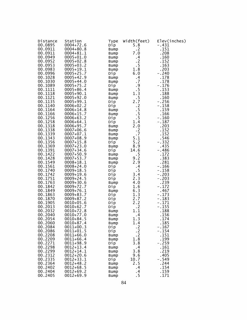
84

Distance Station Type Width(feet) Elev(inches) 00.0895 0004+72.6 Dip 5.8 -.431 00.0911 0004+80.8 Bump .2 .151 00.0911 0004+81.1 Bump 7.0 .208 00.0949 0005+01.0 Bump .4 .160 00.0952 0005+02.8 Bump .2 .152 00.0953 0005+03.2 Bump .5 .163 00.0983 0005+19.1 Bump 1.8 .203 00.0996 0005+25.7 Dip 6.0 -.240 00.1028 0005+42.9 Bump .4 .178 00.1030 0005+44.0 Bump .7 .178 00.1089 0005+75.2 Dip .9 -.176 00.1111 0005+86.4 Bump .5 .153 00.1118 0005+90.1 Bump 1.3 .188 00.1121 0005+92.0 Bump .5 .160 00.1135 0005+99.1 Dip 2.7 -.256 00.1140 0006+02.2 Dip .2 -.158 00.1164 0006+14.8 Bump .5 .159 00.1166 0006+15.7 Bump .5 .166 00.1256 0006+63.2 Dip .5 -.160 00.1258 0006+64.1 Dip 1.4 -.187 00.1318 0006+95.7 Bump 2.0 .203 00.1338 0007+06.6 Bump .2 .152 00.1339 0007+07.1 Bump .7 .152 00.1343 0007+08.9 Bump 5.1 .546 00.1356 0007+15.8 Dip 5.2 -.332 00.1369 0007+23.0 Bump 8.9 .435 00.1391 0007+34.6 Dip 14.6 -.486 00.1422 0007+50.9 Bump .5 .172 00.1428 0007+53.7 Bump 9.2 .383 00.1549 0008+18.1 Bump 2.9 .281 00.1561 0008+24.0 Dip .4 -.166 00.1740 0009+18.5 Dip .5 -.158 00.1742 0009+19.6 Dip 3.4 -.203 00.1751 0009+24.5 Dip 2.3 -.203 00.1763 0009+30.6 Bump 4.0 .239 00.1842 0009+72.7 Dip 1.6 -.172 00.1849 0009+76.1 Bump 6.3 .467 00.1863 0009+83.7 Dip 1.3 -.173 00.1870 0009+87.2 Dip 2.7 -.183 00.1905 0010+05.6 Dip 2.2 -.171 00.2013 0010+62.7 Dip .2 -.155 00.2032 0010+72.8 Bump 1.1 .188 00.2040 0010+77.0 Bump .4 .156 00.2054 0010+84.5 Bump 1.3 .174 00.2060 0010+87.4 Bump 1.4 .185 00.2084 0011+00.3 Dip .2 -.167 00.2086 0011+01.5 Dip .2 -.154 00.2208 0011+66.0 Bump .2 .151 00.2209 0011+66.4 Bump 1.8 .199 00.2271 0011+98.9 Dip 3.8 -.259 00.2298 0012+13.4 Bump .4 .161 00.2299 0012+14.1 Bump 3.8 .219 00.2312 0012+20.6 Bump 9.6 .405 00.2335 0012+33.1 Dip 10.7 -.549 00.2364 0012+48.2 Bump 2.5 .244 00.2402 0012+68.5 Bump .4 .154 00.2404 0012+69.2 Bump .4 .159 00.2405 0012+69.9 Bump .5 .171

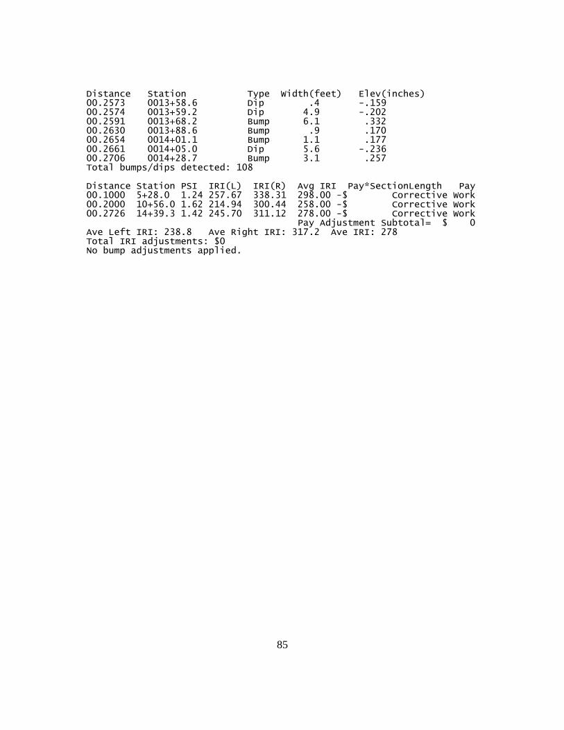
85

Distance Station Type Width(feet) Elev(inches) 00.2573 0013+58.6 Dip .4 -.159 00.2574 0013+59.2 Dip 4.9 -.202 00.2591 0013+68.2 Bump 6.1 .332 00.2630 0013+88.6 Bump .9 .170 00.2654 0014+01.1 Bump 1.1 .177 00.2661 0014+05.0 Dip 5.6 -.236 00.2706 0014+28.7 Bump 3.1 .257 Total bumps/dips detected: 108 Distance Station PSI IRI(L) IRI(R) Avg IRI Pay*SectionLength Pay 00.1000 5+28.0 1.24 257.67 338.31 298.00 -$ Corrective Work 00.2000 10+56.0 1.62 214.94 300.44 258.00 -$ Corrective Work 00.2726 14+39.3 1.42 245.70 311.12 278.00 -$ Corrective Work Pay Adjustment Subtotal= $ 0 Ave Left IRI: 238.8 Ave Right IRI: 317.2 Ave IRI: 278 Total IRI adjustments: $0 No bump adjustments applied.

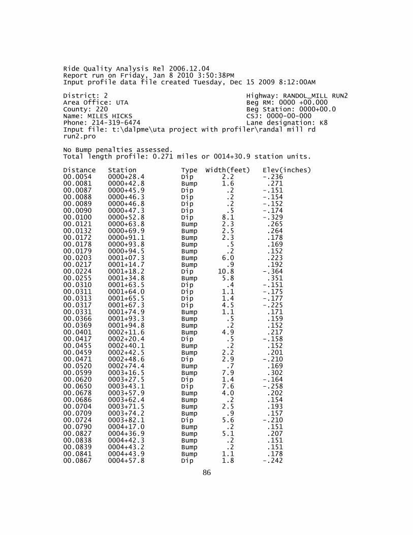
86

Ride Quality Analysis Rel 2006.12.04 Report run on Friday, Jan 8 2010 3:50:38PM Input profile data file created Tuesday, Dec 15 2009 8:12:00AM District: 2 Highway: RANDOL_MILL RUN2 Area Office: UTA Beg RM: 0000 +00.000 County: 220 Beg Station: 0000+00.0 Name: MILES HICKS CSJ: 0000-00-000 Phone: 214-319-6474 Lane designation: K8 Input file: t:\dalpme\uta project with profiler\randal mill rd run2.pro No Bump penalties assessed. Total length profile: 0.271 miles or 0014+30.9 station units. Distance Station Type Width(feet) Elev(inches) 00.0054 0000+28.4 Dip 2.2 -.236 00.0081 0000+42.8 Bump 1.6 .271 00.0087 0000+45.9 Dip .2 -.151 00.0088 0000+46.3 Dip .2 -.154 00.0089 0000+46.8 Dip .2 -.152 00.0090 0000+47.3 Dip .5 -.174 00.0100 0000+52.8 Dip 8.1 -.329 00.0121 0000+63.8 Bump 2.3 .265 00.0132 0000+69.9 Bump 2.5 .264 00.0172 0000+91.1 Bump 2.3 .178 00.0178 0000+93.8 Bump .5 .169 00.0179 0000+94.5 Bump .2 .152 00.0203 0001+07.3 Bump 6.0 .223 00.0217 0001+14.7 Bump .9 .192 00.0224 0001+18.2 Dip 10.8 -.364 00.0255 0001+34.8 Bump 5.8 .351 00.0310 0001+63.5 Dip .4 -.151 00.0311 0001+64.0 Dip 1.1 -.175 00.0313 0001+65.5 Dip 1.4 -.177 00.0317 0001+67.3 Dip 4.5 -.225 00.0331 0001+74.9 Bump 1.1 .171 00.0366 0001+93.3 Bump .5 .159 00.0369 0001+94.8 Bump .2 .152 00.0401 0002+11.6 Bump 4.9 .217 00.0417 0002+20.4 Dip .5 -.158 00.0455 0002+40.1 Bump .2 .152 00.0459 0002+42.5 Bump 2.2 .201 00.0471 0002+48.6 Dip 2.9 -.210 00.0520 0002+74.4 Bump .7 .169 00.0599 0003+16.5 Bump 7.9 .302 00.0620 0003+27.5 Dip 1.4 -.164 00.0650 0003+43.1 Dip 7.6 -.258 00.0678 0003+57.9 Bump 4.0 .202 00.0686 0003+62.4 Bump .2 .154 00.0704 0003+71.5 Bump 2.5 .193 00.0709 0003+74.2 Bump .9 .157 00.0724 0003+82.1 Dip 5.6 -.210 00.0790 0004+17.0 Bump .2 .151 00.0827 0004+36.9 Bump 5.1 .207 00.0838 0004+42.3 Bump .2 .151 00.0839 0004+43.2 Bump .2 .151 00.0841 0004+43.9 Bump 1.1 .178 00.0867 0004+57.8 Dip 1.8 -.242

87

Distance Station Type Width(feet) Elev(inches) 00.0887 0004+68.3 Dip .5 -.187 00.0905 0004+78.0 Dip 5.8 -.427 00.0920 0004+85.8 Bump 5.4 .235 00.0931 0004+91.4 Bump .2 .155 00.0932 0004+92.0 Bump 1.4 .171 00.0959 0005+06.2 Bump .5 .162 00.0960 0005+07.0 Bump .2 .152 00.0963 0005+08.2 Bump .2 .153 00.0994 0005+24.7 Bump 1.6 .224 00.1006 0005+31.2 Dip 6.0 -.254 00.1040 0005+49.2 Bump .7 .195 00.1100 0005+80.8 Dip .4 -.153 00.1119 0005+90.8 Bump 1.1 .162 00.1121 0005+92.0 Bump .4 .153 00.1128 0005+95.7 Bump 2.9 .191 00.1143 0006+03.2 Dip 4.5 -.252 00.1173 0006+19.3 Bump .2 .156 00.1174 0006+20.0 Bump .7 .156 00.1176 0006+21.0 Bump .5 .161 00.1265 0006+68.1 Dip 2.5 -.177 00.1340 0007+07.7 Dip .4 -.159 00.1346 0007+10.6 Bump 8.5 .472 00.1365 0007+20.9 Dip 5.2 -.359 00.1380 0007+28.4 Bump 8.7 .393 00.1401 0007+39.8 Dip 14.6 -.463 00.1432 0007+55.9 Bump .5 .166 00.1437 0007+58.6 Bump 9.4 .385 00.1559 0008+23.1 Bump 2.9 .272 00.1570 0008+29.1 Dip .2 -.159 00.1749 0009+23.4 Dip .7 -.154 00.1751 0009+24.5 Dip 3.4 -.195 00.1760 0009+29.3 Dip 2.3 -.205 00.1772 0009+35.5 Bump 3.8 .256 00.1780 0009+40.0 Bump .4 .157 00.1851 0009+77.6 Dip 1.6 -.180 00.1858 0009+81.0 Bump 6.1 .464 00.1879 0009+92.0 Dip 2.7 -.198 00.1913 0010+09.9 Dip 2.9 -.196 00.2041 0010+77.9 Bump .2 .151 00.2049 0010+81.7 Bump .5 .174 00.2063 0010+89.2 Bump 1.1 .171 00.2068 0010+91.9 Bump 1.8 .197 00.2094 0011+05.9 Dip .5 -.164 00.2159 0011+40.2 Dip .4 -.156 00.2218 0011+70.9 Bump 1.8 .218 00.2237 0011+81.4 Dip .2 -.152 00.2280 0012+03.6 Dip 3.4 -.260 00.2307 0012+17.9 Bump 4.0 .248 00.2318 0012+23.7 Bump .2 .153 00.2321 0012+25.5 Bump 9.4 .403 00.2344 0012+37.6 Dip 10.7 -.540 00.2373 0012+52.7 Bump 2.2 .252 00.2412 0012+73.7 Bump .5 .177 00.2414 0012+74.4 Bump .7 .183 00.2584 0013+64.4 Dip 4.3 -.198 00.2601 0013+73.2 Bump 5.8 .385 00.2639 0013+93.3 Bump .4 .162 00.2663 0014+05.9 Bump .9 .176

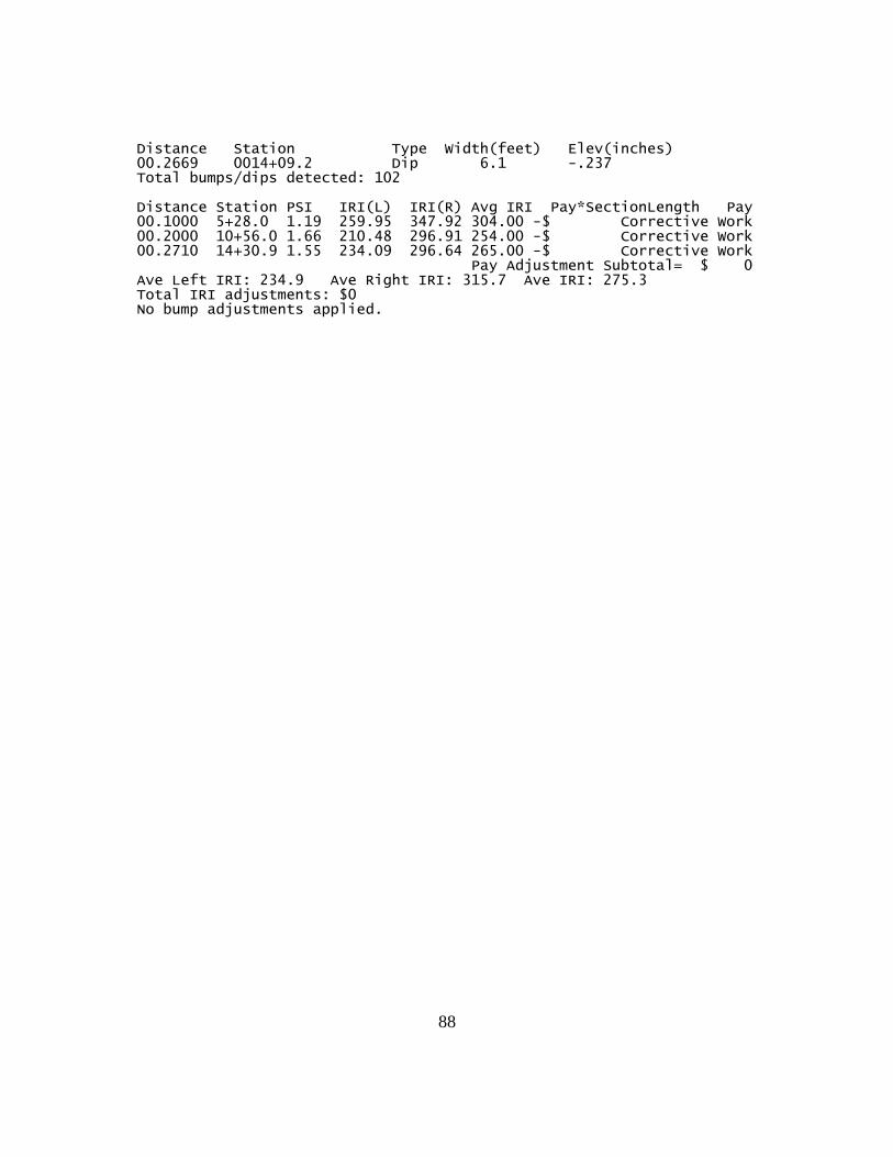
88

Distance Station Type Width(feet) Elev(inches) 00.2669 0014+09.2 Dip 6.1 -.237 Total bumps/dips detected: 102 Distance Station PSI IRI(L) IRI(R) Avg IRI Pay*SectionLength Pay 00.1000 5+28.0 1.19 259.95 347.92 304.00 -$ Corrective Work 00.2000 10+56.0 1.66 210.48 296.91 254.00 -$ Corrective Work 00.2710 14+30.9 1.55 234.09 296.64 265.00 -$ Corrective Work Pay Adjustment Subtotal= $ 0 Ave Left IRI: 234.9 Ave Right IRI: 315.7 Ave IRI: 275.3 Total IRI adjustments: $0 No bump adjustments applied.

89

Ride Quality Analysis Rel 2006.12.04 Report run on Friday, Jan 8 2010 3:50:57PM Input profile data file created Tuesday, Dec 15 2009 8:17:16AM District: 2 Highway: RD_TO_SIX_FLAGS RUN1 Area Office: UTA Beg RM: 0000 +00.000 County: 220 Beg Station: 0000+00.0 Name: MILES HICKS CSJ: 0000-00-000 Phone: 214-319-6474 Lane designation: K8 Input file: t:\dalpme\uta project with profiler\rd to six flags run1.pro No Bump penalties assessed. Total length profile: 0.2963 miles or 0015+64.5 station units. Distance Station Type Width(feet) Elev(inches) 00.0027 0000+14.1 Bump .2 .154 00.0027 0000+14.5 Bump .2 .162 00.0028 0000+14.8 Bump 2.0 .312 00.0037 0000+19.7 Dip 7.9 -.308 00.0053 0000+27.8 Dip .7 -.266 00.0057 0000+30.4 Bump .4 .186 00.0064 0000+34.0 Bump 6.1 .252 00.0144 0000+76.2 Dip 5.1 -.227 00.0154 0000+81.5 Dip .7 -.168 00.0252 0001+33.2 Dip 1.6 -.183 00.0275 0001+45.1 Bump .9 .168 00.0284 0001+49.8 Bump .4 .170 00.0285 0001+50.5 Bump 1.6 .173 00.0288 0001+52.3 Bump .4 .165 00.0289 0001+52.8 Bump 6.7 .216 00.0346 0001+82.8 Bump 4.9 .244 00.0364 0001+92.2 Dip 14.1 -.487 00.0394 0002+08.1 Bump .2 .154 00.0400 0002+11.2 Bump 3.4 .313 00.0439 0002+31.8 Bump .2 .153 00.0440 0002+32.2 Bump .9 .167 00.0453 0002+39.2 Dip .2 -.156 00.0454 0002+39.7 Dip .4 -.156 00.0495 0002+61.2 Dip 4.0 -.203 00.0520 0002+74.6 Bump .5 .193 00.0521 0002+75.3 Bump 2.3 .205 00.0527 0002+78.4 Bump .7 .167 00.0529 0002+79.3 Bump .5 .185 00.0541 0002+85.8 Dip .2 -.151 00.0565 0002+98.5 Bump 2.3 .172 00.0635 0003+35.5 Bump .2 .155 00.0639 0003+37.5 Bump 1.1 .184 00.0655 0003+46.0 Bump 2.5 .211 00.0666 0003+51.6 Bump .2 .152 00.0674 0003+55.7 Dip .2 -.151 00.0678 0003+58.1 Dip 1.8 -.233 00.0682 0003+60.1 Dip .4 -.155 00.0700 0003+69.6 Bump 2.9 .246 00.0716 0003+78.0 Dip .2 -.291 00.0720 0003+80.3 Dip .4 -.212 00.0723 0003+81.6 Dip .5 -.172 00.0724 0003+82.3 Dip 1.4 -.182 00.0727 0003+83.9 Dip 4.9 -.227

90

Distance Station Type Width(feet) Elev(inches) 00.0747 0003+94.4 Bump 5.2 .278 00.0765 0004+04.2 Dip 7.0 -.306 00.0803 0004+23.8 Bump 3.3 .181 00.0902 0004+76.2 Bump 1.1 .186 00.0913 0004+82.2 Bump .7 .160 00.0952 0005+02.8 Dip .9 -.204 00.0954 0005+03.9 Dip 2.3 -.188 00.0962 0005+07.7 Dip .9 -.176 00.0964 0005+08.9 Dip 1.6 -.188 00.0979 0005+16.7 Bump .4 .164 00.0980 0005+17.2 Bump 6.0 .594 00.0994 0005+24.7 Dip 3.3 -.736 00.1001 0005+28.3 Dip .2 -.160 00.1011 0005+33.9 Bump .5 .186 00.1015 0005+35.7 Dip 8.9 -.433 00.1036 0005+47.2 Bump 3.3 .261 00.1044 0005+51.4 Bump 1.4 .209 00.1048 0005+53.2 Bump .2 .152 00.1048 0005+53.6 Bump 3.4 .251 00.1061 0005+60.2 Bump 4.3 .200 00.1074 0005+67.1 Dip 6.0 -.237 00.1095 0005+78.1 Bump 2.7 .224 00.1177 0006+21.5 Dip 2.7 -.185 00.1183 0006+24.6 Dip .2 -.152 00.1192 0006+29.3 Bump 3.8 .223 00.1254 0006+62.1 Bump 7.4 .334 00.1272 0006+71.7 Bump .2 .154 00.1280 0006+75.7 Dip 1.1 -.174 00.1309 0006+91.2 Bump 1.3 .190 00.1312 0006+92.7 Bump .2 .159 00.1327 0007+00.6 Dip .2 -.152 00.1337 0007+05.9 Bump .9 .173 00.1345 0007+10.2 Bump .7 .159 00.1354 0007+14.7 Dip 6.9 -.418 00.1372 0007+24.3 Bump 2.3 .191 00.1382 0007+29.5 Bump .9 .169 00.1385 0007+31.5 Bump .4 .154 00.1417 0007+48.3 Bump 2.3 .174 00.1422 0007+50.9 Bump .2 .152 00.1447 0007+64.0 Dip 1.4 -.313 00.1450 0007+65.8 Dip 4.7 -.283 00.1461 0007+71.4 Dip .2 -.151 00.1473 0007+77.8 Dip .2 -.154 00.1483 0007+83.0 Bump .7 .172 00.1489 0007+86.4 Bump 4.7 .245 00.1503 0007+93.5 Bump 4.7 .365 00.1517 0008+00.9 Dip .5 -.182 00.1519 0008+01.8 Dip .2 -.151 00.1521 0008+02.9 Dip 6.5 -.284 00.1543 0008+14.8 Bump 4.7 .256 00.1559 0008+23.1 Dip 4.2 -.181 00.1594 0008+41.7 Bump 2.7 .447 00.1631 0008+61.2 Dip 3.3 -.193 00.1638 0008+64.9 Dip 1.4 -.352 00.1714 0009+05.0 Dip 2.2 -.204 00.1733 0009+15.3 Bump 3.4 .388 00.1747 0009+22.3 Dip .4 -.158 00.1748 0009+22.8 Dip 2.9 -.228

91

Distance Station Type Width(feet) Elev(inches) 00.1794 0009+47.1 Bump 1.8 .354 00.1798 0009+49.2 Bump 1.6 .216 00.1809 0009+55.2 Dip 4.0 -.247 00.1828 0009+64.9 Bump .2 .152 00.1832 0009+67.3 Bump 5.1 .269 00.1842 0009+72.5 Bump .2 .162 00.1872 0009+88.2 Bump 3.3 .314 00.1888 0009+96.9 Dip 1.3 -.181 00.1898 0010+02.2 Dip 1.4 -.174 00.1907 0010+06.7 Bump 7.9 .384 00.1930 0010+19.0 Dip 5.6 -.458 00.1947 0010+27.8 Bump 4.5 .263 00.1968 0010+39.2 Dip 4.5 -.218 00.1978 0010+44.4 Dip .2 -.158 00.1983 0010+46.8 Bump 4.3 .393 00.2003 0010+57.4 Dip 5.6 -.319 00.2029 0010+71.4 Dip 3.3 -.254 00.2059 0010+87.1 Dip 1.1 -.176 00.2068 0010+91.8 Bump 3.3 .255 00.2085 0011+00.6 Dip .5 -.178 00.2108 0011+12.9 Bump 2.5 .224 00.2120 0011+19.6 Bump 1.6 .261 00.2147 0011+33.7 Bump 2.0 .205 00.2189 0011+55.9 Dip .2 -.162 00.2195 0011+58.8 Bump 5.1 .227 00.2215 0011+69.3 Dip 3.3 -.234 00.2233 0011+79.2 Bump 6.5 .255 00.2258 0011+92.4 Dip 4.7 -.325 00.2320 0012+25.1 Bump .7 .170 00.2338 0012+34.5 Bump 2.5 .252 00.2379 0012+56.4 Dip 8.1 -.333 00.2401 0012+67.7 Bump 9.2 .266 00.2435 0012+85.4 Bump .9 .167 00.2444 0012+90.5 Dip .7 -.154 00.2449 0012+93.0 Dip .9 -.177 00.2451 0012+94.1 Dip .2 -.151 00.2452 0012+94.7 Dip 2.5 -.196 00.2494 0013+16.9 Bump 2.9 .208 00.2529 0013+35.3 Dip .7 -.172 00.2551 0013+46.7 Bump .5 .156 00.2553 0013+47.8 Bump .2 .154 00.2554 0013+48.3 Bump .5 .156 00.2640 0013+93.7 Dip .2 -.157 00.2641 0013+94.6 Dip 8.3 -.249 00.2666 0014+07.8 Bump 9.9 .354 00.2690 0014+20.6 Dip 6.9 -.369 00.2726 0014+39.6 Dip .7 -.176 00.2743 0014+48.2 Bump 1.4 .189 00.2746 0014+50.0 Bump 5.8 .306 00.2762 0014+58.5 Dip 4.7 -.280 00.2772 0014+63.4 Dip .2 -.156 00.2772 0014+63.8 Dip .2 -.158 00.2773 0014+64.3 Dip 1.3 -.177 00.2783 0014+69.4 Bump .2 .160 00.2784 0014+69.7 Bump 2.2 .169 00.2789 0014+72.4 Bump 1.1 .167 00.2791 0014+73.7 Bump 1.4 .256 00.2804 0014+80.4 Bump .2 .156

92

Distance Station Type Width(feet) Elev(inches) 00.2805 0014+80.9 Bump .4 .157 00.2806 0014+81.5 Bump 1.4 .181 00.2820 0014+88.9 Dip .2 -.153 00.2821 0014+89.6 Dip 5.6 -.416 00.2849 0015+04.2 Bump .2 .151 00.2850 0015+05.0 Bump 1.4 .179 00.2854 0015+06.8 Bump .9 .175 00.2868 0015+14.5 Dip 4.7 -.202 00.2886 0015+23.9 Bump 6.7 .269 00.2911 0015+36.9 Dip .4 -.170 00.2912 0015+37.7 Dip .2 -.164 00.2914 0015+38.4 Dip .2 -.165 00.2916 0015+39.8 Dip .7 -.162 00.2921 0015+42.2 Dip 1.3 -.169 00.2939 0015+51.7 Bump 1.4 .172 Total bumps/dips detected: 174 Distance Station PSI IRI(L) IRI(R) Avg IRI Pay*SectionLength Pay 00.1000 5+28.0 1.49 252.54 289.22 271.00 -$ Corrective Work 00.2000 10+56.0 .70 362.96 362.09 363.00 -$ Corrective Work 00.2963 15+64.5 1.06 318.92 318.58 319.00 -$ Corrective Work Pay Adjustment Subtotal= $ 0 Ave Left IRI: 311.4 Ave Right IRI: 323.4 Ave IRI: 317.4 Total IRI adjustments: $0 No bump adjustments applied.

93

Ride Quality Analysis Rel 2006.12.04 Report run on Friday, Jan 8 2010 3:51:26PM Input profile data file created Tuesday, Dec 15 2009 8:17:42AM District: 2 Highway: RD_TO_SIX_FLAGS RUN2 Area Office: UTA Beg RM: 0000 +00.000 County: 220 Beg Station: 0000+00.0 Name: MILES HICKS CSJ: 0000-00-000 Phone: 214-319-6474 Lane designation: K8 Input file: t:\dalpme\uta project with profiler\rd to six flags run2.pro No Bump penalties assessed. Total length profile: 0.2902 miles or 0015+32.3 station units. Distance Station Type Width(feet) Elev(inches) 00.0007 0000+03.8 Bump .4 .179 00.0020 0000+10.3 Bump .2 .151 00.0020 0000+10.7 Bump 3.6 .243 00.0069 0000+36.3 Bump 1.3 .191 00.0072 0000+37.9 Bump .4 .179 00.0074 0000+38.8 Bump .5 .169 00.0093 0000+49.3 Dip 6.0 -.224 00.0202 0001+06.8 Dip 1.3 -.166 00.0232 0001+22.7 Dip .2 -.161 00.0233 0001+23.0 Bump .4 .189 00.0234 0001+23.6 Bump 1.8 .182 00.0238 0001+25.6 Bump 7.4 .209 00.0295 0001+55.9 Bump 5.2 .266 00.0315 0001+66.4 Dip 13.2 -.510 00.0350 0001+84.6 Bump 3.6 .320 00.0389 0002+05.4 Bump .2 .157 00.0403 0002+13.0 Dip .5 -.160 00.0446 0002+35.2 Dip 2.9 -.215 00.0451 0002+38.3 Dip .2 -.155 00.0469 0002+47.9 Bump .7 .192 00.0471 0002+48.8 Bump 1.3 .191 00.0474 0002+50.2 Bump .4 .156 00.0477 0002+51.7 Bump .2 .151 00.0478 0002+52.2 Bump 1.1 .185 00.0491 0002+59.3 Dip .2 -.156 00.0515 0002+71.9 Bump 1.6 .178 00.0518 0002+73.7 Bump .4 .159 00.0585 0003+08.8 Bump .2 .151 00.0589 0003+11.1 Bump 1.1 .198 00.0603 0003+18.5 Bump 3.6 .259 00.0615 0003+24.7 Bump .5 .174 00.0621 0003+27.9 Dip 6.5 -.270 00.0640 0003+38.0 Dip .2 -.154 00.0642 0003+38.9 Dip .2 -.161 00.0657 0003+46.9 Bump 2.3 .185 00.0662 0003+49.4 Bump .9 .169 00.0664 0003+50.7 Bump .7 .174 00.0672 0003+54.8 Dip .4 -.339 00.0677 0003+57.4 Dip 1.1 -.270 00.0693 0003+65.7 Dip .7 -.361 00.0695 0003+66.8 Dip .9 -.645 00.0699 0003+69.1 Bump 4.2 .255 00.0715 0003+77.4 Dip 7.0 -.381

94

Distance Station Type Width(feet) Elev(inches) 00.0749 0003+95.5 Bump .2 .153 00.0752 0003+97.1 Bump 3.3 .199 00.0852 0004+49.9 Bump .9 .198 00.0902 0004+76.4 Dip 3.4 -.263 00.0910 0004+80.4 Dip .2 -.156 00.0913 0004+82.0 Dip .2 -.154 00.0927 0004+89.6 Bump .5 .159 00.0929 0004+90.3 Bump 3.6 .578 00.0936 0004+94.1 Bump 2.3 .332 00.0943 0004+98.1 Dip 3.4 -1.477 00.0953 0005+03.0 Bump 2.0 .260 00.0965 0005+09.5 Dip 1.3 -.255 00.0971 0005+12.6 Dip 5.2 -.424 00.0990 0005+22.7 Bump 3.1 .265 00.0998 0005+27.0 Bump .2 .156 00.0999 0005+27.4 Bump 3.1 .236 00.1010 0005+33.3 Bump 4.9 .191 00.1024 0005+40.6 Dip 6.3 -.250 00.1045 0005+51.8 Bump .2 .153 00.1046 0005+52.1 Bump 2.2 .217 00.1127 0005+95.1 Dip 1.4 -.181 00.1131 0005+96.9 Dip .7 -.163 00.1141 0006+02.7 Bump 3.3 .231 00.1148 0006+06.1 Bump .4 .170 00.1195 0006+30.9 Dip .7 -.163 00.1204 0006+35.6 Bump 7.8 .346 00.1222 0006+45.2 Bump .4 .163 00.1229 0006+49.1 Dip 1.3 -.176 00.1234 0006+51.3 Dip .2 -.152 00.1259 0006+64.7 Bump 1.4 .188 00.1277 0006+74.1 Dip .7 -.173 00.1278 0006+75.0 Dip .2 -.151 00.1287 0006+79.3 Bump .9 .182 00.1295 0006+83.6 Bump 1.3 .168 00.1304 0006+88.3 Dip 6.7 -.427 00.1319 0006+96.7 Bump 3.4 .219 00.1330 0007+02.1 Bump .2 .151 00.1330 0007+02.4 Bump 1.4 .187 00.1335 0007+05.0 Bump .4 .153 00.1345 0007+10.4 Dip .5 -.156 00.1368 0007+22.5 Bump .2 .156 00.1369 0007+22.8 Bump .9 .164 00.1396 0007+37.3 Dip 1.4 -.324 00.1400 0007+39.3 Dip 4.9 -.288 00.1410 0007+44.5 Dip .5 -.167 00.1423 0007+51.6 Dip .2 -.151 00.1432 0007+56.1 Bump .2 .152 00.1433 0007+56.5 Bump .9 .178 00.1440 0007+60.1 Bump 4.5 .235 00.1452 0007+66.6 Bump 4.9 .361 00.1466 0007+74.0 Dip 1.8 -.183 00.1470 0007+76.0 Dip 6.7 -.307 00.1492 0007+87.7 Bump 5.4 .236 00.1509 0007+96.7 Dip 4.3 -.241 00.1524 0008+04.9 Bump .4 .163 00.1544 0008+15.2 Bump 2.7 .420 00.1581 0008+34.9 Dip 2.7 -.198 00.1588 0008+38.5 Dip 1.1 -.343

95

Distance Station Type Width(feet) Elev(inches) 00.1663 0008+78.0 Dip 2.2 -.215 00.1683 0008+88.5 Bump 3.6 .376 00.1696 0008+95.7 Dip 3.4 -.226 00.1744 0009+20.7 Bump 1.6 .301 00.1747 0009+22.5 Bump 1.8 .254 00.1758 0009+28.4 Dip 2.3 -.201 00.1764 0009+31.2 Dip 1.4 -.173 00.1781 0009+40.4 Bump 2.2 .194 00.1786 0009+43.3 Bump 1.1 .214 00.1822 0009+62.1 Bump .9 .178 00.1824 0009+63.3 Bump .2 .151 00.1825 0009+63.9 Bump .2 .158 00.1834 0009+68.6 Dip .9 -.175 00.1836 0009+69.6 Dip 4.0 -.205 00.1849 0009+76.1 Dip .2 -.157 00.1856 0009+80.1 Bump 8.3 .459 00.1872 0009+88.6 Bump .7 .187 00.1874 0009+89.5 Bump 1.6 .204 00.1879 0009+92.2 Dip 5.4 -.816 00.1894 0010+99.8 Bump 5.6 .301 00.1933 0010+20.8 Dip .2 -.155 00.1937 0010+22.6 Bump 1.1 .239 00.1943 0010+26.0 Dip .7 -.182 00.1953 0010+31.2 Dip 4.9 -.265 00.1983 0010+47.1 Dip .4 -.161 00.2012 0010+62.1 Dip .4 -.157 00.2018 0010+65.4 Bump 6.5 .255 00.2035 0010+74.2 Dip 1.6 -.183 00.2042 0010+78.2 Dip 1.1 -.164 00.2059 0010+87.3 Bump 1.8 .229 00.2070 0010+93.0 Bump .5 .176 00.2082 0010+99.2 Dip .4 -.165 00.2083 0011+99.7 Dip .5 -.165 00.2096 0011+06.9 Bump 2.3 .231 00.2139 0011+29.3 Dip .2 -.152 00.2145 0011+32.6 Bump 5.2 .262 00.2163 0011+42.2 Dip 4.2 -.285 00.2184 0011+53.0 Bump 6.5 .283 00.2209 0011+66.6 Dip 3.4 -.398 00.2254 0011+90.1 Dip 1.3 -.194 00.2257 0011+91.7 Dip .2 -.152 00.2270 0011+98.7 Bump .7 .171 00.2288 0012+07.9 Bump 2.3 .252 00.2329 0012+29.8 Dip 8.1 -.311 00.2351 0012+41.4 Bump 9.2 .261 00.2386 0012+59.6 Bump .4 .155 00.2399 0012+66.7 Dip 2.2 -.184 00.2404 0012+69.5 Dip 1.3 -.172 00.2444 0012+90.7 Bump 2.9 .207 00.2480 0013+09.5 Dip .4 -.154 00.2481 0013+10.2 Dip .2 -.151 00.2504 0013+22.1 Bump .5 .163 00.2531 0013+36.6 Dip .2 -.165 00.2586 0013+65.5 Dip .7 -.216 00.2589 0013+67.1 Dip .2 -.151 00.2590 0013+67.6 Dip 9.4 -.253 00.2617 0013+81.7 Bump 9.9 .332 00.2641 0013+94.4 Dip 7.9 -.372

96

Distance Station Type Width(feet) Elev(inches) 00.2694 0014+22.2 Bump 1.1 .173 00.2696 0014+23.5 Bump .4 .159 00.2697 0014+24.0 Bump 5.8 .304 00.2712 0014+31.8 Dip 7.8 -.284 00.2734 0014+43.3 Bump 6.0 .244 00.2746 0014+49.7 Bump .4 .175 00.2755 0014+54.5 Bump 1.3 .172 00.2758 0014+56.2 Bump .5 .158 00.2769 0014+62.0 Dip .4 -.169 00.2770 0014+62.5 Dip .9 -.183 00.2772 0014+63.6 Dip 4.9 -.398 00.2802 0014+79.3 Bump .9 .167 00.2804 0014+80.4 Bump 1.6 .181 00.2819 0014+88.3 Dip 6.0 -.206 00.2837 0014+98.1 Bump 6.1 .285 00.2862 0015+11.3 Dip 1.4 -.175 00.2872 0015+16.3 Dip .4 -.156 00.2873 0015+16.9 Dip .4 -.162 00.2874 0015+17.4 Dip .2 -.156 Total bumps/dips detected: 178 Distance Station PSI IRI(L) IRI(R) Avg IRI Pay*SectionLength Pay 00.1000 5+28.0 1.16 273.44 341.58 308.00 -$ Corrective Work 00.2000 10+56.0 .71 370.01 354.11 362.00 -$ Corrective Work 00.2902 15+32.3 1.08 314.27 318.92 317.00 -$ Corrective Work Pay Adjustment Subtotal= $ 0 Ave Left IRI: 319.4 Ave Right IRI: 338.9 Ave IRI: 329.15 Total IRI adjustments: $0 No bump adjustments applied.

97

APPENDIX B

SURVEYS OF LONGITUDINAL PROFILE

98

Exhibit B-1 Longitudinal Grade for Pecandale Drive (AC) in Arlington, TX (Part 1).

99

Exhibit B-2 Longitudinal Grade for Pecandale Drive (AC) in Arlington, TX (Part 2).

100

Exhibit B-3 Longitudinal Grade for Abram Street (PCC) in Arlington, TX (Part 1).

101


102


103


104

Exhibit B-7 Longitudinal Grade for Randol Mill Road (AC) in Arlington, TX.

105

Exhibit B-8 Longitudinal Grade for Road to Six Flags Street (PCC) in Arlington, TX.

106

APPENDIX C

FUEL MEASUREMENT RAW DATA

107

Study Date Temp.

(ºF)

Humidity

(%)

Wind Speed

(mph)

/direction

Road Sites No. Fuel Consumed

(10-3 GPM)

Average Fuel

Consumption

(10-3 GPM)

November 7, 2008 69 30 7 W Pecandale 1 46.2 43.7

Approx. time: 2pm

2 42.6

3 42.2

Abram 1 39.3 39.8

2 41.0

3 39.1

January 16, 2009 44 48 7 S Pecandale 1 54.2 53.2

Approx. time: 4pm

2 52.9

3 52.6

Abram 1 46.8 46.8

2 42.0

3 51.6

April 21, 2011 85 53 15 S Pecandale 1 53.7 54.1

Approx. time: 5pm

2 55.0

3 53.6

Abram 1 48.4 51.3

2 52.5

3 53.0


Approx. time: 3pm

2 52.8

3 53.3

Abram 1 50.0 48.7

2 48.2

3 47.9

April 28, 2011 64 35 3 N Pecandale 1 52.8 53.8

Approx. time: 10am

2 55.7

3 53.0

Abram 1 47.6 49.7

2 49.8

3 51.8

May 3, 2011 65 43 5 N Pecandale 1 58.8 58.6

Approx. time: 2pm

2 59.1

3 58.0

Abram 1 54.0 53.4

2 53.0

3 53.2

May 5, 2011 76 37 15 S Pecandale 1 56.3 55.1

Approx. time: 2pm

2 53.9

3 55.1

Abram 1 53.0 51.0

2 49.4

3 50.7

Exhibit C-1 Fuel Measurement of Pecandale (AC) vs. Abram (PCC) at Constant Speed of 30 mph.

108

Study Date Temp.

(ºF)

Humidity

(%)

Wind Speed

(mph)

/direction


(10-3 GPM)

Average Fuel

Consumption

(10-3 GPM)

November 7, 2008 69 30 7 W Pecandale 1 236.2 239.0

Approx. time: 2pm 2 240.6

3 240.2

Abram 1 240.2 232.5

2 229.6

3 227.8

January 16, 2009 44 48 7 S Pecandale 1 269.0 260.5


3 268.6

Abram 1 236.8 234.6

2 220.2

3 246.7



3 307.2

Abram 1 239.6 257.7

2 245.9

3 287.5



3 305.7

Abram 1 276.9 271.6

2 269.4

3 268.6

April 28, 2011 64 35 3 N Pecandale 1 280.7 281.5

Approx. time: 10am 2 285.3

3 278.5

Abram 1 278.5 273.7

2 276.9

3 265.6

May 3, 2011 65 43 5 N Pecandale 1 267.1 273.2


3 272.4

Abram 1 286.8 290.6

2 283.7

3 301.2

May 5, 2011 76 37 15 S Pecandale 1 276.2 274.2


3 288.3

Abram 1 270.3 271.9

2 262.6

3 283.0

Exhibit C-2 Fuel Measurement of Pecandale (AC) vs. Abram (PCC) at Acceleration of 3 mph/second.

109

Study Date Temp.

(ºF)

Humidity

(%)

Wind Speed

(mph)

/direction


(10-3 GPM)

Average Fuel

Consumption

(10-3 GPM)

July 3, 2009 81 58 6 S Randol Mill 1 45.3 47.7


3 49.7

Six Flags 1 39.8 41.1

2 42.1

3 41.2

July 23, 2009 77 60 3 N Randol Mill 1 51.5 52.8


3 51.5

Six Flags 1 46.6 45.4

2 46.9

3 42.7

July 24, 2009 78 71 0 Randol Mill 1 52.8 51.7


3 50.1

Six Flags 1 46.5 42.1

2 41.3

3 38.5

April 21, 2011 85 53 15 S Randol Mill 1 48.8 47.8


3 47.0

Six Flags 1 37.0 42.0

2 46.1

3 42.8



3 49.7

Six Flags 1 37.8 39.7

2 41.8

3 39.6

April 28, 2011 64 35 3 N Randol Mill 1 48.0 49.3


3 51.5

Six Flags 1 36.7 42.3

2 44.6

3 45.5

May 3, 2011 65 43 5 N Randol Mill 1 48.1 47.2


3 47.8

Six Flags 1 41.8 42.0

2 42.3

3 41.9

Exhibit C-3 Fuel Measurement of Randol Mill (AC) vs. Road to Six Flags (PCC) at Constant Speed of 30 mph.

110

Study Date Temp.

(ºF)

Humidity

(%)

Wind Speed

(mph)

/direction


(10-3 GPM)

Average Fuel

Consumption

(10-3 GPM)

July 3, 2009 81 58 6 S Randol Mill 1 257.3 256.5


3 258.0

Six Flags 1 224.0 243.3

2 248.9

3 257.1

July 23, 2009 77 60 3 N Randol Mill 1 288.3 266.1


3 261.8

Six Flags 1 231.5 235.1

2 239.9

3 233.8

July 24, 2009 78 71 0 Randol Mill 1 252.0 252.7


3 244.4

Six Flags 1 235.3 240.1

2 250.5

3 234.4



3 234.6

Six Flags 1 236.1 228.8

2 218.7

3 231.5



3 293.6

Six Flags 1 237.6 258.0

2 266.3

3 270.1

April 28, 2011 64 35 3 N Randol Mill 1 274.7 271.6


3 271.6

Six Flags 1 230.0 231.0

2 230.0

3 233.1

May 3, 2011 65 43 5 N Randol Mill 1 245.9 256.3


3 258.8

Six Flags 1 242.1 236.8

2 230.8

3 237.6

Exhibit C-4 Fuel Measurement of Randol Mill (AC) vs. Road to Six Flags (PCC) at Acceleration of 3 mph/second.

111

REFERENCES

1. An, F., Friedman, D., and Ross, M. (2002). "Near-Term Fuel Economy Potential for

Light-Duty Trucks." SEA Technical Paper, 2002-01-1900.

2. Archondo-Callao, R. S., and Faiz, A. (1994). "Estimating Vehicle Operating Costs."

World Bank Technical Paper(234).

3. Bein, P., and Biggs, D. C. (1993). "Critique of Texas Research and Development

Foundation on Vehicle Operating Cost Model." Transportation Research

Record(1395), 114-121.

4. Brown, A. (2009). "Carbon Footprint of HMA and PCC Pavements." International

Conference on Perpetual Pavements.

5. California Energy Commission. (2003). "California State Fuel-Efficient Tire Report:

Volume I." 600-03-001F.

6. Casadei, A., and Broda, R. (2008). "Impact of Vehicle Weight Reduction on Fuel

Economy for Various Vehicle Architectures." FB769 RD.07/71602.2, Ricardo

Inc.

7. Chang, M. F., Evans, L., Herman, R., and Wasielewski, P. (1976). "The Influence of

Vehicle Characteristics, Driver Behavior, and Ambient Temperature on Gasoline

Consumption in Urban Traffic." Transportation Research Record(599), 25-30.

8. Christie, T. (2011). "Research Report Points out Road to Energy Savings." Texas

Asphalt, 30.

112

9. City of Arlington. (2011). "Traffic Count Maps."

<http://www.arlingtontx.gov/publicworks/pdf/2010_Traffic_Counts.pdf>

(November, 2011).

10. Delatte, N. (2008). Concrete Pavement Design, Construction and Performance,

Taylor & Francis.

11. EcoBusinessLinks. (2009). "The Carbon Emissions Offset Directory."

<http://www.ecobusinesslinks.com/carbon_offset_wind_credits_carbon_reductio

n.htm> (May, 2009).

12. Energy and Environmental Analysis Inc. (2001). "Owner Related Fuel Economy

Improvements." Arlington, VA.

13. Evans, L., Herman, R., and Lam, T. (1976a). "Gasoline Consumption in Urban

Traffic." SAE Technical Paper, 760048.

14. Evans, L., Herman, R., and Lam, T. (1976b). "Multivariate Analysis of Traffic

Factors Related to Fuel Consumption in Urban Driving." Transportation Science,

10(2), 205.

15. Federal Highway Administration. (2011). "FHWA Vehicle Types."

<http://www.fhwa.dot.gov/policy/ohpi/vehclass.htm> (May, 2011).

16. Goodyear. (2008). "Factors Affecting Truck Fuel Economy."

<http://www.goodyear.com/truck/pdf/radialretserv/Retread_S9_V.pdf> (June,

2008).

17. Huang, Y. H. (2004). Pavement Analysis and Design, Pearson Prentice Hall, Upper

Saddle River, NJ.

113

18. Jonsson, P., and Hultqvist, B.-Å. (2009). "Measurement of Fuel Consumption on

Asphalt and Concrete Pavements North of Uppsala." Swedish National Road and

Transport Research Institute, Linköping, Sweden.

19. Kutner, M. H., Nachtsheim, C. J., Neter, J., and Li, W. (2005). Applied Linear

Statistical Models, McGraw-Hill.

20. Larson, T. (1992). The Bridge, 22(1).

21. Lubrizol. (2011). "Passenger Car Market Overview."

<http://www.lubrizol.com/EuropeanEngineOils/PCMarketVideo.html> (March,

2011).

22. Nair, H. S., and Bhat, C. R. (2000). "Modeling Trip Duration for Mobile Source

Emissions Forecasting." FHWA/TX-0-1838-7, Center for Transportation

Research, the University of Texas at Austin.

23. North Central Texas Council of Government. (2007). "Transportation Conformity

Determination for the Mobility 2030: The Metropolitan Transportation Plan and

2006-2008 Transportation Improvement Program as Amended."

<http://www.nctcog.org/trans/air/conformity/ConformityDeterminations.asp>

(April, 2009).

24. Ozbay, K., Parker, N. A., Jawad, D., and Hussain, S. (2003). "Guidelines for Life

Cycle Cost Analysis." FHWA-NJ-2003-012, Federal Highway Administration.

25. Pagerit, S., Sharer, P., and Rousseau, A. (2006). "Fuel Economy Sensitivity to

Vehicle Mass for Advanced Vehicle Powertrains." Society of Automotive

Engineers, 2006-01-0665.

114

26. Papagiannakis, A. T. (1999b). "On the Relationship between Truck Operating Costs

and Pavement Roughness." SAE Technical Paper, 1999-01-3783.

27. Papagiannakis, A. T., and Delwar, M. (1999a). "Methodology to Improve Pavement

Investment Decisions." Transportation Research Board, Washington, D.C.

28. Papagiannakis, A. T., and Delwar, M. "Incorporating User Costs into Pavement

Management Decisions." Proceedings of the Fifth International Conference on

Managing Pavements, Seattle, Washington.

29. Peterson, D. E. (1985). "Life-Cycle Cost Analysis of Pavements." National

Cooperative Highway Research Program.

30. Sayers, M. W., and Karamihas, S. M. (1998). "The Little Book of Profiling."

<http://www.umtri.umich.edu/content/LittleBook98R.pdf> (November, 2009).

31. Shell. (2011). "Shell concept lubricant achieves 6.5% fuel economy benefit."

<http://www.shell.com/home/content/lubes/media_centre/news_media_releases/2

011/shell_concept_lubricant.html> (February, 2011).

32. Sovran, G., and Bohn, M. (1981). "Formulae for Tractive Energy Requirements for

Vehicles Driving the EPA Schedule." SAE Technical Paper, 810184.

33. Taylor, G. W., and Patten, J. D. (2006). "Effect of Pavement Structure on Vehicle

Fuel Consumption – Phase III." Technical Report CSTT-HVC-TR-068, Portland

Cement Association, Skokie, Illinois.

34. Texas Department of Transportation. (2004). Standard Specifications for

Construction and Maintenance of Highways, Streets, and Bridges.

115

35. The Daily Green. (2009). "Low Rolling Resistance Tires Save Gas."

<http://www.thedailygreen.com/living-green/blogs/cars-transportation/low-

rolling-resistance-tires-461009> (December, 2010).

36. Thompson, G. (1979). "Fuel Economy Effects of Tires." SDSB 79-13, U.S.

Environmental Protection Agency.

37. Transportation Energy Management Program. (1982). "A Technical Background

Document for Automotive Fuel Economy." DRS-82-01, Ontario Ministry of

Transportation and Communications.

38. TRB Special Report 285. (2006). "The Fuel Tax and Alternatives for Transportation

Funding." Transportation Research Board, Washington, D.C.

39. TRB Special Report 286. (2006). "Tires and Passenger Fuel Economy."

Transportation Research Board, Washington, D.C.

40. U.S. Bureau of Transportation Statistics. (2011). "Number of U.S. Aircraft, Vehicles,

Vessels, and Other Conveyances."

<http://www.bts.gov/publications/national_transportation_statistics/html/table_01

_11.html> (January, 2011).

41. U.S. Department of Energy. (2008). "Annual Energy Review."

<http://www.eia.gov/totalenergy/data/annual/> (June, 2008).

42. U.S. Department of Energy. (2010a). "Gas Mileage Tips."

<http://www.fueleconomy.gov/feg/maintain.shtml> (October, 2010).

116

43. U.S. Department of Energy. (2010b). "Low Rolling Resistance Tires."

<http://www.afdc.energy.gov/afdc/vehicles/fuel_economy_tires_light.html>

(September, 2010).

44. U.S. Department of Energy. (2011). "Fuel Economy: Where the Energy Goes."

<http://www.fueleconomy.gov/feg/atv.shtml> (January, 2011).

45. U.S. Environmental Protection Agency. (1980). "Passenger Car Fuel Economy, EPA

and Road." EPA 460/3-80-010.

46. U.S. Environmental Protection Agency. (2000). "Emission Facts." EPA420-F-00-

013.

47. U.S. Environmental Protection Agency. (2003). "User’s Guide to MOBILE6.1 and

MOBILE6.2." EPA420-R-03-010, Office of Transportation and Air Quality.

48. U.S. Environmental Protection Agency. (2005). "Emission Facts." EPA420-F-05-

001.

49. U.S. Environmental Protection Agency. (2006). "Fuel Economy Labeling of Motor

Vehicles: Revisions to Improve Calculation of Fuel Economy Estimates."

EPA420-D-06-002.

50. VicRoads. (2008). "Moving Towards Carbon Neutral Road Construction - The

Mickleham Road Project."

<http://www.vicroads.vic.gov.au/Home/Moreinfoandservices/Environment/Green

house.htm> (October, 2008).

117

51. Walls, J., and Smith, M. R. (1998). "Life-Cycle Cost Analysis in Pavement Design –

Interim Technical Bulletin." FHWA-SA-98-079, Office of Engineering, Pavement

Division, Federal Highway Administration, Washington, D.C.

52. Washington State Department of Transportation. (2003). "Pavement Types."

<http://training.ce.washington.edu/wsdot/Modules/02_pavement_types/02-

6_body.htm> (April, 2011).

53. Wood, R. A., Downing, B. R., and Pearce, T. C. (1981). "Energy Consumption of an

Electric, a Petrol and a Diesel Powered Light Goods Vehicles in Central London

Traffic." TRRL Report LR 1021, Transport and Road Research Laboratory,

Crowthorne, Berkshire.

54. Zaniewski, J. P. (1989). "Effect of Pavement Surface Type on Fuel Consumption."

SR289.01P, Portland Cement Association, Skokie, Illinois.

55. Zaniewski, J. P., Butler, B. C., Cunningham, G., Elkins, G. E., Paggi, M. S., and

Machemehl, R. (1982). "Vehicle Operating Costs, Fuel Consumption, and

Pavement Type and Condition Factors." DOT-FH-11-9678, Federal Highway

Administration, Washington, D.C.

118

BIOGRAPHICAL INFORMATION

Palinee Sumitsawan is from the city of Phitsanulok, Thailand. She graduated

from Naresuan University, Thailand, with a Bachelor of Engineering degree majoring in

Civil Engineering in 1999. During her final year, she worked with Changmoi Furniture

Co.,Ltd. and Engineering Design and Consultant Co.,Ltd as a civil engineer at the

construction sites. She is a member of the Engineering Institute of Thailand (EIT) under

H.M. the King’s Patronage. In 2001, Palinee received her Master of Science degree in

Transport Engineering and Operations from Newcastle University, UK. She joined

Transport Operations Research Group (TORG) and Institution of Civil Engineers (ICE)

Student Chapter. Palinee has been working as a faculty member in the Department of

Civil Engineering, School of Engineering at the University of Phayao, Thailand, since

2002.

Palinee received scholarships from the Commission on Higher Education,

Ministry of Education, Thailand, to pursue her doctoral degree in Civil Engineering at the

University of Texas at Arlington in 2006. During her study, she served as the Treasurer

and acting President of the Institute of Transportation Engineers (ITE) Student Chapter.

She was appointed as graduate research assistant by Dr. Siamak A. Ardekani. She

worked on a project funded by Ready Mixed Concrete (RMC) Research and Education

Foundation.

119

Palinee received Doctor of Philosophy degree in Civil Engineering from the

University of Texas at Arlington in December 2011.

EFFECT OF PAVEMENT TYPE ON FUEL CONSUMPTION by …

Documents