Effect of Multiple Engine Placement on Aeroelastic Trim and Stability of Flying Wing Aircraft Pezhman Mardanpour a,1,* , Phillip W. Richards a,2 , Omid Nabipour a,3 , Dewey H. Hodges a,4 a Daniel Guggenheim School of Aerospace Engineering Georgia Institute of Technology, Atlanta, Georgia 30332-0150 Abstract Effects of multiple engine placement on flutter characteristics of a backswept flying wing resembling the HORTEN IV are investigated using the code NATASHA (Nonlinear Aeroelastic Trim And Stability of HALE Aircraft). Four identical engines with defined mass, inertia, and angular momentum are placed in different locations along the span with different offsets from the elastic axis while fixing the location of the aircraft c.g. The aircraft ex- periences body freedom flutter along with non-oscillatory instabilities that * Corresponding author Email addresses: [email protected] (Pezhman Mardanpour), [email protected] (Phillip W. Richards), [email protected] (Omid Nabipour), [email protected] (Dewey H. Hodges) 1 PhD Candidate and Graduate Research Assistant, Student member, AIAA, APS and ASME. 2 Graduate Research Assistant, Student member, AIAA. 3 Visiting Scholar, Daniel Guggenheim School of Aerospace Engineering. Student mem- ber, AIAA. 4 Professor, Fellow, AIAA and AHS; member, ASME. Preprint submitted to Journal of Fluids and Structures August 28, 2013

Welcome message from author
This document is posted to help you gain knowledge. Please leave a comment to let me know what you think about it! Share it to your friends and learn new things together.
Transcript

Effect of Multiple Engine Placement on Aeroelastic
Trim and Stability of Flying Wing Aircraft
Pezhman Mardanpoura,1,∗, Phillip W. Richardsa,2, Omid Nabipoura,3,Dewey H. Hodgesa,4
aDaniel Guggenheim School of Aerospace EngineeringGeorgia Institute of Technology, Atlanta, Georgia 30332-0150
Abstract
Effects of multiple engine placement on flutter characteristics of a backswept
flying wing resembling the HORTEN IV are investigated using the code
NATASHA (Nonlinear Aeroelastic Trim And Stability of HALE Aircraft).
Four identical engines with defined mass, inertia, and angular momentum
are placed in different locations along the span with different offsets from
the elastic axis while fixing the location of the aircraft c.g. The aircraft ex-
periences body freedom flutter along with non-oscillatory instabilities that
∗Corresponding authorEmail addresses: [email protected] (Pezhman Mardanpour),
[email protected] (Phillip W. Richards), [email protected] (OmidNabipour), [email protected] (Dewey H. Hodges)
1PhD Candidate and Graduate Research Assistant, Student member, AIAA, APS andASME.
2Graduate Research Assistant, Student member, AIAA.3Visiting Scholar, Daniel Guggenheim School of Aerospace Engineering. Student mem-
ber, AIAA.4Professor, Fellow, AIAA and AHS; member, ASME.
Preprint submitted to Journal of Fluids and Structures August 28, 2013

originate from flight dynamics. Multiple engine placement increases flutter
speed particularly when the engines are placed in the outboard portion of
the wing (60% to 70% span), forward of the elastic axis, while the lift to drag
ratio is affected negligibly. The behavior of the sub- and supercritical eigen-
values is studied for two cases of engine placement. NATASHA captures a
hump body-freedom flutter with low frequency for the clean wing case, which
disappears as the engines are placed on the wings. In neither case is there
any apparent coalescence between the unstable modes. NATASHA captures
other non-oscillatory unstable roots with very small amplitude, apparently
originating with flight dynamics. For the clean-wing case, in the absence of
aerodynamic and gravitational forces, the regions of minimum kinetic energy
density for the first and third bending modes are located around 60% span.
For the second mode, this kinetic energy density has local minima around the
20% and 80% span. The regions of minimum kinetic energy of these modes
are in agreement with calculations that show a noticeable increase in flutter
speed if engines are placed forward of the elastic axis at these regions.
Keywords: Nonlinear Aeroelasticity, Follower Force, Effects of Engine
Placement, HALE Aircraft, Area of Minimum Kinetic Energy, NATASHA
2
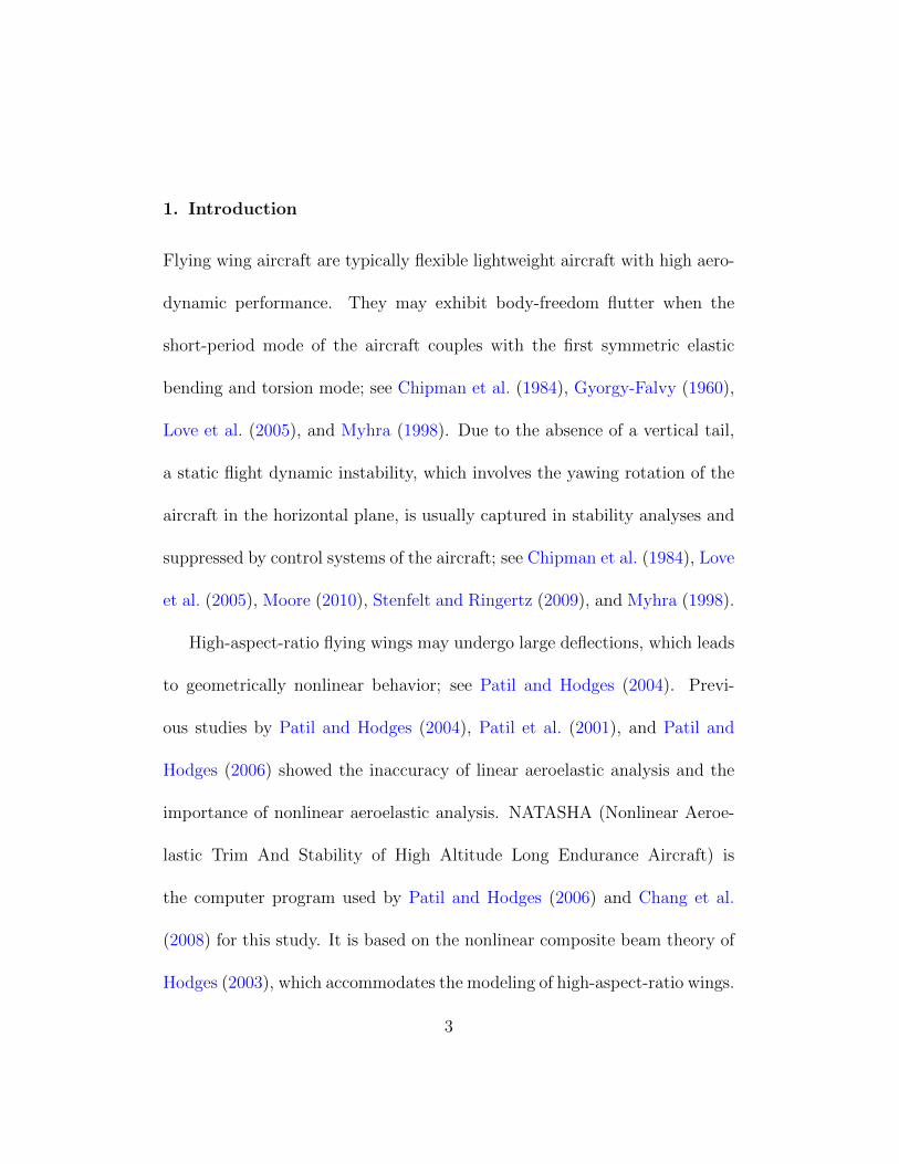
1. Introduction
Flying wing aircraft are typically flexible lightweight aircraft with high aero-
dynamic performance. They may exhibit body-freedom flutter when the
short-period mode of the aircraft couples with the first symmetric elastic
bending and torsion mode; see Chipman et al. (1984), Gyorgy-Falvy (1960),
Love et al. (2005), and Myhra (1998). Due to the absence of a vertical tail,
a static flight dynamic instability, which involves the yawing rotation of the
aircraft in the horizontal plane, is usually captured in stability analyses and
suppressed by control systems of the aircraft; see Chipman et al. (1984), Love
et al. (2005), Moore (2010), Stenfelt and Ringertz (2009), and Myhra (1998).
High-aspect-ratio flying wings may undergo large deflections, which leads
to geometrically nonlinear behavior; see Patil and Hodges (2004). Previ-
ous studies by Patil and Hodges (2004), Patil et al. (2001), and Patil and
Hodges (2006) showed the inaccuracy of linear aeroelastic analysis and the
importance of nonlinear aeroelastic analysis. NATASHA (Nonlinear Aeroe-
lastic Trim And Stability of High Altitude Long Endurance Aircraft) is
the computer program used by Patil and Hodges (2006) and Chang et al.
(2008) for this study. It is based on the nonlinear composite beam theory of
Hodges (2003), which accommodates the modeling of high-aspect-ratio wings.
3

NATASHA uses the aerodynamic theory of Peters et al. (1995) and assesses
aeroelastic stability using the p method. Sotoudeh et al. (2010) presented
additional parametric studies using NATASHA primarily for the purposes
of verification and validation. However, neither the effects of sweep nor of
engine placement were included in these studies. Previous comparisons by
Sotoudeh et al. (2010) showed that results from NATASHA are in excellent
agreement with well-known beam stability solutions (Timoshenko and Gere,
1961; Simitses and Hodges, 2006), the flutter problem of Goland (1945),
experimental data presented by Dowell et al. (1977), and results from well-
established computer codes such as DYMORE (Bauchau and Kang, 1993;
Bauchau, 1998), and RCAS (Saberi et al., 2004). The behavior of sub- and
supercritical eigenvalues was verified by Mardanpour et al. (2012) using the
classical cantilever wing model of Goland (1945) and the continuum aero-
dynamics model of Balakrishnan (2012). In the same work, they studied
the suitability of modeling sweep with NATASHA using the same Goland
model. For the effect of sweep on divergence they compared results from
NATASHA with the approximate formula of Hodges and Pierce (2011), and
for flutter they compared results with work done by Lottati (1985). In both
cases results were in excellent agreement.
4

Effects of follower forces on dynamic instability of beams were studied
by Beck (1952); Bolotin (1959); Como (1966); Wohlhart (1971); Feldt and
Herrmann (1974). Despite engine thrust being a follower force, few studies
included this effect along with aeroelastic effects until the work of Hodges
et al. (2002), who presented a case in which the thrust vectors (from massless
engines) were placed on the outboard portion of the wings of an aircraft with
high aspect ratio wings, thus maximizing thrust effects. They concluded that
increasing engine thrust can either stabilize or destabilize, and flutter speed
and frequency were highly dependent on the ratio of bending stiffness and
torsional stiffness of the wing.
Fazelzadeh et al. (2009) studied the effect of a follower force and mass
arbitrarily placed along a long, straight, homogeneous wing. Their results
emphasize the effect of follower forces along with the external mass magni-
tude and location on the flutter characteristics. Elishakoff and Lottati (1988),
Karpouzian and Librescu (1993), and Fazelzadeh et al. (2009) studied the ef-
fect of sweep on flutter boundaries, but none of them used the geometrically
exact equations for beams. Mardanpour et al. (2012) studied the effect of
engine placement on nonlinear aeroelastic trim and stability of a flying wing
the geometry of which was similar to that of the Horten IV. They modeled
5

each engine as a rigid body with a mass, an inertia matrix, a thrust vector,
and a value of angular momentum. The result of their study showed that
the maximum flutter speed occurs when the engines are just outboard of
60% span; also, the minimum flutter speed occurs when the engine is placed
at wing tips. Both minima and maxima occurred when the engine c.g. was
located forward of the wing elastic axis. In their study, in the absence of
aerodynamics, gravitational forces, and engines, NATASHA found that the
minimum kinetic energy region for the first symmetric elastic free-free bend-
ing mode is near 60% span, which also coincides with the region where the
maximum flutter speed was observed.
In this paper, after briefly reviewing the theory behind NATASHA and
explaining the cases studied, behavior of the eigenvalues is examined along
with an example of the trim and stability for two sets of engine placements
with different offsets from the elastic axis.
Nomenclature
a Deformed beam aerodynamic frame of reference
b Undeformed beam cross-sectional frame of reference
B Deformed beam cross-sectional frame of reference
6

bi Unit vectors in undeformed beam cross-sectional frame of reference (i = 1, 2, 3)
Bi Unit vectors of deformed beam cross-sectional frame of reference (i = 1, 2, 3)
c Chord
cmβ Pitch moment coefficient w.r.t. flap deflection (β)
clα Lift coefficient w.r.t. angle of attack (α)
clβ Lift coefficient w.r.t. flap deflection (β)
e1 Column matrix b1 0 0cT
e Offset of aerodynamic center from the origin of frame of reference along b2
f Column matrix of distributed applied force measures in Bi basis
F Column matrix of internal force measures in Bi basis
g Gravitational vector in Bi basis
H Column matrix of cross-sectional angular momentum measures in Bi basis
i Inertial frame of reference
ii Unit vectors for inertial frame of reference (i = 1, 2, 3)
I Cross-sectional inertia matrix
k Column matrix of undeformed beam initial curvature and twist measures in bi basis
K Column matrix of deformed beam curvature and twist measures in Bi basis
m Column matrix of distributed applied moment measures in Bi basis
M Column matrix of internal moment measures in Bi basis
7
P Column matrix of cross-sectional linear momentum measures in Bi basis
r Column matrix of position vector measures in bi basis
u Column matrix of displacement vector measures in bi basis
V Column matrix of velocity measures in Bi basis
x1 Axial coordinate of beam
β Trailing edge flap angle
γ Column matrix of 1-D generalized force strain measures
∆ Identity matrix
κ Column matrix of elastic twist and curvature measures (1-D generalized moment strain measures)
λ0 Induced flow velocity
µ Mass per unit length
ξ Column matrix of center of mass offset from the frame of reference origin in bi basis
ψ Column matrix of small incremental rotations
Ω Column matrix of cross-sectional angular velocity measures in Bi basis
( )′ Partial derivative of ( ) with respect to x1
˙( ) Partial derivative of ( ) with respect to time
( ) Nodal variable
8

2. Theory
2.1. Nonlinear composite beam theory
B 1
B 2
B 3
Deformed State
Undeformed State
r
R
R
s
ru
x1
b 1
b 2
b 3
R ˆ
r ˆ
Figure 1: Sketch of beam kinematics
The fully intrinsic form of nonlinear composite beam theory of Hodges
(2003) is based on first-order partial differential equations of motion for the
beam that are independent of displacement and rotation variables. They
contain variables that are expressed in the bases of the reference frames of
the undeformed and deformed beams, b(x1) and B(x1, t), respectively; see
Fig. 1. These equations are based on force, moment, angular velocity and
9

velocity with nonlinearities of second order. The equations of motion are
F ′B + KBFB + fB = PB + ΩBPB,
M ′B + KBMB + (e1 + γ)FB +mB = HB + ΩBHB + VBPB,
(1)
where the generalized strains and velocities are related to stress resultants
and moments by the structural constitutive equations
γ
κ
=
R S
ST T
FB
MB
(2)
and the inertial constitutive equations
PB
HB
=
µ∆ −µξ
µξ I
VB
ΩB
. (3)
Finally, strain- and velocity-displacement equations are used to derive the
fully intrinsic kinematical partial differential equations of Hodges (2003),
which are given as
V ′B + KBVB + (e1 + γ)ΩB = γ,
Ω′B + KBΩB = κ.
(4)
10

In this set of equations, FB and MB are column matrices of cross-sectional
stress and moment resultant measures in the B frame, respectively; VB and
ΩB are column matrices of cross-sectional frame velocity and angular velocity
measures in the B frame, respectively; PB and HB are column matrices
of cross-sectional linear and angular momentum measures in the B frame,
respectively; R, S, and T are 3×3 partitions of the cross-sectional flexibility
matrix; ∆ is the 3×3 identity matrix; I is the 3×3 cross-sectional inertia
matrix; ξ is b0 ξ2 ξ3cT with ξ2 and ξ3 the position coordinates of the cross-
sectional mass center with respect to the reference line; µ is the mass per
unit length; the tilde ( ) denotes the antisymmetric 3×3 matrix associated
with the column matrix over which the tilde is placed; ˙( ) denotes the partial
derivative with respect to time; and ( )′ denotes the partial derivative with
respect to the axial coordinate, x1. More details about these equations can
be found in Hodges (2006).
This is a complete set of first-order, partial differential equations. To
solve this complete set of equations, one may eliminate γ and κ using Eq. (2)
and PB and HB using Eq. (3). Then, 12 boundary conditions are needed, in
terms of force (FB), moment (MB), velocity (VB) and angular velocity (ΩB).
The maximum degree of nonlinearities is only two, and because displacement
11
and rotation variables do not appear, singularities caused by finite rotations
are avoided.
If needed, the position and the orientation can be calculated as post-
processing operations by integrating
r′i = Cibe1
(ri + ui)′ = CiB(e1 + γ)
(5)
and
(Cbi)′ = −kCbi
(CBi)′ = −(k + κ)CBi
(6)
2.2. Finite state inflow model of Peters et al.
The two-dimensional finite state aerodynamic model of Peters et al. (1995)
is a state-space, thin-airfoil, inviscid, incompressible approximation of an
infinite-state representation of the aerodynamic loads, which accounts for
induced flow in the wake and apparent mass effects, using known airfoil pa-
rameters. It accommodates large motion of the airfoil as well as deflection of
a small trailing-edge flap. Although the two-dimensional version of this the-
ory does not account for three-dimensional effects associated with the wing
12
tip, published data (Peters et al., 1995; Sotoudeh et al., 2010; Mardanpour
et al., 2012) show this theory is an excellent choice for approximation of
aerodynamic loads acting on high-aspect ratio wings.
The lift, drag and pitching moment at the quarter-chord are given by
Laero = ρb[(cl0 + clββ)VTVa2 − clαVa3b/2− clαVa2(Va3 + λ0 − Ωa1b/2)− cd0VTVa3
](7)
Daero = ρb[−(cl0 + clββ)VTVa3 + clα(Va3 + λ0)
2 − cd0VTVa2
](8)
Maero = 2ρb[(cm0 + cmβ
β)VT − cmαVTVa3 − bclα/8Va2Ωa1 − b2clαΩa1/32 + bclαVa3/8]
(9)
where
VT =√Va2 + Va3 . (10)
sinα =−Va3
VT(11)
αrot =Ωa1b/2
VT(12)
and Va2 , Va3 are the measure numbers of Va and β is the angle of flap deflec-
tion.
The effect of unsteady wake (inflow) and apparent mass appear as λ0 and
13

acceleration terms in the force and moment equation. The inflow model of
Peters et al. (1995) is included to calculate λ0 as:
λ0 =1
2binflowTλ (13)
where λ is the column matrix of inflow states and satisfies
[Ainflow] λ+
(VTb
)λ =
(−Va3 +
b
2Ωa1
)cinflow (14)
and where [Ainflow], binflow, and cinflow are constant matrices derived by
Peters et al. (1995).
3. NATASHA
NATASHA is based on a geometrically exact formulation of the composite
beam theory of Hodges (2006) and the finite-state inflow aerodynamic model
of Peters et al. (1995). The governing equations for structural model are
geometrically exact, fully intrinsic and capable of analyzing the dynamical
behavior of a general, nonuniform, twisted, curved, anisotropic beam under-
going large deformation. The partial differential equations’ dependence on
x1 is approximated by a spatial central differencing presented by the work
14

of Patil and Hodges (2006). The resulting nonlinear ordinary differential
equations are linearized about a static equilibrium state. The equilibrium
state is governed by nonlinear algebraic equations, which NATASHA solves
in obtaining the steady-state trim solution using the Newton-Raphson pro-
cedure; see Patil and Hodges (2006). This system of nonlinear aeroelastic
equations, when linearized about the resulting trim state, leads to a stan-
dard eigenvalue problem which NATASHA uses to analyze the stability of
the structure. NATASHA is also capable of time marching the nonlinear
aeroelastic system of equations using a schedule of the flight controls, which
may be obtained from sequential trim solutions.
4. Case Study
The geometry of the flying wing studied in this paper resembles the HORTEN
IV as described by Gyorgy-Falvy (1960), Myhra (1998), and Mardanpour
et al. (2012); see Fig. 2. This aircraft is modeled using 45 elements. Each
wing is constructed with 19 elements; and the middle part of the aircraft,
which accommodates a hypothetical pilot or cargo, is modeled using six ele-
ments and a lumped mass whose center lies in the aircraft plane of symmetry.
Four engines with varying placement along the span and a set of flaps dis-
15

tributed on the wings comprise the main components of the aircraft flight
control system. As shown in Figs. 2 and 16, η1 and η2 are the dimensionless
distances along b1, along which the engines are located on the right wing;
r1 and r2 are radial offsets of the engines from the elastic axis, normalized
by the maximum radial offset from the elastic axis, rnominal = 0.3 meters; θ1
and θ2 are the polar angles, with θn = 0 (n = 1, 2) pointing upstream. The
properties of engines are presented in Table 1. As the engines were placed
further outboard along the span, the aircraft c.g. migrated aft. In order to
counteract this effect, the concentrated mass in the aircraft plane of symme-
try was displaced such that the c.g. was held constant at (0, -1, -0.1) meters
with respect to the reference point.
The aerodynamic properties of the wing vary linearly from root to tip;
see Table 2. The model properties vary from root to tip of the wings using
these relations:
µ = µroot
(c
croot
)ξ = ξroot
(c
croot
)[R] = [R]root
(c
croot
)[S] = [S]root
(c
croot
)2
[I] = [I]root
(c
croot
)3
[T ] = [T ]root
(c
croot
)3
(15)
These relationships are derived empirically from the Variational Asymptotic
16

Mass of each engine 10 kgAngular momentum of engine 5.829 kg-m2/s
Engine mass moment of inertia:About the b1 axis 0.3 kg-m2
About the b2 axis 0.3 kg-m2
About the b3 axis 0.3 kg-m2
Table 1: Properties of the engines
Aerodynamic coefficient at 25% chord root tipcl0 1.07× 10⁻¹ 5.5× 10⁻³
clα 6.9476 rad−1 6.9981 rad−1
clδ 4.2891 rad−2 4.3288 rad−2
cd0 5.82× 10⁻³ 6.74× 10⁻³
cm0 1.13× 10⁻² −2.4× 10⁻⁴
cmα −1.13× 10⁻² rad−1 −8.3× 10⁻² rad−1
cmδ−6.224× 10⁻¹ rad−1 −7.276× 10⁻¹ rad−1
Table 2: Sectional aerodynamic properties of the wing
Beam Section (VABS) for sections with different chord lengths; see Cesnik
and Hodges (1997) and Yu et al. (2002, 2012). The middle portion of the
aircraft is treated as a rigid body with constant aerodynamic and inertia
properties equal to those at the wing root. Detailed sectional properties of
the wing can be found in Table 3; these properties were tuned such that the
aircraft experiences body-freedom-flutter with the frequencies close to those
of the body-freedom flutter frequency obtained from HORTEN IV pilots as
described by Gyorgy-Falvy (1960), Myhra (1998), and Mardanpour et al.
(2012). See Table 4.
17

Elastic axis (reference line) 25% chordAxial stiffness 1.162× 10⁸ kg/s2
Torsional stiffness 1.883× 10⁵ kg-m2
In-plane bending stiffness 1.349× 10⁷ kg-m2
Out-of-plane bending stiffness 1.660× 10⁵ kg-m2
Mass per unit length 9.193 kg/mInitial Curvature 1.70× 10⁻³/radMass offset −0.285 m
Wing sectional moments of inertia:About the b1 axis 1.0132 kg-mAbout the b2 axis 0.0303 kg-mAbout the b3 axis 0.9829 kg-m
Table 3: Sectional properties of the wing
Engine locations Speed (m/s) Frequency (rad/s) Thrust (N) Flap (deg.)r1 = r2 = θ1 = θ2 = 0
η1=0, η2=0.5 40.8 9.560 23.02 1.257
Table 4: Flutter characteristics of the base model
5. Effects of Engine Placement on Lift to Drag Ratio
Lift to drag ratio analysis is done by calculating the ratio of the equivalent
forces, namely weight and total thrust. Weight of the aircraft is assumed
to be constant, and at constant speed (50 m/s) while the aircraft c.g. was
held constant, NATASHA calculated the total thrust for different engine
placements along the span, including offsets from the elastic axis. In this
analysis, for example, the first engine on the right wing is fixed at η1 with a
particular offset from the elastic axis, and the second engine on the right wing
is further out along the span but with the same offset from the elastic axis.
18

It was observed that engine placement along the span does not significantly
affect L/D of the aircraft; see Figs. 3 – 10, The small variation of L/D can
be attributed to the small static deflections of the wings as the engines are
moved along the span – not due to considerations of the engine aerodynamics.
Figure 11 shows the contour of L/D for varying the offset of the engines
from the elastic axis while fixing their span wise location; i.e., η1 = 0.1 and
η2 = 0.3. It is shown that the change in L/D is not large.
Figure 2: Top view of the flying wing
19

Figure 3: Lift to drag ratio for r1 = r2 = 0.3 and θ1 = θ2 = 0
Figure 4: Lift to drag ratio for r1 = r2 = 0.3 and θ1 = θ2 = 45
20

Figure 5: Lift to drag ratio for r1 = r2 = 0.3 and θ1 = θ2 = 90
Figure 6: Lift to drag ratio for r1 = r2 = 0.3 and θ1 = θ2 = 135
21

Figure 7: Lift to drag ratio for r1 = r2 = 0.3 and θ1 = θ2 = 180
Figure 8: Lift to drag ratio for r1 = r2= 0.3 and θ1 = θ2= 225
22

Figure 9: Lift to drag ratio for r1 = r2= 0.3 and θ1 = θ2= 270
Figure 10: Lift to drag ratio for r1 = r2= 0.3 and θ1 = θ2= 315
23

Figure 11: L/D contour for η1 = 0.1 and η2= 0.3
6. Body Freedom Flutter Characteristics
The behavior of the sub- and supercritical eigenvalues was studied for two
cases of engine placement, both with zero offset from the elastic axis: (a)
η1 = 0 and η2 = 0.5, and (b) η1=0.6 and η2=0.9. For the first case, body-
freedom flutter occurred at 40.8 m/s with a flutter frequency of 9.560 rad/s
while the first symmetric bending mode of the wings couples with the aircraft
short-period mode; see Fig. 13. In the supercritical regime, as the speed
increases, the modal damping peaks and then returns to the stable region (a
so-called hump mode) and another mode becomes unstable; see Fig. 12. The
24

second case experienced flutter at 88 m/s with frequency 47.12 rad/s. The
unstable mode is a mixed motion of in- and out-of-plane bending coupled
with torsion and the aircraft short-period mode.
As the engines are placed further outboard, i.e., case (b), the low-frequency
oscillatory mode presented in case (a) remains stable; see Fig. 14. Instability
occurs at a higher speed (88 m/s). There was no apparent coalescence be-
tween the unstable mode of the aircraft and other modes at the point where
instability occurred; see Fig. 15. In both cases, NATASHA captured other
non-oscillatory unstable roots of flight dynamic origin with very small am-
plitude. The results at the onset of instability for case (a) are presented in
Table 4 and are used for normalization of other results.
25

Figure 12: Real part of the eigenvalues for η1=0 and η2=0.5
Figure 13: Imaginary part of the eigenvalues for η1=0 and η2=0.5
26
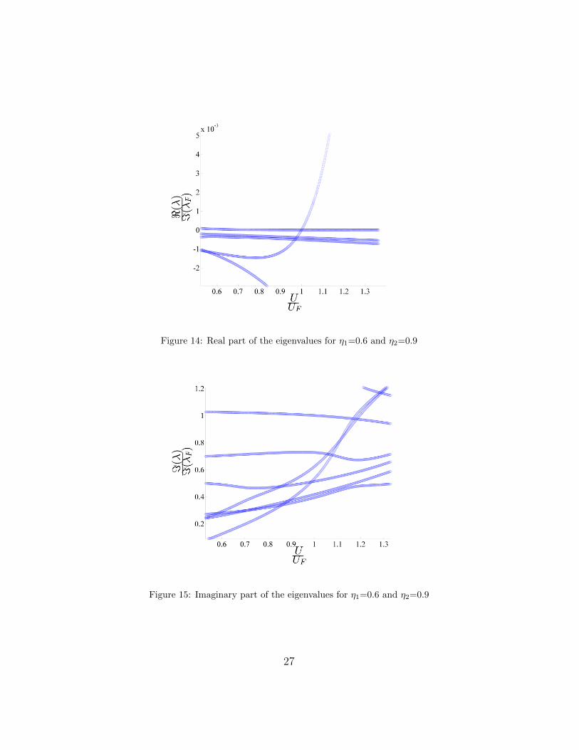
Figure 14: Real part of the eigenvalues for η1=0.6 and η2=0.9
Figure 15: Imaginary part of the eigenvalues for η1=0.6 and η2=0.9
27

7. Effect of Multiple Engine Placement on Body Freedom Flutter
Four identical engines with known mass, moments of inertia, and angular
momentum are symmetrically placed along the span (i.e., in the b1 direction),
and the massless rigid engine mounts are offset from the elastic axis in the
plane of the wing cross section (i.e., along b2 and b3), while the engine
orientations are maintained; see Fig. 16. The engine offsets from the elastic
axis are presented in polar coordinates with (rn, θn) where n is the engine
number. Figures 17 – 25 show the variation in flutter speed for different
engine placements along the span with different offsets from the elastic axis
while one of the engines was kept fixed in a particular location and the
other one moves along the span. It is to be noted that the variability of
flutter speed with engine location is primarily the result of thrust, angular
momentum and inertial properties of the engines rather than changes in the
aerodynamic loads caused by deformation of the wing.
28

Figure 16: Schematic view of the flying wing
When engines are placed along the span with no offset from the elastic
axis, a higher flutter speed is obtained when the second engine is placed at
the outer portion of the wing and the first engine is at an area between 50%
to 70% span; see Fig. 17. This region continues to exhibit high flutter speeds
as engines are placed forward of the elastic axis (i.e. θ is in the first and fourth
quadrant). When the engines are placed behind the elastic axis (i.e. θ is in the
second and third quadrant) there is no significant peak in the flutter speed,
and maximum flutter speed occurs mostly when both engines are closer to
29

the root of the wing; see Figs. 18 – 25. It should be noted that normalized
flutter speeds greater than 3 are beyond the incompressibility assumption in
the aerodynamic model used in NATASHA. The results in this regime of flow
cannot be trusted, but they could be used as an indication of how the trend
of flutter speed might change.
For engine placement forward of the elastic axis, the unstable mode asso-
ciated with the area with noticeable increase in flutter speed, i.e. 50% to 70%
span, contains motion of a first bending-torsion coupled mode with second
and third bending modes; see Figs. 17, 18, 19, 20, and 25.
On the other hand, for engine placement behind the elastic axis, although
the trim solution is symmetric, the unstable mode is antisymmetric – a first
bending-torsion mode; see Figs. 21, 22 and 23. This is caused by excitations
from an antisymmetric flight dynamic mode.
30

Figure 17: Normalized flutter speed for r1 = r2= 0 and θ1 = θ2= 0
Figure 18: Normalized flutter speed for r1 = r2= 0.3 and θ1 = θ2= 0
31

Figure 19: Normalized flutter speed for r1 = r2= 0.3 and θ1 = θ2= 45
Figure 20: Normalized flutter speed for r1 = r2= 0.3 and θ1 = θ2= 90
32

Figure 21: Normalized flutter speed for r1 = r2= 0.3 and θ1 = θ2= 135
Figure 22: Normalized flutter speed for r1 = r2= 0.3 and θ1 = θ2= 180
33
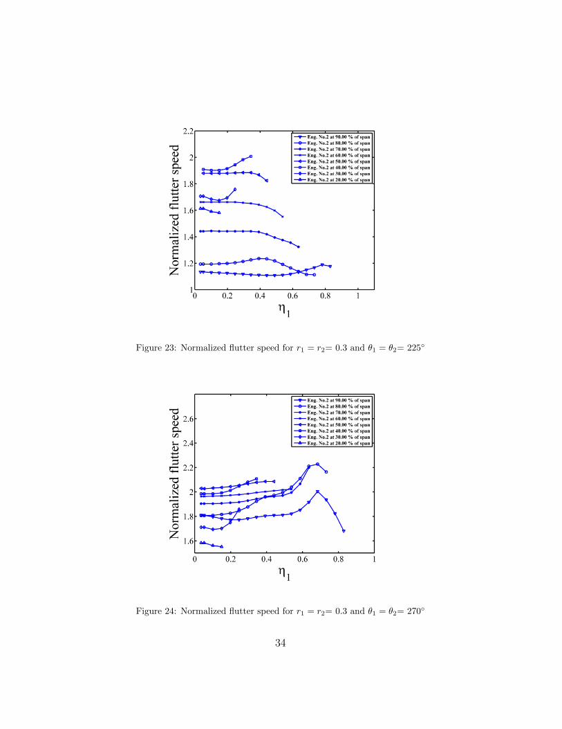
Figure 23: Normalized flutter speed for r1 = r2= 0.3 and θ1 = θ2= 225
Figure 24: Normalized flutter speed for r1 = r2= 0.3 and θ1 = θ2= 270
34

Figure 25: Normalized flutter speed for r1 = r2= 0.3 and θ1 = θ2= 315
The maximum fluctuation of the flutter speed appears to be when the
second engine is at 80% span and the first engine is between 50% to 70%. To
further investigate this area, contour plots of the flutter speed and frequency
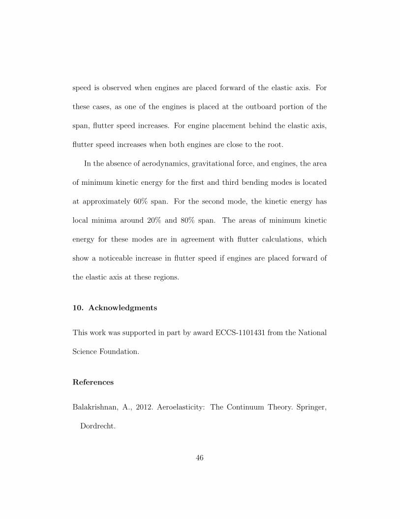
are presented in Figs. 26 – 31, which show the contour of normalized flutter
speed and frequency when the first engine is at 50% span and the second
at 80% span. For engine placement forward of the elastic axis, normalized
flutter speed increases while there is little change in normalized flutter fre-
quency. The same behavior was observed in flutter speed as the first engine
is moved toward the outboard portion of the wing – closer to the second
engine. However, there is a rapid increase in flutter frequency accompanied
35

by a change in the unstable mode shape; see Figs. 28 – 31.
Figure 26: Normalized flutter speed contour for η1 = 0.5 and η2 = 0.8
Figure 27: Normalized flutter frequency contour for η1 = 0.5 and η2 = 0.8
36

Figure 28: Normalized flutter speed contour for η1 = 0.6 and η2 = 0.8
Figure 29: Normalized flutter frequency contour for η1 = 0.6 and η2 = 0.8
37
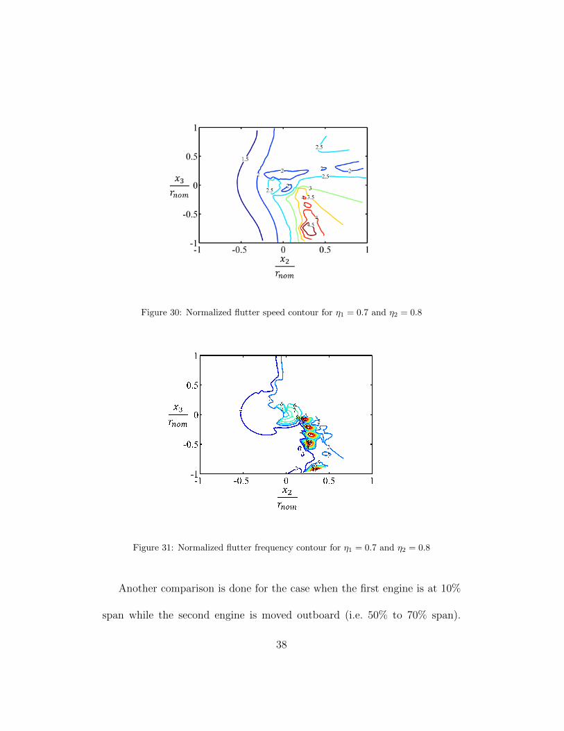
Figure 30: Normalized flutter speed contour for η1 = 0.7 and η2 = 0.8
Figure 31: Normalized flutter frequency contour for η1 = 0.7 and η2 = 0.8
Another comparison is done for the case when the first engine is at 10%
span while the second engine is moved outboard (i.e. 50% to 70% span).
38

Contours of flutter speed and flutter frequency are presented in Figs. 32 –
37. When the second engine is placed at 50% span, as engines are moved
forward of the elastic axis the flutter speed increases and flutter frequency
changes slightly; see Figs. 32 and 33. Placement of the second engine at
60% span increases the flutter speed to a higher range, and flutter frequency
experiences a rapid change as the unstable mode shape changes; see Figs. 34
and 35. When the second engine is placed farther outboard from the first (i.e.
70%), the flutter speed and frequency increase to higher values; see Figs. 36
and 37. In these cases, engine placement forward of the elastic axis increases
the flutter speed.
Figure 32: Normalized flutter speed contour for η1 = 0.1 and η2 = 0.5
39

Figure 33: Normalized flutter frequency contour for η1 = 0.1 and η2 = 0.5
Figure 34: Normalized flutter speed contour for η1 = 0.1 and η2 = 0.6
40

Figure 35: Normalized flutter frequency contour for η1 = 0.1 and η2 = 0.6
Figure 36: Normalized flutter speed contour for η1 = 0.1 and η2 = 0.7
41

Figure 37: Normalized flutter frequency contour for η1 = 0.1 and η2 = 0.7
8. Area of Minimum Kinetic Energy
In the absence of aerodynamics, gravitational force, and engines, NATASHA
was used to calculate the kinetic energy of the modes of the aircraft; see
Figs. 38 – 40. This analysis was done in order to find the region where the
kinetic energy reaches its minimum for the first three lowest frequency free-
free elastic bending modes. Thus, the area of minimum kinetic energy for
the first and third bending modes is located around 60% span; see Figs. 38
and 40. For the second mode, the kinetic energy has local minima at 20%
and 80% span; see Fig. 39.
For engine placement forward of the elastic axis, the unstable mode con-
42

tains a combination of the first, second, and third bending modes; and when
the engines are placed around 60% to 80% span, there is a noticeable increase
in flutter speed. This area is close to the area of minimum kinetic energy of
the first three bending modes; see Figs. 38 – 40.
Figure 38: Normalized kinetic energy of the symmetric first free-free mode of the flying
wing
43

Figure 39: Normalized kinetic energy of the symmetric second free-free mode of the flying
wing
Figure 40: Normalized kinetic energy of the symmetric third free-free mode of the flying
wing
44

9. Concluding Remarks
The aeroelastic trim and stability of a flying-wing aircraft with four en-
gines was analyzed. The aircraft model had a geometry similar to that of
the Horten IV with the addition of four identical engines of specified mass,
moments of inertia, and angular momentum. The four engines are symmet-
rically moved along the span with offsets from the elastic axis while fixing
the location of aircraft c.g. For the clean wing case, the aircraft experiences
body freedom flutter at 40.8 m/s with a flutter frequency of 9.560 rad/s. The
behavior of sub- and supercritical eigenvalues was studied for two cases of
engine placement, both with zero offset from the elastic axis but with differ-
ent locations along the span. The clean-wing case experiences a hump-mode
flutter, and as the engines are moved toward the outer portion of the wing the
unstable mode contains a combination of the first, second, and third bend-
ing along with torsion and the aircraft short period mode. In this case, the
hump-mode is not unstable. In both cases, there is no apparent coalescence
between the unstable modes. NATASHA also captures other non-oscillatory
unstable roots from flight dynamics origin.
This study shows that engine placement does not have any significant
effect on the lift to drag ratio. However, a noticeable increase in flutter
45
speed is observed when engines are placed forward of the elastic axis. For
these cases, as one of the engines is placed at the outboard portion of the
span, flutter speed increases. For engine placement behind the elastic axis,
flutter speed increases when both engines are close to the root.
In the absence of aerodynamics, gravitational force, and engines, the area
of minimum kinetic energy for the first and third bending modes is located
at approximately 60% span. For the second mode, the kinetic energy has
local minima around 20% and 80% span. The areas of minimum kinetic
energy for these modes are in agreement with flutter calculations, which
show a noticeable increase in flutter speed if engines are placed forward of
the elastic axis at these regions.
10. Acknowledgments
This work was supported in part by award ECCS-1101431 from the National
Science Foundation.
References
Balakrishnan, A., 2012. Aeroelasticity: The Continuum Theory. Springer,
Dordrecht.
46

Bauchau, O., 1998. Computational schemes for flexible, nonlinear multi-body
systems. Multibody System Dynamics 2, 169–225.
Bauchau, O. A., Kang, N. K., April 1993. A multibody formulation for he-
licopter structural dynamic analysis. Journal of the American Helicopter
Society 38 (2), 3–14.
Beck, M., 1952. Die Knicklast des einseitig eingespannten, tangential
gedruckten Stabes. Journal of Applied Mathematics and Physics (ZAMP)
3 (3), 225 – 228.
Bolotin, V. V., 1959. On vibrations and stability of bars under the action of
non-conservative forces. In: Kolebaniia v turbomashinakh. USSR, pp. 23
– 42.
Cesnik, C. E. S., Hodges, D. H., January 1997. VABS: a new concept for
composite rotor blade cross-sectional modeling. Journal of the American
Helicopter Society 42 (1), 27 – 38.
Chang, C.-S., Hodges, D. H., Patil, M. J., Mar.-Apr. 2008. Flight dynamics
of highly flexible aircraft. Journal of Aircraft 45 (2), 538 – 545.
Chipman, R. R. F., Rimer, M., Muniz, B., 1984. Body-freedom flutter of a
47

1/2-scale forward swept-wing model, an experimental and analytical study.
Tech. Rep. NAS1-17102, NASA Langley Research Center.
Como, M., 1966. Lateral buckling of a cantilever subjected to a transverse
follower force. International Journal of Solids and Structures 2 (3), 515 –
523.
Dowell, E. H., Traybar, J., Hodges, D. H., 1977. An experimental-theoretical
correlation study of non-linear bending and torsion deformations of a can-
tilever beam. Journal of Sound and Vibration 50 (4), 533–544.
Elishakoff, I., Lottati, I., 1988. Divergence and flutter of nonconservative sys-
tems with intermediate support. Computer Methods in Applied Mechanics
and Engineering 66, 241 – 250.
Fazelzadeh, S., Mazidi, A., Kalantari, H., 2009. Bending-torsional flutter
of wings with an attached mass subjected to a follower force. Journal of
Sound and Vibration 323 (1-2), 148 – 162.
Feldt, W. T., Herrmann, G., 1974. Bending-torsional flutter of a cantilevered
wing containing a tip mass and subjected to a transverse follower force.
Journal of the Franklin Institute 297 (6), 467 – 478.
48

Goland, M., December 1945. The flutter of a uniform cantilever wing. Journal
of Applied Mechanics 12 (4), A197 – A208.
Gyorgy-Falvy, D., June 1960. Performance analysis of the “Horten IV” flying
wing. In: Presented at the 8th O.S.T.I.V. Congress, Cologne, Germany.
Hodges, D. H., June 2003. Geometrically-exact, intrinsic theory for dynamics
of curved and twisted anisotropic beams. AIAA Journal 41 (6), 1131 – 1137.
Hodges, D. H., 2006. Nonlinear Composite Beam Theory. AIAA, Reston,
Virginia.
Hodges, D. H., Patil, M. J., Chae, S., Mar.-Apr. 2002. Effect of thrust on
bending-torsion flutter of wings. Journal of Aircraft 39 (2), 371 – 376.
Hodges, D. H., Pierce, G. A., 2011. Introduction to Structural Dynamics and
Aeroelasticity, 2nd Edition. Cambridge University Press, Cambridge, U.K.
Karpouzian, G., Librescu, L., April 19 – 22, 1993. Exact flutter solution of ad-
vanced anisotropic composite cantilevered wing structure. In: Proceedings
of the 34th Structures, Structural Dynamics, and Materials Conference,
La Jolla, California. pp. 1961 – 1966, AIAA-93-1535-CP.
Lottati, I., Nov. 1985. Flutter and divergence aeroelastic characteristics for
49

composite forward swept cantilevered wing. Journal of Aircraft 22 (11),
1001 – 1007.
Love, M. H., Wieselmann, P., Youngren, H., April 18 – 21, 2005. Body
freedom flutter of high aspect ratio flying wings. In: Proceedings of
the 46th AIAA/ASME/ASCE/AHS/ASC Structures, Structural Dynam-
ics and Materials Conference, Austin, Texas. AIAA, Reston, Virginia.
Mardanpour, P., Hodges, D., Neuhart, R., Graybeal, N., April 23 – 26,
2012. Effect of engine placement on aeroelastic trim and stability of flying
wing aircraft. In: Proceedings of the 53rd AIAA/ASME/ASCE/AHS/ASC
Structures, Structural Dynamics and Materials Conference, Honolulu,
Hawaii. AIAA, Reston, Virginia, AIAA Paper 2012-1634.
Moore, M., September 2010. NASA puffin electric tailsitter VTOL concept.
In: 10th AIAA Aviation Technology, Integration, and Operations (ATIO)
Conference.
Myhra, D., September 1998. The Horten Brothers and Their All-Wing Air-
craft. Schiffer Military/Aviation History. Schiffer Publications, Pennsylva-
nia.
Patil, M. J., Hodges, D. H., Aug. 2004. On the importance of aerodynamic
50
and structural geometrical nonlinearities in aeroelastic behavior of high-
aspect-ratio wings. Journal of Fluids and Structures 19 (7), 905 – 915.
Patil, M. J., Hodges, D. H., 2006. Flight dynamics of highly flexible flying
wings. Journal of Aircraft 43 (6), 1790–1799.
Patil, M. J., Hodges, D. H., Cesnik, C. E. S., Jan.-Feb. 2001. Nonlinear
aeroelasticity and flight dynamics of high-altitude, long-endurance aircraft.
Journal of Aircraft 38 (1), 88 – 94.
Peters, D. A., Karunamoorthy, S., Cao, W.-M., Mar.-Apr. 1995. Finite state
induced flow models; part I: two-dimensional thin airfoil. Journal of Air-
craft 32 (2), 313 – 322.
Saberi, H. A., Khoshlahjeh, M., Ormiston, R. A., Rutkowski, M. J., 2004.
RCAS overview and application to advanced rotorcraft problems. In: 4th
Decennial Specialists’ Conference on Aeromechanics, San Francisco, Cali-
fornia, January 21–23. American Helicopter Society.
Simitses, G. J., Hodges, D. H., 2006. Fundamentals of Structural Stability.
Elsevier, Boston, pp. 264 – 266.
Sotoudeh, Z., Hodges, D. H., Chang, C. S., 2010. Validation studies for
51

aeroelastic trim and stability analysis of highly flexible aircraft. Journal of
Aircraft 47 (4), 1240 – 1247.
Stenfelt, G., Ringertz, U., November-December 2009. Lateral stability and
control of a tailless aircraft configuration. Journal of Aircraft 46 (6), 2161
– 2164.
Timoshenko, S. P., Gere, J. M., 1961. Theory of Elastic Stability, 2nd Edition.
McGraw-Hill Book Company, New York, pp. 88.
Wohlhart, K., 1971. Dynamische Kippstabilitat eines Plattenstreifens unter
Folgelast. Zeitschrift fur Flugwissenschaften 19 (7), 291 – 298.
Yu, W., Hodges, D. H., Ho, J. C., October 2012. Variational asymptotic
beam sectional analysis – an updated version. International Journal of
Engineering Science 59, 40 – 64.
Yu, W., Hodges, D. H., Volovoi, V. V., Cesnik, C. E. S., 2002. On
Timoshenko-like modeling of initially curved and twisted composite beams.
International Journal of Solids and Structures 39 (19), 5101 – 5121.
52
Related Documents