EFFECT OF IMPERFECT DIRECT SIMPLE SHEAR TEST BOUNDARY CONDITIONS ON MONOTONIC AND CYCLIC MEASUREMENTS by Man Ho Daniel Wai A thesis submitted in conformity with the requirements for the degree of Master of Applied Science Graduate Department of Civil and Mineral Engineering University of Toronto © Copyright by Man Ho Daniel Wai 2019

Welcome message from author
This document is posted to help you gain knowledge. Please leave a comment to let me know what you think about it! Share it to your friends and learn new things together.
Transcript

EFFECT OF IMPERFECT DIRECT SIMPLE SHEAR TEST
BOUNDARY CONDITIONS ON MONOTONIC AND
CYCLIC MEASUREMENTS
by
Man Ho Daniel Wai
A thesis submitted in conformity with the requirements
for the degree of Master of Applied Science
Graduate Department of Civil and Mineral Engineering
University of Toronto
© Copyright by Man Ho Daniel Wai 2019
ii
Effect of Imperfect Direct Simple Shear Test Boundary Conditions on
Monotonic and Cyclic Measurements
Man Ho Daniel Wai
Master of Applied Science
Graduate Department of Civil and Mineral Engineering
University of Toronto
2019
Abstract
The direct simple shear (DSS) test is commonly used to assess shear strength of soil, estimate
liquefaction resistance, or calibrate constitutive models. However, constitutive models are
calibrated assuming ideal simple shear stress conditions even though this is not achieved in the
DSS test. Near frictionless vertical boundaries cannot develop the complementary shear stresses
necessary for ideal simple shear conditions. Difficulties in maintaining constant height during
undrained tests violates the constant volume assumption. The top cap holding the top of the
specimen can rock (rotate) during shear also violating the assumed perfect simple shear conditions.
Parametric studies were conducted to investigate the effect of contact friction between the soil and
vertical boundaries, vertical compliance and top cap rocking on the results of undrained DSS tests.
The study simulates an industry-standard SGI type simple shear device using a 3-D finite element
model and an advanced plasticity model to capture soil behaviour.

iii
Acknowledgments
I would like to thank Rocscience Inc. for providing financial and technical support during the
study.
I acknowledge the support of the Natural Sciences and Engineering Research Council of Canada
(NSERC). I would like to thank NSERC for Grant# 401267058 in support of the study.
I would like to thank my supervisor Dr. Mason Ghafghazi for guiding me through my studies.
I would like to thank my fellow graduate students Sartaj Gill, Wyatt Handspiker, Edouardine
Ingabire, Faraz Goodarzi, Wei Liu, Fredric Fong, Mathan Manmatharajan, Mohammad Mozaffari,
Khashayar Nikoonejad, and Emmanuel Sarantonis for their support throughout my studies. Special
acknowledgement to Sartaj Gill, Wei Liu, Khashayar Nikoonejad, and Mathan Manmatharajan for
providing experimental data that is used in this study.

iv
Table of Contents
Acknowledgments.......................................................................................................................... iii
Table of Contents ........................................................................................................................... iv
List of Tables ................................................................................................................................ vii
List of Figures .............................................................................................................................. viii
Chapter 1 Introduction ..............................................................................................................1
1.1 General Remarks ..................................................................................................................1
1.2 Direct simple shear device ...................................................................................................4
1.3 Objective and Scope ............................................................................................................5
1.4 Sign Convention...................................................................................................................6
1.5 Organization .........................................................................................................................6
Chapter 2 Literature Review.....................................................................................................8
2.1 Introduction ..........................................................................................................................8
2.2 Effect of Soil-Ring Friction .................................................................................................9
2.3 Effect of Vertical Compliance on Undrained Tests ...........................................................10
2.4 Effect of Top Cap Rocking ................................................................................................11
2.5 Summary ............................................................................................................................12
Chapter 3 Numerical Analysis of Direct Simple Shear Test Boundary Conditions ...............14
3.1 Introduction ........................................................................................................................14
3.2 Soil Constitutive Model .....................................................................................................14
3.3 Calibration..........................................................................................................................15
3.4 Finite Element Model ........................................................................................................19
3.4.1 Geometry................................................................................................................19
3.4.2 Soil-Ring Interaction ..............................................................................................20
3.4.3 Top Cap ..................................................................................................................20
v
3.4.4 Loading and Boundary Conditions ........................................................................21
3.4.5 Ideal Simple Shear Conditions ..............................................................................21
3.4.6 Mesh sensitivity analysis .......................................................................................22
3.5 Effect of Soil-Ring Friction ...............................................................................................25
3.5.1 Introduction ............................................................................................................25
3.5.2 Results and Discussion ..........................................................................................26
3.6 Effect of Vertical Compliance on Undrained Tests ...........................................................40
3.6.1 Introduction ............................................................................................................40
3.6.2 Results and Discussion ..........................................................................................42
3.7 Effect of Top Cap Rocking During Shear..........................................................................54
3.7.1 Introduction ............................................................................................................54
3.7.2 Results and Discussion ..........................................................................................55
3.8 Conclusions ........................................................................................................................62
3.8.1 Effect of Soil-Ring Friction ...................................................................................62
3.8.2 Effect of Vertical Compliance on Undrained Tests ...............................................63
3.8.3 Effect of Top Cap Rocking During Shear..............................................................63
Chapter 4 Summary and Conclusions ....................................................................................65
4.1 Summary and Conclusions ................................................................................................65
4.1.1 Effect of Soil-Ring Friction ...................................................................................65
4.1.2 Effect of Vertical Compliance on Undrained Tests ...............................................66
4.1.3 Effect of Top Cap Rocking During Shear..............................................................66
4.1.4 Recommendations for Future Work.......................................................................66
References ......................................................................................................................................68
Appendix A Dafalias and Manzari (2004) Model Calibration Results ......................................71
A.1 Calibration of Undrained Monotonic Simple Shear Behaviour: experimental data and
Dafalias and Manzari (2004) model simulations ...............................................................72

vi
A.2 Calibration of Undrained Cyclic Simple Shear Behaviour: experimental data and
Dafalias and Manzari (2004) model simulations ...............................................................76
A.3 Calibration of Undrained Cyclic Simple Shear Behaviour: Dafalias and Manzari
(2004) model simulations varying cyclic stress ratios (CSR) to generate (CSR) vs.
number of cycles to liquefaction plot (Figure 3.4) ............................................................81
A.4 Calibration of Undrained Cyclic Simple Shear Behaviour: other experimental data to
generate cyclic stress ratio (CSR) vs. number of cycles to liquefaction plot (Figure
3.4) .....................................................................................................................................85
Appendix B Mesh Sensitivity Analysis Results .........................................................................97
B.1 Frictionless Vertical Boundaries, Constant Height and No Top Cap Rocking..................98
B.2 Effect of Soil-Ring Friction .............................................................................................100
B.3 Effect of Vertical Compliance on Undrained Tests .........................................................101
B.4 Effect of Top cap Rocking During Shear ........................................................................102
Appendix C Simulation Results ...............................................................................................103
C.1 Effect of Soil-Ring Friction .............................................................................................104
C.1.1 Consolidation .......................................................................................................104
C.1.2 Undrained Monotonic Simple Shear ....................................................................106
C.1.3 Undrained Cyclic Simple Shear ...........................................................................110
C.2 Effect of Vertical Compliance on Undrained Tests .........................................................116
C.2.1 Undrained Monotonic Simple Shear ....................................................................116
C.2.2 Undrained Cyclic Simple Shear ...........................................................................119
C.3 Effect of Top Cap Rocking During Shear........................................................................121
C.3.1 Undrained Monotonic Simple Shear ....................................................................121
C.3.2 Undrained Cyclic Simple Shear ...........................................................................123
Dafalias and Manzari (2004) Constitutive Model UMAT File ...........................127
D.1 Source Code .....................................................................................................................128
D.2 UMAT File.......................................................................................................................128

vii
List of Tables
Table 3.1. Dafalias and Manzari (2004) model calibrated parameters ......................................... 16
Table 3.2: Total computation time for undrained monotonic and cyclic simulations using
different mesh densities and element types .................................................................................. 25
Table 3.3: Percent change of monotonic test results from higher maximum vertical strain for
loose specimen (Dr = 24%) at peak stress (4% shear strain) ........................................................ 45
Table 3.4: Percent change of monotonic test results from higher maximum vertical strain for
dense specimen (Dr = 146%) at 4% shear strain ........................................................................... 49
viii
List of Figures
Figure 1.1: Typical SGI simple shear test boundaries .................................................................... 2
Figure 1.2: Simple shear stress state ............................................................................................... 2
Figure 1.3: SGI type direct simple shear device that is used in this study. .................................... 5
Figure 1.4: Sign convention for key stress and strain components in this study ............................ 6
Figure 3.1: Illustration of the yield, critical state, dilatancy and bounding lines in deviator stress
(q), mean effective stress (p) space (from Dafalias and Manzari, 2004) ...................................... 15
Figure 3.2: Sample calibrated undrained monotonic simple shear test ........................................ 17
Figure 3.3: Sample calibrated undrained cyclic simple shear test ................................................ 18
Figure 3.4: Cyclic stress ratio (CSR) vs. number of cycles to liquefaction for soil relative density
(Dr) of 77% and liquefaction criterion defined by single amplitude shear strain (Liq) ................ 19
Figure 3.5: Finite element model of the DSS test ......................................................................... 20
Figure 3.6: Specimen mesh densities that were analyzed in the mesh sensitivity analysis .......... 23
Figure 3.7: Undrained monotonic test results of loose specimen (Dr = 24%) varying element size
(ES) and element type for frictionless vertical boundaries, constant height and no top cap rocking
....................................................................................................................................................... 24
Figure 3.8: Undrained cyclic test results of loose specimen (Dr = 24%) varying element size (ES)
and element type for frictionless vertical boundaries, constant height and no top cap rocking ... 24
Figure 3.9: Friction on a soil specimen that is encased in a rubber membrane and is confined by
Teflon coated rings ....................................................................................................................... 26
Figure 3.10: End of consolidation stress distribution of loose specimen (Dr = 24%) simulations
for the centre cross section of the specimen (z = 0 mm), varying soil-ring friction angle (soil-ring)
....................................................................................................................................................... 27
ix
Figure 3.11: End of consolidation vertical effective stress contours of loose specimen (Dr = 24%)
simulation for no slip condition, soil-ring friction angle of 30° ................................................... 27
Figure 3.12: Coefficient of lateral earth pressure (K) during consolidation at the core of loose
specimen (Dr = 24%) simulations for varying soil-ring friction angles (soil-ring)......................... 28
Figure 3.13. Stress contours of loose specimen (Dr = 24%) simulation at 4% shear strain for
frictionless vertical boundaries, soil-ring friction angle of 0° ...................................................... 29
Figure 3.14. Stress distribution of loose specimen (Dr = 24%) simulations at peak shear stress
(4% shear strain) for the centre cross section of the specimen (z = 0 mm), varying soil-ring
friction angle (soil-ring) .................................................................................................................. 29
Figure 3.15: Effective normal stress results for monotonic tests of loose specimen (Dr = 24%) for
varying soil-ring friction angles (soil-ring) ..................................................................................... 30
Figure 3.16. Monotonic test results of loose specimen (Dr = 24%) for varying soil-ring friction
angles (soil-ring) ............................................................................................................................. 31
Figure 3.17. Monotonic test results of dense specimen (Dr = 146%) for varying soil-ring friction
angle (soil-ring) ............................................................................................................................... 31
Figure 3.18. Monotonic test results of loose specimen (Dr = 24%) for varying soil-ring friction
angles (soil-ring) during shearing phase only ................................................................................. 32
Figure 3.19. Stress contours of dense specimen (Dr = 146%) simulation at the peak amplitude of
the last cycle for frictionless vertical boundaries, soil-ring friction angle of 0° ........................... 34
Figure 3.20. Stress distribution of dense specimen (Dr = 146%) simulations for the centre cross
section of the specimen (z = 0 mm) during the peak amplitude of the (a) first and (b) last cycle
for varying soil-ring friction angles (soil-ring) ............................................................................... 35
Figure 3.21: Normal stress results for cyclic tests of dense specimen (Dr = 146%) for varying
soil-ring friction angles (soil-ring) .................................................................................................. 36

x
Figure 3.22. Cyclic test results of loose specimen (Dr = 24%) for varying soil-ring friction angles
(soil-ring) ......................................................................................................................................... 37
Figure 3.23. Cyclic test results of dense specimen (Dr = 146%) for varying soil-ring friction
angles (soil-ring) ............................................................................................................................. 38
Figure 3.24. Cyclic test results of loose specimen (Dr = 24%) for varying soil-ring friction angles
(soil-ring) during shearing phase only ............................................................................................ 40
Figure 3.25: Vertical displacement vs. applied vertical stress for SGI type device that was loaded
without soil specimen ................................................................................................................... 41
Figure 3.26: Stress and strain distribution of loose specimen (Dr = 24%) simulations at peak
shear stress (4% shear strain) for the centre cross section of the specimen (z = 0 mm), varying
maximum vertical strain (y,max) during the shearing phase .......................................................... 43
Figure 3.27: Monotonic test results of loose specimen (Dr = 24%) for varying maximum vertical
strain (y,max) during the shearing phase ........................................................................................ 45
Figure 3.28: Reproduced undrained monotonic test results of Ottawa sand on the effect of
vertical compliance on undrained tests from Zekkos et al. (2018) ............................................... 46
Figure 3.29: Reproduced undrained monotonic test results of pea gravel on the effect of vertical
compliance on undrained tests from Zekkos et al. (2018) ............................................................ 46
Figure 3.30: Vertical displacement vs. applied vertical stress for large-size cyclic simple shear
device developed by Geocomp (2019) without soil specimen ..................................................... 46
Figure 3.31: Monotonic test results of dense specimen (Dr = 146%) for varying maximum
vertical strain (y,max) during the shearing phase ........................................................................... 48
Figure 3.32: Reproduced undrained monotonic test results of dense offshore sand on the effect of
vertical compliance on undrained tests from Dyvik and Suzuki (2018) ....................................... 49
Figure 3.33: Reproduced example of offset in specimen height for Kaolin specimen using an
active height control system from Dyvik and Suzuki (2018) ....................................................... 49

xi
Figure 3.34: Stress-strain response for undrained cyclic simple shear simulations of loose
specimen (Dr = 24%) for varying maximum vertical strain (y,max) during the shearing phase.... 51
Figure 3.35: Stress-strain response for undrained cyclic simple shear simulations of dense
specimen (Dr = 146%) for varying maximum vertical strain (y,max) during the shearing phase .. 52
Figure 3.36: Stress-strain response of cyclic tests for dense specimen (Dr = 146%) using two
approaches to model constant height ............................................................................................ 53
Figure 3.37: Stress and strain distribution of dense specimen (Dr = 146%) simulations for the
centre cross section of the specimen (z = 0 mm) during the peak amplitude of the last cycle using
two approaches to model constant height ..................................................................................... 54
Figure 3.38: Potential top cap rocking that is influenced by loading shaft in SGI type device .... 55
Figure 3.39. Stress and strain distribution of loose specimen (Dr = 24%) simulations at peak
shear stress (4% shear strain) for the centre cross section of the specimen (z = 0 mm), varying
maximum top cap rotation angle (,max) ....................................................................................... 57
Figure 3.40: Monotonic test results of loose specimen (Dr = 24%) for varying maximum top cap
rotation angle (,max) .................................................................................................................... 58
Figure 3.41: Monotonic test results of dense specimen (Dr = 146%) for varying maximum top
cap rotation angle (,max) .............................................................................................................. 58
Figure 3.42: Stress and strain distribution of loose specimen (Dr = 24%) simulations during peak
amplitudes (peak) of the first cycle for the centre cross section of the specimen (z = 0 mm),
varying maximum top cap rotation angle (,max) ......................................................................... 60
Figure 3.43: Stress-strain response for undrained cyclic simple shear simulations of loose
specimen (Dr = 24%) for varying maximum top cap rotation angle (,max) ............................... 61
Figure 3.44: Stress-strain response for undrained cyclic simple shear simulations of dense
specimen (Dr = 146%) for varying maximum top cap rotation angle (,max) .............................. 62
1
Chapter 1
Introduction
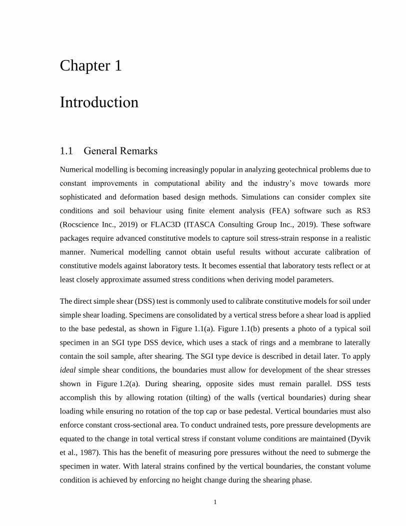
1.1 General Remarks
Numerical modelling is becoming increasingly popular in analyzing geotechnical problems due to
constant improvements in computational ability and the industry’s move towards more
sophisticated and deformation based design methods. Simulations can consider complex site
conditions and soil behaviour using finite element analysis (FEA) software such as RS3
(Rocscience Inc., 2019) or FLAC3D (ITASCA Consulting Group Inc., 2019). These software
packages require advanced constitutive models to capture soil stress-strain response in a realistic
manner. Numerical modelling cannot obtain useful results without accurate calibration of
constitutive models against laboratory tests. It becomes essential that laboratory tests reflect or at
least closely approximate assumed stress conditions when deriving model parameters.
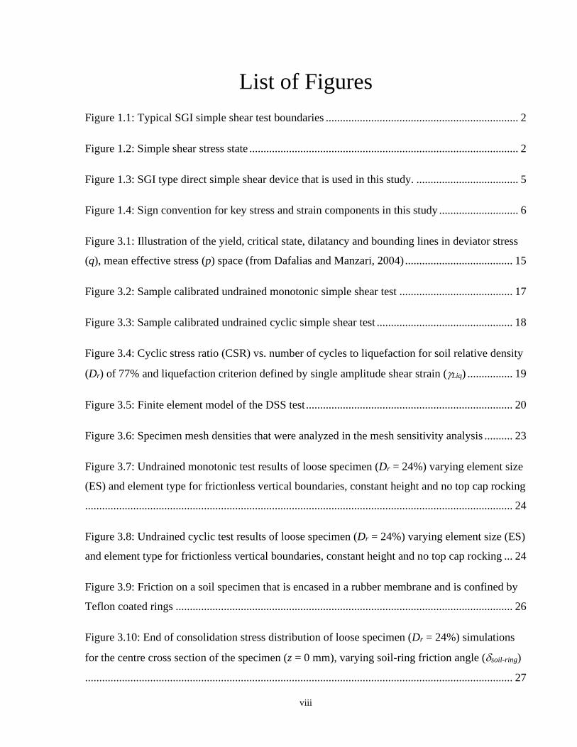
The direct simple shear (DSS) test is commonly used to calibrate constitutive models for soil under
simple shear loading. Specimens are consolidated by a vertical stress before a shear load is applied
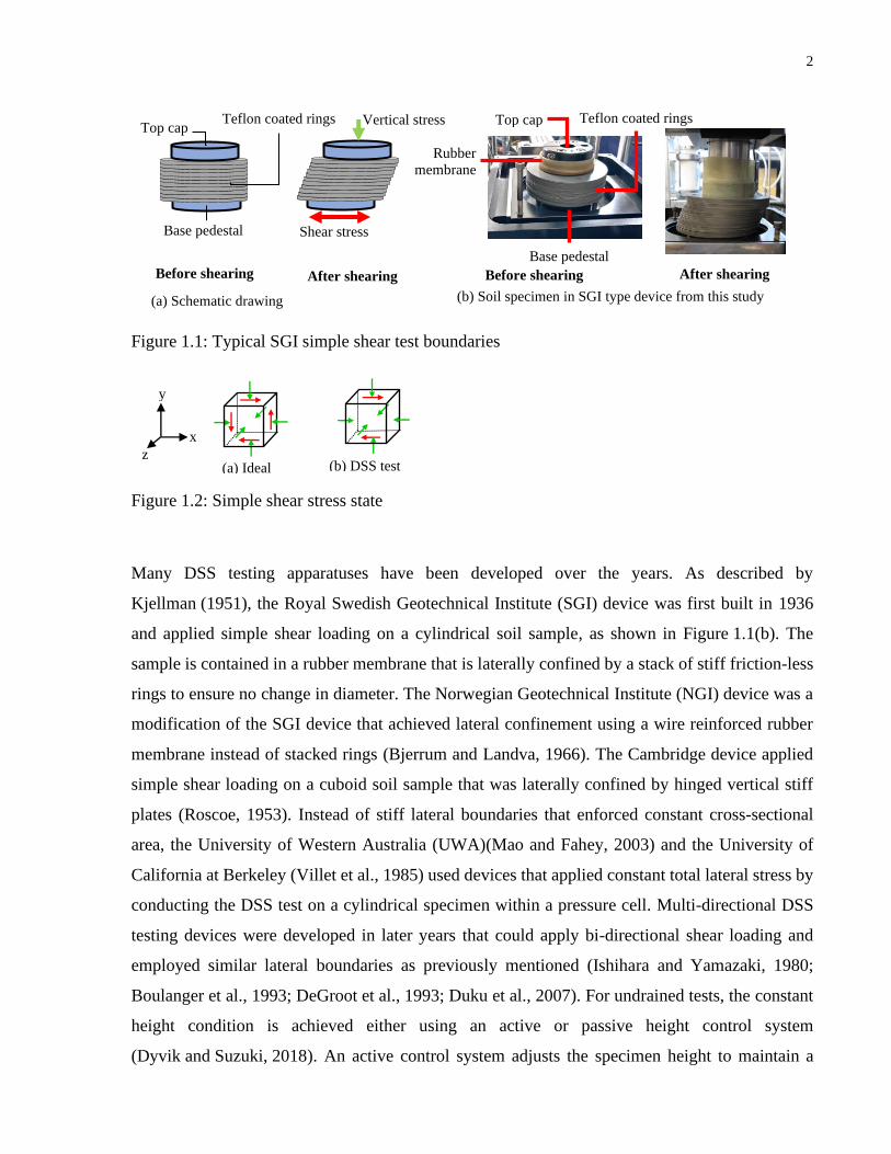
to the base pedestal, as shown in Figure 1.1(a). Figure 1.1(b) presents a photo of a typical soil
specimen in an SGI type DSS device, which uses a stack of rings and a membrane to laterally
contain the soil sample, after shearing. The SGI type device is described in detail later. To apply
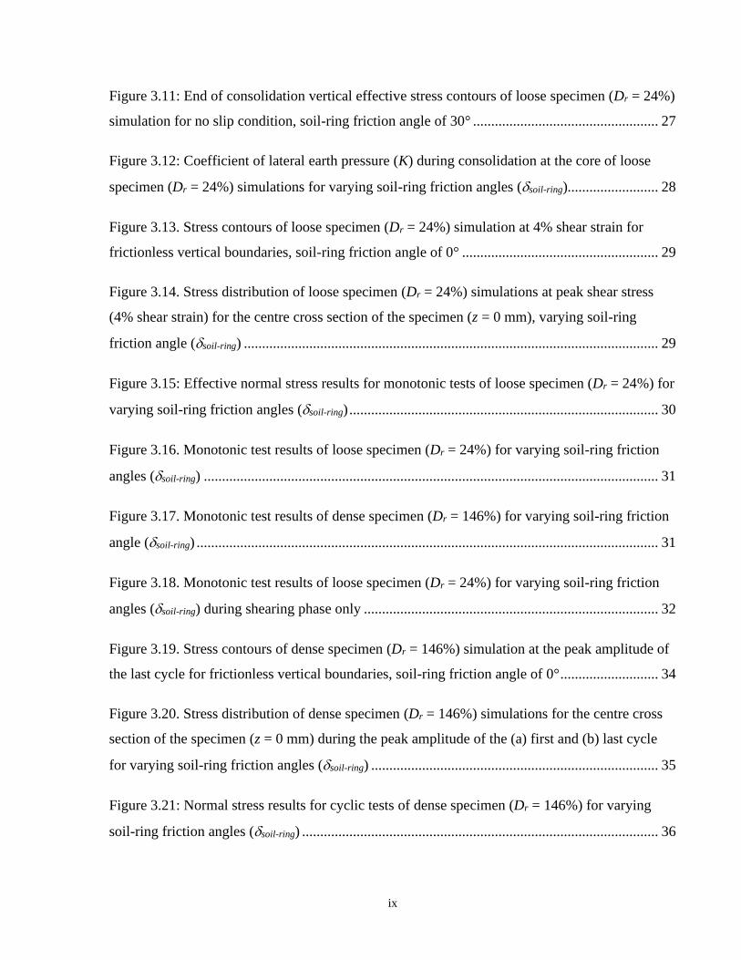
ideal simple shear conditions, the boundaries must allow for development of the shear stresses
shown in Figure 1.2(a). During shearing, opposite sides must remain parallel. DSS tests
accomplish this by allowing rotation (tilting) of the walls (vertical boundaries) during shear
loading while ensuring no rotation of the top cap or base pedestal. Vertical boundaries must also
enforce constant cross-sectional area. To conduct undrained tests, pore pressure developments are
equated to the change in total vertical stress if constant volume conditions are maintained (Dyvik
et al., 1987). This has the benefit of measuring pore pressures without the need to submerge the
specimen in water. With lateral strains confined by the vertical boundaries, the constant volume
condition is achieved by enforcing no height change during the shearing phase.
2
Figure 1.1: Typical SGI simple shear test boundaries
Figure 1.2: Simple shear stress state
Many DSS testing apparatuses have been developed over the years. As described by
Kjellman (1951), the Royal Swedish Geotechnical Institute (SGI) device was first built in 1936
and applied simple shear loading on a cylindrical soil sample, as shown in Figure 1.1(b). The
sample is contained in a rubber membrane that is laterally confined by a stack of stiff friction-less
rings to ensure no change in diameter. The Norwegian Geotechnical Institute (NGI) device was a
modification of the SGI device that achieved lateral confinement using a wire reinforced rubber
membrane instead of stacked rings (Bjerrum and Landva, 1966). The Cambridge device applied
simple shear loading on a cuboid soil sample that was laterally confined by hinged vertical stiff
plates (Roscoe, 1953). Instead of stiff lateral boundaries that enforced constant cross-sectional
area, the University of Western Australia (UWA)(Mao and Fahey, 2003) and the University of
California at Berkeley (Villet et al., 1985) used devices that applied constant total lateral stress by
conducting the DSS test on a cylindrical specimen within a pressure cell. Multi-directional DSS
testing devices were developed in later years that could apply bi-directional shear loading and
employed similar lateral boundaries as previously mentioned (Ishihara and Yamazaki, 1980;
Boulanger et al., 1993; DeGroot et al., 1993; Duku et al., 2007). For undrained tests, the constant
height condition is achieved either using an active or passive height control system
(Dyvik and Suzuki, 2018). An active control system adjusts the specimen height to maintain a
Teflon coated rings Vertical stress Top cap
Shear stress Base pedestal
(a) Schematic drawing (b) Soil specimen in SGI type device from this study
Teflon coated rings
Base pedestal
Top cap
Rubber
membrane
Before shearing After shearing Before shearing After shearing
(a) Ideal (b) DSS test
y
z
x
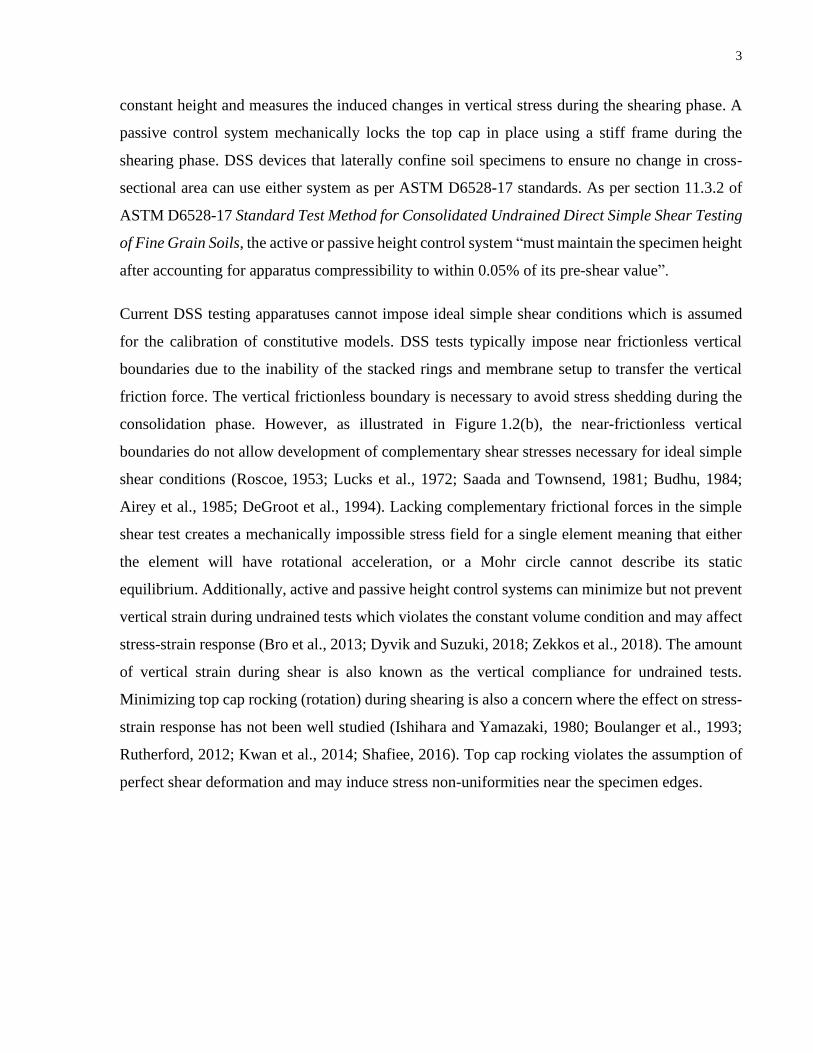
3
constant height and measures the induced changes in vertical stress during the shearing phase. A
passive control system mechanically locks the top cap in place using a stiff frame during the
shearing phase. DSS devices that laterally confine soil specimens to ensure no change in cross-
sectional area can use either system as per ASTM D6528-17 standards. As per section 11.3.2 of
ASTM D6528-17 Standard Test Method for Consolidated Undrained Direct Simple Shear Testing
of Fine Grain Soils, the active or passive height control system “must maintain the specimen height
after accounting for apparatus compressibility to within 0.05% of its pre-shear value”.
Current DSS testing apparatuses cannot impose ideal simple shear conditions which is assumed
for the calibration of constitutive models. DSS tests typically impose near frictionless vertical
boundaries due to the inability of the stacked rings and membrane setup to transfer the vertical
friction force. The vertical frictionless boundary is necessary to avoid stress shedding during the
consolidation phase. However, as illustrated in Figure 1.2(b), the near-frictionless vertical
boundaries do not allow development of complementary shear stresses necessary for ideal simple
shear conditions (Roscoe, 1953; Lucks et al., 1972; Saada and Townsend, 1981; Budhu, 1984;
Airey et al., 1985; DeGroot et al., 1994). Lacking complementary frictional forces in the simple
shear test creates a mechanically impossible stress field for a single element meaning that either
the element will have rotational acceleration, or a Mohr circle cannot describe its static
equilibrium. Additionally, active and passive height control systems can minimize but not prevent
vertical strain during undrained tests which violates the constant volume condition and may affect
stress-strain response (Bro et al., 2013; Dyvik and Suzuki, 2018; Zekkos et al., 2018). The amount
of vertical strain during shear is also known as the vertical compliance for undrained tests.
Minimizing top cap rocking (rotation) during shearing is also a concern where the effect on stress-
strain response has not been well studied (Ishihara and Yamazaki, 1980; Boulanger et al., 1993;
Rutherford, 2012; Kwan et al., 2014; Shafiee, 2016). Top cap rocking violates the assumption of
perfect shear deformation and may induce stress non-uniformities near the specimen edges.
4
Experimental and numerical studies have been conducted to study imperfect boundary effects and
estimate the development of stress non-uniformities. Experimental studies suggest that stress non-
uniformities in DSS devices may cause unreliable stress and strain measurements that cannot be
used to approximate real soil response under ideal simple shear conditions (Budhu, 1984;
DeGroot et al., 1994). Numerical studies provided a more in-depth examination of stress and strain
distribution throughout the specimen in a DSS device during shear (Roscoe, 1953;
Lucks et al., 1972; Shen et al., 1978; Saada and Townsend, 1981; Doherty and Fahey, 2011,
Wijewickreme et al., 2013). In numerical studies, the assumed contact behaviour between soil and
vertical boundaries is unclear and the simulations do not appear to consider the effect of vertical
compliance and top cap rocking during the shearing phase. The effect of soil-ring friction on DSS
testing has not been well studied and may impact the calibration of constitutive models. Higher
contact friction allows better development of complementary shear stresses but may induce stress
non-uniformities during the consolidation phase. Bernhardt et al. (2016) showed from a study of
steel spheres in a DSS apparatus that higher steel spheres to ring friction resulted in more strain
hardening and dilative response. Their results suggest that higher soil-ring friction can potentially
overestimate shear strength properties. Numerical studies are not found that studied the effect of
vertical compliance on stress-strain response of undrained tests. Experimental data shows that
vertical strain during shear within the ASTM D6528-17 tolerance of 0.05% may increase or reduce
the measured shear strength (Bro et al., 2013; Dyvik and Suzuki, 2018; Zekkos et al., 2018). The
effect of top cap rocking (rotation) on stress-strain response is not well studied. Ishihara and
Yamazaki (1980) proposed that top cap rocking during experimental tests may have induced
vertical stress concentrations near the edges of the specimen.
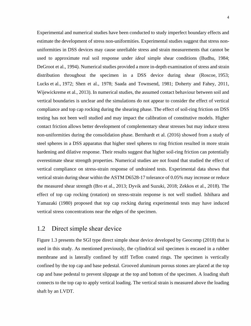
1.2 Direct simple shear device
Figure 1.3 presents the SGI type direct simple shear device developed by Geocomp (2018) that is
used in this study. As mentioned previously, the cylindrical soil specimen is encased in a rubber
membrane and is laterally confined by stiff Teflon coated rings. The specimen is vertically
confined by the top cap and base pedestal. Grooved aluminum porous stones are placed at the top
cap and base pedestal to prevent slippage at the top and bottom of the specimen. A loading shaft
connects to the top cap to apply vertical loading. The vertical strain is measured above the loading
shaft by an LVDT.

5
Figure 1.3: SGI type direct simple shear device that is used in this study.
1.3 Objective and Scope
This dissertation summarizes an investigation into the effect of imperfect boundary conditions in
an SGI type device on the calibration of constitutive models. Figure 1.3 presents the SGI type
device that is used in this study. A numerical study is conducted using three-dimensional (3D)
finite element analysis (FEA) of undrained monotonic and cyclic simple shear tests using the

6
software ABAQUS (Dassault Systèmes, 2012). The soil stress-strain behaviour is captured using
the Dafalias and Manzari (2004) constitutive model for its ability to capture sand plasticity during
both monotonic and cyclic shear loading. The simulation models the stacked rings confining a
typical cylindrical soil specimen. The model is calibrated using triaxial and simple shear test data
of a poorly graded medium sand. Parametric studies are performed to investigate the effect of soil-
ring friction, vertical compliance on undrained tests and top cap rocking during shear for various
soil densities. The effect of soil-ring friction is analyzed by simulations using the minimum and
maximum expected soil-ring friction in the laboratory as well as the soil-ring friction necessary to
achieve ideal simple shear conditions. The effect of vertical compliance is analyzed using
simulations with various vertical strain tolerances during the shearing phase to induce unwanted
volume change in undrained tests. The effect of top cap rocking is analyzed using simulations with
various allowed top cap rotations during the shearing phase. Results from the numerical study are
meant to provide insight on the magnitudes of stress and strain non-uniformities due to imperfect
boundary conditions rather than to precisely commute values for design purposes.
1.4 Sign Convention
The study adopts the compression positive sign convention. Positive directions of shear stress and
rotation are shown in Figure 1.4.
Figure 1.4: Sign convention for key stress and strain components in this study
1.5 Organization
The thesis is organized into four chapters as follows.
Chapter 1 presented the introduction that describes the study topic, objectives and scope, sign
convention and chapter organization.
y
x or z (+)
Rotation
Shear
Compression
x (+)

7
Chapter 2 presents the literature review that summarizes the past experimental and numerical
studies on the effect of imperfect boundary conditions in the direct simple shear test on stress-
strain behaviour. The literature review focuses on studies that investigate the effect of soil-ring
friction, vertical compliance on undrained tests and top cap rocking during shear.
Chapter 3 presents the numerical study of an SGI type device on the effect of imperfect boundary
conditions on stress-strain response. Select results are presented in this chapter to avoid redundant
figures. Each section may include simulation results of only loose or dense specimens. However,
all results can be found in the Appendix.
Chapter 4 summarizes the conclusions from this study.
8
Chapter 2
Literature Review
2.1 Introduction
Experimental studies have been conducted on the effect of imperfect boundary conditions on
stress-strain behaviour in the direct simple shear (DSS) test. DeGroot et al. (1994) conducted
undrained simple shear tests on an elastic material and two cohesive soils in a Geonor DSS device.
The results suggest that stress non-uniformities caused by the device decreased vertical stress
which led to decreased measurements of shear resistance. The reduction in vertical stress and shear
resistance worsens with larger shear strain which may have contributed to excessive strain
softening behaviour that does not represent real soil response. Budhu (1984) conducted monotonic
and cyclic strain-controlled tests on dry sand in elaborately instrumented Cambridge and NGI type
devices to investigate stress and strain distributions. Budhu (1984) reported that the flexible
vertical boundaries of the NGI type device produced non-uniform shear deformation during cyclic
loading and did not adequately maintain constant cross-sectional area. Budhu (1984) also reported
that for monotonic loading the Cambridge device could provide reliable results so long as stress
and strain data are taken at the centre of the specimen. During cyclic loading, results from either
device may be unreliable due to stress non-uniformity that increased after each cycle. Experimental
studies confirm the need to consider the soil to apparatus contact behaviour in numerical analysis
of DSS devices to better understand the imperfect boundary effects that exist in real devices.
Numerical solutions have been developed to study boundary effects on stress concentration in
simple shear tests. Roscoe (1953) used a mathematical stress function that qualitatively showed
shear and vertical stress concentrations around the edges of a specimen in a Cambridge device.
The results agreed with a study of boundary effects in the NGI device using 3D linear elastic FEA
by Luck et al. (1972). They reported that approximately 70% of the total area around the specimen
core has a uniform stress distribution. Saada and Townsend (1981) did not agree with the previous
numerical analyses of the Cambridge and NGI device and argued that the assumed boundary
9
conditions, especially at the vertical boundaries, were physically impossible to impose by the
devices. Shen et al. (1978) also conducted 3D linear elastic FEA of the NGI device and provided
recommendations to improve the uniformity of shear strain distribution. Doherty and Fahey (2011)
then modelled the UWA/Berkeley device using 3D non-linear FEA to better capture real soil
response and showed that stress non-uniformities may underestimate shear strength.
Wijewickreme et al. (2013) appears to have modelled the SGI device using Discrete Element
Method (DEM) analysis to access the mobilized friction angle in the soil specimen during shear.
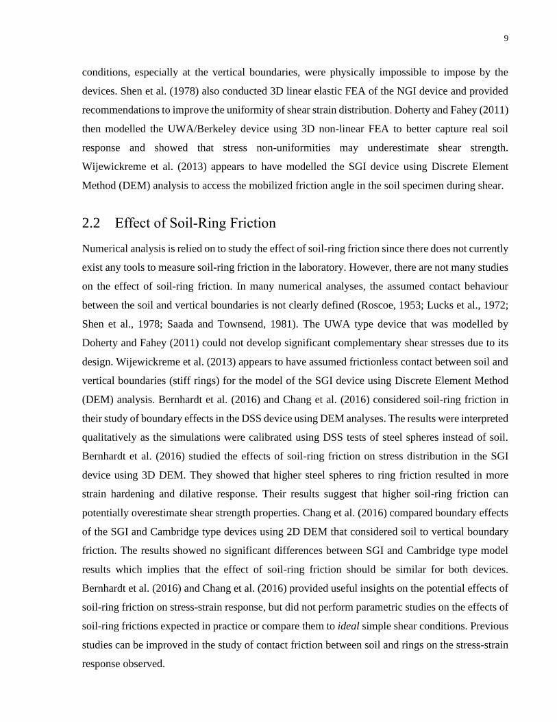
2.2 Effect of Soil-Ring Friction
Numerical analysis is relied on to study the effect of soil-ring friction since there does not currently
exist any tools to measure soil-ring friction in the laboratory. However, there are not many studies
on the effect of soil-ring friction. In many numerical analyses, the assumed contact behaviour
between the soil and vertical boundaries is not clearly defined (Roscoe, 1953; Lucks et al., 1972;
Shen et al., 1978; Saada and Townsend, 1981). The UWA type device that was modelled by
Doherty and Fahey (2011) could not develop significant complementary shear stresses due to its
design. Wijewickreme et al. (2013) appears to have assumed frictionless contact between soil and
vertical boundaries (stiff rings) for the model of the SGI device using Discrete Element Method
(DEM) analysis. Bernhardt et al. (2016) and Chang et al. (2016) considered soil-ring friction in
their study of boundary effects in the DSS device using DEM analyses. The results were interpreted
qualitatively as the simulations were calibrated using DSS tests of steel spheres instead of soil.
Bernhardt et al. (2016) studied the effects of soil-ring friction on stress distribution in the SGI
device using 3D DEM. They showed that higher steel spheres to ring friction resulted in more
strain hardening and dilative response. Their results suggest that higher soil-ring friction can
potentially overestimate shear strength properties. Chang et al. (2016) compared boundary effects
of the SGI and Cambridge type devices using 2D DEM that considered soil to vertical boundary
friction. The results showed no significant differences between SGI and Cambridge type model
results which implies that the effect of soil-ring friction should be similar for both devices.
Bernhardt et al. (2016) and Chang et al. (2016) provided useful insights on the potential effects of
soil-ring friction on stress-strain response, but did not perform parametric studies on the effects of
soil-ring frictions expected in practice or compare them to ideal simple shear conditions. Previous
studies can be improved in the study of contact friction between soil and rings on the stress-strain
response observed.
10
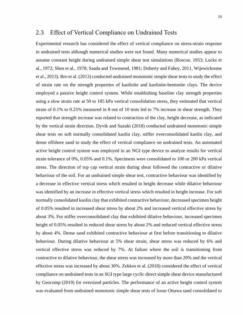
2.3 Effect of Vertical Compliance on Undrained Tests
Experimental research has considered the effect of vertical compliance on stress-strain response
in undrained tests although numerical studies were not found. Many numerical studies appear to
assume constant height during undrained simple shear test simulations (Roscoe, 1953; Lucks et
al., 1972; Shen et al., 1978; Saada and Townsend, 1981; Doherty and Fahey, 2011, Wijewickreme
et al., 2013). Bro et al. (2013) conducted undrained monotonic simple shear tests to study the effect
of strain rate on the strength properties of kaolinite and kaolinite-bentonite clays. The device
employed a passive height control system. While establishing baseline clay strength properties
using a slow strain rate at 50 to 185 kPa vertical consolidation stress, they estimated that vertical
strain of 0.1% to 0.25% measured in 8 out of 10 tests led to 7% increase in shear strength. They
reported that strength increase was related to contraction of the clay, height decrease, as indicated
by the vertical strain direction. Dyvik and Suzuki (2018) conducted undrained monotonic simple
shear tests on soft normally consolidated kaolin clay, stiffer overconsolidated kaolin clay, and
dense offshore sand to study the effect of vertical compliance on undrained tests. An automated
active height control system was employed in an NGI type device to analyze results for vertical
strain tolerance of 0%, 0.05% and 0.1%. Specimens were consolidated to 100 or 200 kPa vertical
stress. The direction of top cap vertical strain during shear followed the contractive or dilative
behaviour of the soil. For an undrained simple shear test, contractive behaviour was identified by
a decrease in effective vertical stress which resulted in height decrease while dilative behaviour
was identified by an increase in effective vertical stress which resulted in height increase. For soft
normally consolidated kaolin clay that exhibited contractive behaviour, decreased specimen height
of 0.05% resulted in increased shear stress by about 2% and increased vertical effective stress by
about 3%. For stiffer overconsolidated clay that exhibited dilative behaviour, increased specimen
height of 0.05% resulted in reduced shear stress by about 2% and reduced vertical effective stress
by about 4%. Dense sand exhibited contractive behaviour at first before transitioning to dilative
behaviour. During dilative behaviour at 5% shear strain, shear stress was reduced by 6% and
vertical effective stress was reduced by 7%. At failure where the soil is transitioning from
contractive to dilative behaviour, the shear stress was increased by more than 20% and the vertical
effective stress was increased by about 30%. Zekkos et al. (2018) considered the effect of vertical
compliance on undrained tests in an SGI type large cyclic direct simple shear device manufactured
by Geocomp (2019) for oversized particles. The performance of an active height control system
was evaluated from undrained monotonic simple shear tests of loose Ottawa sand consolidated to
11
100 kPa vertical stress and loose pea gravel consolidated to 400 kPa vertical stress. Measured
vertical strain varied between 0 and 0.10%. This study did not account for the height changes
allowed by porous stones, which are expected to be larger than the vertical strains that were
measured, so all data likely exceed the ASTM allowed range, and variations were not as significant
as reported. Although the vertical strain during shear measured on tests of Ottawa sand are below
ASTM D6428-17 tolerance of 0.05%, the peak shear stress varied as much as 15%. It was also
reported that the test of pea gravel with measured vertical strain close to ASTM D6428-17
tolerance of 0.05% showed a difference in peak shear stress of 10%. For these tests, higher vertical
strain was shown to increase peak stress and vertical effective stress. Thus, the effect of vertical
compliance on undrained tests cannot be ignored and may have a significant impact on the stress-
strain response. Numerical simulations were not found that studied the effect of vertical
compliance on undrained tests. Numerical simulations can improve the study on the effect of
vertical compliance on undrained tests since they provide more detail than experimental testing on
stress-strain behaviour throughout the specimen.
2.4 Effect of Top Cap Rocking
Numerical studies were not found that investigated the effect of top cap rocking (rotation) on
stress-strain response. Many numerical studies appear to assume no top cap rotation during simple
shear test simulations (Roscoe, 1953; Lucks et al., 1972; Shen et al., 1978; Saada and Townsend,
1981; Doherty and Fahey, 2011; Wijewickreme et al., 2013; Bernhardt et al., 2016; Chang et al.,
2016). However, minimizing top cap rocking is a concern in the design of simple shear devices
(Ishihara and Yamazaki, 1980; Boulanger et al., 1993; Rutherford, 2012; Kwan et al., 2014;
Shafiee, 2016). Ishihara and Yamazaki (1980) used a multi-directional simple shear device to
conduct cyclic tests on saturated sand specimens obtained from the Fuji riverbed. They mentioned
that during cyclic simple shear tests on specimens consolidated to 200 kPa vertical stress, rocking
motions about the horizontal axis may have induced vertical stress differences near the specimen
edge and caused the measured shear strain to be about 2% larger than the actual shear strain applied
to the specimen. However, they do not appear to measure the amount of top cap rotation or the
effect of top cap rocking on stress distribution. Boulanger et al. (1993) conducted undrained cyclic
simple shear tests on saturated sand to evaluate the performance of the University of California at
Berkeley bi-directional simple shear apparatus (UCB-2D). For vertical consolidation stress of 206
kPa and shear stress amplitude of 41.2 kPa, the measured rotation of the specimen based on the

12
vertical strain at the edges was about 0.006°. They noted that the measured rotation was small but
they did not appear to investigate changes in stress-strain response due to the measured rotation.
Kwan et al. (2014) conducted cyclic simple shear tests on uniform Nevada sand using a modified
GCTS cyclic simple shear device. Four loose specimens of about 40% and four dense specimens
of about 70% were tested at a consolidation vertical stress of 100 kPa. It was reported that top cap
rocking caused a difference in vertical displacement of 0.05 mm between the specimen centre and
edge where the max applied shear strain appeared to be about 10%. Based on the reported specimen
dimensions, rocking caused top cap rotation of about 0.03°. They did not appear to report any
changes in stress-strain response due to the measured rotation. Shafiee (2016) conducted undrained
cyclic strain-controlled simple shear tests on dry sand to evaluate the performance of the
University of California at Los Angeles (UCLA) bi-directional broadband simple shear (BB-SS)
device. From the performance data, it appears that for 4% shear strain amplitude and 100 kPa
consolidation vertical stress the maximum rotation angle is about 0.07°. They noted that top cap
rocking caused small vertical strain during shear in comparison to the total average vertical strain
during the tests and did not appear to investigate changes in stress-strain response due to the
measured rotation. These studies provide a range of top cap rotation expected for DSS tests, but
they did not conduct a parametric study on the effect of top cap rocking on stress-strain response.
Higher top cap rotation may induce stress concentrations near the specimen edges. Thus, the effect
of top cap rocking on stress-strain behaviour during the DSS test has not been well studied even
though top cap rocking has been measured during some experimental tests. Numerical studies can
simulate top cap rocking to investigate the effect on stress-strain behaviour for the expected top
cap rotation based on experimental data.
2.5 Summary
Numerical and experimental studies are available in the literature to study the effects of
imperfect boundary conditions on the direct simple shear test. These studies demonstrate that
imperfect boundary conditions develop stress non-uniformities that may cause unreliable stress
and strain measurements. However, the effects of soil-ring friction, vertical compliance on
undrained tests and top cap rocking during shear have not been well studied. Experimental
studies on the effect of vertical compliance on undrained tests suggest that vertical strain induces
unwanted volume change during the shearing phase that can increase shear and vertical stress
during contractive soil behaviour or reduce shear and vertical stress during dilative soil

13
behaviour. Numerical studies are not found that investigate the effect of vertical compliance on
undrained tests. The effect of top cap rocking on stress-strain response has not been studied
although top cap rocking has been measured in some direct simple shear tests. Numerical
analyses that consider imperfect boundary conditions provide information and insights that are
difficult to achieve using experimental studies alone. Thus, the study on the effect of imperfect
boundary conditions in the direct simple shear test can be improved through numerical
simulation of the direct simple shear test.

14
Chapter 3
Numerical Analysis of Direct Simple Shear Test
Boundary Conditions
3.1 Introduction
A numerical study was conducted using three-dimensional (3D) finite element analysis (FEA) to
investigate the effect of imperfect boundary conditions in undrained direct simple shear tests on
stress-strain behaviour. The study investigates the effect of soil-ring friction, vertical compliance
on undrained tests and top cap rocking during shear.
3.2 Soil Constitutive Model
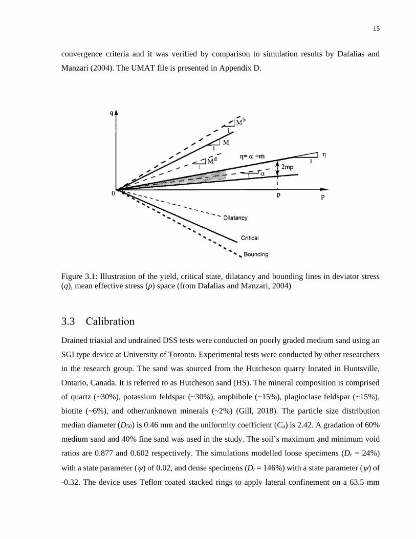
Soil stress-strain behaviour is captured using the Dafalias and Manzari (2004) constitutive model.
The bounding surface model primarily captures sand plasticity due to changes in stress ratio ()
which occur continuously during simple shear tests. Figure 3.1 shows the triaxial space
representation of the formulation. The model uses a thin, open-ended wedge yield surface fixed at
the origin. The model incorporates a rotational hardening parameter () to model sand plasticity
behaviour. The size of the wedge is based on a thickness parameter (m) and defines the region of
elastic behaviour. The thin wedge and rotational hardening parameter are ideal for capturing sand
plasticity during load reversal, such as during cyclic shear loading. The model requires fifteen
parameters that can be categorized according to their use in equations of elasticity, critical state,
yield surface, plastic modulus, dilatancy and fabric-dilatancy. Masin et al. (2018) implemented the
Dafalias and Manzari (2004) model in a user-defined material model (UMAT) file that can be used
in ABAQUS simulations. The UMAT file is publicly available from the database of the
SoilModels project, previously known as the soilmodels.info project, founded by
Gudehus et al. (2008). The UMAT’s numerical stability was improved by adjustments to the
15
convergence criteria and it was verified by comparison to simulation results by Dafalias and
Manzari (2004). The UMAT file is presented in Appendix D.
Figure 3.1: Illustration of the yield, critical state, dilatancy and bounding lines in deviator stress
(q), mean effective stress (p) space (from Dafalias and Manzari, 2004)
3.3 Calibration
Drained triaxial and undrained DSS tests were conducted on poorly graded medium sand using an
SGI type device at University of Toronto. Experimental tests were conducted by other researchers
in the research group. The sand was sourced from the Hutcheson quarry located in Huntsville,
Ontario, Canada. It is referred to as Hutcheson sand (HS). The mineral composition is comprised
of quartz (~30%), potassium feldspar (~30%), amphibole (~15%), plagioclase feldspar (~15%),
biotite (~6%), and other/unknown minerals (~2%) (Gill, 2018). The particle size distribution
median diameter (D50) is 0.46 mm and the uniformity coefficient (Cu) is 2.42. A gradation of 60%
medium sand and 40% fine sand was used in the study. The soil’s maximum and minimum void
ratios are 0.877 and 0.602 respectively. The simulations modelled loose specimens (Dr = 24%)
with a state parameter () of 0.02, and dense specimens (Dr = 146%) with a state parameter () of
0.32. The device uses Teflon coated stacked rings to apply lateral confinement on a 63.5 mm

16
diameter by approximately 20 mm height cylindrical soil sample that is encased in a rubber
membrane. Teflon is a friction reducer that minimizes friction among the rings.
The soil constitutive model was calibrated using experimental data by simulating a single element
model under ideal simple shear conditions which is explained in detail later. Interpretation of
drained triaxial tests established an initial set of parameters using the approach by Taiebat and
Dafalias (2008). Parameters were then adjusted based on undrained monotonic and cyclic simple
shear tests. Initial and adjusted parameters are presented in Table 3.1.
Table 3.1. Dafalias and Manzari (2004) model calibrated parameters
Parameter Type Variable1 Value from
Triaxial Data
Value from Simple
Shear Data
Elasticity Go 75 30
0.2 0.2
Critical state Mtc 1.23 1.23
c 0.715 0.715
c 0.023 0.023
e0 0.81 0.81
0.7 0.7
Yield surface m 0.01 0.01
Plastic modulus h0 8.5 8.5
ch 0.7 0.7
nb 7.0 1.0
Dilatancy A0 0.75 0.34
nd 3.2 3.2
Fabric-dilatancy tensor zmax 4.0 4.0
cz 600 600 1Variables (unit-less) defined by Dafalias and Manzari (2004).
Calibrated undrained monotonic and cyclic simple shear simulation results are presented in
Appendix A from Figure A.1 to Figure A.9. Select results are presented here. Figure 3.2 presents
the (a) shear stress vs. strain and (b) stress path plots for a sample calibrated undrained monotonic
simple shear test. The critical state line (CSL) with the constant volume friction angle ('cv) is also
plotted with the stress path. Figure 3.3 presents plots of (a) shear stress vs. number of cycles, (b)
shear strain vs. number of cycles, (c) vertical stress vs. number of cycles, (d) shear stress vs shear
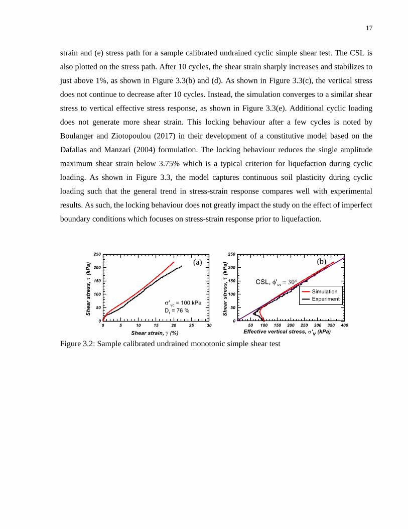
17
strain and (e) stress path for a sample calibrated undrained cyclic simple shear test. The CSL is
also plotted on the stress path. After 10 cycles, the shear strain sharply increases and stabilizes to
just above 1%, as shown in Figure 3.3(b) and (d). As shown in Figure 3.3(c), the vertical stress
does not continue to decrease after 10 cycles. Instead, the simulation converges to a similar shear
stress to vertical effective stress response, as shown in Figure 3.3(e). Additional cyclic loading
does not generate more shear strain. This locking behaviour after a few cycles is noted by
Boulanger and Ziotopoulou (2017) in their development of a constitutive model based on the
Dafalias and Manzari (2004) formulation. The locking behaviour reduces the single amplitude
maximum shear strain below 3.75% which is a typical criterion for liquefaction during cyclic
loading. As shown in Figure 3.3, the model captures continuous soil plasticity during cyclic
loading such that the general trend in stress-strain response compares well with experimental
results. As such, the locking behaviour does not greatly impact the study on the effect of imperfect
boundary conditions which focuses on stress-strain response prior to liquefaction.
Figure 3.2: Sample calibrated undrained monotonic simple shear test
(a) (b)

18
Figure 3.3: Sample calibrated undrained cyclic simple shear test
The liquefaction criterion was modified to compensate for the locking behaviour. Figure 3.4
presents the plot for cyclic stress ratio (CSR) vs. the number of cycles to liquefaction where the
single amplitude shear strain at which liquefaction occurs was changed from 3.75% to 1%.
Experimental and simulation results to generate this plot are presented in Appendix A from
Figure A.1 to Figure A.25. The cyclic stress ratio (CSR) is the ratio of shear stress to consolidation
vertical stress. As shown in Figure 3.4, experimental results compare well for single amplitude
shear strain liquefaction criteria of 3.75% and 1%. Additionally, the experimental and simulation
results compare well. As such, liquefaction in this study was defined as a single amplitude shear
strain of 1% which corresponds to the approximate maximum shear strain when locking occurs. It
should be noted that the simulations are less sensitive to changes in CSR than is observed from
experimental data, as shown in Figure 3.4. However, the effect of CSR on stress-strain response is
not included in the scope of this study and the locking behaviour described earlier does not impact
(a)
(b)
(c)
(d)
(e)

19
the study as the influence of boundary conditions appears to dominate early cycles as demonstrated
later. As such, the calibrated Dafalias and Manzari (2004) model is sufficient for modelling soil
behaviour to study the effects of imperfect boundary conditions on the stress strain-response.
Figure 3.4: Cyclic stress ratio (CSR) vs. number of cycles to liquefaction for soil relative density
(Dr) of 77% and liquefaction criterion defined by single amplitude shear strain (Liq)
3.4 Finite Element Model
3.4.1 Geometry
The simulations modelled a typical 63.5 mm diameter by 20 mm height soil specimen using the
finite element analysis software (FEA) package ABAQUS (Dassault Systèmes, 2012). The
cylindrical specimen was subjected to unidirectional simple shear loading which resulted in
symmetric stress-strain distribution with respect to a vertical cut at the centre that is parallel to the
shearing direction. The half-cylinder model that is shown in Figure 3.5 took advantage of
symmetry in geometry and loads to improve computation speed by reducing the required number
of elements. 20 rigid rings of 1 mm height around the specimen maintained constant diameter. The
mesh consisted of 5820 8-noded linear isoparametric soil elements, 1600 4-noded rigid plate
elements for the rings, and a mix of 2526 4-noded and 3-noded rigid plate elements for the top
cap.

20
Figure 3.5: Finite element model of the DSS test
3.4.2 Soil-Ring Interaction
Each ring moves due to soil movement as a rigid body. A linear friction model captures the contact
behaviour between the soil and the rings, as shown in Equations 1 and 2. The contact frictional
stress (soil-ring) is based on the normal contact pressure (soil-ring) and the soil-ring friction angle
(soil-ring). The contact pressure is computed by the soil-ring normal stiffness (ksoil-ring,n) and
compression of soil against the ring (dsoil-ring).
soil-ring = soil-ring tan(soil-ring) [1]
soil-ring = ksoil-ring,n dsoil-ring [2]
ABAQUS automatically assigns the soil-ring normal stiffness to be much larger than the adjacent
soil element stiffness and employs the Augmented Lagrange method to ensure each ring acts as a
rigid boundary that displaces horizontally during shear loading (Dassault Systèmes, 2012).
3.4.3 Top Cap
Each plate that defines the top cap moves due to applied loads or soil movement as rigid bodies.
As shown in Figure 3.5, the two plates that define the top cap are connected by springs which can
be adjusted to control the allowed vertical strain, vertical compliance, and rotation, rocking, during
the shearing phase. A linear contact pressure model captures the contact behaviour between the
soil and top cap (bottom plate). It was assumed that the top cap would not slip horizontally along
Top face
Front face
Bottom face
Rings Bottom centre,
(x, y, z) = (0,0,0)
Vertical stress
Shear stress
Top cap &
Springs
21
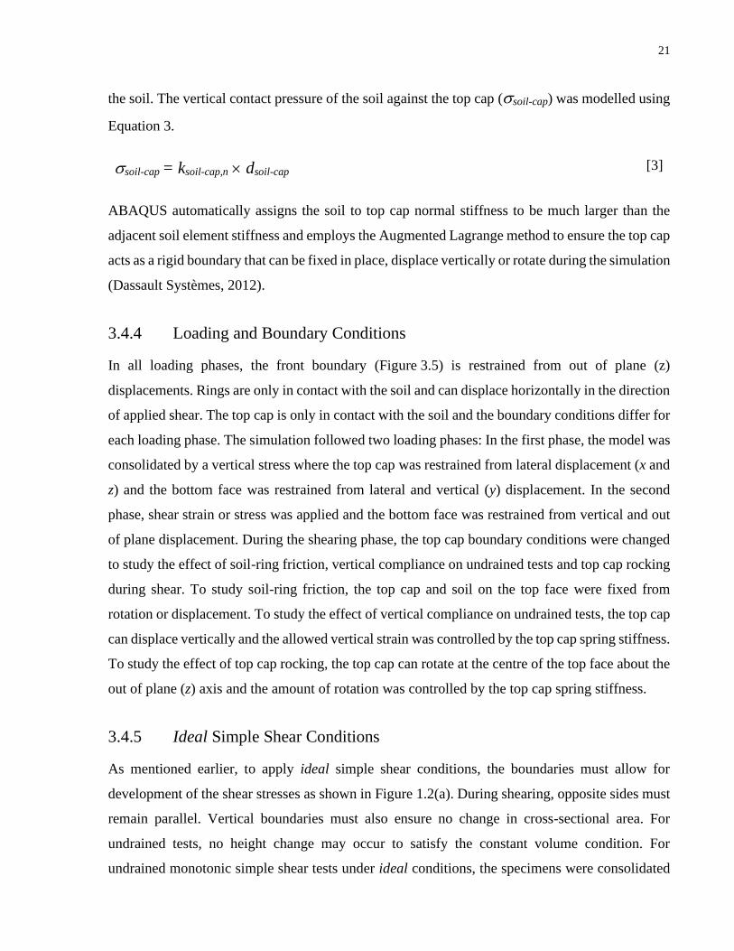
the soil. The vertical contact pressure of the soil against the top cap (soil-cap) was modelled using
Equation 3.
soil-cap = ksoil-cap,n dsoil-cap [3]
ABAQUS automatically assigns the soil to top cap normal stiffness to be much larger than the
adjacent soil element stiffness and employs the Augmented Lagrange method to ensure the top cap
acts as a rigid boundary that can be fixed in place, displace vertically or rotate during the simulation
(Dassault Systèmes, 2012).
3.4.4 Loading and Boundary Conditions
In all loading phases, the front boundary (Figure 3.5) is restrained from out of plane (z)
displacements. Rings are only in contact with the soil and can displace horizontally in the direction
of applied shear. The top cap is only in contact with the soil and the boundary conditions differ for
each loading phase. The simulation followed two loading phases: In the first phase, the model was
consolidated by a vertical stress where the top cap was restrained from lateral displacement (x and
z) and the bottom face was restrained from lateral and vertical (y) displacement. In the second
phase, shear strain or stress was applied and the bottom face was restrained from vertical and out
of plane displacement. During the shearing phase, the top cap boundary conditions were changed
to study the effect of soil-ring friction, vertical compliance on undrained tests and top cap rocking
during shear. To study soil-ring friction, the top cap and soil on the top face were fixed from
rotation or displacement. To study the effect of vertical compliance on undrained tests, the top cap
can displace vertically and the allowed vertical strain was controlled by the top cap spring stiffness.
To study the effect of top cap rocking, the top cap can rotate at the centre of the top face about the
out of plane (z) axis and the amount of rotation was controlled by the top cap spring stiffness.
3.4.5 Ideal Simple Shear Conditions
As mentioned earlier, to apply ideal simple shear conditions, the boundaries must allow for
development of the shear stresses as shown in Figure 1.2(a). During shearing, opposite sides must
remain parallel. Vertical boundaries must also ensure no change in cross-sectional area. For
undrained tests, no height change may occur to satisfy the constant volume condition. For
undrained monotonic simple shear tests under ideal conditions, the specimens were consolidated

22
by a vertical stress constraining lateral strains. Then shear loading was applied constraining all
strains except shear in the direction of loading.
Ideal simple shear conditions were achieved using two methods: The first method used a single
element model which assumes perfect simple shear conditions. Simulations were conducted using
a single element testing software “Incremental Driver” (Niemunis, 2017). The Incremental
Driver’s simplicity allows it to be more computationally efficient than ABAQUS for single
element models under ideal simple shear conditions. The second method works by applying
different soil-ring friction angles during each loading phase of the multi-element SGI type stacked
ring simulation in ABAQUS that is shown in Figure 3.5. Frictionless boundaries were set during
the consolidation phase to ensure uniformly distributed stresses. Conversely, no slip conditions
were set during the shearing phase to develop the necessary complementary shear stresses for ideal
simple shear conditions. The two models produced practically identical results, so the single
element model was used to produce ideal simple shear condition due to its efficiency. The single
element model was also used for model calibration.
3.4.6 Mesh sensitivity analysis
Mesh sensitivity was analyzed by computing simulations using various element sizes (ES) and
meshing pattern. The ES is an approximate length of each element. As shown in Figure 3.6, the
analysis considered uniform meshes of 8-noded isoparametric linear soil elements with ES of (a)
8 mm, (b) 4 mm, and (e) 1 mm, as well as graded meshes with (c) 8-noded linear, and (d) 20-noded
quadratic isoparametric soil elements. The graded meshes begin at an ES of 2 mm at the vertical
boundary and gradually increases to 5 mm at the specimen centre. Smaller elements capture the
expected stress concentrations near the vertical boundaries due to the lack of complementary shear
stresses, while larger elements are sufficient in capturing more uniform stress distribution that is
expected near the centre. The height of elements is restricted to the height of a ring which is 1 mm.
In general, 20-noded quadratic elements perform better than 8-noded linear elements in capturing
highly non-linear stress-strain distribution but require more computation time. In many cases, 8-
noded linear elements are sufficient for capturing the average stress-strain response and
understanding the regions of stress or strain concentrations.

23
Figure 3.6: Specimen mesh densities that were analyzed in the mesh sensitivity analysis
The average stress-strain response and the stress distribution were analyzed to evaluate the quality
of the mesh for this study. Figure 3.7 and Figure 3.8 presents the plots of (a) stress path and (b)
shear stress distribution for undrained monotonic and cyclic simulations of loose specimens (Dr =
24%). The monotonic test was sheared until the peak shear stress was reached which was
approximately 4% shear strain. The simulation with graded mesh of 20-noded elements did not
converge after 3.5% shear strain due to high stress concentrations. The cyclic test was sheared for
one cycle as subsequent cycles had similar stress-strain response. The shear stress distribution plot
is based on the average stress of elements along the top of the specimen at the centre cross section.
The critical state line (CSL) with the constant volume friction angle ('cv) is also plotted with the
stress paths when applicable. The simulations assumed frictionless vertical boundaries, constant
height and no top cap rocking. Figure 3.7(a) and Figure 3.8(a) shows that the stress path is not
sensitive to the tested mesh densities. However, Figure 3.7(b) and Figure 3.8(b) show that the
graded mesh (ES = 2 to 5 mm) or uniform mesh of 1 mm ES performs better in capturing the stress
concentrations near the vertical boundaries. The simulation with graded mesh of 20-noded
elements shows much higher stress concentrations than other simulations near the vertical
boundaries which may have contributed to non-convergence before the target 4% shear strain.
Similar findings were observed in dense specimen (Dr = 146%) simulations which are presented
in Appendix B Figure B.2 and Figure B.4. As shown in Table 3.2, for loose (Dr = 24%) and dense
(Dr = 146%) specimen simulations, the computation time sharply increases when using the graded
mesh (ES = 2 to 5 mm) with 20-noded elements or the uniform mesh of 1 mm ES with 8-noded
elements. To ensure the chosen mesh is sufficient for all analysis in this study, the mesh sensitivity
analysis was also carried out for high soil-ring friction, high vertical strain during undrained tests
(e) ES = 8, Uniform 8-noded linear elements
(c) ES = 2 to 5 mm, Graded 8-noded linear elements
(d) ES = 2 to 5 mm, Graded
20-noded quadratic elements
(a) ES = 8 mm, Uniform
8-noded linear elements
(b) ES = 4 mm, Uniform 8-noded linear elements

24
and high top cap rotation during shear. The stress path plots are presented in Appendix B from
Figure B.5 to Figure B.10. The stress path is not sensitive to the tested mesh densities. As such,
the graded mesh (ES = 2 to 5 mm) with 8-noded elements was selected for the study since the
stress non-uniformities and average stress response were reasonably captured with less
computation time when compared to 20-noded elements or a denser mesh. The chosen graded
mesh is presented in Figure 3.6(c) and the results from using this mesh are shown in green in the
Figure 3.7 and Figure 3.8.
Figure 3.7: Undrained monotonic test results of loose specimen (Dr = 24%) varying element size
(ES) and element type for frictionless vertical boundaries, constant height and no top cap rocking
Figure 3.8: Undrained cyclic test results of loose specimen (Dr = 24%) varying element size (ES)
and element type for frictionless vertical boundaries, constant height and no top cap rocking
(a) Stress path
(b) Top (y = 19.5 mm) along
centre cross section (z = 0 mm)
at peak shear stress
(a) Stress path
(b) Top (y = 19.5 mm) along
centre cross section (z = 0 mm)
at peak of load reversal
25
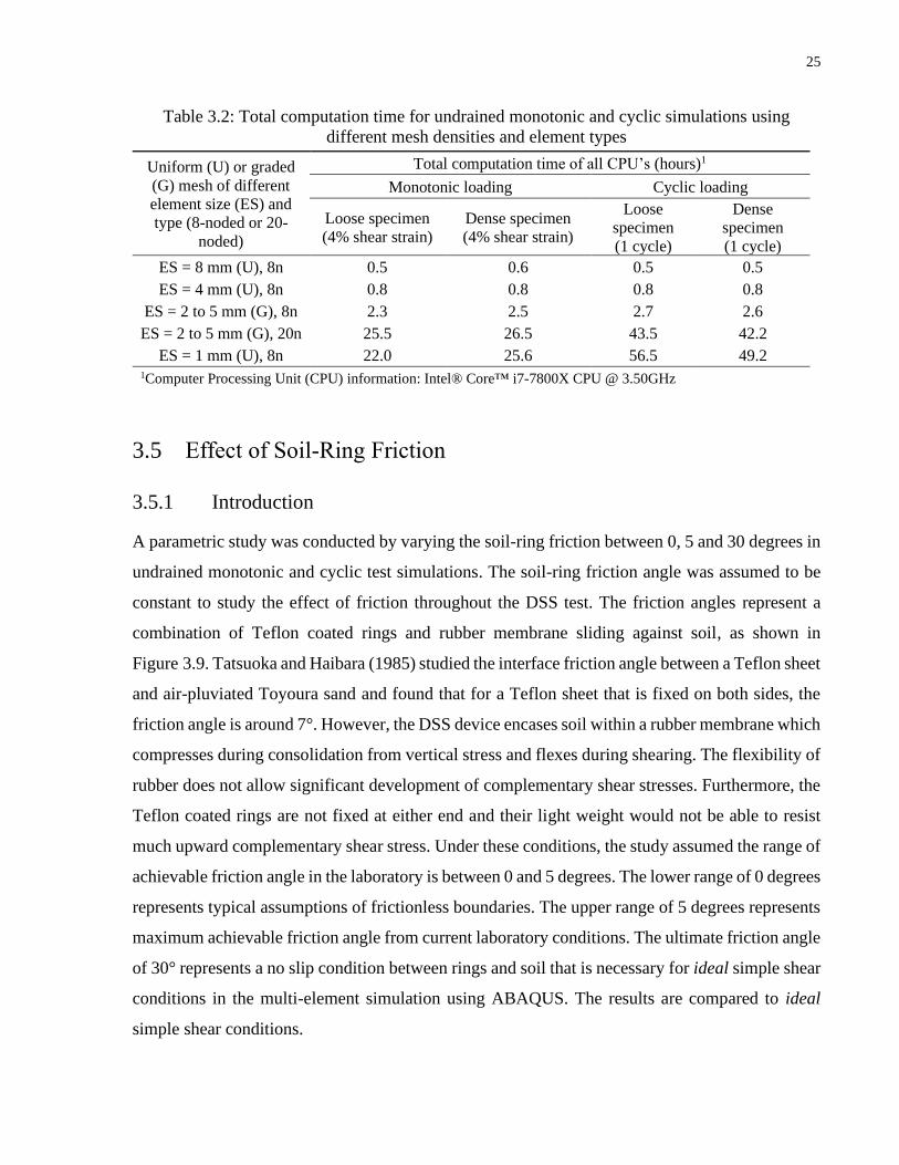
Table 3.2: Total computation time for undrained monotonic and cyclic simulations using
different mesh densities and element types
Uniform (U) or graded
(G) mesh of different
element size (ES) and
type (8-noded or 20-
noded)
Total computation time of all CPU’s (hours)1
Monotonic loading Cyclic loading
Loose specimen
(4% shear strain)
Dense specimen
(4% shear strain)
Loose
specimen
(1 cycle)
Dense
specimen
(1 cycle)
ES = 8 mm (U), 8n 0.5 0.6 0.5 0.5
ES = 4 mm (U), 8n 0.8 0.8 0.8 0.8
ES = 2 to 5 mm (G), 8n 2.3 2.5 2.7 2.6
ES = 2 to 5 mm (G), 20n 25.5 26.5 43.5 42.2
ES = 1 mm (U), 8n 22.0 25.6 56.5 49.2 1Computer Processing Unit (CPU) information: Intel® Core™ i7-7800X CPU @ 3.50GHz
3.5 Effect of Soil-Ring Friction
3.5.1 Introduction
A parametric study was conducted by varying the soil-ring friction between 0, 5 and 30 degrees in
undrained monotonic and cyclic test simulations. The soil-ring friction angle was assumed to be
constant to study the effect of friction throughout the DSS test. The friction angles represent a
combination of Teflon coated rings and rubber membrane sliding against soil, as shown in
Figure 3.9. Tatsuoka and Haibara (1985) studied the interface friction angle between a Teflon sheet
and air-pluviated Toyoura sand and found that for a Teflon sheet that is fixed on both sides, the
friction angle is around 7°. However, the DSS device encases soil within a rubber membrane which
compresses during consolidation from vertical stress and flexes during shearing. The flexibility of
rubber does not allow significant development of complementary shear stresses. Furthermore, the
Teflon coated rings are not fixed at either end and their light weight would not be able to resist
much upward complementary shear stress. Under these conditions, the study assumed the range of
achievable friction angle in the laboratory is between 0 and 5 degrees. The lower range of 0 degrees
represents typical assumptions of frictionless boundaries. The upper range of 5 degrees represents
maximum achievable friction angle from current laboratory conditions. The ultimate friction angle
of 30° represents a no slip condition between rings and soil that is necessary for ideal simple shear
conditions in the multi-element simulation using ABAQUS. The results are compared to ideal
simple shear conditions.

26
Figure 3.9: Friction on a soil specimen that is encased in a rubber membrane and is confined by
Teflon coated rings
3.5.2 Results and Discussion
3.5.2.1 Consolidation
The soil specimen was consolidated to 100 kPa vertical stress (’vc). Only the loose specimen
(Dr = 24%) results are presented here and all results, including those of dense specimens
(Dr = 146%) are presented in Appendix C from Figure C.1 to Figure C.4.
Soil-ring friction affects stress non-uniformities that develop during the consolidation phase.
Figure 3.10 presents the shear and vertical stress distribution of loose specimen simulations based
on the average stress of the elements along the top and sides of the specimen at the centre cross
section. As shown in Figure 3.10(a) and (b), higher soil-ring friction increases shear stresses near
the boundaries. As a result, vertical stress concentrations develop at the top and bottom edges, as
shown in Figure 3.10(c) and Figure 3.11, to maintain uniform axial displacement that is imposed
by the stiff top cap and bottom pedestal. Near the middle, shear stresses are zero and vertical
stresses are uniformly distributed as shown in Figure 3.10(a) and (c). Since the average vertical
stress over the top area must equal the 100 kPa stress that is applied, higher vertical stress
concentrations at the top edges decreases the vertical stress of the top middle area as shown in
Figure 3.10(c). For frictionless vertical boundaries (0°), vertical stress is 100 kPa throughout the
specimen. The same observations on stress non-uniformities are also found in dense specimen
simulations as shown in Appendix C.
Rubber membrane
Teflon coated rings
Soil specimen Membrane to ring
friction
Soil to membrane
friction

27
Figure 3.10: End of consolidation stress distribution of loose specimen (Dr = 24%) simulations for
the centre cross section of the specimen (z = 0 mm), varying soil-ring friction angle (soil-ring)
Figure 3.11: End of consolidation vertical effective stress contours of loose specimen (Dr = 24%)
simulation for no slip condition, soil-ring friction angle of 30°
The coefficient of lateral earth pressure (K), ratio of lateral to vertical stress, at the core (centre) of
the multi-element simulations are compared with the ideal simple shear simulation. Figure 3.12
presents the coefficient of lateral earth pressure at the core (centre) of loose specimens during
consolidation. The coefficient of lateral earth pressure at the core compares well with ideal simple
shear conditions for all soil-ring friction. This is shown in Figure 3.12 for loose specimen
simulations, but is also the case for dense specimen simulations as shown in Appendix C. As such,
stress conditions near the specimen core approximate ideal simple shear conditions despite the
stress non-uniformities near the vertical boundaries due to higher soil-ring friction.
(a) Top (y = 19.5 mm) (b) Left (x = -30.75 mm)
Right (x = 30.75 mm)
(c) Top (y = 19.5 mm)
Max = 143 kPa, Min = 36 kPa
Average over top face = 100 kPa

28
Figure 3.12: Coefficient of lateral earth pressure (K) during consolidation at the core of loose
specimen (Dr = 24%) simulations for varying soil-ring friction angles (soil-ring)
3.5.2.2 Undrained Monotonic Simple Shear
Loose (Dr = 24%) and dense (Dr = 146%) specimen simulations were consolidated to 100 kPa
vertical stress (’vc). They were then sheared until the simulations reached non-convergence or
20% shear strain. The multi-element simulations of the loose and dense specimens reached non-
convergence between 4% and 6% shear strain, respectively. Select results are presented here. All
results are presented in Appendix C from Figure C.5 to Figure C.12.
Soil-ring friction affects stress non-uniformities that develop during the shearing phase.
Figure 3.13 presents the shear and vertical stress contours of the loose specimen simulation at 4%
shear strain, which approximates the peak shear stress for frictionless vertical boundaries. As
shown in Figure 3.13(a), the shear stress contours for the simulation with frictionless vertical
boundaries shows near zero shear stresses, blue colour, near the sides. As a result, frictionless
vertical boundaries cannot develop significant complementary shear stresses. Maximum shear
stress and vertical stress are concentrated at the top and bottom edges of the specimen as shown in
Figure 3.13(a) and Figure 3.13(b). Stresses near the centre are uniformly distributed. As shown in
Figure 3.13(a), shear stresses adjacent to the frictionless vertical boundaries quickly go from zero
to the applied shear stress level. Figure 3.14 presents the shear and vertical stress distribution based
on the average stress of elements along the top and sides of the specimen at the centre cross section.
Figure 3.14(b) shows that complementary shear stresses develop immediately adjacent to the
frictionless vertical boundaries which results in a sharp shear stress gradient that transitions to
core
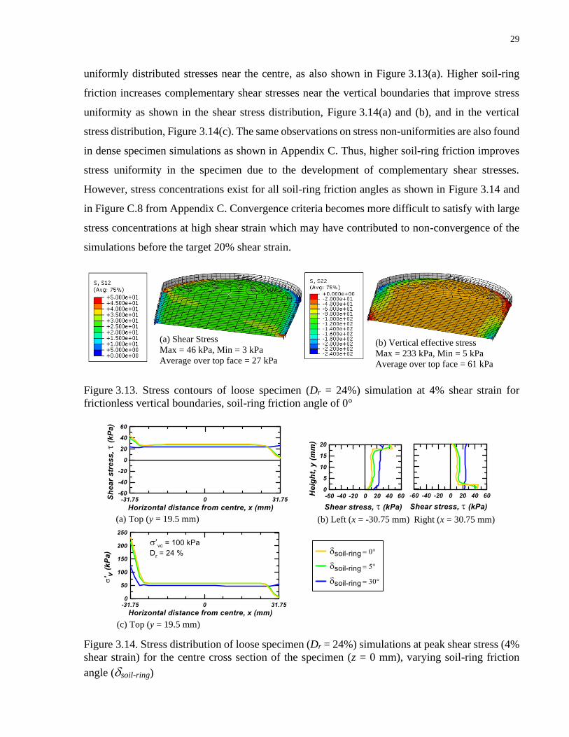
29
uniformly distributed stresses near the centre, as also shown in Figure 3.13(a). Higher soil-ring
friction increases complementary shear stresses near the vertical boundaries that improve stress
uniformity as shown in the shear stress distribution, Figure 3.14(a) and (b), and in the vertical
stress distribution, Figure 3.14(c). The same observations on stress non-uniformities are also found
in dense specimen simulations as shown in Appendix C. Thus, higher soil-ring friction improves
stress uniformity in the specimen due to the development of complementary shear stresses.
However, stress concentrations exist for all soil-ring friction angles as shown in Figure 3.14 and
in Figure C.8 from Appendix C. Convergence criteria becomes more difficult to satisfy with large
stress concentrations at high shear strain which may have contributed to non-convergence of the
simulations before the target 20% shear strain.
Figure 3.13. Stress contours of loose specimen (Dr = 24%) simulation at 4% shear strain for
frictionless vertical boundaries, soil-ring friction angle of 0°
Figure 3.14. Stress distribution of loose specimen (Dr = 24%) simulations at peak shear stress (4%
shear strain) for the centre cross section of the specimen (z = 0 mm), varying soil-ring friction
angle (soil-ring)
(b) Vertical effective stress Max = 233 kPa, Min = 5 kPa
Average over top face = 61 kPa
(a) Shear Stress Max = 46 kPa, Min = 3 kPa
Average over top face = 27 kPa
(a) Top (y = 19.5 mm)
(b) Left (x = -30.75 mm)
Right (x = 30.75 mm)
(c) Top (y = 19.5 mm)
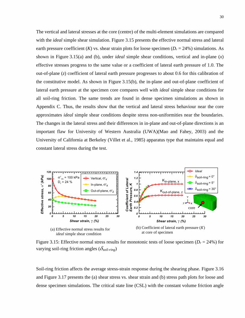
30
The vertical and lateral stresses at the core (centre) of the multi-element simulations are compared
with the ideal simple shear simulation. Figure 3.15 presents the effective normal stress and lateral
earth pressure coefficient (K) vs. shear strain plots for loose specimen (Dr = 24%) simulations. As
shown in Figure 3.15(a) and (b), under ideal simple shear conditions, vertical and in-plane (x)
effective stresses progress to the same value or a coefficient of lateral earth pressure of 1.0. The
out-of-plane (z) coefficient of lateral earth pressure progresses to about 0.6 for this calibration of
the constitutive model. As shown in Figure 3.15(b), the in-plane and out-of-plane coefficient of
lateral earth pressure at the specimen core compares well with ideal simple shear conditions for
all soil-ring friction. The same trends are found in dense specimen simulations as shown in
Appendix C. Thus, the results show that the vertical and lateral stress behaviour near the core
approximates ideal simple shear conditions despite stress non-uniformities near the boundaries.
The changes in the lateral stress and their differences in in-plane and out-of-plane directions is an
important flaw for University of Western Australia (UWA)(Mao and Fahey, 2003) and the
University of California at Berkeley (Villet et al., 1985) apparatus type that maintains equal and
constant lateral stress during the test.
Figure 3.15: Effective normal stress results for monotonic tests of loose specimen (Dr = 24%) for
varying soil-ring friction angles (soil-ring)
Soil-ring friction affects the average stress-strain response during the shearing phase. Figure 3.16
and Figure 3.17 presents the (a) shear stress vs. shear strain and (b) stress path plots for loose and
dense specimen simulations. The critical state line (CSL) with the constant volume friction angle
core
(b) Coefficient of lateral earth pressure (𝐾)
at core of specimen
(a) Effective normal stress results for
ideal simple shear condition
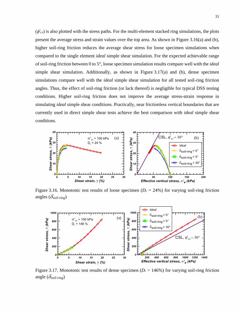
31
('cv) is also plotted with the stress paths. For the multi-element stacked ring simulations, the plots
present the average stress and strain values over the top area. As shown in Figure 3.16(a) and (b),
higher soil-ring friction reduces the average shear stress for loose specimen simulations when
compared to the single element ideal simple shear simulation. For the expected achievable range
of soil-ring friction between 0 to 5°, loose specimen simulation results compare well with the ideal
simple shear simulation. Additionally, as shown in Figure 3.17(a) and (b), dense specimen
simulations compare well with the ideal simple shear simulation for all tested soil-ring friction
angles. Thus, the effect of soil-ring friction (or lack thereof) is negligible for typical DSS testing
conditions. Higher soil-ring friction does not improve the average stress-strain response in
simulating ideal simple shear conditions. Practically, near frictionless vertical boundaries that are
currently used in direct simple shear tests achieve the best comparison with ideal simple shear
conditions.
Figure 3.16. Monotonic test results of loose specimen (Dr = 24%) for varying soil-ring friction
angles (soil-ring)
Figure 3.17. Monotonic test results of dense specimen (Dr = 146%) for varying soil-ring friction
angle (soil-ring)
(a) (b)
(a) (b)
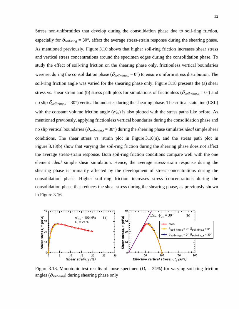
32
Stress non-uniformities that develop during the consolidation phase due to soil-ring friction,
especially for soil-ring = 30°, affect the average stress-strain response during the shearing phase.
As mentioned previously, Figure 3.10 shows that higher soil-ring friction increases shear stress
and vertical stress concentrations around the specimen edges during the consolidation phase. To
study the effect of soil-ring friction on the shearing phase only, frictionless vertical boundaries
were set during the consolidation phase (soil-ring,c = 0°) to ensure uniform stress distribution. The
soil-ring friction angle was varied for the shearing phase only. Figure 3.18 presents the (a) shear
stress vs. shear strain and (b) stress path plots for simulations of frictionless (soil-ring,s = 0°) and
no slip soil-ring,s = 30°) vertical boundaries during the shearing phase. The critical state line (CSL)
with the constant volume friction angle ('cv) is also plotted with the stress paths like before. As
mentioned previously, applying frictionless vertical boundaries during the consolidation phase and
no slip vertical boundaries (soil-ring,s = 30°) during the shearing phase simulates ideal simple shear
conditions. The shear stress vs. strain plot in Figure 3.18(a), and the stress path plot in
Figure 3.18(b) show that varying the soil-ring friction during the shearing phase does not affect
the average stress-strain response. Both soil-ring friction conditions compare well with the one
element ideal simple shear simulation. Hence, the average stress-strain response during the
shearing phase is primarily affected by the development of stress concentrations during the
consolidation phase. Higher soil-ring friction increases stress concentrations during the
consolidation phase that reduces the shear stress during the shearing phase, as previously shown
in Figure 3.16.
Figure 3.18. Monotonic test results of loose specimen (Dr = 24%) for varying soil-ring friction
angles (soil-ring) during shearing phase only
(b) (a)
CSL 'cv
= 30°
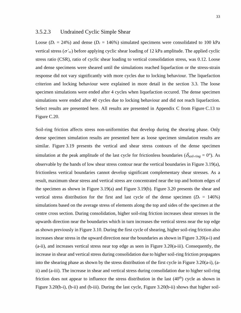
33
3.5.2.3 Undrained Cyclic Simple Shear
Loose (Dr = 24%) and dense (Dr = 146%) simulated specimens were consolidated to 100 kPa
vertical stress (’vc) before applying cyclic shear loading of 12 kPa amplitude. The applied cyclic
stress ratio (CSR), ratio of cyclic shear loading to vertical consolidation stress, was 0.12. Loose
and dense specimens were sheared until the simulations reached liquefaction or the stress-strain
response did not vary significantly with more cycles due to locking behaviour. The liquefaction
criterion and locking behaviour were explained in more detail in the section 3.3. The loose
specimen simulations were ended after 4 cycles when liquefaction occured. The dense specimen
simulations were ended after 40 cycles due to locking behaviour and did not reach liquefaction.
Select results are presented here. All results are presented in Appendix C from Figure C.13 to
Figure C.20.
Soil-ring friction affects stress non-uniformities that develop during the shearing phase. Only
dense specimen simulation results are presented here as loose specimen simulation results are
similar. Figure 3.19 presents the vertical and shear stress contours of the dense specimen
simulation at the peak amplitude of the last cycle for frictionless boundaries (soil-ring = 0°). As
observable by the bands of low shear stress contour near the vertical boundaries in Figure 3.19(a),
frictionless vertical boundaries cannot develop significant complementary shear stresses. As a
result, maximum shear stress and vertical stress are concentrated near the top and bottom edges of
the specimen as shown in Figure 3.19(a) and Figure 3.19(b). Figure 3.20 presents the shear and
vertical stress distribution for the first and last cycle of the dense specimen (Dr = 146%)
simulations based on the average stress of elements along the top and sides of the specimen at the
centre cross section. During consolidation, higher soil-ring friction increases shear stresses in the
upwards direction near the boundaries which in turn increases the vertical stress near the top edge
as shown previously in Figure 3.10. During the first cycle of shearing, higher soil-ring friction also
increases shear stress in the upward direction near the boundaries as shown in Figure 3.20(a-i) and
(a-ii), and increases vertical stress near top edge as seen in Figure 3.20(a-iii). Consequently, the
increase in shear and vertical stress during consolidation due to higher soil-ring friction propagates
into the shearing phase as shown by the stress distribution of the first cycle in Figure 3.20(a-i), (a-
ii) and (a-iii). The increase in shear and vertical stress during consolidation due to higher soil-ring
friction does not appear to influence the stress distribution in the last (40th) cycle as shown in
Figure 3.20(b-i), (b-ii) and (b-iii). During the last cycle, Figure 3.20(b-ii) shows that higher soil-

34
ring friction increases complementary shear stresses near the vertical boundaries that improve
stress uniformity as shown in the shear stress distribution, Figure 3.20(b-i) and Figure 3.20(b-ii),
and in the vertical stress distribution, Figure 3.20(b-iii). Thus, higher soil-ring friction develops
complementary shear stresses that improve stress non-uniformity but are not noticeable until the
stress concentrations that develop during consolidation dissipate with more cycles. Higher soil-
ring friction increases shear and vertical stress concentrations during consolidation that transfer to
the shearing phase. After stress concentrations that develop during consolidation dissipate with
more cycles, the results show that higher soil-ring friction improves stress uniformity in the
specimen due to the development of complementary shear stresses. The same observations are
found in loose specimen simulations, as shown in Figure C.13 from Appendix C. However, for
loose specimen similations, the stress concentrations that develop during consolidation do not fully
dissipate before the simulations end after about 4 cycles due to liquefaction.
Figure 3.19. Stress contours of dense specimen (Dr = 146%) simulation at the peak amplitude of
the last cycle for frictionless vertical boundaries, soil-ring friction angle of 0°
(b) Vertical effective stress Max = 128 kPa, Min = 28 kPa
Average over top face = 54 kPa
(a) Shear Stress Max = 19 kPa, Min = -4 kPa
Average over top face = 13 kPa
35
Figure 3.20. Stress distribution of dense specimen (Dr = 146%) simulations for the centre cross
section of the specimen (z = 0 mm) during the peak amplitude of the (a) first and (b) last cycle for
varying soil-ring friction angles (soil-ring)
The vertical and lateral stresses at the core (centre) of the multi-element simulations are compared
with the ideal simple shear simulation. Figure 3.21 presents the plots of (a) effective normal stress
and (b) lateral earth pressure coefficient (K) vs. number of cycles for dense specimen (Dr = 146%)
simulations. As shown in Figure 3.21(a) and (b), under ideal simple shear conditions vertical and
in-plane (x) stresses progress to the same value or a coefficient of lateral earth pressure of 1.0 .
The out-of-plane (z) coefficient of lateral earth pressure does not vary greatly and progresses to
about 0.5. As shown in Figure 3.21(b), the in-plane and out-of-plane coefficients of lateral earth
pressure at the specimen core (centre) compare well with ideal simple shear conditions for all soil-
ring frictions. The same observations are found in loose specimen simulations as shown in
Appendix C. Thus, despite stress non-uniformities that are caused by higher soil-ring friction,
especially in the first few cycles, the stress behaviour near the core approximates ideal simple
(a-i) Top (y = 20 mm)
(a-ii) Left (x = 0 mm)
Right (x = 63.5 mm)
(a-iii) Top (y = 20 mm)
(b-ii) Left (x = 0 mm)
Right (x = 63.5 mm)
(b-i) Top (y = 20 mm)
(b-iii) Top (y = 20 mm)
(a) Peak amplitude of first cycle (b) Peak amplitude of last cycle
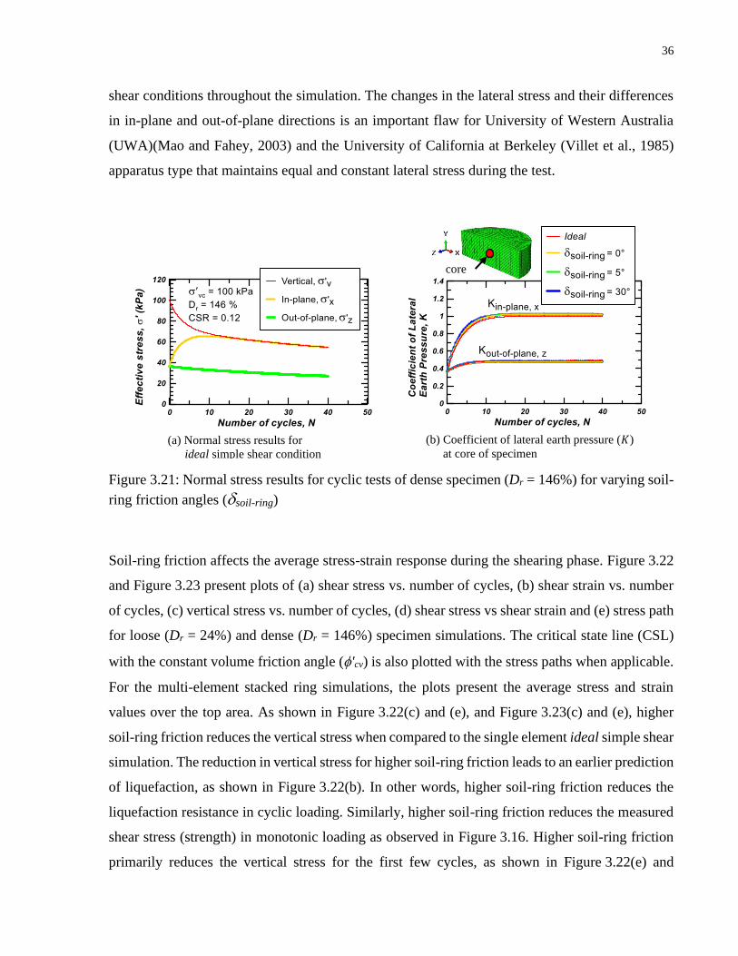
36
shear conditions throughout the simulation. The changes in the lateral stress and their differences
in in-plane and out-of-plane directions is an important flaw for University of Western Australia
(UWA)(Mao and Fahey, 2003) and the University of California at Berkeley (Villet et al., 1985)
apparatus type that maintains equal and constant lateral stress during the test.
Figure 3.21: Normal stress results for cyclic tests of dense specimen (Dr = 146%) for varying soil-
ring friction angles (soil-ring)
Soil-ring friction affects the average stress-strain response during the shearing phase. Figure 3.22
and Figure 3.23 present plots of (a) shear stress vs. number of cycles, (b) shear strain vs. number
of cycles, (c) vertical stress vs. number of cycles, (d) shear stress vs shear strain and (e) stress path
for loose (Dr = 24%) and dense (Dr = 146%) specimen simulations. The critical state line (CSL)
with the constant volume friction angle ('cv) is also plotted with the stress paths when applicable.
For the multi-element stacked ring simulations, the plots present the average stress and strain
values over the top area. As shown in Figure 3.22(c) and (e), and Figure 3.23(c) and (e), higher
soil-ring friction reduces the vertical stress when compared to the single element ideal simple shear
simulation. The reduction in vertical stress for higher soil-ring friction leads to an earlier prediction
of liquefaction, as shown in Figure 3.22(b). In other words, higher soil-ring friction reduces the
liquefaction resistance in cyclic loading. Similarly, higher soil-ring friction reduces the measured
shear stress (strength) in monotonic loading as observed in Figure 3.16. Higher soil-ring friction
primarily reduces the vertical stress for the first few cycles, as shown in Figure 3.22(e) and
(b) Coefficient of lateral earth pressure (𝐾)
at core of specimen
(a) Normal stress results for
ideal simple shear condition
core
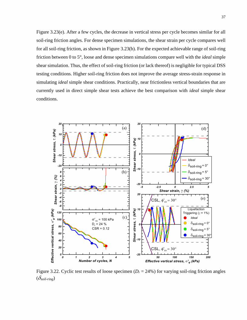
37
Figure 3.23(e). After a few cycles, the decrease in vertical stress per cycle becomes similar for all
soil-ring friction angles. For dense specimen simulations, the shear strain per cycle compares well
for all soil-ring friction, as shown in Figure 3.23(b). For the expected achievable range of soil-ring
friction between 0 to 5°, loose and dense specimen simulations compare well with the ideal simple
shear simulation. Thus, the effect of soil-ring friction (or lack thereof) is negligible for typical DSS
testing conditions. Higher soil-ring friction does not improve the average stress-strain response in
simulating ideal simple shear conditions. Practically, near frictionless vertical boundaries that are
currently used in direct simple shear tests achieve the best comparison with ideal simple shear
conditions.
Figure 3.22. Cyclic test results of loose specimen (Dr = 24%) for varying soil-ring friction angles
(soil-ring)
(a)
(b)
(c)
(d)
(e)
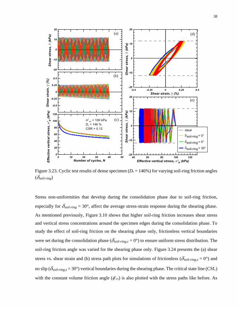
38
Figure 3.23. Cyclic test results of dense specimen (Dr = 146%) for varying soil-ring friction angles
(soil-ring)
Stress non-uniformities that develop during the consolidation phase due to soil-ring friction,
especially for soil-ring = 30°, affect the average stress-strain response during the shearing phase.
As mentioned previously, Figure 3.10 shows that higher soil-ring friction increases shear stress
and vertical stress concentrations around the specimen edges during the consolidation phase. To
study the effect of soil-ring friction on the shearing phase only, frictionless vertical boundaries
were set during the consolidation phase (soil-ring,c = 0°) to ensure uniform stress distribution. The
soil-ring friction angle was varied for the shearing phase only. Figure 3.24 presents the (a) shear
stress vs. shear strain and (b) stress path plots for simulations of frictionless (soil-ring,s = 0°) and
no slip (soil-ring,s = 30°) vertical boundaries during the shearing phase. The critical state line (CSL)
with the constant volume friction angle ('cv) is also plotted with the stress paths like before. As
(a)
(b)
(c)
(d)
(e)

39
mentioned previously, applying frictionless vertical boundaries during the consolidation phase and
no slip vertical boundaries (soil-ring,s = 30°) during the shearing phase simulate ideal simple shear
conditions. The shear strain vs number of cycles plot in Figure 3.24(a), and the stress path plot in
Figure 3.24(b) show that simulation results for both soil-ring friction conditions compare well with
the single element ideal simple shear simulation. The no slip condition shows a slightly smaller
decrease in vertical stress per cycle than the frictionless condition which is due to an increase in
frictional resistance of the vertical boundaries against the contractive behaviour of the soil as
vertical stress decreases. Essentially, transfer of vertical stress from the soil to the top cap is
reduced near the sides due to the increased friction of the vertical boundaries. As shown in
Figure 3.24(b), the no slip vertical boundary condition does not show the large reduction in vertical
stress during the initial cycles as seen in Figure 3.22 when no slip vertical boundaries are used
during both consolidation and shearing phase. Hence, the average stress-strain response during the
shearing phase is primarily affected by the development of stress concentrations during the
consolidation phase. This is also the case with dense specimen simulations as shown in Appendix
C. Higher soil-ring friction increases stress concentrations during the consolidation phase that
reduce the vertical stress during the initial cycles of the shearing phase, as previously shown in
Figure 3.22 and Figure 3.23.
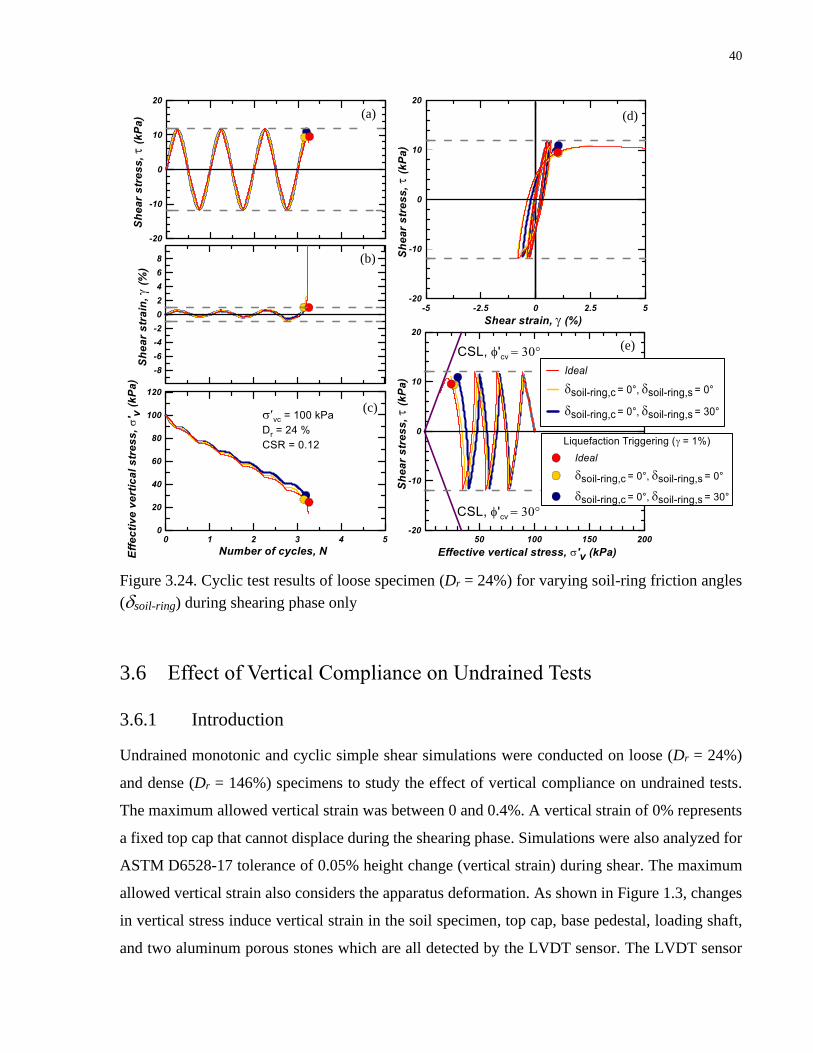
40
Figure 3.24. Cyclic test results of loose specimen (Dr = 24%) for varying soil-ring friction angles
(soil-ring) during shearing phase only
3.6 Effect of Vertical Compliance on Undrained Tests
3.6.1 Introduction
Undrained monotonic and cyclic simple shear simulations were conducted on loose (Dr = 24%)
and dense (Dr = 146%) specimens to study the effect of vertical compliance on undrained tests.
The maximum allowed vertical strain was between 0 and 0.4%. A vertical strain of 0% represents
a fixed top cap that cannot displace during the shearing phase. Simulations were also analyzed for
ASTM D6528-17 tolerance of 0.05% height change (vertical strain) during shear. The maximum
allowed vertical strain also considers the apparatus deformation. As shown in Figure 1.3, changes
in vertical stress induce vertical strain in the soil specimen, top cap, base pedestal, loading shaft,
and two aluminum porous stones which are all detected by the LVDT sensor. The LVDT sensor
(a)
(b)
(c)
(d)
(e)
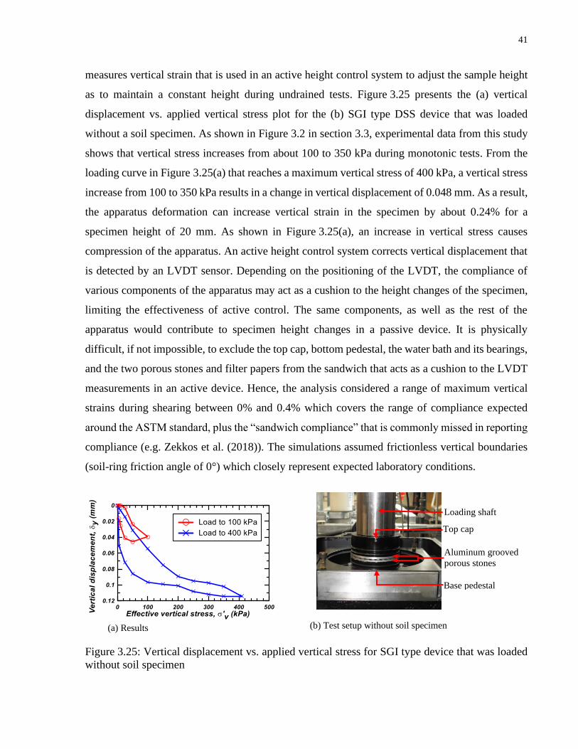
41
measures vertical strain that is used in an active height control system to adjust the sample height
as to maintain a constant height during undrained tests. Figure 3.25 presents the (a) vertical
displacement vs. applied vertical stress plot for the (b) SGI type DSS device that was loaded
without a soil specimen. As shown in Figure 3.2 in section 3.3, experimental data from this study
shows that vertical stress increases from about 100 to 350 kPa during monotonic tests. From the
loading curve in Figure 3.25(a) that reaches a maximum vertical stress of 400 kPa, a vertical stress
increase from 100 to 350 kPa results in a change in vertical displacement of 0.048 mm. As a result,
the apparatus deformation can increase vertical strain in the specimen by about 0.24% for a
specimen height of 20 mm. As shown in Figure 3.25(a), an increase in vertical stress causes
compression of the apparatus. An active height control system corrects vertical displacement that
is detected by an LVDT sensor. Depending on the positioning of the LVDT, the compliance of
various components of the apparatus may act as a cushion to the height changes of the specimen,
limiting the effectiveness of active control. The same components, as well as the rest of the
apparatus would contribute to specimen height changes in a passive device. It is physically
difficult, if not impossible, to exclude the top cap, bottom pedestal, the water bath and its bearings,
and the two porous stones and filter papers from the sandwich that acts as a cushion to the LVDT
measurements in an active device. Hence, the analysis considered a range of maximum vertical
strains during shearing between 0% and 0.4% which covers the range of compliance expected
around the ASTM standard, plus the “sandwich compliance” that is commonly missed in reporting
compliance (e.g. Zekkos et al. (2018)). The simulations assumed frictionless vertical boundaries
(soil-ring friction angle of 0°) which closely represent expected laboratory conditions.
Figure 3.25: Vertical displacement vs. applied vertical stress for SGI type device that was loaded
without soil specimen
(a) Results (b) Test setup without soil specimen
Top cap
Base pedestal
Aluminum grooved
porous stones
Loading shaft
42
3.6.2 Results and Discussion
3.6.2.1 Undrained Monotonic Simple Shear
Loose (Dr = 24%) and dense (Dr = 146%) specimen simulations were consolidated to 100 kPa
vertical stress (’vc). They were then sheared until the simulations reached non-convergence or
20% shear strain. The multi-element simulations of the loose and dense specimens reached non-
convergence between 4% and 13% shear strain. Select results are presented here. All results are
presented in Appendix C from Figure C.21 to Figure C.24.
Vertical compliance of undrained tests does not affect stress non-uniformities. Figure 3.26 presents
the shear and vertical stress distribution at 4% shear strain which approximates the peak shear
stress for loose specimen simulations. The vertical strain distribution along the top nodes of the
specimen is also presented, Figure 3.26(a), and follows a compression positive sign convention.
Stress distributions are based on the average stress of elements along the top of the specimen at
the centre cross section. Figure 3.26(b) and (c) show shear and vertical stress concentrations near
the specimen edges due to frictionless vertical boundaries as previously discussed in section 3.5
on the effect of soil-ring friction. These stress concentrations are also shown in desnse specimen
simulations in Figure C.23 from Appendix C. Convergence criteria becomes more difficult to
satisfy with large stress concentrations at high shear strain which may have contributed to non-
convergence of the simulations before the target 20% shear strain. Higher vertical compliance does
not appear to affect stress concentrations, but does increase the average shear and vertical stress
near the top of the specimen for the loose specimen simulations, as shown in Figure 3.26(b) and
(c), and decrease the average shear and vertical stress near the top of the speciment for dense
specimen simulations, as shown in Figure C.23(b) and (c) in Appendix C. Higher vertical
compliance has negligible effect on shear stresses along the sides, as shown in Figure 3.26(d) and
Figure C.23(d).
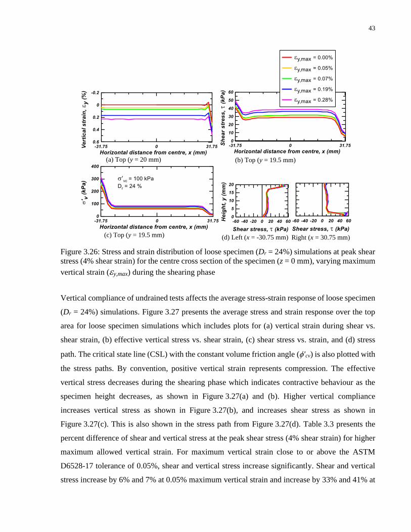
43
Figure 3.26: Stress and strain distribution of loose specimen (Dr = 24%) simulations at peak shear
stress (4% shear strain) for the centre cross section of the specimen (z = 0 mm), varying maximum
vertical strain (y,max) during the shearing phase
Vertical compliance of undrained tests affects the average stress-strain response of loose specimen
(Dr = 24%) simulations. Figure 3.27 presents the average stress and strain response over the top
area for loose specimen simulations which includes plots for (a) vertical strain during shear vs.
shear strain, (b) effective vertical stress vs. shear strain, (c) shear stress vs. strain, and (d) stress
path. The critical state line (CSL) with the constant volume friction angle ('cv) is also plotted with
the stress paths. By convention, positive vertical strain represents compression. The effective
vertical stress decreases during the shearing phase which indicates contractive behaviour as the
specimen height decreases, as shown in Figure 3.27(a) and (b). Higher vertical compliance
increases vertical stress as shown in Figure 3.27(b), and increases shear stress as shown in
Figure 3.27(c). This is also shown in the stress path from Figure 3.27(d). Table 3.3 presents the
percent difference of shear and vertical stress at the peak shear stress (4% shear strain) for higher
maximum allowed vertical strain. For maximum vertical strain close to or above the ASTM
D6528-17 tolerance of 0.05%, shear and vertical stress increase significantly. Shear and vertical
stress increase by 6% and 7% at 0.05% maximum vertical strain and increase by 33% and 41% at
(c) Top (y = 19.5 mm)
(b) Top (y = 19.5 mm)
(d) Left (x = -30.75 mm) Right (x = 30.75 mm)
(a) Top (y = 20 mm)
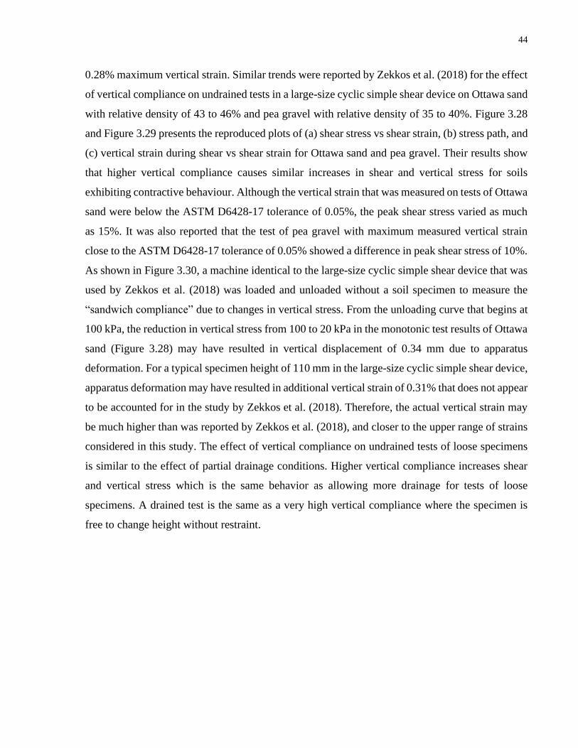
44
0.28% maximum vertical strain. Similar trends were reported by Zekkos et al. (2018) for the effect
of vertical compliance on undrained tests in a large-size cyclic simple shear device on Ottawa sand
with relative density of 43 to 46% and pea gravel with relative density of 35 to 40%. Figure 3.28
and Figure 3.29 presents the reproduced plots of (a) shear stress vs shear strain, (b) stress path, and
(c) vertical strain during shear vs shear strain for Ottawa sand and pea gravel. Their results show
that higher vertical compliance causes similar increases in shear and vertical stress for soils
exhibiting contractive behaviour. Although the vertical strain that was measured on tests of Ottawa
sand were below the ASTM D6428-17 tolerance of 0.05%, the peak shear stress varied as much
as 15%. It was also reported that the test of pea gravel with maximum measured vertical strain
close to the ASTM D6428-17 tolerance of 0.05% showed a difference in peak shear stress of 10%.
As shown in Figure 3.30, a machine identical to the large-size cyclic simple shear device that was
used by Zekkos et al. (2018) was loaded and unloaded without a soil specimen to measure the
“sandwich compliance” due to changes in vertical stress. From the unloading curve that begins at
100 kPa, the reduction in vertical stress from 100 to 20 kPa in the monotonic test results of Ottawa
sand (Figure 3.28) may have resulted in vertical displacement of 0.34 mm due to apparatus
deformation. For a typical specimen height of 110 mm in the large-size cyclic simple shear device,
apparatus deformation may have resulted in additional vertical strain of 0.31% that does not appear
to be accounted for in the study by Zekkos et al. (2018). Therefore, the actual vertical strain may
be much higher than was reported by Zekkos et al. (2018), and closer to the upper range of strains
considered in this study. The effect of vertical compliance on undrained tests of loose specimens
is similar to the effect of partial drainage conditions. Higher vertical compliance increases shear
and vertical stress which is the same behavior as allowing more drainage for tests of loose
specimens. A drained test is the same as a very high vertical compliance where the specimen is
free to change height without restraint.
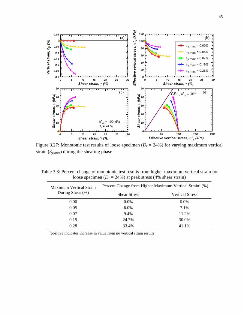
45
Figure 3.27: Monotonic test results of loose specimen (Dr = 24%) for varying maximum vertical
strain (y,max) during the shearing phase
Table 3.3: Percent change of monotonic test results from higher maximum vertical strain for
loose specimen (Dr = 24%) at peak stress (4% shear strain)
Maximum Vertical Strain
During Shear (%)
Percent Change from Higher Maximum Vertical Strain1 (%)
Shear Stress Vertical Stress
0.00 0.0% 0.0%
0.05 6.0% 7.1%
0.07 9.4% 11.2%
0.19 24.7% 30.0%
0.28 33.4% 41.1%
1positive indicates increase in value from no vertical strain results
(a)
(c)
(b)
(d)
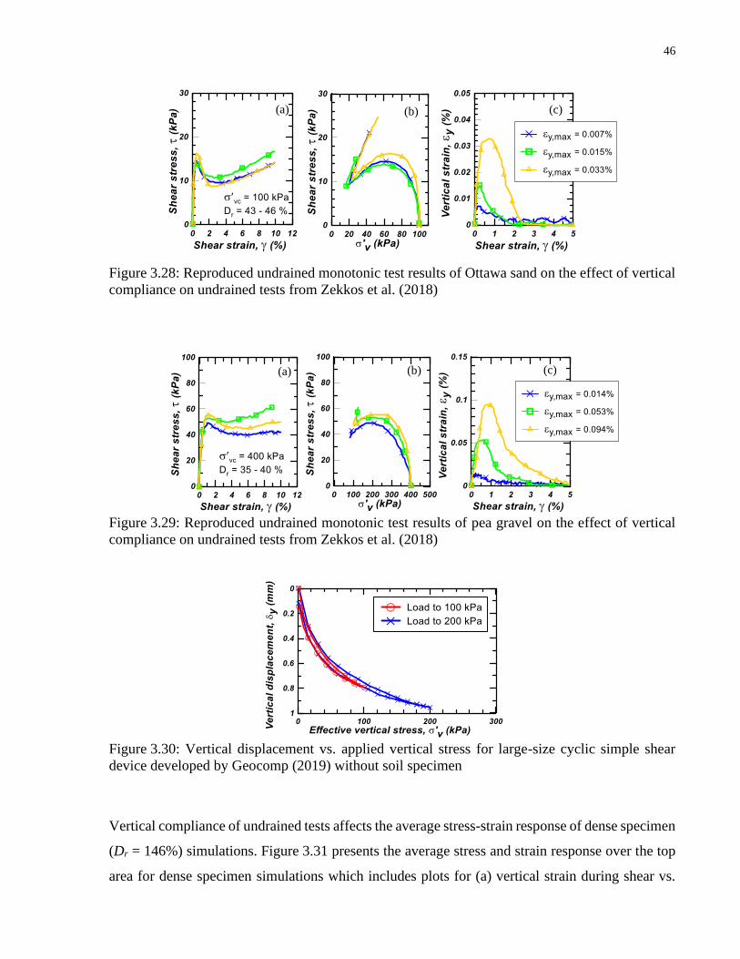
46
Figure 3.28: Reproduced undrained monotonic test results of Ottawa sand on the effect of vertical
compliance on undrained tests from Zekkos et al. (2018)
Figure 3.29: Reproduced undrained monotonic test results of pea gravel on the effect of vertical
compliance on undrained tests from Zekkos et al. (2018)
Figure 3.30: Vertical displacement vs. applied vertical stress for large-size cyclic simple shear
device developed by Geocomp (2019) without soil specimen
Vertical compliance of undrained tests affects the average stress-strain response of dense specimen
(Dr = 146%) simulations. Figure 3.31 presents the average stress and strain response over the top
area for dense specimen simulations which includes plots for (a) vertical strain during shear vs.
(a) (b) (c)
(b) (a) (c)
47
shear strain, (b) effective vertical stress vs. shear strain, (c) shear stress vs. strain, and (d) stress
path. The critical state line (CSL) with the constant volume friction angle ('cv) is also plotted with
the stress paths. The results show primarily dilative behaviour due to an increase in specimen
height, as shown in Figure 3.31(a). From 0 to 1% shear strain, the simulation exhibits contractive
behaviour. However, higher vertical compliance has negligible effect on stress-strain response
during this period. After 1% shear strain, the simulation exhibits dilative behaviour. During
dilative behaviour, higher vertical compliance reduces vertical stress, as shown in Figure 3.31(b),
and reduces shear stress, as shown in Figure 3.31(c). This is also shown in the stress path from
Figure 3.31(d). Table 3.4 presents the percent difference of shear and vertical stress at 4% shear
strain for higher maximum allowed vertical strain. For maximum vertical strain above the ASTM
D6528-17 tolerance of 0.05%, shear and vertical stress are reduced. Shear and vertical stress
decrease by 1% and 1% at 0.05% maximum vertical strain and decrease by 8% and 7% at 0.37%
maximum vertical strain. The results compare well with the work by Dyvik and Suzuki (2018)
who studied the effects of vertical compliance on undrained tests in dense offshore sand with a
relative density of 95%, as shown by the reproduced results in Figure 3.32. Dyvik and Suzuki
(2018) varied the specimen height between zero and an offset constant vertical strain using an
active height control system to study the effect on stress-strain response during the same test. As
shown in Figure 3.33, Dyvik and Suzuki (2018) only presented the vertical strain vs shear strain
plot for Kaolin, but mentioned that a similar pattern was used to offset specimen height for dense
offshore sand. For dense sand, higher vertical compliance increased vertical and shear stress during
contractive behaviour between 0% and about 2% shear strain. Then higher vertical compliance
reduced vertical and shear stress during dilative behaviour from 2% shear strain onwards. During
dilative behaviour at 5% shear strain, it was reported that shear stress was reduced by 6% and
vertical effective stress was reduced by 7%. At failure where the soil is transitioning from
contractive to dilative behaviour, the shear stress was increased by more than 20% and the vertical
effective stress was increased by about 30%. Dyvik and Suzuki (2018) does not appear to consider
the “sandwich compliance” in the reported vertical strain of the soil specimen either. Apparatus
deformation can significantly increase vertical strain as previously shown in Figure 3.25 and
Figure 3.30. Therefore, the actual vertical strain (compliance) of the soil specimen may be greater
than was reported.

48
As discussed in the Chapter 2, the effect of higher vertical compliance on undrained tests is dictated
by contractive or dilative behaviour of the soil (Dyvik and Suzuki, 2018). As shown by the loose
specimen (Dr = 24%) simulation results in Figure 3.27 and reproduced results of Zekkos et al.
(2018) in Figure 3.28 and Figure 3.29, higher vertical compliance increases shear and vertical
stress during contractive behaviour. As shown by the dense specimen (Dr = 146%) simulations
results in Figure 3.31 and reproduced results of Dyvik and Suzuki (2018) in Figure 3.32, higher
vertical compliance reduces shear and vertical stress during dilative behaviour. Changes in shear
and vertical stress are significant close to or above the ASTM D6528-17 vertical strain tolerance
of 0.05%.
Figure 3.31: Monotonic test results of dense specimen (Dr = 146%) for varying maximum vertical
strain (y,max) during the shearing phase
(a)
(c)
(b)
(d)
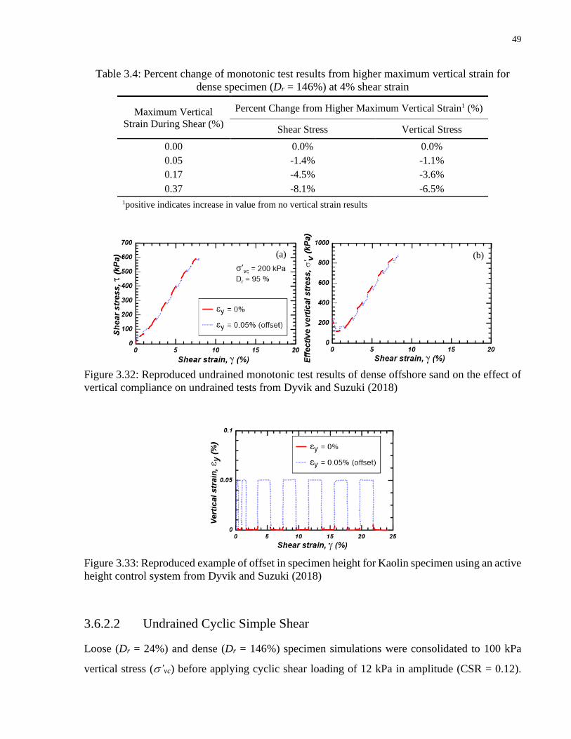
49
Table 3.4: Percent change of monotonic test results from higher maximum vertical strain for
dense specimen (Dr = 146%) at 4% shear strain
Maximum Vertical
Strain During Shear (%)
Percent Change from Higher Maximum Vertical Strain1 (%)
Shear Stress Vertical Stress
0.00 0.0% 0.0%
0.05 -1.4% -1.1%
0.17 -4.5% -3.6%
0.37 -8.1% -6.5%
1positive indicates increase in value from no vertical strain results
Figure 3.32: Reproduced undrained monotonic test results of dense offshore sand on the effect of
vertical compliance on undrained tests from Dyvik and Suzuki (2018)
Figure 3.33: Reproduced example of offset in specimen height for Kaolin specimen using an active
height control system from Dyvik and Suzuki (2018)
3.6.2.2 Undrained Cyclic Simple Shear
Loose (Dr = 24%) and dense (Dr = 146%) specimen simulations were consolidated to 100 kPa
vertical stress (’vc) before applying cyclic shear loading of 12 kPa in amplitude (CSR = 0.12).
(b) (a)

50
Loose and dense specimens were sheared until the simulations reached liquefaction or the stress-
strain response did not vary significantly with more cycles due to locking behaviour. The
liquefaction criterion and locking behaviour were explained in more detail in the section 3.3. The
loose specimen simulations were ended after 4 cycles when liquefaction occured. The dense
specimen simulations were ended after 40 cycles due to locking behaviour and did not reach
liquefaction. All results are presented here and in Appendix C as described later.
Vertical compliance of undrained tests affects the stress-strain response of undrained cyclic simple
shear tests. As shown previously in Figure 3.26 and Figure C.23, higher vertical compliance does
not increase stress concentrations, but does affect the average stress-strain response. Figure 3.34
and Figure 3.35 present plots of (a) vertical strain during shear vs. number of cycles, (b) shear
strain vs. number of cycles, (c) vertical stress vs. number of cycles, (d) shear stress vs shear strain
and (e) stress path for loose and dense specimen simulations. The critical state line (CSL) with the
constant volume friction angle ('cv) is also plotted with the stress paths where applicable. Results
from Figure 3.34 and Figure 3.35 are also presented in Appendix C as shown in Figure C.25 and
Figure C.26. Figure 3.34(a) and Figure 3.35(a) shows that loose and dense simulated specimens
simulations exhibit contractive behaviour while specimen height decreases throughout the
simulations due to vertical compliance. As shown in Figure 3.34(c) and Figure 3.35(c), higher
vertical compliance increases the vertical stress for each cycle as compared to the constant height
simulation. As such, higher vertical compliance increases the number of cycles to liquefaction, as
shown in the shear strain vs. number of cycles plots from Figure 3.34(a) and Figure 3.35(a). Higher
vertical compliance has negligible effect on the magnitude of shear strain. The trends are similar
to loose specimen monotonic test simulations as shown in Figure 3.27, which show that higher
vertical compliance during contractive behaviour increases the vertical stress. An increase in shear
stress, as observed during contractive behaviour in monotonic tests, is not seen in cyclic tests since
the analysis is load-controlled by the applied shear stress amplitude, as shown in Figure 3.34(d)
and (e), and Figure 3.35(d) and (e).
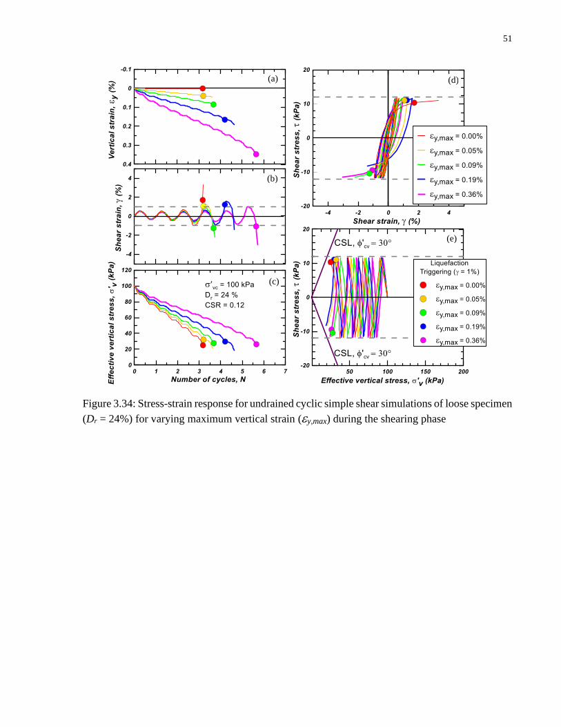
51
Figure 3.34: Stress-strain response for undrained cyclic simple shear simulations of loose specimen
(Dr = 24%) for varying maximum vertical strain (y,max) during the shearing phase
(a)
(b)
(c)
(d)
(e)
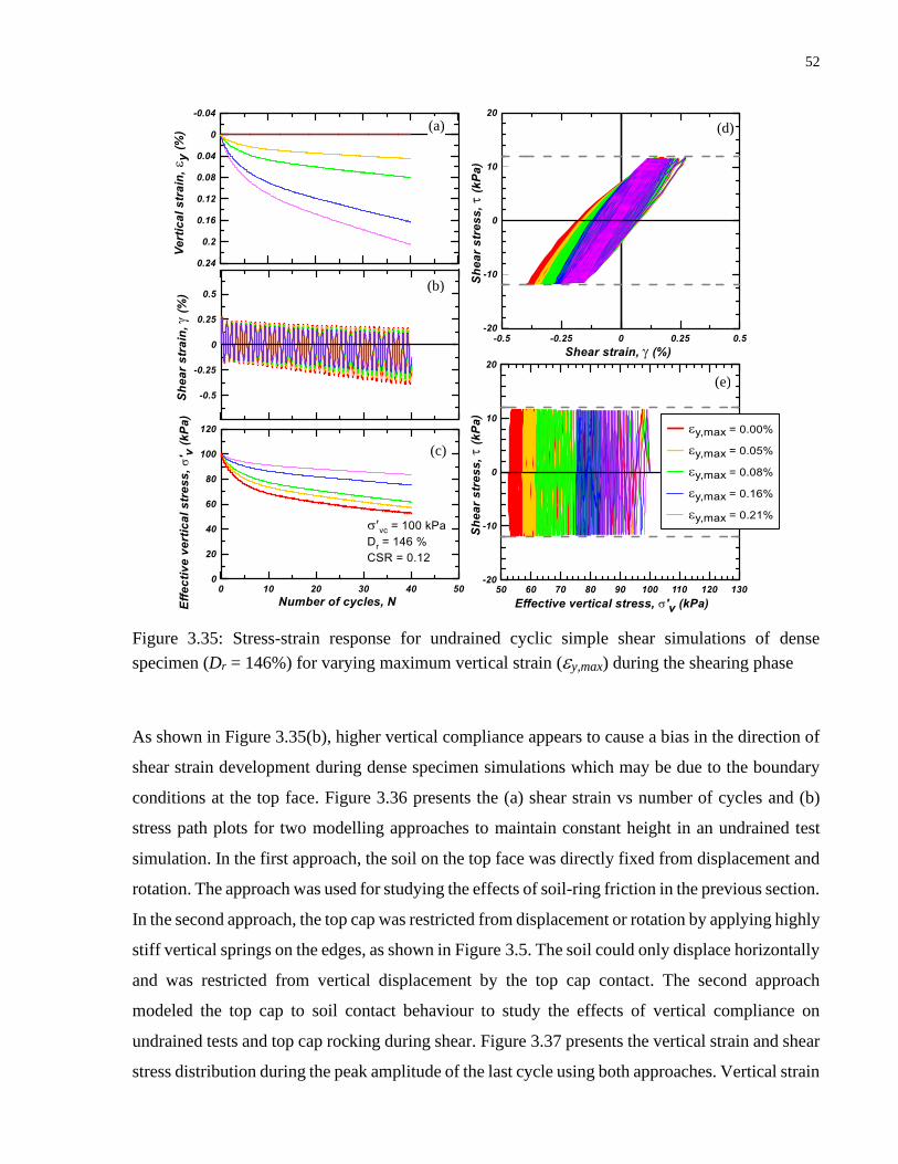
52
Figure 3.35: Stress-strain response for undrained cyclic simple shear simulations of dense
specimen (Dr = 146%) for varying maximum vertical strain (y,max) during the shearing phase
As shown in Figure 3.35(b), higher vertical compliance appears to cause a bias in the direction of
shear strain development during dense specimen simulations which may be due to the boundary
conditions at the top face. Figure 3.36 presents the (a) shear strain vs number of cycles and (b)
stress path plots for two modelling approaches to maintain constant height in an undrained test
simulation. In the first approach, the soil on the top face was directly fixed from displacement and
rotation. The approach was used for studying the effects of soil-ring friction in the previous section.
In the second approach, the top cap was restricted from displacement or rotation by applying highly
stiff vertical springs on the edges, as shown in Figure 3.5. The soil could only displace horizontally
and was restricted from vertical displacement by the top cap contact. The second approach
modeled the top cap to soil contact behaviour to study the effects of vertical compliance on
undrained tests and top cap rocking during shear. Figure 3.37 presents the vertical strain and shear
stress distribution during the peak amplitude of the last cycle using both approaches. Vertical strain
(a)
(b)
(c)
(d)
(e)
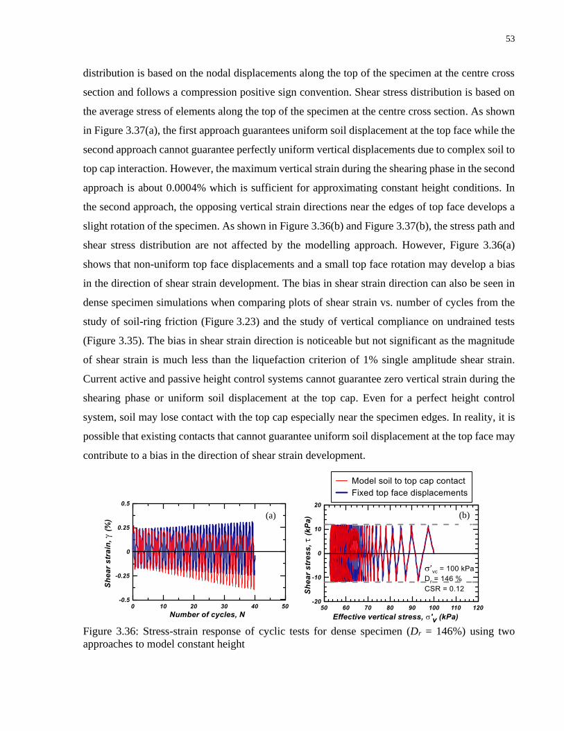
53
distribution is based on the nodal displacements along the top of the specimen at the centre cross
section and follows a compression positive sign convention. Shear stress distribution is based on
the average stress of elements along the top of the specimen at the centre cross section. As shown
in Figure 3.37(a), the first approach guarantees uniform soil displacement at the top face while the
second approach cannot guarantee perfectly uniform vertical displacements due to complex soil to
top cap interaction. However, the maximum vertical strain during the shearing phase in the second
approach is about 0.0004% which is sufficient for approximating constant height conditions. In
the second approach, the opposing vertical strain directions near the edges of top face develops a
slight rotation of the specimen. As shown in Figure 3.36(b) and Figure 3.37(b), the stress path and
shear stress distribution are not affected by the modelling approach. However, Figure 3.36(a)
shows that non-uniform top face displacements and a small top face rotation may develop a bias
in the direction of shear strain development. The bias in shear strain direction can also be seen in
dense specimen simulations when comparing plots of shear strain vs. number of cycles from the
study of soil-ring friction (Figure 3.23) and the study of vertical compliance on undrained tests
(Figure 3.35). The bias in shear strain direction is noticeable but not significant as the magnitude
of shear strain is much less than the liquefaction criterion of 1% single amplitude shear strain.
Current active and passive height control systems cannot guarantee zero vertical strain during the
shearing phase or uniform soil displacement at the top cap. Even for a perfect height control
system, soil may lose contact with the top cap especially near the specimen edges. In reality, it is
possible that existing contacts that cannot guarantee uniform soil displacement at the top face may
contribute to a bias in the direction of shear strain development.
Figure 3.36: Stress-strain response of cyclic tests for dense specimen (Dr = 146%) using two
approaches to model constant height
(a) (b)
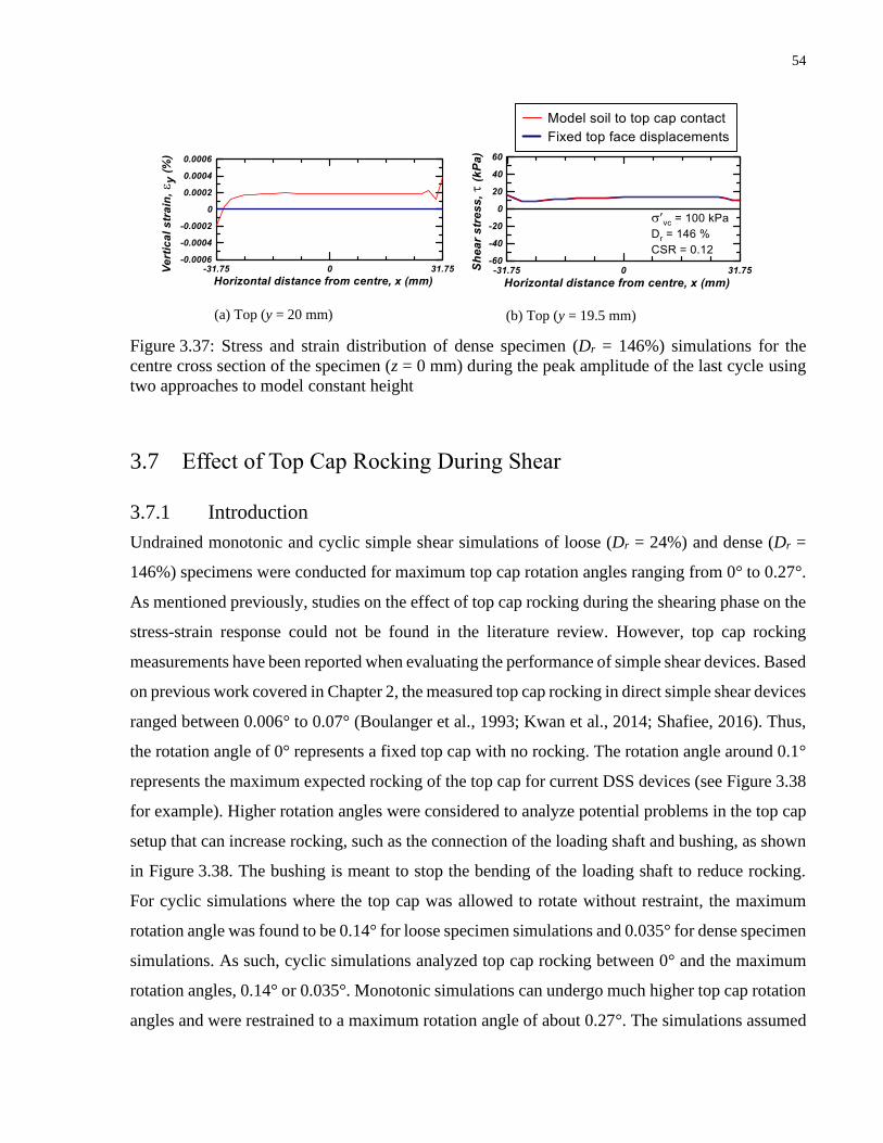
54
Figure 3.37: Stress and strain distribution of dense specimen (Dr = 146%) simulations for the
centre cross section of the specimen (z = 0 mm) during the peak amplitude of the last cycle using
two approaches to model constant height
3.7 Effect of Top Cap Rocking During Shear
3.7.1 Introduction
Undrained monotonic and cyclic simple shear simulations of loose (Dr = 24%) and dense (Dr =
146%) specimens were conducted for maximum top cap rotation angles ranging from 0° to 0.27°.
As mentioned previously, studies on the effect of top cap rocking during the shearing phase on the
stress-strain response could not be found in the literature review. However, top cap rocking
measurements have been reported when evaluating the performance of simple shear devices. Based
on previous work covered in Chapter 2, the measured top cap rocking in direct simple shear devices
ranged between 0.006° to 0.07° (Boulanger et al., 1993; Kwan et al., 2014; Shafiee, 2016). Thus,
the rotation angle of 0° represents a fixed top cap with no rocking. The rotation angle around 0.1°
represents the maximum expected rocking of the top cap for current DSS devices (see Figure 3.38
for example). Higher rotation angles were considered to analyze potential problems in the top cap
setup that can increase rocking, such as the connection of the loading shaft and bushing, as shown
in Figure 3.38. The bushing is meant to stop the bending of the loading shaft to reduce rocking.
For cyclic simulations where the top cap was allowed to rotate without restraint, the maximum
rotation angle was found to be 0.14° for loose specimen simulations and 0.035° for dense specimen
simulations. As such, cyclic simulations analyzed top cap rocking between 0° and the maximum
rotation angles, 0.14° or 0.035°. Monotonic simulations can undergo much higher top cap rotation
angles and were restrained to a maximum rotation angle of about 0.27°. The simulations assumed
(a) Top (y = 20 mm) (b) Top (y = 19.5 mm)
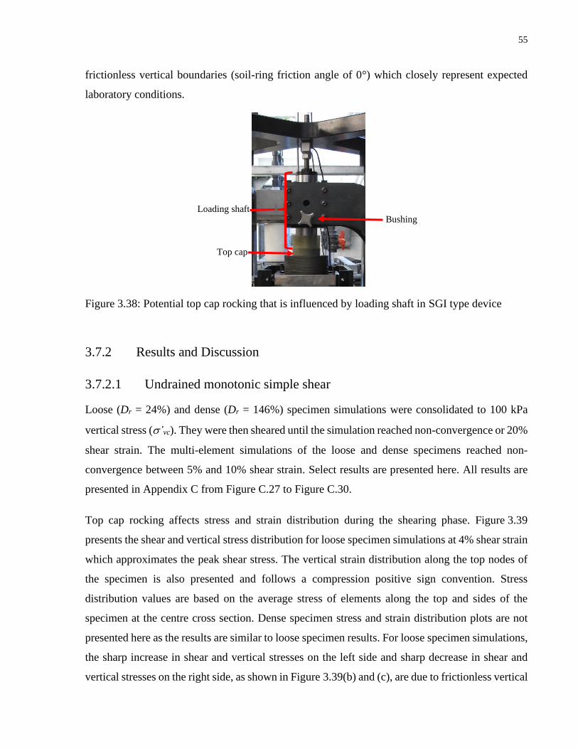
55
frictionless vertical boundaries (soil-ring friction angle of 0°) which closely represent expected
laboratory conditions.
Figure 3.38: Potential top cap rocking that is influenced by loading shaft in SGI type device
3.7.2 Results and Discussion
3.7.2.1 Undrained monotonic simple shear
Loose (Dr = 24%) and dense (Dr = 146%) specimen simulations were consolidated to 100 kPa
vertical stress (’vc). They were then sheared until the simulation reached non-convergence or 20%
shear strain. The multi-element simulations of the loose and dense specimens reached non-
convergence between 5% and 10% shear strain. Select results are presented here. All results are
presented in Appendix C from Figure C.27 to Figure C.30.
Top cap rocking affects stress and strain distribution during the shearing phase. Figure 3.39
presents the shear and vertical stress distribution for loose specimen simulations at 4% shear strain
which approximates the peak shear stress. The vertical strain distribution along the top nodes of
the specimen is also presented and follows a compression positive sign convention. Stress
distribution values are based on the average stress of elements along the top and sides of the
specimen at the centre cross section. Dense specimen stress and strain distribution plots are not
presented here as the results are similar to loose specimen results. For loose specimen simulations,
the sharp increase in shear and vertical stresses on the left side and sharp decrease in shear and
vertical stresses on the right side, as shown in Figure 3.39(b) and (c), are due to frictionless vertical
Loading shaft
Top cap
Bushing
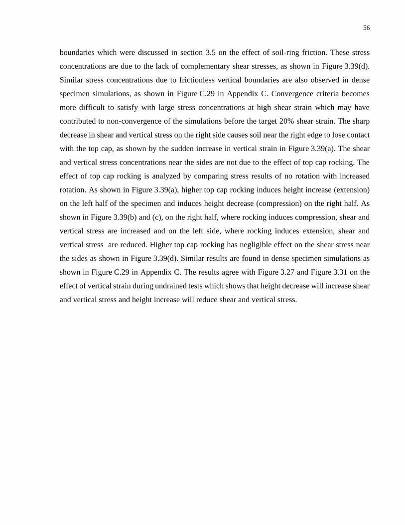
56
boundaries which were discussed in section 3.5 on the effect of soil-ring friction. These stress
concentrations are due to the lack of complementary shear stresses, as shown in Figure 3.39(d).
Similar stress concentrations due to frictionless vertical boundaries are also observed in dense
specimen simulations, as shown in Figure C.29 in Appendix C. Convergence criteria becomes
more difficult to satisfy with large stress concentrations at high shear strain which may have
contributed to non-convergence of the simulations before the target 20% shear strain. The sharp
decrease in shear and vertical stress on the right side causes soil near the right edge to lose contact
with the top cap, as shown by the sudden increase in vertical strain in Figure 3.39(a). The shear
and vertical stress concentrations near the sides are not due to the effect of top cap rocking. The
effect of top cap rocking is analyzed by comparing stress results of no rotation with increased
rotation. As shown in Figure 3.39(a), higher top cap rocking induces height increase (extension)
on the left half of the specimen and induces height decrease (compression) on the right half. As
shown in Figure 3.39(b) and (c), on the right half, where rocking induces compression, shear and
vertical stress are increased and on the left side, where rocking induces extension, shear and
vertical stress are reduced. Higher top cap rocking has negligible effect on the shear stress near
the sides as shown in Figure 3.39(d). Similar results are found in dense specimen simulations as
shown in Figure C.29 in Appendix C. The results agree with Figure 3.27 and Figure 3.31 on the
effect of vertical strain during undrained tests which shows that height decrease will increase shear
and vertical stress and height increase will reduce shear and vertical stress.

57
Figure 3.39. Stress and strain distribution of loose specimen (Dr = 24%) simulations at peak shear
stress (4% shear strain) for the centre cross section of the specimen (z = 0 mm), varying maximum
top cap rotation angle (,max)
Since top cap rocking induces compression on half the specimen and induces extension on the
other half, higher top cap rocking does not seem to affect the average stress-strain response.
Figure 3.40 and Figure 3.41 presents plots of (a) top cap rotation vs. shear strain, (b) effective
vertical stress vs. shear strain, (c) shear stress vs. shear strain, and (d) stress path for loose and
dense specimen simulations. The critical state line (CSL) with the constant volume friction angle
('cv) is also plotted with the stress paths. The plots present the average stress values over the top
area. As shown in Figure 3.40(a) and Figure 3.41(a), the maximum top cap rotation ranges between
0 to 0.27°. As shown in Figure 3.40(d) and Figure 3.41(d), higher top cap rotation has negligible
effect on the stress path. This is also shown in the plots of vertical stress vs. shear strain and shear
stress vs. shear strain that are presented in Figure 3.40(b) and Figure 3.41(b), and Figure 3.40(c)
and Figure 3.41(c). As such, higher top cap rocking has negligible effect on the average stress-
strain response.
(d) Left (x = -30.75 mm)
Right (x = 30.75 mm)
(b) Top (y = 19.5 mm)
(c) Top (y = 19.5 mm)
(a) Top (y = 20 mm)
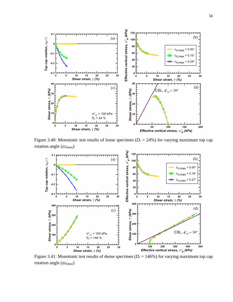
58
Figure 3.40: Monotonic test results of loose specimen (Dr = 24%) for varying maximum top cap
rotation angle (,max)
Figure 3.41: Monotonic test results of dense specimen (Dr = 146%) for varying maximum top cap
rotation angle (,max)
(a)
(b)
(a)
(c)
(b)
(d)
CSL 'cv = 30°
(a)
(c)
(b)
(d)
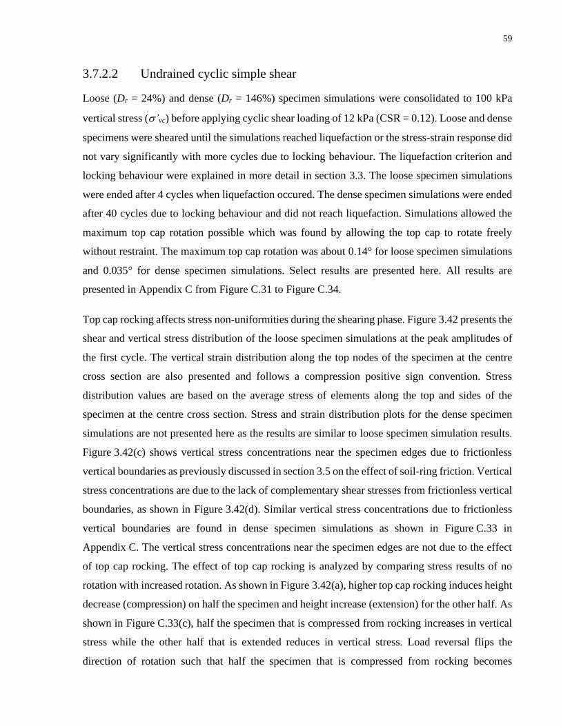
59
3.7.2.2 Undrained cyclic simple shear
Loose (Dr = 24%) and dense (Dr = 146%) specimen simulations were consolidated to 100 kPa
vertical stress (’vc) before applying cyclic shear loading of 12 kPa (CSR = 0.12). Loose and dense
specimens were sheared until the simulations reached liquefaction or the stress-strain response did
not vary significantly with more cycles due to locking behaviour. The liquefaction criterion and
locking behaviour were explained in more detail in section 3.3. The loose specimen simulations
were ended after 4 cycles when liquefaction occured. The dense specimen simulations were ended
after 40 cycles due to locking behaviour and did not reach liquefaction. Simulations allowed the
maximum top cap rotation possible which was found by allowing the top cap to rotate freely
without restraint. The maximum top cap rotation was about 0.14° for loose specimen simulations
and 0.035° for dense specimen simulations. Select results are presented here. All results are
presented in Appendix C from Figure C.31 to Figure C.34.
Top cap rocking affects stress non-uniformities during the shearing phase. Figure 3.42 presents the
shear and vertical stress distribution of the loose specimen simulations at the peak amplitudes of
the first cycle. The vertical strain distribution along the top nodes of the specimen at the centre
cross section are also presented and follows a compression positive sign convention. Stress
distribution values are based on the average stress of elements along the top and sides of the
specimen at the centre cross section. Stress and strain distribution plots for the dense specimen
simulations are not presented here as the results are similar to loose specimen simulation results.
Figure 3.42(c) shows vertical stress concentrations near the specimen edges due to frictionless
vertical boundaries as previously discussed in section 3.5 on the effect of soil-ring friction. Vertical
stress concentrations are due to the lack of complementary shear stresses from frictionless vertical
boundaries, as shown in Figure 3.42(d). Similar vertical stress concentrations due to frictionless
vertical boundaries are found in dense specimen simulations as shown in Figure C.33 in
Appendix C. The vertical stress concentrations near the specimen edges are not due to the effect
of top cap rocking. The effect of top cap rocking is analyzed by comparing stress results of no
rotation with increased rotation. As shown in Figure 3.42(a), higher top cap rocking induces height
decrease (compression) on half the specimen and height increase (extension) for the other half. As
shown in Figure C.33(c), half the specimen that is compressed from rocking increases in vertical
stress while the other half that is extended reduces in vertical stress. Load reversal flips the
direction of rotation such that half the specimen that is compressed from rocking becomes
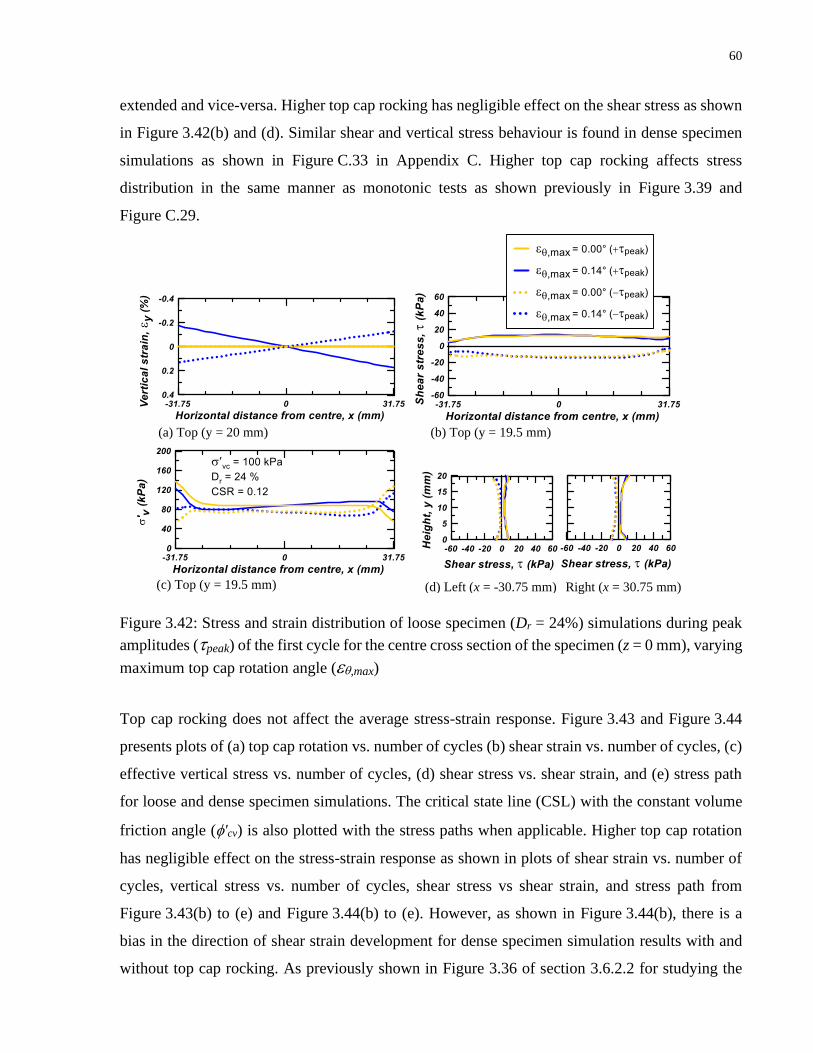
60
extended and vice-versa. Higher top cap rocking has negligible effect on the shear stress as shown
in Figure 3.42(b) and (d). Similar shear and vertical stress behaviour is found in dense specimen
simulations as shown in Figure C.33 in Appendix C. Higher top cap rocking affects stress
distribution in the same manner as monotonic tests as shown previously in Figure 3.39 and
Figure C.29.
Figure 3.42: Stress and strain distribution of loose specimen (Dr = 24%) simulations during peak
amplitudes (peak) of the first cycle for the centre cross section of the specimen (z = 0 mm), varying
maximum top cap rotation angle (,max)
Top cap rocking does not affect the average stress-strain response. Figure 3.43 and Figure 3.44
presents plots of (a) top cap rotation vs. number of cycles (b) shear strain vs. number of cycles, (c)
effective vertical stress vs. number of cycles, (d) shear stress vs. shear strain, and (e) stress path
for loose and dense specimen simulations. The critical state line (CSL) with the constant volume
friction angle ('cv) is also plotted with the stress paths when applicable. Higher top cap rotation
has negligible effect on the stress-strain response as shown in plots of shear strain vs. number of
cycles, vertical stress vs. number of cycles, shear stress vs shear strain, and stress path from
Figure 3.43(b) to (e) and Figure 3.44(b) to (e). However, as shown in Figure 3.44(b), there is a
bias in the direction of shear strain development for dense specimen simulation results with and
without top cap rocking. As previously shown in Figure 3.36 of section 3.6.2.2 for studying the
(d) Left (x = -30.75 mm)
Right (x = 30.75 mm)
(b) Top (y = 19.5 mm)
(c) Top (y = 19.5 mm)
(a) Top (y = 20 mm)
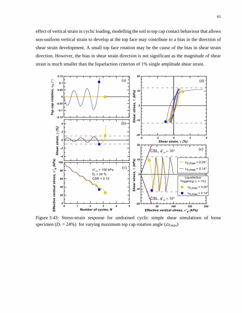
61
effect of vertical strain in cyclic loading, modelling the soil to top cap contact behaviour that allows
non-uniform vertical strain to develop at the top face may contribute to a bias in the direction of
shear strain development. A small top face rotation may be the cause of the bias in shear strain
direction. However, the bias in shear strain direction is not significant as the magnitude of shear
strain is much smaller than the liquefaction criterion of 1% single amplitude shear strain.
Figure 3.43: Stress-strain response for undrained cyclic simple shear simulations of loose
specimen (Dr = 24%) for varying maximum top cap rotation angle (,max)
(a)
(b)
(c)
(d)
(e)

62
Figure 3.44: Stress-strain response for undrained cyclic simple shear simulations of dense
specimen (Dr = 146%) for varying maximum top cap rotation angle (,max)
3.8 Conclusions
3.8.1 Effect of Soil-Ring Friction
Simulations of the SGI type device using stacked rings suggest that typical high quality DSS
equipment adequately capture the ideal simple shear conditions. Increasing soil-ring friction
increases the magnitude of stress non-uniformities that develop adjacent to the vertical boundaries
during the consolidation phase. As a result, shear stresses are reduced during monotonic shear
loading and the vertical stress is reduced for the first few cycles during cyclic shear loading. Higher
soil-ring friction did improve stress uniformity during the shearing phase, but the effect on
consolidation stresses overwrites any advantages of having frictional vertical boundaries.
Practically, near frictionless vertical boundaries achieve the best comparison with ideal simple
shear conditions.
(a)
(b)
(c)
(d)
(e)

63
3.8.2 Effect of Vertical Compliance on Undrained Tests
Simulations of the SGI type device using stacked rings suggest that higher vertical compliance of
undrained tests can significantly affect the stress-strain response. Undrained monotonic
simulations of loose specimens (Dr = 24%) exhibited contractive behaviour (height decrease)
which increased the peak shear stress and corresponding vertical stress by 6% and 7% for ASTM
D6528-17 vertical strain tolerance of 0.05%. Undrained monotonic simulations of dense
specimens (Dr = 146%) exhibited dilative behaviour (height increase) which reduced each of the
shear and vertical stress at 4% shear strain by 1% for ASTM D6528-17 vertical strain tolerance of
0.05%. Vertical strains and their effects on DSS test measurements are likely much higher than
reported in the literature due to unmeasured apparatus deformations (i.e. top cap, base pedestal,
loading shaft, and two aluminum porous stones), which were shown to increase the vertical strain
in a typical direct simple shear apparatus by about 0.24%. This is based on an increase in vertical
stress from about 100 to 350 kPa during experimental monotonic tests. Accounting for ASTM
vertical strain tolerance of 0.05%, the vertical compliance may be as high as 0.29%. For loose
specimen simulations, vertical compliance of 0.28% resulted in contractive behaviour that
increased the peak shear stress and corresponding vertical stress by about 33% and 41%,
respectively. For dense specimen simulations, vertical compliance of 0.37% resulted in dilative
behaviour that reduced the shear and vertical stress at 4% shear strain by 8% and 7%, respectively.
Undrained cyclic simulations exhibited contractive behaviour. As such, higher vertical compliance
increases the vertical stress for each cycle in turn increasing the number of cycles to liquefaction.
Thus, vertical compliance of undrained tests needs to be minimized after accounting for apparatus
deformation to better approximate ideal simple shear conditions during undrained tests.
3.8.3 Effect of Top Cap Rocking During Shear
Simulations of the SGI type device using stacked rings shows that top cap rocking affects stress
non-uniformities in DSS specimens. At the top of the specimen, simulations showed that top cap
rotation induced height decrease (compression) for half the specimen that increased shear and
vertical stress, and induced height increase (extension) for half the specimen that reduced shear
and vertical stress. However, the change in stress distribution is negligible for the expected range
of top cap rotation. Higher top cap rocking within the expected range has negligible effect on the

64
average stress-strain response and is not a problem for approximating ideal simple shear conditions
in direct simple shear tests.
65
Chapter 4
Summary and Conclusions
4.1 Summary and Conclusions
This study investigated the effects of imperfect boundary conditions in the direct simple shear test
on undrained monotonic and cyclic stress-strain response. Imperfect boundary conditions do not
allow the direct simple shear test to achieve ideal simple shear conditions that are assumed for
model calibration. Imperfect boundary conditions were studied through numerical analysis of the
nearly ubiquitous SGI type direct simple shear (DSS) device that uses stacked rings for lateral
confinement. Results from the numerical study are meant to provide insight on the influence of
stress and strain non-uniformities due to imperfect boundary conditions on test measurements
rather than to precisely compute values for design purposes. Where experimental data were
available, simulation results were compared to them and shown to be in general agreement with
them.
4.1.1 Effect of Soil-Ring Friction
A major problem with DSS tests is its near frictionless vertical boundaries that cannot develop
complementary shear stresses necessary for ideal simple shear conditions. Simulations of the SGI
type device demonstrate that the results compares well with ideal simple shear conditions for the
expected range of soil-ring friction. Thus, near frictionless vertical boundaries in current testing
apparatuses are sufficient for approximating ideal simple shear conditions for the calibration of
constitutive models. Higher soil-ring friction did improve stress uniformity during the shearing
phase, but the effect on consolidation stresses overwrite any advantages of having frictional
vertical boundaries. Practically, near frictionless vertical boundaries that are currently used in
direct simple shear tests adequately capture ideal simple shear conditions.
66
4.1.2 Effect of Vertical Compliance on Undrained Tests
Active and passive height control systems can minimize but not eliminate vertical strain during
the shearing phase to approximate undrained (constant volume) conditions. Apparatus
deformation, such as those from the loading shaft, top cap, base pedestal, and porous stones, can
significantly increase the vertical strain during the shearing phase above ASTM D6528-17
tolerance of 0.05% and may not be corrected by the active height control system. These
unmeasured, or very difficult to measure deformations were shown to increase the vertical
compliance in a typical direct simple shear apparatus by about 0.24%. This is based on an increase
in vertical stress from about 100 to 350 kPa during experimental monotonic tests. Accounting for
ASTM vertical strain tolerance of 0.05%, the vertical compliance may be as high as 0.29%. For
loose specimen simulations, vertical compliance of 0.28% resulted in contractive behaviour that
increased the peak shear stress and corresponding vertical stress by about 33% and 41%,
respectively. For dense specimen simulations, vertical compliance of 0.37% resulted in dilative
behaviour that reduced the shear and vertical stress at 4% shear strain by 8% and 7%, respectively.
Simulations of the SGI type device demonstrate that high vertical compliance can significantly
affect the stress-strain response. Undrained cyclic simulations exhibited contractive behaviour. As
such, higher vertical compliance increased the vertical stress for each cycle which increased the
number of cycles to liquefaction.
4.1.3 Effect of Top Cap Rocking During Shear
A problem in DSS tests is top cap rocking that violates the assumption that top and bottom faces
remain parallel in ideal simple shear conditions. Simulations of the SGI type device using stacked
rings demonstrate that the top cap rotation affects the stress non-uniformities, but the change in
stress distribution is negligible for the expected range of top cap rotation. Additionally, higher top
cap rotation within the expected range has negligible effect on the measured stress-strain response.
Thus, top cap rocking for the expected amount of rotation appears not to be a problem in direct
simple shear tests.
4.1.4 Recommendations for Future Work
This study focuses on numerical analysis of imperfect boundary conditions in the direct simple
shear device and can be greatly enhanced by further validation against experimental studies.
67
Experimental studies can validate numerical results that show the effect of higher soil-ring friction
on consolidation stresses overwrite any advantages of having frictional vertical boundaries.
However, there are many challenges in the laboratory to control and measure friction between the
soil and vertical boundaries that needs to be overcome to study the effect of soil-ring friction. As
presented earlier, experimental studies exist on the effect of vertical compliance on undrained tests.
However, more attention is needed on the actual vertical strain of the soil specimen which may be
much higher than is reported after considering apparatus deformation. Numerical results suggest
that the effect of top cap rocking is negligible for the expected range of top cap rotation. Future
experimental studies can verify the expected range of top cap rotation for different apparatus
configurations and conduct a parametric study on the effect of top cap rotation on stress-strain
response. Finally, the current study can be expanded to include a parametric study on the effect of
friction between the soil and porous stones on stress-strain response. A primary function of the
porous stones at the top cap and base pedestal is to prevent soil slippage during shear. Numerical
and experimental studies can study the effect of porous stone material and design on stress-strain
response under monotonic and cyclic loading.
68
References
Airey, D.W., Budhu, M., and Wood, D.M. 1985. Some Aspects of the Behaviour of Soils in Simple
Shear. In Developments in Soil Mechanics and Foundation Engineering: Vol. 2: Stress-
Strain Modelling of Soils. Edited by P. Banerjee, K. and R. Butterfield. Elsevier Applied
Science Publishers. pp. 185-213.
ASTM D6528-17. 2017. Standard Test Method for Consolidated Undrained Direct Simple Shear
Testing of Fine Grain Soils. ASTM International, West Conshohocken, PA, USA.
Available from www.astm.org [accessed 29 May 2018].
Bernhardt, M.L., Biscontin, G., and O'Sullivan, C. 2016. Experimental validation study of 3D
direct simple shear DEM simulations. Soils and Foundations, 56(3): 336-347.
Bjerrum, L., and Landva, A. 1966. Direct Simple-Shear Tests on a Norwegian Quick Clay.
Géotechnique, 16(1): 1-20.
Boulanger, R.W., and Ziotopoulou, K. 2017. PM4Sand (Version 3.1): A sand plasticity model for
earthquake engineering applications - Report No. UCD/CGM-17/01. Center for
Geotechnical Modeling, Department of Civil and Environmental Engineering, University
of California, Davis, CA.
Boulanger, R.W., Chan, C.K., Seed, H.B., Seed, R.B., and Sousa, J.B. 1993. A Low-Compliance
Bi-directional Cyclic Simple Shear Apparatus. Geotechnical Testing Journal, 16(1): 36-45.
Bro, A.D., Stewart, J.P., and Pradel, D.E. 2013. Estimating Undrained Strength of Clays from
Direct Shear Testing at Fast Displacement Rates. In Geocongress 2013: Stability and
Performance of Slopes and Embankments III. Edited by C.L. Meehan and D. Pradel and
M.A. Pando and J.F. Labuz. ASCE, San Diego, California. pp. 106-119.
Budhu, M. 1984. Nonuniformities imposed by simple shear apparatus. Canadian Geotechnical
Journal, 21(1): 125-137.
Chang, W.J., Phantachang, T., and Ieong, W.M. 2016. Evaluation of size and boundary effects in
simple shear tests with distinct element modeling. Journal of GeoEngineering, 11(3): 133-
142.
Dafalias, Y.F., and Manzari, M.T. 2004. Simple plasticity sand model accounting for fabric change
effects. Journal of Engineering Mechanics, 130(6): 622-634.
Dassault Systèmes. 2012. ABAQUS Version 6.12 Unified Finite Element Analysis. Vélizy-
Villacoublay, France.
DeGroot, D.J., Germaine, J.T., and Ladd, C.C. 1993. The Multidirectional Direct Simple Shear
Apparatus. Geotechnical Testing Journal, 16(3): 283-295.
DeGroot, D.J., Germaine, J.T., and Ladd, C.C. 1994. Effect of Nonuniform Stresses on Measured
DSS Stress-Strain Behaviour. Journal of Geotechnical Engineering, 120(5): 892-911.
Doherty, J., and Fahey, M. 2011. Three-dimensional finite element analysis of the direct simple
shear test. Computers and Geotechnics, 38: 917-924.
Duku, P.M., Stewart, J.P., Whang, D.H., and Venugopal, R. 2007. Digitially controlled simple
shear apparatus for dynamic soil testing. Geotechnical Testing Journal, 30(5): 368-377.

69
Dyvik, R., and Suzuki, Y. 2018. Effect of Volume Change in Undrained Direct Simple Shear
Tests. Geotechnical Testing Journal, 42(4): 1075-1082.
doi:https://doi.org/10.1520/GTJ20170287.
Dyvik, R., Berre, T., Lacasse, S., and Raadim, B. 1987. Comparison of truly undrained and
constant volume direct simple shear tests. Géotechnique, 37(1): 3-10.
Geocomp. 2018. Below the Surface - New Addition to our Soil Testing System [online]. Available
from https://www.geocomp.com/files/newsletters/Q2-2018-Geocomp-Newsletter.pdf
[cited 17 April 2019].
Geocomp. 2019. Large Cyclic Direct Simple Shear (Cyclic DSS) Load Frame / Test System
[online]. Available from https://www.geocomp.com/Products/LabSystems/TT-Cyclic-
DSS-Large [cited 20 August 2019].
Gill, S.S. 2018. Minerology of a Sand Sample Using Scanning Electron Microscopy [Unpublished
manuscript]. University of Toronto, Department of Civil and Mineral Engineering,
Toronto, Canada.
Gudehus, G., Amorosi, A., Gens, A., Herle, I., Kolymbas, D., Masin, D., Wood, D.M., Niemunis,
A., Nova, R., Pastor, M., Tamagnini, C., and Viggiani, G. 2008. The soilmodels.info
project. International Journal of Numerical and Analytical Methods in Geomechanics,
32(12): 1571-1572.
Ishihara, K., and Yamazaki, F. 1980. Cyclic simple shear tests on saturated sand in multi-
directional loading. Soils and Foundations, 20(1): 45-59.
ITASCA Consulting Group Inc. 2019. FLAC3D Version 7.0 - Explicit continuum modeling of
non-linear material behaviour in 3D. Minneapolis, USA.
Kjellman, W. 1951. Testing the Shear Strength of Clay in Sweden. Géotechnique, 2(3): 225-232.
Kwan, W.S., Sideras, S., El Mohtar, C.S., and Kramer, S. 2014. Pore pressure generation under
different transient loading histories. In Proceedings of the 10th U.S. National Conference
on Earthquake Engineering: Frontiers of Earthquake Engineering. Earthquake Engineering
Research Institute, Anchorage, Alaska, USA.
Lucks, A.S., Christian, J.T., Brandow, G.E., and Höeg, K. 1972. Stress conditions in NGI simple
shear test. Journal of the Soil Mechanics and Foundations Division, 98(1): 155-160.
Mao, X., and Fahey, M. 2003. Behaviour of calcareous soils in undrained cyclic simple shear.
Géotechnique, 53(8): 715-727.
Masin, D., Martinelli, M., Miriano, C., and Tamagnini, C. 2018. SoilModels project - SANISAND
Abaqus UMAT and Plaxis implementations [online]. Available from
https://soilmodels.com/download/plaxis-umat-sanisand/ [cited 29 May 2018].
Niemunis, A. 2017. SoilModels project - Incremental Driver [online]. Available from
https://soilmodels.com/idriver/ [accessed 29 May 2018].
Rocscience Inc. 2019. RS3 - 3D finite element analysis for advanced analysis. Toronto, Canada.
Roscoe, K.H. 1953. An apparatus for the application of simple shear to soil samples. In
Proceedings of the 3rd International Conference on Soil Mechanics and Foundation
Engineering, Zurich, Switzerland. pp. 186-191.
70
Rutherford, C.J. 2012. Development of a Multi-Directional Direct Simple Shear Testing Device
for Characterization of the Cyclic Shear Response of Marine Clays. Ph.D. thesis,
Department of Civil Engineering, Texas A&M University, Texas, USA.
Saada, A.S., and Townsend, F.C. 1981. State of the Art: Labratory Strength Testing of Soils. In
STP740-EB Laboratory Shear Strength of Soil. Edited by R.N. Yong and F.C. Townsend.
ASTM, West Conshohocken, PA, USA. pp. 7-77.
Shafiee, A. 2016. Cyclic and Post-Cyclic Behavior of Sherman Island Peat. Ph.D. thesis,
Department of Civil Engineering, University of California, California, USA.
Shen, C.K., Sadigh, K., and Herrmann, L.R. 1978. An Analysis of NGI Simple Shear Apparatus
for Cyclic Soil Testing. In STP654-EB Dynamic Geotechnical Testing. Edited by M. Silver
and D. Tiedemann. ASTM, West Conshohocken, PA, USA. pp. 148-162.
Taiebat, M., and Dafalias, Y.F. 2008. SANISAND: Simple anisotropic sand plasticity model.
International Journal for Numerical and Analytical Methods in Geomechanics, 32(8): 915-
948.
Tatsuoka, F., and Haibara, O. 1985. Shear resistance between sand and smooth or lubricated
surfaces. Soils and Foundations, 25(1): 89-98.
Villet, W.C.B., Sitar, N., and Johnson, K.A. 1985. Simple shear tests on highly overconsolidated
offshore silts - Paper No OTC 4918. In Proceedings of the 17th annual Offshore
Technology Conference, Houston, USA. pp. 207-218.
Wijewickreme, D., Dabeet, A., and Byrne, P. 2013. Some Observations on the State of Stress in
the Direct Simple Shear Test Using 3D Discrete Element Analysis. Geotechnical Testing
Journal, 36(2): 292-299.
Zekkos, D., Athanasopoulos-Zekkos, A., Hubler, J., Fei, X., Zehtab, K.H., and Marr, W.A. 2018.
Development of a Large-Size Cyclic Direct Simple Shear Device for Characterization of
Ground Materials with Oversized Particles. Geotechnical Testing Journal, 41(2): 263-279.

71
Appendix A
Dafalias and Manzari (2004) Model Calibration
Results

72
A.1 Calibration of Undrained Monotonic Simple Shear Behaviour:
experimental data and Dafalias and Manzari (2004) model simulations
Figure A.1: Test HVS001M calibrated undrained monotonic simple shear results

73
Figure A.2: Test HVS002M calibrated undrained monotonic simple shear results
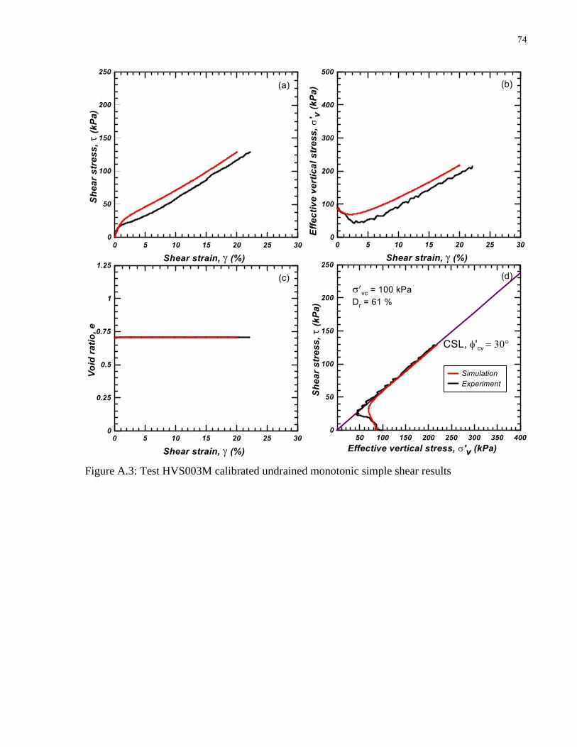
74
Figure A.3: Test HVS003M calibrated undrained monotonic simple shear results
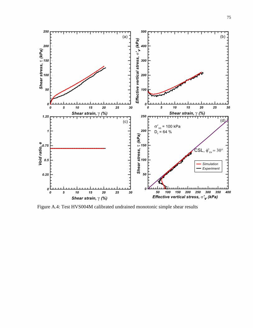
75
Figure A.4: Test HVS004M calibrated undrained monotonic simple shear results
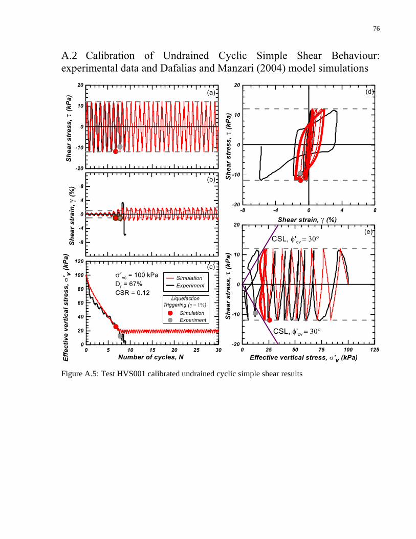
76
A.2 Calibration of Undrained Cyclic Simple Shear Behaviour:
experimental data and Dafalias and Manzari (2004) model simulations
Figure A.5: Test HVS001 calibrated undrained cyclic simple shear results
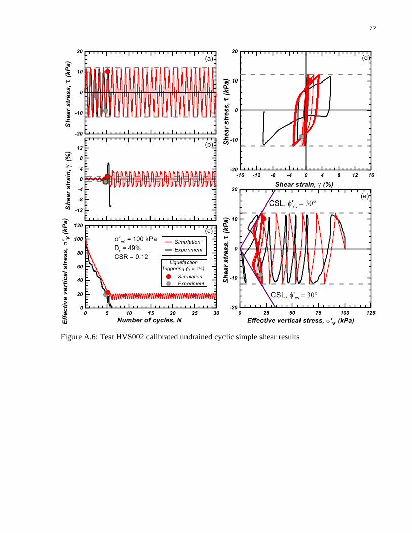
77
Figure A.6: Test HVS002 calibrated undrained cyclic simple shear results
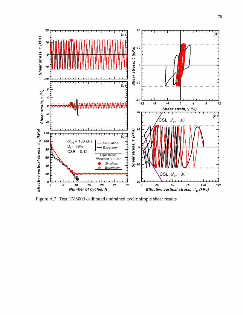
78
Figure A.7: Test HVS003 calibrated undrained cyclic simple shear results
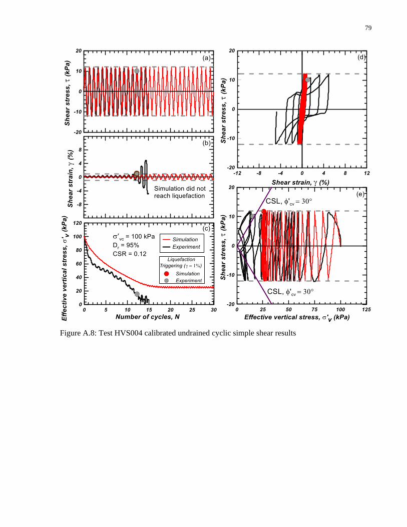
79
Figure A.8: Test HVS004 calibrated undrained cyclic simple shear results
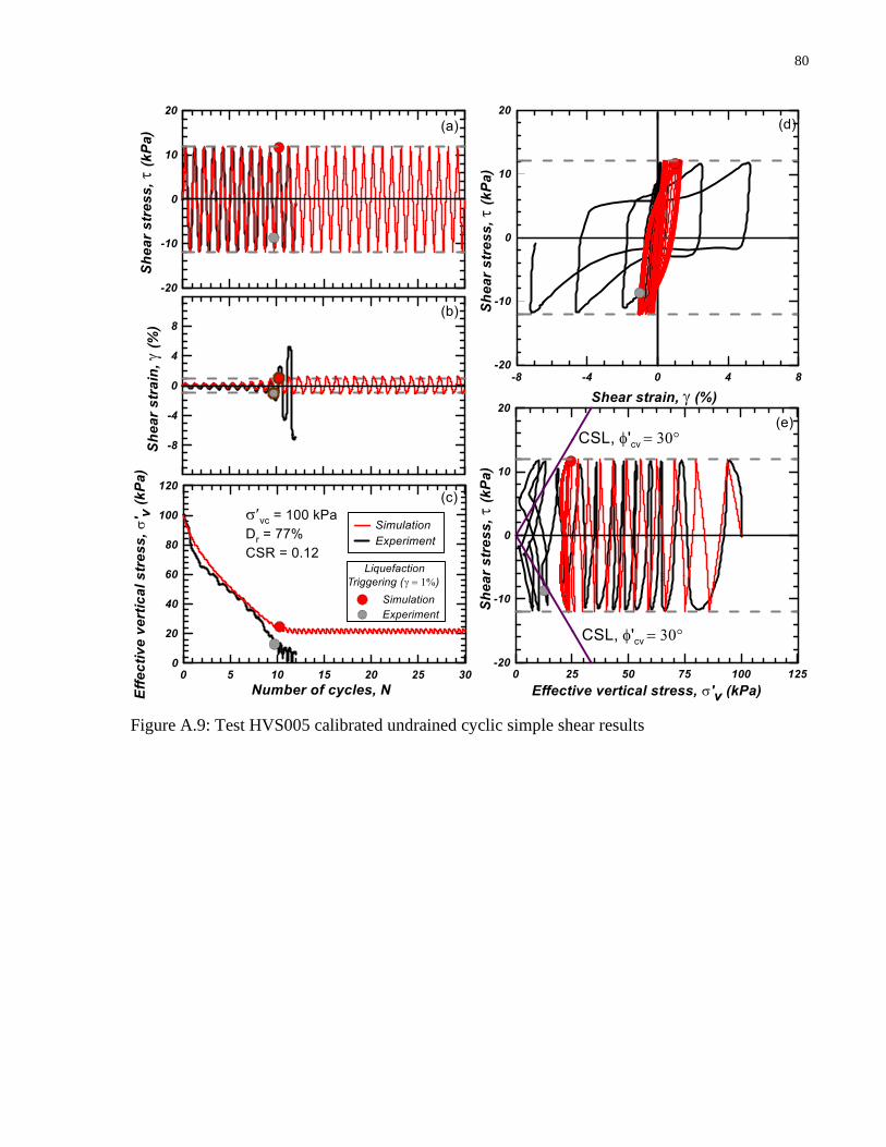
80
Figure A.9: Test HVS005 calibrated undrained cyclic simple shear results

81
A.3 Calibration of Undrained Cyclic Simple Shear Behaviour: Dafalias
and Manzari (2004) model simulations varying cyclic stress ratios (CSR)
to generate (CSR) vs. number of cycles to liquefaction plot (Figure 3.4)
Figure A.10: Test HVS005 undrained cyclic simple shear test simulation at CSR = 0.085
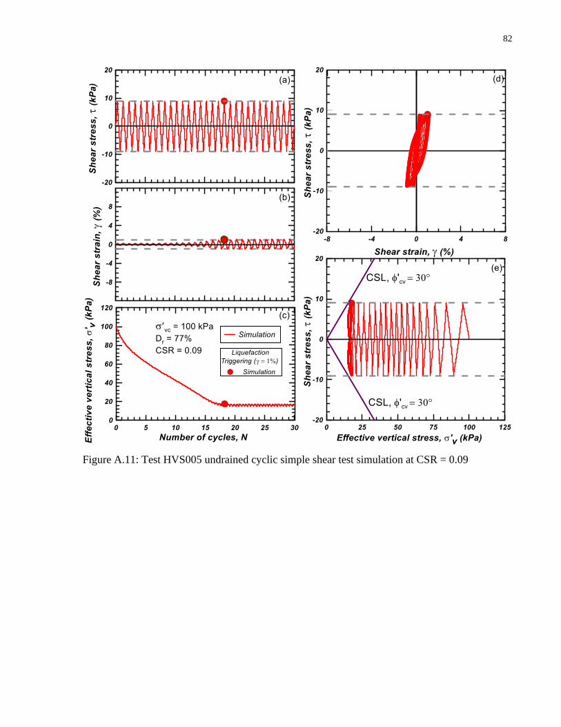
82
Figure A.11: Test HVS005 undrained cyclic simple shear test simulation at CSR = 0.09

83
Figure A.12: Test HVS005 undrained cyclic simple shear test simulation at CSR = 0.10

84
Figure A.13: Test HVS005 undrained cyclic simple shear test simulation at CSR = 0.15

85
A.4 Calibration of Undrained Cyclic Simple Shear Behaviour: other
experimental data to generate cyclic stress ratio (CSR) vs. number of
cycles to liquefaction plot (Figure 3.4)
Figure A.14: Test HVS022 undrained cyclic simple shear experimental results at CSR = 0.12

86
Figure A.15: Test HVS006 undrained cyclic simple shear experimental results at CSR = 0.09
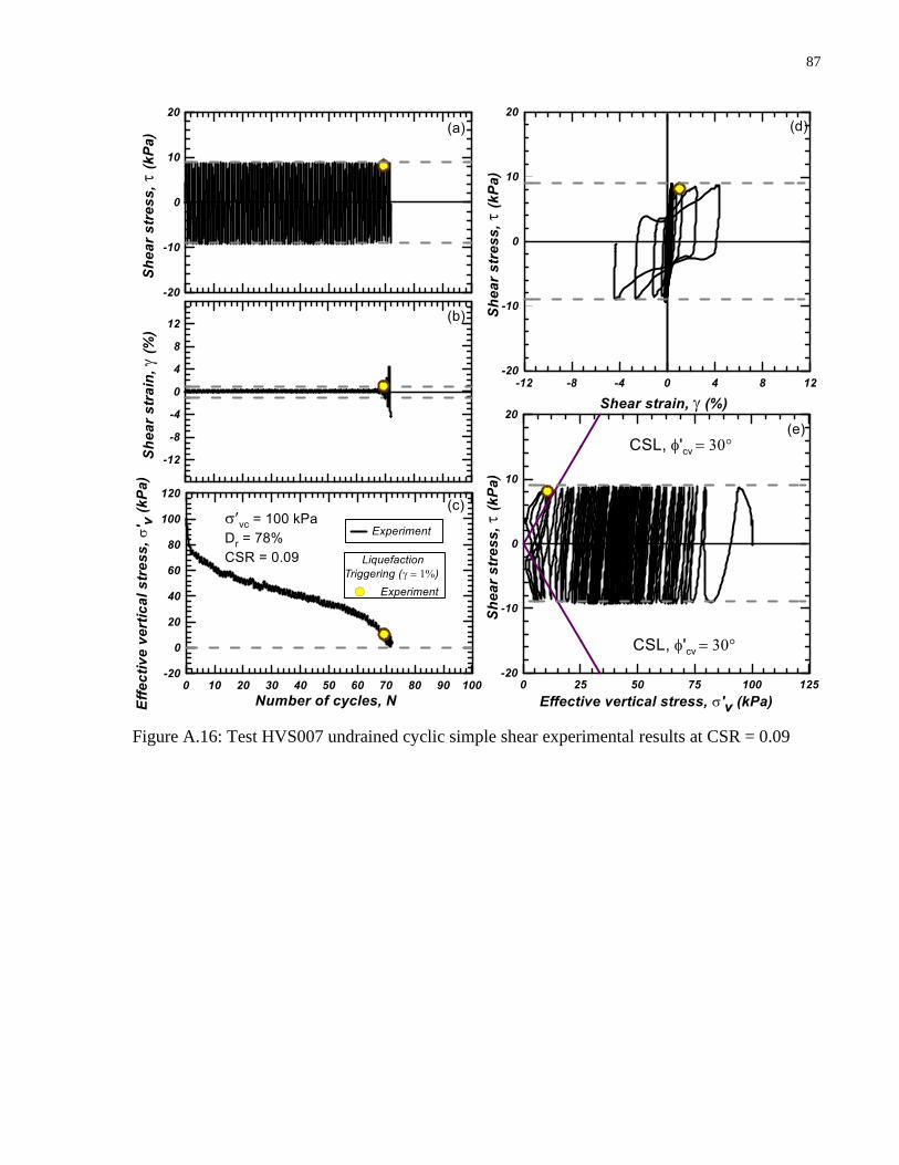
87
Figure A.16: Test HVS007 undrained cyclic simple shear experimental results at CSR = 0.09
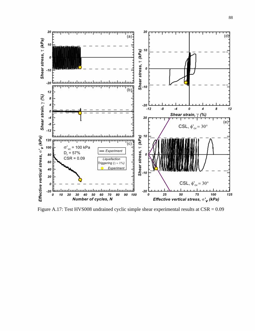
88
Figure A.17: Test HVS008 undrained cyclic simple shear experimental results at CSR = 0.09
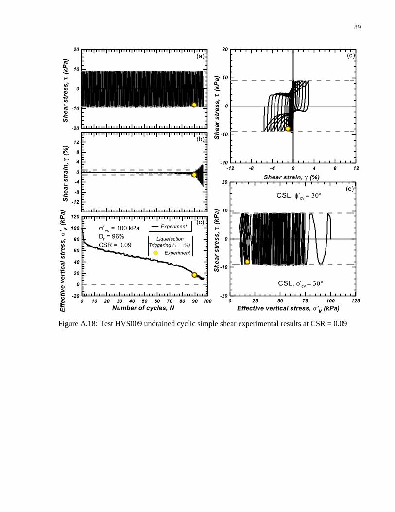
89
Figure A.18: Test HVS009 undrained cyclic simple shear experimental results at CSR = 0.09
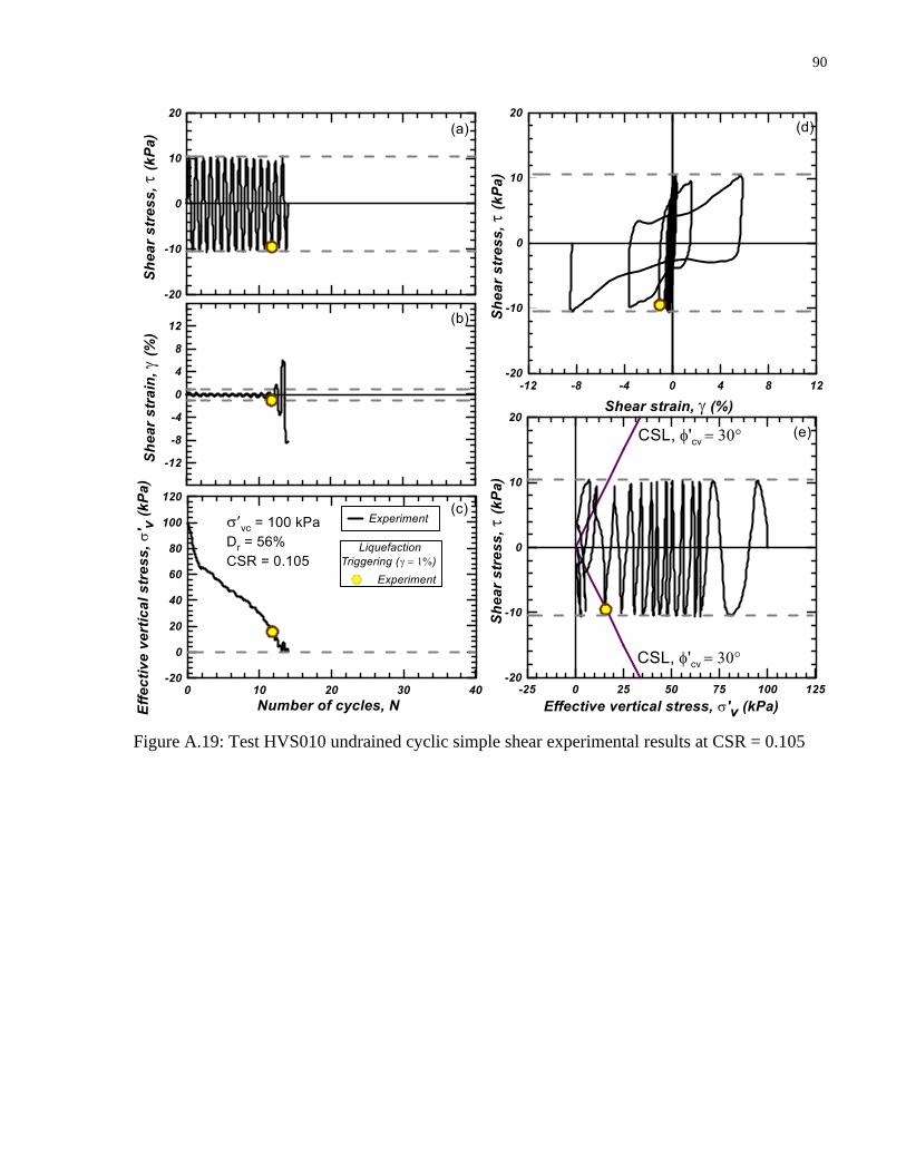
90
Figure A.19: Test HVS010 undrained cyclic simple shear experimental results at CSR = 0.105
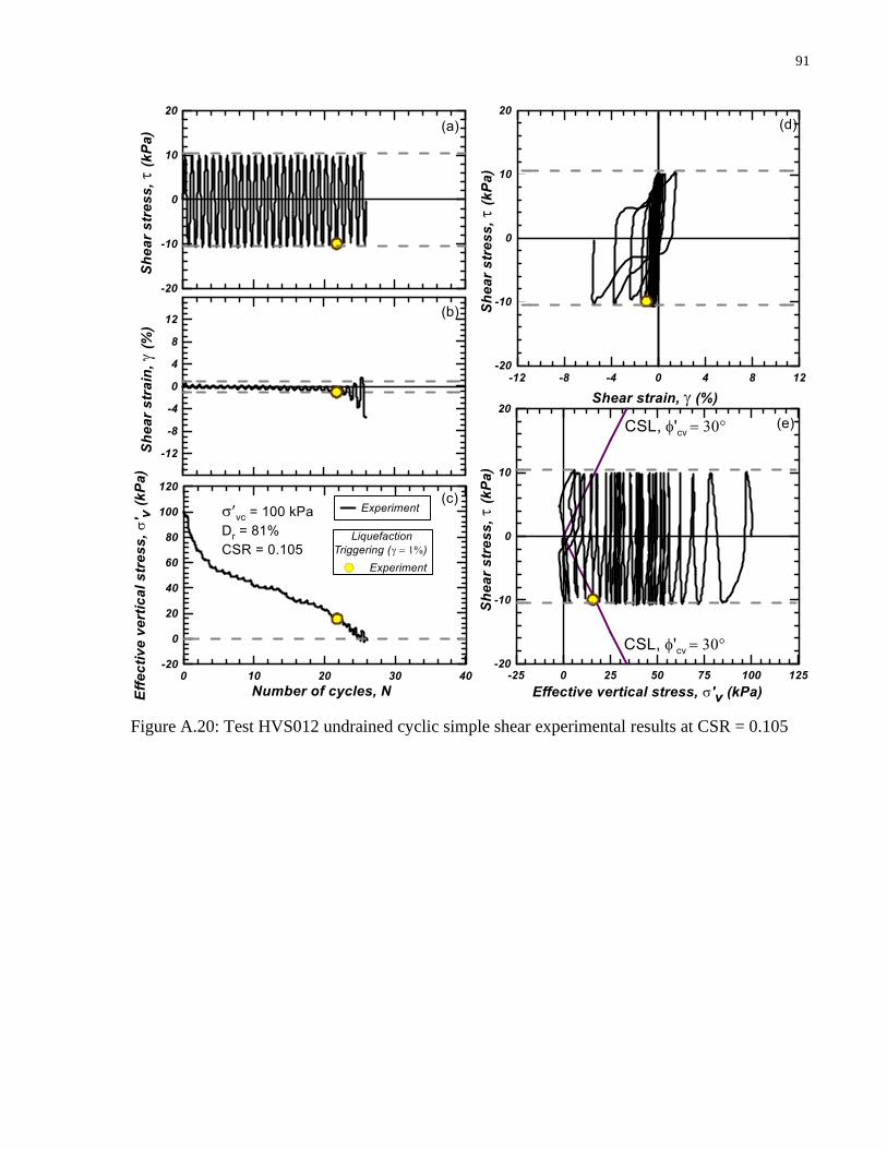
91
Figure A.20: Test HVS012 undrained cyclic simple shear experimental results at CSR = 0.105
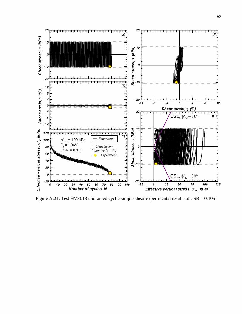
92
Figure A.21: Test HVS013 undrained cyclic simple shear experimental results at CSR = 0.105
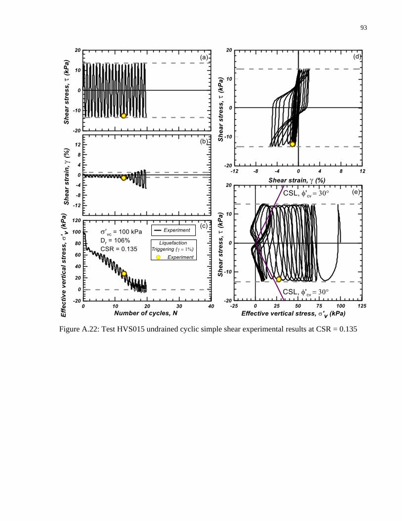
93
Figure A.22: Test HVS015 undrained cyclic simple shear experimental results at CSR = 0.135

94
Figure A.23: Test HVS016 undrained cyclic simple shear experimental results at CSR = 0.135

95
Figure A.24: Test HVS017 undrained cyclic simple shear experimental results at CSR = 0.135
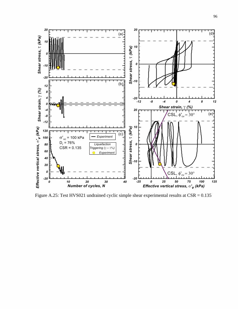
96
Figure A.25: Test HVS021 undrained cyclic simple shear experimental results at CSR = 0.135
97
Appendix B
Mesh Sensitivity Analysis Results

98
B.1 Frictionless Vertical Boundaries, Constant Height and No Top Cap
Rocking
Figure B.1: Undrained monotonic test results of loose specimen (Dr = 24%) varying element size
(ES) and element type for frictionless vertical boundaries, constant height and no top cap rocking
Figure B.2: Undrained monotonic test results of dense specimen (Dr = 146%) varying element size
(ES) and element type for frictionless vertical boundaries, constant height and no top cap rocking
(a) Stress path
(b) Top (y = 19.5 mm) along
centre cross section (z = 0 mm)
at peak shear stress
(a) Stress path
(b) Top (y = 19.5 mm) along
centre cross section (z = 0 mm)
at 4% shear strain

99
Figure B.3: Undrained cyclic test results of loose specimen (Dr = 24%) varying element size (ES)
and element type for frictionless vertical boundaries, constant height and no top cap rocking
Figure B.4: Undrained cyclic test results of dense specimen (Dr = 146%) varying element size (ES)
and element type for frictionless vertical boundaries, constant height and no top cap rocking
(a) Stress path
(b) Top (y = 19.5 mm) along
centre cross section (z = 0 mm)
at peak of load reversal
(a) Stress path
(b) Top (y = 19.5 mm) along
centre cross section (z = 0 mm)
at peak of load reversal
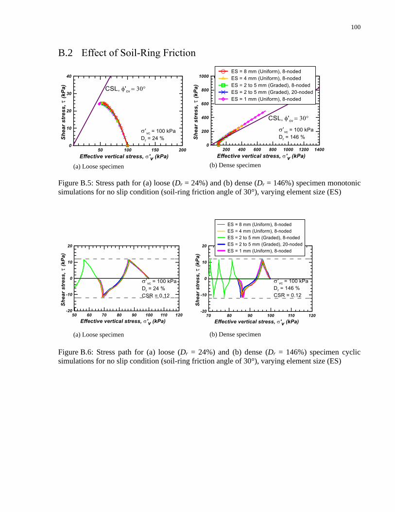
100
B.2 Effect of Soil-Ring Friction
Figure B.5: Stress path for (a) loose (Dr = 24%) and (b) dense (Dr = 146%) specimen monotonic
simulations for no slip condition (soil-ring friction angle of 30°), varying element size (ES)
Figure B.6: Stress path for (a) loose (Dr = 24%) and (b) dense (Dr = 146%) specimen cyclic
simulations for no slip condition (soil-ring friction angle of 30°), varying element size (ES)
(a) Loose specimen (b) Dense specimen
(a) Loose specimen (b) Dense specimen
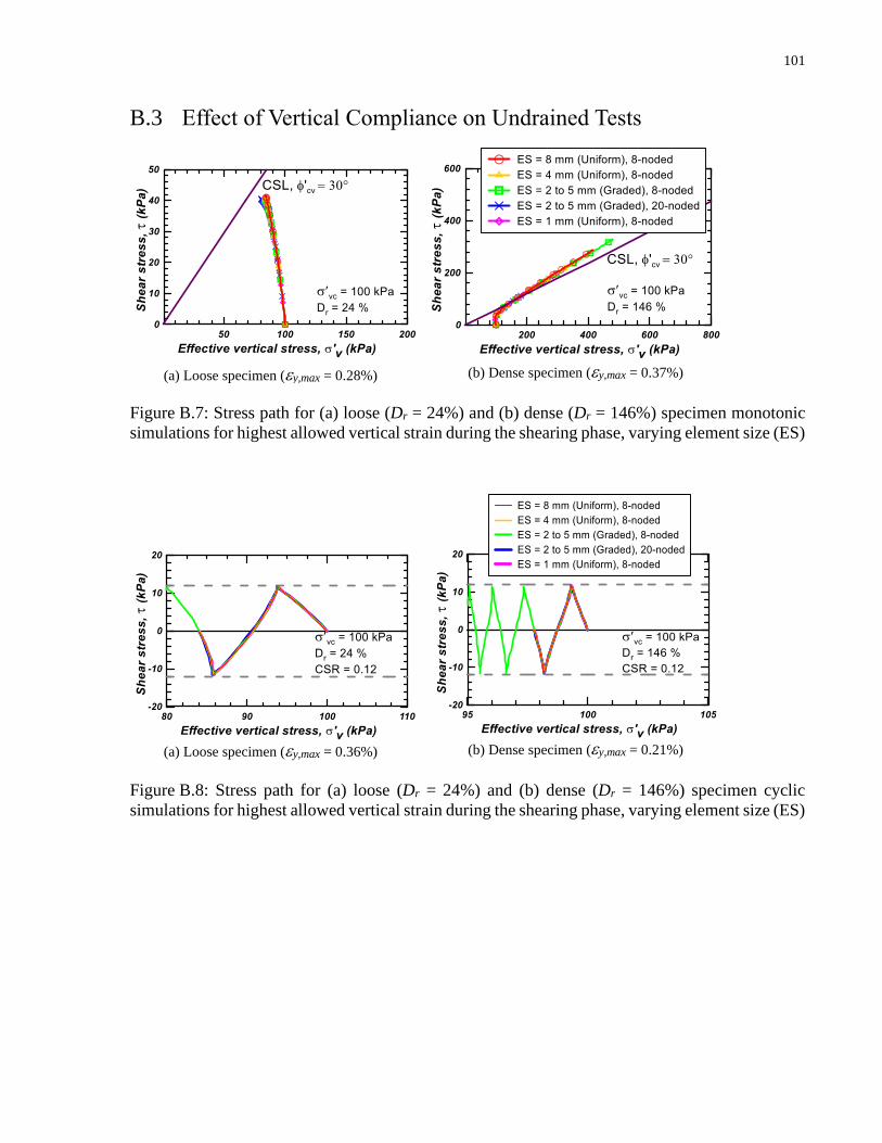
101
B.3 Effect of Vertical Compliance on Undrained Tests
Figure B.7: Stress path for (a) loose (Dr = 24%) and (b) dense (Dr = 146%) specimen monotonic
simulations for highest allowed vertical strain during the shearing phase, varying element size (ES)
Figure B.8: Stress path for (a) loose (Dr = 24%) and (b) dense (Dr = 146%) specimen cyclic
simulations for highest allowed vertical strain during the shearing phase, varying element size (ES)
(a) Loose specimen (y,max = 0.28%) (b) Dense specimen (y,max = 0.37%)
(a) Loose specimen (y,max = 0.36%) (b) Dense specimen (y,max = 0.21%)

102
B.4 Effect of Top cap Rocking During Shear
Figure B.9: Stress path for (a) loose (Dr = 24%) and (b) dense (Dr = 146%) specimen monotonic
simulations for highest top cap rotation (,max) in the analysis, varying element size (ES)
Figure B.10: Stress path for (a) loose (Dr = 24%) and (b) dense (Dr = 146%) specimen cyclic
simulations for highest top cap rotation (,max) in the analysis, varying element size (ES)
(a) Loose specimen (,max = 0.24%) (b) Dense specimen (,max = 0.27%)
(a) Loose specimen (,max = 0.14%) (b) Dense specimen (,max = 0.035%)
103
Appendix C
Simulation Results

104
C.1 Effect of Soil-Ring Friction
C.1.1 Consolidation
Figure C.1: End of consolidation stress distribution of loose specimen (Dr = 24%) simulations for
the centre cross section of the specimen (z = 0 mm), varying soil-ring friction angle (soil-ring)
Figure C.2: Coefficient of lateral earth pressure (K) during consolidation at the core of loose
specimen (Dr = 24%) simulations for varying soil-ring friction angle (soil-ring)
(a) Top (y = 19.5 mm) (b) Left (x = -30.75 mm)
Right (x = 30.75 mm)
(c) Top (y = 19.5 mm)
core

105
Figure C.3: End of consolidation stress distribution of dense specimen (Dr = 146%) simulations
for the centre cross section of the specimen (z = 0 mm), varying soil-ring friction angle (soil-ring)
Figure C.4: Coefficient of lateral earth pressure (K) during consolidation at the core of dense
specimen (Dr = 146%) simulations for varying soil-ring friction angle (soil-ring)
(a) Top (y = 19.5 mm) (b) Left (x = -30.75 mm)
Right (x = 30.75 mm)
(c) Top (y = 19.5 mm)
core
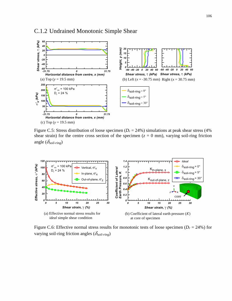
106
C.1.2 Undrained Monotonic Simple Shear
Figure C.5: Stress distribution of loose specimen (Dr = 24%) simulations at peak shear stress (4%
shear strain) for the centre cross section of the specimen (z = 0 mm), varying soil-ring friction
angle (soil-ring)
Figure C.6: Effective normal stress results for monotonic tests of loose specimen (Dr = 24%) for
varying soil-ring friction angles (soil-ring)
(a) Top (y = 19.5 mm)
(b) Left (x = -30.75 mm)
Right (x = 30.75 mm)
(c) Top (y = 19.5 mm)
core
(b) Coefficient of lateral earth pressure (𝐾)
at core of specimen
(a) Effective normal stress results for
ideal simple shear condition

107
Figure C.7: Monotonic test results of loose specimen (Dr = 24%) for varying soil-ring friction
angle (soil-ring)
Figure C.8: Stress distribution of dense specimen (Dr = 146%) simulations at 4% shear strain for
the centre cross section of the specimen (z = 0 mm), varying soil-ring friction angle (soil-ring)
(a) (b)
(c) (d)
(a) Top (y = 19.5 mm)
(b) Left (x = -30.75 mm)
Right (x = 30.75 mm)
(c) Top (y = 19.5 mm)

108
Figure C.9: Effective normal stress results for monotonic tests of dense specimen (Dr = 146%) for
varying soil-ring friction angles (soil-ring)
Figure C.10: Monotonic test results of dense specimen (Dr = 146%) for varying soil-ring friction
angle (soil-ring)
core
(b) Coefficient of lateral earth pressure (𝐾)
at core of specimen
(a) Effective normal stress results for
ideal simple shear condition
(c) (d)
(a) (b)

109
Figure C.11: Monotonic test results of loose specimen (Dr = 24%) varying soil-ring friction angle
(soil-ring) during the shearing phase only
Figure C.12: Monotonic test results of dense specimen (Dr = 146%) varying soil-ring friction angle
(soil-ring) during the shearing phase only
(b) (a)
(c) (d)
(b) (a)
(c) (d)

110
C.1.3 Undrained Cyclic Simple Shear
Figure C.13: Stress distribution of loose specimen (Dr = 24%) simulations for the centre cross
section of the specimen (z = 0 mm) during the peak amplitude of the (a) first and (b) second cycle
for varying soil-ring friction angles (soil-ring)
(a-i) Top (y = 20 mm)
(a-ii) Left (x = 0 mm)
Right (x = 63.5 mm)
(a-iii) Top (y = 20 mm)
(b-ii) Left (x = 0 mm)
Right (x = 63.5 mm)
(b-i) Top (y = 20 mm)
(b-iii) Top (y = 20 mm)
(a) Peak amplitude of first cycle (b) Peak amplitude of second cycle
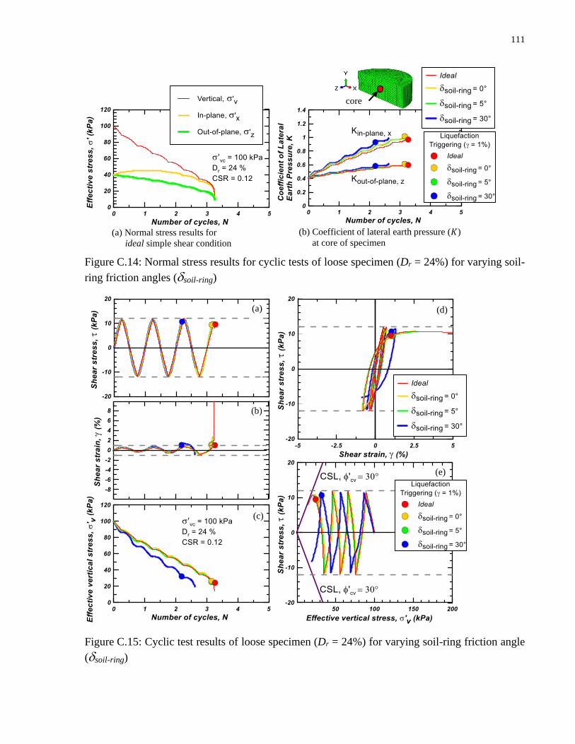
111
Figure C.14: Normal stress results for cyclic tests of loose specimen (Dr = 24%) for varying soil-
ring friction angles (soil-ring)
Figure C.15: Cyclic test results of loose specimen (Dr = 24%) for varying soil-ring friction angle
(soil-ring)
(b) Coefficient of lateral earth pressure (𝐾)
at core of specimen
(a) Normal stress results for
ideal simple shear condition
core
(a)
(b)
(c)
(d)
(e)
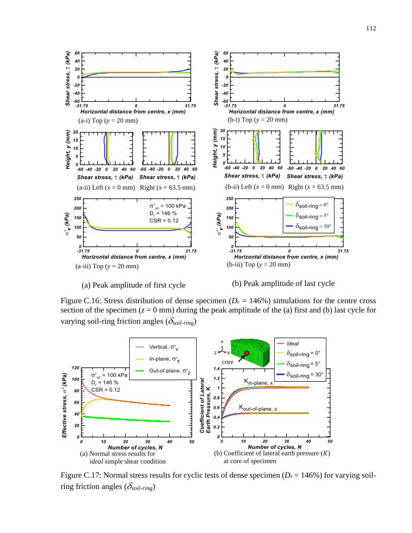
112
Figure C.16: Stress distribution of dense specimen (Dr = 146%) simulations for the centre cross
section of the specimen (z = 0 mm) during the peak amplitude of the (a) first and (b) last cycle for
varying soil-ring friction angles (soil-ring)
Figure C.17: Normal stress results for cyclic tests of dense specimen (Dr = 146%) for varying soil-
ring friction angles (soil-ring)
(a-i) Top (y = 20 mm)
(a-ii) Left (x = 0 mm)
Right (x = 63.5 mm)
(a-iii) Top (y = 20 mm)
(b-ii) Left (x = 0 mm)
Right (x = 63.5 mm)
(b-i) Top (y = 20 mm)
(b-iii) Top (y = 20 mm)
(a) Peak amplitude of first cycle (b) Peak amplitude of last cycle
(b) Coefficient of lateral earth pressure (𝐾)
at core of specimen
(a) Normal stress results for
ideal simple shear condition
core
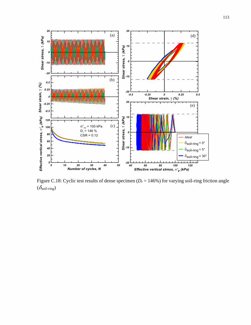
113
Figure C.18: Cyclic test results of dense specimen (Dr = 146%) for varying soil-ring friction angle
(soil-ring)
(a)
(b)
(c)
(d)
(e)
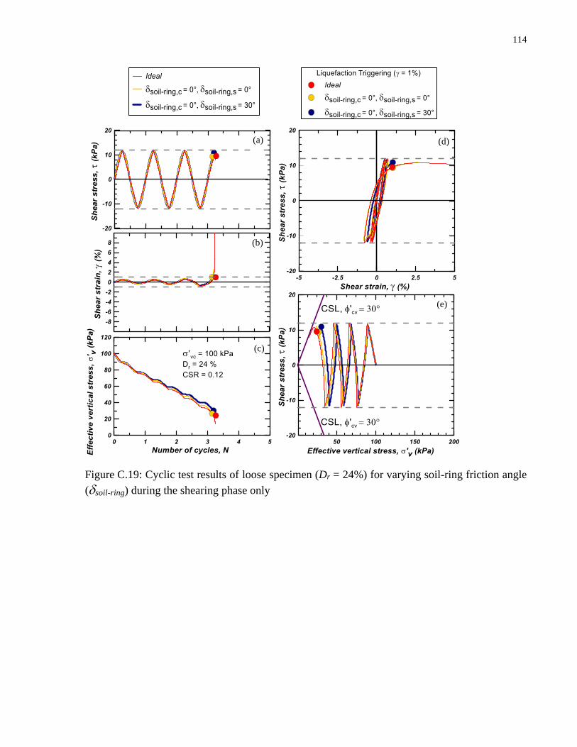
114
Figure C.19: Cyclic test results of loose specimen (Dr = 24%) for varying soil-ring friction angle
(soil-ring) during the shearing phase only
(a)
(b)
(c)
(d)
(e)
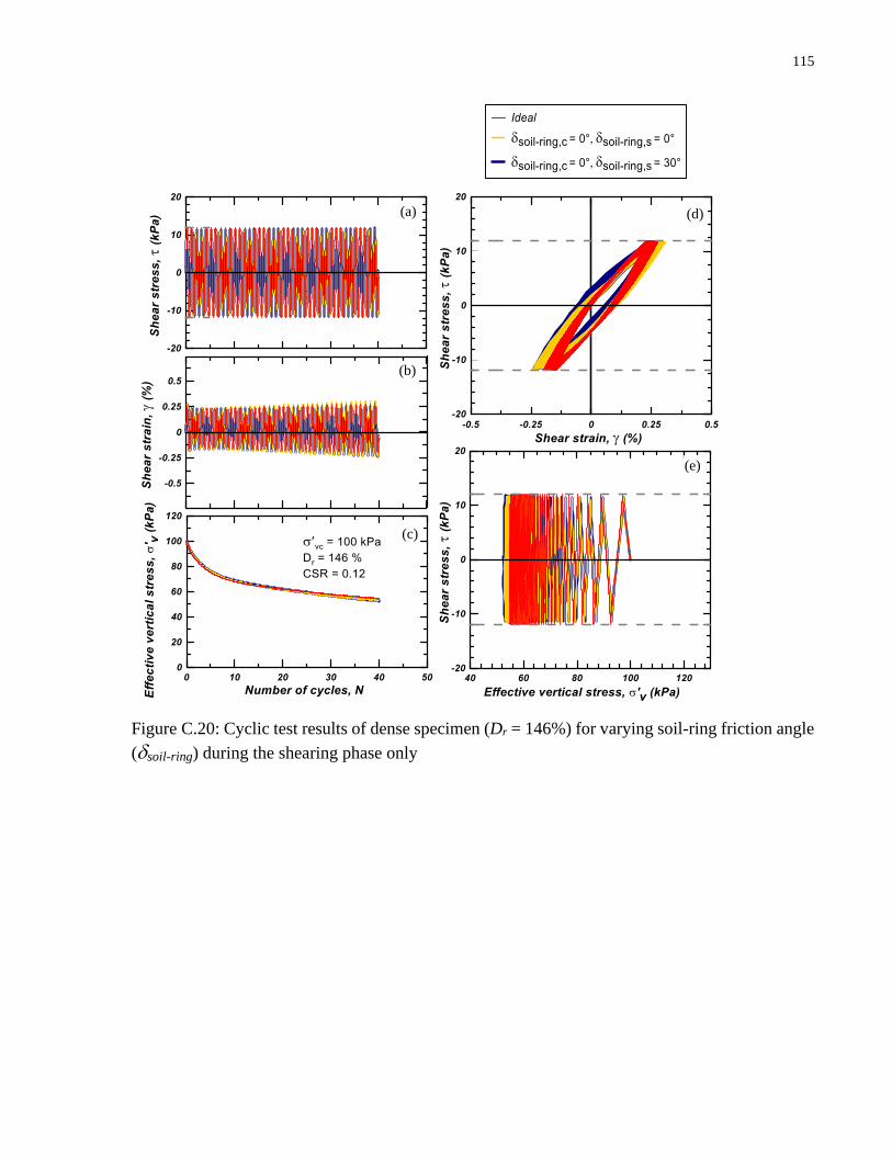
115
Figure C.20: Cyclic test results of dense specimen (Dr = 146%) for varying soil-ring friction angle
(soil-ring) during the shearing phase only
(a)
(b)
(c)
(d)
(e)
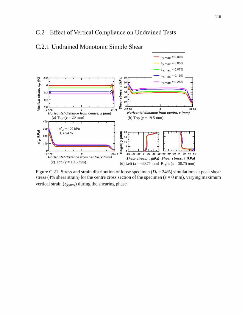
116
C.2 Effect of Vertical Compliance on Undrained Tests
C.2.1 Undrained Monotonic Simple Shear
Figure C.21: Stress and strain distribution of loose specimen (Dr = 24%) simulations at peak shear
stress (4% shear strain) for the centre cross section of the specimen (z = 0 mm), varying maximum
vertical strain (y,max) during the shearing phase
(c) Top (y = 19.5 mm)
(b) Top (y = 19.5 mm)
(d) Left (x = -30.75 mm) Right (x = 30.75 mm)
(a) Top (y = 20 mm)

117
Figure C.22: Monotonic test results of loose specimen (Dr = 24%) for varying maximum vertical
strain (y,max) during the shearing phase
Figure C.23: Stress and strain distribution of dense specimen (Dr = 146%) simulations at 4% shear
strain for the centre cross section of the specimen (z = 0 mm), varying maximum vertical strain
(y,max) during the shearing phase
(a)
(c)
(b)
(d)
(c) Top (y = 19.5 mm)
(b) Top (y = 19.5 mm)
(d) Left (x = -30.75 mm) Right (x = 30.75 mm)
(a) Top (y = 20 mm)

118
Figure C.24: Monotonic test results of dense specimen (Dr = 146%) for varying maximum vertical
strain (y,max) during the shearing phase
(a)
(c)
(b)
(d)
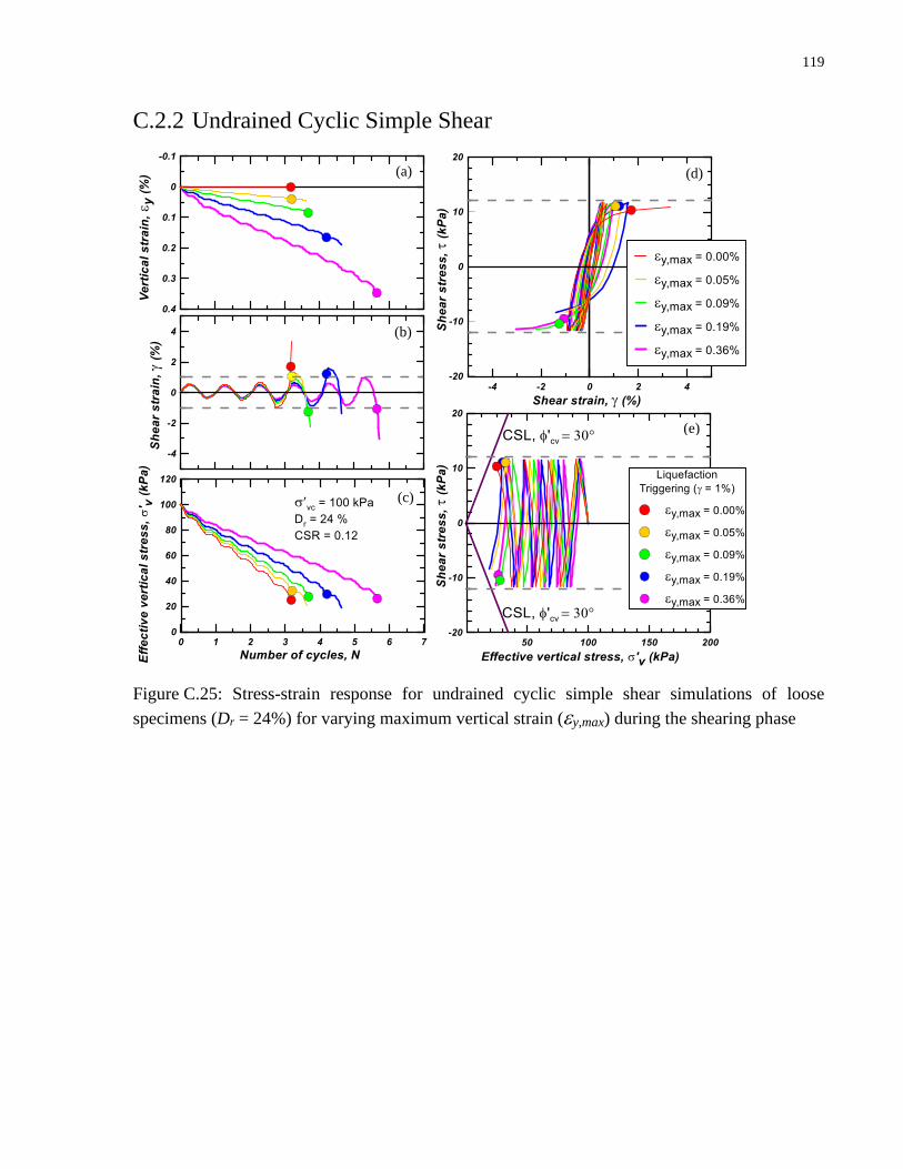
119
C.2.2 Undrained Cyclic Simple Shear
Figure C.25: Stress-strain response for undrained cyclic simple shear simulations of loose
specimens (Dr = 24%) for varying maximum vertical strain (y,max) during the shearing phase
(a)
(b)
(c)
(d)
(e)

120
Figure C.26: Stress-strain response for undrained cyclic simple shear simulations of dense
specimen (Dr = 146%) for varying maximum vertical strain (y,max) during the shearing phase
(a)
(b)
(c)
(d)
(e)
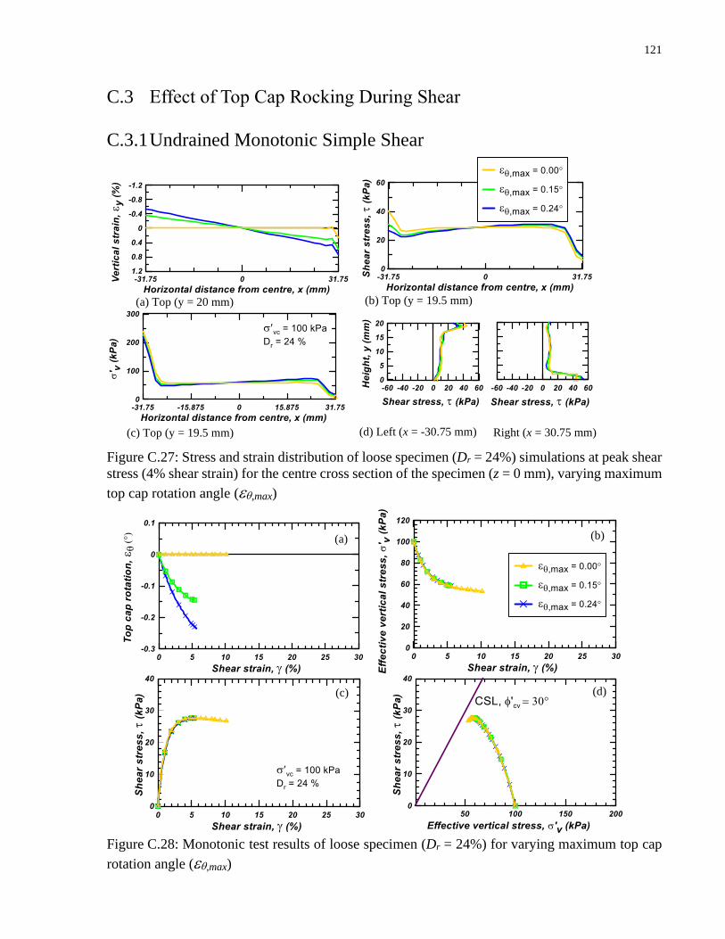
121
C.3 Effect of Top Cap Rocking During Shear
C.3.1 Undrained Monotonic Simple Shear
Figure C.27: Stress and strain distribution of loose specimen (Dr = 24%) simulations at peak shear
stress (4% shear strain) for the centre cross section of the specimen (z = 0 mm), varying maximum
top cap rotation angle (,max)
Figure C.28: Monotonic test results of loose specimen (Dr = 24%) for varying maximum top cap
rotation angle (,max)
(d) Left (x = -30.75 mm)
Right (x = 30.75 mm)
(b) Top (y = 19.5 mm)
(c) Top (y = 19.5 mm)
(a) Top (y = 20 mm)
(a)
(b) CSL 'cv = 30°
(a)
(c)
(b)
(d)

122
Figure C.29: Stress and strain distribution of dense specimen (Dr = 146%) simulations at 4% shear
strain for the centre cross section of the specimen (z = 0 mm), varying maximum top cap rotation
angle (,max)
Figure C.30: Monotonic test results of dense specimen (Dr = 146%) for varying maximum top cap
rotation angle (,max)
(d) Left (x = -30.75 mm)
Right (x = 30.75 mm)
(b) Top (y = 19.5 mm)
(c) Top (y = 19.5 mm)
(a) Top (y = 20 mm)
(a)
(b)
(a)
(c)
(b)
(d)

123
C.3.2 Undrained Cyclic Simple Shear
Figure C.31: Stress and strain distribution of loose specimen (Dr = 24%) simulations during peak
amplitudes (peak) of the first cycle for the centre cross section of the specimen (z = 0 mm), varying
maximum top cap rotation angle (,max)
(d) Left (x = -30.75 mm)
Right (x = 30.75 mm)
(b) Top (y = 19.5 mm)
(c) Top (y = 19.5 mm)
(a) Top (y = 20 mm)

124
Figure C.32: Stress-strain response for undrained cyclic simple shear simulations of loose
specimen (Dr = 24%) for varying maximum top cap rotation angle (,max)
(a)
(b)
(c)
(d)
(e)

125
Figure C.33: Stress and strain distribution of dense specimen (Dr = 146%) simulations during peak
amplitudes (peak) of the first cycle for the centre cross section of the specimen (z = 0 mm), varying
maximum top cap rotation angle (,max)
(d) Left (x = -30.75 mm)
Right (x = 30.75 mm)
(b) Top (y = 19.5 mm)
(c) Top (y = 19.5 mm)
(a) Top (y = 20 mm)
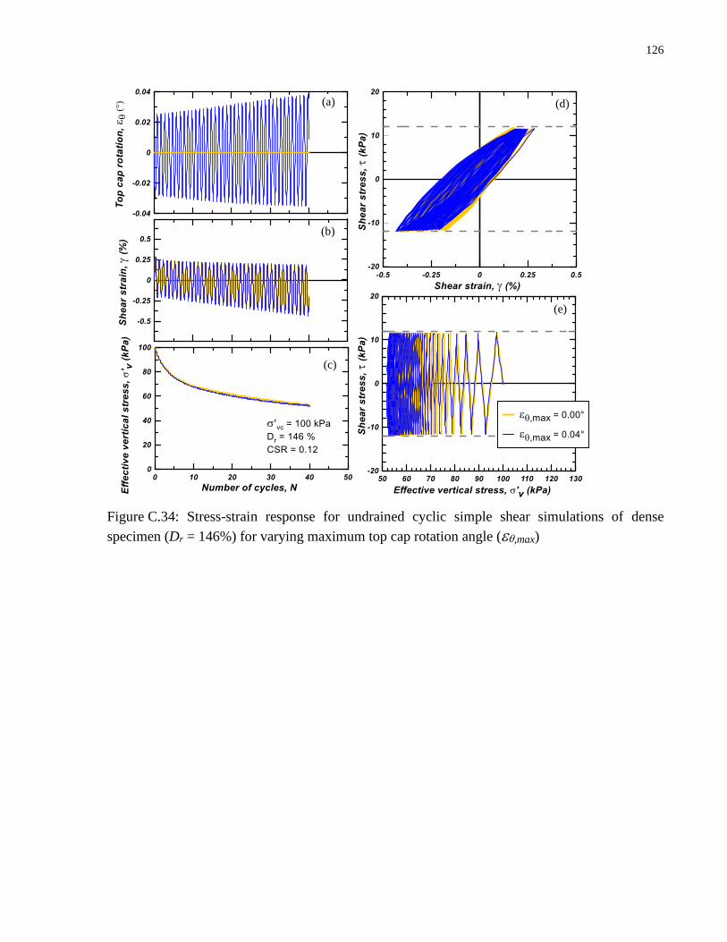
126
Figure C.34: Stress-strain response for undrained cyclic simple shear simulations of dense
specimen (Dr = 146%) for varying maximum top cap rotation angle (,max)
(a)
(b)
(c)
(d)
(e)

127
Dafalias and Manzari (2004) Constitutive Model
UMAT File
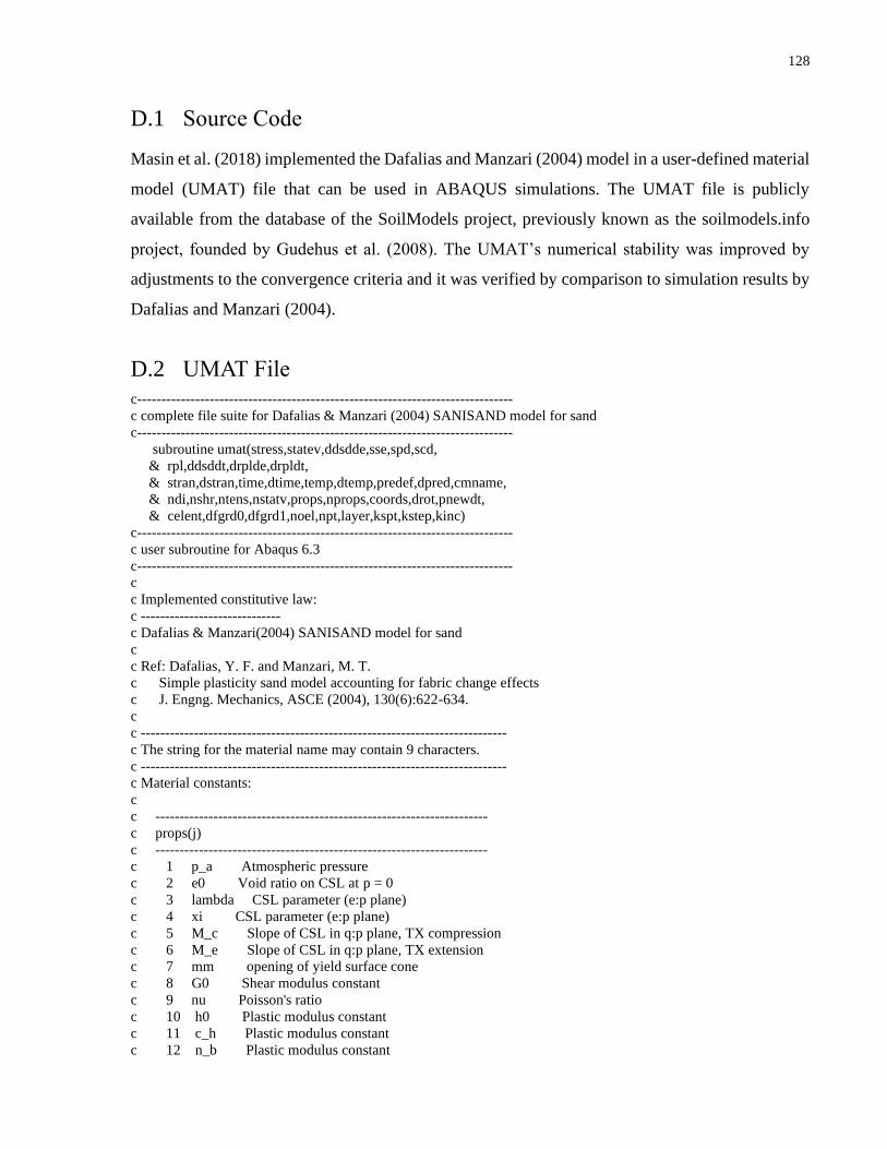
128
D.1 Source Code
Masin et al. (2018) implemented the Dafalias and Manzari (2004) model in a user-defined material
model (UMAT) file that can be used in ABAQUS simulations. The UMAT file is publicly
available from the database of the SoilModels project, previously known as the soilmodels.info
project, founded by Gudehus et al. (2008). The UMAT’s numerical stability was improved by
adjustments to the convergence criteria and it was verified by comparison to simulation results by
Dafalias and Manzari (2004).
D.2 UMAT File
c------------------------------------------------------------------------------
c complete file suite for Dafalias & Manzari (2004) SANISAND model for sand
c------------------------------------------------------------------------------
subroutine umat(stress,statev,ddsdde,sse,spd,scd,
& rpl,ddsddt,drplde,drpldt,
& stran,dstran,time,dtime,temp,dtemp,predef,dpred,cmname,
& ndi,nshr,ntens,nstatv,props,nprops,coords,drot,pnewdt,
& celent,dfgrd0,dfgrd1,noel,npt,layer,kspt,kstep,kinc)
c------------------------------------------------------------------------------
c user subroutine for Abaqus 6.3
c------------------------------------------------------------------------------
c
c Implemented constitutive law:
c -----------------------------
c Dafalias & Manzari(2004) SANISAND model for sand
c
c Ref: Dafalias, Y. F. and Manzari, M. T.
c Simple plasticity sand model accounting for fabric change effects
c J. Engng. Mechanics, ASCE (2004), 130(6):622-634.
c
c ----------------------------------------------------------------------------
c The string for the material name may contain 9 characters.
c ----------------------------------------------------------------------------
c Material constants:
c
c ---------------------------------------------------------------------
c props(j)
c ---------------------------------------------------------------------
c 1 p_a Atmospheric pressure
c 2 e0 Void ratio on CSL at p = 0
c 3 lambda CSL parameter (e:p plane)
c 4 xi CSL parameter (e:p plane)
c 5 M_c Slope of CSL in q:p plane, TX compression
c 6 M_e Slope of CSL in q:p plane, TX extension
c 7 mm opening of yield surface cone
c 8 G0 Shear modulus constant
c 9 nu Poisson's ratio
c 10 h0 Plastic modulus constant
c 11 c_h Plastic modulus constant
c 12 n_b Plastic modulus constant

129
c 13 A0 Dilatancy constant
c 14 n_d Dilatancy constant
c 15 z_max Fabric index constant
c 16 c_z Fabric index constant
c 17 bulk_w Pore water bulk modulus (undrained conditions)
c 18 p_tmult shift of mean stress pt=p_tmult*p_a
c 19 initial value of void ratio
c ----------------------------------------------------------------------
c
c Solution dependent state variables (statev):
c definition via sdvini
c
c group 1: internal variables (14 variables)
c
c 1 ... alpha_11 back stress, orientation of yield surface cone
c 2 ... alpha_22
c 3 ... alpha_33
c 4 ... alpha_12
c 5 ... alpha_13
c 6 ... alpha_23
c
c 7 ... void void ratio
c
c 8 ... Fab_11 fabric tensor z
c 9 ... Fab_22
c 10 ... Fab_33
c 11 ... Fab_12
c 12 ... Fab_13
c 13 ... Fab_23
c
c 14 ... not used
c
c group 2: memory variables for shear reversal (SR) and other purposes
c
c 15 ... alpha_sr_11 alpha value at stress reversal points (discrete update)
c 16 ... alpha_sr_22
c 17 ... alpha_sr_33
c 18 ... alpha_sr_12
c 19 ... alpha_sr_13
c 20 ... alpha_sr_23
c
c 21 ... not used
c 22 ... not used
c 23 ... not used
c 24 ... not used
c 25 ... not used
c 26 ... not used
c 27 ... not used
c
c 28 ... not used
c
c group 3: variables saved for post processing or other purposes
c
c 29 ... pore excess pore pressure (undrained case)
c 30 ... p mean effective stress
c 31 ... q deviator stress
c 32 ... z Lode parameter (cos(3theta))
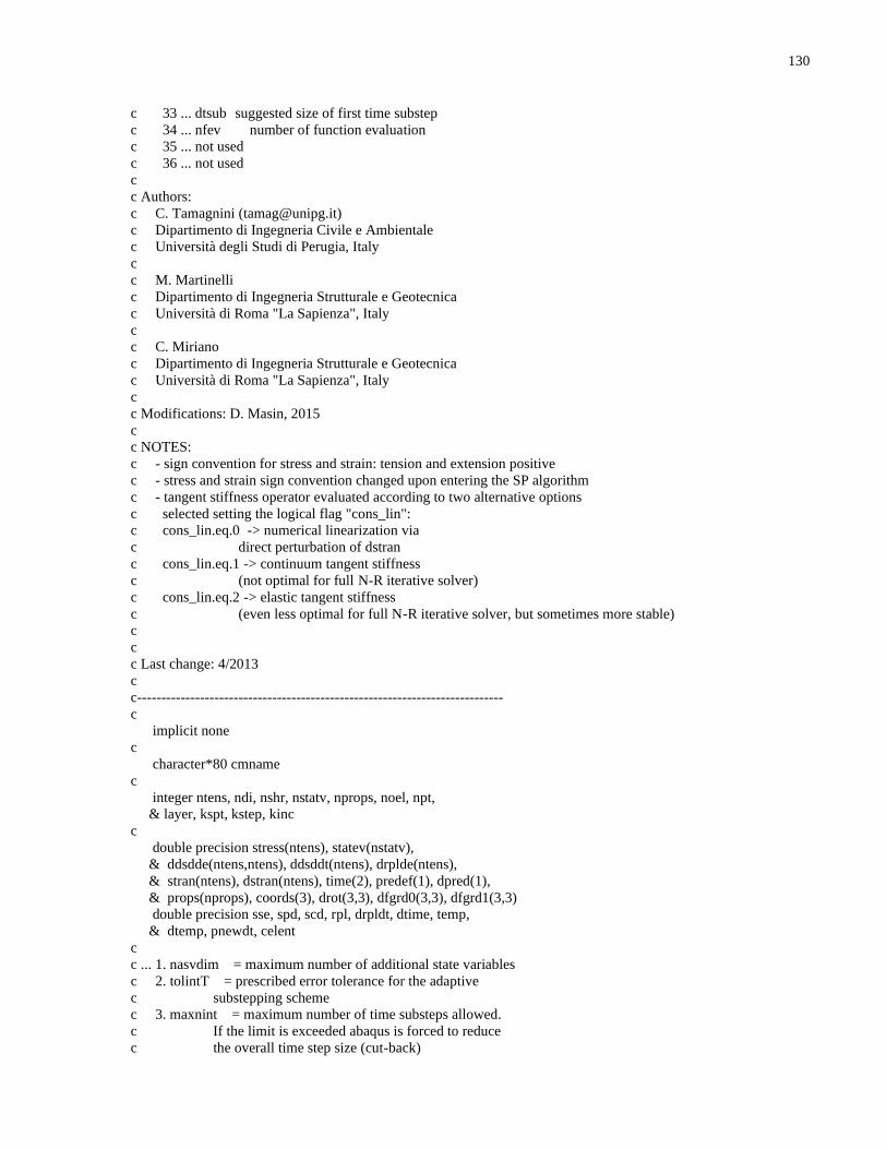
130
c 33 ... dtsub suggested size of first time substep
c 34 ... nfev number of function evaluation
c 35 ... not used
c 36 ... not used
c
c Authors:
c C. Tamagnini ([email protected])
c Dipartimento di Ingegneria Civile e Ambientale
c Università degli Studi di Perugia, Italy
c
c M. Martinelli
c Dipartimento di Ingegneria Strutturale e Geotecnica
c Università di Roma "La Sapienza", Italy
c
c C. Miriano
c Dipartimento di Ingegneria Strutturale e Geotecnica
c Università di Roma "La Sapienza", Italy
c
c Modifications: D. Masin, 2015
c
c NOTES:
c - sign convention for stress and strain: tension and extension positive
c - stress and strain sign convention changed upon entering the SP algorithm
c - tangent stiffness operator evaluated according to two alternative options
c selected setting the logical flag "cons_lin":
c cons_lin.eq.0 -> numerical linearization via
c direct perturbation of dstran
c cons_lin.eq.1 -> continuum tangent stiffness
c (not optimal for full N-R iterative solver)
c cons_lin.eq.2 -> elastic tangent stiffness
c (even less optimal for full N-R iterative solver, but sometimes more stable)
c
c
c Last change: 4/2013
c
c----------------------------------------------------------------------------
c
implicit none
c
character*80 cmname
c
integer ntens, ndi, nshr, nstatv, nprops, noel, npt,
& layer, kspt, kstep, kinc
c
double precision stress(ntens), statev(nstatv),
& ddsdde(ntens,ntens), ddsddt(ntens), drplde(ntens),
& stran(ntens), dstran(ntens), time(2), predef(1), dpred(1),
& props(nprops), coords(3), drot(3,3), dfgrd0(3,3), dfgrd1(3,3)
double precision sse, spd, scd, rpl, drpldt, dtime, temp,
& dtemp, pnewdt, celent
c
c ... 1. nasvdim = maximum number of additional state variables
c 2. tolintT = prescribed error tolerance for the adaptive
c substepping scheme
c 3. maxnint = maximum number of time substeps allowed.
c If the limit is exceeded abaqus is forced to reduce
c the overall time step size (cut-back)
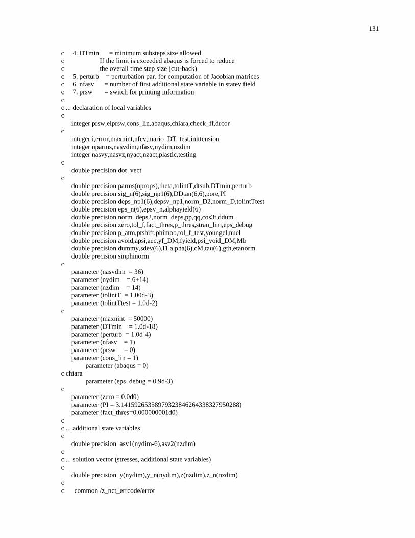
131
c 4. DTmin = minimum substeps size allowed.
c If the limit is exceeded abaqus is forced to reduce
c the overall time step size (cut-back)
c 5. perturb = perturbation par. for computation of Jacobian matrices
c 6. nfasv = number of first additional state variable in statev field
c 7. prsw = switch for printing information
c
c ... declaration of local variables
c
integer prsw,elprsw,cons_lin,abaqus,chiara,check_ff,drcor
c
integer i,error,maxnint,nfev,mario_DT_test,inittension
integer nparms,nasvdim,nfasv,nydim,nzdim
integer nasvy,nasvz,nyact,nzact,plastic,testing
c
double precision dot_vect
c
double precision parms(nprops),theta,tolintT,dtsub,DTmin,perturb
double precision sig_n(6),sig_np1(6),DDtan(6,6),pore,PI
double precision deps_np1(6),depsv_np1,norm_D2,norm_D,tolintTtest
double precision eps_n(6),epsv_n,alphayield(6)
double precision norm_deps2,norm_deps,pp,qq,cos3t,ddum
double precision zero,tol_f,fact_thres,p_thres,stran_lim,eps_debug
double precision p_atm,ptshift,phimob,tol_f_test,youngel,nuel
double precision avoid,apsi,aec,yf_DM,fyield,psi_void_DM,Mb
double precision dummy,sdev(6),I1,alpha(6),cM,tau(6),gth,etanorm
double precision sinphinorm
c
parameter (nasvdim = 36)
parameter (nydim = 6+14)
parameter (nzdim = 14)
parameter (tolintT = 1.00d-3)
parameter (tolintTtest = 1.0d-2)
c
parameter (maxnint = 50000)
parameter (DTmin = 1.0d-18)
parameter (perturb = 1.0d-4)
parameter (nfasv = 1)
parameter (prsw = 0)
parameter (cons_lin = 1)
parameter (abaqus = 0)
c chiara
parameter (eps_debug = 0.9d-3)
c
parameter (zero = 0.0d0)
parameter (PI = 3.14159265358979323846264338327950288)
parameter (fact_thres=0.000000001d0)
c
c ... additional state variables
c
double precision asv1(nydim-6),asv2(nzdim)
c
c ... solution vector (stresses, additional state variables)
c
double precision y(nydim),y_n(nydim),z(nzdim),z_n(nzdim)
c
c common /z_nct_errcode/error
132
c common /z_tolerance/tol_f
c common /z_check_yeld/check_ff
c common /z_drift_correction/drcor
c common /z_threshold_pressure/p_thres
c
tol_f=1.0d-6
tol_f_test=1.0d-6
check_ff=0
drcor=1
plastic=0
phimob=0.0d0
ptshift=0.0d0
c
c
c ... Error Management:
c ----------------
c error = 0 ... no problem in time integration
c error = 1 ... problems in evaluation of the time rate, (e.g. undefined
c stress state), reduce time integration substeps
c error = 3 ... problems in time integration, reduce abaqus load increment
c (cut-back)
c error=10 ... severe error, terminate calculation
c
error=0
c
c ... check problem dimensions
c
if (ndi.ne.3) then
c
write(6,*) 'ERROR: this UMAT can be used only for elements'
write(6,*) ' with 3 direct stress/strain components'
write(6,*) 'noel = ',noel
error=10
c
endif
c open(unit=6,position='Append',file=
c . 'C:/users/david/data/Zhejiang/plaxis-sani/UMATdebug.txt')
c
c ... check material parameters and move them to array parms
c
nparms=nprops
call check_parms_DM(props,parms,nparms)
c
c ... print informations about time integration, useful when problems occur
c
p_atm=parms(1)
p_thres=fact_thres*p_atm
c
elprsw = 0
if (prsw .ne. 0) then
c
c ... print only in some defined elements
c
c if ((noel.eq.101).and.(npt.eq.1)) elprsw = 1
c
endif
133
c
c ... define number of additional state variables
c
call define(nasvy,nasvz)
nyact = 6 + nasvy
nzact = nasvz
if (nyact.gt.nydim) then
write(6,*) 'ERROR:nydim too small; program terminated'
error=10
elseif (nzact.gt.nzdim) then
write(6,*) 'ERROR:nzdim too small; program terminated'
error=10
endif
c
c ... suggested time substep size, and initial excess pore pressure
c
pore = statev(29)
c
c ... changes sign conventions for stresses and strains, compute
c current effective stress tensor and volumetric strain
c
ptshift=parms(18)*parms(1)
do i=1,3
stress(i) = stress(i)-ptshift
enddo
call move_sig(stress,ntens,-1*ptshift,sig_n)
call move_sig(stress,ntens,pore,sig_n)
call move_eps(dstran,ntens,deps_np1,depsv_np1)
call move_eps(stran,ntens,eps_n,epsv_n)
norm_D2=dot_vect(2,deps_np1,deps_np1,6)
norm_D=sqrt(norm_D2)
c chiara
if (eps_n(1).gt.eps_debug) then
chiara=1
end if
c
c ... initialise void ratio and yield surface inclination
c
if (statev(7) .lt. 0.001) then
do i=1,6
alphayield(i)=zero
end do
call deviator(sig_n,alphayield,ddum,pp)
avoid=0
if(parms(19) .le. 5.0) then
avoid=parms(19)
else if(parms(19) .gt. 5.0) then
apsi=parms(19)-10.0d0
aec=parms(2)-parms(3)*(pp/parms(1))**parms(4)
avoid=aec+apsi
endif
statev(7)=avoid
do i=1,6
statev(i)=alphayield(i)/pp
134
statev(i+14)=alphayield(i)/pp
end do
end if
c
c ... move vector of additional state variables into asv1(nydim) and asv2(nzdim)
c
do i=1,nasvy
asv1(i) = statev(i-1+nfasv)
enddo
c
do i=1,nasvz
asv2(i) = statev(i-1+nfasv+nasvy)
enddo
c
c --------------------
c ... Time integration
c --------------------
c
call iniyz(y,nydim,z,nzdim,asv1,nasvy,asv2,nasvz,sig_n,ntens)
call push(y,y_n,nydim)
call push(z,z_n,nzdim)
c
if (elprsw.ne.0) then
write(6,*) '================================================='
write(6,*) ' Call of UMAT - DM SANISAND model: '
write(6,*) '================================================='
call wrista(3,y,nydim,deps_np1,dtime,coords,statev,nstatv,
& parms,nparms,noel,npt,ndi,nshr,kstep,kinc)
endif
c
c ... local integration using adaptive RKF-23 method with error control
c
if((dtsub.le.zero).or.(dtsub.gt.dtime)) then
dtsub = dtime
end if
testing=0
c For use in PLAXIS, activate the following line
c if(kstep.eq.1 .AND. kinc.eq.1) testing=1
c For use in ABAQUS, the line above should be inactive
if(norm_D.eq.0) testing=2
c FEM asking for ddsdde only
nfev = 0 ! initialisation
if(testing.eq.1) then
call rkf23_upd_DM(y,z,nyact,nasvy,nasvz,tolintTtest,maxnint,
& DTmin,deps_np1,parms,nparms,nfev,elprsw,
& mario_DT_test,
& error,tol_f_test,check_ff,drcor,p_thres,plastic)
c ... give original state if the model fails without substepping
if(error.ne.0) then
do i=1,nyact
y(i)=y_n(i)
end do
error=0
135
end if
else if(testing.eq.2) then
do i=1,nyact
y(i)=y_n(i)
end do
c ... Normal RKF23 integration
else !testing.eq.0
call rkf23_upd_DM(y,z,nyact,nasvy,nasvz,tolintT,maxnint,
& DTmin,deps_np1,parms,nparms,nfev,elprsw,
& mario_DT_test,
& error,tol_f,check_ff,drcor,p_thres,plastic)
end if
c
c ... error conditions (if any)
c
if(mario_DT_test.eq.1) then
call wrista(4,y,nydim,deps_np1,dtime,coords,statev,nstatv,
& parms,nparms,noel,npt,ndi,nshr,kstep,kinc)
endif
c
if(error.eq.3) then
c
c ... reduce abaqus load increment
c
call wrista(2,y,nydim,deps_np1,dtime,coords,statev,nstatv,
& parms,nparms,noel,npt,ndi,nshr,kstep,kinc)
write(6,*) 'subroutine UMAT: reduce step size in ABAQUS'
write(6,*) 'error 3 activated'
if(abaqus.ne.0) then
pnewdt = 0.25d0
else
c ... write a message and return the original state
do i=1,nyact
y(i)=y_n(i)
end do
endif
c
c if(abaqus.eq.0) then
c write(6,*) 'analysis ended because number of time '
c write(6,*) 'substeps exceeded maximum number allowed'
c write(6,*) ' (maxnint)'
c call xit_DM
c endif
return
c
elseif(error.eq.10) then
write(6,*) 'error 10 activated'
c
call wrista(2,y,nydim,deps_np1,dtime,coords,statev,nstatv,
& parms,nparms,noel,npt,ndi,nshr,kstep,kinc)
call xit_DM
c
endif
c
c ... update dtsub and nfev

136
c
if(dtsub.le.0.0d0) then
dtsub = 0
else if(dtsub.ge.dtime) then
dtsub = dtime
end if
statev(33)=dtsub
statev(34)=dfloat(nfev)
c
c ... computation of Jacobian matrix
c
error=0
if(cons_lin.eq.0) then
c
c ... parameter of the numerical differentiation
c double precision
c
norm_deps2=dot_vect(2,deps_np1,deps_np1,ntens)
norm_deps=dsqrt(norm_deps2)
theta=perturb*max(norm_deps,1.0d-6)
c
c ... compute consistent tangent via numerical perturbation
c
call pert_DM(y_n,y,z,nyact,nasvy,nasvz,tolintT,maxnint,DTmin,
& deps_np1,parms,nparms,nfev,elprsw,theta,ntens,DDtan,
& error,tol_f,check_ff,drcor,p_thres,plastic)
c
else
c
call tang_stiff(y,z,nyact,nasvy,nasvz,parms,nparms,
& DDtan,cons_lin,
& error,tol_f,check_ff,drcor,p_thres,plastic)
c
endif
c
if(error.ne.0) then
write(6,*) 'some error in pert or tang_stiff, value=',error
c
c call wrista(2,y,nydim,deps_np1,dtime,coords,statev,nstatv,
c & parms,nparms,noel,npt,ndi,nshr,kstep,kinc)
c call xit_DM
c
endif
c
c ... convert solution (stress + cons. tangent) to abaqus format
c update pore pressure and compute total stresses
inittension=0
c just checks for NAN
call check_RKF_DM(inittension,y,nyact,nasvy,parms,nparms)
if (inittension.ne.0) then
do i=1,nyact
y(i)=y_n(i)
end do
end if
c

137
call solout(stress,ntens,asv1,nasvy,asv2,nasvz,ddsdde,
+ y,nydim,z,pore,depsv_np1,parms,nparms,DDtan)
c
c ... updated vector of additional state variables to abaqus statev vector
c
do i=1,nasvy
statev(i-1+nfasv) = asv1(i)
end do
c
do i=1,nasvz
statev(i-1+nfasv+nasvy) = asv2(i)
enddo
c
c ... transfer additional information to statev vector
c
do i=1,6
sig_np1(i)=y(i)
end do
call inv_sig(sig_np1,pp,qq,cos3t)
c
statev(29) = pore
statev(30) = pp
statev(31) = qq
statev(32) = cos3t
cM=parms(6)/parms(5)
alpha(1)=y(7)
alpha(2)=y(8)
alpha(3)=y(9)
alpha(4)=y(10)
alpha(5)=y(11)
alpha(6)=y(12)
call deviator(sig_np1,sdev,I1,pp)
do i=1,6
tau(i)=sdev(i)-pp*alpha(i)
end do
call lode_DM(tau,cM,cos3t,gth,dummy)
etanorm=gth*qq/pp
sinphinorm=3*etanorm/(6+etanorm)
statev(33) = asin(sinphinorm)*180/PI
statev(34) = nfev
c check that bounding surtface is not violated
c if (noel.eq.324 .and. npt.eq.3) then
c fyield=yf_DM(y,nyact,parms,nparms)
c apsi=psi_void_DM(statev(7),pp,parms,nparms)
c Mb=parms(5)*dexp(-parms(12)*apsi)
c write(6,*) 'fyield=',fyield
c write(6,*) 'psi=',apsi
c write(6,*) 'Mb=',Mb
c write(6,*) 'qq/pp*gth=',qq/pp*gth
c write(6,*) '---------------------'
c end if
do i=1,3
stress(i) = stress(i)+ptshift
enddo

138
c close(6)
c
c -----------------------
c End of time integration
c -----------------------
c
return
end
c
c
cccccccccccccccccccccccccccccccccccccccccccccccccccccccccccccccccccccccccccccccc
c
c
c-----------------------------------------------------------------------------
subroutine alpha_th_DM(flag,n,gth,psi,parms,nparms,alpha)
c-----------------------------------------------------------------------------
c calculate tensors:
c
c alpha_c => flag = 1
c alpha_b => flag = 2
c alpha_d => flag = 3
c
c Dafalias & Manzari (2004) SANISAND model for sands
c
c variables allocated in parms
c
c 1 p_a Atmospheric pressure
c 2 e0 Void ratio on CSL at p = 0
c 3 lambda CSL parameter (e:p plane)
c 4 xi CSL parameter (e:p plane)
c 5 M_c Slope of CSL in q:p plane, TX compression
c 6 M_e Slope of CSL in q:p plane, TX extension
c 7 mm opening of yield surface cone
c 8 G0 Shear modulus constant
c 9 nu Poisson's ratio
c 10 h0 Plastic modulus constant
c 11 c_h Plastic modulus constant
c 12 n_b Plastic modulus constant
c 13 A0 Dilatancy constant
c 14 n_d Dilatancy constant
c 15 z_max Fabric index constant
c 16 c_z Fabric index constant
c 17 bulk_w Pore water bulk modulus (undrained conditions)
c
c written 10/2008 (Tamagnini)
c-----------------------------------------------------------------------------
implicit none
c
integer flag,nparms,i
c
double precision n(6),gth,psi,parms(nparms),alpha(6)
double precision M_c,mm,n_b,n_d
c
double precision M,alpha_th
double precision two,three,sqrt23
c
data two,three/2.0d0,3.0d0/
139
c
sqrt23=dsqrt(two/three)
c
c ... recover material parameters
c
M_c=parms(5)
mm=parms(7)
n_b=parms(12)
n_d=parms(14)
c
c ... select which alpha tensor to evaluate
c
if(flag.eq.1) then
c
c ... critical state cone
c
M=M_c
c
elseif(flag.eq.2) then
c
c ... bounding surface cone
c
M=M_c*dexp(-n_b*psi)
c
else
c
c ... dilatancy cone
c
M=M_c*dexp(n_d*psi)
c
endif
c
c ... tensor alpha_ij
c
alpha_th=M*gth-mm
c
do i=1,6
alpha(i)=sqrt23*alpha_th*n(i)
end do
c
return
end
c
c
cccccccccccccccccccccccccccccccccccccccccccccccccccccccccccccccccccccccccccccccc
c
c
c-----------------------------------------------------------------------------
subroutine check_crossing(y,y_tr,n,parms,nparms,prod)
c-----------------------------------------------------------------------------
c
c computes
c
c prod := dsig_tr*grad(f)_k
c
c useful for checking if crossing of yield locus occurs whenever
c f_k = 0 and f_tr > 0
140
c
c variables allocated in vector y(n):
c
c y(1) = sig(1)
c y(2) = sig(2)
c y(3) = sig(3)
c y(4) = sig(4)
c y(5) = sig(5)
c y(6) = sig(6)
c y(7) = alpha(1)
c y(8) = alpha(2)
c y(9) = alpha(3)
c y(10) = alpha(4)
c y(11) = alpha(5)
c y(12) = alpha(6)
c y(13) = void
c y(14) = Fab(1)
c y(15) = Fab(2)
c y(16) = Fab(3)
c y(17) = Fab(4)
c y(18) = Fab(5)
c y(19) = Fab(6)
c y(20) = not used
c
c-----------------------------------------------------------------------------
implicit none
c
integer i,n,nparms
c
double precision dot_vect
c
double precision y(n),y_tr(n),parms(nparms)
double precision P(6),P1(6),dsig_tr(6)
double precision prod
c
c ... gradient of yield surface at state y_k
c
call grad_f_DM(y,n,parms,nparms,P,P1)
c
do i=1,6
dsig_tr(i)=y_tr(i)-y(i)
end do ! i
c
prod=dot_vect(1,P,dsig_tr,6)
c
return
end
c
c
cccccccccccccccccccccccccccccccccccccccccccccccccccccccccccccccccccccccccccccccc
c
c
c-----------------------------------------------------------------------------
subroutine check_parms_DM(props,parms,nprops)
c-----------------------------------------------------------------------------
c checks input material parameters for Dafalias & Manzari (2004)
c SANISAND model for sand
141
c
c Material constants:
c
c ---------------------------------------------------------------------
c props(j)
c ---------------------------------------------------------------------
c 1 p_a Atmospheric pressure
c 2 e0 Void ratio on CSL at p = 0
c 3 lambda CSL parameter (e:p plane)
c 4 xi CSL parameter (e:p plane)
c 5 M_c Slope of CSL in q:p plane, TX compression
c 6 M_e Slope of CSL in q:p plane, TX extension
c 7 mm opening of yield surface cone
c 8 G0 Shear modulus constant
c 9 nu Poisson's ratio
c 10 h0 Plastic modulus constant
c 11 c_h Plastic modulus constant
c 12 n_b Plastic modulus constant
c 13 A0 Dilatancy constant
c 14 n_d Dilatancy constant
c 15 z_max Fabric index constant
c 16 c_z Fabric index constant
c 17 bulk_w Pore water bulk modulus (undrained conditions)
c ---------------------------------------------------------------------
c
c Solution dependent state variables (statev):
c definition via sdvini
c
c group 1: internal variables (14 variables)
c
c 1 ... alpha_11 back stress, orientation of yield surface cone
c 2 ... alpha_22
c 3 ... alpha_33
c 4 ... alpha_12
c 5 ... alpha_13
c 6 ... alpha_23
c
c 7 ... void void ratio
c
c 8 ... Fab_11 fabric tensor z
c 9 ... Fab_22
c 10 ... Fab_33
c 11 ... Fab_12
c 12 ... Fab_13
c 13 ... Fab_23
c
c 14 ... not used
c
c group 2: memory variables for shear reversal (SR) and other purposes
c
c 15 ... alpha_sr_11 alpha value at stress reversal points (discrete update)
c 16 ... alpha_sr_22
c 17 ... alpha_sr_33
c 18 ... alpha_sr_12
c 19 ... alpha_sr_13
c 20 ... alpha_sr_23
c
142
c 21 ... not used
c 22 ... not used
c 23 ... not used
c 24 ... not used
c 25 ... not used
c 26 ... not used
c 27 ... not used
c
c 28 ... not used
c
c group 3: variables saved for post processing or other purposes
c
c 29 ... pore excess pore pressure (undrained case)
c 30 ... p mean effective stress
c 31 ... q deviator stress
c 32 ... z Lode parameter (cos(3theta))
c 33 ... dtsub suggested size of first time substep
c 34 ... nfev number of function evaluation
c 35 ... not used
c 36 ... not used
c
c-----------------------------------------------------------------------------
implicit none
c
integer nprops
c
double precision props(nprops),parms(nprops)
double precision p_a,e0,lambda,xi,M_c,M_e,mm
double precision G0,nu,h0,c_h,n_b,A0,n_d,z_max
double precision c_z,bulk_w,sinphi,PI,sinphiext
c
double precision zero
c
parameter(zero=0.0d0)
parameter(PI=3.14159265358979323846264338327950288)
c
c ... recover material parameters and initial state info
c
p_a=props(1)
e0=props(2)
lambda=props(3)
xi=props(4)
M_c=props(5)
M_e=props(6)
mm=props(7)
G0=props(8)
nu=props(9)
h0=props(10)
c_h=props(11)
n_b=props(12)
A0=props(13)
n_d=props(14)
z_max=props(15)
c_z=props(16)
bulk_w=props(17)
c
143
c ... move vector props into local vector parms
c
call push(props,parms,nprops)
if(parms(5) .gt. 5) then
sinphi=sin(parms(5)/180*PI)
parms(5)=6*sinphi/(3-sinphi)
else
sinphi=3*parms(5)/(6+parms(5))
end if
if(parms(6) .gt. 5) then
sinphiext=sin(parms(6)/180*PI)
parms(6)=6*sinphiext/(3+sinphiext)
else if ((parms(6) .le. 5) .and. (parms(6) .gt. 0.01)) then
sinphiext=3*parms(6)/(6-parms(6))
else
parms(6)=parms(5)*(3-sinphi)/(3+sinphi)
end if
return
end
c
c
cccccccccccccccccccccccccccccccccccccccccccccccccccccccccccccccccccccccccccccccc
c
c
c-----------------------------------------------------------------------------
subroutine define(nasvy,nasvz)
c-----------------------------------------------------------------------------
implicit none
integer nasvy,nasvz
c
c number of additional state variables stored in vectors y and z
c must 14 each (otherwise change nasvdim in umat)
c
c components of ASV(i) stored in y (14 variables)
c
c 1 ... alpha_11 back stress, orientation of yield surface cone
c 2 ... alpha_22
c 3 ... alpha_33
c 4 ... alpha_12
c 5 ... alpha_13
c 6 ... alpha_23
c 7 ... void void ratio
c 8 ... Fab_11 fabric tensor
c 9 ... Fab_22
c 10 ... Fab_33
c 11 ... Fab_12
c 12 ... Fab_13
c 13 ... Fab_23
c 14 ... not used
c
c components of ASV(i) stored in z (14 variables)
c
c 15 ... alpha_sr_11 alpha value at stress reversal points (discrete update)
c 16 ... alpha_sr_22
c 17 ... alpha_sr_33

144
c 18 ... alpha_sr_12
c 19 ... alpha_sr_13
c 20 ... alpha_sr_23
c 21 ... not used
c 22 ... not used
c 23 ... not used
c 24 ... not used
c 25 ... not used
c 26 ... not used
c 27 ... not used
c 28 ... not used
c
nasvy = 14
nasvz = 14
c
return
end
c
c
cccccccccccccccccccccccccccccccccccccccccccccccccccccccccccccccccccccccccccccccc
c
c
c------------------------------------------------------------------------------
subroutine deviator(t,s,trace,mean)
c------------------------------------------------------------------------------
c calculate deviator and trace of 2nd order tensor t(6)
c
c NOTE: Voigt notation is used with the following index conversion
c
c 11 -> 1
c 22 -> 2
c 33 -> 3
c 12 -> 4
c 13 -> 5
c 23 -> 6
c
c------------------------------------------------------------------------------
c
implicit none
c
double precision t(6),s(6),trace,mean
double precision one,three,onethird
c
data one,three/1.0d0,3.0d0/
c
c ... some constants
c
onethird=one/three
c
c ... trace and mean value
c
trace=t(1)+t(2)+t(3)
mean=onethird*trace
c
c ... deviator stress
c
s(1)=t(1)-mean
145
s(2)=t(2)-mean
s(3)=t(3)-mean
s(4)=t(4)
s(5)=t(5)
s(6)=t(6)
c
return
end
c
c
cccccccccccccccccccccccccccccccccccccccccccccccccccccccccccccccccccccccccccccccc
c
c
c------------------------------------------------------------------------------
double precision function distance(alpha_k,alpha,n)
c------------------------------------------------------------------------------
c computes distance function
c
c d = (alpha^k_{ij}-alpha_{ij})n_{ij} (k=sr,b,d)
c
c Dafalias & Manzari (2004) SANISAND model for sands
c
c------------------------------------------------------------------------------
implicit none
c
integer i
c
double precision dot_vect
c
double precision alpha_k(6),alpha(6),n(6),delta(6)
c
do i=1,6
delta(i)=alpha_k(i)-alpha(i)
end do
c
distance=dot_vect(1,delta,n,6)
c
return
end
c
c
cccccccccccccccccccccccccccccccccccccccccccccccccccccccccccccccccccccccccccccccc
c
c
c------------------------------------------------------------------------------
double precision function dot_vect(flag,a,b,n)
c------------------------------------------------------------------------------
c dot product of a 2nd order tensor, stored in Voigt notation
c
c flag = 1 -> vectors are stresses in Voigt notation
c flag = 2 -> vectors are strains in Voigt notation
c flag = 3 -> ordinary dot product between R^n vectors
c------------------------------------------------------------------------------
implicit none
integer i,n,flag
double precision a(n),b(n)
double precision zero,half,one,two,coeff

146
c
parameter(zero=0.0d0,half=0.5d0,one=1.0d0,two=2.0d0)
c
if(flag.eq.1) then
c
c ... stress tensor (or the like)
c
coeff=two
c
elseif(flag.eq.2) then
c
c ... strain tensor (or the like)
c
coeff=half
c
else
c
c ... standard vectors
c
coeff=one
c
end if
c
dot_vect=zero
c
do i=1,n
if(i.le.3) then
dot_vect = dot_vect+a(i)*b(i)
else
dot_vect = dot_vect+coeff*a(i)*b(i)
end if
end do
c
return
end
c
c
cccccccccccccccccccccccccccccccccccccccccccccccccccccccccccccccccccccccccccccccc
c
c
c-----------------------------------------------------------------------------
subroutine drift_corr_DM(y,n,z,nasvz,parms,nparms,tol,switch2,
& mario_DT_test,
& error,tol_f,check_ff,drcor,p_thres,plastic)
c-----------------------------------------------------------------------------
c performs consistent drift correction (see Sloan et al. 2001)
c Dafalias & Manzari(2004) SANISAND model for sand
c
c written 8/2008 (Tamagnini)
c-----------------------------------------------------------------------------
implicit none
c
double precision dot_vect
c
integer switch2,mario_DT_test
c
external matmul

147
double precision yf_DM
c
integer n,nasvz,nparms,i,n_drift,max_ndrift,switch
integer iter, itermax
integer error,check_ff,drcor,plastic
double precision tol_f,p_thres
c
double precision y(n),y0(n),y1(n), z(nasvz),parms(nparms)
double precision gradf(6),gradf1(6),gradg(6),gradg1(6)
double precision DDe(6,6),UU(6),VV(6),h_alpha(6),Kpm1,p1,pp1
double precision f0,tol,zero,one,denom,fnm1,p,three,onethird,f0_p
double precision factor,f1,p_atm
c
parameter(zero=0.0d0,one=1.0d0,three=3.0d0)
parameter(max_ndrift=10000, itermax=1000)
c
c common /z_nct_errcode/error
c
c ... initialize constants and vectors
c
call push(y,y0,n)
c
c ... check if current state is inside the elastic nucleus
c
c Chiara Miriano 15 maggio 2009
c onethird=one/three
c p=(y0(1)+y0(2)+y0(3))*onethird
c if(p.lt.zero) then
c do i=1,3
c y0(i)=y0(i)-p
c end do
c p=(y0(1)+y0(2)+y0(3))*onethird
c end if
c Chiara Miriano 15 maggio 2009
c
f0=yf_DM(y0,n,parms,nparms)
onethird=one/three
p=(y0(1)+y0(2)+y0(3))*onethird
n_drift=0
switch=0
f0_p=f0/p
c DWAI 10 October 2018
c Check error tol to be consistent with rest of UMAT,
c In the future may need to create function to be used by all UMAT to handle error tol calc
if(p.gt.one) f0_p=f0
c END DWAI
c p_atm=parms(1)
c if(p.lt.(p_atm/100)) f0_p=f0_p/1000000
c f0_p=f0
switch2=0
c
do while(f0_p.gt.tol)
cccc do while(f0.gt.tol)

148
c
fnm1=f0
c
c ... current state outside yield surface, correct it until f0 < ftol
c
n_drift=n_drift+1
c
c ... elastic stiffness and gradients of f and g
c
call el_stiff_DM(y0,n,parms,nparms,DDe,
& error,tol_f,check_ff,drcor,p_thres,plastic)
call grad_f_DM(y0,n,parms,nparms,gradf,gradf1)
call grad_g_DM(y0,n,parms,nparms,gradg,gradg1)
c
c ... vectors UU=DDe*gradg and VV=DDe*gradf
c
call matmul(DDe,gradg1,UU,6,6,1)
call matmul(DDe,gradf1,VV,6,6,1)
c
c ... hardening function h_alpha and plastic modulus (1/Kp)
c
call plast_mod_DM(y0,n,z,nasvz,parms,nparms,h_alpha,Kpm1,
& switch2,mario_DT_test,
& error,tol_f,check_ff,drcor,p_thres,plastic)
if (switch2.gt.zero) return
c
if(one/Kpm1.le.zero) then
c write(6,*) 'ERROR: subroutine DRIFT_CORR:'
write(6,*) 'subcritical softening condition'
c write(6,*) 'Kp = ',one/Kpm1
c error=10
error=3
c switch2=1
return
cc switch=1
end if
c
c ... correction for stress (y(1):y(6))
c
if(switch.eq.0) then
do i=1,6
y1(i)=y0(i)-Kpm1*f0*UU(i)
end do
c
c ... correction for hardening variable alpha (y(7):y(12))
c
do i=1,6
y1(6+i)=y0(6+i)+Kpm1*f0*h_alpha(i)
end do
do i=13,n
y1(i)=y0(i)
end do
c
c ... recompute drift at the new state
c
f0=yf_DM(y1,n,parms,nparms)
if(f0.gt.fnm1) then

149
switch=1
c switch2=1
p1=(y1(1)+y1(2)+y1(3))*onethird
c write(*,*)'switch2=',switch2
c write(*,*)'p=',p
c write(*,*)'p1=',p1
c return
else
call push(y1,y0,n)
end if
else
c
c ... normal correction in place of consistent correction
c
c call push(y,y0,n)
call push(y0,y1,n)
f0=yf_DM(y0,n,parms,nparms)
c f1=yf_DM(y1,n,parms,nparms)
denom=dot_vect(1,gradf,gradf,6)
factor=one
f1=f0
ccc iter=0
ccc do while(f1.ge.f0)
ccc iter=iter+1
ccc if (iter.gt.itermax) then
ccc error=10
ccc endif
do i=1,6
y1(i)=y0(i)-f0*gradf(i)/denom/factor
end do
do i=13,n
y1(i)=y0(i)
end do
pp1=(y1(1)+y1(2)+y1(3))*onethird
ccc factor=factor*2
if(pp1.lt.zero)then
c write(*,*)'pp1<0=',pp1
switch2=1
return
endif
f1=yf_DM(y1,n,parms,nparms)
ccc enddo
c write(*,*) 'drift_corr: normal correction'
call push(y1,y0,n)
c pause
end if
c
c ... recompute drift at the new state
c
f0=yf_DM(y0,n,parms,nparms)
p=(y0(1)+y0(2)+y0(3))*onethird
f0_p=f0/p
c DWAI 10 October 2018
150
c Check error tol to be consistent with rest of UMAT,
c In the future may need to create function to be used by all UMAT to handle error tol calc
if(p.gt.one) f0_p=f0
c END DWAI
c if(p.lt.(p_atm/100)) f0_p=f0_p/1000000
c f0_p=f0
c
if(n_drift.gt.max_ndrift) then
write(6,*) 'ERROR: subroutine DRIFT_CORR:'
write(6,*) 'too many iterations, increase tolerance'
write(6,*) 'n_drift = ',n_drift
write(6,*) 'drift = ',f0_p
c error=10
c error=3
c return
f0_p=0
end if
c ... bottom of while loop
c
c write(*,*) 'drift_corr: f0 = ',f0
c write(*,*) 'drift_corr: n_drift = ',n_drift
end do
c
c ... return corrected stress and q into vector y
c
call push(y0,y,n)
c
return
end
c
c-----------------------------------------------------------------------------
subroutine el_stiff_DM(y,n,parms,nparms,DDe,
& error,tol_f,check_ff,drcor,p_thres,plastic)
c------------------------------------------------------------------------------
c subroutine to compute elastic stiffness
c Dafalias &Manzari SANISAND model (2004)
c
c material parameters
c
c 1 p_a Atmospheric pressure
c 2 e0 Void ratio on CSL at p = 0
c 3 lambda CSL parameter (e:p plane)
c 4 xi CSL parameter (e:p plane)
c 5 M_c Slope of CSL in q:p plane, TX compression
c 6 M_e Slope of CSL in q:p plane, TX extension
c 7 mm opening of yield surface cone
c 8 G0 Shear modulus constant
c 9 nu Poisson's ratio
c 10 h0 Plastic modulus constant
c 11 c_h Plastic modulus constant
c 12 n_b Plastic modulus constant
c 13 A0 Dilatancy constant
c 14 n_d Dilatancy constant
c 15 z_max Fabric index constant
c 16 c_z Fabric index constant
151
c 17 bulk_w Pore water bulk modulus (undrained conditions)
c
c variables allocated in vector y(n):
c
c y(1) = sig(1)
c y(2) = sig(2)
c y(3) = sig(3)
c y(4) = sig(4)
c y(5) = sig(5)
c y(6) = sig(6)
c y(7) = alpha(1)
c y(8) = alpha(2)
c y(9) = alpha(3)
c y(10) = alpha(4)
c y(11) = alpha(5)
c y(12) = alpha(6)
c y(13) = void
c y(14) = Fab(1)
c y(15) = Fab(2)
c y(16) = Fab(3)
c y(17) = Fab(4)
c y(18) = Fab(5)
c y(19) = Fab(6)
c y(20) = not used
c
c NOTE: soil mechanics convention (compression positive)
c all stress and strain vectors are 6-dimensional
c------------------------------------------------------------------------------
implicit none
c
integer i,j,n,nparms
c
double precision y(n),parms(nparms)
double precision p_a,G0,nu,ratio
double precision sig1,sig2,sig3,p,void
double precision coeff1,coeff2
double precision Kt,Gt,fe
double precision Id(6,6),IxI(6,6),DDe(6,6)
double precision zero,half,one,two,three
double precision pp,p_thres_E,tenm3
c
integer error,check_ff,drcor,plastic
double precision tol_f,p_thres
parameter(zero=1.0d0,half=0.5d0)
parameter(one=1.0d0,two=2.0d0,three=3.0d0)
parameter(p_thres_E=0.001d0)
cc parameter(tenm3=0.001d0)
c
c common /z_threshold_pressure/p_thres
c
c ... initialize matrices
c
call pzero(Id,36)
call pzero(IxI,36)
call pzero(DDe,36)
c
152
Id(1,1)=one
Id(2,2)=one
Id(3,3)=one
Id(4,4)=half
Id(5,5)=half
Id(6,6)=half
c
IxI(1,1)=one
IxI(2,1)=one
IxI(3,1)=one
IxI(1,2)=one
IxI(2,2)=one
IxI(3,2)=one
IxI(1,3)=one
IxI(2,3)=one
IxI(3,3)=one
c
c ... recover material parameters
c
p_a=parms(1)
G0=parms(8)
nu=parms(9)
c
c ... recover state variables
c
sig1=y(1)
sig2=y(2)
sig3=y(3)
c
void=y(13)
c
c ... mean stress
c
p=(sig1+sig2+sig3)/three
c
pp=p
ccc if(p.lt.p_thres_E)then
ccc pp=p_thres_E
ccc end if
if(p.lt.p_thres)then
pp=p_thres
end if
c
c ... max. shear modulus, tangent shear modulus Gt, tangent bulk modulus Kt
c
ratio=three*(one-two*nu)/(two*(one+nu))
fe=(2.97d0-void)*(2.97d0-void)/(one+void)
Gt=G0*p_a*fe*dsqrt(pp/p_a)
Kt=Gt/ratio
c
c ... elastic stiffness, stored in matrix DDe(6,6)
c
coeff1=Kt-two*Gt/three
coeff2=two*Gt
c
do i=1,6
do j=1,6
153
DDe(i,j)=coeff1*IxI(i,j)+coeff2*Id(i,j)
end do
end do
c
return
end
c
c
cccccccccccccccccccccccccccccccccccccccccccccccccccccccccccccccccccccccccccccccc
c
c
c-----------------------------------------------------------------------------
subroutine f_hypoelas_DM(y,n,parms,nparms,deps,F,
& error,tol_f,check_ff,drcor,p_thres,plastic)
c-----------------------------------------------------------------------------
c
c ... computes the function F(y) for (hypo)elastic processes
c Dafalias & Manzari SANISAND Model (2004)
c
c variables allocated in vector y(n):
c
c y(1) = sig(1)
c y(2) = sig(2)
c y(3) = sig(3)
c y(4) = sig(4)
c y(5) = sig(5)
c y(6) = sig(6)
c y(7) = alpha(1)
c y(8) = alpha(2)
c y(9) = alpha(3)
c y(10) = alpha(4)
c y(11) = alpha(5)
c y(12) = alpha(6)
c y(13) = void
c y(14) = Fab(1)
c y(15) = Fab(2)
c y(16) = Fab(3)
c y(17) = Fab(4)
c y(18) = Fab(5)
c y(19) = Fab(6)
c y(20) = not used
c
c variables allocated in vector z(nasvz):
c
c z(1) = alpha_sr(1)
c z(2) = alpha_sr(2)
c z(3) = alpha_sr(3)
c z(4) = alpha_sr(4)
c z(5) = alpha_sr(5)
c z(6) = alpha_sr(6)
c z(7) = not used
c z(8) = not used
c z(9) = not used
c z(10) = not used
c z(11) = not used
c z(12) = not used
c z(13) = not used
154
c z(14) = not used
c
c written by Tamagnini 10/2008
c
c-----------------------------------------------------------------------------
c
implicit none
c
external matmul
c
integer n,m,nparms
c
double precision y(n),parms(nparms),deps(6)
double precision depsv,void
double precision F(n),De(6,6),dsig_e(6)
double precision one
integer error,check_ff,drcor,plastic
double precision tol_f,p_thres
c
data one/1.0d0/
c
call pzero(F,n)
c
c ... void ratio and volum. strain increment
c
void = y(13)
depsv=deps(1)+deps(2)+deps(3)
c
c ... elastic stiffness matrix
c
call el_stiff_DM(y,n,parms,nparms,De,
& error,tol_f,check_ff,drcor,p_thres,plastic)
c
call matmul(De,deps,dsig_e,6,6,1)
c
F(1)=dsig_e(1)
F(2)=dsig_e(2)
F(3)=dsig_e(3)
F(4)=dsig_e(4)
F(5)=dsig_e(5)
F(6)=dsig_e(6)
c
F(13)=-(one+void)*depsv
c
return
end
c
c
cccccccccccccccccccccccccccccccccccccccccccccccccccccccccccccccccccccccccccccccc
c
c
c-----------------------------------------------------------------------------
subroutine f_plas_DM(y,n,nasvy,z,nz,parms,nparms,deps,kRK,nfev,
& switch2,mario_DT_test,
& error,tol_f,check_ff,drcor,p_thres,plastic)
c-----------------------------------------------------------------------------

155
c calculate coefficient kRK from current state (stored in y and z) and
c strain increment deps
c
c Dafalias & Manzari (2004) SANISAND model for sands
c
c variables allocated in vector y(n):
c
c y(1) = sig(1)
c y(2) = sig(2)
c y(3) = sig(3)
c y(4) = sig(4)
c y(5) = sig(5)
c y(6) = sig(6)
c y(7) = alpha(1)
c y(8) = alpha(2)
c y(9) = alpha(3)
c y(10) = alpha(4)
c y(11) = alpha(5)
c y(12) = alpha(6)
c y(13) = void
c y(14) = Fab(1)
c y(15) = Fab(2)
c y(16) = Fab(3)
c y(17) = Fab(4)
c y(18) = Fab(5)
c y(19) = Fab(6)
c y(20) = not used
c
c variables allocated in vector z(nasvz):
c
c z(1) = alpha_sr(1)
c z(2) = alpha_sr(2)
c z(3) = alpha_sr(3)
c z(4) = alpha_sr(4)
c z(5) = alpha_sr(5)
c z(6) = alpha_sr(6)
c z(7) = not used
c z(8) = not used
c z(9) = not used
c z(10) = not used
c z(11) = not used
c z(12) = not used
c z(13) = not used
c z(14) = not used
c
c written 10/2008 (Tamagnini)
c-----------------------------------------------------------------------------
implicit none
c
integer n,nz,nasvy,nparms,i,nfev
c
integer switch2,mario_DT_test
c
double precision y(n),z(nz),kRK(n),parms(nparms),deps(6)
double precision F_sig(6),F_q(nasvy)
integer error,check_ff,drcor,plastic

156
double precision tol_f,p_thres
c
double precision zero
c
parameter(zero=0.0d0)
c
c common /z_nct_errcode/error
c
c ... update counter for the number of function f(y) evaluations
c
nfev=nfev+1
c
c ... initialize kRK
c
call pzero(kRK,n)
c
c ... build F_sig(6) and F_q(nasv) vectors and move them into kRK
c
call get_F_sig_q(y,n,nasvy,z,nz,parms,nparms,deps,F_sig,F_q,
& switch2,mario_DT_test,error)
if(switch2.gt.zero) return
if(error.eq.10) return
c
do i=1,6
kRK(i)=F_sig(i)
end do
c
do i=1,nasvy
kRK(6+i)=F_q(i)
end do
c
return
end
c
c
cccccccccccccccccccccccccccccccccccccccccccccccccccccccccccccccccccccccccccccccc
c
c
c-----------------------------------------------------------------------------
subroutine get_F_sig_q(y,n,nasvy,z,nz,parms,nparms,deps,F_sig,F_q,
& switch2,mario_DT_test,error)
c-----------------------------------------------------------------------------
c
c computes vectors F_sigma and F_q in F(y)
c Dafalias & Manzari (2004) SANISAND model for sands
c
c variables allocated in vector y(n):
c
c variables allocated in vector y(n):
c
c y(1) = sig(1)
c y(2) = sig(2)
c y(3) = sig(3)
c y(4) = sig(4)
c y(5) = sig(5)

157
c y(6) = sig(6)
c y(7) = alpha(1)
c y(8) = alpha(2)
c y(9) = alpha(3)
c y(10) = alpha(4)
c y(11) = alpha(5)
c y(12) = alpha(6)
c y(13) = void
c y(14) = Fab(1)
c y(15) = Fab(2)
c y(16) = Fab(3)
c y(17) = Fab(4)
c y(18) = Fab(5)
c y(19) = Fab(6)
c y(20) = not used
c
c variables allocated in vector z(nasvz):
c
c z(1) = alpha_sr(1)
c z(2) = alpha_sr(2)
c z(3) = alpha_sr(3)
c z(4) = alpha_sr(4)
c z(5) = alpha_sr(5)
c z(6) = alpha_sr(6)
c z(7) = not used
c z(8) = not used
c z(9) = not used
c z(10) = not used
c z(11) = not used
c z(12) = not used
c z(13) = not used
c z(14) = not used
c
c written 10/2008 (Tamagnini)
c-----------------------------------------------------------------------------
implicit none
external matmul
c
integer switch2,mario_DT_test
c
integer nparms,n,nasvy,nz
c
double precision y(n),z(nz),parms(nparms),deps(6)
double precision Dep(6,6),HH(nasvy,6),F_sig(6),F_q(nasvy)
double precision zero
integer error,check_ff,drcor,plastic
double precision tol_f,p_thres
parameter(zero=0.0d0)
c
c ... compute tangent operators
c
call get_tan_DM(y,n,nasvy,z,nz,parms,nparms,Dep,HH,switch2,
& mario_DT_test,
& error,tol_f,check_ff,drcor,p_thres,plastic)
if(switch2.gt.zero) then
158
c write(*,*) 'get_tan - switch2>0'
return
endif
c
c ... compute F_sig=Dep*deps
c
call matmul(Dep,deps,F_sig,6,6,1)
c
c ... compute F_q=HH*deps
c
call matmul(HH,deps,F_q,nasvy,6,1)
c
return
end
c
c
cccccccccccccccccccccccccccccccccccccccccccccccccccccccccccccccccccccccccccccccc
c
c
c-----------------------------------------------------------------------------
subroutine get_tan_DM(y,ny,nasvy,z,nz,parms,nparms,Dep,Hep,
& switch2,mario_DT_test,
& error,tol_f,check_ff,drcor,p_thres,plastic)
c-----------------------------------------------------------------------------
c computes matrices Dep and Hep
c Dafalias & Manzari (2004) SANISAND model for sands
c
c variables allocated in vector y(n):
c
c y(1) = sig(1)
c y(2) = sig(2)
c y(3) = sig(3)
c y(4) = sig(4)
c y(5) = sig(5)
c y(6) = sig(6)
c y(7) = alpha(1)
c y(8) = alpha(2)
c y(9) = alpha(3)
c y(10) = alpha(4)
c y(11) = alpha(5)
c y(12) = alpha(6)
c y(13) = void
c y(14) = Fab(1)
c y(15) = Fab(2)
c y(16) = Fab(3)
c y(17) = Fab(4)
c y(18) = Fab(5)
c y(19) = Fab(6)
c y(20) = not used
c
c variables allocated in vector z(nasvz):
c
c z(1) = alpha_sr(1)
c z(2) = alpha_sr(2)
c z(3) = alpha_sr(3)
c z(4) = alpha_sr(4)
c z(5) = alpha_sr(5)
159
c z(6) = alpha_sr(6)
c z(7) = not used
c z(8) = not used
c z(9) = not used
c z(10) = not used
c z(11) = not used
c z(12) = not used
c z(13) = not used
c z(14) = not used
c
c material properties allocated in vector parms(nparms):
c
c 1 p_a Atmospheric pressure
c 2 e0 Void ratio on CSL at p = 0
c 3 lambda CSL parameter (e:p plane)
c 4 xi CSL parameter (e:p plane)
c 5 M_c Slope of CSL in q:p plane, TX compression
c 6 M_e Slope of CSL in q:p plane, TX extension
c 7 mm opening of yield surface cone
c 8 G0 Shear modulus constant
c 9 nu Poisson's ratio
c 10 h0 Plastic modulus constant
c 11 c_h Plastic modulus constant
c 12 n_b Plastic modulus constant
c 13 A0 Dilatancy constant
c 14 n_d Dilatancy constant
c 15 z_max Fabric index constant
c 16 c_z Fabric index constant
c 17 bulk_w Pore water bulk modulus (undrained conditions)
c
c NOTE: stress and strain convention: compression positive
c
c written 10/2008 (Tamagnini)
c-----------------------------------------------------------------------------
implicit none
external matmul
c
integer nparms,ny,nz,nasvy,i,j,switch2,iter,iter_max,switch4
integer mario_DT_test
c
double precision dot_vect,distance,psi_void_DM
c
double precision y(ny),z(nz),parms(nparms)
double precision De(6,6),Dep(6,6),Hep(nasvy,6),m(6)
double precision LL(6),LL1(6),RR(6),RR1(6),U(6),V(6)
c
double precision p_a,e0,lambda,xi,M_c,M_e,cM,mm
double precision G0,nu,h0,c_h,n_b
double precision A0,n_d,z_max,c_z,bulk_w
c
double precision sig(6),alpha(6),void,Fab(6)
double precision alpha_sr(6),alpha_b(6)
double precision s(6),tau(6),n(6)
double precision norm2,norm,I1,p,psi,cos3t,gth,dgdth
double precision b0,d_sr,hh,db
double precision Hplas,LDeR,Kp,Kpm1
double precision mtrR,brack_mtrR,tol_ff,tol_dil,Hvs

160
double precision h_alpha(6),h_fab(6),HH_alpha(6,6),HH_fab(6,6)
double precision yf_DM,ff0,chvoid
c
double precision zero,tiny,half,one,two,three,large,kappa
double precision onethird,twothird
integer error,check_ff,drcor,plastic
double precision tol_f,p_thres
c
parameter(zero=0.0d0,one=1.0d0,two=2.0d0,three=3.0d0)
parameter(tiny=1.0d-15,large=1.0e15)
c Heaviside function parameter
parameter(kappa=3.0d2)
c
c common /z_nct_errcode/error
c
data m/1.0d0,1.0d0,1.0d0,0.0d0,0.0d0,0.0d0/
c
switch2=zero
switch4=zero
iter=0
iter_max=1e3
c
c ... initialize constants and vectors
c
onethird=one/three
twothird=two/three
half=one/two
c
call pzero(Dep,36)
call pzero(Hep,6*nasvy)
c
c ... recover material parameters
c
p_a=parms(1)
e0=parms(2)
lambda=parms(3)
xi=parms(4)
M_c=parms(5)
M_e=parms(6)
mm=parms(7)
G0=parms(8)
nu=parms(9)
h0=parms(10)
c_h=parms(11)
n_b=parms(12)
A0=parms(13)
n_d=parms(14)
z_max=parms(15)
c_z=parms(16)
bulk_w=parms(17)
c
cM=M_e/M_c
c
c ... recover state variables
c
do i=1,6

161
sig(i)=y(i)
end do !i
c
do i=1,6
alpha(i)=y(6+i)
end do !i
c
void=y(13)
c
do i=1,6
Fab(i)=y(13+i)
end do !i
c
do i=1,6
alpha_sr(i)=z(i)
end do !i
c
c ... deviator stress and mean pressure
c
call deviator(sig,s,I1,p)
c
c ... stress ratio tensor and unit vector n
c
do i=1,6
tau(i)=s(i)-p*alpha(i)
end do ! i
c
norm2=dot_vect(1,tau,tau,6)
norm=dsqrt(norm2)
if(norm.lt.tiny) then
norm=tiny
endif
do i=1,6
n(i)=tau(i)/norm
c if(n(i).lt.tiny)then
c n(i)=zero
c endif
end do
c
c ... elastic stiffness
c
call el_stiff_DM(y,ny,parms,nparms,De,
& error,tol_f,check_ff,drcor,p_thres,plastic)
c
c ... gradient of yield function L and tensor V=De*L
c
call grad_f_DM(y,ny,parms,nparms,LL,LL1)
call matmul(De,LL1,V,6,6,1)
c
c ... gradient of plastic potential R and tensor U=De*R
c
call grad_g_DM(y,ny,parms,nparms,RR,RR1)
call matmul(De,RR1,U,6,6,1)
c
c ... plastic modulus functions b0 and hh
c
if (dabs(p).gt.zero) then
162
chvoid=c_h*void
if(chvoid.ge.1) then
c error=3
chvoid=0.99999
end if
b0=G0*h0*(one-chvoid)/dsqrt(p/p_a)
else
b0=large
end if
c
d_sr=distance(alpha,alpha_sr,n)
if (d_sr.lt.zero) then
call push(alpha,alpha_sr,6)
c write(*,*) 'alpha updated'
end if
c
if (d_sr.lt.tiny) then
d_sr=tiny
end if
c
hh=b0/d_sr
c
c ... hardening function h_alpha
c
psi=psi_void_DM(void,p,parms,nparms)
call lode_DM(tau,cM,cos3t,gth,dgdth)
call alpha_th_DM(2,n,gth,psi,parms,nparms,alpha_b)
db=distance(alpha_b,alpha,n)
c
do i=1,6
h_alpha(i)=twothird*hh*(alpha_b(i)-alpha(i))
end do
c
c ... hardening function h_fab
c
mtrR=-RR(1)-RR(2)-RR(3)
brack_mtrR=half*(mtrR+dabs(mtrR))
c
c chiara heaviside function
c
cc tol_dil=tol_ff*A0
c
c if((-tol_dil.lt.mtrR).and.(tol_dil.gt.mtrR)) then
c Hvs=one/(1+exp(two*mtrR*kappa))
c bracK_mtrR=Hvs*mtrR
c endif
c
do i=1,6
h_fab(i)=-c_z*brack_mtrR*(z_max*n(i)+Fab(i))
end do
c
c ... plastic moduli Hplas and Kp
c
Hplas=twothird*hh*p*db
if(Hplas.gt.1e+15) then
163
c write(*,*)'Hplas'
endif
c
LDeR=dot_vect(1,LL1,U,6)
c
Kp=LDeR+Hplas
ff0=yf_DM(y,ny,parms,nparms)
c .......................................................................
if(mario_DT_test.eq.zero) then
if(LDeR.lt.zero) then
switch2=1
c write(*,*)'LDeR < 0'
return
endif
if(Kp.lt.zero) then
switch2=1
c write(*,*)'function get_tan: Kp < zero'
return
endif
else
if(LDeR.le.zero) then
switch2=1
c error=3
c write(*,*)'subroutine get_tan_DM: LDeR < 0'
return
endif
endif
if(Kp.lt.zero)then
c write(6,*)'function get_tan: Kp < 0'
error=3
return
endif
call push(alpha_sr,z,6)
Kpm1=one/Kp
c if (Kpm1.lt.tiny) then
c Kpm1=zero
c end if
c
c ... elastoplastic stiffness matrix
c
do i=1,6
do j=1,6
Dep(i,j)=De(i,j)-Kpm1*U(i)*V(j)
end do !j

164
end do !i
c
c ... hardening tensor H_alpha
do i=1,6
do j=1,6
HH_alpha(i,j)=Kpm1*h_alpha(i)*V(j)
end do !j
end do !i
c
c ... hardening tensor H_fab
c
do i=1,6
do j=1,6
HH_fab(i,j)=Kpm1*h_fab(i)*V(j)
end do !j
end do !i
c
c ... Build tangent evolution matrix Hep(nasv,6) row-wise
c
do j=1,6
c
Hep(1,j) =HH_alpha(1,j) ! alpha(1)
Hep(2,j) =HH_alpha(2,j) ! alpha(2)
Hep(3,j) =HH_alpha(3,j) ! alpha(3)
Hep(4,j) =HH_alpha(4,j) ! alpha(4)
Hep(5,j) =HH_alpha(5,j) ! alpha(5)
Hep(6,j) =HH_alpha(6,j) ! alpha(6)
Hep(7,j) =-(one+void)*m(j) ! void
Hep(8,j) =HH_fab(1,j) ! Fab(1)
Hep(9,j) =HH_fab(2,j) ! Fab(2)
Hep(10,j)=HH_fab(3,j) ! Fab(3)
Hep(11,j)=HH_fab(4,j) ! Fab(4)
Hep(12,j)=HH_fab(5,j) ! Fab(5)
Hep(13,j)=HH_fab(6,j) ! Fab(6)
c
end do !j
c
return
end
c
c
cccccccccccccccccccccccccccccccccccccccccccccccccccccccccccccccccccccccccccccccc
c
c
c-----------------------------------------------------------------------------
subroutine grad_f_DM(y,ny,parms,nparms,gradf,gradf1)
c------------------------------------------------------------------------------
c ... subroutine to compute the gradient of yield function at state y
c Dafalias & Manzari (2004) SNAISAND model for sands
c
c P(i) = grad(f) stress-like vector in Voigt notation
c P1(i) = grad(f) strain-like vector in Voigt notation
c
c ... variables allocated in parms
c
c 1 p_a Atmospheric pressure
c 2 e0 Void ratio on CSL at p = 0

165
c 3 lambda CSL parameter (e:p plane)
c 4 xi CSL parameter (e:p plane)
c 5 M_c Slope of CSL in q:p plane, TX compression
c 6 M_e Slope of CSL in q:p plane, TX extension
c 7 mm opening of yield surface cone
c 8 G0 Shear modulus constant
c 9 nu Poisson's ratio
c 10 h0 Plastic modulus constant
c 11 c_h Plastic modulus constant
c 12 n_b Plastic modulus constant
c 13 A0 Dilatancy constant
c 14 n_d Dilatancy constant
c 15 z_max Fabric index constant
c 16 c_z Fabric index constant
c 17 bulk_w Pore water bulk modulus (undrained conditions)
c
c variables allocated in vector y(n):
c
c y(1) = sig(1)
c y(2) = sig(2)
c y(3) = sig(3)
c y(4) = sig(4)
c y(5) = sig(5)
c y(6) = sig(6)
c y(7) = alpha(1)
c y(8) = alpha(2)
c y(9) = alpha(3)
c y(10) = alpha(4)
c y(11) = alpha(5)
c y(12) = alpha(6)
c y(13) = void
c y(14) = Fab(1)
c y(15) = Fab(2)
c y(16) = Fab(3)
c y(17) = Fab(4)
c y(18) = Fab(5)
c y(19) = Fab(6)
c y(20) = not used
c
c NOTE: soil mechanics convention (compression positive)
c all stress and strain vectors are 6-dimensional
c------------------------------------------------------------------------------
implicit none
c
double precision dot_vect
c
integer ny,nparms,i
c
double precision parms(nparms),y(ny),gradf(6),gradf1(6),del(6)
double precision mm,sig(6),s(6),r(6),I1,p
double precision alpha(6),tau(6),n(6)
double precision norm,norm2,v,vv
double precision one,two,three,sqrt23,onethird,small
double precision n1,n2
c
parameter(one=1.0d0,two=2.0d0,three=3.0d0)
parameter(small=1.0d-10)

166
parameter(n1=0.816496580927739,n2=-0.40824829046385)
c
data del/1.0d0,1.0d0,1.0d0,0.0d0,0.0d0,0.0d0/
c
sqrt23=dsqrt(two/three)
onethird=one/three
c
call pzero(n,6)
c
c ... recover material parameters
c
mm=parms(7)
c
c ... recover state variables
c
sig(1)=y(1)
sig(2)=y(2)
sig(3)=y(3)
sig(4)=y(4)
sig(5)=y(5)
sig(6)=y(6)
c
alpha(1)=y(7)
alpha(2)=y(8)
alpha(3)=y(9)
alpha(4)=y(10)
alpha(5)=y(11)
alpha(6)=y(12)
c
c ... deviator stress and mean pressure
c
call deviator(sig,s,I1,p)
c
c ... reduced stress tensor and unit vector
c
do i=1,6
tau(i)=s(i)-p*alpha(i)
end do ! i
c
norm2=dot_vect(1,tau,tau,6)
norm=dsqrt(norm2)
c
if(norm.lt.small) then
norm=small
endif
c
do i=1,6
n(i)=tau(i)/norm
enddo
c
c norm_n=dot_vect(1,n,n,6)
c
c if(norm2.lt.small) then
c n(1)=n1
c n(2)=n2
c n(3)=n2
c endif

167
c
c
c ... coefficient V
c
if(dabs(p).lt.small) then
do i=1,6
r(i)=s(i)/small
enddo
else
do i=1,6
r(i)=s(i)/p
enddo
endif
v=dot_vect(1,r,n,6)
vv=-onethird*v
c
c ... gradient of f
c
do i=1,6
gradf(i)=n(i)+vv*del(i)
if(i.le.3) then
gradf1(i)=gradf(i)
else
gradf1(i)=two*gradf(i)
endif
enddo
c
return
end
c
c
cccccccccccccccccccccccccccccccccccccccccccccccccccccccccccccccccccccccccccccccc
c
c
c-----------------------------------------------------------------------------
subroutine grad_g_DM(y,ny,parms,nparms,gradg,gradg1)
c------------------------------------------------------------------------------
c ... subroutine to compute the gradient of plastic potential at state y
c Dafalias & Manzari (2004) SANISAND model for sands
c
c gradg(i) = grad(g) stress-like vector in Voigt notation
c gradg1(i) = grad(g) strain-like vector in Voigt notation
c
c ... variables allocated in parms
c
c 1 p_a Atmospheric pressure
c 2 e0 Void ratio on CSL at p = 0
c 3 lambda CSL parameter (e:p plane)
c 4 xi CSL parameter (e:p plane)
c 5 M_c Slope of CSL in q:p plane, TX compression
c 6 M_e Slope of CSL in q:p plane, TX extension
c 7 mm opening of yield surface cone
c 8 G0 Shear modulus constant
c 9 nu Poisson's ratio
c 10 h0 Plastic modulus constant
c 11 c_h Plastic modulus constant
c 12 n_b Plastic modulus constant
168
c 13 A0 Dilatancy constant
c 14 n_d Dilatancy constant
c 15 z_max Fabric index constant
c 16 c_z Fabric index constant
c 17 bulk_w Pore water bulk modulus (undrained conditions)
c
c variables allocated in vector y(n):
c
c y(1) = sig(1)
c y(2) = sig(2)
c y(3) = sig(3)
c y(4) = sig(4)
c y(5) = sig(5)
c y(6) = sig(6)
c y(7) = alpha(1)
c y(8) = alpha(2)
c y(9) = alpha(3)
c y(10) = alpha(4)
c y(11) = alpha(5)
c y(12) = alpha(6)
c y(13) = void
c y(14) = Fab(1) (stress--like)
c y(15) = Fab(2)
c y(16) = Fab(3)
c y(17) = Fab(4)
c y(18) = Fab(5)
c y(19) = Fab(6)
c y(20) = not used
c
c NOTE: soil mechanics convention (compression positive)
c all stress and strain vectors are 6-dimensional
c------------------------------------------------------------------------------
implicit none
c
double precision dot_vect,distance,psi_void,psi_void_DM
c
integer ny,nparms,i
c
double precision M_c,M_e,cM,A0
c
double precision parms(nparms),y(ny),gradg(6),gradg1(6)
double precision sig(6),s(6),alpha(6),Fab(6),I1,p
double precision n(6),n2(6),tau(6),Rdev(6)
double precision Ad,alpha_d(6),dd
double precision cos3t,gth,dgdth
double precision void,psi,dil,dil3
c
double precision temp1,temp2,temp3,temp4
double precision norm,norm2
double precision zero,one,two,three,six
double precision half,sqrt6,onethird,small,del(6)
c
integer chiara
c
parameter(half=0.5d0,one=1.0d0,two=2.0d0,three=3.0d0,six=6.0d0)
parameter(zero=0.0d0,small=1.0d-10)
c
169
data del/1.0d0,1.0d0,1.0d0,0.0d0,0.0d0,0.0d0/
c
sqrt6=dsqrt(six)
onethird=one/three
c
call pzero(n,6)
c
c ... recover material parameters
c
M_c=parms(5)
M_e=parms(6)
A0=parms(13)
c
cM=M_e/M_c
c
c ... recover state variables
c
sig(1)=y(1)
sig(2)=y(2)
sig(3)=y(3)
sig(4)=y(4)
sig(5)=y(5)
sig(6)=y(6)
c
alpha(1)=y(7)
alpha(2)=y(8)
alpha(3)=y(9)
alpha(4)=y(10)
alpha(5)=y(11)
alpha(6)=y(12)
c
void=y(13)
c
Fab(1)=y(14)
Fab(2)=y(15)
Fab(3)=y(16)
Fab(4)=y(17)
Fab(5)=y(18)
Fab(6)=y(19)
c
c ... deviator stress and mean pressure
c
call deviator(sig,s,I1,p)
c
c ... stress ratio tensor, unit tensor n and tensor n^2
c
do i=1,6
tau(i)=s(i)-p*alpha(i)
end do ! i
c
norm2=dot_vect(1,tau,tau,6)
norm=dsqrt(norm2)
c
if(norm.lt.small) then
norm=small
endif
do i=1,6
170
n(i)=tau(i)/norm
enddo
c
n2(1)=n(1)*n(1)+n(4)*n(4)+n(5)*n(5)
n2(2)=n(4)*n(4)+n(2)*n(2)+n(6)*n(6)
n2(3)=n(6)*n(6)+n(5)*n(5)+n(3)*n(3)
n2(4)=n(1)*n(4)+n(4)*n(2)+n(6)*n(5)
n2(5)=n(5)*n(1)+n(6)*n(4)+n(3)*n(5)
n2(6)=n(4)*n(5)+n(2)*n(6)+n(6)*n(3)
c
c ... state parameter psi
c
psi=psi_void_DM(void,p,parms,nparms)
c
c ... Lode angle; functions g(theta) and (1/g)dg/dtheta
c
call lode_DM(tau,cM,cos3t,gth,dgdth)
c
c ... vector Rdev
c C&M
temp1=one+three*cos3t*dgdth
temp2=-three*sqrt6*dgdth
do i=1,6
Rdev(i)=temp1*n(i)+temp2*(n2(i)-onethird*del(i))
enddo
c
c ... dilatancy function
c
temp3=dot_vect(1,Fab,n,6)
temp4=half*(temp3+dabs(temp3))
Ad=A0*(one+temp4)
c
call alpha_th_DM(3,n,gth,psi,parms,nparms,alpha_d)
dd = distance(alpha_d,alpha,n)
c Chiara
if((psi.gt.zero).and.(dd.lt.zero)) then
dd=zero
endif
c end Chiara
c
dil=Ad*dd
dil3=onethird*dil
c
do i=1,6
gradg(i)=Rdev(i)+dil3*del(i)
if(i.le.3) then
gradg1(i)=gradg(i)
else
gradg1(i)=two*gradg(i)
endif
enddo
c
return
end
c
c-----------------------------------------------------------------------------
subroutine iniyz(y,nydim,z,nzdim,qq1,nasvy,qq2,nasvz,sig,ntens)
171
c-----------------------------------------------------------------------------
c initializes the vectors of state variables
c
c variables allocated in vector y(n):
c
c y(1) = sig(1)
c y(2) = sig(2)
c y(3) = sig(3)
c y(4) = sig(4)
c y(5) = sig(5)
c y(6) = sig(6)
c y(7) = alpha(1)
c y(8) = alpha(2)
c y(9) = alpha(3)
c y(10) = alpha(4)
c y(11) = alpha(5)
c y(12) = alpha(6)
c y(13) = void
c y(14) = Fab(1)
c y(15) = Fab(2)
c y(16) = Fab(3)
c y(17) = Fab(4)
c y(18) = Fab(5)
c y(19) = Fab(6)
c y(20) = not used
c
c variables allocated in vector z(nasvz):
c
c z(1) = alpha_sr(1)
c z(2) = alpha_sr(2)
c z(3) = alpha_sr(3)
c z(4) = alpha_sr(4)
c z(5) = alpha_sr(5)
c z(6) = alpha_sr(6)
c z(7) = not used
c z(8) = not used
c z(9) = not used
c z(10) = not used
c z(11) = not used
c z(12) = not used
c z(13) = not used
c z(14) = not used
c
c-----------------------------------------------------------------------------
implicit none
c
integer i,nydim,nzdim,nasvy,nasvz,ntens
c
double precision y(nydim),z(nzdim)
double precision qq1(nasvy),qq2(nasvz),sig(ntens)
c
call pzero(y,nydim)
call pzero(z,nzdim)
c
do i=1,ntens
y(i) = sig(i)
enddo

172
c
do i=1,nasvy
y(6+i) = qq1(i)
enddo
c
do i=1,nasvz
z(i) = qq2(i)
enddo
c
return
end
c-----------------------------------------------------------------------------
subroutine intersect_DM(y0,y1,y_star,n,parms,nparms,tol_ff,
& xi,
& error,tol_f,check_ff,drcor,p_thres,plastic)
c-----------------------------------------------------------------------------
c
c ... finds the intersection point between the stress path
c and the yield surface (Papadimitriou & Bouckovalas model)
c using Newton method
c
c variables allocated in vector y(n):
c
c y(1) = sig(1)
c y(2) = sig(2)
c y(3) = sig(3)
c y(4) = sig(4)
c y(5) = sig(5)
c y(6) = sig(6)
c y(7) = alpha(1)
c y(8) = alpha(2)
c y(9) = alpha(3)
c y(10) = alpha(4)
c y(11) = alpha(5)
c y(12) = alpha(6)
c y(13) = void
c y(14) = Fab(1)
c y(15) = Fab(2)
c y(16) = Fab(3)
c y(17) = Fab(4)
c y(18) = Fab(5)
c y(19) = Fab(6)
c y(20) = not used
c
c variables allocated in vector z(nasvz):
c
c z(1) = alpha_sr(1)
c z(2) = alpha_sr(2)
c z(3) = alpha_sr(3)
c z(4) = alpha_sr(4)
c z(5) = alpha_sr(5)
c z(6) = alpha_sr(6)
c z(7) = not used
c z(8) = not used
c z(9) = not used
c z(10) = not used
c z(11) = not used
173
c z(12) = not used
c z(13) = not used
c z(14) = not used
c
c ... variables allocated in parms
c
c 1 p_a Atmospheric pressure
c 2 e0 Void ratio on CSL at p = 0
c 3 lambda CSL parameter (e:p plane)
c 4 xi CSL parameter (e:p plane)
c 5 M_c Slope of CSL in q:p plane, TX compression
c 6 M_e Slope of CSL in q:p plane, TX extension
c 7 mm opening of yield surface cone
c 8 G0 Shear modulus constant
c 9 nu Poisson's ratio
c 10 h0 Plastic modulus constant
c 11 c_h Plastic modulus constant
c 12 n_b Plastic modulus constant
c 13 A0 Dilatancy constant
c 14 n_d Dilatancy constant
c 15 z_max Fabric index constant
c 16 c_z Fabric index constant
c 17 bulk_w Pore water bulk modulus (undrained conditions)
c
c Tamagnini 10/2008
c
c-----------------------------------------------------------------------------
c
implicit none
c
integer n,nparms,maxiter,kiter,i,kiter_bis,bisect
c
double precision yf_DM,dot_vect
c
double precision parms(nparms),y0(n),y1(n),y_star(n),y05(n)
double precision tol_ff,fy_star,err,dfdxi,dfdxi_m1,xi,fy05
double precision dxi, xip1
double precision sig0(6),sig1(6),dsig(6),P_star(6),P1_star(6)
double precision zero,one,half,three,onethird
double precision pp_star,low, fy11, fy00, xi_max, xi_i, pp05
double precision y00(n),y11(n)
integer error,check_ff,drcor,plastic
double precision tol_f,p_thres
c
parameter(zero=0.0d0,one=1.0d0,half=0.5d0,three=3.0d0)
parameter(low=1.0d-10)
c
c common /z_nct_errcode/error
c
xi=one
maxiter=5000
kiter=0
bisect=0
kiter_bis=0
c
do i=1,6

174
sig0(i)=y0(i)
sig1(i)=y1(i)
dsig(i)=sig1(i)-sig0(i)
end do !i
c
call push(y1,y_star,n)
c
fy_star=yf_DM(y_star,n,parms,nparms)
onethird=one/three
pp_star=(y_star(1)+y_star(2)+y_star(3))*onethird
err=dabs(fy_star/pp_star)
if(pp_star.gt.one) err=dabs(fy_star)
c
c
c
if(bisect.eq.0) then
c
c
c ... start Newton iteration
c
do while ((err.gt.tol_ff).and.(bisect.eq.0))
c
kiter=kiter+1
c
call grad_f_DM(y_star,n,parms,nparms,P_star,P1_star)
c
dfdxi=dot_vect(1,P_star,dsig,6)
if (dfdxi.lt.low) then
ccc dfdxi=low
ccc write(*,*)'dfdxi.lt.zero'
bisect=1
endif
dfdxi_m1=one/dfdxi
c
c ... search direction
c
dxi=-dfdxi_m1*fy_star
xip1=xi+dxi
c
c Line search
c
do while ((xip1.lt.zero).or.(xip1.gt.one))
dxi=half*dxi
xip1=xi+dxi
end do
c
xi=xip1
c
c End Line search
c
c ... find new intersection point and yield function value
c
do i=1,n
y_star(i)=y0(i)+xi*(y1(i)-y0(i))
end do !i
c
fy_star=yf_DM(y_star,n,parms,nparms)
175
if (fy_star.lt.zero) then
c write(*,*)'fy_star.lt.zero'
bisect=1
else
onethird=one/three
pp_star=(y_star(1)+y_star(2)+y_star(3))*onethird
err=dabs(fy_star/pp_star)
if(pp_star.gt.one) err=dabs(fy_star)
cccc err=dabs(fy_star)
endif
c
if (kiter.gt.maxiter+1) then
write(6,*) 'ERROR: max no. of iterations exceeded'
write(6,*) 'Subroutine INTERSECT_DM'
write(6,*) 'err = ',err
c error=10
c error=3
c return
err=0
end if
end do ! bottom of Newton iteration
c
c ... check that 0 < xi < 1 (intersection point between initial and final states)
c
if((xi.lt.zero).and.(xi.gt.one)) then
c
write(6,*) 'ERROR: the intersection point found lies'
write(6,*) ' outside the line connecting initial'
write(6,*) ' and trial stress states'
write(6,*) 'Subroutine INTERSECT_DM'
write(6,*) 'xi = ',xi
xi = zero
c error=10
c error=3
return
c
endif
endif
c
if(bisect.eq.1) then
c ... start bisection method
ccc write(*,*) 'bisection method'
c
c find f((a+b)/2)
do i=1,n
y00(i)=y0(i)
y11(i)=y1(i)
enddo
fy00 =yf_DM(y00,n,parms,nparms)
fy11 =yf_DM(y11,n,parms,nparms)
do i=1,n
y05(i)=y0(i)
enddo
176
pp05=(y05(1)+y05(2)+y05(3))*onethird
fy05 =yf_DM(y05,n,parms,nparms)
cccc err = dabs(fy05)
err=abs(fy05/pp05)
if(pp05.gt.one) err=dabs(fy05)
do while(err.gt.tol_ff)
kiter_bis=kiter_bis+1
c
do i=1,6
y05(i)=half*(y00(i)+y11(i))
enddo
fy05 =yf_DM(y05,n,parms,nparms)
pp05=(y05(1)+y05(2)+y05(3))*onethird
cccc err = dabs(fy05)
err=abs(fy05/pp05)
if(pp05.gt.one) err=dabs(fy05)
if(fy05.lt.zero) then
call push(y05,y00,n)
else
call push(y05,y11,n)
endif
if (kiter_bis.gt.maxiter+1) then
write(6,*) 'ERROR: max no. of iterations exceeded'
write(6,*) 'Subroutine INTERSECT_DM - bisection'
write(6,*) 'err = ',err
err=0
c error=10
c error=3
c return
endif
enddo
do i=1,n
y_star(i)=y05(i)
enddo
c xi= (y05(1)-y0(1))/(y1(1)-y0(1))
xi_max=zero
do i=1,6
if((y1(i)-y0(i)).ne.zero) then
xi_i= (y05(i)-y0(i))/(y1(i)-y0(i))
if(xi_i.gt.xi_max) then
xi_max = xi_i
endif
endif
enddo
xi = xi_max
c ... end bisection method
c
endif
177
c
return
end
c
c------------------------------------------------------------------------------
subroutine inv_sig(sig,pp,qq,cos3t)
c------------------------------------------------------------------------------
c calculate invariants of stress tensor
c Dafalias &Manzari SANISAND model (2004)
c
c NOTE: Voigt notation is used with the following index conversion
c
c 11 -> 1
c 22 -> 2
c 33 -> 3
c 12 -> 4
c 13 -> 5
c 23 -> 6
c
c------------------------------------------------------------------------------
c
implicit none
c
double precision sig(6),sdev(6),s2(6)
double precision I1,J2bar,J2bar_sq,J3bar,trs2,trs3
double precision pp,qq,cos3t,numer,denom
c
double precision zero,one,two,three
double precision onethird,half,onept5,sqrt3,tiny
c
double precision dot_vect
c
data zero,one,two,three/0.0d0,1.0d0,2.0d0,3.0d0/
data tiny/1.0d-15/
c
c ... some constants
c
onethird=one/three
half=one/two
onept5=three/two
sqrt3=dsqrt(three)
c
c ... trace and mean stress
c
I1=sig(1)+sig(2)+sig(3)
pp=onethird*I1
c
c ... deviator stress
c
sdev(1)=sig(1)-pp
sdev(2)=sig(2)-pp
sdev(3)=sig(3)-pp
sdev(4)=sig(4)
sdev(5)=sig(5)
sdev(6)=sig(6)
c
178
c ... second invariants
c
trs2=dot_vect(1,sdev,sdev,6)
J2bar=half*trs2
qq=dsqrt(onept5*trs2)
c
c ... components of (sdev_ij)(sdev_jk) (stress-like Voigt vector)
c
s2(1)=sdev(1)*sdev(1)+sdev(4)*sdev(4)+sdev(5)*sdev(5)
s2(2)=sdev(4)*sdev(4)+sdev(2)*sdev(2)+sdev(6)*sdev(6)
s2(3)=sdev(6)*sdev(6)+sdev(5)*sdev(5)+sdev(3)*sdev(3)
s2(4)=sdev(1)*sdev(4)+sdev(4)*sdev(2)+sdev(6)*sdev(5)
s2(5)=sdev(5)*sdev(1)+sdev(6)*sdev(4)+sdev(3)*sdev(5)
s2(6)=sdev(4)*sdev(5)+sdev(2)*sdev(6)+sdev(6)*sdev(3)
c
c ... Lode angle
c
if(trs2.lt.tiny) then
c
cos3t=one
c
else
c
trs3=dot_vect(1,sdev,s2,6)
c
J3bar=onethird*trs3
J2bar_sq=dsqrt(J2bar)
numer=three*sqrt3*J3bar
denom=two*(J2bar_sq**3)
cos3t=numer/denom
if(dabs(cos3t).gt.one) then
cos3t=cos3t/dabs(cos3t)
end if
c
end if
c
return
end
c
c------------------------------------------------------------------------------
subroutine lode_DM(r,cM,cos3t,gth,dgdth)
c------------------------------------------------------------------------------
c calculate cos(3*theta) from deviatoric stress ratio tensor
c tau(i) = s(i)-p*alpha(i) stored in vector r(6)
c
c computes functions g(theta) and (1/g)dg/dtheta from:
c a) Argyris function (Argyris=1) (as in the original paper)
c b) Van Eekelen function (Argyris=0) (more appropriate for high friction angles)
c
c gth = g(theta)
c dgdth = (1/g)dg/dtheta
c
c NOTE: Voigt notation is used with the following index conversion (ABAQUS)
c
c 11 -> 1
c 22 -> 2
c 33 -> 3
179
c 12 -> 4
c 13 -> 5
c 23 -> 6
c
c SM stress convention: compression positive
c
c------------------------------------------------------------------------------
c
implicit none
c
integer Argyris
c
double precision r(6),r2(6)
double precision trr2,trr3,J2bar,J3bar,J2bar_sq
double precision cM,n_VE,n_VEm1,numer,denom,cos3t
c
double precision tmp1,tmp2,tmp3,tmp4,tmp5,tmp6
double precision alpha,beta,gth,dgdth
double precision one,two,three
double precision onethird,half,sqrt3,tiny
c
double precision dot_vect
c
data one,two,three/1.0d0,2.0d0,3.0d0/
data tiny,n_VE/1.0d-15,-0.25d0/
data Argyris/0/
c
c ... some constants
c
onethird=one/three
half=one/two
sqrt3=dsqrt(three)
c
c ... second invariant
c
trr2=dot_vect(1,r,r,6)
J2bar=half*trr2
c
c ... components of (r_ij)(r_jk) (stress-like Voigt vector)
c
r2(1)=r(1)*r(1)+r(4)*r(4)+r(5)*r(5)
r2(2)=r(4)*r(4)+r(2)*r(2)+r(6)*r(6)
r2(3)=r(6)*r(6)+r(5)*r(5)+r(3)*r(3)
r2(4)=r(1)*r(4)+r(4)*r(2)+r(6)*r(5)
r2(5)=r(5)*r(1)+r(6)*r(4)+r(3)*r(5)
r2(6)=r(4)*r(5)+r(2)*r(6)+r(6)*r(3)
c
c ... Lode angle
c
if(trr2.lt.tiny) then
c
cos3t=one
c
else
c
trr3=dot_vect(1,r,r2,6)
c
180
J3bar=onethird*trr3
J2bar_sq=dsqrt(J2bar)
numer=three*sqrt3*J3bar
denom=two*(J2bar_sq**3)
cos3t=numer/denom
if(dabs(cos3t).gt.one) then
cos3t=cos3t/dabs(cos3t)
end if
c
end if
c
c ... g function and its derivative
c
if (Argyris.ne.0) then
c
c ... Argyris function
c
gth=two*cM/((one+cM)-(one-cM)*cos3t)
dgdth=(1-cM)*gth/(two*cM)
c
else
c
c ... Van Eekelen function
c
n_VEm1=one/n_VE
c
tmp1=one/(two**n_VE)
tmp2=cM**n_VEm1
tmp3=one+tmp2
tmp4=one-tmp2
c
alpha=tmp1*(tmp3**n_VE)
beta=tmp4/tmp3
c
tmp5=(one+beta*cos3t)**n_VE
tmp6=one+beta*cos3t
c
gth=alpha*tmp5
dgdth=n_VE*beta/tmp6
c
end if
c
return
end
c
c------------------------------------------------------------------------------
subroutine matmul(a,b,c,l,m,n)
c------------------------------------------------------------------------------
c matrix multiplication
c------------------------------------------------------------------------------
implicit none
c
integer i,j,k,l,m,n
c
double precision a(l,m),b(m,n),c(l,n)
c
do i=1,l

181
do j=1,n
c(i,j) = 0.0d0
do k=1,m
c(i,j) = c(i,j) + a(i,k)*b(k,j)
enddo
enddo
enddo
c
return
end
c
c-----------------------------------------------------------------------------
subroutine move_eps(dstran,ntens,deps,depsv)
c-----------------------------------------------------------------------------
c Move strain/strain increment stran/dstran into eps/deps,
c computes volumetric strain/strain increment and switches
c sign convention from solid to soil mechanics
c
c NOTE:
c stran = strain tensor (extension positive)
c eps = strain tensor (compression positive)
c epsv = vol. strain (compression positive)
c dstran = strain increment tensor (extension positive)
c deps = strain increment tensor (compression positive)
c depsv = vol. strain increment (compression positive)
c
c eps/deps has always 6 components
c-----------------------------------------------------------------------------
implicit none
integer ntens,i
double precision deps(6),dstran(ntens),depsv
c
call pzero(deps,6)
c
do i=1,ntens
deps(i) = -dstran(i)
enddo
c
depsv=deps(1)+deps(2)+deps(3)
c
return
end
c
c-----------------------------------------------------------------------------
subroutine move_sig(stress,ntens,pore,sig)
c-----------------------------------------------------------------------------
c Computes effective stress from total stress (stress) and pore pressure (pore)
c and switches sign convention from solid to soil mechanics
c
c NOTE: stress = total stress tensor (tension positive)
c pore = exc. pore pressure (undrained conds., compression positive)
c sig = effective stress (compression positive)
c
c sig has always 6 components
c-----------------------------------------------------------------------------
implicit none
integer ntens,i

182
double precision sig(6),stress(ntens),pore
c
call pzero(sig,6)
c
do i=1,ntens
if(i.le.3) then
sig(i) = -stress(i)-pore
else
sig(i) = -stress(i)
end if
enddo
c
return
end
c
c-----------------------------------------------------------------------------
subroutine norm_res_DM(y_til,y_hat,ny,norm_R)
c-----------------------------------------------------------------------------
c evaluate norm of residual vector Res=||y_hat-y_til||
c Dafalias & Manzari(2004) SANISAND model for sand
c
c variables allocated in vector y(n):
c
c y(1) = sig(1)
c y(2) = sig(2)
c y(3) = sig(3)
c y(4) = sig(4)
c y(5) = sig(5)
c y(6) = sig(6)
c y(7) = alpha(1)
c y(8) = alpha(2)
c y(9) = alpha(3)
c y(10) = alpha(4)
c y(11) = alpha(5)
c y(12) = alpha(6)
c y(13) = void
c y(14) = Fab(1)
c y(15) = Fab(2)
c y(16) = Fab(3)
c y(17) = Fab(4)
c y(18) = Fab(5)
c y(19) = Fab(6)
c y(20) = not used
c
c written 10/2008 (Tamagnini)
c-----------------------------------------------------------------------------
implicit none
c
integer ny,i
c
double precision y_til(ny),y_hat(ny)
double precision err(ny),norm_R2,norm_R
double precision sig_hat(6),sig_til(6),del_sig(6)
double precision alpha_hat(6),alpha_til(6),del_alpha(6)
double precision Fab_hat(6),Fab_til(6),del_Fab(6)
double precision void_hat,void_til,del_void
double precision norm_sig2,norm_alpha2,norm_Fab2

183
double precision norm_sig,norm_alp,norm_Fab
double precision dot_vect,zero
c
parameter(zero=0.0d0)
c
call pzero(err,ny)
c
c ... recover stress tensor and internal variables
c
do i=1,6
sig_hat(i)=y_hat(i)
sig_til(i)=y_til(i)
del_sig(i)=dabs(sig_hat(i)-sig_til(i))
end do
c
do i=1,6
alpha_hat(i)=y_hat(6+i)
alpha_til(i)=y_til(6+i)
del_alpha(i)=dabs(alpha_hat(i)-alpha_til(i))
end do
c
void_hat=y_hat(13)
void_til=y_til(13)
del_void=dabs(void_hat-void_til)
c
do i=1,6
Fab_hat(i)=y_hat(13+i)
Fab_til(i)=y_til(13+i)
del_Fab(i)=dabs(Fab_hat(i)-Fab_til(i))
end do
c
c ... relative error norms
c
norm_sig2=dot_vect(1,sig_hat,sig_hat,6)
norm_alpha2=dot_vect(1,alpha_hat,alpha_hat,6)
norm_Fab2=dot_vect(1,Fab_hat,Fab_hat,6)
norm_sig=dsqrt(norm_sig2)
norm_alp=dsqrt(norm_alpha2)
norm_Fab=dsqrt(norm_Fab2)
c
if(norm_sig.gt.zero) then
do i=1,6
err(i)=del_sig(i)/norm_sig
end do
end if
c
if(norm_alp.gt.zero) then
do i=1,6
err(6+i)=del_alpha(i)/norm_alp
end do
end if
c
err(13)=del_void/void_hat
c
c if(norm_Fab.gt.zero) then
c do i=1,6
c err(13+i)=del_Fab(i)/norm_Fab

184
c end do
c end if
c
c chiara 4 maggio 2010
c
do i=1,6
if((Fab_til(i).ne.zero).and.(norm_Fab.gt.zero)) then
err(13+i)=del_Fab(i)/norm_Fab
end if
end do
c
c ... global relative error norm
c
norm_R2=dot_vect(3,err,err,ny)
norm_R=dsqrt(norm_R2)
c
return
end
c
c-----------------------------------------------------------------------------
subroutine pert_DM(y_n,y_np1,z,n,nasvy,nasvz,err_tol,
& maxnint,DTmin,deps_np1,parms,
& nparms,nfev,elprsw,theta,ntens,DD,
& error,tol_f,check_ff,drcor,p_thres,plastic)
c-----------------------------------------------------------------------------
c compute numerically consistent tangent stiffness
c Dafalias & Manzari (2004) SANISAND model for sand
c
c written 10/2008 (Tamagnini)
c-----------------------------------------------------------------------------
implicit none
c
integer elprsw
c
integer ntens,jj,kk
integer n,nasvy,nasvz,nparms,nfev
integer maxnint,mario_DT_test
c
double precision y_n(n),y_np1(n),y_star(n),z(nasvz),parms(nparms)
double precision err_tol
double precision theta,DTmin
double precision deps_np1(6),deps_star(6)
double precision dsig(6),DD(6,6)
double precision zero,three
integer error,check_ff,drcor,plastic
double precision tol_f,p_thres
c
parameter(zero=0.0d0,three=3.0d0)
c
c common /z_nct_errcode/error
c common /z_plastic_flag/plastic
c
c ... initialize DD and y_star
c
call pzero(DD,36)
call pzero(y_star,n)

185
c
if(plastic.eq.0) then
c
c ... elastic process, DD = De (explicit)
c
call el_stiff_DM(y_np1,n,parms,nparms,DD,
& error,tol_f,check_ff,drcor,p_thres,plastic)
c
else
c
c ... plastic process, DD computed using numerical perturbation
c loop over strain basis vectors
c
do jj=1,ntens
call push(y_n,y_star,n)
call push(deps_np1,deps_star,ntens)
c
c do jj=1,ntens
c
c ... perturbed strain increment
c
deps_star(jj)=deps_star(jj)+theta
c
c ... perturbed final state, stored in y_star
c
if(error.ne.10) then
call rkf23_upd_DM(y_star,z,n,nasvy,nasvz,err_tol,maxnint,
& DTmin,deps_star,parms,nparms,nfev,elprsw,
& mario_DT_test,
& error,tol_f,check_ff,drcor,p_thres,plastic)
end if
c
c ... stiffness components in column jj (kk = row index, jj = column index)
c
do kk=1,ntens
dsig(kk)=y_star(kk)-y_np1(kk)
DD(kk,jj)=dsig(kk)/theta
end do !kk
c
end do !jj
c
end if
c
return
end
c
c-----------------------------------------------------------------------------
subroutine plast_mod_DM(y,ny,z,nz,parms,nparms,h_alpha,Kpm1,
& switch2,mario_DT_test,
& error,tol_f,check_ff,drcor,p_thres,plastic)
c-----------------------------------------------------------------------------
c computes vector h_hard and plastic modulus Kp
c Dafalias & Manzari(2004) SANISAND model for sand
c
c variables allocated in vector y(n):
c
c y(1) = sig(1)
186
c y(2) = sig(2)
c y(3) = sig(3)
c y(4) = sig(4)
c y(5) = sig(5)
c y(6) = sig(6)
c y(7) = alpha(1)
c y(8) = alpha(2)
c y(9) = alpha(3)
c y(10) = alpha(4)
c y(11) = alpha(5)
c y(12) = alpha(6)
c y(13) = void
c y(14) = Fab(1)
c y(15) = Fab(2)
c y(16) = Fab(3)
c y(17) = Fab(4)
c y(18) = Fab(5)
c y(19) = Fab(6)
c y(20) = not used
c
c variables allocated in vector z(nasvz):
c
c z(1) = alpha_sr(1)
c z(2) = alpha_sr(2)
c z(3) = alpha_sr(3)
c z(4) = alpha_sr(4)
c z(5) = alpha_sr(5)
c z(6) = alpha_sr(6)
c z(7) = not used
c z(8) = not used
c z(9) = not used
c z(10) = not used
c z(11) = not used
c z(12) = not used
c z(13) = not used
c z(14) = not used
c
c material properties allocated in vector parms(nparms):
c
c 1 p_a Atmospheric pressure
c 2 e0 Void ratio on CSL at p = 0
c 3 lambda CSL parameter (e:p plane)
c 4 xi CSL parameter (e:p plane)
c 5 M_c Slope of CSL in q:p plane, TX compression
c 6 M_e Slope of CSL in q:p plane, TX extension
c 7 mm opening of yield surface cone
c 8 G0 Shear modulus constant
c 9 nu Poisson's ratio
c 10 h0 Plastic modulus constant
c 11 c_h Plastic modulus constant
c 12 n_b Plastic modulus constant
c 13 A0 Dilatancy constant
c 14 n_d Dilatancy constant
c 15 z_max Fabric index constant
c 16 c_z Fabric index constant
c 17 bulk_w Pore water bulk modulus (undrained conditions)
c
187
c
c NOTE: stress and strain convention: compression positive
c
c written 10/2008 (Tamagnini)
c-----------------------------------------------------------------------------
implicit none
external matmul
c
integer nparms,ny,nz,i,iter,switch2,mario_DT_test
c
double precision dot_vect,distance,ref_db,psi_void,psi_void_DM
c
double precision y(ny),z(nz),parms(nparms)
double precision De(6,6),h_alpha(6)
double precision LL(6),LL1(6),RR(6),RR1(6),U(6),V(6)
c
double precision p_a,e0,lambda,xi,M_c,M_e,cM,mm
double precision G0,nu,h0,c_h,n_b
double precision A0,n_d,z_max,c_z,bulk_w
c
double precision sig(6),alpha(6),void,Fab(6)
double precision alpha_sr(6),alpha_b(6)
double precision s(6),tau(6),n(6),I1,p,psi,cos3t
double precision b0,d_sr,hh,db,gth,dgdth
double precision HHp,LDeR,Kp,Kpm1,norm2,norm,chvoid
c
double precision zero,tiny,one,two,three,large
double precision twothird
integer error,check_ff,drcor,plastic
double precision tol_f,p_thres
c
parameter(zero=0.0d0,one=1.0d0,two=2.0d0,three=3.0d0)
parameter(tiny=1.0d-15,large=1.0e15)
c
c common /z_nct_errcode/error
c
c ... initialize constants and vectors
c
twothird=two/three
c
c ... recover material parameters
c
p_a=parms(1)
e0=parms(2)
lambda=parms(3)
xi=parms(4)
M_c=parms(5)
M_e=parms(6)
mm=parms(7)
G0=parms(8)
nu=parms(9)
h0=parms(10)
c_h=parms(11)
n_b=parms(12)
A0=parms(13)
n_d=parms(14)
188
z_max=parms(15)
c_z=parms(16)
bulk_w=parms(17)
c
cM=M_e/M_c
c
switch2=zero
iter=0
c
c ... recover state variables
c
do i=1,6
sig(i)=y(i)
end do !i
c
do i=1,6
alpha(i)=y(6+i)
end do !i
c
void=y(13)
c
do i=1,6
Fab(i)=y(13+i)
end do !i
c
do i=1,6
alpha_sr(i)=z(i)
end do !i
c
c ... deviator stress and mean pressure
c
call deviator(sig,s,I1,p)
c
c ... stress ratio tensor and unit vector n
c
do i=1,6
tau(i)=s(i)-p*alpha(i)
end do ! i
c
norm2=dot_vect(1,tau,tau,6)
norm=dsqrt(norm2)
if(norm.lt.tiny) then
norm=tiny
endif
do i=1,6
n(i)=tau(i)/norm
c if(n(i).lt.tiny)then
c n(i)=zero
c endif
end do
c
c ... elastic stiffness
c
call el_stiff_DM(y,ny,parms,nparms,De,
& error,tol_f,check_ff,drcor,p_thres,plastic)
c
c ... gradient of yield function L and tensor V=De*L
189
c
call grad_f_DM(y,ny,parms,nparms,LL,LL1)
call matmul(De,LL1,V,6,6,1)
c
c ... gradient of plastic potential R and tensor U=De*R
c
call grad_g_DM(y,ny,parms,nparms,RR,RR1)
call matmul(De,RR1,U,6,6,1)
c
c ... plastic modulus functions b0 and hh
c
if (dabs(p).gt.zero) then
chvoid=c_h*void
if(chvoid.ge.1) then
c error=3
chvoid=0.99999
end if
b0=G0*h0*(one-chvoid)/dsqrt(p/p_a)
else
b0=large
end if
c
d_sr=distance(alpha,alpha_sr,n)
if (d_sr.lt.zero) then
call push(alpha,alpha_sr,6)
c write(*,*) 'alpha updated'
end if
c
if (d_sr.lt.tiny) then
d_sr=tiny
end if
c
hh=b0/d_sr
c
c ... hardening function h_alpha
c
psi=psi_void_DM(void,p,parms,nparms)
call lode_DM(tau,cM,cos3t,gth,dgdth)
call alpha_th_DM(2,n,gth,psi,parms,nparms,alpha_b)
db=distance(alpha_b,alpha,n)
c
do i=1,6
h_alpha(i)=twothird*hh*(alpha_b(i)-alpha(i))
end do
c
c ... plastic moduli HHp and Kp
c
HHp=twothird*hh*p*db
if(HHp.gt.1e+15) then
c write(*,*)'Hplas'
endif
c
LDeR=dot_vect(1,LL1,U,6)
c
190
Kp=LDeR+HHp
c .......................................................................
if(mario_DT_test.eq.zero) then
if(LDeR.lt.zero) then
switch2=1
c write(*,*)'LDeR < 0'
return
endif
if(Kp.lt.zero) then
switch2=1
c write(*,*)'function plast_mod: Kp < zero'
return
endif
else
if(LDeR.le.zero) then
switch2=1
c error=3
c write(*,*)'subroutine plast_mod_DM: LDeR < 0'
return
endif
endif
if(Kp.lt.zero)then
c write(6,*)'function plast_mod: Kp < zero'
error=3
return
endif
call push(alpha_sr,z,6)
Kpm1=one/Kp
c
return
end
c
c------------------------------------------------------------------------------
double precision function psi_void_DM(void,p,parms,nparms)
c------------------------------------------------------------------------------
c computes state parameter psi (pyknotropy factor)
191
c Dafalias & Manzari (2004) SANISAND model for sands
c------------------------------------------------------------------------------
implicit none
c
integer nparms
c
double precision void,p,parms(nparms)
double precision p_a,e0,lambda,xi,ec
c
c ... recover material parameters
c
p_a=parms(1)
e0=parms(2)
lambda=parms(3)
xi=parms(4)
c
ec=e0-lambda*(p/p_a)**xi
psi_void_DM=void-ec
c
return
end
c
c-----------------------------------------------------------------------------
subroutine push(a,b,n)
c-----------------------------------------------------------------------------
c push vector a into vector b
c-----------------------------------------------------------------------------
implicit none
integer i,n
double precision a(n),b(n)
c
do i=1,n
b(i)=a(i)
enddo
c
return
end
c
subroutine pzero(v,nn)
c
c-----[--.----+----.----+----.-----------------------------------------]
c Purpose: Zero real array of data
c Inputs:
c nn - Length of array
c Outputs:
c v(*) - Array with zero values
c-----[--.----+----.----+----.-----------------------------------------]
implicit none
integer n,nn
double precision v(nn)
do n = 1,nn
v(n) = 0.0d0
end do ! n

192
end
c
c-----------------------------------------------------------------------------
subroutine rkf23_upd_DM(y,z,n,nasvy,nasvz,err_tol,maxnint,DTmin,
& deps_np1,parms,nparms,nfev,elprsw,
& mario_DT_test,
& error,tol_f,check_ff,drcor,p_thres,plastic)
c-----------------------------------------------------------------------------
c Dafalias & Manzari(2004) SANISAND model for sand
c
c numerical solution of y'=f(y)
c explicit, adapive RKF23 scheme with local time step extrapolation
c
c variables allocated in vector y(n):
c
c y(1) = sig(1)
c y(2) = sig(2)
c y(3) = sig(3)
c y(4) = sig(4)
c y(5) = sig(5)
c y(6) = sig(6)
c y(7) = alpha(1)
c y(8) = alpha(2)
c y(9) = alpha(3)
c y(10) = alpha(4)
c y(11) = alpha(5)
c y(12) = alpha(6)
c y(13) = void
c y(14) = Fab(1)
c y(15) = Fab(2)
c y(16) = Fab(3)
c y(17) = Fab(4)
c y(18) = Fab(5)
c y(19) = Fab(6)
c y(20) = not used
c
c variables allocated in vector z(nasvz):
c
c z(1) = alpha_sr(1)
c z(2) = alpha_sr(2)
c z(3) = alpha_sr(3)
c z(4) = alpha_sr(4)
c z(5) = alpha_sr(5)
c z(6) = alpha_sr(6)
c z(7) = not used
c z(8) = not used
c z(9) = not used
c z(10) = not used
c z(11) = not used
c z(12) = not used
c z(13) = not used
c z(14) = not used
c
c-----------------------------------------------------------------------------
implicit none
193
c
integer elprsw,mario,switch2,switch3,mario2
integer mario_DT, mario_DT_test
c
integer n,nasvy,nasvz,nparms,i,ksubst,kreject,nfev
integer maxnint,attempt,maxnint_1
integer error,check_ff,drcor,plastic
double precision tol_f,p_thres
c
double precision y(n),z(nasvz),deps_np1(6)
double precision parms(nparms),DTmin,err_tol,err_tol_1, err_tol_n
double precision zero,half,one,two,three,four,six
double precision ptnine,one6,one3,two3,temp,prod,pt1
double precision z1(nasvz),deps_np1_star(6), z_k(nasvz)
c
double precision y_k(n),y_tr(n),y_star(n),yf_DM,y_k1(n)
double precision y_2(n),y_3(n),y_til(n),y_hat(n)
double precision p_atm,tol_ff,ff_tr,ff_k
double precision T_k,DT_k,xi
double precision kRK_1(n),kRK_2(n),kRK_3(n)
double precision norm_R,S_hull
double precision Fab(6),dev_fab(5),I1,f_p,absfp2
double precision pp,onethird,ptone,p_thres2,tol_ff1,pp_k,pp_tr
double precision ff_k_pp_k,ff_tr_pp_tr,pp_3,pp_2,pp_hat,ten,min_y_tr
double precision iter, pp_kk
c
parameter(zero=0.0d0,one=1.0d0,two=2.0d0,three=3.0d0)
parameter(four=4.0d0,six=6.0d0,half=0.5d0,ptnine=0.9d0)
parameter(pt1=1.0d-3,ptone=0.1d0,ten=1.0d1)
c parameter(drcor=1)
c
c common /z_nct_errcode/error
c common /z_plastic_flag/plastic
c common /z_tolerance/tol_f
c common /z_check_yield/check_ff
c common /z_drift_correction/drcor
c common /z_threshold_pressure/p_thres
c
c
c ... initialize y_k vector and other variables
c
call pzero(y_k,n)
c
one6=one/six
one3=one/three
two3=two/three
c
plastic=0
mario = 0
mario_DT=0
mario_DT_test=0
c
iter=iter+1
ccccc write(*,*)'iter =', iter
ccccc if(iter.gt.145) then

194
ccccc write(*,*)'stop'
ccccc endif
c
c ... start of update process
c
call push(y,y_k,n)
call push(z,z_k,nasvz)
c
c ... set tolerance for yield function
c
p_atm=parms(1)
tol_ff=tol_f*p_atm
c
c ... yield function at current state, T = 0.0
c
c if (check_ff) then
c
ff_k=yf_DM(y_k,n,parms,nparms)
onethird=one/three
pp_k=(y_k(1)+y_k(2)+y_k(3))*onethird
ff_k_pp_k=ff_k/pp_k
if(pp_k.gt.one) ff_k_pp_k=ff_k
c
c ... abort execution if initial state is outside the YS
c
c if (check_ff) then
c
if (ff_k_pp_k.gt.tol_ff) then
cccc if (ff_k.gt.tol_ff) then
c write(6,*) 'ERROR: initial state is outside the YS'
c write(6,*) 'Subroutine RKF23_UPDATE'
c write(*,*) 'f = ',ff_k_pp_k
c write(*,*) 'f = ',ff_k
c error=10
c error=3
c return
c
call drift_corr_DM(y_k,n,z1,nasvz,parms,nparms,tol_ff,
& switch2,mario_DT_test,
& error,tol_f,check_ff,drcor,p_thres,plastic)
end if
c endif
c
c ... compute trial solution (single step) and update z
c
deps_np1_star=deps_np1
call trial_state(y_k,n,parms,nparms,deps_np1_star,y_tr,
& error,tol_f,check_ff,drcor,p_thres,plastic)
pp_tr=(y_tr(1)+y_tr(2)+y_tr(3))*onethird
if((pp_k.gt.(p_thres+p_thres))) then
do while(pp_tr.le.p_thres)
call trial_state(y_k,n,parms,nparms,deps_np1_star,y_tr,
& error,tol_f,check_ff,drcor,p_thres,plastic)
pp_tr=(y_tr(1)+y_tr(2)+y_tr(3))*onethird
195
deps_np1_star=deps_np1_star*half
c write(*,*) 'pp_k>p_thres'
end do
elseif((pp_k.le.(p_thres+p_thres))
&.and.(pp_tr.gt.(p_thres+p_thres))) then
deps_np1_star=deps_np1
call trial_state(y_k,n,parms,nparms,deps_np1_star,y_tr,
& error,tol_f,check_ff,drcor,p_thres,plastic)
pp_tr=(y_tr(1)+y_tr(2)+y_tr(3))*onethird
c write(*,*) 'pp_k<=p_thres and p_tr>p_thres'
elseif((pp_k.le.(p_thres+p_thres))
&.and.(pp_tr.le.(p_thres+p_thres))) then
call push(y_k,y_tr,n)
write(*,*) 'pp_k<=p_thres and pp_tr<=p_thres'
endif
c
c ... yield function at trial state
c
ff_tr=yf_DM(y_tr,n,parms,nparms)
pp_tr=(y_tr(1)+y_tr(2)+y_tr(3))*onethird
ff_tr_pp_tr=ff_tr/pp_tr
if(pp_tr.gt.one) ff_tr_pp_tr=ff_tr
c
c ... compute scalar product of dsig_tr and grad(f)
c to check if crossing of yl occurs
c
call check_crossing(y_k,y_tr,n,parms,nparms,prod)
c
c ... check whether plastic loading, elastic unloading or mixed ep loading
c
if (ff_tr_pp_tr.lt.tol_ff) then
cccc if (ff_tr.lt.tol_ff) then
c
c ... Case 1: Elastic unloading inside the yield function:
c trial state is the final state
c
call push(y_tr,y_k,n)
c
else
c
c ... Case 2: Some plastic loading occurs during the step
c
c ................................................................................................................
c
if(pp_tr.lt.p_thres) then
c (situation not admissible)
c
ccc p_thres2=ptone*p_thres
c
write(*,*) 'Low mean pressure, p=',pp_k
c
c
c........................................................................................................
c
196
c
else
c
if ((ff_k_pp_k.lt.(-tol_ff)).or.(prod.lt.zero)) then
cccc if ((ff_k.lt.(-tol_ff)).or.(prod.lt.zero)) then
c
c ... Case 2a: the initial part of the stress path is inside the YL;
c find the intersection point and update current state at the YL
call intersect_DM(y_k,y_tr,y_star,n,parms,nparms,tol_ff,xi,
& error,tol_f,check_ff,drcor,p_thres,plastic)
call push(y_star,y_k,n)
c
c Chiara 27.08.09 beginning
c
plastic=1
c
c Chiara 27.08.09 end
c
else
c
c Case 2b: all the stress path lies outside the YL
c
xi=zero
c
c Chiara 27.08.09 beginning
c
plastic=1
c
c Chiara 27.08.09 end
c
end if
c
c
c initialize normalized time and normalized time step
c
c
T_k=xi
DT_k=(one-xi)
ksubst=0
kreject=0
nfev=0
attempt=1
maxnint_1=maxnint
err_tol_1=err_tol
err_tol_n=err_tol
switch3=0
c
c ... start substepping
c
ccc mario = zero
c
do while((T_k.lt.one).and.(mario.eq.zero)
&.and.(mario_DT.eq.zero)) !**********************************
c
ccc.and.(attempt.ne.3)
ksubst=ksubst+1
c

197
c ... write substepping info
c
cccc if(iter.gt.145)then
c if(ksubst.gt.82830) then
c write(*,*) ksubst,T_k,DT_k,pp_hat
c endif
cccc endif
c
c ... check for maximum number of substeps
c
c
if((ksubst.gt.maxnint_1).or.(switch3.eq.1)) then
c
if(attempt.eq.1) then
maxnint_1=2.0*maxnint
err_tol_1=1000.0*err_tol
write(*,*) 'I had to increase tolintT,', 'T_k=', T_k
c call push(y_hat,y_k,n)
c call push(z1,z,nasvz)
c call push(y_k,y,n)
attempt=2
DT_k=1-T_k
c return
c
elseif(attempt.eq.2) then
ccc write(*,*) 'number of substeps ',ksubst
ccc write(*,*) 'is too big, step rejected'
write(*,*) 'attempt number ',attempt
ccc write(*,*) 'T_k =',T_k
ccccc error=3
ccccc write(*,*) 'mario1 = one'
mario=one
call push(z1,z,nasvz)
call push(y_k,y,n)
ccccc attempt=3
return
endif
endif
c
c
c ... build RK functions
c
call push(z_k,z1,nasvz)
cc call push(y_k,y_k1,nasvy)
pp_kk=(y_k(1)+y_k(2)+y_k(3))*onethird
c
call f_plas_DM(y_k,n,nasvy,z1,nasvz,parms,nparms,
+ deps_np1,kRK_1,nfev,switch2,mario_DT_test,
& error,tol_f,check_ff,drcor,p_thres,plastic)
if(error.eq.10) return
if (switch2.eq.zero) then
c
c ... find y_2
198
c
temp=half*DT_k
c
do i=1,n
y_2(i)=y_k(i)+temp*kRK_1(i)
end do
c
pp_2=(y_2(1)+y_2(2)+y_2(3))*onethird
c
if(pp_2.gt.zero)then
cc if((y_2(1).gt.zero).and.(y_2(2).gt.zero).and.(y_2(3).gt.zero))then
c
call f_plas_DM(y_2,n,nasvy,z1,nasvz,parms,nparms,
+ deps_np1,kRK_2,nfev,switch2,mario_DT_test,
& error,tol_f,check_ff,drcor,p_thres,plastic)
if(error.eq.10) return
if (switch2.eq.zero) then
c
c ... find y_3
c
do i=1,n
y_3(i)=y_k(i)-DT_k*kRK_1(i)+two*DT_k*kRK_2(i)
end do
c
pp_3=(y_3(1)+y_3(2)+y_3(3))*onethird
c
if(pp_3.gt.zero)then
cc if((y_3(1).gt.zero).and.(y_3(2).gt.zero).and.(y_3(3).gt.zero))then
c
call f_plas_DM(y_3,n,nasvy,z1,nasvz,parms,nparms,
+ deps_np1,kRK_3,nfev,switch2,mario_DT_test,
& error,tol_f,check_ff,drcor,p_thres,plastic)
if(error.eq.10) return
if (switch2.eq.zero) then
c
c ... approx. solutions of 2nd (y_til) and 3rd (y_hat) order
c
do i=1,n
y_til(i)=y_k(i)+DT_k*kRK_2(i)
y_hat(i)=y_k(i)+DT_k*
& (one6*kRK_1(i)+two3*kRK_2(i)+one6*kRK_3(i))
end do
c
c ... local error estimate
c
call norm_res_DM(y_til,y_hat,n,norm_R)
c
c ... time step size estimator according to Hull
c
S_hull=ptnine*DT_k*(err_tol/norm_R)**one3
c
if(norm_R.eq.zero) then
ccc write(*,*)'RKF23: norm_R=0'
ccc error=3
endif
c
199
c
c
c
if ((norm_R.lt.err_tol).and.(attempt.ne.2).and.
& (attempt.ne.3)) then
c
c ... substep is accepted, update y_k and T_k and estimate new substep size DT_k
c
pp_hat=(y_hat(1)+y_hat(2)+y_hat(1))*onethird
if (pp_hat.lt.p_thres) then
write(*,*) 'mario_2 = one'
cccccc error =3
mario=one
endif
c
c ... correct drift from yield surface using Sloan algorithm
c
if(drcor.ne.0) then
call drift_corr_DM(y_hat,n,z1,nasvz,parms,nparms,tol_ff,
& switch2,mario_DT_test,
& error,tol_f,check_ff,drcor,p_thres,plastic)
end if
pp_hat=(y_hat(1)+y_hat(2)+y_hat(1))*onethird
if (switch2.eq.zero) then
call push(y_hat,y_k,n)
call push(z1,z_k,nasvz)
T_k=T_k+DT_k;
DT_k=min(four*DT_k,S_hull)
DT_k=min((one-T_k),DT_k)
endif
c
c
end if
c
c
if ((norm_R.lt.err_tol_1).and.(attempt.eq.2)
& .and.(switch2.eq.zero)) then
c
c ... substep is accepted, update y_k and T_k and estimate new substep size DT_k
c
pp_hat=(y_hat(1)+y_hat(2)+y_hat(1))*onethird
if (pp_hat.lt.p_thres) then
write(*,*) 'mario_3 = one'
mario=one
cccccc error =3
endif
c
c ... correct drift from yield surface using Sloan algorithm
c
cc if (switch2.eq.zero) then
200
if(drcor.ne.0) then
call drift_corr_DM(y_hat,n,z1,nasvz,parms,nparms,tol_ff,
& switch2,mario_DT_test,
& error,tol_f,check_ff,drcor,p_thres,plastic)
end if
if (switch2.eq.zero) then
call push(y_hat,y_k,n)
call push(z1,z_k,nasvz)
T_k=T_k+DT_k;
DT_k=min(four*DT_k,S_hull)
DT_k=min((one-T_k),DT_k)
endif !switch2.eq.zero
cc endif !switch2.eq.zero
c
c
end if !(norm_R.lt.err_tol_1).and.(attempt.eq.2).and.(switch2.eq.zero)
c
c
c
if((norm_R.gt.err_tol).and.(attempt.ne.3)
& .and.(switch2.eq.zero)) then
c
c ... substep is not accepted, recompute with new (smaller) substep size DT
c
c write(*,*) 'substep size ',DT_k,' norm_R =',norm_R
c
DT_k=max(DT_k/four,S_hull)
c
c ... check for minimum step size
c
if(DT_k.lt.DTmin) then
write(*,*) 'substep size ',DT_k,
& ' is too small, step rejected'
DT_k= one - T_k
mario2=1
cc err_tol_n=100.0*err_tol
write(*,*) 'err_tol_n=100*err_tol=',err_tol_n
switch3=1
c write(*,*) 'mario_4 = one'
c error =3
end if
c
end if
c
if((norm_R.lt.err_tol_n).and.(attempt.ne.3)
& .and.(switch2.eq.zero).and.(mario2.eq.one)) then
c
c ... substep is accepted, update y_k and T_k and estimate new substep size DT_k
c
pp_hat=(y_hat(1)+y_hat(2)+y_hat(1))*onethird
if (pp_hat.lt.p_thres) then
write(*,*) 'mario_31 = one; pp_hat<p_thres'
mario=one
201
cccccc error=3
endif
c
c ... correct drift from yield surface using Sloan algorithm
c
cc if (switch2.eq.zero) then
if(drcor.ne.0) then
call drift_corr_DM(y_hat,n,z1,nasvz,parms,nparms,tol_ff,
& switch2,mario_DT_test,
& error,tol_f,check_ff,drcor,p_thres,plastic)
end if
if (switch2.eq.zero) then
call push(y_hat,y_k,n)
call push(z1,z_k,nasvz)
T_k=T_k+DT_k;
DT_k=min(four*DT_k,S_hull)
DT_k=min((one-T_k),DT_k)
endif !switch2.eq.zero
cc endif !switch2.eq.zero
mario2=zero
cc
end if
c
c
if (attempt.eq.3) then
c
write(*,*) 'Third attempt: solution accepted'
c
c ... correct drift from yield surface using Sloan algorithm
c
if(drcor.ne.0) then
call drift_corr_DM(y_k,n,z_k,nasvz,parms,nparms,tol_ff,
& switch2,mario_DT_test,
& error,tol_f,check_ff,drcor,p_thres,plastic)
endif
call push(y_hat,y_k,n)
c
T_k=T_k+DT_k;
c
end if
c
c
c ... if switch2=1 (if switch2=1 occurs in accepted solution part)
if (switch2.ne.zero) then
DT_k=DT_k/four
if(DT_k.lt.DTmin) then
DT_k= one - T_k
ccccccccc mario_DT=1
mario_DT_test=1
write(*,*) 'mario_DT - switch2>0, mario5 = one'
202
ccccccccc error =3
ccccccccc return
cccccc attempt=3
end if
endif
else
c ... if switch2=1 (in kRk_3)
DT_k=DT_k/four
if(DT_k.lt.DTmin) then
DT_k= one - T_k
ccccccccc mario_DT=1
mario_DT_test=1
write(*,*) 'mario_DT - in kRk_3, mario6 = one, pp_3=',pp_3
ccccccccc error =3
ccccccccc return
cccccc attempt=3
end if
endif
else
cc ... if pp_3 lower than zero
DT_k=DT_k/four
if(DT_k.lt.DTmin) then
DT_k= one - T_k
ccccccccc mario_DT=1
mario_DT_test=1
write(*,*) 'mario_DT - pp_3<0, mario7=one, pp_2=',pp_2
ccccccccc error =3
ccccccccc return
cccccc attempt=3
end if
endif
else
c ... if switch2=1 (in kRk_2)
DT_k=DT_k/four
if(DT_k.lt.DTmin) then
DT_k= one - T_k
cccccccc mario_DT=1
mario_DT_test=1
write(*,*) 'mario_DT - kRk_2, mario8=one, pp_2=',pp_2
cccccccc error =3
cccccccc return
cccccc attempt=3
end if
endif
else
c ... if pp_2 lower than zero
DT_k=DT_k/four
if(DT_k.lt.DTmin) then
DT_k= one - T_k
ccccccc mario_DT=1
mario_DT_test=1
write(*,*) 'mario_DT - pp_2<0 - mario9=one, pp_kk=',pp_kk

203
cccccccc error =3
cccccccc return
cccccc attempt=3
end if
endif
c
else
c ... if switch2=1 (in kRk_1)
DT_k=DT_k/four
if(DT_k.lt.DTmin) then
DT_k= one - T_k
cccccccc mario_DT=1
mario_DT_test=1
write(*,*) 'mario_DT - kRk_1, mario10=one, pp_kk=',pp_kk
c
c
ccccccccc error =3
ccccccccc return
cccccc attempt=3
end if
endif
c
c
c
c ... bottom of while loop
c
end do !*****************************************************
c
end if
end if
c
if(mario.eq.1) then !stop solution, keep current configuration
cccccc DT_k=1-T_k
write(*,*) 'attempt number ',attempt
write(*,*) 'accept solution'
call push(z_k,z,nasvz)
call push(y_k,y,n)
c error=3
ccc attempt=1
else if(mario_DT.eq.1) then !abort solution, keep previous configuration
write(*,*) 'mario_DT'
c call push(z1,z,nasvz)
c call push(y_k,y,n)
else
c
call push(y_k,y,n)
call push(z_k,z,nasvz)
c
endif
c
if(drcor.ne.0) then
call drift_corr_DM(y,n,z,nasvz,parms,nparms,tol_ff,
& switch2,mario_DT_test,
& error,tol_f,check_ff,drcor,p_thres,plastic)
endif
if (switch2.ne.zero) then
204
write(*,*) 'RKF23 - drift_corr - switch2>0'
cccccc error=3
return
endif
c
return
c
2000 format('Substep no.',i4,'- T_k=',d12.4,'- DT_k=',d12.4,
&' -pp_hat=',d12.4)
c
end
c
!-----------------------------------------------------------------------------
subroutine solout(stress,ntens,asv1,nasvy,asv2,nasvz,ddsdde,
+ y,nydim,z,pore,depsv_np1,parms,nparms,DD)
!-----------------------------------------------------------------------------
! copy the vector of state variables to umat output
! Dafalias &Manzari SANISAND model (2004)
!
! modified 4/2008 (Tamagnini)
!
! NOTE: solid mechanics convention for stress and strain components
! pore is always positive in compression
!
! depsv_np1 = vol. strain increment, compression positive
! y(1:6) = effective stress, compression positive
! pore = excess pore pressure, compression positive
! stress = total stress, tension positive
!
!-----------------------------------------------------------------------------
implicit none
!
integer nydim,nasvy,nasvz,nparms,ntens,i,j
!
double precision y(nydim),z(nasvz),asv1(nasvy),asv2(nasvz)
double precision stress(ntens),ddsdde(ntens,ntens),DD(6,6)
double precision parms(nparms),bulk_w,pore,depsv_np1
!
bulk_w=parms(17)
!
! ... update excess pore pressure (if undrained cond.), compression positive
!
pore=pore+bulk_w*depsv_np1
!
! updated total stresses (effective stresses stored in y(1:6))
!
do i=1,ntens
if (i.le.3) then
stress(i) = -y(i)-pore
else
stress(i) = -y(i)
end if
enddo
!
! additional state variables
!
do i=1,nasvy
205
asv1(i) = y(6+i)
enddo
!
do i=1,nasvz
asv2(i) = z(i)
enddo
!
! consistent tangent stiffness
!
do j=1,ntens
do i=1,ntens
if((i.le.3).and.(j.le.3)) then
ddsdde(i,j) = DD(i,j)+bulk_w
else
ddsdde(i,j) = DD(i,j)
end if
end do
enddo
!
return
end
c
c-----------------------------------------------------------------------------
subroutine tang_stiff(y,z,n,nasvy,nasvz,parms,nparms,DD,cons_lin,
& error,tol_f,check_ff,drcor,p_thres,plastic)
c-----------------------------------------------------------------------------
c compute continuum tangent stiffness at the end of the step
c Dafalias & Manzari (2004) SANISAND model for sand
c
c written 10/2008 (Tamagnini)
c-----------------------------------------------------------------------------
implicit none
c
integer switch2,mario_DT_test
c
integer n,nasvy,nasvz,nparms,cons_lin
c
double precision y(n),z(nasvz),parms(nparms)
double precision DD(6,6),HH(nasvy,6)
double precision zero,three
integer error,check_ff,drcor,plastic
double precision tol_f,p_thres
parameter(zero=0.0d0,three=3.0d0)
c
c common /z_nct_errcode/error
c common /z_plastic_flag/plastic
c
c ... initialize DD
c
call pzero(DD,36)
c
if(plastic.eq.1 .and. cons_lin.eq.1) then
c
c ... plastic process
c
206
call get_tan_DM(y,n,nasvy,z,nasvz,parms,nparms,DD,HH,switch2,
& mario_DT_test,
& error,tol_f,check_ff,drcor,p_thres,plastic)
else
call el_stiff_DM(y,n,parms,nparms,DD,
& error,tol_f,check_ff,drcor,p_thres,plastic)
c
c ... if switch2=0 (LDeR<0) try Elastic tangent matrix
c
! if(switch2.ne.zero) then
c error=3
! write(*,*) 'tang_stiff - switch2=1 - elastoplastic_matrix=0'
! endif
c
end if
c
return
end
c
c-----------------------------------------------------------------------------
subroutine trial_state(y_k,n,parms,nparms,deps,y_tr,
& error,tol_f,check_ff,drcor,p_thres,plastic)
c-----------------------------------------------------------------------------
c
c ... computes the trial stress state (freezing plastic flow)
c
c eps = strain at the beginning of the step
c deps = strain increment for this step
c
c NOTE:
c
c mode = 1 single step Runge-Kutta 3rd order
c mode = 2 single step forward Euler
c
c-----------------------------------------------------------------------------
c
implicit none
c
integer n,m,nparms,mode,i
c
double precision y_k(n),parms(nparms),deps(6)
double precision y_2(n),y_3(n),y_tr(n)
double precision one,two,three,six
double precision kRK_1(n),kRK_2(n),kRK_3(n)
double precision DT_k,DTk05,DTk2,DTk6,DTk23
integer error,check_ff,drcor,plastic
double precision tol_f,p_thres
c
parameter(mode=1)
c
data one,two,three,six/1.0d0,2.0d0,3.0d0,6.0d0/
c
DT_k=one
c

207
c ... compute F_el
c
call f_hypoelas_DM(y_k,n,parms,nparms,deps,kRK_1,
& error,tol_f,check_ff,drcor,p_thres,plastic)
c
if (mode.eq.1) then
c
c ... 3rd order RK - build F function
c
DTk05=DT_k/two
DTk2=two*DT_k
DTk6=DT_k/six
DTk23=two*DT_k/three
c
do i=1,n
y_2(i)=y_k(i)+DTk05*kRK_1(i)
end do ! i
c
call f_hypoelas_DM(y_2,n,parms,nparms,deps,kRK_2,
& error,tol_f,check_ff,drcor,p_thres,plastic)
c
do i=1,n
y_3(i)=y_k(i)-DT_k*kRK_1(i)+DTk2*kRK_2(i)
end do ! i
c
call f_hypoelas_DM(y_3,n,parms,nparms,deps,kRK_3,
& error,tol_f,check_ff,drcor,p_thres,plastic)
c
do i=1,n
y_tr(i)=y_k(i)+DTk6*kRK_1(i)+DTk23*kRK_2(i)+DTk6*kRK_3(i)
end do ! i
c
else
c
c ... forward Euler
c
do i=1,n
y_tr(i)=y_k(i)+DT_k*kRK_1(i)
end do ! i
c
end if
c
return
end
c
c-----------------------------------------------------------------------------
subroutine wrista(mode,y,nydim,deps_np1,dtime,coords,statev,
& nstatv,parms,nparms,noel,npt,ndi,nshr,kstep,kinc)
c-----------------------------------------------------------------------------
c ... subroutine for managing output messages
c
c mode
c
c all = writes: kstep, kinc, noel, npt
c 2 = writes also: error message,coords(3),parms(nparms),ndi,
c nshr,stress(nstress),deps(nstress),dtime,statev(nstatv)
c 3 = writes also: stress(nstress),deps(nstress),dtime,statev(nstatv)
208
c
c-----------------------------------------------------------------------------
implicit none
c
integer mode,nydim,nstatv,nparms,noel,npt,ndi,nshr,kstep,kinc,i
c
double precision y(nydim),statev(nstatv),parms(nparms)
double precision deps_np1(6),coords(3),dtime
c
c ... writes for mode = 2
c
if (mode.eq.2) then
write(6,*) '==================================================='
write(6,*) ' ERROR: abaqus job failed during call of UMAT'
write(6,*) '==================================================='
write(6,*) ' state dump: '
write(6,*)
endif
c
c ... writes for all mode values
c
if(mode.ne.4) then
write(6,111) 'Step: ',kstep, 'increment: ',kinc,
& 'element: ', noel, 'Integration point: ',npt
write(6,*)
endif
c
c ... writes for mode = 2
c
if (mode.eq.2) then
write(6,*) 'Co-ordinates of material point:'
write(6,104) 'x1 = ',coords(1),' x2 = ',coords(2),' x3 = ',
& coords(3)
write(6,*)
write(6,*) 'Material parameters:'
write(6,*)
do i=1,nparms
write(6,105) 'prop(',i,') = ',parms(i)
enddo
write(6,*)
write(6,102) 'No. of mean components: ',ndi
write(6,102) 'No. of shear components: ',nshr
write(6,*)
endif
c
c ... writes for mode = 2 or 3
c
if ((mode.eq.2).or.(mode.eq.3)) then
write(6,*) 'Stresses:'
write(6,*)
write(6,101) 'sigma(1) = ',y(1)
write(6,101) 'sigma(2) = ',y(2)
write(6,101) 'sigma(3) = ',y(3)
write(6,101) 'sigma(4) = ',y(4)
write(6,101) 'sigma(5) = ',y(5)
write(6,101) 'sigma(6) = ',y(6)
write(6,*)

209
write(6,*) 'Strain increment:'
write(6,*)
write(6,101) 'deps_np1(1) = ',deps_np1(1)
write(6,101) 'deps_np1(2) = ',deps_np1(2)
write(6,101) 'deps_np1(3) = ',deps_np1(3)
write(6,101) 'deps_np1(4) = ',deps_np1(4)
write(6,101) 'deps_np1(5) = ',deps_np1(5)
write(6,101) 'deps_np1(6) = ',deps_np1(6)
write(6,*)
write(6,*) 'Time increment:'
write(6,*)
write(6,108) 'dtime = ',dtime
write(6,*)
write(6,*) 'Internal state variables:'
write(6,*)
write(6,109) 'alpha_11 = ',statev(1)
write(6,109) 'alpha_22 = ',statev(2)
write(6,109) 'alpha_33 = ',statev(3)
write(6,109) 'alpha_12 = ',statev(4)
write(6,109) 'alpha_13 = ',statev(5)
write(6,109) 'alpha_23 = ',statev(6)
write(6,109) 'void = ',statev(7)
write(6,109) 'Fab_11 = ',statev(8)
write(6,109) 'Fab_22 = ',statev(9)
write(6,109) 'Fab_33 = ',statev(10)
write(6,109) 'Fab_12 = ',statev(11)
write(6,109) 'Fab_13 = ',statev(12)
write(6,109) 'Fab_23 = ',statev(13)
write(6,109) 'dummy = ',statev(14)
write(6,109) 'alpha_sr_11 = ',statev(15)
write(6,109) 'alpha_sr_22 = ',statev(16)
write(6,109) 'alpha_sr_33 = ',statev(17)
write(6,109) 'alpha_sr_12 = ',statev(18)
write(6,109) 'alpha_sr_13 = ',statev(19)
write(6,109) 'alpha_sr_23 = ',statev(20)
write(6,109) 'dummy = ',statev(21)
write(6,109) 'dummy = ',statev(22)
write(6,109) 'dummy = ',statev(23)
write(6,109) 'dummy = ',statev(24)
write(6,109) 'dummy = ',statev(25)
write(6,109) 'dummy = ',statev(26)
write(6,109) 'dummy = ',statev(27)
write(6,109) 'dummy = ',statev(28)
write(6,*)
write(6,*) '==================================================='
c
endif
if (mode.eq.4) then
write(6,111) 'Step: ',kstep, 'increment: ',kinc,
& 'element: ', noel, 'Integration point: ',npt
write(6,104) 'DT<DTmin:x1=',coords(1),' x2 = ',
& coords(2),' x3 = ',coords(3)
c write(6,*)
endif
c
101 format(1X,a10,f50.44)

210
102 format(1X,a25,i1)
103 format(1X,a7,i5)
104 format(1X,3(a12,f10.4,2X))
105 format(1X,a5,i2,a4,f20.3)
106 format(1X,3(a9,f12.4,2X))
107 format(1X,3(a10,f12.4,2X))
108 format(1X,a8,f12.4)
109 format(1X,a10,f50.44)
110 format(1X,a5,f10.4)
111 format(1X,a6,i4,2X,a11,i4,2X,a9,i10,2X,a19,i4)
c
return
end
c
c-----------------------------------------------------------------------------
double precision function yf_DM(y,ny,parms,nparms)
c-----------------------------------------------------------------------------
c compute yield function of Dafalias & Manzari (2004)
c SANISAND model for sands
c-----------------------------------------------------------------------------
c
implicit none
c
integer ny,nparms
c
double precision dot_vect
double precision y(ny),parms(nparms)
double precision mm,zero,one,two,three,sqrt23,norm2
double precision sig(6),s(6),trace,p,alpha(6),sbar(6)
c
parameter(zero=0.0d0,one=1.0d0,two=2.0d0,three=3.0d0)
c
c ... some constants and material parameters
c
sqrt23=dsqrt(two/three)
mm=parms(7)
c
c ... recover state variables
c
sig(1)=y(1)
sig(2)=y(2)
sig(3)=y(3)
sig(4)=y(4)
sig(5)=y(5)
sig(6)=y(6)
c
alpha(1)=y(7)
alpha(2)=y(8)
alpha(3)=y(9)
alpha(4)=y(10)
alpha(5)=y(11)
alpha(6)=y(12)
c
c ... mean stress and deviator stress
c
call deviator(sig,s,trace,p)
c
211
sbar(1)=s(1)-p*alpha(1)
sbar(2)=s(2)-p*alpha(2)
sbar(3)=s(3)-p*alpha(3)
sbar(4)=s(4)-p*alpha(4)
sbar(5)=s(5)-p*alpha(5)
sbar(6)=s(6)-p*alpha(6)
c
c ... compute yield function
c
norm2=dot_vect(1,sbar,sbar,6)
yf_DM=dsqrt(norm2)-sqrt23*mm*p
c
return
end
c
c.....MODIFICATO
c
subroutine xit_DM()
stop
return
end
c
c------------------------------------------------------------------------------
subroutine inv_sig_full(sig,pp,qq,cos3t,I1,I2,I3)
c------------------------------------------------------------------------------
c calculate invariants of stress tensor
c
c NOTE: Voigt notation is used with the following index conversion
c
c 11 -> 1
c 22 -> 2
c 33 -> 3
c 12 -> 4
c 13 -> 5
c 23 -> 6
c
c------------------------------------------------------------------------------
c
implicit none
c
double precision sig(6),sdev(6)
double precision eta(6),eta_d(6),eta_d2(6)
double precision xmin1,xmin2,xmin3
double precision tretadev3,pp,qq,cos3t,I1,I2,I3
double precision norm2,norm2sig,norm2eta,numer,denom
c
double precision half,one,two,three,six
double precision onethird,threehalves,sqrt6,tiny
c
double precision dot_vect
c
data half,one/0.5d0,1.0d0/
data two,three,six/2.0d0,3.0d0,6.0d0/
data tiny/1.0d-18/
c
c ... some constants

212
c
onethird=one/three
threehalves=three/two
sqrt6=dsqrt(six)
c
c ... trace and mean stress
c
I1=sig(1)+sig(2)+sig(3)
pp=onethird*I1
c
c ... deviator stress
c
sdev(1)=sig(1)-pp
sdev(2)=sig(2)-pp
sdev(3)=sig(3)-pp
sdev(4)=sig(4)
sdev(5)=sig(5)
sdev(6)=sig(6)
c
c ... normalized stress and dev. normalized stress
c
if(I1.ne.0) then
eta(1)=sig(1)/I1
eta(2)=sig(2)/I1
eta(3)=sig(3)/I1
eta(4)=sig(4)/I1
eta(5)=sig(5)/I1
eta(6)=sig(6)/I1
else
eta(1)=sig(1)/tiny
eta(2)=sig(2)/tiny
eta(3)=sig(3)/tiny
eta(4)=sig(4)/tiny
eta(5)=sig(5)/tiny
eta(6)=sig(6)/tiny
end if
c
eta_d(1)=eta(1)-onethird
eta_d(2)=eta(2)-onethird
eta_d(3)=eta(3)-onethird
eta_d(4)=eta(4)
eta_d(5)=eta(5)
eta_d(6)=eta(6)
c
c ... second invariants
c
norm2=dot_vect(1,sdev,sdev,6)
norm2sig=dot_vect(1,sig,sig,6)
norm2eta=dot_vect(1,eta_d,eta_d,6)
c
qq=dsqrt(threehalves*norm2)
I2=half*(norm2sig-I1*I1)
c
c ... components of (eta_d_ij)(eta_d_jk)
c
eta_d2(1)=eta_d(1)*eta_d(1)+eta_d(4)*eta_d(4)+eta_d(5)*eta_d(5)

213
eta_d2(2)=eta_d(4)*eta_d(4)+eta_d(2)*eta_d(2)+eta_d(6)*eta_d(6)
eta_d2(3)=eta_d(6)*eta_d(6)+eta_d(5)*eta_d(5)+eta_d(3)*eta_d(3)
eta_d2(4)=eta_d(1)*eta_d(4)+eta_d(4)*eta_d(2)+eta_d(6)*eta_d(5)
eta_d2(5)=eta_d(5)*eta_d(1)+eta_d(6)*eta_d(4)+eta_d(3)*eta_d(5)
eta_d2(6)=eta_d(4)*eta_d(5)+eta_d(2)*eta_d(6)+eta_d(6)*eta_d(3)
c
c ... Lode angle
c
if(norm2eta.lt.tiny) then
c
cos3t=-one
c
else
c
tretadev3=dot_vect(1,eta_d,eta_d2,6)
c
numer=-sqrt6*tretadev3
denom=(dsqrt(norm2eta))**3
cos3t=numer/denom
if(dabs(cos3t).gt.one) then
cos3t=cos3t/dabs(cos3t)
end if
c
end if
c
c ... determinant
c
xmin1=sig(2)*sig(3)-sig(6)*sig(6)
xmin2=sig(4)*sig(3)-sig(6)*sig(5)
xmin3=sig(4)*sig(6)-sig(5)*sig(2)
c
I3=sig(1)*xmin1-sig(4)*xmin2+sig(5)*xmin3
c
return
end
c
c-----------------------------------------------------------------------------
subroutine check_RKF_DM(error_RKF,y,ny,nasv,parms,nparms)
c-----------------------------------------------------------------------------
c Checks is RKF23 solout vector y is OK for hypoplasticity
c-----------------------------------------------------------------------------
implicit none
c
integer error_RKF,ny,nasv,i,nparms,testnan,iopt
c
double precision y(ny),parms(nparms)
double precision sig(6),pmean,sig_star(6)
double precision I1,I2,I3,pp,qq,cos3t
double precision ptshift,minstress,sin2phim,tolerance
double precision OCR,omega,fSBS,sensit,cos2phic
double precision coparam,sin2phicco
c
c check for NAN
testnan=0
do i=1,ny
call umatisnan_DM(y(i),testnan)
214
end do
if(testnan.eq.1) error_RKF=1
c
return
end
c
c-----------------------------------------------------------------------------
subroutine umatisnan_DM(chcknum,testnan)
c-----------------------------------------------------------------------------
c
c checks whether number is NaN
c
c-----------------------------------------------------------------------------
double precision chcknum
integer testnan
if (.not.(chcknum .ge. 0. .OR. chcknum .lt. 0.)) testnan=1
if (chcknum .gt. 1.d30) testnan=1
if (chcknum .lt. -1.d30) testnan=1
if (chcknum .ne. chcknum) testnan=1
return
end
Related Documents