Effect of climate conditions on the thermodynamic ...

Energy & Buildings 208 (2020) 109634

Contents lists available at ScienceDirect

Energy & Buildings

journal homepage: www.elsevier.com/locate/enbuild

Effect of climate conditions on the thermodynamic performance of a

data center cooling system under water-side economization

Andrés J. Díaz

a , ∗, Rodrigo Cáceres a , Rodrigo Torres a , José M. Cardemil b , Luis Silva-Llanca

c

a Escuela de Ingeniería Industrial, Facultad de Ingeniería y Ciencias, Universidad Diego Portales, Av. Ejército 441, Santiago, Chile b Departamento de Ingeniería Mecánica, Facultad de Ciencias Físicas y Matemáticas, Universidad de Chile, Av. Beauchef 851, Santiago, Chile c Instituto de Investigación Multidisciplinario en Ciencia y Tecnología, Departamento de Ingeniería Mecánica, Facultad de Ingeniería, Universidad de La

Serena, Benavente 980, La Serena, Chile

a r t i c l e i n f o

Article history:

Received 2 October 2018

Revised 7 October 2019

Accepted 24 November 2019

Available online 25 November 2019

Keywords:

Water-side economizer

Free-cooling

Water consumption

Data center

a b s t r a c t

This paper evaluates the potential of water-side economizers in the refrigeration system of data cen-

ters under different climate conditions. Due to the wide range of conditions along the country (Desert,

Mediterranean, Temperate rainy and Tundra climate), Chile is selected as case study. The number of hours

per year in which economization is possible is estimated using the data base of 22 weather stations

along the country. The refrigeration system is modeled in steady state through a set of thermodynamic

equations simultaneously solved using the Engineering Equation Solver (EES). The system performance is

evaluated by calculating the Coefficient of Performance (COP) and the Water to Energy Ratio (WER). The

latter is a new metric proposed to compare the volume of water required by the system to save 1 MWh

of cooling energy. The thermodynamic analysis shows that the chiller decreases its energy usage if water-

side economizers are implemented in favorable climates such as cool-summer Mediterranean with winter

rain (Csc), temperate rainy (Cfb) and tundra (ET) climates. Here, the use of economizers allows a monthly

increase in the COP of 50 to 120% (compared to the conventional operation) and an annual average COP

ranging from 7.8 to 9.7. These climates also offer an additional gain of lower water requirements, with

annual WER values ranging from 11 to 17 m

3 /MWh. Desert climates, on the other hand, prevent imple-

menting economizers, offering the lowest annual average COP values (5.6–5.7). In climates in which the

complete economization is impossible, the partial use of economizers allows a monthly increase in the

COP of 10 to 45%. The costal influence decreases the system performance, reducing the COP and increas-

ing the WER.

© 2019 Elsevier B.V. All rights reserved.

1

d

e

p

g

F

c

i

r

A

c

s

[

t

e

i

h

d

t

[

t

b

c

h

0

. Introduction

The data center industry experienced a substantial growth

uring the last decade, leading to a significant increase in its

nergy demand [1] . Despite energy efficiency measures deployed,

articularly in developed nations, the energy use remains in steady

rowth, showing no sign of deceleration for the upcoming years.

or instance, data centers in the United States are expected to

onsume nearly 73 billion kWh in 2020, corresponding to a yearly

ncrease rate of 4% between 2014 and 2020 [2] .

Efficient thermal management improves the energy and envi-

onmental performance of data centers mainly for two reasons: (1)

pproximately 40% of the energy consumed by legacy data centers

orresponds to refrigeration (HVAC) [3] ; and (2) for each kWh con-

∗ Corresponding author.

E-mail address: [email protected] (A.J. Díaz).

d

h

h

m

ttps://doi.org/10.1016/j.enbuild.2019.109634

378-7788/© 2019 Elsevier B.V. All rights reserved.

umed, 1.8 liters of water are required by the refrigeration system

2] . Both cooling energy and water consumption are investigated in

his paper, seeking to further the knowledge about the impact of

nergy efficiency techniques on the water demand of the system.

Water consumption in data centers has become an important

ssue to be considered for designing cooling systems. Algorithms

ave been proposed to optimize its use [4] ; a metric has been

efined to estimate the ratio of the total water consumption to

he IT energy use, known as the Water Usage Effectiveness (WUE)

5] ; a Water Footprint analysis has been proposed to evaluate

he data center’s facilities [6] ; and new cooling systems have

een evaluated in terms of their capacity to reduce the water

onsumption [7] .

Regarding cooling energy use, several operational methods,

esign strategies and technology solutions exist for improving how

eat is managed in data centers, such as the implementation of:

ot or cold aisle containment, localized cooling, solar or geother-

al cooling, waste heat recovery and economizers. Some authors

2 A.J. Díaz, R. Cáceres and R. Torres et al. / Energy & Buildings 208 (2020) 109634

t

m

r

s

w

i

d

t

P

w

f

2

C

a

y

w

T

e

r

H

e

s

p

c

c

b

b

r

p

t

f

c

l

c

m

i

s

s

2

2

r

c

t

b

m

l

Nomenclature

COP Coefficient of Performance ˙ C heat capacity rate, kW/K

f frequency

h enthalpy, kJ/kg

load chiller’s cooling load

˙ m mass flow, kg/s

P pressure, kPa ˙ Q heat transfer rate, kW

RH Relative Humidity

T temperature, °C

˙ ∀ flow rate, m

3 /s ˙ W power, kW

WER Water to Energy Ratio, m

3 /MWh

Subscripts

air air

amb ambient

annual annual

c conventional

cf complete free-cooling

c + m controllers and monitoring system

Chiller relative to the chiller

CRAH relative to the CRAH units

CWP Condensed Water Pump

eva chiller’s evaporator

fan relative to the fan

m monthly

mains mains

max maximum

min minimum

n nominal

pf partial free-cooling

pumps relative to the pumps

PP Primary Pump

rack rack

ref referential

room white room

SP Secondary Pump

system relative to the system

tower relative to the cooling tower

Greek symbols

α phase angle

ɛ effectiveness

ω humidity ratio

have also used the concept of Exergy Destruction minimization to

quantify energy savings in data centers [8–12] .

Capozzoli and Primiceri [13] summarized the advantages and

disadvantages in the current state of the existing technologies,

emphasizing the energy saving potential of utilizing economiz-

ers. According to Ni and Bai [14] (in a summary of the energy

performance of 100 data center cooling systems in 2017), more

than half of the data centers they evaluated operate in inefficient

conditions, where the highest potential for improving the energy

conservation in this industry is represented by the implementation

of economizer cycles.

Economizer systems use the data center surrounding environ-

mental conditions in favor of the heat transfer, providing what

is often called “free-cooling” [15–29] . Two types of economizers

are found in data centers: air-side and water-side economizers.

The former uses the filtered cool outside air to remove the heat

from the data center room; the latter uses the facility’s cooling

ower to directly cool the chilled water. Choosing between the

ost suitable option depends on the components employed for

emoving the heat [30] and electricity prices [31] . Even when

ome authors claim that air economizers are more effective than

ater economizers [32–34] , their use could result unattractive

n locations with low electricity prices or high humidification

emand. Nonetheless, both cases reduce the use of compressors,

hus the system achieves significant energy savings, decreasing its

ower Usage Effectiveness (PUE).

Deymi-Dashtebayaz et al. [23] notably combined air-side and

ater-side economizers, along with an air source heat pump

or waste heat recovery. They reported energy savings of up to

50 MWh per year – improving the PUE by 16% – and a yearly

O 2 emission reduction of 267 tons. Zhang et al. [27] estimated

potential water-based free-cooling operation during 17% of the

ear in a region located in northern China, with an extra 32%

hen operated in conjunction with traditional electrical cooling.

hey claimed an average PUE of 1.35.

According to estimates from 2008 [35] , the effective use of

conomizers in representative cities within the United States

educed the Data Centers energy demand by about 20 to 25%.

owever, in hot and humid areas, both air-side and water-side

conomizer systems remain unviable [36 , 37] . The benefits as-

ociated with the use of economizers, and the overall thermal

erformance of data centers, strongly depend on the local weather

onditions [19 , 30 , 35 , 38–43] , rendering geographic location as a

rucial aspect in data center design.

The present work studies the effect of climate conditions on

oth cooling energy and water consumption levels in data centers

y either evaluating the possibility of completely or partially

educing the chiller energy use. Water-side economizers are em-

loyed since they have been recognized not only as a technique

o reduce the cooling energy demand, but also as complement

or other novel thermal management techniques such as: aisle

ontainment [44] , Multi-stage Outdoor Air (MOA) [45] , heat pipe

oops [46] , thermosyphons [28] , liquid desiccant or evaporative

ooling [45] , and temperature adaptive control strategies [47] .

To the best of our knowledge, water-side economization studies

ostly focus on energy and economic savings, essentially neglect-

ng the water consumption aspect. We intend to emphasize water

avings, especially for geographic regions where the resource is

carce, such as a large portion of the Chilean territory.

The specific goals of this paper are:

• Elucidating the relationship between the increase in energy ef-

ficiency and water consumption, since the literature lacks a de-

tailed approach for correlating water consumption with the re-

duction in the cooling energy use levels

• Estimating the number of water-side free-cooling hours under

different climate conditions

• Estimating the effect of climate condition on the data cen-

ter’s thermodynamic performance, since cooling energy use has

been shown to be highly dependent on its geographic location

[48] .

. System description and modeling

.1. Refrigeration system

This paper evaluates the thermodynamic performance of the

efrigeration system shown in Fig. 1 , which is used to provide

old air (0.3 m

3 /s at T 1 = 20 o C, P 1 = 1 bar and 50% RH) to 42 racks

hat dissipate ˙ Q rack = 15 kW each. The refrigeration system has

een modified from [9] and includes a water-side cooling econo-

izer, a counter flow wet cooling tower and a condensed water

oop. Table 1 summarizes the operating conditions of each of

A.J. Díaz, R. Cáceres and R. Torres et al. / Energy & Buildings 208 (2020) 109634 3

Fig. 1. Refrigeration system schematic.

t

r

a

l

p

a

f

he system components, selected according to the manufacturer’s

ecommendation.

In the proposed refrigeration system, air exits the cooling tower

s saturated (100% relative humidity). To prevent freezing, a lower

imit of 3 o C is established for the water leaving the tower.

Table 1

Refrigeration system specifications.

Component Parameter

Room Number of rack

Heat transfer ra

Air flow per rac

CRAH Uniflair, Leonardo Evolution

TDCV 4300

Heat flow dissip

Controllers and

consumption

Fan nominal pow

Maximum air fl

Maximum wate

Chiller Trane CVHE Water flow rate

Water flow rate

Cooling capacity

Plate heat exchanger Armstrong SX29 Effectiveness

Counter flow wet cooling tower

Marley NCF8402

Fan nominal pow

Maximum air fl

Primary pump Grundfos NK

100–250/266, 50 Hz

Isentropic efficie

Pressure drop

Secondary pump Grundfos NK

100–315/334, 50 Hz

Isentropic efficie

Pressure drop

Condensed water pump Grundfos NK

100–315/334, 50 Hz

Isentropic efficie

Pressure drop

A condensed water loop is used to guarantee that a tem-

erature of at least T 19 = T 20 = 20 o C enters the condenser. Here,

Condensed Water Pump (CWP) is used to rise the pressure

rom P 19 = 1 bar to P 20 = 3 bar , as suggested by the chiller’s

manufacturer.

Value

s 42

te per rack 15 kW

k 0.3 m

3 /s

ation capacity 118.6 kW

monitoring system power 3.26 kW

er consumption 5.44 kW

ow rate 8.33 m

3 /s

r flow rate 0.00473 m

3 /s

through the evaporator 0.035 m

3 /s

through the condenser 0.056 m

3 /s

1055.06 kW

90%

er consumption 10 kW

ow rate 78.29 m

3 /s

ncy 80.4%

0.9 bar

ncy 80.2%

2 bar

ncy 80.11%

2 bar

4 A.J. Díaz, R. Cáceres and R. Torres et al. / Energy & Buildings 208 (2020) 109634

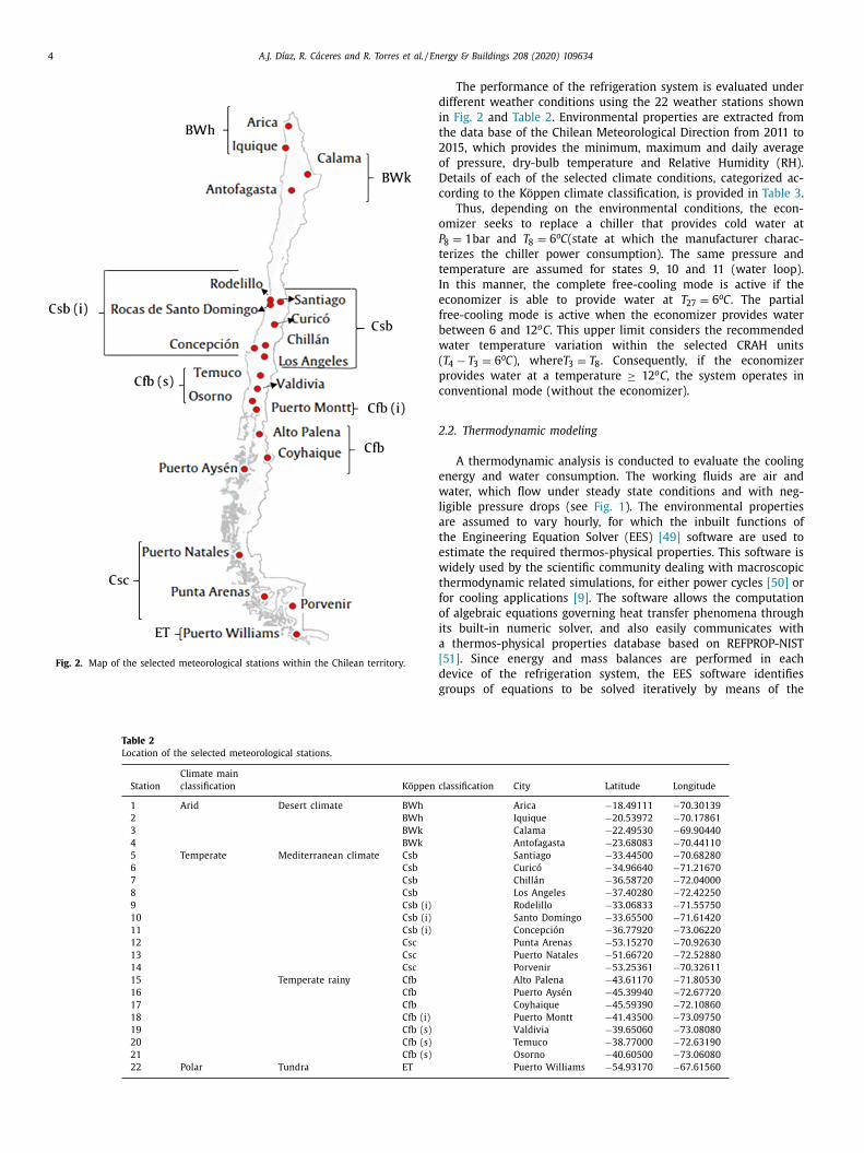
Fig. 2. Map of the selected meteorological stations within the Chilean territory.

d

i

t

2

o

D

c

o

P

t

t

I

e

f

b

w

(

p

c

2

e

w

l

a

t

e

w

t

f

o

i

a

[

d

g

Table 2

Location of the selected meteorological stations.

Station

Climate main

classification Köppen c

1 Arid Desert climate BWh

2 BWh

3 BWk

4 BWk

5 Temperate Mediterranean climate Csb

6 Csb

7 Csb

8 Csb

9 Csb (i)

10 Csb (i)

11 Csb (i)

12 Csc

13 Csc

14 Csc

15 Temperate rainy Cfb

16 Cfb

17 Cfb

18 Cfb (i)

19 Cfb (s)

20 Cfb (s)

21 Cfb (s)

22 Polar Tundra ET

The performance of the refrigeration system is evaluated under

ifferent weather conditions using the 22 weather stations shown

n Fig. 2 and Table 2 . Environmental properties are extracted from

he data base of the Chilean Meteorological Direction from 2011 to

015, which provides the minimum, maximum and daily average

f pressure, dry-bulb temperature and Relative Humidity (RH).

etails of each of the selected climate conditions, categorized ac-

ording to the Köppen climate classification, is provided in Table 3 .

Thus, depending on the environmental conditions, the econ-

mizer seeks to replace a chiller that provides cold water at

8 = 1 bar and T 8 = 6 o C(state at which the manufacturer charac-

erizes the chiller power consumption). The same pressure and

emperature are assumed for states 9, 10 and 11 (water loop).

n this manner, the complete free-cooling mode is active if the

conomizer is able to provide water at T 27 = 6 o C. The partial

ree-cooling mode is active when the economizer provides water

etween 6 and 12 o C . This upper limit considers the recommended

ater temperature variation within the selected CRAH units

T 4 − T 3 = 6 o C), where T 3 = T 8 . Consequently, if the economizer

rovides water at a temperature ≥ 12 o C , the system operates in

onventional mode (without the economizer).

.2. Thermodynamic modeling

A thermodynamic analysis is conducted to evaluate the cooling

nergy and water consumption. The working fluids are air and

ater, which flow under steady state conditions and with neg-

igible pressure drops (see Fig. 1 ). The environmental properties

re assumed to vary hourly, for which the inbuilt functions of

he Engineering Equation Solver (EES) [49] software are used to

stimate the required thermos-physical properties. This software is

idely used by the scientific community dealing with macroscopic

hermodynamic related simulations, for either power cycles [50] or

or cooling applications [9] . The software allows the computation

f algebraic equations governing heat transfer phenomena through

ts built-in numeric solver, and also easily communicates with

thermos-physical properties database based on REFPROP-NIST

51] . Since energy and mass balances are performed in each

evice of the refrigeration system, the EES software identifies

roups of equations to be solved iteratively by means of the

lassification City Latitude Longitude

Arica −18.49111 −70.30139

Iquique −20.53972 −70.17861

Calama −22.49530 −69.90440

Antofagasta −23.68083 −70.44110

Santiago −33.44500 −70.68280

Curicó −34.96640 −71.21670

Chillán −36.58720 −72.04000

Los Angeles −37.40280 −72.42250

Rodelillo −33.06833 −71.55750

Santo Domingo −33.65500 −71.61420

Concepción −36.77920 −73.06220

Punta Arenas −53.15270 −70.92630

Puerto Natales −51.66720 −72.52880

Porvenir −53.25361 −70.32611

Alto Palena −43.61170 −71.80530

Puerto Aysén −45.39940 −72.67720

Coyhaique −45.59390 −72.10860

Puerto Montt −41.43500 −73.09750

Valdivia −39.65060 −73.08080

Temuco −38.77000 −72.63190

Osorno −40.60500 −73.06080

Puerto Williams −54.93170 −67.61560

A.J. Díaz, R. Cáceres and R. Torres et al. / Energy & Buildings 208 (2020) 109634 5

Table 3

Description of Köppen classification.

Köppen classification Description

BWh Hot desert

BWk Cold desert

Csb Warm-summer Mediterranean with winter rain

Csb (i) Warm-summer Mediterranean with winter rain and coastal influence

Csc Cool-summer Mediterranean with winter rain

Cfb Temperate rainy

Cfb (i) Temperate rainy with coastal influence

Cfb (s) Temperate rainy with short summer drought periods

ET Tundra

N

s

1

l

2

m

t

s

C

t

s

W

t

W

r

f

r

c

[

p

W

q

i

I

t

W

c

p

b

2

t

u

w

o

n

a

(

W

fl

[

t

s

e

v

t

e

b

s

f

W

w

m

E

a

i

e

a

[

T

t

T

w

e

I

t

�

ewton-Raphson and the Tarjan blocking algorithm. Here, the

top criterion considers 250 iterations with a residual less than

× 10 −6 , in which each iteration considers a change in variables

ess than 1 × 10 −9 .

.2.1. Estimation of cooling energy use

To estimate the cooling energy use, the Coefficient of Perfor-

ance (COP) is calculated to relate the overall heat dissipated by

he racks to the total power consumed by entire the refrigeration

ystem, as follows

O P system

=

˙ Q room

˙ W system

=

n racks ˙ Q rack

˙ W CRAH +

˙ W chil l er +

˙ W tower +

˙ W pumps

(1)

Here, the CRAH power consumption is calculated considering

he power associated with the fan and controllers and monitoring

ystem (see Table 1 )

˙ CRAH =

˙ W c+ m

+

˙ W fan,CRAH (2)

The fan power of the CRAH units is calculated as function of

he air flow rate as suggested by the fan law

˙ fan,CRAH =

˙ W fan,CRAH,n

(˙ ∀ air,CRAH

˙ ∀ air,CRAH, max

)3

(3)

According to the manufacturer, at T 8 = 6 o C, the selected chiller

equires a nominal power of 21.2 kW under a load of 13%, whereas

or a load of 100% it requires 180.9 kW. The load is defined as the

atio of the heat flow dissipated by the evaporator ( ˙ Q e v a ) to the

hiller cooling capacity (1055.06 kW). As suggested by Meakins

52] , the chiller power demand can be correlated to a third grade

olynomial function of the load as follows

˙ chil l er = 18 . 4257 + 31 . 6728 ( load ) + 0 . 822349 ( load )

2

+131 . 048 ( load ) 3

[ kW ] (4)

The constants of Eq. (4) offer an R

2 value of 99.91%. Eq. (4) re-

uires solving an energy balance first to calculate ˙ Q e v a .

The cooling tower power consumption ( ˙ W tower ) depends only on

ts fan power consumption, which is calculated similar to Eq. (3) .

n accordance to the manufacturer’s recommendations, the ratio of

he water to air flow within the tower is assumed to be 1.2. Thus,

˙ tower =

˙ W tower,n

(˙ m 14

1 . 2 ρ21 ̇ ∀ air,tower, max

)3

(5)

The total power consumption of all pumps ( ˙ W pumps ) is obtained

onsidering each of the isentropic efficiencies, recommended

ressure drops and flow rates of water (obtained through energy

alances).

.2.2. Makeup water consumption

Since a water supply system must be employed to compensate

he water evaporation within the cooling tower, this paper eval-

ates the impact of reducing the cooling energy demand on the

ater consumed by the system. The goal is to identify the effect

f each of the selected climate conditions in terms of their use of

atural resources. The Water to Energy Ratio (WER) is proposed as

new metric to compare the water required by the cooling tower

when economization is possible) with the energy savings. Thus,

ER ≡ Water consumption

Energy savings

[m

3

MWh

](6)

The water consumption can be estimated through the mass

ow rate of water leaving the cooling tower due to evaporation

53] , which is a function of the difference in humidity between

he air entering and exiting the cooling tower.

The estimation of the energy savings requires assuming that the

ystem always operates in conventional mode. Thus, the maximum

nergy demand can be calculated. If the economizer is able to pro-

ide cold water, allowing to reduce the chiller load, then the sys-

em will consume less energy than the conventional mode, and en-

rgy savings will exist. The energy savings represent the difference

etween the maximum energy use and the energy used by the

ystem when either partial or complete free-cooling is available.

Therefore, for each hour of operation, the WER is calculated as

ollows

ER =

⎧ ⎪ ⎨

⎪ ⎩

˙ m 23

˙ W syst em ,c − ˙ W syst em , cf

if complete free − cooling is active

˙ m 23

˙ W syst em ,c − ˙ W syst em , pf

if partial free − cooling is active (7)

here

˙ 23 =

˙ m 21 ( ω 22 − ω 21 ) (8)

Both ω 21 and ω 22 are obtained using the inbuilt functions of

ES. State 21 is given by the environmental data, whereas state 22

ssumes atmospheric pressure and saturated air. In addition, T 22

s obtained through an energy balance in the cooling tower.

The temperature of the makeup water ( T 23 ) is estimated at

ach location as function of ambient, surface and ground temper-

ture, according to the model proposed by Burch and Christensen

54] . Thus,

23 =

[T mains,annual − �T mains sin ( f annual t − αamb − αmains ) − 32

]5

9

(9)

Here, T mains, annual represents the annual average temperature of

he water supplied by the distribution network, given by

mains,annual = T amb,annual + �T (10)

here T amb, annual is the annual average ambient temperature at

ach location, which assumes a temperature shift of �T = 3 . 33 o C.

n Eq. (9) , �T mains is proportional to the ambient temperature and

he pipes depth, which is estimated as follows

T mains = 0 . 9 R ( T max,m

− T min,m

) (11)

6 A.J. Díaz, R. Cáceres and R. Torres et al. / Energy & Buildings 208 (2020) 109634

Table 4

Monthly average temperature and relative humidity at the selected stations.

January February March April May June

Station T, °C RH T, °C RH T, °C RH T, °C RH T, °C RH T, °C RH

1 22.4 0.61 23.2 0.61 22.4 0.63 20.7 0.65 19.3 0.67 17.9 0.65

2 21.6 0.61 22.4 0.60 21.0 0.64 19.3 0.65 18.1 0.66 17.0 0.67

3 22.3 0.33 23.0 0.42 22.2 0.39 20.5 0.30 19.1 0.23 17.7 0.19

4 22.3 0.70 23.0 0.71 22.2 0.73 20.5 0.73 19.1 0.73 17.7 0.73

5 21.8 0.49 21.3 0.49 19.4 0.54 15.5 0.63 12.6 0.70 9.8 0.74

6 21.7 0.56 20.9 0.60 19.3 0.61 15.4 0.65 12.7 0.71 10.0 0.71

7 20.5 0.61 19.3 0.64 13.6 0.69 10.4 0.76 10.5 0.86 8.5 0.90

8 20.7 0.51 19.3 0.54 16.7 0.63 12.8 0.70 10.2 0.71 8.6 0.73

9 17.2 0.76 17.4 0.74 16.6 0.75 14.6 0.77 13.2 0.81 11.6 0.77

10 16.7 0.77 16.1 0.78 13.4 0.81 12.4 0.80 12.0 0.83 10.9 0.81

11 17.5 0.74 16.7 0.76 15.5 0.78 13.4 0.84 11.9 0.88 10.6 0.85

12 11.3 0.62 10.7 0.65 9.6 0.72 6.8 0.77 4.5 0.80 2.6 0.82

13 11.9 0.61 11.6 0.64 10.1 0.66 5.5 0.73 2.9 0.83 2.5 0.77

14 11.5 0.67 10.8 0.70 9.8 0.74 7.4 0.78 4.4 0.82 2.6 0.83

15 13.5 0.55 12.0 0.58 10.1 0.64 8.0 0.76 6.1 0.81 4.5 0.80

16 12.0 0.72 11.6 0.74 7.3 0.80 6.2 0.85 6.0 0.87 4.3 0.85

17 15.4 0.59 14.1 0.65 11.6 0.67 9.2 0.73 6.7 0.81 4.6 0.80

18 15.3 0.78 14.3 0.82 13.0 0.83 11.1 0.88 9.9 0.90 7.5 0.90

19 17.6 0.68 16.3 0.74 13.9 0.80 11.8 0.89 10.6 0.92 8.1 0.92

20 17.6 0.55 16.6 0.57 14.6 0.62 11.9 0.67 10.4 0.70 8.3 0.67

21 16.7 0.61 15.5 0.66 13.4 0.70 11.1 0.79 9.9 0.63 7.2 0.64

22 10.0 0.69 9.2 0.72 8.6 0.74 6.3 0.77 4.0 0.80 2.3 0.81

July August September October November December

Station T, °C RH T, °C RH T, °C RH T, °C RH T, °C RH T, °C RH

1 16.5 0.70 16.5 0.71 17.2 0.71 18.3 0.70 19.9 0.65 21.6 0.63

2 15.3 0.68 15.5 0.68 16.4 0.68 17.3 0.66 18.8 0.63 20.6 0.62

3 16.4 0.18 16.3 0.16 17.1 0.15 18.1 0.15 19.8 0.16 21.4 0.22

4 16.4 0.74 16.3 0.74 17.1 0.73 18.1 0.71 19.8 0.69 21.4 0.69

5 9.2 0.74 11.2 0.72 13.4 0.66 15.5 0.58 18.1 0.49 20.5 0.47

6 9.2 0.72 10.4 0.73 12.6 0.69 14.6 0.64 17.6 0.56 20.3 0.52

7 7.3 0.89 8.8 0.85 10.6 0.80 12.7 0.74 15.6 0.67 18.6 0.60

8 7.5 0.72 8.7 0.73 10.3 0.72 12.4 0.69 15.6 0.60 18.4 0.55

9 10.5 0.80 11.2 0.81 12.3 0.80 12.7 0.79 14.6 0.75 16.1 0.73

10 9.8 0.82 10.8 0.82 11.8 0.83 12.3 0.79 13.7 0.77 15.3 0.76

11 9.2 0.85 10.3 0.83 11.1 0.81 12.5 0.77 14.3 0.73 16.2 0.72

12 2.3 0.83 3.0 0.81 4.7 0.75 7.2 0.67 8.8 0.63 10.1 0.62

13 2.0 0.78 2.6 0.74 4.0 0.70 6.2 0.64 7.6 0.63 10.9 0.60

14 2.4 0.83 3.3 0.81 5.0 0.75 7.2 0.69 8.7 0.66 10.2 0.65

15 3.7 0.85 4.7 0.80 6.3 0.71 8.4 0.62 11.7 0.59 14.5 0.56

16 2.8 0.88 5.0 0.86 5.6 0.80 6.8 0.77 5.9 0.77 5.2 0.74

17 3.4 0.81 4.3 0.80 6.4 0.71 9.0 0.64 11.3 0.62 13.5 0.60

18 7.0 0.89 7.7 0.87 8.6 0.85 10.3 0.82 12.1 0.80 14.0 0.77

19 7.4 0.92 8.5 0.89 9.3 0.84 11.0 0.79 13.2 0.76 15.8 0.71

20 7.4 0.69 6.8 0.49 7.7 0.48 9.1 0.47 12.7 0.57 15.7 0.45

21 7.0 0.61 7.9 0.62 9.0 0.72 10.8 0.72 12.7 0.70 14.8 0.65

22 2.1 0.82 3.2 0.77 4.4 0.72 6.3 0.67 7.4 0.66 8.2 0.70

e

f

a

g

w

t

h

w

t

�

m

p

[

s

t

v

t

where T max, m

and T min, m

are the maximum and minimum monthly

ambient temperatures, respectively; and R is the ratio of ampli-

tudes of ground to surface temperatures given by

R = 0 . 4 + 0 . 01

(T amb,annual − T re f

)1 . 8

o C −1 (12)

where T ref is a reference temperature assumed to be 21 o C .

Finally, frequency ( f annual ) and phase angles ( αamb , αmains ) in

Eq. (9) are obtained assuming that the maximum temperature

takes place on January 15th, thus

f annual =

1

24

αamb

Dayofmax . temp . − 90

o (13)

where αamb = 104 . 8 o and αmains is given as function of the ambient

temperature as follows

αmains = 35

o − 0 . 01

o (T amb,annual − T re f

)1 . 8

o C −1 (14)

2.3. Estimation of the number of free-cooling hours

To evaluate the free-cooling availability, the study considers

8760 h of operation per year. The number of hours in which

ach of the operating modes is available (conventional, partial

ree-cooling and complete free-cooling) depends on the temper-

ture leaving the economizer (state 27), which changes with the

eographical location since the cooling tower interacts directly

ith the environment. An energy balance is conducted to calculate

he thermodynamic state leaving the economizer, as follows

27 = h 26 − ε ˙ C min �T max

˙ m 27

(15)

hich is assumed to be at the saturated liquid state. In Eq. (15) ,

he minimum heat capacity rate is given by min ( ̇ C 24 , ˙ C 26 ) , whereas

T max requires an energy balance in the CWP.

The hourly variation of the environmental properties is esti-

ated using the time at which the minimum and maximum take

lace and a curve fitting to a sinusoidal function, as suggested in

54] . Thus, the thermodynamic performance of the refrigeration

ystem is evaluated for each hour of the year, allowing to estimate

he availability of each of the operating modes, as well as the

ariations in COP and WER. Table 4 shows the monthly average

emperature and RH at each of the selected stations.

A.J. Díaz, R. Cáceres and R. Torres et al. / Energy & Buildings 208 (2020) 109634 7

Fig. 3. Annual free-cooling availability and energy reduction opportunities.

3

p

o

t

l

i

M

f

r

M

o

h

t

(

h

. Climatic influence upon system and component

erformances

This section intends to elucidate the effect of climate conditions

n the thermodynamic performance of the system. Fig. 3 shows

he available free-cooling hours per year at each of the selected

ocations. In desert climates (BWh and BWk) the economization

s impossible. A similar behavior is observed in warm-summer

editerranean climates (Csb), with less than 26% of partial

Fig. 4. Effect of climate conditions on the a

ree-cooling availability, for which the coastal influence (Csb (i))

educes the partial economization to less than 13%.

The free-cooling availability turns significant in cool-summer

editerranean with winter rain (Csc) and tundra climates (ET),

ffering a high number of both complete and partial free-cooling

ours. This is explained by the low temperatures found in

hese climates, with an average annual temperature below 6.8 °C Table 4 ). Temperate climates (Cfb) also offer complete free-cooling

ours, with an average annual temperature below 8 °C, but the

nnual cooling energy use distribution.

8 A.J. Díaz, R. Cáceres and R. Torres et al. / Energy & Buildings 208 (2020) 109634

Fig. 5. Coefficient of performance and water required to achieve it.

Table 5

Percentage of the monthly availability of complete free-cooling.

Station Jan Feb Mar Apr May Jun Jul Aug Sep Oct Nov Dec

1 – – – – – – – – – – – –

2 – – – – – – – – – – – –

3 – – – – – – – – – – – –

4 – – – – – – – – – – – –

5 – – – – – 1.3 2.8 – – – – –

6 – – – – – 0.4 1.9 – – – – –

7 – – – 0.3 0.8 0.3 6.9 1.6 – – – –

8 – – – – 2.2 1.7 10.1 3.9 – – – –

9 – – – – – – – – – – – –

10 – – – – – – 0.1 – – – – –

11 – – – – – – – – – – – –

12 – – – 3.2 13.6 47.1 52.0 38.8 21.5 6.2 1.4 0.3

13 0.7 – 1.5 17.9 50.1 60.3 66.0 56.6 42.6 17.3 7.9 0.4

14 – – – 0.3 17.7 47.8 49.2 39.0 25.4 8.9 1.4 0.7

15 – – – 2.2 1.7 16.7 23.0 21.1 10.3 5.0 – –

16 – – – – – 5.7 32.7 2.4 1.0 0.9 0.7 8.3

17 – – – 0.6 4.2 21.3 33.2 27.6 16.4 6.7 – –

18 – – – – – 1.1 1.2 1.6 – – – –

19 – – – – – 0.8 – – 1.7 – – –

20 – – – – 1.2 2.4 7.1 21.8 20.8 13.6 2.4 0.3

21 – – – – 1.3 13.5 17.7 10.3 1.3 – – –

22 – 0.3 – 5.7 26.1 57.1 59.5 43.8 36.0 18.8 8.3 0.8

q

T

u

w

a

i

(

w

w

u

u

t

a

(

i

partial free-cooling is more important. Here, the coastal influence

(Cfb (i)) reduces the partial free-cooling availability considerably

to less than 24%.

Fig. 4 intends to elucidate which components are the most af-

fected by variations in the climate conditions by showcasing their

annual energy use distribution. The chiller energy use considerably

decreases as the economizer availability increases, proving to be

the component most affected by climate conditions. On the other

hand, CRAH units, pumps and cooling tower show a fairly constant

energy use distribution regardless of climate conditions, since their

thermal performance remains unaffected by the environmental

properties. Therefore, the overall energy use levels greatly depend

on the chiller load.

Fig. 5 shows the annual energy required to dissipate the heat

in excess from the racks, as well as the annual water supply re-

uired to achieve energy savings when economization is possible.

he idea is to elucidate if the reductions in the cooling energy

se due to the economizers lead to a significant increase in the

ater consumption. Here, both high COP and low WER values

re desired. The results show that free-cooling is unavailable

n desert climates; therefore, the lowest COP values are found

5.6–5.7). The highest water requirements are found in climates

ith coastal influence such as warm-summer Mediterranean

ith winter rain (Csb (i)). Considering that the COP is also low

nder these climates, water-side economization underperforms

nder these conditions. Warm-summer Mediterranean with win-

er rain (Csb), temperate rainy with coastal influence (Cfb (i)),

nd temperate rainy with short summer drought periods (Cfb

s)) climates all show a similar behavior; this is, a moderate

ncrease in the COP (6.1–7.3) and relatively low WER values

A.J. Díaz, R. Cáceres and R. Torres et al. / Energy & Buildings 208 (2020) 109634 9

Table 6

Percentage of the monthly availability of partial free-cooling.

Station Jan Feb Mar Apr May Jun Jul Aug Sep Oct Nov Dec

1 – – – – – – – – – – – –

2 – – – – – – – – – – – –

3 – – – – – – – – – – – –

4 – – – – – – – – – – – –

5 – – – 9.9 30.4 50.6 50.8 34.9 22.4 15.1 5.8 –

6 – – – 8.5 28.6 49.4 52.8 46.6 29.9 16.0 2.6 –

7 – – 16.8 41.5 27.3 43.6 48.1 43.3 34.4 23.9 10.7 0.4

8 – – 2.7 21.0 38.6 52.9 55.9 50.7 39.3 31.9 13.6 1.2

9 – – – 0.6 0.7 13.2 28.0 20.2 7.1 5.9 0.6 –

10 – – 4.3 16.0 10.2 25.8 37.0 28.4 14.0 14.2 7.6 0.4

11 – – – 2.8 6.6 15.3 32.1 21.4 20.7 12.5 8.3 0.3

12 36.0 40.0 46.0 78.6 86.0 52.9 47.3 60.1 78.1 74.1 59.0 45.8

13 31.2 32.7 46.2 74.9 49.7 38.3 32.3 40.5 56.8 76.2 70.8 37.1

14 29.7 34.8 41.0 70.6 81.3 50.7 49.9 60.8 72.9 69.2 59.4 43.1

15 23.7 32.4 48.7 58.5 87.2 82.4 76.3 74.9 74.9 57.8 37.9 17.6

16 9.0 10.3 78.9 88.2 87.2 94.3 67.3 95.4 95.4 82.0 95.0 90.1

17 8.3 15.0 32.9 52.8 71.1 75.4 63.3 70.3 63.2 48.3 39.7 20.8

18 0.5 1.5 7.7 11.4 14.0 55.0 62.5 50.0 44.3 27.8 11.4 1.6

19 1.1 0.6 13.0 14.2 8.7 44.0 53.9 39.5 40.3 35.6 21.3 6.6

20 10.2 13.4 24.1 35.6 37.8 60.4 68.5 67.9 49.9 43.3 31.5 19.6

21 3.2 4.0 15.2 23.5 45.0 61.3 60.8 56.6 49.0 34.8 19.6 8.9

22 44.6 50.1 59.1 84.0 73.0 41.3 38.4 55.5 62.4 68.3 65.7 62.2

Table 7

Monthly COP variation.

Station Jan Feb Mar Apr May Jun Jul Aug Sep Oct Nov Dec

1 5.68 5.68 5.68 5.68 5.68 5.68 5.68 5.68 5.68 5.68 5.68 5.68

2 5.68 5.68 5.68 5.68 5.68 5.68 5.68 5.68 5.68 5.68 5.68 5.68

3 5.64 5.64 5.64 5.64 5.65 5.63 5.65 5.65 5.65 5.65 5.65 5.64

4 5.67 5.67 5.67 5.68 5.68 5.68 5.68 5.68 5.68 5.68 5.68 5.68

5 5.67 5.67 5.67 5.84 6.27 7.13 7.33 6.38 6.03 5.91 5.75 5.67

6 5.67 5.67 5.67 5.80 6.18 7.00 7.30 6.76 6.19 5.93 5.70 5.67

7 5.68 5.68 5.92 6.60 6.30 6.67 7.53 6.84 6.43 6.11 5.83 5.68

8 5.68 5.68 5.71 6.08 6.73 7.24 8.19 7.36 6.66 6.32 5.91 5.69

9 5.67 5.67 5.67 5.68 5.68 5.85 6.18 5.97 5.78 5.76 5.68 5.68

10 5.68 5.68 5.74 5.93 5.86 6.15 6.55 6.21 5.93 5.94 5.80 5.68

11 5.68 5.68 5.68 5.72 5.78 5.94 6.41 6.08 6.07 5.90 5.80 5.68

12 6.43 6.52 6.66 8.01 9.69 12.17 12.47 11.50 10.17 8.33 7.42 6.85

13 6.49 6.48 6.92 9.59 12.19 12.82 13.16 12.46 11.60 9.52 8.39 6.73

14 6.24 6.39 6.53 7.48 9.87 11.99 12.21 11.41 10.21 8.35 7.40 6.80

15 6.11 6.30 6.84 7.38 8.17 9.84 10.37 9.90 8.92 7.83 6.58 5.99

16 5.81 5.82 7.44 7.90 7.89 9.24 11.26 8.70 8.49 7.89 8.46 9.33

17 5.80 5.93 6.34 7.01 7.86 9.96 10.72 10.38 9.09 7.71 6.66 6.09

18 5.68 5.70 5.81 5.86 5.89 6.91 7.19 6.91 6.61 6.21 5.83 5.70

19 5.66 5.66 5.87 5.85 5.81 6.53 6.78 6.46 6.63 6.36 6.02 5.75

20 5.85 5.91 6.16 6.43 6.55 7.42 8.12 9.99 9.38 8.46 6.73 6.23

21 5.72 5.73 5.98 6.11 7.00 8.79 9.16 8.26 6.92 6.43 6.04 5.81

22 6.64 6.85 7.05 8.42 10.42 12.65 12.72 11.75 11.05 9.43 8.32 7.43

(

c

M

t

h

r

t

s

t

a

i

p

a

w

(

t

a

a

a

c

a

t

T

i

t

T

e

(

i

w

b

m

22–57 m

3 /MWh). The best opportunities for reductions in both

ooling energy and water consumption are found in Cool-summer

editerranean with winter rain (Csc), temperate rainy (Cfb) and

undra (ET) climates, in which the free-cooling availability is

igher. Here the COP and WER range 7.8–9.7 and 11–17 m

3 /MWh,

espectively.

Since the four seasons are well defined in most of the Chilean

erritory, divided according to the astronomical timing for the

outhern hemisphere, a monthly analysis is presented to evaluate

he system performance through the year. The following analysis

nd comments consider the average values among stations with

dentical climate conditions.

Table 5 shows the percentage of complete free-cooling hours

er month at the selected locations. High complete free-cooling

vailability ( > 10%) is found in cool-summer Mediterranean with

inter rain (Csc) and tundra (ET) climates from May to October

middle of fall to middle of spring). During winter time, the

emperate rainy (Cfb) climate also shows complete free-cooling

vailability, which is reduced when short summer drought periods

re present (Cfb (s)). None or negligible complete free-cooling

vailability is observed in all the remaining climates. In those

limates, except in desert ones, the partial free-cooling appears as

potential solution for reducing the chiller load ( Table 6 ).

In climates with available hours for complete economiza-

ion (Cool-summer Mediterranean with winter rain, Tundra and

emperate rainy), Table 7 shows that the COP can achieve an

mportant augmentation compared to the conventional opera-

ion without the economizer (~50 to 120% increase). Moreover,

able 8 indicates that the water consumption associated to the

nergy savings achieves the lowest values through the year

WER = 7–14 m

3 /MWh).

In the remaining climates, in which partial economization

s possible, the COP increases from ~10 to 45% ( Table 7 ). For

arm-summer Mediterranean with winter rain climates (Csb), the

enefits of partial economization are only significant from the

iddle of fall to winter time ( > 10% increase in the COP); which

10 A.J. Díaz, R. Cáceres and R. Torres et al. / Energy & Buildings 208 (2020) 109634

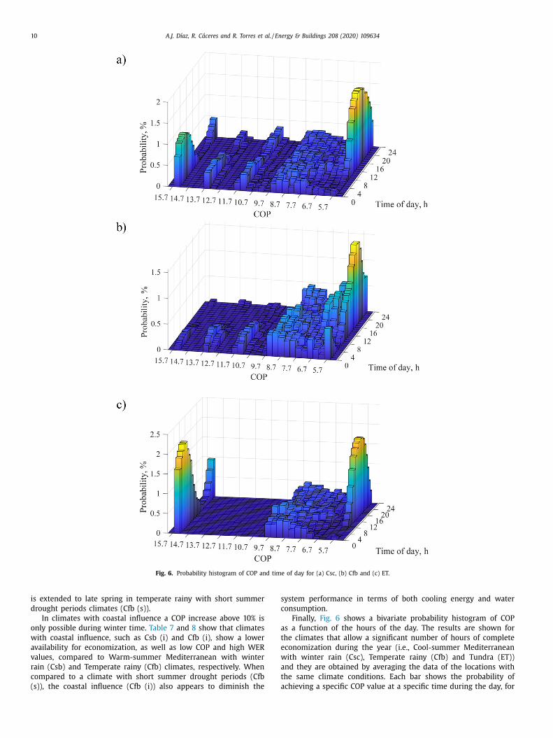
Fig. 6. Probability histogram of COP and time of day for (a) Csc, (b) Cfb and (c) ET.

s

c

a

t

e

w

a

t

a

is extended to late spring in temperate rainy with short summer

drought periods climates (Cfb (s)).

In climates with coastal influence a COP increase above 10% is

only possible during winter time. Table 7 and 8 show that climates

with coastal influence, such as Csb (i) and Cfb (i), show a lower

availability for economization, as well as low COP and high WER

values, compared to Warm-summer Mediterranean with winter

rain (Csb) and Temperate rainy (Cfb) climates, respectively. When

compared to a climate with short summer drought periods (Cfb

(s)), the coastal influence (Cfb (i)) also appears to diminish the

ystem performance in terms of both cooling energy and water

onsumption.

Finally, Fig. 6 shows a bivariate probability histogram of COP

s a function of the hours of the day. The results are shown for

he climates that allow a significant number of hours of complete

conomization during the year (i.e., Cool-summer Mediterranean

ith winter rain (Csc), Temperate rainy (Cfb) and Tundra (ET))

nd they are obtained by averaging the data of the locations with

he same climate conditions. Each bar shows the probability of

chieving a specific COP value at a specific time during the day, for

A.J. Díaz, R. Cáceres and R. Torres et al. / Energy & Buildings 208 (2020) 109634 11

Table 8

Monthly WER variation (in m

3 /MWh).

Station Jan Feb Mar Apr May Jun Jul Aug Sep Oct Nov Dec

1 – – – – – – – – – – – –

2 – – – – – – – – – – – –

3 – – – – – – – – – – – –

4 – – – – – – – – – – – –

5 – – – 120 41 20 19 36 62 89 229 –

6 – – – 146 46 22 20 26 46 83 523 –

7 – – 79 28 37 25 18 23 31 49 112 1366

8 – – 399 54 28 20 15 19 27 37 87 781

9 – – – 1286 1167 107 46 68 171 201 1285 –

10 – – 269 76 103 46 28 41 77 76 148 2000

11 – – – 362 161 75 32 53 53 87 142 2541

12 35 32 28 15 10 8 8 8 10 14 19 25

13 34 34 24 11 8 8 8 8 9 12 15 28

14 43 36 31 17 10 8 8 9 10 15 19 26

15 57 43 25 19 14 10 9 10 12 17 31 73

16 145 132 17 14 14 10 8 11 12 15 12 10

17 159 83 38 22 16 10 8 10 13 18 29 58

18 1668 726 136 101 89 22 19 23 27 42 116 726

19 982 1254 102 106 136 35 28 37 33 40 67 200

20 114 87 47 33 32 19 15 12 13 16 29 49

21 397 309 69 50 23 14 13 15 23 33 60 142

22 28 24 21 13 9 8 7 8 9 12 15 18

w

s

d

I

e

T

4

c

c

a

t

t

p

i

r

M

t

o

d

o

W

o

w

C

p

h

m

w

o

o

d

E

i

u

c

D

A

p

R

hich the sum of all bar heights is equal to one. All three climates

how a high probability of achieving low COP values during the

ay, in which the system operates close to the conventional mode.

t is during the early morning when the probability of reducing the

nergy use increases and the COP can achieve its highest values.

his also occurs at the end of the day in Tundra (ET) climates.

. Conclusions

The potential for implementing water-side economizers in the

ooling system of data centers was investigated under different

limate conditions by estimating the number of free-cooling hours

vailable throughout the year. Chile was selected as case study due

o the wide range of climate conditions found along the territory. A

hermodynamics analysis aimed to investigate the opportunities of

artially reducing the chiller load when complete economization is

nsufficient. For that, the system cooling energy and makeup water

equirements were simultaneously evaluated and contrasted.

Due to their higher economization availability, Cool-summer

editerranean with winter rain (Csc), temperate rainy (Cfb) and

undra (ET) climates offer higher COP and lower WER values. Most

f the economization opportunities appear early in the morning

uring winter time. Throughout the year both Csc and ET climates

ffer a considerable number of partial free-cooling hours.

In desert climates the water-side economization is unfeasible.

arm-summer Mediterranean with winter rain (Csb) climates

ffer less than 26% of partial economization during the year,

hich is reduced to 13% when influenced by the coast (Csb (i)).

sc and ET climates both offer high availability of complete and

artial free-cooling. In Cfb climates the number of free-cooling

ours is also high; however, partial economization appears as the

ain mechanism for reducing the chiller load.

In terms of annual energy and water consumption, climates

ith coastal influence are not recommended for water-side econ-

mization. Such cases presented low COP and high WER values.

In general, in climates with lower availability of complete econ-

mization, the partial free-cooling offers good opportunities for re-

ucing the cooling energy use, in particular during winter time.

ven though the COP can be increased over 10% during winter time

n climates with coastal influence, lower COP and higher WER val-

es are found compared to climates without coastal influence and

limates with short summer drought periods.

eclaration of Competing Interest

None.

cknowledgment

This work was partially sponsored by CONICYT-Chile under

roject FONDECYT 11160172 .

eferences

[1] J. Koomey , Growth in Data Center Electricity Use 2005 to 2010, Growth in DataCenter Electricity Use 2005 to 2010, 9, Analytical Press, 2011 completed at the

request of The New York Times . [2] A. Shehabi , United States Data Center Energy Usage Report , Lawrence Berkeley

National Laboratory , Berkeley , et al. , California (2016) LBNL–1005775 . [3] The Green Grid , Guidelines for energy-efficient datacenters, The Green Grid,

2007 White Paper .

[4] M.A. Islam , et al. , Water-constrained geographic load balancing in data centers,IEEE Trans. Cloud Comput. 5 (2) (2017) 208–220 .

[5] D. Azevedo , S.C. Belady , J. Pouchet , Water Usage Effectiveness (WUE TM ): AGreen Grid Datacenter Sustainability Metric (2011) .

[6] B. Ristic , K. Madani , Z. Makuch , The water footprint of data centers, Sustain-ability 7 (8) (2015) 11260–11284 .

[7] T. Gao , et al. , Experimental and numerical dynamic investigation of an en-

ergy efficient liquid cooled chiller-less data center test facility, Energy Build.91 (2015) 83–96 .

[8] A. Bhalerao , et al. , Rapid prediction of exergy destruction in data centers dueto airflow mixing, Numer. Heat Transf. Part A Appl. 70 (1) (2016) 48–63 .

[9] A.J. Díaz , et al. , Energy and exergy assessment in a perimeter cooled data cen-ter: the value of second law efficiency, Appl. Therm. Eng. (2017) 820–830 .

[10] K. Fouladi , et al. , Optimization of data center cooling efficiency using reduced

order flow modeling within a flow network modeling approach, Appl. Therm.Eng. 124 (2017) 929–939 .

[11] L. Silva-Llanca , et al. , Determining wasted energy in the airside of a perime-ter-cooled data center via direct computation of the exergy destruction, Appl.

Energy 213 (2018) 235–246 . [12] L. Silva-Llanca , et al. , Cooling effectiveness of a data center room under over-

head airflow via entropy generation assessment in transient scenarios, Entropy

21 (1) (2019) 98 . [13] A. Capozzoli , G. Primiceri , Cooling systems in data centers: state of art and

emerging technologies, Energy Procedia 83 (2015) 4 84–4 93 . [14] J. Ni , X. Bai , A review of air conditioning energy performance in data centers,

Renew. Sustain. Energy Rev. 67 (2017) 625–640 . [15] H. Zhang , et al. , Free cooling of data centers: a review, Renew. Sustain. Energy

Rev. 35 (2014) 171–182 . [16] Y.Y. Lui , Waterside and airside economizers design considerations for data cen-

ter facilities, ASHRAE Trans. 116 (1) (2010) 98–108 .

[17] J. Stein , Waterside economizing in data centers: design and control considera-tions, ASHRAE Trans. 115 (2) (2009) 192–200. .

[18] E. Oró, et al. , Energy efficiency and renewable energy integration in data cen-tres. Strategies and modelling review, Renew. Sustain. Energy Rev. 42 (2015)

429–445 .

12 A.J. Díaz, R. Cáceres and R. Torres et al. / Energy & Buildings 208 (2020) 109634

[

[19] H.M. Daraghmeh , C.-.C. Wang , A review of current status of free cooling indatacenters, Appl. Therm. Eng. 114 (2017) 1224–1239 .

[20] A.H. Khalaj , S.K. Halgamuge , A review on efficient thermal management ofair-and liquid-cooled data centers: from chip to the cooling system, Appl. En-

ergy 205 (2017) 1165–1188 . [21] L. Ling , Q. Zhang , L. Zeng , Performance and energy efficiency analysis of data

center cooling plant by using lake water source, Procedia Eng. 205 (2017)3096–3103 .

[22] J. Wang , et al. , Reliability and availability analysis of a hybrid cooling system

with water-side economizer in data center, Build. Environ. 148 (2019) 405–416 .[23] M. Deymi-Dashtebayaz , S.V. Namanlo , A. Arabkoohsar , Simultaneous use of

air-side and water-side economizers with the air source heat pump in adata center for cooling and heating production, Appl. Therm. Eng. 161 (2019)

114133 . [24] H. Cheung , S. Wang , Optimal design of data center cooling systems concerning

multi-chiller system configuration and component selection for energy-effi-

cient operation and maximized free-cooling, Renew. Energy (2019) 1717–1731 . [25] J. Niemann , et al. , Economizer modes of data center cooling systems, Schneider

Electric Data Center Science Center, Whitepaper 160 (2011) . [26] K. Dong , et al. , Research on free cooling of data centers by using indirect cool-

ing of open cooling tower, Procedia Eng. 205 (2017) 2831–2838 . [27] Y. Zhang , Z. Wei , M. Zhang , Free cooling technologies for data centers: energy

saving mechanism and applications, Energy Procedia 143 (2017) 410–415 .

[28] H. Zhang , et al. , A review on thermosyphon and its integrated system withvapor compression for free cooling of data centers, Renew. Sustain. Energy Rev.

81 (2018) 789–798 . [29] J. Choi , J. Jeon , Y. Kim , Cooling performance of a hybrid refrigeration sys-

tem designed for telecommunication equipment rooms, Appl. Therm. Eng. 27(11–12) (2007) 2026–2032 .

[30] A. Agrawal , M. Khichar , S. Jain , Transient simulation of wet cooling strate-

gies for a data center in worldwide climate zones, Energy Build. 127 (2016)352–359 .

[31] E. Oró, et al. , Overview of direct air free cooling and thermal energy storagepotential energy savings in data centres, Appl. Therm. Eng. 85 (2015) 100–110 .

[32] S.-.W. Ham , et al. , Energy saving potential of various air-side economizers in amodular data center, Appl. Energy 138 (2015) 258–275 .

[33] B.A. Hellmer , Consumption analysis of telco and data center cooling and hu-

midification options, ASHRAE Trans. 116 (1) (2010) 118–133 . [34] J. Dai , D. Das , M. Pecht , Prognostics-based risk mitigation for telecom equip-

ment under free air cooling conditions, Appl. Energy 99 (2012) 423–429 . [35] A. Shehabi , et al. , Data center design and location: consequences for electricity

use and greenhouse-gas emissions, Build. Environ. 46 (5) (2011) 990–998 . [36] J. Cho , Y. Kim , Improving energy efficiency of dedicated cooling system and its

contribution towards meeting an energy-optimized data center, Appl. Energy

165 (2016) 967–982 .

[37] J. Cho , et al. , Development of an energy evaluation and design tool for dedi-cated cooling systems of data centers: sensing data center cooling energy effi-

ciency, Energy Build. 96 (2015) 357–372 . [38] L. Phan , C.-.X. Lin , A multi-zone building energy simulation of a data center

model with hot and cold aisles, Energy Build. 77 (2014) 364–376 . [39] H. Bulut , M.A. Aktacir , Determination of free cooling potential: a case study for

Istanbul, Turkey, Appl. Energy 88 (3) (2011) 6 80–6 89 . [40] J. Siriwardana , S. Jayasekara , S.K. Halgamuge , Potential of air-side economizers

for data center cooling: a case study for key Australian cities, Appl. Energy 104

(2013) 207–219 . [41] V. Depoorter , E. Oró, J. Salom , The location as an energy efficiency and re-

newable energy supply measure for data centres in Europe, Appl. Energy 140(2015) 338–349 .

[42] K.-.P. Lee , H.-.L. Chen , Analysis of energy saving potential of air-side free cool-ing for data centers in worldwide climate zones, Energy Build. 64 (2013)

103–112 .

[43] J. Cho , T. Lim , B.S. Kim , Viability of datacenter cooling systems for energy effi-ciency in temperate or subtropical regions: case study, Energy Build. 55 (2012)

189–197 . 44] S.-.W. Ham , J.-.W. Jeong , Impact of aisle containment on energy performance

of a data center when using an integrated water-side economizer, Appl. Therm.Eng. 105 (2016) 372–384 .

[45] J.-.Y. Kim , et al. , Energy conservation effects of a multi-stage outdoor air en-

abled cooling system in a data center, Energy Build. 138 (2017) 257–270 . [46] H. Tian , Z. He , Z. Li , A combined cooling solution for high heat density data

centers using multi-stage heat pipe loops, Energy Build. 94 (2015) 177–188 . [47] B. Durand-Estebe , et al. , Simulation of a temperature adaptive control strategy

for an IWSE economizer in a data center, Appl. Energy 134 (2014) 45–56 . [48] A.H. Khalaj , T. Scherer , S.K. Halgamuge , Energy, environmental and economi-

cal saving potential of data centers with various economizers across Australia,

Appl. Energy 183 (2016) 1528–1549 . [49] S. Klein , F. Alvarado , Engineering Equation Solver Software (EES), F-Chart Soft-

ware, Madison, WI, USA, 2013 . [50] J.M. Cardemil , A.K. da Silva , Parametrized overview of CO2 power cycles for

different operation conditions and configurations–an absolute and relative per-formance analysis, Appl. Therm. Eng. 100 (2016) 146–154 .

[51] E.W. Lemmon , M.O. McLinden , M.L. Huber , M.O. McLinden , NIST reference fluid

thermodynamic and transport properties–REFPROP, Version 7.0, NIST StandardReference Database 23 (2002) .

[52] M.E. Meakins , Energy and Exergy Analysis of Data Center Economizer systems,in Mechanical and Aerospace Engineering, San Jose State University, 2011 .

[53] P. G ̋Osi , Method and chart for the determination of evaporation loss of wetcooling towers, Heat Transf. Eng. 10 (4) (1989) 44–49 .

[54] J. Burch , C. Christensen , Towards development of an algorithm for mains water

temperature, in: Proceedings of the Solar Conference, Citeseer, 2007 .