EECC551 - Shaaban EECC551 - Shaaban #1 Lec # 9 Fall 2008 10-21-2 Input/Output & System Input/Output & System Performance Issues Performance Issues • System Architecture & I/O Connection Structure System Architecture & I/O Connection Structure – Types of Buses/Interconnects in the system. Types of Buses/Interconnects in the system. • I/O Data Transfer Methods. I/O Data Transfer Methods. • System and I/O Performance Metrics. System and I/O Performance Metrics. – I/O Throughput – I/O Latency (Response Time) • Magnetic Disk Characteristics. Magnetic Disk Characteristics. • I/O System Modeling Using Queuing Theory. I/O System Modeling Using Queuing Theory. – Little’s Queuing Law Little’s Queuing Law – Single Server/Single Queue I/O Modeling: M/M/1 Queue Single Server/Single Queue I/O Modeling: M/M/1 Queue – Multiple Servers/Single Queue I/O Modeling: M/M/m Queue Multiple Servers/Single Queue I/O Modeling: M/M/m Queue • Designing an I/O System & System Performance: Designing an I/O System & System Performance: – Determining system performance bottleneck. Determining system performance bottleneck. • (i.e. (i.e. which component creates a system performance bottleneck) 4 th Edition: Chapter 6.1, 6.2, 6.4, 6.5 3 rd Edition: Chapter 7.1-7.3, 7.7, 7.8 Isolated I/O System Architectur Quiz 8 More Specifically steady state queuing theory

EECC551 - Shaaban #1 Lec # 9 Fall 2008 10-21-2008 Input/Output & System Performance Issues System Architecture & I/O Connection StructureSystem Architecture.
Dec 19, 2015
Welcome message from author
This document is posted to help you gain knowledge. Please leave a comment to let me know what you think about it! Share it to your friends and learn new things together.
Transcript

EECC551 - ShaabanEECC551 - Shaaban#1 Lec # 9 Fall 2008 10-21-2008
Input/Output & System Performance IssuesInput/Output & System Performance Issues • System Architecture & I/O Connection StructureSystem Architecture & I/O Connection Structure
– Types of Buses/Interconnects in the system.Types of Buses/Interconnects in the system.
• I/O Data Transfer Methods.I/O Data Transfer Methods.• System and I/O Performance Metrics.System and I/O Performance Metrics.
– I/O Throughput– I/O Latency (Response Time)
• Magnetic Disk Characteristics.Magnetic Disk Characteristics.• I/O System Modeling Using Queuing Theory.I/O System Modeling Using Queuing Theory.
– Little’s Queuing LawLittle’s Queuing Law– Single Server/Single Queue I/O Modeling: M/M/1 QueueSingle Server/Single Queue I/O Modeling: M/M/1 Queue– Multiple Servers/Single Queue I/O Modeling: M/M/m QueueMultiple Servers/Single Queue I/O Modeling: M/M/m Queue
• Designing an I/O System & System Performance:Designing an I/O System & System Performance:– Determining system performance bottleneck.Determining system performance bottleneck.
• (i.e. (i.e. which component creates a system performance bottleneck)
4th Edition: Chapter 6.1, 6.2, 6.4, 6.53rd Edition: Chapter 7.1-7.3, 7.7, 7.8
Isolated I/O System Architecture
Quiz 8
More Specifically steady state queuing theory

EECC551 - ShaabanEECC551 - Shaaban#2 Lec # 9 Fall 2008 10-21-2008
The Von-Neumann Computer ModelThe Von-Neumann Computer Model• Partitioning of the computing engine into components:
– Central Processing Unit (CPU): Control Unit (instruction decode, sequencing of operations), Datapath (registers, arithmetic and logic unit, buses).
– Memory: Instruction (program) and operand (data) storage.
– Input/Output (I/O): Communication between the CPU/memory and the outside world.
-Memory
(instructions, data)
Control
DatapathregistersALU, buses
CPUComputer System
Input
Output
I/O Devices
I/O Subsystem
System performance depends on many aspects of the system (“limited by weakest link in the chain”): The system performance bottleneck
CPU Memory I/OComponents of Total System Execution Time: (or response time)
1
2
3
1
2
3
System Architecture = System components and how the components are connected (system interconnects)
Syst
em I
nter
conn
ects
Syst
em I
nter
conn
ects

EECC551 - ShaabanEECC551 - Shaaban#3 Lec # 9 Fall 2008 10-21-2008
Input and Output (I/O) SubsystemInput and Output (I/O) Subsystem• The I/O subsystem provides the mechanism for
communication between the CPU and the outside world (I/O devices).
• Design factors:– I/O device characteristics (input, output, storage, etc.)
/Performance.– I/O Connection Structure (degree of separation from
memory operations).– I/O interface (the utilization of dedicated I/O and bus
controllers).– Types of buses/system interconnects (processor-memory vs.
I/O buses/interconnects).– I/O data transfer or synchronization method (programmed
I/O, interrupt-driven, DMA).
Including users
Isolated I/O System Architecture
Components of Total System Execution Time:(or response time)
CPU Memory I/O
Including memory
EECC551 - ShaabanEECC551 - Shaaban#4 Lec # 9 Fall 2008 10-21-2008
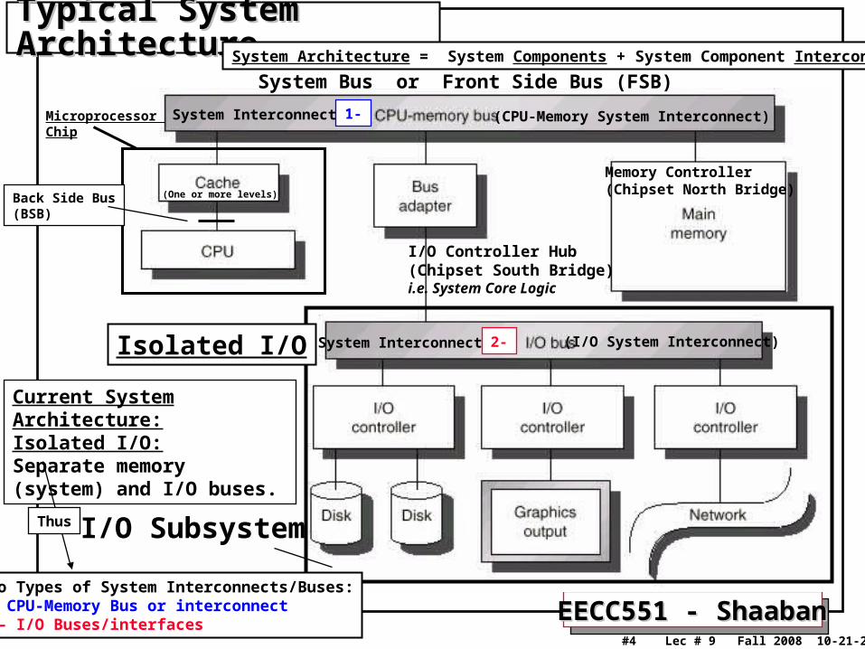
Typical System ArchitectureTypical System Architecture
Current System Architecture:Isolated I/O: Separate memory (system) and I/O buses.
I/O Controller Hub(Chipset South Bridge)i.e. System Core Logic
System Bus or Front Side Bus (FSB)
Memory Controller(Chipset North Bridge)
I/O Subsystem
Microprocessor Chip
Back Side Bus(BSB)
Isolated I/O
System Architecture = System Components + System Component Interconnects
(I/O System Interconnect)
Two Types of System Interconnects/Buses:1- CPU-Memory Bus or interconnect2 – I/O Buses/interfaces
System Interconnects: 1-
System Interconnects: 2-
(CPU-Memory System Interconnect)
(One or more levels)
Thus

EECC551 - ShaabanEECC551 - Shaaban#5 Lec # 9 Fall 2008 10-21-2008
Typical Mainstream System Architecture
SDRAMPC100/PC133100-133MHz64-128 bits wide2-way inteleaved~ 900 MBYTES/SEC )64bit)
Double DateRate (DDR) SDRAMPC3200200 MHz DDR64-128 bits wide4-way interleaved~3.2 GBYTES/SEC (64bit)
RAMbus DRAM (RDRAM)400MHZ DDR16 bits wide (32 banks)~ 1.6 GBYTES/SEC
CPU
Caches
System Bus
I/O Devices
Memory
I/O Controllers
Bus Adapter
DisksDisplaysKeyboards
Networks
NICs
Main I/O BusMemoryController Example: PCI, 33-66MHz
32-64 bits wide 133-528 MB/sPCI-X 133MHz 64-bits wide 1066 MB/s
CPU Core1 GHz - 3.8 GHz4-way SuperscalerRISC or RISC-core (x86): Deep Instruction Pipelines Dynamic scheduling Multiple FP, integer FUs Dynamic branch prediction Hardware speculation
L1
L2 L3
Memory Bus
All Non-blocking cachesL1 16-128K 1-2 way set associative (on chip), separate or unifiedL2 256K- 2M 4-32 way set associative (on chip) unifiedL3 2-16M 8-32 way set associative (on or off chip) unified
Examples: Alpha, AMD K7: EV6, 200-400 MHz Intel PII, PIII: GTL+ 133 MHz Intel P4 800 MHz
NorthBridge
SouthBridge
Chipset
I/O Subsystem
(FSB)
Important issue: Which component creates a system performance bottleneck?
(possiblyon-chip)
Chipset
Front Side Bus
(Isolated I/O Subsystem)
(System Logic) (System Logic)
System Architecture = System Components + System Component Interconnects
Current System Architecture:Isolated I/O: Separate memory (system) and I/O buses.
Two Types of System Interconnects/Buses:1- CPU-Memory Bus or interconnect2 – I/O Buses/interfaces
Thus

EECC551 - ShaabanEECC551 - Shaaban#6 Lec # 9 Fall 2008 10-21-2008
Main Types of Buses/Interconnects in The SystemMain Types of Buses/Interconnects in The SystemProcessor-Memory Bus/Interconnect:
– Should offer very high-speed (bandwidth) and low latency.– Matched to the memory system performance to maximize memory-processor
bandwidth.– Usually system design-specific (not an industry standard).– Examples: Alpha EV6 (AMD K7), Peak bandwidth = 400 MHz x 8 = 3.2 GB/s Intel GTL+ (P3), Peak bandwidth = 133 MHz x 8 = 1 GB/s Intel P4, Peak bandwidth = 800 MHz x 8 = 6.4 GB/s HyperTransport 2.0: 200Mhz-1.4GHz, Peak bandwidth up to 22.8 GB/s (point-to-point system interconnect not a bus)
I/O buses/Interconnects:– Follow bus/interface industry standards.– Usually formed by I/O interface adapters to handle many types of connected I/O devices.– Wide range in the data bandwidth and latency– Not usually interfaced directly to memory instead connected to processor-memory bus
via a bus adapter (system chipset south bridge).– Examples: Main system I/O bus: PCI, PCI-X, PCI Express Storage Interfaces: SATA, PATA, SCSI.
Isolated I/O System Architecture
1
2
System Architecture = System Components + System Component Interconnects
AKA System Bus, Front Side Bus, (FSB)
Sometimes called I/O channels or interfaces

EECC551 - ShaabanEECC551 - Shaaban#7 Lec # 9 Fall 2008 10-21-2008
I/O Interface/ControllerI/O Interface/ControllerI/O Interface, I/O controller or I/O bus adapter:
– Specific to each type of I/O device/interface standard.
– To the CPU, and I/O device, it consists of a set of control and data registers (usually memory-mapped) within the I/O address space.
– On the I/O device side, it forms a localized I/O bus which can be shared by several I/O devices
• (e.g IDE, SCSI, USB ...)
– Handles I/O details (originally done by CPU) such as:• Assembling bits into words,• Low-level error detection and correction• Accepting or providing words in word-sized I/O registers.• Presents a uniform interface to the CPU regardless of I/O
device.
Low-levelI/O Processingoff-loaded from CPU
Industry-standard interfaces
Why?
EECC551 - ShaabanEECC551 - Shaaban#8 Lec # 9 Fall 2008 10-21-2008
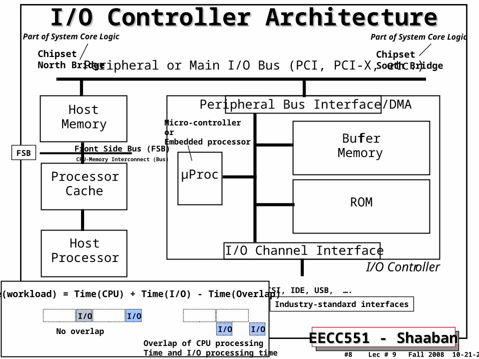
I/O Controller ArchitectureI/O Controller Architecture
Peripheral or Main I/O Bus (PCI, PCI-X, etc.)
HostMemory
ProcessorCache
HostProcessor
Peripheral Bus Interface/DMA
I/O Channel Interface
BufferMemory
ROM
µProc
I/O Controller
ChipsetSouth Bridge
ChipsetNorth Bridge
Micro-controllerorEmbedded processor
SCSI, IDE, USB, ….
Front Side Bus (FSB)CPU-Memory Interconnect (Bus)
Industry-standard interfaces
Part of System Core LogicPart of System Core Logic
FSB
Time(workload) = Time(CPU) + Time(I/O) - Time(Overlap)
No overlap
Overlap of CPU processingTime and I/O processing time
I/O I/O
I/O I/O

EECC551 - ShaabanEECC551 - Shaaban#9 Lec # 9 Fall 2008 10-21-2008
Intel Pentium 4 System Architecture (Using The Intel 925 Chipset)
Source: http://www.anandtech.com/showdoc.aspx?i=2088&p=4
CPU(Including cache) System Bus (Front Side Bus, FSB)
Bandwidth usually should match or exceedthat of main memory
I/O Controller Hub(Chipset South Bridge)
SystemMemoryTwo 8-byte DDR2 Channels
Main I/O Bus(PCI)
Graphics I/O Bus (PCI Express)
Memory Controller Hub(Chipset North Bridge)
Misc.I/OInterfaces
Misc.I/OInterfaces
Storage I/O (Serial ATA)
I/O SubsystemCurrent System Architecture:Isolated I/O: Separate memory and I/O buses.
Isolated I/O
Basic Input Output System (BIOS)
System Core Logic
System Core Logic
System Architecture = System Components + System Component Interconnects

EECC551 - ShaabanEECC551 - Shaaban#10 Lec # 9 Fall 2008 10-21-2008
Bus CharacteristicsBus CharacteristicsOption High performance Low cost/performanceBus width Separate address Multiplex address
& data lines & data lines
Data width Wider is faster Narrower is cheaper (e.g., 64 bits) (e.g., 16 bits)
Transfer size Multiple words has Single-word transferless bus overhead is simpler
Bus masters Multiple Single master(requires arbitration) (no arbitration)
Split Yes, separate No , continuous transaction?Request and Reply connection is cheaper packets gets higher and has lower latencybandwidth(needs multiple masters)
Clocking Synchronous Asynchronous
(e.g . FSB)
FSB = Front Side Bus (Processor-memory Bus or System Bus)

EECC551 - ShaabanEECC551 - Shaaban#11 Lec # 9 Fall 2008 10-21-2008
Example CPU-Memory System BusesExample CPU-Memory System Buses(Front Side Buses, FSBs)(Front Side Buses, FSBs)
Bus Summit Challenge XDBus SP P4
Originator HP SGI Sun IBM Intel
Clock Rate (MHz) 60 48 66 111 800
Split transaction? Yes Yes Yes Yes Yes
Address lines 48 40 ?? ?? ??
Data lines 128 256 144 128 64
Clocks/transfer 4 5 4 ?? ??
Peak (MB/s) 960 1200 1056 1700 6400
Master Multi Multi Multi Multi Multi
Arbitration Central Central Central Central Central
Addressing Physical Physical Physical Physical Physical
Length 13 inches 12 inches 17 inches ?? ??
FSB Bandwidth matched with single 8-byte channel SDRAM
FSB Bandwidth matched with dual channel PC3200 DDR SDRAM

EECC551 - ShaabanEECC551 - Shaaban#12 Lec # 9 Fall 2008 10-21-2008
Main System I/O Bus Example: PCI, PCI-ExpressMain System I/O Bus Example: PCI, PCI-Express
PCI Bus Transaction Latency:
PCI requires 9 cycles @ 33Mhz (272ns) PCI-X requires 10 cycles @ 133MHz (75ns)
Addressing Physical
Master Multi
Arbitration Central
1066133.364PCI-X 1.0
53366.664PCI 2.3
26633.364PCI 2.3
13333.332PCI 2.3
Peak Bandwidth (MB/sec)
Bus Frequency
(MHz)
Bus Width
(bits)
Specification
Legacy PCI
PCI-X 2.0 64 266, 533 2100 , 4200 Not Implemented Yet
PCI = Peripheral Component Interconnect
PCI-Express 1-32 ??? 500-16,000 FormerlyIntel’s 3GIO

EECC551 - ShaabanEECC551 - Shaaban#13 Lec # 9 Fall 2008 10-21-2008
Storage IO Interfaces/BusesStorage IO Interfaces/Buses EIDE/Parallel ATA (PATA) SCSI
Data Width 16 bits 8 or 16 bits (wide)Clock Rate Upto 100MHz 10MHz (Fast)
20MHz (Ultra)40MHz (Ultra2)80MHz (Ultra3)160MHz (Ultra4)
Bus Masters 1 MultipleMax no. devices 2 7 (8-bit bus)
15 (16-bit bus)Peak Bandwidth200 MB/s 320MB/s (Ultra4)
Target Application Desktop Servers
EIDE = Enhanced Integrated Drive ElectronicsATA = Advanced Technology Attachment PATA = Parallel ATA SATA = Serial ATA
SCSI = Small Computer System Interface

EECC551 - ShaabanEECC551 - Shaaban#14 Lec # 9 Fall 2008 10-21-2008
I/O Data Transfer MethodsI/O Data Transfer Methods• Programmed I/O (PIO):Programmed I/O (PIO): PollingPolling (For low-speed I/O) (For low-speed I/O)
– The I/O device puts its status information in a status register.
– The processor must periodically check the status register.
– The processor is totally in control and does all the work.
– Very wasteful of processor time.
– Used for low-speed I/O devices (mice, keyboards etc.)
• Interrupt-Driven I/OInterrupt-Driven I/O (For medium-speed I/O): (For medium-speed I/O):– An interrupt line from the I/O device to the CPU is used to generate an
I/O interrupt indicating that the I/O device needs CPU attention.
– The interrupting device places its identity in an interrupt vector.
– Once an I/O interrupt is detected the current instruction is completed and an I/O interrupt handling routine (by OS) is executed to service the device.
– Used for moderate speed I/O (optical drives, storage, neworks ..)
– Allows overlap of CPU processing time and I/O processing time Time(workload) = Time(CPU) + Time(I/O) - Time(Overlap)
No overlap
Overlap of CPU processingTime and I/O processing time
(e.g data is ready)
1
2
I/O I/O
I/O I/O

EECC551 - ShaabanEECC551 - Shaaban#15 Lec # 9 Fall 2008 10-21-2008
I/O data transfer methods:I/O data transfer methods:Direct Memory Access (DMA)Direct Memory Access (DMA) (For high-speed I/O): (For high-speed I/O): • Implemented with a specialized controller that transfers data between an I/O device
and memory independent of the processor.• The DMA controller becomes the bus master and directs reads and writes between
itself and memory.• Interrupts are still used only on completion of the transfer or when an error occurs.• Low CPU overhead, used in high speed I/O (storage, network interfaces)• Allows more overlap of CPU processing time and I/O processing time than
interrupt-driven I/O.
• DMA transfer steps:– The CPU sets up DMA by supplying device identity, operation, memory address
of source and destination of data, the number of bytes to be transferred.– The DMA controller starts the operation. When the data is available it transfers
the data, including generating memory addresses for data to be transferred.– Once the DMA transfer is complete, the controller interrupts the processor,
which determines whether the entire operation is complete.
3
1
3
2

EECC551 - ShaabanEECC551 - Shaaban#16 Lec # 9 Fall 2008 10-21-2008
I/O: A System Performance PerspectiveI/O: A System Performance Perspective• CPU Performance: Improvement of ~ 60% per year.
• I/O Sub-System Performance: Limited by mechanical delays (disk I/O). Improvement less than 10% per year (IO rate per sec or MB per sec).
• From Amdahl's Law: overall system speed-up is limited by the slowest component:
If I/O is 10% of current processing time:• Increasing CPU performance by 10 times
5 times system performance increase (50% loss in performance)
• Increasing CPU performance by 100 times ~ 10 times system performance (90% loss of performance)
• The I/O system performance bottleneck diminishes the benefit of faster CPUs on overall system performance.
I/O CPU
I/O CPU
I/O
/ 10
/ 10
Speedup = 5.2I/O = 53% CPU = 47%
Originally: I/O = 10% CPU = 90%
Speedup = 9.2I/O = 92% CPU = 8%
Originally: CPU-bound
After: I/O-bound
System performance depends on many aspects of the system (“limited by weakest link in the chain”): The system performance bottleneck
CPU Memory I/O
i.e storage devices (hard drives)

EECC551 - ShaabanEECC551 - Shaaban#17 Lec # 9 Fall 2008 10-21-2008
System & I/O Performance Metrics/ModelingSystem & I/O Performance Metrics/Modeling• Diversity: The variety of I/O devices that can be connected to the system.
• Capacity: The maximum number of I/O devices that can be connected to the system.
• Producer/server Model of I/O: The producer (CPU, human etc.) creates tasks to be performed and places them in a task buffer (queue); the server (I/O device or controller) takes tasks from the queue and performs them.
• I/O Throughput: The maximum data rate that can be transferred to/from an I/O device or sub-system, or the maximum number of I/O tasks or transactions completed by I/O in a certain period of time Maximized when task queue is never empty (server always busy).
• I/O Latency or response time: The time an I/O task takes from the time it is placed in the task buffer or queue until the server (I/O system) finishes the task. Includes I/O device serice time and buffer waiting (or queuing time). Minimized when task queue is always empty (no queuing time).
Response Time = Service Time + Queuing Time
I/O Performance Modeling:
I/O Performance Metrics:
I/O Tasks
I/O Tasks
Task Queue
Producer Server
Producer:i.e User, OS or CPU
Server: i.e I/O device + controller
(FIFO)

EECC551 - ShaabanEECC551 - Shaaban#18 Lec # 9 Fall 2008 10-21-2008
System & I/O Performance Metrics: Throughput• Throughput is a measure of speed—the rate at which the I/O or
storage system delivers data.
• I/O Throughput is measured in two ways:
• I/O rate:– Measured in:
• Accesses/second,
• Transactions Per Second (TPS) or,
• I/O Operations Per Second (IOPS).
– I/O rate is generally used for applications where the size of each request is small, such as in transaction processing.
• Data rate, measured in bytes/second or megabytes/second (MB/s). – Data rate is generally used for applications where the size of each request
is large, such as in scientific and multimedia applications.
1
2
i.e server applications

EECC551 - ShaabanEECC551 - Shaaban#19 Lec # 9 Fall 2008 10-21-2008
System & I/O Performance Metrics: Response time • Response time measures how long a storage (or I/O)
system takes to process an I/O request and access data. – I/O request latency or total processing time per I/O request.
• This time can be measured in several ways. For example:
– One could measure time from the user’s perspective,
– the operating system’s perspective,
– or the disk controller’s perspective, depending on what you view as the storage or I/O system.
Response timeInitiateRequest
I/O RequestDone
(By CPU, User or OS)
CPU time + I/O Bus Transfer Time + Queue Time + I/O controller Time + I/O device service time + ...
The utilization of DMA and I/O device queues and multiple I/O devicesservicing a queue may make throughput >> 1 / response time
I/O Request Started
Or entire system
Is Response time always = 1 / Throughput ?

EECC551 - ShaabanEECC551 - Shaaban#20 Lec # 9 Fall 2008 10-21-2008
Producer ServerQueue(FIFO)
I/O ModelingI/O Modeling: Producer-Server Model Producer-Server Model
• Throughput:– The number of tasks completed by the server in unit time.– In order to get the highest possible throughput:
• The server should never be idle.• The queue should never be empty.
• Response time:– Begins when a task is placed in the queue– Ends when it is completed by the server– In order to minimize the response time:
• The queue should be empty (no waiting time in queue).• The server will be idle at times.
i.e I/O device + controlleri.e User, OS, or CPU
Queue wait time = Tq
Server Service Time per task Tser
Time a task spends waiting in queue
Task Arrival Rate, r tasks/sec
Timesystem =Time in System for a task =
Response Time = Queuing Time + Service Time
I/O TasksI/O TasksProducer Server
Shown above is a (Single Queue + Single Server) Producer-Server Model
Throughput is maximized when:
Response Time is minimized when:
Shown above: Single Queue + Single Server

EECC551 - ShaabanEECC551 - Shaaban#21 Lec # 9 Fall 2008 10-21-2008
Producer-ServerProducer-ServerModelModel
ThroughputThroughput vs. vs. Response TimeResponse Time
Response Time = TimeSystem = TimeQueue + TimeServer = Tq + Tser I/O device + controller
User or CPU
Queue almost emptymost of the timeLess time in queue
Queuefullmost of the time.More timein queue
i.e Utilization = U ranges from 0 to 1 (0 % to 100%)
Tser
TqTask Arrival Rate, r
I/O Tasks
I/O Tasks
(FIFO)
Shown here is a (Single Queue + Single Server) Producer-Server Model
AKA Loading Factor
Single Queue + Single Server
Utilization

EECC551 - ShaabanEECC551 - Shaaban#22 Lec # 9 Fall 2008 10-21-2008
I/O PerformanceI/O Performance: Throughput EnhancementThroughput Enhancement
Producer
ServerQueue
QueueServer
• In general throughput can be improved by:– Throwing more hardware at the problem.
– Reduces load-related latency.
• Response time is much harder to reduce.– e.g. Faster I/O device (i.e server)
I/O device + controller
I/O device + controllere.g CPU
Shown here: Two Queues + Two Servers
I/O TasksI/O
Tasks
I/O Tasks
I/O Tasks
I/O Tasks
Less queuing time
Response Time = TimeSystem = TimeQueue + TimeServer = Tq + Tser
TimeQueue
TimeServer
Ignoring CPUI/O processing timeand other system delays
TqTser

EECC551 - ShaabanEECC551 - Shaaban#23 Lec # 9 Fall 2008 10-21-2008
Seek Time
Magnetic DisksMagnetic DisksCharacteristics:Characteristics:• Diameter (form factor): 2.5in - 5.25in
• Rotational speed: 3,600RPM-15,000 RPM
• Tracks per surface.
• Sectors per track: Outer tracks contain
more sectors.
• Recording or Areal Density: Tracks/in X Bits/in
• Cost Per Megabyte.
• Seek Time: (2-12 ms)
The time needed to move the read/write head arm.
Reported values: Minimum, Maximum, Average.
• Rotation Latency or Delay: (2-8 ms)
The time for the requested sector to be under
the read/write head. (~ time for half a rotation)
• Transfer time: The time needed to transfer a sector of bits.
• Type of controller/interface: SCSI, EIDE
• Disk Controller delay or time.
• Average time to access a sector of data =
average seek time + average rotational delay + transfer time
+ disk controller overhead
(ignoring queuing time)
Bits/ Inch2
Current Rotation speed7200-15000 RPM
Current Areal Density ~ 100 Gbits / Inch2
{
Access time = average seek time + average rotational delay
(PATA, SATA)
Rotation Time
Read/WriteHead
SeekTime
Storage I/O Systems:
EECC551 - ShaabanEECC551 - Shaaban#24 Lec # 9 Fall 2008 10-21-2008
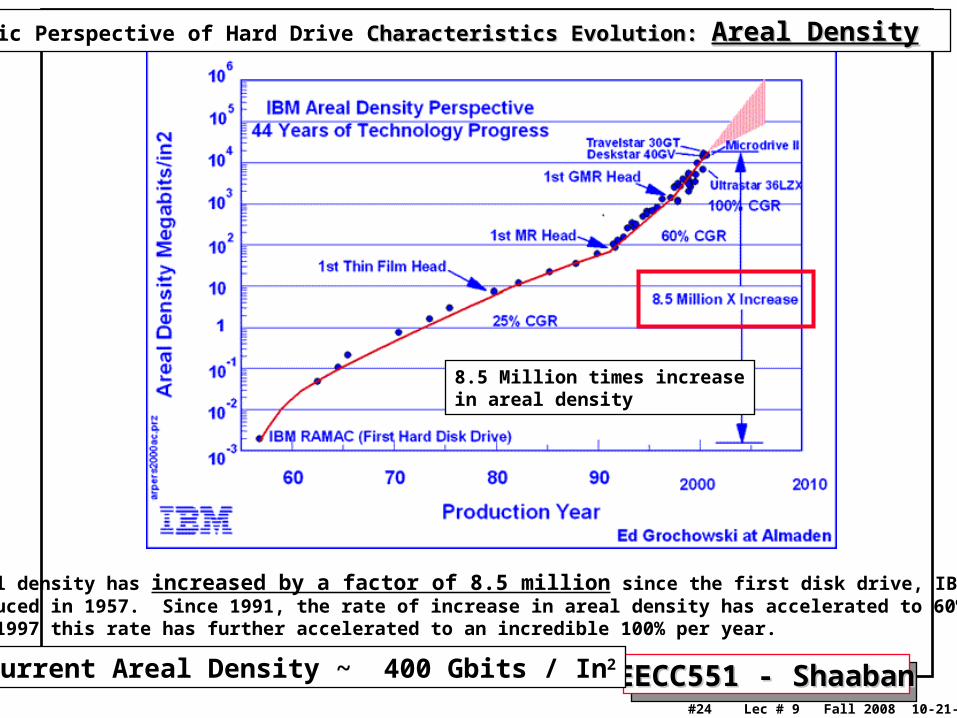
Drive areal density has increased by a factor of 8.5 million since the first disk drive, IBM's RAMAC, was introduced in 1957. Since 1991, the rate of increase in areal density has accelerated to 60% per year, and since 1997 this rate has further accelerated to an incredible 100% per year.
Historic Perspective of Hard Drive Characteristics Evolution: Characteristics Evolution: Areal DensityAreal Density
Current Areal Density ~ 400 Gbits / In2
8.5 Million times increasein areal density

EECC551 - ShaabanEECC551 - Shaaban#25 Lec # 9 Fall 2008 10-21-2008
Historic Perspective of Hard Drive Characteristics Evolution: Characteristics Evolution: Internal Data Transfer RateInternal Data Transfer Rate
Internal data transfer rate increase is influenced by the increase in areal density
100x times increaseover last 20 years

EECC551 - ShaabanEECC551 - Shaaban#26 Lec # 9 Fall 2008 10-21-2008
Historic Perspective of Hard Drive Characteristics Evolution: Characteristics Evolution: Access/Seek TimeAccess/Seek Time
Access/Seek Time is a big factor in service(response) time for small/random disk requests. Limited improvement due to mechanical rotation speed + seek delay
Less than 3x times improvement over 15 years!
Access time = average seek time + average rotational delay
EECC551 - ShaabanEECC551 - Shaaban#27 Lec # 9 Fall 2008 10-21-2008
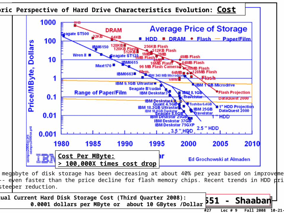
The price per megabyte of disk storage has been decreasing at about 40% per year based on improvements in data density,-- even faster than the price decline for flash memory chips. Recent trends in HDD price per megabyte show an even steeper reduction.
Historic Perspective of Hard Drive Characteristics Evolution: Characteristics Evolution: CostCost
Actual Current Hard Disk Storage Cost (Third Quarter 2008): 0.0001 dollars per MByte or about 10 GBytes /Dollar
Cost Per MByte:> 100,000X times cost drop

EECC551 - ShaabanEECC551 - Shaaban#28 Lec # 9 Fall 2008 10-21-2008
Historic Perspective of Hard Drive Characteristics Evolution: Characteristics Evolution: RoadmapRoadmap
Current Areal Density ~ 100 Gbits / In2

EECC551 - ShaabanEECC551 - Shaaban#29 Lec # 9 Fall 2008 10-21-2008
Basic Disk Performance ExampleBasic Disk Performance Example• Given the following Disk Parameters:
– Average seek time is 5 ms
– Disk spins at 10,000 RPM
– Transfer rate is 40 MB/sec
• Controller overhead is 0.1 ms
• Assume that the disk is idle, so no queuing delay exist.
• What is Average Disk read or write service time for a 500-byte (.5 KB) Sector?
Ave. seek + ave. rot delay + transfer time + controller overhead
= 5 ms + 0.5/(10000 RPM/60) + 0.5 KB/40 MB/s + 0.1 ms
= 5 + 3 + 0.13 + 0.1 = 8.23 ms
Time for half a rotation
(Disk Service Time for this request)Tservice
Or Tser Here: 1KBytes = 103 bytes, MByte = 106 bytes, 1 GByte = 109 bytes
Actual time to process the disk requestis greater and may include CPU I/O processing Timeand queuing time
Access Time

EECC551 - ShaabanEECC551 - Shaaban#30 Lec # 9 Fall 2008 10-21-2008
Introduction to Queuing TheoryIntroduction to Queuing Theory
• Concerned with long term, steady state than in startup: – where => Arrivals = Departures Rate r Rate
• Little’s Law:
Mean number tasks in system = arrival rate x mean response time
• Applies to any system in equilibrium, as long as nothing in the black box is creating or destroying tasks.
Arrivals Departures
Lsys (length or number of tasks in system)
Tsys (System Time)r (arrival rate)
(Steady State)
(Steady State)
Task Arrival Rate, r tasks/sec
Task Task
r

EECC551 - ShaabanEECC551 - Shaaban#31 Lec # 9 Fall 2008 10-21-2008
I/O Performance & Little’s Queuing LawI/O Performance & Little’s Queuing Law
• Given: An I/O system in equilibrium (input rate is equal to output rate) and: – Tser : Average time to service a task = 1/Service rate
– Tq : Average time per task in the queue
– Tsys : Average time per task in the system, or the response time,
the sum of Tser and Tq thus Tsys = Tser + Tq
– r : Average number of arriving tasks/sec (i.e task arrival rate)– Lser : Average number of tasks in service.
– Lq : Average length of queue
– Lsys : Average number of tasks in the system,
the sum of L q and Lser
• Little’s Law states: Lsys = r x Tsys (applied to system)
Lq = r x Tq (applied to queue)
• Server utilization = u = r / Service rate = r x Tser
u must be between 0 and 1 otherwise there would be more tasks arriving than could be serviced
Proc IOC Device
Queue server
System
Tq
Tser
Task arrival rate rtasks/sec
Tsys = Tq + Tser
Here a server is the device (i.e hard drive) and its I/O controller (IOC)
CPUOS or User
(Single Queue + Single Server)
Task Service Time
FIFO
Tasks Tasks
Producer:
Ignoring CPU processing timeand other system delays
AKALoadingFactor
r = Task Arrival rate
EECC551 - ShaabanEECC551 - Shaaban#32 Lec # 9 Fall 2008 10-21-2008
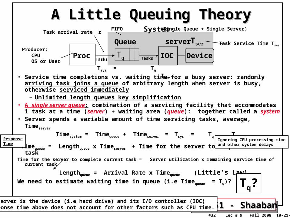
A Little Queuing TheoryA Little Queuing Theory
• Service time completions vs. waiting time for a busy server: randomly arriving task joins a queue of arbitrary length when server is busy, otherwise serviced immediately
– Unlimited length queues key simplification• A single server queue: combination of a servicing facility that accommodates 1
task at a time (server) + waiting area (queue): together called a system• Server spends a variable amount of time servicing tasks, average, Timeserver
Timesystem = Timequeue + Timeserver = Tsys = Tq + Tser
Timequeue = Lengthqueue x Timeserver + Time for the server to complete current taskTime for the server to complete current task = Server utilization x remaining service time of current task
Lengthqueue = Arrival Rate x Timequeue (Little’s Law) We need to estimate waiting time in queue (i.e Timequeue = Tq)?
Proc IOC Device
Queue server
System
Tq
Tser
Task arrival rate r
Tsys = Tq + Tser
Here a server is the device (i.e hard drive) and its I/O controller (IOC)The response time above does not account for other factors such as CPU time.
(Single Queue + Single Server)
CPUOS or User
ResponseTime
Tq?
FIFO
Tasks Tasks
Producer:
Ignoring CPU processing timeand other system delays
Task Service Time Tser

EECC551 - ShaabanEECC551 - Shaaban#33 Lec # 9 Fall 2008 10-21-2008
A Little Queuing Theory
• Server spends a variable amount of time with customers– Arithmetic mean time = m1 = (f1 x T1 + f2 x T2 +...+ fn x Tn)
• where Ti is the time for task i and fi is the frequency of task i
– variance = (f1 x T12 + f2 x T22 +...+ fn x Tn2) – m12
• Must keep track of unit of measure (100 ms2 vs. 0.1 s2 )– Squared coefficient of variance: C2 = variance/m12
• Unitless measure
• Exponential (Poisson) distribution C2 = 1 : most short relative to average, few others long; 90% < 2.3 x average, 63% < average
• Hypoexponential distribution C2 < 1 : most close to average, C2=0.5 => 90% < 2.0 x average, only 57% < average
• Hyperexponential distribution C2 > 1 : further from average C2=2.0 => 90% < 2.8 x average, 69% < average
Proc IOC Device
Queue server
System
Avg.
Variance = (Standard deviation)2
Distributions:
(Single Queue + Single Server)FIFOTask arrival rate rtasks/sec
Task Service Time Tser
Tq
Tser

EECC551 - ShaabanEECC551 - Shaaban#34 Lec # 9 Fall 2008 10-21-2008
A Little Queuing Theory: Average Queue Wait TimeA Little Queuing Theory: Average Queue Wait Time• Calculating average wait time in queue Tq
– If something at server, it takes to complete on average m1(z) = 1/2 x Tser x (1 + C2)– Chance server is busy = u; average delay is u x m1(z) = 1/2 x u x Tser x (1 + C2)– All customers in line must complete; each avg Tser
Timequeue = Time for the server to complete current task + Lengthqueue x Timeserver
Timequeue = Average residual service time + Lengthqueue x Timeserver
Tq = u x m1(z) + Lq x Ts er= 1/2 x u x Tser x (1 + C2) + Lq x Ts er
Tq = 1/2 x u x Ts er x (1 + C2) + r x Tq x Ts er
Tq = 1/2 x u x Ts er x (1 + C2) + u x Tq
Tq x (1 – u) = Ts er x u x (1 + C2) /2
Tq = Ts er x u x (1 + C2) / (2 x (1 – u))
• Notation: r average number of arriving tasks/second
Tser average time to service a tasku server utilization (0..1): u = r x Tser
Tq average time/request in queueLq average length of queue: Lq= r x Tq
Lq = r x Tq
(Little’s Law)
(Rearrange)
A version of this derivation in textbook page 385 (3rd Edition: page 726)
For Single Queue + Single Server
Tq
What if utilization u = 1 ?

EECC551 - ShaabanEECC551 - Shaaban#35 Lec # 9 Fall 2008 10-21-2008
A Little Queuing Theory: M/G/1 and M/M/1A Little Queuing Theory: M/G/1 and M/M/1• Assumptions so far:
– System in equilibrium– Time between two successive task arrivals in line are random– Server can start on next task immediately after prior finishes– No limit to the queue: works First-In-First-Out (FIFO)
– Afterward, all tasks in line must complete; each avg Tser
• Described “memoryless” or Markovian request arrival (M for C2=1 exponentially random), General service distribution (no restrictions), 1 server: M/G/1 queue
• When Service times have C2 = 1, M/M/1 queue
• Tq = Tser x u x (1 + C2) /(2 x (1 – u)) = Tser x u / (1 – u) (Tq average time/task in queue)
Tser average time to service a taskLq Average length of queue Lq = r x Tq = u2 / (1 – u)
u server utilization (0..1): u = r x Tser
ArrivalDistribution
ServiceDistribution
Number ofServers
Queuing Time, Tq
Timesystem = Timequeue + Timeserver = Tsys = Tq + Tser
(In Textbook page 726)
Single Queue + Single Server
ResponseTime
Tq
(i.e C2 =1) (i.e C2 =1)

EECC551 - ShaabanEECC551 - Shaaban#36 Lec # 9 Fall 2008 10-21-2008
Single Queue + Multiple Servers (Disks/Controllers) Single Queue + Multiple Servers (Disks/Controllers)
I/O Modeling:I/O Modeling: M/M/m Queue M/M/m Queue
• I/O system with Markovian request arrival rate r
• A single queue serviced by m servers (disks + controllers) each with Markovian Service rate = 1/ Tser
(and requests are distributed evenly among all servers)
Tq = Tser x u /[m (1 – u)]
where u = r x Tser / m
m number of servers
Tser average time to service a task u server utilization (0..1): u = r x Tser / m
Tq average time/task in queue
Lq Average length of queue Lq = r x Tq
Tsys = Tser + Tq Time in system (mean response time)
Arrival Service Number of servers
Request Arrival Rate
m servers each has service time = Tser
1
2
m
Single Queue
i.e as if the m servers are a single server with an effective service time of Tser / m
Please Note:We will use this simplified formula for M/M/m not the book version 4th Edition on page 388 (3rd Edition: page729)
Tq
r
Tser
(FIFO)
Tasks
i.e C2 = 1
i.e C2 = 1

EECC551 - ShaabanEECC551 - Shaaban#37 Lec # 9 Fall 2008 10-21-2008
I/O Queuing Performance: An M/M/1 ExampleI/O Queuing Performance: An M/M/1 Example• A processor sends 40 disk I/O requests per second, requests & service
are exponentially distributed, average disk service time = 20 ms
• On average: – What is the disk utilization u?– What is the average time spent in the queue, Tq? – What is the average response time for a disk request, Tsys ?– What is the number of requests in the queue Lq? In system, Lsys?
• We have:r average number of arriving requests/second = 40Tser average time to service a request = 20 ms (0.02s)
• We obtain:
u server utilization: u = r x Tser = 40/s x .02s = 0.8 or 80%Tq average time/request in queue = Tser x u / (1 – u)
= 20 x 0.8/(1-0.8) = 20 x 0.8/0.2 = 20 x 4 = 80 ms (0 .08s)Tsys average time/request in system: Tsys = Tq + Tser= 80+ 20 = 100
msLq average length of queue: Lq= r x Tq
= 40/s x 0.08s = 3.2 requests in queueLsys average # tasks in system: Lsys = r x Tsys = 40/s x 0.1s = 4
Tserr i.e C2 = 1
i.e Mean Response Time

EECC551 - ShaabanEECC551 - Shaaban#38 Lec # 9 Fall 2008 10-21-2008
I/O Queuing Performance: An M/M/1 ExampleI/O Queuing Performance: An M/M/1 Example• Previous example with a faster disk with average disk service time = 10 ms• The processor still sends 40 disk I/O requests per second, requests & service
are exponentially distributed
• On average: – How utilized is the disk, u?– What is the average time spent in the queue, Tq? – What is the average response time for a disk request, Tsys ?
• We have:r average number of arriving requests/second = 40Tser average time to service a request = 10 ms (0.01s)
• We obtain:
u server utilization: u = r x Tser = 40/s x .01s = 0.4 or 40%
Tq average time/request in queue = Tser x u / (1 – u) = 10 x 0.4/(1-0.4) = 10 x 0.4/0.6 = 6.67 ms (0 .0067s)
Tsys average time/request in system: Tsys = Tq +Tser=10 + 6.67 = = 16.67 ms
Response time is 100/16.67 = 6 times faster even though the new service time is only 2 times faster due to lower queuing time .
Tser
6.67 ms instead of 80 ms
(Changed from 20 ms to 10 ms)
i.e C2 = 1
i.e Mean Response Time

EECC551 - ShaabanEECC551 - Shaaban#39 Lec # 9 Fall 2008 10-21-2008
Factors Affecting System & I/O PerformanceFactors Affecting System & I/O Performance• I/O processing computational requirements:
– CPU computations available for I/O operations.– Operating system I/O processing policies/routines.– I/O Data Transfer/Processing Method used.
• CPU cycles needed: Polling >> Interrupt Driven > DMA
• I/O Subsystem performance:– Raw performance of I/O devices (i.e magnetic disk performance).– I/O bus capabilities.– I/O subsystem organization. i.e number of devices, array level .. – Loading level (u) of I/O devices (queuing delay, response time).
• Memory subsystem performance:– Available memory bandwidth for I/O operations (For DMA)
• Operating System Policies: – File system vs. Raw I/O.– File cache size and write Policy.– File pre-fetching, etc.
System performance depends on many aspects of the system (“limited by weakest link in the chain”): The system performance bottleneck
CPU Memory I/O
Components of Total System Execution Time:
Tq
Service Time, Tser, Throughput

EECC551 - ShaabanEECC551 - Shaaban#40 Lec # 9 Fall 2008 10-21-2008
System Design (Including I/O)System Design (Including I/O)• When designing a system, the performance of the components
that make it up should be balanced. • Steps for designing I/O systems are:
– List types and performance of I/O devices and buses in the system– Determine target application computational & I/O demands– Determine the CPU resource demands for I/O processing
• CPU clock cycles directly for I/O (e.g. initiate, interrupts, complete)• CPU clock cycles due to stalls waiting for I/O• CPU clock cycles to recover from I/O activity (e.g., cache flush)
– Determine memory and I/O bus resource demands– Assess the system performance of the different ways to organize these
devices:• For each system configuration identify which system component (CPU,
memory, I/O buses, I/O devices etc.) is the performance bottleneck.• Improve performance of the component that poses a system performance
bottleneck
System performance depends on many aspects of the system (“limited by weakest link in the chain”)
IterativeRefinementProcess
IterativeRefinementProcess
System Performance Bottleneck
i.e system configurations

EECC551 - ShaabanEECC551 - Shaaban#41 Lec # 9 Fall 2008 10-21-2008
Here: 1KBytes = 103 bytes, MByte = 106 bytes, 1 GByte = 109 bytes
Example: Determining the System Performance Example: Determining the System Performance Bottleneck (Bottleneck (ignoring I/O queuing delaysignoring I/O queuing delays))
• Assume the following system components:– 500 MIPS CPU– 16-byte wide memory system with 100 ns cycle time– 200 MB/sec I/O bus – 20, 20 MB/sec SCSI-2 buses, with 1 ms controller overhead– 5 disks per SCSI bus: 8 ms seek, 7,200 RPMS, 6MB/sec (100 disks total)
• Other assumptions– All devices/system components can be used to 100% utilization
– Average I/O request size is 16 KB
– I/O Requests are assumed spread evenly on all disks.
– OS uses 10,000 CPU instructions to process a disk I/O request
– Ignore disk/controller queuing delays.(Since I/O queuing delays are ignored here 100% disk utilization is allowed)
• What is the average IOPS?
• What is the average I/O bandwidth?
• What is the average response time per IO operation?
i.e I/O throughput
(i.e u = 1)
(i.e u = 1)
Main system I/O Bus

EECC551 - ShaabanEECC551 - Shaaban#42 Lec # 9 Fall 2008 10-21-2008
• The performance of I/O systems is determined by the system component with the lowest performance (the system performance bottleneck):
– CPU : (500 MIPS)/(10,000 instructions per I/O) = 50,000 IOPS
CPU time per I/O = 10,000 / 500,000,000 = .02 ms
– Main Memory : (16 bytes)/(100 ns x 16 KB per I/O) = 10,000 IOPS
Memory time per I/O = 1/10,000 = .1ms
– I/O bus: (200 MB/sec)/(16 KB per I/O) = 12,500 IOPS
– SCSI-2: (20 buses)/((1 ms + (16 KB)/(20 MB/sec)) per I/O) = 11,111 IOPS
SCSI bus time per I/O = 1ms + 16/20 ms = 1.8ms
– Disks: (100 disks)/((8 ms + 0.5/(7200 RPMS) + (16 KB)/(6 MB/sec)) per I/O) =
6700 IOPS
Tdisk = (8 ms + 0.5/(7200 RPMS) + (16 KB)/(6 MB/sec) = 8+ 4.2+ 2.7 = 14.9ms
• The disks limit the I/O performance to 6700 IOPS
• The average I/O bandwidth is 6700 IOPS x (16 KB/sec) = 107.2 MB/sec
• Response Time Per I/O = Tcpu + Tmemory + Tscsi + Tdisk =
= .02 + .1 + 1.8 + 14.9 = 16.82 ms
Since I/O queuing delays are ignored here 100% disk utilization is allowed
Here: 1KBytes = 103 bytes, MByte = 106 bytes, 1 GByte = 109 bytes
Example: Determining the System I/O BottleneckExample: Determining the System I/O Bottleneck (ignoring queuing delays)(ignoring queuing delays)
Tser
Determining the system performance bottleneck
Throughput:
EECC551 - ShaabanEECC551 - Shaaban#43 Lec # 9 Fall 2008 10-21-2008
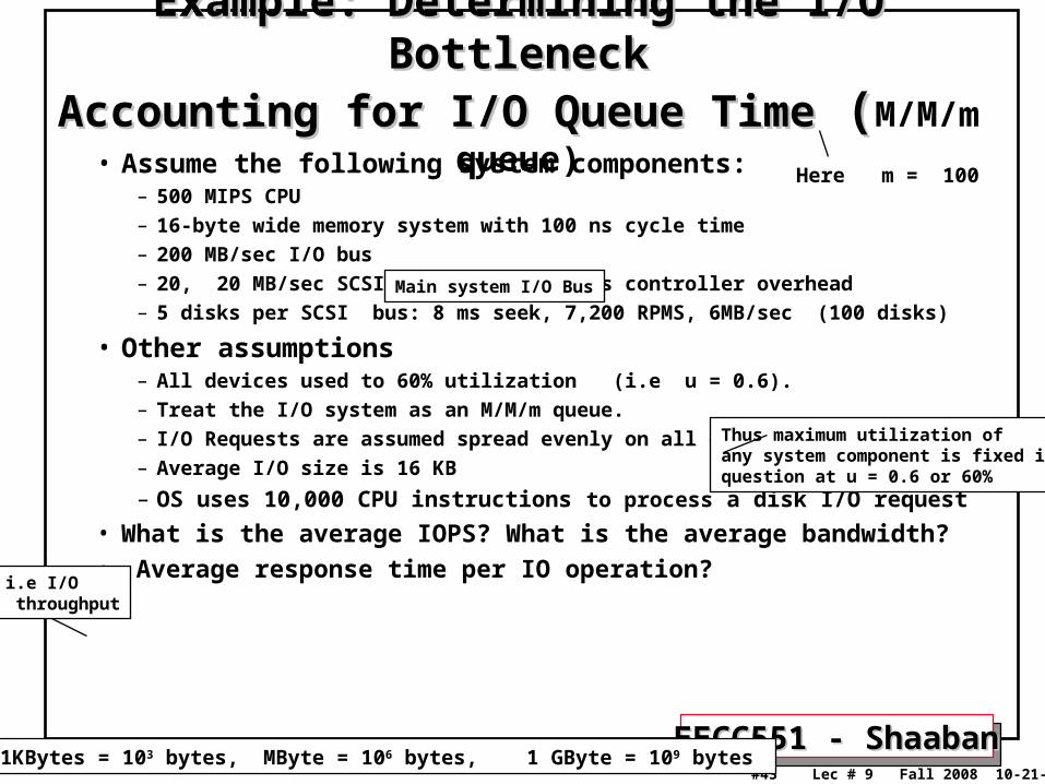
Example: Determining the I/O BottleneckExample: Determining the I/O BottleneckAccounting for I/O Queue TimeAccounting for I/O Queue Time ( (M/M/m queue)
• Assume the following system components:– 500 MIPS CPU– 16-byte wide memory system with 100 ns cycle time– 200 MB/sec I/O bus – 20, 20 MB/sec SCSI-2 buses, with 1 ms controller overhead– 5 disks per SCSI bus: 8 ms seek, 7,200 RPMS, 6MB/sec (100 disks)
• Other assumptions– All devices used to 60% utilization (i.e u = 0.6).– Treat the I/O system as an M/M/m queue.– I/O Requests are assumed spread evenly on all disks.– Average I/O size is 16 KB
– OS uses 10,000 CPU instructions to process a disk I/O request
• What is the average IOPS? What is the average bandwidth?• Average response time per IO operation?
Here m = 100
Here: 1KBytes = 103 bytes, MByte = 106 bytes, 1 GByte = 109 bytes
i.e I/O throughput
Main system I/O Bus
Thus maximum utilization of any system component is fixed in question at u = 0.6 or 60%

EECC551 - ShaabanEECC551 - Shaaban#44 Lec # 9 Fall 2008 10-21-2008
• The performance of I/O systems is still determined by the system component with the lowest performance (the system performance bottleneck):
– CPU : (500 MIPS)/(10,000 instr. per I/O) x .6 = 30,000 IOPS CPU time per I/O = 10,000 / 500,000,000 = .02 ms– Main Memory : (16 bytes)/(100 ns x 16 KB per I/O) x .6 = 6,000 IOPS Memory time per I/O = 1/10,000 = .1ms– I/O bus: (200 MB/sec)/(16 KB per I/O) x .6 = 12,500 IOPS– SCSI-2: (20 buses)/((1 ms + (16 KB)/(20 MB/sec)) per I/O) x .6 = 6,666.6 IOPS SCSI bus time per I/O = 1ms + 16/20 ms = 1.8ms– Disks: (100 disks)/((8 ms + 0.5/(7200 RPMS) + (16 KB)/(6 MB/sec)) per I/O) x .6 = 6,700 x .6 = 4020 IOPS
Tser = (8 ms + 0.5/(7200 RPMS) + (16 KB)/(6 MB/sec) = 8+4.2+2.7 = 14.9ms
• The disks limit the I/O performance to r = 4020 IOPS• The average I/O bandwidth is 4020 IOPS x (16 KB/sec) = 64.3 MB/sec• Tq = Tser x u /[m (1 – u)] = 14.9ms x .6 / [100 x .4 ] = .22 ms • Response Time = Tser + Tq+ Tcpu + Tmemory + Tscsi =
14.9 + .22 + .02 + .1 + 1.8 = 17.04 ms
Example: Determining the I/O BottleneckExample: Determining the I/O Bottleneck
Accounting For I/O Queue Time Accounting For I/O Queue Time ((M/M/m queue)
Here: 1KBytes = 103 bytes, MByte = 106 bytes, 1 GByte = 109 bytes
Determining the system performance bottleneck
Throughput
Using expressionfor Tq for M/M/mfrom slide 36
Total System response time including CPU time and other delays
Related Documents

![Instruction Set Architecture (ISA)meseec.ce.rit.edu/eecc551-fall2000/551-9-12-2000.pdf · 2000. 9. 12. · Instruction Set Architecture (ISA) “... the attributes of a [computing]](https://static.cupdf.com/doc/110x72/61026047fa8db44d1f2dce1d/instruction-set-architecture-isa-2000-9-12-instruction-set-architecture-isa.jpg)