EECC551 - Shaaban EECC551 - Shaaban #1 Lec # 11 Winter 2002 1-29 Input/Output & System Performance Input/Output & System Performance Issues Issues • System I/O Connection Structure System I/O Connection Structure – Types of Buses in the system. Types of Buses in the system. • I/O Data Transfer Methods. I/O Data Transfer Methods. • Cache & I/O. Cache & I/O. • I/O Performance Metrics. I/O Performance Metrics. • Magnetic Disk Characteristics. Magnetic Disk Characteristics. • I/O System Modeling Using Queuing Theory. I/O System Modeling Using Queuing Theory. • Designing an I/O System & System Designing an I/O System & System Performance: Performance: – System performance bottleneck. System performance bottleneck. In textbook: Ch. 7.1-7.3, 7.7, 7.8

EECC551 - Shaaban #1 Lec # 11 Winter 2002 1-29-2003 Input/Output & System Performance Issues System I/O Connection StructureSystem I/O Connection Structure.
Dec 19, 2015
Welcome message from author
This document is posted to help you gain knowledge. Please leave a comment to let me know what you think about it! Share it to your friends and learn new things together.
Transcript
EECC551 - ShaabanEECC551 - Shaaban#1 Lec # 11 Winter 2002 1-29-2003
Input/Output & System Performance IssuesInput/Output & System Performance Issues
• System I/O Connection StructureSystem I/O Connection Structure– Types of Buses in the system.Types of Buses in the system.
• I/O Data Transfer Methods.I/O Data Transfer Methods.
• Cache & I/O.Cache & I/O.
• I/O Performance Metrics.I/O Performance Metrics.
• Magnetic Disk Characteristics.Magnetic Disk Characteristics.
• I/O System Modeling Using Queuing Theory.I/O System Modeling Using Queuing Theory.
• Designing an I/O System & System Performance:Designing an I/O System & System Performance:– System performance bottleneck.System performance bottleneck.
In textbook: Ch. 7.1-7.3, 7.7, 7.8
EECC551 - ShaabanEECC551 - Shaaban#2 Lec # 11 Winter 2002 1-29-2003
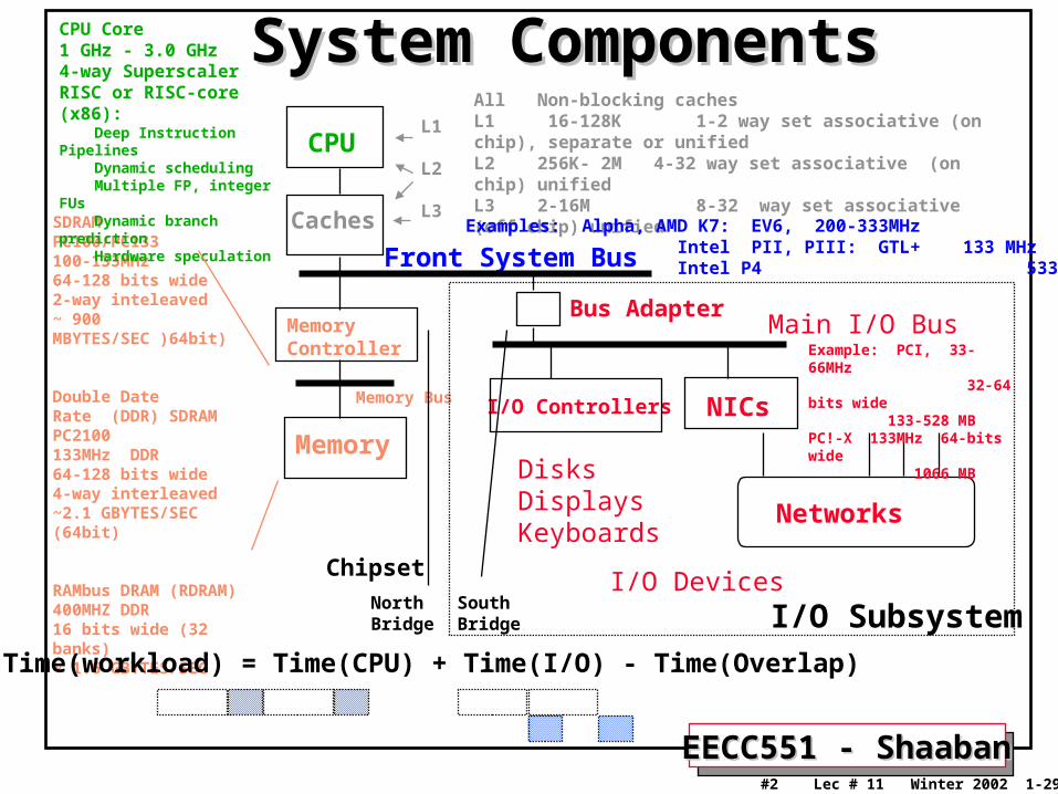
System ComponentsSystem Components
SDRAMPC100/PC133100-133MHz64-128 bits wide2-way inteleaved~ 900 MBYTES/SEC )64bit)
Double DateRate (DDR) SDRAMPC2100133MHz DDR64-128 bits wide4-way interleaved~2.1 GBYTES/SEC (64bit)
RAMbus DRAM (RDRAM)400MHZ DDR16 bits wide (32 banks)~ 1.6 GBYTES/SEC
CPU
Caches
Front System Bus
I/O Devices
Memory
I/O Controllers
Bus Adapter
DisksDisplaysKeyboards
Networks
NICs
Main I/O BusMemoryController Example: PCI, 33-66MHz
32-64 bits wide 133-528 MBPC!-X 133MHz 64-bits wide 1066 MB
CPU Core1 GHz - 3.0 GHz4-way SuperscalerRISC or RISC-core (x86): Deep Instruction Pipelines Dynamic scheduling Multiple FP, integer FUs Dynamic branch prediction Hardware speculation
L1
L2 L3
Memory Bus
All Non-blocking cachesL1 16-128K 1-2 way set associative (on chip), separate or unifiedL2 256K- 2M 4-32 way set associative (on chip) unifiedL3 2-16M 8-32 way set associative (off chip) unified
Examples: Alpha, AMD K7: EV6, 200-333MHz Intel PII, PIII: GTL+ 133 MHz Intel P4 533 MHz
NorthBridge
SouthBridge
Chipset
Time(workload) = Time(CPU) + Time(I/O) - Time(Overlap)
I/O Subsystem
EECC551 - ShaabanEECC551 - Shaaban#3 Lec # 11 Winter 2002 1-29-2003
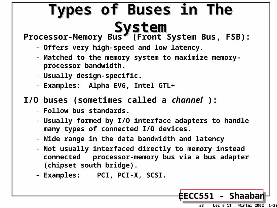
Types of Buses in The SystemTypes of Buses in The SystemProcessor-Memory Bus (Front System Bus, FSB):
– Offers very high-speed and low latency.– Matched to the memory system to maximize memory-processor
bandwidth.– Usually design-specific.– Examples: Alpha EV6, Intel GTL+
I/O buses (sometimes called a channel ):– Follow bus standards.– Usually formed by I/O interface adapters to handle many types of
connected I/O devices.– Wide range in the data bandwidth and latency– Not usually interfaced directly to memory instead connected
processor-memory bus via a bus adapter (chipset south bridge).– Examples: PCI, PCI-X, SCSI.
EECC551 - ShaabanEECC551 - Shaaban#4 Lec # 11 Winter 2002 1-29-2003
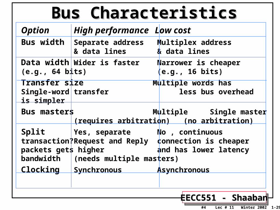
Bus CharacteristicsBus CharacteristicsOption High performance Low costBus width Separate address Multiplex address
& data lines & data lines
Data width Wider is faster Narrower is cheaper (e.g., 64 bits) (e.g., 16 bits)
Transfer size Multiple words has Single-word transferless bus overhead is simpler
Bus masters Multiple Single master(requires arbitration) (no arbitration)
Split Yes, separate No , continuous transaction?Request and Reply connection is cheaper packets gets higher and has lower latencybandwidth(needs multiple masters)
Clocking Synchronous Asynchronous
EECC551 - ShaabanEECC551 - Shaaban#5 Lec # 11 Winter 2002 1-29-2003
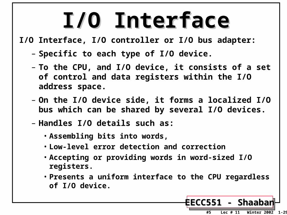
I/O InterfaceI/O InterfaceI/O Interface, I/O controller or I/O bus adapter:
– Specific to each type of I/O device.
– To the CPU, and I/O device, it consists of a set of control and data registers within the I/O address space.
– On the I/O device side, it forms a localized I/O bus which can be shared by several I/O devices.
– Handles I/O details such as:
• Assembling bits into words,
• Low-level error detection and correction
• Accepting or providing words in word-sized I/O registers.
• Presents a uniform interface to the CPU regardless of I/O device.
EECC551 - ShaabanEECC551 - Shaaban#6 Lec # 11 Winter 2002 1-29-2003
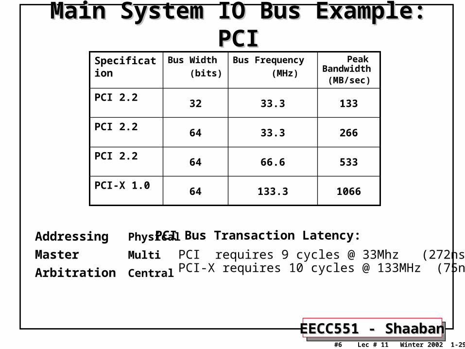
Main System IO Bus Example: PCIMain System IO Bus Example: PCI
1066133.364PCI-X 1.0
53366.664PCI 2.2
26633.364PCI 2.2
13333.332PCI 2.2
Peak Bandwidth (MB/sec)
Bus Frequency
(MHz)
Bus Width
(bits)
Specification
PCI Bus Transaction Latency:
PCI requires 9 cycles @ 33Mhz (272ns) PCI-X requires 10 cycles @ 133MHz (75ns)
Addressing Physical
Master Multi
Arbitration Central
EECC551 - ShaabanEECC551 - Shaaban#7 Lec # 11 Winter 2002 1-29-2003
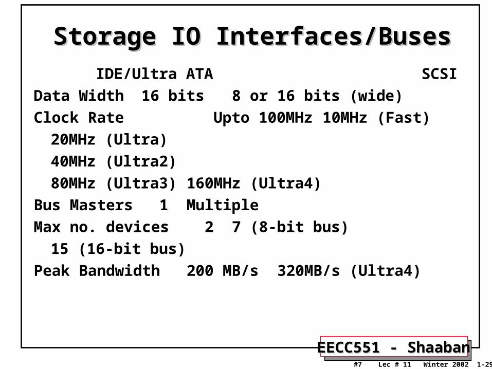
Storage IO Interfaces/BusesStorage IO Interfaces/Buses
IDE/Ultra ATA SCSI
Data Width 16 bits 8 or 16 bits (wide)
Clock Rate Upto 100MHz 10MHz (Fast)
20MHz (Ultra)
40MHz (Ultra2)
80MHz (Ultra3)160MHz (Ultra4)
Bus Masters 1 Multiple
Max no. devices 2 7 (8-bit bus)
15 (16-bit bus)
Peak Bandwidth200 MB/s 320MB/s (Ultra4)
EECC551 - ShaabanEECC551 - Shaaban#8 Lec # 11 Winter 2002 1-29-2003
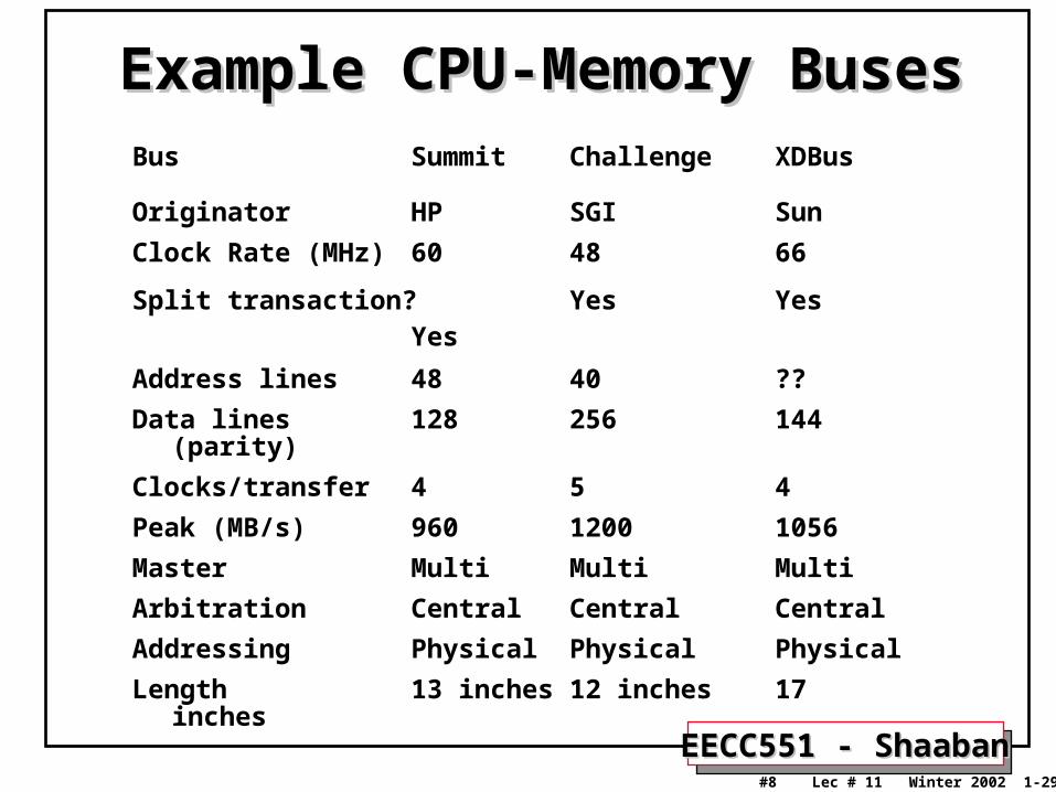
Example CPU-Memory BusesExample CPU-Memory BusesBus Summit Challenge XDBus
Originator HP SGI Sun
Clock Rate (MHz) 60 48 66
Split transaction? Yes Yes Yes
Address lines 48 40 ??
Data lines 128 256 144 (parity)
Clocks/transfer 4 5 4
Peak (MB/s) 960 1200 1056
Master Multi Multi Multi
Arbitration Central Central Central
Addressing Physical Physical Physical
Length 13 inches 12 inches 17 inches
EECC551 - ShaabanEECC551 - Shaaban#9 Lec # 11 Winter 2002 1-29-2003
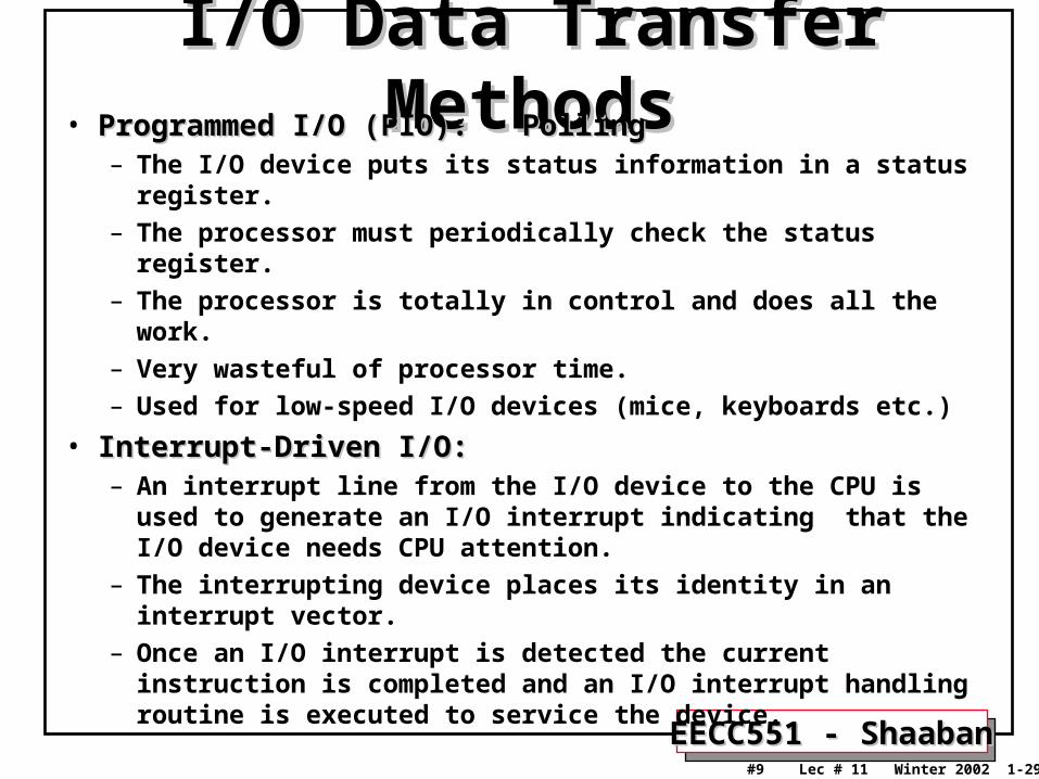
I/O Data Transfer MethodsI/O Data Transfer Methods• Programmed I/O (PIO): PollingProgrammed I/O (PIO): Polling
– The I/O device puts its status information in a status register.
– The processor must periodically check the status register.
– The processor is totally in control and does all the work.
– Very wasteful of processor time.
– Used for low-speed I/O devices (mice, keyboards etc.)
• Interrupt-Driven I/O:Interrupt-Driven I/O:– An interrupt line from the I/O device to the CPU is used to
generate an I/O interrupt indicating that the I/O device needs CPU attention.
– The interrupting device places its identity in an interrupt vector.
– Once an I/O interrupt is detected the current instruction is completed and an I/O interrupt handling routine is executed to service the device.
EECC551 - ShaabanEECC551 - Shaaban#10 Lec # 11 Winter 2002 1-29-2003
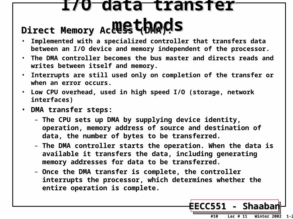
I/O data transfer methodsI/O data transfer methodsDirect Memory Access (DMA):Direct Memory Access (DMA): • Implemented with a specialized controller that transfers data between an I/O
device and memory independent of the processor.
• The DMA controller becomes the bus master and directs reads and writes between itself and memory.
• Interrupts are still used only on completion of the transfer or when an error occurs.
• Low CPU overhead, used in high speed I/O (storage, network interfaces)
• DMA transfer steps:– The CPU sets up DMA by supplying device identity, operation,
memory address of source and destination of data, the number of bytes to be transferred.
– The DMA controller starts the operation. When the data is available it transfers the data, including generating memory addresses for data to be transferred.
– Once the DMA transfer is complete, the controller interrupts the processor, which determines whether the entire operation is complete.

EECC551 - ShaabanEECC551 - Shaaban#11 Lec # 11 Winter 2002 1-29-2003
I/O Controller ArchitectureI/O Controller Architecture
Peripheral or Main I/O Bus (PCI, PCI-X, etc.)
HostMemory
ProcessorCache
HostProcessor
Peripheral Bus Interface/DMA
I/O Channel Interface
BufferMemory
ROM
µProc
I/O Controller
EECC551 - ShaabanEECC551 - Shaaban#12 Lec # 11 Winter 2002 1-29-2003
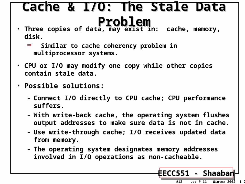
Cache & I/O: The Stale Data ProblemCache & I/O: The Stale Data Problem• Three copies of data, may exist in: cache, memory, disk.
Similar to cache coherency problem in multiprocessor systems.
• CPU or I/O may modify one copy while other copies contain stale data.
• Possible solutions:
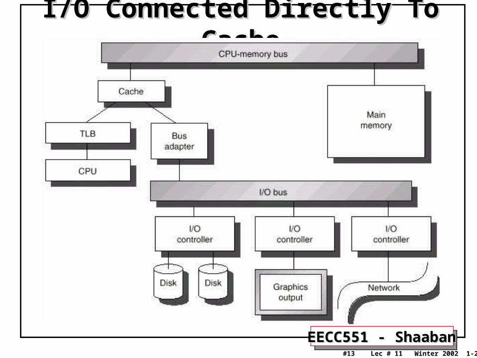
– Connect I/O directly to CPU cache; CPU performance suffers.– With write-back cache, the operating system flushes output
addresses to make sure data is not in cache.– Use write-through cache; I/O receives updated data from
memory.– The operating system designates memory addresses involved in
I/O operations as non-cacheable.
EECC551 - ShaabanEECC551 - Shaaban#13 Lec # 11 Winter 2002 1-29-2003
I/O Connected Directly To CacheI/O Connected Directly To Cache
EECC551 - ShaabanEECC551 - Shaaban#14 Lec # 11 Winter 2002 1-29-2003
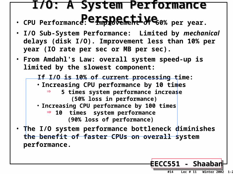
I/O: A System Performance PerspectiveI/O: A System Performance Perspective• CPU Performance: Improvement of 60% per year.
• I/O Sub-System Performance: Limited by mechanical delays (disk I/O). Improvement less than 10% per year (IO rate per sec or MB per sec).
• From Amdahl's Law: overall system speed-up is limited by the slowest component:
If I/O is 10% of current processing time:• Increasing CPU performance by 10 times
5 times system performance increase (50% loss in performance)
• Increasing CPU performance by 100 times 10 times system performance (90% loss of performance)
• The I/O system performance bottleneck diminishes the benefit of faster CPUs on overall system performance.
EECC551 - ShaabanEECC551 - Shaaban#15 Lec # 11 Winter 2002 1-29-2003
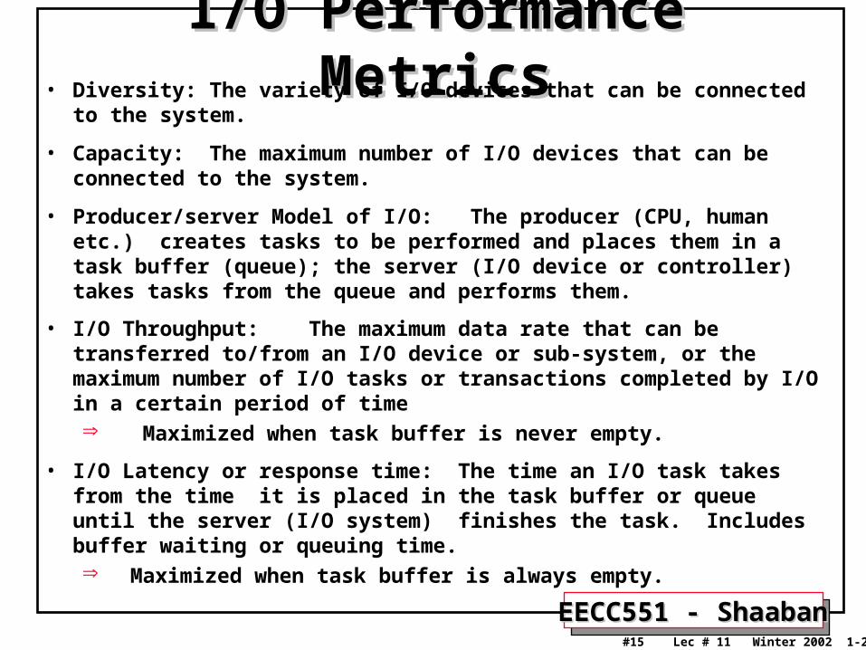
I/O Performance MetricsI/O Performance Metrics• Diversity: The variety of I/O devices that can be connected to the system.
• Capacity: The maximum number of I/O devices that can be connected to the system.
• Producer/server Model of I/O: The producer (CPU, human etc.) creates tasks to be performed and places them in a task buffer (queue); the server (I/O device or controller) takes tasks from the queue and performs them.
• I/O Throughput: The maximum data rate that can be transferred to/from an I/O device or sub-system, or the maximum number of I/O tasks or transactions completed by I/O in a certain period of time Maximized when task buffer is never empty.
• I/O Latency or response time: The time an I/O task takes from the time it is placed in the task buffer or queue until the server (I/O system) finishes the task. Includes buffer waiting or queuing time. Maximized when task buffer is always empty.
EECC551 - ShaabanEECC551 - Shaaban#16 Lec # 11 Winter 2002 1-29-2003
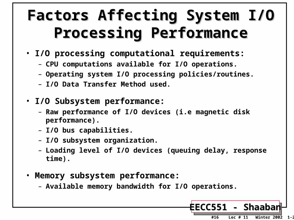
Factors Affecting System I/O Factors Affecting System I/O Processing PerformanceProcessing Performance
• I/O processing computational requirements: – CPU computations available for I/O operations.
– Operating system I/O processing policies/routines.
– I/O Data Transfer Method used.
• I/O Subsystem performance:– Raw performance of I/O devices (i.e magnetic disk performance).
– I/O bus capabilities.
– I/O subsystem organization.
– Loading level of I/O devices (queuing delay, response time).
• Memory subsystem performance:– Available memory bandwidth for I/O operations.
EECC551 - ShaabanEECC551 - Shaaban#17 Lec # 11 Winter 2002 1-29-2003
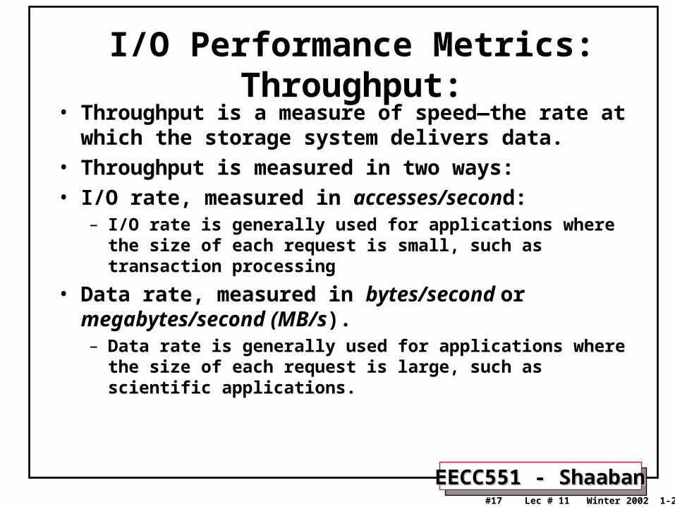
I/O Performance Metrics: Throughput:• Throughput is a measure of speed—the rate at which the
storage system delivers data.
• Throughput is measured in two ways:
• I/O rate, measured in accesses/second:– I/O rate is generally used for applications where the size of each
request is small, such as transaction processing
• Data rate, measured in bytes/second or megabytes/second (MB/s). – Data rate is generally used for applications where the size of
each request is large, such as scientific applications.
EECC551 - ShaabanEECC551 - Shaaban#18 Lec # 11 Winter 2002 1-29-2003
I/O Performance Metrics: Response time
• Response time measures how long a storage system takes to access data. This time can be measured in several ways. For example:
– One could measure time from the user’s perspective,
– the operating system’s perspective,
– or the disk controller’s perspective, depending on what you view as the storage system.
EECC551 - ShaabanEECC551 - Shaaban#19 Lec # 11 Winter 2002 1-29-2003
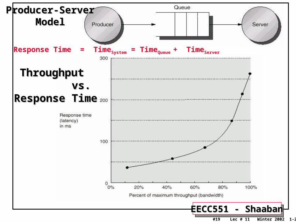
Producer-ServerProducer-ServerModelModel
ThroughputThroughput vs. vs. Response TimeResponse Time
Response Time = TimeSystem = TimeQueue + TimeServer
EECC551 - ShaabanEECC551 - Shaaban#20 Lec # 11 Winter 2002 1-29-2003
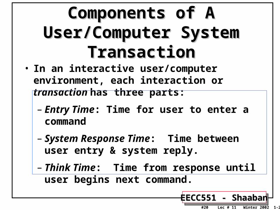
Components of A User/Computer Components of A User/Computer System TransactionSystem Transaction
• In an interactive user/computer environment, each interaction or transaction has three parts:
– Entry Time: Time for user to enter a command
– System Response Time: Time between user entry & system reply.
– Think Time: Time from response until user begins next command.
EECC551 - ShaabanEECC551 - Shaaban#21 Lec # 11 Winter 2002 1-29-2003
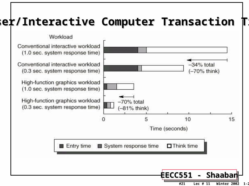
User/Interactive Computer Transaction TimeUser/Interactive Computer Transaction Time
EECC551 - ShaabanEECC551 - Shaaban#22 Lec # 11 Winter 2002 1-29-2003
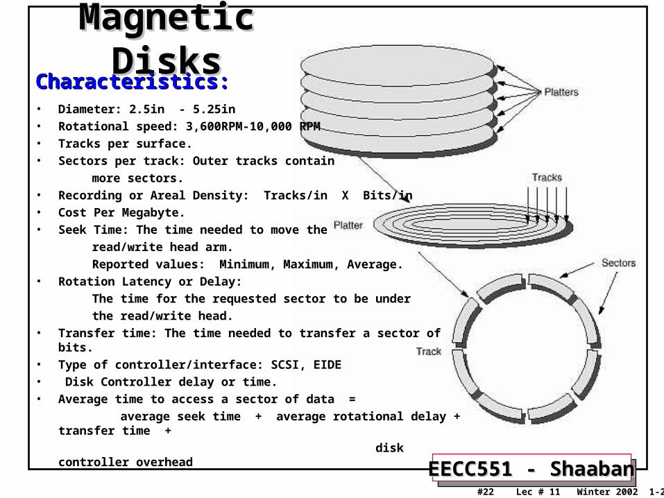
Magnetic DisksMagnetic DisksCharacteristics:Characteristics:• Diameter: 2.5in - 5.25in
• Rotational speed: 3,600RPM-10,000 RPM
• Tracks per surface.
• Sectors per track: Outer tracks contain
more sectors.
• Recording or Areal Density: Tracks/in X Bits/in
• Cost Per Megabyte.
• Seek Time: The time needed to move the
read/write head arm.
Reported values: Minimum, Maximum, Average.
• Rotation Latency or Delay:
The time for the requested sector to be under
the read/write head.
• Transfer time: The time needed to transfer a sector of bits.
• Type of controller/interface: SCSI, EIDE
• Disk Controller delay or time.
• Average time to access a sector of data =
average seek time + average rotational delay + transfer time +
disk controller overhead
EECC551 - ShaabanEECC551 - Shaaban#23 Lec # 11 Winter 2002 1-29-2003
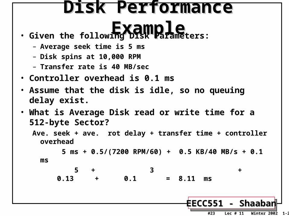
Disk Performance ExampleDisk Performance Example• Given the following Disk Parameters:
– Average seek time is 5 ms
– Disk spins at 10,000 RPM
– Transfer rate is 40 MB/sec
• Controller overhead is 0.1 ms
• Assume that the disk is idle, so no queuing delay exist.
• What is Average Disk read or write time for a 512-byte Sector?Ave. seek + ave. rot delay + transfer time + controller overhead
5 ms + 0.5/(7200 RPM/60) + 0.5 KB/40 MB/s + 0.1 ms
5 + 3 + 0.13 + 0.1 = 8.11 ms
EECC551 - ShaabanEECC551 - Shaaban#24 Lec # 11 Winter 2002 1-29-2003
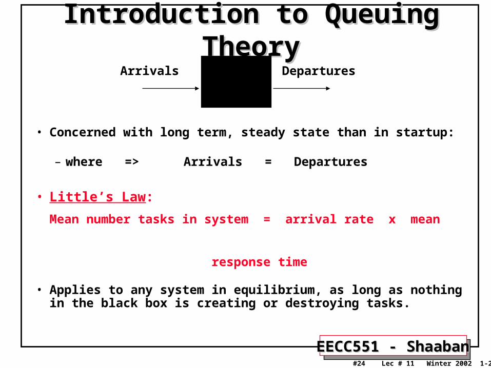
Introduction to Queuing TheoryIntroduction to Queuing Theory
• Concerned with long term, steady state than in startup: – where => Arrivals = Departures
• Little’s Law:
Mean number tasks in system = arrival rate x mean response time
• Applies to any system in equilibrium, as long as nothing in the black box is creating or destroying tasks.
Arrivals Departures
EECC551 - ShaabanEECC551 - Shaaban#25 Lec # 11 Winter 2002 1-29-2003
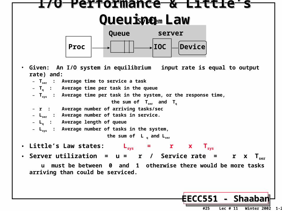
I/O Performance & Little’s Queuing LawI/O Performance & Little’s Queuing Law
• Given: An I/O system in equilibrium input rate is equal to output rate) and: – Tser : Average time to service a task
– Tq : Average time per task in the queue
– Tsys : Average time per task in the system, or the response time,
the sum of Tser and Tq
– r : Average number of arriving tasks/sec– Lser : Average number of tasks in service.
– Lq : Average length of queue
– Lsys : Average number of tasks in the system,
the sum of L q and Lser
• Little’s Law states: Lsys = r x Tsys
• Server utilization = u = r / Service rate = r x Tser
u must be between 0 and 1 otherwise there would be more tasks arriving than could be serviced.
Proc IOC Device
Queue server
System
EECC551 - ShaabanEECC551 - Shaaban#26 Lec # 11 Winter 2002 1-29-2003
A Little Queuing TheoryA Little Queuing Theory
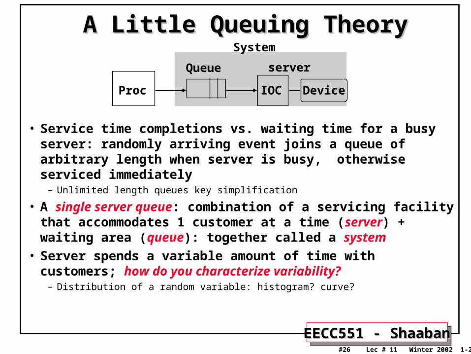
• Service time completions vs. waiting time for a busy server: randomly arriving event joins a queue of arbitrary length when server is busy, otherwise serviced immediately
– Unlimited length queues key simplification
• A single server queue: combination of a servicing facility that accommodates 1 customer at a time (server) + waiting area (queue): together called a system
• Server spends a variable amount of time with customers; how do you characterize variability?
– Distribution of a random variable: histogram? curve?
Proc IOC Device
Queue server
System
EECC551 - ShaabanEECC551 - Shaaban#27 Lec # 11 Winter 2002 1-29-2003
A Little Queuing Theory
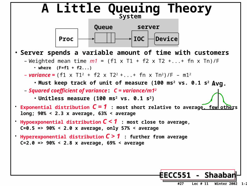
• Server spends a variable amount of time with customers– Weighted mean time m1 = (f1 x T1 + f2 x T2 +...+ fn x Tn)/F
• where (F=f1 + f2...)
– variance = (f1 x T12 + f2 x T22 +...+ fn x Tn2)/F – m12
• Must keep track of unit of measure (100 ms2 vs. 0.1 s2 )– Squared coefficient of variance: C = variance/m12
• Unitless measure (100 ms2 vs. 0.1 s2)
• Exponential distribution C = 1 : most short relative to average, few others long; 90% < 2.3 x average, 63% < average
• Hypoexponential distribution C < 1 : most close to average, C=0.5 => 90% < 2.0 x average, only 57% < average
• Hyperexponential distribution C > 1 : further from average C=2.0 => 90% < 2.8 x average, 69% < average
Proc IOC Device
Queue server
System
Avg.
EECC551 - ShaabanEECC551 - Shaaban#28 Lec # 11 Winter 2002 1-29-2003
A Little Queuing Theory:A Little Queuing Theory:Average Wait TimeAverage Wait Time
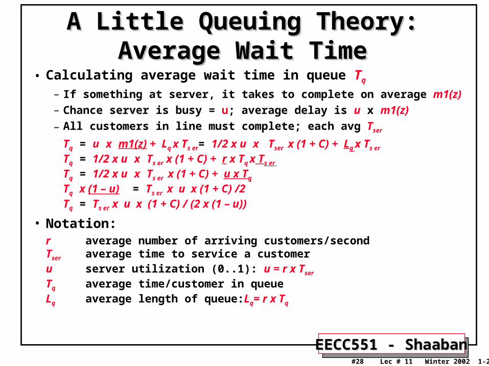
• Calculating average wait time in queue Tq
– If something at server, it takes to complete on average m1(z)– Chance server is busy = u; average delay is u x m1(z)
– All customers in line must complete; each avg Tser
Tq = u x m1(z) + Lq x Ts er= 1/2 x u x Tser x (1 + C) + Lq x Ts er
Tq = 1/2 x u x Ts er x (1 + C) + r x Tq x Ts er
Tq = 1/2 x u x Ts er x (1 + C) + u x Tq
Tq x (1 – u) = Ts er x u x (1 + C) /2Tq = Ts er x u x (1 + C) / (2 x (1 – u))
• Notation: r average number of arriving customers/second
Tser average time to service a customeru server utilization (0..1): u = r x Tser
Tq average time/customer in queueLq average length of queue:Lq= r x Tq
EECC551 - ShaabanEECC551 - Shaaban#29 Lec # 11 Winter 2002 1-29-2003
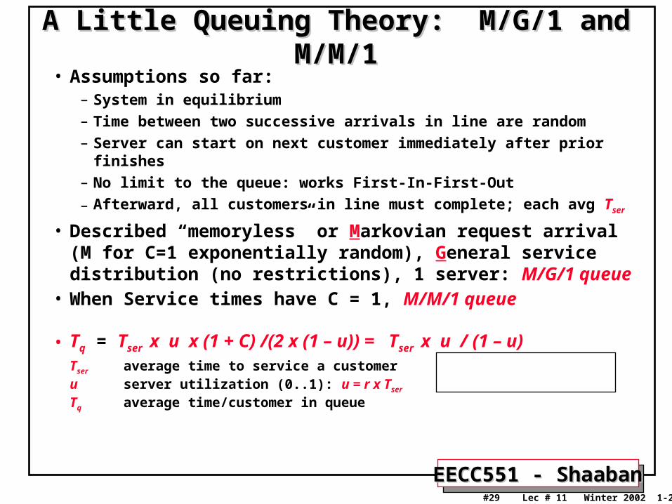
A Little Queuing Theory: M/G/1 and M/M/1A Little Queuing Theory: M/G/1 and M/M/1• Assumptions so far:
– System in equilibrium
– Time between two successive arrivals in line are random
– Server can start on next customer immediately after prior finishes
– No limit to the queue: works First-In-First-Out
– Afterward, all customers in line must complete; each avg Tser
• Described “memoryless” or Markovian request arrival (M for C=1 exponentially random), General service distribution (no restrictions), 1 server: M/G/1 queue
• When Service times have C = 1, M/M/1 queue
• Tq = Tser x u x (1 + C) /(2 x (1 – u)) = Tser x u / (1 – u) Tser average time to service a customer
u server utilization (0..1): u = r x Tser
Tq average time/customer in queue
EECC551 - ShaabanEECC551 - Shaaban#30 Lec # 11 Winter 2002 1-29-2003
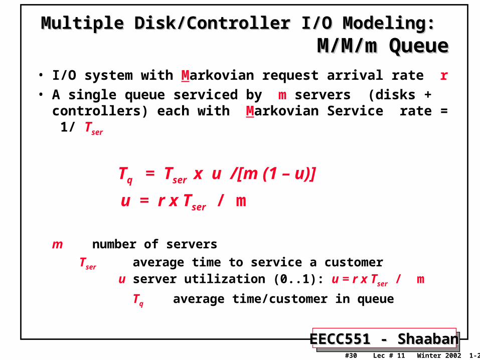
Multiple Disk/Controller I/O Modeling:Multiple Disk/Controller I/O Modeling:
M/M/m Queue M/M/m Queue
• I/O system with Markovian request arrival rate r
• A single queue serviced by m servers (disks + controllers) each with Markovian Service rate = 1/ Tser
Tq = Tser x u /[m (1 – u)]
u = r x Tser / m
m number of servers
Tser average time to service a customer u server utilization (0..1): u = r x Tser / m
Tq average time/customer in queue
EECC551 - ShaabanEECC551 - Shaaban#31 Lec # 11 Winter 2002 1-29-2003
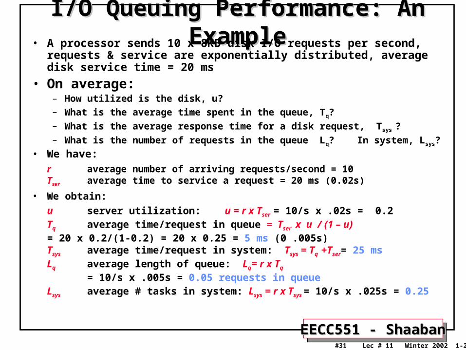
I/O I/O QueuingQueuing Performance: An Example Performance: An Example• A processor sends 10 x 8KB disk I/O requests per second, requests &
service are exponentially distributed, average disk service time = 20 ms
• On average: – How utilized is the disk, u?– What is the average time spent in the queue, Tq? – What is the average response time for a disk request, Tsys ?– What is the number of requests in the queue Lq? In system, Lsys?
• We have:
r average number of arriving requests/second = 10Tser average time to service a request = 20 ms (0.02s)
• We obtain:
u server utilization: u = r x Tser = 10/s x .02s = 0.2Tq average time/request in queue = Tser x u / (1 – u)
= 20 x 0.2/(1-0.2) = 20 x 0.25 = 5 ms (0 .005s)Tsys average time/request in system: Tsys = Tq +Tser= 25 msLq average length of queue: Lq= r x Tq
= 10/s x .005s = 0.05 requests in queueLsys average # tasks in system: Lsys = r x Tsys = 10/s x .025s = 0.25
EECC551 - ShaabanEECC551 - Shaaban#32 Lec # 11 Winter 2002 1-29-2003
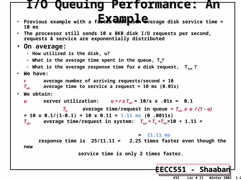
I/O I/O QueuingQueuing Performance: An Example Performance: An Example• Previous example with a faster disk with average disk service time = 10 ms• The processor still sends 10 x 8KB disk I/O requests per second, requests &
service are exponentially distributed
• On average: – How utilized is the disk, u?– What is the average time spent in the queue, Tq? – What is the average response time for a disk request, Tsys ?
• We have:
r average number of arriving requests/second = 10Tser average time to service a request = 10 ms (0.01s)
• We obtain:
u server utilization: u = r x Tser = 10/s x .01s = 0.1
Tq average time/request in queue = Tser x u / (1 – u) = 10 x 0.1/(1-0.1) = 10 x 0.11 = 1.11 ms (0 .0011s)
Tsys average time/request in system: Tsys = Tq +Tser=10 + 1.11 =
= 11.11 ms response time is 25/11.11 = 2.25 times faster even though the new
service time is only 2 times faster.
EECC551 - ShaabanEECC551 - Shaaban#33 Lec # 11 Winter 2002 1-29-2003
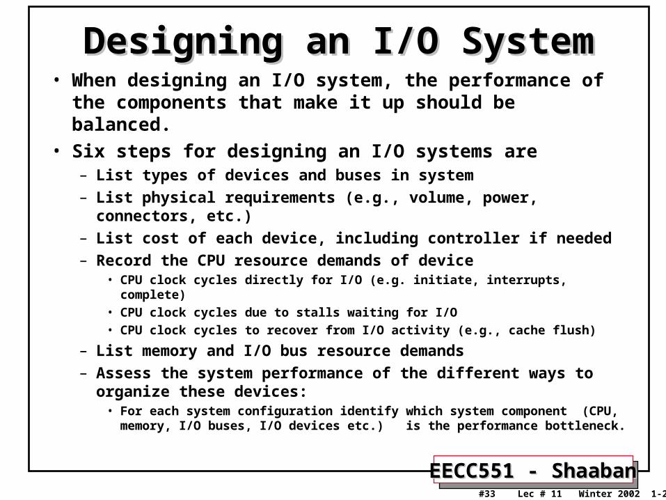
Designing an I/O SystemDesigning an I/O System• When designing an I/O system, the performance of the
components that make it up should be balanced.
• Six steps for designing an I/O systems are– List types of devices and buses in system
– List physical requirements (e.g., volume, power, connectors, etc.)
– List cost of each device, including controller if needed
– Record the CPU resource demands of device• CPU clock cycles directly for I/O (e.g. initiate, interrupts, complete)
• CPU clock cycles due to stalls waiting for I/O
• CPU clock cycles to recover from I/O activity (e.g., cache flush)
– List memory and I/O bus resource demands
– Assess the system performance of the different ways to organize these devices:
• For each system configuration identify which system component (CPU, memory, I/O buses, I/O devices etc.) is the performance bottleneck.
EECC551 - ShaabanEECC551 - Shaaban#34 Lec # 11 Winter 2002 1-29-2003
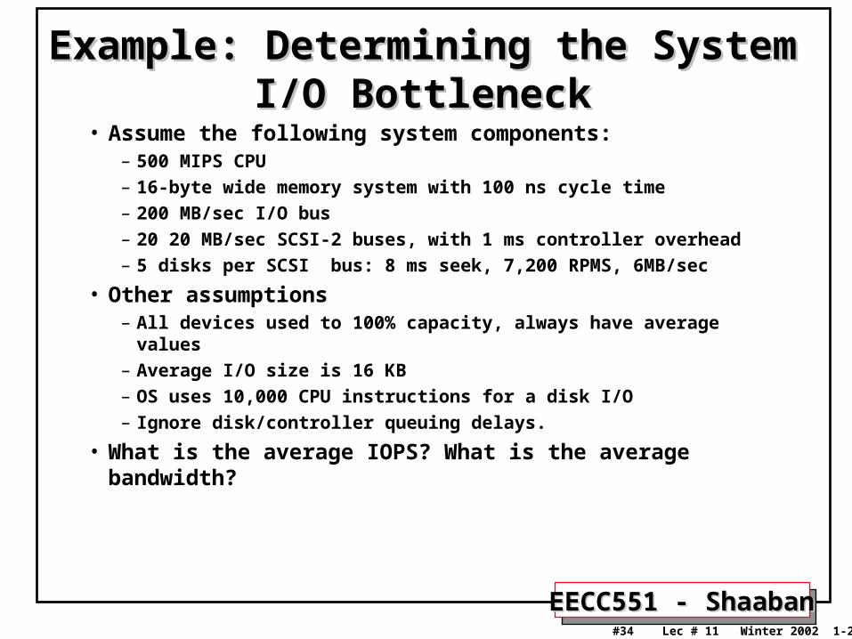
Example: Determining the System I/O Example: Determining the System I/O BottleneckBottleneck
• Assume the following system components:– 500 MIPS CPU
– 16-byte wide memory system with 100 ns cycle time
– 200 MB/sec I/O bus
– 20 20 MB/sec SCSI-2 buses, with 1 ms controller overhead
– 5 disks per SCSI bus: 8 ms seek, 7,200 RPMS, 6MB/sec
• Other assumptions– All devices used to 100% capacity, always have average values
– Average I/O size is 16 KB
– OS uses 10,000 CPU instructions for a disk I/O
– Ignore disk/controller queuing delays.
• What is the average IOPS? What is the average bandwidth?
EECC551 - ShaabanEECC551 - Shaaban#35 Lec # 11 Winter 2002 1-29-2003
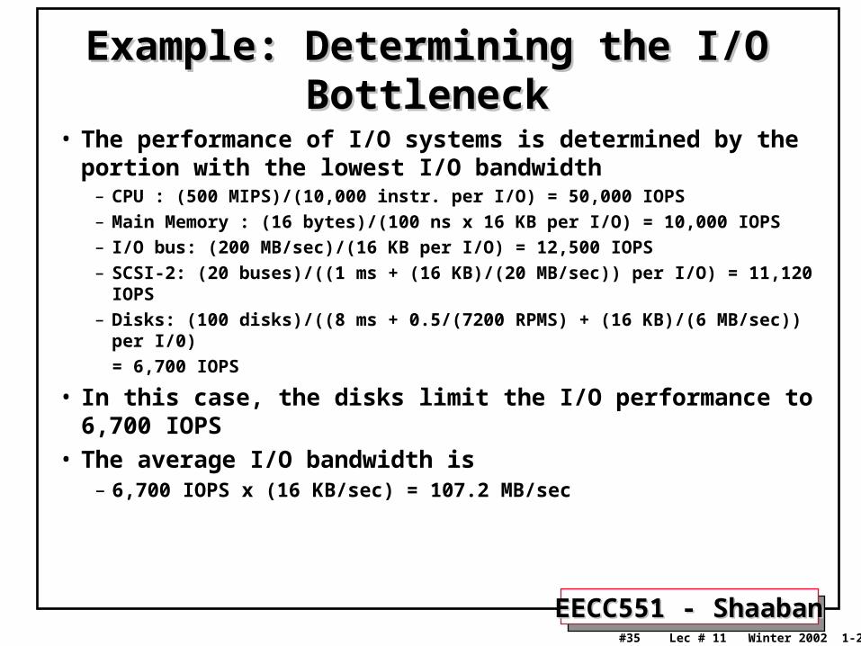
• The performance of I/O systems is determined by the portion with the lowest I/O bandwidth
– CPU : (500 MIPS)/(10,000 instr. per I/O) = 50,000 IOPS
– Main Memory : (16 bytes)/(100 ns x 16 KB per I/O) = 10,000 IOPS
– I/O bus: (200 MB/sec)/(16 KB per I/O) = 12,500 IOPS
– SCSI-2: (20 buses)/((1 ms + (16 KB)/(20 MB/sec)) per I/O) = 11,120 IOPS
– Disks: (100 disks)/((8 ms + 0.5/(7200 RPMS) + (16 KB)/(6 MB/sec)) per I/0)
= 6,700 IOPS
• In this case, the disks limit the I/O performance to 6,700 IOPS
• The average I/O bandwidth is– 6,700 IOPS x (16 KB/sec) = 107.2 MB/sec
Example: Determining the I/O BottleneckExample: Determining the I/O Bottleneck
EECC551 - ShaabanEECC551 - Shaaban#36 Lec # 11 Winter 2002 1-29-2003
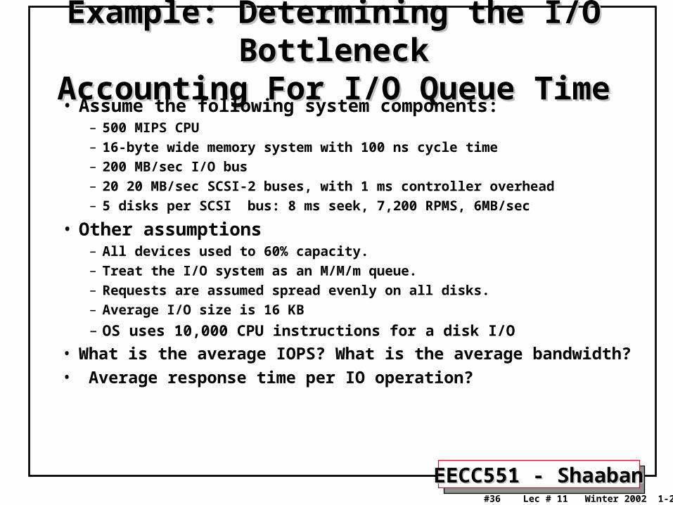
Example: Determining the I/O BottleneckExample: Determining the I/O BottleneckAccounting For I/O Queue TimeAccounting For I/O Queue Time
• Assume the following system components:– 500 MIPS CPU– 16-byte wide memory system with 100 ns cycle time– 200 MB/sec I/O bus – 20 20 MB/sec SCSI-2 buses, with 1 ms controller overhead– 5 disks per SCSI bus: 8 ms seek, 7,200 RPMS, 6MB/sec
• Other assumptions– All devices used to 60% capacity.– Treat the I/O system as an M/M/m queue.– Requests are assumed spread evenly on all disks.– Average I/O size is 16 KB
– OS uses 10,000 CPU instructions for a disk I/O
• What is the average IOPS? What is the average bandwidth?• Average response time per IO operation?
EECC551 - ShaabanEECC551 - Shaaban#37 Lec # 11 Winter 2002 1-29-2003
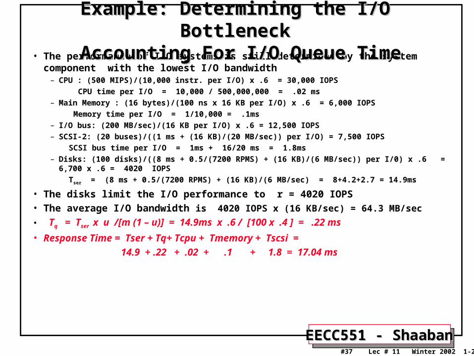
• The performance of I/O systems is still determined by the system component with the lowest I/O bandwidth
– CPU : (500 MIPS)/(10,000 instr. per I/O) x .6 = 30,000 IOPS
CPU time per I/O = 10,000 / 500,000,000 = .02 ms– Main Memory : (16 bytes)/(100 ns x 16 KB per I/O) x .6 = 6,000 IOPS
Memory time per I/O = 1/10,000 = .1ms– I/O bus: (200 MB/sec)/(16 KB per I/O) x .6 = 12,500 IOPS– SCSI-2: (20 buses)/((1 ms + (16 KB)/(20 MB/sec)) per I/O) = 7,500 IOPS
SCSI bus time per I/O = 1ms + 16/20 ms = 1.8ms– Disks: (100 disks)/((8 ms + 0.5/(7200 RPMS) + (16 KB)/(6 MB/sec)) per I/0) x .6 = 6,700 x .6 = 4020 IOPS
Tser = (8 ms + 0.5/(7200 RPMS) + (16 KB)/(6 MB/sec) = 8+4.2+2.7 = 14.9ms
• The disks limit the I/O performance to r = 4020 IOPS• The average I/O bandwidth is 4020 IOPS x (16 KB/sec) = 64.3 MB/sec
• Tq = Tser x u /[m (1 – u)] = 14.9ms x .6 / [100 x .4 ] = .22 ms
• Response Time = Tser + Tq+ Tcpu + Tmemory + Tscsi =
14.9 + .22 + .02 + .1 + 1.8 = 17.04 ms
Example: Determining the I/O BottleneckExample: Determining the I/O Bottleneck Accounting For I/O Queue Time Accounting For I/O Queue Time
Related Documents


