EE513 Audio Signals and Systems Introduction Kevin D. Donohue Electrical and Computer Engineering University of Kentucky

EE513 Audio Signals and Systems Introduction Kevin D. Donohue Electrical and Computer Engineering University of Kentucky.
Dec 17, 2015
Welcome message from author
This document is posted to help you gain knowledge. Please leave a comment to let me know what you think about it! Share it to your friends and learn new things together.
Transcript
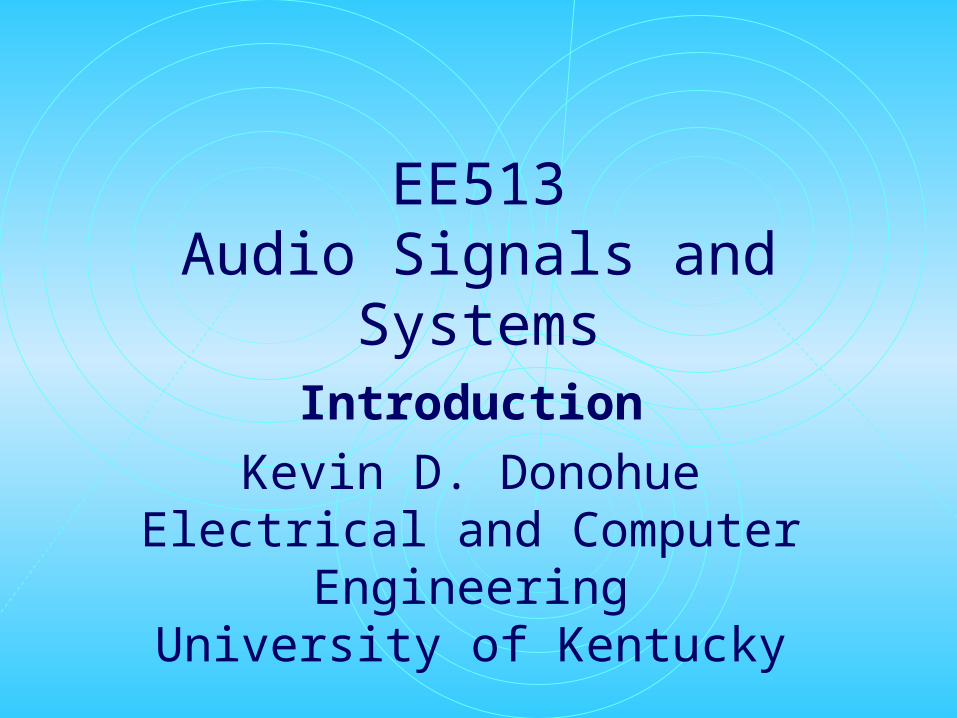
EE513Audio Signals and Systems
Introduction
Kevin D. DonohueElectrical and Computer Engineering
University of Kentucky

Question!
If a tree falls in the forest and nobody is there to hear it, will it make a sound?
Sound provided by http://www.therecordist.com/downloads.html

Ambiguity!
• Merriam-Webster Dictionary:
• Sound a : a particular auditory impression b : the sensation perceived by the sense of hearing c : mechanical radiant energy that is transmitted by longitudinal pressure waves in a material medium (as air) and is the objective cause of hearing.
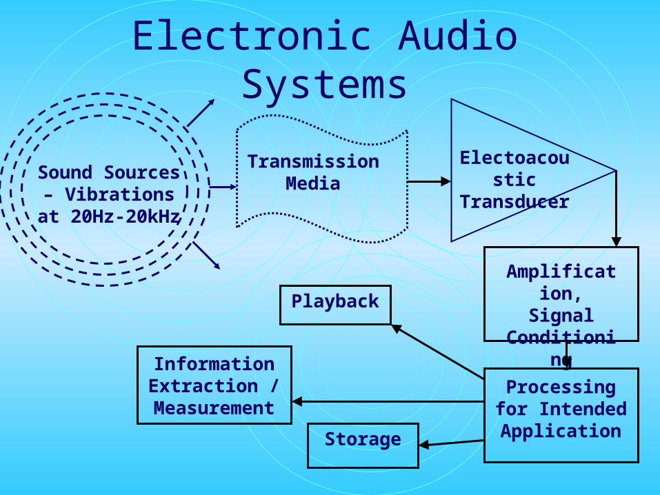
Electronic Audio Systems
Sound Sources – Vibrations at 20Hz-20kHz
Amplification, Signal
Conditioning
Electoacoustic Transducer
Processing for Intended
Application
Transmission Media
Storage
Information Extraction /
Measurement
Playback
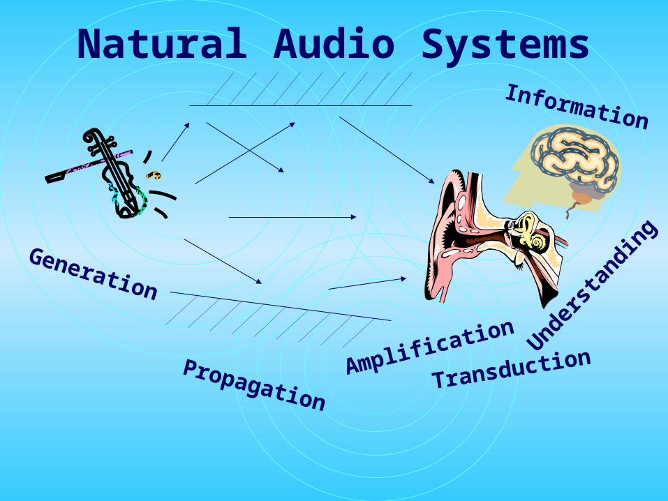
Natural Audio Systems
Generation
Propagation
Amplification
Transduction
Information
Understa
nding
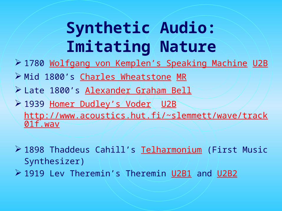
Synthetic Audio: Imitating Nature
1780 Wolfgang von Kemplen’s Speaking Machine U2B Mid 1800’s Charles Wheatstone MR Late 1800’s Alexander Graham Bell 1939 Homer Dudley’s Voder U2B
http://www.acoustics.hut.fi/~slemmett/wave/track01f.wav
1898 Thaddeus Cahill’s Telharmonium (First Music Synthesizer)
1919 Lev Theremin’s Theremin U2B1 and U2B2

Speech Analysis and Synthesis
Communication channels (acoustic and electric)1874/1876 (Antonio Meucci’s)
Alexander Graham Bell’s Telephone.1940’s Homer Dudley’s Channel Vocoder first
analysis-synthesis system

Voice-Coding ModelsThe general speech model:
Speech sounds can be analyzed by determining the states of the vocal system components (vocal chords, track, lips, tongue … ) for each fundamental sound of speech (phoneme).
Unvoiced Speech
Quasi-Periodic
Pulsed Air
Air Burst or
Continuous flow
Voiced Speech
Vocal TractFilter
Vocal Radiator

Spectral Analysis Voiced Speech Spectral envelop => vocal tract formantsHarmonic peaks => vocal chord pitch
0 1000 2000 3000 4000-120
-100
-80
-60
-40Spectrum of Speech Segment - ah
Hertz
dB

Time Analysis Voiced Speech Time envelop => Volume dynamicsOscillations => Vocal chord motion
0 50 100 150 200 250-0.1
-0.05
0
0.05
0.1
Milliseconds
Am
plit
ud
e
Waveform of Speech Segment - ah
12 ms 83 Hz

0.5 1 1.5 2 2.5 3 3.5 4 4.50
1000
2000
3000
4000
-50
-40
-30
-20
-10
0
10
20
Spectrogram Analysis
Time
Fre
qu
ency
There shoeold
doShelived
0 0.5 1 1.5 2 2.5 3 3.5 4 4.5 5-1
0
1

Spectogram of CD sound
2 4 6 8 10 12 140
2000
4000
6000
8000
10000
-20
-15
-10
-5
0
5
10
15
20
25
0 2 4 6 8 10 12 14 16 18-2
0
2
Time
Fre
qu
ency

Speech Recognition
1920’s Radio Rex1950’s (Bell Labs) Digit Recognition
Spectral/Formant analysisFilter Banks
1960’s Neural Networks1970’s ARPA Project for Speech Understanding
Applications of spectral analysis methods FFT, Cepstral/homomorphic, LPC
1970’s Application of pattern matching methods DTW, and HMM

Speech Recognition
1980’sStandardize Training and Test with Large
Corpora (TIMIT) (RM) (DARPA)New Front Ends (feature extractors) more
perceptually basedDominance/Development of HMMBackpropagation and Neural Networks U2BRule-Base AI systems
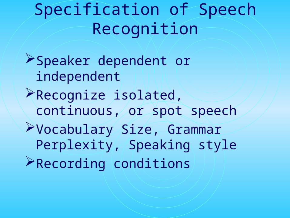
Specification of Speech Recognition
Speaker dependent or independentRecognize isolated, continuous, or spot
speechVocabulary Size, Grammar Perplexity,
Speaking styleRecording conditions
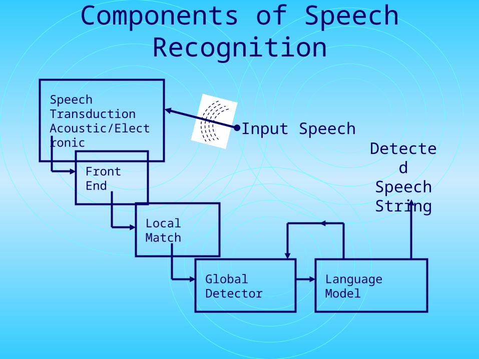
Components of Speech Recognition
Speech Transduction Acoustic/Electronic
Front End
Local Match
Global Detector Language Model
Input SpeechDetected SpeechString
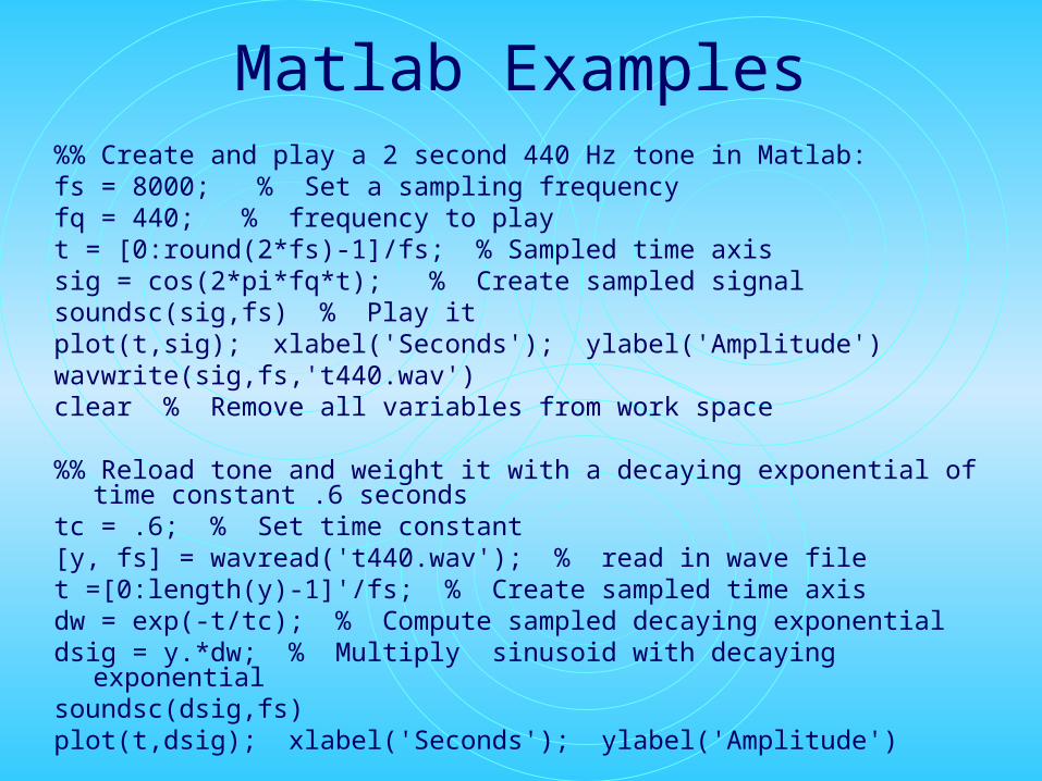
Matlab Examples%% Create and play a 2 second 440 Hz tone in Matlab:fs = 8000; % Set a sampling frequencyfq = 440; % frequency to playt = [0:round(2*fs)-1]/fs; % Sampled time axissig = cos(2*pi*fq*t); % Create sampled signalsoundsc(sig,fs) % Play itplot(t,sig); xlabel('Seconds'); ylabel('Amplitude')wavwrite(sig,fs,'t440.wav')clear % Remove all variables from work space %% Reload tone and weight it with a decaying exponential of time constant .6 secondstc = .6; % Set time constant[y, fs] = wavread('t440.wav'); % read in wave filet =[0:length(y)-1]'/fs; % Create sampled time axisdw = exp(-t/tc); % Compute sampled decaying exponentialdsig = y.*dw; % Multiply sinusoid with decaying exponentialsoundsc(dsig,fs)plot(t,dsig); xlabel('Seconds'); ylabel('Amplitude')

Matlab Examples
Explore demo and help files>> help script SCRIPT About MATLAB scripts and M-files. A SCRIPT file is an external file that contains a sequence of MATLAB statements. By typing the filename, subsequent MATLAB input is obtained from the file. SCRIPT files have a filename extension of ".m" and are often called "M-files". To make a SCRIPT file into a function, see FUNCTION. See also type, echo. Reference page in Help browser doc scriptIn the help window (click on question mark) Go through section on
programming and then go to the demo tab and view a few of the demo.

Matlab Examples
• In class examples …

Matlab Exercise Use the sine/cosine function in Matlab to write a function that
generates a Dorian scale (for testing the function use start tones between 100 and 440 Hz with a sampling rate of 8 kHz). Let the Matlab function input arguments be the starting frequency and the time interval for each scale tone in seconds. Let the output be a vector of samples that can be played with Matlab command “soundsc(v,8000)” (where v is the vector output of your function).
The frequency range of a scale covers one octave, which implies the last frequency is twice the starting frequency. On most fixed pitch instruments, 12 semi-tones or half steps make up the notes within an octave. A minor scale sequentially increases by a whole, half, whole, whole, half, whole, and whole (8 notes altogether – including the starting note).
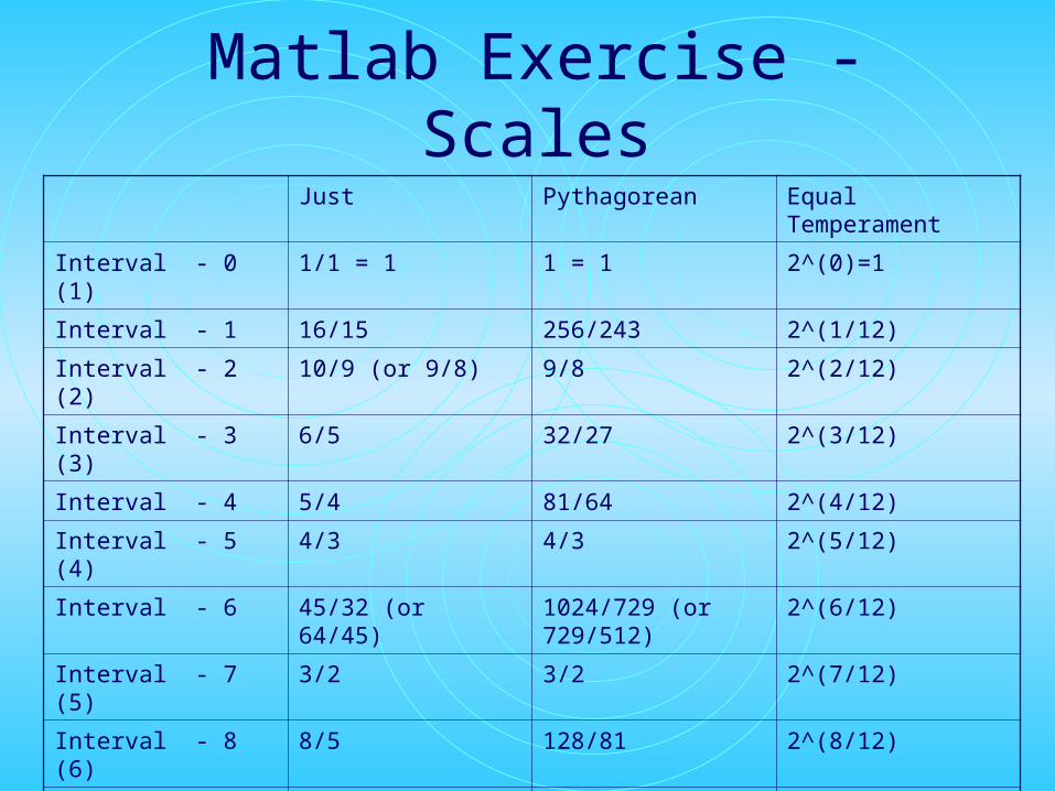
Matlab Exercise - ScalesJust Pythagorean Equal Temperament
Interval - 0 (1) 1/1 = 1 1 = 1 2^(0)=1
Interval - 1 16/15 256/243 2^(1/12)
Interval - 2 (2) 10/9 (or 9/8) 9/8 2^(2/12)
Interval - 3 (3) 6/5 32/27 2^(3/12)
Interval - 4 5/4 81/64 2^(4/12)
Interval - 5 (4) 4/3 4/3 2^(5/12)
Interval - 6 45/32 (or 64/45) 1024/729 (or 729/512) 2^(6/12)
Interval - 7 (5) 3/2 3/2 2^(7/12)
Interval - 8 (6) 8/5 128/81 2^(8/12)
Interval - 9 5/3 27/16 2^(9/12)
Interval - 10 (7) 7/4 (or 16/19 or 9/5) 16/9 2^(10/12)
Interval - 11 15/8 243/128 2^(11/12)
Interval - 12 (8) 2/1 = 2 2/1 = 2 2^(12/12) = 2

Matlab Exercise – Famous Notes
Middle C = 261.626 Hz (standard tuning)
Concert A (A above middle C) = 440 Hz
Middle C = 256 Hz (Scientific tuning)
Lowest note on piano A=27.5 Hz
Highest note on piano C= 4186.009
Related Documents