EE4830 Digital Image Processing Lecture 12

1

Image/Video Compression

April 23, 2007

Lexing Xiexlx at ee.columbia.edu

EE4830 Digital Image ProcessingLecture 12

2

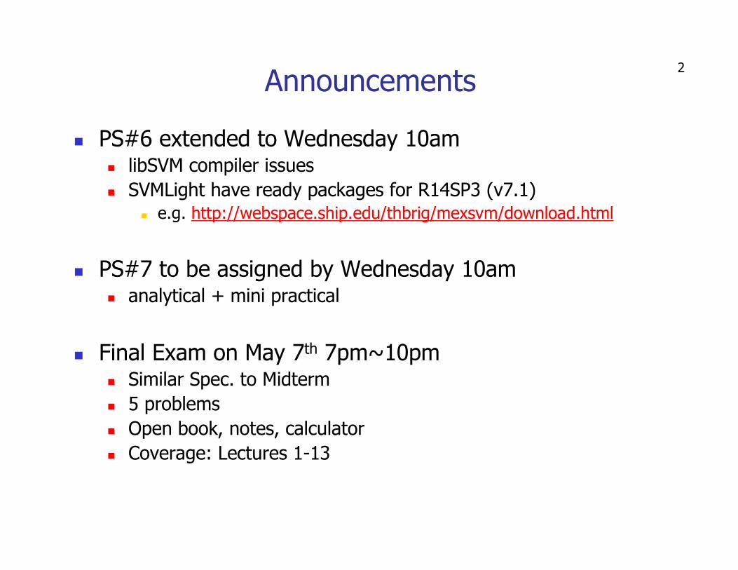
Announcements

� PS#6 extended to Wednesday 10am� libSVM compiler issues

� SVMLight have ready packages for R14SP3 (v7.1)� e.g. http://webspace.ship.edu/thbrig/mexsvm/download.html

� PS#7 to be assigned by Wednesday 10am� analytical + mini practical

� Final Exam on May 7th 7pm~10pm� Similar Spec. to Midterm

� 5 problems

� Open book, notes, calculator

� Coverage: Lectures 1-13

3

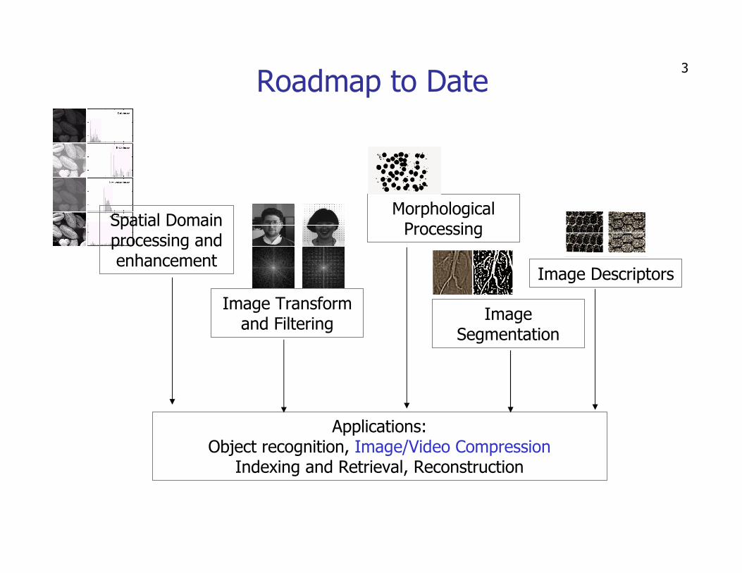
Roadmap to Date

Spatial Domain processing and enhancement

Image Transform and Filtering

Morphological Processing

Image Descriptors

Image Segmentation

Applications:Object recognition, Image/Video Compression

Indexing and Retrieval, Reconstruction

4

Lecture Outline

� Image/Video compression: What and why

� Source coding

� Basic idea

� Entropy coding for i.i.d. symbols

� Coding symbol sequences

� Source coding systems

� Compression standards

� JPEG / MPEG / …

� Recent developments and summary

5

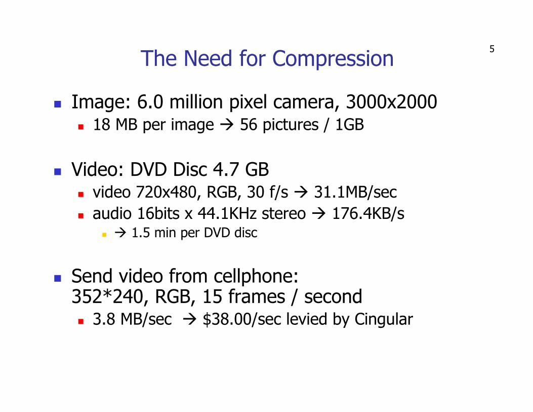
The Need for Compression

� Image: 6.0 million pixel camera, 3000x2000 � 18 MB per image � 56 pictures / 1GB

� Video: DVD Disc 4.7 GB� video 720x480, RGB, 30 f/s � 31.1MB/sec

� audio 16bits x 44.1KHz stereo � 176.4KB/s� � 1.5 min per DVD disc

� Send video from cellphone: 352*240, RGB, 15 frames / second� 3.8 MB/sec � $38.00/sec levied by Cingular

6

Data Compression

� Wikipedia: “data compression, or source coding, is the process of encoding information using fewer bits (or other information-bearing units) than an unencodedrepresentation would use through use of specific encoding schemes.”

� Applications� General data compression: .zip, .gz …

� Image over network: telephone/internet/wireless/etc

� Slow device: � 1xCD-ROM 150KB/s, bluetooth v1.2 up to ~0.25MB/s

� Large multimedia databases

7

Why Can We Compress?

� Two main reasons

� Remove redundancy (Lossless): preserve all information, perfectly recoverable.

� Reduce irrelevance (Lossy): cannot recover all bits.

� Three types of operations� Symbol redundancy: give common values shorts codes and uncommon values longer codes.

� Inter-pixel redundancy: adjacent pixels are highly correlated.

� Perceptual redundancy: not all information is perceived by eye/brain, so throw away those that are not.

8

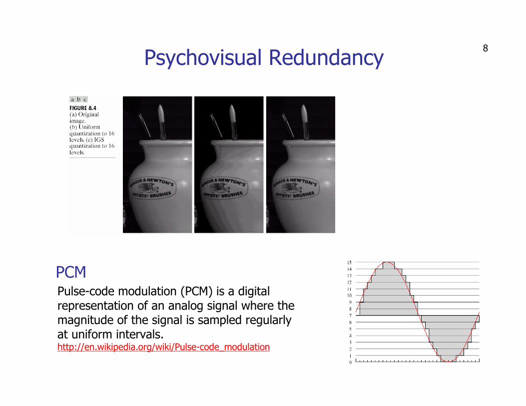
Psychovisual Redundancy

Pulse-code modulation (PCM) is a digital representation of an analog signal where the magnitude of the signal is sampled regularly at uniform intervals.http://en.wikipedia.org/wiki/Pulse-code_modulation

PCM

9

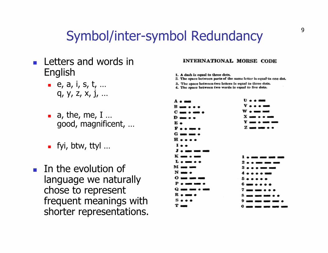
Symbol/inter-symbol Redundancy

� Letters and words in English� e, a, i, s, t, …

q, y, z, x, j, …

� a, the, me, I …good, magnificent, …

� fyi, btw, ttyl …

� In the evolution of language we naturally chose to represent frequent meanings with shorter representations.

10

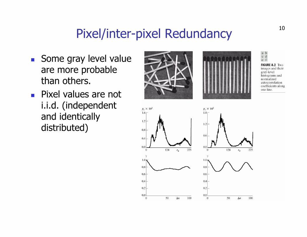
Pixel/inter-pixel Redundancy

� Some gray level value are more probable than others.

� Pixel values are not i.i.d. (independent and identically distributed)

11

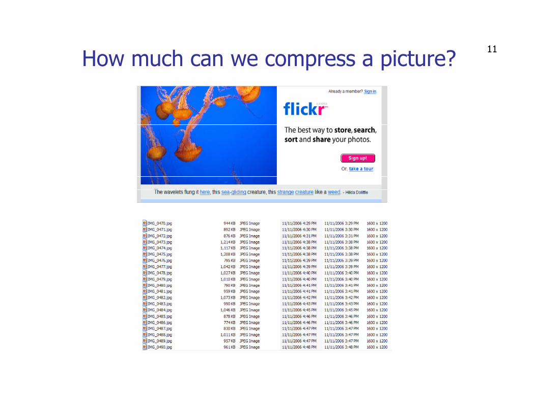
How much can we compress a picture?

12

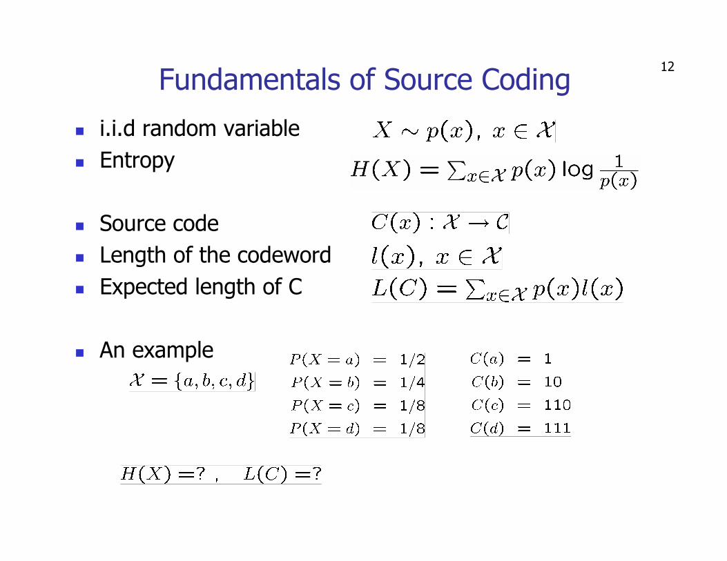
� i.i.d random variable

� Entropy

� Source code

� Length of the codeword

� Expected length of C

� An example

Fundamentals of Source Coding

13

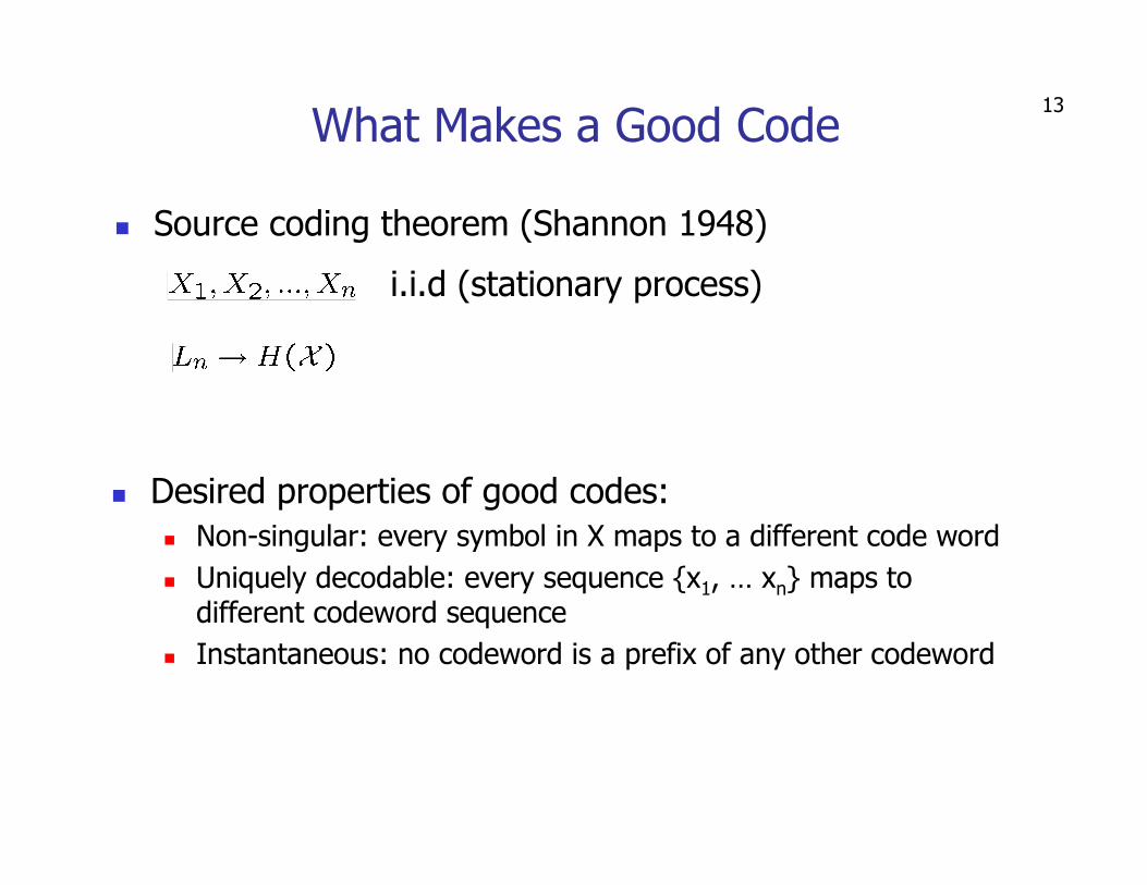
What Makes a Good Code

� Desired properties of good codes:

� Non-singular: every symbol in X maps to a different code word

� Uniquely decodable: every sequence {x1, … xn} maps to different codeword sequence

� Instantaneous: no codeword is a prefix of any other codeword

� Source coding theorem (Shannon 1948)

i.i.d (stationary process)

14

Huffman Codes

� Revisit example

� Is this code: non-singular /uniquely decodable / instantaneous?

� If not, how to improve it?

15

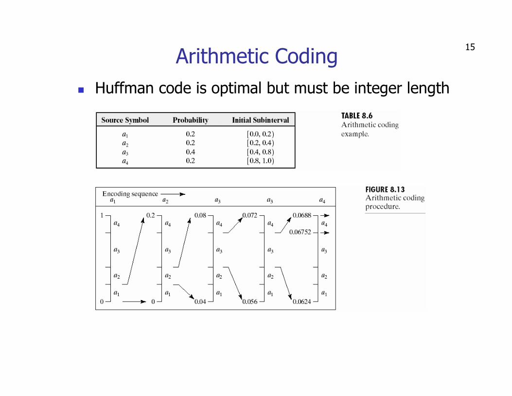
Arithmetic Coding

� Huffman code is optimal but must be integer length

16

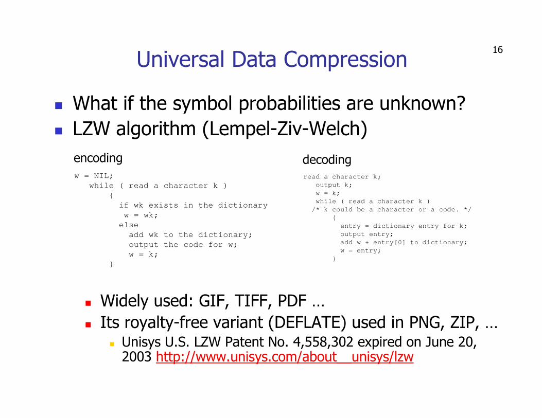
Universal Data Compression

� What if the symbol probabilities are unknown?

� LZW algorithm (Lempel-Ziv-Welch)

w = NIL;

while ( read a character k )

{

if wk exists in the dictionary

w = wk;

else

add wk to the dictionary;

output the code for w;

w = k;

}

read a character k;

output k;

w = k;

while ( read a character k )

/* k could be a character or a code. */

{

entry = dictionary entry for k;

output entry;

add w + entry[0] to dictionary;

w = entry;

}

� Widely used: GIF, TIFF, PDF …

� Its royalty-free variant (DEFLATE) used in PNG, ZIP, …� Unisys U.S. LZW Patent No. 4,558,302 expired on June 20, 2003 http://www.unisys.com/about__unisys/lzw

encoding decoding

17

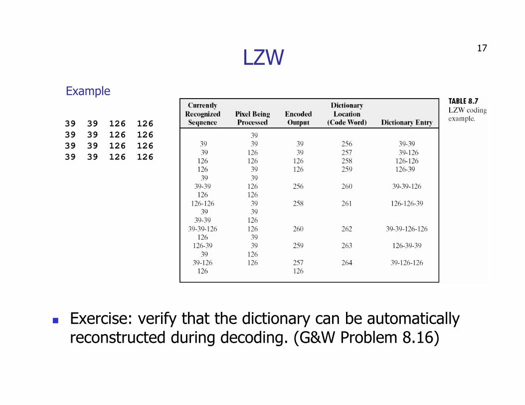
LZW

39 39 126 126

39 39 126 126

39 39 126 126

39 39 126 126

� Exercise: verify that the dictionary can be automatically reconstructed during decoding. (G&W Problem 8.16)

Example

18

Lecture Outline

� Image/Video compression: What and why

� Source coding

� Basic idea

� Entropy coding for i.i.d symbols

� Coding symbol sequences

� Source coding systems

� Compression standards

� JPEG / MPEG / …

� Current developments and future directions

19

Run-Length Coding

� Why is run-length coding with P(X=0) >> P(X=1) actually beneficial?

� See Jain Sec 11.3 (at course works)

� Encode the number of consecutive ‘0’s or ‘1’s

� Used in FAX transmission standard

20

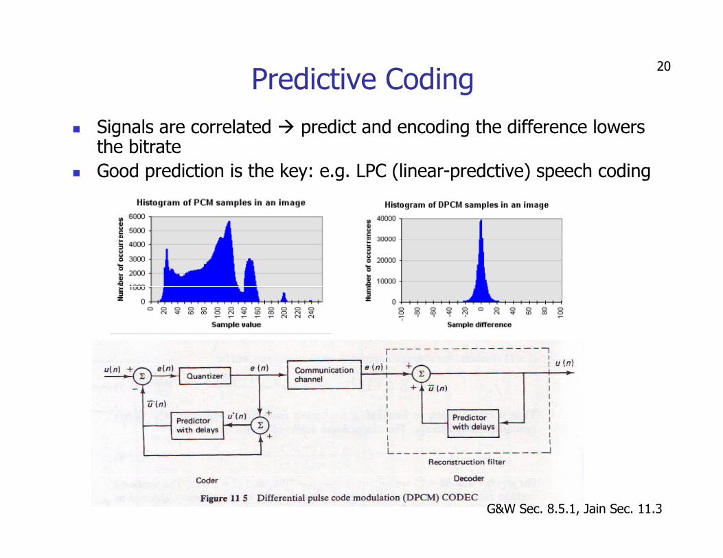
Predictive Coding

� Signals are correlated � predict and encoding the difference lowers the bitrate

� Good prediction is the key: e.g. LPC (linear-predctive) speech coding

G&W Sec. 8.5.1, Jain Sec. 11.3

21

Transform Coding

� Review: properties of unitary transform

� De-correlation: highly correlated input elements �quite uncorrelated output coefficients

� Energy compaction: many common transforms tend to pack a large fraction of signal energy into just a few transform coefficients

22Video ?= Motion Pictures

� Capturing video

� Frame by frame => image sequence

� Image sequence: A 3-D signal

� 2 spatial dimensions & time dimension

� continuous I( x, y, t ) => discrete I( m, n, tk )

� Encode digital video

� Simplest way ~ compress each frame image individually

� e.g., “motion-JPEG”

� only spatial redundancy is explored and reduced

� How about temporal redundancy? Is differential coding good?

� Pixel-by-pixel difference could still be large due to motion

� Need better prediction

23

(From Princeton EE330 S’01 by B.Liu)

Residue after motion compensation

Pixel-wise difference w/o motion compensation

Motion estimation

“Horse ride”

24

Lecture Outline

� Image/Video compression: What and why

� Source coding

� Basic idea

� Entropy coding for i.i.d symbols

� Coding symbol/pixel/image sequences

� Source coding systems

� Quality measures

� Image compression system and algorithms: JPEG

� Video compression system and algorithms: MPEG

� Current developments and future directions

25

Image Quality Measures

� Quality measures

� PSNR (Peak-Signal-to-Noise-Ratio)

� Why would we prefer PSNR over SNR?

� Visual quality

� Compression Artifacts

� Subjective rating scale

−′

=

∑xy

yxfyxfMN

PSNR2

2

10

|),(),(|1

255log10

26

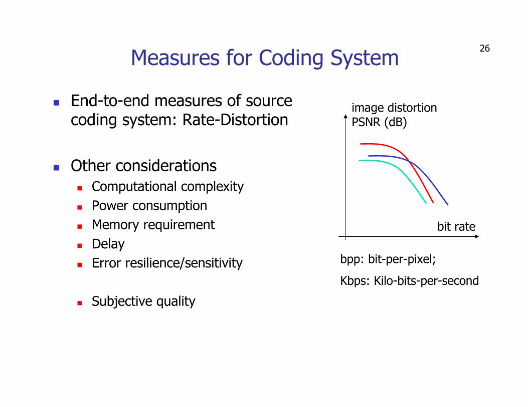
Measures for Coding System

� End-to-end measures of source coding system: Rate-Distortion

� Other considerations

� Computational complexity

� Power consumption

� Memory requirement

� Delay

� Error resilience/sensitivity

� Subjective quality

image distortionPSNR (dB)

bit rate

bpp: bit-per-pixel;

Kbps: Kilo-bits-per-second

27

Image/Video Compression Standards

� Bitstream useful only if the recipient knows the code!

� Standardization efforts are important

� Technology and algorithm benchmark

� System definition and development

� Patent pool management

� Defines the bitstream (decoder), not how you generate them (encoder)!

28

29

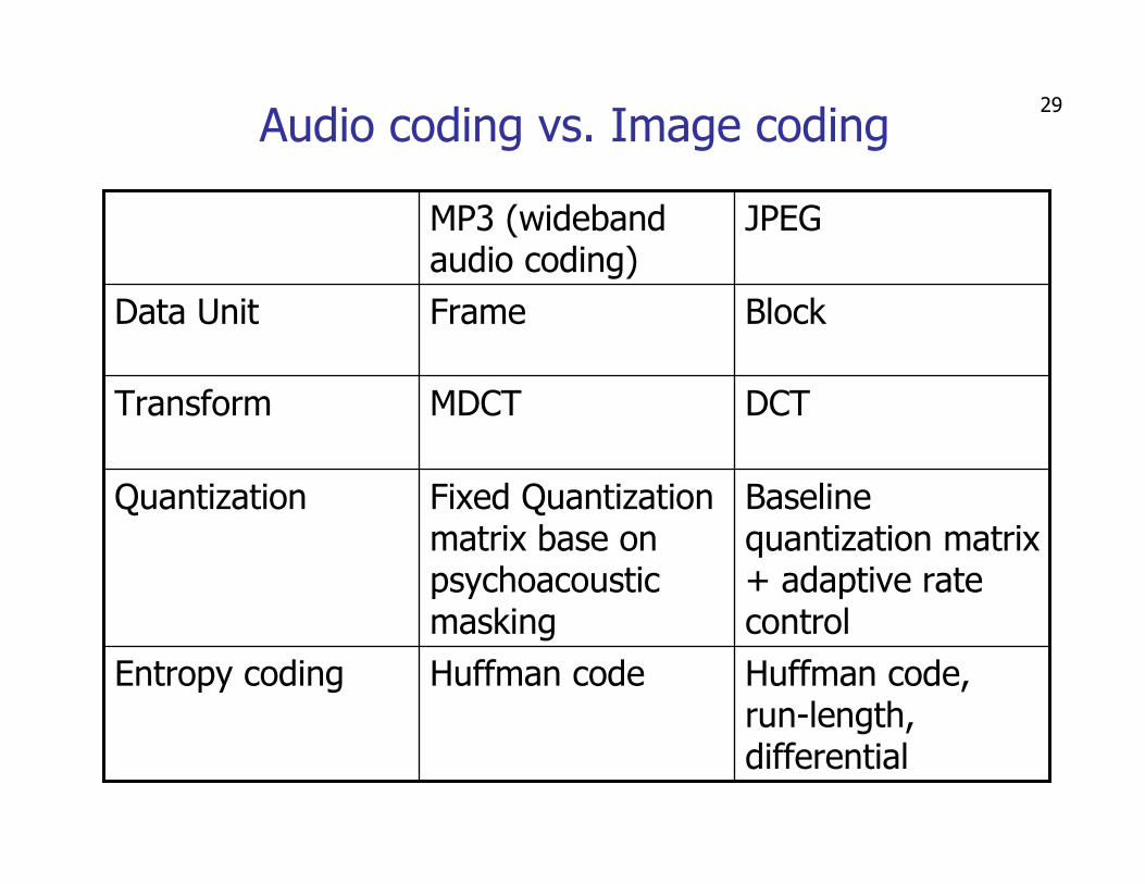
Audio coding vs. Image coding

Huffman code, run-length, differential

Huffman codeEntropy coding

Baseline quantization matrix + adaptive rate control

Fixed Quantization matrix base on psychoacoustic masking

Quantization

DCTMDCTTransform

BlockFrameData Unit

JPEGMP3 (wideband audio coding)

30JPEG Compression Standard (early 1990s)

� JPEG - Joint Photographic Experts Group

� Compression standard of generic continuous-tone still image

� Became an international standard in 1992

� Allow for lossy and lossless encoding of still images� Part-1 DCT-based lossy compression

� average compression ratio 15:1

� Part-2 Predictive-based lossless compression

� Sequential, Progressive, Hierarchical modes� Sequential: encoded in a single left-to-right, top-to-bottom scan

� Progressive: encoded in multiple scans to first produce a quick,rough decoded image when the transmission time is long

� Hierarchical: encoded at multiple resolution to allow accessing low resolution without full decompression

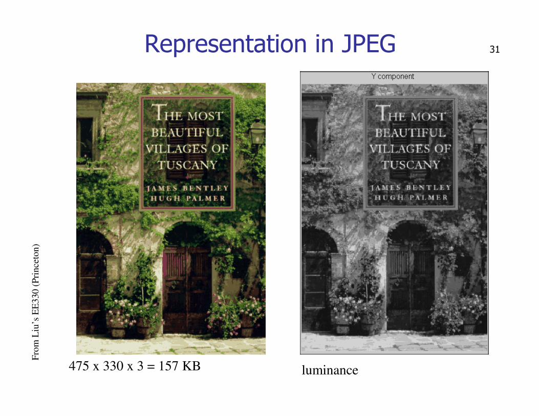
31Representation in JPEG

475 x 330 x 3 = 157 KB luminance

Fro

m L

iu’s

EE

330

(P

rin

ceto

n)

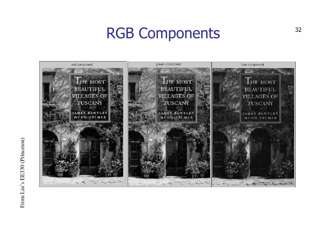
32RGB ComponentsF

rom

Liu

’s E

E3

30

(P

rin

ceto

n)

33Y U V (Y Cb Cr) Components

Assign more bits to Y, less bits to Cb and Cr

Fro

m L

iu’s

EE

330

(P

rin

ceto

n)

34Baseline JPEG Algorithm

� “Baseline”

� Simple, lossy compression

� Subset of other DCT-based modes of JPEG standard

� A few basics

� 8x8 block-DCT based coding

� Shift to zero-mean by subtracting 128 � [-128, 127]

� Allows using signed integer to represent both DC and AC coeff.

� Color (YCbCr / YUV) and downsample� Color components can have lower spatial resolution than luminance

� Interleaving color components

−−

−−=

B

G

R

C

C

Y

r

b

100.0515.0615.0

436.0289.0147.0

114.0587.0299.0

(Based on Wang’s video book Chapt.1)

35

complexity

Block-based Transform

� Why block based?

� High transform computation complexity for larger blocks

� O( m log m × m ) per blockin transform for (MN/m2) blocks

� High complexity in bit allocation

� Block transform captures local info

� Commonly used block sizes: 8x8, 16x16, 8x4, 4x8 … From Jain’s Fig.11.16

36

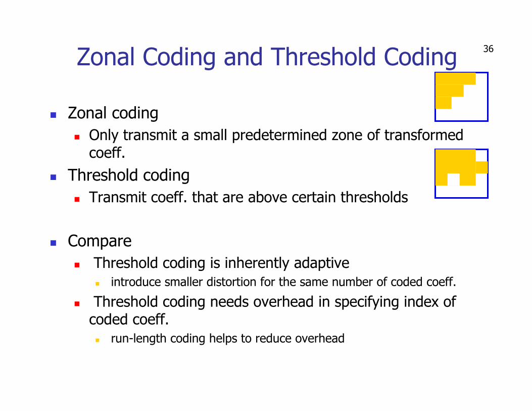
Zonal Coding and Threshold Coding

� Zonal coding

� Only transmit a small predetermined zone of transformed coeff.

� Threshold coding

� Transmit coeff. that are above certain thresholds

� Compare

� Threshold coding is inherently adaptive

� introduce smaller distortion for the same number of coded coeff.

� Threshold coding needs overhead in specifying index of coded coeff.

� run-length coding helps to reduce overhead

37

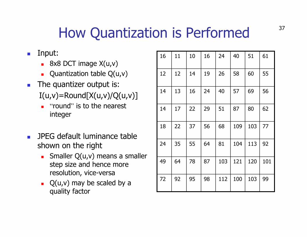
How Quantization is Performed

� Input:

� 8x8 DCT image X(u,v)

� Quantization table Q(u,v)

� The quantizer output is:

I(u,v)=Round[X(u,v)/Q(u,v)]

� “round” is to the nearest integer

� JPEG default luminance table shown on the right

� Smaller Q(u,v) means a smaller step size and hence more resolution, vice-versa

� Q(u,v) may be scaled by a quality factor

9910310011298959272

10112012110387786449

921131048164553524

771031096856372218

6280875129221714

5669574024161314

5560582619141212

6151402416101116

38

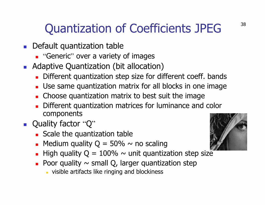
Quantization of Coefficients JPEG

� Default quantization table

� “Generic” over a variety of images

� Adaptive Quantization (bit allocation)

� Different quantization step size for different coeff. bands

� Use same quantization matrix for all blocks in one image

� Choose quantization matrix to best suit the image

� Different quantization matrices for luminance and color components

� Quality factor “Q”

� Scale the quantization table

� Medium quality Q = 50% ~ no scaling

� High quality Q = 100% ~ unit quantization step size

� Poor quality ~ small Q, larger quantization step� visible artifacts like ringing and blockiness

39

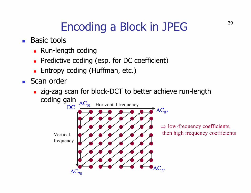
Encoding a Block in JPEG� Basic tools

� Run-length coding

� Predictive coding (esp. for DC coefficient)

� Entropy coding (Huffman, etc.)

� Scan order

� zig-zag scan for block-DCT to better achieve run-length coding gain

Horizontal frequency

Vertical

frequency

DCAC01

AC07

AC70

AC77

⇒ low-frequency coefficients,

then high frequency coefficients

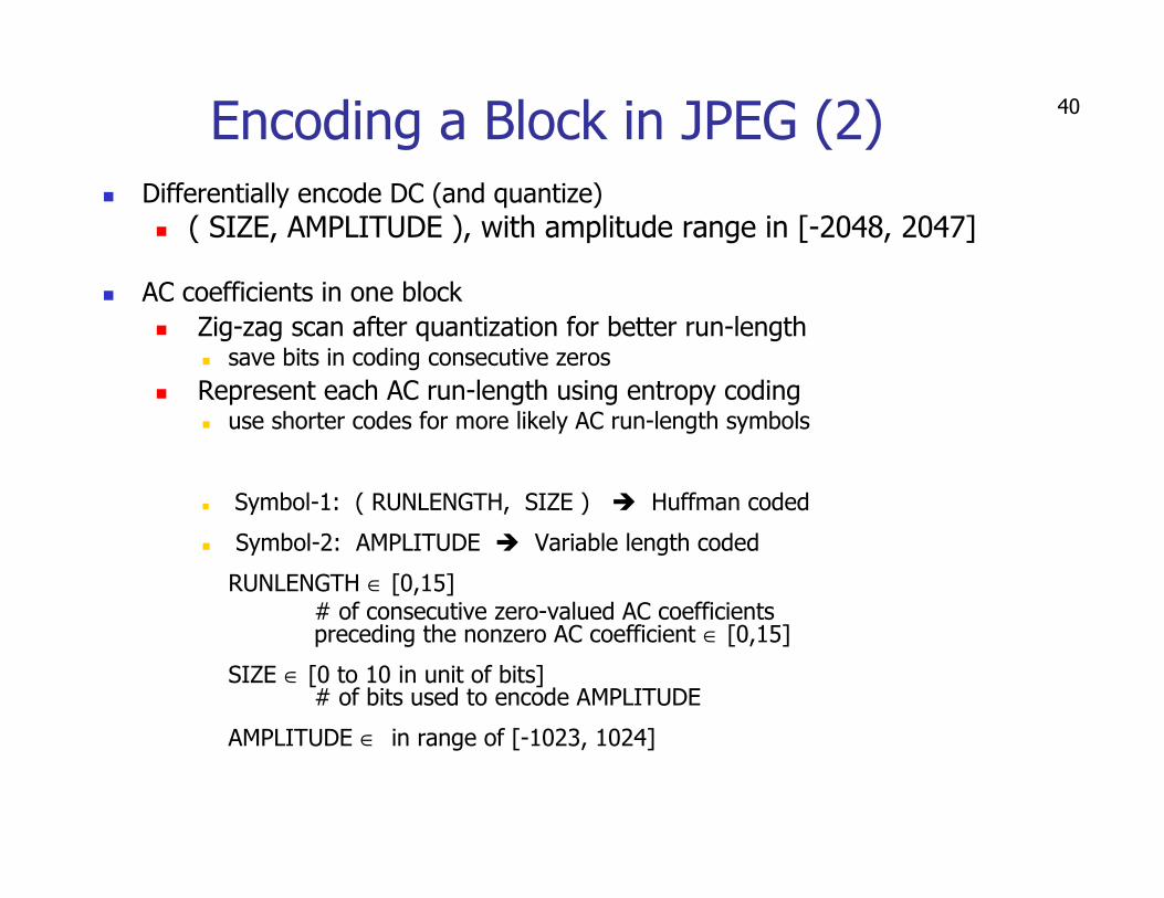
40Encoding a Block in JPEG (2)� Differentially encode DC (and quantize)

� ( SIZE, AMPLITUDE ), with amplitude range in [-2048, 2047]

� AC coefficients in one block

� Zig-zag scan after quantization for better run-length� save bits in coding consecutive zeros

� Represent each AC run-length using entropy coding � use shorter codes for more likely AC run-length symbols

� Symbol-1: ( RUNLENGTH, SIZE ) � Huffman coded

� Symbol-2: AMPLITUDE � Variable length coded

RUNLENGTH ∈ [0,15] # of consecutive zero-valued AC coefficientspreceding the nonzero AC coefficient ∈ [0,15]

SIZE ∈ [0 to 10 in unit of bits] # of bits used to encode AMPLITUDE

AMPLITUDE ∈ in range of [-1023, 1024]

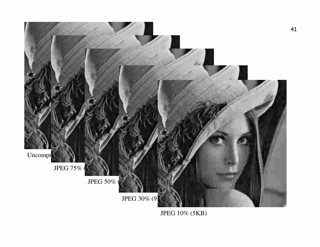
41

Uncompressed (100KB)

JPEG 75% (18KB)

JPEG 50% (12KB)

JPEG 30% (9KB)

JPEG 10% (5KB)

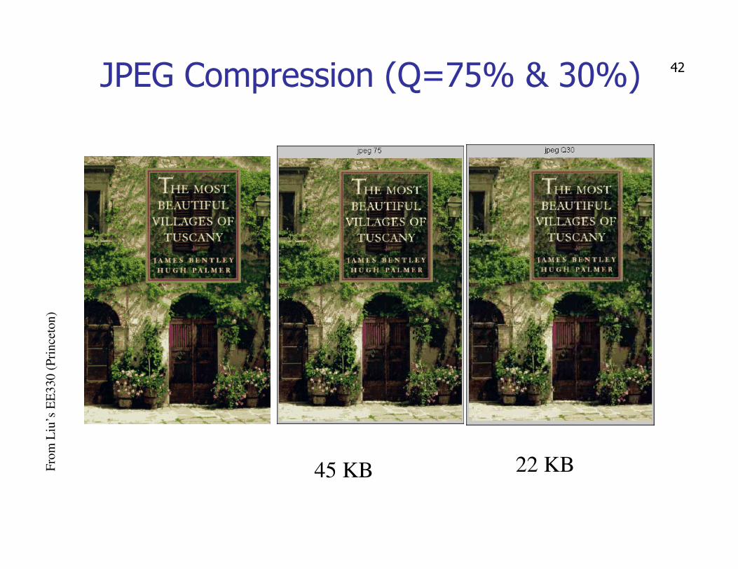
42JPEG Compression (Q=75% & 30%)

45 KB 22 KBFro

m L

iu’s

EE

330

(P

rin

ceto

n)

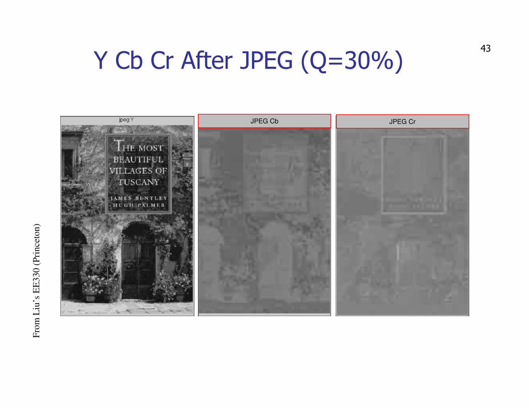
43

Y Cb Cr After JPEG (Q=30%)

Fro

m L

iu’s

EE

330

(P

rin

ceto

n)

JPEG Cb JPEG Cr

44

JPEG 2000

� Better image quality/coding efficiency, esp. low bit-rate compression performance� DWT� Bit-plane coding (EBCOT)� Flexible block sizes� …

� More functionality� Support larger images� Progressive transmission by quality, resolution, component, or

spatial locality� Lossy and Lossless compression� Random access to the bitstream� Region of Interest coding� Robustness to bit errors

45

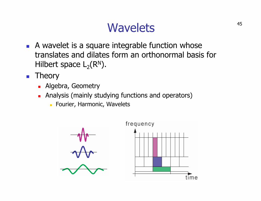
Wavelets

� A wavelet is a square integrable function whose translates and dilates form an orthonormal basis for Hilbert space L2(R

N).

� Theory

� Algebra, Geometry

� Analysis (mainly studying functions and operators)

� Fourier, Harmonic, Wavelets

46

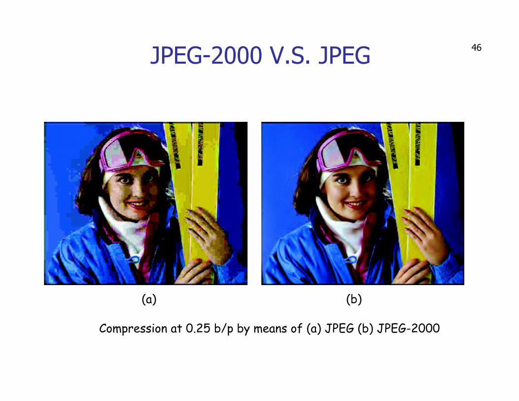
JPEG-2000 V.S. JPEG

(a) (b)

Compression at 0.25 b/p by means of (a) JPEG (b) JPEG-2000

47

JPEG-2000 V.S. JPEG

Compression at 0.2 b/p by means of (a) JPEG (b) JPEG-2000

(a) (b)

48The trade-off:

JPEG2000 has a much Higher computational complexity than JPEG,

especially for larger pictures.

Need parallel

implementation

to reduce

compression

time.

49

Hybrid Video Coding System

mux

de-mux

50

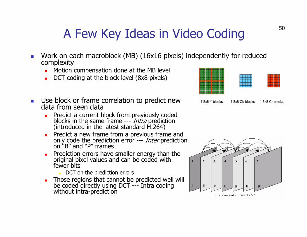
A Few Key Ideas in Video Coding

� Work on each macroblock (MB) (16x16 pixels) independently for reduced complexity� Motion compensation done at the MB level� DCT coding at the block level (8x8 pixels)

� Use block or frame correlation to predict new data from seen data� Predict a current block from previously coded

blocks in the same frame --- Intra prediction (introduced in the latest standard H.264)

� Predict a new frame from a previous frame and only code the prediction error --- Inter prediction on “B” and “P” frames

� Prediction errors have smaller energy than the original pixel values and can be coded with fewer bits

� DCT on the prediction errors

� Those regions that cannot be predicted well will be coded directly using DCT --- Intra coding without intra-prediction

51

Motion Compensation � Help reduce temporal redundancy of video

PREVIOUS FRAME CURRENT FRAME

PREDICTED FRAME PREDICTION ERROR FRAME

Revised from R.Liu Seminar Course ’00 @ UMD

52Motion Estimation

� Help understanding the content of image sequence

� For surveillance

� Help reduce temporal redundancy of video

� For compression

� Stabilizing video by detecting and removing small, noisy global motions

� For building stabilizer in camcorder

� A hard problem in general!

53Block-Matching by Exhaustive Search� Assume block-based translation motion model

� Search every possibility over a specified range for the best matching block � MAD (mean absolute difference) often used for simplicity

From Wang’s

Preprint Fig.6.6

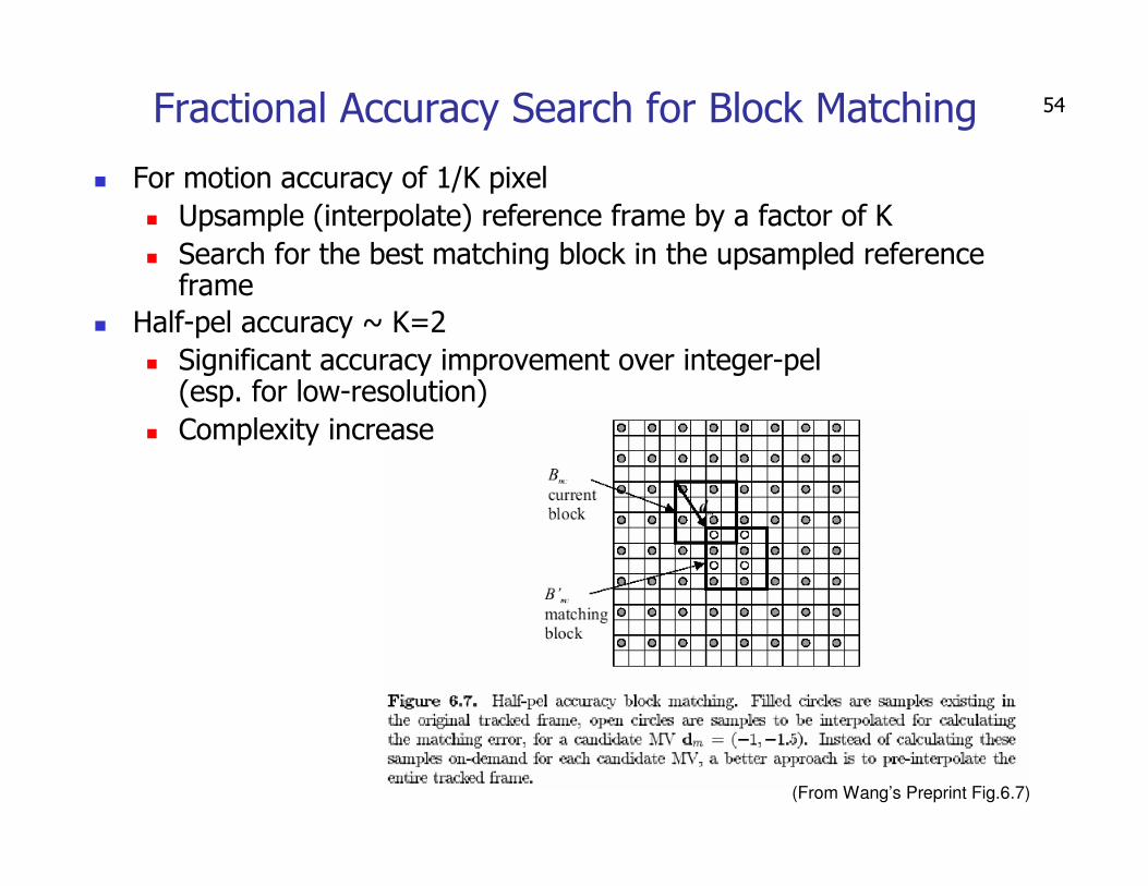
54Fractional Accuracy Search for Block Matching

� For motion accuracy of 1/K pixel

� Upsample (interpolate) reference frame by a factor of K

� Search for the best matching block in the upsampled reference frame

� Half-pel accuracy ~ K=2

� Significant accuracy improvement over integer-pel(esp. for low-resolution)

� Complexity increase

(From Wang’s Preprint Fig.6.7)

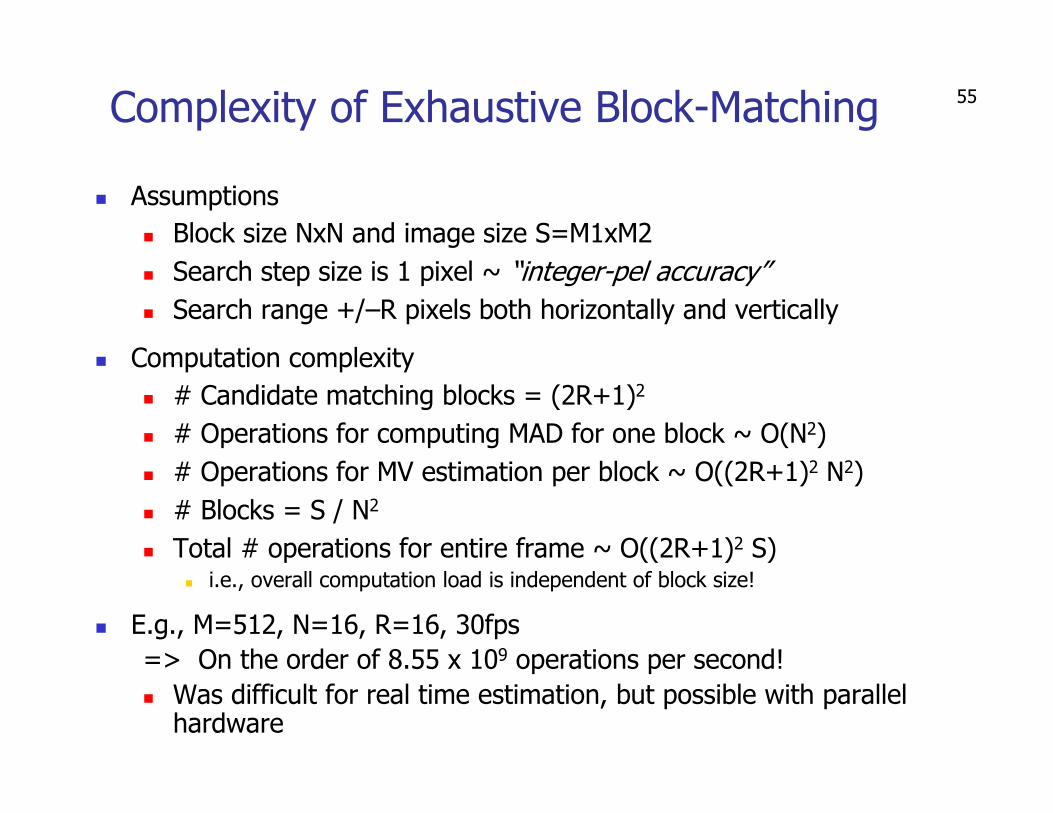
55Complexity of Exhaustive Block-Matching

� Assumptions

� Block size NxN and image size S=M1xM2

� Search step size is 1 pixel ~ “integer-pel accuracy”

� Search range +/–R pixels both horizontally and vertically

� Computation complexity

� # Candidate matching blocks = (2R+1)2

� # Operations for computing MAD for one block ~ O(N2)

� # Operations for MV estimation per block ~ O((2R+1)2 N2)

� # Blocks = S / N2

� Total # operations for entire frame ~ O((2R+1)2 S)� i.e., overall computation load is independent of block size!

� E.g., M=512, N=16, R=16, 30fps

=> On the order of 8.55 x 109 operations per second!

� Was difficult for real time estimation, but possible with parallel hardware

56

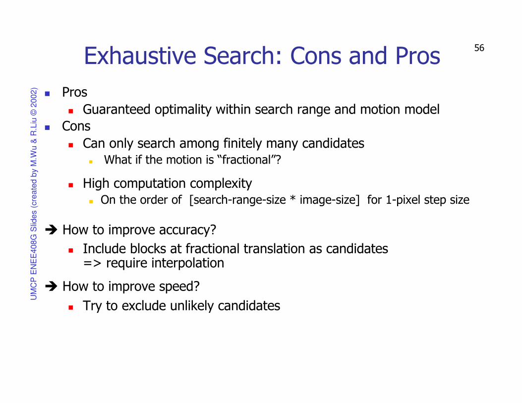
Exhaustive Search: Cons and Pros

� Pros

� Guaranteed optimality within search range and motion model

� Cons

� Can only search among finitely many candidates� What if the motion is “fractional”?

� High computation complexity� On the order of [search-range-size * image-size] for 1-pixel step size

� How to improve accuracy?

� Include blocks at fractional translation as candidates => require interpolation

� How to improve speed?

� Try to exclude unlikely candidates

UM

CP

EN

EE

408

G S

lide

s (

cre

ate

d b

y M

.Wu &

R.L

iu ©

2002

)

57

Fast Algorithms for Block Matching

� Basic ideas

� Matching errors near the best match are generally smaller than far away

� Skip candidates that are unlikely to give good match

(From Wang’s Preprint Fig.6.6)

58

M24

M15 M14 M13

M16

M11

M12

M5 M4 M3

M17 M18 M19

-6 M6 M1 M2 +6

M7 M8 M9

dx

dy

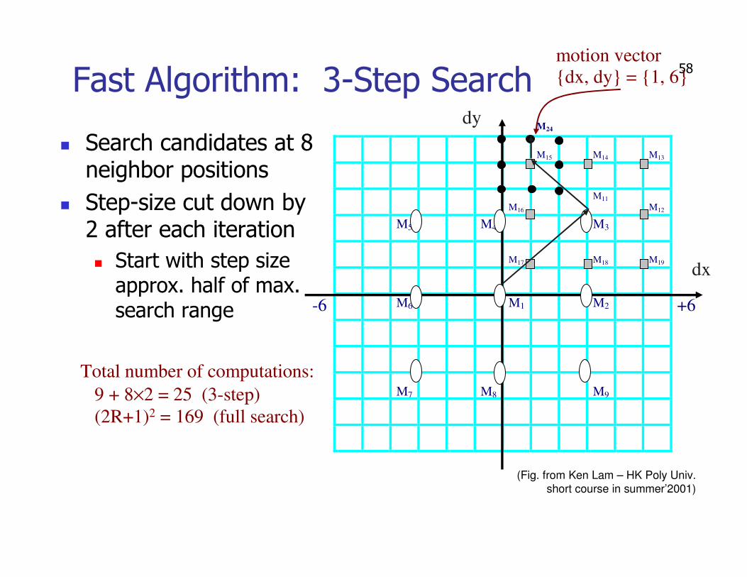
Fast Algorithm: 3-Step Search

� Search candidates at 8 neighbor positions

� Step-size cut down by 2 after each iteration

� Start with step size approx. half of max. search range

motion vector

{dx, dy} = {1, 6}

Total number of computations:

9 + 8×2 = 25 (3-step)

(2R+1)2 = 169 (full search)

(Fig. from Ken Lam – HK Poly Univ. short course in summer’2001)

59

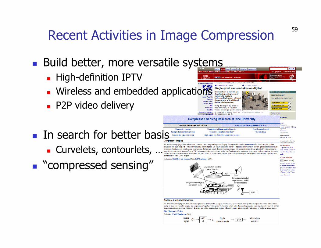
Recent Activities in Image Compression

� Build better, more versatile systems

� High-definition IPTV

� Wireless and embedded applications

� P2P video delivery

� In search for better basis

� Curvelets, contourlets, …

� “compressed sensing”

60

Summary

� The image/video compression problem

� Source coding� For i.i.d. symbols

� For symbol streams

� Image/video compression systems� MPEG/JPEG and beyond

� Next time: multimedia indexing and image reconstruction in medical applications

Part of the slides/materials gratefully taken from:

Wade Trappe (Rutgers), Min Wu (UMD), Yao Wang

(poly tech), Xiuzhen Huang (UCSB), Tony Lin (PKU)