EE C128 / ME C134 – Feedback Control Systems Lecture – Chapter 3 – Modeling in the Time Domain Alexandre Bayen Department of Electrical Engineering & Computer Science University of California Berkeley September 10, 2013 Bayen (EECS, UCB) Feedback Control Systems September 10, 2013 1 / 29

Welcome message from author
This document is posted to help you gain knowledge. Please leave a comment to let me know what you think about it! Share it to your friends and learn new things together.
Transcript

EE C128 / ME C134 – Feedback Control SystemsLecture – Chapter 3 – Modeling in the Time Domain
Alexandre Bayen
Department of Electrical Engineering & Computer ScienceUniversity of California Berkeley
September 10, 2013
Bayen (EECS, UCB) Feedback Control Systems September 10, 2013 1 / 29
Lecture abstract
Topics covered in this presentation
I System variables: states, inputs, outputs, & measurements
I Linear independence
I State space representation
I Conversion between systems in time-, frequency-domain, TF, & statespace representations
Bayen (EECS, UCB) Feedback Control Systems September 10, 2013 2 / 29
Chapter outline
1 3 Modeling in the time domain3.1 Introduction3.2 Some observations3.3 The general state space representation3.4 Applying the state space representation3.5 Converting a transfer function to state space3.6 Converting from state space to a transfer function
Bayen (EECS, UCB) Feedback Control Systems September 10, 2013 3 / 29

3 Modeling in the time domain 3.2 Some observations
1 3 Modeling in the time domain3.1 Introduction3.2 Some observations3.3 The general state space representation3.4 Applying the state space representation3.5 Converting a transfer function to state space3.6 Converting from state space to a transfer function
Bayen (EECS, UCB) Feedback Control Systems September 10, 2013 4 / 29
3 Modeling in the time domain 3.2 Some observations
SS representation, [1, p. 119]
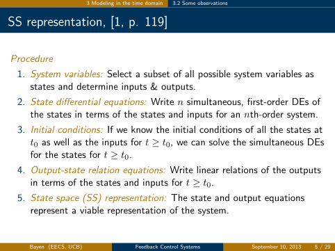
Procedure
1. System variables: Select a subset of all possible system variables asstates and determine inputs & outputs.
2. State differential equations: Write n simultaneous, first-order DEs ofthe states in terms of the states and inputs for an nth-order system.
3. Initial conditions: If we know the initial conditions of all the states att0 as well as the inputs for t ≥ t0, we can solve the simultaneous DEsfor the states for t ≥ t0.
4. Output-state relation equations: Write linear relations of the outputsin terms of the states and inputs for t ≥ t0.
5. State space (SS) representation: The state and output equationsrepresent a viable representation of the system.
Bayen (EECS, UCB) Feedback Control Systems September 10, 2013 5 / 29

3 Modeling in the time domain 3.2 Some observations
Size of system states, inputs & outputs, [1, p. 122]
I States: Typically the minimum number of states required to describea system equals the order of the system DE. We can define morestates than the minimum set; however, within this minimal set thestates must be linearly independent (defined later).
I Inputs & outputs: Single-input, single-output (SISO) systems are aunique case of general multiple-input, multiple-output (MIMO)systems. The output and input of a SISO system are represented byscalar quantities. The outputs and inputs of a MIMO system arerepresented by vector quantities.
Bayen (EECS, UCB) Feedback Control Systems September 10, 2013 6 / 29
3 Modeling in the time domain 3.2 Some observations
Motivational example, [1, p. 120]
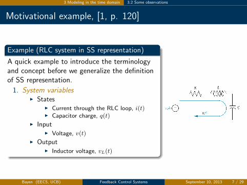
Example (RLC system in SS representation)
A quick example to introduce the terminologyand concept before we generalize the definitionof SS representation.
1. System variablesI States
I Current through the RLC loop, i(t)I Capacitor charge, q(t)
I InputI Voltage, v(t)
I OutputI Inductor voltage, vL(t)
Bayen (EECS, UCB) Feedback Control Systems September 10, 2013 7 / 29
3 Modeling in the time domain 3.2 Some observations
Motivational example, [1, p. 120]
Example (RLC system in SS representation)
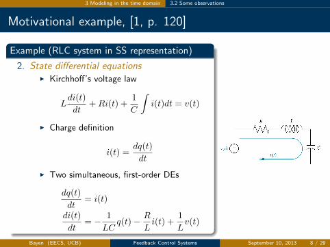
2. State differential equationsI Kirchhoff’s voltage law
Ldi(t)
dt+Ri(t) +
1
C
∫i(t)dt = v(t)
I Charge definition
i(t) =dq(t)
dt
I Two simultaneous, first-order DEs
dq(t)
dt= i(t)
di(t)
dt= − 1
LCq(t)− R
Li(t) +
1
Lv(t)
Bayen (EECS, UCB) Feedback Control Systems September 10, 2013 8 / 29
3 Modeling in the time domain 3.2 Some observations
Motivational example, [1, p. 120]
Example (RLC system in SS representation)
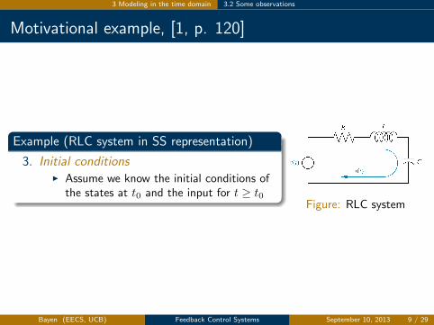
3. Initial conditionsI Assume we know the initial conditions of
the states at t0 and the input for t ≥ t0Figure: RLC system
Bayen (EECS, UCB) Feedback Control Systems September 10, 2013 9 / 29
3 Modeling in the time domain 3.2 Some observations
Motivational example, [1, p. 120]
Example (RLC system in SS representation)
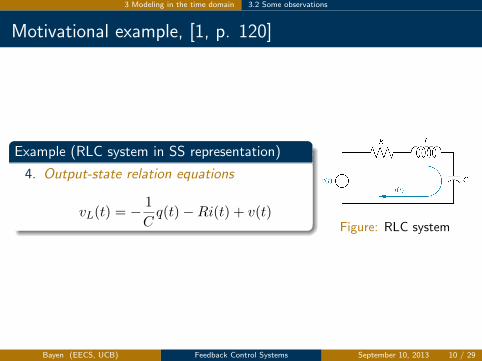
4. Output-state relation equations
vL(t) = −1
Cq(t)−Ri(t) + v(t)
Figure: RLC system
Bayen (EECS, UCB) Feedback Control Systems September 10, 2013 10 / 29
3 Modeling in the time domain 3.2 Some observations
Motivational example, [1, p. 120]
Example (RLC system in SS representation)
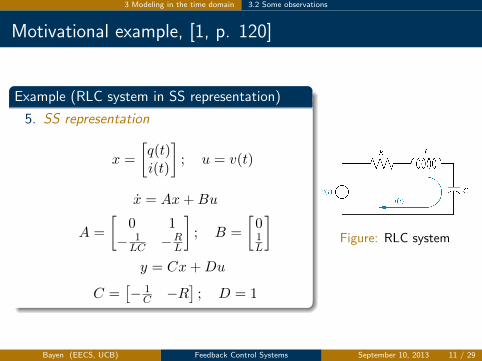
5. SS representation
x =
[q(t)i(t)
]; u = v(t)
x = Ax+Bu
A =
[0 1
− 1LC −R
L
]; B =
[01L
]y = Cx+Du
C =[− 1
C −R]; D = 1
Figure: RLC system
Bayen (EECS, UCB) Feedback Control Systems September 10, 2013 11 / 29

3 Modeling in the time domain 3.3 The general state space representation
1 3 Modeling in the time domain3.1 Introduction3.2 Some observations3.3 The general state space representation3.4 Applying the state space representation3.5 Converting a transfer function to state space3.6 Converting from state space to a transfer function
Bayen (EECS, UCB) Feedback Control Systems September 10, 2013 12 / 29
3 Modeling in the time domain 3.3 The general state space representation
Definitions, [1, p. 123]
I Linear combination: A linear combination of n variables, xi, for i = 1to n, is given by the following sum, S
S = Knxn +Kn−1xn−1 + ...+K1x1
where each Ki is a constant.
I Linear independence: None of the variables can be written as a linearcombination of the others. Variables xi, for i = 1 to n, are said to belinearly independent if their linear combination, S, equals zero only ifevery Ki = 0 and no xi = 0 for all t > 0.
Bayen (EECS, UCB) Feedback Control Systems September 10, 2013 13 / 29
3 Modeling in the time domain 3.3 The general state space representation
Definitions, [1, p. 123]
I System variable: Any variable that responds to an input or initialcondition in a system.
I State: The state variables are a non-unique set of linearlyindependent system variables such that the values of the members ofthe set at time t0 along with known inputs completely determine thevalue of all system variables for all t > t0.
I State vector: A vector whose elements are the states.
I State space: The n-dimensional space whose axes are the states. Atrajectory can be thought of as being mapped out by the state vector,x(t), for a range of t.
Bayen (EECS, UCB) Feedback Control Systems September 10, 2013 14 / 29
3 Modeling in the time domain 3.3 The general state space representation
Equations, [1, p. 123]
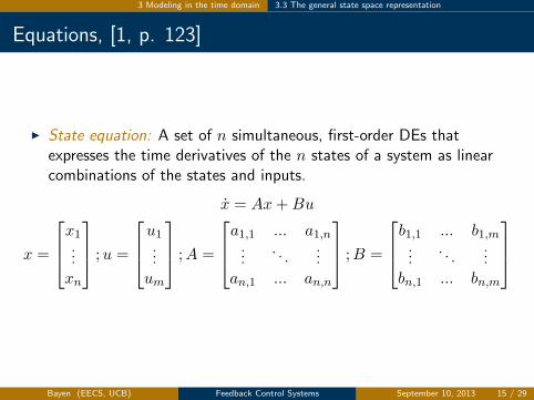
I State equation: A set of n simultaneous, first-order DEs thatexpresses the time derivatives of the n states of a system as linearcombinations of the states and inputs.
x = Ax+Bu
x =
x1...xn
;u =
u1...um
;A =
a1,1 ... a1,n...
. . ....
an,1 ... an,n
;B =
b1,1 ... b1,m...
. . ....
bn,1 ... bn,m
Bayen (EECS, UCB) Feedback Control Systems September 10, 2013 15 / 29
3 Modeling in the time domain 3.3 The general state space representation
Equations, [1, p. 123]
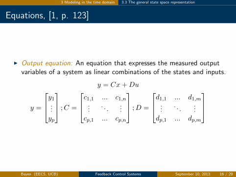
I Output equation: An equation that expresses the measured outputvariables of a system as linear combinations of the states and inputs.
y = Cx+Du
y =
y1...yp
;C =
c1,1 ... c1,n...
. . ....
cp,1 ... cp,n
;D =
d1,1 ... d1,m...
. . ....
dp,1 ... dp,m
Bayen (EECS, UCB) Feedback Control Systems September 10, 2013 16 / 29

3 Modeling in the time domain 3.3 The general state space representation
Variables & their dimensions, [1, p. 123]
x ∈ Rn time derivative of state vector
x ∈ Rn state vector
u ∈ Rm control input vector
y ∈ Rp measured output vector
A ∈ Rn×n system matrix
B ∈ Rm input matrix
C ∈ Rp×n output matrix
D ∈ Rp×m feedforward matrix
Bayen (EECS, UCB) Feedback Control Systems September 10, 2013 17 / 29
3 Modeling in the time domain 3.4 Applying the state space representation
1 3 Modeling in the time domain3.1 Introduction3.2 Some observations3.3 The general state space representation3.4 Applying the state space representation3.5 Converting a transfer function to state space3.6 Converting from state space to a transfer function
Bayen (EECS, UCB) Feedback Control Systems September 10, 2013 18 / 29

3 Modeling in the time domain 3.4 Applying the state space representation
Selecting the states, [1, p. 124]
State requirements
I The states must be linearly independent.
I A minimum number of states must be selected and must be sufficientto describe completely the state of the system. Typically the numberrequired equals the sum of the orders of a set of DEs describing thesystem.
If
I too few states are selected or
I a minimum number of states are selected and are linearly dependent,
it may be impossible to completely express state and output equations aslinear combinations of the states and inputs.
Bayen (EECS, UCB) Feedback Control Systems September 10, 2013 19 / 29
3 Modeling in the time domain 3.4 Applying the state space representation
Selecting the states, [1, p. 124]
Notes concerning adding states to the minimal set of linear independentstates
I Linear independent states: These additional linear independent statesare also decoupled, i.e., they are not required in order to solve for anyof the other linearly independent states or any other dependentsystem variable.
I Linear dependent states: The dimension of the system matrix isincreased unnecessarily, adding difficulty to the solution of the statevector [1, Ch. 4] and hindering the designer’s ability to use statespace methods for design [1, Ch. 12].
Bayen (EECS, UCB) Feedback Control Systems September 10, 2013 20 / 29

3 Modeling in the time domain 3.4 Applying the state space representation
Representing an electrical system, [1, p. 126]
Example (RLC system)
I Problem: Find a state-spacerepresentation in vector-matrixform if the states are thecapacitor voltage, vC , and theinductor current, iL, and theinput is the applied voltage, v,and the output is the resistorcurrent, iR
I Solution: On board
Figure: Electrical system
Bayen (EECS, UCB) Feedback Control Systems September 10, 2013 21 / 29
3 Modeling in the time domain 3.4 Applying the state space representation
Representing a translational mechanical system, [1, p. 130]
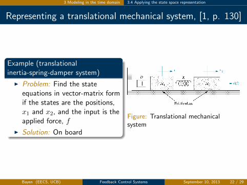
Example (translationalinertia-spring-damper system)
I Problem: Find the stateequations in vector-matrix formif the states are the positions,x1 and x2, and the input is theapplied force, f
I Solution: On board
Figure: Translational mechanicalsystem
Bayen (EECS, UCB) Feedback Control Systems September 10, 2013 22 / 29

3 Modeling in the time domain 3.5 Converting a TF to state space
1 3 Modeling in the time domain3.1 Introduction3.2 Some observations3.3 The general state space representation3.4 Applying the state space representation3.5 Converting a transfer function to state space3.6 Converting from state space to a transfer function
Bayen (EECS, UCB) Feedback Control Systems September 10, 2013 23 / 29
3 Modeling in the time domain 3.5 Converting a TF to state space
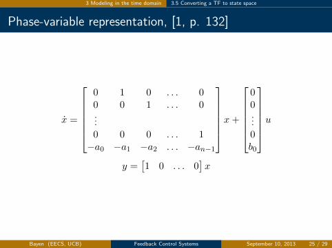
Phase-variable representation, [1, p. 132]
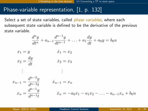
Select a set of state variables, called phase variables, where eachsubsequent state variable is defined to be the derivative of the previousstate variable.
dny
dtn+ an−1
dn−1y
dtn−1+ . . .+ a1
dy
dt+ a0y = b0u
x1 = y x1 = x2
x2 =dy
dtx2 = x3
......
xn−1 =dn−2y
dn−2txn−1 = xn
xn =dn−1y
dn−1txn = −a0x1 − a1x2 − . . .− an−1xn + b0u
Bayen (EECS, UCB) Feedback Control Systems September 10, 2013 24 / 29
3 Modeling in the time domain 3.5 Converting a TF to state space
Phase-variable representation, [1, p. 132]
x =
0 1 0 . . . 00 0 1 . . . 0...0 0 0 . . . 1−a0 −a1 −a2 . . . −an−1
x+
00...0b0
u
y =[1 0 . . . 0
]x
Bayen (EECS, UCB) Feedback Control Systems September 10, 2013 25 / 29
3 Modeling in the time domain 3.5 Converting a TF to state space
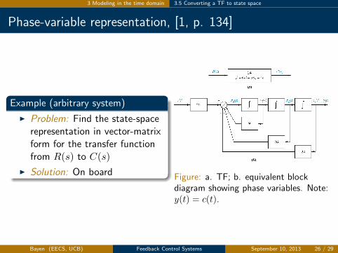
Phase-variable representation, [1, p. 134]
Example (arbitrary system)
I Problem: Find the state-spacerepresentation in vector-matrixform for the transfer functionfrom R(s) to C(s)
I Solution: On board Figure: a. TF; b. equivalent blockdiagram showing phase variables. Note:y(t) = c(t).
Bayen (EECS, UCB) Feedback Control Systems September 10, 2013 26 / 29
3 Modeling in the time domain 3.6 Converting from state space to a TF
1 3 Modeling in the time domain3.1 Introduction3.2 Some observations3.3 The general state space representation3.4 Applying the state space representation3.5 Converting a transfer function to state space3.6 Converting from state space to a transfer function
Bayen (EECS, UCB) Feedback Control Systems September 10, 2013 27 / 29

3 Modeling in the time domain 3.6 Converting from state space to a TF
Converting from SS to a TF, [1, p. 139]
State and output equations
x = Ax+Bu
y = Cx+Du
Laplace transform assuming zero initial conditions
sX(s) = AX(s) +BU(s)
Y (s) = CX(s) +DU(s)
Transfer function matrix
T (s) =Y (s)
U(s)= C(sI −A)−1B +D
Bayen (EECS, UCB) Feedback Control Systems September 10, 2013 28 / 29
3 Modeling in the time domain 3.6 Converting from state space to a TF
Bibliography
Norman S. Nise. Control Systems Engineering, 2011.
Bayen (EECS, UCB) Feedback Control Systems September 10, 2013 29 / 29
Related Documents


![EE C128 / ME C134 Feedback Control Systems - Lecture ...1 { Intro 1.4 Analysis & design objectives Analysis & design objectives, [1, p. 11] Transient response I Due to the system and](https://static.cupdf.com/doc/110x72/60c2b429f20afb5faa4216f0/ee-c128-me-c134-feedback-control-systems-lecture-1-intro-14-analysis.jpg)


