Economic Theory manuscript No. (will be inserted by the editor) Educational Choice, Rural-urban Migration and Economic Development Pei-Ju Liao 1 · Ping Wang 2 · Yin-Chi Wang 3 · Chong K. Yip 4 Received: date / Accepted: date Abstract We develop an overlapping-generations framework of education-based migration that takes place prior to labor-market participation and explore its role for economic development, urbanization and workforce com- position. We show that education-based and work-based migration are substitutes and the equilibrium outcome depends crucially on children’s talent distribution, college costs and selectiveness, urban job opportunities, and migration barriers. We establish conflicting partial- and general-equilibrium effects at work for comparative stat- ics, and examine their locational as well as macroeconomic implications for assessing education and migration policies. Applying our model to fit the data from China over 1980-2007, we find that, although education-based migration only amounts to one-fifth of that of work-based migration, it contributes more to per capita output growth than work-based migration owing to its high-skilled nature. Moreover, the abolishment of education-based migra- tion policy and the relaxation of the work-based migration are found to have limited effects on per capita output and urbanization. Keywords Educational choice · rural-urban migration · urbanization · skill composition · development JEL classification O15 · O53 · R23 · R28 We are grateful for comments from Rick Bond, Kaiji Chen, Victor Couture, Suchin Ge, Chang-Tai Hsieh, B. Ravikumar, Ray Riezman, Michael Song and Dennis Yang, two insightful referees, an associate editor, as well as participants at the AREUEA-ASSA Annual Meetings, the Asian Meetings of the Econometric Society, the Asian Bureau of Finance and Economic Research Conference, the Midwest Macro Meetings, the Public Economic Theory Conference, the Society for Advanced Economic Theory Meeting, the Symposium on Growth and Development, the Society for Economic Dynamics Meeting, and the Regional Science Association International Meeting, and seminar participants at Academia Sinica, Chinese University of Hong Kong, National Taiwan University, National Sun Yat-sen University, Washington University in St. Louis and University of Washington-Seattle. Travel support from the Chinese University of Hong Kong, Tsinghua University, and the Center for Dynamic Economics of Washington University are gratefully acknowledged. An earlier draft has been circulated as NBER Working Paper #23939. Liao thanks the research grant from the Ministry of Science and Technology of Taiwan (MOST 103-2410-H-001-016-MY2). Yip acknowledges support received through a GRF grant from the Research Grants Council of the Hong Kong Special Administrative Region, China (No. CUHK 14501618). Needless to say, the usual disclaimer applies. Pei-Ju Liao [email protected] Ping Wang [email protected] Yin-Chi Wang [email protected] Chong K. Yip [email protected] 1 Department of Economics, National Taiwan University, Taipei, Taiwan. 2 Department of Economics, Washington University in St. Louis & Federal Reserve Bank of St. Louis, St. Louis, USA; NBER, USA. 3 Department of Economics, National Taipei University, New Taipei City, Taiwan. 4 Department of Economics, Chinese University of Hong Kong, Hong Kong SAR.

Welcome message from author
This document is posted to help you gain knowledge. Please leave a comment to let me know what you think about it! Share it to your friends and learn new things together.
Transcript
Economic Theory manuscript No.(will be inserted by the editor)
Educational Choice, Rural-urban Migration and Economic Development
Pei-Ju Liao1 · Ping Wang2 · Yin-Chi Wang3 ·Chong K. Yip4
Received: date / Accepted: date
Abstract We develop an overlapping-generations framework of education-based migration that takes place priorto labor-market participation and explore its role for economic development, urbanization and workforce com-position. We show that education-based and work-based migration are substitutes and the equilibrium outcomedepends crucially on children’s talent distribution, college costs and selectiveness, urban job opportunities, andmigration barriers. We establish conflicting partial- and general-equilibrium effects at work for comparative stat-ics, and examine their locational as well as macroeconomic implications for assessing education and migrationpolicies. Applying our model to fit the data from China over 1980-2007, we find that, although education-basedmigration only amounts to one-fifth of that of work-based migration, it contributes more to per capita output growththan work-based migration owing to its high-skilled nature. Moreover, the abolishment of education-based migra-tion policy and the relaxation of the work-based migration are found to have limited effects on per capita outputand urbanization.
Keywords Educational choice · rural-urban migration · urbanization · skill composition · development
JEL classification O15 · O53 · R23 · R28
We are grateful for comments from Rick Bond, Kaiji Chen, Victor Couture, Suchin Ge, Chang-Tai Hsieh, B. Ravikumar, Ray Riezman, MichaelSong and Dennis Yang, two insightful referees, an associate editor, as well as participants at the AREUEA-ASSA Annual Meetings, the AsianMeetings of the Econometric Society, the Asian Bureau of Finance and Economic Research Conference, the Midwest Macro Meetings, thePublic Economic Theory Conference, the Society for Advanced Economic Theory Meeting, the Symposium on Growth and Development, theSociety for Economic Dynamics Meeting, and the Regional Science Association International Meeting, and seminar participants at AcademiaSinica, Chinese University of Hong Kong, National Taiwan University, National Sun Yat-sen University, Washington University in St. Louis andUniversity of Washington-Seattle. Travel support from the Chinese University of Hong Kong, Tsinghua University, and the Center for DynamicEconomics of Washington University are gratefully acknowledged. An earlier draft has been circulated as NBER Working Paper #23939. Liaothanks the research grant from the Ministry of Science and Technology of Taiwan (MOST 103-2410-H-001-016-MY2). Yip acknowledgessupport received through a GRF grant from the Research Grants Council of the Hong Kong Special Administrative Region, China (No. CUHK14501618). Needless to say, the usual disclaimer applies.
Pei-Ju [email protected]
Ping [email protected]
Yin-Chi [email protected]
Chong K. [email protected]
1 Department of Economics, National Taiwan University, Taipei, Taiwan.2 Department of Economics, Washington University in St. Louis & Federal Reserve Bank of St. Louis, St. Louis, USA;
NBER, USA.3 Department of Economics, National Taipei University, New Taipei City, Taiwan.4 Department of Economics, Chinese University of Hong Kong, Hong Kong SAR.

2 P.-J Liao, Ping Wang, Y.-C. Wang and C. K. Yip
1 Introduction
During the post-WWII period, many developing countries have experienced rapid structural transformation fromtraditional agricultural societies to modern economies. Accompanied by industrialization is a continual process ofrural to urban migration, with labor force shifting toward more productive sectors in cities. Its importance has led toa renewed interest in studying structural change induced rural-urban migration, decades after the celebrated contri-bution by Todaro (1969) and Harris and Todaro (1970). This newer literature has focused primarily on work-based(WB) migration, with two noticeable exceptions by Benabou (1996) and Lucas (2004).1 This is somewhat sur-prising: Since an influential workshop on “Education and Migration” held at Liverpool University (UK) organizedby the Education Study Group of the Development Studies Association (ESGDSA), many empirical scholars inthe areas of education and economics have identified a positive relationship between migration propensities fromrural to urban areas and educational attainment. Such empirical evidence may suggest that better urban educationinduces internal migration or the better educated to migrate to urban. While the former may be called “education-based migration,” the latter may be referred to as “migration-induced education.” In this paper, we shall fill theknowledge gap by constructing a dynamic general equilibrium model of education-based (EB) migration and thenfitting the model to data to examine its macroeconomic consequences for economic development, urbanization andcity workforce composition.
Using census-based, internationally compatible dataset put together by Bernard et al. (2018), one may study(i) (total) migration intensities measured by the ratio of migrants to total population at age 15 or above and (ii)ages at peaked migration intensities. Figure 1 shows a key stylized fact: Age at migration peak is younger incountries with higher migration intensities – some of those young migrants appeared to be not purely work-based.In a subsample of the above dataset (only 10 countries available, all developing economies), reasons for migrationare collected. We find that EB migration in these developing countries accounted for about 13 percent of totalmigration, comparable to the work-based figure of 16 percent.2 Thus, the evidence provides an empirical ground onwhich our paper is designed to understand the individual decision on EB migration in dynamic general equilibrium.
Fig. 1 Age at migration peak and migration intensity
As in the strand of the intergenerational human capital transmission literature, we construct a two-period over-lapping generations framework to model rural-urban migration, where altruistic parents make crucial education-migration decisions for their children, allowing for intergenerational human capital accumulation and income mo-bility. Specifically, rural parents decide whether to send children to urban areas to receive high-quality education.This EB migration would take place prior to the participation in the job market. As stressed by Heckman (1976)and Rosen (1976), schooling not only leads to higher initial human capital at the entry to the job market but also im-proves the efficacy of on-the-job learning. That is, those sent by parents to take high-quality education in cities areexpected to accumulate human capital at higher rates under the learning mechanism elaborated by Lucas (2004).
1 Benabou (1996) stresses on within municipal relocation for better schooling and the resulting phenomenon of human-capital based lo-cational stratification. Lucas (2004), on the contrary, emphasizes on an important force for migration – namely, to accumulate human capitalwhen working in a city – which may be viewed as work-based migration with educational purposes.
2 The subsample includes China, Cambodia, Colombia, Egypt, India, Indonesia, Iran, Iraq, Mexico and Thailand. More than 70 percent ofmigrants are for other reasons such as marriage and relatives.
Educational Choice, Rural-urban Migration and Economic Development 3
For completeness and fair comparison, we introduce WB migration which does not require parental investment –as a result, we model the WB channel as a lottery draw for simplicity. Finally, to better understand the role of EBmigration played in the process of economic development, we incorporate various institutional factors that mayaffect EB and WB migration differently.
We establish sufficient conditions under which the EB migration motive is positive. We characterize a uniquecutoff in children’s ability so that those whose ability above it will be sent to urban areas for higher education.The sufficient conditions require that (i) the probability of finding an urban job via education is reasonably high(Assumption 1) and rewarding (Condition NM) and (ii) the positive “intergenerational effect” to dominate thenegative “direct consumption effect” at least for some parents whose children are sufficiently talented (ConditionI). Basically, the sufficient conditions ensure that the expected net payoff of college education dominates the outsideoptions inclusive of WB migration and rural production.
We further delve into the theory by examining the comparative statics. We refer to the channel via the directincentives for EB migration as the partial-equilibrium effect. The comparative static outcomes are complicatedbecause of a general-equilibrium effect via changes in employment and wages. Nonetheless, we show that, if (i)the probability for the high-skilled to get a low-skilled job in urban areas is higher than that for the low-skilledto migrate to cities via lottery draw, (ii) the probability for the high-skilled to get a high-skilled job is sufficientlylow, (iii) the wage markdown of the high-skilled is sufficiently large, (iv) human capital of the high-skilled isnot too high, and (v) the urban-rural total factor productivity (TFP) gap is not too large (Condition W1), thenthe general-equilibrium effect reinforces the partial-equilibrium effect. In this case, more EB migration occurswhen (i) children are more talented, college admission is less selective, and education becomes less costly, (ii)the EB migration cost decreases permanently or the WB migration cost increases permanently, (iii) the chance forchildren to obtain a high-skilled urban job rises or the chance for children to encounter a low-skilled migrationfalls. We also establish a sufficient condition (Condition W2) under which the general-equilibrium effects of theaforementioned parameter changes always dampen the partial-equilibrium effects, leading to generally ambiguouscomparative-static outcomes. Such potentially opposite effects require us to check the dominance of such effectsin the quantitative applications.
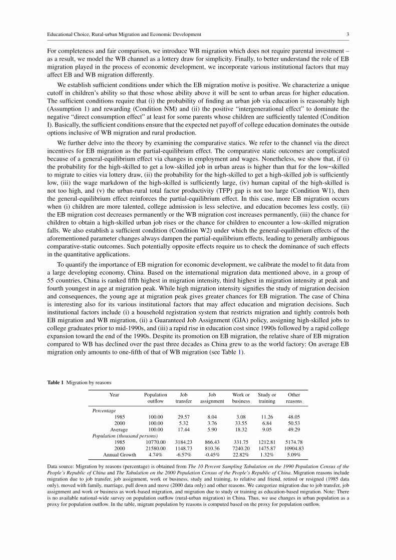
To quantify the importance of EB migration for economic development, we calibrate the model to fit data froma large developing economy, China. Based on the international migration data mentioned above, in a group of55 countries, China is ranked fifth highest in migration intensity, third highest in migration intensity at peak andfourth youngest in age at migration peak. While high migration intensity signifies the study of migration decisionand consequences, the young age at migration peak gives greater chances for EB migration. The case of Chinais interesting also for its various institutional factors that may affect education and migration decisions. Suchinstitutional factors include (i) a household registration system that restricts migration and tightly controls bothEB migration and WB migration, (ii) a Guaranteed Job Assignment (GJA) policy, assigning high-skilled jobs tocollege graduates prior to mid-1990s, and (iii) a rapid rise in education cost since 1990s followed by a rapid collegeexpansion toward the end of the 1990s. Despite its promotion on EB migration, the relative share of EB migrationcompared to WB has declined over the past three decades as China grew to as the world factory: On average EBmigration only amounts to one-fifth of that of WB migration (see Table 1).
Table 1 Migration by reasons
Year Population Job Job Work or Study or Otheroutflow transfer assignment business training reasons
Percentage1985 100.00 29.57 8.04 3.08 11.26 48.052000 100.00 5.32 3.76 33.55 6.84 50.53
Average 100.00 17.44 5.90 18.32 9.05 49.29Population (thousand persons)
1985 10770.00 3184.23 866.43 331.75 1212.81 5174.782000 21580.00 1148.73 810.36 7240.20 1475.87 10904.83
Annual Growth 4.74% -6.57% -0.45% 22.82% 1.32% 5.09%
Data source: Migration by reasons (percentage) is obtained from The 10 Percent Sampling Tabulation on the 1990 Population Census of thePeople’s Republic of China and The Tabulation on the 2000 Population Census of the People’s Republic of China. Migration reasons includemigration due to job transfer, job assignment, work or business, study and training, to relative and friend, retired or resigned (1985 dataonly), moved with family, marriage, pull down and move (2000 data only) and other reasons. We categorize migration due to job transfer, jobassignment and work or business as work-based migration, and migration due to study or training as education-based migration. Note: Thereis no available national-wide survey on population outflow (rural-urban migration) in China. Thus, we use changes in urban population as aproxy for population outflow. In the table, migrant population by reasons is computed based on the proxy for population outflow.

4 P.-J Liao, Ping Wang, Y.-C. Wang and C. K. Yip
We discipline our model to match several key observations from Chinese data during the period from 1980 to2007 prior to the Great Recession, including: (i) education and work based migration flows, (ii) urban productionshares, (iii) high to low skilled employment shares, (iv) urban premium and skill premium, (v) expenditure shareson child rearing, child college education and rural to urban migration, and (vi) Mincerian rate of return of collegeeducation. In addition to TFP growth in rural and urban sectors, we are particularly interested in changes in (i) thecost of migration, (ii) the cost and the selectivity of college education, and (iii) the availability of urban low-skilledjobs, as explicitly examined in our model. To properly capture some key policy changes, we separate our sampleperiod into two regimes, 1980-1994 and 1995-2007. Most prominently, the changes include the abolishment of theGJA in 1994, the relaxation of household registration-induced migration barriers since the mid-1990s, as well asthe rise in college tuition and the expansion of college admission toward the second half of the 1990s, where allchanges occurred around mid-1990s, thus granting the validity of the division into two regimes.
Upon calibrating the model over these two regimes, we investigate the influences of both types of migrationon China’s development and urbanization, and decompose the effects of macroeconomic and institutional factors.This is done by conducting counterfactual exercises shutting down each of the two migration channels one-by-oneand by comparing the counterfactual outcomes with the benchmark counterparts to obtain the contribution of eachmigration channel to changes in per capita output and other measures. We find that EB migration accounts for6.3 percent of changes in per capita output, larger than that of WB migration (4.5 percent). Interestingly, even inregime 2 over the sub-sample period of 1995–2007, we obtain a similar pattern for the comparable contributions ofEB and WB migration (8.0 and 5.9 percent, respectively), despite that the share of EB migration is only about 20percent of the WB share. The intuition of the importance of the EB migration to per capita output is closely relatedto the rise in skill premium over this sub-sample period, as a result of higher urban TFP and expanded employmentof low-skilled workers via WB migration. This finding suggests that without including the quality dimension viathe education channel, the picture of rural to urban migration in China could be severely misleading.
We also conduct counterfactual policy experiments on various economic and institutional factors. We begin byverifying that the general-equilibrium effects of key parameter changes discussed in the theory discussed above allturn out to dampen the direct partial-equilibrium effects. We then find that the TFP growth and the improvementin human capital together account for about two-third of changes in per capita output. Surprisingly, the impacts ofthe termination of GJA and the relaxation of WB migration on per capita output are found limited. This is a resultof the conflicting partial- and general-equilibrium effects. The latter finding on WB migration also reinforces ouremphasis on the important role played by the quality dimension of migration. Thus, the general concern with thetermination of GJA and the much appreciated temporary permits for migrant workers need not be supported by ageneral-equilibrium framework that incorporates the quality dimension of migration. Last but not least, as collegeadmission in our calibrated benchmark economy is rationed, we further construct an unrationed counterfactualeconomy. In this case, we find that there would have been more EB migration than that in the benchmark and, as aresult, total per capita output, urbanization rates and high-skilled composition in urban areas are strengthened whilethe skill premium is lower. Due to a reduction in skill premium, the relative importance played by EB migration inthis unrationed counterfactual economy is weakened with its contribution dropped by more than 40%.
These nontrivial and somewhat surprising findings signify our contribution to the literature. They are useful fordeveloping countries to better design internal migration and education policy if industrialization accompanied byskill-enhanced output growth is an important objective.
Related Literature
The older literature on migration is mostly empirical adopting reduced-from approach or theoretical under staticor partial equilibrium setting. One exception is Glomm (1992), which developed a dynamic general equilibriummodel with persistent urbanization along the equilibrium path; another is Lucas (2004) which rested the analysisin a continuous-time lifecycle framework.
The main migration incentive in Lucas (2004) is that after migration workers can accumulate human capital andhave larger life earnings in urban. In our paper, the main migration incentives (by parents) is to enable their childrento obtain urban residency and possibly obtain high-skilled jobs. Notably, in Lucas (2004), urban workers are allself-employed Robinson Crusoe’s and hence there is no direct interactions among them in the benchmark modelwithout an external effect in learning (to be further discussed in Section 5.3 below). In our paper, urban workers,whether high- or low-skilled, are all directly connected via an aggregate production function. This provides anatural avenue of agglomeration economies.
Our paper adopts a two-location, two-period lived overlapping generations model to study a new, namely,education-based, channel of rural-urban migration in China. It can therefore be compared with the recent, dynamicmodel based studies on job-related internal migration. Bond et al. (2015) examined the effects of reductions intrade and migration barriers on China’s growth and urbanization, focusing on China’s accession to the WorldTrade Organization in 2002, highlighting migration barriers as a main driver for the surplus labor in rural areasand sizable rural-urban migration. Laing et al. (2005) constructed a dynamic search equilibrium model to study the
Educational Choice, Rural-urban Migration and Economic Development 5
macroeconomic consequences of illegal WB migrants in China (the so-called “blind-flow” or pleasant flood) dueto the presence of surplus labor and labor search frictions. As rural to urban migration may depend not only onthe urban-rural wage gap but also on rural land productivity, Ngai et al. (2019) showed that land policy is a majorbarrier on industrialization in China. Finally, Garriga et al. (2020) studied the housing-market boom in China as aconsequence of its structural transformation and the resulting reallocation of labor from rural to urban areas. Theyfound that the rapid increase in urban housing prices can be attributed to this urbanization processes in conjunctionwith a significant reduction in the associated migration costs.3
Methodologically, our emphasis on the idea of parental motivation is in line with Albornoz et al. (2018) whopresented a model of endogenous immigration to study how parents, students and schools interact so as to affectschool systems and students’ performances in host countries. We also echo Ellickson and Zame (2005) who stresson the valuable implications of a competitive model for location in the presence of heterogeneous locations andcostly transportation – in our model, rural and urban differ in many aspects whereas migration is costly.
2 The Model
To facilitate the study of the continual process of rural-urban migration covering both EB and WB channels, weconstruct a dynamic spatial equilibrium model with two-period lived overlapping generations making educationand location choices.
In order to have a better understanding of our model setup, we first provide an institutional background tosupport some essential features to govern our modeling strategy (see the online appendix or our working paper,Liao et al. 2021, for a detailed institutional documentation). We begin with two important institutional features thatare commonly observed in developing countries. First, we restrict skill acquisition to urban college education only,as usually seen in many developing countries. Second, we permit admission selectivity to be relaxed over time as aresult of improved education systems, though education-related costs are rising over time in response to increasededucation demands.4
Because we shall calibrate our model to fit the case of China, it is also worth highlighting two important, China-specific institutional features related to our model of EB migration: the hukou or household registration system andthe zhaosheng or admission policy of higher education. The hukou system maintained a tight control that essen-tially rationed WB migration through the assignment of the hukou certificates. With this hukou system, it is betterjustified to model WB migration by a lottery. On the contrary, the zhaosheng policy enables much less regulatedEB migration. It allows rural students to obtain the urban hukou certificate through college education. Accompa-nied with the zhaosheng policy is the GJA policy prior to 1994 that granted high-skilled jobs to college graduates.Generally, we consider the probabilities for college graduates to obtain either a high-skilled or a low-skilled job,or none and hence to return to rural areas after graduation. This setup enables us to capture the GJA policy in atractable manner, because under such a policy the latter two non-high-skilled job acquisition probabilities can besimply set to zero.
2.1 The Basic Setup
There are two geographical regions, rural (R) and urban (U), with only the latter location that can offer highereducation required for high-skilled jobs.5 The initial masses of high- and low-skilled workers in urban areas areexogenously given by (NH ,NL). We restrict our attention to rural-urban migration, thus for the sake of simplicity,leaving reverse migration from urban to rural areas as exogenous. This is consistent with most of the rural-urban mi-gration research that basically abstracts from reverse migration. Under an overlapping-generations setting, agentslive for two periods and study passively in the location chosen by their parents during their first period of life. In thesecond period, they make decisions for a sequence of events that take place simultaneously. Each agent consumesand gives birth to a single child. Given the talent of the children, parents decide whether to send their children to
3 There are other studies investigating quantitatively or empirically the relationship between migration barriers and rural-urban developmentin China. These studies usually consider static or partial equilibrium settings with different methodologies and research agenda. For brevity, weare thus abstracting them from our literature review.
4 For the particular relevance to the case of China, we note that, using the 2015 data from the Chinese Ministry of Education, 2541 out of the2553 (or 99.53 percent) junior colleges, colleges and universities in China were located in prefectural-level cities or municipalities. Moreover,in China, there was a college education expansion since 1998 and a lift of college tuition control since 1990 that induced sharply rising costs ofcollege education toward late 1990s.
5 We assume that every person in the economy is entitled to a basic level of low-skilled education. This basic level of education is sufficientto handle the farming job in rural areas and the low-skilled job in urban areas. However, in order to be a high-skilled worker, one has to upgradeherself with a high-skilled education which is only available in urban areas. We also assume that over-qualification is not a problem so thathigh-skilled workers can always handle low-skilled jobs and rural farming.
6 P.-J Liao, Ping Wang, Y.-C. Wang and C. K. Yip
urban areas to have college education. The residency of urban households are assumed to pass from one generationto another. By focusing on internal migration, we assume away natural birth or international immigration so thatthe total population is constant over time.
2.1.1 Production
Output is produced using labor inputs in either location, rural or urban.6 We consider two factor-market distortionsby introducing two wedges. One is on the factor price side as a result of unequalized valuation of marginal product,as in the standard misallocation literature, e.g., Hsieh and Klenow (2009). Another is on the factor quantity siderelated to the deviation from the optimal composition of production inputs, which captures the production techniquewedge in Uras and Wang (2017) or the factor-technique mismatch in Wang et al. (2018).
The urban technology (with factor quantity distortion) uses both high-skilled and low-skilled labor and is givenby
YU = AF(NH ,NL
), NH = (NH +ψ)h, (1)
where A > 0 is the urban TFP parameter and h is the level of human capital possessed by high-skilled workers.The outcome of urban education is the acquisition of h, which is assumed to be constant.7 The introduction of thehigh-skilled labor wedge, ψ , enables us to capture any possible input-quantity distortion in production, allowingus to fill the gap relating the employment ratio to the relative factor price. Quantitatively, this permits us to useemployment shares to back out intergenerational mobility, and to use skill premia to pin down the urban relativeTFP as well as the high-skilled labor wedge. Finally, we assume F satisfies all the properties of a neoclassicalproduction function in its arguments, NH and NL: ∂F/∂m > 0 > ∂ 2F/∂m2
(m = NH ,NL
), limm→0 ∂F/∂m = ∞
and limm→∞ ∂F/∂m = 0 (Inada conditions) and F is constant returns in(NH ,NL
).8
Since the classic of Harris and Todaro (1970), it is well documented in the economic development literature thatthe urban labor market is subject to many institutional distortions. To capture this type of factor market distortion,we introduce a labor market wedge τ ∈ (−1,∞) faced by urban firms when hiring high-skilled workers. DenotingwH as the effective high-skilled wage received by high-skilled workers and wL as the low-skilled wage, we obtainthe urban wage rates as follows:
(1+ τ) wH =∂YU
∂ NH= AFNH
, (2)
wL =∂YU
∂NL= AFL, (3)
where FNH= ∂F/∂ NH and FL = ∂F/∂NL.9 Then we have
wH =
(1
1+ τ
FNH
FL
)wL, (4)
that is, the values of marginal products of high- and low-skilled labor are not equalized in efficiency unit. Whenτ > 0, the high-skilled labor would suffer a wage markdown.10
Turning to rural production, the constant-return production technology uses only raw (or low-skilled) labor:
YR = BNR, (5)
where NR is the number of “farmers” in the rural area and B is the TFP in the rural area.11 A competitive labormarket implies that the rural wage rate is:
wR = B. (6)6 We abstract from physical capital to simplify the dynamics and to sharpen the focus on rural-urban migration. Including physical capital
into our model will enhance the importance of EB migration under capital-skill complementarity.7 We can think of h as an index on labor quality or human capital that results from the total number of years in higher education. Because
urban education in our model is measured relative to rural, an education reform improving the quality of rural schools can be translated into areduction in h.
8 Given our specification of the production technology, the presence of the quantity distortion ψ does not affect any of our analytical findingsin the model section. It is only helpful for our quantitative analysis in data matching.
9 Similar to the quantity distortion ψ , the presence of the factor-price distortion τ does not affect any of our analytical findings in the modelsection. We only use it for the quantitative analysis in data matching.
10 It is observed that the high-skilled labor wage of planned economies is usually suppressed. For the case of China, see Maurer-Fazio (1999)for a discussion of this common feature that is generally analyzed in the development literature.
11 We have implicitly assume that rural farming does not require human capital or skill from urban education. So educated high-skilledworkers that come back from urban areas do not have higher productivity in rural production.
Educational Choice, Rural-urban Migration and Economic Development 7
2.1.2 Rural Households
The economy is populated with all females with each adult woman giving birth to one daughter. The interconnec-tion of dynasties can be fully captured by three adjacent generations, labeled sequentially as (i, j,k). Because ruralto urban migration is the focus of our paper, altruistic rural households are the key players in the economy. Ruralhouseholds of generation i can derive utility from their own consumption (ci) and their children’s consumption (c j),subject to an altruistic discounting factor β ∈ (0,1). The generational flow felicity function is common, denotedby u(·) and assumed to be strictly increasing and strictly concave.
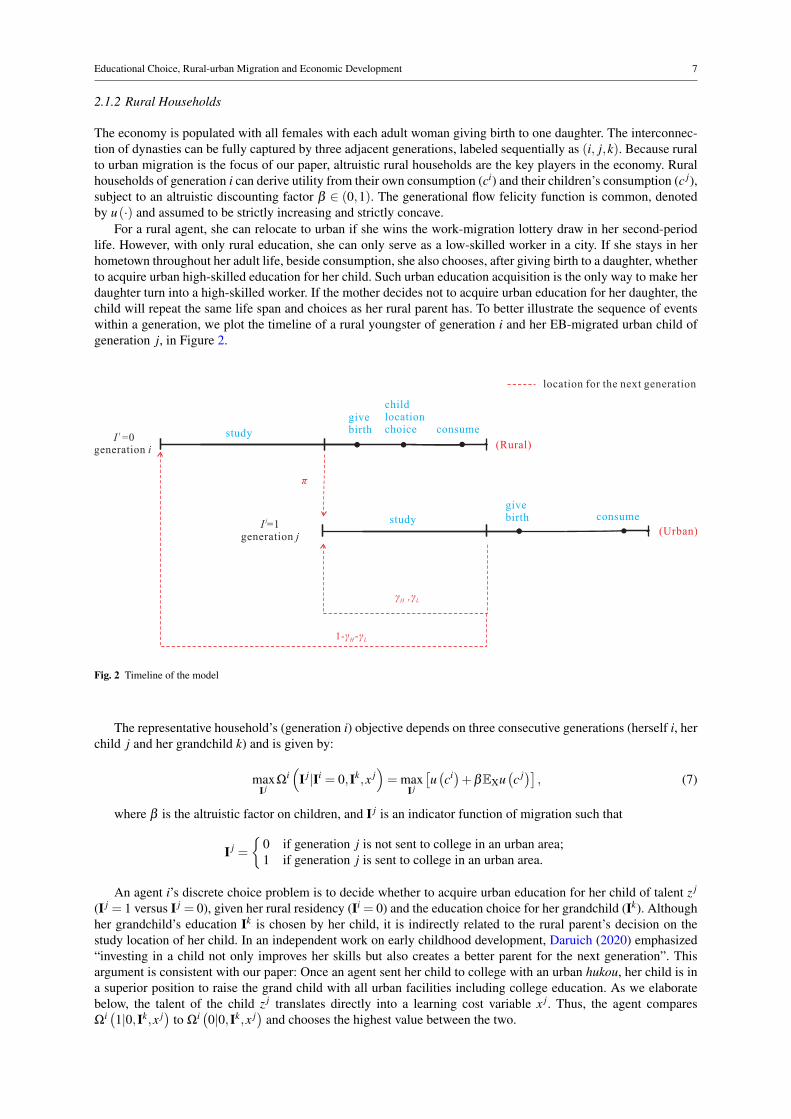
For a rural agent, she can relocate to urban if she wins the work-migration lottery draw in her second-periodlife. However, with only rural education, she can only serve as a low-skilled worker in a city. If she stays in herhometown throughout her adult life, beside consumption, she also chooses, after giving birth to a daughter, whetherto acquire urban high-skilled education for her child. Such urban education acquisition is the only way to make herdaughter turn into a high-skilled worker. If the mother decides not to acquire urban education for her daughter, thechild will repeat the same life span and choices as her rural parent has. To better illustrate the sequence of eventswithin a generation, we plot the timeline of a rural youngster of generation i and her EB-migrated urban child ofgeneration j, in Figure 2.
Fig. 2 Timeline of the model
The representative household’s (generation i) objective depends on three consecutive generations (herself i, herchild j and her grandchild k) and is given by:
maxI j
Ωi(
I j|Ii = 0,Ik,x j)= max
I j
[u(ci)+βEXu
(c j)] , (7)
where β is the altruistic factor on children, and I j is an indicator function of migration such that
I j =
0 if generation j is not sent to college in an urban area;1 if generation j is sent to college in an urban area.
An agent i’s discrete choice problem is to decide whether to acquire urban education for her child of talent z j
(I j = 1 versus I j = 0), given her rural residency (Ii = 0) and the education choice for her grandchild (Ik). Althoughher grandchild’s education Ik is chosen by her child, it is indirectly related to the rural parent’s decision on thestudy location of her child. In an independent work on early childhood development, Daruich (2020) emphasized“investing in a child not only improves her skills but also creates a better parent for the next generation”. Thisargument is consistent with our paper: Once an agent sent her child to college with an urban hukou, her child is ina superior position to raise the grand child with all urban facilities including college education. As we elaboratebelow, the talent of the child z j translates directly into a learning cost variable x j. Thus, the agent comparesΩi(1|0,Ik,x j
)to Ωi
(0|0,Ik,x j
)and chooses the highest value between the two.
8 P.-J Liao, Ping Wang, Y.-C. Wang and C. K. Yip
There are two types of costs in raising children. First, there is a basic requirement for resources, which weassume to be a constant child-rearing cost, denoted by φ . Second, there are costs to improve the child’s quality,which we can summarize as the education cost. There are two components of the education cost. As high-skillededucation is available only in urban areas, there is a constant migration cost for education denoted by σe whichcaptures the basic moving expenses.12 This is the first component of the education cost for children. The secondcomponent is the cost of skill acquisition: the learning cost x j. Since talent matters for learning because peoplewho are more talented study more efficiently, we assume that part of the learning cost depends on the talent of thechild. Specifically, x j is a random variable that depends inversely on both the talents of the child z j and the collegeadmission selectivity parameter a, and positively on the non-talent related basic learning expenses b:
x j ≡ χ(az j)+b, (8)
where χ ′ < 0, χ (0) = ∞ and χ (∞) = 0. The college admission selectivity parameter, a, captures the institutionalfriction of the education system. A decrease in a implies that the urban college education program is more selectivein admission so that the learning cost x j becomes higher for the child with the talent z j. We note that z j ∈
(z j
min,∞)
is drawn from a distribution with cumulative distribution function denoted by G(z j), and z j
min is the minimumsupport of the talent distribution. For simplicity, we assume that parents perfectly observe children’s talent drawand that children’s ability in college learning does not affect the human capital measure in production. Whileimperfect observability requires more complicated expected utility maximization, linking human capital to collegelearning results in ex post heterogeneity within the high-skilled group and hence complicated aggregate production.Either aspect of generalization would reduce the tractability of the model significantly. We assume that z j
min ≤ z j0
which is a cutoff level defined as:
wR− x j0−σe−φ = 0,
where x j0 ≡ χ
(az j
0
)+ b. That is, z j
0 is the talent of the marginally affordable child whose education and rearing
costs fully exhaust the income of her rural parent (i.e., ci = 0). As a result, children whose talent z j that is less thanor equal to z j
0 would not be sent by their parents to acquire urban education. Thus, the budget constraint for a ruralparent is:
ci + I j ·(x j +σe
)+φ = wR. (9)
Notably, while there is no income variation within the rural area, allowing children to have different abilities inschooling implies individual parent’s expenditure and net income for consumption purposes are all different.
Children who are sent to urban areas become high-skilled after receiving their education. Following the pivotalstudies by Todaro (1969) and Harris and Todaro (1970), we assume that they are not guaranteed upon graduationto be high-skilled workers. Specifically, as a college graduate, she may be (i) a high-skilled worker with probabilityγH earning a wage wH = wHh, (ii) a low-skilled worker with probability γL earning a wage wL, or (iii) unable to findan urban career and forced to return to rural to become a farmer with probability 1− γH − γL (reverse migration)earning a rural wage wR.13 Children that remain in the rural area do not incur any cost in education or migrationfor their parents. When these children turn into adults, they either may get recruited via a lottery as low-skilledworkers in urban areas with a probability π to earn wL or work in the rural area to earn wR. The resulting valuationare equalized in the sense of Todaro (1969) and Harris and Todaro (1970) when taking into account the fact thatmore low-skilled are drawn in would push down the urban low-skilled wage and thus there must be a value of π
consistent with the “net” rural-urban migration (i.e., migration inflows to cities net of outflows) given the ratio oflow-skilled workers to total rural population.14
The expected income earned by a household in generation j in the adulthood is given by:
W j = I j [γHwH + γLwL +(1− γH − γL)wR] (10)+(1− I j) [(1−π)wR +π (wL−σw)] ,
12 The migration costs can be interpreted as the costs of obtaining the legal right to stay in cities, transportation costs between hometownsand cities and urban living costs.
13 To focus on the endogenous decision of EB migration, we abstract from the decision of reverse migration from urban to rural as the latterrequires the explicit modeling of the optimization problem of an urban household. Nonetheless, we we conduct robustness checks quantitatively,as reported in Table 6, for various values of this reverse migration probability by varying γL.
14 While for the sake of simplicity these probabilities (γH ,γL,π) are exogenous, the scale and shares of migration from these two channelsare both endogenous as long as rural households are solving the discrete choice problem to decide on whether to send their children to urbancolleges. Thus, this simplifying assumption is viewed innocuous.

Educational Choice, Rural-urban Migration and Economic Development 9
where σw is the constant WB migration cost for the low-skilled workers.15 Then, the children’s budget constraintis given by:
c j + Ik ·[I j (1− γH − γL)+
(1− I j)(1−π)
](xk +σe
)+φ =W j, (11)
where
Ik =
0 if children do not send generation k (grandchildren) to college in an urban area,1 if children send generation k (grandchildren) to college in an urban area,
and(xk +σe
)are the total costs of grandchild going to college in cities. When households of generation i decide
I j, xk is unknown. We use X to denote the random variable of education cost in their objective function Ωi.To compute Ωi
(1|0,Ik,x j
)and Ωi
(0|0,Ik,x j
), we substitute ci = wR− I j ·
(x j +σe
)− φ and c j = W j − Ik ·[
I j (1− γH − γL)+(1− I j
)(1−π)
]·(xk +σe
)−φ into the value functions Ωi, where W j is given by (10):
Ωi(
1|0,Ik,x j)= u
(wR− x j−σe−φ
)+βEXu
[γHwH + γLwL +(1− γH − γL)wR−Ik (X)(1− γH − γL)(X +σe)−φ
],
and Ωi(
0|0,Ik,x j)= u(wR−φ)
+βEXu[(1−π)wR +π (wL−σw)− Ik (X)(1−π)(X +σe)−φ
].
For comparison, we define ∆i(Ik,x j
)as the net gain in value for sending children to urban areas to continue
their education:
∆i(
Ik,x j)≡ Ω
i(
1|0,Ik,x j)−Ω
i(
0|0,Ik,x j)
(12)
= u(wR− x j−σe−φ
)−u(wR−φ)
+βEX
u[γHwH+γLwL+(1-γH -γL)wR-Ik (X)(1-γH -γL)(X+σe) -φ
]-u[(1-π)wR+π (wL-σw) -Ik(X)(1−π)(X+σe) -φ ]
.
Then we have:
I j =
0 if ∆i
(Ik,x j
)< 0
1 if ∆i(Ik,x j
)> 0.
Further, we define n ≡ (NH +ψ)h/NL to be the high-skilled to low-skilled labor ratio. Then the high-skilledand low-skilled effective wage in (2) and (3) can be rewritten as:
(1+ τ)wH = A f ′ (n)h, wL = A[
f (n)−n f ′ (n)], (13)
where A f (n) = AF (n,1) = YU/NL. With wH (wL) is decreasing (increasing) in n, the high-skilled to low-skilledwage ratio wH/wL is decreasing in n with a lower bound at unity. Defining nmax≥ n such that wH (nmax)/wL (nmax)=1, we impose the following condition:
Condition NM: (Sufficiency for Nondegenerate Migration) wH (nmax) = wL (nmax)> B+σw.
If Condition NM holds, then any urban job pays (net of the WB migration cost) better than the rural job. To betterunderstand Condition NM, we plot the high- and low-skilled wages against n in Figure 3.Condition NM guarantees that, as long as children can find a job in cities, rural parents will send them to urban areasto attend college. Our next concern is the likelihood of finding a job in the urban area. We impose an assumptionon the probabilities of acquiring an urban high-skilled job: The probability of finding an urban high-skilled job viaeducation must be higher than that of finding a low-skilled one through any channels.
Assumption 1: (Better Job Opportunity for the High-Skilled) γH > max(γL,π).
Assumption 1 states that the probability of securing a high-skilled job after receiving education is higher thanthe probability of finding a low-skilled job through any channels in the urban area.16 Thus, Condition NM andAssumption 1 together imply that the expected urban wage income is higher than the rural wage income. Since
15 The differentiation of migration costs between EB and WB facilitates our understanding on the costs of rural-urban migration. The effectsthat rural productivity and urban productivity could have on the cost of migration (e.g., via improvement in rural schools, internet access andcommunication cost, and transport cost) can be captured by these cost parameters. It is also realistic, for instance, college students usually enjoycheaper housing provided by the universities which migrant workers do not have.
16 Note that Assumption 1 implies γH + γL > π .

10 P.-J Liao, Ping Wang, Y.-C. Wang and C. K. Yip
Fig. 3 High- and low-skilled wages and rural wage rate
urbanization and development depend on the composition and relative size of the urban workforce, Condition NMand Assumption 1 simply highlight the fact that urban jobs, especially high-skilled ones, are more attractive thanrural jobs to the household. When the talent of the children is sufficiently high, rural parents will then considersending their children to cities to receive education. As a result, the relative supply of high- to low-skilled workersis expected to rise.
We can easily connect our model to various institutional factors often seen in developing countries. First of all,the relaxation of internal migration restrictions that has raised migrants’ chance to get urban jobs is summarizedby the probability parameters γH , γL and π . A relatively higher value of γH + γL may be due to better urban jobopportunities or as a result of encouraging education policy, both lowering the probability of reverse migration.Next, changes in the education policy that alter the value of the EB migration are given by the admission selectivityparameter a and the basic expenditure parameter b in the learning cost variable x j. These education parametersprovide a short cut for studying the effects of education reforms that affect college admission and tuition. Finally,better transportation system and relaxed migration restrictions can also be captured by the resulting reduction inthe moving costs of rural-urban migration given by σe and σw.
In summary, despite some simplification, the migration setup in our model economy is capable of capturing keyfactors that affect migration decisions via both EB and WB migration channels – for example, relative TFP in urbanand rural areas, urban premium, as well as various education policy and institutional barriers. Nonetheless, we notethat a potential endogenous effect not considered here is the rising cost for urban living (including the housingprice hike). However, our quantitative results would be “conservative” by shutting down the positive impact ofEB migration on the urban cost of living and hence the potentially negative impact on WB migration. Should weinclude such an effect, the relative importance of EB migration would be even strengthened. The reader shouldbe warned that, however, generalization in either direction would make the model intractable, especially becausewe must examine decision making by three adjacent generations in which the number of urban (high-skilled andlow-skilled) and rural workers are state variables as a result of changing migration flows over time.
2.2 Population Dynamics
In this section, we study the population dynamics of rural-urban migration. Recall that adults supply labor to themarket and that each one gives birth to only one child, so the entire adult population participates in the labor market.Let (Nt
H ,NtL) be the number of high-skilled and low-skilled workers in the urban area, respectively, and Nt
R be therural labor force, all at time t. Denote J,K ∈ H,L as the type of jobs for generation- j and generation-k urbanworkers respectively. Let δJK be the transitional probability for an urban generation-k worker born to a generation-j urban worker with job J, working as a type K worker in an urban area. Thus, δJK captures job mobility acrossgenerations in urban areas. We then assume:
Assumption 2: (Parental Skill Transmission) δJJ > δJK for J 6= K.
Educational Choice, Rural-urban Migration and Economic Development 11
Assumption 2 implies that the child is more likely to be high-skilled (low-skilled) when the parent is high-skilled(low-skilled). Given that the residency of urban households are passed from one generation to another, we have:
∑K
δJK = 1. (14)
Then, the populations of high-skilled, low-skilled and rural workers evolve according to the following law ofmotion equations:
Nt+1H = δHHNt
H +δLHNtL +Nt
R
∫I j(
z j,Ik)
γHdG(z j),
Nt+1L = δHLNt
H +δLLNtL +Nt
R
∫I j(
z j,Ik)
γLdG(z j)+∫ [
1− I j(
z j,Ik)]
πdG(z j)
,
Nt+1R = (1−δHH −δHL)Nt
H +(1−δLH −δLL)NtL
+NtR
∫I j(
z j,Ik)(1− γH − γL)dG(z j)+
∫ [1− I j
(z j,Ik
)](1−π)dG(z j)
,
where the initial urban and rural labor forces are denoted by N0H ,N
0L and N0
R, respectively. Using (14), we cansimplify the above law of motion expressions to:
Nt+1H = δHHNt
H +(1−δLL)NtL +Nt
R
∫I j(
z j,Ik)
γHdG(z j), (15)
Nt+1L = (1−δHH)Nt
H +δLLNtL +Nt
R
π +
∫I j(
z j,Ik)(γL−π)dG(z j)
, (16)
Nt+1R = Nt
R
(1−π)−
∫I j(
z j,Ik)(γH + γL−π)dG(z j)
. (17)
Finally, combining (15) and (16), we have:
Nt+1U = Nt
U +NtR
1−
∫I j(
z j,Ik)
dG(z j)
π︸ ︷︷ ︸
WB
+NtR
∫I j(
z j,Ik)(γH + γL)dG(z j)︸ ︷︷ ︸
EB︸ ︷︷ ︸migrants
,
where NtU ≡ Nt
H +NtL denotes the total urban workforce at time t.
3 Equilibrium
We begin by characterizing the decision on EB migration and examining the resulting policy implications bypresenting some partial-equilibrium comparative static findings without taking into account general-equilibriumeffects of migration on market wages. Upon defining the dynamic competitive spatial equilibrium, we then charac-terize the equilibrium by performing full comparative statics incorporating the general-equilibrium effects. Finally,we describe a counterfactual economy eliminating the possibility of EB migration that will be used for counterfac-tual analysis in the quantitative exercises.
3.1 Migration Decision and Partial-Equilibrium Comparative Statics
To have a better understanding of such comparative statics, we separate the effect on the utility difference of themarginal parent under EB migration into two parts according to (12):
∆i(
Ik,x j)= u
(wR− x j−σe−φ
)−u(wR−φ)︸ ︷︷ ︸
direct consumption effect
+βEX
u(
c jU
)−u(
c jR
)︸ ︷︷ ︸
intergenerational effect
,
where c jU denotes the consumption of children if they are sent to an urban area and c j
R is the consumption ofchildren if they are kept in a rural area. The direct consumption effect (DCE) is always negative because parents’consumption is lower due to the costs of urban education, whereas the intergenerational effect (IE) is ambiguous.Condition NM and Assumption 1 together assure that the intergenerational effect is positive which is necessary forparents to acquire urban education for their children:

12 P.-J Liao, Ping Wang, Y.-C. Wang and C. K. Yip
Proposition 1: (Positive Motive for Urban Education Acquisition) Under Assumption 1 and Condition NM, theintergenerational effect of migration is positive.
Proof. All proofs are relegated to the Appendix.
The intuition of the above proposition is straightforward. If the probability of finding an urban job via educationis reasonably high (Assumption 1) and rewarding (Condition NM), then the higher expected urban wage providesan incentive for parents to pay the costs of their children’s education via altruism. Otherwise, urban educationwould not be a good “investment” from the parents’ perspective.
We next examine how the net gain in education ∆i(Ik,x j
)responds to changes in the parameterization, i.e., we
examine whether the “marginal” parent (a parent who is indifferent between sending her child to attend college inan urban area or keeping the child in the rural area so that ∆i
(Ik,x j
)= 0) will send her child to receive an education.
By characterizing ∆i(Ik,x j
), we obtain the following proposition for the comparative statics of EB migration from
a partial-equilibrium perspective:
Proposition 2: (Urban Education Acquisition) Under Assumption 1 and Condition NM, more parents will bewilling to acquire urban education for their children if
1. their children are more talented (z j higher), college admission is less selective (a higher), or education becomesless costly (b lower);
2. the chance for their children to obtain an urban job is higher (γH or γL higher);3. the chance for their children to encounter a low-skilled migration decreases (π lower);4. the EB migration cost decreases permanently (σe lower);5. the WB migration cost increases permanently (σw higher).
We have studied the EB migration decision as an outcome of two opposing effects: a negative direct consump-tion effect on the parents and a positive intergenerational effect on the offsprings. If the latter dominates the former,then EB migration takes place. Proposition 2 indicates that EB migration is more likely to arise when children aremore talented, when urban education better facilitates the acquisition of higher-paid urban jobs and is not toocostly, or when WB migration becomes less available. From the cost perspective, it also provides a general guid-ance under which various institutional factors as well as education and migration policies may affect the processof rural-urban migration and economic development.
3.2 Dynamic Competitive Spatial Equilibrium
In equilibrium, all labor markets clear under the factor prices wH ,wL,wR given by (2), (3) and (6):
NdtM = Nt
M, M = H,L,R, (18)
where NdtM denotes labor demand of type-M workers. In addition, the overall population size for each period is
constant:Nt
H +NtL +Nt
R = N, (19)
where N is the constant population size.We define the competitive equilibrium for our model:
Definition: (Dynamic Competitive Spatial Equilibrium) Under Condition NM, Assumptions 1 and 2, a dynamiccompetitive spatial equilibrium (DCSE) of the model consists of migration choices
I j
and wage rates wH ,wL,wR,such that for each period(i) (Optimization) given wage rates wH ,wL,wR,
I j
solves (7) subject to (9), (10) and (11);(ii) (Market clearing) wage rates wH ,wL,wR satisfy (2), (3) and (6), and labor markets clear according to (18);and(iii) (Population evolution) given the initial population
N0
H ,N0L ,N
0R
and the distribution of talent G(z j), the pop-ulation evolves according to (15)–(17) and is restricted by (19).
To conclude this section, we show that there exists a nondegenerate DCSE under the following condition:
Condition I: (Interiority for EB Migration) βπσw > b+σe.
Condition I ensures that the positive intergenerational effect identified in Proposition 1 dominates the negativedirect consumption effect at least for some parents whose children are sufficiently talented. Intuitively, when thechildren’s talent distribution G
(z j)
has an unbounded upper support, this condition requires the EB migration
Educational Choice, Rural-urban Migration and Economic Development 13
costs incurred (b+σe) to be smaller than the expected altruistic discounted WB migration costs (βπσw). With thisadditional condition, we can establish:
Theorem 1: (Nondegenerate Dynamic Competitive Spatial Equilibrium) Under Assumption 1 and Conditions NMand I, a nondegenerate dynamic competitive spatial equilibrium exists in which a positive measure of parents willacquire urban education for their children whose talents are above a unique cutoff.
3.3 Partial- versus General-Equilibrium Effects
The results provided by Proposition 2 can be regarded as partial-equilibrium comparative-static analysis, i.e., itshows the responses of incentive to EB migration given the differential wages in the rural and urban regions. Thegeneral-equilibrium outcomes require solving out for these wages based on (2) and (3), which in turn demand theequilibrium urban high-low skilled labor ratio n. To differentiate the partial- versus general-equilibrium effects,we first note that, the difference is due to the employment effect of n which in turn affects the wages. Accordingto (15) - (17), any parameters that influence the migration decision of parents will affect the population transition(Nt
H ,NtL,N
tR). As a result, the effects of the parameter changes on the urban education decision outcomes studied in
Proposition 2 are all partial and we are going to compute their general-equilibrium effects in this sub-section. Al-though the EB migration comparative statics shown in Propositions 2 are partial, deriving the general-equilibriumones by solving out for n does not alter the intuition or properties that they illustrate. As we are going to showbelow, it is possible that the general-equilibrium effects reinforce the partial-equilibrium ones under plausibleconditions.
We next deliver the general-equilibrium version of the comparative statics findings presented in Proposition 2.To begin, we would like to explain the nature of the general-equilibrium effects: Via migration, the supply of aparticular type of labor, high- or low-skilled, changes, subsequently resulting in changes in the respective marketwages and the incentives for migration. Since the general-equilibrium effects work through the relative labor supply(n) and hence on wages (wH and wL), it is therefore convenient to decompose them into two components: a relativelabor supply effect and a labor induced wage effect. The decomposition is done as follows: Consider a permanentchange in the parameter Q studied in Proposition 2 (Q = x j,σe,σw,γH ,γL,π):
d[∆i(Ik,x j
)]dQ
=∂[Ωi(1|0,Ik,x j
)−Ωi
(0|0,Ik,x j
)]∂Q︸ ︷︷ ︸
partial-equilibrium effect (Prop 2)
+∂[Ωi(1|0,Ik,x j
)−Ωi
(0|0,Ik,x j
)]∂n
dndQ︸ ︷︷ ︸
general-equilibrium effect
=∂[Ωi(1|0,Ik,x j
)−Ωi
(0|0,Ik,x j
)]∂Q
+βEX
Γ(n)︸︷︷︸labor induced wage effect
× dndQ︸︷︷︸
labor supply effect
where Γ(n) is given by,
Γ(n) = u jcU
γHdwH
dn+(u j
cUγL−u j
cRπ) dwL
dn(20)
and u jcS = uc
(c j
S
), S =U,R, denote the location-S marginal utilities facing a marginal parent.
We first examine how the partial-equilibrium comparative statics results of Proposition 2 affect n to get therelative labor supply effect in the following lemma:
Lemma 1: (The Relative Labor Supply Effect) Under Assumption 1 and Condition NM, the relative supply of high-to low-skilled workers (n) rises if
1. children are more talented (z j higher), college admission is less selective (a higher), or education becomes lesscostly (b lower);
2. the chance for children to obtain a high-skilled urban job is higher (γH higher);3. the chance for children to encounter a low-skilled migration decreases (π lower);4. the EB migration cost decreases permanently (σe lower);5. the WB migration cost increases permanently (σw higher).
However, the effect of a change in the chance for children to obtain a low-skilled urban job (γL) on the relativelabor supply (n) is generally ambiguous.
We are now ready to study how wages respond to changes in the relative labor supply, i.e., the labor inducedwage effect. The next lemma characterizes the labor induced wage component of the general-equilibrium effect.
14 P.-J Liao, Ping Wang, Y.-C. Wang and C. K. Yip
Specifically, it provides sufficient conditions that help to sign the labor induced wage effect Γ (n), which measuresthe expected wage gain from EB migration in response to changes in the relative labor supply.
Lemma 2: (The Labor Induced Wage Effect) Let
nc ≡γHh
(1+ τ)(γL−π)
and ϒ(n) = 0, where
ϒ(n)≡ nγLuc
(hA f ′ (n)
1+ τ−φ
)−(
πnmax +γHh
1+ τ
)uc (wR) (21)
where wR ≡ wR− (1−π)(χ(azk)+b+σe
)− φ and wH (nmax)/wL (nmax) = 1. The labor induced wage effect
(Γ(n)) can be characterized as follows:
1. If γL < π or n < nc, then Γ(n)< 0;2. If n > maxn,nc, then Γ(n)> 0.
Following Lemmas 1 and 2 above, we consider two sufficient conditions for signing Γ(n):
Condition W1: (sufficient for Γ(n)> 0) ψ/N > maxn,nc .
Condition W2: (sufficient for Γ(n)< 0) nmax < nc∪γL < π .
While Condition W1 is a sufficient condition for Γ(n) > 0, Condition W2 is a sufficient condition for Γ(n) < 0(noting that nmin = ψ/NU and NU < N). To study the role played by these conditions on the determination of thegeneral-equilibrium effects of a permanent change in parameter Q on EB migration, we recall
d[∆i(Ik,x j;Q
)]dQ
=∂[∆i(Ik,x j;Q
)]∂Q
+βEX
Γ(n)× dn
dQ
. (22)
The partial effects of Q is given by the first term on the RHS of (22), which are characterized in Proposition 2.For given wages, an increase in
(γH ,γL,a,z j,σw
)or a decrease in (b,π,σe) raises the likelihood to earn a higher
urban net wage via EB migration channel and hence raises the relative gain of EB migration. The second termhighlights the general-equilibrium consideration under a change in Q. It works through the change in the urbanhigh- to low-skilled labor supply and hence the urban wages. Recall from Lemma 1 that the effect of a change inthe chance for children to obtain a low-skilled urban job (γL) on the relative labor supply (n) is ambiguous. As aresult, the general-equilibrium wage effects of γL, namely, Γ (dn/dγL), cannot be signed analytically. With regardto changes in other parameters, we have the following general-equilibrium version of Proposition 2:
Proposition 3: (The General-Equilibrium Comparative Statics) Under Assumption 1 and Conditions NM and I, aDCSE possesses the following properties:
1. When Condition W1 is met, the general-equilibrium wage effects of a change in z j,a,b,σe,σw,γH , or π alwaysreinforce the partial-equilibrium effects and more EB migration occurs if(a) children are more talented (z j higher), college admission is less selective (a higher), education becomes
less costly (b lower), the EB migration cost decreases permanently (σe lower), or the WB migration costincreases permanently (σw higher);
(b) the chance for children to obtain a high-skilled urban job rises (γH higher);(c) the chance for children to encounter a low-skilled migration falls (π lower);
2. When Condition W2 is met, the general-equilibrium wage effects of a change in z j,a,b,σe,σw,γH , or π alwaysdampen the partial-equilibrium effects, leading to generally ambiguous comparative-static outcomes.
Notably, Condition W1 is more likely to be satisfied if n,nc become smaller which requires: (i) the probabilityfor the high-skilled to get a low-skilled job be higher than lottery draw for the low-skilled to migrate to cities(γL > π); (ii) the probability for the high-skilled to get a high-skilled job (γH ) be sufficiently low; (iii) the wagemarkdown of the high-skilled (τ) be sufficiently large; (iv) human capital of the high-skilled (h) be not too high;and (v) the urban-rural TFP gap (A/B) be not too large. Under this condition, it is guaranteed that the directpositive partial-equilibrium effect of the aforementioned parameter changes on the EB migration is accompaniedby a reinforcing increase in the expected wage gain from EB migration, thereby leading to definite comparativestatics. On the contrary, Condition W2 is more likely to be satisfied if n,nc become larger which requires: (i) theprobability for the high-skilled to get a high-skilled job (γH ) be sufficiently higher than that of a low-skilled job(γL); (ii) the wage markdown of the high-skilled (τ) be sufficiently small; (iii) human capital of the high-skilled

Educational Choice, Rural-urban Migration and Economic Development 15
(h) be sufficiently high. In this case, the direct positive partial-equilibrium effect may be overturned by the inducedreduction in the expected wage gain via rising relative labor supply (n), thus causing ambiguity in comparativestatics.
As shown in Proposition 3, depending on the parameterization, the general-equilibrium effect of a migration-related parameter change can work against the partial-equilibrium effect, thereby leading to ambiguous net effectson EB migration. In this case, we will source to quantitative analysis to conclude plausible outcomes based on acalibrated economy.
3.4 A Counterfactual Economy with No Education-based Migration
Before closing the theory, we note that, in the absence of EB migration, we have Ii = I j = Ik = 0 and hence therepresentative household’s expected utility is:
u(wR−φ)+βEXu [(1−π)wR +π (wL−σw)−φ ] . (23)
The populations of high-skilled, low-skilled and rural workers evolve according to the following law of motionequations:
Nt+1H = δHHNt
H +δLHNtL, (24)
Nt+1L = δHLNt
H +δLLNtL +πNt
R,
Nt+1R = (1−δHH −δHL)Nt
H +(1−δLH −δLL)NtL +(1−π)Nt
R.
In equilibrium, all labor markets clear under the factor prices wH ,wL,wR:
NdtM = Nt
M, M = H,L,R.
Finally, the overall population size for each period is constant as before:
NtH +Nt
L +NtR = N.
In our counterfactual quantitative analysis when EB migration is absent, these changes will be modified accord-ingly. If WB migration is further eliminated (π = 0) in the counterfactual economy, then rural-urban migrationceases completely. Both scenarios will be studied in Section 4.2.
4 Quantitative Analysis
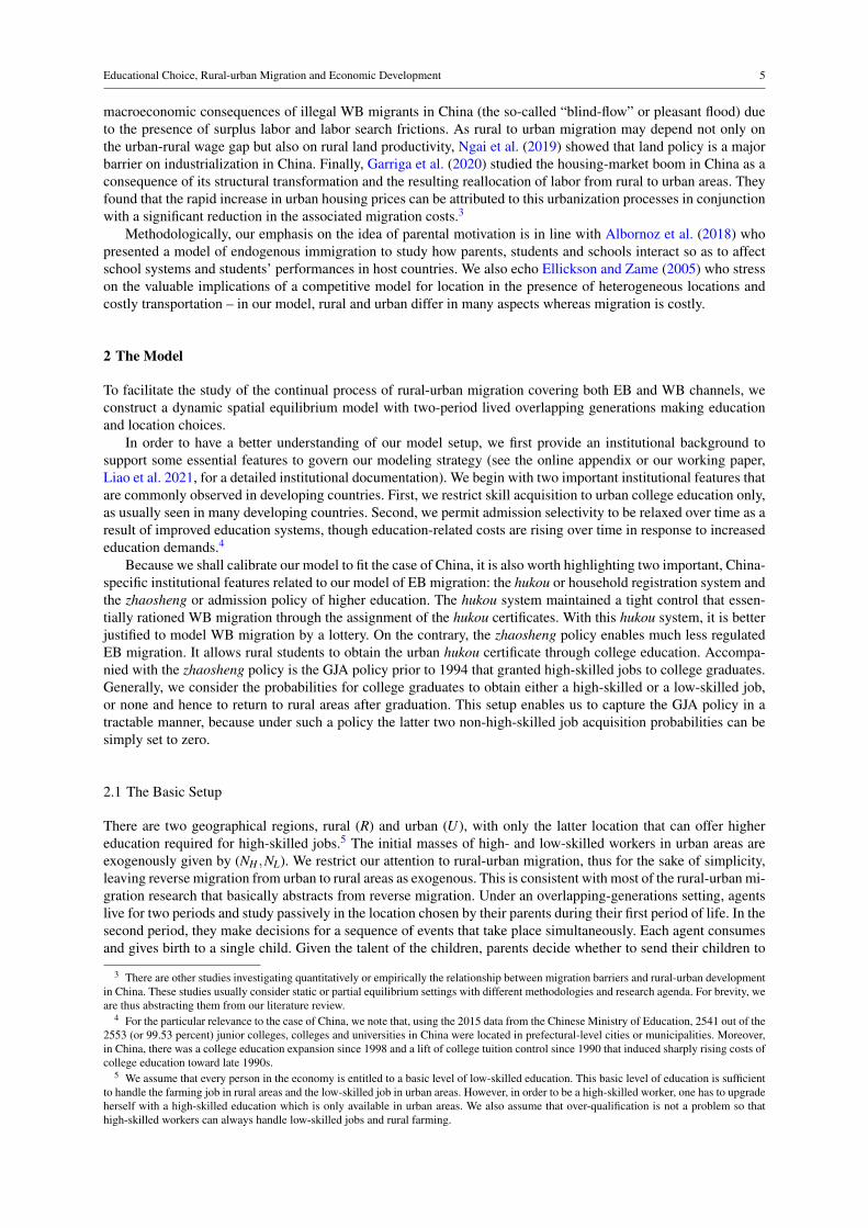
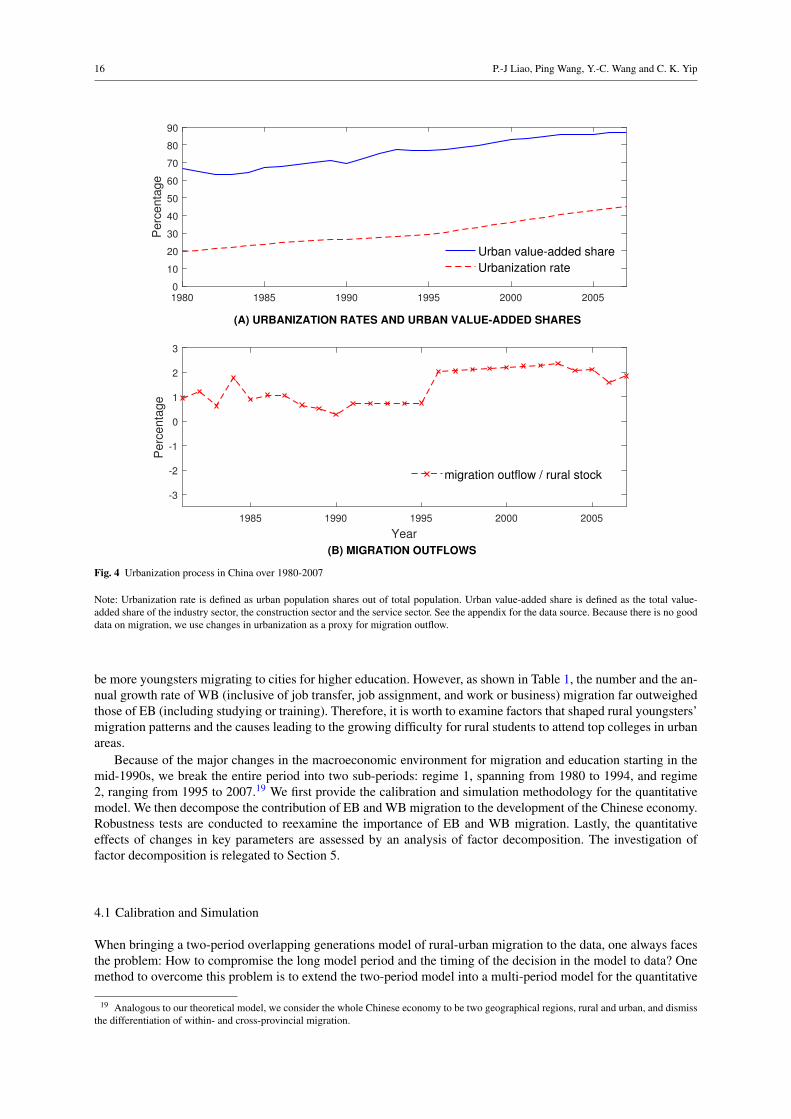
This section presents a calibrated version of our model to study the contribution of the EB migration to the devel-opment of the Chinese economy within the post-reform regime but before the financial tsunami, namely, over theperiod of 1980–2007. During this period, China has experienced rapid economic growth and urbanization. Real percapita GDP has grown at an annual rate of approximately 6.0 percent, whereas the comparable figure since DengXiao-Ping’s Southern Trip in 1992 is 7.6 percent. Meanwhile, as shown in Figure 4, urbanization rates (urbanpopulation shares) and urban value-added shares have increased from 19.4 to 44.9 percent and from 66.7 to 87.3percent, respectively, and the migration flows (proxied by changes in urban population) over rural population havenearly quadrupled, increasing from 0.5 to 1.9 percent.17 Concurrently, more rural students were attending collegesbecause of the college expansion in the late 1990s, while empirical studies have pointed out the phenomenon thatfewer rural students were admitted to top universities. The above observations motivate us to take China as aninteresting example for our quantitative analysis.
Since most of the high-quality universities are located in large metropolises in China, we consider cities asplaces for higher education to take place.18 This complements Lucas (2004) who views cities as places for immi-grants to accumulate human capital when working. In so doing we explore a potentially important, EB channel ofrural to urban migration which has become a unique channel that mitigates migration barriers in China. Studentsattend colleges by passing the National College Entrance Examination to migrate to cities. This institutional mi-gration channel enables us to examine the role of the EB migration in the development of China and to compare theimportance of this channel to that of WB migration. Moreover, due to the college expansion and the facts that mostuniversities are located in cities and urban high-skilled jobs are much better paid, one would expect that there shall
17 For urban output shares, urbanization rates and migration outflows, the correlation coefficients range from 0.71 to 0.96.18 See the online appendix for the related literature, the detailed discussion on the rural-urban disparities in college admission rates and the
inequality in the distribution of educational resources in China.
16 P.-J Liao, Ping Wang, Y.-C. Wang and C. K. Yip
1980 1985 1990 1995 2000 20050
10
20
30
40
50
60
70
80
90
Perc
enta
ge
(A) URBANIZATION RATES AND URBAN VALUE-ADDED SHARES
Urban value-added share
Urbanization rate
1985 1990 1995 2000 2005
Year
-3
-2
-1
0
1
2
3
Perc
enta
ge
(B) MIGRATION OUTFLOWS
migration outflow / rural stock
Fig. 4 Urbanization process in China over 1980-2007
Note: Urbanization rate is defined as urban population shares out of total population. Urban value-added share is defined as the total value-added share of the industry sector, the construction sector and the service sector. See the appendix for the data source. Because there is no gooddata on migration, we use changes in urbanization as a proxy for migration outflow.
be more youngsters migrating to cities for higher education. However, as shown in Table 1, the number and the an-nual growth rate of WB (inclusive of job transfer, job assignment, and work or business) migration far outweighedthose of EB (including studying or training). Therefore, it is worth to examine factors that shaped rural youngsters’migration patterns and the causes leading to the growing difficulty for rural students to attend top colleges in urbanareas.
Because of the major changes in the macroeconomic environment for migration and education starting in themid-1990s, we break the entire period into two sub-periods: regime 1, spanning from 1980 to 1994, and regime2, ranging from 1995 to 2007.19 We first provide the calibration and simulation methodology for the quantitativemodel. We then decompose the contribution of EB and WB migration to the development of the Chinese economy.Robustness tests are conducted to reexamine the importance of EB and WB migration. Lastly, the quantitativeeffects of changes in key parameters are assessed by an analysis of factor decomposition. The investigation offactor decomposition is relegated to Section 5.
4.1 Calibration and Simulation
When bringing a two-period overlapping generations model of rural-urban migration to the data, one always facesthe problem: How to compromise the long model period and the timing of the decision in the model to data? Onemethod to overcome this problem is to extend the two-period model into a multi-period model for the quantitative
19 Analogous to our theoretical model, we consider the whole Chinese economy to be two geographical regions, rural and urban, and dismissthe differentiation of within- and cross-provincial migration.

Educational Choice, Rural-urban Migration and Economic Development 17
analysis.20 Although the modified quantitative model corresponds its model period to the data period, it is a dif-ferent model in nature, and one needs to make sure that all the theoretical results are still valid. In our paper, wedirectly carry the theory to data by considering that each cohort of the rural parents make migration decisions im-mediately upon turning adults and giving birth of their children. This one-to-one mapping between decision timingand cohorts’ generation allows us to assume that every year features repeated cohorts with stationary distribution.In this way, the model period (which we set to be twenty-five years for our two-period overlapping generationsmodel of rural-urban migration) and the annual data become consistent with each other.21
To proceed with the quantitative analysis, we first perform a two-regime calibration to match the regime av-erage data to pin down the regime-common and regime-specific parameters. The former category includes deepparameters in preferences, technologies and the talent distribution, whereas the latter category consists of parame-ters that describe the specific environment of the regime, such as urban and rural TFP, job finding rates, migrationand education costs. The decision rules solved from the two-stage calibration can thus be interpreted as the “mean-year” agent’s decision rules in each regime. Given these regime parameters, we then solve the annual decisionsfrom the EB migration flow data. We calibrate the urban TFPs and the distortionary wedges annually by matchingthe skill premium and the urban premium data.
Below we describe how we conduct the two-regime calibration and the calibration for the annual TFPs anddistortions. The reader is reminded that the return to education is measured in urban-to-rural differences throughoutthe paper. Calibration details and data sources are relegated to the online appendix.
4.1.1 Two-regime Calibration
Total population is normalized to one in every period. Urban (rural) population is the share of urban (rural) tototal population and is computed using the data on populations by rural and urban residence. We term workerswith educational attainment of college and above (below) as high (low)-skilled. Then, using the data on urbanemployment by educational attainment and urban population, we compute the stocks of high- and low-skilledworkers.
The utility function is assumed to take the standard CRRA form:
u(c) =c1−ε −1
1− ε, ε > 1,
where ε is the inverse of the elasticity of intertemporal substitution (EIS). In the literature, the Pareto distribution iscommonly associated with wealth and income, which are believed to be closely related to one’s talent.22 Therefore,we assume that children’s talents z j follow a Pareto distribution, with the CDF given by:
G(z j)= 1−
(zmin
z j
)θ
, z j ≥ zmin,
where zmin and θ are the location and shape parameters of the Pareto distribution, respectively. The learning costx j is inversely related to z j and is assumed to take the form of:
x j =1
az j +b.
With this setup, the higher the college admission selectivity parameter a is, the less selective the college admissionis, and the lower cost born by rural parents to acquire urban education for their children. The urban production YUtakes the following form:
YU = AF(NH ,NL
)= A
[αNρ
H +(1−α)Nρ
L
]1/ρ, α ∈ (0,1) , ρ < 1
where NH = (NH +ψ)h, 1/(1−ρ) is the elasticity of substitution in production for high-skilled and low-skilledinputs, and α is the distribution parameter (which yields the high-skilled labor income share when ρ = 0). Below,we first describe the preset common parameters and then the preset regime-specific parameters, followed by themethods of identifying the remaining parameters.
20 For an example of this approach, see Song et al. (2011).21 The limitation of this approach is that one will not be able to analyze the age composition of workers in the quantitative analysis. As aging
related issues (such as pension and population dividends) are not our focus, once the workers evolution equations are taken care of and themodel implied population stock ratios are matched to the data, this approach shall yield similar results to that of a quantitative multi-periodmodel.
22 For example, Feenberg and Poterba (1993) assumed that the U.S. income follows a Pareto distribution. Their estimated Pareto shapeparameter for the U.S. over the 1980-1990 period is 1.92.

18 P.-J Liao, Ping Wang, Y.-C. Wang and C. K. Yip
China is well known for its high saving rates and low annual time preference rates. We thus set the annualtime preference at 1 percent, which is close to Song et al. (2011). The parental altruistic factor for children β ishence equal to 0.7798. The inverse of the EIS parameter ε is set at 1.5, which is common in the literature. Thereis no nationwide survey of child-rearing costs for rural China. We follow the estimate in the literature to set φ
such that the percentage of the child-rearing cost to rural household income φ is 17.4 percent in both regimes.23
For the Pareto distribution parameters, we normalize zmin to one as typically set in the literature.24 Since talentsare unobservable but are found to be correlated with income levels, we set θ to 2.5 using rural household netincome data from the Chinese Household Income Project (CHIP). Our value is close to the estimate for the UnitedStates. The last preset common parameter is the elasticity of substitution between high-skilled related inputs andlow-skilled labor, 1/(1−ρ). We proxy it by the estimates on the elasticity of substitution between high- and low-skilled workers. As pointed out by previous studies, the estimated values for Asian economies are usually larger,mostly falling between 2 and 7, than those for developed countries, ranging from 1 to 3. We thus choose 1/(1−ρ)to be 3 so that ρ equals 0.6667.
Denote σe (σw) as the EB (WB) migration cost as a percentage of rural household income. Considering WBmigration cost as urban living costs and the required costs for moving to urban areas, we compute σw from CHIPwith the periods over 1980-2002 and obtain a value of 55.54 percent and 30.79 percent of rural household incomefor regimes 1 and 2, respectively. EB migration cost includes the costs of food and dormitory for a college student.Assuming that a student stays in college for four years and adjusting for model periods, we obtain the EB migrationcost σe to be 0.1021 for regime 2. The data on EB migration cost prior to 1996 is not available, so we compute σefor regime 1 by assuming that σe and σw grow at the same rate between the two regimes and obtain σe = 0.1841for regime 1.25
The main spirits of China’s education reforms are captured by the endogenous threshold in talents, controllingadmission selectivity parameter (a) and the cost of college education (b). We will address how to pin down thethreshold talent and a using model equations later. Similar to the cases for calibrating EB and WB migration costs,we denote b as the college education cost as a percentage of rural household income. College education was almostfree of charge before 1990. Thus, we set b in regime 1 to only include stationary, materials and textbooks whileb in regime 2 further includes tuition costs. Using Urban Household Survey (UHS) 2007 and 2008, b equals 0.48percent and 5.28 percent of rural household income in regimes 1 and 2, respectively.26
We note that by calibrating σe, σw and b in ratios of rural incomes, urban and rural TFPs or any productivityeffects of education via the human capital measure h would have quantitative impacts on migration and collegeeducation costs. Thus, the endogenous effects of income factors on migration decisions via changes in migrationand college education costs are quantitatively accounted for in our policy experiments.
Under the linear rural production technology, the scaling factor B is equal to the rural wage rate. Being inter-ested in the relative economic positions of rural and urban China and understanding how regional technologicaldisparities shape individuals’ migration decisions, we normalize rural per capita income in 2007 to one. Then wecompute the rural per capita income over 1980–2007. The averages of B are 0.3685 and 0.7177 for regimes 1 and 2,respectively. It is notable that such normalization of rural per capita income together with zmin = 1 imply that onlyparents with relatively talented children can afford to send their children to college. This is because rural parentshave to maintain their own consumption and pay the child-rearing cost in addition to costs of college educationand EB migration.
We now turn to the rates at which college graduates (only originally from rural China) find jobs and themigration probability for rural workers. All the job finding probabilities are those faced by each cohort. Denote γ ≡γH +γL as the college graduates’ job finding probability, or the urban employment rate for college graduates. Duringthe years of the GJA policy (1951–1994), a college graduate was assigned a stable job (either in the governmentor in state-owned enterprises), usually in an urban work unit. In contrast, after the termination of the GJA policy,jobs for college graduates were no longer guaranteed. In line with the GJA policy, we set γ = γH = 1 and γL = 0 inregime 1, meaning that college graduates from rural China are fully employed as high-skilled workers.27 In regime2, γ < 1. As the data on the employment rate of college graduates from rural China is not available, we use urbanemployment rates from CHIP in 1995, 2002 and 2007 to proxy for the employment rate of college graduates fromrural areas. The average value, 0.9209, is set to be the employment rate in city districts for college graduates inregime 2. Note that γL is the job mismatching rate for college graduates, which we do not have information about.
23 See the online appendix for the details.24 See, e.g., Ghironi and Melitz (2005), Bernard et al. (2003), and Eaton and Kortum (2002).25 We relegate the details of computing the WB and EB migration costs to items 11 and 12 to the online appendix.26 One model period is twenty-five years. Therefore, the cost of college education here is not directly comparable to annual data.27 The main spirit of the GJA policy was that the government provided jobs to college graduates. However, in practice, there existed “mis-
match” problems in the job assignment system. Hence, starting in 1983, the government allowed the hiring units and college graduates to meetprior to the job assignment, which has essentially eliminated the mismatch problem (cf. Qi 2015). It is therefore appropriate to assume γH = 1in regime 1.

Educational Choice, Rural-urban Migration and Economic Development 19
We set γL to 0.05, and γH is thus solved as 0.8709 in regime 2.28 For the probability capturing the rate of WB netmigration flows π , as there is no nationwide survey on rural-urban migration in China during the periods underexamination, we use changes in urban population as a proxy for rural-urban migration flows. We compute π asa ratio of migration flows due to work-related reasons to rural population.29 As reported in Table 2, the averagemigration probabilities for rural workers π in regime 1 and regime 2 are 0.0036 and 0.0083, respectively.30
Table 2 Education-based migration flow and the probability of work-based migration
Education-based migration flow Prob. of work-based migration
Regime 1 0.00058946 0.003554486Regime 2 0.00114381 0.008281515
Source: Authors’ calculation using the average of 1985 and 2000 migration reasons in Table 1.
The next one is the human capital possessed by high-skilled workers relative to low-skilled workers, h. Wefirst compute the average years of schooling for high- and low-skilled workers and take Mincerian coefficientsfrom the literature for the two regimes.31 Following the Mincerian method, we then compute the regime-specifich and obtain 1.3529 and 1.5928 for regimes 1 and 2, respectively. The last preset regime-specific parameters areintergenerational mobility. Assuming that the residences of urban households are passed from one generation toanother and allowing upward mobility, we have δHH = 1, δHL = 0 and δLH + δLL = 1 in both regimes.32 Theprobabilities of remaining low-skilled workers across generations (δLL) in the two regimes are calibrated to matchthe NH/NL ratios using (15)-(17) and the EB migration flows data (computed in the same way as that for migrationflows due to employment as reported in Table 2). Thus, δLL is calibrated as 0.9996 and 0.9883 in regimes 1 and 2,respectively.33 The fall in δLL shows that intergenerational mobility in China has improved over 1995–2007.
The regime-specific price distortions τ faced by urban firms when hiring high-skilled workers, the urban TFPsin the two regimes, the CES production high-skilled labor share α and the high-skilled labor wedge ψ are calibratedto match the regime average skill premiums (wH/wL), urban premiums (wL/wR) and urban production shares(YU/Y ). The targets of urban production shares contain more information in addition to employment and wagemeasures. Thus they can serve to calibrate both α and ψ . The calibrated α and ψ are equal to 0.8461 and 0.0618,the regime-specific distortions τ are 7.1103 and 5.4763, and the urban TFPs in the two regimes are equal to 5.3877and 11.0573, respectively. Our results show that urban TFP is growing faster relative to rural TFP: The impliedannual urban TFP growth rate is 5.47 percent. In addition, the price distortion τ faced by urban firms in regime 2is reduced by more than 22 percent compared to that in regime 1, indicating that the market price distortions dueto the planned economy have been greatly alleviated.
Denote z to be the threshold in children’s talent such that when a child is equipped with the talent z, her parentis indifferent between sending her to college in urban areas or keeping her in the rural hometown. When a childis talented such that z j ≡ 1/
[a(x j−b
)]≥ z, her parent will definitely send her to college (∆i(Ik,x j) ≥ 0 ). The
endogenous threshold z therefore dichotomizes the “destiny” of rural children. Specifically, define NtE as the EB
migration flow at time t. NtE can be written as:
NtE = Nt
R
∫I j(
z j,Ik)
dG(z j) = NtR
(zmin
z
)θ
. (25)
Therefore, z = zmin(NtR/Nt
E)1/θ and z can be obtained using the EB migration flows data. The computed average z
for regimes 1 and 2 are equal to 17.7632 and 13.1391, respectively. The decrease in z captures the college expansionin China: More rural students are going to colleges. With z, we can solve the last parameter a by the indifferenceboundary equation (12). The calibrated a are 1.1489 and 0.4701 for regimes 1 and 2. The decrease in a reflectsthe fact of the draining in rural talents so that college admission is becoming more selective to rural students. This
28 As shown in Section 4.3, our quantitative results are not sensitive to the choice of γL.29 See the online appendix for the details. Although Longitudinal Survey on Rural Urban Migration in China provides migration information,
it only starts in 2008 and does not cover the period that we examine in this paper.30 We notice that migrants with different household registration status would have different urban benefits. However, our focus is the overall
contribution of WB migration compared to that of EB. Our calibration is thus employment-based, rather than household registration-based.Nonetheless, considering workers’ household registration status would not change our main findings.
31 See the online appendix for the details.32 The average years of schooling in China for people aged 15 and over have increased from 4.86 years in 1980 to 7.51 years in 2010, showing
an overall pattern of upward mobility in education.33 We have indeed matched the NH/NL data series, taking into account reverse migration of public employees when computing urban em-
ployment rate.

20 P.-J Liao, Ping Wang, Y.-C. Wang and C. K. Yip
is consistent with the data that it becomes more difficult for rural students to attend top universities in China (e.g.see Yang 2006). Tables 3a and 3b report the calibration results. Based on the above parameters, our next step is tocalibrate the annual urban TFP and annual price distortions for 1981-2007 and to perform a simulation to serve asour benchmark model.
Table 3a Parameters taken from data
Parameter values Data source or assumptionRegime 1 Regime 2
Regime-common parameterδHH 1 1 urban residences pass from one generation to anotherβ 0.7798 0.7798 annual discount factor=1%; Song et al. (2011)ε 1.5 1.5 common setting in the literature
zmin 1 1 Eaton and Kortum (2002)φ 17.4% 17.4% Zhu and Zhang (1996)θ 2.5 2.5 CHIPS 1995 and 2002ρ 0.6667 0.6667 Autor et al. (1998)
Regime-specific parameterγ 1 0.9209 regime 1: due to GJA policy, γH = 1 and γL = 0
regime 2: urban employment rate, CHIPS 1995, 2002 and 2007γH 1 0.8709 regime 1: due to GJA policy
regime 2: see Table 3bγL 0 0.05 regime 1: due to GJA policy
regime 2: see Table 3bπ 0.0036 0.0083 the probability of work-based migration reported in Table 2B 0.3685 0.7177 using rural income in the China Statistical Yearbook 2011;
rural income of 2007 is normalized to oneh 1.3529 1.5928 the China Labor Statistical Yearbook 2002 and 2009
and the China Statistical Yearbook 1998; see the online appendixσe 18.41% 10.21% He and Dong (2007); see the online appendixσw 55.54% 30.79% CHIPS 2002; see the online appendixb 0.48% 5.28% UHS 2007 and 2008; see the online appendix
Table 3b Calibrated parameters
Parameter values Target Model result DataRegime 1 Regime 2 moment Regime 1 Regime 2 Regime 1 Regime 2
Regime-common parameterα 0.8461 0.8461 YU /Y 0.6922 0.8294 0.6922 0.8294ψ 0.0618 0.0618 YU /Y 0.6922 0.8294 0.6922 0.8294
Regime-specific parameter: jointly calibratedγL - 0.05
NH /NL
wL/wR
wH /wL
edu. migration flow
0.04241.77811.22960.059%
0.14662.00761.65760.114%
0.04241.77811.22960.059%
0.14662.00761.65760.114%
δLL 0.9996 0.9883A 5.3877 11.0573τ 7.1103 5.4763z 17.7632 13.1391
Regime-specific parameter: solved by model equationγH - 0.8709 solved by γH = γ− γLa 1.1489 0.4701 solved by equation (12)
Table 3c Model implications
Regime 1 Regime 2 Explanation
1−G(z) 0.075% 0.160% Average education-based migration proportionA/B 14.6188 15.4071 Average urban-rural TFP ratioψcost 0.6459 0.4380 Unit cost reduced by ψ
Ag 5.47% Average annual growth rate of A from 1981 to 2007(A/B)g 0.39% Average annual growth rate of A/B from 1981 to 2007
4.1.2 Calibration of the Annual Urban TFP and Distortions
To calibrate the annual urban TFP and τ , we first need the annual NR, NH and NL based on the model. Followingthe same method in the two-regime calibration, we compute the annual EB migration flows. Together with thedata on NR, NH and NL in 1980 and the calibrated parameters (including γH , γL, π , δHH , δHL, δLH , δLL and θ ),we solve the threshold z of 1980 based on (25). The 1980–1981 WB migration flows are also solved according

Educational Choice, Rural-urban Migration and Economic Development 21
to the equation: NtW = πNt−1
R
[1− (zmin/z)θ
], where Nt
W is WB migration flows. Furthermore, from the evolutionof workers equations (15)–(17), we compute the model implied NR, NH and NL for 1981. We then repeat thisprocedure to obtain annual series for z, NR, NH , and NL. Assuming that the annual growth rate of human capitalis constant over 1980–2007, we compute the annual series of h so that the average human capital in regimes 1and 2 are exactly equal to those in the two-regime calibration. Finally, with the time series data on rural per capitaincome, the annual urban TFP and price distortions τ are solved to match the urban premium (wL/wR) and skillpremium (wH/wL).
1985 1990 1995 2000 20050
2
4
6
8
10
12
14
16
Year
Urb
an a
nd r
ura
l T
FP
Urban TFP
Rural TFP
Fig. 5 Calibrated urban and rural TFP during 1981-2007
Figure 5 plots the calibrated urban TFP and rural TFP for 1981–2007. It can be observed that the urban TFPgrows relatively faster than the rural TFP after 1985, corresponding to China’s economic reform, the privatization ofstate-owned enterprises and the deregulation of price controls. As reported in Table 3c, the relative urban-rural TFPgrowth rate over our sample period is approximately 0.39 percent per year. Figure 6 provides a comparison betweenthe model and the data on urban production (per capita) and total output per capita.34 We define the urbanizationrates in the model as the shares of urban workers. Figure 7 compares the model to the data on urbanization ratesand the stocks of urban high- and low-skilled workers. Our model shows a lower urbanization rate and a smallerstock of low-skilled workers than the data do, with the discrepancies between the model and the data wideningover time. The gaps can be explained by the migration flows inputted when we calibrate the model. Becauseour model only considers two channels of migration, the data on migrants who migrated for non-educational andnon-employment reasons (accounting for approximately 50 percent of total migration) are thus excluded in thecalibration. However, these migrants could migrate due to other reasons but became low-skilled workers later. Asa result, our model underestimates the stock of low-skilled workers and the urbanization rate. Because the modelgenerates fewer workers in urban areas, especially fewer low-skilled workers, the urban production (per capita)in the model is slightly higher than that observed in the data. Additionally, as there are more rural workers inthe model and rural technology is less productive, total output per capita in the model is slightly lower than thatobserved in the data.
34 Based on equations (1) and (5), we use the NH , NL and NR data to calculate urban production (per capita) and total output. See the onlineappendix for details.
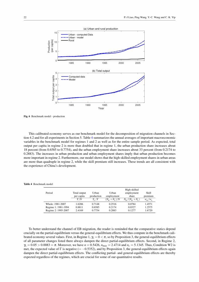
22 P.-J Liao, Ping Wang, Y.-C. Wang and C. K. Yip
1985 1990 1995 2000 20050
5
10
15
Pro
du
ctio
n
(pe
r ca
pita
)
(a) Urban and rural production
Urban - computed Data
Urban - model
Rural
1985 1990 1995 2000 2005
Year
0
1
2
3
4
5
To
tal o
utp
ut
pe
r ca
pita
(b) Total output
Computed data
Model
Fig. 6 Benchmark model - production
This calibrated economy serves as our benchmark model for the decomposition of migration channels in Sec-tion 4.2 and for all experiments in Section 5. Table 4 summarizes the annual averages of important macroeconomicvariables in the benchmark model for regimes 1 and 2 as well as for the entire sample period. As expected, totaloutput per capita in regime 2 is more than doubled that in regime 1, the urban production share increases about18 percent (from 0.6585 to 0.7754), and the urban employment share increases about 33 percent (from 0.2174 to0.2883). The increases in urban production and urban employment shares imply that urban production becomesmore important in regime 2. Furthermore, our model shows that the high-skilled employment shares in urban areasare more than quadruple in regime 2, while the skill premium still increases. These trends are all consistent withthe experience of China’s development.
Table 4 Benchmark model
High-skilledPeriod Total output Urban Urban employment Skill
per capita production employment share premiumY/N YU /Y (NH +NL )/N NH /(NH +NL ) wH /wL
Whole: 1981-2007 1.6206 0.7148 0.2516 0.0784 1.4571Regime 1: 1981-1994 0.8811 0.6585 0.2174 0.0327 1.2575Regime 2: 1995-2007 2.4169 0.7754 0.2883 0.1277 1.6720
To better understand the channel of EB migration, the reader is reminded that the comparative statics dependcrucially on the partial-equilibrium versus the general-equilibrium effects. We thus compute in the benchmark cali-brated economy several values. First, in Regime 1, γL = 0 < π , so by Proposition 3, the general-equilibrium effectsof all parameter changes listed there always dampen the direct partial-equilibrium effects. Second, in Regime 2,γL = 0.05 > 0.0083 = π . Moreover, we have n = 0.5426, nmax = 2.4714 and nc = 5.1345. Thus, Condition W2 ismet, the expected value of Γ is negative (=−0.5352), and by Proposition 3, the general-equilibrium effects againdampen the direct partial-equilibrium effects. The conflicting partial- and general-equilibrium effects are therebyexpected regardless of the regimes, which are crucial for some of our quantitative results.

Educational Choice, Rural-urban Migration and Economic Development 23
1980 1985 1990 1995 2000 20050
0.1
0.2
0.3
0.4
0.5(a) Urbanization rate
Urb
an
iza
tio
n r
ate
Data
Model
1980 1985 1990 1995 2000 20050
0.2
0.4
0.6
0.8(b) Urban high and low skilled labor
Year
Urb
an
hig
h &
lo
w
skill
ed
la
bo
r
Data − high skilled labor
Model − high skilled labor
Data − low skilled labor
Model − low skilled labor
Fig. 7 Benchmark model - urbanization rate and labor share
4.2 Decomposition of Migration Channels
To identify the contribution of each migration channel and to study the total effects of migration on China’s de-velopment process, we eliminate the migration channels sequentially. The effect of the channel under study is thusthe difference between the counterfactual model with the channel being excluded and the benchmark model.
Figure 8 plots urban production (per capita), total output per capita, and urbanization rates under the decompo-sition. The benchmark model and the three scenarios are plotted for comparison: (i) WB migration is eliminated;(ii) EB migration is eliminated; and (iii) both migration channels are eliminated. In the first scenario, when the WBmigration is eliminated, the only “new” source of low-skilled workers coming from countryside is unlucky collegegraduates. As a consequence, there are much fewer productive low-skilled workers in cities, resulting in a largerhigh-low skilled labor ratio and a higher urban production (per capita). Furthermore, as the migration volume viathe WB migration is large, the urbanization rate in this scenario is much lower than the benchmark case. In thesecond scenario in which EB migration is eliminated, once again, as the volume of EB migration that is eliminatedis not large, the urbanization rate in this case is very close to that in the benchmark model. This shows that the ma-jority of rural-urban migration is WB. With fewer productive high-skilled workers in the cities, urban production(per capita) is now slightly lower than that in the benchmark case.
To identify the magnitude of the contribution of migration types to major macroeconomic variables, Table5 reports the percentage change relative to the benchmark model for the above three scenarios. Given the largevolume of WB migration, the conventional wisdom is that the effects of WB migration on output levels should faroutweigh the effects of EB migration. However, our results in Table 5 show that the contribution of EB migrationcannot be overlooked: EB migration and WB migration explain 6.3 percent and 4.5 percent of total output per capitain the benchmark model over the entire sample period, respectively. This could be due to the fact that, comparedwith WB migrants, EB migrants are workers with higher productivity. Therefore, the contribution of EB migrantsto per capita output is amplified. We also find that EB migration contributes to roughly one-third of the high-skilledemployment share in the benchmark model and thereby lowers the skill premium, while WB migration reduces thehigh-skilled employment share and boosts the skill premium. Furthermore, the result suggests that EB migrationis more important in regime 2 than in regime 1: EB migration in regime 2 explains 8.0 percent of total output percapita in the benchmark model, while it only explains 2.0 percent of total output per capita in regime 1. There areseveral conflicting forces influencing the effects of EB migration: A higher skill premium, a higher human capitallevel and a lower EB migration cost in regime 2 attract more migration through the EB migration channel, whereasthe higher tuition cost and the termination of the GJA policy depress EB migration. Our quantitative results show
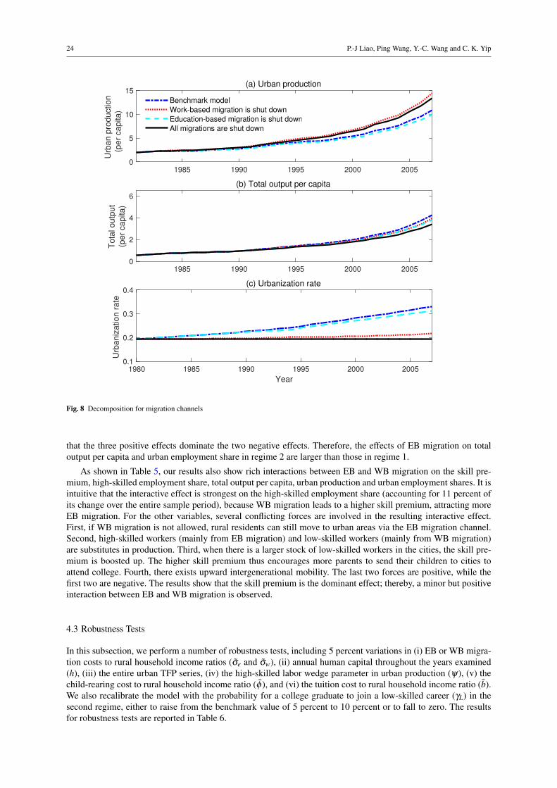
24 P.-J Liao, Ping Wang, Y.-C. Wang and C. K. Yip
1985 1990 1995 2000 20050
5
10
15
Urb
an p
roduction
(per
capita)
(a) Urban production
Benchmark model
Work-based migration is shut down
Education-based migration is shut down
All migrations are shut down
1985 1990 1995 2000 20050
2
4
6
Tota
l outp
ut
(per
capita)
(b) Total output per capita
1980 1985 1990 1995 2000 2005
Year
0.1
0.2
0.3
0.4
Urb
aniz
ation r
ate
(c) Urbanization rate
Fig. 8 Decomposition for migration channels
that the three positive effects dominate the two negative effects. Therefore, the effects of EB migration on totaloutput per capita and urban employment share in regime 2 are larger than those in regime 1.
As shown in Table 5, our results also show rich interactions between EB and WB migration on the skill pre-mium, high-skilled employment share, total output per capita, urban production and urban employment shares. It isintuitive that the interactive effect is strongest on the high-skilled employment share (accounting for 11 percent ofits change over the entire sample period), because WB migration leads to a higher skill premium, attracting moreEB migration. For the other variables, several conflicting forces are involved in the resulting interactive effect.First, if WB migration is not allowed, rural residents can still move to urban areas via the EB migration channel.Second, high-skilled workers (mainly from EB migration) and low-skilled workers (mainly from WB migration)are substitutes in production. Third, when there is a larger stock of low-skilled workers in the cities, the skill pre-mium is boosted up. The higher skill premium thus encourages more parents to send their children to cities toattend college. Fourth, there exists upward intergenerational mobility. The last two forces are positive, while thefirst two are negative. The results show that the skill premium is the dominant effect; thereby, a minor but positiveinteraction between EB and WB migration is observed.
4.3 Robustness Tests
In this subsection, we perform a number of robustness tests, including 5 percent variations in (i) EB or WB migra-tion costs to rural household income ratios (σe and σw), (ii) annual human capital throughout the years examined(h), (iii) the entire urban TFP series, (iv) the high-skilled labor wedge parameter in urban production (ψ), (v) thechild-rearing cost to rural household income ratio (φ ), and (vi) the tuition cost to rural household income ratio (b).We also recalibrate the model with the probability for a college graduate to join a low-skilled career (γL) in thesecond regime, either to raise from the benchmark value of 5 percent to 10 percent or to fall to zero. The resultsfor robustness tests are reported in Table 6.
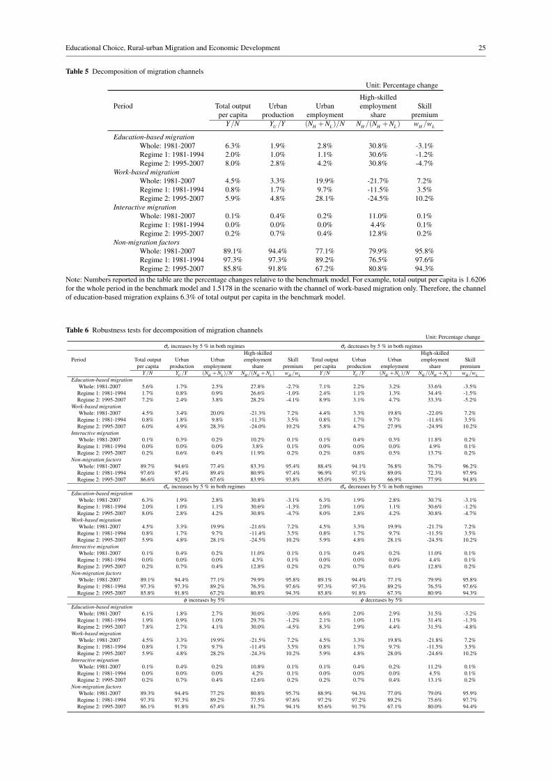
Educational Choice, Rural-urban Migration and Economic Development 25
Table 5 Decomposition of migration channels
Unit: Percentage change
High-skilledPeriod Total output Urban Urban employment Skill
per capita production employment share premiumY/N YU /Y (NH +NL )/N NH /(NH +NL ) wH /wL
Education-based migrationWhole: 1981-2007 6.3% 1.9% 2.8% 30.8% -3.1%Regime 1: 1981-1994 2.0% 1.0% 1.1% 30.6% -1.2%Regime 2: 1995-2007 8.0% 2.8% 4.2% 30.8% -4.7%
Work-based migrationWhole: 1981-2007 4.5% 3.3% 19.9% -21.7% 7.2%Regime 1: 1981-1994 0.8% 1.7% 9.7% -11.5% 3.5%Regime 2: 1995-2007 5.9% 4.8% 28.1% -24.5% 10.2%
Interactive migrationWhole: 1981-2007 0.1% 0.4% 0.2% 11.0% 0.1%Regime 1: 1981-1994 0.0% 0.0% 0.0% 4.4% 0.1%Regime 2: 1995-2007 0.2% 0.7% 0.4% 12.8% 0.2%
Non-migration factorsWhole: 1981-2007 89.1% 94.4% 77.1% 79.9% 95.8%Regime 1: 1981-1994 97.3% 97.3% 89.2% 76.5% 97.6%Regime 2: 1995-2007 85.8% 91.8% 67.2% 80.8% 94.3%
Note: Numbers reported in the table are the percentage changes relative to the benchmark model. For example, total output per capita is 1.6206for the whole period in the benchmark model and 1.5178 in the scenario with the channel of work-based migration only. Therefore, the channelof education-based migration explains 6.3% of total output per capita in the benchmark model.
Table 6 Robustness tests for decomposition of migration channelsUnit: Percentage change
σe increases by 5 % in both regimes σe decreases by 5 % in both regimesHigh-skilled High-skilled
Period Total output Urban Urban employment Skill Total output Urban Urban employment Skillper capita production employment share premium per capita production employment share premium
Y/N YU /Y (NH +NL )/N NH /(NH +NL ) wH /wL Y/N YU /Y (NH +NL )/N NH /(NH +NL ) wH /wL
Education-based migrationWhole: 1981-2007 5.6% 1.7% 2.5% 27.8% -2.7% 7.1% 2.2% 3.2% 33.6% -3.5%
Regime 1: 1981-1994 1.7% 0.8% 0.9% 26.6% -1.0% 2.4% 1.1% 1.3% 34.4% -1.5%Regime 2: 1995-2007 7.2% 2.4% 3.8% 28.2% -4.1% 8.9% 3.1% 4.7% 33.3% -5.2%
Work-based migrationWhole: 1981-2007 4.5% 3.4% 20.0% -21.3% 7.2% 4.4% 3.3% 19.8% -22.0% 7.2%
Regime 1: 1981-1994 0.8% 1.8% 9.8% -11.3% 3.5% 0.8% 1.7% 9.7% -11.6% 3.5%Regime 2: 1995-2007 6.0% 4.9% 28.3% -24.0% 10.2% 5.8% 4.7% 27.9% -24.9% 10.2%
Interactive migrationWhole: 1981-2007 0.1% 0.3% 0.2% 10.2% 0.1% 0.1% 0.4% 0.3% 11.8% 0.2%
Regime 1: 1981-1994 0.0% 0.0% 0.0% 3.8% 0.1% 0.0% 0.0% 0.0% 4.9% 0.1%Regime 2: 1995-2007 0.2% 0.6% 0.4% 11.9% 0.2% 0.2% 0.8% 0.5% 13.7% 0.2%
Non-migration factorsWhole: 1981-2007 89.7% 94.6% 77.4% 83.3% 95.4% 88.4% 94.1% 76.8% 76.7% 96.2%
Regime 1: 1981-1994 97.6% 97.4% 89.4% 80.9% 97.4% 96.9% 97.1% 89.0% 72.3% 97.9%Regime 2: 1995-2007 86.6% 92.0% 67.6% 83.9% 93.8% 85.0% 91.5% 66.9% 77.9% 94.8%
σw increases by 5 % in both regimes σw decreases by 5 % in both regimesEducation-based migration
Whole: 1981-2007 6.3% 1.9% 2.8% 30.8% -3.1% 6.3% 1.9% 2.8% 30.7% -3.1%Regime 1: 1981-1994 2.0% 1.0% 1.1% 30.6% -1.3% 2.0% 1.0% 1.1% 30.6% -1.2%Regime 2: 1995-2007 8.0% 2.8% 4.2% 30.8% -4.7% 8.0% 2.8% 4.2% 30.8% -4.7%
Work-based migrationWhole: 1981-2007 4.5% 3.3% 19.9% -21.6% 7.2% 4.5% 3.3% 19.9% -21.7% 7.2%
Regime 1: 1981-1994 0.8% 1.7% 9.7% -11.4% 3.5% 0.8% 1.7% 9.7% -11.5% 3.5%Regime 2: 1995-2007 5.9% 4.8% 28.1% -24.5% 10.2% 5.9% 4.8% 28.1% -24.5% 10.2%
Interactive migrationWhole: 1981-2007 0.1% 0.4% 0.2% 11.0% 0.1% 0.1% 0.4% 0.2% 11.0% 0.1%
Regime 1: 1981-1994 0.0% 0.0% 0.0% 4.3% 0.1% 0.0% 0.0% 0.0% 4.4% 0.1%Regime 2: 1995-2007 0.2% 0.7% 0.4% 12.8% 0.2% 0.2% 0.7% 0.4% 12.8% 0.2%
Non-migration factorsWhole: 1981-2007 89.1% 94.4% 77.1% 79.9% 95.8% 89.1% 94.4% 77.1% 79.9% 95.8%
Regime 1: 1981-1994 97.3% 97.3% 89.2% 76.5% 97.6% 97.3% 97.3% 89.2% 76.5% 97.6%Regime 2: 1995-2007 85.8% 91.8% 67.2% 80.8% 94.3% 85.8% 91.8% 67.3% 80.9% 94.3%
φ increases by 5% φ decreases by 5%Education-based migration
Whole: 1981-2007 6.1% 1.8% 2.7% 30.0% -3.0% 6.6% 2.0% 2.9% 31.5% -3.2%Regime 1: 1981-1994 1.9% 0.9% 1.0% 29.7% -1.2% 2.1% 1.0% 1.1% 31.4% -1.3%Regime 2: 1995-2007 7.8% 2.7% 4.1% 30.0% -4.5% 8.3% 2.9% 4.4% 31.5% -4.8%
Work-based migrationWhole: 1981-2007 4.5% 3.3% 19.9% -21.5% 7.2% 4.5% 3.3% 19.8% -21.8% 7.2%
Regime 1: 1981-1994 0.8% 1.7% 9.7% -11.4% 3.5% 0.8% 1.7% 9.7% -11.5% 3.5%Regime 2: 1995-2007 5.9% 4.8% 28.2% -24.3% 10.2% 5.9% 4.8% 28.0% -24.6% 10.2%
Interactive migrationWhole: 1981-2007 0.1% 0.4% 0.2% 10.8% 0.1% 0.1% 0.4% 0.2% 11.2% 0.1%
Regime 1: 1981-1994 0.0% 0.0% 0.0% 4.2% 0.1% 0.0% 0.0% 0.0% 4.5% 0.1%Regime 2: 1995-2007 0.2% 0.7% 0.4% 12.6% 0.2% 0.2% 0.7% 0.4% 13.1% 0.2%
Non-migration factorsWhole: 1981-2007 89.3% 94.4% 77.2% 80.8% 95.7% 88.9% 94.3% 77.0% 79.0% 95.9%
Regime 1: 1981-1994 97.3% 97.3% 89.2% 77.5% 97.6% 97.2% 97.2% 89.2% 75.6% 97.7%Regime 2: 1995-2007 86.1% 91.8% 67.4% 81.7% 94.1% 85.6% 91.7% 67.1% 80.0% 94.4%
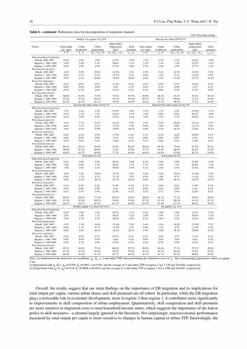
26 P.-J Liao, Ping Wang, Y.-C. Wang and C. K. Yip
Table 6 - continued Robustness tests for decomposition of migration channelsUnit: Percentage change
Reduce b in regime 2 by 20% Increase the urban TFP by 5%
High-skilled High-skilledPeriod Total output Urban Urban employment Skill Total output Urban Urban employment Skill
per capita production employment share premium per capita production employment share premiumY/N YU /Y (NH +NL )/N NH /(NH +NL ) wH /wL Y/N YU /Y (NH +NL )/N NH /(NH +NL ) wH /wL
Education-based migrationWhole: 1981-2007 6.6% 2.0% 2.9% 31.4% -3.2% 7.3% 2.1% 3.2% 34.0% -3.6%
Regime 1: 1981-1994 2.0% 1.0% 1.1% 30.6% -1.2% 2.5% 1.1% 1.3% 35.1% -1.5%Regime 2: 1995-2007 8.4% 2.9% 4.4% 31.6% -4.8% 9.1% 3.0% 4.8% 33.7% -5.3%
Work-based migrationWhole: 1981-2007 4.4% 3.3% 19.8% -21.9% 7.2% 4.5% 3.1% 19.7% -22.2% 7.2%
Regime 1: 1981-1994 0.8% 1.7% 9.7% -11.5% 3.5% 0.8% 1.7% 9.7% -11.8% 3.5%Regime 2: 1995-2007 5.9% 4.7% 28.0% -24.8% 10.2% 6.0% 4.5% 27.9% -25.1% 10.2%
Interactive migrationWhole: 1981-2007 0.2% 0.4% 0.2% 11.4% 0.1% 0.2% 0.4% 0.3% 12.0% 0.2%
Regime 1: 1981-1994 0.0% 0.0% 0.0% 4.4% 0.1% 0.0% 0.1% 0.0% 5.2% 0.1%Regime 2: 1995-2007 0.2% 0.7% 0.4% 13.3% 0.2% 0.3% 0.8% 0.5% 13.9% 0.2%
Non-migration factorsWhole: 1981-2007 88.8% 94.3% 77.0% 79.2% 95.9% 88.0% 94.3% 76.7% 76.2% 96.2%
Regime 1: 1981-1994 97.3% 97.3% 89.2% 76.5% 97.6% 96.7% 97.1% 89.0% 71.5% 97.9%Regime 2: 1995-2007 85.5% 91.7% 67.1% 79.9% 94.4% 84.6% 91.7% 66.9% 77.5% 94.9%
Increase the entire series of h by 5% Decrease the entire series of h by 5%Education-based migration
Whole: 1981-2007 7.3% 2.1% 3.2% 33.8% -3.6% 5.5% 1.7% 2.4% 27.6% -2.7%Regime 1: 1981-1994 2.5% 1.1% 1.3% 34.8% -1.5% 1.6% 0.8% 0.9% 26.2% -1.0%Regime 2: 1995-2007 9.1% 3.0% 4.8% 33.5% -5.3% 7.0% 2.5% 3.7% 28.0% -4.1%
Work-based migrationWhole: 1981-2007 4.4% 3.1% 19.7% -22.1% 7.2% 4.5% 3.5% 20.0% -21.2% 7.2%
Regime 1: 1981-1994 0.8% 1.7% 9.7% -11.8% 3.5% 0.8% 1.8% 9.8% -11.1% 3.5%Regime 2: 1995-2007 5.8% 4.5% 27.9% -25.0% 10.2% 6.0% 5.1% 28.3% -23.9% 10.1%
Interactive migrationWhole: 1981-2007 0.2% 0.4% 0.3% 11.9% 0.2% 0.1% 0.3% 0.2% 10.0% 0.1%
Regime 1: 1981-1994 0.0% 0.0% 0.0% 5.1% 0.1% 0.0% 0.0% 0.0% 3.6% 0.1%Regime 2: 1995-2007 0.3% 0.8% 0.5% 13.8% 0.2% 0.2% 0.6% 0.4% 11.8% 0.2%
Non-migration factorsWhole: 1981-2007 88.1% 94.3% 76.8% 76.4% 96.2% 89.9% 94.5% 77.4% 83.5% 95.4%
Regime 1: 1981-1994 96.8% 97.2% 89.0% 71.9% 97.9% 97.7% 97.4% 89.4% 81.4% 97.4%Regime 2: 1995-2007 84.8% 91.7% 66.9% 77.7% 94.8% 86.8% 91.8% 67.6% 84.1% 93.8%
ψ increases by 5% ψ decreases by 5%Education-based migration
Whole: 1981-2007 6.1% 1.8% 2.8% 30.5% -3.0% 6.5% 2.0% 2.8% 31.0% -3.3%Regime 1: 1981-1994 1.9% 0.9% 1.1% 30.2% -1.2% 2.1% 1.0% 1.1% 30.9% -1.3%Regime 2: 1995-2007 7.8% 2.6% 4.2% 30.6% -4.5% 8.3% 2.9% 4.3% 31.0% -4.9%
Work-based migrationWhole: 1981-2007 4.4% 3.2% 19.9% -21.7% 7.2% 4.5% 3.4% 19.9% -21.6% 7.2%
Regime 1: 1981-1994 0.8% 1.7% 9.7% -11.5% 3.5% 0.8% 1.8% 9.7% -11.4% 3.5%Regime 2: 1995-2007 5.8% 4.7% 28.1% -24.5% 10.2% 6.0% 4.9% 28.1% -24.5% 10.1%
Interactive migrationWhole: 1981-2007 0.1% 0.4% 0.2% 11.0% 0.1% 0.1% 0.4% 0.2% 11.0% 0.1%
Regime 1: 1981-1994 0.0% 0.0% 0.0% 4.4% 0.1% 0.0% 0.0% 0.0% 4.4% 0.1%Regime 2: 1995-2007 0.2% 0.7% 0.4% 12.8% 0.2% 0.2% 0.7% 0.4% 12.9% 0.2%
Non-migration factorsWhole: 1981-2007 89.3% 94.6% 77.1% 80.2% 95.6% 88.8% 94.1% 77.1% 79.6% 96.0%
Regime 1: 1981-1994 97.3% 97.4% 89.2% 76.9% 97.6% 97.2% 97.1% 89.2% 76.1% 97.7%Regime 2: 1995-2007 86.1% 92.1% 67.3% 81.1% 94.0% 85.5% 91.4% 67.2% 80.6% 94.5%
Double regime 2 γL from 0.05 to 0.1 Set regime 2 γL to 0Education-based migration
Whole: 1981-2007 6.2% 1.9% 2.8% 30.1% -3.1% 6.5% 1.9% 2.8% 31.4% -3.2%Regime 1: 1981-1994 2.0% 1.0% 1.1% 30.6% -1.2% 2.0% 1.0% 1.1% 30.6% -1.2%Regime 2: 1995-2007 7.9% 2.7% 4.2% 30.0% -4.5% 8.2% 2.8% 4.2% 31.6% -4.8%
Work-based migrationWhole: 1981-2007 4.5% 3.3% 19.9% -21.4% 7.2% 4.4% 3.3% 19.9% -21.9% 7.2%
Regime 1: 1981-1994 0.8% 1.7% 9.7% -11.5% 3.5% 0.8% 1.7% 9.7% -11.5% 3.5%Regime 2: 1995-2007 6.0% 4.8% 28.1% -24.2% 10.1% 5.9% 4.8% 28.1% -24.8% 10.2%
Interactive migrationWhole: 1981-2007 0.1% 0.4% 0.2% 10.7% 0.1% 0.1% 0.4% 0.2% 11.3% 0.1%
Regime 1: 1981-1994 0.0% 0.0% 0.0% 4.4% 0.1% 0.0% 0.0% 0.0% 4.4% 0.1%Regime 2: 1995-2007 0.2% 0.7% 0.4% 12.5% 0.2% 0.2% 0.7% 0.4% 13.2% 0.2%
Non-migration factorsWhole: 1981-2007 89.1% 94.4% 77.1% 80.6% 95.7% 89.0% 94.4% 77.1% 79.2% 95.8%
Regime 1: 1981-1994 97.3% 97.3% 89.2% 76.5% 97.6% 97.3% 97.3% 89.2% 76.5% 97.6%Regime 2: 1995-2007 86.0% 91.8% 67.3% 81.7% 94.2% 85.7% 91.7% 67.2% 80.0% 94.4%
Note: As mentioned in the main text, we recalibrate γH , δL , a, τ and urban TFP when performing the robustness tests on γL . The corresponding parameters values in regime2 are:(i) Experiment with γL =0.1: γH =0.8709, δL =0.9881, a=0.4768, and the average of τ and urban TFP in regime 2 are 5.139 and 10.6446, respectively.(ii) Experiment with γL =0: γH =0.9210, δL =0.9886, a=0.4639, and the average of τ and urban TFP in regime 2 are 5.1388 and 10.6441, respectively.
Overall, the results suggest that our main findings on the importance of EB migration and its implications fortotal output per capita, various urban shares and skill premium are all robust. In particular, while the EB migrationplays a noticeable role in economic development, more in regime 2 than regime 1, it contributes more significantlyto improvements in skill composition of urban employment. Quantitatively, skill composition and skill premiumare more sensitive to migration costs to rural household income ratios, which suggests the importance of the hukoupolicy to skill measures – a channel largely ignored in the literature. Not surprisingly, macroeconomic performancemeasured by total output per capita is more sensitive to changes in human capital or urban TFP. Interestingly, the
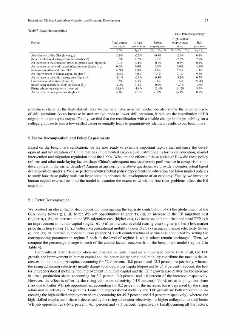
Educational Choice, Rural-urban Migration and Economic Development 27
Table 7 Factor decompositionUnit: Percentage change
High-skilledFactors Total output Urban Urban employment Skill
per capita production employment share premiumY/N YU /Y (NH +NL )/N NH /(NH +NL ) wH /wL
Abolishment of the GJA (lower γH ) -0.9% -0.2% -0.4% -2.9% 0.4%Better work-based job opportunities (higher π) 1.5% 1.2% 8.2% -7.3% 2.9%An increase in the education-based migration cost (higher σe) -0.3% -0.1% -0.1% -0.8% 0.1%An increase in the work-based migration cost (higher σw) 0.0% 0.0% 0.0% 0.0% -0.0%Increases in urban and rural TFP 52.9% 1.8% 1.0% 5.5% -0.8%An improvement in human capital (higher h) 10.8% 3.0% 0.3% 2.1% 9.8%An increase in the child-rearing cost (higher φ ) -1.1% -0.3% -0.5% -3.2% 0.5%Lower market distortion (lower τ) 1.2% 0.3% 0.6% 3.5% 21.4%Better intergenerational mobility (lower δLL ) 12.3% 3.2% -0.0% 49.3% -9.9%Rising admission selectivity (lower a) -24.8% -4.9% -12.4% -64.2% 8.5%An increase in college tuition (higher b) -2.0% -0.5% -1.0% -6.1% 0.9%
robustness check on the high-skilled labor wedge parameter in urban production also shows the important roleof skill premium: As an increase in such wedge tends to lower skill premium, it reduces the contribution of EBmigration to per capita output. Finally, we find that the recalibration with a sizable change in the probability for acollege graduate to join a low-skilled career essentially leads to quantitatively identical results to our benchmark.
5 Factor Decomposition and Policy Experiments
Based on the benchmark calibration, we are now ready to examine important factors that influence the devel-opment and urbanization of China that has implemented large-scaled institutional reforms on education, marketintervention and migration regulation since the 1990s. What are the effects of these policies? How did these policyreforms and other underlaying factors shape China’s subsequent macroeconomic performance in comparison to itsdevelopment in the earlier decades? Aiming at answering the above questions, we provide a counterfactual baseddecomposition analysis. We also perform counterfactual policy experiments on education and labor market policiesto study how these policy tools can be adopted to enhance the development of an economy. Finally, we introducehuman capital externalities into the model to examine the extent to which the free-rider problems affect the EBmigration.
5.1 Factor Decomposition
We conduct an eleven-factor decomposition, investigating the separate contribution of (i) the abolishment of theGJA policy (lower γH ), (ii) better WB job opportunities (higher π), (iii) an increase in the EB migration cost(higher σe), (iv) an increase in the WB migration cost (higher σw), (v) increases in both urban and rural TFP, (vi)an improvement in human capital (higher h), (vii) an increase in child-rearing cost (higher φ ), (viii) less marketprice distortion (lower τ), (ix) better intergenerational mobility (lower δLL), (x) rising admission selectivity (lowera), and (xi) an increase in college tuition (higher b). Each counterfactual experiment is conducted by setting thecorresponding parameter in regime 2 back to the level of regime 1, while others remain unchanged. Then, wecompute the percentage change in each of the counterfactual outcome from the benchmark model (regime 2 inTable 4).
The results of factor decomposition are provided in Table 7 and are summarized below. First of all, the TFPgrowth, the improvement in human capital and the better intergenerational mobility contribute the most to the in-creases in total output per capita, accounting for 52.9 percent, 10.8 percent and 12.3 percent, respectively, whereasthe rising admission selectivity greatly damps total output per capita (depressed by 24.8 percent). Second, the bet-ter intergenerational mobility, the improvement in human capital and the TFP growth also matter for the increasein urban production share, accounting for 3.2 percent, 3.0 percent and 1.8 percent of the increase, respectively.However, the effect is offset by the rising admission selectivity (-4.9 percent). Third, urban employment sharerises due to better WB job opportunities, accounting for 8.2 percent of the increase, but is depressed by the risingadmission selectivity (-12.4 percent). Fourth, intergenerational mobility and TFP growth are both important in in-creasing the high-skilled employment share (accounting for 49.3 percent and 5.5 percent respectively), whereas thehigh-skilled employment share is decreased by the rising admission selectivity, the higher college tuition and betterWB job opportunities (-64.2 percent, -6.1 percent and -7.3 percent, respectively). Finally, among all the factors,
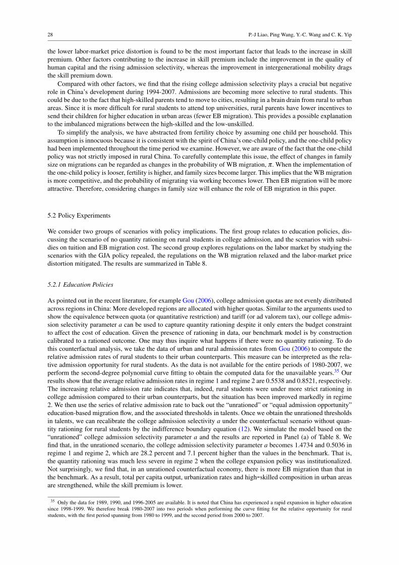
28 P.-J Liao, Ping Wang, Y.-C. Wang and C. K. Yip
the lower labor-market price distortion is found to be the most important factor that leads to the increase in skillpremium. Other factors contributing to the increase in skill premium include the improvement in the quality ofhuman capital and the rising admission selectivity, whereas the improvement in intergenerational mobility dragsthe skill premium down.
Compared with other factors, we find that the rising college admission selectivity plays a crucial but negativerole in China’s development during 1994-2007. Admissions are becoming more selective to rural students. Thiscould be due to the fact that high-skilled parents tend to move to cities, resulting in a brain drain from rural to urbanareas. Since it is more difficult for rural students to attend top universities, rural parents have lower incentives tosend their children for higher education in urban areas (fewer EB migration). This provides a possible explanationto the imbalanced migrations between the high-skilled and the low-unskilled.
To simplify the analysis, we have abstracted from fertility choice by assuming one child per household. Thisassumption is innocuous because it is consistent with the spirit of China’s one-child policy, and the one-child policyhad been implemented throughout the time period we examine. However, we are aware of the fact that the one-childpolicy was not strictly imposed in rural China. To carefully contemplate this issue, the effect of changes in familysize on migrations can be regarded as changes in the probability of WB migration, π . When the implementation ofthe one-child policy is looser, fertility is higher, and family sizes become larger. This implies that the WB migrationis more competitive, and the probability of migrating via working becomes lower. Then EB migration will be moreattractive. Therefore, considering changes in family size will enhance the role of EB migration in this paper.
5.2 Policy Experiments
We consider two groups of scenarios with policy implications. The first group relates to education policies, dis-cussing the scenario of no quantity rationing on rural students in college admission, and the scenarios with subsi-dies on tuition and EB migration cost. The second group explores regulations on the labor market by studying thescenarios with the GJA policy repealed, the regulations on the WB migration relaxed and the labor-market pricedistortion mitigated. The results are summarized in Table 8.
5.2.1 Education Policies
As pointed out in the recent literature, for example Gou (2006), college admission quotas are not evenly distributedacross regions in China: More developed regions are allocated with higher quotas. Similar to the arguments used toshow the equivalence between quota (or quantitative restriction) and tariff (or ad valorem tax), our college admis-sion selectivity parameter a can be used to capture quantity rationing despite it only enters the budget constraintto affect the cost of education. Given the presence of rationing in data, our benchmark model is by constructioncalibrated to a rationed outcome. One may thus inquire what happens if there were no quantity rationing. To dothis counterfactual analysis, we take the data of urban and rural admission rates from Gou (2006) to compute therelative admission rates of rural students to their urban counterparts. This measure can be interpreted as the rela-tive admission opportunity for rural students. As the data is not available for the entire periods of 1980-2007, weperform the second-degree polynomial curve fitting to obtain the computed data for the unavailable years.35 Ourresults show that the average relative admission rates in regime 1 and regime 2 are 0.5538 and 0.8521, respectively.The increasing relative admission rate indicates that, indeed, rural students were under more strict rationing incollege admission compared to their urban counterparts, but the situation has been improved markedly in regime2. We then use the series of relative admission rate to back out the “unrationed” or “equal admission opportunity”education-based migration flow, and the associated thresholds in talents. Once we obtain the unrationed thresholdsin talents, we can recalibrate the college admission selectivity a under the counterfactual scenario without quan-tity rationing for rural students by the indifference boundary equation (12). We simulate the model based on the“unrationed” college admission selectivity parameter a and the results are reported in Panel (a) of Table 8. Wefind that, in the unrationed scenario, the college admission selectivity parameter a becomes 1.4734 and 0.5036 inregime 1 and regime 2, which are 28.2 percent and 7.1 percent higher than the values in the benchmark. That is,the quantity rationing was much less severe in regime 2 when the college expansion policy was institutionalized.Not surprisingly, we find that, in an unrationed counterfactual economy, there is more EB migration than that inthe benchmark. As a result, total per capita output, urbanization rates and high-skilled composition in urban areasare strengthened, while the skill premium is lower.
35 Only the data for 1989, 1990, and 1996-2005 are available. It is noted that China has experienced a rapid expansion in higher educationsince 1998-1999. We therefore break 1980-2007 into two periods when performing the curve fitting for the relative opportunity for ruralstudents, with the first period spanning from 1980 to 1999, and the second period from 2000 to 2007.
Educational Choice, Rural-urban Migration and Economic Development 29
Table 8 Policy experiments
Unit: Percentage change
High-skilledPeriod Total output Urban Urban employment Skill
per capita production employment share premiumY/N YU /Y (NH +NL )/N NH /(NH +NL ) wH /wL
(a) Experiments on education policiesNo quantity rationing in college admission in both regimes
Whole: 1981-2007 3.7% 1.2% 1.8% 19.4% -1.8%Regime 1: 1981-1994 1.7% 0.8% 0.9% 24.9% -1.0%Regime 2: 1995-2007 4.6% 1.5% 2.5% 17.9% -2.5%
Tuition subsidiesA 20% tuition subsidy in regime 2
Regime 2: 1995-2007 0.40% 0.10% 0.20% -3.25% -0.17%A 50% tuition subsidy in regime 2
Regime 2: 1995-2007 1.04% 0.26% 0.52% -10.95% -0.45%Subsidies on education migration cost in regime 2
Education migration cost = 80% of work-based migration costRegime 2: 1995-2007 -2.96% -0.76% -1.45% -8.98% 1.34%
Education migration cost = 20% of work-based migration costRegime 2: 1995-2007 1.67% 0.41% 0.83% 5.01% -0.72%
(b) Experiments on labor market policiesNo GJA in regime 1
Whole: 1981-2007 -1.2% -0.4% -0.5% -7.0% 0.7%Regime 1: 1981-1994 -0.7% -0.3% -0.3% -10.0% 0.4%Regime 2: 1995-2007 -1.4% -0.5% -0.7% -6.1% 0.9%
Better job opportunities in regime 1: π1 = π2Whole: 1981-2007 2.8% 2.4% 14.4% -6.6% 4.2%Regime 1: 1981-1994 0.9% 2.2% 12.5% -11.1% 4.1%Regime 2: 1995-2007 3.6% 2.7% 16.0% -5.4% 4.2%
A 20% subsidy on work-based migration cost in both regimesWhole: 1981-2007 0.0% 0.0% 0.0% 4.7% 0.0%Regime 1: 1981-1994 0.0% 0.0% 0.0% 0.0% 0.0%Regime 2: 1995-2007 0.0% 0.0% 0.0% 6.0% 0.0%
A reduction of market distortion in regime 1 to the lower level of regime 2Whole: 1981-2007 13.7% 4.5% 7.1% -11.3% 46.3%Regime 1: 1981-1994 9.0% 4.0% 5.1% -5.5% 113.3%Regime 2: 1995-2007 15.5% 4.9% 8.7% -12.9% -8.0%
In our benchmark economy, the EB migration cost (σe) only amounts to 33.14 percent of the WB migrationcost (σw). The relatively lower EB migration cost implies the existence of education subsidies in data. Therefore,our benchmark model represents a subsidized outcome. To discuss the subsidies on EB migration cost, we considertwo variations on subsidies: (i) EB migration cost is 80 percent of the WB migration cost, and (ii) EB migration costis 20 percent of the WB migration cost. Compared with the benchmark, the first scenario indicates the subsidy onEB migration cost is reduced so EB migration becomes more costly, coming to roughly 2.4 times of the benchmarkEB migration cost. In contrast, the second scenario considers a subsidy expansion, so that EB migration cost equalsonly 60 percent of the benchmark EB migration cost. As shown in Panel (a) of Table 8, institutionalizing a largersubsidy on EB migration cost than the benchmark economy strengthens the contribution of EB migration to skillcomposition and enhances total output per capita. However, the skill premium is lower with a bigger EB migrationsubsidy.
We also consider an alternative education subsidy, investigating the effect of a 20 percent or 50 percent re-duction in tuition cost, b. Notably, one may view a decrease in b as to relax the credit constraint that limits ruralparents’ ability to send their children to urban colleges. The results in Panel (a) of Table 8 indicate that a subsidyto tuition (or relaxation of the credit constraint) tends to raise the contribution of EB migration to total outputper capita but weakens its contribution to skill composition. This is because that such a subsidy makes parentaldecisions on sending children to urban colleges less dependent on children’s talent.
5.2.2 Labor-Market Policies
As the GJA policy had been in force in China from the 1950s to the mid 1990s, we wonder how the economywould have performed if China had not implemented the GJA policy throughout its history. Here we performa scenario, supposing that there were no GJA policy for the time horizon under study by setting the value ofγH in regime 1 to that of regime 2. That is, jobs are no longer guaranteed for college graduates in regime 1.
30 P.-J Liao, Ping Wang, Y.-C. Wang and C. K. Yip
There are two opposite effects of this policy. Without guaranteed high-skilled jobs, college education becomesless rewarding, resulting in fewer EB migration. However, the skill premium increases because of the decreasingsupply of high-skilled workers, which makes college education more rewarding. Our quantitative result, as shownin Panel (b) of Table 8, suggests that the former effect dominates. Therefore, without the GJA policy throughout thehistory, urban employment would decrease by 0.5 percent, the share of high-skilled employment would decreaseby approximately 7 percent, the skill premium would increase by 0.7 percent and the total output per capita woulddecline by 1.2 percent. We thus conclude that the impact of no GJA on China’s development is relatively small.Notably, the small impact of the GJA policy is due to the ambiguous general-equilibrium effect of γL on EBmigration discussed in Section 3.3 and the conflicting partial- and general-equilibrium effects of γH .
The second experiment explores the effect of a more relaxed regulation on the WB migration since 1980.Because of the household registration reforms, the regulations on WB migration have been gradually relaxed. Weare curious what China would look like if the government had maintained looser regulations for migrant workers.We thus conduct an experiment by increasing the value of π in regime 1 to that of regime 2. The result in Panel(b) of Table 8 suggests that, with a more relaxed regulation on WB migration, there would be more WB migrants,resulting in a larger share of urban employment and an increase in both urban production share and total output percapita. However, the relaxation leads to a lower share of high-skilled employment; thereby a higher skill premium.Although EB migration in Regime 1 is lower, the conflicting general-equilibrium effect resulting from a higherskill premium reduces the negative impact. This explains why the contribution of EB migration in Regime 1 hadnot decreased by as much as the whole period. Compared with the GJA policy, the regulation on WB migrationhas a larger impact on China’s urbanization and development.
In addition to the above WB migration lottery, we also investigate two labor policy experiments: (i) a 20 percentsubsidy on WB migration cost (σw) in both regimes and (ii) a reduction of market price distortion (τ) in regime1 to the lower level of regime 2. The results in Panel (b) of Table 8 suggest that the effect of a subsidy on WBmigration cost is expected to be small as they must work through EB migration choice indirectly. A reduction ofmarket price distortion is found to raise the contribution of EB migration to total output per capita but weaken itscontribution to skill composition, similar to those of an education subsidy.
Before closing the discussion on policy experiments, we briefly discuss some interesting but omitted factorsand their expected effects on our main findings. First, as Table 5 suggests, the EB migration decision dependsnegatively on changes in WB migration (via π). Should we allow for two-way interactions (i.e. endogenous EB andWB migration), one would expect that EB migration may have greater contribution by lowering π , and may leadto a larger share of high-skilled employment. Second, it is also plausible that higher EB migration may enhanceurban productivity, thus reinforcing the incentives for EB migration. Similarly, should we consider learning bydoing and follow Rosen (1976) and Heckman (1976) allowing better-educated to have faster learning on the job,the incentive for EB migration would be even stronger. In either case, our figure about the contribution of EBmigration may again be viewed as on the conservative side. Third, another factor affecting migration is the urbanbenefit that can be regarded as an increase in the expected benefit of migration (see Liao et al. 2020). As a resultof household registration regulations, high-skilled workers generally enjoy more urban benefits than lower-skilledworkers. Given that the substitution effect dominates, we expect that the overall rural-urban migration would behigher but the increase is biased toward EB migration. On the contrary, land entitlement of rural households mayalso affect rural-urban migration in an opposite direction: Ngai et al. (2019) regarded the land policy as a barrier toChina’s industrialization, and Liao et al. (2020) found such a policy can slow down the progress of WB migration.In our model, we can treat land entitlement as an increase in the opportunity cost of migration. Thus, it is expectedto provide opposite outcomes to urban benefits. Fourth, a related issue is the housing market performance asexamined in Garriga et al. (2020). In our model, the rise in housing prices can be reinterpreted as a rising migrationcost to rural households. Because low-skilled workers are expected to be relieved from subsidized policy such aspublic housing, we can regard housing booms as to raise the relative cost of EB migration. This is yet another casewhich yields opposite outcomes to changes in urban benefits. Finally, rural-urban migration is often taken to beclosely related to the structural transformation of industrialization. As discussed in Garriga et al. (2020), duringthe process of structural transformation and on-going rural-urban migration, the relative price of agricultural goodsrises. This is qualitatively equivalent to an increase in the (self-employed) rural wage in our model. As a result oflower incentives for migration, the overall migration is lower and indeed we can show that EB migration would fallrelatively more. Some of those factors could enhance the EB migration but others could favor the WB migration.
5.3 Human Capital Externality
In a now-classic paper by Lucas (1988), human capital externality is incorporated into an education-based en-dogenous growth model. An interesting implication is: Although such within-the-generation positive externalityenhances production, the presence of the free-rider problem reduces individual incentive to undertake education,

Educational Choice, Rural-urban Migration and Economic Development 31
Table 9 Human capital externality - Decomposition of migration channels
Unit: Percentage change
High-skilledPeriod Total output Urban Urban employment Skill
per capita production employment share premiumY/N YU /Y (NH +NL )/N NH /(NH +NL ) wH /wL
The scenario with ξ = 0.01Education-based migration
Whole: 1981-2007 5.8% 1.8% 2.5% 27.7% -2.5%Regime 1: 1981-1994 1.7% 0.9% 0.9% 26.0% -0.8%Regime 2: 1995-2007 7.3% 2.6% 3.8% 28.2% -3.8%
Work-based migrationWhole: 1981-2007 4.6% 3.5% 20.0% -21.2% 7.3%Regime 1: 1981-1994 0.8% 1.8% 9.8% -11.1% 3.6%Regime 2: 1995-2007 6.1% 5.0% 28.3% -23.9% 10.2%
Interactive migrationWhole: 1981-2007 0.1% 0.4% 0.2% 10.1% 0.1%Regime 1: 1981-1994 0.0% 0.0% 0.0% 3.6% 0.1%Regime 2: 1995-2007 0.2% 0.7% 0.4% 11.8% 0.2%
Non-migration factorsWhole: 1981-2007 89.5% 94.4% 77.4% 83.4% 95.1%Regime 1: 1981-1994 97.5% 97.3% 89.4% 81.6% 97.2%Regime 2: 1995-2007 86.4% 91.7% 67.6% 83.9% 93.4%
The scenario with ξ = 0.04Education-based migration
Whole: 1981-2007 4.0% 1.2% 1.5% 18.4% -1.1%Regime 1: 1981-1994 0.9% 0.5% 0.3% 12.2% 0.0%Regime 2: 1995-2007 5.2% 1.9% 2.5% 19.9% -1.9%
Work-based migrationWhole: 1981-2007 4.8% 4.1% 20.3% -19.6% 7.5%Regime 1: 1981-1994 0.8% 2.1% 9.8% -10.3% 3.6%Regime 2: 1995-2007 6.5% 5.8% 28.9% -22.0% 10.4%
Interactive migrationWhole: 1981-2007 0.1% 0.3% 0.1% 7.0% 0.1%Regime 1: 1981-1994 -0.1% 0.0% 0.0% 1.3% 0.0%Regime 2: 1995-2007 0.1% 0.5% 0.2% 8.5% 0.2%
Non-migration factorsWhole: 1981-2007 91.1% 94.5% 78.1% 94.2% 93.5%Regime 1: 1981-1994 98.4% 97.5% 89.9% 96.8% 96.5%Regime 2: 1995-2007 88.2% 91.8% 68.5% 93.5% 91.3%
thus resulting in under-investment in human capital. In an economy with regulations on population mobility, suchas China, how important is the effect of such externality on an economy? To introduce human capital externalityinto our framework, the urban production function is modified as:
YU = A
α
[(NH +ψ)h1−ξ Hξ
]ρ
+(1−α)Nρ
L
1ρ
, α ∈ (0,1) , ρ < 1
where H is the aggregate stock of human capital in the economy and H = NHh in equilibrium; ξ represents thedegree of human capital externality. Other model setup remains unchanged.
Empirically, however, there are many issues regarding the identification of pure education-related human cap-ital externality, typically using Mincerian approach. By instrumenting with compulsory education, Acemoglu andAngrist (2000) found that within the Mincerian framework human capital externality is marginal, about 1 percentusing the U.S. data. To avoid the problems associated with the Mincerian approach, Ciccone and Peri (2006) pro-posed a more rigorous method without requiring estimates of individual return to human capital to which manyproblems are related. They find no evidence of significant human capital externality in American Cities. In linewith their findings, we thus choose to conduct policy experiments with the degree of human capital externality atmodest levels of 1 percent and 4 percent, respectively. The results are summarized in Table 9. Our results reconfirmLucas (1988) that the presence of the free-rider problem reduces the incentives for EB migration. Nonetheless, EBand WB migrations both play comparable roles in income advancing while their quantitative consequences forurbanization and wage premium remain valid.
In an extended model by Lucas (2004), a learning technology with external human capital spillovers from theleaders to the followers is introduced, through which self-employed urban workers are connected. New migrantsin Lucas (2004) with human capital lower than the leaders would not work but rather invest all their time in

32 P.-J Liao, Ping Wang, Y.-C. Wang and C. K. Yip
accumulating human capital (a corner solution due to linear production technology). Upon catching up, they behavethe same as those leaders. Thus, new migrants incur a delay to earn income while new migration after the first wavealso incurs a delay. The migration and production delays are consistent with our negative impact on EB migrationresulting from the free-rider problem. However, in Lucas (2004), as the leaders’ human capital rises over time,migrating to cities to take advantage of the learning externality becomes increasingly attractive, which adds to apositive migration incentive that we do not have. Nonetheless, should such positive incentive effect be considered,the contribution of EB migration would be even greater.
6 Concluding Remarks
Economic development is usually associated with a process of structural transformation and urbanization. Rural tourban migration triggers the process. In this paper, we have constructed a dynamic spatial equilibrium model witha focus on a largely unexplored migration channel: EB migration. We have then conducted quantitative analysis,taking China as an example of special interest to examine the causes and consequences of EB and WB rural-urbanmigration in its development process. We have performed various counterfactual based decomposition analysis andpolicy experiments.
The main takeaway of our quantitative analysis is that migration played an important role in the developmentprocess of China: Rural-urban migration accounted for nearly 11 percent of per capita output changes throughoutthe 1981-2007 period. Particularly, we find that the contribution of EB migration is even larger than that of WBmigration. Because of the considerable impact of EB migration, ignoring the education channel would severelyunder-estimate the effects of migration, particularly the skill-enhanced process of migration. This strong skillenhancing effect of education is consistent with the celebrated contribution by Heckman (1976) and Rosen (1976).
We would, however, like to acknowledge some major limitations of our study. The first, and most importantly,is to recognize that our quantitative analysis is calibration-based. As such, we have tried to fit limited data moments,using averages, growth rates or some key ratios over the entire or each of the sub-sample periods, but leaving otherdata variations aside. Thus, while our findings are viewed valid for investigating macroeconomic consequences,they should not be taken to micro-level issues typically addressed in the micro development and labor economicsliterature. Moreover, to accommodate theoretical analysis, we have to maintained tractability, which limits thegenerality of the model. A list of various omitted factors have been discussed at the end of Section 5.2, with someenhancing the contribution of EB migration but others dampening it. It is possible that some of these factors mightbe incorporated in a pure numerical oriented paper to quantify their precise impacts on the role of EB migration.Another limitation is that our analysis is exclusively positive. Thus, normative analysis such as welfare evaluationof various policies is left behind. To conduct welfare analysis is actually not straightforward. In addition to variousdistortionary factors and intergenerational spillovers, migration itself also causes spatial externality. To properlyaccount for all such complicated welfare effects is beyond the scope of the current study.
Along these lines, it would be interesting to extend our framework to study various migration issues in de-veloping countries. For instance, it has been recognized that rural-urban migration can affect the housing market(for example, Garriga et al. 2020). One may include more formally housing costs as part of the migration decisionfor this purpose. Another possible extension is to allow urban low-skilled workers to accumulate human capital incities, as in Lucas (2004). This will further enhance the importance of the EB migration channel. One could alsoexamine different underlying channels of the WB migration, in particular, the early sample stage of the WB mi-gration channel into state-owned enterprises and the later stage into both state-owned enterprises and private sectorjobs. Moreover, the investment-oriented channel via the blue-stamp scheme for setting up private businesses aswell as investments in properties and factories is worth exploring.36 Furthermore, one may consider an alternationsearch-theoretic framework to study information spillovers via job networks in the process of urbanization. Weleave these interesting topics with nontrivial extensions for future research.
36 Due to economic development, several state governments introduced the blue-stamp urban hukou in the early 1990s to attract professionalworkers and investors. The blue-stamp hukou required an urban infrastructure construction fee for any newcomer in order to obtain a temporaryurban hukou. A detailed discussion is provided in the online appendix.

Educational Choice, Rural-urban Migration and Economic Development 33
Appendix: Mathematical Proofs
Proof of Proposition 1
Denote c jU as the consumption of children if they are sent to an urban area and c j
R as the consumption of childrenif they are kept in a rural area. From (10) and (11) we have:
c jU = γHwH + γLwL +(1− γH − γL)wR− Ik (X)(1− γH − γL)(X +σe)−φ , (26)
c jR = (1−π)wR +π (wL−σw)− Ik (X)(X +σe)−φ . (27)
By subtracting (27) from (26) and rearranging terms, under Condition NM, we have:
c jU − c j
R = γHwH + γLwL +(π− γH − γL)wR + Ik (X)(γH + γL)(X +σe)−π (wL−σw)
= γHwH + γLwL−πwL +(π− γH − γL)wR + Ik (X)(γH + γL)(X +σe)+πσw
> (γH + γL−π) [wL (nmax)−wR]+ Ik (X)(γH + γL)(X +σe)+πσw
> 0.
Because u(·) is strictly increasing and strictly concave, we have:
u(
c jU
)> u
(c j
R
).
Thus, Assumption 1 and Condition NM together guarantee that EX
u(
c jU
)−u(
c jR
)> 0 for all xk ∈ (b,xk
max],
where xkmax ≡ χ
(azk
min
)+b.
Proof of Proposition 2
For notation convenience, we denote u jcS = uc
(c j
S
),S =U,R as the location-S marginal utilities. Recall the argu-
ments of ∆i(Ik,x j
), we have
∆i(
Ik,x j)= u
(wR− x j−σe−φ
)−u(wR−φ)+βEX
u(
c jU
)−u(
c jR
),
c jU = γHwH + γLwL +(1− γH − γL)wR− Ik (X)(1− γH − γL)(X +σe)−φ ,
c jR = (1−π)wR +π (wL−σw)− (1−π)Ik (X)(X +σe)−φ .
We compute:
∂∆i(Ik,x j
)∂x j = −ui
cR< 0
∂∆i(Ik,x j
)∂γH
= βEX
u j
cU
[(wH −wR)+ Ik (X)(X +σe)
]> 0
∂∆i(Ik,x j
)∂γL
= βEX
u j
cU
[(wL−wR)+ Ik (X)(X +σe)
]> 0
∂∆i(Ik,x j
)∂π
= βEXu jcR
[wR− (wL−σw)− Ik(X)(X +σe)
]< 0
Since x j is decreasing in a and z j, but increasing in b, the results follow.To show the comparative statics of the cost parameters, it is straightforward to show the effect of σw on EB
migration:∂∆i
(Ik,x j
)∂σw
= πβEX(u j
cR
)> 0.
For the EB migration cost σe, we have
∂∆i(Ik,x j
)∂σe
=−uicR+βEX
[−(1− γH − γL)u j
cU+(1−π)u j
cR
]Ik (X)
.
34 P.-J Liao, Ping Wang, Y.-C. Wang and C. K. Yip
Next, we note that under Condition NM, c jU > c j
R and u jcU < u j
cR . Define Λ ≡[−(1− γH − γL)u j
cU +(1−π)u jcR
]·Ik (X), then we have βEXΛ < ui
cUiff ∂∆i
(Ik,x j
)/∂σe < 0, i.e.,
∂∆i(
Ik,x j)/∂σe < 0⇔ βEX
[−(1− γH − γL)u j
cU+(1−π)u j
cR
]Ik (X)
< ui
cR.
Recall that (9) and (11),
ciR = wR− I j (X)(X +σe)−φ ,
c jR = (1−π)wR +π (wL−σw)− (1−π)Ik (X)(X +σe)−φ ,
we then compute:
ciR− c j
R =(wR− I j (X)(X +σe)−φ
)−[(1−π)wR +π (wL−σw)− (1−π)Ik (X)(X +σe)−φ
]= −π (wL−σw−wR)− I j (X)(X +σe)+(1−π)Ik (X)(X +σe)
≤ −π
[(wL−σw−wR)+ Ik (X)(X +σe)
]< 0
⇒ uicR
> u jcR
owing to the fact that generation j has a higher expected income and lower migration cost compared to generationi due to their possibility of WB migration. Putting these results together, we get:
∂∆i(Ik,x j
)∂σe
= βEX
[(1−π)u j
cR− (1− γH − γL)u j
cU
]Ik (X)
−ui
cR
≤ βEX
[(1−π)u j
cR− (1− γH − γL)u j
cU−
uicR
β
]Ik (X)
< βEX
[(1−π)u j
cR− (1− γH − γL)u j
cU− u j
cR
β
]Ik (X)
< 0.
The first weak inequality comes the fact that Ik (X) is a binary choice of (0,1), where the second strict inequalitycombines the following facts that β ∈ (0,1) and ui
cR> u j
cR .
Proof of Theorem 1
Recall the net gain in education ∆i(Ik,x j
):
∆i(
Ik,x j)= u
(wR− x j−σe−φ
)−u(wR−φ)︸ ︷︷ ︸
direct consumption effect (DCE)
+βEX
u(
c jU
)−u(
c jR
)︸ ︷︷ ︸
intergenerational effect (IE)
.
Recall the definition that z j0 > 0 such that x j
0 ≡ χ
(az j
0
)+b and
wR− x j0−σe−φ = 0.
In this case, ci = 0 when I j = 1 so that it is not a sustainable equilibrium. As a result, we have
limz j→z
¯j∆
i(
Ik,x j0
)< 0
so that it is not worth sending children to urban to get educated given the low talent level and hence high cost.Otherwise, ∆i
(Ik,x j
0
)> 0 for all levels of talent.
We next examine limz j→∞ ∆i(Ik,x j
)= ∆i
(Ik,b
)and note that ∆i
(Ik,x j
)diminishes as z j increases (x j de-
creases). For the DCE, we have
limz j→∞
DCE = u(wR−b−σe−φ)−u(wR−φ)< 0.

Educational Choice, Rural-urban Migration and Economic Development 35
For the IE, we first compare the arguments of the utility terms and get
c jU − c j
R = γH (wH −φ)+ γL (wL−φ)+(1− γH − γL)[wR− Ik (X)(X +σe)−φ
]−π (wL−σw−φ)− (1−π)
[wR− Ik (X)(X +σe)−φ
]= γHwH + γLwL−π (wL−σw)− (γH + γL−π)φ
−(γH + γL−π)(wR−φ)+(γH + γL−π)Ik (X)(X +σe) .
So we conclude that the IE effect is at its minimum level (or the consumption difference is the smallest) whenIk (X) = 0 ∀X :
∆i(
Ik,x j0
)≥ ∆
i(
Ik = 0,b).
We assume this to be the case for a conservative analysis:
limz j→∞
∆i(
Ik = 0,b)= u(wR−b−σe−φ)−u(wR−φ) (28)
+β
[u [γH (wH −φ)+ γL (wL−φ)+(1− γH − γL)(wR−φ)]
−u [π (wL−σw−φ)+(1−π)(wR−φ)]
].
Combining the arguments of the DCE terms of (28), we have
(wR−b−σe−φ)− (wR−φ) =−(b+σe) . (29)
Combining the arguments of the IE terms of (28), we have
[γH (wH −φ)+ γL (wL−φ)+(1− γH − γL)(wR−φ)] (30)− [π (wL−σw−φ)+(1−π)(wR−φ)]
= γHwH + γLwL−πwL− (γH + γL−π)wR +πσw.
Putting (29) and (30) together we have
−(b+σe)+β [γHwH + γLwL−πwL− (γH + γL−π)wR +πσw]
> −(b+σe)+β [γHwR + γLwR−πwR− (γH + γL−π)wR +πσw]
= −(b+σe)+βπσw.
So we havelim
z j→∞
∆i(
Ik,b)≥ lim
z j→∞
∆i(
Ik = 0,b)> 0 i f βπσw > b+σe.
Since ∆i(Ik,x j
)is decreasing in x j (increasing in z j), a sufficient condition for the existence of a nondegenerate
dynamic competitive spatial equilibrium is βπσw > b+σe so that ∆i(Ik,x j
)= 0 for some z j ∈
(z j
min,∞)
.
Proof of Lemma 1
From (8) and Proposition 2, we can see that all five cases in Lemma 1 result in a rise in migration because
∂∆i(Ik,x j
)∂x j < 0,
∂∆i(Ik,x j
)∂γH
> 0,∂∆i
(Ik,x j
)∂π
< 0, (31)
d∆i(Ik,x j
)dσe
< 0,d∆i(Ik,x j
)dσw
> 0,∂∆i
(Ik,x j
)∂γL
> 0.
Under Assumption 1, migration leads to more high-skilled workers than low-skilled ones, and hence the relativesupply n rises as long as the non-homothetic parameter ψ is not too large. Specifically, it can be shown that∣∣∣∣∣∂Nt+1
H∂Q
∣∣∣∣∣ = γHNtR
∣∣∣∣ ∂
∂Q
[∫I j(
z j,Ik)
dG(z j)
]∣∣∣∣>∣∣∣∣∣∂Nt+1
L∂Q
∣∣∣∣∣= (γL−π)NtR
∣∣∣∣ ∂
∂Q
[∫I j(
z j,Ik)
dG(z j)
]∣∣∣∣ ,
36 P.-J Liao, Ping Wang, Y.-C. Wang and C. K. Yip
for Q = x j,σe,σw,γH ,γL and π . In addition, there is an additional direct effect of these job acquisition probabilities(γH ,γL,π) on n given migration (i.e., for a given ∆i
(Ik,x j
)). Writing out the comparative statics, we have:
∂Nt+1H
∂γH= Nt
R
γH∂
∂γH
[∫I j(
z j,Ik)
dG(z j)
]+∫
I j(
z j,Ik)
dG(z j)︸ ︷︷ ︸direct
> 0, (32)
∂Nt+1L
∂γH= Nt
R (γL−π)∂
∂γH
[∫I j(
z j,Ik)
dG(z j)
]> 0, (33)
∂Nt+1H
∂γL= Nt
RγH∂
∂γL
[∫I j(
z j,Ik)
dG(z j)
]> 0, (34)
∂Nt+1L
∂γL= Nt
R
(γL−π)∂
∂γL
[∫I j(
z j,Ik)
dG(z j)
]+∫
I j(
z j,Ik)
dG(z j)︸ ︷︷ ︸direct
, (35)
∂Nt+1H
∂π= Nt
RγH∂
∂π
[∫I j(
z j,Ik)
dG(z j)
]< 0, (36)
∂Nt+1L
∂π= Nt
R
(γL−π)∂
∂π
[∫I j(
z j,Ik)
dG(z j)
]+
[1−
∫I j(
z j,Ik)
dG(z j)
]︸ ︷︷ ︸
direct
. (37)
From (32), the direct effect of γH on high-skilled labor supply is positive so that n must rise. For an increase in theprobability of getting a low-skilled job in urban from WB migration (π) based on (37), the positive direct effectexpands the low-skilled labor force in urban areas so that n must fall. Finally, for an increase in the probability ofgetting a low-skilled job in urban from EB migration (γL), (35) shows that the positive direct effect expands thelow-skilled labor force in urban areas. As a result, the EB migration effect and the direct job finding effect work inopposite directions so that the net outcomes on n is ambiguous for this case.
Proof of Lemma 2
We apply (13) and compute Γ(n) as follows:
Γ ≡ u jcU
γHdwH
dn+(u j
cUγL−u j
cRπ) dwL
dn
= −A f′′(n)[(
u jcU
γL−u jcR
π)
n−u jcU
γHh1+ τ
]< −A f
′′(n)u j
cU
[(γL−π)n− γHh
1+ τ
]or, sign(Γ) = sign
[(u j
cUγL−u j
cRπ)
n−u jcU
γHh1+ τ
]where the inequality follows from the fact that u j
cU < u jcR . As a result, we have:
(γL−π)n− γHh1+ τ
< 0⇔ (γL−π)(n−nc)< 0⇒ Γ < 0. (38)
Next, we recall thatwH
wL=
wHhwL
=1
1+ τ
h f ′ (n)f (n)−n f ′ (n)
> 1. (39)
and let nmax denote the upper bound for n and is determined by wH (nmax) =wL (nmax), or, f ′ (nmax) =(1+τ) f (nmax)[h+(1+τ)nmax]
.
To a urban worker, we get that c jU is maximized, or u j
cU is minimized, at the highest urban net income, i.e.,
maxc jU = wH −φ =
hA f ′ (n)1+ τ
−φ .

Educational Choice, Rural-urban Migration and Economic Development 37
To a rural worker, we get that c jR is minimized, or u j
cR is minimized, at the lowest rural net income, i.e.,
minc jR = min
[(1−π)wR +π (wL−σw)− (1−π)Ik (X)(X +σe)−φ
]= wR− (1−π)
(xk +σe
)−φ
= wR− (1−π)(
χ
(azk)+b+σe
)−φ ≡ wR
∴ wR = minc jR ≤ c j
R⇒ uc (wR)≥ u jcR.
Thus, recalling the location-S marginal utility notation that u jcS = uc
(c j
S
)where S = R,U , we have:
(u j
cUγL−u j
cRπ)
n−u jcU
γHh1+ τ
>(u j
cUγL−u j
cRπ)
n−u jcR
γHh1+ τ
≥ nγLuc
(hA f ′ (n)
1+ τ−φ
)−(
πn+γHh
1+ τ
)u j
cR
≥ nγLuc
(hA f ′ (n)
1+ τ−φ
)−(
πn+γHh
1+ τ
)uc (wR)
≥ nγLuc
(hA f ′ (n)
1+ τ−φ
)︸ ︷︷ ︸
↑ in n
−(
πnmax +γHh
1+ τ
)uc (wR)≡ ϒ(n) .
The first inequality follows from u jcU < u j
cR . The second weak inequality follows from the fact that u jcU ≥ uc
(maxc j
U
)=
uc
(hA f ′(n)
1+τ−φ
). The third weak inequality follows from the fact that u j
cR ≤ uc
(minc j
R
)= uc (wR). Finally, the last
weak inequality is straightforward because n≤ nmax.
Next, notice that nuc
(hA f ′(n)
1+τ−φ
)and hence ϒ(n) is increasing in n. Also, Let n solves ϒ(n) = 0. Then we
obtain:
n > n⇔ ϒ(n)> 0⇒ Γ > 0. (40)
Inequalities given in (38) and (40) together yield:
n < minn,nc⇒ Γ < 0 and n > maxn,nc⇒ Γ > 0,
which completes the proof.
Proof of Proposition 3
From Proposition 2 and Lemma 1, except for γL, we know that the partial-equilibrium effects on EB migrationwork in the same direction as the relative labor supply component of the general-equilibrium effect for a change inQ, i.e.,
sign
(∂[∆i(Ik,x j;Q
)]∂Q
)= sign
(dndQ
), Q = z j,a,b,σe,σw,γH ,π.
From (22), under Condition W1 that gives Γ > 0, the general-equilibrium effect of Q on EB migration reinforcesthe partial-equilibrium effect. On the contrary, if Condition W2 is imposed so that Γ < 0, then the overall effectof a change in Q on EB migration is ambiguous because the partial- and the general-equilibrium effects work inopposite direction.
38 P.-J Liao, Ping Wang, Y.-C. Wang and C. K. Yip
References
Acemoglu, D., Angrist, J.: How large are human-capital externalities? Evidence from compulsory schooling laws.
NBER Macroeconomics Annual, 15, 9–59 (2000).
Albornoz, F., Cabrales.A, Hauk, E.: Immigration and the school system. Economic Theory, 65, 855–890 (2018).
Autor, D.H., Katz, L.F., Krueger, A.B.: Computing inequality: Have computers changed the labor market? The
Quarterly Journal of Economics, 113(4), 1169–1213 (1998).
Benabou, R.: Equity and efficiency in human capital investment: The local connection. The Review of Economic
Studies, 63(2), 237–264 (1996).
Bernard, A., Bell, M., Cooper, J.: Internal migration and education: A cross-national comparison, Background
Report to the 2019 Global Education Monitoring Report, Paris France: UNESCO (2018).
Bernard, A.B., Eaton, J., Jensen, J.B., Kortum, S.: Plants and productivity in international trade. American Eco-
nomic Review, 93(4), 1268–1290 (2003).
Bond, E., Riezman, R., Wang, P.: Urbanization and economic development: A tale of two barriers. Working Paper
(2015).
Ciccone, A., Peri, G.: Identifying human-capital externalities: Theory with applications. The Review of Economic
Studies, 73(2), 381–412 (2006).
Daruich, D.: The macroeconomic consequences of early childhood development policies. Working Paper (2020).
Eaton, J., Kortum, S.: Technology, geography and trade. Econometrica, 70, 1741–1779 (2002).
Ellickson, B., Zame, W.R.: A competitive model of economic geography. Economic Theory, 25, 89–103 (2005).
Feenberg, D.R., Poterba, J.M.: Income inequality and the incomes of very high-income taxpayers: Evidence from
tax returns? In: Poterba, J. (eds.) Tax Policy and the Economy, 7, NBER, MIT Press (1993).
Garriga, C., Hedlund, A., Tang, Y., Wang, P.: Rural-urban migration, structural transformation, and housing mar-
kets in China. NBER Working Paper No. 23819 (2020).
Ghironi, F., Melitz, M.: International trade and macroeconomic dynamics with heterogeneous firms. The Quarterly
Journal of Economics, 120, 865–915 (2005).
Glomm, G.: A model of growth and migration. The Canadian Journal of Economics, 25(4), 901–922 (1992).
Gou, R.: Examining equality in higher education from the perspective of rural-urban access to higher education.
Research in Educational Development, 5, 29–31 (2006) (in Chinese).
Harris, J.R., Todaro, M.P.: Migration, unemployment and development: A two-sector analysis. The American Eco-
nomic Review, 60(1), 126–142 (1970).
He, Z., Dong, N.: A study of family consumption of higher education in Zhejiang Province based on the construc-
tion of a harmonious society – A comparative analysis with other seven provinces and municipalities. China
Higher Education Research, 5, 23–26 (2007).
Heckman, J.J.: A life-cycle model of earnings, learning, and consumption. Journal of Political Economy, 84, No.
4, Part 2: Essays in labor economies in honor of H. Gregg Lewis, S11-S44 (1976).
Hsieh, C.-T., Klenow, P.J.: Misallocation and manufacturing TFP in China and India. Quarterly Journal of Eco-
nomics, 124(4), 1403–1448 (2009).
Laing, D., Park, C., Wang, P.: A modified Harris-Todaro model of rural-urban migration for China. In: Kwan, F.
and Yu, E. (eds.) Critical Issues in China’s Growth and Development. pp. 245–264. London: Ashgate (2005).
Liao, P.-J., Wang, P., Wang, Y.-C., Yip, C.K.: To stay or to migrate? When Becker meets Harris-Todaro. NBER
Working paper No. 27767 (2020).

Educational Choice, Rural-urban Migration and Economic Development 39
Liao, P.-J., Wang, P., Wang, Y.-C., Yip, C.K.: Educational choice, rural-urban migration and economic develop-
ment. Working Paper (2021). https://bit.ly/3qi96ZD.
Lucas, R.E.: On the mechanics of economic development. Journal of Monetary Economics, 22(1), 3–42 (1988).
Lucas, R.E.: Life earnings and rural-urban migration. Journal of Political Economy, 112(S1), S29–S59 (2004).
Maurer-Fazio, M.: Earnings and education in China’s transition to a market economy Survey evidence from 1989
and 1992. China Economic Review, 10(1), 17–40 (1999).
Ngai, L.R., Pissarides, C.A., Wang, J.: China’s mobility barriers and employment allocations. Journal of the Euro-
pean Economic Association, 17(5), 1617–1653 (2019).
Qi, W.N.: The state logic of college graduates’ employment system in Mainland China: Employment as a political
issue. In: National Academy for Educational Research (eds.) New Visions for Higher Education: Comparison
& prospects, 63–96. Angle, Taipei. https://books.google.com.tw/books?id=Eh-ADwAAQBAJ (2015) (in
Chinese).
Rosen, S.: A theory of life earnings. Journal of Political Economy, 84(4), Part 2: Essays in labor economies in
honor of H. Gregg Lewis, S45–S67 (1976).
Song, Z., Storesletten, K., Zilibotti, F.: Growing like China. American Economic Review, 101(1), 196–233 (2011).
Todaro, M.P.: A model of labor migration and urban unemployment in less developed countries. American Eco-
nomic Review, 59, 138–148 (1969).
Uras, B., Wang, P.: Production flexibility, misallocation and total factor productivity. NBER Working Paper No.
23970 (2017).
Wang, P., Wong, T.-N., Yip, C.K.: Mismatch and assimilation. NBER Working Paper No. 24960 (2018).
Yang, D.P.: Access to higher education : Widening social class disparities. Tsinghua Journal of Education, 27(1),
19–25 (2006) (in Chinese).
Zhu, C., Zhang, Y.: Cost and benefit of rural children in the Xianyang province of China. Population and Eco-
nomics, 5, 13–22 (1996) (in Chinese).

Noname manuscript No.(will be inserted by the editor)
Online Appendix for “Educational Choice, Rural-urban Migration andEconomic Development”
Pei-Ju Liao1 · Ping Wang2 · Yin-Chi Wang3 ·Chong K. Yip4
January 2021
Appendix A: Institutional Background in China
In the early 1950s of China, because jobs in urban areas were better paid, many citizens moved to cities. Thisthen created a serious problem of the so-called “blind flows” (of rural workers into cities). As a result, Chinaimplemented the household registration system, hukou, to solve the blind-flow problem. The important role ofeducation-based (EB) migration (zhaosheng) in China’s development is then closely related to the hukou regulation.In this section, we briefly review the institutional background of the hukou system, its reforms and zhaosheng.
The household registration system and its reforms
China introduced the hukou regulation system in 1958. A citizen’s hukou contained two parts: Hukou suozaidi (theplace of hukou registration) and Hukou leibie (the type of hukou registration: “agricultural” and “non-agricultural”).Hukou suozaidi was a person’s presumed regular residence, such as cities, towns, villages or state farms. Everyonewas required to register in one and only one place of residence. This determined the place where the person receivedbenefits and social welfare. Hukou leibie was mainly used to determine a person’s entitlements to state-subsidizedfood grain (commodity grain). A citizen with “non-agricultural” hukou status would lose the right to rent landand the right to inherit the land that her parents rented. The above two classifications were different. Urban areascontained both agricultural and non-agricultural hukou populations. People with non-agricultural hukou may livein both urban and rural areas. Therefore, a “formal urban hukou holder” refers to an urban and non-agriculturalhukou holder. Before 1997, hukou registration place and type were inherited from a person’s mother. Since 1997,they can be inherited from a person’s mother or father.
Under the hukou system, nongzhuanfei, changing from agriculture to non-agriculture, was the only methodto obtain an official urban hukou. The regular channels of nongzhuanfei included (i) recruitment by a state-ownedenterprise (zhaogong), (ii) promotion to a senior administrative job (zhaogan) and (iii) enrolment in an institution ofhigher education (zhaosheng). Official rural-urban migration involved both changes in hukou registration place andin registration type. To complete the nongzhuanfei process, a person had to satisfy both the migration requirementsand obtain a quota, which was controlled by the central government at approximately 0.15–0.2 percent of thenon-agricultural hukou population in each area.
The hukou system not only regulated internal population movement but also governed the social and economicaspects of a citizen’s life. In rural areas, which were organized through the commune system, all rural residentshad to participate in agricultural production to receive food rations for their households. In urban areas, under thepre-reform periods, state governments essentially controlled job assignments, grain rations, education for children,health benefits and housing purchase rights. There were few jobs outside the state-owned enterprises. Without anurban hukou, people were not able to survive. Therefore, people in China lost their freedom of migration beforethe economic reform.1 Email: [email protected]. Department of Economics, National Taiwan University, Taipei, Taiwan.2 Email: [email protected]. Department of Economics, Washington University in St. Louis & Federal Reserve Bank of St. Louis, St.
Louis, USA; NBER, USA.3 Corresponding author. Email: [email protected]. Department of Economics, National Taipei University, New Taipei City, Taiwan.4 Email: [email protected]. Department of Economics, Chinese University of Hong Kong, Hong Kong SAR.

A series of economic reforms began in the late 1970s. Since then, the increasingly market-oriented economy,the rural-urban income gap and the demand for cheap labor from rural areas have greatly increased informal rural-urban migrants, which has led to the continual relaxation of the hukou system.
The interesting part of the hukou reforms was the relaxation of migration regulations for the general public.For example, state governments implemented a new type of urban hukou with “self-supplied food grain” in 1984.In addition, due to the demands of economic development, several state governments introduced the blue-stampurban hukou in the early 1990s to attract professional workers and investors. The blue-stamp hukou required anurban infrastructure construction fee for any newcomer, ranging from a few thousand to some fifty thousand yuan.It allowed people to obtain a temporary urban hukou. However, the blue-stamp hukou was different from the officialurban hukou obtained through nongzhuanfei in that it provided limited rights and obligations and was only validin that city. The blue-stamp hukou could be upgraded to an official urban hukou under certain conditions and aftersome years.
In 2005, the deputy minister of public security stated that eleven provinces had begun or would soon begin toimplement a unified urban-rural household registration system, removing the distinctions between agricultural andnon-agricultural hukou types. An updated statement in 2007 repeated the same points and included a list of twelveprovincial-level units. In the statement of 2014, the government further adjusted migration policies according tothe size of a city. The ultimate aim of the hukou reforms is to establish a unified hukou registration system, abolishthe regulations of migration and provide social benefits to all residents.
Education-based migration policy
Here we briefly review the procedure of rural students to obtain an urban hukou through the channel of zhaosheng.Educational reforms in the late 1990s of China are also discussed.
To obtain formal urban hukou through zhaosheng, rural students in China must pass the National CollegeEntrance Examination, gaokao, to be admitted to universities. The gaokao system was established at the beginningof the 1950s, abolished during the Cultural Revolution, and restored in 1977. Because of the scarcity of educationresources, acceptance rates were very low, especially in the 1980s. As most universities and colleges in Chinawere located in urban areas, they were considered as urban collective units. Once a rural student was admittedto a university or a college, upon starting her freshman year, the student could voluntarily move her hukou tothe school and obtain an urban hukou. However, such urban hukou was temporary. The youth’s hukou would beremoved from the school after graduation and moved to her work unit if she successfully found a job; otherwise,she was required to move her hukou back to her hometown. During the years of the Guaranteed Job Assignment(GJA) policy (1951–1994), a college graduate was assigned a stable government job, usually in an urban workunit. Her hukou was thus transferred to the urban work unit immediately after graduation, allowing her to keep anurban hukou henceforth. However, after the termination of the GJA policy, governmental jobs for college graduateswere no longer guaranteed. More specifically, the reform of the GJA policy started in 1989, but it was officiallyended in 1996. Tibet, which abolished the system in 2007, was the last place to terminate the distribution systemof graduation. With the abolishment of the GJA policy, if a college graduate failed to find an urban job upongraduation, she could temporarily assign her hukou to the collective joint household of a personal exchange centerif she was still searching for an urban job or moved her hukou back to her hometown. Therefore, under China’shukou system, entering college through the gaokao provided a formal channel for rural-urban migration, and itprovided rural youths with greater upward mobility in society.
Education reforms
Since 1996, China has introduced a series of educational reforms, notably the college education expansion andincreases in college tuition. The expansion policy has provided broader access to students from rural areas. Forexample, Gou (2006) shows that, from 1996 to 2005, the number of rural students admitted to colleges haveincreased from 507,500 to 3,038,100 people, while the number of urban students have increased from 520,300 to2,692,700 people. The admission rate for rural students also increased from 18.7 percent in 1989 to 62.9 percentin 2005. Meanwhile, the rise in college tuition has placed a heavier burden on rural parents for children’s collegeeducation. Researchers have noticed the phenomenon that fewer and fewer rural students were admitted to topuniversities, and the rural-urban disparity in access to top universities has been discussed in studies such as Li

(2007) and Qiao (2010). College expansion, increases in college tuition and rural-urban inequality in access to topschools all affect parents’ EB migration decisions. Therefore, our model is designed to capture the main spirits ofthese educational reforms in China.
Besides, the regional inequality in the distribution of educational resource is also observed in China. Wu andLuo (2012) point out that about two-thirds of higher education institutions either affiliated directly under the Min-istry of Education or supported by the 211 Project are located in province capital cities, and few higher educationinstitutions are located in cities that are smaller than prefecture level. Hu and Vargas (2015) found that college lo-cation is significantly associated with salary levels after controlling for job locations in China. Based on these facts,we thus assume that urban areas are the only places for higher education, i.e. college education is not available inrural areas.
Appendix B: Data and Calibration
1. Population
(1) Rural and urban populationTable 1-4 of the China Population and Employment Statistical Yearbook 2010 reported the fraction of rural
(urban) population as a percentage of total population in China during the 1952–2009 period. We directly borrowthe time series data from 1980 to 2007 for our rural and urban population (NR and NU ) data. The data in thecalibration for regime 1 are the simple average of 1980–1994; for regime 2, the simple average of 1995–2007.
(2) High-skilled and low-skilled workersThe China labor Statistical Yearbook reported the educational attainment composition of urban employment
(as a percentage of total urban employment). Thus, workers whose educational attainment is categorized as collegeand above are defined as high-skilled workers. However, urban data are only available for 2002–2007. Thus, wefirst use 2002–2007 data to compute an urban to national ratio (a ratio of educational attainment composition ofurban employment to that of the entire country). The ratio is approximately 2.457. Second, for the years 1982,1990, 1995–1999, and 2001, the fraction of high-skilled workers as a percentage of total urban employment iscomputed using nationwide data and is adjusted by the urban to nationwide ratio. The national data for 1996–1999 and 2001–2007 are also from the China labor Statistical Yearbook. The data for 1982 are from 1 PercentSampling Tabulation on the 1982 Population Census of the People’s Republic of China. The data for 1990 are fromthe China Population Statistical Yearbook 1994. The data for 1995 are available in 1995 China 1% PopulationSampling Survey Data. For the years 1980, 1985, and 2000, the educational attainment for total population inBarro and Lee (2001) is adjusted by the urban to nationwide ratio to obtain NH/NU . Third, we interpolate data forthe years for which no data are available. Finally, the fraction of high-skilled workers as a percentage of total urbanemployment is multiplied by NU to obtain NH . Then, NL is the difference between NU and NH . The data in thecalibration for regime 1 reflect the simple average of 1980–1994, and for regime 2, the average is for 1995–2007.
(3) Rural to urban migration flowsThere is no available nationwide survey on rural to urban migration for the periods of China that we examine.
Here, we use changes in urban population as a proxy for total rural to urban migrants. We are aware that changesin urban population is equal to the amount of rural-urban migrants only if births and deaths in urban areas arenet out exactly. However, as shown in Table B-1, we find that the net birth rates (net of death) in urban and ruralareas are quite stable during the periods that we examine. Since there is no nationwide available data on rural-urban migration, we use changes in urban population as a proxy. In addition, we believe that the actual rural-urbanmigration could be larger than our proxy because the birth rates and mortality rates are both higher in rural areasthan those in urban areas.
The total number of rural to urban migrants is then divided by the stock of rural population to obtain the flowof migrants (as a percentage of the rural population). In the calibration, we take the simple average on the flowof migrants for 1981–1994 to be the flow of migrants in the first regime. The second regime is the average of the1995–2007 flows. Finally, the average flows of migrants are multiplied by the working-related and studying ortraining reasons (the average of 1985 and 2000) to obtain the probabilities of working migration and zhaoshengflow, respectively.
(4) Migration reasons

Table B-1 Net birth rates in China
Unit: ‰Urban areas Rural areas
Year Birth Mortality Net Birth Mortality Netrate rate birth rate rate rate birth rate
1980 14.17 5.48 8.69 18.82 6.47 12.351981 16.45 5.14 11.31 21.55 6.53 15.021982 18.24 5.28 12.96 21.97 7.00 14.971983 15.99 5.92 10.07 19.89 7.69 12.201984 15.00 5.86 9.14 17.90 6.73 11.171985 14.02 5.96 8.06 19.17 6.66 12.511986 17.39 5.75 11.64 21.94 6.74 15.201987 - - - - - -1988 - - - - - -1989 16.73 5.78 10.95 23.27 6.81 16.461990 16.14 5.71 10.43 22.80 7.01 15.791991 15.49 5.50 9.99 21.17 7.13 14.041992 15.47 5.77 9.70 19.09 6.91 12.181993 15.37 5.99 9.38 19.06 6.89 12.171994 15.13 5.53 9.60 18.84 6.80 12.041995 14.76 5.53 9.23 18.08 6.99 11.091996 14.47 5.65 8.82 18.02 6.94 11.081997 14.52 5.58 8.94 17.43 6.90 10.531998 13.67 5.31 8.36 17.05 7.01 10.041999 13.18 5.51 7.67 16.13 6.88 9.25
Source: China Statistical Yearbook 1990 and 2000. Data for 1987, 1988, and years after 1999 are not available.
The 10 Percent Sampling Tabulation on the 1990 Population Census of the People’s Republic of China reportedthe number of immigrants by type of usual residence and cause of migration for 1985. We choose “the numberof immigrants from town and county of this province” and “the number of immigrants from town and county ofother provinces” to be rural to urban migration in 1985. Then, the fraction of migrants due to each reason as apercentage of total rural to urban migration is computed. The Tabulation on the 2000 Population Census of thePeople’s Republic of China only reported the number of emigrants and the reasons for emigration. We thus choosethe number of emigrants from towns and counties to represent rural to urban migration in 2000. Then, the fractionof migrants for each reason as a percentage of total rural to urban migration is computed. Finally, we categorizemigration due to job transfers, job assignments, and work or business as working-related reasons. The migrationdue to studying or training is categorized as migration via zhaosheng.
2. Human capital
Table B-2 summarizes average years of schooling for the group of college and above and the group of less thancollege. The urban employment by education in 1995 data are from the China Statistical Yearbook 1998. The 2002and 2009 data are from the China Labor Statistical Yearbook 2002 and 2009, respectively. We further assume thatthe years of schooling for graduate school is equal to 18 years, 16 years for college, 14 years for junior college, 12years for senior high, 9 years for junior high, 6 years for primary school, and 1 year for semi-illiterate or illiterate.Then, weighted average years of schooling for college and above and less than college are computed. Table B-3provides the average years of schooling for 1981, 1988, 1995, and 2002. For years without data, they are computedby backward extrapolation based on 1995, 2002, and 2009 data. In the calibration, years of schooling in regime 1(8.02 and 14.10) is the average of 1981 and 1988 and regime 2 (8.95 and 14.52) is the average of 1995 and 2002.
To compute the human capital possessed by high-skilled workers relative to low-skilled workers, the Mincerianmethod is employed. The education returns coefficients in China reported by Zhang et al. (2005) are 0.0497 and0.0836 for 1980–1994 and 1995–2007, respectively. Thus, the human capital in regime 1 is equal to e0.0479∗14.1
e0.0479∗8.02 . The
human capital in regime 2 is e0.0835∗14.52
e0.0835∗8.95 .
3. Urban employment rate
In the model, γH + γL refers to the employment rate of college graduates who migrated from rural areas. However,no data are available. Thus, we use the urban employment rate as a proxy. Urban employment rate is computed by

Table B-2 Urban employment by education
Education Attainment Years of schooling 1995 2002 2009College or above 10.6% 15.9% 16.2%
Graduate 18 0.3% 0.5%College 16 4.4% 5.8%Junior college 14 11.2% 9.9%
Average years of schooling college or above 14.63 14.84Below college 89.4% 84.1% 83.8%
Senior high 12 24.6% 26.6% 20.7%Junior high 9 39.7% 41.0% 45.6%Primary 6 20.4% 13.6% 15.4%Semi-illiterate or illiterate 1 4.7% 2.9% 2.1%
Average years of schooling below college 8.72 9.19 8.99Source: China Statistical Yearbook and China Labour Statistical Yearbook.
Table B-3 Average years of schooling
Year Below college College or above1981 7.79* 14.00*1988 8.25* 14.21*1995 8.72 14.42*2002 9.19 14.63Average: 1981-2002 8.49 14.31Average: 1981 and 1988 8.02 14.10Average: 1995 and 2002 8.95 14.52
Note: * denotes those numbers are obtained from backward extrapolation using on 1995,2002 and 2009 data.
using the number of urban working or employed workers divided by the sum of the number of urban working oremployed workers and the number of workers who are waiting for a job or unemployed. The urban employmentrate of 1995 is computed using 1995 CHIP urban individual data; the value of 2002 is computed using 2002 CHIPurban individual income, consumption, and employment data; and the value of 2007 is computed using 2007 CHIP(or RUMiC 2008). The average of them is the urban employment rate in the calibration.
China has introduced lots of reforms in the public sector in the late 1990s. Many workers were “off post” orxiagang during the reforms. These workers still had their hukou with their employers (and hence stay in cities)as only by doing this they could obtain compensations for the loss of their jobs. Xiagang workers are usuallylow-skilled workers, senior in age and difficult to find a job again. See Lee (2000) for more information on thecharacteristics of xiagang workers. In the calibration, we have matched the NH/NL data series and considered xia-gang when computing urban employment rate. Therefore, the employment composition change due to the reformsis being taken care of.
4. Urban value added share and urban labor income shares
Bai and Qian (2010) reported the sectoral labor income shares and the sectoral composition of value-added atfactor cost for the 1978–2004 period of China. The urban value-added shares are the sum of sectoral value-addedshares of the industry, construction and service sectors reported in Bai and Qian (2010). To compute the urbanlabor income share, the aforementioned three sectoral value-added shares are divided by the urban value-addedshare and then are multiplied by the corresponding sectoral labor income share to obtain a time series of urbanlabor income shares. In the calibration, the urban labor income share is the average of 1980–1994 in regime 1 andof 1995–2004 in regime 2.
5. Rural per capita income
The China Statistical Yearbook 2011 reported rural real per capita income from 1978 to 2011. However, during theperiod before 1990, only data for 1978, 1980, and 1985 are available. We thus use interpolation to compute ruralreal income per capita for 1981–1984 and 1986–1989. Then, the rural real income per capita of 2007 is normalized
to one. The rural real income per capita for other years is adjusted accordingly. In the calibration, the rural incomeof regime 1 is the average of rural real income per capita during the 1980–1994 period. The rural income of regime2 is the average of 1995–2007.
6. Skill premium
Zhang et al. (2005) estimate the skill premium for China during the 1988–2001 period, while Ge and Yang (2014)estimate it for 1992–2007. Using the ratio of the skill premium in Zhang et al. (2005) to that in Ge and Yang(2014), we construct a time series for the skill premium for 1988–2007 based on Zhang et al. (2005). Furthermore,Lee (1999) estimates the skill premium for China in 1980 and 1988. However, the estimate in Lee (1999) is higherthan that reported by others because the estimate is based on a survey of SOEs. Therefore, we first compute thegrowth rate of the skill premium from 1980 to 1988 in Lee (1999). Then, using the estimate of the skill premium in1988 in Zhang et al. (2005) and the growth rate computed from Lee (1999), the skill premium in 1980 is obtained.Finally, curve fitting with polynomial 3 is used to construct a series for the skill premium from 1980 to 2007. Inthe calibration, the skill premium of regime 1 is the average of 1980–1994. The skill premium of regime 2 is theaverage of 1995–2007.
7. Urban premium
The urban premium is defined as the ratio of the low-skilled wage to the rural wage. The China Statistical Yearbook2011 also reported urban real income per capita for 1978–2011. Thus, we are able to compute a ratio of urban torural income per capita. Because urban income per capita is a weighted average of the high-skilled wage andthe low-skilled wage, we are now able to compute the urban premium using the skill premium data, urban-ruralincome per capita ratios, and the ratios of high- to low-skilled worker stocks. However, during the period before1990, data are only available for 1978, 1980, and 1985. We thus use interpolation to compute the urban premiumsfor 1981–1984 and 1986–1989.
8. Shape parameter of the Pareto distribution
Chinese Household Income Project (CHIP) 1995 and 2002 reports rural household net income data. We first com-pute the mean of the rural household net income for each year. Then the rural household net income is divided bythe average number of rural household members to obtain the average of rural individual income. Similarly, wecompute the standard deviation and the variance of the rural individual income. Finally, using the formulas for themean and variance of Pareto distribution, we are able to back out the value of θ , which is roughly equal to 2.5138for 1991-2002. We thus set θ to 2.5. Our estimated value is close to the value (2.11) reported by Feenberg andPoterba (1993) for the United State during the period from 1950 to 1990. The average number of rural householdmembers is roughly equal to 4. The data on the number of rural household members is also from CHIP 1995 and2002.
9. Elasticity of substitution between high- and low-skilled labor
The estimated value of the elasticity of substitution between high- and low-skilled labor in the production function1/(1−ρ) for developed countries is between 1 and 3. For example, Autor, Katz and Krueger (1998), Acemoglu(2003), and Ciccone and Peri (2005). However, the elasticity of substitution between high- and low-skilled labor indeveloping countries are usually higher. For example, Toh and Tat (2012) estimate that the value for Singapore is4.249. Te Velde and Morrissey (2004) use data from Singapore, Hong Kong, Korea, the Philippines and Thailandand obtained a value of 2.78. The results in Gindling and Sun (2002) imply that the value in Taiwan is between 2.3and 7.4. We choose the value to be 3, the maximum value in developed countries and within the estimated rangefor developing countries.
10. Child-rearing cost
Zhu and Zhang (1996) estimated that the average child-rearing cost in rural villages in Xianyang, which is locatedin the Shaanxi province of China, was approximately 17.4 percent of family income for a child aged 0–16 in 1995.Since national-wide survey on child-rearing costs is not available for rural China, we adopt the value in Zhu andZhang (1996) to be our child-rearing cost.
11. Work-based migration cost
CHIP 2002 rural-urban migrant individual data provides information on the expenditures occurred in the first monthwhen migrant workers arrived at the city over1980-2002. In the calculation of the work-based (WB) migrationcost, food and housing costs are counted as regular costs, while city expansion fee, certification fee and others areconsidered as one-time cost. Our WB migration cost is thus the sum of the above costs, adjusted for model periodsand expressed as a percentage of rural household income. Rural household income is computed by multiplyingrural real per capita income by the average number of rural household members. Rural real per capita income isobtained from the China Statistical Yearbook 2011 and the average number of rural household members is fromthe China Rural Statistical Yearbook.
Tombe and Zhu (2015) found a high moving cost for Chinese migrant workers, roughly equal to the annualincome of a rural worker. For the United States, the estimated migration costs are between one-half and two-thirds of average annual household income, such as Bayer and Juessen (2012) and Lkhagvasuren (2014). Our WBmigration cost is consistent with the literature.
12. Education-based migration cost
He and Dong (2007) reports the annual cost of food and dormitory for a college student in 1996-2005. It is about63.78 percent of annual rural household income. We use the estimate in He and Dong (2007) and assume that astudent stays in college for four years to compute our EB migration cost. It is adjusted by model periods.
13. Direct college cost
The direct college cost as a percentage of rural household income b is computed based on Urban Household Survey(UHS) 2007 and 2008. Because college education was almost free of charge before 1990, the value of b in regime1 includes stationary, materials and textbooks only, while the value of b in regime 2 includes not only stationary,materials and textbooks but also college tuitions. College tuition as a percentage of rural household income rangesfrom 22.8 percent in UHS to 35.2 percent in CHIP. We therefore assume college tuition is 30 percent of ruralhousehold income in the computation of b in regime 2. Then, the value of b equals 0.48 percent and 5.28 percentof rural household income in regimes 1 and 2, respectively.
14. Urban and rural production
(1) Urban productionThe computed data for urban production is calculated by the urban production function. Using the calibrated
parameters, the calibrated time series of urban TFP, the time series data of high-skilled workers, and the time seriesdata of low-skilled workers, we are able to obtain the computed data for urban production. The computed data forurban production (per capita) is the computed data for urban production divided by the time series data for high-and low-skilled workers.(2) Rural production
The computed data for rural production is obtained from the rural production function. Because we have timeseries data of rural per capita income (2007 is normalized to one) and the stock of the rural population, we are ableto obtain the computed data for rural production.(3) Total output
The computed total output is the sum of the computed data for urban production and rural production.
15. Urban and rural college admission ratesThe urban and rural college admission rates data are taken from Table 1 and Table 3 in Gou (2006).
References for the Online Appendix
Acemoglu, Daron, 2003, “Cross-country inequality trends,” The Economic Journal, 113, F121-F149.
Autor, David H., Lawrence F. Katz, and Alan B. Krueger, 1998, “Computing inequality: have computers
changed the labor market?” The Quarterly Journal of Economics, 113(4), pp. 1169-1213.
Bai, Chong-En and Zhenjie Qian, 2010, “The factor income distribution in China: 1978-2007,” China Eco-
nomic Review, 21, pp. 650-670.
Barro, Robert J. and Jong-Wha Lee, 2001, “International data on educational attainment updates and implica-
tions,” Oxford Economic Papers 53(3), pp.541-563.
Bayer, Christian and Falko Juessen, 2012, “On the dynamics of interstate migration: Migration costs and self-
selection,” Review of Economic Dynamics, 15, pp. 377-401.
Ciccone, Antonio and Giovanni Peri, 2005, “Long-run substitutability between more and less educated work-
ers: Evidence from U.S. states, 1950-1990,” The Review of Economics and Statistics, 87(4), pp. 652-663.
Feenberg, Daniel R. and James M. Poterba, 1993, “Income inequality and the incomes of very high-income
taxpayers: Evidence from tax returns,” in Tax policy and the economy, Vol. 7, edited by James Poterba, NBER,
MIT Press.
Ge, Suqin and Dennis Tao Yang, 2014, “Changes in China’s wage structure,” Journal of the European Eco-
nomic Association, 12(2), pp. 300-336.
Gindling, T.H. and Way Sun, 2002, “Higher education planning and the wages of workers with higher education
in Taiwan,” Economics of Education Review, 21(2), pp. 153-169.
Gou, Renmin, 2006, “Examining equality in higher education from the perspective of rural-urban access to
higher education,” Research in Educational Development, 5, pp. 29-31. (in Chinese).
He, Zhiyun and Naihan Dong, 2007, “A study of family consumption of higher education in Zhejiang Province
based on the construction of a harmonious society – A comparative analysis with other seven provinces and mu-
nicipalities,” China Hihger Education Research, 5, pp. 23-26.
Hu, Anning and Nicholas Vargas, 2015, Economic consequences of horizontal stratification in postsecondary
education: evidence from urban China,” Higher Education, 70(3), pp. 337–358.
Lee, Hong Yung, 2000, “Xiagang, the Chinese style of laying off workers,” Asian Survey, 40(6), pp. 914-937.
Lee, Young, 1999, “Wages and employment in China’s SOEs, 1980-1994: Corporatization, market develop-
ment, and insider forces,” Journal of Comparative Economics, 27, pp. 702-729.
Li, Wenli, 2007, “Family background, financial constraint and higher education attendance in China,” Eco-
nomics of Education Review, 26, pp. 725-735.
Lkhagvasuren, Damba, 2014, “Education, mobility and the college wage premium,” European Economic Re-
view, 67, pp. 159-173.
Qiao, Jinzhong, 2010, “On the rural-urban disparity in access to higher education opportunities in China,”
Chinese Education and Society, 43(4), pp. 22-31.

Te Velde, Dirk and Oliver Morrissey, 2004, “Foreign direct investment, skills and wage inequality in East Asia,”
Journal of the Asia Pacific Economy, 9(3), pp. 348-369.
Toh, Ruby and Hui Weng Tat, 2012, “Trade liberalization, labor demand shifts and earnings inequality in
Singapore,” Review of Urban and Regional Development Studies, 24(3), pp. 65-82.
Tombe, Trevor and Xiaodong Zhu, 2015, “Trade, migration and regional income differences: evidence from
China,” Working paper.
Wu, Hongjun and Yingzi Luo, 2012, “Vertical distribution structure of colleges and universities in China:
The phenomenon of assembling in political centers,” Modern Education Management (Chinese), 5, pp. 11–16 (in
Chinese).
Zhang, Junsen, Yaohui Zhao, Albert Park, and Xiaoqing Song, 2005, “Economic returns to schooling in urban
China 1988 to 2001,” Journal of Comparative Economics, 33, pp. 730-752.
Zhu, Chuzhu and Yougan Zhang, 1996, “Cost and benefit of rural children in the Xianyang province of China,”
Population and Economics 5, pp. 13-22 (in Chinese).
Related Documents