Edge-enhancement postprocessing using artificial dissipation

Edge enhancement postprocessing using artificial dissipation

A. Averbuch1 B. Epstein2 N. Fishelov1 E. Turkel3

1School of Computer Sciences

Tel Aviv University, Tel Aviv 69978, Israel

2The Academic College of Tel Aviv - Yaffo

4 Antokolsky street, Tel Aviv, 64044, Israel

3School of Mathematical Sciences

Tel Aviv University, Tel Aviv 69978, Israel

Abstract

We present a method to enhance, by post-processing, the performance of gradient-based edge

detectors. It improves the performance of the edge detector by adding terms which are similar to

the artificial dissipation that appear in the numerical solution of hyperbolic PDEs. This term is

added to the output of the edge detector. The edges that are missed or blurred by the edge detector

are reconstructed through the addition of the artificial dissipation terms. Edges that are detected

correctly by the edge detector are preserved. We present the theory of the artificial dissipation

and its improvement of the quality of the detected edges. We demonstrate the performance of the

algorithm on diverse images.

1 Introduction

When the compressible fluid dynamic equations are solved by a central difference scheme, artificial

dissipation terms are added for two fundamental reasons. One reason is to eliminate oscillations in the

neighborhood of discontinuities. The second reason is to provide high frequency damping to achieve

satisfactory convergence to a steady state (see [5, 11]). These are accomplished by adding second and

fourth order finite differences respectively to the conservation laws.

It is well known that high frequency components characterize edges. In contrast to fluid dynamics

the artificial dissipation terms will not be used to damp the high frequencies, but rather to find and

strengthen those pixels that are characterized by high frequency components. In edge detector methods

1

such as Sobel operator, Canny [2] or wavelets [3], one of the steps of the methods is the use of a smoothing

mask and its convolution with the image. Smoothing causes a loss of high frequencies with a consequent

loss of edge pixels sharpness. Using the artificial dissipation we can recover these edges. Thus, the

dissipation terms are used with the opposite sign so that they sharpen the edge rather than smooth

them. Nevertheless, we continue to use the language of artificial dissipation rather than anti-dissipation

to conform with the notation used in other contexts. Although most edge detectors do a reasonable job

of locating edges in simple pictures, they fail to find many edges in more complicated situations where

shadows and overlapping bodies occur. Postprocessing by adding the artificial dissipation will improve

the edge detection.

The main advantage of the proposed method is that it is classified as an add-on to the output

of a gradient-based edge detector and substantially improves the performance of the edge detector.

We demonstrate the capabilities of this algorithm by adding the proposed method to improve the

performance of the Canny [2] edge detector. The use of a gray level image for displaying the edges

requires some adjustment of the postprocessing. The second derivatives are used in an entirely different

manner than in finding the zero crossings of the Laplacian. Furthermore, the fourth derivative terms are

as important as the second derivative terms. There has been relatively little use of higher derivatives

within the context of partial differential equations, see however [13]. Higher derivatives amplify the

noise and so one needs a nonlinear term to reduce the higher order derivatives in the presence of noise

[1]. In this study we ignore the presence of noise and so only consider linear operators. The use of

an artificial viscosity can be considered as a non-iterative approximation to the solution of partial

differential equations e.g. [8, 9, 10, 13] and the overview in [12].

The paper has the following structure: in section 2 we define a set of artificial dissipation operators.

The artificial dissipation model and its association to differential equations is explained in section 3.

In section 4 we discuss the choice of the artificial dissipation model coefficients. We demonstrate the

performance of the algorithm in section 5.

2 The artificial dissipation operators

2.1 The main concept of the model

We use Canny edge detection which follows the following steps: 1. Convolution of the source image

with a Gaussian in x and y directions. 2. Convolution of the smoothed data with the derivative of a

Gaussian. 3. Non-maximum suppression - finding edge pixels that are a local maximum in the gradient

direction. 4. Hysteresis thresholding of edge pixels. Starting at pixels with a value greater than the

high threshold, trace a connected sequence of pixels that have a value greater than the low threshold.

We consider ways of improving edge detection. We do not wish to change the basic edge detector

2

used by the practitioner but rather suggest a postprocessor to improve the results. Our examples will

use the basic Canny edge detector since it is in wide use. Since we will strengthen the edges we are not

interested in the thinning portion of the Canny detector and so this is not included [7]. If one wishes

to thin the edges it should be done after the postprocessing rather than before. The postprocessing is

independent of the underlying edge detector and should achieve four goals:

1. Edges that are detected correctly by an edge detector should not be degraded.

2. Missed edges should be detected and reconstructed.

3. Blurred or aliased edges should be enhanced.

4. Easy and cheap to implement.

The added dissipation is based on the original image and is added to the output from an existing

edge detector. Thus, it does not require finding of zeros. Therefore, the add-on mechanism will not

eliminate previously labelled edges and so will not improve the treatment of false edges.

To analyze the artificial dissipation model for edge detection, we present a connection between the

edge detection algorithm and partial differential equations (PDEs). This will provide the motivation

for the proposed model. In addition, it will explain why the model satisfies the requirements formulated

above. We analyze the mechanism that allows the artificial dissipation to enhance the edge detector.

We again stress that the artificial dissipation terms are only added to a pre-existing edge detector.

Hence, even though the postprocessor involves a Laplacian it is used in a very different manner than

the usual use of the Laplacian in edge detection, see e.g. [4]. We do not seek the zeros of the Laplacian

but instead add its value to an existing edge detector. Similarly, it is different than gradient based edge

detectors since no thresholding is used. The only freedom allowed is the size of the constant multiplying

the artificial dissipations which is well established for the solution of conservation laws.

2.2 Definition of artificial dissipation operators

We define a set of operators that are dissipative and are applied to the original image. The result

of this operation is a new image, which carries information about the original image. We add the

negative of a dissipation operator to the image and so it is anti-dissipative i.e. sharpens the edge.

However, to conform with the nomenclature used in differential equations we shall call these operators

artificial dissipation operators. The operator is added to the result of a gradient-based edge detector.

Its purpose is to enhance the gradient edge detector and not be a substitute. Thus, we shall use the

output of the Canny operator and improve on it, finding additional edges and sharpening the existing

edges previously found by the edge detector. All comparisons will be between the gray level images

produced by the Canny edge detector and the enhancements of the postprocessing.

3

In Figs. (2.1a) and (2.1b) we demonstrate how the addition of the artificial dissipation substantially

enhances the performance of the Canny edge detection. In Fig. (2.1a) we display the original image

(left) and the results of the Canny edge detection (right). In Fig. (2.1b) (left) we see the output

after the addition of the artificial dissipation. The performance of the combined Canny and artificial

dissipation is displayed in Fig. (2.1b) (right). We see that the postprocessed image has many more

edges than the Canny edge detector. More detailed results are presented in section 5.

Figure 2.1a: Left: Original image. Right: Result of Canny edge detector

Figure 2.1b: Left: Applying the artificial dissipation operator on the original image. Right: Adding

the artificial dissipation (left) to the output of the edge detector, Fig. (2.1a).

To study the effect of these dissipation operators we consider the one dimensional advection equation

∂u

∂t+

∂u

∂x= 0 (2.1)

and a numerical approximation of the space derivative by central differences. To avoid odd-even point

decoupling, i.e. creation of sawtooth waves, dissipation terms are added. Thus we get

∂u

∂t+

∂u

∂x− ε2

∂2u

∂x2+ ε4

∂4u

∂x4= 0 ε2 > 0 ε4 > 0. (2.2)

The artificial viscosity parameters ε2 and ε4 are chosen to optimize the damping properties of the

scheme for highly oscillatory modes. The spatial derivatives in Eq. (2.2) are approximated with central

differences scheme by choosing ∆x = 1 between the pixels with second order accuracy. Then we obtain

4

∂u

∂t= −ui+1 − ui−1

2+ ε2(ui−1 − 2ui + ui+1) − ε4(ui−2 − 4ui−1 + 6ui − 4ui+1 + ui+2). (2.3)

Let u denote the Fourier transform of u and let θ be the Fourier variable. Taking the Fourier transform

of Eq. (2.3) we obtain the frequency response

du

dt=

[−i sin θ − 2ε2(1 − cos θ) − 4ε4(1 − cos θ)2]u. (2.4)

The artificial dissipation operators will be applied in four directions: x, y, y = x and y = −x. We

denote the direction y = x as µ and the direction y = −x as ν. Let I(i, j) be a discrete gray level image.

Approximating the second and fourth order spatial derivatives with central differences, the artificial

dissipation terms have the form:

AD = (ε2(D2x + D2

y + D2µ + D2

ν) − ε4(D4x + D4

y + D4µ + D4

ν) (2.5)

where

D2x = ∇x∆xI(i, j) = I(i − 1, j) − 2I(i, j) + I(i + 1, j), (2.6)

D4x = ∇x∆x∇x∆xI(i, j) = I(i − 2, j) − 4I(i − 1, j) + 6I(i, j) − 4I(i + 1, j) + I(i + 2, j). (2.7)

D2 and D4 in the other directions are similarly defined. ε2 and ε4 are defined in section (4.1).

To distinguish the directions we denote by α, β the Fourier variables in the x and y directions,

respectively. Then the following frequency responses are obtained:

F(D2x) = −2(1 − cos α) F(D4

x) = 4(1 − cos α)2,

F(D2y) = 2(1 − cos β) F(D4

y) = 4(1 − cos β)2.

The amplitude of these operators is small for low frequencies and large for high frequencies. We

define high pass filters in the x and y direction, writing the masks explicitly

D2x =

⎛⎜⎜⎝

0 0 0

1 -2 1

0 0 0

⎞⎟⎟⎠ D4

x =

⎛⎜⎜⎜⎜⎜⎜⎜⎜⎝

0 0 0 0 0

0 0 0 0 0

1 -4 6 -4 1

0 0 0 0 0

0 0 0 0 0

⎞⎟⎟⎟⎟⎟⎟⎟⎟⎠

(2.8)

D2y =

⎛⎜⎜⎝

0 1 0

0 −2 0

0 1 0

⎞⎟⎟⎠ D4

y =

⎛⎜⎜⎜⎜⎜⎜⎜⎜⎝

0 0 1 0 0

0 0 −4 0 0

0 0 6 0 0

0 0 −4 0 0

0 0 1 0 0

⎞⎟⎟⎟⎟⎟⎟⎟⎟⎠

. (2.9)

5

The results are improved by applying additional filters in the diagonal directions. We define high

pass filters in the µ and ν directions

D2µ =

⎛⎜⎜⎝

0 0 1

0 -2 0

1 0 0

⎞⎟⎟⎠ D4

µ =

⎛⎜⎜⎜⎜⎜⎜⎜⎜⎝

0 0 0 0 1

0 0 0 -4 0

0 0 6 0 0

0 -4 0 0 0

1 0 0 0 0

⎞⎟⎟⎟⎟⎟⎟⎟⎟⎠

(2.10)

D2ν =

⎛⎜⎜⎝

1 0 0

0 −2 0

0 0 1

⎞⎟⎟⎠ D4

ν =

⎛⎜⎜⎜⎜⎜⎜⎜⎜⎝

1 0 0 0 0

0 −4 0 0 0

0 0 6 0 0

0 0 0 −4 0

0 0 0 0 1

⎞⎟⎟⎟⎟⎟⎟⎟⎟⎠

. (2.11)

3 The artificial dissipation model

3.1 PDE description

We design the postprocessing by imagining a wave propagating through the image. A perfect edge

detector does not shift the location of the edge. However, in practice, for complicated images, the

detected edges may not be located exactly at the correct pixel. We consider postprocessing operation

on the output of an arbitrary edge detection algorithm. The postprocessing operation has to consider

the fact there might be an artificial shift in the location of the edges. We eliminate oscillations in these

motions by adding the dissipation terms uxx and uxxxx.

We approximate ux using forward and backward differences. To use the notation of finite differences

we introduce a h as the distance between points/pixels. We then define

∆u∆=

u(x + h) − u(x)h

∇u∆=

u(x) − u(x − h)h

.

We can express the backward difference as a central difference plus an artificial dissipation then we get

∇u =u(x + h) − u(x − h)

2h− h

2u(x + h) − 2u(x) + u(x − h)

h2=

12

(∇u + ∆u) − h

2∇∆u (3.1)

where12

(∇u + ∆u) =u(x + h) − u(x − h)

2h

is central differencing and

∇∆u =u(x + h) − 2u(x) − u(x − h)

h2

6

is an approximation to the dissipative term uxx. We introduce a parameter ε2 and rewrite the approxi-

mation to the advection equation as a central difference with a dissipative addition using an adjustable

parameter. Approximating the time derivative by formal differencing we get

u(t + τ) − u(t)τ

= −12

(∇u + ∆u) + ε2h∇∆u. (3.2)

where τ is the time step. We wish equation (3.2) to be a stable approximation of the advection equation

(2.1) for an appropriate choice of ε2 and ∆th . We use von Neumann stability analysis.

u(x, t) = λneimϕ where 0 ≤ ϕ ≤ 2π, t = nτ

where λ represents the growth/decline in time. Rewriting (3.2) yields

un+1m − un

m

τ+

unm+1 − un

m−1

2h− ε2

unm+1 − 2un

m + unm−1

h= 0.

Substituting the ansatz into this approximation we find that

λ − 1τ

=−i sinϕ

h− ε2

h2(2 cos ϕ − 2) =

−i sinϕ

h− 4ε2

h2sin2 ϕ

2.

Denote iε = ε2h , σ = τ

h and θ = sin2 ϕ2 . Note that 0 ≤ θ ≤ 1. Then, λ = 1 − iσ sinϕ − 4σεθ

|λ|2 = σ2 sin2 ϕ + (1 − 4σεθ)2 = 4σ2θ(1 − θ) + (1 − 4σεθ)2

= 4σ2θ(1 − θ) + 1 − 8σεθ + 16σ2ε2θ2.

For stability we require that there is no growth in time i.e. |λ2| ≤ 1, i.e., σ2[4θ(1− θ)+ 16ε2θ2] ≤ 8σεθ.

This is equivalent to σ[4(1 − θ) + 16ε2θ] ≤ 8ε, and the stability requirement takes the form

σ ≤ 2ε

1 − θ + 4θ(ε)2=

2ε

1 + θ(4(ε)2 − 1)

for θ between 0 and 1. Two possibilities occur:

1. 4ε2 − 1 ≥ 0. RHS is minimal for θ = 1. Thus, we require σ ≤ 12ε , hence, σ ≤ 1.

2. 4ε2 − 1 < 0, then σ ≤ 2ε < 1.

A central difference approximation in space, without an artificial dissipation, coupled with a forward

difference in time is unstable for the one dimensional advection equation for any ratio σ = τh . We add

a dissipative term to stabilize the method.

We apply this analysis to restore edge information that is partly lost or blurred during the edge

detection process. We first treat the case of locating and reconstructing step edges. The solution to the

7

advection equation is a translation of the initial condition to the right (x+). We consider the advection

equation with the initial condition

u(x, t = 0) =

⎧⎨⎩ 1 x ≤ 0

0 otherwise.

Let xt = t be the shift of x = 0 at time t. Then the solution to the advection equation (2.1) at time

t with this initial condition is

u(x, t) =

⎧⎨⎩ 1 x ≤ xt

0 otherwise.(3.3)

After the next time step we have:

u(x, t + ∆t) =

⎧⎨⎩ 1 x ≤ xt+τ

0 otherwise.

Define (see Fig. 3.1)

ϕt(x) =

⎧⎨⎩ 1 x = xt+∆t

0 otherwise.(3.4)

Figure 3.1: ϕt(x)

ϕt(x) is the expected output of an edge detector. In practice one computes an approximation which

may have some oscillations. We improve this approximation by adding an artificial dissipation. We

verify that our requirements are satisfied. The analysis is done for two cases. Case 1 deals with the

case where the postprocessing phase (adding artificial dissipation) does not “harm” the already good

Canny detected edges. Case 2 demonstrates how the postprocessing procedure restores lost edges that

Canny did not reveal.

case 1: We verify that the detected edge is neither blurred nor degraded by the post processing. We

choose a step edge, which is described in (3.3). The original image contains a step edge, which we

8

assume is detected correctly by an edge detector. In the dissipation model we add ε2uxx, based

on the original image, to the output of the edge detector. For demonstration purposes only we

shall assume ε2 = 1. We approximate the second derivative by a central difference, (2.6, 2.7).

Using Eq. (2.6) at the edge xt and its immediate neighbor xt+∆t we get

D2x(i = xt, j) = 1 − 2 + 0 = −1

D2x(i = xt+∆t, j) = 1 − 0 + 0 = +1 (3.5)

D2x(i, j) does not contribute any new information for other points. We add dissipation terms (3.5)

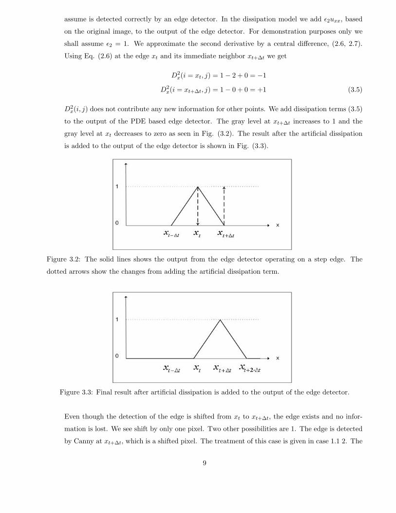
to the output of the PDE based edge detector. The gray level at xt+∆t increases to 1 and the

gray level at xt decreases to zero as seen in Fig. (3.2). The result after the artificial dissipation

is added to the output of the edge detector is shown in Fig. (3.3).

Figure 3.2: The solid lines shows the output from the edge detector operating on a step edge. The

dotted arrows show the changes from adding the artificial dissipation term.

Figure 3.3: Final result after artificial dissipation is added to the output of the edge detector.

Even though the detection of the edge is shifted from xt to xt+∆t, the edge exists and no infor-

mation is lost. We see shift by only one pixel. Two other possibilities are 1. The edge is detected

by Canny at xt+∆t, which is a shifted pixel. The treatment of this case is given in case 1.1 2. The

9

edge is detected by Canny at two points xt and xt+∆t (see Fig. (3.4)). The treatment of this case

is given in case 1.2.

Figure 3.4: The step edge is detected at both xt and xt+∆t.

case 1.1: In this case, the edge is detected at xt+∆t, the addition of the dissipation term ε2uxx

does not modify the output from the edge detector. We assume, for simplicity, that this

image has only two gray values, white (0) and black (1). The output is restricted to gray

levels between 0 and 1. If we add D2x(i = xt, j) = −1 to the value at xt, which is zero, the new

value should be less than 0, therefore, it remains 0. The addition of D2x(i = xt+∆t, j) = +1 at

xt+∆t, should exceed 1 and is again restricted. Therefore, the additional artificial dissipation

does not affect the result of a gradient-based edge detector. If the image consists of more

than two gray values, the addition of the dissipation term uxx at xt+∆t, can only strengthen

the edge. Figure (3.5) shows the influence of the addition of the artificial dissipation. In

figure (3.6) we can see the final result after the addition of the artificial dissipation to the

result of an edge detector.

10

Figure 3.5: How the dissipation affects the edge at xt+∆t. The arrows show how the edges change.

Figure 3.6: The final result after the artificial dissipation is added.

case 1.2: We consider an edge that is detected at both xt and xt+∆t. The result of an edge

detector that detects a step edge at two points can be seen in figure (3.4). By adding

the dissipation term uxx we sharpen the edge in the following way: after the addition, the

detection will be at xt+∆t only. Referring to Eq. (3.5) we see that by adding the artificial

dissipation term the value of the image at the point xt decreases, while it increases at xt+∆t.

The effects of adding the artificial dissipation terms to the output from an edge detector on

each point are shown in Fig. (3.7). Figures (3.8) is the final result.

11

Figure 3.7: How the addition of artificial dissipation affects the output from an edge detector.

Figure 3.8: The final output after adding the artificial dissipation.

We conclude that the addition of the second order dissipation term satisfies the first require-

ment by preserving the detected edge without degrading it.

case 2: Our second goal is to show that the artificial dissipation model can reconstruct edges

that are either missed or blurred by an edge detector. The reconstruction is based on the

original image. We consider a step edge as the input image, but this time the result after

the edge detector consists of zeros only. This describes the worst possible case, assuming

that the edge is missed. Figure (3.9) shows the input step edge.

As previously calculated, Eq. (3.5) gives the values at xt and xt+∆t are D2x(xt, j) = −1,

D2x(xt+∆t, j) = 1. Adding -1 to the value at xt+∆t we obtain values smaller than 0, therefore,

it remains 0. On the other hand, when we add 1 to the value of xt the missed edge is

reconstructed. The influence of this addition is illustrated in figure (3.10). The final result,

which is the reconstructed edge, is shown in figure (3.11). The artificial dissipation after it

was added to the output of the edge detector reconstructed the missed edge.

12

Figure 3.9: The input step edge.

Figure 3.10: The effect of the addition of the dissipation term uxx on a missed edge.

Figure 3.11: The final output: the reconstructed edge.

Having analyzed the effect of the dissipation operators on the physical edge in the image we now

consider the effect in the frequency domain. We reconsider the step edge that is constructed via the

solution of the advection equation ut + ux = 0. Detection of a step edge using this approach gives us

13

the following piecewise constant function:

ϕt(x) =

⎧⎪⎪⎪⎪⎪⎨⎪⎪⎪⎪⎪⎩

1h(x − xt) xt ≤ x ≤ xt+∆t

1 x = xt+∆t

1h(xt+2∆t − x) xt+∆t ≤ x ≤ xt+2∆t

0 otherwise

(3.6)

Detection of a step edge, with the step at xt+∆t, is illustrated in figure (3.12).

Figure 3.12: A step edge detected at xt+∆t.

Applying the Fourier transform on Eq. (3.6) produces

ϕt(x) =1h

∫ xt+∆t

xt

(x − xt)e−iξx dx +1h

∫ xt+2∆t

xt+∆t

(xt+2∆t − x)e−iξx dx =2

ξ2he−iξxt+∆t (1 − cos ξh) .

We see that high frequencies do not decay rapidly since the function is not sufficiently smooth because

the function is not differentiable at xt, xt+∆t, xt+2∆t. So the Fourier coefficients decay as ξ−2. We

conclude that high Fourier components contain important information that should be restored by an

edge detector. In a situation where the high component information is not fully captured, the addition

of the artificial dissipation retrieves this information from the original image.

3.2 PDE based description of roof edges

After discussing the artificial dissipation for a PDE based description of step edges, we analyze the

effect of this model on roof edges. We consider the one dimensional linear wave equation

utt − uxx = 0 (3.7)

with the initial conditions

u(x, 0) = g(x), ut(x, 0) = −g′(x). (3.8)

The solution of the one dimensional wave equation is composed of two waves; one moves to the right

and the other moves to the left.

u(x, t) = F (x + t) + G(x − t). (3.9)

14

From (3.8) F = 0, and so the solution has the form:

u(x, t) = G(x − t) = g(x − t). (3.10)

We stabilize the numerical solution of utt − uxx = 0 by adding a fourth order dissipation term uxxxx.

utt − uxx − ε4h2uxxxx = 0 (3.11)

We discretize this by

un+1m − 2un

m + un−1m

τ2=

unm+1 − 2un

m + unm−1

h2+ ε4

unm+2 − 4un

m+1 + 6unm − 4un

m−1 + unm+2

h2. (3.12)

Let unm = λneimρ, t = nτ be a solution of (3.12). We substitute this ansatz and divide by λn−1eimρ.

Then,

λ2 − 2λ + 1τ2

=λ

h2(2 cos ρ − 2) +

λ

h2ε4(2 cos 2ρ − 8 cos ρ + 6).

Define σ = τ2

h2 and θ = sin2 ρ2 , where 0 ≤ θ ≤ 1. Then,

λ2 − 2λ + 1 = −4λσθ + 2λσε4(2 cos2 ρ − 1 − 4 cos ρ + 3)

= −4λσθ + 4λσε4(2θ)2 = −4λσθ + 16λσε4θ2

So

λ2 − 2λ[1 − 2σθ + 8σε4θ2] + 1 = 0

Define C = 1 − 2σθ + 8σε4θ2. Then, λ2 − 2λC + 1 = 0 and λ = C ± √

C2 − 1. For stability we

require that |λ| ≤ 1 and so |C| ≤ 1 which implies |λ| = 1. Stability requires ε4 < 14 and then σ < 4.

However, this large value of ε4 tends to blur the edges. Instead we choose ε4 = 132 and σ < 8

7 . Hence,

adding the dissipation term makes the equation more stable.

We now describe the detection of roof edges using a PDE (Eq. (3.11)). To detect a roof edge we

examine the solution of the one dimensional linear wave equation as it advances in time. We assume

∆t = h. Consider u(x, 0), the initial condition for utt − uxx = 0. As time progresses, the initial wave

moves to the right. Figure (3.13) shows the wave at time t = 0.

15

Figure 3.13: u(x, t) at t = 0.

Consider the solution of Eq. (3.10) at times t−∆t, t and t + ∆t. Figure (3.14) shows u(x, t−∆t),

u(x, t) and u(x, t + ∆t).

Figure 3.14: Same roof edge at times u(x, t − ∆t), u(x, t) and u(x, t − ∆t) shifted ∆t from each other.

Let u(x, t) be the solution of utt − uxx = 0. An approximation of −utt with ∆t = h is

ξ(x, t) = −u(x, t + ∆t) + 2u(x, t) − u(x, t − ∆t)

Let ξ(x, t) be the solution for a roof edge. In figure (3.15) we plot −ξ(x, t).

Figure 3.15: The detection of a roof edge is interpreted as −ξ(x, t).

16

The numerical stability is stabilized by adding the artificial dissipation term uxxxx which is calculated

from the original image. As for the step edge case, the addition of uxxxx has to satisfy three requirements:

1. Roof edges that are detected correctly by the edge detector should not be degraded.

2. Missed roof edges should be detected and reconstructed.

3. Blurred or aliased roof edges should be enhanced.

case 1: reconstruction of a roof edge that is missed or blurred . Taking a closer look at the

structure of the roof edge, we realize that the addition of a second order dissipation term will not

reconstruct the lost information and we have to use a fourth order dissipation term. To follow

the reconstruction process, we look at a roof edge with a slope ±(1 − ε) and size 2k + 1 points.

This is shown is figure (3.16). The reconstructed information will be retrieved from the original

image by applying a fourth order dissipation operator as given in Eq. (2.7).

Figure 3.16: A roof edge with slopes ±(1 − ε).

We choose the distance between the grid points as h = 1 and use Eq. (2.7) to compute the

postprocessing for the pixels xt−∆t, xt and xt+∆t. We get:

D4x(i = xt−∆t, j) = −2(1 − ε)

D4x(i = xt+∆t, j) = −2(1 − ε)

D4x(i = xt, j) = 4(1 − ε).

(3.13)

The fourth order dissipation term added to the image is −uxxxx. Hence, the response at xt−∆t

and xt+∆t is positive (see figure (3.17)). Although the extreme point of the roof is not enhanced,

by choosing ε4 large enough we can reconstruct the roof edge information. We also get a response

at xt−k∆t and xt+k∆t since there is a discontinuity in the first derivative of the roof function. In

figure (3.17) we see the points where the fourth order operator gives a positive response. At these

points the artificial viscosity increases the gray value, and so reconstructs the lost edge.

17

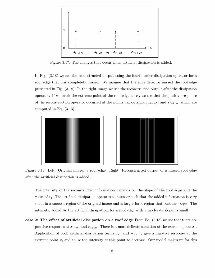
Figure 3.17: The changes that occur when artificial dissipation is added.

In Fig. (3.18) we see the reconstructed output using the fourth order dissipation operator for a

roof edge that was completely missed. We assume that the edge detector missed the roof edge

presented in Fig. (3.18). In the right image we see the reconstructed output after the dissipation

operator. If we mark the extreme point of the roof edge as xt, we see that the positive response

of the reconstruction operator occurred at the points xt−∆t, xt+∆t, xt−k∆t and xt+k∆t, which are

computed in Eq. (3.13).

Figure 3.18: Left: Original image: a roof edge. Right: Reconstructed output of a missed roof edge

after the artificial dissipation is added.

The intensity of the reconstructed information depends on the slope of the roof edge and the

value of ε4. The artificial dissipation operates as a sensor such that the added information is very

small in a smooth region of the original image and is larger for a region that contains edges. The

intensity, added by the artificial dissipation, for a roof edge with a moderate slope, is small.

case 2: The effect of artificial dissipation on a roof edge From Eq. (3.13) we see that there are

positive responses at xt−∆t and xt+∆t. There is a more delicate situation at the extreme point xt.

Application of both artificial dissipation terms uxx and −uxxxx give a negative response at the

extreme point xt and cause the intensity at this point to decrease. Our model makes up for this

18

loss by adding information about the edge at the two points that are near its top. Figure (3.19)

shows the effect of the artificial dissipation operators on a roof edge that is detected correctly. In

the left image we see a correct detection of a roof edge. The input is the roof edge in the original

image of Fig. (3.19) (left). In the right image we see the effect after the artificial dissipation

operator is added. We see that the gray value at the extreme point slightly decreases and the

detection is spread over five points instead of one (see Fig. (3.19) right).

Figure 3.19: Left: Roof edge detected correctly by an edge detector. Right: Result after adding the

retrieved information to the output of edge detector.

4 Choosing the coefficients ε2 and ε4

In section 3 we reviewed the properties of the artificial dissipation add-on model when applied to step

and roof edges. The derivative of the one-dimensional advection equation describes the detection of

a step edge. In order to enhance a step edge that is degraded after applying an edge detector, we

add a second order dissipative term uxx. The second derivative of the one dimensional wave equation,

describes the detection of a roof edge. A degraded roof edge is enhanced by the addition of a fourth

order dissipative term uxxxx. We defined a set of operators for the implementation of the add-on model

(see (2.8 - 2.11)).

An image frequently contains both step and roof edges. When reconstructing degraded or blurred

edges, we apply a sequence of operators, in all the directions. Some of these operators enhance step

edges while the others enhance roof edges. The operators that enhance step edges are an approximation

to the second derivative uxx (see (2.6)). Operators for enhancing roof edges are an approximation to the

fourth derivative uxxxx (see (2.7)). The result of each operator is multiplied by a coefficient and then

added to the output of a gradient-based edge detector. The operators are applied in four directions:

x, y, y = x and y = −x, where y = x and y = −x are denoted by µ and ν respectively. The total

dissipation is given by Eq. (2.5).

We want to estimate the values of ε2 and ε4. We refer to two cases that affect this choice.

19

1. The effect of the fourth order dissipation operator on a step edge.

2. The effect of the second order dissipation operator on a roof edge.

case 1: Effect of the fourth order dissipation operator on a step edge The one dimensional ad-

vection equation with the addition of dissipative terms has the form

ut + ux − hε2uxx + h3ε4uxxxx = 0.

Consider the step edge

u(x, t) =

⎧⎨⎩ 1 x ≤ xt

0 otherwise.

In section 3.1 we showed that the second order dissipation operator described in Eq. (2.6) enhances

the point xt+∆t. The fourth order dissipation operator, −uxxxx, affects the points xt+∆t and xt−∆t.

−D4x(i = xt−∆t, j) = −(1 − 4 + 6 − 4 + 0) = +1.

−D4x(i = xt, j) = −(1 − 4 + 6 − 0 + 0) = −3.

−D4x(i = xt+∆t, j) = −(1 − 4 + 0 − 0 + 0) = +3.

−D4x(i = xt+2∆t, j) = −(1 − 0 + 0 − 0 + 0) = −1.

(4.1)

The second order dissipation operator with ε2 large enough produces the correct effect. In addi-

tion, the fourth order dissipation operator enhances the point xt−∆t, when there is no need to do

so. We conclude that there is a resemblance between the effect of the second and fourth order

dissipation operators on a step edge. It is not required for ε4 to be large for the fourth order

dissipation operator to enhance a step edge.

case 2: Effect of second order dissipation on a roof edge. Consider the wave equation, (3.7).

We add a constant multiple of a fourth order dissipative term to get utt − uxx − h3ε4uxxxx = 0.

One cannot add a second order dissipative term to the wave equation. Consider a roof edge of

width 2k + 1 points, with an extremal point at xt. As shown in section 3.2, the value at the

extremal point xt is degraded. The dissipation operator degrades the value at the extremal point.

To reconstruct a missed or blurred roof edge we enhance it with fourth order operators. ε4 needs

to be large enough to affect the result.

4.1 Choice of the values of ε2 and ε4

We first estimate ε2. Consider a binary image with zero for black and one for white. Assume that the

image contains a step edge that is missed by an edge detector. We wish to reconstruct the edge by

20

adding artificial dissipation operators. The four operators that implement the second order dissipation

term will contribute the most in the reconstruction process. We showed that the operator along the

edge, does not contribute to the reconstruction. Therefore, only three of the four operators affect the

edge enhancement process, which implies ε2 = 13 .

The value of ε2 is applied to binary images. For gray level images we found that the results are

improved when a larger ε2 is chosen. Therefore, we choose

ε2 =12. (4.2)

This corresponds to changing the central difference to a one-sided difference, (3.1).

The effect of the second order dissipation coefficient on a roof edge is described above. The second

order operator degrades the value of the extremal point of the roof edge. The fourth order operators

have the same effect at this point. Therefore, we focus on enhancing the two points that are near the

extremal point of the roof edge instead of the extremal point itself. Since the second order operators

have no effect on the value of the two points next to the extremal point of a roof edge, the value of ε2

can be large, and we can still reconstruct missed or blurred roof edges.

Now we estimate the value of ε4. The effect of the fourth order operators have on a roof edge

depends on its slope. If the roof edge has a moderate slope, we do not want to enhance it too much.

The effect on a roof edge with a steep slope will be more noticeable, therefore, ε4 should not have too

large a value. Experiments demonstrate that the value of ε4 = 0.025 produces good results. Another

reason for keeping ε4 relatively small is the effect the fourth order operators have on step edges. We

showed that the fourth order operator affects two points of the step edge. Increasing the value of ε4

makes the output too noisy, as information is added to points that are in a relatively smooth area. Our

final choice for ε4 is

ε4 =132

∼ 0.03 . (4.3)

The parameters ε2 and ε4 can be adaptively tuned to achieve the best performance. The use of

these values produced very good results on a large variety of images. The same values are used in

all our experiments described in section 5. A generalization of this would be to make the parameters

depend on the normalized gradients of the picture. Hence, ε2 and ε4 would be small in regions where

the gradients are small. A similar process is used in CFD to reduce ε2 in smooth regions of the flow.

A typical detector, in the x direction, for this is [11]

|I(i + 1, j) − 2I(i, j) + I(i − 1, j)|δ (I(i + 1, j) + 2I(i, j) + I(i − 1, j)) + (1 − δ) (|I(i + 1, j) − I(i, j)| + |I(i, j) − I(i − 1, j)|) (4.4)

With 0 ≤ δ ≤ 1. A more non-linear scheme is suggested by Jameson in the CUSP scheme [6].

21

4.2 Pseudo code of the algorithm

We present a pseudo code describing the implementation of the algorithm. The input contains two

files: 1. The original image. 2. Description of the edges after applying an edge detector on the original

image. We apply the artificial dissipation operators on the original image. This is kept in a temporary

array which we call “temp” and is initialized.

The artificial dissipation operators are given by Eqs. (2.8 - 2.11). The eight artificial dissipation

operators are denoted as D2x,D4

x, D2y, D4

y, D2µ, D4

µ, D2ν and D4

ν .

The pseudo code for the algorithm is:

1. (a) For each pixel (i, j) in the original image compute D2x ( Eq. (2.8)).

(b) Multiply the result from D2x by ε2.

(c) Add this value to pixel (i, j) in the “temp” image.

(d) For each pixel (i, j) in the original image compute D4x (Eq. (2.8)).

(e) Multiply the result from D4x by −ε4.

(f) Add this value to pixel (i, j) in the“temp” image.

2. Repeat these operations when D2x is replaced with D2

y ( Eq. 2.9), D2µ (Eq. 2.10) and D2

ν ( Eq.

2.11) and D4x is replaced with D4

y ( Eq. 2.9 ) , D4µ ( Eq. 2.10) and D4

ν ( Eq. 2.11).

3. For the final result add the“temp” image with the output of an edge detector.

5 Results

We now demonstrate that adding an artificial dissipation to the output of an edge detector gives

enhanced results. The effects of using the diagonal dissipation are presented in Figs 6.1a-6.1d. We see

that Fig. 6.1b has a much better description of the scarf especially parallel to the stripes in the scarf.

Adding the dissipation in the diagonal directions gives an even better description of theses stripes as

seen in Fig. 6.1d. In the larger picture of Barbara we compare the improved algorithm with the original

Canny edge detector. We see that the edges on Barbara’s scarf which are blurred and aliased in Fig.

6.2a are reconstructed in Fig. 6.2b. In addition the edges of the map and chair are sharpened. In

Figs. 6.3a - 6.3c we show a closeup of Barbara’s scarf. Canny detected 30% of the edges and after the

artificial dissipation was added - 88% of the edges were detected.

We next consider a racing car. We see in Figs. 6.4b-6.4c that the text is much clearer when the

artificial dissipation is added to the Canny edge detector. In Figs. 6.5a - 6.5c we show a blowup of the

car hood. The lettering in Fig. 6.5c is much clearer than in Fig. 6.5b. While Canny detected only

42% of the edges, adding artificial dissipation raised the percentage of detected edges to be 95%. The

22

improvement is even more obvious in the images of the tools shown in Figs. 6.6b-6.6c. The carpet

is almost non-existent in the original Canny detection but shows up nicely after the addition of the

artificial dissipation. Similarly the end of the couch in the top-right corner is unclear due to the cloth

in the Canny detector but again is clear in the improved version of the edge detector. In summary

many new edges are reconstructed in Fig. 6.6c compared with Fig. 6.6b. This is especially noticeable

in the lines in both the couch and the carpet.

6 Conclusions

We introduce an algorithm for edge enhancement in gray level images. We reconstruct edges that

are missed or blurred by a gradient-based edge detector while preserving the edges that are correctly

detected. The improvement is accomplished by adding artificial dissipation operators, based on the

original image, to the output from gradient based edge detector. To recover a binary image thresholding

is used. An alternative would be to apply the Canny algorithm to the enhanced image. The results

demonstrate that many more edges are found and the texture is improved when the Canny edge detector

is supplemented by the artificial dissipation.

Figure 6.1a: Barbara’s scarf - the original image

Figure 6.1b: The edges of Barbara’s scarf detected by the Canny edge detector

23

Figure 6.1c: Edges of Barbara’s scarf detected by Canny with dissipation add-on in x and y directions

Figure 6.1d: Edges of Barbara’s scarf detected by Canny with dissipation add-on in all four directions

Figure 6.2a: The original image.

24

Figure 6.2b: The output from Canny edge detector.

Figure 6.2c: The output from a Canny edge detector with artificial dissipation add-on.

Figure 6.3a: Zoom of the original image (Fig. 6.2a).

25

Figure 6.3b: Zoom of result from Canny edge detector.

Figure 6.3c: Zoom of result from Canny edge detector + additional artificial dissipation.

Figure 6.4a: The original image.

26

Figure 6.4b: The output from a Canny edge detector.

Figure 6.4c: The output from a Canny edge detector + additional artificial dissipation.

Figure 6.5a: Zoom of the original image (Fig. 6.4a).

27

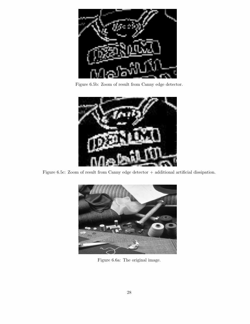
Figure 6.5b: Zoom of result from Canny edge detector.

Figure 6.5c: Zoom of result from Canny edge detector + additional artificial dissipation.

Figure 6.6a: The original image.

28

Figure 6.6b: The output from a Canny edge detector. Many of the edges are missing.

Figure 6.6c: The output from a Canny edge detector + artificial dissipation

6.1 Noisy images

The dissipation operator amplifies the noise in the original image. If we add it to the output from

the Canny edge detection the outcome will be very noisy. Therefore, we add an additional check: The

gradient in the output from the Canny edge detection is computed for each pixel. If the gradient is

zero the dissipation term is not added to this pixel. Otherwise, dissipation is added. The left images

in Figs. 6.7 - 6.10 were added with 5-20% of uniform noise.

29

Figure 6.7: Left: Original image with the additional of 5% uniform noise. Middle: The output from

the application of the Canny edge detection on the left image. Right: The output from a Canny edge

detector + artificial dissipation on the left image.

Figure 6.8: Left: Original image with the additional of 10% uniform noise. Middle: The output from

the application of the Canny edge detection on the left image. Right: The output from a Canny edge

detector + artificial dissipation on the left image.

30

Figure 6.9: Left: Original image with the additional of 15% uniform noise. Middle: The output from

the application of the Canny edge detection on the left image. Right: The output from a Canny edge

detector + artificial dissipation on the left image.

Figure 6.10: Left: Original image with the additional of 20% uniform noise. Middle: The output from

the application of the Canny edge detection on the left image. Right: The output from a Canny edge

detector + artificial dissipation on the left image.

References

[1] L. Alvarez, P.-L. Lions and J.-M. Morel, Image Selective Smoothing and Edge Detection by Nonlinear

Diffusion, SIAM J. Numer. Anal. 123:199-257, 1992.

[2] J. Canny, A computational approach for edge detection, IEEE Trans. Pattern Anal. Machine Intell.,

vol. 8, no. 6, 679-698, 1986.

31

[3] J. Froment and S. Mallat, Second generation compact image coding with wavelets, in Chui CK (ed.)

Wavelets: A Tutorial in Theory and Applications, Vol. 2, Academic Press, 655-678, 1992.

[4] R.C. Gonzalez and R.E. Woods, Digital Image Processing - Second edition Prentice Hall, Upper

Saddle River, New Jersey, 2002.

[5] A. Jameson, W. Schmidt and E. Turkel, Numerical Solutions of the Euler Equations by Finite

Volume Methods Using Runge-Kutta Time-Stepping Schemes AIAA Paper 8l-l259, 198l.

[6] A. Jameson, Analysis and Design of Numerical Schemes for Gas Dynamics I: Artificial Diffusion,

Upwind Biasing, Limiters and their Effect on Accuracy and Multigrid Convergence, Inter. Jour.

Comput. Fluid Dynamics, 4:171-218, 1995.

[7] J.R. Parker, Algorithms for Image Processing and Computer Vision John Wiley & Sons, New York,

1997.

[8] P. Perona and J. Malik, Scale Space and Edge Detection using Anisotropic Diffusion, IEEE Trans.

Pattern Anal. Machine Intell., 12:629-639, 1990.

[9] L.I. Rudin, S. Osher and E. Fatemi, Nonlinear Total Variation Based Noise Removal Algorithms,

Physica D 60:259-268, 1992.

[10] N. Sochen, R. Kimmel and A.M. Bruckstein, Diffusions and Confusions in Signal and Image

Processing, Kluwer Academic Publishers, the Netherlands, 2001.

[11] R.C. Swanson and E. Turkel, On Central Difference and Upwind Schemes, Journal Comput.

Physics, 101:292-306, 1992.

[12] J. Weickert, Anisotropic Diffusion in Image Processing B.G. Teubner, Stuttgart, 1998.

[13] Y-L You, Fourth-Order Partial Differential Equations for Noise Removal, IEEE Trans. Image

Proc., 9:1723-1730, 2000.

32