Economics Units 3+4 Notes

UNIT 3 NOTES CHAPTER 1 NOTES

Definitions: Living standards:

Material: Level of economic wellbeing of individuals. It relates to quantity of goods and services

available for consumption, or GDP per capita. (Assuming equitable income distribution).

Non-Material: General happiness, affected by living conditions, freedom, peace, health, environment,

crime etc.

Relationship: Increase in material can lead to decrease in non-material, due to increased pollution,

stress etc.

Economics: Study of how to use our limited resources in a way that maximises the quantity of goods

and services produced to meet the unlimited needs and wants of society.

Scarcity: There will always be limited resources and unlimited needs and wants.

Resources:

Natural: Land, Oil, minerals, water etc.

Labour: Human, both physical and intellectual.

Capital: Manufactured items used to help create other goods and services. Machines etc.

Opportunity Cost: The value of the next best alternative foregone. In order to produce one thing we

must forgo producing something else, due to our limited resources.

Opp. Cost exists for individuals, businesses and governments.

Production Possibility Frontier: Limit of production between 2 items, given constant level of resources.

Point B has highest total production – maximises efficiency.

Point X has underuse of resources – inefficient.

Point Y is unattainable, and attempting to reach it will

cause inflation, due to demand outstripping supply.

To increase the PPF (moving it left) we need to acquire

more resources or use the current ones more efficiently.

Efficient allocation of resources: Desirable situation where

our scarce resources are used in ways that maximise our

production levels or GDP.

Markets 1. What and how much to produce? Consumer sovereignty provides for 80% of resource

allocation. Government allocates other 20%. Consumers dictate by their choices what they want

produced, and businesses do so in order to make profits.

2. How to produce? Method of production, use of machinery. Usually aims to cut costs.

3. For whom to produce? Who does the profit go to? In Australia’s capitalist system, owners

(shareholders) keep profits.

Types of markets:

Pure competition: Many sellers – very strong competition – no product/brand differentiation – ease of

entry/exit into market – ‘price takers’ – compete only on price. Example – fruit & veg markets.

Monopolistic competition: Many sellers – some small product differentiation – some brand loyalty –

moderate ease of entry. Example – restaurants.

Oligopoly: Few sellers – large product differentiation – large brand loyalty – difficult ease of entry.

Example – airlines, banks.

Monopoly: One seller – weak/no competition – no differentiation – very difficult/impossible entry into

market – ‘price taker’ – sets own prices. Example – Australia Post.

Advantages and disadvantages of competition:

Advantages: Forces firms to increase quality and decrease prices, increases exportability.

Disadvantages: Super-aggressive cost-cutting could reduce product quality and safety.

Preconditions for a competitive market:

1. Consumer sovereignty: Consumers dictate how resources are to be used.

2. Identical products.

3. Ease of entry

4. Firms want to maximise profits – do so by cutting costs.

5. Consumers and sellers have the same information.

Laws and characteristics of demand and supply:

Demand

Demand has an inverse relationship with price – the lower the price, the more of a product is

demanded.

Price elasticity of demand:

Elastic demand: Demand is elastic if a small change in price will cause a large change in quantity

demanded.

Unit elasticity: Change in demand is exactly proportionate to change in price – 10% fall in price = 10%

rise in demand.

Inelastic demand: Demand is inelastic if a large change in price will only cause a small change in

quantity demanded.

Determinants of demand elasticity:

1. Type of item: Necessities will be inelastic, whereas luxury and unnecessary items will be elastic

2. Substitutability: Items that can easily be substituted (e.g. soft drinks) will have elastic demand,

whereas items that cannot be substituted (cigarettes) will have inelastic demand.

3. Time period: In the short term it may be harder to find alternatives, so demand will be inelastic,

but in the long term demand will always be elastic.

4. Cost and relative importance: Cheaper items will be more inelastic, whereas expensive items

will be more elastic.

5. Complementary items: Cheap complementary items that are used with expensive products (e.g.

water for a swimming pool) will have inelastic demand.

Factors affecting demand:

1. Changes in wages and disposable income levels

2. Changes in interest rates

3. Changes in prices of substitutes or complementary items

4. Changes in consumer confidence

5. Changes in population size

Supply

Supply has a direct relationship with price, meaning that as prices rise, quantity supplied will increase.

Price elasticity of supply:

Elastic: Small change in price leads to large change in quantity supplied.

Unit elasticity: Proportionate change in price/supply – 10% rise in price = 10% increase is supply.

Inelastic: Large change in price only causes small change in quantity supplied.

Determinants of supply elasticity:

1. Storability: If an item can be stored for a long time (paper) then it will have elastic supply as

suppliers can immediately release higher quantities to the market. If an item cannot be stored

(fresh fruit) then suppliers cannot increase supply, regardless of price changes.

2. Resource mobility and unused industry capacity: If resources can quickly be procured to

increase production, or there are spare resources that can be activated, then supply is elastic as

more can be immediately produced.

3. Time period: In the short term it is difficult to increase supply, but in the long term it will always

be possible. E.g. fruit growers – takes time to grow fruit.

Factors affecting supply:

1. Changes in profitability

2. Changes in wages and production costs

3. Changes in interest rates

4. Changes in company tax rates

5. Changes in government assistance/subsidies

Equilibrium price: The price at which the demand and supply lines meet = market price.

Effect of increases in demand/supply:

In general, the bigger the demand (i.e. the further right it moves), the higher the equilibrium price,

and vice versa.

The higher the supply (i.e. the further right it moves) the lower the equilibrium price, and vice versa.

Market failure

Types of market failure and their solutions:

Markets fail when socially undesirable goods are overproduced – government increases tax to slow

production.

Markets fail when socially desirable goods are under-produced – government gives subsidies to increase

production, or produces it themselves.

Markets fail when competition is weak – government aims to increase competition by disallowing anti-

competitive practices (ACCC), deregulating markets, and reducing tariffs.

Markets fail when there is asymmetric information – if the seller knows more than the buyer, he can

claim an unfair price.

Markets fail when externalities occur – when third parties are affected by the transaction by pollution,

noise, etc.

Markets fail because of the ‘free-rider’ problem – when public goods or services are non-excludable,

e.g. defence, street lighting, there is no way to force consumers to pay for it, thus reducing profit for

producers. Since producers don’t want to manufacture these goods, the government must do it instead.

Government failure:

Minimum wage: The minimum wage set a floor price for labour, causing unemployment. Rectified by

enterprise bargaining.

Tariffs – decreased competition and hence efficiency.

Regulation of markets e.g. airlines, banks, caused decreased competition and hence efficiency.

CHAPTER 2 NOTES

Economic Activity: Term that relates to the actions of individuals, firms and governments to help generate

goods and services, employment, and incomes.

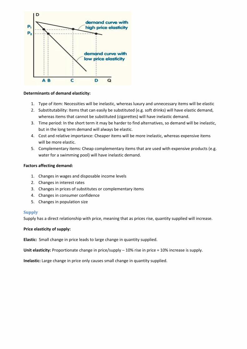
The business cycle diagram:

Peak: Unemployment at lowest level – demand inflation at highest point – may result in a boom where

resources are fully used but are not able to meet demand.

Ideal: Ideal point on the graph. Found on long-term-trend line midway between peak and a boom. Here

unemployment due to lack of demand is not high, and demand inflation is not high.

The government will use demand-side policy to steer the economy to this point.

Trough: High unemployment due to lack of demand – low inflation – may be a recession (2 quarters of

negative economic growth), if severe.

Indicators and measurements

Economic activity: Measured by the Australian Bureau of Statistics using Gross Domestic Product. GDP

is the measure of the total spending on Australian finished goods and services. Chain-volume GDP takes

into account inflation.

Non-market activity: Activity that isn’t bought or sold, e.g. household chores, volunteer work.

Indicators:

Lagging indicators: Indicators which reveal how the economy was previously, for example GDP, as by

the time the data has been collated and released, some time has passed.

Coincident indicators: Indicators which reveal how the economy is performing at that point in time, e.g.

monthly retail sales.

Leading indicators: Indicators which predict how the economy will perform in the future, e.g. consumer

or business confidence.

Effects of economic growth on living standards: Material: In the short term will increase due to higher GDP per capita. May decrease later if resources

are used up.

Non-material: May increase in the short term due to improved conditions, but could decrease in the

short and long term due to stress, pollution, climate change.

Aggregate Demand Definition: Total aggregate spending on locally made goods and services.

Consists of: Consumers (C) + Business Investment (I) + Government consumption and investment (G1

and G2) + Net exports (Exports (X) – Imports (M)).

Demand-side economic theory developed by John Maynard Keynes in the 1930’s. Keynes said that

instability in the components of AD was responsible for cyclical upswings and downswings in the

economy.

Rising AD causes increased consumption and hence increased production. May cause boom and

inflation.

Falling AD causes reduced consumption and hence decreased production. May cause recession and

unemployment.

Ideal level of AD is when growth is neither excessive nor insufficient.

Aggregate Demand theory does not account for stagflation – rising prices but falling production.

Components of Aggregate Demand

Private consumption (C): Represents 60% of AD. Mostly affected by consumer confidence, household

disposable income, interest rates. Mostly stable.

Private investment (I): Business spending on capital equipment. Approximately 22% of AD. Mostly

affected by business confidence, tax and interest rates. Quite unstable – major cause of changes in AD.

Government consumption (G1): Government spending on its own running costs, as well as ongoing

expenses such as health, education and defence. Represents 16% of AD, but changes due to factors such

as population size, election promises, budget income and the state if the economy.

Government investment (G2): Public expenditure on capital equipment. Improves our production

capacity. Around 3% of AD, but changes due to economic conditions, population size.

Net exports (X – M): Difference between foreign spending on our exports and our spending on foreign

products. Typically around + or – 4%. Behaves erratically, affected by the terms of trade index,

consumer and business confidence, domestic and overseas economic conditions.

Factors affecting Aggregate Demand 1. Consumer confidence (C, M) – relates to households expectations about future employment

and income. The higher the consumer confidence, the higher C and M will be and vice versa.

2. Business confidence (I, M) – relates to business expectations about future profits. The higher

the business confidence, the higher I and M will be and vice versa.

3. Overseas economic activity (X) – overseas conditions affect exports as during an overseas

recession demand for our exports drops and vice versa.

4. Household disposable income (C, M) – money available for spending by households after tax.

The higher the disposable income (due to tax changes) the higher C and M will be, and vice

versa.

5. Exchange rate (X, M) – when the Australian dollar is high, we get less for our exports so they

drop, and our imports cost less so they rise, and vice versa.

6. Terms of Trade index (X, M) – calculated by (export price index)/(import price index) x 100. The

higher the index, the more we are getting for our exports relative to imports, so the higher X is

compared to I.

7. Population growth rate (C, G, M) – the faster the population grows, the quicker demand

increases.

8. Budgetary policy (All) – Expansionary policy increases demand, contractionary policy decreases

it.

9. RBA interest rates (C, I, X, M) – high interest rates cause demand to fall and vice versa.

Aggregate supply

Definition: Total annual quantity of all finished goods and services produced in Australia.

Development: Was the favoured theory pre-Keynes. Adam Smith, John Stuart Mill and Jean Batiste Say

were its main proponents.

Characterised by Say’s Law: ‘Supply creates its own demand’, meaning that the more that is produced,

the more that will be spent. Limited resources would be the only factor affecting economic growth.

Disproven by the Great Depression.

Revitalised by Arthur Laffer, proponent of ‘Reagonomics’ which advocated creating favourable supply-

side factors to increase production, such as incentivisation.

In order for AD to increase without causing inflation, AS must increase also. Therefore governments will

always work to make favourable supply-side factors to increase production.

Determinants of aggregate supply:

1. Quantity, quality, and efficiency of resources available: The more resources we have, the

higher quality they are, and the more efficiently they are used, will increase our productive

capacity. New discoveries of resources, or increases in research, education and technology

allowing them to be used better, will increase AS.

2. Business profit levels: When business profits are high, businesses invest in more capital

equipment, allowing them to produce more in the future.

3. All production costs: When production costs (Real unit labour costs (wage costs per unit),

interest rates, costs of materials, exchange rates causing materials from overseas to be more

expensive) go up, business profits fall and AS falls.

4. Labour force participation rates: The more labour available, the cheaper it is, and the more

labour resources businesses can afford in order to produce, so production and AS increase.

5. Government aggregate supply-side policies: E.g. on immigration, tariffs, subsidies, incentives,

tax breaks, legislation like carbon trading scheme, deregulation, privatisation, all impact on

resource allocation, costs, employment, incomes and living standards.

Recent trends in demand and supply side factors:

FACTOR PEAK: 2005-08 TROUGH: 2008-09 (Global Financial Crisis)

RECOVERY: 2009-10

DEMAND SIDE FACTORS

Consumer and Business Confidence

Consumer confidence above average - range from 103-117. Business confidence also very strong. Caused high (C) and (I), boosting AD.

Massive fall in consumer optimism – down to 85 points. Businesses wary of falling demand, cut investment. Large drops in (C) and (I).

Slow rises in consumer confidence, aided by RBA interest rate rises. Massive rises in business confidence. Caused increases in (C), (I) and (M).

Overseas Activity

Major trading partners having boom periods, boosted demand for exports. Record high Terms of Trade index – 130 points – meant value of exports rose relative to imports.

Impact of Global Financial Crisis – recessions for most major trading partners. Caused large drop in demand for exports.

Demand for exports (particularly from China) rose as overseas countries recovered from recession, hence boosting exports and AD.

Population Growth

Surge in Australia’s birth-rate and increase in immigration causes population to grow at 1.3 – 1.6%, above normal growth. This causes stronger demand for (C) and higher levels of AD.

Drop off in immigration (skilled workers program) causes population growth to slow, reducing AD growth.

Still small levels of population growth not helping the recovery.

Government Budgetary Policies and RBA Monetary Policies

Contractionary policy to reduce (G) and hence AD growth in order to prevent inflation. RBA interest rates also very high.

Expansionary policy to avoid recession and aid recovery - $22 billion infrastructure plan, stimulus package. RBA interest rate down to record low.

Expansionary policy still in place to aid recovery. Interest rates rising to prevent growth becoming too strong.

SUPPLY SIDE FACTORS

PEAK: 2005-08 TROUGH: 2008-09 (Global Financial Crisis)

RECOVERY: 2009-10

Government Policies for AS

Tax reform to lower business costs. Efforts to procure more resources to expand productive capacity, allowing AS to increase.

Increased incentives to businesses to keep AS up, including tax rebates, subsidies, and business car program.

Reduced business incentives and grants, but there are still some in place to help lift AS.

Falling Real Unit Labour Costs

Fall in average annual change of RULCs of about 0.7%. Caused extra business profitability, increasing business investment and hence productive capacity.



Bottlenecks Serious bottlenecks and shortages limited growth in Australia’s productive capacity. Especially in areas of skilled labour and infrastructure.

Government announced plans for major infrastructure projects and skilled migrant program to increase productive capacity and hence future levels of AS.

Continued expansion of infrastructure projects to increase productive capacity and hence AS.

Productivity Cycle

Small growth in labour productivity (1.1% pa) caused small growth in productive capacity and hence AS.

Less business investment in capital equipment and labour due to GFC caused drop in productive capacity, lowering AS.

Increased business investment and government infrastructure projects expand productive capacity and hence AS.

CHAPTER 3 NOTES

Government goal of low inflation

Definitions Inflation: Sustained increase in prices of goods and services over time.

Deflation: When the prices of goods and services are decreasing over time.

Disinflation: When there is inflation, but at a decreasing rate.

Measuring inflation

The ABS measures inflation quarterly using the Consumer Price Index. The index takes a base year

(1989-90) of 100 points, and calculates the percentage rise each year.

The index is based on the regimen – the basket of approx 100,000 commonly used goods and services,

subdivided into categories, e.g. food, transportation. The ABS reviews and changes the regimen

periodically. Items in the regimen are given different weightings in the calculation to account for their

relative importance, e.g. food and housing are worth more than alcohol.

The prices surveyed are those of major retailers, e.g. Coles, Myer.

Annual CPI rise (%) =

Limitations of the CPI as a measure of inflation:

1. The CPI is not representative of all households, as it is biased towards metropolitan households.

Additionally, some items in the regimen may not be applicable to some households.

2. The effect of one-off volatile events could affect the index, e.g. the prices of fruit can be

affected by sudden floods or droughts. The underlying price index takes this into account by

removing volatile items from the regimen.

3. The base year is arbitrary, and may have been particularly high/low, affecting the future CPI

calculations.

Government goal of low inflation Government goal of low inflation: That inflation be low and below that of our major trading partners,

typically 2-3%.

<2% or negative inflation is not desirable would indicate that there is little to no economic growth.

Effects of high inflation on living standards:

1. High inflation puts local producers and exporters at a competitive disadvantage compared to

overseas producers, as high inflation increases their prices. Hence there are lower profits, forces

closures and redundancies, reduces living standards. However importers may see benefits.

2. High inflation undermines economic growth, as it erodes consumer and business confidence

and causes increased interest rates.

3. High inflation encourages inefficiency in resource allocation, as those with wealth will invest in

speculative assets, e.g. property and shares. While this increases their own living standards, it

reduces the amount of investment in productive assets. This eventually harms economic

growth. Increase in speculative investment as opposed to productive investment.

4. Fixed income earners cannot cope with the rising prices as their incomes cannot increase to

compensate for them, hence their living standards suffer. However speculators can make large

gains during times of high inflation.

5. Higher interest rates will affect variable mortgages, reducing the living standards of those with

large mortgages.

Recent trends in the inflation rate

Inflation rates were generally within the goal rate, averaging 3.1% over the 10 years prior to 2008.

Occasional spikes, such as in 2001, 06, 08 put inflation way above goal rate, as high as 4.5%.

Due to GFC in late 2008, inflation fell to below the goal rate, down to 1.5%.

Factors affecting inflation:

In general, factors causing high economic activity will also increase inflation, and vice versa.

Anything causing higher prices for producers, e.g. higher exchange rate, drought, oil prices etc will

increase cost inflation, and vice versa.

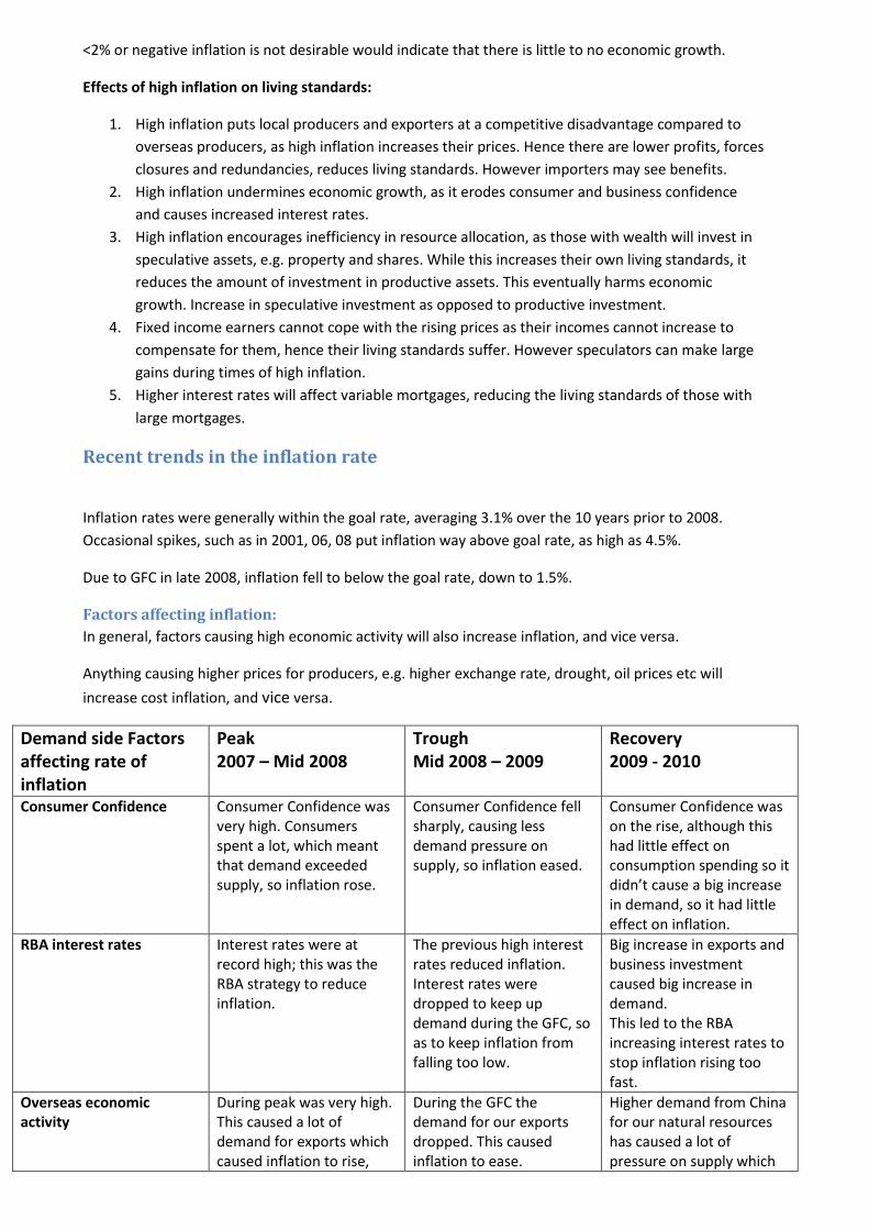
Demand side Factors affecting rate of inflation

Peak 2007 – Mid 2008

Trough Mid 2008 – 2009

Recovery 2009 - 2010

Consumer Confidence Consumer Confidence was very high. Consumers spent a lot, which meant that demand exceeded supply, so inflation rose.

Consumer Confidence fell sharply, causing less demand pressure on supply, so inflation eased.

Consumer Confidence was on the rise, although this had little effect on consumption spending so it didn’t cause a big increase in demand, so it had little effect on inflation.

RBA interest rates Interest rates were at record high; this was the RBA strategy to reduce inflation.

The previous high interest rates reduced inflation. Interest rates were dropped to keep up demand during the GFC, so as to keep inflation from falling too low.

Big increase in exports and business investment caused big increase in demand. This led to the RBA increasing interest rates to stop inflation rising too fast.

Overseas economic activity

During peak was very high. This caused a lot of demand for exports which caused inflation to rise,

During the GFC the demand for our exports dropped. This caused inflation to ease.

Higher demand from China for our natural resources has caused a lot of pressure on supply which

could lead to an increase in inflation.

Supply side Factors affecting rate of inflation

Peak 2007 – Mid 2008

Trough Mid 2008 - 2009

Recovery 2009 - 2010

Rising oil prices

Demand continues to outstrip supply during boom period. Supply restricted due to political conditions and wars.

Cost inflation in production of oil decreased therefore allowing an increase in supply allowing prices to fall.

Recently prices have continued to rise since supply has been restricted.

Changing exchange rate Exchange rate rose strongly making imports cheaper for Australians. Buy raw materials from overseas, thus production costs are low. This eased cost inflation

Australian $ fell due to poor economic patterns, which increased cost of importing materials and equipment. These rises were passed onto consumers. This accelerated cost inflation.

Exchange rate rose strongly making imports cheaper for Australians. Buy raw materials from overseas, thus production costs are low. This eased cost inflation

Wage costs Under the fair pay commission: Increase in the min wage by $60 a week, adding to production costs and rising inflation prices. Enterprise bargaining system: Increase of around 4% due to growing labour shortages contributing to cost pressures and inflation.

Wage prices were negotiated based on productivity rises, thus easing cost pressures on firms.

Wage prices were negotiated based on productivity rises, thus easing cost pressures on firms.

Cost of materials Costs grow sharply at an average of over 10% per year, adding to cost inflation. Commodities boom, prices high. Mainly due to overseas countries like China.

Due to poor exchange rate conditions, cost of imported materials rose. Commodities boom disappeared during the trough due to GFC.

In risk of commodities boom due to recovery in China and India.

Interest rates RBA increased interest rates adding to production costs and cost inflation.

Interest rates were low. The RBA had an expansionary stance. Therefore cost inflation was reduced.

Interest rates are being steadily increased by RBA, with goal to return to neutral stance. This increased cost inflation.

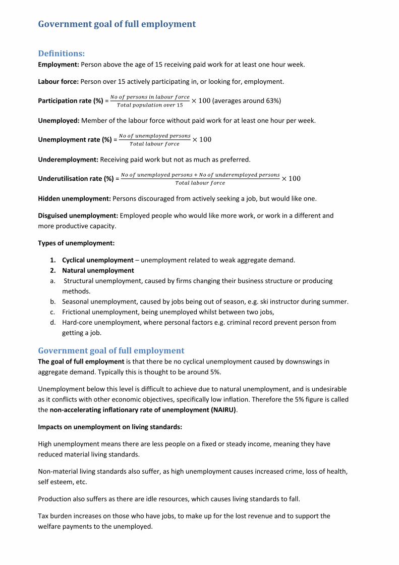
Government goal of full employment

Definitions: Employment: Person above the age of 15 receiving paid work for at least one hour week.

Labour force: Person over 15 actively participating in, or looking for, employment.

Participation rate (%) = (averages around 63%)

Unemployed: Member of the labour force without paid work for at least one hour per week.

Unemployment rate (%) =

Underemployment: Receiving paid work but not as much as preferred.

Underutilisation rate (%) =

Hidden unemployment: Persons discouraged from actively seeking a job, but would like one.

Disguised unemployment: Employed people who would like more work, or work in a different and

more productive capacity.

Types of unemployment:

1. Cyclical unemployment – unemployment related to weak aggregate demand.

2. Natural unemployment

a. Structural unemployment, caused by firms changing their business structure or producing

methods.

b. Seasonal unemployment, caused by jobs being out of season, e.g. ski instructor during summer.

c. Frictional unemployment, being unemployed whilst between two jobs,

d. Hard-core unemployment, where personal factors e.g. criminal record prevent person from

getting a job.

Government goal of full employment The goal of full employment is that there be no cyclical unemployment caused by downswings in

aggregate demand. Typically this is thought to be around 5%.

Unemployment below this level is difficult to achieve due to natural unemployment, and is undesirable

as it conflicts with other economic objectives, specifically low inflation. Therefore the 5% figure is called

the non-accelerating inflationary rate of unemployment (NAIRU).

Impacts on unemployment on living standards:

High unemployment means there are less people on a fixed or steady income, meaning they have

reduced material living standards.

Non-material living standards also suffer, as high unemployment causes increased crime, loss of health,

self esteem, etc.

Production also suffers as there are idle resources, which causes living standards to fall.

Tax burden increases on those who have jobs, to make up for the lost revenue and to support the

welfare payments to the unemployed.

Measuring unemployment Labour force survey: All unemployment statistics are collated by the ABS through their national survey.

Limitations of the survey:

1. Small sample size – only 0.7% of population surveyed, may produce inaccuracies.

2. Arbitrary definitions of employment - why is 1 hour a week ‘employed’?

3. Hidden unemployed not accounted for – as they are not actively seeking work, they are not

counted as part of the labour force.

4. False information – people may lie to survey to protect their own interests e.g. welfare.

Recent trends in employment in Australia Prior to GFC (mid 2008): Full employment was achieved in the boom years prior to 2008, down from

7.4% in 1999-2000.

Unemployment was down to as low as 4% in 2008, causing higher inflation as NAIRU was breached.

In general, prior to GFC, the unemployment and underutilisation rates fell, whereas the participation

rate increased.

After GFC (2008-10): Unemployment rose due to fall in aggregate demand, however it did not hit the

heights expected (8.5%) instead peaking at around 5.8%, within the goal rate.

A partial reason for the small increase was the policy of reducing workers’ hours instead of laying them

off, so while unemployment may not have increased much, there was a substantial increase in the level

of underemployed persons and hence the underutilisation rate.

Demand and Supply factors affecting full employment In general, any factor which increases AD will reduce unemployment, and vice versa.

Any factor which increases production costs will increase unemployment, and vice versa.

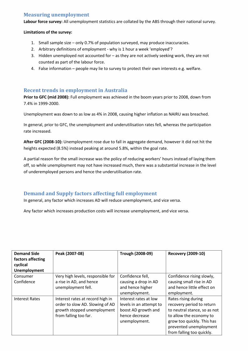
Demand Side factors affecting cyclical Unemployment

Peak (2007-08) Trough (2008-09) Recovery (2009-10)

Consumer Confidence

Very high levels, responsible for a rise in AD, and hence unemployment fell.

Confidence fell, causing a drop in AD and hence higher unemployment.

Confidence rising slowly, causing small rise in AD and hence little effect on employment.

Interest Rates Interest rates at record high in order to slow AD. Slowing of AD growth stopped unemployment from falling too far.

Interest rates at low levels in an attempt to boost AD growth and hence decrease unemployment.

Rates rising during recovery period to return to neutral stance, so as not to allow the economy to grow too quickly. This has prevented unemployment from falling too quickly.

Overseas Economic Activity

High levels of economic activity meant high demand for our products, especially commodities; hence employment rose to help meet the demand.

The large drop in demand for exports caused by the GFC resulted in higher unemployment, particularly in the export industries.

High demand for commodities from countries such as China and India means that unemployment has fallen, as employment in commodities and export industries has increased.

Business Confidence

Very high levels of business confidence, causing growth in AD which in turn lowers unemployment.

Business Confidence fell, causing a drop in AD and hence higher unemployment.

Business Confidence is booming, creating stronger AD and helping to decrease unemployment at a quick rate.

Supply side factors affecting cyclical unemployment


Labour shortages and immigration

Despite the increased participation and immigration rates, there was still strong demand for labour.

Labour shortages disappeared to the global recession, so this did not cause unemployment to rise.

Reduced immigration intake means that there is still strong demand for labour.

Wages - RULCs Gradual decrease in RULCs cause producers to hire more workers, lowering unemployment.

Gradual decrease in RULCs cause producers to hire more workers, lowering unemployment.

Gradual decrease in RULCs cause producers to hire more workers, lowering unemployment.

Interest rates Rise in interest rates during this period caused costs for producers to rise, leading to them laying off workers, raising unemployment.

The fall in interest rates caused business costs to lower, allowing companies to hire more workers. This helped slow the rise in unemployment.

The small rise in interest rates is too small to have made a significant impact on production costs so it has little effect on unemployment.

Structural change by local firms

High profits for local producers meant that there was little need for structural change, so there were few lay-offs, leading to low unemployment. However the growing practice of relocating workforces to China has increased unemployment.

Falling profits forced firms to lay off large number of workers, causing unemployment to rise.

As profits begin to rise there is no longer a problem with redundancies, so unemployment is kept stable. However there are still local jobs being given to overseas workers, causing unemployment to rise.

Government goal of external stability

Definitions: Balance of Payments Account: Is a statistical record of the money values of different types of

transactions between Australia and the rest of the world. Money received by Australia are credits,

whereas money spent by Australia are debits. The Balance of Payments account is made up of:

1. The Current Account: This account records all international transfers of Goods, Incomes,

Services, and Transfer payments. (GIST). The balance on the current account is made up of the

net total (credits minus debits) of each of the four sections. Typically the account runs at a large

deficit (currently ~ $71b), mainly due to the large debit balance of the Net Income section.

2. The Capital and Financial Accounts:

1. The capital account is made up of the transfers of all capital funds, typically transferred by

migrants moving their bank accounts, as well as non-produced, non-financial assets such as

patents and trademarks. The balance on the capital account is the net result of the capital

transfers and the net acquisition of non-capital assets.

2. The financial account is made up of net investments (direct, portfolio, or other), being the

total invested in Australian businesses (credits) less the total invested by Australians in

overseas businesses (debits), and the Reserve assets, which are the transactions made by

the RBA and the Federal government.

3. There is a Net Errors and Omissions Account, which takes into account all supposed errors

and ensures that both sides of the balance of payments account balance.

Net Foreign Debt: This is the total amount owed by Australians, both by the government (public sector)

and by businesses (private sector) to overseas institutions, less what is owed to Australian institutions

by overseas entities.

The exchange rate: The price received for the Australian dollar when buying other currencies. The price

is subject to normal demand and supply rules, meaning that an appreciation in the A$ is caused by more

demand (due to high overseas activity, selling of exports, low interest rates, improved terms of trade)

and/or less supply, and a depreciation in the A$ is caused by less demand (due to poor overseas

economic conditions, low interest rates) and/or more supply (due to high domestic economic activity).

The Trade Weighted Index: The TWI is the average exchange rate for a basket of foreign currencies,

weighted for their relative importance for Australia. The higher the TWI, the more Australia is receiving

on average for the A$.

Terms of Trade: The price Australia receives for our exports, relative to the price paid for imports.

Government goal of external stability The goal of external stability has three components:

1. That the Current Account Deficit should not be too large as a percentage of GDP. A generally

accepted figure is that it be no more than 3-4%.

2. The exchange rate should be reasonably stable. Although there is no set target for the exchange

rate, erratic and unpredictable behaviour taking it to either extreme is undesirable.

3. That the Net Foreign Debt and its associated repayments not be too high. However, a small

amount of debt is acceptable, as long as the capital raised is put towards productive uses.

Reasons for goal Not having external stability would affect living standards in the following ways:

CAD component: When the CAD is too large, this indicates that imports are outweighing exports,

leading to an economic slowdown and unemployment. Conversely, when the CAD is small, there are

strong exports relative to imports, indicating economic growth and hence low unemployment.

Exchange rate component: A very low exchange rate for the A$ causes inflation. This is because exports

become very cheap, leading to a growth in X and hence in AD. Strong AD growth causes inflation. In

addition, a low A$ causes cost inflation as producers using imported materials have higher costs. A low

A$ would also affect income distribution as it would allow exporters’ incomes to rise faster than those

of the general population.

On the other hand, a too high exchange rate for the A$ causes exports to slow and imports to grow,

leading to a slowdown in AD and hence unemployment.

NFD component: Having a high NFD, caused by low levels of domestic savings, means that companies

and the government must borrow from overseas in order to raise capital. This borrowing requires

repayments as well as interest costs, limiting the amount of investment that can be done in Australia

due to the high interest costs, as well as pushing up prices here.

In general, goal of external stability is NOT compatible with goals of economic growth and full

employment. This is because during times of strong economic growth, and hence full employment, we

see fast growth in imports and investment in Australia, worsening the CAD and perhaps the NFD.

Relationships between the CAD, exchange rate, and NFD In general, any change in one will affect the others, as well as our living standards.

When the A$ goes up: This increases imports and decreases exports, increasing the CAD. Repayments

and interest payments on foreign borrowing become cheaper (as repayments are made in the foreign

currency), so the NFD goes down.

When the A$ goes down: This increases exports and decreases imports, decreasing the CAD.

Repayments and interest payments on foreign borrowing become more expensive, so the NFD goes up.

When NFD goes up: Supply of A$ is high, causing a depreciation. This reduces imports and increases

exports, decreasing the CAD. However the repayments of the debt along with the interest increase the

deficit on the Net Incomes section of the CAD, thereby increasing it.

When NFD goes down: Supply of A$ is low, causing an appreciation. This reduces exports and increases

imports, increasing the CAD. However the lower repayments of the debt along with the interest

decrease the deficit on the Net Incomes section of the CAD, thereby decreasing it.

Recent trends in Australia’s external stability CAD: The CAD has in general been fairly large over the past few years, increasing from $40b in 2002 to

$71b in 2009. The CAD : GDP ratio has also increased beyond the goal rate, up to over 6%. This is

despite the huge demand for our exports and the subsequent record rise in the ToT (mainly

commodities to China) and mainly because of the income section of the current account.

A$: The A$ did rise steadily prior to 2009, almost doubling in value from 51 US cents in 2002 to 96 US

cents in 2008. However, since the GFC there has been a fall in the value of the A$ and the TWI, and it

has been volatile ever since, with slow appreciation as a general trend.

NFD: The NFD continues to grow, reaching a record high of 54.2% of GDP in 2008. Although the NFD

continues to rise, during 20008-09 it fell as a percentage of GDP, indicating that GDP growth was faster

than the NFD growth. However due to recent and continuing government deficits it may rise sharply in

the near future.

Influences on external stability In general, cyclical factors which increase AD will increase the CAD, decrease the A$ and hence cause

the NFD to grow.

Supply side factors tend to cause on-going levels of CAD, a rising NFD and a decreasing A$.

Demand side factors affecting External Stability


Consumer Confidence

High confidence in this period resulted in higher spending on Imports, so the CAD rose to a record 5.9% of GDP.

Lower consumer confidence caused lower spending on imports, so the CAD fell to 4.4%.

Slight increase on import spending, begins to raise CAD.

Business Confidence High confidence in this period resulted in higher spending on Imports, so the CAD rose to a record 5.9% of GDP.

Lower business confidence caused lower spending on imports, so the CAD fell to 4.4%.

High business confidence during recovery causes increase in investment including foreign imports, raising the CAD.

Interest Rates High interest rates during this period caused investment in our banks from overseas, leading to the A$ appreciating. This led to the CAD worsening as our exports were less competitive.

Despite lower interest rates in Australia, rates were still higher than overseas so there was still demand for A$ to invest, leading to an appreciation of the AUD.

Rise in interest rates before any other country causes increase in foreign investment, causing A$ to appreciate, and hence CAD to become bigger.

Overseas Economic Conditions

Strong demand for our exports from China, raises exports and hence lowers the CAD. Also increases demand for A$, causing it to appreciate.

Slight decrease in demand for exports, slows drop in CAD. Lessened demand for A$ slows appreciation of AUD.

Demand from India and China as high as ever, reducing upward pressure on the CAD.

Supply side factors affecting External Stability


Real Unit Labour Costs

Gradually decreasing but still high wage costs reduce Australia’s competitiveness and productive efficiency. This means more imports and fewer exports, increasing the CAD.



Oil Prices Very high oil prices during this period, peaking at around US$150 a barrel, pushed up import costs of oil necessary for production, causing overall imports to rise and hence increasing the CAD.

Oil prices fell dramatically, causing import costs for oil to be lower, hence reducing imports and the CAD.

Slow increase in oil prices gradually raises import costs of production, increasing imports and the CAD.

Exchange Rates Steadily rising exchange rate between the A$ and the USD meant that imports were cheaper for Australian production, resulting in a lower CAD.

Large fall in the value of the A$ compared to the USD meant that imports for Australian production became more expensive, increasing the CAD.

Rising though volatile A$ is causing import prices to fall, helping to reduce the CAD.

A factor with a significant impact on the NFD is the low level of domestic savings, which forces the

government and businesses to borrow from abroad. Factors which encourage domestic saving should

work to decrease the NFD.

Government Protectionism v Free Trade Protectionist policies such as tariffs, local subsidies, import quotas, anti-dumping laws, and preferential

treatment of local companies have various claimed benefits, such as:

1. Protection of infant industries which otherwise would not have been able to compete with

overseas companies.

2. Protection of local industry in case of war when overseas products will not be available.

3. Helps ensure economic stability by reducing effect of overseas booms and recessions on local

exporters.

4. Help maintain Australian jobs by keeping these companies competitive locally.

Disadvantages of protectionist policies are that they encourage inefficiency and incompetitiveness,

which in the long run is worse for the economy and employment, and also that they reduce our

opportunities for exports.

Free trade means that there are none or very limited restrictions on international trade between

countries. Claimed advantages of free trade are:

1. Encourages greater efficiency, as local companies will allocate resources into areas where they

have a comparative cost advantage against overseas, causing economies of scale to reduce

production costs and hence maximise employment and incomes.

2. Increased international trade, leading to more jobs and employment.

3. Lower inflation due to more competitive prices from overseas.

Recently the Australian government has moved towards free trade, abolishing most tariffs and all

import quotas, slashing local subsidies and increasing free trade agreements.

Government goal of Equity in income distribution

Definitions: Earned income: Wages, salaries representing reward for personal physical or mental effort.

Unearned income: Interest, dividends, rents, profits – arise from ownership of assets such as property

and shares.

Factor income: Incomes from production and/or selling of a product. Combination of both earned and

unearned income.

Transfer income: Incomes received from government handouts, e.g. welfare, pensions.

Private income is all income from all personal sources, e.g. wages, interest, dividends plus welfare and benefits equals gross income, i.e. total income from all sources minus personal income tax equals disposable household incomes, i.e. total income after tax plus receipt of indirect benefits such as subsidised or free government services such as education, health equals the social wage income minus payment of indirect taxes such as GST, excise taxes equals final income, meaning income after all government redistribution has taken place.

Government goal of equity in income distribution The government goal is that the distribution of income be equitable such that there is no absolute

poverty, and everyone has access to a basic level of goods and services enough to enjoy basic living

standards at a level that is acceptable to society.

The goal is not to have income equality, whereby everyone would be earning the same; it is only to have

equity, whereby no one is earning too little.

Impact of equitable distribution:

1. Provides everyone with basic living standards

2. Ensures better resource allocation, as otherwise products would only be made to satisfy the rich

who have all the money. With equity, more products are made to satisfy the needs of the entire

range of society.

3. If distribution were to be completely equal (for example with extremely steep progressive tax

scales or overgenerous welfare) there would be no motivation to work (especially to do the

dangerous or dirty jobs), which would encourage inefficiency and unemployment. Some

inequality is considered a good thing as it encourages motivation and hard work. In addition,

too much equality leading to inefficiency would result in slower economic growth and reduced

living standards, as well as cost inflation.

Measuring distribution of income The ABS measures the distribution of income with a survey of approximately 0.2% of the population.

Equivalised income measures income using a fairer scale by taking into account income per person,

Based on the size of the income unit. The income unit is the amount of people dependent on each

individual source of income. A single source of income providing support for a large number of people

has an equivalised income less than the same income providing support for fewer people.

After receiving information to determine the level of final income, the ABS divides the population into

quintiles in ascending order dependent on the amount of income for each quintile.

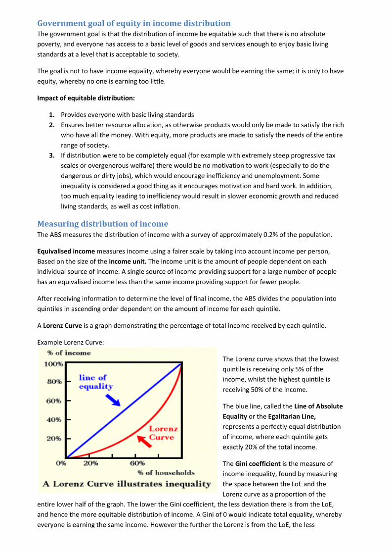
A Lorenz Curve is a graph demonstrating the percentage of total income received by each quintile.

Example Lorenz Curve:

The Lorenz curve shows that the lowest

quintile is receiving only 5% of the

income, whilst the highest quintile is

receiving 50% of the income.

The blue line, called the Line of Absolute

Equality or the Egalitarian Line,

represents a perfectly equal distribution

of income, where each quintile gets

exactly 20% of the total income.

The Gini coefficient is the measure of

income inequality, found by measuring

the space between the LoE and the

Lorenz curve as a proportion of the

entire lower half of the graph. The lower the Gini coefficient, the less deviation there is from the LoE,

and hence the more equitable distribution of income. A Gini of 0 would indicate total equality, whereby

everyone is earning the same income. However the further the Lorenz is from the LoE, the less

equitable the distribution of income is. A Gini of 1 would indicate total inequality, whereby 1 person is

earning all the income.

The Poverty Line

Another measure of relative income is the poverty line. In Australia we use the Henderson poverty line,

which is an estimation of the lowest income that one could survive on with even the most basic of living

standards. Anyone earning less than this amount is said to be below the poverty line, and hence in

poverty.

The amount of income is measured using disposable household income, i.e. after tax but before the

addition of indirect benefits. The poverty line is constantly adjusted to take into account inflation. The

poverty line is also adjusted using equivalence scales to measure equivalised income depending on the

size of the income unit, i.e. a larger income unit will need a higher level of income in order to survive.

Limitations of measuring personal income distribution:

1. Definitional problems relating to the definition of poverty and equity. For example there may be

great inequality, with a high Gini coefficient, yet still equity as everyone has a sufficient income

to live on.

2. Statistical problems relating to survey error and misinformation.

3. Subjectivity of poverty measures, e.g. exact placement of Henderson poverty line.

Recent trends in Australia’s income distribution Australia’s current Gini coefficient (last measured in 2006) is 0.307. This is fairly consistent with the last

few years.

In general, the income of all quintiles has increased over the last few years at a rate higher than

inflation, leading to increased purchasing power and living standards.

Although Australia’s overall poverty rate fell, there was a recent rise of children in poverty, particularly

in Aboriginal communities.

Factors influencing the equitable distribution of income In general, any factors (demand or supply) causing an increase in unemployment will increase inequity,

and vice versa.

Any factors (demand or supply) causing an increase in inflation will also reduce living standards of the

poor, and hence increase inequity, and vice versa.

The decline of centralised wage fixing, whereby the government set a minimum weekly wage for each

industry, in favour of enterprise bargaining, whereby employees negotiate their own wages, has in

general terms led to a decrease in equality, as those who are able to negotiate for high wages due to

the skilled nature of their jobs have been in a much better position than those in unskilled jobs, who are

unable to procure suitable wages. However, when linked to increased productivity, enterprise

bargaining can result in increased wages, as well as better economic growth and hence better living

standards for all.

The WorkChoices Act, introduced by the Howard government, and the abolition of the Unfair Dismissal

laws, both of which made it easier for workers to be fired, may have contributed to inequality as less

people were able to keep their jobs. This act was abolished by the Rudd government in 2008.

Changes in the proportion of people in part time work also affect inequality. In general, prior to the GFC

there was a move towards full-time employment, reducing inequality. However after the GFC a lot of

full-time workers became part-time, increasing inequality.

The drought, which has caused the agricultural sector to suffer large losses, has also contributed to

income inequality.

UNIT 4 NOTES CHAPTER 4

Definitions Budgetary (fiscal) Policy: Relates to the anticipated changes in the level and composition of

government receipts (revenues) and outlays (expenses) for the coming budgetary period.

Direct taxes: Taxes which are levied directly onto the income of individuals and companies.

Indirect taxes: Taxes applied on the sale of goods and services or added to the price of other items.

Tax mix: The balance between direct and indirect taxes as a source of government revenue. Currently

~68% of revenues come from direct taxes, and 26% comes from indirect taxes.

Tax base: Refers to how broadly the particular tax is applied. For example, the GST is applied on most

but not all goods and services.

Tax burden: The rate at which the tax is applied. Hence higher income earners face a larger tax burden

than low income earners.

Discretionary stabilisers: Stabilisers which are actively put into place via deliberate decisions from the

government or treasurer.

Automatic stabilisers: Stabilisers which automatically work counter-cyclically to reduce the effect of

upswings or downswings in the business cycle.

Aims of budgetary policy The government uses budgetary policy to influence all of its goals regarding both domestic and external

stability. These goals are strong and sustainable economic growth, full employment, low inflation,

equity in income distribution and external stability. The overall goal that links all these is the

maximisation of living standards, so the overall aim of budgetary policy is to maximise living standards.

The focus or priorities of budgetary policy will vary depending on the current economic situation, or the

political goals of the government.

Types of government revenues and expenses

Revenues

There are three main sources of government revenue: direct taxes, indirect taxes, and non-tax revenue.

Direct taxes, such as PAYG income tax, company tax and capital gains tax make up the majority (68%) of

government revenue.

The PAYG income tax is a direct tax on incomes which makes up around 40% of all government

revenue. The tax is progressive, meaning it is applied at a higher rate the more you earn. The top

bracket has been reduced over time from 75% to 45% on incomes above $180,000.

The company tax rate is a proportional tax levied at 30%, regardless of profits. This has come down

from 49%, as it was in 1986, and is scheduled to fall further to 28% by 2015.

The capital gains tax (CGT) is a direct tax on all gains made on capital, such as property and shares. The

CGT is applied at a rate of half the rate of the appropriate income tax, and hence has an effective top

rate of 23.25%.

Indirect taxes make up another 26% of government revenue. These taxes include the GST, excise taxes,

and customs duties or tariffs.

The GST is a tax levied on most goods and services at a flat 10% rate. Items exempt include those that

are basic necessities, such as certain food items, residential rent, and utility bills. This tax is generally

considered regressive, as it takes a larger proportion of income from low income earners than that of

high income earners for the same item.

Excise taxes are those levied on certain goods such as alcohol and tobacco, petrol and coal. It is charged

at a flat rate per kilo. These raise around 9% of government revenue.

Taxes should fulfil 3 principles: They should be simple (understandable by all those who it applies to),

fair (encourage equity and fairness) and efficient (should not have a significant impact on decision

making, otherwise they are interfering in the free operation of the market).

Non-tax revenue includes all things that are not tax, such as asset sales, repayments of loans by

states/other governments, HECS repayments, Government Business Enterprise profits and license

revenues. These make up approximately 8% of government revenue.

Expenses

Government expenses (G1+G2) are broad and wide ranging. They include transfer and welfare

payments (typically 33% of all spending), spending on health (16%), education (10%), transport (2%)

and defence (6%), as well as spending on national infrastructure and government operational

expenses (6%).

G1 expenses are those such as salaries and operating expenses for administration, as well as day-to-day

spending on health, education, and defence.

G2 expenses are those such as infrastructure building and purchase of equipment.

Transfer payment expenses are not included in G1 or G2 as they are technically spent by the recipient,

not the government. Recording them as G1 or G2 would mean they end up being counted twice in AD, as

they represent a part of C as well.

The aim of expenses is generally to provide services to the community, either completely free or at a

subsidised price. The user-pays principle, which means users are charged at least some part of the cost

of a government service, is increasingly common.

Budget Outcomes There are three types of budget outcomes:

1. Balanced budget: This is when expenses roughly equal revenues, meaning that there is no

deficit and no surplus. This is indicative of a neutral stance, as the government is looking to

neither stimulate nor restrain economic growth. This type of budget has little effect on

economic growth, inflation, or unemployment.

2. Budget deficit: This is when expenses outweigh revenues, meaning that there is a deficit.

Typically this outcome will be used during a period of poor economic growth; hence it is

indicative of an expansionary stance. The extra cash flowing into the economy as opposed to

coming out of it will help to stimulate AD in order to steer clear of a recession and help the

economy to rebound. Deficits can be financed in three different ways:

a. Overseas borrowing: The government could borrow money from overseas, either from

other governments or from banks. The problem with this approach is that it increases

the Net Foreign Debt and worsens the Current Account Deficit, so it is bad for external

stability.

b. Borrow from the RBA: The government could either use up the savings it has deposited

with the RBA during surplus times, or it could sell the RBA bonds. This is effectively

printing more money, and is seen as a very expansionary stance.

c. Borrow from the public or financial sector: The government could raise funds by selling

bonds or securities directly to the public. This was the main method used during the

GFC. However, this may cause a ‘crowding out’ of the financial sector, and cause raised

interest rates which in turn may cause depressed public spending and investment.

3. Budget Surplus: This is when revenues outweigh expenses, meaning there is a surplus. This will

typically be the policy during times of strong growth, as the government will try to restrain AD

so as not to cause inflation. As such, this is indicative of a contractionary stance. By removing

cash from the economy, the government aims to reduce spending and hence inflationary

pressure on AD. The government has three options of what to with the surplus:

a. Repay debt: The government could repay any debt it has accumulated through

previous deficits.

b. Save with the RBA: The government could save the money with the RBA for use

during deficit times.

c. Add to the balance in special funds: The money could be used to set up the special

funds such as the Building Australia Fund, the Education Investment Fund, or the

Hospitals fund. It is hoped that through good investment the values of these savings

will increase over time.

Effect of one off events: One off events can have a huge impact on the predicted budgte outconme, eg

the GFC in 2008 changed the projected budget outcome from a $21b surplus to a deficit of $32.1b. This

change was caused by the advent of both automatic and discretionary stabilisers implemented to

respond to the crisis.

The Headline Balance: This is the cash differential between total cash received and total cash spent by

the government. This may make the outcome look more impressive, due to the impact of one-off events

such as asset sales.

The Underlying Balance: The Headline balance less the impact from one off events.

The Fiscal Balance: The fiscal balance is calculated through the accrual approach, meaning revenues

earned but not received as well as expenses accrued but not paid are also calculated as part of the

balance. The government will have a long term aim to maintain a fiscal balance over the duration of the

business cycle, meaning that all deficits are paid for by the surpluses gathered, leading to a neutral

balance over the long term.

Stabilisers Stabilisers work to counteract upswings and downswings in the economy, so that the effect of booms

and troughs is not so severe. There are teo types of stabilisers:

Automatic stabilisers: These are naturally counter-cyclical, and work without any government

intervention. The main two examples of these are PAYG income taxes and welfare. During a boom,

incomes naturally rise and employment goes up, so there is automatically more tax revenue and less

welfare payments, contributing to a budget surplus and a more contractionary stance, as is appropriate

to counteract a boom.

During a trough, incomes and employment decrease, so tax revenue decreases and welfpare payments

increase, contributing to a deficit budget and a more expansionary stance, counteracting the trough.

Discretionary (structural) stabilisers: These are stabilisers implemented by the government in order to

combat changes in the economy when automatic stabilisers are not deemed sufficient.

Using budgetary policy to achieve economic goals

Economic Growth, Full Employment and Low Inflation In general, the government will use budgetary policy to contract the economy when economic growth is

too strong and unemployment is low enough to cause inflationary pressures.

It will use budgetary policy to expand the economy during times when economic growth is too small

and unemployment is too high, with the aim of increasing AD and hence employment.

Contractionary period – 05-08

During this time, budgetary policies to contract AD include:

1. Surplus budgets

2. Automatic stabilisers

Policies to increase employment included training and apprenticeships.

(There were also PAYG tax cuts during this period)

Expansionary period – 08-09

During this time, budgetary policies to expand AD include:

1. Deficit budgets

2. Cuts in tax rates

3. Tax breaks for small businesses

4. Massive infrastructure spending

5. Cash handouts (stimulus package)

Weaknesses of using budgetary policy to pursue the goals of sustainable economic growth and full

employment:

1. Long time lags before the impact of some discretionary stabilisers is felt, such as with

infrastructure spending, may result in the policy becoming pro-cyclical rather than counter-

cyclical.

2. Financial constraints on the budget preventing the deficit from becoming too large may thwart

the government’s plans for spending during a recession.

3. Incompatibility between goals, such as the need for strong growth and employment at the

same time as low inflation, equity, and external stability, may cause the pursuit of one goal via

budgetary policy to be detrimental to the pursuit of a different one.

4. Political constraints, either from the Upper House blocking policies, the States blocking policies,

or the possibility of a voter backlash may prevent the government from putting out necessary

policies.

5. The reaction of the nation to budgetary measures such as a deficit to boost economic growth

may not be as strong as desired, so the policy may not have the desired effect.

External stability The government will always look to promote domestic stability through budgetary policy. However, in

times of poor economic growth, expansionary policies such as deficit budgets which are harmful to

external stability will still be prioritised.

The government will accept that a CAD:GDP ratio of about 3-4% is inevitable and well be caused by

structural issues, such as poor cost competitiveness, the large NFD, and the savings-investment gap.

However, anything above that will be considered a cyclical issue, whereby it will rise during booms and

fall during troughs.

Budget Surpluses: These help to reduce the NFD, as the government can use the surplus money to pay

off debt. This also helps with the CAD as the repayments and interest payments are smaller.

They also affect the CAD as they help to contract AD, which reduces the amount of imports being

bought, and also frees up domestic products for export overseas.

Budget Deficits: These are generally very bad for external stability, as the increase in government debt

can cause an increase in the NFD, whilst the expanded economy as a result of the deficit could cause a

spillover into imports, reducing the CAD.

In general, the goals of economic growth, low inflation and full employment are incompatible with the

goal of external stability, so policies to help one will harm the other.

Specific policies and their effect on external stability:

1. Cuts in PAYG taxes / increases in welfare – cause an increase in consumption, both domestic

and overseas, increasing the CAD.

2. Government spending on imported goods – spending on areas such as defence which involve

large quantities of imported goods increase the CAD.

3. Government overseas aid – money spent on aid overseas increases the CAD.

Policies to increase national savings:

One of the main causes of Australia’s large NFD, as well as the resultant CAD increase, is the savings-

investment gap. This means that the level of national savings in Australia is not sufficient to provide

capital for investment by Australian governments and businesses. This requires businesses to look

overseas for capital to use for investment, hence increasing the NFD.

Therefore, any policy which helps promote national savings will help with the goal of external stability

by narrowing the savings-investment gap. Such policies include:

1. Superannuation co-contribution scheme: The government matched any super contributions up

to $3,000, which encouraged people to save with super funds.

2. Tax breaks for super contributions.

3. Reduced taxes to allow families to save more.

4. Tax cuts on interest earned on savings (50% off first $1000).

Weaknesses of using budgetary policy to pursue the goal of external stability:

1. Long time lags between the need for a policy, its implementation, and its desired effect may

reduce the effectiveness of the policy.

2. Conflict with other goals, particularly the need for strong economic growth and low

unemployment, may cause policies which help with external stability harm the pursuit of

another goal.

3. Structural causes of the CAD may not be tackled by budgetary policy.

Equity in income distribution Budgetary policy has a large effect on equity. The government will use budgetary policy to promote its

goal of equity in income distribution in the following ways.

During a boom, when inflationary expectations are high, the government will use a contractionary

surplus budget, so as to slow AD and hence reduce inflation. This prevents the erosion of purchasing

power of those on low or fixed incomes, improving their equity situation.

During a trough/recession, when there is increased unemployment and reduced incomes, the

government will run an expansionary deficit budget so as to increase AD. This will result in increased

employment and incomes, improving the goal of equity.

The government can also use specific budgetary policies to redistribute final incomes. The PAYG income

tax is progressive, meaning that people earning more are taxed at a higher rate. This reduces their final

income, and means that the revenue earned by the government can be redistributed to those in need

via welfare payments, which raises their final income and hence encourages a more equitable

distribution.

In recent times, there have been cuts to the tax rates payable on the lowest brackets, and the margins

on some brackets have been raised to negate the effects of bracket creep (fiscal drag). This has allowed

people on lower incomes to retain more of their income, hence improving equity. In addition, tax

rebates have been made available to those on low incomes, such as for education and childcare, which

also improves equity.

Welfare payments are another major budgetary policy that has an affect on equity. Payments for

unemployment, disability, aged pension, youth allowance and rent assistance all help people on low

incomes to cope, increasing equity.

Recently there have been measures to tighten access to welfare, such as the means and asset testing

and the work for the dole scheme to encourage people to get off welfare, and to prevent abuse of the

system.

Indirect taxes, (taxes on an item rather than the person) which are considered regressive as they take a

higher proportion of income from the poor than the rich, are an area of budgetary policy which actually

serves to decrease equity. In order to combat this, the government has introduced measures to make

these taxes impact less on the poor, such as exempting basic necessities from GST, lowering the petrol

excise tax, and increasing taxes on luxury items such as luxury cars.

Indirect benefits usually help the poor more than the rich, as the services they provide, such as

subsidised or free healthcare, schooling, childcare and housing are far more likely to be used by those

on low incomes than by those on high incomes, who prefer the private system for its quality of service.

Therefore, these indirect benefits provide far more value to the poor than the rich, improving their final

income. However, recent shifts towards an increased user-pays principle has seen the prices of public

services rise for users, decreasing the access of the poor to these services and hence harming the

pursuit of equity.

Recent budgetary policies to combat the GFC, such as the Building Australia Fund, the Education and

Investment Fund and the Health and Hospitals Fund should improve the quality of service provided on

the public system, improving the access to basic services for the needy.

Incentives to promote superannuation savings have also impacted on equity, as by encouraging people

to save more for retirement using policies such as the co-contribution fund and the increased

compulsory contribution, the government helps to ensure that people have enough of an income to

support them after retirement, thereby improving their access to goods and services and improving the

pursuit of equity.

Weaknesses of using budgetary policy to pursue the goal of equity in income distribution:

1. Limitations on the effectiveness of direct taxes to reallocate incomes, particularly caused by

the ever-decreasing tax rates on personal and business incomes, prevent the redistribution of

income. In addition, black market income cannot be taxed.

2. Weaknesses of welfare payments, either because of tightening of access to payments are

because of the extremely low amounts, mean that they are not as an effective means of

redistributing income.

3. Regressive taxes such as the GST and excise taxes have a larger effect on the poor than the rich.

4. Indirect taxes have limitations as the increased use of the user-pays principle and funding cuts

for public services mean they are not as effective in providing services to the poor.

5. Conflict with other objectives, financial constraints, time lags – see other goals.

CHAPTER 5

Monetary policy is a macroeconomic tool wielded by the Reserve bank of Australia designed to manage

the level of Aggregate Demand. It involves the regulation of the nation’s money and the rate at which

money flows into the economy via the financial sector, particularly through the application of market

operations designed to influence the cost of credit.

Definition of money Money consists of items that can be used as a measure or store of value, or a medium of exchange.

The Money Supply or the amount of money in circulation is measured by the RBA.

The volume of all coins and notes held by the non-bank public as well deposits of banks with the

RBA

Plus the volume of operating and fixed bank deposits

Equals M3

Plus net deposits of savings in non-bank financial institutions (NBFIs)

Equals Broad Money.

The process of credit creation is when one person deposits money into a bank, which is then lent out to

another person. That person spends the money, and the recipient also deposits it into his bank. Thus

there have been two deposits with the same amount of money, and hence credit has been created.

The percentage that a bank can lend out of all of it’s receipts is set by the Australian Prudential

Regulation Authority, who ensure that banks retain a minimum amount of funds needed to pay off

short-term claimants, and is currently 12.5%

Nature of the financial sector The financial sector is made up of Australia’s financial institutions, such as banks (including the RBA),

building societies, managed funds and the stock exchange, who play a pivotal role in the in the money

market through their lendings and borrowings with each other and with households.

Over the past few decades there has been financial deregulation which is the process of removing

unnecessary government restrictions and legislation which are impediments to the efficiency of the

financial sector. The main aim of financial deregulation is that the financial system runs more efficiently,

for example by allowing competition to the ‘Big 4’ banks to encourage them to increase efficiency.

Aims of monetary policy Monetary policy has two main aims:

1. Low inflation (or stability of the currency): The RBA aims to fight high inflation and keep

inflation within the goal rate of 2-3%. This is done primarily by manipulating the cost of credit.

2. Sustainable economic growth and full employment: After having achieved the goal of low

inflation, the RBA will seek to promote economic growth and employment, using counter-

cyclical measures.

The first goal of low inflation is seen as the priority goal as it is believed that it acts as a precondition o

achieving the second goal of economic growth, i.e. with too high inflation it is impossible to have good

economic conditions.

Through achieving these two goals, the RBA hopes to fulfil its charter to raise the living standards of

Australians.

In the period from 2005-08, the focus of the RBA was very much on low inflation, as is evidenced by

their eight interest rate rises to combat rising inflation. After the GFC in late 2008, when falling demand

made inflation no longer a worry, the RBA switched its focus to ensuring strong growth and

unemployment, hence the huge fall in interest rates.

Nature of monetary policies The RBA’s main instrument is its ability to alter the cost of credit, which is the annual cost of borrowing

or the annual return on savings.

The strategy used by the RBA to alter interest rates is made up of the following stages:

Example is method of raising interest rates:

1. Following the decision to alter rates made in the RBA’s monthly meetings, the RBA will

announce its new target rate and the reasons for the change.

2. The RBA will then sell large volumes of government bonds or securities, usually at a discounted

rate so as to increase their attractiveness to investors, into the short-term (overnight) money

market. This has the effect of depleting the exchange settlement accounts that each bank holds

with the RBA, as the money deposited in these accounts is used to buy the securities. This step

is called market operations in the short-term money market.

3. Since the banks now need to top-up their exchange settlement accounts, and there is limited

funds available due to the large amounts being hoarded by the RBA, the competition for funds

to borrow increases, which raises the cost of credit.

The banks then pass these rises in their own borrowing costs onto the consumers so as to protect their

profits and reduce their own borrowing, which sees interest rates on mortgages, overdrafts, credit

cards, variable loans etc rise.

Through the transmission mechanism, these rises in interest rates on loans cause less spending by

consumers and businesses as they have less discretionary income, which results in less C, I and M, and

therefore less demand-inflationary measures.

The RBA has caused a reduction in the inflation rate, through employing a contractionary stance to slow

spending. In order to employ an expansionary stance to boost spending when the situation requires it,

the opposite process is used, whereby the RBA buys government securities so as to increase the supply

of credit, thereby reducing the cost of credit and interest rates and therefore increasing spending.

Effect on the economy of changing the cash rate:

1. Savings and Investment Channel –When interest rates increase, it costs more to borrow money. This

means that the effective cost of certain things, such as houses will be much higher. Higher interest rates

will also mean that the return on savings is higher. As such, people are encouraged to save (ie delay

expenditure) so that they can gain a higher return. These two things work together to reduce the level

of consumption and investment in the Australian economy.

2. Cash Flow Channel – There is also a direct impact of increasing interest rates on the cash flow of

businesses and individuals with existing loans. When interest rates increase, the discretionary funds

available to these people will be lower. As such, any change in the cash rate will have flow on effects for

the cash flow of people and businesses in the economy, and this in turn will affect their ability and

willingness to spend.

3. Money and Credit Channel – Whilst the first two channels consider the cost of borrowing, here we

are looking at the availability of borrowing. In brief, when interest rates increase it is more difficult to

obtain funds for borrowing, and therefore new borrowers are less likely to arise. With fewer new loans

in the market, the increases in consumption and investment expenditure may not be able to be

maintained, and as such aggregate demand will either fall, or increase at a slower rate.

4. Asset Prices Channel – A change in interest rates will have flow on effects for the value of certain

assets within the economy. Any asset considered an “investment” (such as shares) and also property

will be affected by changing interest rates. For example, if interest rates fall then demand for these

assets will increase. With an increase in demand, the value of these assets will also increase. With a

stronger asset base, many people will be more inclined to spend the funds that they have available, and

as such aggregate demand will increase. (The true impact of this channel is uncertain, however an

understanding of this process can be very beneficial if you want to be an investor!)

5. The Exchange Rate Channel – Changing interest rates can have a strong impact on the value of the

Australian dollar in the foreign exchange market. When interest rates increase investors around the

world will want to invest in Australian securities to benefit from these increased returns. To make these

investments, they will need to change their money into Australian dollars, increasing demand for our

currency. This may lead to an appreciation of the Australian dollar, and in turn this may reduce demand

for our exports. Once again, this could lead to a decrease in aggregate demand.

Another policy option open to the RBA is a dirty float, meaning they either buy or sell large quantities of

Australian dollars so as to stabilise erratic and uninformed fluctuations in the exchange rate.

Ever since the floating of the A$ in 1983, the dollar has been open to normal demand/supply market

rules, whereby an increase in demand/decrease in supply will cause the A$ to appreciate, and vice

versa. Therefore in order to cause an appreciation in the dollar the RBA will buy large amounts of dollars

using its foreign currency reserves so as to make the dollar scarcer and therefore increase in price. In

order to cause a depreciation in the dollar, the RBA will sell large amounts of dollars, having the

opposite effect.

Effect of a dirty float:

A rise in the value of the dollar could cause increased import spending and reduced exporting,

increasing the CAD and decrease AD, whereas a fall in the value of the dollar would cause a rise in

exports and a fall in imports, causing a reduced CAD and higher AD.

Connection between interest rate and exchange rate:

An increase in the interest rate makes it more profitable for foreign investors to invest money in

Australia due to the higher returns (as Australia generally has higher rates than overseas) therefore

causing more demand for the dollar and therefore an appreciation, whereas a decrease in the interest

rate may lead to money being invested elsewhere, causing a decrease in demand and therefore a

depreciation.

The final policy option open to the RBA is persuasion. This means that the RBA uses its considerable

influence on financial markets to affect a change. For example, if the RBA desires an increase in

spending to boost employment, it could release a statement with a positive outlook for the future of the

economy, which would encourage businesses to increase investment spending and may cause increased

household consumption.

Using monetary policy to pursue government goals The RBA’s primary concern is domestic economic stability, defined as low inflation (stability of the

currency), strong and sustainable economic growth, and full employment.

The RBA will use a counter-cyclical stance in order to do this, whereby during a boom, a contractionary

policy in which money supply is tightened will be used, and during a trough an expansionary stance, in

which money supply is loosened, will be used.

The RBA will use a checklist to decide which stance is necessary at which time. The main factors are:

1. Inflation: When inflation is outside the goal range of 2-3%, the RBA will attempt to bring it back

into the range.

2. National spending and production: The RBA monitors these trends to see the direction and

state of the economy. Of particular concern to the RBA would be if national spending, including

both household consumption and business investment, is rising faster than growth in

productive output, as this would indicate future shortages and inflation.

3. The labour market: The conditions in the labour market, including the unemployment rate,

participation rate, number and length of vacancies, would indicate to the RBA whether the

economy is running at or near capacity or if there is the possibility of more growth without

inflation. For example, a fall in unemployment to the NAIRU would cause the RBA to increase

interest rates, and a rise in unemployment would cause them to lower rates.

4. Budgetary policy stance: The RBA will decide whether the current stance of budgetary policy is

helping or preventing the achievement of domestic stability, and act accordingly to rectify the

situation. For example, when the government were giving large tax cuts in 2006-08, the RBA

increased interest rates so that the tax cuts would not cause inflation.

5. Overseas economic conditions: The RBA will monitor overseas conditions, and the potential

effects on the Australian economy, in deciding what stance to take.

Specific actions of monetary policy:

2006-08: During this period, in which Australia had an economic boom resulting in low unemployment

(4.8%) strong economic growth and high inflation (4.5%), the RBA adopted a contractionary stance,

evidenced by their 12 rises in the target cash rate, from 4.25% in 2002 to 7.25% in 2008. This was

designed to slow aggregate demand and therefore inflation. The RBA also used its policy of persuasion,

as the RBA governor repeatedly stressed that household debt was out of control, hoping to slow

household spending.

A policy the RBA could have used would be to employ a dirty float to raise the value of the dollar, which

would have resulted in lower exports and more imports, thereby slowing AD.

2008-09: Following the GFC which saw a rise in unemployment (to 5.8%) a drop in economic growth (to

-0.25% in one quarter) and a drop in inflation (to 1.5%) the RBA attempted to stimulate economic

growth by lowering the cash rate. The RBA dropped the cash rate 6 times in quick succession, bringing it

down from 7.25% to 3% (although this was still much higher than most overseas interest rates) in the

space of a year.

Relationships between budgetary and monetary policy In general, the policies have been compatible, as both tried to slow AD during the boom period and

stimulate it during the trough period. However there have been occasions when the policy strands were

in conflict.

For example, tax cuts by the government (particularly the Howard government pre-election) during the

boom period may have been responsible for some of the growth in aggregate demand, whereas at the

same time the RBA was attempting to restrain AD through higher interest rates. Another example of

conflict was when the RBA was attempting to lower interest rates, and the government was

implementing a deficit budget. Since the deficit requires a lot of borrowed funds, this ‘crowded out’ the

private sector, meaning that they had less access to credit, thereby causing the interest rates to

increase, contrary to the RBA’s wishes.

There could also be conflict when the government and RBA are prioritising different goals, for example

when the government is seeking to improve external stability but the RBA is trying to stimulate AD.

Strengths and weaknesses of monetary policy Strength Effect on Monetary Policy Budgetary policy

Quick implementation

Since the RBA sits fortnightly, it can react very quickly to changing conditions to implement new policies.

In contrast, the budget is only brought out annually, although the government does have the option of using ‘mini budgets’ as seen in 2008-09.

Independence of politics

Since the RBA is independent of the government and is not elected, it will not be scared to make unpopular decisions if necessary.

In contrast, the government must remain on the good side of the people, so may not be inclined to make important economic decisions out of fear for their unpopularity.

Weakness Effect on Monetary Policy Budgetary policy

Slow impact Changes in the cash rate do not affect the economy immediately, with only 40% of the impact of a change felt after 12 months, 80% after 2 years and the full impact only after 3 years.

In contrast, budgetary policies such as automatic stabilisers can work very quickly to impact the economy.

Precision/bluntness Monetary policy is a very blunt instrument, as changes in the cash rate affect every

In contrast, budgetary policy can be very precise (such as microeconomic

single sector of the economy, even those with different economic situations which might not have needed the change.

reforms) and target and affect only what the government wants it to.

Effectiveness Monetary policy is not always effective, as changes in the cash rate do not always have an effect on peoples spending. For example, despite high interest rates in 2006-08, AD still grew and inflation was still high.

In contrast, automatic stabilisers as well as discretionary budgetary policies are generally considered to be very effective in impacting the economy in the desired way.

CHAPTER 6

Definition of Aggregate Supply policies:

Aggregate Supply Policies are those government policies which seek to make supply-side conditions

more favourable for Australian producers, so as to improve levels of production, efficiency,

competitiveness, and Australia’s productive capacity. This is achieved by increasing the amount able to

be produced by the economy.

Aims of AS policies:

In general, these policies will work to promote all of the government goals for the economy.

1. Sustainable growth: This goal is promoted due to the increase in productive capacity, which

allows the economy to increase. Without an increase in AS, the economy is prevented from

growing without significant inflationary pressures. These policies generally aim to increase

production through encouraging efficiency.

Types of efficiency:

Allocative efficiency means that resources are allocated to the areas which best serve

the needs and wants of society, as well as the nation’s productive interests , such as

industries where there is a comparative cost advantage.

Productive (technical) efficiency means that businesses use the most efficient means of

production, both in terms of cost and use of resources, by utilising best international

practices and the most efficient technology.

Inter-temporal efficiency is the need to ensure that we have an efficient spread of

resource use in the long term, so as to ensure that we have a balance between the

consumption of resources immediately as well as a saving of resources for future

investment.

Dynamic efficiency refers to the ability to adapt quickly and at low cost to

changed economic conditions and thereby maintain output

and productivity performance despite economic 'shocks'. Dynamic efficiency is pursued

through microeconomic reform and increased competition, which provide incentives for

businesses to innovate and adapt.

http://en.wikipedia.org/w/index.php?title=Economic_conditions&action=edit&redlink=1

http://en.wikipedia.org/wiki/Productivity

http://en.wikipedia.org/wiki/Microeconomic_reform

http://en.wikipedia.org/wiki/Competition

2. Low inflation: This goal is promoted mainly by increasing productivity and cutting the costs of

production, through encouraging greater efficiency. This results in lower final prices, thereby

reducing cost inflation.

3. External stability: AS policies can be used to promote the goal of external stability and a

moderate CAD by reducing our imports, increasing exports and reducing net foreign debt. This is

achieved through policies such as infrastructure projects and immigration, which expand

Australia’s productive capacity, meaning that there is less need for importing and more

available fro exporting, which improves the CAD. Policies which reduce the NFD are those which

promote saving, such as the superannuation co-contribution scheme.

4. Full employment: This goal is promoted as by creating more favourable supply side conditions,

the government ensures that profits are higher and that there are less business closures. This

helps create jobs and reduce structural unemployment. However, short-term structural

unemployment is a common result of AS policies.

5. Equitable distribution of income: Basic access to goods and services are promoted by AS

policies through the achieving of lower cost inflation, lower unemployment, increased income

per capita, increased social indirect benefits, and the possibility of increased welfare due to the

higher tax revenues brought about by the greater efficiency.

Through the pursuing of these five goals via AS policies, the government aims to bring about higher

material and non-material living standards for Australians.

Microeconomic reform policy

Trade liberalisation

Trade liberalisation is the process of removing the restrictions on trade between nations, and the

promoting of Free Trade Agreements. Such restrictions include:

o Tariffs – a tax on all imported goods at the time of import.

o Subsidies – payments to Australian industries to enable them to compete with overseas

producers, for example to the car industry.

o Import quotas – quotas on the maximum amount of any good that can be imported.

o Anti-dumping laws – laws preventing the dumping of large quantities of goods into Australia at

or below cost price.

The purpose of trade liberalisation is to increase efficiency in Australian producers. Prior to trade

liberalisation, domestic producers were largely protected from overseas competition, as the tariffs and

import quotas meant that overseas goods could not compete with Australian made goods. This meant

that they could be efficient, not cost-effective, and generally unproductive. However, trade

liberalisation mean that the prices and availability of goods from overseas has dropped significantly over

time, forcing Australian producers to become more efficient and cost effective in order to lower prices

to a level whereby they could compete with the overseas producers.

- Tariffs have been cut from 35% in 1970 to around 5% now, although it varies per industry

sector.

- Subsidies have been cut from $25b in 1970 to >$2b now.

- There are now 5 FTAs, up from 0 in 1970 with New Zealand, Singapore, Thailand, the US, and

Chile.

Impact of trade liberalisation:

TL has reduced cost inflation, by encouraging greater efficiency and the reallocation of resources to

areas where Australia has a comparative cost advantage, meaning that we are better suited to those

production types than overseas, hence allowing us to become competitive and reducing prices.

In the short-term, TL may have reduced economic growth, as the growth in imports saw reduced AD and

possible business closures, which cause lower AS and GDP. This may have also seen short-term

increases in structural unemployment, as businesses attempt to restructure to become more efficicent,

or close down altogether. However, in the long term, the reallocation of resources to areas of

comparative cost advantage, as well as the increased exports and greater efficiency, has caused

Australia’s rate of sustainable economic growth grow, as well as unemployment figures to fall.

In the short term, TL may have worsened the CAD, by making imports more attractive and hence

increasing our import spending. However, in the long term, with greater efficiency there are more

goods made locally at more competitive prices, which both reduces importing and increases exporting,

thereby improving the CAD.

The long term effects of lower inflation, lower unemployment, and greater economic growth has been

to increase equity in income distribution by ensuring that more people have adequate incomes, thereby

increasing living standards. However in the short term, the increased unemployment may have caused a

drop in living standards.

Budgetary policies to increase Aggregate Supply Budgetary policies involve the changes in the level and composition of government outlays and

revenues. These can be used to help boost AS.

In general, reduced taxes are thought to boost AS, as they cause greater incentive to work, and

therefore greater efficiency in the workforce. This is true of PAYG income taxes, as reduced taxes

increase motivation to work harder, for longer hours, get increased training for a higher paid job,

participate in the labour force, and negate the effects of bracket creep. This in turn causes increased

efficiency, and an increased productive capacity, thereby boosting AS. In addition, this works with

company taxes, as it increases motivation to increase company profits by increasing efficiency, use of

technology and best practice, and therefore production. Lower capital gains taxes also encourage

greater productive investment, therefore increasing AS.

At the same time, reduced welfare, and tightened access to welfare, can help to increase the

participation rate and hence the productivity of the labour force, as when welfare payments are lower

and harder to access people are encouraged to seek employment as an alternative source of income,

thereby increasing AS.

Budgetary measures which increase national savings will help increase productivity, as it helps reduce

the domestic cost of credit and reduce the need to borrow from abroad. When interest rates are lower,

this causes increased profits, which in turn results in greater business investment and production, hence

increasing AS. These measures also reduce the structural CAD. This can be done by promoting

household savings using policies such as the superannuation co-contribution scheme, reductions in tax

rates, tax breaks for super contributions, and other like policies.

Using infrastructure to outlays to boost AS:

National infrastructure is the fundamental capital facilities and systems serving the nation’s needs, such

as roads, rail, power plants, schools, and water supplies.

These projects were usually paid for by the government. The impact of this was that projects often

come in above budget, causing a burden on the government’s budget and possible national debt.

Recently the trend has been for a public/private partnership when building infrastructure projects,

meaning that they are more likely to be cost effective as private companies will always be looking to

turn a profit.

In general, increased infrastructure will allow the level of aggregate supply to grow, as with more

infrastructures there is more scope for production. When Australia’s economy is running at full capacity,

(i.e. on the Production Possibility Frontier) as it was on 2005-08, increasing infrastructure reduces

bottlenecks and restraints which are preventing further production, thereby allowing the economy to

expand without demand inflation. When the average age of the nation’s infrastructure is high, this

indicates outdated and possibly broken infrastructure, which would limit the amount of use that could

be generated from them. Recent infrastructure projects, such as the deepening of the Port Phillip Bay

and the National Broadband Network, will expand Australia’s Aggregate Supply, as they allow for more

production.

Specialist infrastructure funds, such as the Building Australia Fund, Health and Hospitals Fund, and

Education Investment Fund, have been set up to increase and renew infrastructure in specific areas.

Asset sales, as well as privatisation of GBEs, (such as Telstra, Qantas, Commonwealth Bank) can also

increase productive capacity, as private businesses will always be motivated to return a profit. As such,

they will work with greater efficiency and productivity and have better access to capital needed for

investment, thereby increasing AS.

Impacts on economic goals:

Lower taxes and interest rates, as well as better infrastructure, should see cost inflation fall.

The increased AS produced by these measures should increase the sustainable rate of economic growth

and employment.

Increased supply and efficiency should increase the competitiveness and availability of our exports,

thereby reducing the CAD.

Equity and living standards are thus improved due to the increased purchasing power and increased

incomes.

Nature of immigration as a supply side measure Immigration policy can be used to increase AS, as an increase in skilled workers helps to improve our

labour resources and hence productive capacity.

The immigration target, the desired level of immigration has steadily grown over the last few years.

Immigration in all 3 categories (skilled, family, humanitarian) has grown, from around 140,000 in 2006

to around 190,000 in 2009.

Immigration is especially desirable as Australia has an ageing population, meaning the average age is

increasing. This is a problem as it means that soon a larger proportion of the population will be beyond

retirement age, causing a strain on the budget due to more welfare outlays and less tax revenue, as well

as labour shortages due to the relatively smaller workforce. Therefore an influx of young, skilled

workers can be used to offset this trend.

Immigration increases productive capacity, improves our sustainable rate of economic growth, and

helps lower cost inflation, as demonstrated by the graph:

Nature of environmental policies and impact on AS A major problem facing the entire world is the effects of climate change. Climate change represents a

negative externality, which is a form of market failure whereby a third party is affected by economic

transactions. This is because production of goods causes pollution and carbon emissions, which

contribute to the polluting of the atmosphere, a public good.

Attempts to reduce carbon emissions, such as the Kyoto protocols and the Carbon Pollution Reduction

Scheme, will invariably reduce AS and the productive capacity in the short term, as well as causing cost

inflation, as they cause costs of productions to rise. However, in the long term it is hoped that the

prevention of damage to the environment will result in maintained economic growth without the threat

of increased natural disasters, therefore causing both material and non-material living standards to rise.

Summary of the CPRS: The Carbon Pollution Reduction Scheme is a proposed cap-and-trade scheme,

whereby producers would be allocated a set amount of carbon credits per year, where each carbon

credit allowed for one tonne of C02 emissions. This would set a cap on the total amount of carbon able

to be emitted by Australian businesses each year. Producers would then be able to buy carbon credits

from other companies who used less than their allowance, which would permit them to emit more

carbon at a significant cost. The price of the credits would be regulated by demand and supply. In

theory, this would encourage or even force businesses to reduce their emissions through more ‘green’

production methods.

Note the CPRS has not yet been implemented due to its failure in passing the upper house of the federal

parliament.

Other environmental policies include water policies, such as the Victorian desalination plant,

international co-operative initiatives to cut global emissions, and encouragement of alternative

renewable energy sources.

Impact of environmental policies (esp. The CPRS) on government goals:

Cost inflation is likely to rise in the short term due to the increased costs of production, but should

thereafter return to normal.

Economic growth per capita would likely slow by around 0.1%, causing reduced material living

standards. This effect would be more pronounced in carbon-intensive industries such as energy and

mining.

Short term unemployment could result from businesses being forced to cut costs due to the CPRS,

however in the long term many jobs would be created in other industries such as the production of

green technology and energy.

The CPRS could cause Australian businesses to become less competitive due to the higher production

costs, thereby reducing exports and increasing the CAD.

Intially, income distribution and living standards would worsen due to the poorer economic conditions.

However a range of government strategies would try to offset this, such as using the extra tax revenue

to increase welfare.

Relationships between AS and AD policies Policy mix: The combination of government budgetary policies, including macroeconomic demand and

supply policies as well as microeconomic reform, used to promote each of the government’s economic

goals.

Note that these are just comments on the relationship of the policy mix, not examples of specific AS/AD

policies used to tackle each goal.

Inflation: Policies have largely been compatible, as policies which help with AS will also usually help

reduce cost inflation. However, there have been inconsistencies, such as lower PAYG taxes which

reduce cost inflation but also increase demand inflation, and infrastructure projects which reduce cost

inflation by growing efficiency and reducing bottlenecks will also increase demand inflation by

increasing demand.

Strong and sustainable economic growth: The policies were compatible during the trough period, as

the AS polices such as infrastructure projects also helped with the stimulating of AD. However, before

the GFC, some AS expansion policies such as reduced taxes may have been in conflict with AD policy,

which was contractionary.

In general, AS policies will help with sustainable economic growth by increasing productive capacity,

thereby allowing the economy to grow without inflationary pressures.

Unemployment: AS policies such as the skills training and immigration policies helped to prevent

employment from falling too far by increasing the workforce, thereby helping the AD contractionary

goal of not letting unemployment fall below the NAIRU.

Conflicts may arise as since AS policies are generally designed to increase efficiency, this may cause an

increase in unemployment as companies try to cut costs. However after the GFC, AD policies have been

trying to boost the economy and hence reduce unemployment.

External stability: Since AS policies work to increase efficiency and productive capacity, they will always

work to improve the structural CAD (with the exception of the CPRS and the short term effects of trade

liberalisation). However, expansionary AD policies such as the stimulus package after the GFC have the

effect of increasing imports, which worsen the CAD.

Equity in income distribution / living standards: These policies are mostly compatible as AS policies aim

to increase efficiency and production, hence lifting GDP per capita and reducing cost inflation, while AD

policies also seek to have improved equity and living standards through the use of welfare, progressive

taxes and other policies.

However some AS policies cause short term decreases in equity and living standards, such as when

trade liberalisation and the CPRS cause unemployment and reduced incomes.

Notes written by Yitzi Kennard 2010. Compiled from ‘Economics Down Under’ 6th edition, and

http://economics.mrwood.com.au/

http://economics.mrwood.com.au/

Economics Units 3+4 Notes

Documents