Economics of alternative simulated manual asparagus harvesting strategies

AGRICULTURAL

www.elsevier.com/locate/agsy

Agricultural Systems 92 (2007) 266–294

SYSTEMS

Economics of alternative simulated manualasparagus harvesting strategies

Tiziano Cembali *, Raymond J. Folwell, Ray G. Huffaker,Jill J. McCluskey, Phil R. Wandschneider

School of Economic Sciences, Washington State University, P.O. Box 646210,

Pullman, WA 99164-6210, United States

Received 30 November 2004; received in revised form 23 March 2006; accepted 30 March 2006

Abstract

Asparagus is harvested daily during the production season. The adoption of harvestingstrategies less or more frequent than the traditional 24-h strategy has not occurred becauseof problems in hiring manual labor. A model that predicts daily harvest and the impact of dif-ferent harvesting strategies was developed. This paper presents a bioeconomic model, capableof predicting daily asparagus harvests, composed by different mathematical functions: emer-gence, density dynamics, spear growth, diameter, weight, carbohydrates reserve dynamics,and profit. The bioeconomic model was used to simulate yield, number of harvests, profit,and the total cost of harvest for every year in the period 1989–2004. A simulation with theminimum wage harvesting constraint was developed and is labeled as the constrained model.The model was evaluated using data from different locations for four consecutive years inWashington State (USA) asparagus fields. The impact of the minimum wage requirementswas estimated in terms of yield and profit for both processed and fresh asparagus. The tradi-tional harvest interval of 24 h was compared to a more frequent (12 h) and a less frequent(48 h) interval. Manual harvest with the interval of 12 h showed the best results in terms ofyields and profits for both processed and fresh asparagus. Gains in profits with the actual pro-duction conditions in Washington State were US$183.88/ha and US$210.60/ha for processedand fresh product, respectively. The 48-h strategy resulted in decreased yields and profits.� 2006 Elsevier Ltd. All rights reserved.

0308-521X/$ - see front matter � 2006 Elsevier Ltd. All rights reserved.

doi:10.1016/j.agsy.2006.03.009

* Corresponding author. Tel.: +1 509 335 5556; fax: +1 509 335 1173.E-mail address: [email protected] (T. Cembali).

mailto:[email protected]

T. Cembali et al. / Agricultural Systems 92 (2007) 266–294 267

Keywords: Asparagus; Harvest; Bioeconomic model; Mathematical model; Simulation

1. Introduction

Asparagus is generally harvested daily during the production season. The dailyharvesting decision depends upon whether or not sufficient spear growth hasoccurred in the asparagus bed to justify the harvesting expense since the last harvest.The actual harvesting usually occurs only once each day starting in the early morn-ing and ending in the early afternoon. The yield maximizing harvesting strategywould be to cut a spear as it reaches the desirable length, so multiple daily harvestswould be needed to maximize yields. This is because the energy used by the plant(crown) can be directed toward new spears rather than adding length to spears thatare already at the required length for harvest and marketing.

By law in the State of Washington (USA) as well as in the rest of the UnitedStates, manual labor is paid at least the minimum wage. Considering that asparagusgrowers pay a per unit amount to the manual labor to harvest asparagus, the har-vesting becomes reality only when the revenue (quantity times the price per unitreceived) is at least equal to the minimum wage pay for the workers. The growermust make some monetary augmentations to guarantee the minimum wages if payreceived for harvesting by manual labor does not meet this condition. This representsa constraint on the competitiveness of the Washington (USA) asparagus industrybecause the minimum wage is the highest in USA (US$7.16/h for 2003) (DOL, 2004).

Daily harvests remain the common practice. Increasing the number of harvestsper day would mean multiple cuttings per day. This has not been done because ofthe difficulty in recruiting manual labor willing to harvest in the afternoon when tem-perature are generally high. No research has been conducted to show the potentialproduction using such a harvesting strategy.

The adoption of a strategy with less frequent than daily harvests has not been con-sidered profitable because an asparagus grower is paid on a given acceptable lengthand any additional length to the spear is trimmed. By not harvesting daily, the quan-tity of asparagus trimmed (not payable) is greater because spears tend to be longerthan the required length. This creates a waste of carbohydrate (CHO) reserve thatcould be used to produce a marketable or payable product.

The only research focused on harvest strategies was done by Lampert et al.(1980). They addressed the issue of harvesting strategies using a simulation model.Their approach considered the length of the harvesting season and the possibilityto skip a harvesting season every nth year. Stout et al. (1967) addressed this issueof different frequency of harvest from an economic perspective, but they did notrelate the study to the biological response of plants with the different strategy. Nei-ther of these research efforts addressed the issue of predicting daily harvests ofasparagus. Also, their modeling approach did not allow for evaluating differentharvesting strategies within a season considering the biological impact of suchstrategies on the asparagus crown.

268 T. Cembali et al. / Agricultural Systems 92 (2007) 266–294

A bioeconomic growth simulation model for asparagus capable of predictingdaily harvest is a necessary tool to analyze alternative harvesting strategies. Dueto harvesting issues, asparagus field experiments can be extremely expensive. In addi-tion, variability in weather conditions, pests, and weeds can affect the data of fieldtrials. A bioeconomic growth simulation model would represent the solution for pre-liminary screening of different harvesting strategies.

This paper represents the first attempt to address the issue of manual harvestingusing a bioeconomic model. The specific objectives of this paper are: (1) to present anasparagus growth model capable to predict daily harvests; (2) to integrate the biolog-ical growth model with the economic decisions that the grower takes into account inthe harvesting decisions; and (3) to determine the impact on profits of different har-vesting strategies involving frequencies of manual harvests.

This paper is organized into four sections: (1) model description; (2) methods; (3)results and discussion; and (4) conclusions. In general, the model description sectionis divided into: theoretical bioeconomic model, empirical bioeconomic model, biol-ogy and agronomy, and economics. The biology and agronomy subsection includes:(1) emergence and density dynamics; (2) spear growth, diameter, and weight; (3)CHO dynamics; and (4) production conditions.

2. Model description

2.1. The theoretical bioeconomic model

In the model it was assumed that the manager would select a harvesting intensitythat maximizes profit subject to the CHO constraint. In the model, harvesting isstopped at the minimum CHO level in order to not negatively impact the productionin the following years. The number of asparagus spears harvested at time t (H(t))represented the harvest intensity, that could be defined as the control variable in adynamic optimization framework. The CHO level and the total number of asparagusin the field were the state variables of the model. In the theoretical model the payableweight of a spear was a function of the plant’s reserve of CHO, in accordance toLampert et al. (1980). The harvesting costs were assumed decreasing as the numberof spears available for harvesting increased. This last assumption was made becausethe higher the number of the spears available, the greater the efficiency of the manuallabor. The theoretical model can be written mathematically as:

maxXT�1

t¼0

½pHðtÞPW ðCRðtÞÞ � rðHðtÞÞHðtÞ�1t

s:t: CRðt þ 1Þ � CRðtÞ ¼ HðtÞW ðCRðtÞÞrNðt þ 1Þ � NðtÞ ¼ EðtÞ � HðtÞ

ð1Þ

where p is the price per unit of asparagus, H(t) is the number of asparagus spears har-vested, PW(CR(t)) is the payable weight of asparagus expressed as an increasing func-tion of the CHO reserve at time t, r(H(t)) is the harvesting cost and is identified as a


decreasing function of the number of asparagus spears harvested, 1t is the discountterm defined as 1

ð1þdÞ, where d is the daily discount rate, CR(t) is the CHO reserve attime t, W(CR(t)) is the total weight of the spear at time t expressed as an increasingfunction of the CHO reserve, r is the transformation coefficient of CHO into freshasparagus weight, N(t) is the number of spears of asparagus at time t, and E(t) isthe number of asparagus emerged at time t. Table 1 report the complete summaryof variables symbols, definitions, and units for all the variables used in the model.

Eq. (1) can solved using the Lagrange multiplier method. The Lagrangian expres-sion of the problem, following Clark (1990, p. 235), is:

L¼XT�1

t¼0

½pHðtÞPW ðCRðtÞÞ� rðHðtÞÞHðtÞ�1tþkðtÞ½CRðtþ1Þ�CRðtÞ�HðtÞW ðCRðtÞÞr�þlðtÞ½Nðtþ1Þ�NðtÞ�EðtÞþHðtÞ�

� �

ð2Þwhere k(t) and l(t) are shadow prices of a unit of CHO and a spear of asparagus,respectively. The shadow price represents the amount that the objective functionwould increase if the constraint were relaxed by one unit (e.g. an extra unit ofCHO would be available for the production). The initial and terminal values ofthe state variable were given, CR(0) represented the initial CHO reserve (at time0), and CR(T) represented the final CHO reserve (at time T). Therefore, harvestwas interrupted when CR(T) was less or equal to the minimum value of CHO(CRmin).

The necessary conditions for optimality are:

oLoHðtÞ ¼ ½pPW ðCRðtÞÞ � r0HðtÞ � rðHðtÞÞ�bt � kðtÞW ðCRðtÞÞrþ lðtÞ ¼ 0 ð3Þ

oLoCRðtÞ ¼ pHðtÞ oPW ðCRðtÞÞ

oCRðtÞ bt � kðtÞ � kðt � 1Þ

� kðtÞ oW ðCRðtÞÞoCRðtÞ HðtÞr ¼ 0 ð4Þ

oLokðtÞ ¼ CRðt þ 1Þ � CRðtÞ � HðtÞW ðtÞr ¼ 0 ð5Þ

oLolðtÞ ¼ �lðtÞ þ lðt � 1Þ ¼ 0 ð6Þ

Solving for the shadow prices k(t), and l(t) and the adjoint equations, in equilib-rium the following conditions exist:

lðtÞ � lðt � 1Þ ¼ 0 ð7Þ

lðtÞ ¼ k ð8Þ

kðtÞ ¼ ½pPW ðCRðtÞÞ � r0HðtÞ � rðHðtÞÞ�bt

W ðCRðtÞÞr þ kW ðCRðtÞÞr ð9Þ

kðtÞ � kðt � 1Þ ¼ pHðtÞ oPW ðCRðtÞÞoCRðtÞ bt � kðtÞ oW ðCRðtÞÞ

oCRðtÞ rHðtÞ ð10Þ

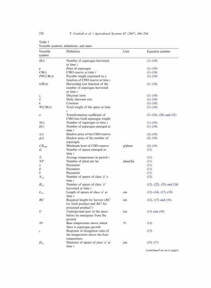
Table 1Variable symbols, definitions, and units

Variablesymbol

Definition Unit Equation number

H(t) Number of asparagus harvestedat time t

(1)–(10)

p Price of asparagus (1)–(10)CR(t) CHO reserve at time t (1)–(10)PW(CR(t)) Payable weight expressed as a

function of CHO reserve at time t

(1)–(10)

r(H(t)) Harvesting cost function of thenumber of asparagus harvestedat time t

(1)–(10)

1 Discount term (1)–(10)d Daily discount rate (1)–(10)k Constant (1)–(10)W(CR(t)) Total weight of the spear at time

t

(1)–(10)

r Transformation coefficient ofCHO into fresh asparagus weight

(1)–(10), (20) and (21)

N(t) Number of asparagus at time t (1)–(10)E(t) Number of asparagus emerged at

time t

(1)–(10)

k(t) Shadow price of the CHO reserve (2)–(10)l(t) Shadow price of the number of

asparagus(2)–(10)

CRmin Minimum level of CHO reserve g/plant (2)–(10)Et Number of spears emerged at

time t

(11)

Tt Average temperature in period t (11)NP Number of plant per ha plant/ha (11)a Parameter (11)b Parameter (11)h Parameter (11)Na,t Number of spears of class ‘a’ a

time t

(12)

Ha,t Number of spears of class ‘a’harvested at time t

(12), (22), (23) and (24)

La,t Length of spears of class ‘a’ attime t

cm (12)–(14), (17)–(19)

RLy Required length for harvest (RLf

for fresh product and RLp forprocessed product’’)

cm (12), (17) and (18)

U Underground part of the spearbefore its emergence from theground

cm (13) and (19)

Tb Base temperature above whichthere is asparagus growth

�C (13)

c Response of elongation rates ofthe temperature above the basetemperature

(13)

Da,t Diameter of spears of class ‘a’ attime t

cm (15)–(17)

(continued on next page)


Table 1 (continued)

Variablesymbol

Definition Unit Equation number

Dmax Maximum spear diameter cm (15)CLt CHO level per plant at time t g/plant (15)Cmin Minimum level of CHO for spear

productiong/plant (15)

Dk Michaelis–Menten controlparameter

(15)

PWa,t Payable weight of spears of class‘a’ at time t

g (17), (22) and (24)

f Correction factor forapproximation of spear volumeto cylinder volume

(17)

d Density of the spear kg/cm3 (17)Lmax Maximum length at which a

spear has commercial valuecm (17)

Wa,t Total weight of a spear of class‘a’ at time t

kg (19)–(21)

CRt CHO reserve at time t g/plant (20) and (21)CLt CHO level at time t, that is equal

to CRt subtracted by the emergedspears

g/plant (21)

I Seasonal profit per hectare withmanual harvest

$/ha (22)

Py Price of asparagus (Pf for freshasparagus, and Pp for processedasparagus)

US$/kg (22)

w Percent of spears harvested thatare not marketable

% (22) and (24)

Cy Manual harvesting cost per unit(Cf for fresh asparagus, and Cp

for processed asparagus)

US$/kg (22)

OC Other cost involved in themanual harvest (housing forlabor, and management costs)

US$/ha (22)

CF Fixed costs (except managementfees, amortized establishmentcosts, and land rent)

US$/ha (22)

CV Variable costs except theharvesting costs

US$/ha (22)

Zt Total harvesting time h (23) and (24)w Walking time spent in harvesting

1 ha of asparagush (23)

pt Picking time for one asparagus s (23) and (24)r Minimum wage per hour US$/ha (24)


Eq. (7) shows that the value of the shadow price of the number of spears does notchange over time. Therefore, the shadow price of an additional spear is considered asconstant (k), as reported in Eq. (8). Eq. (9) represents the shadow price of a unit ofCHO reserve at time t. Intuitively, the numerator of the first term of Eq. (9) identifies:


the value of a spear (term pPW(CR(t))), the marginal cost of harvest composed byr 0H(t) which is negative because of decreasing costs, and r(H(t)). The shadow priceof a unit of CHO, k(t), is represented by the value of a spear, the cost savings in har-vesting it, its opportunity cost of leaving the spear for future harvests, and its cost ofharvest, all deflated by the CHO used by the plant in producing it. In other words, k(t)is the net present value of a spear deflated by the units of CHO used for it.

The change in shadow price of the CHO reserve is represented by Eq. (10). Thefirst term represents the net present value of the change of the weight of payablespears due to a change in CHO reserve. The second term can be identified as theproduct between the shadow price of CHO and the change in quantity of CHO con-sumed to produce H(t) spears. More simply, it is the value of the change in CHOconsumed (or saved) in producing the spears harvested at time t (H(t)) because ofthe change in CHO reserve.

By solving the system of equations for H(t), it is possible to have the analyticalsolution of the number of asparagus spears harvested at each time t. Although a sim-ulation model was used to describe the harvesting problem, the theoretical economicmodel represents the starting point for understanding the decision problem of anasparagus producer. By harvesting more frequently than the optimal rate the pro-ducer will maximize yield, but not the profit because the harvesting cost are decreas-ing as the per time amount harvested increases. On the other hand, by harvesting lessfrequent than the optimal frequency, the manager will benefit by the cost savings ofthe lower harvesting costs, but will loose part of the potential yield because of theincreased waste in CHO due to the spear growth over the required length.

2.2. Empirical bioeconomic model description

The economic model was used to develop a more pragmatic growth model. Theasparagus growth model was build as a dynamic simulation model. The simulationframework was preferred to the optimization structure because of greater flexibilityfor model evaluation and to reproduce growers harvesting decisions. The model inte-grates biological and agronomic characteristics of asparagus. The time frame used inthe model is the hour, in fact spear emergence and spear growth were consideredhourly. This allows the schedule of the harvests at different times during the day.The model includes a number of parameters from recent publications and prelimin-ary field trials conducted by Washington State University (USA).

The asparagus bioeconomic model is a decision support tool to provide informa-tion and insights on hand harvesting, and to assist asparagus growers on the dailymanagement practices during the production season. While other models attemptedto incorporate the entire cycle of the asparagus field in the biological model (Lam-pert et al., 1980; Wilson et al., 2002a), in this bioeconomic model only the productionpart was considered. The underlying reason of this decision was to focus more on thedaily harvesting decisions. Growers do not want to reduce their CHO content belowa minimum level, because that would negatively affect future yields. Therefore, in themodel the harvest would stop when the minimum level of CHO is reached. Growersin New Zealand and US used this approach following a recently introduced decision


management tool, AspireNZ (Wilson et al., 2002b) for New Zealand and AspireUS(Drost, 2003) for the United States.

It was implicitly assumed that the plants were able to recover the CHO used in theproduction and have the recommended level restored by the beginning of the next har-vesting season. This assumption was necessary to focus on the model evaluation andon the harvesting strategies. Cembali et al. (2006) focused on modeling the asparaguscycle and studied the inter-year impact of stopping the harvest at different CHO levels.The assumption in this paper is consistent with the finding from Cembali et al. (2006).By stopping the harvest at the minimum CHO level advised (200 g/plant), the plantsare able to restore the CHO level in the remaining months before next productioncycle. If the harvest is interrupted at a lower level, then the production of the followingyear would be impacted because the plants have less time to assimilate CHO.

The asparagus growth model represents a single field of 1 ha. The harvest fre-quency and the harvest schedule can be chosen, as well as the density of plantsper hectare, and the total energy reservoir per plant in percentage of CHO on rootdry weight. This implies that the model is flexible in adapting to different productionsituations. For example, some fields may have a greater production potential becauseof the greater CHO reserve (Wilson et al., 1999a) and a higher number of plants thanothers (McCormick and Thomsen, 1990). The model considers a full production fieldthat can produce 6160 kg/ha per year which is typical for Washington State (USA).

2.3. Biology and agronomy

2.3.1. Emergence and density dynamics

The first spear emergence was predetermined in the model by a set day (5 April).This approach is similar to the model of Lampert et al. (1980). In the literature,researchers have tried to predict the first spear emergence of an asparagus field usingdegree days. Although Dufault (1996) suggests that soil temperatures should be usedto predict the first emergence, researchers prefer to use the ambient air temperature.Base temperatures adopted ranged from 4.4 �C (Blumenfield et al., 1961; Bouwkampand McCully, 1972) to 7.1 �C (Wilson et al., 1999b). Results of simulations using theapproach on first spear emergence from Wilson et al. (2002a) were not consistentwith the commercial practices in the state of Washington (USA). Using the base tem-perature would allow for first emergences 15–20 days earlier than when usuallyoccur.

In relation to the number of spears that emerged, both models from Wilson et al.(2002a) and Lampert et al. (1980) assumed that each plant of asparagus carries a cer-tain amount of spears that are growing simultaneously. The spears emerge through-out the growing season. Although the results from Lampert et al. (1980) (25.6 spearsper plant) agreed with a previous work by Ellison and Scheer (1959), they do notreflect the dynamics of asparagus field in high density plantings. For example,McCormick and Thomsen (1990) reported that the number of spears per plantranges from 9.5 to 5.7 for density of 19,000–44,000 plants/ha, respectively. Wilsonet al. (2002a) did not report the plant density assumed in their study, so a compar-ison with this model is not possible. Lampert et al. (1980) simulated five plants, and


by comparing the yield per plant with a commercial production level, it would beequivalent to a density of 7500 plant/ha, lower than the densities currently adopted.

In this model, to determine the number of spears emerged in each period (hour)the following transcendental emergence function was adopted:

Et ¼ aT ht expðbT tÞNP ð11Þ

where Et is the number of spears emerged in the period t, Tt is the average air tem-perature in the period t, NP is the number of plants, a, h, and b are parameters of thefunction. The values of NP and the other parameters are reported in Table 2. Thevalues of the parameters were determined using the results of field trials conductedin Prosser, Washington (USA) (Dean, 1999).

The two components of the density dynamics are spears emerged and spears har-vested. Although, the number of spears in a field might be affected by environmental

Table 2Parameter’s values for the equations

Parameter Equation number Value Source

a (11) 5.95 · 10�10 Curve fitting from Dean (1999)h (11) 5 Curve fitting from Dean (1999)b (11) 0.21 Curve fitting from Dean (1999)NP (11) 42,000 Ball et al. (2002)RLf (12), (17) and (18) 22.86 cm USDA (1996)RLp (12), (17) and (18) 19.05 cm Seneca Foods Corporation (2002)U (13) and (19) 12 cm Wilson et al. (1999a)Tb (13) and (14) 7.1 �C Wilson et al. (1999a)c (13) 0.02232 Wilson et al. (1999a)L0,t (13) and (14) 1.27 cm Cembali (unpublished data, 2003)Dmax (15) 2.8 cm Lampert et al. (1980)Cmin (15) 168.5 g Scott et al. (1939)Dk (15) 55 Calibrated valueCL0 (15) 270 g Drost (personal communication, 2003)f (17) and (19) 0.75 Value fitting datad (17) and (19) 0.95 Hopper and Folwell (1999)Lmax (17) and (18) 34.29 cm Holmes (personal communication, 2004)r = bset/dw (20) and (21) 7.78 Calculated valuebset (20) and (21) 0.7 Penning de Vries et al. (1974)dw (20) and (21) 0.09 Wilson et al. (2002a,b)CR0 = CR(0) (20) 270 g Drost (personal communication, 2003)CRmin = CR(T) (20) 200 g Drost (personal communication, 2003)Pf (22) US$0.99/kg Schreiber (personal communication, 2004)Pp (22) US$1.19/kg Seneca Food Corporation (personal

communication, 2004)w (22) and (24) 50% Value fitting field dataCf = Cp (22) and (24) US$0.51/kg Ball (personal communication, 2004)CF (22) US$388.36/ha Ball et al. (2002)CV (22) US$837.64/ ha Ball et al. (2002)OC (22) US$407.73/ ha Holmes (personal communications, 2004)r (24) US$7.16/h DOL (2004)w (23) 1.8 h Calculated valuept (23) 1.31 s Calculated value


factors as wind, insects, and temporary lack of moisture, those adverse factors werenot included in the model. The model accounts for harvested and marketable spears.The marketable spears are expressed as a percentage of the total spears in the field.The total spears in the field are represented by the spears emerged, spears that arebelow the marketable length (not ready to be harvested), and the spears that areabove the marketable length and therefore ready to be harvested. After emergence,the dynamics of the number of spears is only affected by the harvest. Spears are har-vested once their length is above the minimum length required in the fresh or pro-cessed market. Spear number dynamics is then ruled by the following equation:

Na;t ¼ Na�1;t�1 � Ha;t for a P 1 if La;t P RLy ; ð12Þ

where Na,t is the number of spears of class ‘a’ at time t, (note that N0,t�1 = Et�1),Na�1,t�1 is the number of spears of class ‘a � 1’ at time t � 1, Ha,t is the numberof spears of class ‘a’ harvested in period t, La,t is the length of the spears of class‘a’ at time t, RLy is the required length (RLf is the required length for the fresh mar-ket, and RLp is the required length for the processed market). Recall that Ha,t is po-sitive if the spears’ length of class ‘a’ at time t are greater than the required length(RLh) for harvest. More consideration on Ha,t were made in the economics section.The class indicates age and is expressed in hours of life since emergence. For exam-ple, N61,t indicates the number of spears of 61 h of age at time t. The values of theparameters RLf, and RLp are reported in Table 2. Variable symbols, definitions,and units are reported in Table 1.

2.3.2. Spear growth, diameter, and weight

The asparagus growth model utilizes the spear growth model developed by Wil-son et al. (1999b). Eqs. (13) and (14) report the growth function for a spear of class‘a’ in the period t:

La;t ¼ ðLa�1;t�1 þ UÞ expðcðT t � TbÞÞ � U ð13ÞLa;t ¼ La�1;t�1 if T t 6 Tb ð14Þ

where La,t is the length of ‘a’ spear of class a at time t, U is the underground part ofthe spear before its emergence from the ground, Tt is the average air temperature forperiod t, Tb is the base temperature above which there is asparagus spear growth,and c is the response of elongation rates of the temperature (Tt) above the base tem-perature (Tb). The length for spears just emerged, class 0, (L0,t) was predetermined,its value is reported in Table 2. Eq. (14) represents the spear growth constraint, andshows that if temperatures are equal or lower the base temperature, there is no speargrowth. The values of the parameters U, c, Tb, and L0,t are reported in Table 2.

The base temperature (Tb) reported by Wilson et al. (1999b) was considered a reli-able measure in determining spear length because it was estimated with field data,but it was not used in determining first emergence. Using hourly temperature, themodel accounts for frosting period by interrupting the growth when the temperatureis below Tb. For asparagus, frosting damages are not common. Rajeev and Wisniew-ski (1992) reported frost hardiness (defined as the temperature at which 50% injury


occurred) to temperature lower than �2.8 �C. Some frost damages can occur whenthe temperature is lower than �1 �C for 4–5 h. However, in Washington tempera-tures below �2 �C for 2 h only occurred in one year over the 16 years of weather dataavailable. In the model, frost damages were accounted together with other damagesthat may occur to spears (e.g. wind, and insects) in Eq. (22) with the term w (percentof asparagus that are not marketable).

Spear diameter is highly influenced by CHO reserve in the roots (Tiedjens, 1924;Norton, 1913; Ellison and Scheer, 1959). Therefore, it was decided to adopt theMichaelis–Menten functional form used by Lampert et al. (1980) to account forthe change in diameter over the season. Eq. (15) represents the relationship betweenspear diameter and CHO reserve in the root. Eq. (16) represents the dynamics ofspear diameter as the spear becomes older.

D1;t ¼DmaxðCLt�1 � CminÞDk þ CLt�1 þ Cmin

ð15Þ

Da;t ¼ Da�1;t�1 for a P 2 ð16Þ

where D1,t is the diameter of spears of class ‘1’ at time t, Dmax is the maximum speardiameter, CLt�1 is the CHO level per plant at time t � 1 (when the spear emerged),Cmin is the minimum level of CHO level for spear production, and Dk is a Michaelis–Menten control parameter. The values of the parameters Dmax, Cmin, Dk, and theinitial value of CHO level per plant (CL0) are presented in Table 2. TheMichaelis–Menten control parameter used by Lampert et al. (1980) has beenadjusted to obtain diameter lower values that are more representatives of thecommercial production conditions in Washington State (USA).

Eq. (15) does not take into account directly other factors that may affect the spearsize (e.g. heat stress, over harvest, drought). Those factors influence indirectly theCHO level of the plant, and consequently the spear diameter. With the assumptionof restoring the original CHO level, these factors do not play a relevant role in themodel. The impact of low level of CHO at the beginning of the production seasoncan be found in Cembali et al. (2006) were the impact of over and under harvestingis estimated.

The weight of each spear was calculated using a weight function as in Lampertet al. (1980). In the model each spear is harvested only if its length is greater thanthe required length (RLy). Therefore, in calculating the product harvested the modelonly considered the portion of spear of the payable length. On the other hand, theremaining portion of the spear (called trimmed part) consumed CHO, and this con-sumption was considered in the use of CHO. In addition, the underground portionof the spear (the portion from the root to the ground) was accounted for in the CHOusage. The model also considered that as the spear length reached a certain height(Lmax), it did not have any commercial value because of low quality. In fact, whena spear continues to grow over Lmax it starts to develop open branches (crooked) thatmake it unmarketable. The value of the limiting length (Lmax) is reported in Table 2.Eqs. (17) and (18) describe the payable product, while Eq. (19) explain the effectiveweight of the asparagus for the CHO balance.


PW a;t ¼ ðRLyÞ Da;t

2

� �2

pðf ÞðdÞ if RLy < La;t < Lmax ð17Þ

PW a;t ¼ 0 if La;t < RLy or La;t > Lmax ð18Þ

W a;t ¼ ðU þ La;tÞDa;t

2

� �2

pðf ÞðdÞ ð19Þ

where PWa,t is the payable weight of a spear of class ‘a’ at time t, RLy is the requiredlength, Da,t is the diameter of the spear of class ‘a’ at time t, f is the correction factorfor the approximation of spear volume to cylinder volume, d is the density of thespear, and Wa,t is the total weight of a spear of class ‘a’ at time t. The values ofthe parameters used in Eqs. (17)–(19) are reported in Table 2. Variable symbols, def-initions, and units are reported in Table 1.

2.3.3. CHO reserve dynamics

Asparagus yields depend on the CHO reserve. As mentioned before, recentresearch has focused on using the CHO root content as an indicator for crop man-agement purposes (Wilson et al., 2002b). The idea underlying this asparagus decisionsupport system was to ensure a high level of CHO during the harvest, and to preserveCHO reserve for the following year. In the model, when plants reach the minimumCHO level the harvest is stopped for the year under consideration.

The initial and the minimum optimal level of CHO content during the productionperiod were defined using values from Drost (personal communication, 2003) andassuming an average dry weight of 600 g per plant (Wilson et al., 2002a). In themodel, the consumption of CHO was adopted from Wilson et al. (2002a). The var-iable that accounts for the CHO reserve at time t was defined as CRt. For computa-tional purposes another variable that accounts for the level of CHO was defined inthe model as CLt. In this way, the consumption of CHO for spears not yet harvestedwas considered in calculating the diameter of the new spears emerging. Eqs. (20) and(21) defined those two variables

CRt ¼ CRt�1 � rX

a

H a;tW a;t ð20Þ

CLt ¼ CRt � rX

a

Na;tW a;t ð21Þ

where r is the transformation coefficient of CHO in asparagus fresh weight, r = dw/bset, and bset is the biosynthetic efficiency of transforming CHO in asparagus drymatter, and dw is the dry weight content of asparagus. Values of these last twoparameters are presented in Table 2.

2.3.4. Production conditions

The model was developed for the 1-ha asparagus field with a plants density of42,000 plants/ha in full production and the row spacing assumed was 1.37 m. Thefield was assumed to be cultivated according the accepted practices in the State ofWashington (USA). The production level of an asparagus field for this area varies


from year to year and location to location, but, on average is around 6160 kg/ha/yr(Ball et al., 2002). The model was intended to predict the daily production of anasparagus field as described above. The model might also be used to predict dailyproductions for fields with a variable plant stand by changing the value of the var-iable NP in Eq. (11). For example, the model could be used to determine the produc-tion during the lifecycle by changing the plant density to account for mortality.

Asparagus production can be for the fresh or processed market. These two differ-ent markets have different grading requirements in terms of length. The fresh marketprefers all green spears of 22.86 cm length and the processing market requires spearsof 19.05 cm in length. Growers in both markets are allowed to bring in asparaguswith some basal white portion (underground portion) for a maximum of 2.54 cmlength. In the model, it was assumed that the product for both markets was a greenspear. The reason of this assumption was because those are the harvesting practicescommonly adopted (Holmes, personal communications, 2003). It was assumed thatthe asparagus field responded in the same manner for those two different cuttingheights and that the production was driven by temperature and by CHO reserve.

The CHO reserve value of 450 mg/g was considered as the starting value (CR(0)),while the terminal value (CR(T)) was 330 mg/g of dry roots (Drost, personal com-munication, 2003). Those levels are equivalent to 270 g/plant and 200 g/plant ofCHO assuming an average dry weight per plant of 600 g. No mortality of the plantswas assumed. The first emergence was assumed to be on 5 April at 1:00 am. Theweather data utilized was from Mathew Corner, a weather station located in themain asparagus production area of Washington State (USA). The hourly tempera-ture was used to model the biodynamics of the asparagus field.

2.4. Economics

Profits generated by the manual harvest were calculated using the following profitfunction:

P ¼ P y

Xa;t

ðHa;tPW a;tÞð1� wÞ �X

a;t

ðH a;tPW a;tÞCy � OC � CF � CV ð22Þ

where P is the seasonal profit per hectare with manual harvest, Py is the price ofasparagus (Pf indicates fresh asparagus, and Pp processed asparagus), Ha,t is thenumber of spears of class ‘a’ harvested at time t, PWa,t is the payable weight ofthe spear of class ‘a’ harvested at time t, w represents the percent of harvested spearsthat are not marketable, Cy represents the harvesting cost per unit of product withthe manual harvest (Cf indicates fresh asparagus, and Cp processed asparagus),OC represents other costs involved in the manual harvest (housing for labor, andmanagement costs), CF represents the fixed costs (except management fees, amor-tized establishment costs, and land rent), and CV represents the variable costs exceptthe harvest. The values of the parameters Pf, Pp, w, Cf, Cp, OC, CF, and CV used inthe simulation model are reported in Table 2.

Two models with different constraints on the harvesting were considered. Anunconstrained model, where harvest was allowed, as described in the emergence


and density dynamics subsection, when there were spears above the required length(RLy). A constrained model was also considered to account for the minimum wagerequirements in the harvesting decisions. Not all the farmers in Washington State arewilling to pay the monetary augmentation on the harvesting cost. Those farmers pre-fer to harvest only when the minimum wage is assured to manual labor, because theyhave belief that the expected profit will be greater. This economic constraint wasintegrated with the length requirements for harvesting.

To account for the wage constraint, the time spent in manual harvesting was esti-mated. The time of manual harvest was assumed to be a function of the time spentfor walking, cutting and handling the spears, and the number of spears ready for har-vest present in the field. In the constrained bioeconomic model, if the costs of manualharvest (considered as the product of the quantity harvested and the per unit cost ofharvesting) were lower than the potential minimum wage pay rate for harvesting,then there was no harvest. Harvest only occurred if it was possible to guaranteethe minimum wage requirement. Eq. (23) reports the function used to estimate thetime spent for manual harvesting and Eq. (24) the harvesting constraint.

Zt ¼ wþ ptX

a

H a;t ð23Þ

Xa

Ha;t

> 0 if CyP

aðHa;tPW a;tÞð1� wÞP rZt

¼ 0 otherwise

(ð24Þ

where Zt is the total harvesting time, w is the walking time spent in harvesting 1 ha ofasparagus, pt is the cutting time,

PaH a;t is the sum in number of the spears har-

vested, and r is the minimum wage per hour. The values of the parameters w, pt,and r adopted in the simulation are reported in Table 2. Variable symbols, defini-tions, and units are reported in Table 1.

3. Methods

The model was evaluated using different statistics to determine its ability in pre-dicting daily productions. Then, two scenario situations were modeled. In each case,a hectare of asparagus in ‘‘normal production conditions’’ was assumed. The firstscenario was a production simulation for the constrained and unconstrained bioeco-nomic model. The second scenario was a simulation of different harvesting frequen-cies. Historical hourly weather data from 1989 to 2004 for the location of MathewCorner, Washington (USA) were used to simulate daily production for both scenar-ios (PAWS, 2004).

3.1. Evaluation of the production model

Model evaluation was based upon aggregate daily production data from receivingstations from a major asparagus processor in Washington State (USA). Receivingstations at different locations were used to test the model robustness in simulating


the daily production in different areas. Data from 2000 throughout 2003 were used inthe evaluation procedure. Table 3 lists the receiving stations used, the representativeweather station for that area, the contracted area (ha), the contracted and actual pro-duction (kg/ha) for each year. These data were used to compare the simulationresults with actual data.

The unconstrained model was used in the simulation. The aggregated dataincluded a variety of production situations, from young bearing fields to old aspar-agus fields. The simulation results are compared to an aggregated large sample toavoid having specific production site characteristics to influence the model evalua-tion. These results in assessing the validity of the model were applied to a varietyof commercial production situations as a result of the method followed.

Data of daily aggregated production for four consecutive years for several loca-tions (four locations for 2002 and 2003, and three locations for 2000 and 2001) wereused in the evaluation process. An actual series of daily production was consideredthe production recorded for one year by a location. Then the simulated series fromthe model were compared to the actual series and the two series were compared todetermine how similar or how different they were. The closer the two series (simu-lated and actual) were, the better was the model able to predict daily productionsfor a certain location in a certain year.

The model was evaluated using 14 independent series. Each location was evalu-ated using a simulation with weather data of the closest weather station available.

Table 3Receiving stations used for model validation: locations, names, contracted areas, contracted yields, andactual yields received during the years 2000 thorough 2003

Receiving station location(name)

Weather station Contractedarea (ha)

Contractedyield (kg/ha)

Actual yieldreceived (kg/ha)

2000Pasco (Unit 15) CBC Pasco 1246 4008 4056Pasco (Gibbons) Mathews Corner 1272 4519 5107Sunnyside (Sunnyside) Sunnyside 330 3815 4164Pasco (Ice Harbor) Fishhook 454 4425 4121

2001Pasco (Unit 15) CBC Pasco 935 4875 6047Pasco (Gibbons) Mathews Corner 1384 4659 4849Sunnyside (Sunnyside) Sunnyside 327 4591 5189Pasco (Ice Harbor) Fishhook 396 4335 5089

2002Pasco (Unit 15) CBC Pasco 1106 5119 5592Pasco (Gibbons) Mathews Corner 1178 4779 5042Sunnyside (Sunnyside) Sunnyside 585 4148 4778

2003Pasco (Unit 15) CBC Pasco 1168 4932 5621Pasco (Gibbons) Mathews Corner 1236 4692 5082Sunnyside (Sunnyside) Sunnyside 567 3889 5205


The 14 series had different input, and the model was evaluated on its ability to pre-dict daily productions.

The model was evaluated using 10 different statistics: mean square error (MSE),mean absolute deviation (MAD), mean absolute percent error (MAPE), Pearsoncorrelation coefficient (PCC), v2 test (CHI-SQUARE) (Goldsmith and Hebert,2004), autocorrelation function test for period comparison (ACF-T), cross-correla-tion function test for phase lag detection (CCF-T), mean comparison (MC), percentof error in variation (PEV), and discrepancy coefficient (DC), (Barlas, 1989). TheACF-T, and CHI-SQUARE are statistical tests, while the others are statistics thatrepresented different aspects of the variation between the actual and the simulateddaily asparagus production.

The smaller the calculated values for MSE, MAD, MAPE, MC, and PEV, thesmaller were the differences between the actual and the simulated daily production.The calculated value for PCC can range between �1 and 1, it represents the level andthe direction (positive or negative) of correlation. A calculated value close to 1 indi-cated a strong positive correlation between the two series. The DC represents the rel-ative discrepancy between the simulated and the actual production and it rangesbetween 0 and 1. A value close to zero represents low relative discrepancy (Gold-smith and Hebert, 2004).

The CHI-SQUARE tested the joint hypothesis that each individual simulatedoutcome (Si) was equal to the actual value (Ai) for that time period. The null hypoth-esis (Ho) would be rejected if at least one predicted value were statistically differentthan the actual value (Ho: Ai = Si for all i). The ACF-T and the CCF-T tests focuson the behavior pattern evaluation (Barlas, 1989). In particular the ACF-T can beused to detect errors in the periods of behavior patterns. The autocorrelation func-tion was then calculated for lag k = 0, 1, . . ., n � 1, where n is the number of simu-lated daily productions. Individual tests for each lag value were performed todetermine whether the autocorrelation function of the actual data is equal to theautocorrelation function for the simulated sequence. The percentages of the caseswhere the simulated values were not statistically different from the actual were con-sidered. The CCF-T is similar to the ACF-T. However, its focus is to check how theactual and the simulated data are correlated at different time lags (Barlas, 1989), ormore simply if they are out of phase or not. If the cross-correlation function has itsmaximum value at the lag equal to zero, then the two series are completely in phase.Appendix A reports the formulas and additional information on the statistics used.

3.2. Scenario 1: production simulation

Scenario 1 simulated the production of a hectare of asparagus to show the out-come of the simulation model for 16 years. This scenario was chosen to highlightthe profit performances of manual harvesting for the fresh and processed productusing both the constrained and unconstrained model. In the unconstrained modelit was assumed that harvesting occurs each day at 5 a.m. if there were spears longerthan the required minimum length (RLh). The constrained model, as describedbefore, presented an additional constraint (Eq. (24)). The cost of harvesting had


to provide minimum wage to the manual labor. For both models, if their respectiveconstraints did not hold, then harvesting would take place the following day.Detailed results were obtained for each year: (1) yield (kg/ha); (2) number of har-vests; (3) profit for the manual harvest (US$/ha); and cost of harvesting (US$/ha).

3.3. Scenario 2: comparison of harvesting schedules

Because of the lack of information in the literature for different asparagus harvest-ing strategies, scenario 2 was used to determine yield, number of harvests, profits,and costs of harvesting at different time intervals of 12, 24 (control), and 48 h.The listed harvesting intervals were chosen because the harvesting was always duringthe day. In fact, with the 12 h interval the model allowed harvest to occur at 5.00,and 17.00; with the 24 h interval at 5.00; and with the 48 h interval the model allowedharvest to occur at 5.00 of alternating days. Both the constrained and the uncon-strained models were simulated at different harvesting schedules. Statistical differ-ences were tested for each combination of results.

4. Results and discussion

4.1. Model evaluation

Model evaluation of predicted asparagus daily yield productions were based onsimulations performed across years and locations. For purposes of demonstrationthe results for 2001 at the location of Unit 15 in Pasco, Washington (USA) are pre-sented in Fig. 1. The results of the model evaluation procedures used are presented inTable 4. Four years of actual data for a total of fourteen different years and locationscombinations were compared to the simulated series. Each location differed from theothers because of the different hourly temperatures. The series were independent byeach other.

Daily values of the actual harvested asparagus ranged between 0 (no harvest) to270 kg/ha/day, and the average value in a season was approximate to 110 kg/ha/day. Values for MSE ranged between a minimum of 1232.47 and a maximum of2776.05. The MAD represents more intuitively the real error of the simulationmodel because it is expressed in kg/ha/day. The lowest value of MAD recordedwas 24.49 kg/ha/day, while the highest was 36.55 kg/ha/day. The result of theMAD indicated that the model, on average predicted values, was quite close tothe real observations.

Only in five situations the MAPE was below 50%. In the two worse situations theMAPE was above 100%. These cases were both in the same year (2002) and theirlocation was quite close, which suggests there might have been the influence of otherweather variables (e.g. frost, wind). The PCC calculated were mostly over 0.70,except for three cases and two of them were the same as the high MAPE.

There was a failure to reject the Ho of the CHI-SQUARE test. This result wasexpected. Goldsmith and Hebert (2004) obtained similar results in their model vali-

0

50

100

150

200

250

300

4/12

/200

1

4/19

/200

1

4/26

/200

1

5/3/2

001

5/10

/200

1

5/17

/200

1

5/24

/200

1

5/31

/200

1

6/7/2

001

Date

kg/ha per day

Actual Simulated

Fig. 1. Actual versus simulated daily asparagus production for the Unit 15, 2001.

Table 4Evaluation results 2000 thorough 2003

Year and receivingstation

MSE(kg/ha/day)2

MAD(kg/ha/day)

MAPE(%)

PCC ACF-T(%)

MC(%)

PEV(%)

DC

2000Unit 15 2776.05 38.45 94.70 0.67 93.44 50.85 65.88 0.46Gibbons 1253.66 27.87 53.95 0.81 97.06 20.22 35.87 0.34Sunnyside 2043.37 36.55 69.26 0.78 88.41 48.09 90.28 0.44Ice Harbor 1902.88 34.22 78.28 0.84 94.12 50.12 65.56 0.37

2001Unit 15 1617.11 31.47 40.54 0.77 85.96 2.30 16.97 0.34Gibbons 2269.36 35.20 57.24 0.74 96.49 15.88 44.98 0.40Sunnyside 2133.00 33.53 47.80 0.74 75.86 7.96 53.49 0.41Ice Harbor 2270.51 34.72 56.15 0.72 77.59 12.15 46.85 0.41

2002Unit 15 2236.38 29.13 142.19 0.49 75.81 8.90 4.11 0.50Gibbons 1508.87 24.49 224.87 0.69 85.25 13.60 0.73 0.40Sunnyside 1406.28 25.26 60.26 0.70 85.48 18.44 19.88 0.39

2003Unit 15 1297.02 26.79 46.97 0.73 87.30 2.64 5.44 0.37Gibbons 1410.45 28.77 49.14 0.73 83.33 2.86 8.39 0.37Sunnyside 1232.47 25.44 46.10 0.74 91.80 3.53 11.76 0.36



dation. Despite this, it can be argued that the model is still consistent and robust.This test only stated that at least one predicted value was statistically different fromthe actual value. Recalling that the number of values predicted ranged from 58 to 70per case, it is expected that some of the predicted values will not be statistically equalto the actual production.

ACF-T indicated that in twelve of the fourteen cases 80% or more of the autocor-relation functions (n � 1 for every case) of the actual data were not statistically dif-ferent from the corresponding autocorrelation functions of the simulated data. In theremaining two cases this percentage was above 70%, supporting that the simulatedseries did not differ from the actual data. The results for the CCF-T were also posi-tive in validating the model in trend patterns for all cases.

In six cases the results of the MC were below the 10% and in three cases werearound 50%. This difference was mainly due to the lower production capability ofthe contracted asparagus at a certain receiving station with respect to the potentialin production assumed in the model (6164 kg/ha per season). Table 4 contains theexpected yields for each receiving station and year. In all cases the production waslower than the production assumed in the model. Weather or agronomic reasonsinfluenced the difference in the asparagus harvested per day between the actualand the simulated series (e.g. frosts, windy weather, pests, etc.).

The PEV had contrasting results, although in one case the actual and the simu-lated data had almost the same PEV value with a difference of only 0.73%. In sevencases the values of PEV were lower than 20%. In two of the four years examined thesimulation seemed not to perform well in terms of PEV. The DC values calculatedranged from 0.342 to 0.504 and indicated some relative discrepancy between theactual and the simulated series.

The simulations showed a similarity in trends and correlation with the actual pro-duction of asparagus. The dissimilarities were due mainly a difference in potentialyield between the model and the aggregated data. This finding associated with theother tests supported the prediction capability of the simulation model of daily har-vesting of asparagus. Lampert et al. (1980) did not discuss the validity of its model inpredicting daily production levels. Only the yearly average production per plant wasreported. In addition, they did not use hourly temperatures as input for the model,but daily averages. This difference approach is critical in determining the ability topredict daily production because it has lower precision in predicting growth andemergence. The work from Wilson et al. (2002a) does not report the results and doesnot specify if the daily or hourly temperature is used.

Another difference between our model and the ones developed by Lampert et al.(1980) and Wilson et al. (2002a) is the integration of the economic constraint to theharvest. This aspect adds more accuracy to the predicted daily production because itsimulates the decision process a producer has to face in harvesting asparagus.

The validity of the model can be visually determined from Fig. 1. At the begin-ning, the model was able to predict the daily production following the same patternas the actual yield. Then around the end of April (30 April) the model predictedlower daily productions for 3 days. On 5 May the predicted and actual values werealmost the same. After that period, the predicted daily production had the same


pattern as the actual values did except in two periods (12–14 May, and 22–25 April)where the actual yield are lower than the predicted.

When the predicted yields were higher than the actual, it could be due to extensivewind damages that were not accounted directly by the model, but by a proxy con-stant (w) during the season. Also, emergence might have been affected by adverseconditions that were not accounted. On the other hand, when the model predictedlower yield than the actual recorded data, it might be due to a lower number of spearemerged in previous periods or due to the fact that the model is not able to react rap-idly to the changing weather conditions. The model could benefit from ad hoc fieldtrials that focus on modeling spear emergence.

4.2. Scenario 1: production simulation

The production simulation was performed for both the processed and the freshasparagus. Detail results for the constrained model for the processed and the freshproduct are reported in Tables 5 and 6, while average results for both models andboth asparagus products are reported in Table 7. The yield generated by the uncon-strained model was always higher than the constrained model. Intuitively, becausethe constraint on the harvest lowered the number of harvests, then the losses ofCHO to produce non-payable product (spear growth exceeding the RLy) weregreater, with a negative impact on the overall potential yield. The yield obtainedfor the fresh product was always higher than for the processed product.

Table 5Yearly results of the constrained simulated daily harvest of processed product

Year Yield (kg/ha) Numberof harvests (#)

Profit for manualharvest (US$/ha)

Total cost ofharvesting (US$/ha)

1989 5774.80 46 2313.00 3335.881990 6024.77 55 2483.83 3462.621991 6116.29 58 2546.38 3509.031992 6000.64 49 2467.34 3450.391993 6000.72 52 2467.39 3450.431994 5930.99 47 2419.74 3415.071995 6100.19 51 2535.38 3500.871996 5705.92 58 2265.93 3300.951997 6010.21 52 2473.88 3455.241998 5970.98 50 2447.07 3435.351999 6088.47 58 2527.37 3494.922000 6018.68 53 2479.67 3459.542001 5887.75 49 2390.19 3393.152002 6100.89 54 2535.86 3501.222003 6109.11 56 2541.47 3505.392004 5962.61 52 2441.35 3431.10

Average 5987.69 52.50 2458.49 3443.82Minimum 5705.92 46.00 2265.93 3300.95Maximum 6116.29 58.00 2546.38 3509.03

Table 6Yearly results of the constrained simulated daily harvest of fresh product

Year Yield(kg/ha)

Number ofharvests (#)

Profit for manualharvest (US$/ha)

Total cost ofharvesting (US$/ha)

1989 6213.76 47 1352.70 3558.451990 6617.59 55 1546.78 3763.221991 6637.99 54 1556.58 3773.561992 6172.55 45 1332.89 3537.561993 6054.79 47 1276.30 3477.841994 6153.26 45 1323.62 3527.781995 6327.60 47 1407.41 3616.181996 6264.09 56 1376.89 3583.971997 6295.74 49 1392.10 3600.021998 6403.96 48 1444.11 3654.901999 6421.85 56 1452.71 3663.972000 6521.53 52 1500.61 3714.512001 6011.81 45 1255.64 3456.052002 6469.75 53 1475.73 3688.262003 6451.08 52 1466.76 3678.792004 6430.86 51 1457.04 3668.53

Average 6340.51 50.13 1413.62 3622.72Minimum 6011.81 45.00 1255.64 3456.05Maximum 6637.99 56.00 1556.58 3773.56

Table 7Average simulated yearly results for the unconstrained and constrained simulation model of manualharvest for both the processed and fresh asparagus (1989–2003)

Asparagusutilization

Model used Yield(kg/ha)


Profit formanual harvest(US$/ha)

Total costof harvesting(US$/ha)

Processed Unconstrained 6140.86bA 58.94aA 2563.17aA 3521.49bA

Processed Constrained 5987.69c 52.50b 2458.49b 3443.82cFresh Unconstrained 6394.19a 52.63b 1439.41c 3649.94aFresh Constrained 6340.51a 50.13b 1413.62c 3622.72a

A Average values followed by same lower case letter are not significantly different at P 6 0.05 accordingto LSD test.


Processed asparagus required a shorter spear length to be harvested; consequentlya higher number of spears were harvested. Each time a spear was harvested, theunderground portion did not account for as payable product (it was accounted asa loss), but it did consume CHO affecting negatively the potential yield. Either thework of Lampert et al. (1980) or Wilson et al. (2002a) did not address the differencein potential yield between fresh and processed asparagus.

Profits for processed product were higher despite the lower production because ofits higher price. The average profit simulated per ha with the constrained model formanual harvesting was US$2458.49 for processed asparagus, and US$1413.62 forfresh products. Yields simulated with the constrained model were similar to the


common production levels in Washington (6160 kg/ha), and were 5987.69 for theprocess asparagus and 6340.51 kg/ha for fresh.

The numbers of harvests simulated with the constrained model were not statisti-cally different. The number of harvests was 52.63 for processed asparagus and 50.13,for fresh product. Costs were higher for the fresh product because of the cost struc-ture adopted (US$/kg of asparagus harvested) and the higher production for thefresh product. The total cost of harvesting included the term defined in Eq. (22) asOC that account for housing for labor and management costs.

The constraint accounting for minimum wage generated differences for bothprocessed and fresh asparagus with respect to the unconstrained model. This resultconfirmed the fact that minimum wage represents an additional cost forWashington asparagus growers. The impact of the minimum wage constraint isUS$104.68/ha for the processed asparagus, and US$25.79/ha for the fresh aspar-agus. Intuitively, the time spent in walking and picking up asparagus is almost thesame for processed and fresh asparagus, but processed asparagus spears aresmaller and weight less. The constraint for minimum wage is statisticallysignificant only for processed asparagus.

Tables 5 and 6 show the variability in predicting yield, that shows how sensible isthe model to the hourly temperature in forecasting daily productions. The economicconstraint has a direct impact on the number of harvest. As described before, if theexpected pay for the manual worker does not guarantee the minimum wage, harvestis postponed to the next day. That, associated with the different temperatures, causesthe differences in number of harvests.

Previous literature approach the issue of harvesting asparagus either from a bio-logical view (Lampert et al., 1980; Wilson et al., 2002a) or from an economic per-spective (Stout et al., 1967; Michalson and Thomas, 1972), but there is not astudy that integrated the biological and economic implications of harvestingasparagus.

There is no literature examining the impact of the wage constraint on asparagusproduction. The harvesting constraint used in this model represents the harvestingconditions for the State of Washington (USA). However, different production areasmay have different economic conditions or contracts for harvesting asparagus. Themodel presented can be modified and different harvesting constraint can be set todetermine the impact on the daily production from both an economic and agronomicperspective.

4.3. Scenario 2: comparison of harvesting schedules

The constrained model yields for both the processed and fresh product were sta-tistically higher for the 12 h interval of harvests (Table 8). Gains in yield by increas-ing the frequency of harvest to the 12 h interval were 269.05 and 438.21 kg/ha, forthe processed and fresh product. The main reason of this result was that the freshproduct has a taller spear that, because of the spear growth function (Eq. (13)),grows faster. Therefore, by increasing the harvesting interval, there would be lesstrimmed product that consumed CHO. Increasing the frequency of harvest would

Table 8Average simulated yearly results for the unconstrained and constrained simulated daily manual harvestsfor both the processed and fresh asparagus at different frequencies (1989–2003)

Asparagusutilization

Model used Frequencyof harvest(h)

Yield(kg/ha)


Profit formanual harvest(US$/ha)

Total cost ofharvest(US$/ha)

Processed Unconstrained 12 6490.32aA 123.44aA 2802.00aA 3698.68aA

Processed Unconstrained 24 6140.86b 58.94b 2563.17b 3521.49bProcessed Unconstrained 48 4987.56c 26.94c 1774.98c 2936.70c

Processed Constrained 12 6256.74aA 81.19aA 2642.37aA 3580.25aA

Processed Constrained 24 5987.69b 52.50b 2458.49b 3443.82bProcessed Constrained 48 4901.83c 26.13c 1716.38c 2893.22c

Fresh Unconstrained 12 6915.33aA 109.81aA 1689.88aA 3914.19aA

Fresh Unconstrained 24 6394.19b 52.63b 1439.41b 3649.94bFresh Unconstrained 48 4598.67c 24.13c 576.48c 2739.51c

Fresh Constrained 12 6778.72aA 84.94aA 1624.22aA 3844.92aA

Fresh Constrained 24 6340.51b 50.13b 1413.62b 3622.72bFresh Constrained 48 4521.77c 23.50c 539.53c 2700.52c

A Average values followed by same lower case letter are not significantly different at P 6 0.05 accordingto LSD test.


increase the potential yield production of the asparagus field. Assuming the samecost structure of the classic 24 h interval, there would be an equivalent to an increasein profits.

Increases in profit calculated with the constrained model adopting the 12 h inter-val harvesting strategy instead of the 24 h were US$183.88/ha for the processedproduct and US$210.60/ha for fresh asparagus. These results showed that multipledaily harvests might represent a way to increase yields and profits without negativelyaffecting the production of the following year.

The 48 h harvesting interval had yields and profit levels significantly lower thanthe control interval (24 h). The 48 h interval harvesting strategy, using the con-strained model, generated yields of 4901.83 for processed asparagus and4521.77 kg/ha for fresh product (Table 8). Those values represented a reduction inyields of 1085.86 and 1818.74 kg/ha for the processed and fresh product, respec-tively. Results in terms of profits were similar. Reductions in profit wereUS$742.11/ha for the processed asparagus and US$874.09/ha for fresh product.

Results with the unconstrained model in increasing the frequency of harvestingresulted in an increase in yield of 349.46 for the processed asparagus and521.14 kg/ha for fresh. The gain in yield by increasing the harvesting frequencywas greater in the unconstrained model. Similar results were found in terms of theprofits. The 12 h harvesting interval had a gain in profit of US$238.83/ha andUS$250.47/ha for the processed and fresh product, respectively. The profit levelsby moving from the 24 h interval to the 12 h for the processed product increasedby US$54.95/ha for the constrained model. This indicated that if there were no


economic constraint on the harvest, growers could benefit an extra US$50.06/ha bymoving to the 12 h strategy.

The constrained simulation model is more relevant in supplying information onharvesting interval decisions to the grower in Washington. The unconstrainedmodel, on the other hand, had no economic constraints on the harvest, thereforeits results were relevant in growing conditions where manual labor does not repre-sent a limitation to the asparagus crop. A change in the minimum wage requirement,as well as any other economic variable might change these results. Among the resultspresented, the only ones that would be unchanged if economic conditions wouldchange are the yields from the unconstrained simulation model.

These results indicated a potential gain with manual harvest for asparagus grow-ers in reducing the interval of harvest from 24 to 12 h. The gain was in both yieldsand profits. The 48 h interval strategy presented the lowest profit and yieldperformances.

There are several studies in the literature that examine the issue of differentharvesting strategies for asparagus. Lampert et al. (1980) examined the impactof harvesting every other year, two years out of three, and three years out offour, and they compared those findings with the every year results and concludingthat yield is higher if harvest occurs every year. Stout et al. (1967) considered dif-ferent harvesting strategies for non-selective mechanical harvester for asparagus(daily, one harvest every two days, one every three days, and one every fourdays) concluding that the right interval depends on the capacity of the mechanicalharvester. With manual harvesting, the availability of labor might be hard to findin case of multiple daily harvests because of high temperatures during the day.Despite it is more profitable harvesting asparagus at the 12 h interval (whenthe harvesting constraint is satisfied), it might not be feasible to embrace byasparagus producers.

This paper adds to the existing literature the idea to explore multiple daily har-vests for asparagus. If mechanical harvesting is adopted this could represent anopportunity. The model shows flexibility for changing assumptions that could beused to further investigate those aspects. This allow to determine faster if a harvest-ing strategy might or might not increase yields. Using the traditional field research itcould have been taken years, but the model allow identifying harvesting strategiesthat could increase profitability in a shorter time.

5. Conclusions

This paper represents a contribution to the existing literature of harvesting aspar-agus. It is the first to incorporate economics to the decision of harvesting asparagususing a bioeconomic model. In addition, it is the only attempt to predict the dailyproduction of asparagus. The bioeconomic model developed was able to calculatethe impact of harvesting decisions and economic constraints. The outcomes of differ-ent harvesting strategies and the impact of the minimum wage constraint wereidentified.


The bioeconomic model was developed and validated using 10 different statisticalmethods to test its prediction capabilities in forecasting the daily harvest for severallocations in Washington State (from five to three locations) in four different years(2000–2003). The testing procedure adopted proved that the model was able to pre-dict the daily production of asparagus in different locations with a good degree ofprecision.

The model was used to simulate yield, number of harvests, profits, and the totalcosts of harvesting for every year in the period 1989–2004 using the weather datafrom a location in Washington. By comparing the results of the unconstrainedand constrained model, it was possible to evaluate the impact of the minimum wagerequirements for Washington on the yields and profits for both processed and freshasparagus.

The impact of different harvesting intervals was identified with the bioeconomicmodel. The traditional harvest interval of 24 h was compared to a more frequent(12 h) and a less frequent interval (48 h). Manual harvest with the interval of 12 hshowed the best results in terms of yields and profits for both the processed andfresh asparagus. Gains in profits with the actual production conditions in Wash-ington were US$183.88/ha and US$210.60/ha for processed and fresh product,respectively. Although it might not be possible to hire manual labor for multipledaily harvests, these results showed that there is a potential gain also for the man-ual labor involved.

Appendix A

In this appendix the formulas used to calculate the statistics and the testsdescribed in the Model evaluation section are discussed.

1. MSE (mean square error)

MSE ¼

Pni¼1

ðAi � SiÞ2

nðGoldsmith and Hebert; 2004Þ ðA1Þ

where Ai is the actual production for day i, Si is the simulated production forday i, and n is the number of days in which production occurred.

2. MAD (mean absolute deviation)

MAD ¼

Pni¼1

jAi � Sij


3. MAPE (mean absolute percent error)

MSE ¼

Pni¼1

jAi�Si jAi

� �� 100


4. PCC (Pearson correlation coefficient)


PCC ¼

Pni¼1

ðAi � AÞðSi � SÞ

ðn� 1ÞSASE

ðGoldsmith and Hebert; 2004Þ ðA4Þ

where A is the average actual production per day, S is the average simulatedproduction per day, SA is the sample standard deviation for the actual data,and SS is the sample standard deviation for the simulated production. The va-lue of the Pearson coefficient is between �1 and 1. The value 0 indicates no cor-relation, the value 1and �1 indicate perfect positive and negative correlation,respectively. Closer to 1 is the PCC, more correlated are the two series, and forvalidation purposes the better is the simulation model.

5. CHI-SQUARE (joint Chi-square test)

v2 ¼Xn

i¼1

ðSi � AiÞ2

AiðGoldsmith and Hebert; 2004Þ ðA5Þ

The chi-square statistics (v2) is found with the above equation. It is testedwhether each predicted (or simulated) production value is equal to the actualvalue recorded for that day. This is a joint test, therefore the null hypothesis(Ho) will be reject if at least one of the values is statistically different than itsprediction (Ha). In the case of validation a failure to reject the Ho will be a signof no statistical difference between the actual and the simulated series. Detailsof the joint hypothesis testing are reported below.
Ho: Si = Ai for i = 1, 2, 3, . . ., n.Ha: Si 6¼ Ai for at least one i.
6. ACF-T (autocorrelation function test) The autocorrelation function (r(k)) ofthe actual and simulated series should be the same for lag valuesk = 0, 1, 2, . . ., n. Each value of both the actual and the simulated series wereindicated generically by xi. The autocorrelation function is equal to:

rðkÞ ¼ CovðkÞVarðxiÞ

ðBarlas; 1989Þ ðA6Þ

where the Cov(k) is expressed by

CovðkÞ ¼

Pn�k

i¼1

ðxi � �xÞðxiþk � �xÞ

nðA7Þ

The hypothesis testing will be similar to the one seen for the chi-square testing.However, in this case an individual test is carried out. The null hypothesis (Ho)will be that the autocorrelation functions for the simulated and actual seriesare equal (given the same lag considered) or similarly that there is no differencein the periods of the two behavior patterns test (Barlas, 1989). The confidenceinterval was calculated for each value of lag k using the variance of the auto-correlation function (Var(r(k))) and the standard error (Se(dk)) of the distancebetween rS(k) (autocorrelation function of the simulated series) and rA(k)(autocorrelation function of the actual series) using the following formulas:


VarðrðkÞÞ ¼

Pn�1

i¼1

ðn� iÞðrðk � iÞ þ rðk þ iÞ � 2rðkÞrðiÞÞ2

nðnþ 2Þ ðA8Þ

SeðdkÞ ¼ffiffiffiffiffiffiffiffiffiffiffiffiffiffiffiffiffiffiffiffiffiffiffiffiffiffiffiffiffiffiffiffiffiffiffiffiffiffiffiffiffiffiffiffiffiffiffiffiffiffiVarðrSðkÞÞ þ VarðrAðkÞÞ

pðA9Þ

The individual hypothesis are:
Ho: rA(k) = rS(k) for k = 1, 2, 3, . . ., n � 1.Ha: rA(k) 6¼ rS(k) for k = 1, 2, 3, . . ., n � 1.
7. CCF-T (cross-correlation function test)The cross-correlation function testdetects if the two series are perfectly in phase. If that is the case the cross-correlation function has the highest value with a phase lag equal to zero.The two cross-correlation functions considered were:

CovSAðkÞ ¼

Pni¼kðSi � SÞðAi�k � AÞ

nSSSA

for k ¼ 0; 1; 2; . . . ; n� 1


CovSAðkÞ ¼

Pni¼�kðAi � AÞðSiþk � SÞ

nSSSA

for k ¼ 0;�1;�2; . . . ;�nþ 1


8. MC (mean comparison)

MC ¼ jS � AjjAj ðBarlas; 1989Þ ðA12Þ

The MC indicates the percent of error in the difference between means.9. PEV (percent error of variation)

PEV ¼ jSS � SAjjSAj


where SS is the standard deviation of the simulated series, and SA is the stan-dard deviation of the actual series. The PEV indicates the difference in the var-iation among the two series. It expresses the percent of error in variations ofthe sample estimate.

10. DC (discrepancy coefficient)

DC ¼

ffiffiffiffiffiffiffiffiffiffiffiffiffiffiffiffiffiffiffiffiffiffiffiffiffiffiffiffiffiffiffiffiffiffiffiffiffiffiffiffiffiffiPni¼1

ðSi � S � Ai þ AÞ2sffiffiffiffiffiffiffiffiffiffiffiffiffiffiffiffiffiffiffiffiffiffiffiPni¼1

ðSi � SÞ2s ffiffiffiffiffiffiffiffiffiffiffiffiffiffiffiffiffiffiffiffiffiffiffiffiPn

i¼1

ðAi � AÞ2s ðBarlas; 1989Þ ðA14Þ


The DC ranges from 0 to 1. It indicates the relative discrepancy between the actualproduction data and the simulated values. Its purpose in validation will be to sum-marize and report the relative discrepancy.

References

Ball, T., Folwell, R.J., Holmes, D., 2002. Establishment and annual production costs for Washingtonasparagus in 2001. Farm Business Management Reports, EB1779. Cooperative Extension WashingtonState University, Pullman, USA.

Barlas, Y., 1989. Multiple tests for validation if system dynamics type of simulation models. EuropeanJournal of Operation Research 42, 59–87.

Blumenfield, D., Meinken, K.W., LeCompte, S.B., 1961. A field study of asparagus growth. Proc. Amer.Soc. Hort. Sci. 77, 386–392.

Bouwkamp, J., McCully, J., 1972. Competition and survival in female plants of Asparagus officinalis. J.Am. Soc. Hort. Sci. 97, 74–76.

Cembali, T., Folwell, R.J., McCluskey, J.J., Huffaker, R.G., Wandschneider, P.R., 2006. Economicanalysis of the inter-year effect of alternative harvesting strategies for asparagus. J. Veg. Sci. 12, 29–50.

Clark, C.W., 1990. Mathematical Bioeconomics – The Optimal Management of Renewable Resources.second ed. Wiley, New York, 386pp.

Dean, B.B., 1999. The effect of temperature on asparagus spear growth and correlation of heat unitsaccumulated in the field with spear yield. Acta Hort. 479, 289–295.

DOL, 2004. Minimum Wage Laws in the States. Department of Labor, Washington, DC, USA. Availablefrom: <http://www.dol.gov/esa/minwage/america.htm#Washington> .

Drost Dan, 2003. AspireUS. Logan, UT, USA. Available from: <www.aspireus.com>..Dufault, R.J., 1996. Relationship between soil temperatures and spring asparagus spear emergence in

coastal South Carolina. Acta Hort. 415, 157–161.Ellison, J.H., Scheer, D.F., 1959. Yield related to brush vigor in asparagus. Proc. Am. Soc. Hort. Sci. 73,

339–344.Goldsmith, P.D., Hebert, Y., 2004. System dynamics, agriculture economics, and the process of model

validation. Working paper, University of Illinois..Hopper, R.J., Folwell, R.J., 1999. Effects of mechanized harvesting on revenues from processed asparagus.

Acta Hort. 479, 447–451.Lampert, E.P., Johnson, D.T., Tai, A.W., Kilpatrick, G., Antosiak, R.A., Crowley, P.H., Goodman, E.D.,

1980. A computer simulation to maximize asparagus yield. J. Am. Hort. Sci. 105, 37–42.McCormick, S.L., Thomsen, D.L., 1990. Management of spear number, size, quality and yield in green

asparagus through crown depth and population. Acta Hort. 271, 151–157.Michalson, E.L., Thomas, W.C., 1972. Economics of asparagus production and harvest mechanization in

Washington. Wash. Agr. Exp. Stat. Bull. 759, 12.Norton, J.B., 1913. Methods used in breeding asparagus for rust resistance. Bull. US Dept. Agr. Bur. Plant

Ind. 263..PAWS, 2004. Washington State University Public Agricultural Weather System. Prosser, WA, USA.

Available from: <http://index.prosser.wsu.edu/>.Penning de Vries, F.W.T., Brunsting, A.H.M., van Laar, H.H., 1974. Products, requirements and

efficiency of biosynthesis: a quantitative approach. J. Theor. Biol. 45, 339–377.Rajeev, A., Wisniewski, M.E., 1992. Frost hardiness of Asparagus officinalis L. HortScience 27, 823–824.Scott, L.E., Mitchell, J., McGinty, R., 1939. Effects of certain treatments on the CHO reserves of

asparagus crowns. S.C. Agr. Exp. Stat. Bull. 321, 5–37.Seneca Foods Corporation, 2002. Asparagus Raw Product Grade Specifications. Dayton, Washington,

USA.Stout, B.A., Kline, C.K., Hoglund, C.R., 1967. Economics of mechanical asparagus harvesting systems.

Mich. State Univ. Exp. Stat. Farm Sci. Res. Rep. 64, 10.Tiedjens, V.A., 1924. Some physiological aspects of Asparagus officinalis. Proc. Am. Soc. Hort. Sci. 21,

129–140.

http://www.dol.gov/esa/minwage/america.htm#Washington

http://www.aspireus.com

http://index.prosser.wsu.edu/


USDA-AMS, 1996. United States Standards for Grades of Fresh Asparagus. United States Department ofAgriculture, Agricultural Marketing Service, Fruit and Vegetable Division, Washington, DC, USA.

Wilson, D.R., Sinton, S.M., Wright, C.E., 1999a. Influence of time of spear harvest on root systemresources during the annual growth cycle of asparagus. Acta Hort. 479, 313–319.

Wilson, D.R., Cloughley, C.G., Sinton, S.M., 1999b. Model of the influence of temperature on theelongation rate of asparagus spears. Acta Hort. 479, 297–301.

Wilson, D.R., Cloughley, C.G., Jamienson, P.D., Sinton, S.M., 2002a. A model of asparagus growthphysiology. Acta Hort. 589, 297–301.

Wilson, D.R., Cloughley, C.G., Sinton, S.M., 2002b. AspireNZ: a decision support system for managingroot CHO in asparagus. Acta Hort. 589, 51–58.

Economics of alternative simulated manual asparagus harvesting strategies

Documents