Economics 173 Business Statistics Lecture 6 Fall, 2001 Professor J. Petry

Economics 173Business Statistics

Lecture 6

Fall, 2001

Professor J. Petry

http://www.cba.uiuc.edu/jpetry/Econ_173_fa01/

2

General Announcements• For efficiency reasons, questions regarding the lecture materials

will have to wait until after class, lab session, office hours or web-board.

• We will no longer require using the Z-table, nor any other table at the back of the book. – The counterintuitive nature of the tables and our ability to use excel in its

place make this choice optimal.– We will provide the critical value to which you can compare a test statistic

value, a p-value to which you can compare a significance level, or some means to find the necessary values without using the tables in your book.

• We will do our best to keep lectures as close to the schedule as possible. Regardless of the lecture pace, our schedule as printed in the Course Outline should dictate your reading schedule.

Chapter 11

Inference About the Description of a Single

Population

Inference About the Description of a Single

Population

4

11.1 Introduction

• In this chapter we utilize the approach developed before for making statistical inference about populations.– Identify the parameter to be estimated or tested .– Specify the parameter’s estimator and its sampling

distribution.– Construct an interval estimator or perform a test.

5

• We will develop techniques to estimate and test three population parameters.– The expected value – The variance 2

– The population proportion p (for qualitative data)• Examples

– A bank conducts a survey to estimate the number of times customers will actually use ATM machines.

– A random sample of processing times is taken to test the mean production time and the variance of production time on a production line.

6

• Recall that when is known is normally distributed

– If the sample is drawn from a normal population, or if– the population is not normal but the sample is sufficiently large.

• When is unknown, we use its point estimator s,

and the Z statistic is replaced then by the t-statistic

x

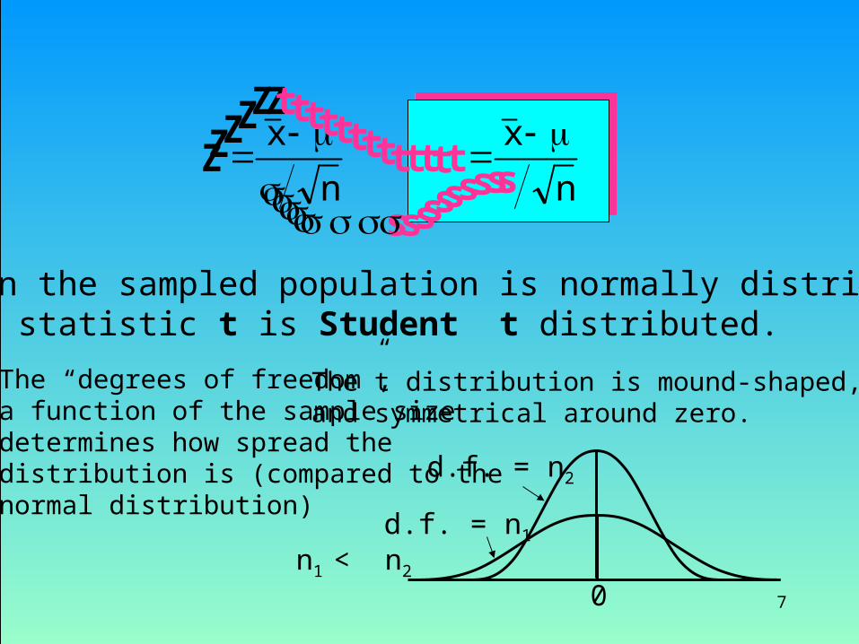
11.2 Inference About a Population Mean When the Population Standard Deviation Is Unknown

7

n

x

sn

x

Z t

s ss s

When the sampled population is normally distributed,the statistic t is Student t distributed.

0

The t distribution is mound-shaped, and symmetrical around zero.

The “degrees of freedom”,a function of the sample sizedetermines how spread thedistribution is (compared to the normal distribution)

d.f. = n2

d.f. = n1

n1 < n2

ZZZZZt t t t t t t t t t t

sss s s

t

8

Testing the population mean when the population standard deviation is unknown

• If the population is normally distributed, the test statistic for when is unknown is t.

• This statistic is Student t distributed with n-1 degrees of freedom.

ns

xt

ns

xt

9

• Example 11.1 Trainees productivity– In order to determine the number of workers required

to meet demand, the productivity of newly hired trainees is studied.

– It is believed that trainees can process and distribute more than 450 packages per hour within one week of hiring.

– Can we conclude that this belief is correct, based on productivity observation of 50 trainees?

10

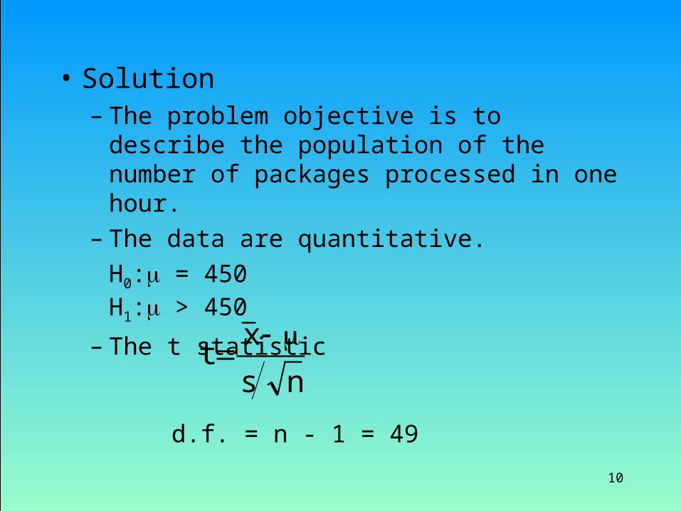
• Solution– The problem objective is to describe the population

of the number of packages processed in one hour.– The data are quantitative.

H0: = 450H1: > 450

– The t statistic

d.f. = n - 1 = 49ns

xt

11

– Solving by hand• The rejection region is t > t,n - 1

• t,n - 1 = t.05,49 = approximately to 1.676. (=critical value)• From the data we have

83.3855.1507s

.55.15071n

nx

xs

and,38.46050019,23

x

thus,357,671,10x019,23x

2i2

i2

2ii

12

• The test statistic is

89.15083.38

45038.460

ns

xt

• Since 1.89 > 1.676 we reject the null hypothesis in favor of the alternative.

• There is sufficient evidence to infer that the mean productivity of trainees one week after being hired is greater than 450 packages at .05 significance level.

1.676 1.89

Rejection region

13

Test of Hypothesis About MU (SIGMA Unknown)Data505 Test of MU = 450 Vs MU greater than 450400 Sample standard deviation = 38.8271499 Sample mean = 460.38415 Test Statistic: t = 1.8904418 P-Value = 0.0323...

• Since .0323 < .05, we reject the null hypothesis in favor of the alternative. Or, as in last slide 1.89 (the test statistic) is more extreme than 1.68 (the critical value). You would be given the critical value in this example.

• There is sufficient evidence to infer that the mean productivity of trainees one week after being hired is greater than 450 packages at .05 significance level.

.05

.0323

1.68 1.89

14

Estimating the population mean when the population standard deviation is unknown

• Confidence interval estimator of when is unknown

1n.f.dn

stx 2 1n.f.d

n

stx 2

15

11.3 Inference About a Population Variance

• Some times we are interested in making inference about the variability of processes.

• Examples:– The consistency of a production process for quality

control purposes.– Investors use variance as a measure of risk.

• To draw inference about variability, the parameter of interest is 2.

16

• The sample variance s2 is an unbiased, consistent and efficient point estimator for 2.

• The statistic has a distribution called Chi-squared, if the population is normally distributed.

2

2s)1n(

1n.f.ds)1n(

2

22

1n.f.ds)1n(

2

22

d.f. = 1

d.f. = 5 d.f. = 10

17

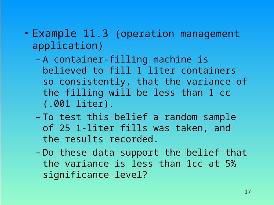
• Example 11.3 (operation management application)– A container-filling machine is believed to fill 1 liter

containers so consistently, that the variance of the filling will be less than 1 cc (.001 liter).

– To test this belief a random sample of 25 1-liter fills was taken, and the results recorded.

– Do these data support the belief that the variance is less than 1cc at 5% significance level?

18

• Solution– The problem objective is to describe the population of 1-liter fills

from a filling machine. – The data are quantitative, and we are interested in the variability

of the fills.– The complete test is:

H0: 2 = 1

H1: 2 <1

21n,1

2

2

22

isregionrejectionThe

.s)1n(

isstatistictestThe

We want to prove that the process is consistent

We want to prove that the process is consistent

19

– Solving by hand• Note that (n - 1)s2 = (xi - x)2 = xi

2 - xi/n • From the sample (data is presented in units of cc-1000 to avoid rounding)

we can calculate xi = -3.6, and xi2 = 21.3.

• Then (n - 1)s2 = 21.3 - (-3.6)2/25 = 20.8.• The complete test is shown next

.05.0,3485.

.

,8.208484.13

.8484.13

,8.201

8.20)1(

2125,95.

21,1

22

22

valueP

hypothesisnullthe

rejectnotdoSince

sn

n

There is insufficient evidence to reject the hypothesis thatthe variance is equal to 1cc,in favor of the hypothesis thatit is smaller.

20

13.8484 20.8

Rejectionregion

8484.132 2

2125,95.

= .05

Do not reject the null hypothesis

P-value = .3485

21

11.4 Inference About a Population Proportion

• When the population consists of qualitative or categorical data, the only inference we can make is about the proportion of occurrence of a certain value.

• The parameter “p” was used before to calculate probabilities using the binomial distribution.

22

.

.

ˆ

sizesamplen

successesofnumberthex

wheren

xp

.

.

ˆ

sizesamplen

successesofnumberthex

wheren

xp

• Statistic and sampling distribution– the statistic employed is

– Under certain conditions, [np > 5 and n(1-p) > 5], is approximately normally distributed, with

= p and 2 = p(1 - p)/n.p̂

23

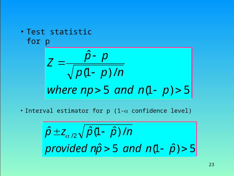
• Test statistic for p

• Interval estimator for p (1- confidence level)

5)1(5

/)1(

ˆ

pnandnpwhere

npp

ppZ

5)1(5

/)1(

ˆ

pnandnpwhere

npp

ppZ

5)ˆ1(5ˆ

/)ˆ1(ˆˆ 2/

pnandpnprovided

nppzp

5)ˆ1(5ˆ

/)ˆ1(ˆˆ 2/

pnandpnprovided

nppzp

24

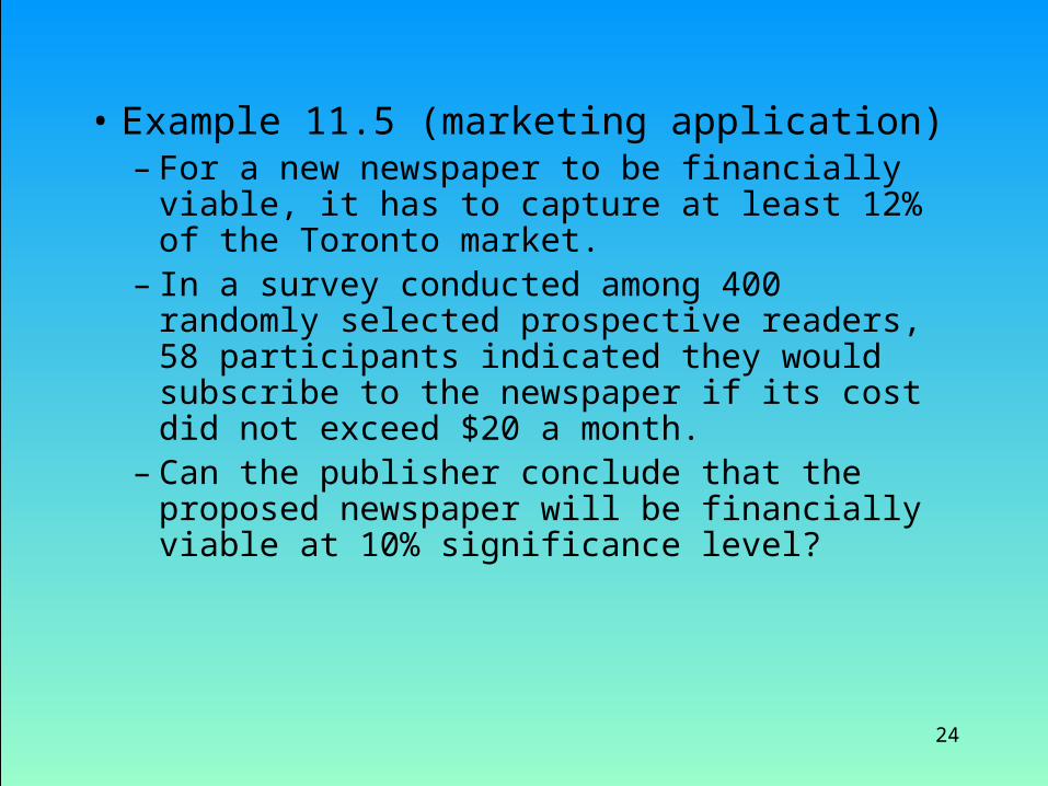
• Example 11.5 (marketing application)– For a new newspaper to be financially viable, it has

to capture at least 12% of the Toronto market.– In a survey conducted among 400 randomly selected

prospective readers, 58 participants indicated they would subscribe to the newspaper if its cost did not exceed $20 a month.

– Can the publisher conclude that the proposed newspaper will be financially viable at 10% significance level?

25

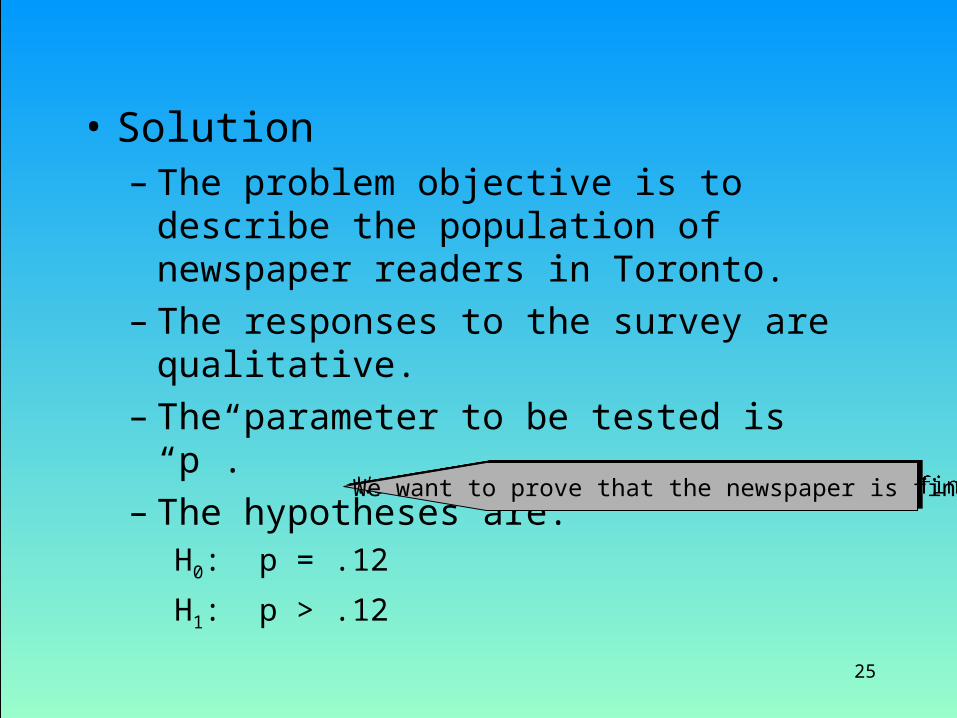
• Solution– The problem objective is to describe the population

of newspaper readers in Toronto.– The responses to the survey are qualitative.– The parameter to be tested is “p”.– The hypotheses are:

H0: p = .12

H1: p > .12 We want to prove that the newspaper is financially viableWe want to prove that the newspaper is financially viable

26

– Solving by hand• The rejection region is z > z = z.10 = 1.28. (= critical value)• The sample proportion is• The value of the test statistic is

• The p-value is = P(Z>1.54) = .0618; alpha =0.10

145.40058p̂

54.1400/)12.1(12.

12.145.

n/)p1(p

pp̂Z

There is sufficient evidence to reject the null hypothesisin favor of the alternative hypothesis. At 10% significance level we can argue that at least 12% of Toronto’s readers will subscribe to the new newspaper.

27

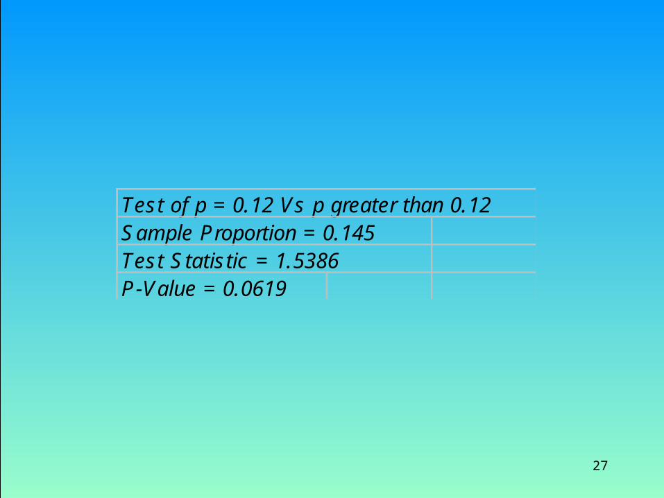
Test of p = 0.12 Vs p greater than 0.12Sample Proportion = 0.145Test Statistic = 1.5386P-Value = 0.0619

28

• Example 11.6 (marketing application)– In a survey of 2000 TV viewers at 11.40 p.m. on a

certain night, 226 indicated they watched “The Tonight Show”.

– Estimate the number of TVs tuned to the Tonight Show in a typical night, if there are 100 million potential television sets. Use a 95% confidence level.

– Solution

014.113.

2000/)887(.113.96.1113.n/)p̂1(p̂zp̂ 2/

29

Selecting the Sample Size to Estimate the Proportion

• The interval estimator for the proportion is

• Thus, if we wish to estimate the proportion to within W, we can write

• The required sample size is

n/)p̂1(p̂zp̂ 2/

n/)p̂1(p̂zW 2/

2

2/

Wn/)p̂1(p̂z

n

2

2/

Wn/)p̂1(p̂z

n

30

• Example– Suppose we want to estimate the proportion of

customers who prefer our company’s brand to within .03 with 95% confidence.

– Find the sample size needed to guarantee that this requirement is met.

– SolutionW = .03; 1 - = .95, therefore /2 = .025, so z.025 = 1.96

2

03.)p̂1(p̂96.1

n

Since the sample has not yet been taken, the sample proportionis still unknown.

We proceed using either one of the following two methods:

31

• Method 1:– There is no knowledge about the value of

• Let , which results in the largest possible n needed for a 1- confidence interval.

• If the sample proportion does not equal .5, the actual W will be narrower than .03.

5.p̂ Wp̂

p̂

068,103.

)5.1(5.96.1n

2

68303.

)2.1(2.96.1n

2

• Method 2:– There is some idea about the value of

• Use the value of to calculate the sample size p̂p̂