Economics 111.3 Winter 14 March 31 st , 2014 Lecture 29 Ch. 13: Pure monopoly

Welcome message from author
This document is posted to help you gain knowledge. Please leave a comment to let me know what you think about it! Share it to your friends and learn new things together.
Transcript

Economics 111.3 Winter 14
March 31st, 2014Lecture 29
Ch. 13: Pure monopoly

FINAL EXAM is based on chapters 3, 4, 5 (up to p. 116), 6 (up to p. 138), 8, 9, 10 (up to p. 230, 11, 12, 13, and 14Its format: 100 Multiple-Choice Questions When and Where: April 21, from 7:00 p.m. to 10:00 p.m; STM 140Extra Office Hours: April 19, from1:00 p.m. to 3:00 p.m.
Final Exam:

Monopoly Demand: a summary
1. Marginal revenue is less than price2. The monopolist is a price-maker3. The monopolist sets prices in the
elastic region of demand


Q P TR0 $172
1 162
2 152
3 142
4 132
5 122
6 112
7 102
8 92
9 82
10 72
Demand (AR) and MR: calculation
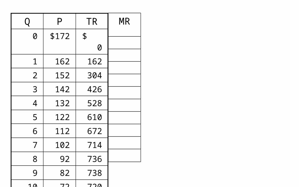
Q P TR0 $172 $ 0
1 162 162
2 152 304
3 142 426
4 132 528
5 122 610
6 112 672
7 102 714
8 92 736
9 82 738
10 72 720
MR

Q P TR0 $172 $ 0
1 162 162
2 152 304
3 142 426
4 132 528
5 122 610
6 112 672
7 102 714
8 92 736
9 82 738
10 72 720
MR
$162]
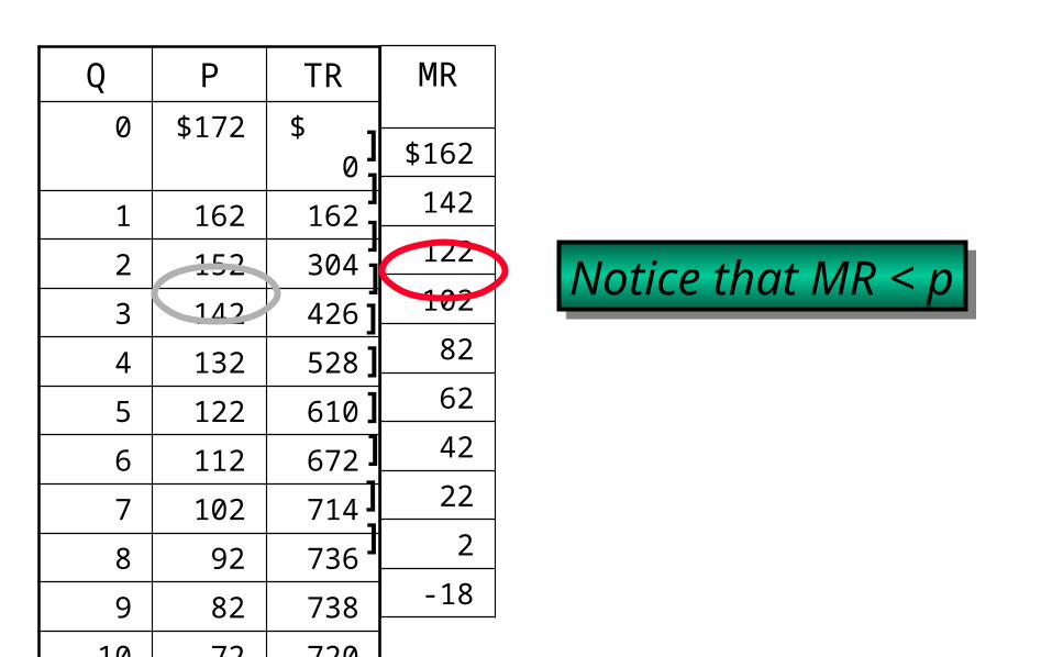
Q P TR0 $172 $ 0
1 162 162
2 152 304
3 142 426
4 132 528
5 122 610
6 112 672
7 102 714
8 92 736
9 82 738
10 72 720
MR
$162
142
122
102
82
62
42
22
2
-18
Notice that MR < pNotice that MR < p
]]]]]]]]]]
The Monopolist’s Price and Output Graphically
• To determine the profit-maximizing price and quantity: – one first finds output (where MC = MR), and then – extends a vertical line for that output, up
to the demand curve to find the price (Pm).

Q
D
MR
200
175
150
125
100
75
50
25 0 1 2 3 4 5 6 7 8 9 10
P
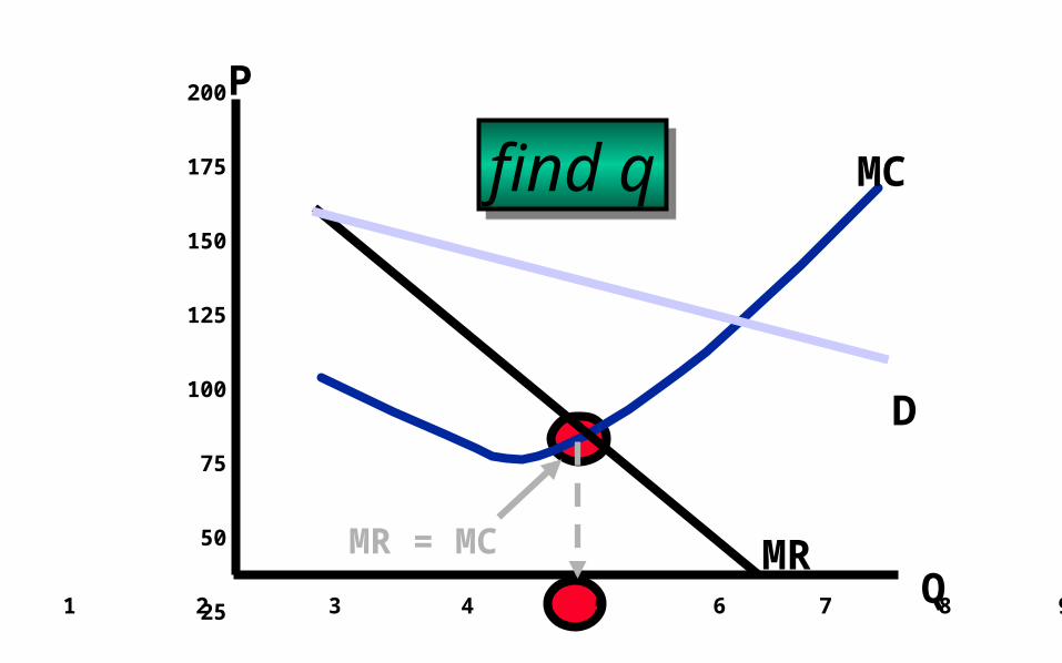
MCfind qfind q
MR = MCQ
D
MR
200
175
150
125
100
75
50
25 0 1 2 3 4 5 6 7 8 9 10
P

MC
$122= p
find pfind p
Q
D
MR
200
175
150
125
100
75
50
25 0 1 2 3 4 5 6 7 8 9 10
P

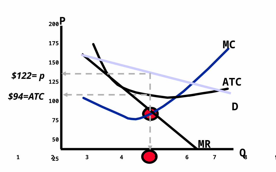
MCfind ATCfind ATC
Q
D
MR
200
175
150
125
100
75
50
25 0 1 2 3 4 5 6 7 8 9 10
P
ATC$122= p
MC
ATC$94=ATC
Q
D
MR
200
175
150
125
100
75
50
25 0 1 2 3 4 5 6 7 8 9 10
P
$122= p
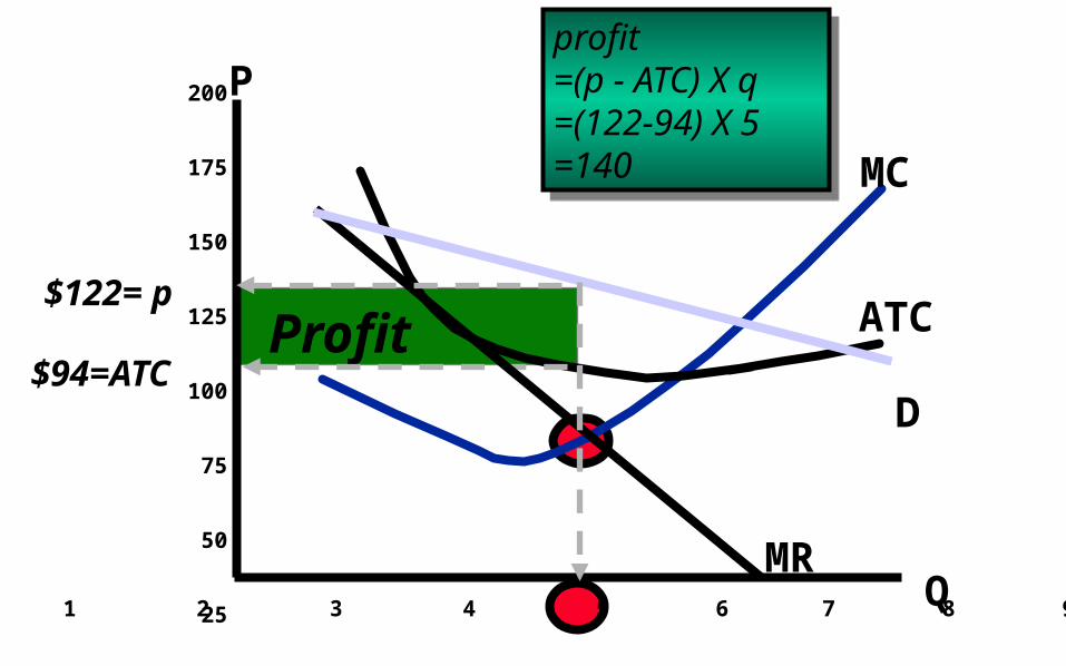
MC
Profit
profit=(p - ATC) X q=(122-94) X 5=140
profit=(p - ATC) X q=(122-94) X 5=140
$94=ATC
Q
D
MR
200
175
150
125
100
75
50
25 0 1 2 3 4 5 6 7 8 9 10
P
ATC$122= p

MC
p
qMR D
q1
p1
q1 supplied at p1q1 supplied at p1
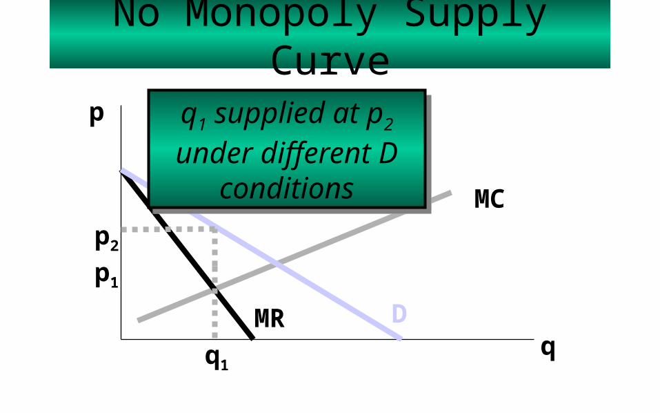
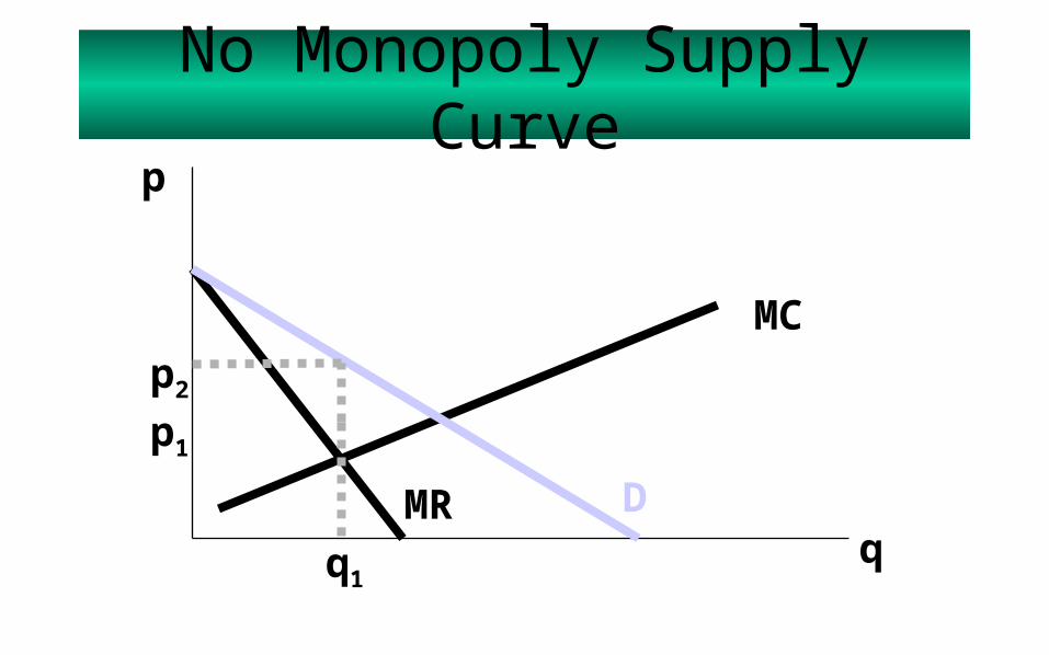
No Monopoly Supply Curve
MC
p
qq1
p1
p2
DMR
q1 supplied at p2 under different D
conditions
q1 supplied at p2 under different D
conditions
No Monopoly Supply Curve
MC
p
qq1
p1
p2
DMR
No Monopoly Supply Curve

A Monopolist Making a Profit
Price
ATC
MC
Quantity
PM
0MR D
QM
ProfitCM
A
B
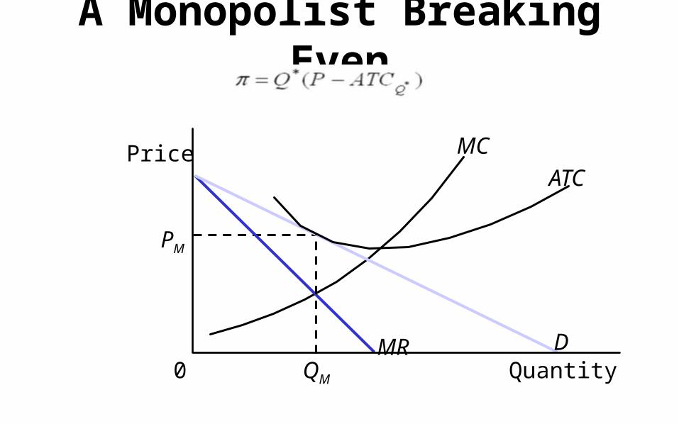
A Monopolist Breaking Even
Price MC
Quantity
PM
0MR D
QM
ATC

A Monopolist Making a Loss
Price ATCMC
Quantity0MR D
QM
LossPM
CMB
A


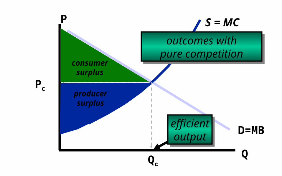
Comparing Monopoly and Perfect Competition
• Profit-maximizing output for the monopolist, like profit maximizing output for the competitor in a perfectly competitive market is where MC = MR.
• Because the monopolist’s marginal revenue is below its price, its equilibrium output is less than, and price is higher than that of a perfectly competitive market.
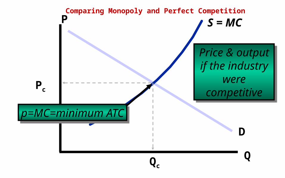
Q
P
D
Pc
Qc
S = MC
Price & output if the industry
were competitive
Price & output if the industry
were competitive
p=MC=minimum ATCp=MC=minimum ATC
Comparing Monopoly and Perfect Competition
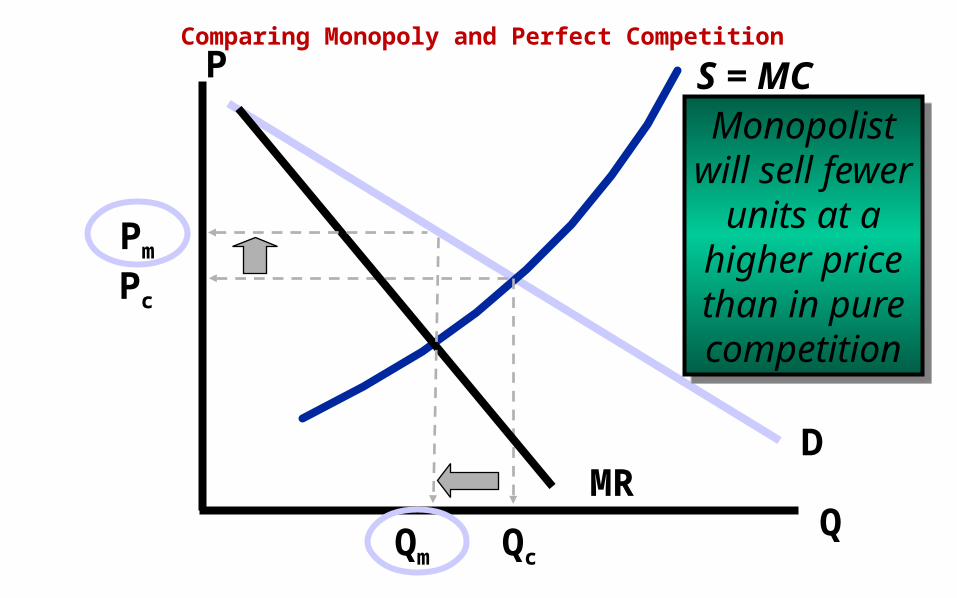
Q
P
DMR
Pc
Qc
Pm
Qm
Monopolistwill sell fewer
units at ahigher pricethan in purecompetition
Monopolistwill sell fewer
units at ahigher pricethan in purecompetition
S = MCComparing Monopoly and Perfect Competition
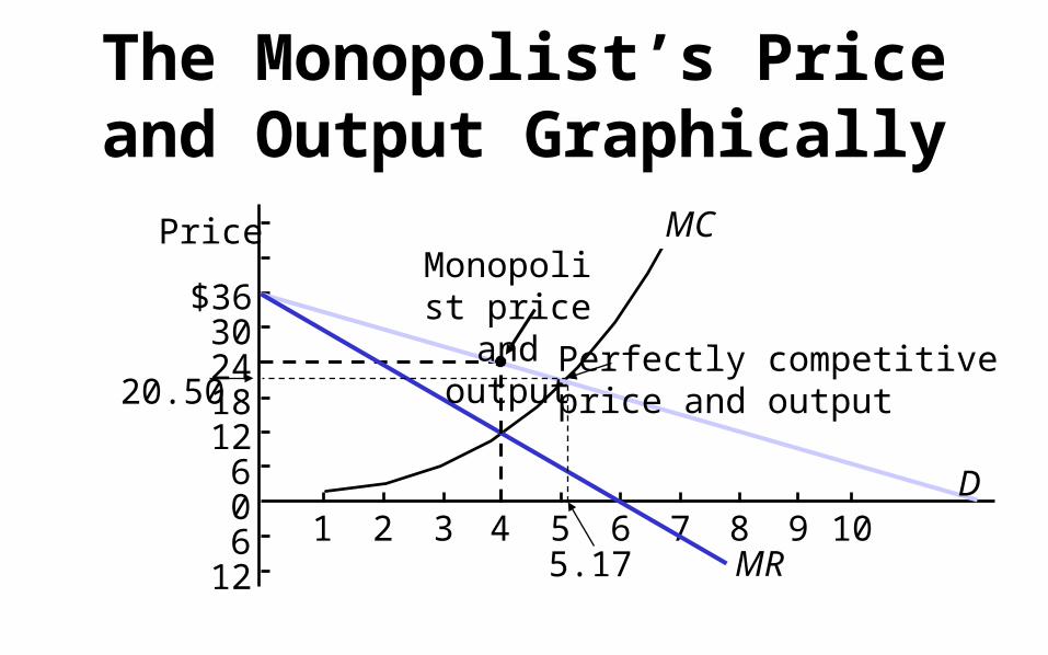
The Monopolist’s Price and Output Graphically
$3630241812
606
12
Price MC
1 2 3 4 5 6 7 8 9 10D
MR
Monopolist price and
output20.50
5.17
Perfectly competitive price and output
Q
P
D=MB
Pc
Qc
S = MC
consumersurplus
producersurplus
efficientoutput
efficientoutput
outcomes withpure competition
outcomes withpure competition

Q
P
D=MBMR
Pc
Qc
Pm
Qm
S = MC
consumersurplus
producersurplus
monopoly’s gain B
C
outcomes withpure monopoly
outcomes withpure monopoly
deadweightloss
deadweightloss

© 2010 Pearson Education Canada


ANSWER SHOWN BELOW:
ANSWER SHOWN BELOW:
Related Documents