For sale by the Superintendent of Documents, U.S. Government Printing Office Internet: bookstore.gpo.gov Phone: toll free (866) 512-1800; DC area (202) 512-1800 Fax: (202) 512-2104 Mail: Stop IDCC, Washington, DC 20402-0001 ISBN 978-0-16-084824-7 transmitted to the congress february 2010 together with the annual report of the council of economic advisers united states government printing office washington : 2010 economic report of the president

Welcome message from author
This document is posted to help you gain knowledge. Please leave a comment to let me know what you think about it! Share it to your friends and learn new things together.
Transcript

For sale by the Superintendent of Documents, U.S. Government Printing OfficeInternet: bookstore.gpo.gov Phone: toll free (866) 512-1800; DC area (202) 512-1800
Fax: (202) 512-2104 Mail: Stop IDCC, Washington, DC 20402-0001
ISBN 978-0-16-084824-7
transmitted to the congressfebruary 2010
together withthe annual report
of thecouncil of economic advisers
united states government printing officewashington : 2010
e c o n o m i cr e p o r t
o f t h e
p r e s i d e n t


iii
C O N T E N T S
ECONOMIC REPORT OF THE PRESIDENT ........................................... 1ANNUAL REPORT OF THE COUNCIL OF ECONOMIC ADVISERS* 11CHAPTER 1. TO RESCUE, REBALANCE, AND REBUILD .............. 25CHAPTER 2. RESCUING THE ECONOMY FROM THE GREAT
RECESSION ........................................................................ 39CHAPTER 3 CRISIS AND RECOVERY IN THE WORLD
ECONOMY ........................................................................ 81CHAPTER 4. SAVING AND INVESTMENT ....................................... 113CHAPTER 5. ADDRESSING THE LONG-RUN FISCAL
CHALLENGE ..................................................................... 137CHAPTER 6. BUILDING A SAFER FINANCIAL SYSTEM .............. 159CHAPTER 7. REFORMING HEALTH CARE ...................................... 181CHAPTER 8. STRENGTHENING THE AMERICAN LABOR
FORCE ................................................................................. 213CHAPTER 9. TRANSFORMING THE ENERGY SECTOR AND
ADDRESSING CLIMATE CHANGE ............................ 235CHAPTER 10. FOSTERING PRODUCTIVITY GROWTH
THROUGH INNOVATION AND TRADE ................. 259REFERENCES ............................................................................................... 285APPENDIX A. REPORT TO THE PRESIDENT ON THE
ACTIVITIES OF THE COUNCIL OFECONOMIC ADVISERS DURING 2009 ...................... 305
APPENDIX B. STATISTICAL TABLES RELATING TO INCOME,EMPLOYMENT, AND PRODUCTION ....................... 319
____________*For a detailed table of contents of the Council’s Report, see page 15.
Page

economic reportof the
president

Economic Report of the President | 3
economic report of the president
To the Congress of the United States:
As we begin a new year, the American people are still experiencingthe effects of a recession as deep and painful as any we have known ingenerations. Traveling across this country, I have met countless men andwomen who have lost jobs these past two years. I have met small businessowners struggling to pay for health care for their workers; seniors unableto afford prescriptions; parents worried about paying the bills and savingfor their children’s future and their own retirement. And the effects of thisrecession come in the aftermath of a decade of declining economic securityfor the middle class and those who aspire to it.
At the same time, over the past two years, we have also seen reasonfor hope: the resilience of the American people who have held fast—even in the face of hardship—to an unrelenting faith in the promise ofour country.
It is that determination that has helped the American peopleovercome difficult periods in our Nation’s history. And it is this persever-ance that remains our great strength today. After all, our workers are asproductive as ever. American businesses are still leaders in innovation.Our potential is still unrivaled. Our task as a Nation—and our missionas an Administration—is to harness that innovative spirit, that productiveenergy, and that potential in order to create jobs, raise incomes, and fostereconomic growth that is sustained and broadly shared. It’s not enoughto move the economy from recession to recovery. We must rebuild theeconomy on a new and stronger foundation.
I can report that over the past year, this work has begun. In thecoming year, this work continues. But to understand where we must goin the next year and beyond, it is important to remember where we beganone year ago.

4 | Economic Report of the President
Last January, years of irresponsible risk-taking and debt-fueledspeculation—unchecked by sound oversight—led to the near-collapseof our financial system. We were losing an average of 700,000 jobs eachmonth. Over the course of one year, $13 trillion of Americans’ householdwealth had evaporated as stocks, pensions, and home values plummeted.Our gross domestic product was falling at the fastest rate in a quartercentury. The flow of credit, vital to the functioning of businesses large andsmall, had ground to a halt. The fear among economists, from across thepolitical spectrum, was that we could sink into a second Great Depression.
Immediately, we took a series of difficult steps to prevent thatcatastrophe for American families and businesses. We acted to get lendingflowing again so ordinary Americans could get financing to buy homesand cars, to go to college, and to start businesses of their own; and sobusinesses, large and small, could access loans to make payroll, buy equip-ment, hire workers, and expand. We enacted measures to stem the tide offoreclosures in our housing market, helping responsible homeowners stayin their homes and helping to stop the broader decline in home values.
To achieve this, and to prevent an economic collapse, we were forcedto use authority enacted under the previous Administration to extendassistance to some of the very banks and financial institutions whoseactions had helped precipitate the turmoil. We also took steps to preventthe collapse of the American auto industry, which faced a crisis partlyof its own making, to prevent another round of widespread job losses inan already fragile time. These decisions were not popular, but they werenecessary. Indeed, the decision to stabilize the financial system helped toavert a larger catastrophe, and thanks to the efficient management of therescue—with added transparency and accountability—we have recoveredmost of the money provided to banks.
In addition, even as we worked to address the crises in our bankingsector, in our housing market, and in our auto industry, we also beganattacking our economic crisis on a broader front. Less than one monthafter taking office, we enacted the most sweeping economic recoverypackage in history: the American Recovery and Reinvestment Act of2009. The Recovery Act not only provided tax cuts to small businesses and95 percent of working families and provided emergency relief to those outof work or without health insurance; it also began to lay a new foundationfor long-term growth. With investments in health care, education, infra-structure, and clean energy, the Recovery Act has saved or created roughlytwo million jobs so far, and it has begun the hard work of transforming oureconomy to thrive in the modern, global era.

Economic Report of the President | 5
Because of these and other steps, we can safely say that we’ve avoidedthe depression many feared. Our economy is growing again, and thegrowth over the last three months was the strongest in six years. But whileeconomic growth is important, it means nothing to somebody who haslost a job and can’t find another. For Americans looking for work, a goodjob is the only good news that matters. And that’s why our work is farfrom complete.
It is true that the steps we have taken have slowed the flood of joblosses from 691,000 per month in the first quarter of 2009 to 69,000 in thelast quarter. But stemming the tide of job loss isn’t enough. More than7 million jobs have been lost since the recession began two years ago. Thisrepresents not only a terrible human tragedy, but also a very deep holefrom which we’ll have to climb out. Until jobs are being created to replacethose we’ve lost—until America is back at work—my Administration willnot rest and this recovery will not be finished.
That’s why I am continuing to call on the Congress to pass a jobs bill.I’ve proposed a package that includes tax relief for small businesses to spurhiring, that accelerates construction on roads, bridges, and waterways,and that creates incentives for homeowners to invest in energy efficiency,because this will create jobs, save families money, and reduce pollutionthat harms our environment.
It is also essential that as we promote private sector hiring, wecontinue to take steps to prevent layoffs of critical public servants liketeachers, firefighters, and police officers, whose jobs are threatened byState and local budget shortfalls. To do otherwise would not only worsenunemployment and hamper our recovery; it would also undermine ourcommunities. And we cannot forget the millions of people who have losttheir jobs. The Recovery Act provided support for these families hardest-hit by this recession, and that support must continue.
At the same time, long before this crisis hit, middle-class familieswere under growing strain. For decades, Washington failed to addressfundamental weaknesses in the economy: rising health care costs, growingdependence on foreign oil, an education system unable to prepare all ofour children for the jobs of the future. In recent years, spending bills andtax cuts for the very wealthiest were approved without paying for any ofit, leaving behind a mountain of debt. And while Wall Street gambledwithout regard for the consequences, Washington looked the other way.
As a result, the economy may have been working for some at thevery top, but it was not working for all American families. Year after year,folks were forced to work longer hours, spend more time away from their

6 | Economic Report of the President
loved ones, all while their incomes flat-lined and their sense of economicsecurity evaporated. Growth in our country was neither sustained norbroadly shared. Instead of a prosperity powered by smart ideas and soundinvestments, growth was fueled in large part by a rapid rise in consumerborrowing and consumer spending.
Beneath the statistics are the stories of hardship I’ve heard allacross America—hardships that began long before this recession hit twoyears ago. For too many, there has long been a sense that the Americandream—a chance to make your own way, to work hard and support yourfamily, save for college and retirement, own a home—was slipping away.And this sense of anxiety has been combined with a deep frustration thatWashington either didn’t notice, or didn’t care enough to act.
These weaknesses have not only made our economy moresusceptible to the kind of crisis we have been through. They have alsomeant that even in good times the economy did not produce nearly enoughgains for middle-class families. Typical American families saw their stan-dards of living stagnate, rather than rise as they had for generations. Thatis why, in the aftermath of this crisis, and after years of inaction, what isclear is that we cannot go back to business as usual.
That is why, as we strive to meet the crisis of the moment, we arecontinuing to lay a new foundation for prosperity: a foundation on whichthe middle class can prosper and grow, where if you are willing to workhard, you can find a good job, afford a home, send your children to world-class schools, afford high-quality health care, and enjoy retirement securityin your later years. This is the heart of the American Dream, and it is atthe core of our efforts to not only rebuild this economy—but to rebuild itstronger than before. And this work has already begun.
Already, we have made historic strides to reform and improve oureducation system. We have launched a Race to the Top in which schoolsare competing to create the most innovative programs, especially in mathand science. We have already made college more affordable, even as weseek to increase student aid by ending a wasteful subsidy that serves onlyto line the pockets of lenders with tens of billions of taxpayer dollars. AndI’ve proposed a new American Graduation Initiative and set this goal: by2020, America will once again have the highest proportion of college grad-uates in the world. For we know that in this new century, growth will bepowered not by what consumers can borrow and spend, but what talented,skilled workers can create and export.
Already, we have made historic strides to improve our health caresystem, essential to our economic prosperity. The burdens this system

Economic Report of the President | 7
places on workers, businesses, and governments is simply unsustainable.And beyond the economic cost—which is vast—there is also a terriblehuman toll. That’s why we’ve extended health insurance to millions morechildren; invested in health information technology through the RecoveryAct to improve care and reduce costly errors; and provided the largestboost to medical research in our history. And I continue to fight to passreal, meaningful health insurance reforms that will get costs under controlfor families, businesses, and governments, protect people from the worstpractices of insurance companies, and make coverage more affordable andsecure for people with insurance, as well as those without it.
Already, we have begun to build a new clean energy economy. TheRecovery Act included the largest investment in clean energy in history,investments that are today creating jobs across America in the industriesthat will power our future: developing wind energy, solar technology, andclean energy vehicles. But this work has only just begun. Other countriesaround the world understand that the nation that leads the clean energyeconomy will be the nation that leads the global economy. I want Americato be that nation. That is why we are working toward legislation that willcreate new incentives to finally make renewable energy the profitablekind of energy in America. It’s not only essential for our planet and oursecurity, it’s essential for our economy.
But this is not all we must do. For growth to be truly sustainable—for our prosperity to be truly shared and our living standards to actuallyrise—we need to move beyond an economy that is fueled by budget deficitsand consumer demand. In other words, in order to create jobs and raiseincomes for the middle class over the long run, we need to export moreand borrow less from around the world, and we need to save more moneyand take on less debt here at home. As we rebuild, we must also rebalance.In order to achieve this, we’ll need to grow this economy by growing ourcapacity to innovate in burgeoning industries, while putting a stop to irre-sponsible budget policies and financial dealings that have led us into sucha deep fiscal and economic hole.
That begins with policies that will promote innovation throughoutour economy. To spur the discoveries that will power new jobs, new busi-nesses—and perhaps new industries—I have challenged both the publicsector and the private sector to devote more resources to research anddevelopment. And to achieve this, my budget puts us on a path to doubleinvestment in key research agencies and makes the research and experi-mentation tax credit permanent. We are also pursuing policies that willhelp us export more of our goods around the world, especially by small

8 | Economic Report of the President
businesses and farmers. And by harnessing the growth potential of inter-national trade—while ensuring that other countries play by the rules andthat all Americans share in the benefits—we will support millions of good,high-paying jobs.
But hand in hand with increasing our reliance on the Nation’singenuity is decreasing our reliance on the Nation’s credit card, as well asreining in the excess and abuse in our financial sector that led large firmsto take on extraordinary risks and extraordinary liabilities.
When my Administration took office, the surpluses our Nationhad enjoyed at the start of the last decade had disappeared as a result ofthe failure to pay for two large tax cuts, two wars, and a new entitlementprogram. And decades of neglect of rising health care costs had put ourbudget on an unsustainable path.
In the long term, we cannot have sustainable and durable economicgrowth without getting our fiscal house in order. That is why even as weincreased our short-term deficit to rescue the economy, we have refusedto go along with business as usual, taking responsibility for every dollar wespend. Last year, we combed the budget, cutting waste and excess wher-ever we could, a process that will continue in the coming years. We arepursuing health insurance reforms that are essential to reining in deficits.I’ve called for a fee to be paid by the largest financial firms so that theAmerican people are fully repaid for bailing out the financial sector. AndI’ve proposed a freeze on nonsecurity discretionary spending for threeyears, a bipartisan commission to address the long-term structural imbal-ance between expenditures and revenues, and the enactment of “pay-go”rules so that Congress has to account for every dollar it spends.
In addition, I’ve proposed a set of common sense reforms to preventfuture financial crises. For while the financial system is far stronger todaythan it was one year ago, it is still operating under the same rules that ledto its near-collapse. These are rules that allowed firms to act contrary tothe interests of customers; to hide their exposure to debt through complexfinancial dealings that few understood; to benefit from taxpayer-insureddeposits while making speculative investments to increase their ownprofits; and to take on risks so vast that they posed a threat to the entireeconomy and the jobs of tens of millions of Americans.
That is why we are seeking reforms to empower consumers withthe benefit of a new consumer watchdog charged with making sure thatfinancial information is clear and transparent; to close loopholes thatallowed big financial firms to trade risky financial products like creditdefaults swaps and other derivatives without any oversight; to identify

Economic Report of the President | 9
system-wide risks that could cause a financial meltdown; to strengthencapital and liquidity requirements to make the system more stable; and toensure that the failure of any large firm does not take the economy downwith it. Never again will the American taxpayer be held hostage by a bankthat is “too big to fail.”
Through these reforms, we seek not to undermine our markets butto make them stronger: to promote a vibrant, fair, and transparent finan-cial system that is far more resistant to the reckless, irresponsible activitiesthat might lead to another meltdown. And these kinds of reforms are inthe shared interest of firms on Wall Street and families on Main Street.
These have been a very tough two years. American families andbusinesses have paid a heavy price for failures of responsibility from WallStreet to Washington. Our task now is to move beyond these failures, totake responsibility for our future once more. That is how we will createnew jobs in new industries, harnessing the incredible generative andcreative capacity of our people. That is how we’ll achieve greater economicsecurity and opportunity for middle-class families in this country. Thatis how in this new century we will rebuild our economy stronger thanever before.
the white housefebruary 2010

the annual reportof the
council of economic advisers

13
letter of transmittal
Council of Economic AdvisersWashington, D.C., February 11, 2010
Mr. President:The Council of Economic Advisers herewith submits its 2010
Annual Report in accordance of the Employment Act of 1946 as amendedby the Full Employment and Balanced Growth Act of 1978.Sincerely,
Christina D. RomerChair
Austan GoolsbeeMember
Cecilia Elena RouseMember

15
C O N T E N T S
CHAPTER 1. TO RESCUE, REBALANCE, AND REBUILD ......... 25
Rescuing an Economy in Freefall ............................................ 26Rescuing the Economy from the Great Recession ........................ 28Crisis and Recovery in the World Economy ................................ 29
Rebalancing the Economy on the Path to FullEmployment ...................................................................................... 29
Saving and Investment .................................................................. 29Addressing the Long-Run Fiscal Challenge ................................. 31Building a Safer Financial System ............................................... 32
Rebuilding a Stronger Economy .............................................. 33Reforming Health Care ................................................................. 33Strengthening the American Labor Force .................................... 35Transforming the Energy Sector and Addressing ClimateChange ............................................................................................ 36Fostering Productivity Growth Through Innovation andTrade .............................................................................................. 37
Conclusion ........................................................................................ 38
CHAPTER 2. RESCUING THE ECONOMY FROM THEGREAT RECESSION ................................................................................ 39
An Economy in Freefall ............................................................... 39The Run-Up to the Recession ........................................................ 40The Downturn ............................................................................... 41Wall Street and Main Street ......................................................... 44
The Unprecedented Policy Response ...................................... 46Monetary Policy ............................................................................. 47Financial Rescue ............................................................................ 49Fiscal Stimulus ............................................................................... 51Housing Policy ............................................................................... 55
The Effects of the Policies ........................................................ 56
Page

16 | Annual Report of the Council of Economic Advisers
The Financial Sector ...................................................................... 57Housing ........................................................................................... 60Overall Economic Activity ............................................................. 63The Labor Market .......................................................................... 68
The Challenges Ahead .................................................................. 72Deteriorating Forecasts .................................................................. 72The Administration Forecast ......................................................... 75Responsible Policies to Spur Job Creation ..................................... 78
Conclusion ......................................................................................... 79
CHAPTER 3. CRISIS AND RECOVERY IN THE WORLDECONOMY ................................................................................................. 81
International Dimensions of the Crisis ................................ 82Spread of the Financial Shock ....................................................... 82The Collapse of World Trade ........................................................ 87The Collapse in Financial Flows ................................................... 89The Decline in Output Around the Globe .................................... 90
Policy Responses Around the Globe ........................................ 93Monetary Policy in the Crisis ........................................................ 93Central Bank Liquidity Swaps ....................................................... 96Fiscal Policy in the Crisis ............................................................... 98Trade Policy in the Crisis ............................................................... 100
The Role of International Institutions ................................ 100The G-20 ......................................................................................... 100The International Monetary Fund ................................................ 101
The Beginning of Recovery Around the Globe ................... 102The Impact of Fiscal Policy ............................................................ 104The World Economy in the Near Term ........................................ 106Global Imbalances in the Crisis ..................................................... 108
Conclusion ......................................................................................... 111
CHAPTER 4. SAVING AND INVESTMENT ..................................... 113
The Path of Consumption Spending ...................................... 114The Determinants of Saving .......................................................... 115Implications for Recent and Future Saving Behavior .................. 117
The Future of the Housing Market andConstruction .................................................................................... 120
The Housing Market ...................................................................... 121

Contents | 17
Commercial Real Estate ................................................................. 123Business Investment ....................................................................... 126
Investment in the Recovery ............................................................ 126Investment in the Long Run .......................................................... 127
The Current Account ................................................................... 129Determinants of the Current Account .......................................... 129The Current Account in the Recovery and in the Long Run ....... 132Steps to Encourage Exports ............................................................ 133
Conclusion ......................................................................................... 135
CHAPTER 5. ADDRESSING THE LONG-RUN FISCALCHALLENGE .............................................................................................. 137
The Long-Run Fiscal Challenge ............................................... 137Sources of the Long-Run Fiscal Challenge .................................... 139The Role of the Recovery Act and Other Rescue Operations ....... 143
An Anchor for Fiscal Policy ...................................................... 144The Effects of Budget Deficits ........................................................ 145Feasible Long-Run Fiscal Policies .................................................. 146The Choice of a Fiscal Anchor ....................................................... 148
Reaching the Fiscal Target ........................................................ 149General Principles .......................................................................... 149Comprehensive Health Care Reform ............................................ 150Restoring Balance to the Tax Code ............................................... 151Eliminating Wasteful Spending ..................................................... 155
Conclusion: The Distance Still to Go ................................... 156
CHAPTER 6. BUILDING A SAFER FINANCIAL SYSTEM ........... 159
What Is Financial Intermediation? ......................................... 160The Economics of Financial Intermediation ................................ 160Types of Financial Intermediaries ................................................. 163
The Regulation of Financial Intermediation in theUnited States .................................................................................... 166Financial Crises: The Collapse of FinancialIntermediation ................................................................................. 170
Confidence Contagion .................................................................... 170Counterparty Contagion ................................................................ 172Coordination Contagion ................................................................ 173
Preventing Future Crises: Regulatory Reform ................. 174

18 | Annual Report of the Council of Economic Advisers
Promote Robust Supervision and Regulation of FinancialFirms ............................................................................................... 175Establish Comprehensive Regulation of Financial Markets ........ 176Provide the Government with the Tools It Needs to ManageFinancial Crises .............................................................................. 178Raise International Regulatory Standards and ImproveInternational Cooperation ............................................................. 179Protect Consumers and Investors from Financial Abuse ............ 179
Conclusion ......................................................................................... 180
CHAPTER 7. REFORMING HEALTH CARE .................................... 181
The Current State of the U.S. Health Care Sector ......... 182Rising Health Spending in the United States ................................ 182Market Failures in the Current U.S. Health Care System:Theoretical Background ................................................................. 185System-Wide Evidence of Inefficient Spending ............................ 188Declining Coverage and Strains on Particular Groups andSectors .............................................................................................. 191
Health Policies Enacted in 2009 ............................................... 196Expansion of the CHIP Program ................................................... 197Subsidized COBRA Coverage ........................................................ 197Temporary Federal Medical Assistance Percentage (FMAP)Increase ........................................................................................... 199Recovery Act Measures to Improve the Quality and Efficiencyof Health Care ................................................................................ 201
2009 Health Reform Legislation ............................................... 202Insurance Market Reforms: Strengthening and SecuringCoverage .......................................................................................... 202Expansions in Health Insurance Coverage Through theExchange ......................................................................................... 205Economic and Health Benefits of Expanding HealthInsurance Coverage ........................................................................ 206Reducing the Growth Rate of Health Care Costs in the Publicand Private Sectors ......................................................................... 207The Economic Benefits of Slowing the Growth Rate of HealthCare Costs ....................................................................................... 210
Conclusion ......................................................................................... 211

Contents | 19
CHAPTER 8. STRENGTHENING THE AMERICANLABOR FORCE .......................................................................................... 213
Challenges Facing American Workers .................................. 214Unemployment ............................................................................... 214Sectoral Change .............................................................................. 216Stagnating Incomes for Middle-Class Families ............................ 217
Policies to Support Workers ...................................................... 219Education and Training: The Groundwork forLong-Term Prosperity ................................................................... 221
Benefits of Education ..................................................................... 221Trends in U.S. Educational Attainment ....................................... 222U.S. Student Achievement ............................................................. 226
A Path Toward Improved Educational Performance ...... 227Postsecondary Education ............................................................... 228Training and Adult Education ...................................................... 229Elementary and Secondary Education .......................................... 231Early Childhood Education ........................................................... 233
Conclusion ......................................................................................... 234
CHAPTER 9. TRANSFORMING THE ENERGY SECTORAND ADDRESSING CLIMATE CHANGE .......................................... 235
Greenhouse Gas Emissions, Climate, and EconomicWell-Being ......................................................................................... 236
Greenhouse Gases ........................................................................... 237Temperature Change ...................................................................... 238Impact on Economic Well-Being ................................................... 239
Jump-Starting the Transition to Clean Energy ................. 243Recovery Act Investments in Clean Energy .................................. 243Short-Run Macroeconomic Effects of the Clean EnergyInvestments ..................................................................................... 246
Other Domestic Actions to Mitigate ClimateChange ................................................................................................. 247Market-Based Approaches to Advance the CleanEnergy Transformation and Address Climate Change ... 248
Cap-and-Trade Program Basics .................................................... 248Ways to Contain Costs in an Effective Cap-and-TradeSystem .............................................................................................. 250

20 | Annual Report of the Council of Economic Advisers
Coverage of Gases and Industries .................................................. 253The American Clean Energy and Security Act ............................. 254
International Action on Climate Change Is Needed ....... 255Partnerships with Major Developed and EmergingEconomies ....................................................................................... 256Phasing Out Fossil Fuel Subsidies ................................................. 257
Conclusion ......................................................................................... 257
CHAPTER 10. FOSTERING PRODUCTIVITY GROWTHTHROUGH INNOVATION AND TRADE ......................................... 259
The Role of Productivity Growth in Driving LivingStandards ........................................................................................... 261
Recent Trends in Productivity in the United States ..................... 262Sources of Productivity Growth ..................................................... 264
Fostering Productivity Growth Through Innovation ... 266The Importance of Basic Research ................................................ 267Private Research and Experimentation ........................................ 269Protection of Intellectual Property Rights ..................................... 270Spurring Progress in National Priority Areas .............................. 272Increasing Openness and Transparency ....................................... 272
Trade as an Engine of Productivity Growth andHigher Living Standards ............................................................. 274
The United States and International Trade ................................. 275Sources of Productivity Growth from International Trade ......... 276Encouraging Trade and Enforcing Trade Agreements ................ 280
Ensuring the Gains from Productivity GrowthAre Widely Shared ......................................................................... 282Conclusion ......................................................................................... 284
REFERENCES ............................................................................................. 285
appendixesA. Report to the President on the Activities of the Council of
Economic Advisers During 2009 .................................................. 305B. Statistical Tables Relating to Income, Employment, and
Production ...................................................................................... 319
Contents | 21
list of figures1-1. House Prices Adjusted for Inflation ............................................. 271-2. Monthly Change in Payroll Employment .................................... 281-3. Personal Consumption Expenditures as a Share of GDP .......... 301-4. Actual and Projected Budget Surpluses in January 2009
under Previous Policy ..................................................................... 311-5. Real Median Family Income .......................................................... 331-6. Total Compensation Including and Excluding Health
Insurance ........................................................................................... 341-7. Mean Years of Schooling by Birth Cohort ................................... 361-8. R&D Spending as a Percent of GDP ............................................. 372-1. House Prices Adjusted for Inflation ............................................. 402-2. Income and Consumption Around the 2008 Tax Rebate ......... 422-3. TED Spread and Moody’s BAA-AAA Spread Through
December 2008 ................................................................................. 432-4. Assets on the Federal Reserve’s Balance Sheet ............................ 482-5. TED Spread and Moody’s BAA-AAA Spread Through
December 2009 ................................................................................. 572-6. S&P 500 Stock Price Index ............................................................. 582-7. Monthly Gross SBA 7(a) and 504 Loan Approvals .................... 602-8. 30-Year Fixed Rate Mortgage Rate ............................................... 612-9. FHFA and LoanPerformance National House Price Indexes ... 632-10. Real GDP Growth ............................................................................ 642-11. Real GDP: Actual and Statistical Baseline Projection ............... 652-12. Contributions to Real GDP Growth ............................................. 662-13. Average Monthly Change in Employment .................................. 682-14. Estimated Effect of the Recovery Act on Employment .............. 692-15. Contributions to the Change in Employment ............................. 712-16. Okun’s Law, 2000-2009 ................................................................... 743-1. Interbank Market Rates .................................................................. 833-2. Nominal Trade-Weighted Dollar Index ....................................... 853-3. OECD Exports-to-GDP Ratio ....................................................... 873-4. Vertical Specialization and the Collapse in Trade ...................... 883-5. Cross-Border Gross Purchases and Sales of Long-Term
Assets ................................................................................................. 903-6. Industrial Production in Advanced Economies .......................... 913-7. Industrial Production in Emerging Economies .......................... 923-8. Headline Inflation, 12-Month Change ......................................... 933-9. Policy Rates in Economies with Major Central Banks ............... 94
22 | Annual Report of the Council of Economic Advisers
3-10. Change in Central Bank Assets ..................................................... 953-11. Central Bank Liquidity Swaps of the Federal Reserve ................ 973-12. Tax Share and Discretionary Stimulus ......................................... 993-13. Outperforming Expectations and Stimulus ................................. 1053-14. OECD Countries: GDP and Unemployment ............................. 1083-15. Current Account Deficits or Surpluses ........................................ 1104-1. Personal Consumption Expenditures as a Share of GDP .......... 1144-2. Personal Saving Rate Versus Wealth Ratio .................................. 1154-3. Personal Saving Rate: Actual Versus Model ............................... 1184-4. Actual Personal Saving Versus Counterfactual Personal
Saving ................................................................................................. 1194-5. Single-Family Housing Starts ......................................................... 1214-6. Homeownership Rate ...................................................................... 1224-7. Fixed Investment in Structures by Type ...................................... 1244-8. Commercial Real Estate Prices and Loan Delinquencies .......... 1254-9. Nonstructures Investment as a Share of Nominal GDP ............ 1284-10. Saving, Investment, and the Current Account as a Percent
of GDP ............................................................................................... 1324-11. Growth of U.S. Exports and Rest-of-World Income:
1960-2008 .......................................................................................... 1345-1. Actual and Projected Budget Surpluses in January 2009
under Previous Policy ..................................................................... 1385-2. Actual and Projected Government Debt Held by the Public
under Previous Policy ..................................................................... 1395-3. Budgetary Cost of Previous Administration Policy ................... 1415-4. Causes of Rising Spending on Medicare, Medicaid, and
Social Security .................................................................................. 1425-5. Budget Comparison: January 2001 and January 2009 .............. 1435-6. Effect of the Recovery Act on the Deficit ..................................... 1445-7. Top Statutory Tax Rates ................................................................. 1535-8. Evolution of Average Tax Rates .................................................... 1546-1. Financial Intermediation: Saving into Investment .................... 1616-2. Financial Sector Assets .................................................................... 1636-3. Share of Financial Sector Assets by Type ..................................... 1646-4. Confidence Contagion .................................................................... 1716-5. Counterparty Contagion ................................................................ 1736-6. Coordination Contagion ................................................................ 1747-1. National Health Expenditures as a Share of GDP ...................... 1837-2. Total Compensation Including and Excluding Health
Insurance ........................................................................................... 184
Contents | 23
7-3. Child and Infant Mortality Across G-7 Countries ..................... 1907-4. Insurance Rates of Non-Elderly Adults ........................................ 1927-5. Percent of Americans Uninsured by Age ..................................... 1937-6. Share of Non-Elderly Individuals Uninsured by Poverty
Status .................................................................................................. 1947-7. Medicare Part D Out-of-Pocket Costs by Total Prescription
Drug Spending ................................................................................. 1957-8. Share Uninsured among Adults Aged 18 and Over ................... 1987-9. Monthly Medicaid Enrollment Across the States ....................... 2008-1. Unemployment and Underemployment Rates ........................... 2148-2. Unemployment Rates by Race ....................................................... 2158-3. Real Median Family Income and Median Individual
Earnings ............................................................................................ 2188-4. Share of Pre-Tax Income Going to the Top 10 Percent of
Families ............................................................................................. 2198-5. Total Wage and Salary Income by Educational Group ............. 2228-6. Mean Years of Schooling by Birth Cohort ................................... 2248-7. Educational Attainment by Birth Cohort, 2007 .......................... 2258-8. Long-Term Trend Math Performance ......................................... 2279-1. Projected Global Carbon Dioxide Concentrations with No
Additional Action ............................................................................ 2389-2. Recovery Act Clean Energy Appropriations by Category ......... 2469-3. United States, China, and World Carbon Dioxide
Emissions .......................................................................................... 25510-1. Non-Farm Labor Productivity and Per Capita Income ............. 26110-2. Labor Productivity Growth since 1947 ........................................ 26210-3. R&D Spending as a Percent of GDP ............................................. 27010-4. Exports as a Share of GDP ............................................................. 27510-5. Intra-Industry Trade, U.S. Manufacturing .................................. 278
list of tables2-1. Cyclically Sensitive Elements of Labor Market Adjustment ..... 702-2. Forecast and Actual Macroeconomic Outcomes ........................ 732-3. Administration Economic Forecast .............................................. 753-1. 2009 Fiscal Stimulus as Share of GDP, G-20 Members ............. 983-2. Stimulus and Growth in Advanced G-20 Countries .................. 1045-1. Government Debt-to-GDP Ratio in Selected OECD
Countries (percent) ......................................................................... 147
24 | Annual Report of the Council of Economic Advisers
list of boxes2-1. Potential Real GDP Growth ........................................................... 764-1. Unemployment and the Current Account ................................... 1307-1. The Impact of Health Reform on State and Local
Governments .................................................................................... 2088-1. The Recession’s Impact on the Education System ...................... 2248-2. Community Colleges: A Crucial Component of Our
Higher Education System ............................................................... 2309-1. Climate Change in the United States and Potential Impacts .... 2409-2. Expected Consumption Loss Associated with Temperature
Increase .............................................................................................. 2419-3. The European Union’s Experience with Emissions Trading .... 252
10-1. Overview of the Administration’s Innovation Agenda .............. 266

285
REFERENCES
Chapter To Rescue, Rebalance, and Rebuild
Congressional Budget Office. 2009a. The Budget and Economic Outlook:Fiscal Years 2009 to 2019.
————. 2009b. The Long-Term Budget Outlook.Goldin, Claudia, and Lawrence F. Katz. 2007. “Long-Run Changes in the
Wage Structure: Narrowing, Widening, Polarizing.” BrookingsPapers on Economic Activity, no. 2: 135–67.
Group of Twenty. 2009. “Leaders’ Statement: The Pittsburgh Summit.”September 24–25 (www.g20.org/Documents/pittsburgh_summit_leaders_statement_250909.pdf).
Kaiser Family Foundation and Health Research and Educational Trust.2009. Employer Health Benefits: 2009 Annual Survey. MenloPark, CA, and Chicago, IL: Henry J. Kaiser Family Foundation andHealth Research and Educational Trust.
Shiller, Robert J. 2005. Irrational Exuberance. 2nd ed. Princeton UniversityPress.
Chapter Rescuing the Economy from the Great Recession
Almeida, Heitor, et al. 2009. “Corporate Debt Maturity and the Real Effectsof the 2007 Credit Crisis.” Working Paper 14990. Cambridge, MA:National Bureau of Economic Research (May).
286 | References
Bernanke, Ben S. 1983. “Nonmonetary Effects of the Financial Crisis in thePropagation of the Great Depression.” American Economic Review73, no. 3: 257–76.
Broda, Christian, and Jonathan Parker. 2008. “The Impact of the 2008 TaxRebates on Consumer Spending: Preliminary Evidence.” WorkingPaper. University of Chicago, Graduate School of Business (July).
Campello, Murillo, John Graham, and Campbell R. Harvey. 2009. “TheReal Effects of Financial Constraints: Evidence from a FinancialCrisis.” Working Paper 15552. Cambridge, MA: National Bureauof Economic Research (December).
Congressional Budget Office. 2009a. “Estimated Impact of the AmericanRecovery and Reinvestment Act on Employment and EconomicOutput as of September 2009.” November.
————. 2009b. Letter to the Honorable Charles E. Grassley. “EstimatedMacroeconomic Impacts of the American Recovery andReinvestment Act of 2009.” March 2.
Council of Economic Advisers. 2009. “Economic Analysis of the CarAllowance Rebate System (‘Cash for Clunkers’).” September.
————. 2010. “The Economic Impact of the American Recovery andReinvestment Act of 2009.” Second Quarterly Report to Congress.January.
Gertler, Mark, and Simon Gilchrist. 1994. “Monetary Policy, BusinessCycles, and the Behavior of Small Manufacturing Firms.” QuarterlyJournal of Economics 109, no. 2: 309–40.
Kashyap, Anil K, Owen A. Lamont, and Jeremy C. Stein. 1994. “CreditConditions and the Cyclical Behavior of Inventories.” QuarterlyJournal of Economics 109, no. 3: 565–92.
Lamont, Owen A. 1997. “Cash Flow and Investment: Evidence fromInternal Capital Markets.” Journal of Finance 52, no. 1: 83–109.
Peek, Joe, and Eric S. Rosengren. 2000. “Collateral Damage: Effects ofthe Japanese Bank Crisis on Real Activity in the United States.”American Economic Review 90, no. 1: 30–45.
Rauh, Joshua D. 2006. “Investment and Financing Constraints: Evidencefrom the Funding of Corporate Pension Plans.” Journal of Finance61, no. 1: 33–71.
Rudebusch, Glenn D. 2009. “The Fed’s Monetary Policy Response to theCurrent Crisis.” FRBSF Economic Letter 2009-17. Federal ReserveBank of San Francisco (May).
References | 287
Sahm, Claudia R., Matthew D. Shapiro, and Joel B. Slemrod. 2009.“Household Response to the 2008 Tax Rebate: Survey Evidence andAggregate Implications.” Working Paper 15421. Cambridge, MA:National Bureau of Economic Research (October).
Shiller, Robert J. 2005. Irrational Exuberance. 2nd ed. Princeton UniversityPress.
Chapter Crisis and Recovery in the World Economy
Baldwin, Richard, ed. 2009. TheGreat Trade Collapse: Causes, Consequencesand Prospects. VoxEU.org Ebook.
Bown, Chad P. Forthcoming. “The Global Resort to Antidumping,Safeguards, and Other Trade Remedies Amidst the EconomicCrisis.” In Trade Implications of Policy Responses to the Crisis,edited by Simon J. Evenett and Bernard Hoekman.
Council of Economic Advisers. 2009. “The Effects of Fiscal Stimulus: ACross-Country Perspective.” September.
Eichengreen, Barry, and Douglas A. Irwin. 2009. “The Slide to Protectionismin the Great Depression: Who Succumbed and Why?” WorkingPaper 15142. Cambridge, MA: National Bureau of EconomicResearch (July).
Fender, Ingo, and Jacob Gyntelberg. 2008. “Overview: Global FinancialCrisis Spurs Unprecedented Policy Actions.” BIS Quarterly Review(December): 1–24.
Freund, Caroline. 2009. “Demystifying the Collapse in Trade.” VoxEU.org.Horton, Mark, Manmohan Kumar, and Paolo Mauro. 2009. “The State
of Public Finances: A Cross-Country Fiscal Monitor.” IMFStaff Position Note SPN/09/21. Washington, DC: InternationalMonetary Fund (July).
International Monetary Fund. 2009a. World Economic Outlook: October2009. Washington, DC.
———— (Strategy, Policy and Review Department). 2009b. “Review ofRecent Crisis Programs.” Washington, DC. September.

288 | References
Johnson, Robert C., and Guillermo Noguera. 2009. “Accounting forIntermediates: Production Sharing and Trade in Value Added.”Working Paper. Princeton University and University of California,Berkeley (May).
Lane, Philip R., and Jay C. Shambaugh. Forthcoming. “Financial ExchangeRates and International Currency Exposures.” American EconomicReview.
Levchenko, Andrei A., Logan Lewis, and Linda L. Tesar. 2009. “The Collapseof International Trade During the 2008–2009 Crisis: In Search ofthe Smoking Gun.” Research Seminar in International EconomicsDiscussion Paper 592. University of Michigan (October).
McGuire, Patrick, and Goetz von Peter. 2009. “The U.S. Dollar Shortage inGlobal Banking.” BIS Quarterly Review (March): 47–63.
Miroudot, Sébastien, and Alexandros Ragoussis. 2009. “Vertical Trade,Trade Costs and FDI.” Trade Policy Working Paper 89. Paris:Organisation for Economic Co-operation and Development (July).
Mora, Jesse, and William Powers. 2009. “Did Trade Credit ProblemsDeepen the Great Trade Collapse?” In The Great Trade Collapse:Causes, Consequences and Prospects, edited by Richard Baldwin.VoxEU.org Ebook.
Obstfeld, Maurice, and Kenneth Rogoff. 2009. “Global Imbalances and theFinancial Crisis: Products of Common Causes.” Discussion Paper7606. Washington, DC: Center for Economic Policy Research(December).
Organisation for Economic Co-operation and Development. 2009a.Economic Outlook No. 85. Paris.
————. 2009b. Economic Outlook No. 86. Paris.
Chapter Saving and Investment
Auerbach, Alan J., Jinyong Cai, and Laurence J. Kotlikoff. 1991. “U.S.Demographics and Saving: Predictions of Three Saving Models.”Carnegie-Rochester Conference Series on Public Policy 34, no. 1:135–56.
References | 289
Benartzi, Shlomo, and Richard Thaler. 2004. “Save More Tomorrow: UsingBehavioral Economics to Increase Employee Savings.” Journal ofPolitical Economy 112, no. S1: S164–87.
Carroll, Christopher D., Jeffrey C. Fuhrer, and David W. Wilcox. 1994.“Does Consumer Sentiment Forecast Household Spending? If So,Why?” American Economic Review 84, no. 5: 1397–408.
Congressional Budget Office. 2008. “The Outlook for Housing Starts, 2009to 2012.” Background Paper. November.
Dynan, Karen E. 2009. “Changing Household Financial Opportunitiesand Economic Security.” Journal of Economic Perspectives 23, no.4: 49–68.
Edelberg, Wendy. 2006. “‘Risk-Based Pricing of Interest Rates for ConsumerLoans.” Journal of Monetary Economics 53, no. 8: 2283–98.
Getter, Darryl. 2006. “Consumer Credit Risk and Pricing.” Journal ofConsumer Affairs 40, no. 1: 41–63.
Jappelli, Tullio, and Marco Pagano. 1993. “Information Sharing in CreditMarkets.” Journal of Finance 48, no. 5: 1693–718.
Lown, Cara S., and Donald P. Morgan. 2006. “The Credit Cycle and theBusiness Cycle: New Findings Using the Loan Officer OpinionSurvey.” Journal of Money, Credit, and Banking 38, no. 6: 1575–97.
Macroeconomic Advisers. 2009. “The Trough in Housing Starts: Are WeThere Yet?” Macro Focus 4, no. 5: 1–9.
Melitz, Marc J. 2003. “The Impact of Trade on Intra-Industry Reallocationsand Aggregate Industry Productivity.” Econometrica 71, no. 6:1695–725.
Muellbauer, John N. 2007. “Housing, Credit and Consumer Expenditure.”In Housing, Housing Finance, and Monetary Policy, pp. 267–334.Kansas City: Federal Reserve Bank of Kansas City.
Office of Management and Budget. 2009. The Budget of the United States,Fiscal Year 2010.

290 | References
Chapter Addressing the Long-Run Fiscal Challenge
Alesina, Alberto, and Roberto Perotti. 1997. “Fiscal Adjustments in OECDCountries: Composition and Macroeconomic Effects.” IMF StaffPapers 44, no. 2: 210–48.
Ardagna, Silvia, Francesco Caselli, and Timothy Lane. 2007. “FiscalDiscipline and the Cost of Public Debt Service: Some Estimatesfor OECD Countries.” B.E. Journal of Macroeconomics 7, no. 1(Topics), Article 28.
Auerbach, Alan J., and William G. Gale. 2009. “The Economic Crisisand the Fiscal Crisis: 2009 and Beyond, An Update.” WorkingPaper. Brookings Institution, Washington, DC, and University ofCalifornia, Berkeley (September).
Autor, David H., and Mark G. Duggan. 2006. “The Growth in the SocialSecurity Disability Rolls: A Fiscal Crisis Unfolding.” Journal ofEconomic Perspectives 20, no. 3: 71–96.
Belasco, Amy. 2009. “The Cost of Iraq, Afghanistan, and Other Global Waron Terror Operations since 9/11.” Washington, DC: CongressionalResearch Service. September.
Congressional Budget Office. 2000. The Long-Term Budget Outlook.————. 2001. The Budget and Economic Outlook: Fiscal Years 2002–2011.————. 2009a. The Budget and Economic Outlook: Fiscal Years 2009 to
2019.————. 2009b. Letter to the Honorable Charles E. Grassley. “Estimated
Macroeconomic Impacts of the American Recovery andReinvestment Act of 2009.” March 2.
————. 2009c. Letter to the Honorable Harry Reid. “Patient Protectionand Affordable Care Act.” November 18.
————. 2009d. Letter to the Honorable Harry Reid. “Patient Protection andAffordable Care Act, Incorporating the Manager’s Amendment.”December 19.
————. 2009e. Letter to the Honorable John D. Dingell. “H.R. 3962,Affordable Health Care for America Act.” November 20.
————. 2009f. The Long-Term Budget Outlook.
References | 291
————. 2009g. A Preliminary Analysis of the President’s Budget and anUpdate of CBO’s Budget and Economic Outlook. SupplementalData on Spending Projections, Medicare Baseline. (www.cbo.gov/budget/factsheets/2009b/medicare.pdf).
Council of Economic Advisers. 2009a. “The Economic Case for HealthCare Reform.” June.
————. 2009b. “The Economic Case for Health Care Reform: Update.”December.
Department of the Treasury (Internal Revenue Service). 2009. Statistics ofIncome Bulletin 28, no. 4.
———— (Office of Tax Analysis). 2010. “Capital Gains and Taxes Paid onCapital Gains for Returns with Positive Net Capital Gains, 1954-2007.” January. (www.treasury.gov/offices/tax-policy/library/capgain1-2010.pdf).
Engen, Eric M., and R. Glenn Hubbard. 2005. “Federal Government Debtand Interest Rates.” NBER Macroeconomics Annual 19: 83–138.
Feenberg, Daniel, and Elizabeth Coutts. 1993. “An Introduction to theTAXSIM Model.” Journal of Policy Analysis and Management 12,no. 1: 189–94.
Gale, William G., and Peter R. Orszag. 2003. “Economic Effects of SustainedBudget Deficits.” National Tax Journal 56, no. 3: 463–85.
Giavazzi, Francesco, and Marco Pagano. 1990. “Can Severe FiscalContractions Be Expansionary? Tales of Two Small EuropeanCountries.” NBER Macroeconomics Annual 5: 75–111.
Laubach, Thomas. 2009. “New Evidence on the Interest Rate Effects ofBudget Deficits and Debt.” Journal of the European EconomicAssociation 7, no. 4: 858–85.
Office of Management and Budget. 2010. Budget of the U.S. Government,Fiscal Year 2011.
Organisation for Economic Co-operation and Development. 2009. EconomicOutlook No. 86. Paris.
Romer, Christina D., and David H. Romer. Forthcoming. “TheMacroeconomic Effects of Tax Changes: Estimates Based on a NewMeasure of Fiscal Shocks.” American Economic Review.
Social Security Administration. 2009. National Average Wage Index.(www.socialsecurity.gov/OACT/COLA/AWI.html).

292 | References
Urban-Brookings Tax Policy Center. 2010. “2001–2008 Individual Incomeand Estate Tax Cuts with AMT Patch Distribution of Federal TaxChange by Cash Income Percentile, 2010.” Microsimulation Model.Washington, DC.
Wachtel, Paul, and John Young. 1987. “Deficit Announcements andInterest Rates.” American Economic Review 77, no. 5: 1007–12.
Chapter Building a Safer Financial System
Department of the Treasury. 2009. Financial Regulatory Reform: A NewFoundation, Rebuilding Financial Supervision and Regulation.
Hedge Fund Research. 2009. HFR Market Microstructure Hedge FundIndustry Report—Year End 2008. Chicago.
Chapter Reforming Health Care
America’s Health Insurance Plans (Center for Policy and Research). 2009.“Individual Health Insurance 2009: A Comprehensive Survey ofPremiums, Availability, and Benefits.” Washington, DC.
Arrow, Kenneth. 1963. “Uncertainty and the Welfare Economics of MedicalCare.” American Economic Review 53, no. 5: 941–73.
Commonwealth Fund. 2008. “2008 International Health Policy Survey ofSicker Adults.” New York.
Congressional Budget Office. 2008. “Opportunities to Increase Efficiencyin Health Care.” Statement of Peter R. Orszag at the Health ReformSummit of the Senate Committee on Finance. June 16 (www.cbo.gov/ftpdocs/93xx/doc9384/06-16-HealthSummit.pdf).
————. 2009a. Letter to the Honorable Evan Bayh. “An Analysis of HealthInsurance Premiums under the Patient Protection and AffordableCare Act.” November 30.

References | 293
————. 2009b. Letter to the Honorable Harry Reid. “Patient Protection andAffordable Care Act, Incorporating the Manager’s Amendment.”December 19.
————. 2009c. Letter to the Honorable John D. Dingell. “H.R. 3962,Affordable Health Care for America Act.” November 20.
————. 2009d. The Long-Term Budget Outlook.Council of Economic Advisers. 2009a. “The Economic Case for Health
Care Reform.” June.————. 2009b. “The Economic Case for Health Care Reform: Update.”
December.————. 2009c. “The Economic Effects of Health Care Reform on Small
Businesses and Their Employees.” July.————. 2009d. “The Impact of Health Insurance Reform on State and
Local Governments.” September.Currie, Janet, and Jonathan Gruber. 1996a. “Health Insurance Eligibility,
Utilization of Medical Care, and Child Health.” Quarterly Journalof Economics 111, no. 2: 431–66.
————. 1996b. “Saving Babies: The Efficacy and Cost of Recent Changesin the Medicaid Eligibility of Pregnant Women.” Journal of PoliticalEconomy 104, no. 6: 1263–96.
DeNavas-Walt, Carmen, Bernadette D. Proctor, and Jessica C. Smith. 2009.Income, Poverty, and Health Insurance Coverage in the UnitedStates: 2008. Department of Commerce, Census Bureau.
Department of Health and Human Services (Agency for Healthcare Researchand Quality, Center for Financing, Access and Cost Trends). 2009.2007 Medical Expenditure Panel Survey—Household Component.
Department of the Treasury. 2009. “The Risk of Losing Health Insuranceover a Decade: New Findings from Longitudinal Data.” September.
Doty, Michelle, et al. 2009. “Failure to Protect: Why the IndividualInsurance Market Is Not a Viable Option for Most U.S. Families.”New York: Commonwealth Fund. July.
Gabel, Jon, et al. 2006. “Generosity and Adjusted Premiums in Job-BasedInsurance: Hawaii Is Up, Wyoming Is Down.” Health Affairs 25,no. 3: 832–43.
Hadley, Jack, et al. 2008. “Covering the Uninsured in 2008: Current Costs,Sources of Payment, and Incremental Costs.” Health Affairs WebExclusive 27, no. 5: w399–415.

294 | References
Hoadley, Jack, et al. 2008. “The Medicare Part D Coverage Gap: Costsand Consequences in 2007.” Menlo Park, CA: Kaiser FamilyFoundation and Health Research and Educational Trust.
Hussey, Peter S., et al. 2009. “Controlling U.S. Health Care Spending—Separating Promising from Unpromising Approaches.” NewEngland Journal of Medicine 361, no. 22: 2109–11.
Kaiser Family Foundation and Health Research and Educational Trust.2009. Employer Health Benefits: 2009 Annual Survey. MenloPark, CA, and Chicago, IL: Henry J. Kaiser Family Foundation andHealth Research and Educational Trust.
Long, Sharon K., and Paul B. Masi. 2009. “Access and Affordability: AnUpdate on Health Reform in Massachusetts, Fall 2008.” HealthAffairs Web Exclusive 28, no. 4: w578–87.
Maciosek, Michael V., et al. 2006. “Priorities among Effective ClinicalPreventive Services: Results of a Systematic Review and Analysis.”American Journal of Preventive Medicine 31, no. 1: 52–61.
Martinez, Michael E., and Robin A. Cohen. 2008. “Health InsuranceCoverage: Early Release of Estimates from the National HealthInterview Survey, January–June 2008.” Centers for Disease Controland Prevention, National Center for Health Statistics. December.
————. 2009. “Health Insurance Coverage: Early Release of Estimatesfrom the National Health Interview Survey, January–June 2009.”Centers for Disease Control and Prevention, National Center forHealth Statistics. December.
Mokdad, Ali H., et al. 2004. “Actual Causes of Death in the United States,2000.” Journal of the American Medical Association 291, no. 10:1238–45.
Nolte, Ellen, and C. Martin McKee. 2008. “Measuring the Health of Nations:Updating an Earlier Analysis.” Health Affairs 27, no. 1: 58–71.
Organisation for Economic Co-operation and Development (Directoratefor Employment, Labour and Social Affairs). 2009. OECD HealthData 2009. Paris.
Ross, Donna Cohen, and Marian Jarlenski. 2009. A Foundation for HealthReform: Findings of a 50 State Survey of Eligibility Rules, Enrollmentand Renewal Procedures, and Cost-Sharing Practices in Medicaidand CHIP for Children and Parents During 2009. Washington, DC:Kaiser Family Foundation and Health Research and EducationalTrust, Commission on Medicaid and the Uninsured.
References | 295
Sisko, Andrea, et al. 2009. “Health Spending Projections Through 2018:Recession Effects Add Uncertainty to the Outlook.” Health AffairsWeb Exclusive 28, no. 2: w346–57.
United Nations (Economic and Social Affairs, Population Division). 2007.“World Population Prospects: The 2006 Revision.” New York.
USA Today, Kaiser Family Foundation and Health Research and EducationalTrust, and Harvard School of Public Health. 2006. NationalSurvey of Households Affected by Cancer. (www.kff.org/kaiserpolls/pomr112006pkg.cfm).
Waxman, Henry J., and Joe Barton. 2009. “Memorandum to Membersand Staff of the Subcommittee on Oversight and Investigations:Supplemental Information Regarding the Individual HealthInsurance Market,” U.S. House of Representatives, Committee onEnergy and Commerce. June 16.
Wennberg, John, E., Elliot S. Fisher, and Jonathan S. Skinner. 2002.“Geography and the Debate over Medicare Reform.” Health AffairsWeb Exclusive (February): w96–114.
Chapter Strengthening the American Labor Force
Adelman, Clifford. 1998. “The Kiss of Death? An Alternative View ofCollege Remediation.” National Crosstalk 6, no. 3: 11.
Barnett, W. Steven, and Leonard N. Masse. 2007. “Comparative Benefit-CostAnalysis of the Abecedarian Program and Its Policy Implications.”Economics of Education Review 26, no. 1: 113–25.
Barrow, Lisa, and Cecilia Rouse. 2005. “Does College Still Pay?” Economists’Voice 2, no. 4, Article 3.
Bettinger, Eric P., and Bridget Terry Long. 2007. “Institutional Responsesto Reduce Inequalities in College Outcomes: Remedial andDevelopmental Courses in Higher Education.” In EconomicInequality and Higher Education: Access, Persistence, and Success,edited by Stacy Dickert-Conlin and Ross Rubenstein, pp. 69–100.New York: Russell Sage Foundation Press.
296 | References
Card, David. 1999. “The Causal Effect of Education on Earnings.” InHandbook of Labor Economics, Vol. 3, edited by Orley Ashenfelterand David Card, pp. 1801–63. Amsterdam: Elsevier Science.
College Board. 2009. Trends in College Pricing 2009. Washington, DC.Council of Economic Advisers. 2010. “The Economic Impact of the
American Recovery and Reinvestment Act of 2009.” SecondQuarterly Report to Congress. January.
Currie, Janet, and Duncan Thomas. 1995. “Does Head Start Make aDifference?” American Economic Review 85, no. 3: 341–64.
Cutler, David, and Adriana Lleras-Muney. 2006. “Education and Health:Evaluating Theories and Evidence.” Working Paper 12352.Cambridge, MA: National Bureau of Economic Research (July).
Dee, Thomas S. 2004. “Are There Civic Returns to Education?” Journal ofPublic Economics 88, no. 9–10: 1697–720.
DeLong, J. Bradford, Claudia Goldin, and Lawrence F. Katz. 2003.“Sustaining U.S. Economic Growth.” In Agenda for the Nation,edited by Henry J. Aaron, James M. Lindsay, and Pietro S. Nivola,pp. 17–60. Washington, DC: Brookings Institution.
Dyke, Andrew, et al. 2006. “The Effects of Welfare-to-Work ProgramActivities on Labor Market Outcomes.” Journal of Labor Economics24, no. 3: 567–608.
Dynarski, Susan. 2003. “Does Aid Matter? Measuring the Effect of StudentAid on College Attendance and Completion.” American EconomicReview 93, no. 1: 279–88.
Figlio, David, and Cecilia Rouse. 2006. “Do Accountability and VoucherThreats Improve Low-Performing Schools?” Journal of PublicEconomics 90, no. 1–2: 239–55.
Goldin, Claudia, and Lawrence F. Katz. 2007. “Long-Run Changes in theWage Structure: Narrowing, Widening, Polarizing.” BrookingsPapers on Economic Activity, no. 2: 135–67.
————. 2008. The Race Between Education and Technology. Cambridge,MA: Belknap Press of Harvard University Press.
Grossman, Michael. 2005. “Education and Nonmarket Outcomes.”Working Paper 11582. Cambridge, MA: National Bureau ofEconomic Research (August).

References | 297
Hair, Elizabeth, et al. 2006. “Children’s School Readiness in the ECLS-K:Predictions to Academic, Health, and Social Outcomes in FirstGrade.” Early Childhood Research Quarterly 21, no. 4: 431–54.
Heinrich, Carolyn, Peter Mueser, and Kenneth Troske. 2008. “WorkforceInvestment Act Non-Experimental Net Impact Evaluation: FinalReport.” Columbia, MD: IMPAQ International.
Hotz, V. Joseph, Guido Imbens, and Jacob Klerman. 2006. “Evaluatingthe Differential Effects of Alternative Welfare-to-Work TrainingComponents: A Reanalysis of the California GAIN Program.”Journal of Labor Economics 24, no. 3: 521–66.
Jacobson, Louis, Robert J. LaLonde, and Daniel G. Sullivan. 1993. “EarningsLosses of Displaced Workers.” American Economic Review 83, no.4: 685–709.
————. 2005. “Estimating the Returns to Community College Schoolingfor Displaced Workers.” Journal of Econometrics 125, no. 1–2:271–304.
Jones, Charles I. 2002. “Sources of U.S. Economic Growth in a World ofIdeas.” American Economic Review 92, no. 1: 220–39.
Kahn, Lisa. Forthcoming. “The Long-Term Labor Market Consequences ofGraduating from College in a Bad Economy.” Labour Economics.
Kane, Thomas J., and Cecilia E. Rouse. 1999. “The Community College:Educating Students at the Margin Between College and Work.”Journal of Economic Perspectives 13, no. 1: 63–84.
Karoly, Lynn A., et al. 1998. Investing in Our Children: What We Knowand Don’t Know about the Costs and Benefits of Early ChildhoodInterventions. Santa Monica, CA: RAND.
Kopczuk, Wojciech, Emmanuel Saez, and Jae Song. Forthcoming. “EarningsInequality and Mobility in the United States: Evidence from SocialSecurity Data since 1937.” Quarterly Journal of Economics.
Lankford, Hamilton, Susanna Loeb, and James Wyckoff. 2002. “TeacherSorting and the Plight of Urban Schools: A Descriptive Analysis.”Educational Evaluation and Policy Analysis 22, no. 1: 37–62.
Lochner, Lance, and Enrico Moretti. 2004. “The Effect of Education onCrime: Evidence from Prison Inmates, Arrests, and Self-Reports.”American Economic Review 94, no. 1: 155–89.
298 | References
Manpower Demonstration Research Corporation. 1983. Summaryand Findings of the National Supported Work Demonstration.Cambridge, MA: Ballinger.
Marcotte, Dave E., et al. 2005. “The Returns of a Community CollegeEducation: Evidence from the National Education LongitudinalSurvey.” Educational Evaluation and Policy Analysis 27, no. 2:157–76.
Moretti, Enrico. 2004. “Estimating the Social Return to Higher Education:Evidence from Longitudinal and Repeated Cross-Sectional Data.”Journal of Econometrics 121, no. 1–2: 175–212.
Obama, President Barack. 2009a. “Address to Joint Session ofCongress.” Washington, DC, February 24 (www.whitehouse.gov/the_press_office/remarks-of-president-barack-obama-address-to-joint-session-of-congress).
————. 2009b. “Remarks at the Annual Meeting of the National Academyof Sciences.” Washington, DC, April 27 (www.whitehouse.gov/the_press_office/Remarks-by-the-President-at-the-National-Academy-of-Sciences-Annual-Meeting).
Oreopoulos, Philip, Marianne Page, and Ann Huff Stevens. 2008. “TheIntergenerational Effects of Worker Displacement.” Journal ofLabor Economics 26, no. 3: 455–500.
Oreopoulos, Philip, Till von Wachter, and Andrew Heisz. 2006. “TheShort- and Long-Term Career Effects of Graduating in a Recession:Hysteresis and Heterogeneity in the Market for College Graduates.”Working Paper 12159. Cambridge, MA: National Bureau ofEconomic Research (April).
Organisation for Economic Co-operation and Development. 2009.Education at a Glance 2009: OECD Indicators. Paris.
Oyer, Paul. 2006. “Initial Labour Market Conditions and Long-TermOutcomes for Economists.” Journal of Economic Perspectives 20,no. 3: 143–60.
Piketty, Thomas, and Emmanuel Saez. 2003. “Income Inequality in theUnited States: 1913–1998.” Quarterly Journal of Economics 118,no. 1: 1–39.
Richburg-Hayes, LaShawn, et al. 2009. “Rewarding Persistence: Effectsof a Performance-Based Scholarship Program for Low-IncomeParents.” New York: MDRC.

References | 299
Rouse, Cecilia, et al. 2007. “Feeling the Florida Heat? How Low-PerformingSchools Respond to Voucher and Accountability Pressure.”Working Paper 13681. Cambridge, MA: National Bureau ofEconomic Research (December).
Schweinhart, Lawrence, et al. 1985. “Effects of the Perry Preschool Programon Youths Through Age 19.” Topics in Early Childhood SpecialEducation 5, no. 2: 26–35.
Scrivener, Susan, Colleen Sommo, and Herbert Collado. 2009. “GettingBack on Track: Effects of a Community College Program forProbationary Students.” New York: MDRC. April.
Scrivener, Susan, et al. 2008. “A Good Start: Two-Year Effects of a FreshmanLearning Community Program at Kingsborough CommunityCollege.” New York: MDRC. March.
Chapter Transforming the Energy Sector and
Addressing Climate Change
Burgess, Robin, et al. 2009. “Weather and Death in India: Mechanisms andImplications for Climate Change.” Working Paper. MassachusettsInstitute of Technology (April).
Burtraw, Dallas, and Karen Palmer. 2004. “SO2 Cap-and-Trade Programin the United States: A ‘Living Legend’ of Market Effectiveness.”In Choosing Environmental Policy: Comparing Instruments andOutcomes in the United States and Europe, edited by WinstonHarrington, Richard Morgenstern, and Thomas Sterner, pp. 41–66.Washington, DC: Resources for the Future Press.
Burtraw, Dallas, and Sarah Jo Szambelan. 2009. “U.S. Emissions TradingMarkets for SO2 and NOX.” Discussion Paper 09-40. Washington,DC: Resources for the Future (October).
CNA Corporation. 2007. National Security and the Threat of ClimateChange. Alexandria, VA.
Council of Economic Advisers. 2010. “The Economic Impact of theAmerican Recovery and Reinvestment Act of 2009.” SecondQuarterly Report to Congress. January.

300 | References
Department of Energy (Energy Information Administration). 2009a.Annual Energy Outlook 2010: Early Release Overview. DOE/EIA-0383.
———— (Energy Information Administration). 2009b. Annual EnergyOutlook 2009 with Projections to 2030. DOE/EIA-0383.
————. 2009c. “Energy Conservation Standards for Refrigerated Bottledor Canned Beverage Vending Machines, Final Rule.” FederalRegister 74, no. 167: 44914–68.
Deschênes, Olivier, and Michael Greenstone. 2007. “The EconomicImpacts of Climate Change: Evidence from Agricultural Outputand Random Fluctuations in Weather.” American Economic Review97, no. 1: 354–85.
————. 2008. “Climate Change, Mortality and Adaptation: Evidence fromAnnual Fluctuations in Weather in the U.S.” Working Paper 07-19.Massachusetts Institute of Technology, Department of Economics(December).
Ellerman, A. Denny, Paul Joskow, and David Harrison. 2003. EmissionsTrading in the U.S.: Experience, Lessons, and Consideration forGreenhouse Gases. Washington, DC: Pew Center on GlobalClimate Change.
Environmental Protection Agency. 2006. “Acid Rain Program: 2005Progress Report.” EPA-430-R-06-015.
————. 2009. “EPA Analysis of the American Clean Energy and SecurityAct of 2009 H.R. 2454 in the 111th Congress.” June.
Fell, Harrison, and Richard Morgenstern. 2009. “Alternative Approaches toCost Containment in a Cap-and-Trade System.” Discussion Paper09-14. Washington, DC: Resources for the Future (April).
Guiteras, Raymond. 2009. “The Impact of Climate Change on IndianAgriculture.” Working Paper. University of Maryland (September).
Hayhoe, Katherine, et al. 1999. “Costs of Multi-Greenhouse Gas ReductionTargets for the USA.” Science 286, no. 5441: 905–06.
Hope, Chris. 2006. “The Marginal Impact of CO2 from PAGE2002:An Integrated Assessment Model Incorporating the IPCC’s FiveReasons for Concern.” Integrated Assessment Journal 6, no. 1:19–56.

References | 301
Intergovernmental Panel on Climate Change. 2007. “Summary forPolicymakers.” In Climate Change 2007: The Physical Science Basis,Contribution of Working Group I to the Fourth Assessment Reportof the Intergovernmental Panel on Climate Change. CambridgeUniversity Press.
Karl, Thomas R., Jerry M. Melillo, and Thomas C. Peterson, eds. 2009.Global Climate Change Impacts in the United States. U.S. GlobalChange Research Program. Cambridge University Press.
Kinderman, Georg, et al. 2008. “Global Cost Estimates of Reducing CarbonEmissions Through Avoided Deforestation.” Proceedings of theNational Academy of Sciences 105, no. 30: 10302–07.
Organisation for Economic Co-operation and Development. 2009. TheEconomics of Climate Change Mitigation: Policies and Options forGlobal Action Beyond 2012. Paris.
Paltsev, Sergey, et al. 2009. “The Cost of Climate Policy in the UnitedStates.” Report 173. Massachusetts Institute of Technology, JointProgram on the Science and Policy of Global Change (April).
Pizer, William, et al. 2006. “Modeling Economy-Wide Versus SectoralClimate Policies Using Combined Aggregate-Sectoral Models.”Energy Journal 27, no. 3: 135–68.
Point Carbon Advisory Services. 2008. “EU ETS Phase II—The Potentialand Scale of Windfall Profits in the Power Sector.” Report for theWorld Wildlife Foundation. Oslo. March.
Schlenker, Wolfram, and Michael J. Roberts. 2009. “Nonlinear TemperatureEffects Indicate Severe Damages to U.S. Crop Yields under ClimateChange.” Proceedings of the National Academy of Sciences 106, no.37: 15594–608.
Schneider, Lambert. 2007. “Is the CDM Fulfilling Its Environmental andSustainable Development Objectives? An Evaluation of the CDMand Options for Improvement.” Report prepared for the WorldWildlife Foundation. Berlin: Öko-Institut. November.
Webster, Mort, et al. 2009. “Analysis of Climate Policy Targets underUncertainty.” Report 180. Massachusetts Institute of Technology,Joint Program on the Science and Policy of Global Change(September).

302 | References
Chapter Fostering Productivity Growth Through
Innovation and Trade
Bernard, Andrew, et al. 2007. “Firms in International Trade.” Journal ofEconomic Perspectives 21, no. 3: 105–30.
Caselli, Francesco. 2005. “Accounting for Cross-Country IncomeDifferences.” In Handbook of Economic Growth, edited by PhilippeAghion and Steven N. Durlauf, pp. 679–741. Amsterdam: Elsevier.
Department of Commerce (Bureau of Economic Analysis). 1973. LongTerm Economic Growth: 1860-1970.
Eichengreen, Barry, and Douglas A. Irwin. 2009. “The Slide to Protectionismin the Great Depression: Who Succumbed and Why?” WorkingPaper 15142. Cambridge, MA: National Bureau of EconomicResearch (July).
Feyrer, James. 2009. “Trade and Income: Exploiting Time Series inGeography.” Working Paper 14910. Cambridge, MA: NationalBureau of Economic Research (October).
Frankel, Jeffrey A., and David Romer. 1999. “Does Trade Cause Growth?”American Economic Review 89, no. 3: 379–99.
Hall, Bronwyn H., Jacques Mairesse, and Pierre Mohnen. 2009. “Measuringthe Returns to R&D.” Working Paper 15622. Cambridge, MA:National Bureau of Economic Research (December).
Hall, Robert E., and Charles I. Jones. 1999. “Why Do Some CountriesProduce So Much More Output per Worker than Others?” QuarterlyJournal of Economics 114, no. 1: 83–116.
Hendricks, Lutz. 2002. “How Important Is Human Capital for Development?Evidence from Immigrant Earnings.” American Economic Review92, no. 1: 198–219.
Hsieh, Chang-Tai, and Peter J. Klenow. 2007. “Relative Prices and RelativeProsperity.” American Economic Review 97, no. 3: 562–85.
Hummels, David, Jun Ishii, and Kei-Mu Yi. 2001. “The Nature and Growthof Vertical Specialization in World Trade.” Journal of InternationalEconomics 54, no. 1: 75–96.
Jones, Charles I. 2001. “Was an Industrial Revolution Inevitable? EconomicGrowth over the Very Long Run.” B.E. Journal of Macroeconomics1, no. 2 (Advances), Article 1.
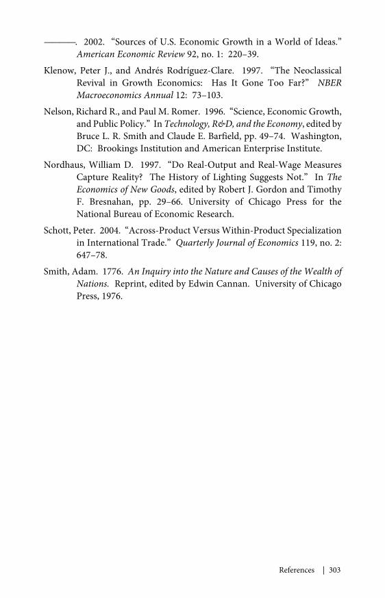
References | 303
————. 2002. “Sources of U.S. Economic Growth in a World of Ideas.”American Economic Review 92, no. 1: 220–39.
Klenow, Peter J., and Andrés Rodríguez-Clare. 1997. “The NeoclassicalRevival in Growth Economics: Has It Gone Too Far?” NBERMacroeconomics Annual 12: 73–103.
Nelson, Richard R., and Paul M. Romer. 1996. “Science, Economic Growth,and Public Policy.” InTechnology, R&D, and the Economy, edited byBruce L. R. Smith and Claude E. Barfield, pp. 49–74. Washington,DC: Brookings Institution and American Enterprise Institute.
Nordhaus, William D. 1997. “Do Real-Output and Real-Wage MeasuresCapture Reality? The History of Lighting Suggests Not.” In TheEconomics of New Goods, edited by Robert J. Gordon and TimothyF. Bresnahan, pp. 29–66. University of Chicago Press for theNational Bureau of Economic Research.
Schott, Peter. 2004. “Across-Product Versus Within-Product Specializationin International Trade.” Quarterly Journal of Economics 119, no. 2:647–78.
Smith, Adam. 1776. An Inquiry into the Nature and Causes of the Wealth ofNations. Reprint, edited by Edwin Cannan. University of ChicagoPress, 1976.

25
C H A P T E R 1
TO RESCUE, REBALANCE,AND REBUILD
President Obama took office at a time of economic crisis. The recessionthat began in December 2007 had accelerated following the financial
crisis in September 2008. By January 2009, 11.9 million people were unem-ployed and real gross domestic product (GDP) was falling at a breakneckpace. The possibility of a second Great Depression was frighteningly real.
In the first months of the Administration, the President and Congresstook unprecedented actions to restore demand, stabilize financial markets,and put people back to work. Just 28 days after his inauguration, thePresident signed the American Recovery and Reinvestment Act of 2009, theboldest countercyclical fiscal stimulus in American history. The FinancialStability Plan, announced in February, included wide-ranging measures tostrengthen the banking system, increase consumer and business lending,and stem foreclosures and support the housing market. These and a host ofother actions stabilized the financial system, supported those most directlyaffected by the recession, and walked the economy back from the brink.
But the Administration always knew that stabilizing the economywould not be enough. The problems that led to the crisis were years in themaking. Continued action will be necessary to return the economy to fullemployment. In the process, an important rebalancing will need to occur.For too many years, America’s growth and prosperity were fed by a boom inconsumer spending stemming from rising asset prices and easy credit. TheFederal Government had likewise been living beyond its means, resulting inlarge and growing budget deficits. And our regulatory system had failed tokeep up with financial innovation, allowing risky practices to endanger thesystem and the economy. For this reason, the Administration has sought tohelp restore the economy to health on a foundation of greater investment,fiscal responsibility, and a well-functioning and secure financial system.

26 | Chapter 1
Even this important rebalancing would not be sufficient. In additionto the problems that had set the stage for the crisis, long-term challenges hadbeen ignored and the U.S. economy was failing at some of its central tasks.Our health care system was beset by steadily rising costs, and millions ofAmericans either had no health insurance at all or were unsure whether theircoverage would be there when they needed it. Middle-class families had seentheir real incomes stagnate during the previous eight years, while those atthe top of the income distribution had seen their incomes soar. A failure toslow the consumption of fossil fuels had contributed to global warming andcontinued dependence on foreign oil. And a country built on its record ofinnovation was failing to invest enough in research and development.
The President has dedicated his Administration to dealing with theselong-run problems as well. As the new decade opens, Congress has comecloser than ever before to passing landmark legislation reforming the healthinsurance system. This legislation would make health insurance more securefor those who have it and affordable for those who do not, and it would slowthe growth rate of health care costs. Over the past year, the Administrationhas also worked with Congress to make important new investments tosustain and improve K-12 education and community colleges, jump-start thetransition to a clean energy economy, and spur innovation through increasedresearch and development. These and numerous other initiatives will helpto rebuild the American economy stronger than before and put us on thepath to sustained growth and prosperity. Enacting these policies will helpto ensure that our children and grandchildren inherit a country as full ofpromise and as economically secure as ever in our history.
Rescuing an Economy in Freefall
In December 2007, the American economy entered what at firstseemed likely to be a mild recession. As Figure 1-1 shows, real house prices(that is, house prices adjusted for inflation) had risen to unprecedented levels,almost doubling between 1997 and 2006. The rapid run-up in prices wasaccompanied by a residential construction boom and the proliferation ofcomplex mortgages and mortgage-related financial assets. The fall of nationalhouse prices starting in early 2007, and the associated declines in the valuesof mortgage-backed and other related assets, led to a slowdown in the growthof consumer spending, increases in mortgage defaults and home foreclosures,significant strains on financial institutions, and reduced credit availability.
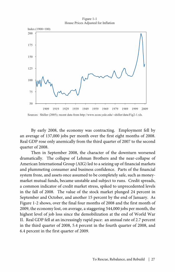
To Rescue, Rebalance, and Rebuild | 27
By early 2008, the economy was contracting. Employment fell byan average of 137,000 jobs per month over the first eight months of 2008.Real GDP rose only anemically from the third quarter of 2007 to the secondquarter of 2008.
Then in September 2008, the character of the downturn worseneddramatically. The collapse of Lehman Brothers and the near-collapse ofAmerican International Group (AIG) led to a seizing up of financial marketsand plummeting consumer and business confidence. Parts of the financialsystem froze, and assets once assumed to be completely safe, such as money-market mutual funds, became unstable and subject to runs. Credit spreads,a common indicator of credit market stress, spiked to unprecedented levelsin the fall of 2008. The value of the stock market plunged 24 percent inSeptember and October, and another 15 percent by the end of January. AsFigure 1-2 shows, over the final four months of 2008 and the first month of2009, the economy lost, on average, a staggering 544,000 jobs per month, thehighest level of job loss since the demobilization at the end of World WarII. Real GDP fell at an increasingly rapid pace: an annual rate of 2.7 percentin the third quarter of 2008, 5.4 percent in the fourth quarter of 2008, and6.4 percent in the first quarter of 2009.
50
75
100
125
150
175
200
1909 1919 1929 1939 1949 1959 1969 1979 1989 1999 2009
Figure 1-1House Prices Adjusted for Inflation
Index (1900=100)
Sources: Shiller (2005); recent data from http://www.econ.yale.edu/~shiller/data/Fig2-1.xls.
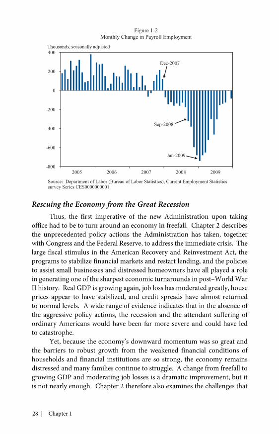
28 | Chapter 1
Rescuing the Economy from the Great RecessionThus, the first imperative of the new Administration upon taking
office had to be to turn around an economy in freefall. Chapter 2 describesthe unprecedented policy actions the Administration has taken, togetherwith Congress and the Federal Reserve, to address the immediate crisis. Thelarge fiscal stimulus in the American Recovery and Reinvestment Act, theprograms to stabilize financial markets and restart lending, and the policiesto assist small businesses and distressed homeowners have all played a rolein generating one of the sharpest economic turnarounds in post–World WarII history. Real GDP is growing again, job loss has moderated greatly, houseprices appear to have stabilized, and credit spreads have almost returnedto normal levels. A wide range of evidence indicates that in the absence ofthe aggressive policy actions, the recession and the attendant suffering ofordinary Americans would have been far more severe and could have ledto catastrophe.
Yet, because the economy’s downward momentum was so great andthe barriers to robust growth from the weakened financial conditions ofhouseholds and financial institutions are so strong, the economy remainsdistressed and many families continue to struggle. A change from freefall togrowing GDP and moderating job losses is a dramatic improvement, but itis not nearly enough. Chapter 2 therefore also examines the challenges that
-800
-600
-400
-200
0
200
400
Figure 1-2Monthly Change in Payroll Employment
Thousands, seasonally adjusted
Dec-2007
Sep-2008
Jan-2009
2005 2006 2007 2008 2009
Source: Department of Labor (Bureau of Labor Statistics), Current Employment Statisticssurvey Series CES0000000001.
To Rescue, Rebalance, and Rebuild | 29
remain in achieving a full recovery. It discusses some possible additionalmeasures to spur private sector job creation.
Crisis and Recovery in the World EconomyIn the early fall of 2008, there was hope that the impact of the crisis
on the rest of the world would be limited. Those hopes were dashed duringthe months that followed. In the fourth quarter of 2008 and the first quarterof 2009, real GDP fell sharply—often at double-digit rates—in the UnitedKingdom, Germany, Japan, Taiwan, and elsewhere. The surprisingly rapidspread of the downturn to the rest of the world reduced the demand for U.S.exports sharply, and so magnified our economic contraction.
The worldwide crisis required a worldwide response. Chapter 3describes both the actions taken by individual countries and those takenthrough international institutions and cooperation. As described in theleaders’ statement from the September summit of the Group of Twenty(G-20) nations, the result was “the largest and most coordinated fiscal andmonetary stimulus ever undertaken” (Group of Twenty 2009). Just as theactions in the United States have begun to turn the domestic economyaround, these international actions appear to have put the worst of the globalcrisis behind us. But the firmness of the budding recovery varies consider-ably across countries, and significant challenges still remain.
Rebalancing the Economy on thePath to Full Employment
The path from budding recovery to full employment will surely bea difficult one. The problems that sowed the seeds of the financial crisisneed to be dealt with so that the economy emerges from the recession witha stronger, more durable prosperity. There needs to be a rebalancing ofthe economy away from low personal saving and large government budgetdeficits and toward investment. Our financial system must be strengthenedboth to provide the lending needed to support the recovery and to reducethe risk of future crises.
Saving and InvestmentThe expansion of the 2000s was fueled in part by high consumption.
As Figure 1-3 shows, the share of GDP that takes the form of consumptionhas been on a generally upward trend for decades and reached unprec-edented heights in the 2000s. The personal saving rate fell to exceptionallylow levels, and trade deficits were large and persistent. A substantial amount
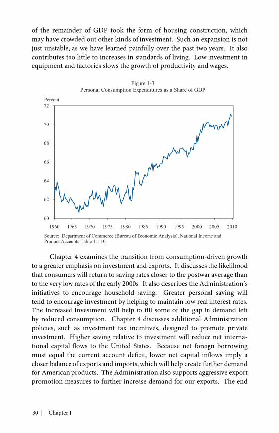
30 | Chapter 1
of the remainder of GDP took the form of housing construction, whichmay have crowded out other kinds of investment. Such an expansion is notjust unstable, as we have learned painfully over the past two years. It alsocontributes too little to increases in standards of living. Low investment inequipment and factories slows the growth of productivity and wages.
Chapter 4 examines the transition from consumption-driven growthto a greater emphasis on investment and exports. It discusses the likelihoodthat consumers will return to saving rates closer to the postwar average thanto the very low rates of the early 2000s. It also describes the Administration’sinitiatives to encourage household saving. Greater personal saving willtend to encourage investment by helping to maintain low real interest rates.The increased investment will help to fill some of the gap in demand leftby reduced consumption. Chapter 4 discusses additional Administrationpolicies, such as investment tax incentives, designed to promote privateinvestment. Higher saving relative to investment will reduce net interna-tional capital flows to the United States. Because net foreign borrowingmust equal the current account deficit, lower net capital inflows imply acloser balance of exports and imports, which will help create further demandfor American products. The Administration also supports aggressive exportpromotion measures to further increase demand for our exports. The end
60
62
64
66
68
70
72
1960 1965 1970 1975 1980 1985 1990 1995 2000 2005 2010
Figure 1-3Personal Consumption Expenditures as a Share of GDP
Percent
Source: Department of Commerce (Bureau of Economic Analysis), National Income andProduct Accounts Table 1.1.10.
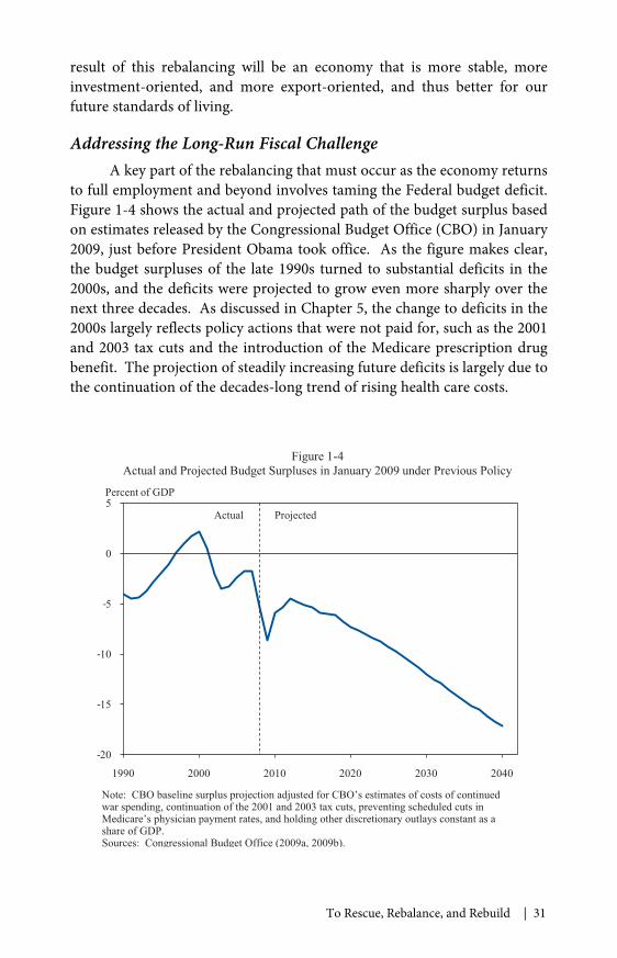
To Rescue, Rebalance, and Rebuild | 31
result of this rebalancing will be an economy that is more stable, moreinvestment-oriented, and more export-oriented, and thus better for ourfuture standards of living.
Addressing the Long-Run Fiscal ChallengeA key part of the rebalancing that must occur as the economy returns
to full employment and beyond involves taming the Federal budget deficit.Figure 1-4 shows the actual and projected path of the budget surplus basedon estimates released by the Congressional Budget Office (CBO) in January2009, just before President Obama took office. As the figure makes clear,the budget surpluses of the late 1990s turned to substantial deficits in the2000s, and the deficits were projected to grow even more sharply over thenext three decades. As discussed in Chapter 5, the change to deficits in the2000s largely reflects policy actions that were not paid for, such as the 2001and 2003 tax cuts and the introduction of the Medicare prescription drugbenefit. The projection of steadily increasing future deficits is largely due tothe continuation of the decades-long trend of rising health care costs.
-20
-15
-10
-5
0
5
1990 2000 2010 2020 2030 2040
Figure 1-4Actual and Projected Budget Surpluses in January 2009 under Previous Policy
Percent of GDP
ProjectedActual
Note: CBO baseline surplus projection adjusted for CBO’s estimates of costs of continuedwar spending, continuation of the 2001 and 2003 tax cuts, preventing scheduled cuts inMedicare’s physician payment rates, and holding other discretionary outlays constant as ashare of GDP.Sources: Congressional Budget Office (2009a, 2009b).

32 | Chapter 1
Chapter 5 describes the likely consequences of these projected deficitsover time and the importance of restoring fiscal discipline. It also discussesthe President’s plan for facing this challenge. A period of severe economicweakness is no time for a large fiscal contraction. Instead, the Nation musttackle the long-run deficit problem through actions that address the under-lying sources of the problem over time. The single most important step thatcan be taken to reduce future deficits is to adopt health care reform that slowsthe growth rate of costs without compromising the quality of care. In addi-tion, the President’s fiscal 2011 budget includes other significant measures,such as allowing President Bush’s tax cuts for the highest-income earnersto expire, reforming international tax rules to discourage tax avoidance andencourage investment in the United States, and imposing a three-year freezein nonsecurity discretionary spending; alongside a proposal for a bipartisancommission process to address the long-run gap between revenues andexpenditures.
Building a Safer Financial SystemRisky credit practices both encouraged some of the imprudent rise in
consumption and homebuilding in the previous decade and set the stage forthe financial crisis. Chapter 6 analyzes the role that financial intermediariesplay in the economy and diagnoses what went wrong during the meltdownof financial markets. The crisis showed that the Nation’s financial regula-tory structure, much of which had not been fundamentally changed sincethe 1930s, failed to keep up with the evolution of financial markets. Thecurrent system provided too little protection for the economy from actionsthat could threaten financial stability and too little protection for ordinaryAmericans in their dealings with sophisticated and powerful financial insti-tutions and other providers of credit. Strengthening our financial system isthus a key element of the rebalancing needed to assure stable, robust growth.
Chapter 6 discusses financial regulatory modernization. What isneeded is a system where capital requirements and sensible rules are setin a way to control excessive risk-taking; where regulators can considerrisks to the system as a whole and not just to individual institutions; whereinstitutions cannot choose their regulators; where regulators no longer facethe unacceptable choice between the disorganized, catastrophic failure of afinancial institution and a taxpayer-funded bailout; and where a dedicatedagency has consumer protection as its central mandate. For this reason, thePresident put forward a comprehensive plan for financial regulatory reformlast June and is working with Congress to ensure passage of these criticalreforms this year.
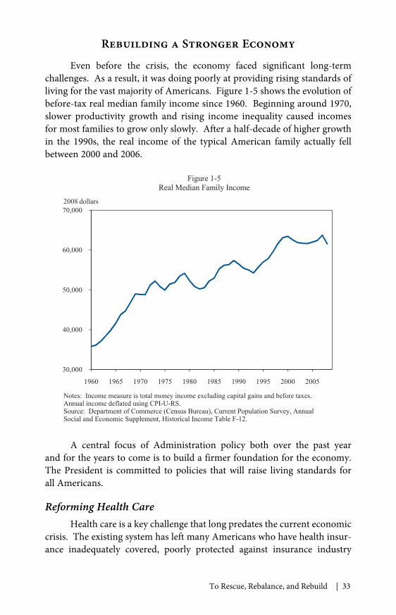
To Rescue, Rebalance, and Rebuild | 33
Rebuilding a Stronger Economy
Even before the crisis, the economy faced significant long-termchallenges. As a result, it was doing poorly at providing rising standards ofliving for the vast majority of Americans. Figure 1-5 shows the evolution ofbefore-tax real median family income since 1960. Beginning around 1970,slower productivity growth and rising income inequality caused incomesfor most families to grow only slowly. After a half-decade of higher growthin the 1990s, the real income of the typical American family actually fellbetween 2000 and 2006.
A central focus of Administration policy both over the past yearand for the years to come is to build a firmer foundation for the economy.The President is committed to policies that will raise living standards forall Americans.
Reforming Health CareHealth care is a key challenge that long predates the current economic
crisis. The existing system has left many Americans who have health insur-ance inadequately covered, poorly protected against insurance industry
30,000
40,000
50,000
60,000
70,000
1960 1965 1970 1975 1980 1985 1990 1995 2000 2005
Figure 1-5Real Median Family Income
2008 dollars
Notes: Income measure is total money income excluding capital gains and before taxes.Annual income deflated using CPI-U-RS.Source: Department of Commerce (Census Bureau), Current Population Survey, AnnualSocial and Economic Supplement, Historical Income Table F-12.
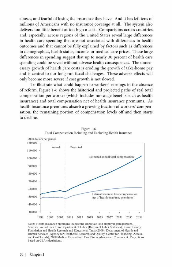
34 | Chapter 1
abuses, and fearful of losing the insurance they have. And it has left tens ofmillions of Americans with no insurance coverage at all. The system alsodelivers too little benefit at too high a cost. Comparisons across countriesand, especially, across regions of the United States reveal large differencesin health care spending that are not associated with differences in healthoutcomes and that cannot be fully explained by factors such as differencesin demographics, health status, income, or medical care prices. These largedifferences in spending suggest that up to nearly 30 percent of health carespending could be saved without adverse health consequences. The unnec-essary growth of health care costs is eroding the growth of take-home payand is central to our long-run fiscal challenges. These adverse effects willonly become more severe if cost growth is not slowed.
To illustrate what could happen to workers’ earnings in the absenceof reform, Figure 1-6 shows the historical and projected paths of real totalcompensation per worker (which includes nonwage benefits such as healthinsurance) and total compensation net of health insurance premiums. Ashealth insurance premiums absorb a growing fraction of workers’ compen-sation, the remaining portion of compensation levels off and then startsto decline.
30,000
40,000
50,000
60,000
70,000
80,000
90,000
100,000
110,000
120,000
1999 2003 2007 2011 2015 2019 2023 2027 2031 2035 2039
Estimated annual total compensation
Estimated annual total compensationnet of health insurance premiums
Projected
Figure 1-6Total Compensation Including and Excluding Health Insurance
2008 dollars per person
Actual
Note: Health insurance premiums include the employee- and employer-paid portions.Sources: Actual data from Department of Labor (Bureau of Labor Statistics); Kaiser FamilyFoundation and Health Research and Educational Trust (2009); Department of Health andHuman Services (Agency for Healthcare Research and Quality, Center for Financing, Access,and Cost Trends), 2008 Medical Expenditure Panel Survey-Insurance Component. Projectionsbased on CEA calculations.

To Rescue, Rebalance, and Rebuild | 35
Chapter 7 describes the actions the Administration and Congresstook in 2009 to begin the process of improvement, including an expansionof the Children’s Health Insurance Program to provide access to health carefor millions of children and important investments in the modernizationof the health care system through the Recovery Act. It also describes thekey elements of successful health insurance reform and discusses the prog-ress that has been made on reform legislation. Successful reform involvesmaking insurance more secure for those who have it and expanding coverageto those who lack it. It must include delivery system reforms, reductionsin waste and improper payments in the Medicare system, and changes inconsumer and firm incentives that will slow the growth rate of costs substan-tially, while maintaining and even improving quality. Slowing the growthrate of health care costs will have benefits throughout the economy: it willraise standards of living for families, help reduce the Federal budget deficitrelative to what it otherwise would be, benefit state and local governments,and encourage job growth and improved macroeconomic performance.
Strengthening the American Labor ForceAmerican workers have suffered greatly in the current recession.
As described in Chapter 8, long-term unemployment is at record levels.The unemployment rate, which was 10 percent for the country as awhole in December, is far higher for blacks, Hispanics, and other demo-graphic groups. The decline in house prices has eroded the nest eggsthat many Americans had been counting on for their retirement. TheAdministration has initiated many actions to help support workers andtheir families through the recession and beyond. These actions rangefrom extended and expanded unemployment insurance, to measuresto make health insurance more affordable, to initiatives to promoteretirement saving.
American workers also face the persistent problem of stagnatingincomes. A key determinant of growth in standards of living is the rate ofincrease in the education and skills of our workforce. More and more jobsrequire education and training beyond the high school level, along with theability to complete tasks that are open-ended and interactive. But, as Figure1-7 shows, the years of education U.S. workers have brought to the labormarket have risen little in the past four decades. And, as is well known, U.S.students lag behind those from many other countries in their performanceon standardized tests.
Chapter 8 describes the Administration’s initiatives to improve theskills of our workers. The Administration is pursuing reform to eliminatewasteful subsidies to student loan providers, the savings from which will fund
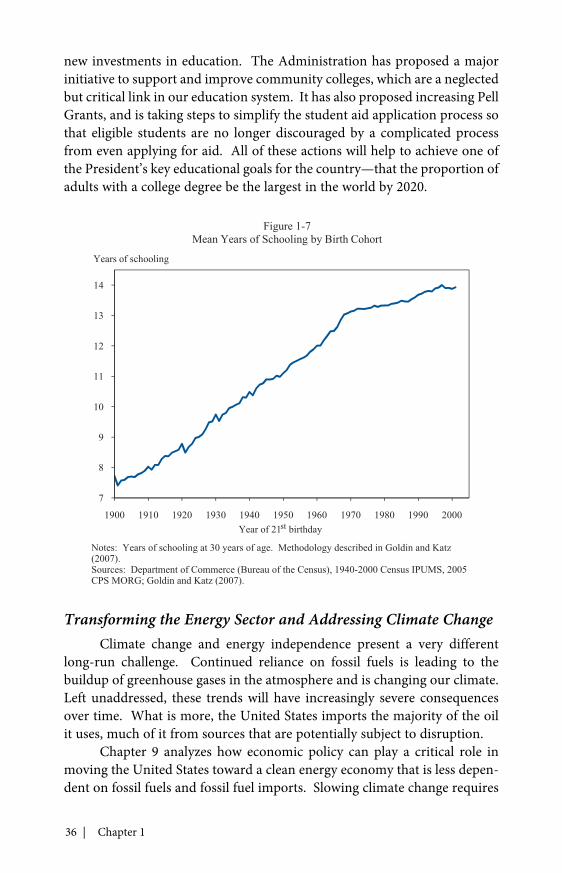
36 | Chapter 1
new investments in education. The Administration has proposed a majorinitiative to support and improve community colleges, which are a neglectedbut critical link in our education system. It has also proposed increasing PellGrants, and is taking steps to simplify the student aid application process sothat eligible students are no longer discouraged by a complicated processfrom even applying for aid. All of these actions will help to achieve one ofthe President’s key educational goals for the country—that the proportion ofadults with a college degree be the largest in the world by 2020.
Transforming the Energy Sector and Addressing Climate ChangeClimate change and energy independence present a very different
long-run challenge. Continued reliance on fossil fuels is leading to thebuildup of greenhouse gases in the atmosphere and is changing our climate.Left unaddressed, these trends will have increasingly severe consequencesover time. What is more, the United States imports the majority of the oilit uses, much of it from sources that are potentially subject to disruption.
Chapter 9 analyzes how economic policy can play a critical role inmoving the United States toward a clean energy economy that is less depen-dent on fossil fuels and fossil fuel imports. Slowing climate change requires
7
8
9
10
11
12
13
14
1900 1910 1920 1930 1940 1950 1960 1970 1980 1990 2000
Figure 1-7Mean Years of Schooling by Birth Cohort
Years of schooling
Year of 21 birthday
Notes: Years of schooling at 30 years of age. Methodology described in Goldin and Katz(2007).Sources: Department of Commerce (Bureau of the Census), 1940-2000 Census IPUMS, 2005CPS MORG; Goldin and Katz (2007).
st
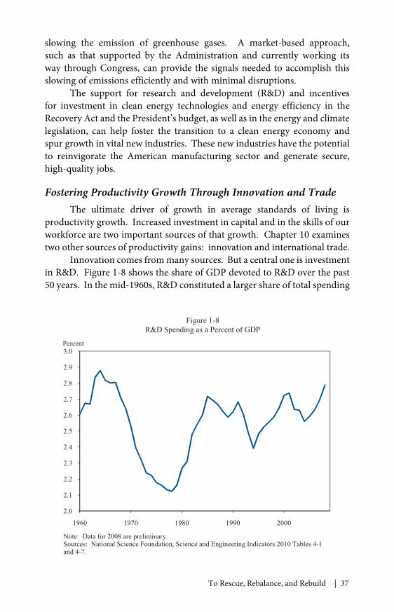
To Rescue, Rebalance, and Rebuild | 37
slowing the emission of greenhouse gases. A market-based approach,such as that supported by the Administration and currently working itsway through Congress, can provide the signals needed to accomplish thisslowing of emissions efficiently and with minimal disruptions.
The support for research and development (R&D) and incentivesfor investment in clean energy technologies and energy efficiency in theRecovery Act and the President’s budget, as well as in the energy and climatelegislation, can help foster the transition to a clean energy economy andspur growth in vital new industries. These new industries have the potentialto reinvigorate the American manufacturing sector and generate secure,high-quality jobs.
Fostering Productivity Growth Through Innovation and TradeThe ultimate driver of growth in average standards of living is
productivity growth. Increased investment in capital and in the skills of ourworkforce are two important sources of that growth. Chapter 10 examinestwo other sources of productivity gains: innovation and international trade.
Innovation comes from many sources. But a central one is investmentin R&D. Figure 1-8 shows the share of GDP devoted to R&D over the past50 years. In the mid-1960s, R&D constituted a larger share of total spending
2.0
2.1
2.2
2.3
2.4
2.5
2.6
2.7
2.8
2.9
3.0
1960 1970 1980 1990 2000
Figure 1-8R&D Spending as a Percent of GDP
Percent
Note: Data for 2008 are preliminary.Sources: National Science Foundation, Science and Engineering Indicators 2010 Tables 4-1and 4-7.

38 | Chapter 1
than it has in the past decade. And in some other countries, such as Korea,Sweden, and Japan, R&D spending is a larger fraction of GDP than in theUnited States. The President is committed to raising the share of outputdevoted to R&D to 3 percent, so that America can continue to be a leaderin new technologies and American workers and businesses can benefit frommore rapid economic growth.
Through the Recovery Act and other measures, the Administrationis investing both directly in basic scientific research and development andin the infrastructure to support that research. Most innovation, however,comes from the private sector. Here, the Administration is providing criticalincentives for R&D both in general and in such vital areas as clean energytechnologies. The Administration is also pursuing a wide range of policiesto support the small businesses that contribute so much to technologicalprogress—policies ranging from programs to maintain the flow of credit tosmall businesses to health insurance reform that will help level the playingfield between small and large businesses.
Finally, international trade can be an important source of productivitygrowth and incentives for innovation. Trade has the potential to allow theU.S. economy to expand output in areas where it is more productive andto enable higher-productivity firms to expand. Access to a world marketencourages American firms to invest in the research needed to become tech-nological leaders. Through these routes, a free and fair trade regime can playan important part in lifting living standards in the long run. But for trade toplay this role, it is essential to enforce existing trade rules and pursue policiesthat ensure that the benefits of trade are widely shared.
Conclusion
The past year has been one of great challenge for all Americans.Nearly every family has been touched in some way by the fallout from thecrisis in financial markets, the drying up of credit, and the rise in unem-ployment. These challenges, moreover, have come after a decade in whichordinary Americans have seen their living standards stagnate, their healthinsurance become less secure, and their environment deteriorate.
The rest of this Report describes in more detail the actions thePresident has taken to end the recession, foster stable growth by rebalancingproduction and demand, and rebuild the foundation of the Americaneconomy. More fundamentally, it describes the work that remains to bedone to create the prosperous, dynamic economy the American people needand deserve.

39
C H A P T E R 2
RESCUING THE ECONOMYFROM THE GREAT RECESSION
The first and most fundamental task the Administration faced whenPresident Obama took office was to rescue an economy in freefall. In
November 2008, employment was declining at a rate of more than half amillion jobs per month, and credit markets were stretched almost to thebreaking point. As the economy entered 2009, the decline accelerated, withjob loss in January reaching almost three-quarters of a million. The Presidentresponded by working with Congress to take unprecedented actions. Thesesteps, together with measures taken by the Federal Reserve and other finan-cial regulators, have succeeded in stabilizing the economy and beginningthe process of healing a severely shaken economic and financial system. Butmuch work remains. With high unemployment and continued job losses, itis clear that recovery must remain the key focus of 2010.
An Economy in Freefall
According to the National Bureau of Economic Research, the UnitedStates entered a recession in December 2007. Unlike most postwar reces-sions, this downturn was not caused by tight monetary policy aimed atcurbing inflation. Although economists will surely analyze this downturnextensively in the years to come, there is widespread consensus that itscentral precipitating factor was a boom and bust in asset prices, especiallyhouse prices. The boom was fueled in part by irresponsible and in somecases predatory lending practices, risky investment strategies, faulty creditratings, and lax regulation. When the boom ended, the result was wide-spread defaults and crippling blows to key financial institutions, magnifyingthe decline in house prices and causing enormous spillovers to the remainderof the economy.
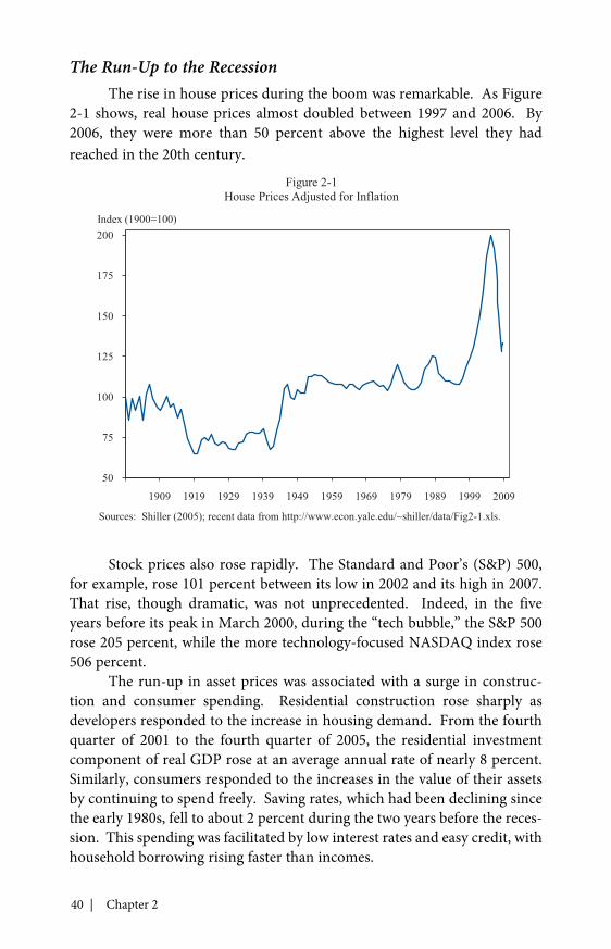
40 | Chapter 2
The Run-Up to the RecessionThe rise in house prices during the boom was remarkable. As Figure
2-1 shows, real house prices almost doubled between 1997 and 2006. By2006, they were more than 50 percent above the highest level they hadreached in the 20th century.
Stock prices also rose rapidly. The Standard and Poor’s (S&P) 500,for example, rose 101 percent between its low in 2002 and its high in 2007.That rise, though dramatic, was not unprecedented. Indeed, in the fiveyears before its peak in March 2000, during the “tech bubble,” the S&P 500rose 205 percent, while the more technology-focused NASDAQ index rose506 percent.
The run-up in asset prices was associated with a surge in construc-tion and consumer spending. Residential construction rose sharply asdevelopers responded to the increase in housing demand. From the fourthquarter of 2001 to the fourth quarter of 2005, the residential investmentcomponent of real GDP rose at an average annual rate of nearly 8 percent.Similarly, consumers responded to the increases in the value of their assetsby continuing to spend freely. Saving rates, which had been declining sincethe early 1980s, fell to about 2 percent during the two years before the reces-sion. This spending was facilitated by low interest rates and easy credit, withhousehold borrowing rising faster than incomes.
50
75
100
125
150
175
200
1909 1919 1929 1939 1949 1959 1969 1979 1989 1999 2009
Figure 2-1House Prices Adjusted for Inflation
Index (1900=100)
Sources: Shiller (2005); recent data from http://www.econ.yale.edu/~shiller/data/Fig2-1.xls.
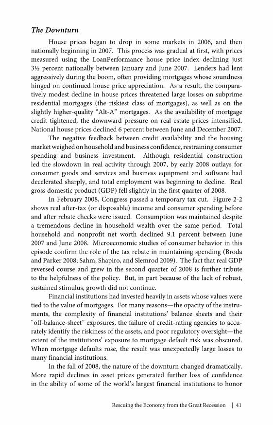
Rescuing the Economy from the Great Recession | 41
The DownturnHouse prices began to drop in some markets in 2006, and then
nationally beginning in 2007. This process was gradual at first, with pricesmeasured using the LoanPerformance house price index declining just3½ percent nationally between January and June 2007. Lenders had lentaggressively during the boom, often providing mortgages whose soundnesshinged on continued house price appreciation. As a result, the compara-tively modest decline in house prices threatened large losses on subprimeresidential mortgages (the riskiest class of mortgages), as well as on theslightly higher-quality “Alt-A” mortgages. As the availability of mortgagecredit tightened, the downward pressure on real estate prices intensified.National house prices declined 6 percent between June and December 2007.
The negative feedback between credit availability and the housingmarket weighed on household and business confidence, restraining consumerspending and business investment. Although residential constructionled the slowdown in real activity through 2007, by early 2008 outlays forconsumer goods and services and business equipment and software haddecelerated sharply, and total employment was beginning to decline. Realgross domestic product (GDP) fell slightly in the first quarter of 2008.
In February 2008, Congress passed a temporary tax cut. Figure 2-2shows real after-tax (or disposable) income and consumer spending beforeand after rebate checks were issued. Consumption was maintained despitea tremendous decline in household wealth over the same period. Totalhousehold and nonprofit net worth declined 9.1 percent between June2007 and June 2008. Microeconomic studies of consumer behavior in thisepisode confirm the role of the tax rebate in maintaining spending (Brodaand Parker 2008; Sahm, Shapiro, and Slemrod 2009). The fact that real GDPreversed course and grew in the second quarter of 2008 is further tributeto the helpfulness of the policy. But, in part because of the lack of robust,sustained stimulus, growth did not continue.
Financial institutions had invested heavily in assets whose values weretied to the value of mortgages. For many reasons—the opacity of the instru-ments, the complexity of financial institutions’ balance sheets and their“off-balance-sheet” exposures, the failure of credit-rating agencies to accu-rately identify the riskiness of the assets, and poor regulatory oversight—theextent of the institutions’ exposure to mortgage default risk was obscured.When mortgage defaults rose, the result was unexpectedly large losses tomany financial institutions.
In the fall of 2008, the nature of the downturn changed dramatically.More rapid declines in asset prices generated further loss of confidencein the ability of some of the world’s largest financial institutions to honor
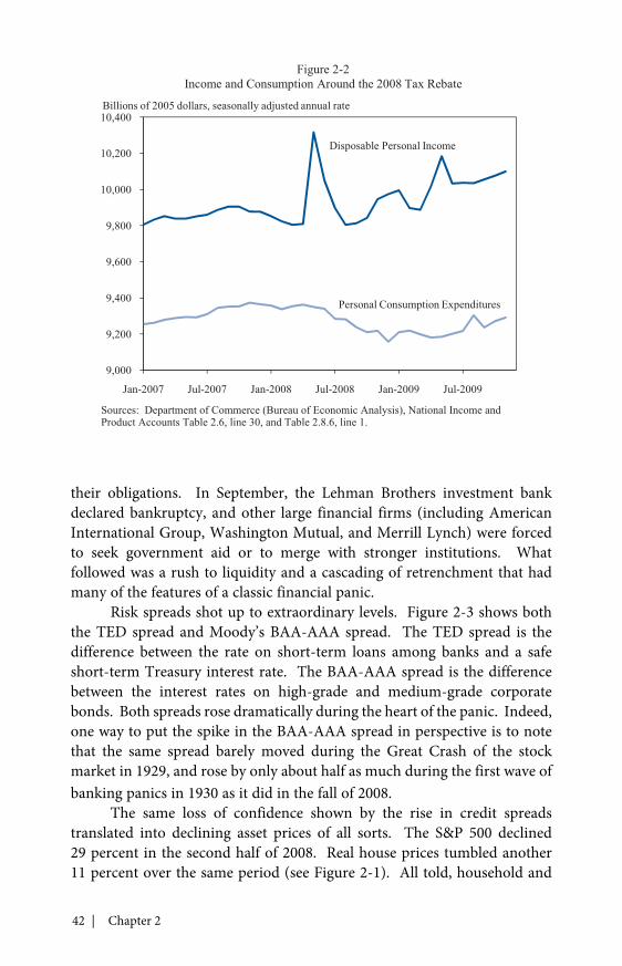
42 | Chapter 2
their obligations. In September, the Lehman Brothers investment bankdeclared bankruptcy, and other large financial firms (including AmericanInternational Group, Washington Mutual, and Merrill Lynch) were forcedto seek government aid or to merge with stronger institutions. Whatfollowed was a rush to liquidity and a cascading of retrenchment that hadmany of the features of a classic financial panic.
Risk spreads shot up to extraordinary levels. Figure 2-3 shows boththe TED spread and Moody’s BAA-AAA spread. The TED spread is thedifference between the rate on short-term loans among banks and a safeshort-term Treasury interest rate. The BAA-AAA spread is the differencebetween the interest rates on high-grade and medium-grade corporatebonds. Both spreads rose dramatically during the heart of the panic. Indeed,one way to put the spike in the BAA-AAA spread in perspective is to notethat the same spread barely moved during the Great Crash of the stockmarket in 1929, and rose by only about half as much during the first wave ofbanking panics in 1930 as it did in the fall of 2008.
The same loss of confidence shown by the rise in credit spreadstranslated into declining asset prices of all sorts. The S&P 500 declined29 percent in the second half of 2008. Real house prices tumbled another11 percent over the same period (see Figure 2-1). All told, household and
9,000
9,200
9,400
9,600
9,800
10,000
10,200
10,400
Jan-2007 Jul-2007 Jan-2008 Jul-2008 Jan-2009 Jul-2009
Figure 2-2Income and Consumption Around the 2008 Tax Rebate
Billions of 2005 dollars, seasonally adjusted annual rate
Disposable Personal Income
Personal Consumption Expenditures
Sources: Department of Commerce (Bureau of Economic Analysis), National Income andProduct Accounts Table 2.6, line 30, and Table 2.8.6, line 1.
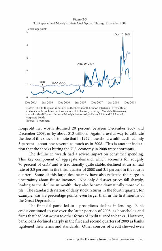
Rescuing the Economy from the Great Recession | 43
nonprofit net worth declined 20 percent between December 2007 andDecember 2008, or by about $13 trillion. Again, a useful way to calibratethe size of this shock is to note that in 1929, household wealth declined only3 percent—about one-seventh as much as in 2008. This is another indica-tion that the shocks hitting the U.S. economy in 2008 were enormous.
The decline in wealth had a severe impact on consumer spending.This key component of aggregate demand, which accounts for roughly70 percent of GDP and is traditionally quite stable, declined at an annualrate of 3.5 percent in the third quarter of 2008 and 3.1 percent in the fourthquarter. Some of this large decline may have also reflected the surge inuncertainty about future incomes. Not only did asset prices fall sharply,leading to the decline in wealth; they also became dramatically more vola-tile. The standard deviation of daily stock returns in the fourth quarter, forexample, was 4.3 percentage points, even larger than in the first months ofthe Great Depression.
The financial panic led to a precipitous decline in lending. Bankcredit continued to rise over the latter portion of 2008, as households andfirms that had lost access to other forms of credit turned to banks. However,bank loans declined sharply in the first and second quarters of 2009 as bankstightened their terms and standards. Other sources of credit showed even
0
1
2
3
4
5
Dec-2005 Jun-2006 Dec-2006 Jun-2007 Dec-2007 Jun-2008 Dec-2008
Figure 2-3TED Spread and Moody’s BAA-AAA Spread Through December2008
Percentage points
Aug. 20, 2007
Oct. 10, 2008
BAA-AAATED
Notes: The TED spread is defined as the three-month London Interbank Offered Rate(Libor) less the yield on the three-month U.S. Treasury security. Moody’s BAA-AAAspread is the difference between Moody's indexes of yields on AAA and BAA ratedcorporate bonds.Source: Bloomberg.
44 | Chapter 2
more substantial declines. One particularly important market is that forcommercial paper (short-term notes issued by firms to finance key operatingcosts such as payroll and inventory). The market for lower-tier nonfinancial(A2/P2) commercial paper collapsed in the fall of 2008, with the averagedaily value of new issues falling from $8.0 billion in the second quarter of2008 to $4.3 billion in the fourth quarter. In addition, securitization ofautomobile loans, credit card receivables, student loans, and commercialmortgages ground to a halt.
This freezing of credit markets, together with the decline in wealthand confidence, caused consumer spending and residential investment tofall sharply. Real GDP declined at an annual rate of 2.7 percent in the thirdquarter of 2008, 5.4 percent in the fourth quarter, and 6.4 percent in thefirst quarter of 2009. Industrial production, which had been falling steadilyover the first eight months of 2008, plummeted in the final four months—dropping at an annual rate of 18 percent.
Many industries were battered by the financial crisis and the resultingeconomic downturn. The American automobile industry was hit particu-larly hard. Sales of light motor vehicles, which had exceeded 16 millionunits every year from 1999 to 2007, fell to an annual rate of only 9.5 millionin the first quarter of 2009. Employment in the motor vehicle and partsindustry declined by 240,000 over the 12 months through January 2009.Two domestic manufacturers, General Motors (GM) and Chrysler, requiredemergency loans in late December 2008 and early January 2009 to avoiddisorderly bankruptcy.
The most disturbing manifestation of the rapid slowdown in theeconomy was the dramatic increase in job loss. Over the first months of2008, job losses were typically between 100,000 and 200,000 per month.In October, the economy lost 380,000 jobs; in November, 597,000 jobs.By January, the economy was losing jobs at a rate of 741,000 per month.Commensurate with this terrible rate of job loss, the unemployment raterose rapidly—from 6.2 percent in September 2008 to 7.7 percent in January2009. It then continued to rise by roughly one-half of a percentage point permonth through the winter and spring; it reached 9.4 percent in May, andended the year at 10.0 percent.
Wall Street and Main StreetAs described in more detail later, policymakers have focused much
of their response to the crisis on stabilizing the financial system. ManyAmericans are troubled by these policies. Because to a large extent it wasthe actions of credit market participants that led to the crisis, people ask whypolicymakers should take actions focused on restoring credit markets.

Rescuing the Economy from the Great Recession | 45
The basic reason for these policies is that the health of credit marketsis critically important to the functioning of our economy. Large firms usecommercial paper to finance their biweekly payrolls and pay suppliers formaterials to keep production lines going. Small firms rely on bank loans tomeet their payrolls and pay for supplies while they wait for payment of theiraccounts receivable. Home purchases depend on mortgages; automobilepurchases depend on car loans; college educations depend on student loans;and purchases of everyday items depend on credit cards.
The events of the past two years provide a dramatic demonstrationof the importance of credit in the modern economy. As the President saidin his inaugural address, “Our workers are no less productive than whenthis crisis began. Our minds are no less inventive, our goods and servicesno less needed.” Yet developments in financial markets—rises and fallsin home and equity prices and in the availability of credit—have led to acollapse of spending, and hence to a precipitous decline in output and tounemployment for millions.
Numerous academic studies before the crisis had also shown that theavailability of credit is critical to investment, hiring, and production. Onestudy, for example, found that when a parent company earns high profitsand so has less need to rely on credit, the additional funds lead to higherinvestment by subsidiaries in completely unrelated lines of business (Lamont1997). Another found that when a small change in a firm’s circumstancesfrees up a large amount of funds that would otherwise have to go to pensioncontributions, the result is a large change in spending on capital goods(Rauh 2006). Other studies have shown that when the Federal Reservetightens monetary policy, small firms, which typically have more difficultyobtaining financing, are hit especially hard (Gertler and Gilchrist 1994), andfirms without access to public debt markets cut their inventories much moresharply than firms that have such access (Kashyap, Lamont, and Stein 1994).
Research before the crisis had also found that financial market disrup-tions could affect the real economy. Ben Bernanke, who is now Chairmanof the Federal Reserve, demonstrated a link between the disruption oflending caused by bank failures and the worsening of the Great Depression(Bernanke 1983). A smaller but more modern example is provided by theimpact of Japan’s financial crisis in the 1990s on the United States: construc-tion lending, new construction, and construction employment were moreadversely affected in U.S. states where subsidiaries of Japanese banks hada larger role, and thus where credit availability was more affected by thecollapse of Japan’s bubble (Peek and Rosengren 2000). That a financialdisruption in a trading partner can have a detectable adverse impact on oureconomy through its impact on credit availability suggests that the effect of
46 | Chapter 2
a full-fledged financial crisis at home would be enormous—an implicationthat, sadly, has proven to be correct.
Finally, microeconomic evidence from the recent crisis also shows theimportance of the financial system to the real economy. For example, firmsthat happened to have long-term debt coming due after the crisis began,and thus faced high costs of refinancing, cut their investment much morethan firms that did not (Almeida et al. 2009). Another study found that amajority of corporate chief financial officers surveyed reported that theirfirms faced financing constraints during the crisis, and that the constrainedfirms on average planned to reduce investment spending, research anddevelopment, and employment sharply compared with the unconstrainedfirms (Campello, Graham, and Harvey 2009).
In short, the goal of the policies to stabilize the financial system wasnot to help financial institutions. The goal was to help ordinary Americans.When the financial system is not working, individuals and businesses cannotget credit, demand and production plummet, and job losses skyrocket.Thus, an essential step in healing the real economy is to heal the financialsystem. The alternative of letting financial institutions suffer the conse-quences of their mistakes would have led to a collapse of credit markets andvastly greater suffering for millions and millions of Americans.
The policies to rescue the financial sector were, however, costly, andoften had the side effect of benefiting the very institutions whose irrespon-sible actions contributed to the crisis. That is one reason that the Presidenthas endorsed a Financial Crisis Responsibility Fee on the largest financialfirms to repay the Federal Government for its extraordinary actions. Asdiscussed in Chapter 6, the Administration has also proposed a compre-hensive plan for financial regulatory reform that will help ensure that WallStreet does not return to the risky practices that were a central cause of therecent crisis.
The Unprecedented Policy Response
Given the magnitude of the shocks that hit the economy in the fall of2008 and the winter of 2009, the downturn could have turned into a secondGreat Depression. That it has not is a tribute to the aggressive and effec-tive policy response. This response involved the Federal Reserve and otherfinancial regulators, the Administration, and Congress. The policy toolswere similarly multifaceted, including monetary policy, financial marketinterventions, fiscal policy, and policies targeted specifically at housing.
Rescuing the Economy from the Great Recession | 47
Monetary PolicyThe first line of defense against a weak economy is the interest rate
policy of the independent Federal Reserve. By increasing or decreasing thequantity of reserves it supplies to the banking system, the Federal Reservecan lower or raise the Federal funds rate, which is the interest rate at whichbanks lend to one another. The funds rate influences other interest ratesin the economy and so has important effects on economic activity. Usingchanges in the target level of the funds rate as their main tool of counter-cyclical policy, monetary policymakers had kept inflation low and the realeconomy remarkably stable for more than two decades.
The Federal Reserve has used interest rate policy aggressively in therecent episode. The target level of the funds rate at the beginning of 2007was 5¼ percent. The Federal Reserve cut the target by 1 percentage pointover the last four months of 2007 and by an additional 2¼ percentage pointsover the first four months of 2008. After the events of September, it cut thetarget in three additional steps in October and December, bringing it to itscurrent level of 0 to ¼ percent.
Conventional interest rate policy, however, could do little to dealwith the enormous disruptions to credit markets. As a result, the FederalReserve has used a range of unconventional tools to address those disrup-tions directly. For example, in March 2008, it created the Primary DealerCredit Facility and the Term Securities Lending Facility to provide liquiditysupport for primary dealers (that is, financial institutions that trade directlywith the Federal Reserve) and the key financial markets in which theyoperate. In October 2008, when the critical market for commercial paperthreatened to stop functioning, the Federal Reserve responded by setting upthe Commercial Paper Funding Facility to backstop the market.
Once the Federal Reserve’s target for the funds rate was effectivelylowered to zero in December 2008, there was another reason to use uncon-ventional tools. Nominal interest rates generally cannot fall below zero:because holding currency guarantees a nominal return of zero, no one iswilling to make loans at a negative nominal interest rate. As a result, whenthe Federal funds rate is zero, supplying more reserves does not drive itlower. Statistical estimates suggest that based on the Federal Reserve’s usualresponse to inflation and unemployment, the subdued level of inflation andthe weak state of the economy would have led the central bank to reduce itstarget for the funds rate by about an additional 5 percentage points if it couldhave (Rudebusch 2009).
This desire to provide further stimulus, coupled with the inability touse conventional interest rate policy, led the Federal Reserve to undertakelarge-scale asset purchases to reduce long-term interest rates. In March
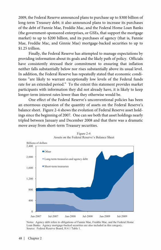
48 | Chapter 2
2009, the Federal Reserve announced plans to purchase up to $300 billion oflong-term Treasury debt; it also announced plans to increase its purchasesof the debt of Fannie Mae, Freddie Mac, and the Federal Home Loan Banks(the government-sponsored enterprises, or GSEs, that support the mortgagemarket) to up to $200 billion, and its purchases of agency (that is, FannieMae, Freddie Mac, and Ginnie Mae) mortgage-backed securities to up to$1.25 trillion.
Finally, the Federal Reserve has attempted to manage expectations byproviding information about its goals and the likely path of policy. Officialshave consistently stressed their commitment to ensuring that inflationneither falls substantially below nor rises substantially above its usual level.In addition, the Federal Reserve has repeatedly stated that economic condi-tions “are likely to warrant exceptionally low levels of the Federal fundsrate for an extended period.” To the extent this statement provides marketparticipants with information they did not already have, it is likely to keeplonger-term interest rates lower than they otherwise would be.
One effect of the Federal Reserve’s unconventional policies has beenan enormous expansion of the quantity of assets on the Federal Reserve’sbalance sheet. Figure 2-4 shows the evolution of Federal Reserve asset hold-ings since the beginning of 2007. One can see both that asset holdings nearlytripled between January and December 2008 and that there was a dramaticmove away from short-term Treasury securities.
0
400
800
1,200
1,600
2,000
2,400
Jan-2007 Jul-2007 Jan-2008 Jul-2008 Jan-2009 Jul-2009
Other
Long-term treasuries and agency debt
Short-term treasuries
Figure 2-4Assets on the Federal Reserve’s Balance Sheet
Billions of dollars
Notes: Agency debt refers to obligations of Fannie Mae, Freddie Mac, and the Federal HomeLoan Banks. Agency mortgage-backed securities are also included in this category.Source: Federal Reserve Board, H.4.1 Table 1.
Rescuing the Economy from the Great Recession | 49
The flip side of the large increase in the Federal Reserve’s assetholdings is a large increase in the quantity of reserves it has supplied to thefinancial system. Some observers have expressed concern that the largeexpansion in reserves could lead to inflation. In this regard, two key pointsshould be kept in mind. First, as already described, most statistical modelssuggest that the Federal Reserve’s target interest rate would be substan-tially lower than it is today if it were not constrained by the fact that theFederal funds rate cannot fall below zero. As a result, monetary policy isin fact unusually tight given the state of the economy, not unusually loose.Second, the Federal Reserve has the tools it needs to prevent the reservesfrom leading to inflation. It can drain the reserves from the financial systemthrough sales of the assets it has acquired or other actions. Indeed, despitethe weak state of the economy, the return of credit market conditions towardnormal is leading to the natural unwinding of some of the exceptional creditmarket programs. Another reliable way the Federal Reserve can keep thereserves from creating inflationary pressure is by using its relatively newability to raise the interest rate it pays on reserves: banks will be unwillingto lend the reserves at low interest rates if they can obtain a higher return ontheir balances held at the Federal Reserve.
Financial RescueEfforts to stabilize the financial system have been a central part of
the policy response. As just discussed, even before the financial crisis inSeptember 2008, the Federal Reserve was taking steps to ease pressureson credit markets. The events of the fall led to even stronger actions. OnSeptember 7, Fannie Mae and Freddie Mac were placed in conservator-ship under the Federal Housing Finance Agency to prevent a potentiallysevere disruption of mortgage lending. On September 16, concern aboutthe potentially catastrophic effects of a disorderly failure of AmericanInternational Group (AIG) caused the Federal Reserve to extend the firm an$85 billion line of credit. On September 19, concerns about the possibilityof runs on money-market mutual funds led the Treasury to announce atemporary guarantee program for these funds.
On October 3, Congress passed and President Bush signed theEmergency Economic Stabilization Act of 2008. This Act provided upto $700 billion for the Troubled Asset Relief Program (TARP) for thepurchase of distressed assets and for capital injections into financial institu-tions, although the second $350 billion required presidential notificationto Congress and could be disallowed by a vote of both houses. The initial$350 billion was used mainly to purchase preferred equity shares in finan-cial institutions, thereby providing the institutions with more capital to helpthem withstand the crisis.

50 | Chapter 2
At President-Elect Obama’s request, President Bush notified Congresson January 12, 2009 of his plan to release the second $350 billion of TARPfunds. With strong support from the incoming Administration, the Senatedefeated a resolution disapproving the release. These funds provided policy-makers with critical resources needed to ensure financial stability.
On February 10, 2009, Secretary of the Treasury Timothy Geithnerannounced the Administration’s Financial Stability Plan. The plan repre-sented a new, comprehensive approach to the financial rescue that soughtto tackle the interlocking sources of instability and increase credit flows.An overarching theme was a focus on transparency and accountability torebuild confidence in financial markets and protect taxpayer resources.
A key element of the plan was the Supervisory Capital AssessmentProgram (or “stress test”). The purpose was to assess the capital needs ofthe country’s 19 largest financial institutions should economic and finan-cial conditions deteriorate further. Institutions that were found to need anadditional capital buffer would be encouraged to raise private capital andwould be provided with temporary government capital if those efforts didnot succeed. This program was intended not just to examine the capitalpositions of the institutions and ensure that they obtained more capital ifneeded, but also to strengthen private investors’ confidence in the soundnessof the institutions’ balance sheets, and so strengthen the institutions’ abilityto obtain private capital.
Another element of the plan was the Consumer and Business LendingInitiative, which was aimed at maintaining the flow of credit. In November2008, the Federal Reserve had created the Term Asset-Backed SecuritiesLoan Facility to help counteract the dramatic decline in securitized lending.In the February announcement of the Financial Stability Plan, the Treasurygreatly expanded the resources of the not-yet-implemented facility. TheTreasury increased its commitment to $100 billion to leverage up to $1 tril-lion of lending for businesses and households. By facilitating securitization,the program was designed to help unfreeze credit and lower interest ratesfor auto loans, credit card loans, student loans, and small business loansguaranteed by the Small Business Administration (SBA).
A third element of the plan was a Treasury partnership with theFederal Deposit Insurance Corporation and the Federal Reserve to createthe Public-Private Investment Program. A central purpose was to removetroubled assets from the balance sheets of financial institutions, therebyreducing uncertainty about their financial strength and increasing theirability to raise capital and hence their willingness to lend. Partnership withthe private sector served two important objectives: it leveraged scarce publicfunds, and it used private competition and incentives to ensure that thegovernment did not overpay for assets.
Rescuing the Economy from the Great Recession | 51
There were two other key components of the Financial Stability Plan.One was a wide-ranging program to reduce mortgage interest rates and helpresponsible homeowners stay in their homes. These policies are describedlater in the section on housing policy. The other component was a rangeof measures to help small businesses. Many of these were included in theAmerican Recovery and Reinvestment Act and are discussed in the section onfiscal stimulus.
Failure of the two troubled domestic automakers (GM and Chrysler)threatened economy-wide repercussions that would have been magnifiedby related problems at the automakers’ associated financial institutions(GMAC and Chrysler Financial). To avoid these consequences, the BushAdministration set up the Auto Industry Financing Program within theTARP. This program extended $17.4 billion in funding to the two compa-nies in late December 2008 and early January 2009. The program alsoextended $7.5 billion in funding to the two auto finance companies aroundthe same time. Upon taking office, the Obama Administration requiredthe automakers to submit plans for restructuring and a return to viabilitybefore additional funds were committed. To sustain the industry duringthis planning process, the Treasury established the Warranty CommitmentProgram to reassure consumers that warranties of the troubled firms wouldbe honored. It also initiated the Auto Supplier Support Program to maintainstability in the auto supply base.
Over the spring of 2009, the Administration’s Auto Task Forceworked with GM and Chrysler to produce plans for viability. In the caseof Chrysler, the task force determined that viability could be achieved bymerging with the Italian automaker Fiat. For GM, the task force determinedthat substantial reductions in costs were necessary and charged the companywith producing a more aggressive restructuring plan. For both companies, aquick, targeted bankruptcy was judged to be the most efficient and successfulway to restructure. Chrysler filed for bankruptcy on April 30, 2009; GM, onJune 1. In addition to concessions by all stakeholders, including workers,retirees, creditors, and suppliers, the U.S. Government invested substantialfunds to bring about the orderly restructuring. In all, more than $80 billionof TARP funds had been authorized for the motor vehicle industry as ofSeptember 20, 2009.
Fiscal StimulusThe signature element of the Administration’s policy response to the
crisis was the American Recovery and Reinvestment Act of 2009 (ARRA).The President signed the Recovery Act in Denver on February 17, just28 days after taking office. At an estimated cost of $787 billion, the Act is
52 | Chapter 2
the largest countercyclical fiscal action in American history. It provides taxcuts and increases in government spending equivalent to roughly 2 percentof GDP in 2009 and 2¼ percent of GDP in 2010. To put those figures inperspective, the largest expansionary swing in the budget during FranklinRoosevelt’s New Deal was an increase in the deficit of about 1½ percent ofGDP in fiscal 1936. That expansion, however, was counteracted the verynext fiscal year by a contraction that was even larger.
The fiscal stimulus was designed to fill part of the shortfall inaggregate demand caused by the collapse of private demand and the FederalReserve’s inability to lower short-term interest rates further. It was partof a comprehensive package that included stabilizing the financial system,helping responsible homeowners avoid foreclosure, and aiding small busi-nesses through tax relief and increased lending. The President set as a goalfor the fiscal stimulus that it raise employment by 3½ million relative to whatit otherwise would have been.
Several principles guided the design of the stimulus. One was thatit be spread over two years, reflecting the Administration’s view that theeconomy would need substantial support for more than one year. At thesame time, the Administration also strongly supported keeping the stimulusexplicitly temporary. It was not to be an excuse to permanently expand thesize of government.
A second key principle was that the stimulus be well diversified.Different types of stimulus affect the economy in different ways. Individualtax cuts, for example, affect production and employment in a wide range ofindustries by encouraging households to spend more on consumer goods,while government investments in infrastructure directly increase construc-tion activity and employment. In addition, underlying economic conditionsaffect the efficacy of fiscal policy in ways that can be quantitatively importantand sometimes difficult to forecast. Likewise, different types of stimulusaffect the economy with different speeds. For instance, aid to individualsdirectly affected by the recession tends to be spent relatively quickly, whilenew investment projects require more time. Because of the need to providebroad support to the economy over an extended period, the Administrationsupported a stimulus plan that included a broad range of fiscal actions.
A third principle was that emergency spending should aim to addresslong-term needs. Some spending, such as unemployment insurance, isaimed at helping those directly affected by the recession maintain a decentstandard of living. But government investment spending should aim tocreate enduring capital investments that increase productivity and growth.
The Recovery Act reflected those guiding principles. The CongressionalBudget Office (CBO) estimated that almost one-quarter of the stimulus
Rescuing the Economy from the Great Recession | 53
would be spent by the end of the third quarter of 2009, and an additional halfwould be spent over the next four quarters (Congressional Budget Office2009b). So far, the pace of the spending and tax cuts has largely matchedCBO’s estimates.
The final package was very well diversified. Roughly one-third tookthe form of tax cuts. The most significant of these was the Making WorkPay tax credit, which cut taxes for 95 percent of working families. Taxes fora typical family were reduced by $800 per couple for each of 2009 and 2010.Another provision of the bill provided roughly $14 billion for one-timepayments of $250 to seniors, veterans, and people with disabilities. Themacroeconomic effects of these payments are likely to be similar to thoseof tax cuts.
Businesses received important tax cuts as well. The most importantof these was an extension of bonus depreciation, which reduced taxes onnew investments by allowing firms to immediately deduct half the cost ofproperty and equipment purchases. One advantage of such temporaryinvestment incentives is that they can affect the timing of investment,moving some investment from future years when the economy does nothave a deficiency of aggregate demand to the present, when it does.
In addition, because the financial market disruptions had aparticularly paralyzing effect on the financial plans of small businesses,the Act included additional measures targeted specifically at those busi-nesses. Tax cuts for small businesses included an expansion of provisionsallowing for the carryback of net operating losses, a temporary 75 percentexclusion from capital gains taxes on small business stock, and the abilityto immediately expense up to $250,000 of qualified investment purchases.In addition to reducing taxes, these provisions improve cash flow at firmsfacing credit constraints and provide extra incentives for individuals toinvest in small businesses. The Act also included measures to help increasesmall business lending through the SBA. In particular, it raised to 90percent the maximum guarantee on SBA general purpose and workingcapital loans (the 7(a) program) and eliminated fees on both 7(a) loansand loans for fixed-asset capital and real estate investment projects (the504 program).
Another important part of the stimulus consisted of fiscal relief to stategovernments. Because almost every state has a balanced-budget require-ment, the declines in revenues caused by the recession forced states to cutspending or raise taxes, thereby further contracting demand and magnifyingthe downturn. Federal fiscal relief can help prevent these contractionaryresponses, helping to maintain critical state services and state employment,prevent tax increases on families already suffering from the recession, and

54 | Chapter 2
cushion the fall in demand. And because many states were already raisingtaxes and cutting spending when the ARRA was passed, the effects werelikely to occur relatively quickly. The Act therefore included roughly $140billion of state fiscal relief.
The Recovery Act also included approximately $90 billion of supportfor individuals directly affected by the recession. This support serves twocritical purposes. First, it provides relief from the recession’s devastatingimpact on families and individuals. Second, because the recipients typicallyspend this support quickly, it provides an immediate boost to the broadereconomy. Among the major components of this relief were an extensionand expansion of unemployment insurance benefits, subsidies to help theunemployed continue to obtain health insurance, and additional fundingfor the Supplemental Nutritional Assistance Program. The Act also reducedtaxes on unemployment insurance benefits, the effect of which is similar toan expansion of benefits.
Finally, the Recovery Act included direct government investmentspending. Because government investment raises output in the short runboth through its direct effects and by increasing the incomes and spendingof the workers employed on the projects, its output effects are particularlylarge. In addition, because this type of stimulus is spent less quickly thanother types, it will play a vital role in providing support to the economyafter 2009. And by funding critical investments, this spending will raise theeconomy’s output even in the long run.
The Act included funding both for traditional government investmentprojects, such as transportation infrastructure and basic scientific research,and for initial investments to jump-start private investment in emergingnew areas, such as health information technology, a smart electrical grid,and clean energy technologies. The Act also included tax credits for specifictypes of private spending, such as home weatherization and advanced energymanufacturing, which are likely to have effects similar to direct governmentinvestment spending. Altogether, roughly one-third of the budget impactof the Recovery Act will take the form of these investments and tax credits.
Fiscal stimulus actions did not end with the passage and implementa-tion of the Recovery Act. In June 2009, the Administration worked withCongress to set up the Car Allowance Rebate System (CARS). Commonlyknown as the “Cash for Clunkers” program, CARS gave rebates of upto $4,500 to consumers who replaced older cars and trucks with newer,more fuel-efficient models. The program was in effect for July and mostof August. After the program’s popularity led to quick exhaustion of theoriginal funding of $1 billion, the funding was increased to $3 billion toallow more consumers to participate.

Rescuing the Economy from the Great Recession | 55
In November, the Worker, Homeownership, and Business AssistanceAct of 2009 cut taxes for struggling businesses and strengthened the safety netfor workers. In particular, the Act extended the net operating loss provisionsof the Recovery Act that allowed small businesses to count their losses thisyear against taxes paid in previous years for an additional year, and expandedthe benefit to medium and large businesses. The Act also provided up to20 additional weeks of unemployment insurance benefits for workers whowere reaching the end of their emergency unemployment benefits. InDecember, an amendment to the Department of Defense AppropriationsAct of 2010 continued through the end of February 2010 the unemploymentinsurance provisions of the Recovery Act, the November extension of emer-gency benefits, and the COBRA subsidy program that helps unemployedworkers maintain their health insurance. It also expanded the COBRApremium subsidy period from 9 to 15 months and extended the increasedguarantees and fee waivers for SBA loans.
Housing PolicyThe economic and financial crisis began in the housing market, and
an important part of the policy response has been directed at that market.The Administration initiated the Making Home Affordable program(MHA) in March 2009. This program was designed to support low mort-gage rates, keep millions of homeowners in their homes, and stabilize thehousing market.
As described earlier, the Federal Reserve undertook large-scalepurchases of GSE debt and mortgage-backed securities in an effort to reducemortgage interest rates. At the same time, the Treasury Department madean increased funding commitment to the GSEs. This increased governmentsupport for the agencies also reduced their borrowing costs and so helpedlower mortgage interest rates.
Importantly, MHA also included a program to help householdstake advantage of lower interest rates. The Home Affordable RefinanceProgram helps families whose homes have lost value and whose mortgagepayments can be reduced by refinancing at historically low interest rates.This program expanded the opportunity to refinance to borrowers withloans owned or guaranteed by the GSEs who had a mortgage balance up to125 percent of their home’s current value.
Another key component of MHA is the Home Affordable ModificationProgram (HAMP), which is providing up to $75 billion to encourage loanmodifications. It offers incentives to investors, lenders, servicers, andhomeowners to encourage mortgage modifications in which all stakeholdersshare in the cost of ensuring that responsible homeowners can afford their

56 | Chapter 2
monthly mortgage payments. To protect taxpayers, HAMP focuses onsound modifications. No payments are made by the government unlessthe modification lasts for at least three months, and all the payments aredesigned around the principle of “pay for success.” All parties have alignedincentives under the program to achieve successful modifications at anaffordable and sustainable level.
The Administration has supported additional programs to help thehousing sector. The Recovery Act included an $8,000 first-time homebuyer’scredit for home purchases made before December 1, 2009. As with tempo-rary investment incentives, this credit can help the economy by changingthe timing of decisions, bringing buyers into the housing market who werenot planning on becoming homeowners until after 2009 or were postponingtheir purchases in light of the distress in the market. In November, thiscredit was expanded and extended by the Workers, Homeownership, andBusiness Assistance Act of 2009.
TheRecoveryActalsogaveconsiderableresources to theNeighborhoodStabilization Program, a program administered by the Department ofHousing and Urban Development to stabilize communities that havesuffered from foreclosures and abandoned homes. The Administration alsoprovided assistance to state and local housing finance agencies and theirefforts to aid distressed homeowners, stimulate first-time home buying, andprovide affordable rental homes. These agencies had faced a significantliquidity crisis resulting from disruptions in financial markets.
The Effects of the Policies
The condition of the American economy has changed dramatically inthe past year. At the beginning of 2009, financial markets were functioningpoorly, house prices were plummeting, and output and employment werein freefall. Today, financial markets have stabilized and credit is starting toflow again, house prices have leveled off, output is growing, and the employ-ment situation is stabilizing. Because of the depth of the economy’s fall, weare a long way from full recovery, and significant challenges remain. But thetrajectory of the economy is vastly improved.
There is strong evidence that the policy response has been centralto this turnaround. The actions to stabilize credit markets have preventedfurther destructive failures of major financial institutions and helped main-tain lending in key areas. The housing and mortgage policies have kepthundreds of thousands of homeowners in their homes and brought mort-gage rates to historic lows. The speed of the economy’s change in directionhas been remarkable and matches up well with the timing of the fiscal
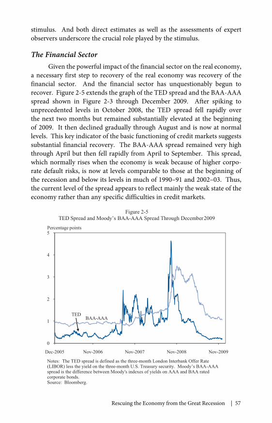
Rescuing the Economy from the Great Recession | 57
stimulus. And both direct estimates as well as the assessments of expertobservers underscore the crucial role played by the stimulus.
The Financial SectorGiven the powerful impact of the financial sector on the real economy,
a necessary first step to recovery of the real economy was recovery of thefinancial sector. And the financial sector has unquestionably begun torecover. Figure 2-5 extends the graph of the TED spread and the BAA-AAAspread shown in Figure 2-3 through December 2009. After spiking tounprecedented levels in October 2008, the TED spread fell rapidly overthe next two months but remained substantially elevated at the beginningof 2009. It then declined gradually through August and is now at normallevels. This key indicator of the basic functioning of credit markets suggestssubstantial financial recovery. The BAA-AAA spread remained very highthrough April but then fell rapidly from April to September. This spread,which normally rises when the economy is weak because of higher corpo-rate default risks, is now at levels comparable to those at the beginning ofthe recession and below its levels in much of 1990–91 and 2002–03. Thus,the current level of the spread appears to reflect mainly the weak state of theeconomy rather than any specific difficulties in credit markets.
0
1
2
3
4
5
Dec-2005 Nov-2006 Nov-2007 Nov-2008 Nov-2009
Figure 2-5TED Spread and Moody’s BAA-AAA Spread Through December2009
Percentage points
BAA-AAATED
Notes: The TED spread is defined as the three-month London Interbank Offer Rate(LIBOR) less the yield on the three-month U.S. Treasury security. Moody’s BAA-AAAspread is the difference between Moody's indexes of yields on AAA and BAA ratedcorporate bonds.Source: Bloomberg.
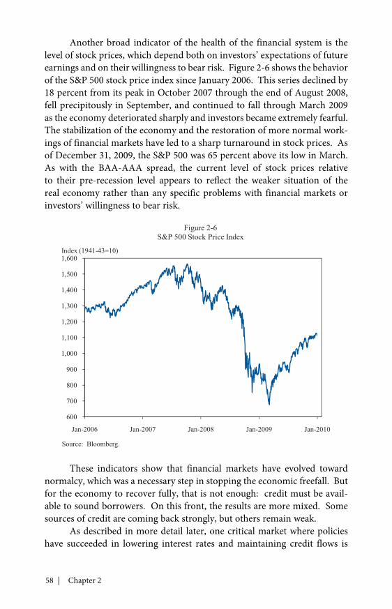
58 | Chapter 2
Another broad indicator of the health of the financial system is thelevel of stock prices, which depend both on investors’ expectations of futureearnings and on their willingness to bear risk. Figure 2-6 shows the behaviorof the S&P 500 stock price index since January 2006. This series declined by18 percent from its peak in October 2007 through the end of August 2008,fell precipitously in September, and continued to fall through March 2009as the economy deteriorated sharply and investors became extremely fearful.The stabilization of the economy and the restoration of more normal work-ings of financial markets have led to a sharp turnaround in stock prices. Asof December 31, 2009, the S&P 500 was 65 percent above its low in March.As with the BAA-AAA spread, the current level of stock prices relativeto their pre-recession level appears to reflect the weaker situation of thereal economy rather than any specific problems with financial markets orinvestors’ willingness to bear risk.
These indicators show that financial markets have evolved towardnormalcy, which was a necessary step in stopping the economic freefall. Butfor the economy to recover fully, that is not enough: credit must be avail-able to sound borrowers. On this front, the results are more mixed. Somesources of credit are coming back strongly, but others remain weak.
As described in more detail later, one critical market where policieshave succeeded in lowering interest rates and maintaining credit flows is
600
700
800
900
1,000
1,100
1,200
1,300
1,400
1,500
1,600
Jan-2006 Jan-2007 Jan-2008 Jan-2009 Jan-2010
Figure 2-6S&P 500 Stock Price Index
Index (1941-43=10)
Source: Bloomberg.
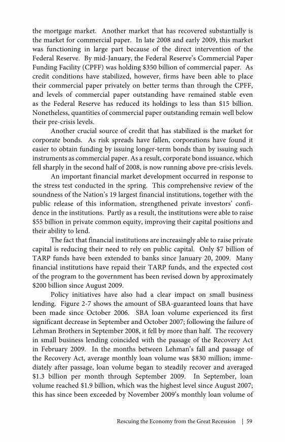
Rescuing the Economy from the Great Recession | 59
the mortgage market. Another market that has recovered substantially isthe market for commercial paper. In late 2008 and early 2009, this marketwas functioning in large part because of the direct intervention of theFederal Reserve. By mid-January, the Federal Reserve’s Commercial PaperFunding Facility (CPFF) was holding $350 billion of commercial paper. Ascredit conditions have stabilized, however, firms have been able to placetheir commercial paper privately on better terms than through the CPFF,and levels of commercial paper outstanding have remained stable evenas the Federal Reserve has reduced its holdings to less than $15 billion.Nonetheless, quantities of commercial paper outstanding remain well belowtheir pre-crisis levels.
Another crucial source of credit that has stabilized is the market forcorporate bonds. As risk spreads have fallen, corporations have found iteasier to obtain funding by issuing longer-term bonds than by issuing suchinstruments as commercial paper. As a result, corporate bond issuance, whichfell sharply in the second half of 2008, is now running above pre-crisis levels.
An important financial market development occurred in response tothe stress test conducted in the spring. This comprehensive review of thesoundness of the Nation’s 19 largest financial institutions, together with thepublic release of this information, strengthened private investors’ confi-dence in the institutions. Partly as a result, the institutions were able to raise$55 billion in private common equity, improving their capital positions andtheir ability to lend.
The fact that financial institutions are increasingly able to raise privatecapital is reducing their need to rely on public capital. Only $7 billion ofTARP funds have been extended to banks since January 20, 2009. Manyfinancial institutions have repaid their TARP funds, and the expected costof the program to the government has been revised down by approximately$200 billion since August 2009.
Policy initiatives have also had a clear impact on small businesslending. Figure 2-7 shows the amount of SBA-guaranteed loans that havebeen made since October 2006. SBA loan volume experienced its firstsignificant decrease in September and October 2007; following the failure ofLehman Brothers in September 2008, it fell by more than half. The recoveryin small business lending coincided with the passage of the Recovery Actin February 2009. In the months between Lehman’s fall and passage ofthe Recovery Act, average monthly loan volume was $830 million; imme-diately after passage, loan volume began to steadily recover and averaged$1.3 billion per month through September 2009. In September, loanvolume reached $1.9 billion, which was the highest level since August 2007;this has since been exceeded by November 2009’s monthly loan volume of
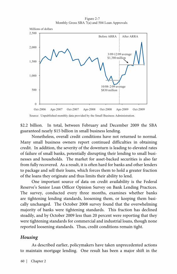
60 | Chapter 2
$2.2 billion. In total, between February and December 2009 the SBAguaranteed nearly $15 billion in small business lending.
Nonetheless, overall credit conditions have not returned to normal.Many small business owners report continued difficulties in obtainingcredit. In addition, the severity of the downturn is leading to elevated ratesof failure of small banks, potentially disrupting their lending to small busi-nesses and households. The market for asset-backed securities is also farfrom fully recovered. As a result, it is often hard for banks and other lendersto package and sell their loans, which forces them to hold a greater fractionof the loans they originate and thus limits their ability to lend.
One important source of data on credit availability is the FederalReserve’s Senior Loan Officer Opinion Survey on Bank Lending Practices.The survey, conducted every three months, examines whether banksare tightening lending standards, loosening them, or keeping them basi-cally unchanged. The October 2008 survey found that the overwhelmingmajority of banks were tightening standards. This fraction has declinedsteadily, and by October 2009 less than 20 percent were reporting that theywere tightening standards for commercial and industrial loans, though nonereported loosening standards. Thus, credit conditions remain tight.
HousingAs described earlier, policymakers have taken unprecedented actions
to maintain mortgage lending. One result has been a major shift in the
0
500
1,000
1,500
2,000
2,500
Oct-2006 Apr-2007 Oct-2007 Apr-2008 Oct-2008 Apr-2009 Oct-2009
Figure 2-7
Monthly Gross SBA 7(a) and 504 Loan Approvals
Millions of dollars
Before ARRA After ARRA
10/08-2/09 average$830 million
3/09-12/09 average$1,380million
Source: Unpublished monthly data provided by the Small Business Administration.
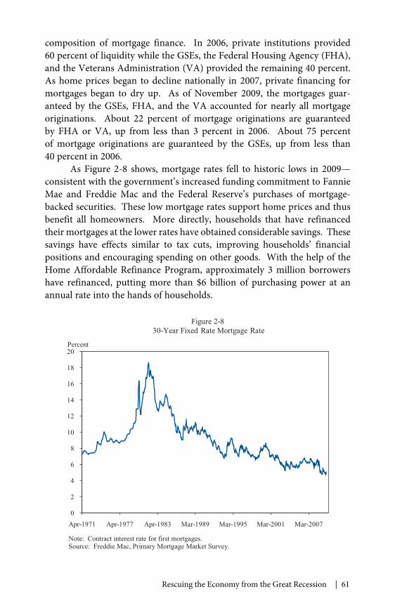
Rescuing the Economy from the Great Recession | 61
composition of mortgage finance. In 2006, private institutions provided60 percent of liquidity while the GSEs, the Federal Housing Agency (FHA),and the Veterans Administration (VA) provided the remaining 40 percent.As home prices began to decline nationally in 2007, private financing formortgages began to dry up. As of November 2009, the mortgages guar-anteed by the GSEs, FHA, and the VA accounted for nearly all mortgageoriginations. About 22 percent of mortgage originations are guaranteedby FHA or VA, up from less than 3 percent in 2006. About 75 percentof mortgage originations are guaranteed by the GSEs, up from less than40 percent in 2006.
As Figure 2-8 shows, mortgage rates fell to historic lows in 2009—consistent with the government’s increased funding commitment to FannieMae and Freddie Mac and the Federal Reserve’s purchases of mortgage-backed securities. These low mortgage rates support home prices and thusbenefit all homeowners. More directly, households that have refinancedtheir mortgages at the lower rates have obtained considerable savings. Thesesavings have effects similar to tax cuts, improving households’ financialpositions and encouraging spending on other goods. With the help of theHome Affordable Refinance Program, approximately 3 million borrowershave refinanced, putting more than $6 billion of purchasing power at anannual rate into the hands of households.
0
2
4
6
8
10
12
14
16
18
20
Apr-1971 Apr-1977 Apr-1983 Mar-1989 Mar-1995 Mar-2001 Mar-2007
Figure 2-830-Year Fixed Rate Mortgage Rate
Percent
Note: Contract interest rate for first mortgages.Source: Freddie Mac, Primary Mortgage Market Survey.

62 | Chapter 2
In addition, the Home Affordable Modification Program has beensuccessful in encouraging mortgage modifications. When the program waslaunched, the Administration estimated that it could offer help to as manyas 3 million to 4 million borrowers through the end of 2012. On October8, 2009, the Administration announced that servicers had begun more than500,000 trial modifications, nearly a month ahead of the original goal. Asof November, the monthly pace of trial modifications exceeded the monthlypace of completed foreclosures. Of course, not all trial modifications willbecome permanent, but the Administration is making every effort to ensurethat as many sound modifications as possible do.
One important result of the policies aimed at the housing marketand of the broader policies to support the economy is that the housingmarket appears to have stabilized. National home price indexes havebeen relatively steady for the past several months, as shown in Figure 2-9.The Federal Housing Finance Agency purchase-only house price index,which is constructed using only conforming mortgages (that is, mortgageseligible for purchase by the GSEs), has changed little since late 2008. TheLoanPerformance house price index, another closely watched measure thatuses conforming and nonconforming mortgages with coverage of repeatsales transactions for more than 85 percent of the population, rose 6 percentbetween March and August 2009 before declining slightly in recent months.In addition, the pace of sales of existing single-family homes has increasedsubstantially. Sales in the fourth quarter of 2009 were 29 percent abovetheir low in the first quarter of 2009 and comparable to levels in the first halfof 2007.
Finally, there are signs of renewed building activity. After falling81 percent from their peak in September 2005 to their low in January 2009,single-family housing permits (a leading indicator of housing construc-tion) rose 49 percent through December 2009. Similarly, after falling for14 consecutive quarters, the residential investment component of real GDProse in the third and fourth quarters of 2009.
Inventories of vacant homes for sale remain at high levels, and manyvacant homes are being held off the market and will likely be put up forsale as home prices increase. This overhang may lead to some additionalprice declines, although prices are unlikely to fall at the same rate as theydid during the crisis. Thus, the recovery of the housing sector is likely to beslow. Of course, we should neither expect nor want the housing market toreturn to its pre-crisis condition. In the long run, as discussed in more detailin Chapter 4, neither the extraordinarily high levels of housing constructionand price appreciation before the crisis nor the extraordinarily low levels ofconstruction and the rapid price declines during the crisis are sustainable.
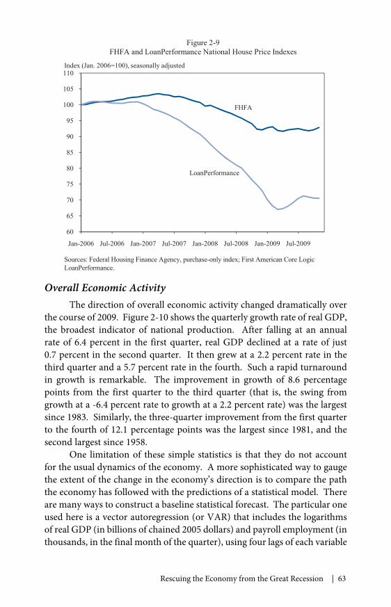
Rescuing the Economy from the Great Recession | 63
Overall Economic ActivityThe direction of overall economic activity changed dramatically over
the course of 2009. Figure 2-10 shows the quarterly growth rate of real GDP,the broadest indicator of national production. After falling at an annualrate of 6.4 percent in the first quarter, real GDP declined at a rate of just0.7 percent in the second quarter. It then grew at a 2.2 percent rate in thethird quarter and a 5.7 percent rate in the fourth. Such a rapid turnaroundin growth is remarkable. The improvement in growth of 8.6 percentagepoints from the first quarter to the third quarter (that is, the swing fromgrowth at a -6.4 percent rate to growth at a 2.2 percent rate) was the largestsince 1983. Similarly, the three-quarter improvement from the first quarterto the fourth of 12.1 percentage points was the largest since 1981, and thesecond largest since 1958.
One limitation of these simple statistics is that they do not accountfor the usual dynamics of the economy. A more sophisticated way to gaugethe extent of the change in the economy’s direction is to compare the paththe economy has followed with the predictions of a statistical model. Thereare many ways to construct a baseline statistical forecast. The particular oneused here is a vector autoregression (or VAR) that includes the logarithmsof real GDP (in billions of chained 2005 dollars) and payroll employment (inthousands, in the final month of the quarter), using four lags of each variable
60
65
70
75
80
85
90
95
100
105
110
Jan-2006 Jul-2006 Jan-2007 Jul-2007 Jan-2008 Jul-2008 Jan-2009 Jul-2009
Figure 2-9FHFA and LoanPerformance National House Price Indexes
Index (Jan. 2006=100), seasonally adjusted
LoanPerformance
FHFA
Sources: Federal Housing Finance Agency, purchase-only index; First American Core LogicLoanPerformance.
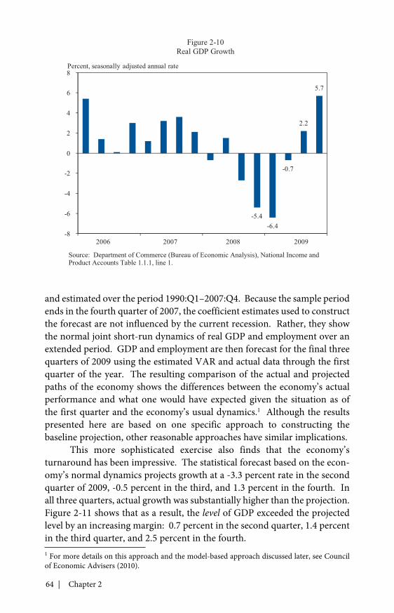
64 | Chapter 2
and estimated over the period 1990:Q1–2007:Q4. Because the sample periodends in the fourth quarter of 2007, the coefficient estimates used to constructthe forecast are not influenced by the current recession. Rather, they showthe normal joint short-run dynamics of real GDP and employment over anextended period. GDP and employment are then forecast for the final threequarters of 2009 using the estimated VAR and actual data through the firstquarter of the year. The resulting comparison of the actual and projectedpaths of the economy shows the differences between the economy’s actualperformance and what one would have expected given the situation as ofthe first quarter and the economy’s usual dynamics.1 Although the resultspresented here are based on one specific approach to constructing thebaseline projection, other reasonable approaches have similar implications.
This more sophisticated exercise also finds that the economy’sturnaround has been impressive. The statistical forecast based on the econ-omy’s normal dynamics projects growth at a -3.3 percent rate in the secondquarter of 2009, -0.5 percent in the third, and 1.3 percent in the fourth. Inall three quarters, actual growth was substantially higher than the projection.Figure 2-11 shows that as a result, the level of GDP exceeded the projectedlevel by an increasing margin: 0.7 percent in the second quarter, 1.4 percentin the third quarter, and 2.5 percent in the fourth.1 For more details on this approach and the model-based approach discussed later, see Councilof Economic Advisers (2010).
-5.4-6.4
-0.7
2.2
5.7
-8
-6
-4
-2
0
2
4
6
8
Figure 2-10Real GDP Growth
Percent, seasonally adjusted annual rate
2006 2007 2008 2009
Source: Department of Commerce (Bureau of Economic Analysis), National Income andProduct Accounts Table 1.1.1, line 1.
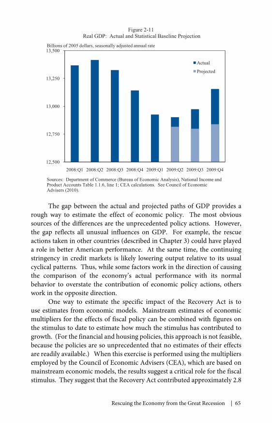
Rescuing the Economy from the Great Recession | 65
The gap between the actual and projected paths of GDP provides arough way to estimate the effect of economic policy. The most obvioussources of the differences are the unprecedented policy actions. However,the gap reflects all unusual influences on GDP. For example, the rescueactions taken in other countries (described in Chapter 3) could have playeda role in better American performance. At the same time, the continuingstringency in credit markets is likely lowering output relative to its usualcyclical patterns. Thus, while some factors work in the direction of causingthe comparison of the economy’s actual performance with its normalbehavior to overstate the contribution of economic policy actions, otherswork in the opposite direction.
One way to estimate the specific impact of the Recovery Act is touse estimates from economic models. Mainstream estimates of economicmultipliers for the effects of fiscal policy can be combined with figures onthe stimulus to date to estimate how much the stimulus has contributed togrowth. (For the financial and housing policies, this approach is not feasible,because the policies are so unprecedented that no estimates of their effectsare readily available.) When this exercise is performed using the multipliersemployed by the Council of Economic Advisers (CEA), which are based onmainstream economic models, the results suggest a critical role for the fiscalstimulus. They suggest that the Recovery Act contributed approximately 2.8
12,500
12,750
13,000
13,250
13,500
2008:Q1 2008:Q2 2008:Q3 2008:Q4 2009:Q1 2009:Q2 2009:Q3 2009:Q4
Actual
Projected
Figure 2-11Real GDP: Actual and Statistical Baseline Projection
Billions of 2005 dollars, seasonally adjusted annual rate
Sources: Department of Commerce (Bureau of Economic Analysis), National Income andProduct Accounts Table 1.1.6, line 1; CEA calculations. See Council of EconomicAdvisers (2010).
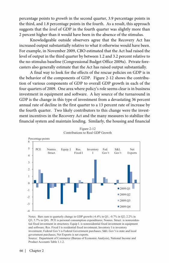
66 | Chapter 2
percentage points to growth in the second quarter, 3.9 percentage points inthe third, and 1.8 percentage points in the fourth. As a result, this approachsuggests that the level of GDP in the fourth quarter was slightly more than2 percent higher than it would have been in the absence of the stimulus.
Knowledgeable outside observers agree that the Recovery Act hasincreased output substantially relative to what it otherwise would have been.For example, in November 2009, CBO estimated that the Act had raised thelevel of output in the third quarter by between 1.2 and 3.2 percent relative tothe no-stimulus baseline (Congressional Budget Office 2009a). Private fore-casters also generally estimate that the Act has raised output substantially.
A final way to look for the effects of the rescue policies on GDP is inthe behavior of the components of GDP. Figure 2-12 shows the contribu-tion of various components of GDP to overall GDP growth in each of thefour quarters of 2009. One area where policy’s role seems clear is in businessinvestment in equipment and software. A key source of the turnaround inGDP is the change in this type of investment from a devastating 36 percentannual rate of decline in the first quarter to a 13 percent rate of increase bythe fourth quarter. Two likely contributors to this change were the invest-ment incentives in the Recovery Act and the many measures to stabilize thefinancial system and maintain lending. Similarly, the housing and financial
-4
-3
-2
-1
0
1
2
3
4
5
6
2009:Q1
2009:Q2
2009:Q3
2009:Q4
Figure 2-12Contributions to Real GDP Growth
Percentage points
PCE Nonres.Struct.
Res.Fixed I
InventoryI
Fed.Gov’t
S&LGov’t
NetExports
Equip. I
Notes: Bars sum to quarterly change in GDP growth (-6.4% in Q1; -0.7% in Q2; 2.2% inQ3; 5.7% in Q4). PCE is personal consumption expenditures; Nonres. Struct. is nonresiden-tial fixed investment in structures; Equip I. is nonresidential fixed investment in equipmentand software; Res. Fixed I is residential fixed investment; Inventory I is inventoryinvestment; Federal Gov’t is Federal Government purchases; S&L Gov’t is state and localgovernment purchases; Net Exports is net exports.Source: Department of Commerce (Bureau of Economic Analysis), National Income andProduct Accounts Table 1.1.2.
Rescuing the Economy from the Great Recession | 67
market policies were surely important to the swing in the growth of residen-tial investment from a 38 percent annual rate of decline in the first quarterto increases in the third and fourth quarters.
Two other components showing evidence of the policies’ effectsare personal consumption expenditures and state and local governmentpurchases. The Making Work Pay tax credit and the aid to individualsdirectly affected by the recession meant that households did not have to cuttheir consumption spending as much as they otherwise would have, andthe Cash for Clunkers program provided important incentives for motorvehicle purchases in the third quarter. Consumption was little changed inthe first two quarters of 2009 and then rose at a healthy 2.8 percent annualrate in the third quarter—driven in considerable part by a 44 percent rate ofincrease in purchases of motor vehicles and parts—and at a 2.0 percent ratein the fourth quarter. And, despite the dire budgetary situations of state andlocal governments, their purchases rose at the fastest pace in more than fiveyears in the second quarter and were basically stable in the third and fourthquarters. This stability almost surely could not have occurred in the absenceof the fiscal relief to the states.
The figure also shows the large role of inventory investment inmagnifying macroeconomic fluctuations. When the economy goes intoa recession, firms want to cut their inventories. As a result, inventoryinvestment moves from its usual slightly positive level to sharply negative,contributing to the fall in output. Then, as firms moderate their inventoryreductions, inventory investment rises—that is, becomes less negative—contributing to the recovery of output.
Finally, the turnaround in the automobile industry has beensubstantial. The Cash for Clunkers program appears to have generateda sharp increase in demand for automobiles in July and August 2009(Council of Economic Advisers 2009). Sales of light motor vehicles averaged12.6 million units at an annual rate during these two months, up froman annual rate of 9.6 million units in the second quarter. Although someobservers had hypothesized that the July and August sales boost would beoffset by a corresponding loss of sales in the months immediately following,sales in September (9.2 million at an annual rate) roughly matched thepace of sales in the first half of 2009, and sales subsequently rebounded to a10.8 million unit annual pace in the fourth quarter. Employment in motorvehicles and parts hit a low of 633,300 in June 2009 and has increasedmodestly since then. In December 2009, employment was 655,200.
Both GM and Chrysler proceeded through bankruptcy in an efficientmanner, and the new companies emerged far more quickly than outsideexperts thought would be possible. The companies are performing in line
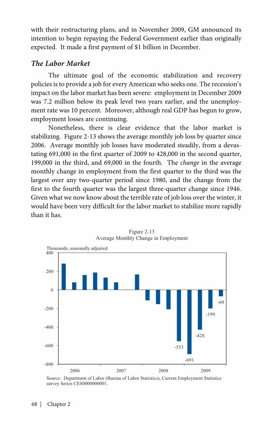
68 | Chapter 2
with their restructuring plans, and in November 2009, GM announced itsintention to begin repaying the Federal Government earlier than originallyexpected. It made a first payment of $1 billion in December.
The Labor MarketThe ultimate goal of the economic stabilization and recovery
policies is to provide a job for every American who seeks one. The recession’simpact on the labor market has been severe: employment in December 2009was 7.2 million below its peak level two years earlier, and the unemploy-ment rate was 10 percent. Moreover, although real GDP has begun to grow,employment losses are continuing.
Nonetheless, there is clear evidence that the labor market isstabilizing. Figure 2-13 shows the average monthly job loss by quarter since2006. Average monthly job losses have moderated steadily, from a devas-tating 691,000 in the first quarter of 2009 to 428,000 in the second quarter,199,000 in the third, and 69,000 in the fourth. The change in the averagemonthly change in employment from the first quarter to the third was thelargest over any two-quarter period since 1980, and the change from thefirst to the fourth quarter was the largest three-quarter change since 1946.Given what we now know about the terrible rate of job loss over the winter, itwould have been very difficult for the labor market to stabilize more rapidlythan it has.
-553
-691
-428
-199
-69
-800
-600
-400
-200
0
200
400
Figure 2-13Average Monthly Change in Employment
Thousands, seasonally adjusted
2006 2007 2008 2009Source: Department of Labor (Bureau of Labor Statistics), Current Employment Statisticssurvey Series CES0000000001.
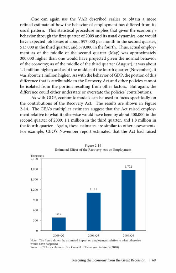
Rescuing the Economy from the Great Recession | 69
One can again use the VAR described earlier to obtain a morerefined estimate of how the behavior of employment has differed from itsusual pattern. This statistical procedure implies that given the economy’sbehavior through the first quarter of 2009 and its usual dynamics, one wouldhave expected job losses of about 597,000 per month in the second quarter,513,000 in the third quarter, and 379,000 in the fourth. Thus, actual employ-ment as of the middle of the second quarter (May) was approximately300,000 higher than one would have projected given the normal behaviorof the economy; as of the middle of the third quarter (August), it was about1.1 million higher; and as of the middle of the fourth quarter (November), itwas about 2.1 million higher. As with the behavior of GDP, the portion of thisdifference that is attributable to the Recovery Act and other policies cannotbe isolated from the portion resulting from other factors. But again, thedifference could either understate or overstate the policies’ contributions.
As with GDP, economic models can be used to focus specifically onthe contributions of the Recovery Act. The results are shown in Figure2-14. The CEA’s multiplier estimates suggest that the Act raised employ-ment relative to what it otherwise would have been by about 400,000 in thesecond quarter of 2009, 1.1 million in the third quarter, and 1.8 million inthe fourth quarter. Again, these estimates are similar to other assessments.For example, CBO’s November report estimated that the Act had raised
385
1,111
1,772
0
300
600
900
1,200
1,500
1,800
2,100
2009:Q2 2009:Q3 2009:Q4
Figure 2-14Estimated Effect of the Recovery Act on Employment
Thousands
Note: The figure shows the estimated impact on employment relative to what otherwisewould have happened.Source: CEA calculations. See Council of Economic Advisers (2010).
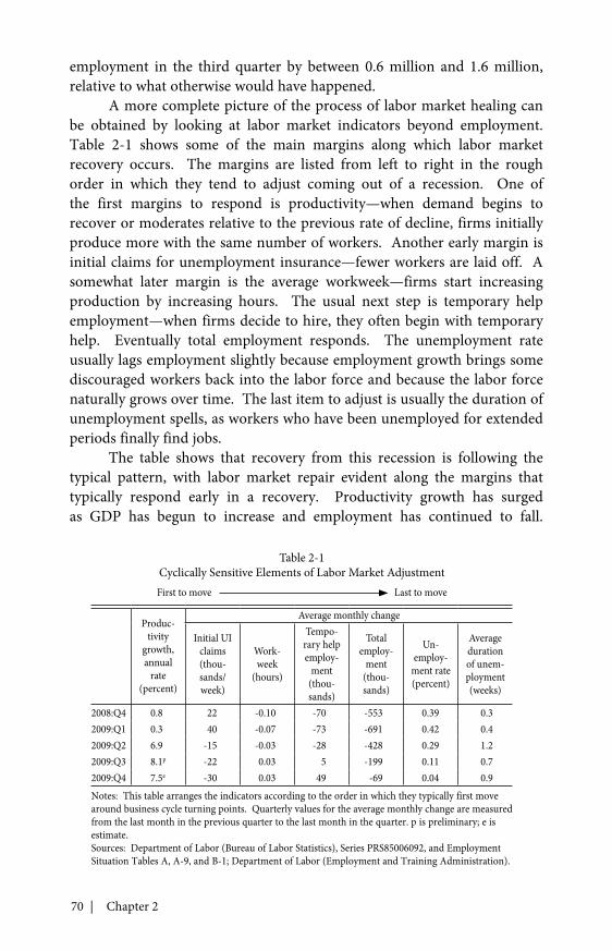
70 | Chapter 2
employment in the third quarter by between 0.6 million and 1.6 million,relative to what otherwise would have happened.
A more complete picture of the process of labor market healing canbe obtained by looking at labor market indicators beyond employment.Table 2-1 shows some of the main margins along which labor marketrecovery occurs. The margins are listed from left to right in the roughorder in which they tend to adjust coming out of a recession. One ofthe first margins to respond is productivity—when demand begins torecover or moderates relative to the previous rate of decline, firms initiallyproduce more with the same number of workers. Another early margin isinitial claims for unemployment insurance—fewer workers are laid off. Asomewhat later margin is the average workweek—firms start increasingproduction by increasing hours. The usual next step is temporary helpemployment—when firms decide to hire, they often begin with temporaryhelp. Eventually total employment responds. The unemployment rateusually lags employment slightly because employment growth brings somediscouraged workers back into the labor force and because the labor forcenaturally grows over time. The last item to adjust is usually the duration ofunemployment spells, as workers who have been unemployed for extendedperiods finally find jobs.
The table shows that recovery from this recession is following thetypical pattern, with labor market repair evident along the margins thattypically respond early in a recovery. Productivity growth has surgedas GDP has begun to increase and employment has continued to fall.
Table 2-1Cyclically Sensitive Elements of Labor Market AdjustmentFirst to move Last to move
Produc-tivity
growth,annual
rate(percent)
Average monthly change
Initial UIclaims(thou-sands/week)
Work-week
(hours)
Tempo-rary helpemploy-
ment(thou-sands)
Totalemploy-
ment(thou-sands)
Un-employ-
ment rate(percent)
Averagedurationof unem-ployment(weeks)
2008:Q4 0.8 22 -0.10 -70 -553 0.39 0.32009:Q1 0.3 40 -0.07 -73 -691 0.42 0.42009:Q2 6.9 -15 -0.03 -28 -428 0.29 1.22009:Q3 8.1p -22 0.03 5 -199 0.11 0.72009:Q4 7.5e -30 0.03 49 -69 0.04 0.9Notes: This table arranges the indicators according to the order in which they typically first movearound business cycle turning points. Quarterly values for the average monthly change are measuredfrom the last month in the previous quarter to the last month in the quarter. p is preliminary; e isestimate.Sources: Department of Labor (Bureau of Labor Statistics), Series PRS85006092, and EmploymentSituation Tables A, A-9, and B-1; Department of Labor (Employment and Training Administration).
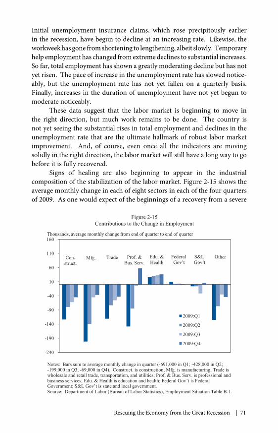
Rescuing the Economy from the Great Recession | 71
Initial unemployment insurance claims, which rose precipitously earlierin the recession, have begun to decline at an increasing rate. Likewise, theworkweek has gone from shortening to lengthening, albeit slowly. Temporaryhelp employment has changed from extreme declines to substantial increases.So far, total employment has shown a greatly moderating decline but has notyet risen. The pace of increase in the unemployment rate has slowed notice-ably, but the unemployment rate has not yet fallen on a quarterly basis.Finally, increases in the duration of unemployment have not yet begun tomoderate noticeably.
These data suggest that the labor market is beginning to move inthe right direction, but much work remains to be done. The country isnot yet seeing the substantial rises in total employment and declines in theunemployment rate that are the ultimate hallmark of robust labor marketimprovement. And, of course, even once all the indicators are movingsolidly in the right direction, the labor market will still have a long way to gobefore it is fully recovered.
Signs of healing are also beginning to appear in the industrialcomposition of the stabilization of the labor market. Figure 2-15 shows theaverage monthly change in each of eight sectors in each of the four quartersof 2009. As one would expect of the beginnings of a recovery from a severe
-240
-190
-140
-90
-40
10
60
110
160
2009:Q1
2009:Q2
2009:Q3
2009:Q4
Figure 2-15Contributions to the Change in Employment
Thousands, average monthly change from end of quarter to end of quarter
Con-struct.
Mfg. Trade Prof. &Bus. Serv.
Edu. &Health
FederalGov’t
S&LGov’t
Other
Notes: Bars sum to average monthly change in quarter (-691,000 in Q1; -428,000 in Q2;-199,000 in Q3; -69,000 in Q4). Construct. is construction; Mfg. is manufacturing; Trade iswholesale and retail trade, transportation, and utilities; Prof. & Bus. Serv. is professional andbusiness services; Edu. & Health is education and health; Federal Gov’t is FederalGovernment; S&L Gov’t is state and local government.Source: Department of Labor (Bureau of Labor Statistics), Employment Situation Table B-1.
72 | Chapter 2
recession, the moderation in job losses has been particularly pronounced inmanufacturing and construction, two of the most cyclically sensitive sectors.There has also been a sharp turnaround in professional business services,driven largely by renewed employment growth in temporary help services.
One area where the Recovery Act appears to have had a direct impacton employment is in state and local government. Despite the enormousharm the recession has done to their budgets, employment in state andlocal governments has fallen relatively little. Indeed, employment instate and local government, particularly in public education, rose in thefourth quarter.
The Challenges Ahead
The financial and economic rescue policies have helped avert aneconomic calamity and brought about a sharp change in the economy’sdirection. Output has begun growing again, and employment appearspoised to do so as well. But even when the country has returned to a pathof steadily growing output and employment, the economy will be far fromfully recovered. Since the recession began in December 2007, 7.2 millionjobs have been lost. It will take many months of robust job creation to erasethat employment deficit. For this reason, it is important to explore policiesto speed recovery and spur job creation.
Deteriorating ForecastsThis jobs deficit is much larger than the vast majority of observers
anticipated at the end of 2008. This is not the result of a slow economic turn-around. On the contrary, as described above, the change in the economy’sdirection has been remarkably rapid given the economy’s condition in thefirst quarter of 2009. Rather, the jobs deficit reflects two developments.
The first development is the unanticipated severity of the downturn inthe real economy in 2008 and early 2009. Table 2-2 shows consensus fore-casts from November 2008 through February 2009, along with preliminaryand actual estimates of real GDP growth. The table shows that the magni-tude of the fall in GDP in the fourth quarter of 2008 and the first quarterof 2009—driven in part by the unexpectedly strong spread of the crisis tothe rest of the world—surprised most observers. The Blue Chip Consensusreleased in mid-December 2008 projected fourth quarter growth would be-4.1 percent and first quarter growth would be -2.4 percent. The actualvalues turned out to be -5.4 percent and -6.4 percent. The Blue Chip forecastreleased in mid-January also projected a substantially smaller decline in firstquarter real GDP than actually occurred.
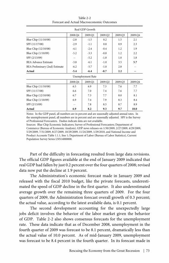
Rescuing the Economy from the Great Recession | 73
Part of the difficulty in forecasting resulted from large data revisions.The official GDP figures available at the end of January 2009 indicated thatreal GDP had fallen by just 0.2 percent over the four quarters of 2008; reviseddata now put the decline at 1.9 percent.
The Administration’s economic forecast made in January 2009 andreleased with the fiscal 2010 budget, like the private forecasts, underesti-mated the speed of GDP decline in the first quarter. It also underestimatedaverage growth over the remaining three quarters of 2009. For the fourquarters of 2009, the Administration forecast overall growth of 0.3 percent;the actual value, according to the latest available data, is 0.1 percent.
The second development accounting for the unexpectedly largejobs deficit involves the behavior of the labor market given the behaviorof GDP. Table 2-2 also shows consensus forecasts for the unemploymentrate. These data indicate that as of December 2008, unemployment in thefourth quarter of 2009 was forecast to be 8.1 percent, dramatically less thanthe actual value of 10.0 percent. As of mid-January 2009, unemploymentwas forecast to be 8.4 percent in the fourth quarter. In its forecast made in
Table 2-2Forecast and Actual Macroeconomic Outcomes
Real GDP Growth
2008:Q4 2009:Q1 2009:Q2 2009:Q3 2009:Q4Blue Chip (11/10/08) -2.8 -1.5 0.2 1.5 2.1SPF (11/17/08) -2.9 -1.1 0.8 0.9 2.3Blue Chip (12/10/08) -4.1 -2.4 -0.4 1.2 1.9Blue Chip (1/10/09) -5.2 -3.3 -0.8 1.2 2.2SPF (2/13/09) -- -5.2 -1.8 1.0 1.8BEA Advance Estimate -3.8 -6.1 -1.0 3.5 5.7BEA Preliminary (2nd) Estimate -6.2 -5.7 -1.0 2.8 --Actual -5.4 -6.4 -0.7 2.2 --
Unemployment Rate
2008:Q4 2009:Q1 2009:Q2 2009:Q3 2009:Q4Blue Chip (11/10/08) 6.5 6.9 7.3 7.6 7.7SPF (11/17/08) 6.6 7.0 7.4 7.6 7.7Blue Chip (12/10/08) 6.7 7.3 7.7 8.0 8.1Blue Chip (1/10/09) 6.9 7.4 7.9 8.3 8.4SPF (2/13/09) -- 7.8 8.3 8.7 8.9Actual 6.9 8.2 9.3 9.7 10.0Notes: In the GDP panel, all numbers are in percent and are seasonally adjusted annual rates. Inthe unemployment panel, all numbers are in percent and are seasonally adjusted. SPF is the Surveyof Professional Forecasters. Dashes indicate data are not available.Sources: Blue Chip Economic Indicators; Survey of Professional Forecasters; Department ofCommerce (Bureau of Economic Analysis), GDP news releases on 1/30/2009, 2/27/2009, 4/29/2009,5/29/2009, 7/31/2009, 8/27/2009, 10/29/2009, 11/24/2009, 1/29/2010, and National Income andProduct Accounts Table 1.1.1, line 1; Department of Labor (Bureau of Labor Statistics), CurrentPopulation Survey Series LNS14000000.
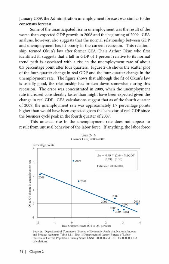
74 | Chapter 2
January 2009, the Administration unemployment forecast was similar to theconsensus forecast.
Some of the unanticipated rise in unemployment was the result of theworse-than-expected GDP growth in 2008 and the beginning of 2009. CEAanalysis, however, also suggests that the normal relationship between GDPand unemployment has fit poorly in the current recession. This relation-ship, termed Okun’s law after former CEA Chair Arthur Okun who firstidentified it, suggests that a fall in GDP of 1 percent relative to its normaltrend path is associated with a rise in the unemployment rate of about0.5 percentage point after four quarters. Figure 2-16 shows the scatter plotof the four-quarter change in real GDP and the four-quarter change in theunemployment rate. The figure shows that although the fit of Okun’s lawis usually good, the relationship has broken down somewhat during thisrecession. The error was concentrated in 2009, when the unemploymentrate increased considerably faster than might have been expected given thechange in real GDP. CEA calculations suggest that as of the fourth quarterof 2009, the unemployment rate was approximately 1.7 percentage pointshigher than would have been expected given the behavior of real GDP sincethe business cycle peak in the fourth quarter of 2007.
This unusual rise in the unemployment rate does not appear toresult from unusual behavior of the labor force. If anything, the labor force
2000
2001
2002 2003
200420052006
2007
2008
2009
-1
0
1
2
3
4
-2 -1 0 1 2 3 4
Q4
toQ
4ch
ange
inun
empl
oym
entr
ate
Figure 2-16Okun’s Law, 2000-2009
Percentage points
ru = 0.49 * (2.64 - %rGDP)(0.09) (0.30)
Estimated 2000-2008.
Real Output Growth (Q4 to Q4, percent)
Sources: Department of Commerce (Bureau of Economic Analysis), National Incomeand Product Accounts Table 1.1.1, line 1; Department of Labor (Bureau of LaborStatistics), Current Population Survey Series LNS11000000 and LNS113000000; CEAcalculations.
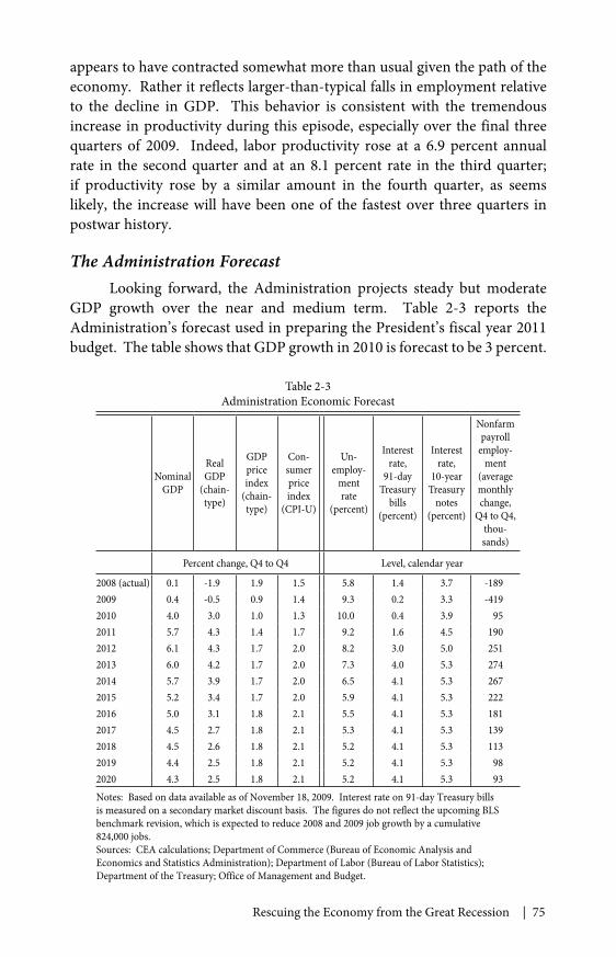
Rescuing the Economy from the Great Recession | 75
appears to have contracted somewhat more than usual given the path of theeconomy. Rather it reflects larger-than-typical falls in employment relativeto the decline in GDP. This behavior is consistent with the tremendousincrease in productivity during this episode, especially over the final threequarters of 2009. Indeed, labor productivity rose at a 6.9 percent annualrate in the second quarter and at an 8.1 percent rate in the third quarter;if productivity rose by a similar amount in the fourth quarter, as seemslikely, the increase will have been one of the fastest over three quarters inpostwar history.
The Administration ForecastLooking forward, the Administration projects steady but moderate
GDP growth over the near and medium term. Table 2-3 reports theAdministration’s forecast used in preparing the President’s fiscal year 2011budget. The table shows that GDP growth in 2010 is forecast to be 3 percent.
Table 2-3Administration Economic Forecast
NominalGDP
RealGDP
(chain-type)
GDPpriceindex
(chain-type)
Con-sumerpriceindex
(CPI-U)
Un-employ-
mentrate
(percent)
Interestrate,
91-dayTreasury
bills(percent)
Interestrate,
10-yearTreasury
notes(percent)
Nonfarmpayroll
employ-ment
(averagemonthlychange,
Q4 to Q4,thou-sands)
Percent change, Q4 to Q4 Level, calendar year
2008 (actual) 0.1 -1.9 1.9 1.5 5.8 1.4 3.7 -1892009 0.4 -0.5 0.9 1.4 9.3 0.2 3.3 -4192010 4.0 3.0 1.0 1.3 10.0 0.4 3.9 952011 5.7 4.3 1.4 1.7 9.2 1.6 4.5 1902012 6.1 4.3 1.7 2.0 8.2 3.0 5.0 2512013 6.0 4.2 1.7 2.0 7.3 4.0 5.3 2742014 5.7 3.9 1.7 2.0 6.5 4.1 5.3 2672015 5.2 3.4 1.7 2.0 5.9 4.1 5.3 2222016 5.0 3.1 1.8 2.1 5.5 4.1 5.3 1812017 4.5 2.7 1.8 2.1 5.3 4.1 5.3 1392018 4.5 2.6 1.8 2.1 5.2 4.1 5.3 1132019 4.4 2.5 1.8 2.1 5.2 4.1 5.3 982020 4.3 2.5 1.8 2.1 5.2 4.1 5.3 93Notes: Based on data available as of November 18, 2009. Interest rate on 91-day Treasury billsis measured on a secondary market discount basis. The figures do not reflect the upcoming BLSbenchmark revision, which is expected to reduce 2008 and 2009 job growth by a cumulative824,000 jobs.Sources: CEA calculations; Department of Commerce (Bureau of Economic Analysis andEconomics and Statistics Administration); Department of Labor (Bureau of Labor Statistics);Department of the Treasury; Office of Management and Budget.
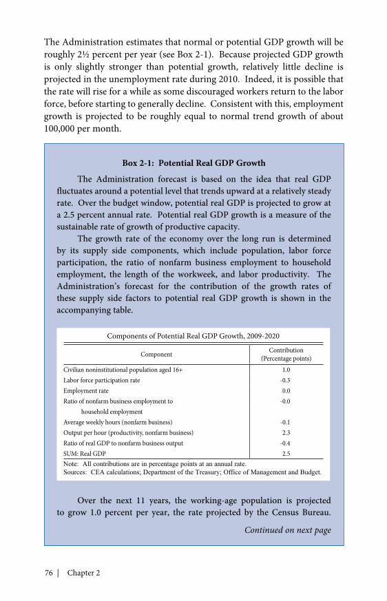
76 | Chapter 2
Box 2-1: Potential Real GDP Growth
The Administration forecast is based on the idea that real GDPfluctuates around a potential level that trends upward at a relatively steadyrate. Over the budget window, potential real GDP is projected to grow ata 2.5 percent annual rate. Potential real GDP growth is a measure of thesustainable rate of growth of productive capacity.
The growth rate of the economy over the long run is determinedby its supply side components, which include population, labor forceparticipation, the ratio of nonfarm business employment to householdemployment, the length of the workweek, and labor productivity. TheAdministration’s forecast for the contribution of the growth rates ofthese supply side factors to potential real GDP growth is shown in theaccompanying table.
Over the next 11 years, the working-age population is projectedto grow 1.0 percent per year, the rate projected by the Census Bureau.
The Administration estimates that normal or potential GDP growth will beroughly 2½ percent per year (see Box 2-1). Because projected GDP growthis only slightly stronger than potential growth, relatively little decline isprojected in the unemployment rate during 2010. Indeed, it is possible thatthe rate will rise for a while as some discouraged workers return to the laborforce, before starting to generally decline. Consistent with this, employmentgrowth is projected to be roughly equal to normal trend growth of about100,000 per month.
Continued on next page
Components of Potential Real GDP Growth, 2009-2020
Component Contribution(Percentage points)
Civilian noninstitutional population aged 16+ 1.0Labor force participation rate -0.3Employment rate 0.0Ratio of nonfarm business employment to -0.0
household employmentAverage weekly hours (nonfarm business) -0.1Output per hour (productivity, nonfarm business) 2.3Ratio of real GDP to nonfarm business output -0.4SUM: Real GDP 2.5Note: All contributions are in percentage points at an annual rate.Sources: CEA calculations; Department of the Treasury; Office of Management and Budget.
Rescuing the Economy from the Great Recession | 77
The normal or potential labor force participation rate, which fell at a0.3 percent annual rate during the past 8 years, is expected to continuedeclining at that pace. The continued projected decline results from theaging baby boom generation entering their retirement years. The potentialemployment rate (that is, 1 minus the normal or potential unemploy-ment rate) is not expected to contribute to potential GDP growth becauseno change is anticipated in the unemployment rate consistent withstable inflation. The potential ratio of nonfarm business employmentto household employment is also expected to be flat during the forecasthorizon—consistent with its average behavior in the long run. This wouldbe a change, however, from its puzzling 0.5 percent annual rate of declineduring the past business cycle. The potential workweek is projected toedge down slightly (0.1 percent per year). This is a slightly shallower paceof decline than over the past 50 years, when it declined 0.3 percent peryear. Over the 11-year projection interval, some firming of the workweekwould be a natural labor market accommodation to the anticipated declinein labor force participation.
Potential growth of labor productivity is projected at 2.3 percent peryear, a conservative forecast relative to its measured product-side growthrate (2.8 percent) between the past two business cycle peaks, but close toan alternative income-side measure of productivity growth (2.2 percent)during the same period. The ratio of real GDP to nonfarm business outputis expected to continue to subtract from overall growth as it has over mostlong periods, because the nonfarm business sector generally grows fasterthan other sectors, such as government, households, and nonprofit insti-tutions. Together, the sum of all of the components is the growth rate ofpotential real GDP, which is 2.5 percent per year.
As Table 2-3 shows, actual real GDP is projected to grow morerapidly than potential real GDP over most of the forecast horizon. Themost important reason for the difference is that the actual employ-ment rate is projected to rise as millions of workers who are currentlyunemployed return to employment and so contribute to GDP growth.
Traditionally, the large amount of slack would be expected to putsubstantial downward pressure on wage and price inflation. For this reason,inflation is projected to remain low in 2010. However, because inflationaryexpectations remain well anchored, inflation is not likely to slow dramati-cally or become negative (that is, turn into deflation).
Box 2-1, continued
78 | Chapter 2
In 2011, slightly higher GDP growth of approximately 4 percentis projected (again measured from fourth quarter to fourth quarter).Consistent with this, stronger employment growth and a more substantialdecline in the unemployment rate are expected in 2011. However, becauseGDP growth is still not projected to be as robust as that following someother deep recessions, continued large output gaps are anticipated. This willlimit the upward movement of the inflation rate toward a pace consistentwith the Federal Reserve’s long-term target inflation rate of about 2 percent.Moreover, employment growth is unlikely to be large enough to reduce theemployment shortfall dramatically in 2011.
Responsible Policies to Spur Job CreationThis large employment gap and the prospects that it is likely to recede
only slowly make a compelling case for additional measures to spur privatesector job creation. The Administration is therefore exploring a range ofpossibilities and working with Congress to pass measures into law.
Several principles are guiding this process. First, at a time whenthe budget deficit is large and the country faces significant long-run fiscalchallenges, measures must be cost-effective. Second, given that the employ-ment consequences of the recession have been severe, measures must focusparticularly on job creation. And third, measures must be tailored to thestate of the economy: the policies that are appropriate when an economy iscontracting rapidly may not be the same as those that are appropriate for aneconomy that is growing again but operating below capacity.
Guided by these principles, the Administration has identified three keypriorities. One is a multifaceted program to jump-start job creation by smallbusinesses, which are critical to growth and have been particularly harmedby the recession. Among the possible policies in this area are investmentincentives, tax incentives for hiring, and additional steps to increase the avail-ability of loans backed by the Small Business Administration. These policiesmay be particularly effective at a time when the economy is growing—so thatthe question for many firms is not whether to hire but when—and at a timewhen credit availability remains an important constraint.
Initiatives to encourage energy efficiency and clean energy are anotherpriority. One proposal involves incentives for homeowners to retrofittheir homes for energy efficiency. Because in many cases the effect of suchincentives would be to lead homeowners to make cost-saving investmentsearlier than they otherwise would have, they might have an especially largeimpact. In addition, the employment effects would be concentrated inconstruction, an area that has been particularly hard-hit by the recession.

Rescuing the Economy from the Great Recession | 79
The Administration has also supported extending tax credits through theDepartment of Energy that promote the manufacture of advanced energyproducts and providing incentives to increase the energy efficiency of publicand nonprofit buildings.
A third priority is infrastructure investment. The experience of theRecovery Act suggests that spending on infrastructure is an effective way toput people back to work while creating lasting investments that raise futureproductivity. For this reason, the Administration is supporting an addi-tional investment of up to $50 billion in roads, bridges, airports, transit, rail,and water projects. Funneling some of these funds through programs suchas the Transportation Investment Generating Economic Recovery (TIGER)program at the Department of Transportation, which is a competitive grantprogram, could offer a way to ensure that the projects with the highestreturns receive top priority.
Finally, it is critical to maintain our support for the individuals andfamilies most affected by the recession by extending the emergency fundingfor such programs as unemployment insurance and health insurance subsi-dies for the unemployed. This support not only cushions the worst effects ofthe downturn, but also boosts spending and so spurs job creation. Similarly,it is important to maintain support for state and local governments. Thebudgets of these governments remain under severe strain, and many arecutting back in anticipation of fiscal year 2011 deficits. Additional fiscalsupport could therefore have a rapid impact on spending, and would do soby maintaining crucial services and preventing harmful tax increases.
Conclusion
The recession that began at the end of 2007 became the “GreatRecession” following the financial crisis in the fall of 2008. In the wake ofthe collapse of Lehman Brothers in September, American families faceddevastating job losses, high unemployment, scarce credit, and lost wealth.Late 2008 and 2009 will be remembered as a time of great trial for Americanworkers, businesses, and families.
But 2009 should also be remembered as a year when even more tragiclosses and dislocation did not occur. As terrible as this recession has been,a second Great Depression would have been far worse. Had policymakersnot responded as aggressively as they did to shore up the financial system,maintain demand, and provide relief to those directly harmed by thedownturn, the outcome could have been much more dire.
As 2010 begins, there are strong signs that the American economy isstarting to recover. Housing and financial markets appear to have stabilized
80 | Chapter 2
and real GDP is growing again. The labor market also appears to be healing,showing the expected early pattern of response to output expansion.
With millions of Americans still unemployed, much work remains torestore the American economy to health. It will take a prolonged and robustGDP expansion to eliminate the large jobs deficit that has opened up overthe course of the recession. Only when the unemployment rate has returnedto normal levels and families are once again secure in their jobs, homes, andsavings will this terrible recession truly be over.
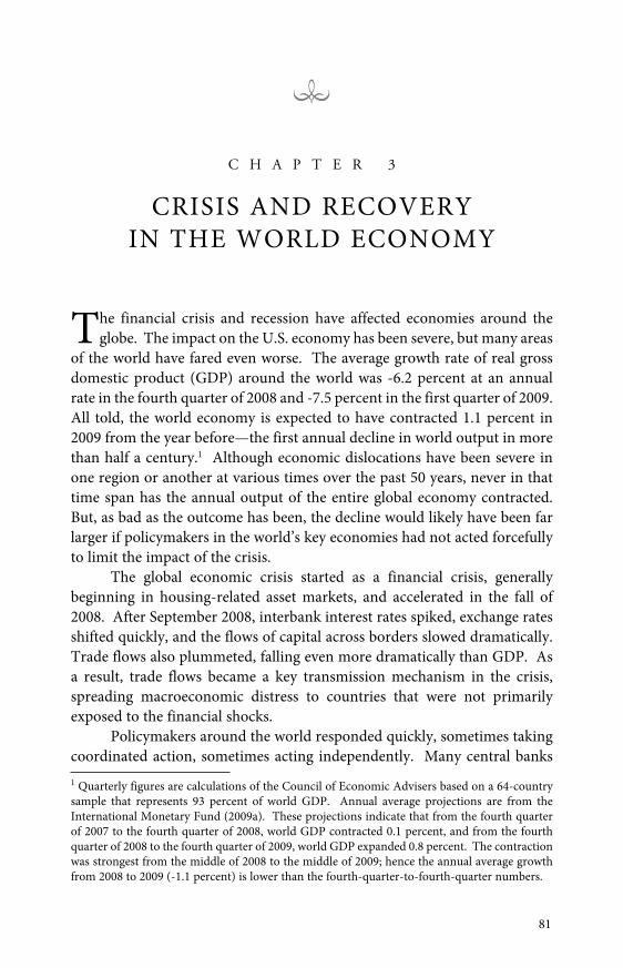
81
C H A P T E R 3
CRISIS AND RECOVERYIN THE WORLD ECONOMY
The financial crisis and recession have affected economies around theglobe. The impact on the U.S. economy has been severe, but many areas
of the world have fared even worse. The average growth rate of real grossdomestic product (GDP) around the world was -6.2 percent at an annualrate in the fourth quarter of 2008 and -7.5 percent in the first quarter of 2009.All told, the world economy is expected to have contracted 1.1 percent in2009 from the year before—the first annual decline in world output in morethan half a century.1 Although economic dislocations have been severe inone region or another at various times over the past 50 years, never in thattime span has the annual output of the entire global economy contracted.But, as bad as the outcome has been, the decline would likely have been farlarger if policymakers in the world’s key economies had not acted forcefullyto limit the impact of the crisis.
The global economic crisis started as a financial crisis, generallybeginning in housing-related asset markets, and accelerated in the fall of2008. After September 2008, interbank interest rates spiked, exchange ratesshifted quickly, and the flows of capital across borders slowed dramatically.Trade flows also plummeted, falling even more dramatically than GDP. Asa result, trade flows became a key transmission mechanism in the crisis,spreading macroeconomic distress to countries that were not primarilyexposed to the financial shocks.
Policymakers around the world responded quickly, sometimes takingcoordinated action, sometimes acting independently. Many central banks1 Quarterly figures are calculations of the Council of Economic Advisers based on a 64-countrysample that represents 93 percent of world GDP. Annual average projections are from theInternational Monetary Fund (2009a). These projections indicate that from the fourth quarterof 2007 to the fourth quarter of 2008, world GDP contracted 0.1 percent, and from the fourthquarter of 2008 to the fourth quarter of 2009, world GDP expanded 0.8 percent. The contractionwas strongest from the middle of 2008 to the middle of 2009; hence the annual average growthfrom 2008 to 2009 (-1.1 percent) is lower than the fourth-quarter-to-fourth-quarter numbers.

82 | Chapter 3
cut interest rates nearly to zero and expanded their balance sheets to try tostimulate lending and keep their economies going. They also lent large sumsto one another to prevent dislocations caused by a lack of foreign currencyin some markets. Beyond the central bank actions, governments intervenedmore broadly in banks and financial markets as well. Governments alsospent large sums in fiscal stimulus to avoid massive drop-offs in aggregatedemand. In a welcome development, they did not, however, restrict trade inan attempt to turn away imports.
The global economy is now seeing the beginnings of recovery.Financial markets have rebounded, trade is recovering, and GDP growthrates are again positive. Recovery is far from complete or certain, and somerisks remain: lending is still constrained, and unemployment is painfullyhigh. But, at the start of 2010, the world economy is no longer at the edge ofcollapse, and the elements of a sound recovery seem to be coming into place.
International Dimensions of the Crisis
The worldwide contraction had roots in many financial phenomena,and its rapid spread can be seen in a number of financial indicators.Borrowing costs increased, U.S. dollars were scarce in foreign markets,and exchange rates moved rapidly. Yet, despite problems in U.S. financialmarkets, there was no U.S. dollar crisis, and while currency markets movedrapidly, many of the emerging-market currency depreciations were tempo-rary and not accompanied by cascading defaults. Thus, the world economywas better positioned for recovery than it might have been.
Spread of the Financial ShockOne of the early indicators of the crisis was the large spike in the
interest rate banks charge one another that took place as the value of assetsheld on bank balance sheets came into question. After the investment bankLehman Brothers declared bankruptcy in September 2008, banks grew evenwarier about lending to each other. This fear of lending to one another canbe seen by comparing the interbank lending rate with the risk-free over-night interest rate. Similar to the TED spread, the Libor-OIS spread (theLondon interbank offered rate minus the overnight indexed swap) givessuch a comparison for dollar loans, and comparable spreads are availablefor loans in other currencies. As Figure 3-1 shows, the spike in spreads fordollar loans was larger earlier, but the increase in interbank lending rateswas sharp in dollars, pounds, and euros alike. Banks simply refused to lendto one another at low rates in these major financial systems. Furthermore,concerns about which firms might go bankrupt sent the cost of insuring
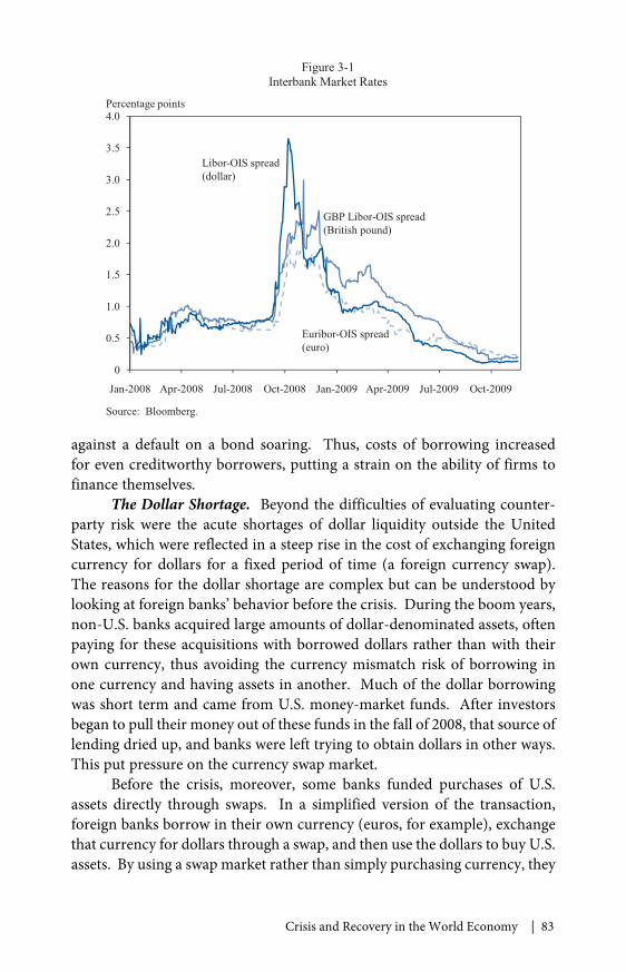
Crisis and Recovery in the World Economy | 83
against a default on a bond soaring. Thus, costs of borrowing increasedfor even creditworthy borrowers, putting a strain on the ability of firms tofinance themselves.
The Dollar Shortage. Beyond the difficulties of evaluating counter-party risk were the acute shortages of dollar liquidity outside the UnitedStates, which were reflected in a steep rise in the cost of exchanging foreigncurrency for dollars for a fixed period of time (a foreign currency swap).The reasons for the dollar shortage are complex but can be understood bylooking at foreign banks’ behavior before the crisis. During the boom years,non-U.S. banks acquired large amounts of dollar-denominated assets, oftenpaying for these acquisitions with borrowed dollars rather than with theirown currency, thus avoiding the currency mismatch risk of borrowing inone currency and having assets in another. Much of the dollar borrowingwas short term and came from U.S. money-market funds. After investorsbegan to pull their money out of these funds in the fall of 2008, that source oflending dried up, and banks were left trying to obtain dollars in other ways.This put pressure on the currency swap market.
Before the crisis, moreover, some banks funded purchases of U.S.assets directly through swaps. In a simplified version of the transaction,foreign banks borrow in their own currency (euros, for example), exchangethat currency for dollars through a swap, and then use the dollars to buy U.S.assets. By using a swap market rather than simply purchasing currency, they
0
0.5
1.0
1.5
2.0
2.5
3.0
3.5
4.0
Jan-2008 Apr-2008 Jul-2008 Oct-2008 Jan-2009 Apr-2009 Jul-2009 Oct-2009
Figure 3-1Interbank Market Rates
Percentage points
GBP Libor-OIS spread(British pound)
Euribor-OIS spread(euro)
Libor-OIS spread(dollar)
Source: Bloomberg.

84 | Chapter 3
even out the currency risk (McGuire and von Peter 2009),2 but they are leftwith a funding risk. If no one will lend them dollars when their swap is due,they may have to sell their dollar assets (some of which may have fallen invalue) to pay back the dollars they owe. When banks became very nervousabout taking on risk, demand greatly increased the price of currency swaps.
Unwinding Carry Trades. As concerns about the stability of thefinancial markets heightened over the course of 2008, investors respondedby trying to deleverage and reduce some of their exposed risky positions.The desire to undo risky positions coupled with the dollar shortage led toswift movements in currency markets, especially an unwinding of the “carrytrade.” In the carry trade, an investor borrows money in a low-interest-ratecurrency (for example, the Japanese yen), sells that currency for a higher-interest-rate currency (for example, the Australian dollar), and invests themoney in that currency. If interest rates are 1 percent in Japan and 6 percentin Australia, the investor stands to collect a 5 percent profit if exchange ratesdo not move. Although economic theory suggests that currency movementsshould offset this expected profit, over short horizons, if the exchange ratedoes not move, investors can make a profit. This happened in the mid-2000s, and the carry trade became a favorite strategy for hedge funds andother investors.
The popularity of the trade became self-fulfilling as the continuedflows of money into higher-interest-rate currencies helped them appreciateand made the trade even more profitable. But, as the crisis hit, investorstried to reduce their risk and leverage. This unwinding process meant rapidsales of high-interest-rate currencies and rapid purchases of low-interest-ratecurrencies. Currencies that had low interest rates and had been known asfunding currencies (such as the Japanese yen) rose rapidly in value, and thecurrencies of a number of popular carry-trade destinations (such as Australia,Brazil, and Iceland) depreciated swiftly. Thus, as the crisis hit, borrowingbecame more expensive and currency markets were increasingly volatile.
The Dollar During the Crisis. Although in many ways the crisis wastriggered within U.S. asset markets, the response was not a run on the U.S.dollar; instead the dollar strengthened notably. Some observers had arguedthat the high U.S. current account deficit and problems in the U.S. housingand other asset markets might lead to an unwillingness to hold U.S. assetsmore broadly, which could have triggered a depreciation of the dollar. Butboth the need for foreign banks to cover their dollar borrowing and theneed for other investors to repay loans borrowed in dollars (including forcarry trades) generated strong demand for dollars. Further, the desire to
2 The swap means they have borrowed dollars and lent euros. In this way, they borrowed eurosat home and lent them in the swap, and they owe dollars in the swap but also own dollar assets.Thus, their foreign currency position is balanced.
Crisis and Recovery in the World Economy | 85
avoid risky investments at the height of the crisis led to a “flight to safety,”with many investors buying dollars and U.S. Treasury bills. As seen inFigure 3-2, the trade-weighted value of the dollar increased 18 percentfrom July 2008 to its peak in March 2009. The movement of the dollar wasbroad-based, with sharp appreciations against most major trade partners;the main exceptions were Japan, where the yen appreciated even moreagainst the world as the carry trade unwound, and China, which had reestab-lished its peg to the dollar in July of 2008 and therefore had a stable exchangerate against the dollar.
Currency Volatility in Emerging Markets. The deleveraging andfall in risk appetite contributed to large and in some cases sharp swings inthe currencies of many emerging economies, but the impact of these largedepreciations varied. Some of the sharpest depreciations, such as those inBrazil, Korea, and Mexico, were largely temporary. The currencies of allthree countries depreciated more than 50 percent against the dollar betweenthe end of July 2008 and February 2009, but by the end of November 2009Korea’s currency was down only 15 percent and Brazil’s only 12 percent.Mexico was still 29 percent below its summer 2008 value.3
3 The starting point for comparison is important. Korea had been depreciating in early 2008 aswell, while Brazil and Mexico were appreciating. Thus, by the end of November 2009, Brazil hadappreciated slightly from the start of 2008 while Korea had depreciated 24 percent and Mexico18 percent.
90
95
100
105
110
115
Jan-2005 Jan-2006 Jan-2007 Jan-2008 Jan-2009 Jan-2010
Figure 3-2Nominal Trade-Weighted Dollar Index
Index (Jan. 1997=100), monthly averages
Note: The index is constructed such that an upward movement represents an appreciation ofthe dollar.Source: Federal Reserve Board, G.5.
86 | Chapter 3
Some countries with large current account deficits faced morepressure. The region with the sharpest declines in the value of its currenciesagainst the dollar was Eastern Europe, where the currencies of Hungary,Poland, and Ukraine all depreciated more than 50 percent between July2008 and February 2009, and others depreciated nearly as much. These largedepreciations resulted in part from the strengthening of the dollar againstthe euro, as many of these countries are closely tied with Europe, but someof these currencies remained weak even when other countries started tostrengthen against the dollar.
A large depreciation can especially lead to broad damage in aneconomy if there are negative balance-sheet effects. In this setting, acountry may have few foreign assets but extensive liabilities denominatedin foreign currency. As the exchange rate depreciates, the foreign currencyloans become more expensive in local currency. This was particularly aconcern in Eastern Europe, where many countries borrowed substantiallyin foreign currency leading up to the crisis. In Hungary, for example, manyindividuals took out mortgages in foreign currency. The depreciation of theHungarian forint thus put pressure on both individuals and bank balancesheets. There was widespread concern that the Western European banks,such as those in Austria, that had made loans in Eastern Europe would facesubstantial losses. Both the Organisation for Economic Co-operation andDevelopment (OECD) and the International Monetary Fund (IMF) warnedof potentially serious bank problems in Austria because of these concerns.By the end of 2009, however, those concerns had not materialized. Austriahas had to shore up its banks, but there has not been widespread contagionfrom Eastern Europe.
During the peak of the crisis, the spreads on emerging-market bondsspiked, but they returned toward more standard levels over time, andoutright financial collapse was avoided. There are a number of reasonsfor the more contained impact of the exchange-rate movements duringthe crisis. In the past decade, many developing countries have reduced thecurrency mismatch on their balance sheets by borrowing less, increasingtheir stocks of foreign exchange reserves, and shifting away from debtfinance (Lane and Shambaugh forthcoming). The improved fiscal positionsof some countries likely also helped, as did the strong policy response andcoordination described later. Some vulnerable countries also benefited fromthe strengthening of the IMF’s lending capabilities (discussed later). Thefailure of this shock to turn into a series of deep sustained financial collapsesacross the emerging world was a welcome development that left the worldeconomy better positioned for a quick turnaround.
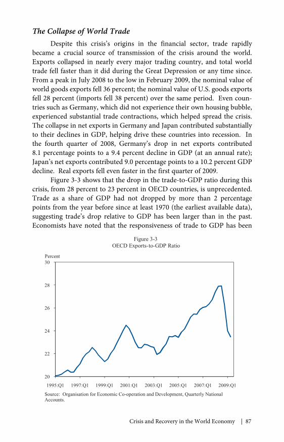
Crisis and Recovery in the World Economy | 87
The Collapse of World TradeDespite this crisis’s origins in the financial sector, trade rapidly
became a crucial source of transmission of the crisis around the world.Exports collapsed in nearly every major trading country, and total worldtrade fell faster than it did during the Great Depression or any time since.From a peak in July 2008 to the low in February 2009, the nominal value ofworld goods exports fell 36 percent; the nominal value of U.S. goods exportsfell 28 percent (imports fell 38 percent) over the same period. Even coun-tries such as Germany, which did not experience their own housing bubble,experienced substantial trade contractions, which helped spread the crisis.The collapse in net exports in Germany and Japan contributed substantiallyto their declines in GDP, helping drive these countries into recession. Inthe fourth quarter of 2008, Germany’s drop in net exports contributed8.1 percentage points to a 9.4 percent decline in GDP (at an annual rate);Japan’s net exports contributed 9.0 percentage points to a 10.2 percent GDPdecline. Real exports fell even faster in the first quarter of 2009.
Figure 3-3 shows that the drop in the trade-to-GDP ratio during thiscrisis, from 28 percent to 23 percent in OECD countries, is unprecedented.Trade as a share of GDP had not dropped by more than 2 percentagepoints from the year before since at least 1970 (the earliest available data),suggesting trade’s drop relative to GDP has been larger than in the past.Economists have noted that the responsiveness of trade to GDP has been
20
22
24
26
28
30
1995:Q1 1997:Q1 1999:Q1 2001:Q1 2003:Q1 2005:Q1 2007:Q1 2009:Q1
Figure 3-3OECD Exports-to-GDP Ratio
Percent
Source: Organisation for Economic Co-operation and Development, Quarterly NationalAccounts.
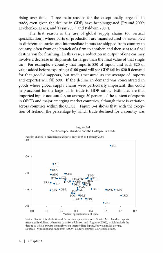
88 | Chapter 3
rising over time. Three main reasons for the exceptionally large fall intrade, even given the decline in GDP, have been suggested (Freund 2009;Levchenko, Lewis, and Tesar 2009; and Baldwin 2009).
The first reason is the use of global supply chains (or verticalspecialization), where parts of production are manufactured or assembledin different countries and intermediate inputs are shipped from country tocountry, often from one branch of a firm to another, and then sent to a finaldestination for finishing. In this case, a reduction in output of one car mayinvolve a decrease in shipments far larger than the final value of that singlecar. For example, a country that imports $80 of inputs and adds $20 ofvalue added before exporting a $100 good will see GDP fall by $20 if demandfor that good disappears, but trade (measured as the average of importsand exports) will fall $90. If the decline in demand was concentrated ingoods where global supply chains were particularly important, this couldhelp account for the large fall in trade-to-GDP ratios. Estimates are thatimported inputs account for, on average, 30 percent of the content of exportsin OECD and major emerging market countries, although there is variationacross countries within the OECD. Figure 3-4 shows that, with the excep-tion of Ireland, the percentage by which trade declined for a country was
ARG
AUS
AUT BEL
BRACAN
CHE
CHN
CZE
DEU DNK
ESP
FIN
FRA
GBR
GRC
HUN
IDN
IND
IRL
ITAJPN KOR
LUX
MEXNLD
NZL
POL PRT
SVK
SWE
TWN
USA
-50
-40
-30
-20
-10
0.0 0.1 0.2 0.3 0.4 0.5 0.6 0.7
Figure 3-4Vertical Specialization and the Collapse in Trade
Percent change in merchandise exports, July 2008 to February 2009
Vertical specialization of trade
Notes: See text for definition of the vertical specialization of trade. Merchandise exportsmeasured in dollars. Alternate data from Johnson and Noguera (2009), which include thedegree to which exports themselves are intermediate inputs, show a similar picture.Sources: Miroudot and Ragoussis (2009); country sources; CEA calculations.
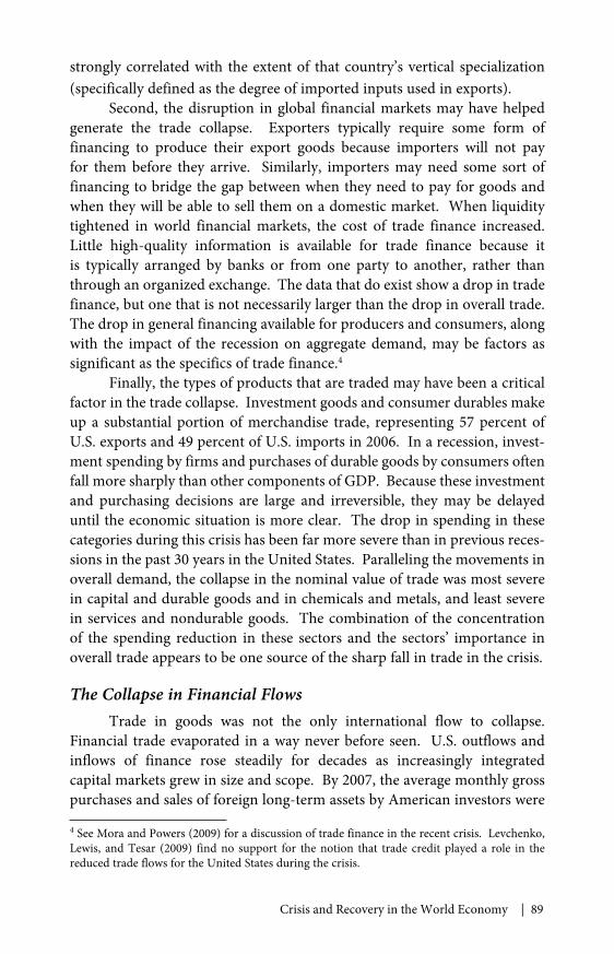
Crisis and Recovery in the World Economy | 89
strongly correlated with the extent of that country’s vertical specialization(specifically defined as the degree of imported inputs used in exports).
Second, the disruption in global financial markets may have helpedgenerate the trade collapse. Exporters typically require some form offinancing to produce their export goods because importers will not payfor them before they arrive. Similarly, importers may need some sort offinancing to bridge the gap between when they need to pay for goods andwhen they will be able to sell them on a domestic market. When liquiditytightened in world financial markets, the cost of trade finance increased.Little high-quality information is available for trade finance because itis typically arranged by banks or from one party to another, rather thanthrough an organized exchange. The data that do exist show a drop in tradefinance, but one that is not necessarily larger than the drop in overall trade.The drop in general financing available for producers and consumers, alongwith the impact of the recession on aggregate demand, may be factors assignificant as the specifics of trade finance.4
Finally, the types of products that are traded may have been a criticalfactor in the trade collapse. Investment goods and consumer durables makeup a substantial portion of merchandise trade, representing 57 percent ofU.S. exports and 49 percent of U.S. imports in 2006. In a recession, invest-ment spending by firms and purchases of durable goods by consumers oftenfall more sharply than other components of GDP. Because these investmentand purchasing decisions are large and irreversible, they may be delayeduntil the economic situation is more clear. The drop in spending in thesecategories during this crisis has been far more severe than in previous reces-sions in the past 30 years in the United States. Paralleling the movements inoverall demand, the collapse in the nominal value of trade was most severein capital and durable goods and in chemicals and metals, and least severein services and nondurable goods. The combination of the concentrationof the spending reduction in these sectors and the sectors’ importance inoverall trade appears to be one source of the sharp fall in trade in the crisis.
The Collapse in Financial FlowsTrade in goods was not the only international flow to collapse.
Financial trade evaporated in a way never before seen. U.S. outflows andinflows of finance rose steadily for decades as increasingly integratedcapital markets grew in size and scope. By 2007, the average monthly grosspurchases and sales of foreign long-term assets by American investors were
4 See Mora and Powers (2009) for a discussion of trade finance in the recent crisis. Levchenko,Lewis, and Tesar (2009) find no support for the notion that trade credit played a role in thereduced trade flows for the United States during the crisis.
90 | Chapter 3
$1.4 trillion, and foreigners’ purchases and sales of U.S. long-term assetswere $4.9 trillion. Each group both bought and sold a considerable amountof their holdings, so that net purchases by Americans were $19 billion amonth and net purchases by foreign investors were $84 billion a month.
When the crisis hit, there was a massive deglobalization of financethat was unprecedented and in many ways more extreme than the collapsein goods and services trade. Figure 3-5 shows that the scale of cross-borderflows was cut in half after years of fairly steady climbing. Net purchases byboth home and foreign investors actually became negative in the fall of 2008(that is, there were more sales than purchases). Americans pulled fundshome at such a fast pace that from July to November of 2008, Americans onnet sold foreign assets worth $143 billion. Foreign investors also liquidatedtheir positions, selling a net $92 billion in U.S. holdings. Hence, outflowsfrom foreign investors returning to their home markets were offset in partby inflows from Americans bringing money back to the United States, likelyreducing the impact of the outflows.
The Decline in Output Around the GlobeWhile the triggers of the crisis are generally considered financial in
nature, these shocks were rapidly transmitted to the real economy. Whathad been a financial market shock or a trade collapse became a full-fledgedrecession in countries around the world. The financial disruption was so
0
1
2
3
4
5
6
7
8
Jul-1989 Jul-1992 Jul-1995 Jul-1998 Jul-2001 Jul-2004 Jul-2007
Figure 3-5Cross-Border Gross Purchases and Sales of Long-Term Assets
Trillions of dollars, 3-month moving average
Source: Department of the Treasury (Treasury International Capital System).
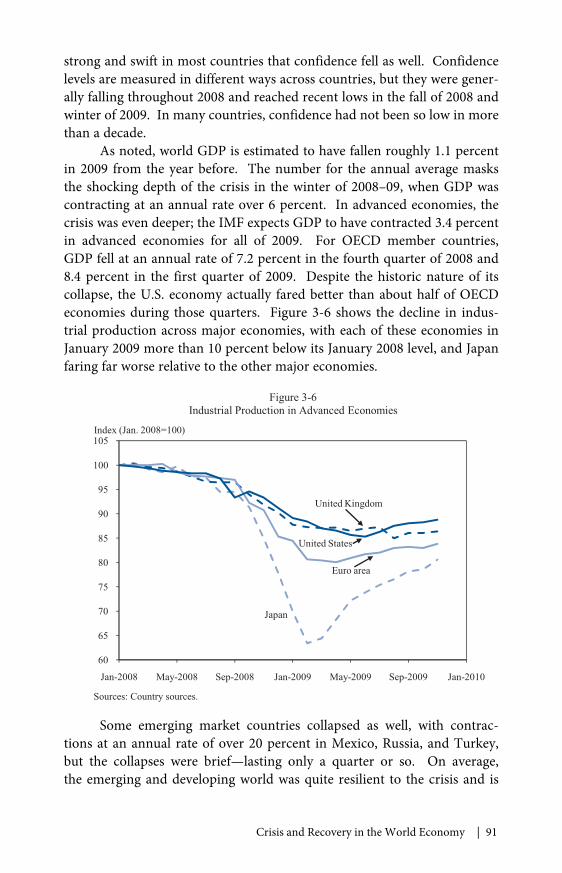
Crisis and Recovery in the World Economy | 91
strong and swift in most countries that confidence fell as well. Confidencelevels are measured in different ways across countries, but they were gener-ally falling throughout 2008 and reached recent lows in the fall of 2008 andwinter of 2009. In many countries, confidence had not been so low in morethan a decade.
As noted, world GDP is estimated to have fallen roughly 1.1 percentin 2009 from the year before. The number for the annual average masksthe shocking depth of the crisis in the winter of 2008–09, when GDP wascontracting at an annual rate over 6 percent. In advanced economies, thecrisis was even deeper; the IMF expects GDP to have contracted 3.4 percentin advanced economies for all of 2009. For OECD member countries,GDP fell at an annual rate of 7.2 percent in the fourth quarter of 2008 and8.4 percent in the first quarter of 2009. Despite the historic nature of itscollapse, the U.S. economy actually fared better than about half of OECDeconomies during those quarters. Figure 3-6 shows the decline in indus-trial production across major economies, with each of these economies inJanuary 2009 more than 10 percent below its January 2008 level, and Japanfaring far worse relative to the other major economies.
Some emerging market countries collapsed as well, with contrac-tions at an annual rate of over 20 percent in Mexico, Russia, and Turkey,but the collapses were brief—lasting only a quarter or so. On average,the emerging and developing world was quite resilient to the crisis and is
60
65
70
75
80
85
90
95
100
105
Jan-2008 May-2008 Sep-2008 Jan-2009 May-2009 Sep-2009 Jan-2010
Figure 3-6Industrial Production in Advanced Economies
Index (Jan. 2008=100)
Japan
Euro area
United Kingdom
United States
Sources: Country sources.
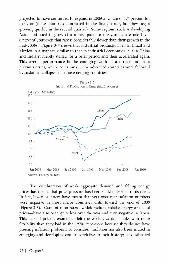
92 | Chapter 3
projected to have continued to expand in 2009 at a rate of 1.7 percent forthe year (these countries contracted in the first quarter, but they begangrowing quickly in the second quarter). Some regions, such as developingAsia, continued to grow at a robust pace for the year as a whole (over6 percent), but even that rate is considerably slower than their growth in themid-2000s. Figure 3-7 shows that industrial production fell in Brazil andMexico in a manner similar to that in industrial economies, but in Chinaand India it merely stalled for a brief period and then accelerated again.This overall performance in the emerging world is a turnaround fromprevious crises, where recessions in the advanced countries were followedby sustained collapses in some emerging countries.
The combination of weak aggregate demand and falling energyprices has meant that price pressure has been starkly absent in this crisis.In fact, lower oil prices have meant that year-over-year inflation numberswere negative in most major countries until toward the end of 2009(Figure 3-8). Core inflation rates—which exclude volatile energy and foodprices—have also been quite low over the year and even negative in Japan.This lack of price pressure has left the world’s central banks with moreflexibility than they had in the 1970s recessions because they do not havepressing inflation problems to consider. Inflation has also been muted inemerging and developing countries relative to their history; it is estimated
80
85
90
95
100
105
110
115
120
125
Jan-2008 May-2008 Sep-2008 Jan-2009 May-2009 Sep-2009 Jan-2010
Figure 3-7Industrial Production in Emerging Economies
Index (Jan. 2008=100)
China
India
Brazil
Mexico
Sources: Country sources.
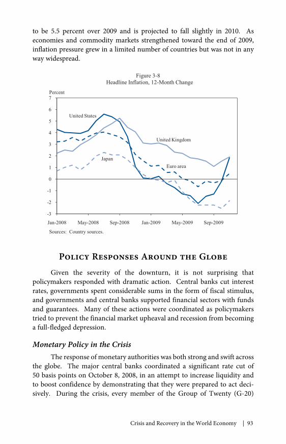
Crisis and Recovery in the World Economy | 93
to be 5.5 percent over 2009 and is projected to fall slightly in 2010. Aseconomies and commodity markets strengthened toward the end of 2009,inflation pressure grew in a limited number of countries but was not in anyway widespread.
Policy Responses Around the GlobeGiven the severity of the downturn, it is not surprising that
policymakers responded with dramatic action. Central banks cut interestrates, governments spent considerable sums in the form of fiscal stimulus,and governments and central banks supported financial sectors with fundsand guarantees. Many of these actions were coordinated as policymakerstried to prevent the financial market upheaval and recession from becominga full-fledged depression.
Monetary Policy in the CrisisThe response of monetary authorities was both strong and swift across
the globe. The major central banks coordinated a significant rate cut of50 basis points on October 8, 2008, in an attempt to increase liquidity andto boost confidence by demonstrating that they were prepared to act deci-sively. During the crisis, every member of the Group of Twenty (G-20)
-3
-2
-1
0
1
2
3
4
5
6
7
Jan-2008 May-2008 Sep-2008 Jan-2009 May-2009 Sep-2009
United Kingdom
Japan
Figure 3-8Headline Inflation, 12-Month Change
Percent
United States
Euro area
Sources: Country sources.
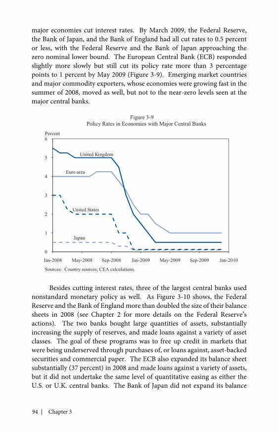
94 | Chapter 3
major economies cut interest rates. By March 2009, the Federal Reserve,the Bank of Japan, and the Bank of England had all cut rates to 0.5 percentor less, with the Federal Reserve and the Bank of Japan approaching thezero nominal lower bound. The European Central Bank (ECB) respondedslightly more slowly but still cut its policy rate more than 3 percentagepoints to 1 percent by May 2009 (Figure 3-9). Emerging market countriesand major commodity exporters, whose economies were growing fast in thesummer of 2008, moved as well, but not to the near-zero levels seen at themajor central banks.
Besides cutting interest rates, three of the largest central banks usednonstandard monetary policy as well. As Figure 3-10 shows, the FederalReserve and the Bank of England more than doubled the size of their balancesheets in 2008 (see Chapter 2 for more details on the Federal Reserve’sactions). The two banks bought large quantities of assets, substantiallyincreasing the supply of reserves, and made loans against a variety of assetclasses. The goal of these programs was to free up credit in markets thatwere being underserved through purchases of, or loans against, asset-backedsecurities and commercial paper. The ECB also expanded its balance sheetsubstantially (37 percent) in 2008 and made loans against a variety of assets,but it did not undertake the same level of quantitative easing as either theU.S. or U.K. central banks. The Bank of Japan did not expand its balance
0
1
2
3
4
5
6
Jan-2008 May-2008 Sep-2008 Jan-2009 May-2009 Sep-2009 Jan-2010
Figure 3-9Policy Rates in Economies with Major Central Banks
Percent
Euro area
United Kingdom
Japan
United States
Sources: Country sources; CEA calculations.
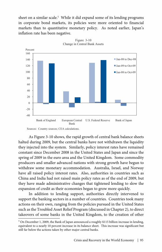
Crisis and Recovery in the World Economy | 95
sheet on a similar scale.5 While it did expand some of its lending programsin corporate bond markets, its policies were more oriented to financialmarkets than to quantitative monetary policy. As noted earlier, Japan’sinflation rate has been negative.
As Figure 3-10 shows, the rapid growth of central bank balance sheetshalted during 2009, but the central banks have not withdrawn the liquiditythey injected into the system. Similarly, policy interest rates have remainedconstant since December 2008 in the United States and Japan and since thespring of 2009 in the euro area and the United Kingdom. Some commodityproducers and smaller advanced nations with strong growth have begun towithdraw some monetary accommodation. Australia, Israel, and Norwayhave all raised policy interest rates. Also, authorities in countries such asChina and India had not raised main policy rates as of the end of 2009, butthey have made administrative changes that tightened lending to slow theexpansion of credit as their economies began to grow more quickly.
In addition to lending support, authorities directly intervened tosupport the banking sectors in a number of countries. Countries took manyactions on their own, ranging from the policies pursued in the United Statessuch as the Troubled Asset Relief Program (discussed in Chapter 2), to directtakeovers of some banks in the United Kingdom, to the creation of other5 On December 1, 2009, the Bank of Japan announced a roughly $115 billion increase in lending,equivalent to a nearly 10 percent increase in its balance sheet. This increase was significant butstill far below the actions taken by other major central banks.
-40
-20
0
20
40
60
80
100
120
140
160
Bank of England European CentralBank
U.S. Federal Reserve Bank of Japan
Jan-08 to Dec-08
Jan-09 to Oct-09
Jan-08 to Oct-09
Figure 3-10Change in Central Bank Assets
Percent
Sources: Country sources; CEA calculations.
96 | Chapter 3
entities to centralize some bad assets and clean the balance sheets of otherbanks in Switzerland and Ireland, to general support and guarantees in awide range of countries.
Central Bank Liquidity SwapsIn addition to the coordination of rate cuts, one other important form
of international coordination took place across central banks. As noted, adollar funding shortage materialized abroad, as the normal channels for thetransmission of dollar liquidity from U.S. markets to the global financialsystem broke down. This shortage presented a unique set of challengesto central banks. They could have simply provided domestic currencyand left banks to sell it for dollars, but the foreign exchange swaps marketin which such transactions are usually conducted was severely impaired.Alternatively, central banks could have used dollar reserves to provideforeign currency funds, but few advanced countries (outside of Japan) hadsufficient foreign currency holdings to fully address the foreign currencyfunding needs of their banking systems.
Central banks whose currencies were in demand responded to theshortage by providing large amounts of liquidity to partner central banksthrough central bank liquidity swaps.6 In many of these arrangements, theFederal Reserve purchased foreign currency in exchange for U.S. dollars andat the same time agreed to return the foreign currency for the same quantityof dollars at a specific date in the future. When foreign central banks drewdollars in this way to fund their auctions of dollar liquidity in local markets,the Federal Reserve received interest equal to what the foreign central bankswere receiving on the lending operations. The Federal Reserve first usedthese swaps in late 2007 on a relatively small scale. But, as shown in Figure3-11, from August 2008 through December 2008 these swaps increasedfrom $67 billion to $553 billion. This massive supply of liquidity was largerthan the available lending facilities of the IMF. The United States extendedthis program to major emerging market countries as well on October 29,2008, providing lines of up to $30 billion each to Brazil, Mexico, Singapore,and Korea.
As the acute funding needs have subsided, nearly all of the centralbank swaps have been unwound, and the Federal Reserve has announcedthat it anticipates that these swap arrangements will be closed by February1, 2010. There was no long-term funding cost to the Federal Reservefrom these swap lines; moreover, the Federal Reserve’s counterparties inthese transactions were the central banks of other countries, and the loans
6 See Fender and Gyntelberg (2008) for a more comprehensive discussion.
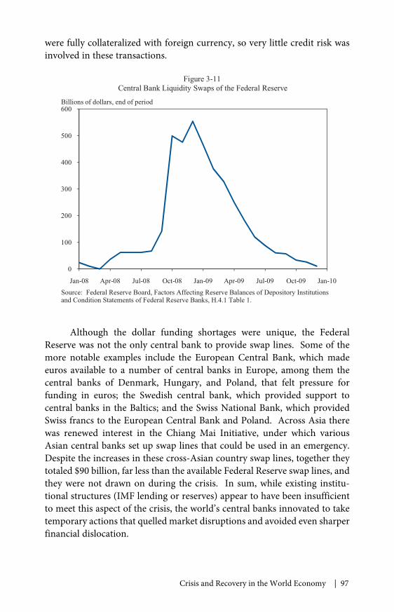
Crisis and Recovery in the World Economy | 97
were fully collateralized with foreign currency, so very little credit risk wasinvolved in these transactions.
Although the dollar funding shortages were unique, the FederalReserve was not the only central bank to provide swap lines. Some of themore notable examples include the European Central Bank, which madeeuros available to a number of central banks in Europe, among them thecentral banks of Denmark, Hungary, and Poland, that felt pressure forfunding in euros; the Swedish central bank, which provided support tocentral banks in the Baltics; and the Swiss National Bank, which providedSwiss francs to the European Central Bank and Poland. Across Asia therewas renewed interest in the Chiang Mai Initiative, under which variousAsian central banks set up swap lines that could be used in an emergency.Despite the increases in these cross-Asian country swap lines, together theytotaled $90 billion, far less than the available Federal Reserve swap lines, andthey were not drawn on during the crisis. In sum, while existing institu-tional structures (IMF lending or reserves) appear to have been insufficientto meet this aspect of the crisis, the world’s central banks innovated to taketemporary actions that quelled market disruptions and avoided even sharperfinancial dislocation.
0
100
200
300
400
500
600
Jan-08 Apr-08 Jul-08 Oct-08 Jan-09 Apr-09 Jul-09 Oct-09 Jan-10
Figure 3-11Central Bank Liquidity Swaps of the Federal Reserve
Billions of dollars, end of period
Source: Federal Reserve Board, Factors Affecting Reserve Balances of Depository Institutionsand Condition Statements of Federal Reserve Banks, H.4.1 Table 1.
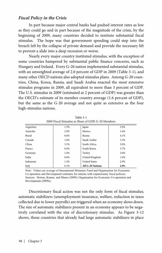
98 | Chapter 3
Fiscal Policy in the CrisisIn part because major central banks had pushed interest rates as low
as they could go and in part because of the magnitude of the crisis, by thebeginning of 2009, many countries decided to institute substantial fiscalstimulus. The hope was that government spending could step into thebreach left by the collapse of private demand and provide the necessary liftto prevent a slide into a deep recession or worse.
Nearly every major country instituted stimulus, with the exception ofsome countries hampered by substantial public finance concerns, such asHungary and Ireland. Every G-20 nation implemented substantial stimulus,with an unweighted average of 2.0 percent of GDP in 2009 (Table 3-1), andmany other OECD nations also adopted stimulus plans. Among G-20 coun-tries, China, Korea, Russia, and Saudi Arabia enacted the most extensivestimulus programs in 2009, all equivalent to more than 3 percent of GDP.The U.S. stimulus in 2009 (estimated at 2 percent of GDP) was greater thanthe OECD’s estimate of its member country average (1.6 percent of GDP),but the same as the G-20 average and not quite as extensive as the fourhigh-stimulus nations.
Discretionary fiscal action was not the only form of fiscal stimulus;automatic stabilizers (unemployment insurance, welfare, reduction in taxescollected due to lower payrolls) are triggered when an economy slows down.The size of automatic stabilizers present in an economy appears to be nega-tively correlated with the size of discretionary stimulus. As Figure 3-12shows, those countries that already had large automatic stabilizers in place
Table 3-12009 Fiscal Stimulus as Share of GDP, G-20 Members
Argentina 1.5% Japan 2.9%Australia 2.9% Mexico 1.6%Brazil 0.6% Russia 4.1%Canada 1.8% Saudi Arabia 3.3%China 3.1% South Africa 3.0%France 0.6% South Korea 3.7%Germany 1.6% Turkey 2.0%India 0.6% United Kingdom 1.6%Indonesia 1.4% United States 2.0%Italy 0.1% All G-20 Nations 2.0%Note: Values are average of International Monetary Fund and Organisation for EconomicCo-operation and Development estimates for nations with expansionary fiscal policies.Sources: Horton, Kumar, and Mauro (2009); Organisation for Economic Co-operation andDevelopment (2009a).
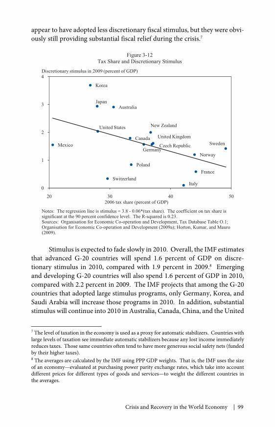
Crisis and Recovery in the World Economy | 99
appear to have adopted less discretionary fiscal stimulus, but they were obvi-ously still providing substantial fiscal relief during the crisis.7
Stimulus is expected to fade slowly in 2010. Overall, the IMF estimatesthat advanced G-20 countries will spend 1.6 percent of GDP on discre-tionary stimulus in 2010, compared with 1.9 percent in 2009.8 Emergingand developing G-20 countries will also spend 1.6 percent of GDP in 2010,compared with 2.2 percent in 2009. The IMF projects that among the G-20countries that adopted large stimulus programs, only Germany, Korea, andSaudi Arabia will increase those programs in 2010. In addition, substantialstimulus will continue into 2010 in Australia, Canada, China, and the United
7 The level of taxation in the economy is used as a proxy for automatic stabilizers. Countries withlarge levels of taxation see immediate automatic stabilizers because any lost income immediatelyreduces taxes. Those same countries often tend to have more generous social safety nets (fundedby their higher taxes).8 The averages are calculated by the IMF using PPP GDP weights. That is, the IMF uses the sizeof an economy—evaluated at purchasing power parity exchange rates, which take into accountdifferent prices for different types of goods and services—to weight the different countries inthe averages.
Australia
CanadaCzech Republic
France
Germany
Italy
Japan
Korea
Mexico
New Zealand
Norway
Poland
Sweden
Switzerland
United Kingdom
United States
0
1
2
3
4
20 30 40 50
Figure 3-12Tax Share and Discretionary Stimulus
Discretionary stimulus in 2009 (percent of GDP)
2006 tax share (percent of GDP)
Notes: The regression line is stimulus = 3.8 - 0.06*(tax share). The coefficient on tax share issignificant at the 90 percent confidence level. The R-squared is 0.23.Sources: Organisation for Economic Co-operation and Development, Tax Database Table O.1;Organisation for Economic Co-operation and Development (2009a); Horton, Kumar, and Mauro(2009).

100 | Chapter 3
States.9 Thus, substantial fiscal stimulus should continue to support therecovering world economy. The crucial question will be whether sufficientprivate demand has been rekindled by late 2010 to pick up the economicslack as stimulus unwinds.
Trade Policy in the CrisisAn extremely welcome development is the policy that was not called
on during the crisis: trade protectionism. Frequently viewed as an accel-erant of the Great Depression, protectionism has been largely absent duringthe current crisis. In the Great Depression, trade protectionism came intoplay after the crisis had started and was not a cause of the Depression itself(Eichengreen and Irwin 2009). But the extensive barriers that built up in thefirst few years of the Depression meant that as production rebounded, tradelevels could not do so. In the current crisis, rather than respond to decliningexports with increasing tariffs, countries left markets open, allowing for thepossibility of a rebound in world trade. No major country has instituteddramatic trade restrictions. Furthermore, while antidumping and coun-tervailing duty investigations have increased, the value of imports facingpossible new import restrictions by G-20 countries stemming from newtrade remedy investigations begun between 2008:Q1 and 2009:Q1 representsless than 0.5 percent of those countries’ imports (Bown forthcoming).
The Role of International Institutions
Rather than resort to beggar-thy-neighbor policies, this crisis has beencharacterized by international policy coordination. National policies didnot take place in a vacuum; to the contrary, nations used a number of inter-national institutions to coordinate and communicate their rescue efforts.
The G-20The G-20, which includes 19 nations plus the European Union, was
the locus of much of the coordination on trade policy, financial policy, andcrisis response. Its membership is composed of most of the world’s largesteconomies—both advanced and emerging—and makes up nearly 90 percentof world gross national product.
The first G-20 leaders’ summit was held at the peak of the crisis inNovember 2008. At that point, G-20 countries committed to keep theirmarkets open, adopt policies to support the global economy, and stabilizethe financial sector. Leaders also began discussing financial reforms thatwould help prevent a repeat of the crisis.9 Japan has announced additional stimulus since these estimates and will also be providingextensive stimulus in 2010.

Crisis and Recovery in the World Economy | 101
The second G-20 leaders’ summit took place in April 2009 at theheight of concern about rapid falls in GDP and trade. Leaders of the world’slargest economies pledged to “do everything necessary to ensure recovery,to repair our financial systems and to maintain the global flow of capital.”Furthermore, they committed to work together on tax and financial poli-cies. Perhaps the most notable act of world coordination was the decision toprovide substantial new funding to the IMF. U.S. leadership helped secure acommitment by the G-20 leaders to provide over $800 billion to fund multi-lateral banks broadly, with over $500 billion of those funds allocated to theIMF in particular.
In September 2009, the G-20 leaders met in Pittsburgh. They notedthat international cooperation and national action had been critical inarresting the crisis and putting the world’s economies on the path towardrecovery. They also recognized that continued action was necessary, pledgedto “sustain our strong policy response until a durable recovery is secured,”and committed to avoid premature withdrawal of stimulus. The leaders alsofocused on the policies, regulations, and reforms that would be needed toensure a strong recovery while avoiding the practices and vulnerabilities thatgave rise to boom-bust cycles and the current crisis. They launched a newFramework for Strong, Sustainable, and Balanced Growth that committedthe G-20 countries to work together to assess how their policies fit togetherand evaluate whether they were “collectively consistent with more sustain-able and balanced growth.” Further, the leaders committed to act togetherto improve the global financial system through financial regulatory reformsand actions to increase capital in the system.
Given the central role the G-20 had played in the response to thecrisis, it is not surprising that the leaders agreed in Pittsburgh to make theG-20 the premier forum for their economic coordination. This shift reflectsthe growing importance of key emerging economies such as India andChina—a shift that was reinforced by the agreement in Pittsburgh to realignquota shares and voting weights in the IMF and World Bank to better reflectshifts in the global economy.
The International Monetary FundThe IMF’s role has changed considerably over time, from being
the shepherd of the world’s Bretton Woods fixed exchange rate system tobecoming a crisis manager. In a systemic bank run, a central bank some-times steps in as the lender of last resort. The IMF is not a central bank andcan neither print money nor regulate countries’ behavior in advance of acrisis, but it has played a coordinating and funding role in many crises. Asthe scale of the current crisis became apparent, it was clear that the IMF’s
102 | Chapter 3
funds were insufficient to backstop a large systemic crisis, particularly inadvanced nations. While it is still unlikely to be able to arrest a run onmajor advanced country financial systems, the increase in resources stem-ming from the G-20 summit has roughly tripled the resources available tothe IMF and left it better suited to quell runs in individual countries.
As the IMF’s resources were expanded, the institution took a numberof concrete interventions. It set up emergency lines of credit (called FlexibleCredit Lines) with Colombia, Mexico, and Poland, which in total are worthover $80 billion. These lines were intended to provide immediate liquidityin the event of a run by investors, but also to signal to the markets thatfunds were available, making a run less likely. Now, rather than have togo to the IMF for funds during a crisis, these countries are “pre-approved”for loans. In each of these countries, markets responded positively to theannouncement of the credit lines, with the cost of insuring the countries’bonds narrowing (International Monetary Fund 2009b). The IMF alsonegotiated a set of standby agreements with 15 countries, committing atotal of $75 billion to help them survive the economic crisis by smoothingcurrent account adjustments and mitigating liquidity pressures. IMFanalysis suggests that this program discouraged large exchange-rate swingsin these countries (International Monetary Fund 2009b). These actions aswell as the very existence of a better-funded global lender may have helpedto keep the contraction short and to prevent sustained currency crises inmany emerging nations.
The Beginning of Recovery Around the Globe
In contrast to the Great Depression, where poor policy actions—monetary, fiscal, regulatory, and protectionist—helped turn a sharp globaldownturn into the worst worldwide collapse the modern economy hasknown, the recent massive policy response helped stop the spiraling ofthis Great Recession. Already financial markets have stabilized, GDP hasbegun to grow, and trade has begun to rebound. The crisis is far from over,however; most notably, employment in many countries is still distressinglyweak. But the world economy appears to have avoided the outright collapsethat was feared at one point and is now moving toward recovery.
The second quarter of 2009 saw the first hints of recovery in manycountries. World average growth was 2.4 percent, and even OECD coun-tries registered a positive 0.2 percent growth rate.10 The rebound caughtmany by surprise. The IMF and the OECD had revised projections steadily10 World weighted average quarterly real GDP growth rates at a seasonally adjusted annualrate are from CEA calculations. The OECD growth rate is from the OECD quarterly nationalaccounts database.
Crisis and Recovery in the World Economy | 103
downward through the winter and spring, but by the middle of 2009 manyeconomies had returned to growth. The one-quarter improvement in annu-alized growth of 5.7 percentage points (from -6.4 percent to -0.7 percentfrom the first to the second quarter of 2009) in the United States was oneof the largest improvements in decades, but other countries that had deepercontractions rebounded even more. Annualized growth rates improvedmore than 14 percentage points in Germany and Japan, while growth ratesrose more than 30 percentage points in Malaysia, Singapore, Taiwan, andTurkey. Other emerging markets, such as China, India, and Indonesia,which did not contract but faced lower growth during the crisis, reboundedto growth rates on par with their performance during the 2000s (if not therapid booms of 2006–07).
Trade had collapsed quickly, and it has begun to rebound quickly aswell. Beginning in March, when GDP was still falling rapidly, exports beganto turn. From lows in February 2009, nominal world goods exports in dollarterms had grown 20 percent by October. U.S. nominal goods exports pickedup later but had grown 17 percent from their April lows by October. AsGDP began to rise, trade volume began to grow faster. Annualized growthfor world real exports was 2.4 percent in the second quarter of 2009 and16.8 percent in the third quarter. By comparison, world weighted averageannualized real GDP growth in the second and third quarters of 2009 was2.4 percent and 3.4 percent, respectively.
Financial markets are rebounding as well. Net cross-border financialflows are near their pre-crisis levels, and gross flows are increasing (althoughas of October 2009 they were still less than 80 percent of their average levelin 2008). Libor-OIS spreads have fallen to more typical levels, and equiva-lent measures in other markets have subsided as well. Stock market indexesin the United States, Japan, the United Kingdom, and the European Unionhave all risen substantially. By October 2009, all were above their levels inOctober 2008, making up dramatic losses in early 2009. House prices havestabilized in most markets. Furthermore, the cost of insuring emerging-market bonds, which had spiked in the fall of 2008, is now back roughly toits pre-crisis level. The value of the dollar, which rose dramatically duringthe crisis, has retreated toward its value before the crisis (see Figure 3-2).From the end of March 2009 through December, the dollar depreciated10 percent against a basket of currencies. The trade-weighted value isroughly at the same level as in the fall of 2007 and above its lows in 2008.
Potential financial problems still exist. Banks around the world maynot have recognized all the losses on their balance sheets. The shock wavesfrom the threatened default by Dubai World in November 2009 showedthat there are still concerns in the market about potential bad debts on
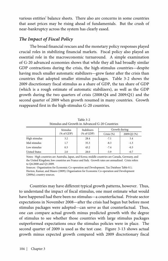
104 | Chapter 3
various entities’ balance sheets. There also are concerns in some countriesthat asset prices may be rising ahead of fundamentals. But the crush ofnear-bankruptcy across the system has clearly eased.
The Impact of Fiscal PolicyThe broad financial rescues and the monetary policy responses played
crucial roles in stabilizing financial markets. Fiscal policy also played anessential role in the macroeconomic turnaround. A simple examinationof G-20 advanced economies shows that while they all had broadly similarGDP contractions during the crisis, the high-stimulus countries—despitehaving much smaller automatic stabilizers—grew faster after the crisis thancountries that adopted smaller stimulus packages. Table 3-2 shows the2009 discretionary fiscal stimulus as a share of GDP, the tax share of GDP(which is a rough estimate of automatic stabilizers), as well as the GDPgrowth during the two quarters of crisis (2008:Q4 and 2009:Q1) and thesecond quarter of 2009 when growth resumed in many countries. Growthreappeared first in the high-stimulus G-20 countries.
Countries may have different typical growth patterns, however. Thus,to understand the impact of fiscal stimulus, one must estimate what wouldhave happened had there been no stimulus—a counterfactual. Private sectorexpectations in November 2008—after the crisis had begun but before moststimulus packages were adopted—can serve as that counterfactual. Thus,one can compare actual growth minus predicted growth with the degreeof stimulus to see whether those countries with large stimulus packagesoutperformed expectations once the stimulus policies were in place. Thesecond quarter of 2009 is used as the test case. Figure 3-13 shows actualgrowth minus expected growth compared with 2009 discretionary fiscal
Table 3-2Stimulus and Growth in Advanced G-20 Countries
Stimulus(% of GDP)
Stabilizers(% of GDP)
Growth during:Crisis (%) 2009:Q2 (%)
High stimulus 3.2 28.4 -7.1 5.4Mid stimulus 1.7 35.3 -8.3 -1.3Low stimulus 0.3 43.2 -7.4 -0.3United States 2.0 28.0 -5.9 -0.7Notes: High countries are Australia, Japan, and Korea; middle countries are Canada, Germany, andthe United Kingdom; low countries are France and Italy. Growth rates are annualized. Crisis refersto Q4:2008 and Q1:2009.Sources: Organisation for Economic Co-operation and Development, Tax Database Table 0.1;Horton, Kumar, and Mauro (2009); Organisation for Economic Co-operation and Development(2009a); country sources.
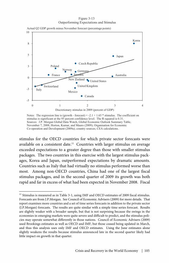
Crisis and Recovery in the World Economy | 105
stimulus for the OECD countries for which private sector forecasts wereavailable on a consistent date.11 Countries with larger stimulus on averageexceeded expectations to a greater degree than those with smaller stimuluspackages. The two countries in this exercise with the largest stimulus pack-ages, Korea and Japan, outperformed expectations by dramatic amounts.Countries such as Italy that had virtually no stimulus performed worse thanmost. Among non-OECD countries, China had one of the largest fiscalstimulus packages, and in the second quarter of 2009 its growth was bothrapid and far in excess of what had been expected in November 2008. Fiscal
11 Stimulus is measured as in Table 3-1, using IMF and OECD estimates of 2009 fiscal stimulus.Forecasts are from J.P.Morgan. See Council of Economic Advisers (2009) for more details. Thatreport examines more countries and a set of time series forecasts in addition to the private sector(J.P.Morgan) forecasts. The results are quite similar with a simple time series forecast. Resultsare slightly weaker with a broader sample, but that is not surprising because the swings in theeconomies in emerging markets were quite severe and difficult to predict, and the stimulus poli-cies may operate somewhat differently in those nations. Council of Economic Advisers (2009)used Brookings estimates as well as OECD and IMF, but those ceased being updated in March,and thus this analysis uses only IMF and OECD estimates. Using the June estimates aloneslightly weakens the results because stimulus announced late in the second quarter likely hadlittle impact on growth in that quarter.
Australia
Canada
Czech Republic
FranceGermany
Italy
Japan
Korea
Mexico
New Zealand
NorwayPoland
Sweden
Switzerland United KingdomUnited States
-5
-3
0
3
5
8
10
0 1 2 3 4
Figure 3-13Outperforming Expectations and Stimulus
Actual Q2 GDP growth minus November forecast (percentage points)
Discretionary stimulus in 2009 (percent of GDP)
Notes: The regression line is (growth - forecast) = -2.1 + 1.65 * stimulus. The coefficient onstimulus is significant at the 95 percent confidence level. The R-squared is 0.31.Sources: J.P. Morgan Global Data Watch, Global Economic Outlook Summary Table,November 7, 2008; Horton, Kumar, and Mauro (2009); Organisation for EconomicCo-operation and Development (2009a); country sources; CEA calculations.

106 | Chapter 3
stimulus seems to have been important in restarting world economic growthin the second quarter of 2009.
After the second quarter of 2009, the relationship between stimulusand growth weakens somewhat. High-stimulus countries still exceedexpectations relative to low-stimulus countries, but the relationship is notstatistically significant. It may be that quarterly growth projections madenearly a year in advance are not precise enough a measure of a third-quartergrowth counterfactual.
The World Economy in the Near TermWhile the return to GDP and export growth is encouraging, exports
are still far below their level in the summer of 2008, and GDP is now farbelow its prior trend level. The IMF currently forecasts annual world growthof 3.1 percent in 2010; the OECD projects 3.4 percent.12 For advanced coun-tries, the forecasts are even more restrained: the IMF projects 1.3 percent,the OECD 1.9 percent for OECD countries. The IMF forecasts world tradeto grow 2.5 percent in 2010; the OECD, 6.0 percent. These forecasts maybe conservative. The IMF forecast would leave trade at a much lower shareof GDP than before the crisis, and even if trade growth met the OECD’smore aggressive forecast, trade would not reach its previous level as a shareof GDP for some time. Given that trade declined faster than GDP in thecrisis, it is possible it will continue to bounce back faster as well, surpassingthese estimates.
How Fast Will Countries Grow? There is an open question abouthow fast countries will grow following the crisis. After typical recessions, themagnitude of a recovery often matches the depth of the drop. In this way,GDP returns not only to its previous growth rate, but to its previous trendpath as well. If, however, the world’s advanced economies emerge from thecrisis only slowly and simply return to stable growth rates, output will beon a permanently lower path. A financial crisis could lower the future levelof output by generating lower levels of labor, capital, or the productivity ofthose factors. If the economy returns to full employment, and productivitygrowth remains on trend, though, capital should eventually return to itspre-crisis path because the incentives to invest will be high. Thus, as longas the economy eventually returns to full employment, the long-run impactof the crisis chiefly rests on productivity growth in the years ahead. Chapter10 discusses the prospects and importance of productivity in more detail.
Some research suggests financial crises may result in a slow growthpattern (International Monetary Fund 2009a), with substantial average12 IMF estimates are from International Monetary Fund (2009a). OECD estimates are fromOrganisation for Economic Co-operation and Development (2009b).
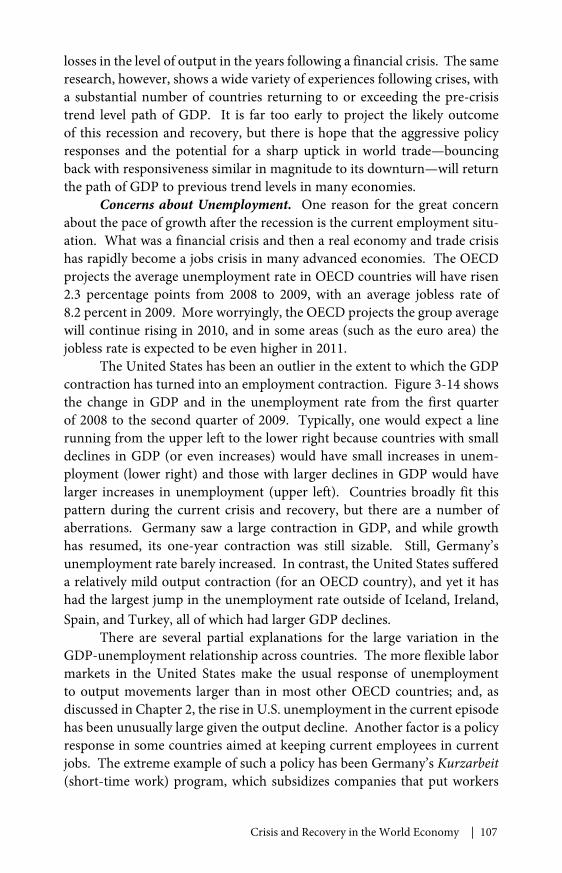
Crisis and Recovery in the World Economy | 107
losses in the level of output in the years following a financial crisis. The sameresearch, however, shows a wide variety of experiences following crises, witha substantial number of countries returning to or exceeding the pre-crisistrend level path of GDP. It is far too early to project the likely outcomeof this recession and recovery, but there is hope that the aggressive policyresponses and the potential for a sharp uptick in world trade—bouncingback with responsiveness similar in magnitude to its downturn—will returnthe path of GDP to previous trend levels in many economies.
Concerns about Unemployment. One reason for the great concernabout the pace of growth after the recession is the current employment situ-ation. What was a financial crisis and then a real economy and trade crisishas rapidly become a jobs crisis in many advanced economies. The OECDprojects the average unemployment rate in OECD countries will have risen2.3 percentage points from 2008 to 2009, with an average jobless rate of8.2 percent in 2009. More worryingly, the OECD projects the group averagewill continue rising in 2010, and in some areas (such as the euro area) thejobless rate is expected to be even higher in 2011.
The United States has been an outlier in the extent to which the GDPcontraction has turned into an employment contraction. Figure 3-14 showsthe change in GDP and in the unemployment rate from the first quarterof 2008 to the second quarter of 2009. Typically, one would expect a linerunning from the upper left to the lower right because countries with smalldeclines in GDP (or even increases) would have small increases in unem-ployment (lower right) and those with larger declines in GDP would havelarger increases in unemployment (upper left). Countries broadly fit thispattern during the current crisis and recovery, but there are a number ofaberrations. Germany saw a large contraction in GDP, and while growthhas resumed, its one-year contraction was still sizable. Still, Germany’sunemployment rate barely increased. In contrast, the United States suffereda relatively mild output contraction (for an OECD country), and yet it hashad the largest jump in the unemployment rate outside of Iceland, Ireland,Spain, and Turkey, all of which had larger GDP declines.
There are several partial explanations for the large variation in theGDP-unemployment relationship across countries. The more flexible labormarkets in the United States make the usual response of unemploymentto output movements larger than in most other OECD countries; and, asdiscussed in Chapter 2, the rise in U.S. unemployment in the current episodehas been unusually large given the output decline. Another factor is a policyresponse in some countries aimed at keeping current employees in currentjobs. The extreme example of such a policy has been Germany’s Kurzarbeit(short-time work) program, which subsidizes companies that put workers
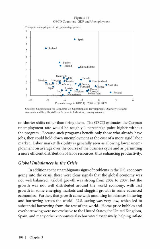
108 | Chapter 3
on shorter shifts rather than firing them. The OECD estimates the Germanunemployment rate would be roughly 1 percentage point higher withoutthe program. Because such programs benefit only those who already havejobs, they could hold down unemployment at the cost of a more rigid labormarket. Labor market flexibility is generally seen as allowing lower unem-ployment on average over the course of the business cycle and as permittinga more efficient distribution of labor resources, thus enhancing productivity.
Global Imbalances in the CrisisIn addition to the unambiguous signs of problems in the U.S. economy
going into the crisis, there were clear signals that the global economy wasnot well balanced. Global growth was strong from 2002 to 2007, but thegrowth was not well distributed around the world economy, with fastgrowth in some emerging markets and sluggish growth in some advancedeconomies. Further, that growth came with mounting imbalances in savingand borrowing across the world. U.S. saving was very low, which led tosubstantial borrowing from the rest of the world. Home price bubbles andoverborrowing were not exclusive to the United States; the United Kingdom,Spain, and many other economies also borrowed extensively, helping inflate
AustraliaAustria
Belgium
CanadaDenmark
Finland France
Germany
Greece
Hungary
Ireland
ItalyJapan Korea
Luxembourg
Netherlands
New Zealand
Norway Poland
Portugal
Spain
Sweden
Switzerland
UK
United StatesIceland
Mexico
Turkey
0
1
2
3
4
5
6
7
8
9
10
-12 -9 -6 -3 0 3 6
Figure 3-14OECD Countries: GDP and Unemployment
Change in unemployment rate, percentage points
Percent change in GDP, Q1:2008 to Q2:2009
Sources: Organisation for Economic Co-Operation and Development, Quarterly NationalAccounts and Key Short-Term Economic Indicators; country sources.
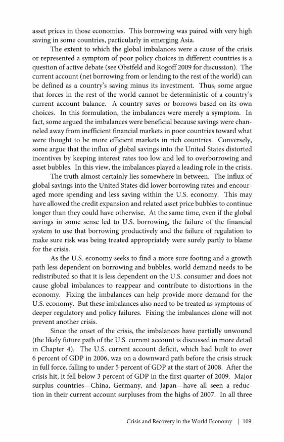
Crisis and Recovery in the World Economy | 109
asset prices in those economies. This borrowing was paired with very highsaving in some countries, particularly in emerging Asia.
The extent to which the global imbalances were a cause of the crisisor represented a symptom of poor policy choices in different countries is aquestion of active debate (see Obstfeld and Rogoff 2009 for discussion). Thecurrent account (net borrowing from or lending to the rest of the world) canbe defined as a country’s saving minus its investment. Thus, some arguethat forces in the rest of the world cannot be deterministic of a country’scurrent account balance. A country saves or borrows based on its ownchoices. In this formulation, the imbalances were merely a symptom. Infact, some argued the imbalances were beneficial because savings were chan-neled away from inefficient financial markets in poor countries toward whatwere thought to be more efficient markets in rich countries. Conversely,some argue that the influx of global savings into the United States distortedincentives by keeping interest rates too low and led to overborrowing andasset bubbles. In this view, the imbalances played a leading role in the crisis.
The truth almost certainly lies somewhere in between. The influx ofglobal savings into the United States did lower borrowing rates and encour-aged more spending and less saving within the U.S. economy. This mayhave allowed the credit expansion and related asset price bubbles to continuelonger than they could have otherwise. At the same time, even if the globalsavings in some sense led to U.S. borrowing, the failure of the financialsystem to use that borrowing productively and the failure of regulation tomake sure risk was being treated appropriately were surely partly to blamefor the crisis.
As the U.S. economy seeks to find a more sure footing and a growthpath less dependent on borrowing and bubbles, world demand needs to beredistributed so that it is less dependent on the U.S. consumer and does notcause global imbalances to reappear and contribute to distortions in theeconomy. Fixing the imbalances can help provide more demand for theU.S. economy. But these imbalances also need to be treated as symptoms ofdeeper regulatory and policy failures. Fixing the imbalances alone will notprevent another crisis.
Since the onset of the crisis, the imbalances have partially unwound(the likely future path of the U.S. current account is discussed in more detailin Chapter 4). The U.S. current account deficit, which had built to over6 percent of GDP in 2006, was on a downward path before the crisis struckin full force, falling to under 5 percent of GDP at the start of 2008. After thecrisis hit, it fell below 3 percent of GDP in the first quarter of 2009. Majorsurplus countries—China, Germany, and Japan—have all seen a reduc-tion in their current account surpluses from the highs of 2007. In all three
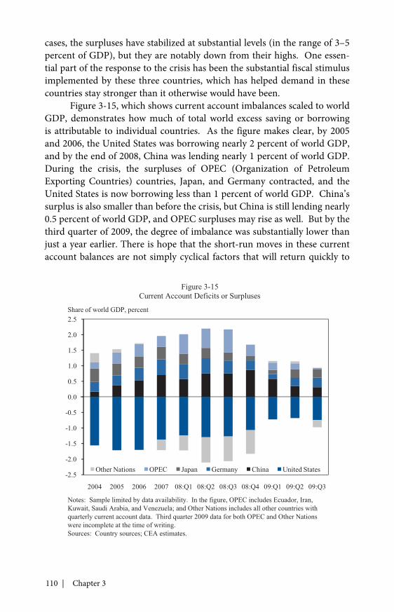
110 | Chapter 3
cases, the surpluses have stabilized at substantial levels (in the range of 3–5percent of GDP), but they are notably down from their highs. One essen-tial part of the response to the crisis has been the substantial fiscal stimulusimplemented by these three countries, which has helped demand in thesecountries stay stronger than it otherwise would have been.
Figure 3-15, which shows current account imbalances scaled to worldGDP, demonstrates how much of total world excess saving or borrowingis attributable to individual countries. As the figure makes clear, by 2005and 2006, the United States was borrowing nearly 2 percent of world GDP,and by the end of 2008, China was lending nearly 1 percent of world GDP.During the crisis, the surpluses of OPEC (Organization of PetroleumExporting Countries) countries, Japan, and Germany contracted, and theUnited States is now borrowing less than 1 percent of world GDP. China’ssurplus is also smaller than before the crisis, but China is still lending nearly0.5 percent of world GDP, and OPEC surpluses may rise as well. But by thethird quarter of 2009, the degree of imbalance was substantially lower thanjust a year earlier. There is hope that the short-run moves in these currentaccount balances are not simply cyclical factors that will return quickly to
-2.5
-2.0
-1.5
-1.0
-0.5
0.0
0.5
1.0
1.5
2.0
2.5
2004 2005 2006 2007 08:Q1 08:Q2 08:Q3 08:Q4 09:Q1 09:Q2 09:Q3
Other Nations OPEC Japan Germany China United States
Figure 3-15Current Account Deficits or Surpluses
Share of world GDP, percent
Notes: Sample limited by data availability. In the figure, OPEC includes Ecuador, Iran,Kuwait, Saudi Arabia, and Venezuela; and Other Nations includes all other countries withquarterly current account data. Third quarter 2009 data for both OPEC and Other Nationswere incomplete at the time of writing.Sources: Country sources; CEA estimates.
Crisis and Recovery in the World Economy | 111
former levels but rather that they represent a more sustained rebalancing ofworld demand.
Net export growth is often a key source of growth propelling a countryout of a financial crisis. But in a global crisis, not every country can increaseexports and decrease imports simultaneously. Someone must buy theproducts that are being sold, and the world’s current accounts must balanceout. Thus far, the crisis has come with a reduction in imbalances, withstrong growth and smaller surpluses in many surplus countries. Whetherthese shifts become a permanent part of the world economy or policies andgrowth models revert to the pattern of the 2000s will be an important areafor policy coordination.
Conclusion
The period from September 2008 to the end of 2009 will beremembered as a historic period in the world economy. The drops in GDPand trade may stand for many decades as the largest worldwide economiccrisis since the Great Depression. In contrast to the Depression, however,the history of the period may also show how aggressive policy action andinternational coordination can help turn the world economy from the edgeof disaster. The recovery is unsteady and, especially with regard to unem-ployment, incomplete, but compared with a year ago, the positive shift intrends in the world economy has been dramatic.

113
C H A P T E R 4
SAVING AND INVESTMENT
The United States appears poised to begin its recovery from the mostsevere recession since the Great Depression. But as discussed in Chapter
2, the recession has been unusually deep, and the crisis has caused declinesin credit availability as well as weak consumer and business confidence. As aresult, achieving the private spending necessary to support a robust and fullrecovery has been, and will continue to be, challenging.
Moreover, as the President has repeatedly emphasized, it is notenough simply to return to the path the economy was on before the slump.The growth that preceded the recession saw high consumption spending,low private saving, excessive housing construction, unsustainable run-upsin asset prices (especially for assets related directly or indirectly to housing),and high budget and trade deficits. That path was unstable—as we havelearned at enormous cost—and undermined long-run prosperity. Thus, asthe economy recovers, a rebalancing will be necessary. The compositionof spending needs to be reoriented in a way that will put us on a path tosustained, stable prosperity.
In thinking about the twin challenges of recovery and reorientation, itis useful to consider the division of demand into its components. Overall oraggregate demand can be classified into personal consumption expenditures,residential investment, business investment, net exports, and governmentpurchases of goods and services. Government purchases, which consist ofsuch items as Federal expenditures on national defense and state and localspending on education, are relatively stable. This is especially true when onerecalls that government transfers, such as spending on Medicare or SocialSecurity, are not part of government purchases but rather are elements ofpersonal income. Thus, it is the behavior of the remaining components thatwill be central to addressing the challenges of generating enough demandfor recovery and a better composition of demand for long-run growthand stability.
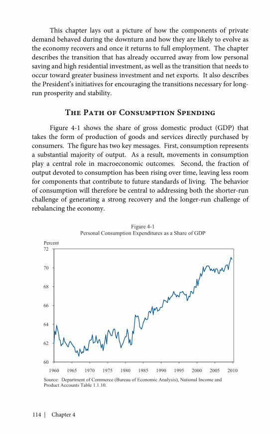
114 | Chapter 4
This chapter lays out a picture of how the components of privatedemand behaved during the downturn and how they are likely to evolve asthe economy recovers and once it returns to full employment. The chapterdescribes the transition that has already occurred away from low personalsaving and high residential investment, as well as the transition that needs tooccur toward greater business investment and net exports. It also describesthe President’s initiatives for encouraging the transitions necessary for long-run prosperity and stability.
The Path of Consumption Spending
Figure 4-1 shows the share of gross domestic product (GDP) thattakes the form of production of goods and services directly purchased byconsumers. The figure has two key messages. First, consumption representsa substantial majority of output. As a result, movements in consumptionplay a central role in macroeconomic outcomes. Second, the fraction ofoutput devoted to consumption has been rising over time, leaving less roomfor components that contribute to future standards of living. The behaviorof consumption will therefore be central to addressing both the shorter-runchallenge of generating a strong recovery and the longer-run challenge ofrebalancing the economy.
60
62
64
66
68
70
72
1960 1965 1970 1975 1980 1985 1990 1995 2000 2005 2010
Figure 4-1Personal Consumption Expenditures as a Share of GDP
Percent
Source: Department of Commerce (Bureau of Economic Analysis), National Income andProduct Accounts Table 1.1.10.
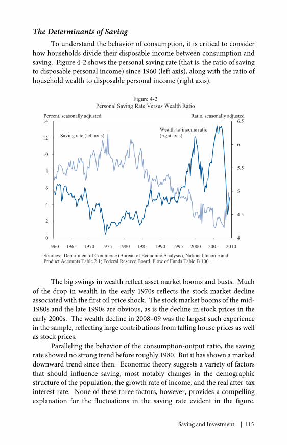
Saving and Investment | 115
The Determinants of SavingTo understand the behavior of consumption, it is critical to consider
how households divide their disposable income between consumption andsaving. Figure 4-2 shows the personal saving rate (that is, the ratio of savingto disposable personal income) since 1960 (left axis), along with the ratio ofhousehold wealth to disposable personal income (right axis).
The big swings in wealth reflect asset market booms and busts. Muchof the drop in wealth in the early 1970s reflects the stock market declineassociated with the first oil price shock. The stock market booms of the mid-1980s and the late 1990s are obvious, as is the decline in stock prices in theearly 2000s. The wealth decline in 2008–09 was the largest such experiencein the sample, reflecting large contributions from falling house prices as wellas stock prices.
Paralleling the behavior of the consumption-output ratio, the savingrate showed no strong trend before roughly 1980. But it has shown a markeddownward trend since then. Economic theory suggests a variety of factorsthat should influence saving, most notably changes in the demographicstructure of the population, the growth rate of income, and the real after-taxinterest rate. None of these three factors, however, provides a compellingexplanation for the fluctuations in the saving rate evident in the figure.
4
4.5
5
5.5
6
6.5
0
2
4
6
8
10
12
14
1960 1965 1970 1975 1980 1985 1990 1995 2000 2005 2010
Figure 4-2Personal Saving Rate Versus Wealth Ratio
detsujdayllanosaes,oitaRdetsujdayllanosaes,tnecreP
Wealth-to-income ratio(right axis)Saving rate (left axis)
Sources: Department of Commerce (Bureau of Economic Analysis), National Income andProduct Accounts Table 2.1; Federal Reserve Board, Flow of Funds Table B.100.
116 | Chapter 4
Indeed, some of the factors should probably have pushed saving up in recentdecades, not down. A 1991 study, for example, predicted that the saving ratewould rise as the baby boom generation entered its high-saving preretire-ment years (Auerbach, Cai, and Kotlikoff 1991). Instead, the saving rate fellsteadily as the boomers approached retirement (the first boomers claimedearly Social Security benefits in 2008).
Figure 4-2 suggests to the eye, and statistical analysis confirms, astrong negative association between the saving rate and the wealth-to-income ratio. This relationship has been interpreted as reflecting the effectof wealth on spending: a run-up in wealth leads to less need for saving.Such an interpretation is unsatisfying, however, because it leaves a key ques-tion unanswered: If wealth movements cause saving rate movements, whatcauses wealth movements? More broadly, it leaves open the possibility thatboth saving choices and asset price movements are a consequence of somedeeper underlying force. For example, an increase in optimism about futureeconomic conditions might lead both to a spending boom and to a generalbidding up of asset prices. In that case, the true moving force would notbe wealth changes per se; instead, both asset prices and saving would beresponding to the increase in optimism.
Survey data measuring “consumer sentiment” or “consumer confi-dence” do, in fact, have substantial forecasting power for near-term spendinggrowth, and are also associated with contemporaneous movements in assetprices (Carroll, Fuhrer, and Wilcox 1994). Such surveys are therefore auseful part of a macroeconomist’s forecasting tool kit. But such surveys havenot proven useful in explaining long-term trends like the secular decline inthe saving rate.
Emerging economic research suggests another underlyingexplanation that may be more potent: movements in the availability ofcredit. A substantial academic literature has documented the expansion ofcredit since the era of financial liberalization that began in the early 1980s(Dynan 2009). Many factors have contributed to this expansion; perhaps themost prominent explanation (aside from the liberalization itself) is the tele-communications and computer revolutions, which together have permittedthe construction of ever-more-detailed databases on consumer credit histo-ries, giving creditors a far more precise ability to tailor credit offers to thepersonal characteristics of individual borrowers (Jappelli and Pagano 1993).A beneficial effect of this information revolution has been that many peoplewho had previously been unable to obtain credit have for the first time beenable to borrow to buy a home, to start a business, or to undertake many otheruseful activities (Edelberg 2006; Getter 2006).
Saving and Investment | 117
A reduction in saving, however, is almost the inevitable consequenceof a general increase in the ability to borrow. If there is less need to savefor a down payment for a home, for a child’s education, for unforeseenemergencies, or for spending of any other kind, then the likelihood is thatless saving will be done. Of course, eventually the saving rate should mostlyrecover from any dip caused by a one-time increase in the availability ofcredit, because whatever extra debt was incurred must be paid back overtime (and paying back debt is another form of saving). This recovery insaving, however, may take a long time. If, in the meantime, credit avail-ability increases again, the gradual small increase in saving that reflects debtrepayment could easily be obscured by the new drop in saving occasioned bythe continuing expansion in credit availability.
How much of the decline in the saving rate was due to a gradual, butcumulatively large, increase in credit availability is not easy to determine,partly because an aggregate measure of credit availability is difficult toconstruct. Recent research on commercial lending has argued that a goodmeasure of the change in credit supply is provided by the Federal Reserve’sSenior Loan Officer Opinion Survey on Bank Lending Practices, in whichmanagers at leading financial institutions are asked for their assessmentsof credit conditions for businesses (Lown and Morgan 2006). Building onthat research, one study has proposed that a measure of the level of creditavailability to consumers can be constructed simply by accumulating thesequence of readings from this survey’s measure of credit availability toconsumers (Muellbauer 2007).1
Economic theory suggests that one further element may be importantin understanding spending and saving choices around times of recession:the intensity of consumers’ precautionary motive for saving. Because therisk of becoming unemployed is perhaps the greatest threat to most people’sfuture financial stability, the unemployment rate has sometimes been usedas a proxy for the intensity of the precautionary saving motive.
Implications for Recent and Future Saving BehaviorFigure 4-3 shows the relationship between the measured saving rate
and a simple statistical model that relates the saving rate to the wealth-to-income ratio, a slightly modified version of Muellbauer’s credit availabilityindex, and the unemployment rate. The statistical model is estimated overthe sample period 1966:Q3 to 2009:Q3. All three variables have statisticallyimportant predictive power, with the two most important measures beingthe measure of credit conditions and the wealth-to-income ratio.1 Specifically, each quarter the survey asks about banks’ willingness to make consumer install-ment loans now as opposed to three months ago.
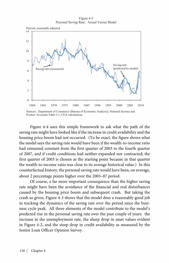
118 | Chapter 4
Figure 4-4 uses this simple framework to ask what the path of thesaving rate might have looked like if the increase in credit availability and thehousing price boom had not occurred. (To be exact, the figure shows whatthe model says the saving rate would have been if the wealth-to-income ratiohad remained constant from the first quarter of 2003 to the fourth quarterof 2007, and if credit conditions had neither expanded nor contracted; thefirst quarter of 2003 is chosen as the starting point because in that quarterthe wealth-to-income ratio was close to its average historical value.) In thiscounterfactual history, the personal saving rate would have been, on average,about 2 percentage points higher over the 2003–07 period.
Of course, a far more important consequence than the higher savingrate might have been the avoidance of the financial and real disturbancescaused by the housing price boom and subsequent crash. But taking thecrash as given, Figure 4-3 shows that the model does a reasonably good jobin tracking the dynamics of the saving rate over the period since the busi-ness cycle peak. All three elements of the model contribute to the model’spredicted rise in the personal saving rate over the past couple of years: theincrease in the unemployment rate, the sharp drop in asset values evidentin Figure 4-2, and the steep drop in credit availability as measured by theSenior Loan Officer Opinion Survey.
0
2
4
6
8
10
12
14
1960 1965 1970 1975 1980 1985 1990 1995 2000 2005 2010
Figure 4-3Personal Saving Rate: Actual Versus Model
Percent, seasonally adjusted
Saving rate(predicted by model)Saving rate (measured)
Sources: Department of Commerce (Bureau of Economic Analysis), National Income andProduct Accounts Table 2.1; CEA calculations.
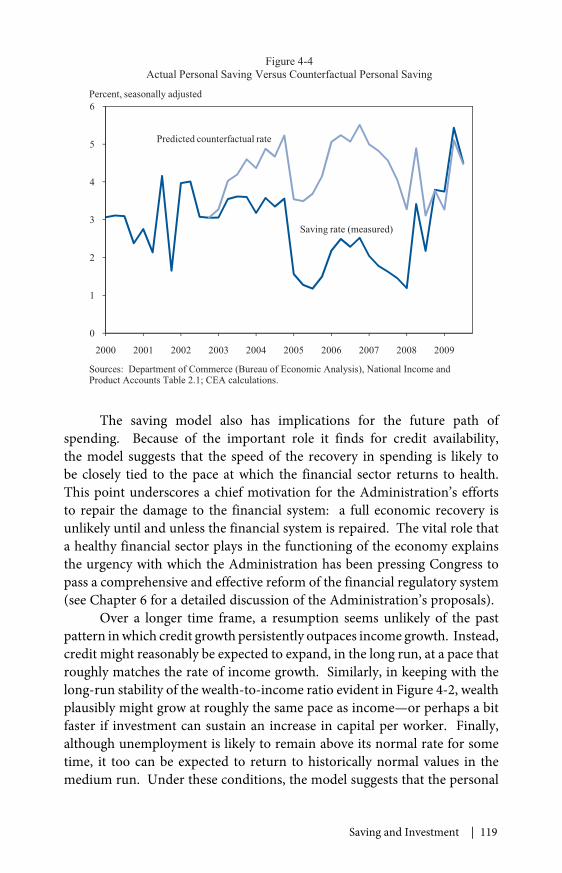
Saving and Investment | 119
The saving model also has implications for the future path ofspending. Because of the important role it finds for credit availability,the model suggests that the speed of the recovery in spending is likely tobe closely tied to the pace at which the financial sector returns to health.This point underscores a chief motivation for the Administration’s effortsto repair the damage to the financial system: a full economic recovery isunlikely until and unless the financial system is repaired. The vital role thata healthy financial sector plays in the functioning of the economy explainsthe urgency with which the Administration has been pressing Congress topass a comprehensive and effective reform of the financial regulatory system(see Chapter 6 for a detailed discussion of the Administration’s proposals).
Over a longer time frame, a resumption seems unlikely of the pastpattern in which credit growth persistently outpaces income growth. Instead,credit might reasonably be expected to expand, in the long run, at a pace thatroughly matches the rate of income growth. Similarly, in keeping with thelong-run stability of the wealth-to-income ratio evident in Figure 4-2, wealthplausibly might grow at roughly the same pace as income—or perhaps a bitfaster if investment can sustain an increase in capital per worker. Finally,although unemployment is likely to remain above its normal rate for sometime, it too can be expected to return to historically normal values in themedium run. Under these conditions, the model suggests that the personal
0
1
2
3
4
5
6
2000 2001 2002 2003 2004 2005 2006 2007 2008 2009
Figure 4-4Actual Personal Saving Versus Counterfactual Personal Saving
Percent, seasonally adjusted
Saving rate (measured)
Predicted counterfactual rate
Sources: Department of Commerce (Bureau of Economic Analysis), National Income andProduct Accounts Table 2.1; CEA calculations.
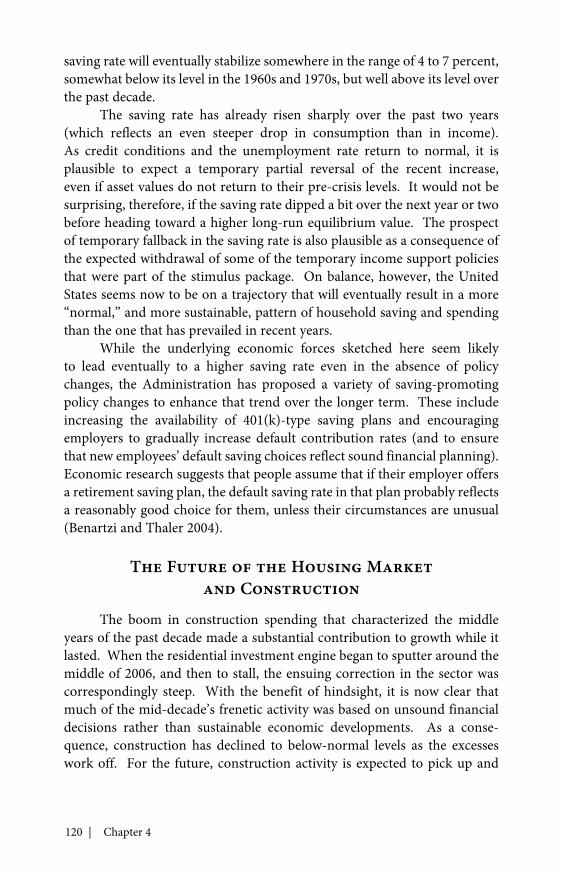
120 | Chapter 4
saving rate will eventually stabilize somewhere in the range of 4 to 7 percent,somewhat below its level in the 1960s and 1970s, but well above its level overthe past decade.
The saving rate has already risen sharply over the past two years(which reflects an even steeper drop in consumption than in income).As credit conditions and the unemployment rate return to normal, it isplausible to expect a temporary partial reversal of the recent increase,even if asset values do not return to their pre-crisis levels. It would not besurprising, therefore, if the saving rate dipped a bit over the next year or twobefore heading toward a higher long-run equilibrium value. The prospectof temporary fallback in the saving rate is also plausible as a consequence ofthe expected withdrawal of some of the temporary income support policiesthat were part of the stimulus package. On balance, however, the UnitedStates seems now to be on a trajectory that will eventually result in a more“normal,” and more sustainable, pattern of household saving and spendingthan the one that has prevailed in recent years.
While the underlying economic forces sketched here seem likelyto lead eventually to a higher saving rate even in the absence of policychanges, the Administration has proposed a variety of saving-promotingpolicy changes to enhance that trend over the longer term. These includeincreasing the availability of 401(k)-type saving plans and encouragingemployers to gradually increase default contribution rates (and to ensurethat new employees’ default saving choices reflect sound financial planning).Economic research suggests that people assume that if their employer offersa retirement saving plan, the default saving rate in that plan probably reflectsa reasonably good choice for them, unless their circumstances are unusual(Benartzi and Thaler 2004).
The Future of the Housing Marketand Construction
The boom in construction spending that characterized the middleyears of the past decade made a substantial contribution to growth while itlasted. When the residential investment engine began to sputter around themiddle of 2006, and then to stall, the ensuing correction in the sector wascorrespondingly steep. With the benefit of hindsight, it is now clear thatmuch of the mid-decade’s frenetic activity was based on unsound financialdecisions rather than sustainable economic developments. As a conse-quence, construction has declined to below-normal levels as the excesseswork off. For the future, construction activity is expected to pick up and
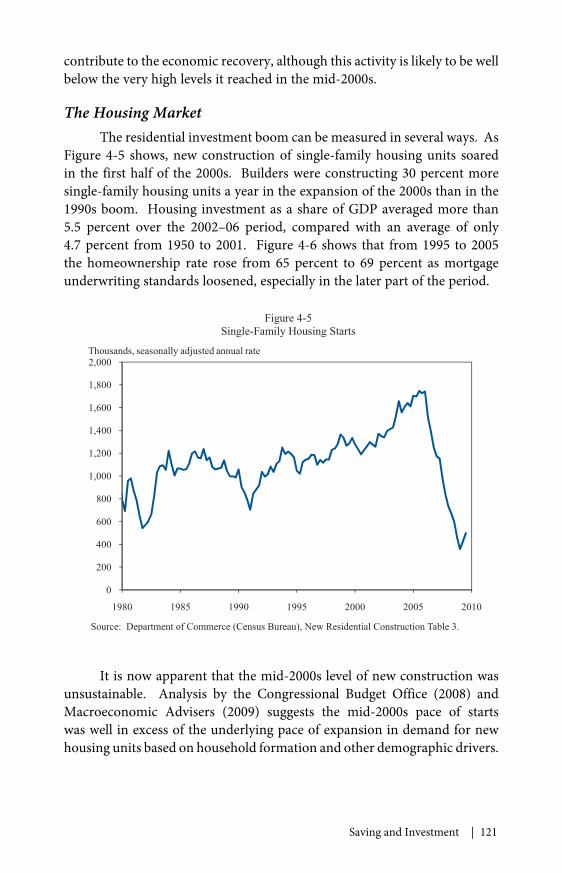
Saving and Investment | 121
contribute to the economic recovery, although this activity is likely to be wellbelow the very high levels it reached in the mid-2000s.
The Housing MarketThe residential investment boom can be measured in several ways. As
Figure 4-5 shows, new construction of single-family housing units soaredin the first half of the 2000s. Builders were constructing 30 percent moresingle-family housing units a year in the expansion of the 2000s than in the1990s boom. Housing investment as a share of GDP averaged more than5.5 percent over the 2002–06 period, compared with an average of only4.7 percent from 1950 to 2001. Figure 4-6 shows that from 1995 to 2005the homeownership rate rose from 65 percent to 69 percent as mortgageunderwriting standards loosened, especially in the later part of the period.
It is now apparent that the mid-2000s level of new construction wasunsustainable. Analysis by the Congressional Budget Office (2008) andMacroeconomic Advisers (2009) suggests the mid-2000s pace of startswas well in excess of the underlying pace of expansion in demand for newhousing units based on household formation and other demographic drivers.
0
200
400
600
800
1,000
1,200
1,400
1,600
1,800
2,000
1980 1985 1990 1995 2000 2005 2010
Figure 4-5Single-Family Housing Starts
Thousands, seasonally adjusted annual rate
Source: Department of Commerce (Census Bureau), New Residential Construction Table 3.
122 | Chapter 4
The boom was followed by an equally dramatic bust. From their peakin the third quarter of 2005 to the first quarter of 2009, single-family housingstarts fell by more than a factor of four. The homeownership rate reversedcourse, and by the second quarter of 2009 had returned to its 2000 level. Theshare of housing investment in GDP plummeted to 2.4 percent in the secondquarter of 2009.
Just as the mid-decade’s high levels of construction and housingmarket activity were not sustainable, the recent extremely low levels ofconstruction will not persist indefinitely. In 2009, housing starts and theshare of housing investment in GDP were well below their previous histor-ical lows. In the long run, sounder underwriting standards will requiremore would-be homeowners to take time to save for a down payment beforebuying a home, suggesting that the homeownership rate will ultimatelysettle at a level lower than its recent peaks. Nonetheless, as the popula-tion grows and the housing stock depreciates, new residential constructionwill be required to meet demand. The analyses by the CongressionalBudget Office (2008) and Macroeconomic Advisers (2009) suggest thatthe underlying demographic trend of household formation is consistentwith growth in demand of between 1.1 million and 1.3 million new single-family housing units per year, more than double the pace of single-familyhousing starts in November 2009. Indeed, since the second quarter of 2009,housing construction has already rebounded a bit, making its first positive
62
63
64
65
66
67
68
69
70
1980 1985 1990 1995 2000 2005 2010
Figure 4-6Homeownership Rate
Percent, seasonally adjusted
Source: Department of Commerce (Census Bureau), Residential Vacancies andHomeownership Table 4.
Saving and Investment | 123
contribution to GDP growth in the third quarter of 2009 since the end of2005. But, as described in Chapter 2, the stocks of new homes and existinghomes for sale, vacant homes that are not currently on the market, andhomes that are in the process of foreclosure and that are likely to be put onthe market at some point remain high. As a result, construction demand islikely to rise to its long-run level only gradually while some demand is metby the stock of existing units.
In short, as the housing market stabilizes and returns to a more normalcondition, its role as a major drag on economic growth seems to be ending,and it is likely to contribute to the recovery. But residential constructioncannot be expected to be the engine for GDP growth that it was during thehousing boom of the mid-2000s.
Commercial Real EstateThe market for commercial real estate has also suffered in the
recession. Commercial real estate encompasses a wide range of properties,from small businesses that occupy a single stand-alone structure to largeshopping malls owned by a consortium of investors.
Problems in the commercial real estate sector are less obviously a resultof overbuilding than those in the residential sector; instead, they reflect thesharp decline in demand for commercial space and the overall decline in theeconomy. The value of commercial real estate increased notably between2005 to 2007, spurred by easy credit conditions, as measured for example inthe Senior Loan Officer Opinion Survey. By the end of 2004, the net numberof banks reporting they had eased lending standards for commercial realestate loans was persistently larger than at any point in the history of theseries. Most banks did not begin tightening standards again until the end of2006. The relative quantity of financing also increased over this period; theratio of the change in the value of commercial real estate mortgages to newconstruction, which should increase when debt financing becomes relativelyattractive, reached a 45-year high in 2003 and then continued to climb,peaking at the end of 2005 at more than three times the historical average.2
In the nonresidential sector, high prices did not translate into adramatic increase in new construction (Figure 4-7). Rather, existing ownersof nonresidential properties used the cheap financing and price increasesto refinance or sell. Several factors appear to have played a role in limiting2 The numerator of the ratio is the seasonally adjusted change in commercial and multifamilyresidential mortgages (Federal Reserve, Flow of Funds Tables F219 and F220). The denominatoris seasonally adjusted construction of commercial and health care structures, multifamily struc-tures, and miscellaneous other nonresidential structures (Department of Commerce, Bureau ofEconomic Analysis, National Income and Product Accounts Table 5.3.5). The median of theratio from 1958 to 2000 is 0.46, while the 2005:Q4 value is 1.50.
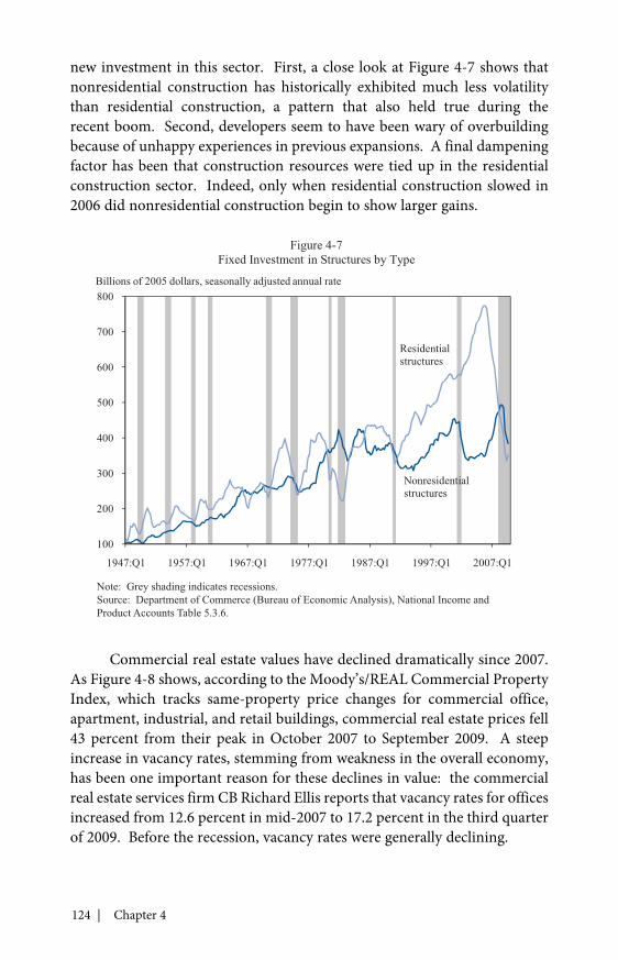
124 | Chapter 4
new investment in this sector. First, a close look at Figure 4-7 shows thatnonresidential construction has historically exhibited much less volatilitythan residential construction, a pattern that also held true during therecent boom. Second, developers seem to have been wary of overbuildingbecause of unhappy experiences in previous expansions. A final dampeningfactor has been that construction resources were tied up in the residentialconstruction sector. Indeed, only when residential construction slowed in2006 did nonresidential construction begin to show larger gains.
Commercial real estate values have declined dramatically since 2007.As Figure 4-8 shows, according to the Moody’s/REAL Commercial PropertyIndex, which tracks same-property price changes for commercial office,apartment, industrial, and retail buildings, commercial real estate prices fell43 percent from their peak in October 2007 to September 2009. A steepincrease in vacancy rates, stemming from weakness in the overall economy,has been one important reason for these declines in value: the commercialreal estate services firm CB Richard Ellis reports that vacancy rates for officesincreased from 12.6 percent in mid-2007 to 17.2 percent in the third quarterof 2009. Before the recession, vacancy rates were generally declining.
100
200
300
400
500
600
700
800
1947:Q1 1957:Q1 1967:Q1 1977:Q1 1987:Q1 1997:Q1 2007:Q1
Figure 4-7Fixed Investment in Structures by Type
Billions of 2005 dollars, seasonally adjusted annual rate
Residentialstructures
Nonresidentialstructures
Note: Grey shading indicates recessions.Source: Department of Commerce (Bureau of Economic Analysis), National Income andProduct Accounts Table 5.3.6.
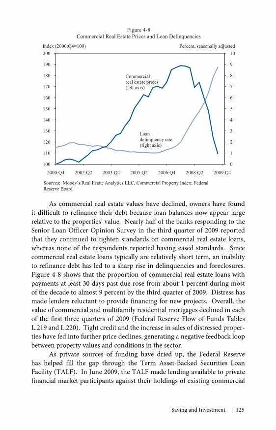
Saving and Investment | 125
As commercial real estate values have declined, owners have foundit difficult to refinance their debt because loan balances now appear largerelative to the properties’ value. Nearly half of the banks responding to theSenior Loan Officer Opinion Survey in the third quarter of 2009 reportedthat they continued to tighten standards on commercial real estate loans,whereas none of the respondents reported having eased standards. Sincecommercial real estate loans typically are relatively short term, an inabilityto refinance debt has led to a sharp rise in delinquencies and foreclosures.Figure 4-8 shows that the proportion of commercial real estate loans withpayments at least 30 days past due rose from about 1 percent during mostof the decade to almost 9 percent by the third quarter of 2009. Distress hasmade lenders reluctant to provide financing for new projects. Overall, thevalue of commercial and multifamily residential mortgages declined in eachof the first three quarters of 2009 (Federal Reserve Flow of Funds TablesL.219 and L.220). Tight credit and the increase in sales of distressed proper-ties have fed into further price declines, generating a negative feedback loopbetween property values and conditions in the sector.
As private sources of funding have dried up, the Federal Reservehas helped fill the gap through the Term Asset-Backed Securities LoanFacility (TALF). In June 2009, the TALF made lending available to privatefinancial market participants against their holdings of existing commercial
0
1
2
3
4
5
6
7
8
9
10
100
110
120
130
140
150
160
170
180
190
200
2000:Q4 2002:Q2 2003:Q4 2005:Q2 2006:Q4 2008:Q2 2009:Q4
Commercialreal estate prices(left axis)
Loandelinquency rate(right axis)
Figure 4-8Commercial Real Estate Prices and Loan Delinquencies
detsujdayllanosaes,tnecreP)001=4Q:0002(xednI
Sources: Moody’s/Real Estate Analytics LLC, Commercial Property Index; FederalReserve Board.

126 | Chapter 4
mortgage-backed securities (CMBS), thereby increasing liquidity in theCMBS market. In November 2009, the TALF made its first loans againstnewly issued CMBS. The provision of TALF financing for these newlyissued securities may prove particularly important in allowing borrowersto refinance.
The negative feedback loop between credit conditions, the sale ofdistressed commercial properties, and commercial property values may leadto further price declines. Eventually, however, a combination of economicrecovery and an improvement in financing conditions should help pricesstabilize. Still, as with the residential mortgage market, commercial realestate financing will likely not return any time soon to the easy termsthat prevailed before the collapse. Experience in previous business cyclessuggests that recovery of the sector will lag the economy as a whole.
Business Investment
If consumption and construction are not the drivers of growth goingforward in the way they were in the early 2000s, two components of privatedemand are left to fill the gap: business investment excluding structures,and net exports.3 Nonstructures investment could well become again (as itwas in the 1990s) a driving force in the expansion of aggregate demand andeconomic production. And in the long run, its share in GDP could reachlevels higher than those of the first part of the decade.
Investment in the RecoveryInvestment spending (other than structures) plummeted in late 2008
and early 2009. This investment spending fell so low that, after accountingfor depreciation, estimates of the absolute stock of capital showed stagnationin 2008 and even a decline in the first quarter of 2009. Falling spending inthis category reflected falling business confidence, as indicated, for example,in the Federal Reserve Bank of Philadelphia’s Business Outlook DiffusionIndex; this index was negative every month from October 2008 to July2009, signaling that more businesses thought conditions were deterioratingthan thought they were improving. Similarly, the National Federation ofIndependent Business Index of Small Business Optimism hit its lowest pointsince 1980 in March 2009.
3 In the National Income and Product Accounts, construction of commercial structures isclassified as part of business investment. Given that the boom and bust were concentratedin residential and commercial construction, however, for discussing recent and prospectivedevelopments it is more useful to consider commercial construction investment together withresidential investment, as was done in the previous section. Thus, the discussion that follows islargely concerned with nonstructures investment.
Saving and Investment | 127
Investment of this kind firmed in the second half of 2009, coincidingwith improvements in business confidence. Indeed, investment in equip-ment and software increased at a 13 percent annual rate in the fourthquarter. Nevertheless, the cumulative erosion has been so substantial thatyears of strong growth will be necessary to fully recover from the nadir.As a result, recovery of spending in this area is likely to make a substantialcontribution to the recovery of the overall economy.
Investment in the Long RunIn the long run, the share of business investment is likely not just to
return to its pre-recession levels, but to exceed them. During the boom ofthe 1990s, the share of business investment in equipment and software as afraction of GDP rose from a post-Gulf-War recession low of 6.9 percent in1991 to 9.6 percent in 2000. During that period, investment in informationprocessing equipment and software made the largest contribution to theincrease, as shown in Figure 4-9. Information technology (IT) investmentgrew an astounding 18 percent per year on average from 1991 to 2000.Other investment in equipment and software, which includes industrial,transportation, and construction equipment, accelerated as well, and grew asa share of GDP over this period. This high level of investment in the 1990sincreased industrial capacity by an average of 4 percent per year.
As the figure shows, the boom came to an end at the beginning ofthe 2000s, when investment in every category of equipment and softwarefell sharply as a share of GDP. The recovery in business investment inequipment and software after the 2001 recession was weak. IT investmentgrew at a historically tepid pace of 6 percent per year from 2003 to 2007, farbelow pre-2000 growth rates. Non-IT investment growth was also muted,with spending on industrial equipment growing at an annual pace of only3.7 percent from 2003 to 2007, down from an average of 5.4 percent in the1990s. Investment in transportation equipment surpassed its 1999 peakonly for one quarter in 2006. In the recovery following the 2001–02 reces-sion, the peak value of non-IT equipment investment as a share of GDP wasonly 4.3 percent (in 2006), a level that does not even match the historicalaverage value of that series in the period from 1980 to 2000. Productioncapacity in the sector grew an average of 0.6 percent per year from 2003 to2007, substantially below the average pace of growth in the 1990s. Takenas a whole, these figures suggest that business investment may have beenabnormally low over the course of the post-2001 expansion.
There are strong reasons to expect investment’s role in the economywill be larger in the future. In the long run, the real interest rate will adjustto bring the demand for the economy’s output in line with the economy’s
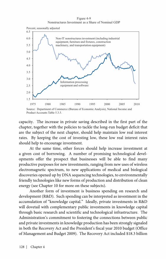
128 | Chapter 4
capacity. The increase in private saving described in the first part of thechapter, together with the policies to tackle the long-run budget deficit thatare the subject of the next chapter, should help maintain low real interestrates. By keeping the cost of investing low, these low real interest ratesshould help to encourage investment.
At the same time, other forces should help increase investment ata given cost of borrowing. A number of promising technological devel-opments offer the prospect that businesses will be able to find manyproductive purposes for new investments, ranging from new uses of wirelesselectromagnetic spectrum, to new applications of medical and biologicaldiscoveries opened up by DNA sequencing technologies, to environmentallyfriendly technologies like new forms of production and distribution of cleanenergy (see Chapter 10 for more on these subjects).
Another form of investment is business spending on research anddevelopment (R&D). Such spending can be interpreted as investment in theaccumulation of “knowledge capital.” Ideally, private investments in R&Dwill dovetail with complementary public investments in knowledge capitalthrough basic research and scientific and technological infrastructure. TheAdministration’s commitment to fostering the connections between publicand private investments in knowledge production has been strongly signaledin both the Recovery Act and the President’s fiscal year 2010 budget (Officeof Management and Budget 2009). The Recovery Act included $18.3 billion
1.5
2.0
2.5
3.0
3.5
4.0
4.5
5.0
5.5
6.0
6.5
1975 1980 1985 1990 1995 2000 2005 2010
Figure 4-9Nonstructures Investment as a Share of Nominal GDP
Percent, seasonally adjusted
Information processingequipment and software
Non-IT nonstructures investment (including industrialequipment, furniture and fixtures, constructionmachinery, and transportation equipment)
Source: Department of Commerce (Bureau of Economic Analysis), National Income andProduct Accounts Table 5.3.5.
Saving and Investment | 129
of direct spending on research, one of the largest direct increases in suchspending in the Nation’s history. In addition, more than $80 billion ofRecovery Act funds were targeted toward technology and science infrastruc-ture. The Administration’s first budget proposed to double the researchspending by three key science agencies: the National Science Foundation,the Department of Energy’s Office of Science, and the Department ofCommerce’s National Institute of Standards and Technology. And to fosterprivate sector innovation, the budget also included the full $74 billion cost ofmaking the research and experimentation tax credit permanent in order togive businesses the certainty they need to invest, innovate, and grow.
With reduced demand from consumption and housing tending tomake the real interest rate lower than it otherwise would be, and increasedinvestment demand from the many newly developing technologies andincentives for R&D, a larger portion of the economy’s output is likely to bedevoted to investment. And, because business investment contributes notonly to aggregate demand but also to aggregate supply and productivity, alarger role for investment will create a stronger economy going forward.
The Current Account
The picture of future growth in the United States described in theprevious sections depends less on borrowing and consumption than didgrowth in the past decade. This view has important implications for ourinteractions with other countries and the current account.
Determinants of the Current AccountThe current account is the trade balance plus net income on overseas
assets and unilateral transfers like foreign aid and remittances. The tradebalance, or net exports, represents the bulk of the current account and isresponsible for a large majority of short-run movements in it. To a firstapproximation, a current account deficit implies that the trade balance isnegative or, equivalently, that our exports are less than our imports. Atthe same time, the current account deficit must also be matched by the netborrowing of the United States from the rest of the world. If we spend morethan we earn, we must borrow the money to do so. In the national incomeaccounting sense, the definition of the current account can be reduced tonational saving minus investment (plus some measurement error).
This accounting definition provides a description but not anexplanation of the drivers of the current account. One important driveris the business cycle. As Box 4-1 explains, over the last 30 years, the U.S.current account deficit tended to be larger when the economy was booming
130 | Chapter 4
and unemployment was low. In a boom, investment tends to rise and savingtends to fall, generating a current account deficit. When the economystruggles, investment often falls and saving often rises, generating a surplus(or a smaller deficit). In countries that rely more on exports to drive theirgrowth, an acceleration in growth can be associated with a rising currentaccount surplus (or smaller deficit).
Current accounts do not need to be balanced in every country inevery year. At any point in time, countries may offer more investmentopportunities than their desired level of saving at a given interest rate canfund, making them net borrowers, resulting in a current account deficit.Other countries may have an excess of saving over desired investment,making them net lenders (a current account surplus). However, in the
Box 4-1: Unemployment and the Current Account
The relationship between the level of unemployment and the currentaccount balance is complicated. People frequently argue that imports—and specifically the current account deficit—displace U.S. workers andgenerate higher unemployment. However, the main determinant ofunemployment in the short and medium runs is the state of the businesscycle. The scatter plot of the current account and the unemployment ratesince 1980, shown in the accompanying figure, displays a positive relation-ship. Historically, a smaller current account deficit has coincided with ahigher unemployment rate. Both were being driven by cyclical economicfactors: in a recession, the current account balance improved, and unem-ployment was high. In a boom, the current account balance deteriorated,and unemployment was low. This usual pattern has been at work inthe current recession. The U.S. current account deficit narrowed from6.4 percent of GDP in the third quarter of 2006 to 2.8 percent of GDP inthe second quarter of 2009. At the same time, unemployment rose from4.6 percent to 9.3 percent.
The relationship between unemployment and the current accountbalance can be different in countries that have relied more heavily onexports for growth. For example, in Germany, the unemployment rate fellfrom 11.7 percent in 2005 to 9.0 percent in 2007 while the current accountsurplus rose from 5.1 percent of GDP to 7.9 percent. Likewise, in Japan,unemployment fell from 2005 to 2007 as the current account surplusrose. Given the slack in the U.S. economy, a shift toward a currentaccount surplus could increase aggregate demand and help lower theunemployment rate.
Continued on next page
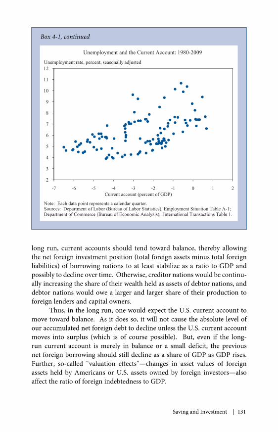
Saving and Investment | 131
long run, current accounts should tend toward balance, thereby allowingthe net foreign investment position (total foreign assets minus total foreignliabilities) of borrowing nations to at least stabilize as a ratio to GDP andpossibly to decline over time. Otherwise, creditor nations would be continu-ally increasing the share of their wealth held as assets of debtor nations, anddebtor nations would owe a larger and larger share of their production toforeign lenders and capital owners.
Thus, in the long run, one would expect the U.S. current account tomove toward balance. As it does so, it will not cause the absolute level ofour accumulated net foreign debt to decline unless the U.S. current accountmoves into surplus (which is of course possible). But, even if the long-run current account is merely in balance or a small deficit, the previousnet foreign borrowing should still decline as a share of GDP as GDP rises.Further, so-called “valuation effects”—changes in asset values of foreignassets held by Americans or U.S. assets owned by foreign investors—alsoaffect the ratio of foreign indebtedness to GDP.
2
3
4
5
6
7
8
9
10
11
12
-7 -6 -5 -4 -3 -2 -1 0 1 2
Unemployment and the Current Account: 1980-2009
Unemployment rate, percent, seasonally adjusted
Current account (percent of GDP)
Note: Each data point represents a calendar quarter.Sources: Department of Labor (Bureau of Labor Statistics), Employment Situation Table A-1;Department of Commerce (Bureau of Economic Analysis), International Transactions Table 1.
Box 4-1, continued
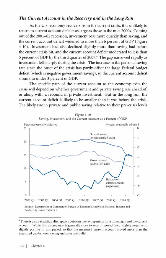
132 | Chapter 4
The Current Account in the Recovery and in the Long RunAs the U.S. economy recovers from the current crisis, it is unlikely to
return to current account deficits as large as those in the mid-2000s. Comingout of the 2001–02 recession, investment rose more quickly than saving, andthe current account deficit widened to more than 6 percent of GDP (Figure4-10). Investment had also declined slightly more than saving had beforethe current crisis hit, and the current account deficit moderated to less than5 percent of GDP by the third quarter of 2007.4 The gap narrowed rapidly asinvestment fell sharply during the crisis. The increase in the personal savingrate since the onset of the crisis has partly offset the large Federal budgetdeficit (which is negative government saving), so the current account deficitshrank to under 3 percent of GDP.
The specific path of the current account as the economy exits thecrisis will depend on whether government and private saving rise ahead of,or along with, a rebound in private investment. But in the long run, thecurrent account deficit is likely to be smaller than it was before the crisis.The likely rise in private and public saving relative to their pre-crisis levels
4 There is also a statistical discrepancy between the saving-minus-investment gap and the currentaccount. While this discrepancy is generally close to zero, it moved from slightly negative toslightly positive in this period, so that the measured current account moved more than themeasured gap between saving and investment did.
-7
-6
-5
-4
-3
-2
-1
0
0
5
10
15
20
25
2002:Q1 2003:Q1 2004:Q1 2005:Q1 2006:Q1 2007:Q1 2008:Q1 2009:Q1
Figure 4-10Saving, Investment, and the Current Account as a Percent of GDP
Percent, seasonally adjusted Percent, seasonally adjusted
Gross domesticinvestment (left axis)
Balance oncurrent account(right axis)
Gross nationalsaving (left axis)
Source: Department of Commerce (Bureau of Economic Analysis), National Income andProduct Accounts Table 5.1.
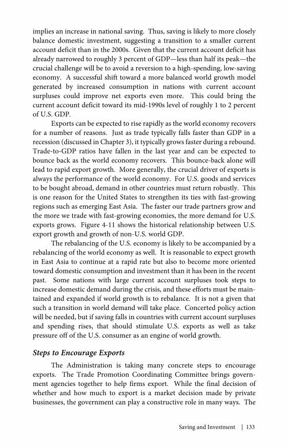
Saving and Investment | 133
implies an increase in national saving. Thus, saving is likely to more closelybalance domestic investment, suggesting a transition to a smaller currentaccount deficit than in the 2000s. Given that the current account deficit hasalready narrowed to roughly 3 percent of GDP—less than half its peak—thecrucial challenge will be to avoid a reversion to a high-spending, low-savingeconomy. A successful shift toward a more balanced world growth modelgenerated by increased consumption in nations with current accountsurpluses could improve net exports even more. This could bring thecurrent account deficit toward its mid-1990s level of roughly 1 to 2 percentof U.S. GDP.
Exports can be expected to rise rapidly as the world economy recoversfor a number of reasons. Just as trade typically falls faster than GDP in arecession (discussed in Chapter 3), it typically grows faster during a rebound.Trade-to-GDP ratios have fallen in the last year and can be expected tobounce back as the world economy recovers. This bounce-back alone willlead to rapid export growth. More generally, the crucial driver of exports isalways the performance of the world economy. For U.S. goods and servicesto be bought abroad, demand in other countries must return robustly. Thisis one reason for the United States to strengthen its ties with fast-growingregions such as emerging East Asia. The faster our trade partners grow andthe more we trade with fast-growing economies, the more demand for U.S.exports grows. Figure 4-11 shows the historical relationship between U.S.export growth and growth of non-U.S. world GDP.
The rebalancing of the U.S. economy is likely to be accompanied by arebalancing of the world economy as well. It is reasonable to expect growthin East Asia to continue at a rapid rate but also to become more orientedtoward domestic consumption and investment than it has been in the recentpast. Some nations with large current account surpluses took steps toincrease domestic demand during the crisis, and these efforts must be main-tained and expanded if world growth is to rebalance. It is not a given thatsuch a transition in world demand will take place. Concerted policy actionwill be needed, but if saving falls in countries with current account surplusesand spending rises, that should stimulate U.S. exports as well as takepressure off of the U.S. consumer as an engine of world growth.
Steps to Encourage ExportsThe Administration is taking many concrete steps to encourage
exports. The Trade Promotion Coordinating Committee brings govern-ment agencies together to help firms export. While the final decision ofwhether and how much to export is a market decision made by privatebusinesses, the government can play a constructive role in many ways. The
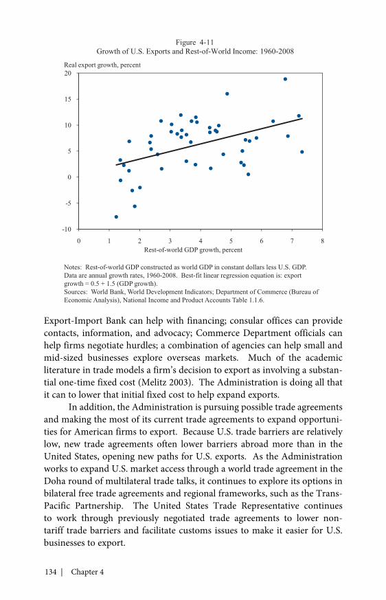
134 | Chapter 4
Export-Import Bank can help with financing; consular offices can providecontacts, information, and advocacy; Commerce Department officials canhelp firms negotiate hurdles; a combination of agencies can help small andmid-sized businesses explore overseas markets. Much of the academicliterature in trade models a firm’s decision to export as involving a substan-tial one-time fixed cost (Melitz 2003). The Administration is doing all thatit can to lower that initial fixed cost to help expand exports.
In addition, the Administration is pursuing possible trade agreementsand making the most of its current trade agreements to expand opportuni-ties for American firms to export. Because U.S. trade barriers are relativelylow, new trade agreements often lower barriers abroad more than in theUnited States, opening new paths for U.S. exports. As the Administrationworks to expand U.S. market access through a world trade agreement in theDoha round of multilateral trade talks, it continues to explore its options inbilateral free trade agreements and regional frameworks, such as the Trans-Pacific Partnership. The United States Trade Representative continuesto work through previously negotiated trade agreements to lower non-tariff trade barriers and facilitate customs issues to make it easier for U.S.businesses to export.
-10
-5
0
5
10
15
20
0 1 2 3 4 5 6 7 8
Figure 4-11Growth of U.S. Exports and Rest-of-World Income: 1960-2008
Real export growth, percent
Rest-of-world GDP growth, percent
Notes: Rest-of-world GDP constructed as world GDP in constant dollars less U.S. GDP.Data are annual growth rates, 1960-2008. Best-fit linear regression equation is: exportgrowth = 0.5 + 1.5 (GDP growth).Sources: World Bank, World Development Indicators; Department of Commerce (Bureau ofEconomic Analysis), National Income and Product Accounts Table 1.1.6.
Saving and Investment | 135
Not all of these developments will necessarily increase net exports(or the current account) of the United States. Since the current accountequals net lending to or borrowing from the world, moving the currentaccount balance requires adjustments in saving and investment as well asmore opportunities to export. In the long run, increases in demand forU.S. exports resulting from export promotion or reduced trade barriers willgenerate higher standards of living, but through improved terms of trade,not an increase in net exports. Further, the simple recovery of world tradevolumes will increase exports and imports alike. As discussed in Chapter10, this increase in trade can increase productivity and living standards, butit will not change the current account. However, rapid world growth anddeclining current account surpluses abroad should lead to an increase inU.S. exports. This can help increase U.S. net exports and hence contributeto the recovery.
As with higher investment, lower current account deficits haveimportant long-run benefits. Lower foreign indebtedness than the countryotherwise would have had means reduced interest payments to foreigners.Equivalently, it means that foreigners have on net smaller claims on theoutput produced in the United States. Thus, lower current account deficitswill raise standards of living in the long run.
Conclusion
Economic policy should not aim to return the economy to the path ofunstable, unsustainable, unhealthy growth it was on before the wrenchingevents of the past two years. We should—and can—achieve somethingbetter. Growth that is not fueled by unsustainable borrowing, and growththat is based on productive investments, is more stable than the growth ofrecent decades. And growth that is associated with higher saving will leadto greater accumulation of wealth, and so greater growth in our standardsof living.
137
C H A P T E R 5
ADDRESSING THE LONG-RUNFISCAL CHALLENGE
After several years of budget surpluses, the Federal Government beganrunning consistent, substantial deficits in the 2002 fiscal year. Because
the deficits absorbed a significant portion of private saving, they were onereason that the economic expansion of the 2000s was led by consumptionand foreign borrowing rather than investment and net exports. More trou-bling than the deficits of the recent past, however, is the long-term fiscaloutlook the Administration inherited. Even before the increased spendingnecessary to rescue and stabilize the economy, the policy choices of theprevious eight years and projected increases in spending on health care andSocial Security had already put the government on a path of rising deficitsand debt. Thus, a key step in rebalancing the economy and restoring itslong-run health must be putting fiscal policy on a sound, sustainable footing.
This chapter discusses the fiscal challenges the Administrationinherited, the dangers posed by large and growing deficits, and theAdministration’s measures and plans for addressing these challenges. TheAdministration and Congress are already taking important steps, mostnotably through their efforts toward comprehensive health care reform. Thelegislation currently under consideration addresses rapidly rising health carecosts, which are one of the central drivers of the long-run fiscal problem.The fiscal problem is multifaceted, however, and was decades in the making.As a result, no single step can fully address it. Much work remains, andbipartisan cooperation will be essential.
The Long-Run Fiscal Challenge
When President Obama took office in January 2009, fiscal policy wason a deteriorating course. Figure 5-1 shows the grim outlook for the budgetprojected by the Congressional Budget Office (CBO) under the assumption
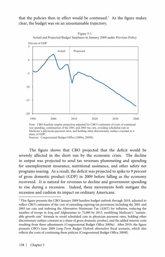
138 | Chapter 5
that the policies then in effect would be continued.1 As the figure makesclear, the budget was on an unsustainable trajectory.
The figure shows that CBO projected that the deficit would beseverely affected in the short run by the economic crisis. The declinein output was projected to send tax revenues plummeting and spendingfor unemployment insurance, nutritional assistance, and other safety netprograms soaring. As a result, the deficit was projected to spike to 9 percentof gross domestic product (GDP) in 2009 before falling as the economyrecovered. It is natural for revenues to decline and government spendingto rise during a recession. Indeed, these movements both mitigate therecession and cushion its impact on ordinary Americans.1 This figure presents the CBO January 2009 baseline budget outlook through 2019, adjusted toreflect CBO’s estimates of the cost of extending expiring tax provisions including the 2001 and2003 tax cuts and indexing the Alternative Minimum Tax (AMT) for inflation, reducing thenumber of troops in Iraq and Afghanistan to 75,000 by 2013, modifying Medicare’s “sustain-able growth rate” formula to avoid scheduled cuts in physician payment rates, holding otherdiscretionary outlays constant as a share of gross domestic product, and the added interest costsresulting from these adjustments (Congressional Budget Office 2009a). After 2019, the figurepresents CBO’s June 2009 Long-Term Budget Outlook alternative fiscal scenario, which alsoreflects the costs of continuing these policies (Congressional Budget Office 2009f).
-20
-15
-10
-5
0
5
1990 2000 2010 2020 2030 2040
Figure 5-1Actual and Projected Budget Surpluses in January 2009 under Previous Policy
Percent of GDP
ProjectedActual
Note: CBO baseline surplus projection adjusted for CBO’s estimates of costs of continuedwar spending, continuation of the 2001 and 2003 tax cuts, avoiding scheduled cuts inMedicare’s physician payment rates, and holding other discretionary outlays constant as ashare of GDP.Sources: Congressional Budget Office (2009a, 2009f).
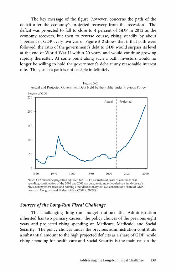
Addressing the Long-Run Fiscal Challenge | 139
The key message of the figure, however, concerns the path of thedeficit after the economy’s projected recovery from the recession. Thedeficit was projected to fall to close to 4 percent of GDP in 2012 as theeconomy recovers, but then to reverse course, rising steadily by about1 percent of GDP every two years. Figure 5-2 shows that if that path werefollowed, the ratio of the government’s debt to GDP would surpass its levelat the end of World War II within 20 years, and would continue growingrapidly thereafter. At some point along such a path, investors would nolonger be willing to hold the government’s debt at any reasonable interestrate. Thus, such a path is not feasible indefinitely.
Sources of the Long-Run Fiscal ChallengeThe challenging long-run budget outlook the Administration
inherited has two primary causes: the policy choices of the previous eightyears and projected rising spending on Medicare, Medicaid, and SocialSecurity. The policy choices under the previous administration contributea substantial amount to the high projected deficits as a share of GDP, whilerising spending for health care and Social Security is the main reason the
0
50
100
150
200
250
1920 1940 1960 1980 2000 2020 2040
Figure 5-2Actual and Projected Government Debt Held by the Public under Previous Policy
Percent of GDP
Actual Projected
Note: CBO baseline projection adjusted for CBO’s estimates of costs of continued warspending, continuation of the 2001 and 2003 tax cuts, avoiding scheduled cuts in Medicare’sphysician payment rates, and holding other discretionary outlays constant as a share of GDP.Sources: Congressional Budget Office (2009a, 2009f).
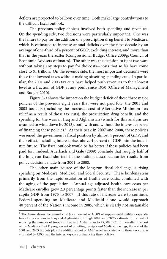
140 | Chapter 5
deficits are projected to balloon over time. Both make large contributions tothe difficult fiscal outlook.
The previous policy choices involved both spending and revenues.On the spending side, two decisions were particularly important. One wasthe failure to pay for the addition of a prescription drug benefit to Medicare,which is estimated to increase annual deficits over the next decade by anaverage of one-third of a percent of GDP, excluding interest, and more thanthat in the years thereafter (Congressional Budget Office 2009g; Council ofEconomic Advisers estimates). The other was the decision to fight two warswithout taking any steps to pay for the costs—costs that so far have comeclose to $1 trillion. On the revenue side, the most important decisions werethose that lowered taxes without making offsetting spending cuts. In partic-ular, the 2001 and 2003 tax cuts have helped push revenues to their lowestlevel as a fraction of GDP at any point since 1950 (Office of Managementand Budget 2010).
Figure 5-3 shows the impact on the budget deficit of these three majorpolicies of the previous eight years that were not paid for: the 2001 and2003 tax cuts (including the increased cost of Alternative Minimum Taxrelief as a result of those tax cuts), the prescription drug benefit, and thespending for the wars in Iraq and Afghanistan (which for this analysis areassumed to wind down by 2013), both with and without the interest expenseof financing these policies.2 At their peak in 2007 and 2008, these policiesworsened the government’s fiscal position by almost 4 percent of GDP, andtheir effect, including interest, rises above 4 percent of GDP into the indefi-nite future. The fiscal outlook would be far better if these policies had beenpaid for. Indeed, Auerbach and Gale (2009) conclude that roughly half ofthe long-run fiscal shortfall in the outlook described earlier results frompolicy decisions made from 2001 to 2008.
The other main source of the long-run fiscal challenge is risingspending on Medicare, Medicaid, and Social Security. These burdens stemprimarily from the rapid escalation of health care costs, combined withthe aging of the population. Annual age-adjusted health care costs perMedicare enrollee grew 2.3 percentage points faster than the increase in percapita GDP from 1975 to 2007. If this rate of increase were to continue,Federal spending on Medicare and Medicaid alone would approach40 percent of the Nation’s income in 2085, which is clearly not sustainable
2 The figure shows the annual cost (as a percent of GDP) of supplemental military expendi-tures for operations in Iraq and Afghanistan through 2009 and CBO’s estimate of the cost ofreducing the number of troops in Iraq and Afghanistan to 75,000 by 2013 thereafter; the costof the Medicare Part D program net of offsetting receipts and Medicaid savings; the cost of the2001 and 2003 tax cuts plus the additional cost of AMT relief associated with those tax cuts, asestimated by CBO; and the interest expense of financing these policies.
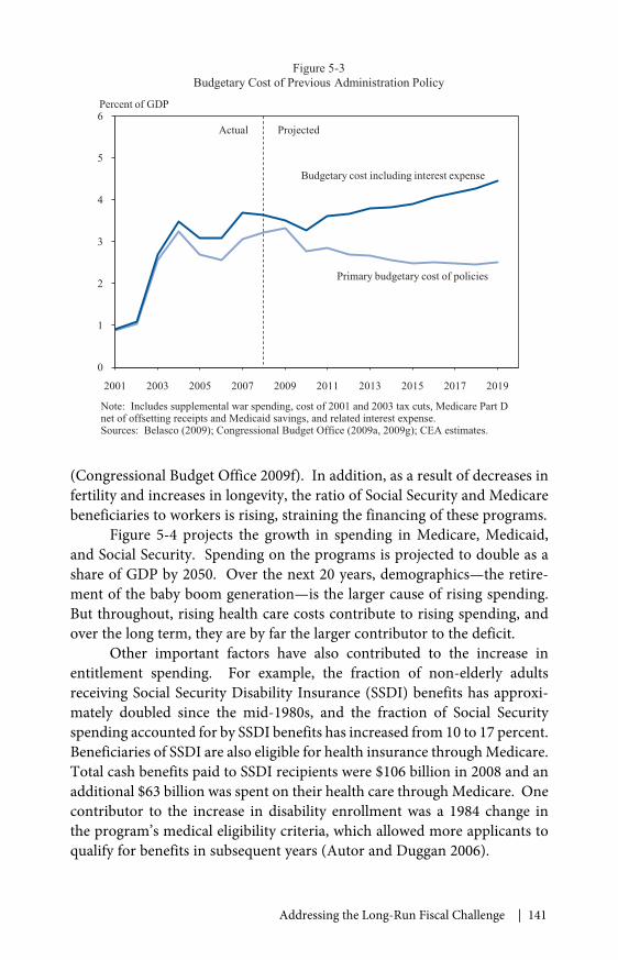
Addressing the Long-Run Fiscal Challenge | 141
(Congressional Budget Office 2009f). In addition, as a result of decreases infertility and increases in longevity, the ratio of Social Security and Medicarebeneficiaries to workers is rising, straining the financing of these programs.
Figure 5-4 projects the growth in spending in Medicare, Medicaid,and Social Security. Spending on the programs is projected to double as ashare of GDP by 2050. Over the next 20 years, demographics—the retire-ment of the baby boom generation—is the larger cause of rising spending.But throughout, rising health care costs contribute to rising spending, andover the long term, they are by far the larger contributor to the deficit.
Other important factors have also contributed to the increase inentitlement spending. For example, the fraction of non-elderly adultsreceiving Social Security Disability Insurance (SSDI) benefits has approxi-mately doubled since the mid-1980s, and the fraction of Social Securityspending accounted for by SSDI benefits has increased from 10 to 17 percent.Beneficiaries of SSDI are also eligible for health insurance through Medicare.Total cash benefits paid to SSDI recipients were $106 billion in 2008 and anadditional $63 billion was spent on their health care through Medicare. Onecontributor to the increase in disability enrollment was a 1984 change inthe program’s medical eligibility criteria, which allowed more applicants toqualify for benefits in subsequent years (Autor and Duggan 2006).
0
1
2
3
4
5
6
2001 2003 2005 2007 2009 2011 2013 2015 2017 2019
Figure 5-3Budgetary Cost of Previous Administration Policy
Percent of GDP
Primary budgetary cost of policies
Budgetary cost including interest expense
Actual Projected
Note: Includes supplemental war spending, cost of 2001 and 2003 tax cuts, Medicare Part Dnet of offsetting receipts and Medicaid savings, and related interest expense.Sources: Belasco (2009); Congressional Budget Office (2009a, 2009g); CEA estimates.
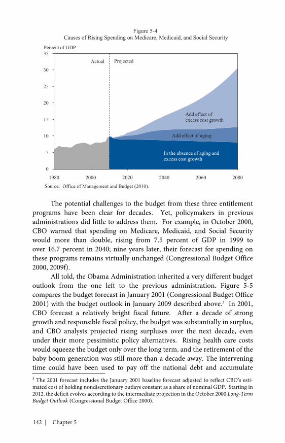
142 | Chapter 5
The potential challenges to the budget from these three entitlementprograms have been clear for decades. Yet, policymakers in previousadministrations did little to address them. For example, in October 2000,CBO warned that spending on Medicare, Medicaid, and Social Securitywould more than double, rising from 7.5 percent of GDP in 1999 toover 16.7 percent in 2040; nine years later, their forecast for spending onthese programs remains virtually unchanged (Congressional Budget Office2000, 2009f).
All told, the Obama Administration inherited a very different budgetoutlook from the one left to the previous administration. Figure 5-5compares the budget forecast in January 2001 (Congressional Budget Office2001) with the budget outlook in January 2009 described above.3 In 2001,CBO forecast a relatively bright fiscal future. After a decade of stronggrowth and responsible fiscal policy, the budget was substantially in surplus,and CBO analysts projected rising surpluses over the next decade, evenunder their more pessimistic policy alternatives. Rising health care costswould squeeze the budget only over the long term, and the retirement of thebaby boom generation was still more than a decade away. The interveningtime could have been used to pay off the national debt and accumulate3 The 2001 forecast includes the January 2001 baseline forecast adjusted to reflect CBO’s esti-mated cost of holding nondiscretionary outlays constant as a share of nominal GDP. Starting in2012, the deficit evolves according to the intermediate projection in the October 2000 Long-TermBudget Outlook (Congressional Budget Office 2000).
0
5
10
15
20
25
30
35
1980 2000 2020 2040 2060 2080
Figure 5-4Causes of Rising Spending on Medicare, Medicaid, and Social Security
Percent of GDP
In the absence of aging andexcess cost growth
Add effect ofexcess cost growth
Add effect of aging
ProjectedActual
Source: Office of Management and Budget (2010).
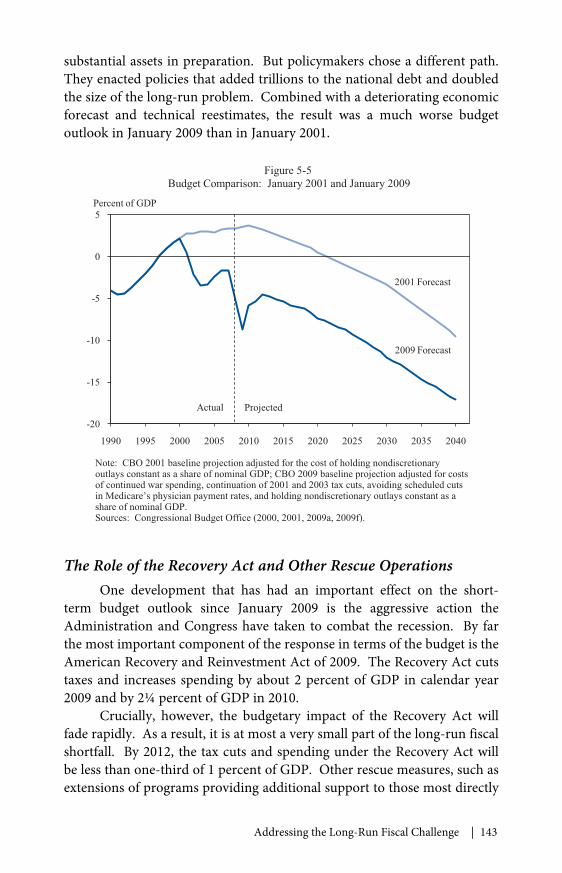
Addressing the Long-Run Fiscal Challenge | 143
substantial assets in preparation. But policymakers chose a different path.They enacted policies that added trillions to the national debt and doubledthe size of the long-run problem. Combined with a deteriorating economicforecast and technical reestimates, the result was a much worse budgetoutlook in January 2009 than in January 2001.
The Role of the Recovery Act and Other Rescue OperationsOne development that has had an important effect on the short-
term budget outlook since January 2009 is the aggressive action theAdministration and Congress have taken to combat the recession. By farthe most important component of the response in terms of the budget is theAmerican Recovery and Reinvestment Act of 2009. The Recovery Act cutstaxes and increases spending by about 2 percent of GDP in calendar year2009 and by 2¼ percent of GDP in 2010.
Crucially, however, the budgetary impact of the Recovery Act willfade rapidly. As a result, it is at most a very small part of the long-run fiscalshortfall. By 2012, the tax cuts and spending under the Recovery Act willbe less than one-third of 1 percent of GDP. Other rescue measures, such asextensions of programs providing additional support to those most directly
-20
-15
-10
-5
0
5
1990 1995 2000 2005 2010 2015 2020 2025 2030 2035 2040
Figure 5-5Budget Comparison: January 2001 and January 2009
Percent of GDP
2001 Forecast
2009 Forecast
Actual Projected
Note: CBO 2001 baseline projection adjusted for the cost of holding nondiscretionaryoutlays constant as a share of nominal GDP; CBO 2009 baseline projection adjusted for costsof continued war spending, continuation of 2001 and 2003 tax cuts, avoiding scheduled cutsin Medicare’s physician payment rates, and holding nondiscretionary outlays constant as ashare of nominal GDP.Sources: Congressional Budget Office (2000, 2001, 2009a, 2009f).
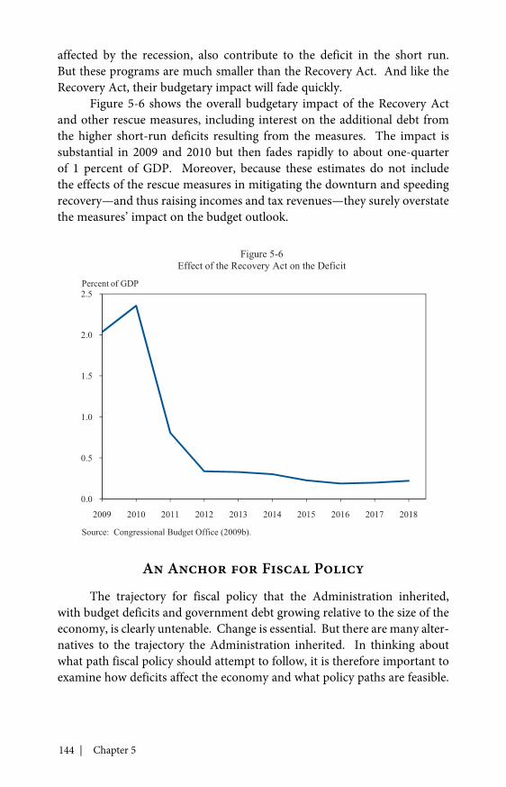
144 | Chapter 5
affected by the recession, also contribute to the deficit in the short run.But these programs are much smaller than the Recovery Act. And like theRecovery Act, their budgetary impact will fade quickly.
Figure 5-6 shows the overall budgetary impact of the Recovery Actand other rescue measures, including interest on the additional debt fromthe higher short-run deficits resulting from the measures. The impact issubstantial in 2009 and 2010 but then fades rapidly to about one-quarterof 1 percent of GDP. Moreover, because these estimates do not includethe effects of the rescue measures in mitigating the downturn and speedingrecovery—and thus raising incomes and tax revenues—they surely overstatethe measures’ impact on the budget outlook.
An Anchor for Fiscal Policy
The trajectory for fiscal policy that the Administration inherited,with budget deficits and government debt growing relative to the size of theeconomy, is clearly untenable. Change is essential. But there are many alter-natives to the trajectory the Administration inherited. In thinking aboutwhat path fiscal policy should attempt to follow, it is therefore important toexamine how deficits affect the economy and what policy paths are feasible.
0.0
0.5
1.0
1.5
2.0
2.5
2009 2010 2011 2012 2013 2014 2015 2016 2017 2018
Figure 5-6Effect of the Recovery Act on the Deficit
Percent of GDP
Source: Congressional Budget Office (2009b).

Addressing the Long-Run Fiscal Challenge | 145
The Effects of Budget DeficitsTwo factors are critical in shaping the economic effects of budget
deficits: the state of the economy, and the size and duration of the deficits.Consider first the state of the economy. A central lesson of macroeconomicsis that in an economy operating below capacity, higher deficits raise outputand employment. Transfer payments (such as unemployment benefits)and tax cuts encourage private consumption and investment spending.Government investments and other purchases contribute to higher outputand employment directly and, by raising incomes, also encourage furtherprivate spending.
In the current situation, as discussed in Chapter 2, monetarypolicymakers are constrained because nominal interest rates cannot belowered below zero, and so they are unlikely to raise interest rates quicklyin response to fiscal expansion. As a result, the fiscal expansion attribut-able to the Recovery Act is likely to increase private investment as well asprivate consumption and government purchases. Finally, in a precariousenvironment like the one of the past year, expansionary fiscal policy maymake the difference between an economy spiraling into depression and oneembarking on a self-sustaining recovery, and so have a dramatic impacton outcomes. As described more fully in Chapter 2, these benefits of fiscalexpansion were precisely the motivation for the Administration’s pursuit ofthe Recovery Act and other stimulus policies over the past year.
When the economy is operating at normal capacity, the effects ofhigher budget deficits are very different. In such a setting, the stimulusfrom deficits leads not to higher output, but only (perhaps after a delay) toa change in the composition of output. To finance its deficits, the govern-ment must borrow money, competing against businesses and individualsseeking to finance new productive investments. As a result, deficits driveup interest rates, discouraging private investment. Hence, deficit spendingdiverts resources that would otherwise be invested in productive privatecapital—new business investments in plant, equipment, machinery, andsoftware, or investments in human capital through education and training—into government purchases or private consumption. To the extent that theprivate investments nonetheless occur but are financed by borrowing fromabroad, the country has the benefit of the capital, but at the cost of increasedforeign indebtedness. The result is that Americans’ claims on future outputare lower.
In sum, in normal times, higher budget deficits impede therebalancing of output toward investment and net exports described inChapter 4; lower deficits contribute to that rebalancing. In addition, budget
146 | Chapter 5
deficits were one source of the “global imbalances” discussed in Chapter 3that have been implicated by some analysts as part of the cause of the finan-cial and economic crisis. Finally, higher budget deficits and the higher levelsof debt they imply may reduce policymakers’ ability to turn to expansionaryfiscal policy in the event of a crisis.
Although determining the impact of large budget deficits oncapital formation and interest rates is a difficult and contentious issue,the bulk of the evidence points to important effects. For example,several studies find that increases in projected deficits raise interestrates (Wachtel and Young 1987; Engen and Hubbard 2005; Laubach2009). A careful review concludes that the weight of the evidence indi-cates that budget deficits raise interest rates moderately (Gale and Orszag2003). Examining the international evidence, another study reaches asimilar conclusion (Ardagna, Caselli, and Lane 2007).
The economic impact of budget deficits depends not only on thecondition of the economy but also on their magnitude and persistence. Amoderate period of large deficits in a weak economy will speed recoveryin the short run and leave the government with only modestly higher debtin the long run. Even in an economy operating at capacity, a temporaryperiod of high deficits is manageable, as the experience of World War IIshows compellingly. Once full employment was reached, the high wartimespending surely crowded out investment and thus caused standards of livingafter the war to be lower than they otherwise would have been. But that costaside, the enormous temporary deficits that reached 30 percent of GDP atthe peak of the war created no long-run problems.
In contrast, the effects of large deficits and debt that grow indefinitelyand without bound relative to the size of the economy are very different—and potentially very dangerous. If a government tried to follow such a path,eventually its debt would exceed the amount investors were willing to holdat a reasonable interest rate. At that point, the situation would spiral out ofcontrol. Rising interest costs would worsen the fiscal situation; this wouldfurther reduce investors’ willingness to hold the government’s debt, raisinginterest costs further; and so on. Eventually, investors would be unwilling tohold the debt at any interest rate.
Feasible Long-Run Fiscal PoliciesInvestors have no qualms about holding some government debt.
Indeed, many desire the safety of such an investment. And crucially, in aneconomy in which private incomes and wealth, as well as the government’stax base, are growing, the amount of debt investors are willing to hold also
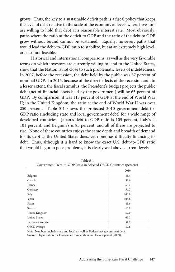
Addressing the Long-Run Fiscal Challenge | 147
grows. Thus, the key to a sustainable deficit path is a fiscal policy that keepsthe level of debt relative to the scale of the economy at levels where investorsare willing to hold that debt at a reasonable interest rate. Most obviously,paths where the ratio of the deficit to GDP and the ratio of the debt to GDPgrow without bound cannot be sustained. Equally, however, paths thatwould lead the debt-to-GDP ratio to stabilize, but at an extremely high level,are also not feasible.
Historical and international comparisons, as well as the very favorableterms on which investors are currently willing to lend to the United States,show that the Nation is not close to such problematic levels of indebtedness.In 2007, before the recession, the debt held by the public was 37 percent ofnominal GDP. In 2015, because of the direct effects of the recession and, toa lesser extent, the fiscal stimulus, the President’s budget projects the publicdebt (net of financial assets held by the government) will be 65 percent ofGDP. By comparison, it was 113 percent of GDP at the end of World WarII; in the United Kingdom, the ratio at the end of World War II was over250 percent. Table 5-1 shows the projected 2010 government debt-to-GDP ratio (including state and local government debt) for a wide range ofdeveloped countries. Japan’s debt-to-GDP ratio is 105 percent, Italy’s is101 percent, and Belgium’s is 85 percent, and all of these are projected torise. None of these countries enjoys the same depth and breadth of demandfor its debt as the United States does, yet none has difficulty financing itsdebt. Thus, although it is hard to know the exact U.S. debt-to-GDP ratiothat would begin to pose problems, it is clearly well above current levels.
Table 5-1Government Debt-to-GDP Ratio in Selected OECD Countries (percent)
2010Belgium 85.4Canada 32.6France 60.7Germany 54.7Italy 100.8Japan 104.6Spain 41.6Sweden -13.1United Kingdom 59.0United States 65.2Euro-area average 57.9OECD average 57.6Note: Numbers include state and local as well as Federal net government debt.Source: Organisation for Economic Co-operation and Development (2009).
148 | Chapter 5
The Choice of a Fiscal AnchorIt is essential that the United States follow a fiscal policy that
stabilizes the debt-to-GDP ratio at a feasible level. In thinking about thespecific level of that ratio that policymakers should aim for, it is useful tothink about the implications that different levels of the budget deficit havefor the level of government debt in the long run. In particular, considerpaths where the deficit as a percent of GDP stabilizes at some level. If thedeficit-to-GDP ratio and the growth rate of nominal GDP are both steady,the debt-to-GDP ratio will settle down to the ratio of the deficit-to-GDP ratioto the growth rate of nominal GDP.4 For example, if the deficit is 1 percentof GDP and nominal GDP is growing at 5 percent per year, the debt-to-GDPratio will stabilize at 20 percent. Similarly, if the deficit-to-GDP ratio andthe growth rate of nominal GDP are both 4 percent, the debt-to-GDP ratiowill stabilize at 100 percent. Instead of thinking about various possible long-run targets for the debt-to-GDP ratio, policymakers can consider possibletargets for the deficit-to-GDP ratio and their accompanying implications forthe long-run debt-to-GDP ratio.
The choice among different deficit-to-GDP ratios involves tradeoffs.Lower deficits, and thus lower debt in the long run, have obvious advan-tages: a higher capital stock, lower foreign indebtedness, smaller globalimbalances, and more fiscal room to maneuver. But lower deficits havedisadvantages as well. They require smaller government programs, highertaxes, or both. Because Medicare, Medicaid, and Social Security will growfaster than GDP in coming decades even after the best efforts to make thoseprograms as efficient as possible, significant cuts in government spendingwould impose substantial costs. And higher taxes can reduce incentives towork, save, and invest.
Based on these considerations, the Administration believes that anappropriate medium-run goal is to balance the primary budget—the budgetexcluding interest payments on the debt. Including interest payments,this target will result in total deficits of approximately 3 percent of GDP.With real GDP growth of about 2.5 percent per year and inflation of about4 To see this, consider the case where the deficit-to-GDP ratio equals the growth rate of GDP.Then the dollar amount of debt issued in a year (that is, the deficit) equals the dollar increasein GDP. If the debt-to-GDP ratio is 100 percent—the amount of debt outstanding equalsGDP—then the percent increase in debt exactly equals the percent increase in GDP, and thedebt-to-GDP ratio holds steady at 100 percent. If, however, the amount of debt outstanding isless than nominal GDP, then adding a dollar to the debt results in a larger percentage increase inthe debt than does a dollar added to GDP. Hence, the debt-to-GDP ratio will rise. If the amountof debt outstanding is more than nominal GDP, then the percent increase in debt is smallerthan the percent increase in GDP and the debt-to-GDP ratio falls. Thus, the debt-to-GDP ratioconverges to the ratio of the deficit-to-GDP ratio to the growth rate of GDP, which in this caseis 100 percent.

Addressing the Long-Run Fiscal Challenge | 149
2 percent per year, nominal GDP growth will be about 4.5 percent per yearin the long run. Thus a target for the total deficit-to-GDP ratio of 3 percentimplies that the debt-to-GDP ratio will stabilize at less than 70 percent.Because the debt-to-GDP ratio is projected to rise to about 65 percent in afew years, such a target implies that the debt-to-GDP ratio will change littleonce the economy has recovered from the current recession. A debt-to-GDPratio of around two-thirds is comfortably within the range of historical andinternational experience. It represents substantial fiscal discipline relativeto the trajectory the Administration inherited. Stabilizing the ratio ratherthan continuing on a path where it is continually growing is imperative, andstabilizing it at around its post-crisis level has considerable benefits and is anatural focal point.
Reaching the Fiscal Target
Bringing the primary budget into balance and keeping it there will notbe easy. Noninterest spending outstrips tax revenues by a large margin inthe budget inherited by the Administration. More importantly, the trajec-tory of policy implied that spending would continue to exceed revenues evenafter the economy had recovered and that the deficit would rise steadily fordecades to come. The economic developments and policy decisions that putfiscal policy on that course took place over many years. Thus, moving policyback onto a sound path will not happen all at once.
General PrinciplesIn broad terms, the right way to tackle the long-run fiscal problem is
not through a sharp, immediate fiscal contraction, but through policies thatsteadily address the underlying drivers of deficits over time. Large spendingcuts or tax increases are exactly the wrong medicine for an economy withhigh unemployment and considerable unused capacity: just as fiscalstimulus raises income and employment in such an environment, mistimedattempts at fiscal discipline have the opposite effects. Any short-run fiscalcontraction can best be tolerated at a time when the Federal Reserve is nolonger constrained by the zero bound on nominal interest rates, and so hasthe tools to counteract any contractionary macroeconomic impacts.
The dangers of a large immediate contraction are powerfully illus-trated by America’s experience in the Great Depression. In 1937, after fouryears of very rapid growth but with the economy still far from fully recovered,both fiscal and monetary policy turned sharply contractionary: the veterans’bonus program of the previous year was discontinued, Social Security taxeswere collected for the first time, and the Federal Reserve doubled reserve

150 | Chapter 5
requirements. The consequences of this premature policy tightening weredevastating: real GDP fell by 3 percent in 1938, unemployment spiked from14 percent to 19 percent, and the strong recovery was cut short.
The impact of actions taken today to gradually bring the long-runsources of the deficit problem under control would be very different. Suchpolicies do not involve a sharp short-run contraction that could derail anascent recovery. Because the effects cumulate over time, however, they canhave a large effect on the long-term fiscal outlook.
Policies that provide gradual but permanent and growing deficitreduction have another potential advantage. By improving the outlookfor the long-term performance of the economy, they can improve businessand consumer confidence today. As a result, deficit-improving policieswhose effects are felt mainly in the future can actually boost the economyin the short run. There is considerable evidence that such “expansionaryfiscal contractions” are not just a theoretical possibility (see, for example,Giavazzi and Pagano 1990; Alesina and Perotti 1997; Romer and Romerforthcoming).
In keeping with these general considerations, the Administration istaking actions in three important areas that will have a material impact onthe deficit in the medium and long terms.
Comprehensive Health Care ReformThe first and single most important step toward improving the
country’s long-run fiscal prospects is the enactment of comprehensive healthcare reform that will slow the growth rate of costs. Beyond the obviousimportance for Americans’ well-being and economic security, the healthreform legislation being considered by Congress would save money. Therapid growth of health care costs is a central source of the country’s fiscaldifficulties. CBO has estimated that both the bill passed by the House inNovember 2009 and the bill passed by the Senate in December 2009 wouldsignificantly reduce the deficit over the next decade (Congressional BudgetOffice 2009e, 2009d). But the more important factor for the long-run fiscalsituation is that, as discussed in more detail in Chapter 7, the bills containcrucial measures that experts believe will lead to lower growth in costswhile expanding access to coverage, increasing affordability, and improvingquality. Given the central role of rising health costs in the long-run deficitprojections, these measures would therefore lead to substantial improve-ments in the budget situation over time.
In November 2009, CBO’s analysis of the Senate health care bill foundthat “Medicare spending under the bill would increase at an average annual

Addressing the Long-Run Fiscal Challenge | 151
rate of roughly 6 percent during the next two decades—well below theroughly 8 percent annual growth rate of the past two decades” (CongressionalBudget Office 2009c). In December, the Council of Economic Advisersestimated that the fundamental health care reform in the Senate bill wouldreduce the annual growth rate of Medicare and Medicaid costs by a fullpercentage point below what it would otherwise be in the coming decade,and by even more in the following decade (Council of Economic Advisers2009b). These reductions reflect specific measures directed at identifiablesources of wasteful spending and fraud combined with institutional reformsthat will help counter the forces leading to excessive cost growth.
Such a reduction in the growth rate of health care costs would havea more profound effect on the long-run fiscal situation of the country thanvirtually any other fiscal decision being contemplated today. Even if theslowdown in cost growth held steady at 1 percentage point annually ratherthan rising in the second decade, it would reduce the budget deficit in2030 by about 2 percent of GDP relative to what it otherwise would be. Intoday’s terms, this is equivalent to almost $300 billion per year. Most ofthese savings reflect the direct impact of lower health care costs on Federalspending. To the extent that health care reform also slows the growth ofprivate sector health insurance costs, which are tax preferred, employeesin the private sector will benefit from higher wages and the Treasury fromincreased revenues; this becomes a second source of budget savings. Andthese direct savings are magnified by lower interest costs resulting fromthe reduced debt accumulation in the years preceding 2030 (Council ofEconomic Advisers 2009a). The need to expand coverage would reducethe overall impact of health care reform on the budget deficit somewhat.However, these costs of expansion would be more than offset even withinthe coming decade. Thereafter, reform will lower the deficit by increasingamounts over time.
Restoring Balance to the Tax CodeThe second major step the Administration is taking to address the
long-run fiscal challenge is restoring balance to the tax code that has beenlost since 2001. The 2001 and 2003 tax cuts disproportionately favoredwealthy taxpayers. According to estimates from the Urban-Brookings TaxPolicy Center (2010), in 2010 the 2001 and 2003 tax cuts will increase theafter-tax income of the poorest 20 percent of the population by 0.5 percent(about $51), the middle 20 percent by 2.6 percent ($1,023), and the top1 percent by 6.7 percent ($72,910). About 67 percent of the tax cuts wentto the top 20 percent of taxpayers, and 26 percent to the top 1 percent.
152 | Chapter 5
These tax cuts for the wealthiest Americans took place when the incomesof ordinary Americans were stagnating and inequality was reaching almostunprecedented levels. In other words, the tax cuts exacerbated the broadertrend rather than mitigated it.
The President has consistently maintained that the tax cuts went toofar in cutting taxes for people making more than $250,000 per year andthat the country could not afford the tax breaks given to that group overthe past eight years. That is why one important plank of his fiscal respon-sibility framework is to rebalance the tax code, so that it is similar to whatexisted in the late 1990s for those making more than $250,000 per year.Specifically, the Administration has proposed letting the marginal tax rateson ordinary income and capital gains for people making more than $250,000per year return to the levels they were in 2000. It has also proposed settingthe tax rate on dividends for high-income taxpayers to the same 20 percentrate that would apply to capital gains—which is lower than the rate in the1990s—and letting all other features of the 2001 and 2003 tax cuts expire forthese taxpayers. In addition, it has proposed limiting the rate of deductionsfor high-income taxpayers to 28 percent, so that the wealthy do not obtainproportionately larger benefits from their deductions than other Americansdo. None of these changes would take effect until 2011, so they would notaffect disposable incomes as the economy recovers in 2010. Nonetheless,they would raise nearly $1 trillion over the next 10 years and even moreover the longer run. Equivalently, they would reduce the budget deficitby more than 0.5 percent of GDP in the medium run and somewhat moreover time.
As just discussed, most of these changes would merely bring the taxrates on high-income taxpayers back to their levels in the 1990s. To theextent that some go further, on balance they are more than offset by thefact that some common types of income—dividends, for example—willhave rates significantly lower than in the 1990s. Looking at tax policy overU.S. postwar history more broadly shows even more clearly how moderatethe proposed changes are. Figure 5-7 shows the top marginal tax rates onordinary income and capital gains over time and their levels under theAdministration’s proposals. For ordinary income, a top rate of 39.6 percent,while higher than in the past eight years, is not high compared with the ratesthat prevailed during most of the past several decades and even during mostof the Reagan administration. For capital gains, the 20 percent rate is lowerthan in many previous periods and is certainly not unusual. And for divi-dends, the 20 percent rate proposed by the Administration would be lowerthan under any other modern president save the last.
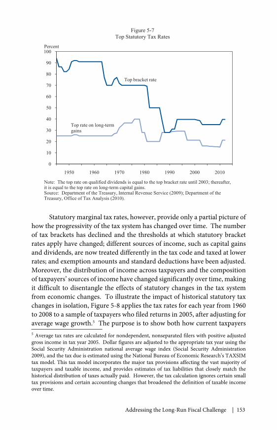
Addressing the Long-Run Fiscal Challenge | 153
Statutory marginal tax rates, however, provide only a partial picture ofhow the progressivity of the tax system has changed over time. The numberof tax brackets has declined and the thresholds at which statutory bracketrates apply have changed; different sources of income, such as capital gainsand dividends, are now treated differently in the tax code and taxed at lowerrates; and exemption amounts and standard deductions have been adjusted.Moreover, the distribution of income across taxpayers and the compositionof taxpayers’ sources of income have changed significantly over time, makingit difficult to disentangle the effects of statutory changes in the tax systemfrom economic changes. To illustrate the impact of historical statutory taxchanges in isolation, Figure 5-8 applies the tax rates for each year from 1960to 2008 to a sample of taxpayers who filed returns in 2005, after adjusting foraverage wage growth.5 The purpose is to show both how current taxpayers5 Average tax rates are calculated for nondependent, nonseparated filers with positive adjustedgross income in tax year 2005. Dollar figures are adjusted to the appropriate tax year using theSocial Security Administration national average wage index (Social Security Administration2009), and the tax due is estimated using the National Bureau of Economic Research’s TAXSIMtax model. This tax model incorporates the major tax provisions affecting the vast majority oftaxpayers and taxable income, and provides estimates of tax liabilities that closely match thehistorical distribution of taxes actually paid. However, the tax calculation ignores certain smalltax provisions and certain accounting changes that broadened the definition of taxable incomeover time.
0
10
20
30
40
50
60
70
80
90
100
1950 1960 1970 1980 1990 2000 2010
Figure 5-7Top Statutory Tax Rates
Percent
Top bracket rate
Top rate on long-termgains
Note: The top rate on qualified dividends is equal to the top bracket rate until 2003; thereafter,it is equal to the top rate on long-term capital gains.Source: Department of the Treasury, Internal Revenue Service (2009); Department of theTreasury, Office of Tax Analysis (2010).
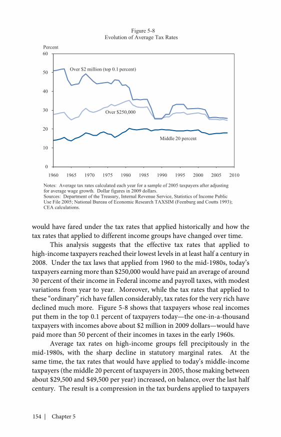
154 | Chapter 5
would have fared under the tax rates that applied historically and how thetax rates that applied to different income groups have changed over time.
This analysis suggests that the effective tax rates that applied tohigh-income taxpayers reached their lowest levels in at least half a century in2008. Under the tax laws that applied from 1960 to the mid-1980s, today’staxpayers earning more than $250,000 would have paid an average of around30 percent of their income in Federal income and payroll taxes, with modestvariations from year to year. Moreover, while the tax rates that applied tothese “ordinary” rich have fallen considerably, tax rates for the very rich havedeclined much more. Figure 5-8 shows that taxpayers whose real incomesput them in the top 0.1 percent of taxpayers today—the one-in-a-thousandtaxpayers with incomes above about $2 million in 2009 dollars—would havepaid more than 50 percent of their incomes in taxes in the early 1960s.
Average tax rates on high-income groups fell precipitously in themid-1980s, with the sharp decline in statutory marginal rates. At thesame time, the tax rates that would have applied to today’s middle-incometaxpayers (the middle 20 percent of taxpayers in 2005, those making betweenabout $29,500 and $49,500 per year) increased, on balance, over the last halfcentury. The result is a compression in the tax burdens applied to taxpayers
0
10
20
30
40
50
60
1960 1965 1970 1975 1980 1985 1990 1995 2000 2005 2010
Figure 5-8Evolution of Average Tax Rates
Percent
Over $2 million (top 0.1 percent)
Over $250,000
Middle 20 percent
Notes: Average tax rates calculated each year for a sample of 2005 taxpayers after adjustingfor average wage growth. Dollar figures in 2009 dollars.Sources: Department of the Treasury, Internal Revenue Service, Statistics of Income PublicUse File 2005; National Bureau of Economic Research TAXSIM (Feenburg and Coutts 1993);CEA calculations.

Addressing the Long-Run Fiscal Challenge | 155
with different incomes—the difference between the average tax rates onhigh-income groups and those on middle-class households is narrower thanat any other time in modern history. All told, because of legislative changesin the tax code, the after-tax income of the very-high-income group—theirdisposable income and purchasing power—is more than 50 percent higherthan it would have been under historical tax rates and brackets, while that ofthe middle class is slightly lower.
Under the Administration’s proposals, tax rates on taxpayers earningmore than $250,000 would be very close to the levels that prevailed in the1990s, leaving statutory tax rates on higher-income taxpayers far below thelevels that prevailed until the mid-1980s. The rebalancing of the tax codewould not affect middle-class taxpayers—except, of course, to the extentthat a better fiscal picture enhances medium- and long-term prospects foreconomic growth.
The need to restore balance is also evident in our corporate tax system,which encourages businesses to move jobs overseas and to transfer profitsto tax havens abroad in order to avoid taxes at home. The Administration’splan to reform international tax laws would reduce these incentives.
Balance also requires that the largest and most highly levered financialfirms reimburse taxpayers for the extraordinary assistance provided to themthrough the Troubled Asset Relief Program. The President has proposeda modest Financial Crisis Responsibility Fee to ensure that the cost of thefinancial rescue is not borne by taxpayers. Moreover, the fee would providea deterrent against the excessive leverage that helped contribute to the crisis.
Eliminating Wasteful SpendingThe third step the Administration is taking to confront the long-term
deficit is cutting unnecessary spending. The President pledged to elimi-nate programs that are not working. Last year, the Administration eitherproposed or enacted cuts to 121 specific programs; these proposed cutstotaled $17 billion in the first year and hundreds of billions of dollars overthe 10-year budget window. They include billions of dollars in terminationsof defense programs such as the F-22 fighter aircraft and the new Presidentialhelicopter, cuts in subsidies for large, high-income agribusinesses, andmore than $40 billion in savings over the next 10 years from eliminatingunnecessary subsidies to financial institutions in the private studentloan market.
In its fiscal 2011 budget, the Administration is proposing anotherimportant measure for spending restraint: a three-year freeze in all nonse-curity discretionary spending starting in 2011. The freeze would be a tough
156 | Chapter 5
measure of shared sacrifice. By 2013, it would reduce overall nonsecurityfunding by $30 billion per year relative to current inflation-adjusted fundinglevels.
The President also strongly supports restoring the pay-as-you-gorequirement (PAYGO) that was in place in the 1990s. This law, whichrequires that lawmakers make the tough choices needed to offset the costs ofnew nonemergency spending or tax changes, helped move the governmentbudget from deficit to surplus a decade ago. PAYGO is an important tool toforce the government to live within its means and move the budget towardfiscal sustainability.
These measures mean that once the temporary rise in governmentspending necessitated by the economic crisis has ended, spending will be ona lower path than it otherwise would have been. Moreover, both the multi-year freeze and steps to identify additional unnecessary spending each yearmake the reduction gradual rather than sudden. As a result, the cumulativereduction is substantial, yet there is never a sudden, potentially disruptivedrop in spending.
Conclusion: The Distance Still to Go
The actions the Administration has taken and is proposing wouldreduce deficits by more than $1 trillion over the next 10 years and by evenmore after that. These actions are significantly bolder steps toward deficitreduction than any taken in decades, and they will face serious opposition bythose with vested interests. Even with these actions, however, the primarybudget is forecast to remain in deficit in 2015. And the longer-run fiscalproblem facing the country still centers on the growth of health care costsand the aging of the population. Thus, barring a substantial and sustainedquickening of economic growth above its usual trend rate, further steps willbe needed to get the deficit down to the target in the medium and long run.
Regardless of the form they take, these additional steps to reducethe deficit will involve sacrifices by a broad range of groups and significantcompromise. Thus, a bipartisan effort will be essential. That is why thePresident is issuing an executive order creating a bipartisan fiscal commis-sion to report back with a package of measures for additional deficitreduction. The charge to the commission is to propose both medium-termactions to close the gap between noninterest expenditures and tax revenuesand additional steps to address the longer-term issues associated with risinghealth care costs, the aging of the population, and the persistent deficit.The commission’s recommendations will form an important foundation onwhich to base policy decisions moving forward.

Addressing the Long-Run Fiscal Challenge | 157
The Administration understands that addressing the long-run fiscalchallenge will be a long and difficult task requiring commitment and sharedsacrifice. But the President also believes that Americans deserve for andexpect policymakers to deal with the ever-rising deficit. The changes even-tually enacted will be central to the long-run preservation of both America’sfinancial strength and the standards of living of ordinary Americans.

159
C H A P T E R 6
BUILDING A SAFERFINANCIAL SYSTEM
From the ashes of the Great Depression, our leaders built a national systemof financial regulation. Before 1933, there was no national regulator for
stock and bond markets, no required disclosure by public firms, no nationaloversight of mutual funds or investment advisors, no insurance for bankdepositors, and few restrictions on the activities of banks or other financialinstitutions. By 1940, landmark legislation had created the Securities andExchange Commission, the Federal Deposit Insurance Corporation, newand important powers for the Federal Reserve, and disclosure requirementsfor virtually every major player in financial markets. The pieces of this regu-latory structure fit together in a relatively cohesive whole, and the UnitedStates enjoyed a long period of relative financial calm. In the 60 years beforethe Great Depression, our Nation experienced seven episodes of financialpanic, in which many banks were forced to shut their windows and declinedto redeem deposit accounts. In the nearly 80 years since the Depression, nota single financial crisis has risen to that level.
Although the system of regulation put together during the Depressionserved us well for many years, warning signs appeared periodically. Thesavings and loan crisis of the late 1980s and early 1990s showed howbanking regulation itself can have unintended consequences. At that time,deregulation coupled with generous deposit insurance combined to createa dangerous pattern of risk-taking that eventually led to a large Federalbailout of the financial system. In 1998, the collapse of Long-Term CapitalManagement highlighted gaps in the regulatory structure and induced theFederal Reserve Bank of New York to organize an unprecedented privaterescue of an unregulated hedge fund. In 2001, the collapse of Enron laid barethe complexity of the financial operations at seemingly nonfinancial corpora-tions and posed new challenges for accountants, policymakers, and analysts.Regulatory changes in the past 30 years responded to the specific weaknessesdemonstrated by these crises, but these changes were incremental and lacked

160 | Chapter 6
a strategic plan. Throughout this period, the architecture created after theGreat Depression was becoming increasingly inadequate to handle ongoingfinancial innovation. It was in this vacuum that financial innovation acceler-ated during the first decade of the 21st century.
The weaknesses in our outdated regulatory system nearly droveour economy into a second Great Depression. After the bankruptcy ofLehman Brothers in September 2008, credit markets froze and the FederalGovernment was forced to embark on increasingly aggressive interventionin financial markets. But as bad as the situation was, it could have beenmuch worse. Courage and creativity during the depths of the crisis, andforceful stewardship by the Administration in the aftermath, have enabledour Nation to escape a second Great Depression. Chapter 2 of this reportdiscusses the major elements of the Administration’s recovery plan. Thischapter focuses on the long-term changes necessary to prevent future crises.
What Is Financial Intermediation?
Suppose that the world woke up tomorrow to find all the banks gone,along with insurance companies, investment banks, mutual funds, and allthe other institutions where ordinary people put their savings. What wouldhappen? In the short run, people could keep their savings in mattressesand piggy banks, and the only apparent losses would be the forgone interestand dividends. But with no easy way to get the savings from piggy banksinto productive investment, the economy would face bigger problems veryquickly. Entrepreneurs with ideas would find it difficult to get capital. Largecompanies in need of money to restructure their operations would have noway to borrow against their future earnings. Young families would haveno way to buy a house until they had personally saved enough to affordthe whole thing. Our system of financial intermediation makes possible allthose activities, and the infrastructure to perform that function is necessarilycomplex and costly.
The Economics of Financial IntermediationFigure 6-1 is a simplified diagram of the main function of financial
intermediation: transforming savings into investment. The ultimate sourceof funds is shown on the left: individuals and institutions that have the finalclaim on wealth and wish to save some of it for the future. The ultimate useof funds is shown on the right: the productive activities that need funds forinvestment. The middle of the diagram can be classified as “financial inter-mediation.” Financial intermediation uses either markets (like the stockmarket) or institutions (like a bank) to channel savings into investment.
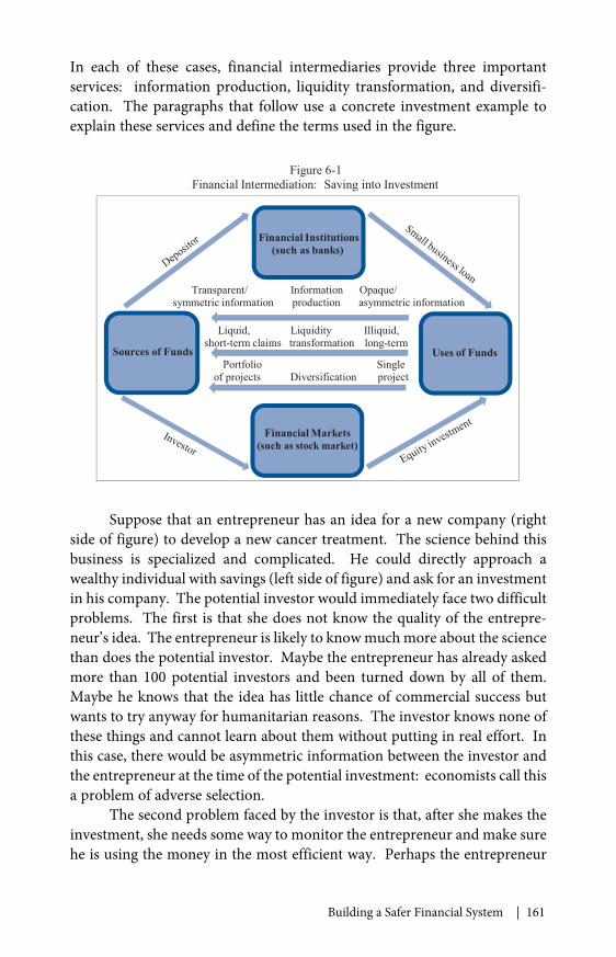
Building a Safer Financial System | 161
In each of these cases, financial intermediaries provide three importantservices: information production, liquidity transformation, and diversifi-cation. The paragraphs that follow use a concrete investment example toexplain these services and define the terms used in the figure.
Suppose that an entrepreneur has an idea for a new company (rightside of figure) to develop a new cancer treatment. The science behind thisbusiness is specialized and complicated. He could directly approach awealthy individual with savings (left side of figure) and ask for an investmentin his company. The potential investor would immediately face two difficultproblems. The first is that she does not know the quality of the entrepre-neur’s idea. The entrepreneur is likely to know much more about the sciencethan does the potential investor. Maybe the entrepreneur has already askedmore than 100 potential investors and been turned down by all of them.Maybe he knows that the idea has little chance of commercial success butwants to try anyway for humanitarian reasons. The investor knows none ofthese things and cannot learn about them without putting in real effort. Inthis case, there would be asymmetric information between the investor andthe entrepreneur at the time of the potential investment: economists call thisa problem of adverse selection.
The second problem faced by the investor is that, after she makes theinvestment, she needs some way to monitor the entrepreneur and make surehe is using the money in the most efficient way. Perhaps the entrepreneur
Figure 6-1Financial Intermediation: Saving into Investment
Sources of Funds
Financial Institutions(such as banks)
Uses of Funds
Financial Markets(such as stock market)
Transparent/ Information Opaque/symmetric information production asymmetric information
Liquid, Liquidity Illiquid,short-term claims transformation long-term
Portfolio Singleof projects Diversification project

162 | Chapter 6
will decide to use the money for some other business or research purpose.How will the investor know? Even worse, what is to prevent the entrepre-neur from using the funds for his personal benefit or taking the moneywithout putting in any effort? In this case, there would be additional asym-metric information introduced after the investment was made: economistscall this a problem of moral hazard.
To solve these adverse selection and moral hazard problems, theinvestor will need to expend some resources. She will need to study thetechnology, evaluate its chances for scientific and commercial success, andthen carefully watch over the entrepreneur after the investment is made.These activities are difficult and costly, and there is no reason to believe thata typical source of funds (whose main qualification is that she has money toinvest) would also be the best person to solve these problems. One importantservice of financial intermediation is to efficiently solve the adverse selectionand moral hazard problems that come with the transformation of savings intoinvestment. This chapter refers to this service as information production.
The second main service of financial intermediation is liquidity trans-formation. Consider how long it takes to develop a cancer treatment. Inthe United States, all new drug treatments must pass through a complexregulatory review stretched over many years. Even if a drug is eventuallyapproved, the path to commercial success can take many more years. Mostinvestors do not want to wait that long to see any return on their money.Individual investors have uncertain liquidity needs—jobs can be lost, familymembers can get sick—and even institutional investors are subject to perfor-mance evaluation over short periods. Overall, investment projects tend tohave long production times, while investment sources prefer to have easyaccess to their money. Somebody, somewhere, must be willing to absorbthe liquidity needs of the economy. In practice, these needs are provided byliquidity transformation: financial institutions and markets transform long-term (illiquid) investment projects into short-term (liquid) claims.
Liquidity transformation is also important for another, moreworrisome, reason: it is the main source of the fragility that can lead toa financial crisis. Because most intermediaries have illiquid assets andliquid liabilities, any broad-based attempt by creditors to call liabilities atthe same time creates an impossible situation for the intermediary. Theclassic example is a bank run, where holders of deposits (liquid liabilities)all “run” at the same time to withdraw their funds, leaving banks unable tosell the illiquid business loans and mortgages quickly enough to meet thesedemands. The same process can occur in a wide variety of nonbank institu-tions, as is discussed at length later in this chapter.
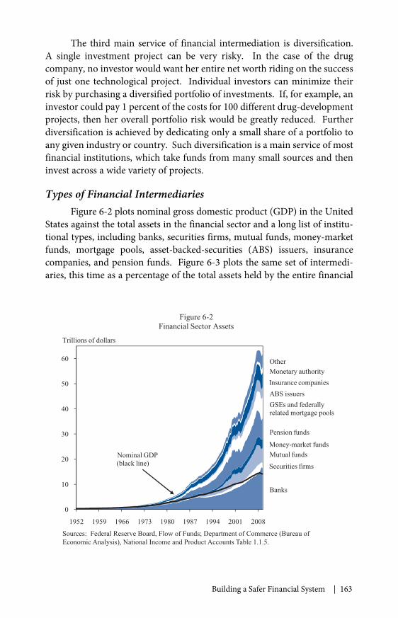
Building a Safer Financial System | 163
The third main service of financial intermediation is diversification.A single investment project can be very risky. In the case of the drugcompany, no investor would want her entire net worth riding on the successof just one technological project. Individual investors can minimize theirrisk by purchasing a diversified portfolio of investments. If, for example, aninvestor could pay 1 percent of the costs for 100 different drug-developmentprojects, then her overall portfolio risk would be greatly reduced. Furtherdiversification is achieved by dedicating only a small share of a portfolio toany given industry or country. Such diversification is a main service of mostfinancial institutions, which take funds from many small sources and theninvest across a wide variety of projects.
Types of Financial IntermediariesFigure 6-2 plots nominal gross domestic product (GDP) in the United
States against the total assets in the financial sector and a long list of institu-tional types, including banks, securities firms, mutual funds, money-marketfunds, mortgage pools, asset-backed-securities (ABS) issuers, insurancecompanies, and pension funds. Figure 6-3 plots the same set of intermedi-aries, this time as a percentage of the total assets held by the entire financial
0
10
20
30
40
50
60
1952 1959 1966 1973 1980 1987 1994 2001 2008
Banks
Money-market fundsMutual funds
Securities firms
GSEs and federallyrelated mortgage pools
ABS issuers
Monetary authorityOther
Figure 6-2Financial Sector Assets
Trillions of dollars
Nominal GDP(black line)
Insurance companies
Pension funds
Sources: Federal Reserve Board, Flow of Funds; Department of Commerce (Bureau ofEconomic Analysis), National Income and Product Accounts Table 1.1.5.
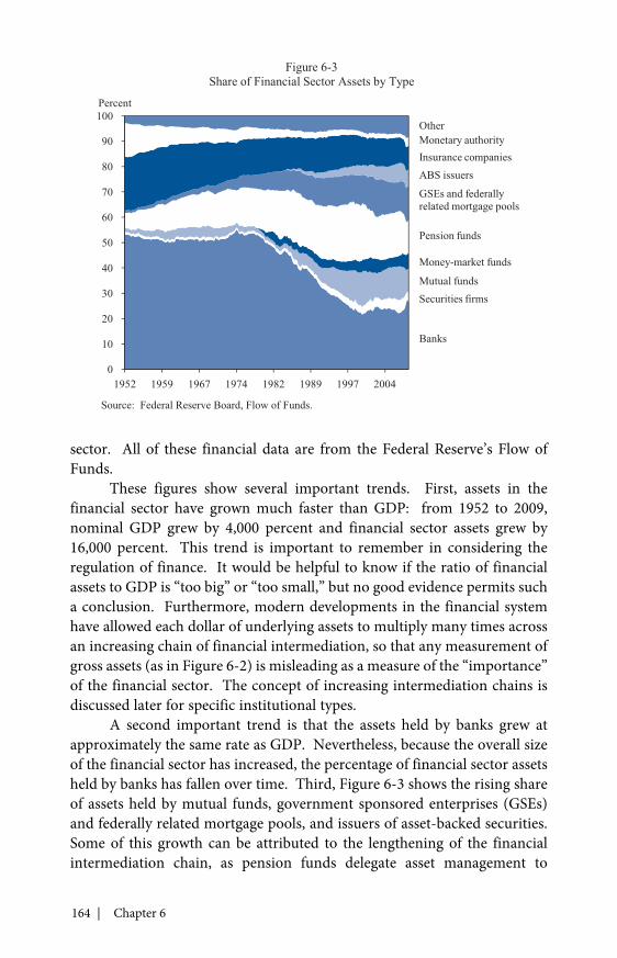
164 | Chapter 6
sector. All of these financial data are from the Federal Reserve’s Flow ofFunds.
These figures show several important trends. First, assets in thefinancial sector have grown much faster than GDP: from 1952 to 2009,nominal GDP grew by 4,000 percent and financial sector assets grew by16,000 percent. This trend is important to remember in considering theregulation of finance. It would be helpful to know if the ratio of financialassets to GDP is “too big” or “too small,” but no good evidence permits sucha conclusion. Furthermore, modern developments in the financial systemhave allowed each dollar of underlying assets to multiply many times acrossan increasing chain of financial intermediation, so that any measurement ofgross assets (as in Figure 6-2) is misleading as a measure of the “importance”of the financial sector. The concept of increasing intermediation chains isdiscussed later for specific institutional types.
A second important trend is that the assets held by banks grew atapproximately the same rate as GDP. Nevertheless, because the overall sizeof the financial sector has increased, the percentage of financial sector assetsheld by banks has fallen over time. Third, Figure 6-3 shows the rising shareof assets held by mutual funds, government sponsored enterprises (GSEs)and federally related mortgage pools, and issuers of asset-backed securities.Some of this growth can be attributed to the lengthening of the financialintermediation chain, as pension funds delegate asset management to
0
10
20
30
40
50
60
70
80
90
100
1952 1959 1967 1974 1982 1989 1997 2004
Figure 6-3Share of Financial Sector Assets by Type
Percent
Banks
Money-market funds
Mutual fundsSecurities firms
GSEs and federallyrelated mortgage pools
ABS issuers
Monetary authorityOther
Insurance companies
Pension funds
Source: Federal Reserve Board, Flow of Funds.
Building a Safer Financial System | 165
mutual funds, banks sell mortgages to mortgage pools, and money-marketfunds purchase securities from these pools.
Three long-standing institutional types are banks, securities firms,and insurance companies. Banks, including commercial banks, bankholding companies, savings institutions (thrifts), and credit unions, arestill the largest component of the financial sector, with $16.5 trillion inassets as of June 2009. Although bank assets represent 26.7 percent of thefinancial sector, their share has fallen precipitously since 1952, when it was53.2 percent. Securities firms, also known as investment banks or broker-dealers, had $2.0 trillion in assets, comprising 3.2 percent of the sector inJune 2009. This percentage was down considerably from an average of5.1 percent in 2007, because most of the largest securities firms wentbankrupt, were acquired by banks, or formally converted to banks duringthe crisis. Insurance companies have $5.9 trillion in assets, comprising9.5 percent of the sector as of June 2009.
Mutual funds and pension funds are a second layer of intermedia-tion, often standing in between investors and another institution or market.Mutual funds had $9.7 trillion in assets, comprising 15.7 percent of thesector, in June 2009, up from only 1.6 percent in 1952 and 3.1 percent in1980. Mutual funds take money from retail investors and invest in publicsecurities. An important subgroup of mutual funds are money-marketfunds (MMFs), which are broken out separately in these figures and in theunderlying Federal Reserve data. In 1990, MMFs held less than $500 billionin assets; by June 2009, their total assets were $3.6 trillion, comprising5.8 percent of total financial assets. MMFs invest only in relatively safe,short-term assets. Pension funds are a large and growing share of the sector,with assets of $8.3 trillion making up 13.5 percent of total financial assetsin June 2009. Many pension assets are reinvested in mutual funds, so theyshow up twice in the overall totals. Thus, some of the growth in overallsector assets is driven by this extra step of intermediation.
The next category in Figure 6-2 is GSEs and federally related mort-gage pools, with $8.4 trillion in assets in June 2009. Beginning in the 1930s,various nonbank sources emerged to buy mortgages on the secondarymarket. By the end of the 1970s, federally related mortgage pools—whichinclude those established by GSEs known as Fannie Mae and Freddie Mac—had almost $100 billion in assets. The growth of GSEs added an extra layer tothe financial intermediation of mortgages. Here, the bank provides a loan toa borrower but then resells this loan to a GSE. The bank may hold debt secu-rities issued by the GSE, and the GSE creates a pool that holds the mortgage.
In addition to those created by GSEs, private mortgage pools, focusingon “subprime” borrowers, have grown substantially in the past 10 years.

166 | Chapter 6
These private mortgage pools issue securities backed by the mortgages; thesesecurities, known as mortgage-backed securities (MBSs), are purchased andheld by mutual funds or other financial intermediaries. They are one typeof an asset-backed security managed by an ABS issuer. ABS issuers do notconfine themselves to mortgages; they also pool and securitize auto loans,student loans, credit card debt, and many other types of debt. Twenty yearsago, few ABS issuers existed, but by June 2009 they held $3.8 trillion in assetsand comprised 6.2 percent of total financial sector assets.
The remaining categories in Figures 6-2 and 6-3 are the monetaryauthority (the Federal Reserve) and “other.” As discussed in Chapter 2,the assets of the monetary authority increased rapidly during the crisis, butthe increase is expected to be reversed as the Federal Reserve exits fromits emergency programs and begins reducing the large stock of long-termsecurities it had purchased. The “other” category includes special purposevehicles created to manage the emergency lending programs and variousother minor groups of intermediaries.
Hedge funds are an increasingly important financial intermediary,but they are not included in Figures 6-2 and 6-3. Because of a lack of dataon domestic hedge funds, the Federal Reserve classifies such funds as partof the household sector and computes the assets of this sector as a residualafter everything else is added together and subtracted from total assets. TheFederal Reserve is unable to get a clean number for hedge funds because theyare largely unregulated private investment pools that are not required toreport their holdings to any official source. Unofficial sources estimate theamount of assets held by hedge funds to have been $1.7 trillion in 2008, butin the absence of regulatory oversight, this estimate is less reliable than theother totals shown in Figure 6-2 (Hedge Fund Research 2009).
The Regulation of Financial Intermediationin the United States
Private institutions and markets should clearly play the central role infinancial intermediation. But government also has a role. Economists gener-ally favor government regulation of markets that exhibit a market failure ofsome kind. This chapter has already discussed two types of market failure:adverse selection and moral hazard. Both can be classified as special casesof asymmetric information, where different parties to a contract do not havethe same information. The financial intermediation system alleviates asym-metric-information problems between savers and investors, but informationcan also be asymmetric between buyers and sellers of financial services.Just as physicians almost always know more than patients about medicine,
Building a Safer Financial System | 167
and lawyers more than their clients about law, banks and financial advisorsshould be expected to know more than their investors about investmentopportunities. For this reason, there will always be a consumer protectionbasis for some government regulation of financial services.
Consumer protection was an important motivation for several impor-tant pieces of Depression-era legislation. The first two, the Securities Act of1933 and the Securities Exchange Act of 1934, set forth a long list of require-ments for issuing and trading public securities. The list included many typesof public disclosure that persist to this day, including information aboutexecutive compensation, stockholdings, balance sheets, and income state-ments. The 1934 Act also created the Securities and Exchange Commission(SEC), the agency responsible for enforcing the new rules. These securitieslaws were the first Federal laws to regulate organized financial exchanges.
With regulated markets came the growth of intermediaries to servicethem. These intermediaries gained Federal oversight with the InvestmentAdvisers Act of 1940 (for publicly available investment advisory services)and the Investment Company Act of 1940 (for mutual funds). In total, thesefour pieces of legislation enacted between 1933 and 1940 represented a hugechange in the regulatory structure of financial markets and in most cases canbe considered attempts to lessen adverse selection and moral hazard prob-lems between investors, intermediaries, and investments.
Depression-era laws also strengthened the national system of bankregulation, adding new elements to a long pre-Depression history ofFederal regulation. Beginning with the National Bank Act of 1864, federallychartered banks have been examined regularly for capital adequacy. State-chartered banks received similar examinations from both state and Federalbanking agencies. Such examinations are a form of microprudential regula-tion, with a focus on the safety and soundness of individual institutions inisolation and with the aim of reducing asymmetric-information problems.Few bank depositors have the time or incentive to conduct detailed reviewsof their banks. When regulators conduct periodic reviews and publicizethe results, they create a public good of information about the safety andsoundness of individual banks. Furthermore, examinations and regulationscan constrain excessive risk-taking by federally insured institutions, a moralhazard problem faced by the government, rather than by bank depositors, inpart because of deposit insurance.
The microprudential approach, however, is not well suited to handlerisks to the entire financial system. The next section of this chapter discussesin detail the spread of crises. For now, it is sufficient to think of a crisis asan occasion when there is a sudden increase in the asymmetric-informationproblem in the financial system, as can happen after a large economic shock
168 | Chapter 6
or the failure of a major bank. The microprudential system of bank exami-nation can alleviate asymmetric-information problems in normal times, butbecause the government relies on careful periodic examinations, staggeredacross banks, it does not have the capacity to examine all banks quickly aftera shock or to evaluate the risk that a single bank failure will have on otherinstitutions. Faced with a large economic shock, bank customers can ratio-nally fear for the safety of their deposits. Since the upside of leaving one’smoney at a bank in such a situation is relatively small, but the downside—losing all one’s money—is large, it is individually rational for depositorsto withdraw their money when uncertainty increases. What is rationalfor individual depositors, however, puts an impossible strain on the wholebanking system, since the liquidity transformation performed by bankscannot be quickly reversed; the illiquid loans and mortgages held by bankscannot immediately be returned to all depositors as cash.
One partial solution to the liquidity problem during banking crisesis to create a “lender of last resort.” This lender stands ready to make cashloans to banks that are backed by illiquid collateral: essentially, this lenderserves as a new layer of liquidity transformation above the banks. This formof macroprudential policy was the traditional solution to banking crises inEurope in the 19th century but did not come to the United States until theFederal Reserve Act of 1913 created the first version of the Federal ReserveSystem as a lender of last resort.
But a lender of last resort, by itself, is unable to prevent bank runsacross the entire system. Even illiquid collateral must be given a value bythe lender—by law the Federal Reserve can only make secured loans—andif the entire system is failing at the same time, there may be no way for acentral bank to estimate reasonable valuations quickly enough. A lender oflast resort is designed to solve liquidity problems, not solvency problems, butin a severe crisis, these two problems can become inextricably tied together.(This problem arose during the current crisis, when Lehman Brothers wasunable to provide enough collateral to qualify for sufficient Federal Reserveloans.) During the Great Depression, some 9,000 bank failures occurredbetween 1930 and 1933, well above the number of failures in earlier panics.Shortly after taking office in 1933, President Franklin Roosevelt gave his first“fireside chat” and implied a government guarantee for all bank deposits.The Banking Act of 1933 made the guarantee explicit by creating depositinsurance through a new agency, the Federal Deposit Insurance Corporation(FDIC). In the 75 years that followed, the United States averaged fewer than30 commercial bank failures a year. The FDIC is a crucial piece of macro-prudential regulation in that it provides a guarantee to all insured banks,regardless of the condition of any specific bank. Within the account limits
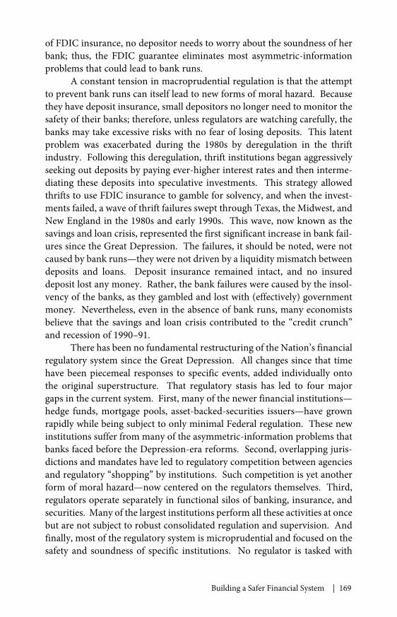
Building a Safer Financial System | 169
of FDIC insurance, no depositor needs to worry about the soundness of herbank; thus, the FDIC guarantee eliminates most asymmetric-informationproblems that could lead to bank runs.
A constant tension in macroprudential regulation is that the attemptto prevent bank runs can itself lead to new forms of moral hazard. Becausethey have deposit insurance, small depositors no longer need to monitor thesafety of their banks; therefore, unless regulators are watching carefully, thebanks may take excessive risks with no fear of losing deposits. This latentproblem was exacerbated during the 1980s by deregulation in the thriftindustry. Following this deregulation, thrift institutions began aggressivelyseeking out deposits by paying ever-higher interest rates and then interme-diating these deposits into speculative investments. This strategy allowedthrifts to use FDIC insurance to gamble for solvency, and when the invest-ments failed, a wave of thrift failures swept through Texas, the Midwest, andNew England in the 1980s and early 1990s. This wave, now known as thesavings and loan crisis, represented the first significant increase in bank fail-ures since the Great Depression. The failures, it should be noted, were notcaused by bank runs—they were not driven by a liquidity mismatch betweendeposits and loans. Deposit insurance remained intact, and no insureddeposit lost any money. Rather, the bank failures were caused by the insol-vency of the banks, as they gambled and lost with (effectively) governmentmoney. Nevertheless, even in the absence of bank runs, many economistsbelieve that the savings and loan crisis contributed to the “credit crunch”and recession of 1990–91.
There has been no fundamental restructuring of the Nation’s financialregulatory system since the Great Depression. All changes since that timehave been piecemeal responses to specific events, added individually ontothe original superstructure. That regulatory stasis has led to four majorgaps in the current system. First, many of the newer financial institutions—hedge funds, mortgage pools, asset-backed-securities issuers—have grownrapidly while being subject to only minimal Federal regulation. These newinstitutions suffer from many of the asymmetric-information problems thatbanks faced before the Depression-era reforms. Second, overlapping juris-dictions and mandates have led to regulatory competition between agenciesand regulatory “shopping” by institutions. Such competition is yet anotherform of moral hazard—now centered on the regulators themselves. Third,regulators operate separately in functional silos of banking, insurance, andsecurities. Many of the largest institutions perform all these activities at oncebut are not subject to robust consolidated regulation and supervision. Andfinally, most of the regulatory system is microprudential and focused on thesafety and soundness of specific institutions. No regulator is tasked with

170 | Chapter 6
taking a macroprudential approach, which attempts to monitor, recognize,and alleviate risks to the financial system as a whole. Such macroprudentialregulation would require explicit rules for the orderly resolution of all largefinancial institutions, not just the banks currently resolved by the FDIC.In short, because of these four gaps, the failure of one institution imposesnegative externalities on others, and there is no coherent system for fixingthese externalities.
Of the four gaps, the last requires the most urgent reform and thebiggest change in regulatory thinking. The financial crisis made clear howrapidly failures can spread across institutions and affect the whole system.A primary challenge of macroprudential regulation is to recognize such“contagion” and categorize and counteract all the different ways it canmanifest. The next section of the chapter turns to this task.
Financial Crises:The Collapse of Financial Intermediation
A financial crisis is a collapse of financial intermediation. In a crisis,the ability of the financial system to move savings into investment is severelyimpaired. In an extreme crisis, banks close their doors, financial markets shutdown, businesses are unable to finance their operations, and households arechallenged to find credit. A financial crisis can be triggered by events thatare completely external to the financial system. If a large macroeconomicshock hits all banks at the same time, regulators can do little to control thedamage. Some crises, however, are triggered or exacerbated by shocks to asmall group of institutions that then spread to others. This spread, knownas contagion, is a form of negative externality imposed by distressed institu-tions. The recent financial crisis involved three different types of contagion,referred to in this chapter as confidence contagion, counterparty contagion,and coordination contagion. A macroprudential regulator must have thetools to handle all three.
Confidence ContagionThe classic example of a “run on the bank” is shown in Figure 6-4.
Banks are mostly financed by deposits, which are then lent out as loans tobusinesses and mortgages for homeowners. A bank’s balance sheet has amaturity mismatch between assets (the loans) and liabilities (the deposits):the loans are long term, with payments coming over many years, while thedeposits are short term and can be withdrawn at any time. The liquiditytransformation service of the bank works in ordinary times but breaks downif all the depositors ask for their money back at the same time.
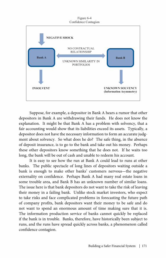
Building a Safer Financial System | 171
Suppose, for example, a depositor in Bank A hears a rumor that otherdepositors in Bank A are withdrawing their funds. He does not know theexplanation. It might be that Bank A has a problem with solvency, that afair accounting would show that its liabilities exceed its assets. Typically, adepositor does not have the necessary information to form an accurate judg-ment about solvency. So what does he do? The safe thing, in the absenceof deposit insurance, is to go to the bank and take out his money. Perhapsthese other depositors know something that he does not. If he waits toolong, the bank will be out of cash and unable to redeem his account.
It is easy to see how the run at Bank A could lead to runs at otherbanks. The public spectacle of long lines of depositors waiting outside abank is enough to make other banks’ customers nervous—the negativeexternality on confidence. Perhaps Bank A had many real estate loans insome trouble area, and Bank B has an unknown number of similar loans.The issue here is that bank depositors do not want to take the risk of leavingtheir money in a failing bank. Unlike stock market investors, who expectto take risks and face complicated problems in forecasting the future pathof company profits, bank depositors want their money to be safe and donot want to spend an enormous amount of time making sure that it is.The information production service of banks cannot quickly be replacedif the bank is in trouble. Banks, therefore, have historically been subject toruns, and the runs have spread quickly across banks, a phenomenon calledconfidence contagion.
Figure 6-4Confidence Contagion
Bank A Bank B
NO CONTRACTUALRELATIONSHIP
UNKNOWN SIMILARITY INPORTFOLIOS
INSOLVENT UNKNOWN SOLVENCY(Information Asymmetry)
NEGATIVE SHOCK
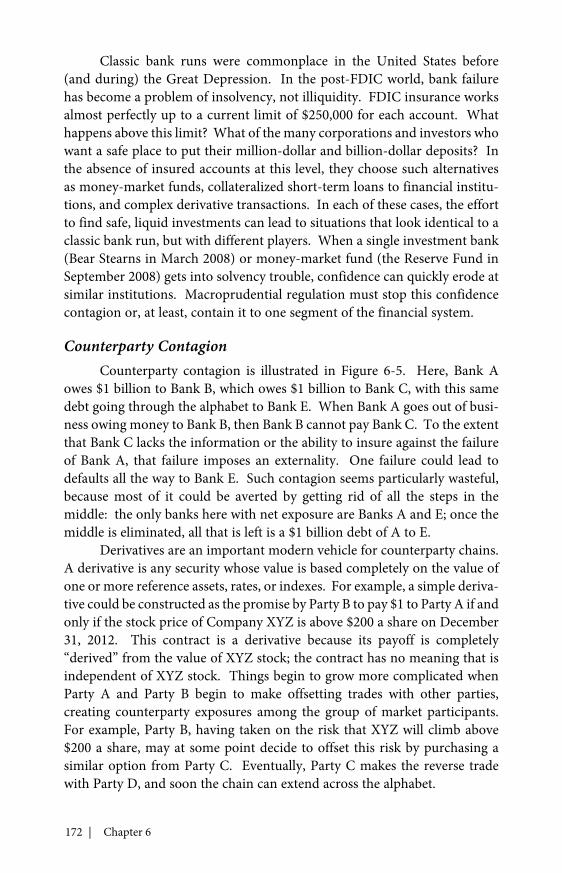
172 | Chapter 6
Classic bank runs were commonplace in the United States before(and during) the Great Depression. In the post-FDIC world, bank failurehas become a problem of insolvency, not illiquidity. FDIC insurance worksalmost perfectly up to a current limit of $250,000 for each account. Whathappens above this limit? What of the many corporations and investors whowant a safe place to put their million-dollar and billion-dollar deposits? Inthe absence of insured accounts at this level, they choose such alternativesas money-market funds, collateralized short-term loans to financial institu-tions, and complex derivative transactions. In each of these cases, the effortto find safe, liquid investments can lead to situations that look identical to aclassic bank run, but with different players. When a single investment bank(Bear Stearns in March 2008) or money-market fund (the Reserve Fund inSeptember 2008) gets into solvency trouble, confidence can quickly erode atsimilar institutions. Macroprudential regulation must stop this confidencecontagion or, at least, contain it to one segment of the financial system.
Counterparty ContagionCounterparty contagion is illustrated in Figure 6-5. Here, Bank A
owes $1 billion to Bank B, which owes $1 billion to Bank C, with this samedebt going through the alphabet to Bank E. When Bank A goes out of busi-ness owing money to Bank B, then Bank B cannot pay Bank C. To the extentthat Bank C lacks the information or the ability to insure against the failureof Bank A, that failure imposes an externality. One failure could lead todefaults all the way to Bank E. Such contagion seems particularly wasteful,because most of it could be averted by getting rid of all the steps in themiddle: the only banks here with net exposure are Banks A and E; once themiddle is eliminated, all that is left is a $1 billion debt of A to E.
Derivatives are an important modern vehicle for counterparty chains.A derivative is any security whose value is based completely on the value ofone or more reference assets, rates, or indexes. For example, a simple deriva-tive could be constructed as the promise by Party B to pay $1 to Party A if andonly if the stock price of Company XYZ is above $200 a share on December31, 2012. This contract is a derivative because its payoff is completely“derived” from the value of XYZ stock; the contract has no meaning that isindependent of XYZ stock. Things begin to grow more complicated whenParty A and Party B begin to make offsetting trades with other parties,creating counterparty exposures among the group of market participants.For example, Party B, having taken on the risk that XYZ will climb above$200 a share, may at some point decide to offset this risk by purchasing asimilar option from Party C. Eventually, Party C makes the reverse tradewith Party D, and soon the chain can extend across the alphabet.
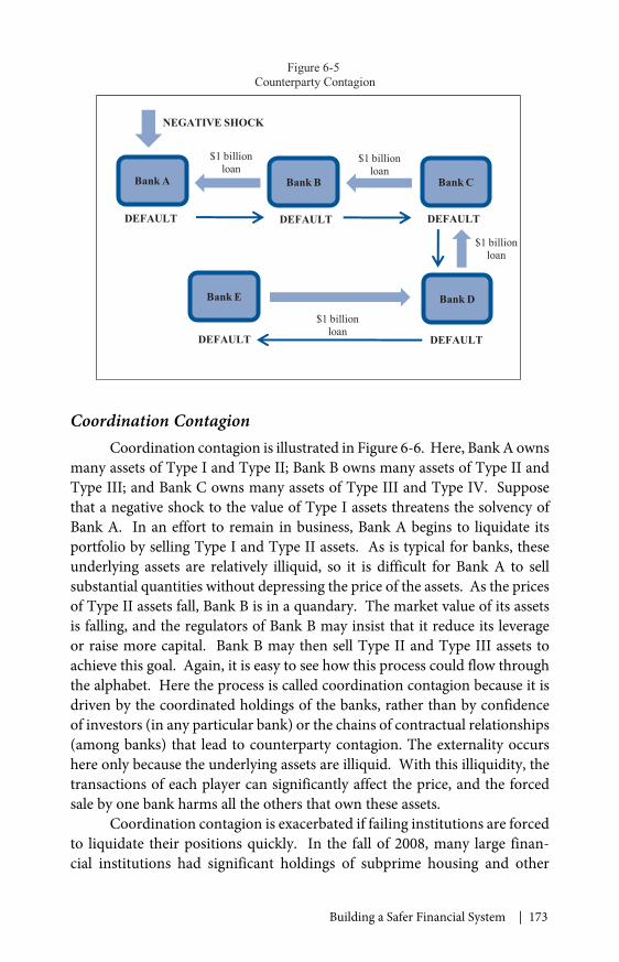
Building a Safer Financial System | 173
Coordination ContagionCoordination contagion is illustrated in Figure 6-6. Here, Bank A owns
many assets of Type I and Type II; Bank B owns many assets of Type II andType III; and Bank C owns many assets of Type III and Type IV. Supposethat a negative shock to the value of Type I assets threatens the solvency ofBank A. In an effort to remain in business, Bank A begins to liquidate itsportfolio by selling Type I and Type II assets. As is typical for banks, theseunderlying assets are relatively illiquid, so it is difficult for Bank A to sellsubstantial quantities without depressing the price of the assets. As the pricesof Type II assets fall, Bank B is in a quandary. The market value of its assetsis falling, and the regulators of Bank B may insist that it reduce its leverageor raise more capital. Bank B may then sell Type II and Type III assets toachieve this goal. Again, it is easy to see how this process could flow throughthe alphabet. Here the process is called coordination contagion because it isdriven by the coordinated holdings of the banks, rather than by confidenceof investors (in any particular bank) or the chains of contractual relationships(among banks) that lead to counterparty contagion. The externality occurshere only because the underlying assets are illiquid. With this illiquidity, thetransactions of each player can significantly affect the price, and the forcedsale by one bank harms all the others that own these assets.
Coordination contagion is exacerbated if failing institutions are forcedto liquidate their positions quickly. In the fall of 2008, many large finan-cial institutions had significant holdings of subprime housing and other
Figure 6-5Counterparty Contagion
Bank A Bank B Bank C
Bank E
$1 billionloan
$1 billionloan
DEFAULT DEFAULT DEFAULT
$1 billionloan
DEFAULTDEFAULT
$1 billionloan
NEGATIVE SHOCK
Bank D
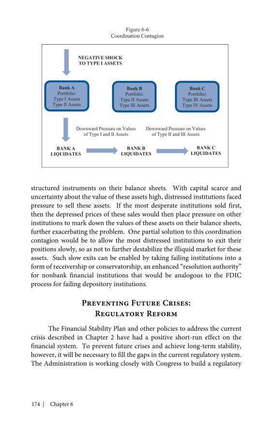
174 | Chapter 6
structured instruments on their balance sheets. With capital scarce anduncertainty about the value of these assets high, distressed institutions facedpressure to sell these assets. If the most desperate institutions sold first,then the depressed prices of these sales would then place pressure on otherinstitutions to mark down the values of these assets on their balance sheets,further exacerbating the problem. One partial solution to this coordinationcontagion would be to allow the most distressed institutions to exit theirpositions slowly, so as not to further destabilize the illiquid market for theseassets. Such slow exits can be enabled by taking failing institutions into aform of receivership or conservatorship, an enhanced “resolution authority”for nonbank financial institutions that would be analogous to the FDICprocess for failing depository institutions.
Preventing Future Crises:Regulatory Reform
The Financial Stability Plan and other policies to address the currentcrisis described in Chapter 2 have had a positive short-run effect on thefinancial system. To prevent future crises and achieve long-term stability,however, it will be necessary to fill the gaps in the current regulatory system.The Administration is working closely with Congress to build a regulatory
Figure 6-6Coordination Contagion
Bank APortfolio:
Type I AssetsType II Assets
Bank BPortfolio:
Type II AssetsType III Assets
BANK ALIQUIDATES
NEGATIVE SHOCKTO TYPE I ASSETS
Bank CPortfolio:
Type III AssetsType IV Assets
BANK BLIQUIDATES
BANK CLIQUIDATES
Downward Pressure on Valuesof Type I and II Assets
Downward Pressure on Valuesof Type II and III Assets

Building a Safer Financial System | 175
system for the 21st century.1 The plan for regulatory reform has five keyparts, each covering a different aspect of the financial intermediation systemillustrated by Figure 6-1. The parts of the plan are discussed below, withreferences back to the relevant sections of Figure 6-1.
Promote Robust Supervision and Regulation of Financial FirmsIf the recent financial crisis has proven anything, it is that we have
outgrown our Depression-era financial regulatory system. Although mostof the largest, most interconnected, and most highly leveraged financialfirms were subject to some form of supervision and regulation before thecrisis, those forms of oversight proved inadequate and inconsistent. Thefinancial institutions at the top of Figure 6-1 are a varied group that is nolonger dominated by traditional commercial banks. A modern regulatorysystem must account for the entire group.
Three primary weaknesses inherent in the current system led to thecrisis. First, capital and liquidity requirements for institutions were simplynot high enough. Regulation failed because firms were not required to holdsufficient capital to cover trading assets, high-risk loans, and off-balance-sheetcommitments, or to hold increased capital during good times in preparationfor bad times. Nor were firms required to plan for liquidity shortages.
Second, various agencies shared responsibility for supervising theconsolidated operations of large financial firms. This fragmentation ofsupervisory responsibility, in addition to loopholes in the legal definition ofa “bank,” made it possible for owners of banks and other insured depositoryinstitutions to shop for the most lenient regulator.
Finally, other types of financial institutions were subject to insufficientgovernment oversight. Money-market funds were vulnerable to runs, butunlike their banking cousins, they lacked both regulators and insurers.Major investment banks were subject to a regulatory regime through theSEC that is now moot, since large independent investment banks no longerexist. Meanwhile, hedge funds and other private pools of capital operatedcompletely outside the existing supervisory framework.
In combination, these three sets of weaknesses increased the likelihoodthat some firms would fail and made it less likely that problems at these firmswould be detected early. This was a breakdown in the supervision undercurrent authority over individual institutions. But glaring problems werealso created by a lack of focus on large, interconnected, and highly leveragedinstitutions that could inflict harm both on the financial system and on the
1 This section is based heavily on the Administration’s white paper on financial reform(Department of the Treasury 2009).
176 | Chapter 6
economy if they failed. No regulators were tasked with responsibility forcontagion, whether from confidence, counterparties, or coordination.
To solve these problems and ensure the long-term health of thefinancial system, the government must create a new foundation for theregulation of financial institutions. To do that, the Administration willpromote more robust and consistent regulatory standards for all financialinstitutions. Not only should similar financial institutions face the samesupervisory and regulatory standards, but the system can contain no gaps,loopholes, or opportunities for arbitrage.
The Administration has also proposed creating a Financial ServicesOversight Council (FSOC). This body, chaired by the Secretary of theTreasury, would facilitate coordination of policy and resolution of disputesand identify emerging risks and gaps in supervision in firms and marketactivities. The heads of the principal Federal financial regulators would bemembers of the Council, which would benefit from a permanent staff at theDepartment of the Treasury.
Finally, the Federal Reserve’s current supervisory authority for bankholding companies must evolve along with the financial system. Regardlessof whether they own an insured depository institution, all large, intercon-nected firms whose failure may threaten the stability of the entire systemshould be subject to consolidated supervision by the Federal Reserve. Tothat end, the Administration proposes creating a single point of account-ability for the consolidated supervision of all companies that own a bank.These firms should not be allowed or able to escape oversight of their riskyactivities by manipulating their legal structures.
Taken together, these proposals will help reduce the weaknesses inthe financial regulatory system by more stringently regulating the largest,most interconnected, and most highly leveraged institutions. In effect,the Administration’s proposals would operate on the simple principle thatfirms that could pose higher risks should be subject to higher standards.Furthermore, both the Federal Reserve and the FSOC would operatethrough a macroprudential prism and be wary of contagion in all its forms.
Establish Comprehensive Regulation of Financial MarketsThe financial crisis followed a long and remarkable period of growth
and innovation in the Nation’s financial markets. These new financialmarkets, found in the bottom part of Figure 6-1, still rely on regulationput together in response to the Great Depression, when stocks and bondswere the main financial products for which there were significant markets.But over time, new financial instruments allowed credit risks to be spreadwidely, enabling investors to diversify their portfolios in new ways and

Building a Safer Financial System | 177
allowing banks to shed exposures that once would have had to remain ontheir balance sheets. As discussed earlier, securitization allowed mortgagesand other loans to be aggregated with similar loans, segmented, and sold intranches to a large and diverse pool of new investors with varied risk prefer-ences. Credit derivatives created a way for banks to transfer much of theircredit exposure to third parties without the outright selling of the underlyingassets. At the time, this innovation in the distribution of risk was perceivedto increase financial stability, promote efficiency, and contribute to a betterallocation of resources.
Far from transparently distributing risk, however, the innovationsoften resulted in opaque and complex risk concentrations. Furthermore, theinnovations arose too rapidly for the market’s infrastructure, which consistsof payment, clearing, and settlement systems, to accommodate them, andfor the Nation’s financial supervisors to keep up with them. Furthermore,many individual financial institutions’ risk management systems failed tokeep up. The result was a disastrous buildup of risk in the over-the-counter(OTC) derivatives markets. In the run-up to the crisis, many believed thesemarkets would distribute risk to those most able to bear it. Instead, thesemarkets became a major source of counterparty contagion during the crisis.
In response to these problems, the Administration proposes creatinga more coherent and coordinated regulatory framework for the marketsfor OTC derivatives and asset-backed securities. The Administration’sproposal, which aims to improve both transparency and market discipline,would impose record-keeping and reporting requirements on all OTC deriv-atives. The Administration further proposes strengthening the prudentialregulation of all dealers in the OTC derivative markets and requiring allstandardized OTC derivative transactions to be executed in regulated andtransparent venues and cleared through regulated central counterparties.The primary goal of these regulatory changes is to reduce the possibility ofthe sort of counterparty contagion seen in the recent crisis. Moving activityto a centralized clearinghouse can effectively break the chain of failures bynetting out middleman parties. A successful clearinghouse can reduce thecounterparty contagion illustrated in Figure 6-5 to a single debt owned byBank A to Bank E, thus sparing Banks B, C, and D from the problems.
The Administration has also proposed enhancing the Federal Reserve’sauthority over market infrastructure to reduce the potential for contagionamong financial firms and markets. After all, even a clearinghouse can fail,and regulators must be alert to this danger. Finally, the Administrationproposes harmonizing the statutory and regulatory regimes between thefutures and securities markets. Although important distinctions existbetween the two, many differences in regulation between them are no longer

178 | Chapter 6
justifiable. In particular, the growth and innovation in derivatives andderivatives markets have highlighted the need to address gaps and incon-sistencies in the regulation of these products by the Commodity FuturesTrading Commission (CFTC) and the SEC. In October 2009, the SEC andthe CFTC issued a joint report identifying major areas necessary to reconciletheir regulatory approaches and outlining a series of regulatory and statutoryrecommendations to narrow or where possible eliminate those differences.
Provide the Government with the Tools It Needs to ManageFinancial Crises
During the recent crisis, the financial system was strained by thefailure or near-failure of some of the largest and most interconnected finan-cial firms. Thanks to lessons learned from past crises, the current systemalready has strong procedures for handling bank failure. However, when abank holding company or other nonbank financial firm is in severe distress,it has only two options: obtain outside capital or file for bankruptcy. In anormal economic climate, these options would be suitable and would poseno consequences for broader financial stability. However, during a crisis,distressed institutions may be hard-pressed to raise sufficient private capital.Thus, if a large, interconnected bank holding company or other nonbankfinancial firm nears failure during a financial crisis, its only two options areuntenable: to obtain emergency funding from the U.S. Government, as inthe case of AIG; or to file for bankruptcy, as in the case of Lehman Brothers.Neither option manages the resolution of the firm in a manner that limitsdamage to the broader economy at minimal cost to the taxpayer.
This situation is unacceptable. A way must be found to address thepotential failure of a bank holding company or other nonbank financial firmwhen the stability of the financial system is at risk. To solve this issue, theAdministration proposes creating a new authority modeled on the existingauthority of the FDIC. The Administration has also proposed that theFederal Reserve Board receive prior written approval from the Secretaryof the Treasury for emergency lending under its “unusual and exigentcircumstances” authority to improve accountability in the use of other crisistools. The goal of these proposals is to allow for an orderly resolution ofall large institutions—not just banks—so that the coordination contagiondepicted in Figure 6-6 does not again threaten the entire financial system.Taking nonbank financial institutions into receivership or conservatorshipwould make it possible to sell assets slowly and with minimal disruption tothe values of similar assets at otherwise healthy institutions.

Building a Safer Financial System | 179
Raise International Regulatory Standards and ImproveInternational Cooperation
The system in Figure 6-1 cannot be managed by one country alone,because its interconnections are global. As the recent crisis has illustrated,financial stress can spread quickly and easily across borders. Yet regulationis still set largely in a national context and has failed to effectively adapt.Without consistent supervision and regulation, rational financial institutionswill see opportunity in this situation and move their activities to jurisdictionswith looser standards. This can create a “race to the bottom” situation.
The United States is addressing this issue by playing a strong leader-ship role in efforts to coordinate international financial policy through theGroup of Twenty (G-20), the G-20’s newly established Financial StabilityBoard, and the Basel Committee on Banking Supervision. The goal is topromote international initiatives compatible with the domestic regulatoryreforms described in this report. These efforts have already borne fruit. InSeptember, the G-20 met in Pittsburgh and agreed in principle to this goal.And while those processes are ongoing, significant progress has been madein agreements strengthening prudential requirements, including capital andliquidity standards; expanding the scope of regulation to nonbank finan-cial institutions, hedge funds, and over-the-counter derivatives markets;and reinforcing international cooperation on the supervision of globallyactive firms.
Protect Consumers and Investors from Financial AbuseBefore the financial crisis, numerous Federal and state regulations
protected consumers against fraud and promoted understanding of finan-cial products like credit cards and mortgages. But as abusive practicesspread, particularly in the subprime and nontraditional mortgage markets,the Nation’s outdated regulatory framework proved inadequate in crucialways. Although multiple agencies now have authority over consumerprotection in financial products, the supervisory framework for enforcingthose regulations has significant shortcomings rooted in history. State andFederal banking regulators have a primary mission to promote safe andsound banking practices—placing consumer protection in a subordinateposition—while other agencies have a clear mission but limited tools andjurisdiction. In the run-up to the financial crisis, mortgage companies andother firms outside of the purview of bank regulation exploited the lack ofclear accountability by selling subprime mortgages that were overly compli-cated and unsuited to borrowers’ particular financial situations. Banks and
180 | Chapter 6
thrifts eventually followed suit, with disastrous results for consumers and thefinancial system at large.
In 2009, Congress, the Administration, and numerous financialregulators took significant measures to address some of the most obviousinadequacies in the consumer protection framework. One notable achieve-ment was the Credit Card Accountability, Responsibility, and DisclosureAct, signed into law by the President on May 22, 2009. This Act outlawssome of the most unfair and deceptive practices in the credit card industry.For example, it requires that payments be applied to the balances with thehighest interest rate first; bans retroactive increases in interest rates forreasons having nothing to do with the cardholder’s record with the creditcard; prohibits a variety of gimmicks with due dates and “double-cycle fees”;and requires clearer disclosure and ensures consumer choice.
However, given the weaknesses that the recent financial crisis high-lighted, it is clear that the consumer protection system needs comprehensivereform across all markets. For that reason the Administration has proposedcreating a single regulatory agency, a Consumer Financial Protection Agency(CFPA), with the authority and accountability to make sure that consumerprotection regulations are written fairly and enforced vigorously. The CFPAshould reduce gaps in Federal supervision and enforcement, improve coor-dination with the states, set higher standards for financial intermediaries,and promote consistent regulation of similar products.
Conclusion
Our Nation’s system of financial intermediation is a powerful enginefor economic growth. Productive investment projects are risky, complex toevaluate and monitor, and require long periods of waiting with no returnsand illiquid capital. Investors who provide the funds for these projectswould be far less willing to do so if they had to absorb all these risks andcosts. Bridging the gap between savings and investment requires the effortsof millions of talented professionals collectively performing the services ofinformation production, liquidity transformation, and diversification. Inthe recent financial crisis this complex system broke down.
To prevent another such crisis from paralyzing our economy, theAdministration has embarked on an ambitious plan to modernize theframework of financial regulation. The keystone of the new framework isan emphasis on macroprudential regulation. The regulatory system’s pastfocus on individual institutions served the Nation well for many decadesbut is now outdated. A modern system that can meet the needs of the 21stcentury must have the tools to monitor and regulate the interconnectionsthat cause financial crises.

181
C H A P T E R 7
REFORMING HEALTH CARE
In recent years, rising health care costs in the United States have imposedtremendous economic burdens on families, employers, and governments
at every level. The number of people without health insurance has also risensteadily, with recent estimates from the Census Bureau indicating that morethan 46 million were uninsured in 2008.
With the severe recession exacerbating these problems, Congressand the President worked together during the past year to enact severalhealth care policies to cushion the impact of the economic downturn onindividuals and families. For example, just two weeks after taking office, thePresident signed into law an expansion of the Children’s Health InsuranceProgram (CHIP), which will extend health insurance to nearly 4 millionlow- and middle-income uninsured children by 2013. Additionally, legis-lation that increased funding for COBRA (Consolidated Omnibus BudgetReconciliation Act) health insurance coverage allowed many workingAmericans who lost their jobs to receive subsidized health insurance forthemselves and their families, helping to reduce the number of uninsuredbelow what it otherwise would have been.
In late 2009, both the House and the Senate passed major healthreform bills, bringing the United States closer to comprehensive healthinsurance reform than ever before. The legislation would expand insur-ance coverage to more than 30 million Americans, improve the quality ofcare and the security of insurance coverage for individuals with insurance,and reduce the growth rate of costs in both the private and public sectors.These reforms would improve the health and economic well-being of tensof millions of Americans, allow employers to pay higher wages to theiremployees and to hire more workers, and reduce the burden of rising healthcare costs on Federal, state, and local governments.

182 | Chapter 7
The Current State of theU.S. Health Care Sector
Although health outcomes in the United States have improved steadilyin recent decades, the U.S. health care sector is beset by rising spending,declining rates of health insurance coverage, and inefficiencies in thedelivery of care. In the United States, as in most other developed countries,advances in medical care have contributed to increases in life expectancyand reductions in infant mortality. Yet the unrelenting rise in health carecosts in both the private and public sectors has placed a steadily increasingburden on American families, businesses, and governments at all levels.
Rising Health Spending in the United StatesFor the past several decades, health care spending in the United States
has consistently risen more rapidly than gross domestic product (GDP).Recent projections suggest that total spending in the U.S. health care sectorexceeded $2.5 trillion in 2009, representing 17.6 percent of GDP (Sisko etal. 2009)—approximately twice its share in 1980 and a substantially greaterportion of GDP than that of any other member of the Organisation forEconomic Co-Operation and Development (OECD). As shown in Figure7-1, estimates from the Congressional Budget Office (CBO) in June 2009projected that this trend would continue in the absence of significanthealth insurance reform. More specifically, CBO estimated that health carespending would account for one-fourth of GDP by 2025 and one-third by2040 (Congressional Budget Office 2009d).
The steady growth in health care spending has placed an increasinglyheavy financial burden on individuals and families, with a steadily growingshare of workers’ total compensation going to health care costs. Accordingto the most recent data from the U.S. Census Bureau, inflation-adjustedmedian household income in the United States declined 4.3 percent from1999 to 2008 (from $52,587 to $50,303), and real weekly median earnings forfull-time workers increased just 1.8 percent. During that same period, thereal average total cost of employer-sponsored health insurance for a familypolicy rose by more than 69 percent (Kaiser Family Foundation and HealthResearch and Educational Trust 2009).
Because firms choose to compensate workers with either wages orbenefits such as employer-sponsored health insurance, increasing healthcare costs tend to “crowd out” increases in wages. Therefore, these rapid
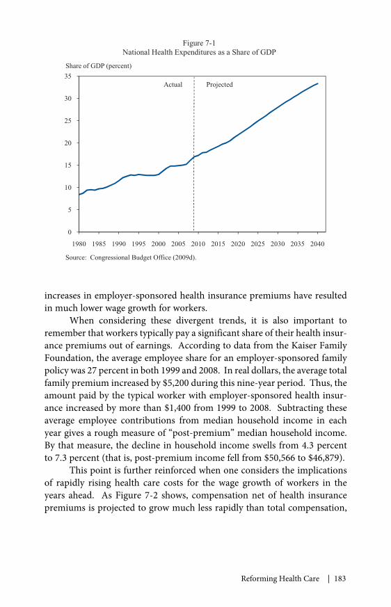
Reforming Health Care | 183
increases in employer-sponsored health insurance premiums have resultedin much lower wage growth for workers.
When considering these divergent trends, it is also important toremember that workers typically pay a significant share of their health insur-ance premiums out of earnings. According to data from the Kaiser FamilyFoundation, the average employee share for an employer-sponsored familypolicy was 27 percent in both 1999 and 2008. In real dollars, the average totalfamily premium increased by $5,200 during this nine-year period. Thus, theamount paid by the typical worker with employer-sponsored health insur-ance increased by more than $1,400 from 1999 to 2008. Subtracting theseaverage employee contributions from median household income in eachyear gives a rough measure of “post-premium” median household income.By that measure, the decline in household income swells from 4.3 percentto 7.3 percent (that is, post-premium income fell from $50,566 to $46,879).
This point is further reinforced when one considers the implicationsof rapidly rising health care costs for the wage growth of workers in theyears ahead. As Figure 7-2 shows, compensation net of health insurancepremiums is projected to grow much less rapidly than total compensation,
0
5
10
15
20
25
30
35
1980 1985 1990 1995 2000 2005 2010 2015 2020 2025 2030 2035 2040
Figure 7-1National Health Expenditures as a Share of GDP
Share of GDP (percent)
Actual Projected
Source: Congressional Budget Office (2009d).
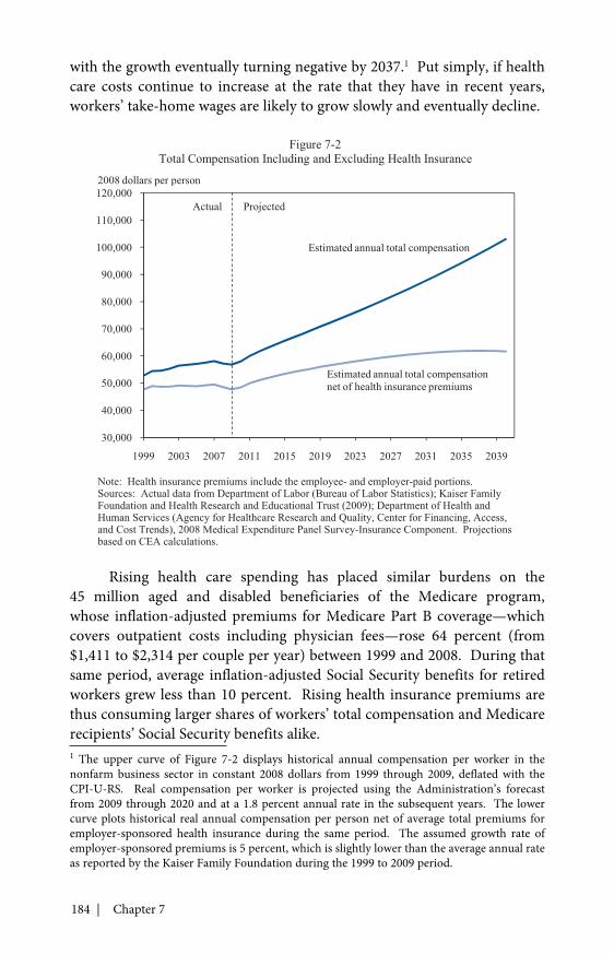
184 | Chapter 7
with the growth eventually turning negative by 2037.1 Put simply, if healthcare costs continue to increase at the rate that they have in recent years,workers’ take-home wages are likely to grow slowly and eventually decline.
Rising health care spending has placed similar burdens on the45 million aged and disabled beneficiaries of the Medicare program,whose inflation-adjusted premiums for Medicare Part B coverage—whichcovers outpatient costs including physician fees—rose 64 percent (from$1,411 to $2,314 per couple per year) between 1999 and 2008. During thatsame period, average inflation-adjusted Social Security benefits for retiredworkers grew less than 10 percent. Rising health insurance premiums arethus consuming larger shares of workers’ total compensation and Medicarerecipients’ Social Security benefits alike.1 The upper curve of Figure 7-2 displays historical annual compensation per worker in thenonfarm business sector in constant 2008 dollars from 1999 through 2009, deflated with theCPI-U-RS. Real compensation per worker is projected using the Administration’s forecastfrom 2009 through 2020 and at a 1.8 percent annual rate in the subsequent years. The lowercurve plots historical real annual compensation per person net of average total premiums foremployer-sponsored health insurance during the same period. The assumed growth rate ofemployer-sponsored premiums is 5 percent, which is slightly lower than the average annual rateas reported by the Kaiser Family Foundation during the 1999 to 2009 period.
30,000
40,000
50,000
60,000
70,000
80,000
90,000
100,000
110,000
120,000
1999 2003 2007 2011 2015 2019 2023 2027 2031 2035 2039
Estimated annual total compensation
Estimated annual total compensationnet of health insurance premiums
Figure 7-2Total Compensation Including and Excluding Health Insurance
2008 dollars per person
Actual Projected
Note: Health insurance premiums include the employee- and employer-paid portions.Sources: Actual data from Department of Labor (Bureau of Labor Statistics); Kaiser FamilyFoundation and Health Research and Educational Trust (2009); Department of Health andHuman Services (Agency for Healthcare Research and Quality, Center for Financing, Access,and Cost Trends), 2008 Medical Expenditure Panel Survey-Insurance Component. Projectionsbased on CEA calculations.

Reforming Health Care | 185
The corrosive effects of rising health insurance premiums have notbeen limited to businesses and individuals. Increases in outlays for programssuch as Medicare and Medicaid and rising expenditures for uncompensatedcare caused by increasing numbers of uninsured Americans have alsostrained the budgets of Federal, state, and local governments. The fractionof Federal spending devoted to health care rose from 11.1 percent in 1980to 25.2 percent in 2008. In the absence of reform, this trend is projected tocontinue, resulting in lower spending on other programs, higher taxes, orincreases in the Federal deficit.
The upward trend in health care spending has also posed problems forstate governments, with spending on the means-tested Medicaid programnow the second largest category of outlays in their budgets, just behindelementary and secondary education. Because virtually all state govern-ments must balance their budgets each year, the rapid increases in Medicaidspending have forced lawmakers to decide whether to cut spending in areassuch as public safety and education or to increase taxes.
If health care costs continue rising, the consequences forgovernment budgets at the local, state, and Federal level could be dire. Andas discussed in Chapter 5, projected increases in the costs of the Medicare andMedicaid programs are a key source of the Federal Government’s long-termfiscal challenges.
Market Failures in the Current U.S. Health Care System:Theoretical Background
As described by Nobel Laureate Kenneth Arrow in a seminal 1963paper, an individual’s choice to purchase health insurance is rooted inthe economics of risk and uncertainty. Over their lifetimes, people facesubstantial risks from events that are largely beyond their control. Whenpossible, those who are risk-averse prefer to hedge against these risks bypurchasing insurance (Arrow 1963).
Health care is no exception. When people become sick, they facepotentially debilitating medical bills and often must stop working and forgoearnings. Moreover, medical expenses are not equally distributed: annualmedical costs for most people are relatively small, but some people face ruin-ously large costs. Although total health care costs for the median respondentin the 2007 Medical Expenditure Panel Survey were less than $1,100, costs forthose at the 90th percentile of the distribution were almost 14 times higher(Department of Health and Human Services 2009). As a result, risk-aversepeople prefer to trade an uncertain stream of expenses for medical care forthe certainty of a regular insurance payment, which buys a policy that paysfor the high cost of treatment during illness or injury. Economic theory and

186 | Chapter 7
common sense suggest that purchasing health insurance to hedge the riskassociated with the economic costs of poor health makes people better off.
Health insurance markets, however, do not function perfectly. Theeconomics literature documents four primary impediments: adverse selec-tion, moral hazard, the Samaritan’s dilemma, and problems arising fromincomplete insurance contracts. In a health insurance market characterizedby these and other sources of inefficiency, well-designed government policyhas the potential to reduce costs, improve efficiency, and benefit patients bystabilizing risk pools for insurance coverage and providing needed coverageto those who otherwise could not afford it.
Adverse Selection. In the case of adverse selection, buyers and sellershave asymmetric information about the characteristics of market partici-pants. People with larger health risks want to buy more generous insurance,while those with smaller health risks want lower premiums for coverage.Insurers cannot perfectly determine whether a potential purchaser is a largeor small health risk.
To understand how adverse selection can harm insurance markets,suppose that a group of individuals is given a choice to buy health insuranceor pay for medical costs out-of-pocket. The insurance rates for the groupwill depend on the average cost of health care for those who elect to purchaseinsurance. The healthiest members of the group may decide that the insur-ance is too expensive, given their expected costs. If they choose not to getinsurance, the average cost of care for those who purchase insurance willincrease. As premiums increase, more and more healthy individuals maychoose to leave the insurance market, further increasing average health carecosts for those who purchase insurance. Over time, this winnowing processcan lead to declining insurance rates and even an unraveling of health insur-ance markets. Without changes to the structure of insurance markets, themarkets can break down, and fewer people can receive insurance than wouldbe optimal. Subsidies to encourage individuals to purchase health insurancecan help combat adverse selection, as can regulations requiring that indi-viduals purchase insurance, because both ensure that healthier people enterthe risk pool along with their less healthy counterparts.
Under current institutional arrangements, adverse selection is likelyto be an especially large problem for small businesses and for peoplepurchasing insurance in the individual market. In large firms, whereemployees are generally hired for reasons unrelated to their health, high-and low-risk employees are automatically pooled together, reducing theprobability of low-risk employees opting out of coverage or high-riskworkers facing extremely high premiums. In contrast, small employerscannot pool risk across a large group of workers, and thus the average risk

Reforming Health Care | 187
of a given small firm’s employee pool can be significantly above or belowthe population average. As such, similar to the market for individual insur-ance described above, firms with low-risk worker pools will tend to optout of insurance coverage, leaving firms with high-risk pools to pay muchhigher premiums.
Moral Hazard. A second problem with health insurance is moralhazard: the tendency for some people to use more health care because theyare insulated from its price. When individuals purchase insurance, they nolonger pay the full cost of their medical care. As a result, insurance mayinduce some people to consume health care on which they place muchless value than the actual cost of this care or discourage patients and theirdoctors from choosing the most efficient treatment. This extra consumptioncould increase average medical costs and, ultimately, insurance premiums.The presence of moral hazard suggests that research into which treatmentsdeliver the greatest health benefits could encourage doctors and patients toadopt best practices.
Samaritan’s Dilemma. A third source of inefficiency in the insurancemarket is that society’s desire to treat all patients, even those who do nothave insurance and cannot pay for their care, gives rise to the Samaritan’sdilemma. Because governments and their citizens naturally wish to providecare for those who need it, people who lack insurance and cannot pay formedical care can still receive some care when they fall ill. Some people mayeven choose not to purchase insurance because they understand that emer-gency care may still be available to them. In the context of adverse selection,a low insurance rate is a symptom of underlying inefficiencies. Viewedthrough the lens of the Samaritan’s dilemma, in contrast, the millions ofuninsured Americans are one source of health care inefficiencies.
The burden of paying for some of this uncompensated care is passedon to people who do purchase insurance. The result is a “hidden tax” onhealth insurance premiums, which in turn exacerbates adverse selectionby raising premiums for individuals who do not opt out of coverage. Oneestimate suggests that the total amount of uncompensated care for theuninsured was approximately $56 billion in 2008 (Hadley et al. 2008).
Incomplete Insurance Contracts. Many economic transactionsinvolve a single, straightforward interaction between a buyer and a seller. Inmany purchases of goods, for example, the prospective buyer can look thegood over carefully, decide whether or not to purchase it, and never interactwith the seller again. Health insurance, in contrast, involves a complexrelationship between an insurance company and a patient that can last yearsor even decades. It is not possible to foresee and spell out in detail everycontingency that may arise and what is and is not covered.

188 | Chapter 7
When individuals are healthy, their medical costs are typically lowerthan their premiums, and these patients are profitable for insurance compa-nies. When patients become ill, however, they may no longer be profitable.Insurance companies therefore have a financial incentive to find ways todeny care or drop coverage when individuals become sick, underminingthe central purpose of insurance. For example, in most states, insurancecompanies can rescind coverage if individuals fail to list any medical condi-tions—even those they know nothing about—on their initial health statusquestionnaire. Entire families can lose vital health insurance coveragein this manner. A House committee investigation found that three largeinsurers rescinded nearly 20,000 policies over a five-year period, saving thesecompanies $300 million that would otherwise have been paid out as claims(Waxman and Barton 2009).
A closely related problem is that insurance companies are reluctantto accept patients who may have high costs in the future. As a result,individuals with preexisting conditions find obtaining health insuranceextremely expensive, regardless of whether the conditions are costly today.This is a major problem in the individual market for health insurance.Forty-four states now permit insurance companies to deny coverage, chargeinflated premiums, or refuse to cover whole categories of illnesses becauseof preexisting medical conditions. A recent survey found that 36 percentof non-elderly adults attempting to purchase insurance in the individualmarket in the previous three years faced higher premiums or denial ofcoverage because of preexisting conditions (Doty et al. 2009). In anothersurvey, 1 in 10 people with cancer said they could not obtain health coverage,and 6 percent said they lost their coverage because of being diagnosed withthe disease (USA Today, Kaiser Family Foundation, and Harvard School ofPublic Health 2006). And the problem affects not only people with seriousmedical conditions, but also young and healthy people with relatively minorconditions such as allergies or asthma.
System-Wide Evidence of Inefficient SpendingWhile an extensive literature in economic theory makes the case for
market failure in the provision of health insurance, a substantial body ofevidence documents the pervasiveness of inefficient allocation of spendingand resources throughout the health care system. Evidence that health carespending may be inefficient comes from analyses of the relationship betweenhealth care spending and health outcomes, both across states in our ownNation and across countries around the world.
Within the United States, research suggests that the substantiallyhigher rates of health care utilization in some geographic areas are not
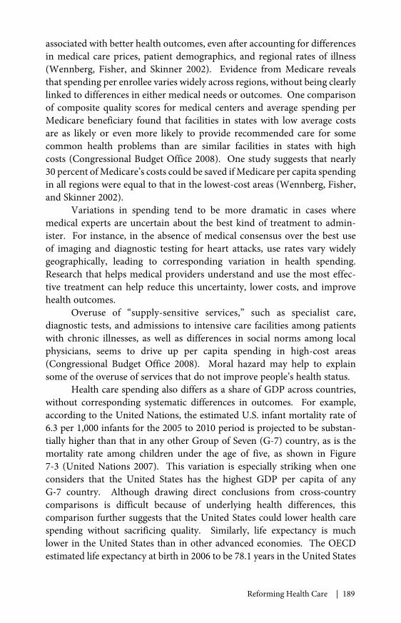
Reforming Health Care | 189
associated with better health outcomes, even after accounting for differencesin medical care prices, patient demographics, and regional rates of illness(Wennberg, Fisher, and Skinner 2002). Evidence from Medicare revealsthat spending per enrollee varies widely across regions, without being clearlylinked to differences in either medical needs or outcomes. One comparisonof composite quality scores for medical centers and average spending perMedicare beneficiary found that facilities in states with low average costsare as likely or even more likely to provide recommended care for somecommon health problems than are similar facilities in states with highcosts (Congressional Budget Office 2008). One study suggests that nearly30 percent of Medicare’s costs could be saved if Medicare per capita spendingin all regions were equal to that in the lowest-cost areas (Wennberg, Fisher,and Skinner 2002).
Variations in spending tend to be more dramatic in cases wheremedical experts are uncertain about the best kind of treatment to admin-ister. For instance, in the absence of medical consensus over the best useof imaging and diagnostic testing for heart attacks, use rates vary widelygeographically, leading to corresponding variation in health spending.Research that helps medical providers understand and use the most effec-tive treatment can help reduce this uncertainty, lower costs, and improvehealth outcomes.
Overuse of “supply-sensitive services,” such as specialist care,diagnostic tests, and admissions to intensive care facilities among patientswith chronic illnesses, as well as differences in social norms among localphysicians, seems to drive up per capita spending in high-cost areas(Congressional Budget Office 2008). Moral hazard may help to explainsome of the overuse of services that do not improve people’s health status.
Health care spending also differs as a share of GDP across countries,without corresponding systematic differences in outcomes. For example,according to the United Nations, the estimated U.S. infant mortality rate of6.3 per 1,000 infants for the 2005 to 2010 period is projected to be substan-tially higher than that in any other Group of Seven (G-7) country, as is themortality rate among children under the age of five, as shown in Figure7-3 (United Nations 2007). This variation is especially striking when oneconsiders that the United States has the highest GDP per capita of anyG-7 country. Although drawing direct conclusions from cross-countrycomparisons is difficult because of underlying health differences, thiscomparison further suggests that the United States could lower health carespending without sacrificing quality. Similarly, life expectancy is muchlower in the United States than in other advanced economies. The OECDestimated life expectancy at birth in 2006 to be 78.1 years in the United States
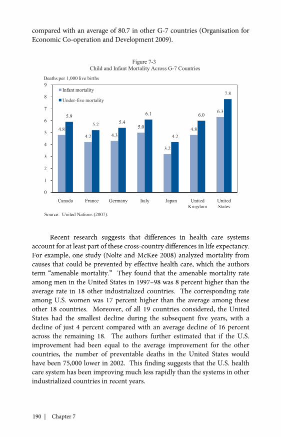
190 | Chapter 7
compared with an average of 80.7 in other G-7 countries (Organisation forEconomic Co-operation and Development 2009).
Recent research suggests that differences in health care systemsaccount for at least part of these cross-country differences in life expectancy.For example, one study (Nolte and McKee 2008) analyzed mortality fromcauses that could be prevented by effective health care, which the authorsterm “amenable mortality.” They found that the amenable mortality rateamong men in the United States in 1997–98 was 8 percent higher than theaverage rate in 18 other industrialized countries. The corresponding rateamong U.S. women was 17 percent higher than the average among theseother 18 countries. Moreover, of all 19 countries considered, the UnitedStates had the smallest decline during the subsequent five years, with adecline of just 4 percent compared with an average decline of 16 percentacross the remaining 18. The authors further estimated that if the U.S.improvement had been equal to the average improvement for the othercountries, the number of preventable deaths in the United States wouldhave been 75,000 lower in 2002. This finding suggests that the U.S. healthcare system has been improving much less rapidly than the systems in otherindustrialized countries in recent years.
4.84.2 4.3
5.0
3.2
4.8
6.35.9
5.2 5.4
6.1
4.2
6.0
7.8
0
1
2
3
4
5
6
7
8
9
Canada France Germany Italy Japan UnitedKingdom
UnitedStates
Infant mortality
Under-five mortality
Figure 7-3Child and Infant Mortality Across G-7 Countries
Deaths per 1,000 live births
Source: United Nations (2007).

Reforming Health Care | 191
A further indication that our health care system is in need of reformis that satisfaction with care has, if anything, been declining despite thesubstantial increases in spending. Not surprisingly, this decline in satisfac-tion has been concentrated among people without health insurance, whoseranks have swelled considerably during the past decade. For example, from2000 to 2009, the fraction of uninsured U.S. residents reporting that theywere satisfied with their health care fell from 36 to 26 percent. And not onlyhas dissatisfaction with our health care system increased over time, it is alsonoticeably greater than dissatisfaction with systems in many other developednations (Commonwealth Fund 2008).
Declining Coverage and Strains on Particular Groups and SectorsThe preceding analysis shows that at an aggregate level, there are
major inefficiencies in the current health care system. But, because of thenature of the market failures in health care, the current system works partic-ularly poorly in certain parts of the economy and places disproportionateburdens on certain groups. Moreover, because of rising costs, many of thestrains are increasing over time.
Declining Coverage among Non-Elderly Adults. The rapid increasein health insurance premiums in recent years has caused many firms to stopoffering health insurance to their workers, forcing employees either to payhigher prices for coverage in the individual market (which is often muchless generous than coverage in the group market) or to go without healthinsurance entirely. According to the Kaiser Family Foundation, between2000 and 2009, the share of firms offering health insurance to their workersfell from 69 to 60 percent. Furthermore, 8 percent of firms offering coveragein 2009 reported that they were somewhat or very likely to drop coveragein 2010.
Largely because of these falling offer rates, private health insurancecoverage declined substantially during this same period. As shown in Figure7-4, the fraction of non-elderly adults in the United States with private healthinsurance coverage fell from 75.5 percent in 2000 to 69.5 percent in 2008.
These numbers, however, provide just a snapshot of health insurancecoverage in the United States because they measure the fraction of peoplewho are uninsured at a point in time and thus obscure the fact that a largefraction of the population has been uninsured at some point in the past.According to recent research, at least 48 percent of non-elderly Americanswere uninsured at some point between 1996 and 2006 (Department of theTreasury 2009).
192 | Chapter 7
Although roughly half of the 2000–2008 decline in private coveragedisplayed in Figure 7-4 has been offset by an increase in public healthinsurance, the share of non-elderly adults without health insurance never-theless rose from 17.2 to 20.3 percent. In other words, approximately5.9 million more adults were uninsured in 2008 than would have been hadthe fraction uninsured remained constant since 2000. The decline in privatehealth insurance coverage was similarly large among children, although itwas more than offset by increases in public health insurance (most notablyMedicaid and CHIP), so that less than 10 percent of children were uninsuredby 2008 (DeNavas-Walt, Proctor, and Smith 2009).
The generosity of private health insurance coverage has also beendeclining in recent years. For example, from 2006 to 2009, the fraction ofcovered workers enrolled in an employer-sponsored plan with a deduct-ible of $1,000 or greater for single coverage more than doubled, from 10 to22 percent. The increase in deductibles was also striking among coveredworkers with family coverage. For example, during this same three-yearperiod, the fraction of enrollees in preferred provider organizations witha deductible of $2,000 or more increased from 8 to 17 percent. Similarincreases in cost-sharing were apparent for visits with primary care physi-cians. The fraction of covered workers with a copayment of $25 or morefor an office visit with a primary care physician increased from 12 to31 percent from 2004 to 2009. These rising costs in the private market
65
67
69
71
73
75
77
79
81
83
85
2000 2001 2002 2003 2004 2005 2006 2007 2008
Figure 7-4Insurance Rates of Non-Elderly Adults
Percent insured
All coverage
Private coverage
Source: DeNavas-Walt, Proctor, and Smith (2009).
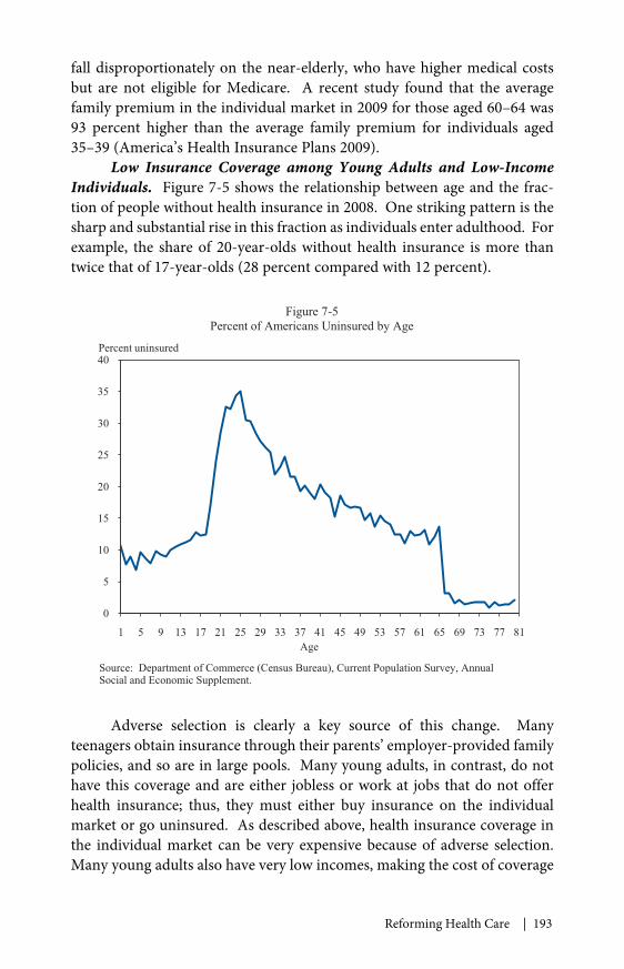
Reforming Health Care | 193
fall disproportionately on the near-elderly, who have higher medical costsbut are not eligible for Medicare. A recent study found that the averagefamily premium in the individual market in 2009 for those aged 60–64 was93 percent higher than the average family premium for individuals aged35–39 (America’s Health Insurance Plans 2009).
Low Insurance Coverage among Young Adults and Low-IncomeIndividuals. Figure 7-5 shows the relationship between age and the frac-tion of people without health insurance in 2008. One striking pattern is thesharp and substantial rise in this fraction as individuals enter adulthood. Forexample, the share of 20-year-olds without health insurance is more thantwice that of 17-year-olds (28 percent compared with 12 percent).
Adverse selection is clearly a key source of this change. Manyteenagers obtain insurance through their parents’ employer-provided familypolicies, and so are in large pools. Many young adults, in contrast, do nothave this coverage and are either jobless or work at jobs that do not offerhealth insurance; thus, they must either buy insurance on the individualmarket or go uninsured. As described above, health insurance coverage inthe individual market can be very expensive because of adverse selection.Many young adults also have very low incomes, making the cost of coverage
0
5
10
15
20
25
30
35
40
1 5 9 13 17 21 25 29 33 37 41 45 49 53 57 61 65 69 73 77 81
Figure 7-5Percent of Americans Uninsured by Age
Percent uninsured
Age
Source: Department of Commerce (Census Bureau), Current Population Survey, AnnualSocial and Economic Supplement.
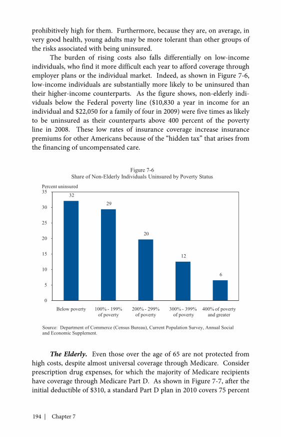
194 | Chapter 7
prohibitively high for them. Furthermore, because they are, on average, invery good health, young adults may be more tolerant than other groups ofthe risks associated with being uninsured.
The burden of rising costs also falls differentially on low-incomeindividuals, who find it more difficult each year to afford coverage throughemployer plans or the individual market. Indeed, as shown in Figure 7-6,low-income individuals are substantially more likely to be uninsured thantheir higher-income counterparts. As the figure shows, non-elderly indi-viduals below the Federal poverty line ($10,830 a year in income for anindividual and $22,050 for a family of four in 2009) were five times as likelyto be uninsured as their counterparts above 400 percent of the povertyline in 2008. These low rates of insurance coverage increase insurancepremiums for other Americans because of the “hidden tax” that arises fromthe financing of uncompensated care.
The Elderly. Even those over the age of 65 are not protected fromhigh costs, despite almost universal coverage through Medicare. Considerprescription drug expenses, for which the majority of Medicare recipientshave coverage through Medicare Part D. As shown in Figure 7-7, after theinitial deductible of $310, a standard Part D plan in 2010 covers 75 percent
32
29
20
12
6
0
5
10
15
20
25
30
35
Below poverty 100% - 199%of poverty
200% - 299%of poverty
300% - 399%of poverty
400% of povertyand greater
Figure 7-6Share of Non-Elderly Individuals Uninsured by Poverty Status
Percent uninsured
Source: Department of Commerce (Census Bureau), Current Population Survey, Annual Socialand Economic Supplement.
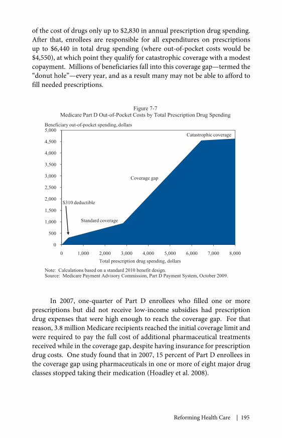
Reforming Health Care | 195
of the cost of drugs only up to $2,830 in annual prescription drug spending.After that, enrollees are responsible for all expenditures on prescriptionsup to $6,440 in total drug spending (where out-of-pocket costs would be$4,550), at which point they qualify for catastrophic coverage with a modestcopayment. Millions of beneficiaries fall into this coverage gap—termed the“donut hole”—every year, and as a result many may not be able to afford tofill needed prescriptions.
In 2007, one-quarter of Part D enrollees who filled one or moreprescriptions but did not receive low-income subsidies had prescriptiondrug expenses that were high enough to reach the coverage gap. For thatreason, 3.8 million Medicare recipients reached the initial coverage limit andwere required to pay the full cost of additional pharmaceutical treatmentsreceived while in the coverage gap, despite having insurance for prescriptiondrug costs. One study found that in 2007, 15 percent of Part D enrollees inthe coverage gap using pharmaceuticals in one or more of eight major drugclasses stopped taking their medication (Hoadley et al. 2008).
0
500
1,000
1,500
2,000
2,500
3,000
3,500
4,000
4,500
5,000
0 1,000 2,000 3,000 4,000 5,000 6,000 7,000 8,000
Figure 7-7Medicare Part D Out-of-Pocket Costs by Total Prescription Drug Spending
Beneficiary out-of-pocket spending, dollars
Coverage gap
$310 deductible
Catastrophic coverage
Standard coverage
Total prescription drug spending, dollars
Note: Calculations based on a standard 2010 benefit design.Source: Medicare Payment Advisory Commission, Part D Payment System, October 2009.

196 | Chapter 7
Small Businesses. As described earlier, adverse selection is a seriousproblem for small businesses, which do not have large numbers of workersto pool risks. This problem manifests itself in two forms. The first is highcosts. Because of high broker fees and administrative costs as well as adverseselection, small firms pay up to 18 percent more per worker for the samepolicy than do large firms (Gabel et al. 2006). The second is low coverage.Employees at small businesses are almost three times as likely as theircounterparts at large firms to be uninsured (29 percent versus 11 percent,according to the March 2009 Current Population Survey). And among smallbusinesses that do offer insurance, only 22 percent of covered workers areoffered a choice of more than one type of plan (Kaiser Family Foundationand Health Research and Educational Trust 2009).
In recent years, small businesses and their employees have had anespecially difficult time managing the rapidly rising cost of health care.Consistent with this, the share of firms with three to nine employees offeringhealth insurance to their workers fell from 57 to 46 percent between 2000and 2009.
As discussed in a Council of Economic Advisers report issued inJuly 2009, high insurance costs in the small-group market discourage entre-preneurs from launching their own companies, and the low availability ofinsurance discourages many people from working at small firms (Councilof Economic Advisers 2009c). As a result, the current system discouragesentrepreneurship and hurts the competitiveness of existing small businesses.Given the key role of small businesses in job creation and growth, this harmsthe entire economy.
Taken together, the trends summarized in this section demon-strate that in recent years the rapid rise in health insurance premiums hasreduced the take-home pay of American workers and eaten into increasesin Medicare recipients’ Social Security benefits. Fewer firms are electing tooffer health insurance to their workers, and those that do are reducing thegenerosity of that coverage through increased cost-sharing. Fewer individ-uals each year can afford to purchase health insurance coverage. The currentsystem places small businesses at a competitive disadvantage. And finally,the steady increases in health care spending strain the budgets of families,businesses, and governments at every level, and demonstrate the need forhealth insurance reform that slows the growth rate of costs.
Health Policies Enacted in
Since taking office, the President has signed into law a series ofprovisions aimed at expanding health insurance coverage, improving thequality of care, and reducing the growth rate of health care spending. The

Reforming Health Care | 197
American Recovery and Reinvestment Act of 2009 provided vital support tothose hit hardest by the economic downturn while helping to ensure accessto doctors, nurses, and hospitals for Americans who lost jobs and income.At the same time, legislation extended health insurance coverage to millionsof children, and improvements in health system quality and efficiency bene-fited the entire health care system. These necessary first steps have set thestage for a more fundamental reform of the U.S. health care system, one thatwill ensure access to affordable, high-quality coverage and that genuinelyslows the growth rate of health care spending.
Expansion of the CHIP ProgramJust two weeks after taking office, the President signed into law the
Children’s Health Insurance Program Reauthorization Act, which providesfunding that expands access to nearly 4 million additional children by2013. This guarantee of coverage also kept millions of children from losinginsurance in the midst of the recession, when many workers lost employer-sponsored coverage for themselves and their dependents. An examination ofdata from recent surveys by the Centers for Disease Control and Preventionfound that private coverage among children fell by 2.5 percentage pointsfrom the first six months of 2008 to the first six months of 2009. Despite thefall in private coverage, however, fewer children were uninsured during thatsix-month period in 2009, in large part because public coverage increased by3 percentage points (Martinez and Cohen 2008, 2009).
Approximately 7 million children (1 in every 10) were uninsured in2008 (DeNavas-Walt, Proctor, and Smith 2009). Once fully phased in, theCHIP reauthorization legislation signed by the President will lower thatnumber by as much as half from the 2008 baseline. In the future, this newlegislation will enhance the quality of medical care for children and improvetheir health. Research has convincingly shown that expanding healthinsurance to children is very cost-effective, because it not only increasesaccess to care but also substantially lowers mortality (Currie and Gruber1996a, 1996b).
Subsidized COBRA CoverageIn part because of the difficulty of purchasing health insurance on the
individual market (owing to adverse selection), most Americans get healthinsurance through their own or a family member’s job. And what is truefor dependent children is true for their parents: when economic condi-tions deteriorate, the number of people with employer-sponsored healthinsurance tends to fall. However, unlike the case with children, duringthe current recession public coverage has only offset part of the reduction
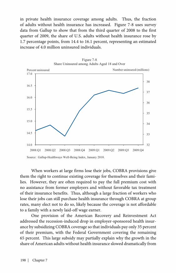
198 | Chapter 7
in private health insurance coverage among adults. Thus, the fractionof adults without health insurance has increased. Figure 7-8 uses surveydata from Gallup to show that from the third quarter of 2008 to the firstquarter of 2009, the share of U.S. adults without health insurance rose by1.7 percentage points, from 14.4 to 16.1 percent, representing an estimatedincrease of 4.0 million uninsured individuals.
When workers at large firms lose their jobs, COBRA provisions givethem the right to continue existing coverage for themselves and their fami-lies. However, they are often required to pay the full premium cost withno assistance from former employers and without favorable tax treatmentof their insurance benefits. Thus, although a large fraction of workers wholose their jobs can still purchase health insurance through COBRA at grouprates, many elect not to do so, likely because the coverage is not affordableto a family with a newly laid-off wage earner.
One provision of the American Recovery and Reinvestment Actaddressed the recession-induced drop in employer-sponsored health insur-ance by subsidizing COBRA coverage so that individuals pay only 35 percentof their premium, with the Federal Government covering the remaining65 percent. This large subsidy may partially explain why the growth in theshare of American adults without health insurance slowed dramatically from
32
33
34
35
36
37
38
14.0
14.5
15.0
15.5
16.0
16.5
17.0
2008:Q1 2008:Q2 2008:Q3 2008:Q4 2009:Q1 2009:Q2 2009:Q3 2009:Q4
Figure 7-8Share Uninsured among Adults Aged 18 and Over
Percent uninsured Number uninsured (millions)
Source: Gallup-Healthways Well-Being Index, January 2010.

Reforming Health Care | 199
the first to the fourth quarter of 2009, even while the unemployment ratecontinued to rise. While the average rate of uninsurance in 2009 was still1.4 percentage points higher than the average in 2008, the rate was fairlyconstant throughout 2009. Thus, while the CHIP expansion was providingstable coverage to millions of children who would otherwise have lost it,the COBRA subsidy was further reinforcing access to coverage for workingparents and families who faced unemployment.
Temporary Federal Medical Assistance Percentage (FMAP)Increase
Historically, declines in employer-sponsored health insurance haveled to increases in the number of people who qualify for public health insur-ance through programs such as Medicaid, which insured 45.8 million U.S.residents in December 2007. Because almost half of all Medicaid spendingis typically financed by state governments, state Medicaid spending tends torise substantially when economic conditions deteriorate. Coupled with therecession-induced drop in state tax revenues, these increases in Medicaidenrollment place a considerable strain on state budgets. And becausevirtually every state is required to balance its budget each year, increases inMedicaid enrollment often leave states with little choice but to raise taxes,lay off employees, reduce spending on public safety, education, and otherimportant priorities, or reduce Medicaid benefits, provider payments, oreligibility. These policies are especially problematic when the economy is insevere recession, because they can stifle economic recovery.
Figure 7-9 uses administrative data from all 50 states and theDistrict of Columbia to contrast the growth in Medicaid enrollment inthe months leading up to the start of the recession in December 2007with the corresponding growth during the recession.2 An examina-tion of the data displayed in the figure reveals that, after growing from45.2 million in September 2006 to 45.8 million in December 2007, the numberof Medicaid recipients increased much more rapidly in the subsequent21 months, and stood at 51.1 million in September 2009. This representsan increase of 253,000 Medicaid recipients per month during the reces-sion, versus an average increase of just 36,000 per month in the preceding15 months.
2 Data on state Medicaid enrollment were derived from direct communication between theCouncil of Economic Advisers and state health departments in 50 states and the District ofColumbia. Monthly enrollment from September 2006 through September 2009 was reportedby all states with the exception of Vermont in the first 10 months considered. For each monthfrom September 2006 through June 2007 in Vermont, the state’s July 2007 Medicaid enrollmentwas used.

200 | Chapter 7
To help states pay for an expanding Medicaid program withoutraising taxes or cutting key services, one important component of theRecovery Act was a temporary increase in each state’s Federal MedicalAssistance Percentage (FMAP), the share of Medicaid spending paid by theFederal Government. This fiscal relief allowed states to avoid cutbacks totheir Medicaid programs or other adjustments that would have exacerbatedthe effects of the recession. The increased FMAPs were larger for stateswhere unemployment increased the most, because their financial strainswere greatest. To qualify for the increased FMAPs, states were required tomaintain Medicaid eligibility at pre-recession levels.
A recent report by the Kaiser Family Foundation confirms thatsupport from the Recovery Act—as well as the expansion of coverage forchildren enacted several weeks earlier in February 2009—was essential topreserving the ability of states to offer health insurance coverage to thosemost in need. In fact, more than half the states expanded access to healthinsurance coverage for low-income children, parents, and pregnant womenin Medicaid and CHIP in 2009 (Ross and Jarlenski 2009).
44
45
46
47
48
49
50
51
52
Sep-06 Jan-07 May-07 Sep-07 Jan-08 May-08 Sep-08 Jan-09 May-09 Sep-09
Figure 7-9Monthly Medicaid Enrollment Across the States
Enrollment (millions)
Source: Information from individual state health departments, compiled by CEA.

Reforming Health Care | 201
Recovery Act Measures to Improve the Quality and Efficiency ofHealth Care
Beyond supporting jobless workers and their families in the midstof the recession, the Recovery Act addressed structural weaknesses in thehealth care system by investing in its infrastructure and its workforce. Theseinvestments will help to build a health care system with lower costs andbetter health outcomes for the long term.
For example, the Recovery Act invested $2 billion in health centersfor new construction, renovation of existing facilities, and expansion ofcoverage. An additional $500 million was allocated to bolster the primarycare workforce to improve access to primary care in underserved areas.The Act provided a further $1 billion in funding for public health activi-ties to improve prevention and to incentivize wellness initiatives for thosewith chronic illness; both measures are aimed at improving the quality ofcare and ultimately bringing down costs. The Act also increased spendingon comparative effectiveness research by $1.1 billion, to give doctors andpatients access to the most credible and up-to-date information about whichtreatments are likely to work best.
One final component of the Recovery Act was the Health InformationTechnology for Economic and Clinical Health Act, which expanded theadoption and use of health information technology through infrastructureformation, information security improvements, and incentives for adop-tion and meaningful use of certified health information technology. Thisinvestment in developing computerized medical records will reduce healthcare spending and improve quality while securing patients’ confidentialinformation.
These investments build a foundation for comprehensive healthinsurance reform by adding to the ranks of doctors, nurses, and other healthcare providers, especially in critical fields like primary care, and in areas ofthe country with the greatest need for a more robust medical workforce.Moreover, the investments in comparative effectiveness research and healthinformation technology will make it much easier for information and qualityimprovements to spread rapidly between doctors, medical practices, andhospitals across the public and private sectors. When combined with thewide range of delivery system changes included in health insurance reformlegislation, these investments are expected to contain costs and improvequality over the long run.
In summary, legislation passed in 2009 helped extend or continuehealth insurance coverage for the workers, families, and children affectedby the current recession. Rather than focusing solely on today’s crisis, the

202 | Chapter 7
legislation lays the groundwork for a reformed health care system thataddresses the weaknesses, flaws, and inefficiencies of the status quo.
Health Reform Legislation
As this Report goes to press, Congress has come closer to passingcomprehensive health insurance reform than ever before, with major billshaving passed both the House and the Senate. As of this writing, whetherthose bills will lead to enactment of final legislation in the near future isuncertain. Nonetheless, the bills contain important features that wouldexpand coverage, slow the growth rate of costs while improving the qualityof care, and benefit individuals, businesses, and governments at every level.This section discusses the major features of the two bills—the House’sAffordable Health Care for America Act and the Senate’s Patient Protectionand Affordable Care Act.
Insurance Market Reforms: Strengthening and SecuringCoverage
Both the House and the Senate bills contain important features thatwould immediately expand coverage and increase access to preventive care.The legislation would also strengthen regulation of the health insurancemarket, improve consumer protections, and secure coverage for more than30 million Americans. These regulations would correct insurance marketfailures by preventing health insurers from responding to adverse selectionby raising rates and denying coverage, thus stabilizing risk pools to secureaccess to affordable coverage.
Both versions of the legislation provide immediate Federal supportfor a new program to provide coverage to uninsured Americans withpreexisting conditions. Combined with strong new consumer protections,these measures would ensure that millions of Americans can immediatelypurchase coverage at more affordable prices despite their personal medicalhistory or health risks. Health insurance reform also makes immediateinvestments in community health centers, which would improve accessto coverage among the most vulnerable populations. Both the House andSenate versions of reform immediately create reinsurance programs foremployer health plans, providing coverage for early retirees to preventthem from becoming uninsured before they are covered by Medicare.Additionally, reform legislation would immediately begin to reform deliverysystems for health care and improve transparency and choice for consumers.For example, the Senate proposal would create a website that would help

Reforming Health Care | 203
consumers compare coverage options by summarizing important aspectsof each insurance contract in a consistent and easy-to-understand format.
New laws would help cover millions of young adults as they transitioninto the workforce by requiring insurers to allow extended family coveragefor dependents through their mid-20s. The CBO and the Joint Committeeon Taxation estimate that this requirement would lower average premiumsper person in the large-group market by increasing the number of relativelyhealthy low-cost people in large-group pools (Congressional Budget Office2009a).
In the years following reform, legislation would put into place strongnew consumer protections to prevent denials of coverage or excessive costsfor the less healthy. Insurers would be required to renew any policy forwhich the premium has been paid in full. Insurers could not refuse to renewbecause someone became sick, nor could they drop or water down insurancecoverage for those who are or become ill. To prevent insurers from chargingexcessively high rates to the less healthy, reform legislation would also enactadjusted community rating rules for premiums.
Banning such treatment of individuals with preexisting conditionswould not only allow insurance markets to better help individuals hedgeagainst the risk of health care costs, but may also make the U.S. labor marketmore efficient. Without such protections, adults with preexisting conditionsmay be reluctant to change insurance providers and expose themselves toincreased premiums. Workers who receive health insurance through theiremployers may therefore be less willing to change jobs, creating “job lock”that discourages desirable adjustments in the labor market.
In both versions of reform legislation, these provisions are linkedwith incentives for individuals to obtain coverage and for firms to insuretheir workers. While preventing insurance companies from discriminatingbased on preexisting conditions will help some of the neediest members ofour society, in isolation these reforms could increase costs for individualswithout preexisting conditions, potentially aggravating adverse selection.Without a responsibility to maintain health insurance coverage, individualscould forgo purchasing coverage until they fell ill, and thus not contributeto a shared insurance risk pool until their expected costs rose sharply.However, with restrictions on exclusions for preexisting conditions in place,high-cost individuals who sign up after falling ill could obtain coverage atlow premiums. Thus, individuals who had contributed toward coveragewould be faced with higher costs, potentially driving even more individualsout of coverage. To prevent a spiral of increasing costs and decreasing insur-ance rates resulting from adverse selection, both the House and the Senatebills establish a principle of joint individual and employer responsibility to

204 | Chapter 7
obtain and provide insurance, and would provide subsidies and tax creditsthat would assist in this process.
The bills would address other features of many health plans that limittheir ability to help individuals insure against financial risk. Currently,insurers can put yearly and lifetime limits on coverage. For people withdiseases such as cancer, life-saving treatment is often very costly, andexceeding annual and lifetime benefit limits can lead to bankruptcy. Thisproblem is especially severe in the individual and small-group markets,where insurers have more discretion in designing policies. Insurance plansthat allow individuals to bankrupt themselves may be socially inefficientbecause of the Samaritan’s dilemma: medical bills that are unpaid when apatient becomes bankrupt impose a hidden tax on other participants in thehealth care market.
In addition to these insurance market reforms, legislation passed byCongress would require coverage of preventive care and exempt preven-tive care benefits from deductibles and other cost-sharing requirements inMedicare and private insurance. Evidence suggests that not only are certainpreventive care measures cost-effective, but they can also help to preventdiseases that are responsible for roughly half of yearly mortality in theUnited States (Mokdad et al. 2004). Some measures, such as smoking cessa-tion programs, discussing aspirin use with high-risk adults, and childhoodimmunizations, may even lower total health care spending (Maciosek et al.2006). Because many people change insurance companies several times overthe course of their lives, insurance companies may underinvest in preven-tive care that is cost-effective but does not reduce medical costs until far inthe future. By encouraging all insurance companies to invest in preventivecare, health insurance reform would increase the efficiency of the healthcare sector.
Finally, reform legislation takes steps to make prescription drugcoverage more affordable and secure for senior citizens. The legislationwould increase the initial coverage limit under Medicare Part D by $500in 2010 and also provide 50 percent price discounts for brand-name drugsin the “donut hole” discussed earlier. This discount would allow manyMedicare Part D recipients to reduce their out-of-pocket spending onprescription drugs. Not only would fewer beneficiaries have to pay the fullcost of their prescription drugs while in the donut hole, but those who doreach this coverage gap would also benefit from increased coverage beforereaching that point.
In summary, within the first few years after passage, reform legislationin Congress would guarantee coverage for those with preexisting conditions,reform private insurance markets with strong consumer protections that

Reforming Health Care | 205
would stabilize risk pools and mitigate adverse selection, and strengthenpublic coverage under Medicare.
Expansions in Health Insurance Coverage Through the ExchangeCentral to both the House and the Senate bills is the health insurance
exchange, which would allow individuals and employees of small businessesto choose among many different insurance plans. The exchange wouldprovide a centralized marketplace to allow individuals, families, and smallfirms to pool together and purchase coverage much like larger firms dotoday, improving consumer choice and increasing pressure on insurers tooffer lower prices and more generous benefits to attract customers. In itsfirst year of operation, the exchange would be open to qualified individualsand small businesses.
Individuals and small businesses, which might otherwise purchasehealth insurance in the individual or small-group markets, would benefitfrom the economies of scale and greater buying leverage in the exchange,which could result in much lower premiums. The exchange would alsoprovide transparent information on plan quality, out-of-pocket costs,covered benefits, and premiums for each offered plan, enabling individualsto select the plan that best fits their and their family’s needs. The availabilityof easy-to-compare premium information would provide a powerful incen-tive for health insurers to price competitively, thus making coverage moreaffordable for participants in the exchange.
The new exchange would be especially beneficial for small businessemployees, who, as described earlier, face particularly severe challenges inthe health insurance market. The bills would enable small businesses thatmeet certain criteria to purchase insurance through the exchange, allowingthem and their workers to buy better coverage at lower costs. Moreover,many small businesses that provide health insurance for their employeeswould receive a tax credit to alleviate their disproportionately higher costsand to encourage coverage. The tax credit would lower the cost of coverageby as much as 50 percent. Reform would make it easier for small businessesto recruit talented workers and would also increase workers’ incentivesto start their own small businesses. A recent analysis of the Senate billby the CBO found that premiums for a given amount of coverage for thesame set of people or small businesses would fall in the individual andsmall-group markets as a result of reductions in administrative costs andincreased competition in a centralized marketplace (Congressional BudgetOffice 2009a).
Most individuals who select a plan in the exchange would be eligiblefor subsidies that reduce the cost of their coverage. In both the House and

206 | Chapter 7
Senate bills, subsidies would be available to certain individuals and familieswith incomes below 400 percent of the Federal poverty line. The premiumand out-of-pocket spending subsidies for plans purchased in the exchangewould be larger for lower-income families, many of whom cannot afford thecost of a private plan. In addition, individuals with incomes below about133 to 150 percent of the poverty line would be eligible for health insurancethrough the Medicaid program.
In the exchange, Federal subsidies would be tied to premiums forrelatively lower-cost “reference” plans. Beneficiaries would, however, beable to buy more extensive coverage at an additional, unsubsidized cost.
Economic and Health Benefits of Expanding Health InsuranceCoverage
CBO analyses of both the House and Senate bills indicate that, in partbecause of the creation of the exchanges and the expansion in Medicaid,more than 30 million Americans who would otherwise be uninsured wouldobtain coverage as a result of reform. These coverage expansions wouldimprove not only the health and the economic well-being of affected indi-viduals and families, but also the broader economy.
A comprehensive body of literature demonstrates that beinguninsured leads to poorer medical treatment, worse health status, andhigher mortality rates. Across a range of acute conditions and chronicdiseases, uninsured Americans have worse outcomes, higher rates ofpreventable death, and lower-quality care. Additionally, being uninsuredimposes on families a significant financial risk of bankruptcy caused bymedical expenses.
Evidence from the state of Massachusetts—which expanded healthinsurance to all but 2.6 percent of its population in a 2006 reform effort—finds that expanding coverage increased regular medical care and loweredfinancial burdens for residents who gained coverage. Only 17.4 percent ofadults with family incomes of less than 300 percent of the Federal povertyline reported forgoing care because of costs in 2008, compared with27.3 percent in the pre-reform baseline in 2006 (Long and Masi 2009).
Taken together, this evidence strongly suggests that expandingcoverage for Americans through health insurance reform would directlybenefit millions of families by giving them access to the care they needto maintain their health without substantial financial burdens and risks.Moreover, because of the fixed costs of developing health care infrastructuresuch as trauma centers, increasing the share of people with health insurancecan improve health outcomes for people with insurance as well.

Reforming Health Care | 207
Beyond the improvements for individuals and families,coverage expansions would produce benefits that extend throughoutthe entire economy. A CEA report in June 2009 estimated thateconomic gains from reduced financial risk for the uninsured totaled$40 billion per year (Council of Economic Advisers 2009a). Moreover, theCEA report found an economic value of more than $180 billion per yearfrom averting preventable deaths caused by a lack of insurance. Takentogether, these gains would far exceed the cost of extending coverage to thecurrently uninsured population.
The economic benefits of expanding coverage would extend to labormarkets in the form of reduced absenteeism and greater productivity.According to the 2009 March Current Population Survey, 18.7 million non-elderly adults report having one or more disabilities that prevent or limitthe work they can perform; of that total, 3.1 million lack health insurance.Approximately 50 percent of non-elderly adults who work report having atleast one serious medical condition. Previous research has documented theindirect costs to employers of health-related productivity losses. Some ofthe costliest conditions—depression, migraines, and asthma—can often beeffectively managed with prescription medications made more affordableby health insurance. This suggests that expanding access to coverage wouldimprove productivity and labor supply by creating a healthier workforce thatwould lose fewer hours to preventable illnesses or disabilities.
Reducing the Growth Rate of Health Care Costs in the Public andPrivate Sectors
The House and Senate bills contain a number of provisions that wouldreduce the growth rate of health care spending in both the public and privatesectors. Both bills create pilot programs in Medicare to bundle providerpayments for an episode of care rather than for individual procedures.Under bundled payments, Medicare would provide a single reimburse-ment for an entire episode of care rather than multiple reimbursementsfor individual treatments. This payment strategy would give providers,organized around a hospital or group of physicians, a stronger incentive tocoordinate and provide quality care efficiently rather than carry out low-value or unnecessary treatments and procedures. Recent research in theNew England Journal of Medicine suggests that bundled payments couldimprove quality and substantially reduce health care spending (Hussey etal. 2009). The Department of Health and Human Services would be givenauthority to expand or extend successful pilot programs without additionallegislative action.

208 | Chapter 7
Both bills also include measures that directly reduce waste in thecurrent health care system. One example of such waste is the substantialoverpayment to Medicare Advantage plans, which are currently paid anaverage of 14 percent more per recipient than traditional Medicare. Thereform bills would reduce these overpayments, saving more than $100 billionbetween 2010 and 2019 (Congressional Budget Office 2009b). Reducingthe overpayments would also lower Medicare recipients’ Part B premiumsbelow what they otherwise would be and would extend the solvency of theMedicare Trust Fund.
Another component of the legislation that has the potential toslow the growth rate of health care spending is the Independent PaymentAdvisory Board included in the Senate bill. This board would have theauthority to propose changes to the Medicare program both to improve thequality of care and to reduce the growth rate of program spending. AbsentCongressional action, these recommendations would be automaticallyimplemented.
Using the the CEA analysis of the House and Senate bills alongwith projections from CBO about the level of Federal spending onMedicare, Medicaid, and CHIP, it is possible to estimate the effect ofreform on the growth rate of Federal health care spending. Recent CEAanalyses of the House and Senate bills find that reform would lower totalFederal spending on Medicare, Medicaid, and CHIP by 2019 below whatit otherwise would have been (Council of Economic Advisers 2009b).Moreover, between 2016 and 2019, both bills would lower the annualgrowth rate of Federal spending on these programs by approximately1.0 percentage point. State and local governments would also benefitfinancially from health insurance reform, as described in Box 7-1.
Box 7-1: The Impact of Health Reform on State and Local Governments
Although slowing the growth in health care costs will help the long-run fiscal situation of the Federal Government, some observers worryabout how reform will affect state and local governments. To help ensurethat virtually all Americans receive health insurance, both the Senate andthe House bills call for expanding Medicaid eligibility. Because Medicaidis partly funded by states, some state officials fear that the state fiscalsituation will deteriorate as a consequence of reform.
As documented by a CEA report published in September (Councilof Economic Advisers 2009d), however, health insurance reform would
Continued on next page

Reforming Health Care | 209
In addition to these public savings, the reform proposals would reducethe growth of health care costs in the private sector. One important mecha-nism through which reform could reduce these costs is the excise tax onhigh-cost insurance plans included in the Senate bill. Under current tax law,employer compensation in the form of wages is subject to the income tax,while compensation in the form of employer-provided health care benefitsis not. Individuals may therefore have an incentive to obtain more generoushealth insurance than they would if wages and health insurance faced moreequal tax treatment. Absent other incentives for individuals to obtain insur-ance, the preferential tax treatment of health insurance may be beneficial,because it encourages firms to provide health insurance to their workersand facilitates pooling. Nonetheless, placing no limit on this subsidy likelyleads to health insurance that is more generous than would be efficient insome cases.
To help contain the growth in the cost of these plans withoutjeopardizing the risk-pooling benefits, the Senate bill would impose a taxon only the most expensive employer-sponsored plans. Although only asmall share of plans would be affected, CEA estimates based on data fromthe CBO suggest that the excise tax on high-cost insurance plans wouldreduce the growth rate of annual health care costs in the private sector by0.5 percentage point per year from 2012 to 2018. The excise tax wouldencourage workers and their firms’ human resources departments to bemore watchful consumers and would give insurers a powerful incentive to
improve the fiscal health of state and local governments in at least threeimportant ways. First, state and local governments are already spendingbillions of dollars each year providing coverage to the uninsured; thesecosts would fall significantly as a consequence of health reform. Second,encouraging all individuals to become insured would reduce the hiddentax paid by providers of health insurance. Because state and local govern-ments employ more than 19 million people, the total savings fromremoving the hidden tax is likely to be substantial. Third, an excise tax onhigh-cost plans would boost workers’ wages by billions of dollars each yearand thus increase state income tax revenues.
To understand the net consequences of reform for the fiscal healthof state and local governments, the CEA studied the impact of reform for16 states that are diverse along many important dimensions: geographic,economic, and demographic. For every state studied, health reform wouldresult in substantial savings for state and local governments.
Box 7-1, continued
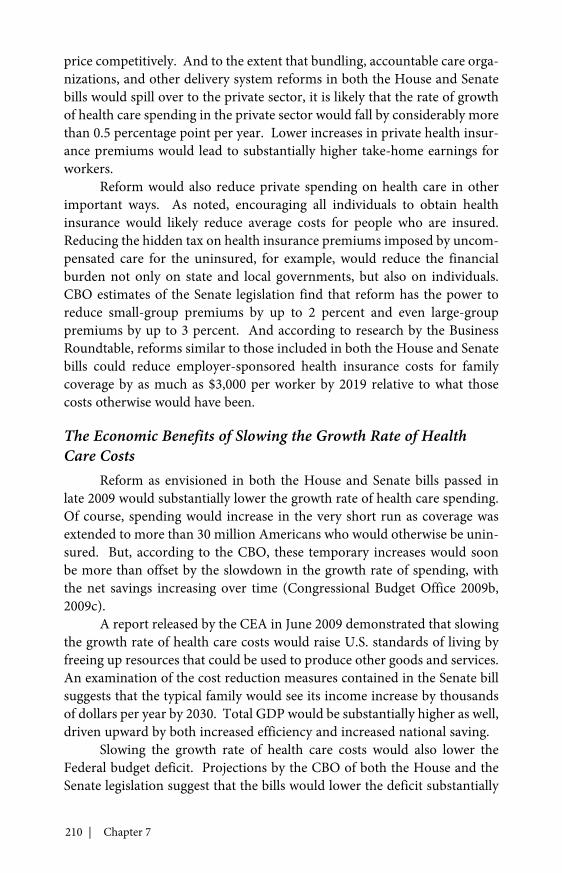
210 | Chapter 7
price competitively. And to the extent that bundling, accountable care orga-nizations, and other delivery system reforms in both the House and Senatebills would spill over to the private sector, it is likely that the rate of growthof health care spending in the private sector would fall by considerably morethan 0.5 percentage point per year. Lower increases in private health insur-ance premiums would lead to substantially higher take-home earnings forworkers.
Reform would also reduce private spending on health care in otherimportant ways. As noted, encouraging all individuals to obtain healthinsurance would likely reduce average costs for people who are insured.Reducing the hidden tax on health insurance premiums imposed by uncom-pensated care for the uninsured, for example, would reduce the financialburden not only on state and local governments, but also on individuals.CBO estimates of the Senate legislation find that reform has the power toreduce small-group premiums by up to 2 percent and even large-grouppremiums by up to 3 percent. And according to research by the BusinessRoundtable, reforms similar to those included in both the House and Senatebills could reduce employer-sponsored health insurance costs for familycoverage by as much as $3,000 per worker by 2019 relative to what thosecosts otherwise would have been.
The Economic Benefits of Slowing the Growth Rate of HealthCare Costs
Reform as envisioned in both the House and Senate bills passed inlate 2009 would substantially lower the growth rate of health care spending.Of course, spending would increase in the very short run as coverage wasextended to more than 30 million Americans who would otherwise be unin-sured. But, according to the CBO, these temporary increases would soonbe more than offset by the slowdown in the growth rate of spending, withthe net savings increasing over time (Congressional Budget Office 2009b,2009c).
A report released by the CEA in June 2009 demonstrated that slowingthe growth rate of health care costs would raise U.S. standards of living byfreeing up resources that could be used to produce other goods and services.An examination of the cost reduction measures contained in the Senate billsuggests that the typical family would see its income increase by thousandsof dollars per year by 2030. Total GDP would be substantially higher as well,driven upward by both increased efficiency and increased national saving.
Slowing the growth rate of health care costs would also lower theFederal budget deficit. Projections by the CBO of both the House and theSenate legislation suggest that the bills would lower the deficit substantially

Reforming Health Care | 211
in the upcoming decade, and even more in the next decade. These savingswould obviate large tax increases or cuts in other important priority areas.As discussed in Chapter 5, it would be the single most important step towardaddressing the Nation’s long-run fiscal challenges.
Finally, reform that genuinely slows the growth of health care costscould increase employment for a period of time by lowering the unemploy-ment rate that is consistent with steady inflation. These effects could beimportant, with CEA estimates suggesting an increase of more than 300,000jobs for a period of time if health care costs grew by 1 percentage point lesseach year.
Conclusion
In recent years, health care costs in the Nation’s private and publicsectors have been rising at an unsustainable rate, and the fraction ofAmericans who are uninsured has steadily increased. These trends haveimposed tremendous burdens on individuals, employers, and governmentsat every level, and the problems have grown yet more severe during the pasttwo years with the onset of the worst recession since the Great Depression.
Last year, the President signed into law several policies that have cush-ioned the worst of the economic downturn, including an expansion in theChildren’s Health Insurance Program and an extension of COBRA coveragefor displaced workers and their families. Other policies, such as increasedfunding for health information technology, will improve the long-runefficiency and quality of the health care sector.
Legislation passed by both the House and the Senate in late 2009would expand health insurance coverage to tens of millions of Americanswhile slowing the growth rate of health care costs. These reforms wouldimprove the health and the economic well-being of individuals and families,help small businesses, stimulate job creation, and ease strains on Federal,state, and local governments imposed by rapidly rising health care costs.

213
C H A P T E R 8
STRENGTHENING THEAMERICAN LABOR FORCE
The recession has been extremely difficult for American workers andfamilies. One in ten workers is now unemployed, wages and hours
worked have fallen, and many families are struggling to make ends meet.Making matters worse, the recession followed a sustained period of risinginequality and stagnation in the living standards of typical Americanworkers. A central challenge in coming years will be to smooth thetransition to a sustainable growth path with more widely shared prosperity.
As we begin to recover from the recession, we will see a new andmuch-changed labor market. Some industries that grew unsustainablylarge in recent years, such as construction and finance, will recover but willnot immediately return to past employment levels. The same may be truefor traditional manufacturing, which has been shrinking as a share of theeconomy for decades. The pace of employment decline will surely moderateafter the recession, but many former workers in traditional manufacturingwill need to transition into new, growing sectors.
In the place of the declining industries will come new opportunitiesfor American workers. Health care will remain an important source ofgrowth in the labor market, as will high-technology sectors including cleanenergy industries and advanced manufacturing. Well-trained and highlyskilled workers will be best positioned to secure good jobs in these new andgrowing sectors. The best way to prepare our workforce for the challengesand opportunities that lie ahead is by strengthening our education system,creating a seamless, efficient path for every American from childhood toentry into the labor market as a skilled worker ready to meet the needs ofthe new labor market.
Both individuals and the economy as a whole benefit from increasededucational attainment and improved school quality. A focus on access,equity, and quality for all American students, from early childhood throughhigh school and into postsecondary education and training throughout
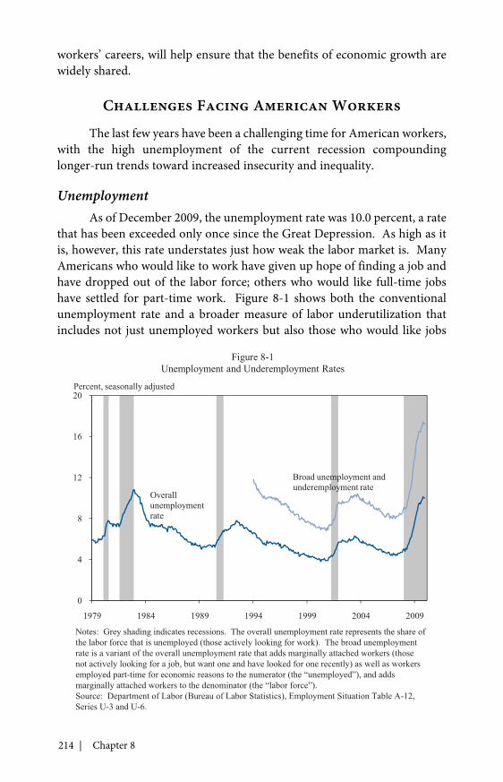
214 | Chapter 8
workers’ careers, will help ensure that the benefits of economic growth arewidely shared.
Challenges Facing American Workers
The last few years have been a challenging time for American workers,with the high unemployment of the current recession compoundinglonger-run trends toward increased insecurity and inequality.
UnemploymentAs of December 2009, the unemployment rate was 10.0 percent, a rate
that has been exceeded only once since the Great Depression. As high as itis, however, this rate understates just how weak the labor market is. ManyAmericans who would like to work have given up hope of finding a job andhave dropped out of the labor force; others who would like full-time jobshave settled for part-time work. Figure 8-1 shows both the conventionalunemployment rate and a broader measure of labor underutilization thatincludes not just unemployed workers but also those who would like jobs
0
4
8
12
16
20
1979 1984 1989 1994 1999 2004 2009
Figure 8-1Unemployment and Underemployment Rates
Percent, seasonally adjusted
Broad unemployment andunderemployment rate
Overallunemploymentrate
Notes: Grey shading indicates recessions. The overall unemployment rate represents the share ofthe labor force that is unemployed (those actively looking for work). The broad unemploymentrate is a variant of the overall unemployment rate that adds marginally attached workers (thosenot actively looking for a job, but want one and have looked for one recently) as well as workersemployed part-time for economic reasons to the numerator (the “unemployed”), and addsmarginally attached workers to the denominator (the “labor force”).Source: Department of Labor (Bureau of Labor Statistics), Employment Situation Table A-12,Series U-3 and U-6.
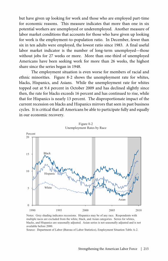
Strengthening the American Labor Force | 215
but have given up looking for work and those who are employed part-timefor economic reasons. This measure indicates that more than one in sixpotential workers are unemployed or underemployed. Another measure oflabor market conditions that accounts for those who have given up lookingfor work is the employment-to-population ratio. In December, fewer thansix in ten adults were employed, the lowest ratio since 1983. A final usefullabor market indicator is the number of long-term unemployed—thosewithout jobs for 27 weeks or more. More than one-third of unemployedAmericans have been seeking work for more than 26 weeks, the highestshare since the series began in 1948.
The employment situation is even worse for members of racial andethnic minorities. Figure 8-2 shows the unemployment rate for whites,blacks, Hispanics, and Asians. While the unemployment rate for whitestopped out at 9.4 percent in October 2009 and has declined slightly sincethen, the rate for blacks exceeds 16 percent and has continued to rise, whilethat for Hispanics is nearly 13 percent. The disproportionate impact of thecurrent recession on blacks and Hispanics mirrors that seen in past businesscycles. It is critical that all Americans be able to participate fully and equallyin our economic recovery.
0
5
10
15
20
1990 1995 2000 2005 2010
Figure 8-2Unemployment Rates by Race
Percent
White
Black
Hispanic
Asian
Notes: Grey shading indicates recessions. Hispanics may be of any race. Respondents withmultiple races are excluded from the white, black, and Asian categories. Series for whites,blacks, and Hispanics are seasonally adjusted. Asian series is not seasonally adjusted and is notavailable before 2000.Source: Department of Labor (Bureau of Labor Statistics), Employment Situation Table A-2.
216 | Chapter 8
Even a quick return to job growth will not immediately eliminateemployment problems, as it will take time to create the millions of newjobs needed to return to normal employment levels. Many workers willhave difficulty finding work for some time to come. Extended periods ofhigh unemployment and low job creation rates mean that many displacedworkers will exhaust their unemployment insurance benefits before jobsbecome available in large numbers. After months or even years of unem-ployment, most who exhaust their benefits will likely have used up whateversavings they had when they lost their jobs. Many will be forced to turn topublic assistance—Temporary Assistance for Needy Families, SupplementalNutritional Assistance (formerly known as food stamps), or other similarprograms—to make ends meet.
Sustained periods of low labor demand also have negativerepercussions for the long-run health of the economy. Mounting evidenceindicates that displacement during bad economic times leads to long-runreductions in workers’ productivity (Jacobson, LaLonde, and Sullivan 1993),likely because the displaced workers lose job skills, fall out of habits neededfor successful employment, and have trouble convincing employers thatthey will be good employees. The resulting loss of “human capital” reducesworkers’ earning power, even after the economy recovers.
Deep downturns have particularly large effects on young Americans.The unemployment rate for teenagers in December was 27.1 percent.Research shows that teens who first enter the labor market during arecession can have trouble getting their feet onto the first rung of the careerladder, leaving them a step or more behind throughout their lives (Kahnforthcoming; Oreopoulos, von Wachter, and Heisz 2006; Oyer 2006). Thereis also evidence that when parents lose their jobs, their children’s long-runeconomic opportunities suffer (Oreopoulos, Page, and Stevens 2008).
Sectoral ChangeThe Great Recession has aggravated an already challenging trend:
sectoral shifts that are changing the nature of work. While most Americanworkers were once engaged in producing food and manufactured goods,often through physical labor that did not require a great deal of training,the United States is increasingly a knowledge-based society where workersproduce services using analytical skills. The changing economy offerstremendous opportunities for American workers in high technology, in thenew clean energy economy, in health care, and in other high-skill fields.
Accompanying these shifts in the composition of employment havebeen changes in the institutions that govern the labor market. The prototyp-ical American career once involved working for a single employer for many

Strengthening the American Labor Force | 217
years, backed by a union that bargained for steady wage increases and for apension that promised a stable, guaranteed income in retirement. The labormarket has changed. Fewer than one in seven workers belongs to a union,and most people can count on changing employers several times over theircareers. Moreover, the vast majority of retirement plans are now “definedcontribution,” meaning that workers’ retirement incomes depend on thesuccess of their individual investment decisions and on the performanceof asset markets as a whole. This shift has meant added risk for workers,particularly those whose planned retirements coincide with downturns inasset prices.
Stagnating Incomes for Middle-Class FamiliesA final major challenge facing American workers is the decades-long
stagnation in living standards for typical families and the related increase ininequality. Figure 8-3 offers two looks at income trends over the past halfcentury. First, it shows real median family income—the level at which halfof families have higher income and half have lower income—over time. Themedian rose steadily until 1970, but then the rate of growth slowed substan-tially, and since 2000, the median has actually fallen.
One determinant of family income is the number of individualsworking outside of the home. Female labor force participation has risendramatically: in 1960, just over 40 percent of adult women (aged 18–54)participated in the labor force; by 2000, approximately three-quarters did.This increase in female labor force participation contributed to the rise infamily incomes. However, the female labor force participation rate has beenroughly stable since 2000, and there are not likely to be future increases inparticipation as dramatic as those seen in the past. Further increases infamily incomes will likely rely on growth in individual earnings.
The other two series in Figure 8-3 show the median earnings formen and women working full-time, year-round jobs. Real median femaleyear-round earnings have grown steadily by about 1.1 percent per year onaverage since 1960, reflecting in part the gradual leveling of labor marketbarriers to women’s career advancement. But real male earnings have beenessentially flat since the early 1970s. One source of the stagnation of medianmale earnings and the reduced growth rate of median female earnings isthat productivity growth slowed betwen 1973 and 1995 (Chapter 10). Butthis is not a complete explanation. Even at a reduced growth rate, Americanworkers’ productivity has more than doubled in the last 40 years.
A partial explanation for the divergence between productivity andearnings is the rapid rise in health care costs in recent years: an ever-greatershare of the compensation paid by employers has gone toward health
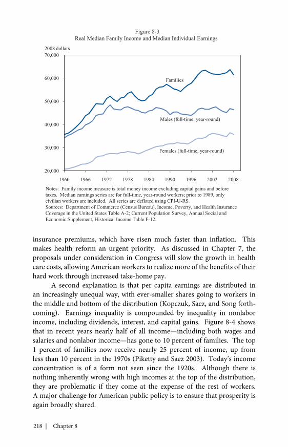
218 | Chapter 8
insurance premiums, which have risen much faster than inflation. Thismakes health reform an urgent priority. As discussed in Chapter 7, theproposals under consideration in Congress will slow the growth in healthcare costs, allowing American workers to realize more of the benefits of theirhard work through increased take-home pay.
A second explanation is that per capita earnings are distributed inan increasingly unequal way, with ever-smaller shares going to workers inthe middle and bottom of the distribution (Kopczuk, Saez, and Song forth-coming). Earnings inequality is compounded by inequality in nonlaborincome, including dividends, interest, and capital gains. Figure 8-4 showsthat in recent years nearly half of all income—including both wages andsalaries and nonlabor income—has gone to 10 percent of families. The top1 percent of families now receive nearly 25 percent of income, up fromless than 10 percent in the 1970s (Piketty and Saez 2003). Today’s incomeconcentration is of a form not seen since the 1920s. Although there isnothing inherently wrong with high incomes at the top of the distribution,they are problematic if they come at the expense of the rest of workers.A major challenge for American public policy is to ensure that prosperity isagain broadly shared.
20,000
30,000
40,000
50,000
60,000
70,000
1960 1966 1972 1978 1984 1990 1996 2002 2008
Figure 8-3Real Median Family Income and Median Individual Earnings
2008 dollars
Males (full-time, year-round)
Females (full-time, year-round)
Families
Notes: Family income measure is total money income excluding capital gains and beforetaxes. Median earnings series are for full-time, year-round workers; prior to 1989, onlycivilian workers are included. All series are deflated using CPI-U-RS.Sources: Department of Commerce (Census Bureau), Income, Poverty, and Health InsuranceCoverage in the United States Table A-2; Current Population Survey, Annual Social andEconomic Supplement, Historical Income Table F-12.
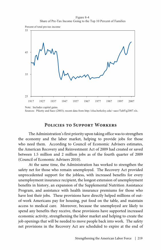
Strengthening the American Labor Force | 219
Policies to Support Workers
The Administration’s first priority upon taking office was to strengthenthe economy and the labor market, helping to provide jobs for thosewho need them. According to Council of Economic Advisers estimates,the American Recovery and Reinvestment Act of 2009 had created or savedbetween 1.5 million and 2 million jobs as of the fourth quarter of 2009(Council of Economic Advisers 2010).
At the same time, the Administration has worked to strengthen thesafety net for those who remain unemployed. The Recovery Act providedunprecedented support for the jobless, with increased benefits for everyunemployment insurance recipient, the longest extension of unemploymentbenefits in history, an expansion of the Supplemental Nutrition AssistanceProgram, and assistance with health insurance premiums for those whohave lost their jobs. These provisions have directly helped millions of out-of-work Americans pay for housing, put food on the table, and maintainaccess to medical care. Moreover, because the unemployed are likely tospend any benefits they receive, these provisions have supported increasedeconomic activity, strengthening the labor market and helping to create thejob openings that will be needed to move people back into work. The safetynet provisions in the Recovery Act are scheduled to expire at the end of
25
35
45
55
1917 1927 1937 1947 1957 1967 1977 1987 1997 2007
Figure 8-4
Percent of total pre-tax income
Note: Includes capital gains.Sources: Piketty and Saez (2003); recent data from http://elsa.berkeley.edu/~saez/TabFig2007.xls.
Share of Pre-Tax Income Going to the Top 10 Percent of Families

220 | Chapter 8
February 2010, but because of the ongoing weakness in the labor market, theAdministration is working with Congress to extend them further.
The Recovery Act also included provisions to reform theunemployment insurance system, making it work more effectively in today’seconomy. These provisions extend unemployment insurance eligibility tomany low-wage and part-time workers who were not previously eligible.These and other recent initiatives will also make it possible for many unem-ployed workers to draw out-of-work benefits while participating in trainingthat prepares them to enter new fields.
Even after the labor market recovers, the dynamic American economywill continue to pose challenges—while also creating opportunities—forworkers. Rapid technological change will cause shifts in the labor market,forcing some workers into unanticipated mid-life career changes. Policy canhelp to ease these transitions. Most important, it can ensure that workers whomay switch careers several times during their lifetimes are able to maintainhealth insurance and to support themselves in retirement. As discussed inChapter 7, comprehensive health care reform will eliminate preexisting condi-tions restrictions in health insurance and improve access to insurance in theindividual market. These changes will make it much easier for people to main-tain insurance when they change jobs or pursue entrepreneurial opportunities.
Declines in stock prices and home values have put serious pressureon many Americans’ retirement plans and have highlighted the importanceof improved retirement security. The Administration has proposed severalmeasures to increase saving by low- and middle-income workers. Effortsinclude expanded access to retirement plans along with rule changes tostreamline enrollment in 401(k) and IRA programs, facilitate simple savingstrategies, and reorient program default options to emphasize saving. And,most important, the Administration is committed to protecting SocialSecurity, thus ensuring that it can provide a reliable source of income forfuture retirees, as it has for their parents and grandparents.
Health and retirement security need to be accompanied by labormarket institutions that support and protect workers. Labor unions havelong been a force helping to raise standards of living for middle-classfamilies. They remain important, and we need to reinforce the principle thatworkers who wish to join a union should have the right to do so.
Another set of institutions in need of attention is our immigrationsystem. The current framework absorbs considerable resources but doesnot serve anyone—native workers, employers, taxpayers, or potentialimmigrants—well. Particular problems are posed by the presence of largenumbers of unauthorized immigrants and the lengthy queues—some over20 years—for legal residency.

Strengthening the American Labor Force | 221
Reform of the immigration system can strengthen our economy andlabor market. Reform should provide a path for those who are currently hereillegally to come out of the shadows. It should include strengthened bordercontrols and better enforcement of laws against employing undocumentedworkers, along with programs to help immigrants and their children quicklyintegrate into their communities and American society. Future immigra-tion policy should be more responsive to our economy’s changing needs.Reform of the employment-based visa and permanent residency programswill also help reduce the incentives to immigrate illegally by giving potentialimmigrants a more viable legal path into the United States.
Education and Training:The Groundwork for Long-Term Prosperity
Rebuilding our economy on a more sustainable basis, investing infuture productivity, fostering technological and other forms of innovation,and reforming our health care system to deliver better outcomes at lower costsare all crucial to long-run increases in living standards, and all are discussedelsewhere in this report. But one fundamental component of a strategy toensure balanced, sustained, and widely shared growth is a robust system ofeducation and training. The positive link between education and workerproductivity—the cornerstone of economic prosperity—is well established.In fact, research has credited education with up to one-third of the produc-tivity growth in the United States from the 1950s to the 1990s (Jones 2002).
Benefits of EducationAt the individual level, there is a strong relationship between
educational attainment and earnings (Card 1999). The earnings premiumshows up at all levels of education. Those who complete one year of post-secondary education earn more than those who stop after high school,while those who complete two years or finish degrees earn more still. Andjob training for the unemployed has been shown by rigorous studies toraise participants’ future earnings (Manpower Demonstration ResearchCorporation 1983; Jacobson, LaLonde, and Sullivan 2005).
The earnings premium associated with education is far larger thanthe cost—in tuition and forgone earnings—of remaining in school (Barrowand Rouse 2005), and it has grown in recent decades. Figure 8-5 showsthe trends in the average annual earnings of individuals with high schooldiplomas but no college and of those with bachelor’s degrees. In the mid-1960s, college graduates earned roughly 50 percent more than high schoolgraduates, on average; by 2008, the premium had more than doubled.

222 | Chapter 8
Education has other important benefits besides increased earnings.For example, recent studies have found that education improves people’shealth (Cutler and Lleras-Muney 2006; Grossman 2005). The explanationmay be that better educated people make better health-related decisions,such as exercising or not smoking, or that education allows for easier navi-gation of a complex health care system. Education’s benefits also extendbeyond the individual. More educated people commit fewer crimes, votemore, and are more likely to support free speech (Dee 2004; Lochnerand Moretti 2004). They also make their neighbors and coworkers moreproductive (Moretti 2004).
Trends in U.S. Educational AttainmentThe United States has historically had the world’s best education
system. Although most European countries once limited advanced educa-tion to the economic elite, the United States has historically made it broadlyavailable. U.S secondary schools have been free and generally acces-sible since early in the 20th century. By the 1950s, nearly 80 percent ofolder teens (aged 15–19) in the United States were enrolled in secondaryschool, compared with fewer than 40 percent in Western Europe. The
0
30,000
60,000
90,000
1963 1973 1983 1993 2003
Figure 8-5Total Wage and Salary Income by Educational Group
Total wage and salary income, 2008 dollars
College graduates
Notes: Figures for full-time workers aged 25-65 who worked 50-52 weeks in the calendaryear. Before 1991, education groups are defined based on the highest grade of school or yearof college completed. Beginning in 1991, groups are defined based on the highest degree ordiploma earned. Incomes are deflated using the CPI-U.Source: Department of Labor (Bureau of Labor Statistics), March Current Population Survey,1964-2009.
High school graduates

Strengthening the American Labor Force | 223
widespread expansion of state colleges and universities, begun under theMorrill Land Grant Act of 1862, led to even further advances in Americaneducation. Average educational attainment of people born in 1975 wasover five years higher than that of those born in 1895. About 50 percentof the gain was attributable to increases in high school education, about30 percent to increases in college and postcollege education, and theremainder to continued increases in elementary education (Goldin and Katz2008). During the second half of the 20th century, as educational attain-ment rose worldwide, the United States became a clear leader in graduateeducation, attracting the brightest students from around the world. Someremained in the United States, adding importantly to the Nation’s humancapital stock and its diversity, while others returned to their home countriesand used the education they got here to help increase prosperity there.
Harvard economists Claudia Goldin and Lawrence Katz contend thatAmerica’s strong educational system helped make the United States therichest nation in the world (Goldin and Katz 2008). Over the past severaldecades, however, U.S. leadership in education has slipped. Although theNation remains preeminent in postgraduate education, we can no longerclaim to be home to the most educated people in the world.
For decades, the number of educated American workers grew fasterthan did the demand for them. But beginning with the cohort that completedits schooling in the early 1970s, the growth rate in the supply of educatedAmericans slowed significantly. This can be seen in Figure 8-6, which showsthe mean years of schooling of Americans by year of birth. High schooland college graduation rates, which grew steadily for many decades, beganto stagnate, and younger generations no longer graduate at significantlyhigher rates than did previous generations. This slowdown in the growth ofeducational attainment has contributed to rising income inequality, as theshortage of college-educated workers has meant rising wages for high-skillwork and falling wages for work requiring less education. The current reces-sion may provide an opportunity to reverse this slowdown but only if oureducation system can keep up with increased demand (Box 8-1).
Meanwhile, other developed countries have continued to improvetheir educational outcomes, and the United States has slipped behind severalother advanced countries at both the high school and postsecondary levels.Among the cohort born between 1943 and 1952—a group that largelycompleted its education by the late 1970s—the United States leads the worldin the share with at least a bachelor’s degree or the equivalent. In morerecent cohorts, the percentage completing college has been roughly stablein the United States while increasing substantially in several peer countries.Figure 8-7 shows that only 40 percent of Americans born between 1973 and
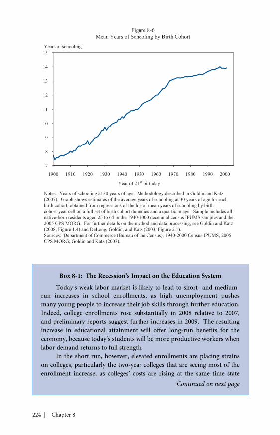
224 | Chapter 8
7
8
9
10
11
12
13
14
15
1900 1910 1920 1930 1940 1950 1960 1970 1980 1990 2000
Figure 8-6Mean Years of Schooling by Birth Cohort
Years of schooling
Year of 21 birthday
Notes: Years of schooling at 30 years of age. Methodology described in Goldin and Katz(2007). Graph shows estimates of the average years of schooling at 30 years of age for eachbirth cohort, obtained from regressions of the log of mean years of schooling by birthcohort-year cell on a full set of birth cohort dummies and a quartic in age. Sample includes allnative-born residents aged 25 to 64 in the 1940-2000 decennial census IPUMS samples and the2005 CPS MORG. For further details on the method and data processing, see Goldin and Katz(2008, Figure 1.4) and DeLong, Goldin, and Katz (2003, Figure 2.1).Sources: Department of Commerce (Bureau of the Census), 1940-2000 Census IPUMS, 2005CPS MORG; Goldin and Katz (2007).
st
Box 8-1: The Recession’s Impact on the Education System
Today’s weak labor market is likely to lead to short- and medium-run increases in school enrollments, as high unemployment pushesmany young people to increase their job skills through further education.Indeed, college enrollments rose substantially in 2008 relative to 2007,and preliminary reports suggest further increases in 2009. The resultingincrease in educational attainment will offer long-run benefits for theeconomy, because today’s students will be more productive workers whenlabor demand returns to full strength.
In the short run, however, elevated enrollments are placing strainson colleges, particularly the two-year colleges that are seeing most of theenrollment increase, as colleges’ costs are rising at the same time state
Continued on next page
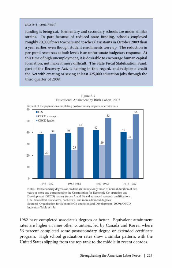
Strengthening the American Labor Force | 225
1982 have completed associate’s degrees or better. Equivalent attainmentrates are higher in nine other countries, led by Canada and Korea, where56 percent completed some postsecondary degree or extended certificateprogram. High school graduation rates show a similar pattern, with theUnited States slipping from the top rank to the middle in recent decades.
39 4042
40
20
2529
34
39
45
5356
0
10
20
30
40
50
60
1943-1952 1953-1962 1963-1972 1973-1982
U.S.OECD averageOECD leader
Figure 8-7Educational Attainment by Birth Cohort, 2007
Percent of the population completing postsecondary degrees or credentials
Notes: Postsecondary degrees or credentials include only those of normal duration of twoyears or more and correspond to the Organisation for Economic Co-operation andDevelopment (OECD) tertiary (types A and B) and advanced research qualifications.U.S. data reflect associate’s, bachelor’s, and more advanced degrees.Sources: Organisation for Economic Co-operation and Development (2009); OECDIndicators Table A1.3a.
funding is being cut. Elementary and secondary schools are under similarstrains. In part because of reduced state funding, schools employedroughly 70,000 fewer teachers and teachers’ assistants in October 2009 thana year earlier, even though student enrollments were up. The reduction inper-pupil resources at both levels is an unfortunate budgetary response. Atthis time of high unemployment, it is desirable to encourage human capitalformation, not make it more difficult. The State Fiscal Stabilization Fund,part of the Recovery Act, is helping in this regard, and recipients creditthe Act with creating or saving at least 325,000 education jobs through thethird quarter of 2009.
Box 8-1, continued

226 | Chapter 8
U.S. Student AchievementU.S. student achievement, as measured by assessments that capture
how much students know at particular ages or grades, has improved notablyin recent years, even as attainment has stagnated. The most reliable barom-eter is the National Assessment of Education Progress (NAEP), which hasbeen administered consistently for more than three decades. Figure 8-8shows average NAEP math scores for students at three different ages from1978 through 2008. The performance of 9-year-olds (who are typicallyenrolled in 4th grade) and 13-year-olds (typically 8th grade) has improvedover the past 35 years. The size of the achievement gains is impressive. Nearlythree-quarters of 13-year-olds in 2008 scored above the 1978 median, withsimilar gains throughout the distribution. The performance of 17-year-olds(typically 12th graders) has also improved, although the gain was smaller.
Despite recent progress, American students are not doing as wellas they should. In addition to average performance, the NAEP programmeasures the fraction of students who attain target achievement levelsdefined based on the skills that children at each age and grade should havemastered. A student is judged “proficient” if he or she demonstrates age- orgrade-appropriate competency over challenging subject matter and showsan ability to apply knowledge to real-world situations. In the most recenttests, only 31 percent of 8th graders were proficient in reading and only34 percent in math. Proficiency rates are similar in 4th grade.
For some subgroups, proficiency rates were much lower. Only12 percent of black students and 17 percent of Hispanics were proficient inmath in 8th grade. The low achievement in these subgroups is also reflectedin low attainment. In 2000, only 81 percent of black young adults (aged30–34) had graduated from high school, and only 15 percent had bachelor’sdegrees. Although racial and ethnic gaps have narrowed importantly inrecent decades—the black-white and Hispanic-white mathematics gaps atage 13 in the NAEP long-term trend data are each only two-thirds as largeas in 1978—the low attainment and achievement of black and Hispanicstudents remain disturbing evidence of educational inequality in our society.Our future prosperity depends on ensuring that American children from allbackgrounds have the opportunity to become productive workers.
Nowhere does low performance more acutely affect the health ofthe U.S. economy than in the areas of science, technology, engineering,and mathematics (known commonly by the acronym STEM). Employersfrequently report that they have difficulty finding Americans with thequalifications needed for technical jobs and are forced to look abroad forsuitably skilled workers. Indeed, international comparisons show thatother countries achieve higher outcomes in STEM skills than we do. In
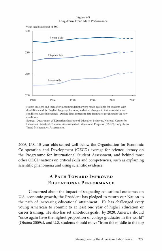
Strengthening the American Labor Force | 227
2006, U.S. 15-year-olds scored well below the Organisation for EconomicCo-operation and Development (OECD) average for science literacy onthe Programme for International Student Assessment, and behind mostother OECD nations on critical skills and competencies, such as explainingscientific phenomena and using scientific evidence.
A Path Toward ImprovedEducational Performance
Concerned about the impact of stagnating educational outcomes onU.S. economic growth, the President has pledged to return our Nation tothe path of increasing educational attainment. He has challenged everyyoung American to commit to at least one year of higher education orcareer training. He also has set ambitious goals: by 2020, America should“once again have the highest proportion of college graduates in the world”(Obama 2009a), and U.S. students should move “from the middle to the top
200
240
280
320
1978 1984 1990 1996 2002 2008
Figure 8-8Long-Term Trend Math Performance
Mean scale score out of 500
9-year-olds
13-year-olds
17-year-olds
Notes: In 2004 and thereafter, accommodations were made available for students withdisabilities and for English language learners, and other changes in test administrationconditions were introduced. Dashed lines represent data from tests given under the newconditions.Source: Department of Education (Institute of Education Sciences, National Center forEducation Statistics), National Assessment of Educational Progress (NAEP), Long-TermTrend Mathematics Assessments.

228 | Chapter 8
of the pack in science and math” (Obama 2009b). Meeting these challengeswill require substantial commitment and reform, not just at the postsec-ondary level but also in elementary and high schools and even in earlychildhood programs.
Postsecondary EducationThe Nation’s postsecondary education system encompasses a diverse
group of institutions, including public, nonprofit, and for-profit organiza-tions offering education ranging from short-term skill refresher programsup to doctoral degrees.
In many of our peer countries, postsecondary education is entirely orlargely state funded, with little direct cost to the student. U.S. postsecondarystudents, however, are generally charged tuition and fees, which have risensubstantially in real terms over the past three decades. It is important tokeep in mind that most of our students do not pay full tuition, as more than60 percent of full-time students receive grant aid, and millions more alsobenefit from Federal tax credits and deductions for tuition. But increasesin financial aid and Federal assistance have not kept up with rising costs,and the net price of attendance at four-year public colleges has risen nearly20 percent over the past decade (College Board 2009).
Young people may have trouble financing expensive investmentsin college education even when these investments will pay off throughincreased long-term earnings. Thus, rising college costs represent animportant barrier to enrollment. One study indicates that a $1,000 reduc-tion in net college costs increases the probability of attending collegeby 5 percentage points and leads students to complete about one-fifthof a year more college (Dynarski 2003). Thus the dramatic increasein the price of college has likely had an adverse impact on collegeattendance and completion. Moreover, the impact of cost increases isnot evenly distributed: while students from high-income families canrelatively easily absorb the increases, students from lower-income families aredisproportionately deterred.
The rising cost of college is affecting educational attainment andwill continue to do so unless we find ways to make college more afford-able. To this end, the Administration has secured historic investments instudent aid, including more than $100 billion over the next 10 years formore generous Pell Grants, much of it financed through the elimination ofwasteful subsidies to private lenders in the student loan program. This willensure that virtually all students eligible for Pell Grants will receive largerawards. In addition, the Administration is taking steps to dramaticallysimplify the student aid application process, the complexity of which deters

Strengthening the American Labor Force | 229
many aid-eligible students from even applying. This simplification willhelp millions more students benefit from the Federal investments in collegeaccessibility and affordability.
Tuition is not the only barrier to college completion. A great manystudents, including nearly half of those at two-year institutions, begin collegebut fail to graduate. Completion rates are particularly low for low-incomestudents. One way to raise completion rates is through better design ofthe institutional environment. Recent rigorous studies have shown thatimprovements such as enhanced student services, changes in how classes areorganized, innovations in how remedial education is structured, and basingsome portion of financial aid on student performance can all contribute toimproved persistence (Scrivener et al. 2008; Scrivener, Sommo, and Collado2009; Richburg-Hayes et al. 2009).
Training and Adult EducationAn often-overlooked component of the Nation’s education system,
one in which the government makes a major investment, is job trainingand adult education. In 2009, the Federal Government devoted more than$17 billion to job training and employment services and spent substantialadditional funds on Pell Grants for vocational and adult education students.Training is provided by a diverse set of institutions, including proprietary(for-profit) schools, four-year colleges, community-based organizations,and public vocational and technical schools. Box 8-2 discusses a particularlyimportant type of training provider, community colleges.
Studies have documented that training and adult education programsimprove participants’ labor market outcomes. For example, a recent studyfound that Workforce Investment Act training programs for adults boostedemployment and earnings, on average, although results varied substantiallyacross states (Heinrich, Mueser, and Troske 2008). Evidence is also growingthat state training programs for adults can have large positive impacts onlong-term earnings (Hotz, Imbens, and Klerman 2006; Dyke et al. 2006).
Education and training for adults play critical roles in helpingdisplaced workers regain employment in the short term and in helpingthem obtain and refresh their skills in the face of an ever-changing work-place. For example, one study of displaced workers in Washington Statesuggests that attending a community college after displacement during the1990s increased long-term earnings about 9 percent for men and about13 percent for women (Jacobson, LaLonde, and Sullivan 2005). The benefitswere greatest for academic courses in math and science, as well as for coursesrelated to the health professions, technical trades (such as air conditionerrepair), and technical professions (such as software development).

230 | Chapter 8
Although research demonstrates the value of training programs, thereis no doubt that the current system could be more effective. Five strategiesthat could improve effectiveness are: aligning goals across different elementsof the education and training system and constructing a cumulative curric-ulum; collaborating with employers to ensure that curricula are aligned withworkforce needs and regional economies; making sure that scheduling is flex-ible and that curricula meet the needs of older and nontraditional students;providing incentives and flexibility for institutions and programs to continu-ally improve and innovate; and establishing a stronger accountability systemthat measures the right things, makes performance data available in an easilyunderstood format, and does not create perverse incentives to avoid servingpopulations that most need assistance. Reauthorization of the WorkforceInvestment Act will provide an opportunity to implement these strategies.
Box 8-2: Community Colleges: A Crucial Component ofOur Higher Education System
Community colleges are an important but often overlookedcomponent of the Nation’s postsecondary education system. Thesecolleges may offer academic programs preparing students to transfer tofour-year colleges to complete bachelor’s degrees, academic and vocationalprograms leading to terminal associate’s degrees or certificates, remedialeducation for those who want to attend college but who left high schoolinsufficiently prepared, and short-term job training or other educationalexperiences. Most also offer contract training in which they work directlywith the public sector, employers, and other clients (such as prisons) todevelop and provide training for specific occupations or purposes.
Community colleges are public institutions that typically charge verylow tuition and primarily serve commuters, which makes them accessibleto people who do not have the resources for a four-year college. Theygenerally have “open door” admissions policies, requiring only a highschool diploma or an ability to benefit from the educational experience.This makes them a good choice for older and nontraditional students, aswell as for potential students who want to pursue additional education andbuild their human capital but want or need to do so at relatively low cost.
More than 35 percent of first-time college freshmen enroll atcommunity colleges. These colleges also serve about 35 percent of indi-viduals receiving job training through the Workforce Investment Act,along with a notable proportion of adults attending adult basic education,English as a second language, and General Educational Development
Continued on next page

Strengthening the American Labor Force | 231
Elementary and Secondary EducationStudents who leave high school with inadequate academic preparation
face greater challenges to success in postsecondary training. In 2001, nearlyone-third of first-year college students in the United States needed to takeremedial classes in reading, writing, or mathematics, at an estimated costof more than $1 billion (Bettinger and Long 2007). The need for remedia-tion is a clear warning sign that a student may later drop out. In one study,students who needed the most remediation were only about half as likely tocomplete college as their peers who were better prepared (Adelman 1998).Of course, students who leave high school well prepared are more successfulin the labor market as well as in college.
The task of improving college and labor market preparedness beginsin elementary and secondary school, if not earlier. Among the mostimportant contributors to enhanced student outcomes is effective teaching.Common sense and research both recognize the importance of high-qualityteachers, and yet too few teachers reach that standard. Improvementsare needed in teacher training, recruitment, evaluation, and in-serviceprofessional development.
Not only is the supply of high-quality teachers insufficient but theirdistribution across schools is inequitable. Frequently, schools with high
(GED) preparation classes. Researchers have estimated that attending acommunity college significantly raises earnings, even for individuals whodo not complete degrees (Kane and Rouse 1999; Marcotte et al. 2005).
Community colleges will form the linchpin of efforts to increasecollege attendance and graduation rates. The Administration has proposeda new program of competitive grants for implementing college completioninitiatives, with a focus on community colleges. Along with the sortsof strategies mentioned above for training programs more generally,community college initiatives could include building better partnershipsbetween colleges, businesses, the workforce investment system, and otherworkforce partners to create career pathways for workers; expandingcourse offerings including those built on partnerships between collegesand high schools; and stronger accountability for results. These strategieswill help both to strengthen colleges and to raise completion rates. Theproposed program also recognizes the need to learn from such investmentand therefore supports record levels of funding for research to evaluate theinitiatives’ effectiveness.
Box 8-2, continued

232 | Chapter 8
concentrations of minority and low-income students, the very schools thatneed quality teachers the most, cannot recruit and retain skilled educators.In New York State, 21 percent of black students had teachers who failed theirgeneral knowledge certification exam on the first attempt, compared with7 percent of white students (Lankford, Loeb, and Wyckoff 2002). A partic-ular problem is high teacher turnover: high-poverty and high-minorityschools have much higher turnover than do schools with more advantagedstudents. Some districts have begun experimenting with financial incen-tives for teaching in high-need schools; these efforts need to be rigorouslyevaluated and, if they are found to be successful, disseminated widely.
Improving teacher quality, however, is not the only promising strategyfor change. Others include extending both the school day and the schoolyear. Many successful strategies have emerged from schools that were givenfreedom to explore new and creative approaches to long-standing problems.Although traditional public schools can be agents for change, the publiccharter school model is tailor-made for such innovation. The Nation’sexperience with charter schools has been fairly brief, but evidence to datesuggests that some of these schools have found successful strategies forraising student achievement. An important future challenge will be to takethese strategies and other innovative school models to scale, even as schoolscontinue to search for ever-better approaches.
Although most reforms in recent years have focused on elementaryschools, high school reform is now rising to the top of the education policyagenda. Promising approaches to improving secondary education includeprograms that offer opportunities for accelerated instruction and individual-ized learning, programs to expand access to early college coursework beforefinishing high school, residential schools for disadvantaged students, andspecialty career-focused academies.
An environment that supports innovation must be coupled withstrong accountability. Some innovations are bound to be unsuccessful, andindeed there is substantial variation in the quality of both public and charterschools. Strong accountability systems that promote effective instructionalapproaches can provide incentives for all school stakeholders to perform attheir best and help to identify struggling schools in need of intervention.Systems are needed to identify failing schools, based on high-quality studentassessments as well as other metrics. At the same time, accountabilitystrategies must be carefully crafted to discourage “teaching to the test” andother approaches that aim at the measures used for evaluating schools ratherthan at true student learning. Accountability strategies must also recognizethat student achievement reflects family, community, and peer influences aswell as that of the school.

Strengthening the American Labor Force | 233
Providing incentives for schools identified as failing to improve cansignificantly improve student outcomes. Several states have done just that.Sixteen years ago, Massachusetts began setting curriculum frameworksand holding schools accountable for student performance. Massachusettsstudents have historically scored above the national average on variousacademic achievement measures, but since passing school accountabilityreform, Massachusetts has moved even farther ahead. In Florida, too, astrong school accountability plan, implemented in 1999, has shown positiveresults (Figlio and Rouse 2006; Rouse et al. 2007).
The Recovery Act included an unprecedented Federal investmentin elementary and secondary education. The Race to the Top Fundprovides competitive grants to reward and encourage states that havetaken strong measures to improve teacher quality, develop meaningfulincentives, incorporate data into decisionmaking, and raise student achieve-ment in low-achieving schools. The upcoming reauthorization of theElementary and Secondary Education Act provides an opportunity to makefurther progress.
Early Childhood EducationHigh-quality elementary and secondary schools are necessary, but
they are not enough. In recent years, researchers and educators have learneda great deal about how important the school readiness of entering kinder-garteners is to later academic and labor market success. School readinessinvolves both academic skills, as measured by vocabulary size, complexity ofspoken language, and basic counting, and social and emotional skills suchas the ability to follow directions and self-regulate. Children who arriveat school without these skills lack the foundation on which later learningwill build.
Recent research indicates that as many as 45 percent of enteringkindergarteners are ill-prepared to succeed in school (Hair et al. 2006).Reducing the share of at-risk preschoolers is critical to strengtheningAmerica’s educational system and its labor market in the long run. High-quality early childhood interventions can significantly improve schoolreadiness, especially for low-income children. Intensive programs thatcombine high-quality preschool with home visits and parenting supporthave been shown to raise children’s later test scores and educationalattainment and also to reduce teen pregnancy rates and criminality (Karolyet al. 1998; Schweinhart et al. 1985).
The programs on which the most compelling research is basedinclude small classes, highly educated teachers with training in early child-hood education, and stimulating curricula. They feature parent training

234 | Chapter 8
components that help parents reinforce what the teachers do in the class-room. The programs also assist teachers in identifying health and behaviorproblems that can inhibit children’s intellectual and emotional develop-ment. Importantly, even intensive, expensive programs are cost-effective.For example, one particularly intensive program was found to produce$2.50 in long-run savings for taxpayers for every dollar spent, because inadulthood the participating children earned higher incomes, used fewereducational and government resources, and had lower health care costs(Barnett and Masse 2007).
Less intensive programs can be effective as well. The Head Startprogram provides an academically enriching preschool environment for3- and 4-year-olds, at a cost in 2008 of only about $7,000 per child per year.Although the quality of Head Start centers varies widely, studies have foundthat attendance at a well-run center improves children’s later-life outcomes(Currie and Thomas 1995).
Ensuring that all families have access to the services and support theyneed to help prepare their children for kindergarten will require a strongsystem of high-quality preschools and other early-learning centers. Providersmust be held to high standards and given the resources—including quali-fied staff and teachers—needed for success. And when children leave theirpreschool and prekindergarten programs, they must have access to qualitykindergartens that ease the transition to elementary school.
Conclusion
The recession has taken a severe toll on American workers and manywill continue to suffer from its effects for some time to come. A strong safetynet will be essential to helping working families through this trying time. Asthe economy strengthens, we must rebuild our labor market institutions inways that ensure that prosperity and economic security are more widely shared.
Going forward, workers who have strong analytic and interactiveskills will be best able to secure good jobs and to contribute to continuedU.S. prosperity. Education must begin in preschool, because children’slong-run success depends on arriving in kindergarten ready to learn, and beavailable throughout adulthood, because our increasingly dynamic economyrequires lifelong learning. The Administration’s education agenda willstrengthen our education and training institutions at all levels.

235
C H A P T E R 9
TRANSFORMING THE ENERGYSECTOR AND ADDRESSING
CLIMATE CHANGE
The President has called climate change “one of the defining challengesof our time.” If steps are not taken to reduce atmospheric concentra-
tions of carbon dioxide (CO2) and other greenhouse gases, scientists projectthat the world could face a significant increase in the global average surfacetemperature. Projections indicate that CO2 concentrations may doublefrom pre-industrial levels as early as 2050, and that the higher concentra-tions are associated with a likely long-run temperature increase of 2 to 4.5°C (3.6 to 8.1 °F). With temperatures at that level, climate change will leadto a range of negative impacts, including increased mortality rates, reducedagricultural yields in many parts of the world, and rising sea levels that couldinundate low-lying coastal areas.
The planet has not experienced such rapid warming on a global scalein many thousands of years, and never as a result of emissions from humanactivity. By far the largest contribution to this warming comes from carbon-intensive fossil fuels, which the world depends on for cooking, heatingand cooling homes and offices, transportation, generating electricity, andmanufacturing products such as cement and steel.
The potential for significant damages if emissions from these activi-ties are not curbed makes it crucial for the world to transform the energysector. This transformation will entail developing entirely new industriesand making major changes in the way energy is produced, distributed, andused. New technologies will be developed and new jobs created. The UnitedStates can play a leadership role in these efforts and become a world leaderin clean energy technologies. The transformation to a clean energy economywill also reduce our Nation’s dependence on oil and improve nationalsecurity, and could reduce other pollutants in addition to greenhouse gases.
As this transformation unfolds, two market failures provide amotivation for government policy. First, greenhouse gas emissions are a

236 | Chapter 9
classic example of a negative externality. As emitters of greenhouse gasescontribute to climate change, they impose costs on others that are not takeninto account when making decisions about how to produce and consumeenergy-intensive goods. Second, the development of new technologies haspositive externalities. As discussed in Chapter 10, the developers of newtechnologies generally capture much less than the full benefit of their ideasto consumers, firms, and future innovators, and thus underinvest in researchand development.
This diagnosis of the market failures underlying climate changeprovides clear guidance about the role of policy in the area. First, policyshould take steps to ensure that the market provides the correct signalsto greenhouse gas emitters about the full cost of their emissions. Second,policy should actively promote the development of new technologies.One way to accomplish these goals is through a market-based approachto reducing greenhouse gases combined with government incentives topromote research and development of new clean energy technologies.Once policy has ensured that markets are providing the correct signalsand incentives, the operation of market forces can find the most effectiveand efficient paths to the clean energy economy. The Administration’spolicies in this area are guided by these principles.
Greenhouse Gas Emissions, Climate,and Economic Well-Being
The world’s dependence on carbon-intensive fuels is projected tocontinue to increase global average temperature as greenhouse gas emis-sions build in the atmosphere. These emissions are particularly problematicbecause many are long-lived: for instance, it will take a century for slightlymore than half of the carbon dioxide now in the atmosphere to be naturallyremoved. The atmospheric buildup of greenhouse gases since the start ofthe industrial revolution has already raised average global temperature byroughly 0.8 °C (1.4 °F). If the concentrations of all greenhouse gases andaerosols resulting from human activity could somehow be kept constantat current levels, the temperature would still go up about another 0.4 0C(0.7 °F) by the end of the century. It is important to note that the overallimpact of today’s emissions would be even higher were it not for the offset-ting net cooling effect of increases in atmospheric aerosols such as particulatematter caused by the incomplete combustion of fossil fuels in coal-firedpower plants.
But keeping atmospheric concentrations constant at today’s level isvirtually impossible. Any additional greenhouse gas emissions contribute
Transforming the Energy Sector and Addressing Climate Change | 237
to atmospheric concentrations. And because of projected economicgrowth, particularly in developing countries, greenhouse gas emissionswill continue to grow. Moreover, the sources of atmospheric aerosolsthat have partly offset the greenhouse warming experienced so far are notlikely to grow apace because governments around the world are takingactions to curb these emissions to improve public health and controlacid rain.
Greenhouse GasesThe principal long-lived greenhouse gases whose concentrations have
been affected by human activity are carbon dioxide, methane, nitrous oxide,and halocarbons. Sulfur hexafluoride, though emitted in smaller quantities,is also a very potent greenhouse gas. All have increased significantly frompre-industrial levels. Carbon dioxide is emitted when fossil fuel is burnedto heat and cool homes, fuel vehicles, and manufacture products such ascement and steel. Deforestation also releases carbon dioxide stored in treesand soil. The primary sources of methane and nitrous oxide are agriculturalpractices, natural gas use, and landfills. Halocarbons originate from refrig-eration and industrial processes, while sulfur hexafluoride emissions mainlystem from electrical and industrial applications.
The pre-industrial atmospheric concentration of carbon dioxide wasabout 280 parts per million (ppm), meaning that 280 out of every millionmolecules of gas in the atmosphere were carbon dioxide. As of December2009, its concentration had increased to about 387 ppm. Taking into accountother long-lived greenhouse gases would result in a higher warming poten-tial, but the net cooling effect of aerosols that have been added by humansto the atmosphere nearly cancels the effect of those other gases. Thus, theoverall effect of human activity on the atmosphere to date is (coincidentally)about the same as that of the carbon dioxide increase alone.
A variety of models project that, absent climate policy, atmosphericconcentrations of carbon dioxide will continue to grow, reaching levelsranging from 610 to 1030 ppm by 2100 (Figure 9-1). When the warmingeffects of other long-lived greenhouse gases are included, this range isequivalent to 830 to 1530 ppm. The breadth of the range reflects uncertaintyabout future energy supply, energy demand, and the future behavior of thecarbon cycle.1
1 Underlying uncertainty about future energy supply is uncertainty regarding the costs andpenetration rates of technology, and resource availability. Uncertainty about future energydemand is driven by uncertainty regarding growth in population, gross domestic product, andenergy efficiency.
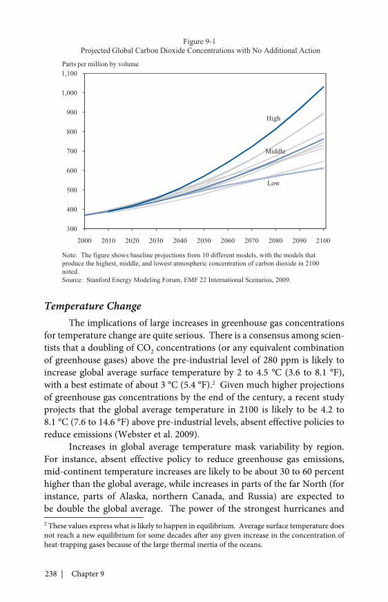
238 | Chapter 9
Temperature ChangeThe implications of large increases in greenhouse gas concentrations
for temperature change are quite serious. There is a consensus among scien-tists that a doubling of CO2 concentrations (or any equivalent combinationof greenhouse gases) above the pre-industrial level of 280 ppm is likely toincrease global average surface temperature by 2 to 4.5 °C (3.6 to 8.1 °F),with a best estimate of about 3 °C (5.4 °F).2 Given much higher projectionsof greenhouse gas concentrations by the end of the century, a recent studyprojects that the global average temperature in 2100 is likely to be 4.2 to8.1 °C (7.6 to 14.6 °F) above pre-industrial levels, absent effective policies toreduce emissions (Webster et al. 2009).
Increases in global average temperature mask variability by region.For instance, absent effective policy to reduce greenhouse gas emissions,mid-continent temperature increases are likely to be about 30 to 60 percenthigher than the global average, while increases in parts of the far North (forinstance, parts of Alaska, northern Canada, and Russia) are expected tobe double the global average. The power of the strongest hurricanes and2 These values express what is likely to happen in equilibrium. Average surface temperature doesnot reach a new equilibrium for some decades after any given increase in the concentration ofheat-trapping gases because of the large thermal inertia of the oceans.
300
400
500
600
700
800
900
1,000
1,100
2000 2010 2020 2030 2040 2050 2060 2070 2080 2090 2100
Figure 9-1Projected Global Carbon Dioxide Concentrations with No Additional Action
Parts per million by volume
High
Low
Middle
Note: The figure shows baseline projections from 10 different models, with the models thatproduce the highest, middle, and lowest atmospheric concentration of carbon dioxide in 2100noted.Source: Stanford Energy Modeling Forum, EMF 22 International Scenarios, 2009.
Transforming the Energy Sector and Addressing Climate Change | 239
typhoons is likely to grow, as are the frequency and intensity of extremeweather events such as heat waves, heavy precipitation, floods, and droughts.One study, for example, estimates that the number of days that meantemperature (calculated as the average of the daily minimum and dailymaximum) in the United States will exceed 90 °F will increase from aboutone day a year between 1968 and 2002 to over 20 days a year by the end ofthe century (Deschênes and Greenstone 2008).
As the increase in global average temperature warms seawater andexpands its volume, sea levels are projected to rise. Melting glaciers alsocontribute to sea-level rise. Sea level has already risen about 0.6 feet since1900; it is projected to rise another 0.6 to 1.9 feet because of volume expan-sion and glacial melt by the end of the century. These estimates excludepossible rapid ice loss from the Greenland and Antarctic ice sheets, eventsthat are highly uncertain but that could cause another 2 feet or more of sealevel rise by 2100. Without expensive adaptation, low-lying land in coastalareas around the world could become permanently flooded as a result.
Impact on Economic Well-BeingAlthough predicting future economic impacts associated with increases
in global average temperature involves a large degree of uncertainty, theseeconomic effects are likely to be significant and largely negative, and to varysubstantially by region. Even for countries that may be less vulnerable, largenegative economic impacts in other regions will inevitably jeopardize theirsecurity and well-being. For instance, the temperature extremes and otherchanges in climate patterns associated with global average temperatureincreases of 2 °C (3.6 °F) or more are projected to increase mortality ratesand reduce agricultural productivity in many regions, threaten the healthand sustainability of many ecosystems, and necessitate expensive measuresto adapt to these changes. Box 9-1 discusses recent research on projectedphysical and economic impacts in the United States.
Some regions of the world are expected to be particularly hard-hit. For example, low-lying and island countries are especially vulnerableto sea-level rise. Further, developing countries, especially those outsidemoderate temperature zones, may be especially poorly equipped to confronttemperature changes. Recent research, for example, suggests that Indiamay experience substantial declines in agricultural yields and increases inmortality rates (Guiteras 2009; Burgess et al. 2009).
These projected changes are predicated on likely increases in globalmean temperature. Particularly worrisome is the possibility of much greatertemperature change, should more extreme projections prove accurate.Although more drastic increases are less likely, their consequences could be
240 | Chapter 9
devastating. For example, the costs of climate change are expected to grownonlinearly (that is, more rapidly) as temperatures rise (Box 9-2).
In the United States, continued reliance on petroleum-based fuelsposes challenges that go beyond climate change. It makes the economysusceptible to potentially costly spikes in crude oil prices and imposessignificant national security costs. A panel of retired senior militaryofficers and national security experts concluded that unabated climatechange may act as a “threat multiplier” to foment further instability insome of the world’s most unstable regions (CNA Corporation 2007).Fossil fuel consumption is also associated with other forms of pollutionthat harm human health, such as particulate, sulfur dioxide, and mercuryemissions from coal-powered electricity generation.
Box 9-1: Climate Change in the United States and Potential Impacts
The average temperature in the United States has risen more than1 °C (2 °F) over the past 50 years. However, this increase masks consider-able regional variation. For instance, the temperature increase in Alaskahas been more than twice the U.S. average. By the end of the century, theUnited Nations Intergovernmental Panel on Climate Change projects thataverage continental U.S. temperatures will increase by another 1.5 to 4.5°C (about 2.7 to 8.1 °F) absent climate policy (Intergovernmental Panelon Climate Change 2007). Greater increases are possible, dependingin part on how fast emissions rise over time. Climate change will likelybring substantial changes to water resources, energy supply, transporta-tion, agriculture, ecosystems, and public health. Potential effects on U.S.water availability and agriculture are described below (Karl, Melillo, andPeterson 2009).
Precipitation already has increased an average of 5 percent over thepast 50 years, with increases of up to 25 percent in parts of the Northeastand Midwest and decreases of up to 20 percent in parts of the Southeast. Inthe future, these trends will likely be amplified. The amount of rain fallingin the heaviest downpours has increased an average of 20 percent over thepast century, a trend that is expected to continue. In addition, Atlantichurricanes and the strongest cold-season storms in the North are likelyto become more powerful. In recent decades, the West has seen moredroughts, greater wildfire frequency, and a longer fire season. Increasesin temperature and reductions in rainfall frequency will likely exacerbatefuture droughts and wildfires.
Continued on next page
Transforming the Energy Sector and Addressing Climate Change | 241
Although warmer temperatures may extend the growing seasonin the United States for many crops, large increases in temperature alsomay harm growth and yields. One study finds that yields are relativelyunaffected by changes in mean temperature, but that they are vulnerable toan increase in the number of very hot days (Schlenker and Roberts 2009).That said, another study finds that expected changes in temperature in theUnited States will have a relatively small impact on overall agriculturalprofits (Deschênes and Greenstone 2007). Neither study accounts forthe possible increase in yields from elevated carbon dioxide levels or thepossible decrease in yields from increased pests, weeds, and disease.
Climate change is also likely to bring increased weather uncertainty.Extreme weather events—droughts and downpours—may have cata-strophic effects on crops in some years. Growing crops in warmer climatesrequires more water, which will be particularly challenging in regions suchas the Southeast that will likely face decreased water availability.
American farmers have substantial capacity for innovation and arealready taking steps to adapt to climate change. For instance, they arechanging planting dates and adopting crop varieties with greater resistanceto heat or drought. They can also undertake more elaborate change. Inareas projected to become hotter and drier, some farmers have returned todryland farming (instead of irrigation) to help the soil absorb more mois-ture from the rain. How well the private sector can adapt to the effects ofclimate change and at what cost is still an open question.
Box 9-1, continued
Box 9-2: Expected Consumption Loss Associated withTemperature Increase
One major uncertainty regarding climate change is the relationshipbetween temperature change and living standards, usually measuredas total consumption. The highly respected PAGE model produces anestimate of this relationship (see Box 9-2 figure). Specifically, it reportsthe expected decline in consumption as a fraction of GDP in the year2100. The range of these estimates is represented by the dotted lines thatrepresent the 5th and 95th percentile of the damage estimates. The rangereflects uncertainty about the sensitivity of the climate system to increasedgreenhouse gas concentrations, the probability of catastrophic events, andseveral other factors.
Continued on next page
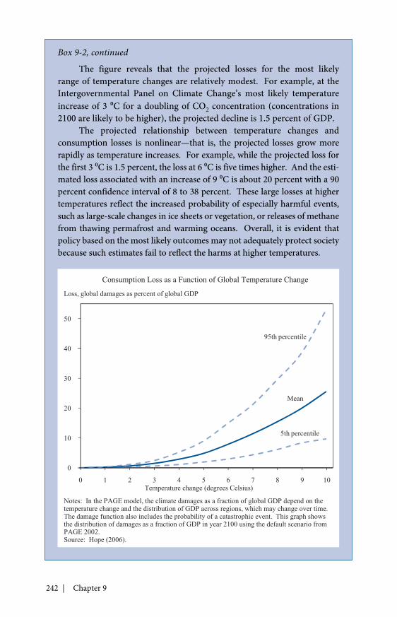
242 | Chapter 9
The figure reveals that the projected losses for the most likelyrange of temperature changes are relatively modest. For example, at theIntergovernmental Panel on Climate Change’s most likely temperatureincrease of 3 0C for a doubling of CO2 concentration (concentrations in2100 are likely to be higher), the projected decline is 1.5 percent of GDP.
The projected relationship between temperature changes andconsumption losses is nonlinear—that is, the projected losses grow morerapidly as temperature increases. For example, while the projected loss forthe first 3 0C is 1.5 percent, the loss at 6 0C is five times higher. And the esti-mated loss associated with an increase of 9 0C is about 20 percent with a 90percent confidence interval of 8 to 38 percent. These large losses at highertemperatures reflect the increased probability of especially harmful events,such as large-scale changes in ice sheets or vegetation, or releases of methanefrom thawing permafrost and warming oceans. Overall, it is evident thatpolicy based on the most likely outcomes may not adequately protect societybecause such estimates fail to reflect the harms at higher temperatures.
Box 9-2, continued
0
10
20
30
40
50
0 1 2 3 4 5 6 7 8 9 10
Consumption Loss as a Function of Global Temperature Change
Loss, global damages as percent of global GDP
5th percentile
Mean
95th percentile
Temperature change (degrees Celsius)
Notes: In the PAGE model, the climate damages as a fraction of global GDP depend on thetemperature change and the distribution of GDP across regions, which may change over time.The damage function also includes the probability of a catastrophic event. This graph showsthe distribution of damages as a fraction of GDP in year 2100 using the default scenario fromPAGE 2002.Source: Hope (2006).
Transforming the Energy Sector and Addressing Climate Change | 243
Jump-Starting the Transition to Clean Energy
To make the transition to a clean energy economy, the United Statesand the rest of the world need to reduce their reliance on carbon-intensivefossil fuels. The American Reinvestment and Recovery Act of 2009 providesa jump-start to this transition by providing about $60 billion in directspending and $30 billion in tax credits (Council of Economic Advisers 2010).These Recovery Act investments were carefully chosen and provide a soup-to-nuts approach across a spectrum of energy-related activities, rangingfrom taking advantage of existing opportunities to improve energy efficiencyto investing in innovative high-technology solutions that are currently littlemore than ideas. These investments will help create a new generation ofjobs, reduce dependence on oil, enhance national security, and protect theworld from the dangers of climate change. Ultimately, the investments willput the United States on a path to becoming a global leader in clean energy.
Recovery Act Investments in Clean EnergyA market-based approach to reducing greenhouse gases (discussed
in detail later) will provide incentives for research and development (R&D)into new clean energy technologies as firms search for ever cheaper ways toaddress the negative externality associated with their emissions. However, asalready described, there is a separate externality in the area of R&D. Becauseit is difficult for the person or firm doing research to capture all of the returns,the private market supplies too little R&D—particularly for more basic formsof R&D, less so as ideas move toward demonstration and deployment. In thiscase, government R&D policies can complement the use of a market-basedapproach to reducing greenhouse gas emissions and yield large benefits tosociety. A policy that broadly incentivizes energy R&D is more likely tomaximize social returns than a narrow one targeted at a specific technologybecause it allows the market, rather than the government, to pick winners.Likewise, funding efforts in support of basic R&D are less likely to crowd outprivate investment because differences between private and social returns toinnovation are largest for basic R&D.
In its 2011 proposed budget, the Administration has stated a commit-ment to fund R&D as part of its comprehensive approach to transformthe way we use and produce energy while addressing climate change. TheRecovery Act investments begun in 2009 are a first step in this clean energytransformation. They fall into eight categories that are briefly described here.

244 | Chapter 9
Energy Efficiency. The Recovery Act promotes energy efficiencythrough investments that reduce energy consumption in many sectorsof the economy. For instance, the Act appropriates $5 billion to theWeatherization Assistance Program to pay up to $6,500 per dwelling unitfor energy efficiency retrofits in low-income homes. The Recovery Act alsoappropriates $3.2 billion to the Energy Efficiency and Conservation BlockGrant program, most of which will go to U.S. states, territories, local govern-ments, and Indian tribes to fund projects that improve energy efficiency,reduce energy use, and lower fossil fuel emissions.
Renewable Generation. The Recovery Act investments in renew-able energy generation also are leading to the installation of wind turbines,solar panels, and other renewable energy sources. The Energy InformationAdministration projects that the fraction of the Nation’s electricity gener-ated from renewable energy, excluding conventional hydroelectric power,will grow from 3 percent in 2008 to almost 7 percent in 2012 in large partbecause of the renewal of Federal tax credits and the funding of new loanguarantees for renewable energy through the Recovery Act (Department ofEnergy 2009a).
Grid Modernization. As the United States transitions to greater use ofintermittent renewable energy sources such as wind and solar, the RecoveryAct is financing the construction of new transmission lines that can supportelectricity generated by renewable energy. The Act is also investing in newtechnologies that will improve electricity storage capabilities and the moni-toring of electricity use through “smart grid” devices, such as sophisticatedelectric meters. These investments will improve the reliability, flexibility,and efficiency of the Nation’s electricity grid.
Advanced Vehicles and Fuels Technologies. The Recovery Act isfunding research on and deployment of the next generation of automobilebatteries, advanced biofuels, plug-in hybrids, and all-electric vehicles, as wellas the necessary support infrastructure. These efforts are expected to reducethe Nation’s dependence on oil in the transportation sector.
Traditional Transit and High-Speed Rail. Grants from the RecoveryAct also will help upgrade the reliability and service of public transit andconventional intercity railroad systems. For example, $8 billion is going toimprove existing, or build new, high-speed rail in 100- to 600-mile intercitycorridors. Investments in high-speed rail and public transit will increaseenergy efficiency by improving both access and reliability, thus making itpossible for more people to switch to rail or public transit from autos orother less energy-efficient forms of transportation.
Carbon Capture and Storage. One approach to limiting greenhousegas emissions is to capture and store carbon from fossil-fuel combustion to

Transforming the Energy Sector and Addressing Climate Change | 245
keep it from entering the atmosphere. The abundance of coal reserves in theUnited States makes developing such technologies and overcoming barriersto their use a particular priority. For instance, technology to capture carbondioxide emissions has been used in industrial applications but has not beenused on a commercial scale to capture emissions from power generation.Likewise, although some carbon has been stored deep in the ocean or under-ground in depleted oil reservoirs, questions remain about the permanenceof these and other types of storage. The Recovery Act is funding crucialresearch, development, and demonstration of these technologies.
Innovation and Job Training. The Recovery Act is also investingin the science and technology needed to build the foundation for the cleanenergy economy. For instance, a total of $400 million has been allocated tothe Advanced Research Projects Agency-Energy (ARPA-E) program, whichfunds creative new research ideas aimed at accelerating the pace of innova-tion in advanced energy technologies that would not be funded by industrybecause of technical or financial uncertainty. The Recovery Act also helpsfund the training of workers for jobs in the energy efficiency and cleanenergy industries of the future.
Clean Energy Equipment Manufacturing. The Recovery Actinvestments are increasing the Nation’s capacity to manufacture windturbines, solar panels, electric vehicles, batteries, and other clean energycomponents domestically. As the United States transitions away from fossilfuels, demand for advanced energy products will grow, and these invest-ments in clean energy will help American manufacturers participate insupplying the needed goods.
Total Recovery Act Energy Investments. The Recovery Act isinvesting in 56 projects and activities that are related to transitioning theeconomy to clean energy. Forty-five are spending provisions with a totalappropriation of $60.7 billion, and another 11 are tax incentives that theOffice of Tax Analysis estimates will cost $29.5 billion through fiscal year2019, for a total investment of over $90 billion. In some cases, a relativelysmall amount of Federal investment leverages a larger amount of non-Federal support. Throughout this section, only the expected subsidy cost ofthe Federal investment is counted toward the appropriation.3
The largest clean energy investments from the Recovery Act go torenewable energy generation and transmission, energy efficiency, andtransit. Figure 9-2 illustrates how this $90 billion investment is distributedacross the eight categories of projects described above, along with a ninth“other” category containing programs that do not fit elsewhere.3 Because of the public nature of the Bonneville and Western Area Power Administrations, theaccounting of clean energy investments described here measures the projected drawdown of theborrowing authority to these agencies as the Recovery Act appropriation.
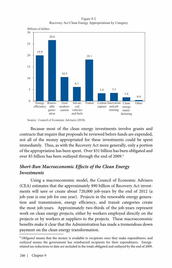
246 | Chapter 9
Because most of the clean energy investments involve grants andcontracts that require that proposals be reviewed before funds are expended,not all of the money appropriated for these investments could be spentimmediately. Thus, as with the Recovery Act more generally, only a portionof the appropriation has been spent. Over $31 billion has been obligated andover $5 billion has been outlayed through the end of 2009.4
Short-Run Macroeconomic Effects of the Clean EnergyInvestments
Using a macroeconomic model, the Council of Economic Advisers(CEA) estimates that the approximately $90 billion of Recovery Act invest-ments will save or create about 720,000 job-years by the end of 2012 (ajob-year is one job for one year). Projects in the renewable energy genera-tion and transmission, energy efficiency, and transit categories createthe most job-years. Approximately two-thirds of the job-years representwork on clean energy projects, either by workers employed directly on theprojects or by workers at suppliers to the projects. These macroeconomicbenefits make it clear that the Administration has made a tremendous downpayment on the clean energy transformation.4 Obligated means that the money is available to recipients once they make expenditures, andoutlayed means the government has reimbursed recipients for their expenditures. Energy-related tax reductions to date are included in the totals obligated and outlayed by the end of 2009.
19.9
26.6
10.5
6.1
18.1
3.4 3.51.6
0.40
5
10
15
20
25
30
Figure 9-2Recovery Act Clean Energy Appropriations by Category
Billions of dollars
Energyefficiency
Renew-able
gener-ation
Gridmodern-ization
Advan-ced
vehiclesand fuels
Transit Carboncapture
Innovationand jobtraining
Cleanenergymanu-
facturing
Other
Source: Council of Economic Advisers (2010).
Transforming the Energy Sector and Addressing Climate Change | 247
Other Domestic Actions toMitigate Climate Change
In his first year in office, the President took several other significantand concrete steps to transform the energy sector and address climatechange. Significantly, the Environmental Protection Agency (EPA) issuedtwo findings in December 2009. The first finding was that six greenhousegases endanger public health and welfare. The second finding was that theemissions of these greenhouse gases from motor vehicles cause or contributeto pollution that threatens public health and welfare. These findings do notin and of themselves trigger any requirements for emitters, but they lay thefoundation for regulating greenhouse gas emissions.
Following up on these findings, the Administration has proposedthe first mandatory greenhouse gas emission standards for new passengervehicles. The standards are expected to be finalized in the spring of 2010.By model year 2016, new cars and light trucks sold in the United States willbe required to meet a fleet-wide tailpipe emissions limit equivalent to astandard of about 35.5 miles per gallon if met entirely through fuel economyimprovements. The EPA estimates that these standards will save about36 billion gallons of fuel and reduce vehicle greenhouse gas emissions byabout 760 million metric tons in CO2-equivalent terms over the lifetime ofthe vehicles.
The Administration also proposed renewable fuel standards consis-tent with the Energy Independence and Security Act (EISA), which requiresthat a minimum volume of renewable fuel be added to gasoline sold in theUnited States. Renewable fuels are derived from bio-based feedstocks suchas corn, soy, sugar cane, or cellulose that have fewer life-cycle greenhouse gasemissions than the gasoline or diesel they replace. When fully implemented,the standards will increase the volume of renewable fuel blended intogasoline from 9 billion gallons in 2008 to 36 billion gallons by 2022.
The Administration also has been proactive in establishing minimumenergy efficiency standards for a wide variety of consumer products andcommercial equipment. For instance, standards were proposed or finalizedin 2009 for microwave ovens, dishwashers, small electric motors, lighting,vending machines, residential water heaters, and commercial clotheswashers, among others. Overall, these actions will reduce energy consump-tion and, in turn, greenhouse gas emissions. The Energy InformationAdministration’s 2009 Annual Energy Outlook projected that by 2030,higher fuel economy and lighting efficiency standards will contribute tolowering energy use per capita by 10 percent, compared with fairly stableenergy use per capita between 1980 and 2008 (Department of Energy
248 | Chapter 9
2009b). The 2010 Annual Energy Outlook highlights appliance and buildingefficiency standards as one reason for lower projected carbon dioxide emis-sions growth, underscoring the benefits of these regulations (Department ofEnergy 2009a).
Beginning in 2010, the United States will begin collectingcomprehensive high-quality data on greenhouse gases from large emittersin many sectors of the economy (for instance, electricity generators andcement producers). When fully implemented, this program will cover about85 percent of U.S. emissions. The information supplied will provide a basisfor formulating policy on how best to reduce emissions in the future. Itwill also be a valuable tool to allow industry to track emissions over time.Specifically, these data will make it possible for industry and government toidentify the cheapest ways to reduce greenhouse gas emissions.
Finally, the President issued an Executive Order requiring Federalagencies to set and meet aggressive goals for greenhouse gas emission reduc-tions. Importantly, agencies are instructed to pursue reductions that lowerenergy expenses and save taxpayers money.
Market-Based Approaches to Advancethe Clean Energy Transformation
and Address Climate Change
Greenhouse gas emissions, as noted, are a classic example of anegative externality. Emitters of greenhouse gases contribute to climatechange, thus imposing a cost on others that is not accounted for whenmaking decisions about how to produce and consume energy-intensivegoods. For this reason, policymakers should ensure that the market providesthe correct signals to greenhouse-gas emitters about the full cost of theiremissions. Once policy has ensured that markets are providing the correctsignals and incentives, the operation of market forces can find the mosteffective and efficient paths to the clean energy economy. The Presidenthas included a market-based cap-and-trade approach in his 2010 and 2011budgets as a way to accomplish this goal. This section describes the basicsof this approach, including several potential ways to minimize compliancecosts. It then discusses a specific proposal consistent with the President’sgoals for reducing greenhouse gas emissions.
Cap-and-Trade Program BasicsA cap-and-trade approach sets a limit on, or caps, total annual
aggregate greenhouse gas emissions and then divides the cap into

Transforming the Energy Sector and Addressing Climate Change | 249
emission allowances. These allowances are allocated to firms throughsome combination of an auction and free allocation.5 Firms may trade theallowances among themselves but are required to hold an allowance for eachton of greenhouse gas they emit. The aggregate cap limits the number ofallowances available, ensuring their scarcity and thus establishing a price inthe market for allowances. In this way, a cap-and-trade approach providescertainty in the quantity of emission reductions but allows the price of allow-ances to fluctuate with changes in the demand and supply.
Creating a market for greenhouse gas emissions gives firms flexibilityin how they reduce emissions. Absent other regulatory requirements, afirm subject to the cap can choose to comply by changing its input mix (forinstance, switching from coal to natural gas), modifying the underlyingtechnology used in production (using more energy-efficient equipment,for example), or purchasing allowances from other entities with lowerabatement costs. Such flexibility reaps rewards. A cap-and-trade programinduces firms to seek out and exploit the lowest-cost ways of cutting emis-sions. It takes advantage of the profit motive and leverages private sectorimagination and ingenuity to find ways to lower emissions.
Cap-and-trade programs already have proven successful. The UnitedStates has been using a cap-and-trade approach to reduce sulfur dioxide(SO2) emissions since 1995. One study found that using a cap-and-tradeapproach instead of a performance standard to reduce sulfur dioxide emis-sions caused some firms to move away from putting scrubbers on theirsmokestacks to cheaper ways of meeting the cap, such as by blendingdifferent fuels (Burtraw and Palmer 2004). As a result, compliance costs ofthe SO2 cap-and-trade program have been dramatically lower than predicted.
Finally, a cap-and-trade approach promotes innovation. A carbonprice will give firms the certainty they need to make riskier long-term invest-ments that could identify novel and substantially cheaper ways to reduceemissions. Evidence shows that pricing sulfur dioxide emissions througha cap-and-trade approach has produced patentable innovations as firmssearch for ever cheaper ways to abate (Burtraw and Szambelan 2009).
In the case of greenhouse gases, possible innovations range from newtechniques to capture and store carbon generated by coal-burning electricityplants, to carbon-eating trees and algae, to the development of new types ofrenewable fuels. Indeed, such innovation—and the opportunity it provides
5 In his fiscal year 2011 proposed budget, the President supports using allowance revenue tocompensate vulnerable families, communities, and businesses during the transition to the cleanenergy economy, as well as in support of clean energy technologies and adapting to the impactsof climate change.
250 | Chapter 9
to make the United States a world leader in clean energy technologies—is akey motivation for the Administration’s energy and climate policies.
Ways to Contain Costs in an Effective Cap-and-Trade SystemThere are a wide variety of ways to contain costs within a cap-and-
trade framework. For instance, cap-and-trade programs may incorporatebanking and borrowing of emission allowances over time, set ceilings orfloors on allowance prices, or permit the use of offsets as ways to smooth thecosts of compliance over time. A brief review of these mechanisms follows.
Banking and Borrowing. A cap-and-trade approach can be designedto give polluters flexibility in the timing of emission reductions throughbanking and borrowing. To limit allowance price volatility, sources canmake greater reductions early if it is cheaper to do so and bank their allow-ances for future use. Likewise, firms can manage costs by borrowing againstfuture reductions, allowing them to emit more today in return for moredrastic reductions later.
Evidence shows that banking has played a particularly powerful rolein helping firms to hedge uncertainty in the costs of the SO2 cap-and-tradeprogram over time. Anticipating that the cap originally set in 1995 wouldbecome more stringent in 2000, firms began to bank allowances for futureuse soon after the system was put in place. By 1999, almost 70 percent ofavailable allowances in the market had been banked. Once the more strin-gent cap was in place, the banked allowances were drawn down to meetthe cap, with about a 40 percent decrease in the size of the allowance bankbetween 2000 and 2005 (Environmental Protection Agency 2006).
In contrast, the inability of firms to bank or borrow in SouthernCalifornia’s nitrous oxide market played a significant role in increased pricevolatility during the State’s electricity crisis in 2000 when firms met soaringdemand for electricity by running old, dirty generators. One study foundthat the absence of banking and borrowing was an important contrib-uting factor to the roughly tenfold increase in the price of nitrous oxideallowances, resulting in power plants subject to the cap eventually seekingexemption from the program (Ellerman, Joskow, and Harrison 2003).
Price Ceilings or Floors. While banking and borrowing allow firms tosmooth costs over time, they may not guard against unexpected and poten-tially longer-lasting changes in allowance prices caused by such factors as arecession or economic boom, fuel price fluctuations, or unexpected varia-tion in the pace of technological development. Consequently, cap-and-tradesystems often include protections against prices that are deemed too high.For example, in the Northeast’s greenhouse gas trading system, allowance
Transforming the Energy Sector and Addressing Climate Change | 251
prices above certain thresholds trigger additional flexibilities that reducecompliance costs.6
Another way for a cap-and-trade program to mitigate the effects ofunexpected changes would be to specify an upper or lower limit, or both, onallowance prices. An upper limit protects firms and consumers from unex-pectedly high prices. When the price reaches the upper limit, additionalallowances are sold to prevent further escalation. A lower limit on allowanceprices ensures that cheap abatement opportunities continue to be pursued.For example, cap-and-trade legislation recently passed by the U.S. House ofRepresentatives reserves a small share of allowances to be auctioned if theprice rises above a predetermined threshold and also sets a minimum pricefor allowances that are auctioned. One study finds that, for a given cumula-tive emissions reduction, a combined price ceiling and floor can reduce costsby almost 20 percent compared with a cap-and-trade program without anycost-containment mechanisms (Fell and Morgenstern 2009). On the otherhand, it is possible that a floor or ceiling can cause total emissions to differfrom the legislated cap.
Offsets. Offsets also can be an important cost-containment featureof a cap-and-trade program. Offsets are credits generated by reducingemissions in a sector outside the program; they can be purchased by a firmsubject to the cap to meet its compliance obligations. Because greenhousegases are global pollutants—they cause the same damage no matter wherethey are emitted—offsets offer the appealing prospect of achieving specifiedemissions reductions at a lower cost.
The purchase of offsets from the forestry and agricultural sectorscould play a potentially important role in reducing the compliance costs offirms subject to the cap (Kinderman et al. 2008; Environmental ProtectionAgency 2009). And under some cap-and-trade programs, domestic firmsmay purchase international offsets to meet their compliance obligations.This possibility may encourage a foreign country to build a solar power plantrather than a coal plant so that it can sell the offsets in the U.S. market.
Despite these important advantages, however, it is crucial that theclaimed reductions from offsets be real—otherwise the system will effec-tively provide payments without actually reducing emissions. Indeed,Europe’s experience with a project-based approach to international offsetssuggests that concerns about the environmental integrity of claimed
6 Above $7 per ton (in 2005 dollars), a firm can cover up to 5 percent of its emissions withdomestic offsets, up from 3.3 percent. At $10 per ton (in 2005 dollars plus a 2 percent increaseper year), this amount increases to 10 percent of emissions and may include international offsets.
252 | Chapter 9
emissions reductions are well founded (Box 9-3).7 If offsets are going tobe included as part of a cap-and-trade program, substantial investmentsin rigorous monitoring methods, such as combining remote sensing withon-the-ground monitoring, to verify greenhouse gas reductions are crucial.
7 Cap-and-trade programs that allow project-level offsets are particularly susceptible to creditingactivity that would have occurred anyway or that is replaced by high-carbon activities elsewhere(leakage). One way to reduce the potential for leakage is a sector- or country-based framework,in which sectors or governments receive credit in exchange for implementing policies to reduceemissions. The legislation passed by the U.S. House of Representatives includes a sector-basedapproach to international offsets.
Box 9-3: The European Union’s Experience with Emissions Trading
One of the pillars of the President’s proposed response to climatechange is a cap-and-trade system to reduce U.S. emissions of greenhousegases. The European Union’s Emission Trading Scheme (ETS), the world’sfirst mandatory cap-and-trade program for carbon dioxide emissions, waslaunched in 2005 to meet emission reduction targets agreed to under theKyoto Protocol. The first phase of the ETS—from 2005 to 2007—appliedto several high-emitting industrial sectors, including power generation, in25 countries and covered just over 40 percent of all European Union (EU)emissions. Although data limitations and uncertainty over baseline emis-sions preclude researchers from assessing the precise magnitude of thereductions, one estimate suggests that the ETS reduced EU emissions byabout 4 percent in 2005 and 2006 relative to what the level would have beenin its absence. Because of the flexibility offered under the cap-and-tradeprogram, these reductions occurred where it was cheapest to achieve them.That said, the ETS offers three important cautionary lessons as the UnitedStates explores how best to implement its own cap-and-trade system.
One lesson is the importance of carefully establishing a baseline forcurrent and future emissions, so that the price sends an accurate signal tofirms regarding how much to abate and innovate based on the expectedfuture value of reductions. During the first phase of the ETS, EU countriesallocated allowances based on firms’ estimates of their historic emissions.In April 2006, when monitoring data became available, the data showedthat actual emissions were already below the cap. Allowance prices imme-diately fell from about €30 ($38) per metric ton to less than €10 ($13)before settling at €15−€20 ($19−$25) for the next few months.
The EU experience also demonstrates that distributing nearly allallowances to industry at no cost can lead to large windfall profits. TheEuropean Union distributed nearly 100 percent of allowances free to
Continued on next page
Transforming the Energy Sector and Addressing Climate Change | 253
Coverage of Gases and IndustriesAlthough carbon dioxide made up about 83 percent of U.S.
greenhouse emissions in 2008, a cap-and-trade approach that gives firmsflexibility in where they reduce emissions, both in terms of the greenhousegas and the economic sector, can lower firms’ compliance costs. One studyfound that achieving an emission goal by cutting both methane and carbondioxide emissions rather than carbon dioxide alone could reduce firms’abatement costs in the United States by over 25 percent in the medium run(Hayhoe et al. 1999).
Costs are also affected by the number of industries covered by the cap,with the general principle being that greater coverage lowers the marginalcost of emissions reductions. A recent study comparing alternative waysto achieve a 5 percent reduction in emissions found that the cap-and-tradeprogram’s costs to the economy were twice as large when manufacturing wasexcluded as they were under an economy-wide approach (Pizer et al. 2006).
firms subject to the cap in Phase 1 and only auctioned a small portion ofallowances for Phase 2 (2008−12). One estimate (Point Carbon AdvisoryServices 2008) suggests that during Phase 2, electricity generators inGermany will reap the highest windfall profits of all participating EUcountries, on the order of €14 billion to €34 billion ($20 billion to$49 billion). In countries with low-greenhouse-gas emitters, electricitygenerators are expected to benefit less. For instance, in Spain, windfallprofits are estimated to be about €1 billion to €4 billion ($1 billion to$6 billion). In Phase 3 (2013–20), the European Union plans to auctionthe majority of allowances.
Finally, it is important to ensure that any offsets from domesticand international sources reflect real reductions. Otherwise, they mayendanger the environmental integrity of the cap. The ETS allows limiteduse of project-based international offsets from the United Nations’ CleanDevelopment Mechanism (CDM) in place of domestic emission reduc-tions. A review of a random sample of offset project proposals in the CDMprogram from 2004 to 2007 estimated that “additionality” was unlikely orquestionable for roughly 40 percent of registered projects, representing20 percent of emissions reductions, meaning they would have occurredanyway (Schneider 2007). Although the CDM has worked to improve itsaccounting procedures over time, the EU’s experience demonstrates theimportance of designing an offsets program carefully.
Box 9-3, continued
254 | Chapter 9
The American Clean Energy and Security ActIn June 2009, the U.S. House of Representatives passed legislation—the
American Clean Energy and Security Act (ACES)—that includes a cap-and-trade program consistent with the President’s goal of reducing greenhousegas emissions by more than 80 percent by 2050, and the Senate is currentlyengaged in a bipartisan effort to develop a bill.
Projected Climate Benefits. Based on two analyses of the ACESlegislation, U.S. actions would reduce cumulative greenhouse gas emissionsby approximately 110 billion to 150 billion metric tons in CO2-equivalentsby 2050 (Paltsev et al. 2009; Environmental Protection Agency 2009). TheEPA estimates that emission reductions of this magnitude, when combinedwith comparable action by other countries consistent with reducing worldemissions by 50 percent in 2050, is expected to limit warming in 2100 to lessthan 2 °C (3.6 °F) relative to the pre-industrial global average temperature,with a likely range of about 1.0 to 2.5 °C (1.8 to 4.5 °F).
To derive the possible benefits associated with the U.S. contributionto these emission reductions, the CEA calculates that the ACES will result inapproximately$1.6 trillionto$2.0 trillionofavoidedglobaldamages inpresentvalue terms between 2012 and 2050 (in 2005 dollars).8 The value of avoideddamages includes such benefits as lower mortality rates, higher agriculturalyields, money saved on adaptation measures, and the reduced likelihood ofsmall-probability but high-impact catastrophic events. Further, the benefitswill be significantly larger if U.S. policy induces other countries to undertakereductions in greenhouse gas emissions.
Projected Economic Costs. The estimated cost of meeting the capsoutlined in the ACES legislation is relatively small. Recent research suggeststhat the ACES will result in a loss of consumption on the order of 1 to2 percent in 2050 (Environmental Protection Agency 2009; Paltsev etal. 2009). On a per household basis, the average annual consumptionloss would be between $80 and $400 a year between 2012 and 2050 (in2005 dollars).
8 The CEA uses estimates of the projected decline in emissions between 2012 and 2050 based onthe President’s proposed reductions in emissions and uses the central estimate of $20 a ton for aunit of carbon dioxide emitted in 2007 (in 2007 dollars) that was recently developed as an interimvalue for regulatory analyses (Department of Energy 2009c). Additionally, it assumes that thebenefit of reducing one additional ton of carbon dioxide grows at 3 percent over time and thatfuture damages from current emissions are discounted using an average of 5 percent. SeveralFederal agencies have used these values in recent proposed rulemakings but have requestedcomment prior to the final rulemaking, so these estimates may be revised.
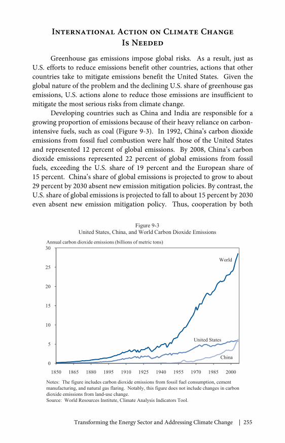
Transforming the Energy Sector and Addressing Climate Change | 255
International Action on Climate ChangeIs Needed
Greenhouse gas emissions impose global risks. As a result, just asU.S. efforts to reduce emissions benefit other countries, actions that othercountries take to mitigate emissions benefit the United States. Given theglobal nature of the problem and the declining U.S. share of greenhouse gasemissions, U.S. actions alone to reduce those emissions are insufficient tomitigate the most serious risks from climate change.
Developing countries such as China and India are responsible for agrowing proportion of emissions because of their heavy reliance on carbon-intensive fuels, such as coal (Figure 9-3). In 1992, China’s carbon dioxideemissions from fossil fuel combustion were half those of the United Statesand represented 12 percent of global emissions. By 2008, China’s carbondioxide emissions represented 22 percent of global emissions from fossilfuels, exceeding the U.S. share of 19 percent and the European share of15 percent. China’s share of global emissions is projected to grow to about29 percent by 2030 absent new emission mitigation policies. By contrast, theU.S. share of global emissions is projected to fall to about 15 percent by 2030even absent new emission mitigation policy. Thus, cooperation by both
0
5
10
15
20
25
30
1850 1865 1880 1895 1910 1925 1940 1955 1970 1985 2000
Figure 9-3United States, China, and World Carbon Dioxide Emissions
Annual carbon dioxide emissions (billions of metric tons)
World
United States
China
Notes: The figure includes carbon dioxide emissions from fossil fuel consumption, cementmanufacturing, and natural gas flaring. Notably, this figure does not include changes in carbondioxide emissions from land-use change.Source: World Resources Institute, Climate Analysis Indicators Tool.

256 | Chapter 9
past and future contributors to emissions will be required to stabilize theatmospheric concentrations of greenhouse gases.
In keeping with this goal, the Administration has actively pursuedpartnerships with major developed and emerging economies to advanceefforts to reduce greenhouse gas emissions and promote economicdevelopment that lowers emission intensity.
Partnerships with Major Developed and Emerging EconomiesThe President has worked to further a series of international
agreements to address climate change. For example, he launched the MajorEconomies Forum on Energy and Climate to engage 17 developed andemerging economies in a dialogue on climate change. In July, the leaders ofthese countries agreed that greenhouse gas emissions should peak in devel-oped and developing countries alike, and recognized the scientific view thatthe increase in global average temperature above pre-industrial levels oughtnot to exceed 2 °C (3.6 °F). They also agreed to coordinate and dramati-cally increase investment in research, development, and deployment oflow-carbon energy technologies with a goal of doubling such investment by2015. Finally, the leaders agreed to mobilize financial resources in supportof mitigation and adaptation activities, recognizing that the group should beresponsive to developing-country needs in this area.
Also in July, leaders from the Group of Eight (G-8) countries agreedto undertake robust aggregate and individual medium-term emission reduc-tions consistent with the objective of cutting global emissions by at least50 percent by 2050. Additionally, under the Montreal Protocol, the UnitedStates jointly proposed with Canada and Mexico to phase down emissionsof hydrofluorocarbons, a potent greenhouse gas used in refrigeration, firesuppression, and other industrial activities. This action alone would achieveabout 10 percent of the greenhouse gas emission reductions needed to meetthe agreed G-8 goal of a 50 percent reduction by 2050.
In December, the Administration worked with major emergingeconomies, including Brazil, China, India, and South Africa, developedcountries, and other regions around the world to secure agreement onthe Copenhagen Accord. For the first time, the international communityestablished a long-term goal to limit warming of global average temperatureto no more than 2 °C (3.6 °F). Also for the first time, all major economiesagreed to take action to address climate change. Under the Accord, bothdeveloped and major emerging economies are in the process of submittingtheir emission mitigation commitments and actions to reduce greenhousegas emissions. Every two years, developing countries will report on emissionmitigation efforts, which will be subject to international consultation and
Transforming the Energy Sector and Addressing Climate Change | 257
analysis under clearly defined guidelines. Establishing transparent review ofdeveloped and developing country mitigation activities will help ensure thatcountries stand behind their commitments.
Furthermore, under the Accord, in the context of meaningful mitiga-tion actions and transparency, developed countries committed to a goal ofjointly mobilizing $100 billion a year in funding from a variety of private andpublic sources for developing countries by 2020. This funding will build onan immediate effort by developed countries to support forestry, adaptation,and emissions mitigation with funding approaching $30 billion sometime inthe 2010 to 2012 timeframe. There will be a special focus on directing thisfunding to the poorest and most vulnerable developing countries.
Phasing Out Fossil Fuel SubsidiesThe United States also spearheaded an agreement in September to
phase out fossil fuel subsidies among G-20 countries, a goal seconded bycountries in the Asian-Pacific Economic Cooperation (APEC) in November.The G-20 also called on all nations to phase out such subsidies world-wide. Fossil fuel subsidies are particularly large in non-OECD countries,such as India and Russia. Twenty of the largest non-OECD governmentsspent about $300 billion on fossil fuel subsidies in 2007. Together, thiscoordinated action to reduce subsidies can free up resources, especially indeveloping countries, to target other social needs such as public health andeducation. One model estimates that eliminating fossil fuel subsidies inthe major non-OECD countries alone would reduce greenhouse gas emis-sions by more than 7 billion metric tons of CO2-equivalent, enough to fulfillalmost 15 percent of the agreed-upon G-8 goal of reducing global emis-sions by 50 percent by 2050 (Organisation for Economic Co-operation andDevelopment 2009).
In the United States, these subsidies—including tax credits,deductions, expensing practices, and exemptions—are worth about$44 billion in tax revenues between 2010 and 2019. Their elimination willhelp put cleaner fuels, such as those derived from renewable sources, on amore equal footing and reduce wasteful consumption of fossil-fuel basedenergy caused by underpricing. Proper pricing of fossil fuels will also helpreduce reliance on petroleum, thus enhancing energy security and aiding inthe achievement of climate mitigation goals.
Conclusion
Today’s economy is dependent on carbon-intensive fuels that aredirectly linked to an increase in global average temperature. Continued

258 | Chapter 9
reliance on these fuels will have a range of negative impacts, includingincreased mortality rates, reduced agricultural productivity in many loca-tions, higher sea levels, and the need for costly adaptation efforts. For thesereasons, a clean energy transformation is essential.
Through his comprehensive plan, the President has set the countryon course to achieve this goal. He has taken several significant and concretesteps to transform the energy sector and address climate change throughthe American Reinvestment and Recovery Act and through targeted regula-tion. To address externalities associated with greenhouse gas emissions,the President has proposed a market-based cap-and-trade approach. Thesecombined efforts will stimulate the research and development necessary toadvance new clean energy technologies. Because of the global nature of theclimate change problem, the Administration is also actively pursuing part-nerships with other countries to advance efforts to transition the world toclean energy and reduce greenhouse gas emissions.

259
C H A P T E R 1 0
FOSTERING PRODUCTIVITYGROWTH THROUGH INNOVATION
AND TRADE
Americans have always believed in building a better future. Eachgeneration has strived to pass on higher standards of living to their
children than they themselves experienced. And for most of Americanhistory, this goal has been realized. Per capita income has risen strongly formost of the past two centuries.
Such economic growth stems from a number of factors. Investmentin skills and education, or human capital, is a key determinant. The UnitedStates has a long history of investing in people, and this has enabled Americanworkers to be among the most productive in the world. Investment in phys-ical capital is also important. The tremendous accumulation of machines,buildings, and infrastructure has been a source of America’s prosperity, andtimes of particularly great investment, such as the 1950s and 1960s, havebeen times of particularly rapid advances in standards of living.
Because investing in people and capital is important to themaintenance and growth of standards of living, the President has fashionedan ambitious agenda of improvements in education, incentives for invest-ment, and financial regulatory reform to ensure that we have the financialsystem needed to support such investment. These initiatives have beendescribed in detail in earlier chapters.
But as important as investments in labor and capital have been andwill continue to be, they are not the only sources of growth. A third, moreamorphous factor has also played a central role in American economicgrowth: advances in the overall productivity of that labor and capital. Oneneed only think of a few of the technological changes of the past century—the airplane, antibiotics, computers, fiber-optic cables, and the Internet—tosee that technological discovery and innovation are central to improvedstandards of living. Such innovations not only make us richer as a country,they have the potential to fundamentally alter the very way we live our livesand interact with one another.

260 | Chapter 10
As discussed throughout this Report, in the past decade Americaneconomic growth has slowed in important ways. American families sawtheir median income actually fall from 2000 to 2006. An important part ofrestoring growth and increases in standards of living is spurring innovationand increases in productivity. American firms and universities will naturallyplay the leading role in this endeavor. But that does not mean governmenthas no role to play. Indeed, overwhelming evidence shows that innovationcreates positive “externalities”—benefits for others beyond the individuals orfirms who originally produce new ideas. Since inventors do not reap the fullrewards, on its own the market will produce less innovation than is optimal.Public policy therefore has a powerful role to play in fostering pursuit of themyriad possibilities for scientific, technical, and analytical advances.
At its best, trade between regions of the country and across borderscan also be an engine of growth. Trade has the potential to allow the U.S.economy to expand output in areas where it is more productive and toenable higher-productivity firms to expand. Access to a world marketencourages American firms to invest in the research needed to become tech-nological leaders. Through these routes, a free and fair trade regime can playan important part in lifting living standards in the long run.
Based on an understanding that progress springs from achieving theproper balance between generous rewards for the creation of new ideas andencouraging the best of those ideas to spread widely, the Administrationhas formulated a comprehensive “innovation agenda” that reaches farbeyond the traditional scope of science and technology policy. This agendatouches everything from improvements in the Patent and TrademarkOffice, to increased government investments in research and development(R&D), to engaging the world economy in ways that ensure that the UnitedStates achieves the maximum benefits from trade’s productivity-enhancingpotential. This chapter discusses the key components of the agenda in detail.
All advances in productivity, whether from scientific breakthroughs,changes in the organization of firms, or increased international trade,involve losers as well as winners. Because productivity growth is the criticalsource of improved standards of living, the most effective way to addressthe painful impacts for those harmed by progress is not to stifle new ideasor trade. Rather, it is to build a robust system of support that can help easethe transition from employment in declining firms and industries to jobs innew, higher-paying, higher-productivity areas. Even more important arebroad-based policies that ensure that the gains from rising productivity arewidely shared: progressive taxation, a health care system that provides secu-rity and stability, a strong educational system, and a secure social safety net.
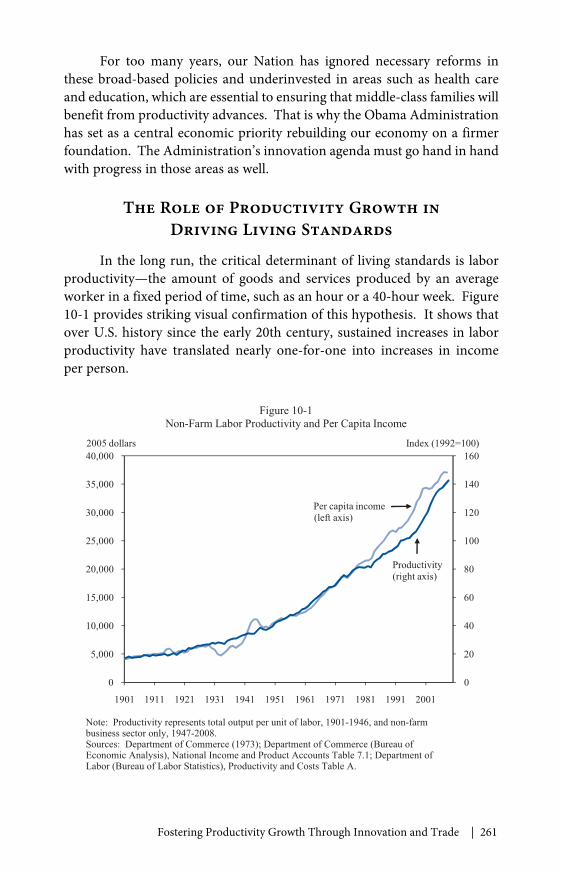
Fostering Productivity Growth Through Innovation and Trade | 261
For too many years, our Nation has ignored necessary reforms inthese broad-based policies and underinvested in areas such as health careand education, which are essential to ensuring that middle-class families willbenefit from productivity advances. That is why the Obama Administrationhas set as a central economic priority rebuilding our economy on a firmerfoundation. The Administration’s innovation agenda must go hand in handwith progress in those areas as well.
The Role of Productivity Growth inDriving Living Standards
In the long run, the critical determinant of living standards is laborproductivity—the amount of goods and services produced by an averageworker in a fixed period of time, such as an hour or a 40-hour week. Figure10-1 provides striking visual confirmation of this hypothesis. It shows thatover U.S. history since the early 20th century, sustained increases in laborproductivity have translated nearly one-for-one into increases in incomeper person.
0
20
40
60
80
100
120
140
160
0
5,000
10,000
15,000
20,000
25,000
30,000
35,000
40,000
1901 1911 1921 1931 1941 1951 1961 1971 1981 1991 2001
Figure 10-1Non-Farm Labor Productivity and Per Capita Income
)001=2991(xednIsrallod5002
Productivity(right axis)
Per capita income(left axis)
Note: Productivity represents total output per unit of labor, 1901-1946, and non-farmbusiness sector only, 1947-2008.Sources: Department of Commerce (1973); Department of Commerce (Bureau ofEconomic Analysis), National Income and Product Accounts Table 7.1; Department ofLabor (Bureau of Labor Statistics), Productivity and Costs Table A.
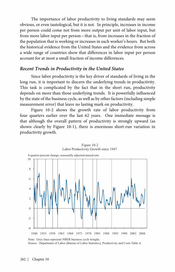
262 | Chapter 10
The importance of labor productivity to living standards may seemobvious, or even tautological, but it is not. In principle, increases in incomeper person could come not from more output per unit of labor input, butfrom more labor input per person—that is, from increases in the fraction ofthe population that is working or increases in each worker’s hours. But boththe historical evidence from the United States and the evidence from acrossa wide range of countries show that differences in labor input per personaccount for at most a small fraction of income differences.
Recent Trends in Productivity in the United StatesSince labor productivity is the key driver of standards of living in the
long run, it is important to discern the underlying trends in productivity.This task is complicated by the fact that in the short run, productivitydepends on more than those underlying trends. It is powerfully influencedby the state of the business cycle, as well as by other factors (including simplemeasurement error) that leave no lasting mark on productivity.
Figure 10-2 shows the growth rate of labor productivity fromfour quarters earlier over the last 62 years. One immediate message isthat although the overall pattern of productivity is strongly upward (asshown clearly by Figure 10-1), there is enormous short-run variation inproductivity growth.
-4
-2
0
2
4
6
8
10
1948 1953 1958 1963 1968 1973 1978 1983 1988 1993 1998 2003 2008
Figure 10-2Labor Productivity Growth since 1947
4-quarter percent change, seasonally adjusted annual rate
Note: Grey lines represent NBER business cycle troughs.Source: Department of Labor (Bureau of Labor Statistics), Productivity and Costs Table A.

Fostering Productivity Growth Through Innovation and Trade | 263
A more subtle message is that the average or trend rate of productivitygrowth is not constant but changes substantially over extended periods. It isconventional to divide the era from the beginning of the sample until about1995 into two periods: the “immediate postwar” period from 1947 through1972, and the “productivity growth slowdown” period from 1973 through1995. In the immediate postwar period, the average rate of productivitygrowth was 2.8 percent per year. During the productivity growth slowdown,it was only 1.4 percent.
This division into different periods lets one see the cumulativeimportance of even seemingly modest changes in productivity growth. Forexample, if the high productivity growth of the immediate postwar periodhad continued through 1995 instead of slowing, the level of productivity in1995—and hence standards of living—would have been more than one-thirdhigher than they actually were.
The pattern of productivity growth since 1995 is somewhatcomplicated. From 1996:Q1 to the last available observation (2009:Q3), itaveraged 2.7 percent per year, almost equal to its rate over the immediatepostwar period. But that rapid growth was concentrated in the first partof the period. In the first eight years (1996:Q1 to 2003:Q4), productivitygrowth averaged 3.3 percent; in the four years before the business cycle peak(2004:Q1 to 2007:Q4), it averaged only 1.7 percent. A four-year period is tooshort to confidently determine underlying trends. But productivity growthin the years leading up to the recession was not strong enough to generaterobust increases in standards of living.
A final pattern revealed by Figure 10-2 is a relationship betweenproductivity growth and the business cycle. Productivity growth tends to fallduring recessions and surge near their ends (marked by the vertical lines inFigure 10-2). This pattern has been operating strongly in the current reces-sion. Productivity growth averaged less than 1 percent at an annual rateover the first five quarters of the recession, but then surged in 2009:Q2 and2009:Q3, and appears to have remained high in 2009:Q4.
This recent experience highlights the importance of distinguishingbetween cyclical movements in productivity and longer-term movements:the pattern in productivity growth in 2009 largely reflects the fact thatemployment moves more slowly than production over the business cycle.The sluggishness of employment growth has meant that even as outputreached its low point and began to recover, employment continued todecline. This cyclical improvement in productivity is obviously of a differentcharacter than the secular improvements that are the source of long-runincreases in standards of living. Over the course of 2009, standards of livingclearly did not follow productivity closely. But once the cyclical dynamics

264 | Chapter 10
play themselves out, the usual long-term role of productivity growth indriving income growth is bound to reassert itself. An important goal ofpolicy is to make the long-term path of productivity as favorable as possible.
Sources of Productivity GrowthProductivity growth is the overwhelming determinant of the progress
of economic well-being over extended periods. It is therefore imperative tounderstand what determines productivity growth. Three sources have beenidentified as key.
The first source is the accumulation of physical capital—the machines,tools, computers, factories, infrastructure, and so on that workers use toproduce output. Each year, some of our Nation’s economic output takes theform of these capital goods. When workers have more or better capital towork with, they are more productive.
The second source is the accumulation of human capital—workers’education, skills, and training. The accumulation of human capital is justas much an investment as the accumulation of physical capital is. Whensome of the economy’s output takes the form of physical capital goods ratherthan consumption, we are forgoing some consumption today in exchangefor the ability to produce more in the future. Likewise, when students andteachers are in a classroom, or when an experienced worker is taking time totrain a new hire, resources that could be used to produce goods for currentconsumption are being used instead for activities that increase futureproductive capacity. And just as a worker with better equipment is moreproductive, so too is a worker with more skills.
The third source of productivity growth is increases in the amountthat can be produced from given amounts of physical and human capital.This factor goes by various names, such as “total factor productivity growth”or “the Solow residual.” It encompasses all the forces that cause changesin how much an economy produces from its stocks of physical and humancapital. Most obviously, it encompasses advances in knowledge and tech-nology. These advances in knowledge and technology allow factory workersto build better automobiles and electronics from the same raw materials;they allow doctors to provide more accurate diagnoses and prescribe bettertreatments in the same office visit; and much more.
But total factor productivity growth includes more than advances inknowledge and technology. For example, if an economy faces an increasein crime, individuals may devote more of their skills and physical capitalto protecting the goods they have rather than producing more goods,and so total factor productivity growth may be low or even negative. If acountry switches from central planning to a market-based economy, then

Fostering Productivity Growth Through Innovation and Trade | 265
workers and capital are likely to be allocated more effectively, and so outputgiven the economy’s stocks of physical and human capital may increasegreatly. Changes in these types of “organizational capital” (or “institu-tional” or “social” capital) are potentially critical determinants of total factorproductivity growth.
Research has not just identified changes in these three factors(physical capital, human capital, and total factor productivity) as criticaldeterminants of productivity growth; it has also come to a fairly clear viewabout their relative importance. Perhaps surprisingly, the ranking of thethree factors appears to be the same whether one is trying to understand theenormous growth in productivity over extended periods in the United States(for example, Jones 2002), or the vast differences in the level of productivityacross countries (for example, Hall and Jones 1999).1
The factor that is most obvious and easiest to quantify—physical capital accumulation—turns out to be only moderately important.Differences in the fraction of output devoted to physical capital investmentaccount for some portion of both long-run productivity growth and cross-country productivity differences, and increases in investment can have asignificant impact on productivity growth, and hence on standards of living.At the same time, the evidence suggests that the other factors are evenmore important.2
One of those more important factors is human capital accumulation.Increases in the education and skills of the workforce play a substantial rolein the long-term growth of labor productivity, and cross-country differencesin human capital per worker are important to cross-country differences inlabor productivity. Thus, increases in human capital investment through astronger educational system and greater educational attainment at all levels,together with lifetime learning, provide another powerful route to raisingproductivity growth and standards of living.
The most important determinant is not physical or human capitalaccumulation, but changes in how much can be produced with them—thatis, total factor productivity growth. Again, this finding applies to both long-term growth and cross-country differences. At an intuitive level, this resultis not surprising. It seems very plausible that the most important reason weare so much more productive than our forebears is that, for reasons ranging1 See also Klenow and Rodríguez-Clare 1997; Hendricks 2002; Caselli 2005; and Hsieh andKlenow 2007.2 There is a subtlety here. When total factor productivity or human capital improves, the resultis higher output, which then leads to more physical capital investment if the fraction of the econ-omy’s output that is invested does not change. The decompositions that find a moderate rolefor physical capital assign these indirect effects of total factor productivity and human capitalinvestment to those factors, and not to physical capital. If those effects are instead assigned tophysical capital, its importance increases greatly.

266 | Chapter 10
from advances in basic scientific knowledge to improved ways of organizingthe workplace, we have found vastly better ways of producing output from agiven set of inputs. Likewise, it is likely that a key reason the United Statesoutperformed the Soviet Union economically in the postwar period wasnot that the United States was better at channeling its productive capacityinto producing capital goods and its children into education (both of whichthe Soviet Union did on a very large scale), but that the United States’ free-market institutions led it to produce more from its inputs, and led to myriadinnovations that widened the productivity gap over time.
This discussion implies that in order to foster improvements instandards of living, policy should foster investment in physical capital,investment in human capital, and crucially, improvements in total factorproductivity. Physical and human capital investment are discussed inearlier chapters—most notably Chapter 4 (as well as Chapters 5 and 6) inthe case of physical capital investment, and Chapter 8 in the case of humancapital. The remainder of this chapter turns to measures to improve totalfactor productivity. Such improvements in total factor productivity can bedescribed broadly as “innovations.”
Fostering Productivity GrowthThrough Innovation
Because total factor productivity reflects all determinants of laborproductivity other than physical and human capital, it has a wide range ofelements. As a result, there are many avenues along which well-designedpolicies can work to improve total factor productivity. It is for this reasonthat the Administration has proposed a comprehensive innovation agenda(Box 10-1).
Box 10-1: Overview of the Administration’s Innovation Agenda
On a September 21 visit to New York’s Hudson Valley CommunityCollege, President Obama presented the first comprehensive descriptionof the Administration’s Innovation Agenda, the conceptual frameworkunderpinning the wide range of initiatives that the Administration hasundertaken that share a common aim of fostering innovation.
The Agenda has three elements. The first is a commitment to investin the building blocks of innovation, including basic scientific researchand infrastructure, as articulated in detail in the body of this chapter.
Continued on next page
Fostering Productivity Growth Through Innovation and Trade | 267
The Importance of Basic ResearchOne uncontroversial conclusion of work on the determinants of
productivity growth is that the payoff to investment in basic scientific andtechnological research has been vast, at least in some fields and over thelong run. Breakthroughs on fundamental questions of physics, chemistry,biology, and other sciences have powered the transformations of economicproduction that underlie much of the productivity growth measured(however imperfectly) in economic statistics (Nordhaus 1997; Nelson andRomer 1996).
The Administration has taken that lesson to heart in its support forbasic research in science and technology, especially in two areas wherethe need for progress is pressing: energy and biomedical research. TheDepartment of Energy has created a new Advanced Research ProjectsAgency-Energy (ARPA-E), with the objective of pursuing breakthroughs
The second is a recognition of the vital role that competitive markets anda healthy environment for entrepreneurial risk-taking play in spurringinnovation; reform of the Patent Office, improving the accessibility andusefulness of government statistics, and increasing the predictability andtransparency of government policy are all parts of this effort. The finalpart of the agenda is a particular focus on innovation targeted towardspecific national priorities, including the development of alternativeenergy sources, reducing costs and improving medical care through theuse of health information technology, the creation of a “smart grid” thatwill allow more efficient use of existing energy generation capacity, andinitiatives aimed at inventing cleaner and more fuel-efficient transporta-tion technologies.
The Agenda builds on over $100 billion of funds appropriated inthe American Recovery and Reinvestment Act of 2009 for the support ofinnovation, education, and technological and scientific infrastructure. Italso encompasses directives to regulatory and executive branch agenciesdesigned to help them refocus their missions to support the Agenda inwhatever ways are most appropriate to their usual activities. A final keytool is the commitment to science-based, data-driven policymaking thatbrings to bear all the intellectual, statistical, informational, and analyticalresources necessary to make sure that government policies achieve theirstated aims as efficiently and effectively as possible.
Box 10-1, continued

268 | Chapter 10
that could fundamentally change the way we use and produce energy. Inthe medical and biological sciences, the Administration has ended restric-tions on Federal funding for embryonic stem cell research, and in September2009 it announced $5 billion in grants under the American Recovery andReinvestment Act to fund cutting-edge medical research.
Across all areas, the Recovery Act included $18.3 billion for researchfunding. Because the Administration’s commitment to evidence-basedpolicymaking will require substantial improvements in the ability to reli-ably measure economic outcomes, the Act committed $1 billion to the 2010Census as a first step in a longer-term effort to revamp the Nation’s statis-tical infrastructure—a process that will not only improve policymaking butwill also help private businesses make better decisions (for example, aboutwhere to locate new production or sales facilities).
In addition, the fiscal year 2011 budget enhances research fundingin numerous ways. First, it continues to work to fulfill the President’spledge to double the budgets of three key science agencies (the NationalScience Foundation, the Department of Energy’s Office of Science, andthe Department of Commerce’s National Institute of Standards andTechnology). Second, it boosts funding for biomedical research at theNational Institutes of Health by $1 billion to $32.1 billion. Third, it rein-vigorates climate change research through increased investments in earthobservations and climate science in agencies such as the U.S. GeologicalSurvey and the National Oceanic and Atmospheric Administration. Fourth,it funds potentially groundbreaking discoveries with a boost to Departmentof Defense basic research and $300 million for the Department of Energy’sARPA-E program. Finally, it supports world-class agricultural research fornational needs such as food safety and bioenergy with $429 million for thecompetitive research grants program in the Department of Agriculture’snew National Institute of Food and Agriculture.
As part of the innovation agenda, and to ensure that the increasedresearch funds are spent well, the Administration has also instructed agen-cies to work on constructing a set of systematic tools to track the long-termresults of federally sponsored research, such as journal articles publishedand cited, patents obtained, medical advances achieved, or other measurableconsequences (particularly in areas of national importance such as health orenergy). Although the fruits of this effort will not be available for a numberof years, the project is one of the most promising in the Administration’sefforts at turning the evaluation of scientific research into a “scienceof science.”

Fostering Productivity Growth Through Innovation and Trade | 269
Private Research and ExperimentationScientific breakthroughs are only the first step in producing
improvements in total factor productivity and hence living standards.Benjamin Franklin’s discovery that lightning was a form of electricity did notproduce an immediate reduction in damage from electrical storms; muchfurther research and development was necessary to turn that discovery intothe lightning rod (though by late in his life Franklin was able to observe aflourishing industry that had been built upon his insight).
Measuring the returns to the economy as a whole from private researchand experimentation is almost as formidable a challenge as measuring thereturns to basic research. But most studies find that aggregate returns tosuch spending are much higher than the returns to ordinary investments inphysical capital. Some work estimates the aggregate returns at 50 percent orhigher (Hall, Mairesse, and Mohnen 2009).
These returns are mostly not received by the firms or individuals whopay for the work, because the ideas ultimately benefit others in many wayswhose value is not captured through markets. Economic theory provides aclear prescription for policy toward activities that have measurable positiveexternalities: the activities should be subsidized.
This is the logic behind the research and experimentation (R&E) taxcredit that has been an off-and-on part of the tax code for many years. Butthe credit’s effectiveness has been hampered by chronic uncertainty abouthow long it will remain in force. Partly for budgetary accounting reasons,the R&E tax credit has been treated for many years as a temporary provi-sion that was scheduled to expire at some point in the near future. Yet eachyear (except for 1995), Congress and the President have agreed (sometimesat the last minute) to extend the credit. The effect has been to substantiallyincrease the uncertainty that firms face about the costs that they will end uppaying for their research and experimentation projects; this uncertainty canhave a serious negative effect on research, which is already a highly uncer-tain investment. The problem is particularly acute for the kinds of projectsthat might be expected to have the highest returns: long-term projects thatrequire continuing expenditures over many years. For such projects, uncer-tainty about whether the R&E tax credit will be in place through the durationof the project can make the difference between pursuing or abandoningthe research. The Administration therefore supports efforts in Congressto make the R&E tax credit permanent, so that the highest-return long-runprojects can be confidently started without uncertainty about whether thecredit will be there for the duration.
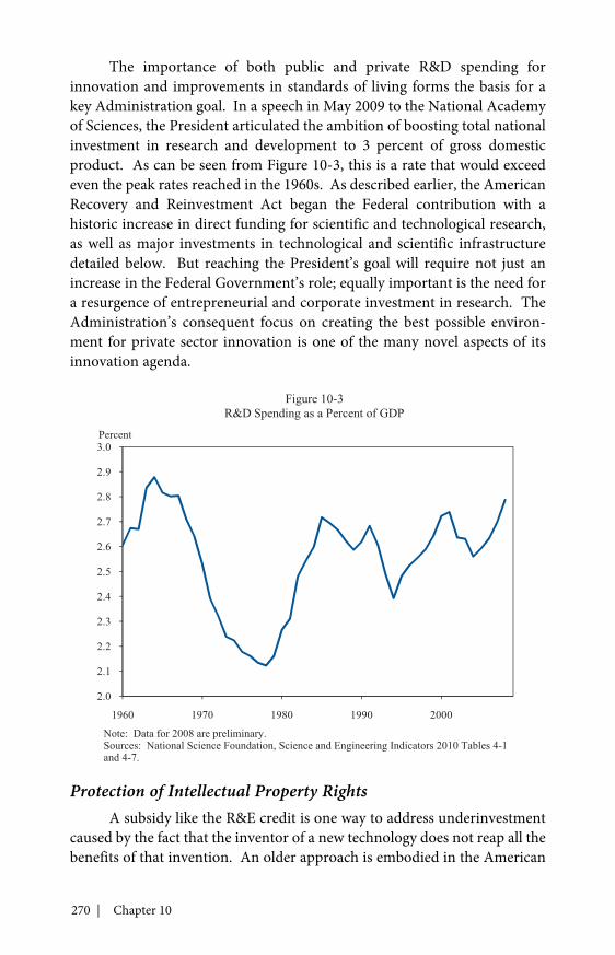
270 | Chapter 10
The importance of both public and private R&D spending forinnovation and improvements in standards of living forms the basis for akey Administration goal. In a speech in May 2009 to the National Academyof Sciences, the President articulated the ambition of boosting total nationalinvestment in research and development to 3 percent of gross domesticproduct. As can be seen from Figure 10-3, this is a rate that would exceedeven the peak rates reached in the 1960s. As described earlier, the AmericanRecovery and Reinvestment Act began the Federal contribution with ahistoric increase in direct funding for scientific and technological research,as well as major investments in technological and scientific infrastructuredetailed below. But reaching the President’s goal will require not just anincrease in the Federal Government’s role; equally important is the need fora resurgence of entrepreneurial and corporate investment in research. TheAdministration’s consequent focus on creating the best possible environ-ment for private sector innovation is one of the many novel aspects of itsinnovation agenda.
Protection of Intellectual Property RightsA subsidy like the R&E credit is one way to address underinvestment
caused by the fact that the inventor of a new technology does not reap all thebenefits of that invention. An older approach is embodied in the American
2.0
2.1
2.2
2.3
2.4
2.5
2.6
2.7
2.8
2.9
3.0
1960 1970 1980 1990 2000
Figure 10-3R&D Spending as a Percent of GDP
Percent
Note: Data for 2008 are preliminary.Sources: National Science Foundation, Science and Engineering Indicators 2010 Tables 4-1and 4-7.

Fostering Productivity Growth Through Innovation and Trade | 271
system of patents and copyrights that had its origins in the Constitution (andbefore that, in the English legal system).
One leading scholar (Jones 2001) has argued that the invention ofways to protect intellectual property may have been a trigger for the indus-trial revolution that led to the modern era of economic growth. In thisinterpretation of history, the creation of a legal system that could protectintellectual property may have been one of the most important “techno-logical” developments in human history. Though this interpretation canbe debated, the practical implication is surely correct: achieving the properbalance between the private and the societal rewards from innovation is acritical element in creating and sustaining long-run economic growth.
The existing U.S. patent system developed over many years in responseto the needs of an industrial economy. That system has been under consider-able strain in the past couple of decades as the United States and the worldhave moved increasingly toward a “knowledge-based” economy. The Patentand Trademark Office (PTO) has been required to answer many questionsthat could not have been imagined in 1952 when the current patent statutewas written, such as how and whether to grant patents for human genes or forInternet advertising tools. Further, the sheer volume of information necessaryto evaluate a patent application, which might now arrive from any country inthe world and might rely on ideas that even an expert might be unfamiliar with,has made the PTO’s job increasingly daunting. As a result of these challenges,the agency currently faces a backlog of over 700,000 unexamined applications.Waiting times on a patent application can extend to four years or more. Thecosts that such waiting times impose on firms are substantial; and delays imposea particularly large burden on startup firms that rely on patents to attract venturecapital funding—precisely the kind of firms that the Administration’s innovationagenda is particularly designed to help.
While the PTO has made progress in responding to these problems,most notably by developing a “peer review” system modeled on academicpublishing, observers agree that the patent system is in need of an overhaul.The Administration has endorsed the aims of bills pending in Congressthat would address many of these problems, particularly by giving the PTOauthority to set fees that cover the cost of application processing, and also bybarring diversion of fees to projects unrelated to PTO activities. The PTO isalso in the process of creating an Office of the Chief Economist, which willprovide a mechanism for better integration into patent policy of economicresearch on how to properly reward innovation without stifling thewidespread use of good ideas.
In recognition of the role of innovation and intellectual propertyin advancing continued U.S. leadership in the global economy, in 2008

272 | Chapter 10
Congress created the Office of the United States Intellectual PropertyEnforcement Coordinator. This office is charged with creating and imple-menting a strategy to coordinate and enhance enforcement of intellectualproperty rights in the United States and overseas. By ensuring that theAdministration has a coordinated strategy, this office will work to ensurethat the effort of American workers and businesses to produce creative andinnovative products and services is valued fairly around the world.
Spurring Progress in National Priority AreasMuch of the Administration’s innovation agenda is aimed at creating
a general economic environment that encourages innovation across theboard. But the Administration has also focused special attention on certainareas where particular national needs are urgent. These include invest-ments in building a “smart grid” to enhance the reliability, flexibility, andefficiency of the electricity transmission grid; research on renewable energytechnologies like wind, solar, and biofuels; and support for research intoadvanced vehicle technologies. These investments are motivated not onlyby the perception that technological breakthroughs are possible and wouldbe highly valuable, but also by the enormous potential benefits that suchbreakthroughs could have in terms of enhancing national security, miti-gating pollution, and stemming climate change. These are also investmentsthat have a direct impact on creating high-paying, durable jobs—somethingthat is particularly valuable at a time of high unemployment. Thus, as notedin Chapter 9, investments in the clean energy transformation involve twolayers of externalities: innovators fail to receive the full economic benefitsof their breakthroughs as measured by market valuation, and the marketvaluation itself understates the true social benefits of the breakthroughs.
Another priority, given the looming threat that health care spendingposes to the Federal budget, is developing technologies for measuringand monitoring health more efficiently. Through the Recovery Act,the Administration has allocated substantial funds to development of a21st-century system of medical recordkeeping that should jump-start workin this area.
Increasing Openness and TransparencyTo noneconomists, the idea that the legal system or the Patent Office
is a form of technology seems a bit of a stretch. Even more challenging isthe idea that a society’s overall degree of openness and transparency maybe a key determinant of economic progress. Yet a substantial body ofeconomic research has found that measures of openness and transparency

Fostering Productivity Growth Through Innovation and Trade | 273
in governmental policymaking processes have a strong association withgrowth outcomes.
There are several reasons why this may be so. One fairly simple oneis that openness and transparency make it more difficult for special intereststo achieve their aims at the expense of the public. Another view, which isnot in conflict with the first, is that the process of requiring policies to beexplained and encouraging wide discussion about them yields new ideas andimprovements of existing ideas that might not otherwise have occurred evento the cleverest and most well-motivated public servant.
A more speculative proposition is that a commitment to opennessand transparency on the part of the government is a form of investment inthe kind of “organizational capital” described earlier. Economic researchhas found a strong correlation between measures of governmental transpar-ency or openness and private sector productivity. Interpretations of thisrelationship are a matter of debate; some scholars argue that higher levelsof productivity and income cause citizens to demand better government;others argue that both governmental openness and private productivity area reflection of deeper unmeasured forces; and some advocate the straight-forward view that open and transparent government has a direct effect inproducing greater private sector efficiency.
The Administration’s commitment in this area has been on fulldisplay in the unprecedented openness and transparency surroundingimplementation of the Recovery Act. The most obvious manifestation ofthis transparency is the creation of the independent Recovery Accountabilityand Transparency Board charged with monitoring and reporting on thegovernment spending under the Act. Likewise, the requirement that recipi-ents report on job creation and retention each quarter provides a new sourceof information on the employment impact of the Act. The knowledge gener-ated by the data collection and measurement under the Recovery Act will bevaluable in assessing economic policymaking for years to come.
The principles of openness, accountability, and public input are farbroader than just the Recovery Act, however. The Administration’s “opengovernment” initiative aims to harness the power of the Internet to bring thesame commitment to transparency and accountability to every part of theFederal Government. New tools for this purpose are being developed notonly by government agencies but by the private sector, by open source soft-ware programmers, and by citizens around the country. It seems plausiblethat eventually the new kinds of openness and transparency made possibleby new forms of technology will have the same kinds of positive effects ongrowth that openness and transparency seem to have had across countriesin the past.

274 | Chapter 10
Trade as an Engine of Productivity Growthand Higher Living Standards
Specialization has long been understood to be an important source ofproductivity growth. In his Wealth of Nations, Adam Smith (1776) extolledthe virtues of specialization in the pin factory where many different special-ized laborers were involved in producing a simple pin. Perhaps the mostimportant form of specialization is a transition from a subsistence society,where people produce all their consumption goods themselves, to a marketeconomy, where people focus on particular skills and occupations anddepend on purchases for their daily needs. Another significant transition,though, is one from a country that must produce everything its inhabitantswant to consume toward one that specializes in particular goods and servicesand sells them on global markets for other goods and services.
Increases in trade and increases in GDP tend to go hand in hand, butuntangling whether economic growth is generating more trade or whethertrade is lifting growth is a difficult task. Creative research, however, has beenable to demonstrate the causal role trade plays in increasing the amounta society can produce. One study demonstrated that countries that weregeographically better suited for trade (because of their proximity to tradingpartners, access to ports, and the like) have higher levels of GDP (Frankeland Romer 1999). Another demonstrated that the same relationship can beseen across time (Feyrer 2009).3
Initially, trade was about introducing products (such as spices) fromone market to another, providing consumers with choices they previouslydid not have. Still today, trade can offer consumers different goods anddifferent varieties of products already available to them and bring newtechnology from other countries. By allowing countries to specialize basedon skills or endowments, trade can also allow countries to improve theirstandards of living. Trade can also help a country increase its overall outputby allowing firms or industries to take advantage of economies of scale orby encouraging the growth of more productive firms. Thus, trade has thepotential to increase the overall quantity of goods and services that a giveneconomy can produce with its resources—and hence increase the overallstandard of living—making global commerce a cooperative, not a competi-tive venture. A clear rules-based system with enforcement of those rules canhelp ensure that trade is mutually beneficial.3 The transition from sea to air traffic for much of the world’s trade has meant more of acollapsing of distance for some nations than others. Because some sea-based trading routes areinconvenient, a shift to air transport has increased trade more for some nations than others.Controlling for other features, countries whose trade has increased due to this transition havegrown faster than other countries.
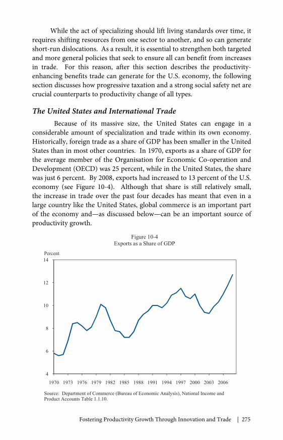
Fostering Productivity Growth Through Innovation and Trade | 275
While the act of specializing should lift living standards over time, itrequires shifting resources from one sector to another, and so can generateshort-run dislocations. As a result, it is essential to strengthen both targetedand more general policies that seek to ensure all can benefit from increasesin trade. For this reason, after this section describes the productivity-enhancing benefits trade can generate for the U.S. economy, the followingsection discusses how progressive taxation and a strong social safety net arecrucial counterparts to productivity change of all types.
The United States and International TradeBecause of its massive size, the United States can engage in a
considerable amount of specialization and trade within its own economy.Historically, foreign trade as a share of GDP has been smaller in the UnitedStates than in most other countries. In 1970, exports as a share of GDP forthe average member of the Organisation for Economic Co-operation andDevelopment (OECD) was 25 percent, while in the United States, the sharewas just 6 percent. By 2008, exports had increased to 13 percent of the U.S.economy (see Figure 10-4). Although that share is still relatively small,the increase in trade over the past four decades has meant that even in alarge country like the United States, global commerce is an important partof the economy and—as discussed below—can be an important source ofproductivity growth.
4
6
8
10
12
14
1970 1973 1976 1979 1982 1985 1988 1991 1994 1997 2000 2003 2006
Figure 10-4Exports as a Share of GDP
Percent
Source: Department of Commerce (Bureau of Economic Analysis), National Income andProduct Accounts Table 1.1.10.

276 | Chapter 10
Millions of American workers contribute to the production ofgoods and services that are exported to foreign markets, and their jobs, onaverage, pay higher wages than a typical job. The Commerce Departmentestimates that in 2008 U.S. exports represented the work of roughly10 million American workers. The majority of these export-supported jobswere related to the export of goods; millions more were related to servicesexports and nearly a million were related to agricultural exports. The manu-facturing sector is particularly connected to exports; 20 to 30 percent ofmanufacturing employment in the United States in 2008 was supported byexports. These estimates represent the number of job-equivalents based ontotal hours needed to produce the volume of exports. Because few workersproduce exclusively exports or inputs for exports, the number of workerswho are involved with exports is likely much larger than 10 million.
Currently, the U.S. economy is far from full employment, and anyincreased production could generate an increase in jobs. Chapter 4 discusseshow an increase in exports may be an important part of GDP growth in themedium term. In the long run, though, the principal contribution of anincrease in the trade share will be the increase in productivity and livingstandards it can generate. Thus, the rise in the export share of the economyfrom 6 percent in 1970 to 13 percent today represents specialization, assome workers who produced goods for domestic use have moved intoexport sectors. The following sections describe the ways in which trade canincrease productivity.
Sources of Productivity Growth from International TradeProductivity growth can come from a number of channels. Trade can
allow increased specialization; it can allow increased scale of production;and it can allow more productive firms to grow rapidly, increasing theirshare of the economy.
Specialization. In the United States, a primary source of trade-relatedproductivity growth is specialization. The concept of Ricardian compara-tive advantage—that nations specialize in producing the goods that theycan produce cheaply relative to other goods—can be seen in a number ofaspects of U.S. trade. America makes far more aircraft, grain, plastics, andequipment (optical, photographic, and medical) than it consumes. In theseproduct areas, the United States has a substantial trade surplus, totaling over$100 billion in 2008. Conversely, the United States produces less electricalequipment, clothing, furniture, and toys than it consumes, and thereforeimports more of these goods than it exports. If America cut its produc-tion of aircraft, where it has a comparative advantage, by the $50 billion it
Fostering Productivity Growth Through Innovation and Trade | 277
currently exports on net and instead tried to produce more of the goods wecurrently import, productivity would likely be lower.
Specialization also takes place within industries. For example, withinthe broad category of “electrical machinery and equipment,” Americaimports telephones (including cell phones) and computer monitors,but exports electronic integrated circuits. Specialization can even takeplace within more narrow product classifications (for example, computermemory). Advanced countries with higher wages tend to produce andexport more high-quality products even as they import lower-cost, lower-quality products from abroad in the same product type. Economistsrefer to this within-product differentiation as the “quality ladder,” andextensive research in recent years has noted this pattern of specializationwithin products (Schott 2004). Over time, high-skill countries climb thequality ladder, making higher-quality products and increasingly importinglow-skill products.
For example, consider the category “electrically erasable program-mable read-only memory.” The United States both imports and exportsbillions of dollars worth of products in this category every year, but theaverage unit price of the exports is roughly three times the average unitprice of the imports. The U.S. products may have bigger memories withmore complex production processes or be of higher quality than the cheaperimports. In any event, the imports and exports do not appear to be overlap-ping. Again, such a division of labor allows for higher standards of livingacross the world.
Intra-Industry Trade. Beyond specialization, trade can generateproductivity advances in a number of ways. One important channel is thattrade can allow companies to achieve a scale of production that they couldnot attain by selling just to the local market, thus increasing their produc-tivity. Within any given economy, there is a limit to the quantity of a specificgood that the domestic market will want to consume. The ability to manufac-ture more of a product than domestic consumption supports and exchangeit for other products—even ones that are extremely similar to the exportedgood—can be quite beneficial. It results in economies of scale that can beinternal to a firm, where one company grows quite large and productive atmaking one good, or to a region, where a particular good tends to be made ina given physical location as a substantial amount of expertise builds up there.
Trade in which different quality or simply different brand products aretraded in both directions, known as intra-industry trade, represents between40 and 50 percent of trade in the world economy. For the manufacturingindustry of the United States, that figure is even higher. As Figure 10-5shows, intra-industry foreign trade moved from roughly 65 percent of U.S.
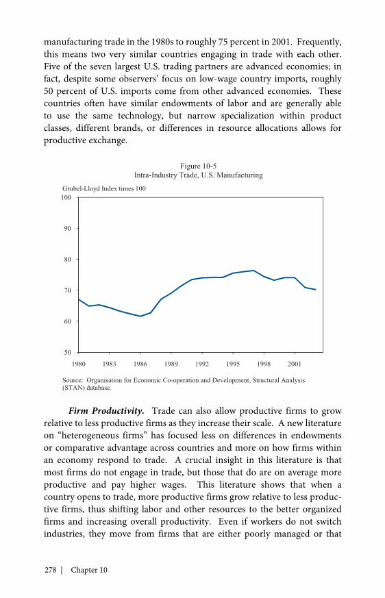
278 | Chapter 10
manufacturing trade in the 1980s to roughly 75 percent in 2001. Frequently,this means two very similar countries engaging in trade with each other.Five of the seven largest U.S. trading partners are advanced economies; infact, despite some observers’ focus on low-wage country imports, roughly50 percent of U.S. imports come from other advanced economies. Thesecountries often have similar endowments of labor and are generally ableto use the same technology, but narrow specialization within productclasses, different brands, or differences in resource allocations allows forproductive exchange.
Firm Productivity. Trade can also allow productive firms to growrelative to less productive firms as they increase their scale. A new literatureon “heterogeneous firms” has focused less on differences in endowmentsor comparative advantage across countries and more on how firms withinan economy respond to trade. A crucial insight in this literature is thatmost firms do not engage in trade, but those that do are on average moreproductive and pay higher wages. This literature shows that when acountry opens to trade, more productive firms grow relative to less produc-tive firms, thus shifting labor and other resources to the better organizedfirms and increasing overall productivity. Even if workers do not switchindustries, they move from firms that are either poorly managed or that
50
60
70
80
90
100
1980 1983 1986 1989 1992 1995 1998 2001
Figure 10-5Intra-Industry Trade, U.S. Manufacturing
Grubel-Lloyd Index times 100
Source: Organisation for Economic Co-operation and Development, Structural Analysis(STAN) database.
Fostering Productivity Growth Through Innovation and Trade | 279
use less advanced technology and production processes toward the moreproductive firms. Thus, firm-level evidence demonstrates that tradeallows not only economy-wide advances through resource allocation, butalso allows within-industry productivity advances through reallocation ofresources across firms. This shift has clear welfare-enhancing impacts; seeBernard et al. (2007) for a general overview of this literature.
Vertical Specialization. Thus far, the discussion regarding sources ofproductivity growth in international trade has assumed that finished goodsare being bought and sold across borders. The world of trade, though, haschanged substantially. Today, multinational corporations (U.S. or foreign-based) are involved in 64 percent of U.S. goods trade (imports and exports),and fully 19 percent of U.S. goods exports are sales from a U.S. multinationalfirm to its affiliates abroad. An increase in international vertical specializa-tion, where firms have production in multiple countries and break up theproduction of a particular good into stages across different countries, hascontributed significantly to growth in world trade. The process can be withina large firm or intermediate inputs can be bought and sold on the market.Decreased trade costs have made it easier to break up the value chain ofproduction as various parts of production can be done in different placesand an in-process good can be shipped many times before final assembly.One study estimates that roughly one-third of the growth in world tradefrom 1970 to 1990 was attributable to the growth in vertical-specializationexports (Hummels, Ishii, and Yi 2001). Calculations about the extent ofvertical specialization vary from estimates that 30 percent of OECD exportscontain imported inputs to estimates that intermediate inputs account forup to 60 percent of world trade.4
A trade system in which the same firms are both importers andexporters complicates considerations of the impacts of trade on differentgroups, as comparative advantage may not matter as much for a particulargood as for a particular task or piece of the production process. Specializationby process should allow the United States to focus on jobs oriented towardthe processes that match the human capital, physical capital, and technologyin the United States, again increasing productivity. But it has also raisedfears that the process of adjustment could be disruptive, as a broader rangeof jobs could be exposed to international competition. The crucial policygoal is to harness the benefits of trade and ensure that its benefits are sharedbroadly by all Americans.
4 The 30 percent figure refers specifically to the share of exports that is made from importedinputs—sometimes called the vertical specialization of exports. The larger figure includes thevolume of trade that is imports of intermediate goods used in the production of goods for eitherexports or the home market.
280 | Chapter 10
Encouraging Trade and Enforcing Trade AgreementsAll of these aspects of trade highlight its potential to contribute to the
long-run expansion of productivity in the United States. Many of the advan-tages of increased trade come from opening foreign markets to the productsof U.S. workers. The best way to guarantee reliable access is through nego-tiated trade agreements and consistent enforcement of existing trade rules.As noted in Chapter 3, one positive development in the recent crisis is that,for the most part, countries did not resort to protectionism; that is, they didnot close their markets to imports. Had they done so, the dislocation in U.S.employment would likely have been much worse. As it was, U.S. importsof goods and services fell 34 percent and exports dropped 26 percent fromJuly 2008 to April 2009. From their peak in the third quarter of 2008 untilthe trough in the second quarter of 2009, the nominal value of exports ofgoods and services fell more than $400 billion at an annual rate, a drop ofalmost 3 percent of GDP. Imports also dropped substantially. In the longrun, such a decline in world trade would be harmful for the U.S. economy.If trade had stayed at that depressed level, with lower trade surpluses in theUnited States’ main export goods and smaller trade deficits in our importgoods, the long-run dislocations from the crisis would have been worse thannow expected. But U.S. exports are rebounding, opening the possibility thatmany workers who lost jobs in the crisis may find employment in the sameproductive industries where they were before the crisis.
Several explanations have been offered for this avoidance ofprotectionism during the crisis. One is the availability of macroeconomicpolicy tools such as fiscal and monetary policy (Eichengreen and Irwin2009); another is the public commitments made by leaders at the Groupof Twenty summits to avoid protectionist strategies. But the clear andconcrete rules-based trade system was helpful as well. That rules-basedsystem, embodied by the World Trade Organization (WTO) and by othertrade commitments, allows the United States to take steps to ensure thatother countries will abide by their obligations. It is also designed to give U.S.workers and firms confidence about the economic environment they will befacing and confidence that commitments made when trade agreements arenegotiated will be kept. In addition, creating predictable and enforceablemarkets for innovative and creative works grounded in intellectual propertyrights is essential to spurring and protecting U.S. investments in technologyand innovation.
The Administration recognizes that simply negotiating tradeframeworks is not enough; robust enforcement of trade rules is an impor-tant part of our engagement in the world economy. The Administrationhas taken many trade enforcement actions recently. For example, the

Fostering Productivity Growth Through Innovation and Trade | 281
Administration has continued pressing a WTO case that challenged China’streatment of U.S. auto parts exports. The ruling in this case resulted inChina having to change its policies and increase its openness to U.S. exports.The United States (joined by Mexico and the European Union) has alsoinitiated an action challenging China’s use of subsidies and taxes to keepinput costs low for firms in China, which lowers the cost of final goods fromChina relative to the world. Further, the Administration takes very seri-ously the “Special 301” process under which it monitors the protection andenforcement of intellectual property rights. In 2009, it added Canada to thepriority watch list because Canada has not implemented key proposals toimprove enforcement and protection of intellectual property rights. Actionslike these represent the Administration’s intent (made explicit, for example,in United States Trade Representative Ronald Kirk’s speeches5) to enforcetrade rules and aggressively pursue actions to open markets to U.S. exports.
As noted in Chapter 4, the Administration is currently pursuing theseand other options to expand American exports, recognizing that increasingexports will be a key part of the U.S. growth model. Increases in our exportsin the short run can help to return the economy to full employment. Overthe longer run, increases in trade provide avenues for the United States toincrease productivity through specialization, scale, and firm effects, and inturn, increase standards of living for American families.
Currently, a number of other trade expansion opportunities exist forthe United States. The Administration supports a strong market-openingagreement for both goods and services in the WTO Doha Round negotia-tions and is continuing to work with U.S. trade partners on potential freetrade agreements. Because the United States is a relatively open economy,negotiated trade deals often involve substantial improvements in access forU.S. exports to other countries relative to the market opening made by theUnited States.
It is also important that these trade frameworks protect productivity-enhancing innovation through adequate provisions for intellectual propertyrights and that they reflect our values regarding workers and the environ-ment. An example of the Administration’s actions to improve the world’strading regime is seen in the way the Administration is working to engageour trading partners across the Pacific region in a new regional agreement(the Trans-Pacific Partnership). It will be a high-standards agreement thatexpands trade in a way that is beneficial to the economy, workers, small busi-nesses, and farmers, and is consistent with the values of the United States.
In addition to benefits to the United States, trade benefits our tradepartners. This is of direct benefit to Americans in the sense that as these5 See for example his speech at Mon Valley Works—Edgar Thomson Plant on July 16, 2009.

282 | Chapter 10
economies grow, they can grow as a destination for U.S. exports. Tradecan also have large benefits for the poorest countries. In particular,multilateral agreements that open trade flows between developing countriescan have substantial impacts on poorer countries, and trade relations withthe United States can be a crucial part of the path to development for thepoorest countries. For example, the African Growth and Opportunity Actseeks to increase two-way trade with poor nations in sub-Saharan Africa,help integrate these countries into the global economy, and do so in a waythat improves their institutions and reduces poverty. As developmentin the poorest nations of the world is in our national interest strategi-cally, economically, and morally, trade presents win-win opportunities toadvance development.
Ensuring the Gains fromProductivity Growth Are Widely Shared
Any productivity advance—be it from technological change, trade, orother factors—will have different impacts across the economy. As discussedearlier, productivity advances are crucial to an increase in living standards.Still, those firms that do not make a specific advance will likely contract orfail, and some workers in the affected industry may face losses. Likewise,international trade can have disparate effects across industries, firms, andworkers. In both cases, society on average will be better off because theeconomy is able to generate a higher standard of living. But the recent stag-nation in median real wages despite positive productivity growth (discussedin Chapter 8) highlights the challenge of ensuring that the gains fromproductivity growth are widely spread.
The potential for productivity advances to generate disparities inoutcomes suggests the need for strong social policy to support those whodo not immediately benefit and to ensure that gains from trade and produc-tivity advances are shared by all. Because identifying directly impactedindividuals is difficult, the logical response to productivity advances is astrong social safety net that ensures that all benefit from the rise in livingstandards. Trade theory suggests that trade liberalization can generate gainsthat are large enough that they can be shared in a way that every memberof society is made better off. In the past, however, the gains from our tradepolicies have not been shared sufficiently, and technological change andglobalization have left many behind.
Trade adjustment assistance, worker retraining, and temporary reliefprograms are ways the Federal Government can and does support those

Fostering Productivity Growth Through Innovation and Trade | 283
who do not benefit from these advances. The Administration has supportedtrade adjustment assistance, which provides additional unemploymentfunds, retraining, and health coverage assistance, and has made trade adjust-ment assistance available to a wider set of employees through the Trade andGlobalization Adjustment Assistance Act of 2009.
These specific institutions, though, are not enough. More broad-basedpolicy must ensure that as the economy grows in the long run, it enhancesliving standards for all citizens. Progressive taxation—which can be justi-fied in many ways—is supported by the uneven outcomes from productivityadvances and globalization. Those whose incomes rise can pay a largershare of total taxes and still be better off than before the gains. By doingso, they support lower taxes for others whose incomes may have declined.This process makes everyone better off and thus supports innovation andopen borders by minimizing the number of people who feel threatened byproductivity advances and therefore oppose them.
For example, the ability to sell books across borders certainlyenhanced the income J.K. Rowling was able to collect from writing thefamous Harry Potter books. Had she been able to sell her books only inthe United Kingdom, her audience and income would have been muchsmaller. In addition, millions of American readers benefited from theincreased consumer choice and the ability to purchase her books. Similarly,more Americans can work as well-paid aircraft engineers or manufacturingemployees for Boeing or as technology specialists for Apple because thosefirms are able to sell on a world market. At the same time, it is distinctlypossible that some American authors who would have captured a largershare of the “magic-oriented book” market had there been no trade inliterature were crowded out by Rowling’s success, or that some handheldmusic device engineer in the United Kingdom has had to find another careerbecause of Apple’s success.
A progressive tax rate combined with trade allows those who realizesubstantial income gains from globalization to still prosper a great deal rela-tive to the state where there is no trade and incomes are taxed at a flat rate.And it does so while making sure that those who face lower incomes fromglobalization also obtain benefits—not just through the lower prices andexpanded choices associated with trade, but also through lower taxation.
Beyond a progressive tax rate, a strong social safety net can cushionthe disruption generated by a dynamic economy. Unemployment insurancecan provide temporary income. A robust health care system can ensure thattemporary dislocations do not generate drastic consequences. And a vibranteducation system can prepare workers for changing economic needs.

284 | Chapter 10
Conclusion
Advances in productivity are crucial to increasing the living standardsof all Americans—to building a better future. Innovation initiatives, suchas increased research and development, targeted investments, strongerintellectual property rights, and harnessing trade’s productivity-enhancingpotential, are all essential parts of lifting living standards in the long run.But to ensure living standards are rising for all, a dynamic open economydepends on a robust social infrastructure. Education improvementsdescribed in Chapter 8 are crucial to creating a well-trained labor force ableto thrive in a flexible economy where innovation and trade may reshapeindustries over time. A sound health care system is needed to provide thecertainty that changing jobs will not mean a loss of health services. And aproductive, well-regulated financial system is essential to allocate capitalto growing sectors. Thus, the initiatives being taken today as part of theAdministration’s rescue-and-rebuild programs are not meant only tocorrect the problems of today, but to set the stage for strong growth overdecades to come.

A P P E N D I X A
REPORT TO THE PRESIDENTON THE ACTIVITIES OF THE
COUNCIL OF ECONOMICADVISERS DURING 2009

307
letter of transmittal
Council of Economic AdvisersWashington, D.C., December 31, 2009
Mr. President:The Council of Economic Advisers submits this report on its
activities during calendar year 2009 in accordance with the requirements ofthe Congress, as set forth in section 10(d) of the Employment Act of 1946 asamended by the Full Employment and Balanced Growth Act of 1978.
Sincerely,Christina D. Romer, ChairAustan Goolsbee, MemberCecilia Elena Rouse, Member

308 | Appendix A
Council Members and Their Dates of Service
Name Position Oath of office date Separation date
Edwin G. Nourse Chairman August 9, 1946 November 1, 1949Leon H. Keyserling Vice Chairman August 9, 1946
Acting Chairman November 2, 1949Chairman May 10, 1950 January 20, 1953
John D. Clark Member August 9, 1946Vice Chairman May 10, 1950 February 11, 1953
Roy Blough Member June 29, 1950 August 20, 1952Robert C. Turner Member September 8, 1952 January 20, 1953Arthur F. Burns Chairman March 19, 1953 December 1, 1956Neil H. Jacoby Member September 15, 1953 February 9, 1955Walter W. Stewart Member December 2, 1953 April 29, 1955Raymond J. Saulnier Member April 4, 1955
Chairman December 3, 1956 January 20, 1961Joseph S. Davis Member May 2, 1955 October 31, 1958Paul W. McCracken Member December 3, 1956 January 31, 1959Karl Brandt Member November 1, 1958 January 20, 1961Henry C. Wallich Member May 7, 1959 January 20, 1961Walter W. Heller Chairman January 29, 1961 November 15, 1964James Tobin Member January 29, 1961 July 31, 1962Kermit Gordon Member January 29, 1961 December 27, 1962Gardner Ackley Member August 3, 1962
Chairman November 16, 1964 February 15, 1968John P. Lewis Member May 17, 1963 August 31, 1964Otto Eckstein Member September 2, 1964 February 1, 1966Arthur M. Okun Member November 16, 1964
Chairman February 15, 1968 January 20, 1969James S. Duesenberry Member February 2, 1966 June 30, 1968Merton J. Peck Member February 15, 1968 January 20, 1969Warren L. Smith Member July 1, 1968 January 20, 1969Paul W. McCracken Chairman February 4, 1969 December 31, 1971Hendrik S. Houthakker Member February 4, 1969 July 15, 1971Herbert Stein Member February 4, 1969
Chairman January 1, 1972 August 31, 1974Ezra Solomon Member September 9, 1971 March 26, 1973Marina v.N. Whitman Member March 13, 1972 August 15, 1973Gary L. Seevers Member July 23, 1973 April 15, 1975William J. Fellner Member October 31, 1973 February 25, 1975Alan Greenspan Chairman September 4, 1974 January 20, 1977Paul W. MacAvoy Member June 13, 1975 November 15, 1976Burton G. Malkiel Member July 22, 1975 January 20, 1977Charles L. Schultze Chairman January 22, 1977 January 20, 1981William D. Nordhaus Member March 18, 1977 February 4, 1979Lyle E. Gramley Member March 18, 1977 May 27, 1980

Activities of the Council of Economic Advisers During 2009 | 309
Council Members and Their Dates of Service
Name Position Oath of office date Separation date
George C. Eads Member June 6, 1979 January 20, 1981Stephen M. Goldfeld Member August 20, 1980 January 20, 1981Murray L. Weidenbaum Chairman February 27, 1981 August 25, 1982William A. Niskanen Member June 12, 1981 March 30, 1985Jerry L. Jordan Member July 14, 1981 July 31, 1982Martin Feldstein Chairman October 14, 1982 July 10, 1984William Poole Member December 10, 1982 January 20, 1985Beryl W. Sprinkel Chairman April 18, 1985 January 20, 1989Thomas Gale Moore Member July 1, 1985 May 1, 1989Michael L. Mussa Member August 18, 1986 September 19, 1988Michael J. Boskin Chairman February 2, 1989 January 12, 1993John B. Taylor Member June 9, 1989 August 2, 1991Richard L. Schmalensee Member October 3, 1989 June 21, 1991David F. Bradford Member November 13, 1991 January 20, 1993Paul Wonnacott Member November 13, 1991 January 20, 1993Laura D’Andrea Tyson Chair February 5, 1993 April 22, 1995Alan S. Blinder Member July 27, 1993 June 26, 1994Joseph E. Stiglitz Member July 27, 1993
Chairman June 28, 1995 February 10, 1997Martin N. Baily Member June 30, 1995 August 30, 1996Alicia H. Munnell Member January 29, 1996 August 1, 1997Janet L. Yellen Chair February 18, 1997 August 3, 1999Jeffrey A. Frankel Member April 23, 1997 March 2, 1999Rebecca M. Blank Member October 22, 1998 July 9, 1999Martin N. Baily Chairman August 12, 1999 January 19, 2001Robert Z. Lawrence Member August 12, 1999 January 12, 2001Kathryn L. Shaw Member May 31, 2000 January 19, 2001R. Glenn Hubbard Chairman May 11, 2001 February 28, 2003Mark B. McClellan Member July 25, 2001 November 13, 2002Randall S. Kroszner Member November 30, 2001 July 1, 2003N. Gregory Mankiw Chairman May 29, 2003 February 18, 2005Kristin J. Forbes Member November 21, 2003 June 3, 2005Harvey S. Rosen Member November 21, 2003
Chairman February 23, 2005 June 10, 2005Ben S. Bernanke Chairman June 21, 2005 January 31, 2006Katherine Baicker Member November 18, 2005 July 11, 2007Matthew J. Slaughter Member November 18, 2005 March 1, 2007Edward P. Lazear Chairman February 27, 2006 January 20, 2009Donald B. Marron Member July 17, 2008 January 20, 2009Christina D. Romer Chair January 29, 2009Austan Goolsbee Member March 11, 2009Cecilia E. Rouse Member March 11, 2009


Activities of the Council of Economic Advisers During 2009 | 311
Report to the Presidenton the Activities of the
Council of Economic AdvisersDuring
The Council of Economic Advisers was established by the EmploymentAct of 1946 to provide the President with objective economic analysis andadvice on the development and implementation of a wide range of domesticand international economic policy issues.
The Chair of the Council
Christina D. Romer was nominated as Chair of the Council by thePresident on January 20, 2009. She was confirmed by the Senate on January28, and took the oath of office on January 29. Dr. Romer is on a leave ofabsence from the University of California, Berkeley, where she is the Classof 1957-Garff B. Wilson Professor of Economics.
The Chair is a member of the President’s Cabinet and is responsiblefor communicating the Council’s views on economic matters directly to thePresident through personal discussions and written reports. Dr. Romerrepresents the Council at the daily Presidential economics briefing, dailyWhite House senior staff meetings, budget meetings, Cabinet meetings, avariety of inter-agency meetings, and other formal and informal meetingswith the President, the Vice President, and other senior government officials.She also meets frequently with members of Congress in both formal hear-ings and informal meetings to discuss economic issues and Administrationpriorities. She travels within the United States and overseas to present theAdministration’s views on the economy. Dr. Romer is the Council’s chiefpublic spokesperson. She directs the work of the Council and exercisesultimate responsibility for the work of the professional staff.
Dr. Romer succeeded Edward P. Lazear, whose tenure ended withthe inauguration of the new President. Dr. Lazear returned to StanfordUniversity, where he is the Jack Steele Parker Professor of Human ResourcesManagement and Economics in the Graduate School of Business and theMorris Arnold Cox Senior Fellow at the Hoover Institution.

312 | Appendix A
The Members of the Council
The other Members of the Council are Austan Goolsbee and CeciliaRouse. They were nominated by the President on January 20, 2009,confirmed by the Senate on March 10, and took their oaths of office onMarch 11. Dr. Goolsbee also serves as the Staff Director and Chief Economistof the President’s Economic Recovery Advisory Board. Dr. Goolsbee is ona leave of absence from the University of Chicago, where he is the RobertP. Gwinn Professor of Economics in the Booth School of Business. Dr.Rouse is on a leave of absence from Princeton University, where she is theTheodore A. Wells ’29 Professor of Economics and Public Affairs. TheMembers represent the Council at a wide variety of meetings and frequentlyattend meetings with the President and the Vice President.
The Chair and the Members work as a team on most economic policyissues. The Chair works on the whole range of issues under the Council’spurview, with a particular focus on macroeconomics and health care. Dr.Goolsbee focuses especially on issues related to housing, financial markets,and tax policy. Dr. Rouse focuses especially on issues related to labormarkets, education, and international trade.
The term of Donald B. Marron as a Member of the Council endedwith the inauguration of the new President. He is currently president ofMarron Economics, LLC.
Areas of Activity
Macroeconomic PoliciesA central function of the Council is to advise the President on all major
macroeconomic issues and developments. The Council is actively involvedin all aspects of macroeconomic policy. In 2009, the central macroeconomicissues included monitoring the financial and economic crisis; formulatingthe policy response, including the American Recovery and ReinvestmentAct of 2009, the Financial Stability Plan, and additional measures targeted tospur job creation and deal with problems in specific sectors; evaluating theeffects of the policies and the economy’s response; health insurance reform;and setting priorities for the budget. In this process, the Council worksclosely with the Department of the Treasury, the Office of Management andBudget, the National Economic Council, White House senior staff, and otheragencies and officials.
The Council prepares for the President, the Vice President, and theWhite House senior staff a daily economic briefing memo analyzing currenteconomic developments, and almost-daily memos on key economic data

Activities of the Council of Economic Advisers During 2009 | 313
releases. The Chair also makes more in-depth presentations on the state ofthe economy to these officials and to the Cabinet.
The Council, the Department of Treasury, and the Office ofManagement and Budget—the Administration’s economic “troika”—are responsible for producing the economic forecasts that underlie theAdministration’s budget proposals. The Council initiates the forecastingprocess twice each year, consulting with a wide variety of outside sources,including leading private sector forecasters and other government agencies.
The Council issued a series of reports in 2009. Among those mostdirectly related to macroeconomic policy were a report issued in May onestimation methodology for the jobs impact of specific programs of theRecovery Act; a report in June on the economic effects of comprehensivehealth insurance reform; a report in September on the macroeconomiceffects of the Recovery Act; and three shorter reports accompanying thatreport focusing on the effects of state fiscal relief, the effects of the “Cash forClunkers” program, and the cross-country experience with fiscal policy inthe crisis.
The Council continued its efforts to improve the public’sunderstanding of economic developments and of the Administration’seconomic policies through briefings with the economic and financial press,discussions with outside economists, and presentations to outside organiza-tions. The Chair and Members also regularly met to exchange views on themacroeconomy with the Chairman and Members of the Board of Governorsof the Federal Reserve System.
Microeconomic PoliciesThroughout the year, the Council was an active participant in the
analysis and consideration of a broad range of microeconomic policy issues.The Council was actively engaged in policy discussions on health insurancereform, financial regulatory reform, clean energy, the environment, educa-tion, and numerous labor market issues. As with macroeconomic policy, theCouncil works closely with other economic agencies, White House seniorstaff, and other agencies on these issues. Among the specific microeco-nomic issues that received particular attention in 2009 were small businesslending; foreclosure mitigation and prevention; unemployment insurance;the condition and prospects of the American automobile industry; the roleof cost-benefit analysis in regulatory policy; estimating the social benefitsof reduced carbon emissions; reform of K-12 education; student financialaid; community colleges; potential developments in the U.S. labor marketover the next five to ten years; and key indicators of family well-being in therecession and accompanying policy responses.
314 | Appendix A
Many of the reports issued by the Council in 2009 were primarilyconcerned with microeconomic issues. In addition to its major health carereport in June, the Council issued three other reports on health insurancereform over the course of the year—one on its impact on small businessesand their employees in July, one on its impact on state and local govern-ments in September, and an update of the June report in December. TheCouncil also issued an extensive report on the “jobs of tomorrow” in Julyand a report on simplifying student aid in September.
International Economic PoliciesThe Council was involved in a range of international trade and finance
issues, with a particular emphasis on the consequences of the internationalfinancial crisis and the related global economic slowdown. The Council wasan active participant in discussions at global and bilateral levels. CouncilMembers and staff regularly met with economists, policy officials, andgovernment officials of other countries to discuss issues relating to the globaleconomy and participated in the first Strategic and Economic Dialogue withChina in July 2009.
The Council was particularly active in examining policies that couldhelp speed the global economy out of the current crisis. It carefully trackeddevelopments in the global economy and considered the potential medium-run impacts of the current crisis. It was also an active participant in thePresidential Study Directive examining the development policies of theUnited States Government, providing analysis and support to the effortto review the interactions between the United States and countries in thedeveloping world.
On the international trade front, the Council was an activeparticipant in the trade policy process, occupying a position on the TradePolicy Staff Committee and the Trade Policy Review Group. The Councilprovided analysis and recommendations on a range of trade-related issuesinvolving the enforcement of existing trade agreements, reviews of currentU.S. trade policies, and consideration of future policies. The Council wasalso an active participant on the Trade Promotion Coordinating Committee,helping to examine the ways in which exports may support economicgrowth in the years to come. In the area of investment and security, theCouncil participated on the Committee on Foreign Investment in the UnitedStates (CFIUS), discussing individual cases before CFIUS.
The Council is a leading participant in the Organisation for EconomicCo-operation and Development (OECD), an important forum for economiccooperation among high-income industrial economies. Dr. Romer is

Activities of the Council of Economic Advisers During 2009 | 315
chair of the OECD’s Economic Policy Committee, and Council staffparticipate actively in working-party meetings on macroeconomic policyand coordination.
Public Information
The Council’s annual Economic Report of the President is animportant vehicle for presenting the Administration’s domestic and interna-tional economic policies. It is available for purchase through the GovernmentPrinting Office, and is viewable on-line at www.gpoaccess.gov/eop.
The Council prepared numerous reports in 2009, and the Chair andMembers gave numerous public speeches and testified to Congress. Thereports, texts of speeches, and written statements accompanying testimonyare available at the Council’s website, www.whitehouse.gov/cea.
Finally, the Council publishes the monthly Economic Indicators,which is available on-line at www.gpoaccess.gov/indicators.
The Staff of the Council of Economic Advisers
The staff of the Council consists of the senior staff, senior economists,staff economists, research assistants, analysts, and the administrative andsupport staff. The staff at the end of 2009 were:
Senior StaffSenior staff play key managerial and analytical roles at the Council.
They direct operations, perform central Council functions, and representthe Council in meetings with other agencies and White House offices.Nan M. Gibson .......................... Chief of StaffMichael B. Greenstone ............. Chief EconomistSteven N. Braun ......................... Director of Macroeconomic ForecastingAdrienne Pilot ........................... Director of Statistical Office
Senior EconomistsSenior economists are Ph.D. economists on leave from academic
institutions, government agencies, or private research institutions. Theyparticipate actively in the policy process, represent the Council in inter-agency meetings, and have primary responsibility for the economic analysisand reports prepared by the Council. Each senior economist is typically aprimary author of one of the chapters in this Report.

316 | Appendix A
Christopher D. Carroll ............. MacroeconomicsMark G. Duggan ........................ HealthW. Adam Looney ...................... Public Finance, Tax PolicyAndrew Metrick ........................ FinanceJesse M. Rothstein ..................... Labor, Education, WelfareJay C. Shambaugh ..................... International Macroeconomics and TradeAnn Wolverton ......................... Energy, Environment, Natural Resources
Staff EconomistsStaff economists are typically graduate students on leave from their
Ph.D. training in economics. They conduct advanced statistical analysis,contribute to reports, and generally support the research and analysismission of the Council.Sharon E. Boyd .......................... HealthGabriel Chodorow-Reich ......... International Macroeconomics and TradeLaura J. Feiveson ....................... Macroeconomics, FinanceJoshua K. Goldman ................... Energy, Environment, InfrastructureSarena F. Goodman .................. Education, Labor, Public FinanceJoshua K. Hausman .................. MacroeconomicsZachary D. Liscow .................... Public Finance, Labor, EnvironmentWilliam G. Woolston ............... Health, Education
Research AssistantsResearch assistants are typically college graduates with significant
coursework in economics. They conduct statistical analysis and data collec-tion, and generally support the research and analysis mission of the Council.Both staff economists and research assistants contribute to this Report andplay a crucial role in ensuring the accuracy of all Council documents.Peter N. Ganong ........................ Labor, Public Finance, EnvironmentClare M. Hove ........................... MacroeconomicsMichael P. Shapiro .................... Health, International Economics
Statistical OfficeThe Statistical Office gathers, administers, and produces statistical
information for the Council. Duties include preparing the statisticalappendix to the Economic Report of the President and the monthly publica-tion Economic Indicators. The staff also creates background materials foreconomic analysis and verifies statistical content in Presidential memoranda.The Office serves as the Council’s liaison to the statistical community.

Activities of the Council of Economic Advisers During 2009 | 317
Brian A. Amorosi ...................... Program AnalystDagmara A. Mocala .................. Program Analyst
Administrative OfficeThe Administrative Office provides general support for the
Council’s activities. This includes financial management, ethics, humanresource management, travel, operations of facilities, security, informationtechnology, and telecommunications management support.Rosemary M. Rogers ................. Administrative OfficerArchana A. Snyder .................... Financial OfficerDoris T. Searles .......................... Information Management Specialist
Office of the ChairJulie B. Siegel .............................. Special Assistant to the ChairLisa D. Branch ........................... Executive Assistant to the Members and
Assistant to the Chief Economist
Staff SupportSharon K. Thomas .................... Administrative Support Assistant
Other StaffBrenda Szittya and Martha Gottron provided editorial assistance in
the preparation of the 2010 Economic Report of the President.C. Bennett Blau and Gabrielle A. Elul served as staff assistants. Mr.
Blau also served as editor of the Morning Economic Bulletin.Student interns provide invaluable help with research projects, day-
to-day operations, and fact-checking. Interns during the year were: MichaelD. Arena; Jana Curry; Samantha G. Ellner; Brett B. Flagg; Karen R. Li; DevinK. Mattson; Allison L. Moore; Seth H. Werfel; Carl C. Wheeler; Kie C.Riedel; Rebecca A. Wilson; Yuelan L. Wu; and Allen Yang.
Departures
Jane E. Ihrig left her position as Chief Economist of the Council inJanuary to return to the Federal Reserve Board. Pierce E. Scranton left hisposition as Chief of Staff in January. He was succeeded by Karen Anderson,who left the Council in November for maternity leave.
The senior economists who resigned during the year (with their insti-tutions after leaving the Council in parentheses) were: Jean M. Abraham(University of Minnesota); Scott J. Adams (University of Wisconsin);

318 | Appendix A
Benjamin N. Dennis (Department of the Treasury); Erik W. Durbin(Sullivan and Cromwell, LLP); Wendy M. Edelberg (Financial Crisis InquiryCommission); Elizabeth A. Kopits (Environmental Protection Agency);Michael S. Piwowar (Senate Banking Committee); William M. Powers(International Trade Commission); and Robert P. Rebelein (Vassar College).
The staff economists who resigned during 2009 were Kristopher J.Dawsey, Elizabeth Schultz, and Brian Waters. Those who served as researchassistants at the Council and resigned during 2009 were Michael Love andAditi P. Sen.
There were three retirements at the Council in 2009: Alice Williams,Sandy Daigle and Mary Jones. Ms. Williams devoted 39 years andMs. Daigle 23 years to the Council. Their untiring commitment, dedica-tion, and loyalty in serving the Council, the Chairs, and the people of theUnited States over the years was extraordinary and will be greatly missed.Ms. Jones’s 23 years of dedication to the senior economists and CouncilMembers was a testament to her commitment to the Council and wasgreatly appreciated.

A P P E N D I X B
STATISTICAL TABLES RELATING TOINCOME, EMPLOYMENT,
AND PRODUCTION
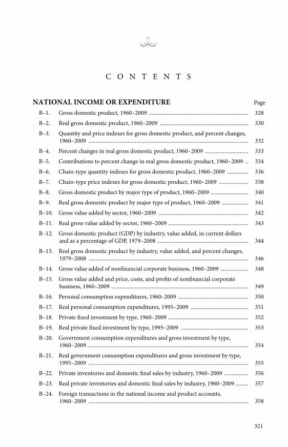
321
PageNATIONAL INCOME OR EXPENDITUREB–1. Gross domestic product, 1960–2009 ....................................................................... 328B–2. Real gross domestic product, 1960–2009 ............................................................... 330B–3. Quantity and price indexes for gross domestic product, and percent changes,
1960–2009 .................................................................................................................. 332B–4. Percent changes in real gross domestic product, 1960–2009 ............................... 333B–5. Contributions to percent change in real gross domestic product, 1960–2009 .. 334B–6. Chain-type quantity indexes for gross domestic product, 1960–2009 ............... 336B–7. Chain-type price indexes for gross domestic product, 1960–2009 ..................... 338B–8. Gross domestic product by major type of product, 1960–2009 ........................... 340B–9. Real gross domestic product by major type of product, 1960–2009 ................... 341B–10. Gross value added by sector, 1960–2009 ................................................................ 342B–11. Real gross value added by sector, 1960–2009 ......................................................... 343B–12. Gross domestic product (GDP) by industry, value added, in current dollars
and as a percentage of GDP, 1979–2008 ................................................................. 344B–13. Real gross domestic product by industry, value added, and percent changes,
1979–2008 .................................................................................................................. 346B–14. Gross value added of nonfinancial corporate business, 1960–2009 .................... 348B–15. Gross value added and price, costs, and profits of nonfinancial corporate
business, 1960–2009 .................................................................................................. 349B–16. Personal consumption expenditures, 1960–2009 .................................................. 350B–17. Real personal consumption expenditures, 1995–2009 ......................................... 351B–18. Private fixed investment by type, 1960–2009 ......................................................... 352B–19. Real private fixed investment by type, 1995–2009 ................................................ 353B–20. Government consumption expenditures and gross investment by type,
1960–2009 ................................................................................................................... 354B–21. Real government consumption expenditures and gross investment by type,
1995–2009 .................................................................................................................. 355B–22. Private inventories and domestic final sales by industry, 1960–2009 ................. 356B–23. Real private inventories and domestic final sales by industry, 1960–2009 ......... 357B–24. Foreign transactions in the national income and product accounts,
1960–2009 .................................................................................................................. 358
C O N T E N T S
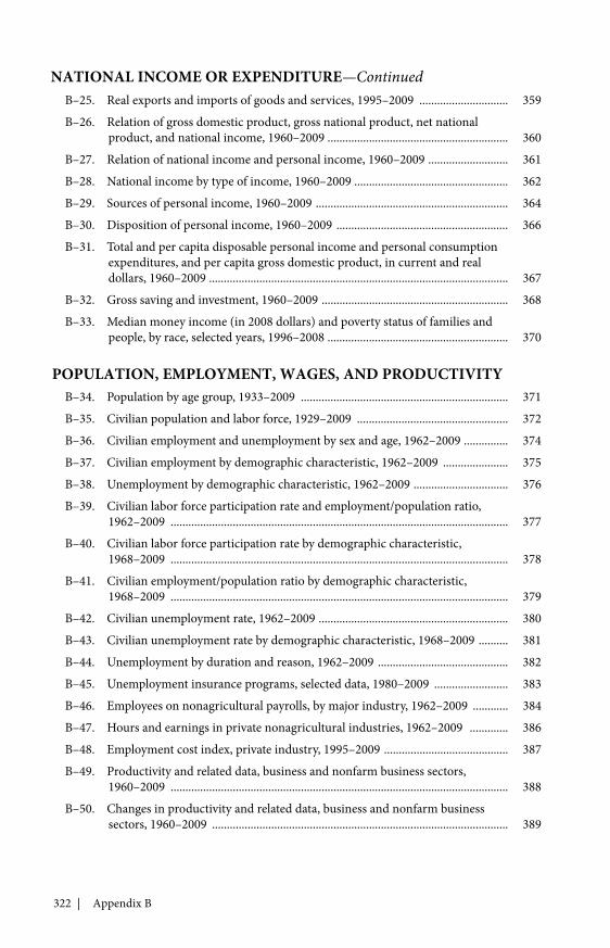
322 | Appendix B
B–25. Real exports and imports of goods and services, 1995–2009 .............................. 359B–26. Relation of gross domestic product, gross national product, net national
product, and national income, 1960–2009 ............................................................. 360B–27. Relation of national income and personal income, 1960–2009 ........................... 361B–28. National income by type of income, 1960–2009 .................................................... 362B–29. Sources of personal income, 1960–2009 ................................................................. 364B–30. Disposition of personal income, 1960–2009 .......................................................... 366B–31. Total and per capita disposable personal income and personal consumption
expenditures, and per capita gross domestic product, in current and realdollars, 1960–2009 ..................................................................................................... 367
B–32. Gross saving and investment, 1960–2009 ............................................................... 368B–33. Median money income (in 2008 dollars) and poverty status of families and
people, by race, selected years, 1996–2008 ............................................................. 370
POPULATION, EMPLOYMENT, WAGES, AND PRODUCTIVITYB–34. Population by age group, 1933–2009 ...................................................................... 371B–35. Civilian population and labor force, 1929–2009 ................................................... 372B–36. Civilian employment and unemployment by sex and age, 1962–2009 ............... 374B–37. Civilian employment by demographic characteristic, 1962–2009 ...................... 375B–38. Unemployment by demographic characteristic, 1962–2009 ................................ 376B–39. Civilian labor force participation rate and employment/population ratio,
1962–2009 .................................................................................................................. 377B–40. Civilian labor force participation rate by demographic characteristic,
1968–2009 .................................................................................................................. 378B–41. Civilian employment/population ratio by demographic characteristic,
1968–2009 .................................................................................................................. 379B–42. Civilian unemployment rate, 1962–2009 ................................................................ 380B–43. Civilian unemployment rate by demographic characteristic, 1968–2009 .......... 381B–44. Unemployment by duration and reason, 1962–2009 ............................................ 382B–45. Unemployment insurance programs, selected data, 1980–2009 ......................... 383B–46. Employees on nonagricultural payrolls, by major industry, 1962–2009 ............ 384B–47. Hours and earnings in private nonagricultural industries, 1962–2009 ............. 386B–48. Employment cost index, private industry, 1995–2009 .......................................... 387B–49. Productivity and related data, business and nonfarm business sectors,
1960–2009 .................................................................................................................. 388B–50. Changes in productivity and related data, business and nonfarm business
sectors, 1960–2009 .................................................................................................... 389
NATIONAL INCOME OR EXPENDITURE—Continued
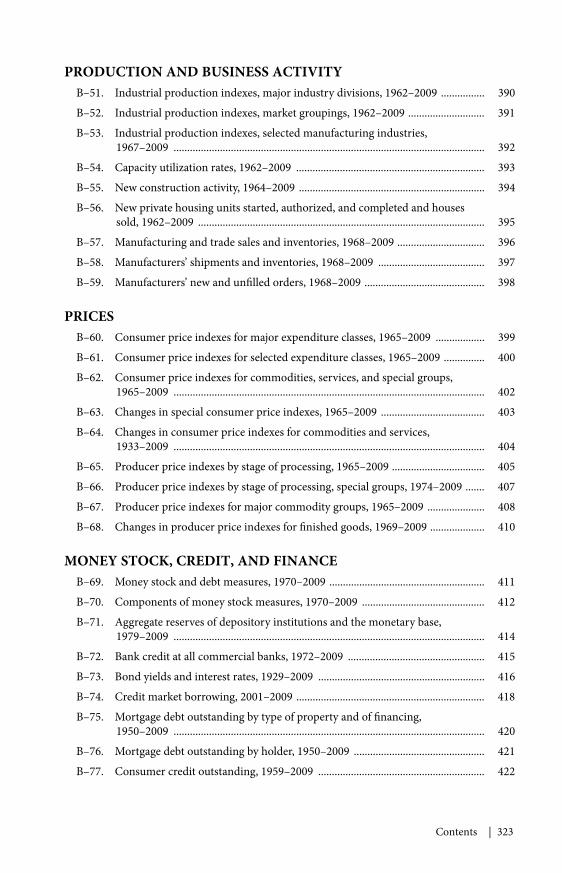
Contents | 323
PRODUCTION AND BUSINESS ACTIVITYB–51. Industrial production indexes, major industry divisions, 1962–2009 ................ 390B–52. Industrial production indexes, market groupings, 1962–2009 ............................ 391B–53. Industrial production indexes, selected manufacturing industries,
1967–2009 .................................................................................................................. 392B–54. Capacity utilization rates, 1962–2009 ..................................................................... 393B–55. New construction activity, 1964–2009 .................................................................... 394B–56. New private housing units started, authorized, and completed and houses
sold, 1962–2009 ......................................................................................................... 395B–57. Manufacturing and trade sales and inventories, 1968–2009 ................................ 396B–58. Manufacturers’ shipments and inventories, 1968–2009 ....................................... 397B–59. Manufacturers’ new and unfilled orders, 1968–2009 ............................................ 398
PRICESB–60. Consumer price indexes for major expenditure classes, 1965–2009 .................. 399B–61. Consumer price indexes for selected expenditure classes, 1965–2009 ............... 400B–62. Consumer price indexes for commodities, services, and special groups,
1965–2009 .................................................................................................................. 402B–63. Changes in special consumer price indexes, 1965–2009 ...................................... 403B–64. Changes in consumer price indexes for commodities and services,
1933–2009 .................................................................................................................. 404B–65. Producer price indexes by stage of processing, 1965–2009 .................................. 405B–66. Producer price indexes by stage of processing, special groups, 1974–2009 ....... 407B–67. Producer price indexes for major commodity groups, 1965–2009 ..................... 408B–68. Changes in producer price indexes for finished goods, 1969–2009 .................... 410
MONEY STOCK, CREDIT, AND FINANCEB–69. Money stock and debt measures, 1970–2009 ......................................................... 411B–70. Components of money stock measures, 1970–2009 ............................................. 412B–71. Aggregate reserves of depository institutions and the monetary base,
1979–2009 .................................................................................................................. 414B–72. Bank credit at all commercial banks, 1972–2009 .................................................. 415B–73. Bond yields and interest rates, 1929–2009 ............................................................. 416B–74. Credit market borrowing, 2001–2009 ..................................................................... 418B–75. Mortgage debt outstanding by type of property and of financing,
1950–2009 .................................................................................................................. 420B–76. Mortgage debt outstanding by holder, 1950–2009 ................................................ 421B–77. Consumer credit outstanding, 1959–2009 ............................................................. 422
324 | Appendix B
GOVERNMENT FINANCEB–78. Federal receipts, outlays, surplus or deficit, and debt, fiscal years, 1943–2011 .. 423B–79. Federal receipts, outlays, surplus or deficit, and debt, as percent of gross
domestic product, fiscal years 1937–2011 .............................................................. 424B–80. Federal receipts and outlays, by major category, and surplus or deficit, fiscal
years 1943–2011 ........................................................................................................ 425B–81. Federal receipts, outlays, surplus or deficit, and debt, fiscal years 2006–2011 ... 426B–82. Federal and State and local government current receipts and expenditures,
national income and product accounts (NIPA), 1960–2009 ............................... 427B–83. Federal and State and local government current receipts and expenditures,
national income and product accounts (NIPA), by major type, 1960–2009 ..... 428B–84. Federal Government current receipts and expenditures, national income and
product accounts (NIPA), 1960–2009 .................................................................... 429B–85. State and local government current receipts and expenditures, national
income and product accounts (NIPA), 1960–2009 ............................................... 430B–86. State and local government revenues and expenditures, selected fiscal years,
1942–2007 .................................................................................................................. 431B–87. U.S. Treasury securities outstanding by kind of obligation, 1970–2009 ............. 432B–88. Maturity distribution and average length of marketable interest-bearing
public debt securities held by private investors, 1970–2009 ................................ 433B–89. Estimated ownership of U.S. Treasury securities, 2000–2009 .............................. 434
CORPORATE PROFITS AND FINANCEB–90. Corporate profits with inventory valuation and capital consumption
adjustments, 1960–2009 ........................................................................................... 435B–91. Corporate profits by industry, 1960–2009 .............................................................. 436B–92. Corporate profits of manufacturing industries, 1960–2009 ................................. 437B–93. Sales, profits, and stockholders’ equity, all manufacturing corporations,
1968–2009 .................................................................................................................. 438B–94. Relation of profits after taxes to stockholders’ equity and to sales, all
manufacturing corporations, 1959–2009 ............................................................... 439B–95. Historical stock prices and yields, 1949–2003 ....................................................... 440B–96. Common stock prices and yields, 2000–2009 ........................................................ 441
AGRICULTUREB–97. Farm income, 1948–2009 .......................................................................................... 442B–98. Farm business balance sheet, 1952–2009 ................................................................ 443B–99. Farm output and productivity indexes, 1948–2008 ............................................... 444B–100. Farm input use, selected inputs, 1948–2009 ........................................................... 445
Contents | 325
B–101. Agricultural price indexes and farm real estate value, 1975–2009 ...................... 446B–102. U.S. exports and imports of agricultural commodities, 1950–2009 .................... 447
INTERNATIONAL STATISTICSB–103. U.S. international transactions, 1946–2009 ............................................................ 448B–104. U.S. international trade in goods by principal end-use category, 1965–2009 .... 450B–105. U.S. international trade in goods by area, 2001–2009 ........................................... 451B–106. U.S. international trade in goods on balance of payments (BOP) and Census
basis, and trade in services on BOP basis, 1981–2009 ......................................... 452B–107. International investment position of the United States at year-end,
2001–2008 .................................................................................................................. 453B–108. Industrial production and consumer prices, major industrial countries,
1982–2009 .................................................................................................................. 454B–109. Civilian unemployment rate, and hourly compensation, major industrial
countries, 1982–2009 ................................................................................................ 455B–110. Foreign exchange rates, 1988–2009 ......................................................................... 456B–111. International reserves, selected years, 1972–2009 ................................................. 457B–112. Growth rates in real gross domestic product, 1991–2010 .................................... 458
AGRICULTURE—Continued
General Notes | 327
General NotesDetail in these tables may not add to totals because of rounding.
Because of the formula used for calculating real gross domesticproduct (GDP), the chained (2005) dollar estimates for the detailedcomponents do not add to the chained-dollar value of GDP or toany intermediate aggregate. The Department of Commerce (Bureauof Economic Analysis) no longer publishes chained-dollar estimatesprior to 1995, except for selected series.
Unless otherwise noted, all dollar figures are in current dollars.
Symbols used:p Preliminary.... Not available (also, not applicable).
Data in these tables reflect revisions made by the source agenciesthrough January 29, 2010. In particular, tables containing nationalincome and product accounts (NIPA) estimates reflect revisionsreleased by the Department of Commerce in July 2009.
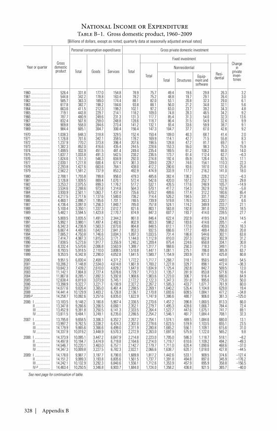
328 | Appendix B
Table B–1. Gross domestic product, 1960–2009[Billions of dollars, except as noted; quarterly data at seasonally adjusted annual rates]
Year or quarterGross
domesticproduct
Personal consumption expenditures Gross private domestic investment
Total Goods Services Total
Fixed investmentChange
inprivateinven-tories
Total
NonresidentialResi-
dentialTotal StructuresEquip-
ment andsoftware
1960 ...................... 526.4 331.8 177.0 154.8 78.9 75.7 49.4 19.6 29.8 26.3 3.21961 ...................... 544.8 342.2 178.8 163.4 78.2 75.2 48.8 19.7 29.1 26.4 3.01962 ...................... 585.7 363.3 189.0 174.4 88.1 82.0 53.1 20.8 32.3 29.0 6.11963 ...................... 617.8 382.7 198.2 184.6 93.8 88.1 56.0 21.2 34.8 32.1 5.61964 ...................... 663.6 411.5 212.3 199.2 102.1 97.2 63.0 23.7 39.2 34.3 4.81965 ...................... 719.1 443.8 229.7 214.1 118.2 109.0 74.8 28.3 46.5 34.2 9.21966 ...................... 787.7 480.9 249.6 231.3 131.3 117.7 85.4 31.3 54.0 32.3 13.61967 ...................... 832.4 507.8 259.0 248.8 128.6 118.7 86.4 31.5 54.9 32.4 9.91968 ...................... 909.8 558.0 284.6 273.4 141.2 132.1 93.4 33.6 59.9 38.7 9.11969 ...................... 984.4 605.1 304.7 300.4 156.4 147.3 104.7 37.7 67.0 42.6 9.21970 ...................... 1,038.3 648.3 318.8 329.5 152.4 150.4 109.0 40.3 68.7 41.4 2.01971 ...................... 1,126.8 701.6 342.1 359.5 178.2 169.9 114.1 42.7 71.5 55.8 8.31972 ...................... 1,237.9 770.2 373.8 396.4 207.6 198.5 128.8 47.2 81.7 69.7 9.11973 ...................... 1,382.3 852.0 416.6 435.4 244.5 228.6 153.3 55.0 98.3 75.3 15.91974 ...................... 1,499.5 932.9 451.5 481.4 249.4 235.4 169.5 61.2 108.2 66.0 14.01975 ...................... 1,637.7 1,033.8 491.3 542.5 230.2 236.5 173.7 61.4 112.4 62.7 –6.31976 ...................... 1,824.6 1,151.3 546.3 604.9 292.0 274.8 192.4 65.9 126.4 82.5 17.11977 ...................... 2,030.1 1,277.8 600.4 677.4 361.3 339.0 228.7 74.6 154.1 110.3 22.31978 ...................... 2,293.8 1,427.6 663.6 764.1 438.0 412.2 280.6 93.6 187.0 131.6 25.81979 ...................... 2,562.2 1,591.2 737.9 853.2 492.9 474.9 333.9 117.7 216.2 141.0 18.01980 ...................... 2,788.1 1,755.8 799.8 956.0 479.3 485.6 362.4 136.2 226.2 123.2 –6.31981 ...................... 3,126.8 1,939.5 869.4 1,070.1 572.4 542.6 420.0 167.3 252.7 122.6 29.81982 ...................... 3,253.2 2,075.5 899.3 1,176.2 517.2 532.1 426.5 177.6 248.9 105.7 –14.91983 ...................... 3,534.6 2,288.6 973.8 1,314.8 564.3 570.1 417.2 154.3 262.9 152.9 –5.81984 ...................... 3,930.9 2,501.1 1,063.7 1,437.4 735.6 670.2 489.6 177.4 312.2 180.6 65.41985 ...................... 4,217.5 2,717.6 1,137.6 1,580.0 736.2 714.4 526.2 194.5 331.7 188.2 21.81986 ...................... 4,460.1 2,896.7 1,195.6 1,701.1 746.5 739.9 519.8 176.5 343.3 220.1 6.61987 ...................... 4,736.4 3,097.0 1,256.3 1,840.7 785.0 757.8 524.1 174.2 349.9 233.7 27.11988 ...................... 5,100.4 3,350.1 1,337.3 2,012.7 821.6 803.1 563.8 182.8 381.0 239.3 18.51989 ...................... 5,482.1 3,594.5 1,423.8 2,170.7 874.9 847.3 607.7 193.7 414.0 239.5 27.71990 ...................... 5,800.5 3,835.5 1,491.3 2,344.2 861.0 846.4 622.4 202.9 419.5 224.0 14.51991 ...................... 5,992.1 3,980.1 1,497.4 2,482.6 802.9 803.3 598.2 183.6 414.6 205.1 –.41992 ...................... 6,342.3 4,236.9 1,563.3 2,673.6 864.8 848.5 612.1 172.6 439.6 236.3 16.31993 ...................... 6,667.4 4,483.6 1,642.3 2,841.2 953.3 932.5 666.6 177.2 489.4 266.0 20.81994 ...................... 7,085.2 4,750.8 1,746.6 3,004.3 1,097.3 1,033.5 731.4 186.8 544.6 302.1 63.81995 ...................... 7,414.7 4,987.3 1,815.5 3,171.7 1,144.0 1,112.9 810.0 207.3 602.8 302.9 31.21996 ...................... 7,838.5 5,273.6 1,917.7 3,355.9 1,240.2 1,209.4 875.4 224.6 650.8 334.1 30.81997 ...................... 8,332.4 5,570.6 2,006.8 3,563.9 1,388.7 1,317.7 968.6 250.3 718.3 349.1 71.01998 ...................... 8,793.5 5,918.5 2,110.0 3,808.5 1,510.8 1,447.1 1,061.1 275.1 786.0 385.9 63.71999 ...................... 9,353.5 6,342.8 2,290.0 4,052.8 1,641.5 1,580.7 1,154.9 283.9 871.0 425.8 60.82000 ...................... 9,951.5 6,830.4 2,459.1 4,371.2 1,772.2 1,717.7 1,268.7 318.1 950.5 449.0 54.52001 ...................... 10,286.2 7,148.8 2,534.0 4,614.8 1,661.9 1,700.2 1,227.8 329.7 898.1 472.4 –38.32002 ...................... 10,642.3 7,439.2 2,610.0 4,829.2 1,647.0 1,634.9 1,125.4 282.8 842.7 509.5 12.02003 ...................... 11,142.1 7,804.0 2,727.4 5,076.6 1,729.7 1,713.3 1,135.7 281.9 853.8 577.6 16.42004 ...................... 11,867.8 8,285.1 2,892.3 5,392.8 1,968.6 1,903.6 1,223.0 306.7 916.4 680.6 64.92005 ...................... 12,638.4 8,819.0 3,073.9 5,745.1 2,172.2 2,122.3 1,347.3 351.8 995.6 775.0 50.02006 ...................... 13,398.9 9,322.7 3,221.7 6,100.9 2,327.2 2,267.2 1,505.3 433.7 1,071.7 761.9 60.02007 ...................... 14,077.6 9,826.4 3,365.0 6,461.4 2,288.5 2,269.1 1,640.2 535.4 1,104.8 629.0 19.42008 ...................... 14,441.4 10,129.9 3,403.2 6,726.8 2,136.1 2,170.8 1,693.6 609.5 1,084.1 477.2 –34.82009 p .................... 14,258.7 10,092.6 3,257.6 6,835.0 1,622.9 1,747.9 1,386.6 480.7 906.0 361.3 –125.02006: I .................. 13,183.5 9,148.2 3,180.8 5,967.4 2,336.5 2,270.6 1,457.2 396.8 1,060.5 813.3 66.0
II ................. 13,347.8 9,266.6 3,206.5 6,060.1 2,352.1 2,279.7 1,495.3 428.6 1,066.7 784.4 72.4III ................ 13,452.9 9,391.8 3,250.5 6,141.3 2,333.5 2,264.4 1,522.7 447.6 1,075.1 741.7 69.1IV ................ 13,611.5 9,484.1 3,249.1 6,235.0 2,286.5 2,254.2 1,546.1 461.7 1,084.4 708.1 32.3
2007: I .................. 13,795.6 9,658.5 3,306.3 6,352.2 2,267.2 2,254.1 1,574.1 489.5 1,084.6 680.0 13.1II ................. 13,997.2 9,762.5 3,338.2 6,424.3 2,302.0 2,278.6 1,623.5 519.9 1,103.5 655.1 23.5III ................ 14,179.9 9,865.6 3,366.6 6,499.0 2,311.9 2,280.8 1,665.2 556.1 1,109.1 615.6 31.0IV ................ 14,337.9 10,019.2 3,448.9 6,570.3 2,272.9 2,263.0 1,697.9 575.9 1,122.0 565.2 9.8
2008: I .................. 14,373.9 10,095.1 3,447.2 6,647.9 2,214.8 2,223.0 1,705.0 586.3 1,118.7 518.1 –8.2II ................. 14,497.8 10,194.7 3,474.9 6,719.8 2,164.6 2,214.0 1,719.7 610.6 1,109.2 494.2 –49.3III ................ 14,546.7 10,220.1 3,463.0 6,757.1 2,142.7 2,179.7 1,711.0 620.4 1,090.6 468.6 –37.0IV ................ 14,347.3 10,009.8 3,227.5 6,782.3 2,022.1 2,066.6 1,638.7 620.7 1,018.0 427.8 –44.5
2009: I .................. 14,178.0 9,987.7 3,197.7 6,790.0 1,689.9 1,817.2 1,442.6 533.1 909.5 374.6 –127.4II ................. 14,151.2 9,999.3 3,193.8 6,805.6 1,561.5 1,737.7 1,391.8 494.8 897.0 345.9 –176.2III ................ 14,242.1 10,132.9 3,292.3 6,840.6 1,556.1 1,712.6 1,353.9 457.9 895.9 358.8 –156.5IV p ............. 14,463.4 10,250.5 3,346.8 6,903.7 1,684.0 1,724.0 1,358.2 436.8 921.5 365.7 –40.0
See next page for continuation of table.
National Income or Expenditure
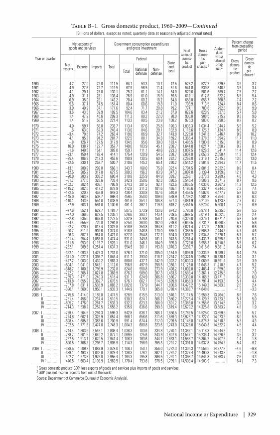
National Income or Expenditure | 329
Table B–1. Gross domestic product, 1960–2009—Continued[Billions of dollars, except as noted; quarterly data at seasonally adjusted annual rates]
Year or quarter
Net exports ofgoods and services
Government consumption expendituresand gross investment Final
sales ofdomes-
ticproduct
Grossdomes-
ticpur-
chases 1
Adden-dum:Gross
nationalprod-uct 2
Percent changefrom preceding
period
Netexports Exports Imports Total
FederalStateandlocal
Grossdomes-
ticproduct
Grossdomes-
ticpur-
chases 1Total National
defenseNon-
defense
1960 ...................... 4.2 27.0 22.8 111.5 64.1 53.3 10.7 47.5 523.2 522.2 529.6 3.9 3.21961 ...................... 4.9 27.6 22.7 119.5 67.9 56.5 11.4 51.6 541.8 539.8 548.3 3.5 3.41962 ...................... 4.1 29.1 25.0 130.1 75.2 61.1 14.1 54.9 579.6 581.6 589.7 7.5 7.71963 ...................... 4.9 31.1 26.1 136.4 76.9 61.0 15.9 59.5 612.1 612.8 622.2 5.5 5.41964 ...................... 6.9 35.0 28.1 143.2 78.4 60.2 18.2 64.8 658.8 656.7 668.6 7.4 7.21965 ...................... 5.6 37.1 31.5 151.4 80.4 60.6 19.8 71.0 709.9 713.5 724.4 8.4 8.61966 ...................... 3.9 40.9 37.1 171.6 92.4 71.7 20.8 79.2 774.1 783.8 792.8 9.5 9.91967 ...................... 3.6 43.5 39.9 192.5 104.6 83.4 21.2 87.9 822.6 828.9 837.8 5.7 5.81968 ...................... 1.4 47.9 46.6 209.3 111.3 89.2 22.0 98.0 900.8 908.5 915.9 9.3 9.61969 ...................... 1.4 51.9 50.5 221.4 113.3 89.5 23.8 108.2 975.3 983.0 990.5 8.2 8.21970 ...................... 4.0 59.7 55.8 233.7 113.4 87.6 25.8 120.3 1,036.3 1,034.4 1,044.7 5.5 5.21971 ...................... .6 63.0 62.3 246.4 113.6 84.6 29.1 132.8 1,118.6 1,126.2 1,134.4 8.5 8.91972 ...................... –3.4 70.8 74.2 263.4 119.6 86.9 32.7 143.8 1,228.8 1,241.3 1,246.4 9.9 10.21973 ...................... 4.1 95.3 91.2 281.7 122.5 88.1 34.3 159.2 1,366.4 1,378.2 1,394.9 11.7 11.01974 ...................... –.8 126.7 127.5 317.9 134.5 95.6 39.0 183.4 1,485.5 1,500.3 1,515.0 8.5 8.91975 ...................... 16.0 138.7 122.7 357.7 149.0 103.9 45.1 208.7 1,644.0 1,621.7 1,650.7 9.2 8.11976 ...................... –1.6 149.5 151.1 383.0 159.7 111.1 48.6 223.3 1,807.5 1,826.2 1,841.4 11.4 12.61977 ...................... –23.1 159.4 182.4 414.1 175.4 120.9 54.5 238.7 2,007.8 2,053.2 2,050.4 11.3 12.41978 ...................... –25.4 186.9 212.3 453.6 190.9 130.5 60.4 262.7 2,268.0 2,319.1 2,315.3 13.0 13.01979 ...................... –22.5 230.1 252.7 500.7 210.6 145.2 65.4 290.2 2,544.2 2,584.8 2,594.2 11.7 11.51980 ...................... –13.1 280.8 293.8 566.1 243.7 168.0 75.8 322.4 2,794.5 2,801.2 2,822.3 8.8 8.41981 ...................... –12.5 305.2 317.8 627.5 280.2 196.2 83.9 347.3 3,097.0 3,139.4 3,159.8 12.1 12.11982 ...................... –20.0 283.2 303.2 680.4 310.8 225.9 84.9 369.7 3,268.1 3,273.2 3,289.7 4.0 4.31983 ...................... –51.7 277.0 328.6 733.4 342.9 250.6 92.3 390.5 3,540.4 3,586.3 3,571.7 8.7 9.61984 ...................... –102.7 302.4 405.1 796.9 374.3 281.5 92.7 422.6 3,865.5 4,033.6 3,967.2 11.2 12.51985 ...................... –115.2 302.0 417.2 878.9 412.8 311.2 101.6 466.1 4,195.6 4,332.7 4,244.0 7.3 7.41986 ...................... –132.5 320.3 452.9 949.3 438.4 330.8 107.6 510.9 4,453.5 4,592.6 4,477.7 5.8 6.01987 ...................... –145.0 363.8 508.7 999.4 459.5 350.0 109.6 539.9 4,709.2 4,881.3 4,754.0 6.2 6.31988 ...................... –110.1 443.9 554.0 1,038.9 461.6 354.7 106.8 577.3 5,081.9 5,210.5 5,123.8 7.7 6.71989 ...................... –87.9 503.1 591.0 1,100.6 481.4 362.1 119.3 619.2 5,454.5 5,570.0 5,508.1 7.5 6.91990 ...................... –77.6 552.1 629.7 1,181.7 507.5 373.9 133.6 674.2 5,786.0 5,878.1 5,835.0 5.8 5.51991 ...................... –27.0 596.6 623.5 1,236.1 526.6 383.1 143.4 709.5 5,992.5 6,019.1 6,022.0 3.3 2.41992 ...................... –32.8 635.0 667.8 1,273.5 532.9 376.8 156.1 740.6 6,326.0 6,375.1 6,371.4 5.8 5.91993 ...................... –64.4 655.6 720.0 1,294.8 525.0 363.0 162.0 769.8 6,646.5 6,731.7 6,698.5 5.1 5.61994 ...................... –92.7 720.7 813.4 1,329.8 518.6 353.8 164.8 811.2 7,021.4 7,177.9 7,109.2 6.3 6.61995 ...................... –90.7 811.9 902.6 1,374.0 518.8 348.8 170.0 855.3 7,383.5 7,505.3 7,444.3 4.7 4.61996 ...................... –96.3 867.7 964.0 1,421.0 527.0 354.8 172.2 894.0 7,807.7 7,934.8 7,870.1 5.7 5.71997 ...................... –101.4 954.4 1,055.8 1,474.4 531.0 349.8 181.1 943.5 8,261.4 8,433.7 8,355.8 6.3 6.31998 ...................... –161.8 953.9 1,115.7 1,526.1 531.0 346.1 184.9 995.0 8,729.8 8,955.3 8,810.8 5.5 6.21999 ...................... –262.1 989.3 1,251.4 1,631.3 554.9 361.1 193.8 1,076.3 9,292.7 9,615.6 9,381.3 6.4 7.42000 ...................... –382.1 1,093.2 1,475.3 1,731.0 576.1 371.0 205.0 1,154.9 9,896.9 10,333.5 9,989.2 6.4 7.52001 ...................... –371.0 1,027.7 1,398.7 1,846.4 611.7 393.0 218.7 1,234.7 10,324.5 10,657.2 10,338.1 3.4 3.12002 ...................... –427.2 1,003.0 1,430.2 1,983.3 680.6 437.7 242.9 1,302.7 10,630.3 11,069.5 10,691.4 3.5 3.92003 ...................... –504.1 1,041.0 1,545.1 2,112.6 756.5 497.9 258.5 1,356.1 11,125.8 11,646.3 11,210.8 4.7 5.22004 ...................... –618.7 1,180.2 1,798.9 2,232.8 824.6 550.8 273.9 1,408.2 11,802.8 12,486.4 11,959.0 6.5 7.22005 ...................... –722.7 1,305.1 2,027.8 2,369.9 876.3 589.0 287.3 1,493.6 12,588.4 13,361.1 12,735.5 6.5 7.02006 ...................... –769.3 1,471.0 2,240.3 2,518.4 931.7 624.9 306.8 1,586.7 13,339.0 14,168.2 13,471.3 6.0 6.02007 ...................... –713.8 1,655.9 2,369.7 2,676.5 976.7 662.1 314.5 1,699.8 14,058.3 14,791.4 14,193.3 5.1 4.42008 ...................... –707.8 1,831.1 2,538.9 2,883.2 1,082.6 737.9 344.7 1,800.6 14,476.2 15,149.2 14,583.3 2.6 2.42009 p .................... –390.1 1,560.0 1,950.1 2,933.3 1,144.9 779.1 365.8 1,788.4 14,383.7 14,648.8 .............. –1.3 –3.32006: I .................. –775.8 1,414.0 2,189.8 2,474.5 928.5 615.5 313.0 1,546.1 13,117.5 13,959.3 13,264.0 8.6 7.6
II ................. –781.4 1,456.0 2,237.4 2,510.5 930.3 624.1 306.2 1,580.2 13,275.4 14,129.2 13,423.3 5.1 5.0III ................ –805.7 1,476.0 2,281.7 2,533.3 932.2 623.3 308.9 1,601.2 13,383.8 14,258.6 13,514.8 3.2 3.7IV ................ –714.3 1,538.2 2,252.5 2,555.2 935.9 636.6 299.3 1,619.4 13,579.2 14,325.8 13,683.2 4.8 1.9
2007: I .................. –729.4 1,564.9 2,294.3 2,599.3 942.8 636.7 306.1 1,656.5 13,782.5 14,525.0 13,859.5 5.5 5.7II ................. –724.8 1,602.1 2,326.9 2,657.4 968.1 656.6 311.6 1,689.3 13,973.7 14,722.0 14,073.3 6.0 5.5III ................ –698.4 1,685.2 2,383.6 2,700.9 991.4 674.4 317.0 1,709.5 14,148.8 14,878.3 14,318.3 5.3 4.3IV ................ –702.5 1,771.6 2,474.0 2,748.3 1,004.3 680.8 323.6 1,743.9 14,328.0 15,040.3 14,522.2 4.5 4.4
2008: I .................. –744.4 1,803.6 2,548.1 2,808.4 1,038.3 703.6 334.8 1,770.1 14,382.1 15,118.3 14,544.9 1.0 2.1II ................. –738.7 1,901.5 2,640.2 2,877.1 1,069.5 725.6 343.9 1,807.6 14,547.1 15,236.4 14,626.6 3.5 3.2III ................ –757.5 1,913.1 2,670.5 2,941.4 1,108.3 763.6 344.7 1,833.1 14,583.7 15,304.2 14,707.5 1.4 1.8IV ................ –590.5 1,706.2 2,296.7 2,905.9 1,114.3 758.9 355.3 1,791.7 14,391.8 14,937.8 14,454.3 –5.4 –9.2
2009: I .................. –378.5 1,509.3 1,887.9 2,879.0 1,106.7 750.7 356.0 1,772.3 14,305.3 14,556.5 14,277.9 –4.6 –9.8II ................. –339.1 1,493.7 1,832.8 2,929.4 1,138.3 776.2 362.1 1,791.2 14,327.4 14,490.3 14,243.8 –.8 –1.8III ................ –402.2 1,573.8 1,976.0 2,955.4 1,164.3 795.8 368.5 1,791.1 14,398.7 14,644.3 14,363.7 2.6 4.3IV p ............. –440.5 1,663.4 2,103.9 2,969.5 1,170.4 793.8 376.5 1,799.1 14,503.4 14,903.9 .............. 6.4 7.3
1 Gross domestic product (GDP) less exports of goods and services plus imports of goods and services.2 GDP plus net income receipts from rest of the world.Source: Department of Commerce (Bureau of Economic Analysis).
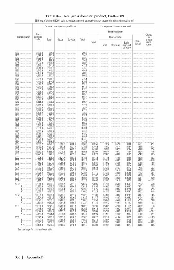
330 | Appendix B
Table B–2. Real gross domestic product, 1960–2009[Billions of chained (2005) dollars, except as noted; quarterly data at seasonally adjusted annual rates]
Year or quarterGross
domesticproduct
Personal consumption expenditures Gross private domestic investment
Total Goods Services Total
Fixed investmentChange
inprivateinven-tories
Total
NonresidentialResi-
dentialTotal StructuresEquip-
ment andsoftware
1960 ...................... 2,830.9 1,784.4 ................. ................. 296.5 ................. ................. ................. ................. ................. ...................1961 ...................... 2,896.9 1,821.2 ................. ................. 294.6 ................. ................. ................. ................. ................. ...................1962 ...................... 3,072.4 1,911.2 ................. ................. 332.0 ................. ................. ................. ................. ................. ...................1963 ...................... 3,206.7 1,989.9 ................. ................. 354.3 ................. ................. ................. ................. ................. ...................1964 ...................... 3,392.3 2,108.4 ................. ................. 383.5 ................. ................. ................. ................. ................. ...................1965 ...................... 3,610.1 2,241.8 ................. ................. 437.3 ................. ................. ................. ................. ................. ...................1966 ...................... 3,845.3 2,369.0 ................. ................. 475.8 ................. ................. ................. ................. ................. ...................1967 ...................... 3,942.5 2,440.0 ................. ................. 454.1 ................. ................. ................. ................. ................. ...................1968 ...................... 4,133.4 2,580.7 ................. ................. 480.5 ................. ................. ................. ................. ................. ...................1969 ...................... 4,261.8 2,677.4 ................. ................. 508.5 ................. ................. ................. ................. ................. ...................1970 ...................... 4,269.9 2,740.2 ................. ................. 475.1 ................. ................. ................. ................. ................. ...................1971 ...................... 4,413.3 2,844.6 ................. ................. 529.3 ................. ................. ................. ................. ................. ...................1972 ...................... 4,647.7 3,019.5 ................. ................. 591.9 ................. ................. ................. ................. ................. ...................1973 ...................... 4,917.0 3,169.1 ................. ................. 661.3 ................. ................. ................. ................. ................. ...................1974 ...................... 4,889.9 3,142.8 ................. ................. 612.6 ................. ................. ................. ................. ................. ...................1975 ...................... 4,879.5 3,214.1 ................. ................. 504.1 ................. ................. ................. ................. ................. ...................1976 ...................... 5,141.3 3,393.1 ................. ................. 605.9 ................. ................. ................. ................. ................. ...................1977 ...................... 5,377.7 3,535.9 ................. ................. 697.4 ................. ................. ................. ................. ................. ...................1978 ...................... 5,677.6 3,691.8 ................. ................. 781.5 ................. ................. ................. ................. ................. ...................1979 ...................... 5,855.0 3,779.5 ................. ................. 806.4 ................. ................. ................. ................. ................. ...................1980 ...................... 5,839.0 3,766.2 ................. ................. 717.9 ................. ................. ................. ................. ................. ...................1981 ...................... 5,987.2 3,823.3 ................. ................. 782.4 ................. ................. ................. ................. ................. ...................1982 ...................... 5,870.9 3,876.7 ................. ................. 672.8 ................. ................. ................. ................. ................. ...................1983 ...................... 6,136.2 4,098.3 ................. ................. 735.5 ................. ................. ................. ................. ................. ...................1984 ...................... 6,577.1 4,315.6 ................. ................. 952.1 ................. ................. ................. ................. ................. ...................1985 ...................... 6,849.3 4,540.4 ................. ................. 943.3 ................. ................. ................. ................. ................. ...................1986 ...................... 7,086.5 4,724.5 ................. ................. 936.9 ................. ................. ................. ................. ................. ...................1987 ...................... 7,313.3 4,870.3 ................. ................. 965.7 ................. ................. ................. ................. ................. ...................1988 ...................... 7,613.9 5,066.6 ................. ................. 988.5 ................. ................. ................. ................. ................. ...................1989 ...................... 7,885.9 5,209.9 ................. ................. 1,028.1 ................. ................. ................. ................. ................. ...................1990 ...................... 8,033.9 5,316.2 .................. .................. 993.5 .................. .................. .................. .................. .................. ...................1991 ...................... 8,015.1 5,324.2 .................. .................. 912.7 .................. .................. .................. .................. .................. ...................1992 ...................... 8,287.1 5,505.7 .................. .................. 986.7 .................. .................. .................. .................. .................. ...................1993 ...................... 8,523.4 5,701.2 .................. .................. 1,074.8 .................. .................. .................. .................. .................. ...................1994 ...................... 8,870.7 5,918.9 .................. .................. 1,220.9 .................. .................. .................. .................. .................. ...................1995 ...................... 9,093.7 6,079.0 1,898.6 4,208.2 1,258.9 1,235.7 792.2 342.0 493.0 456.1 32.11996 ...................... 9,433.9 6,291.2 1,983.6 4,331.4 1,370.3 1,346.5 866.2 361.4 545.4 492.5 31.21997 ...................... 9,854.3 6,523.4 2,078.2 4,465.0 1,540.8 1,470.8 970.8 387.9 620.4 501.8 77.41998 ...................... 10,283.5 6,865.5 2,218.6 4,661.8 1,695.1 1,630.4 1,087.4 407.7 710.4 540.4 71.61999 ...................... 10,779.8 7,240.9 2,395.3 4,852.8 1,844.3 1,782.1 1,200.9 408.2 810.9 574.2 68.52000 ...................... 11,226.0 7,608.1 2,521.7 5,093.3 1,970.3 1,913.8 1,318.5 440.0 895.8 580.0 60.22001 ...................... 11,347.2 7,813.9 2,600.9 5,218.7 1,831.9 1,877.6 1,281.8 433.3 866.9 583.3 –41.82002 ...................... 11,553.0 8,021.9 2,706.6 5,318.1 1,807.0 1,798.1 1,180.2 356.6 830.3 613.8 12.82003 ...................... 11,840.7 8,247.6 2,829.9 5,418.4 1,871.6 1,856.2 1,191.0 343.0 851.4 664.3 17.32004 ...................... 12,263.8 8,532.7 2,955.3 5,577.6 2,058.2 1,992.5 1,263.0 346.7 917.3 729.5 66.32005 ...................... 12,638.4 8,819.0 3,073.9 5,745.1 2,172.2 2,122.3 1,347.3 351.8 995.6 775.0 50.02006 ...................... 12,976.2 9,073.5 3,173.9 5,899.7 2,230.4 2,171.3 1,453.9 384.0 1,069.6 718.2 59.42007 ...................... 13,254.1 9,313.9 3,273.7 6,040.8 2,146.2 2,126.3 1,544.3 441.4 1,097.0 585.0 19.52008 ...................... 13,312.2 9,290.9 3,206.0 6,083.1 1,989.4 2,018.4 1,569.7 486.8 1,068.6 451.1 –25.92009 p .................... 12,988.7 9,237.3 3,143.7 6,090.5 1,522.8 1,646.7 1,289.1 391.0 887.9 359.1 –111.72006: I .................. 12,915.9 8,986.6 3,145.7 5,841.0 2,264.7 2,200.2 1,424.9 364.8 1,060.7 775.2 65.8
II ................. 12,962.5 9,035.0 3,150.8 5,884.2 2,261.2 2,189.9 1,450.3 383.7 1,066.3 740.1 72.5III ................ 12,965.9 9,090.7 3,176.4 5,914.3 2,229.6 2,162.2 1,466.0 393.2 1,072.0 697.4 67.5IV ................ 13,060.7 9,181.6 3,222.5 5,959.4 2,166.0 2,132.9 1,474.5 394.6 1,079.3 660.2 31.8
2007: I .................. 13,099.9 9,265.1 3,253.9 6,011.7 2,132.6 2,118.8 1,489.6 409.2 1,078.1 631.7 14.5II ................. 13,204.0 9,291.5 3,255.4 6,036.2 2,162.2 2,137.7 1,530.3 430.7 1,095.2 610.4 23.3III ................ 13,321.1 9,335.6 3,280.6 6,055.5 2,166.5 2,135.6 1,565.8 456.8 1,101.3 572.9 29.8IV ................ 13,391.2 9,363.6 3,304.8 6,059.7 2,123.4 2,113.0 1,591.3 469.1 1,113.3 525.0 10.3
2008: I .................. 13,366.9 9,349.6 3,262.1 6,087.1 2,082.9 2,079.2 1,598.9 476.8 1,111.9 483.2 .6II ................. 13,415.3 9,351.0 3,257.8 6,092.5 2,026.5 2,064.8 1,604.4 493.2 1,097.7 462.9 –37.1III ................ 13,324.6 9,267.7 3,193.6 6,072.4 1,990.7 2,020.4 1,579.2 493.1 1,071.0 443.3 –29.7IV ................ 13,141.9 9,195.3 3,110.4 6,080.4 1,857.7 1,909.3 1,496.1 484.0 993.7 415.0 –37.4
2009: I .................. 12,925.4 9,209.2 3,129.8 6,076.0 1,558.5 1,687.5 1,321.2 419.4 887.5 367.9 –113.9II ................. 12,901.5 9,189.0 3,105.4 6,078.8 1,456.7 1,631.9 1,288.4 400.0 876.5 344.4 –160.2III ................ 12,973.0 9,252.6 3,159.6 6,090.6 1,474.4 1,626.7 1,269.0 380.2 879.8 359.6 –139.2IV p ............. 13,155.0 9,298.5 3,180.0 6,116.4 1,601.8 1,640.6 1,278.1 364.6 907.7 364.6 –33.5
See next page for continuation of table.
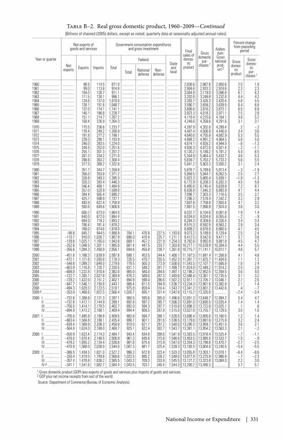
National Income or Expenditure | 331
Table B–2. Real gross domestic product, 1960–2009—Continued[Billions of chained (2005) dollars, except as noted; quarterly data at seasonally adjusted annual rates]
Year or quarter
Net exports ofgoods and services
Government consumption expendituresand gross investment Final
sales ofdomes-
ticproduct
Grossdomestic
pur-chases 1
Adden-dum:Gross
nationalprod-uct 2
Percent changefrom preceding
period
Netexports Exports Imports Total
FederalStateandlocal
Grossdomes-
ticproduct
Grossdomes-
ticpur-
chases 1Total National
defenseNon-
defense
1960 ...................... ............. 98.5 114.5 871.0 ............. .............. ............. ............. 2,836.6 2,867.6 2,850.6 2.5 1.81961 ...................... ............. 99.0 113.8 914.8 ............. .............. ............. ............. 2,904.6 2,933.3 2,918.6 2.3 2.31962 ...................... ............. 104.0 126.7 971.1 ............. .............. ............. ............. 3,064.9 3,119.0 3,096.8 6.1 6.31963 ...................... ............. 111.5 130.1 996.1 ............. .............. ............. ............. 3,202.6 3,248.8 3,232.8 4.4 4.21964 ...................... ............. 124.6 137.0 1,018.0 ............. .............. ............. ............. 3,393.7 3,426.3 3,420.4 5.8 5.51965 ...................... ............. 128.1 151.6 1,048.7 ............. .............. ............. ............. 3,590.7 3,659.2 3,639.5 6.4 6.81966 ...................... ............. 137.0 174.1 1,141.1 ............. .............. ............. ............. 3,806.6 3,910.2 3,873.1 6.5 6.91967 ...................... ............. 140.1 186.8 1,228.7 ............. .............. ............. ............. 3,923.3 4,018.2 3,971.1 2.5 2.81968 ...................... ............. 151.1 214.7 1,267.2 ............. .............. ............. ............. 4,119.4 4,225.6 4,164.1 4.8 5.21969 ...................... ............. 158.4 226.9 1,264.3 ............. .............. ............. ............. 4,248.6 4,358.6 4,291.6 3.1 3.11970 ...................... ............. 175.5 236.6 1,233.7 ............. .............. ............. ............. 4,287.9 4,352.0 4,299.4 .2 –.21971 ...................... ............. 178.4 249.2 1,206.9 ............. .............. ............. ............. 4,407.4 4,506.9 4,446.0 3.4 3.61972 ...................... ............. 191.8 277.2 1,198.1 ............. .............. ............. ............. 4,640.6 4,755.8 4,682.9 5.3 5.51973 ...................... ............. 228.0 290.1 1,193.9 ............. .............. ............. ............. 4,888.2 4,991.2 4,964.5 5.8 5.01974 ...................... ............. 246.0 283.5 1,224.0 ............. .............. ............. ............. 4,874.1 4,926.2 4,944.0 –.6 –1.31975 ...................... ............. 244.5 252.0 1,251.6 ............. .............. ............. ............. 4,926.3 4,872.0 4,921.4 –.2 –1.11976 ...................... ............. 255.1 301.3 1,257.2 ............. .............. ............. ............. 5,120.2 5,189.2 5,191.2 5.4 6.51977 ...................... ............. 261.3 334.2 1,271.0 ............. .............. ............. ............. 5,344.9 5,464.4 5,433.7 4.6 5.31978 ...................... ............. 288.8 363.2 1,308.4 ............. .............. ............. ............. 5,639.7 5,763.2 5,733.2 5.6 5.51979 ...................... ............. 317.5 369.2 1,332.8 ............. .............. ............. ............. 5,841.2 5,903.3 5,930.2 3.1 2.41980 ...................... ............. 351.7 344.7 1,358.8 ............. .............. ............. ............. 5,878.7 5,789.6 5,913.4 –.3 –1.91981 ...................... ............. 356.0 353.8 1,371.2 ............. .............. ............. ............. 5,959.5 5,944.7 6,052.5 2.5 2.71982 ...................... ............. 328.8 349.3 1,395.3 ............. .............. ............. ............. 5,923.3 5,865.4 5,939.1 –1.9 –1.31983 ...................... ............. 320.3 393.4 1,446.3 ............. .............. ............. ............. 6,172.9 6,208.3 6,202.3 4.5 5.81984 ...................... ............. 346.4 489.1 1,494.9 ............. .............. ............. ............. 6,495.6 6,745.4 6,639.8 7.2 8.71985 ...................... ............. 357.0 520.9 1,599.0 ............. .............. ............. ............. 6,838.9 7,045.3 6,893.9 4.1 4.41986 ...................... ............. 384.4 565.4 1,696.2 ............. .............. ............. ............. 7,098.7 7,303.3 7,116.5 3.5 3.71987 ...................... ............. 425.7 598.9 1,737.1 ............. .............. ............. ............. 7,296.2 7,518.4 7,342.2 3.2 2.91988 ...................... ............. 493.9 622.4 1,758.9 ............. .............. ............. ............. 7,607.8 7,758.8 7,650.4 4.1 3.21989 ...................... ............. 550.6 649.8 1,806.8 ............. .............. ............. ............. 7,867.5 7,990.9 7,924.0 3.6 3.01990 ...................... .............. 600.2 673.0 1,864.0 .............. .............. .............. .............. 8,032.7 8,104.6 8,081.8 1.9 1.41991 ...................... .............. 640.0 672.0 1,884.4 .............. .............. .............. .............. 8,034.8 8,034.6 8,055.6 –.2 –.91992 ...................... .............. 684.0 719.2 1,893.2 .............. .............. .............. .............. 8,284.3 8,309.6 8,326.4 3.4 3.41993 ...................... .............. 706.4 781.4 1,878.2 .............. .............. .............. .............. 8,515.3 8,592.9 8,563.2 2.9 3.41994 ...................... .............. 768.0 874.6 1,878.0 .............. .............. .............. .............. 8,809.2 8,976.0 8,900.5 4.1 4.51995 ...................... –98.8 845.7 944.5 1,888.9 704.1 476.8 227.5 1,183.6 9,073.2 9,189.0 9,129.4 2.5 2.41996 ...................... –110.7 916.0 1,026.7 1,907.9 696.0 470.4 225.7 1,211.1 9,412.5 9,542.0 9,471.1 3.7 3.81997 ...................... –139.8 1,025.1 1,165.0 1,943.8 689.1 457.2 231.9 1,254.3 9,782.6 9,992.8 9,881.8 4.5 4.71998 ...................... –252.6 1,048.5 1,301.1 1,985.0 681.4 447.5 233.7 1,303.8 10,217.1 10,539.9 10,304.0 4.4 5.51999 ...................... –356.6 1,094.3 1,450.9 2,056.1 694.6 455.8 238.7 1,361.8 10,715.7 11,141.1 10,812.1 4.8 5.72000 ...................... –451.6 1,188.3 1,639.9 2,097.8 698.1 453.5 244.4 1,400.1 11,167.5 11,681.4 11,268.8 4.1 4.82001 ...................... –472.1 1,121.6 1,593.8 2,178.3 726.5 470.7 255.5 1,452.3 11,391.7 11,825.7 11,404.6 1.1 1.22002 ...................... –548.8 1,099.2 1,648.0 2,279.6 779.5 505.3 273.9 1,500.6 11,543.5 12,107.7 11,606.9 1.8 2.42003 ...................... –603.9 1,116.8 1,720.7 2,330.5 831.1 549.2 281.7 1,499.7 11,824.8 12,449.2 11,914.2 2.5 2.82004 ...................... –688.0 1,222.8 1,910.8 2,362.0 865.0 580.4 284.6 1,497.1 12,198.2 12,952.5 12,358.5 3.6 4.02005 ...................... –722.7 1,305.1 2,027.8 2,369.9 876.3 589.0 287.3 1,493.6 12,588.4 13,361.1 12,735.5 3.1 3.22006 ...................... –729.2 1,422.0 2,151.2 2,402.1 894.9 598.4 296.6 1,507.2 12,917.1 13,705.7 13,046.1 2.7 2.62007 ...................... –647.7 1,546.1 2,193.8 2,443.1 906.4 611.5 294.9 1,536.7 13,234.3 13,901.6 13,362.8 2.1 1.42008 ...................... –494.3 1,629.3 2,123.5 2,518.1 975.9 659.4 316.4 1,543.7 13,341.2 13,801.2 13,442.6 .4 –.72009 p .................... –353.8 1,468.6 1,822.5 2,566.4 1,026.7 695.1 331.4 1,542.8 13,115.2 13,335.8 .............. –2.4 –3.42006: I .................. –732.6 1,388.8 2,121.3 2,397.1 900.5 595.6 305.0 1,496.6 12,851.3 13,648.7 12,994.2 5.4 4.7
II ................. –732.8 1,412.1 2,144.9 2,399.1 892.8 597.2 295.7 1,506.3 12,891.0 13,695.5 13,035.4 1.4 1.4III ................ –756.5 1,414.1 2,170.5 2,402.7 892.0 594.3 297.7 1,510.8 12,898.3 13,722.8 13,025.1 .1 .8IV ................ –694.9 1,473.2 2,168.1 2,409.4 894.4 606.5 287.8 1,515.0 13,027.8 13,755.7 13,129.5 3.0 1.0
2007: I .................. –705.0 1,485.9 2,190.8 2,409.5 882.8 594.7 288.1 1,526.5 13,086.4 13,805.0 13,160.5 1.2 1.4II ................. –683.4 1,504.8 2,188.1 2,435.4 898.7 607.1 291.6 1,536.5 13,179.6 13,887.6 13,275.9 3.2 2.4III ................ –638.4 1,569.9 2,208.3 2,458.9 919.0 621.7 297.2 1,540.0 13,290.3 13,959.7 13,451.5 3.6 2.1IV ................ –564.0 1,624.0 2,188.0 2,468.7 925.1 622.4 302.7 1,543.7 13,381.1 13,954.2 13,563.3 2.1 –.2
2008: I .................. –550.9 1,623.4 2,174.3 2,484.7 943.4 634.8 308.6 1,541.9 13,363.5 13,916.4 13,525.4 –.7 –1.1II ................. –476.0 1,670.4 2,146.5 2,506.9 961.3 645.6 315.8 1,546.6 13,453.5 13,885.5 13,533.7 1.5 –.9III ................ –479.2 1,655.2 2,134.4 2,536.6 991.6 675.4 315.9 1,547.0 13,354.3 13,798.8 13,470.7 –2.7 –2.5IV ................ –470.9 1,568.0 2,038.9 2,544.0 1,007.3 681.7 325.4 1,539.3 13,193.5 13,604.0 13,240.5 –5.4 –5.5
2009: I .................. –386.5 1,434.5 1,821.0 2,527.2 996.3 672.8 323.4 1,533.3 13,055.8 13,303.1 13,018.1 –6.4 –8.6II ................. –330.4 1,419.5 1,749.8 2,568.6 1,023.5 695.2 328.2 1,548.0 13,077.8 13,225.9 12,986.8 –.7 –2.3III ................ –357.4 1,478.8 1,836.2 2,585.5 1,043.3 709.3 333.8 1,545.5 13,127.2 13,323.8 13,084.0 2.2 3.0IV p ............. –341.1 1,541.6 1,882.7 2,584.4 1,043.5 703.1 340.4 1,544.3 13,200.2 13,490.3 .............. 5.7 5.1
1 Gross domestic product (GDP) less exports of goods and services plus imports of goods and services.2 GDP plus net income receipts from rest of the world.Source: Department of Commerce (Bureau of Economic Analysis).
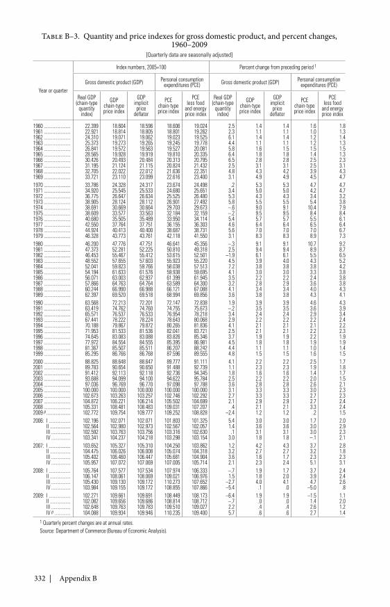
332 | Appendix B
Table B–3. Quantity and price indexes for gross domestic product, and percent changes,1960–2009
[Quarterly data are seasonally adjusted]
Year or quarter
Index numbers, 2005=100 Percent change from preceding period 1
Gross domestic product (GDP) Personal consumptionexpenditures (PCE) Gross domestic product (GDP) Personal consumption
expenditures (PCE)
Real GDP(chain-type
quantityindex)
GDPchain-typeprice index
GDPimplicit
pricedeflator
PCEchain-typeprice index
PCEless food
and energyprice index
Real GDP(chain-type
quantityindex)
GDPchain-typeprice index
GDPimplicit
pricedeflator
PCEchain-typeprice index
PCEless food
and energyprice index
1960 ...................... 22.399 18.604 18.596 18.606 19.024 2.5 1.4 1.4 1.6 1.81961 ...................... 22.921 18.814 18.805 18.801 19.262 2.3 1.1 1.1 1.0 1.31962 ...................... 24.310 19.071 19.062 19.023 19.525 6.1 1.4 1.4 1.2 1.41963 ...................... 25.373 19.273 19.265 19.245 19.778 4.4 1.1 1.1 1.2 1.31964 ...................... 26.841 19.572 19.563 19.527 20.081 5.8 1.6 1.5 1.5 1.51965 ...................... 28.565 19.928 19.919 19.810 20.335 6.4 1.8 1.8 1.4 1.31966 ...................... 30.426 20.493 20.484 20.313 20.795 6.5 2.8 2.8 2.5 2.31967 ...................... 31.195 21.124 21.115 20.824 21.432 2.5 3.1 3.1 2.5 3.11968 ...................... 32.705 22.022 22.012 21.636 22.351 4.8 4.3 4.2 3.9 4.31969 ...................... 33.721 23.110 23.099 22.616 23.400 3.1 4.9 4.9 4.5 4.71970 ...................... 33.786 24.328 24.317 23.674 24.498 .2 5.3 5.3 4.7 4.71971 ...................... 34.920 25.545 25.533 24.680 25.651 3.4 5.0 5.0 4.2 4.71972 ...................... 36.775 26.647 26.634 25.525 26.480 5.3 4.3 4.3 3.4 3.21973 ...................... 38.905 28.124 28.112 26.901 27.492 5.8 5.5 5.5 5.4 3.81974 ...................... 38.691 30.669 30.664 29.703 29.673 –.6 9.0 9.1 10.4 7.91975 ...................... 38.609 33.577 33.563 32.184 32.159 –.2 9.5 9.5 8.4 8.41976 ...................... 40.680 35.505 35.489 33.950 34.114 5.4 5.7 5.7 5.5 6.11977 ...................... 42.550 37.764 37.751 36.155 36.303 4.6 6.4 6.4 6.5 6.41978 ...................... 44.924 40.413 40.400 38.687 38.731 5.6 7.0 7.0 7.0 6.71979 ...................... 46.328 43.773 43.761 42.118 41.550 3.1 8.3 8.3 8.9 7.31980 ...................... 46.200 47.776 47.751 46.641 45.356 –.3 9.1 9.1 10.7 9.21981 ...................... 47.373 52.281 52.225 50.810 49.318 2.5 9.4 9.4 8.9 8.71982 ...................... 46.453 55.467 55.412 53.615 52.501 –1.9 6.1 6.1 5.5 6.51983 ...................... 48.552 57.655 57.603 55.923 55.220 4.5 3.9 4.0 4.3 5.21984 ...................... 52.041 59.823 59.766 58.038 57.513 7.2 3.8 3.8 3.8 4.21985 ...................... 54.194 61.633 61.576 59.938 59.695 4.1 3.0 3.0 3.3 3.81986 ...................... 56.071 63.003 62.937 61.399 61.945 3.5 2.2 2.2 2.4 3.81987 ...................... 57.866 64.763 64.764 63.589 64.300 3.2 2.8 2.9 3.6 3.81988 ...................... 60.244 66.990 66.988 66.121 67.088 4.1 3.4 3.4 4.0 4.31989 ...................... 62.397 69.520 69.518 68.994 69.856 3.6 3.8 3.8 4.3 4.11990 ...................... 63.568 72.213 72.201 72.147 72.838 1.9 3.9 3.9 4.6 4.31991 ...................... 63.419 74.762 74.760 74.755 75.673 –.2 3.5 3.5 3.6 3.91992 ...................... 65.571 76.537 76.533 76.954 78.218 3.4 2.4 2.4 2.9 3.41993 ...................... 67.441 78.222 78.224 78.643 80.068 2.9 2.2 2.2 2.2 2.41994 ...................... 70.188 79.867 79.872 80.265 81.836 4.1 2.1 2.1 2.1 2.21995 ...................... 71.953 81.533 81.536 82.041 83.721 2.5 2.1 2.1 2.2 2.31996 ...................... 74.645 83.083 83.088 83.826 85.346 3.7 1.9 1.9 2.2 1.91997 ...................... 77.972 84.554 84.555 85.395 86.981 4.5 1.8 1.8 1.9 1.91998 ...................... 81.367 85.507 85.511 86.207 88.242 4.4 1.1 1.1 1.0 1.41999 ...................... 85.295 86.766 86.768 87.596 89.555 4.8 1.5 1.5 1.6 1.52000 ...................... 88.825 88.648 88.647 89.777 91.111 4.1 2.2 2.2 2.5 1.72001 ...................... 89.783 90.654 90.650 91.488 92.739 1.1 2.3 2.3 1.9 1.82002 ...................... 91.412 92.113 92.118 92.736 94.345 1.8 1.6 1.6 1.4 1.72003 ...................... 93.688 94.099 94.100 94.622 95.784 2.5 2.2 2.2 2.0 1.52004 ...................... 97.036 96.769 96.770 97.098 97.788 3.6 2.8 2.8 2.6 2.12005 ...................... 100.000 100.000 100.000 100.000 100.000 3.1 3.3 3.3 3.0 2.32006 ...................... 102.673 103.263 103.257 102.746 102.292 2.7 3.3 3.3 2.7 2.32007 ...................... 104.872 106.221 106.214 105.502 104.699 2.1 2.9 2.9 2.7 2.42008 ...................... 105.331 108.481 108.483 109.031 107.207 .4 2.1 2.1 3.3 2.42009 p .................... 102.772 109.754 109.777 109.252 108.828 –2.4 1.2 1.2 .2 1.52006: I .................. 102.196 102.071 102.071 101.803 101.325 5.4 3.0 3.0 1.7 2.0
II ................. 102.564 102.980 102.973 102.567 102.057 1.4 3.6 3.6 3.0 2.9III ................ 102.592 103.763 103.756 103.316 102.630 .1 3.1 3.1 3.0 2.3IV ................ 103.341 104.237 104.218 103.298 103.154 3.0 1.8 1.8 –.1 2.1
2007: I .................. 103.652 105.327 105.310 104.250 103.862 1.2 4.2 4.3 3.7 2.8II ................. 104.475 106.026 106.008 105.074 104.318 3.2 2.7 2.7 3.2 1.8III ................ 105.402 106.460 106.447 105.681 104.904 3.6 1.6 1.7 2.3 2.3IV ................ 105.957 107.072 107.069 107.005 105.714 2.1 2.3 2.4 5.1 3.1
2008: I .................. 105.764 107.577 107.534 107.974 106.333 –.7 1.9 1.7 3.7 2.4II ................. 106.147 108.061 108.069 109.021 106.976 1.5 1.8 2.0 3.9 2.4III ................ 105.430 109.130 109.172 110.273 107.652 –2.7 4.0 4.1 4.7 2.6IV ................ 103.984 109.155 109.172 108.855 107.866 –5.4 .1 .0 –5.0 .8
2009: I .................. 102.271 109.661 109.691 108.449 108.173 –6.4 1.9 1.9 –1.5 1.1II ................. 102.082 109.656 109.686 108.814 108.712 –.7 .0 .0 1.4 2.0III ................ 102.648 109.763 109.783 109.510 109.027 2.2 .4 .4 2.6 1.2IV p ............. 104.088 109.934 109.946 110.235 109.400 5.7 .6 .6 2.7 1.4
1 Quarterly percent changes are at annual rates.Source: Department of Commerce (Bureau of Economic Analysis).
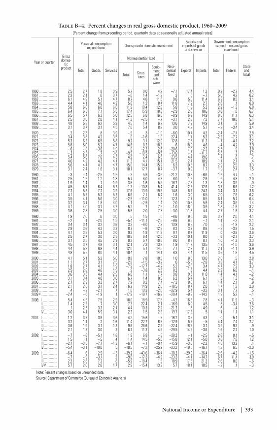
National Income or Expenditure | 333
Table B–4. Percent changes in real gross domestic product, 1960–2009[Percent change from preceding period; quarterly data at seasonally adjusted annual rates]
Year or quarterGross
domes-tic
product
Personal consumptionexpenditures Gross private domestic investment
Exports andimports of goods
and services
Government consumptionexpenditures and gross
investment
Total Goods Services
Nonresidential fixed
Resi-dentialfixed
Exports Imports Total FederalStateandlocalTotal Struc-
tures
Equip-mentandsoft-ware
1960 ..................... 2.5 2.7 1.8 3.9 5.7 8.0 4.2 –7.1 17.4 1.3 0.2 –2.7 4.41961 ..................... 2.3 2.1 .6 3.7 –.6 1.4 –1.9 .3 .5 –.7 5.0 4.2 6.21962 ..................... 6.1 4.9 5.1 4.7 8.7 4.6 11.6 9.6 5.0 11.4 6.2 8.5 3.11963 ..................... 4.4 4.1 4.0 4.2 5.6 1.2 8.4 11.8 7.2 2.7 2.6 .1 6.01964 ..................... 5.8 6.0 6.0 6.0 11.9 10.4 12.8 5.8 11.8 5.3 2.2 –1.3 6.81965 ..................... 6.4 6.3 7.1 5.5 17.4 15.9 18.3 –2.9 2.8 10.6 3.0 .0 6.71966 ..................... 6.5 5.7 6.3 5.0 12.5 6.8 16.0 –8.9 6.9 14.9 8.8 11.1 6.31967 ..................... 2.5 3.0 2.0 4.1 –1.3 –2.5 –.7 –3.1 2.3 7.3 7.7 10.0 5.11968 ..................... 4.8 5.8 6.2 5.3 4.5 1.4 6.2 13.6 7.9 14.9 3.1 .8 5.91969 ..................... 3.1 3.7 3.1 4.5 7.6 5.4 8.8 3.0 4.8 5.7 –.2 –3.4 3.41970 ..................... .2 2.3 .8 3.9 –.5 .3 –1.0 –6.0 10.7 4.3 –2.4 –7.4 2.81971 ..................... 3.4 3.8 4.2 3.5 .0 –1.6 1.0 27.4 1.7 5.3 –2.2 –7.7 3.11972 ..................... 5.3 6.2 6.5 5.8 9.2 3.1 12.9 17.8 7.5 11.3 –.7 –4.1 2.21973 ..................... 5.8 5.0 5.2 4.7 14.6 8.2 18.3 –.6 18.9 4.6 –.4 –4.2 2.91974 ..................... –.6 –.8 –3.6 1.9 .8 –2.2 2.6 –20.6 7.9 –2.3 2.5 .9 3.81975 ..................... –.2 2.3 .7 3.8 –9.9 –10.5 –9.5 –13.0 –.6 –11.1 2.3 .3 3.71976 ..................... 5.4 5.6 7.0 4.3 4.9 2.4 6.3 23.5 4.4 19.6 .4 .0 .71977 ..................... 4.6 4.2 4.3 4.1 11.3 4.1 15.1 21.5 2.4 10.9 1.1 2.1 .41978 ..................... 5.6 4.4 4.1 4.7 15.0 14.4 15.2 6.3 10.5 8.7 2.9 2.5 3.31979 ..................... 3.1 2.4 1.6 3.1 10.1 12.7 8.7 –3.7 9.9 1.7 1.9 2.4 1.51980 ..................... –.3 –.4 –2.5 1.5 –.3 5.9 –3.6 –21.2 10.8 –6.6 1.9 4.7 –.11981 ..................... 2.5 1.5 1.2 1.8 5.7 8.0 4.3 –8.0 1.2 2.6 .9 4.8 –2.01982 ..................... –1.9 1.4 .7 1.9 –3.8 –1.6 –5.2 –18.2 –7.6 –1.3 1.8 3.9 .01983 ..................... 4.5 5.7 6.4 5.2 –1.3 –10.8 5.4 41.4 –2.6 12.6 3.7 6.6 1.21984 ..................... 7.2 5.3 7.2 3.9 17.6 13.9 19.8 14.8 8.2 24.3 3.4 3.1 3.61985 ..................... 4.1 5.2 5.3 5.2 6.6 7.1 6.4 1.6 3.0 6.5 7.0 7.8 6.21986 ..................... 3.5 4.1 5.6 3.0 –2.9 –11.0 1.9 12.3 7.7 8.5 6.1 5.7 6.41987 ..................... 3.2 3.1 1.8 4.0 –.1 –2.9 1.4 2.0 10.8 5.9 2.4 3.6 1.41988 ..................... 4.1 4.0 3.7 4.2 5.2 .7 7.5 –1.0 16.0 3.9 1.3 –1.6 3.71989 ..................... 3.6 2.8 2.5 3.0 5.6 2.0 7.3 –3.0 11.5 4.4 2.7 1.6 3.71990 ..................... 1.9 2.0 .6 3.0 .5 1.5 .0 –8.6 9.0 3.6 3.2 2.0 4.11991 ..................... –.2 .1 –2.0 1.5 –5.4 –11.1 –2.6 –9.6 6.6 –.1 1.1 –.2 2.11992 ..................... 3.4 3.4 3.2 3.6 3.2 –6.0 7.3 13.8 6.9 7.0 .5 –1.8 2.21993 ..................... 2.9 3.6 4.2 3.2 8.7 –.6 12.5 8.2 3.3 8.6 –.8 –3.9 1.51994 ..................... 4.1 3.8 5.3 3.0 9.2 1.8 11.9 9.7 8.7 11.9 .0 –3.8 2.61995 ..................... 2.5 2.7 3.0 2.5 10.5 6.4 12.0 –3.3 10.1 8.0 .6 –2.7 2.71996 ..................... 3.7 3.5 4.5 2.9 9.3 5.7 10.6 8.0 8.3 8.7 1.0 –1.2 2.31997 ..................... 4.5 3.7 4.8 3.1 12.1 7.3 13.8 1.9 11.9 13.5 1.9 –1.0 3.61998 ..................... 4.4 5.2 6.8 4.4 12.0 5.1 14.5 7.7 2.3 11.7 2.1 –1.1 3.91999 ..................... 4.8 5.5 8.0 4.1 10.4 .1 14.1 6.3 4.4 11.5 3.6 1.9 4.52000 ..................... 4.1 5.1 5.3 5.0 9.8 7.8 10.5 1.0 8.6 13.0 2.0 .5 2.82001 ..................... 1.1 2.7 3.1 2.5 –2.8 –1.5 –3.2 .6 –5.6 –2.8 3.8 4.1 3.72002 ..................... 1.8 2.7 4.1 1.9 –7.9 –17.7 –4.2 5.2 –2.0 3.4 4.7 7.3 3.32003 ..................... 2.5 2.8 4.6 1.9 .9 –3.8 2.5 8.2 1.6 4.4 2.2 6.6 –.12004 ..................... 3.6 3.5 4.4 2.9 6.0 1.1 7.7 9.8 9.5 11.0 1.4 4.1 –.22005 ..................... 3.1 3.4 4.0 3.0 6.7 1.4 8.5 6.2 6.7 6.1 .3 1.3 –.22006 ..................... 2.7 2.9 3.3 2.7 7.9 9.2 7.4 –7.3 9.0 6.1 1.4 2.1 .92007 ..................... 2.1 2.6 3.1 2.4 6.2 14.9 2.6 –18.5 8.7 2.0 1.7 1.3 2.02008 ..................... .4 –.2 –2.1 .7 1.6 10.3 –2.6 –22.9 5.4 –3.2 3.1 7.7 .52009 p ................... –2.4 –.6 –1.9 .1 –17.9 –19.7 –16.9 –20.4 –9.9 –14.2 1.9 5.2 –.12006: I ................. 5.4 4.5 7.5 2.9 18.0 18.9 17.8 –4.2 16.5 7.8 4.1 11.9 –.3
II ................ 1.4 2.2 .7 3.0 7.3 22.4 2.1 –16.9 6.9 4.5 .3 –3.4 2.6III ............... .1 2.5 3.3 2.1 4.4 10.3 2.2 –21.2 .6 4.9 .6 –.4 1.2IV ............... 3.0 4.1 5.9 3.1 2.3 1.5 2.8 –19.7 17.8 –.5 1.1 1.1 1.1
2007: I ................. 1.2 3.7 3.9 3.6 4.2 15.6 –.5 –16.2 3.5 4.3 .0 –5.1 3.1II ................ 3.2 1.1 .2 1.6 11.4 22.7 6.5 –12.9 5.2 –.5 4.4 7.4 2.7III ............... 3.6 1.9 3.1 1.3 9.6 26.6 2.2 –22.4 18.5 3.7 3.9 9.3 .9IV ............... 2.1 1.2 3.0 .3 6.7 11.2 4.5 –29.5 14.5 –3.6 1.6 2.7 1.0
2008: I ................. –.7 –.6 –5.1 1.8 1.9 6.8 –.5 –28.2 –.1 –2.5 2.6 8.1 –.5II ................ 1.5 .1 –.5 .4 1.4 14.5 –5.0 –15.8 12.1 –5.0 3.6 7.8 1.2III ............... –2.7 –3.5 –7.7 –1.3 –6.1 –.1 –9.4 –15.9 –3.6 –2.2 4.8 13.2 .1IV ............... –5.4 –3.1 –10.0 .5 –19.5 –7.2 –25.9 –23.2 –19.5 –16.7 1.2 6.5 –2.0
2009: I ................. –6.4 .6 2.5 –.3 –39.2 –43.6 –36.4 –38.2 –29.9 –36.4 –2.6 –4.3 –1.5II ................ –.7 –.9 –3.1 .2 –9.6 –17.3 –4.9 –23.3 –4.1 –14.7 6.7 11.4 3.9III ............... 2.2 2.8 7.2 .8 –5.9 –18.4 1.5 18.9 17.8 21.3 2.6 8.0 –.6IV p ............ 5.7 2.0 2.6 1.7 2.9 –15.4 13.3 5.7 18.1 10.5 –.2 .1 –.3
Note: Percent changes based on unrounded data.Source: Department of Commerce (Bureau of Economic Analysis).
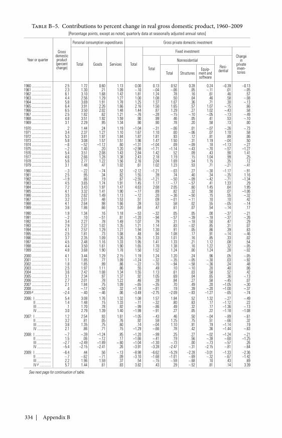
334 | Appendix B
Table B–5. Contributions to percent change in real gross domestic product, 1960–2009[Percentage points, except as noted; quarterly data at seasonally adjusted annual rates]
Year or quarter
Grossdomesticproduct(percentchange)
Personal consumption expenditures Gross private domestic investment
Total Goods Services Total
Fixed investmentChange
inprivateinven-tories
Total
NonresidentialResi-
dentialTotal StructuresEquip-
ment andsoftware
1960 ...................... 2.5 1.72 0.60 1.13 0.00 0.13 0.52 0.28 0.24 –0.39 –0.131961 ...................... 2.3 1.30 .21 1.09 –.10 –.04 –.06 .05 –.11 .01 –.051962 ...................... 6.1 3.10 1.68 1.42 1.81 1.24 .78 .16 .61 .46 .571963 ...................... 4.4 2.56 1.29 1.27 1.00 1.08 .50 .04 .46 .58 –.081964 ...................... 5.8 3.69 1.91 1.78 1.25 1.37 1.07 .36 .71 .30 –.131965 ...................... 6.4 3.91 2.26 1.66 2.16 1.50 1.65 .57 1.07 –.15 .661966 ...................... 6.5 3.50 2.02 1.48 1.44 .87 1.29 .27 1.02 –.43 .581967 ...................... 2.5 1.82 .62 1.21 –.76 –.28 –.15 –.10 –.05 –.13 –.491968 ...................... 4.8 3.51 1.92 1.59 .90 .99 .46 .05 .41 .53 –.101969 ...................... 3.1 2.29 .95 1.34 .90 .90 .78 .20 .58 .13 .001970 ...................... .2 1.44 .24 1.19 –1.04 –.31 –.06 .01 –.07 –.26 –.731971 ...................... 3.4 2.37 1.27 1.10 1.67 1.10 .00 –.06 .07 1.10 .581972 ...................... 5.3 3.81 1.97 1.84 1.87 1.81 .93 .12 .81 .89 .061973 ...................... 5.8 3.08 1.57 1.51 1.96 1.47 1.50 .31 1.19 –.04 .501974 ...................... –.6 –.52 –1.12 .60 –1.31 –1.04 .09 –.09 .18 –1.13 –.271975 ...................... –.2 1.40 .20 1.20 –2.98 –1.71 –1.14 –.43 –.70 –.57 –1.271976 ...................... 5.4 3.51 2.08 1.43 2.84 1.42 .52 .09 .43 .90 1.411977 ...................... 4.6 2.66 1.28 1.38 2.43 2.18 1.19 .15 1.04 .99 .251978 ...................... 5.6 2.77 1.22 1.56 2.16 2.04 1.69 .54 1.15 .35 .121979 ...................... 3.1 1.48 .47 1.02 .61 1.02 1.23 .53 .71 –.21 –.411980 ...................... –.3 –.22 –.74 .52 –2.12 –1.21 –.03 .27 –.30 –1.17 –.911981 ...................... 2.5 .95 .34 .62 1.55 .39 .74 .40 .34 –.35 1.161982 ...................... –1.9 .86 .19 .67 –2.55 –1.21 –.50 –.09 –.42 –.71 –1.341983 ...................... 4.5 3.65 1.74 1.91 1.45 1.17 –.17 –.57 .41 1.33 .291984 ...................... 7.2 3.43 1.97 1.47 4.63 2.68 2.05 .60 1.45 .64 1.951985 ...................... 4.1 3.32 1.41 1.90 –.17 .89 .82 .32 .50 .07 –1.061986 ...................... 3.5 2.62 1.49 1.13 –.12 .20 –.36 –.50 .15 .55 –.321987 ...................... 3.2 2.01 .48 1.53 .51 .09 –.01 –.11 .10 .10 .421988 ...................... 4.1 2.64 .98 1.66 .39 .53 .58 .02 .55 –.05 –.141989 ...................... 3.6 1.86 .66 1.20 .64 .47 .61 .07 .54 –.14 .171990 ...................... 1.9 1.34 .16 1.18 –.53 –.32 .05 .05 .00 –.37 –.211991 ...................... –.2 .10 –.51 .61 –1.20 –.94 –.57 –.39 –.18 –.37 –.261992 ...................... 3.4 2.27 .78 1.49 1.07 .79 .31 –.18 .50 .47 .291993 ...................... 2.9 2.37 1.02 1.35 1.21 1.14 .83 –.02 .85 .31 .071994 ...................... 4.1 2.57 1.29 1.27 1.94 1.30 .91 .05 .86 .39 .631995 ...................... 2.5 1.81 .73 1.08 .48 .94 1.08 .17 .91 –.14 –.461996 ...................... 3.7 2.35 1.09 1.26 1.35 1.33 1.01 .16 .85 .33 .021997 ...................... 4.5 2.48 1.16 1.33 1.95 1.41 1.33 .21 1.12 .08 .541998 ...................... 4.4 3.50 1.61 1.90 1.65 1.70 1.38 .16 1.22 .32 –.051999 ...................... 4.8 3.68 1.90 1.78 1.50 1.52 1.24 .00 1.24 .28 –.022000 ...................... 4.1 3.44 1.29 2.15 1.19 1.24 1.20 .24 .96 .05 –.052001 ...................... 1.1 1.85 .77 1.09 –1.24 –.32 –.35 –.05 –.30 .03 –.922002 ...................... 1.8 1.85 .99 .86 –.22 –.70 –.94 –.58 –.36 .24 .482003 ...................... 2.5 1.97 1.11 .86 .55 .49 .10 –.10 .20 .40 .062004 ...................... 3.6 2.42 1.08 1.34 1.55 1.13 .61 .03 .58 .52 .422005 ...................... 3.1 2.34 .97 1.37 .92 1.05 .69 .04 .65 .36 –.132006 ...................... 2.7 2.01 .78 1.22 .46 .39 .84 .27 .58 –.45 .072007 ...................... 2.1 1.84 .75 1.09 –.65 –.35 .70 .49 .20 –1.05 –.302008 ...................... .4 –.17 –.50 .32 –1.18 –.81 .19 .39 –.20 –1.00 –.372009 p .................... –2.4 –.40 –.46 .06 –3.49 –2.75 –2.09 –.83 –1.27 –.65 –.742006: I .................. 5.4 3.08 1.76 1.32 1.08 1.57 1.84 .52 1.32 –.27 –.49
II ................. 1.4 1.48 .15 1.33 –.11 –.32 .80 .63 .17 –1.12 .22III ................ .1 1.70 .78 .92 –.99 –.86 .49 .32 .17 –1.36 –.13IV ................ 3.0 2.79 1.39 1.40 –1.99 –.91 .27 .05 .22 –1.18 –1.08
2007: I .................. 1.2 2.54 .93 1.61 –1.05 –.43 .46 .50 –.04 –.89 –.61II ................. 3.2 .81 .05 .76 .92 .59 1.25 .75 .51 –.66 .32III ................ 3.6 1.35 .75 .60 .14 –.04 1.10 .91 .19 –1.14 .19IV ................ 2.1 .86 .71 .15 –1.29 –.66 .78 .42 .36 –1.44 –.63
2008: I .................. –.7 –.39 –1.24 .85 –1.20 –.99 .25 .27 –.02 –1.24 –.21II ................. 1.5 .06 –.12 .17 –1.66 –.41 .19 .56 –.38 –.60 –1.25III ................ –2.7 –2.49 –1.89 –.60 –1.04 –1.30 –.73 .00 –.73 –.57 .26IV ................ –5.4 –2.15 –2.41 .26 –3.91 –3.28 –2.47 –.31 –2.15 –.81 –.64
2009: I .................. –6.4 .44 .56 –.13 –8.98 –6.62 –5.29 –2.28 –3.01 –1.33 –2.36II ................. –.7 –.62 –.71 .09 –3.10 –1.68 –1.01 –.69 –.32 –.67 –1.42III ................ 2.2 1.96 1.59 .37 .54 –.15 –.59 –.68 .10 .43 .69IV p ............. 5.7 1.44 .61 .83 3.82 .43 .29 –.52 .81 .14 3.39
See next page for continuation of table.
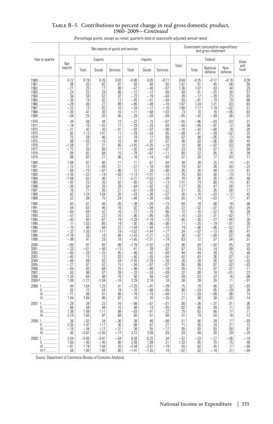
National Income or Expenditure | 335
Table B–5. Contributions to percent change in real gross domestic product,1960–2009—Continued
[Percentage points, except as noted; quarterly data at seasonally adjusted annual rates]
Year or quarter
Net exports of goods and services Government consumption expendituresand gross investment
Netexports
Exports ImportsTotal
Federal StateandlocalTotal Goods Services Total Goods Services Total National
defenseNon-
defense
1960 ...................... 0.72 0.78 0.76 0.02 –0.06 0.05 –0.11 0.04 –0.35 –0.17 –0.18 0.391961 ...................... .06 .03 .02 .01 .03 .00 .02 1.07 .51 .45 .06 .561962 ...................... –.21 .25 .17 .08 –.47 –.40 –.07 1.36 1.07 .63 .44 .291963 ...................... .24 .35 .29 .06 –.12 –.12 .00 .58 .01 –.25 .26 .571964 ...................... .36 .59 .52 .07 –.23 –.19 –.04 .49 –.17 –.39 .23 .651965 ...................... –.30 .15 .02 .13 –.45 –.41 –.04 .65 –.01 –.19 .19 .661966 ...................... –.29 .36 .27 .09 –.65 –.49 –.16 1.87 1.24 1.21 .03 .631967 ...................... –.22 .12 .02 .10 –.34 –.17 –.16 1.68 1.17 1.19 –.02 .511968 ...................... –.30 .41 .30 .10 –.71 –.68 –.03 .73 .10 .16 –.06 .631969 ...................... –.04 .25 .20 .05 –.29 –.20 –.09 –.05 –.42 –.49 .06 .371970 ...................... .34 .56 .44 .12 –.22 –.15 –.07 –.55 –.86 –.83 –.03 .311971 ...................... –.19 .10 –.02 .11 –.29 –.33 .04 –.50 –.85 –.97 .12 .361972 ...................... –.21 .42 .43 –.01 –.63 –.57 –.06 –.16 –.42 –.60 .18 .261973 ...................... .82 1.12 1.01 .11 –.29 –.34 .05 –.08 –.41 –.39 –.02 .331974 ...................... .75 .58 .46 .12 .18 .17 .00 .52 .08 –.05 .13 .441975 ...................... .89 –.05 –.16 .10 .94 .87 .07 .48 .03 –.06 .09 .451976 ...................... –1.08 .37 .31 .05 –1.45 –1.35 –.10 .10 .00 –.02 .03 .091977 ...................... –.72 .20 .08 .11 –.92 –.84 –.07 .23 .19 .07 .12 .041978 ...................... .05 .82 .68 .15 –.78 –.67 –.11 .60 .22 .05 .16 .381979 ...................... .66 .82 .77 .06 –.16 –.14 –.02 .37 .20 .17 .03 .171980 ...................... 1.68 .97 .86 .11 .71 .67 .04 .38 .39 .25 .14 –.011981 ...................... –.15 .12 –.09 .21 –.27 –.18 –.09 .19 .42 .38 .04 –.231982 ...................... –.60 –.73 –.67 –.06 .12 .20 –.08 .35 .35 .48 –.13 .011983 ...................... –1.35 –.22 –.19 –.03 –1.13 –1.01 –.13 .76 .63 .50 .13 .131984 ...................... –1.58 .63 .46 .17 –2.21 –1.83 –.39 .70 .30 .35 –.05 .401985 ...................... –.42 .23 .20 .02 –.65 –.52 –.13 1.41 .74 .60 .14 .671986 ...................... –.30 .54 .26 .28 –.84 –.82 –.02 1.27 .55 .47 .08 .711987 ...................... .16 .77 .56 .21 –.61 –.39 –.22 .51 .35 .35 .00 .171988 ...................... .82 1.24 1.04 .20 –.43 –.36 –.07 .26 –.16 –.03 –.12 .421989 ...................... .52 .99 .75 .24 –.48 –.38 –.09 .55 .14 –.03 .17 .411990 ...................... .43 .81 .56 .26 –.38 –.26 –.13 .64 .18 .00 .18 .461991 ...................... .64 .63 .46 .16 .02 –.04 .05 .22 –.02 –.07 .05 .241992 ...................... –.05 .68 .52 .16 –.72 –.78 .06 .10 –.16 –.32 .16 .261993 ...................... –.57 .32 .23 .10 –.90 –.85 –.05 –.16 –.33 –.31 –.02 .171994 ...................... –.43 .85 .67 .19 –1.28 –1.18 –.10 .00 –.30 –.27 –.04 .301995 ...................... .11 1.03 .85 .19 –.92 –.86 –.06 .11 –.20 –.19 –.01 .301996 ...................... –.15 .90 .68 .22 –1.04 –.94 –.10 .19 –.08 –.06 –.02 .271997 ...................... –.32 1.30 1.11 .19 –1.62 –1.44 –.17 .34 –.07 –.13 .06 .411998 ...................... –1.18 .26 .18 .08 –1.43 –1.21 –.22 .38 –.07 –.09 .02 .451999 ...................... –.99 .47 .29 .18 –1.45 –1.31 –.14 .63 .12 .07 .04 .512000 ...................... –.85 .91 .82 .08 –1.76 –1.52 –.24 .36 .03 –.02 .05 .332001 ...................... –.20 –.61 –.48 –.13 .41 .39 .02 .67 .24 .14 .09 .432002 ...................... –.65 –.20 –.25 .05 –.46 –.42 –.04 .84 .44 .28 .15 .402003 ...................... –.45 .15 .12 .03 –.60 –.55 –.04 .42 .43 .36 .07 –.012004 ...................... –.66 .89 .55 .34 –1.55 –1.29 –.26 .26 .28 .26 .02 –.022005 ...................... –.27 .67 .52 .15 –.94 –.87 –.07 .06 .09 .07 .02 –.032006 ...................... –.05 .93 .68 .25 –.98 –.80 –.18 .26 .15 .07 .07 .112007 ...................... .63 .96 .57 .39 –.33 –.24 –.09 .32 .09 .10 –.01 .232008 ...................... 1.20 .64 .48 .16 .56 .58 –.02 .59 .53 .37 .16 .062009 p .................... 1.08 –1.21 –1.04 –.16 2.28 2.18 .10 .38 .39 .28 .11 –.012006: I .................. .44 1.64 1.23 .41 –1.20 –.81 –.39 .75 .79 .46 .32 –.03
II ................. .02 .72 .54 .18 –.70 –.66 –.05 .06 –.24 .05 –.29 .30III ................ –.71 .06 .01 .05 –.78 –.74 –.04 .11 –.03 –.09 .06 .14IV ................ 1.94 1.84 .96 .87 .10 .35 –.25 .21 .08 .38 –.30 .14
2007: I .................. –.29 .39 .23 .16 –.68 –.67 –.01 .00 –.36 –.37 .01 .36II ................. .66 .58 .48 .10 .08 .13 –.05 .82 .50 .39 .11 .32III ................ 1.36 1.99 1.11 .88 –.63 –.41 –.22 .75 .63 .46 .17 .11IV ................ 2.24 1.65 .97 .68 .60 .51 .08 .31 .19 .03 .16 .12
2008: I .................. .36 –.02 .34 –.36 .38 .46 –.08 .51 .56 .39 .17 –.05II ................. 2.35 1.47 1.17 .30 .88 .67 .21 .71 .55 .34 .21 .15III ................ –.10 –.48 –.17 –.31 .38 .55 –.17 .95 .93 .93 .00 .01IV ................ .45 –2.67 –2.50 –.17 3.12 3.09 .03 .24 .49 .20 .29 –.25
2009: I .................. 2.64 –3.95 –3.41 –.54 6.58 6.25 .34 –.52 –.33 –.27 –.06 –.19II ................. 1.65 –.45 –.45 .00 2.09 1.89 .21 1.33 .85 .70 .15 .48III ................ –.81 1.78 1.58 .20 –2.59 –2.41 –.18 .55 .62 .45 .17 –.08IV p ............. .50 1.90 1.90 .00 –1.41 –1.55 .14 –.02 .02 –.19 .21 –.04
Source: Department of Commerce (Bureau of Economic Analysis).
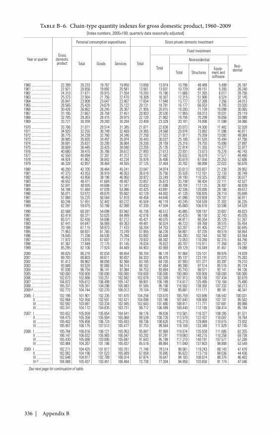
336 | Appendix B
Table B–6. Chain-type quantity indexes for gross domestic product, 1960–2009[Index numbers, 2005=100; quarterly data seasonally adjusted]
Year or quarterGross
domesticproduct
Personal consumption expenditures Gross private domestic investment
Total Goods Services Total
Fixed investment
Total
NonresidentialResi-
dentialTotal StructuresEquip-
ment andsoftware
1960 ...................... 22.399 20.233 19.767 19.850 13.650 13.974 10.796 48.488 5.499 26.1671961 ...................... 22.921 20.650 19.892 20.581 13.561 13.931 10.729 49.151 5.393 26.2401962 ...................... 24.310 21.671 20.915 21.554 15.283 15.190 11.666 51.393 6.017 28.7561963 ...................... 25.373 22.564 21.750 22.470 16.309 16.367 12.315 51.986 6.524 32.1451964 ...................... 26.841 23.908 23.047 23.807 17.654 17.948 13.777 57.399 7.356 34.0131965 ...................... 28.565 25.420 24.679 25.122 20.131 19.781 16.177 66.553 8.705 33.0201966 ...................... 30.426 26.862 26.245 26.367 21.905 20.915 18.200 71.109 10.098 30.0651967 ...................... 31.195 27.667 26.758 27.451 20.903 20.530 17.955 69.313 10.031 29.1191968 ...................... 32.705 29.263 28.415 28.915 22.120 21.962 18.756 70.299 10.656 33.0891969 ...................... 33.721 30.359 29.283 30.204 23.409 23.329 20.181 74.096 11.598 34.0661970 ...................... 33.786 31.071 29.514 31.385 21.871 22.838 20.073 74.300 11.482 32.0281971 ...................... 34.920 32.255 30.749 32.469 24.365 24.568 20.074 73.082 11.596 40.8111972 ...................... 36.775 34.239 32.760 34.346 27.250 27.522 21.917 75.359 13.092 48.0641973 ...................... 38.905 35.935 34.457 35.974 30.443 30.037 25.106 81.520 15.494 47.7561974 ...................... 38.691 35.637 33.200 36.664 28.200 28.159 25.316 79.755 15.890 37.8971975 ...................... 38.609 36.445 33.425 38.040 23.205 25.135 22.814 71.355 14.377 32.9771976 ...................... 40.680 38.475 35.766 39.672 27.893 27.613 23.931 73.073 15.276 40.7431977 ...................... 42.550 40.094 37.301 41.312 32.107 31.582 26.632 76.079 17.577 49.4901978 ...................... 44.924 41.862 38.842 43.234 35.978 35.406 30.618 87.058 20.253 52.6061979 ...................... 46.328 42.857 39.464 44.555 37.125 37.404 33.702 98.098 22.022 50.6761980 ...................... 46.200 42.705 38.464 45.241 33.047 34.974 33.613 103.837 21.230 39.9521981 ...................... 47.373 43.353 38.919 46.053 36.019 35.756 35.528 112.161 22.133 36.7491982 ...................... 46.453 43.958 39.190 46.950 30.972 33.249 34.190 110.325 20.982 30.0771983 ...................... 48.552 46.471 41.684 49.407 33.857 35.673 33.748 98.404 22.111 42.5271984 ...................... 52.041 48.935 44.688 51.341 43.833 41.698 39.704 112.125 26.497 48.8391985 ...................... 54.194 51.484 47.039 53.996 43.425 43.891 42.336 120.095 28.180 49.6121986 ...................... 56.071 53.572 49.670 55.602 43.129 44.402 41.126 106.935 28.714 55.6991987 ...................... 57.866 55.225 50.564 57.818 44.458 44.646 41.096 103.859 29.107 56.8111988 ...................... 60.244 57.451 52.442 60.272 45.504 46.118 43.245 104.539 31.302 56.2351989 ...................... 62.397 59.075 53.766 62.098 47.330 47.504 45.660 106.616 33.596 54.5281990 ...................... 63.568 60.281 54.099 63.942 45.736 46.512 45.885 108.187 33.607 49.8231991 ...................... 63.419 60.371 53.025 64.899 42.016 43.496 43.425 96.150 32.743 45.0351992 ...................... 65.571 62.430 54.696 67.212 45.421 46.075 44.811 90.354 35.129 51.2671993 ...................... 67.441 64.647 56.969 69.363 49.481 50.024 48.723 89.768 39.515 55.4541994 ...................... 70.188 67.115 59.973 71.433 56.204 54.703 53.207 91.405 44.227 60.8451995 ...................... 71.953 68.931 61.765 73.249 57.955 58.226 58.801 97.235 49.519 58.8541996 ...................... 74.645 71.336 64.530 75.394 63.082 63.448 64.293 102.744 54.782 63.5541997 ...................... 77.972 73.970 67.607 77.719 70.932 69.302 72.053 110.280 62.315 64.7561998 ...................... 81.367 77.849 72.175 81.145 78.034 76.822 80.707 115.911 71.358 69.7371999 ...................... 85.295 82.106 77.924 84.469 84.903 83.969 89.129 116.049 81.451 74.0982000 ...................... 88.825 86.270 82.034 88.654 90.704 90.178 97.864 125.101 89.976 74.8392001 ...................... 89.783 88.603 84.611 90.837 84.333 88.470 95.137 123.191 87.073 75.2632002 ...................... 91.412 90.962 88.050 92.568 83.185 84.726 87.593 101.377 83.397 79.2102003 ...................... 93.688 93.520 92.060 94.314 86.162 87.464 88.398 97.514 85.516 85.7242004 ...................... 97.036 96.754 96.141 97.084 94.753 93.884 93.743 98.571 92.141 94.1362005 ...................... 100.000 100.000 100.000 100.000 100.000 100.000 100.000 100.000 100.000 100.0002006 ...................... 102.673 102.886 103.251 102.692 102.678 102.309 107.913 109.180 107.434 92.6792007 ...................... 104.872 105.612 106.499 105.147 98.801 100.189 114.617 125.495 110.184 75.4902008 ...................... 105.331 105.351 104.296 105.883 91.585 95.106 116.502 138.392 107.332 58.2132009 p .................... 102.772 104.744 102.270 106.012 70.104 77.590 95.681 111.171 89.181 46.3412006: I .................. 102.196 101.901 102.335 101.670 104.258 103.670 105.759 103.696 106.542 100.031
II ................. 102.564 102.450 102.501 102.421 104.098 103.186 107.643 109.068 107.101 95.502III ................ 102.592 103.081 103.334 102.945 102.643 101.880 108.811 111.771 107.681 89.988IV ................ 103.341 104.112 104.835 103.731 99.712 100.499 109.440 112.185 108.414 85.194
2007: I .................. 103.652 105.059 105.854 104.641 98.176 99.838 110.561 116.327 108.285 81.521II ................. 104.475 105.358 105.904 105.068 99.539 100.726 113.579 122.437 110.007 78.764III ................ 105.402 105.858 106.724 105.403 99.736 100.626 116.219 129.869 110.615 73.932IV ................ 105.957 106.175 107.513 105.477 97.753 99.564 118.109 133.348 111.829 67.745
2008: I .................. 105.764 106.016 106.121 105.953 95.887 97.969 118.674 135.559 111.685 62.355II ................. 106.147 106.032 105.983 106.047 93.292 97.291 119.083 140.215 110.258 59.738III ................ 105.430 105.088 103.895 105.697 91.643 95.199 117.210 140.191 107.577 57.208IV ................ 103.984 104.267 101.186 105.837 85.519 89.964 111.040 137.603 99.808 53.549
2009: I .................. 102.271 104.425 101.817 105.761 71.746 79.514 98.061 119.243 89.143 47.478II ................. 102.082 104.196 101.023 105.809 67.059 76.895 95.623 113.716 88.036 44.436III ................ 102.648 104.917 102.789 106.014 67.874 76.647 94.183 108.074 88.370 46.403IV p ............. 104.088 105.437 103.451 106.464 73.738 77.304 94.858 103.650 91.174 47.046
See next page for continuation of table.
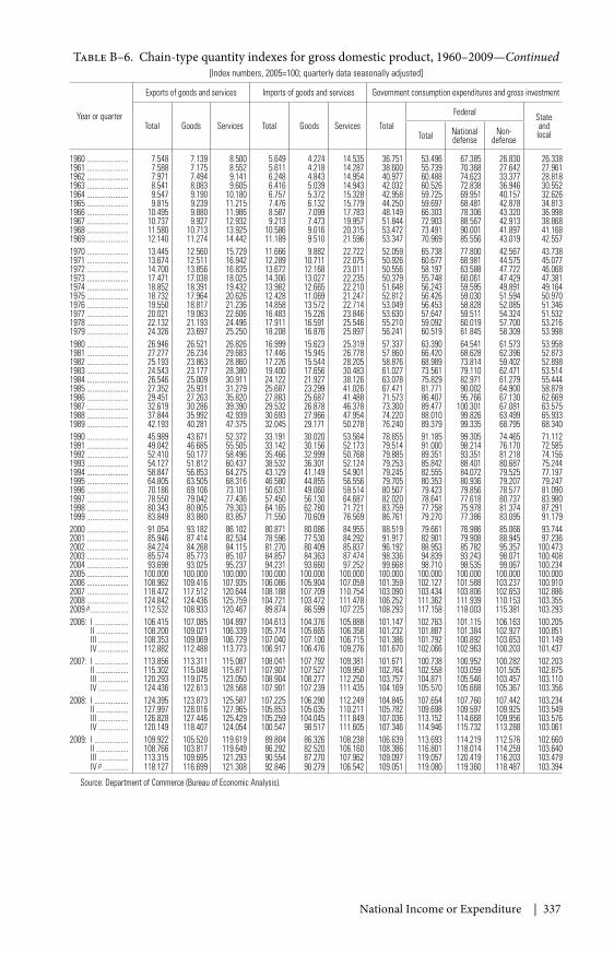
National Income or Expenditure | 337
Table B–6. Chain-type quantity indexes for gross domestic product, 1960–2009—Continued[Index numbers, 2005=100; quarterly data seasonally adjusted]
Year or quarter
Exports of goods and services Imports of goods and services Government consumption expenditures and gross investment
Total Goods Services Total Goods Services TotalFederal State
andlocalTotal National
defenseNon-
defense
1960 ...................... 7.548 7.139 8.500 5.649 4.224 14.535 36.751 53.496 67.385 26.830 26.3381961 ...................... 7.588 7.175 8.552 5.611 4.218 14.287 38.600 55.739 70.368 27.642 27.9611962 ...................... 7.971 7.494 9.141 6.248 4.843 14.954 40.977 60.488 74.623 33.377 28.8181963 ...................... 8.541 8.083 9.605 6.416 5.039 14.943 42.032 60.526 72.838 36.946 30.5521964 ...................... 9.547 9.190 10.180 6.757 5.372 15.328 42.958 59.725 69.951 40.157 32.6261965 ...................... 9.815 9.239 11.215 7.476 6.132 15.779 44.250 59.697 68.481 42.878 34.8131966 ...................... 10.495 9.880 11.986 8.587 7.099 17.783 48.149 66.303 78.306 43.320 36.9981967 ...................... 10.737 9.927 12.932 9.213 7.473 19.957 51.844 72.903 88.567 42.913 38.8681968 ...................... 11.580 10.713 13.925 10.586 9.016 20.315 53.472 73.491 90.001 41.897 41.1681969 ...................... 12.140 11.274 14.442 11.189 9.510 21.596 53.347 70.969 85.556 43.019 42.5571970 ...................... 13.445 12.560 15.729 11.666 9.882 22.722 52.059 65.738 77.800 42.567 43.7381971 ...................... 13.674 12.511 16.942 12.289 10.711 22.075 50.926 60.677 68.981 44.575 45.0771972 ...................... 14.700 13.856 16.835 13.672 12.168 23.011 50.556 58.197 63.588 47.722 46.0681973 ...................... 17.471 17.038 18.025 14.306 13.027 22.235 50.379 55.748 60.061 47.429 47.3811974 ...................... 18.852 18.391 19.432 13.982 12.665 22.210 51.648 56.243 59.595 49.891 49.1641975 ...................... 18.732 17.964 20.626 12.428 11.069 21.247 52.812 56.426 59.030 51.594 50.9701976 ...................... 19.550 18.817 21.236 14.858 13.572 22.714 53.049 56.453 58.828 52.085 51.3461977 ...................... 20.021 19.063 22.606 16.483 15.226 23.846 53.630 57.647 59.511 54.324 51.5321978 ...................... 22.132 21.193 24.496 17.911 16.591 25.546 55.210 59.092 60.019 57.700 53.2161979 ...................... 24.326 23.697 25.250 18.208 16.876 25.897 56.241 60.519 61.845 58.309 53.9981980 ...................... 26.946 26.521 26.826 16.999 15.623 25.319 57.337 63.390 64.541 61.573 53.9581981 ...................... 27.277 26.234 29.683 17.446 15.945 26.778 57.860 66.420 68.628 62.396 52.8731982 ...................... 25.193 23.863 28.860 17.226 15.544 28.205 58.876 68.989 73.814 59.402 52.8981983 ...................... 24.543 23.177 28.380 19.400 17.656 30.483 61.027 73.561 79.110 62.471 53.5141984 ...................... 26.546 25.009 30.911 24.122 21.927 38.126 63.078 75.829 82.971 61.279 55.4441985 ...................... 27.352 25.931 31.279 25.687 23.299 41.026 67.471 81.771 90.002 64.900 58.8791986 ...................... 29.451 27.263 35.820 27.883 25.687 41.488 71.573 86.407 95.766 67.130 62.6691987 ...................... 32.619 30.286 39.390 29.532 26.878 46.378 73.300 89.477 100.301 67.081 63.5751988 ...................... 37.844 35.992 42.939 30.693 27.966 47.954 74.220 88.010 99.826 63.499 65.9331989 ...................... 42.193 40.281 47.375 32.045 29.171 50.278 76.240 89.379 99.335 68.795 68.3401990 ...................... 45.989 43.671 52.372 33.191 30.020 53.564 78.655 91.185 99.305 74.465 71.1121991 ...................... 49.042 46.685 55.505 33.142 30.156 52.173 79.514 91.000 98.214 76.170 72.5851992 ...................... 52.410 50.177 58.496 35.466 32.999 50.768 79.885 89.351 93.351 81.218 74.1561993 ...................... 54.127 51.812 60.437 38.532 36.301 52.124 79.253 85.842 88.401 80.687 75.2441994 ...................... 58.847 56.853 64.275 43.129 41.149 54.901 79.245 82.555 84.072 79.525 77.1971995 ...................... 64.805 63.505 68.316 46.580 44.855 56.556 79.705 80.353 80.936 79.207 79.2471996 ...................... 70.186 69.106 73.101 50.631 49.060 59.514 80.507 79.423 79.856 78.577 81.0901997 ...................... 78.550 79.042 77.436 57.450 56.130 64.687 82.020 78.641 77.618 80.737 83.9801998 ...................... 80.343 80.805 79.303 64.165 62.780 71.721 83.759 77.758 75.978 81.374 87.2911999 ...................... 83.849 83.880 83.857 71.550 70.609 76.569 86.761 79.270 77.386 83.095 91.1792000 ...................... 91.054 93.182 86.102 80.871 80.086 84.955 88.519 79.661 76.986 85.066 93.7442001 ...................... 85.946 87.414 82.534 78.596 77.530 84.292 91.917 82.901 79.908 88.945 97.2362002 ...................... 84.224 84.268 84.115 81.270 80.409 85.837 96.192 88.953 85.782 95.357 100.4732003 ...................... 85.574 85.773 85.107 84.857 84.363 87.474 98.336 94.839 93.243 98.071 100.4082004 ...................... 93.698 93.025 95.237 94.231 93.660 97.252 99.668 98.710 98.535 99.067 100.2342005 ...................... 100.000 100.000 100.000 100.000 100.000 100.000 100.000 100.000 100.000 100.000 100.0002006 ...................... 108.962 109.416 107.935 106.086 105.904 107.059 101.359 102.127 101.588 103.237 100.9102007 ...................... 118.472 117.512 120.644 108.188 107.709 110.754 103.090 103.434 103.806 102.653 102.8862008 ...................... 124.842 124.436 125.759 104.721 103.472 111.478 106.252 111.362 111.939 110.153 103.3552009 p .................... 112.532 108.933 120.467 89.874 86.599 107.225 108.293 117.158 118.003 115.381 103.2932006: I .................. 106.415 107.085 104.897 104.613 104.376 105.888 101.147 102.763 101.115 106.163 100.205
II ................. 108.200 109.021 106.339 105.774 105.665 106.358 101.232 101.887 101.384 102.927 100.851III ................ 108.353 109.069 106.729 107.040 107.100 106.715 101.386 101.792 100.892 103.653 101.149IV ................ 112.882 112.488 113.773 106.917 106.476 109.276 101.670 102.066 102.963 100.203 101.437
2007: I .................. 113.856 113.311 115.087 108.041 107.792 109.381 101.671 100.738 100.952 100.282 102.203II ................. 115.302 115.048 115.871 107.907 107.527 109.950 102.764 102.558 103.059 101.505 102.875III ................ 120.293 119.075 123.050 108.904 108.277 112.250 103.757 104.871 105.546 103.457 103.110IV ................ 124.436 122.613 128.568 107.901 107.239 111.435 104.169 105.570 105.668 105.367 103.356
2008: I .................. 124.395 123.873 125.587 107.225 106.290 112.249 104.845 107.654 107.760 107.442 103.234II ................. 127.997 128.016 127.965 105.853 105.035 110.211 105.782 109.698 109.597 109.925 103.549III ................ 126.828 127.446 125.429 105.259 104.045 111.849 107.036 113.152 114.668 109.956 103.576IV ................ 120.149 118.407 124.054 100.547 98.517 111.605 107.346 114.946 115.732 113.288 103.061
2009: I .................. 109.922 105.520 119.619 89.804 86.326 108.238 106.639 113.693 114.219 112.576 102.660II ................. 108.766 103.817 119.649 86.292 82.520 106.160 108.386 116.801 118.014 114.259 103.640III ................ 113.315 109.695 121.293 90.554 87.270 107.962 109.097 119.057 120.419 116.203 103.479IV p ............. 118.127 116.699 121.308 92.846 90.279 106.542 109.051 119.080 119.360 118.487 103.394
Source: Department of Commerce (Bureau of Economic Analysis).
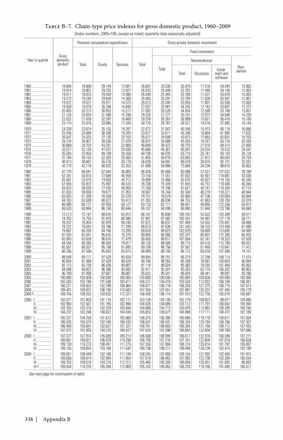
338 | Appendix B
Table B–7. Chain-type price indexes for gross domestic product, 1960–2009[Index numbers, 2005=100, except as noted; quarterly data seasonally adjusted]
Year or quarterGross
domesticproduct
Personal consumption expenditures Gross private domestic investment
Total Goods Services Total
Fixed investment
Total
NonresidentialResi-
dentialTotal StructuresEquip-
ment andsoftware
1960 ...................... 18.604 18.606 29.144 13.581 26.607 25.530 33.978 11.516 54.445 12.9621961 ...................... 18.814 18.801 29.253 13.827 26.533 25.449 33.783 11.446 54.146 12.9831962 ...................... 19.071 19.023 29.404 14.090 26.548 25.465 33.788 11.537 53.878 13.0031963 ...................... 19.273 19.245 29.648 14.306 26.463 25.391 33.784 11.636 53.581 12.9011964 ...................... 19.572 19.527 29.971 14.573 26.613 25.545 33.955 11.801 53.558 13.0031965 ...................... 19.928 19.810 30.286 14.846 27.037 25.981 34.342 12.143 53.607 13.3721966 ...................... 20.493 20.313 30.953 15.277 27.592 26.528 34.854 12.580 53.749 13.8571967 ...................... 21.124 20.824 31.499 15.786 28.320 27.271 35.741 12.973 54.940 14.3391968 ...................... 22.022 21.636 32.597 16.468 29.378 28.367 36.999 13.621 56.416 15.1001969 ...................... 23.110 22.616 33.860 17.326 30.770 29.767 38.527 14.518 57.985 16.1441970 ...................... 24.328 23.674 35.152 18.287 32.072 31.047 40.348 15.473 60.119 16.6661971 ...................... 25.545 24.680 36.208 19.285 33.671 32.611 42.246 16.664 61.905 17.6321972 ...................... 26.647 25.525 37.135 20.103 35.077 34.009 43.673 17.863 62.651 18.7031973 ...................... 28.124 26.901 39.350 21.078 36.972 35.888 45.355 19.247 63.716 20.3591974 ...................... 30.669 29.703 44.261 22.868 40.648 39.422 49.733 21.910 68.414 22.4601975 ...................... 33.577 32.184 47.837 24.836 45.666 44.361 56.581 24.534 78.523 24.5471976 ...................... 35.505 33.950 49.709 26.558 48.190 46.932 59.718 25.741 83.143 26.1241977 ...................... 37.764 36.155 52.363 28.560 51.805 50.616 63.805 27.973 88.083 28.7591978 ...................... 40.413 38.687 55.576 30.779 56.030 54.891 68.078 30.675 92.731 32.2811979 ...................... 43.773 42.118 60.832 33.353 61.099 59.866 73.606 34.238 98.610 35.9021980 ...................... 47.776 46.641 67.644 36.805 66.836 65.468 80.098 37.421 107.032 39.7891981 ...................... 52.281 50.810 72.669 40.558 73.154 71.551 87.832 42.567 114.681 43.0361982 ...................... 55.467 53.615 74.650 43.712 76.899 75.468 92.670 45.927 119.155 45.3401983 ...................... 57.655 55.923 75.997 46.433 76.706 75.349 91.843 44.757 119.406 46.3801984 ...................... 59.823 58.038 77.435 48.850 77.256 75.790 91.621 45.147 118.364 47.7141985 ...................... 61.633 59.938 78.677 51.053 78.047 76.744 92.340 46.219 118.221 48.9441986 ...................... 63.003 61.399 78.309 53.378 79.737 78.579 93.908 47.106 120.094 50.9941987 ...................... 64.763 63.589 80.827 55.413 81.263 80.036 94.753 47.863 120.750 53.0791988 ...................... 66.990 66.121 82.958 58.127 83.120 82.111 96.857 49.895 122.256 54.9131989 ...................... 69.520 68.994 86.150 60.844 85.107 84.099 98.890 51.848 123.786 56.6801990 ...................... 72.213 72.147 89.678 63.812 86.747 85.808 100.783 53.522 125.389 58.0111991 ...................... 74.762 74.755 91.870 66.586 87.981 87.082 102.341 54.491 127.178 58.7711992 ...................... 76.537 76.954 92.978 69.240 87.672 86.831 101.488 54.502 125.681 59.4861993 ...................... 78.222 78.643 93.786 71.299 88.673 87.838 101.540 56.103 124.408 61.8901994 ...................... 79.867 80.265 94.740 73.205 89.828 89.023 102.029 58.089 123.695 64.0691995 ...................... 81.533 82.041 95.625 75.370 90.840 90.060 102.247 60.601 122.265 66.4031996 ...................... 83.083 83.826 96.676 77.479 90.455 89.817 101.054 62.141 119.323 67.8281997 ...................... 84.554 85.395 96.563 79.817 90.120 89.589 99.775 64.516 115.788 69.5571998 ...................... 85.507 86.207 95.106 81.695 89.109 88.756 97.587 67.480 110.641 71.4121999 ...................... 86.766 87.596 95.603 83.515 88.989 88.700 96.173 69.559 107.406 74.1512000 ...................... 88.648 89.777 97.520 85.824 89.954 89.751 96.219 72.298 106.114 77.4152001 ...................... 90.654 91.488 97.429 88.428 90.748 90.553 95.788 76.087 103.603 80.9942002 ...................... 92.113 92.736 96.430 90.807 91.118 90.924 95.363 79.292 101.494 83.0022003 ...................... 94.099 94.622 96.380 93.692 92.411 92.301 95.355 82.174 100.287 86.9532004 ...................... 96.769 97.098 97.867 96.687 95.632 95.541 96.834 88.441 99.897 93.2962005 ...................... 100.000 100.000 100.000 100.000 100.000 100.000 100.000 100.000 100.000 100.0002006 ...................... 103.263 102.746 101.508 103.411 104.371 104.419 103.534 112.922 100.194 106.0812007 ...................... 106.221 105.502 102.789 106.964 106.677 106.718 106.209 121.275 100.715 107.5132008 ...................... 108.481 109.031 106.150 110.582 107.355 107.551 107.897 125.207 101.455 105.7792009 p .................... 109.754 109.252 103.632 112.221 106.458 106.114 107.510 122.759 102.010 100.6872006: I .................. 102.071 101.803 101.116 102.171 103.139 103.195 102.279 108.823 99.977 104.890
II ................. 102.980 102.567 101.765 102.998 104.026 104.089 103.112 111.791 100.042 105.940III ................ 103.763 103.316 102.329 103.844 104.666 104.713 103.878 113.962 100.285 106.295IV ................ 104.237 103.298 100.822 104.630 105.653 105.677 104.868 117.111 100.472 107.199
2007: I .................. 105.327 104.250 101.612 105.668 106.375 106.380 105.686 119.716 100.611 107.604II ................. 106.026 105.074 102.548 106.433 106.547 106.591 106.104 120.794 100.766 107.307III ................ 106.460 105.681 102.627 107.327 106.761 106.803 106.354 121.786 100.712 107.455IV ................ 107.072 107.005 104.370 108.427 107.024 107.096 106.693 122.804 100.769 107.686
2008: I .................. 107.577 107.974 105.689 109.213 106.586 106.909 106.617 122.976 100.590 107.271II ................. 108.061 109.021 106.678 110.296 106.745 107.210 107.161 123.800 101.019 106.838III ................ 109.130 110.273 108.451 111.275 107.350 107.866 108.314 125.814 101.797 105.807IV ................ 109.155 108.855 103.784 111.542 108.738 108.217 109.498 128.238 102.415 103.198
2009: I .................. 109.661 108.449 102.186 111.749 108.245 107.668 109.154 127.092 102.450 101.915II ................. 109.656 108.814 102.864 111.954 107.019 106.463 107.993 123.706 102.304 100.554III ................ 109.763 109.510 104.216 112.312 105.465 105.265 106.656 120.451 101.802 99.863IV p ............. 109.934 110.235 105.264 112.869 105.102 105.062 106.238 119.786 101.485 100.417
See next page for continuation of table.
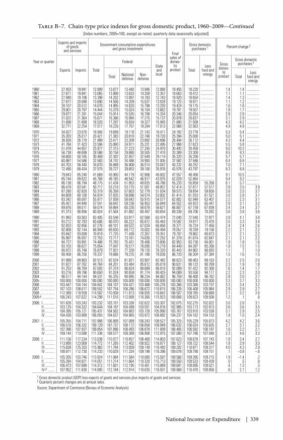
National Income or Expenditure | 339
Table B–7. Chain-type price indexes for gross domestic product, 1960–2009—Continued[Index numbers, 2005=100, except as noted; quarterly data seasonally adjusted]
Year or quarter
Exports and importsof goods
and servicesGovernment consumption expenditures
and gross investmentFinal
sales ofdomes-
ticproduct
Gross domesticpurchases 1 Percent change 2
Exports Imports Total
FederalStateandlocal
TotalLess
food andenergy
Grossdomes-
ticproduct
Gross domesticpurchases 1
Total Nationaldefense
Non-defense Total
Lessfood andenergy
1960 ................. 27.453 19.941 12.809 13.677 13.440 13.946 12.066 18.455 18.220 ............... 1.4 1.4 ..............1961 ................. 27.871 19.941 13.065 13.908 13.633 14.359 12.357 18.663 18.412 ............... 1.1 1.1 ..............1962 ................. 27.940 19.706 13.398 14.202 13.897 14.783 12.743 18.920 18.654 ............... 1.4 1.3 ..............1963 ................. 27.877 20.088 13.690 14.506 14.209 15.037 13.028 19.125 18.871 ............... 1.1 1.2 ..............1964 ................. 28.107 20.512 14.070 14.995 14.620 15.798 13.293 19.424 19.175 ............... 1.6 1.6 ..............1965 ................. 29.001 20.797 14.444 15.379 15.024 16.104 13.662 19.781 19.507 ............... 1.8 1.7 ..............1966 ................. 29.877 21.281 15.044 15.914 15.535 16.708 14.334 20.346 20.054 ............... 2.8 2.8 ..............1967 ................. 31.022 21.364 15.671 16.386 15.994 17.215 15.137 20.978 20.637 ............... 3.1 2.9 ..............1968 ................. 31.698 21.689 16.520 17.287 16.834 18.327 15.945 21.880 21.508 ............... 4.3 4.2 ..............1969 ................. 32.771 22.254 17.517 18.226 17.757 19.284 17.013 22.968 22.563 ............... 4.9 4.9 ..............1970 ................. 34.027 23.570 18.945 19.699 19.116 21.143 18.411 24.182 23.778 ............... 5.3 5.4 ..............1971 ................. 35.283 25.017 20.421 21.383 20.810 22.746 19.720 25.394 25.000 ............... 5.0 5.1 ..............1972 ................. 36.928 26.770 21.989 23.471 23.209 23.892 20.896 26.494 26.112 ............... 4.3 4.4 ..............1973 ................. 41.784 31.423 23.594 25.080 24.911 25.231 22.495 27.968 27.623 ............... 5.5 5.8 ..............1974 ................. 51.478 44.957 25.977 27.315 27.223 27.245 24.970 30.493 30.459 ............... 9.0 10.3 ..............1975 ................. 56.738 48.699 28.586 30.158 29.880 30.505 27.410 33.389 33.300 ............... 9.5 9.3 ..............1976 ................. 58.600 50.165 30.469 32.302 32.057 32.549 29.114 35.320 35.208 ............... 5.7 5.7 ..............1977 ................. 60.987 54.586 32.583 34.742 34.486 34.993 31.005 37.582 37.586 ............... 6.4 6.8 ..............1978 ................. 64.703 58.440 34.670 36.888 36.908 36.514 33.042 40.232 40.252 ............... 7.0 7.1 ..............1979 ................. 72.490 68.434 37.575 39.727 39.853 39.100 35.976 43.576 43.797 ............... 8.3 8.8 ..............1980 ................. 79.843 85.240 41.669 43.900 44.179 42.906 40.002 47.557 48.408 ............... 9.1 10.5 ..............1981 ................. 85.744 89.822 45.768 48.165 48.542 46.917 43.975 52.029 52.864 ............... 9.4 9.2 ..............1982 ................. 86.138 86.794 48.775 51.434 51.953 49.825 46.786 55.233 55.859 55.358 6.1 5.7 ..............1983 ................. 86.478 83.541 50.717 53.218 53.775 51.501 48.857 57.414 57.817 57.517 3.9 3.5 3.91984 ................. 87.280 82.820 53.319 56.358 57.603 52.779 51.034 59.573 59.854 59.650 3.8 3.5 3.71985 ................. 84.609 80.100 54.974 57.635 58.696 54.574 53.002 61.414 61.553 61.521 3.0 2.8 3.11986 ................. 83.342 80.097 55.977 57.938 58.642 55.915 54.577 62.802 62.948 63.407 2.2 2.3 3.11987 ................. 85.451 84.948 57.541 58.642 59.236 56.953 56.849 64.552 64.923 65.447 2.8 3.1 3.21988 ................. 89.876 89.011 59.074 59.884 60.326 58.679 58.621 66.807 67.159 67.839 3.4 3.4 3.71989 ................. 91.373 90.956 60.924 61.504 61.882 60.497 60.654 69.338 69.706 70.282 3.8 3.8 3.61990 ................. 91.993 93.563 63.405 63.548 63.917 62.568 63.474 72.040 72.540 72.977 3.9 4.1 3.81991 ................. 93.212 92.783 65.606 66.070 66.222 65.672 65.443 74.592 74.917 75.470 3.5 3.3 3.41992 ................. 92.833 92.856 67.276 68.101 68.522 67.034 66.856 76.371 76.724 77.450 2.4 2.4 2.61993 ................. 92.808 92.144 68.949 69.830 69.712 70.002 68.494 78.057 78.339 79.156 2.2 2.1 2.21994 ................. 93.842 93.009 70.819 71.725 71.438 72.267 70.351 79.707 79.962 80.873 2.1 2.1 2.21995 ................. 95.997 95.557 72.753 73.717 73.161 74.830 72.252 81.379 81.674 82.647 2.1 2.1 2.21996 ................. 94.727 93.891 74.488 75.763 75.431 76.406 73.806 82.953 83.150 84.001 1.9 1.8 1.61997 ................. 93.103 90.627 75.854 77.047 76.517 78.095 75.219 84.449 84.397 85.266 1.8 1.5 1.51998 ................. 90.972 85.748 76.879 77.931 77.328 79.120 76.320 85.443 84.962 86.093 1.1 .7 1.01999 ................. 90.408 86.250 79.337 79.886 79.225 81.188 79.036 86.720 86.304 87.384 1.5 1.6 1.52000 ................. 91.999 89.963 82.513 82.524 81.821 83.907 82.482 88.623 88.463 89.163 2.2 2.5 2.02001 ................. 91.627 87.762 84.764 84.201 83.484 85.612 85.019 90.631 90.123 90.769 2.3 1.9 1.82002 ................. 91.253 86.784 87.003 87.318 86.624 88.689 86.810 92.089 91.422 92.300 1.6 1.4 1.72003 ................. 93.216 89.796 90.650 91.024 90.659 91.774 90.425 94.089 93.550 94.177 2.2 2.3 2.02004 ................. 96.517 94.144 94.531 95.335 94.895 96.234 94.062 96.759 96.400 96.762 2.8 3.0 2.72005 ................. 100.000 100.000 100.000 100.000 100.000 100.000 100.000 100.000 100.000 100.000 3.3 3.7 3.32006 ................. 103.447 104.144 104.842 104.107 104.421 103.468 105.276 103.266 103.380 103.157 3.3 3.4 3.22007 ................. 107.103 108.017 109.552 107.754 108.286 106.672 110.615 106.226 106.408 105.984 2.9 2.9 2.72008 ................. 112.389 119.559 114.502 110.938 111.913 108.935 116.642 108.507 109.765 108.689 2.1 3.2 2.62009 p ............... 106.243 107.022 114.298 111.516 112.089 110.360 115.923 109.666 109.823 109.508 1.2 .1 .82006: I ............. 101.828 103.243 103.232 103.101 103.336 102.622 103.307 102.075 102.275 102.022 3.0 2.8 3.1
II ............ 103.125 104.322 104.644 104.187 104.499 103.551 104.916 102.985 103.173 102.913 3.6 3.6 3.5III ........... 104.395 105.121 105.437 104.502 104.883 103.728 105.990 103.767 103.910 103.538 3.1 2.9 2.5IV ........... 104.438 103.889 106.055 104.637 104.965 103.972 106.892 104.237 104.162 104.153 1.8 1.0 2.4
2007: I ............. 105.355 104.711 107.888 106.808 107.089 106.243 108.527 105.325 105.229 105.073 4.2 4.2 3.6II ............ 106.516 106.332 109.129 107.737 108.172 106.858 109.949 106.032 106.024 105.635 2.7 3.1 2.2III ........... 107.396 107.937 109.854 107.896 108.493 106.678 111.009 106.465 106.592 106.187 1.6 2.2 2.1IV ........... 109.144 113.088 111.336 108.577 109.389 106.908 112.975 107.080 107.786 107.040 2.3 4.6 3.3
2008: I ............. 111.156 117.234 113.038 110.077 110.857 108.469 114.803 107.623 108.678 107.743 1.9 3.4 2.7II ............ 113.890 123.069 114.772 111.265 112.402 108.922 116.877 108.127 109.722 108.544 1.8 3.9 3.0III ........... 115.638 125.203 115.963 111.784 113.059 109.149 118.493 109.202 110.871 109.317 4.0 4.3 2.9IV ........... 108.871 112.730 114.233 110.628 111.334 109.198 116.396 109.078 109.790 109.151 .1 –3.8 –.6
2009: I ............. 105.265 103.746 113.924 111.084 111.584 110.085 115.587 109.566 109.395 109.215 1.9 –1.4 .2II ............ 105.284 104.821 114.051 111.214 111.664 110.320 115.713 109.550 109.533 109.439 .0 .5 .8III ........... 106.473 107.688 114.312 111.601 112.195 110.401 115.889 109.681 109.895 109.521 .4 1.3 .3IV p ........ 107.952 111.830 114.905 112.164 112.914 110.635 116.501 109.868 110.470 109.856 .6 2.1 1.2
1 Gross domestic product (GDP) less exports of goods and services plus imports of goods and services.2 Quarterly percent changes are at annual rates.Source: Department of Commerce (Bureau of Economic Analysis).
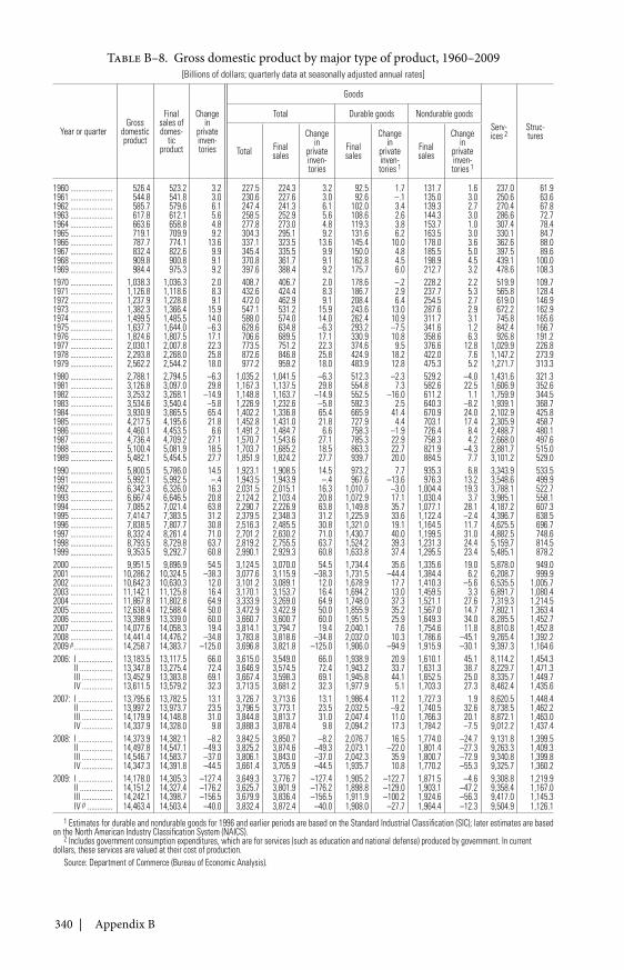
340 | Appendix B
Table B–8. Gross domestic product by major type of product, 1960–2009[Billions of dollars; quarterly data at seasonally adjusted annual rates]
Year or quarterGross
domesticproduct
Finalsales ofdomes-
ticproduct
Changein
privateinven-tories
Goods
Serv-ices 2
Struc-tures
Total Durable goods Nondurable goods
Total Finalsales
Changein
privateinven-tories
Finalsales
Changein
privateinven-tories 1
Finalsales
Changein
privateinven-tories 1
1960 ...................... 526.4 523.2 3.2 227.5 224.3 3.2 92.5 1.7 131.7 1.6 237.0 61.91961 ...................... 544.8 541.8 3.0 230.6 227.6 3.0 92.6 –.1 135.0 3.0 250.6 63.61962 ...................... 585.7 579.6 6.1 247.4 241.3 6.1 102.0 3.4 139.3 2.7 270.4 67.81963 ...................... 617.8 612.1 5.6 258.5 252.9 5.6 108.6 2.6 144.3 3.0 286.6 72.71964 ...................... 663.6 658.8 4.8 277.8 273.0 4.8 119.3 3.8 153.7 1.0 307.4 78.41965 ...................... 719.1 709.9 9.2 304.3 295.1 9.2 131.6 6.2 163.5 3.0 330.1 84.71966 ...................... 787.7 774.1 13.6 337.1 323.5 13.6 145.4 10.0 178.0 3.6 362.6 88.01967 ...................... 832.4 822.6 9.9 345.4 335.5 9.9 150.0 4.8 185.5 5.0 397.5 89.61968 ...................... 909.8 900.8 9.1 370.8 361.7 9.1 162.8 4.5 198.9 4.5 439.1 100.01969 ...................... 984.4 975.3 9.2 397.6 388.4 9.2 175.7 6.0 212.7 3.2 478.6 108.31970 ...................... 1,038.3 1,036.3 2.0 408.7 406.7 2.0 178.6 –.2 228.2 2.2 519.9 109.71971 ...................... 1,126.8 1,118.6 8.3 432.6 424.4 8.3 186.7 2.9 237.7 5.3 565.8 128.41972 ...................... 1,237.9 1,228.8 9.1 472.0 462.9 9.1 208.4 6.4 254.5 2.7 619.0 146.91973 ...................... 1,382.3 1,366.4 15.9 547.1 531.2 15.9 243.6 13.0 287.6 2.9 672.2 162.91974 ...................... 1,499.5 1,485.5 14.0 588.0 574.0 14.0 262.4 10.9 311.7 3.1 745.8 165.61975 ...................... 1,637.7 1,644.0 –6.3 628.6 634.8 –6.3 293.2 –7.5 341.6 1.2 842.4 166.71976 ...................... 1,824.6 1,807.5 17.1 706.6 689.5 17.1 330.9 10.8 358.6 6.3 926.8 191.21977 ...................... 2,030.1 2,007.8 22.3 773.5 751.2 22.3 374.6 9.5 376.6 12.8 1,029.9 226.81978 ...................... 2,293.8 2,268.0 25.8 872.6 846.8 25.8 424.9 18.2 422.0 7.6 1,147.2 273.91979 ...................... 2,562.2 2,544.2 18.0 977.2 959.2 18.0 483.9 12.8 475.3 5.2 1,271.7 313.31980 ...................... 2,788.1 2,794.5 –6.3 1,035.2 1,041.5 –6.3 512.3 –2.3 529.2 –4.0 1,431.6 321.31981 ...................... 3,126.8 3,097.0 29.8 1,167.3 1,137.5 29.8 554.8 7.3 582.6 22.5 1,606.9 352.61982 ...................... 3,253.2 3,268.1 –14.9 1,148.8 1,163.7 –14.9 552.5 –16.0 611.2 1.1 1,759.9 344.51983 ...................... 3,534.6 3,540.4 –5.8 1,226.9 1,232.6 –5.8 592.3 2.5 640.3 –8.2 1,939.1 368.71984 ...................... 3,930.9 3,865.5 65.4 1,402.2 1,336.8 65.4 665.9 41.4 670.9 24.0 2,102.9 425.81985 ...................... 4,217.5 4,195.6 21.8 1,452.8 1,431.0 21.8 727.9 4.4 703.1 17.4 2,305.9 458.71986 ...................... 4,460.1 4,453.5 6.6 1,491.2 1,484.7 6.6 758.3 –1.9 726.4 8.4 2,488.7 480.11987 ...................... 4,736.4 4,709.2 27.1 1,570.7 1,543.6 27.1 785.3 22.9 758.3 4.2 2,668.0 497.61988 ...................... 5,100.4 5,081.9 18.5 1,703.7 1,685.2 18.5 863.3 22.7 821.9 –4.3 2,881.7 515.01989 ...................... 5,482.1 5,454.5 27.7 1,851.9 1,824.2 27.7 939.7 20.0 884.5 7.7 3,101.2 529.01990 ...................... 5,800.5 5,786.0 14.5 1,923.1 1,908.5 14.5 973.2 7.7 935.3 6.8 3,343.9 533.51991 ...................... 5,992.1 5,992.5 –.4 1,943.5 1,943.9 –.4 967.6 –13.6 976.3 13.2 3,548.6 499.91992 ...................... 6,342.3 6,326.0 16.3 2,031.5 2,015.1 16.3 1,010.7 –3.0 1,004.4 19.3 3,788.1 522.71993 ...................... 6,667.4 6,646.5 20.8 2,124.2 2,103.4 20.8 1,072.9 17.1 1,030.4 3.7 3,985.1 558.11994 ...................... 7,085.2 7,021.4 63.8 2,290.7 2,226.9 63.8 1,149.8 35.7 1,077.1 28.1 4,187.2 607.31995 ...................... 7,414.7 7,383.5 31.2 2,379.5 2,348.3 31.2 1,225.9 33.6 1,122.4 –2.4 4,396.7 638.51996 ...................... 7,838.5 7,807.7 30.8 2,516.3 2,485.5 30.8 1,321.0 19.1 1,164.5 11.7 4,625.5 696.71997 ...................... 8,332.4 8,261.4 71.0 2,701.2 2,630.2 71.0 1,430.7 40.0 1,199.5 31.0 4,882.5 748.61998 ...................... 8,793.5 8,729.8 63.7 2,819.2 2,755.5 63.7 1,524.2 39.3 1,231.3 24.4 5,159.7 814.51999 ...................... 9,353.5 9,292.7 60.8 2,990.1 2,929.3 60.8 1,633.8 37.4 1,295.5 23.4 5,485.1 878.22000 ...................... 9,951.5 9,896.9 54.5 3,124.5 3,070.0 54.5 1,734.4 35.6 1,335.6 19.0 5,878.0 949.02001 ...................... 10,286.2 10,324.5 –38.3 3,077.6 3,115.9 –38.3 1,731.5 –44.4 1,384.4 6.2 6,208.7 999.92002 ...................... 10,642.3 10,630.3 12.0 3,101.2 3,089.1 12.0 1,678.9 17.7 1,410.3 –5.6 6,535.5 1,005.72003 ...................... 11,142.1 11,125.8 16.4 3,170.1 3,153.7 16.4 1,694.2 13.0 1,459.5 3.3 6,891.7 1,080.42004 ...................... 11,867.8 11,802.8 64.9 3,333.9 3,269.0 64.9 1,748.0 37.3 1,521.1 27.6 7,319.3 1,214.52005 ...................... 12,638.4 12,588.4 50.0 3,472.9 3,422.9 50.0 1,855.9 35.2 1,567.0 14.7 7,802.1 1,363.42006 ...................... 13,398.9 13,339.0 60.0 3,660.7 3,600.7 60.0 1,951.5 25.9 1,649.3 34.0 8,285.5 1,452.72007 ...................... 14,077.6 14,058.3 19.4 3,814.1 3,794.7 19.4 2,040.1 7.6 1,754.6 11.8 8,810.8 1,452.82008 ...................... 14,441.4 14,476.2 –34.8 3,783.8 3,818.6 –34.8 2,032.0 10.3 1,786.6 –45.1 9,265.4 1,392.22009 p .................... 14,258.7 14,383.7 –125.0 3,696.8 3,821.8 –125.0 1,906.0 –94.9 1,915.9 –30.1 9,397.3 1,164.62006: I .................. 13,183.5 13,117.5 66.0 3,615.0 3,549.0 66.0 1,938.9 20.9 1,610.1 45.1 8,114.2 1,454.3
II ................. 13,347.8 13,275.4 72.4 3,646.9 3,574.5 72.4 1,943.2 33.7 1,631.3 38.7 8,229.7 1,471.3III ................ 13,452.9 13,383.8 69.1 3,667.4 3,598.3 69.1 1,945.8 44.1 1,652.5 25.0 8,335.7 1,449.7IV ................ 13,611.5 13,579.2 32.3 3,713.5 3,681.2 32.3 1,977.9 5.1 1,703.3 27.3 8,462.4 1,435.6
2007: I .................. 13,795.6 13,782.5 13.1 3,726.7 3,713.6 13.1 1,986.4 11.2 1,727.3 1.9 8,620.5 1,448.4II ................. 13,997.2 13,973.7 23.5 3,796.5 3,773.1 23.5 2,032.5 –9.2 1,740.5 32.6 8,738.5 1,462.2III ................ 14,179.9 14,148.8 31.0 3,844.8 3,813.7 31.0 2,047.4 11.0 1,766.3 20.1 8,872.1 1,463.0IV ................ 14,337.9 14,328.0 9.8 3,888.3 3,878.4 9.8 2,094.2 17.3 1,784.2 –7.5 9,012.2 1,437.4
2008: I .................. 14,373.9 14,382.1 –8.2 3,842.5 3,850.7 –8.2 2,076.7 16.5 1,774.0 –24.7 9,131.8 1,399.5II ................. 14,497.8 14,547.1 –49.3 3,825.2 3,874.6 –49.3 2,073.1 –22.0 1,801.4 –27.3 9,263.3 1,409.3III ................ 14,546.7 14,583.7 –37.0 3,806.1 3,843.0 –37.0 2,042.3 35.9 1,800.7 –72.9 9,340.8 1,399.8IV ................ 14,347.3 14,391.8 –44.5 3,661.4 3,705.9 –44.5 1,935.7 10.8 1,770.2 –55.3 9,325.7 1,360.2
2009: I .................. 14,178.0 14,305.3 –127.4 3,649.3 3,776.7 –127.4 1,905.2 –122.7 1,871.5 –4.6 9,308.8 1,219.9II ................. 14,151.2 14,327.4 –176.2 3,625.7 3,801.9 –176.2 1,898.8 –129.0 1,903.1 –47.2 9,358.4 1,167.0III ................ 14,242.1 14,398.7 –156.5 3,679.9 3,836.4 –156.5 1,911.9 –100.2 1,924.6 –56.3 9,417.0 1,145.3IV p ............. 14,463.4 14,503.4 –40.0 3,832.4 3,872.4 –40.0 1,908.0 –27.7 1,964.4 –12.3 9,504.9 1,126.1
1 Estimates for durable and nondurable goods for 1996 and earlier periods are based on the Standard Industrial Classification (SIC); later estimates are basedon the North American Industry Classification System (NAICS).
2 Includes government consumption expenditures, which are for services (such as education and national defense) produced by government. In currentdollars, these services are valued at their cost of production.
Source: Department of Commerce (Bureau of Economic Analysis).
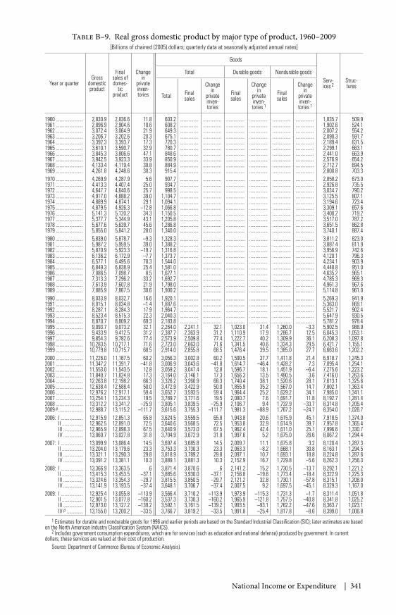
National Income or Expenditure | 341
Table B–9. Real gross domestic product by major type of product, 1960–2009[Billions of chained (2005) dollars; quarterly data at seasonally adjusted annual rates]
Year or quarterGross
domesticproduct
Finalsales ofdomes-
ticproduct
Changein
privateinven-tories
Goods
Serv-ices 2
Struc-tures
Total Durable goods Nondurable goods
Total Finalsales
Changein
privateinven-tories
Finalsales
Changein
privateinven-tories 1
Finalsales
Changein
privateinven-tories 1
1960 ...................... 2,830.9 2,836.6 11.8 603.2 ............... ............... ............... ............... ............... ............... 1,835.7 509.91961 ...................... 2,896.9 2,904.6 10.6 608.2 ............... ............... ............... ............... ............... ............... 1,902.6 524.11962 ...................... 3,072.4 3,064.9 21.9 649.3 ............... ............... ............... ............... ............... ............... 2,007.2 554.21963 ...................... 3,206.7 3,202.6 20.3 675.1 ............... ............... ............... ............... ............... ............... 2,090.3 591.71964 ...................... 3,392.3 3,393.7 17.3 720.3 ............... ............... ............... ............... ............... ............... 2,189.4 631.51965 ...................... 3,610.1 3,590.7 32.9 780.7 ............... ............... ............... ............... ............... ............... 2,299.1 663.11966 ...................... 3,845.3 3,806.6 47.1 848.6 ............... ............... ............... ............... ............... ............... 2,441.0 663.91967 ...................... 3,942.5 3,923.3 33.9 850.9 ............... ............... ............... ............... ............... ............... 2,576.9 654.21968 ...................... 4,133.4 4,119.4 30.8 884.9 ............... ............... ............... ............... ............... ............... 2,712.7 694.51969 ...................... 4,261.8 4,248.6 30.3 915.4 ............... ............... ............... ............... ............... ............... 2,800.8 703.31970 ...................... 4,269.9 4,287.9 5.6 907.7 ............... ............... ............... ............... ............... ............... 2,858.2 673.01971 ...................... 4,413.3 4,407.4 25.0 934.7 ............... ............... ............... ............... ............... ............... 2,926.8 735.51972 ...................... 4,647.7 4,640.6 25.7 998.5 ............... ............... ............... ............... ............... ............... 3,034.7 790.21973 ...................... 4,917.0 4,888.2 39.0 1,104.7 ............... ............... ............... ............... ............... ............... 3,125.5 807.11974 ...................... 4,889.9 4,874.1 29.1 1,094.1 ............... ............... ............... ............... ............... ............... 3,194.6 723.41975 ...................... 4,879.5 4,926.3 –12.8 1,066.8 ............... ............... ............... ............... ............... ............... 3,309.1 657.61976 ...................... 5,141.3 5,120.2 34.3 1,150.5 ............... ............... ............... ............... ............... ............... 3,400.2 719.21977 ...................... 5,377.7 5,344.9 43.1 1,205.8 ............... ............... ............... ............... ............... ............... 3,517.0 787.21978 ...................... 5,677.6 5,639.7 45.6 1,286.8 ............... ............... ............... ............... ............... ............... 3,651.5 862.81979 ...................... 5,855.0 5,841.2 28.0 1,340.0 ............... ............... ............... ............... ............... ............... 3,740.1 887.41980 ...................... 5,839.0 5,878.7 –9.3 1,328.3 ............... ............... ............... ............... ............... ............... 3,811.2 823.01981 ...................... 5,987.2 5,959.5 39.0 1,388.2 ............... ............... ............... ............... ............... ............... 3,887.4 811.91982 ...................... 5,870.9 5,923.3 –19.7 1,316.8 ............... ............... ............... ............... ............... ............... 3,956.9 742.61983 ...................... 6,136.2 6,172.9 –7.7 1,373.7 ............... ............... ............... ............... ............... ............... 4,120.1 796.31984 ...................... 6,577.1 6,495.6 78.3 1,544.0 ............... ............... ............... ............... ............... ............... 4,234.1 903.91985 ...................... 6,849.3 6,838.9 25.4 1,581.0 ............... ............... ............... ............... ............... ............... 4,448.8 951.01986 ...................... 7,086.5 7,098.7 8.5 1,627.1 ............... ............... ............... ............... ............... ............... 4,635.2 965.11987 ...................... 7,313.3 7,296.2 33.2 1,692.7 ............... ............... ............... ............... ............... ............... 4,785.3 969.31988 ...................... 7,613.9 7,607.8 21.9 1,798.0 ............... ............... ............... ............... ............... ............... 4,961.3 967.61989 ...................... 7,885.9 7,867.5 30.6 1,900.2 ............... ............... ............... ............... ............... ............... 5,114.8 961.01990 ...................... 8,033.9 8,032.7 16.6 1,920.1 ............... ............... ............... ............... ............... ............... 5,269.3 941.91991 ...................... 8,015.1 8,034.8 –1.4 1,887.6 ............... ............... ............... ............... ............... ............... 5,363.0 869.11992 ...................... 8,287.1 8,284.3 17.9 1,964.7 ............... ............... ............... ............... ............... ............... 5,521.7 902.41993 ...................... 8,523.4 8,515.3 22.3 2,040.3 ............... ............... ............... ............... ............... ............... 5,647.9 930.51994 ...................... 8,870.7 8,809.2 69.3 2,183.8 ............... ............... ............... ............... ............... ............... 5,781.2 978.41995 ...................... 9,093.7 9,073.2 32.1 2,264.0 2,241.1 32.1 1,023.0 31.4 1,260.0 –3.3 5,902.5 988.91996 ...................... 9,433.9 9,412.5 31.2 2,387.7 2,363.9 31.2 1,110.9 17.9 1,286.7 12.5 6,045.3 1,053.11997 ...................... 9,854.3 9,782.6 77.4 2,573.9 2,509.8 77.4 1,222.7 40.2 1,309.9 36.1 6,208.3 1,097.81998 ...................... 10,283.5 10,217.1 71.6 2,723.0 2,663.0 71.6 1,341.5 40.6 1,334.3 29.5 6,421.7 1,155.11999 ...................... 10,779.8 10,715.7 68.5 2,914.0 2,855.8 68.5 1,476.4 39.5 1,385.0 27.7 6,663.6 1,202.22000 ...................... 11,226.0 11,167.5 60.2 3,056.3 3,002.8 60.2 1,590.5 37.7 1,411.8 21.4 6,918.7 1,245.32001 ...................... 11,347.2 11,391.7 –41.8 3,006.9 3,043.6 –41.8 1,614.7 –46.4 1,428.2 7.3 7,095.4 1,254.12002 ...................... 11,553.0 11,543.5 12.8 3,059.2 3,047.4 12.8 1,596.7 18.1 1,451.9 –6.4 7,275.6 1,223.22003 ...................... 11,840.7 11,824.8 17.3 3,164.0 3,146.1 17.3 1,656.3 13.5 1,490.5 3.6 7,416.0 1,263.62004 ...................... 12,263.8 12,198.2 66.3 3,326.2 3,260.9 66.3 1,740.4 38.1 1,520.6 28.1 7,613.1 1,325.62005 ...................... 12,638.4 12,588.4 50.0 3,472.9 3,422.9 50.0 1,855.9 35.2 1,567.0 14.7 7,802.1 1,363.42006 ...................... 12,976.2 12,917.1 59.4 3,652.7 3,593.5 59.4 1,964.4 25.2 1,629.2 34.1 7,985.0 1,341.12007 ...................... 13,254.1 13,234.3 19.5 3,789.7 3,771.6 19.5 2,080.7 7.6 1,691.7 11.8 8,192.7 1,281.42008 ...................... 13,312.2 13,341.2 –25.9 3,805.1 3,839.5 –25.9 2,106.7 9.4 1,732.9 –33.7 8,314.8 1,205.42009 p .................... 12,988.7 13,115.2 –111.7 3,615.6 3,755.3 –111.7 1,981.3 –88.9 1,767.2 –24.7 8,354.0 1,026.72006: I .................. 12,915.9 12,851.3 65.8 3,624.5 3,559.5 65.8 1,943.8 20.6 1,615.9 45.1 7,918.5 1,374.0
II ................. 12,962.5 12,891.0 72.5 3,640.6 3,568.5 72.5 1,953.8 32.9 1,614.9 39.7 7,957.8 1,365.4III ................ 12,965.9 12,898.3 67.5 3,640.9 3,573.0 67.5 1,962.4 42.4 1,611.0 25.1 7,996.6 1,330.7IV ................ 13,060.7 13,027.8 31.8 3,704.9 3,672.9 31.8 1,997.6 5.2 1,675.0 26.6 8,067.2 1,294.4
2007: I .................. 13,099.9 13,086.4 14.5 3,697.4 3,685.8 14.5 2,009.7 11.1 1,675.8 3.2 8,120.4 1,287.3II ................. 13,204.0 13,179.6 23.3 3,753.3 3,730.3 23.3 2,063.3 –8.2 1,668.1 30.8 8,163.1 1,294.5III ................ 13,321.1 13,290.3 29.8 3,818.9 3,789.2 29.8 2,097.1 10.7 1,693.1 18.8 8,224.8 1,287.6IV ................ 13,391.2 13,381.1 10.3 3,889.1 3,881.3 10.3 2,152.9 16.7 1,729.8 –5.6 8,262.3 1,256.3
2008: I .................. 13,366.9 13,363.5 .6 3,871.4 3,870.6 .6 2,141.2 15.2 1,730.5 –13.7 8,292.1 1,221.2II ................. 13,415.3 13,453.5 –37.1 3,885.6 3,930.0 –37.1 2,156.8 –19.6 1,773.4 –18.4 8,322.9 1,225.3III ................ 13,324.6 13,354.3 –29.7 3,815.5 3,850.5 –29.7 2,121.2 32.8 1,730.1 –57.8 8,315.1 1,208.0IV ................ 13,141.9 13,193.5 –37.4 3,648.1 3,706.7 –37.4 2,007.5 9.2 1,697.5 –45.1 8,329.3 1,167.0
2009: I .................. 12,925.4 13,055.8 –113.9 3,566.4 3,710.2 –113.9 1,973.9 –115.3 1,731.3 –1.7 8,311.4 1,051.8II ................. 12,901.5 13,077.8 –160.2 3,537.3 3,730.3 –160.2 1,965.9 –121.8 1,757.5 –40.8 8,341.8 1,025.2III ................ 12,973.0 13,127.2 –139.2 3,592.1 3,761.5 –139.2 1,993.5 –93.1 1,762.2 –47.6 8,363.7 1,023.1IV p ............. 13,155.0 13,200.2 –33.5 3,766.7 3,819.2 –33.5 1,991.8 –25.4 1,817.8 –8.6 8,399.0 1,006.8
1 Estimates for durable and nondurable goods for 1996 and earlier periods are based on the Standard Industrial Classification (SIC); later estimates are basedon the North American Industry Classification System (NAICS).
2 Includes government consumption expenditures, which are for services (such as education and national defense) produced by government. In currentdollars, these services are valued at their cost of production.
Source: Department of Commerce (Bureau of Economic Analysis).
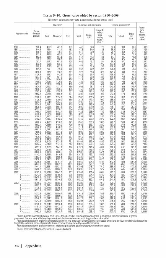
342 | Appendix B
Table B–10. Gross value added by sector, 1960–2009[Billions of dollars; quarterly data at seasonally adjusted annual rates]
Year or quarterGross
domesticproduct
Business 1 Households and institutions General government 3
Adden-dum:Gross
housingvalueadded
Total Nonfarm 1 Farm Total House-holds
Nonprofitinstitu-tions
servinghouse-holds 2
Total FederalStateandlocal
1960 ...................... 526.4 419.9 401.7 18.2 44.5 32.6 12.0 62.0 33.0 28.9 39.91961 ...................... 544.8 431.4 413.1 18.3 47.3 34.6 12.8 66.0 34.4 31.6 42.81962 ...................... 585.7 463.9 445.5 18.4 51.0 37.0 14.0 70.7 36.5 34.2 46.01963 ...................... 617.8 488.0 469.5 18.5 54.3 39.1 15.2 75.5 38.4 37.1 48.91964 ...................... 663.6 524.9 507.5 17.3 57.7 41.2 16.5 81.1 40.7 40.4 51.61965 ...................... 719.1 570.7 550.7 19.9 61.8 43.6 18.2 86.6 42.4 44.2 54.91966 ...................... 787.7 624.3 603.5 20.8 66.6 46.2 20.4 96.8 47.2 49.6 58.21967 ...................... 832.4 653.6 633.5 20.1 71.8 49.1 22.7 107.0 51.5 55.5 62.11968 ...................... 909.8 713.5 693.0 20.5 77.5 51.9 25.6 118.8 56.3 62.5 65.91969 ...................... 984.4 769.1 746.3 22.8 85.4 56.0 29.4 130.0 59.9 70.0 71.31970 ...................... 1,038.3 802.2 778.5 23.7 92.6 59.8 32.8 143.5 64.0 79.5 76.71971 ...................... 1,126.8 868.3 842.9 25.4 102.2 65.5 36.7 156.4 67.7 88.6 83.91972 ...................... 1,237.9 957.1 927.5 29.7 111.4 70.8 40.5 169.4 71.5 97.9 91.11973 ...................... 1,382.3 1,077.4 1,030.6 46.8 121.7 76.5 45.2 183.2 73.9 109.3 98.31974 ...................... 1,499.5 1,164.5 1,120.3 44.2 133.6 83.0 50.6 201.3 79.6 121.8 106.81975 ...................... 1,637.7 1,265.8 1,220.1 45.6 147.5 90.8 56.7 224.5 87.3 137.2 117.21976 ...................... 1,824.6 1,420.7 1,377.7 43.0 160.5 98.7 61.8 243.5 93.8 149.7 126.61977 ...................... 2,030.1 1,590.0 1,546.5 43.5 175.5 107.9 67.6 264.6 102.0 162.6 140.51978 ...................... 2,293.8 1,809.4 1,758.7 50.7 196.9 121.3 75.6 287.5 109.7 177.8 155.51979 ...................... 2,562.2 2,028.5 1,968.4 60.1 220.8 136.0 84.8 313.0 117.6 195.4 172.91980 ...................... 2,788.1 2,186.1 2,134.7 51.4 253.5 156.5 97.0 348.5 131.2 217.3 199.81981 ...................... 3,126.8 2,454.0 2,389.0 65.0 287.5 177.8 109.7 385.3 147.4 237.9 228.81982 ...................... 3,253.2 2,514.9 2,454.5 60.4 319.3 196.7 122.7 419.0 161.2 257.7 255.71983 ...................... 3,534.6 2,741.1 2,696.2 44.9 348.2 212.5 135.6 445.4 171.2 274.1 277.71984 ...................... 3,930.9 3,065.5 3,001.3 64.2 380.3 231.0 149.3 485.1 192.1 293.1 301.31985 ...................... 4,217.5 3,283.9 3,220.5 63.4 410.1 250.3 159.8 523.4 205.0 318.4 333.11986 ...................... 4,460.1 3,461.5 3,402.1 59.5 442.3 268.0 174.3 556.3 212.6 343.7 359.71987 ...................... 4,736.4 3,662.0 3,600.5 61.5 482.8 288.0 194.8 591.5 223.3 368.2 385.51988 ...................... 5,100.4 3,940.2 3,879.4 60.7 529.7 313.1 216.6 630.6 234.8 395.8 415.31989 ...................... 5,482.1 4,235.7 4,162.0 73.8 574.2 337.2 237.0 672.2 246.4 425.8 443.41990 ...................... 5,800.5 4,453.9 4,376.6 77.3 624.0 363.3 260.6 722.7 258.8 463.9 477.81991 ...................... 5,992.1 4,558.6 4,488.0 70.6 665.9 383.7 282.2 767.6 274.8 492.8 508.11992 ...................... 6,342.3 4,829.2 4,748.9 80.4 711.1 405.3 305.9 801.9 282.0 519.9 538.61993 ...................... 6,667.4 5,084.1 5,012.7 71.4 752.1 428.3 323.8 831.2 285.2 546.0 562.91994 ...................... 7,085.2 5,425.2 5,341.3 83.9 800.0 461.3 338.7 859.9 285.2 574.7 602.61995 ...................... 7,414.7 5,677.8 5,608.7 69.1 852.1 492.2 359.9 884.8 283.6 601.2 640.71996 ...................... 7,838.5 6,030.2 5,936.9 93.3 897.0 519.8 377.2 911.3 287.6 623.7 671.31997 ...................... 8,332.4 6,442.8 6,354.9 87.9 949.2 550.9 398.3 940.3 290.0 650.3 708.61998 ...................... 8,793.5 6,810.8 6,731.6 79.2 1,010.1 583.9 426.3 972.5 292.2 680.3 745.31999 ...................... 9,353.5 7,249.0 7,177.8 71.2 1,082.9 628.4 454.5 1,021.6 300.4 721.2 798.32000 ...................... 9,951.5 7,715.5 7,641.9 73.6 1,157.2 673.5 483.7 1,078.8 315.1 763.7 849.92001 ...................... 10,286.2 7,913.6 7,837.4 76.2 1,232.9 719.5 513.4 1,139.6 324.9 814.7 904.42002 ...................... 10,642.3 8,132.8 8,060.5 72.3 1,298.0 746.0 552.1 1,211.4 351.8 859.6 932.52003 ...................... 11,142.1 8,502.8 8,410.3 92.4 1,347.2 762.7 584.5 1,292.2 382.9 909.3 938.22004 ...................... 11,867.8 9,084.6 8,966.4 118.3 1,423.8 806.0 617.7 1,359.3 412.0 947.3 988.72005 ...................... 12,638.4 9,695.5 9,593.5 102.0 1,506.4 864.4 642.0 1,436.5 438.7 997.7 1,054.02006 ...................... 13,398.9 10,284.1 10,191.1 93.1 1,602.9 924.8 678.1 1,512.0 460.6 1,051.3 1,130.82007 ...................... 14,077.6 10,789.0 10,672.8 116.2 1,686.9 973.7 713.1 1,601.8 485.7 1,116.0 1,205.42008 ...................... 14,441.4 10,953.1 10,821.0 132.1 1,799.9 1,048.7 751.2 1,688.4 515.2 1,173.2 1,306.52009 p .................... 14,258.7 10,668.7 10,562.2 106.5 1,830.0 1,062.2 767.7 1,760.0 558.7 1,201.3 1,331.32006: I .................. 13,183.5 10,129.8 10,043.0 86.7 1,570.4 906.0 664.4 1,483.2 455.8 1,027.5 1,104.9
II ................. 13,347.8 10,246.9 10,156.4 90.6 1,599.3 924.3 675.0 1,501.6 459.7 1,041.9 1,127.8III ................ 13,452.9 10,311.9 10,218.2 93.6 1,619.6 938.4 681.2 1,521.4 462.4 1,059.0 1,146.7IV ................ 13,611.5 10,447.9 10,346.6 101.3 1,622.0 930.4 691.6 1,541.6 464.7 1,076.9 1,143.7
2007: I .................. 13,795.6 10,572.3 10,462.3 110.0 1,648.7 947.4 701.3 1,574.5 480.7 1,093.8 1,166.8II ................. 13,997.2 10,737.4 10,626.8 110.6 1,666.4 958.3 708.1 1,593.4 484.0 1,109.3 1,185.6III ................ 14,179.9 10,872.9 10,758.4 114.5 1,697.6 981.7 716.0 1,609.3 487.3 1,122.0 1,217.5IV ................ 14,337.9 10,973.3 10,843.9 129.5 1,734.6 1,007.6 727.0 1,629.9 490.9 1,139.0 1,251.8
2008: I .................. 14,373.9 10,952.7 10,809.7 143.1 1,761.5 1,025.0 736.5 1,659.7 505.3 1,154.4 1,274.6II ................. 14,497.8 11,022.1 10,889.6 132.6 1,796.2 1,050.6 745.5 1,679.5 511.8 1,167.7 1,306.2III ................ 14,546.7 11,034.7 10,901.6 133.0 1,812.4 1,057.1 755.3 1,699.6 518.5 1,181.1 1,318.3IV ................ 14,347.3 10,802.9 10,683.3 119.6 1,829.5 1,062.0 767.5 1,715.0 525.2 1,189.7 1,326.9
2009: I .................. 14,178.0 10,614.2 10,510.4 103.8 1,823.9 1,063.4 760.5 1,739.8 543.8 1,196.0 1,330.0II ................. 14,151.2 10,578.5 10,473.0 105.5 1,814.7 1,054.5 760.1 1,758.0 554.3 1,203.8 1,322.9III ................ 14,242.1 10,641.0 10,540.6 100.4 1,836.5 1,065.6 770.9 1,764.7 563.6 1,201.1 1,335.6IV p ............. 14,463.4 10,840.9 10,724.7 116.2 1,844.8 1,065.4 779.4 1,777.7 573.3 1,204.4 1,336.8
1 Gross domestic business value added equals gross domestic product excluding gross value added of households and institutions and of generalgovernment. Nonfarm value added equals gross domestic business value added excluding gross farm value added.
2 Equals compensation of employees of nonprofit institutions, the rental value of nonresidential fixed assets owned and used by nonprofit institutions servinghouseholds, and rental income of persons for tenant-occupied housing owned by nonprofit institutions.
3 Equals compensation of general government employees plus general government consumption of fixed capital.Source: Department of Commerce (Bureau of Economic Analysis).
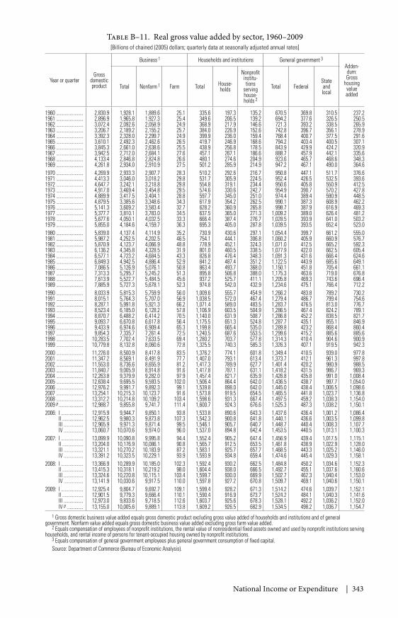
National Income or Expenditure | 343
Table B–11. Real gross value added by sector, 1960–2009[Billions of chained (2005) dollars; quarterly data at seasonally adjusted annual rates]
Year or quarterGross
domesticproduct
Business 1 Households and institutions General government 3
Adden-dum:Gross
housingvalueadded
Total Nonfarm 1 Farm Total House-holds
Nonprofitinstitu-tions
servinghouse-holds 2
Total FederalStateandlocal
1960 ...................... 2,830.9 1,928.1 1,889.6 25.1 335.6 197.3 135.2 670.5 369.8 310.5 237.21961 ...................... 2,896.9 1,965.8 1,927.3 25.4 349.6 206.5 139.2 694.2 377.6 326.5 250.51962 ...................... 3,072.4 2,092.6 2,058.9 24.9 368.9 217.9 146.6 721.3 393.2 338.5 265.91963 ...................... 3,206.7 2,189.2 2,155.2 25.7 384.0 226.9 152.6 742.8 396.7 356.1 278.91964 ...................... 3,392.3 2,328.0 2,299.7 24.9 399.9 236.0 159.4 768.4 400.7 377.5 291.61965 ...................... 3,610.1 2,492.3 2,462.6 26.5 419.7 246.9 168.6 794.2 403.4 400.5 307.11966 ...................... 3,845.3 2,661.0 2,638.6 25.5 438.9 256.8 178.5 843.9 429.9 424.2 320.91967 ...................... 3,942.5 2,712.0 2,684.1 27.6 457.1 267.1 186.6 888.7 457.9 442.1 335.61968 ...................... 4,133.4 2,846.8 2,824.8 26.6 480.1 274.6 204.9 923.6 465.7 468.6 348.31969 ...................... 4,261.8 2,934.0 2,910.9 27.5 501.2 285.9 214.9 947.2 467.1 490.0 364.61970 ...................... 4,269.9 2,933.3 2,907.7 28.3 510.2 292.6 216.7 950.8 447.1 511.7 376.61971 ...................... 4,413.3 3,046.0 3,018.2 29.8 531.7 305.9 224.5 952.4 426.5 532.5 393.61972 ...................... 4,647.7 3,242.1 3,218.8 29.8 554.8 319.1 234.4 950.6 405.8 550.9 412.51973 ...................... 4,917.0 3,469.4 3,454.8 29.5 574.6 330.6 242.7 954.9 390.7 570.2 427.81974 ...................... 4,889.9 3,417.5 3,404.1 28.8 597.7 345.0 251.0 974.4 389.4 590.9 448.51975 ...................... 4,879.5 3,385.6 3,348.6 34.3 617.9 354.2 262.5 990.1 387.3 608.9 462.21976 ...................... 5,141.3 3,609.2 3,583.4 32.7 628.2 360.9 265.8 998.7 387.9 616.9 469.31977 ...................... 5,377.7 3,810.1 3,783.0 34.5 637.5 365.0 271.3 1,009.2 389.0 626.4 481.21978 ...................... 5,677.6 4,050.1 4,032.5 33.3 666.4 387.4 276.7 1,028.5 393.9 641.0 503.21979 ...................... 5,855.0 4,184.6 4,159.7 36.3 695.3 405.0 287.8 1,039.5 393.5 652.4 523.01980 ...................... 5,839.0 4,137.4 4,114.9 35.2 730.9 430.6 297.1 1,054.4 399.7 661.2 555.01981 ...................... 5,987.2 4,252.5 4,202.5 46.5 754.1 444.1 306.8 1,060.2 405.9 660.9 576.71982 ...................... 5,870.9 4,123.7 4,066.9 48.8 778.9 452.1 324.3 1,071.0 412.5 665.2 592.31983 ...................... 6,136.2 4,345.8 4,328.5 31.9 801.0 460.5 338.5 1,077.9 422.0 662.5 605.41984 ...................... 6,577.1 4,723.2 4,684.5 43.3 826.8 476.4 348.3 1,091.3 431.6 666.4 624.61985 ...................... 6,849.3 4,942.5 4,886.4 52.9 841.2 487.4 351.2 1,122.5 443.9 685.6 649.11986 ...................... 7,086.5 5,126.9 5,076.1 50.8 863.4 493.7 368.0 1,150.1 451.8 705.4 661.11987 ...................... 7,313.3 5,295.7 5,245.2 51.3 895.8 506.8 388.0 1,175.3 463.6 719.0 676.81988 ...................... 7,613.9 5,522.7 5,484.5 45.6 937.2 525.7 411.1 1,205.8 469.3 743.6 696.41989 ...................... 7,885.9 5,727.3 5,678.1 52.3 974.8 542.0 432.9 1,234.6 475.1 766.4 712.21990 ...................... 8,033.9 5,815.3 5,759.9 56.0 1,009.6 555.7 454.9 1,266.2 483.8 789.2 730.21991 ...................... 8,015.1 5,764.3 5,707.0 56.9 1,038.5 572.0 467.4 1,279.4 486.7 799.4 754.61992 ...................... 8,287.1 5,991.8 5,921.3 66.2 1,071.4 589.0 483.5 1,283.7 476.5 813.0 776.71993 ...................... 8,523.4 6,185.0 6,128.2 57.8 1,106.9 603.5 504.9 1,286.5 467.4 824.2 789.11994 ...................... 8,870.7 6,488.2 6,414.2 70.5 1,140.0 631.9 508.7 1,286.8 452.2 838.5 821.71995 ...................... 9,093.7 6,670.8 6,617.8 56.4 1,175.5 651.3 524.8 1,287.7 435.1 855.1 846.91996 ...................... 9,433.9 6,974.6 6,909.4 65.3 1,199.8 665.4 535.0 1,289.8 423.2 868.4 860.41997 ...................... 9,854.3 7,335.7 7,261.4 72.5 1,240.5 687.6 553.5 1,299.6 415.2 885.6 885.61998 ...................... 10,283.5 7,702.4 7,633.5 69.4 1,280.2 703.7 577.8 1,314.3 410.4 904.6 900.91999 ...................... 10,779.8 8,132.8 8,060.6 72.8 1,325.5 740.3 585.3 1,326.3 407.1 919.5 942.32000 ...................... 11,226.0 8,500.9 8,417.8 83.5 1,376.2 774.1 601.8 1,349.4 410.5 939.0 977.82001 ...................... 11,347.2 8,569.1 8,491.9 77.7 1,407.0 793.1 613.4 1,373.7 412.1 961.3 997.82002 ...................... 11,553.0 8,736.6 8,655.9 81.2 1,417.3 789.9 627.7 1,401.4 420.2 980.9 988.52003 ...................... 11,840.7 9,005.9 8,914.8 91.6 1,417.8 787.1 631.1 1,418.2 431.5 986.7 969.32004 ...................... 12,263.8 9,379.9 9,282.0 97.9 1,457.4 821.7 635.9 1,426.8 435.8 991.0 1,008.42005 ...................... 12,638.4 9,695.5 9,593.5 102.0 1,506.4 864.4 642.0 1,436.5 438.7 997.7 1,054.02006 ...................... 12,976.2 9,991.7 9,892.3 99.1 1,539.8 898.0 642.0 1,445.0 438.4 1,006.5 1,098.62007 ...................... 13,254.1 10,215.3 10,123.7 91.6 1,573.8 919.5 654.5 1,465.5 441.8 1,023.7 1,136.82008 ...................... 13,312.2 10,214.8 10,109.2 103.4 1,598.6 931.3 667.4 1,497.5 459.2 1,038.3 1,154.02009 p .................... 12,988.7 9,855.8 9,741.7 111.4 1,600.7 924.3 676.6 1,525.3 487.3 1,038.2 1,150.12006: I .................. 12,915.9 9,944.7 9,850.1 93.8 1,533.8 890.6 643.3 1,437.6 436.4 1,001.2 1,086.4
II ................. 12,962.5 9,980.3 9,873.8 107.3 1,542.3 900.8 641.8 1,440.1 436.6 1,003.5 1,099.8III ................ 12,965.9 9,971.3 9,871.4 99.5 1,546.1 905.7 640.7 1,448.7 440.4 1,008.3 1,107.7IV ................ 13,060.7 10,070.6 9,974.0 96.0 1,537.0 894.8 642.4 1,453.5 440.5 1,013.1 1,100.3
2007: I .................. 13,099.9 10,090.8 9,995.8 94.4 1,552.4 905.2 647.4 1,456.9 439.4 1,017.5 1,115.1II ................. 13,204.0 10,176.9 10,086.1 90.8 1,565.7 912.5 653.5 1,461.8 438.9 1,022.9 1,128.0III ................ 13,321.1 10,270.2 10,183.9 87.2 1,583.1 925.7 657.7 1,468.5 443.3 1,025.2 1,146.0IV ................ 13,391.2 10,323.5 10,229.1 93.9 1,593.9 934.8 659.4 1,474.6 445.4 1,029.3 1,158.1
2008: I .................. 13,366.9 10,289.9 10,185.0 102.3 1,592.4 930.2 662.5 1,484.8 450.2 1,034.6 1,152.3II ................. 13,415.3 10,318.1 10,219.2 98.0 1,604.4 938.0 666.5 1,492.7 455.1 1,037.6 1,160.6III ................ 13,324.6 10,220.8 10,115.1 103.4 1,599.7 930.0 669.9 1,502.7 462.3 1,040.4 1,153.0IV ................ 13,141.9 10,030.6 9,917.5 110.0 1,597.8 927.2 670.8 1,509.7 469.1 1,040.6 1,150.1
2009: I .................. 12,925.4 9,804.7 9,692.7 109.1 1,599.4 928.2 671.3 1,514.2 474.6 1,039.7 1,152.1II ................. 12,901.5 9,779.3 9,666.4 110.1 1,590.4 916.9 673.7 1,524.2 484.1 1,040.3 1,141.6III ................ 12,973.0 9,833.6 9,718.5 112.6 1,603.7 925.6 678.3 1,528.1 492.2 1,036.2 1,152.0IV p ............. 13,155.0 10,005.6 9,889.1 113.8 1,609.2 926.5 682.9 1,534.5 498.2 1,036.7 1,154.7
1 Gross domestic business value added equals gross domestic product excluding gross value added of households and institutions and of generalgovernment. Nonfarm value added equals gross domestic business value added excluding gross farm value added.
2 Equals compensation of employees of nonprofit institutions, the rental value of nonresidential fixed assets owned and used by nonprofit institutions servinghouseholds, and rental income of persons for tenant-occupied housing owned by nonprofit institutions.
3 Equals compensation of general government employees plus general government consumption of fixed capital.Source: Department of Commerce (Bureau of Economic Analysis).
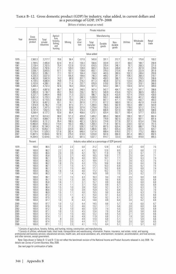
344 | Appendix B
Table B–12. Gross domestic product (GDP) by industry, value added, in current dollars andas a percentage of GDP, 1979–2008
[Billions of dollars; except as noted]
YearGross
domesticproduct
Private industries
Totalprivate
industries
Agricul-ture,
forestry,fishing,
andhunting
MiningCon-struc-tion
Manufacturing
Utilities Wholesaletrade
RetailtradeTotal
manufac-turing
Durablegoods
Non-durablegoods
Value added
1979 ........... 2,563.3 2,217.7 70.6 58.4 127.0 543.8 331.1 212.7 51.9 175.8 193.21980 ........... 2,789.5 2,405.8 62.0 91.3 130.3 556.6 333.9 222.7 60.0 188.7 200.91981 ........... 3,128.4 2,702.5 75.4 122.9 131.8 616.5 370.4 246.1 70.7 208.3 221.01982 ........... 3,255.0 2,792.6 71.3 120.0 128.8 603.2 353.4 249.8 81.7 207.9 229.91983 ........... 3,536.7 3,043.5 57.1 103.1 139.8 653.1 379.3 273.8 91.6 222.9 261.61984 ........... 3,933.2 3,395.1 77.1 107.2 164.4 724.0 443.5 280.5 102.3 249.4 293.61985 ........... 4,220.3 3,637.0 77.1 105.4 184.6 740.3 449.2 291.1 109.2 268.3 318.71986 ........... 4,462.8 3,842.9 74.2 68.9 207.7 766.0 459.3 306.7 114.4 278.5 336.61987 ........... 4,739.5 4,080.4 79.8 71.5 218.2 811.3 483.8 327.5 123.0 285.3 349.91988 ........... 5,103.8 4,399.1 80.2 71.4 232.7 876.9 519.0 357.9 122.8 318.1 366.01989 ........... 5,484.4 4,732.3 92.8 76.0 244.8 927.3 543.2 384.1 135.9 337.4 389.01990 ........... 5,803.1 4,997.8 96.7 84.9 248.5 947.4 542.7 404.7 142.9 347.7 398.81991 ........... 5,995.9 5,138.7 89.2 76.0 230.2 957.5 540.9 416.6 152.5 360.5 405.51992 ........... 6,337.7 5,440.4 99.6 71.3 232.5 996.7 562.8 433.8 157.4 378.9 430.01993 ........... 6,657.4 5,729.3 93.1 72.1 248.3 1,039.9 593.1 446.8 165.3 401.2 458.01994 ........... 7,072.2 6,110.5 105.6 73.6 274.4 1,118.8 647.7 471.1 174.6 442.7 493.31995 ........... 7,397.6 6,407.2 93.1 74.1 287.0 1,177.3 677.2 500.0 181.5 457.0 514.91996 ........... 7,816.9 6,795.2 113.8 87.5 311.7 1,209.4 706.5 502.9 183.3 489.1 543.81997 ........... 8,304.3 7,247.5 110.7 92.6 337.6 1,279.8 755.5 524.3 179.6 521.2 574.21998 ........... 8,747.0 7,652.5 102.4 74.8 374.4 1,343.9 806.9 537.0 180.8 542.9 598.61999 ........... 9,268.4 8,127.2 93.8 85.4 406.6 1,373.1 820.4 552.7 185.4 577.7 635.52000 ........... 9,817.0 8,614.3 98.0 121.3 435.9 1,426.2 865.3 560.9 189.3 591.7 662.42001 ........... 10,128.0 8,869.7 97.9 118.7 469.5 1,341.3 778.9 562.5 202.3 607.1 691.62002 ........... 10,469.6 9,131.2 95.4 106.5 482.3 1,352.6 774.8 577.9 207.3 615.4 719.62003 ........... 10,960.8 9,542.3 114.4 143.3 496.2 1,359.3 771.8 587.5 220.0 637.0 751.52004 ........... 11,685.9 10,194.3 142.2 171.3 539.2 1,427.9 807.5 620.4 240.3 686.7 776.92005 ........... 12,421.9 10,853.1 133.3 223.8 605.4 1,480.6 845.1 635.5 239.5 722.4 824.72006 ........... 13,178.4 11,529.3 121.6 262.4 646.0 1,577.4 899.4 678.0 272.7 773.2 866.52007 ........... 13,807.5 12,064.6 167.9 275.0 610.8 1,616.8 922.0 694.9 281.4 805.3 892.52008 ........... 14,264.6 12,424.6 157.7 325.3 581.5 1,637.7 914.7 723.0 306.0 818.8 885.5
Percent Industry value added as a percentage of GDP (percent)
1979 ........... 100.0 86.5 2.8 2.3 5.0 21.2 12.9 8.3 2.0 6.9 7.51980 ........... 100.0 86.2 2.2 3.3 4.7 20.0 12.0 8.0 2.2 6.8 7.21981 ........... 100.0 86.4 2.4 3.9 4.2 19.7 11.8 7.9 2.3 6.7 7.11982 ........... 100.0 85.8 2.2 3.7 4.0 18.5 10.9 7.7 2.5 6.4 7.11983 ........... 100.0 86.1 1.6 2.9 4.0 18.5 10.7 7.7 2.6 6.3 7.41984 ........... 100.0 86.3 2.0 2.7 4.2 18.4 11.3 7.1 2.6 6.3 7.51985 ........... 100.0 86.2 1.8 2.5 4.4 17.5 10.6 6.9 2.6 6.4 7.61986 ........... 100.0 86.1 1.7 1.5 4.7 17.2 10.3 6.9 2.6 6.2 7.51987 ........... 100.0 86.1 1.7 1.5 4.6 17.1 10.2 6.9 2.6 6.0 7.41988 ........... 100.0 86.2 1.6 1.4 4.6 17.2 10.2 7.0 2.4 6.2 7.21989 ........... 100.0 86.3 1.7 1.4 4.5 16.9 9.9 7.0 2.5 6.2 7.11990 ........... 100.0 86.1 1.7 1.5 4.3 16.3 9.4 7.0 2.5 6.0 6.91991 ........... 100.0 85.7 1.5 1.3 3.8 16.0 9.0 6.9 2.5 6.0 6.81992 ........... 100.0 85.8 1.6 1.1 3.7 15.7 8.9 6.8 2.5 6.0 6.81993 ........... 100.0 86.1 1.4 1.1 3.7 15.6 8.9 6.7 2.5 6.0 6.91994 ........... 100.0 86.4 1.5 1.0 3.9 15.8 9.2 6.7 2.5 6.3 7.01995 ........... 100.0 86.6 1.3 1.0 3.9 15.9 9.2 6.8 2.5 6.2 7.01996 ........... 100.0 86.9 1.5 1.1 4.0 15.5 9.0 6.4 2.3 6.3 7.01997 ........... 100.0 87.3 1.3 1.1 4.1 15.4 9.1 6.3 2.2 6.3 6.91998 ........... 100.0 87.5 1.2 .9 4.3 15.4 9.2 6.1 2.1 6.2 6.81999 ........... 100.0 87.7 1.0 .9 4.4 14.8 8.9 6.0 2.0 6.2 6.92000 ........... 100.0 87.7 1.0 1.2 4.4 14.5 8.8 5.7 1.9 6.0 6.72001 ........... 100.0 87.6 1.0 1.2 4.6 13.2 7.7 5.6 2.0 6.0 6.82002 ........... 100.0 87.2 .9 1.0 4.6 12.9 7.4 5.5 2.0 5.9 6.92003 ........... 100.0 87.1 1.0 1.3 4.5 12.4 7.0 5.4 2.0 5.8 6.92004 ........... 100.0 87.2 1.2 1.5 4.6 12.2 6.9 5.3 2.1 5.9 6.62005 ........... 100.0 87.4 1.1 1.8 4.9 11.9 6.8 5.1 1.9 5.8 6.62006 ........... 100.0 87.5 .9 2.0 4.9 12.0 6.8 5.1 2.1 5.9 6.62007 ........... 100.0 87.4 1.2 2.0 4.4 11.7 6.7 5.0 2.0 5.8 6.52008 ........... 100.0 87.1 1.1 2.3 4.1 11.5 6.4 5.1 2.1 5.7 6.2
1 Consists of agriculture, forestry, fishing, and hunting; mining; construction; and manufacturing.2 Consists of utilities; wholesale trade; retail trade; transportation and warehousing; information; finance, insurance, real estate, rental, and leasing;
professional and business services; educational services, health care, and social assistance; arts, entertainment, recreation, accommodation, and food services;and other services, except government.
Note: Data shown in Tables B–12 and B–13 do not reflect the benchmark revision of the National Income and Product Accounts released in July 2009. Fordetails see Survey of Current Business, May 2009.
See next page for continuation of table.
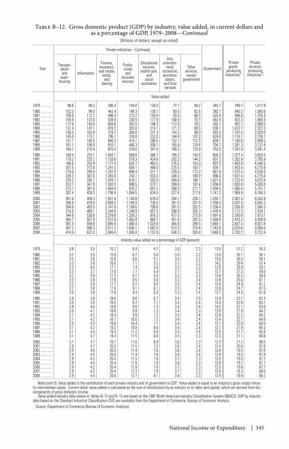
National Income or Expenditure | 345
Table B–12. Gross domestic product (GDP) by industry, value added, in current dollars andas a percentage of GDP, 1979–2008—Continued
[Billions of dollars; except as noted]
Year
Private industries—Continued
GovernmentPrivategoods-
producingindustries 1
Privateservices-producing
industries 2
Transpor-tationand
ware-housing
Information
Finance,insurance,real estate,
rental,and
leasing
Profes-sionaland
businessservices
Educationalservices,
health care,and
socialassistance
Arts,entertain-
ment,recreation,accommo-
dation,and foodservices
Otherservices,except
government
Value added
1979 ............. 96.6 90.3 390.3 164.0 120.5 77.1 58.2 345.7 799.7 1,417.91980 ............. 102.3 99.0 442.4 186.3 139.7 83.5 62.6 383.7 840.2 1,565.61981 ............. 109.9 112.7 498.4 213.2 159.9 93.5 68.5 425.9 946.6 1,755.91982 ............. 105.9 123.6 539.9 230.9 177.9 100.9 70.7 462.4 923.3 1,869.31983 ............. 117.8 140.0 604.6 262.5 198.3 112.0 79.2 493.1 953.1 2,090.51984 ............. 131.4 147.1 670.2 303.8 214.1 121.2 89.3 538.1 1,072.7 2,322.31985 ............. 136.3 162.9 729.7 340.8 231.3 134.3 98.0 583.3 1,107.4 2,529.51986 ............. 145.6 173.1 795.1 378.8 252.0 144.9 107.2 620.0 1,116.7 2,726.11987 ............. 151.1 185.0 840.3 414.1 286.5 152.1 112.3 659.1 1,180.8 2,899.51988 ............. 161.1 194.0 910.1 466.3 309.1 165.9 124.4 704.7 1,261.3 3,137.81989 ............. 164.1 210.4 975.4 518.0 347.0 180.2 133.9 752.0 1,341.0 3,391.41990 ............. 169.4 225.1 1,042.1 569.8 386.7 195.2 142.6 805.3 1,377.4 3,620.41991 ............. 178.2 235.2 1,103.6 579.3 424.8 202.2 144.2 857.2 1,352.8 3,785.91992 ............. 186.6 250.9 1,177.4 626.7 463.5 216.2 153.0 897.3 1,400.0 4,040.51993 ............. 201.0 272.6 1,241.5 659.1 488.0 225.5 163.7 928.1 1,453.4 4,275.91994 ............. 218.0 294.0 1,297.8 698.4 511.1 235.0 173.2 961.8 1,572.4 4,538.01995 ............. 226.3 307.6 1,383.0 743.1 533.3 248.3 180.9 990.4 1,631.4 4,775.81996 ............. 235.2 335.7 1,470.7 810.1 552.5 264.4 188.1 1,021.6 1,722.4 5,072.81997 ............. 253.7 347.8 1,593.3 896.5 573.1 289.8 197.4 1,056.8 1,820.8 5,426.81998 ............. 273.7 381.6 1,684.6 976.2 601.5 306.0 211.1 1,094.5 1,895.4 5,757.11999 ............. 287.4 439.3 1,798.4 1,064.5 634.5 327.8 217.8 1,141.2 1,958.9 6,168.32000 ............. 301.6 458.3 1,931.0 1,140.8 678.4 350.1 229.1 1,202.7 2,081.5 6,532.82001 ............. 296.9 476.9 2,059.2 1,165.9 739.3 361.5 241.5 1,258.3 2,027.5 6,842.22002 ............. 304.6 483.0 2,141.9 1,189.0 799.6 381.5 252.5 1,338.4 2,036.9 7,094.32003 ............. 316.6 489.1 2,244.6 1,248.9 857.3 398.9 265.3 1,418.4 2,113.3 7,429.12004 ............. 344.6 530.6 2,378.8 1,338.2 916.3 427.5 273.9 1,491.6 2,280.6 7,913.72005 ............. 364.7 557.8 2,527.9 1,463.9 969.7 451.8 287.5 1,568.8 2,443.2 8,409.92006 ............. 387.4 559.6 2,685.8 1,566.4 1,025.8 484.9 299.5 1,649.1 2,607.4 8,921.82007 ............. 407.2 586.3 2,811.2 1,694.1 1,087.0 513.3 315.6 1,742.9 2,670.6 9,394.02008 ............. 414.9 622.0 2,848.4 1,805.8 1,157.9 536.3 326.8 1,840.0 2,702.2 9,722.4
Industry value added as a percentage of GDP (percent)
1979 ............. 3.8 3.5 15.2 6.4 4.7 3.0 2.3 13.5 31.2 55.31980 ............. 3.7 3.5 15.9 6.7 5.0 3.0 2.2 13.8 30.1 56.11981 ............. 3.5 3.6 15.9 6.8 5.1 3.0 2.2 13.6 30.3 56.11982 ............. 3.3 3.8 16.6 7.1 5.5 3.1 2.2 14.2 28.4 57.41983 ............. 3.3 4.0 17.1 7.4 5.6 3.2 2.2 13.9 26.9 59.11984 ............. 3.3 3.7 17.0 7.7 5.4 3.1 2.3 13.7 27.3 59.01985 ............. 3.2 3.9 17.3 8.1 5.5 3.2 2.3 13.8 26.2 59.91986 ............. 3.3 3.9 17.8 8.5 5.6 3.2 2.4 13.9 25.0 61.11987 ............. 3.2 3.9 17.7 8.7 6.0 3.2 2.4 13.9 24.9 61.21988 ............. 3.2 3.8 17.8 9.1 6.1 3.3 2.4 13.8 24.7 61.51989 ............. 3.0 3.8 17.8 9.4 6.3 3.3 2.4 13.7 24.5 61.81990 ............. 2.9 3.9 18.0 9.8 6.7 3.4 2.5 13.9 23.7 62.41991 ............. 3.0 3.9 18.4 9.7 7.1 3.4 2.4 14.3 22.6 63.11992 ............. 2.9 4.0 18.6 9.9 7.3 3.4 2.4 14.2 22.1 63.81993 ............. 3.0 4.1 18.6 9.9 7.3 3.4 2.5 13.9 21.8 64.21994 ............. 3.1 4.2 18.4 9.9 7.2 3.3 2.4 13.6 22.2 64.21995 ............. 3.1 4.2 18.7 10.0 7.2 3.4 2.4 13.4 22.1 64.61996 ............. 3.0 4.3 18.8 10.4 7.1 3.4 2.4 13.1 22.0 64.91997 ............. 3.1 4.2 19.2 10.8 6.9 3.5 2.4 12.7 21.9 65.31998 ............. 3.1 4.4 19.3 11.2 6.9 3.5 2.4 12.5 21.7 65.81999 ............. 3.1 4.7 19.4 11.5 6.8 3.5 2.3 12.3 21.1 66.62000 ............. 3.1 4.7 19.7 11.6 6.9 3.6 2.3 12.3 21.2 66.52001 ............. 2.9 4.7 20.3 11.5 7.3 3.6 2.4 12.4 20.0 67.62002 ............. 2.9 4.6 20.5 11.4 7.6 3.6 2.4 12.8 19.5 67.82003 ............. 2.9 4.5 20.5 11.4 7.8 3.6 2.4 12.9 19.3 67.82004 ............. 2.9 4.5 20.4 11.5 7.8 3.7 2.3 12.8 19.5 67.72005 ............. 2.9 4.5 20.4 11.8 7.8 3.6 2.3 12.6 19.7 67.72006 ............. 2.9 4.2 20.4 11.9 7.8 3.7 2.3 12.5 19.8 67.72007 ............. 2.9 4.2 20.4 12.3 7.9 3.7 2.3 12.6 19.3 68.02008 ............. 2.9 4.4 20.0 12.7 8.1 3.8 2.3 12.9 18.9 68.2
Note (cont’d): Value added is the contribution of each private industry and of government to GDP. Value added is equal to an industry’s gross output minusits intermediate inputs. Current-dollar value added is calculated as the sum of distributions by an industry to its labor and capital, which are derived from thecomponents of gross domestic income.
Value added industry data shown in Tables B–12 and B–13 are based on the 1997 North American Industry Classification System (NAICS). GDP by industrydata based on the Standard Industrial Classification (SIC) are available from the Department of Commerce, Bureau of Economic Analysis.
Source: Department of Commerce (Bureau of Economic Analysis).
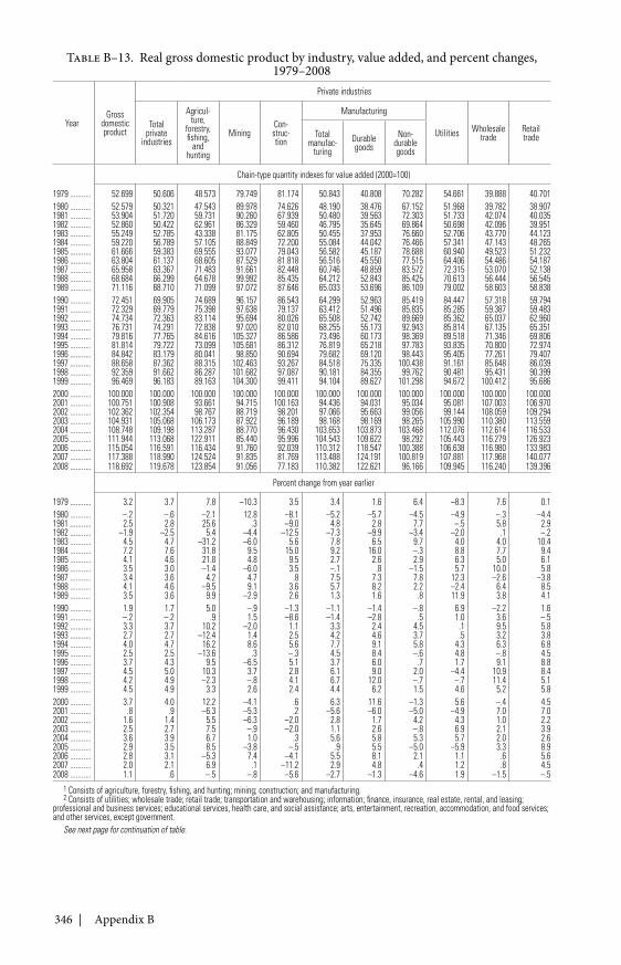
346 | Appendix B
Table B–13. Real gross domestic product by industry, value added, and percent changes,1979–2008
YearGross
domesticproduct
Private industries
Totalprivate
industries
Agricul-ture,
forestry,fishing,
andhunting
MiningCon-struc-tion
Manufacturing
Utilities Wholesaletrade
RetailtradeTotal
manufac-turing
Durablegoods
Non-durablegoods
Chain-type quantity indexes for value added (2000=100)
1979 ........... 52.699 50.606 48.573 79.749 81.174 50.843 40.808 70.282 54.661 39.888 40.7011980 ........... 52.579 50.321 47.543 89.978 74.626 48.190 38.476 67.152 51.968 39.782 38.9071981 ........... 53.904 51.720 59.731 90.260 67.939 50.480 39.563 72.303 51.733 42.074 40.0351982 ........... 52.860 50.422 62.961 86.329 59.460 46.795 35.645 69.864 50.698 42.096 39.9511983 ........... 55.249 52.785 43.338 81.175 62.805 50.455 37.953 76.660 52.706 43.770 44.1231984 ........... 59.220 56.789 57.105 88.849 72.200 55.084 44.042 76.466 57.341 47.143 48.2651985 ........... 61.666 59.383 69.555 93.077 79.043 56.582 45.187 78.688 60.940 49.523 51.2321986 ........... 63.804 61.137 68.605 87.529 81.818 56.516 45.550 77.515 64.406 54.486 54.1871987 ........... 65.958 63.367 71.483 91.661 82.448 60.746 48.859 83.572 72.315 53.070 52.1381988 ........... 68.684 66.299 64.678 99.992 85.435 64.212 52.843 85.425 70.613 56.444 56.5451989 ........... 71.116 68.710 71.099 97.072 87.646 65.033 53.696 86.109 79.002 58.603 58.8381990 ........... 72.451 69.905 74.689 96.157 86.543 64.299 52.963 85.419 84.447 57.318 59.7941991 ........... 72.329 69.779 75.398 97.638 79.137 63.412 51.496 85.835 85.285 59.387 59.4831992 ........... 74.734 72.363 83.114 95.694 80.026 65.508 52.742 89.669 85.362 65.037 62.9601993 ........... 76.731 74.291 72.838 97.020 82.010 68.255 55.173 92.943 85.814 67.135 65.3511994 ........... 79.816 77.765 84.616 105.327 86.586 73.496 60.173 98.369 89.518 71.346 69.8061995 ........... 81.814 79.722 73.099 105.681 86.312 76.819 65.218 97.783 93.835 70.800 72.9741996 ........... 84.842 83.179 80.041 98.850 90.694 79.682 69.120 98.443 95.405 77.261 79.4071997 ........... 88.658 87.362 88.315 102.463 93.267 84.518 75.335 100.438 91.161 85.648 86.0391998 ........... 92.359 91.662 86.287 101.682 97.087 90.181 84.355 99.762 90.481 95.431 90.3991999 ........... 96.469 96.183 89.163 104.300 99.411 94.104 89.627 101.298 94.672 100.412 95.6862000 ........... 100.000 100.000 100.000 100.000 100.000 100.000 100.000 100.000 100.000 100.000 100.0002001 ........... 100.751 100.908 93.661 94.715 100.163 94.436 94.031 95.034 95.081 107.003 106.9702002 ........... 102.362 102.354 98.767 88.719 98.201 97.066 95.663 99.056 99.144 108.059 109.2942003 ........... 104.931 105.068 106.173 87.922 96.189 98.168 98.169 98.265 105.990 110.380 113.5592004 ........... 108.748 109.198 113.287 88.770 96.430 103.653 103.873 103.468 112.076 112.614 116.5332005 ........... 111.944 113.068 122.911 85.440 95.996 104.543 109.622 98.292 105.443 116.279 126.9232006 ........... 115.054 116.591 116.434 91.760 92.039 110.312 118.547 100.388 106.638 116.980 133.9832007 ........... 117.388 118.990 124.524 91.835 81.769 113.488 124.191 100.819 107.881 117.968 140.0772008 ........... 118.692 119.678 123.854 91.056 77.183 110.382 122.621 96.166 109.945 116.240 139.396
Percent change from year earlier
1979 ........... 3.2 3.7 7.8 –10.3 3.5 3.4 1.6 6.4 –8.3 7.6 0.11980 ........... –.2 –.6 –2.1 12.8 –8.1 –5.2 –5.7 –4.5 –4.9 –.3 –4.41981 ........... 2.5 2.8 25.6 .3 –9.0 4.8 2.8 7.7 –.5 5.8 2.91982 ........... –1.9 –2.5 5.4 –4.4 –12.5 –7.3 –9.9 –3.4 –2.0 .1 –.21983 ........... 4.5 4.7 –31.2 –6.0 5.6 7.8 6.5 9.7 4.0 4.0 10.41984 ........... 7.2 7.6 31.8 9.5 15.0 9.2 16.0 –.3 8.8 7.7 9.41985 ........... 4.1 4.6 21.8 4.8 9.5 2.7 2.6 2.9 6.3 5.0 6.11986 ........... 3.5 3.0 –1.4 –6.0 3.5 –.1 .8 –1.5 5.7 10.0 5.81987 ........... 3.4 3.6 4.2 4.7 .8 7.5 7.3 7.8 12.3 –2.6 –3.81988 ........... 4.1 4.6 –9.5 9.1 3.6 5.7 8.2 2.2 –2.4 6.4 8.51989 ........... 3.5 3.6 9.9 –2.9 2.6 1.3 1.6 .8 11.9 3.8 4.11990 ........... 1.9 1.7 5.0 –.9 –1.3 –1.1 –1.4 –.8 6.9 –2.2 1.61991 ........... –.2 –.2 .9 1.5 –8.6 –1.4 –2.8 .5 1.0 3.6 –.51992 ........... 3.3 3.7 10.2 –2.0 1.1 3.3 2.4 4.5 .1 9.5 5.81993 ........... 2.7 2.7 –12.4 1.4 2.5 4.2 4.6 3.7 .5 3.2 3.81994 ........... 4.0 4.7 16.2 8.6 5.6 7.7 9.1 5.8 4.3 6.3 6.81995 ........... 2.5 2.5 –13.6 .3 –.3 4.5 8.4 –.6 4.8 –.8 4.51996 ........... 3.7 4.3 9.5 –6.5 5.1 3.7 6.0 .7 1.7 9.1 8.81997 ........... 4.5 5.0 10.3 3.7 2.8 6.1 9.0 2.0 –4.4 10.9 8.41998 ........... 4.2 4.9 –2.3 –.8 4.1 6.7 12.0 –.7 –.7 11.4 5.11999 ........... 4.5 4.9 3.3 2.6 2.4 4.4 6.2 1.5 4.6 5.2 5.82000 ........... 3.7 4.0 12.2 –4.1 .6 6.3 11.6 –1.3 5.6 –.4 4.52001 ........... .8 .9 –6.3 –5.3 .2 –5.6 –6.0 –5.0 –4.9 7.0 7.02002 ........... 1.6 1.4 5.5 –6.3 –2.0 2.8 1.7 4.2 4.3 1.0 2.22003 ........... 2.5 2.7 7.5 –.9 –2.0 1.1 2.6 –.8 6.9 2.1 3.92004 ........... 3.6 3.9 6.7 1.0 .3 5.6 5.8 5.3 5.7 2.0 2.62005 ........... 2.9 3.5 8.5 –3.8 –.5 .9 5.5 –5.0 –5.9 3.3 8.92006 ........... 2.8 3.1 –5.3 7.4 –4.1 5.5 8.1 2.1 1.1 .6 5.62007 ........... 2.0 2.1 6.9 .1 –11.2 2.9 4.8 .4 1.2 .8 4.52008 ........... 1.1 .6 –.5 –.8 –5.6 –2.7 –1.3 –4.6 1.9 –1.5 –.5
1 Consists of agriculture, forestry, fishing, and hunting; mining; construction; and manufacturing.2 Consists of utilities; wholesale trade; retail trade; transportation and warehousing; information; finance, insurance, real estate, rental, and leasing;
professional and business services; educational services, health care, and social assistance; arts, entertainment, recreation, accommodation, and food services;and other services, except government.
See next page for continuation of table.
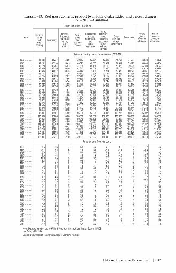
National Income or Expenditure | 347
Table B–13. Real gross domestic product by industry, value added, and percent changes,1979–2008—Continued
Year
Private industries—Continued
GovernmentPrivategoods-
producingindustries 1
Privateservices-producing
industries 2
Transpor-tationand
ware-housing
Information
Finance,insurance,real estate,
rental,and
leasing
Profes-sionaland
businessservices
Educationalservices,
health care,and
socialassistance
Arts,entertain-
ment,recreation,accommo-
dation,and foodservices
Otherservices,except
government
Chain-type quantity indexes for value added (2000=100)
1979 ............. 48.252 34.231 52.965 39.387 63.234 53.512 75.703 77.721 56.085 48.1201980 ............. 47.232 36.394 55.414 40.529 66.887 52.407 74.411 79.023 53.880 48.7641981 ............. 46.178 38.257 56.573 41.554 68.455 54.193 72.329 79.328 55.783 49.9231982 ............. 43.855 38.155 56.986 41.345 68.856 55.695 69.103 79.456 52.029 49.7941983 ............. 49.486 41.017 58.734 44.142 71.153 59.784 72.470 80.178 53.361 52.6371984 ............. 52.121 40.717 61.282 48.913 72.366 62.194 77.498 81.038 59.454 55.7271985 ............. 52.715 42.039 62.812 52.748 73.629 66.167 80.936 83.172 62.569 58.1041986 ............. 53.021 42.672 63.965 56.860 75.166 69.642 82.885 85.105 62.534 60.5761987 ............. 55.690 45.764 65.941 60.050 80.273 68.742 84.221 86.753 66.173 62.2561988 ............. 57.990 47.649 68.652 64.420 80.570 71.515 89.044 88.812 69.104 65.1861989 ............. 59.507 51.150 70.359 68.787 84.002 73.872 92.188 90.984 70.366 68.0331990 ............. 62.281 53.420 71.877 72.073 87.047 76.063 94.369 93.215 69.858 69.8771991 ............. 65.060 54.441 73.051 69.786 89.285 74.232 91.258 93.658 68.214 70.3191992 ............. 68.758 57.568 74.863 72.008 91.728 77.250 92.502 94.134 70.330 73.0741993 ............. 71.988 61.445 76.931 73.224 92.199 78.787 95.195 94.055 72.128 75.0471994 ............. 77.827 65.223 78.506 75.430 92.413 80.604 98.624 94.407 77.818 77.7451995 ............. 80.473 67.996 80.732 77.382 93.503 83.542 99.714 94.250 79.572 79.7731996 ............. 84.585 72.714 82.893 82.053 94.144 86.796 99.072 94.768 82.596 83.3771997 ............. 88.373 74.559 86.786 87.432 94.809 90.310 99.291 95.864 87.229 87.4071998 ............. 91.454 82.252 90.201 91.976 95.603 93.446 101.871 96.923 91.878 91.5911999 ............. 95.301 95.467 94.994 96.898 97.304 96.836 100.236 98.009 95.402 96.4342000 ............. 100.000 100.000 100.000 100.000 100.000 100.000 100.000 100.000 100.000 100.0002001 ............. 97.354 104.034 103.858 99.346 103.186 99.292 98.337 100.794 95.654 102.5842002 ............. 99.531 106.263 104.800 99.192 107.527 101.022 98.667 102.467 96.853 104.1072003 ............. 101.534 109.430 107.288 103.554 112.257 104.138 100.615 103.776 97.402 107.4962004 ............. 110.780 122.221 110.433 107.750 115.949 108.114 100.770 104.252 101.328 111.6922005 ............. 115.253 132.881 115.054 113.709 119.231 110.366 102.776 104.962 101.915 116.6242006 ............. 117.627 136.503 119.756 117.579 123.043 114.158 102.381 105.509 104.628 120.4142007 ............. 120.592 147.542 122.183 122.646 125.627 116.126 102.756 106.914 103.880 123.8702008 ............. 116.091 155.211 122.100 129.361 131.207 118.049 103.026 109.033 100.718 125.879
Percent change from year earlier
1979 ............. 5.6 8.6 5.2 6.8 4.2 2.8 0.8 1.3 2.7 4.21980 ............. –2.1 6.3 4.6 2.9 5.8 –2.1 –1.7 1.7 –3.9 1.31981 ............. –2.2 5.1 2.1 2.5 2.3 3.4 –2.8 .4 3.5 2.41982 ............. –5.0 –.3 .7 –.5 .6 2.8 –4.5 .2 –6.7 –.31983 ............. 12.8 7.5 3.1 6.8 3.3 7.3 4.9 .9 2.6 5.71984 ............. 5.3 –.7 4.3 10.8 1.7 4.0 6.9 1.1 11.4 5.91985 ............. 1.1 3.2 2.5 7.8 1.7 6.4 4.4 2.6 5.2 4.31986 ............. .6 1.5 1.8 7.8 2.1 5.3 2.4 2.3 –.1 4.31987 ............. 5.0 7.2 3.1 5.6 6.8 –1.3 1.6 1.9 5.8 2.81988 ............. 4.1 4.1 4.1 7.3 .4 4.0 5.7 2.4 4.4 4.71989 ............. 2.6 7.3 2.5 6.8 4.3 3.3 3.5 2.4 1.8 4.41990 ............. 4.7 4.4 2.2 4.8 3.6 3.0 2.4 2.5 –.7 2.71991 ............. 4.5 1.9 1.6 –3.2 2.6 –2.4 –3.3 .5 –2.4 .61992 ............. 5.7 5.7 2.5 3.2 2.7 4.1 1.4 .5 3.1 3.91993 ............. 4.7 6.7 2.8 1.7 .5 2.0 2.9 –.1 2.6 2.71994 ............. 8.1 6.1 2.0 3.0 .2 2.3 3.6 .4 7.9 3.61995 ............. 3.4 4.3 2.8 2.6 1.2 3.6 1.1 –.2 2.3 2.61996 ............. 5.1 6.9 2.7 6.0 .7 3.9 –.6 .5 3.8 4.51997 ............. 4.5 2.5 4.7 6.6 .7 4.0 .2 1.2 5.6 4.81998 ............. 3.5 10.3 3.9 5.2 .8 3.5 2.6 1.1 5.3 4.81999 ............. 4.2 16.1 5.3 5.4 1.8 3.6 –1.6 1.1 3.8 5.32000 ............. 4.9 4.7 5.3 3.2 2.8 3.3 –.2 2.0 4.8 3.72001 ............. –2.6 4.0 3.9 –.7 3.2 –.7 –1.7 .8 –4.3 2.62002 ............. 2.2 2.1 .9 –.2 4.2 1.7 .3 1.7 1.3 1.52003 ............. 2.0 3.0 2.4 4.4 4.4 3.1 2.0 1.3 .6 3.32004 ............. 9.1 11.7 2.9 4.1 3.3 3.8 .2 .5 4.0 3.92005 ............. 4.0 8.7 4.2 5.5 2.8 2.1 2.0 .7 .6 4.42006 ............. 2.1 2.7 4.1 3.4 3.2 3.4 –.4 .5 2.7 3.22007 ............. 2.5 8.1 2.0 4.3 2.1 1.7 .4 1.3 –.7 2.92008 ............. –3.7 5.2 –.1 5.5 4.4 1.7 .3 2.0 –3.0 1.6
Note: Data are based on the 1997 North American Industry Classification System (NAICS).See Note, Table B–12.Source: Department of Commerce (Bureau of Economic Analysis).
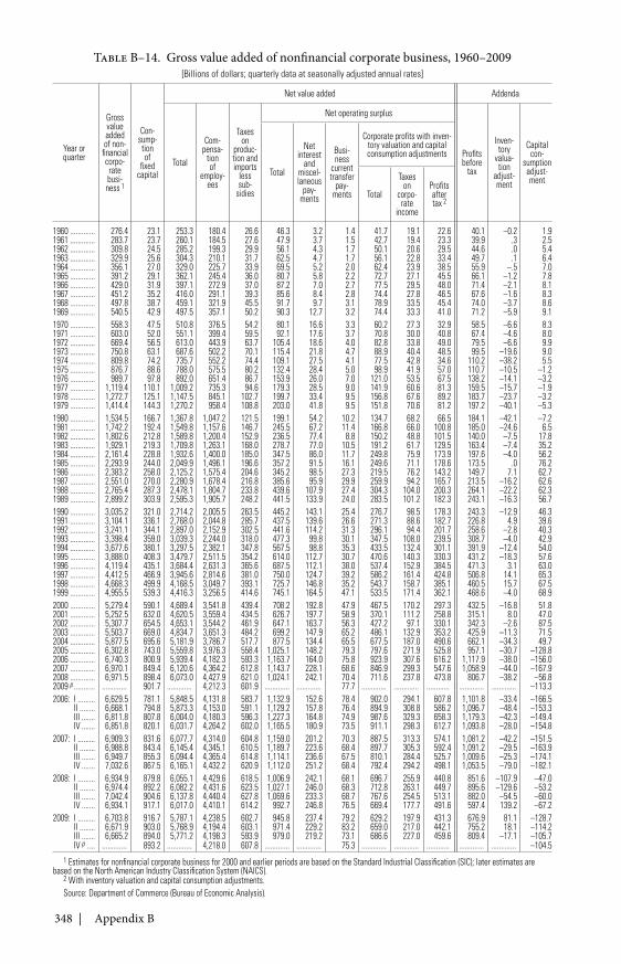
348 | Appendix B
Table B–14. Gross value added of nonfinancial corporate business, 1960–2009[Billions of dollars; quarterly data at seasonally adjusted annual rates]
Year orquarter
Grossvalueaddedof non-
financialcorpo-ratebusi-ness 1
Con-sump-tionof
fixedcapital
Net value added Addenda
Total
Com-pensa-
tionof
employ-ees
Taxeson
produc-tion andimports
lesssub-
sidies
Net operating surplus
Profitsbefore
tax
Inven-tory
valua-tion
adjust-ment
Capitalcon-
sumptionadjust-ment
Total
Netinterest
andmiscel-laneous
pay-ments
Busi-ness
currenttransfer
pay-ments
Corporate profits with inven-tory valuation and capitalconsumption adjustments
Total
Taxeson
corpo-rate
income
Profitsaftertax 2
1960 ............. 276.4 23.1 253.3 180.4 26.6 46.3 3.2 1.4 41.7 19.1 22.6 40.1 –0.2 1.91961 ............. 283.7 23.7 260.1 184.5 27.6 47.9 3.7 1.5 42.7 19.4 23.3 39.9 .3 2.51962 ............. 309.8 24.5 285.2 199.3 29.9 56.1 4.3 1.7 50.1 20.6 29.5 44.6 .0 5.41963 ............. 329.9 25.6 304.3 210.1 31.7 62.5 4.7 1.7 56.1 22.8 33.4 49.7 .1 6.41964 ............. 356.1 27.0 329.0 225.7 33.9 69.5 5.2 2.0 62.4 23.9 38.5 55.9 –.5 7.01965 ............. 391.2 29.1 362.1 245.4 36.0 80.7 5.8 2.2 72.7 27.1 45.5 66.1 –1.2 7.81966 ............. 429.0 31.9 397.1 272.9 37.0 87.2 7.0 2.7 77.5 29.5 48.0 71.4 –2.1 8.11967 ............. 451.2 35.2 416.0 291.1 39.3 85.6 8.4 2.8 74.4 27.8 46.5 67.6 –1.6 8.31968 ............. 497.8 38.7 459.1 321.9 45.5 91.7 9.7 3.1 78.9 33.5 45.4 74.0 –3.7 8.61969 ............. 540.5 42.9 497.5 357.1 50.2 90.3 12.7 3.2 74.4 33.3 41.0 71.2 –5.9 9.11970 ............. 558.3 47.5 510.8 376.5 54.2 80.1 16.6 3.3 60.2 27.3 32.9 58.5 –6.6 8.31971 ............. 603.0 52.0 551.1 399.4 59.5 92.1 17.6 3.7 70.8 30.0 40.8 67.4 –4.6 8.01972 ............. 669.4 56.5 613.0 443.9 63.7 105.4 18.6 4.0 82.8 33.8 49.0 79.5 –6.6 9.91973 ............. 750.8 63.1 687.6 502.2 70.1 115.4 21.8 4.7 88.9 40.4 48.5 99.5 –19.6 9.01974 ............. 809.8 74.2 735.7 552.2 74.4 109.1 27.5 4.1 77.5 42.8 34.6 110.2 –38.2 5.51975 ............. 876.7 88.6 788.0 575.5 80.2 132.4 28.4 5.0 98.9 41.9 57.0 110.7 –10.5 –1.21976 ............. 989.7 97.8 892.0 651.4 86.7 153.9 26.0 7.0 121.0 53.5 67.5 138.2 –14.1 –3.21977 ............. 1,119.4 110.1 1,009.2 735.3 94.6 179.3 28.5 9.0 141.9 60.6 81.3 159.5 –15.7 –1.91978 ............. 1,272.7 125.1 1,147.5 845.1 102.7 199.7 33.4 9.5 156.8 67.6 89.2 183.7 –23.7 –3.21979 ............. 1,414.4 144.3 1,270.2 958.4 108.8 203.0 41.8 9.5 151.8 70.6 81.2 197.2 –40.1 –5.31980 ............. 1,534.5 166.7 1,367.8 1,047.2 121.5 199.1 54.2 10.2 134.7 68.2 66.5 184.1 –42.1 –7.21981 ............. 1,742.2 192.4 1,549.8 1,157.6 146.7 245.5 67.2 11.4 166.8 66.0 100.8 185.0 –24.6 6.51982 ............. 1,802.6 212.8 1,589.8 1,200.4 152.9 236.5 77.4 8.8 150.2 48.8 101.5 140.0 –7.5 17.81983 ............. 1,929.1 219.3 1,709.8 1,263.1 168.0 278.7 77.0 10.5 191.2 61.7 129.5 163.4 –7.4 35.21984 ............. 2,161.4 228.8 1,932.6 1,400.0 185.0 347.5 86.0 11.7 249.8 75.9 173.9 197.6 –4.0 56.21985 ............. 2,293.9 244.0 2,049.9 1,496.1 196.6 357.2 91.5 16.1 249.6 71.1 178.6 173.5 .0 76.21986 ............. 2,383.2 258.0 2,125.2 1,575.4 204.6 345.2 98.5 27.3 219.5 76.2 143.2 149.7 7.1 62.71987 ............. 2,551.0 270.0 2,280.9 1,678.4 216.8 385.6 95.9 29.9 259.9 94.2 165.7 213.5 –16.2 62.61988 ............. 2,765.4 287.3 2,478.1 1,804.7 233.8 439.6 107.9 27.4 304.3 104.0 200.3 264.1 –22.2 62.31989 ............. 2,899.2 303.9 2,595.3 1,905.7 248.2 441.5 133.9 24.0 283.5 101.2 182.3 243.1 –16.3 56.71990 ............. 3,035.2 321.0 2,714.2 2,005.5 263.5 445.2 143.1 25.4 276.7 98.5 178.3 243.3 –12.9 46.31991 ............. 3,104.1 336.1 2,768.0 2,044.8 285.7 437.5 139.6 26.6 271.3 88.6 182.7 226.8 4.9 39.61992 ............. 3,241.1 344.1 2,897.0 2,152.9 302.5 441.6 114.2 31.3 296.1 94.4 201.7 258.6 –2.8 40.31993 ............. 3,398.4 359.0 3,039.3 2,244.0 318.0 477.3 99.8 30.1 347.5 108.0 239.5 308.7 –4.0 42.91994 ............. 3,677.6 380.1 3,297.5 2,382.1 347.8 567.5 98.8 35.3 433.5 132.4 301.1 391.9 –12.4 54.01995 ............. 3,888.0 408.3 3,479.7 2,511.5 354.2 614.0 112.7 30.7 470.6 140.3 330.3 431.2 –18.3 57.61996 ............. 4,119.4 435.1 3,684.4 2,631.3 365.6 687.5 112.1 38.0 537.4 152.9 384.5 471.3 3.1 63.01997 ............. 4,412.5 466.9 3,945.6 2,814.6 381.0 750.0 124.7 39.2 586.2 161.4 424.8 506.8 14.1 65.31998 ............. 4,668.3 499.9 4,168.5 3,049.7 393.1 725.7 146.8 35.2 543.7 158.7 385.1 460.5 15.7 67.51999 ............. 4,955.5 539.3 4,416.3 3,256.5 414.6 745.1 164.5 47.1 533.5 171.4 362.1 468.6 –4.0 68.92000 ............. 5,279.4 590.1 4,689.4 3,541.8 439.4 708.2 192.8 47.9 467.5 170.2 297.3 432.5 –16.8 51.82001 ............. 5,252.5 632.0 4,620.5 3,559.4 434.5 626.7 197.7 58.9 370.1 111.2 258.8 315.1 8.0 47.02002 ............. 5,307.7 654.5 4,653.1 3,544.2 461.9 647.1 163.7 56.3 427.2 97.1 330.1 342.3 –2.6 87.52003 ............. 5,503.7 669.0 4,834.7 3,651.3 484.2 699.2 147.9 65.2 486.1 132.9 353.2 425.9 –11.3 71.52004 ............. 5,877.5 695.6 5,181.9 3,786.7 517.7 877.5 134.4 65.5 677.5 187.0 490.6 662.1 –34.3 49.72005 ............. 6,302.8 743.0 5,559.8 3,976.3 558.4 1,025.1 148.2 79.3 797.6 271.9 525.8 957.1 –30.7 –128.82006 ............. 6,740.3 800.9 5,939.4 4,182.3 593.3 1,163.7 164.0 75.8 923.9 307.6 616.2 1,117.9 –38.0 –156.02007 ............. 6,970.1 849.4 6,120.6 4,364.2 612.8 1,143.7 228.1 68.6 846.9 299.3 547.6 1,058.9 –44.0 –167.92008 ............. 6,971.5 898.4 6,073.0 4,427.9 621.0 1,024.1 242.1 70.4 711.6 237.8 473.8 806.7 –38.2 –56.82009 p ........... ............. 901.7 ............. 4,212.3 601.9 ............. ............. 77.7 ............. ............. ............ ............. ............. –113.32006: I ......... 6,629.5 781.1 5,848.5 4,131.8 583.7 1,132.9 152.6 78.4 902.0 294.1 607.8 1,101.8 –33.4 –166.5
II ........ 6,668.1 794.8 5,873.3 4,153.0 591.1 1,129.2 157.8 76.4 894.9 308.8 586.2 1,096.7 –48.4 –153.3III ....... 6,811.8 807.8 6,004.0 4,180.3 596.3 1,227.3 164.8 74.9 987.6 329.3 658.3 1,179.3 –42.3 –149.4IV ....... 6,851.8 820.1 6,031.7 4,264.2 602.0 1,165.5 180.9 73.5 911.1 298.3 612.7 1,093.8 –28.0 –154.8
2007: I ......... 6,909.3 831.6 6,077.7 4,314.0 604.8 1,159.0 201.2 70.3 887.5 313.3 574.1 1,081.2 –42.2 –151.5II ........ 6,988.8 843.4 6,145.4 4,345.1 610.5 1,189.7 223.6 68.4 897.7 305.3 592.4 1,091.2 –29.5 –163.9III ....... 6,949.7 855.3 6,094.4 4,365.4 614.8 1,114.1 236.6 67.5 810.1 284.4 525.7 1,009.6 –25.3 –174.1IV ....... 7,032.6 867.5 6,165.1 4,432.2 620.9 1,112.0 251.2 68.4 792.4 294.2 498.1 1,053.5 –79.0 –182.1
2008: I ......... 6,934.9 879.8 6,055.1 4,429.6 618.5 1,006.9 242.1 68.1 696.7 255.9 440.8 851.6 –107.9 –47.0II ........ 6,974.4 892.2 6,082.2 4,431.6 623.5 1,027.1 246.0 68.3 712.8 263.1 449.7 895.6 –129.6 –53.2III ....... 7,042.4 904.6 6,137.8 4,440.4 627.8 1,069.6 233.3 68.7 767.6 254.5 513.1 882.0 –54.5 –60.0IV ....... 6,934.1 917.1 6,017.0 4,410.1 614.2 992.7 246.8 76.5 669.4 177.7 491.6 597.4 139.2 –67.2
2009: I ......... 6,703.8 916.7 5,787.1 4,238.5 602.7 945.8 237.4 79.2 629.2 197.9 431.3 676.9 81.1 –128.7II ........ 6,671.9 903.0 5,768.9 4,194.4 603.1 971.4 229.2 83.2 659.0 217.0 442.1 755.2 18.1 –114.2III ....... 6,665.2 894.0 5,771.2 4,198.3 593.9 979.0 219.2 73.1 686.6 227.0 459.6 809.4 –17.1 –105.7IV p .... ............. 893.2 ............. 4,218.0 607.8 ............. ............. 75.3 ............. ............. ............ ............. ............. –104.5
1 Estimates for nonfinancial corporate business for 2000 and earlier periods are based on the Standard Industrial Classification (SIC); later estimates arebased on the North American Industry Classification System (NAICS).
2 With inventory valuation and capital consumption adjustments.Source: Department of Commerce (Bureau of Economic Analysis).
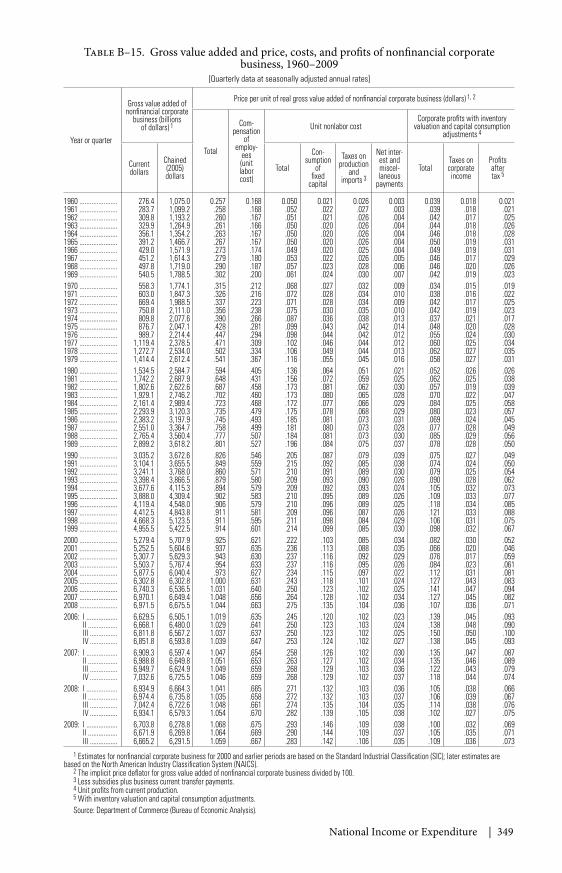
National Income or Expenditure | 349
Table B–15. Gross value added and price, costs, and profits of nonfinancial corporatebusiness, 1960–2009
[Quarterly data at seasonally adjusted annual rates]
Year or quarter
Gross value added ofnonfinancial corporate
business (billionsof dollars) 1
Price per unit of real gross value added of nonfinancial corporate business (dollars) 1, 2
Total
Com-pensation
ofemploy-
ees(unitlaborcost)
Unit nonlabor costCorporate profits with inventory
valuation and capital consumptionadjustments 4
Currentdollars
Chained(2005)dollars
Total
Con-sumption
offixed
capital
Taxes onproduction
andimports 3
Net inter-est andmiscel-laneous
payments
TotalTaxes oncorporateincome
Profitsaftertax 5
1960 ...................... 276.4 1,075.0 0.257 0.168 0.050 0.021 0.026 0.003 0.039 0.018 0.0211961 ...................... 283.7 1,099.2 .258 .168 .052 .022 .027 .003 .039 .018 .0211962 ...................... 309.8 1,193.2 .260 .167 .051 .021 .026 .004 .042 .017 .0251963 ...................... 329.9 1,264.9 .261 .166 .050 .020 .026 .004 .044 .018 .0261964 ...................... 356.1 1,354.2 .263 .167 .050 .020 .026 .004 .046 .018 .0281965 ...................... 391.2 1,466.7 .267 .167 .050 .020 .026 .004 .050 .019 .0311966 ...................... 429.0 1,571.9 .273 .174 .049 .020 .025 .004 .049 .019 .0311967 ...................... 451.2 1,614.3 .279 .180 .053 .022 .026 .005 .046 .017 .0291968 ...................... 497.8 1,719.0 .290 .187 .057 .023 .028 .006 .046 .020 .0261969 ...................... 540.5 1,788.5 .302 .200 .061 .024 .030 .007 .042 .019 .0231970 ...................... 558.3 1,774.1 .315 .212 .068 .027 .032 .009 .034 .015 .0191971 ...................... 603.0 1,847.3 .326 .216 .072 .028 .034 .010 .038 .016 .0221972 ...................... 669.4 1,988.5 .337 .223 .071 .028 .034 .009 .042 .017 .0251973 ...................... 750.8 2,111.0 .356 .238 .075 .030 .035 .010 .042 .019 .0231974 ...................... 809.8 2,077.6 .390 .266 .087 .036 .038 .013 .037 .021 .0171975 ...................... 876.7 2,047.1 .428 .281 .099 .043 .042 .014 .048 .020 .0281976 ...................... 989.7 2,214.4 .447 .294 .098 .044 .042 .012 .055 .024 .0301977 ...................... 1,119.4 2,378.5 .471 .309 .102 .046 .044 .012 .060 .025 .0341978 ...................... 1,272.7 2,534.0 .502 .334 .106 .049 .044 .013 .062 .027 .0351979 ...................... 1,414.4 2,612.4 .541 .367 .116 .055 .045 .016 .058 .027 .0311980 ...................... 1,534.5 2,584.7 .594 .405 .136 .064 .051 .021 .052 .026 .0261981 ...................... 1,742.2 2,687.9 .648 .431 .156 .072 .059 .025 .062 .025 .0381982 ...................... 1,802.6 2,622.6 .687 .458 .173 .081 .062 .030 .057 .019 .0391983 ...................... 1,929.1 2,746.2 .702 .460 .173 .080 .065 .028 .070 .022 .0471984 ...................... 2,161.4 2,989.4 .723 .468 .172 .077 .066 .029 .084 .025 .0581985 ...................... 2,293.9 3,120.3 .735 .479 .175 .078 .068 .029 .080 .023 .0571986 ...................... 2,383.2 3,197.9 .745 .493 .185 .081 .073 .031 .069 .024 .0451987 ...................... 2,551.0 3,364.7 .758 .499 .181 .080 .073 .028 .077 .028 .0491988 ...................... 2,765.4 3,560.4 .777 .507 .184 .081 .073 .030 .085 .029 .0561989 ...................... 2,899.2 3,618.2 .801 .527 .196 .084 .075 .037 .078 .028 .0501990 ...................... 3,035.2 3,672.6 .826 .546 .205 .087 .079 .039 .075 .027 .0491991 ...................... 3,104.1 3,655.5 .849 .559 .215 .092 .085 .038 .074 .024 .0501992 ...................... 3,241.1 3,768.0 .860 .571 .210 .091 .089 .030 .079 .025 .0541993 ...................... 3,398.4 3,866.5 .879 .580 .209 .093 .090 .026 .090 .028 .0621994 ...................... 3,677.6 4,115.3 .894 .579 .209 .092 .093 .024 .105 .032 .0731995 ...................... 3,888.0 4,309.4 .902 .583 .210 .095 .089 .026 .109 .033 .0771996 ...................... 4,119.4 4,548.0 .906 .579 .210 .096 .089 .025 .118 .034 .0851997 ...................... 4,412.5 4,843.8 .911 .581 .209 .096 .087 .026 .121 .033 .0881998 ...................... 4,668.3 5,123.5 .911 .595 .211 .098 .084 .029 .106 .031 .0751999 ...................... 4,955.5 5,422.5 .914 .601 .214 .099 .085 .030 .098 .032 .0672000 ...................... 5,279.4 5,707.9 .925 .621 .222 .103 .085 .034 .082 .030 .0522001 ...................... 5,252.5 5,604.6 .937 .635 .236 .113 .088 .035 .066 .020 .0462002 ...................... 5,307.7 5,629.3 .943 .630 .237 .116 .092 .029 .076 .017 .0592003 ...................... 5,503.7 5,767.4 .954 .633 .237 .116 .095 .026 .084 .023 .0612004 ...................... 5,877.5 6,040.4 .973 .627 .234 .115 .097 .022 .112 .031 .0812005 ...................... 6,302.8 6,302.8 1.000 .631 .243 .118 .101 .024 .127 .043 .0832006 ...................... 6,740.3 6,536.5 1.031 .640 .250 .123 .102 .025 .141 .047 .0942007 ...................... 6,970.1 6,649.4 1.048 .656 .264 .128 .102 .034 .127 .045 .0822008 ...................... 6,971.5 6,675.5 1.044 .663 .275 .135 .104 .036 .107 .036 .0712006: I .................. 6,629.5 6,505.1 1.019 .635 .245 .120 .102 .023 .139 .045 .093
II ................. 6,668.1 6,480.0 1.029 .641 .250 .123 .103 .024 .138 .048 .090III ................ 6,811.8 6,567.2 1.037 .637 .250 .123 .102 .025 .150 .050 .100IV ................ 6,851.8 6,593.8 1.039 .647 .253 .124 .102 .027 .138 .045 .093
2007: I .................. 6,909.3 6,597.4 1.047 .654 .258 .126 .102 .030 .135 .047 .087II ................. 6,988.8 6,649.8 1.051 .653 .263 .127 .102 .034 .135 .046 .089III ................ 6,949.7 6,624.9 1.049 .659 .268 .129 .103 .036 .122 .043 .079IV ................ 7,032.6 6,725.5 1.046 .659 .268 .129 .102 .037 .118 .044 .074
2008: I .................. 6,934.9 6,664.3 1.041 .665 .271 .132 .103 .036 .105 .038 .066II ................. 6,974.4 6,735.8 1.035 .658 .272 .132 .103 .037 .106 .039 .067III ................ 7,042.4 6,722.6 1.048 .661 .274 .135 .104 .035 .114 .038 .076IV ................ 6,934.1 6,579.3 1.054 .670 .282 .139 .105 .038 .102 .027 .075
2009: I .................. 6,703.8 6,278.8 1.068 .675 .293 .146 .109 .038 .100 .032 .069II ................. 6,671.9 6,269.8 1.064 .669 .290 .144 .109 .037 .105 .035 .071III ................ 6,665.2 6,291.5 1.059 .667 .283 .142 .106 .035 .109 .036 .073
1 Estimates for nonfinancial corporate business for 2000 and earlier periods are based on the Standard Industrial Classification (SIC); later estimates arebased on the North American Industry Classification System (NAICS).
2 The implicit price deflator for gross value added of nonfinancial corporate business divided by 100.3 Less subsidies plus business current transfer payments.4 Unit profits from current production.5 With inventory valuation and capital consumption adjustments.Source: Department of Commerce (Bureau of Economic Analysis).
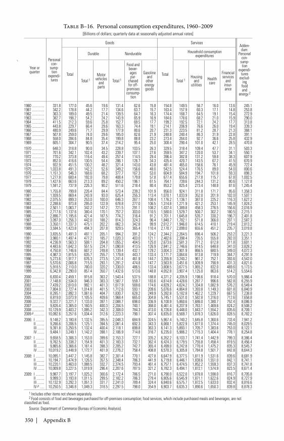
350 | Appendix B
Table B–16. Personal consumption expenditures, 1960–2009[Billions of dollars; quarterly data at seasonally adjusted annual rates]
Year orquarter
Personalcon-
sump-tion
expendi-tures
Goods ServicesAdden-dum:
Personalcon-
sump-tion
expendi-tures
exclud-ing
foodand
energy 2
Total
Durable Nondurable
Total
Household consumptionexpenditures
Total 1Motor
vehiclesand
partsTotal 1
Food andbever-agespur-
chasedfor off-
premisesconsump-
tion
Gasolineand
otherenergygoods
Total 1Housing
andutilities
Healthcare
Financialservices
andinsur-ance
1960 .............. 331.8 177.0 45.6 19.6 131.4 62.6 15.8 154.8 149.5 56.7 16.0 13.6 245.11961 .............. 342.2 178.8 44.2 17.7 134.6 63.7 15.7 163.4 157.9 60.3 17.1 14.8 253.81962 .............. 363.3 189.0 49.5 21.4 139.5 64.7 16.3 174.4 168.7 64.5 19.1 15.4 272.91963 .............. 382.7 198.2 54.2 24.2 143.9 65.9 16.9 184.6 178.6 68.2 21.0 15.9 290.01964 .............. 411.5 212.3 59.6 25.8 152.7 69.5 17.7 199.2 192.5 72.1 24.2 17.7 313.81965 .............. 443.8 229.7 66.4 29.6 163.3 74.4 19.1 214.1 206.9 76.6 26.0 19.4 339.31966 .............. 480.9 249.6 71.7 29.9 177.9 80.6 20.7 231.3 223.5 81.2 28.7 21.3 368.11967 .............. 507.8 259.0 74.0 29.6 185.0 82.6 21.9 248.8 240.4 86.3 31.9 22.8 391.11968 .............. 558.0 284.6 84.8 35.4 199.8 88.8 23.2 273.4 264.0 92.7 36.6 25.8 432.91969 .............. 605.1 304.7 90.5 37.4 214.2 95.4 25.0 300.4 290.4 101.0 42.1 28.5 470.81970 .............. 648.3 318.8 90.0 34.5 228.8 103.5 26.3 329.5 318.4 109.4 47.7 31.1 503.31971 .............. 701.6 342.1 102.4 43.2 239.7 107.1 27.6 359.5 347.2 120.0 53.7 34.1 550.11972 .............. 770.2 373.8 116.4 49.4 257.4 114.5 29.4 396.4 382.8 131.2 59.8 38.3 607.91973 .............. 852.0 416.6 130.5 54.4 286.1 126.7 34.3 435.4 420.7 143.5 67.2 41.5 670.91974 .............. 932.9 451.5 130.2 48.2 321.4 143.0 43.8 481.4 465.0 158.6 76.1 45.9 722.41975 .............. 1,033.8 491.3 142.2 52.6 349.2 156.6 48.0 542.5 524.4 176.5 89.0 54.0 800.61976 .............. 1,151.3 546.3 168.6 68.2 377.7 167.3 53.0 604.9 584.9 194.7 101.8 59.3 898.31977 .............. 1,277.8 600.4 192.0 79.8 408.4 179.8 57.8 677.4 655.6 217.8 115.7 67.8 1,002.51978 .............. 1,427.6 663.6 213.3 89.2 450.2 196.1 61.5 764.1 739.6 244.3 131.2 80.6 1,127.81979 .............. 1,591.2 737.9 226.3 90.2 511.6 218.4 80.4 853.2 825.4 273.4 148.8 87.6 1,245.41980 .............. 1,755.8 799.8 226.4 84.4 573.4 239.2 101.9 956.0 924.1 311.8 171.7 95.6 1,358.31981 .............. 1,939.5 869.4 243.9 93.0 625.4 255.3 113.4 1,070.1 1,033.9 352.0 201.9 102.0 1,507.11982 .............. 2,075.5 899.3 253.0 100.0 646.3 267.1 108.4 1,176.2 1,136.1 387.0 225.2 116.3 1,627.21983 .............. 2,288.6 973.8 295.0 122.9 678.8 277.0 106.5 1,314.8 1,271.9 421.2 253.1 145.9 1,824.21984 .............. 2,501.1 1,063.7 342.2 147.2 721.5 291.1 108.2 1,437.4 1,389.8 458.3 276.5 156.6 2,016.91985 .............. 2,717.6 1,137.6 380.4 170.1 757.2 303.0 110.5 1,580.0 1,529.7 500.7 302.2 180.5 2,215.11986 .............. 2,896.7 1,195.6 421.4 187.5 774.2 316.4 91.2 1,701.1 1,645.8 535.7 330.2 196.7 2,401.81987 .............. 3,097.0 1,256.3 442.0 188.2 814.3 324.3 96.4 1,840.7 1,782.1 571.8 366.0 207.1 2,587.31988 .............. 3,350.1 1,337.3 475.1 202.2 862.3 342.8 99.9 2,012.7 1,946.0 614.5 410.1 219.4 2,813.21989 .............. 3,594.5 1,423.8 494.3 207.8 929.5 365.4 110.4 2,170.7 2,099.0 655.6 451.2 235.7 3,019.81990 .............. 3,835.5 1,491.3 497.1 205.1 994.2 391.2 124.2 2,344.2 2,264.5 696.4 506.2 253.2 3,221.31991 .............. 3,980.1 1,497.4 477.2 185.7 1,020.3 403.0 121.1 2,482.6 2,398.4 735.5 555.8 282.0 3,351.11992 .............. 4,236.9 1,563.3 508.1 204.8 1,055.2 404.5 125.0 2,673.6 2,581.3 771.2 612.8 311.8 3,601.11993 .............. 4,483.6 1,642.3 551.5 224.7 1,090.8 413.5 126.9 2,841.2 2,746.6 814.5 648.8 341.0 3,828.21994 .............. 4,750.8 1,746.6 607.2 249.8 1,139.4 432.1 129.2 3,004.3 2,901.9 866.5 680.5 349.0 4,072.31995 .............. 4,987.3 1,815.5 635.7 255.7 1,179.8 443.7 133.4 3,171.7 3,064.6 913.8 719.9 364.7 4,291.91996 .............. 5,273.6 1,917.7 676.3 273.5 1,241.4 461.9 144.7 3,355.9 3,240.2 961.2 752.1 393.6 4,542.01997 .............. 5,570.6 2,006.8 715.5 293.1 1,291.2 474.8 147.7 3,563.9 3,451.6 1,009.9 790.9 431.3 4,821.61998 .............. 5,918.5 2,110.0 780.0 320.2 1,330.0 486.5 133.4 3,808.5 3,677.5 1,065.2 832.0 469.6 5,173.51999 .............. 6,342.8 2,290.0 857.4 350.7 1,432.6 513.6 148.8 4,052.8 3,907.4 1,125.0 863.6 514.2 5,554.62000 .............. 6,830.4 2,459.1 915.8 363.2 1,543.4 537.5 188.8 4,371.2 4,205.9 1,198.6 918.4 570.0 5,966.42001 .............. 7,148.8 2,534.0 946.3 383.3 1,587.7 559.7 183.6 4,614.8 4,428.6 1,287.7 996.6 562.8 6,255.92002 .............. 7,439.2 2,610.0 992.1 401.3 1,617.9 569.6 174.6 4,829.2 4,624.2 1,334.8 1,082.9 576.2 6,549.42003 .............. 7,804.0 2,727.4 1,014.8 401.5 1,712.6 593.1 209.6 5,076.6 4,864.8 1,393.8 1,149.3 601.8 6,840.92004 .............. 8,285.1 2,892.3 1,061.6 404.7 1,830.7 628.2 249.9 5,392.8 5,182.8 1,462.2 1,229.7 667.5 7,238.82005 .............. 8,819.0 3,073.9 1,105.5 409.6 1,968.4 665.0 304.8 5,745.1 5,531.0 1,582.8 1,316.0 712.6 7,658.82006 .............. 9,322.7 3,221.7 1,133.0 397.1 2,088.7 698.0 336.9 6,100.9 5,860.6 1,686.0 1,380.7 752.4 8,086.92007 .............. 9,826.4 3,365.0 1,160.5 400.3 2,204.5 740.1 368.0 6,461.4 6,207.9 1,763.1 1,469.6 824.2 8,508.22008 .............. 10,129.9 3,403.2 1,095.2 342.3 2,308.0 784.3 413.0 6,726.8 6,448.0 1,843.7 1,554.2 835.6 8,709.12009 p ............ 10,092.6 3,257.6 1,034.4 312.6 2,223.3 790.1 307.4 6,835.0 6,569.7 1,878.3 1,626.0 828.5 8,782.22006: I .......... 9,148.2 3,180.8 1,132.5 395.5 2,048.3 684.9 324.5 5,967.4 5,740.2 1,645.8 1,360.6 733.4 7,941.2
II ......... 9,266.6 3,206.5 1,125.1 394.5 2,081.4 692.3 343.3 6,060.1 5,822.9 1,677.0 1,374.4 745.0 8,029.5III ........ 9,391.8 3,250.5 1,132.4 400.4 2,118.1 699.8 363.3 6,141.3 5,893.1 1,705.7 1,383.6 753.0 8,122.1IV ........ 9,484.1 3,249.1 1,142.2 398.1 2,106.9 714.8 316.7 6,235.0 5,986.2 1,715.3 1,404.4 778.1 8,254.8
2007: I .......... 9,658.5 3,306.3 1,153.0 399.6 2,153.3 727.1 335.2 6,352.2 6,103.7 1,741.4 1,442.9 799.3 8,386.4II ......... 9,762.5 3,338.2 1,154.9 401.3 2,183.3 732.1 362.4 6,424.3 6,179.5 1,755.8 1,458.4 819.5 8,456.4III ........ 9,865.6 3,366.6 1,161.4 398.3 2,205.2 742.7 365.4 6,499.0 6,242.8 1,770.4 1,475.2 835.3 8,545.7IV ........ 10,019.2 3,448.9 1,172.7 401.9 2,276.2 758.4 408.8 6,570.3 6,305.8 1,784.8 1,501.7 842.8 8,644.3
2008: I .......... 10,095.1 3,447.2 1,145.8 382.7 2,301.4 770.1 427.8 6,647.9 6,377.5 1,811.9 1,531.6 839.6 8,681.9II ......... 10,194.7 3,474.9 1,126.5 357.5 2,348.4 786.3 441.9 6,719.8 6,446.1 1,838.6 1,551.0 842.1 8,741.1III ........ 10,220.1 3,463.0 1,088.5 332.7 2,374.5 793.4 461.4 6,757.1 6,474.5 1,852.2 1,559.3 837.3 8,741.8IV ........ 10,009.8 3,227.5 1,019.9 296.4 2,207.6 787.5 321.2 6,782.3 6,494.1 1,872.1 1,574.9 823.5 8,671.4
2009: I .......... 9,987.7 3,197.7 1,025.2 300.6 2,172.4 786.5 271.0 6,790.0 6,522.0 1,878.8 1,598.0 816.7 8,705.8II ......... 9,999.3 3,193.8 1,011.5 299.5 2,182.2 786.3 279.4 6,805.6 6,545.9 1,871.1 1,622.6 824.9 8,727.9III ........ 10,132.9 3,292.3 1,051.3 331.7 2,241.0 789.4 324.4 6,840.6 6,575.7 1,872.5 1,633.0 832.4 8,816.6IV p ..... 10,250.5 3,346.8 1,049.3 318.5 2,297.5 798.0 354.9 6,903.7 6,635.3 1,890.6 1,650.3 839.8 8,878.3
1 Includes other items not shown separately.2 Food consists of food and beverages purchased for off-premises consumption; food services, which include purchased meals and beverages, are not
classified as food.Source: Department of Commerce (Bureau of Economic Analysis).
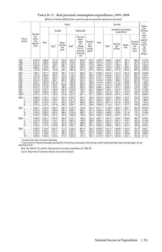
National Income or Expenditure | 351
Table B–17. Real personal consumption expenditures, 1995–2009[Billions of chained (2005) dollars; quarterly data at seasonally adjusted annual rates]
Year orquarter
Personalcon-
sump-tion
expendi-tures
Goods ServicesAdden-dum:
Personalcon-
sump-tion
expendi-tures
exclud-ing
foodand
energy 2
Total
Durable Nondurable
Total
Household consumptionexpenditures
Total 1Motor
vehiclesand
partsTotal 1
Food andbever-agespur-
chasedfor off-
premisesconsump-
tion
Gasolineand
otherenergygoods
Total 1Housing
andutilities
Healthcare
Financialservices
andinsur-ance
1995 .............. 6,079.0 1,898.6 511.6 255.6 1,437.8 548.5 264.3 4,208.2 4,068.6 1,234.9 947.5 489.4 5,126.41996 .............. 6,291.2 1,983.6 549.8 268.0 1,479.4 554.0 268.5 4,331.4 4,183.3 1,261.7 967.1 507.8 5,321.91997 .............. 6,523.4 2,078.2 594.7 286.1 1,522.9 558.9 273.9 4,465.0 4,327.2 1,290.4 997.1 525.2 5,543.31998 .............. 6,865.5 2,218.6 667.2 316.1 1,580.3 565.5 283.8 4,661.8 4,510.6 1,329.8 1,029.5 558.6 5,862.91999 .............. 7,240.9 2,395.3 753.8 345.1 1,660.9 587.4 292.5 4,852.8 4,690.4 1,371.8 1,045.6 605.6 6,202.52000 .............. 7,608.1 2,521.7 819.9 356.1 1,714.7 600.6 287.1 5,093.3 4,917.8 1,413.7 1,081.5 665.4 6,548.62001 .............. 7,813.9 2,600.9 864.4 374.3 1,745.6 607.6 289.2 5,218.7 5,028.8 1,451.5 1,135.4 660.7 6,745.72002 .............. 8,021.9 2,706.6 930.0 394.0 1,780.2 609.0 294.0 5,318.1 5,109.3 1,462.0 1,202.3 658.3 6,941.92003 .............. 8,247.6 2,829.9 986.1 405.3 1,845.6 622.4 302.2 5,418.4 5,199.0 1,480.2 1,229.4 657.8 7,142.02004 .............. 8,532.7 2,955.3 1,051.0 411.3 1,904.6 639.2 306.5 5,577.6 5,359.3 1,512.8 1,268.6 691.8 7,402.62005 .............. 8,819.0 3,073.9 1,105.5 409.6 1,968.4 665.0 304.8 5,745.1 5,531.0 1,582.8 1,316.0 712.6 7,658.82006 .............. 9,073.5 3,173.9 1,150.4 396.6 2,023.6 686.2 298.4 5,899.7 5,664.4 1,616.7 1,340.0 735.4 7,905.72007 .............. 9,313.9 3,273.7 1,199.9 402.4 2,074.8 700.7 300.7 6,040.8 5,796.1 1,631.8 1,375.5 772.3 8,126.32008 .............. 9,290.9 3,206.0 1,146.3 347.5 2,057.3 700.7 287.4 6,083.1 5,817.6 1,647.2 1,416.4 759.8 8,123.62009 p ............ 9,237.3 3,143.7 1,100.5 316.8 2,037.3 697.1 292.7 6,090.5 5,833.9 1,657.6 1,446.2 758.7 8,069.32006: I .......... 8,986.6 3,145.7 1,142.3 393.3 2,003.7 676.7 296.4 5,841.0 5,618.2 1,598.9 1,337.3 726.0 7,837.8
II ......... 9,035.0 3,150.8 1,139.4 393.2 2,011.6 684.2 297.2 5,884.2 5,652.1 1,617.8 1,339.2 731.3 7,868.0III ........ 9,090.7 3,176.4 1,152.1 400.3 2,024.5 686.6 300.0 5,914.3 5,671.4 1,627.6 1,335.8 735.6 7,914.3IV ........ 9,181.6 3,222.5 1,167.9 399.7 2,054.7 697.5 299.9 5,959.4 5,716.0 1,622.5 1,347.7 748.8 8,002.8
2007: I .......... 9,265.1 3,253.9 1,183.7 402.4 2,070.3 700.8 301.5 6,011.7 5,770.8 1,629.3 1,365.1 762.8 8,074.9II ......... 9,291.5 3,255.4 1,189.9 404.1 2,066.1 696.2 301.3 6,036.2 5,799.2 1,630.1 1,371.7 776.7 8,106.7III ........ 9,335.6 3,280.6 1,205.0 400.5 2,076.8 699.2 301.5 6,055.5 5,809.8 1,634.6 1,377.6 779.1 8,146.4IV ........ 9,363.6 3,304.8 1,221.2 402.6 2,086.0 706.6 298.5 6,059.7 5,804.8 1,633.1 1,387.6 770.5 8,177.1
2008: I .......... 9,349.6 3,262.1 1,193.2 384.4 2,070.1 708.0 292.6 6,087.1 5,827.3 1,643.8 1,409.0 766.1 8,164.7II ......... 9,351.0 3,257.8 1,175.7 361.4 2,081.4 708.9 289.9 6,092.5 5,831.2 1,647.3 1,418.2 763.8 8,170.8III ........ 9,267.7 3,193.6 1,139.6 337.8 2,051.5 699.6 280.1 6,072.4 5,805.2 1,641.6 1,416.1 758.5 8,120.1IV ........ 9,195.3 3,110.4 1,076.8 306.2 2,026.1 686.4 287.2 6,080.4 5,806.6 1,656.3 1,422.4 750.6 8,038.7
2009: I .......... 9,209.2 3,129.8 1,087.2 311.2 2,035.5 687.4 293.2 6,076.0 5,817.2 1,656.9 1,434.3 751.4 8,047.7II ......... 9,189.0 3,105.4 1,071.7 306.2 2,025.7 693.5 294.0 6,078.8 5,826.7 1,651.8 1,448.2 756.1 8,028.2III ........ 9,252.6 3,159.6 1,122.7 335.2 2,033.3 700.1 292.7 6,090.6 5,834.3 1,654.0 1,448.6 761.8 8,086.3IV p ..... 9,298.5 3,180.0 1,120.3 314.7 2,054.6 707.3 290.7 6,116.4 5,857.2 1,667.8 1,453.7 765.5 8,115.1
1 Includes other items not shown separately.2 Food consists of food and beverages purchased for off-premises consumption; food services, which include purchased meals and beverages, are not
classified as food.Note: See Table B–2 for data for total personal consumption expenditures for 1960–94.Source: Department of Commerce (Bureau of Economic Analysis).
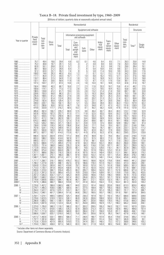
352 | Appendix B
Table B–18. Private fixed investment by type, 1960–2009[Billions of dollars; quarterly data at seasonally adjusted annual rates]
Year or quarterPrivatefixed
invest-ment
Nonresidential Residential
Totalnon-resi-den-tial
Struc-tures
Equipment and software
Totalresi-den-tial 1
Structures
Total
Information processing equipmentand software
Indus-trial
equip-ment
Trans-por-
tationequip-ment
Otherequip-ment
Total 1 Singlefamily
Total
Com-puters
andperiph-
eralequip-ment
Soft-ware Other
1960 ...................... 75.7 49.4 19.6 29.8 4.9 0.2 0.1 4.6 9.4 8.5 7.1 26.3 25.8 14.91961 ...................... 75.2 48.8 19.7 29.1 5.3 .3 .2 4.8 8.8 8.0 7.0 26.4 25.9 14.11962 ...................... 82.0 53.1 20.8 32.3 5.7 .3 .2 5.1 9.3 9.8 7.5 29.0 28.4 15.11963 ...................... 88.1 56.0 21.2 34.8 6.5 .7 .4 5.4 10.0 9.4 8.8 32.1 31.5 16.01964 ...................... 97.2 63.0 23.7 39.2 7.4 .9 .5 5.9 11.4 10.6 9.9 34.3 33.6 17.61965 ...................... 109.0 74.8 28.3 46.5 8.5 1.2 .7 6.7 13.7 13.2 11.0 34.2 33.5 17.81966 ...................... 117.7 85.4 31.3 54.0 10.7 1.7 1.0 8.0 16.2 14.5 12.7 32.3 31.6 16.61967 ...................... 118.7 86.4 31.5 54.9 11.3 1.9 1.2 8.2 16.9 14.3 12.4 32.4 31.6 16.81968 ...................... 132.1 93.4 33.6 59.9 11.9 1.9 1.3 8.7 17.3 17.6 13.0 38.7 37.9 19.51969 ...................... 147.3 104.7 37.7 67.0 14.6 2.4 1.8 10.4 19.1 18.9 14.4 42.6 41.6 19.71970 ...................... 150.4 109.0 40.3 68.7 16.6 2.7 2.3 11.6 20.3 16.2 15.6 41.4 40.2 17.51971 ...................... 169.9 114.1 42.7 71.5 17.3 2.8 2.4 12.2 19.5 18.4 16.3 55.8 54.5 25.81972 ...................... 198.5 128.8 47.2 81.7 19.5 3.5 2.8 13.2 21.4 21.8 19.0 69.7 68.1 32.81973 ...................... 228.6 153.3 55.0 98.3 23.1 3.5 3.2 16.3 26.0 26.6 22.6 75.3 73.6 35.21974 ...................... 235.4 169.5 61.2 108.2 27.0 3.9 3.9 19.2 30.7 26.3 24.3 66.0 64.1 29.71975 ...................... 236.5 173.7 61.4 112.4 28.5 3.6 4.8 20.2 31.3 25.2 27.4 62.7 60.8 29.61976 ...................... 274.8 192.4 65.9 126.4 32.7 4.4 5.2 23.1 34.1 30.0 29.6 82.5 80.4 43.91977 ...................... 339.0 228.7 74.6 154.1 39.2 5.7 5.5 28.0 39.4 39.3 36.3 110.3 107.9 62.21978 ...................... 412.2 280.6 93.6 187.0 48.7 7.6 6.3 34.8 47.7 47.3 43.2 131.6 128.9 72.81979 ...................... 474.9 333.9 117.7 216.2 58.5 10.2 8.1 40.2 56.2 53.6 47.9 141.0 137.8 72.31980 ...................... 485.6 362.4 136.2 226.2 68.8 12.5 9.8 46.4 60.7 48.4 48.3 123.2 119.8 52.91981 ...................... 542.6 420.0 167.3 252.7 81.5 17.1 11.8 52.5 65.5 50.6 55.2 122.6 118.9 52.01982 ...................... 532.1 426.5 177.6 248.9 88.3 18.9 14.0 55.3 62.7 46.8 51.2 105.7 102.0 41.51983 ...................... 570.1 417.2 154.3 262.9 100.1 23.9 16.4 59.8 58.9 53.5 50.4 152.9 148.6 72.51984 ...................... 670.2 489.6 177.4 312.2 121.5 31.6 20.4 69.6 68.1 64.4 58.1 180.6 175.9 86.41985 ...................... 714.4 526.2 194.5 331.7 130.3 33.7 23.8 72.9 72.5 69.0 59.9 188.2 183.1 87.41986 ...................... 739.9 519.8 176.5 343.3 136.8 33.4 25.6 77.7 75.4 70.5 60.7 220.1 214.6 104.11987 ...................... 757.8 524.1 174.2 349.9 141.2 35.8 29.0 76.4 76.7 68.1 63.9 233.7 227.9 117.21988 ...................... 803.1 563.8 182.8 381.0 154.9 38.0 34.2 82.8 84.2 72.9 69.0 239.3 233.2 120.11989 ...................... 847.3 607.7 193.7 414.0 172.6 43.1 41.9 87.6 93.3 67.9 80.2 239.5 233.4 120.91990 ...................... 846.4 622.4 202.9 419.5 177.2 38.6 47.6 90.9 92.1 70.0 80.2 224.0 218.0 112.91991 ...................... 803.3 598.2 183.6 414.6 182.9 37.7 53.7 91.5 89.3 71.5 70.8 205.1 199.4 99.41992 ...................... 848.5 612.1 172.6 439.6 199.9 44.0 57.9 98.1 93.0 74.7 72.0 236.3 230.4 122.01993 ...................... 932.5 666.6 177.2 489.4 217.6 47.9 64.3 105.4 102.2 89.4 80.2 266.0 259.9 140.11994 ...................... 1,033.5 731.4 186.8 544.6 235.2 52.4 68.3 114.6 113.6 107.7 88.1 302.1 295.9 162.31995 ...................... 1,112.9 810.0 207.3 602.8 263.0 66.1 74.6 122.3 129.0 116.1 94.7 302.9 296.5 153.51996 ...................... 1,209.4 875.4 224.6 650.8 290.1 72.8 85.5 131.9 136.5 123.2 101.0 334.1 327.7 170.81997 ...................... 1,317.7 968.6 250.3 718.3 330.3 81.4 107.5 141.4 140.4 135.5 112.1 349.1 342.8 175.21998 ...................... 1,447.1 1,061.1 275.1 786.0 366.1 87.9 126.0 152.2 147.4 147.1 125.4 385.9 379.2 199.41999 ...................... 1,580.7 1,154.9 283.9 871.0 417.1 97.2 157.3 162.5 149.1 174.4 130.4 425.8 418.5 223.82000 ...................... 1,717.7 1,268.7 318.1 950.5 478.2 103.2 184.5 190.6 162.9 170.8 138.6 449.0 441.2 236.82001 ...................... 1,700.2 1,227.8 329.7 898.1 452.5 87.6 186.6 178.4 151.9 154.2 139.5 472.4 464.4 249.12002 ...................... 1,634.9 1,125.4 282.8 842.7 419.8 79.7 183.0 157.0 141.7 141.6 139.6 509.5 501.3 265.92003 ...................... 1,713.3 1,135.7 281.9 853.8 430.9 77.6 191.3 162.0 142.6 132.9 147.5 577.6 569.1 310.62004 ...................... 1,903.6 1,223.0 306.7 916.4 455.3 80.2 205.7 169.4 142.0 161.1 157.9 680.6 671.4 377.62005 ...................... 2,122.3 1,347.3 351.8 995.6 475.3 78.9 218.0 178.4 159.6 181.7 178.9 775.0 765.2 433.52006 ...................... 2,267.2 1,505.3 433.7 1,071.7 505.2 84.9 229.8 190.6 178.4 198.2 189.8 761.9 751.6 416.02007 ...................... 2,269.1 1,640.2 535.4 1,104.8 537.4 89.2 245.6 202.5 193.2 181.7 192.6 629.0 618.6 305.22008 ...................... 2,170.8 1,693.6 609.5 1,084.1 562.9 86.7 264.1 212.1 193.8 132.3 195.1 477.2 467.2 185.82009 p .................... 1,747.9 1,386.6 480.7 906.0 519.9 74.7 241.8 203.4 150.4 72.4 163.2 361.3 352.0 105.22006: I .................. 2,270.6 1,457.2 396.8 1,060.5 498.7 84.0 223.3 191.4 168.0 203.8 190.0 813.3 803.0 465.6
II ................. 2,279.7 1,495.3 428.6 1,066.7 500.5 84.1 227.5 188.9 180.7 195.5 190.0 784.4 774.2 435.2III ................ 2,264.4 1,522.7 447.6 1,075.1 510.1 86.7 232.1 191.4 181.4 195.3 188.2 741.7 731.4 398.7IV ................ 2,254.2 1,546.1 461.7 1,084.4 511.6 84.8 236.2 190.5 183.7 198.2 191.0 708.1 697.8 364.5
2007: I .................. 2,254.1 1,574.1 489.5 1,084.6 525.1 88.8 238.3 197.9 182.1 192.3 185.2 680.0 669.6 339.8II ................. 2,278.6 1,623.5 519.9 1,103.5 530.1 86.9 242.6 200.6 198.8 183.0 191.6 655.1 644.8 324.0III ................ 2,280.8 1,665.2 556.1 1,109.1 538.4 88.2 246.7 203.6 199.0 176.5 195.2 615.6 605.3 298.0IV ................ 2,263.0 1,697.9 575.9 1,122.0 555.8 93.1 254.8 208.0 192.9 175.1 198.2 565.2 554.8 259.1
2008: I .................. 2,223.0 1,705.0 586.3 1,118.7 566.3 93.7 263.2 209.5 195.3 164.3 192.7 518.1 507.9 220.5II ................. 2,214.0 1,719.7 610.6 1,109.2 576.2 92.9 268.0 215.3 197.3 143.8 192.0 494.2 484.0 197.4III ................ 2,179.7 1,711.0 620.4 1,090.6 568.8 84.3 266.4 218.1 194.8 125.9 201.1 468.6 458.7 176.0IV ................ 2,066.6 1,638.7 620.7 1,018.0 540.2 75.8 258.7 205.6 187.9 95.3 194.7 427.8 418.3 149.1
2009: I .................. 1,817.2 1,442.6 533.1 909.5 508.3 71.1 240.5 196.7 157.8 65.4 178.0 374.6 365.2 111.8II ................. 1,737.7 1,391.8 494.8 897.0 512.2 72.0 240.2 200.1 151.4 70.6 162.7 345.9 336.8 93.1III ................ 1,712.6 1,353.9 457.9 895.9 519.0 72.5 241.4 205.1 146.5 73.2 157.2 358.8 349.6 105.2IV p ............. 1,724.0 1,358.2 436.8 921.5 540.3 83.3 245.1 211.9 145.9 80.5 154.8 365.7 356.5 110.9
1 Includes other items not shown separately.Source: Department of Commerce (Bureau of Economic Analysis).
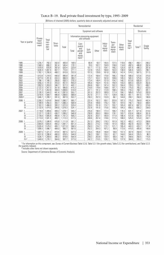
National Income or Expenditure | 353
Table B–19. Real private fixed investment by type, 1995–2009[Billions of chained (2005) dollars; quarterly data at seasonally adjusted annual rates]
Year or quarterPrivatefixed
invest-ment
Nonresidential Residential
Totalnon-resi-den-tial
Struc-tures
Equipment and software
Totalresi-den-tial 2
Structures
Total
Information processing equipmentand software
Indus-trial
equip-ment
Trans-por-
tationequip-ment
Otherequip-ment
Total 2 Singlefamily
Total
Com-puters
andperiph-
eralequip-ment 1
Soft-ware Other
1995 ...................... 1,235.7 792.2 342.0 493.0 149.5 ............. 66.9 93.7 145.5 131.5 110.6 456.1 450.1 240.21996 ...................... 1,346.5 866.2 361.4 545.4 179.1 ............. 78.5 102.7 150.9 136.8 114.8 492.5 486.8 262.41997 ...................... 1,470.8 970.8 387.9 620.4 220.8 ............. 101.7 111.5 154.1 148.2 125.9 501.8 496.3 261.61998 ...................... 1,630.4 1,087.4 407.7 710.4 271.1 ............. 122.8 125.5 160.8 162.0 138.8 540.4 534.5 290.11999 ...................... 1,782.1 1,200.9 408.2 810.9 332.0 ............. 151.5 139.9 161.8 190.3 142.4 574.2 567.5 311.52000 ...................... 1,913.8 1,318.5 440.0 895.8 391.9 ............. 172.4 168.4 175.8 186.2 150.4 580.0 572.6 315.02001 ...................... 1,877.6 1,281.8 433.3 866.9 390.2 ............. 173.7 163.2 162.8 169.6 149.3 583.3 575.6 315.42002 ...................... 1,798.1 1,180.2 356.6 830.3 379.3 ............. 173.4 148.4 151.9 154.2 148.2 613.8 605.9 327.72003 ...................... 1,856.2 1,191.0 343.0 851.4 405.0 ............. 185.6 156.4 151.6 140.4 155.0 664.3 655.9 362.62004 ...................... 1,992.5 1,263.0 346.7 917.3 443.1 ............. 204.6 168.1 147.4 162.3 164.4 729.5 720.1 406.12005 ...................... 2,122.3 1,347.3 351.8 995.6 475.3 ............. 218.0 178.4 159.6 181.7 178.9 775.0 765.2 433.52006 ...................... 2,171.3 1,453.9 384.0 1,069.6 514.8 ............. 227.1 191.2 172.9 196.5 185.5 718.2 708.1 391.12007 ...................... 2,126.3 1,544.3 441.4 1,097.0 555.7 ............. 241.5 202.3 180.9 177.4 184.1 585.0 575.0 283.92008 ...................... 2,018.4 1,569.7 486.8 1,068.6 588.8 ............. 257.0 211.1 174.7 128.9 180.3 451.1 441.5 179.72009 p .................... 1,646.7 1,289.1 391.0 887.9 553.7 ............. 238.3 202.3 133.9 66.1 144.8 359.1 350.0 108.82006: I .................. 2,200.2 1,424.9 364.8 1,060.7 505.7 ............. 222.4 192.2 165.1 202.6 187.3 775.2 764.9 442.4
II ................. 2,189.9 1,450.3 383.7 1,066.3 508.9 ............. 224.8 189.8 176.2 194.1 187.0 740.1 730.0 409.4III ................ 2,162.2 1,466.0 393.2 1,072.0 520.4 ............. 228.5 191.9 174.7 193.7 183.4 697.4 687.3 374.6IV ................ 2,132.9 1,474.5 394.6 1,079.3 524.1 ............. 232.8 191.0 175.6 195.5 184.3 660.2 650.2 338.0
2007: I .................. 2,118.8 1,489.6 409.2 1,078.1 540.2 ............. 235.0 198.4 172.4 188.2 178.3 631.7 621.6 314.0II ................. 2,137.7 1,530.3 430.7 1,095.2 546.9 ............. 238.9 200.3 186.9 178.1 183.7 610.4 600.4 301.6III ................ 2,135.6 1,565.8 456.8 1,101.3 558.2 ............. 242.6 203.1 185.9 171.8 186.4 572.9 562.9 277.9IV ................ 2,113.0 1,591.3 469.1 1,113.3 577.5 ............. 249.6 207.4 178.6 171.5 188.0 525.0 515.0 242.1
2008: I .................. 2,079.2 1,598.9 476.8 1,111.9 591.7 ............. 257.3 209.2 179.3 161.9 182.3 483.2 473.3 208.6II ................. 2,064.8 1,604.4 493.2 1,097.7 601.3 ............. 260.3 214.2 178.6 141.0 180.9 462.9 453.0 189.1III ................ 2,020.4 1,579.2 493.1 1,071.0 594.5 ............. 258.3 216.7 173.7 121.7 185.4 443.3 433.7 171.8IV ................ 1,909.3 1,496.1 484.0 993.7 567.6 ............. 252.2 204.3 167.2 90.9 172.6 415.0 405.8 149.4
2009: I .................. 1,687.5 1,321.2 419.4 887.5 537.5 ............. 235.5 195.8 140.8 59.8 157.3 367.9 358.9 112.9II ................. 1,631.9 1,288.4 400.0 876.5 544.8 ............. 236.2 199.1 135.2 62.7 144.0 344.4 335.5 96.3III ................ 1,626.7 1,269.0 380.2 879.8 554.9 ............. 239.2 203.9 130.4 66.0 140.1 359.6 350.5 110.4IV p ............. 1,640.6 1,278.1 364.6 907.7 577.6 ............. 242.2 210.5 129.2 76.0 137.9 364.6 355.2 115.5
1 For information on this component, see Survey of Current Business Table 5.3.6, Table 5.3.1 (for growth rates), Table 5.3.2 (for contributions), and Table 5.3.3(for quantity indexes).
2 Includes other items not shown separately.Source: Department of Commerce (Bureau of Economic Analysis).
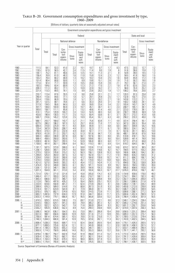
354 | Appendix B
Table B–20. Government consumption expenditures and gross investment by type,1960–2009
[Billions of dollars; quarterly data at seasonally adjusted annual rates]
Year or quarter
Government consumption expenditures and gross investment
Total
Federal State and local
Total
National defense Nondefense
Total
Con-sump-tion
expen-ditures
Gross investment
Total
Con-sump-tion
expen-ditures
Gross investment
Total
Con-sump-tion
expen-ditures
Gross investment
Struc-tures
Equip-mentandsoft-ware
Struc-tures
Equip-mentandsoft-ware
Struc-tures
Equip-mentandsoft-ware
1960 ...................... 111.5 64.1 53.3 41.0 2.2 10.1 10.7 8.7 1.7 0.3 47.5 33.5 12.7 1.21961 ...................... 119.5 67.9 56.5 42.7 2.4 11.5 11.4 9.0 1.9 .6 51.6 36.6 13.8 1.31962 ...................... 130.1 75.2 61.1 46.6 2.0 12.5 14.1 11.3 2.1 .8 54.9 39.0 14.5 1.31963 ...................... 136.4 76.9 61.0 48.3 1.6 11.0 15.9 12.4 2.3 1.2 59.5 41.9 16.0 1.51964 ...................... 143.2 78.4 60.2 48.8 1.3 10.2 18.2 14.0 2.5 1.6 64.8 45.8 17.2 1.81965 ...................... 151.4 80.4 60.6 50.6 1.1 8.9 19.8 15.1 2.8 1.9 71.0 50.2 19.0 1.91966 ...................... 171.6 92.4 71.7 59.9 1.3 10.5 20.8 15.9 2.8 2.1 79.2 56.1 21.0 2.11967 ...................... 192.5 104.6 83.4 69.9 1.2 12.3 21.2 17.0 2.2 1.9 87.9 62.6 23.0 2.31968 ...................... 209.3 111.3 89.2 77.1 1.2 10.9 22.0 18.2 2.1 1.7 98.0 70.4 25.2 2.41969 ...................... 221.4 113.3 89.5 78.1 1.5 9.9 23.8 20.2 1.9 1.7 108.2 79.8 25.6 2.71970 ...................... 233.7 113.4 87.6 76.5 1.3 9.8 25.8 22.1 2.1 1.7 120.3 91.5 25.8 3.01971 ...................... 246.4 113.6 84.6 77.1 1.8 5.7 29.1 24.9 2.5 1.7 132.8 102.7 27.0 3.11972 ...................... 263.4 119.6 86.9 79.5 1.8 5.7 32.7 28.2 2.7 1.8 143.8 113.2 27.1 3.51973 ...................... 281.7 122.5 88.1 79.4 2.1 6.6 34.3 29.4 3.1 1.8 159.2 126.0 29.1 4.11974 ...................... 317.9 134.5 95.6 84.5 2.2 8.9 39.0 33.4 3.4 2.2 183.4 143.7 34.7 4.91975 ...................... 357.7 149.0 103.9 90.9 2.3 10.7 45.1 38.7 4.1 2.4 208.7 165.1 38.1 5.51976 ...................... 383.0 159.7 111.1 95.8 2.1 13.2 48.6 41.4 4.6 2.7 223.3 179.5 38.1 5.71977 ...................... 414.1 175.4 120.9 104.2 2.4 14.4 54.5 46.5 5.0 3.0 238.7 195.9 36.9 5.91978 ...................... 453.6 190.9 130.5 112.7 2.5 15.3 60.4 50.6 6.1 3.7 262.7 213.2 42.8 6.61979 ...................... 500.7 210.6 145.2 123.8 2.5 18.9 65.4 55.1 6.3 4.0 290.2 233.3 49.0 7.81980 ...................... 566.1 243.7 168.0 143.7 3.2 21.1 75.8 63.8 7.1 4.9 322.4 258.4 55.1 8.91981 ...................... 627.5 280.2 196.2 167.3 3.2 25.7 83.9 71.0 7.7 5.3 347.3 282.3 55.4 9.51982 ...................... 680.4 310.8 225.9 191.1 4.0 30.8 84.9 72.1 6.8 6.0 369.7 304.9 54.2 10.61983 ...................... 733.4 342.9 250.6 208.7 4.8 37.1 92.3 77.7 6.7 7.8 390.5 324.1 54.2 12.21984 ...................... 796.9 374.3 281.5 232.8 4.9 43.8 92.7 77.1 7.0 8.7 422.6 347.7 60.5 14.41985 ...................... 878.9 412.8 311.2 253.7 6.2 51.3 101.6 84.7 7.3 9.6 466.1 381.8 67.6 16.81986 ...................... 949.3 438.4 330.8 267.9 6.8 56.1 107.6 90.1 8.0 9.5 510.9 418.1 74.2 18.61987 ...................... 999.4 459.5 350.0 283.6 7.7 58.8 109.6 90.1 9.0 10.4 539.9 441.4 78.8 19.61988 ...................... 1,038.9 461.6 354.7 293.5 7.4 53.9 106.8 88.3 6.8 11.7 577.3 471.0 84.8 21.51989 ...................... 1,100.6 481.4 362.1 299.4 6.4 56.3 119.3 99.1 6.9 13.4 619.2 504.5 88.7 26.01990 ...................... 1,181.7 507.5 373.9 308.0 6.1 59.8 133.6 111.0 8.0 14.6 674.2 547.0 98.5 28.71991 ...................... 1,236.1 526.6 383.1 319.7 4.6 58.8 143.4 118.6 9.2 15.7 709.5 577.5 103.2 28.91992 ...................... 1,273.5 532.9 376.8 315.2 5.2 56.3 156.1 128.9 10.3 16.9 740.6 606.2 104.2 30.11993 ...................... 1,294.8 525.0 363.0 307.5 5.3 50.1 162.0 133.7 11.2 17.0 769.8 634.2 104.5 31.21994 ...................... 1,329.8 518.6 353.8 300.8 5.8 47.2 164.8 139.9 10.2 14.7 811.2 668.2 108.7 34.31995 ...................... 1,374.0 518.8 348.8 297.0 6.7 45.1 170.0 143.2 10.8 16.0 855.3 701.3 117.3 36.71996 ...................... 1,421.0 527.0 354.8 303.2 6.3 45.4 172.2 143.4 11.3 17.5 894.0 730.2 126.8 36.91997 ...................... 1,474.4 531.0 349.8 304.5 6.1 39.2 181.1 153.0 9.9 18.2 943.5 764.5 139.5 39.41998 ...................... 1,526.1 531.0 346.1 300.3 5.8 39.9 184.9 154.3 10.8 19.9 995.0 808.6 143.6 42.91999 ...................... 1,631.3 554.9 361.1 313.0 5.4 42.8 193.8 160.3 10.7 22.7 1,076.3 870.6 159.7 46.12000 ...................... 1,731.0 576.1 371.0 321.8 5.4 43.8 205.0 174.2 8.3 22.6 1,154.9 930.6 176.0 48.32001 ...................... 1,846.4 611.7 393.0 342.0 5.3 45.6 218.7 188.1 8.1 22.5 1,234.7 994.2 192.3 48.22002 ...................... 1,983.3 680.6 437.7 380.7 5.8 51.2 242.9 209.8 9.9 23.2 1,302.7 1,049.4 205.8 47.52003 ...................... 2,112.6 756.5 497.9 435.2 7.3 55.4 258.5 225.1 10.3 23.1 1,356.1 1,096.5 211.8 47.82004 ...................... 2,232.8 824.6 550.8 481.2 7.1 62.4 273.9 240.2 9.1 24.6 1,408.2 1,139.1 220.2 48.92005 ...................... 2,369.9 876.3 589.0 514.8 7.5 66.8 287.3 251.0 8.3 28.0 1,493.6 1,212.0 230.8 50.82006 ...................... 2,518.4 931.7 624.9 543.9 8.1 72.9 306.8 267.1 9.5 30.2 1,586.7 1,282.3 249.9 54.52007 ...................... 2,676.5 976.7 662.1 574.9 10.5 76.8 314.5 273.9 11.1 29.5 1,699.8 1,366.1 277.2 56.42008 ...................... 2,883.2 1,082.6 737.9 634.0 12.9 91.0 344.7 300.4 11.7 32.5 1,800.6 1,452.4 290.9 57.32009 p .................... 2,933.3 1,144.9 779.1 666.8 16.7 95.5 365.8 320.0 13.2 32.6 1,788.4 1,430.9 301.9 55.52006: I .................. 2,474.5 928.5 615.5 538.3 7.5 69.7 313.0 272.1 8.6 32.3 1,546.1 1,254.5 238.4 53.2
II ................. 2,510.5 930.3 624.1 541.2 8.0 74.8 306.2 267.2 9.2 29.7 1,580.2 1,274.6 251.3 54.3III ................ 2,533.3 932.2 623.3 543.7 7.8 71.8 308.9 269.4 9.3 30.2 1,601.2 1,292.7 253.6 54.9IV ................ 2,555.2 935.9 636.6 552.3 8.9 75.4 299.3 259.8 10.8 28.7 1,619.4 1,307.6 256.3 55.5
2007: I .................. 2,599.3 942.8 636.7 554.3 9.5 73.0 306.1 266.8 10.4 28.8 1,656.5 1,331.2 269.4 56.0II ................. 2,657.4 968.1 656.6 568.8 10.9 76.9 311.6 271.2 10.9 29.5 1,689.3 1,357.3 275.7 56.3III ................ 2,700.9 991.4 674.4 585.1 10.5 78.8 317.0 275.6 11.7 29.7 1,709.5 1,373.6 279.4 56.5IV ................ 2,748.3 1,004.3 680.8 591.4 10.9 78.5 323.6 282.1 11.3 30.2 1,743.9 1,402.5 284.5 56.9
2008: I .................. 2,808.4 1,038.3 703.6 609.7 11.5 82.4 334.8 293.5 10.4 30.9 1,770.1 1,429.3 283.5 57.3II ................. 2,877.1 1,069.5 725.6 622.4 12.1 91.1 343.9 300.8 11.1 32.0 1,807.6 1,458.3 291.5 57.7III ................ 2,941.4 1,108.3 763.6 655.2 13.0 95.3 344.7 300.7 12.3 31.7 1,833.1 1,480.4 295.4 57.3IV ................ 2,905.9 1,114.3 758.9 648.8 14.8 95.3 355.3 306.6 13.2 35.6 1,791.7 1,441.7 293.2 56.8
2009: I .................. 2,879.0 1,106.7 750.7 642.9 15.8 91.9 356.0 311.3 13.2 31.5 1,772.3 1,424.4 292.5 55.4II ................. 2,929.4 1,138.3 776.2 662.7 16.4 97.2 362.1 316.4 13.2 32.4 1,791.2 1,429.9 305.8 55.4III ................ 2,955.4 1,164.3 795.8 679.3 18.5 98.0 368.5 321.9 13.3 33.2 1,791.1 1,429.8 305.9 55.4IV p ............. 2,969.5 1,170.4 793.8 682.4 16.3 95.1 376.5 330.3 13.0 33.2 1,799.1 1,439.7 303.5 55.9
Source: Department of Commerce (Bureau of Economic Analysis).
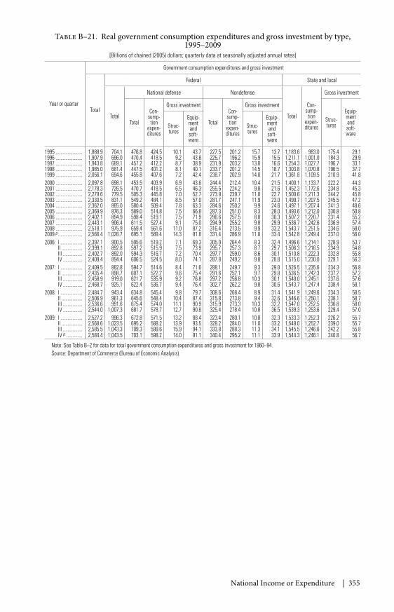
National Income or Expenditure | 355
Table B–21. Real government consumption expenditures and gross investment by type,1995–2009
[Billions of chained (2005) dollars; quarterly data at seasonally adjusted annual rates]
Year or quarter
Government consumption expenditures and gross investment
Total
Federal State and local
Total
National defense Nondefense
Total
Con-sump-tion
expen-ditures
Gross investment
Total
Con-sump-tion
expen-ditures
Gross investment
Total
Con-sump-tion
expen-ditures
Gross investment
Struc-tures
Equip-mentandsoft-ware
Struc-tures
Equip-mentandsoft-ware
Struc-tures
Equip-mentandsoft-ware
1995 ...................... 1,888.9 704.1 476.8 424.5 10.1 43.7 227.5 201.2 15.7 13.7 1,183.6 983.0 175.4 29.11996 ...................... 1,907.9 696.0 470.4 418.5 9.2 43.8 225.7 196.2 15.9 15.5 1,211.1 1,001.0 184.3 29.91997 ...................... 1,943.8 689.1 457.2 412.2 8.7 38.9 231.9 203.2 13.8 16.6 1,254.3 1,027.7 196.7 33.11998 ...................... 1,985.0 681.4 447.5 401.2 8.1 40.1 233.7 201.2 14.5 18.7 1,303.8 1,070.8 196.5 37.71999 ...................... 2,056.1 694.6 455.8 407.6 7.2 42.4 238.7 202.9 14.0 21.7 1,361.8 1,109.5 210.9 41.82000 ...................... 2,097.8 698.1 453.5 403.9 6.9 43.6 244.4 212.4 10.4 21.5 1,400.1 1,133.7 222.2 44.32001 ...................... 2,178.3 726.5 470.7 418.5 6.5 46.3 255.5 224.2 9.8 21.6 1,452.3 1,172.6 234.8 45.32002 ...................... 2,279.6 779.5 505.3 445.8 7.0 52.7 273.9 239.7 11.8 22.7 1,500.6 1,211.3 244.2 45.82003 ...................... 2,330.5 831.1 549.2 484.1 8.5 57.0 281.7 247.1 11.9 23.0 1,499.7 1,207.5 245.5 47.22004 ...................... 2,362.0 865.0 580.4 509.4 7.8 63.3 284.6 250.2 9.9 24.6 1,497.1 1,207.4 241.3 48.62005 ...................... 2,369.9 876.3 589.0 514.8 7.5 66.8 287.3 251.0 8.3 28.0 1,493.6 1,212.0 230.8 50.82006 ...................... 2,402.1 894.9 598.4 519.1 7.5 71.9 296.6 257.5 8.8 30.3 1,507.2 1,220.7 231.4 55.22007 ...................... 2,443.1 906.4 611.5 527.4 9.1 75.0 294.9 255.2 9.8 29.9 1,536.7 1,242.6 236.9 57.42008 ...................... 2,518.1 975.9 659.4 561.6 11.0 87.2 316.4 273.5 9.9 33.2 1,543.7 1,251.5 234.6 58.02009 p .................... 2,566.4 1,026.7 695.1 589.4 14.3 91.8 331.4 286.9 11.0 33.4 1,542.8 1,249.4 237.0 56.02006: I .................. 2,397.1 900.5 595.6 519.2 7.1 69.3 305.0 264.4 8.3 32.4 1,496.6 1,214.1 228.9 53.7
II ................. 2,399.1 892.8 597.2 515.9 7.5 73.9 295.7 257.3 8.7 29.7 1,506.3 1,216.5 234.9 54.8III ................ 2,402.7 892.0 594.3 516.7 7.2 70.4 297.7 259.0 8.6 30.1 1,510.8 1,222.3 232.8 55.8IV ................ 2,409.4 894.4 606.5 524.5 8.0 74.1 287.8 249.2 9.8 28.8 1,515.0 1,230.0 229.1 56.3
2007: I .................. 2,409.5 882.8 594.7 514.6 8.4 71.6 288.1 249.7 9.3 29.0 1,526.5 1,235.6 234.3 56.8II ................. 2,435.4 898.7 607.1 522.2 9.6 75.4 291.6 252.1 9.7 29.8 1,536.5 1,242.3 237.2 57.2III ................ 2,458.9 919.0 621.7 535.9 9.2 76.8 297.2 256.8 10.3 30.1 1,540.0 1,245.1 237.6 57.6IV ................ 2,468.7 925.1 622.4 536.7 9.4 76.4 302.7 262.2 9.8 30.6 1,543.7 1,247.4 238.4 58.1
2008: I .................. 2,484.7 943.4 634.8 545.4 9.8 79.7 308.6 268.4 8.9 31.4 1,541.9 1,249.6 234.3 58.5II ................. 2,506.9 961.3 645.6 548.4 10.4 87.4 315.8 273.8 9.4 32.6 1,546.6 1,250.1 238.1 58.7III ................ 2,536.6 991.6 675.4 574.0 11.1 90.9 315.9 273.3 10.3 32.2 1,547.0 1,252.5 236.8 58.0IV ................ 2,544.0 1,007.3 681.7 578.7 12.7 90.8 325.4 278.4 10.8 36.5 1,539.3 1,253.6 229.4 57.0
2009: I .................. 2,527.2 996.3 672.8 571.5 13.2 88.4 323.4 280.1 10.8 32.3 1,533.3 1,252.3 226.2 55.7II ................. 2,568.6 1,023.5 695.2 588.2 13.9 93.5 328.2 284.0 11.0 33.2 1,548.0 1,252.7 239.0 55.7III ................ 2,585.5 1,043.3 709.3 599.6 15.9 94.1 333.8 288.3 11.3 34.1 1,545.5 1,246.6 242.2 55.8IV p ............. 2,584.4 1,043.5 703.1 598.2 14.0 91.1 340.4 295.2 11.1 33.9 1,544.3 1,246.1 240.8 56.7
Note: See Table B–2 for data for total government consumption expenditures and gross investment for 1960–94.Source: Department of Commerce (Bureau of Economic Analysis).
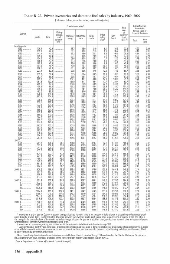
356 | Appendix B
Table B–22. Private inventories and domestic final sales by industry, 1960–2009[Billions of dollars, except as noted; seasonally adjusted]
Quarter
Private inventories 1Finalsales
ofdomestic
busi-ness 3
Ratio of privateinventories
to final sales ofdomestic business
Total 2 Farm
Mining,utilities,
andconstruc-
tion 2
Manufac-turing
Wholesaletrade
Retailtrade
Otherindus-tries 2
Non-farm 2
Total Non-farm
Fourth quarter:1960 ................ 136.4 42.9 ................. 48.7 16.9 21.9 6.1 93.5 32.3 4.22 2.891961 ................ 139.8 44.6 ................. 50.1 17.3 21.3 6.6 95.2 33.9 4.12 2.811962 ................ 147.4 47.0 ................. 53.2 18.0 22.7 6.6 100.5 35.6 4.14 2.821963 ................ 149.9 44.4 ................. 55.1 19.5 23.9 7.1 105.5 37.9 3.95 2.781964 ................ 154.5 42.2 ................. 58.6 20.8 25.2 7.7 112.2 40.8 3.79 2.751965 ................ 169.4 47.2 ................. 63.4 22.5 28.0 8.3 122.2 44.9 3.77 2.721966 ................ 185.6 47.3 ................. 73.0 25.8 30.6 8.9 138.3 47.4 3.92 2.921967 ................ 194.8 45.7 ................. 79.9 28.1 30.9 10.1 149.1 49.9 3.90 2.991968 ................ 208.1 48.8 ................. 85.1 29.3 34.2 10.6 159.3 55.0 3.79 2.901969 ................ 227.4 52.8 ................. 92.6 32.5 37.5 12.0 174.6 58.7 3.88 2.981970 ................ 235.7 52.4 ................. 95.5 36.4 38.5 12.9 183.3 61.9 3.81 2.961971 ................ 253.7 59.3 ................. 96.6 39.4 44.7 13.7 194.4 67.5 3.76 2.881972 ................ 283.6 73.7 ................. 102.1 43.1 49.8 14.8 209.9 75.7 3.74 2.771973 ................ 351.5 102.2 ................. 121.5 51.7 58.4 17.7 249.4 83.7 4.20 2.981974 ................ 405.6 87.6 ................. 162.6 66.9 63.9 24.7 318.1 89.8 4.52 3.541975 ................ 408.5 89.5 ................. 162.2 66.5 64.4 25.9 319.0 101.1 4.04 3.161976 ................ 439.6 85.3 ................. 178.7 74.1 73.0 28.5 354.2 111.2 3.95 3.191977 ................ 482.0 90.6 ................. 193.2 84.0 80.9 33.3 391.4 124.0 3.89 3.161978 ................ 570.9 119.3 ................. 219.8 99.0 94.1 38.8 451.7 143.6 3.98 3.151979 ................ 667.6 134.9 ................. 261.8 119.5 104.7 46.6 532.6 159.4 4.19 3.341980 ................ 739.0 140.3 ................. 293.4 139.4 111.7 54.1 598.7 174.1 4.24 3.441981 ................ 779.1 127.4 ................. 313.1 148.8 123.2 66.6 651.7 186.7 4.17 3.491982 ................ 773.9 131.3 ................. 304.6 147.9 123.2 66.8 642.6 194.8 3.97 3.301983 ................ 796.9 131.7 ................. 308.9 153.4 137.6 65.2 665.1 215.7 3.69 3.081984 ................ 869.0 131.4 ................. 344.5 169.1 157.0 66.9 737.6 233.6 3.72 3.161985 ................ 875.9 125.8 ................. 333.3 175.9 171.4 69.5 750.2 249.5 3.51 3.011986 ................ 858.0 113.0 ................. 320.6 182.0 176.2 66.3 745.1 264.2 3.25 2.821987 ................ 924.2 119.9 ................. 339.6 195.8 199.1 69.9 804.4 277.7 3.33 2.901988 ................ 999.7 130.7 ................. 372.4 213.9 213.2 69.5 869.1 304.1 3.29 2.861989 ................ 1,044.3 129.6 ................. 390.5 222.8 231.4 70.1 914.7 322.8 3.23 2.831990 ................ 1,082.0 133.1 ................. 404.5 236.8 236.6 71.0 948.9 335.9 3.22 2.821991 ................ 1,057.2 123.2 ................. 384.1 239.2 240.2 70.5 934.0 345.7 3.06 2.701992 ................ 1,082.6 133.1 ................. 377.6 248.3 249.4 74.3 949.5 370.9 2.92 2.561993 ................ 1,116.0 132.3 ................. 380.1 258.6 268.6 76.5 983.7 391.4 2.85 2.511994 ................ 1,194.5 134.5 ................. 404.3 281.5 293.6 80.6 1,060.0 413.9 2.89 2.561995 ................ 1,257.2 131.1 ................. 424.5 303.7 312.2 85.6 1,126.1 436.0 2.88 2.58
NAICS:1996 ................ 1,284.7 136.6 31.1 421.0 285.1 328.7 82.1 1,148.1 465.6 2.76 2.471997 ................ 1,327.3 136.9 33.0 432.0 302.5 335.9 87.1 1,190.4 492.2 2.70 2.421998 ................ 1,341.6 120.5 36.6 432.3 312.0 349.2 91.1 1,221.1 525.8 2.55 2.321999 ................ 1,432.7 124.3 38.5 457.6 334.8 377.7 99.8 1,308.4 557.2 2.57 2.352000 ................ 1,524.0 132.1 42.3 476.5 357.7 400.8 114.6 1,391.8 588.3 2.59 2.372001 ................ 1,447.3 126.2 45.3 440.9 335.8 386.0 113.0 1,321.1 603.0 2.40 2.192002 ................ 1,489.1 135.9 46.5 443.7 343.2 408.0 111.8 1,353.2 608.5 2.45 2.222003 ................ 1,545.7 151.0 54.7 447.6 352.6 425.5 114.3 1,394.7 646.3 2.39 2.162004 ................ 1,681.5 157.2 64.1 487.2 388.9 460.9 123.2 1,524.3 685.2 2.45 2.222005 ................ 1,804.6 165.2 81.7 531.5 422.8 473.7 129.8 1,639.4 728.7 2.48 2.25
2006: I .................. 1,820.2 158.4 79.2 543.4 430.3 478.0 130.8 1,661.8 745.2 2.44 2.23II ................. 1,861.7 157.6 81.5 561.5 444.3 483.0 133.9 1,704.2 753.7 2.47 2.26III ................ 1,896.9 165.3 86.3 571.4 450.0 487.8 136.2 1,731.6 758.7 2.50 2.28IV ................ 1,917.1 165.1 90.7 575.7 456.4 491.6 137.7 1,752.0 771.9 2.48 2.27
2007: I .................. 1,951.8 177.4 94.5 581.9 463.7 494.1 140.2 1,774.5 784.3 2.49 2.26II ................. 1,972.6 175.1 98.1 590.7 468.2 498.0 142.5 1,797.5 795.0 2.48 2.26III ................ 2,003.9 183.3 94.4 599.0 477.3 506.1 143.8 1,820.6 804.7 2.49 2.26IV ................ 2,070.6 188.4 95.3 625.3 499.9 513.6 148.2 1,882.2 813.7 2.54 2.31
2008: I .................. 2,124.9 195.8 102.9 646.1 514.2 514.3 151.6 1,929.1 810.9 2.62 2.38II ................. 2,199.7 210.0 114.5 673.3 531.0 516.4 154.6 1,989.8 818.3 2.69 2.43III ................ 2,177.8 200.9 114.6 655.3 528.2 520.7 158.2 1,976.9 814.4 2.67 2.43IV ................ 2,015.9 178.4 100.1 592.8 482.7 506.4 155.5 1,837.5 800.0 2.52 2.30
2009: I .................. 1,948.1 171.9 96.4 575.8 464.3 489.7 150.0 1,776.1 794.1 2.45 2.24II ................. 1,912.2 171.6 96.8 567.4 449.6 478.5 148.3 1,740.6 792.5 2.41 2.20III ................ 1,892.3 168.6 97.7 564.3 436.6 477.1 147.9 1,723.7 795.3 2.38 2.17IV p ............. 1,914.2 167.0 98.1 570.0 445.6 484.5 148.9 1,747.2 801.3 2.39 2.18
1 Inventories at end of quarter. Quarter-to-quarter change calculated from this table is not the current-dollar change in private inventories component ofgross domestic product (GDP). The former is the difference between two inventory stocks, each valued at its respective end-of-quarter prices. The latter isthe change in the physical volume of inventories valued at average prices of the quarter. In addition, changes calculated from this table are at quarterly rates,whereas change in private inventories is stated at annual rates.
2 Inventories of construction, mining, and utilities establishments are included in other industries through 1995.3 Quarterly totals at monthly rates. Final sales of domestic business equals final sales of domestic product less gross output of general government, gross
value added of nonprofit institutions, compensation paid to domestic workers, and space rent for owner-occupied housing. Includes a small amount of finalsales by farm and by government enterprises.
Note: The industry classification of inventories is on an establishment basis. Estimates through 1995 are based on the Standard Industrial Classification(SIC). Beginning with 1996, estimates are based on the North American Industry Classification System (NAICS).
Source: Department of Commerce (Bureau of Economic Analysis).
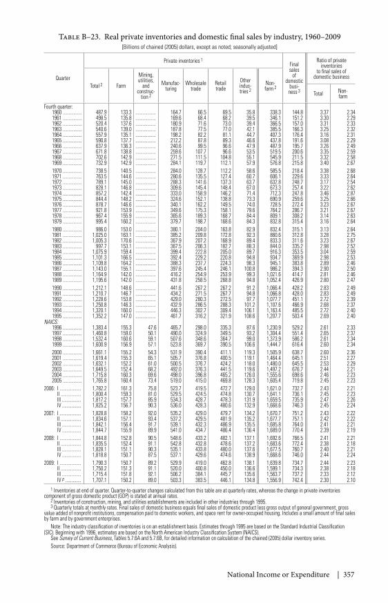
National Income or Expenditure | 357
Table B–23. Real private inventories and domestic final sales by industry, 1960–2009[Billions of chained (2005) dollars, except as noted; seasonally adjusted]
Quarter
Private inventories 1Finalsales
ofdomestic
busi-ness 3
Ratio of privateinventories
to final sales ofdomestic business
Total 2 Farm
Mining,utilities,
andconstruc-
tion 2
Manufac-turing
Wholesaletrade
Retailtrade
Otherindus-tries 2
Non-farm 2
Total Non-farm
Fourth quarter:1960 ................ 487.9 133.3 ................. 164.7 66.5 69.5 35.8 338.3 144.8 3.37 2.341961 ................ 498.5 135.8 ................. 169.6 68.4 68.2 39.5 346.1 151.2 3.30 2.291962 ................ 520.4 137.6 ................. 180.9 71.6 73.0 39.4 366.5 157.0 3.31 2.331963 ................ 540.6 139.0 ................. 187.8 77.5 77.0 42.1 385.5 166.3 3.25 2.321964 ................ 557.9 135.1 ................. 198.2 82.2 81.1 44.7 407.3 176.4 3.16 2.311965 ................ 590.8 137.7 ................. 212.2 87.8 89.3 46.6 437.8 191.6 3.08 2.291966 ................ 637.9 136.3 ................. 240.6 99.5 96.6 47.9 487.9 195.7 3.26 2.491967 ................ 671.8 138.8 ................. 259.6 107.7 96.6 53.5 519.5 200.6 3.35 2.591968 ................ 702.6 142.9 ................. 271.5 111.5 104.8 55.1 545.9 211.5 3.32 2.581969 ................ 732.9 142.9 ................. 284.1 119.7 112.1 57.9 576.8 215.8 3.40 2.671970 ................ 738.5 140.5 ................. 284.0 128.7 112.2 58.6 585.5 218.4 3.38 2.681971 ................ 763.5 144.6 ................. 280.6 135.5 127.4 60.7 606.1 229.6 3.33 2.641972 ................ 789.1 145.0 ................. 288.3 141.6 137.3 63.7 632.8 248.7 3.17 2.541973 ................ 828.1 146.8 ................. 309.6 145.4 148.4 67.0 673.3 257.4 3.22 2.621974 ................ 857.2 142.4 ................. 333.0 158.9 146.2 71.4 712.3 247.8 3.46 2.871975 ................ 844.4 148.2 ................. 324.6 152.1 138.8 73.3 690.9 259.6 3.25 2.661976 ................ 878.7 146.6 ................. 340.1 162.2 149.5 74.0 728.5 272.4 3.23 2.671977 ................ 921.8 153.9 ................. 349.6 175.3 158.1 79.6 764.2 286.7 3.21 2.671978 ................ 967.4 155.9 ................. 365.6 189.3 168.7 84.4 809.1 308.2 3.14 2.631979 ................ 995.4 160.2 ................. 379.7 198.7 168.6 84.3 832.8 315.4 3.16 2.641980 ................ 986.0 153.0 ................. 380.1 204.0 163.8 82.9 832.4 315.1 3.13 2.641981 ................ 1,025.0 163.1 ................. 385.2 209.8 172.8 92.3 860.6 312.8 3.28 2.751982 ................ 1,005.3 170.6 ................. 367.9 207.2 168.9 89.4 833.3 311.6 3.23 2.671983 ................ 997.7 153.1 ................. 367.5 206.3 182.7 88.3 844.0 335.2 2.98 2.521984 ................ 1,075.9 159.4 ................. 399.4 222.8 205.0 89.7 916.3 353.5 3.04 2.591985 ................ 1,101.3 166.5 ................. 392.4 229.2 220.8 94.8 934.7 369.9 2.98 2.531986 ................ 1,109.8 164.2 ................. 388.3 237.7 224.3 98.3 945.1 383.8 2.89 2.461987 ................ 1,143.0 155.1 ................. 397.6 245.4 246.1 100.8 986.2 394.3 2.90 2.501988 ................ 1,164.9 142.0 ................. 416.2 254.9 253.9 99.3 1,021.6 414.7 2.81 2.461989 ................ 1,195.6 142.0 ................. 431.8 258.5 268.8 94.8 1,052.4 426.9 2.80 2.471990 ................ 1,212.1 148.6 ................. 441.6 267.2 267.2 91.2 1,066.4 428.2 2.83 2.491991 ................ 1,210.7 146.7 ................. 434.2 271.5 267.7 94.8 1,066.8 428.0 2.83 2.491992 ................ 1,228.6 153.8 ................. 429.0 280.3 272.5 97.7 1,077.7 451.1 2.72 2.391993 ................ 1,250.8 146.3 ................. 432.9 286.5 288.3 101.2 1,107.6 466.9 2.68 2.371994 ................ 1,320.1 160.0 ................. 446.3 302.7 309.4 106.1 1,163.4 485.5 2.72 2.401995 ................ 1,352.2 147.0 ................. 461.7 316.2 321.9 108.6 1,207.7 503.4 2.69 2.40
NAICS:1996 ................ 1,383.4 155.3 47.6 465.7 298.0 335.3 87.6 1,230.9 529.2 2.61 2.331997 ................ 1,460.8 159.0 50.1 490.0 324.9 349.5 93.2 1,304.4 551.4 2.65 2.371998 ................ 1,532.4 160.6 59.1 507.6 348.6 364.7 99.0 1,373.9 586.2 2.61 2.341999 ................ 1,600.9 156.9 57.1 523.8 369.7 390.5 106.6 1,444.7 616.4 2.60 2.342000 ................ 1,661.1 155.2 54.3 531.9 390.4 411.1 119.3 1,505.9 638.7 2.60 2.362001 ................ 1,619.4 155.3 65.1 505.7 376.8 400.5 119.1 1,464.4 645.1 2.51 2.272002 ................ 1,632.1 152.2 61.0 500.5 376.7 424.2 118.0 1,480.0 645.5 2.53 2.292003 ................ 1,649.5 152.4 68.2 492.0 376.3 441.5 119.6 1,497.2 676.7 2.44 2.212004 ................ 1,715.8 160.3 69.6 498.0 396.8 465.2 126.0 1,555.6 698.6 2.46 2.232005 ................ 1,765.8 160.4 73.4 519.0 415.0 469.8 128.3 1,605.4 719.8 2.45 2.23
2006: I .................. 1,782.2 161.3 75.8 523.7 419.5 472.7 129.0 1,621.0 732.7 2.43 2.21II ................. 1,800.4 159.3 81.0 529.5 424.5 474.8 130.7 1,641.1 736.1 2.45 2.23III ................ 1,817.2 157.7 85.9 534.3 428.7 478.3 131.9 1,659.5 735.9 2.47 2.26IV ................ 1,825.2 156.7 90.3 536.0 428.3 480.6 132.9 1,668.6 746.3 2.45 2.24
2007: I .................. 1,828.8 158.2 92.0 535.2 429.0 479.7 134.2 1,670.7 751.2 2.43 2.22II ................. 1,834.6 157.1 93.4 537.2 429.5 481.9 135.2 1,677.7 757.1 2.42 2.22III ................ 1,842.1 156.4 91.7 539.1 432.3 486.9 135.5 1,685.8 764.0 2.41 2.21IV ................ 1,844.7 155.9 89.9 541.0 434.7 486.4 136.4 1,689.0 770.4 2.39 2.19
2008: I .................. 1,844.8 152.8 90.5 548.6 433.2 482.1 137.1 1,692.6 766.5 2.41 2.21II ................. 1,835.5 152.4 91.1 542.8 432.8 478.6 137.2 1,683.6 772.4 2.38 2.18III ................ 1,828.1 151.1 90.3 535.1 433.8 480.0 137.6 1,677.5 760.7 2.40 2.21IV ................ 1,818.8 150.7 87.5 537.1 429.6 474.6 138.9 1,668.6 746.0 2.44 2.24
2009: I .................. 1,790.3 150.7 89.2 529.9 419.0 462.8 138.1 1,639.8 734.7 2.44 2.23II ................. 1,750.2 151.3 91.1 520.0 400.8 450.0 136.6 1,599.1 734.3 2.38 2.18III ................ 1,715.4 151.8 92.1 506.2 384.1 445.7 135.6 1,563.7 737.2 2.33 2.12IV p ............. 1,707.1 150.2 89.0 503.3 383.5 446.1 134.8 1,556.9 742.4 2.30 2.10
1 Inventories at end of quarter. Quarter-to-quarter changes calculated from this table are at quarterly rates, whereas the change in private inventoriescomponent of gross domestic product (GDP) is stated at annual rates.
2 Inventories of construction, mining, and utilities establishments are included in other industries through 1995.3 Quarterly totals at monthly rates. Final sales of domestic business equals final sales of domestic product less gross output of general government, gross
value added of nonprofit institutions, compensation paid to domestic workers, and space rent for owner-occupied housing. Includes a small amount of final salesby farm and by government enterprises.
Note: The industry classification of inventories is on an establishment basis. Estimates through 1995 are based on the Standard Industrial Classification(SIC). Beginning with 1996, estimates are based on the North American Industry Classification System (NAICS).
See Survey of Current Business, Tables 5.7.6A and 5.7.6B, for detailed information on calculation of the chained (2005) dollar inventory series.Source: Department of Commerce (Bureau of Economic Analysis).
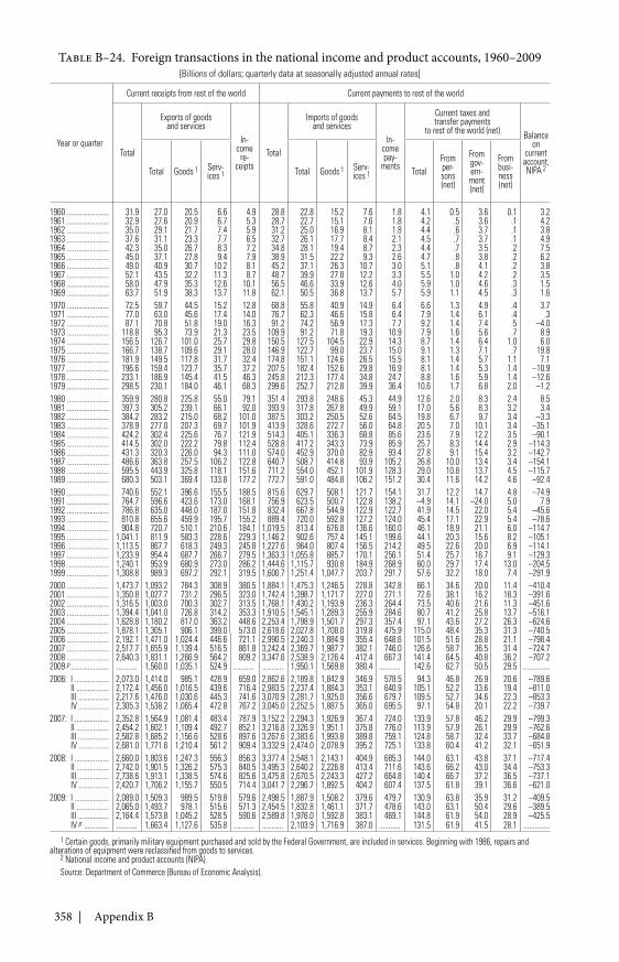
358 | Appendix B
Table B–24. Foreign transactions in the national income and product accounts, 1960–2009[Billions of dollars; quarterly data at seasonally adjusted annual rates]
Year or quarter
Current receipts from rest of the world Current payments to rest of the world
Total
Exports of goodsand services
In-come
re-ceipts
Total
Imports of goodsand services
In-comepay-
ments
Current taxes andtransfer payments
to rest of the world (net) Balanceon
currentaccount,NIPA 2Total Goods 1 Serv-
ices 1 Total Goods 1 Serv-ices 1 Total
Fromper-sons(net)
Fromgov-ern-ment(net)
Frombusi-ness(net)
1960 ...................... 31.9 27.0 20.5 6.6 4.9 28.8 22.8 15.2 7.6 1.8 4.1 0.5 3.6 0.1 3.21961 ...................... 32.9 27.6 20.9 6.7 5.3 28.7 22.7 15.1 7.6 1.8 4.2 .5 3.6 .1 4.21962 ...................... 35.0 29.1 21.7 7.4 5.9 31.2 25.0 16.9 8.1 1.8 4.4 .6 3.7 .1 3.81963 ...................... 37.6 31.1 23.3 7.7 6.5 32.7 26.1 17.7 8.4 2.1 4.5 .7 3.7 .1 4.91964 ...................... 42.3 35.0 26.7 8.3 7.2 34.8 28.1 19.4 8.7 2.3 4.4 .7 3.5 .2 7.51965 ...................... 45.0 37.1 27.8 9.4 7.9 38.9 31.5 22.2 9.3 2.6 4.7 .8 3.8 .2 6.21966 ...................... 49.0 40.9 30.7 10.2 8.1 45.2 37.1 26.3 10.7 3.0 5.1 .8 4.1 .2 3.81967 ...................... 52.1 43.5 32.2 11.3 8.7 48.7 39.9 27.8 12.2 3.3 5.5 1.0 4.2 .2 3.51968 ...................... 58.0 47.9 35.3 12.6 10.1 56.5 46.6 33.9 12.6 4.0 5.9 1.0 4.6 .3 1.51969 ...................... 63.7 51.9 38.3 13.7 11.8 62.1 50.5 36.8 13.7 5.7 5.9 1.1 4.5 .3 1.61970 ...................... 72.5 59.7 44.5 15.2 12.8 68.8 55.8 40.9 14.9 6.4 6.6 1.3 4.9 .4 3.71971 ...................... 77.0 63.0 45.6 17.4 14.0 76.7 62.3 46.6 15.8 6.4 7.9 1.4 6.1 .4 .31972 ...................... 87.1 70.8 51.8 19.0 16.3 91.2 74.2 56.9 17.3 7.7 9.2 1.4 7.4 .5 –4.01973 ...................... 118.8 95.3 73.9 21.3 23.5 109.9 91.2 71.8 19.3 10.9 7.9 1.6 5.6 .7 8.91974 ...................... 156.5 126.7 101.0 25.7 29.8 150.5 127.5 104.5 22.9 14.3 8.7 1.4 6.4 1.0 6.01975 ...................... 166.7 138.7 109.6 29.1 28.0 146.9 122.7 99.0 23.7 15.0 9.1 1.3 7.1 .7 19.81976 ...................... 181.9 149.5 117.8 31.7 32.4 174.8 151.1 124.6 26.5 15.5 8.1 1.4 5.7 1.1 7.11977 ...................... 196.6 159.4 123.7 35.7 37.2 207.5 182.4 152.6 29.8 16.9 8.1 1.4 5.3 1.4 –10.91978 ...................... 233.1 186.9 145.4 41.5 46.3 245.8 212.3 177.4 34.8 24.7 8.8 1.6 5.9 1.4 –12.61979 ...................... 298.5 230.1 184.0 46.1 68.3 299.6 252.7 212.8 39.9 36.4 10.6 1.7 6.8 2.0 –1.21980 ...................... 359.9 280.8 225.8 55.0 79.1 351.4 293.8 248.6 45.3 44.9 12.6 2.0 8.3 2.4 8.51981 ...................... 397.3 305.2 239.1 66.1 92.0 393.9 317.8 267.8 49.9 59.1 17.0 5.6 8.3 3.2 3.41982 ...................... 384.2 283.2 215.0 68.2 101.0 387.5 303.2 250.5 52.6 64.5 19.8 6.7 9.7 3.4 –3.31983 ...................... 378.9 277.0 207.3 69.7 101.9 413.9 328.6 272.7 56.0 64.8 20.5 7.0 10.1 3.4 –35.11984 ...................... 424.2 302.4 225.6 76.7 121.9 514.3 405.1 336.3 68.8 85.6 23.6 7.9 12.2 3.5 –90.11985 ...................... 414.5 302.0 222.2 79.8 112.4 528.8 417.2 343.3 73.9 85.9 25.7 8.3 14.4 2.9 –114.31986 ...................... 431.3 320.3 226.0 94.3 111.0 574.0 452.9 370.0 82.9 93.4 27.8 9.1 15.4 3.2 –142.71987 ...................... 486.6 363.8 257.5 106.2 122.8 640.7 508.7 414.8 93.9 105.2 26.8 10.0 13.4 3.4 –154.11988 ...................... 595.5 443.9 325.8 118.1 151.6 711.2 554.0 452.1 101.9 128.3 29.0 10.8 13.7 4.5 –115.71989 ...................... 680.3 503.1 369.4 133.8 177.2 772.7 591.0 484.8 106.2 151.2 30.4 11.6 14.2 4.6 –92.41990 ...................... 740.6 552.1 396.6 155.5 188.5 815.6 629.7 508.1 121.7 154.1 31.7 12.2 14.7 4.8 –74.91991 ...................... 764.7 596.6 423.6 173.0 168.1 756.9 623.5 500.7 122.8 138.2 –4.9 14.1 –24.0 5.0 7.91992 ...................... 786.8 635.0 448.0 187.0 151.8 832.4 667.8 544.9 122.9 122.7 41.9 14.5 22.0 5.4 –45.61993 ...................... 810.8 655.6 459.9 195.7 155.2 889.4 720.0 592.8 127.2 124.0 45.4 17.1 22.9 5.4 –78.61994 ...................... 904.8 720.7 510.1 210.6 184.1 1,019.5 813.4 676.8 136.6 160.0 46.1 18.9 21.1 6.0 –114.71995 ...................... 1,041.1 811.9 583.3 228.6 229.3 1,146.2 902.6 757.4 145.1 199.6 44.1 20.3 15.6 8.2 –105.11996 ...................... 1,113.5 867.7 618.3 249.3 245.8 1,227.6 964.0 807.4 156.5 214.2 49.5 22.6 20.0 6.9 –114.11997 ...................... 1,233.9 954.4 687.7 266.7 279.5 1,363.3 1,055.8 885.7 170.1 256.1 51.4 25.7 16.7 9.1 –129.31998 ...................... 1,240.1 953.9 680.9 273.0 286.2 1,444.6 1,115.7 930.8 184.9 268.9 60.0 29.7 17.4 13.0 –204.51999 ...................... 1,308.8 989.3 697.2 292.1 319.5 1,600.7 1,251.4 1,047.7 203.7 291.7 57.6 32.2 18.0 7.4 –291.92000 ...................... 1,473.7 1,093.2 784.3 308.9 380.5 1,884.1 1,475.3 1,246.5 228.8 342.8 66.1 34.6 20.0 11.4 –410.42001 ...................... 1,350.8 1,027.7 731.2 296.5 323.0 1,742.4 1,398.7 1,171.7 227.0 271.1 72.6 38.1 16.2 18.3 –391.62002 ...................... 1,316.5 1,003.0 700.3 302.7 313.5 1,768.1 1,430.2 1,193.9 236.3 264.4 73.5 40.6 21.6 11.3 –451.62003 ...................... 1,394.4 1,041.0 726.8 314.2 353.3 1,910.5 1,545.1 1,289.3 255.9 284.6 80.7 41.2 25.8 13.7 –516.12004 ...................... 1,628.8 1,180.2 817.0 363.2 448.6 2,253.4 1,798.9 1,501.7 297.3 357.4 97.1 43.6 27.2 26.3 –624.62005 ...................... 1,878.1 1,305.1 906.1 399.0 573.0 2,618.6 2,027.8 1,708.0 319.8 475.9 115.0 48.4 35.3 31.3 –740.52006 ...................... 2,192.1 1,471.0 1,024.4 446.6 721.1 2,990.5 2,240.3 1,884.9 355.4 648.6 101.5 51.6 28.8 21.1 –798.42007 ...................... 2,517.7 1,655.9 1,139.4 516.5 861.8 3,242.4 2,369.7 1,987.7 382.1 746.0 126.6 58.7 36.5 31.4 –724.72008 ...................... 2,640.3 1,831.1 1,266.9 564.2 809.2 3,347.6 2,538.9 2,126.4 412.4 667.3 141.4 64.5 40.8 36.2 –707.22009 p .................... ........... 1,560.0 1,035.1 524.9 ........... ........... 1,950.1 1,569.8 380.4 ........... 142.6 62.7 50.5 29.5 ..............2006: I .................. 2,073.0 1,414.0 985.1 428.9 659.0 2,862.6 2,189.8 1,842.9 346.9 578.5 94.3 46.8 26.9 20.6 –789.6
II ................. 2,172.4 1,456.0 1,016.5 439.6 716.4 2,983.5 2,237.4 1,884.3 353.1 640.9 105.1 52.2 33.6 19.4 –811.0III ................ 2,217.6 1,476.0 1,030.6 445.3 741.6 3,070.9 2,281.7 1,925.0 356.6 679.7 109.5 52.7 34.6 22.3 –853.3IV ................ 2,305.3 1,538.2 1,065.4 472.8 767.2 3,045.0 2,252.5 1,887.5 365.0 695.5 97.1 54.8 20.1 22.2 –739.7
2007: I .................. 2,352.8 1,564.9 1,081.4 483.4 787.9 3,152.2 2,294.3 1,926.9 367.4 724.0 133.9 57.8 46.2 29.9 –799.3II ................. 2,454.2 1,602.1 1,109.4 492.7 852.1 3,216.8 2,326.9 1,951.1 375.8 776.0 113.9 57.9 26.1 29.9 –762.6III ................ 2,582.8 1,685.2 1,156.6 528.6 897.6 3,267.6 2,383.6 1,993.8 389.8 759.1 124.8 58.7 32.4 33.7 –684.8IV ................ 2,681.0 1,771.6 1,210.4 561.2 909.4 3,332.9 2,474.0 2,078.9 395.2 725.1 133.8 60.4 41.2 32.1 –651.9
2008: I .................. 2,660.0 1,803.6 1,247.3 556.3 856.3 3,377.4 2,548.1 2,143.1 404.9 685.3 144.0 63.1 43.8 37.1 –717.4II ................. 2,742.0 1,901.5 1,326.2 575.3 840.5 3,495.3 2,640.2 2,226.8 413.4 711.6 143.6 66.2 43.0 34.4 –753.3III ................ 2,738.6 1,913.1 1,338.5 574.6 825.6 3,475.8 2,670.5 2,243.3 427.2 664.8 140.4 66.7 37.2 36.5 –737.1IV ................ 2,420.7 1,706.2 1,155.7 550.5 714.4 3,041.7 2,296.7 1,892.5 404.2 607.4 137.5 61.8 39.1 36.6 –621.0
2009: I .................. 2,089.0 1,509.3 989.5 519.8 579.6 2,498.5 1,887.9 1,508.2 379.6 479.7 130.9 63.8 35.9 31.2 –409.5II ................. 2,065.0 1,493.7 978.1 515.6 571.3 2,454.5 1,832.8 1,461.1 371.7 478.6 143.0 63.1 50.4 29.6 –389.5III ................ 2,164.4 1,573.8 1,045.2 528.5 590.6 2,589.8 1,976.0 1,592.8 383.1 469.1 144.8 61.9 54.0 28.9 –425.5IV p ............. ........... 1,663.4 1,127.6 535.8 ........... ........... 2,103.9 1,716.9 387.0 ........... 131.5 61.9 41.5 28.1 ..............
1 Certain goods, primarily military equipment purchased and sold by the Federal Government, are included in services. Beginning with 1986, repairs andalterations of equipment were reclassified from goods to services.
2 National income and product accounts (NIPA).Source: Department of Commerce (Bureau of Economic Analysis).
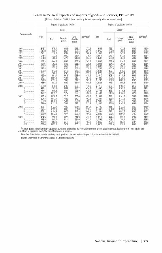
National Income or Expenditure | 359
Table B–25. Real exports and imports of goods and services, 1995–2009[Billions of chained (2005) dollars; quarterly data at seasonally adjusted annual rates]
Year or quarter
Exports of goods and services Imports of goods and services
Total
Goods 1
Services 1 Total
Goods 1
Services 1
Total Durablegoods
Non-durablegoods
Total Durablegoods
Non-durablegoods
1995 ...................... 845.7 575.4 363.6 216.2 272.6 944.5 766.1 422.9 360.0 180.91996 ...................... 916.0 626.2 405.4 223.4 291.7 1,026.7 837.9 468.1 384.1 190.31997 ...................... 1,025.1 716.2 478.7 237.9 308.9 1,165.0 958.7 545.4 424.1 206.91998 ...................... 1,048.5 732.2 494.2 237.6 316.4 1,301.1 1,072.3 617.2 462.9 229.41999 ...................... 1,094.3 760.0 517.8 240.8 334.6 1,450.9 1,206.0 707.1 500.2 244.92000 ...................... 1,188.3 844.3 584.6 256.5 343.5 1,639.9 1,367.9 814.8 549.2 271.72001 ...................... 1,121.6 792.0 535.9 255.2 329.3 1,593.8 1,324.2 764.5 564.2 269.62002 ...................... 1,099.2 763.5 505.6 259.1 335.6 1,648.0 1,373.4 796.5 580.2 274.52003 ...................... 1,116.8 777.2 514.5 263.8 339.6 1,720.7 1,440.9 830.6 615.2 279.82004 ...................... 1,222.8 842.9 571.0 272.2 380.0 1,910.8 1,599.7 945.0 655.8 311.02005 ...................... 1,305.1 906.1 624.9 281.2 399.0 2,027.8 1,708.0 1,025.4 682.6 319.82006 ...................... 1,422.0 991.4 691.9 299.6 430.6 2,151.2 1,808.8 1,115.3 694.5 342.42007 ...................... 1,546.1 1,064.8 749.1 316.1 481.3 2,193.8 1,839.6 1,139.8 701.4 354.22008 ...................... 1,629.3 1,127.5 784.0 342.7 501.7 2,123.5 1,767.3 1,089.2 678.5 356.52009 p .................... 1,468.6 987.0 650.9 331.6 480.6 1,822.5 1,479.1 858.8 612.5 342.92006: I .................. 1,388.8 970.3 678.3 292.1 418.5 2,121.3 1,782.7 1,103.2 681.2 338.6
II ................. 1,412.1 987.8 688.2 299.7 424.3 2,144.9 1,804.7 1,109.0 696.7 340.1III ................ 1,414.1 988.3 688.4 299.9 425.8 2,170.5 1,829.3 1,116.8 712.6 341.3IV ................ 1,473.2 1,019.2 712.7 306.7 453.9 2,168.1 1,818.6 1,132.3 687.6 349.5
2007: I .................. 1,485.9 1,026.7 721.5 305.6 459.2 2,190.8 1,841.1 1,141.5 700.6 349.8II ................. 1,504.8 1,042.4 732.0 310.7 462.3 2,188.1 1,836.5 1,127.8 709.0 351.6III ................ 1,569.9 1,078.9 758.4 320.9 490.9 2,208.3 1,849.4 1,144.3 706.4 359.0IV ................ 1,624.0 1,111.0 784.6 327.2 512.9 2,188.0 1,831.6 1,145.5 689.6 356.4
2008: I .................. 1,623.4 1,122.4 783.3 338.6 501.1 2,174.3 1,815.4 1,132.0 686.7 359.0II ................. 1,670.4 1,159.9 808.3 351.0 510.5 2,146.5 1,794.0 1,122.3 676.4 352.5III ................ 1,655.2 1,154.8 807.0 347.8 500.4 2,134.4 1,777.1 1,097.6 680.2 357.7IV ................ 1,568.0 1,072.9 737.4 333.3 494.9 2,038.9 1,682.6 1,004.7 670.7 356.9
2009: I .................. 1,434.5 956.1 637.3 314.9 477.2 1,821.0 1,474.4 835.3 629.4 346.2II ................. 1,419.5 940.7 611.4 324.0 477.4 1,749.8 1,409.4 798.1 602.1 339.5III ................ 1,478.8 993.9 651.8 337.2 483.9 1,836.2 1,490.6 863.5 618.4 345.3IV p ............. 1,541.6 1,057.4 702.9 350.2 484.0 1,882.7 1,541.9 938.3 600.0 340.7
1 Certain goods, primarily military equipment purchased and sold by the Federal Government, are included in services. Beginning with 1986, repairs andalterations of equipment were reclassified from goods to services.
Note: See Table B–2 for data for total exports of goods and services and total imports of goods and services for 1960–94.Source: Department of Commerce (Bureau of Economic Analysis).
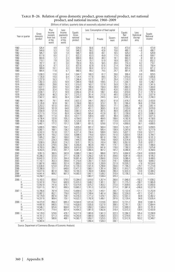
360 | Appendix B
Table B–26. Relation of gross domestic product, gross national product, net nationalproduct, and national income, 1960–2009
[Billions of dollars; quarterly data at seasonally adjusted annual rates]
Year or quarterGross
domesticproduct
Plus:Incomereceiptsfrom rest
of theworld
Less:Income
paymentsto restof theworld
Equals:Gross
nationalproduct
Less: Consumption of fixed capitalEquals:
Netnationalproduct
Less:Statisticaldiscrep-
ancy
Equals:NationalincomeTotal Private Govern-
ment
1960 ...................... 526.4 4.9 1.8 529.6 56.6 41.6 15.0 473.0 –1.0 473.91961 ...................... 544.8 5.3 1.8 548.3 58.2 42.6 15.6 490.1 –.6 490.71962 ...................... 585.7 5.9 1.8 589.7 60.6 44.1 16.5 529.2 .3 528.91963 ...................... 617.8 6.5 2.1 622.2 63.3 45.9 17.5 558.9 –.8 559.71964 ...................... 663.6 7.2 2.3 668.6 66.4 48.3 18.1 602.2 .8 601.41965 ...................... 719.1 7.9 2.6 724.4 70.7 51.9 18.9 653.7 1.5 652.21966 ...................... 787.7 8.1 3.0 792.8 76.5 56.5 20.0 716.3 6.2 710.11967 ...................... 832.4 8.7 3.3 837.8 82.9 61.6 21.4 754.9 4.5 750.41968 ...................... 909.8 10.1 4.0 915.9 90.4 67.4 23.0 825.5 4.3 821.21969 ...................... 984.4 11.8 5.7 990.5 99.2 74.5 24.7 891.4 2.9 888.51970 ...................... 1,038.3 12.8 6.4 1,044.7 108.3 81.7 26.6 936.4 6.9 929.51971 ...................... 1,126.8 14.0 6.4 1,134.4 117.8 89.5 28.2 1,016.6 11.0 1,005.61972 ...................... 1,237.9 16.3 7.7 1,246.4 127.2 97.7 29.4 1,119.3 8.9 1,110.31973 ...................... 1,382.3 23.5 10.9 1,394.9 140.8 109.5 31.3 1,254.1 8.0 1,246.11974 ...................... 1,499.5 29.8 14.3 1,515.0 163.7 127.8 35.9 1,351.3 9.8 1,341.51975 ...................... 1,637.7 28.0 15.0 1,650.7 190.4 150.4 39.9 1,460.3 16.3 1,444.01976 ...................... 1,824.6 32.4 15.5 1,841.4 208.2 165.5 42.6 1,633.3 23.5 1,609.81977 ...................... 2,030.1 37.2 16.9 2,050.4 231.8 186.1 45.6 1,818.6 21.2 1,797.41978 ...................... 2,293.8 46.3 24.7 2,315.3 261.4 212.0 49.5 2,053.9 26.1 2,027.91979 ...................... 2,562.2 68.3 36.4 2,594.2 298.9 244.5 54.4 2,295.3 47.0 2,248.31980 ...................... 2,788.1 79.1 44.9 2,822.3 344.1 282.3 61.8 2,478.2 45.3 2,433.01981 ...................... 3,126.8 92.0 59.1 3,159.8 393.3 323.2 70.1 2,766.4 36.6 2,729.81982 ...................... 3,253.2 101.0 64.5 3,289.7 433.5 356.4 77.1 2,856.2 4.8 2,851.41983 ...................... 3,534.6 101.9 64.8 3,571.7 451.1 369.5 81.6 3,120.6 49.7 3,070.91984 ...................... 3,930.9 121.9 85.6 3,967.2 474.3 387.5 86.9 3,492.8 31.5 3,461.31985 ...................... 4,217.5 112.4 85.9 4,244.0 505.4 412.8 92.7 3,738.6 42.3 3,696.31986 ...................... 4,460.1 111.0 93.4 4,477.7 538.5 439.1 99.4 3,939.2 67.7 3,871.51987 ...................... 4,736.4 122.8 105.2 4,754.0 571.1 464.5 106.6 4,182.9 32.9 4,150.01988 ...................... 5,100.4 151.6 128.3 5,123.8 611.0 497.1 113.9 4,512.8 –9.5 4,522.31989 ...................... 5,482.1 177.2 151.2 5,508.1 651.5 529.6 121.8 4,856.6 56.1 4,800.51990 ...................... 5,800.5 188.5 154.1 5,835.0 691.2 560.4 130.8 5,143.7 84.2 5,059.51991 ...................... 5,992.1 168.1 138.2 6,022.0 724.4 585.4 138.9 5,297.6 79.7 5,217.91992 ...................... 6,342.3 151.8 122.7 6,371.4 744.4 599.9 144.5 5,627.1 110.0 5,517.11993 ...................... 6,667.4 155.2 124.0 6,698.5 778.0 626.4 151.6 5,920.5 135.8 5,784.71994 ...................... 7,085.2 184.1 160.0 7,109.2 819.2 661.0 158.2 6,290.1 108.8 6,181.31995 ...................... 7,414.7 229.3 199.6 7,444.3 869.5 704.6 164.8 6,574.9 52.5 6,522.31996 ...................... 7,838.5 245.8 214.2 7,870.1 912.5 743.4 169.2 6,957.6 25.9 6,931.71997 ...................... 8,332.4 279.5 256.1 8,355.8 963.8 789.7 174.1 7,392.0 –14.0 7,406.01998 ...................... 8,793.5 286.2 268.9 8,810.8 1,020.5 841.6 179.0 7,790.3 –85.3 7,875.61999 ...................... 9,353.5 319.5 291.7 9,381.3 1,094.4 907.2 187.2 8,286.9 –71.1 8,358.02000 ...................... 9,951.5 380.5 342.8 9,989.2 1,184.3 986.8 197.5 8,804.9 –134.0 8,938.92001 ...................... 10,286.2 323.0 271.1 10,338.1 1,256.2 1,051.6 204.6 9,081.9 –103.4 9,185.22002 ...................... 10,642.3 313.5 264.4 10,691.4 1,305.0 1,094.0 210.9 9,386.4 –22.1 9,408.52003 ...................... 11,142.1 353.3 284.6 11,210.8 1,354.1 1,135.9 218.1 9,856.8 16.6 9,840.22004 ...................... 11,867.8 448.6 357.4 11,959.0 1,432.8 1,200.9 231.9 10,526.2 –7.8 10,534.02005 ...................... 12,638.4 573.0 475.9 12,735.5 1,541.4 1,290.8 250.6 11,194.2 –79.7 11,273.82006 ...................... 13,398.9 721.1 648.6 13,471.3 1,660.7 1,391.4 269.3 11,810.7 –220.6 12,031.22007 ...................... 14,077.6 861.8 746.0 14,193.3 1,760.0 1,469.6 290.4 12,433.3 –14.8 12,448.22008 ...................... 14,441.4 809.2 667.3 14,583.3 1,847.1 1,536.2 310.9 12,736.2 101.0 12,635.22009 p .................... 14,258.7 ................... ................... ................... 1,863.7 1,538.4 325.3 ................... ................... .....................2006: I .................. 13,183.5 659.0 578.5 13,264.0 1,618.0 1,357.4 260.6 11,646.0 –192.2 11,838.2
II ................. 13,347.8 716.4 640.9 13,423.3 1,648.2 1,381.1 267.1 11,775.2 –190.7 11,965.9III ................ 13,452.9 741.6 679.7 13,514.8 1,675.2 1,403.2 272.0 11,839.6 –253.4 12,093.0IV ................ 13,611.5 767.2 695.5 13,683.2 1,701.3 1,423.9 277.4 11,981.9 –246.0 12,227.9
2007: I .................. 13,795.6 787.9 724.0 13,859.5 1,726.7 1,443.1 283.7 12,132.8 –121.1 12,253.9II ................. 13,997.2 852.1 776.0 14,073.3 1,749.4 1,461.4 288.0 12,324.0 –97.1 12,421.1III ................ 14,179.9 897.6 759.1 14,318.3 1,771.2 1,478.7 292.5 12,547.2 64.9 12,482.2IV ................ 14,337.9 909.4 725.1 14,522.2 1,792.8 1,495.1 297.6 12,729.4 94.0 12,635.4
2008: I .................. 14,373.9 856.3 685.3 14,544.9 1,813.6 1,510.6 303.0 12,731.2 69.8 12,661.5II ................. 14,497.8 840.5 711.6 14,626.6 1,835.6 1,527.0 308.5 12,791.1 126.7 12,664.4III ................ 14,546.7 825.6 664.8 14,707.5 1,858.2 1,544.4 313.8 12,849.3 68.3 12,781.0IV ................ 14,347.3 714.4 607.4 14,454.3 1,881.0 1,562.6 318.4 12,573.3 139.4 12,433.9
2009: I .................. 14,178.0 579.6 479.7 14,277.9 1,883.6 1,561.3 322.3 12,394.3 185.4 12,208.9II ................. 14,151.2 571.3 478.6 14,243.8 1,864.0 1,540.5 323.5 12,379.8 161.7 12,218.1III ................ 14,242.1 590.6 469.1 14,363.7 1,850.7 1,525.5 325.2 12,512.9 163.2 12,349.7IV p ............. 14,463.4 ................... ................... ................... 1,856.4 1,526.3 330.1 ................... ................... .....................
Source: Department of Commerce (Bureau of Economic Analysis).
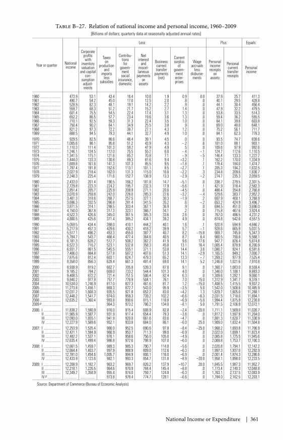
National Income or Expenditure | 361
Table B–27. Relation of national income and personal income, 1960–2009[Billions of dollars; quarterly data at seasonally adjusted annual rates]
Year or quarter Nationalincome
Less: Plus: Equals:
Corporateprofitswith
inventoryvaluation
and capitalcon-
sumptionadjust-ments
Taxeson
productionand
importsless
subsidies
Contribu-tionsfor
govern-mentsocial
insurance,domestic
Netinterest
andmiscel-laneous
paymentson
assets
Businesscurrenttransfer
payments(net)
Currentsurplus
ofgovern-mententer-prises
Wageaccruals
lessdisburse-
ments
Personalincomereceipts
onassets
Personalcurrenttransferreceipts
Personalincome
1960 ........................ 473.9 53.1 43.4 16.4 10.6 1.9 0.9 0.0 37.9 25.7 411.31961 ........................ 490.7 54.2 45.0 17.0 12.5 2.0 .8 .0 40.1 29.5 428.81962 ........................ 528.9 62.3 48.1 19.1 14.2 2.2 .9 .0 44.1 30.4 456.41963 ........................ 559.7 68.3 51.2 21.7 15.2 2.7 1.4 .0 47.9 32.2 479.51964 ........................ 601.4 75.5 54.5 22.4 17.4 3.1 1.3 .0 53.8 33.5 514.31965 ........................ 652.2 86.5 57.7 23.4 19.6 3.6 1.3 .0 59.4 36.2 555.51966 ........................ 710.1 92.5 59.3 31.3 22.4 3.5 1.0 .0 64.1 39.6 603.81967 ........................ 750.4 90.2 64.1 34.9 25.5 3.8 .9 .0 69.0 48.0 648.11968 ........................ 821.2 97.3 72.2 38.7 27.1 4.3 1.2 .0 75.2 56.1 711.71969 ........................ 888.5 94.5 79.3 44.1 32.7 4.9 1.0 .0 84.1 62.3 778.31970 ........................ 929.5 82.5 86.6 46.4 39.1 4.5 .0 .0 93.5 74.7 838.61971 ........................ 1,005.6 96.1 95.8 51.2 43.9 4.3 –.2 .6 101.0 88.1 903.11972 ........................ 1,110.3 111.4 101.3 59.2 47.9 4.9 .5 .0 109.6 97.9 992.61973 ........................ 1,246.1 124.5 112.0 75.5 55.2 6.0 –.4 –.1 124.7 112.6 1,110.51974 ........................ 1,341.5 115.1 121.6 85.2 70.8 7.1 –.9 –.5 146.4 133.3 1,222.71975 ........................ 1,444.0 133.3 130.8 89.3 81.6 9.4 –3.2 .1 162.2 170.0 1,334.91976 ........................ 1,609.8 161.6 141.3 101.3 85.5 9.5 –1.8 .1 178.4 184.0 1,474.71977 ........................ 1,797.4 191.8 152.6 113.1 101.1 8.5 –2.7 .1 205.3 194.2 1,632.51978 ........................ 2,027.9 218.4 162.0 131.3 115.0 10.8 –2.2 .3 234.8 209.6 1,836.71979 ........................ 2,248.3 225.4 171.6 152.7 138.9 13.3 –2.9 –.2 274.7 235.3 2,059.51980 ........................ 2,433.0 201.4 190.5 166.2 181.8 14.7 –5.1 .0 338.7 279.5 2,301.51981 ........................ 2,729.8 223.3 224.2 195.7 232.3 17.9 –5.6 .1 421.9 318.4 2,582.31982 ........................ 2,851.4 205.7 225.9 208.9 271.1 20.6 –4.5 .0 488.4 354.8 2,766.81983 ........................ 3,070.9 259.8 242.0 226.0 285.3 22.6 –3.2 –.4 529.6 383.7 2,952.21984 ........................ 3,461.3 318.6 268.7 257.5 327.1 30.3 –1.9 .2 607.9 400.1 3,268.91985 ........................ 3,696.3 332.5 286.8 281.4 341.5 35.2 .6 –.2 653.2 424.9 3,496.71986 ........................ 3,871.5 314.1 298.5 303.4 367.1 36.9 .9 .0 694.5 451.0 3,696.01987 ........................ 4,150.0 367.8 317.3 323.1 366.7 34.1 .2 .0 715.8 467.6 3,924.41988 ........................ 4,522.3 426.6 345.0 361.5 385.3 33.6 2.6 .0 767.0 496.5 4,231.21989 ........................ 4,800.5 425.6 371.4 385.2 434.1 39.2 4.9 .0 874.8 542.6 4,557.51990 ........................ 5,059.5 434.4 398.0 410.1 444.2 40.1 1.6 .1 920.8 594.9 4,846.71991 ........................ 5,217.9 457.3 429.6 430.2 418.2 39.9 5.7 –.1 928.6 665.9 5,031.51992 ........................ 5,517.1 496.2 453.3 455.0 387.7 40.7 8.2 –15.8 909.7 745.8 5,347.31993 ........................ 5,784.7 543.7 466.4 477.4 364.6 40.5 8.7 6.4 900.5 790.8 5,568.11994 ........................ 6,181.3 628.2 512.7 508.2 362.2 41.9 9.6 17.6 947.7 826.4 5,874.81995 ........................ 6,522.3 716.2 523.1 532.8 358.3 45.8 13.1 16.4 1,005.4 878.9 6,200.91996 ........................ 6,931.7 801.5 545.5 555.1 371.1 53.8 14.4 3.6 1,080.7 924.1 6,591.61997 ........................ 7,406.0 884.8 577.8 587.2 407.6 51.3 14.1 –2.9 1,165.5 949.2 7,000.71998 ........................ 7,875.6 812.4 603.1 624.7 479.3 65.2 13.3 –.7 1,269.2 977.9 7,525.41999 ........................ 8,358.0 856.3 628.4 661.3 481.4 69.0 14.1 5.2 1,246.8 1,021.6 7,910.82000 ........................ 8,938.9 819.2 662.7 705.8 539.3 87.0 9.1 .0 1,360.7 1,083.0 8,559.42001 ........................ 9,185.2 784.2 669.0 733.2 544.4 101.3 4.0 .0 1,346.0 1,188.1 8,883.32002 ........................ 9,408.5 872.2 721.4 751.5 506.4 82.4 6.3 .0 1,309.6 1,282.1 9,060.12003 ........................ 9,840.2 977.8 757.7 778.9 504.1 76.1 7.0 15.0 1,312.9 1,341.7 9,378.12004 ........................ 10,534.0 1,246.9 817.0 827.3 461.6 81.7 1.2 –15.0 1,408.5 1,415.5 9,937.22005 ........................ 11,273.8 1,456.1 869.3 872.7 543.0 95.9 –3.5 5.0 1,542.0 1,508.6 10,485.92006 ........................ 12,031.2 1,608.3 935.5 921.8 652.2 83.0 –4.2 1.3 1,829.7 1,605.0 11,268.12007 ........................ 12,448.2 1,541.7 974.0 959.3 739.2 102.2 –6.6 –6.3 2,031.5 1,718.0 11,894.12008 ........................ 12,635.2 1,360.4 993.8 990.6 815.1 118.8 –6.9 –5.0 1,994.4 1,875.9 12,238.82009 p ...................... ............... ................. 964.3 973.2 786.2 134.0 –8.1 5.0 1,791.5 2,106.9 12,072.12006: I .................... 11,838.2 1,590.9 916.0 915.4 608.9 82.8 –2.4 –20.0 1,711.1 1,569.0 11,026.7
II ................... 11,965.9 1,597.7 931.9 917.4 654.4 79.3 –3.8 .0 1,817.2 1,597.9 11,204.0III .................. 12,093.0 1,655.1 941.9 920.8 661.6 83.6 –4.7 .0 1,881.3 1,620.7 11,336.9IV .................. 12,227.9 1,589.6 952.1 933.8 684.0 86.1 –6.0 25.0 1,909.0 1,632.4 11,504.8
2007: I .................... 12,253.9 1,535.4 966.0 952.5 690.6 97.8 –8.4 –25.0 1,968.2 1,693.8 11,706.9II ................... 12,421.1 1,594.9 966.9 953.7 711.3 99.0 –6.9 .0 2,022.0 1,699.1 11,823.4III .................. 12,482.2 1,537.1 976.1 958.6 756.0 105.0 –4.9 .0 2,065.8 1,725.5 11,945.6IV .................. 12,635.4 1,499.4 986.8 972.6 798.9 107.0 –6.0 .0 2,069.8 1,753.7 12,100.3
2008: I .................... 12,661.5 1,459.7 989.3 985.3 790.7 114.8 –5.6 .0 2,020.8 1,794.1 12,142.2II ................... 12,664.4 1,403.7 997.9 988.9 809.0 112.6 –6.3 .0 1,997.3 1,937.0 12,292.9III .................. 12,781.0 1,454.6 1,005.7 994.9 806.1 116.0 –6.9 .0 2,001.4 1,874.3 12,286.6IV .................. 12,433.9 1,123.6 982.1 993.3 854.7 131.8 –8.9 –20.0 1,958.1 1,898.0 12,233.5
2009: I .................... 12,208.9 1,182.7 963.2 969.7 826.2 137.9 –10.7 20.0 1,845.5 1,987.3 11,952.7II ................... 12,218.1 1,226.5 964.6 970.9 784.4 145.4 –8.8 .0 1,773.4 2,140.3 12,048.8III .................. 12,349.7 1,358.9 955.4 974.0 759.7 124.8 –6.3 .0 1,763.1 2,137.5 12,083.9IV p ............... ............... ................. 973.8 978.4 774.7 128.1 –6.6 .0 1,784.0 2,162.5 12,203.1
Source: Department of Commerce (Bureau of Economic Analysis).
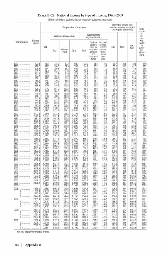
362 | Appendix B
Table B–28. National income by type of income, 1960–2009[Billions of dollars; quarterly data at seasonally adjusted annual rates]
Year or quarter Nationalincome
Compensation of employeesProprietors’ income with
inventory valuation and capitalconsumption adjustments Rental
incomeof
per-sonswith
capitalcon-
sump-tion
adjust-ment
Total
Wage and salary accruals Supplements towages and salaries
Total Farm Non-farm
Total Govern-ment Other Total
Employercontribu-tions for
employeepension
andinsurance
funds
Employercontribu-tions forgovern-
mentsocialinsur-ance
1960 ...................... 473.9 296.4 272.9 49.2 223.7 23.6 14.3 9.3 50.7 10.6 40.1 17.01961 ...................... 490.7 305.3 280.5 52.5 228.0 24.8 15.2 9.6 53.2 11.2 42.0 17.71962 ...................... 528.9 327.1 299.4 56.3 243.0 27.8 16.6 11.2 55.3 11.2 44.1 18.61963 ...................... 559.7 345.2 314.9 60.0 254.8 30.4 18.0 12.4 56.5 11.0 45.5 19.31964 ...................... 601.4 370.7 337.8 64.9 272.9 32.9 20.3 12.6 59.4 9.8 49.6 19.41965 ...................... 652.2 399.5 363.8 69.9 293.8 35.7 22.7 13.1 63.9 12.0 51.9 19.91966 ...................... 710.1 442.7 400.3 78.4 321.9 42.3 25.5 16.8 68.2 13.0 55.2 20.51967 ...................... 750.4 475.1 429.0 86.5 342.5 46.1 28.1 18.0 69.8 11.6 58.2 20.91968 ...................... 821.2 524.3 472.0 96.7 375.3 52.3 32.4 20.0 74.2 11.7 62.5 20.61969 ...................... 888.5 577.6 518.3 105.6 412.7 59.3 36.5 22.8 77.5 12.8 64.7 20.91970 ...................... 929.5 617.2 551.6 117.2 434.3 65.7 41.8 23.8 78.5 12.9 65.6 21.11971 ...................... 1,005.6 658.9 584.5 126.8 457.8 74.4 47.9 26.4 84.7 13.4 71.3 22.21972 ...................... 1,110.3 725.1 638.8 137.9 500.9 86.4 55.2 31.2 96.0 17.0 79.0 23.11973 ...................... 1,246.1 811.2 708.8 148.8 560.0 102.5 62.7 39.8 113.6 29.1 84.6 23.91974 ...................... 1,341.5 890.2 772.3 160.5 611.8 118.0 73.3 44.7 113.5 23.5 90.0 24.01975 ...................... 1,444.0 949.1 814.8 176.2 638.6 134.3 87.6 46.7 119.6 22.0 97.6 23.41976 ...................... 1,609.8 1,059.3 899.7 188.9 710.8 159.6 105.2 54.4 132.2 17.2 115.0 22.11977 ...................... 1,797.4 1,180.5 994.2 202.6 791.6 186.4 125.3 61.1 146.0 16.0 130.1 19.61978 ...................... 2,027.9 1,335.5 1,120.6 220.0 900.6 214.9 143.4 71.5 167.5 19.9 147.6 20.91979 ...................... 2,248.3 1,498.3 1,253.3 237.1 1,016.2 245.0 162.4 82.6 181.1 22.2 159.0 22.61980 ...................... 2,433.0 1,647.6 1,373.4 261.5 1,112.0 274.2 185.2 88.9 173.5 11.7 161.8 28.51981 ...................... 2,729.8 1,819.7 1,511.4 285.8 1,225.5 308.3 204.7 103.6 181.6 19.0 162.6 36.51982 ...................... 2,851.4 1,919.6 1,587.5 307.5 1,280.0 332.1 222.4 109.8 174.8 13.3 161.5 38.11983 ...................... 3,070.9 2,035.5 1,677.5 324.8 1,352.7 358.0 238.1 119.9 190.7 6.2 184.5 38.21984 ...................... 3,461.3 2,245.4 1,844.9 348.1 1,496.8 400.5 261.5 139.0 233.1 20.9 212.1 40.01985 ...................... 3,696.3 2,411.7 1,982.6 373.9 1,608.7 429.2 281.5 147.7 246.1 21.0 225.1 41.91986 ...................... 3,871.5 2,557.7 2,102.3 397.2 1,705.1 455.3 297.5 157.9 262.6 22.8 239.7 33.81987 ...................... 4,150.0 2,735.6 2,256.3 423.1 1,833.1 479.4 313.1 166.3 294.2 28.9 265.3 34.21988 ...................... 4,522.3 2,954.2 2,439.8 452.0 1,987.7 514.4 329.7 184.6 334.8 26.8 308.0 40.21989 ...................... 4,800.5 3,131.3 2,583.1 481.1 2,101.9 548.3 354.6 193.7 351.6 33.0 318.6 42.41990 ...................... 5,059.5 3,326.3 2,741.2 519.0 2,222.2 585.1 378.6 206.5 365.1 32.2 333.0 49.81991 ...................... 5,217.9 3,438.3 2,814.5 548.8 2,265.7 623.9 408.7 215.1 367.3 27.5 339.8 61.61992 ...................... 5,517.1 3,631.4 2,957.8 572.0 2,385.8 673.6 445.2 228.4 414.9 35.8 379.1 84.61993 ...................... 5,784.7 3,797.1 3,083.0 589.0 2,494.0 714.1 474.4 239.7 449.6 32.0 417.6 114.11994 ...................... 6,181.3 3,998.5 3,248.5 609.5 2,639.0 750.1 495.9 254.1 485.1 35.6 449.5 142.91995 ...................... 6,522.3 4,195.2 3,434.4 629.0 2,805.4 760.8 496.7 264.1 516.0 23.4 492.6 154.61996 ...................... 6,931.7 4,391.4 3,620.0 648.1 2,971.9 771.4 496.6 274.8 583.7 38.4 545.2 170.41997 ...................... 7,406.0 4,665.6 3,873.6 671.8 3,201.8 792.0 502.4 289.6 628.2 32.6 595.6 176.51998 ...................... 7,875.6 5,023.2 4,180.9 701.2 3,479.7 842.3 535.1 307.2 687.5 28.9 658.7 191.51999 ...................... 8,358.0 5,353.9 4,465.2 733.7 3,731.5 888.8 565.4 323.3 746.8 28.5 718.3 208.22000 ...................... 8,938.9 5,788.8 4,827.7 779.7 4,048.0 961.2 615.9 345.2 817.5 29.6 787.8 215.32001 ...................... 9,185.2 5,979.3 4,952.2 821.9 4,130.3 1,027.1 669.1 358.0 870.7 30.5 840.2 232.42002 ...................... 9,408.5 6,110.8 4,997.3 873.1 4,124.2 1,113.5 747.4 366.1 890.3 18.5 871.8 218.72003 ...................... 9,840.2 6,382.6 5,154.6 913.3 4,241.3 1,228.0 845.6 382.4 930.6 36.5 894.1 204.22004 ...................... 10,534.0 6,693.4 5,410.7 952.8 4,457.9 1,282.7 874.6 408.1 1,033.8 49.7 984.1 198.42005 ...................... 11,273.8 7,065.0 5,706.0 991.5 4,714.5 1,359.1 931.6 427.5 1,069.8 43.9 1,025.9 178.22006 ...................... 12,031.2 7,477.0 6,070.1 1,035.2 5,035.0 1,406.9 960.1 446.7 1,133.0 29.3 1,103.6 146.52007 ...................... 12,448.2 7,856.5 6,402.6 1,089.1 5,313.5 1,453.8 993.0 460.8 1,096.4 39.4 1,056.9 144.92008 ...................... 12,635.2 8,037.4 6,540.8 1,141.3 5,399.6 1,496.6 1,023.9 472.7 1,106.3 48.7 1,057.5 210.42009 p .................... ................ 7,841.3 6,335.6 1,182.5 5,153.1 1,505.7 1,043.9 461.8 1,042.3 29.9 1,012.4 268.32006: I .................. 11,838.2 7,353.7 5,958.9 1,019.0 4,939.9 1,394.8 950.7 444.1 1,126.9 28.4 1,098.5 161.3
II ................. 11,965.9 7,419.9 6,018.6 1,028.3 4,990.3 1,401.3 956.8 444.5 1,133.2 28.4 1,104.8 153.2III ................ 12,093.0 7,484.1 6,075.4 1,041.0 5,034.5 1,408.7 962.7 445.9 1,131.2 28.4 1,102.8 140.3IV ................ 12,227.9 7,650.3 6,227.6 1,052.3 5,175.4 1,422.6 970.4 452.2 1,140.6 32.2 1,108.4 131.2
2007: I .................. 12,253.9 7,757.2 6,318.6 1,073.2 5,245.3 1,438.6 980.5 458.1 1,094.2 36.7 1,057.5 121.1II ................. 12,421.1 7,819.7 6,372.2 1,084.2 5,288.0 1,447.5 989.4 458.2 1,096.0 35.7 1,060.3 140.3III ................ 12,482.2 7,869.6 6,412.5 1,093.2 5,319.4 1,457.1 996.9 460.2 1,093.2 37.5 1,055.7 150.2IV ................ 12,635.4 7,979.3 6,507.3 1,105.8 5,401.4 1,472.1 1,005.2 466.9 1,102.1 47.9 1,054.2 168.0
2008: I .................. 12,661.5 8,017.5 6,533.0 1,125.3 5,407.7 1,484.5 1,014.0 470.5 1,115.2 57.2 1,057.9 179.9II ................. 12,664.4 8,032.8 6,539.2 1,136.4 5,402.8 1,493.5 1,021.7 471.8 1,111.9 49.4 1,062.5 202.8III ................ 12,781.0 8,069.1 6,567.7 1,148.5 5,419.2 1,501.4 1,026.7 474.7 1,114.4 49.3 1,065.1 222.2IV ................ 12,433.9 8,030.3 6,523.5 1,154.9 5,368.6 1,506.8 1,033.2 473.6 1,083.6 39.0 1,044.5 236.7
2009: I .................. 12,208.9 7,825.8 6,327.8 1,171.8 5,156.0 1,498.0 1,037.8 460.2 1,037.8 27.3 1,010.5 245.9II ................. 12,218.1 7,815.9 6,313.1 1,184.4 5,128.8 1,502.8 1,042.0 460.8 1,028.0 28.9 999.1 262.0III ................ 12,349.7 7,841.5 6,333.2 1,184.8 5,148.4 1,508.3 1,046.1 462.2 1,037.9 25.8 1,012.0 277.9IV p ............. ............... 7,882.1 6,368.2 1,189.0 5,179.2 1,513.8 1,049.8 464.1 1,065.5 37.4 1,028.1 287.4
See next page for continuation of table.
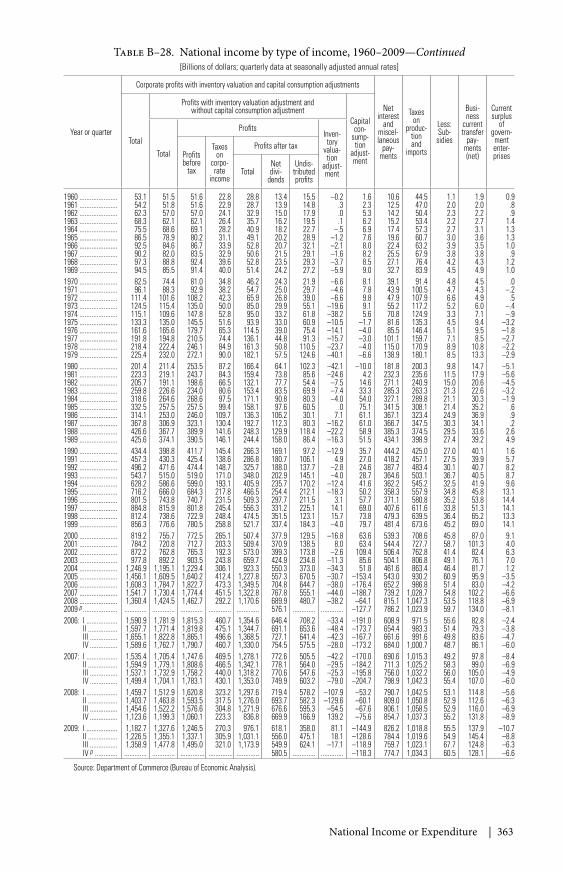
National Income or Expenditure | 363
Table B–28. National income by type of income, 1960–2009—Continued[Billions of dollars; quarterly data at seasonally adjusted annual rates]
Year or quarter
Corporate profits with inventory valuation and capital consumption adjustments
Netinterest
andmiscel-laneous
pay-ments
Taxeson
produc-tionand
imports
Less:Sub-
sidies
Busi-ness
currenttransfer
pay-ments(net)
Currentsurplus
ofgovern-mententer-prises
Total
Profits with inventory valuation adjustment andwithout capital consumption adjustment
Capitalcon-
sump-tion
adjust-ment
Total
ProfitsInven-tory
valua-tion
adjust-ment
Profitsbefore
tax
Taxeson
corpo-rate
income
Profits after tax
TotalNetdivi-
dends
Undis-tributedprofits
1960 ...................... 53.1 51.5 51.6 22.8 28.8 13.4 15.5 –0.2 1.6 10.6 44.5 1.1 1.9 0.91961 ...................... 54.2 51.8 51.6 22.9 28.7 13.9 14.8 .3 2.3 12.5 47.0 2.0 2.0 .81962 ...................... 62.3 57.0 57.0 24.1 32.9 15.0 17.9 .0 5.3 14.2 50.4 2.3 2.2 .91963 ...................... 68.3 62.1 62.1 26.4 35.7 16.2 19.5 .1 6.2 15.2 53.4 2.2 2.7 1.41964 ...................... 75.5 68.6 69.1 28.2 40.9 18.2 22.7 –.5 6.9 17.4 57.3 2.7 3.1 1.31965 ...................... 86.5 78.9 80.2 31.1 49.1 20.2 28.9 –1.2 7.6 19.6 60.7 3.0 3.6 1.31966 ...................... 92.5 84.6 86.7 33.9 52.8 20.7 32.1 –2.1 8.0 22.4 63.2 3.9 3.5 1.01967 ...................... 90.2 82.0 83.5 32.9 50.6 21.5 29.1 –1.6 8.2 25.5 67.9 3.8 3.8 .91968 ...................... 97.3 88.8 92.4 39.6 52.8 23.5 29.3 –3.7 8.5 27.1 76.4 4.2 4.3 1.21969 ...................... 94.5 85.5 91.4 40.0 51.4 24.2 27.2 –5.9 9.0 32.7 83.9 4.5 4.9 1.01970 ...................... 82.5 74.4 81.0 34.8 46.2 24.3 21.9 –6.6 8.1 39.1 91.4 4.8 4.5 .01971 ...................... 96.1 88.3 92.9 38.2 54.7 25.0 29.7 –4.6 7.8 43.9 100.5 4.7 4.3 –.21972 ...................... 111.4 101.6 108.2 42.3 65.9 26.8 39.0 –6.6 9.8 47.9 107.9 6.6 4.9 .51973 ...................... 124.5 115.4 135.0 50.0 85.0 29.9 55.1 –19.6 9.1 55.2 117.2 5.2 6.0 –.41974 ...................... 115.1 109.6 147.8 52.8 95.0 33.2 61.8 –38.2 5.6 70.8 124.9 3.3 7.1 –.91975 ...................... 133.3 135.0 145.5 51.6 93.9 33.0 60.9 –10.5 –1.7 81.6 135.3 4.5 9.4 –3.21976 ...................... 161.6 165.6 179.7 65.3 114.5 39.0 75.4 –14.1 –4.0 85.5 146.4 5.1 9.5 –1.81977 ...................... 191.8 194.8 210.5 74.4 136.1 44.8 91.3 –15.7 –3.0 101.1 159.7 7.1 8.5 –2.71978 ...................... 218.4 222.4 246.1 84.9 161.3 50.8 110.5 –23.7 –4.0 115.0 170.9 8.9 10.8 –2.21979 ...................... 225.4 232.0 272.1 90.0 182.1 57.5 124.6 –40.1 –6.6 138.9 180.1 8.5 13.3 –2.91980 ...................... 201.4 211.4 253.5 87.2 166.4 64.1 102.3 –42.1 –10.0 181.8 200.3 9.8 14.7 –5.11981 ...................... 223.3 219.1 243.7 84.3 159.4 73.8 85.6 –24.6 4.2 232.3 235.6 11.5 17.9 –5.61982 ...................... 205.7 191.1 198.6 66.5 132.1 77.7 54.4 –7.5 14.6 271.1 240.9 15.0 20.6 –4.51983 ...................... 259.8 226.6 234.0 80.6 153.4 83.5 69.9 –7.4 33.3 285.3 263.3 21.3 22.6 –3.21984 ...................... 318.6 264.6 268.6 97.5 171.1 90.8 80.3 –4.0 54.0 327.1 289.8 21.1 30.3 –1.91985 ...................... 332.5 257.5 257.5 99.4 158.1 97.6 60.5 .0 75.1 341.5 308.1 21.4 35.2 .61986 ...................... 314.1 253.0 246.0 109.7 136.3 106.2 30.1 7.1 61.1 367.1 323.4 24.9 36.9 .91987 ...................... 367.8 306.9 323.1 130.4 192.7 112.3 80.3 –16.2 61.0 366.7 347.5 30.3 34.1 .21988 ...................... 426.6 367.7 389.9 141.6 248.3 129.9 118.4 –22.2 58.9 385.3 374.5 29.5 33.6 2.61989 ...................... 425.6 374.1 390.5 146.1 244.4 158.0 86.4 –16.3 51.5 434.1 398.9 27.4 39.2 4.91990 ...................... 434.4 398.8 411.7 145.4 266.3 169.1 97.2 –12.9 35.7 444.2 425.0 27.0 40.1 1.61991 ...................... 457.3 430.3 425.4 138.6 286.8 180.7 106.1 4.9 27.0 418.2 457.1 27.5 39.9 5.71992 ...................... 496.2 471.6 474.4 148.7 325.7 188.0 137.7 –2.8 24.6 387.7 483.4 30.1 40.7 8.21993 ...................... 543.7 515.0 519.0 171.0 348.0 202.9 145.1 –4.0 28.7 364.6 503.1 36.7 40.5 8.71994 ...................... 628.2 586.6 599.0 193.1 405.9 235.7 170.2 –12.4 41.6 362.2 545.2 32.5 41.9 9.61995 ...................... 716.2 666.0 684.3 217.8 466.5 254.4 212.1 –18.3 50.2 358.3 557.9 34.8 45.8 13.11996 ...................... 801.5 743.8 740.7 231.5 509.3 297.7 211.5 3.1 57.7 371.1 580.8 35.2 53.8 14.41997 ...................... 884.8 815.9 801.8 245.4 556.3 331.2 225.1 14.1 69.0 407.6 611.6 33.8 51.3 14.11998 ...................... 812.4 738.6 722.9 248.4 474.5 351.5 123.1 15.7 73.8 479.3 639.5 36.4 65.2 13.31999 ...................... 856.3 776.6 780.5 258.8 521.7 337.4 184.3 –4.0 79.7 481.4 673.6 45.2 69.0 14.12000 ...................... 819.2 755.7 772.5 265.1 507.4 377.9 129.5 –16.8 63.6 539.3 708.6 45.8 87.0 9.12001 ...................... 784.2 720.8 712.7 203.3 509.4 370.9 138.5 8.0 63.4 544.4 727.7 58.7 101.3 4.02002 ...................... 872.2 762.8 765.3 192.3 573.0 399.3 173.8 –2.6 109.4 506.4 762.8 41.4 82.4 6.32003 ...................... 977.8 892.2 903.5 243.8 659.7 424.9 234.8 –11.3 85.6 504.1 806.8 49.1 76.1 7.02004 ...................... 1,246.9 1,195.1 1,229.4 306.1 923.3 550.3 373.0 –34.3 51.8 461.6 863.4 46.4 81.7 1.22005 ...................... 1,456.1 1,609.5 1,640.2 412.4 1,227.8 557.3 670.5 –30.7 –153.4 543.0 930.2 60.9 95.9 –3.52006 ...................... 1,608.3 1,784.7 1,822.7 473.3 1,349.5 704.8 644.7 –38.0 –176.4 652.2 986.8 51.4 83.0 –4.22007 ...................... 1,541.7 1,730.4 1,774.4 451.5 1,322.8 767.8 555.1 –44.0 –188.7 739.2 1,028.7 54.8 102.2 –6.62008 ...................... 1,360.4 1,424.5 1,462.7 292.2 1,170.6 689.9 480.7 –38.2 –64.1 815.1 1,047.3 53.5 118.8 –6.92009 p .................... ............. ............. ............. ............. ............. 576.1 ............. ............. –127.7 786.2 1,023.9 59.7 134.0 –8.12006: I .................. 1,590.9 1,781.9 1,815.3 460.7 1,354.6 646.4 708.2 –33.4 –191.0 608.9 971.5 55.6 82.8 –2.4
II ................. 1,597.7 1,771.4 1,819.8 475.1 1,344.7 691.1 653.6 –48.4 –173.7 654.4 983.3 51.4 79.3 –3.8III ................ 1,655.1 1,822.8 1,865.1 496.6 1,368.5 727.1 641.4 –42.3 –167.7 661.6 991.6 49.8 83.6 –4.7IV ................ 1,589.6 1,762.7 1,790.7 460.7 1,330.0 754.5 575.5 –28.0 –173.2 684.0 1,000.7 48.7 86.1 –6.0
2007: I .................. 1,535.4 1,705.4 1,747.6 469.5 1,278.1 772.6 505.5 –42.2 –170.0 690.6 1,015.3 49.2 97.8 –8.4II ................. 1,594.9 1,779.1 1,808.6 466.5 1,342.1 778.1 564.0 –29.5 –184.2 711.3 1,025.2 58.3 99.0 –6.9III ................ 1,537.1 1,732.9 1,758.2 440.0 1,318.2 770.6 547.6 –25.3 –195.8 756.0 1,032.2 56.0 105.0 –4.9IV ................ 1,499.4 1,704.1 1,783.1 430.1 1,353.0 749.9 603.2 –79.0 –204.7 798.9 1,042.3 55.4 107.0 –6.0
2008: I .................. 1,459.7 1,512.9 1,620.8 323.2 1,297.6 719.4 578.2 –107.9 –53.2 790.7 1,042.5 53.1 114.8 –5.6II ................. 1,403.7 1,463.8 1,593.5 317.5 1,276.0 693.7 582.3 –129.6 –60.1 809.0 1,050.8 52.9 112.6 –6.3III ................ 1,454.6 1,522.2 1,576.6 304.8 1,271.9 676.6 595.3 –54.5 –67.6 806.1 1,058.5 52.9 116.0 –6.9IV ................ 1,123.6 1,199.3 1,060.1 223.3 836.8 669.9 166.9 139.2 –75.6 854.7 1,037.3 55.2 131.8 –8.9
2009: I .................. 1,182.7 1,327.6 1,246.5 270.3 976.1 618.1 358.0 81.1 –144.9 826.2 1,018.8 55.5 137.9 –10.7II ................. 1,226.5 1,355.1 1,337.1 305.9 1,031.1 556.0 475.1 18.1 –128.6 784.4 1,019.6 54.9 145.4 –8.8III ................ 1,358.9 1,477.8 1,495.0 321.0 1,173.9 549.9 624.1 –17.1 –118.9 759.7 1,023.1 67.7 124.8 –6.3IV p ............. ............. ............. .............. .............. ............. 580.5 ............. ............. –118.3 774.7 1,034.3 60.5 128.1 –6.6
Source: Department of Commerce (Bureau of Economic Analysis).
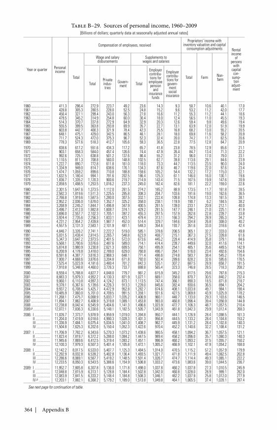
364 | Appendix B
Table B–29. Sources of personal income, 1960–2009[Billions of dollars; quarterly data at seasonally adjusted annual rates]
Year or quarter Personalincome
Compensation of employees, receivedProprietors’ income with
inventory valuation and capitalconsumption adjustments Rental
incomeof
personswith
capitalcon-
sump-tion
adjust-ment
Total
Wage and salarydisbursements
Supplements towages and salaries
Total Farm Non-farm
TotalPrivateindus-tries
Govern-ment Total
Employercontribu-tions for
employeepension
andinsurance
funds
Employercontribu-tions forgovern-mentsocial
insurance
1960 ...................... 411.3 296.4 272.9 223.7 49.2 23.6 14.3 9.3 50.7 10.6 40.1 17.01961 ...................... 428.8 305.3 280.5 228.0 52.5 24.8 15.2 9.6 53.2 11.2 42.0 17.71962 ...................... 456.4 327.1 299.4 243.0 56.3 27.8 16.6 11.2 55.3 11.2 44.1 18.61963 ...................... 479.5 345.2 314.9 254.8 60.0 30.4 18.0 12.4 56.5 11.0 45.5 19.31964 ...................... 514.3 370.7 337.8 272.9 64.9 32.9 20.3 12.6 59.4 9.8 49.6 19.41965 ...................... 555.5 399.5 363.8 293.8 69.9 35.7 22.7 13.1 63.9 12.0 51.9 19.91966 ...................... 603.8 442.7 400.3 321.9 78.4 42.3 25.5 16.8 68.2 13.0 55.2 20.51967 ...................... 648.1 475.1 429.0 342.5 86.5 46.1 28.1 18.0 69.8 11.6 58.2 20.91968 ...................... 711.7 524.3 472.0 375.3 96.7 52.3 32.4 20.0 74.2 11.7 62.5 20.61969 ...................... 778.3 577.6 518.3 412.7 105.6 59.3 36.5 22.8 77.5 12.8 64.7 20.91970 ...................... 838.6 617.2 551.6 434.3 117.2 65.7 41.8 23.8 78.5 12.9 65.6 21.11971 ...................... 903.1 658.3 584.0 457.4 126.6 74.4 47.9 26.4 84.7 13.4 71.3 22.21972 ...................... 992.6 725.1 638.8 501.2 137.6 86.4 55.2 31.2 96.0 17.0 79.0 23.11973 ...................... 1,110.5 811.3 708.8 560.0 148.8 102.5 62.7 39.8 113.6 29.1 84.6 23.91974 ...................... 1,222.7 890.7 772.8 611.8 161.0 118.0 73.3 44.7 113.5 23.5 90.0 24.01975 ...................... 1,334.9 949.0 814.7 638.6 176.1 134.3 87.6 46.7 119.6 22.0 97.6 23.41976 ...................... 1,474.7 1,059.2 899.6 710.8 188.8 159.6 105.2 54.4 132.2 17.2 115.0 22.11977 ...................... 1,632.5 1,180.4 994.1 791.6 202.5 186.4 125.3 61.1 146.0 16.0 130.1 19.61978 ...................... 1,836.7 1,335.2 1,120.3 900.6 219.7 214.9 143.4 71.5 167.5 19.9 147.6 20.91979 ...................... 2,059.5 1,498.5 1,253.5 1,016.2 237.3 245.0 162.4 82.6 181.1 22.2 159.0 22.61980 ...................... 2,301.5 1,647.6 1,373.5 1,112.0 261.5 274.2 185.2 88.9 173.5 11.7 161.8 28.51981 ...................... 2,582.3 1,819.6 1,511.3 1,225.5 285.8 308.3 204.7 103.6 181.6 19.0 162.6 36.51982 ...................... 2,766.8 1,919.6 1,587.5 1,280.0 307.5 332.1 222.4 109.8 174.8 13.3 161.5 38.11983 ...................... 2,952.2 2,036.0 1,678.0 1,352.7 325.2 358.0 238.1 119.9 190.7 6.2 184.5 38.21984 ...................... 3,268.9 2,245.2 1,844.7 1,496.8 347.9 400.5 261.5 139.0 233.1 20.9 212.1 40.01985 ...................... 3,496.7 2,412.0 1,982.8 1,608.7 374.1 429.2 281.5 147.7 246.1 21.0 225.1 41.91986 ...................... 3,696.0 2,557.7 2,102.3 1,705.1 397.2 455.3 297.5 157.9 262.6 22.8 239.7 33.81987 ...................... 3,924.4 2,735.6 2,256.3 1,833.1 423.1 479.4 313.1 166.3 294.2 28.9 265.3 34.21988 ...................... 4,231.2 2,954.2 2,439.8 1,987.7 452.0 514.4 329.7 184.6 334.8 26.8 308.0 40.21989 ...................... 4,557.5 3,131.3 2,583.1 2,101.9 481.1 548.3 354.6 193.7 351.6 33.0 318.6 42.41990 ...................... 4,846.7 3,326.2 2,741.1 2,222.2 519.0 585.1 378.6 206.5 365.1 32.2 333.0 49.81991 ...................... 5,031.5 3,438.4 2,814.5 2,265.7 548.8 623.9 408.7 215.1 367.3 27.5 339.8 61.61992 ...................... 5,347.3 3,647.2 2,973.5 2,401.5 572.0 673.6 445.2 228.4 414.9 35.8 379.1 84.61993 ...................... 5,568.1 3,790.6 3,076.6 2,487.6 589.0 714.1 474.4 239.7 449.6 32.0 417.6 114.11994 ...................... 5,874.8 3,980.9 3,230.8 2,621.3 609.5 750.1 495.9 254.1 485.1 35.6 449.5 142.91995 ...................... 6,200.9 4,178.8 3,418.0 2,789.0 629.0 760.8 496.7 264.1 516.0 23.4 492.6 154.61996 ...................... 6,591.6 4,387.7 3,616.3 2,968.3 648.1 771.4 496.6 274.8 583.7 38.4 545.2 170.41997 ...................... 7,000.7 4,668.6 3,876.6 3,204.8 671.8 792.0 502.4 289.6 628.2 32.6 595.6 176.51998 ...................... 7,525.4 5,023.9 4,181.6 3,480.4 701.2 842.3 535.1 307.2 687.5 28.9 658.7 191.51999 ...................... 7,910.8 5,348.8 4,460.0 3,726.3 733.7 888.8 565.4 323.3 746.8 28.5 718.3 208.22000 ...................... 8,559.4 5,788.8 4,827.7 4,048.0 779.7 961.2 615.9 345.2 817.5 29.6 787.8 215.32001 ...................... 8,883.3 5,979.3 4,952.2 4,130.3 821.9 1,027.1 669.1 358.0 870.7 30.5 840.2 232.42002 ...................... 9,060.1 6,110.8 4,997.3 4,124.2 873.1 1,113.5 747.4 366.1 890.3 18.5 871.8 218.72003 ...................... 9,378.1 6,367.6 5,139.6 4,226.3 913.3 1,228.0 845.6 382.4 930.6 36.5 894.1 204.22004 ...................... 9,937.2 6,708.4 5,425.7 4,472.9 952.8 1,282.7 874.6 408.1 1,033.8 49.7 984.1 198.42005 ...................... 10,485.9 7,060.0 5,701.0 4,709.5 991.5 1,359.1 931.6 427.5 1,069.8 43.9 1,025.9 178.22006 ...................... 11,268.1 7,475.7 6,068.9 5,033.7 1,035.2 1,406.9 960.1 446.7 1,133.0 29.3 1,103.6 146.52007 ...................... 11,894.1 7,862.7 6,408.9 5,319.8 1,089.1 1,453.8 993.0 460.8 1,096.4 39.4 1,056.9 144.92008 ...................... 12,238.8 8,042.4 6,545.9 5,404.6 1,141.3 1,496.6 1,023.9 472.7 1,106.3 48.7 1,057.5 210.42009 p .................... 12,072.1 7,836.3 6,330.6 5,148.1 1,182.5 1,505.7 1,043.9 461.8 1,042.3 29.9 1,012.4 268.32006: I .................. 11,026.7 7,373.7 5,978.9 4,959.9 1,019.0 1,394.8 950.7 444.1 1,126.9 28.4 1,098.5 161.3
II ................. 11,204.0 7,419.9 6,018.6 4,990.3 1,028.3 1,401.3 956.8 444.5 1,133.2 28.4 1,104.8 153.2III ................ 11,336.9 7,484.1 6,075.4 5,034.5 1,041.0 1,408.7 962.7 445.9 1,131.2 28.4 1,102.8 140.3IV ................ 11,504.8 7,625.3 6,202.6 5,150.4 1,052.3 1,422.6 970.4 452.2 1,140.6 32.2 1,108.4 131.2
2007: I .................. 11,706.9 7,782.2 6,343.6 5,270.3 1,073.2 1,438.6 980.5 458.1 1,094.2 36.7 1,057.5 121.1II ................. 11,823.4 7,819.7 6,372.2 5,288.0 1,084.2 1,447.5 989.4 458.2 1,096.0 35.7 1,060.3 140.3III ................ 11,945.6 7,869.6 6,412.5 5,319.4 1,093.2 1,457.1 996.9 460.2 1,093.2 37.5 1,055.7 150.2IV ................ 12,100.3 7,979.3 6,507.3 5,401.4 1,105.8 1,472.1 1,005.2 466.9 1,102.1 47.9 1,054.2 168.0
2008: I .................. 12,142.2 8,017.5 6,533.0 5,407.7 1,125.3 1,484.5 1,014.0 470.5 1,115.2 57.2 1,057.9 179.9II ................. 12,292.9 8,032.8 6,539.2 5,402.8 1,136.4 1,493.5 1,021.7 471.8 1,111.9 49.4 1,062.5 202.8III ................ 12,286.6 8,069.1 6,567.7 5,419.2 1,148.5 1,501.4 1,026.7 474.7 1,114.4 49.3 1,065.1 222.2IV ................ 12,233.5 8,050.3 6,543.5 5,388.6 1,154.9 1,506.8 1,033.2 473.6 1,083.6 39.0 1,044.5 236.7
2009: I .................. 11,952.7 7,805.8 6,307.8 5,136.0 1,171.8 1,498.0 1,037.8 460.2 1,037.8 27.3 1,010.5 245.9II ................. 12,048.8 7,815.9 6,313.1 5,128.8 1,184.4 1,502.8 1,042.0 460.8 1,028.0 28.9 999.1 262.0III ................ 12,083.9 7,841.5 6,333.2 5,148.4 1,184.8 1,508.3 1,046.1 462.2 1,037.9 25.8 1,012.0 277.9IV p ............. 12,203.1 7,882.1 6,368.2 5,179.2 1,189.0 1,513.8 1,049.8 464.1 1,065.5 37.4 1,028.1 287.4
See next page for continuation of table.
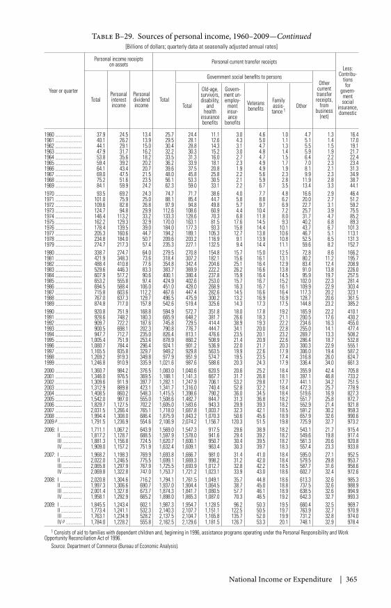
National Income or Expenditure | 365
Table B–29. Sources of personal income, 1960–2009—Continued[Billions of dollars; quarterly data at seasonally adjusted annual rates]
Year or quarter
Personal income receiptson assets Personal current transfer receipts
Less:Contribu-
tionsfor
govern-mentsocial
insurance,domestic
TotalPersonalinterestincome
Personaldividendincome
Total
Government social benefits to personsOther
currenttransferreceipts,
frombusiness
(net)
Total
Old-age,survivors,disability,
andhealth
insurancebenefits
Govern-ment un-employ-
mentinsur-ance
benefits
Veteransbenefits
Familyassis-tance 1
Other
1960 ...................... 37.9 24.5 13.4 25.7 24.4 11.1 3.0 4.6 1.0 4.7 1.3 16.41961 ...................... 40.1 26.2 13.9 29.5 28.1 12.6 4.3 5.0 1.1 5.1 1.4 17.01962 ...................... 44.1 29.1 15.0 30.4 28.8 14.3 3.1 4.7 1.3 5.5 1.5 19.11963 ...................... 47.9 31.7 16.2 32.2 30.3 15.2 3.0 4.8 1.4 5.9 1.9 21.71964 ...................... 53.8 35.6 18.2 33.5 31.3 16.0 2.7 4.7 1.5 6.4 2.2 22.41965 ...................... 59.4 39.2 20.2 36.2 33.9 18.1 2.3 4.9 1.7 7.0 2.3 23.41966 ...................... 64.1 43.4 20.7 39.6 37.5 20.8 1.9 4.9 1.9 8.1 2.1 31.31967 ...................... 69.0 47.5 21.5 48.0 45.8 25.8 2.2 5.6 2.3 9.9 2.3 34.91968 ...................... 75.2 51.6 23.5 56.1 53.3 30.5 2.1 5.9 2.8 11.9 2.8 38.71969 ...................... 84.1 59.9 24.2 62.3 59.0 33.1 2.2 6.7 3.5 13.4 3.3 44.11970 ...................... 93.5 69.2 24.3 74.7 71.7 38.6 4.0 7.7 4.8 16.6 2.9 46.41971 ...................... 101.0 75.9 25.0 88.1 85.4 44.7 5.8 8.8 6.2 20.0 2.7 51.21972 ...................... 109.6 82.8 26.8 97.9 94.8 49.8 5.7 9.7 6.9 22.7 3.1 59.21973 ...................... 124.7 94.8 29.9 112.6 108.6 60.9 4.4 10.4 7.2 25.7 3.9 75.51974 ...................... 146.4 113.2 33.2 133.3 128.6 70.3 6.8 11.8 8.0 31.7 4.7 85.21975 ...................... 162.2 129.3 32.9 170.0 163.1 81.5 17.6 14.5 9.3 40.2 6.8 89.31976 ...................... 178.4 139.5 39.0 184.0 177.3 93.3 15.8 14.4 10.1 43.7 6.7 101.31977 ...................... 205.3 160.6 44.7 194.2 189.1 105.3 12.7 13.8 10.6 46.7 5.1 113.11978 ...................... 234.8 184.0 50.7 209.6 203.2 116.9 9.1 13.9 10.8 52.5 6.5 131.31979 ...................... 274.7 217.3 57.4 235.3 227.1 132.5 9.4 14.4 11.1 59.6 8.2 152.71980 ...................... 338.7 274.7 64.0 279.5 270.8 154.8 15.7 15.0 12.5 72.8 8.6 166.21981 ...................... 421.9 348.3 73.6 318.4 307.2 182.1 15.6 16.1 13.1 80.2 11.2 195.71982 ...................... 488.4 410.8 77.6 354.8 342.4 204.6 25.1 16.4 12.9 83.4 12.4 208.91983 ...................... 529.6 446.3 83.3 383.7 369.9 222.2 26.2 16.6 13.8 91.0 13.8 226.01984 ...................... 607.9 517.2 90.6 400.1 380.4 237.8 15.9 16.4 14.5 95.9 19.7 257.51985 ...................... 653.2 555.8 97.4 424.9 402.6 253.0 15.7 16.7 15.2 102.0 22.3 281.41986 ...................... 694.5 588.4 106.0 451.0 428.0 268.9 16.3 16.7 16.1 109.9 22.9 303.41987 ...................... 715.8 603.6 112.2 467.6 447.4 282.6 14.5 16.6 16.4 117.3 20.2 323.11988 ...................... 767.0 637.3 129.7 496.5 475.9 300.2 13.2 16.9 16.9 128.7 20.6 361.51989 ...................... 874.8 717.0 157.8 542.6 519.4 325.6 14.3 17.3 17.5 144.8 23.2 385.21990 ...................... 920.8 751.9 168.8 594.9 572.7 351.8 18.0 17.8 19.2 165.9 22.2 410.11991 ...................... 928.6 748.2 180.3 665.9 648.2 381.7 26.6 18.3 21.1 200.5 17.6 430.21992 ...................... 909.7 722.2 187.6 745.8 729.5 414.4 38.9 19.3 22.2 234.6 16.3 455.01993 ...................... 900.5 698.1 202.3 790.8 776.7 444.7 34.1 20.0 22.8 255.0 14.1 477.41994 ...................... 947.7 712.7 235.0 826.4 813.1 476.6 23.5 20.1 23.2 269.7 13.3 508.21995 ...................... 1,005.4 751.9 253.4 878.9 860.2 508.9 21.4 20.9 22.6 286.4 18.7 532.81996 ...................... 1,080.7 784.4 296.4 924.1 901.2 536.9 22.0 21.7 20.3 300.3 22.9 555.11997 ...................... 1,165.5 835.8 329.7 949.2 929.8 563.5 19.9 22.6 17.9 306.0 19.4 587.21998 ...................... 1,269.2 919.3 349.8 977.9 951.9 574.7 19.5 23.5 17.4 316.8 26.0 624.71999 ...................... 1,246.8 910.9 335.9 1,021.6 987.6 588.6 20.3 24.3 17.9 336.4 34.0 661.32000 ...................... 1,360.7 984.2 376.5 1,083.0 1,040.6 620.5 20.6 25.2 18.4 355.9 42.4 705.82001 ...................... 1,346.0 976.5 369.5 1,188.1 1,141.3 667.7 31.7 26.8 18.1 397.1 46.8 733.22002 ...................... 1,309.6 911.9 397.7 1,282.1 1,247.9 706.1 53.2 29.8 17.7 441.1 34.2 751.52003 ...................... 1,312.9 889.8 423.1 1,341.7 1,316.0 740.4 52.8 32.2 18.4 472.3 25.7 778.92004 ...................... 1,408.5 860.2 548.3 1,415.5 1,398.6 790.2 36.0 34.5 18.4 519.6 16.9 827.32005 ...................... 1,542.0 987.0 555.0 1,508.6 1,482.7 844.7 31.3 36.8 18.2 551.7 25.8 872.72006 ...................... 1,829.7 1,127.5 702.2 1,605.0 1,583.6 943.3 29.9 39.3 18.2 552.9 21.4 921.82007 ...................... 2,031.5 1,266.4 765.1 1,718.0 1,687.8 1,003.7 32.3 42.1 18.5 591.2 30.2 959.32008 ...................... 1,994.4 1,308.0 686.4 1,875.9 1,843.2 1,070.3 50.6 45.6 18.9 657.9 32.6 990.62009 p .................... 1,791.5 1,236.9 554.6 2,106.9 2,074.2 1,156.7 120.3 51.5 19.8 725.9 32.7 973.22006: I .................. 1,711.1 1,067.2 643.9 1,569.0 1,547.3 917.5 29.6 38.9 18.2 543.1 21.7 915.4
II ................. 1,817.2 1,128.7 688.5 1,597.9 1,578.0 941.6 29.4 39.2 18.2 549.6 19.8 917.4III ................ 1,881.3 1,156.8 724.5 1,620.7 1,600.1 950.7 30.4 39.5 18.2 561.3 20.6 920.8IV ................ 1,909.0 1,157.2 751.9 1,632.4 1,609.1 963.4 30.3 39.7 18.3 557.4 23.3 933.8
2007: I .................. 1,968.2 1,198.3 769.9 1,693.8 1,666.7 981.0 31.4 41.0 18.4 595.0 27.1 952.5II ................. 2,022.0 1,246.5 775.5 1,699.1 1,669.3 998.2 31.2 42.0 18.4 579.5 29.8 953.7III ................ 2,065.8 1,297.9 767.9 1,725.5 1,693.9 1,012.7 32.8 42.2 18.5 587.7 31.6 958.6IV ................ 2,069.8 1,322.8 747.0 1,753.7 1,721.2 1,023.1 33.9 43.0 18.6 602.7 32.4 972.6
2008: I .................. 2,020.8 1,304.6 716.2 1,794.1 1,761.5 1,049.1 35.7 44.8 18.6 613.3 32.6 985.3II ................. 1,997.3 1,306.6 690.7 1,937.0 1,904.4 1,064.5 38.7 45.0 18.8 737.5 32.6 988.9III ................ 2,001.4 1,327.8 673.7 1,874.3 1,841.7 1,080.5 57.7 46.1 18.9 638.5 32.6 994.9IV ................ 1,958.1 1,292.9 665.2 1,898.0 1,865.3 1,087.0 70.3 46.5 19.2 642.3 32.7 993.3
2009: I .................. 1,845.5 1,243.4 602.1 1,987.3 1,954.7 1,128.5 96.2 50.3 19.5 660.4 32.5 969.7II ................. 1,773.4 1,241.1 532.3 2,140.3 2,107.7 1,151.1 122.5 50.5 19.7 763.9 32.7 970.9III ................ 1,763.1 1,234.9 528.2 2,137.5 2,104.7 1,165.8 135.7 52.0 19.9 731.2 32.8 974.0IV p ............. 1,784.0 1,228.2 555.8 2,162.5 2,129.6 1,181.5 126.7 53.3 20.1 748.1 32.9 978.4
1 Consists of aid to families with dependent children and, beginning in 1996, assistance programs operating under the Personal Responsibility and WorkOpportunity Reconciliation Act of 1996.
Source: Department of Commerce (Bureau of Economic Analysis).
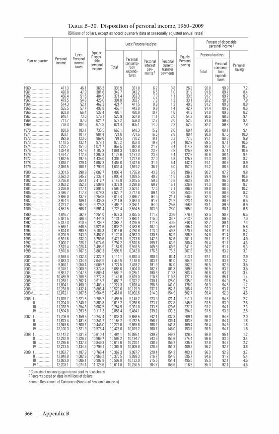
366 | Appendix B
Table B–30. Disposition of personal income, 1960–2009[Billions of dollars, except as noted; quarterly data at seasonally adjusted annual rates]
Year or quarter Personalincome
Less:Personalcurrenttaxes
Equals:Dispos-
ablepersonalincome
Less: Personal outlays
Equals:Personalsaving
Percent of disposablepersonal income 2
Total
Personalconsump-
tionexpendi-
tures
Personalinterest
pay-ments 1
Personalcurrenttransfer
payments
Personal outlays
PersonalsavingTotal
Personalconsump-
tionexpendi-
tures
1960 ...................... 411.3 46.1 365.2 338.9 331.8 6.2 0.8 26.3 92.8 90.9 7.21961 ...................... 428.8 47.3 381.6 349.7 342.2 6.5 1.0 31.9 91.6 89.7 8.41962 ...................... 456.4 51.6 404.9 371.4 363.3 7.0 1.1 33.5 91.7 89.7 8.31963 ...................... 479.5 54.6 425.0 391.8 382.7 7.9 1.2 33.1 92.2 90.0 7.81964 ...................... 514.3 52.1 462.3 421.7 411.5 8.9 1.3 40.5 91.2 89.0 8.81965 ...................... 555.5 57.7 497.8 455.1 443.8 9.9 1.4 42.7 91.4 89.2 8.61966 ...................... 603.8 66.4 537.4 493.1 480.9 10.7 1.6 44.3 91.8 89.5 8.21967 ...................... 648.1 73.0 575.1 520.9 507.8 11.1 2.0 54.2 90.6 88.3 9.41968 ...................... 711.7 87.0 624.7 572.2 558.0 12.2 2.0 52.5 91.6 89.3 8.41969 ...................... 778.3 104.5 673.8 621.4 605.1 14.0 2.2 52.5 92.2 89.8 7.81970 ...................... 838.6 103.1 735.5 666.1 648.3 15.2 2.6 69.4 90.6 88.1 9.41971 ...................... 903.1 101.7 801.4 721.0 701.6 16.6 2.8 80.4 90.0 87.5 10.01972 ...................... 992.6 123.6 869.0 791.5 770.2 18.1 3.2 77.5 91.1 88.6 8.91973 ...................... 1,110.5 132.4 978.1 875.2 852.0 19.8 3.4 102.9 89.5 87.1 10.51974 ...................... 1,222.7 151.0 1,071.7 957.5 932.9 21.2 3.4 114.2 89.3 87.0 10.71975 ...................... 1,334.9 147.6 1,187.3 1,061.3 1,033.8 23.7 3.8 125.9 89.4 87.1 10.61976 ...................... 1,474.7 172.3 1,302.3 1,179.6 1,151.3 23.9 4.4 122.8 90.6 88.4 9.41977 ...................... 1,632.5 197.5 1,435.0 1,309.7 1,277.8 27.0 4.8 125.3 91.3 89.0 8.71978 ...................... 1,836.7 229.4 1,607.3 1,465.0 1,427.6 31.9 5.4 142.4 91.1 88.8 8.91979 ...................... 2,059.5 268.7 1,790.9 1,633.4 1,591.2 36.2 6.0 157.5 91.2 88.8 8.81980 ...................... 2,301.5 298.9 2,002.7 1,806.4 1,755.8 43.6 6.9 196.3 90.2 87.7 9.81981 ...................... 2,582.3 345.2 2,237.1 2,000.4 1,939.5 49.3 11.5 236.7 89.4 86.7 10.61982 ...................... 2,766.8 354.1 2,412.7 2,148.8 2,075.5 59.5 13.8 263.9 89.1 86.0 10.91983 ...................... 2,952.2 352.3 2,599.8 2,372.9 2,288.6 69.2 15.1 226.9 91.3 88.0 8.71984 ...................... 3,268.9 377.4 2,891.5 2,595.2 2,501.1 77.0 17.1 296.3 89.8 86.5 10.21985 ...................... 3,496.7 417.3 3,079.3 2,825.7 2,717.6 89.4 18.8 253.6 91.8 88.3 8.21986 ...................... 3,696.0 437.2 3,258.8 3,012.4 2,896.7 94.5 21.1 246.5 92.4 88.9 7.61987 ...................... 3,924.4 489.1 3,435.3 3,211.9 3,097.0 91.7 23.2 223.4 93.5 90.2 6.51988 ...................... 4,231.2 504.9 3,726.3 3,469.7 3,350.1 94.0 25.6 256.6 93.1 89.9 6.91989 ...................... 4,557.5 566.1 3,991.4 3,726.4 3,594.5 103.9 28.0 265.0 93.4 90.1 6.61990 ...................... 4,846.7 592.7 4,254.0 3,977.3 3,835.5 111.3 30.6 276.7 93.5 90.2 6.51991 ...................... 5,031.5 586.6 4,444.9 4,131.7 3,980.1 115.0 36.7 313.2 93.0 89.5 7.01992 ...................... 5,347.3 610.5 4,736.7 4,388.7 4,236.9 111.3 40.5 348.1 92.7 89.4 7.31993 ...................... 5,568.1 646.5 4,921.6 4,636.2 4,483.6 107.0 45.6 285.4 94.2 91.1 5.81994 ...................... 5,874.8 690.5 5,184.3 4,913.6 4,750.8 113.0 49.8 270.7 94.8 91.6 5.21995 ...................... 6,200.9 743.9 5,457.0 5,170.8 4,987.3 130.6 52.9 286.3 94.8 91.4 5.21996 ...................... 6,591.6 832.0 5,759.6 5,478.5 5,273.6 147.3 57.6 281.1 95.1 91.6 4.91997 ...................... 7,000.7 926.2 6,074.6 5,794.2 5,570.6 159.7 63.9 280.4 95.4 91.7 4.61998 ...................... 7,525.4 1,026.4 6,498.9 6,157.5 5,918.5 169.5 69.5 341.5 94.7 91.1 5.31999 ...................... 7,910.8 1,107.5 6,803.3 6,595.5 6,342.8 176.5 76.2 207.8 96.9 93.2 3.12000 ...................... 8,559.4 1,232.3 7,327.2 7,114.1 6,830.4 200.3 83.4 213.1 97.1 93.2 2.92001 ...................... 8,883.3 1,234.8 7,648.5 7,443.5 7,148.8 203.7 91.0 204.9 97.3 93.5 2.72002 ...................... 9,060.1 1,050.4 8,009.7 7,727.5 7,439.2 191.3 97.0 282.2 96.5 92.9 3.52003 ...................... 9,378.1 1,000.3 8,377.8 8,088.0 7,804.0 182.7 101.3 289.8 96.5 93.2 3.52004 ...................... 9,937.2 1,047.8 8,889.4 8,585.7 8,285.1 190.3 110.3 303.7 96.6 93.2 3.42005 ...................... 10,485.9 1,208.6 9,277.3 9,149.6 8,819.0 210.8 119.8 127.7 98.6 95.1 1.42006 ...................... 11,268.1 1,352.4 9,915.7 9,680.7 9,322.7 230.1 128.0 235.0 97.6 94.0 2.42007 ...................... 11,894.1 1,490.9 10,403.1 10,224.3 9,826.4 256.8 141.0 178.9 98.3 94.5 1.72008 ...................... 12,238.8 1,432.4 10,806.4 10,520.0 10,129.9 237.7 152.3 286.4 97.3 93.7 2.72009 p .................... 12,072.1 1,107.6 10,964.5 10,461.8 10,092.6 214.3 154.9 502.7 95.4 92.0 4.62006: I .................. 11,026.7 1,321.5 9,705.2 9,493.5 9,148.2 223.9 121.4 211.7 97.8 94.3 2.2
II ................. 11,204.0 1,340.2 9,863.8 9,618.2 9,266.6 223.7 127.8 245.6 97.5 93.9 2.5III ................ 11,336.9 1,354.3 9,982.5 9,754.9 9,391.8 233.5 129.6 227.7 97.7 94.1 2.3IV ................ 11,504.8 1,393.5 10,111.2 9,856.4 9,484.1 239.2 133.2 254.8 97.5 93.8 2.5
2007: I .................. 11,706.9 1,459.5 10,247.4 10,038.3 9,658.5 242.1 137.8 209.1 98.0 94.3 2.0II ................. 11,823.4 1,481.8 10,341.7 10,158.2 9,762.5 256.2 139.4 183.5 98.2 94.4 1.8III ................ 11,945.6 1,500.7 10,445.0 10,275.6 9,865.6 268.2 141.8 169.4 98.4 94.5 1.6IV ................ 12,100.3 1,521.9 10,578.4 10,425.0 10,019.2 260.7 145.0 153.5 98.5 94.7 1.5
2008: I .................. 12,142.2 1,531.8 10,610.4 10,484.1 10,095.1 239.8 149.2 126.3 98.8 95.1 1.2II ................. 12,292.9 1,326.2 10,966.7 10,592.2 10,194.7 243.9 153.6 374.4 96.6 93.0 3.4III ................ 12,286.6 1,437.3 10,849.3 10,613.6 10,220.1 238.3 155.2 235.7 97.8 94.2 2.2IV ................ 12,233.5 1,434.3 10,799.1 10,389.9 10,009.8 228.8 151.3 409.2 96.2 92.7 3.8
2009: I .................. 11,952.7 1,187.3 10,765.4 10,362.3 9,987.7 220.4 154.2 403.1 96.3 92.8 3.7II ................. 12,048.8 1,082.6 10,966.2 10,370.5 9,999.3 216.7 154.5 595.7 94.6 91.2 5.4III ................ 12,083.9 1,086.1 10,997.8 10,502.8 10,132.9 215.5 154.4 495.0 95.5 92.1 4.5IV p ............. 12,203.1 1,074.4 11,128.6 10,611.8 10,250.5 204.7 156.6 516.9 95.4 92.1 4.6
1 Consists of nonmortgage interest paid by households.2 Percents based on data in millions of dollars.Source: Department of Commerce (Bureau of Economic Analysis).
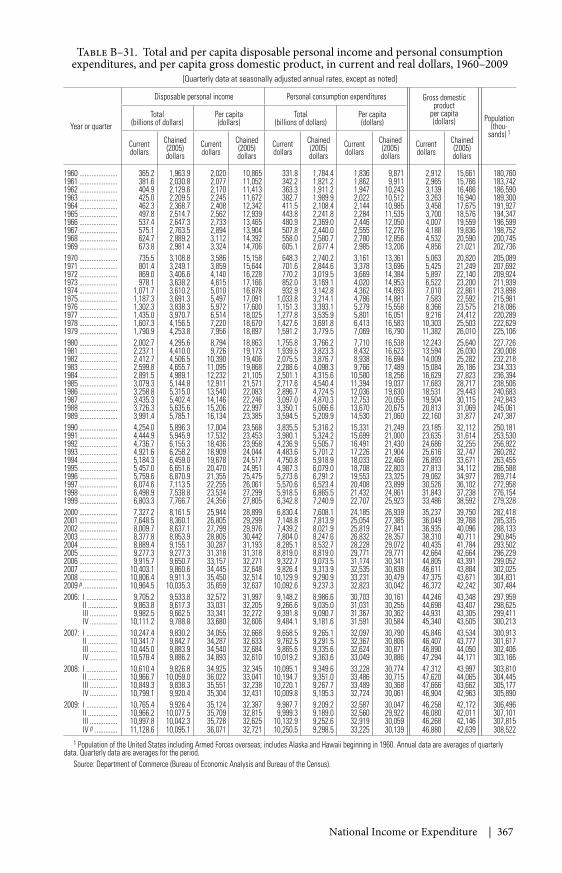
National Income or Expenditure | 367
Table B–31. Total and per capita disposable personal income and personal consumptionexpenditures, and per capita gross domestic product, in current and real dollars, 1960–2009
[Quarterly data at seasonally adjusted annual rates, except as noted]
Year or quarter
Disposable personal income Personal consumption expenditures Gross domesticproduct
per capita(dollars) Population
(thou-sands) 1
Total(billions of dollars)
Per capita(dollars)
Total(billions of dollars)
Per capita(dollars)
Currentdollars
Chained(2005)dollars
Currentdollars
Chained(2005)dollars
Currentdollars
Chained(2005)dollars
Currentdollars
Chained(2005)dollars
Currentdollars
Chained(2005)dollars
1960 ...................... 365.2 1,963.9 2,020 10,865 331.8 1,784.4 1,836 9,871 2,912 15,661 180,7601961 ...................... 381.6 2,030.8 2,077 11,052 342.2 1,821.2 1,862 9,911 2,965 15,766 183,7421962 ...................... 404.9 2,129.6 2,170 11,413 363.3 1,911.2 1,947 10,243 3,139 16,466 186,5901963 ...................... 425.0 2,209.5 2,245 11,672 382.7 1,989.9 2,022 10,512 3,263 16,940 189,3001964 ...................... 462.3 2,368.7 2,408 12,342 411.5 2,108.4 2,144 10,985 3,458 17,675 191,9271965 ...................... 497.8 2,514.7 2,562 12,939 443.8 2,241.8 2,284 11,535 3,700 18,576 194,3471966 ...................... 537.4 2,647.3 2,733 13,465 480.9 2,369.0 2,446 12,050 4,007 19,559 196,5991967 ...................... 575.1 2,763.5 2,894 13,904 507.8 2,440.0 2,555 12,276 4,188 19,836 198,7521968 ...................... 624.7 2,889.2 3,112 14,392 558.0 2,580.7 2,780 12,856 4,532 20,590 200,7451969 ...................... 673.8 2,981.4 3,324 14,706 605.1 2,677.4 2,985 13,206 4,856 21,021 202,7361970 ...................... 735.5 3,108.8 3,586 15,158 648.3 2,740.2 3,161 13,361 5,063 20,820 205,0891971 ...................... 801.4 3,249.1 3,859 15,644 701.6 2,844.6 3,378 13,696 5,425 21,249 207,6921972 ...................... 869.0 3,406.6 4,140 16,228 770.2 3,019.5 3,669 14,384 5,897 22,140 209,9241973 ...................... 978.1 3,638.2 4,615 17,166 852.0 3,169.1 4,020 14,953 6,522 23,200 211,9391974 ...................... 1,071.7 3,610.2 5,010 16,878 932.9 3,142.8 4,362 14,693 7,010 22,861 213,8981975 ...................... 1,187.3 3,691.3 5,497 17,091 1,033.8 3,214.1 4,786 14,881 7,583 22,592 215,9811976 ...................... 1,302.3 3,838.3 5,972 17,600 1,151.3 3,393.1 5,279 15,558 8,366 23,575 218,0861977 ...................... 1,435.0 3,970.7 6,514 18,025 1,277.8 3,535.9 5,801 16,051 9,216 24,412 220,2891978 ...................... 1,607.3 4,156.5 7,220 18,670 1,427.6 3,691.8 6,413 16,583 10,303 25,503 222,6291979 ...................... 1,790.9 4,253.8 7,956 18,897 1,591.2 3,779.5 7,069 16,790 11,382 26,010 225,1061980 ...................... 2,002.7 4,295.6 8,794 18,863 1,755.8 3,766.2 7,710 16,538 12,243 25,640 227,7261981 ...................... 2,237.1 4,410.0 9,726 19,173 1,939.5 3,823.3 8,432 16,623 13,594 26,030 230,0081982 ...................... 2,412.7 4,506.5 10,390 19,406 2,075.5 3,876.7 8,938 16,694 14,009 25,282 232,2181983 ...................... 2,599.8 4,655.7 11,095 19,868 2,288.6 4,098.3 9,766 17,489 15,084 26,186 234,3331984 ...................... 2,891.5 4,989.1 12,232 21,105 2,501.1 4,315.6 10,580 18,256 16,629 27,823 236,3941985 ...................... 3,079.3 5,144.8 12,911 21,571 2,717.6 4,540.4 11,394 19,037 17,683 28,717 238,5061986 ...................... 3,258.8 5,315.0 13,540 22,083 2,896.7 4,724.5 12,036 19,630 18,531 29,443 240,6831987 ...................... 3,435.3 5,402.4 14,146 22,246 3,097.0 4,870.3 12,753 20,055 19,504 30,115 242,8431988 ...................... 3,726.3 5,635.6 15,206 22,997 3,350.1 5,066.6 13,670 20,675 20,813 31,069 245,0611989 ...................... 3,991.4 5,785.1 16,134 23,385 3,594.5 5,209.9 14,530 21,060 22,160 31,877 247,3871990 ...................... 4,254.0 5,896.3 17,004 23,568 3,835.5 5,316.2 15,331 21,249 23,185 32,112 250,1811991 ...................... 4,444.9 5,945.9 17,532 23,453 3,980.1 5,324.2 15,699 21,000 23,635 31,614 253,5301992 ...................... 4,736.7 6,155.3 18,436 23,958 4,236.9 5,505.7 16,491 21,430 24,686 32,255 256,9221993 ...................... 4,921.6 6,258.2 18,909 24,044 4,483.6 5,701.2 17,226 21,904 25,616 32,747 260,2821994 ...................... 5,184.3 6,459.0 19,678 24,517 4,750.8 5,918.9 18,033 22,466 26,893 33,671 263,4551995 ...................... 5,457.0 6,651.6 20,470 24,951 4,987.3 6,079.0 18,708 22,803 27,813 34,112 266,5881996 ...................... 5,759.6 6,870.9 21,355 25,475 5,273.6 6,291.2 19,553 23,325 29,062 34,977 269,7141997 ...................... 6,074.6 7,113.5 22,255 26,061 5,570.6 6,523.4 20,408 23,899 30,526 36,102 272,9581998 ...................... 6,498.9 7,538.8 23,534 27,299 5,918.5 6,865.5 21,432 24,861 31,843 37,238 276,1541999 ...................... 6,803.3 7,766.7 24,356 27,805 6,342.8 7,240.9 22,707 25,923 33,486 38,592 279,3282000 ...................... 7,327.2 8,161.5 25,944 28,899 6,830.4 7,608.1 24,185 26,939 35,237 39,750 282,4182001 ...................... 7,648.5 8,360.1 26,805 29,299 7,148.8 7,813.9 25,054 27,385 36,049 39,768 285,3352002 ...................... 8,009.7 8,637.1 27,799 29,976 7,439.2 8,021.9 25,819 27,841 36,935 40,096 288,1332003 ...................... 8,377.8 8,853.9 28,805 30,442 7,804.0 8,247.6 26,832 28,357 38,310 40,711 290,8452004 ...................... 8,889.4 9,155.1 30,287 31,193 8,285.1 8,532.7 28,228 29,072 40,435 41,784 293,5022005 ...................... 9,277.3 9,277.3 31,318 31,318 8,819.0 8,819.0 29,771 29,771 42,664 42,664 296,2292006 ...................... 9,915.7 9,650.7 33,157 32,271 9,322.7 9,073.5 31,174 30,341 44,805 43,391 299,0522007 ...................... 10,403.1 9,860.6 34,445 32,648 9,826.4 9,313.9 32,535 30,838 46,611 43,884 302,0252008 ...................... 10,806.4 9,911.3 35,450 32,514 10,129.9 9,290.9 33,231 30,479 47,375 43,671 304,8312009 p .................... 10,964.5 10,035.3 35,659 32,637 10,092.6 9,237.3 32,823 30,042 46,372 42,242 307,4842006: I .................. 9,705.2 9,533.8 32,572 31,997 9,148.2 8,986.6 30,703 30,161 44,246 43,348 297,959
II ................. 9,863.8 9,617.3 33,031 32,205 9,266.6 9,035.0 31,031 30,255 44,698 43,407 298,625III ................ 9,982.5 9,662.5 33,341 32,272 9,391.8 9,090.7 31,367 30,362 44,931 43,305 299,411IV ................ 10,111.2 9,788.8 33,680 32,606 9,484.1 9,181.6 31,591 30,584 45,340 43,505 300,213
2007: I .................. 10,247.4 9,830.2 34,055 32,668 9,658.5 9,265.1 32,097 30,790 45,846 43,534 300,913II ................. 10,341.7 9,842.7 34,287 32,633 9,762.5 9,291.5 32,367 30,806 46,407 43,777 301,617III ................ 10,445.0 9,883.9 34,540 32,684 9,865.6 9,335.6 32,624 30,871 46,890 44,050 302,406IV ................ 10,578.4 9,886.2 34,893 32,610 10,019.2 9,363.6 33,049 30,886 47,294 44,171 303,166
2008: I .................. 10,610.4 9,826.8 34,925 32,345 10,095.1 9,349.6 33,228 30,774 47,312 43,997 303,810II ................. 10,966.7 10,059.0 36,022 33,041 10,194.7 9,351.0 33,486 30,715 47,620 44,065 304,445III ................ 10,849.3 9,838.3 35,551 32,238 10,220.1 9,267.7 33,489 30,368 47,666 43,662 305,177IV ................ 10,799.1 9,920.4 35,304 32,431 10,009.8 9,195.3 32,724 30,061 46,904 42,963 305,890
2009: I .................. 10,765.4 9,926.4 35,124 32,387 9,987.7 9,209.2 32,587 30,047 46,258 42,172 306,496II ................. 10,966.2 10,077.5 35,709 32,815 9,999.3 9,189.0 32,560 29,922 46,080 42,011 307,101III ................ 10,997.8 10,042.3 35,728 32,625 10,132.9 9,252.6 32,919 30,059 46,268 42,146 307,815IV p ............. 11,128.6 10,095.1 36,071 32,721 10,250.5 9,298.5 33,225 30,139 46,880 42,639 308,522
1 Population of the United States including Armed Forces overseas; includes Alaska and Hawaii beginning in 1960. Annual data are averages of quarterlydata. Quarterly data are averages for the period.
Source: Department of Commerce (Bureau of Economic Analysis and Bureau of the Census).
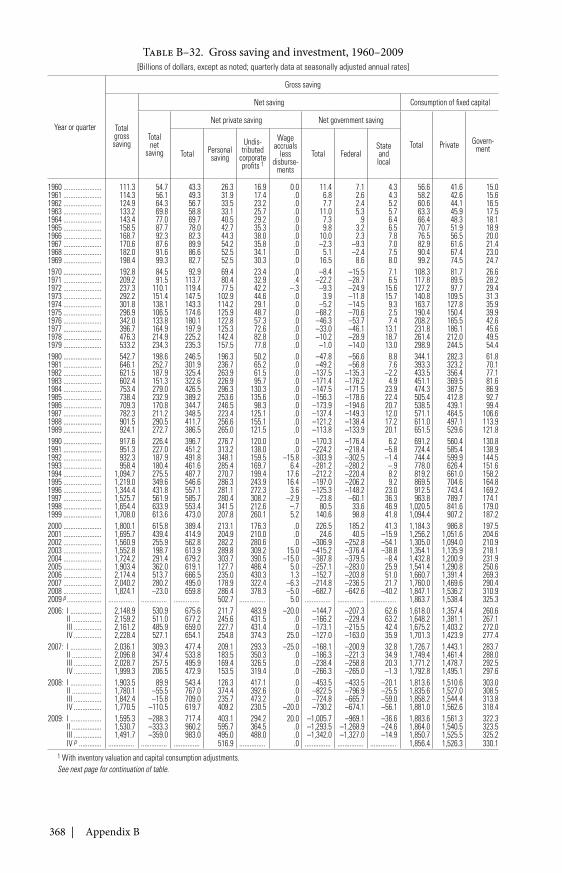
368 | Appendix B
Table B–32. Gross saving and investment, 1960–2009[Billions of dollars, except as noted; quarterly data at seasonally adjusted annual rates]
Year or quarter
Gross saving
Totalgrosssaving
Net saving Consumption of fixed capital
Totalnet
saving
Net private saving Net government saving
Total Private Govern-mentTotal Personal
saving
Undis-tributed
corporateprofits 1
Wageaccruals
lessdisburse-
ments
Total FederalStateandlocal
1960 ...................... 111.3 54.7 43.3 26.3 16.9 0.0 11.4 7.1 4.3 56.6 41.6 15.01961 ...................... 114.3 56.1 49.3 31.9 17.4 .0 6.8 2.6 4.3 58.2 42.6 15.61962 ...................... 124.9 64.3 56.7 33.5 23.2 .0 7.7 2.4 5.2 60.6 44.1 16.51963 ...................... 133.2 69.8 58.8 33.1 25.7 .0 11.0 5.3 5.7 63.3 45.9 17.51964 ...................... 143.4 77.0 69.7 40.5 29.2 .0 7.3 .9 6.4 66.4 48.3 18.11965 ...................... 158.5 87.7 78.0 42.7 35.3 .0 9.8 3.2 6.5 70.7 51.9 18.91966 ...................... 168.7 92.3 82.3 44.3 38.0 .0 10.0 2.3 7.8 76.5 56.5 20.01967 ...................... 170.6 87.6 89.9 54.2 35.8 .0 –2.3 –9.3 7.0 82.9 61.6 21.41968 ...................... 182.0 91.6 86.6 52.5 34.1 .0 5.1 –2.4 7.5 90.4 67.4 23.01969 ...................... 198.4 99.3 82.7 52.5 30.3 .0 16.5 8.6 8.0 99.2 74.5 24.71970 ...................... 192.8 84.5 92.9 69.4 23.4 .0 –8.4 –15.5 7.1 108.3 81.7 26.61971 ...................... 209.2 91.5 113.7 80.4 32.9 .4 –22.2 –28.7 6.5 117.8 89.5 28.21972 ...................... 237.3 110.1 119.4 77.5 42.2 –.3 –9.3 –24.9 15.6 127.2 97.7 29.41973 ...................... 292.2 151.4 147.5 102.9 44.6 .0 3.9 –11.8 15.7 140.8 109.5 31.31974 ...................... 301.8 138.1 143.3 114.2 29.1 .0 –5.2 –14.5 9.3 163.7 127.8 35.91975 ...................... 296.9 106.5 174.6 125.9 48.7 .0 –68.2 –70.6 2.5 190.4 150.4 39.91976 ...................... 342.0 133.8 180.1 122.8 57.3 .0 –46.3 –53.7 7.4 208.2 165.5 42.61977 ...................... 396.7 164.9 197.9 125.3 72.6 .0 –33.0 –46.1 13.1 231.8 186.1 45.61978 ...................... 476.3 214.9 225.2 142.4 82.8 .0 –10.2 –28.9 18.7 261.4 212.0 49.51979 ...................... 533.2 234.3 235.3 157.5 77.8 .0 –1.0 –14.0 13.0 298.9 244.5 54.41980 ...................... 542.7 198.6 246.5 196.3 50.2 .0 –47.8 –56.6 8.8 344.1 282.3 61.81981 ...................... 646.1 252.7 301.9 236.7 65.2 .0 –49.2 –56.8 7.6 393.3 323.2 70.11982 ...................... 621.5 187.9 325.4 263.9 61.5 .0 –137.5 –135.3 –2.2 433.5 356.4 77.11983 ...................... 602.4 151.3 322.6 226.9 95.7 .0 –171.4 –176.2 4.9 451.1 369.5 81.61984 ...................... 753.4 279.0 426.5 296.3 130.3 .0 –147.5 –171.5 23.9 474.3 387.5 86.91985 ...................... 738.4 232.9 389.2 253.6 135.6 .0 –156.3 –178.6 22.4 505.4 412.8 92.71986 ...................... 709.3 170.8 344.7 246.5 98.3 .0 –173.9 –194.6 20.7 538.5 439.1 99.41987 ...................... 782.3 211.2 348.5 223.4 125.1 .0 –137.4 –149.3 12.0 571.1 464.5 106.61988 ...................... 901.5 290.5 411.7 256.6 155.1 .0 –121.2 –138.4 17.2 611.0 497.1 113.91989 ...................... 924.1 272.7 386.5 265.0 121.5 .0 –113.8 –133.9 20.1 651.5 529.6 121.81990 ...................... 917.6 226.4 396.7 276.7 120.0 .0 –170.3 –176.4 6.2 691.2 560.4 130.81991 ...................... 951.3 227.0 451.2 313.2 138.0 .0 –224.2 –218.4 –5.8 724.4 585.4 138.91992 ...................... 932.3 187.9 491.8 348.1 159.5 –15.8 –303.9 –302.5 –1.4 744.4 599.9 144.51993 ...................... 958.4 180.4 461.6 285.4 169.7 6.4 –281.2 –280.2 –.9 778.0 626.4 151.61994 ...................... 1,094.7 275.5 487.7 270.7 199.4 17.6 –212.2 –220.4 8.2 819.2 661.0 158.21995 ...................... 1,219.0 349.6 546.6 286.3 243.9 16.4 –197.0 –206.2 9.2 869.5 704.6 164.81996 ...................... 1,344.4 431.8 557.1 281.1 272.3 3.6 –125.3 –148.2 23.0 912.5 743.4 169.21997 ...................... 1,525.7 561.9 585.7 280.4 308.2 –2.9 –23.8 –60.1 36.3 963.8 789.7 174.11998 ...................... 1,654.4 633.9 553.4 341.5 212.6 –.7 80.5 33.6 46.9 1,020.5 841.6 179.01999 ...................... 1,708.0 613.6 473.0 207.8 260.1 5.2 140.6 98.8 41.8 1,094.4 907.2 187.22000 ...................... 1,800.1 615.8 389.4 213.1 176.3 .0 226.5 185.2 41.3 1,184.3 986.8 197.52001 ...................... 1,695.7 439.4 414.9 204.9 210.0 .0 24.6 40.5 –15.9 1,256.2 1,051.6 204.62002 ...................... 1,560.9 255.9 562.8 282.2 280.6 .0 –306.9 –252.8 –54.1 1,305.0 1,094.0 210.92003 ...................... 1,552.8 198.7 613.9 289.8 309.2 15.0 –415.2 –376.4 –38.8 1,354.1 1,135.9 218.12004 ...................... 1,724.2 291.4 679.2 303.7 390.5 –15.0 –387.8 –379.5 –8.4 1,432.8 1,200.9 231.92005 ...................... 1,903.4 362.0 619.1 127.7 486.4 5.0 –257.1 –283.0 25.9 1,541.4 1,290.8 250.62006 ...................... 2,174.4 513.7 666.5 235.0 430.3 1.3 –152.7 –203.8 51.0 1,660.7 1,391.4 269.32007 ...................... 2,040.2 280.2 495.0 178.9 322.4 –6.3 –214.8 –236.5 21.7 1,760.0 1,469.6 290.42008 ...................... 1,824.1 –23.0 659.8 286.4 378.3 –5.0 –682.7 –642.6 –40.2 1,847.1 1,536.2 310.92009 p .................... ............... ............... ............... 502.7 ............... 5.0 ............... ............... ............... 1,863.7 1,538.4 325.32006: I .................. 2,148.9 530.9 675.6 211.7 483.9 –20.0 –144.7 –207.3 62.6 1,618.0 1,357.4 260.6
II ................. 2,159.2 511.0 677.2 245.6 431.5 .0 –166.2 –229.4 63.2 1,648.2 1,381.1 267.1III ................ 2,161.2 485.9 659.0 227.7 431.4 .0 –173.1 –215.5 42.4 1,675.2 1,403.2 272.0IV ................ 2,228.4 527.1 654.1 254.8 374.3 25.0 –127.0 –163.0 35.9 1,701.3 1,423.9 277.4
2007: I .................. 2,036.1 309.3 477.4 209.1 293.3 –25.0 –168.1 –200.9 32.8 1,726.7 1,443.1 283.7II ................. 2,096.8 347.4 533.8 183.5 350.3 .0 –186.3 –221.3 34.9 1,749.4 1,461.4 288.0III ................ 2,028.7 257.5 495.9 169.4 326.5 .0 –238.4 –258.8 20.3 1,771.2 1,478.7 292.5IV ................ 1,999.3 206.5 472.9 153.5 319.4 .0 –266.3 –265.0 –1.3 1,792.8 1,495.1 297.6
2008: I .................. 1,903.5 89.9 543.4 126.3 417.1 .0 –453.5 –433.5 –20.1 1,813.6 1,510.6 303.0II ................. 1,780.1 –55.5 767.0 374.4 392.6 .0 –822.5 –796.9 –25.5 1,835.6 1,527.0 308.5III ................ 1,842.4 –15.8 709.0 235.7 473.2 .0 –724.8 –665.7 –59.0 1,858.2 1,544.4 313.8IV ................ 1,770.5 –110.5 619.7 409.2 230.5 –20.0 –730.2 –674.1 –56.1 1,881.0 1,562.6 318.4
2009: I .................. 1,595.3 –288.3 717.4 403.1 294.2 20.0 –1,005.7 –969.1 –36.6 1,883.6 1,561.3 322.3II ................. 1,530.7 –333.3 960.2 595.7 364.5 .0 –1,293.5 –1,268.9 –24.6 1,864.0 1,540.5 323.5III ................ 1,491.7 –359.0 983.0 495.0 488.0 .0 –1,342.0 –1,327.0 –14.9 1,850.7 1,525.5 325.2IV p ............. ............... ............... ............... 516.9 ............... .0 ............... ............... ............... 1,856.4 1,526.3 330.1
1 With inventory valuation and capital consumption adjustments.See next page for continuation of table.
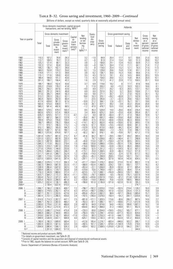
National Income or Expenditure | 369
Table B–32. Gross saving and investment, 1960–2009—Continued[Billions of dollars, except as noted; quarterly data at seasonally adjusted annual rates]
Year or quarter
Gross domestic investment, capital accounttransactions, and net lending, NIPA 2
Statis-ticaldis-
crep-ancy
Addenda:
Total
Gross domestic investmentCapital
ac-counttrans-
actions(net) 4
Netlendingor net
borrow-ing(–),
NIPA 2, 5
Grossprivatesaving
Gross government saving
Netdomes-
ticinvest-ment
Grosssavingas a
percentof grossnationalincome
Netsavingas a
percentof grossnationalincome
Total
Grossprivatedomes-
ticinvest-ment
Grossgovern-
mentinvest-ment 3
Total FederalStateandlocal
1960 .................... 110.3 107.2 78.9 28.3 ............ 3.2 –1.0 84.9 26.4 17.7 8.7 50.6 21.0 10.31961 .................... 113.7 109.5 78.2 31.3 ............ 4.2 –.6 91.9 22.4 13.4 9.0 51.3 20.8 10.21962 .................... 125.2 121.4 88.1 33.3 ............ 3.8 .3 100.8 24.1 13.9 10.3 60.9 21.2 10.91963 .................... 132.3 127.4 93.8 33.6 ............ 4.9 –.8 104.7 28.4 17.4 11.1 64.1 21.4 11.21964 .................... 144.2 136.7 102.1 34.6 ............ 7.5 .8 118.0 25.4 13.2 12.1 70.3 21.5 11.51965 .................... 160.0 153.8 118.2 35.6 ............ 6.2 1.5 129.8 28.6 15.9 12.8 83.1 21.9 12.11966 .................... 174.9 171.1 131.3 39.8 ............ 3.8 6.2 138.7 30.0 15.3 14.6 94.6 21.5 11.71967 .................... 175.1 171.6 128.6 43.0 ............ 3.5 4.5 151.5 19.1 4.5 14.5 88.6 20.5 10.51968 .................... 186.4 184.8 141.2 43.6 ............ 1.5 4.3 154.0 28.0 12.2 15.8 94.4 20.0 10.11969 .................... 201.3 199.7 156.4 43.3 ............ 1.6 2.9 157.2 41.2 23.9 17.3 100.5 20.1 10.01970 .................... 199.7 196.0 152.4 43.6 ............ 3.7 6.9 174.6 18.2 .6 17.7 87.6 18.6 8.11971 .................... 220.2 219.9 178.2 41.8 ............ .3 11.0 203.2 6.0 –12.2 18.3 102.2 18.6 8.11972 .................... 246.2 250.2 207.6 42.6 ............ –4.0 8.9 217.1 20.2 –8.3 28.5 123.1 19.2 8.91973 .................... 300.2 291.3 244.5 46.8 ............ 8.9 8.0 257.0 35.2 5.2 30.0 150.6 21.1 10.91974 .................... 311.6 305.7 249.4 56.3 ............ 6.0 9.8 271.1 30.7 3.7 27.0 142.0 20.1 9.21975 .................... 313.2 293.3 230.2 63.1 ............ 19.8 16.3 325.1 –28.2 –50.9 22.7 102.9 18.2 6.51976 .................... 365.4 358.4 292.0 66.4 ............ 7.1 23.5 345.6 –3.7 –32.3 28.6 150.2 18.8 7.41977 .................... 417.9 428.8 361.3 67.5 ............ –10.9 21.2 384.1 12.6 –23.1 35.7 197.1 19.6 8.11978 .................... 502.4 515.0 438.0 77.1 ............ –12.6 26.1 437.1 39.2 –3.9 43.2 253.6 20.8 9.41979 .................... 580.2 581.4 492.9 88.5 ............ –1.2 47.0 479.7 53.5 13.0 40.5 282.4 20.9 9.21980 .................... 588.0 579.5 479.3 100.3 ............ 8.5 45.3 528.8 14.0 –26.6 40.6 235.4 19.5 7.21981 .................... 682.6 679.3 572.4 106.9 ............ 3.4 36.6 625.2 20.9 –23.0 43.8 285.9 20.7 8.11982 .................... 626.2 629.5 517.2 112.3 –0.1 –3.2 4.8 681.9 –60.4 –97.7 37.3 196.0 18.9 5.71983 .................... 652.1 687.2 564.3 122.9 –.1 –35.0 49.7 692.2 –89.8 –135.6 45.8 236.0 17.1 4.31984 .................... 784.9 875.0 735.6 139.4 –.1 –89.9 31.5 814.0 –60.6 –126.9 66.3 400.6 19.1 7.11985 .................... 780.7 895.0 736.2 158.8 –.2 –114.1 42.3 802.0 –63.6 –130.6 67.0 389.5 17.6 5.51986 .................... 777.1 919.7 746.5 173.2 –.2 –142.5 67.7 783.8 –74.5 –143.0 68.6 381.3 16.1 3.91987 .................... 815.1 969.2 785.0 184.3 –.2 –153.9 32.9 813.0 –30.8 –94.2 63.4 398.1 16.6 4.51988 .................... 892.0 1,007.7 821.6 186.1 –.4 –115.4 –9.5 908.8 –7.3 –79.3 72.0 396.7 17.6 5.71989 .................... 980.3 1,072.6 874.9 197.7 –.2 –92.2 56.1 916.1 8.0 –70.6 78.7 421.2 17.0 5.01990 .................... 1,001.8 1,076.7 861.0 215.7 6.7 –81.6 84.2 957.1 –39.5 –108.7 69.2 385.5 16.0 3.91991 .................... 1,031.0 1,023.2 802.9 220.3 4.6 3.2 79.7 1,036.6 –85.3 –146.4 61.1 298.8 16.0 3.81992 .................... 1,042.3 1,087.9 864.8 223.1 –.8 –44.8 110.0 1,091.7 –159.4 –227.9 68.5 343.5 14.9 3.01993 .................... 1,094.2 1,172.8 953.3 219.4 1.5 –80.0 135.8 1,088.0 –129.5 –202.4 72.9 394.8 14.6 2.71994 .................... 1,203.5 1,318.2 1,097.3 220.9 1.9 –116.6 108.8 1,148.6 –53.9 –140.3 86.4 499.0 15.6 3.91995 .................... 1,271.6 1,376.6 1,144.0 232.6 1.1 –106.2 52.5 1,251.2 –32.2 –124.5 92.3 507.2 16.5 4.71996 .................... 1,370.3 1,484.4 1,240.2 244.2 .9 –115.1 25.9 1,300.5 43.9 –66.3 110.2 571.9 17.1 5.51997 .................... 1,511.7 1,641.0 1,388.7 252.4 1.2 –130.6 –14.0 1,375.4 150.3 22.4 127.9 677.2 18.2 6.71998 .................... 1,569.1 1,773.6 1,510.8 262.9 1.0 –205.5 –85.3 1,394.9 259.5 116.4 143.1 753.1 18.6 7.11999 .................... 1,637.0 1,928.9 1,641.5 287.4 5.2 –297.1 –71.1 1,380.3 327.8 183.9 143.9 834.5 18.1 6.52000 .................... 1,666.2 2,076.5 1,772.2 304.3 1.4 –411.7 –134.0 1,376.2 424.0 273.0 151.0 892.2 17.8 6.12001 .................... 1,592.3 1,984.0 1,661.9 322.0 –11.7 –380.0 –103.4 1,466.5 229.2 129.1 100.1 727.7 16.2 4.22002 .................... 1,538.9 1,990.4 1,647.0 343.5 1.8 –453.4 –22.1 1,656.8 –95.9 –163.6 67.7 685.4 14.6 2.42003 .................... 1,569.4 2,085.5 1,729.7 355.8 3.8 –519.9 16.6 1,749.8 –197.1 –285.5 88.4 731.4 13.9 1.82004 .................... 1,716.3 2,340.9 1,968.6 372.4 –1.1 –623.5 –7.8 1,880.1 –155.9 –284.6 128.7 908.2 14.4 2.42005 .................... 1,823.7 2,564.2 2,172.2 392.0 –11.1 –729.5 –79.7 1,909.9 –6.5 –182.6 176.1 1,022.9 14.9 2.82006 .................... 1,953.8 2,752.2 2,327.2 425.1 4.2 –802.6 –220.6 2,057.9 116.5 –97.2 213.8 1,091.6 15.9 3.82007 .................... 2,025.4 2,750.0 2,288.5 461.6 2.2 –726.8 –14.8 1,964.6 75.6 –123.9 199.5 990.0 14.4 2.02008 .................... 1,925.2 2,632.4 2,136.1 496.3 –.4 –706.8 101.0 2,195.9 –371.8 –522.8 151.0 785.3 12.6 –.22009 p .................. ............. 2,138.4 1,622.9 515.5 ............ ................ ............ ............. ............. ............. ............. 274.7 ............. ..............2006: I ................ 1,956.7 2,746.2 2,336.5 409.7 7.2 –796.7 –192.2 2,033.0 115.9 –103.5 219.4 1,128.2 16.0 3.9
II ............... 1,968.5 2,779.5 2,352.1 427.4 4.3 –815.4 –190.7 2,058.2 101.0 –123.4 224.4 1,131.3 15.9 3.8III .............. 1,907.7 2,761.1 2,333.5 427.6 2.4 –855.8 –253.4 2,062.2 98.9 –107.7 206.6 1,085.8 15.7 3.5IV .............. 1,982.4 2,722.1 2,286.5 435.6 2.8 –742.5 –246.0 2,078.0 150.4 –54.2 204.7 1,020.8 16.0 3.8
2007: I ................ 1,914.9 2,714.3 2,267.2 447.1 2.5 –801.8 –121.1 1,920.5 115.6 –90.6 206.2 987.5 14.6 2.2II ............... 1,999.7 2,762.3 2,302.0 460.2 .8 –763.3 –97.1 1,995.1 101.7 –109.6 211.2 1,012.9 14.8 2.5III .............. 2,093.6 2,778.4 2,311.9 466.6 2.8 –687.6 64.9 1,974.6 54.0 –145.5 199.6 1,007.2 14.2 1.8IV .............. 2,093.3 2,745.2 2,272.9 472.3 2.7 –654.6 94.0 1,968.0 31.3 –149.8 181.1 952.4 13.9 1.4
2008: I ................ 1,973.2 2,690.7 2,214.8 475.9 2.8 –720.3 69.8 2,054.0 –150.5 –316.2 165.7 877.1 13.2 .6II ............... 1,906.8 2,660.2 2,164.6 495.5 3.0 –756.4 126.7 2,294.1 –514.0 –677.3 163.3 824.6 12.3 –.4III .............. 1,910.6 2,647.8 2,142.7 505.0 –11.6 –725.5 68.3 2,253.3 –411.0 –544.7 133.7 789.6 12.6 –.1IV .............. 1,909.9 2,530.9 2,022.1 508.9 4.0 –625.1 139.4 2,182.3 –411.8 –553.0 141.2 650.0 12.4 –.8
2009: I ................ 1,780.8 2,190.3 1,689.9 500.4 3.1 –412.6 185.4 2,278.7 –683.4 –846.6 163.2 306.7 11.3 –2.0II ............... 1,692.4 2,082.0 1,561.5 520.4 3.0 –392.5 161.7 2,500.7 –970.0 –1,144.9 174.9 218.0 10.9 –2.4III .............. 1,654.9 2,080.4 1,556.1 524.3 2.9 –428.4 163.2 2,508.5 –1,016.8 –1,201.0 184.2 229.7 10.5 –2.5IV p ........... ............. 2,201.0 1,684.0 517.0 ............ ................ ............ ............. ............. ............. ............. 344.6 ............. ..............
2 National income and product accounts (NIPA).3 For details on government investment, see Table B–20.4 Consists of capital transfers and the acquisition and disposal of nonproduced nonfinancial assets.5 Prior to 1982, equals the balance on current account, NIPA (see Table B–24).Source: Department of Commerce (Bureau of Economic Analysis).
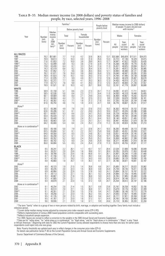
370 | Appendix B
Table B–33. Median money income (in 2008 dollars) and poverty status of families andpeople, by race, selected years, 1996–2008
Year
Families 1People belowpoverty level
Median money income (in 2008 dollars)of people 15 years old and over
with income 2
Number(mil-lions)
Medianmoneyincome
(in2008dol-
lars) 2
Below poverty level
Total Femalehouseholder
Number(mil-lions)
Percent
Males Females
Number(mil-lions)
PercentNumber
(mil-lions)
Percent Allpeople
Year-round
full-timeworkers
Allpeople
Year-round
full-timeworkers
ALL RACES1996 ....................................... 70.2 $57,801 7.7 11.0 4.2 32.6 36.5 13.7 $32,568 $45,829 $17,511 $34,0731997 ....................................... 70.9 59,613 7.3 10.3 4.0 31.6 35.6 13.3 33,723 47,146 18,329 34,8151998 ....................................... 71.6 61,653 7.2 10.0 3.8 29.9 34.5 12.7 34,947 47,822 19,035 35,4261999 3 ..................................... 73.2 63,099 6.8 9.3 3.6 27.8 32.8 11.9 35,268 48,393 19,776 35,3622000 4 ..................................... 73.8 63,430 6.4 8.7 3.3 25.4 31.6 11.3 35,437 48,625 20,084 36,4122001 ....................................... 74.3 62,519 6.8 9.2 3.5 26.4 32.9 11.7 35,391 48,812 20,205 36,9952002 ....................................... 75.6 61,852 7.2 9.6 3.6 26.5 34.6 12.1 34,993 48,480 20,121 37,0662003 ....................................... 76.2 61,671 7.6 10.0 3.9 28.0 35.9 12.5 35,040 48,587 20,205 37,0552004 5 ..................................... 76.9 61,623 7.8 10.2 4.0 28.3 37.0 12.7 34,784 47,495 20,138 36,6082005 ....................................... 77.4 61,976 7.7 9.9 4.0 28.7 37.0 12.6 34,493 46,529 20,487 36,6782006 ....................................... 78.5 62,372 7.7 9.8 4.1 28.3 36.5 12.3 34,455 48,010 21,373 37,3642007 ....................................... 77.9 63,712 7.6 9.8 4.1 28.3 37.3 12.5 34,472 48,000 21,726 37,5572008 ....................................... 78.9 61,521 8.1 10.3 4.2 28.7 39.8 13.2 33,161 47,779 20,867 36,688WHITE1996 ....................................... 58.9 61,158 5.1 8.6 2.3 27.3 24.7 11.2 34,092 47,472 17,711 34,6511997 ....................................... 59.5 62,536 5.0 8.4 2.3 27.7 24.4 11.0 34,930 48,310 18,448 35,4051998 ....................................... 60.1 64,669 4.8 8.0 2.1 24.9 23.5 10.5 36,469 49,067 19,282 36,0181999 3 ..................................... 61.1 66,004 4.4 7.3 1.9 22.5 22.2 9.8 37,039 50,670 19,838 36,1812000 4 ..................................... 61.3 66,302 4.3 7.1 1.8 21.2 21.6 9.5 37,255 50,328 20,104 37,4482001 ....................................... 61.6 65,754 4.6 7.4 1.9 22.4 22.7 9.9 36,776 49,607 20,251 37,517
Alone 62002 ....................................... 62.3 65,386 4.9 7.8 2.0 22.6 23.5 10.2 36,363 49,518 20,152 37,5802003 ....................................... 62.6 65,286 5.1 8.1 2.2 24.0 24.3 10.5 35,977 49,335 20,396 37,6862004 5 ..................................... 63.1 64,657 5.3 8.4 2.3 24.7 25.3 10.8 35,729 48,554 20,175 37,3092005 ....................................... 63.4 65,420 5.1 8.0 2.3 25.3 24.9 10.6 35,490 48,192 20,590 37,6092006 ....................................... 64.1 65,440 5.1 8.0 2.4 25.1 24.4 10.3 36,140 49,051 21,445 37,9372007 ....................................... 63.6 66,903 5.0 7.9 2.3 24.7 25.1 10.5 36,491 49,050 21,879 38,1392008 ....................................... 64.2 65,000 5.4 8.4 2.4 25.2 27.0 11.2 35,120 49,924 20,950 37,210
Alone or in combination 62002 ....................................... 63.0 65,166 5.0 7.9 2.1 22.6 24.1 10.3 36,283 49,448 20,113 37,5662003 ....................................... 63.5 65,094 5.2 8.1 2.2 24.2 25.0 10.6 35,891 49,261 20,359 37,6722004 5 ..................................... 64.0 64,500 5.4 8.5 2.3 24.8 26.1 10.9 35,651 48,429 20,140 37,2662005 ....................................... 64.3 65,208 5.2 8.1 2.4 25.5 25.6 10.7 35,406 48,021 20,535 37,5302006 ....................................... 65.0 65,352 5.2 8.0 2.4 25.0 25.2 10.4 35,959 48,982 21,399 37,8992007 ....................................... 64.4 66,702 5.2 8.0 2.4 24.8 25.9 10.6 36,377 48,980 21,818 38,1042008 ....................................... 65.0 64,804 5.5 8.5 2.4 25.4 27.9 11.3 35,013 49,755 20,921 37,177BLACK1996 ....................................... 8.5 36,241 2.2 26.1 1.7 43.7 9.7 28.4 22,534 37,080 16,086 30,0491997 ....................................... 8.4 38,257 2.0 23.6 1.6 39.8 9.1 26.5 24,205 35,976 17,453 30,4481998 ....................................... 8.5 38,788 2.0 23.4 1.6 40.8 9.1 26.1 25,487 36,240 17,330 31,4801999 3 ..................................... 8.7 41,156 1.9 21.8 1.5 39.2 8.4 23.6 26,414 38,965 19,093 32,4872000 4 ..................................... 8.7 42,105 1.7 19.3 1.3 34.3 8.0 22.5 26,685 38,120 19,856 32,1952001 ....................................... 8.8 40,860 1.8 20.7 1.4 35.2 8.1 22.7 26,106 38,821 19,801 33,197
Alone 62002 ....................................... 8.9 40,123 1.9 21.5 1.4 35.8 8.6 24.1 25,805 38,217 20,022 33,0622003 ....................................... 8.9 40,235 2.0 22.3 1.5 36.9 8.8 24.4 25,739 39,135 19,411 32,3362004 5 ..................................... 8.9 40,064 2.0 22.8 1.5 37.6 9.0 24.7 25,864 36,157 19,787 33,2222005 ....................................... 9.1 39,113 2.0 22.1 1.5 36.1 9.2 24.9 24,984 37,755 19,445 33,4872006 ....................................... 9.3 40,867 2.0 21.6 1.5 36.6 9.0 24.3 26,765 37,885 20,400 33,0362007 ....................................... 9.3 41,685 2.0 22.1 1.5 37.3 9.2 24.5 26,814 38,148 20,511 32,8052008 ....................................... 9.4 39,879 2.1 22.0 1.5 37.2 9.4 24.7 25,254 38,612 20,197 32,186
Alone or in combination 62002 ....................................... 9.1 40,254 2.0 21.4 1.5 35.7 8.9 23.9 25,742 38,258 19,952 33,1562003 ....................................... 9.1 40,514 2.0 22.1 1.5 36.8 9.1 24.3 25,679 39,176 19,363 32,3992004 5 ..................................... 9.1 40,261 2.1 22.8 1.5 37.6 9.4 24.7 25,890 36,146 19,773 33,2762005 ....................................... 9.3 39,256 2.1 22.0 1.5 36.2 9.5 24.7 24,935 37,657 19,405 33,4912006 ....................................... 9.5 41,135 2.0 21.5 1.5 36.4 9.4 24.2 26,777 37,921 20,359 33,0872007 ....................................... 9.5 41,767 2.1 22.0 1.6 37.2 9.7 24.4 26,783 38,193 20,469 32,8892008 ....................................... 9.6 39,936 2.1 21.9 1.6 37.1 9.9 24.6 25,118 38,365 20,203 32,204
1 The term “family” refers to a group of two or more persons related by birth, marriage, or adoption and residing together. Every family must include areference person.
2 Current dollar median money income adjusted by consumer price index research series (CPI-U-RS).3 Reflects implementation of Census 2000–based population controls comparable with succeeding years.4 Reflects household sample expansion.5 For 2004, figures are revised to reflect a correction to the weights in the 2005 Annual Social and Economic Supplement.6 Data are for “white alone,” for “white alone or in combination,” for “black alone,” and for “black alone or in combination.” (“Black” is also “black
or African American.”) Beginning with data for 2002 the Current Population Survey allowed respondents to choose more than one race; for earlier yearsrespondents could report only one race group.
Note: Poverty thresholds are updated each year to reflect changes in the consumer price index (CPI-U).For details see publication Series P–60 on the Current Population Survey and Annual Social and Economic Supplements.Source: Department of Commerce (Bureau of the Census).
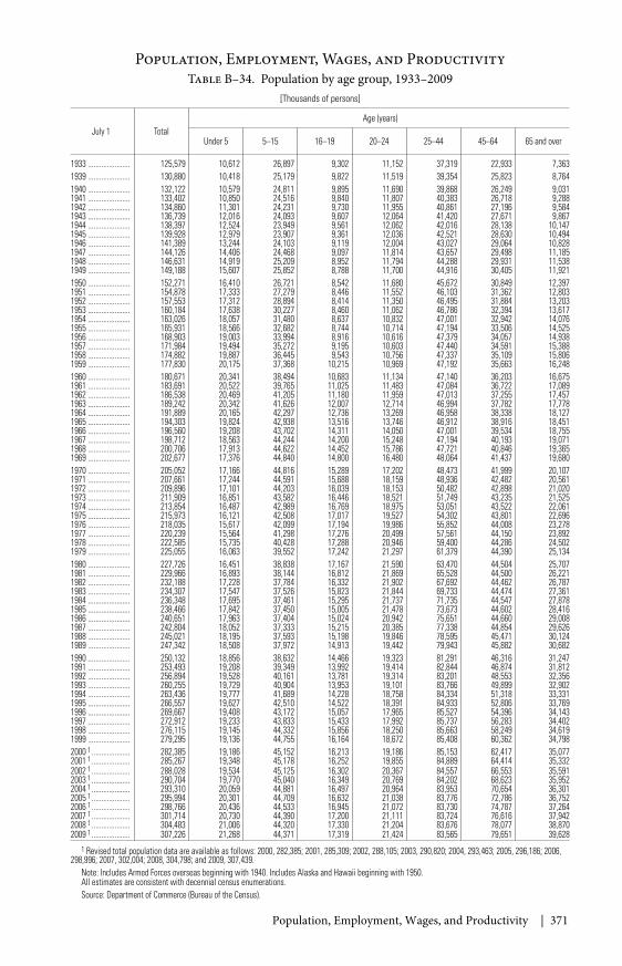
Population, Employment, Wages, and Productivity | 371
Table B–34. Population by age group, 1933–2009[Thousands of persons]
July 1 TotalAge (years)
Under 5 5–15 16–19 20–24 25–44 45–64 65 and over
1933 ...................... 125,579 10,612 26,897 9,302 11,152 37,319 22,933 7,3631939 ...................... 130,880 10,418 25,179 9,822 11,519 39,354 25,823 8,7641940 ...................... 132,122 10,579 24,811 9,895 11,690 39,868 26,249 9,0311941 ...................... 133,402 10,850 24,516 9,840 11,807 40,383 26,718 9,2881942 ...................... 134,860 11,301 24,231 9,730 11,955 40,861 27,196 9,5841943 ...................... 136,739 12,016 24,093 9,607 12,064 41,420 27,671 9,8671944 ...................... 138,397 12,524 23,949 9,561 12,062 42,016 28,138 10,1471945 ...................... 139,928 12,979 23,907 9,361 12,036 42,521 28,630 10,4941946 ...................... 141,389 13,244 24,103 9,119 12,004 43,027 29,064 10,8281947 ...................... 144,126 14,406 24,468 9,097 11,814 43,657 29,498 11,1851948 ...................... 146,631 14,919 25,209 8,952 11,794 44,288 29,931 11,5381949 ...................... 149,188 15,607 25,852 8,788 11,700 44,916 30,405 11,9211950 ...................... 152,271 16,410 26,721 8,542 11,680 45,672 30,849 12,3971951 ...................... 154,878 17,333 27,279 8,446 11,552 46,103 31,362 12,8031952 ...................... 157,553 17,312 28,894 8,414 11,350 46,495 31,884 13,2031953 ...................... 160,184 17,638 30,227 8,460 11,062 46,786 32,394 13,6171954 ...................... 163,026 18,057 31,480 8,637 10,832 47,001 32,942 14,0761955 ...................... 165,931 18,566 32,682 8,744 10,714 47,194 33,506 14,5251956 ...................... 168,903 19,003 33,994 8,916 10,616 47,379 34,057 14,9381957 ...................... 171,984 19,494 35,272 9,195 10,603 47,440 34,591 15,3881958 ...................... 174,882 19,887 36,445 9,543 10,756 47,337 35,109 15,8061959 ...................... 177,830 20,175 37,368 10,215 10,969 47,192 35,663 16,2481960 ...................... 180,671 20,341 38,494 10,683 11,134 47,140 36,203 16,6751961 ...................... 183,691 20,522 39,765 11,025 11,483 47,084 36,722 17,0891962 ...................... 186,538 20,469 41,205 11,180 11,959 47,013 37,255 17,4571963 ...................... 189,242 20,342 41,626 12,007 12,714 46,994 37,782 17,7781964 ...................... 191,889 20,165 42,297 12,736 13,269 46,958 38,338 18,1271965 ...................... 194,303 19,824 42,938 13,516 13,746 46,912 38,916 18,4511966 ...................... 196,560 19,208 43,702 14,311 14,050 47,001 39,534 18,7551967 ...................... 198,712 18,563 44,244 14,200 15,248 47,194 40,193 19,0711968 ...................... 200,706 17,913 44,622 14,452 15,786 47,721 40,846 19,3651969 ...................... 202,677 17,376 44,840 14,800 16,480 48,064 41,437 19,6801970 ...................... 205,052 17,166 44,816 15,289 17,202 48,473 41,999 20,1071971 ...................... 207,661 17,244 44,591 15,688 18,159 48,936 42,482 20,5611972 ...................... 209,896 17,101 44,203 16,039 18,153 50,482 42,898 21,0201973 ...................... 211,909 16,851 43,582 16,446 18,521 51,749 43,235 21,5251974 ...................... 213,854 16,487 42,989 16,769 18,975 53,051 43,522 22,0611975 ...................... 215,973 16,121 42,508 17,017 19,527 54,302 43,801 22,6961976 ...................... 218,035 15,617 42,099 17,194 19,986 55,852 44,008 23,2781977 ...................... 220,239 15,564 41,298 17,276 20,499 57,561 44,150 23,8921978 ...................... 222,585 15,735 40,428 17,288 20,946 59,400 44,286 24,5021979 ...................... 225,055 16,063 39,552 17,242 21,297 61,379 44,390 25,1341980 ...................... 227,726 16,451 38,838 17,167 21,590 63,470 44,504 25,7071981 ...................... 229,966 16,893 38,144 16,812 21,869 65,528 44,500 26,2211982 ...................... 232,188 17,228 37,784 16,332 21,902 67,692 44,462 26,7871983 ...................... 234,307 17,547 37,526 15,823 21,844 69,733 44,474 27,3611984 ...................... 236,348 17,695 37,461 15,295 21,737 71,735 44,547 27,8781985 ...................... 238,466 17,842 37,450 15,005 21,478 73,673 44,602 28,4161986 ...................... 240,651 17,963 37,404 15,024 20,942 75,651 44,660 29,0081987 ...................... 242,804 18,052 37,333 15,215 20,385 77,338 44,854 29,6261988 ...................... 245,021 18,195 37,593 15,198 19,846 78,595 45,471 30,1241989 ...................... 247,342 18,508 37,972 14,913 19,442 79,943 45,882 30,6821990 ...................... 250,132 18,856 38,632 14,466 19,323 81,291 46,316 31,2471991 ...................... 253,493 19,208 39,349 13,992 19,414 82,844 46,874 31,8121992 ...................... 256,894 19,528 40,161 13,781 19,314 83,201 48,553 32,3561993 ...................... 260,255 19,729 40,904 13,953 19,101 83,766 49,899 32,9021994 ...................... 263,436 19,777 41,689 14,228 18,758 84,334 51,318 33,3311995 ...................... 266,557 19,627 42,510 14,522 18,391 84,933 52,806 33,7691996 ...................... 269,667 19,408 43,172 15,057 17,965 85,527 54,396 34,1431997 ...................... 272,912 19,233 43,833 15,433 17,992 85,737 56,283 34,4021998 ...................... 276,115 19,145 44,332 15,856 18,250 85,663 58,249 34,6191999 ...................... 279,295 19,136 44,755 16,164 18,672 85,408 60,362 34,7982000 1 .................... 282,385 19,186 45,152 16,213 19,186 85,153 62,417 35,0772001 1 .................... 285,267 19,348 45,178 16,252 19,855 84,889 64,414 35,3322002 1 .................... 288,028 19,534 45,125 16,302 20,367 84,557 66,553 35,5912003 1 .................... 290,704 19,770 45,040 16,349 20,769 84,202 68,623 35,9522004 1 .................... 293,310 20,059 44,881 16,497 20,964 83,953 70,654 36,3012005 1 .................... 295,994 20,301 44,709 16,632 21,038 83,776 72,786 36,7522006 1 .................... 298,766 20,436 44,533 16,945 21,072 83,730 74,787 37,2642007 1 .................... 301,714 20,730 44,390 17,200 21,111 83,724 76,616 37,9422008 1 .................... 304,483 21,006 44,320 17,330 21,204 83,676 78,077 38,8702009 1 .................... 307,226 21,268 44,371 17,319 21,424 83,565 79,651 39,628
1 Revised total population data are available as follows: 2000, 282,385; 2001, 285,309; 2002, 288,105; 2003, 290,820; 2004, 293,463; 2005, 296,186; 2006,298,996; 2007, 302,004; 2008, 304,798; and 2009, 307,439.
Note: Includes Armed Forces overseas beginning with 1940. Includes Alaska and Hawaii beginning with 1950.All estimates are consistent with decennial census enumerations.Source: Department of Commerce (Bureau of the Census).
Population, Employment, Wages, and Productivity
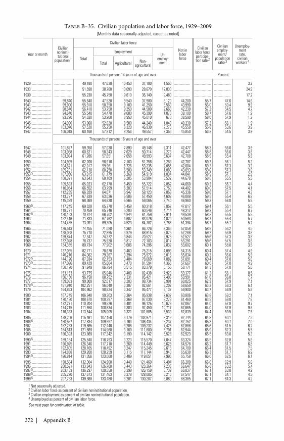
372 | Appendix B
Table B–35. Civilian population and labor force, 1929–2009[Monthly data seasonally adjusted, except as noted]
Year or monthCivilian
noninsti-tutional
population 1
Civilian labor force
Not inlaborforce
Civilianlabor forceparticipa-tion rate 2
Civilianemploy-ment/
populationratio 3
Unemploy-mentrate,
civilianworkers 4
Total
EmploymentUn-
employ-mentTotal Agricultural Non-
agricultural
Thousands of persons 14 years of age and over Percent
1929 ...................... .................... 49,180 47,630 10,450 37,180 1,550 .................. ................... ................... 3.21933 ...................... .................... 51,590 38,760 10,090 28,670 12,830 .................. ................... ................... 24.91939 ...................... .................... 55,230 45,750 9,610 36,140 9,480 .................. ................... ................... 17.21940 ...................... 99,840 55,640 47,520 9,540 37,980 8,120 44,200 55.7 47.6 14.61941 ...................... 99,900 55,910 50,350 9,100 41,250 5,560 43,990 56.0 50.4 9.91942 ...................... 98,640 56,410 53,750 9,250 44,500 2,660 42,230 57.2 54.5 4.71943 ...................... 94,640 55,540 54,470 9,080 45,390 1,070 39,100 58.7 57.6 1.91944 ...................... 93,220 54,630 53,960 8,950 45,010 670 38,590 58.6 57.9 1.21945 ...................... 94,090 53,860 52,820 8,580 44,240 1,040 40,230 57.2 56.1 1.91946 ...................... 103,070 57,520 55,250 8,320 46,930 2,270 45,550 55.8 53.6 3.91947 ...................... 106,018 60,168 57,812 8,256 49,557 2,356 45,850 56.8 54.5 3.9
Thousands of persons 16 years of age and over
1947 ...................... 101,827 59,350 57,038 7,890 49,148 2,311 42,477 58.3 56.0 3.91948 ...................... 103,068 60,621 58,343 7,629 50,714 2,276 42,447 58.8 56.6 3.81949 ...................... 103,994 61,286 57,651 7,658 49,993 3,637 42,708 58.9 55.4 5.91950 ...................... 104,995 62,208 58,918 7,160 51,758 3,288 42,787 59.2 56.1 5.31951 ...................... 104,621 62,017 59,961 6,726 53,235 2,055 42,604 59.2 57.3 3.31952 ...................... 105,231 62,138 60,250 6,500 53,749 1,883 43,093 59.0 57.3 3.01953 5 .................... 107,056 63,015 61,179 6,260 54,919 1,834 44,041 58.9 57.1 2.91954 ...................... 108,321 63,643 60,109 6,205 53,904 3,532 44,678 58.8 55.5 5.51955 ...................... 109,683 65,023 62,170 6,450 55,722 2,852 44,660 59.3 56.7 4.41956 ...................... 110,954 66,552 63,799 6,283 57,514 2,750 44,402 60.0 57.5 4.11957 ...................... 112,265 66,929 64,071 5,947 58,123 2,859 45,336 59.6 57.1 4.31958 ...................... 113,727 67,639 63,036 5,586 57,450 4,602 46,088 59.5 55.4 6.81959 ...................... 115,329 68,369 64,630 5,565 59,065 3,740 46,960 59.3 56.0 5.51960 5 .................... 117,245 69,628 65,778 5,458 60,318 3,852 47,617 59.4 56.1 5.51961 ...................... 118,771 70,459 65,746 5,200 60,546 4,714 48,312 59.3 55.4 6.71962 5 .................... 120,153 70,614 66,702 4,944 61,759 3,911 49,539 58.8 55.5 5.51963 ...................... 122,416 71,833 67,762 4,687 63,076 4,070 50,583 58.7 55.4 5.71964 ...................... 124,485 73,091 69,305 4,523 64,782 3,786 51,394 58.7 55.7 5.21965 ...................... 126,513 74,455 71,088 4,361 66,726 3,366 52,058 58.9 56.2 4.51966 ...................... 128,058 75,770 72,895 3,979 68,915 2,875 52,288 59.2 56.9 3.81967 ...................... 129,874 77,347 74,372 3,844 70,527 2,975 52,527 59.6 57.3 3.81968 ...................... 132,028 78,737 75,920 3,817 72,103 2,817 53,291 59.6 57.5 3.61969 ...................... 134,335 80,734 77,902 3,606 74,296 2,832 53,602 60.1 58.0 3.51970 ...................... 137,085 82,771 78,678 3,463 75,215 4,093 54,315 60.4 57.4 4.91971 ...................... 140,216 84,382 79,367 3,394 75,972 5,016 55,834 60.2 56.6 5.91972 5 .................... 144,126 87,034 82,153 3,484 78,669 4,882 57,091 60.4 57.0 5.61973 5 .................... 147,096 89,429 85,064 3,470 81,594 4,365 57,667 60.8 57.8 4.91974 ...................... 150,120 91,949 86,794 3,515 83,279 5,156 58,171 61.3 57.8 5.61975 ...................... 153,153 93,775 85,846 3,408 82,438 7,929 59,377 61.2 56.1 8.51976 ...................... 156,150 96,158 88,752 3,331 85,421 7,406 59,991 61.6 56.8 7.71977 ...................... 159,033 99,009 92,017 3,283 88,734 6,991 60,025 62.3 57.9 7.11978 5 .................... 161,910 102,251 96,048 3,387 92,661 6,202 59,659 63.2 59.3 6.11979 ...................... 164,863 104,962 98,824 3,347 95,477 6,137 59,900 63.7 59.9 5.81980 ...................... 167,745 106,940 99,303 3,364 95,938 7,637 60,806 63.8 59.2 7.11981 ...................... 170,130 108,670 100,397 3,368 97,030 8,273 61,460 63.9 59.0 7.61982 ...................... 172,271 110,204 99,526 3,401 96,125 10,678 62,067 64.0 57.8 9.71983 ...................... 174,215 111,550 100,834 3,383 97,450 10,717 62,665 64.0 57.9 9.61984 ...................... 176,383 113,544 105,005 3,321 101,685 8,539 62,839 64.4 59.5 7.51985 ...................... 178,206 115,461 107,150 3,179 103,971 8,312 62,744 64.8 60.1 7.21986 5 .................... 180,587 117,834 109,597 3,163 106,434 8,237 62,752 65.3 60.7 7.01987 ...................... 182,753 119,865 112,440 3,208 109,232 7,425 62,888 65.6 61.5 6.21988 ...................... 184,613 121,669 114,968 3,169 111,800 6,701 62,944 65.9 62.3 5.51989 ...................... 186,393 123,869 117,342 3,199 114,142 6,528 62,523 66.5 63.0 5.31990 5 .................... 189,164 125,840 118,793 3,223 115,570 7,047 63,324 66.5 62.8 5.61991 ...................... 190,925 126,346 117,718 3,269 114,449 8,628 64,578 66.2 61.7 6.81992 ...................... 192,805 128,105 118,492 3,247 115,245 9,613 64,700 66.4 61.5 7.51993 ...................... 194,838 129,200 120,259 3,115 117,144 8,940 65,638 66.3 61.7 6.91994 5 .................... 196,814 131,056 123,060 3,409 119,651 7,996 65,758 66.6 62.5 6.11995 ...................... 198,584 132,304 124,900 3,440 121,460 7,404 66,280 66.6 62.9 5.61996 ...................... 200,591 133,943 126,708 3,443 123,264 7,236 66,647 66.8 63.2 5.41997 5 .................... 203,133 136,297 129,558 3,399 126,159 6,739 66,837 67.1 63.8 4.91998 5 .................... 205,220 137,673 131,463 3,378 128,085 6,210 67,547 67.1 64.1 4.51999 5 .................... 207,753 139,368 133,488 3,281 130,207 5,880 68,385 67.1 64.3 4.2
1 Not seasonally adjusted.2 Civilian labor force as percent of civilian noninstitutional population.3 Civilian employment as percent of civilian noninstitutional population.4 Unemployed as percent of civilian labor force.See next page for continuation of table.
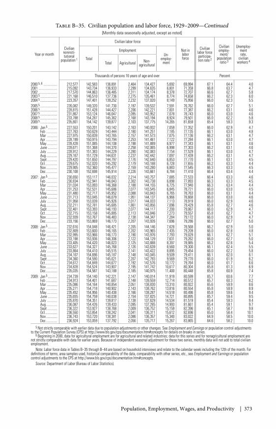
Population, Employment, Wages, and Productivity | 373
Table B–35. Civilian population and labor force, 1929–2009—Continued[Monthly data seasonally adjusted, except as noted]
Year or monthCivilian
noninsti-tutional
population 1
Civilian labor force
Not inlaborforce
Civilianlabor forceparticipa-tion rate 2
Civilianemploy-ment/
populationratio 3
Unemploy-mentrate,
civilianworkers 4
Total
EmploymentUn-
employ-mentTotal Agricultural Non-
agricultural
Thousands of persons 16 years of age and over Percent
2000 5, 6 ................ 212,577 142,583 136,891 2,464 134,427 5,692 69,994 67.1 64.4 4.02001 ...................... 215,092 143,734 136,933 2,299 134,635 6,801 71,359 66.8 63.7 4.72002 ...................... 217,570 144,863 136,485 2,311 134,174 8,378 72,707 66.6 62.7 5.82003 5 .................... 221,168 146,510 137,736 2,275 135,461 8,774 74,658 66.2 62.3 6.02004 5 .................... 223,357 147,401 139,252 2,232 137,020 8,149 75,956 66.0 62.3 5.52005 5 .................... 226,082 149,320 141,730 2,197 139,532 7,591 76,762 66.0 62.7 5.12006 5 .................... 228,815 151,428 144,427 2,206 142,221 7,001 77,387 66.2 63.1 4.62007 5 .................... 231,867 153,124 146,047 2,095 143,952 7,078 78,743 66.0 63.0 4.62008 5 .................... 233,788 154,287 145,362 2,168 143,194 8,924 79,501 66.0 62.2 5.82009 5 .................... 235,801 154,142 139,877 2,103 137,775 14,265 81,659 65.4 59.3 9.32006: Jan 5 ........... 227,553 150,201 143,142 2,163 140,932 7,059 77,352 66.0 62.9 4.7
Feb ............. 227,763 150,629 143,444 2,180 141,251 7,185 77,135 66.1 63.0 4.8Mar ............ 227,975 150,839 143,765 2,157 141,573 7,075 77,136 66.2 63.1 4.7Apr ............. 228,199 150,915 143,794 2,253 141,461 7,122 77,284 66.1 63.0 4.7May ............ 228,428 151,085 144,108 2,198 141,889 6,977 77,343 66.1 63.1 4.6June ........... 228,671 151,368 144,370 2,258 142,065 6,998 77,303 66.2 63.1 4.6July ............ 228,912 151,383 144,229 2,280 142,083 7,154 77,529 66.1 63.0 4.7Aug ............. 229,167 151,729 144,631 2,237 142,442 7,097 77,439 66.2 63.1 4.7Sept ............ 229,420 151,650 144,797 2,176 142,640 6,853 77,770 66.1 63.1 4.5Oct .............. 229,675 152,020 145,292 2,179 143,188 6,728 77,655 66.2 63.3 4.4Nov ............. 229,905 152,360 145,477 2,159 143,280 6,883 77,545 66.3 63.3 4.5Dec ............. 230,108 152,698 145,914 2,226 143,661 6,784 77,410 66.4 63.4 4.4
2007: Jan 5 ........... 230,650 153,117 146,032 2,214 143,757 7,085 77,533 66.4 63.3 4.6Feb ............. 230,834 152,941 146,043 2,302 143,738 6,898 77,893 66.3 63.3 4.5Mar ............ 231,034 153,093 146,368 2,188 144,155 6,725 77,940 66.3 63.4 4.4Apr ............. 231,253 152,531 145,686 2,077 143,545 6,845 78,721 66.0 63.0 4.5May ............ 231,480 152,717 145,952 2,088 143,843 6,765 78,763 66.0 63.1 4.4June ........... 231,713 153,045 146,079 1,951 144,137 6,966 78,668 66.0 63.0 4.6July ............ 231,958 153,039 145,926 2,017 144,033 7,113 78,919 66.0 62.9 4.6Aug ............. 232,211 152,781 145,685 1,861 143,856 7,096 79,429 65.8 62.7 4.6Sept ............ 232,461 153,393 146,193 2,077 144,117 7,200 79,067 66.0 62.9 4.7Oct .............. 232,715 153,158 145,885 2,113 143,846 7,273 79,557 65.8 62.7 4.7Nov ............. 232,939 153,767 146,483 2,138 144,347 7,284 79,172 66.0 62.9 4.7Dec ............. 233,156 153,869 146,173 2,207 143,926 7,696 79,286 66.0 62.7 5.0
2008: Jan 5 ........... 232,616 154,048 146,421 2,205 144,146 7,628 78,568 66.2 62.9 5.0Feb ............. 232,809 153,600 146,165 2,202 143,965 7,435 79,209 66.0 62.8 4.8Mar ............ 232,995 153,966 146,173 2,190 143,976 7,793 79,029 66.1 62.7 5.1Apr ............. 233,198 153,936 146,306 2,122 144,129 7,631 79,262 66.0 62.7 5.0May ............ 233,405 154,420 146,023 2,125 143,888 8,397 78,985 66.2 62.6 5.4June ........... 233,627 154,327 145,768 2,126 143,639 8,560 79,300 66.1 62.4 5.5July ............ 233,864 154,410 145,515 2,141 143,422 8,895 79,454 66.0 62.2 5.8Aug ............. 234,107 154,696 145,187 2,148 143,045 9,509 79,411 66.1 62.0 6.1Sept ............ 234,360 154,590 145,021 2,207 142,793 9,569 79,770 66.0 61.9 6.2Oct .............. 234,612 154,849 144,677 2,192 142,576 10,172 79,764 66.0 61.7 6.6Nov ............. 234,828 154,524 143,907 2,195 141,742 10,617 80,304 65.8 61.3 6.9Dec ............. 235,035 154,587 143,188 2,185 140,975 11,400 80,448 65.8 60.9 7.4
2009: Jan 5 ........... 234,739 154,140 142,221 2,147 140,014 11,919 80,599 65.7 60.6 7.7Feb ............. 234,913 154,401 141,687 2,148 139,559 12,714 80,512 65.7 60.3 8.2Mar ............ 235,086 154,164 140,854 2,051 138,830 13,310 80,922 65.6 59.9 8.6Apr ............. 235,271 154,718 140,902 2,143 138,762 13,816 80,554 65.8 59.9 8.9May ............ 235,452 154,956 140,438 2,166 138,287 14,518 80,496 65.8 59.6 9.4June ........... 235,655 154,759 140,038 2,154 137,825 14,721 80,895 65.7 59.4 9.5July ............ 235,870 154,351 139,817 2,138 137,629 14,534 81,519 65.4 59.3 9.4Aug ............. 236,087 154,426 139,433 2,095 137,285 14,993 81,661 65.4 59.1 9.7Sept ............ 236,322 153,927 138,768 2,009 136,752 15,159 82,396 65.1 58.7 9.8Oct .............. 236,550 153,854 138,242 2,041 136,311 15,612 82,696 65.0 58.4 10.1Nov ............. 236,743 153,720 138,381 2,086 136,357 15,340 83,022 64.9 58.5 10.0Dec ............. 236,924 153,059 137,792 2,056 135,717 15,267 83,865 64.6 58.2 10.0
5 Not strictly comparable with earlier data due to population adjustments or other changes. See Employment and Earnings or population control adjustmentsto the Current Population Survey (CPS) at http://www.bls.gov/cps/documentation.htm#concepts for details on breaks in series.
6 Beginning in 2000, data for agricultural employment are for agricultural and related industries; data for this series and for nonagricultural employment arenot strictly comparable with data for earlier years. Because of independent seasonal adjustment for these two series, monthly data will not add to total civilianemployment.
Note: Labor force data in Tables B–35 through B–44 are based on household interviews and relate to the calendar week including the 12th of the month. Fordefinitions of terms, area samples used, historical comparability of the data, comparability with other series, etc., see Employment and Earnings or populationcontrol adjustments to the CPS at http://www.bls.gov/cps/documentation.htm#concepts.
Source: Department of Labor (Bureau of Labor Statistics).
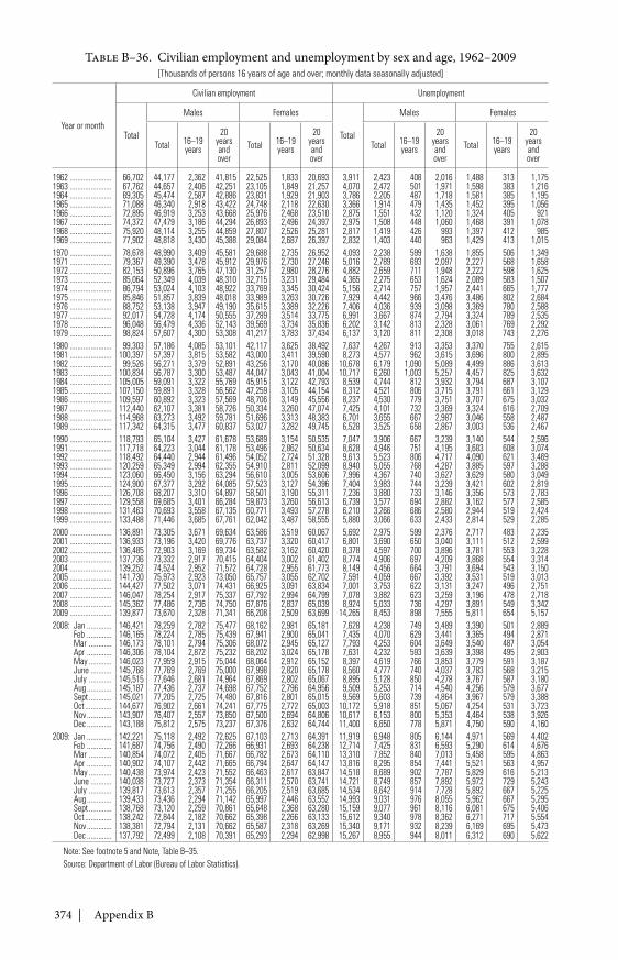
374 | Appendix B
Table B–36. Civilian employment and unemployment by sex and age, 1962–2009[Thousands of persons 16 years of age and over; monthly data seasonally adjusted]
Year or month
Civilian employment Unemployment
Total
Males Females
Total
Males Females
Total 16–19years
20yearsandover
Total 16–19years
20yearsandover
Total 16–19years
20yearsandover
Total 16–19years
20yearsandover
1962 ...................... 66,702 44,177 2,362 41,815 22,525 1,833 20,693 3,911 2,423 408 2,016 1,488 313 1,1751963 ...................... 67,762 44,657 2,406 42,251 23,105 1,849 21,257 4,070 2,472 501 1,971 1,598 383 1,2161964 ...................... 69,305 45,474 2,587 42,886 23,831 1,929 21,903 3,786 2,205 487 1,718 1,581 385 1,1951965 ...................... 71,088 46,340 2,918 43,422 24,748 2,118 22,630 3,366 1,914 479 1,435 1,452 395 1,0561966 ...................... 72,895 46,919 3,253 43,668 25,976 2,468 23,510 2,875 1,551 432 1,120 1,324 405 9211967 ...................... 74,372 47,479 3,186 44,294 26,893 2,496 24,397 2,975 1,508 448 1,060 1,468 391 1,0781968 ...................... 75,920 48,114 3,255 44,859 27,807 2,526 25,281 2,817 1,419 426 993 1,397 412 9851969 ...................... 77,902 48,818 3,430 45,388 29,084 2,687 26,397 2,832 1,403 440 963 1,429 413 1,0151970 ...................... 78,678 48,990 3,409 45,581 29,688 2,735 26,952 4,093 2,238 599 1,638 1,855 506 1,3491971 ...................... 79,367 49,390 3,478 45,912 29,976 2,730 27,246 5,016 2,789 693 2,097 2,227 568 1,6581972 ...................... 82,153 50,896 3,765 47,130 31,257 2,980 28,276 4,882 2,659 711 1,948 2,222 598 1,6251973 ...................... 85,064 52,349 4,039 48,310 32,715 3,231 29,484 4,365 2,275 653 1,624 2,089 583 1,5071974 ...................... 86,794 53,024 4,103 48,922 33,769 3,345 30,424 5,156 2,714 757 1,957 2,441 665 1,7771975 ...................... 85,846 51,857 3,839 48,018 33,989 3,263 30,726 7,929 4,442 966 3,476 3,486 802 2,6841976 ...................... 88,752 53,138 3,947 49,190 35,615 3,389 32,226 7,406 4,036 939 3,098 3,369 780 2,5881977 ...................... 92,017 54,728 4,174 50,555 37,289 3,514 33,775 6,991 3,667 874 2,794 3,324 789 2,5351978 ...................... 96,048 56,479 4,336 52,143 39,569 3,734 35,836 6,202 3,142 813 2,328 3,061 769 2,2921979 ...................... 98,824 57,607 4,300 53,308 41,217 3,783 37,434 6,137 3,120 811 2,308 3,018 743 2,2761980 ...................... 99,303 57,186 4,085 53,101 42,117 3,625 38,492 7,637 4,267 913 3,353 3,370 755 2,6151981 ...................... 100,397 57,397 3,815 53,582 43,000 3,411 39,590 8,273 4,577 962 3,615 3,696 800 2,8951982 ...................... 99,526 56,271 3,379 52,891 43,256 3,170 40,086 10,678 6,179 1,090 5,089 4,499 886 3,6131983 ...................... 100,834 56,787 3,300 53,487 44,047 3,043 41,004 10,717 6,260 1,003 5,257 4,457 825 3,6321984 ...................... 105,005 59,091 3,322 55,769 45,915 3,122 42,793 8,539 4,744 812 3,932 3,794 687 3,1071985 ...................... 107,150 59,891 3,328 56,562 47,259 3,105 44,154 8,312 4,521 806 3,715 3,791 661 3,1291986 ...................... 109,597 60,892 3,323 57,569 48,706 3,149 45,556 8,237 4,530 779 3,751 3,707 675 3,0321987 ...................... 112,440 62,107 3,381 58,726 50,334 3,260 47,074 7,425 4,101 732 3,369 3,324 616 2,7091988 ...................... 114,968 63,273 3,492 59,781 51,696 3,313 48,383 6,701 3,655 667 2,987 3,046 558 2,4871989 ...................... 117,342 64,315 3,477 60,837 53,027 3,282 49,745 6,528 3,525 658 2,867 3,003 536 2,4671990 ...................... 118,793 65,104 3,427 61,678 53,689 3,154 50,535 7,047 3,906 667 3,239 3,140 544 2,5961991 ...................... 117,718 64,223 3,044 61,178 53,496 2,862 50,634 8,628 4,946 751 4,195 3,683 608 3,0741992 ...................... 118,492 64,440 2,944 61,496 54,052 2,724 51,328 9,613 5,523 806 4,717 4,090 621 3,4691993 ...................... 120,259 65,349 2,994 62,355 54,910 2,811 52,099 8,940 5,055 768 4,287 3,885 597 3,2881994 ...................... 123,060 66,450 3,156 63,294 56,610 3,005 53,606 7,996 4,367 740 3,627 3,629 580 3,0491995 ...................... 124,900 67,377 3,292 64,085 57,523 3,127 54,396 7,404 3,983 744 3,239 3,421 602 2,8191996 ...................... 126,708 68,207 3,310 64,897 58,501 3,190 55,311 7,236 3,880 733 3,146 3,356 573 2,7831997 ...................... 129,558 69,685 3,401 66,284 59,873 3,260 56,613 6,739 3,577 694 2,882 3,162 577 2,5851998 ...................... 131,463 70,693 3,558 67,135 60,771 3,493 57,278 6,210 3,266 686 2,580 2,944 519 2,4241999 ...................... 133,488 71,446 3,685 67,761 62,042 3,487 58,555 5,880 3,066 633 2,433 2,814 529 2,2852000 ...................... 136,891 73,305 3,671 69,634 63,586 3,519 60,067 5,692 2,975 599 2,376 2,717 483 2,2352001 ...................... 136,933 73,196 3,420 69,776 63,737 3,320 60,417 6,801 3,690 650 3,040 3,111 512 2,5992002 ...................... 136,485 72,903 3,169 69,734 63,582 3,162 60,420 8,378 4,597 700 3,896 3,781 553 3,2282003 ...................... 137,736 73,332 2,917 70,415 64,404 3,002 61,402 8,774 4,906 697 4,209 3,868 554 3,3142004 ...................... 139,252 74,524 2,952 71,572 64,728 2,955 61,773 8,149 4,456 664 3,791 3,694 543 3,1502005 ...................... 141,730 75,973 2,923 73,050 65,757 3,055 62,702 7,591 4,059 667 3,392 3,531 519 3,0132006 ...................... 144,427 77,502 3,071 74,431 66,925 3,091 63,834 7,001 3,753 622 3,131 3,247 496 2,7512007 ...................... 146,047 78,254 2,917 75,337 67,792 2,994 64,799 7,078 3,882 623 3,259 3,196 478 2,7182008 ...................... 145,362 77,486 2,736 74,750 67,876 2,837 65,039 8,924 5,033 736 4,297 3,891 549 3,3422009 ...................... 139,877 73,670 2,328 71,341 66,208 2,509 63,699 14,265 8,453 898 7,555 5,811 654 5,1572008: Jan ............. 146,421 78,259 2,782 75,477 68,162 2,981 65,181 7,628 4,238 749 3,489 3,390 501 2,889
Feb ............. 146,165 78,224 2,785 75,439 67,941 2,900 65,041 7,435 4,070 629 3,441 3,365 494 2,871Mar ............ 146,173 78,101 2,794 75,306 68,072 2,945 65,127 7,793 4,253 604 3,649 3,540 487 3,054Apr ............. 146,306 78,104 2,872 75,232 68,202 3,024 65,178 7,631 4,232 593 3,639 3,398 495 2,903May ............ 146,023 77,959 2,915 75,044 68,064 2,912 65,152 8,397 4,619 766 3,853 3,779 591 3,187June ........... 145,768 77,769 2,769 75,000 67,998 2,820 65,178 8,560 4,777 740 4,037 3,783 568 3,215July ............ 145,515 77,646 2,681 74,964 67,869 2,802 65,067 8,895 5,128 850 4,278 3,767 587 3,180Aug ............. 145,187 77,436 2,737 74,698 67,752 2,796 64,956 9,509 5,253 714 4,540 4,256 579 3,677Sept ............ 145,021 77,205 2,725 74,480 67,816 2,801 65,015 9,569 5,603 739 4,864 3,967 579 3,388Oct .............. 144,677 76,902 2,661 74,241 67,775 2,772 65,003 10,172 5,918 851 5,067 4,254 531 3,723Nov ............. 143,907 76,407 2,557 73,850 67,500 2,694 64,806 10,617 6,153 800 5,353 4,464 538 3,926Dec ............. 143,188 75,812 2,575 73,237 67,376 2,632 64,744 11,400 6,650 778 5,871 4,750 590 4,160
2009: Jan ............. 142,221 75,118 2,492 72,625 67,103 2,713 64,391 11,919 6,948 805 6,144 4,971 569 4,402Feb ............. 141,687 74,756 2,490 72,266 66,931 2,693 64,238 12,714 7,425 831 6,593 5,290 614 4,676Mar ............ 140,854 74,072 2,405 71,667 66,782 2,673 64,110 13,310 7,852 840 7,013 5,458 595 4,863Apr ............. 140,902 74,107 2,442 71,665 66,794 2,647 64,147 13,816 8,295 854 7,441 5,521 563 4,957May ............ 140,438 73,974 2,423 71,552 66,463 2,617 63,847 14,518 8,689 902 7,787 5,829 616 5,213June ........... 140,038 73,727 2,373 71,354 66,311 2,570 63,741 14,721 8,749 857 7,892 5,972 729 5,243July ............ 139,817 73,613 2,357 71,255 66,205 2,519 63,685 14,534 8,642 914 7,728 5,892 667 5,225Aug ............. 139,433 73,436 2,294 71,142 65,997 2,446 63,552 14,993 9,031 976 8,055 5,962 667 5,295Sept ............ 138,768 73,120 2,259 70,861 65,648 2,368 63,280 15,159 9,077 961 8,116 6,081 675 5,406Oct .............. 138,242 72,844 2,182 70,662 65,398 2,266 63,133 15,612 9,340 978 8,362 6,271 717 5,554Nov ............. 138,381 72,794 2,131 70,662 65,587 2,318 63,269 15,340 9,171 932 8,239 6,169 695 5,473Dec ............. 137,792 72,499 2,108 70,391 65,293 2,294 62,998 15,267 8,955 944 8,011 6,312 690 5,622
Note: See footnote 5 and Note, Table B–35.Source: Department of Labor (Bureau of Labor Statistics).
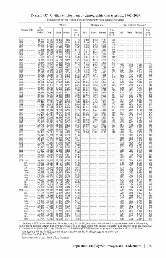
Population, Employment, Wages, and Productivity | 375
Table B–37. Civilian employment by demographic characteristic, 1962–2009[Thousands of persons 16 years of age and over; monthly data seasonally adjusted]
Year or monthAll
civilianworkers
White 1 Black and other 1 Black or African American 1
Total Males FemalesBothsexes16–19
Total Males FemalesBothsexes16–19
Total Males FemalesBothsexes16–19
1962 ...................... 66,702 59,698 40,016 19,682 3,774 7,003 4,160 2,843 420 .............. .............. ............. ...............1963 ...................... 67,762 60,622 40,428 20,194 3,851 7,140 4,229 2,911 404 .............. .............. ............. ...............1964 ...................... 69,305 61,922 41,115 20,807 4,076 7,383 4,359 3,024 440 .............. .............. ............. ...............1965 ...................... 71,088 63,446 41,844 21,602 4,562 7,643 4,496 3,147 474 .............. .............. ............. ...............1966 ...................... 72,895 65,021 42,331 22,690 5,176 7,877 4,588 3,289 545 .............. .............. ............. ...............1967 ...................... 74,372 66,361 42,833 23,528 5,114 8,011 4,646 3,365 568 .............. .............. ............. ...............1968 ...................... 75,920 67,750 43,411 24,339 5,195 8,169 4,702 3,467 584 .............. .............. ............. ...............1969 ...................... 77,902 69,518 44,048 25,470 5,508 8,384 4,770 3,614 609 .............. .............. ............. ...............1970 ...................... 78,678 70,217 44,178 26,039 5,571 8,464 4,813 3,650 574 .............. .............. ............. ...............1971 ...................... 79,367 70,878 44,595 26,283 5,670 8,488 4,796 3,692 538 .............. .............. ............. ...............1972 ...................... 82,153 73,370 45,944 27,426 6,173 8,783 4,952 3,832 573 7,802 4,368 3,433 5091973 ...................... 85,064 75,708 47,085 28,623 6,623 9,356 5,265 4,092 647 8,128 4,527 3,601 5701974 ...................... 86,794 77,184 47,674 29,511 6,796 9,610 5,352 4,258 652 8,203 4,527 3,677 5541975 ...................... 85,846 76,411 46,697 29,714 6,487 9,435 5,161 4,275 615 7,894 4,275 3,618 5071976 ...................... 88,752 78,853 47,775 31,078 6,724 9,899 5,363 4,536 611 8,227 4,404 3,823 5081977 ...................... 92,017 81,700 49,150 32,550 7,068 10,317 5,579 4,739 619 8,540 4,565 3,975 5081978 ...................... 96,048 84,936 50,544 34,392 7,367 11,112 5,936 5,177 703 9,102 4,796 4,307 5711979 ...................... 98,824 87,259 51,452 35,807 7,356 11,565 6,156 5,409 727 9,359 4,923 4,436 5791980 ...................... 99,303 87,715 51,127 36,587 7,021 11,588 6,059 5,529 689 9,313 4,798 4,515 5471981 ...................... 100,397 88,709 51,315 37,394 6,588 11,688 6,083 5,606 637 9,355 4,794 4,561 5051982 ...................... 99,526 87,903 50,287 37,615 5,984 11,624 5,983 5,641 565 9,189 4,637 4,552 4281983 ...................... 100,834 88,893 50,621 38,272 5,799 11,941 6,166 5,775 543 9,375 4,753 4,622 4161984 ...................... 105,005 92,120 52,462 39,659 5,836 12,885 6,629 6,256 607 10,119 5,124 4,995 4741985 ...................... 107,150 93,736 53,046 40,690 5,768 13,414 6,845 6,569 666 10,501 5,270 5,231 5321986 ...................... 109,597 95,660 53,785 41,876 5,792 13,937 7,107 6,830 681 10,814 5,428 5,386 5361987 ...................... 112,440 97,789 54,647 43,142 5,898 14,652 7,459 7,192 742 11,309 5,661 5,648 5871988 ...................... 114,968 99,812 55,550 44,262 6,030 15,156 7,722 7,434 774 11,658 5,824 5,834 6011989 ...................... 117,342 101,584 56,352 45,232 5,946 15,757 7,963 7,795 813 11,953 5,928 6,025 6251990 ...................... 118,793 102,261 56,703 45,558 5,779 16,533 8,401 8,131 801 12,175 5,995 6,180 5981991 ...................... 117,718 101,182 55,797 45,385 5,216 16,536 8,426 8,110 690 12,074 5,961 6,113 4941992 ...................... 118,492 101,669 55,959 45,710 4,985 16,823 8,482 8,342 684 12,151 5,930 6,221 4921993 ...................... 120,259 103,045 56,656 46,390 5,113 17,214 8,693 8,521 691 12,382 6,047 6,334 4941994 ...................... 123,060 105,190 57,452 47,738 5,398 17,870 8,998 8,872 763 12,835 6,241 6,595 5521995 ...................... 124,900 106,490 58,146 48,344 5,593 18,409 9,231 9,179 826 13,279 6,422 6,857 5861996 ...................... 126,708 107,808 58,888 48,920 5,667 18,900 9,319 9,580 832 13,542 6,456 7,086 6131997 ...................... 129,558 109,856 59,998 49,859 5,807 19,701 9,687 10,014 853 13,969 6,607 7,362 6311998 ...................... 131,463 110,931 60,604 50,327 6,089 20,532 10,089 10,443 962 14,556 6,871 7,685 7361999 ...................... 133,488 112,235 61,139 51,096 6,204 21,253 10,307 10,945 968 15,056 7,027 8,029 6912000 ...................... 136,891 114,424 62,289 52,136 6,160 .............. .............. ............. ............. 15,156 7,082 8,073 7112001 ...................... 136,933 114,430 62,212 52,218 5,817 .............. .............. ............. ............. 15,006 6,938 8,068 6372002 ...................... 136,485 114,013 61,849 52,164 5,441 .............. .............. ............. ............. 14,872 6,959 7,914 6112003 ...................... 137,736 114,235 61,866 52,369 5,064 .............. .............. ............. ............. 14,739 6,820 7,919 5162004 ...................... 139,252 115,239 62,712 52,527 5,039 .............. .............. ............. ............. 14,909 6,912 7,997 5202005 ...................... 141,730 116,949 63,763 53,186 5,105 .............. .............. ............. ............. 15,313 7,155 8,158 5362006 ...................... 144,427 118,833 64,883 53,950 5,215 .............. .............. ............. ............. 15,765 7,354 8,410 6182007 ...................... 146,047 119,792 65,289 54,503 4,990 .............. .............. ............. ............. 16,051 7,500 8,551 5662008 ...................... 145,362 119,126 64,624 54,501 4,697 .............. .............. ............. ............. 15,953 7,398 8,554 5412009 ...................... 139,877 114,996 61,630 53,366 4,138 .............. .............. ............. ............. 15,025 6,817 8,208 4422008: Jan ............. 146,421 119,926 65,220 54,706 4,797 .............. .............. ............. ............. 16,079 7,554 8,524 573
Feb ............. 146,165 119,665 65,161 54,504 4,788 .............. .............. ............. ............. 16,165 7,560 8,604 572Mar ............ 146,173 119,695 65,135 54,559 4,839 .............. .............. ............. ............. 16,127 7,477 8,650 527Apr ............. 146,306 119,676 65,040 54,636 4,961 .............. .............. ............. ............. 16,218 7,533 8,685 573May ............ 146,023 119,624 65,029 54,595 4,910 .............. .............. ............. ............. 16,030 7,448 8,582 558June ........... 145,768 119,441 64,837 54,604 4,729 .............. .............. ............. ............. 16,026 7,462 8,563 527July ............ 145,515 119,382 64,885 54,497 4,623 .............. .............. ............. ............. 15,950 7,377 8,573 533Aug ............. 145,187 119,016 64,580 54,436 4,642 .............. .............. ............. ............. 16,024 7,495 8,529 594Sept ............ 145,021 119,031 64,368 54,663 4,607 .............. .............. ............. ............. 15,742 7,329 8,413 564Oct .............. 144,677 118,697 64,153 54,543 4,609 .............. .............. ............. ............. 15,787 7,286 8,501 535Nov ............. 143,907 118,018 63,789 54,229 4,487 .............. .............. ............. ............. 15,676 7,150 8,526 473Dec ............. 143,188 117,335 63,284 54,050 4,421 .............. .............. ............. ............. 15,646 7,126 8,520 483
2009: Jan ............. 142,221 116,709 62,836 53,873 4,409 .............. .............. ............. ............. 15,463 7,014 8,449 496Feb ............. 141,687 116,427 62,487 53,939 4,494 .............. .............. ............. ............. 15,296 6,940 8,356 455Mar ............ 140,854 115,663 61,908 53,755 4,346 .............. .............. ............. ............. 15,176 6,865 8,311 461Apr ............. 140,902 115,896 62,019 53,877 4,300 .............. .............. ............. ............. 15,119 6,839 8,281 496May ............ 140,438 115,451 61,895 53,557 4,315 .............. .............. ............. ............. 15,066 6,822 8,244 442June ........... 140,038 115,102 61,665 53,437 4,205 .............. .............. ............. ............. 15,048 6,792 8,255 448July ............ 139,817 114,984 61,648 53,336 4,140 .............. .............. ............. ............. 15,050 6,832 8,219 476Aug ............. 139,433 114,784 61,510 53,274 4,060 .............. .............. ............. ............. 14,914 6,745 8,169 460Sept ............ 138,768 114,215 61,237 52,979 3,980 .............. .............. ............. ............. 14,754 6,694 8,060 401Oct .............. 138,242 113,754 60,953 52,801 3,816 .............. .............. ............. ............. 14,763 6,748 8,015 409Nov ............. 138,381 113,669 60,833 52,836 3,820 .............. .............. ............. ............. 14,904 6,755 8,148 373Dec ............. 137,792 113,339 60,598 52,741 3,804 .............. .............. ............. ............. 14,758 6,765 7,992 379
1 Beginning in 2003, persons who selected this race group only. Prior to 2003, persons who selected more than one race were included in the group theyidentified as the main race. Data for “black or African American” were for “black” prior to 2003. Data discontinued for “black and other” series. See Employmentand Earnings or concepts and methodology of the Current Population Survey (CPS) at http://www.bls.gov/cps/documentation.htm#concepts for details.
Note: Beginning with data for 2000, detail will not sum to total because data for all race groups are not shown here.See footnote 5 and Note, Table B–35.Source: Department of Labor (Bureau of Labor Statistics).
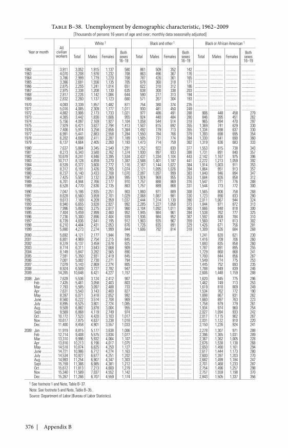
376 | Appendix B
Table B–38. Unemployment by demographic characteristic, 1962–2009[Thousands of persons 16 years of age and over; monthly data seasonally adjusted]
Year or monthAll
civilianworkers
White 1 Black and other 1 Black or African American 1
Total Males FemalesBothsexes16–19
Total Males FemalesBothsexes16–19
Total Males FemalesBothsexes16–19
1962 ...................... 3,911 3,052 1,915 1,137 580 861 509 352 142 .............. .............. ............. ...............1963 ...................... 4,070 3,208 1,976 1,232 708 863 496 367 176 .............. .............. ............. ...............1964 ...................... 3,786 2,999 1,779 1,220 708 787 426 361 165 .............. .............. ............. ...............1965 ...................... 3,366 2,691 1,556 1,135 705 678 360 318 171 .............. .............. ............. ...............1966 ...................... 2,875 2,255 1,241 1,014 651 622 310 312 186 .............. .............. ............. ...............1967 ...................... 2,975 2,338 1,208 1,130 635 638 300 338 203 .............. .............. ............. ...............1968 ...................... 2,817 2,226 1,142 1,084 644 590 277 313 194 .............. .............. ............. ...............1969 ...................... 2,832 2,260 1,137 1,123 660 571 267 304 193 .............. .............. ............. ...............1970 ...................... 4,093 3,339 1,857 1,482 871 754 380 374 235 .............. .............. ............. ...............1971 ...................... 5,016 4,085 2,309 1,777 1,011 930 481 450 249 .............. .............. ............. ...............1972 ...................... 4,882 3,906 2,173 1,733 1,021 977 486 491 288 906 448 458 2791973 ...................... 4,365 3,442 1,836 1,606 955 924 440 484 280 846 395 451 2621974 ...................... 5,156 4,097 2,169 1,927 1,104 1,058 544 514 318 965 494 470 2971975 ...................... 7,929 6,421 3,627 2,794 1,413 1,507 815 692 355 1,369 741 629 3301976 ...................... 7,406 5,914 3,258 2,656 1,364 1,492 779 713 355 1,334 698 637 3301977 ...................... 6,991 5,441 2,883 2,558 1,284 1,550 784 766 379 1,393 698 695 3541978 ...................... 6,202 4,698 2,411 2,287 1,189 1,505 731 774 394 1,330 641 690 3601979 ...................... 6,137 4,664 2,405 2,260 1,193 1,473 714 759 362 1,319 636 683 3331980 ...................... 7,637 5,884 3,345 2,540 1,291 1,752 922 830 377 1,553 815 738 3431981 ...................... 8,273 6,343 3,580 2,762 1,374 1,930 997 933 388 1,731 891 840 3571982 ...................... 10,678 8,241 4,846 3,395 1,534 2,437 1,334 1,104 443 2,142 1,167 975 3961983 ...................... 10,717 8,128 4,859 3,270 1,387 2,588 1,401 1,187 441 2,272 1,213 1,059 3921984 ...................... 8,539 6,372 3,600 2,772 1,116 2,167 1,144 1,022 384 1,914 1,003 911 3531985 ...................... 8,312 6,191 3,426 2,765 1,074 2,121 1,095 1,026 394 1,864 951 913 3571986 ...................... 8,237 6,140 3,433 2,708 1,070 2,097 1,097 999 383 1,840 946 894 3471987 ...................... 7,425 5,501 3,132 2,369 995 1,924 969 955 353 1,684 826 858 3121988 ...................... 6,701 4,944 2,766 2,177 910 1,757 888 869 316 1,547 771 776 2881989 ...................... 6,528 4,770 2,636 2,135 863 1,757 889 868 331 1,544 773 772 3001990 ...................... 7,047 5,186 2,935 2,251 903 1,860 971 889 308 1,565 806 758 2681991 ...................... 8,628 6,560 3,859 2,701 1,029 2,068 1,087 981 330 1,723 890 833 2801992 ...................... 9,613 7,169 4,209 2,959 1,037 2,444 1,314 1,130 390 2,011 1,067 944 3241993 ...................... 8,940 6,655 3,828 2,827 992 2,285 1,227 1,058 373 1,844 971 872 3131994 ...................... 7,996 5,892 3,275 2,617 960 2,104 1,092 1,011 360 1,666 848 818 3001995 ...................... 7,404 5,459 2,999 2,460 952 1,945 984 961 394 1,538 762 777 3251996 ...................... 7,236 5,300 2,896 2,404 939 1,936 984 952 367 1,592 808 784 3101997 ...................... 6,739 4,836 2,641 2,195 912 1,903 935 967 359 1,560 747 813 3021998 ...................... 6,210 4,484 2,431 2,053 876 1,726 835 891 329 1,426 671 756 2811999 ...................... 5,880 4,273 2,274 1,999 844 1,606 792 814 318 1,309 626 684 2682000 ...................... 5,692 4,121 2,177 1,944 795 .............. .............. ............. ............. 1,241 620 621 2302001 ...................... 6,801 4,969 2,754 2,215 845 .............. .............. ............. ............. 1,416 709 706 2602002 ...................... 8,378 6,137 3,459 2,678 925 .............. .............. ............. ............. 1,693 835 858 2602003 ...................... 8,774 6,311 3,643 2,668 909 .............. .............. ............. ............. 1,787 891 895 2552004 ...................... 8,149 5,847 3,282 2,565 890 .............. .............. ............. ............. 1,729 860 868 2412005 ...................... 7,591 5,350 2,931 2,419 845 .............. .............. ............. ............. 1,700 844 856 2672006 ...................... 7,001 5,002 2,730 2,271 794 .............. .............. ............. ............. 1,549 774 775 2532007 ...................... 7,078 5,143 2,869 2,274 805 .............. .............. ............. ............. 1,445 752 693 2352008 ...................... 8,924 6,509 3,727 2,782 947 .............. .............. ............. ............. 1,788 949 839 2462009 ...................... 14,265 10,648 6,421 4,227 1,157 .............. .............. ............. ............. 2,606 1,448 1,159 2882008: Jan ............. 7,628 5,536 3,124 2,412 907 .............. .............. ............. ............. 1,620 845 775 296
Feb ............. 7,435 5,461 3,058 2,403 803 .............. .............. ............. ............. 1,462 749 713 253Mar ............ 7,793 5,585 3,097 2,488 733 .............. .............. ............. ............. 1,619 810 809 249Apr ............. 7,631 5,543 3,143 2,400 827 .............. .............. ............. ............. 1,534 762 772 190May ............ 8,397 6,071 3,418 2,652 992 .............. .............. ............. ............. 1,698 867 831 262June ........... 8,560 6,222 3,514 2,708 969 .............. .............. ............. ............. 1,660 897 763 223July ............ 8,895 6,525 3,801 2,724 1,085 .............. .............. ............. ............. 1,758 979 779 261Aug ............. 9,509 6,882 3,878 3,004 955 .............. .............. ............. ............. 1,934 974 960 254Sept ............ 9,569 6,868 4,119 2,749 974 .............. .............. ............. ............. 2,027 1,094 933 242Oct .............. 10,172 7,523 4,420 3,103 1,017 .............. .............. ............. ............. 2,017 1,115 902 267Nov ............. 10,617 7,875 4,637 3,238 1,018 .............. .............. ............. ............. 2,031 1,122 910 220Dec ............. 11,400 8,458 4,901 3,557 1,033 .............. .............. ............. ............. 2,150 1,226 924 241
2009: Jan ............. 11,919 8,815 5,177 3,638 1,006 .............. .............. ............. ............. 2,278 1,307 971 288Feb ............. 12,714 9,408 5,575 3,834 1,077 .............. .............. ............. ............. 2,396 1,365 1,031 289Mar ............ 13,310 9,996 5,932 4,064 1,107 .............. .............. ............. ............. 2,367 1,362 1,005 228Apr ............. 13,816 10,213 6,196 4,017 1,075 .............. .............. ............. ............. 2,676 1,538 1,138 268May ............ 14,518 10,874 6,625 4,250 1,127 .............. .............. ............. ............. 2,650 1,490 1,161 294June ........... 14,721 10,986 6,712 4,274 1,163 .............. .............. ............. ............. 2,617 1,444 1,173 280July ............ 14,534 10,927 6,677 4,251 1,202 .............. .............. ............. ............. 2,600 1,397 1,203 270Aug ............. 14,993 11,254 6,907 4,347 1,303 .............. .............. ............. ............. 2,682 1,499 1,184 247Sept ............ 15,159 11,366 6,985 4,381 1,212 .............. .............. ............. ............. 2,701 1,468 1,233 287Oct .............. 15,612 11,813 7,213 4,600 1,279 .............. .............. ............. ............. 2,754 1,496 1,257 298Nov ............. 15,340 11,589 7,037 4,552 1,142 .............. .............. ............. ............. 2,757 1,559 1,198 370Dec ............. 15,267 11,266 6,707 4,559 1,174 .............. .............. ............. ............. 2,843 1,505 1,337 356
1 See footnote 1 and Note, Table B–37.Note: See footnote 5 and Note, Table B–35.Source: Department of Labor (Bureau of Labor Statistics).
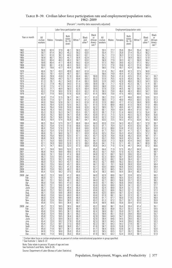
Population, Employment, Wages, and Productivity | 377
Table B–39. Civilian labor force participation rate and employment/population ratio,1962–2009
[Percent 1; monthly data seasonally adjusted]
Year or month
Labor force participation rate Employment/population ratio
Allcivilianworkers
Males FemalesBothsexes16–19years
White 2Blackand
other 2
Blackor
AfricanAmeri-can 2
Allcivilianworkers
Males FemalesBothsexes16–19years
White 2Blackand
other 2
Blackor
AfricanAmeri-can 2
1962 ...................... 58.8 82.0 37.9 46.1 58.3 63.2 ............ 55.5 77.7 35.6 39.4 55.4 56.3 ............1963 ...................... 58.7 81.4 38.3 45.2 58.2 63.0 ............ 55.4 77.1 35.8 37.4 55.3 56.2 ............1964 ...................... 58.7 81.0 38.7 44.5 58.2 63.1 ............ 55.7 77.3 36.3 37.3 55.5 57.0 ............1965 ...................... 58.9 80.7 39.3 45.7 58.4 62.9 ............ 56.2 77.5 37.1 38.9 56.0 57.8 ............1966 ...................... 59.2 80.4 40.3 48.2 58.7 63.0 ............ 56.9 77.9 38.3 42.1 56.8 58.4 ............1967 ...................... 59.6 80.4 41.1 48.4 59.2 62.8 ............ 57.3 78.0 39.0 42.2 57.2 58.2 ............1968 ...................... 59.6 80.1 41.6 48.3 59.3 62.2 ............ 57.5 77.8 39.6 42.2 57.4 58.0 ............1969 ...................... 60.1 79.8 42.7 49.4 59.9 62.1 ............ 58.0 77.6 40.7 43.4 58.0 58.1 ............1970 ...................... 60.4 79.7 43.3 49.9 60.2 61.8 ............ 57.4 76.2 40.8 42.3 57.5 56.8 ............1971 ...................... 60.2 79.1 43.4 49.7 60.1 60.9 ............ 56.6 74.9 40.4 41.3 56.8 54.9 ............1972 ...................... 60.4 78.9 43.9 51.9 60.4 60.2 59.9 57.0 75.0 41.0 43.5 57.4 54.1 53.71973 ...................... 60.8 78.8 44.7 53.7 60.8 60.5 60.2 57.8 75.5 42.0 45.9 58.2 55.0 54.51974 ...................... 61.3 78.7 45.7 54.8 61.4 60.3 59.8 57.8 74.9 42.6 46.0 58.3 54.3 53.51975 ...................... 61.2 77.9 46.3 54.0 61.5 59.6 58.8 56.1 71.7 42.0 43.3 56.7 51.4 50.11976 ...................... 61.6 77.5 47.3 54.5 61.8 59.8 59.0 56.8 72.0 43.2 44.2 57.5 52.0 50.81977 ...................... 62.3 77.7 48.4 56.0 62.5 60.4 59.8 57.9 72.8 44.5 46.1 58.6 52.5 51.41978 ...................... 63.2 77.9 50.0 57.8 63.3 62.2 61.5 59.3 73.8 46.4 48.3 60.0 54.7 53.61979 ...................... 63.7 77.8 50.9 57.9 63.9 62.2 61.4 59.9 73.8 47.5 48.5 60.6 55.2 53.81980 ...................... 63.8 77.4 51.5 56.7 64.1 61.7 61.0 59.2 72.0 47.7 46.6 60.0 53.6 52.31981 ...................... 63.9 77.0 52.1 55.4 64.3 61.3 60.8 59.0 71.3 48.0 44.6 60.0 52.6 51.31982 ...................... 64.0 76.6 52.6 54.1 64.3 61.6 61.0 57.8 69.0 47.7 41.5 58.8 50.9 49.41983 ...................... 64.0 76.4 52.9 53.5 64.3 62.1 61.5 57.9 68.8 48.0 41.5 58.9 51.0 49.51984 ...................... 64.4 76.4 53.6 53.9 64.6 62.6 62.2 59.5 70.7 49.5 43.7 60.5 53.6 52.31985 ...................... 64.8 76.3 54.5 54.5 65.0 63.3 62.9 60.1 70.9 50.4 44.4 61.0 54.7 53.41986 ...................... 65.3 76.3 55.3 54.7 65.5 63.7 63.3 60.7 71.0 51.4 44.6 61.5 55.4 54.11987 ...................... 65.6 76.2 56.0 54.7 65.8 64.3 63.8 61.5 71.5 52.5 45.5 62.3 56.8 55.61988 ...................... 65.9 76.2 56.6 55.3 66.2 64.0 63.8 62.3 72.0 53.4 46.8 63.1 57.4 56.31989 ...................... 66.5 76.4 57.4 55.9 66.7 64.7 64.2 63.0 72.5 54.3 47.5 63.8 58.2 56.91990 ...................... 66.5 76.4 57.5 53.7 66.9 64.4 64.0 62.8 72.0 54.3 45.3 63.7 57.9 56.71991 ...................... 66.2 75.8 57.4 51.6 66.6 63.8 63.3 61.7 70.4 53.7 42.0 62.6 56.7 55.41992 ...................... 66.4 75.8 57.8 51.3 66.8 64.6 63.9 61.5 69.8 53.8 41.0 62.4 56.4 54.91993 ...................... 66.3 75.4 57.9 51.5 66.8 63.8 63.2 61.7 70.0 54.1 41.7 62.7 56.3 55.01994 ...................... 66.6 75.1 58.8 52.7 67.1 63.9 63.4 62.5 70.4 55.3 43.4 63.5 57.2 56.11995 ...................... 66.6 75.0 58.9 53.5 67.1 64.3 63.7 62.9 70.8 55.6 44.2 63.8 58.1 57.11996 ...................... 66.8 74.9 59.3 52.3 67.2 64.6 64.1 63.2 70.9 56.0 43.5 64.1 58.6 57.41997 ...................... 67.1 75.0 59.8 51.6 67.5 65.2 64.7 63.8 71.3 56.8 43.4 64.6 59.4 58.21998 ...................... 67.1 74.9 59.8 52.8 67.3 66.0 65.6 64.1 71.6 57.1 45.1 64.7 60.9 59.71999 ...................... 67.1 74.7 60.0 52.0 67.3 65.9 65.8 64.3 71.6 57.4 44.7 64.8 61.3 60.62000 ...................... 67.1 74.8 59.9 52.0 67.3 ............. 65.8 64.4 71.9 57.5 45.2 64.9 ............. 60.92001 ...................... 66.8 74.4 59.8 49.6 67.0 ............. 65.3 63.7 70.9 57.0 42.3 64.2 ............. 59.72002 ...................... 66.6 74.1 59.6 47.4 66.8 ............. 64.8 62.7 69.7 56.3 39.6 63.4 ............. 58.12003 ...................... 66.2 73.5 59.5 44.5 66.5 ............. 64.3 62.3 68.9 56.1 36.8 63.0 ............. 57.42004 ...................... 66.0 73.3 59.2 43.9 66.3 ............. 63.8 62.3 69.2 56.0 36.4 63.1 ............. 57.22005 ...................... 66.0 73.3 59.3 43.7 66.3 ............. 64.2 62.7 69.6 56.2 36.5 63.4 ............. 57.72006 ...................... 66.2 73.5 59.4 43.7 66.5 ............. 64.1 63.1 70.1 56.6 36.9 63.8 ............. 58.42007 ...................... 66.0 73.2 59.3 41.3 66.4 ............. 63.7 63.0 69.8 56.6 34.8 63.6 ............. 58.42008 ...................... 66.0 73.0 59.5 40.2 66.3 ............. 63.7 62.2 68.5 56.2 32.6 62.8 ............. 57.32009 ...................... 65.4 72.0 59.2 37.5 65.8 ............. 62.4 59.3 64.5 54.4 28.4 60.2 ............. 53.22008: Jan ............. 66.2 73.3 59.6 41.2 66.5 ............. 64.0 62.9 69.6 56.7 33.9 63.5 ............. 58.2
Feb ............. 66.0 73.1 59.3 40.0 66.2 ............. 63.7 62.8 69.5 56.5 33.4 63.3 ............. 58.4Mar ............ 66.1 73.1 59.5 40.1 66.3 ............. 64.0 62.7 69.3 56.6 33.7 63.3 ............. 58.2Apr ............. 66.0 73.0 59.5 41.0 66.2 ............. 64.0 62.7 69.2 56.6 34.6 63.3 ............. 58.5May ............ 66.2 73.1 59.6 42.1 66.4 ............. 63.8 62.6 69.0 56.5 34.1 63.2 ............. 57.7June ........... 66.1 73.0 59.5 40.4 66.3 ............. 63.6 62.4 68.8 56.4 32.7 63.1 ............. 57.6July ............ 66.0 73.2 59.3 40.5 66.4 ............. 63.6 62.2 68.6 56.2 32.1 63.0 ............. 57.3Aug ............. 66.1 73.0 59.6 39.9 66.4 ............. 64.4 62.0 68.4 56.1 32.4 62.7 ............. 57.4Sept ............ 66.0 73.0 59.4 40.0 66.3 ............. 63.6 61.9 68.1 56.1 32.3 62.7 ............. 56.3Oct .............. 66.0 72.9 59.5 39.8 66.4 ............. 63.6 61.7 67.7 56.0 31.8 62.4 ............. 56.4Nov ............. 65.8 72.6 59.4 38.5 66.2 ............. 63.2 61.3 67.2 55.7 30.7 62.0 ............. 55.9Dec ............. 65.8 72.5 59.5 38.4 66.1 ............. 63.4 60.9 66.6 55.6 30.4 61.6 ............. 55.8
2009: Jan ............. 65.7 72.3 59.5 38.5 66.0 ............. 63.2 60.6 66.1 55.4 30.4 61.4 ............. 55.1Feb ............. 65.7 72.3 59.6 38.8 66.1 ............. 63.0 60.3 65.8 55.2 30.3 61.2 ............. 54.5Mar ............ 65.6 72.0 59.5 38.1 66.0 ............. 62.4 59.9 65.1 55.0 29.7 60.7 ............. 54.0Apr ............. 65.8 72.4 59.6 38.1 66.2 ............. 63.2 59.9 65.1 55.0 29.8 60.8 ............. 53.7May ............ 65.8 72.5 59.5 38.4 66.3 ............. 62.9 59.6 64.9 54.7 29.5 60.6 ............. 53.5June ........... 65.7 72.3 59.4 38.3 66.1 ............. 62.6 59.4 64.6 54.5 29.0 60.3 ............. 53.3July ............ 65.4 72.0 59.2 37.9 65.9 ............. 62.5 59.3 64.5 54.4 28.6 60.2 ............. 53.3Aug ............. 65.4 72.2 59.1 37.5 66.0 ............. 62.2 59.1 64.3 54.2 27.8 60.1 ............. 52.7Sept ............ 65.1 71.8 58.8 36.8 65.7 ............. 61.6 58.7 63.9 53.8 27.2 59.7 ............. 52.1Oct .............. 65.0 71.8 58.7 36.1 65.6 ............. 61.7 58.4 63.6 53.6 26.1 59.4 ............. 52.0Nov ............. 64.9 71.5 58.8 35.8 65.4 ............. 62.2 58.5 63.5 53.7 26.2 59.4 ............. 52.5Dec ............. 64.6 71.0 58.6 35.6 65.0 ............. 61.9 58.2 63.2 53.4 25.9 59.1 ............. 51.9
1 Civilian labor force or civilian employment as percent of civilian noninstitutional population in group specified.2 See footnote 1, Table B–37.Note: Data relate to persons 16 years of age and over.See footnote 5 and Note, Table B–35.Source: Department of Labor (Bureau of Labor Statistics).
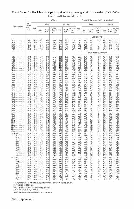
378 | Appendix B
Table B–40. Civilian labor force participation rate by demographic characteristic, 1968–2009[Percent 1; monthly data seasonally adjusted]
Year or monthAll
civilianwork-
ers
White 2 Black and other or black or African American 2
Total
Males Females
Total
Males Females
Total 16–19years
20 yearsandover
Total 16–19years
20 yearsandover
Total 16–19years
20 yearsandover
Total 16–19years
20 yearsandover
Black and other 2
1968 ...................... 59.6 59.3 80.4 55.9 83.2 40.7 43.0 40.4 62.2 77.7 49.7 82.2 49.3 34.8 51.41969 ...................... 60.1 59.9 80.2 56.8 83.0 41.8 44.6 41.5 62.1 76.9 49.6 81.4 49.8 34.6 52.01970 ...................... 60.4 60.2 80.0 57.5 82.8 42.6 45.6 42.2 61.8 76.5 47.4 81.4 49.5 34.1 51.81971 ...................... 60.2 60.1 79.6 57.9 82.3 42.6 45.4 42.3 60.9 74.9 44.7 80.0 49.2 31.2 51.81972 ...................... 60.4 60.4 79.6 60.1 82.0 43.2 48.1 42.7 60.2 73.9 46.0 78.6 48.8 32.3 51.2
Black or African American 2
1972 ...................... 60.4 60.4 79.6 60.1 82.0 43.2 48.1 42.7 59.9 73.6 46.3 78.5 48.7 32.2 51.21973 ...................... 60.8 60.8 79.4 62.0 81.6 44.1 50.1 43.5 60.2 73.4 45.7 78.4 49.3 34.2 51.61974 ...................... 61.3 61.4 79.4 62.9 81.4 45.2 51.7 44.4 59.8 72.9 46.7 77.6 49.0 33.4 51.41975 ...................... 61.2 61.5 78.7 61.9 80.7 45.9 51.5 45.3 58.8 70.9 42.6 76.0 48.8 34.2 51.11976 ...................... 61.6 61.8 78.4 62.3 80.3 46.9 52.8 46.2 59.0 70.0 41.3 75.4 49.8 32.9 52.51977 ...................... 62.3 62.5 78.5 64.0 80.2 48.0 54.5 47.3 59.8 70.6 43.2 75.6 50.8 32.9 53.61978 ...................... 63.2 63.3 78.6 65.0 80.1 49.4 56.7 48.7 61.5 71.5 44.9 76.2 53.1 37.3 55.51979 ...................... 63.7 63.9 78.6 64.8 80.1 50.5 57.4 49.8 61.4 71.3 43.6 76.3 53.1 36.8 55.41980 ...................... 63.8 64.1 78.2 63.7 79.8 51.2 56.2 50.6 61.0 70.3 43.2 75.1 53.1 34.9 55.61981 ...................... 63.9 64.3 77.9 62.4 79.5 51.9 55.4 51.5 60.8 70.0 41.6 74.5 53.5 34.0 56.01982 ...................... 64.0 64.3 77.4 60.0 79.2 52.4 55.0 52.2 61.0 70.1 39.8 74.7 53.7 33.5 56.21983 ...................... 64.0 64.3 77.1 59.4 78.9 52.7 54.5 52.5 61.5 70.6 39.9 75.2 54.2 33.0 56.81984 ...................... 64.4 64.6 77.1 59.0 78.7 53.3 55.4 53.1 62.2 70.8 41.7 74.8 55.2 35.0 57.61985 ...................... 64.8 65.0 77.0 59.7 78.5 54.1 55.2 54.0 62.9 70.8 44.6 74.4 56.5 37.9 58.61986 ...................... 65.3 65.5 76.9 59.3 78.5 55.0 56.3 54.9 63.3 71.2 43.7 74.8 56.9 39.1 58.91987 ...................... 65.6 65.8 76.8 59.0 78.4 55.7 56.5 55.6 63.8 71.1 43.6 74.7 58.0 39.6 60.01988 ...................... 65.9 66.2 76.9 60.0 78.3 56.4 57.2 56.3 63.8 71.0 43.8 74.6 58.0 37.9 60.11989 ...................... 66.5 66.7 77.1 61.0 78.5 57.2 57.1 57.2 64.2 71.0 44.6 74.4 58.7 40.4 60.61990 ...................... 66.5 66.9 77.1 59.6 78.5 57.4 55.3 57.6 64.0 71.0 40.7 75.0 58.3 36.8 60.61991 ...................... 66.2 66.6 76.5 57.3 78.0 57.4 54.1 57.6 63.3 70.4 37.3 74.6 57.5 33.5 60.01992 ...................... 66.4 66.8 76.5 56.9 78.0 57.7 52.5 58.1 63.9 70.7 40.6 74.3 58.5 35.2 60.81993 ...................... 66.3 66.8 76.2 56.6 77.7 58.0 53.5 58.3 63.2 69.6 39.5 73.2 57.9 34.6 60.21994 ...................... 66.6 67.1 75.9 57.7 77.3 58.9 55.1 59.2 63.4 69.1 40.8 72.5 58.7 36.3 60.91995 ...................... 66.6 67.1 75.7 58.5 77.1 59.0 55.5 59.2 63.7 69.0 40.1 72.5 59.5 39.8 61.41996 ...................... 66.8 67.2 75.8 57.1 77.3 59.1 54.7 59.4 64.1 68.7 39.5 72.3 60.4 38.9 62.61997 ...................... 67.1 67.5 75.9 56.1 77.5 59.5 54.1 59.9 64.7 68.3 37.4 72.2 61.7 39.9 64.01998 ...................... 67.1 67.3 75.6 56.6 77.2 59.4 55.4 59.7 65.6 69.0 40.7 72.5 62.8 42.5 64.81999 ...................... 67.1 67.3 75.6 56.4 77.2 59.6 54.5 59.9 65.8 68.7 38.6 72.4 63.5 38.8 66.12000 ...................... 67.1 67.3 75.5 56.5 77.1 59.5 54.5 59.9 65.8 69.2 39.2 72.8 63.1 39.6 65.42001 ...................... 66.8 67.0 75.1 53.7 76.9 59.4 52.4 59.9 65.3 68.4 37.9 72.1 62.8 37.3 65.22002 ...................... 66.6 66.8 74.8 50.3 76.7 59.3 50.8 60.0 64.8 68.4 37.3 72.1 61.8 34.7 64.42003 ...................... 66.2 66.5 74.2 47.5 76.3 59.2 47.9 59.9 64.3 67.3 31.1 71.5 61.9 33.7 64.62004 ...................... 66.0 66.3 74.1 47.4 76.2 58.9 46.7 59.7 63.8 66.7 30.0 70.9 61.5 32.8 64.22005 ...................... 66.0 66.3 74.1 46.2 76.2 58.9 47.6 59.7 64.2 67.3 32.6 71.3 61.6 32.2 64.42006 ...................... 66.2 66.5 74.3 46.9 76.4 59.0 46.6 59.9 64.1 67.0 32.3 71.1 61.7 35.6 64.22007 ...................... 66.0 66.4 74.0 44.3 76.3 59.0 44.6 60.1 63.7 66.8 29.4 71.2 61.1 31.2 64.02008 ...................... 66.0 66.3 73.7 43.0 76.1 59.2 43.3 60.3 63.7 66.7 29.1 71.1 61.3 29.7 64.32009 ...................... 65.4 65.8 72.8 40.3 75.3 59.1 40.9 60.4 62.4 65.0 26.4 69.6 60.3 27.9 63.42008: Jan ............. 66.2 66.5 74.0 42.3 76.5 59.2 45.2 60.2 64.0 67.7 37.8 71.2 61.1 27.7 64.3
Feb ............. 66.0 66.2 73.8 42.2 76.3 59.0 43.5 60.1 63.7 66.8 28.0 71.4 61.1 33.9 63.8Mar ............ 66.1 66.3 73.8 42.1 76.3 59.1 43.2 60.2 64.0 66.6 26.2 71.3 62.0 31.9 64.9Apr ............. 66.0 66.2 73.7 43.8 76.0 59.0 44.8 60.0 64.0 66.5 25.5 71.4 61.9 31.5 64.8May ............ 66.2 66.4 73.9 45.8 76.1 59.2 44.4 60.3 63.8 66.6 30.4 70.9 61.5 31.0 64.5June ........... 66.1 66.3 73.8 43.9 76.1 59.2 43.2 60.4 63.6 66.9 28.2 71.4 60.9 27.8 64.1July ............ 66.0 66.4 74.1 44.0 76.4 59.1 43.2 60.2 63.6 66.7 29.5 71.1 61.0 29.9 64.0Aug ............. 66.1 66.4 73.7 42.6 76.1 59.3 42.9 60.4 64.4 67.5 31.1 71.8 61.8 32.1 64.7Sept ............ 66.0 66.3 73.7 42.5 76.1 59.2 42.8 60.4 63.6 67.0 30.0 71.4 60.8 30.0 63.8Oct .............. 66.0 66.4 73.7 42.8 76.1 59.4 43.1 60.5 63.6 66.7 31.9 70.9 61.1 27.9 64.3Nov ............. 65.8 66.2 73.5 42.4 75.9 59.2 41.6 60.4 63.2 65.6 24.9 70.4 61.2 26.7 64.5Dec ............. 65.8 66.1 73.2 41.7 75.6 59.3 41.5 60.5 63.4 66.2 26.7 70.8 61.2 27.1 64.5
2009: Jan ............. 65.7 66.0 73.1 41.3 75.5 59.2 41.5 60.4 63.2 66.0 27.5 70.5 61.0 30.7 63.9Feb ............. 65.7 66.1 73.1 41.7 75.5 59.4 43.6 60.6 63.0 65.8 27.0 70.3 60.7 28.3 63.9Mar ............ 65.6 66.0 72.8 40.8 75.3 59.4 42.6 60.6 62.4 65.1 23.5 70.0 60.2 27.6 63.3Apr ............. 65.8 66.2 73.2 40.3 75.7 59.5 42.0 60.7 63.2 66.2 29.2 70.5 60.8 27.7 64.0May ............ 65.8 66.3 73.4 41.8 75.9 59.4 41.6 60.6 62.9 65.6 25.0 70.3 60.6 29.7 63.6June ........... 65.7 66.1 73.2 40.3 75.7 59.2 42.1 60.4 62.6 64.9 25.2 69.5 60.7 29.0 63.8July ............ 65.4 65.9 73.1 40.9 75.6 59.1 41.1 60.3 62.5 64.7 26.7 69.2 60.6 28.9 63.7Aug ............. 65.4 66.0 73.1 41.8 75.5 59.1 40.5 60.4 62.2 64.8 25.0 69.4 60.1 27.8 63.2Sept ............ 65.1 65.7 72.9 40.3 75.4 58.8 39.5 60.1 61.6 64.0 25.8 68.4 59.6 25.6 62.9Oct .............. 65.0 65.6 72.7 39.6 75.3 58.8 38.7 60.2 61.7 64.6 26.1 69.0 59.4 26.7 62.5Nov ............. 64.9 65.4 72.4 37.5 75.0 58.7 38.9 60.1 62.2 65.0 30.2 69.0 59.8 25.5 63.1Dec ............. 64.6 65.0 71.7 37.8 74.3 58.6 39.0 60.0 61.9 64.6 27.6 68.8 59.7 27.5 62.7
1 Civilian labor force as percent of civilian noninstitutional population in group specified.2 See footnote 1, Table B–37.Note: Data relate to persons 16 years of age and over.See footnote 5 and Note, Table B–35.Source: Department of Labor (Bureau of Labor Statistics).
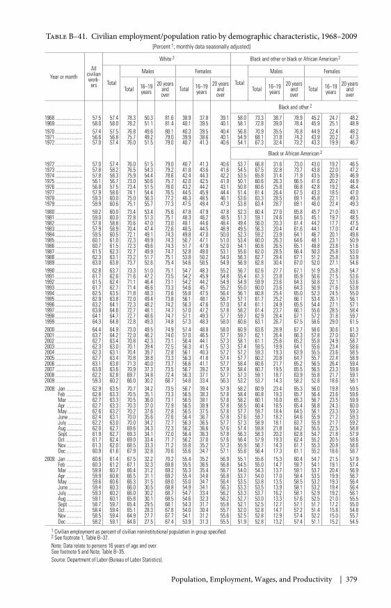
Population, Employment, Wages, and Productivity | 379
Table B–41. Civilian employment/population ratio by demographic characteristic, 1968–2009[Percent 1; monthly data seasonally adjusted]
Year or monthAll
civilianwork-
ers
White 2 Black and other or black or African American 2
Total
Males Females
Total
Males Females
Total 16–19years
20 yearsandover
Total 16–19years
20 yearsandover
Total 16–19years
20 yearsandover
Total 16–19years
20 yearsandover
Black and other 2
1968 ...................... 57.5 57.4 78.3 50.3 81.6 38.9 37.8 39.1 58.0 73.3 38.7 78.9 45.2 24.7 48.21969 ...................... 58.0 58.0 78.2 51.1 81.4 40.1 39.5 40.1 58.1 72.8 39.0 78.4 45.9 25.1 48.91970 ...................... 57.4 57.5 76.8 49.6 80.1 40.3 39.5 40.4 56.8 70.9 35.5 76.8 44.9 22.4 48.21971 ...................... 56.6 56.8 75.7 49.2 79.0 39.9 38.6 40.1 54.9 68.1 31.8 74.2 43.9 20.2 47.31972 ...................... 57.0 57.4 76.0 51.5 79.0 40.7 41.3 40.6 54.1 67.3 32.4 73.2 43.3 19.9 46.7
Black or African American 2
1972 ...................... 57.0 57.4 76.0 51.5 79.0 40.7 41.3 40.6 53.7 66.8 31.6 73.0 43.0 19.2 46.51973 ...................... 57.8 58.2 76.5 54.3 79.2 41.8 43.6 41.6 54.5 67.5 32.8 73.7 43.8 22.0 47.21974 ...................... 57.8 58.3 75.9 54.4 78.6 42.4 44.3 42.2 53.5 65.8 31.4 71.9 43.5 20.9 46.91975 ...................... 56.1 56.7 73.0 50.6 75.7 42.0 42.5 41.9 50.1 60.6 26.3 66.5 41.6 20.2 44.91976 ...................... 56.8 57.5 73.4 51.5 76.0 43.2 44.2 43.1 50.8 60.6 25.8 66.8 42.8 19.2 46.41977 ...................... 57.9 58.6 74.1 54.4 76.5 44.5 45.9 44.4 51.4 61.4 26.4 67.5 43.3 18.5 47.01978 ...................... 59.3 60.0 75.0 56.3 77.2 46.3 48.5 46.1 53.6 63.3 28.5 69.1 45.8 22.1 49.31979 ...................... 59.9 60.6 75.1 55.7 77.3 47.5 49.4 47.3 53.8 63.4 28.7 69.1 46.0 22.4 49.31980 ...................... 59.2 60.0 73.4 53.4 75.6 47.8 47.9 47.8 52.3 60.4 27.0 65.8 45.7 21.0 49.11981 ...................... 59.0 60.0 72.8 51.3 75.1 48.3 46.2 48.5 51.3 59.1 24.6 64.5 45.1 19.7 48.51982 ...................... 57.8 58.8 70.6 47.0 73.0 48.1 44.6 48.4 49.4 56.0 20.3 61.4 44.2 17.7 47.51983 ...................... 57.9 58.9 70.4 47.4 72.6 48.5 44.5 48.9 49.5 56.3 20.4 61.6 44.1 17.0 47.41984 ...................... 59.5 60.5 72.1 49.1 74.3 49.8 47.0 50.0 52.3 59.2 23.9 64.1 46.7 20.1 49.81985 ...................... 60.1 61.0 72.3 49.9 74.3 50.7 47.1 51.0 53.4 60.0 26.3 64.6 48.1 23.1 50.91986 ...................... 60.7 61.5 72.3 49.6 74.3 51.7 47.9 52.0 54.1 60.6 26.5 65.1 48.8 23.8 51.61987 ...................... 61.5 62.3 72.7 49.9 74.7 52.8 49.0 53.1 55.6 62.0 28.5 66.4 50.3 25.8 53.01988 ...................... 62.3 63.1 73.2 51.7 75.1 53.8 50.2 54.0 56.3 62.7 29.4 67.1 51.2 25.8 53.91989 ...................... 63.0 63.8 73.7 52.6 75.4 54.6 50.5 54.9 56.9 62.8 30.4 67.0 52.0 27.1 54.61990 ...................... 62.8 63.7 73.3 51.0 75.1 54.7 48.3 55.2 56.7 62.6 27.7 67.1 51.9 25.8 54.71991 ...................... 61.7 62.6 71.6 47.2 73.5 54.2 45.9 54.8 55.4 61.3 23.8 65.9 50.6 21.5 53.61992 ...................... 61.5 62.4 71.1 46.4 73.1 54.2 44.2 54.9 54.9 59.9 23.6 64.3 50.8 22.1 53.61993 ...................... 61.7 62.7 71.4 46.6 73.3 54.6 45.7 55.2 55.0 60.0 23.6 64.3 50.9 21.6 53.81994 ...................... 62.5 63.5 71.8 48.3 73.6 55.8 47.5 56.4 56.1 60.8 25.4 65.0 52.3 24.5 55.01995 ...................... 62.9 63.8 72.0 49.4 73.8 56.1 48.1 56.7 57.1 61.7 25.2 66.1 53.4 26.1 56.11996 ...................... 63.2 64.1 72.3 48.2 74.2 56.3 47.6 57.0 57.4 61.1 24.9 65.5 54.4 27.1 57.11997 ...................... 63.8 64.6 72.7 48.1 74.7 57.0 47.2 57.8 58.2 61.4 23.7 66.1 55.6 28.5 58.41998 ...................... 64.1 64.7 72.7 48.6 74.7 57.1 49.3 57.7 59.7 62.9 28.4 67.1 57.2 31.8 59.71999 ...................... 64.3 64.8 72.8 49.3 74.8 57.3 48.3 58.0 60.6 63.1 26.7 67.5 58.6 29.0 61.52000 ...................... 64.4 64.9 73.0 49.5 74.9 57.4 48.8 58.0 60.9 63.6 28.9 67.7 58.6 30.6 61.32001 ...................... 63.7 64.2 72.0 46.2 74.0 57.0 46.5 57.7 59.7 62.1 26.4 66.3 57.8 27.0 60.72002 ...................... 62.7 63.4 70.8 42.3 73.1 56.4 44.1 57.3 58.1 61.1 25.6 65.2 55.8 24.9 58.72003 ...................... 62.3 63.0 70.1 39.4 72.5 56.3 41.5 57.3 57.4 59.5 19.9 64.1 55.6 23.4 58.62004 ...................... 62.3 63.1 70.4 39.7 72.8 56.1 40.3 57.2 57.2 59.3 19.3 63.9 55.5 23.6 58.52005 ...................... 62.7 63.4 70.8 38.8 73.3 56.3 41.8 57.4 57.7 60.2 20.8 64.7 55.7 22.4 58.92006 ...................... 63.1 63.8 71.3 40.0 73.7 56.6 41.1 57.7 58.4 60.6 21.7 65.2 56.5 26.4 59.42007 ...................... 63.0 63.6 70.9 37.3 73.5 56.7 39.2 57.9 58.4 60.7 19.5 65.5 56.5 23.3 59.82008 ...................... 62.2 62.8 69.7 34.8 72.4 56.3 37.1 57.7 57.3 59.1 18.7 63.9 55.8 21.7 59.12009 ...................... 59.3 60.2 66.0 30.2 68.7 54.8 33.4 56.3 53.2 53.7 14.3 58.2 52.8 18.6 56.12008: Jan ............. 62.9 63.5 70.7 34.2 73.5 56.7 39.4 57.9 58.2 60.9 23.4 65.3 56.0 19.8 59.5
Feb ............. 62.8 63.3 70.5 35.1 73.3 56.5 38.3 57.8 58.4 60.8 19.3 65.7 56.4 23.6 59.6Mar ............ 62.7 63.3 70.5 36.0 73.1 56.5 38.1 57.8 58.2 60.1 16.0 65.3 56.7 23.5 59.9Apr ............. 62.7 63.3 70.3 37.0 72.9 56.5 38.9 57.8 58.5 60.4 18.5 65.4 56.8 24.3 60.0May ............ 62.6 63.2 70.2 37.6 72.8 56.5 37.5 57.8 57.7 59.7 18.4 64.5 56.1 23.3 59.3June ........... 62.4 63.1 70.0 35.6 72.6 56.4 36.7 57.8 57.6 59.7 18.2 64.6 55.9 21.2 59.3July ............ 62.2 63.0 70.0 34.2 72.7 56.3 36.5 57.7 57.3 58.9 18.1 63.7 55.9 21.7 59.2Aug ............. 62.0 62.7 69.6 34.3 72.3 56.2 36.6 57.6 57.4 59.8 21.8 64.2 55.5 22.5 58.8Sept ............ 61.9 62.7 69.3 34.1 72.0 56.4 36.3 57.8 56.3 58.3 20.2 62.8 54.7 21.8 57.9Oct .............. 61.7 62.4 69.0 33.4 71.7 56.2 37.0 57.6 56.4 57.9 19.3 62.4 55.2 20.5 58.6Nov ............. 61.3 62.0 68.5 33.3 71.2 55.8 35.2 57.3 55.9 56.7 14.3 61.7 55.3 20.8 58.6Dec ............. 60.9 61.6 67.9 32.8 70.6 55.6 34.7 57.1 55.8 56.4 17.3 61.1 55.2 18.6 58.7
2009: Jan ............. 60.6 61.4 67.5 32.2 70.2 55.4 35.2 56.9 55.1 55.6 15.3 60.4 54.7 21.5 57.9Feb ............. 60.3 61.2 67.1 32.3 69.8 55.5 36.5 56.8 54.5 55.0 14.7 59.7 54.1 19.1 57.4Mar ............ 59.9 60.7 66.4 31.2 69.2 55.3 35.4 56.7 54.0 54.3 13.7 59.1 53.7 20.4 56.9Apr ............. 59.9 60.8 66.5 31.1 69.2 55.4 34.8 56.8 53.7 54.0 17.0 58.4 53.5 19.9 56.7May ............ 59.6 60.6 66.3 31.5 69.0 55.0 34.7 56.4 53.5 53.8 13.5 58.5 53.2 19.3 56.4June ........... 59.4 60.3 66.0 30.5 68.8 54.9 34.1 56.3 53.3 53.5 13.9 58.1 53.2 19.4 56.4July ............ 59.3 60.2 66.0 30.2 68.7 54.7 33.4 56.2 53.3 53.7 16.2 58.1 52.9 19.2 56.1Aug ............. 59.1 60.1 65.8 30.1 68.5 54.6 32.3 56.2 52.7 53.0 13.3 57.6 52.5 21.0 55.5Sept ............ 58.7 59.7 65.4 29.5 68.1 54.3 31.7 55.8 52.1 52.5 12.7 57.1 51.7 17.2 55.0Oct .............. 58.4 59.4 65.1 28.3 67.8 54.0 30.4 55.7 52.0 52.8 14.7 57.2 51.4 15.8 54.8Nov ............. 58.5 59.4 64.9 27.7 67.7 54.1 31.2 55.6 52.5 52.8 12.9 57.4 52.2 15.0 55.7Dec ............. 58.2 59.1 64.6 27.5 67.4 53.9 31.3 55.5 51.9 52.8 13.2 57.4 51.1 15.2 54.5
1 Civilian employment as percent of civilian noninstitutional population in group specified.2 See footnote 1, Table B–37.Note: Data relate to persons 16 years of age and over.See footnote 5 and Note, Table B–35.Source: Department of Labor (Bureau of Labor Statistics).
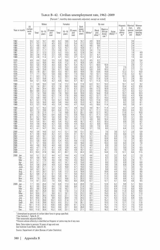
380 | Appendix B
Table B–42. Civilian unemployment rate, 1962–2009[Percent 1; monthly data seasonally adjusted, except as noted]
Year or monthAll
civilianwork-
ers
Males FemalesBothsexes16–19years
By race Hispanicor
Latinoethnic-
ity 4
Marriedmen,
spousepres-ent
Womenwho
maintainfamilies(NSA) 3
Total 16–19years
20 yearsandover
Total 16–19years
20 yearsandover
White 2Blackand
other 2
Black orAfricanAmeri-can 2
Asian(NSA) 2, 3
1962 .............. 5.5 5.2 14.7 4.6 6.2 14.6 5.4 14.7 4.9 10.9 ............. ............... ............... 3.6 .............1963 .............. 5.7 5.2 17.2 4.5 6.5 17.2 5.4 17.2 5.0 10.8 ............. ............... ............... 3.4 .............1964 .............. 5.2 4.6 15.8 3.9 6.2 16.6 5.2 16.2 4.6 9.6 ............. ............... ............... 2.8 .............1965 .............. 4.5 4.0 14.1 3.2 5.5 15.7 4.5 14.8 4.1 8.1 ............. ............... ............... 2.4 .............1966 .............. 3.8 3.2 11.7 2.5 4.8 14.1 3.8 12.8 3.4 7.3 ............. ............... ............... 1.9 .............1967 .............. 3.8 3.1 12.3 2.3 5.2 13.5 4.2 12.9 3.4 7.4 ............. ............... ............... 1.8 4.91968 .............. 3.6 2.9 11.6 2.2 4.8 14.0 3.8 12.7 3.2 6.7 ............. ............... ............... 1.6 4.41969 .............. 3.5 2.8 11.4 2.1 4.7 13.3 3.7 12.2 3.1 6.4 ............. ............... ............... 1.5 4.41970 .............. 4.9 4.4 15.0 3.5 5.9 15.6 4.8 15.3 4.5 8.2 ............. ............... ............... 2.6 5.41971 .............. 5.9 5.3 16.6 4.4 6.9 17.2 5.7 16.9 5.4 9.9 ............. ............... ............... 3.2 7.31972 .............. 5.6 5.0 15.9 4.0 6.6 16.7 5.4 16.2 5.1 10.0 10.4 ............... ............... 2.8 7.21973 .............. 4.9 4.2 13.9 3.3 6.0 15.3 4.9 14.5 4.3 9.0 9.4 ............... 7.5 2.3 7.11974 .............. 5.6 4.9 15.6 3.8 6.7 16.6 5.5 16.0 5.0 9.9 10.5 ............... 8.1 2.7 7.01975 .............. 8.5 7.9 20.1 6.8 9.3 19.7 8.0 19.9 7.8 13.8 14.8 ............... 12.2 5.1 10.01976 .............. 7.7 7.1 19.2 5.9 8.6 18.7 7.4 19.0 7.0 13.1 14.0 ............... 11.5 4.2 10.11977 .............. 7.1 6.3 17.3 5.2 8.2 18.3 7.0 17.8 6.2 13.1 14.0 ............... 10.1 3.6 9.41978 .............. 6.1 5.3 15.8 4.3 7.2 17.1 6.0 16.4 5.2 11.9 12.8 ............... 9.1 2.8 8.51979 .............. 5.8 5.1 15.9 4.2 6.8 16.4 5.7 16.1 5.1 11.3 12.3 ............... 8.3 2.8 8.31980 .............. 7.1 6.9 18.3 5.9 7.4 17.2 6.4 17.8 6.3 13.1 14.3 ............... 10.1 4.2 9.21981 .............. 7.6 7.4 20.1 6.3 7.9 19.0 6.8 19.6 6.7 14.2 15.6 ............... 10.4 4.3 10.41982 .............. 9.7 9.9 24.4 8.8 9.4 21.9 8.3 23.2 8.6 17.3 18.9 ............... 13.8 6.5 11.71983 .............. 9.6 9.9 23.3 8.9 9.2 21.3 8.1 22.4 8.4 17.8 19.5 ............... 13.7 6.5 12.21984 .............. 7.5 7.4 19.6 6.6 7.6 18.0 6.8 18.9 6.5 14.4 15.9 ............... 10.7 4.6 10.31985 .............. 7.2 7.0 19.5 6.2 7.4 17.6 6.6 18.6 6.2 13.7 15.1 ............... 10.5 4.3 10.41986 .............. 7.0 6.9 19.0 6.1 7.1 17.6 6.2 18.3 6.0 13.1 14.5 ............... 10.6 4.4 9.81987 .............. 6.2 6.2 17.8 5.4 6.2 15.9 5.4 16.9 5.3 11.6 13.0 ............... 8.8 3.9 9.21988 .............. 5.5 5.5 16.0 4.8 5.6 14.4 4.9 15.3 4.7 10.4 11.7 ............... 8.2 3.3 8.11989 .............. 5.3 5.2 15.9 4.5 5.4 14.0 4.7 15.0 4.5 10.0 11.4 ............... 8.0 3.0 8.11990 .............. 5.6 5.7 16.3 5.0 5.5 14.7 4.9 15.5 4.8 10.1 11.4 ............... 8.2 3.4 8.31991 .............. 6.8 7.2 19.8 6.4 6.4 17.5 5.7 18.7 6.1 11.1 12.5 ............... 10.0 4.4 9.31992 .............. 7.5 7.9 21.5 7.1 7.0 18.6 6.3 20.1 6.6 12.7 14.2 ............... 11.6 5.1 10.01993 .............. 6.9 7.2 20.4 6.4 6.6 17.5 5.9 19.0 6.1 11.7 13.0 ............... 10.8 4.4 9.71994 .............. 6.1 6.2 19.0 5.4 6.0 16.2 5.4 17.6 5.3 10.5 11.5 ............... 9.9 3.7 8.91995 .............. 5.6 5.6 18.4 4.8 5.6 16.1 4.9 17.3 4.9 9.6 10.4 ............... 9.3 3.3 8.01996 .............. 5.4 5.4 18.1 4.6 5.4 15.2 4.8 16.7 4.7 9.3 10.5 ............... 8.9 3.0 8.21997 .............. 4.9 4.9 16.9 4.2 5.0 15.0 4.4 16.0 4.2 8.8 10.0 ............... 7.7 2.7 8.11998 .............. 4.5 4.4 16.2 3.7 4.6 12.9 4.1 14.6 3.9 7.8 8.9 ............... 7.2 2.4 7.21999 .............. 4.2 4.1 14.7 3.5 4.3 13.2 3.8 13.9 3.7 7.0 8.0 ............... 6.4 2.2 6.42000 .............. 4.0 3.9 14.0 3.3 4.1 12.1 3.6 13.1 3.5 ............ 7.6 3.6 5.7 2.0 5.92001 .............. 4.7 4.8 16.0 4.2 4.7 13.4 4.1 14.7 4.2 ............ 8.6 4.5 6.6 2.7 6.62002 .............. 5.8 5.9 18.1 5.3 5.6 14.9 5.1 16.5 5.1 ............ 10.2 5.9 7.5 3.6 8.02003 .............. 6.0 6.3 19.3 5.6 5.7 15.6 5.1 17.5 5.2 ............ 10.8 6.0 7.7 3.8 8.52004 .............. 5.5 5.6 18.4 5.0 5.4 15.5 4.9 17.0 4.8 ............ 10.4 4.4 7.0 3.1 8.02005 .............. 5.1 5.1 18.6 4.4 5.1 14.5 4.6 16.6 4.4 ............ 10.0 4.0 6.0 2.8 7.82006 .............. 4.6 4.6 16.9 4.0 4.6 13.8 4.1 15.4 4.0 ............ 8.9 3.0 5.2 2.4 7.12007 .............. 4.6 4.7 17.6 4.1 4.5 13.8 4.0 15.7 4.1 ............ 8.3 3.2 5.6 2.5 6.52008 .............. 5.8 6.1 21.2 5.4 5.4 16.2 4.9 18.7 5.2 ............ 10.1 4.0 7.6 3.4 8.02009 .............. 9.3 10.3 27.8 9.6 8.1 20.7 7.5 24.3 8.5 ............ 14.8 7.3 12.1 6.6 11.52008: Jan ..... 5.0 5.1 21.2 4.4 4.7 14.4 4.2 17.8 4.4 ............ 9.2 3.2 6.4 2.7 7.0
Feb ..... 4.8 4.9 18.4 4.4 4.7 14.6 4.2 16.5 4.4 ............ 8.3 3.0 6.2 2.7 6.7Mar .... 5.1 5.2 17.8 4.6 4.9 14.2 4.5 16.0 4.5 ............ 9.1 3.6 6.9 2.9 7.1Apr ..... 5.0 5.1 17.1 4.6 4.7 14.1 4.3 15.6 4.4 ............ 8.6 3.2 6.9 2.8 6.8May .... 5.4 5.6 20.8 4.9 5.3 16.9 4.7 18.9 4.8 ............ 9.6 3.8 6.9 2.9 6.9June ... 5.5 5.8 21.1 5.1 5.3 16.8 4.7 19.0 5.0 ............ 9.4 4.5 7.7 3.0 7.9July .... 5.8 6.2 24.1 5.4 5.3 17.3 4.7 20.8 5.2 ............ 9.9 4.0 7.5 3.3 8.5Aug ..... 6.1 6.4 20.7 5.7 5.9 17.2 5.4 18.9 5.5 ............ 10.8 4.4 8.0 3.6 9.6Sept .... 6.2 6.8 21.3 6.1 5.5 17.1 5.0 19.3 5.5 ............ 11.4 3.8 8.0 3.9 8.2Oct ...... 6.6 7.1 24.2 6.4 5.9 16.1 5.4 20.3 6.0 ............ 11.3 3.8 8.9 4.1 8.8Nov ..... 6.9 7.5 23.8 6.8 6.2 16.6 5.7 20.3 6.3 ............ 11.5 4.8 8.8 4.3 9.3Dec ..... 7.4 8.1 23.2 7.4 6.6 18.3 6.0 20.8 6.7 ............ 12.1 5.1 9.4 4.6 9.5
2009: Jan ..... 7.7 8.5 24.4 7.8 6.9 17.3 6.4 20.9 7.0 ............ 12.8 6.2 9.9 5.1 10.3Feb ..... 8.2 9.0 25.0 8.4 7.3 18.6 6.8 21.8 7.5 ............ 13.5 6.9 11.0 5.6 10.3Mar .... 8.6 9.6 25.9 8.9 7.6 18.2 7.1 22.0 8.0 ............ 13.5 6.4 11.6 6.0 10.8Apr ..... 8.9 10.1 25.9 9.4 7.6 17.6 7.2 21.8 8.1 ............ 15.0 6.6 11.4 6.3 10.0May .... 9.4 10.5 27.1 9.8 8.1 19.1 7.5 23.2 8.6 ............ 15.0 6.7 12.7 6.7 11.0June ... 9.5 10.6 26.5 10.0 8.3 22.1 7.6 24.3 8.7 ............ 14.8 8.2 12.3 6.9 11.7July .... 9.4 10.5 27.9 9.8 8.2 20.9 7.6 24.5 8.7 ............ 14.7 8.3 12.4 6.9 12.6Aug ..... 9.7 11.0 29.9 10.2 8.3 21.4 7.7 25.7 8.9 ............ 15.2 7.5 13.0 7.1 12.2Sept .... 9.8 11.0 29.9 10.3 8.5 22.2 7.9 26.1 9.1 ............ 15.5 7.4 12.7 7.3 11.6Oct ...... 10.1 11.4 31.0 10.6 8.8 24.0 8.1 27.6 9.4 ............ 15.7 7.5 13.1 7.5 12.9Nov ..... 10.0 11.2 30.4 10.4 8.6 23.1 8.0 26.8 9.3 ............ 15.6 7.3 12.7 7.5 11.4Dec ..... 10.0 11.0 30.9 10.2 8.8 23.1 8.2 27.1 9.0 ............ 16.2 8.4 12.9 7.3 13.0
1 Unemployed as percent of civilian labor force in group specified.2 See footnote 1, Table B–37.3 Not seasonally adjusted (NSA).4 Persons whose ethnicity is identified as Hispanic or Latino may be of any race.Note: Data relate to persons 16 years of age and over.See footnote 5 and Note, Table B–35.Source: Department of Labor (Bureau of Labor Statistics).
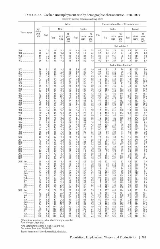
Population, Employment, Wages, and Productivity | 381
Table B–43. Civilian unemployment rate by demographic characteristic, 1968–2009[Percent 1; monthly data seasonally adjusted]
Year or monthAll
civilianwork-
ers
White 2 Black and other or black or African American 2
Total
Males Females
Total
Males Females
Total 16–19years
20yearsandover
Total 16–19years
20yearsandover
Total 16–19years
20yearsandover
Total 16–19years
20yearsandover
Black and other 2
1968 ...................... 3.6 3.2 2.6 10.1 2.0 4.3 12.1 3.4 6.7 5.6 22.1 3.9 8.3 28.7 6.31969 ...................... 3.5 3.1 2.5 10.0 1.9 4.2 11.5 3.4 6.4 5.3 21.4 3.7 7.8 27.6 5.81970 ...................... 4.9 4.5 4.0 13.7 3.2 5.4 13.4 4.4 8.2 7.3 25.0 5.6 9.3 34.5 6.91971 ...................... 5.9 5.4 4.9 15.1 4.0 6.3 15.1 5.3 9.9 9.1 28.8 7.3 10.9 35.4 8.71972 ...................... 5.6 5.1 4.5 14.2 3.6 5.9 14.2 4.9 10.0 8.9 29.7 6.9 11.4 38.4 8.8
Black or African American 2
1972 ...................... 5.6 5.1 4.5 14.2 3.6 5.9 14.2 4.9 10.4 9.3 31.7 7.0 11.8 40.5 9.01973 ...................... 4.9 4.3 3.8 12.3 3.0 5.3 13.0 4.3 9.4 8.0 27.8 6.0 11.1 36.1 8.61974 ...................... 5.6 5.0 4.4 13.5 3.5 6.1 14.5 5.1 10.5 9.8 33.1 7.4 11.3 37.4 8.81975 ...................... 8.5 7.8 7.2 18.3 6.2 8.6 17.4 7.5 14.8 14.8 38.1 12.5 14.8 41.0 12.21976 ...................... 7.7 7.0 6.4 17.3 5.4 7.9 16.4 6.8 14.0 13.7 37.5 11.4 14.3 41.6 11.71977 ...................... 7.1 6.2 5.5 15.0 4.7 7.3 15.9 6.2 14.0 13.3 39.2 10.7 14.9 43.4 12.31978 ...................... 6.1 5.2 4.6 13.5 3.7 6.2 14.4 5.2 12.8 11.8 36.7 9.3 13.8 40.8 11.21979 ...................... 5.8 5.1 4.5 13.9 3.6 5.9 14.0 5.0 12.3 11.4 34.2 9.3 13.3 39.1 10.91980 ...................... 7.1 6.3 6.1 16.2 5.3 6.5 14.8 5.6 14.3 14.5 37.5 12.4 14.0 39.8 11.91981 ...................... 7.6 6.7 6.5 17.9 5.6 6.9 16.6 5.9 15.6 15.7 40.7 13.5 15.6 42.2 13.41982 ...................... 9.7 8.6 8.8 21.7 7.8 8.3 19.0 7.3 18.9 20.1 48.9 17.8 17.6 47.1 15.41983 ...................... 9.6 8.4 8.8 20.2 7.9 7.9 18.3 6.9 19.5 20.3 48.8 18.1 18.6 48.2 16.51984 ...................... 7.5 6.5 6.4 16.8 5.7 6.5 15.2 5.8 15.9 16.4 42.7 14.3 15.4 42.6 13.51985 ...................... 7.2 6.2 6.1 16.5 5.4 6.4 14.8 5.7 15.1 15.3 41.0 13.2 14.9 39.2 13.11986 ...................... 7.0 6.0 6.0 16.3 5.3 6.1 14.9 5.4 14.5 14.8 39.3 12.9 14.2 39.2 12.41987 ...................... 6.2 5.3 5.4 15.5 4.8 5.2 13.4 4.6 13.0 12.7 34.4 11.1 13.2 34.9 11.61988 ...................... 5.5 4.7 4.7 13.9 4.1 4.7 12.3 4.1 11.7 11.7 32.7 10.1 11.7 32.0 10.41989 ...................... 5.3 4.5 4.5 13.7 3.9 4.5 11.5 4.0 11.4 11.5 31.9 10.0 11.4 33.0 9.81990 ...................... 5.6 4.8 4.9 14.3 4.3 4.7 12.6 4.1 11.4 11.9 31.9 10.4 10.9 29.9 9.71991 ...................... 6.8 6.1 6.5 17.6 5.8 5.6 15.2 5.0 12.5 13.0 36.3 11.5 12.0 36.0 10.61992 ...................... 7.5 6.6 7.0 18.5 6.4 6.1 15.8 5.5 14.2 15.2 42.0 13.5 13.2 37.2 11.81993 ...................... 6.9 6.1 6.3 17.7 5.7 5.7 14.7 5.2 13.0 13.8 40.1 12.1 12.1 37.4 10.71994 ...................... 6.1 5.3 5.4 16.3 4.8 5.2 13.8 4.6 11.5 12.0 37.6 10.3 11.0 32.6 9.81995 ...................... 5.6 4.9 4.9 15.6 4.3 4.8 13.4 4.3 10.4 10.6 37.1 8.8 10.2 34.3 8.61996 ...................... 5.4 4.7 4.7 15.5 4.1 4.7 12.9 4.1 10.5 11.1 36.9 9.4 10.0 30.3 8.71997 ...................... 4.9 4.2 4.2 14.3 3.6 4.2 12.8 3.7 10.0 10.2 36.5 8.5 9.9 28.7 8.81998 ...................... 4.5 3.9 3.9 14.1 3.2 3.9 10.9 3.4 8.9 8.9 30.1 7.4 9.0 25.3 7.91999 ...................... 4.2 3.7 3.6 12.6 3.0 3.8 11.3 3.3 8.0 8.2 30.9 6.7 7.8 25.1 6.82000 ...................... 4.0 3.5 3.4 12.3 2.8 3.6 10.4 3.1 7.6 8.0 26.2 6.9 7.1 22.8 6.22001 ...................... 4.7 4.2 4.2 13.9 3.7 4.1 11.4 3.6 8.6 9.3 30.4 8.0 8.1 27.5 7.02002 ...................... 5.8 5.1 5.3 15.9 4.7 4.9 13.1 4.4 10.2 10.7 31.3 9.5 9.8 28.3 8.82003 ...................... 6.0 5.2 5.6 17.1 5.0 4.8 13.3 4.4 10.8 11.6 36.0 10.3 10.2 30.3 9.22004 ...................... 5.5 4.8 5.0 16.3 4.4 4.7 13.6 4.2 10.4 11.1 35.6 9.9 9.8 28.2 8.92005 ...................... 5.1 4.4 4.4 16.1 3.8 4.4 12.3 3.9 10.0 10.5 36.3 9.2 9.5 30.3 8.52006 ...................... 4.6 4.0 4.0 14.6 3.5 4.0 11.7 3.6 8.9 9.5 32.7 8.3 8.4 25.9 7.52007 ...................... 4.6 4.1 4.2 15.7 3.7 4.0 12.1 3.6 8.3 9.1 33.8 7.9 7.5 25.3 6.72008 ...................... 5.8 5.2 5.5 19.1 4.9 4.9 14.4 4.4 10.1 11.4 35.9 10.2 8.9 26.8 8.12009 ...................... 9.3 8.5 9.4 25.2 8.8 7.3 18.4 6.8 14.8 17.5 46.0 16.3 12.4 33.4 11.52008: Jan ............. 5.0 4.4 4.6 19.1 3.9 4.2 12.8 3.8 9.2 10.1 38.0 8.3 8.3 28.7 7.5
Feb ............. 4.8 4.4 4.5 16.8 4.0 4.2 11.9 3.8 8.3 9.0 31.1 8.0 7.7 30.3 6.5Mar ............ 5.1 4.5 4.5 14.5 4.1 4.4 11.8 4.0 9.1 9.8 39.1 8.5 8.6 26.5 7.7Apr ............. 5.0 4.4 4.6 15.4 4.1 4.2 13.2 3.7 8.6 9.2 27.4 8.4 8.2 22.9 7.5May ............ 5.4 4.8 5.0 18.1 4.4 4.6 15.4 4.1 9.6 10.4 39.4 9.0 8.8 24.7 8.1June ........... 5.5 5.0 5.1 18.9 4.5 4.7 15.0 4.2 9.4 10.7 35.5 9.6 8.2 24.0 7.5July ............ 5.8 5.2 5.5 22.3 4.8 4.8 15.5 4.2 9.9 11.7 38.7 10.4 8.3 27.3 7.5Aug ............. 6.1 5.5 5.7 19.5 5.1 5.2 14.5 4.8 10.8 11.5 29.8 10.6 10.1 30.1 9.2Sept ............ 6.2 5.5 6.0 19.7 5.4 4.8 15.2 4.3 11.4 13.0 32.8 12.0 10.0 27.3 9.2Oct .............. 6.6 6.0 6.4 21.8 5.8 5.4 14.2 4.9 11.3 13.3 39.5 11.9 9.6 26.3 8.9Nov ............. 6.9 6.3 6.8 21.4 6.1 5.6 15.4 5.2 11.5 13.6 42.5 12.4 9.6 21.9 9.2Dec ............. 7.4 6.7 7.2 21.5 6.6 6.2 16.3 5.7 12.1 14.7 35.3 13.8 9.8 31.3 8.9
2009: Jan ............. 7.7 7.0 7.6 22.0 7.0 6.3 15.0 5.9 12.8 15.7 44.4 14.4 10.3 30.1 9.4Feb ............. 8.2 7.5 8.2 22.4 7.6 6.6 16.3 6.1 13.5 16.4 45.6 15.1 11.0 32.5 10.1Mar ............ 8.6 8.0 8.7 23.5 8.1 7.0 17.1 6.5 13.5 16.6 41.7 15.6 10.8 26.0 10.1Apr ............. 8.9 8.1 9.1 22.9 8.5 6.9 17.1 6.4 15.0 18.4 41.7 17.2 12.1 28.2 11.4May ............ 9.4 8.6 9.7 24.6 9.0 7.4 16.6 6.9 15.0 17.9 46.2 16.7 12.3 34.8 11.3June ........... 9.5 8.7 9.8 24.4 9.2 7.4 19.0 6.8 14.8 17.5 44.8 16.4 12.4 33.1 11.5July ............ 9.4 8.7 9.8 26.1 9.1 7.4 18.7 6.8 14.7 17.0 39.2 16.0 12.8 33.5 11.9Aug ............. 9.7 8.9 10.1 28.1 9.3 7.5 20.2 7.0 15.2 18.2 46.8 17.0 12.7 24.5 12.2Sept ............ 9.8 9.1 10.2 26.8 9.6 7.6 19.7 7.1 15.5 18.0 50.8 16.5 13.3 32.7 12.5Oct .............. 10.1 9.4 10.6 28.6 9.9 8.0 21.4 7.4 15.7 18.1 43.6 17.0 13.6 40.7 12.5Nov ............. 10.0 9.3 10.4 26.0 9.8 7.9 20.0 7.4 15.6 18.7 57.1 16.8 12.8 41.4 11.7Dec ............. 10.0 9.0 10.0 27.4 9.3 8.0 19.8 7.4 16.2 18.2 52.2 16.6 14.3 44.8 13.1
1 Unemployed as percent of civilian labor force in group specified.2 See footnote 1, Table B–37.Note: Data relate to persons 16 years of age and over.See footnote 5 and Note, Table B–35.Source: Department of Labor (Bureau of Labor Statistics).
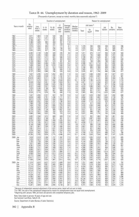
382 | Appendix B
Table B–44. Unemployment by duration and reason, 1962–2009[Thousands of persons, except as noted; monthly data seasonally adjusted 1]
Year or monthUn-
employ-ment
Duration of unemployment Reason for unemployment
Lessthan 5weeks
5–14weeks
15–26weeks
27weeks
andover
Average(mean)
duration(weeks)
Medianduration(weeks)
Job losers 3
Jobleavers
Re-entrants
NewentrantsTotal On
layoff Other
1962 ...................... 3,911 1,663 1,134 534 585 14.7 .............. .............. .............. .............. .............. .............. ...............1963 ...................... 4,070 1,751 1,231 535 553 14.0 .............. .............. .............. .............. .............. .............. ...............1964 ...................... 3,786 1,697 1,117 491 482 13.3 .............. .............. .............. .............. .............. .............. ...............1965 ...................... 3,366 1,628 983 404 351 11.8 .............. .............. .............. .............. .............. .............. ...............1966 ...................... 2,875 1,573 779 287 239 10.4 .............. .............. .............. .............. .............. .............. ...............1967 2 .................... 2,975 1,634 893 271 177 8.7 2.3 1,229 394 836 438 945 3961968 ...................... 2,817 1,594 810 256 156 8.4 4.5 1,070 334 736 431 909 4071969 ...................... 2,832 1,629 827 242 133 7.8 4.4 1,017 339 678 436 965 4131970 ...................... 4,093 2,139 1,290 428 235 8.6 4.9 1,811 675 1,137 550 1,228 5041971 ...................... 5,016 2,245 1,585 668 519 11.3 6.3 2,323 735 1,588 590 1,472 6301972 ...................... 4,882 2,242 1,472 601 566 12.0 6.2 2,108 582 1,526 641 1,456 6771973 ...................... 4,365 2,224 1,314 483 343 10.0 5.2 1,694 472 1,221 683 1,340 6491974 ...................... 5,156 2,604 1,597 574 381 9.8 5.2 2,242 746 1,495 768 1,463 6811975 ...................... 7,929 2,940 2,484 1,303 1,203 14.2 8.4 4,386 1,671 2,714 827 1,892 8231976 ...................... 7,406 2,844 2,196 1,018 1,348 15.8 8.2 3,679 1,050 2,628 903 1,928 8951977 ...................... 6,991 2,919 2,132 913 1,028 14.3 7.0 3,166 865 2,300 909 1,963 9531978 ...................... 6,202 2,865 1,923 766 648 11.9 5.9 2,585 712 1,873 874 1,857 8851979 ...................... 6,137 2,950 1,946 706 535 10.8 5.4 2,635 851 1,784 880 1,806 8171980 ...................... 7,637 3,295 2,470 1,052 820 11.9 6.5 3,947 1,488 2,459 891 1,927 8721981 ...................... 8,273 3,449 2,539 1,122 1,162 13.7 6.9 4,267 1,430 2,837 923 2,102 9811982 ...................... 10,678 3,883 3,311 1,708 1,776 15.6 8.7 6,268 2,127 4,141 840 2,384 1,1851983 ...................... 10,717 3,570 2,937 1,652 2,559 20.0 10.1 6,258 1,780 4,478 830 2,412 1,2161984 ...................... 8,539 3,350 2,451 1,104 1,634 18.2 7.9 4,421 1,171 3,250 823 2,184 1,1101985 ...................... 8,312 3,498 2,509 1,025 1,280 15.6 6.8 4,139 1,157 2,982 877 2,256 1,0391986 ...................... 8,237 3,448 2,557 1,045 1,187 15.0 6.9 4,033 1,090 2,943 1,015 2,160 1,0291987 ...................... 7,425 3,246 2,196 943 1,040 14.5 6.5 3,566 943 2,623 965 1,974 9201988 ...................... 6,701 3,084 2,007 801 809 13.5 5.9 3,092 851 2,241 983 1,809 8161989 ...................... 6,528 3,174 1,978 730 646 11.9 4.8 2,983 850 2,133 1,024 1,843 6771990 ...................... 7,047 3,265 2,257 822 703 12.0 5.3 3,387 1,028 2,359 1,041 1,930 6881991 ...................... 8,628 3,480 2,791 1,246 1,111 13.7 6.8 4,694 1,292 3,402 1,004 2,139 7921992 ...................... 9,613 3,376 2,830 1,453 1,954 17.7 8.7 5,389 1,260 4,129 1,002 2,285 9371993 ...................... 8,940 3,262 2,584 1,297 1,798 18.0 8.3 4,848 1,115 3,733 976 2,198 9191994 ...................... 7,996 2,728 2,408 1,237 1,623 18.8 9.2 3,815 977 2,838 791 2,786 6041995 ...................... 7,404 2,700 2,342 1,085 1,278 16.6 8.3 3,476 1,030 2,446 824 2,525 5791996 ...................... 7,236 2,633 2,287 1,053 1,262 16.7 8.3 3,370 1,021 2,349 774 2,512 5801997 ...................... 6,739 2,538 2,138 995 1,067 15.8 8.0 3,037 931 2,106 795 2,338 5691998 ...................... 6,210 2,622 1,950 763 875 14.5 6.7 2,822 866 1,957 734 2,132 5201999 ...................... 5,880 2,568 1,832 755 725 13.4 6.4 2,622 848 1,774 783 2,005 4692000 ...................... 5,692 2,558 1,815 669 649 12.6 5.9 2,517 852 1,664 780 1,961 4342001 ...................... 6,801 2,853 2,196 951 801 13.1 6.8 3,476 1,067 2,409 835 2,031 4592002 ...................... 8,378 2,893 2,580 1,369 1,535 16.6 9.1 4,607 1,124 3,483 866 2,368 5362003 ...................... 8,774 2,785 2,612 1,442 1,936 19.2 10.1 4,838 1,121 3,717 818 2,477 6412004 ...................... 8,149 2,696 2,382 1,293 1,779 19.6 9.8 4,197 998 3,199 858 2,408 6862005 ...................... 7,591 2,667 2,304 1,130 1,490 18.4 8.9 3,667 933 2,734 872 2,386 6662006 ...................... 7,001 2,614 2,121 1,031 1,235 16.8 8.3 3,321 921 2,400 827 2,237 6162007 ...................... 7,078 2,542 2,232 1,061 1,243 16.8 8.5 3,515 976 2,539 793 2,142 6272008 ...................... 8,924 2,932 2,804 1,427 1,761 17.9 9.4 4,789 1,176 3,614 896 2,472 7662009 ...................... 14,265 3,165 3,828 2,775 4,496 24.4 15.1 9,160 1,630 7,530 882 3,187 1,0352008: Jan ............. 7,628 2,619 2,399 1,157 1,382 17.5 9.0 3,874 1,055 2,819 831 2,202 685
Feb ............. 7,435 2,623 2,378 1,106 1,313 16.9 8.6 3,870 996 2,875 781 2,113 660Mar ............ 7,793 2,759 2,494 1,156 1,316 16.4 8.4 4,144 1,065 3,078 794 2,123 705Apr ............. 7,631 2,468 2,504 1,294 1,374 17.0 9.3 4,016 1,094 2,922 860 2,128 631May ............ 8,397 3,259 2,416 1,193 1,579 16.8 8.1 4,209 1,093 3,117 877 2,485 807June ........... 8,560 2,751 2,980 1,309 1,603 17.4 9.4 4,386 1,095 3,291 858 2,506 771July ............ 8,895 2,872 2,834 1,427 1,679 17.1 9.7 4,589 1,041 3,549 871 2,703 829Aug ............. 9,509 3,291 2,848 1,570 1,860 17.7 9.4 4,958 1,262 3,695 1,014 2,657 826Sept ............ 9,569 2,916 3,073 1,613 2,014 18.6 10.2 5,275 1,366 3,909 982 2,594 811Oct .............. 10,172 3,098 3,115 1,770 2,270 19.8 10.5 5,763 1,330 4,433 936 2,651 826Nov ............. 10,617 3,312 3,307 1,776 2,214 18.7 9.9 6,266 1,442 4,824 924 2,697 735Dec ............. 11,400 3,294 3,535 1,987 2,612 19.6 10.7 6,729 1,550 5,179 1,007 2,802 820
2009: Jan ............. 11,919 3,633 3,622 2,073 2,689 19.9 10.6 7,251 1,468 5,784 912 2,792 792Feb ............. 12,714 3,364 3,961 2,405 2,964 20.0 11.4 7,878 1,519 6,359 820 2,912 1,016Mar ............ 13,310 3,314 4,032 2,574 3,241 20.8 11.9 8,434 1,581 6,853 884 3,017 881Apr ............. 13,816 3,284 3,962 2,571 3,725 21.8 13.1 8,867 1,638 7,229 887 3,127 919May ............ 14,518 3,219 4,300 2,983 4,030 22.9 14.9 9,428 1,842 7,586 909 3,200 977June ........... 14,721 3,152 3,994 3,404 4,440 24.4 18.2 9,562 1,741 7,821 822 3,322 969July ............ 14,534 3,181 3,539 2,847 4,972 25.3 15.9 9,549 1,670 7,880 882 3,306 994Aug ............. 14,993 2,992 4,093 2,825 5,024 25.2 15.5 9,814 1,704 8,110 835 3,294 1,096Sept ............ 15,159 2,938 3,838 2,958 5,447 26.5 17.8 10,236 1,918 8,318 869 3,255 1,134Oct .............. 15,612 3,131 3,671 3,184 5,620 27.2 19.0 10,261 1,671 8,590 909 3,461 1,114Nov ............. 15,340 2,774 3,517 3,075 5,901 28.6 20.2 9,965 1,548 8,418 929 3,221 1,270Dec ............. 15,267 2,929 3,486 2,840 6,130 29.1 20.5 9,701 1,558 8,143 932 3,334 1,270
1 Because of independent seasonal adjustment of the various series, detail will not sum to totals.2 For 1967, the sum of the unemployed categorized by reason for unemployment does not equal total unemployment.3 Beginning with January 1994, job losers and persons who completed temporary jobs.Note: Data relate to persons 16 years of age and over.See footnote 5 and Note, Table B–35.Source: Department of Labor (Bureau of Labor Statistics).
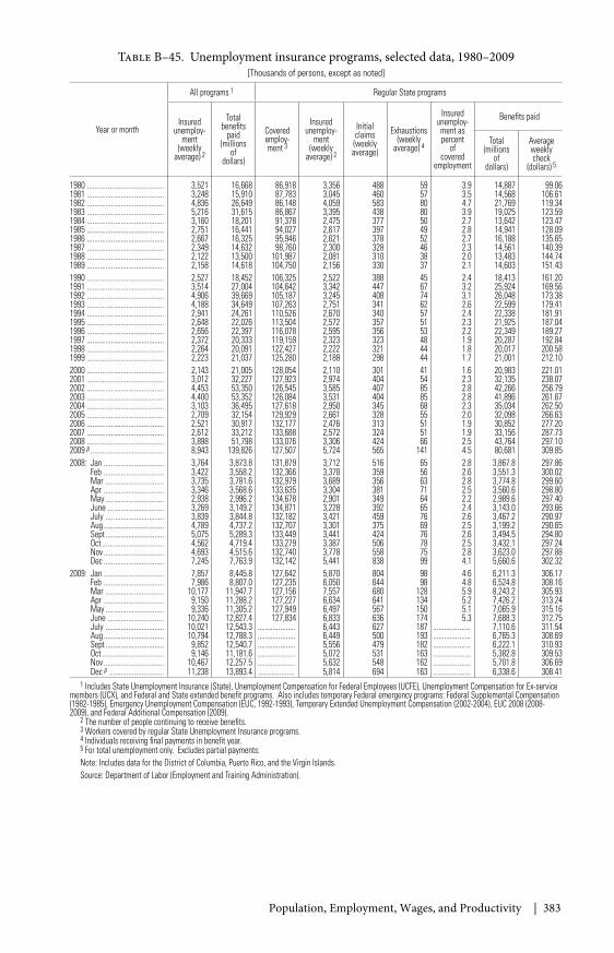
Population, Employment, Wages, and Productivity | 383
Table B–45. Unemployment insurance programs, selected data, 1980–2009[Thousands of persons, except as noted]
Year or month
All programs 1 Regular State programs
Insuredunemploy-
ment(weekly
average) 2
Totalbenefits
paid(millions
ofdollars)
Coveredemploy-ment 3
Insuredunemploy-
ment(weekly
average) 2
Initialclaims(weeklyaverage)
Exhaustions(weekly
average) 4
Insuredunemploy-
ment aspercent
ofcovered
employment
Benefits paid
Total(millions
ofdollars)
Averageweeklycheck
(dollars) 5
1980 ......................................... 3,521 16,668 86,918 3,356 488 59 3.9 14,887 99.061981 ......................................... 3,248 15,910 87,783 3,045 460 57 3.5 14,568 106.611982 ......................................... 4,836 26,649 86,148 4,059 583 80 4.7 21,769 119.341983 ......................................... 5,216 31,615 86,867 3,395 438 80 3.9 19,025 123.591984 ......................................... 3,160 18,201 91,378 2,475 377 50 2.7 13,642 123.471985 ......................................... 2,751 16,441 94,027 2,617 397 49 2.8 14,941 128.091986 ......................................... 2,667 16,325 95,946 2,621 378 52 2.7 16,188 135.651987 ......................................... 2,349 14,632 98,760 2,300 328 46 2.3 14,561 140.391988 ......................................... 2,122 13,500 101,987 2,081 310 38 2.0 13,483 144.741989 ......................................... 2,158 14,618 104,750 2,156 330 37 2.1 14,603 151.431990 ......................................... 2,527 18,452 106,325 2,522 388 45 2.4 18,413 161.201991 ......................................... 3,514 27,004 104,642 3,342 447 67 3.2 25,924 169.561992 ......................................... 4,906 39,669 105,187 3,245 408 74 3.1 26,048 173.381993 ......................................... 4,188 34,649 107,263 2,751 341 62 2.6 22,599 179.411994 ......................................... 2,941 24,261 110,526 2,670 340 57 2.4 22,338 181.911995 ......................................... 2,648 22,026 113,504 2,572 357 51 2.3 21,925 187.041996 ......................................... 2,656 22,397 116,078 2,595 356 53 2.2 22,349 189.271997 ......................................... 2,372 20,333 119,159 2,323 323 48 1.9 20,287 192.841998 ......................................... 2,264 20,091 122,427 2,222 321 44 1.8 20,017 200.581999 ......................................... 2,223 21,037 125,280 2,188 298 44 1.7 21,001 212.102000 ......................................... 2,143 21,005 128,054 2,110 301 41 1.6 20,983 221.012001 ......................................... 3,012 32,227 127,923 2,974 404 54 2.3 32,135 238.072002 ......................................... 4,453 53,350 126,545 3,585 407 85 2.8 42,266 256.792003 ......................................... 4,400 53,352 126,084 3,531 404 85 2.8 41,896 261.672004 ......................................... 3,103 36,495 127,618 2,950 345 68 2.3 35,034 262.502005 ......................................... 2,709 32,154 129,929 2,661 328 55 2.0 32,098 266.632006 ......................................... 2,521 30,917 132,177 2,476 313 51 1.9 30,852 277.202007 ......................................... 2,612 33,212 133,688 2,572 324 51 1.9 33,156 287.732008 ......................................... 3,898 51,798 133,076 3,306 424 66 2.5 43,764 297.102009 p ....................................... 8,943 139,826 127,507 5,724 565 141 4.5 80,681 309.852008: Jan ................................ 3,764 3,873.8 131,879 3,712 516 65 2.8 3,867.8 297.86
Feb ................................ 3,422 3,558.2 132,366 3,378 359 56 2.6 3,551.3 300.02Mar ............................... 3,735 3,781.6 132,979 3,689 356 63 2.8 3,774.8 299.60Apr ................................ 3,346 3,568.6 133,635 3,304 381 71 2.5 3,560.6 298.80May ............................... 2,938 2,996.2 134,678 2,901 349 64 2.2 2,989.6 297.40June .............................. 3,269 3,149.2 134,871 3,228 392 65 2.4 3,143.0 293.66July ............................... 3,839 3,844.8 132,182 3,421 459 76 2.6 3,467.2 290.97Aug ................................ 4,789 4,737.2 132,707 3,301 375 69 2.5 3,199.2 290.65Sept ............................... 5,075 5,289.3 133,449 3,441 424 76 2.6 3,494.5 294.80Oct ................................. 4,562 4,719.4 133,279 3,387 506 78 2.5 3,432.1 297.24Nov ................................ 4,693 4,515.6 132,740 3,778 558 75 2.8 3,623.0 297.88Dec ................................ 7,245 7,763.9 132,142 5,441 838 99 4.1 5,660.6 302.32
2009: Jan ................................ 7,857 8,445.8 127,642 5,870 804 98 4.6 6,211.3 306.17Feb ................................ 7,986 8,807.0 127,235 6,050 644 98 4.8 6,524.8 308.16Mar ............................... 10,177 11,947.7 127,156 7,557 680 128 5.9 8,243.2 305.93Apr ................................ 9,150 11,288.2 127,227 6,634 641 134 5.2 7,426.2 313.24May ............................... 9,336 11,305.2 127,949 6,497 567 150 5.1 7,065.9 315.16June .............................. 10,240 12,827.4 127,834 6,833 636 174 5.3 7,688.3 312.75July ............................... 10,021 12,543.3 .................... 6,443 627 187 .................... 7,110.6 311.54Aug ................................ 10,794 12,788.3 .................... 6,449 500 193 .................... 6,765.3 308.69Sept ............................... 9,852 12,540.7 .................... 5,556 479 182 .................... 6,222.1 310.93Oct ................................. 9,146 11,181.6 .................... 5,072 531 163 .................... 5,382.8 309.53Nov ................................ 10,467 12,257.5 .................... 5,632 548 162 .................... 5,701.8 306.69Dec p ............................. 11,238 13,893.4 ................... 5,814 694 163 .................... 6,338.6 308.41
1 Includes State Unemployment Insurance (State), Unemployment Compensation for Federal Employees (UCFE), Unemployment Compensation for Ex-servicemembers (UCX), and Federal and State extended benefit programs. Also includes temporary Federal emergency programs: Federal Supplemental Compensation(1982-1985), Emergency Unemployment Compensation (EUC, 1992-1993), Temporary Extended Unemployment Compensation (2002-2004), EUC 2008 (2008-2009), and Federal Additional Compensation (2009).
2 The number of people continuing to receive benefits.3 Workers covered by regular State Unemployment Insurance programs.4 Individuals receiving final payments in benefit year.5 For total unemployment only. Excludes partial payments.Note: Includes data for the District of Columbia, Puerto Rico, and the Virgin Islands.Source: Department of Labor (Employment and Training Administration).
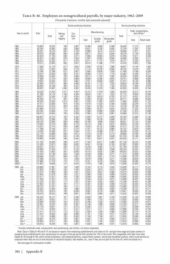
384 | Appendix B
Table B–46. Employees on nonagricultural payrolls, by major industry, 1962–2009[Thousands of persons; monthly data seasonally adjusted]
Year or month Total
Goods-producing industries Service-providing industries
TotalMining
andlogging
Con-struc-tion
ManufacturingTotal
Trade, transportation,and utilities 1
Total Durablegoods
Nondurablegoods Total Retail trade
1962 ...................... 55,659 19,203 709 2,997 15,498 9,099 6,399 36,455 11,215 5,6721963 ...................... 56,764 19,385 694 3,060 15,631 9,226 6,405 37,379 11,367 5,7811964 ...................... 58,391 19,733 697 3,148 15,888 9,414 6,474 38,658 11,677 5,9771965 ...................... 60,874 20,595 694 3,284 16,617 9,973 6,644 40,279 12,139 6,2621966 ...................... 64,020 21,740 690 3,371 17,680 10,803 6,878 42,280 12,611 6,5301967 ...................... 65,931 21,882 679 3,305 17,897 10,952 6,945 44,049 12,950 6,7111968 ...................... 68,023 22,292 671 3,410 18,211 11,137 7,074 45,731 13,334 6,9771969 ...................... 70,512 22,893 683 3,637 18,573 11,396 7,177 47,619 13,853 7,2951970 ...................... 71,006 22,179 677 3,654 17,848 10,762 7,086 48,827 14,144 7,4631971 ...................... 71,335 21,602 658 3,770 17,174 10,229 6,944 49,734 14,318 7,6571972 ...................... 73,798 22,299 672 3,957 17,669 10,630 7,039 51,499 14,788 8,0381973 ...................... 76,912 23,450 693 4,167 18,589 11,414 7,176 53,462 15,349 8,3711974 ...................... 78,389 23,364 755 4,095 18,514 11,432 7,082 55,025 15,693 8,5361975 ...................... 77,069 21,318 802 3,608 16,909 10,266 6,643 55,751 15,606 8,6001976 ...................... 79,502 22,025 832 3,662 17,531 10,640 6,891 57,477 16,128 8,9661977 ...................... 82,593 22,972 865 3,940 18,167 11,132 7,035 59,620 16,765 9,3591978 ...................... 86,826 24,156 902 4,322 18,932 11,770 7,162 62,670 17,658 9,8791979 ...................... 89,932 24,997 1,008 4,562 19,426 12,220 7,206 64,935 18,303 10,1801980 ...................... 90,528 24,263 1,077 4,454 18,733 11,679 7,054 66,265 18,413 10,2441981 ...................... 91,289 24,118 1,180 4,304 18,634 11,611 7,023 67,172 18,604 10,3641982 ...................... 89,677 22,550 1,163 4,024 17,363 10,610 6,753 67,127 18,457 10,3721983 ...................... 90,280 22,110 997 4,065 17,048 10,326 6,722 68,171 18,668 10,6351984 ...................... 94,530 23,435 1,014 4,501 17,920 11,050 6,870 71,095 19,653 11,2231985 ...................... 97,511 23,585 974 4,793 17,819 11,034 6,784 73,926 20,379 11,7331986 ...................... 99,474 23,318 829 4,937 17,552 10,795 6,757 76,156 20,795 12,0781987 ...................... 102,088 23,470 771 5,090 17,609 10,767 6,842 78,618 21,302 12,4191988 ...................... 105,345 23,909 770 5,233 17,906 10,969 6,938 81,436 21,974 12,8081989 ...................... 108,014 24,045 750 5,309 17,985 11,004 6,981 83,969 22,510 13,1081990 ...................... 109,487 23,723 765 5,263 17,695 10,737 6,958 85,764 22,666 13,1821991 ...................... 108,375 22,588 739 4,780 17,068 10,220 6,848 85,787 22,281 12,8961992 ...................... 108,726 22,095 689 4,608 16,799 9,946 6,853 86,631 22,125 12,8281993 ...................... 110,844 22,219 666 4,779 16,774 9,901 6,872 88,625 22,378 13,0211994 ...................... 114,291 22,774 659 5,095 17,020 10,132 6,889 91,517 23,128 13,4911995 ...................... 117,298 23,156 641 5,274 17,241 10,373 6,868 94,142 23,834 13,8971996 ...................... 119,708 23,409 637 5,536 17,237 10,486 6,751 96,299 24,239 14,1431997 ...................... 122,776 23,886 654 5,813 17,419 10,705 6,714 98,890 24,700 14,3891998 ...................... 125,930 24,354 645 6,149 17,560 10,911 6,649 101,576 25,186 14,6091999 ...................... 128,993 24,465 598 6,545 17,322 10,831 6,491 104,528 25,771 14,9702000 ...................... 131,785 24,649 599 6,787 17,263 10,877 6,386 107,136 26,225 15,2802001 ...................... 131,826 23,873 606 6,826 16,441 10,336 6,105 107,952 25,983 15,2392002 ...................... 130,341 22,557 583 6,716 15,259 9,485 5,774 107,784 25,497 15,0252003 ...................... 129,999 21,816 572 6,735 14,510 8,964 5,546 108,183 25,287 14,9172004 ...................... 131,435 21,882 591 6,976 14,315 8,925 5,390 109,553 25,533 15,0582005 ...................... 133,703 22,190 628 7,336 14,226 8,956 5,271 111,513 25,959 15,2802006 ...................... 136,086 22,531 684 7,691 14,155 8,981 5,174 113,556 26,276 15,3532007 ...................... 137,598 22,233 724 7,630 13,879 8,808 5,071 115,366 26,630 15,5202008 ...................... 137,066 21,419 774 7,215 13,431 8,476 4,955 115,646 26,385 15,3562009 p .................... 131,997 18,938 727 6,234 11,978 7,360 4,618 113,059 25,263 14,7742008: Jan ............. 138,080 21,981 748 7,489 13,744 8,710 5,034 116,099 26,717 15,572
Feb ............. 137,936 21,887 750 7,445 13,692 8,673 5,019 116,049 26,655 15,526Mar ............ 137,814 21,800 756 7,401 13,643 8,637 5,006 116,014 26,629 15,506Apr ............. 137,654 21,679 756 7,337 13,586 8,587 4,999 115,975 26,562 15,458May ............ 137,517 21,612 763 7,293 13,556 8,567 4,989 115,905 26,503 15,420June ........... 137,356 21,507 770 7,232 13,505 8,533 4,972 115,849 26,467 15,404July ............ 137,228 21,432 777 7,201 13,454 8,502 4,952 115,796 26,425 15,380Aug ............. 137,053 21,351 787 7,177 13,387 8,439 4,948 115,702 26,354 15,335Sept ............ 136,732 21,247 794 7,131 13,322 8,392 4,930 115,485 26,257 15,278Oct .............. 136,352 21,063 794 7,066 13,203 8,300 4,903 115,289 26,157 15,217Nov ............. 135,755 20,814 793 6,939 13,082 8,216 4,866 114,941 26,005 15,126Dec ............. 135,074 20,532 789 6,841 12,902 8,085 4,817 114,542 25,843 15,038
2009: Jan ............. 134,333 20,127 781 6,706 12,640 7,881 4,759 114,206 25,735 14,992Feb ............. 133,652 19,832 771 6,593 12,468 7,753 4,715 113,820 25,605 14,934Mar ............ 133,000 19,520 754 6,470 12,296 7,620 4,676 113,480 25,479 14,872Apr ............. 132,481 19,253 740 6,367 12,146 7,490 4,656 113,228 25,371 14,840May ............ 132,178 19,041 731 6,310 12,000 7,372 4,628 113,137 25,308 14,812June ........... 131,715 18,829 721 6,231 11,877 7,271 4,606 112,886 25,258 14,792July ............ 131,411 18,713 715 6,162 11,836 7,248 4,588 112,698 25,174 14,747Aug ............. 131,257 18,583 706 6,096 11,781 7,204 4,577 112,674 25,146 14,726Sept ............ 131,118 18,488 705 6,043 11,740 7,169 4,571 112,630 25,090 14,686Oct .............. 130,991 18,379 700 5,987 11,692 7,134 4,558 112,612 25,031 14,647Nov p .......... 130,995 18,321 704 5,960 11,657 7,105 4,552 112,674 24,999 14,633Dec p .......... 130,910 18,240 703 5,907 11,630 7,089 4,541 112,670 24,962 14,623
1 Includes wholesale trade, transportation and warehousing, and utilities, not shown separately.Note: Data in Tables B–46 and B–47 are based on reports from employing establishments and relate to full- and part-time wage and salary workers in
nonagricultural establishments who received pay for any part of the pay period that includes the 12th of the month. Not comparable with labor force data(Tables B–35 through B–44), which include proprietors, self-employed persons, unpaid family workers, and private household workers; which count persons asemployed when they are not at work because of industrial disputes, bad weather, etc., even if they are not paid for the time off; which are based on a
See next page for continuation of table.
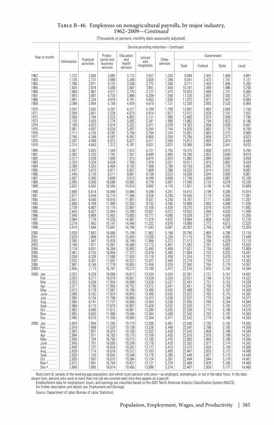
Population, Employment, Wages, and Productivity | 385
Table B–46. Employees on nonagricultural payrolls, by major industry,1962–2009—Continued
[Thousands of persons; monthly data seasonally adjusted]
Year or month
Service-providing industries—Continued
Information Financialactivities
Profes-sional andbusinessservices
Educationand
healthservices
Leisureand
hospitalityOther
services
Government
Total Federal State Local
1962 ...................... 1,723 2,656 3,885 3,172 3,557 1,243 9,004 2,455 1,669 4,8811963 ...................... 1,735 2,731 3,990 3,288 3,639 1,288 9,341 2,473 1,747 5,1211964 ...................... 1,766 2,811 4,137 3,438 3,772 1,346 9,711 2,463 1,856 5,3921965 ...................... 1,824 2,878 4,306 3,587 3,951 1,404 10,191 2,495 1,996 5,7001966 ...................... 1,908 2,961 4,517 3,770 4,127 1,475 10,910 2,690 2,141 6,0801967 ...................... 1,955 3,087 4,720 3,986 4,269 1,558 11,525 2,852 2,302 6,3711968 ...................... 1,991 3,234 4,918 4,191 4,453 1,638 11,972 2,871 2,442 6,6601969 ...................... 2,048 3,404 5,156 4,428 4,670 1,731 12,330 2,893 2,533 6,9041970 ...................... 2,041 3,532 5,267 4,577 4,789 1,789 12,687 2,865 2,664 7,1581971 ...................... 2,009 3,651 5,328 4,675 4,914 1,827 13,012 2,828 2,747 7,4371972 ...................... 2,056 3,784 5,523 4,863 5,121 1,900 13,465 2,815 2,859 7,7901973 ...................... 2,135 3,920 5,774 5,092 5,341 1,990 13,862 2,794 2,923 8,1461974 ...................... 2,160 4,023 5,974 5,322 5,471 2,078 14,303 2,858 3,039 8,4071975 ...................... 2,061 4,047 6,034 5,497 5,544 2,144 14,820 2,882 3,179 8,7581976 ...................... 2,111 4,155 6,287 5,756 5,794 2,244 15,001 2,863 3,273 8,8651977 ...................... 2,185 4,348 6,587 6,052 6,065 2,359 15,258 2,859 3,377 9,0231978 ...................... 2,287 4,599 6,972 6,427 6,411 2,505 15,812 2,893 3,474 9,4461979 ...................... 2,375 4,843 7,312 6,767 6,631 2,637 16,068 2,894 3,541 9,6331980 ...................... 2,361 5,025 7,544 7,072 6,721 2,755 16,375 3,000 3,610 9,7651981 ...................... 2,382 5,163 7,782 7,357 6,840 2,865 16,180 2,922 3,640 9,6191982 ...................... 2,317 5,209 7,848 7,515 6,874 2,924 15,982 2,884 3,640 9,4581983 ...................... 2,253 5,334 8,039 7,766 7,078 3,021 16,011 2,915 3,662 9,4341984 ...................... 2,398 5,553 8,464 8,193 7,489 3,186 16,159 2,943 3,734 9,4821985 ...................... 2,437 5,815 8,871 8,657 7,869 3,366 16,533 3,014 3,832 9,6871986 ...................... 2,445 6,128 9,211 9,061 8,156 3,523 16,838 3,044 3,893 9,9011987 ...................... 2,507 6,385 9,608 9,515 8,446 3,699 17,156 3,089 3,967 10,1001988 ...................... 2,585 6,500 10,090 10,063 8,778 3,907 17,540 3,124 4,076 10,3391989 ...................... 2,622 6,562 10,555 10,616 9,062 4,116 17,927 3,136 4,182 10,6091990 ...................... 2,688 6,614 10,848 10,984 9,288 4,261 18,415 3,196 4,305 10,9141991 ...................... 2,677 6,558 10,714 11,506 9,256 4,249 18,545 3,110 4,355 11,0811992 ...................... 2,641 6,540 10,970 11,891 9,437 4,240 18,787 3,111 4,408 11,2671993 ...................... 2,668 6,709 11,495 12,303 9,732 4,350 18,989 3,063 4,488 11,4381994 ...................... 2,738 6,867 12,174 12,807 10,100 4,428 19,275 3,018 4,576 11,6821995 ...................... 2,843 6,827 12,844 13,289 10,501 4,572 19,432 2,949 4,635 11,8491996 ...................... 2,940 6,969 13,462 13,683 10,777 4,690 19,539 2,877 4,606 12,0561997 ...................... 3,084 7,178 14,335 14,087 11,018 4,825 19,664 2,806 4,582 12,2761998 ...................... 3,218 7,462 15,147 14,446 11,232 4,976 19,909 2,772 4,612 12,5251999 ...................... 3,419 7,648 15,957 14,798 11,543 5,087 20,307 2,769 4,709 12,8292000 ...................... 3,630 7,687 16,666 15,109 11,862 5,168 20,790 2,865 4,786 13,1392001 ...................... 3,629 7,808 16,476 15,645 12,036 5,258 21,118 2,764 4,905 13,4492002 ...................... 3,395 7,847 15,976 16,199 11,986 5,372 21,513 2,766 5,029 13,7182003 ...................... 3,188 7,977 15,987 16,588 12,173 5,401 21,583 2,761 5,002 13,8202004 ...................... 3,118 8,031 16,394 16,953 12,493 5,409 21,621 2,730 4,982 13,9092005 ...................... 3,061 8,153 16,954 17,372 12,816 5,395 21,804 2,732 5,032 14,0412006 ...................... 3,038 8,328 17,566 17,826 13,110 5,438 21,974 2,732 5,075 14,1672007 ...................... 3,032 8,301 17,942 18,322 13,427 5,494 22,218 2,734 5,122 14,3622008 ...................... 2,997 8,146 17,778 18,855 13,459 5,528 22,500 2,764 5,178 14,5572009 p .................... 2,856 7,773 16,787 19,272 13,180 5,412 22,516 2,830 5,182 14,5042008: Jan ............. 3,022 8,229 18,069 18,613 13,534 5,524 22,391 2,737 5,157 14,497
Feb ............. 3,025 8,211 18,018 18,657 13,529 5,533 22,421 2,746 5,153 14,522Mar ............ 3,023 8,204 17,954 18,698 13,528 5,537 22,441 2,751 5,152 14,538Apr ............. 3,017 8,190 17,950 18,752 13,512 5,541 22,451 2,758 5,159 14,534May ............ 3,013 8,179 17,887 18,798 13,495 5,542 22,488 2,763 5,167 14,558June ........... 3,006 8,162 17,824 18,843 13,490 5,535 22,522 2,765 5,175 14,582July ............ 2,995 8,154 17,788 18,888 13,473 5,536 22,537 2,776 5,184 14,577Aug ............. 2,990 8,141 17,727 18,950 13,454 5,530 22,556 2,768 5,204 14,584Sept ............ 2,986 8,115 17,675 18,957 13,428 5,532 22,535 2,771 5,192 14,572Oct .............. 2,982 8,088 17,612 18,981 13,395 5,535 22,539 2,775 5,194 14,570Nov ............. 2,965 8,043 17,488 19,044 13,344 5,509 22,543 2,783 5,197 14,563Dec ............. 2,940 8,010 17,356 19,080 13,304 5,477 22,532 2,778 5,196 14,558
2009: Jan ............. 2,924 7,954 17,205 19,119 13,268 5,461 22,540 2,793 5,192 14,555Feb ............. 2,918 7,898 17,029 19,138 13,236 5,449 22,547 2,796 5,192 14,559Mar ............ 2,905 7,857 16,910 19,158 13,202 5,426 22,543 2,808 5,186 14,549Apr ............. 2,884 7,811 16,783 19,175 13,168 5,420 22,616 2,876 5,189 14,551May ............ 2,858 7,784 16,756 19,215 13,195 5,416 22,605 2,860 5,189 14,556June ........... 2,845 7,751 16,655 19,248 13,176 5,420 22,533 2,817 5,174 14,542July ............ 2,834 7,737 16,624 19,262 13,177 5,415 22,475 2,826 5,149 14,500Aug ............. 2,829 7,714 16,618 19,312 13,163 5,405 22,487 2,825 5,172 14,490Sept ............ 2,828 7,703 16,642 19,348 13,176 5,395 22,448 2,827 5,173 14,448Oct .............. 2,826 7,697 16,675 19,384 13,134 5,381 22,484 2,844 5,179 14,461Nov p .......... 2,812 7,691 16,764 19,421 13,121 5,378 22,488 2,839 5,180 14,469Dec p .......... 2,806 7,695 16,814 19,456 13,096 5,374 22,467 2,830 5,177 14,460
Note (cont’d): sample of the working-age population; and which count persons only once—as employed, unemployed, or not in the labor force. In the datashown here, persons who work at more than one job are counted each time they appear on a payroll.
Establishment data for employment, hours, and earnings are classified based on the 2007 North American Industry Classification System (NAICS).For further description and details see Employment and Earnings.Source: Department of Labor (Bureau of Labor Statistics).
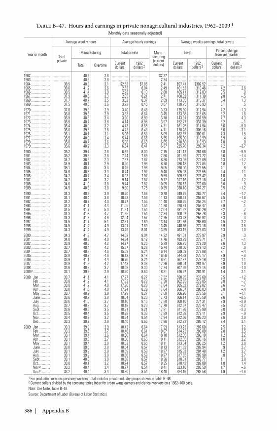
386 | Appendix B
Table B–47. Hours and earnings in private nonagricultural industries, 1962–2009 1
[Monthly data seasonally adjusted]
Year or month
Average weekly hours Average hourly earnings Average weekly earnings, total private
Totalprivate
Manufacturing Total private Manu-facturing(currentdollars)
Level Percent changefrom year earlier
Total Overtime Currentdollars
1982dollars 2
Currentdollars
1982dollars 2
Currentdollars
1982dollars 2
1962 ...................... ................... 40.5 2.8 ................... ................... $2.27 ................... ................... ................... .....................1963 ...................... ................... 40.6 2.8 ................... ................... 2.34 ................... ................... ................... .....................1964 ...................... 38.5 40.8 3.1 $2.53 $7.86 2.41 $97.41 $302.52 ................... .....................1965 ...................... 38.6 41.2 3.6 2.63 8.04 2.49 101.52 310.46 4.2 2.61966 ...................... 38.5 41.4 3.9 2.73 8.13 2.60 105.11 312.83 3.5 .81967 ...................... 37.9 40.6 3.3 2.85 8.21 2.71 108.02 311.30 2.8 –.51968 ...................... 37.7 40.7 3.5 3.02 8.37 2.89 113.85 315.37 5.4 1.31969 ...................... 37.5 40.6 3.6 3.22 8.45 3.07 120.75 316.93 6.1 .51970 ...................... 37.0 39.8 2.9 3.40 8.46 3.23 125.80 312.94 4.2 –1.31971 ...................... 36.8 39.9 2.9 3.63 8.64 3.45 133.58 318.05 6.2 1.61972 ...................... 36.9 40.6 3.4 3.90 8.99 3.70 143.91 331.59 7.7 4.31973 ...................... 36.9 40.7 3.8 4.14 8.98 3.97 152.77 331.39 6.2 –.11974 ...................... 36.4 40.0 3.2 4.43 8.65 4.31 161.25 314.94 5.6 –5.01975 ...................... 36.0 39.5 2.6 4.73 8.48 4.71 170.28 305.16 5.6 –3.11976 ...................... 36.1 40.1 3.1 5.06 8.58 5.09 182.67 309.61 7.3 1.51977 ...................... 35.9 40.3 3.4 5.44 8.66 5.55 195.30 310.99 6.9 .41978 ...................... 35.8 40.4 3.6 5.88 8.69 6.05 210.50 310.93 7.8 .01979 ...................... 35.6 40.2 3.3 6.34 8.41 6.57 225.70 299.34 7.2 –3.71980 ...................... 35.2 39.7 2.8 6.85 8.00 7.15 241.12 281.68 6.8 –5.91981 ...................... 35.2 39.8 2.8 7.44 7.89 7.86 261.89 277.72 8.6 –1.41982 ...................... 34.7 38.9 2.3 7.87 7.87 8.36 273.09 273.09 4.3 –1.71983 ...................... 34.9 40.1 2.9 8.20 7.96 8.70 286.18 277.84 4.8 1.71984 ...................... 35.1 40.7 3.4 8.49 7.96 9.05 298.00 279.55 4.1 .61985 ...................... 34.9 40.5 3.3 8.74 7.92 9.40 305.03 276.55 2.4 –1.11986 ...................... 34.7 40.7 3.4 8.93 7.97 9.59 309.87 276.42 1.6 .01987 ...................... 34.7 40.9 3.7 9.14 7.87 9.77 317.16 273.18 2.4 –1.21988 ...................... 34.6 41.0 3.8 9.44 7.82 10.05 326.62 270.60 3.0 –.91989 ...................... 34.5 40.9 3.8 9.80 7.75 10.35 338.10 267.27 3.5 –1.21990 ...................... 34.3 40.5 3.9 10.20 7.66 10.78 349.75 262.77 3.4 –1.71991 ...................... 34.1 40.4 3.8 10.52 7.59 11.13 358.51 258.67 2.5 –1.61992 ...................... 34.2 40.7 4.0 10.77 7.55 11.40 368.25 258.24 2.7 –.21993 ...................... 34.3 41.1 4.4 11.05 7.54 11.70 378.91 258.47 2.9 .11994 ...................... 34.5 41.7 5.0 11.34 7.54 12.04 391.22 260.29 3.2 .71995 ...................... 34.3 41.3 4.7 11.65 7.54 12.34 400.07 258.78 2.3 –.61996 ...................... 34.3 41.3 4.8 12.04 7.57 12.75 413.28 259.92 3.3 .41997 ...................... 34.5 41.7 5.1 12.51 7.69 13.14 431.86 265.60 4.5 2.21998 ...................... 34.5 41.4 4.9 13.01 7.89 13.45 448.56 272.18 3.9 2.51999 ...................... 34.3 41.4 4.9 13.49 8.01 13.85 463.15 275.03 3.3 1.02000 ...................... 34.3 41.3 4.7 14.02 8.04 14.32 481.01 275.97 3.9 .32001 ...................... 34.0 40.3 4.0 14.54 8.12 14.76 493.79 275.71 2.7 –.12002 ...................... 33.9 40.5 4.2 14.97 8.25 15.29 506.75 279.20 2.6 1.32003 ...................... 33.7 40.4 4.2 15.37 8.28 15.74 518.06 279.13 2.2 .02004 ...................... 33.7 40.8 4.6 15.69 8.24 16.14 529.09 277.88 2.1 –.42005 ...................... 33.8 40.7 4.6 16.13 8.18 16.56 544.33 276.17 2.9 –.62006 ...................... 33.9 41.1 4.4 16.76 8.24 16.81 567.87 279.19 4.3 1.12007 ...................... 33.9 41.2 4.2 17.43 8.33 17.26 590.04 281.97 3.9 1.02008 ...................... 33.6 40.8 3.7 18.08 8.30 17.74 607.99 279.14 3.0 –1.02009 p .................... 33.1 39.8 2.9 18.60 8.60 18.21 616.37 284.91 1.4 2.12008: Jan ............. 33.7 41.1 4.1 17.77 8.27 17.52 598.85 278.60 3.5 –1.2
Feb ............. 33.8 41.2 4.1 17.83 8.28 17.58 602.65 279.85 3.8 –.7Mar ............ 33.8 41.2 4.0 17.90 8.28 17.64 605.02 279.82 3.6 –.7Apr ............. 33.8 41.0 4.0 17.94 8.29 17.64 606.37 280.03 3.8 –.4May ............ 33.7 40.9 3.9 17.99 8.27 17.68 606.26 278.56 3.1 –1.1June ........... 33.6 40.9 3.8 18.04 8.20 17.73 606.14 275.59 2.6 –2.5July ............ 33.6 41.0 3.7 18.10 8.16 17.80 608.16 274.31 2.9 –2.9Aug ............. 33.7 40.8 3.7 18.18 8.20 17.78 612.67 276.47 3.5 –2.2Sept ............ 33.6 40.5 3.5 18.21 8.21 17.81 611.86 275.99 3.0 –2.3Oct .............. 33.5 40.4 3.5 18.28 8.33 17.89 612.38 279.11 2.9 –.9Nov ............. 33.4 40.2 3.2 18.34 8.54 17.94 612.56 285.23 2.6 2.0Dec ............. 33.3 39.9 2.9 18.40 8.65 17.96 612.72 288.12 2.4 3.1
2009: Jan ............. 33.3 39.8 2.9 18.43 8.64 17.99 613.72 287.60 2.5 3.2Feb ............. 33.3 39.5 2.7 18.46 8.61 18.07 614.72 286.80 2.0 2.5Mar ............ 33.1 39.4 2.6 18.50 8.64 18.10 612.35 286.10 1.2 2.2Apr ............. 33.1 39.6 2.7 18.50 8.65 18.11 612.35 286.16 1.0 2.2May ............ 33.1 39.4 2.8 18.53 8.65 18.11 613.34 286.25 1.2 2.8June ........... 33.0 39.5 2.8 18.54 8.57 18.13 611.82 282.94 .9 2.7July ............ 33.1 39.9 2.9 18.59 8.59 18.27 615.33 284.48 1.2 3.7Aug ............. 33.1 39.9 3.0 18.66 8.58 18.27 617.65 283.98 .8 2.7Sept ............ 33.1 40.0 3.0 18.68 8.57 18.36 618.31 283.77 1.1 2.8Oct .............. 33.0 40.1 3.2 18.74 8.57 18.35 618.42 282.88 1.0 1.4Nov p .......... 33.2 40.4 3.4 18.77 8.54 18.41 623.16 283.59 1.7 –.6Dec p .......... 33.2 40.4 3.4 18.80 8.54 18.40 624.16 283.58 1.9 –1.6
1 For production or nonsupervisory workers; total includes private industry groups shown in Table B–46.2 Current dollars divided by the consumer price index for urban wage earners and clerical workers on a 1982=100 base.Note: See Note, Table B–46.Source: Department of Labor (Bureau of Labor Statistics).
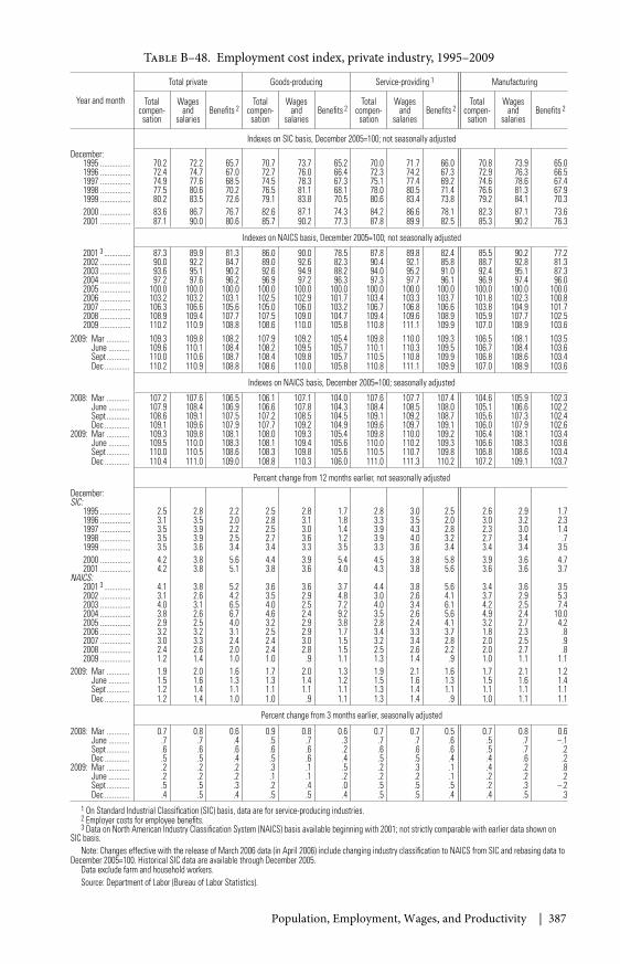
Population, Employment, Wages, and Productivity | 387
Table B–48. Employment cost index, private industry, 1995–2009
Year and month
Total private Goods-producing Service-providing 1 Manufacturing
Totalcompen-
sation
Wagesand
salariesBenefits 2
Totalcompen-
sation
Wagesand
salariesBenefits 2
Totalcompen-
sation
Wagesand
salariesBenefits 2
Totalcompen-
sation
Wagesand
salariesBenefits 2
Indexes on SIC basis, December 2005=100; not seasonally adjusted
December:1995 ................ 70.2 72.2 65.7 70.7 73.7 65.2 70.0 71.7 66.0 70.8 73.9 65.01996 ................ 72.4 74.7 67.0 72.7 76.0 66.4 72.3 74.2 67.3 72.9 76.3 66.51997 ................ 74.9 77.6 68.5 74.5 78.3 67.3 75.1 77.4 69.2 74.6 78.6 67.41998 ................ 77.5 80.6 70.2 76.5 81.1 68.1 78.0 80.5 71.4 76.6 81.3 67.91999 ................ 80.2 83.5 72.6 79.1 83.8 70.5 80.6 83.4 73.8 79.2 84.1 70.32000 ................ 83.6 86.7 76.7 82.6 87.1 74.3 84.2 86.6 78.1 82.3 87.1 73.62001 ................ 87.1 90.0 80.6 85.7 90.2 77.3 87.8 89.9 82.5 85.3 90.2 76.3
Indexes on NAICS basis, December 2005=100; not seasonally adjusted
2001 3 .............. 87.3 89.9 81.3 86.0 90.0 78.5 87.8 89.8 82.4 85.5 90.2 77.22002 ................ 90.0 92.2 84.7 89.0 92.6 82.3 90.4 92.1 85.8 88.7 92.8 81.32003 ................ 93.6 95.1 90.2 92.6 94.9 88.2 94.0 95.2 91.0 92.4 95.1 87.32004 ................ 97.2 97.6 96.2 96.9 97.2 96.3 97.3 97.7 96.1 96.9 97.4 96.02005 ................ 100.0 100.0 100.0 100.0 100.0 100.0 100.0 100.0 100.0 100.0 100.0 100.02006 ................ 103.2 103.2 103.1 102.5 102.9 101.7 103.4 103.3 103.7 101.8 102.3 100.82007 ................ 106.3 106.6 105.6 105.0 106.0 103.2 106.7 106.8 106.6 103.8 104.9 101.72008 ................ 108.9 109.4 107.7 107.5 109.0 104.7 109.4 109.6 108.9 105.9 107.7 102.52009 ................ 110.2 110.9 108.8 108.6 110.0 105.8 110.8 111.1 109.9 107.0 108.9 103.6
2009: Mar ............ 109.3 109.8 108.2 107.9 109.2 105.4 109.8 110.0 109.3 106.5 108.1 103.5June ........... 109.6 110.1 108.4 108.2 109.5 105.7 110.1 110.3 109.5 106.7 108.4 103.6Sept ............ 110.0 110.6 108.7 108.4 109.8 105.7 110.5 110.8 109.9 106.8 108.6 103.4Dec ............. 110.2 110.9 108.8 108.6 110.0 105.8 110.8 111.1 109.9 107.0 108.9 103.6
Indexes on NAICS basis, December 2005=100; seasonally adjusted
2008: Mar ............ 107.2 107.6 106.5 106.1 107.1 104.0 107.6 107.7 107.4 104.6 105.9 102.3June ........... 107.9 108.4 106.9 106.6 107.8 104.3 108.4 108.5 108.0 105.1 106.6 102.2Sept ............ 108.6 109.1 107.5 107.2 108.5 104.5 109.1 109.2 108.7 105.6 107.3 102.4Dec ............. 109.1 109.6 107.9 107.7 109.2 104.9 109.6 109.7 109.1 106.0 107.9 102.6
2009: Mar ............ 109.3 109.8 108.1 108.0 109.3 105.4 109.8 110.0 109.2 106.4 108.1 103.4June ........... 109.5 110.0 108.3 108.1 109.4 105.6 110.0 110.2 109.3 106.6 108.3 103.6Sept ............ 110.0 110.5 108.6 108.3 109.8 105.6 110.5 110.7 109.8 106.8 108.6 103.4Dec ............. 110.4 111.0 109.0 108.8 110.3 106.0 111.0 111.3 110.2 107.2 109.1 103.7
Percent change from 12 months earlier, not seasonally adjusted
December:SIC:
1995 ................ 2.5 2.8 2.2 2.5 2.8 1.7 2.8 3.0 2.5 2.6 2.9 1.71996 ................ 3.1 3.5 2.0 2.8 3.1 1.8 3.3 3.5 2.0 3.0 3.2 2.31997 ................ 3.5 3.9 2.2 2.5 3.0 1.4 3.9 4.3 2.8 2.3 3.0 1.41998 ................ 3.5 3.9 2.5 2.7 3.6 1.2 3.9 4.0 3.2 2.7 3.4 .71999 ................ 3.5 3.6 3.4 3.4 3.3 3.5 3.3 3.6 3.4 3.4 3.4 3.52000 ................ 4.2 3.8 5.6 4.4 3.9 5.4 4.5 3.8 5.8 3.9 3.6 4.72001 ................ 4.2 3.8 5.1 3.8 3.6 4.0 4.3 3.8 5.6 3.6 3.6 3.7
NAICS:2001 3 .............. 4.1 3.8 5.2 3.6 3.6 3.7 4.4 3.8 5.6 3.4 3.6 3.52002 ................ 3.1 2.6 4.2 3.5 2.9 4.8 3.0 2.6 4.1 3.7 2.9 5.32003 ................ 4.0 3.1 6.5 4.0 2.5 7.2 4.0 3.4 6.1 4.2 2.5 7.42004 ................ 3.8 2.6 6.7 4.6 2.4 9.2 3.5 2.6 5.6 4.9 2.4 10.02005 ................ 2.9 2.5 4.0 3.2 2.9 3.8 2.8 2.4 4.1 3.2 2.7 4.22006 ................ 3.2 3.2 3.1 2.5 2.9 1.7 3.4 3.3 3.7 1.8 2.3 .82007 ................ 3.0 3.3 2.4 2.4 3.0 1.5 3.2 3.4 2.8 2.0 2.5 .92008 ................ 2.4 2.6 2.0 2.4 2.8 1.5 2.5 2.6 2.2 2.0 2.7 .82009 ................ 1.2 1.4 1.0 1.0 .9 1.1 1.3 1.4 .9 1.0 1.1 1.1
2009: Mar ............ 1.9 2.0 1.6 1.7 2.0 1.3 1.9 2.1 1.6 1.7 2.1 1.2June ........... 1.5 1.6 1.3 1.3 1.4 1.2 1.5 1.6 1.3 1.5 1.6 1.4Sept ............ 1.2 1.4 1.1 1.1 1.1 1.1 1.3 1.4 1.1 1.1 1.1 1.1Dec ............. 1.2 1.4 1.0 1.0 .9 1.1 1.3 1.4 .9 1.0 1.1 1.1
Percent change from 3 months earlier, seasonally adjusted
2008: Mar ............ 0.7 0.8 0.6 0.9 0.8 0.6 0.7 0.7 0.5 0.7 0.8 0.6June ........... .7 .7 .4 .5 .7 .3 .7 .7 .6 .5 .7 –.1Sept ............ .6 .6 .6 .6 .6 .2 .6 .6 .6 .5 .7 .2Dec ............. .5 .5 .4 .5 .6 .4 .5 .5 .4 .4 .6 .2
2009: Mar ............ .2 .2 .2 .3 .1 .5 .2 .3 .1 .4 .2 .8June ........... .2 .2 .2 .1 .1 .2 .2 .2 .1 .2 .2 .2Sept ............ .5 .5 .3 .2 .4 .0 .5 .5 .5 .2 .3 –.2Dec ............. .4 .5 .4 .5 .5 .4 .5 .5 .4 .4 .5 .3
1 On Standard Industrial Classification (SIC) basis, data are for service-producing industries.2 Employer costs for employee benefits.3 Data on North American Industry Classification System (NAICS) basis available beginning with 2001; not strictly comparable with earlier data shown on
SIC basis.Note: Changes effective with the release of March 2006 data (in April 2006) include changing industry classification to NAICS from SIC and rebasing data to
December 2005=100. Historical SIC data are available through December 2005.Data exclude farm and household workers.Source: Department of Labor (Bureau of Labor Statistics).
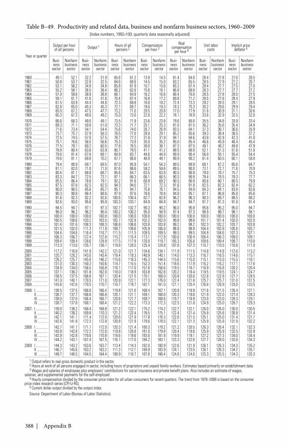
388 | Appendix B
Table B–49. Productivity and related data, business and nonfarm business sectors, 1960–2009[Index numbers, 1992=100; quarterly data seasonally adjusted]
Year or quarter
Output per hourof all persons Output 1 Hours of all
persons 2Compensation
per hour 3Real
compensationper hour 4
Unit laborcosts
Implicit pricedeflator 5
Busi-ness
sector
Nonfarmbusiness
sector
Busi-ness
sector
Nonfarmbusiness
sector
Busi-ness
sector
Nonfarmbusiness
sector
Busi-ness
sector
Nonfarmbusiness
sector
Busi-ness
sector
Nonfarmbusiness
sector
Busi-ness
sector
Nonfarmbusiness
sector
Busi-ness
sector
Nonfarmbusiness
sector
1960 ................. 49.1 52.1 32.2 31.9 65.6 61.2 13.9 14.5 61.4 64.0 28.4 27.8 27.0 26.51961 ................. 50.8 53.7 32.8 32.5 64.6 60.6 14.5 15.0 63.2 65.5 28.5 27.9 27.2 26.71962 ................. 53.1 56.2 34.9 34.8 65.8 61.9 15.1 15.6 65.3 67.4 28.4 27.7 27.5 27.01963 ................. 55.2 58.1 36.5 36.4 66.2 62.6 15.6 16.1 66.8 68.8 28.3 27.7 27.7 27.21964 ................. 57.0 59.8 38.9 38.8 68.1 64.9 16.2 16.6 68.4 70.0 28.5 27.8 28.0 27.51965 ................. 59.1 61.7 41.6 41.6 70.4 67.4 16.8 17.2 69.8 71.2 28.5 27.8 28.4 27.91966 ................. 61.5 63.9 44.4 44.6 72.3 69.8 18.0 18.2 72.4 73.3 29.2 28.5 29.1 28.51967 ................. 62.8 65.0 45.3 45.3 72.1 69.7 19.0 19.3 74.3 75.3 30.2 29.6 29.9 29.41968 ................. 65.0 67.2 47.5 47.7 73.2 71.0 20.5 20.8 77.0 77.9 31.6 30.9 31.1 30.61969 ................. 65.3 67.3 49.0 49.2 75.0 73.0 22.0 22.2 78.1 78.9 33.6 32.9 32.5 32.01970 ................. 66.6 68.3 49.0 49.1 73.5 71.9 23.6 23.8 79.6 80.0 35.5 34.8 33.9 33.41971 ................. 69.3 71.1 50.8 51.0 73.3 71.7 25.1 25.3 81.0 81.5 36.2 35.6 35.4 34.81972 ................. 71.6 73.4 54.1 54.4 75.6 74.0 26.7 26.9 83.5 84.1 37.3 36.7 36.6 35.91973 ................. 73.7 75.7 57.9 58.3 78.5 77.0 29.0 29.1 85.2 85.6 39.3 38.4 38.5 37.21974 ................. 72.5 74.5 57.0 57.5 78.7 77.2 31.8 31.9 84.1 84.6 43.8 42.9 42.3 41.01975 ................. 75.1 76.6 56.5 56.6 75.3 73.9 35.0 35.2 85.0 85.4 46.6 45.9 46.4 45.41976 ................. 77.5 79.1 60.2 60.5 77.8 76.5 38.0 38.1 87.3 87.5 49.1 48.2 48.8 47.91977 ................. 78.8 80.4 63.6 63.9 80.7 79.5 41.1 41.2 88.5 88.9 52.1 51.3 51.8 51.01978 ................. 79.6 81.4 67.6 68.1 84.9 83.7 44.6 44.9 89.9 90.4 56.0 55.1 55.4 54.41979 ................. 79.6 81.1 69.8 70.2 87.7 86.6 48.9 49.1 89.9 90.2 61.4 60.5 60.1 59.01980 ................. 79.4 80.9 69.1 69.5 87.0 85.9 54.1 54.3 89.5 89.9 68.1 67.2 65.6 64.71981 ................. 81.1 82.0 71.0 71.0 87.6 86.6 59.2 59.6 89.5 90.0 73.1 72.7 71.6 70.91982 ................. 80.4 81.1 68.8 68.7 85.6 84.7 63.5 63.8 90.5 90.9 79.0 78.7 75.7 75.31983 ................. 83.3 84.7 72.5 73.1 87.1 86.3 66.1 66.5 90.3 90.9 79.4 78.5 78.3 77.71984 ................. 85.5 86.4 78.8 79.1 92.2 91.6 68.9 69.2 90.5 90.9 80.6 80.1 80.5 79.91985 ................. 87.5 87.8 82.5 82.5 94.3 94.0 72.1 72.3 91.6 91.8 82.5 82.3 82.4 82.21986 ................. 90.0 90.5 85.6 85.7 95.1 94.7 75.8 76.1 94.5 94.9 84.3 84.1 83.8 83.61987 ................. 90.3 90.8 88.4 88.6 97.9 97.6 78.6 78.8 94.8 95.1 87.1 86.8 85.8 85.61988 ................. 91.6 92.3 92.2 92.6 100.6 100.4 82.7 82.8 96.2 96.3 90.3 89.7 88.5 88.21989 ................. 92.6 93.0 95.6 95.9 103.3 103.1 84.9 84.9 94.7 94.7 91.7 91.3 91.8 91.41990 ................. 94.5 94.7 97.1 97.3 102.7 102.7 90.3 90.2 96.0 95.8 95.6 95.2 95.0 94.71991 ................. 96.0 96.2 96.2 96.4 100.2 100.2 95.0 94.9 97.4 97.3 98.9 98.7 98.1 98.11992 ................. 100.0 100.0 100.0 100.0 100.0 100.0 100.0 100.0 100.0 100.0 100.0 100.0 100.0 100.01993 ................. 100.5 100.6 103.2 103.5 102.7 102.9 102.2 102.0 99.8 99.6 101.7 101.4 102.0 102.01994 ................. 101.4 101.6 108.3 108.3 106.8 106.6 103.8 103.8 99.2 99.2 102.3 102.2 103.7 103.81995 ................. 101.5 102.0 111.3 111.8 109.7 109.6 105.9 106.0 98.8 98.9 104.4 103.9 105.6 105.71996 ................. 104.4 104.6 116.4 116.7 111.5 111.5 109.5 109.5 99.5 99.5 104.9 104.6 107.3 107.11997 ................. 106.3 106.2 122.4 122.6 115.2 115.4 113.1 112.9 100.6 100.4 106.4 106.3 109.0 109.11998 ................. 109.4 109.4 128.6 128.9 117.5 117.9 120.0 119.7 105.3 105.0 109.6 109.4 109.7 110.01999 ................. 113.3 113.0 135.7 136.1 119.8 120.5 125.4 124.8 107.8 107.3 110.7 110.5 110.6 111.02000 ................. 117.2 116.8 141.9 142.2 121.0 121.7 134.6 134.1 111.9 111.5 114.8 114.8 112.6 113.22001 ................. 120.7 120.2 143.0 143.4 118.4 119.3 140.9 140.1 114.0 113.3 116.7 116.5 114.6 115.12002 ................. 126.2 125.7 145.8 146.2 115.6 116.3 145.3 144.5 115.6 115.0 115.1 115.0 115.5 116.12003 ................. 131.0 130.3 150.3 150.6 114.7 115.5 152.3 151.4 118.6 117.9 116.2 116.2 117.1 117.62004 ................. 134.9 134.0 156.5 156.8 116.1 117.0 157.6 156.6 119.5 118.7 116.9 116.8 120.2 120.42005 ................. 137.1 136.2 161.8 162.0 118.0 118.9 163.8 162.8 120.2 119.4 119.5 119.5 124.1 124.72006 ................. 138.5 137.5 166.8 167.1 120.4 121.5 170.1 169.0 120.8 120.0 122.8 122.9 127.7 128.52007 ................. 141.0 140.1 170.5 171.0 120.9 122.1 177.3 176.0 122.4 121.6 125.7 125.7 131.0 131.52008 ................. 143.6 142.6 170.5 170.7 118.7 119.7 182.1 181.0 121.1 120.4 126.8 126.9 133.0 133.52006: I ............. 138.5 137.5 166.0 166.4 119.8 121.0 168.4 167.1 120.8 119.9 121.6 121.5 126.4 127.1
II ............ 138.7 137.7 166.6 166.8 120.1 121.1 169.1 168.0 120.3 119.6 121.9 122.0 127.4 128.3III ........... 138.0 137.0 166.4 166.7 120.6 121.7 169.7 168.6 119.7 118.9 123.0 123.0 128.3 129.1IV ........... 138.7 137.8 168.1 168.4 121.2 122.2 173.3 172.3 122.5 121.8 124.9 125.0 128.7 129.3
2007: I ............. 139.0 138.2 168.4 168.8 121.2 122.1 175.2 174.2 122.7 122.1 126.0 126.0 130.0 130.5II ............ 140.2 139.2 169.8 170.3 121.2 122.4 176.5 175.1 122.4 121.4 125.9 125.8 130.9 131.4III ........... 142.1 141.1 171.4 172.0 120.6 121.9 177.8 176.3 122.6 121.5 125.1 125.0 131.4 131.7IV ........... 142.6 141.8 172.3 172.8 120.8 121.9 179.6 178.5 122.1 121.3 125.9 125.9 131.9 132.2
2008: I ............. 142.7 141.7 171.7 172.0 120.3 121.4 180.3 179.2 121.2 120.5 126.3 126.4 132.1 132.3II ............ 143.8 142.8 172.2 172.6 119.8 120.8 181.0 179.8 120.4 119.6 125.9 125.9 132.5 132.9III ........... 143.9 142.8 170.6 170.8 118.6 119.6 183.0 181.8 119.9 119.1 127.2 127.3 134.0 134.4IV ........... 144.2 143.1 167.4 167.5 116.1 117.0 184.2 183.1 123.3 122.6 127.7 128.0 133.6 134.3
2009: I ............. 144.3 143.2 163.6 163.7 113.4 114.3 182.0 180.9 122.6 121.9 126.1 126.3 134.3 135.2II ............ 146.7 145.6 163.2 163.2 111.3 112.1 184.9 183.9 124.1 123.5 126.1 126.3 134.2 135.1III ........... 149.7 148.5 164.5 164.4 109.9 110.7 187.6 186.4 124.8 124.0 125.3 125.5 134.3 135.3
1 Output refers to real gross domestic product in the sector.2 Hours at work of all persons engaged in sector, including hours of proprietors and unpaid family workers. Estimates based primarily on establishment data.3 Wages and salaries of employees plus employers’ contributions for social insurance and private benefit plans. Also includes an estimate of wages,
salaries, and supplemental payments for the self-employed.4 Hourly compensation divided by the consumer price index for all urban consumers for recent quarters. The trend from 1978–2008 is based on the consumer
price index research series (CPI-U-RS).5 Current dollar output divided by the output index.Source: Department of Labor (Bureau of Labor Statistics).
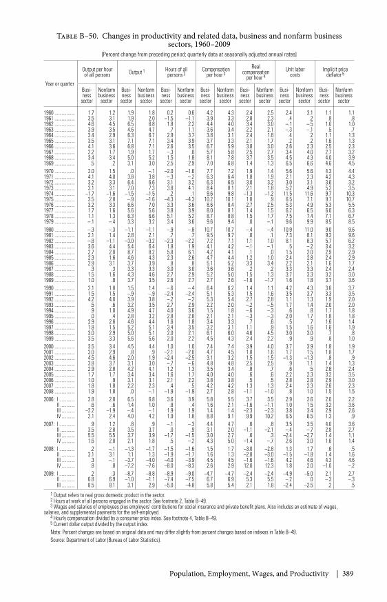
Population, Employment, Wages, and Productivity | 389
Table B–50. Changes in productivity and related data, business and nonfarm businesssectors, 1960–2009
[Percent change from preceding period; quarterly data at seasonally adjusted annual rates]
Year or quarter
Output per hourof all persons Output 1 Hours of all
persons 2Compensation
per hour 3Real
compensationper hour 4
Unit laborcosts
Implicit pricedeflator 5
Busi-ness
sector
Nonfarmbusiness
sector
Busi-ness
sector
Nonfarmbusiness
sector
Busi-ness
sector
Nonfarmbusiness
sector
Busi-ness
sector
Nonfarmbusiness
sector
Busi-ness
sector
Nonfarmbusiness
sector
Busi-ness
sector
Nonfarmbusiness
sector
Busi-ness
sector
Nonfarmbusiness
sector
1960 ................. 1.7 1.2 1.9 1.8 0.2 0.6 4.2 4.3 2.4 2.5 2.4 3.1 1.1 1.11961 ................. 3.5 3.1 1.9 2.0 –1.5 –1.1 3.9 3.3 2.8 2.3 .4 .2 .8 .81962 ................. 4.6 4.5 6.5 6.8 1.8 2.2 4.4 4.0 3.4 3.0 –.1 –.5 1.0 1.01963 ................. 3.9 3.5 4.6 4.7 .7 1.1 3.6 3.4 2.2 2.1 –.3 –.1 .5 .71964 ................. 3.4 2.9 6.3 6.7 2.9 3.7 3.8 3.1 2.4 1.8 .4 .2 1.1 1.31965 ................. 3.5 3.1 7.1 7.1 3.4 3.9 3.7 3.3 2.1 1.7 .2 .2 1.6 1.31966 ................. 4.1 3.6 6.8 7.1 2.6 3.5 6.7 5.9 3.8 3.0 2.6 2.3 2.5 2.31967 ................. 2.2 1.7 1.9 1.7 –.3 .0 5.7 5.8 2.5 2.7 3.4 4.0 2.7 3.21968 ................. 3.4 3.4 5.0 5.2 1.5 1.8 8.1 7.8 3.7 3.5 4.5 4.3 4.0 3.91969 ................. .5 .2 3.1 3.0 2.5 2.9 7.0 6.8 1.4 1.3 6.5 6.6 4.6 4.51970 ................. 2.0 1.5 .0 –.1 –2.0 –1.6 7.7 7.2 1.9 1.4 5.6 5.6 4.3 4.41971 ................. 4.1 4.0 3.8 3.8 –.3 –.2 6.3 6.4 1.8 1.9 2.1 2.3 4.2 4.31972 ................. 3.2 3.3 6.4 6.6 3.1 3.2 6.3 6.5 3.0 3.2 3.0 3.1 3.6 3.21973 ................. 3.1 3.1 7.0 7.3 3.8 4.1 8.4 8.1 2.1 1.8 5.2 4.9 5.2 3.51974 ................. –1.7 –1.6 –1.5 –1.5 .2 .1 9.6 9.8 –1.3 –1.2 11.5 11.6 9.7 10.31975 ................. 3.5 2.8 –.9 –1.6 –4.3 –4.3 10.2 10.1 1.0 .9 6.5 7.1 9.7 10.71976 ................. 3.2 3.3 6.6 7.0 3.3 3.6 8.6 8.4 2.7 2.5 5.3 4.9 5.3 5.51977 ................. 1.7 1.6 5.6 5.6 3.8 3.9 8.0 8.1 1.4 1.5 6.2 6.5 6.0 6.31978 ................. 1.1 1.3 6.3 6.6 5.1 5.2 8.7 8.8 1.5 1.7 7.5 7.4 7.1 6.71979 ................. –.1 –.4 3.3 3.2 3.4 3.6 9.6 9.4 .0 –.1 9.6 9.9 8.5 8.51980 ................. –.3 –.3 –1.1 –1.1 –.9 –.8 10.7 10.7 –.4 –.4 10.9 11.0 9.0 9.61981 ................. 2.1 1.4 2.8 2.1 .7 .7 9.5 9.7 .0 .1 7.3 8.1 9.2 9.61982 ................. –.8 –1.1 –3.0 –3.2 –2.3 –2.2 7.2 7.1 1.1 1.0 8.1 8.3 5.7 6.21983 ................. 3.6 4.4 5.4 6.4 1.8 1.9 4.1 4.2 –.1 –.1 .5 –.2 3.4 3.21984 ................. 2.7 2.0 8.7 8.2 5.8 6.1 4.2 4.1 .1 .0 1.5 2.0 2.9 2.91985 ................. 2.3 1.6 4.6 4.3 2.3 2.6 4.7 4.4 1.2 1.0 2.4 2.8 2.4 2.91986 ................. 2.9 3.1 3.7 3.9 .8 .8 5.1 5.2 3.3 3.4 2.2 2.1 1.6 1.71987 ................. .3 .3 3.3 3.3 3.0 3.0 3.6 3.6 .2 .2 3.3 3.3 2.4 2.41988 ................. 1.5 1.6 4.3 4.6 2.7 2.9 5.2 5.0 1.5 1.3 3.7 3.3 3.2 3.01989 ................. 1.0 .8 3.7 3.5 2.6 2.7 2.7 2.6 –1.6 –1.7 1.6 1.8 3.7 3.61990 ................. 2.1 1.8 1.5 1.4 –.6 –.4 6.4 6.2 1.4 1.1 4.2 4.3 3.6 3.71991 ................. 1.5 1.5 –.9 –.9 –2.4 –2.4 5.1 5.3 1.5 1.6 3.5 3.7 3.3 3.51992 ................. 4.2 4.0 3.9 3.8 –.2 –.2 5.3 5.4 2.7 2.8 1.1 1.3 1.9 2.01993 ................. .5 .6 3.2 3.5 2.7 2.9 2.2 2.0 –.2 –.5 1.7 1.4 2.0 2.01994 ................. .9 1.0 4.9 4.7 4.0 3.6 1.5 1.8 –.6 –.3 .6 .8 1.7 1.81995 ................. .0 .4 2.8 3.2 2.8 2.8 2.1 2.1 –.3 –.3 2.0 1.7 1.8 1.81996 ................. 2.9 2.6 4.6 4.4 1.6 1.8 3.4 3.3 .7 .6 .5 .7 1.6 1.41997 ................. 1.8 1.5 5.2 5.1 3.4 3.5 3.2 3.1 1.1 .9 1.5 1.6 1.6 1.91998 ................. 3.0 2.9 5.0 5.1 2.0 2.1 6.1 6.0 4.6 4.5 3.0 3.0 .7 .81999 ................. 3.5 3.3 5.6 5.6 2.0 2.2 4.5 4.3 2.4 2.2 .9 .9 .8 1.02000 ................. 3.5 3.4 4.5 4.4 1.0 1.0 7.4 7.4 3.9 4.0 3.7 3.9 1.8 1.92001 ................. 3.0 2.9 .8 .9 –2.1 –2.0 4.7 4.5 1.8 1.6 1.7 1.5 1.8 1.72002 ................. 4.5 4.6 2.0 1.9 –2.4 –2.5 3.1 3.2 1.5 1.5 –1.3 –1.3 .8 .92003 ................. 3.8 3.7 3.1 3.0 –.7 –.6 4.8 4.8 2.5 2.5 .9 1.1 1.4 1.32004 ................. 2.9 2.8 4.2 4.1 1.2 1.3 3.5 3.4 .8 .7 .6 .5 2.6 2.42005 ................. 1.7 1.7 3.4 3.4 1.6 1.7 4.0 4.0 .6 .6 2.2 2.3 3.2 3.52006 ................. 1.0 .9 3.1 3.1 2.1 2.2 3.8 3.8 .5 .5 2.8 2.8 2.9 3.02007 ................. 1.8 1.8 2.2 2.3 .4 .5 4.2 4.2 1.3 1.3 2.4 2.3 2.6 2.32008 ................. 1.9 1.8 .0 –.1 –1.9 –1.9 2.7 2.8 –1.1 –1.0 .8 1.0 1.5 1.52006: I ............. 2.8 2.8 6.5 6.8 3.6 3.9 5.8 5.5 3.7 3.5 2.9 2.6 2.0 2.2
II ............ .6 .6 1.4 1.0 .8 .4 1.6 2.1 –1.6 –1.1 1.0 1.5 3.2 3.6III ........... –2.2 –1.9 –.4 –.1 1.9 1.9 1.4 1.4 –2.3 –2.3 3.8 3.4 2.9 2.6IV ........... 2.1 2.4 4.0 4.2 1.9 1.8 8.8 9.1 9.9 10.2 6.5 6.5 1.3 .9
2007: I ............. .9 1.2 .8 .9 –.1 –.3 4.4 4.7 .6 .8 3.5 3.5 4.0 3.6II ............ 3.5 2.8 3.5 3.7 .0 .9 3.1 2.0 –1.1 –2.1 –.4 –.7 2.8 2.7III ........... 5.5 5.5 3.7 3.9 –1.7 –1.5 3.0 2.7 .6 .3 –2.4 –2.7 1.4 1.1IV ........... 1.6 2.0 2.1 1.8 .5 –.2 4.3 5.0 –1.4 –.7 2.6 3.0 1.6 1.4
2008: I ............. .2 –.1 –1.3 –1.7 –1.5 –1.6 1.5 1.7 –3.0 –2.8 1.3 1.7 .6 .5II ............ 3.1 3.1 1.1 1.3 –1.9 –1.7 1.6 1.3 –2.8 –3.0 –1.5 –1.8 1.4 1.6III ........... .3 –.1 –3.7 –4.0 –4.0 –3.9 4.5 4.5 –1.6 –1.6 4.2 4.6 4.3 4.6IV ........... .8 .8 –7.2 –7.6 –8.0 –8.3 2.6 2.9 12.0 12.3 1.8 2.0 –1.0 –.2
2009: I ............. .2 .3 –8.7 –8.8 –8.9 –9.0 –4.7 –4.7 –2.4 –2.4 –4.9 –5.0 2.1 2.7II ............ 6.8 6.9 –1.0 –1.1 –7.4 –7.5 6.7 6.9 5.3 5.5 –.2 .0 –.3 –.3III ........... 8.5 8.1 3.1 2.9 –5.0 –4.8 5.8 5.4 2.1 1.8 –2.4 –2.5 .2 .5
1 Output refers to real gross domestic product in the sector.2 Hours at work of all persons engaged in the sector. See footnote 2, Table B–49.3 Wages and salaries of employees plus employers’ contributions for social insurance and private benefit plans. Also includes an estimate of wages,
salaries, and supplemental payments for the self-employed.4 Hourly compensation divided by a consumer price index. See footnote 4, Table B–49.5 Current dollar output divided by the output index.Note: Percent changes are based on original data and may differ slightly from percent changes based on indexes in Table B–49.Source: Department of Labor (Bureau of Labor Statistics).
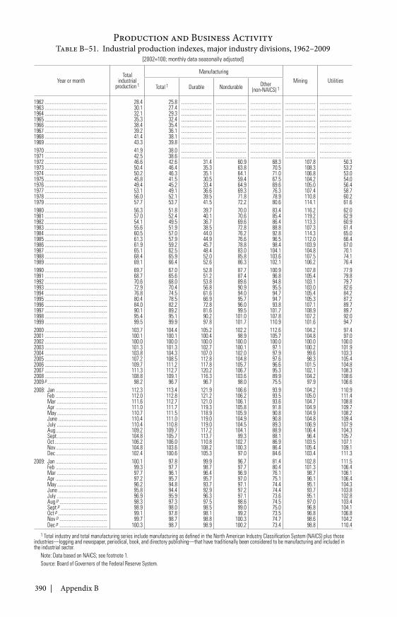
390 | Appendix B
Table B–51. Industrial production indexes, major industry divisions, 1962–2009[2002=100; monthly data seasonally adjusted]
Year or monthTotal
industrialproduction 1
ManufacturingMining Utilities
Total 1 Durable Nondurable Other(non-NAICS) 1
1962 ................................................... 28.4 25.8 ......................... ......................... ......................... ......................... ..........................1963 ................................................... 30.1 27.4 ......................... ......................... ......................... ......................... ..........................1964 ................................................... 32.1 29.3 ......................... ......................... ......................... ......................... ..........................1965 ................................................... 35.3 32.4 ......................... ......................... ......................... ......................... ..........................1966 ................................................... 38.4 35.4 ......................... ......................... ......................... ......................... ..........................1967 ................................................... 39.2 36.1 ......................... ......................... ......................... ......................... ..........................1968 ................................................... 41.4 38.1 ......................... ......................... ......................... ......................... ..........................1969 ................................................... 43.3 39.8 ......................... ......................... ......................... ......................... ..........................1970 ................................................... 41.9 38.0 ......................... ......................... ......................... ......................... ..........................1971 ................................................... 42.5 38.6 ......................... ......................... ......................... ......................... ..........................1972 ................................................... 46.6 42.6 31.4 60.9 68.3 107.8 50.31973 ................................................... 50.4 46.4 35.3 63.8 70.5 108.3 53.21974 ................................................... 50.2 46.3 35.1 64.1 71.0 106.8 53.01975 ................................................... 45.8 41.5 30.5 59.4 67.5 104.2 54.01976 ................................................... 49.4 45.2 33.4 64.9 69.6 105.0 56.41977 ................................................... 53.1 49.1 36.6 69.3 76.3 107.4 58.71978 ................................................... 56.0 52.1 39.5 71.8 78.9 110.8 60.21979 ................................................... 57.7 53.7 41.5 72.2 80.6 114.1 61.61980 ................................................... 56.3 51.8 39.7 70.0 83.4 116.2 62.01981 ................................................... 57.0 52.4 40.1 70.6 85.4 119.2 62.91982 ................................................... 54.1 49.5 36.7 69.6 86.4 113.3 60.91983 ................................................... 55.6 51.9 38.5 72.8 88.8 107.3 61.41984 ................................................... 60.5 57.0 44.0 76.2 92.8 114.3 65.01985 ................................................... 61.3 57.9 44.9 76.6 96.5 112.0 66.41986 ................................................... 61.9 59.2 45.7 78.8 98.4 103.9 67.01987 ................................................... 65.1 62.5 48.4 83.0 104.1 104.8 70.11988 ................................................... 68.4 65.9 52.0 85.8 103.6 107.5 74.11989 ................................................... 69.1 66.4 52.6 86.3 102.1 106.2 76.41990 ................................................... 69.7 67.0 52.8 87.7 100.9 107.8 77.91991 ................................................... 68.7 65.6 51.2 87.4 96.8 105.4 79.81992 ................................................... 70.6 68.0 53.8 89.6 94.8 103.1 79.71993 ................................................... 72.9 70.4 56.8 90.9 95.5 103.0 82.61994 ................................................... 76.8 74.5 61.6 94.0 94.7 105.4 84.21995 ................................................... 80.4 78.5 66.9 95.7 94.7 105.3 87.21996 ................................................... 84.0 82.2 72.8 96.0 93.8 107.1 89.71997 ................................................... 90.1 89.2 81.6 99.5 101.7 108.9 89.71998 ................................................... 95.4 95.1 90.2 101.0 107.8 107.2 92.01999 ................................................... 99.5 99.9 97.8 101.7 110.9 101.6 94.72000 ................................................... 103.7 104.4 105.2 102.2 112.6 104.2 97.42001 ................................................... 100.1 100.1 100.4 98.9 105.7 104.8 97.02002 ................................................... 100.0 100.0 100.0 100.0 100.0 100.0 100.02003 ................................................... 101.3 101.3 102.7 100.1 97.1 100.2 101.92004 ................................................... 103.8 104.3 107.0 102.0 97.9 99.6 103.32005 ................................................... 107.2 108.5 112.8 104.8 97.6 98.3 105.42006 ................................................... 109.7 111.2 117.8 105.7 96.6 101.5 104.82007 ................................................... 111.3 112.7 120.2 106.7 95.3 102.1 108.32008 ................................................... 108.8 109.1 116.3 103.6 89.9 104.2 108.62009 p ................................................. 98.2 96.7 96.7 98.0 75.5 97.9 106.62008: Jan .......................................... 112.3 113.4 121.9 106.6 93.9 104.2 110.9
Feb .......................................... 112.0 112.8 121.2 106.2 93.5 105.0 111.4Mar ......................................... 111.6 112.7 121.0 106.1 93.6 104.7 108.8Apr .......................................... 111.0 111.7 119.3 105.8 91.8 104.9 109.7May ......................................... 110.7 111.5 118.9 105.9 90.8 104.9 108.2June ........................................ 110.4 111.0 119.0 104.9 90.8 104.8 109.4July ......................................... 110.4 110.8 119.0 104.5 89.3 106.9 107.9Aug .......................................... 109.2 109.7 117.2 104.1 88.9 106.4 104.3Sept ......................................... 104.8 105.7 113.7 99.3 88.1 96.4 105.7Oct ........................................... 106.2 106.0 110.8 102.7 86.9 103.5 107.1Nov .......................................... 104.8 103.6 108.2 100.3 86.4 105.4 109.1Dec .......................................... 102.4 100.6 105.3 97.0 84.6 103.4 111.3
2009: Jan .......................................... 100.1 97.8 99.9 96.7 81.4 102.8 111.5Feb .......................................... 99.3 97.7 98.7 97.7 80.4 101.3 106.4Mar ......................................... 97.7 96.1 96.4 96.9 76.1 98.7 106.1Apr .......................................... 97.2 95.7 95.7 97.0 75.1 96.1 106.4May ......................................... 96.2 94.8 93.7 97.1 74.4 95.1 104.3June ........................................ 95.8 94.4 92.9 97.2 74.4 93.7 103.8July ......................................... 96.9 95.9 96.3 97.1 73.6 95.1 102.8Aug p ....................................... 98.3 97.3 97.5 98.6 74.5 97.0 103.4Sept p ...................................... 98.9 98.0 98.5 99.0 75.0 96.8 104.1Oct p ........................................ 99.1 97.8 98.1 99.2 73.5 96.8 106.8Nov p ....................................... 99.7 98.7 98.8 100.3 74.7 98.6 104.2Dec p ....................................... 100.3 98.7 98.9 100.2 73.4 98.8 110.4
1 Total industry and total manufacturing series include manufacturing as defined in the North American Industry Classification System (NAICS) plus thoseindustries—logging and newspaper, periodical, book, and directory publishing—that have traditionally been considered to be manufacturing and included inthe industrial sector.
Note: Data based on NAICS; see footnote 1.Source: Board of Governors of the Federal Reserve System.
Production and Business Activity
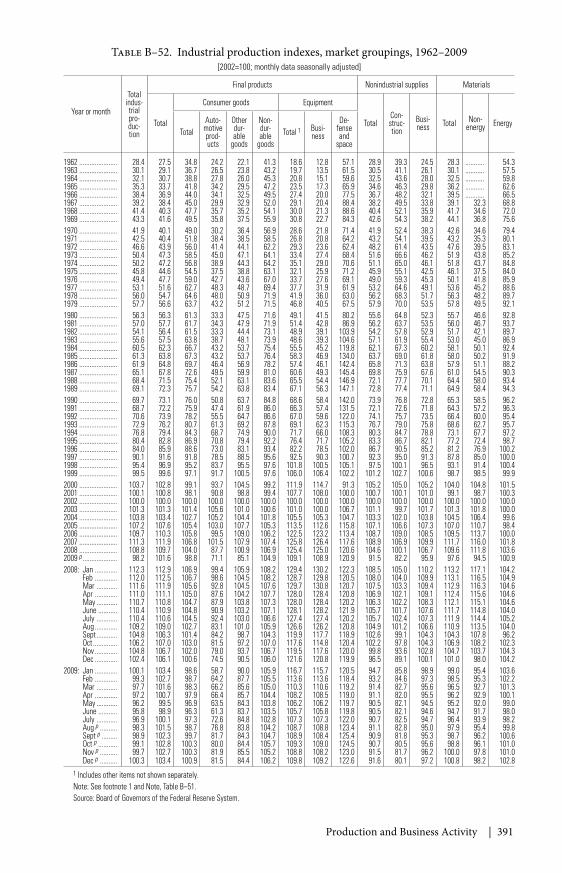
Production and Business Activity | 391
Table B–52. Industrial production indexes, market groupings, 1962–2009[2002=100; monthly data seasonally adjusted]
Year or month
Totalindus-trialpro-duc-tion
Final products Nonindustrial supplies Materials
Total
Consumer goods Equipment
TotalCon-struc-tion
Busi-ness Total Non-
energy EnergyTotal
Auto-motiveprod-ucts
Otherdur-able
goods
Non-dur-able
goodsTotal 1 Busi-
ness
De-fenseand
space
1962 ...................... 28.4 27.5 34.8 24.2 22.1 41.3 18.6 12.8 57.1 28.9 39.3 24.5 28.3 ........... 54.31963 ...................... 30.1 29.1 36.7 26.5 23.8 43.2 19.7 13.5 61.5 30.5 41.1 26.1 30.1 ........... 57.51964 ...................... 32.1 30.7 38.8 27.8 26.0 45.3 20.8 15.1 59.6 32.5 43.6 28.0 32.5 ........... 59.81965 ...................... 35.3 33.7 41.8 34.2 29.5 47.2 23.5 17.3 65.9 34.6 46.3 29.8 36.2 ........... 62.61966 ...................... 38.4 36.9 44.0 34.1 32.5 49.5 27.4 20.0 77.5 36.7 48.2 32.1 39.5 ........... 66.51967 ...................... 39.2 38.4 45.0 29.9 32.9 52.0 29.1 20.4 88.4 38.2 49.5 33.8 39.1 32.3 68.81968 ...................... 41.4 40.3 47.7 35.7 35.2 54.1 30.0 21.3 88.6 40.4 52.1 35.9 41.7 34.6 72.01969 ...................... 43.3 41.6 49.5 35.8 37.5 55.9 30.8 22.7 84.3 42.6 54.3 38.2 44.1 36.8 75.61970 ...................... 41.9 40.1 49.0 30.2 36.4 56.9 28.6 21.8 71.4 41.9 52.4 38.3 42.6 34.6 79.41971 ...................... 42.5 40.4 51.8 38.4 38.5 58.5 26.8 20.8 64.2 43.2 54.1 39.5 43.2 35.3 80.11972 ...................... 46.6 43.9 56.0 41.4 44.1 62.2 29.3 23.6 62.4 48.2 61.4 43.5 47.6 39.5 83.11973 ...................... 50.4 47.3 58.5 45.0 47.1 64.1 33.4 27.4 68.4 51.6 66.6 46.2 51.9 43.8 85.21974 ...................... 50.2 47.2 56.8 38.9 44.3 64.2 35.1 29.0 70.6 51.1 65.0 46.1 51.8 43.7 84.81975 ...................... 45.8 44.6 54.5 37.5 38.8 63.1 32.1 25.9 71.2 45.9 55.1 42.5 46.1 37.5 84.01976 ...................... 49.4 47.7 59.0 42.7 43.6 67.0 33.7 27.6 69.1 49.0 59.3 45.3 50.1 41.8 85.91977 ...................... 53.1 51.6 62.7 48.3 48.7 69.4 37.7 31.9 61.9 53.2 64.6 49.1 53.6 45.2 88.61978 ...................... 56.0 54.7 64.6 48.0 50.9 71.9 41.9 36.0 63.0 56.2 68.3 51.7 56.3 48.2 89.71979 ...................... 57.7 56.6 63.7 43.2 51.2 71.5 46.8 40.5 67.5 57.9 70.0 53.5 57.8 49.5 92.11980 ...................... 56.3 56.3 61.3 33.3 47.5 71.6 49.1 41.5 80.2 55.6 64.8 52.3 55.7 46.6 92.81981 ...................... 57.0 57.7 61.7 34.3 47.9 71.9 51.4 42.8 86.9 56.2 63.7 53.5 56.0 46.7 93.71982 ...................... 54.1 56.4 61.5 33.3 44.4 73.1 48.9 39.1 103.9 54.2 57.8 52.9 51.7 42.1 89.71983 ...................... 55.6 57.5 63.8 38.7 48.1 73.9 48.6 39.3 104.6 57.1 61.9 55.4 53.0 45.0 86.91984 ...................... 60.5 62.3 66.7 43.2 53.7 75.4 55.5 45.2 119.8 62.1 67.3 60.2 58.1 50.1 92.41985 ...................... 61.3 63.8 67.3 43.2 53.7 76.4 58.3 46.9 134.0 63.7 69.0 61.8 58.0 50.2 91.91986 ...................... 61.9 64.8 69.7 46.4 56.9 78.2 57.4 46.1 142.4 65.8 71.3 63.8 57.9 51.1 88.21987 ...................... 65.1 67.8 72.6 49.5 59.9 81.0 60.6 49.3 145.4 69.8 75.9 67.6 61.0 54.5 90.31988 ...................... 68.4 71.5 75.4 52.1 63.1 83.6 65.5 54.4 146.9 72.1 77.7 70.1 64.4 58.0 93.41989 ...................... 69.1 72.3 75.7 54.2 63.8 83.4 67.1 56.3 147.1 72.8 77.4 71.1 64.9 58.4 94.31990 ...................... 69.7 73.1 76.0 50.8 63.7 84.8 68.6 58.4 142.0 73.9 76.8 72.8 65.3 58.5 96.21991 ...................... 68.7 72.2 75.9 47.4 61.9 86.0 66.3 57.4 131.5 72.1 72.6 71.8 64.3 57.2 96.31992 ...................... 70.6 73.9 78.2 55.5 64.7 86.6 67.0 59.6 122.0 74.1 75.7 73.5 66.4 60.0 95.41993 ...................... 72.9 76.2 80.7 61.3 69.2 87.8 69.1 62.3 115.3 76.7 79.0 75.8 68.6 62.7 95.71994 ...................... 76.8 79.4 84.3 68.7 74.9 90.0 71.7 66.0 108.3 80.3 84.7 78.8 73.1 67.7 97.21995 ...................... 80.4 82.8 86.9 70.8 79.4 92.2 76.4 71.7 105.2 83.3 86.7 82.1 77.2 72.4 98.71996 ...................... 84.0 85.9 88.6 73.0 83.1 93.4 82.2 78.5 102.0 86.7 90.5 85.2 81.2 76.9 100.21997 ...................... 90.1 91.6 91.8 78.5 88.5 95.6 92.5 90.3 100.7 92.3 95.0 91.3 87.8 85.0 100.01998 ...................... 95.4 96.9 95.2 83.7 95.5 97.6 101.8 100.5 105.1 97.5 100.1 96.5 93.1 91.4 100.41999 ...................... 99.5 99.6 97.1 91.7 100.5 97.6 106.0 106.4 102.2 101.2 102.7 100.6 98.7 98.5 99.92000 ...................... 103.7 102.8 99.1 93.7 104.5 99.2 111.9 114.7 91.3 105.2 105.0 105.2 104.0 104.8 101.52001 ...................... 100.1 100.8 98.1 90.8 98.8 99.4 107.7 108.0 100.0 100.7 100.1 101.0 99.1 98.7 100.32002 ...................... 100.0 100.0 100.0 100.0 100.0 100.0 100.0 100.0 100.0 100.0 100.0 100.0 100.0 100.0 100.02003 ...................... 101.3 101.3 101.4 105.6 101.0 100.6 101.0 100.0 106.7 101.1 99.7 101.7 101.3 101.8 100.02004 ...................... 103.8 103.4 102.7 105.2 104.4 101.8 105.5 105.3 104.7 103.3 102.0 103.8 104.5 106.4 99.62005 ...................... 107.2 107.6 105.4 103.0 107.7 105.3 113.5 112.6 115.8 107.1 106.6 107.3 107.0 110.7 98.42006 ...................... 109.7 110.3 105.8 99.5 109.0 106.2 122.5 123.2 113.4 108.7 109.0 108.5 109.5 113.7 100.02007 ...................... 111.3 111.9 106.8 101.5 107.9 107.4 125.8 126.4 117.6 108.9 106.9 109.9 111.7 116.0 101.82008 ...................... 108.8 109.7 104.0 87.7 100.9 106.9 125.4 125.0 120.6 104.6 100.1 106.7 109.6 111.8 103.62009 p .................... 98.2 101.6 98.8 71.1 85.1 104.9 109.1 108.9 120.9 91.5 82.2 95.9 97.6 94.5 100.92008: Jan ............. 112.3 112.9 106.9 99.4 105.9 108.2 129.4 130.2 122.3 108.5 105.0 110.2 113.2 117.1 104.2
Feb ............. 112.0 112.5 106.7 98.6 104.5 108.2 128.7 129.8 120.5 108.0 104.0 109.9 113.1 116.5 104.9Mar ............ 111.6 111.9 105.6 92.8 104.5 107.6 129.7 130.8 120.7 107.5 103.3 109.4 112.9 116.3 104.6Apr ............. 111.0 111.1 105.0 87.6 104.2 107.7 128.0 128.4 120.8 106.9 102.1 109.1 112.4 115.6 104.6May ............ 110.7 110.8 104.7 87.9 103.8 107.3 128.0 128.4 120.2 106.3 102.2 108.3 112.1 115.1 104.6June ........... 110.4 110.9 104.8 90.9 103.2 107.1 128.1 128.2 121.9 105.7 101.7 107.6 111.7 114.8 104.0July ............ 110.4 110.6 104.5 92.4 103.0 106.6 127.4 127.4 120.2 105.7 102.4 107.3 111.9 114.4 105.2Aug ............. 109.2 109.0 102.7 83.1 101.0 105.9 126.6 126.2 120.8 104.9 101.2 106.6 110.9 113.5 104.0Sept ............ 104.8 106.3 101.4 84.2 98.7 104.3 119.9 117.7 118.9 102.6 99.1 104.3 104.3 107.8 96.2Oct .............. 106.2 107.0 103.0 81.5 97.2 107.0 117.6 114.8 120.4 102.2 97.8 104.3 106.9 108.2 102.3Nov ............. 104.8 106.7 102.0 79.0 93.7 106.7 119.5 117.6 120.0 99.8 93.6 102.8 104.7 103.7 104.3Dec ............. 102.4 106.1 100.6 74.5 90.5 106.0 121.6 120.8 119.9 96.5 89.1 100.1 101.0 98.0 104.2
2009: Jan ............. 100.1 103.4 98.6 58.7 90.0 105.9 116.7 115.7 120.5 94.7 85.8 98.9 99.0 95.4 103.6Feb ............. 99.3 102.7 98.7 64.2 87.7 105.5 113.6 113.6 118.4 93.2 84.6 97.3 98.5 95.3 102.2Mar ............ 97.7 101.6 98.3 66.2 85.6 105.0 110.3 110.6 119.2 91.4 82.7 95.6 96.5 92.7 101.3Apr ............. 97.2 100.7 97.9 66.4 85.7 104.4 108.2 108.5 119.0 91.1 82.0 95.5 96.2 92.9 100.1May ............ 96.2 99.5 96.9 63.5 84.3 103.8 106.2 106.2 119.7 90.5 82.1 94.5 95.2 92.0 99.0June ........... 95.8 98.9 96.3 61.3 83.7 103.5 105.7 105.8 119.8 90.5 82.1 94.6 94.7 91.7 98.0July ............ 96.9 100.1 97.3 72.6 84.8 102.8 107.3 107.3 122.0 90.7 82.5 94.7 96.4 93.9 98.2Aug p .......... 98.3 101.5 98.7 76.8 83.8 104.2 108.7 108.8 123.4 91.1 82.8 95.0 97.9 95.4 99.8Sept p ......... 98.9 102.3 99.7 81.7 84.3 104.7 108.9 108.4 125.4 90.9 81.8 95.3 98.7 96.2 100.6Oct p ........... 99.1 102.8 100.3 80.0 84.4 105.7 109.3 109.0 124.5 90.7 80.5 95.6 98.8 96.1 101.0Nov p .......... 99.7 102.7 100.3 81.9 85.5 105.2 108.8 108.2 123.0 91.5 81.7 96.2 100.0 97.8 101.0Dec p .......... 100.3 103.4 100.9 81.5 84.4 106.2 109.8 109.2 122.6 91.6 80.1 97.2 100.8 98.2 102.8
1 Includes other items not shown separately.Note: See footnote 1 and Note, Table B–51.Source: Board of Governors of the Federal Reserve System.
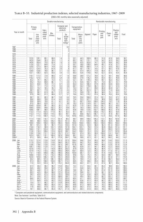
392 | Appendix B
Table B–53. Industrial production indexes, selected manufacturing industries, 1967–2009[2002=100; monthly data seasonally adjusted]
Year or month
Durable manufacturing Nondurable manufacturing
Primarymetal Fabri-
catedmetalprod-ucts
Ma-chinery
Computer andelectronicproducts
Transportationequipment
Apparel PaperPrinting
andsup-port
Chem-ical
Plasticsand
rubberprod-ucts
Food
Total
Ironand
steelprod-ucts
Total
Se-lectedhigh-tech-
nology 1
Total
Motorvehi-clesand
parts
1967 ...................... ............. ............. ............. ............. ............. 0.3 ............. ............. ............. ............. ............. ............. ............. ..............1968 ...................... ............. ............. ............. ............. ............. .3 ............. ............. ............. ............. ............. ............. ............. ..............1969 ...................... ............. ............. ............. ............. ............. .3 ............. ............. ............. ............. ............. ............. ............. ..............1970 ...................... ............. ............. ............. ............. ............. .3 ............. ............. ............. ............. ............. ............. ............. ..............1971 ...................... ............. ............. ............. ............. ............. .3 ............. ............. ............. ............. ............. ............. ............. ..............1972 ...................... 122.0 129.1 69.1 68.0 1.4 .3 53.1 44.3 169.9 66.3 51.6 47.8 34.9 58.71973 ...................... 142.0 154.8 76.3 78.5 1.7 .4 60.7 50.7 175.1 71.6 54.2 52.3 39.2 58.81974 ...................... 145.6 165.4 75.0 82.4 1.9 .5 55.9 43.5 163.0 74.7 52.6 54.4 38.2 59.41975 ...................... 113.0 122.7 64.8 71.8 1.7 .5 50.7 38.0 159.5 64.6 49.1 47.8 32.7 58.31976 ...................... 120.0 127.3 69.4 74.9 2.0 .6 56.8 48.5 168.5 71.4 52.7 53.5 36.2 63.01977 ...................... 121.2 124.4 75.3 81.8 2.6 .8 61.7 55.1 179.1 74.5 57.1 58.2 42.6 64.11978 ...................... 129.0 133.6 79.0 88.1 3.1 1.0 65.7 57.4 184.3 77.9 60.4 61.1 44.1 66.11979 ...................... 132.1 138.3 82.5 93.0 3.9 1.3 66.3 52.6 174.6 79.0 62.2 62.5 43.4 65.41980 ...................... 116.1 117.3 77.8 88.5 4.7 1.6 58.8 38.8 177.2 78.8 62.7 59.1 38.6 66.61981 ...................... 116.2 121.6 77.3 87.6 5.4 1.9 56.6 37.8 176.2 79.9 64.3 60.1 40.9 67.51982 ...................... 82.2 74.7 69.2 73.3 6.1 2.2 52.1 34.1 178.5 78.6 69.1 56.2 40.2 70.11983 ...................... 84.2 75.4 69.8 66.1 7.1 2.6 57.5 43.5 183.7 83.7 74.3 60.1 43.7 70.91984 ...................... 92.3 83.0 75.9 77.2 8.7 3.4 65.3 52.2 186.3 87.9 80.9 63.6 50.5 72.31985 ...................... 85.2 77.1 77.0 77.4 9.3 3.6 68.7 54.2 179.0 86.2 84.2 63.1 52.5 74.91986 ...................... 83.2 75.2 76.5 76.2 9.6 3.7 70.3 54.1 181.1 89.8 88.4 65.9 54.7 76.11987 ...................... 89.7 85.7 77.9 77.8 11.0 4.5 72.9 56.1 182.3 92.7 94.9 71.0 60.6 77.71988 ...................... 100.2 99.7 81.9 85.7 12.3 5.4 77.4 59.9 179.1 96.4 98.0 75.1 63.2 79.71989 ...................... 97.9 96.2 81.3 88.8 12.7 5.7 78.9 59.3 170.2 97.4 98.4 76.5 65.4 79.91990 ...................... 96.7 95.1 80.3 86.7 13.8 6.4 76.5 55.8 166.8 97.4 102.1 78.3 67.2 82.31991 ...................... 90.8 86.9 76.6 81.4 14.3 6.9 73.4 53.3 167.7 97.6 98.9 78.0 66.5 83.81992 ...................... 93.0 90.9 79.0 81.1 16.1 8.2 76.1 60.7 170.9 100.0 104.3 79.2 71.6 85.41993 ...................... 97.5 96.4 82.0 87.2 17.7 9.6 78.3 67.0 174.9 101.1 104.6 80.1 76.7 87.61994 ...................... 104.9 103.9 89.1 95.5 20.7 12.1 82.0 77.0 178.4 105.5 105.7 82.2 83.0 88.21995 ...................... 106.0 105.6 94.6 102.2 26.7 16.9 82.1 79.3 178.6 107.0 107.3 83.5 85.1 90.41996 ...................... 108.6 108.1 98.0 105.8 34.5 24.1 83.6 79.9 173.6 103.7 108.0 85.3 87.9 88.61997 ...................... 113.3 111.4 102.5 111.6 46.1 35.3 91.1 86.1 171.6 105.9 110.2 90.3 93.4 91.01998 ...................... 115.3 111.2 105.8 114.5 59.2 49.1 99.2 90.6 162.5 106.7 111.5 91.8 96.7 95.01999 ...................... 115.1 111.9 106.4 112.0 77.2 70.0 104.6 100.5 155.6 107.6 112.4 93.6 101.9 96.02000 ...................... 111.4 110.8 110.7 117.7 101.4 98.3 99.7 99.9 148.0 105.3 113.1 95.0 102.9 97.72001 ...................... 99.5 96.8 102.6 104.2 103.3 101.3 96.2 91.4 126.9 99.3 106.3 93.4 96.9 97.72002 ...................... 100.0 100.0 100.0 100.0 100.0 100.0 100.0 100.0 100.0 100.0 100.0 100.0 100.0 100.02003 ...................... 99.1 101.2 98.7 99.7 114.3 120.5 101.0 103.5 92.8 96.8 96.2 101.3 100.3 101.02004 ...................... 110.0 118.2 98.9 103.7 129.9 137.9 100.7 103.7 79.8 97.6 96.9 105.6 101.5 101.12005 ...................... 108.0 110.1 103.4 110.2 144.5 158.8 104.5 103.9 76.9 97.5 99.2 109.3 102.3 104.22006 ...................... 112.6 119.3 109.0 115.5 163.8 189.1 104.2 100.2 75.3 97.6 99.8 112.7 102.9 105.42007 ...................... 110.0 115.8 112.1 116.4 176.7 213.7 106.1 97.4 76.5 95.9 100.6 114.1 104.7 109.52008 ...................... 102.4 105.2 110.1 109.4 192.9 238.0 96.1 83.3 72.6 92.1 93.9 108.8 99.1 111.12009 p .................... 67.3 59.9 89.4 85.7 172.9 204.1 79.6 59.9 62.3 82.1 80.2 104.2 84.2 110.72008: Jan ............. 113.2 121.8 113.6 114.9 191.0 237.5 106.4 94.6 75.9 95.5 98.6 114.0 103.5 111.3
Feb ............. 111.9 123.4 113.5 113.6 194.0 242.2 105.2 94.2 75.3 94.0 97.1 113.2 102.9 111.4Mar ............ 110.6 119.6 113.6 114.8 197.5 248.1 101.6 88.7 74.0 94.8 98.0 112.6 101.9 112.4Apr ............. 109.7 118.0 112.6 111.2 199.2 251.2 98.2 83.9 73.1 94.1 96.9 112.2 100.9 112.2May ............ 107.8 114.5 112.1 110.9 199.4 250.3 97.9 83.9 71.5 96.2 96.4 112.1 100.8 111.5June ........... 107.9 114.3 110.5 110.6 199.0 248.4 100.1 86.4 72.5 94.3 93.4 111.0 101.2 111.2July ............ 110.1 118.9 109.8 109.2 198.0 246.6 100.9 88.7 73.7 94.0 91.9 110.6 101.5 110.5Aug ............. 108.6 116.9 110.2 110.2 196.6 243.6 94.6 79.2 74.2 94.2 93.0 109.7 99.4 110.7Sept ............ 102.0 104.9 109.2 107.3 194.2 240.0 88.2 79.9 72.8 91.3 92.3 101.0 97.7 110.4Oct .............. 93.2 88.5 107.3 106.1 188.4 228.4 85.1 76.9 71.4 89.7 91.9 106.7 96.0 111.8Nov ............. 81.4 68.3 106.0 104.0 180.7 214.3 86.5 74.2 69.6 85.9 90.6 103.2 93.7 111.7Dec ............. 71.9 53.3 102.4 99.7 176.2 204.9 88.3 69.2 67.7 81.3 87.4 98.7 89.4 108.6
2009: Jan ............. 67.3 48.4 98.2 96.2 174.9 204.2 75.3 51.2 65.5 80.1 85.3 99.8 88.2 108.3Feb ............. 64.5 49.0 95.6 94.0 171.6 199.5 77.7 55.8 64.5 82.9 82.7 101.6 86.0 109.5Mar ............ 60.7 44.8 91.3 88.7 171.4 200.4 78.0 56.7 64.7 78.9 81.6 101.3 83.4 109.0Apr ............. 60.3 43.5 89.4 86.6 172.5 203.6 77.3 56.6 63.1 78.2 80.1 102.7 82.9 109.8May ............ 59.2 45.9 87.5 83.9 170.3 199.0 74.0 52.4 63.6 80.9 79.6 102.4 82.2 110.9June ........... 61.1 53.0 87.2 82.0 169.6 199.7 72.3 49.5 59.5 82.5 80.2 103.1 82.2 110.3July ............ 68.0 64.3 87.2 82.6 173.3 205.5 80.4 61.1 60.9 82.6 79.9 103.8 83.2 109.2Aug p .......... 71.7 69.9 87.6 84.2 174.2 205.8 82.3 63.6 61.3 84.4 80.2 105.1 83.6 111.8Sept p ......... 73.4 73.7 88.2 83.1 173.8 204.4 86.2 69.0 61.4 83.7 79.4 106.5 84.2 111.7Oct p ........... 74.3 78.6 88.0 85.0 174.1 206.2 84.6 67.3 60.9 81.7 79.2 106.5 85.3 113.0Nov p .......... 77.8 80.0 87.9 83.5 173.9 206.4 85.0 68.3 61.6 85.8 79.0 108.3 86.2 112.9Dec p .......... 78.1 80.8 88.7 85.4 176.7 211.4 85.1 68.3 61.9 84.0 78.5 109.7 86.6 112.0
1 Computers and peripheral equipment, communications equipment, and semiconductors and related electronic components.Note: See footnote 1 and Note, Table B–51.Source: Board of Governors of the Federal Reserve System.
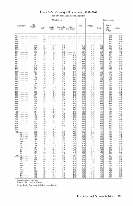
Production and Business Activity | 393
Table B–54. Capacity utilization rates, 1962–2009[Percent 1; monthly data seasonally adjusted]
Year or month Totalindustry 2
Manufacturing
Mining Utilities
Stage-of-process
Total 2 Durablegoods
Nondurablegoods
Other(non-NAICS) 2 Crude
Primaryand
semi-finished
Finished
1962 ...................... ................... 81.4 ................... ................... ....................... .................. .................. .................. 81.5 81.61963 ...................... ................... 83.5 ................... ................... ....................... .................. .................. .................. 83.8 83.41964 ...................... ................... 85.6 ................... ................... ....................... .................. .................. .................. 87.8 84.61965 ...................... ................... 89.5 ................... ................... ....................... .................. .................. .................. 91.0 88.81966 ...................... ................... 91.1 ................... ................... ....................... .................. .................. .................. 91.4 91.11967 ...................... 87.0 87.2 87.5 86.3 ....................... 81.2 94.5 81.1 85.0 88.21968 ...................... 87.4 87.1 87.3 86.5 ....................... 83.6 95.1 83.4 86.8 87.11969 ...................... 87.4 86.7 87.1 86.2 ....................... 86.7 96.8 85.6 88.1 85.61970 ...................... 81.3 79.5 77.7 82.2 ....................... 89.1 96.3 85.1 81.5 78.21971 ...................... 79.7 78.0 75.5 81.9 ....................... 87.8 94.7 84.3 81.7 75.71972 ...................... 84.7 83.4 82.1 85.3 85.8 90.7 95.3 88.5 88.2 79.71973 ...................... 88.3 87.6 88.5 86.6 84.7 91.6 93.3 90.4 92.1 83.11974 ...................... 85.1 84.4 84.6 84.2 82.8 90.9 86.9 91.1 87.4 80.11975 ...................... 75.7 73.5 71.6 76.0 77.2 89.0 85.1 83.9 75.1 73.51976 ...................... 79.7 78.2 76.3 81.0 77.5 89.4 85.5 86.9 80.0 76.71977 ...................... 83.4 82.4 81.2 84.2 83.3 89.5 86.6 88.9 84.5 79.91978 ...................... 85.0 84.3 83.8 84.9 85.0 89.6 86.9 88.4 86.2 82.11979 ...................... 85.0 84.0 84.1 83.6 85.7 91.1 87.0 89.3 86.0 81.81980 ...................... 80.7 78.7 77.6 79.5 87.1 91.1 85.5 88.9 78.8 79.51981 ...................... 79.6 77.0 75.2 78.8 87.5 90.8 84.4 89.1 77.3 77.61982 ...................... 73.7 70.9 66.6 76.3 87.4 84.2 80.2 82.2 70.5 73.31983 ...................... 74.9 73.5 68.7 79.5 88.1 79.8 79.6 79.8 74.5 73.31984 ...................... 80.5 79.4 76.8 82.4 89.5 85.7 82.1 85.6 81.1 77.41985 ...................... 79.3 78.2 75.7 80.8 90.3 84.3 81.8 83.9 79.7 76.81986 ...................... 78.6 78.4 75.3 81.9 88.9 77.6 81.0 79.3 79.7 77.11987 ...................... 81.2 81.0 77.6 84.8 90.7 80.3 83.6 83.1 82.8 78.71988 ...................... 84.3 84.0 82.0 86.1 88.6 84.3 86.6 86.8 85.8 81.61989 ...................... 83.7 83.2 81.6 85.0 85.3 85.3 86.8 87.3 84.7 81.41990 ...................... 82.5 81.7 79.4 84.4 83.8 86.9 86.5 88.2 82.7 80.61991 ...................... 79.8 78.4 75.1 82.4 81.0 85.1 87.8 85.6 79.8 78.01992 ...................... 80.4 79.5 76.9 82.7 80.0 84.6 86.3 85.6 81.5 77.91993 ...................... 81.5 80.4 78.6 82.6 81.2 85.9 88.3 85.9 83.5 78.01994 ...................... 83.5 82.7 81.7 84.3 81.1 87.7 88.4 88.2 86.5 79.01995 ...................... 84.0 83.2 82.5 84.3 82.0 88.1 89.3 89.0 86.6 79.71996 ...................... 83.4 82.2 81.8 82.9 80.7 90.4 90.8 88.8 85.8 79.21997 ...................... 84.2 83.2 82.7 83.6 84.9 91.4 90.3 90.7 86.2 80.21998 ...................... 83.0 81.8 81.2 82.2 85.6 89.2 92.7 87.7 84.3 80.41999 ...................... 81.9 80.7 80.4 80.3 86.1 86.1 94.1 86.6 84.2 78.32000 ...................... 81.7 80.1 80.0 79.1 87.9 90.7 93.8 88.5 84.4 77.12001 ...................... 76.1 73.8 71.4 75.8 83.4 90.4 89.6 85.3 77.4 72.52002 ...................... 74.6 72.7 69.3 76.3 80.8 86.1 87.7 82.7 76.6 70.72003 ...................... 75.8 73.7 70.6 76.9 82.0 88.0 86.0 84.4 77.7 71.62004 ...................... 77.9 76.2 73.5 78.6 84.5 88.3 84.8 86.1 79.8 73.32005 ...................... 80.1 78.6 76.3 80.6 84.4 88.6 85.2 86.5 81.7 76.02006 ...................... 80.9 79.4 77.9 80.7 83.0 90.4 83.4 88.3 81.7 77.12007 ...................... 80.6 79.0 77.2 80.8 81.3 89.2 85.4 87.8 81.0 77.52008 ...................... 77.6 75.1 72.6 77.7 76.0 90.1 83.8 86.5 77.3 74.12009 p .................... 70.2 66.9 60.4 74.1 64.0 84.2 80.2 82.0 67.5 68.52008: Jan ............. 80.5 78.5 76.8 80.2 79.8 90.6 86.5 88.8 80.6 77.1
Feb ............. 80.2 78.0 76.1 79.8 79.3 91.2 86.7 88.9 80.3 76.6Mar ............ 79.8 77.8 75.8 79.7 79.4 90.8 84.5 88.8 79.6 76.3Apr ............. 79.2 77.0 74.6 79.4 77.8 90.9 85.1 88.5 79.4 75.2May ............ 78.9 76.7 74.3 79.4 76.8 90.8 83.7 88.6 78.8 75.0June ........... 78.7 76.3 74.2 78.6 76.7 90.7 84.4 87.6 78.7 74.9July ............ 78.6 76.1 74.1 78.3 75.4 92.3 83.1 88.7 78.3 74.6Aug ............. 77.6 75.3 73.0 77.9 75.0 91.8 80.2 88.3 77.1 73.7Sept ............ 74.5 72.5 70.7 74.3 74.3 83.1 81.2 78.7 74.9 72.2Oct .............. 75.4 72.7 68.8 76.8 73.3 89.2 82.1 84.7 75.4 71.5Nov ............. 74.4 71.1 67.2 75.1 72.9 90.7 83.5 84.7 73.5 71.2Dec ............. 72.7 69.0 65.4 72.6 71.3 89.0 85.1 82.1 71.4 70.3
2009: Jan ............. 71.1 67.1 62.0 72.4 68.7 88.4 85.1 81.5 69.7 68.5Feb ............. 70.6 67.1 61.2 73.2 67.8 87.1 81.1 81.7 68.5 68.6Mar ............ 69.5 66.0 59.9 72.8 64.2 84.9 80.8 79.5 67.1 68.2Apr ............. 69.2 65.8 59.4 72.9 63.4 82.7 80.9 79.5 67.0 67.6May ............ 68.5 65.3 58.2 73.2 62.9 81.9 79.2 79.8 65.9 67.0June ........... 68.3 65.1 57.8 73.3 63.0 80.7 78.7 79.5 65.8 66.6July ............ 69.2 66.2 59.9 73.4 62.4 82.0 77.8 81.0 66.5 67.6Aug p .......... 70.2 67.2 60.7 74.6 63.2 83.8 78.2 82.7 67.1 68.9Sept p ......... 70.8 67.8 61.4 75.1 63.7 83.7 78.5 83.9 67.6 69.3Oct p ........... 71.0 67.8 61.2 75.4 62.5 83.8 80.5 83.8 67.9 69.5Nov p .......... 71.5 68.5 61.7 76.4 63.6 85.5 78.4 85.6 68.2 69.9Dec p .......... 72.0 68.6 61.8 76.5 62.6 85.7 82.9 86.1 68.9 70.2
1 Output as percent of capacity.2 See footnote 1 and Note, Table B–51.Source: Board of Governors of the Federal Reserve System.
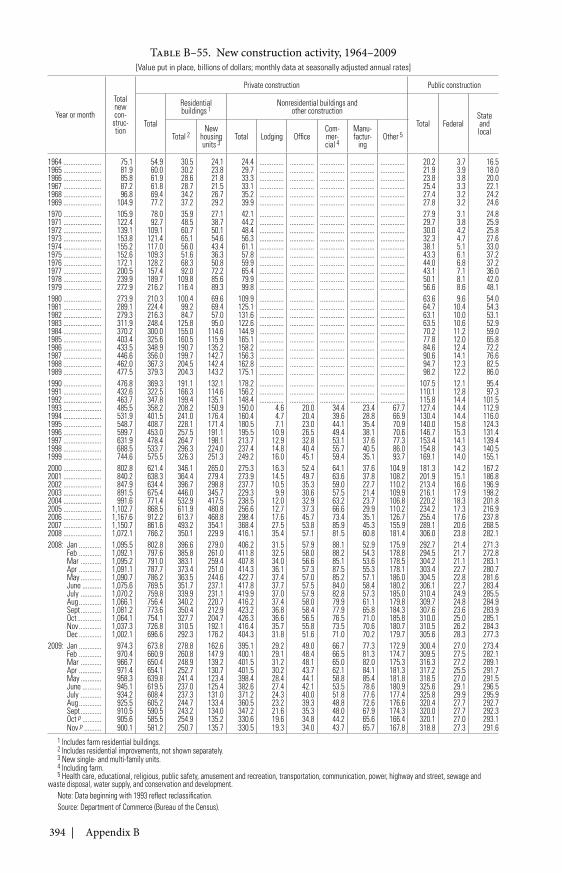
394 | Appendix B
Table B–55. New construction activity, 1964–2009[Value put in place, billions of dollars; monthly data at seasonally adjusted annual rates]
Year or month
Totalnewcon-
struc-tion
Private construction Public construction
Total
Residentialbuildings 1
Nonresidential buildings andother construction
Total FederalStateandlocalTotal 2
Newhousingunits 3
Total Lodging OfficeCom-mer-cial 4
Manu-factur-
ingOther 5
1964 ...................... 75.1 54.9 30.5 24.1 24.4 .............. .............. .............. .............. .............. 20.2 3.7 16.51965 ...................... 81.9 60.0 30.2 23.8 29.7 .............. .............. .............. .............. .............. 21.9 3.9 18.01966 ...................... 85.8 61.9 28.6 21.8 33.3 .............. .............. .............. .............. .............. 23.8 3.8 20.01967 ...................... 87.2 61.8 28.7 21.5 33.1 .............. .............. .............. .............. .............. 25.4 3.3 22.11968 ...................... 96.8 69.4 34.2 26.7 35.2 .............. .............. .............. .............. .............. 27.4 3.2 24.21969 ...................... 104.9 77.2 37.2 29.2 39.9 .............. .............. .............. .............. .............. 27.8 3.2 24.61970 ...................... 105.9 78.0 35.9 27.1 42.1 .............. .............. .............. .............. .............. 27.9 3.1 24.81971 ...................... 122.4 92.7 48.5 38.7 44.2 .............. .............. .............. .............. .............. 29.7 3.8 25.91972 ...................... 139.1 109.1 60.7 50.1 48.4 .............. .............. .............. .............. .............. 30.0 4.2 25.81973 ...................... 153.8 121.4 65.1 54.6 56.3 .............. .............. .............. .............. .............. 32.3 4.7 27.61974 ...................... 155.2 117.0 56.0 43.4 61.1 .............. .............. .............. .............. .............. 38.1 5.1 33.01975 ...................... 152.6 109.3 51.6 36.3 57.8 .............. .............. .............. .............. .............. 43.3 6.1 37.21976 ...................... 172.1 128.2 68.3 50.8 59.9 .............. .............. .............. .............. .............. 44.0 6.8 37.21977 ...................... 200.5 157.4 92.0 72.2 65.4 .............. .............. .............. .............. .............. 43.1 7.1 36.01978 ...................... 239.9 189.7 109.8 85.6 79.9 .............. .............. .............. .............. .............. 50.1 8.1 42.01979 ...................... 272.9 216.2 116.4 89.3 99.8 .............. .............. .............. .............. .............. 56.6 8.6 48.11980 ...................... 273.9 210.3 100.4 69.6 109.9 .............. .............. .............. .............. .............. 63.6 9.6 54.01981 ...................... 289.1 224.4 99.2 69.4 125.1 .............. .............. .............. .............. .............. 64.7 10.4 54.31982 ...................... 279.3 216.3 84.7 57.0 131.6 .............. .............. .............. .............. .............. 63.1 10.0 53.11983 ...................... 311.9 248.4 125.8 95.0 122.6 .............. .............. .............. .............. .............. 63.5 10.6 52.91984 ...................... 370.2 300.0 155.0 114.6 144.9 .............. .............. .............. .............. .............. 70.2 11.2 59.01985 ...................... 403.4 325.6 160.5 115.9 165.1 .............. .............. .............. .............. .............. 77.8 12.0 65.81986 ...................... 433.5 348.9 190.7 135.2 158.2 .............. .............. .............. .............. .............. 84.6 12.4 72.21987 ...................... 446.6 356.0 199.7 142.7 156.3 .............. .............. .............. .............. .............. 90.6 14.1 76.61988 ...................... 462.0 367.3 204.5 142.4 162.8 .............. .............. .............. .............. .............. 94.7 12.3 82.51989 ...................... 477.5 379.3 204.3 143.2 175.1 .............. .............. .............. .............. .............. 98.2 12.2 86.01990 ...................... 476.8 369.3 191.1 132.1 178.2 .............. .............. .............. .............. .............. 107.5 12.1 95.41991 ...................... 432.6 322.5 166.3 114.6 156.2 .............. .............. .............. .............. .............. 110.1 12.8 97.31992 ...................... 463.7 347.8 199.4 135.1 148.4 .............. .............. .............. .............. .............. 115.8 14.4 101.51993 ...................... 485.5 358.2 208.2 150.9 150.0 4.6 20.0 34.4 23.4 67.7 127.4 14.4 112.91994 ...................... 531.9 401.5 241.0 176.4 160.4 4.7 20.4 39.6 28.8 66.9 130.4 14.4 116.01995 ...................... 548.7 408.7 228.1 171.4 180.5 7.1 23.0 44.1 35.4 70.9 140.0 15.8 124.31996 ...................... 599.7 453.0 257.5 191.1 195.5 10.9 26.5 49.4 38.1 70.6 146.7 15.3 131.41997 ...................... 631.9 478.4 264.7 198.1 213.7 12.9 32.8 53.1 37.6 77.3 153.4 14.1 139.41998 ...................... 688.5 533.7 296.3 224.0 237.4 14.8 40.4 55.7 40.5 86.0 154.8 14.3 140.51999 ...................... 744.6 575.5 326.3 251.3 249.2 16.0 45.1 59.4 35.1 93.7 169.1 14.0 155.12000 ...................... 802.8 621.4 346.1 265.0 275.3 16.3 52.4 64.1 37.6 104.9 181.3 14.2 167.22001 ...................... 840.2 638.3 364.4 279.4 273.9 14.5 49.7 63.6 37.8 108.2 201.9 15.1 186.82002 ...................... 847.9 634.4 396.7 298.8 237.7 10.5 35.3 59.0 22.7 110.2 213.4 16.6 196.92003 ...................... 891.5 675.4 446.0 345.7 229.3 9.9 30.6 57.5 21.4 109.9 216.1 17.9 198.22004 ...................... 991.6 771.4 532.9 417.5 238.5 12.0 32.9 63.2 23.7 106.8 220.2 18.3 201.82005 ...................... 1,102.7 868.5 611.9 480.8 256.6 12.7 37.3 66.6 29.9 110.2 234.2 17.3 216.92006 ...................... 1,167.6 912.2 613.7 468.8 298.4 17.6 45.7 73.4 35.1 126.7 255.4 17.6 237.82007 ...................... 1,150.7 861.6 493.2 354.1 368.4 27.5 53.8 85.9 45.3 155.9 289.1 20.6 268.52008 ...................... 1,072.1 766.2 350.1 229.9 416.1 35.4 57.1 81.5 60.8 181.4 306.0 23.8 282.12008: Jan ............. 1,095.5 802.8 396.6 279.0 406.2 31.5 57.9 88.1 52.9 175.9 292.7 21.4 271.3
Feb ............. 1,092.1 797.6 385.8 261.0 411.8 32.5 58.0 88.2 54.3 178.8 294.5 21.7 272.8Mar ............ 1,095.2 791.0 383.1 259.4 407.8 34.0 56.6 85.1 53.6 178.5 304.2 21.1 283.1Apr ............. 1,091.1 787.7 373.4 251.0 414.3 36.1 57.3 87.5 55.3 178.1 303.4 22.7 280.7May ............ 1,090.7 786.2 363.5 244.6 422.7 37.4 57.0 85.2 57.1 186.0 304.5 22.8 281.6June ........... 1,075.6 769.5 351.7 237.1 417.8 37.7 57.5 84.0 58.4 180.2 306.1 22.7 283.4July ............ 1,070.2 759.8 339.9 231.1 419.9 37.0 57.9 82.8 57.3 185.0 310.4 24.9 285.5Aug ............. 1,066.1 756.4 340.2 220.7 416.2 37.4 58.0 79.9 61.1 179.8 309.7 24.8 284.9Sept ............ 1,081.2 773.6 350.4 212.9 423.2 36.8 58.4 77.9 65.8 184.3 307.6 23.6 283.9Oct .............. 1,064.1 754.1 327.7 204.7 426.3 36.6 56.5 76.5 71.0 185.8 310.0 25.0 285.1Nov ............. 1,037.3 726.8 310.5 192.1 416.4 35.7 55.8 73.5 70.6 180.7 310.5 26.2 284.3Dec ............. 1,002.1 696.6 292.3 176.2 404.3 31.8 51.6 71.0 70.2 179.7 305.6 28.3 277.3
2009: Jan ............. 974.3 673.8 278.8 162.6 395.1 29.2 49.0 66.7 77.3 172.9 300.4 27.0 273.4Feb ............. 970.4 660.9 260.8 147.9 400.1 29.1 48.4 66.5 81.3 174.7 309.5 27.5 282.1Mar ............ 966.7 650.4 248.9 139.2 401.5 31.2 48.1 65.0 82.0 175.3 316.3 27.2 289.1Apr ............. 971.4 654.1 252.7 130.7 401.5 30.2 43.7 62.1 84.1 181.3 317.2 25.5 291.7May ............ 958.3 639.8 241.4 123.4 398.4 28.4 44.1 58.8 85.4 181.8 318.5 27.0 291.5June ........... 945.1 619.5 237.0 125.4 382.6 27.4 42.1 53.5 78.6 180.9 325.6 29.1 296.5July ............ 934.2 608.4 237.3 131.0 371.2 24.3 40.0 51.8 77.6 177.4 325.8 29.9 295.9Aug ............. 925.5 605.2 244.7 133.4 360.5 23.2 39.3 48.8 72.6 176.6 320.4 27.7 292.7Sept ............ 910.5 590.5 243.2 134.0 347.2 21.6 35.3 48.0 67.9 174.3 320.0 27.7 292.3Oct p ........... 905.6 585.5 254.9 135.2 330.6 19.6 34.8 44.2 65.6 166.4 320.1 27.0 293.1Nov p .......... 900.1 581.2 250.7 135.7 330.5 19.3 34.0 43.7 65.7 167.8 318.8 27.3 291.6
1 Includes farm residential buildings.2 Includes residential improvements, not shown separately.3 New single- and multi-family units.4 Including farm.5 Health care, educational, religious, public safety, amusement and recreation, transportation, communication, power, highway and street, sewage and
waste disposal, water supply, and conservation and development.Note: Data beginning with 1993 reflect reclassification.Source: Department of Commerce (Bureau of the Census).
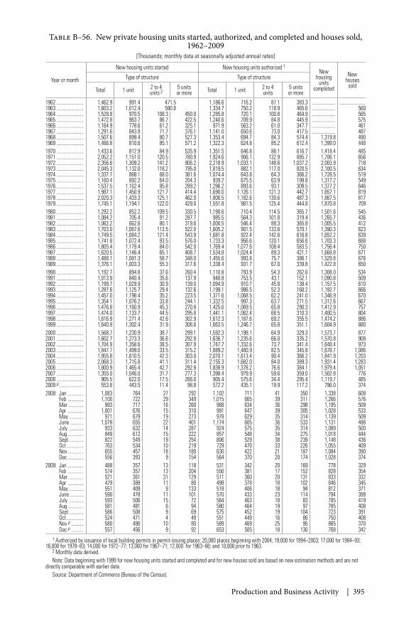
Production and Business Activity | 395
Table B–56. New private housing units started, authorized, and completed and houses sold,1962–2009
[Thousands; monthly data at seasonally adjusted annual rates]
Year or month
New housing units started New housing units authorized 1New
housingunits
completed
Newhouses
soldType of structure Type of structure
Total 1 unit 2 to 4units 2
5 unitsor more Total 1 unit 2 to 4
units5 unitsor more
1962 ...................... 1,462.9 991.4 471.5 1,186.6 716.2 87.1 383.3 ................... .....................1963 ...................... 1,603.2 1,012.4 590.8 1,334.7 750.2 118.9 465.6 ................... 5601964 ...................... 1,528.8 970.5 108.3 450.0 1,285.8 720.1 100.8 464.9 ................... 5651965 ...................... 1,472.8 963.7 86.7 422.5 1,240.6 709.9 84.8 445.9 ................... 5751966 ...................... 1,164.9 778.6 61.2 325.1 971.9 563.2 61.0 347.7 ................... 4611967 ...................... 1,291.6 843.9 71.7 376.1 1,141.0 650.6 73.0 417.5 ................... 4871968 ...................... 1,507.6 899.4 80.7 527.3 1,353.4 694.7 84.3 574.4 1,319.8 4901969 ...................... 1,466.8 810.6 85.1 571.2 1,322.3 624.8 85.2 612.4 1,399.0 4481970 ...................... 1,433.6 812.9 84.9 535.9 1,351.5 646.8 88.1 616.7 1,418.4 4851971 ...................... 2,052.2 1,151.0 120.5 780.9 1,924.6 906.1 132.9 885.7 1,706.1 6561972 ...................... 2,356.6 1,309.2 141.2 906.2 2,218.9 1,033.1 148.6 1,037.2 2,003.9 7181973 ...................... 2,045.3 1,132.0 118.2 795.0 1,819.5 882.1 117.0 820.5 2,100.5 6341974 ...................... 1,337.7 888.1 68.0 381.6 1,074.4 643.8 64.3 366.2 1,728.5 5191975 ...................... 1,160.4 892.2 64.0 204.3 939.2 675.5 63.9 199.8 1,317.2 5491976 ...................... 1,537.5 1,162.4 85.8 289.2 1,296.2 893.6 93.1 309.5 1,377.2 6461977 ...................... 1,987.1 1,450.9 121.7 414.4 1,690.0 1,126.1 121.3 442.7 1,657.1 8191978 ...................... 2,020.3 1,433.3 125.1 462.0 1,800.5 1,182.6 130.6 487.3 1,867.5 8171979 ...................... 1,745.1 1,194.1 122.0 429.0 1,551.8 981.5 125.4 444.8 1,870.8 7091980 ...................... 1,292.2 852.2 109.5 330.5 1,190.6 710.4 114.5 365.7 1,501.6 5451981 ...................... 1,084.2 705.4 91.2 287.7 985.5 564.3 101.8 319.4 1,265.7 4361982 ...................... 1,062.2 662.6 80.1 319.6 1,000.5 546.4 88.3 365.8 1,005.5 4121983 ...................... 1,703.0 1,067.6 113.5 522.0 1,605.2 901.5 133.6 570.1 1,390.3 6231984 ...................... 1,749.5 1,084.2 121.4 543.9 1,681.8 922.4 142.6 616.8 1,652.2 6391985 ...................... 1,741.8 1,072.4 93.5 576.0 1,733.3 956.6 120.1 656.6 1,703.3 6881986 ...................... 1,805.4 1,179.4 84.0 542.0 1,769.4 1,077.6 108.4 583.5 1,756.4 7501987 ...................... 1,620.5 1,146.4 65.1 408.7 1,534.8 1,024.4 89.3 421.1 1,668.8 6711988 ...................... 1,488.1 1,081.3 58.7 348.0 1,455.6 993.8 75.7 386.1 1,529.8 6761989 ...................... 1,376.1 1,003.3 55.3 317.6 1,338.4 931.7 67.0 339.8 1,422.8 6501990 ...................... 1,192.7 894.8 37.6 260.4 1,110.8 793.9 54.3 262.6 1,308.0 5341991 ...................... 1,013.9 840.4 35.6 137.9 948.8 753.5 43.1 152.1 1,090.8 5091992 ...................... 1,199.7 1,029.9 30.9 139.0 1,094.9 910.7 45.8 138.4 1,157.5 6101993 ...................... 1,287.6 1,125.7 29.4 132.6 1,199.1 986.5 52.3 160.2 1,192.7 6661994 ...................... 1,457.0 1,198.4 35.2 223.5 1,371.6 1,068.5 62.2 241.0 1,346.9 6701995 ...................... 1,354.1 1,076.2 33.8 244.1 1,332.5 997.3 63.7 271.5 1,312.6 6671996 ...................... 1,476.8 1,160.9 45.3 270.8 1,425.6 1,069.5 65.8 290.3 1,412.9 7571997 ...................... 1,474.0 1,133.7 44.5 295.8 1,441.1 1,062.4 68.5 310.3 1,400.5 8041998 ...................... 1,616.9 1,271.4 42.6 302.9 1,612.3 1,187.6 69.2 355.5 1,474.2 8861999 ...................... 1,640.9 1,302.4 31.9 306.6 1,663.5 1,246.7 65.8 351.1 1,604.9 8802000 ...................... 1,568.7 1,230.9 38.7 299.1 1,592.3 1,198.1 64.9 329.3 1,573.7 8772001 ...................... 1,602.7 1,273.3 36.6 292.8 1,636.7 1,235.6 66.0 335.2 1,570.8 9082002 ...................... 1,704.9 1,358.6 38.5 307.9 1,747.7 1,332.6 73.7 341.4 1,648.4 9732003 ...................... 1,847.7 1,499.0 33.5 315.2 1,889.2 1,460.9 82.5 345.8 1,678.7 1,0862004 ...................... 1,955.8 1,610.5 42.3 303.0 2,070.1 1,613.4 90.4 366.2 1,841.9 1,2032005 ...................... 2,068.3 1,715.8 41.1 311.4 2,155.3 1,682.0 84.0 389.3 1,931.4 1,2832006 ...................... 1,800.9 1,465.4 42.7 292.8 1,838.9 1,378.2 76.6 384.1 1,979.4 1,0512007 ...................... 1,355.0 1,046.0 31.7 277.3 1,398.4 979.9 59.6 359.0 1,502.8 7762008 ...................... 905.5 622.0 17.5 266.0 905.4 575.6 34.4 295.4 1,119.7 4852009 p .................... 553.8 443.5 11.4 98.8 572.2 435.1 19.9 117.2 796.0 3742008: Jan ............. 1,083 764 27 292 1,102 711 41 350 1,338 608
Feb ............. 1,100 722 29 349 1,015 665 39 311 1,266 576Mar ............ 993 717 16 260 968 634 36 298 1,195 509Apr ............. 1,001 676 15 310 991 647 39 305 1,028 533May ............ 971 679 19 273 978 629 35 314 1,139 509June ........... 1,078 655 22 401 1,174 605 36 533 1,131 488July ............ 933 632 14 287 924 575 35 314 1,089 500Aug ............. 849 612 15 222 857 548 34 275 1,018 444Sept ............ 822 549 19 254 806 529 38 239 1,148 436Oct .............. 763 534 10 219 729 470 33 226 1,055 409Nov ............. 655 457 18 180 630 422 21 187 1,084 390Dec ............. 556 393 9 154 564 370 20 174 1,028 374
2009: Jan ............. 488 357 13 118 531 342 20 169 778 329Feb ............. 574 357 13 204 550 381 17 152 828 354Mar ............ 521 361 31 129 511 360 20 131 833 332Apr ............. 479 388 11 80 498 378 18 102 846 345May ............ 551 409 9 133 518 406 18 94 812 371June ........... 590 478 11 101 570 433 23 114 794 399July ............ 593 506 15 72 564 463 18 83 785 419Aug ............. 581 481 6 94 580 464 19 97 785 408Sept ............ 586 508 9 69 575 452 19 104 723 391Oct .............. 524 471 4 49 551 449 16 86 750 408Nov p .......... 580 490 10 80 589 469 25 95 865 370Dec p .......... 557 456 9 92 653 505 18 130 768 342
1 Authorized by issuance of local building permits in permit-issuing places: 20,000 places beginning with 2004; 19,000 for 1994–2003; 17,000 for 1984–93;16,000 for 1978–83; 14,000 for 1972–77; 13,000 for 1967–71; 12,000 for 1963–66; and 10,000 prior to 1963.
2 Monthly data derived.Note: Data beginning with 1999 for new housing units started and completed and for new houses sold are based on new estimation methods and are not
directly comparable with earlier data.Source: Department of Commerce (Bureau of the Census).
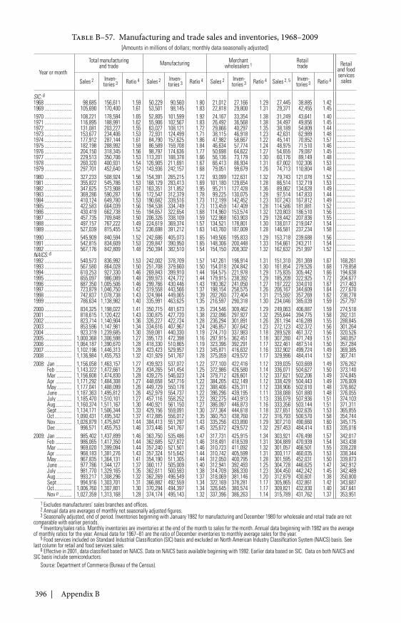
396 | Appendix B
Table B–57. Manufacturing and trade sales and inventories, 1968–2009[Amounts in millions of dollars; monthly data seasonally adjusted]
Year or month
Total manufacturingand trade Manufacturing Merchant
wholesalers 1Retailtrade Retail
and foodservices
salesSales 2 Inven-tories 3 Ratio 4 Sales 2 Inven-
tories 3 Ratio 4 Sales 2 Inven-tories 3 Ratio 4 Sales 2, 5 Inven-
tories 3 Ratio 4
SIC: 61968 ...................... 98,685 156,611 1.59 50,229 90,560 1.80 21,012 27,166 1.29 27,445 38,885 1.42 ...............1969 ...................... 105,690 170,400 1.61 53,501 98,145 1.83 22,818 29,800 1.31 29,371 42,455 1.45 ...............1970 ...................... 108,221 178,594 1.65 52,805 101,599 1.92 24,167 33,354 1.38 31,249 43,641 1.40 ...............1971 ...................... 116,895 188,991 1.62 55,906 102,567 1.83 26,492 36,568 1.38 34,497 49,856 1.45 ...............1972 ...................... 131,081 203,227 1.55 63,027 108,121 1.72 29,866 40,297 1.35 38,189 54,809 1.44 ...............1973 ...................... 153,677 234,406 1.53 72,931 124,499 1.71 38,115 46,918 1.23 42,631 62,989 1.48 ...............1974 ...................... 177,912 287,144 1.61 84,790 157,625 1.86 47,982 58,667 1.22 45,141 70,852 1.57 ...............1975 ...................... 182,198 288,992 1.59 86,589 159,708 1.84 46,634 57,774 1.24 48,975 71,510 1.46 ...............1976 ...................... 204,150 318,345 1.56 98,797 174,636 1.77 50,698 64,622 1.27 54,655 79,087 1.45 ...............1977 ...................... 229,513 350,706 1.53 113,201 188,378 1.66 56,136 73,179 1.30 60,176 89,149 1.48 ...............1978 ...................... 260,320 400,931 1.54 126,905 211,691 1.67 66,413 86,934 1.31 67,002 102,306 1.53 ...............1979 ...................... 297,701 452,640 1.52 143,936 242,157 1.68 79,051 99,679 1.26 74,713 110,804 1.48 ...............1980 ...................... 327,233 508,924 1.56 154,391 265,215 1.72 93,099 122,631 1.32 79,743 121,078 1.52 ...............1981 ...................... 355,822 545,786 1.53 168,129 283,413 1.69 101,180 129,654 1.28 86,514 132,719 1.53 ...............1982 ...................... 347,625 573,908 1.67 163,351 311,852 1.95 95,211 127,428 1.36 89,062 134,628 1.49 ...............1983 ...................... 369,286 590,287 1.56 172,547 312,379 1.78 99,225 130,075 1.28 97,514 147,833 1.44 ...............1984 ...................... 410,124 649,780 1.53 190,682 339,516 1.73 112,199 142,452 1.23 107,243 167,812 1.49 ...............1985 ...................... 422,583 664,039 1.56 194,538 334,749 1.73 113,459 147,409 1.28 114,586 181,881 1.52 ...............1986 ...................... 430,419 662,738 1.55 194,657 322,654 1.68 114,960 153,574 1.32 120,803 186,510 1.56 ...............1987 ...................... 457,735 709,848 1.50 206,326 338,109 1.59 122,968 163,903 1.29 128,442 207,836 1.55 ...............1988 ...................... 497,157 767,222 1.49 224,619 369,374 1.57 134,521 178,801 1.30 138,017 219,047 1.54 ...............1989 ...................... 527,039 815,455 1.52 236,698 391,212 1.63 143,760 187,009 1.28 146,581 237,234 1.58 ...............1990 ...................... 545,909 840,594 1.52 242,686 405,073 1.65 149,506 195,833 1.29 153,718 239,688 1.56 ...............1991 ...................... 542,815 834,609 1.53 239,847 390,950 1.65 148,306 200,448 1.33 154,661 243,211 1.54 ...............1992 ...................... 567,176 842,809 1.48 250,394 382,510 1.54 154,150 208,302 1.32 162,632 251,997 1.52 ...............NAICS: 61992 ...................... 540,573 836,992 1.53 242,002 378,709 1.57 147,261 196,914 1.31 151,310 261,369 1.67 168,2611993 ...................... 567,580 864,028 1.50 251,708 379,660 1.50 154,018 204,842 1.30 161,854 279,526 1.68 179,8581994 ...................... 610,253 927,330 1.46 269,843 399,910 1.44 164,575 221,978 1.29 175,835 305,442 1.66 194,6381995 ...................... 655,097 986,089 1.48 289,973 424,772 1.44 179,915 238,392 1.29 185,209 322,925 1.72 204,6771996 ...................... 687,350 1,005,506 1.46 299,766 430,446 1.43 190,362 241,050 1.27 197,222 334,010 1.67 217,4631997 ...................... 723,879 1,046,750 1.42 319,558 443,566 1.37 198,154 258,575 1.26 206,167 344,609 1.64 227,6701998 ...................... 742,837 1,078,738 1.43 324,984 449,065 1.39 202,260 272,404 1.31 215,592 357,269 1.62 238,2781999 ...................... 786,634 1,138,982 1.40 335,991 463,625 1.35 216,597 290,318 1.30 234,046 385,039 1.59 257,7972000 ...................... 834,325 1,198,022 1.41 350,715 481,673 1.35 234,546 309,462 1.29 249,063 406,887 1.59 274,5182001 ...................... 818,615 1,120,422 1.43 330,875 427,720 1.38 232,096 297,927 1.32 255,644 394,775 1.58 282,1312002 ...................... 823,714 1,140,904 1.36 326,227 422,724 1.28 236,294 301,891 1.26 261,194 416,289 1.55 288,8452003 ...................... 853,596 1,147,981 1.34 334,616 407,967 1.24 246,857 307,642 1.23 272,123 432,372 1.56 301,2642004 ...................... 923,319 1,239,685 1.30 359,081 440,330 1.19 274,710 337,983 1.18 289,528 461,372 1.56 320,5262005 ...................... 1,000,368 1,306,598 1.27 395,173 472,398 1.16 297,915 362,451 1.18 307,280 471,749 1.51 340,0572006 ...................... 1,064,187 1,390,670 1.28 418,330 510,865 1.19 323,396 392,291 1.17 322,461 487,514 1.50 357,2842007 ...................... 1,102,196 1,446,313 1.28 423,423 529,957 1.23 345,871 416,632 1.16 332,902 499,724 1.49 369,3852008 ...................... 1,136,984 1,455,753 1.32 431,929 541,767 1.28 375,059 429,572 1.17 329,996 484,414 1.52 367,7412008: Jan ............. 1,156,058 1,463,157 1.27 439,923 537,072 1.22 377,100 422,416 1.12 339,035 503,669 1.49 376,262
Feb ............. 1,143,322 1,472,661 1.29 434,265 541,454 1.25 372,986 426,580 1.14 336,071 504,627 1.50 373,140Mar ............ 1,156,608 1,474,830 1.28 439,275 546,023 1.24 379,712 426,601 1.12 337,621 502,206 1.49 374,845Apr ............. 1,171,292 1,484,308 1.27 448,658 547,716 1.22 384,205 432,149 1.12 338,429 504,443 1.49 376,009May ............ 1,177,041 1,488,099 1.26 449,729 550,178 1.22 388,406 435,311 1.12 338,906 502,610 1.48 376,662June ........... 1,187,363 1,495,812 1.26 452,979 554,737 1.22 396,296 439,195 1.11 338,088 501,880 1.48 376,055July ............ 1,185,470 1,510,101 1.27 457,116 558,252 1.22 392,275 443,913 1.13 336,079 507,936 1.51 374,103Aug ............. 1,160,374 1,511,167 1.30 440,921 561,150 1.27 386,097 446,873 1.16 333,356 503,144 1.51 371,311Sept ............ 1,134,171 1,506,344 1.33 429,156 559,091 1.30 377,364 444,618 1.18 327,651 502,635 1.53 365,855Oct .............. 1,090,431 1,495,342 1.37 412,885 556,012 1.35 360,753 438,760 1.22 316,793 500,570 1.58 354,744Nov ............. 1,026,879 1,475,847 1.44 384,413 551,297 1.43 335,256 433,890 1.29 307,210 490,660 1.60 345,175Dec ............. 996,571 1,455,753 1.46 373,446 541,767 1.45 325,672 429,572 1.32 297,453 484,414 1.63 335,016
2009: Jan ............. 985,402 1,437,899 1.46 363,750 535,486 1.47 317,731 425,915 1.34 303,921 476,498 1.57 342,017Feb ............. 986,065 1,417,350 1.44 362,685 527,872 1.46 318,491 418,539 1.31 304,889 470,939 1.54 343,438Mar ............ 969,020 1,399,094 1.44 357,240 521,501 1.46 310,723 411,092 1.32 301,057 466,501 1.55 339,228Apr ............. 968,183 1,381,276 1.43 357,324 515,642 1.44 310,742 405,599 1.31 300,117 460,035 1.53 338,344May ............ 967,835 1,364,131 1.41 354,190 511,305 1.44 312,050 400,795 1.28 301,595 452,031 1.50 339,873June ........... 977,786 1,344,127 1.37 360,117 505,009 1.40 312,941 392,493 1.25 304,728 446,625 1.47 342,912July ............ 981,770 1,329,165 1.35 362,611 500,593 1.38 314,709 386,330 1.23 304,450 442,242 1.45 342,489Aug ............. 993,217 1,308,296 1.32 362,269 496,549 1.37 318,069 381,146 1.20 312,879 430,601 1.38 350,800Sept ............ 994,916 1,303,701 1.31 366,882 492,559 1.34 322,169 378,281 1.17 305,865 432,861 1.42 343,687Oct .............. 1,006,760 1,307,801 1.30 370,294 494,397 1.34 326,645 380,574 1.17 309,821 432,830 1.40 347,641Nov p .......... 1,027,359 1,313,168 1.28 374,174 495,143 1.32 337,396 386,263 1.14 315,789 431,762 1.37 353,951
1 Excludes manufacturers’ sales branches and offices.2 Annual data are averages of monthly not seasonally adjusted figures.3 Seasonally adjusted, end of period. Inventories beginning with January 1982 for manufacturing and December 1980 for wholesale and retail trade are not
comparable with earlier periods.4 Inventory/sales ratio. Monthly inventories are inventories at the end of the month to sales for the month. Annual data beginning with 1982 are the average
of monthly ratios for the year. Annual data for 1967–81 are the ratio of December inventories to monthly average sales for the year.5 Food services included on Standard Industrial Classification (SIC) basis and excluded on North American Industry Classification System (NAICS) basis. See
last column for retail and food services sales.6 Effective in 2001, data classified based on NAICS. Data on NAICS basis available beginning with 1992. Earlier data based on SIC. Data on both NAICS and
SIC basis include semiconductors.Source: Department of Commerce (Bureau of the Census).
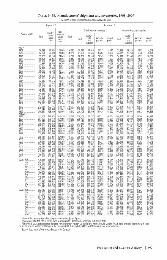
Production and Business Activity | 397
Table B–58. Manufacturers’ shipments and inventories, 1968–2009[Millions of dollars; monthly data seasonally adjusted]
Year or month
Shipments 1 Inventories 2
TotalDurablegoodsindus-tries
Non-durablegoodsindus-tries
Total
Durable goods industries Nondurable goods industries
TotalMateri-
alsand
supplies
Work inprocess
Finishedgoods Total
Materi-alsand
supplies
Work inprocess
Finishedgoods
SIC: 31968 ...................... 50,229 27,624 22,605 90,560 58,732 17,344 27,213 14,175 31,828 12,328 4,852 14,6481969 ...................... 53,501 29,403 24,098 98,145 64,598 18,636 30,282 15,680 33,547 12,753 5,120 15,6741970 ...................... 52,805 28,156 24,649 101,599 66,651 19,149 29,745 17,757 34,948 13,168 5,271 16,5091971 ...................... 55,906 29,924 25,982 102,567 66,136 19,679 28,550 17,907 36,431 13,686 5,678 17,0671972 ...................... 63,027 33,987 29,040 108,121 70,067 20,807 30,713 18,547 38,054 14,677 5,998 17,3791973 ...................... 72,931 39,635 33,296 124,499 81,192 25,944 35,490 19,758 43,307 18,147 6,729 18,4311974 ...................... 84,790 44,173 40,617 157,625 101,493 35,070 42,530 23,893 56,132 23,744 8,189 24,1991975 ...................... 86,589 43,598 42,991 159,708 102,590 33,903 43,227 25,460 57,118 23,565 8,834 24,7191976 ...................... 98,797 50,623 48,174 174,636 111,988 37,457 46,074 28,457 62,648 25,847 9,929 26,8721977 ...................... 113,201 59,168 54,033 188,378 120,877 40,186 50,226 30,465 67,501 27,387 10,961 29,1531978 ...................... 126,905 67,731 59,174 211,691 138,181 45,198 58,848 34,135 73,510 29,619 12,085 31,8061979 ...................... 143,936 75,927 68,009 242,157 160,734 52,670 69,325 38,739 81,423 32,814 13,910 34,6991980 ...................... 154,391 77,419 76,972 265,215 174,788 55,173 76,945 42,670 90,427 36,606 15,884 37,9371981 ...................... 168,129 83,727 84,402 283,413 186,443 57,998 80,998 47,447 96,970 38,165 16,194 42,6111982 ...................... 163,351 79,212 84,139 311,852 200,444 59,136 86,707 54,601 111,408 44,039 18,612 48,7571983 ...................... 172,547 85,481 87,066 312,379 199,854 60,325 86,899 52,630 112,525 44,816 18,691 49,0181984 ...................... 190,682 97,940 92,742 339,516 221,330 66,031 98,251 57,048 118,186 45,692 19,328 53,1661985 ...................... 194,538 101,279 93,259 334,749 218,193 63,904 98,162 56,127 116,556 44,106 19,442 53,0081986 ...................... 194,657 103,238 91,419 322,654 211,997 61,331 97,000 53,666 110,657 42,335 18,124 50,1981987 ...................... 206,326 108,128 98,198 338,109 220,799 63,562 102,393 54,844 117,310 45,319 19,270 52,7211988 ...................... 224,619 118,458 106,161 369,374 242,468 69,611 112,958 59,899 126,906 49,396 20,559 56,9511989 ...................... 236,698 123,158 113,540 391,212 257,513 72,435 122,251 62,827 133,699 50,674 21,653 61,3721990 ...................... 242,686 123,776 118,910 405,073 263,209 73,559 124,130 65,520 141,864 52,645 22,817 66,4021991 ...................... 239,847 121,000 118,847 390,950 250,019 70,834 114,960 64,225 140,931 53,011 22,815 65,1051992 ...................... 250,394 128,489 121,905 382,510 238,105 69,459 104,424 64,222 144,405 54,007 23,532 66,866NAICS: 31992 ...................... 242,002 126,572 115,430 378,709 238,102 69,737 104,211 64,154 140,607 53,179 23,304 64,1241993 ...................... 251,708 133,712 117,996 379,660 238,737 72,657 101,999 64,081 140,923 54,289 23,305 63,3291994 ...................... 269,843 147,005 122,838 399,910 253,141 78,573 106,556 68,012 146,769 57,161 24,383 65,2251995 ...................... 289,973 158,568 131,405 424,772 267,358 85,473 106,658 75,227 157,414 60,725 25,755 70,9341996 ...................... 299,766 164,883 134,883 430,446 272,495 86,226 110,563 75,706 157,951 59,101 26,438 72,4121997 ...................... 319,558 178,949 140,610 443,566 281,074 92,292 109,960 78,822 162,492 60,160 28,478 73,8541998 ...................... 324,984 185,966 139,019 449,065 290,700 93,629 115,235 81,836 158,365 58,223 27,044 73,0981999 ...................... 335,991 193,895 142,096 463,625 296,553 97,959 114,111 84,483 167,072 61,098 28,741 77,2332000 ...................... 350,715 197,807 152,908 481,673 306,727 106,214 111,196 89,317 174,946 61,509 30,015 83,4222001 ...................... 330,875 181,201 149,674 427,720 267,533 91,194 93,776 82,563 160,187 55,798 27,056 77,3332002 ...................... 326,227 176,968 149,259 422,724 260,265 88,512 92,231 79,522 162,459 56,593 27,793 78,0732003 ...................... 334,616 178,549 156,067 407,967 246,712 82,301 88,499 75,912 161,255 56,899 26,965 77,3912004 ...................... 359,081 188,722 170,359 440,330 264,794 92,129 90,932 81,733 175,536 61,760 29,821 83,9552005 ...................... 395,173 202,070 193,103 472,398 283,220 98,134 98,590 86,496 189,178 66,502 32,668 90,0082006 ...................... 418,330 213,408 204,923 510,865 309,320 108,592 104,910 95,818 201,545 69,816 35,968 95,7612007 ...................... 423,423 213,572 209,851 529,957 319,923 109,057 113,569 97,297 210,034 73,222 38,106 98,7062008 ...................... 431,929 207,801 224,128 541,767 342,699 115,800 130,373 96,526 199,068 68,138 36,423 94,5072008: Jan ............. 439,923 215,887 224,036 537,072 321,132 109,728 114,690 96,714 215,940 75,588 40,448 99,904
Feb ............. 434,265 212,974 221,291 541,454 323,203 110,129 116,281 96,793 218,251 75,794 41,745 100,712Mar ............ 439,275 212,170 227,105 546,023 326,847 111,359 118,462 97,026 219,176 75,691 41,634 101,851Apr ............. 448,658 214,371 234,287 547,716 329,380 112,303 120,140 96,937 218,336 75,688 40,883 101,765May ............ 449,729 213,192 236,537 550,178 331,525 112,846 121,409 97,270 218,653 76,358 42,147 100,148June ........... 452,979 212,691 240,288 554,737 333,786 113,958 122,319 97,509 220,951 76,274 41,114 103,563July ............ 457,116 214,430 242,686 558,252 336,804 115,823 123,246 97,735 221,448 76,073 42,417 102,958Aug ............. 440,921 206,941 233,980 561,150 339,813 116,182 124,636 98,995 221,337 75,837 42,223 103,277Sept ............ 429,156 206,450 222,706 559,091 340,723 116,712 125,223 98,788 218,368 76,113 41,480 100,775Oct .............. 412,885 198,521 214,364 556,012 341,408 116,664 126,525 98,219 214,604 74,097 39,533 100,974Nov ............. 384,413 190,015 194,398 551,297 341,207 116,702 127,358 97,147 210,090 71,562 38,404 100,124Dec ............. 373,446 189,253 184,193 541,767 342,699 115,800 130,373 96,526 199,068 68,138 36,423 94,507
2009: Jan ............. 363,750 177,696 186,054 535,486 338,475 115,240 129,265 93,970 197,011 66,897 37,221 92,893Feb ............. 362,685 176,094 186,591 527,872 334,112 114,345 127,694 92,073 193,760 65,599 36,648 91,513Mar ............ 357,240 173,884 183,356 521,501 328,422 112,272 125,769 90,381 193,079 64,949 37,122 91,008Apr ............. 357,324 173,480 183,844 515,642 324,569 110,135 125,256 89,178 191,073 64,050 37,212 89,811May ............ 354,190 169,440 184,750 511,305 320,714 108,234 124,856 87,624 190,591 64,106 37,160 89,325June ........... 360,117 169,672 190,445 505,009 315,984 106,139 124,091 85,754 189,025 63,838 36,685 88,502July ............ 362,611 174,982 187,629 500,593 312,367 103,840 123,880 84,647 188,226 64,118 36,454 87,654Aug ............. 362,269 172,366 189,903 496,549 308,133 102,920 121,442 83,771 188,416 63,832 36,872 87,712Sept ............ 366,882 174,914 191,968 492,559 305,056 102,367 120,306 82,383 187,503 63,632 37,166 86,705Oct .............. 370,294 175,345 194,949 494,397 304,023 101,161 120,971 81,891 190,374 64,548 38,065 87,761Nov p .......... 374,174 175,747 198,427 495,143 303,120 100,262 121,261 81,597 192,023 65,850 38,465 87,708
1 Annual data are averages of monthly not seasonally adjusted figures.2 Seasonally adjusted, end of period. Data beginning with 1982 are not comparable with earlier data.3 Effective in 2001, data classified based on North American Industry Classification System (NAICS). Data on NAICS basis available beginning with 1992.
Earlier data based on Standard Industrial Classification (SIC). Data on both NAICS and SIC basis include semiconductors.Source: Department of Commerce (Bureau of the Census).
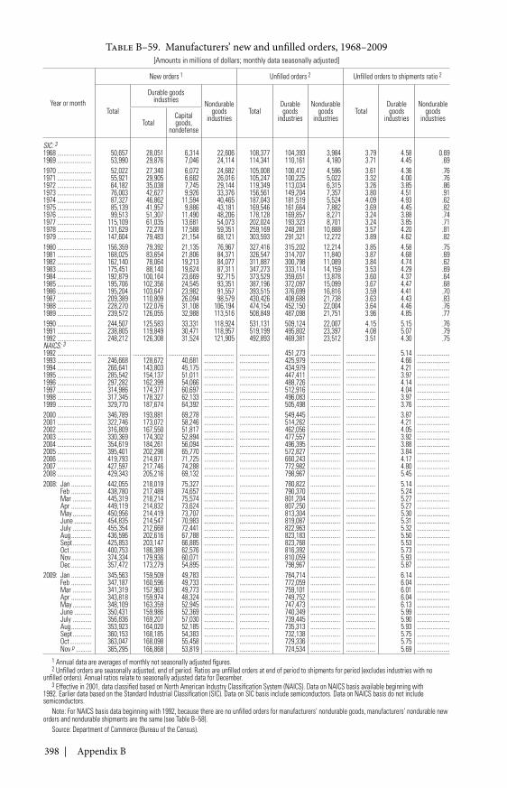
398 | Appendix B
Table B–59. Manufacturers’ new and unfilled orders, 1968–2009[Amounts in millions of dollars; monthly data seasonally adjusted]
Year or month
New orders 1 Unfilled orders 2 Unfilled orders to shipments ratio 2
Total
Durable goodsindustries Nondurable
goodsindustries
TotalDurablegoods
industries
Nondurablegoods
industriesTotal
Durablegoods
industries
Nondurablegoods
industriesTotalCapitalgoods,
nondefense
SIC: 31968 ...................... 50,657 28,051 6,314 22,606 108,377 104,393 3,984 3.79 4.58 0.691969 ...................... 53,990 29,876 7,046 24,114 114,341 110,161 4,180 3.71 4.45 .691970 ...................... 52,022 27,340 6,072 24,682 105,008 100,412 4,596 3.61 4.36 .761971 ...................... 55,921 29,905 6,682 26,016 105,247 100,225 5,022 3.32 4.00 .761972 ...................... 64,182 35,038 7,745 29,144 119,349 113,034 6,315 3.26 3.85 .861973 ...................... 76,003 42,627 9,926 33,376 156,561 149,204 7,357 3.80 4.51 .911974 ...................... 87,327 46,862 11,594 40,465 187,043 181,519 5,524 4.09 4.93 .621975 ...................... 85,139 41,957 9,886 43,181 169,546 161,664 7,882 3.69 4.45 .821976 ...................... 99,513 51,307 11,490 48,206 178,128 169,857 8,271 3.24 3.88 .741977 ...................... 115,109 61,035 13,681 54,073 202,024 193,323 8,701 3.24 3.85 .711978 ...................... 131,629 72,278 17,588 59,351 259,169 248,281 10,888 3.57 4.20 .811979 ...................... 147,604 79,483 21,154 68,121 303,593 291,321 12,272 3.89 4.62 .821980 ...................... 156,359 79,392 21,135 76,967 327,416 315,202 12,214 3.85 4.58 .751981 ...................... 168,025 83,654 21,806 84,371 326,547 314,707 11,840 3.87 4.68 .691982 ...................... 162,140 78,064 19,213 84,077 311,887 300,798 11,089 3.84 4.74 .621983 ...................... 175,451 88,140 19,624 87,311 347,273 333,114 14,159 3.53 4.29 .691984 ...................... 192,879 100,164 23,669 92,715 373,529 359,651 13,878 3.60 4.37 .641985 ...................... 195,706 102,356 24,545 93,351 387,196 372,097 15,099 3.67 4.47 .681986 ...................... 195,204 103,647 23,982 91,557 393,515 376,699 16,816 3.59 4.41 .701987 ...................... 209,389 110,809 26,094 98,579 430,426 408,688 21,738 3.63 4.43 .831988 ...................... 228,270 122,076 31,108 106,194 474,154 452,150 22,004 3.64 4.46 .761989 ...................... 239,572 126,055 32,988 113,516 508,849 487,098 21,751 3.96 4.85 .771990 ...................... 244,507 125,583 33,331 118,924 531,131 509,124 22,007 4.15 5.15 .761991 ...................... 238,805 119,849 30,471 118,957 519,199 495,802 23,397 4.08 5.07 .791992 ...................... 248,212 126,308 31,524 121,905 492,893 469,381 23,512 3.51 4.30 .75NAICS: 31992 ...................... ................... ................... ................... ................... ................... 451,273 ................... ................... 5.14 .....................1993 ...................... 246,668 128,672 40,681 ................... ................... 425,979 ................... ................... 4.66 .....................1994 ...................... 266,641 143,803 45,175 ................... ................... 434,979 ................... ................... 4.21 .....................1995 ...................... 285,542 154,137 51,011 ................... ................... 447,411 ................... ................... 3.97 .....................1996 ...................... 297,282 162,399 54,066 ................... ................... 488,726 ................... ................... 4.14 .....................1997 ...................... 314,986 174,377 60,697 ................... ................... 512,916 ................... ................... 4.04 .....................1998 ...................... 317,345 178,327 62,133 ................... ................... 496,083 ................... ................... 3.97 .....................1999 ...................... 329,770 187,674 64,392 ................... ................... 505,498 ................... ................... 3.76 .....................2000 ...................... 346,789 193,881 69,278 ................... ................... 549,445 ................... ................... 3.87 .....................2001 ...................... 322,746 173,072 58,246 ................... ................... 514,262 ................... ................... 4.21 .....................2002 ...................... 316,809 167,550 51,817 ................... ................... 462,056 ................... ................... 4.05 .....................2003 ...................... 330,369 174,302 52,894 ................... ................... 477,557 ................... ................... 3.92 .....................2004 ...................... 354,619 184,261 56,094 ................... ................... 496,395 ................... ................... 3.88 .....................2005 ...................... 395,401 202,298 65,770 ................... ................... 572,827 ................... ................... 3.84 .....................2006 ...................... 419,793 214,871 71,725 ................... ................... 660,243 ................... ................... 4.17 .....................2007 ...................... 427,597 217,746 74,288 ................... ................... 772,982 ................... ................... 4.80 .....................2008 ...................... 429,343 205,216 69,132 ................... ................... 798,967 ................... ................... 5.45 .....................2008: Jan ............. 442,055 218,019 75,327 ................... ................... 780,822 ................... ................... 5.14 .....................
Feb ............. 438,780 217,489 74,657 ................... ................... 790,370 ................... ................... 5.24 .....................Mar ............ 445,319 218,214 75,574 ................... ................... 801,204 ................... ................... 5.27 .....................Apr ............. 449,119 214,832 73,624 ................... ................... 807,250 ................... ................... 5.27 .....................May ............ 450,956 214,419 73,707 ................... ................... 813,304 ................... ................... 5.30 .....................June ........... 454,835 214,547 70,983 ................... ................... 819,087 ................... ................... 5.31 .....................July ............ 455,354 212,668 72,441 ................... ................... 822,963 ................... ................... 5.32 .....................Aug ............. 436,596 202,616 67,788 ................... ................... 823,183 ................... ................... 5.50 .....................Sept ............ 425,853 203,147 66,885 ................... ................... 823,768 ................... ................... 5.53 .....................Oct .............. 400,753 186,389 62,576 ................... ................... 816,392 ................... ................... 5.73 .....................Nov ............. 374,334 179,936 60,071 ................... ................... 810,059 ................... ................... 5.93 .....................Dec ............. 357,472 173,279 54,895 ................... ................... 798,967 ................... ................... 5.87 .....................
2009: Jan ............. 345,563 159,509 49,783 ................... ................... 784,714 ................... ................... 6.14 .....................Feb ............. 347,187 160,596 49,733 ................... ................... 772,059 ................... ................... 6.04 .....................Mar ............ 341,319 157,963 49,773 ................... ................... 759,101 ................... ................... 6.01 .....................Apr ............. 343,818 159,974 48,324 ................... ................... 749,752 ................... ................... 6.04 .....................May ............ 348,109 163,359 52,945 ................... ................... 747,473 ................... ................... 6.13 .....................June ........... 350,431 159,986 52,369 ................... ................... 740,349 ................... ................... 5.99 .....................July ............ 356,836 169,207 57,030 ................... ................... 739,445 ................... ................... 5.90 .....................Aug ............. 353,923 164,020 52,185 ................... ................... 735,313 ................... ................... 5.93 .....................Sept ............ 360,153 168,185 54,383 ................... ................... 732,138 ................... ................... 5.75 .....................Oct .............. 363,047 168,098 55,458 ................... ................... 729,336 ................... ................... 5.75 .....................Nov p .......... 365,295 166,868 53,819 ................... ................... 724,534 ................... ................... 5.69 .....................
1 Annual data are averages of monthly not seasonally adjusted figures.2 Unfilled orders are seasonally adjusted, end of period. Ratios are unfilled orders at end of period to shipments for period (excludes industries with no
unfilled orders). Annual ratios relate to seasonally adjusted data for December.3 Effective in 2001, data classified based on North American Industry Classification System (NAICS). Data on NAICS basis available beginning with
1992. Earlier data based on the Standard Industrial Classification (SIC). Data on SIC basis include semiconductors. Data on NAICS basis do not includesemiconductors.
Note: For NAICS basis data beginning with 1992, because there are no unfilled orders for manufacturers’ nondurable goods, manufacturers’ nondurable neworders and nondurable shipments are the same (see Table B–58).
Source: Department of Commerce (Bureau of the Census).
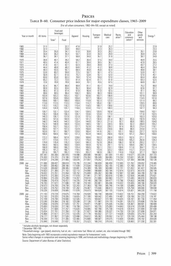
Prices | 399
Table B–60. Consumer price indexes for major expenditure classes, 1965–2009[For all urban consumers; 1982–84=100, except as noted]
Year or month All items
Food andbeverages
Apparel Housing Transpor-tation
Medicalcare
Recre-ation 2
Educationand
communi-cation 2
Othergoodsand
servicesEnergy 3
Total 1 Food
1965 ...................... 31.5 ................. 32.2 47.8 ................. 31.9 25.2 ................. ................. ................ 22.91966 ...................... 32.4 ................. 33.8 49.0 ................. 32.3 26.3 ................. ................. ................ 23.31967 ...................... 33.4 35.0 34.1 51.0 30.8 33.3 28.2 ................. ................. 35.1 23.81968 ...................... 34.8 36.2 35.3 53.7 32.0 34.3 29.9 ................. ................. 36.9 24.21969 ...................... 36.7 38.1 37.1 56.8 34.0 35.7 31.9 ................. ................. 38.7 24.81970 ...................... 38.8 40.1 39.2 59.2 36.4 37.5 34.0 ................. ................. 40.9 25.51971 ...................... 40.5 41.4 40.4 61.1 38.0 39.5 36.1 ................. ................. 42.9 26.51972 ...................... 41.8 43.1 42.1 62.3 39.4 39.9 37.3 ................. ................. 44.7 27.21973 ...................... 44.4 48.8 48.2 64.6 41.2 41.2 38.8 ................. ................. 46.4 29.41974 ...................... 49.3 55.5 55.1 69.4 45.8 45.8 42.4 ................. ................. 49.8 38.11975 ...................... 53.8 60.2 59.8 72.5 50.7 50.1 47.5 ................. ................. 53.9 42.11976 ...................... 56.9 62.1 61.6 75.2 53.8 55.1 52.0 ................. ................. 57.0 45.11977 ...................... 60.6 65.8 65.5 78.6 57.4 59.0 57.0 ................. ................. 60.4 49.41978 ...................... 65.2 72.2 72.0 81.4 62.4 61.7 61.8 ................. ................. 64.3 52.51979 ...................... 72.6 79.9 79.9 84.9 70.1 70.5 67.5 ................. ................. 68.9 65.71980 ...................... 82.4 86.7 86.8 90.9 81.1 83.1 74.9 ................. ................. 75.2 86.01981 ...................... 90.9 93.5 93.6 95.3 90.4 93.2 82.9 ................. ................. 82.6 97.71982 ...................... 96.5 97.3 97.4 97.8 96.9 97.0 92.5 ................. ................. 91.1 99.21983 ...................... 99.6 99.5 99.4 100.2 99.5 99.3 100.6 ................. ................. 101.1 99.91984 ...................... 103.9 103.2 103.2 102.1 103.6 103.7 106.8 ................. ................. 107.9 100.91985 ...................... 107.6 105.6 105.6 105.0 107.7 106.4 113.5 ................. ................. 114.5 101.61986 ...................... 109.6 109.1 109.0 105.9 110.9 102.3 122.0 ................. ................. 121.4 88.21987 ...................... 113.6 113.5 113.5 110.6 114.2 105.4 130.1 ................. ................. 128.5 88.61988 ...................... 118.3 118.2 118.2 115.4 118.5 108.7 138.6 ................. ................. 137.0 89.31989 ...................... 124.0 124.9 125.1 118.6 123.0 114.1 149.3 ................. ................. 147.7 94.31990 ...................... 130.7 132.1 132.4 124.1 128.5 120.5 162.8 ................. ................. 159.0 102.11991 ...................... 136.2 136.8 136.3 128.7 133.6 123.8 177.0 ................. ................. 171.6 102.51992 ...................... 140.3 138.7 137.9 131.9 137.5 126.5 190.1 ................. ................. 183.3 103.01993 ...................... 144.5 141.6 140.9 133.7 141.2 130.4 201.4 90.7 85.5 192.9 104.21994 ...................... 148.2 144.9 144.3 133.4 144.8 134.3 211.0 92.7 88.8 198.5 104.61995 ...................... 152.4 148.9 148.4 132.0 148.5 139.1 220.5 94.5 92.2 206.9 105.21996 ...................... 156.9 153.7 153.3 131.7 152.8 143.0 228.2 97.4 95.3 215.4 110.11997 ...................... 160.5 157.7 157.3 132.9 156.8 144.3 234.6 99.6 98.4 224.8 111.51998 ...................... 163.0 161.1 160.7 133.0 160.4 141.6 242.1 101.1 100.3 237.7 102.91999 ...................... 166.6 164.6 164.1 131.3 163.9 144.4 250.6 102.0 101.2 258.3 106.62000 ...................... 172.2 168.4 167.8 129.6 169.6 153.3 260.8 103.3 102.5 271.1 124.62001 ...................... 177.1 173.6 173.1 127.3 176.4 154.3 272.8 104.9 105.2 282.6 129.32002 ...................... 179.9 176.8 176.2 124.0 180.3 152.9 285.6 106.2 107.9 293.2 121.72003 ...................... 184.0 180.5 180.0 120.9 184.8 157.6 297.1 107.5 109.8 298.7 136.52004 ...................... 188.9 186.6 186.2 120.4 189.5 163.1 310.1 108.6 111.6 304.7 151.42005 ...................... 195.3 191.2 190.7 119.5 195.7 173.9 323.2 109.4 113.7 313.4 177.12006 ...................... 201.6 195.7 195.2 119.5 203.2 180.9 336.2 110.9 116.8 321.7 196.92007 ...................... 207.342 203.300 202.916 118.998 209.586 184.682 351.054 111.443 119.577 333.328 207.7232008 ...................... 215.303 214.225 214.106 118.907 216.264 195.549 364.065 113.254 123.631 345.381 236.6662009 ...................... 214.537 218.249 217.955 120.078 217.057 179.252 375.613 114.272 127.393 368.586 193.1262008: Jan ............. 211.080 208.837 208.618 115.795 212.244 190.839 360.459 112.083 121.762 339.052 219.465
Feb ............. 211.693 209.462 209.166 117.839 213.026 190.520 362.155 112.365 121.766 340.191 219.311Mar ............ 213.528 209.692 209.385 120.881 214.389 195.189 363.000 112.731 121.832 341.827 230.505Apr ............. 214.823 211.365 211.102 122.113 214.890 198.608 363.184 112.874 122.073 343.410 240.194May ............ 216.632 212.251 212.054 120.752 215.809 205.262 363.396 112.987 122.348 344.709 257.106June ........... 218.815 213.383 213.243 117.019 217.941 211.787 363.616 112.991 122.828 345.885 275.621July ............ 219.964 215.326 215.299 114.357 219.610 212.806 363.963 113.277 123.445 346.810 280.833Aug ............. 219.086 216.419 216.422 116.376 219.148 206.739 364.477 113.786 124.653 346.990 266.283Sept ............ 218.783 217.672 217.696 121.168 218.184 203.861 365.036 114.032 125.505 348.166 258.020Oct .............. 216.573 218.705 218.738 122.243 217.383 192.709 365.746 114.169 125.686 349.276 231.561Nov ............. 212.425 218.752 218.749 121.262 216.467 173.644 366.613 114.078 125.758 349.040 189.938Dec ............. 210.228 218.839 218.805 117.078 216.073 164.628 367.133 113.674 125.921 349.220 171.158
2009: Jan ............. 211.143 219.729 219.675 114.764 216.928 166.738 369.830 113.822 126.151 350.259 174.622Feb ............. 212.193 219.333 219.205 118.825 217.180 169.542 372.405 114.461 126.190 351.223 178.741Mar ............ 212.709 218.794 218.600 122.545 217.374 169.647 373.189 114.625 126.187 361.156 177.454Apr ............. 213.240 218.364 218.162 123.208 217.126 171.987 374.170 114.261 126.273 370.606 179.704May ............ 213.856 218.076 217.826 121.751 216.971 175.997 375.026 114.264 126.467 369.901 186.909June ........... 215.693 218.030 217.740 118.799 218.071 183.735 375.093 114.643 126.519 370.595 205.408July ............ 215.351 217.608 217.257 115.620 218.085 182.798 375.739 114.619 126.914 372.894 201.938Aug ............. 215.834 217.701 217.350 117.130 217.827 184.386 376.537 114.755 128.128 372.699 204.971Sept ............ 215.969 217.617 217.218 122.476 217.178 183.932 377.727 114.629 129.035 374.219 202.243Oct .............. 216.177 217.957 217.526 123.998 216.612 185.362 378.552 114.157 129.128 375.444 199.198Nov ............. 216.330 217.733 217.265 122.465 215.808 188.587 379.575 113.820 128.845 376.702 204.026Dec ............. 215.949 218.049 217.637 119.357 215.523 188.318 379.516 113.212 128.883 377.330 202.301
1 Includes alcoholic beverages, not shown separately.2 December 1997=100.3 Household energy—gas (piped), electricity, fuel oil, etc.—and motor fuel. Motor oil, coolant, etc. also included through 1982.Note: Data beginning with 1983 incorporate a rental equivalence measure for homeowners’ costs.Series reflect changes in composition and renaming beginning in 1998, and formula and methodology changes beginning in 1999.Source: Department of Labor (Bureau of Labor Statistics).
Prices
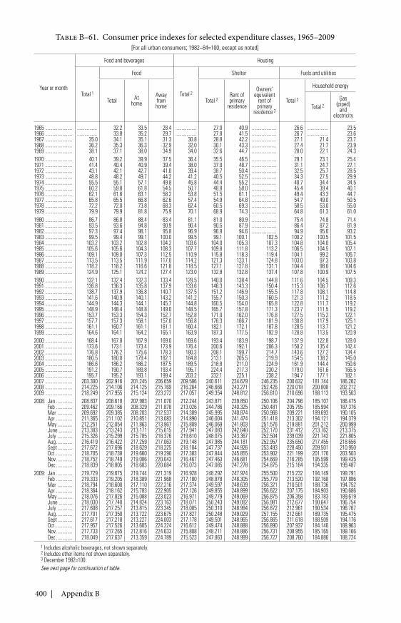
400 | Appendix B
Table B–61. Consumer price indexes for selected expenditure classes, 1965–2009[For all urban consumers; 1982–84=100, except as noted]
Year or month
Food and beverages Housing
Total 1
Food
Total 2
Shelter Fuels and utilities
Total Athome
Awayfromhome
Total 2Rent ofprimary
residence
Owners’equivalent
rent ofprimary
residence 3
Total 2
Household energy
Total 2
Gas(piped)
andelectricity
1965 ...................... ................ 32.2 33.5 28.4 ................. 27.0 40.9 .................... 26.6 ................. 23.51966 ...................... ................ 33.8 35.2 29.7 ................. 27.8 41.5 .................... 26.7 ................. 23.61967 ...................... 35.0 34.1 35.1 31.3 30.8 28.8 42.2 .................... 27.1 21.4 23.71968 ...................... 36.2 35.3 36.3 32.9 32.0 30.1 43.3 .................... 27.4 21.7 23.91969 ...................... 38.1 37.1 38.0 34.9 34.0 32.6 44.7 .................... 28.0 22.1 24.31970 ...................... 40.1 39.2 39.9 37.5 36.4 35.5 46.5 .................... 29.1 23.1 25.41971 ...................... 41.4 40.4 40.9 39.4 38.0 37.0 48.7 .................... 31.1 24.7 27.11972 ...................... 43.1 42.1 42.7 41.0 39.4 38.7 50.4 .................... 32.5 25.7 28.51973 ...................... 48.8 48.2 49.7 44.2 41.2 40.5 52.5 .................... 34.3 27.5 29.91974 ...................... 55.5 55.1 57.1 49.8 45.8 44.4 55.2 .................... 40.7 34.4 34.51975 ...................... 60.2 59.8 61.8 54.5 50.7 48.8 58.0 .................... 45.4 39.4 40.11976 ...................... 62.1 61.6 63.1 58.2 53.8 51.5 61.1 .................... 49.4 43.3 44.71977 ...................... 65.8 65.5 66.8 62.6 57.4 54.9 64.8 .................... 54.7 49.0 50.51978 ...................... 72.2 72.0 73.8 68.3 62.4 60.5 69.3 .................... 58.5 53.0 55.01979 ...................... 79.9 79.9 81.8 75.9 70.1 68.9 74.3 .................... 64.8 61.3 61.01980 ...................... 86.7 86.8 88.4 83.4 81.1 81.0 80.9 .................... 75.4 74.8 71.41981 ...................... 93.5 93.6 94.8 90.9 90.4 90.5 87.9 .................... 86.4 87.2 81.91982 ...................... 97.3 97.4 98.1 95.8 96.9 96.9 94.6 .................... 94.9 95.6 93.21983 ...................... 99.5 99.4 99.1 100.0 99.5 99.1 100.1 102.5 100.2 100.5 101.51984 ...................... 103.2 103.2 102.8 104.2 103.6 104.0 105.3 107.3 104.8 104.0 105.41985 ...................... 105.6 105.6 104.3 108.3 107.7 109.8 111.8 113.2 106.5 104.5 107.11986 ...................... 109.1 109.0 107.3 112.5 110.9 115.8 118.3 119.4 104.1 99.2 105.71987 ...................... 113.5 113.5 111.9 117.0 114.2 121.3 123.1 124.8 103.0 97.3 103.81988 ...................... 118.2 118.2 116.6 121.8 118.5 127.1 127.8 131.1 104.4 98.0 104.61989 ...................... 124.9 125.1 124.2 127.4 123.0 132.8 132.8 137.4 107.8 100.9 107.51990 ...................... 132.1 132.4 132.3 133.4 128.5 140.0 138.4 144.8 111.6 104.5 109.31991 ...................... 136.8 136.3 135.8 137.9 133.6 146.3 143.3 150.4 115.3 106.7 112.61992 ...................... 138.7 137.9 136.8 140.7 137.5 151.2 146.9 155.5 117.8 108.1 114.81993 ...................... 141.6 140.9 140.1 143.2 141.2 155.7 150.3 160.5 121.3 111.2 118.51994 ...................... 144.9 144.3 144.1 145.7 144.8 160.5 154.0 165.8 122.8 111.7 119.21995 ...................... 148.9 148.4 148.8 149.0 148.5 165.7 157.8 171.3 123.7 111.5 119.21996 ...................... 153.7 153.3 154.3 152.7 152.8 171.0 162.0 176.8 127.5 115.2 122.11997 ...................... 157.7 157.3 158.1 157.0 156.8 176.3 166.7 181.9 130.8 117.9 125.11998 ...................... 161.1 160.7 161.1 161.1 160.4 182.1 172.1 187.8 128.5 113.7 121.21999 ...................... 164.6 164.1 164.2 165.1 163.9 187.3 177.5 192.9 128.8 113.5 120.92000 ...................... 168.4 167.8 167.9 169.0 169.6 193.4 183.9 198.7 137.9 122.8 128.02001 ...................... 173.6 173.1 173.4 173.9 176.4 200.6 192.1 206.3 150.2 135.4 142.42002 ...................... 176.8 176.2 175.6 178.3 180.3 208.1 199.7 214.7 143.6 127.2 134.42003 ...................... 180.5 180.0 179.4 182.1 184.8 213.1 205.5 219.9 154.5 138.2 145.02004 ...................... 186.6 186.2 186.2 187.5 189.5 218.8 211.0 224.9 161.9 144.4 150.62005 ...................... 191.2 190.7 189.8 193.4 195.7 224.4 217.3 230.2 179.0 161.6 166.52006 ...................... 195.7 195.2 193.1 199.4 203.2 232.1 225.1 238.2 194.7 177.1 182.12007 ...................... 203.300 202.916 201.245 206.659 209.586 240.611 234.679 246.235 200.632 181.744 186.2622008 ...................... 214.225 214.106 214.125 215.769 216.264 246.666 243.271 252.426 220.018 200.808 202.2122009 ...................... 218.249 217.955 215.124 223.272 217.057 249.354 248.812 256.610 210.696 188.113 193.5632008: Jan ............. 208.837 208.618 207.983 211.070 212.244 243.871 239.850 250.106 204.796 185.107 186.475
Feb ............. 209.462 209.166 208.329 211.878 213.026 244.786 240.325 250.481 205.795 185.994 187.376Mar ............ 209.692 209.385 208.203 212.537 214.389 245.995 240.874 250.966 209.221 189.693 190.105Apr ............. 211.365 211.102 210.851 213.083 214.890 246.004 241.474 251.418 213.302 194.121 194.379May ............ 212.251 212.054 211.863 213.967 215.809 246.069 241.803 251.576 219.881 201.212 200.999June ........... 213.383 213.243 213.171 215.015 217.941 247.083 242.640 252.170 231.412 213.762 213.375July ............ 215.326 215.299 215.785 216.376 219.610 248.075 243.367 252.504 239.039 221.742 221.805Aug ............. 216.419 216.422 217.259 217.063 219.148 247.985 244.181 252.957 235.650 217.455 218.656Sept ............ 217.672 217.696 218.629 218.225 218.184 247.737 244.926 253.493 228.450 209.501 210.950Oct .............. 218.705 218.738 219.660 219.290 217.383 247.844 245.855 253.902 221.199 201.176 203.503Nov ............. 218.752 218.749 219.086 220.043 216.467 247.463 246.681 254.669 216.285 195.599 199.435Dec ............. 218.839 218.805 218.683 220.684 216.073 247.085 247.278 254.875 215.184 194.335 199.487
2009: Jan ............. 219.729 219.675 219.744 221.319 216.928 248.292 247.974 255.500 215.232 194.149 199.791Feb ............. 219.333 219.205 218.389 221.968 217.180 248.878 248.305 255.779 213.520 192.168 197.886Mar ............ 218.794 218.600 217.110 222.216 217.374 249.597 248.639 256.321 210.501 188.736 194.752Apr ............. 218.364 218.162 215.783 222.905 217.126 249.855 248.899 256.622 207.175 184.903 190.686May ............ 218.076 217.826 215.088 223.023 216.971 249.779 249.069 256.875 206.358 183.783 189.619June ........... 218.030 217.740 214.824 223.163 218.071 250.243 249.092 256.981 212.677 190.647 196.754July ............ 217.608 217.257 213.815 223.345 218.085 250.310 248.994 256.872 212.961 190.534 196.767Aug ............. 217.701 217.350 213.722 223.675 217.827 250.248 249.029 257.155 212.661 189.735 195.475Sept ............ 217.617 217.218 213.227 224.003 217.178 249.501 248.965 256.865 211.618 188.509 194.176Oct .............. 217.957 217.526 213.605 224.224 216.612 249.474 248.888 256.890 207.937 184.146 188.963Nov ............. 217.733 217.265 212.816 224.633 215.808 248.211 248.886 256.731 208.955 185.165 189.166Dec ............. 218.049 217.637 213.359 224.789 215.523 247.863 248.999 256.727 208.760 184.886 188.724
1 Includes alcoholic beverages, not shown separately.2 Includes other items not shown separately.3 December 1982=100.See next page for continuation of table.
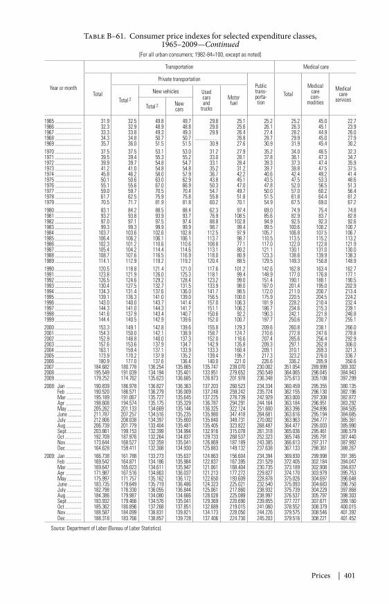
Prices | 401
Table B–61. Consumer price indexes for selected expenditure classes,1965–2009—Continued
[For all urban consumers; 1982-84=100, except as noted]
Year or month
Transportation Medical care
Total
Private transportationPublictrans-porta-tion
TotalMedical
carecom-
modities
Medicalcare
servicesTotal 2
New vehicles Usedcarsand
trucks
MotorfuelTotal 2 New
cars
1965 ...................... 31.9 32.5 49.8 49.7 29.8 25.1 25.2 25.2 45.0 22.71966 ...................... 32.3 32.9 48.9 48.8 29.0 25.6 26.1 26.3 45.1 23.91967 ...................... 33.3 33.8 49.3 49.3 29.9 26.4 27.4 28.2 44.9 26.01968 ...................... 34.3 34.8 50.7 50.7 ................... 26.8 28.7 29.9 45.0 27.91969 ...................... 35.7 36.0 51.5 51.5 30.9 27.6 30.9 31.9 45.4 30.21970 ...................... 37.5 37.5 53.1 53.0 31.2 27.9 35.2 34.0 46.5 32.31971 ...................... 39.5 39.4 55.3 55.2 33.0 28.1 37.8 36.1 47.3 34.71972 ...................... 39.9 39.7 54.8 54.7 33.1 28.4 39.3 37.3 47.4 35.91973 ...................... 41.2 41.0 54.8 54.8 35.2 31.2 39.7 38.8 47.5 37.51974 ...................... 45.8 46.2 58.0 57.9 36.7 42.2 40.6 42.4 49.2 41.41975 ...................... 50.1 50.6 63.0 62.9 43.8 45.1 43.5 47.5 53.3 46.61976 ...................... 55.1 55.6 67.0 66.9 50.3 47.0 47.8 52.0 56.5 51.31977 ...................... 59.0 59.7 70.5 70.4 54.7 49.7 50.0 57.0 60.2 56.41978 ...................... 61.7 62.5 75.9 75.8 55.8 51.8 51.5 61.8 64.4 61.21979 ...................... 70.5 71.7 81.9 81.8 60.2 70.1 54.9 67.5 69.0 67.21980 ...................... 83.1 84.2 88.5 88.4 62.3 97.4 69.0 74.9 75.4 74.81981 ...................... 93.2 93.8 93.9 93.7 76.9 108.5 85.6 82.9 83.7 82.81982 ...................... 97.0 97.1 97.5 97.4 88.8 102.8 94.9 92.5 92.3 92.61983 ...................... 99.3 99.3 99.9 99.9 98.7 99.4 99.5 100.6 100.2 100.71984 ...................... 103.7 103.6 102.6 102.8 112.5 97.9 105.7 106.8 107.5 106.71985 ...................... 106.4 106.2 106.1 106.1 113.7 98.7 110.5 113.5 115.2 113.21986 ...................... 102.3 101.2 110.6 110.6 108.8 77.1 117.0 122.0 122.8 121.91987 ...................... 105.4 104.2 114.4 114.6 113.1 80.2 121.1 130.1 131.0 130.01988 ...................... 108.7 107.6 116.5 116.9 118.0 80.9 123.3 138.6 139.9 138.31989 ...................... 114.1 112.9 119.2 119.2 120.4 88.5 129.5 149.3 150.8 148.91990 ...................... 120.5 118.8 121.4 121.0 117.6 101.2 142.6 162.8 163.4 162.71991 ...................... 123.8 121.9 126.0 125.3 118.1 99.4 148.9 177.0 176.8 177.11992 ...................... 126.5 124.6 129.2 128.4 123.2 99.0 151.4 190.1 188.1 190.51993 ...................... 130.4 127.5 132.7 131.5 133.9 98.0 167.0 201.4 195.0 202.91994 ...................... 134.3 131.4 137.6 136.0 141.7 98.5 172.0 211.0 200.7 213.41995 ...................... 139.1 136.3 141.0 139.0 156.5 100.0 175.9 220.5 204.5 224.21996 ...................... 143.0 140.0 143.7 141.4 157.0 106.3 181.9 228.2 210.4 232.41997 ...................... 144.3 141.0 144.3 141.7 151.1 106.2 186.7 234.6 215.3 239.11998 ...................... 141.6 137.9 143.4 140.7 150.6 92.2 190.3 242.1 221.8 246.81999 ...................... 144.4 140.5 142.9 139.6 152.0 100.7 197.7 250.6 230.7 255.12000 ...................... 153.3 149.1 142.8 139.6 155.8 129.3 209.6 260.8 238.1 266.02001 ...................... 154.3 150.0 142.1 138.9 158.7 124.7 210.6 272.8 247.6 278.82002 ...................... 152.9 148.8 140.0 137.3 152.0 116.6 207.4 285.6 256.4 292.92003 ...................... 157.6 153.6 137.9 134.7 142.9 135.8 209.3 297.1 262.8 306.02004 ...................... 163.1 159.4 137.1 133.9 133.3 160.4 209.1 310.1 269.3 321.32005 ...................... 173.9 170.2 137.9 135.2 139.4 195.7 217.3 323.2 276.0 336.72006 ...................... 180.9 177.0 137.6 136.4 140.0 221.0 226.6 336.2 285.9 350.62007 ...................... 184.682 180.778 136.254 135.865 135.747 239.070 230.002 351.054 289.999 369.3022008 ...................... 195.549 191.039 134.194 135.401 133.951 279.652 250.549 364.065 296.045 384.9432009 ...................... 179.252 174.762 135.623 136.685 126.973 201.978 236.348 375.613 305.108 397.2992008: Jan ............. 190.839 186.978 136.827 136.363 137.203 260.523 234.334 360.459 295.355 380.135
Feb ............. 190.520 186.571 136.279 136.009 137.248 259.242 235.724 362.155 296.130 382.196Mar ............ 195.189 191.067 135.727 135.645 137.225 278.739 242.929 363.000 297.308 382.872Apr ............. 198.608 194.574 135.175 135.329 136.787 294.291 244.164 363.184 296.951 383.292May ............ 205.262 201.133 134.669 135.144 136.325 322.124 251.600 363.396 294.896 384.505June ........... 211.787 207.257 134.516 135.235 135.980 347.418 264.681 363.616 295.194 384.685July ............ 212.806 208.038 134.397 135.800 135.840 349.731 270.002 363.963 294.777 385.361Aug ............. 206.739 201.779 133.404 135.481 135.405 323.822 268.487 364.477 295.003 385.990Sept ............ 203.861 199.153 132.399 134.994 132.916 315.078 261.318 365.036 295.461 386.579Oct .............. 192.709 187.976 132.264 134.837 129.733 268.537 252.323 365.746 295.791 387.440Nov ............. 173.644 168.527 132.359 135.041 126.869 187.189 243.385 366.613 297.317 387.992Dec ............. 164.628 159.411 132.308 134.930 125.883 149.132 237.638 367.133 298.361 388.267
2009: Jan ............. 166.738 161.788 133.273 135.637 124.863 156.604 234.394 369.830 299.998 391.365Feb ............. 169.542 164.871 134.186 135.984 122.837 167.395 231.529 372.405 302.184 394.047Mar ............ 169.647 165.023 134.611 135.947 121.061 168.404 230.735 373.189 302.908 394.837Apr ............. 171.987 167.516 134.863 136.037 121.213 177.272 229.827 374.170 303.979 395.753May ............ 175.997 171.757 135.162 136.172 122.650 193.609 228.878 375.026 304.697 396.648June ........... 183.735 179.649 135.719 136.486 124.323 225.021 232.540 375.093 304.683 396.750July ............ 182.798 178.330 136.055 136.844 125.061 217.860 238.932 375.739 304.229 397.868Aug ............. 184.386 179.987 134.080 134.666 128.028 225.089 238.997 376.537 305.797 398.303Sept ............ 183.932 179.466 134.576 135.041 129.369 220.690 239.855 377.727 307.671 399.160Oct .............. 185.362 180.896 137.268 137.851 132.689 219.015 241.060 378.552 308.379 400.015Nov ............. 188.587 184.099 138.831 139.821 134.173 228.050 244.226 379.575 308.546 401.392Dec ............. 188.318 183.766 138.857 139.728 137.406 224.730 245.203 379.516 308.221 401.452
Source: Department of Labor (Bureau of Labor Statistics).
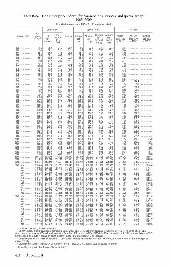
402 | Appendix B
Table B–62. Consumer price indexes for commodities, services, and special groups,1965–2009
[For all urban consumers; 1982–84=100, except as noted]
Year or monthAll
items(CPI-U) 1
Commodities
Services
Special indexes All items
Allcom-
modities
Com-modities
lessfood
All itemslessfood
All itemsless
energy
All itemsless
food andenergy
All itemsless
medicalcare
CPI-U-X1(Dec. 1982
= 97.6) 2
CPI-U-RS(Dec. 1977
= 100) 3
C-CPI-U(Dec. 1999
= 100) 4
1965 ...................... 31.5 35.2 37.2 26.6 31.6 32.5 32.7 32.0 34.2 .................... ......................1966 ...................... 32.4 36.1 37.7 27.6 32.3 33.5 33.5 33.0 35.2 .................... ......................1967 ...................... 33.4 36.8 38.6 28.8 33.4 34.4 34.7 33.7 36.3 .................... ......................1968 ...................... 34.8 38.1 40.0 30.3 34.9 35.9 36.3 35.1 37.7 .................... ......................1969 ...................... 36.7 39.9 41.7 32.4 36.8 38.0 38.4 37.0 39.4 .................... ......................1970 ...................... 38.8 41.7 43.4 35.0 39.0 40.3 40.8 39.2 41.3 .................... ......................1971 ...................... 40.5 43.2 45.1 37.0 40.8 42.0 42.7 40.8 43.1 .................... ......................1972 ...................... 41.8 44.5 46.1 38.4 42.0 43.4 44.0 42.1 44.4 .................... ......................1973 ...................... 44.4 47.8 47.7 40.1 43.7 46.1 45.6 44.8 47.2 .................... ......................1974 ...................... 49.3 53.5 52.8 43.8 48.0 50.6 49.4 49.8 51.9 .................... ......................1975 ...................... 53.8 58.2 57.6 48.0 52.5 55.1 53.9 54.3 56.2 .................... ......................1976 ...................... 56.9 60.7 60.5 52.0 56.0 58.2 57.4 57.2 59.4 .................... ......................1977 ...................... 60.6 64.2 63.8 56.0 59.6 61.9 61.0 60.8 63.2 .................... ......................1978 ...................... 65.2 68.8 67.5 60.8 63.9 66.7 65.5 65.4 67.5 104.4 ......................1979 ...................... 72.6 76.6 75.3 67.5 71.2 73.4 71.9 72.9 74.0 114.4 ......................1980 ...................... 82.4 86.0 85.7 77.9 81.5 81.9 80.8 82.8 82.3 127.1 ......................1981 ...................... 90.9 93.2 93.1 88.1 90.4 90.1 89.2 91.4 90.1 139.2 ......................1982 ...................... 96.5 97.0 96.9 96.0 96.3 96.1 95.8 96.8 95.6 147.6 ......................1983 ...................... 99.6 99.8 100.0 99.4 99.7 99.6 99.6 99.6 99.6 153.9 ......................1984 ...................... 103.9 103.2 103.1 104.6 104.0 104.3 104.6 103.7 103.9 160.2 ......................1985 ...................... 107.6 105.4 105.2 109.9 108.0 108.4 109.1 107.2 107.6 165.7 ......................1986 ...................... 109.6 104.4 101.7 115.4 109.8 112.6 113.5 108.8 109.6 168.7 ......................1987 ...................... 113.6 107.7 104.3 120.2 113.6 117.2 118.2 112.6 113.6 174.4 ......................1988 ...................... 118.3 111.5 107.7 125.7 118.3 122.3 123.4 117.0 118.3 180.8 ......................1989 ...................... 124.0 116.7 112.0 131.9 123.7 128.1 129.0 122.4 124.0 188.6 ......................1990 ...................... 130.7 122.8 117.4 139.2 130.3 134.7 135.5 128.8 130.7 198.0 ......................1991 ...................... 136.2 126.6 121.3 146.3 136.1 140.9 142.1 133.8 136.2 205.1 ......................1992 ...................... 140.3 129.1 124.2 152.0 140.8 145.4 147.3 137.5 140.3 210.3 ......................1993 ...................... 144.5 131.5 126.3 157.9 145.1 150.0 152.2 141.2 144.5 215.5 ......................1994 ...................... 148.2 133.8 127.9 163.1 149.0 154.1 156.5 144.7 148.2 220.1 ......................1995 ...................... 152.4 136.4 129.8 168.7 153.1 158.7 161.2 148.6 152.4 225.4 ......................1996 ...................... 156.9 139.9 132.6 174.1 157.5 163.1 165.6 152.8 156.9 231.4 ......................1997 ...................... 160.5 141.8 133.4 179.4 161.1 167.1 169.5 156.3 160.5 236.4 ......................1998 ...................... 163.0 141.9 132.0 184.2 163.4 170.9 173.4 158.6 163.0 239.7 ......................1999 ...................... 166.6 144.4 134.0 188.8 167.0 174.4 177.0 162.0 166.6 244.7 ......................2000 ...................... 172.2 149.2 139.2 195.3 173.0 178.6 181.3 167.3 172.2 252.9 102.02001 ...................... 177.1 150.7 138.9 203.4 177.8 183.5 186.1 171.9 177.1 260.0 104.32002 ...................... 179.9 149.7 136.0 209.8 180.5 187.7 190.5 174.3 179.9 264.2 105.62003 ...................... 184.0 151.2 136.5 216.5 184.7 190.6 193.2 178.1 184.0 270.1 107.82004 ...................... 188.9 154.7 138.8 222.8 189.4 194.4 196.6 182.7 188.9 277.4 110.52005 ...................... 195.3 160.2 144.5 230.1 196.0 198.7 200.9 188.7 195.3 286.7 113.72006 ...................... 201.6 164.0 148.0 238.9 202.7 203.7 205.9 194.7 201.6 296.1 117.02007 ...................... 207.342 167.509 149.720 246.848 208.098 208.925 210.729 200.080 207.342 304.5 119.9572008 ...................... 215.303 174.764 155.310 255.498 215.528 214.751 215.572 207.777 215.303 316.2 123.8802009 ...................... 214.537 169.698 147.071 259.154 214.008 218.433 219.235 206.555 214.537 315.0 .......................2008: Jan ............. 211.080 171.179 152.531 250.648 211.512 211.846 213.138 203.569 211.080 310.0 121.868
Feb ............. 211.693 171.530 152.799 251.527 212.136 212.545 213.866 204.136 211.693 310.9 122.224Mar ............ 213.528 173.884 155.881 252.817 214.236 213.420 214.866 205.992 213.528 313.6 123.177Apr ............. 214.823 175.838 157.870 253.426 215.462 213.851 215.059 207.317 214.823 315.5 123.817May ............ 216.632 178.341 160.880 254.509 217.411 214.101 215.180 209.170 216.632 318.1 124.617June ........... 218.815 180.534 163.385 256.668 219.757 214.600 215.553 211.408 218.815 321.3 125.554July ............ 219.964 181.087 163.364 258.422 220.758 215.335 216.045 212.576 219.964 323.0 126.088Aug ............. 219.086 179.148 160.341 258.638 219.552 215.873 216.476 211.653 219.086 321.7 125.815Sept ............ 218.783 179.117 159.825 258.059 218.991 216.397 216.862 211.321 218.783 321.3 125.746Oct .............. 216.573 175.257 154.250 257.559 216.250 216.695 217.023 209.021 216.573 318.0 124.757Nov ............. 212.425 167.673 144.055 256.967 211.421 216.417 216.690 204.721 212.425 311.9 122.257Dec ............. 210.228 163.582 138.536 256.731 208.855 215.930 216.100 202.442 210.228 308.7 120.634
2009: Jan ............. 211.143 164.360 139.258 257.780 209.777 216.586 216.719 203.281 211.143 310.1 121.208Feb ............. 212.193 165.891 141.491 258.328 211.076 217.325 217.685 204.265 212.193 311.6 121.901Mar ............ 212.709 166.645 142.728 258.597 211.775 218.033 218.639 204.766 212.709 312.4 122.182Apr ............. 213.240 167.816 144.464 258.466 212.464 218.388 219.143 205.275 213.240 313.1 122.506May ............ 213.856 169.060 146.261 258.433 213.236 218.323 219.128 205.876 213.856 314.0 122.898June ........... 215.693 171.593 149.697 259.544 215.389 218.440 219.283 207.764 215.693 316.7 123.967July ............ 215.351 170.483 148.386 259.992 215.069 218.421 219.350 207.388 215.351 316.2 123.711Aug ............. 215.834 171.081 149.155 260.355 215.617 218.642 219.596 207.855 215.834 316.9 123.955Sept ............ 215.969 171.559 149.846 260.136 215.795 219.076 220.137 207.949 215.969 317.1 124.021Oct .............. 216.177 172.252 150.663 259.844 215.986 219.624 220.731 208.131 216.177 317.5 124.179Nov ............. 216.330 173.061 151.847 259.323 216.207 219.291 220.384 208.250 216.330 317.7 124.231Dec ............. 215.949 172.572 151.052 259.055 215.703 219.048 220.025 207.860 215.949 317.1 123.965
1 Consumer price index, all urban consumers.2 CPI-U-X1 reflects a rental equivalence approach to homeowners’ costs for the CPI-U for years prior to 1983, the first year for which the official index
incorporates such a measure. CPI-U-X1 is rebased to the December 1982 value of the CPI-U (1982–84=100) and is identical with CPI-U data from December 1982forward. Data prior to 1967 estimated by moving the series at the same rate as the CPI-U for each year.
3 Consumer price index research series (CPI-U-RS) using current methods introduced in June 1999. Data for 2009 are preliminary. All data are subject torevision annually.
4 Chained consumer price index (C-CPI-U) introduced in August 2002. Data for 2008 and 2009 are subject to revision.Source: Department of Labor (Bureau of Labor Statistics).
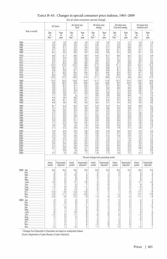
Prices | 403
Table B–63. Changes in special consumer price indexes, 1965–2009[For all urban consumers; percent change]
Year or month
All items All items lessfood
All items lessenergy
All items lessfood and energy
All items lessmedical care
Dec.to
Dec. 1
Yearto
year
Dec.to
Dec. 1
Yearto
year
Dec.to
Dec. 1
Yearto
year
Dec.to
Dec. 1
Yearto
year
Dec.to
Dec. 1
Yearto
year
1965 ....................................... 1.9 1.6 1.6 1.6 1.9 1.6 1.5 1.2 1.9 1.61966 ....................................... 3.5 2.9 3.5 2.2 3.4 3.1 3.3 2.4 3.4 3.11967 ....................................... 3.0 3.1 3.3 3.4 3.2 2.7 3.8 3.6 2.7 2.11968 ....................................... 4.7 4.2 5.0 4.5 4.9 4.4 5.1 4.6 4.7 4.21969 ....................................... 6.2 5.5 5.6 5.4 6.5 5.8 6.2 5.8 6.1 5.41970 ....................................... 5.6 5.7 6.6 6.0 5.4 6.1 6.6 6.3 5.2 5.91971 ....................................... 3.3 4.4 3.0 4.6 3.4 4.2 3.1 4.7 3.2 4.11972 ....................................... 3.4 3.2 2.9 2.9 3.5 3.3 3.0 3.0 3.4 3.21973 ....................................... 8.7 6.2 5.6 4.0 8.2 6.2 4.7 3.6 9.1 6.41974 ....................................... 12.3 11.0 12.2 9.8 11.7 9.8 11.1 8.3 12.2 11.21975 ....................................... 6.9 9.1 7.3 9.4 6.6 8.9 6.7 9.1 6.7 9.01976 ....................................... 4.9 5.8 6.1 6.7 4.8 5.6 6.1 6.5 4.5 5.31977 ....................................... 6.7 6.5 6.4 6.4 6.7 6.4 6.5 6.3 6.7 6.31978 ....................................... 9.0 7.6 8.3 7.2 9.1 7.8 8.5 7.4 9.1 7.61979 ....................................... 13.3 11.3 14.0 11.4 11.1 10.0 11.3 9.8 13.4 11.51980 ....................................... 12.5 13.5 13.0 14.5 11.7 11.6 12.2 12.4 12.5 13.61981 ....................................... 8.9 10.3 9.8 10.9 8.5 10.0 9.5 10.4 8.8 10.41982 ....................................... 3.8 6.2 4.1 6.5 4.2 6.7 4.5 7.4 3.6 5.91983 ....................................... 3.8 3.2 4.1 3.5 4.5 3.6 4.8 4.0 3.6 2.91984 ....................................... 3.9 4.3 3.9 4.3 4.4 4.7 4.7 5.0 3.9 4.11985 ....................................... 3.8 3.6 4.1 3.8 4.0 3.9 4.3 4.3 3.5 3.41986 ....................................... 1.1 1.9 .5 1.7 3.8 3.9 3.8 4.0 .7 1.51987 ....................................... 4.4 3.6 4.6 3.5 4.1 4.1 4.2 4.1 4.3 3.51988 ....................................... 4.4 4.1 4.2 4.1 4.7 4.4 4.7 4.4 4.2 3.91989 ....................................... 4.6 4.8 4.5 4.6 4.6 4.7 4.4 4.5 4.5 4.61990 ....................................... 6.1 5.4 6.3 5.3 5.2 5.2 5.2 5.0 5.9 5.21991 ....................................... 3.1 4.2 3.3 4.5 3.9 4.6 4.4 4.9 2.7 3.91992 ....................................... 2.9 3.0 3.2 3.5 3.0 3.2 3.3 3.7 2.7 2.81993 ....................................... 2.7 3.0 2.7 3.1 3.1 3.2 3.2 3.3 2.6 2.71994 ....................................... 2.7 2.6 2.6 2.7 2.6 2.7 2.6 2.8 2.5 2.51995 ....................................... 2.5 2.8 2.7 2.8 2.9 3.0 3.0 3.0 2.5 2.71996 ....................................... 3.3 3.0 3.1 2.9 2.9 2.8 2.6 2.7 3.3 2.81997 ....................................... 1.7 2.3 1.8 2.3 2.1 2.5 2.2 2.4 1.6 2.31998 ....................................... 1.6 1.6 1.5 1.4 2.4 2.3 2.4 2.3 1.5 1.51999 ....................................... 2.7 2.2 2.8 2.2 2.0 2.0 1.9 2.1 2.6 2.12000 ....................................... 3.4 3.4 3.5 3.6 2.6 2.4 2.6 2.4 3.3 3.32001 ....................................... 1.6 2.8 1.3 2.8 2.8 2.7 2.7 2.6 1.4 2.72002 ....................................... 2.4 1.6 2.6 1.5 1.8 2.3 1.9 2.4 2.2 1.42003 ....................................... 1.9 2.3 1.5 2.3 1.5 1.5 1.1 1.4 1.8 2.22004 ....................................... 3.3 2.7 3.4 2.5 2.2 2.0 2.2 1.8 3.2 2.62005 ....................................... 3.4 3.4 3.6 3.5 2.2 2.2 2.2 2.2 3.3 3.32006 ....................................... 2.5 3.2 2.6 3.4 2.5 2.5 2.6 2.5 2.5 3.22007 ....................................... 4.1 2.8 4.0 2.7 2.8 2.6 2.4 2.3 4.0 2.82008 ....................................... .1 3.8 –.8 3.6 2.4 2.8 1.8 2.3 –.1 3.82009 ....................................... 2.7 –.4 3.3 –.7 1.4 1.7 1.8 1.7 2.7 –.6
Percent change from preceding month
Unad-justed
Seasonallyadjusted
Unad-justed
Seasonallyadjusted
Unad-justed
Seasonallyadjusted
Unad-justed
Seasonallyadjusted
Unad-justed
Seasonallyadjusted
2008: Jan .............................. 0.5 0.4 0.4 0.3 0.5 0.3 0.4 0.3 0.5 0.3Feb .............................. .3 .2 .3 .1 .3 .1 .3 .1 .3 .2Mar ............................. .9 .4 1.0 .4 .4 .2 .5 .2 .9 .4Apr .............................. .6 .2 .6 .0 .2 .2 .1 .1 .6 .2May ............................. .8 .5 .9 .5 .1 .2 .1 .2 .9 .5June ............................ 1.0 .9 1.1 1.0 .2 .3 .2 .3 1.1 1.0July ............................. .5 .7 .5 .7 .3 .4 .2 .3 .6 .8Aug .............................. –.4 .0 –.5 –.1 .2 .2 .2 .2 –.4 .0Sept ............................. –.1 .0 –.3 .0 .2 .2 .2 .1 –.2 .0Oct ............................... –1.0 –.8 –1.3 –1.0 .1 .1 .1 .0 –1.1 –.9Nov .............................. –1.9 –1.7 –2.2 –2.0 –.1 .1 –.2 .1 –2.1 –1.8Dec .............................. –1.0 –.8 –1.2 –.9 –.2 .0 –.3 .0 –1.1 –.9
2009: Jan .............................. .4 .3 .4 .3 .3 .2 .3 .2 .4 .3Feb .............................. .5 .4 .6 .5 .3 .1 .4 .2 .5 .4Mar ............................. .2 –.1 .3 –.1 .3 .1 .4 .2 .2 –.2Apr .............................. .2 .0 .3 .0 .2 .2 .2 .3 .2 .0May ............................. .3 .1 .4 .2 .0 .1 .0 .1 .3 .1June ............................ .9 .7 1.0 .9 .1 .2 .1 .2 .9 .8July ............................. –.2 .0 –.1 .0 .0 .0 .0 .1 –.2 .0Aug .............................. .2 .4 .3 .5 .1 .1 .1 .1 .2 .5Sept ............................. .1 .2 .1 .2 .2 .1 .2 .2 .0 .2Oct ............................... .1 .3 .1 .3 .3 .2 .3 .2 .1 .3Nov .............................. .1 .4 .1 .5 –.2 .0 –.2 .0 .1 .4Dec .............................. –.2 .1 –.2 .1 –.1 .1 –.2 .1 –.2 .1
1 Changes from December to December are based on unadjusted indexes.Source: Department of Labor (Bureau of Labor Statistics).
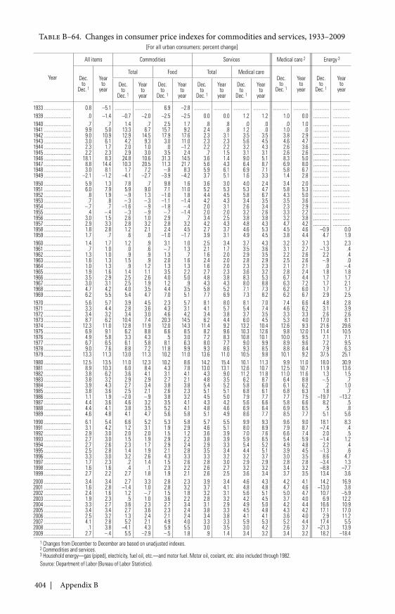
404 | Appendix B
Table B–64. Changes in consumer price indexes for commodities and services, 1933–2009[For all urban consumers: percent change]
Year
All items Commodities Services Medical care 2 Energy 3
Dec.to
Dec. 1
Yearto
year
Total Food Total Medical careDec.
toDec. 1
Yearto
year
Dec.to
Dec. 1
Yearto
yearDec.
toDec. 1
Yearto
year
Dec.to
Dec. 1
Yearto
year
Dec.to
Dec. 1
Yearto
year
Dec.to
Dec. 1
Yearto
year
1933 ...................... 0.8 –5.1 ............. ............. 6.9 –2.8 ............. ............. ............. ............ ............. ............ ............. ..............1939 ...................... .0 –1.4 –0.7 –2.0 –2.5 –2.5 0.0 0.0 1.2 1.2 1.0 0.0 ............. ..............1940 ...................... .7 .7 1.4 .7 2.5 1.7 .8 .8 .0 .0 .0 1.0 ............. ..............1941 ...................... 9.9 5.0 13.3 6.7 15.7 9.2 2.4 .8 1.2 .0 1.0 .0 ............. ..............1942 ...................... 9.0 10.9 12.9 14.5 17.9 17.6 2.3 3.1 3.5 3.5 3.8 2.9 ............. ..............1943 ...................... 3.0 6.1 4.2 9.3 3.0 11.0 2.3 2.3 5.6 4.5 4.6 4.7 ............. ..............1944 ...................... 2.3 1.7 2.0 1.0 .0 –1.2 2.2 2.2 3.2 4.3 2.6 3.6 ............. ..............1945 ...................... 2.2 2.3 2.9 3.0 3.5 2.4 .7 1.5 3.1 3.1 2.6 2.6 ............. ..............1946 ...................... 18.1 8.3 24.8 10.6 31.3 14.5 3.6 1.4 9.0 5.1 8.3 5.0 ............. ..............1947 ...................... 8.8 14.4 10.3 20.5 11.3 21.7 5.6 4.3 6.4 8.7 6.9 8.0 ............. ..............1948 ...................... 3.0 8.1 1.7 7.2 –.8 8.3 5.9 6.1 6.9 7.1 5.8 6.7 ............. ..............1949 ...................... –2.1 –1.2 –4.1 –2.7 –3.9 –4.2 3.7 5.1 1.6 3.3 1.4 2.8 ............. ..............1950 ...................... 5.9 1.3 7.8 .7 9.8 1.6 3.6 3.0 4.0 2.4 3.4 2.0 ............. ..............1951 ...................... 6.0 7.9 5.9 9.0 7.1 11.0 5.2 5.3 5.3 4.7 5.8 5.3 ............. ..............1952 ...................... .8 1.9 –.9 1.3 –1.0 1.8 4.4 4.5 5.8 6.7 4.3 5.0 ............. ..............1953 ...................... .7 .8 –.3 –.3 –1.1 –1.4 4.2 4.3 3.4 3.5 3.5 3.6 ............. ..............1954 ...................... –.7 .7 –1.6 –.9 –1.8 –.4 2.0 3.1 2.6 3.4 2.3 2.9 ............. ..............1955 ...................... .4 –.4 –.3 –.9 –.7 –1.4 2.0 2.0 3.2 2.6 3.3 2.2 ............. ..............1956 ...................... 3.0 1.5 2.6 1.0 2.9 .7 3.4 2.5 3.8 3.8 3.2 3.8 ............. ..............1957 ...................... 2.9 3.3 2.8 3.2 2.8 3.2 4.2 4.3 4.8 4.3 4.7 4.2 ............. ..............1958 ...................... 1.8 2.8 1.2 2.1 2.4 4.5 2.7 3.7 4.6 5.3 4.5 4.6 –0.9 0.01959 ...................... 1.7 .7 .6 .0 –1.0 –1.7 3.9 3.1 4.9 4.5 3.8 4.4 4.7 1.91960 ...................... 1.4 1.7 1.2 .9 3.1 1.0 2.5 3.4 3.7 4.3 3.2 3.7 1.3 2.31961 ...................... .7 1.0 .0 .6 –.7 1.3 2.1 1.7 3.5 3.6 3.1 2.7 –1.3 .41962 ...................... 1.3 1.0 .9 .9 1.3 .7 1.6 2.0 2.9 3.5 2.2 2.6 2.2 .41963 ...................... 1.6 1.3 1.5 .9 2.0 1.6 2.4 2.0 2.8 2.9 2.5 2.6 –.9 .01964 ...................... 1.0 1.3 .9 1.2 1.3 1.3 1.6 2.0 2.3 2.3 2.1 2.1 .0 –.41965 ...................... 1.9 1.6 1.4 1.1 3.5 2.2 2.7 2.3 3.6 3.2 2.8 2.4 1.8 1.81966 ...................... 3.5 2.9 2.5 2.6 4.0 5.0 4.8 3.8 8.3 5.3 6.7 4.4 1.7 1.71967 ...................... 3.0 3.1 2.5 1.9 1.2 .9 4.3 4.3 8.0 8.8 6.3 7.2 1.7 2.11968 ...................... 4.7 4.2 4.0 3.5 4.4 3.5 5.8 5.2 7.1 7.3 6.2 6.0 1.7 1.71969 ...................... 6.2 5.5 5.4 4.7 7.0 5.1 7.7 6.9 7.3 8.2 6.2 6.7 2.9 2.51970 ...................... 5.6 5.7 3.9 4.5 2.3 5.7 8.1 8.0 8.1 7.0 7.4 6.6 4.8 2.81971 ...................... 3.3 4.4 2.8 3.6 4.3 3.1 4.1 5.7 5.4 7.4 4.6 6.2 3.1 3.91972 ...................... 3.4 3.2 3.4 3.0 4.6 4.2 3.4 3.8 3.7 3.5 3.3 3.3 2.6 2.61973 ...................... 8.7 6.2 10.4 7.4 20.3 14.5 6.2 4.4 6.0 4.5 5.3 4.0 17.0 8.11974 ...................... 12.3 11.0 12.8 11.9 12.0 14.3 11.4 9.2 13.2 10.4 12.6 9.3 21.6 29.61975 ...................... 6.9 9.1 6.2 8.8 6.6 8.5 8.2 9.6 10.3 12.6 9.8 12.0 11.4 10.51976 ...................... 4.9 5.8 3.3 4.3 .5 3.0 7.2 8.3 10.8 10.1 10.0 9.5 7.1 7.11977 ...................... 6.7 6.5 6.1 5.8 8.1 6.3 8.0 7.7 9.0 9.9 8.9 9.6 7.2 9.51978 ...................... 9.0 7.6 8.8 7.2 11.8 9.9 9.3 8.6 9.3 8.5 8.8 8.4 7.9 6.31979 ...................... 13.3 11.3 13.0 11.3 10.2 11.0 13.6 11.0 10.5 9.8 10.1 9.2 37.5 25.11980 ...................... 12.5 13.5 11.0 12.3 10.2 8.6 14.2 15.4 10.1 11.3 9.9 11.0 18.0 30.91981 ...................... 8.9 10.3 6.0 8.4 4.3 7.8 13.0 13.1 12.6 10.7 12.5 10.7 11.9 13.61982 ...................... 3.8 6.2 3.6 4.1 3.1 4.1 4.3 9.0 11.2 11.8 11.0 11.6 1.3 1.51983 ...................... 3.8 3.2 2.9 2.9 2.7 2.1 4.8 3.5 6.2 8.7 6.4 8.8 –.5 .71984 ...................... 3.9 4.3 2.7 3.4 3.8 3.8 5.4 5.2 5.8 6.0 6.1 6.2 .2 1.01985 ...................... 3.8 3.6 2.5 2.1 2.6 2.3 5.1 5.1 6.8 6.1 6.8 6.3 1.8 .71986 ...................... 1.1 1.9 –2.0 –.9 3.8 3.2 4.5 5.0 7.9 7.7 7.7 7.5 –19.7 –13.21987 ...................... 4.4 3.6 4.6 3.2 3.5 4.1 4.3 4.2 5.6 6.6 5.8 6.6 8.2 .51988 ...................... 4.4 4.1 3.8 3.5 5.2 4.1 4.8 4.6 6.9 6.4 6.9 6.5 .5 .81989 ...................... 4.6 4.8 4.1 4.7 5.6 5.8 5.1 4.9 8.6 7.7 8.5 7.7 5.1 5.61990 ...................... 6.1 5.4 6.6 5.2 5.3 5.8 5.7 5.5 9.9 9.3 9.6 9.0 18.1 8.31991 ...................... 3.1 4.2 1.2 3.1 1.9 2.9 4.6 5.1 8.0 8.9 7.9 8.7 –7.4 .41992 ...................... 2.9 3.0 2.0 2.0 1.5 1.2 3.6 3.9 7.0 7.6 6.6 7.4 2.0 .51993 ...................... 2.7 3.0 1.5 1.9 2.9 2.2 3.8 3.9 5.9 6.5 5.4 5.9 –1.4 1.21994 ...................... 2.7 2.6 2.3 1.7 2.9 2.4 2.9 3.3 5.4 5.2 4.9 4.8 2.2 .41995 ...................... 2.5 2.8 1.4 1.9 2.1 2.8 3.5 3.4 4.4 5.1 3.9 4.5 –1.3 .61996 ...................... 3.3 3.0 3.2 2.6 4.3 3.3 3.3 3.2 3.2 3.7 3.0 3.5 8.6 4.71997 ...................... 1.7 2.3 .2 1.4 1.5 2.6 2.8 3.0 2.9 2.9 2.8 2.8 –3.4 1.31998 ...................... 1.6 1.6 .4 .1 2.3 2.2 2.6 2.7 3.2 3.2 3.4 3.2 –8.8 –7.71999 ...................... 2.7 2.2 2.7 1.8 1.9 2.1 2.6 2.5 3.6 3.4 3.7 3.5 13.4 3.62000 ...................... 3.4 3.4 2.7 3.3 2.8 2.3 3.9 3.4 4.6 4.3 4.2 4.1 14.2 16.92001 ...................... 1.6 2.8 –1.4 1.0 2.8 3.2 3.7 4.1 4.8 4.8 4.7 4.6 –13.0 3.82002 ...................... 2.4 1.6 1.2 –.7 1.5 1.8 3.2 3.1 5.6 5.1 5.0 4.7 10.7 –5.92003 ...................... 1.9 2.3 .5 1.0 3.6 2.2 2.8 3.2 4.2 4.5 3.7 4.0 6.9 12.22004 ...................... 3.3 2.7 3.6 2.3 2.7 3.4 3.1 2.9 4.9 5.0 4.2 4.4 16.6 10.92005 ...................... 3.4 3.4 2.7 3.6 2.3 2.4 3.8 3.3 4.5 4.8 4.3 4.2 17.1 17.02006 ...................... 2.5 3.2 1.3 2.4 2.1 2.4 3.4 3.8 4.1 4.1 3.6 4.0 2.9 11.22007 ...................... 4.1 2.8 5.2 2.1 4.9 4.0 3.3 3.3 5.9 5.3 5.2 4.4 17.4 5.52008 ...................... .1 3.8 –4.1 4.3 5.9 5.5 3.0 3.5 3.0 4.2 2.6 3.7 –21.3 13.92009 ...................... 2.7 –.4 5.5 –2.9 –.5 1.8 .9 1.4 3.4 3.2 3.4 3.2 18.2 –18.4
1 Changes from December to December are based on unadjusted indexes.2 Commodities and services.3 Household energy—gas (piped), electricity, fuel oil, etc.—and motor fuel. Motor oil, coolant, etc. also included through 1982.Source: Department of Labor (Bureau of Labor Statistics).
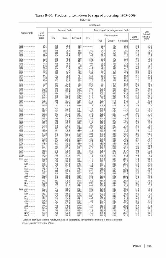
Prices | 405
Table B–65. Producer price indexes by stage of processing, 1965–2009[1982=100]
Year or month
Finished goods
Totalfinishedgoods
Consumer foods Finished goods excluding consumer foodsTotal
finishedconsumer
goodsTotal Crude Processed TotalConsumer goods Capital
equipmentTotal Durable Nondurable
1965 ...................... 34.1 36.8 39.0 36.8 ................... 33.6 43.2 28.8 33.8 34.21966 ...................... 35.2 39.2 41.5 39.2 ................... 34.1 43.4 29.3 34.6 35.41967 ...................... 35.6 38.5 39.6 38.8 35.0 34.7 44.1 30.0 35.8 35.61968 ...................... 36.6 40.0 42.5 40.0 35.9 35.5 45.1 30.6 37.0 36.51969 ...................... 38.0 42.4 45.9 42.3 36.9 36.3 45.9 31.5 38.3 37.91970 ...................... 39.3 43.8 46.0 43.9 38.2 37.4 47.2 32.5 40.1 39.11971 ...................... 40.5 44.5 45.8 44.7 39.6 38.7 48.9 33.5 41.7 40.21972 ...................... 41.8 46.9 48.0 47.2 40.4 39.4 50.0 34.1 42.8 41.51973 ...................... 45.6 56.5 63.6 55.8 42.0 41.2 50.9 36.1 44.2 46.01974 ...................... 52.6 64.4 71.6 63.9 48.8 48.2 55.5 44.0 50.5 53.11975 ...................... 58.2 69.8 71.7 70.3 54.7 53.2 61.0 48.9 58.2 58.21976 ...................... 60.8 69.6 76.7 69.0 58.1 56.5 63.7 52.4 62.1 60.41977 ...................... 64.7 73.3 79.5 72.7 62.2 60.6 67.4 56.8 66.1 64.31978 ...................... 69.8 79.9 85.8 79.4 66.7 64.9 73.6 60.0 71.3 69.41979 ...................... 77.6 87.3 92.3 86.8 74.6 73.5 80.8 69.3 77.5 77.51980 ...................... 88.0 92.4 93.9 92.3 86.7 87.1 91.0 85.1 85.8 88.61981 ...................... 96.1 97.8 104.4 97.2 95.6 96.1 96.4 95.8 94.6 96.61982 ...................... 100.0 100.0 100.0 100.0 100.0 100.0 100.0 100.0 100.0 100.01983 ...................... 101.6 101.0 102.4 100.9 101.8 101.2 102.8 100.5 102.8 101.31984 ...................... 103.7 105.4 111.4 104.9 103.2 102.2 104.5 101.1 105.2 103.31985 ...................... 104.7 104.6 102.9 104.8 104.6 103.3 106.5 101.7 107.5 103.81986 ...................... 103.2 107.3 105.6 107.4 101.9 98.5 108.9 93.3 109.7 101.41987 ...................... 105.4 109.5 107.1 109.6 104.0 100.7 111.5 94.9 111.7 103.61988 ...................... 108.0 112.6 109.8 112.7 106.5 103.1 113.8 97.3 114.3 106.21989 ...................... 113.6 118.7 119.6 118.6 111.8 108.9 117.6 103.8 118.8 112.11990 ...................... 119.2 124.4 123.0 124.4 117.4 115.3 120.4 111.5 122.9 118.21991 ...................... 121.7 124.1 119.3 124.4 120.9 118.7 123.9 115.0 126.7 120.51992 ...................... 123.2 123.3 107.6 124.4 123.1 120.8 125.7 117.3 129.1 121.71993 ...................... 124.7 125.7 114.4 126.5 124.4 121.7 128.0 117.6 131.4 123.01994 ...................... 125.5 126.8 111.3 127.9 125.1 121.6 130.9 116.2 134.1 123.31995 ...................... 127.9 129.0 118.8 129.8 127.5 124.0 132.7 118.8 136.7 125.61996 ...................... 131.3 133.6 129.2 133.8 130.5 127.6 134.2 123.3 138.3 129.51997 ...................... 131.8 134.5 126.6 135.1 130.9 128.2 133.7 124.3 138.2 130.21998 ...................... 130.7 134.3 127.2 134.8 129.5 126.4 132.9 122.2 137.6 128.91999 ...................... 133.0 135.1 125.5 135.9 132.3 130.5 133.0 127.9 137.6 132.02000 ...................... 138.0 137.2 123.5 138.3 138.1 138.4 133.9 138.7 138.8 138.22001 ...................... 140.7 141.3 127.7 142.4 140.4 141.4 134.0 142.8 139.7 141.52002 ...................... 138.9 140.1 128.5 141.0 138.3 138.8 133.0 139.8 139.1 139.42003 ...................... 143.3 145.9 130.0 147.2 142.4 144.7 133.1 148.4 139.5 145.32004 ...................... 148.5 152.7 138.2 153.9 147.2 150.9 135.0 156.6 141.4 151.72005 ...................... 155.7 155.7 140.2 156.9 155.5 161.9 136.6 172.0 144.6 160.42006 ...................... 160.4 156.7 151.3 157.1 161.0 169.2 136.9 182.6 146.9 166.02007 ...................... 166.6 167.0 170.2 166.7 166.2 175.6 138.3 191.7 149.5 173.52008 ...................... 177.1 178.3 175.5 178.6 176.6 189.1 141.2 210.5 153.8 186.32009 p .................... 172.6 175.5 157.8 177.3 171.2 179.6 144.3 194.3 156.8 179.22008: Jan ............. 172.0 174.5 199.3 172.1 171.0 181.9 140.1 200.3 151.4 180.1
Feb ............. 172.3 173.6 180.6 173.0 171.7 182.7 140.2 201.4 151.8 180.4Mar ............ 175.1 176.0 194.3 174.2 174.6 187.1 139.9 208.2 151.8 184.2Apr ............. 176.5 175.5 177.6 175.3 176.4 189.6 140.5 211.7 152.4 185.8May ............ 179.8 177.6 172.1 178.2 180.1 195.0 140.3 220.0 152.7 190.3June ........... 182.4 180.0 183.0 179.7 182.8 199.0 139.7 226.4 152.7 193.8July ............ 185.1 181.0 164.1 182.7 185.9 203.4 139.6 233.1 153.3 197.2Aug ............. 182.2 181.3 159.8 183.5 182.2 197.5 140.2 223.9 153.9 193.2Sept ............ 182.2 181.5 168.9 182.8 182.1 197.2 140.3 223.4 154.3 193.0Oct .............. 177.4 180.7 170.0 181.8 176.3 187.0 144.8 205.4 157.0 185.5Nov ............. 172.0 179.8 175.2 180.3 169.6 177.0 144.2 190.6 156.9 178.2Dec ............. 168.8 177.7 161.7 179.4 166.1 171.5 144.4 182.1 157.2 173.7
2009: Jan ............. 170.4 177.7 169.7 178.4 168.0 174.4 144.3 186.5 157.4 175.8Feb ............. 169.9 175.0 155.6 177.0 168.0 174.5 144.3 186.6 157.2 175.2Mar ............ 169.1 173.8 155.0 175.8 167.2 173.5 144.1 185.2 156.9 174.2Apr ............. 170.3 175.9 165.4 176.9 168.3 175.2 144.4 187.7 156.8 176.0May ............ 171.1 174.0 134.6 178.3 169.7 177.5 144.2 191.2 156.3 177.3June ........... 174.3 176.1 156.2 178.2 173.1 182.7 144.7 198.7 156.6 181.7July ............ 172.4 173.5 141.8 177.0 171.3 180.2 143.3 195.7 155.9 179.2Aug ............. 174.2 173.9 145.5 177.0 173.4 183.3 143.8 200.1 156.4 181.6Sept 1 ......... 173.4 173.9 145.0 177.0 172.5 181.9 143.1 198.4 156.1 180.6Oct 1 ........... 174.1 175.9 165.4 176.9 172.9 182.0 145.0 197.6 157.2 181.2Nov 1 .......... 176.2 176.8 173.4 177.0 175.2 185.3 145.6 202.2 157.6 183.9Dec 1 ........... 176.2 179.7 186.6 178.7 174.6 184.6 144.9 201.4 157.2 184.1
1 Data have been revised through August 2009; data are subject to revision four months after date of original publication.See next page for continuation of table.
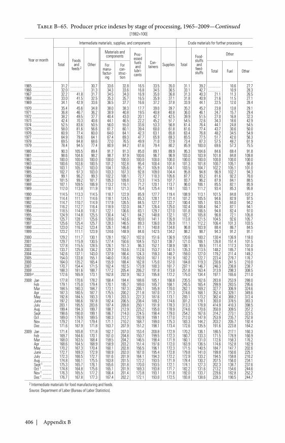
406 | Appendix B
Table B–65. Producer price indexes by stage of processing, 1965–2009—Continued[1982=100]
Year or month
Intermediate materials, supplies, and components Crude materials for further processing
TotalFoodsand
feeds 2Other
Materials andcomponents Proc-
essedfuelsand
lubri-cants
Con-tainers Supplies Total
Food-stuffsand
feed-stuffs
Other
Formanu-factur-
ing
Forcon-
struc-tion
Total Fuel Other
1965 ...................... 31.2 .............. 30.7 33.6 32.8 16.5 33.5 35.0 31.1 39.2 .............. 10.6 27.71966 ...................... 32.0 .............. 31.3 34.3 33.6 16.8 34.5 36.5 33.1 42.7 .............. 10.9 28.31967 ...................... 32.2 41.8 31.7 34.5 34.0 16.9 35.0 36.8 31.3 40.3 21.1 11.3 26.51968 ...................... 33.0 41.5 32.5 35.3 35.7 16.5 35.9 37.1 31.8 40.9 21.6 11.5 27.11969 ...................... 34.1 42.9 33.6 36.5 37.7 16.6 37.2 37.8 33.9 44.1 22.5 12.0 28.41970 ...................... 35.4 45.6 34.8 38.0 38.3 17.7 39.0 39.7 35.2 45.2 23.8 13.8 29.11971 ...................... 36.8 46.7 36.2 38.9 40.8 19.5 40.8 40.8 36.0 46.1 24.7 15.7 29.41972 ...................... 38.2 49.5 37.7 40.4 43.0 20.1 42.7 42.5 39.9 51.5 27.0 16.8 32.31973 ...................... 42.4 70.3 40.6 44.1 46.5 22.2 45.2 51.7 54.5 72.6 34.3 18.6 42.91974 ...................... 52.5 83.6 50.5 56.0 55.0 33.6 53.3 56.8 61.4 76.4 44.1 24.8 54.51975 ...................... 58.0 81.6 56.6 61.7 60.1 39.4 60.0 61.8 61.6 77.4 43.7 30.6 50.01976 ...................... 60.9 77.4 60.0 64.0 64.1 42.3 63.1 65.8 63.4 76.8 48.2 34.5 54.91977 ...................... 64.9 79.6 64.1 67.4 69.3 47.7 65.9 69.3 65.5 77.5 51.7 42.0 56.31978 ...................... 69.5 84.8 68.6 72.0 76.5 49.9 71.0 72.9 73.4 87.3 57.5 48.2 61.91979 ...................... 78.4 94.5 77.4 80.9 84.2 61.6 79.4 80.2 85.9 100.0 69.6 57.3 75.51980 ...................... 90.3 105.5 89.4 91.7 91.3 85.0 89.1 89.9 95.3 104.6 84.6 69.4 91.81981 ...................... 98.6 104.6 98.2 98.7 97.9 100.6 96.7 96.9 103.0 103.9 101.8 84.8 109.81982 ...................... 100.0 100.0 100.0 100.0 100.0 100.0 100.0 100.0 100.0 100.0 100.0 100.0 100.01983 ...................... 100.6 103.6 100.5 101.2 102.8 95.4 100.4 101.8 101.3 101.8 100.7 105.1 98.81984 ...................... 103.1 105.7 103.0 104.1 105.6 95.7 105.9 104.1 103.5 104.7 102.2 105.1 101.01985 ...................... 102.7 97.3 103.0 103.3 107.3 92.8 109.0 104.4 95.8 94.8 96.9 102.7 94.31986 ...................... 99.1 96.2 99.3 102.2 108.1 72.7 110.3 105.6 87.7 93.2 81.6 92.2 76.01987 ...................... 101.5 99.2 101.7 105.3 109.8 73.3 114.5 107.7 93.7 96.2 87.9 84.1 88.51988 ...................... 107.1 109.5 106.9 113.2 116.1 71.2 120.1 113.7 96.0 106.1 85.5 82.1 85.91989 ...................... 112.0 113.8 111.9 118.1 121.3 76.4 125.4 118.1 103.1 111.2 93.4 85.3 95.81990 ...................... 114.5 113.3 114.5 118.7 122.9 85.9 127.7 119.4 108.9 113.1 101.5 84.8 107.31991 ...................... 114.4 111.1 114.6 118.1 124.5 85.3 128.1 121.4 101.2 105.5 94.6 82.9 97.51992 ...................... 114.7 110.7 114.9 117.9 126.5 84.5 127.7 122.7 100.4 105.1 93.5 84.0 94.21993 ...................... 116.2 112.7 116.4 118.9 132.0 84.7 126.4 125.0 102.4 108.4 94.7 87.1 94.11994 ...................... 118.5 114.8 118.7 122.1 136.6 83.1 129.7 127.0 101.8 106.5 94.8 82.4 97.01995 ...................... 124.9 114.8 125.5 130.4 142.1 84.2 148.8 132.1 102.7 105.8 96.8 72.1 105.81996 ...................... 125.7 128.1 125.6 128.6 143.6 90.0 141.1 135.9 113.8 121.5 104.5 92.6 105.71997 ...................... 125.6 125.4 125.7 128.3 146.5 89.3 136.0 135.9 111.1 112.2 106.4 101.3 103.51998 ...................... 123.0 116.2 123.4 126.1 146.8 81.1 140.8 134.8 96.8 103.9 88.4 86.7 84.51999 ...................... 123.2 111.1 123.9 124.6 148.9 84.6 142.5 134.2 98.2 98.7 94.3 91.2 91.12000 ...................... 129.2 111.7 130.1 128.1 150.7 102.0 151.6 136.9 120.6 100.2 130.4 136.9 118.02001 ...................... 129.7 115.9 130.5 127.4 150.6 104.5 153.1 138.7 121.0 106.1 126.8 151.4 101.52002 ...................... 127.8 115.5 128.5 126.1 151.3 96.3 152.1 138.9 108.1 99.5 111.4 117.3 101.02003 ...................... 133.7 125.9 134.2 129.7 153.6 112.6 153.7 141.5 135.3 113.5 148.2 185.7 116.92004 ...................... 142.6 137.1 143.0 137.9 166.4 124.3 159.3 146.7 159.0 127.0 179.2 211.4 149.22005 ...................... 154.0 133.8 155.1 146.0 176.6 150.0 167.1 151.9 182.2 122.7 223.4 279.7 176.72006 ...................... 164.0 135.2 165.4 155.9 188.4 162.8 175.0 157.0 184.8 119.3 230.6 241.5 210.02007 ...................... 170.7 154.4 171.5 162.4 192.5 173.9 180.3 161.7 207.1 146.7 246.3 236.8 238.72008 ...................... 188.3 181.6 188.7 177.2 205.4 206.2 191.8 173.8 251.8 163.4 313.9 298.3 308.52009 p .................... 172.6 165.9 173.1 162.8 202.9 162.3 195.8 172.2 175.0 134.4 197.1 165.6 211.02008: Jan ............. 177.8 170.6 178.2 168.4 194.4 188.6 185.1 166.8 235.5 162.6 283.8 253.9 288.0
Feb ............. 179.1 175.0 179.4 170.1 195.7 189.0 185.7 168.1 245.5 165.4 299.9 283.5 295.6Mar ............ 184.5 180.3 184.7 173.1 197.3 206.1 185.9 170.0 262.1 169.2 327.7 306.9 324.6Apr ............. 187.3 180.5 187.7 175.5 200.2 211.8 187.0 171.3 274.6 168.1 352.4 329.1 349.6May ............ 192.8 184.5 193.3 179.1 203.3 227.3 187.6 173.1 293.1 173.2 382.4 369.2 372.4June ........... 197.2 186.6 197.8 182.4 206.5 238.4 189.2 174.6 301.2 178.1 393.0 378.5 383.3July ............ 203.1 195.5 203.6 187.4 209.8 250.1 191.9 178.3 313.3 178.9 414.9 410.3 398.5Aug ............. 199.4 194.3 199.7 188.7 212.9 225.2 195.0 178.9 274.6 170.6 350.0 309.5 357.2Sept ............ 198.6 190.0 199.1 186.7 214.0 224.5 198.4 179.0 254.2 167.6 314.2 273.1 323.5Oct .............. 189.0 179.9 189.5 180.3 212.2 193.9 199.1 177.0 212.0 147.9 253.9 235.7 252.8Nov ............. 179.2 174.7 179.4 171.1 210.2 168.7 199.0 175.3 183.3 144.2 203.2 205.7 192.4Dec ............. 171.6 167.9 171.8 163.7 207.9 151.2 198.1 173.4 172.6 135.5 191.6 223.8 164.2
2009: Jan ............. 171.4 165.8 171.8 162.7 207.0 153.4 200.8 172.9 170.2 136.1 186.5 217.1 160.3Feb ............. 169.7 164.6 170.1 161.0 204.8 150.7 199.5 172.3 160.7 133.3 171.5 178.9 160.9Mar ............ 168.0 163.5 168.4 159.5 204.2 146.5 198.4 171.9 160.1 131.0 172.6 158.3 176.2Apr ............. 168.6 164.5 168.9 158.9 203.2 151.4 197.6 172.0 163.9 136.5 174.6 152.8 182.9May ............ 170.2 167.3 170.4 160.1 202.8 156.5 196.1 172.3 171.5 140.5 184.7 147.7 202.6June ........... 172.7 169.3 172.9 160.9 202.0 167.0 195.4 172.8 179.8 141.0 199.8 150.6 225.1July ............ 172.3 166.5 172.7 161.6 201.9 164.1 194.3 172.2 172.9 133.2 194.5 159.8 210.2Aug ............. 174.8 166.1 175.5 163.8 201.5 172.2 193.5 171.9 178.4 130.2 207.5 156.0 234.1Sept 1 ......... 175.3 165.7 176.1 165.6 201.8 170.0 193.5 172.1 174.1 127.3 202.3 138.7 237.6Oct 1 ........... 174.8 164.8 175.6 165.1 201.9 169.3 193.8 171.7 182.2 131.6 213.2 154.6 244.6Nov 1 .......... 176.3 165.5 177.2 166.4 201.4 173.8 193.1 171.8 192.0 133.7 229.6 182.8 252.2Dec 1 ........... 176.7 167.8 177.3 167.4 202.2 172.1 193.0 172.5 193.8 138.6 228.3 190.5 244.7
2 Intermediate materials for food manufacturing and feeds.Source: Department of Labor (Bureau of Labor Statistics).
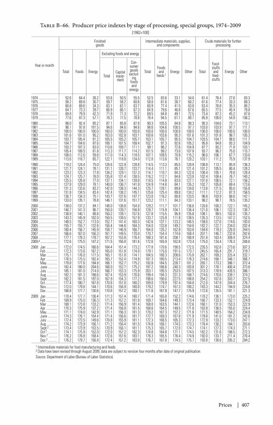
Prices | 407
Table B–66. Producer price indexes by stage of processing, special groups, 1974–2009[1982=100]
Year or month
Finishedgoods
Intermediate materials, supplies,and components
Crude materials for furtherprocessing
Total Foods Energy
Excluding foods and energy
TotalFoodsand
feeds 1Energy Other Total
Food-stuffsand
feed-stuffs
Energy OtherTotal
Capitalequip-ment
Con-sumergoods
exclud-ing
foodsand
energy
1974 ...................... 52.6 64.4 26.2 53.6 50.5 55.5 52.5 83.6 33.1 54.0 61.4 76.4 27.8 83.31975 ...................... 58.2 69.8 30.7 59.7 58.2 60.6 58.0 81.6 38.7 60.2 61.6 77.4 33.3 69.31976 ...................... 60.8 69.6 34.3 63.1 62.1 63.7 60.9 77.4 41.5 63.8 63.4 76.8 35.3 80.21977 ...................... 64.7 73.3 39.7 66.9 66.1 67.3 64.9 79.6 46.8 67.6 65.5 77.5 40.4 79.81978 ...................... 69.8 79.9 42.3 71.9 71.3 72.2 69.5 84.8 49.1 72.5 73.4 87.3 45.2 87.81979 ...................... 77.6 87.3 57.1 78.3 77.5 78.8 78.4 94.5 61.1 80.7 85.9 100.0 54.9 106.21980 ...................... 88.0 92.4 85.2 87.1 85.8 87.8 90.3 105.5 84.9 90.3 95.3 104.6 73.1 113.11981 ...................... 96.1 97.8 101.5 94.6 94.6 94.6 98.6 104.6 100.5 97.7 103.0 103.9 97.7 111.71982 ...................... 100.0 100.0 100.0 100.0 100.0 100.0 100.0 100.0 100.0 100.0 100.0 100.0 100.0 100.01983 ...................... 101.6 101.0 95.2 103.0 102.8 103.1 100.6 103.6 95.3 101.6 101.3 101.8 98.7 105.31984 ...................... 103.7 105.4 91.2 105.5 105.2 105.7 103.1 105.7 95.5 104.7 103.5 104.7 98.0 111.71985 ...................... 104.7 104.6 87.6 108.1 107.5 108.4 102.7 97.3 92.6 105.2 95.8 94.8 93.3 104.91986 ...................... 103.2 107.3 63.0 110.6 109.7 111.1 99.1 96.2 72.6 104.9 87.7 93.2 71.8 103.11987 ...................... 105.4 109.5 61.8 113.3 111.7 114.2 101.5 99.2 73.0 107.8 93.7 96.2 75.0 115.71988 ...................... 108.0 112.6 59.8 117.0 114.3 118.5 107.1 109.5 70.9 115.2 96.0 106.1 67.7 133.01989 ...................... 113.6 118.7 65.7 122.1 118.8 124.0 112.0 113.8 76.1 120.2 103.1 111.2 75.9 137.91990 ...................... 119.2 124.4 75.0 126.6 122.9 128.8 114.5 113.3 85.5 120.9 108.9 113.1 85.9 136.31991 ...................... 121.7 124.1 78.1 131.1 126.7 133.7 114.4 111.1 85.1 121.4 101.2 105.5 80.4 128.21992 ...................... 123.2 123.3 77.8 134.2 129.1 137.3 114.7 110.7 84.3 122.0 100.4 105.1 78.8 128.41993 ...................... 124.7 125.7 78.0 135.8 131.4 138.5 116.2 112.7 84.6 123.8 102.4 108.4 76.7 140.21994 ...................... 125.5 126.8 77.0 137.1 134.1 139.0 118.5 114.8 83.0 127.1 101.8 106.5 72.1 156.21995 ...................... 127.9 129.0 78.1 140.0 136.7 141.9 124.9 114.8 84.1 135.2 102.7 105.8 69.4 173.61996 ...................... 131.3 133.6 83.2 142.0 138.3 144.3 125.7 128.1 89.8 134.0 113.8 121.5 85.0 155.81997 ...................... 131.8 134.5 83.4 142.4 138.2 145.1 125.6 125.4 89.0 134.2 111.1 112.2 87.3 156.51998 ...................... 130.7 134.3 75.1 143.7 137.6 147.7 123.0 116.2 80.8 133.5 96.8 103.9 68.6 142.11999 ...................... 133.0 135.1 78.8 146.1 137.6 151.7 123.2 111.1 84.3 133.1 98.2 98.7 78.5 135.22000 ...................... 138.0 137.2 94.1 148.0 138.8 154.0 129.2 111.7 101.7 136.6 120.6 100.2 122.1 145.22001 ...................... 140.7 141.3 96.7 150.0 139.7 156.9 129.7 115.9 104.1 136.4 121.0 106.1 122.3 130.72002 ...................... 138.9 140.1 88.8 150.2 139.1 157.6 127.8 115.5 95.9 135.8 108.1 99.5 102.0 135.72003 ...................... 143.3 145.9 102.0 150.5 139.5 157.9 133.7 125.9 111.9 138.5 135.3 113.5 147.2 152.52004 ...................... 148.5 152.7 113.0 152.7 141.4 160.3 142.6 137.1 123.2 146.5 159.0 127.0 174.6 193.02005 ...................... 155.7 155.7 132.6 156.4 144.6 164.3 154.0 133.8 149.2 154.6 182.2 122.7 234.0 202.42006 ...................... 160.4 156.7 145.9 158.7 146.9 166.7 164.0 135.2 162.8 163.8 184.8 119.3 226.9 244.52007 ...................... 166.6 167.0 156.3 161.7 149.5 170.0 170.7 154.4 174.6 168.4 207.1 146.7 232.8 282.62008 ...................... 177.1 178.3 178.7 167.2 153.8 176.4 188.3 181.6 208.1 180.9 251.8 163.4 309.4 324.42009 p .................... 172.6 175.5 147.2 171.5 156.8 181.6 172.6 165.9 162.8 173.4 175.0 134.4 176.3 248.62008: Jan ............. 172.0 174.5 166.6 164.4 151.4 173.2 177.8 170.6 190.5 172.5 235.5 162.6 273.6 307.3
Feb ............. 172.3 173.6 167.2 165.0 151.8 174.0 179.1 175.0 191.5 173.7 245.5 165.4 291.7 319.7Mar ............ 175.1 176.0 177.5 165.1 151.8 174.1 184.5 180.3 208.6 175.8 262.1 169.2 325.4 332.1Apr ............. 176.5 175.5 182.4 165.7 152.4 174.8 187.3 180.5 213.4 178.3 274.6 168.1 346.1 366.7May ............ 179.8 177.6 194.8 166.1 152.7 175.2 192.8 184.5 228.7 181.2 293.1 173.2 386.1 372.4June ........... 182.4 180.0 204.6 166.0 152.7 175.2 197.2 186.6 240.3 183.8 301.2 178.1 400.4 373.8July ............ 185.1 181.0 214.0 166.7 153.3 175.9 203.1 195.5 253.5 187.5 313.3 178.9 426.5 386.1Aug ............. 182.2 181.3 198.6 167.4 153.9 176.6 199.4 194.3 231.3 188.7 274.6 170.6 339.1 374.2Sept ............ 182.2 181.5 197.0 167.9 154.3 177.2 198.6 190.0 227.5 188.8 254.2 167.6 303.7 337.5Oct .............. 177.4 180.7 167.8 170.8 157.0 180.2 189.0 179.9 197.4 184.8 212.0 147.9 244.4 276.7Nov ............. 172.0 179.8 144.1 170.6 156.9 180.0 179.2 174.7 167.3 180.2 183.3 144.2 194.9 224.8Dec ............. 168.8 177.7 130.6 170.8 157.2 180.1 171.6 167.9 147.7 175.9 172.6 135.5 181.1 221.3
2009: Jan ............. 170.4 177.7 136.4 171.3 157.4 180.7 171.4 165.8 152.2 174.6 170.2 136.1 173.0 225.2Feb ............. 169.9 175.0 136.3 171.3 157.2 181.0 169.7 164.6 149.3 173.4 160.7 133.3 152.1 224.9Mar ............ 169.1 173.8 133.2 171.4 156.9 181.4 168.0 163.5 144.1 172.6 160.1 131.0 153.3 222.9Apr ............. 170.3 175.9 137.2 171.4 156.8 181.5 168.6 164.5 149.5 171.8 163.9 136.5 155.0 224.4May ............ 171.1 174.0 142.9 171.1 156.3 181.3 170.2 167.3 157.2 171.6 171.5 140.5 164.2 234.9June ........... 174.3 176.1 154.4 171.4 156.6 181.7 172.7 169.3 167.8 171.9 179.8 141.0 181.2 242.6July ............ 172.4 173.5 149.6 170.8 155.9 181.1 172.3 166.5 165.3 172.3 172.9 133.2 173.0 247.1Aug ............. 174.2 173.9 156.1 171.2 156.4 181.5 174.8 166.1 174.5 173.3 178.4 130.2 184.1 263.6Sept 2 ......... 173.4 173.9 153.5 170.9 156.1 181.1 175.3 165.7 172.0 174.7 174.1 127.3 174.3 271.1Oct 2 ........... 174.1 175.9 152.0 172.0 157.2 182.3 174.8 164.8 171.1 174.5 182.2 131.6 188.5 272.3Nov 2 .......... 176.2 176.8 158.4 172.6 157.6 183.1 176.3 165.5 176.4 174.9 192.0 133.7 211.4 270.4Dec 2 ........... 176.2 179.7 156.8 172.4 157.2 183.0 176.7 167.8 174.5 175.7 193.8 138.6 205.2 284.2
1 Intermediate materials for food manufacturing and feeds.2 Data have been revised through August 2009; data are subject to revision four months after date of original publication.Source: Department of Labor (Bureau of Labor Statistics).
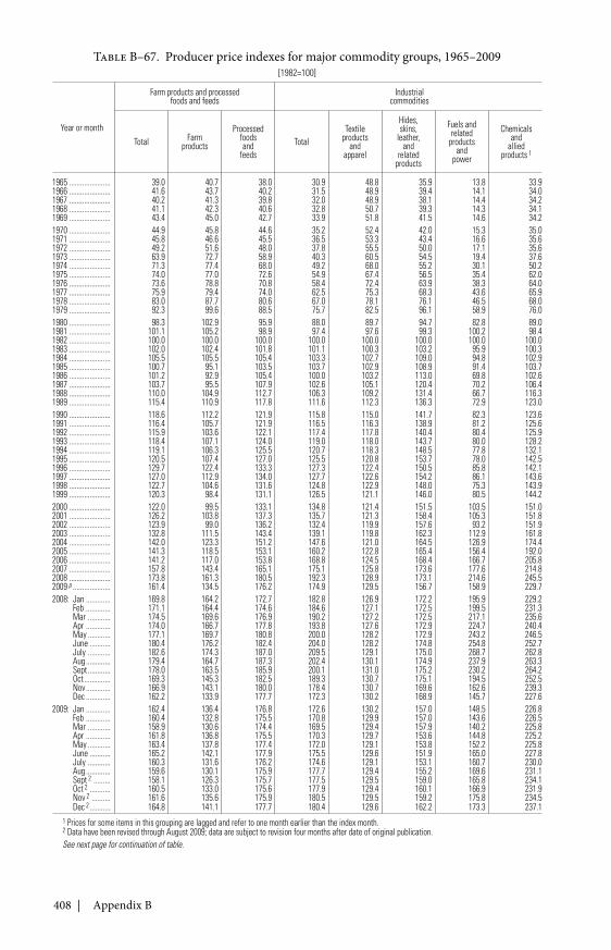
408 | Appendix B
Table B–67. Producer price indexes for major commodity groups, 1965–2009[1982=100]
Year or month
Farm products and processedfoods and feeds
Industrialcommodities
Total Farmproducts
Processedfoodsand
feedsTotal
Textileproducts
andapparel
Hides,skins,
leather,and
relatedproducts
Fuels andrelated
productsand
power
Chemicalsand
alliedproducts 1
1965 ...................... 39.0 40.7 38.0 30.9 48.8 35.9 13.8 33.91966 ...................... 41.6 43.7 40.2 31.5 48.9 39.4 14.1 34.01967 ...................... 40.2 41.3 39.8 32.0 48.9 38.1 14.4 34.21968 ...................... 41.1 42.3 40.6 32.8 50.7 39.3 14.3 34.11969 ...................... 43.4 45.0 42.7 33.9 51.8 41.5 14.6 34.21970 ...................... 44.9 45.8 44.6 35.2 52.4 42.0 15.3 35.01971 ...................... 45.8 46.6 45.5 36.5 53.3 43.4 16.6 35.61972 ...................... 49.2 51.6 48.0 37.8 55.5 50.0 17.1 35.61973 ...................... 63.9 72.7 58.9 40.3 60.5 54.5 19.4 37.61974 ...................... 71.3 77.4 68.0 49.2 68.0 55.2 30.1 50.21975 ...................... 74.0 77.0 72.6 54.9 67.4 56.5 35.4 62.01976 ...................... 73.6 78.8 70.8 58.4 72.4 63.9 38.3 64.01977 ...................... 75.9 79.4 74.0 62.5 75.3 68.3 43.6 65.91978 ...................... 83.0 87.7 80.6 67.0 78.1 76.1 46.5 68.01979 ...................... 92.3 99.6 88.5 75.7 82.5 96.1 58.9 76.01980 ...................... 98.3 102.9 95.9 88.0 89.7 94.7 82.8 89.01981 ...................... 101.1 105.2 98.9 97.4 97.6 99.3 100.2 98.41982 ...................... 100.0 100.0 100.0 100.0 100.0 100.0 100.0 100.01983 ...................... 102.0 102.4 101.8 101.1 100.3 103.2 95.9 100.31984 ...................... 105.5 105.5 105.4 103.3 102.7 109.0 94.8 102.91985 ...................... 100.7 95.1 103.5 103.7 102.9 108.9 91.4 103.71986 ...................... 101.2 92.9 105.4 100.0 103.2 113.0 69.8 102.61987 ...................... 103.7 95.5 107.9 102.6 105.1 120.4 70.2 106.41988 ...................... 110.0 104.9 112.7 106.3 109.2 131.4 66.7 116.31989 ...................... 115.4 110.9 117.8 111.6 112.3 136.3 72.9 123.01990 ...................... 118.6 112.2 121.9 115.8 115.0 141.7 82.3 123.61991 ...................... 116.4 105.7 121.9 116.5 116.3 138.9 81.2 125.61992 ...................... 115.9 103.6 122.1 117.4 117.8 140.4 80.4 125.91993 ...................... 118.4 107.1 124.0 119.0 118.0 143.7 80.0 128.21994 ...................... 119.1 106.3 125.5 120.7 118.3 148.5 77.8 132.11995 ...................... 120.5 107.4 127.0 125.5 120.8 153.7 78.0 142.51996 ...................... 129.7 122.4 133.3 127.3 122.4 150.5 85.8 142.11997 ...................... 127.0 112.9 134.0 127.7 122.6 154.2 86.1 143.61998 ...................... 122.7 104.6 131.6 124.8 122.9 148.0 75.3 143.91999 ...................... 120.3 98.4 131.1 126.5 121.1 146.0 80.5 144.22000 ...................... 122.0 99.5 133.1 134.8 121.4 151.5 103.5 151.02001 ...................... 126.2 103.8 137.3 135.7 121.3 158.4 105.3 151.82002 ...................... 123.9 99.0 136.2 132.4 119.9 157.6 93.2 151.92003 ...................... 132.8 111.5 143.4 139.1 119.8 162.3 112.9 161.82004 ...................... 142.0 123.3 151.2 147.6 121.0 164.5 126.9 174.42005 ...................... 141.3 118.5 153.1 160.2 122.8 165.4 156.4 192.02006 ...................... 141.2 117.0 153.8 168.8 124.5 168.4 166.7 205.82007 ...................... 157.8 143.4 165.1 175.1 125.8 173.6 177.6 214.82008 ...................... 173.8 161.3 180.5 192.3 128.9 173.1 214.6 245.52009 p .................... 161.4 134.5 176.2 174.9 129.5 156.7 158.9 229.72008: Jan ............. 169.8 164.2 172.7 182.8 126.9 172.2 195.9 229.2
Feb ............. 171.1 164.4 174.6 184.6 127.1 172.5 199.5 231.3Mar ............ 174.5 169.6 176.9 190.2 127.2 172.5 217.1 235.6Apr ............. 174.0 166.7 177.8 193.8 127.6 172.9 224.7 240.4May ............ 177.1 169.7 180.8 200.0 128.2 172.9 243.2 246.5June ........... 180.4 176.2 182.4 204.0 128.2 174.8 254.8 252.7July ............ 182.6 174.3 187.0 209.5 129.1 175.0 268.7 262.8Aug ............. 179.4 164.7 187.3 202.4 130.1 174.9 237.9 263.3Sept ............ 178.0 163.5 185.9 200.1 131.0 175.2 230.2 264.2Oct .............. 169.3 145.3 182.5 189.3 130.7 175.1 194.5 252.5Nov ............. 166.9 143.1 180.0 178.4 130.7 169.6 162.6 239.3Dec ............. 162.2 133.9 177.7 172.3 130.2 168.9 145.7 227.6
2009: Jan ............. 162.4 136.4 176.8 172.6 130.2 157.0 148.5 226.8Feb ............. 160.4 132.8 175.5 170.8 129.9 157.0 143.6 226.5Mar ............ 158.9 130.6 174.4 169.5 129.4 157.9 140.2 225.8Apr ............. 161.8 136.8 175.5 170.3 129.7 153.6 144.8 225.2May ............ 163.4 137.8 177.4 172.0 129.1 153.8 152.2 225.8June ........... 165.2 142.1 177.9 175.5 129.6 151.9 165.0 227.8July ............ 160.3 131.6 176.2 174.6 129.1 153.1 160.7 230.0Aug ............. 159.6 130.1 175.9 177.7 129.4 155.2 169.6 231.1Sept 2 ......... 158.1 126.3 175.7 177.5 129.5 159.0 165.8 234.1Oct 2 ........... 160.5 133.0 175.6 177.9 129.4 160.1 166.9 231.9Nov 2 .......... 161.6 135.6 175.9 180.5 129.5 159.2 175.8 234.5Dec 2 ........... 164.8 141.1 177.7 180.4 129.6 162.2 173.3 237.1
1 Prices for some items in this grouping are lagged and refer to one month earlier than the index month.2 Data have been revised through August 2009; data are subject to revision four months after date of original publication.See next page for continuation of table.
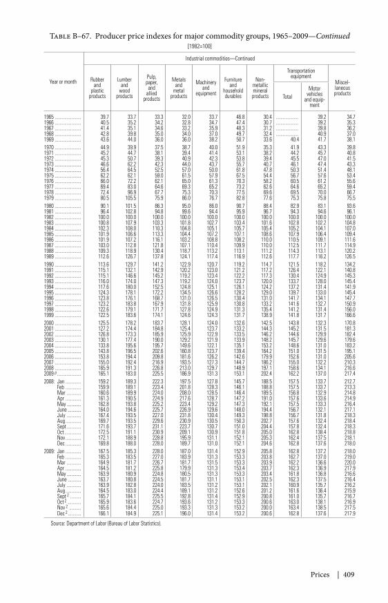
Prices | 409
Table B–67. Producer price indexes for major commodity groups, 1965–2009—Continued[1982=100]
Year or month
Industrial commodities—Continued
Rubberand
plasticproducts
Lumberand
woodproducts
Pulp,paper,and
alliedproducts
Metalsand
metalproducts
Machineryand
equipment
Furnitureand
householddurables
Non-metallicmineralproducts
Transportationequipment
Miscel-laneousproductsTotal
Motorvehicles
and equip-ment
1965 ...................... 39.7 33.7 33.3 32.0 33.7 46.8 30.4 ................... 39.2 34.71966 ...................... 40.5 35.2 34.2 32.8 34.7 47.4 30.7 ................... 39.2 35.31967 ...................... 41.4 35.1 34.6 33.2 35.9 48.3 31.2 ................... 39.8 36.21968 ...................... 42.8 39.8 35.0 34.0 37.0 49.7 32.4 ................... 40.9 37.01969 ...................... 43.6 44.0 36.0 36.0 38.2 50.7 33.6 40.4 41.7 38.11970 ...................... 44.9 39.9 37.5 38.7 40.0 51.9 35.3 41.9 43.3 39.81971 ...................... 45.2 44.7 38.1 39.4 41.4 53.1 38.2 44.2 45.7 40.81972 ...................... 45.3 50.7 39.3 40.9 42.3 53.8 39.4 45.5 47.0 41.51973 ...................... 46.6 62.2 42.3 44.0 43.7 55.7 40.7 46.1 47.4 43.31974 ...................... 56.4 64.5 52.5 57.0 50.0 61.8 47.8 50.3 51.4 48.11975 ...................... 62.2 62.1 59.0 61.5 57.9 67.5 54.4 56.7 57.6 53.41976 ...................... 66.0 72.2 62.1 65.0 61.3 70.3 58.2 60.5 61.2 55.61977 ...................... 69.4 83.0 64.6 69.3 65.2 73.2 62.6 64.6 65.2 59.41978 ...................... 72.4 96.9 67.7 75.3 70.3 77.5 69.6 69.5 70.0 66.71979 ...................... 80.5 105.5 75.9 86.0 76.7 82.8 77.6 75.3 75.8 75.51980 ...................... 90.1 101.5 86.3 95.0 86.0 90.7 88.4 82.9 83.1 93.61981 ...................... 96.4 102.8 94.8 99.6 94.4 95.9 96.7 94.3 94.6 96.11982 ...................... 100.0 100.0 100.0 100.0 100.0 100.0 100.0 100.0 100.0 100.01983 ...................... 100.8 107.9 103.3 101.8 102.7 103.4 101.6 102.8 102.2 104.81984 ...................... 102.3 108.0 110.3 104.8 105.1 105.7 105.4 105.2 104.1 107.01985 ...................... 101.9 106.6 113.3 104.4 107.2 107.1 108.6 107.9 106.4 109.41986 ...................... 101.9 107.2 116.1 103.2 108.8 108.2 110.0 110.5 109.1 111.61987 ...................... 103.0 112.8 121.8 107.1 110.4 109.9 110.0 112.5 111.7 114.91988 ...................... 109.3 118.9 130.4 118.7 113.2 113.1 111.2 114.3 113.1 120.21989 ...................... 112.6 126.7 137.8 124.1 117.4 116.9 112.6 117.7 116.2 126.51990 ...................... 113.6 129.7 141.2 122.9 120.7 119.2 114.7 121.5 118.2 134.21991 ...................... 115.1 132.1 142.9 120.2 123.0 121.2 117.2 126.4 122.1 140.81992 ...................... 115.1 146.6 145.2 119.2 123.4 122.2 117.3 130.4 124.9 145.31993 ...................... 116.0 174.0 147.3 119.2 124.0 123.7 120.0 133.7 128.0 145.41994 ...................... 117.6 180.0 152.5 124.8 125.1 126.1 124.2 137.2 131.4 141.91995 ...................... 124.3 178.1 172.2 134.5 126.6 128.2 129.0 139.7 133.0 145.41996 ...................... 123.8 176.1 168.7 131.0 126.5 130.4 131.0 141.7 134.1 147.71997 ...................... 123.2 183.8 167.9 131.8 125.9 130.8 133.2 141.6 132.7 150.91998 ...................... 122.6 179.1 171.7 127.8 124.9 131.3 135.4 141.2 131.4 156.01999 ...................... 122.5 183.6 174.1 124.6 124.3 131.7 138.9 141.8 131.7 166.62000 ...................... 125.5 178.2 183.7 128.1 124.0 132.6 142.5 143.8 132.3 170.82001 ...................... 127.2 174.4 184.8 125.4 123.7 133.2 144.3 145.2 131.5 181.32002 ...................... 126.8 173.3 185.9 125.9 122.9 133.5 146.2 144.6 129.9 182.42003 ...................... 130.1 177.4 190.0 129.2 121.9 133.9 148.2 145.7 129.6 179.62004 ...................... 133.8 195.6 195.7 149.6 122.1 135.1 153.2 148.6 131.0 183.22005 ...................... 143.8 196.5 202.6 160.8 123.7 139.4 164.2 151.0 131.5 195.12006 ...................... 153.8 194.4 209.8 181.6 126.2 142.6 179.9 152.6 131.0 205.62007 ...................... 155.0 192.4 216.9 193.5 127.3 144.7 186.2 155.0 132.2 210.32008 ...................... 165.9 191.3 226.8 213.0 129.7 148.9 197.1 158.6 134.1 216.62009 p .................... 165.1 183.0 225.5 186.9 131.3 153.1 202.4 162.2 137.0 217.42008: Jan ............. 159.2 189.3 222.3 197.5 127.8 145.7 188.5 157.5 133.7 212.7
Feb ............. 159.9 189.1 223.4 201.8 128.3 146.1 188.8 157.5 133.7 213.3Mar ............ 160.6 189.9 224.0 208.0 128.5 146.4 189.5 156.8 132.9 214.8Apr ............. 161.3 190.5 224.9 217.6 128.7 147.2 191.0 157.6 133.6 214.9May ............ 162.8 193.8 225.2 223.4 129.2 147.3 192.1 157.5 133.3 216.4June ........... 164.0 194.6 225.7 226.9 129.6 148.0 194.4 156.7 132.1 217.1July ............ 167.4 193.5 227.0 231.8 130.4 149.3 198.8 156.7 131.8 218.3Aug ............. 169.7 193.5 229.6 230.9 130.5 150.3 202.7 157.6 132.4 218.4Sept ............ 171.6 193.7 231.1 223.7 130.7 151.0 204.4 157.8 132.4 218.3Oct .............. 172.5 191.1 230.9 209.1 130.9 151.8 205.0 162.8 138.4 218.8Nov ............. 172.1 188.9 228.8 195.9 131.1 152.1 205.3 162.4 137.5 218.1Dec ............. 169.8 188.0 228.0 189.7 131.0 152.1 204.6 162.8 137.6 218.0
2009: Jan ............. 167.5 185.3 228.0 187.0 131.4 152.9 205.8 162.8 137.2 218.0Feb ............. 165.3 183.5 227.0 183.9 131.3 153.3 203.8 162.7 137.0 219.0Mar ............ 164.9 181.7 226.7 181.7 131.5 153.3 203.9 162.2 136.6 220.0Apr ............. 164.5 181.2 225.8 179.9 131.3 153.4 203.7 162.3 136.9 217.9May ............ 163.9 180.9 224.8 180.5 131.3 153.3 203.4 161.8 136.8 216.6June ........... 163.7 180.8 224.5 181.7 131.1 153.1 202.5 162.3 137.5 216.4July ............ 163.9 182.8 224.0 183.5 131.2 153.1 202.1 160.9 135.7 216.2Aug ............. 164.5 183.0 224.4 189.1 131.2 152.6 201.2 161.6 136.4 215.9Sept 2 ......... 165.7 184.1 225.5 192.8 131.4 152.9 200.8 161.0 135.7 216.7Oct 2 ........... 165.9 183.6 224.7 193.6 131.2 153.3 200.6 163.0 138.1 216.9Nov 2 .......... 165.6 184.4 225.0 193.3 131.3 153.2 200.0 163.4 138.5 217.5Dec 2 ........... 166.1 184.9 225.1 196.0 131.4 153.2 200.6 162.8 137.6 217.9
Source: Department of Labor (Bureau of Labor Statistics).
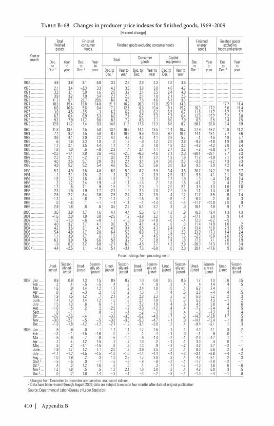
410 | Appendix B
Table B–68. Changes in producer price indexes for finished goods, 1969–2009[Percent change]
Year ormonth
Totalfinishedgoods
Finishedconsumer
foodsFinished goods excluding consumer foods
Finishedenergygoods
Finished goodsexcluding
foods and energy
Dec.to
Dec. 1
Yearto
year
Dec.to
Dec. 1
Yearto
year
Total Consumergoods
Capitalequipment Dec.
toDec. 1
Yearto
year
Dec.to
Dec. 1
Yearto
yearDec. toDec. 1
Year toyear
Dec. toDec. 1
Year toyear
Dec. toDec. 1
Year toyear
1969 ............... 4.9 3.8 8.1 6.0 3.3 2.8 2.8 2.3 4.8 3.5 ............. ............. ............. .............1970 ............... 2.1 3.4 –2.3 3.3 4.3 3.5 3.8 3.0 4.8 4.7 ............. ............. ............. .............1971 ............... 3.3 3.1 5.8 1.6 2.0 3.7 2.1 3.5 2.4 4.0 ............. ............. ............. .............1972 ............... 3.9 3.2 7.9 5.4 2.3 2.0 2.1 1.8 2.1 2.6 ............. ............. ............. .............1973 ............... 11.7 9.1 22.7 20.5 6.6 4.0 7.5 4.6 5.1 3.3 ............. ............. ............. .............1974 ............... 18.3 15.4 12.8 14.0 21.1 16.2 20.3 17.0 22.7 14.3 ............. ............. 17.7 11.41975 ............... 6.6 10.6 5.6 8.4 7.2 12.1 6.8 10.4 8.1 15.2 16.3 17.2 6.0 11.41976 ............... 3.8 4.5 –2.5 –.3 6.2 6.2 6.0 6.2 6.5 6.7 11.6 11.7 5.7 5.71977 ............... 6.7 6.4 6.9 5.3 6.8 7.1 6.7 7.3 7.2 6.4 12.0 15.7 6.2 6.01978 ............... 9.3 7.9 11.7 9.0 8.3 7.2 8.5 7.1 8.0 7.9 8.5 6.5 8.4 7.51979 ............... 12.8 11.2 7.4 9.3 14.8 11.8 17.6 13.3 8.8 8.7 58.1 35.0 9.4 8.91980 ............... 11.8 13.4 7.5 5.8 13.4 16.2 14.1 18.5 11.4 10.7 27.9 49.2 10.8 11.21981 ............... 7.1 9.2 1.5 5.8 8.7 10.3 8.6 10.3 9.2 10.3 14.1 19.1 7.7 8.61982 ............... 3.6 4.1 2.0 2.2 4.2 4.6 4.2 4.1 3.9 5.7 –.1 –1.5 4.9 5.71983 ............... .6 1.6 2.3 1.0 .0 1.8 –.9 1.2 2.0 2.8 –9.2 –4.8 1.9 3.01984 ............... 1.7 2.1 3.5 4.4 1.1 1.4 .8 1.0 1.8 2.3 –4.2 –4.2 2.0 2.41985 ............... 1.8 1.0 .6 –.8 2.2 1.4 2.1 1.1 2.7 2.2 –.2 –3.9 2.7 2.51986 ............... –2.3 –1.4 2.8 2.6 –4.0 –2.6 –6.6 –4.6 2.1 2.0 –38.1 –28.1 2.7 2.31987 ............... 2.2 2.1 –.2 2.1 3.2 2.1 4.1 2.2 1.3 1.8 11.2 –1.9 2.1 2.41988 ............... 4.0 2.5 5.7 2.8 3.2 2.4 3.1 2.4 3.6 2.3 –3.6 –3.2 4.3 3.31989 ............... 4.9 5.2 5.2 5.4 4.8 5.0 5.3 5.6 3.8 3.9 9.5 9.9 4.2 4.41990 ............... 5.7 4.9 2.6 4.8 6.9 5.0 8.7 5.9 3.4 3.5 30.7 14.2 3.5 3.71991 ............... –.1 2.1 –1.5 –.2 .3 3.0 –.7 2.9 2.5 3.1 –9.6 4.1 3.1 3.61992 ............... 1.6 1.2 1.6 –.6 1.6 1.8 1.6 1.8 1.7 1.9 –.3 –.4 2.0 2.41993 ............... .2 1.2 2.4 1.9 –.4 1.1 –1.4 .7 1.8 1.8 –4.1 .3 .4 1.21994 ............... 1.7 .6 1.1 .9 1.9 .6 2.0 –.1 2.0 2.1 3.5 –1.3 1.6 1.01995 ............... 2.3 1.9 1.9 1.7 2.3 1.9 2.3 2.0 2.2 1.9 1.1 1.4 2.6 2.11996 ............... 2.8 2.7 3.4 3.6 2.6 2.4 3.7 2.9 .4 1.2 11.7 6.5 .6 1.41997 ............... –1.2 .4 –.8 .7 –1.2 .3 –1.5 .5 –.6 –.1 –6.4 .2 .0 .31998 ............... .0 –.8 .1 –.1 –.1 –1.1 –.1 –1.4 .0 –.4 –11.7 –10.0 2.5 .91999 ............... 2.9 1.8 .8 .6 3.5 2.2 5.1 3.2 .3 .0 18.1 4.9 .9 1.72000 ............... 3.6 3.8 1.7 1.6 4.1 4.4 5.5 6.1 1.2 .9 16.6 19.4 1.3 1.32001 ............... –1.6 2.0 1.8 3.0 –2.6 1.7 –3.9 2.2 .0 .6 –17.1 2.8 .9 1.42002 ............... 1.2 –1.3 –.6 –.8 1.7 –1.5 2.9 –1.8 –.6 –.4 12.3 –8.2 –.5 .12003 ............... 4.0 3.2 7.7 4.1 3.0 3.0 4.1 4.3 .8 .3 11.4 14.9 1.0 .22004 ............... 4.2 3.6 3.1 4.7 4.5 3.4 5.5 4.3 2.4 1.4 13.4 10.8 2.3 1.52005 ............... 5.4 4.8 1.7 2.0 6.4 5.6 8.8 7.3 1.2 2.3 23.9 17.3 1.4 2.42006 ............... 1.1 3.0 1.7 .6 1.0 3.5 .4 4.5 2.3 1.6 –2.0 10.0 2.0 1.52007 ............... 6.2 3.9 7.6 6.6 5.8 3.2 7.7 3.8 1.4 1.8 17.8 7.1 2.0 1.92008 ............... –.9 6.3 3.2 6.8 –2.1 6.3 –4.8 7.7 4.3 2.9 –20.3 14.3 4.5 3.42009 p ............. 4.4 –2.5 1.1 –1.6 5.1 –3.1 7.6 –5.0 .0 2.0 20.1 –17.6 .9 2.6
Percent change from preceding month
Unad-justed
Season-ally ad-justed
Unad-justed
Season-ally ad-justed
Unad-justed
Season-ally ad-justed
Unad-justed
Season-ally ad-justed
Unad-justed
Season-ally ad-justed
Unad-justed
Season-ally ad-justed
Unad-justed
Season-ally ad-justed
2008: Jan ...... 0.9 0.9 1.3 1.5 0.8 0.7 1.0 0.8 0.5 0.5 1.7 1.3 0.6 0.5Feb ...... .2 .4 –.5 –.5 .4 .8 .4 .9 .3 .4 .4 1.4 .4 .5Mar ..... 1.6 .9 1.4 1.2 1.7 .7 2.4 1.0 .0 .1 6.2 2.4 .1 .1Apr ...... .8 .2 –.3 .2 1.0 .2 1.3 .1 .4 .5 2.8 –.4 .4 .5May ..... 1.9 1.5 1.2 .7 2.1 1.7 2.8 2.3 .2 .3 6.8 5.2 .2 .3June .... 1.4 1.3 1.4 1.2 1.5 1.3 2.1 1.8 .0 .3 5.0 4.3 –.1 .2July ..... 1.5 1.3 .6 .6 1.7 1.5 2.2 1.9 .4 .5 4.6 3.8 .4 .6Aug ...... –1.6 –.5 .2 .2 –2.0 –.7 –2.9 –1.2 .4 .4 –7.2 –3.4 .4 .5Sept ..... .0 –.1 .1 .0 –.1 –.1 –.2 –.3 .3 .4 –.8 –1.3 .3 .4Oct ....... –2.6 –2.6 –.4 .1 –3.2 –3.3 –5.2 –4.9 1.7 .6 –14.8 –12.8 1.7 .5Nov ...... –3.0 –2.7 –.5 –.5 –3.8 –3.3 –5.3 –4.7 –.1 .0 –14.1 –12.4 –.1 .0Dec ...... –1.9 –1.8 –1.2 –1.2 –2.1 –1.9 –3.1 –3.0 .2 .4 –9.4 –9.1 .1 .3
2009: Jan ...... .9 .9 .0 .1 1.1 1.1 1.7 1.6 .1 .1 4.4 4.1 .3 .2Feb ...... –.3 –.1 –1.5 –1.6 .0 .3 .1 .4 –.1 .0 –.1 .9 .0 .1Mar ..... –.5 –.9 –.7 –.8 –.5 –1.0 –.6 –1.4 –.2 –.1 –2.3 –4.7 .1 .1Apr ...... .7 .4 1.2 1.5 .7 .2 1.0 .2 –.1 .1 3.0 .4 .0 .1May ..... .5 .2 –1.1 –1.5 .8 .5 1.3 .9 –.3 –.2 4.2 2.7 –.2 –.1June .... 1.9 1.7 1.2 1.1 2.0 1.8 2.9 2.5 .2 .4 8.0 6.6 .2 .4July ..... –1.1 –1.2 –1.5 –1.5 –1.0 –1.0 –1.4 –1.4 –.4 –.3 –3.1 –3.8 –.4 –.2Aug ...... 1.0 1.9 .2 .3 1.2 2.2 1.7 3.0 .3 .4 4.3 8.1 .2 .3Sept 2 .. –.5 –.5 .0 –.1 –.5 –.6 –.8 –.8 –.2 –.1 –1.7 –2.0 –.2 –.1Oct 2 .... .4 .3 1.2 1.6 .2 .0 .1 .3 .7 –.7 –1.0 1.6 .6 –.6Nov 2 ... 1.2 1.8 .5 .5 1.3 2.1 1.8 3.0 .3 .4 4.2 6.9 .3 .5Dec 2 .... .0 .2 1.6 1.4 –.3 –.1 –.4 –.2 –.3 –.1 –1.0 –.4 –.1 .0
1 Changes from December to December are based on unadjusted indexes.2 Data have been revised through August 2009; data are subject to revision four months after date of original publication.Source: Department of Labor (Bureau of Labor Statistics).
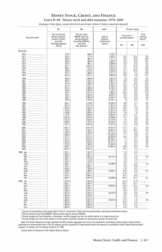
Money Stock, Credit, and Finance | 411
Table B–69. Money stock and debt measures, 1970–2009[Averages of daily figures, except debt end-of-period basis; billions of dollars, seasonally adjusted]
Year and month
M1 M2 Debt 1 Percent change
Sum of currency,demand deposits,travelers checks,
and othercheckable deposits
(OCDs)
M1 plus retailMMMF balances,savings deposits
(including MMDAs),and small
time deposits 2
Debt ofdomestic
nonfinancialsectors
From year or6 months earlier 3
Frompreviousperiod 4
M1 M2 Debt
December:1970 ........................................ 214.4 626.5 1,420.2 .................. .................. ...................1971 ........................................ 228.3 710.3 1,555.2 6.5 13.4 9.51972 ........................................ 249.2 802.3 1,711.2 9.2 13.0 10.01973 ........................................ 262.9 855.5 1,895.5 5.5 6.6 10.71974 ........................................ 274.2 902.1 2,069.9 4.3 5.4 9.21975 ........................................ 287.1 1,016.2 2,261.8 4.7 12.6 9.31976 ........................................ 306.2 1,152.0 2,505.3 6.7 13.4 10.81977 ........................................ 330.9 1,270.3 2,826.6 8.1 10.3 12.81978 ........................................ 357.3 1,366.0 3,211.2 8.0 7.5 13.81979 ........................................ 381.8 1,473.7 3,603.0 6.9 7.9 12.21980 ........................................ 408.5 1,599.8 3,953.5 7.0 8.6 9.51981 ........................................ 436.7 1,755.5 4,361.7 6.9 9.7 10.41982 ........................................ 474.8 1,909.3 4,783.4 8.7 8.8 10.41983 ........................................ 521.4 2,125.7 5,359.2 9.8 11.3 12.01984 ........................................ 551.6 2,308.8 6,146.2 5.8 8.6 14.81985 ........................................ 619.8 2,494.6 7,123.1 12.4 8.0 15.61986 ........................................ 724.7 2,731.4 7,966.3 16.9 9.5 11.91987 ........................................ 750.2 2,830.8 8,670.1 3.5 3.6 9.01988 ........................................ 786.7 2,993.9 9,450.7 4.9 5.8 9.01989 ........................................ 792.9 3,158.4 10,152.1 .8 5.5 7.21990 ........................................ 824.7 3,276.8 10,834.9 4.0 3.7 6.51991 ........................................ 897.0 3,377.0 11,301.4 8.8 3.1 4.31992 ........................................ 1,024.9 3,430.2 11,816.5 14.3 1.6 4.51993 ........................................ 1,129.6 3,480.7 12,391.4 10.2 1.5 4.71994 ........................................ 1,150.6 3,496.5 12,973.6 1.9 .5 4.61995 ........................................ 1,127.5 3,640.3 13,667.5 –2.0 4.1 5.21996 ........................................ 1,081.6 3,819.6 14,399.8 –4.1 4.9 5.41997 ........................................ 1,072.8 4,033.0 15,210.8 –.8 5.6 5.61998 ........................................ 1,095.8 4,376.3 16,216.4 2.1 8.5 6.61999 ........................................ 1,122.7 4,634.6 17,291.6 2.5 5.9 6.42000 ........................................ 1,087.7 4,917.9 18,167.3 –3.1 6.1 5.02001 ........................................ 1,182.2 5,434.1 19,302.3 8.7 10.5 6.32002 ........................................ 1,220.4 5,785.9 20,710.2 3.2 6.5 7.32003 ........................................ 1,306.9 6,073.7 22,420.4 7.1 5.0 8.12004 ........................................ 1,377.1 6,415.2 24,426.9 5.4 5.6 8.92005 ........................................ 1,375.3 6,679.2 26,756.1 –.1 4.1 9.52006 ........................................ 1,367.9 7,079.5 29,151.3 –.5 6.0 9.02007 ........................................ 1,375.8 7,509.4 31,694.5 .6 6.1 8.72008 ........................................ 1,594.7 8,241.6 33,564.9 15.9 9.8 5.92009 ........................................ 1,693.3 8,524.3 ........................................... 6.2 3.4 ...................
2008: Jan ..................................... 1,381.1 7,542.3 ........................................... 1.8 6.3 ...................Feb ..................................... 1,387.0 7,631.7 ........................................... 2.2 7.1 ...................Mar .................................... 1,389.7 7,691.6 32,131.5 2.5 7.6 5.5Apr ..................................... 1,392.1 7,716.3 ........................................... 1.9 7.3 ...................May .................................... 1,391.5 7,739.0 ........................................... 2.3 7.1 ...................June ................................... 1,398.1 7,751.1 32,395.8 3.2 6.4 3.3July .................................... 1,415.1 7,802.7 ........................................... 4.9 6.9 ...................Aug ..................................... 1,400.0 7,790.6 ........................................... 1.9 4.2 ...................Sept .................................... 1,459.5 7,898.2 33,062.1 10.0 5.4 8.2Oct ...................................... 1,472.7 8,014.7 ........................................... 11.6 7.7 ...................Nov ..................................... 1,518.1 8,065.3 ........................................... 18.2 8.4 ...................Dec ..................................... 1,594.7 8,241.6 33,564.9 28.1 12.7 6.1
2009: Jan ..................................... 1,573.8 8,302.6 ........................................... 22.4 12.8 ...................Feb ..................................... 1,562.1 8,340.7 ........................................... 23.2 14.1 ...................Mar .................................... 1,564.3 8,392.7 33,932.0 14.4 12.5 4.3Apr ..................................... 1,592.7 8,343.7 ........................................... 16.3 8.2 ...................May .................................... 1,593.0 8,416.1 ........................................... 9.9 8.7 ...................June ................................... 1,641.0 8,442.2 34,310.5 5.8 4.9 4.5July .................................... 1,649.9 8,436.5 ........................................... 9.7 3.2 ...................Aug ..................................... 1,648.3 8,413.2 ........................................... 11.0 1.7 ...................Sept .................................... 1,660.8 8,452.3 34,551.9 12.3 1.4 2.8Oct ...................................... 1,673.8 8,481.3 ........................................... 10.2 3.3 ....................Nov ..................................... 1,685.6 8,508.9 ........................................... 11.6 2.2 ....................Dec ..................................... 1,693.3 8,524.3 ........................................... 6.4 1.9 ...................
1 Consists of outstanding credit market debt of the U.S. Government, State and local governments, and private nonfinancial sectors.2 Money market mutual fund (MMMF). Money market deposit account (MMDA).3 Annual changes are from December to December; monthly changes are from six months earlier at a simple annual rate.4 Annual changes are from fourth quarter to fourth quarter. Quarterly changes are from previous quarter at annual rate.Note: The Federal Reserve no longer publishes the M3 monetary aggregate and most of its components. Institutional money market mutual funds is
published as a memorandum item in the H.6 release, and the component on large-denomination time deposits is published in other Federal Reserve Boardreleases. For details, see H.6 release of March 23, 2006.
Source: Board of Governors of the Federal Reserve System.
Money Stock, Credit, and Finance
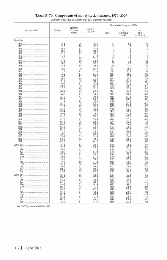
412 | Appendix B
Table B–70. Components of money stock measures, 1970–2009[Averages of daily figures; billions of dollars, seasonally adjusted]
Year and month CurrencyNonbanktravelerschecks
Demanddeposits
Other checkable deposits (OCDs)
TotalAt
commercialbanks
Atthrift
institutions
December:1970 ................................................... 48.6 0.9 164.7 0.1 0.0 0.11971 ................................................... 52.0 1.0 175.1 .2 .0 .21972 ................................................... 56.2 1.2 191.6 .2 .0 .21973 ................................................... 60.8 1.4 200.3 .3 .0 .31974 ................................................... 67.0 1.7 205.1 .4 .2 .41975 ................................................... 72.8 2.1 211.3 .9 .4 .51976 ................................................... 79.5 2.6 221.5 2.7 1.3 1.41977 ................................................... 87.4 2.9 236.4 4.2 1.8 2.31978 ................................................... 96.0 3.3 249.5 8.5 5.3 3.11979 ................................................... 104.8 3.5 256.6 16.8 12.7 4.21980 ................................................... 115.3 3.9 261.2 28.1 20.8 7.31981 ................................................... 122.5 4.1 231.4 78.7 63.0 15.61982 ................................................... 132.5 4.1 234.1 104.1 80.5 23.61983 ................................................... 146.2 4.7 238.5 132.1 97.3 34.81984 ................................................... 156.1 5.0 243.4 147.1 104.7 42.41985 ................................................... 167.7 5.6 266.9 179.5 124.7 54.91986 ................................................... 180.4 6.1 302.9 235.2 161.0 74.21987 ................................................... 196.7 6.6 287.7 259.2 178.2 81.01988 ................................................... 212.0 7.0 287.1 280.6 192.5 88.11989 ................................................... 222.3 6.9 278.6 285.1 197.4 87.71990 ................................................... 246.5 7.7 276.8 293.7 208.7 85.01991 ................................................... 267.1 7.7 289.6 332.5 241.6 90.91992 ................................................... 292.1 8.2 340.0 384.6 280.8 103.81993 ................................................... 321.6 8.0 385.4 414.6 302.6 112.01994 ................................................... 354.5 8.6 383.6 404.0 297.4 106.61995 ................................................... 372.8 9.0 389.0 356.6 249.0 107.61996 ................................................... 394.7 8.8 402.3 275.9 172.1 103.81997 ................................................... 425.4 8.4 393.8 245.2 148.3 96.91998 ................................................... 460.5 8.5 376.7 250.0 143.9 106.11999 ................................................... 517.9 8.6 352.9 243.3 139.7 103.72000 ................................................... 531.2 8.3 309.9 238.4 133.2 105.22001 ................................................... 581.1 8.0 335.7 257.4 142.0 115.42002 ................................................... 626.3 7.8 306.8 279.6 154.3 125.32003 ................................................... 662.5 7.7 326.4 310.3 175.2 135.02004 ................................................... 697.7 7.5 343.5 328.3 187.0 141.32005 ................................................... 724.1 7.2 325.0 319.1 180.9 138.22006 ................................................... 749.6 6.7 305.3 306.3 177.7 128.62007 ................................................... 759.8 6.3 301.9 307.8 174.4 133.52008 ................................................... 815.3 5.5 459.7 314.3 180.2 134.12009 ................................................... 862.1 5.1 441.7 384.5 233.9 150.6
2008: Jan ................................................ 757.2 6.2 306.7 311.0 175.6 135.4Feb ................................................ 757.0 6.2 310.8 313.0 177.2 135.9Mar ............................................... 759.1 6.2 311.8 312.6 177.5 135.1Apr ................................................ 758.8 6.1 314.4 312.8 177.3 135.5May ............................................... 762.7 6.2 309.1 313.4 175.2 138.2June .............................................. 768.4 6.1 311.7 312.0 176.3 135.7July ............................................... 774.9 5.9 320.8 313.5 175.8 137.7Aug ................................................ 776.7 5.9 311.5 306.0 170.1 135.9Sept ............................................... 781.1 5.8 359.6 313.0 175.7 137.3Oct ................................................. 796.6 5.7 360.2 310.2 175.2 135.0Nov ................................................ 806.3 5.6 399.6 306.6 171.5 135.1Dec ................................................ 815.3 5.5 459.7 314.3 180.2 134.1
2009: Jan ................................................ 827.2 5.5 428.4 312.7 177.0 135.7Feb ................................................ 836.8 5.5 397.3 322.4 182.2 140.3Mar ............................................... 842.9 5.4 390.5 325.5 184.5 141.0Apr ................................................ 847.8 5.3 406.2 333.3 191.6 141.6May ............................................... 849.2 5.3 401.9 336.7 195.1 141.5June .............................................. 852.3 5.2 434.0 349.5 210.4 139.1July ............................................... 854.2 5.1 435.7 354.9 215.2 139.8Aug ................................................ 857.7 5.1 426.9 358.6 219.1 139.5Sept ............................................... 861.4 5.1 430.4 363.9 222.2 141.7Oct ................................................. 862.6 5.1 432.2 373.9 226.2 147.6Nov ................................................ 861.7 5.1 434.5 384.3 236.3 148.0Dec ................................................ 862.1 5.1 441.7 384.5 233.9 150.6
See next page for continuation of table.
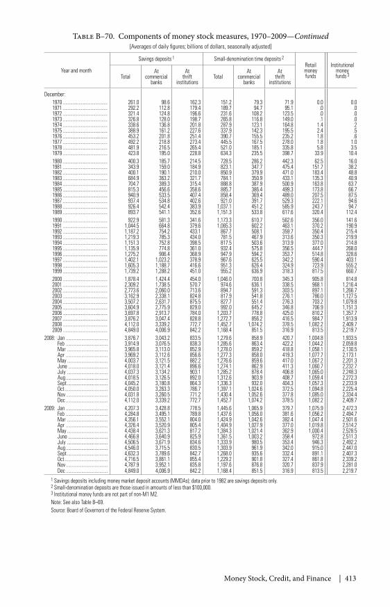
Money Stock, Credit, and Finance | 413
Table B–70. Components of money stock measures, 1970–2009—Continued[Averages of daily figures; billions of dollars, seasonally adjusted]
Year and month
Savings deposits 1 Small-denomination time deposits 2
Retailmoneyfunds
Institutionalmoneyfunds 3Total
Atcommercial
banks
Atthrift
institutionsTotal
Atcommercial
banks
Atthrift
institutions
December:1970 ..................................... 261.0 98.6 162.3 151.2 79.3 71.9 0.0 0.01971 ..................................... 292.2 112.8 179.4 189.7 94.7 95.1 .0 .01972 ..................................... 321.4 124.8 196.6 231.6 108.2 123.5 .0 .01973 ..................................... 326.8 128.0 198.7 265.8 116.8 149.0 .1 .01974 ..................................... 338.6 136.8 201.8 287.9 123.1 164.8 1.4 .21975 ..................................... 388.9 161.2 227.6 337.9 142.3 195.5 2.4 .51976 ..................................... 453.2 201.8 251.4 390.7 155.5 235.2 1.8 .61977 ..................................... 492.2 218.8 273.4 445.5 167.5 278.0 1.8 1.01978 ..................................... 481.9 216.5 265.4 521.0 185.1 335.8 5.8 3.51979 ..................................... 423.8 195.0 228.8 634.3 235.5 398.7 33.9 10.41980 ..................................... 400.3 185.7 214.5 728.5 286.2 442.3 62.5 16.01981 ..................................... 343.9 159.0 184.9 823.1 347.7 475.4 151.7 38.21982 ..................................... 400.1 190.1 210.0 850.9 379.9 471.0 183.4 48.81983 ..................................... 684.9 363.2 321.7 784.1 350.9 433.1 135.3 40.91984 ..................................... 704.7 389.3 315.4 888.8 387.9 500.9 163.8 63.71985 ..................................... 815.3 456.6 358.6 885.7 386.4 499.3 173.8 66.71986 ..................................... 940.9 533.5 407.4 858.4 369.4 489.0 207.5 87.51987 ..................................... 937.4 534.8 402.6 921.0 391.7 529.3 222.1 94.61988 ..................................... 926.4 542.4 383.9 1,037.1 451.2 585.9 243.7 94.71989 ..................................... 893.7 541.1 352.6 1,151.3 533.8 617.6 320.4 112.41990 ..................................... 922.9 581.3 341.6 1,173.3 610.7 562.6 356.0 141.61991 ..................................... 1,044.5 664.8 379.6 1,065.3 602.2 463.1 370.2 190.91992 ..................................... 1,187.2 754.2 433.1 867.7 508.1 359.7 350.4 215.41993 ..................................... 1,219.3 785.3 434.0 781.5 467.9 313.6 350.3 219.91994 ..................................... 1,151.3 752.8 398.5 817.5 503.6 313.9 377.0 214.81995 ..................................... 1,135.9 774.8 361.0 932.4 575.8 356.5 444.7 268.01996 ..................................... 1,275.2 906.4 368.9 947.9 594.2 353.7 514.8 328.61997 ..................................... 1,402.1 1,023.2 378.9 967.6 625.5 342.2 590.4 403.11998 ..................................... 1,605.3 1,188.7 416.6 951.3 626.4 324.9 723.9 555.21999 ..................................... 1,739.2 1,288.2 451.0 955.2 636.9 318.3 817.5 660.72000 ..................................... 1,878.4 1,424.4 454.0 1,046.0 700.8 345.3 905.8 814.82001 ..................................... 2,309.2 1,738.5 570.7 974.6 636.1 338.5 968.1 1,216.42002 ..................................... 2,773.6 2,060.0 713.6 894.7 591.3 303.5 897.1 1,266.72003 ..................................... 3,162.9 2,338.1 824.8 817.9 541.8 276.1 786.0 1,127.52004 ..................................... 3,507.2 2,631.7 875.5 827.7 551.4 276.3 703.2 1,079.82005 ..................................... 3,604.9 2,775.9 829.0 992.0 645.2 346.8 706.9 1,151.32006 ..................................... 3,697.8 2,913.7 784.0 1,203.7 778.8 425.0 810.2 1,357.72007 ..................................... 3,876.2 3,047.4 828.8 1,272.7 856.2 416.5 984.7 1,913.92008 ..................................... 4,112.0 3,339.2 772.7 1,452.7 1,074.2 378.5 1,082.2 2,409.72009 ..................................... 4,849.0 4,006.9 842.2 1,168.4 851.5 316.9 813.5 2,219.7
2008: Jan ................................... 3,876.7 3,043.2 833.5 1,279.6 858.9 420.7 1,004.8 1,933.5Feb ................................... 3,914.9 3,076.5 838.3 1,285.6 863.4 422.2 1,044.2 2,059.8Mar .................................. 3,965.8 3,113.0 852.9 1,278.0 859.2 418.8 1,058.1 2,130.5Apr ................................... 3,969.2 3,112.6 856.6 1,277.3 858.0 419.3 1,077.7 2,173.1May .................................. 4,003.7 3,121.5 882.2 1,276.6 859.6 417.0 1,067.2 2,201.3June ................................. 4,018.0 3,121.4 896.6 1,274.1 862.9 411.3 1,060.7 2,232.7July .................................. 4,037.3 3,134.2 903.1 1,285.2 878.4 406.8 1,065.0 2,248.3Aug ................................... 4,018.5 3,126.5 892.0 1,312.6 903.9 408.7 1,059.4 2,272.3Sept .................................. 4,045.2 3,180.8 864.3 1,336.3 932.0 404.3 1,057.3 2,233.9Oct .................................... 4,050.0 3,263.3 786.7 1,397.1 1,024.6 372.5 1,094.8 2,225.4Nov ................................... 4,031.8 3,260.5 771.2 1,430.4 1,052.6 377.8 1,085.0 2,334.4Dec ................................... 4,112.0 3,339.2 772.7 1,452.7 1,074.2 378.5 1,082.2 2,409.7
2009: Jan ................................... 4,207.3 3,428.8 778.5 1,445.6 1,065.9 379.7 1,075.9 2,472.3Feb ................................... 4,284.8 3,495.1 789.8 1,437.6 1,056.0 381.6 1,056.2 2,494.7Mar .................................. 4,356.1 3,552.1 804.0 1,424.9 1,042.6 382.4 1,047.4 2,501.6Apr ................................... 4,326.4 3,520.9 805.4 1,404.9 1,027.9 377.0 1,019.8 2,514.2May .................................. 4,438.4 3,621.3 817.2 1,384.3 1,021.4 362.9 1,000.4 2,528.5June ................................. 4,466.8 3,640.9 825.9 1,361.5 1,003.2 358.4 972.8 2,511.3July .................................. 4,506.5 3,671.9 834.6 1,333.9 980.5 353.4 946.3 2,492.2Aug ................................... 4,546.0 3,715.5 830.5 1,303.9 961.9 342.0 915.0 2,447.0Sept .................................. 4,632.3 3,789.6 842.7 1,268.0 935.6 332.4 891.1 2,407.3Oct .................................... 4,716.5 3,861.1 855.4 1,229.2 901.8 327.4 861.8 2,339.2Nov ................................... 4,787.9 3,952.1 835.8 1,197.6 876.8 320.7 837.9 2,281.0Dec ................................... 4,849.0 4,006.9 842.2 1,168.4 851.5 316.9 813.5 2,219.7
1 Savings deposits including money market deposit accounts (MMDAs); data prior to 1982 are savings deposits only.2 Small-denomination deposits are those issued in amounts of less than $100,000.3 Institutional money funds are not part of non-M1 M2.Note: See also Table B–69.Source: Board of Governors of the Federal Reserve System.
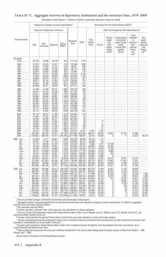
414 | Appendix B
Table B–71. Aggregate reserves of depository institutions and the monetary base, 1979–2009[Averages of daily figures 1; millions of dollars; seasonally adjusted, except as noted]
Year and month
Adjusted for changes in reserve requirements 2 Borrowings from the Federal Reserve (NSA) 3
Reserves of depository institutions
Monetarybase Total 4
Termauctioncredit
Other borrowings from the Federal Reserve 5
Total Non-borrowed Required Excess
(NSA) 3 Primary
Primarydealer
andother
broker-dealercredit 6
Asset-backedcommercial
paper moneymarket
mutual fundliquidityfacility
Creditextended
toAmerican
Inter-nationalGroup,
Inc.,net 7
Termasset-backed
securitiesloan
facility,net 8
December:1979 .............. 20,720 19,248 20,279 442 131,143 1,473 .............. .............. ............... ...................... .................. ................1980 .............. 22,015 20,325 21,501 514 142,004 1,690 .............. .............. ............... ...................... .................. ................1981 .............. 22,443 21,807 22,124 319 149,021 636 .............. .............. ............... ...................... .................. ................1982 .............. 23,600 22,966 23,100 500 160,127 634 .............. .............. ............... ...................... .................. ................1983 .............. 25,367 24,593 24,806 561 175,467 774 .............. .............. ............... ...................... .................. ................1984 .............. 26,913 23,727 26,078 835 187,252 3,186 .............. .............. ............... ...................... .................. ................1985 .............. 31,569 30,250 30,505 1,063 203,555 1,318 .............. .............. ............... ...................... .................. ................1986 .............. 38,840 38,014 37,667 1,173 223,416 827 .............. .............. ............... ...................... .................. ................1987 .............. 38,913 38,135 37,893 1,019 239,829 777 .............. .............. ............... ...................... .................. ................1988 .............. 40,453 38,738 39,392 1,061 256,897 1,716 .............. .............. ............... ...................... .................. ................1989 .............. 40,486 40,221 39,545 941 267,774 265 .............. .............. ............... ...................... .................. ................1990 .............. 41,766 41,440 40,101 1,665 293,278 326 .............. .............. ............... ...................... .................. ................1991 .............. 45,516 45,324 44,526 990 317,543 192 .............. .............. ............... ...................... .................. ................1992 .............. 54,421 54,298 53,267 1,154 350,882 124 .............. .............. ............... ...................... .................. ................1993 .............. 60,566 60,484 59,497 1,069 386,586 82 .............. .............. ............... ...................... .................. ................1994 .............. 59,466 59,257 58,295 1,171 418,313 209 .............. .............. ............... ...................... .................. ................1995 .............. 56,483 56,226 55,193 1,290 434,610 257 .............. .............. ............... ...................... .................. ................1996 .............. 50,185 50,030 48,766 1,418 452,088 155 .............. .............. ............... ...................... .................. ................1997 .............. 46,875 46,551 45,189 1,687 479,996 324 .............. .............. ............... ...................... .................. ................1998 .............. 45,172 45,055 43,659 1,512 513,954 117 .............. .............. ............... ...................... .................. ................1999 .............. 42,173 41,852 40,879 1,294 593,740 9 320 .............. .............. ............... ...................... .................. ................2000 .............. 38,724 38,515 37,399 1,325 584,984 210 .............. .............. ............... ...................... .................. ................2001 .............. 41,428 41,361 39,785 1,643 635,567 67 .............. .............. ............... ...................... .................. ................2002 .............. 40,339 40,259 38,331 2,008 681,648 80 .............. .............. ............... ...................... .................. ................2003 .............. 42,630 42,585 41,583 1,047 720,391 46 .............. 17 ............... ...................... .................. ................2004 .............. 46,540 46,478 44,631 1,909 759,378 63 .............. 11 ............... ...................... .................. ................2005 .............. 45,089 44,920 43,188 1,901 787,579 169 .............. 97 ............... ...................... .................. ................2006 .............. 43,220 43,029 41,357 1,863 812,411 191 .............. 111 ............... ...................... .................. ................2007 .............. 43,214 27,783 41,429 1,784 824,373 15,431 11,613 3,787 ............... ...................... .................. ................2008 .............. 820,306 166,740 52,972 767,333 1,654,068 653,565 438,327 88,245 47,631 32,102 47,206 ................2009 .............. 1,138,633 968,706 63,187 1,075,446 2,017,698 169,927 82,014 19,025 0 0 22,023 46,310
2008: Jan ............ 42,289 –3,371 40,641 1,648 820,299 45,659 44,516 1,137 ............... ...................... .................. ................Feb ............ 43,397 –16,760 41,782 1,615 820,953 60,157 60,000 155 ............... ...................... .................. ................Mar ........... 45,119 –49,405 42,474 2,644 824,824 94,524 75,484 1,617 16,168 ...................... .................. ................Apr ............ 44,789 –90,620 43,052 1,737 823,692 135,410 100,000 9,624 25,764 ...................... .................. ................May ........... 45,708 –110,073 43,869 1,838 827,435 155,780 127,419 14,076 14,238 ...................... .................. ................June .......... 45,674 –125,604 43,449 2,225 833,059 171,278 150,000 14,225 6,908 ...................... .................. ................July ........... 45,274 –120,390 43,361 1,913 839,687 165,664 150,000 15,204 255 ...................... .................. ................Aug ............ 46,258 –121,821 44,382 1,876 843,236 168,078 150,000 17,980 0 ...................... .................. ................Sept ........... 103,583 –186,522 44,101 59,483 905,225 290,105 149,814 32,632 53,473 31,877 22,187 ................Oct ............. 315,458 –332,861 48,299 267,159 1,130,444 648,319 244,778 94,017 114,953 117,457 77,047 ................Nov ............ 609,305 –89,480 50,484 558,821 1,435,013 698,786 393,088 95,839 60,655 71,009 78,070 ................Dec ............ 820,306 166,740 52,972 767,333 1,654,068 653,565 438,327 88,245 47,631 32,102 47,206 ................
2009: Jan ............ 856,993 293,496 58,813 798,180 1,702,465 563,496 403,523 70,436 33,061 17,745 38,690 ................Feb ............ 699,935 117,438 56,486 643,449 1,555,039 582,497 438,822 65,463 26,250 13,533 38,414 ................Mar ........... 779,497 167,385 54,891 724,605 1,640,732 612,111 477,049 62,513 20,292 7,857 43,328 1,061Apr ............ 881,019 322,825 56,658 824,362 1,747,298 558,194 444,933 47,324 10,918 4,267 45,057 5,649May ........... 900,866 375,418 56,797 844,068 1,768,832 525,448 403,970 40,124 701 23,347 44,915 12,367June .......... 809,196 370,473 57,840 751,355 1,679,687 438,722 316,868 37,302 0 18,891 43,057 22,552July ........... 794,995 428,033 62,015 732,980 1,666,475 366,961 255,119 34,366 0 6,230 43,108 27,993Aug ............ 828,466 497,017 62,639 765,827 1,703,377 331,450 224,490 32,147 0 184 40,021 33,898Sept ........... 922,473 615,646 62,408 860,065 1,800,961 306,827 196,731 29,243 0 79 39,074 41,036Oct ............. 1,056,405 791,347 61,673 994,732 1,936,564 265,058 155,396 25,163 0 28 41,222 42,765Nov ............ 1,140,488 923,181 63,200 1,077,288 2,018,813 217,307 110,049 20,434 0 0 43,222 43,497Dec ............ 1,138,633 968,706 63,187 1,075,446 2,017,698 169,927 82,014 19,025 0 0 22,023 46,310
1 Data are prorated averages of biweekly (maintenance period) averages of daily figures.2 Aggregate reserves incorporate adjustments for discontinuities associated with regulatory changes to reserve requirements. For details on aggregate
reserves series see Federal Reserve Bulletin.3 Not seasonally adjusted (NSA).4 Includes secondary, seasonal, other credit extensions, and adjustment not shown separately.5 Does not include credit extensions made by the Federal Reserve Bank of New York to Maiden Lane LLC, Maiden Lane II LLC, Maiden Lane III LLC, and
Commercial Paper Funding Facility LLC.6 Includes credit extended through the Primary Dealer Credit Facility and credit extended to certain other broker-dealers.7 Includes outstanding principal and capitalized interest net of unamortized deferred commitment fees and allowance for loan restructuring. Excludes credit
extended to consolidated LLCs as described in footnote 5.8 Includes credit extended by Federal Reserve Bank of New York to eligible borrowers through the Term Asset-Backed Securities Loan Facility, net of
unamortized deferred administrative fees.9 Total includes borrowing under the terms and conditions established for the Century Date Change Special Liquidity Facility in effect from October 1, 1999
through April 7, 2000.Source: Board of Governors of the Federal Reserve System.
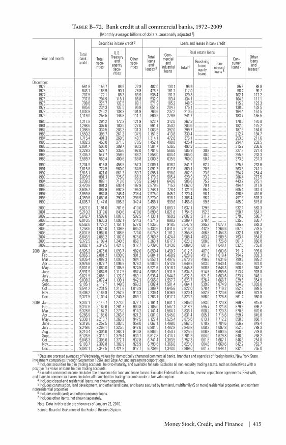
Money Stock, Credit, and Finance | 415
Table B–72. Bank credit at all commercial banks, 1972–2009[Monthly average; billions of dollars, seasonally adjusted 1]
Year and monthTotalbankcredit
Securities in bank credit 2 Loans and leases in bank credit
Totalsecu-rities
U.S.Treasury
andagencysecu-rities
Othersecu-rities
Totalloansand
leases 3
Com-mercial
andindustrial
loans
Real estate loansCon-
sumerloans 6
Otherloansand
leases 7Total 4Revolving
homeequityloans
Com-mercialloans 5
December:1972 .............................. 561.8 159.7 86.9 72.8 402.0 133.1 96.9 ................ ................ 85.3 86.81973 .............................. 643.1 166.9 90.1 76.8 476.2 161.2 117.0 ................ ................ 98.4 99.71974 .............................. 707.5 172.1 88.2 83.9 535.4 191.3 129.8 ................ ................ 102.1 112.21975 .............................. 737.8 204.9 118.1 86.8 532.9 183.4 134.1 ................ ................ 104.3 111.11976 .............................. 798.6 226.7 137.5 89.1 571.9 185.2 148.5 ................ ................ 115.8 122.31977 .............................. 885.6 234.3 137.5 96.8 651.3 204.7 175.1 ................ ................ 138.0 133.51978 .............................. 1,003.8 240.2 138.3 101.9 763.6 237.2 210.5 ................ ................ 164.4 151.51979 .............................. 1,119.0 258.5 146.8 111.7 860.5 279.6 241.7 ................ ................ 183.7 155.51980 .............................. 1,217.8 294.2 172.2 121.9 923.7 312.0 262.3 ................ ................ 178.6 170.81981 .............................. 1,298.6 307.6 180.5 127.0 991.1 350.2 283.6 ................ ................ 182.0 175.21982 .............................. 1,398.5 334.5 203.2 131.3 1,063.9 392.0 299.7 ................ ................ 187.6 184.61983 .............................. 1,550.2 398.7 261.2 137.5 1,151.5 413.8 330.4 ................ ................ 212.7 194.71984 .............................. 1,715.4 401.3 260.5 140.7 1,314.1 472.8 376.1 ................ ................ 253.5 211.61985 .............................. 1,902.2 450.0 271.5 178.5 1,452.1 499.8 425.4 ................ ................ 294.4 232.51986 .............................. 2,084.7 503.0 309.7 193.3 1,581.7 536.5 493.3 ................ ................ 315.2 236.61987 .............................. 2,229.3 527.7 335.6 192.0 1,701.6 566.6 585.9 30.8 ................ 327.8 221.41988 .............................. 2,405.7 547.7 359.5 188.2 1,858.0 604.4 665.0 40.0 ................ 355.3 233.31989 .............................. 2,569.7 569.4 400.6 168.8 2,000.3 635.5 760.0 50.4 ................ 373.5 231.31990 .............................. 2,704.9 615.8 458.5 157.3 2,089.1 638.2 841.7 62.2 ................ 375.6 233.61991 .............................. 2,815.8 724.5 560.0 164.5 2,091.3 617.6 869.1 70.5 ................ 363.6 241.11992 .............................. 2,916.1 821.0 661.3 159.7 2,095.1 598.0 887.9 73.8 ................ 354.7 254.41993 .............................. 3,070.5 891.3 725.0 166.3 2,179.2 585.4 929.9 73.3 ................ 386.4 277.51994 .............................. 3,238.2 889.1 713.6 175.5 2,349.1 643.6 986.6 75.2 ................ 443.7 275.11995 .............................. 3,470.8 891.3 693.4 197.9 2,579.5 715.2 1,062.0 79.1 ................ 484.4 317.91996 .............................. 3,635.7 887.6 692.3 195.3 2,748.1 778.4 1,121.9 85.4 ................ 505.4 342.41997 .............................. 3,959.8 984.8 746.4 238.4 2,975.0 845.2 1,220.4 98.1 ................ 498.8 410.61998 .............................. 4,359.6 1,089.6 790.7 298.9 3,270.0 938.1 1,308.4 96.2 ................ 497.3 526.31999 .............................. 4,605.7 1,147.6 805.2 342.4 3,458.1 999.6 1,456.8 99.5 ................ 485.9 515.82000 .............................. 5,027.0 1,191.6 781.6 410.0 3,835.5 1,083.7 1,637.1 129.5 ................ 532.4 582.32001 .............................. 5,210.2 1,319.6 840.6 479.0 3,890.6 1,021.8 1,754.3 152.3 ................ 550.4 564.12002 .............................. 5,642.7 1,509.6 1,007.0 502.5 4,133.1 960.2 2,007.2 211.7 ................ 579.0 586.72003 .............................. 6,010.5 1,636.3 1,092.1 544.3 4,374.2 898.2 2,209.7 278.4 ................ 635.6 630.72004 .............................. 6,563.6 1,728.2 1,151.1 577.0 4,835.5 918.5 2,547.8 395.2 1,077.7 685.9 683.32005 .............................. 7,258.6 1,825.0 1,139.8 685.2 5,433.6 1,041.6 2,916.0 442.9 1,266.6 697.6 778.52006 .............................. 8,037.8 1,962.6 1,188.6 774.0 6,075.3 1,181.2 3,355.8 466.8 1,454.3 732.1 806.22007 .............................. 8,843.5 2,083.2 1,107.6 975.6 6,760.3 1,424.4 3,588.4 483.2 1,589.5 793.4 954.02008 .............................. 9,372.5 2,109.4 1,240.3 869.1 7,263.1 1,617.7 3,823.2 588.0 1,726.8 861.4 960.82009 .............................. 9,082.1 2,342.5 1,424.8 917.7 6,739.6 1,343.0 3,809.0 601.7 1,648.1 832.6 755.0
2008: Jan ............................ 8,926.2 2,075.8 1,093.7 982.0 6,850.4 1,450.7 3,612.5 487.0 1,603.6 791.7 995.6Feb ............................ 8,965.3 2,081.2 1,090.0 991.2 6,884.1 1,468.9 3,628.8 491.6 1,618.4 794.2 992.3Mar ........................... 9,035.4 2,082.3 1,097.6 984.7 6,953.1 1,497.6 3,670.9 496.8 1,631.6 799.5 985.2Apr ............................ 8,976.6 2,072.7 1,096.5 976.2 6,903.9 1,512.6 3,649.5 503.0 1,640.4 804.8 937.0May ........................... 9,001.6 2,080.0 1,105.5 974.5 6,921.6 1,518.7 3,645.8 508.6 1,648.3 808.3 948.7June .......................... 8,992.9 2,084.9 1,117.5 967.4 6,908.0 1,531.5 3,634.3 514.5 1,659.6 813.4 928.8July ........................... 9,021.5 2,085.1 1,122.0 963.1 6,936.4 1,544.3 3,622.3 521.6 1,663.6 823.7 946.1Aug ............................ 9,038.2 2,072.4 1,130.1 942.3 6,965.8 1,557.7 3,623.7 526.4 1,666.7 829.5 954.9Sept ........................... 9,195.1 2,112.7 1,149.5 963.2 7,082.4 1,581.4 3,664.1 539.8 1,674.9 834.9 1,002.0Oct ............................. 9,541.2 2,231.5 1,217.6 1,013.9 7,309.7 1,645.6 3,822.0 578.4 1,719.2 852.6 989.5Nov ............................ 9,406.2 2,166.8 1,252.5 914.3 7,239.4 1,636.9 3,820.4 582.6 1,723.6 858.1 923.9Dec ............................ 9,372.5 2,109.4 1,240.3 869.1 7,263.1 1,617.7 3,823.2 588.0 1,726.8 861.4 960.8
2009: Jan ............................ 9,337.1 2,145.7 1,273.0 872.7 7,191.4 1,601.1 3,805.0 593.0 1,720.8 869.8 915.6Feb ............................ 9,347.6 2,162.6 1,261.7 900.8 7,185.0 1,587.1 3,818.2 595.7 1,721.6 879.9 899.7Mar ........................... 9,328.6 2,187.2 1,273.0 914.2 7,141.4 1,564.1 3,836.1 600.2 1,720.3 870.6 870.6Apr ............................ 9,266.9 2,185.0 1,263.8 921.2 7,081.9 1,545.0 3,831.4 605.1 1,715.6 859.7 845.8May ........................... 9,338.1 2,210.7 1,263.2 947.5 7,127.4 1,525.4 3,875.6 613.1 1,712.2 858.3 868.1June .......................... 9,319.6 2,252.5 1,293.5 959.0 7,067.1 1,499.0 3,862.5 610.9 1,704.6 856.2 849.4July ........................... 9,249.6 2,268.1 1,325.5 942.6 6,981.5 1,482.8 3,846.8 608.3 1,697.8 852.6 799.3Aug ............................ 9,210.4 2,304.0 1,363.1 940.8 6,906.5 1,450.7 3,825.5 606.9 1,690.5 850.5 779.8Sept ........................... 9,126.9 2,314.1 1,379.4 934.7 6,812.8 1,414.7 3,781.9 604.0 1,679.8 848.0 768.2Oct ............................. 9,046.3 2,305.0 1,372.1 932.8 6,741.4 1,383.5 3,757.3 601.8 1,667.1 846.6 754.0Nov ............................ 9,103.7 2,309.8 1,382.9 926.9 6,793.8 1,366.0 3,823.0 604.6 1,660.6 842.2 762.7Dec ............................ 9,082.1 2,342.5 1,424.8 917.7 6,739.6 1,343.0 3,809.0 601.7 1,648.1 832.6 755.0
1 Data are prorated averages of Wednesday values for domestically chartered commercial banks, branches and agencies of foreign banks, New York Stateinvestment companies (through September 1996), and Edge Act and agreement corporations.
2 Includes securities held in trading accounts, held-to-maturity, and available for sale. Excludes all non-security trading assets, such as derivatives with apositive fair value or loans held in trading accounts.
3 Excludes unearned income. Includes the allowance for loan and lease losses. Excludes Federal funds sold to, reverse repurchase agreements (RPs) with,and loans to commercial banks. Includes all loans held in trading accounts under a fair value option.
4 Includes closed-end residential loans, not shown separately.5 Includes construction, land development, and other land loans, and loans secured by farmland, multifamily (5 or more) residential properties, and nonfarm
nonresidential properties.6 Includes credit cards and other consumer loans.7 Includes other items, not shown separately.Note: Data in this table are shown as of January 22, 2010.Source: Board of Governors of the Federal Reserve System.
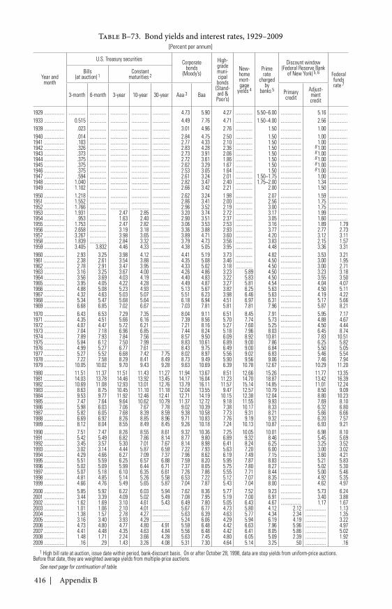
416 | Appendix B
Table B–73. Bond yields and interest rates, 1929–2009[Percent per annum]
Year andmonth
U.S. Treasury securities Corporatebonds
(Moody’s)
High-grademuni-cipal
bonds(Stand-ard &Poor’s)
New-homemort-gage
yields 4
Primerate
chargedby
banks 5
Discount window(Federal Reserve Bank
of New York) 5, 6 Federalfundsrate 7
Bills(at auction) 1
Constantmaturities 2
3-month 6-month 3-year 10-year 30-year Aaa 3 Baa Primarycredit
Adjust-mentcredit
1929 ................. .............. .............. .............. .............. .............. 4.73 5.90 4.27 .............. 5.50–6.00 ................. 5.16 ...............1933 ................. 0.515 .............. .............. .............. .............. 4.49 7.76 4.71 .............. 1.50–4.00 ................. 2.56 ...............1939 ................. .023 .............. .............. .............. .............. 3.01 4.96 2.76 .............. 1.50 ................. 1.00 ...............1940 ................. .014 .............. .............. .............. .............. 2.84 4.75 2.50 .............. 1.50 ................. 1.00 ...............1941 ................. .103 .............. .............. .............. .............. 2.77 4.33 2.10 .............. 1.50 ................. 1.00 ...............1942 ................. .326 .............. .............. .............. .............. 2.83 4.28 2.36 .............. 1.50 ................. 8 1.00 ...............1943 ................. .373 .............. .............. .............. .............. 2.73 3.91 2.06 .............. 1.50 ................. 8 1.00 ...............1944 ................. .375 .............. .............. .............. .............. 2.72 3.61 1.86 .............. 1.50 ................. 8 1.00 ...............1945 ................. .375 .............. .............. .............. .............. 2.62 3.29 1.67 .............. 1.50 ................. 8 1.00 ...............1946 ................. .375 .............. .............. .............. .............. 2.53 3.05 1.64 .............. 1.50 ................. 8 1.00 ...............1947 ................. .594 .............. .............. .............. .............. 2.61 3.24 2.01 .............. 1.50–1.75 ................. 1.00 ...............1948 ................. 1.040 .............. .............. .............. .............. 2.82 3.47 2.40 .............. 1.75–2.00 ................. 1.34 ...............1949 ................. 1.102 .............. .............. .............. .............. 2.66 3.42 2.21 .............. 2.00 ................. 1.50 ...............1950 ................. 1.218 .............. .............. .............. .............. 2.62 3.24 1.98 .............. 2.07 ................. 1.59 ...............1951 ................. 1.552 .............. .............. .............. .............. 2.86 3.41 2.00 .............. 2.56 ................. 1.75 ...............1952 ................. 1.766 .............. .............. .............. .............. 2.96 3.52 2.19 .............. 3.00 ................. 1.75 ...............1953 ................. 1.931 .............. 2.47 2.85 .............. 3.20 3.74 2.72 .............. 3.17 ................. 1.99 ...............1954 ................. .953 .............. 1.63 2.40 .............. 2.90 3.51 2.37 .............. 3.05 ................. 1.60 ...............1955 ................. 1.753 .............. 2.47 2.82 .............. 3.06 3.53 2.53 .............. 3.16 ................. 1.89 1.791956 ................. 2.658 .............. 3.19 3.18 .............. 3.36 3.88 2.93 .............. 3.77 ................. 2.77 2.731957 ................. 3.267 .............. 3.98 3.65 .............. 3.89 4.71 3.60 .............. 4.20 ................. 3.12 3.111958 ................. 1.839 .............. 2.84 3.32 .............. 3.79 4.73 3.56 .............. 3.83 ................. 2.15 1.571959 ................. 3.405 3.832 4.46 4.33 .............. 4.38 5.05 3.95 .............. 4.48 ................. 3.36 3.311960 ................. 2.93 3.25 3.98 4.12 .............. 4.41 5.19 3.73 .............. 4.82 ................. 3.53 3.211961 ................. 2.38 2.61 3.54 3.88 .............. 4.35 5.08 3.46 .............. 4.50 ................. 3.00 1.951962 ................. 2.78 2.91 3.47 3.95 .............. 4.33 5.02 3.18 .............. 4.50 ................. 3.00 2.711963 ................. 3.16 3.25 3.67 4.00 .............. 4.26 4.86 3.23 5.89 4.50 ................. 3.23 3.181964 ................. 3.56 3.69 4.03 4.19 .............. 4.40 4.83 3.22 5.83 4.50 ................. 3.55 3.501965 ................. 3.95 4.05 4.22 4.28 .............. 4.49 4.87 3.27 5.81 4.54 ................. 4.04 4.071966 ................. 4.88 5.08 5.23 4.93 .............. 5.13 5.67 3.82 6.25 5.63 ................. 4.50 5.111967 ................. 4.32 4.63 5.03 5.07 .............. 5.51 6.23 3.98 6.46 5.63 ................. 4.19 4.221968 ................. 5.34 5.47 5.68 5.64 .............. 6.18 6.94 4.51 6.97 6.31 ................. 5.17 5.661969 ................. 6.68 6.85 7.02 6.67 .............. 7.03 7.81 5.81 7.81 7.96 ................. 5.87 8.211970 ................. 6.43 6.53 7.29 7.35 .............. 8.04 9.11 6.51 8.45 7.91 ................. 5.95 7.171971 ................. 4.35 4.51 5.66 6.16 .............. 7.39 8.56 5.70 7.74 5.73 ................. 4.88 4.671972 ................. 4.07 4.47 5.72 6.21 .............. 7.21 8.16 5.27 7.60 5.25 ................. 4.50 4.441973 ................. 7.04 7.18 6.96 6.85 .............. 7.44 8.24 5.18 7.96 8.03 ................. 6.45 8.741974 ................. 7.89 7.93 7.84 7.56 .............. 8.57 9.50 6.09 8.92 10.81 ................. 7.83 10.511975 ................. 5.84 6.12 7.50 7.99 .............. 8.83 10.61 6.89 9.00 7.86 ................. 6.25 5.821976 ................. 4.99 5.27 6.77 7.61 .............. 8.43 9.75 6.49 9.00 6.84 ................. 5.50 5.051977 ................. 5.27 5.52 6.68 7.42 7.75 8.02 8.97 5.56 9.02 6.83 ................. 5.46 5.541978 ................. 7.22 7.58 8.29 8.41 8.49 8.73 9.49 5.90 9.56 9.06 ................. 7.46 7.941979 ................. 10.05 10.02 9.70 9.43 9.28 9.63 10.69 6.39 10.78 12.67 ................. 10.29 11.201980 ................. 11.51 11.37 11.51 11.43 11.27 11.94 13.67 8.51 12.66 15.26 ................. 11.77 13.351981 ................. 14.03 13.78 14.46 13.92 13.45 14.17 16.04 11.23 14.70 18.87 ................. 13.42 16.391982 ................. 10.69 11.08 12.93 13.01 12.76 13.79 16.11 11.57 15.14 14.85 ................. 11.01 12.241983 ................. 8.63 8.75 10.45 11.10 11.18 12.04 13.55 9.47 12.57 10.79 ................. 8.50 9.091984 ................. 9.53 9.77 11.92 12.46 12.41 12.71 14.19 10.15 12.38 12.04 ................. 8.80 10.231985 ................. 7.47 7.64 9.64 10.62 10.79 11.37 12.72 9.18 11.55 9.93 ................. 7.69 8.101986 ................. 5.98 6.03 7.06 7.67 7.78 9.02 10.39 7.38 10.17 8.33 ................. 6.32 6.801987 ................. 5.82 6.05 7.68 8.39 8.59 9.38 10.58 7.73 9.31 8.21 ................. 5.66 6.661988 ................. 6.69 6.92 8.26 8.85 8.96 9.71 10.83 7.76 9.19 9.32 ................. 6.20 7.571989 ................. 8.12 8.04 8.55 8.49 8.45 9.26 10.18 7.24 10.13 10.87 ................. 6.93 9.211990 ................. 7.51 7.47 8.26 8.55 8.61 9.32 10.36 7.25 10.05 10.01 ................. 6.98 8.101991 ................. 5.42 5.49 6.82 7.86 8.14 8.77 9.80 6.89 9.32 8.46 ................. 5.45 5.691992 ................. 3.45 3.57 5.30 7.01 7.67 8.14 8.98 6.41 8.24 6.25 ................. 3.25 3.521993 ................. 3.02 3.14 4.44 5.87 6.59 7.22 7.93 5.63 7.20 6.00 ................. 3.00 3.021994 ................. 4.29 4.66 6.27 7.09 7.37 7.96 8.62 6.19 7.49 7.15 ................. 3.60 4.211995 ................. 5.51 5.59 6.25 6.57 6.88 7.59 8.20 5.95 7.87 8.83 ................. 5.21 5.831996 ................. 5.02 5.09 5.99 6.44 6.71 7.37 8.05 5.75 7.80 8.27 ................. 5.02 5.301997 ................. 5.07 5.18 6.10 6.35 6.61 7.26 7.86 5.55 7.71 8.44 ................. 5.00 5.461998 ................. 4.81 4.85 5.14 5.26 5.58 6.53 7.22 5.12 7.07 8.35 ................. 4.92 5.351999 ................. 4.66 4.76 5.49 5.65 5.87 7.04 7.87 5.43 7.04 8.00 ................. 4.62 4.972000 ................. 5.85 5.92 6.22 6.03 5.94 7.62 8.36 5.77 7.52 9.23 ................. 5.73 6.242001 ................. 3.44 3.39 4.09 5.02 5.49 7.08 7.95 5.19 7.00 6.91 ................. 3.40 3.882002 ................. 1.62 1.69 3.10 4.61 5.43 6.49 7.80 5.05 6.43 4.67 ................. 1.17 1.672003 ................. 1.01 1.06 2.10 4.01 .............. 5.67 6.77 4.73 5.80 4.12 2.12 ................. 1.132004 ................. 1.38 1.57 2.78 4.27 .............. 5.63 6.39 4.63 5.77 4.34 2.34 ................. 1.352005 ................. 3.16 3.40 3.93 4.29 .............. 5.24 6.06 4.29 5.94 6.19 4.19 ................. 3.222006 ................. 4.73 4.80 4.77 4.80 4.91 5.59 6.48 4.42 6.63 7.96 5.96 ................. 4.972007 ................. 4.41 4.48 4.35 4.63 4.84 5.56 6.48 4.42 6.41 8.05 5.86 ................. 5.022008 ................. 1.48 1.71 2.24 3.66 4.28 5.63 7.45 4.80 6.05 5.09 2.39 ................. 1.922009 ................. .16 .29 1.43 3.26 4.08 5.31 7.30 4.64 5.14 3.25 .50 ................. .16
1 High bill rate at auction, issue date within period, bank-discount basis. On or after October 28, 1998, data are stop yields from uniform-price auctions.Before that date, they are weighted average yields from multiple-price auctions.
See next page for continuation of table.
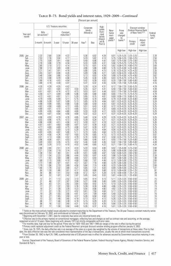
Money Stock, Credit, and Finance | 417
Table B–73. Bond yields and interest rates, 1929–2009—Continued[Percent per annum]
Year andmonth
U.S. Treasury securities Corporatebonds
(Moody's)
High-grademuni-cipal
bonds(Stand-ard &Poor's)
New-homemort-gage
yields 4
Primerate
chargedby
banks 5
Discount window(Federal Reserve Bank
of New York) 5, 6 Federalfundsrate 7
Bills(at auction) 1
Constantmaturities 2
3-month 6-month 3-year 10-year 30-year Aaa 3 Baa Primarycredit
Adjust-mentcredit
High-low High-low High-low
2005: Jan ........ 2.32 2.60 3.39 4.22 ............. 5.36 6.02 4.28 6.01 5.25–5.25 3.25–3.25 ................ 2.28Feb ........ 2.53 2.76 3.54 4.17 ............. 5.20 5.82 4.14 5.75 5.50–5.25 3.50–3.25 ................ 2.50Mar ....... 2.75 3.00 3.91 4.50 ............. 5.40 6.06 4.42 5.82 5.75–5.50 3.75–3.50 ................ 2.63Apr ........ 2.78 3.06 3.79 4.34 ............. 5.33 6.05 4.31 5.84 5.75–5.75 3.75–3.75 ................ 2.79May ....... 2.85 3.10 3.72 4.14 ............. 5.15 6.01 4.16 5.82 6.00–5.75 4.00–3.75 ................ 3.00June ...... 2.98 3.13 3.69 4.00 ............. 4.96 5.86 4.08 5.76 6.25–6.00 4.25–4.00 ................ 3.04July ....... 3.21 3.41 3.91 4.18 ............. 5.06 5.95 4.15 5.76 6.25–6.25 4.25–4.25 ................ 3.26Aug ........ 3.45 3.67 4.08 4.26 ............. 5.09 5.96 4.21 5.83 6.50–6.25 4.50–4.25 ................ 3.50Sept ....... 3.46 3.68 3.96 4.20 ............. 5.13 6.03 4.28 5.99 6.75–6.50 4.75–4.50 ................ 3.62Oct ......... 3.70 3.98 4.29 4.46 ............. 5.35 6.30 4.49 6.03 6.75–6.75 4.75–4.75 ................ 3.78Nov ........ 3.90 4.16 4.43 4.54 ............. 5.42 6.39 4.53 6.20 7.00–7.00 5.00–5.00 ................ 4.00Dec ........ 3.89 4.19 4.39 4.47 ............. 5.37 6.32 4.43 6.39 7.25–7.00 5.25–5.00 ................ 4.16
2006: Jan ........ 4.20 4.29 4.35 4.42 ............. 5.29 6.24 4.31 6.12 7.50–7.25 5.50–5.25 ................ 4.29Feb ........ 4.41 4.51 4.64 4.57 4.54 5.35 6.27 4.41 6.40 7.50–7.50 5.50–5.50 ................ 4.49Mar ....... 4.51 4.61 4.74 4.72 4.73 5.53 6.41 4.44 6.53 7.75–7.50 5.75–5.50 ................ 4.59Apr ........ 4.59 4.71 4.89 4.99 5.06 5.84 6.68 4.60 6.64 7.75–7.75 5.75–5.75 ................ 4.79May ....... 4.72 4.81 4.97 5.11 5.20 5.95 6.75 4.61 6.69 8.00–7.75 6.00–5.75 ................ 4.94June ...... 4.79 4.95 5.09 5.11 5.15 5.89 6.78 4.64 6.79 8.25–8.00 6.25–6.00 ................ 4.99July ....... 4.96 5.09 5.07 5.09 5.13 5.85 6.76 4.64 6.81 8.25–8.25 6.25–6.25 ................ 5.24Aug ........ 4.98 4.99 4.85 4.88 5.00 5.68 6.59 4.43 6.87 8.25–8.25 6.25–6.25 ................ 5.25Sept ....... 4.82 4.90 4.69 4.72 4.85 5.51 6.43 4.30 6.72 8.25–8.25 6.25–6.25 ................ 5.25Oct ......... 4.89 4.91 4.72 4.73 4.85 5.51 6.42 4.32 6.69 8.25–8.25 6.25–6.25 ................ 5.25Nov ........ 4.95 4.95 4.64 4.60 4.69 5.33 6.20 4.17 6.55 8.25–8.25 6.25–6.25 ................ 5.25Dec ........ 4.84 4.87 4.58 4.56 4.68 5.32 6.22 4.17 6.37 8.25–8.25 6.25–6.25 ................ 5.24
2007: Jan ........ 4.96 4.93 4.79 4.76 4.85 5.40 6.34 4.29 6.35 8.25–8.25 6.25–6.25 ................ 5.25Feb ........ 5.02 4.96 4.75 4.72 4.82 5.39 6.28 4.21 6.31 8.25–8.25 6.25–6.25 ................ 5.26Mar ....... 4.96 4.90 4.51 4.56 4.72 5.30 6.27 4.18 6.22 8.25–8.25 6.25–6.25 ................ 5.26Apr ........ 4.87 4.87 4.60 4.69 4.87 5.47 6.39 4.32 6.21 8.25–8.25 6.25–6.25 ................ 5.25May ....... 4.77 4.80 4.69 4.75 4.90 5.47 6.39 4.37 6.22 8.25–8.25 6.25–6.25 ................ 5.25June ...... 4.63 4.77 5.00 5.10 5.20 5.79 6.70 4.64 6.54 8.25–8.25 6.25–6.25 ................ 5.25July ....... 4.83 4.85 4.82 5.00 5.11 5.73 6.65 4.64 6.70 8.25–8.25 6.25–6.25 ................ 5.26Aug ........ 4.34 4.56 4.34 4.67 4.93 5.79 6.65 4.73 6.73 8.25–8.25 6.25–5.75 ................ 5.02Sept ....... 4.01 4.13 4.06 4.52 4.79 5.74 6.59 4.57 6.58 8.25–7.75 5.75–5.25 ................ 4.94Oct ......... 3.96 4.08 4.01 4.53 4.77 5.66 6.48 4.41 6.55 7.75–7.50 5.25–5.00 ................ 4.76Nov ........ 3.49 3.63 3.35 4.15 4.52 5.44 6.40 4.45 6.42 7.50–7.50 5.00–5.00 ................ 4.49Dec ........ 3.08 3.29 3.13 4.10 4.53 5.49 6.65 4.22 6.21 7.50–7.25 5.00–4.75 ................ 4.24
2008: Jan ........ 2.86 2.84 2.51 3.74 4.33 5.33 6.54 4.00 6.02 7.25–6.00 4.75–3.50 ................ 3.94Feb ........ 2.21 2.09 2.19 3.74 4.52 5.53 6.82 4.35 5.96 6.00–6.00 3.50–3.50 ................ 2.98Mar ....... 1.38 1.53 1.80 3.51 4.39 5.51 6.89 4.67 5.92 6.00–5.25 3.50–2.50 ................ 2.61Apr ........ 1.32 1.54 2.23 3.68 4.44 5.55 6.97 4.43 5.98 5.25–5.00 2.50–2.25 ................ 2.28May ....... 1.71 1.82 2.69 3.88 4.60 5.57 6.93 4.34 6.01 5.00–5.00 2.25–2.25 ................ 1.98June ...... 1.89 2.15 3.08 4.10 4.69 5.68 7.07 4.48 6.13 5.00–5.00 2.25–2.25 ................ 2.00July ....... 1.72 1.99 2.87 4.01 4.57 5.67 7.16 4.88 6.29 5.00–5.00 2.25–2.25 ................ 2.01Aug ........ 1.79 1.96 2.70 3.89 4.50 5.64 7.15 4.90 6.33 5.00–5.00 2.25–2.25 ................ 2.00Sept ....... 1.46 1.78 2.32 3.69 4.27 5.65 7.31 5.03 6.09 5.00–5.00 2.25–2.25 ................ 1.81Oct ......... .84 1.39 1.86 3.81 4.17 6.28 8.88 5.68 6.10 5.00–4.00 2.25–1.25 ................ .97Nov ........ .30 .86 1.51 3.53 4.00 6.12 9.21 5.28 6.16 4.00–4.00 1.25–1.25 ................ .39Dec ........ .04 .32 1.07 2.42 2.87 5.05 8.43 5.53 5.67 4.00–3.25 1.25–0.50 ................ .16
2009: Jan ........ .12 .31 1.13 2.52 3.13 5.05 8.14 5.13 5.11 3.25–3.25 0.50–0.50 ................ .15Feb ........ .31 .46 1.37 2.87 3.59 5.27 8.08 5.00 5.09 3.25–3.25 0.50–0.50 ................ .22Mar ....... .25 .43 1.31 2.82 3.64 5.50 8.42 5.15 5.10 3.25–3.25 0.50–0.50 ................ .18Apr ........ .17 .37 1.32 2.93 3.76 5.39 8.39 4.88 4.96 3.25–3.25 0.50–0.50 ................ .15May ....... .19 .31 1.39 3.29 4.23 5.54 8.06 4.60 4.92 3.25–3.25 0.50–0.50 ................ .18June ...... .17 .32 1.76 3.72 4.52 5.61 7.50 4.84 5.17 3.25–3.25 0.50–0.50 ................ .21July ....... .19 .29 1.55 3.56 4.41 5.41 7.09 4.69 5.40 3.25–3.25 0.50–0.50 ................ .16Aug ........ .18 .27 1.65 3.59 4.37 5.26 6.58 4.58 5.32 3.25–3.25 0.50–0.50 ................ .16Sept ....... .13 .22 1.48 3.40 4.19 5.13 6.31 4.13 5.26 3.25–3.25 0.50–0.50 ................ .15Oct ......... .08 .17 1.46 3.39 4.19 5.15 6.29 4.20 5.14 3.25–3.25 0.50–0.50 ................ .12Nov ........ .06 .16 1.32 3.40 4.31 5.19 6.32 4.35 5.08 3.25–3.25 0.50–0.50 ................ .12Dec ........ .07 .17 1.38 3.59 4.49 5.26 6.37 4.16 5.01 3.25–3.25 0.50–0.50 ................ .12
2 Yields on the more actively traded issues adjusted to constant maturities by the Department of the Treasury. The 30-year Treasury constant maturity serieswas discontinued on February 18, 2002, and reintroduced on February 9, 2006.
3 Beginning with December 7, 2001, data for corporate Aaa series are industrial bonds only.4 Effective rate (in the primary market) on conventional mortgages, reflecting fees and charges as well as contract rate and assuming, on the average,
repayment at end of 10 years. Rates beginning with January 1973 not strictly comparable with prior rates.5 For monthly data, high and low for the period. Prime rate for 1929–1933 and 1947–1948 are ranges of the rate in effect during the period.6 Primary credit replaced adjustment credit as the Federal Reserve's principal discount window lending program effective January 9, 2003.7 Since July 19, 1975, the daily effective rate is an average of the rates on a given day weighted by the volume of transactions at these rates. Prior to that
date, the daily effective rate was the rate considered most representative of the day's transactions, usually the one at which most transactions occurred.8 From October 30, 1942 to April 24, 1946, a preferential rate of 0.50 percent was in effect for advances secured by Government securities maturing in one
year or less.Sources: Department of the Treasury, Board of Governors of the Federal Reserve System, Federal Housing Finance Agency, Moody's Investors Service, and
Standard & Poor's.
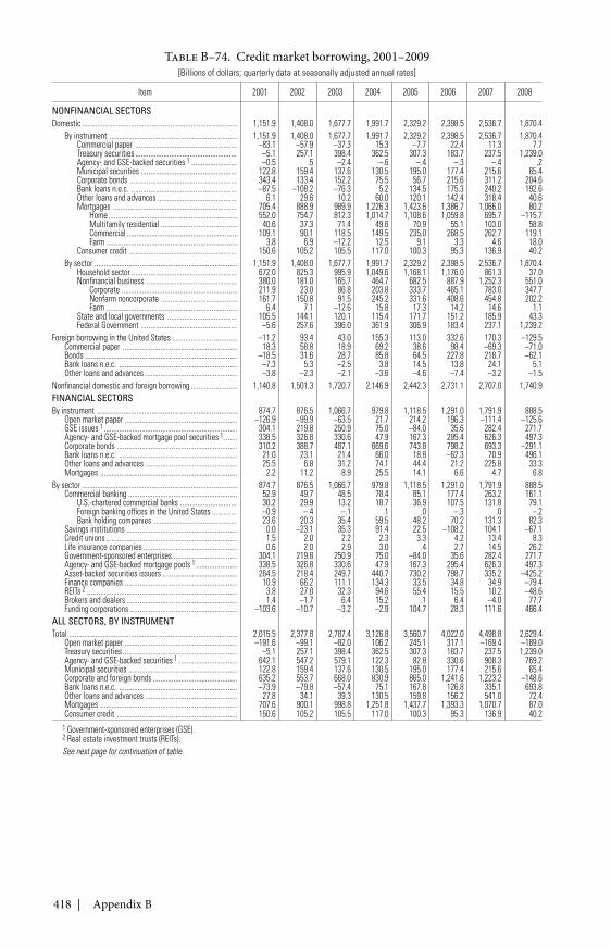
418 | Appendix B
Table B–74. Credit market borrowing, 2001–2009[Billions of dollars; quarterly data at seasonally adjusted annual rates]
Item 2001 2002 2003 2004 2005 2006 2007 2008
NONFINANCIAL SECTORSDomestic ................................................................................... 1,151.9 1,408.0 1,677.7 1,991.7 2,329.2 2,398.5 2,536.7 1,870.4
By instrument .................................................................... 1,151.9 1,408.0 1,677.7 1,991.7 2,329.2 2,398.5 2,536.7 1,870.4Commercial paper ...................................................... –83.1 –57.9 –37.3 15.3 –7.7 22.4 11.3 7.7Treasury securities ...................................................... –5.1 257.1 398.4 362.5 307.3 183.7 237.5 1,239.0Agency- and GSE-backed securities 1 ........................ –0.5 .5 –2.4 –.6 –.4 –.3 –.4 .2Municipal securities ................................................... 122.8 159.4 137.6 130.5 195.0 177.4 215.6 65.4Corporate bonds ......................................................... 343.4 133.4 152.2 75.5 56.7 215.6 311.2 204.6Bank loans n.e.c. ........................................................ –87.5 –108.2 –76.3 5.2 134.5 175.3 240.2 192.6Other loans and advances .......................................... 6.1 29.6 10.2 60.0 120.1 142.4 318.4 40.6Mortgages .................................................................. 705.4 888.9 989.9 1,226.3 1,423.6 1,386.7 1,066.0 80.2
Home..................................................................... 552.0 754.7 812.3 1,014.7 1,108.6 1,059.8 695.7 –115.7Multifamily residential ......................................... 40.6 37.3 71.4 49.6 70.9 55.1 103.0 58.8Commercial ........................................................... 109.1 90.1 118.5 149.5 235.0 268.5 262.7 119.1Farm ...................................................................... 3.8 6.9 –12.2 12.5 9.1 3.3 4.6 18.0
Consumer credit ......................................................... 150.6 105.2 105.5 117.0 100.3 95.3 136.9 40.2By sector ............................................................................ 1,151.9 1,408.0 1,677.7 1,991.7 2,329.2 2,398.5 2,536.7 1,870.4
Household sector ........................................................ 672.0 825.3 995.9 1,049.6 1,168.1 1,176.0 861.3 37.0Nonfinancial business ................................................ 380.0 181.0 165.7 464.7 682.5 887.9 1,252.3 551.0
Corporate .............................................................. 211.9 23.0 86.8 203.8 333.7 465.1 783.0 347.7Nonfarm noncorporate ......................................... 161.7 150.8 91.5 245.2 331.6 408.6 454.8 202.2Farm ...................................................................... 6.4 7.1 –12.6 15.8 17.3 14.2 14.6 1.1
State and local governments ..................................... 105.5 144.1 120.1 115.4 171.7 151.2 185.9 43.3Federal Government ................................................... –5.6 257.6 396.0 361.9 306.9 183.4 237.1 1,239.2
Foreign borrowing in the United States ................................... –11.2 93.4 43.0 155.3 113.0 332.6 170.3 –129.5Commercial paper ............................................................. 18.3 58.8 18.9 69.2 38.6 98.4 –69.3 –71.0Bonds ................................................................................. –18.5 31.6 28.7 85.8 64.5 227.8 218.7 –62.1Bank loans n.e.c. ............................................................... –7.3 5.3 –2.5 3.8 14.5 13.8 24.1 5.1Other loans and advances ................................................. –3.8 –2.3 –2.1 –3.6 –4.6 –7.4 –3.2 –1.5
Nonfinancial domestic and foreign borrowing ......................... 1,140.8 1,501.3 1,720.7 2,146.9 2,442.3 2,731.1 2,707.0 1,740.9FINANCIAL SECTORSBy instrument ........................................................................... 874.7 876.5 1,066.7 979.8 1,118.5 1,291.0 1,791.9 888.5
Open market paper ............................................................ –126.9 –99.9 –63.5 21.7 214.2 196.3 –111.4 –125.6GSE issues 1 ....................................................................... 304.1 219.8 250.9 75.0 –84.0 35.6 282.4 271.7Agency- and GSE-backed mortgage pool securities 1 ....... 338.5 326.8 330.6 47.9 167.3 295.4 626.3 497.3Corporate bonds ................................................................ 310.2 388.7 487.1 669.6 743.8 798.2 693.3 –291.1Bank loans n.e.c. ............................................................... 21.0 23.1 21.4 66.0 18.8 –62.3 70.9 496.1Other loans and advances ................................................. 25.5 6.8 31.2 74.1 44.4 21.2 225.8 33.3Mortgages ......................................................................... 2.2 11.2 8.9 25.5 14.1 6.6 4.7 6.8
By sector ................................................................................... 874.7 876.5 1,066.7 979.8 1,118.5 1,291.0 1,791.9 888.5Commercial banking .......................................................... 52.9 49.7 48.5 78.4 85.1 177.4 263.2 161.1
U.S.-chartered commercial banks .............................. 30.2 29.9 13.2 18.7 36.9 107.5 131.8 79.1Foreign banking offices in the United States ............. –0.9 –.4 –.1 .1 .0 –.3 .0 –.2Bank holding companies ............................................ 23.6 20.3 35.4 59.5 48.2 70.2 131.3 82.3
Savings institutions ........................................................... 0.0 –23.1 35.3 91.4 22.5 –108.2 104.1 –67.1Credit unions ...................................................................... 1.5 2.0 2.2 2.3 3.3 4.2 13.4 8.3Life insurance companies .................................................. 0.6 2.0 2.9 3.0 .4 2.7 14.5 26.2Government-sponsored enterprises .................................. 304.1 219.8 250.9 75.0 –84.0 35.6 282.4 271.7Agency- and GSE-backed mortgage pools 1 ...................... 338.5 326.8 330.6 47.9 167.3 295.4 626.3 497.3Asset-backed securities issuers ........................................ 264.5 218.4 249.7 440.7 730.2 798.7 335.2 –425.2Finance companies ............................................................ 10.9 66.2 111.1 134.3 33.5 34.8 34.9 –79.4REITs 2 ................................................................................ 3.8 27.0 32.3 94.6 55.4 15.5 10.2 –48.6Brokers and dealers ........................................................... 1.4 –1.7 6.4 15.2 .1 6.4 –4.0 77.7Funding corporations ......................................................... –103.6 –10.7 –3.2 –2.9 104.7 28.3 111.6 466.4
ALL SECTORS, BY INSTRUMENTTotal .......................................................................................... 2,015.5 2,377.8 2,787.4 3,126.8 3,560.7 4,022.0 4,498.8 2,629.4
Open market paper ............................................................ –191.6 –99.1 –82.0 106.2 245.1 317.1 –169.4 –189.0Treasury securities ............................................................. –5.1 257.1 398.4 362.5 307.3 183.7 237.5 1,239.0Agency- and GSE-backed securities 1 ............................... 642.1 547.2 579.1 122.3 82.8 330.6 908.3 769.2Municipal securities .......................................................... 122.8 159.4 137.6 130.5 195.0 177.4 215.6 65.4Corporate and foreign bonds ............................................. 635.2 553.7 668.0 830.9 865.0 1,241.6 1,223.2 –148.6Bank loans n.e.c. ............................................................... –73.9 –79.8 –57.4 75.1 167.8 126.8 335.1 693.8Other loans and advances ................................................. 27.8 34.1 39.3 130.5 159.8 156.2 541.0 72.4Mortgages ......................................................................... 707.6 900.1 998.8 1,251.8 1,437.7 1,393.3 1,070.7 87.0Consumer credit ................................................................ 150.6 105.2 105.5 117.0 100.3 95.3 136.9 40.2
1 Government-sponsored enterprises (GSE).2 Real estate investment trusts (REITs).See next page for continuation of table.
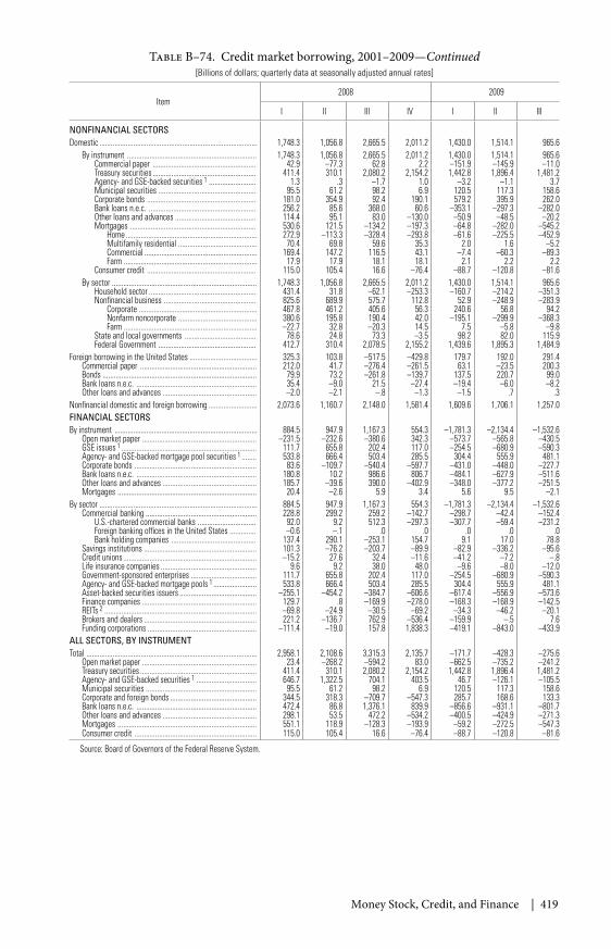
Money Stock, Credit, and Finance | 419
Table B–74. Credit market borrowing, 2001–2009—Continued[Billions of dollars; quarterly data at seasonally adjusted annual rates]
Item2008 2009
I II III IV I II III
NONFINANCIAL SECTORSDomestic .................................................................................... 1,748.3 1,056.8 2,665.5 2,011.2 1,430.0 1,514.1 965.6
By instrument ..................................................................... 1,748.3 1,056.8 2,665.5 2,011.2 1,430.0 1,514.1 965.6Commercial paper ....................................................... 42.9 –77.3 62.8 2.2 –151.9 –145.9 –11.0Treasury securities ....................................................... 411.4 310.1 2,080.2 2,154.2 1,442.8 1,896.4 1,481.2Agency- and GSE-backed securities 1 ......................... 1.3 .3 –1.7 1.0 –3.2 –1.1 3.7Municipal securities .................................................... 95.5 61.2 98.2 6.9 120.5 117.3 158.6Corporate bonds .......................................................... 181.0 354.9 92.4 190.1 579.2 395.9 262.0Bank loans n.e.c. ......................................................... 256.2 85.6 368.0 60.6 –353.1 –297.3 –282.0Other loans and advances ........................................... 114.4 95.1 83.0 –130.0 –50.9 –48.5 –20.2Mortgages ................................................................... 530.6 121.5 –134.2 –197.3 –64.8 –282.0 –545.2
Home...................................................................... 272.9 –113.3 –328.4 –293.8 –61.6 –225.5 –452.9Multifamily residential .......................................... 70.4 69.8 59.6 35.3 2.0 1.6 –5.2Commercial ............................................................ 169.4 147.2 116.5 43.1 –7.4 –60.3 –89.3Farm ....................................................................... 17.9 17.9 18.1 18.1 2.1 2.2 2.2
Consumer credit .......................................................... 115.0 105.4 16.6 –76.4 –88.7 –120.8 –81.6By sector ............................................................................. 1,748.3 1,056.8 2,665.5 2,011.2 1,430.0 1,514.1 965.6
Household sector ......................................................... 431.4 31.8 –62.1 –253.3 –160.7 –214.2 –351.3Nonfinancial business ................................................. 825.6 689.9 575.7 112.8 52.9 –248.9 –283.9
Corporate ............................................................... 467.8 461.2 405.6 56.3 240.6 56.8 94.2Nonfarm noncorporate .......................................... 380.6 195.8 190.4 42.0 –195.1 –299.9 –368.3Farm ....................................................................... –22.7 32.8 –20.3 14.5 7.5 –5.8 –9.8
State and local governments ...................................... 78.6 24.8 73.3 –3.5 98.2 82.0 115.9Federal Government .................................................... 412.7 310.4 2,078.5 2,155.2 1,439.6 1,895.3 1,484.9
Foreign borrowing in the United States .................................... 325.3 103.8 –517.5 –429.8 179.7 192.0 291.4Commercial paper .............................................................. 212.0 41.7 –276.4 –261.5 63.1 –23.5 200.3Bonds .................................................................................. 79.9 73.2 –261.8 –139.7 137.5 220.7 99.0Bank loans n.e.c. ................................................................ 35.4 –9.0 21.5 –27.4 –19.4 –6.0 –8.2Other loans and advances .................................................. –2.0 –2.1 –.8 –1.3 –1.5 .7 .3
Nonfinancial domestic and foreign borrowing .......................... 2,073.6 1,160.7 2,148.0 1,581.4 1,609.6 1,706.1 1,257.0FINANCIAL SECTORSBy instrument ............................................................................ 884.5 947.9 1,167.3 554.3 –1,781.3 –2,134.4 –1,532.6
Open market paper ............................................................. –231.5 –232.6 –380.6 342.3 –573.7 –565.8 –430.5GSE issues 1 ........................................................................ 111.7 655.8 202.4 117.0 –254.5 –680.9 –590.3Agency- and GSE-backed mortgage pool securities 1 ........ 533.8 666.4 503.4 285.5 304.4 555.9 481.1Corporate bonds ................................................................. 83.6 –109.7 –540.4 –597.7 –431.0 –448.0 –227.7Bank loans n.e.c. ................................................................ 180.8 10.2 986.6 806.7 –484.1 –627.9 –511.6Other loans and advances .................................................. 185.7 –39.6 390.0 –402.9 –348.0 –377.2 –251.5Mortgages .......................................................................... 20.4 –2.6 5.9 3.4 5.6 9.5 –2.1
By sector .................................................................................... 884.5 947.9 1,167.3 554.3 –1,781.3 –2,134.4 –1,532.6Commercial banking ........................................................... 228.8 299.2 259.2 –142.7 –298.7 –42.4 –152.4
U.S.-chartered commercial banks ............................... 92.0 9.2 512.3 –297.3 –307.7 –59.4 –231.2Foreign banking offices in the United States .............. –0.6 –.1 .0 .0 .0 .0 .0Bank holding companies ............................................. 137.4 290.1 –253.1 154.7 9.1 17.0 78.8
Savings institutions ............................................................ 101.3 –76.2 –203.7 –89.9 –82.9 –336.2 –95.6Credit unions ....................................................................... –15.2 27.6 32.4 –11.6 –41.2 –7.2 –.8Life insurance companies ................................................... 9.6 9.2 38.0 48.0 –9.6 –8.0 –12.0Government-sponsored enterprises ................................... 111.7 655.8 202.4 117.0 –254.5 –680.9 –590.3Agency- and GSE-backed mortgage pools 1 ....................... 533.8 666.4 503.4 285.5 304.4 555.9 481.1Asset-backed securities issuers ......................................... –255.1 –454.2 –384.7 –606.6 –617.4 –556.9 –573.6Finance companies ............................................................. 129.7 .8 –169.9 –278.0 –168.3 –168.9 –142.5REITs 2 ................................................................................. –69.8 –24.9 –30.5 –69.2 –34.3 –46.2 –20.1Brokers and dealers ............................................................ 221.2 –136.7 762.9 –536.4 –159.9 –.5 7.6Funding corporations .......................................................... –111.4 –19.0 157.8 1,838.3 –419.1 –843.0 –433.9
ALL SECTORS, BY INSTRUMENTTotal ........................................................................................... 2,958.1 2,108.6 3,315.3 2,135.7 –171.7 –428.3 –275.6
Open market paper ............................................................. 23.4 –268.2 –594.2 83.0 –662.5 –735.2 –241.2Treasury securities .............................................................. 411.4 310.1 2,080.2 2,154.2 1,442.8 1,896.4 1,481.2Agency- and GSE-backed securities 1 ................................ 646.7 1,322.5 704.1 403.5 46.7 –126.1 –105.5Municipal securities ........................................................... 95.5 61.2 98.2 6.9 120.5 117.3 158.6Corporate and foreign bonds .............................................. 344.5 318.3 –709.7 –547.3 285.7 168.6 133.3Bank loans n.e.c. ................................................................ 472.4 86.8 1,376.1 839.9 –856.6 –931.1 –801.7Other loans and advances .................................................. 298.1 53.5 472.2 –534.2 –400.5 –424.9 –271.3Mortgages .......................................................................... 551.1 118.9 –128.3 –193.9 –59.2 –272.5 –547.3Consumer credit ................................................................. 115.0 105.4 16.6 –76.4 –88.7 –120.8 –81.6
Source: Board of Governors of the Federal Reserve System.
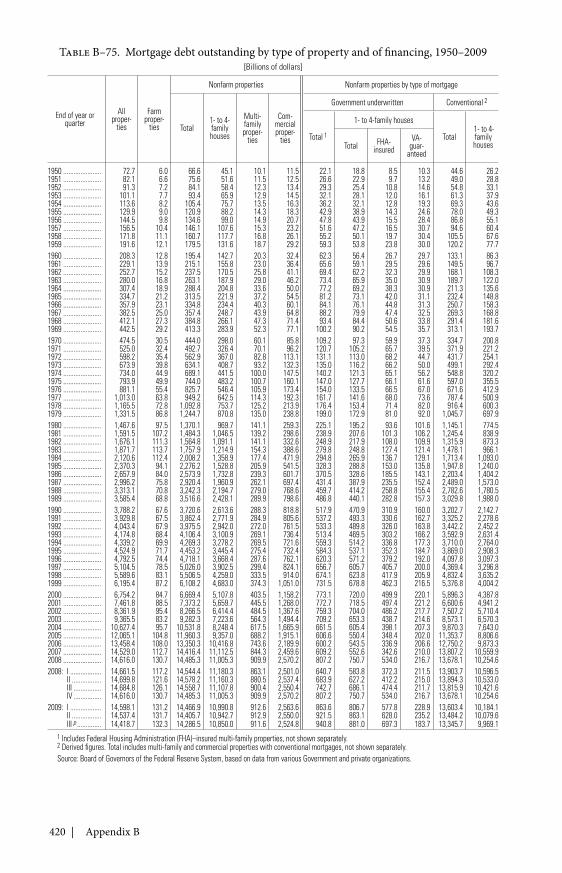
420 | Appendix B
Table B–75. Mortgage debt outstanding by type of property and of financing, 1950–2009[Billions of dollars]
End of year orquarter
Allproper-
ties
Farmproper-
ties
Nonfarm properties Nonfarm properties by type of mortgage
Total1- to 4-familyhouses
Multi-familyproper-
ties
Com-mercialproper-
ties
Government underwritten Conventional 2
Total 1
1- to 4-family houses
Total1- to 4-familyhousesTotal FHA-
insuredVA-
guar-anteed
1950 ...................... 72.7 6.0 66.6 45.1 10.1 11.5 22.1 18.8 8.5 10.3 44.6 26.21951 ...................... 82.1 6.6 75.6 51.6 11.5 12.5 26.6 22.9 9.7 13.2 49.0 28.81952 ...................... 91.3 7.2 84.1 58.4 12.3 13.4 29.3 25.4 10.8 14.6 54.8 33.11953 ...................... 101.1 7.7 93.4 65.9 12.9 14.5 32.1 28.1 12.0 16.1 61.3 37.91954 ...................... 113.6 8.2 105.4 75.7 13.5 16.3 36.2 32.1 12.8 19.3 69.3 43.61955 ...................... 129.9 9.0 120.9 88.2 14.3 18.3 42.9 38.9 14.3 24.6 78.0 49.31956 ...................... 144.5 9.8 134.6 99.0 14.9 20.7 47.8 43.9 15.5 28.4 86.8 55.11957 ...................... 156.5 10.4 146.1 107.6 15.3 23.2 51.6 47.2 16.5 30.7 94.6 60.41958 ...................... 171.8 11.1 160.7 117.7 16.8 26.1 55.2 50.1 19.7 30.4 105.5 67.61959 ...................... 191.6 12.1 179.5 131.6 18.7 29.2 59.3 53.8 23.8 30.0 120.2 77.71960 ...................... 208.3 12.8 195.4 142.7 20.3 32.4 62.3 56.4 26.7 29.7 133.1 86.31961 ...................... 229.1 13.9 215.1 155.8 23.0 36.4 65.6 59.1 29.5 29.6 149.5 96.71962 ...................... 252.7 15.2 237.5 170.5 25.8 41.1 69.4 62.2 32.3 29.9 168.1 108.31963 ...................... 280.0 16.8 263.1 187.9 29.0 46.2 73.4 65.9 35.0 30.9 189.7 122.01964 ...................... 307.4 18.9 288.4 204.8 33.6 50.0 77.2 69.2 38.3 30.9 211.3 135.61965 ...................... 334.7 21.2 313.5 221.9 37.2 54.5 81.2 73.1 42.0 31.1 232.4 148.81966 ...................... 357.9 23.1 334.8 234.4 40.3 60.1 84.1 76.1 44.8 31.3 250.7 158.31967 ...................... 382.5 25.0 357.4 248.7 43.9 64.8 88.2 79.9 47.4 32.5 269.3 168.81968 ...................... 412.1 27.3 384.8 266.1 47.3 71.4 93.4 84.4 50.6 33.8 291.4 181.61969 ...................... 442.5 29.2 413.3 283.9 52.3 77.1 100.2 90.2 54.5 35.7 313.1 193.71970 ...................... 474.5 30.5 444.0 298.0 60.1 85.8 109.2 97.3 59.9 37.3 334.7 200.81971 ...................... 525.0 32.4 492.7 326.4 70.1 96.2 120.7 105.2 65.7 39.5 371.9 221.21972 ...................... 598.2 35.4 562.9 367.0 82.8 113.1 131.1 113.0 68.2 44.7 431.7 254.11973 ...................... 673.9 39.8 634.1 408.7 93.2 132.3 135.0 116.2 66.2 50.0 499.1 292.41974 ...................... 734.0 44.9 689.1 441.5 100.0 147.5 140.2 121.3 65.1 56.2 548.8 320.21975 ...................... 793.9 49.9 744.0 483.2 100.7 160.1 147.0 127.7 66.1 61.6 597.0 355.51976 ...................... 881.1 55.4 825.7 546.4 105.9 173.4 154.0 133.5 66.5 67.0 671.6 412.91977 ...................... 1,013.0 63.8 949.2 642.5 114.3 192.3 161.7 141.6 68.0 73.6 787.4 500.91978 ...................... 1,165.5 72.8 1,092.8 753.7 125.2 213.9 176.4 153.4 71.4 82.0 916.4 600.31979 ...................... 1,331.5 86.8 1,244.7 870.8 135.0 238.8 199.0 172.9 81.0 92.0 1,045.7 697.91980 ...................... 1,467.6 97.5 1,370.1 969.7 141.1 259.3 225.1 195.2 93.6 101.6 1,145.1 774.51981 ...................... 1,591.5 107.2 1,484.3 1,046.5 139.2 298.6 238.9 207.6 101.3 106.2 1,245.4 838.91982 ...................... 1,676.1 111.3 1,564.8 1,091.1 141.1 332.6 248.9 217.9 108.0 109.9 1,315.9 873.31983 ...................... 1,871.7 113.7 1,757.9 1,214.9 154.3 388.6 279.8 248.8 127.4 121.4 1,478.1 966.11984 ...................... 2,120.6 112.4 2,008.2 1,358.9 177.4 471.9 294.8 265.9 136.7 129.1 1,713.4 1,093.01985 ...................... 2,370.3 94.1 2,276.2 1,528.8 205.9 541.5 328.3 288.8 153.0 135.8 1,947.8 1,240.01986 ...................... 2,657.9 84.0 2,573.9 1,732.8 239.3 601.7 370.5 328.6 185.5 143.1 2,203.4 1,404.21987 ...................... 2,996.2 75.8 2,920.4 1,960.9 262.1 697.4 431.4 387.9 235.5 152.4 2,489.0 1,573.01988 ...................... 3,313.1 70.8 3,242.3 2,194.7 279.0 768.6 459.7 414.2 258.8 155.4 2,782.6 1,780.51989 ...................... 3,585.4 68.8 3,516.6 2,428.1 289.9 798.6 486.8 440.1 282.8 157.3 3,029.8 1,988.01990 ...................... 3,788.2 67.6 3,720.6 2,613.6 288.3 818.8 517.9 470.9 310.9 160.0 3,202.7 2,142.71991 ...................... 3,929.8 67.5 3,862.4 2,771.9 284.9 805.6 537.2 493.3 330.6 162.7 3,325.2 2,278.61992 ...................... 4,043.4 67.9 3,975.5 2,942.0 272.0 761.5 533.3 489.8 326.0 163.8 3,442.2 2,452.21993 ...................... 4,174.8 68.4 4,106.4 3,100.9 269.1 736.4 513.4 469.5 303.2 166.2 3,592.9 2,631.41994 ...................... 4,339.2 69.9 4,269.3 3,278.2 269.5 721.6 559.3 514.2 336.8 177.3 3,710.0 2,764.01995 ...................... 4,524.9 71.7 4,453.2 3,445.4 275.4 732.4 584.3 537.1 352.3 184.7 3,869.0 2,908.31996 ...................... 4,792.5 74.4 4,718.1 3,668.4 287.6 762.1 620.3 571.2 379.2 192.0 4,097.8 3,097.31997 ...................... 5,104.5 78.5 5,026.0 3,902.5 299.4 824.1 656.7 605.7 405.7 200.0 4,369.4 3,296.81998 ...................... 5,589.6 83.1 5,506.5 4,259.0 333.5 914.0 674.1 623.8 417.9 205.9 4,832.4 3,635.21999 ...................... 6,195.4 87.2 6,108.2 4,683.0 374.3 1,051.0 731.5 678.8 462.3 216.5 5,376.8 4,004.22000 ...................... 6,754.2 84.7 6,669.4 5,107.8 403.5 1,158.2 773.1 720.0 499.9 220.1 5,896.3 4,387.82001 ...................... 7,461.8 88.5 7,373.2 5,659.7 445.5 1,268.0 772.7 718.5 497.4 221.2 6,600.6 4,941.22002 ...................... 8,361.9 95.4 8,266.5 6,414.4 484.5 1,367.6 759.3 704.0 486.2 217.7 7,507.2 5,710.42003 ...................... 9,365.5 83.2 9,282.3 7,223.6 564.3 1,494.4 709.2 653.3 438.7 214.6 8,573.1 6,570.32004 ...................... 10,627.4 95.7 10,531.8 8,248.4 617.5 1,665.9 661.5 605.4 398.1 207.3 9,870.3 7,643.02005 ...................... 12,065.1 104.8 11,960.3 9,357.0 688.2 1,915.1 606.6 550.4 348.4 202.0 11,353.7 8,806.62006 ...................... 13,458.4 108.0 13,350.3 10,416.8 743.6 2,189.9 600.2 543.5 336.9 206.6 12,750.2 9,873.32007 ...................... 14,529.0 112.7 14,416.4 11,112.5 844.3 2,459.6 609.2 552.6 342.6 210.0 13,807.2 10,559.92008 ...................... 14,616.0 130.7 14,485.3 11,005.3 909.9 2,570.2 807.2 750.7 534.0 216.7 13,678.1 10,254.62008: I .................. 14,661.5 117.2 14,544.4 11,180.3 863.1 2,501.0 640.7 583.8 372.3 211.5 13,903.7 10,596.5
II ................. 14,699.8 121.6 14,578.2 11,160.3 880.5 2,537.4 683.9 627.2 412.2 215.0 13,894.3 10,533.0III ................ 14,684.8 126.1 14,558.7 11,107.8 900.4 2,550.4 742.7 686.1 474.4 211.7 13,815.9 10,421.6IV ................ 14,616.0 130.7 14,485.3 11,005.3 909.9 2,570.2 807.2 750.7 534.0 216.7 13,678.1 10,254.6
2009: I .................. 14,598.1 131.2 14,466.9 10,990.8 912.6 2,563.6 863.6 806.7 577.8 228.9 13,603.4 10,184.1II ................. 14,537.4 131.7 14,405.7 10,942.7 912.9 2,550.0 921.5 863.1 628.0 235.2 13,484.2 10,079.6III p .............. 14,418.7 132.3 14,286.5 10,850.0 911.6 2,524.8 940.8 881.0 697.3 183.7 13,345.7 9,969.1
1 Includes Federal Housing Administration (FHA)–insured multi-family properties, not shown separately.2 Derived figures. Total includes multi-family and commercial properties with conventional mortgages, not shown separately.Source: Board of Governors of the Federal Reserve System, based on data from various Government and private organizations.
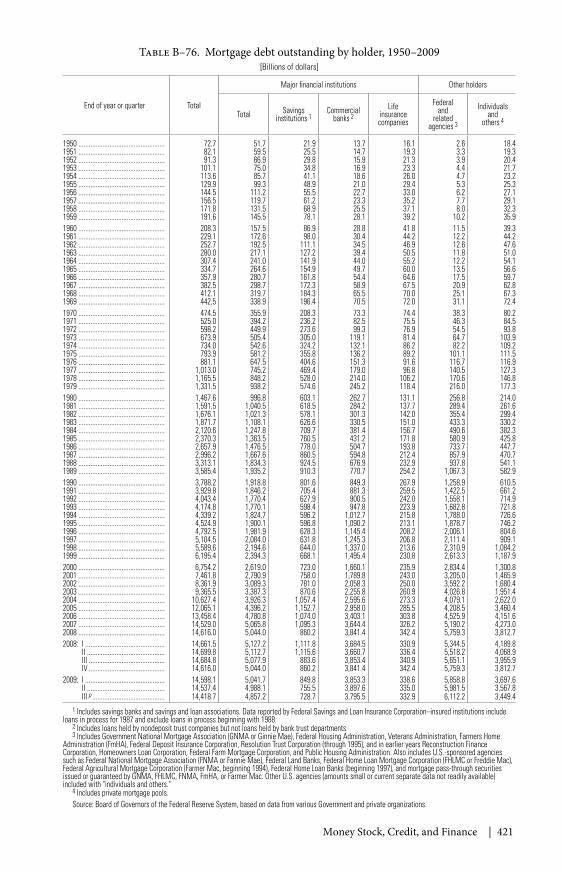
Money Stock, Credit, and Finance | 421
Table B–76. Mortgage debt outstanding by holder, 1950–2009[Billions of dollars]
End of year or quarter Total
Major financial institutions Other holders
Total Savingsinstitutions 1
Commercialbanks 2
Lifeinsurancecompanies
Federaland
relatedagencies 3
Individualsand
others 4
1950 .................................................. 72.7 51.7 21.9 13.7 16.1 2.6 18.41951 .................................................. 82.1 59.5 25.5 14.7 19.3 3.3 19.31952 .................................................. 91.3 66.9 29.8 15.9 21.3 3.9 20.41953 .................................................. 101.1 75.0 34.8 16.9 23.3 4.4 21.71954 .................................................. 113.6 85.7 41.1 18.6 26.0 4.7 23.21955 .................................................. 129.9 99.3 48.9 21.0 29.4 5.3 25.31956 .................................................. 144.5 111.2 55.5 22.7 33.0 6.2 27.11957 .................................................. 156.5 119.7 61.2 23.3 35.2 7.7 29.11958 .................................................. 171.8 131.5 68.9 25.5 37.1 8.0 32.31959 .................................................. 191.6 145.5 78.1 28.1 39.2 10.2 35.91960 .................................................. 208.3 157.5 86.9 28.8 41.8 11.5 39.31961 .................................................. 229.1 172.6 98.0 30.4 44.2 12.2 44.21962 .................................................. 252.7 192.5 111.1 34.5 46.9 12.6 47.61963 .................................................. 280.0 217.1 127.2 39.4 50.5 11.8 51.01964 .................................................. 307.4 241.0 141.9 44.0 55.2 12.2 54.11965 .................................................. 334.7 264.6 154.9 49.7 60.0 13.5 56.61966 .................................................. 357.9 280.7 161.8 54.4 64.6 17.5 59.71967 .................................................. 382.5 298.7 172.3 58.9 67.5 20.9 62.81968 .................................................. 412.1 319.7 184.3 65.5 70.0 25.1 67.31969 .................................................. 442.5 338.9 196.4 70.5 72.0 31.1 72.41970 .................................................. 474.5 355.9 208.3 73.3 74.4 38.3 80.21971 .................................................. 525.0 394.2 236.2 82.5 75.5 46.3 84.51972 .................................................. 598.2 449.9 273.6 99.3 76.9 54.5 93.81973 .................................................. 673.9 505.4 305.0 119.1 81.4 64.7 103.91974 .................................................. 734.0 542.6 324.2 132.1 86.2 82.2 109.21975 .................................................. 793.9 581.2 355.8 136.2 89.2 101.1 111.51976 .................................................. 881.1 647.5 404.6 151.3 91.6 116.7 116.91977 .................................................. 1,013.0 745.2 469.4 179.0 96.8 140.5 127.31978 .................................................. 1,165.5 848.2 528.0 214.0 106.2 170.6 146.81979 .................................................. 1,331.5 938.2 574.6 245.2 118.4 216.0 177.31980 .................................................. 1,467.6 996.8 603.1 262.7 131.1 256.8 214.01981 .................................................. 1,591.5 1,040.5 618.5 284.2 137.7 289.4 261.61982 .................................................. 1,676.1 1,021.3 578.1 301.3 142.0 355.4 299.41983 .................................................. 1,871.7 1,108.1 626.6 330.5 151.0 433.3 330.21984 .................................................. 2,120.6 1,247.8 709.7 381.4 156.7 490.6 382.31985 .................................................. 2,370.3 1,363.5 760.5 431.2 171.8 580.9 425.81986 .................................................. 2,657.9 1,476.5 778.0 504.7 193.8 733.7 447.71987 .................................................. 2,996.2 1,667.6 860.5 594.8 212.4 857.9 470.71988 .................................................. 3,313.1 1,834.3 924.5 676.9 232.9 937.8 541.11989 .................................................. 3,585.4 1,935.2 910.3 770.7 254.2 1,067.3 582.91990 .................................................. 3,788.2 1,918.8 801.6 849.3 267.9 1,258.9 610.51991 .................................................. 3,929.8 1,846.2 705.4 881.3 259.5 1,422.5 661.21992 .................................................. 4,043.4 1,770.4 627.9 900.5 242.0 1,558.1 714.91993 .................................................. 4,174.8 1,770.1 598.4 947.8 223.9 1,682.8 721.81994 .................................................. 4,339.2 1,824.7 596.2 1,012.7 215.8 1,788.0 726.61995 .................................................. 4,524.9 1,900.1 596.8 1,090.2 213.1 1,878.7 746.21996 .................................................. 4,792.5 1,981.9 628.3 1,145.4 208.2 2,006.1 804.61997 .................................................. 5,104.5 2,084.0 631.8 1,245.3 206.8 2,111.4 909.11998 .................................................. 5,589.6 2,194.6 644.0 1,337.0 213.6 2,310.9 1,084.21999 .................................................. 6,195.4 2,394.3 668.1 1,495.4 230.8 2,613.3 1,187.92000 .................................................. 6,754.2 2,619.0 723.0 1,660.1 235.9 2,834.4 1,300.82001 .................................................. 7,461.8 2,790.9 758.0 1,789.8 243.0 3,205.0 1,465.92002 .................................................. 8,361.9 3,089.3 781.0 2,058.3 250.0 3,592.2 1,680.42003 .................................................. 9,365.5 3,387.3 870.6 2,255.8 260.9 4,026.8 1,951.42004 .................................................. 10,627.4 3,926.3 1,057.4 2,595.6 273.3 4,079.1 2,622.02005 .................................................. 12,065.1 4,396.2 1,152.7 2,958.0 285.5 4,208.5 3,460.42006 .................................................. 13,458.4 4,780.8 1,074.0 3,403.1 303.8 4,525.9 4,151.62007 .................................................. 14,529.0 5,065.8 1,095.3 3,644.4 326.2 5,190.2 4,273.02008 .................................................. 14,616.0 5,044.0 860.2 3,841.4 342.4 5,759.3 3,812.72008: I .............................................. 14,661.5 5,127.2 1,111.8 3,684.5 330.9 5,344.5 4,189.8
II ............................................. 14,699.8 5,112.7 1,115.6 3,660.7 336.4 5,518.2 4,068.9III ............................................ 14,684.8 5,077.9 883.6 3,853.4 340.9 5,651.1 3,955.9IV ............................................ 14,616.0 5,044.0 860.2 3,841.4 342.4 5,759.3 3,812.7
2009: I .............................................. 14,598.1 5,041.7 849.8 3,853.3 338.6 5,858.8 3,697.6II ............................................. 14,537.4 4,988.1 755.5 3,897.6 335.0 5,981.5 3,567.8III p .......................................... 14,418.7 4,857.2 728.7 3,795.5 332.9 6,112.2 3,449.4
1 Includes savings banks and savings and loan associations. Data reported by Federal Savings and Loan Insurance Corporation–insured institutions includeloans in process for 1987 and exclude loans in process beginning with 1988.
2 Includes loans held by nondeposit trust companies but not loans held by bank trust departments.3 Includes Government National Mortgage Association (GNMA or Ginnie Mae), Federal Housing Administration, Veterans Administration, Farmers Home
Administration (FmHA), Federal Deposit Insurance Corporation, Resolution Trust Corporation (through 1995), and in earlier years Reconstruction FinanceCorporation, Homeowners Loan Corporation, Federal Farm Mortgage Corporation, and Public Housing Administration. Also includes U.S.-sponsored agenciessuch as Federal National Mortgage Association (FNMA or Fannie Mae), Federal Land Banks, Federal Home Loan Mortgage Corporation (FHLMC or Freddie Mac),Federal Agricultural Mortgage Corporation (Farmer Mac, beginning 1994), Federal Home Loan Banks (beginning 1997), and mortgage pass-through securitiesissued or guaranteed by GNMA, FHLMC, FNMA, FmHA, or Farmer Mac. Other U.S. agencies (amounts small or current separate data not readily available)included with "individuals and others."
4 Includes private mortgage pools.Source: Board of Governors of the Federal Reserve System, based on data from various Government and private organizations.
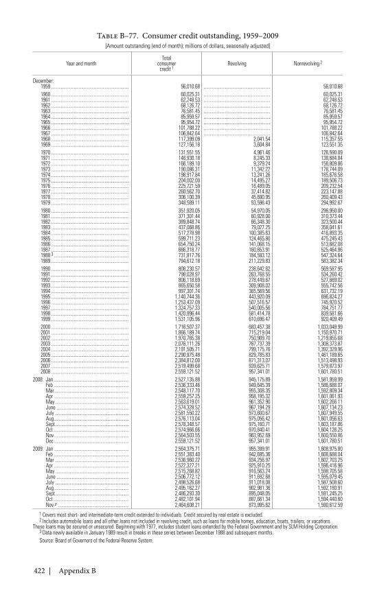
422 | Appendix B
Table B–77. Consumer credit outstanding, 1959–2009[Amount outstanding (end of month); millions of dollars, seasonally adjusted]
Year and monthTotal
consumercredit 1
Revolving Nonrevolving 2
December:1959 ................................................................. 56,010.68 ........................................................ 56,010.681960 ................................................................. 60,025.31 ........................................................ 60,025.311961 ................................................................. 62,248.53 ........................................................ 62,248.531962 ................................................................. 68,126.72 ........................................................ 68,126.721963 ................................................................. 76,581.45 ........................................................ 76,581.451964 ................................................................. 85,959.57 ........................................................ 85,959.571965 ................................................................. 95,954.72 ........................................................ 95,954.721966 ................................................................. 101,788.22 ........................................................ 101,788.221967 ................................................................. 106,842.64 ........................................................ 106,842.641968 ................................................................. 117,399.09 2,041.54 115,357.551969 ................................................................. 127,156.18 3,604.84 123,551.351970 ................................................................. 131,551.55 4,961.46 126,590.091971 ................................................................. 146,930.18 8,245.33 138,684.841972 ................................................................. 166,189.10 9,379.24 156,809.861973 ................................................................. 190,086.31 11,342.22 178,744.091974 ................................................................. 198,917.84 13,241.26 185,676.581975 ................................................................. 204,002.00 14,495.27 189,506.731976 ................................................................. 225,721.59 16,489.05 209,232.541977 ................................................................. 260,562.70 37,414.82 223,147.881978 ................................................................. 306,100.39 45,690.95 260,409.431979 ................................................................. 348,589.11 53,596.43 294,992.671980 ................................................................. 351,920.05 54,970.05 296,950.001981 ................................................................. 371,301.44 60,928.00 310,373.441982 ................................................................. 389,848.74 66,348.30 323,500.441983 ................................................................. 437,068.86 79,027.25 358,041.611984 ................................................................. 517,278.98 100,385.63 416,893.351985 ................................................................. 599,711.23 124,465.80 475,245.431986 ................................................................. 654,750.24 141,068.15 513,682.081987 ................................................................. 686,318.77 160,853.91 525,464.861988 3 ............................................................... 731,917.76 184,593.12 547,324.641989 ................................................................. 794,612.18 211,229.83 583,382.341990 ................................................................. 808,230.57 238,642.62 569,587.951991 ................................................................. 798,028.97 263,768.55 534,260.421992 ................................................................. 806,118.69 278,449.67 527,669.021993 ................................................................. 865,650.58 309,908.02 555,742.561994 ................................................................. 997,301.74 365,569.56 631,732.191995 ................................................................. 1,140,744.36 443,920.09 696,824.271996 ................................................................. 1,253,437.09 507,516.57 745,920.521997 ................................................................. 1,324,757.33 540,005.56 784,751.771998 ................................................................. 1,420,996.44 581,414.78 839,581.661999 ................................................................. 1,531,105.96 610,696.47 920,409.492000 ................................................................. 1,716,507.37 683,457.38 1,033,049.992001 ................................................................. 1,866,189.74 715,219.04 1,150,970.712002 ................................................................. 1,970,765.38 750,909.70 1,219,855.682003 ................................................................. 2,076,111.26 767,737.39 1,308,373.872004 ................................................................. 2,191,505.71 799,175.76 1,392,329.962005 ................................................................. 2,290,975.48 829,785.83 1,461,189.652006 ................................................................. 2,384,812.00 871,313.07 1,513,498.932007 ................................................................. 2,519,499.68 939,625.71 1,579,873.972008 ................................................................. 2,559,121.52 957,341.01 1,601,780.51
2008: Jan ............................................................... 2,527,135.88 945,175.89 1,581,959.99Feb ............................................................... 2,536,333.46 949,645.39 1,586,688.07Mar .............................................................. 2,548,117.70 955,308.35 1,592,809.34Apr ............................................................... 2,559,257.25 958,195.32 1,601,061.93May .............................................................. 2,563,619.01 961,352.90 1,602,266.11June ............................................................. 2,574,328.52 967,194.29 1,607,134.23July .............................................................. 2,581,550.22 973,600.67 1,607,949.55Aug ............................................................... 2,576,113.04 975,056.42 1,601,056.63Sept .............................................................. 2,578,348.57 975,160.71 1,603,187.86Oct ................................................................ 2,574,966.66 970,840.41 1,604,126.25Nov ............................................................... 2,564,503.55 963,952.69 1,600,550.86Dec ............................................................... 2,559,121.52 957,341.01 1,601,780.51
2009: Jan ............................................................... 2,564,375.71 955,399.91 1,608,975.80Feb ............................................................... 2,551,383.40 942,695.36 1,608,688.04Mar .............................................................. 2,536,960.22 934,256.97 1,602,703.25Apr ............................................................... 2,522,327.21 925,910.25 1,596,416.96May .............................................................. 2,515,268.82 916,563.24 1,598,705.58June ............................................................. 2,506,772.12 911,692.68 1,595,079.45July .............................................................. 2,498,526.68 911,018.08 1,587,508.60Aug ............................................................... 2,495,162.27 902,981.36 1,592,180.91Sept .............................................................. 2,486,293.30 895,048.05 1,591,245.25Oct ................................................................ 2,482,101.94 887,661.34 1,594,440.60Nov p ............................................................ 2,464,608.21 873,995.62 1,590,612.59
1 Covers most short- and intermediate-term credit extended to individuals. Credit secured by real estate is excluded.2 Includes automobile loans and all other loans not included in revolving credit, such as loans for mobile homes, education, boats, trailers, or vacations.
These loans may be secured or unsecured. Beginning with 1977, includes student loans extended by the Federal Government and by SLM Holding Corporation.3 Data newly available in January 1989 result in breaks in these series between December 1988 and subsequent months.Source: Board of Governors of the Federal Reserve System.
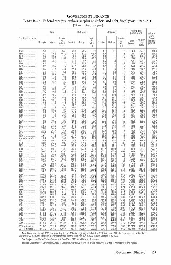
Government Finance | 423
Table B–78. Federal receipts, outlays, surplus or deficit, and debt, fiscal years, 1943–2011[Billions of dollars; fiscal years]
Fiscal year or period
Total On-budget Off-budget Federal debt(end of period) Adden-
dum:Gross
domesticproductReceipts Outlays
Surplusor
deficit(–)
Receipts OutlaysSurplus
ordeficit
(–)Receipts Outlays
Surplusor
deficit(–)
GrossFederal
Held bythe
public
1943 ....................... 24.0 78.6 –54.6 22.9 78.5 –55.6 1.1 0.1 1.0 142.6 127.8 180.31944 ....................... 43.7 91.3 –47.6 42.5 91.2 –48.7 1.3 .1 1.2 204.1 184.8 209.21945 ....................... 45.2 92.7 –47.6 43.8 92.6 –48.7 1.3 .1 1.2 260.1 235.2 221.41946 ....................... 39.3 55.2 –15.9 38.1 55.0 –17.0 1.2 .2 1.0 271.0 241.9 222.61947 ....................... 38.5 34.5 4.0 37.1 34.2 2.9 1.5 .3 1.2 257.1 224.3 233.21948 ....................... 41.6 29.8 11.8 39.9 29.4 10.5 1.6 .4 1.2 252.0 216.3 256.61949 ....................... 39.4 38.8 .6 37.7 38.4 –.7 1.7 .4 1.3 252.6 214.3 271.31950 ....................... 39.4 42.6 –3.1 37.3 42.0 –4.7 2.1 .5 1.6 256.9 219.0 273.11951 ....................... 51.6 45.5 6.1 48.5 44.2 4.3 3.1 1.3 1.8 255.3 214.3 320.21952 ....................... 66.2 67.7 –1.5 62.6 66.0 –3.4 3.6 1.7 1.9 259.1 214.8 348.71953 ....................... 69.6 76.1 –6.5 65.5 73.8 –8.3 4.1 2.3 1.8 266.0 218.4 372.51954 ....................... 69.7 70.9 –1.2 65.1 67.9 –2.8 4.6 2.9 1.7 270.8 224.5 377.01955 ....................... 65.5 68.4 –3.0 60.4 64.5 –4.1 5.1 4.0 1.1 274.4 226.6 395.91956 ....................... 74.6 70.6 3.9 68.2 65.7 2.5 6.4 5.0 1.5 272.7 222.2 427.01957 ....................... 80.0 76.6 3.4 73.2 70.6 2.6 6.8 6.0 .8 272.3 219.3 450.91958 ....................... 79.6 82.4 –2.8 71.6 74.9 –3.3 8.0 7.5 .5 279.7 226.3 460.01959 ....................... 79.2 92.1 –12.8 71.0 83.1 –12.1 8.3 9.0 –.7 287.5 234.7 490.21960 ....................... 92.5 92.2 .3 81.9 81.3 .5 10.6 10.9 –.2 290.5 236.8 518.91961 ....................... 94.4 97.7 –3.3 82.3 86.0 –3.8 12.1 11.7 .4 292.6 238.4 529.91962 ....................... 99.7 106.8 –7.1 87.4 93.3 –5.9 12.3 13.5 –1.3 302.9 248.0 567.81963 ....................... 106.6 111.3 –4.8 92.4 96.4 –4.0 14.2 15.0 –.8 310.3 254.0 599.21964 ....................... 112.6 118.5 –5.9 96.2 102.8 –6.5 16.4 15.7 .6 316.1 256.8 641.51965 ....................... 116.8 118.2 –1.4 100.1 101.7 –1.6 16.7 16.5 .2 322.3 260.8 687.51966 ....................... 130.8 134.5 –3.7 111.7 114.8 –3.1 19.1 19.7 –.6 328.5 263.7 755.81967 ....................... 148.8 157.5 –8.6 124.4 137.0 –12.6 24.4 20.4 4.0 340.4 266.6 810.01968 ....................... 153.0 178.1 –25.2 128.1 155.8 –27.7 24.9 22.3 2.6 368.7 289.5 868.41969 ....................... 186.9 183.6 3.2 157.9 158.4 –.5 29.0 25.2 3.7 365.8 278.1 948.11970 ....................... 192.8 195.6 –2.8 159.3 168.0 –8.7 33.5 27.6 5.9 380.9 283.2 1,012.71971 ....................... 187.1 210.2 –23.0 151.3 177.3 –26.1 35.8 32.8 3.0 408.2 303.0 1,080.01972 ....................... 207.3 230.7 –23.4 167.4 193.5 –26.1 39.9 37.2 2.7 435.9 322.4 1,176.51973 ....................... 230.8 245.7 –14.9 184.7 200.0 –15.2 46.1 45.7 .3 466.3 340.9 1,310.61974 ....................... 263.2 269.4 –6.1 209.3 216.5 –7.2 53.9 52.9 1.1 483.9 343.7 1,438.51975 ....................... 279.1 332.3 –53.2 216.6 270.8 –54.1 62.5 61.6 .9 541.9 394.7 1,560.21976 ....................... 298.1 371.8 –73.7 231.7 301.1 –69.4 66.4 70.7 –4.3 629.0 477.4 1,738.1Transition quarter .. 81.2 96.0 –14.7 63.2 77.3 –14.1 18.0 18.7 –.7 643.6 495.5 459.41977 ....................... 355.6 409.2 –53.7 278.7 328.7 –49.9 76.8 80.5 –3.7 706.4 549.1 1,973.51978 ....................... 399.6 458.7 –59.2 314.2 369.6 –55.4 85.4 89.2 –3.8 776.6 607.1 2,217.51979 ....................... 463.3 504.0 –40.7 365.3 404.9 –39.6 98.0 99.1 –1.1 829.5 640.3 2,501.41980 ....................... 517.1 590.9 –73.8 403.9 477.0 –73.1 113.2 113.9 –.7 909.0 711.9 2,724.21981 ....................... 599.3 678.2 –79.0 469.1 543.0 –73.9 130.2 135.3 –5.1 994.8 789.4 3,057.01982 ....................... 617.8 745.7 –128.0 474.3 594.9 –120.6 143.5 150.9 –7.4 1,137.3 924.6 3,223.71983 ....................... 600.6 808.4 –207.8 453.2 660.9 –207.7 147.3 147.4 –.1 1,371.7 1,137.3 3,440.71984 ....................... 666.4 851.8 –185.4 500.4 685.6 –185.3 166.1 166.2 –.1 1,564.6 1,307.0 3,844.41985 ....................... 734.0 946.3 –212.3 547.9 769.4 –221.5 186.2 176.9 9.2 1,817.4 1,507.3 4,146.31986 ....................... 769.2 990.4 –221.2 568.9 806.8 –237.9 200.2 183.5 16.7 2,120.5 1,740.6 4,403.91987 ....................... 854.3 1,004.0 –149.7 640.9 809.2 –168.4 213.4 194.8 18.6 2,346.0 1,889.8 4,651.41988 ....................... 909.2 1,064.4 –155.2 667.7 860.0 –192.3 241.5 204.4 37.1 2,601.1 2,051.6 5,008.51989 ....................... 991.1 1,143.7 –152.6 727.4 932.8 –205.4 263.7 210.9 52.8 2,867.8 2,190.7 5,399.51990 ....................... 1,032.0 1,253.0 –221.0 750.3 1,027.9 –277.6 281.7 225.1 56.6 3,206.3 2,411.6 5,734.51991 ....................... 1,055.0 1,324.2 –269.2 761.1 1,082.5 –321.4 293.9 241.7 52.2 3,598.2 2,689.0 5,930.51992 ....................... 1,091.2 1,381.5 –290.3 788.8 1,129.2 –340.4 302.4 252.3 50.1 4,001.8 2,999.7 6,242.01993 ....................... 1,154.3 1,409.4 –255.1 842.4 1,142.8 –300.4 311.9 266.6 45.3 4,351.0 3,248.4 6,587.31994 ....................... 1,258.6 1,461.8 –203.2 923.6 1,182.4 –258.8 335.0 279.4 55.7 4,643.3 3,433.1 6,976.61995 ....................... 1,351.8 1,515.8 –164.0 1,000.7 1,227.1 –226.4 351.1 288.7 62.4 4,920.6 3,604.4 7,341.11996 ....................... 1,453.1 1,560.5 –107.4 1,085.6 1,259.6 –174.0 367.5 300.9 66.6 5,181.5 3,734.1 7,718.31997 ....................... 1,579.2 1,601.1 –21.9 1,187.3 1,290.5 –103.2 392.0 310.6 81.4 5,369.2 3,772.3 8,211.71998 ....................... 1,721.7 1,652.5 69.3 1,305.9 1,335.9 –29.9 415.8 316.6 99.2 5,478.2 3,721.1 8,663.01999 ....................... 1,827.5 1,701.8 125.6 1,383.0 1,381.1 1.9 444.5 320.8 123.7 5,605.5 3,632.4 9,208.42000 ....................... 2,025.2 1,789.0 236.2 1,544.6 1,458.2 86.4 480.6 330.8 149.8 5,628.7 3,409.8 9,821.02001 ....................... 1,991.1 1,862.9 128.2 1,483.6 1,516.1 –32.4 507.5 346.8 160.7 5,769.9 3,319.6 10,225.32002 ....................... 1,853.1 2,010.9 –157.8 1,337.8 1,655.2 –317.4 515.3 355.7 159.7 6,198.4 3,540.4 10,543.92003 ....................... 1,782.3 2,159.9 –377.6 1,258.5 1,796.9 –538.4 523.8 363.0 160.8 6,760.0 3,913.4 10,979.82004 ....................... 1,880.1 2,292.9 –412.7 1,345.4 1,913.3 –568.0 534.7 379.5 155.2 7,354.7 4,295.5 11,685.62005 ....................... 2,153.6 2,472.0 –318.3 1,576.1 2,069.8 –493.6 577.5 402.2 175.3 7,905.3 4,592.2 12,445.72006 ....................... 2,406.9 2,655.1 –248.2 1,798.5 2,233.0 –434.5 608.4 422.1 186.3 8,451.4 4,829.0 13,224.92007 ....................... 2,568.0 2,728.7 –160.7 1,932.9 2,275.1 –342.2 635.1 453.6 181.5 8,950.7 5,035.1 13,896.02008 ....................... 2,524.0 2,982.6 –458.6 1,866.0 2,507.8 –641.9 658.0 474.8 183.3 9,986.1 5,803.1 14,439.02009 ....................... 2,105.0 3,517.7 –1,412.7 1,451.0 3,000.7 –1,549.7 654.0 517.0 137.0 11,875.9 7,544.7 14,237.22010 (estimates) .... 2,165.1 3,720.7 –1,555.6 1,529.9 3,163.7 –1,633.8 635.2 557.0 78.2 13,786.6 9,297.7 14,623.92011 (estimates) .... 2,567.2 3,833.9 –1,266.7 1,893.1 3,255.7 –1,362.6 674.1 578.2 95.9 15,144.0 10,498.3 15,299.0
Note: Fiscal years through 1976 were on a July 1–June 30 basis; beginning with October 1976 (fiscal year 1977), the fiscal year is on an October 1–September 30 basis. The transition quarter is the three-month period from July 1, 1976 through September 30, 1976.
See Budget of the United States Government, Fiscal Year 2011, for additional information.Sources: Department of Commerce (Bureau of Economic Analysis), Department of the Treasury, and Office of Management and Budget.
Government Finance
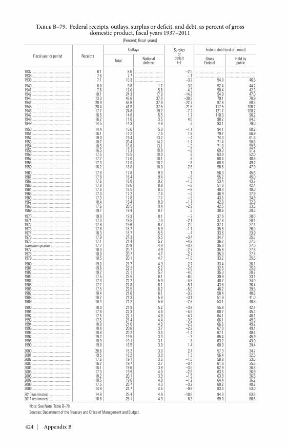
424 | Appendix B
Table B–79. Federal receipts, outlays, surplus or deficit, and debt, as percent of grossdomestic product, fiscal years 1937–2011
[Percent; fiscal years]
Fiscal year or period ReceiptsOutlays Surplus
ordeficit
(–)
Federal debt (end of period)
Total Nationaldefense
GrossFederal
Held bypublic
1937 ........................................... 6.1 8.6 ............................... –2.5 ............................... ................................1938 ........................................... 7.6 7.7 ............................... –.1 ............................... ................................1939 ........................................... 7.1 10.3 ............................... –3.2 54.0 46.51940 ........................................... 6.8 9.8 1.7 –3.0 52.4 44.21941 ........................................... 7.6 12.0 5.6 –4.3 50.4 42.31942 ........................................... 10.1 24.3 17.8 –14.2 54.9 47.01943 ........................................... 13.3 43.6 37.0 –30.3 79.1 70.91944 ........................................... 20.9 43.6 37.8 –22.7 97.6 88.31945 ........................................... 20.4 41.9 37.5 –21.5 117.5 106.21946 ........................................... 17.7 24.8 19.2 –7.2 121.7 108.71947 ........................................... 16.5 14.8 5.5 1.7 110.3 96.21948 ........................................... 16.2 11.6 3.5 4.6 98.2 84.31949 ........................................... 14.5 14.3 4.8 .2 93.1 79.01950 ........................................... 14.4 15.6 5.0 –1.1 94.1 80.21951 ........................................... 16.1 14.2 7.4 1.9 79.7 66.91952 ........................................... 19.0 19.4 13.2 –.4 74.3 61.61953 ........................................... 18.7 20.4 14.2 –1.7 71.4 58.61954 ........................................... 18.5 18.8 13.1 –.3 71.8 59.51955 ........................................... 16.5 17.3 10.8 –.8 69.3 57.21956 ........................................... 17.5 16.5 10.0 .9 63.9 52.01957 ........................................... 17.7 17.0 10.1 .8 60.4 48.61958 ........................................... 17.3 17.9 10.2 –.6 60.8 49.21959 ........................................... 16.2 18.8 10.0 –2.6 58.6 47.91960 ........................................... 17.8 17.8 9.3 .1 56.0 45.61961 ........................................... 17.8 18.4 9.4 –.6 55.2 45.01962 ........................................... 17.6 18.8 9.2 –1.3 53.4 43.71963 ........................................... 17.8 18.6 8.9 –.8 51.8 42.41964 ........................................... 17.6 18.5 8.5 –.9 49.3 40.01965 ........................................... 17.0 17.2 7.4 –.2 46.9 37.91966 ........................................... 17.3 17.8 7.7 –.5 43.5 34.91967 ........................................... 18.4 19.4 8.8 –1.1 42.0 32.91968 ........................................... 17.6 20.5 9.4 –2.9 42.5 33.31969 ........................................... 19.7 19.4 8.7 .3 38.6 29.31970 ........................................... 19.0 19.3 8.1 –.3 37.6 28.01971 ........................................... 17.3 19.5 7.3 –2.1 37.8 28.11972 ........................................... 17.6 19.6 6.7 –2.0 37.1 27.41973 ........................................... 17.6 18.7 5.9 –1.1 35.6 26.01974 ........................................... 18.3 18.7 5.5 –.4 33.6 23.91975 ........................................... 17.9 21.3 5.5 –3.4 34.7 25.31976 ........................................... 17.1 21.4 5.2 –4.2 36.2 27.5Transition quarter ...................... 17.7 20.9 4.8 –3.2 35.0 27.01977 ........................................... 18.0 20.7 4.9 –2.7 35.8 27.81978 ........................................... 18.0 20.7 4.7 –2.7 35.0 27.41979 ........................................... 18.5 20.1 4.7 –1.6 33.2 25.61980 ........................................... 19.0 21.7 4.9 –2.7 33.4 26.11981 ........................................... 19.6 22.2 5.2 –2.6 32.5 25.81982 ........................................... 19.2 23.1 5.7 –4.0 35.3 28.71983 ........................................... 17.5 23.5 6.1 –6.0 39.9 33.11984 ........................................... 17.3 22.2 5.9 –4.8 40.7 34.01985 ........................................... 17.7 22.8 6.1 –5.1 43.8 36.41986 ........................................... 17.5 22.5 6.2 –5.0 48.2 39.51987 ........................................... 18.4 21.6 6.1 –3.2 50.4 40.61988 ........................................... 18.2 21.3 5.8 –3.1 51.9 41.01989 ........................................... 18.4 21.2 5.6 –2.8 53.1 40.61990 ........................................... 18.0 21.9 5.2 –3.9 55.9 42.11991 ........................................... 17.8 22.3 4.6 –4.5 60.7 45.31992 ........................................... 17.5 22.1 4.8 –4.7 64.1 48.11993 ........................................... 17.5 21.4 4.4 –3.9 66.1 49.31994 ........................................... 18.0 21.0 4.0 –2.9 66.6 49.21995 ........................................... 18.4 20.6 3.7 –2.2 67.0 49.11996 ........................................... 18.8 20.2 3.4 –1.4 67.1 48.41997 ........................................... 19.2 19.5 3.3 –.3 65.4 45.91998 ........................................... 19.9 19.1 3.1 .8 63.2 43.01999 ........................................... 19.8 18.5 3.0 1.4 60.9 39.42000 ........................................... 20.6 18.2 3.0 2.4 57.3 34.72001 ........................................... 19.5 18.2 3.0 1.3 56.4 32.52002 ........................................... 17.6 19.1 3.3 –1.5 58.8 33.62003 ........................................... 16.2 19.7 3.7 –3.4 61.6 35.62004 ........................................... 16.1 19.6 3.9 –3.5 62.9 36.82005 ........................................... 17.3 19.9 4.0 –2.6 63.5 36.92006 ........................................... 18.2 20.1 3.9 –1.9 63.9 36.52007 ........................................... 18.5 19.6 4.0 –1.2 64.4 36.22008 ........................................... 17.5 20.7 4.3 –3.2 69.2 40.22009 ........................................... 14.8 24.7 4.6 –9.9 83.4 53.02010 (estimates) ........................ 14.8 25.4 4.9 –10.6 94.3 63.62011 (estimates) ........................ 16.8 25.1 4.9 –8.3 99.0 68.6
Note: See Note, Table B–78.Sources: Department of the Treasury and Office of Management and Budget.
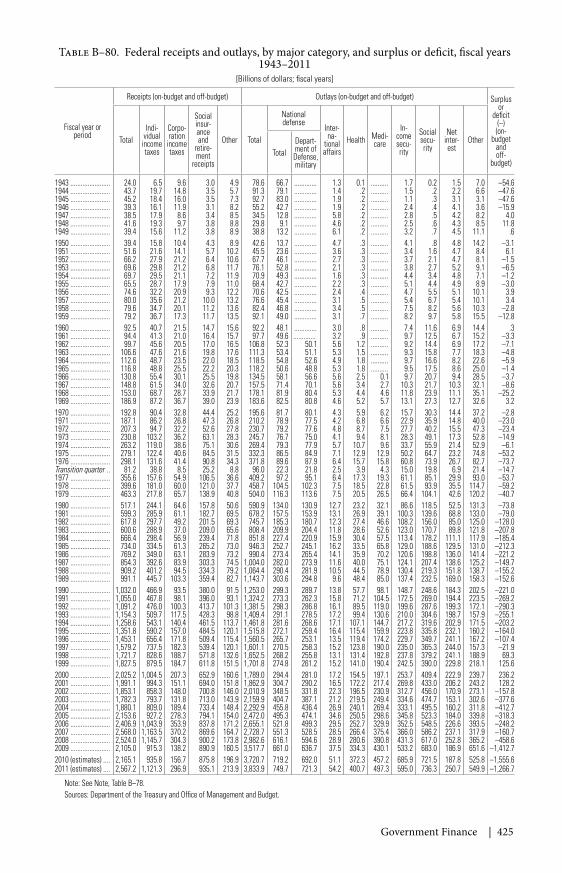
Government Finance | 425
Table B–80. Federal receipts and outlays, by major category, and surplus or deficit, fiscal years1943–2011
[Billions of dollars; fiscal years]
Fiscal year orperiod
Receipts (on-budget and off-budget) Outlays (on-budget and off-budget) Surplusor
deficit(–)
(on-budget
andoff-
budget)
TotalIndi-
vidualincometaxes
Corpo-ration
incometaxes
Socialinsur-anceand
retire-ment
receipts
Other Total
Nationaldefense
Inter-na-
tionalaffairs
Health Medi-care
In-comesecu-rity
Socialsecu-rity
Netinter-est
OtherTotal
Depart-ment ofDefense,military
1943 ....................... 24.0 6.5 9.6 3.0 4.9 78.6 66.7 ............. 1.3 0.1 .......... 1.7 0.2 1.5 7.0 –54.61944 ....................... 43.7 19.7 14.8 3.5 5.7 91.3 79.1 ............. 1.4 .2 .......... 1.5 .2 2.2 6.6 –47.61945 ....................... 45.2 18.4 16.0 3.5 7.3 92.7 83.0 ............. 1.9 .2 .......... 1.1 .3 3.1 3.1 –47.61946 ....................... 39.3 16.1 11.9 3.1 8.2 55.2 42.7 ............. 1.9 .2 .......... 2.4 .4 4.1 3.6 –15.91947 ....................... 38.5 17.9 8.6 3.4 8.5 34.5 12.8 ............. 5.8 .2 .......... 2.8 .5 4.2 8.2 4.01948 ....................... 41.6 19.3 9.7 3.8 8.8 29.8 9.1 ............. 4.6 .2 .......... 2.5 .6 4.3 8.5 11.81949 ....................... 39.4 15.6 11.2 3.8 8.9 38.8 13.2 ............. 6.1 .2 .......... 3.2 .7 4.5 11.1 .61950 ....................... 39.4 15.8 10.4 4.3 8.9 42.6 13.7 ............. 4.7 .3 .......... 4.1 .8 4.8 14.2 –3.11951 ....................... 51.6 21.6 14.1 5.7 10.2 45.5 23.6 ............. 3.6 .3 .......... 3.4 1.6 4.7 8.4 6.11952 ....................... 66.2 27.9 21.2 6.4 10.6 67.7 46.1 ............. 2.7 .3 .......... 3.7 2.1 4.7 8.1 –1.51953 ....................... 69.6 29.8 21.2 6.8 11.7 76.1 52.8 ............. 2.1 .3 .......... 3.8 2.7 5.2 9.1 –6.51954 ....................... 69.7 29.5 21.1 7.2 11.9 70.9 49.3 ............. 1.6 .3 .......... 4.4 3.4 4.8 7.1 –1.21955 ....................... 65.5 28.7 17.9 7.9 11.0 68.4 42.7 ............. 2.2 .3 .......... 5.1 4.4 4.9 8.9 –3.01956 ....................... 74.6 32.2 20.9 9.3 12.2 70.6 42.5 ............. 2.4 .4 .......... 4.7 5.5 5.1 10.1 3.91957 ....................... 80.0 35.6 21.2 10.0 13.2 76.6 45.4 ............. 3.1 .5 .......... 5.4 6.7 5.4 10.1 3.41958 ....................... 79.6 34.7 20.1 11.2 13.6 82.4 46.8 ............. 3.4 .5 .......... 7.5 8.2 5.6 10.3 –2.81959 ....................... 79.2 36.7 17.3 11.7 13.5 92.1 49.0 ............. 3.1 .7 .......... 8.2 9.7 5.8 15.5 –12.81960 ....................... 92.5 40.7 21.5 14.7 15.6 92.2 48.1 ............. 3.0 .8 .......... 7.4 11.6 6.9 14.4 .31961 ....................... 94.4 41.3 21.0 16.4 15.7 97.7 49.6 ............. 3.2 .9 .......... 9.7 12.5 6.7 15.2 –3.31962 ....................... 99.7 45.6 20.5 17.0 16.5 106.8 52.3 50.1 5.6 1.2 .......... 9.2 14.4 6.9 17.2 –7.11963 ....................... 106.6 47.6 21.6 19.8 17.6 111.3 53.4 51.1 5.3 1.5 .......... 9.3 15.8 7.7 18.3 –4.81964 ....................... 112.6 48.7 23.5 22.0 18.5 118.5 54.8 52.6 4.9 1.8 .......... 9.7 16.6 8.2 22.6 –5.91965 ....................... 116.8 48.8 25.5 22.2 20.3 118.2 50.6 48.8 5.3 1.8 .......... 9.5 17.5 8.6 25.0 –1.41966 ....................... 130.8 55.4 30.1 25.5 19.8 134.5 58.1 56.6 5.6 2.5 0.1 9.7 20.7 9.4 28.5 –3.71967 ....................... 148.8 61.5 34.0 32.6 20.7 157.5 71.4 70.1 5.6 3.4 2.7 10.3 21.7 10.3 32.1 –8.61968 ....................... 153.0 68.7 28.7 33.9 21.7 178.1 81.9 80.4 5.3 4.4 4.6 11.8 23.9 11.1 35.1 –25.21969 ....................... 186.9 87.2 36.7 39.0 23.9 183.6 82.5 80.8 4.6 5.2 5.7 13.1 27.3 12.7 32.6 3.21970 ....................... 192.8 90.4 32.8 44.4 25.2 195.6 81.7 80.1 4.3 5.9 6.2 15.7 30.3 14.4 37.2 –2.81971 ....................... 187.1 86.2 26.8 47.3 26.8 210.2 78.9 77.5 4.2 6.8 6.6 22.9 35.9 14.8 40.0 –23.01972 ....................... 207.3 94.7 32.2 52.6 27.8 230.7 79.2 77.6 4.8 8.7 7.5 27.7 40.2 15.5 47.3 –23.41973 ....................... 230.8 103.2 36.2 63.1 28.3 245.7 76.7 75.0 4.1 9.4 8.1 28.3 49.1 17.3 52.8 –14.91974 ....................... 263.2 119.0 38.6 75.1 30.6 269.4 79.3 77.9 5.7 10.7 9.6 33.7 55.9 21.4 52.9 –6.11975 ....................... 279.1 122.4 40.6 84.5 31.5 332.3 86.5 84.9 7.1 12.9 12.9 50.2 64.7 23.2 74.8 –53.21976 ....................... 298.1 131.6 41.4 90.8 34.3 371.8 89.6 87.9 6.4 15.7 15.8 60.8 73.9 26.7 82.7 –73.7Transition quarter .. 81.2 38.8 8.5 25.2 8.8 96.0 22.3 21.8 2.5 3.9 4.3 15.0 19.8 6.9 21.4 –14.71977 ....................... 355.6 157.6 54.9 106.5 36.6 409.2 97.2 95.1 6.4 17.3 19.3 61.1 85.1 29.9 93.0 –53.71978 ....................... 399.6 181.0 60.0 121.0 37.7 458.7 104.5 102.3 7.5 18.5 22.8 61.5 93.9 35.5 114.7 –59.21979 ....................... 463.3 217.8 65.7 138.9 40.8 504.0 116.3 113.6 7.5 20.5 26.5 66.4 104.1 42.6 120.2 –40.71980 ....................... 517.1 244.1 64.6 157.8 50.6 590.9 134.0 130.9 12.7 23.2 32.1 86.6 118.5 52.5 131.3 –73.81981 ....................... 599.3 285.9 61.1 182.7 69.5 678.2 157.5 153.9 13.1 26.9 39.1 100.3 139.6 68.8 133.0 –79.01982 ....................... 617.8 297.7 49.2 201.5 69.3 745.7 185.3 180.7 12.3 27.4 46.6 108.2 156.0 85.0 125.0 –128.01983 ....................... 600.6 288.9 37.0 209.0 65.6 808.4 209.9 204.4 11.8 28.6 52.6 123.0 170.7 89.8 121.8 –207.81984 ....................... 666.4 298.4 56.9 239.4 71.8 851.8 227.4 220.9 15.9 30.4 57.5 113.4 178.2 111.1 117.9 –185.41985 ....................... 734.0 334.5 61.3 265.2 73.0 946.3 252.7 245.1 16.2 33.5 65.8 129.0 188.6 129.5 131.0 –212.31986 ....................... 769.2 349.0 63.1 283.9 73.2 990.4 273.4 265.4 14.1 35.9 70.2 120.6 198.8 136.0 141.4 –221.21987 ....................... 854.3 392.6 83.9 303.3 74.5 1,004.0 282.0 273.9 11.6 40.0 75.1 124.1 207.4 138.6 125.2 –149.71988 ....................... 909.2 401.2 94.5 334.3 79.2 1,064.4 290.4 281.9 10.5 44.5 78.9 130.4 219.3 151.8 138.7 –155.21989 ....................... 991.1 445.7 103.3 359.4 82.7 1,143.7 303.6 294.8 9.6 48.4 85.0 137.4 232.5 169.0 158.3 –152.61990 ....................... 1,032.0 466.9 93.5 380.0 91.5 1,253.0 299.3 289.7 13.8 57.7 98.1 148.7 248.6 184.3 202.5 –221.01991 ....................... 1,055.0 467.8 98.1 396.0 93.1 1,324.2 273.3 262.3 15.8 71.2 104.5 172.5 269.0 194.4 223.5 –269.21992 ....................... 1,091.2 476.0 100.3 413.7 101.3 1,381.5 298.3 286.8 16.1 89.5 119.0 199.6 287.6 199.3 172.1 –290.31993 ....................... 1,154.3 509.7 117.5 428.3 98.8 1,409.4 291.1 278.5 17.2 99.4 130.6 210.0 304.6 198.7 157.9 –255.11994 ....................... 1,258.6 543.1 140.4 461.5 113.7 1,461.8 281.6 268.6 17.1 107.1 144.7 217.2 319.6 202.9 171.5 –203.21995 ....................... 1,351.8 590.2 157.0 484.5 120.1 1,515.8 272.1 259.4 16.4 115.4 159.9 223.8 335.8 232.1 160.2 –164.01996 ....................... 1,453.1 656.4 171.8 509.4 115.4 1,560.5 265.7 253.1 13.5 119.4 174.2 229.7 349.7 241.1 167.2 –107.41997 ....................... 1,579.2 737.5 182.3 539.4 120.1 1,601.1 270.5 258.3 15.2 123.8 190.0 235.0 365.3 244.0 157.3 –21.91998 ....................... 1,721.7 828.6 188.7 571.8 132.6 1,652.5 268.2 255.8 13.1 131.4 192.8 237.8 379.2 241.1 188.9 69.31999 ....................... 1,827.5 879.5 184.7 611.8 151.5 1,701.8 274.8 261.2 15.2 141.0 190.4 242.5 390.0 229.8 218.1 125.62000 ....................... 2,025.2 1,004.5 207.3 652.9 160.6 1,789.0 294.4 281.0 17.2 154.5 197.1 253.7 409.4 222.9 239.7 236.22001 ....................... 1,991.1 994.3 151.1 694.0 151.8 1,862.9 304.7 290.2 16.5 172.2 217.4 269.8 433.0 206.2 243.2 128.22002 ....................... 1,853.1 858.3 148.0 700.8 146.0 2,010.9 348.5 331.8 22.3 196.5 230.9 312.7 456.0 170.9 273.1 –157.82003 ....................... 1,782.3 793.7 131.8 713.0 143.9 2,159.9 404.7 387.1 21.2 219.5 249.4 334.6 474.7 153.1 302.6 –377.62004 ....................... 1,880.1 809.0 189.4 733.4 148.4 2,292.9 455.8 436.4 26.9 240.1 269.4 333.1 495.5 160.2 311.8 –412.72005 ....................... 2,153.6 927.2 278.3 794.1 154.0 2,472.0 495.3 474.1 34.6 250.5 298.6 345.8 523.3 184.0 339.8 –318.32006 ....................... 2,406.9 1,043.9 353.9 837.8 171.2 2,655.1 521.8 499.3 29.5 252.7 329.9 352.5 548.5 226.6 393.5 –248.22007 ....................... 2,568.0 1,163.5 370.2 869.6 164.7 2,728.7 551.3 528.5 28.5 266.4 375.4 366.0 586.2 237.1 317.9 –160.72008 ....................... 2,524.0 1,145.7 304.3 900.2 173.8 2,982.6 616.1 594.6 28.9 280.6 390.8 431.3 617.0 252.8 365.2 –458.62009 ....................... 2,105.0 915.3 138.2 890.9 160.5 3,517.7 661.0 636.7 37.5 334.3 430.1 533.2 683.0 186.9 651.6 –1,412.72010 (estimates) .... 2,165.1 935.8 156.7 875.8 196.9 3,720.7 719.2 692.0 51.1 372.3 457.2 685.9 721.5 187.8 525.8 –1,555.62011 (estimates) .... 2,567.2 1,121.3 296.9 935.1 213.9 3,833.9 749.7 721.3 54.2 400.7 497.3 595.0 736.3 250.7 549.9 –1,266.7
Note: See Note, Table B–78.Sources: Department of the Treasury and Office of Management and Budget.
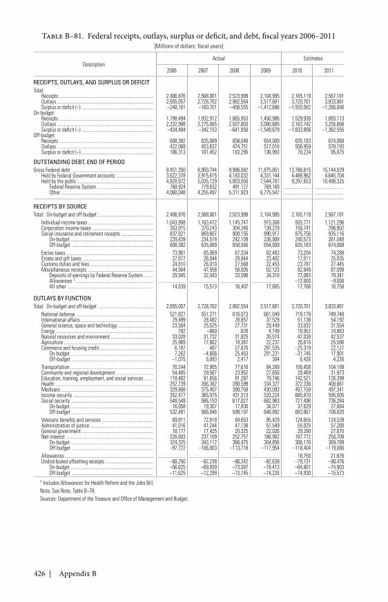
426 | Appendix B
Table B–81. Federal receipts, outlays, surplus or deficit, and debt, fiscal years 2006–2011[Millions of dollars; fiscal years]
DescriptionActual Estimates
2006 2007 2008 2009 2010 2011
RECEIPTS, OUTLAYS, AND SURPLUS OR DEFICITTotal:
Receipts ............................................................................... 2,406,876 2,568,001 2,523,999 2,104,995 2,165,119 2,567,181Outlays ................................................................................. 2,655,057 2,728,702 2,982,554 3,517,681 3,720,701 3,833,861Surplus or deficit (–) ............................................................ –248,181 –160,701 –458,555 –1,412,686 –1,555,582 –1,266,680
On-budget:Receipts ............................................................................... 1,798,494 1,932,912 1,865,953 1,450,986 1,529,936 1,893,113Outlays ................................................................................. 2,232,988 2,275,065 2,507,803 3,000,665 3,163,742 3,255,668Surplus or deficit (–) ............................................................ –434,494 –342,153 –641,850 –1,549,679 –1,633,806 –1,362,555
Off-budget:Receipts ............................................................................... 608,382 635,089 658,046 654,009 635,183 674,068Outlays ................................................................................. 422,069 453,637 474,751 517,016 556,959 578,193Surplus or deficit (–) ............................................................ 186,313 181,452 183,295 136,993 78,224 95,875
OUTSTANDING DEBT, END OF PERIODGross Federal debt ..................................................................... 8,451,350 8,950,744 9,986,082 11,875,851 13,786,615 15,144,029
Held by Federal Government accounts ............................... 3,622,378 3,915,615 4,183,032 4,331,144 4,488,962 4,645,704Held by the public ................................................................ 4,828,972 5,035,129 5,803,050 7,544,707 9,297,653 10,498,325
Federal Reserve System ............................................... 768,924 779,632 491,127 769,160 ....................... ........................Other ............................................................................. 4,060,048 4,255,497 5,311,923 6,775,547 ....................... ........................
RECEIPTS BY SOURCETotal: On-budget and off-budget ............................................... 2,406,876 2,568,001 2,523,999 2,104,995 2,165,119 2,567,181
Individual income taxes ....................................................... 1,043,908 1,163,472 1,145,747 915,308 935,771 1,121,296Corporation income taxes ................................................... 353,915 370,243 304,346 138,229 156,741 296,902Social insurance and retirement receipts ........................... 837,821 869,607 900,155 890,917 875,756 935,116
On-budget ..................................................................... 229,439 234,518 242,109 236,908 240,573 261,048Off-budget .................................................................... 608,382 635,089 658,046 654,009 635,183 674,068
Excise taxes ......................................................................... 73,961 65,069 67,334 62,483 73,204 74,288Estate and gift taxes ........................................................... 27,877 26,044 28,844 23,482 17,011 25,035Customs duties and fees ..................................................... 24,810 26,010 27,568 22,453 23,787 27,445Miscellaneous receipts ....................................................... 44,584 47,556 50,005 52,123 82,849 87,099
Deposits of earnings by Federal Reserve System ........ 29,945 32,043 33,598 34,318 77,083 79,341Allowances 1 ................................................................. ....................... ....................... ....................... ....................... –12,000 –9,000All other ........................................................................ 14,639 15,513 16,407 17,805 17,766 16,758
OUTLAYS BY FUNCTIONTotal: On-budget and off-budget ............................................... 2,655,057 2,728,702 2,982,554 3,517,681 3,720,701 3,833,861
National defense ................................................................. 521,827 551,271 616,073 661,049 719,179 749,748International affairs ............................................................. 29,499 28,482 28,857 37,529 51,138 54,192General science, space and technology .............................. 23,584 25,525 27,731 29,449 33,032 31,554Energy .................................................................................. 782 –860 628 4,749 18,952 24,863Natural resources and environment .................................... 33,028 31,732 31,825 35,574 47,039 42,537Agriculture ........................................................................... 25,969 17,662 18,387 22,237 26,610 25,590Commerce and housing credit ............................................. 6,187 487 27,870 291,535 –25,319 22,127
On-budget ..................................................................... 7,262 –4,606 25,453 291,231 –31,745 17,901Off-budget .................................................................... –1,075 5,093 2,417 304 6,426 4,226
Transportation ...................................................................... 70,244 72,905 77,616 84,289 106,458 104,189Community and regional development ............................... 54,465 29,567 23,952 27,650 28,469 31,973Education, training, employment, and social services ........ 118,482 91,656 91,287 79,746 142,521 126,399Health .................................................................................. 252,739 266,382 280,599 334,327 372,336 400,661Medicare .............................................................................. 329,868 375,407 390,758 430,093 457,159 497,341Income security ................................................................... 352,477 365,975 431,313 533,224 685,870 595,005Social security ..................................................................... 548,549 586,153 617,027 682,963 721,496 736,284
On-budget ..................................................................... 16,058 19,307 17,830 34,071 37,629 27,664Off-budget .................................................................... 532,491 566,846 599,197 648,892 683,867 708,620
Veterans benefits and services ........................................... 69,811 72,818 84,653 95,429 124,655 124,539Administration of justice ..................................................... 41,016 41,244 47,138 51,549 55,025 57,280General government ............................................................ 18,177 17,425 20,325 22,026 29,290 27,670Net interest ......................................................................... 226,603 237,109 252,757 186,902 187,772 250,709
On-budget ..................................................................... 324,325 343,112 366,475 304,856 306,176 369,789Off-budget .................................................................... –97,722 –106,003 –113,718 –117,954 –118,404 –119,080
Allowances .......................................................................... ....................... ....................... ....................... ....................... 18,750 21,676Undistributed offsetting receipts ........................................ –68,250 –82,238 –86,242 –92,639 –79,731 –90,476
On-budget ..................................................................... –56,625 –69,939 –73,097 –78,413 –64,801 –74,903Off-budget .................................................................... –11,625 –12,299 –13,145 –14,226 –14,930 –15,573
1 Includes Allowances for Health Reform and the Jobs Bill.Note: See Note, Table B–78.Sources: Department of the Treasury and Office of Management and Budget.
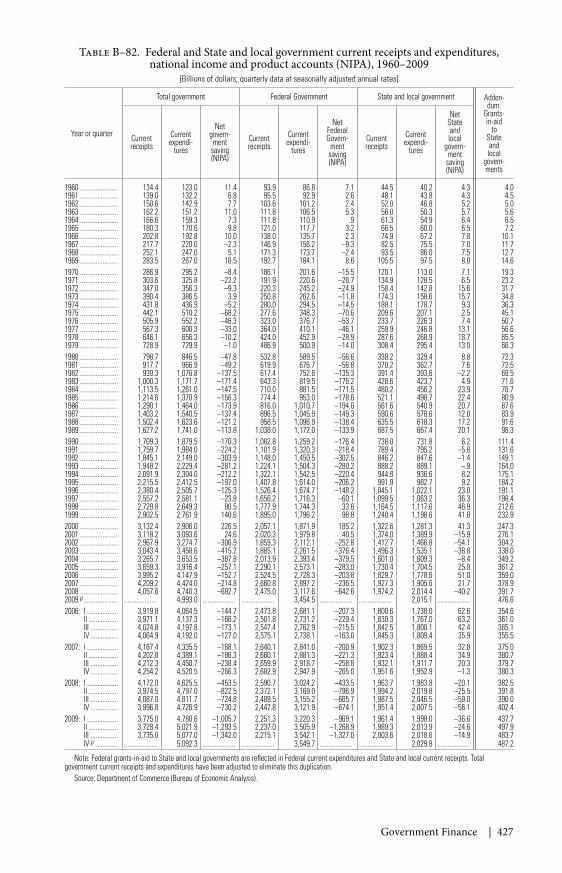
Government Finance | 427
Table B–82. Federal and State and local government current receipts and expenditures,national income and product accounts (NIPA), 1960–2009
[Billions of dollars; quarterly data at seasonally adjusted annual rates]
Year or quarter
Total government Federal Government State and local government Adden-dum:
Grants-in-aid
toStateandlocal
govern-ments
Currentreceipts
Currentexpendi-
tures
Netgovern-ment
saving(NIPA)
Currentreceipts
Currentexpendi-
tures
NetFederalGovern-
mentsaving(NIPA)
Currentreceipts
Currentexpendi-
tures
NetStateandlocal
govern-ment
saving(NIPA)
1960 ...................... 134.4 123.0 11.4 93.9 86.8 7.1 44.5 40.2 4.3 4.01961 ...................... 139.0 132.2 6.8 95.5 92.9 2.6 48.1 43.8 4.3 4.51962 ...................... 150.6 142.9 7.7 103.6 101.2 2.4 52.0 46.8 5.2 5.01963 ...................... 162.2 151.2 11.0 111.8 106.5 5.3 56.0 50.3 5.7 5.61964 ...................... 166.6 159.3 7.3 111.8 110.9 .9 61.3 54.9 6.4 6.51965 ...................... 180.3 170.6 9.8 121.0 117.7 3.2 66.5 60.0 6.5 7.21966 ...................... 202.8 192.8 10.0 138.0 135.7 2.3 74.9 67.2 7.8 10.11967 ...................... 217.7 220.0 –2.3 146.9 156.2 –9.3 82.5 75.5 7.0 11.71968 ...................... 252.1 247.0 5.1 171.3 173.7 –2.4 93.5 86.0 7.5 12.71969 ...................... 283.5 267.0 16.5 192.7 184.1 8.6 105.5 97.5 8.0 14.61970 ...................... 286.9 295.2 –8.4 186.1 201.6 –15.5 120.1 113.0 7.1 19.31971 ...................... 303.6 325.8 –22.2 191.9 220.6 –28.7 134.9 128.5 6.5 23.21972 ...................... 347.0 356.3 –9.3 220.3 245.2 –24.9 158.4 142.8 15.6 31.71973 ...................... 390.4 386.5 3.9 250.8 262.6 –11.8 174.3 158.6 15.7 34.81974 ...................... 431.8 436.9 –5.2 280.0 294.5 –14.5 188.1 178.7 9.3 36.31975 ...................... 442.1 510.2 –68.2 277.6 348.3 –70.6 209.6 207.1 2.5 45.11976 ...................... 505.9 552.2 –46.3 323.0 376.7 –53.7 233.7 226.3 7.4 50.71977 ...................... 567.3 600.3 –33.0 364.0 410.1 –46.1 259.9 246.8 13.1 56.61978 ...................... 646.1 656.3 –10.2 424.0 452.9 –28.9 287.6 268.9 18.7 65.51979 ...................... 728.9 729.9 –1.0 486.9 500.9 –14.0 308.4 295.4 13.0 66.31980 ...................... 798.7 846.5 –47.8 532.8 589.5 –56.6 338.2 329.4 8.8 72.31981 ...................... 917.7 966.9 –49.2 619.9 676.7 –56.8 370.2 362.7 7.6 72.51982 ...................... 939.3 1,076.8 –137.5 617.4 752.6 –135.3 391.4 393.6 –2.2 69.51983 ...................... 1,000.3 1,171.7 –171.4 643.3 819.5 –176.2 428.6 423.7 4.9 71.61984 ...................... 1,113.5 1,261.0 –147.5 710.0 881.5 –171.5 480.2 456.2 23.9 76.71985 ...................... 1,214.6 1,370.9 –156.3 774.4 953.0 –178.6 521.1 498.7 22.4 80.91986 ...................... 1,290.1 1,464.0 –173.9 816.0 1,010.7 –194.6 561.6 540.9 20.7 87.61987 ...................... 1,403.2 1,540.5 –137.4 896.5 1,045.9 –149.3 590.6 578.6 12.0 83.91988 ...................... 1,502.4 1,623.6 –121.2 958.5 1,096.9 –138.4 635.5 618.3 17.2 91.61989 ...................... 1,627.2 1,741.0 –113.8 1,038.0 1,172.0 –133.9 687.5 667.4 20.1 98.31990 ...................... 1,709.3 1,879.5 –170.3 1,082.8 1,259.2 –176.4 738.0 731.8 6.2 111.41991 ...................... 1,759.7 1,984.0 –224.2 1,101.9 1,320.3 –218.4 789.4 795.2 –5.8 131.61992 ...................... 1,845.1 2,149.0 –303.9 1,148.0 1,450.5 –302.5 846.2 847.6 –1.4 149.11993 ...................... 1,948.2 2,229.4 –281.2 1,224.1 1,504.3 –280.2 888.2 889.1 –.9 164.01994 ...................... 2,091.9 2,304.0 –212.2 1,322.1 1,542.5 –220.4 944.8 936.6 8.2 175.11995 ...................... 2,215.5 2,412.5 –197.0 1,407.8 1,614.0 –206.2 991.9 982.7 9.2 184.21996 ...................... 2,380.4 2,505.7 –125.3 1,526.4 1,674.7 –148.2 1,045.1 1,022.1 23.0 191.11997 ...................... 2,557.2 2,581.1 –23.8 1,656.2 1,716.3 –60.1 1,099.5 1,063.2 36.3 198.41998 ...................... 2,729.8 2,649.3 80.5 1,777.9 1,744.3 33.6 1,164.5 1,117.6 46.9 212.61999 ...................... 2,902.5 2,761.9 140.6 1,895.0 1,796.2 98.8 1,240.4 1,198.6 41.8 232.92000 ...................... 3,132.4 2,906.0 226.5 2,057.1 1,871.9 185.2 1,322.6 1,281.3 41.3 247.32001 ...................... 3,118.2 3,093.6 24.6 2,020.3 1,979.8 40.5 1,374.0 1,389.9 –15.9 276.12002 ...................... 2,967.9 3,274.7 –306.9 1,859.3 2,112.1 –252.8 1,412.7 1,466.8 –54.1 304.22003 ...................... 3,043.4 3,458.6 –415.2 1,885.1 2,261.5 –376.4 1,496.3 1,535.1 –38.8 338.02004 ...................... 3,265.7 3,653.5 –387.8 2,013.9 2,393.4 –379.5 1,601.0 1,609.3 –8.4 349.22005 ...................... 3,659.3 3,916.4 –257.1 2,290.1 2,573.1 –283.0 1,730.4 1,704.5 25.9 361.22006 ...................... 3,995.2 4,147.9 –152.7 2,524.5 2,728.3 –203.8 1,829.7 1,778.6 51.0 359.02007 ...................... 4,209.2 4,424.0 –214.8 2,660.8 2,897.2 –236.5 1,927.3 1,905.6 21.7 378.92008 ...................... 4,057.6 4,740.3 –682.7 2,475.0 3,117.6 –642.6 1,974.2 2,014.4 –40.2 391.72009 p .................... ................... 4,993.0 ................... ................... 3,454.5 ................... ................... 2,015.1 ................... 476.62006: I .................. 3,919.8 4,064.5 –144.7 2,473.8 2,681.1 –207.3 1,800.6 1,738.0 62.6 354.6
II ................. 3,971.1 4,137.3 –166.2 2,501.8 2,731.2 –229.4 1,830.3 1,767.0 63.2 361.0III ................ 4,024.8 4,197.8 –173.1 2,547.4 2,762.9 –215.5 1,842.5 1,800.1 42.4 365.1IV ................ 4,064.9 4,192.0 –127.0 2,575.1 2,738.1 –163.0 1,845.3 1,809.4 35.9 355.5
2007: I .................. 4,167.4 4,335.5 –168.1 2,640.1 2,841.0 –200.9 1,902.3 1,869.5 32.8 375.0II ................. 4,202.8 4,389.1 –186.3 2,660.1 2,881.3 –221.3 1,923.4 1,888.4 34.9 380.7III ................ 4,212.3 4,450.7 –238.4 2,659.9 2,918.7 –258.8 1,932.1 1,911.7 20.3 379.7IV ................ 4,254.2 4,520.5 –266.3 2,682.9 2,947.9 –265.0 1,951.6 1,952.9 –1.3 380.3
2008: I .................. 4,172.0 4,625.5 –453.5 2,590.7 3,024.2 –433.5 1,963.7 1,983.8 –20.1 382.5II ................. 3,974.5 4,797.0 –822.5 2,372.1 3,169.0 –796.9 1,994.2 2,019.8 –25.5 391.8III ................ 4,087.0 4,811.7 –724.8 2,489.5 3,155.2 –665.7 1,987.5 2,046.5 –59.0 390.0IV ................ 3,996.8 4,726.9 –730.2 2,447.8 3,121.9 –674.1 1,951.4 2,007.5 –56.1 402.4
2009: I .................. 3,775.0 4,780.6 –1,005.7 2,251.3 3,220.3 –969.1 1,961.4 1,998.0 –36.6 437.7II ................. 3,728.4 5,021.9 –1,293.5 2,237.0 3,505.9 –1,268.9 1,989.3 2,013.9 –24.6 497.9III ................ 3,735.0 5,077.0 –1,342.0 2,215.1 3,542.1 –1,327.0 2,003.6 2,018.6 –14.9 483.7IV p ............. ................... 5,092.3 ................... ................... 3,549.7 ................... ................... 2,029.8 ................... 487.2
Note: Federal grants-in-aid to State and local governments are reflected in Federal current expenditures and State and local current receipts. Totalgovernment current receipts and expenditures have been adjusted to eliminate this duplication.
Source: Department of Commerce (Bureau of Economic Analysis).
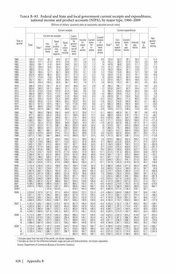
428 | Appendix B
Table B–83. Federal and State and local government current receipts and expenditures,national income and product accounts (NIPA), by major type, 1960–2009
[Billions of dollars; quarterly data at seasonally adjusted annual rates]
Year orquarter
Current receipts Current expenditures
Netgovern-ment
savingTotal
Current tax receipts Contri-butions
forgovern-mentsocialinsur-ance
Incomere-
ceiptson
assets
Currenttrans-
ferre-
ceipts
Currentsurplus
ofgovern-
mententer-prises
Total 2
Con-sump-tion
expen-ditures
Currenttrans-
ferpay-
ments
Interestpay-
ments
Sub-si-
diesTotal 1Per-
sonalcurrenttaxes
Taxeson
produc-tionand
imports
Taxeson
corpo-rate
income
1960 ........... 134.4 113.4 46.1 44.5 22.7 16.5 2.7 0.9 0.9 123.0 83.3 28.1 10.4 1.1 11.41961 ........... 139.0 117.1 47.3 47.0 22.8 17.1 2.9 1.1 .8 132.2 88.2 31.9 10.2 2.0 6.81962 ........... 150.6 126.1 51.6 50.4 24.0 19.2 3.2 1.2 .9 142.9 96.8 32.8 11.1 2.3 7.71963 ........... 162.2 134.4 54.6 53.4 26.2 21.7 3.4 1.3 1.4 151.2 102.7 34.3 12.0 2.2 11.01964 ........... 166.6 137.5 52.1 57.3 28.0 22.5 3.7 1.6 1.3 159.3 108.6 35.1 12.9 2.7 7.31965 ........... 180.3 149.5 57.7 60.7 30.9 23.5 4.1 1.9 1.3 170.6 115.9 38.0 13.7 3.0 9.81966 ........... 202.8 163.5 66.4 63.2 33.7 31.4 4.7 2.2 1.0 192.8 131.8 42.0 15.1 3.9 10.01967 ........... 217.7 173.8 73.0 67.9 32.7 35.0 5.5 2.5 .9 220.0 149.5 50.3 16.4 3.8 –2.31968 ........... 252.1 203.1 87.0 76.4 39.4 38.8 6.4 2.6 1.2 247.0 165.7 58.4 18.8 4.2 5.11969 ........... 283.5 228.4 104.5 83.9 39.7 44.3 7.0 2.7 1.0 267.0 178.2 64.1 20.2 4.5 16.51970 ........... 286.9 229.2 103.1 91.4 34.4 46.6 8.2 2.9 .0 295.2 190.1 77.3 23.1 4.8 –8.41971 ........... 303.6 240.3 101.7 100.5 37.7 51.5 9.0 3.1 –.2 325.8 204.7 92.2 24.5 4.7 –22.21972 ........... 347.0 273.8 123.6 107.9 41.9 59.6 9.5 3.6 .5 356.3 220.8 103.0 26.3 6.6 –9.31973 ........... 390.4 299.3 132.4 117.2 49.3 76.0 11.6 3.9 –.4 386.5 234.8 115.2 31.3 5.2 3.91974 ........... 431.8 328.1 151.0 124.9 51.8 85.8 14.4 4.5 –.9 436.9 261.7 135.9 35.6 3.3 –5.21975 ........... 442.1 334.3 147.6 135.3 50.9 89.9 16.1 5.1 –3.2 510.2 294.6 171.3 40.0 4.5 –68.21976 ........... 505.9 383.6 172.3 146.4 64.2 102.0 16.3 5.8 –1.8 552.2 316.6 184.3 46.3 5.1 –46.31977 ........... 567.3 431.0 197.5 159.7 73.0 113.9 18.4 6.8 –2.7 600.3 346.6 195.9 50.8 7.1 –33.01978 ........... 646.1 484.8 229.4 170.9 83.5 132.1 23.2 8.2 –2.2 656.3 376.5 210.9 60.2 8.9 –10.21979 ........... 728.9 537.9 268.7 180.1 88.0 153.7 30.8 9.4 –2.9 729.9 412.3 236.0 72.9 8.5 –1.01980 ........... 798.7 585.6 298.9 200.3 84.8 167.2 39.9 11.1 –5.1 846.5 465.9 281.7 89.1 9.8 –47.81981 ........... 917.7 663.5 345.2 235.6 81.1 196.9 50.2 12.7 –5.6 966.9 520.6 318.1 116.7 11.5 –49.21982 ........... 939.3 659.5 354.1 240.9 63.1 210.1 58.9 15.3 –4.5 1,076.8 568.1 354.7 138.9 15.0 –137.51983 ........... 1,000.3 694.1 352.3 263.3 77.2 227.2 65.3 16.9 –3.2 1,171.7 610.5 382.5 156.9 21.3 –171.41984 ........... 1,113.5 762.5 377.4 289.8 94.0 258.8 74.3 19.7 –1.9 1,261.0 657.6 395.3 187.3 21.1 –147.51985 ........... 1,214.6 823.9 417.3 308.1 96.5 282.8 84.0 23.4 .6 1,370.9 720.1 420.4 208.8 21.4 –156.31986 ........... 1,290.1 868.8 437.2 323.4 106.5 304.9 89.7 25.9 .9 1,464.0 776.1 446.6 216.3 24.9 –173.91987 ........... 1,403.2 965.7 489.1 347.5 127.1 324.6 85.6 27.0 .2 1,540.5 815.1 464.4 230.8 30.3 –137.41988 ........... 1,502.4 1,018.9 504.9 374.5 137.2 363.2 89.9 27.9 2.6 1,623.6 852.8 493.6 247.7 29.5 –121.21989 ........... 1,627.2 1,109.2 566.1 398.9 141.5 386.9 93.7 32.5 4.9 1,741.0 902.9 538.1 272.5 27.4 –113.81990 ........... 1,709.3 1,161.3 592.7 425.0 140.6 412.1 98.0 36.3 1.6 1,879.5 966.0 592.4 294.2 27.0 –170.31991 ........... 1,759.7 1,179.9 586.6 457.1 133.6 432.2 97.0 44.9 5.7 1,984.0 1,015.8 628.9 311.7 27.5 –224.21992 ........... 1,845.1 1,239.7 610.5 483.4 143.1 457.1 89.6 50.5 8.2 2,149.0 1,050.4 756.3 312.3 30.1 –303.91993 ........... 1,948.2 1,317.8 646.5 503.1 165.4 479.6 86.8 55.3 8.7 2,229.4 1,075.4 804.6 312.7 36.7 –281.21994 ........... 2,091.9 1,425.6 690.5 545.2 186.7 510.7 86.0 60.0 9.6 2,304.0 1,108.9 839.9 322.7 32.5 –212.21995 ........... 2,215.5 1,516.7 743.9 557.9 211.0 535.5 91.8 58.4 13.1 2,412.5 1,141.4 882.4 353.9 34.8 –197.01996 ........... 2,380.4 1,641.5 832.0 580.8 223.6 557.9 99.9 66.8 14.4 2,505.7 1,176.7 929.2 364.6 35.2 –125.31997 ........... 2,557.2 1,780.0 926.2 611.6 237.1 590.3 103.6 69.3 14.1 2,581.1 1,222.1 954.6 370.6 33.8 –23.81998 ........... 2,729.8 1,910.8 1,026.4 639.5 239.2 627.8 102.7 75.3 13.3 2,649.3 1,263.2 978.1 371.6 36.4 80.51999 ........... 2,902.5 2,035.8 1,107.5 673.6 248.8 664.6 106.4 81.7 14.1 2,761.9 1,343.9 1,014.9 357.9 45.2 140.62000 ........... 3,132.4 2,202.8 1,232.3 708.6 254.7 709.4 118.8 92.3 9.1 2,906.0 1,426.6 1,071.5 362.0 45.8 226.52001 ........... 3,118.2 2,163.7 1,234.8 727.7 193.5 736.9 114.6 98.9 4.0 3,093.6 1,524.4 1,169.0 341.5 58.7 24.62002 ........... 2,967.9 2,002.1 1,050.4 762.8 181.3 755.2 99.9 104.3 6.3 3,274.7 1,639.9 1,280.9 312.6 41.4 –306.92003 ........... 3,043.4 2,047.9 1,000.3 806.8 231.8 782.8 96.8 108.9 7.0 3,458.6 1,756.8 1,354.8 298.0 49.1 –415.22004 ........... 3,265.7 2,213.2 1,047.8 863.4 292.0 831.7 100.3 119.3 1.2 3,653.5 1,860.4 1,440.1 306.6 46.4 –387.82005 ........... 3,659.3 2,546.8 1,208.6 930.2 395.9 877.4 111.9 126.7 –3.5 3,916.4 1,977.9 1,534.9 342.7 60.9 –257.12006 ........... 3,995.2 2,807.4 1,352.4 986.8 454.2 926.4 129.6 136.0 –4.2 4,147.9 2,093.3 1,631.0 372.2 51.4 –152.72007 ........... 4,209.2 2,960.6 1,490.9 1,028.7 426.7 964.2 143.3 147.7 –6.6 4,424.0 2,214.9 1,743.3 411.0 54.8 –214.82008 ........... 4,057.6 2,758.0 1,432.4 1,047.3 263.3 995.6 144.2 166.7 –6.9 4,740.3 2,386.9 1,904.0 395.9 53.5 –682.72009 p ......... ............. ............. 1,107.6 1,023.9 ............. 978.3 164.3 189.0 –8.1 4,993.0 2,417.8 2,136.4 379.1 59.7 ...............2006: I ....... 3,919.8 2,747.6 1,321.5 971.5 443.4 920.0 122.2 132.4 –2.4 4,064.5 2,064.8 1,590.0 354.1 55.6 –144.7
II ...... 3,971.1 2,791.1 1,340.2 983.3 456.4 921.9 127.4 134.5 –3.8 4,137.3 2,083.1 1,627.3 375.4 51.4 –166.2III ..... 4,024.8 2,835.1 1,354.3 991.6 477.2 925.3 132.0 137.0 –4.7 4,197.8 2,105.8 1,651.2 391.1 49.8 –173.1IV ..... 4,064.9 2,855.7 1,393.5 1,000.7 439.7 938.4 136.9 139.9 –6.0 4,192.0 2,119.7 1,655.5 368.2 48.7 –127.0
2007: I ....... 4,167.4 2,935.1 1,459.5 1,015.3 447.4 957.3 140.4 143.0 –8.4 4,335.5 2,152.2 1,730.7 403.3 49.2 –168.1II ...... 4,202.8 2,963.1 1,481.8 1,025.2 442.0 958.5 142.8 145.3 –6.9 4,389.1 2,197.2 1,714.4 419.1 58.3 –186.3III ..... 4,212.3 2,960.4 1,500.7 1,032.2 414.3 963.4 144.9 148.5 –4.9 4,450.7 2,234.3 1,744.5 415.8 56.0 –238.4IV ..... 4,254.2 2,983.6 1,521.9 1,042.3 403.2 977.5 145.1 153.9 –6.0 4,520.5 2,275.9 1,783.7 405.5 55.4 –266.3
2008: I ....... 4,172.0 2,884.1 1,531.8 1,042.5 295.0 990.3 143.7 159.4 –5.6 4,625.5 2,332.5 1,825.2 414.6 53.1 –453.5II ...... 3,974.5 2,679.8 1,326.2 1,050.8 288.4 993.9 145.1 162.0 –6.3 4,797.0 2,381.5 1,966.7 395.9 52.9 –822.5III ..... 4,087.0 2,786.2 1,437.3 1,058.5 275.7 999.9 143.2 164.5 –6.9 4,811.7 2,436.4 1,898.7 423.8 52.9 –724.8IV ..... 3,996.8 2,681.8 1,434.3 1,037.3 194.2 998.4 144.6 181.0 –8.9 4,726.9 2,397.1 1,925.3 349.3 55.2 –730.2
2009: I ....... 3,775.0 2,463.7 1,187.3 1,018.8 244.2 974.8 156.5 190.7 –10.7 4,780.6 2,378.6 2,009.2 337.3 55.5 –1,005.7II ...... 3,728.4 2,395.4 1,082.6 1,019.6 281.2 976.0 166.5 199.3 –8.8 5,021.9 2,409.0 2,175.2 382.8 54.9 –1,293.5III ..... 3,735.0 2,416.7 1,086.1 1,023.1 296.7 979.0 165.7 180.0 –6.3 5,077.0 2,431.0 2,174.4 403.8 67.7 –1,342.0IV p .. ............. ............. 1,074.4 1,034.3 ............. 983.4 168.5 186.1 –6.6 5,092.3 2,452.4 2,186.8 392.6 60.5 ...............
1 Includes taxes from the rest of the world, not shown separately.2 Includes an item for the difference between wage accruals and disbursements, not shown separately.Source: Department of Commerce (Bureau of Economic Analysis).
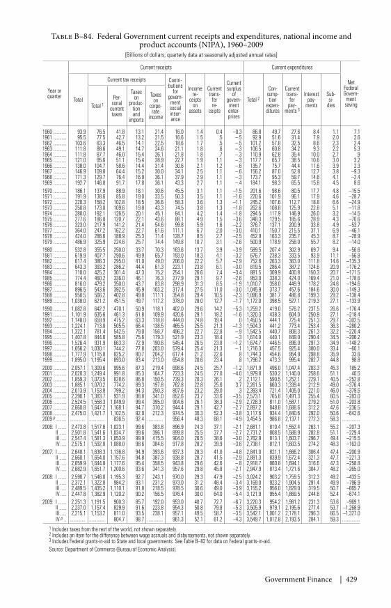
Government Finance | 429
Table B–84. Federal Government current receipts and expenditures, national income andproduct accounts (NIPA), 1960–2009
[Billions of dollars; quarterly data at seasonally adjusted annual rates]
Year orquarter
Current receipts Current expenditures
NetFederalGovern-
mentsaving
Total
Current tax receipts Contri-butions
forgovern-mentsocialinsur-ance
Incomere-
ceiptson
assets
Currenttrans-
ferre-
ceipts
Currentsurplus
ofgovern-mententer-prises
Total 2
Con-sump-tion
expen-ditures
Currenttrans-
ferpay-
ments 3
Interestpay-
ments
Sub-si-
diesTotal 1Per-
sonalcurrenttaxes
Taxeson
produc-tionand
imports
Taxeson
corpo-rate
income
1960 ........... 93.9 76.5 41.8 13.1 21.4 16.0 1.4 0.4 –0.3 86.8 49.7 27.6 8.4 1.1 7.11961 ........... 95.5 77.5 42.7 13.2 21.5 16.6 1.5 .5 –.5 92.9 51.6 31.4 7.9 2.0 2.61962 ........... 103.6 83.3 46.5 14.1 22.5 18.6 1.7 .5 –.5 101.2 57.8 32.5 8.6 2.3 2.41963 ........... 111.8 88.6 49.1 14.7 24.6 21.1 1.8 .6 –.3 106.5 60.8 34.2 9.3 2.2 5.31964 ........... 111.8 87.7 46.0 15.4 26.1 21.8 1.8 .7 –.3 110.9 62.8 35.4 10.0 2.7 .91965 ........... 121.0 95.6 51.1 15.4 28.9 22.7 1.9 1.1 –.3 117.7 65.7 38.5 10.6 3.0 3.21966 ........... 138.0 104.7 58.6 14.4 31.4 30.6 2.1 1.2 –.6 135.7 75.7 44.4 11.6 3.9 2.31967 ........... 146.9 109.8 64.4 15.2 30.0 34.1 2.5 1.1 –.6 156.2 87.0 52.8 12.7 3.8 –9.31968 ........... 171.3 129.7 76.4 16.9 36.1 37.9 2.9 1.1 –.3 173.7 95.3 59.7 14.6 4.1 –2.41969 ........... 192.7 146.0 91.7 17.8 36.1 43.3 2.7 1.1 –.4 184.1 98.3 65.5 15.8 4.5 8.61970 ........... 186.1 137.9 88.9 18.1 30.6 45.5 3.1 1.1 –1.5 201.6 98.6 80.5 17.7 4.8 –15.51971 ........... 191.9 138.6 85.8 19.0 33.5 50.3 3.5 1.1 –1.6 220.6 101.9 96.1 17.9 4.6 –28.71972 ........... 220.3 158.2 102.8 18.5 36.6 58.3 3.6 1.3 –1.1 245.2 107.6 112.7 18.8 6.6 –24.91973 ........... 250.8 173.0 109.6 19.8 43.3 74.5 3.8 1.3 –1.8 262.6 108.8 125.9 22.8 5.1 –11.81974 ........... 280.0 192.1 126.5 20.1 45.1 84.1 4.2 1.4 –1.8 294.5 117.9 146.9 26.0 3.2 –14.51975 ........... 277.6 186.8 120.7 22.1 43.6 88.1 4.9 1.5 –3.6 348.3 129.5 185.6 28.9 4.3 –70.61976 ........... 323.0 217.9 141.2 21.4 54.6 99.8 5.9 1.6 –2.2 376.7 137.1 200.9 33.8 4.9 –53.71977 ........... 364.0 247.2 162.2 22.7 61.6 111.1 6.7 2.0 –3.0 410.1 150.7 215.5 37.1 6.9 –46.11978 ........... 424.0 286.6 188.9 25.3 71.4 128.7 8.5 2.7 –2.5 452.9 163.3 235.7 45.3 8.7 –28.91979 ........... 486.9 325.9 224.6 25.7 74.4 149.8 10.7 3.1 –2.6 500.9 178.9 258.0 55.7 8.2 –14.01980 ........... 532.8 355.5 250.0 33.7 70.3 163.6 13.7 3.9 –3.9 589.5 207.4 302.9 69.7 9.4 –56.61981 ........... 619.9 407.7 290.6 49.9 65.7 193.0 18.3 4.1 –3.2 676.7 238.3 333.5 93.9 11.1 –56.81982 ........... 617.4 386.3 295.0 41.0 49.0 206.0 22.2 5.7 –2.9 752.6 263.3 363.0 111.8 14.6 –135.31983 ........... 643.3 393.2 286.2 44.4 61.3 223.1 23.8 6.1 –3.0 819.5 286.4 387.2 124.6 20.9 –176.21984 ........... 710.0 425.2 301.4 47.3 75.2 254.1 26.6 7.4 –3.4 881.5 309.9 400.8 150.3 20.7 –171.51985 ........... 774.4 460.2 336.0 46.1 76.3 277.9 29.1 9.7 –2.6 953.0 338.3 424.0 169.4 21.0 –178.61986 ........... 816.0 479.2 350.0 43.7 83.8 298.9 31.3 8.5 –1.9 1,010.7 358.0 449.9 178.2 24.6 –194.61987 ........... 896.5 543.6 392.5 45.9 103.2 317.4 27.5 11.0 –3.0 1,045.9 373.7 457.6 184.6 30.0 –149.31988 ........... 958.5 566.2 402.8 49.8 111.1 354.8 29.4 10.5 –2.3 1,096.9 381.7 486.8 199.3 29.2 –138.41989 ........... 1,038.0 621.2 451.5 49.7 117.2 378.0 28.0 12.7 –1.7 1,172.0 398.5 527.1 219.3 27.1 –133.91990 ........... 1,082.8 642.2 470.1 50.9 118.1 402.0 29.6 14.2 –5.3 1,259.2 419.0 576.2 237.5 26.6 –176.41991 ........... 1,101.9 635.6 461.3 61.8 109.9 420.6 29.1 18.2 –1.6 1,320.3 438.3 604.0 250.9 27.1 –218.41992 ........... 1,148.0 659.9 475.2 63.3 118.8 444.0 24.8 19.4 .0 1,450.5 444.1 725.4 251.3 29.7 –302.51993 ........... 1,224.1 713.0 505.5 66.4 138.5 465.5 25.5 21.3 –1.3 1,504.3 441.2 773.4 253.4 36.3 –280.21994 ........... 1,322.1 781.4 542.5 79.0 156.7 496.2 22.7 22.8 –.9 1,542.5 440.7 808.3 261.3 32.2 –220.41995 ........... 1,407.8 844.6 585.8 75.6 179.3 521.9 23.3 18.4 –.3 1,614.0 440.1 849.0 290.4 34.5 –206.21996 ........... 1,526.4 931.9 663.3 72.9 190.6 545.4 26.5 23.8 –1.2 1,674.7 446.5 896.0 297.3 34.9 –148.21997 ........... 1,656.2 1,030.1 744.2 77.8 203.0 579.4 25.4 21.3 –.1 1,716.3 457.5 925.4 300.0 33.4 –60.11998 ........... 1,777.9 1,115.8 825.2 80.7 204.2 617.4 21.2 22.6 .8 1,744.3 454.6 954.9 298.8 35.9 33.61999 ........... 1,895.0 1,195.4 893.0 83.4 213.0 654.8 20.6 23.4 .8 1,796.2 473.3 995.4 282.7 44.8 98.82000 ........... 2,057.1 1,309.6 995.6 87.3 219.4 698.6 24.5 25.7 –1.2 1,871.9 496.0 1,047.4 283.3 45.3 185.22001 ........... 2,020.3 1,249.4 991.8 85.3 164.7 723.3 24.5 27.0 –4.0 1,979.8 530.2 1,140.0 258.6 51.1 40.52002 ........... 1,859.3 1,073.5 828.6 86.8 150.5 739.3 20.3 26.1 .2 2,112.1 590.5 1,252.1 229.1 40.5 –252.82003 ........... 1,885.1 1,070.2 774.2 89.3 197.8 762.8 22.8 25.6 3.7 2,261.5 660.3 1,339.4 212.9 49.0 –376.42004 ........... 2,013.9 1,153.8 799.2 94.3 250.3 807.6 23.2 29.0 .3 2,393.4 721.4 1,405.0 221.0 46.0 –379.52005 ........... 2,290.1 1,383.7 931.9 98.8 341.0 852.6 23.7 33.6 –3.5 2,573.1 765.8 1,491.3 255.4 60.5 –283.02006 ........... 2,524.5 1,558.3 1,049.9 99.4 395.0 904.6 26.1 38.3 –2.9 2,728.3 811.0 1,587.1 279.2 51.0 –203.82007 ........... 2,660.8 1,647.2 1,168.1 94.7 370.2 944.4 29.1 42.7 –2.7 2,897.2 848.8 1,688.6 312.2 47.6 –236.52008 ........... 2,475.0 1,421.7 1,102.5 92.0 212.3 974.5 30.3 52.3 –3.8 3,117.6 934.4 1,840.6 292.0 50.6 –642.62009 p ......... ............. ............. 836.5 92.4 ............. 956.4 48.3 68.1 –4.9 3,454.5 986.8 2,137.1 272.3 58.3 ...............2006: I ....... 2,473.8 1,517.6 1,023.1 99.6 383.8 896.9 24.3 37.1 –2.1 2,681.1 810.4 1,552.4 263.1 55.2 –207.3
II ...... 2,501.8 1,541.6 1,034.7 99.6 396.1 899.8 25.5 37.7 –2.7 2,731.2 808.5 1,588.9 282.8 51.1 –229.4III ..... 2,547.4 1,581.3 1,053.9 99.9 415.5 904.0 26.5 38.6 –3.0 2,762.9 813.1 1,603.7 296.7 49.4 –215.5IV ..... 2,575.1 1,592.8 1,088.0 98.6 384.6 917.8 28.2 39.9 –3.6 2,738.1 812.1 1,603.5 274.2 48.3 –163.0
2007: I ....... 2,640.1 1,638.3 1,136.8 94.9 393.6 937.3 28.3 41.0 –4.8 2,841.0 821.1 1,666.2 306.4 47.4 –200.9II ...... 2,660.1 1,654.0 1,157.6 94.8 387.3 938.8 28.7 41.5 –2.9 2,881.3 839.9 1,672.4 321.3 47.7 –221.3III ..... 2,659.9 1,644.8 1,177.6 95.4 358.5 943.8 29.6 42.6 –.8 2,918.7 860.8 1,694.1 316.6 47.3 –258.8IV ..... 2,682.9 1,651.7 1,200.6 93.6 341.3 957.6 29.8 45.8 –2.1 2,947.9 873.4 1,721.6 304.7 48.2 –265.0
2008: I ....... 2,590.7 1,546.0 1,195.3 92.7 243.1 970.0 29.3 47.9 –2.5 3,024.2 903.2 1,759.5 312.3 49.2 –433.5II ...... 2,372.1 1,322.8 984.2 93.1 231.2 973.0 31.2 48.4 –3.4 3,169.0 923.2 1,904.5 291.4 49.9 –796.9III ..... 2,489.5 1,435.2 1,110.1 91.8 218.5 978.5 30.6 49.0 –3.9 3,155.2 956.0 1,829.0 319.5 50.7 –665.7IV ..... 2,447.8 1,382.9 1,120.2 90.2 156.5 976.4 30.0 64.0 –5.4 3,121.9 955.4 1,869.5 244.6 52.4 –674.1
2009: I ....... 2,251.3 1,191.5 900.3 85.7 192.0 953.0 40.7 72.7 –6.7 3,220.3 954.2 1,981.2 231.3 53.6 –969.1II ...... 2,237.0 1,157.4 829.9 91.6 223.8 954.3 50.8 79.8 –5.3 3,505.9 979.1 2,195.6 277.4 53.7 –1,268.9III ..... 2,215.1 1,153.2 811.0 93.5 238.1 957.1 49.5 58.7 –3.5 3,542.1 1,001.2 2,178.1 296.3 66.5 –1,327.0IV p .. ............. ............. 804.7 98.7 ............. 961.3 52.1 61.2 –4.3 3,549.7 1,012.8 2,193.5 284.1 59.3 ...............
1 Includes taxes from the rest of the world, not shown separately.2 Includes an item for the difference between wage accruals and disbursements, not shown separately.3 Includes Federal grants-in-aid to State and local governments. See Table B–82 for data on Federal grants-in-aid.Source: Department of Commerce (Bureau of Economic Analysis).
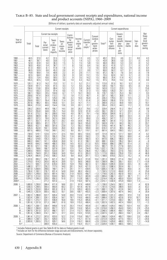
430 | Appendix B
Table B–85. State and local government current receipts and expenditures, national incomeand product accounts (NIPA), 1960–2009
[Billions of dollars; quarterly data at seasonally adjusted annual rates]
Year orquarter
Current receipts Current expenditures
NetStateandlocal
govern-ment
saving
Total
Current tax receipts Contri-butions
forgovern-mentsocialinsur-ance
Incomere-
ceiptson
assets
Currenttransfer
re-ceipts 1
Currentsurplus
ofgovern-mententer-prises
Total 2
Con-sump-tion
expen-ditures
Govern-mentsocialbenefit
pay-ments
toper-sons
Interestpay-
ments
Sub-si-
diesTotalPer-
sonalcurrenttaxes
Taxeson
produc-tionand
imports
Taxeson
corpo-rate
income
1960 ........... 44.5 37.0 4.2 31.5 1.2 0.5 1.3 4.5 1.2 40.2 33.5 4.6 2.1 0.0 4.31961 ........... 48.1 39.7 4.6 33.8 1.3 .5 1.4 5.2 1.3 43.8 36.6 5.0 2.2 .0 4.31962 ........... 52.0 42.8 5.0 36.3 1.5 .5 1.5 5.8 1.4 46.8 39.0 5.3 2.4 .0 5.21963 ........... 56.0 45.8 5.4 38.7 1.7 .6 1.6 6.4 1.6 50.3 41.9 5.7 2.7 .0 5.71964 ........... 61.3 49.8 6.1 41.8 1.8 .7 1.9 7.3 1.6 54.9 45.8 6.2 2.9 .0 6.41965 ........... 66.5 53.9 6.6 45.3 2.0 .8 2.2 8.0 1.7 60.0 50.2 6.7 3.1 .0 6.51966 ........... 74.9 58.8 7.8 48.8 2.2 .8 2.6 11.1 1.6 67.2 56.1 7.6 3.4 .0 7.81967 ........... 82.5 64.0 8.6 52.8 2.6 .9 3.0 13.1 1.5 75.5 62.6 9.2 3.7 .0 7.01968 ........... 93.5 73.4 10.6 59.5 3.3 .9 3.5 14.2 1.5 86.0 70.4 11.4 4.2 .0 7.51969 ........... 105.5 82.5 12.8 66.0 3.6 1.0 4.3 16.2 1.5 97.5 79.8 13.2 4.4 .0 8.01970 ........... 120.1 91.3 14.2 73.3 3.7 1.1 5.2 21.1 1.5 113.0 91.5 16.1 5.3 .0 7.11971 ........... 134.9 101.7 15.9 81.5 4.3 1.2 5.5 25.2 1.4 128.5 102.7 19.3 6.5 .0 6.51972 ........... 158.4 115.6 20.9 89.4 5.3 1.3 5.9 34.0 1.6 142.8 113.2 22.0 7.5 .1 15.61973 ........... 174.3 126.3 22.8 97.4 6.0 1.5 7.8 37.3 1.5 158.6 126.0 24.1 8.5 .1 15.71974 ........... 188.1 136.0 24.5 104.8 6.7 1.7 10.2 39.3 .9 178.7 143.7 25.3 9.6 .1 9.31975 ........... 209.6 147.4 26.9 113.2 7.3 1.8 11.2 48.7 .4 207.1 165.1 30.8 11.1 .2 2.51976 ........... 233.7 165.7 31.1 125.0 9.6 2.2 10.4 55.0 .4 226.3 179.5 34.1 12.5 .2 7.41977 ........... 259.9 183.7 35.4 136.9 11.4 2.8 11.7 61.4 .3 246.8 195.9 37.0 13.7 .2 13.11978 ........... 287.6 198.2 40.5 145.6 12.1 3.4 14.7 71.1 .3 268.9 213.2 40.8 14.9 .2 18.71979 ........... 308.4 212.0 44.0 154.4 13.6 3.9 20.1 72.7 –.3 295.4 233.3 44.3 17.2 .3 13.01980 ........... 338.2 230.0 48.9 166.7 14.5 3.6 26.3 79.5 –1.2 329.4 258.4 51.2 19.4 .4 8.81981 ........... 370.2 255.8 54.6 185.7 15.4 3.9 32.0 81.0 –2.4 362.7 282.3 57.1 22.8 .4 7.61982 ........... 391.4 273.2 59.1 200.0 14.0 4.0 36.7 79.1 –1.6 393.6 304.9 61.2 27.1 .5 –2.21983 ........... 428.6 300.9 66.1 218.9 15.9 4.1 41.4 82.4 –.2 423.7 324.1 66.9 32.3 .4 4.91984 ........... 480.2 337.3 76.0 242.5 18.8 4.7 47.7 89.0 1.5 456.2 347.7 71.2 37.0 .4 23.91985 ........... 521.1 363.7 81.4 262.1 20.2 4.9 54.8 94.5 3.2 498.7 381.8 77.3 39.4 .3 22.41986 ........... 561.6 389.5 87.2 279.7 22.7 6.0 58.4 105.0 2.8 540.9 418.1 84.3 38.2 .3 20.71987 ........... 590.6 422.1 96.6 301.6 23.9 7.2 58.2 100.0 3.1 578.6 441.4 90.7 46.2 .3 12.01988 ........... 635.5 452.8 102.1 324.6 26.0 8.4 60.5 109.0 4.8 618.3 471.0 98.5 48.4 .4 17.21989 ........... 687.5 488.0 114.6 349.1 24.2 9.0 65.7 118.1 6.7 667.4 504.5 109.3 53.2 .4 20.11990 ........... 738.0 519.1 122.6 374.1 22.5 10.0 68.5 133.5 6.9 731.8 547.0 127.7 56.8 .4 6.21991 ........... 789.4 544.3 125.3 395.3 23.6 11.6 68.0 158.2 7.3 795.2 577.5 156.5 60.8 .4 –5.81992 ........... 846.2 579.8 135.3 420.1 24.4 13.1 64.8 180.3 8.3 847.6 606.2 180.0 61.0 .4 –1.41993 ........... 888.2 604.7 141.1 436.8 26.9 14.1 61.3 198.1 9.9 889.1 634.2 195.2 59.4 .4 –.91994 ........... 944.8 644.2 148.0 466.3 30.0 14.5 63.3 212.3 10.5 936.6 668.2 206.7 61.4 .3 8.21995 ........... 991.9 672.1 158.1 482.4 31.7 13.6 68.5 224.2 13.5 982.7 701.3 217.6 63.5 .3 9.21996 ........... 1,045.1 709.6 168.7 507.9 33.0 12.5 73.4 234.0 15.6 1,022.1 730.2 224.3 67.3 .3 23.01997 ........... 1,099.5 749.9 182.0 533.8 34.1 10.8 78.2 246.4 14.2 1,063.2 764.5 227.6 70.6 .4 36.31998 ........... 1,164.5 794.9 201.2 558.8 34.9 10.4 81.5 265.3 12.5 1,117.6 808.6 235.8 72.8 .4 46.91999 ........... 1,240.4 840.4 214.5 590.2 35.8 9.8 85.8 291.1 13.3 1,198.6 870.6 252.3 75.2 .4 41.82000 ........... 1,322.6 893.2 236.7 621.3 35.2 10.8 94.3 313.9 10.4 1,281.3 930.6 271.4 78.8 .5 41.32001 ........... 1,374.0 914.3 243.0 642.4 28.9 13.7 90.0 348.0 8.0 1,389.9 994.2 305.1 83.0 7.7 –15.92002 ........... 1,412.7 928.7 221.8 676.0 30.9 15.9 79.6 382.3 6.1 1,466.8 1,049.4 333.0 83.5 .9 –54.12003 ........... 1,496.3 977.7 226.2 717.5 34.0 20.1 74.0 421.3 3.3 1,535.1 1,096.5 353.4 85.1 .1 –38.82004 ........... 1,601.0 1,059.4 248.6 769.1 41.7 24.1 77.1 439.4 1.0 1,609.3 1,139.1 384.3 85.6 .4 –8.42005 ........... 1,730.4 1,163.1 276.7 831.4 54.9 24.8 88.3 454.3 .1 1,704.5 1,212.0 404.8 87.3 .4 25.92006 ........... 1,829.7 1,249.0 302.5 887.4 59.2 21.8 103.5 456.7 –1.3 1,778.6 1,282.3 402.9 93.0 .4 51.02007 ........... 1,927.3 1,313.4 322.8 934.0 56.5 19.8 114.2 483.9 –3.9 1,905.6 1,366.1 433.7 98.7 7.1 21.72008 ........... 1,974.2 1,336.3 330.0 955.3 51.0 21.1 113.9 506.1 –3.2 2,014.4 1,452.4 455.0 103.9 3.0 –40.22009 p ......... ............. ............. 271.2 931.6 ............. 21.9 116.0 597.5 –3.2 2,015.1 1,430.9 475.9 106.8 1.4 ...............2006: I ....... 1,800.6 1,230.0 298.4 871.9 59.6 23.1 97.9 449.9 –.3 1,738.0 1,254.5 392.2 91.0 .4 62.6
II ...... 1,830.3 1,249.5 305.5 883.8 60.2 22.1 101.9 457.8 –1.1 1,767.0 1,274.6 399.4 92.6 .4 63.2III ..... 1,842.5 1,253.8 300.4 891.8 61.6 21.3 105.5 463.5 –1.6 1,800.1 1,292.7 412.6 94.5 .4 42.4IV ..... 1,845.3 1,262.9 305.5 902.2 55.1 20.6 108.7 455.5 –2.3 1,809.4 1,307.6 407.4 94.0 .4 35.9
2007: I ....... 1,902.3 1,296.8 322.7 920.4 53.8 20.0 112.0 477.0 –3.6 1,869.5 1,331.2 439.5 97.0 1.9 32.8II ...... 1,923.4 1,309.1 324.1 930.4 54.7 19.7 114.0 484.5 –4.0 1,888.4 1,357.3 422.6 97.8 10.7 34.9III ..... 1,932.1 1,315.7 323.1 936.8 55.8 19.6 115.3 485.6 –4.1 1,911.7 1,373.6 430.2 99.2 8.8 20.3IV ..... 1,951.6 1,331.9 321.3 948.7 61.9 19.9 115.3 488.4 –3.9 1,952.9 1,402.5 442.4 100.8 7.2 –1.3
2008: I ....... 1,963.7 1,338.1 336.4 949.8 51.9 20.3 114.4 493.9 –3.1 1,983.8 1,429.3 448.2 102.4 4.0 –20.1II ...... 1,994.2 1,356.9 342.0 957.7 57.2 20.8 114.0 505.4 –2.9 2,019.8 1,458.3 454.0 104.5 2.9 –25.5III ..... 1,987.5 1,351.0 327.2 966.7 57.1 21.4 112.7 505.5 –3.1 2,046.5 1,480.4 459.7 104.3 2.1 –59.0IV ..... 1,951.4 1,298.9 314.1 947.1 37.7 22.0 114.5 519.5 –3.5 2,007.5 1,441.7 458.3 104.7 2.8 –56.1
2009: I ....... 1,961.4 1,272.2 287.0 933.0 52.2 21.8 115.8 555.7 –4.0 1,998.0 1,424.4 465.7 106.0 2.0 –36.6II ...... 1,989.3 1,238.1 252.7 928.0 57.4 21.7 115.7 617.4 –3.5 2,013.9 1,429.9 477.5 105.4 1.2 –24.6III ..... 2,003.6 1,263.5 275.2 929.7 58.6 21.9 116.2 604.9 –2.9 2,018.6 1,429.8 480.0 107.5 1.2 –14.9IV p .. ............. ............. 269.8 935.6 ............. 22.1 116.4 612.1 –2.3 2,029.8 1,439.7 480.5 108.5 1.2 ...............
1 Includes Federal grants-in-aid. See Table B–82 for data on Federal grants-in-aid.2 Includes an item for the difference between wage accruals and disbursements, not shown separately.Source: Department of Commerce (Bureau of Economic Analysis).
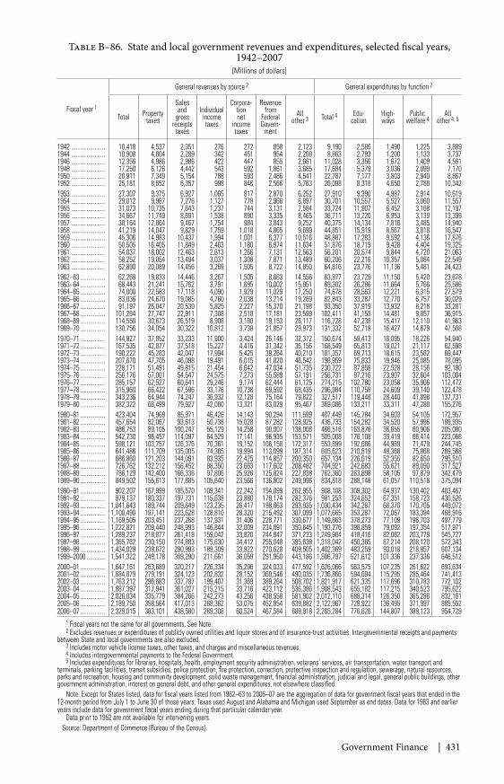
Government Finance | 431
Table B–86. State and local government revenues and expenditures, selected fiscal years,1942–2007
[Millions of dollars]
Fiscal year 1
General revenues by source 2 General expenditures by function 2
Total Propertytaxes
Salesand
grossreceipts
taxes
Individualincometaxes
Corpora-tionnet
incometaxes
Revenuefrom
FederalGovern-
ment
Allother 3 Total 4 Edu-
cationHigh-ways
Publicwelfare 4
Allother 4, 5
1942 ...................... 10,418 4,537 2,351 276 272 858 2,123 9,190 2,586 1,490 1,225 3,8891944 ...................... 10,908 4,604 2,289 342 451 954 2,269 8,863 2,793 1,200 1,133 3,7371946 ...................... 12,356 4,986 2,986 422 447 855 2,661 11,028 3,356 1,672 1,409 4,5911948 ...................... 17,250 6,126 4,442 543 592 1,861 3,685 17,684 5,379 3,036 2,099 7,1701950 ...................... 20,911 7,349 5,154 788 593 2,486 4,541 22,787 7,177 3,803 2,940 8,8671952 ...................... 25,181 8,652 6,357 998 846 2,566 5,763 26,098 8,318 4,650 2,788 10,3421953 ...................... 27,307 9,375 6,927 1,065 817 2,870 6,252 27,910 9,390 4,987 2,914 10,6191954 ...................... 29,012 9,967 7,276 1,127 778 2,966 6,897 30,701 10,557 5,527 3,060 11,5571955 ...................... 31,073 10,735 7,643 1,237 744 3,131 7,584 33,724 11,907 6,452 3,168 12,1971956 ...................... 34,667 11,749 8,691 1,538 890 3,335 8,465 36,711 13,220 6,953 3,139 13,3991957 ...................... 38,164 12,864 9,467 1,754 984 3,843 9,252 40,375 14,134 7,816 3,485 14,9401958 ...................... 41,219 14,047 9,829 1,759 1,018 4,865 9,699 44,851 15,919 8,567 3,818 16,5471959 ...................... 45,306 14,983 10,437 1,994 1,001 6,377 10,516 48,887 17,283 9,592 4,136 17,8761960 ...................... 50,505 16,405 11,849 2,463 1,180 6,974 11,634 51,876 18,719 9,428 4,404 19,3251961 ...................... 54,037 18,002 12,463 2,613 1,266 7,131 12,563 56,201 20,574 9,844 4,720 21,0631962 ...................... 58,252 19,054 13,494 3,037 1,308 7,871 13,489 60,206 22,216 10,357 5,084 22,5491963 ...................... 62,890 20,089 14,456 3,269 1,505 8,722 14,850 64,816 23,776 11,136 5,481 24,4231962–63 ................ 62,269 19,833 14,446 3,267 1,505 8,663 14,556 63,977 23,729 11,150 5,420 23,6781963–64 ................ 68,443 21,241 15,762 3,791 1,695 10,002 15,951 69,302 26,286 11,664 5,766 25,5861964–65 ................ 74,000 22,583 17,118 4,090 1,929 11,029 17,250 74,678 28,563 12,221 6,315 27,5791965–66 ................ 83,036 24,670 19,085 4,760 2,038 13,214 19,269 82,843 33,287 12,770 6,757 30,0291966–67 ................ 91,197 26,047 20,530 5,825 2,227 15,370 21,198 93,350 37,919 13,932 8,218 33,2811967–68 ................ 101,264 27,747 22,911 7,308 2,518 17,181 23,599 102,411 41,158 14,481 9,857 36,9151968–69 ................ 114,550 30,673 26,519 8,908 3,180 19,153 26,117 116,728 47,238 15,417 12,110 41,9631969–70 ................ 130,756 34,054 30,322 10,812 3,738 21,857 29,973 131,332 52,718 16,427 14,679 47,5081970–71 ................ 144,927 37,852 33,233 11,900 3,424 26,146 32,372 150,674 59,413 18,095 18,226 54,9401971–72 ................ 167,535 42,877 37,518 15,227 4,416 31,342 36,156 168,549 65,813 19,021 21,117 62,5981972–73 ................ 190,222 45,283 42,047 17,994 5,425 39,264 40,210 181,357 69,713 18,615 23,582 69,4471973–74 ................ 207,670 47,705 46,098 19,491 6,015 41,820 46,542 198,959 75,833 19,946 25,085 78,0951974–75 ................ 228,171 51,491 49,815 21,454 6,642 47,034 51,735 230,722 87,858 22,528 28,156 92,1801975–76 ................ 256,176 57,001 54,547 24,575 7,273 55,589 57,191 256,731 97,216 23,907 32,604 103,0041976–77 ................ 285,157 62,527 60,641 29,246 9,174 62,444 61,125 274,215 102,780 23,058 35,906 112,4721977–78 ................ 315,960 66,422 67,596 33,176 10,738 69,592 68,435 296,984 110,758 24,609 39,140 122,4781978–79 ................ 343,236 64,944 74,247 36,932 12,128 75,164 79,822 327,517 119,448 28,440 41,898 137,7311979–80 ................ 382,322 68,499 79,927 42,080 13,321 83,029 95,467 369,086 133,211 33,311 47,288 155,2761980–81 ................ 423,404 74,969 85,971 46,426 14,143 90,294 111,599 407,449 145,784 34,603 54,105 172,9571981–82 ................ 457,654 82,067 93,613 50,738 15,028 87,282 128,925 436,733 154,282 34,520 57,996 189,9351982–83 ................ 486,753 89,105 100,247 55,129 14,258 90,007 138,008 466,516 163,876 36,655 60,906 205,0801983–84 ................ 542,730 96,457 114,097 64,529 17,141 96,935 153,571 505,008 176,108 39,419 66,414 223,0681984–85 ................ 598,121 103,757 126,376 70,361 19,152 106,158 172,317 553,899 192,686 44,989 71,479 244,7451985–86 ................ 641,486 111,709 135,005 74,365 19,994 113,099 187,314 605,623 210,819 49,368 75,868 269,5681986–87 ................ 686,860 121,203 144,091 83,935 22,425 114,857 200,350 657,134 226,619 52,355 82,650 295,5101987–88 ................ 726,762 132,212 156,452 88,350 23,663 117,602 208,482 704,921 242,683 55,621 89,090 317,5271988–89 ................ 786,129 142,400 166,336 97,806 25,926 125,824 227,838 762,360 263,898 58,105 97,879 342,4791989–90 ................ 849,502 155,613 177,885 105,640 23,566 136,802 249,996 834,818 288,148 61,057 110,518 375,0941990–91 ................ 902,207 167,999 185,570 109,341 22,242 154,099 262,955 908,108 309,302 64,937 130,402 403,4671991–92 ................ 979,137 180,337 197,731 115,638 23,880 179,174 282,376 981,253 324,652 67,351 158,723 430,5261992–93 ................ 1,041,643 189,744 209,649 123,235 26,417 198,663 293,935 1,030,434 342,287 68,370 170,705 449,0721993–94 ................ 1,100,490 197,141 223,628 128,810 28,320 215,492 307,099 1,077,665 353,287 72,067 183,394 468,9161994–95 ................ 1,169,505 203,451 237,268 137,931 31,406 228,771 330,677 1,149,863 378,273 77,109 196,703 497,7791995–96 ................ 1,222,821 209,440 248,993 146,844 32,009 234,891 350,645 1,193,276 398,859 79,092 197,354 517,9711996–97 ................ 1,289,237 218,877 261,418 159,042 33,820 244,847 371,233 1,249,984 418,416 82,062 203,779 545,7271997–98 ................ 1,365,762 230,150 274,883 175,630 34,412 255,048 395,639 1,318,042 450,365 87,214 208,120 572,3431998–99 ................ 1,434,029 239,672 290,993 189,309 33,922 270,628 409,505 1,402,369 483,259 93,018 218,957 607,1341999–2000 ............ 1,541,322 249,178 309,290 211,661 36,059 291,950 443,186 1,506,797 521,612 101,336 237,336 646,5122000–01 ................ 1,647,161 263,689 320,217 226,334 35,296 324,033 477,592 1,626,066 563,575 107,235 261,622 693,6342001–02 ................ 1,684,879 279,191 324,123 202,832 28,152 360,546 490,035 1,736,866 594,694 115,295 285,464 741,4132002–03 ................ 1,763,212 296,683 337,787 199,407 31,369 389,264 508,702 1,821,917 621,335 117,696 310,783 772,1022003–04 ................ 1,887,397 317,941 361,027 215,215 33,716 423,112 536,386 1,908,543 655,182 117,215 340,523 795,6222004–05 ................ 2,026,034 335,779 384,266 242,273 43,256 438,558 581,902 2,012,110 688,314 126,350 365,286 832,1612005–06 ................ 2,189,750 358,564 417,013 268,362 53,075 452,854 639,882 2,122,967 728,922 136,495 371,997 885,5522006–07 ................ 2,329,015 383,101 438,580 289,308 60,524 467,584 689,918 2,265,284 776,626 144,807 389,123 954,729
1 Fiscal years not the same for all governments. See Note.2 Excludes revenues or expenditures of publicly owned utilities and liquor stores and of insurance-trust activities. Intergovernmental receipts and payments
between State and local governments are also excluded.3 Includes motor vehicle license taxes, other taxes, and charges and miscellaneous revenues.4 Includes intergovernmental payments to the Federal Government.5 Includes expenditures for libraries, hospitals, health, employment security administration, veterans’ services, air transportation, water transport and
terminals, parking facilities, transit subsidies, police protection, fire protection, correction, protective inspection and regulation, sewerage, natural resources,parks and recreation, housing and community development, solid waste management, financial administration, judicial and legal, general public buildings, othergovernment administration, interest on general debt, and other general expenditures, not elsewhere classified.
Note: Except for States listed, data for fiscal years listed from 1962–63 to 2006–07 are the aggregation of data for government fiscal years that ended in the12-month period from July 1 to June 30 of those years; Texas used August and Alabama and Michigan used September as end dates. Data for 1963 and earlieryears include data for government fiscal years ending during that particular calendar year.
Data prior to 1952 are not available for intervening years.Source: Department of Commerce (Bureau of the Census).
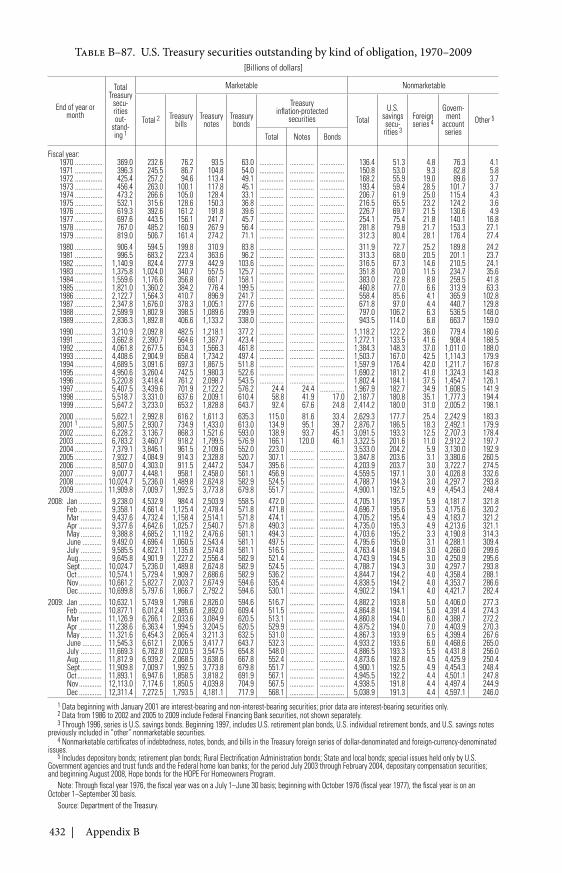
432 | Appendix B
Table B–87. U.S. Treasury securities outstanding by kind of obligation, 1970–2009[Billions of dollars]
End of year ormonth
TotalTreasury
secu-ritiesout-
stand-ing 1
Marketable Nonmarketable
Total 2 Treasurybills
Treasurynotes
Treasurybonds
Treasuryinflation-protected
securities TotalU.S.
savingssecu-rities 3
Foreignseries 4
Govern-ment
accountseries
Other 5
Total Notes Bonds
Fiscal year:1970 ................ 369.0 232.6 76.2 93.5 63.0 .............. .............. .............. 136.4 51.3 4.8 76.3 4.11971 ................ 396.3 245.5 86.7 104.8 54.0 .............. .............. .............. 150.8 53.0 9.3 82.8 5.81972 ................ 425.4 257.2 94.6 113.4 49.1 .............. .............. .............. 168.2 55.9 19.0 89.6 3.71973 ................ 456.4 263.0 100.1 117.8 45.1 .............. .............. .............. 193.4 59.4 28.5 101.7 3.71974 ................ 473.2 266.6 105.0 128.4 33.1 .............. .............. .............. 206.7 61.9 25.0 115.4 4.31975 ................ 532.1 315.6 128.6 150.3 36.8 .............. .............. .............. 216.5 65.5 23.2 124.2 3.61976 ................ 619.3 392.6 161.2 191.8 39.6 .............. .............. .............. 226.7 69.7 21.5 130.6 4.91977 ................ 697.6 443.5 156.1 241.7 45.7 .............. .............. .............. 254.1 75.4 21.8 140.1 16.81978 ................ 767.0 485.2 160.9 267.9 56.4 .............. .............. .............. 281.8 79.8 21.7 153.3 27.11979 ................ 819.0 506.7 161.4 274.2 71.1 .............. .............. .............. 312.3 80.4 28.1 176.4 27.41980 ................ 906.4 594.5 199.8 310.9 83.8 .............. .............. .............. 311.9 72.7 25.2 189.8 24.21981 ................ 996.5 683.2 223.4 363.6 96.2 .............. .............. .............. 313.3 68.0 20.5 201.1 23.71982 ................ 1,140.9 824.4 277.9 442.9 103.6 .............. .............. .............. 316.5 67.3 14.6 210.5 24.11983 ................ 1,375.8 1,024.0 340.7 557.5 125.7 .............. .............. .............. 351.8 70.0 11.5 234.7 35.61984 ................ 1,559.6 1,176.6 356.8 661.7 158.1 .............. .............. .............. 383.0 72.8 8.8 259.5 41.81985 ................ 1,821.0 1,360.2 384.2 776.4 199.5 .............. .............. .............. 460.8 77.0 6.6 313.9 63.31986 ................ 2,122.7 1,564.3 410.7 896.9 241.7 .............. .............. .............. 558.4 85.6 4.1 365.9 102.81987 ................ 2,347.8 1,676.0 378.3 1,005.1 277.6 .............. .............. .............. 671.8 97.0 4.4 440.7 129.81988 ................ 2,599.9 1,802.9 398.5 1,089.6 299.9 .............. .............. .............. 797.0 106.2 6.3 536.5 148.01989 ................ 2,836.3 1,892.8 406.6 1,133.2 338.0 .............. .............. .............. 943.5 114.0 6.8 663.7 159.01990 ................ 3,210.9 2,092.8 482.5 1,218.1 377.2 .............. .............. .............. 1,118.2 122.2 36.0 779.4 180.61991 ................ 3,662.8 2,390.7 564.6 1,387.7 423.4 .............. .............. .............. 1,272.1 133.5 41.6 908.4 188.51992 ................ 4,061.8 2,677.5 634.3 1,566.3 461.8 .............. .............. .............. 1,384.3 148.3 37.0 1,011.0 188.01993 ................ 4,408.6 2,904.9 658.4 1,734.2 497.4 .............. .............. .............. 1,503.7 167.0 42.5 1,114.3 179.91994 ................ 4,689.5 3,091.6 697.3 1,867.5 511.8 .............. .............. .............. 1,597.9 176.4 42.0 1,211.7 167.81995 ................ 4,950.6 3,260.4 742.5 1,980.3 522.6 .............. .............. .............. 1,690.2 181.2 41.0 1,324.3 143.81996 ................ 5,220.8 3,418.4 761.2 2,098.7 543.5 .............. .............. .............. 1,802.4 184.1 37.5 1,454.7 126.11997 ................ 5,407.5 3,439.6 701.9 2,122.2 576.2 24.4 24.4 .............. 1,967.9 182.7 34.9 1,608.5 141.91998 ................ 5,518.7 3,331.0 637.6 2,009.1 610.4 58.8 41.9 17.0 2,187.7 180.8 35.1 1,777.3 194.41999 ................ 5,647.2 3,233.0 653.2 1,828.8 643.7 92.4 67.6 24.8 2,414.2 180.0 31.0 2,005.2 198.12000 ................ 5,622.1 2,992.8 616.2 1,611.3 635.3 115.0 81.6 33.4 2,629.3 177.7 25.4 2,242.9 183.32001 1 .............. 5,807.5 2,930.7 734.9 1,433.0 613.0 134.9 95.1 39.7 2,876.7 186.5 18.3 2,492.1 179.92002 ................ 6,228.2 3,136.7 868.3 1,521.6 593.0 138.9 93.7 45.1 3,091.5 193.3 12.5 2,707.3 178.42003 ................ 6,783.2 3,460.7 918.2 1,799.5 576.9 166.1 120.0 46.1 3,322.5 201.6 11.0 2,912.2 197.72004 ................ 7,379.1 3,846.1 961.5 2,109.6 552.0 223.0 .............. .............. 3,533.0 204.2 5.9 3,130.0 192.92005 ................ 7,932.7 4,084.9 914.3 2,328.8 520.7 307.1 .............. .............. 3,847.8 203.6 3.1 3,380.6 260.52006 ................ 8,507.0 4,303.0 911.5 2,447.2 534.7 395.6 .............. .............. 4,203.9 203.7 3.0 3,722.7 274.52007 ................ 9,007.7 4,448.1 958.1 2,458.0 561.1 456.9 .............. .............. 4,559.5 197.1 3.0 4,026.8 332.62008 ................ 10,024.7 5,236.0 1,489.8 2,624.8 582.9 524.5 .............. .............. 4,788.7 194.3 3.0 4,297.7 293.82009 ................ 11,909.8 7,009.7 1,992.5 3,773.8 679.8 551.7 .............. .............. 4,900.1 192.5 4.9 4,454.3 248.4
2008: Jan ............. 9,238.0 4,532.9 984.4 2,503.9 558.5 472.0 .............. .............. 4,705.1 195.7 5.9 4,181.7 321.8Feb ............. 9,358.1 4,661.4 1,125.4 2,478.4 571.8 471.8 .............. .............. 4,696.7 195.6 5.3 4,175.6 320.2Mar ............ 9,437.6 4,732.4 1,158.4 2,514.1 571.8 474.1 .............. .............. 4,705.2 195.4 4.9 4,183.7 321.2Apr ............. 9,377.6 4,642.6 1,025.7 2,540.7 571.8 490.3 .............. .............. 4,735.0 195.3 4.9 4,213.6 321.1May ............ 9,388.8 4,685.2 1,119.2 2,476.6 581.1 494.3 .............. .............. 4,703.6 195.2 3.3 4,190.8 314.3June ........... 9,492.0 4,696.4 1,060.5 2,543.4 581.1 497.5 .............. .............. 4,795.6 195.0 3.1 4,288.1 309.4July ............ 9,585.5 4,822.1 1,135.8 2,574.8 581.1 516.5 .............. .............. 4,763.4 194.8 3.0 4,266.0 299.6Aug ............. 9,645.8 4,901.9 1,227.2 2,556.4 582.9 521.4 .............. .............. 4,743.9 194.5 3.0 4,250.9 295.6Sept ............ 10,024.7 5,236.0 1,489.8 2,624.8 582.9 524.5 .............. .............. 4,788.7 194.3 3.0 4,297.7 293.8Oct .............. 10,574.1 5,729.4 1,909.7 2,686.6 582.9 536.2 .............. .............. 4,844.7 194.2 4.0 4,358.4 288.1Nov ............. 10,661.2 5,822.7 2,003.7 2,674.9 594.6 535.4 .............. .............. 4,838.5 194.2 4.0 4,353.7 286.6Dec ............. 10,699.8 5,797.6 1,866.7 2,792.2 594.6 530.1 .............. .............. 4,902.2 194.1 4.0 4,421.7 282.4
2009: Jan ............. 10,632.1 5,749.9 1,798.6 2,826.0 594.6 516.7 .............. .............. 4,882.2 193.8 5.0 4,406.0 277.3Feb ............. 10,877.1 6,012.4 1,985.6 2,892.0 609.4 511.5 .............. .............. 4,864.8 194.1 5.0 4,391.4 274.3Mar ............ 11,126.9 6,266.1 2,033.6 3,084.9 620.5 513.1 .............. .............. 4,860.8 194.0 6.0 4,388.7 272.2Apr ............. 11,238.6 6,363.4 1,994.5 3,204.5 620.5 529.9 .............. .............. 4,875.2 194.0 7.0 4,403.9 270.3May ............ 11,321.6 6,454.3 2,065.4 3,211.3 632.5 531.0 .............. .............. 4,867.3 193.9 6.5 4,399.4 267.6June ........... 11,545.3 6,612.1 2,006.5 3,417.7 643.7 532.3 .............. .............. 4,933.2 193.6 6.0 4,468.6 265.0July ............ 11,669.3 6,782.8 2,020.5 3,547.5 654.8 548.0 .............. .............. 4,886.5 193.3 5.5 4,431.8 256.0Aug ............. 11,812.9 6,939.2 2,068.5 3,638.6 667.8 552.4 .............. .............. 4,873.6 192.8 4.5 4,425.9 250.4Sept ............ 11,909.8 7,009.7 1,992.5 3,773.8 679.8 551.7 .............. .............. 4,900.1 192.5 4.9 4,454.3 248.4Oct .............. 11,893.1 6,947.6 1,858.5 3,818.2 691.9 567.1 .............. .............. 4,945.5 192.2 4.4 4,501.1 247.8Nov ............. 12,113.0 7,174.6 1,850.5 4,039.8 704.9 567.5 .............. .............. 4,938.5 191.8 4.4 4,497.4 244.9Dec ............. 12,311.4 7,272.5 1,793.5 4,181.1 717.9 568.1 .............. .............. 5,038.9 191.3 4.4 4,597.1 246.0
1 Data beginning with January 2001 are interest-bearing and non-interest-bearing securities; prior data are interest-bearing securities only.2 Data from 1986 to 2002 and 2005 to 2009 include Federal Financing Bank securities, not shown separately.3 Through 1996, series is U.S. savings bonds. Beginning 1997, includes U.S. retirement plan bonds, U.S. individual retirement bonds, and U.S. savings notes
previously included in “other” nonmarketable securities.4 Nonmarketable certificates of indebtedness, notes, bonds, and bills in the Treasury foreign series of dollar-denominated and foreign-currency-denominated
issues.5 Includes depository bonds; retirement plan bonds; Rural Electrification Administration bonds; State and local bonds; special issues held only by U.S.
Government agencies and trust funds and the Federal home loan banks; for the period July 2003 through February 2004, depositary compensation securities;and beginning August 2008, Hope bonds for the HOPE For Homeowners Program.
Note: Through fiscal year 1976, the fiscal year was on a July 1–June 30 basis; beginning with October 1976 (fiscal year 1977), the fiscal year is on anOctober 1–September 30 basis.
Source: Department of the Treasury.
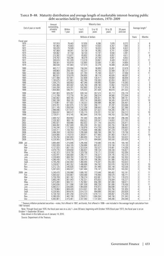
Government Finance | 433
Table B–88. Maturity distribution and average length of marketable interest-bearing publicdebt securities held by private investors, 1970–2009
End of year or monthAmount
outstanding,privately
held
Maturity classAverage length 1
Within1 year
1 to 5years
5 to 10years
10 to 20years
20 yearsand over
Millions of dollars Years Months
Fiscal year:1970 ...................................... 157,910 76,443 57,035 8,286 7,876 8,272 3 81971 ...................................... 161,863 74,803 58,557 14,503 6,357 7,645 3 61972 ...................................... 165,978 79,509 57,157 16,033 6,358 6,922 3 31973 ...................................... 167,869 84,041 54,139 16,385 8,741 4,564 3 11974 ...................................... 164,862 87,150 50,103 14,197 9,930 3,481 2 111975 ...................................... 210,382 115,677 65,852 15,385 8,857 4,611 2 81976 ...................................... 279,782 150,296 90,578 24,169 8,087 6,652 2 71977 ...................................... 326,674 161,329 113,319 33,067 8,428 10,531 2 111978 ...................................... 356,501 163,819 132,993 33,500 11,383 14,805 3 31979 ...................................... 380,530 181,883 127,574 32,279 18,489 20,304 3 71980 ...................................... 463,717 220,084 156,244 38,809 25,901 22,679 3 91981 ...................................... 549,863 256,187 182,237 48,743 32,569 30,127 4 01982 ...................................... 682,043 314,436 221,783 75,749 33,017 37,058 3 111983 ...................................... 862,631 379,579 294,955 99,174 40,826 48,097 4 11984 ...................................... 1,017,488 437,941 332,808 130,417 49,664 66,658 4 61985 ...................................... 1,185,675 472,661 402,766 159,383 62,853 88,012 4 111986 ...................................... 1,354,275 506,903 467,348 189,995 70,664 119,365 5 31987 ...................................... 1,445,366 483,582 526,746 209,160 72,862 153,016 5 91988 ...................................... 1,555,208 524,201 552,993 232,453 74,186 171,375 5 91989 ...................................... 1,654,660 546,751 578,333 247,428 80,616 201,532 6 01990 ...................................... 1,841,903 626,297 630,144 267,573 82,713 235,176 6 11991 ...................................... 2,113,799 713,778 761,243 280,574 84,900 273,304 6 01992 ...................................... 2,363,802 808,705 866,329 295,921 84,706 308,141 5 111993 ...................................... 2,562,336 858,135 978,714 306,663 94,345 324,479 5 101994 ...................................... 2,719,861 877,932 1,128,322 289,998 88,208 335,401 5 81995 ...................................... 2,870,781 1,002,875 1,157,492 290,111 87,297 333,006 5 41996 ...................................... 3,011,185 1,058,558 1,212,258 306,643 111,360 322,366 5 31997 ...................................... 2,998,846 1,017,913 1,206,993 321,622 154,205 298,113 5 51998 ...................................... 2,856,637 940,572 1,105,175 319,331 157,347 334,212 5 101999 ...................................... 2,728,011 915,145 962,644 378,163 149,703 322,356 6 02000 ...................................... 2,469,152 858,903 791,540 355,382 167,082 296,246 6 22001 ...................................... 2,328,302 900,178 650,522 329,247 174,653 273,702 6 12002 ...................................... 2,492,821 939,986 802,032 311,176 203,816 235,811 5 62003 ...................................... 2,804,092 1,057,049 955,239 351,552 243,755 196,497 5 12004 ...................................... 3,145,244 1,127,850 1,150,979 414,728 243,036 208,652 4 112005 ...................................... 3,334,411 1,100,783 1,279,646 499,386 281,229 173,367 4 102006 ...................................... 3,496,359 1,140,553 1,295,589 589,748 290,733 179,736 4 112007 ...................................... 3,634,666 1,176,510 1,309,871 677,905 291,963 178,417 4 102008 ...................................... 4,745,256 2,042,003 1,468,455 719,347 352,430 163,022 4 12009 ...................................... 6,228,565 2,604,676 2,074,723 994,689 350,550 203,928 4 1
2008: Jan ................................... 3,805,408 1,315,046 1,295,456 710,580 319,185 165,140 4 9Feb ................................... 3,933,939 1,454,105 1,294,886 691,672 319,156 174,120 4 8Mar .................................. 4,127,033 1,607,155 1,323,534 702,527 319,481 174,336 4 5Apr ................................... 4,079,776 1,509,658 1,366,837 709,124 338,330 155,827 4 6May .................................. 4,162,323 1,618,739 1,329,756 718,171 333,602 162,056 4 6June ................................. 4,203,441 1,580,568 1,396,177 730,327 334,145 162,224 4 6July .................................. 4,328,809 1,668,784 1,439,791 716,694 341,086 162,453 4 5Aug ................................... 4,386,440 1,774,790 1,390,479 706,395 351,906 162,870 4 5Sept .................................. 4,745,256 2,042,003 1,468,455 719,347 352,430 163,022 4 1Oct .................................... 5,238,827 2,462,352 1,496,698 764,782 352,076 162,919 3 10Nov ................................... 5,312,125 2,540,826 1,490,667 761,948 355,148 163,536 3 10Dec ................................... 5,307,633 2,406,537 1,607,484 776,147 354,202 163,262 3 10
2009: Jan ................................... 5,240,470 2,336,988 1,606,792 773,548 360,402 162,741 3 11Feb ................................... 5,505,532 2,543,867 1,659,368 776,956 358,570 166,771 3 11Mar .................................. 5,759,709 2,601,162 1,790,274 833,981 357,716 176,575 3 11Apr ................................... 5,800,248 2,601,043 1,792,321 875,653 376,004 155,227 3 11May .................................. 5,815,094 2,660,151 1,762,962 856,289 367,080 168,611 3 11June ................................. 5,943,636 2,611,596 1,891,559 900,239 361,806 178,436 3 11July .................................. 6,065,512 2,636,005 1,964,000 916,972 360,698 187,837 4 0Aug ................................... 6,179,984 2,669,428 2,014,501 951,363 352,756 191,935 4 0Sept .................................. 6,228,565 2,604,676 2,074,723 994,689 350,550 203,928 4 1Oct .................................... 6,138,150 2,481,258 2,073,374 1,019,112 349,067 215,339 4 3Nov ................................... 6,386,026 2,462,190 2,259,073 1,084,264 349,156 231,343 4 3Dec ................................... 6,483,901 2,415,461 2,337,392 1,137,420 349,280 244,348 4 4
1 Treasury inflation-protected securities—notes, first offered in 1997, and bonds, first offered in 1998—are included in the average length calculation from1997 forward.
Note: Through fiscal year 1976, the fiscal year was on a July 1–June 30 basis; beginning with October 1976 (fiscal year 1977), the fiscal year is on anOctober 1–September 30 basis.
Data shown in this table are as of January 14, 2010.Source: Department of the Treasury.
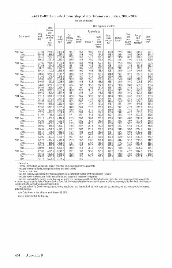
434 | Appendix B
Table B–89. Estimated ownership of U.S. Treasury securities, 2000–2009[Billions of dollars]
End of monthTotalpublicdebt 1
FederalReserve
andIntragov-ernmen-
talhold-ings 2
Held by private investors
Totalprivately
held
De-positoryinstitu-tions 3
U.S.savingsbonds 4
Pension fundsInsur-ance
compa-nies
Mutualfunds 6
Stateandlocal
govern-ments
Foreignand
inter-national 7
Otherinves-tors 8Private 5
Stateandlocal
govern-ments
2000: Mar .................. 5,773.4 2,590.6 3,182.8 237.7 185.3 150.2 196.9 120.0 222.3 306.3 1,085.0 679.1June ................. 5,685.9 2,698.6 2,987.3 222.2 184.6 149.0 194.9 116.5 205.4 309.3 1,060.7 544.8Sept .................. 5,674.2 2,737.9 2,936.3 220.5 184.3 147.9 185.5 113.7 207.8 307.9 1,038.8 529.9Dec ................... 5,662.2 2,781.8 2,880.4 201.5 184.8 145.0 179.1 110.2 225.7 310.0 1,015.2 509.0
2001: Mar .................. 5,773.7 2,880.9 2,892.8 188.0 184.8 153.4 177.3 109.1 225.3 316.9 1,012.5 525.5June ................. 5,726.8 3,004.2 2,722.6 188.1 185.5 148.5 183.1 108.1 221.0 324.8 983.3 380.3Sept .................. 5,807.5 3,027.8 2,779.7 189.1 186.4 149.9 166.8 106.8 234.1 321.2 992.2 433.1Dec ................... 5,943.4 3,123.9 2,819.5 181.5 190.3 145.8 155.1 105.7 261.9 328.4 1,040.1 410.7
2002: Mar .................. 6,006.0 3,156.8 2,849.2 187.6 191.9 152.7 163.3 114.0 266.1 327.6 1,057.2 388.8June ................. 6,126.5 3,276.7 2,849.8 204.7 192.7 152.1 153.9 122.0 253.8 333.6 1,123.1 313.8Sept .................. 6,228.2 3,303.5 2,924.8 209.3 193.3 154.5 156.3 130.4 256.8 338.6 1,188.6 297.0Dec ................... 6,405.7 3,387.2 3,018.5 222.6 194.9 153.8 158.9 139.7 281.0 354.7 1,235.6 277.4
2003: Mar .................. 6,460.8 3,390.8 3,069.9 153.4 196.9 165.8 162.1 139.5 296.6 350.0 1,275.2 330.4June ................. 6,670.1 3,505.4 3,164.7 145.1 199.1 170.2 161.3 138.7 302.3 347.9 1,371.9 328.2Sept .................. 6,783.2 3,515.3 3,268.0 146.8 201.5 167.7 155.5 137.4 287.1 357.7 1,443.3 371.1Dec ................... 6,998.0 3,620.1 3,377.9 153.1 203.8 172.1 148.6 136.5 280.8 364.2 1,523.1 395.6
2004: Mar .................. 7,131.1 3,628.3 3,502.8 162.8 204.4 169.8 143.6 141.0 280.8 374.1 1,670.0 356.3June ................. 7,274.3 3,742.8 3,531.5 158.6 204.6 173.3 134.9 144.1 258.7 381.2 1,735.4 340.6Sept .................. 7,379.1 3,772.0 3,607.0 138.5 204.1 174.0 140.8 147.4 255.0 381.7 1,794.5 371.0Dec ................... 7,596.1 3,905.6 3,690.6 125.0 204.4 173.7 151.0 149.7 254.1 389.1 1,849.3 394.3
2005: Mar .................. 7,776.9 3,921.6 3,855.4 141.8 204.2 177.3 158.0 152.4 261.1 412.0 1,952.2 396.4June ................. 7,836.5 4,033.5 3,803.0 126.9 204.2 181.0 171.3 155.0 248.7 444.0 1,877.5 394.5Sept .................. 7,932.7 4,067.8 3,864.9 125.3 203.6 184.2 164.8 159.0 244.7 467.6 1,929.6 386.0Dec ................... 8,170.4 4,199.8 3,970.6 117.1 205.1 184.9 153.8 160.4 251.3 481.4 2,033.9 382.6
2006: Mar .................. 8,371.2 4,257.2 4,114.0 115.3 205.9 186.7 153.0 161.3 248.7 486.1 2,082.1 475.0June ................. 8,420.0 4,389.2 4,030.8 117.1 205.2 192.1 150.9 161.2 244.2 499.4 1,977.8 482.8Sept .................. 8,507.0 4,432.8 4,074.2 113.5 203.6 201.9 155.6 160.6 235.7 502.1 2,025.3 475.8Dec ................... 8,680.2 4,558.1 4,122.1 114.8 202.4 207.5 157.1 159.0 250.7 516.9 2,103.1 410.6
2007: Mar .................. 8,849.7 4,576.6 4,273.1 119.7 200.3 221.7 159.2 150.8 264.5 535.0 2,194.8 427.1June ................. 8,867.7 4,715.1 4,152.6 110.4 198.6 232.5 160.2 142.1 267.7 580.3 2,192.0 268.7Sept .................. 9,007.7 4,738.0 4,269.7 119.6 197.1 246.7 165.6 133.4 306.3 541.4 2,235.3 324.1Dec ................... 9,229.2 4,833.5 4,395.7 129.7 196.4 257.6 168.8 123.3 362.9 531.5 2,353.2 272.2
2008: Mar .................. 9,437.6 4,694.7 4,742.9 125.3 195.3 270.5 169.4 129.4 484.4 521.6 2,505.8 341.2June ................. 9,492.0 4,685.8 4,806.2 112.7 194.9 276.7 169.1 135.5 477.2 513.4 2,587.2 339.4Sept .................. 10,024.7 4,692.7 5,332.0 130.0 194.2 292.5 171.6 140.6 656.1 499.3 2,799.5 448.3Dec ................... 10,699.8 4,806.4 5,893.4 105.0 194.0 297.2 174.6 160.5 768.8 483.1 3,075.9 634.4
2009: Mar .................. 11,126.9 4,785.2 6,341.7 129.1 193.9 305.9 173.2 179.7 716.0 477.9 3,264.6 901.4June ................. 11,545.3 5,026.8 6,518.5 140.8 193.5 312.4 172.7 189.7 695.0 488.4 3,382.1 943.8Sept .................. 11,909.8 5,127.1 6,782.7 199.0 192.4 324.5 176.7 196.3 643.0 502.5 3,497.4 1,050.9Dec ................... 12,311.4 5,276.9 7,034.5 ............... 191.3 ............... ............... ............... ............... ............... ............... ................
1 Face value.2 Federal Reserve holdings exclude Treasury securities held under repurchase agreements.3 Includes commercial banks, savings institutions, and credit unions.4 Current accrual value.5 Includes Treasury securities held by the Federal Employees Retirement System Thrift Savings Plan “G Fund.”6 Includes money market mutual funds, mutual funds, and closed-end investment companies.7 Includes nonmarketable foreign series, Treasury securities, and Treasury deposit funds. Excludes Treasury securities held under repurchase agreements
in custody accounts at the Federal Reserve Bank of New York. Estimates reflect benchmarks to this series at differing intervals; for further detail, see TreasuryBulletin and http://www.treas.gov/tic/ticsec2.shtml
8 Includes individuals, Government-sponsored enterprises, brokers and dealers, bank personal trusts and estates, corporate and noncorporate businesses,and other investors.
Note: Data shown in this table are as of January 25, 2010.Source: Department of the Treasury.
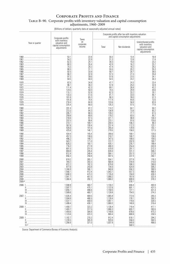
Corporate Profits and Finance | 435
Table B–90. Corporate profits with inventory valuation and capital consumptionadjustments, 1960–2009
[Billions of dollars; quarterly data at seasonally adjusted annual rates]
Year or quarter
Corporate profitswith inventoryvaluation and
capital consumptionadjustments
Taxeson
corporateincome
Corporate profits after tax with inventory valuationand capital consumption adjustments
Total Net dividends
Undistributed profitswith inventoryvaluation and
capital consumptionadjustments
1960 ................................................. 53.1 22.8 30.3 13.4 16.91961 ................................................. 54.2 22.9 31.3 13.9 17.41962 ................................................. 62.3 24.1 38.3 15.0 23.21963 ................................................. 68.3 26.4 42.0 16.2 25.71964 ................................................. 75.5 28.2 47.4 18.2 29.21965 ................................................. 86.5 31.1 55.5 20.2 35.31966 ................................................. 92.5 33.9 58.7 20.7 38.01967 ................................................. 90.2 32.9 57.3 21.5 35.81968 ................................................. 97.3 39.6 57.6 23.5 34.11969 ................................................. 94.5 40.0 54.5 24.2 30.31970 ................................................. 82.5 34.8 47.7 24.3 23.41971 ................................................. 96.1 38.2 57.9 25.0 32.91972 ................................................. 111.4 42.3 69.1 26.8 42.21973 ................................................. 124.5 50.0 74.5 29.9 44.61974 ................................................. 115.1 52.8 62.3 33.2 29.11975 ................................................. 133.3 51.6 81.7 33.0 48.71976 ................................................. 161.6 65.3 96.3 39.0 57.31977 ................................................. 191.8 74.4 117.4 44.8 72.61978 ................................................. 218.4 84.9 133.6 50.8 82.81979 ................................................. 225.4 90.0 135.3 57.5 77.81980 ................................................. 201.4 87.2 114.2 64.1 50.21981 ................................................. 223.3 84.3 138.9 73.8 65.21982 ................................................. 205.7 66.5 139.2 77.7 61.51983 ................................................. 259.8 80.6 179.2 83.5 95.71984 ................................................. 318.6 97.5 221.1 90.8 130.31985 ................................................. 332.5 99.4 233.1 97.6 135.61986 ................................................. 314.1 109.7 204.5 106.2 98.31987 ................................................. 367.8 130.4 237.4 112.3 125.11988 ................................................. 426.6 141.6 285.0 129.9 155.11989 ................................................. 425.6 146.1 279.5 158.0 121.51990 ................................................. 434.4 145.4 289.0 169.1 120.01991 ................................................. 457.3 138.6 318.7 180.7 138.01992 ................................................. 496.2 148.7 347.5 188.0 159.51993 ................................................. 543.7 171.0 372.7 202.9 169.71994 ................................................. 628.2 193.1 435.1 235.7 199.41995 ................................................. 716.2 217.8 498.3 254.4 243.91996 ................................................. 801.5 231.5 570.0 297.7 272.31997 ................................................. 884.8 245.4 639.4 331.2 308.21998 ................................................. 812.4 248.4 564.1 351.5 212.61999 ................................................. 856.3 258.8 597.5 337.4 260.12000 ................................................. 819.2 265.1 554.1 377.9 176.32001 ................................................. 784.2 203.3 580.9 370.9 210.02002 ................................................. 872.2 192.3 679.9 399.3 280.62003 ................................................. 977.8 243.8 734.0 424.9 309.22004 ................................................. 1,246.9 306.1 940.8 550.3 390.52005 ................................................. 1,456.1 412.4 1,043.7 557.3 486.42006 ................................................. 1,608.3 473.3 1,135.0 704.8 430.32007 ................................................. 1,541.7 451.5 1,090.2 767.8 322.42008 ................................................. 1,360.4 292.2 1,068.2 689.9 378.32009 p ............................................... ..................................... ..................................... ..................................... 576.1 .......................................2006: I ............................................. 1,590.9 460.7 1,130.2 646.4 483.9
II ............................................ 1,597.7 475.1 1,122.6 691.1 431.5III ........................................... 1,655.1 496.6 1,158.5 727.1 431.4IV ........................................... 1,589.6 460.7 1,128.8 754.5 374.3
2007: I ............................................. 1,535.4 469.5 1,065.9 772.6 293.3II ............................................ 1,594.9 466.5 1,128.4 778.1 350.3III ........................................... 1,537.1 440.0 1,097.1 770.6 326.5IV ........................................... 1,499.4 430.1 1,069.3 749.9 319.4
2008: I ............................................. 1,459.7 323.2 1,136.4 719.4 417.1II ............................................ 1,403.7 317.5 1,086.3 693.7 392.6III ........................................... 1,454.6 304.8 1,149.8 676.6 473.2IV ........................................... 1,123.6 223.3 900.4 669.9 230.5
2009: I ............................................. 1,182.7 270.3 912.4 618.1 294.2II ............................................ 1,226.5 305.9 920.6 556.0 364.5III ........................................... 1,358.9 321.0 1,037.9 549.9 488.0IV p ........................................ ..................................... ..................................... ..................................... 580.5 .......................................
Source: Department of Commerce (Bureau of Economic Analysis).
Corporate Profits and Finance
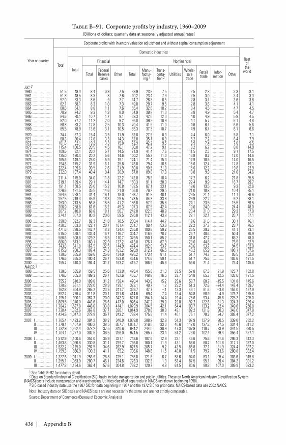
436 | Appendix B
Table B–91. Corporate profits by industry, 1960–2009[Billions of dollars; quarterly data at seasonally adjusted annual rates]
Year or quarter
Corporate profits with inventory valuation adjustment and without capital consumption adjustment
Total
Domestic industries
Restof
theworldTotal
Financial Nonfinancial
TotalFederalReservebanks
Other TotalManu-factur-ing 1
Trans-porta-tion 2
UtilitiesWhole-
saletrade
Retailtrade
Infor-mation Other
SIC: 31960 ...................... 51.5 48.3 8.4 0.9 7.5 39.9 23.8 7.5 ............. 2.5 2.8 ............. 3.3 3.11961 ...................... 51.8 48.5 8.3 .8 7.6 40.2 23.4 7.9 ............. 2.5 3.0 ............. 3.4 3.31962 ...................... 57.0 53.3 8.6 .9 7.7 44.7 26.3 8.5 ............. 2.8 3.4 ............. 3.6 3.81963 ...................... 62.1 58.1 8.3 1.0 7.3 49.8 29.7 9.5 ............. 2.8 3.6 ............. 4.1 4.11964 ...................... 68.6 64.1 8.8 1.1 7.6 55.4 32.6 10.2 ............. 3.4 4.5 ............. 4.7 4.51965 ...................... 78.9 74.2 9.3 1.3 8.0 64.9 39.8 11.0 ............. 3.8 4.9 ............. 5.4 4.71966 ...................... 84.6 80.1 10.7 1.7 9.1 69.3 42.6 12.0 ............. 4.0 4.9 ............. 5.9 4.51967 ...................... 82.0 77.2 11.2 2.0 9.2 66.0 39.2 10.9 ............. 4.1 5.7 ............. 6.1 4.81968 ...................... 88.8 83.2 12.8 2.5 10.3 70.4 41.9 11.0 ............. 4.6 6.4 ............. 6.6 5.61969 ...................... 85.5 78.9 13.6 3.1 10.5 65.3 37.3 10.7 ............. 4.9 6.4 ............. 6.1 6.61970 ...................... 74.4 67.3 15.4 3.5 11.9 52.0 27.5 8.3 ............. 4.4 6.0 ............. 5.8 7.11971 ...................... 88.3 80.4 17.6 3.3 14.3 62.8 35.1 8.9 ............. 5.2 7.2 ............. 6.4 7.91972 ...................... 101.6 92.1 19.2 3.3 15.8 72.9 42.2 9.5 ............. 6.9 7.4 ............. 7.0 9.51973 ...................... 115.4 100.5 20.5 4.5 16.1 80.0 47.2 9.1 ............. 8.2 6.7 ............. 8.8 14.91974 ...................... 109.6 92.1 20.2 5.7 14.5 71.9 41.4 7.6 ............. 11.5 2.3 ............. 9.1 17.51975 ...................... 135.0 120.4 20.2 5.6 14.6 100.2 55.2 11.0 ............. 13.8 8.2 ............. 12.0 14.61976 ...................... 165.6 149.1 25.0 5.9 19.1 124.1 71.4 15.3 ............. 12.9 10.5 ............. 14.0 16.51977 ...................... 194.8 175.7 31.9 6.1 25.8 143.8 79.4 18.6 ............. 15.6 12.4 ............. 17.8 19.11978 ...................... 222.4 199.6 39.5 7.6 31.9 160.0 90.5 21.8 ............. 15.6 12.3 ............. 19.8 22.91979 ...................... 232.0 197.4 40.4 9.4 30.9 157.0 89.8 17.0 ............. 18.8 9.9 ............. 21.6 34.61980 ...................... 211.4 175.9 34.0 11.8 22.2 142.0 78.3 18.4 ............. 17.2 6.2 ............. 21.8 35.51981 ...................... 219.1 189.4 29.1 14.4 14.7 160.3 91.1 20.3 ............. 22.4 9.9 ............. 16.7 29.71982 ...................... 191.1 158.5 26.0 15.2 10.8 132.5 67.1 23.1 ............. 19.6 13.5 ............. 9.3 32.61983 ...................... 226.6 191.5 35.5 14.6 21.0 156.0 76.2 29.5 ............. 21.0 18.8 ............. 10.4 35.11984 ...................... 264.6 228.1 34.4 16.4 18.0 193.7 91.8 40.1 ............. 29.5 21.1 ............. 11.1 36.61985 ...................... 257.5 219.4 45.9 16.3 29.5 173.5 84.3 33.8 ............. 23.9 22.2 ............. 9.2 38.11986 ...................... 253.0 213.5 56.8 15.5 41.2 156.8 57.9 35.8 ............. 24.1 23.5 ............. 15.5 39.51987 ...................... 306.9 258.8 61.6 16.2 45.3 197.3 87.5 42.4 ............. 19.0 24.0 ............. 24.4 48.01988 ...................... 367.7 310.8 68.8 18.1 50.7 242.0 122.5 48.9 ............. 20.4 21.0 ............. 29.3 57.01989 ...................... 374.1 307.0 80.2 20.6 59.5 226.8 112.1 43.8 ............. 22.1 22.1 ............. 26.7 67.11990 ...................... 398.8 322.7 92.3 21.8 70.5 230.4 114.4 44.7 ............. 19.6 21.6 ............. 30.1 76.11991 ...................... 430.3 353.8 122.1 20.7 101.4 231.7 99.4 53.8 ............. 22.2 27.7 ............. 28.7 76.51992 ...................... 471.6 398.5 142.7 18.3 124.4 255.8 100.8 59.2 ............. 25.5 29.2 ............. 41.1 73.11993 ...................... 515.0 438.1 133.4 16.7 116.7 304.7 116.8 70.2 ............. 26.7 40.6 ............. 50.4 76.91994 ...................... 586.6 508.6 129.2 18.5 110.7 379.5 150.1 85.2 ............. 31.8 47.2 ............. 65.2 78.01995 ...................... 666.0 573.1 160.1 22.9 137.2 413.0 176.7 87.9 ............. 28.0 44.8 ............. 75.5 92.91996 ...................... 743.8 641.8 167.5 22.5 144.9 474.4 192.0 93.7 ............. 40.6 53.7 ............. 94.5 102.01997 ...................... 815.9 708.3 187.4 24.3 163.2 520.9 212.2 86.5 ............. 48.2 65.9 ............. 108.1 107.61998 ...................... 738.6 635.9 159.6 25.6 134.0 476.2 173.4 81.1 ............. 51.7 74.7 ............. 95.5 102.81999 ...................... 776.6 655.0 190.4 26.7 163.8 464.6 174.6 59.1 ............. 51.7 75.6 ............. 103.6 121.52000 ...................... 755.7 610.0 194.4 31.2 163.2 415.7 166.5 45.8 ............. 55.6 71.4 ............. 76.4 145.6NAICS: 31998 ...................... 738.6 635.9 159.5 25.6 133.9 476.4 155.8 21.3 33.5 52.8 67.3 21.9 123.7 102.81999 ...................... 776.6 655.0 189.3 26.7 162.6 465.7 148.8 16.5 33.7 54.8 65.7 12.5 133.6 121.52000 ...................... 755.7 610.0 189.6 31.2 158.4 420.4 143.9 15.2 25.6 58.7 60.7 –15.5 131.8 145.62001 ...................... 720.8 551.1 228.0 28.9 199.1 323.1 49.7 1.2 25.2 51.3 72.6 –24.4 147.4 169.72002 ...................... 762.8 604.9 265.2 23.5 241.7 339.7 47.7 –.1 12.3 49.1 81.6 –3.8 153.0 157.92003 ...................... 892.2 726.4 311.8 20.1 291.8 414.6 69.4 7.4 12.4 54.8 88.9 4.9 176.7 165.82004 ...................... 1,195.1 990.1 362.3 20.0 342.3 627.8 154.1 14.4 19.4 75.6 93.4 45.6 225.2 205.02005 ...................... 1,609.5 1,370.0 443.6 26.6 417.0 926.4 247.2 29.0 29.8 92.2 122.6 81.3 324.3 239.42006 ...................... 1,784.7 1,527.8 448.0 33.8 414.1 1,079.9 304.5 42.1 54.4 103.7 133.2 92.4 349.6 256.82007 ...................... 1,730.4 1,382.6 367.8 37.7 330.1 1,014.9 278.6 30.0 49.1 102.2 121.6 90.3 343.0 347.82008 ...................... 1,424.5 1,047.3 278.9 35.7 243.2 768.4 175.5 11.4 40.1 75.1 78.2 84.7 303.4 377.22007: I .................. 1,705.4 1,423.2 384.2 38.2 346.0 1,039.0 288.9 32.9 51.3 107.9 127.9 90.5 339.6 282.2
II ................. 1,779.1 1,467.9 406.2 38.5 367.7 1,061.7 316.0 33.0 46.6 117.0 137.2 77.5 334.4 311.2III ................ 1,732.9 1,362.4 378.2 37.5 340.6 984.2 244.0 30.9 47.3 107.9 118.7 93.9 341.5 370.5IV ................ 1,704.1 1,277.0 302.5 36.5 266.0 974.5 265.7 23.4 51.2 76.0 102.4 99.4 356.4 427.1
2008: I .................. 1,512.9 1,100.6 357.0 35.9 321.1 743.6 187.6 12.9 33.1 46.6 75.6 91.6 296.3 412.3II ................. 1,463.8 1,096.8 330.8 31.1 299.7 766.0 160.1 11.9 43.1 56.6 80.2 101.8 312.1 367.0III ................ 1,522.2 1,125.0 297.5 34.6 262.9 827.5 205.7 9.2 43.5 85.8 77.1 81.9 324.4 397.2IV ................ 1,199.3 866.9 130.3 41.1 89.2 736.6 148.6 11.5 40.8 111.5 79.7 63.6 280.8 332.4
2009: I .................. 1,327.6 1,011.9 253.9 28.8 225.1 758.0 121.6 6.7 53.6 94.0 83.1 95.4 303.6 315.8II ................. 1,355.1 1,053.9 280.7 46.1 234.6 773.3 132.3 1.3 53.4 87.5 95.1 99.4 304.2 301.2III ................ 1,477.8 1,154.6 362.4 57.6 304.8 792.2 129.7 4.8 61.5 80.6 98.8 107.0 309.9 323.2
1 See Table B–92 for industry detail.2 Data on Standard Industrial Classification (SIC) basis include transportation and public utilities. Those on North American Industry Classification System
(NAICS) basis include transporation and warehousing. Utilities classified separately in NAICS (as shown beginning 1998).3 SIC-based industry data use the 1987 SIC for data beginning in 1987 and the 1972 SIC for prior data. NAICS-based data use 2002 NAICS.Note: Industry data on SIC basis and NAICS basis are not necessarily the same and are not strictly comparable.Source: Department of Commerce (Bureau of Economic Analysis).
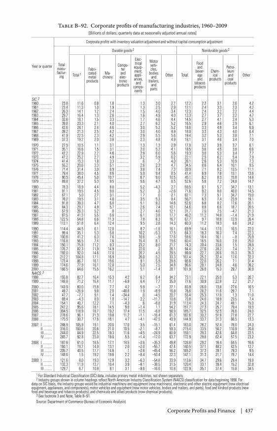
Corporate Profits and Finance | 437
Table B–92. Corporate profits of manufacturing industries, 1960–2009[Billions of dollars; quarterly data at seasonally adjusted annual rates]
Year or quarter
Corporate profits with inventory valuation adjustment and without capital consumption adjustment
Totalmanu-factur-
ing
Durable goods 2 Nondurable goods 2
Total 1Fabri-catedmetal
products
Ma-chinery
Compu-terand
elec-tronic
products
Elec-tricalequip-ment,appli-ances,
andcompo-nents
Motorvehi-cles,
bodiesand
trailers,and
parts
Other Total
Foodand
bever-ageand
tobaccoproducts
Chem-ical
products
Petro-leumandcoal
products
Other
SIC: 31960 ............... 23.8 11.6 0.8 1.8 .............. 1.3 3.0 2.7 12.2 2.2 3.1 2.6 4.21961 ............... 23.4 11.3 1.0 1.9 .............. 1.3 2.5 2.9 12.1 2.4 3.3 2.3 4.21962 ............... 26.3 14.1 1.2 2.4 .............. 1.5 4.0 3.4 12.3 2.4 3.2 2.2 4.41963 ............... 29.7 16.4 1.3 2.6 .............. 1.6 4.9 4.0 13.3 2.7 3.7 2.2 4.71964 ............... 32.6 18.1 1.5 3.3 .............. 1.7 4.6 4.4 14.5 2.7 4.1 2.4 5.31965 ............... 39.8 23.3 2.1 4.0 .............. 2.7 6.2 5.2 16.5 2.9 4.6 2.9 6.11966 ............... 42.6 24.1 2.4 4.6 .............. 3.0 5.2 5.2 18.6 3.3 4.9 3.4 6.91967 ............... 39.2 21.3 2.5 4.2 .............. 3.0 4.0 4.9 18.0 3.3 4.3 4.0 6.41968 ............... 41.9 22.5 2.3 4.2 .............. 2.9 5.5 5.6 19.4 3.2 5.3 3.8 7.11969 ............... 37.3 19.2 2.0 3.8 .............. 2.3 4.8 4.9 18.1 3.1 4.6 3.4 7.01970 ............... 27.5 10.5 1.1 3.1 .............. 1.3 1.3 2.9 17.0 3.2 3.9 3.7 6.11971 ............... 35.1 16.6 1.5 3.1 .............. 2.0 5.2 4.1 18.5 3.6 4.5 3.8 6.61972 ............... 42.2 22.9 2.2 4.6 .............. 2.9 6.0 5.6 19.3 3.0 5.3 3.4 7.71973 ............... 47.2 25.2 2.7 4.9 .............. 3.2 5.9 6.2 22.1 2.5 6.2 5.4 7.91974 ............... 41.4 15.3 1.8 3.3 .............. .6 .7 4.0 26.1 2.6 5.3 10.9 7.31975 ............... 55.2 20.6 3.3 5.1 .............. 2.6 2.3 4.7 34.5 8.6 6.4 10.1 9.51976 ............... 71.4 31.4 3.9 6.9 .............. 3.8 7.4 7.3 39.9 7.1 8.2 13.5 11.11977 ............... 79.4 38.0 4.5 8.6 .............. 5.9 9.4 8.5 41.4 6.9 7.8 13.1 13.61978 ............... 90.5 45.4 5.0 10.7 .............. 6.7 9.0 10.5 45.1 6.2 8.3 15.8 14.81979 ............... 89.8 37.2 5.3 9.5 .............. 5.6 4.7 8.5 52.6 5.8 7.2 24.8 14.71980 ............... 78.3 18.9 4.4 8.0 .............. 5.2 –4.3 2.7 59.5 6.1 5.7 34.7 13.11981 ............... 91.1 19.5 4.5 9.0 .............. 5.2 .3 –2.6 71.6 9.2 8.0 40.0 14.51982 ............... 67.1 5.0 2.7 3.1 .............. 1.7 .0 2.1 62.1 7.3 5.1 34.7 15.01983 ............... 76.2 19.5 3.1 4.0 .............. 3.5 5.3 8.4 56.7 6.3 7.4 23.9 19.11984 ............... 91.8 39.3 4.7 6.0 .............. 5.1 9.2 14.6 52.6 6.8 8.2 17.6 20.11985 ............... 84.3 29.7 4.9 5.7 .............. 2.6 7.4 10.1 54.6 8.8 6.6 18.7 20.51986 ............... 57.9 26.3 5.2 .8 .............. 2.7 4.6 12.1 31.7 7.5 7.5 –4.7 21.31987 ............... 87.5 41.3 5.5 5.6 .............. 6.1 3.8 17.7 46.2 11.2 14.6 –1.4 21.91988 ............... 122.5 54.8 6.6 11.3 .............. 7.8 6.3 16.7 67.7 9.7 18.8 12.9 26.41989 ............... 112.1 51.8 6.4 12.4 .............. 9.5 2.8 14.3 60.3 11.2 18.3 6.6 24.21990 ............... 114.4 44.5 6.1 12.0 .............. 8.7 –1.8 16.1 69.9 14.4 17.0 16.5 22.01991 ............... 99.4 35.1 5.3 5.8 .............. 10.2 –5.3 17.5 64.3 18.3 16.3 7.4 22.31992 ............... 100.8 41.2 6.3 7.6 .............. 10.6 –.9 17.6 59.6 18.4 16.1 –.8 25.91993 ............... 116.8 56.5 7.4 7.6 .............. 15.4 6.1 19.6 60.4 16.5 16.0 2.8 25.01994 ............... 150.1 75.8 11.2 9.3 .............. 23.2 8.0 21.7 74.3 20.4 23.6 1.5 28.91995 ............... 176.7 82.3 11.9 14.9 .............. 22.0 .2 26.1 94.4 27.6 28.2 7.4 31.21996 ............... 192.0 92.0 14.6 17.0 .............. 20.7 4.5 29.5 99.9 22.7 26.6 15.3 35.31997 ............... 212.2 104.8 17.1 16.9 .............. 26.0 5.2 33.3 107.4 25.2 32.4 17.6 32.31998 ............... 173.4 86.7 16.1 19.6 .............. 9.1 5.9 29.8 86.6 22.0 26.2 7.1 31.41999 ............... 174.6 77.9 16.1 12.0 .............. 5.3 7.5 34.8 96.6 28.1 24.8 4.6 39.22000 ............... 166.5 64.6 15.5 16.2 .............. 5.1 –1.4 28.1 101.9 26.0 15.3 29.7 30.9NAICS: 31998 ............... 155.8 82.7 16.4 15.3 4.2 6.2 6.4 34.2 73.1 22.1 25.0 5.3 20.71999 ............... 148.8 71.2 16.4 11.7 –6.8 6.4 7.7 35.9 77.6 30.9 22.8 2.2 21.72000 ............... 143.9 60.0 15.8 7.7 4.2 5.9 –.7 27.1 83.9 26.0 13.8 27.6 16.52001 ............... 49.7 –26.9 9.8 2.0 –48.6 1.9 –8.9 16.8 76.6 28.2 11.6 29.7 7.12002 ............... 47.7 –7.7 9.1 1.4 –34.4 .0 –4.5 20.7 55.4 25.3 17.8 1.3 11.02003 ............... 69.4 –4.3 8.0 1.0 –14.7 2.2 –11.7 10.8 73.8 24.0 18.9 23.5 7.42004 ............... 154.1 40.7 12.2 7.1 –4.3 .6 –6.8 31.9 113.4 24.3 24.7 49.1 15.32005 ............... 247.2 95.6 18.1 14.5 9.0 –1.4 1.1 54.2 151.7 27.3 25.7 79.4 19.32006 ............... 304.5 118.9 18.7 19.2 17.4 11.5 –6.8 58.9 185.7 32.5 52.5 76.6 24.02007 ............... 278.6 96.1 21.3 19.8 11.2 –1.1 –16.4 61.3 182.6 30.2 51.9 77.8 22.72008 ............... 175.5 30.7 17.6 16.1 4.7 –4.1 –47.5 43.9 144.9 33.7 31.3 66.5 13.32007: I ........... 288.9 105.9 19.1 20.0 17.0 3.5 –15.1 61.4 183.0 28.2 52.4 78.0 24.3
II .......... 316.0 100.6 20.6 21.0 10.5 –2.1 –8.7 59.3 215.4 33.5 50.2 110.9 20.8III ......... 244.0 84.9 22.5 19.3 11.6 –4.5 –24.9 60.9 159.1 29.3 42.6 64.8 22.5IV ......... 265.7 92.8 23.0 19.0 5.5 –1.4 –17.0 63.7 172.9 29.8 62.4 57.5 23.2
2008: I ........... 187.6 61.0 18.5 17.1 14.5 –3.6 –35.3 49.8 126.6 29.2 16.4 64.5 16.6II .......... 160.1 19.7 14.9 13.1 2.0 –2.0 –55.7 47.4 140.5 37.1 48.2 42.5 12.7III ......... 205.7 40.5 17.7 14.6 .1 –2.6 –45.4 56.2 165.2 37.3 39.1 79.3 9.5IV ......... 148.6 1.5 19.2 19.6 2.2 –8.4 –53.4 22.3 147.1 31.3 21.7 79.7 14.4
2009: I ........... 121.6 8.0 19.3 12.8 3.2 –6.3 –54.8 33.9 113.6 34.7 29.6 29.4 19.8II .......... 132.3 11.9 13.7 10.4 3.9 –9.1 –38.5 31.5 120.4 33.1 39.4 15.2 32.8III ......... 129.7 6.7 10.9 8.1 3.1 –9.6 –16.6 10.8 122.9 35.1 37.4 15.8 34.5
1 For Standard Industrial Classification (SIC) data, includes primary metal industries, not shown separately.2 Industry groups shown in column headings reflect North American Industry Classification System (NAICS) classification for data beginning 1998. For
data on SIC basis, the industry groups would be industrial machinery and equipment (now machinery), electronic and other electric equipment (now electricalequipment, appliances, and components), motor vehicles and equipment (now motor vehicles, bodies and trailers, and parts), food and kindred products (nowfood and beverage and tobacco products), and chemicals and allied products (now chemical products).
3 See footnote 3 and Note, Table B–91.Source: Department of Commerce (Bureau of Economic Analysis).
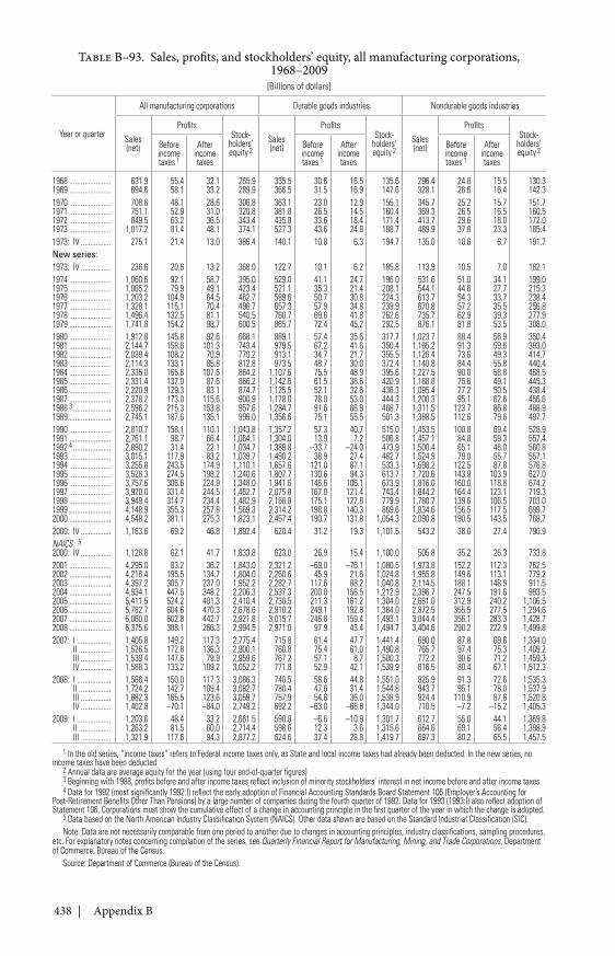
438 | Appendix B
Table B–93. Sales, profits, and stockholders’ equity, all manufacturing corporations,1968–2009
[Billions of dollars]
Year or quarter
All manufacturing corporations Durable goods industries Nondurable goods industries
Sales(net)
ProfitsStock-
holders’equity 2
Sales(net)
ProfitsStock-
holders’equity 2
Sales(net)
ProfitsStock-
holders’equity 2
Beforeincometaxes 1
Afterincometaxes
Beforeincometaxes 1
Afterincometaxes
Beforeincometaxes 1
Afterincometaxes
1968 ...................... 631.9 55.4 32.1 265.9 335.5 30.6 16.5 135.6 296.4 24.8 15.5 130.31969 ...................... 694.6 58.1 33.2 289.9 366.5 31.5 16.9 147.6 328.1 26.6 16.4 142.31970 ...................... 708.8 48.1 28.6 306.8 363.1 23.0 12.9 155.1 345.7 25.2 15.7 151.71971 ...................... 751.1 52.9 31.0 320.8 381.8 26.5 14.5 160.4 369.3 26.5 16.5 160.51972 ...................... 849.5 63.2 36.5 343.4 435.8 33.6 18.4 171.4 413.7 29.6 18.0 172.01973 ...................... 1,017.2 81.4 48.1 374.1 527.3 43.6 24.8 188.7 489.9 37.8 23.3 185.41973: IV ................ 275.1 21.4 13.0 386.4 140.1 10.8 6.3 194.7 135.0 10.6 6.7 191.7New series:1973: IV ................ 236.6 20.6 13.2 368.0 122.7 10.1 6.2 185.8 113.9 10.5 7.0 182.11974 ...................... 1,060.6 92.1 58.7 395.0 529.0 41.1 24.7 196.0 531.6 51.0 34.1 199.01975 ...................... 1,065.2 79.9 49.1 423.4 521.1 35.3 21.4 208.1 544.1 44.6 27.7 215.31976 ...................... 1,203.2 104.9 64.5 462.7 589.6 50.7 30.8 224.3 613.7 54.3 33.7 238.41977 ...................... 1,328.1 115.1 70.4 496.7 657.3 57.9 34.8 239.9 670.8 57.2 35.5 256.81978 ...................... 1,496.4 132.5 81.1 540.5 760.7 69.6 41.8 262.6 735.7 62.9 39.3 277.91979 ...................... 1,741.8 154.2 98.7 600.5 865.7 72.4 45.2 292.5 876.1 81.8 53.5 308.01980 ...................... 1,912.8 145.8 92.6 668.1 889.1 57.4 35.6 317.7 1,023.7 88.4 56.9 350.41981 ...................... 2,144.7 158.6 101.3 743.4 979.5 67.2 41.6 350.4 1,165.2 91.3 59.6 393.01982 ...................... 2,039.4 108.2 70.9 770.2 913.1 34.7 21.7 355.5 1,126.4 73.6 49.3 414.71983 ...................... 2,114.3 133.1 85.8 812.8 973.5 48.7 30.0 372.4 1,140.8 84.4 55.8 440.41984 ...................... 2,335.0 165.6 107.6 864.2 1,107.6 75.5 48.9 395.6 1,227.5 90.0 58.8 468.51985 ...................... 2,331.4 137.0 87.6 866.2 1,142.6 61.5 38.6 420.9 1,188.8 75.6 49.1 445.31986 ...................... 2,220.9 129.3 83.1 874.7 1,125.5 52.1 32.6 436.3 1,095.4 77.2 50.5 438.41987 ...................... 2,378.2 173.0 115.6 900.9 1,178.0 78.0 53.0 444.3 1,200.3 95.1 62.6 456.61988 3 .................... 2,596.2 215.3 153.8 957.6 1,284.7 91.6 66.9 468.7 1,311.5 123.7 86.8 488.91989 ...................... 2,745.1 187.6 135.1 999.0 1,356.6 75.1 55.5 501.3 1,388.5 112.6 79.6 497.71990 ...................... 2,810.7 158.1 110.1 1,043.8 1,357.2 57.3 40.7 515.0 1,453.5 100.8 69.4 528.91991 ...................... 2,761.1 98.7 66.4 1,064.1 1,304.0 13.9 7.2 506.8 1,457.1 84.8 59.3 557.41992 4 .................... 2,890.2 31.4 22.1 1,034.7 1,389.8 –33.7 –24.0 473.9 1,500.4 65.1 46.0 560.81993 ...................... 3,015.1 117.9 83.2 1,039.7 1,490.2 38.9 27.4 482.7 1,524.9 79.0 55.7 557.11994 ...................... 3,255.8 243.5 174.9 1,110.1 1,657.6 121.0 87.1 533.3 1,598.2 122.5 87.8 576.81995 ...................... 3,528.3 274.5 198.2 1,240.6 1,807.7 130.6 94.3 613.7 1,720.6 143.9 103.9 627.01996 ...................... 3,757.6 306.6 224.9 1,348.0 1,941.6 146.6 106.1 673.9 1,816.0 160.0 118.8 674.21997 ...................... 3,920.0 331.4 244.5 1,462.7 2,075.8 167.0 121.4 743.4 1,844.2 164.4 123.1 719.31998 ...................... 3,949.4 314.7 234.4 1,482.9 2,168.8 175.1 127.8 779.9 1,780.7 139.6 106.5 703.01999 ...................... 4,148.9 355.3 257.8 1,569.3 2,314.2 198.8 140.3 869.6 1,834.6 156.5 117.5 699.72000 ...................... 4,548.2 381.1 275.3 1,823.1 2,457.4 190.7 131.8 1,054.3 2,090.8 190.5 143.5 768.72000: IV ................ 1,163.6 69.2 46.8 1,892.4 620.4 31.2 19.3 1,101.5 543.2 38.0 27.4 790.9NAICS: 52000: IV ................ 1,128.8 62.1 41.7 1,833.8 623.0 26.9 15.4 1,100.0 505.8 35.2 26.3 733.82001 ...................... 4,295.0 83.2 36.2 1,843.0 2,321.2 –69.0 –76.1 1,080.5 1,973.8 152.2 112.3 762.52002 ...................... 4,216.4 195.5 134.7 1,804.0 2,260.6 45.9 21.6 1,024.8 1,955.8 149.6 113.1 779.22003 ...................... 4,397.2 305.7 237.0 1,952.2 2,282.7 117.6 88.2 1,040.8 2,114.5 188.1 148.9 911.52004 ...................... 4,934.1 447.5 348.2 2,206.3 2,537.3 200.0 156.5 1,212.9 2,396.7 247.5 191.6 993.52005 ...................... 5,411.5 524.2 401.3 2,410.4 2,730.5 211.3 161.2 1,304.0 2,681.0 312.9 240.2 1,106.52006 ...................... 5,782.7 604.6 470.3 2,678.6 2,910.2 249.1 192.8 1,384.0 2,872.5 355.5 277.5 1,294.62007 ...................... 6,060.0 602.8 442.7 2,921.8 3,015.7 246.8 159.4 1,493.1 3,044.4 356.1 283.3 1,428.72008 ...................... 6,375.6 388.1 266.3 2,994.5 2,971.0 97.9 43.4 1,494.7 3,404.6 290.2 222.9 1,499.82007: I .................. 1,405.8 149.2 117.3 2,775.4 715.8 61.4 47.7 1,441.4 690.0 87.8 69.6 1,334.0
II ................. 1,526.5 172.8 136.3 2,900.1 760.8 75.4 61.0 1,490.8 765.7 97.4 75.3 1,409.2III ................ 1,539.4 147.6 79.9 2,959.6 767.2 57.1 8.7 1,500.3 772.2 90.6 71.2 1,459.3IV ................ 1,588.3 133.2 109.2 3,052.2 771.8 52.9 42.1 1,539.9 816.5 80.4 67.1 1,512.3
2008: I .................. 1,566.4 150.0 117.3 3,086.3 740.5 58.6 44.8 1,551.0 825.9 91.3 72.6 1,535.3II ................. 1,724.2 142.7 109.4 3,082.7 780.4 47.6 31.4 1,544.8 943.7 95.1 78.0 1,537.9III ................ 1,682.3 165.5 123.6 3,059.7 757.9 54.6 36.0 1,538.9 924.4 110.9 87.6 1,520.8IV ................ 1,402.8 –70.1 –84.0 2,749.2 692.2 –63.0 –68.8 1,344.0 710.5 –7.2 –15.2 1,405.3
2009: I .................. 1,203.6 48.4 33.2 2,661.5 590.8 –6.6 –10.9 1,301.7 612.7 55.0 44.1 1,359.8II ................. 1,263.2 81.5 60.0 2,714.4 598.6 12.3 3.6 1,315.6 664.6 69.1 56.4 1,398.9III ................ 1,321.9 117.6 94.3 2,877.2 624.6 37.4 28.8 1,419.7 697.3 80.2 65.5 1,457.5
1 In the old series, “income taxes” refers to Federal income taxes only, as State and local income taxes had already been deducted. In the new series, noincome taxes have been deducted
2 Annual data are average equity for the year (using four end-of-quarter figures)3 Beginning with 1988, profits before and after income taxes reflect inclusion of minority stockholders’ interest in net income before and after income taxes4 Data for 1992 (most significantly 1992:I) reflect the early adoption of Financial Accounting Standards Board Statement 106 (Employer’s Accounting for
Post-Retirement Benefits Other Than Pensions) by a large number of companies during the fourth quarter of 1992. Data for 1993 (1993:I) also reflect adoption ofStatement 106. Corporations must show the cumulative effect of a change in accounting principle in the first quarter of the year in which the change is adopted.
5 Data based on the North American Industry Classification System (NAICS). Other data shown are based on the Standard Industrial Classification (SIC).Note: Data are not necessarily comparable from one period to another due to changes in accounting principles, industry classifications, sampling procedures,
etc. For explanatory notes concerning compilation of the series, see Quarterly Financial Report for Manufacturing, Mining, and Trade Corporations, Departmentof Commerce, Bureau of the Census.
Source: Department of Commerce (Bureau of the Census).
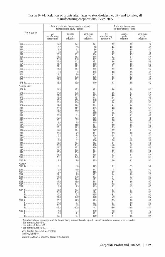
Corporate Profits and Finance | 439
Table B–94. Relation of profits after taxes to stockholders’ equity and to sales, allmanufacturing corporations, 1959–2009
Year or quarter
Ratio of profits after income taxes (annual rate)to stockholders’ equity—percent 1
Profits after income taxesper dollar of sales—cents
Allmanufacturingcorporations
Durablegoods
industries
Nondurablegoods
industries
Allmanufacturingcorporations
Durablegoods
industries
Nondurablegoods
industries
1959 ...................................... 10.4 10.4 10.4 4.8 4.8 4.91960 ...................................... 9.2 8.5 9.8 4.4 4.0 4.81961 ...................................... 8.9 8.1 9.6 4.3 3.9 4.71962 ...................................... 9.8 9.6 9.9 4.5 4.4 4.71963 ...................................... 10.3 10.1 10.4 4.7 4.5 4.91964 ...................................... 11.6 11.7 11.5 5.2 5.1 5.41965 ...................................... 13.0 13.8 12.2 5.6 5.7 5.51966 ...................................... 13.4 14.2 12.7 5.6 5.6 5.61967 ...................................... 11.7 11.7 11.8 5.0 4.8 5.31968 ...................................... 12.1 12.2 11.9 5.1 4.9 5.21969 ...................................... 11.5 11.4 11.5 4.8 4.6 5.01970 ...................................... 9.3 8.3 10.3 4.0 3.5 4.51971 ...................................... 9.7 9.0 10.3 4.1 3.8 4.51972 ...................................... 10.6 10.8 10.5 4.3 4.2 4.41973 ...................................... 12.8 13.1 12.6 4.7 4.7 4.81973: IV ................................ 13.4 12.9 14.0 4.7 4.5 5.0New series:1973: IV ................................ 14.3 13.3 15.3 5.6 5.0 6.11974 ...................................... 14.9 12.6 17.1 5.5 4.7 6.41975 ...................................... 11.6 10.3 12.9 4.6 4.1 5.11976 ...................................... 13.9 13.7 14.2 5.4 5.2 5.51977 ...................................... 14.2 14.5 13.8 5.3 5.3 5.31978 ...................................... 15.0 16.0 14.2 5.4 5.5 5.31979 ...................................... 16.4 15.4 17.4 5.7 5.2 6.11980 ...................................... 13.9 11.2 16.3 4.8 4.0 5.61981 ...................................... 13.6 11.9 15.2 4.7 4.2 5.11982 ...................................... 9.2 6.1 11.9 3.5 2.4 4.41983 ...................................... 10.6 8.1 12.7 4.1 3.1 4.91984 ...................................... 12.5 12.4 12.5 4.6 4.4 4.81985 ...................................... 10.1 9.2 11.0 3.8 3.4 4.11986 ...................................... 9.5 7.5 11.5 3.7 2.9 4.61987 ...................................... 12.8 11.9 13.7 4.9 4.5 5.21988 2 .................................... 16.1 14.3 17.8 5.9 5.2 6.61989 ...................................... 13.5 11.1 16.0 4.9 4.1 5.71990 ...................................... 10.6 7.9 13.1 3.9 3.0 4.81991 ...................................... 6.2 1.4 10.6 2.4 .5 4.11992 3 .................................... 2.1 –5.1 8.2 .8 –1.7 3.11993 ...................................... 8.0 5.7 10.0 2.8 1.8 3.71994 ...................................... 15.8 16.3 15.2 5.4 5.3 5.51995 ...................................... 16.0 15.4 16.6 5.6 5.2 6.01996 ...................................... 16.7 15.7 17.6 6.0 5.5 6.51997 ...................................... 16.7 16.3 17.1 6.2 5.8 6.71998 ...................................... 15.8 16.4 15.2 5.9 5.9 6.01999 ...................................... 16.4 16.1 16.8 6.2 6.1 6.42000 ...................................... 15.1 12.5 18.7 6.1 5.4 6.92000: IV ................................ 9.9 7.0 13.9 4.0 3.1 5.1NAICS: 42000: IV ................................ 9.1 5.6 14.3 3.7 2.5 5.22001 ...................................... 2.0 –7.0 14.7 .8 –3.3 5.72002 ...................................... 7.5 2.1 14.5 3.2 1.0 5.82003 ...................................... 12.1 8.5 16.3 5.4 3.9 7.02004 ...................................... 15.8 12.9 19.3 7.1 6.2 8.02005 ...................................... 16.7 12.4 21.7 7.4 5.9 9.02006 ...................................... 17.6 13.9 21.4 8.1 6.6 9.72007 ...................................... 15.2 10.7 19.8 7.3 5.3 9.32008 ...................................... 8.9 2.9 14.9 4.2 1.5 6.52007: I .................................. 16.9 13.2 20.9 8.3 6.7 10.1
II ................................. 18.8 16.4 21.4 8.9 8.0 9.8III ................................ 10.8 2.3 19.5 5.2 1.1 9.2IV ................................ 14.3 10.9 17.8 6.9 5.4 8.2
2008: I .................................. 15.2 11.5 18.9 7.5 6.0 8.8II ................................. 14.2 8.1 20.3 6.3 4.0 8.3III ................................ 16.2 9.3 23.0 7.3 4.7 9.5IV ................................ –12.2 –20.5 –4.3 –6.0 –9.9 –2.1
2009: I .................................. 5.0 –3.4 13.0 2.8 –1.9 7.2II ................................. 8.8 1.1 16.1 4.7 .6 8.5III ................................ 13.1 8.1 18.0 7.1 4.6 9.4
1 Annual ratios based on average equity for the year (using four end-of-quarter figures). Quarterly ratios based on equity at end of quarter.2 See footnote 3, Table B–93.3 See footnote 4, Table B–93.4 See footnote 5, Table B–93.Note: Based on data in millions of dollars.See Note, Table B–93.Source: Department of Commerce (Bureau of the Census).
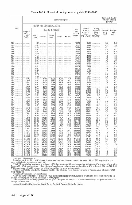
440 | Appendix B
Table B–95. Historical stock prices and yields, 1949–2003
Year
Common stock prices 1Common stock yields(Standard & Poor’s)
(percent) 5
New York Stock Exchange (NYSE) indexes 2
DowJones
industrialaverage 2
Standard& Poor’s
compositeindex
(1941–43=10) 2
Nasdaqcomposite
index(Feb. 5,
1971=100) 2
Dividend-priceratio 6
Earnings-priceratio 7
Composite(Dec. 31,
2002=5,000) 3
December 31, 1965=50
Com-posite Industrial Transpor-
tation Utility 4 Finance
1949 ................. ................ 9.02 ................ ................ ................ ................ 179.48 15.23 .................... 6.59 15.481950 ................. ................ 10.87 ................ ................ ................ ................ 216.31 18.40 .................... 6.57 13.991951 ................. ................ 13.08 ................ ................ ................ ................ 257.64 22.34 .................... 6.13 11.821952 ................. ................ 13.81 ................ ................ ................ ................ 270.76 24.50 .................... 5.80 9.471953 ................. ................ 13.67 ................ ................ ................ ................ 275.97 24.73 .................... 5.80 10.261954 ................. ................ 16.19 ................ ................ ................ ................ 333.94 29.69 .................... 4.95 8.571955 ................. ................ 21.54 ................ ................ ................ ................ 442.72 40.49 .................... 4.08 7.951956 ................. ................ 24.40 ................ ................ ................ ................ 493.01 46.62 .................... 4.09 7.551957 ................. ................ 23.67 ................ ................ ................ ................ 475.71 44.38 .................... 4.35 7.891958 ................. ................ 24.56 ................ ................ ................ ................ 491.66 46.24 .................... 3.97 6.231959 ................. ................ 30.73 ................ ................ ................ ................ 632.12 57.38 .................... 3.23 5.781960 ................. ................ 30.01 ................ ................ ................ ................ 618.04 55.85 .................... 3.47 5.901961 ................. ................ 35.37 ................ ................ ................ ................ 691.55 66.27 .................... 2.98 4.621962 ................. ................ 33.49 ................ ................ ................ ................ 639.76 62.38 .................... 3.37 5.821963 ................. ................ 37.51 ................ ................ ................ ................ 714.81 69.87 .................... 3.17 5.501964 ................. ................ 43.76 ................ ................ ................ ................ 834.05 81.37 .................... 3.01 5.321965 ................. ................ 47.39 ................ ................ ................ ................ 910.88 88.17 .................... 3.00 5.591966 ................. 487.92 46.15 46.18 50.26 90.81 44.45 873.60 85.26 .................... 3.40 6.631967 ................. 536.84 50.77 51.97 53.51 90.86 49.82 879.12 91.93 .................... 3.20 5.731968 ................. 585.47 55.37 58.00 50.58 88.38 65.85 906.00 98.70 .................... 3.07 5.671969 ................. 578.01 54.67 57.44 46.96 85.60 70.49 876.72 97.84 .................... 3.24 6.081970 ................. 483.39 45.72 48.03 32.14 74.47 60.00 753.19 83.22 .................... 3.83 6.451971 ................. 573.33 54.22 57.92 44.35 79.05 70.38 884.76 98.29 107.44 3.14 5.411972 ................. 637.52 60.29 65.73 50.17 76.95 78.35 950.71 109.20 128.52 2.84 5.501973 ................. 607.11 57.42 63.08 37.74 75.38 70.12 923.88 107.43 109.90 3.06 7.121974 ................. 463.54 43.84 48.08 31.89 59.58 49.67 759.37 82.85 76.29 4.47 11.591975 ................. 483.55 45.73 50.52 31.10 63.00 47.14 802.49 86.16 77.20 4.31 9.151976 ................. 575.85 54.46 60.44 39.57 73.94 52.94 974.92 102.01 89.90 3.77 8.901977 ................. 567.66 53.69 57.86 41.09 81.84 55.25 894.63 98.20 98.71 4.62 10.791978 ................. 567.81 53.70 58.23 43.50 78.44 56.65 820.23 96.02 117.53 5.28 12.031979 ................. 616.68 58.32 64.76 47.34 76.41 61.42 844.40 103.01 136.57 5.47 13.461980 ................. 720.15 68.10 78.70 60.61 74.69 64.25 891.41 118.78 168.61 5.26 12.661981 ................. 782.62 74.02 85.44 72.61 77.81 73.52 932.92 128.05 203.18 5.20 11.961982 ................. 728.84 68.93 78.18 60.41 79.49 71.99 884.36 119.71 188.97 5.81 11.601983 ................. 979.52 92.63 107.45 89.36 93.99 95.34 1,190.34 160.41 285.43 4.40 8.031984 ................. 977.33 92.46 108.01 85.63 92.89 89.28 1,178.48 160.46 248.88 4.64 10.021985 ................. 1,142.97 108.09 123.79 104.11 113.49 114.21 1,328.23 186.84 290.19 4.25 8.121986 ................. 1,438.02 136.00 155.85 119.87 142.72 147.20 1,792.76 236.34 366.96 3.49 6.091987 ................. 1,709.79 161.70 195.31 140.39 148.59 146.48 2,275.99 286.83 402.57 3.08 5.481988 ................. 1,585.14 149.91 180.95 134.12 143.53 127.26 2,060.82 265.79 374.43 3.64 8.011989 ................. 1,903.36 180.02 216.23 175.28 174.87 151.88 2,508.91 322.84 437.81 3.45 7.421990 ................. 1,939.47 183.46 225.78 158.62 181.20 133.26 2,678.94 334.59 409.17 3.61 6.471991 ................. 2,181.72 206.33 258.14 173.99 185.32 150.82 2,929.33 376.18 491.69 3.24 4.791992 ................. 2,421.51 229.01 284.62 201.09 198.91 179.26 3,284.29 415.74 599.26 2.99 4.221993 ................. 2,638.96 249.58 299.99 242.49 228.90 216.42 3,522.06 451.41 715.16 2.78 4.461994 ................. 2,687.02 254.12 315.25 247.29 209.06 209.73 3,793.77 460.42 751.65 2.82 5.831995 ................. 3,078.56 291.15 367.34 269.41 220.30 238.45 4,493.76 541.72 925.19 2.56 6.091996 ................. 3,787.20 358.17 453.98 327.33 249.77 303.89 5,742.89 670.50 1,164.96 2.19 5.241997 ................. 4,827.35 456.54 574.52 414.60 283.82 424.48 7,441.15 873.43 1,469.49 1.77 4.571998 ................. 5,818.26 550.26 681.57 468.69 378.12 516.35 8,625.52 1,085.50 1,794.91 1.49 3.461999 ................. 6,546.81 619.16 774.78 491.60 473.73 530.86 10,464.88 1,327.33 2,728.15 1.25 3.172000 ................. 6,805.89 643.66 810.63 413.60 477.65 553.13 10,734.90 1,427.22 3,783.67 1.15 3.632001 ................. 6,397.85 605.07 748.26 443.59 377.30 595.61 10,189.13 1,194.18 2,035.00 1.32 2.952002 ................. 5,578.89 527.62 657.37 431.10 260.85 555.27 9,226.43 993.94 1,539.73 1.61 2.922003 3 ............... 5,447.46 ............... 633.18 436.51 237.77 565.75 8,993.59 965.23 1,647.17 1.77 3.84
1 Averages of daily closing prices.2 Includes stocks as follows: for NYSE, all stocks listed; for Dow Jones industrial average, 30 stocks; for Standard & Poor’s (S&P) composite index, 500
stocks; and for Nasdaq composite index, over 5,000.3 The NYSE relaunched the composite index on January 9, 2003, incorporating new definitions, methodology, and base value. (The composite index based on
December 31, 1965=50 was discontinued.) Subset indexes on financial, energy, and health care were released by the NYSE on January 8, 2004 (see Table B–96).NYSE indexes shown in this table for industrials, utilities, transportation, and finance were discontinued.
4 Effective April 1993, the NYSE doubled the value of the utility index to facilitate trading of options and futures on the index. Annual indexes prior to 1993reflect the doubling.
5 Based on 500 stocks in the S&P composite index.6 Aggregate cash dividends (based on latest known annual rate) divided by aggregate market value based on Wednesday closing prices. Monthly data are
averages of weekly figures; annual data are averages of monthly figures.7 Quarterly data are ratio of earnings (after taxes) for four quarters ending with particular quarter-to-price index for last day of that quarter. Annual data are
averages of quarterly ratios.Sources: New York Stock Exchange, Dow Jones & Co., Inc., Standard & Poor’s, and Nasdaq Stock Market.
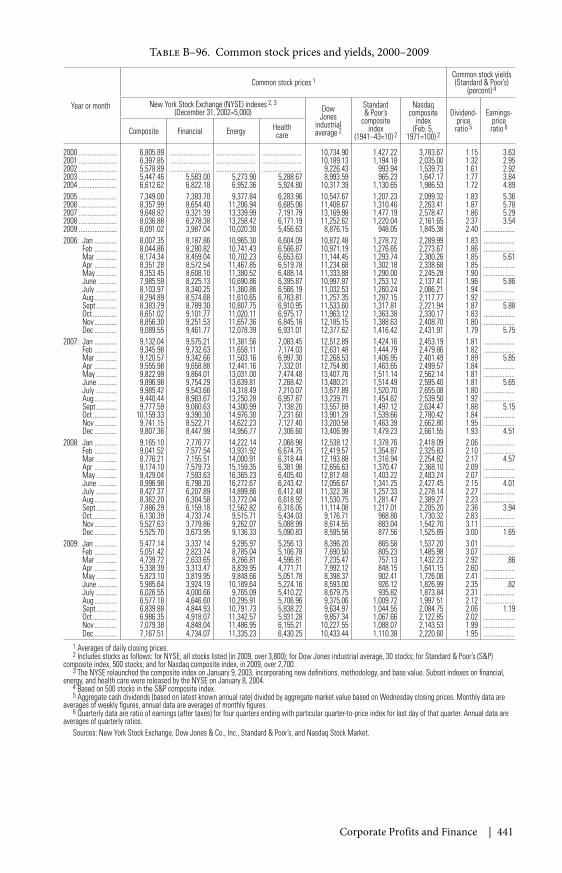
Corporate Profits and Finance | 441
Table B–96. Common stock prices and yields, 2000–2009
Year or month
Common stock prices 1Common stock yields(Standard & Poor’s)
(percent) 4
New York Stock Exchange (NYSE) indexes 2, 3(December 31, 2002=5,000) Dow
Jonesindustrialaverage 2
Standard& Poor’s
compositeindex
(1941–43=10) 2
Nasdaqcomposite
index(Feb. 5,
1971=100) 2
Dividend-priceratio 5
Earnings-priceratio 6Composite Financial Energy Health
care
2000 ...................... 6,805.89 ....................... ....................... ....................... 10,734.90 1,427.22 3,783.67 1.15 3.632001 ...................... 6,397.85 ....................... ....................... ....................... 10,189.13 1,194.18 2,035.00 1.32 2.952002 ...................... 5,578.89 ....................... ....................... ....................... 9,226.43 993.94 1,539.73 1.61 2.922003 ...................... 5,447.46 5,583.00 5,273.90 5,288.67 8,993.59 965.23 1,647.17 1.77 3.842004 ...................... 6,612.62 6,822.18 6,952.36 5,924.80 10,317.39 1,130.65 1,986.53 1.72 4.892005 ...................... 7,349.00 7,383.70 9,377.84 6,283.96 10,547.67 1,207.23 2,099.32 1.83 5.362006 ...................... 8,357.99 8,654.40 11,206.94 6,685.06 11,408.67 1,310.46 2,263.41 1.87 5.782007 ...................... 9,648.82 9,321.39 13,339.99 7,191.79 13,169.98 1,477.19 2,578.47 1.86 5.292008 ...................... 8,036.88 6,278.38 13,258.42 6,171.19 11,252.62 1,220.04 2,161.65 2.37 3.542009 ...................... 6,091.02 3,987.04 10,020.30 5,456.63 8,876.15 948.05 1,845.38 2.40 ..................2006: Jan ............. 8,007.35 8,187.86 10,965.30 6,604.09 10,872.48 1,278.72 2,289.99 1.83 ..................
Feb ............. 8,044.86 8,280.82 10,741.43 6,566.87 10,971.19 1,276.65 2,273.67 1.86 ..................Mar ............ 8,174.34 8,459.04 10,702.23 6,653.63 11,144.45 1,293.74 2,300.26 1.85 5.61Apr ............. 8,351.28 8,572.54 11,467.85 6,519.78 11,234.68 1,302.18 2,338.68 1.85 ..................May ............ 8,353.45 8,608.10 11,380.52 6,488.14 11,333.88 1,290.00 2,245.28 1.90 ..................June ........... 7,985.59 8,225.13 10,690.86 6,395.87 10,997.97 1,253.12 2,137.41 1.96 5.86July ............ 8,103.97 8,340.25 11,360.86 6,566.19 11,032.53 1,260.24 2,086.21 1.94 ..................Aug ............. 8,294.89 8,574.68 11,610.65 6,763.81 11,257.35 1,287.15 2,117.77 1.92 ..................Sept ............ 8,383.29 8,789.30 10,807.75 6,910.95 11,533.60 1,317.81 2,221.94 1.87 5.88Oct .............. 8,651.02 9,101.77 11,020.11 6,975.17 11,963.12 1,363.38 2,330.17 1.83 ..................Nov ............. 8,856.30 9,251.53 11,657.36 6,845.16 12,185.15 1,388.63 2,408.70 1.80 ..................Dec ............. 9,089.55 9,461.77 12,078.39 6,931.01 12,377.62 1,416.42 2,431.91 1.79 5.75
2007: Jan ............. 9,132.04 9,575.21 11,381.56 7,083.45 12,512.89 1,424.16 2,453.19 1.81 ..................Feb ............. 9,345.98 9,732.63 11,658.11 7,174.03 12,631.48 1,444.79 2,479.86 1.82 ..................Mar ............ 9,120.57 9,342.66 11,503.16 6,997.30 12,268.53 1,406.95 2,401.49 1.89 5.85Apr ............. 9,555.98 9,658.88 12,441.16 7,332.01 12,754.80 1,463.65 2,499.57 1.84 ..................May ............ 9,822.99 9,864.01 13,031.00 7,474.48 13,407.76 1,511.14 2,562.14 1.81 ..................June ........... 9,896.98 9,754.29 13,639.81 7,268.42 13,480.21 1,514.49 2,595.40 1.81 5.65July ............ 9,985.42 9,543.66 14,318.49 7,210.07 13,677.89 1,520.70 2,655.08 1.80 ..................Aug ............. 9,440.44 8,963.67 13,250.28 6,957.87 13,239.71 1,454.62 2,539.50 1.92 ..................Sept ............ 9,777.59 9,060.63 14,300.99 7,138.20 13,557.69 1,497.12 2,634.47 1.88 5.15Oct .............. 10,159.33 9,390.30 14,976.30 7,231.60 13,901.28 1,539.66 2,780.42 1.84 ..................Nov ............. 9,741.15 8,522.71 14,622.23 7,127.40 13,200.58 1,463.39 2,662.80 1.95 ..................Dec ............. 9,807.36 8,447.99 14,956.77 7,306.60 13,406.99 1,479.23 2,661.55 1.93 4.51
2008: Jan ............. 9,165.10 7,776.77 14,222.14 7,068.98 12,538.12 1,378.76 2,418.09 2.06 ..................Feb ............. 9,041.52 7,577.54 13,931.92 6,674.75 12,419.57 1,354.87 2,325.83 2.10 ..................Mar ............ 8,776.21 7,155.51 14,000.91 6,318.44 12,193.88 1,316.94 2,254.82 2.17 4.57Apr ............. 9,174.10 7,579.73 15,159.35 6,381.98 12,656.63 1,370.47 2,368.10 2.09 ..................May ............ 9,429.04 7,593.63 16,365.23 6,405.40 12,812.48 1,403.22 2,483.24 2.07 ..................June ........... 8,996.98 6,798.20 16,272.67 6,243.42 12,056.67 1,341.25 2,427.45 2.15 4.01July ............ 8,427.37 6,207.89 14,899.86 6,412.48 11,322.38 1,257.33 2,278.14 2.27 ..................Aug ............. 8,362.20 6,304.58 13,772.04 6,618.92 11,530.75 1,281.47 2,389.27 2.23 ..................Sept ............ 7,886.29 6,159.18 12,562.82 6,316.05 11,114.08 1,217.01 2,205.20 2.36 3.94Oct .............. 6,130.39 4,733.74 9,515.71 5,434.03 9,176.71 968.80 1,730.32 2.83 ..................Nov ............. 5,527.63 3,779.86 9,262.07 5,088.99 8,614.55 883.04 1,542.70 3.11 ..................Dec ............. 5,525.70 3,673.95 9,136.33 5,090.83 8,595.56 877.56 1,525.89 3.00 1.65
2009: Jan ............. 5,477.14 3,337.14 9,295.97 5,256.13 8,396.20 865.58 1,537.20 3.01 ..................Feb ............. 5,051.42 2,823.74 8,785.04 5,106.78 7,690.50 805.23 1,485.98 3.07 ..................Mar ............ 4,739.72 2,633.65 8,266.81 4,596.81 7,235.47 757.13 1,432.23 2.92 .86Apr ............. 5,338.39 3,313.47 8,839.95 4,771.71 7,992.12 848.15 1,641.15 2.60 ..................May ............ 5,823.10 3,819.95 9,848.66 5,051.78 8,398.37 902.41 1,726.08 2.41 ..................June ........... 5,985.64 3,924.19 10,189.64 5,224.16 8,593.00 926.12 1,826.99 2.35 .82July ............ 6,026.55 4,000.66 9,765.09 5,410.22 8,679.75 935.82 1,873.84 2.31 ..................Aug ............. 6,577.18 4,646.60 10,295.91 5,706.96 9,375.06 1,009.72 1,997.51 2.12 ..................Sept ............ 6,839.88 4,844.93 10,791.73 5,838.22 9,634.97 1,044.55 2,084.75 2.06 1.19Oct .............. 6,986.35 4,918.07 11,342.57 5,931.28 9,857.34 1,067.66 2,122.85 2.02 ..................Nov ............. 7,079.38 4,848.04 11,486.95 6,155.21 10,227.55 1,088.07 2,143.53 1.99 ..................Dec ............. 7,167.51 4,734.07 11,335.23 6,430.25 10,433.44 1,110.38 2,220.60 1.95 ..................
1 Averages of daily closing prices.2 Includes stocks as follows: for NYSE, all stocks listed (in 2009, over 3,800); for Dow Jones industrial average, 30 stocks; for Standard & Poor’s (S&P)
composite index, 500 stocks; and for Nasdaq composite index, in 2009, over 2,700.3 The NYSE relaunched the composite index on January 9, 2003, incorporating new definitions, methodology, and base value. Subset indexes on financial,
energy, and health care were released by the NYSE on January 8, 2004.4 Based on 500 stocks in the S&P composite index.5 Aggregate cash dividends (based on latest known annual rate) divided by aggregate market value based on Wednesday closing prices. Monthly data are
averages of weekly figures, annual data are averages of monthly figures.6 Quarterly data are ratio of earnings (after taxes) for four quarters ending with particular quarter-to-price index for last day of that quarter. Annual data are
averages of quarterly ratios.Sources: New York Stock Exchange, Dow Jones & Co., Inc., Standard & Poor’s, and Nasdaq Stock Market.
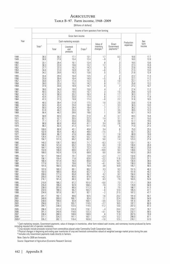
442 | Appendix B
Table B–97. Farm income, 1948–2009[Billions of dollars]
Year
Income of farm operators from farming
Gross farm income
Productionexpenses
Netfarm
incomeTotal 1
Cash marketing receiptsValue ofinventorychanges 3
DirectGovernmentpayments 4Total
Livestockand
productsCrops 2
1948 ...................... 36.5 30.2 17.1 13.1 1.7 0.3 18.8 17.71949 ...................... 30.8 27.8 15.4 12.4 –.9 .2 18.0 12.81950 ...................... 33.1 28.4 16.1 12.4 .8 .3 19.5 13.61951 ...................... 38.3 32.8 19.6 13.2 1.2 .3 22.3 15.91952 ...................... 37.7 32.5 18.2 14.3 .9 .3 22.8 14.91953 ...................... 34.4 31.0 16.9 14.1 –.6 .2 21.5 13.01954 ...................... 34.2 29.8 16.3 13.6 .5 .3 21.8 12.41955 ...................... 33.4 29.5 16.0 13.5 .2 .2 22.2 11.31956 ...................... 33.9 30.4 16.4 14.0 –.5 .6 22.7 11.21957 ...................... 34.8 29.7 17.4 12.3 .6 1.0 23.7 11.11958 ...................... 39.0 33.5 19.2 14.2 .8 1.1 25.8 13.21959 ...................... 37.9 33.6 18.9 14.7 .0 .7 27.2 10.71960 ...................... 38.6 34.0 19.0 15.0 .4 .7 27.4 11.21961 ...................... 40.5 35.2 19.5 15.7 .3 1.5 28.6 12.01962 ...................... 42.3 36.5 20.2 16.3 .6 1.7 30.3 12.11963 ...................... 43.4 37.5 20.0 17.4 .6 1.7 31.6 11.81964 ...................... 42.3 37.3 19.9 17.4 –.8 2.2 31.8 10.51965 ...................... 46.5 39.4 21.9 17.5 1.0 2.5 33.6 12.91966 ...................... 50.5 43.4 25.0 18.4 –.1 3.3 36.5 14.01967 ...................... 50.5 42.8 24.4 18.4 .7 3.1 38.2 12.31968 ...................... 51.8 44.2 25.5 18.7 .1 3.5 39.5 12.31969 ...................... 56.4 48.2 28.6 19.6 .1 3.8 42.1 14.31970 ...................... 58.8 50.5 29.5 21.0 .0 3.7 44.5 14.41971 ...................... 62.1 52.7 30.5 22.3 1.4 3.1 47.1 15.01972 ...................... 71.1 61.1 35.6 25.5 .9 4.0 51.7 19.51973 ...................... 98.9 86.9 45.8 41.1 3.4 2.6 64.6 34.41974 ...................... 98.2 92.4 41.3 51.1 –1.6 .5 71.0 27.31975 ...................... 100.6 88.9 43.1 45.8 3.4 .8 75.0 25.51976 ...................... 102.9 95.4 46.3 49.0 –1.5 .7 82.7 20.21977 ...................... 108.8 96.2 47.6 48.6 1.1 1.8 88.9 19.91978 ...................... 128.4 112.4 59.2 53.2 1.9 3.0 103.2 25.21979 ...................... 150.7 131.5 69.2 62.3 5.0 1.4 123.3 27.41980 ...................... 149.3 139.7 68.0 71.7 –6.3 1.3 133.1 16.11981 ...................... 166.3 141.6 69.2 72.5 6.5 1.9 139.4 26.91982 ...................... 164.1 142.6 70.3 72.3 –1.4 3.5 140.3 23.81983 ...................... 153.9 136.8 69.6 67.2 –10.9 9.3 139.6 14.31984 ...................... 168.0 142.8 72.9 69.9 6.0 8.4 142.0 26.01985 ...................... 161.1 144.0 70.1 73.9 –2.3 7.7 132.6 28.51986 ...................... 156.1 135.4 71.6 63.8 –2.2 11.8 125.0 31.11987 ...................... 168.4 141.8 76.0 65.8 –2.3 16.7 130.4 38.01988 ...................... 177.9 151.3 79.6 71.6 –4.1 14.5 138.3 39.61989 ...................... 191.6 160.5 83.6 76.9 3.8 10.9 145.1 46.51990 ...................... 197.8 169.3 89.1 80.2 3.3 9.3 151.5 46.31991 ...................... 192.0 168.0 85.8 82.2 –.2 8.2 151.8 40.21992 ...................... 200.6 171.5 85.8 85.7 4.2 9.2 150.4 50.21993 ...................... 205.0 178.3 90.5 87.8 –4.2 13.4 158.3 46.71994 ...................... 216.1 181.4 88.3 93.1 8.3 7.9 163.5 52.61995 ...................... 210.8 188.2 87.2 101.0 –5.0 7.3 171.1 39.81996 ...................... 235.8 199.4 92.9 106.5 7.9 7.3 176.9 58.91997 ...................... 238.0 207.8 96.5 111.3 .6 7.5 186.7 51.31998 ...................... 232.6 196.5 94.2 102.2 –.6 12.4 185.5 47.11999 ...................... 234.9 187.8 95.7 92.1 –.2 21.5 187.2 47.72000 ...................... 241.7 192.1 99.6 92.5 1.6 23.2 191.0 50.72001 ...................... 249.9 200.0 106.7 93.4 1.1 22.4 195.0 54.92002 ...................... 230.6 194.6 93.9 100.7 –3.5 12.4 191.4 39.12003 ...................... 258.6 216.1 105.7 110.5 –2.7 16.5 197.7 60.92004 ...................... 294.7 238.0 123.5 114.5 11.2 13.0 207.3 87.32005 ...................... 298.4 241.0 124.9 116.1 –.4 24.4 219.7 78.72006 ...................... 291.2 240.9 118.6 122.3 –3.1 15.8 232.7 58.52007 ...................... 338.4 288.5 138.6 149.9 .6 11.9 267.5 70.92008 ...................... 377.1 324.2 141.1 183.1 –2.4 12.2 290.0 87.12009 p .................... 335.2 282.1 118.4 163.6 –1.0 12.5 278.1 57.0
1 Cash marketing receipts, Government payments, value of changes in inventories, other farm-related cash income, and nonmoney income produced by farmsincluding imputed rent of operator residences.
2 Crop receipts include proceeds received from commodities placed under Commodity Credit Corporation loans.3 Physical changes in beginning and ending year inventories of crop and livestock commodities valued at weighted average market prices during the year.4 Includes only Government payments made directly to farmers.Note: Data for 2009 are forecasts.Source: Department of Agriculture (Economic Research Service).
Agriculture
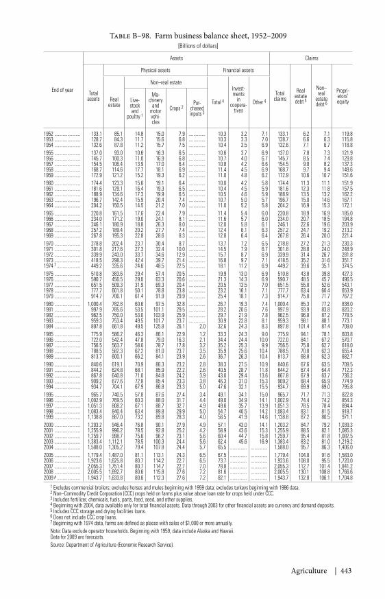
Agriculture | 443
Table B–98. Farm business balance sheet, 1952–2009[Billions of dollars]
End of year
Assets Claims
Totalassets
Physical assets Financial assets
Totalclaims
Realestatedebt 5
Non–real
estatedebt 6
Propri-etors’equityReal
estate
Non–real estate
Total 4
Invest-ments
incoopera-
tivesOther 4Live-
stockand
poultry 1
Ma-chinery
andmotorvehi-cles
Crops 2Pur-
chasedinputs 3
1952 ...................... 133.1 85.1 14.8 15.0 7.9 .............. 10.3 3.2 7.1 133.1 6.2 7.1 119.81953 ...................... 128.7 84.3 11.7 15.6 6.8 .............. 10.3 3.3 7.0 128.7 6.6 6.3 115.81954 ...................... 132.6 87.8 11.2 15.7 7.5 .............. 10.4 3.5 6.9 132.6 7.1 6.7 118.81955 ...................... 137.0 93.0 10.6 16.3 6.5 .............. 10.6 3.7 6.9 137.0 7.8 7.3 121.91956 ...................... 145.7 100.3 11.0 16.9 6.8 .............. 10.7 4.0 6.7 145.7 8.5 7.4 129.81957 ...................... 154.5 106.4 13.9 17.0 6.4 .............. 10.8 4.2 6.6 154.5 9.0 8.2 137.31958 ...................... 168.7 114.6 17.7 18.1 6.9 .............. 11.4 4.5 6.9 168.7 9.7 9.4 149.61959 ...................... 172.9 121.2 15.2 19.3 6.2 .............. 11.0 4.8 6.2 172.9 10.6 10.7 151.61960 ...................... 174.4 123.3 15.6 19.1 6.4 .............. 10.0 4.2 5.8 174.4 11.3 11.1 151.91961 ...................... 181.6 129.1 16.4 19.3 6.5 .............. 10.4 4.5 5.9 181.6 12.3 11.8 157.51962 ...................... 188.9 134.6 17.3 19.9 6.5 .............. 10.5 4.6 5.9 188.9 13.5 13.2 162.21963 ...................... 196.7 142.4 15.9 20.4 7.4 .............. 10.7 5.0 5.7 196.7 15.0 14.6 167.11964 ...................... 204.2 150.5 14.5 21.2 7.0 .............. 11.0 5.2 5.8 204.2 16.9 15.3 172.11965 ...................... 220.8 161.5 17.6 22.4 7.9 .............. 11.4 5.4 6.0 220.8 18.9 16.9 185.01966 ...................... 234.0 171.2 19.0 24.1 8.1 .............. 11.6 5.7 6.0 234.0 20.7 18.5 194.81967 ...................... 246.1 180.9 18.8 26.3 8.0 .............. 12.0 5.8 6.1 246.1 22.6 19.6 203.91968 ...................... 257.2 189.4 20.2 27.7 7.4 .............. 12.4 6.1 6.3 257.2 24.7 19.2 213.21969 ...................... 267.8 195.3 22.8 28.6 8.3 .............. 12.8 6.4 6.4 267.8 26.4 20.0 221.41970 ...................... 278.8 202.4 23.7 30.4 8.7 .............. 13.7 7.2 6.5 278.8 27.2 21.3 230.31971 ...................... 301.8 217.6 27.3 32.4 10.0 .............. 14.5 7.9 6.7 301.8 28.8 24.0 248.91972 ...................... 339.9 243.0 33.7 34.6 12.9 .............. 15.7 8.7 6.9 339.9 31.4 26.7 281.81973 ...................... 418.5 298.3 42.4 39.7 21.4 .............. 16.8 9.7 7.1 418.5 35.2 31.6 351.71974 7 .................... 449.2 335.6 24.6 48.5 22.5 .............. 18.1 11.2 6.9 449.2 39.6 35.1 374.51975 ...................... 510.8 383.6 29.4 57.4 20.5 .............. 19.9 13.0 6.9 510.8 43.8 39.8 427.31976 ...................... 590.7 456.5 29.0 63.3 20.6 .............. 21.3 14.3 6.9 590.7 48.5 45.7 496.51977 ...................... 651.5 509.3 31.9 69.3 20.4 .............. 20.5 13.5 7.0 651.5 55.8 52.6 543.11978 ...................... 777.7 601.8 50.1 78.8 23.8 .............. 23.2 16.1 7.1 777.7 63.4 60.4 653.91979 ...................... 914.7 706.1 61.4 91.9 29.9 .............. 25.4 18.1 7.3 914.7 75.8 71.7 767.21980 ...................... 1,000.4 782.8 60.6 97.5 32.8 .............. 26.7 19.3 7.4 1,000.4 85.3 77.2 838.01981 ...................... 997.9 785.6 53.5 101.1 29.5 .............. 28.2 20.6 7.6 997.9 93.9 83.8 820.21982 ...................... 962.5 750.0 53.0 103.9 25.9 .............. 29.7 21.9 7.8 962.5 96.8 87.2 778.51983 ...................... 959.3 753.4 49.5 101.7 23.7 .............. 30.9 22.8 8.1 959.3 98.1 88.1 773.11984 ...................... 897.8 661.8 49.5 125.8 26.1 2.0 32.6 24.3 8.3 897.8 101.4 87.4 709.01985 ...................... 775.9 586.2 46.3 86.1 22.9 1.2 33.3 24.3 9.0 775.9 94.1 78.1 603.81986 ...................... 722.0 542.4 47.8 79.0 16.3 2.1 34.4 24.4 10.0 722.0 84.1 67.2 570.71987 ...................... 756.5 563.7 58.0 78.7 17.8 3.2 35.2 25.3 9.9 756.5 75.8 62.7 618.01988 ...................... 788.5 582.3 62.2 81.0 23.7 3.5 35.9 25.6 10.4 788.5 70.8 62.3 655.41989 ...................... 813.7 600.1 66.2 84.1 23.9 2.6 36.7 26.3 10.4 813.7 68.8 62.3 682.71990 ...................... 840.6 619.1 70.9 86.3 23.2 2.8 38.3 27.5 10.9 840.6 67.6 63.5 709.51991 ...................... 844.2 624.8 68.1 85.9 22.2 2.6 40.5 28.7 11.8 844.2 67.4 64.4 712.31992 ...................... 867.8 640.8 71.0 84.8 24.2 3.9 43.0 29.4 13.6 867.8 67.9 63.7 736.21993 ...................... 909.2 677.6 72.8 85.4 23.3 3.8 46.3 31.0 15.3 909.2 68.4 65.9 774.91994 ...................... 934.7 704.1 67.9 86.8 23.3 5.0 47.6 32.1 15.5 934.7 69.9 69.0 795.81995 ...................... 965.7 740.5 57.8 87.6 27.4 3.4 49.1 34.1 15.0 965.7 71.7 71.3 822.81996 ...................... 1,002.9 769.5 60.3 88.0 31.7 4.4 49.0 34.9 14.1 1,002.9 74.4 74.2 854.31997 ...................... 1,051.3 808.2 67.1 88.7 32.7 4.9 49.6 35.7 13.9 1,051.3 78.5 78.4 894.41998 ...................... 1,083.4 840.4 63.4 89.8 29.9 5.0 54.7 40.5 14.2 1,083.4 83.1 81.5 918.71999 ...................... 1,138.8 887.0 73.2 89.8 28.3 4.0 56.5 41.9 14.6 1,138.8 87.2 80.5 971.12000 ...................... 1,203.2 946.4 76.8 90.1 27.9 4.9 57.1 43.0 14.1 1,203.2 84.7 79.2 1,039.32001 ...................... 1,255.9 996.2 78.5 92.8 25.2 4.2 58.9 43.6 15.3 1,255.9 88.5 82.1 1,085.32002 ...................... 1,259.7 998.7 75.6 96.2 23.1 5.6 60.4 44.7 15.8 1,259.7 95.4 81.8 1,082.52003 ...................... 1,383.4 1,112.1 78.5 100.3 24.4 5.6 62.4 45.6 16.9 1,383.4 83.2 81.0 1,219.22004 ...................... 1,588.0 1,305.2 79.4 107.8 24.4 5.7 65.5 .............. .............. 1,588.0 95.7 86.3 1,406.02005 ...................... 1,779.4 1.487.0 81.1 113.1 24.3 6.5 67.5 .............. .............. 1,779.4 104.8 91.6 1,583.02006 ...................... 1,923.6 1,625.8 80.7 114.2 22.7 6.5 73.7 .............. .............. 1,923.6 108.0 95.5 1,720.02007 ...................... 2,055.3 1,751.4 80.7 114.7 22.7 7.0 78.8 .............. .............. 2,055.3 112.7 101.4 1,841.22008 ...................... 2,005.5 1,692.7 80.6 115.8 27.6 7.2 81.6 .............. .............. 2,005.5 130.1 108.8 1,766.62009 p .................... 1,943.7 1,633.8 80.6 112.3 27.6 7.2 82.1 .............. .............. 1,943.7 132.8 106.1 1,704.8
1 Excludes commercial broilers; excludes horses and mules beginning with 1959 data; excludes turkeys beginning with 1986 data.2 Non–Commodity Credit Corporation (CCC) crops held on farms plus value above loan rate for crops held under CCC.3 Includes fertilizer, chemicals, fuels, parts, feed, seed, and other supplies.4 Beginning with 2004, data available only for total financial assets. Data through 2003 for other financial assets are currency and demand deposits.5 Includes CCC storage and drying facilities loans.6 Does not include CCC crop loans.7 Beginning with 1974 data, farms are defined as places with sales of $1,000 or more annually.Note: Data exclude operator households. Beginning with 1959, data include Alaska and Hawaii.Data for 2009 are forecasts.Source: Department of Agriculture (Economic Research Service).
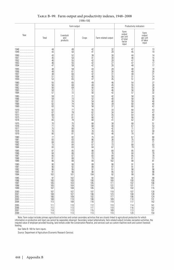
444 | Appendix B
Table B–99. Farm output and productivity indexes, 1948–2008[1996=100]
Year
Farm output Productivity indicators
TotalLivestock
andproducts
Crops Farm-related output
Farmoutput
per unitof totalfactorinput
Farmoutputper unitof labor
input
1948 .......................... 44 49 42 32 47 131949 .......................... 43 50 41 28 45 141950 .......................... 43 52 39 30 44 141951 .......................... 45 54 41 30 46 151952 .......................... 46 55 42 28 47 161953 .......................... 46 55 42 27 47 171954 .......................... 47 58 42 26 48 171955 .......................... 48 59 43 28 48 181956 .......................... 49 61 42 30 49 201957 .......................... 48 60 42 31 48 211958 .......................... 51 62 46 35 51 241959 .......................... 53 65 47 45 51 241960 .......................... 55 65 49 46 54 271961 .......................... 56 68 49 45 55 281962 .......................... 56 69 50 44 55 281963 .......................... 58 71 52 46 56 301964 .......................... 57 72 50 42 57 321965 .......................... 59 71 53 42 58 331966 .......................... 59 73 52 40 58 361967 .......................... 61 74 54 40 59 401968 .......................... 62 74 56 39 60 401969 .......................... 63 74 58 37 60 421970 .......................... 62 77 55 33 60 431971 .......................... 67 79 62 34 64 471972 .......................... 68 81 62 35 64 481973 .......................... 70 81 66 42 66 501974 .......................... 65 78 60 41 62 471975 .......................... 70 75 68 38 68 511976 .......................... 71 79 68 40 67 531977 .......................... 75 80 74 42 71 571978 .......................... 76 80 76 45 67 591979 .......................... 80 81 83 46 70 611980 .......................... 77 82 75 43 67 601981 .......................... 83 83 86 36 75 651982 .......................... 84 83 87 72 77 711983 .......................... 73 84 67 73 68 631984 .......................... 83 83 84 67 79 731985 .......................... 87 85 88 80 85 831986 .......................... 84 86 83 76 84 791987 .......................... 85 87 83 84 85 781988 .......................... 81 88 73 99 81 731989 .......................... 86 88 84 102 88 811990 .......................... 90 90 89 96 91 911991 .......................... 90 92 89 97 91 911992 .......................... 96 95 97 91 98 981993 .......................... 91 96 88 95 92 981994 .......................... 102 101 104 92 99 951995 .......................... 97 102 92 104 92 891996 .......................... 100 100 100 100 100 1001997 .......................... 105 103 105 111 102 1061998 .......................... 105 104 104 122 101 1111999 .......................... 107 108 105 128 102 1152000 .......................... 107 107 107 118 107 1282001 .......................... 108 107 106 123 108 1282002 .......................... 106 109 102 117 106 1242003 .......................... 108 110 106 109 110 1312004 .......................... 113 108 116 118 117 1422005 .......................... 111 110 112 110 114 1412006 .......................... 112 113 111 118 116 1522007 .......................... 114 113 115 109 113 1512008 .......................... 113 113 113 110 120 154
Note: Farm output includes primary agricultural activities and certain secondary activities that are closely linked to agricultural production for whichinformation on production and input use cannot be separately observed. Secondary output (alternatively, farm-related output) includes recreation activities, theimputed value of employer-provided housing, land rentals under the Conservation Reserve, and services such as custom machine work and custom livestockfeeding.
See Table B–100 for farm inputs.Source: Department of Agriculture (Economic Research Service).
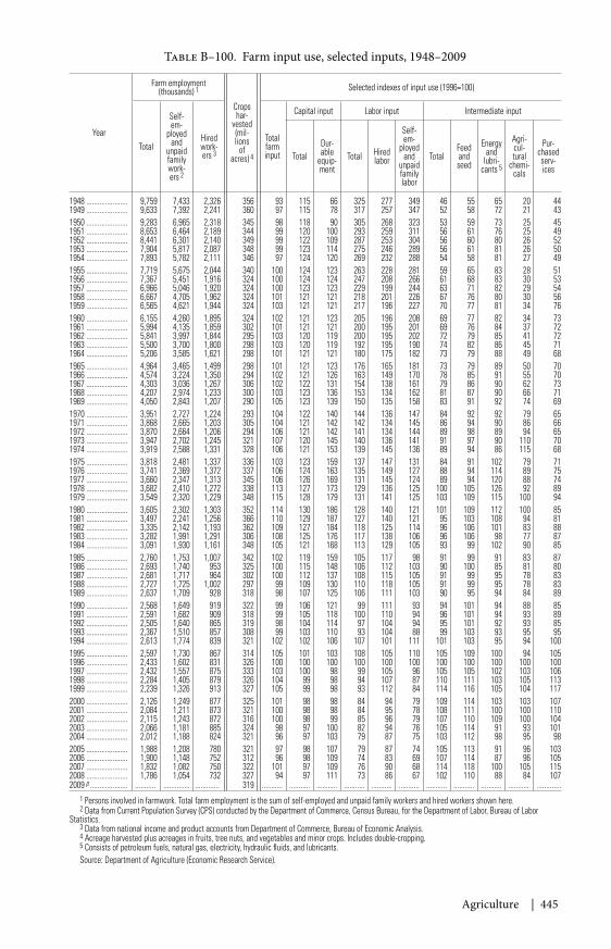
Agriculture | 445
Table B–100. Farm input use, selected inputs, 1948–2009
Year
Farm employment(thousands) 1
Cropshar-
vested(mil-lions
ofacres) 4
Selected indexes of input use (1996=100)
Total
Self-em-
ployedand
unpaidfamilywork-ers 2
Hiredwork-ers 3
Totalfarminput
Capital input Labor input Intermediate input
TotalDur-able
equip-ment
Total Hiredlabor
Self-em-
ployedand
unpaidfamilylabor
TotalFeedandseed
Energyand
lubri-cants 5
Agri-cul-tural
chemi-cals
Pur-chasedserv-ices
1948 ...................... 9,759 7,433 2,326 356 93 115 66 325 277 349 46 55 65 20 441949 ...................... 9,633 7,392 2,241 360 97 115 78 317 257 347 52 58 72 21 431950 ...................... 9,283 6,965 2,318 345 98 118 90 305 268 323 53 59 73 25 451951 ...................... 8,653 6,464 2,189 344 99 120 100 293 259 311 56 61 76 25 491952 ...................... 8,441 6,301 2,140 349 99 122 109 287 253 304 56 60 80 26 521953 ...................... 7,904 5,817 2,087 348 99 123 114 275 246 289 56 61 81 26 501954 ...................... 7,893 5,782 2,111 346 97 124 120 269 232 288 54 58 81 27 491955 ...................... 7,719 5,675 2,044 340 100 124 123 263 228 281 59 65 83 28 511956 ...................... 7,367 5,451 1,916 324 100 124 124 247 208 266 61 68 83 30 531957 ...................... 6,966 5,046 1,920 324 100 123 123 229 199 244 63 71 82 29 541958 ...................... 6,667 4,705 1,962 324 101 121 121 218 201 226 67 76 80 30 561959 ...................... 6,565 4,621 1,944 324 103 121 121 217 196 227 70 77 81 34 761960 ...................... 6,155 4,260 1,895 324 102 121 123 205 196 208 69 77 82 34 731961 ...................... 5,994 4,135 1,859 302 101 121 121 200 195 201 69 76 84 37 721962 ...................... 5,841 3,997 1,844 295 103 120 119 200 195 202 72 79 85 41 721963 ...................... 5,500 3,700 1,800 298 103 120 119 192 195 190 74 82 86 45 711964 ...................... 5,206 3,585 1,621 298 101 121 121 180 175 182 73 79 88 49 681965 ...................... 4,964 3,465 1,499 298 101 121 123 176 165 181 73 79 89 50 701966 ...................... 4,574 3,224 1,350 294 102 121 126 163 149 170 78 85 91 55 701967 ...................... 4,303 3,036 1,267 306 102 122 131 154 138 161 79 86 90 62 731968 ...................... 4,207 2,974 1,233 300 103 123 136 153 134 162 81 87 90 66 711969 ...................... 4,050 2,843 1,207 290 105 123 139 150 135 158 83 91 92 74 691970 ...................... 3,951 2,727 1,224 293 104 122 140 144 136 147 84 92 92 79 651971 ...................... 3,868 2,665 1,203 305 104 121 142 142 134 145 86 94 90 86 661972 ...................... 3,870 2,664 1,206 294 106 121 142 141 134 144 89 98 89 94 651973 ...................... 3,947 2,702 1,245 321 107 120 145 140 136 141 91 97 90 110 701974 ...................... 3,919 2,588 1,331 328 106 121 153 139 145 136 89 94 86 115 681975 ...................... 3,818 2,481 1,337 336 103 123 159 137 147 131 84 91 102 79 711976 ...................... 3,741 2,369 1,372 337 106 124 163 135 149 127 88 94 114 89 751977 ...................... 3,660 2,347 1,313 345 106 126 169 131 145 124 89 94 120 88 741978 ...................... 3,682 2,410 1,272 338 113 127 173 129 136 125 100 105 126 92 891979 ...................... 3,549 2,320 1,229 348 115 128 179 131 141 125 103 109 115 100 941980 ...................... 3,605 2,302 1,303 352 114 130 186 128 140 121 101 109 112 100 851981 ...................... 3,497 2,241 1,256 366 110 129 187 127 140 121 95 103 108 94 811982 ...................... 3,335 2,142 1,193 362 109 127 184 118 125 114 96 106 101 83 881983 ...................... 3,282 1,991 1,291 306 108 125 176 117 138 106 96 106 98 77 871984 ...................... 3,091 1,930 1,161 348 105 121 168 113 129 105 93 99 102 90 851985 ...................... 2,760 1,753 1,007 342 102 119 159 105 117 98 91 99 91 83 871986 ...................... 2,693 1,740 953 325 100 115 148 106 112 103 90 100 85 81 801987 ...................... 2,681 1,717 964 302 100 112 137 108 115 105 91 99 95 78 831988 ...................... 2,727 1,725 1,002 297 99 109 130 110 118 105 91 99 95 78 831989 ...................... 2,637 1,709 928 318 98 107 125 106 111 103 90 95 94 84 891990 ...................... 2,568 1,649 919 322 99 106 121 99 111 93 94 101 94 88 851991 ...................... 2,591 1,682 909 318 99 105 118 100 110 94 96 101 94 93 891992 ...................... 2,505 1,640 865 319 98 104 114 97 104 94 95 101 92 93 851993 ...................... 2,367 1,510 857 308 99 103 110 93 104 88 99 103 93 95 951994 ...................... 2,613 1,774 839 321 102 102 106 107 101 111 101 103 95 94 1001995 ...................... 2,597 1,730 867 314 105 101 103 108 105 110 105 109 100 94 1051996 ...................... 2,433 1,602 831 326 100 100 100 100 100 100 100 100 100 100 1001997 ...................... 2,432 1,557 875 333 103 100 98 99 105 96 105 105 102 103 1061998 ...................... 2,284 1,405 879 326 104 99 98 94 107 87 110 111 103 105 1131999 ...................... 2,239 1,326 913 327 105 99 98 93 112 84 114 116 105 104 1172000 ...................... 2,126 1,249 877 325 101 98 98 84 94 79 109 114 103 103 1072001 ...................... 2,084 1,211 873 321 100 98 98 84 95 78 108 111 100 100 1102002 ...................... 2,115 1,243 872 316 100 98 99 85 96 79 107 110 109 100 1042003 ...................... 2,066 1,181 885 324 98 97 100 82 94 76 105 114 91 93 1012004 ...................... 2,012 1,188 824 321 96 97 103 79 87 75 103 112 98 95 982005 ...................... 1,988 1,208 780 321 97 98 107 79 87 74 105 113 91 96 1032006 ...................... 1,900 1,148 752 312 96 98 109 74 83 69 107 114 87 96 1052007 ...................... 1,832 1,082 750 322 101 97 109 76 90 68 114 118 100 105 1152008 ...................... 1,786 1,054 732 327 94 97 111 73 86 67 102 110 88 84 1072009 p .................... ........... .............. ............. 319 ........... ........... ........... ........... ........... ........... ........... ........... ........... ........... .............
1 Persons involved in farmwork. Total farm employment is the sum of self-employed and unpaid family workers and hired workers shown here.2 Data from Current Population Survey (CPS) conducted by the Department of Commerce, Census Bureau, for the Department of Labor, Bureau of Labor
Statistics.3 Data from national income and product accounts from Department of Commerce, Bureau of Economic Analysis.4 Acreage harvested plus acreages in fruits, tree nuts, and vegetables and minor crops. Includes double-cropping.5 Consists of petroleum fuels, natural gas, electricity, hydraulic fluids, and lubricants.Source: Department of Agriculture (Economic Research Service).
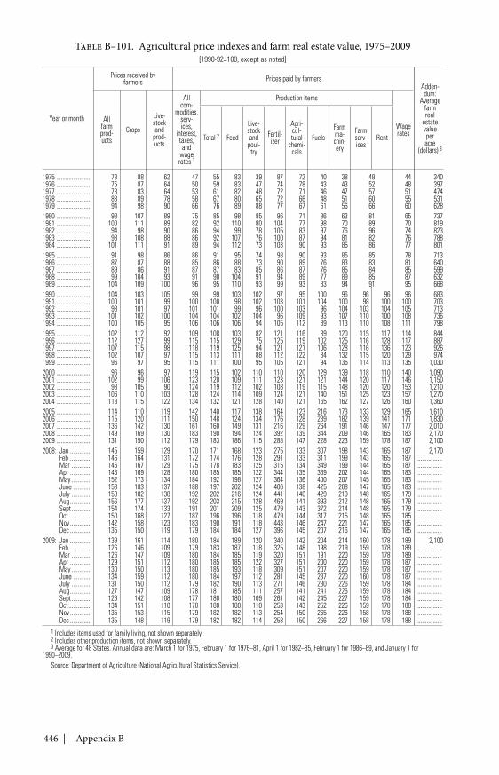
446 | Appendix B
Table B–101. Agricultural price indexes and farm real estate value, 1975–2009[1990-92=100, except as noted]
Year or month
Prices received byfarmers Prices paid by farmers
Adden-dum:
Averagefarmreal
estatevalueperacre
(dollars) 3
Allfarmprod-ucts
Crops
Live-stockand
prod-ucts
Allcom-
modities,serv-ices,
interest,taxes,and
wagerates 1
Production items
WageratesTotal 2 Feed
Live-stockand
poul-try
Fertil-izer
Agri-cul-tural
chemi-cals
FuelsFarmma-chin-ery
Farmserv-ices
Rent
1975 ...................... 73 88 62 47 55 83 39 87 72 40 38 48 44 3401976 ...................... 75 87 64 50 59 83 47 74 78 43 43 52 48 3971977 ...................... 73 83 64 53 61 82 48 72 71 46 47 57 51 4741978 ...................... 83 89 78 58 67 80 65 72 66 48 51 60 55 5311979 ...................... 94 98 90 66 76 89 88 77 67 61 56 66 60 6281980 ...................... 98 107 89 75 85 98 85 96 71 86 63 81 65 7371981 ...................... 100 111 89 82 92 110 80 104 77 98 70 89 70 8191982 ...................... 94 98 90 86 94 99 78 105 83 97 76 96 74 8231983 ...................... 98 108 88 86 92 107 76 100 87 94 81 82 76 7881984 ...................... 101 111 91 89 94 112 73 103 90 93 85 86 77 8011985 ...................... 91 98 86 86 91 95 74 98 90 93 85 85 78 7131986 ...................... 87 87 88 85 86 88 73 90 89 76 83 83 81 6401987 ...................... 89 86 91 87 87 83 85 86 87 76 85 84 85 5991988 ...................... 99 104 93 91 90 104 91 94 89 77 89 85 87 6321989 ...................... 104 109 100 96 95 110 93 99 93 83 94 91 95 6681990 ...................... 104 103 105 99 99 103 102 97 95 100 96 96 96 96 6831991 ...................... 100 101 99 100 100 98 102 103 101 104 100 98 100 100 7031992 ...................... 98 101 97 101 101 99 96 100 103 96 104 103 104 105 7131993 ...................... 101 102 100 104 104 102 104 96 109 93 107 110 100 108 7361994 ...................... 100 105 95 106 106 106 94 105 112 89 113 110 108 111 7981995 ...................... 102 112 92 109 108 103 82 121 116 89 120 115 117 114 8441996 ...................... 112 127 99 115 115 129 75 125 119 102 125 116 128 117 8871997 ...................... 107 115 98 118 119 125 94 121 121 106 128 116 136 123 9261998 ...................... 102 107 97 115 113 111 88 112 122 84 132 115 120 129 9741999 ...................... 96 97 95 115 111 100 95 105 121 94 135 114 113 135 1,0302000 ...................... 96 96 97 119 115 102 110 110 120 129 139 118 110 140 1,0902001 ...................... 102 99 106 123 120 109 111 123 121 121 144 120 117 146 1,1502002 ...................... 98 105 90 124 119 112 102 108 119 115 148 120 120 153 1,2102003 ...................... 106 110 103 128 124 114 109 124 121 140 151 125 123 157 1,2702004 ...................... 118 115 122 134 132 121 128 140 121 165 162 127 126 160 1,3602005 ...................... 114 110 119 142 140 117 138 164 123 216 173 133 129 165 1,6102006 ...................... 115 120 111 150 148 124 134 176 128 239 182 139 141 171 1,8302007 ...................... 136 142 130 161 160 149 131 216 129 264 191 146 147 177 2,0102008 ...................... 149 169 130 183 190 194 124 392 139 344 209 146 165 183 2,1702009 ...................... 131 150 112 179 183 186 115 288 147 228 223 159 178 187 2,1002008: Jan ............. 145 159 129 170 171 168 123 275 133 307 198 143 165 187 2,170
Feb ............. 146 164 131 172 174 176 128 291 133 311 199 143 165 187 ................Mar ............ 146 167 129 175 178 183 125 315 134 349 199 144 165 187 ................Apr ............. 146 169 128 180 185 185 122 344 135 369 202 144 165 183 ................May ............ 152 173 134 184 192 198 127 364 136 400 207 145 165 183 ................June ........... 158 183 137 188 197 202 124 406 138 425 208 147 165 183 ................July ............ 159 182 138 192 202 216 124 441 140 429 210 148 165 179 ................Aug ............. 156 177 137 192 203 215 128 469 141 393 212 148 165 179 ................Sept ............ 154 174 133 191 201 209 125 479 143 372 214 148 165 179 ................Oct .............. 150 168 127 187 196 196 118 479 144 317 215 148 165 185 ................Nov ............. 142 158 123 183 190 191 118 443 146 247 221 147 165 185 ................Dec ............. 135 150 119 179 184 184 127 396 145 207 216 147 165 185 ................
2009: Jan ............. 139 161 114 180 184 189 120 340 142 204 214 160 178 189 2,100Feb ............. 126 146 109 179 183 187 118 325 148 198 219 159 178 189 ................Mar ............ 126 147 109 180 184 185 119 320 151 191 220 159 178 189 ................Apr ............. 129 151 112 180 185 185 122 327 151 200 220 159 178 187 ................May ............ 130 150 113 180 185 193 118 309 151 207 220 159 178 187 ................June ........... 134 159 112 180 184 197 112 281 145 237 220 160 178 187 ................July ............ 131 150 112 179 182 190 113 271 146 230 226 159 178 184 ................Aug ............. 127 147 109 178 181 185 111 257 141 241 226 159 178 184 ................Sept ............ 126 142 108 177 180 180 109 261 142 245 227 159 178 184 ................Oct .............. 134 151 110 178 180 180 110 253 143 252 226 159 178 188 ................Nov ............. 135 153 115 179 182 182 113 254 150 265 226 158 178 188 ................Dec ............. 135 148 119 179 182 182 114 258 150 266 227 158 178 188 ................
1 Includes items used for family living, not shown separately.2 Includes other production items, not shown separately.3 Average for 48 States. Annual data are: March 1 for 1975, February 1 for 1976–81, April 1 for 1982–85, February 1 for 1986–89, and January 1 for
1990–2009.Source: Department of Agriculture (National Agricultural Statistics Service).
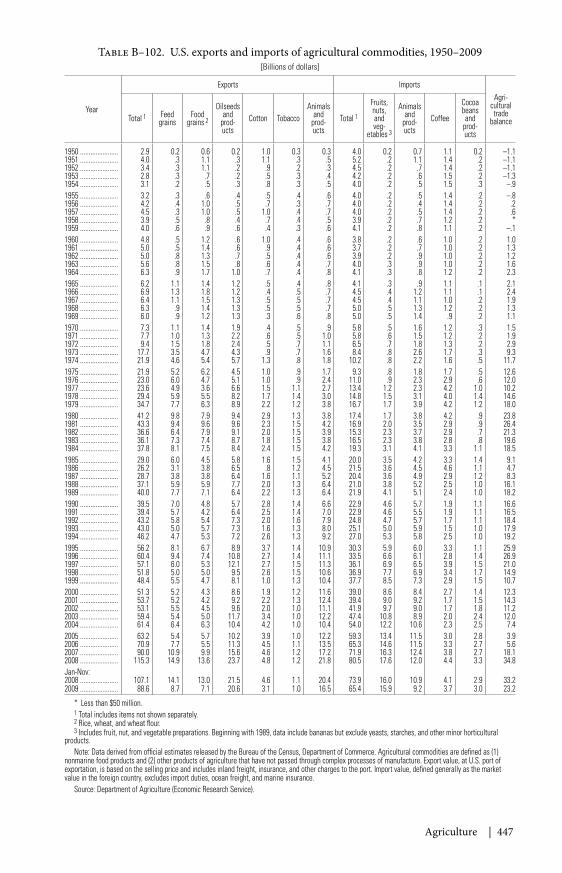
Agriculture | 447
Table B–102. U.S. exports and imports of agricultural commodities, 1950–2009[Billions of dollars]
Year
Exports ImportsAgri-
culturaltrade
balanceTotal 1 Feedgrains
Foodgrains 2
Oilseedsand
prod-ucts
Cotton TobaccoAnimals
andprod-ucts
Total 1
Fruits,nuts,andveg-
etables 3
Animalsand
prod-ucts
Coffee
Cocoabeansand
prod-ucts
1950 ...................... 2.9 0.2 0.6 0.2 1.0 0.3 0.3 4.0 0.2 0.7 1.1 0.2 –1.11951 ...................... 4.0 .3 1.1 .3 1.1 .3 .5 5.2 .2 1.1 1.4 .2 –1.11952 ...................... 3.4 .3 1.1 .2 .9 .2 .3 4.5 .2 .7 1.4 .2 –1.11953 ...................... 2.8 .3 .7 .2 .5 .3 .4 4.2 .2 .6 1.5 .2 –1.31954 ...................... 3.1 .2 .5 .3 .8 .3 .5 4.0 .2 .5 1.5 .3 –.91955 ...................... 3.2 .3 .6 .4 .5 .4 .6 4.0 .2 .5 1.4 .2 –.81956 ...................... 4.2 .4 1.0 .5 .7 .3 .7 4.0 .2 .4 1.4 .2 .21957 ...................... 4.5 .3 1.0 .5 1.0 .4 .7 4.0 .2 .5 1.4 .2 .61958 ...................... 3.9 .5 .8 .4 .7 .4 .5 3.9 .2 .7 1.2 .2 *1959 ...................... 4.0 .6 .9 .6 .4 .3 .6 4.1 .2 .8 1.1 .2 –.11960 ...................... 4.8 .5 1.2 .6 1.0 .4 .6 3.8 .2 .6 1.0 .2 1.01961 ...................... 5.0 .5 1.4 .6 .9 .4 .6 3.7 .2 .7 1.0 .2 1.31962 ...................... 5.0 .8 1.3 .7 .5 .4 .6 3.9 .2 .9 1.0 .2 1.21963 ...................... 5.6 .8 1.5 .8 .6 .4 .7 4.0 .3 .9 1.0 .2 1.61964 ...................... 6.3 .9 1.7 1.0 .7 .4 .8 4.1 .3 .8 1.2 .2 2.31965 ...................... 6.2 1.1 1.4 1.2 .5 .4 .8 4.1 .3 .9 1.1 .1 2.11966 ...................... 6.9 1.3 1.8 1.2 .4 .5 .7 4.5 .4 1.2 1.1 .1 2.41967 ...................... 6.4 1.1 1.5 1.3 .5 .5 .7 4.5 .4 1.1 1.0 .2 1.91968 ...................... 6.3 .9 1.4 1.3 .5 .5 .7 5.0 .5 1.3 1.2 .2 1.31969 ...................... 6.0 .9 1.2 1.3 .3 .6 .8 5.0 .5 1.4 .9 .2 1.11970 ...................... 7.3 1.1 1.4 1.9 .4 .5 .9 5.8 .5 1.6 1.2 .3 1.51971 ...................... 7.7 1.0 1.3 2.2 .6 .5 1.0 5.8 .6 1.5 1.2 .2 1.91972 ...................... 9.4 1.5 1.8 2.4 .5 .7 1.1 6.5 .7 1.8 1.3 .2 2.91973 ...................... 17.7 3.5 4.7 4.3 .9 .7 1.6 8.4 .8 2.6 1.7 .3 9.31974 ...................... 21.9 4.6 5.4 5.7 1.3 .8 1.8 10.2 .8 2.2 1.6 .5 11.71975 ...................... 21.9 5.2 6.2 4.5 1.0 .9 1.7 9.3 .8 1.8 1.7 .5 12.61976 ...................... 23.0 6.0 4.7 5.1 1.0 .9 2.4 11.0 .9 2.3 2.9 .6 12.01977 ...................... 23.6 4.9 3.6 6.6 1.5 1.1 2.7 13.4 1.2 2.3 4.2 1.0 10.21978 ...................... 29.4 5.9 5.5 8.2 1.7 1.4 3.0 14.8 1.5 3.1 4.0 1.4 14.61979 ...................... 34.7 7.7 6.3 8.9 2.2 1.2 3.8 16.7 1.7 3.9 4.2 1.2 18.01980 ...................... 41.2 9.8 7.9 9.4 2.9 1.3 3.8 17.4 1.7 3.8 4.2 .9 23.81981 ...................... 43.3 9.4 9.6 9.6 2.3 1.5 4.2 16.9 2.0 3.5 2.9 .9 26.41982 ...................... 36.6 6.4 7.9 9.1 2.0 1.5 3.9 15.3 2.3 3.7 2.9 .7 21.31983 ...................... 36.1 7.3 7.4 8.7 1.8 1.5 3.8 16.5 2.3 3.8 2.8 .8 19.61984 ...................... 37.8 8.1 7.5 8.4 2.4 1.5 4.2 19.3 3.1 4.1 3.3 1.1 18.51985 ...................... 29.0 6.0 4.5 5.8 1.6 1.5 4.1 20.0 3.5 4.2 3.3 1.4 9.11986 ...................... 26.2 3.1 3.8 6.5 .8 1.2 4.5 21.5 3.6 4.5 4.6 1.1 4.71987 ...................... 28.7 3.8 3.8 6.4 1.6 1.1 5.2 20.4 3.6 4.9 2.9 1.2 8.31988 ...................... 37.1 5.9 5.9 7.7 2.0 1.3 6.4 21.0 3.8 5.2 2.5 1.0 16.11989 ...................... 40.0 7.7 7.1 6.4 2.2 1.3 6.4 21.9 4.1 5.1 2.4 1.0 18.21990 ...................... 39.5 7.0 4.8 5.7 2.8 1.4 6.6 22.9 4.6 5.7 1.9 1.1 16.61991 ...................... 39.4 5.7 4.2 6.4 2.5 1.4 7.0 22.9 4.6 5.5 1.9 1.1 16.51992 ...................... 43.2 5.8 5.4 7.3 2.0 1.6 7.9 24.8 4.7 5.7 1.7 1.1 18.41993 ...................... 43.0 5.0 5.7 7.3 1.6 1.3 8.0 25.1 5.0 5.9 1.5 1.0 17.91994 ...................... 46.2 4.7 5.3 7.2 2.6 1.3 9.2 27.0 5.3 5.8 2.5 1.0 19.21995 ...................... 56.2 8.1 6.7 8.9 3.7 1.4 10.9 30.3 5.9 6.0 3.3 1.1 25.91996 ...................... 60.4 9.4 7.4 10.8 2.7 1.4 11.1 33.5 6.6 6.1 2.8 1.4 26.91997 ...................... 57.1 6.0 5.3 12.1 2.7 1.5 11.3 36.1 6.9 6.5 3.9 1.5 21.01998 ...................... 51.8 5.0 5.0 9.5 2.6 1.5 10.6 36.9 7.7 6.9 3.4 1.7 14.91999 ...................... 48.4 5.5 4.7 8.1 1.0 1.3 10.4 37.7 8.5 7.3 2.9 1.5 10.72000 ...................... 51.3 5.2 4.3 8.6 1.9 1.2 11.6 39.0 8.6 8.4 2.7 1.4 12.32001 ...................... 53.7 5.2 4.2 9.2 2.2 1.3 12.4 39.4 9.0 9.2 1.7 1.5 14.32002 ...................... 53.1 5.5 4.5 9.6 2.0 1.0 11.1 41.9 9.7 9.0 1.7 1.8 11.22003 ...................... 59.4 5.4 5.0 11.7 3.4 1.0 12.2 47.4 10.8 8.9 2.0 2.4 12.02004 ...................... 61.4 6.4 6.3 10.4 4.2 1.0 10.4 54.0 12.2 10.6 2.3 2.5 7.42005 ...................... 63.2 5.4 5.7 10.2 3.9 1.0 12.2 59.3 13.4 11.5 3.0 2.8 3.92006 ...................... 70.9 7.7 5.5 11.3 4.5 1.1 13.5 65.3 14.6 11.5 3.3 2.7 5.62007 ...................... 90.0 10.9 9.9 15.6 4.6 1.2 17.2 71.9 16.3 12.4 3.8 2.7 18.12008 ...................... 115.3 14.9 13.6 23.7 4.8 1.2 21.8 80.5 17.6 12.0 4.4 3.3 34.8Jan-Nov:2008 ...................... 107.1 14.1 13.0 21.5 4.6 1.1 20.4 73.9 16.0 10.9 4.1 2.9 33.22009 ...................... 88.6 8.7 7.1 20.6 3.1 1.0 16.5 65.4 15.9 9.2 3.7 3.0 23.2
* Less than $50 million.1 Total includes items not shown separately.2 Rice, wheat, and wheat flour.3 Includes fruit, nut, and vegetable preparations. Beginning with 1989, data include bananas but exclude yeasts, starches, and other minor horticultural
products.Note: Data derived from official estimates released by the Bureau of the Census, Department of Commerce. Agricultural commodities are defined as (1)
nonmarine food products and (2) other products of agriculture that have not passed through complex processes of manufacture. Export value, at U.S. port ofexportation, is based on the selling price and includes inland freight, insurance, and other charges to the port. Import value, defined generally as the marketvalue in the foreign country, excludes import duties, ocean freight, and marine insurance.
Source: Department of Agriculture (Economic Research Service).
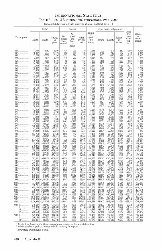
448 | Appendix B
Table B–103. U.S. international transactions, 1946–2009[Millions of dollars; quarterly data seasonally adjusted. Credits (+), debits (–)]
Year or quarter
Goods 1 ServicesBalance
ongoodsand
services
Income receipts and paymentsUnilat-
eralcurrenttrans-fers,net 2
Balanceon
currentaccountExports Imports
Balanceon
goods
Netmilitarytrans-
actions 2
Nettraveland
trans-por-
tation
Otherservices,
netReceipts Payments
Balanceon
income
1946 ...................... 11,764 –5,067 6,697 –424 733 310 7,316 772 –212 560 –2,991 4,8851947 ...................... 16,097 –5,973 10,124 –358 946 145 10,857 1,102 –245 857 –2,722 8,9921948 ...................... 13,265 –7,557 5,708 –351 374 175 5,906 1,921 –437 1,484 –4,973 2,4171949 ...................... 12,213 –6,874 5,339 –410 230 208 5,367 1,831 –476 1,355 –5,849 8731950 ...................... 10,203 –9,081 1,122 –56 –120 242 1,188 2,068 –559 1,509 –4,537 –1,8401951 ...................... 14,243 –11,176 3,067 169 298 254 3,788 2,633 –583 2,050 –4,954 8841952 ...................... 13,449 –10,838 2,611 528 83 309 3,531 2,751 –555 2,196 –5,113 6141953 ...................... 12,412 –10,975 1,437 1,753 –238 307 3,259 2,736 –624 2,112 –6,657 –1,2861954 ...................... 12,929 –10,353 2,576 902 –269 305 3,514 2,929 –582 2,347 –5,642 2191955 ...................... 14,424 –11,527 2,897 –113 –297 299 2,786 3,406 –676 2,730 –5,086 4301956 ...................... 17,556 –12,803 4,753 –221 –361 447 4,618 3,837 –735 3,102 –4,990 2,7301957 ...................... 19,562 –13,291 6,271 –423 –189 482 6,141 4,180 –796 3,384 –4,763 4,7621958 ...................... 16,414 –12,952 3,462 –849 –633 486 2,466 3,790 –825 2,965 –4,647 7841959 ...................... 16,458 –15,310 1,148 –831 –821 573 69 4,132 –1,061 3,071 –4,422 –1,2821960 ...................... 19,650 –14,758 4,892 –1,057 –964 639 3,508 4,616 –1,238 3,379 –4,062 2,8241961 ...................... 20,108 –14,537 5,571 –1,131 –978 732 4,195 4,999 –1,245 3,755 –4,127 3,8221962 ...................... 20,781 –16,260 4,521 –912 –1,152 912 3,370 5,618 –1,324 4,294 –4,277 3,3871963 ...................... 22,272 –17,048 5,224 –742 –1,309 1,036 4,210 6,157 –1,560 4,596 –4,392 4,4141964 ...................... 25,501 –18,700 6,801 –794 –1,146 1,161 6,022 6,824 –1,783 5,041 –4,240 6,8231965 ...................... 26,461 –21,510 4,951 –487 –1,280 1,480 4,664 7,437 –2,088 5,350 –4,583 5,4311966 ...................... 29,310 –25,493 3,817 –1,043 –1,331 1,497 2,940 7,528 –2,481 5,047 –4,955 3,0311967 ...................... 30,666 –26,866 3,800 –1,187 –1,750 1,742 2,604 8,021 –2,747 5,274 –5,294 2,5831968 ...................... 33,626 –32,991 635 –596 –1,548 1,759 250 9,367 –3,378 5,990 –5,629 6111969 ...................... 36,414 –35,807 607 –718 –1,763 1,964 91 10,913 –4,869 6,044 –5,735 3991970 ...................... 42,469 –39,866 2,603 –641 –2,038 2,330 2,254 11,748 –5,515 6,233 –6,156 2,3311971 ...................... 43,319 –45,579 –2,260 653 –2,345 2,649 –1,303 12,707 –5,435 7,272 –7,402 –1,4331972 ...................... 49,381 –55,797 –6,416 1,072 –3,063 2,965 –5,443 14,765 –6,572 8,192 –8,544 –5,7951973 ...................... 71,410 –70,499 911 740 –3,158 3,406 1,900 21,808 –9,655 12,153 –6,913 7,1401974 ...................... 98,306 –103,811 –5,505 165 –3,184 4,231 –4,292 27,587 –12,084 15,503 –9,249 1,9621975 ...................... 107,088 –98,185 8,903 1,461 –2,812 4,854 12,404 25,351 –12,564 12,787 –7,075 18,1161976 ...................... 114,745 –124,228 –9,483 931 –2,558 5,027 –6,082 29,375 –13,311 16,063 –5,686 4,2951977 ...................... 120,816 –151,907 –31,091 1,731 –3,565 5,680 –27,246 32,354 –14,217 18,137 –5,226 –14,3351978 ...................... 142,075 –176,002 –33,927 857 –3,573 6,879 –29,763 42,088 –21,680 20,408 –5,788 –15,1431979 ...................... 184,439 –212,007 –27,568 –1,313 –2,935 7,251 –24,565 63,834 –32,961 30,873 –6,593 –2851980 ...................... 224,250 –249,750 –25,500 –1,822 –997 8,912 –19,407 72,606 –42,532 30,073 –8,349 2,3171981 ...................... 237,044 –265,067 –28,023 –844 144 12,552 –16,172 86,529 –53,626 32,903 –11,702 5,0301982 ...................... 211,157 –247,642 –36,485 112 –992 13,209 –24,156 91,747 –56,583 35,164 –16,544 –5,5361983 ...................... 201,799 –268,901 –67,102 –563 –4,227 14,124 –57,767 90,000 –53,614 36,386 –17,310 –38,6911984 ...................... 219,926 –332,418 –112,492 –2,547 –8,438 14,404 –109,073 108,819 –73,756 35,063 –20,335 –94,3441985 ...................... 215,915 –338,088 –122,173 –4,390 –9,798 14,483 –121,880 98,542 –72,819 25,723 –21,998 –118,1551986 ...................... 223,344 –368,425 –145,081 –5,181 –8,779 20,502 –138,538 97,064 –81,571 15,494 –24,132 –147,1771987 ...................... 250,208 –409,765 –159,557 –3,844 –8,010 19,728 –151,684 108,184 –93,891 14,293 –23,265 –160,6551988 ...................... 320,230 –447,189 –126,959 –6,320 –3,013 21,725 –114,566 136,713 –118,026 18,687 –25,274 –121,1531989 ...................... 359,916 –477,665 –117,749 –6,749 3,551 27,805 –93,142 161,287 –141,463 19,824 –26,169 –99,4861990 ...................... 387,401 –498,438 –111,037 –7,599 7,501 30,270 –80,864 171,742 –143,192 28,550 –26,654 –78,9681991 ...................... 414,083 –491,020 –76,937 –5,275 16,560 34,516 –31,136 149,214 –125,085 24,131 9,904 2,8971992 ...................... 439,631 –536,528 –96,897 –1,448 19,969 39,164 –39,212 133,766 –109,531 24,234 –36,636 –51,6131993 ...................... 456,943 –589,394 –132,451 1,383 19,714 41,040 –70,311 136,057 –110,741 25,316 –39,811 –84,8051994 ...................... 502,859 –668,690 –165,831 2,570 16,305 48,463 –98,493 166,521 –149,375 17,146 –40,265 –121,6121995 ...................... 575,204 –749,374 –174,170 4,600 21,772 51,414 –96,384 210,244 –189,353 20,891 –38,074 –113,5671996 ...................... 612,113 –803,113 –191,000 5,385 25,015 56,535 –104,065 226,129 –203,811 22,318 –43,017 –124,7641997 ...................... 678,366 –876,794 –198,428 4,968 22,152 63,035 –108,273 256,804 –244,195 12,609 –45,062 –140,7261998 ...................... 670,416 –918,637 –248,221 5,220 10,210 66,651 –166,140 261,819 –257,554 4,265 –53,187 –215,0621999 ...................... 683,965 –1,031,784 –347,819 2,593 7,085 73,051 –265,090 293,925 –280,037 13,888 –50,428 –301,6302000 ...................... 771,994 –1,226,684 –454,690 317 2,486 72,052 –379,835 350,918 –329,864 21,054 –58,645 –417,4262001 ...................... 718,711 –1,148,609 –429,898 –2,296 –3,254 69,943 –365,505 290,797 –259,075 31,722 –64,487 –398,2702002 ...................... 685,170 –1,168,002 –482,831 –7,158 –4,245 72,633 –421,601 280,942 –253,544 27,398 –64,948 –459,1512003 ...................... 715,848 –1,264,860 –549,012 –11,981 –11,475 77,433 –495,034 320,456 –275,147 45,309 –71,794 –521,5192004 ...................... 806,161 –1,477,996 –671,835 –13,518 –14,275 89,640 –609,987 413,739 –346,519 67,219 –88,362 –631,1302005 ...................... 892,337 –1,683,188 –790,851 –10,536 –13,006 99,124 –715,268 535,263 –462,905 72,358 –105,772 –748,6832006 ...................... 1,015,812 –1,863,072 –847,260 –7,119 –10,873 104,893 –760,359 682,221 –634,136 48,085 –91,273 –803,5472007 ...................... 1,138,384 –1,969,375 –830,992 –7,384 2,345 134,609 –701,422 818,931 –728,085 90,845 –115,996 –726,5732008 ...................... 1,276,994 –2,117,245 –840,252 –13,881 16,175 142,021 –695,936 764,637 –646,406 118,231 –128,363 –706,0682008: I .................. 315,637 –534,482 –218,846 –2,543 3,076 35,659 –182,653 202,927 –166,241 36,686 –33,330 –179,298
II ................. 332,876 –554,372 –221,496 –3,055 4,922 36,784 –182,847 198,796 –172,521 26,274 –31,147 –187,719III ................ 337,912 –559,002 –221,090 –4,664 5,595 34,217 –185,942 195,319 –161,194 34,125 –32,361 –184,178IV ................ 290,569 –469,389 –178,820 –3,618 2,581 35,363 –144,495 167,596 –146,450 21,146 –31,527 –154,875
2009: I .................. 249,374 –373,411 –124,036 –3,017 1,985 32,661 –92,408 135,352 –117,051 18,301 –30,343 –104,450II ................. 246,134 –361,621 –115,487 –1,855 3,509 32,592 –81,240 135,074 –118,404 16,670 –33,410 –97,980III p .............. 263,911 –396,050 –132,138 –2,044 3,939 32,865 –97,378 140,403 –116,694 23,709 –34,365 –108,034
1 Adjusted from Census data for differences in valuation, coverage, and timing; excludes military.2 Includes transfers of goods and services under U.S. military grant programs.See next page for continuation of table.
International Statistics
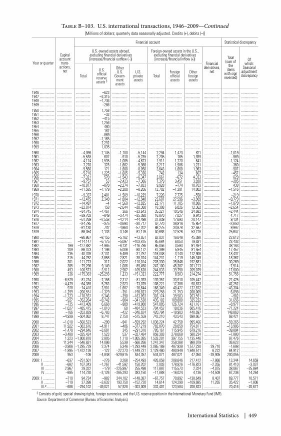
International Statistics | 449
Table B–103. U.S. international transactions, 1946–2009—Continued[Millions of dollars; quarterly data seasonally adjusted. Credits (+), debits (–)]
Year or quarter
Capitalaccounttrans-
actions,net
Financial account Statistical discrepancy
U.S.-owned assets abroad,excluding financial derivatives[increase/financial outflow (–)]
Foreign-owned assets in the U.S.,excluding financial derivatives[increase/financial inflow (+)]
Financialderivatives,
net
Total(sum of
theitems
with signreversed)
Ofwhich:
SeasonaladjustmentdiscrepancyTotal
U.S.officialreserveassets 3
OtherU.S.
Govern-ment
assets
U.S.privateassets
TotalForeignofficialassets
Otherforeignassets
1946 ................. ................. ................. –623 ................. ................. ................. ................. ................. .................. ................. ...................1947 ................. ................. ................. –3,315 ................. ................. ................. ................. ................. .................. ................. ...................1948 ................. ................. ................. –1,736 ................. ................. ................. ................. ................. .................. ................. ...................1949 ................. ................. ................. –266 ................. ................. ................. ................. ................. .................. ................. ...................1950 ................. ................. ................. 1,758 ................. ................. ................. ................. ................. .................. ................. ...................1951 ................. ................. ................. –33 ................. ................. ................. ................. ................. .................. ................. ...................1952 ................. ................. ................. –415 ................. ................. ................. ................. ................. .................. ................. ...................1953 ................. ................. ................. 1,256 ................. ................. ................. ................. ................. .................. ................. ...................1954 ................. ................. ................. 480 ................. ................. ................. ................. ................. .................. ................. ...................1955 ................. ................. ................. 182 ................. ................. ................. ................. ................. .................. ................. ...................1956 ................. ................. ................. –869 ................. ................. ................. ................. ................. .................. ................. ...................1957 ................. ................. ................. –1,165 ................. ................. ................. ................. ................. .................. ................. ...................1958 ................. ................. ................. 2,292 ................. ................. ................. ................. ................. .................. ................. ...................1959 ................. ................. ................. 1,035 ................. ................. ................. ................. ................. .................. ................. ...................1960 ................. ................. –4,099 2,145 –1,100 –5,144 2,294 1,473 821 .................. –1,019 ...................1961 ................. ................. –5,538 607 –910 –5,235 2,705 765 1,939 .................. –989 ...................1962 ................. ................. –4,174 1,535 –1,085 –4,623 1,911 1,270 641 .................. –1,124 ...................1963 ................. ................. –7,270 378 –1,662 –5,986 3,217 1,986 1,231 .................. –360 ...................1964 ................. ................. –9,560 171 –1,680 –8,050 3,643 1,660 1,983 .................. –907 ...................1965 ................. ................. –5,716 1,225 –1,605 –5,336 742 134 607 .................. –457 ...................1966 ................. ................. –7,321 570 –1,543 –6,347 3,661 –672 4,333 .................. 629 ...................1967 ................. ................. –9,757 53 –2,423 –7,386 7,379 3,451 3,928 .................. –205 ...................1968 ................. ................. –10,977 –870 –2,274 –7,833 9,928 –774 10,703 .................. 438 ...................1969 ................. ................. –11,585 –1,179 –2,200 –8,206 12,702 –1,301 14,002 .................. –1,516 ...................1970 ................. ................. –9,337 2,481 –1,589 –10,229 7,226 7,775 –550 .................. –219 ...................1971 ................. ................. –12,475 2,349 –1,884 –12,940 23,687 27,596 –3,909 .................. –9,779 ...................1972 ................. ................. –14,497 –4 –1,568 –12,925 22,171 11,185 10,986 .................. –1,879 ...................1973 ................. ................. –22,874 158 –2,644 –20,388 18,388 6,026 12,362 .................. –2,654 ...................1974 ................. ................. –34,745 –1,467 366 –33,643 35,227 10,546 24,682 .................. –2,444 ...................1975 ................. ................. –39,703 –849 –3,474 –35,380 16,870 7,027 9,843 .................. 4,717 ...................1976 ................. ................. –51,269 –2,558 –4,214 –44,498 37,839 17,693 20,147 .................. 9,134 ...................1977 ................. ................. –34,785 –375 –3,693 –30,717 52,770 36,816 15,954 .................. –3,650 ...................1978 ................. ................. –61,130 732 –4,660 –57,202 66,275 33,678 32,597 .................. 9,997 ...................1979 ................. ................. –66,054 –1,133 –3,746 –61,176 40,693 –12,526 53,218 .................. 25,647 ...................1980 ................. ................. –86,967 –8,155 –5,162 –73,651 62,037 16,649 45,388 .................. 22,613 ...................1981 ................. ................. –114,147 –5,175 –5,097 –103,875 85,684 6,053 79,631 .................. 23,433 ...................1982 ................. 199 –127,882 –4,965 –6,131 –116,786 95,056 3,593 91,464 .................. 38,163 ...................1983 ................. 209 –66,373 –1,196 –5,006 –60,172 87,399 5,845 81,554 .................. 17,457 ...................1984 ................. 235 –40,376 –3,131 –5,489 –31,757 116,048 3,140 112,908 .................. 18,437 ...................1985 ................. 315 –44,752 –3,858 –2,821 –38,074 144,231 –1,119 145,349 .................. 18,362 ...................1986 ................. 301 –111,723 312 –2,022 –110,014 228,330 35,648 192,681 .................. 30,269 ...................1987 ................. 365 –79,296 9,149 1,006 –89,450 247,100 45,387 201,713 .................. –7,514 ...................1988 ................. 493 –106,573 –3,912 2,967 –105,628 244,833 39,758 205,075 .................. –17,600 ...................1989 ................. 336 –175,383 –25,293 1,233 –151,323 222,777 8,503 214,274 .................. 51,756 ...................1990 ................. –6,579 –81,234 –2,158 2,317 –81,393 139,357 33,910 105,447 .................. 27,425 ...................1991 ................. –4,479 –64,389 5,763 2,923 –73,075 108,221 17,388 90,833 .................. –42,252 ...................1992 ................. 978 –74,410 3,901 –1,667 –76,644 168,349 40,477 127,872 .................. –43,304 ...................1993 ................. –1,299 –200,551 –1,379 –351 –198,823 279,758 71,753 208,005 .................. 6,898 ...................1994 ................. –1,723 –178,937 5,346 –390 –183,893 303,174 39,583 263,591 .................. –902 ...................1995 ................. –927 –352,264 –9,742 –984 –341,538 435,102 109,880 325,222 .................. 31,656 ...................1996 ................. –735 –413,409 6,668 –989 –419,088 547,885 126,724 421,161 .................. –8,977 ...................1997 ................. –1,027 –485,475 –1,010 68 –484,533 704,452 19,036 685,416 .................. –77,224 ...................1998 ................. –766 –353,829 –6,783 –422 –346,624 420,794 –19,903 440,697 .................. 148,863 ...................1999 ................. –4,939 –504,062 8,747 2,750 –515,559 742,210 43,543 698,667 .................. 68,421 ...................2000 ................. –1,010 –560,523 –290 –941 –559,292 1,038,224 42,758 995,466 .................. –59,265 ...................2001 ................. 11,922 –382,616 –4,911 –486 –377,219 782,870 28,059 754,811 .................. –13,906 ...................2002 ................. –1,470 –294,646 –3,681 345 –291,310 795,161 115,945 679,216 .................. –39,894 ...................2003 ................. –3,480 –325,424 1,523 537 –327,484 858,303 278,069 580,234 .................. –7,880 ...................2004 ................. 1,323 –1,000,870 2,805 1,710 –1,005,385 1,533,201 397,755 1,135,446 .................. 97,476 ...................2005 ................. 11,344 –546,631 14,096 5,539 –566,266 1,247,347 259,268 988,079 .................. 36,623 ...................2006 ................. –3,906 –1,285,729 2,374 5,346 –1,293,449 2,065,169 487,939 1,577,230 29,710 –1,698 ...................2007 ................. –1,895 –1,472,126 –122 –22,273 –1,449,731 2,129,460 480,949 1,648,511 6,222 64,912 ...................2008 ................. 953 –106 –4,848 –529,615 534,357 534,071 487,021 47,050 –28,905 200,055 ...................2008: I ............. –637 –251,501 –276 3,268 –254,493 426,058 208,646 217,412 –7,966 13,344 14,659
II ............ –682 107,343 –1,267 –41,592 150,202 2,003 178,826 –176,823 –2,355 81,410 –3,037III ........... 2,967 29,322 –179 –225,997 255,498 117,897 115,573 2,324 –4,075 38,067 –25,884IV ........... –695 114,730 –3,126 –265,293 383,150 –11,888 –16,024 4,136 –14,509 67,236 14,264
2009: I ............. –710 94,734 –982 244,102 –148,387 –67,757 70,892 –138,649 8,407 69,777 10,571II ............ –719 37,398 –3,632 193,750 –152,720 14,614 124,299 –109,685 11,265 35,422 –1,806III p ......... –686 –294,102 –49,021 57,928 –303,009 332,407 123,584 208,823 .................. 70,416 –20,677
3 Consists of gold, special drawing rights, foreign currencies, and the U.S. reserve position in the International Monetary Fund (IMF).Source: Department of Commerce (Bureau of Economic Analysis).
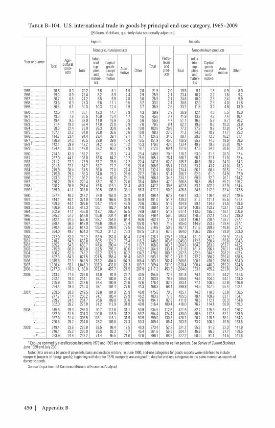
450 | Appendix B
Table B–104. U.S. international trade in goods by principal end-use category, 1965–2009[Billions of dollars; quarterly data seasonally adjusted]
Year or quarter
Exports Imports
TotalAgri-
culturalprod-ucts
Nonagricultural products
Total
Petro-leumand
prod-ucts
Nonpetroleum products
Total
Indus-trialsup-pliesand
materi-als
Capitalgoodsexceptauto-
motive
Auto-motive Other Total
Indus-trialsup-pliesand
materi-als
Capitalgoodsexceptauto-
motive
Auto-motive Other
1965 ................. 26.5 6.3 20.2 7.6 8.1 1.9 2.6 21.5 2.0 19.5 9.1 1.5 0.9 8.01966 ................. 29.3 6.9 22.4 8.2 8.9 2.4 2.9 25.5 2.1 23.4 10.2 2.2 1.8 9.21967 ................. 30.7 6.5 24.2 8.5 9.9 2.8 3.0 26.9 2.1 24.8 10.0 2.5 2.4 9.91968 ................. 33.6 6.3 27.3 9.6 11.1 3.5 3.2 33.0 2.4 30.6 12.0 2.8 4.0 11.81969 ................. 36.4 6.1 30.3 10.3 12.4 3.9 3.7 35.8 2.6 33.2 11.8 3.4 4.9 13.01970 ................. 42.5 7.4 35.1 12.3 14.7 3.9 4.3 39.9 2.9 36.9 12.4 4.0 5.5 15.01971 ................. 43.3 7.8 35.5 10.9 15.4 4.7 4.5 45.6 3.7 41.9 13.8 4.3 7.4 16.41972 ................. 49.4 9.5 39.9 11.9 16.9 5.5 5.6 55.8 4.7 51.1 16.3 5.9 8.7 20.21973 ................. 71.4 18.0 53.4 17.0 22.0 6.9 7.6 70.5 8.4 62.1 19.6 8.3 10.3 23.91974 ................. 98.3 22.4 75.9 26.3 30.9 8.6 10.0 103.8 26.6 77.2 27.8 9.8 12.0 27.51975 ................. 107.1 22.2 84.8 26.8 36.6 10.6 10.8 98.2 27.0 71.2 24.0 10.2 11.7 25.31976 ................. 114.7 23.4 91.4 28.4 39.1 12.1 11.7 124.2 34.6 89.7 29.8 12.3 16.2 31.41977 ................. 120.8 24.3 96.5 29.8 39.8 13.4 13.5 151.9 45.0 106.9 35.7 14.0 18.6 38.61978 1 ............... 142.1 29.9 112.2 34.2 47.5 15.2 15.3 176.0 42.6 133.4 40.7 19.3 25.0 48.41979 ................. 184.4 35.5 149.0 52.2 60.2 17.9 18.7 212.0 60.4 151.6 47.5 24.6 26.6 52.81980 ................. 224.3 42.0 182.2 65.1 76.3 17.4 23.4 249.8 79.5 170.2 53.0 31.6 28.3 57.41981 ................. 237.0 44.1 193.0 63.6 84.2 19.7 25.5 265.1 78.4 186.7 56.1 37.1 31.0 62.41982 ................. 211.2 37.3 173.9 57.7 76.5 17.2 22.4 247.6 62.0 185.7 48.6 38.4 34.3 64.31983 ................. 201.8 37.1 164.7 52.7 71.7 18.5 21.8 268.9 55.1 213.8 53.7 43.7 43.0 73.31984 ................. 219.9 38.4 181.5 56.8 77.0 22.4 25.3 332.4 58.1 274.4 66.1 60.4 56.5 91.41985 ................. 215.9 29.6 186.3 54.8 79.3 24.9 27.2 338.1 51.4 286.7 62.6 61.3 64.9 97.91986 ................. 223.3 27.2 196.2 59.4 82.8 25.1 28.9 368.4 34.3 334.1 69.9 72.0 78.1 114.21987 ................. 250.2 29.8 220.4 63.7 92.7 27.6 36.4 409.8 42.9 366.8 70.8 85.1 85.2 125.71988 ................. 320.2 38.8 281.4 82.6 119.1 33.4 46.3 447.2 39.6 407.6 83.1 102.2 87.9 134.41989 1 ............... 359.9 41.1 318.8 90.5 136.9 35.1 56.3 477.7 50.9 426.8 84.6 112.3 87.4 142.51990 ................. 387.4 40.2 347.2 97.0 153.0 36.2 61.0 498.4 62.3 436.1 83.0 116.4 88.2 148.51991 ................. 414.1 40.1 374.0 101.6 166.6 39.9 65.9 491.0 51.7 439.3 81.3 121.1 85.5 151.41992 ................. 439.6 44.1 395.6 101.7 176.4 46.9 70.6 536.5 51.6 484.9 89.1 134.8 91.5 169.61993 ................. 456.9 43.6 413.3 105.1 182.7 51.6 74.0 589.4 51.5 537.9 100.8 153.2 102.1 182.01994 ................. 502.9 47.1 455.8 112.7 205.7 57.5 79.9 668.7 51.3 617.4 113.6 185.0 118.1 200.61995 ................. 575.2 57.2 518.0 135.6 234.4 61.4 86.5 749.4 56.0 693.3 128.5 222.1 123.7 219.01996 ................. 612.1 61.5 550.6 138.7 254.0 64.4 93.6 803.1 72.7 730.4 136.1 228.4 128.7 237.11997 ................. 678.4 58.5 619.9 148.6 295.8 73.4 102.0 876.8 71.8 805.0 144.9 253.6 139.4 267.11998 ................. 670.4 53.2 617.3 139.4 299.8 72.5 105.5 918.6 50.9 867.7 151.6 269.8 148.6 297.71999 ................. 684.0 49.7 634.3 140.3 311.2 75.3 107.5 1,031.8 67.8 964.0 156.3 295.7 179.0 333.02000 ................. 772.0 52.8 719.2 163.9 357.0 80.4 117.9 1,226.7 120.3 1,106.4 181.9 347.0 195.9 381.62001 ................. 718.7 54.9 663.8 150.5 321.7 75.4 116.2 1,148.6 103.6 1,045.0 172.5 298.4 189.8 384.32002 ................. 685.2 54.5 630.7 147.6 290.4 78.9 113.7 1,168.0 103.5 1,064.5 164.6 283.9 203.7 412.22003 ................. 715.8 60.9 655.0 162.5 293.7 80.6 118.2 1,264.9 133.1 1,131.8 181.4 296.4 210.1 443.82004 ................. 806.2 62.9 743.2 192.2 327.5 89.2 134.2 1,478.0 180.5 1,297.5 232.5 344.5 228.2 492.42005 ................. 892.3 64.9 827.5 221.5 358.4 98.4 149.2 1,683.2 251.9 1,431.3 272.7 380.7 239.4 538.52006 ................. 1,015.8 72.9 942.9 263.2 404.0 107.3 168.4 1,863.1 302.4 1,560.6 300.1 420.0 256.6 584.02007 ................. 1,138.4 92.1 1,046.3 302.3 433.0 121.3 189.7 1,969.4 331.0 1,638.4 308.4 446.0 259.2 624.82008 ................. 1,277.0 118.0 1,159.0 372.0 457.7 121.5 207.9 2,117.2 453.3 1,664.0 333.1 455.2 233.8 641.92006: I ............. 243.4 17.5 226.0 61.0 97.9 26.7 40.5 454.6 72.9 381.8 74.1 101.9 64.2 141.6
II ............ 252.1 18.0 234.1 65.7 100.8 26.4 41.2 463.8 78.2 385.6 74.4 104.0 64.1 143.0III ........... 255.9 18.4 237.6 67.4 100.9 26.6 42.6 476.4 82.9 393.4 77.1 106.5 62.9 146.9IV ........... 264.4 19.0 245.3 69.1 104.4 27.6 44.3 468.3 68.4 399.9 74.5 107.5 65.4 152.4
2007: I ............. 269.5 20.0 249.5 69.8 104.9 28.9 46.0 475.6 70.5 405.1 74.8 110.0 63.8 156.5II ............ 277.7 21.4 256.2 74.7 105.4 29.9 46.2 483.3 77.8 405.5 78.4 109.9 63.1 154.1III ........... 289.2 24.5 264.7 76.6 109.9 30.6 47.6 494.1 82.3 411.8 78.5 112.1 66.3 154.8IV ........... 302.0 26.2 275.8 81.2 112.9 31.8 49.8 516.4 100.4 416.0 76.7 114.1 66.0 159.3
2008: I ............. 315.6 29.3 286.3 90.7 113.6 31.1 50.9 534.5 112.6 421.9 82.7 115.3 63.7 160.2II ............ 332.9 31.6 301.3 100.0 116.9 31.2 53.2 554.4 124.4 430.0 86.5 117.5 62.1 163.9III ........... 337.9 31.4 306.5 103.1 118.1 31.9 53.5 559.0 130.8 428.2 90.2 115.5 58.1 164.3IV ........... 290.6 25.7 264.8 78.2 109.0 27.3 50.3 469.4 85.4 383.9 73.7 106.9 49.9 153.5
2009: I ............. 249.4 23.6 225.8 63.5 98.4 17.5 46.3 373.4 52.2 321.2 55.2 91.8 32.3 141.9II ............ 246.1 25.2 220.9 65.5 93.3 16.7 45.4 361.6 56.9 304.7 46.9 86.5 31.7 139.5III p ......... 263.9 24.8 239.2 74.4 95.5 21.6 47.6 396.1 68.9 327.2 50.0 91.1 44.5 141.6
1 End-use commodity classifications beginning 1978 and 1989 are not strictly comparable with data for earlier periods. See Survey of Current Business,June 1988 and July 2001.
Note: Data are on a balance of payments basis and exclude military. In June 1990, end-use categories for goods exports were redefined to includereexports (exports of foreign goods); beginning with data for 1978, reexports are assigned to detailed end-use categories in the same manner as exports ofdomestic goods.
Source: Department of Commerce (Bureau of Economic Analysis).
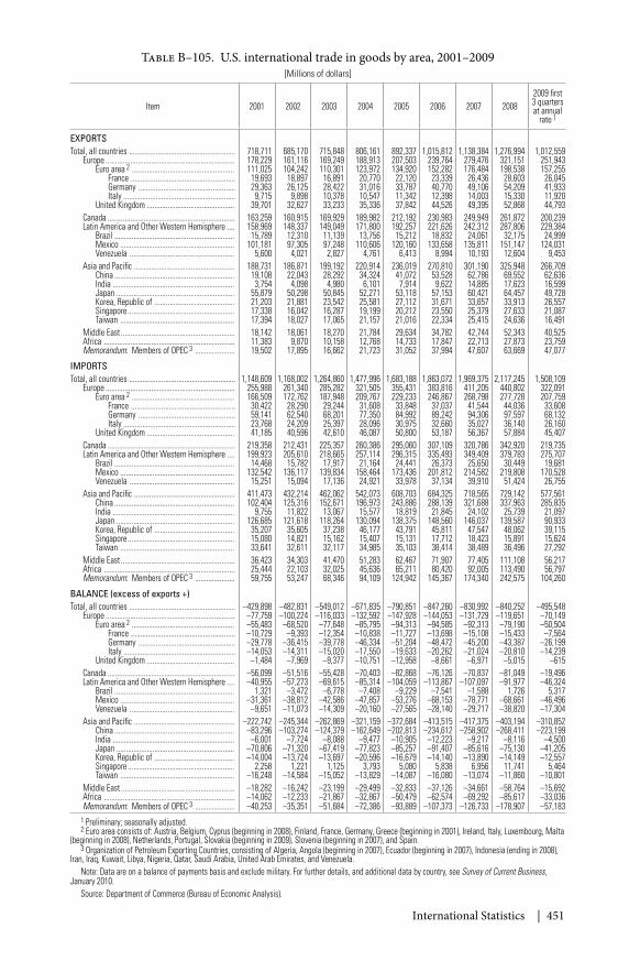
International Statistics | 451
Table B–105. U.S. international trade in goods by area, 2001–2009[Millions of dollars]
Item 2001 2002 2003 2004 2005 2006 2007 20082009 first3 quartersat annual
rate 1
EXPORTSTotal, all countries ........................................................ 718,711 685,170 715,848 806,161 892,337 1,015,812 1,138,384 1,276,994 1,012,559
Europe .................................................................... 178,229 161,116 169,249 188,913 207,503 239,764 279,476 321,151 251,943Euro area 2 ...................................................... 111,025 104,242 110,301 123,972 134,920 152,282 176,484 198,538 157,255
France ....................................................... 19,693 18,897 16,891 20,770 22,120 23,339 26,436 28,603 26,045Germany ................................................... 29,363 26,125 28,422 31,016 33,787 40,770 49,106 54,209 41,933Italy ........................................................... 9,715 9,898 10,378 10,547 11,342 12,398 14,003 15,330 11,920
United Kingdom .............................................. 39,701 32,627 33,233 35,336 37,842 44,526 49,395 52,868 44,793Canada ................................................................... 163,259 160,915 169,929 189,982 212,192 230,983 249,949 261,872 200,239Latin America and Other Western Hemisphere .... 158,969 148,337 149,049 171,800 192,257 221,626 242,312 287,806 229,384
Brazil ............................................................... 15,789 12,310 11,139 13,756 15,212 18,832 24,061 32,175 24,999Mexico ............................................................ 101,181 97,305 97,248 110,606 120,160 133,658 135,811 151,147 124,031Venezuela ....................................................... 5,600 4,021 2,827 4,761 6,413 8,994 10,193 12,604 9,453
Asia and Pacific ..................................................... 188,731 186,871 199,192 220,914 236,019 270,810 301,190 325,948 266,709China ............................................................... 19,108 22,043 28,292 34,324 41,072 53,528 62,786 69,552 62,636India ................................................................ 3,754 4,098 4,980 6,101 7,914 9,622 14,885 17,623 16,599Japan .............................................................. 55,879 50,298 50,845 52,271 53,118 57,153 60,421 64,457 49,728Korea, Republic of .......................................... 21,203 21,881 23,542 25,581 27,112 31,671 33,657 33,913 26,557Singapore ........................................................ 17,338 16,042 16,287 19,199 20,212 23,550 25,379 27,633 21,087Taiwan ............................................................ 17,394 18,027 17,065 21,157 21,016 22,334 25,415 24,636 16,491
Middle East ............................................................ 18,142 18,061 18,270 21,784 29,634 34,782 42,744 52,343 40,525Africa ..................................................................... 11,383 9,870 10,158 12,768 14,733 17,847 22,713 27,873 23,759Memorandum: Members of OPEC 3 ..................... 19,502 17,895 16,662 21,723 31,052 37,994 47,607 63,669 47,077
IMPORTSTotal, all countries ........................................................ 1,148,609 1,168,002 1,264,860 1,477,996 1,683,188 1,863,072 1,969,375 2,117,245 1,508,109
Europe .................................................................... 255,988 261,340 285,282 321,505 355,431 383,816 411,205 440,802 322,091Euro area 2 ...................................................... 166,509 172,762 187,948 209,767 229,233 246,867 268,798 277,728 207,759
France ....................................................... 30,422 28,290 29,244 31,608 33,848 37,037 41,544 44,036 33,608Germany ................................................... 59,141 62,540 68,201 77,350 84,992 89,242 94,306 97,597 68,132Italy ........................................................... 23,768 24,209 25,397 28,096 30,975 32,660 35,027 36,140 26,160
United Kingdom .............................................. 41,185 40,596 42,610 46,087 50,800 53,187 56,367 57,884 45,407Canada ................................................................... 219,358 212,431 225,357 260,386 295,060 307,109 320,786 342,920 219,735Latin America and Other Western Hemisphere .... 199,923 205,610 218,665 257,114 296,315 335,493 349,409 379,783 275,707
Brazil ............................................................... 14,468 15,782 17,917 21,164 24,441 26,373 25,650 30,449 19,681Mexico ............................................................ 132,542 136,117 139,834 158,464 173,436 201,812 214,582 219,808 170,528Venezuela ....................................................... 15,251 15,094 17,136 24,921 33,978 37,134 39,910 51,424 26,755
Asia and Pacific ..................................................... 411,473 432,214 462,062 542,073 608,703 684,325 718,565 729,142 577,561China ............................................................... 102,404 125,316 152,671 196,973 243,886 288,139 321,688 337,963 285,835India ................................................................ 9,755 11,822 13,067 15,577 18,819 21,845 24,102 25,739 21,097Japan .............................................................. 126,685 121,618 118,264 130,094 138,375 148,560 146,037 139,587 90,933Korea, Republic of .......................................... 35,207 35,605 37,238 46,177 43,791 45,811 47,547 48,062 39,115Singapore ........................................................ 15,080 14,821 15,162 15,407 15,131 17,712 18,423 15,891 15,624Taiwan ............................................................ 33,641 32,611 32,117 34,985 35,103 38,414 38,489 36,496 27,292
Middle East ............................................................ 36,423 34,303 41,470 51,283 62,467 71,907 77,405 111,108 56,217Africa ..................................................................... 25,444 22,103 32,025 45,636 65,211 80,420 92,005 113,490 56,797Memorandum: Members of OPEC 3 ..................... 59,755 53,247 68,346 94,109 124,942 145,367 174,340 242,575 104,260
BALANCE (excess of exports +)Total, all countries ........................................................ –429,898 –482,831 –549,012 –671,835 –790,851 –847,260 –830,992 –840,252 –495,548
Europe .................................................................... –77,759 –100,224 –116,033 –132,592 –147,928 –144,053 –131,729 –119,651 –70,149Euro area 2 ...................................................... –55,483 –68,520 –77,648 –85,795 –94,313 –94,585 –92,313 –79,190 –50,504
France ....................................................... –10,729 –9,393 –12,354 –10,838 –11,727 –13,698 –15,108 –15,433 –7,564Germany ................................................... –29,778 –36,415 –39,778 –46,334 –51,204 –48,472 –45,200 –43,387 –26,199Italy ........................................................... –14,053 –14,311 –15,020 –17,550 –19,633 –20,262 –21,024 –20,810 –14,239
United Kingdom .............................................. –1,484 –7,969 –9,377 –10,751 –12,958 –8,661 –6,971 –5,015 –615Canada ................................................................... –56,099 –51,516 –55,428 –70,403 –82,868 –76,126 –70,837 –81,049 –19,496Latin America and Other Western Hemisphere .... –40,955 –57,273 –69,615 –85,314 –104,059 –113,867 –107,097 –91,977 –46,324
Brazil ............................................................... 1,321 –3,472 –6,778 –7,408 –9,229 –7,541 –1,588 1,726 5,317Mexico ............................................................ –31,361 –38,812 –42,586 –47,857 –53,276 –68,153 –78,771 –68,661 –46,496Venezuela ....................................................... –9,651 –11,073 –14,309 –20,160 –27,565 –28,140 –29,717 –38,820 –17,304
Asia and Pacific ..................................................... –222,742 –245,344 –262,869 –321,159 –372,684 –413,515 –417,375 –403,194 –310,852China ............................................................... –83,296 –103,274 –124,379 –162,649 –202,813 –234,612 –258,902 –268,411 –223,199India ................................................................ –6,001 –7,724 –8,088 –9,477 –10,905 –12,223 –9,217 –8,116 –4,500Japan .............................................................. –70,806 –71,320 –67,419 –77,823 –85,257 –91,407 –85,616 –75,130 –41,205Korea, Republic of .......................................... –14,004 –13,724 –13,697 –20,596 –16,679 –14,140 –13,890 –14,149 –12,557Singapore ........................................................ 2,258 1,221 1,125 3,793 5,080 5,838 6,956 11,741 5,464Taiwan ............................................................ –16,248 –14,584 –15,052 –13,829 –14,087 –16,080 –13,074 –11,860 –10,801
Middle East ............................................................ –18,282 –16,242 –23,199 –29,499 –32,833 –37,126 –34,661 –58,764 –15,692Africa ..................................................................... –14,062 –12,233 –21,867 –32,867 –50,479 –62,574 –69,292 –85,617 –33,036Memorandum: Members of OPEC 3 ..................... –40,253 –35,351 –51,684 –72,386 –93,889 –107,373 –126,733 –178,907 –57,183
1 Preliminary; seasonally adjusted.2 Euro area consists of: Austria, Belgium, Cyprus (beginning in 2008), Finland, France, Germany, Greece (beginning in 2001), Ireland, Italy, Luxembourg, Malta
(beginning in 2008), Netherlands, Portugal, Slovakia (beginning in 2009), Slovenia (beginning in 2007), and Spain.3 Organization of Petroleum Exporting Countries, consisting of Algeria, Angola (beginning in 2007), Ecuador (beginning in 2007), Indonesia (ending in 2008),
Iran, Iraq, Kuwait, Libya, Nigeria, Qatar, Saudi Arabia, United Arab Emirates, and Venezuela.Note: Data are on a balance of payments basis and exclude military. For further details, and additional data by country, see Survey of Current Business,
January 2010.Source: Department of Commerce (Bureau of Economic Analysis).
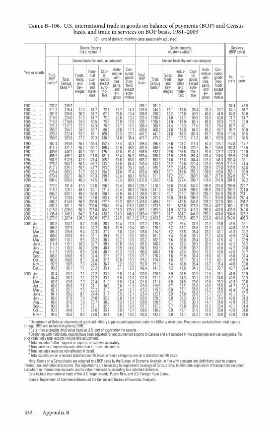
452 | Appendix B
Table B–106. U.S. international trade in goods on balance of payments (BOP) and Censusbasis, and trade in services on BOP basis, 1981–2009
[Billions of dollars; monthly data seasonally adjusted]
Year or month
Goods: Exports(f.a.s. value) 1, 2
Goods: Imports(customs value) 5
Services(BOP basis)
Total,BOP
basis 3
Census basis (by end-use category)
Total,BOPbasis
Census basis (by end-use category)
Ex-ports
Im-portsTotal,
Censusbasis 3, 4
Foods,feeds,
andbev-
erages
Indus-trialsup-pliesand
mate-rials
Capi-tal
goodsexceptauto-mo-tive
Auto-motivevehi-cles,parts,anden-
gines
Con-sumergoods(non-food)
exceptauto-
motive
Total,Censusbasis 4
Foods,feeds,
andbev-
erages
Indus-trialsup-pliesand
mate-rials
Capi-tal
goodsexceptauto-mo-tive
Auto-motivevehi-cles,parts,anden-
gines
Con-sumergoods(non-food)
exceptauto-
motive
1981 .............. 237.0 238.7 ........... ........... ........... ........... ........... 265.1 261.0 ........... ........... ........... ........... .......... 57.4 45.51982 .............. 211.2 216.4 31.3 61.7 72.7 15.7 14.3 247.6 244.0 17.1 112.0 35.4 33.3 39.7 64.1 51.71983 .............. 201.8 205.6 30.9 56.7 67.2 16.8 13.4 268.9 258.0 18.2 107.0 40.9 40.8 44.9 64.3 55.01984 .............. 219.9 224.0 31.5 61.7 72.0 20.6 13.3 332.4 6 330.7 21.0 123.7 59.8 53.5 60.0 71.2 67.71985 .............. 215.9 7 218.8 24.0 58.5 73.9 22.9 12.6 338.1 6 336.5 21.9 113.9 65.1 66.8 68.3 73.2 72.91986 .............. 223.3 7 227.2 22.3 57.3 75.8 21.7 14.2 368.4 365.4 24.4 101.3 71.8 78.2 79.4 86.7 80.11987 .............. 250.2 254.1 24.3 66.7 86.2 24.6 17.7 409.8 406.2 24.8 111.0 84.5 85.2 88.7 98.7 90.81988 .............. 320.2 322.4 32.3 85.1 109.2 29.3 23.1 447.2 441.0 24.8 118.3 101.4 87.7 95.9 110.9 98.51989 .............. 359.9 363.8 37.2 99.3 138.8 34.8 36.4 477.7 473.2 25.1 132.3 113.3 86.1 102.9 127.1 102.51990 .............. 387.4 393.6 35.1 104.4 152.7 37.4 43.3 498.4 495.3 26.6 143.2 116.4 87.3 105.7 147.8 117.71991 .............. 414.1 421.7 35.7 109.7 166.7 40.0 45.9 491.0 488.5 26.5 131.6 120.7 85.7 108.0 164.3 118.51992 .............. 439.6 448.2 40.3 109.1 175.9 47.0 51.4 536.5 532.7 27.6 138.6 134.3 91.8 122.7 177.3 119.61993 .............. 456.9 465.1 40.6 111.8 181.7 52.4 54.7 589.4 580.7 27.9 145.6 152.4 102.4 134.0 185.9 123.81994 .............. 502.9 512.6 42.0 121.4 205.0 57.8 60.0 668.7 663.3 31.0 162.0 184.4 118.3 146.3 200.4 133.11995 .............. 575.2 584.7 50.5 146.2 233.0 61.8 64.4 749.4 743.5 33.2 181.8 221.4 123.8 159.9 219.2 141.41996 .............. 612.1 625.1 55.5 147.7 253.0 65.0 70.1 803.1 795.3 35.7 204.5 228.1 128.9 172.0 239.5 152.61997 .............. 678.4 689.2 51.5 158.2 294.5 74.0 77.4 876.8 869.7 39.7 213.8 253.3 139.8 193.8 256.1 165.91998 .............. 670.4 682.1 46.4 148.3 299.4 72.4 80.3 918.6 911.9 41.2 200.1 269.5 148.7 217.0 262.8 180.71999 .............. 684.0 695.8 46.0 147.5 310.8 75.3 80.9 1,031.8 1,024.6 43.6 221.4 295.7 179.0 241.9 281.9 199.22000 .............. 772.0 781.9 47.9 172.6 356.9 80.4 89.4 1,226.7 1,218.0 46.0 299.0 347.0 195.9 281.8 298.6 223.72001 .............. 718.7 729.1 49.4 160.1 321.7 75.4 88.3 1,148.6 1,141.0 46.6 273.9 298.0 189.8 284.3 286.2 221.82002 .............. 685.2 693.1 49.6 156.8 290.4 78.9 84.4 1,168.0 1,161.4 49.7 267.7 283.3 203.7 307.8 292.3 231.12003 .............. 715.8 724.8 55.0 173.0 293.7 80.6 89.9 1,264.9 1,257.1 55.8 313.8 295.9 210.1 333.9 304.3 250.42004 .............. 806.2 814.9 56.6 203.9 327.5 89.2 103.2 1,478.0 1,469.7 62.1 412.8 343.6 228.2 372.9 353.1 291.22005 .............. 892.3 901.1 59.0 233.0 358.4 98.4 115.3 1,683.2 1,673.5 68.1 523.8 379.3 239.4 407.2 389.1 313.52006 .............. 1,015.8 1,026.0 66.0 276.0 404.0 107.3 129.1 1,863.1 1,853.9 74.9 602.0 418.3 256.6 442.6 435.9 349.02007 .............. 1,138.4 1,148.2 84.3 316.4 433.0 121.3 146.0 1,969.4 1,957.0 81.7 634.7 444.5 259.2 474.6 504.8 375.22008 .............. 1,277.0 1,287.4 108.3 388.0 457.7 121.5 161.3 2,117.2 2,103.6 89.0 779.5 453.7 233.8 481.6 549.6 405.32008: Jan ..... 103.8 104.7 8.7 30.0 38.2 10.4 13.3 177.7 176.8 7.2 65.4 37.9 21.2 39.8 45.5 33.1
Feb ..... 106.8 107.9 9.0 32.2 38.1 10.9 13.4 180.1 178.3 7.2 63.7 38.6 22.3 41.2 44.8 33.2Mar .... 105.1 105.8 9.4 32.3 37.4 9.8 12.8 176.6 174.9 7.2 63.5 38.4 20.2 40.1 45.3 33.2Apr ..... 109.0 109.8 9.5 33.1 39.1 10.2 13.5 183.5 181.8 7.4 68.0 39.1 21.2 40.5 45.9 33.4May .... 109.5 110.1 9.5 34.2 38.4 10.2 13.5 183.2 182.3 7.6 68.0 39.4 20.4 41.5 47.1 33.9June ... 114.4 115.1 10.0 36.7 39.4 10.8 14.0 187.6 186.7 7.4 73.2 38.5 20.5 41.4 47.2 34.2July .... 117.2 118.2 10.0 37.9 40.1 11.5 14.6 194.5 193.3 7.5 79.9 38.7 20.3 41.0 47.2 34.8Aug ..... 114.7 115.9 9.9 37.0 40.4 10.3 13.9 186.8 186.1 7.8 73.4 38.0 19.3 42.0 47.0 35.7Sept .... 106.0 106.6 9.0 32.4 37.6 10.2 13.5 177.7 176.2 7.6 65.9 38.4 18.6 40.1 46.0 34.4Oct ...... 103.8 104.8 8.3 31.4 37.5 10.0 13.3 175.2 174.4 7.6 66.1 37.2 17.9 40.1 45.9 33.9Nov ..... 97.5 98.5 7.9 27.6 36.4 9.2 13.2 151.8 151.0 7.4 48.8 35.4 16.7 37.4 44.0 33.0Dec ..... 89.2 90.1 7.1 23.2 35.1 8.1 12.6 142.4 141.9 7.2 43.6 34.1 15.2 36.7 43.7 32.4
2009: Jan ..... 82.4 83.2 7.1 22.2 33.2 5.6 11.4 130.0 129.6 6.9 38.5 31.9 11.5 36.1 41.6 30.9Feb ..... 84.4 85.2 7.1 22.2 33.3 6.0 12.8 121.6 121.2 6.7 34.3 30.1 10.2 34.6 40.9 30.3Mar .... 82.6 83.6 7.3 22.4 31.9 6.0 12.4 121.8 121.4 6.8 34.5 29.6 10.6 35.2 40.3 30.0Apr ..... 80.0 80.8 7.6 21.1 30.9 5.8 11.9 119.9 119.5 6.7 33.7 28.6 10.5 35.5 41.7 30.3May .... 82.1 83.1 7.9 23.2 31.0 5.4 12.1 119.3 119.0 6.8 33.1 28.9 10.2 35.5 41.4 30.0June ... 84.1 85.0 8.1 24.4 31.4 5.5 12.1 122.4 122.1 6.9 37.0 28.9 11.1 33.7 42.1 30.7July .... 86.8 87.8 7.8 24.8 32.2 6.8 12.4 129.5 129.3 6.8 38.3 30.1 13.4 35.4 42.6 31.3Aug ..... 86.8 87.6 7.9 25.7 30.9 7.3 12.3 128.8 128.4 6.7 37.5 30.1 14.7 34.8 42.9 31.2Sept .... 90.3 91.1 7.5 27.1 32.5 7.5 12.8 137.7 137.3 6.7 42.9 30.9 16.3 35.4 43.1 31.4Oct ...... 93.5 94.8 7.7 27.6 33.7 7.9 13.7 138.6 138.2 6.9 41.1 31.9 16.9 36.6 43.5 31.6Nov p .. 94.6 95.6 9.0 27.0 34.1 8.6 13.0 143.0 142.6 6.8 43.1 33.2 16.9 38.0 43.6 31.6
1 Department of Defense shipments of grant-aid military supplies and equipment under the Military Assistance Program are excluded from total exportsthrough 1985 and included beginning 1986.
2 F.a.s. (free alongside ship) value basis at U.S. port of exportation for exports.3 Beginning with 1989 data, exports have been adjusted for undocumented exports to Canada and are included in the appropriate end-use categories. For
prior years, only total exports include this adjustment.4 Total includes “other” exports or imports, not shown separately.5 Total arrivals of imported goods other than in-transit shipments.6 Total includes revisions not reflected in detail.7 Total exports are on a revised statistical month basis; end-use categories are on a statistical month basis.Note: Goods on a Census basis are adjusted to a BOP basis by the Bureau of Economic Analysis, in line with concepts and definitions used to prepare
international and national accounts. The adjustments are necessary to supplement coverage of Census data, to eliminate duplication of transactions recordedelsewhere in international accounts, and to value transactions according to a standard definition.
Data include international trade of the U.S. Virgin Islands, Puerto Rico, and U.S. Foreign Trade Zones.Source: Department of Commerce (Bureau of the Census and Bureau of Economic Analysis).
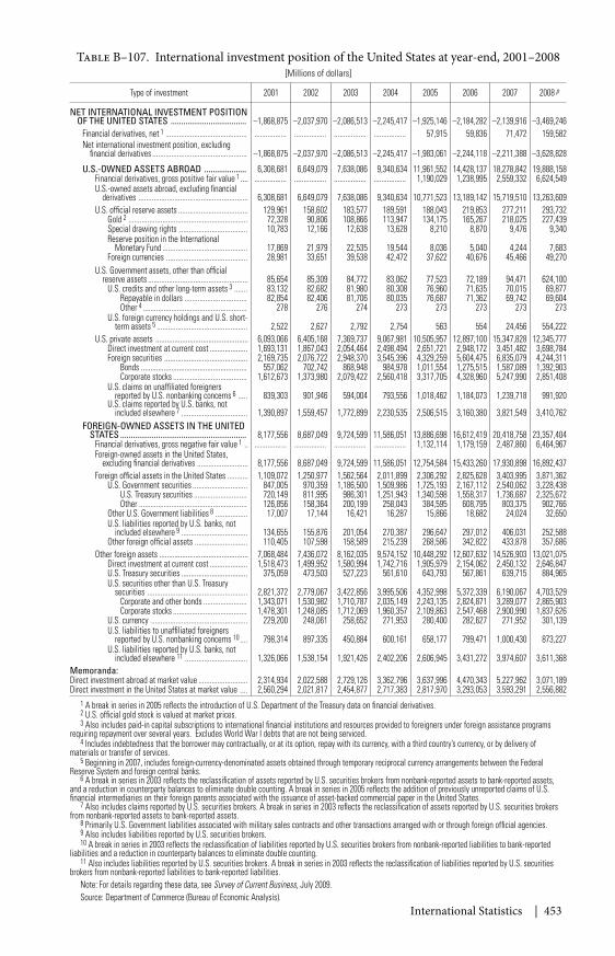
International Statistics | 453
Table B–107. International investment position of the United States at year-end, 2001–2008[Millions of dollars]
Type of investment 2001 2002 2003 2004 2005 2006 2007 2008 p
NET INTERNATIONAL INVESTMENT POSITIONOF THE UNITED STATES .................................... –1,868,875 –2,037,970 –2,086,513 –2,245,417 –1,925,146 –2,184,282 –2,139,916 –3,469,246
Financial derivatives, net 1 ........................................... ................. ................. ................. ................. 57,915 59,836 71,472 159,582Net international investment position, excluding
financial derivatives .................................................. –1,868,875 –2,037,970 –2,086,513 –2,245,417 –1,983,061 –2,244,118 –2,211,388 –3,628,828
U.S.-OWNED ASSETS ABROAD .................... 6,308,681 6,649,079 7,638,086 9,340,634 11,961,552 14,428,137 18,278,842 19,888,158Financial derivatives, gross positive fair value 1 .... ................. ................. ................. ................. 1,190,029 1,238,995 2,559,332 6,624,549U.S.-owned assets abroad, excluding financial
derivatives .......................................................... 6,308,681 6,649,079 7,638,086 9,340,634 10,771,523 13,189,142 15,719,510 13,263,609U.S. official reserve assets ..................................... 129,961 158,602 183,577 189,591 188,043 219,853 277,211 293,732
Gold 2 ............................................................... 72,328 90,806 108,866 113,947 134,175 165,267 218,025 227,439Special drawing rights .................................... 10,783 12,166 12,638 13,628 8,210 8,870 9,476 9,340Reserve position in the International
Monetary Fund ............................................. 17,869 21,979 22,535 19,544 8,036 5,040 4,244 7,683Foreign currencies ........................................... 28,981 33,651 39,538 42,472 37,622 40,676 45,466 49,270
U.S. Government assets, other than officialreserve assets ..................................................... 85,654 85,309 84,772 83,062 77,523 72,189 94,471 624,100
U.S. credits and other long-term assets 3 ....... 83,132 82,682 81,980 80,308 76,960 71,635 70,015 69,877Repayable in dollars ................................. 82,854 82,406 81,706 80,035 76,687 71,362 69,742 69,604Other 4 ....................................................... 278 276 274 273 273 273 273 273
U.S. foreign currency holdings and U.S. short-term assets 5 ................................................ 2,522 2,627 2,792 2,754 563 554 24,456 554,222
U.S. private assets ................................................. 6,093,066 6,405,168 7,369,737 9,067,981 10,505,957 12,897,100 15,347,828 12,345,777Direct investment at current cost .................... 1,693,131 1,867,043 2,054,464 2,498,494 2,651,721 2,948,172 3,451,482 3,698,784Foreign securities ............................................ 2,169,735 2,076,722 2,948,370 3,545,396 4,329,259 5,604,475 6,835,079 4,244,311
Bonds ........................................................ 557,062 702,742 868,948 984,978 1,011,554 1,275,515 1,587,089 1,392,903Corporate stocks ....................................... 1,612,673 1,373,980 2,079,422 2,560,418 3,317,705 4,328,960 5,247,990 2,851,408
U.S. claims on unaffiliated foreignersreported by U.S. nonbanking concerns 6 ..... 839,303 901,946 594,004 793,556 1,018,462 1,184,073 1,239,718 991,920
U.S. claims reported by U.S. banks, notincluded elsewhere 7 ................................... 1,390,897 1,559,457 1,772,899 2,230,535 2,506,515 3,160,380 3,821,549 3,410,762
FOREIGN-OWNED ASSETS IN THE UNITEDSTATES ............................................................ 8,177,556 8,687,049 9,724,599 11,586,051 13,886,698 16,612,419 20,418,758 23,357,404
Financial derivatives, gross negative fair value 1 .. ................. ................. ................. ................. 1,132,114 1,179,159 2,487,860 6,464,967Foreign-owned assets in the United States,
excluding financial derivatives ........................... 8,177,556 8,687,049 9,724,599 11,586,051 12,754,584 15,433,260 17,930,898 16,892,437Foreign official assets in the United States ........... 1,109,072 1,250,977 1,562,564 2,011,899 2,306,292 2,825,628 3,403,995 3,871,362
U.S. Government securities ............................. 847,005 970,359 1,186,500 1,509,986 1,725,193 2,167,112 2,540,062 3,228,438U.S. Treasury securities ............................ 720,149 811,995 986,301 1,251,943 1,340,598 1,558,317 1,736,687 2,325,672Other ......................................................... 126,856 158,364 200,199 258,043 384,595 608,795 803,375 902,766
Other U.S. Government liabilities 8 ................. 17,007 17,144 16,421 16,287 15,866 18,682 24,024 32,650U.S. liabilities reported by U.S. banks, not
included elsewhere 9 ................................... 134,655 155,876 201,054 270,387 296,647 297,012 406,031 252,588Other foreign official assets ............................ 110,405 107,598 158,589 215,239 268,586 342,822 433,878 357,686
Other foreign assets ............................................... 7,068,484 7,436,072 8,162,035 9,574,152 10,448,292 12,607,632 14,526,903 13,021,075Direct investment at current cost .................... 1,518,473 1,499,952 1,580,994 1,742,716 1,905,979 2,154,062 2,450,132 2,646,847U.S. Treasury securities ................................... 375,059 473,503 527,223 561,610 643,793 567,861 639,715 884,965U.S. securities other than U.S. Treasury
securities ..................................................... 2,821,372 2,779,067 3,422,856 3,995,506 4,352,998 5,372,339 6,190,067 4,703,529Corporate and other bonds ....................... 1,343,071 1,530,982 1,710,787 2,035,149 2,243,135 2,824,871 3,289,077 2,865,903Corporate stocks ....................................... 1,478,301 1,248,085 1,712,069 1,960,357 2,109,863 2,547,468 2,900,990 1,837,626
U.S. currency ................................................... 229,200 248,061 258,652 271,953 280,400 282,627 271,952 301,139U.S. liabilities to unaffiliated foreigners
reported by U.S. nonbanking concerns 10 .... 798,314 897,335 450,884 600,161 658,177 799,471 1,000,430 873,227U.S. liabilities reported by U.S. banks, not
included elsewhere 11 ................................. 1,326,066 1,538,154 1,921,426 2,402,206 2,606,945 3,431,272 3,974,607 3,611,368Memoranda:Direct investment abroad at market value .......................... 2,314,934 2,022,588 2,729,126 3,362,796 3,637,996 4,470,343 5,227,962 3,071,189Direct investment in the United States at market value .... 2,560,294 2,021,817 2,454,877 2,717,383 2,817,970 3,293,053 3,593,291 2,556,882
1 A break in series in 2005 reflects the introduction of U.S. Department of the Treasury data on financial derivatives.2 U.S. official gold stock is valued at market prices.3 Also includes paid-in capital subscriptions to international financial institutions and resources provided to foreigners under foreign assistance programs
requiring repayment over several years. Excludes World War I debts that are not being serviced.4 Includes indebtedness that the borrower may contractually, or at its option, repay with its currency, with a third country’s currency, or by delivery of
materials or transfer of services.5 Beginning in 2007, includes foreign-currency-denominated assets obtained through temporary reciprocal currency arrangements between the Federal
Reserve System and foreign central banks.6 A break in series in 2003 reflects the reclassification of assets reported by U.S. securities brokers from nonbank-reported assets to bank-reported assets,
and a reduction in counterparty balances to eliminate double counting. A break in series in 2005 reflects the addition of previously unreported claims of U.S.financial intermediaries on their foreign parents associated with the issuance of asset-backed commercial paper in the United States.
7 Also includes claims reported by U.S. securities brokers. A break in series in 2003 reflects the reclassification of assets reported by U.S. securities brokersfrom nonbank-reported assets to bank-reported assets.
8 Primarily U.S. Government liabilities associated with military sales contracts and other transactions arranged with or through foreign official agencies.9 Also includes liabilities reported by U.S. securities brokers.10 A break in series in 2003 reflects the reclassification of liabilities reported by U.S. securities brokers from nonbank-reported liabilities to bank-reported
liabilities and a reduction in counterparty balances to eliminate double counting.11 Also includes liabilities reported by U.S. securities brokers. A break in series in 2003 reflects the reclassification of liabilities reported by U.S. securities
brokers from nonbank-reported liabilities to bank-reported liabilities.Note: For details regarding these data, see Survey of Current Business, July 2009.Source: Department of Commerce (Bureau of Economic Analysis).
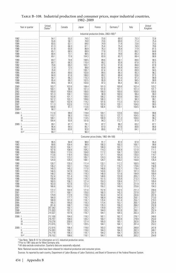
454 | Appendix B
Table B–108. Industrial production and consumer prices, major industrial countries,1982–2009
Year or quarter UnitedStates 1 Canada Japan France Germany 2 Italy United
Kingdom
Industrial production (Index, 2002=100) 3
1982 .................................. 54.1 53.2 74.5 73.6 69.5 73.3 72.81983 .................................. 55.6 56.1 76.8 73.6 69.8 71.4 75.41984 .................................. 60.5 63.1 84.0 74.9 71.9 73.8 75.51985 .................................. 61.3 66.3 87.1 75.4 75.4 74.9 79.61986 .................................. 61.9 65.8 86.9 76.3 76.9 77.9 81.51987 .................................. 65.1 68.5 89.9 77.8 77.2 80.2 84.81988 .................................. 68.4 73.1 98.5 81.0 79.9 85.3 88.91989 .................................. 69.1 72.9 104.3 83.9 83.7 88.4 90.81990 .................................. 69.7 70.9 108.5 89.6 88.1 88.6 90.51991 .................................. 68.7 68.3 110.4 89.2 93.9 87.8 87.51992 .................................. 70.6 69.2 103.7 87.5 91.8 86.8 87.81993 .................................. 72.9 72.5 99.8 83.8 84.9 84.8 89.71994 .................................. 76.8 77.1 100.7 87.4 87.4 89.9 94.51995 .................................. 80.4 80.6 103.8 89.5 88.3 95.3 96.21996 .................................. 84.0 81.6 106.0 89.2 88.4 93.6 97.51997 .................................. 90.1 86.2 110.3 92.5 91.0 97.3 98.91998 .................................. 95.4 89.2 102.5 95.9 94.4 98.5 99.91999 .................................. 99.5 94.4 103.0 97.3 95.4 98.3 101.42000 .................................. 103.7 102.6 108.4 101.0 100.8 102.4 103.22001 .................................. 100.1 98.4 101.3 101.8 101.1 101.3 101.72002 .................................. 100.0 100.0 100.0 100.0 100.0 100.0 100.02003 .................................. 101.3 100.1 103.0 98.9 100.5 99.4 99.32004 .................................. 103.8 101.7 108.0 100.2 103.6 99.0 100.42005 .................................. 107.2 103.7 109.6 100.3 107.1 98.3 99.12006 .................................. 109.7 102.9 114.2 101.6 113.3 101.8 99.22007 .................................. 111.3 102.6 117.6 102.8 120.1 104.0 99.52008 .................................. 108.8 97.2 113.6 100.4 120.1 100.5 96.42009 p ................................ 98.2 ........................... 88.3 ........................... ........................... ........................... .............................2008: I .............................. 112.0 99.0 119.8 104.1 123.6 105.6 99.6
II ............................. 110.7 98.3 118.4 102.2 122.7 104.5 98.2III ............................ 108.1 97.6 114.5 100.9 121.3 100.0 96.2IV ............................ 104.4 93.9 101.6 94.3 112.7 91.9 91.7
2009: I .............................. 99.1 87.7 79.1 87.7 98.2 83.2 87.1II ............................. 96.4 84.5 85.7 87.0 97.6 80.6 86.6III ............................ 98.0 83.8 92.0 89.6 101.2 84.1 85.8IV p ......................... 99.7 ........................... 96.3 ........................... ........................... ........................... .............................
Consumer prices (Index, 1982–84=100)
1982 .................................. 96.5 94.9 98.0 91.7 97.0 87.8 95.41983 .................................. 99.6 100.4 99.9 100.3 100.3 100.7 99.81984 .................................. 103.9 104.7 102.1 108.0 102.7 111.5 104.81985 .................................. 107.6 108.9 104.2 114.3 104.9 121.8 111.11986 .................................. 109.6 113.5 104.8 117.2 104.7 128.9 114.91987 .................................. 113.6 118.4 105.0 121.1 105.0 135.0 119.71988 .................................. 118.3 123.2 105.7 124.3 106.3 141.9 125.61989 .................................. 124.0 129.3 108.1 128.7 109.2 150.8 135.41990 .................................. 130.7 135.5 111.4 133.1 112.2 160.5 148.21991 .................................. 136.2 143.1 115.0 137.3 116.7 170.6 156.91992 .................................. 140.3 145.2 117.0 140.6 122.7 179.4 162.71993 .................................. 144.5 147.9 118.5 143.6 128.1 187.3 165.31994 .................................. 148.2 148.2 119.3 146.0 131.6 194.9 169.41995 .................................. 152.4 151.4 119.2 148.6 133.9 205.2 175.11996 .................................. 156.9 153.8 119.3 151.5 135.8 213.3 179.41997 .................................. 160.5 156.2 121.4 153.3 138.4 217.7 185.01998 .................................. 163.0 157.8 122.2 154.3 139.7 221.9 191.41999 .................................. 166.6 160.5 121.8 155.2 140.5 225.6 194.32000 .................................. 172.2 164.9 121.0 157.8 142.5 231.3 200.02001 .................................. 177.1 169.1 120.0 160.3 145.3 237.8 203.72002 .................................. 179.9 172.9 119.0 163.4 147.4 243.6 207.02003 .................................. 184.0 177.7 118.7 166.9 148.9 250.1 213.02004 .................................. 188.9 181.0 118.7 170.4 151.4 255.7 219.32005 .................................. 195.3 185.0 118.3 173.4 153.7 260.7 225.62006 .................................. 201.6 188.7 118.6 176.3 156.2 266.2 232.82007 .................................. 207.342 192.7 118.7 178.9 159.7 271.1 242.72008 .................................. 215.303 197.3 120.3 184.0 163.9 280.1 252.42009 p ................................ 214.537 197.9 118.7 184.1 164.5 282.3 251.12008: I .............................. 212.100 194.0 119.2 182.1 162.7 276.7 248.0
II ............................. 216.757 198.0 120.2 184.7 163.9 279.9 253.0III ............................ 219.278 200.0 121.4 185.0 165.1 282.6 255.4IV ............................ 213.075 197.1 120.5 184.1 164.1 281.4 253.2
2009: I .............................. 212.015 196.4 119.0 183.3 164.0 280.8 247.8II ............................. 214.263 198.1 119.0 184.3 164.3 282.3 249.7III ............................ 215.718 198.3 118.7 184.2 164.7 282.9 251.9IV p ......................... 216.152 198.6 118.1 184.7 164.9 283.2 254.8
1 See Note, Table B–51 for information on U.S. industrial production series.2 Prior to 1991 data are for West Germany only.3 All data exclude construction. Quarterly data are seasonally adjusted.Note: National sources data have been rebased for industrial production and consumer prices.Sources: As reported by each country, Department of Labor (Bureau of Labor Statistics), and Board of Governors of the Federal Reserve System.
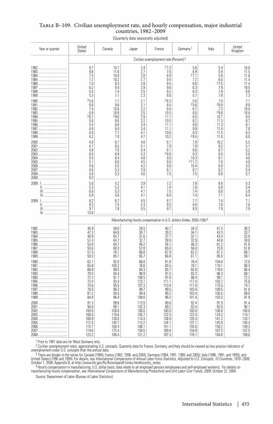
International Statistics | 455
Table B–109. Civilian unemployment rate, and hourly compensation, major industrialcountries, 1982–2009
[Quarterly data seasonally adjusted]
Year or quarter UnitedStates Canada Japan France Germany 1 Italy United
Kingdom
Civilian unemployment rate (Percent) 2
1982 .................................. 9.7 10.7 2.4 3 7.3 5.6 5.4 10.81983 .................................. 9.6 11.6 2.7 7.6 6.9 5.9 11.51984 .................................. 7.5 10.9 2.8 8.9 3 7.1 5.9 11.81985 .................................. 7.2 10.2 2.7 9.4 7.2 6.0 11.41986 .................................. 7.0 9.3 2.8 9.5 6.6 3 7.5 11.41987 .................................. 6.2 8.4 2.9 9.6 6.3 7.9 10.51988 .................................. 5.5 7.4 2.5 9.2 6.3 7.9 8.61989 .................................. 5.3 7.1 2.3 8.6 5.7 7.8 7.31990 .................................. 3 5.6 7.7 2.1 3 8.3 5.0 7.0 7.11991 .................................. 6.8 9.8 2.1 8.5 3 5.6 3 6.9 8.91992 .................................. 7.5 10.6 2.2 9.4 6.7 7.3 10.01993 .................................. 6.9 10.8 2.5 10.5 8.0 3 9.8 10.41994 .................................. 3 6.1 3 9.6 2.9 11.1 8.5 10.7 9.51995 .................................. 5.6 8.6 3.2 10.5 8.2 11.3 8.71996 .................................. 5.4 8.8 3.4 11.1 9.0 11.3 8.11997 .................................. 4.9 8.4 3.4 11.1 9.9 11.4 7.01998 .................................. 4.5 7.7 4.1 10.6 9.3 11.5 6.31999 .................................. 4.2 7.0 4.7 10.2 3 8.5 11.0 6.02000 .................................. 4.0 6.1 4.8 8.7 7.8 10.2 5.52001 .................................. 4.7 6.5 5.1 7.9 7.9 9.2 5.12002 .................................. 5.8 7.0 5.4 8.1 8.6 8.7 5.22003 .................................. 6.0 6.9 5.3 3 8.6 9.3 8.5 5.02004 .................................. 5.5 6.4 4.8 9.0 10.3 8.1 4.82005 .................................. 5.1 6.0 4.5 9.0 3 11.2 7.8 4.92006 .................................. 4.6 5.5 4.2 9.0 10.4 6.9 5.52007 .................................. 4.6 5.3 3.9 8.1 8.7 6.2 5.42008 .................................. 5.8 5.3 4.0 7.5 7.5 6.8 5.72009 .................................. 9.3 ........................... ........................... ........................... ........................... ........................... .............................2008: I .............................. 5.0 5.2 3.9 7.2 7.8 6.6 5.3
II ............................. 5.3 5.3 4.1 7.4 7.6 6.9 5.4III ............................ 6.0 5.3 4.1 7.5 7.4 6.8 5.9IV ............................ 6.9 5.6 4.1 8.0 7.4 7.1 6.4
2009: I .............................. 8.2 6.7 4.5 8.7 7.7 7.4 7.1II ............................. 9.3 7.5 5.3 9.3 8.0 7.6 7.8III ............................ 9.7 7.8 5.5 9.7 8.0 7.9 7.9IV ............................ 10.0 ........................... ........................... ........................... ........................... ........................... .............................
Manufacturing hourly compensation in U.S. dollars (Index, 2002=100) 4
1982 .................................. 45.9 59.8 28.5 40.7 34.3 41.5 36.31983 .................................. 47.3 64.0 30.7 39.3 34.1 43.3 33.71984 .................................. 48.9 64.7 31.6 37.7 32.1 43.4 32.01985 .................................. 51.4 64.7 32.7 39.9 32.9 44.8 34.01986 .................................. 53.8 64.7 48.2 54.1 46.3 61.2 41.81987 .................................. 55.6 69.3 57.8 65.0 58.4 75.9 51.81988 .................................. 57.5 78.1 66.8 67.9 62.2 81.2 60.11989 .................................. 59.3 85.1 65.7 66.8 61.1 85.0 59.11990 .................................. 62.1 92.0 66.8 81.8 76.4 104.8 72.01991 .................................. 65.8 100.2 76.6 83.5 79.1 110.1 80.31992 .................................. 68.9 99.5 84.3 93.7 92.0 118.0 80.41993 .................................. 70.5 94.4 98.9 91.5 92.2 96.3 69.11994 .................................. 72.2 91.7 109.5 97.0 98.4 99.1 72.21995 .................................. 73.4 93.4 123.1 111.1 117.4 103.7 75.81996 .................................. 74.6 95.5 107.3 110.4 117.0 115.5 74.71997 .................................. 76.5 96.3 99.7 99.5 103.4 109.5 81.81998 .................................. 81.2 94.5 94.4 99.2 103.4 105.5 89.01999 .................................. 84.8 96.4 108.6 98.2 101.4 103.3 91.92000 .................................. 91.3 99.6 113.9 89.6 92.4 91.9 91.42001 .................................. 94.8 98.1 102.3 89.2 92.4 92.0 90.72002 .................................. 100.0 100.0 100.0 100.0 100.0 100.0 100.02003 .................................. 108.0 116.6 105.7 122.5 122.4 124.2 114.12004 .................................. 108.9 130.0 114.3 138.9 135.3 141.2 133.72005 .................................. 112.5 145.7 113.2 144.1 137.1 145.9 140.42006 .................................. 114.7 160.4 106.1 151.1 144.0 150.2 149.32007 .................................. 119.6 175.4 104.5 169.4 159.9 167.5 167.52008 .................................. 123.2 180.4 121.2 187.3 176.1 184.6 159.0
1 Prior to 1991 data are for West Germany only.2 Civilian unemployment rates, approximating U.S. concepts. Quarterly data for France, Germany, and Italy should be viewed as less precise indicators of
unemployment under U.S. concepts than the annual data.3 There are breaks in the series for Canada (1994), France (1982, 1990, and 2003), Germany (1984, 1991, 1999, and 2005), Italy (1986, 1991, and 1993), and
United States (1990 and 1994). For details, see International Comparisons of Annual Labor Force Statistics, Adjusted to U.S. Concepts, 10 Countries, 1970–2008,October 1, 2009, Appendix B, at http://www.bls.gov/fls/flscomparelf/notes.htm#country_notes.
4 Hourly compensation in manufacturing, U.S. dollar basis; data relate to all employed persons (employees and self-employed workers). For details onmanufacturing hourly compensation, see International Comparisons of Manufacturing Productivity and Unit Labor Cost Trends, 2008, October 22, 2009.
Source: Department of Labor (Bureau of Labor Statistics).
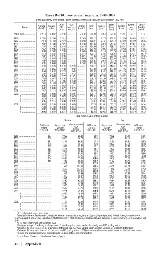
456 | Appendix B
Table B–110. Foreign exchange rates, 1988–2009[Foreign currency units per U.S. dollar, except as noted; certified noon buying rates in New York]
Period Australia(dollar) 1
Canada(dollar)
China,P.R.
(yuan)
EMUMembers(euro) 1, 2
Germany(mark) 2
Japan(yen)
Mexico(peso)
SouthKorea(won)
Sweden(krona)
Switzer-land
(franc)
UnitedKingdom(pound) 1
March 1973 ...................... 1.2716 0.9967 2.2401 ................ 2.8132 261.90 0.013 398.85 4.4294 3.2171 2.4724
1988 ................................. 0.7841 1.2306 3.7314 ................ 1.7570 128.17 2.273 734.52 6.1370 1.4643 1.78131989 ................................. .7919 1.1842 3.7673 ................ 1.8808 138.07 2.461 674.13 6.4559 1.6369 1.63821990 ................................. .7807 1.1668 4.7921 ................ 1.6166 145.00 2.813 710.64 5.9231 1.3901 1.78411991 ................................. .7787 1.1460 5.3337 ................ 1.6610 134.59 3.018 736.73 6.0521 1.4356 1.76741992 ................................. .7352 1.2085 5.5206 ................ 1.5618 126.78 3.095 784.66 5.8258 1.4064 1.76631993 ................................. .6799 1.2902 5.7795 ................ 1.6545 111.08 3.116 805.75 7.7956 1.4781 1.50161994 ................................. .7316 1.3664 8.6397 ................ 1.6216 102.18 3.385 806.93 7.7161 1.3667 1.53191995 ................................. .7407 1.3725 8.3700 ................ 1.4321 93.96 6.447 772.69 7.1406 1.1812 1.57851996 ................................. .7828 1.3638 8.3389 ................ 1.5049 108.78 7.600 805.00 6.7082 1.2361 1.56071997 ................................. .7437 1.3849 8.3193 ................ 1.7348 121.06 7.918 953.19 7.6446 1.4514 1.63761998 ................................. .6291 1.4836 8.3008 ................ 1.7597 130.99 9.152 1,400.40 7.9522 1.4506 1.65731999 ................................. .6454 1.4858 8.2783 1.0653 ................ 113.73 9.553 1,189.84 8.2740 1.5045 1.61722000 ................................. .5815 1.4855 8.2784 .9232 ................ 107.80 9.459 1,130.90 9.1735 1.6904 1.51562001 ................................. .5169 1.5487 8.2770 .8952 ................ 121.57 9.337 1,292.02 10.3425 1.6891 1.43962002 ................................. .5437 1.5704 8.2771 .9454 ................ 125.22 9.663 1,250.31 9.7233 1.5567 1.50252003 ................................. .6524 1.4008 8.2772 1.1321 ................ 115.94 10.793 1,192.08 8.0787 1.3450 1.63472004 ................................. .7365 1.3017 8.2768 1.2438 ................ 108.15 11.290 1,145.24 7.3480 1.2428 1.83302005 ................................. .7627 1.2115 8.1936 1.2449 ................ 110.11 10.894 1,023.75 7.4710 1.2459 1.82042006 ................................. .7535 1.1340 7.9723 1.2563 ................ 116.31 10.906 954.32 7.3718 1.2532 1.84342007 ................................. .8391 1.0734 7.6058 1.3711 ................ 117.76 10.928 928.97 6.7550 1.1999 2.00202008 ................................. .8537 1.0660 6.9477 1.4726 ................ 103.39 11.143 1,098.71 6.5846 1.0816 1.85452009 ................................. .7927 1.1412 6.8307 1.3935 ................ 93.68 13.498 1,274.63 7.6539 1.0860 1.56612008: I ............................. .9058 1.0039 7.1590 1.5007 ................ 105.17 10.803 956.12 6.2668 1.0670 1.9790
II ............................ .9436 1.0099 6.9578 1.5625 ................ 104.62 10.428 1,017.02 5.9862 1.0316 1.9712III ........................... .8879 1.0411 6.8375 1.5030 ................ 107.58 10.328 1,064.56 6.3175 1.0734 1.8924IV ........................... .6735 1.2115 6.8400 1.3202 ................ 96.01 13.061 1,360.86 7.7957 1.1560 1.5704
2009: I ............................. .6644 1.2455 6.8361 1.3035 ................ 93.78 14.384 1,415.27 8.4107 1.1487 1.4344II ............................ .7609 1.1682 6.8293 1.3619 ................ 97.42 13.315 1,282.78 7.9239 1.1123 1.5502III ........................... .8332 1.0980 6.8306 1.4304 ................ 93.54 13.261 1,237.55 7.2907 1.0623 1.6410IV ........................... .9090 1.0557 6.8271 1.4762 ................ 89.88 13.062 1,166.70 7.0114 1.0219 1.6335
Trade-weighted value of the U.S. dollar
Nominal Real 7
G-10 index(March
1973=100) 3
Broad index(January
1997=100) 4
Major currenciesindex
(March1973=100) 5
OITP index(January
1997=100) 6
Broad index(March
1973=100) 4
Major currenciesindex
(March1973=100) 5
OITP index(March
1973=100) 6
1988 ................................. 92.7 60.92 90.43 24.07 92.09 84.24 115.571989 ................................. 98.6 66.90 94.29 29.61 93.83 88.58 110.111990 ................................. 89.1 71.41 89.91 40.10 91.30 85.21 109.761991 ................................. 89.8 74.35 88.59 46.69 89.77 83.54 108.851992 ................................. 86.6 76.91 87.00 53.13 87.88 82.40 105.241993 ................................. 93.2 83.78 89.90 63.37 89.23 85.65 102.611994 ................................. 91.3 90.87 88.43 80.54 89.06 85.30 102.621995 ................................. 84.2 92.65 83.41 92.51 86.61 81.43 102.681996 ................................. 87.3 97.46 87.25 98.24 88.62 86.34 99.681997 ................................. 96.4 104.43 93.93 104.64 93.34 93.63 100.731998 ................................. 98.8 115.89 98.45 125.89 101.32 98.70 113.931999 ................................. ............................ 116.04 96.89 129.20 100.69 98.44 112.642000 ................................. ........................... 119.45 101.58 129.84 104.55 105.08 112.822001 ................................. ........................... 125.93 107.67 135.91 110.56 112.54 117.352002 ................................. ........................... 126.67 105.99 140.36 110.71 110.92 119.812003 ................................. ........................... 119.11 92.99 143.52 104.00 97.85 121.412004 ................................. ........................... 113.63 85.37 143.38 99.38 90.86 120.052005 ................................. ........................... 110.71 83.71 138.89 97.75 90.67 116.382006 ................................. ........................... 108.52 82.46 135.38 96.64 90.58 113.702007 ................................. ........................... 103.40 77.84 130.28 92.03 86.40 108.072008 ................................. ........................... 99.83 74.34 127.23 88.29 83.44 103.022009 ................................. ........................... 105.87 77.75 136.68 91.84 86.55 107.532008: I ............................. ........................... 97.31 71.97 124.96 85.92 80.36 101.27
II ............................ ........................... 95.80 70.87 123.01 85.61 80.10 100.86III ........................... ........................... 97.88 73.46 123.79 87.58 83.28 101.56IV ........................... ........................... 108.35 81.19 137.18 94.06 90.03 108.39
2009: I ............................. ........................... 111.12 82.68 141.89 95.95 91.41 111.07II ............................ ........................... 107.08 79.41 136.91 93.43 88.74 108.48III ........................... ........................... 103.69 75.45 135.01 90.58 84.55 106.98IV ........................... ........................... 101.61 73.58 132.91 87.41 81.51 103.59
1 U.S. dollars per foreign currency unit.2 European Economic and Monetary Union (EMU) members consists of Austria, Belgium, Cyprus (beginning in 2008), Finland, France, Germany, Greece
(beginning in 2001), Ireland, Italy, Luxembourg, Malta (beginning in 2008), Netherlands, Portugal, Slovakia (beginning in 2009), Slovenia (beginning in 2007), andSpain.
3 G-10 index discontinued after December 1998.4 Weighted average of the foreign exchange value of the dollar against the currencies of a broad group of U.S. trading partners.5 Subset of the broad index. Consists of currencies of the Euro area, Australia, Canada, Japan, Sweden, Switzerland, and the United Kingdom.6 Subset of the broad index. Consists of other important U.S. trading partners (OITP) whose currencies are not heavily traded outside their home markets.7 Adjusted for changes in consumer price indexes for the United States and other countries.Source: Board of Governors of the Federal Reserve System.
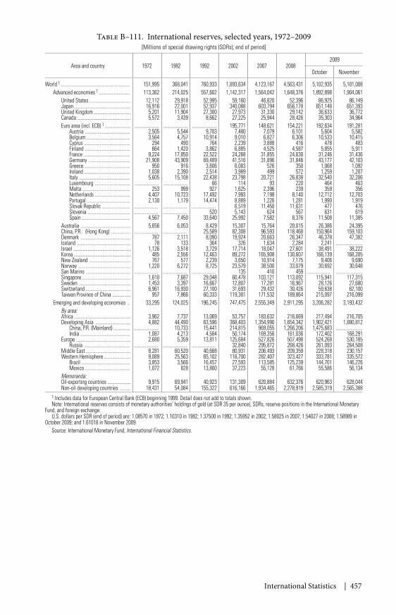
International Statistics | 457
Table B–111. International reserves, selected years, 1972–2009[Millions of special drawing rights (SDRs); end of period]
Area and country 1972 1982 1992 2002 2007 20082009
October November
World 1 ......................................................... 151,995 368,041 760,933 1,893,634 4,123,167 4,563,431 5,102,935 5,101,008Advanced economies 1 ......................... 113,362 214,025 557,602 1,142,317 1,564,042 1,648,376 1,892,898 1,904,061
United States .................................. 12,112 29,918 52,995 59,160 46,820 52,396 86,925 86,149Japan .............................................. 16,916 22,001 52,937 340,088 603,794 656,178 651,148 651,393United Kingdom .............................. 5,201 11,904 27,300 27,973 31,330 29,142 36,633 36,772Canada ............................................ 5,572 3,439 8,662 27,225 25,944 28,426 35,303 34,964Euro area (incl. ECB) 1 ..................... .................... .................... .................... 195,771 148,621 154,221 192,634 191,281
Austria ..................................... 2,505 5,544 9,703 7,480 7,079 6,101 5,604 5,582Belgium .................................... 3,564 4,757 10,914 9,010 6,827 6,306 10,533 10,415Cyprus ...................................... 294 490 764 2,239 3,888 416 478 483Finland ..................................... 664 1,420 3,862 6,885 4,525 4,587 5,855 5,911France ...................................... 9,224 17,850 22,522 24,268 31,855 24,630 31,246 31,436Germany .................................. 21,908 43,909 69,489 41,516 31,896 31,846 43,177 42,103Greece ...................................... 950 916 3,606 6,083 526 350 1,068 1,092Ireland ...................................... 1,038 2,390 2,514 3,989 499 572 1,259 1,207Italy .......................................... 5,605 15,108 22,438 23,798 20,721 26,838 32,540 32,206Luxembourg ............................. .................... .................... 66 114 93 220 464 463Malta ....................................... 253 999 927 1,625 2,396 239 359 356Netherlands ............................. 4,407 10,723 17,492 7,993 7,198 8,140 12,712 12,703Portugal .................................... 2,130 1,179 14,474 8,889 1,226 1,281 1,990 1,919Slovak Republic ....................... .................... .................... .................... 6,519 11,450 11,631 477 476Slovenia ................................... .................... .................... 520 5,143 624 567 631 619Spain ........................................ 4,567 7,450 33,640 25,992 7,582 8,376 11,508 11,385
Australia ......................................... 5,656 6,053 8,429 15,307 15,764 20,015 26,386 24,395China, P.R.: (Hong Kong) ................ .................... .................... 25,589 82,308 96,593 118,468 150,964 159,103Denmark ......................................... 787 2,111 8,090 19,924 20,663 26,347 46,378 47,382Iceland ............................................ 78 133 364 326 1,634 2,284 2,241 ......................Israel ............................................... 1,126 3,518 3,729 17,714 18,047 27,601 38,491 38,222Korea ............................................... 485 2,556 12,463 89,272 165,908 130,607 166,139 168,205New Zealand .................................. 767 577 2,239 3,650 10,914 7,175 9,406 9,690Norway ........................................... 1,220 6,272 8,725 23,579 38,500 33,079 30,692 30,648San Marino ..................................... .................... .................... .................... 135 410 459 .................... ......................Singapore ........................................ 1,610 7,687 29,048 60,478 103,121 113,092 115,941 117,315Sweden ........................................... 1,453 3,397 16,667 12,807 17,281 16,967 28,126 27,680Switzerland ..................................... 6,961 16,930 27,100 31,693 29,432 30,426 59,638 62,100Taiwan Province of China ............... 957 7,866 60,333 119,381 171,532 189,864 215,097 216,099
Emerging and developing economies .. 33,295 124,025 196,245 747,475 2,555,349 2,911,295 3,206,282 3,193,432By area:Africa .............................................. 3,962 7,737 13,069 53,757 183,632 216,669 217,494 216,705Developing Asia ............................. 4,882 44,490 63,596 368,403 1,354,990 1,654,342 1,902,421 1,880,812
China, P.R. (Mainland) .............. .................... 10,733 15,441 214,815 969,055 1,266,206 1,475,683 ......................India ......................................... 1,087 4,213 4,584 50,174 169,356 161,036 172,402 168,291
Europe ............................................. 2,680 5,359 13,811 125,684 527,826 507,498 524,268 530,185Russia ...................................... .................... .................... .................... 32,840 295,872 268,426 261,093 264,508
Middle East ..................................... 8,281 60,520 40,668 80,931 206,493 209,359 228,318 230,157Western Hemisphere ...................... 9,089 25,563 65,102 118,700 282,407 323,427 333,781 335,572
Brazil ........................................ 3,853 3,566 16,457 27,593 113,585 125,239 144,701 146,226Mexico ..................................... 1,072 828 13,800 37,223 55,128 61,766 55,586 56,134
Memoranda:Oil-exporting countries ................... 9,915 69,941 40,923 131,309 620,884 632,376 620,963 628,044Non-oil developing countries ......... 18,431 54,084 155,322 616,166 1,934,465 2,278,919 2,585,319 2,565,388
1 Includes data for European Central Bank (ECB) beginning 1999. Detail does not add to totals shown.Note: International reserves consists of monetary authorities’ holdings of gold (at SDR 35 per ounce), SDRs, reserve positions in the International Monetary
Fund, and foreign exchange.U.S. dollars per SDR (end of period) are: 1.08570 in 1972; 1.10310 in 1982; 1.37500 in 1992; 1.35952 in 2002; 1.58025 in 2007; 1.54027 in 2008; 1.58989 in
October 2009; and 1.61018 in November 2009.Source: International Monetary Fund, International Financial Statistics.
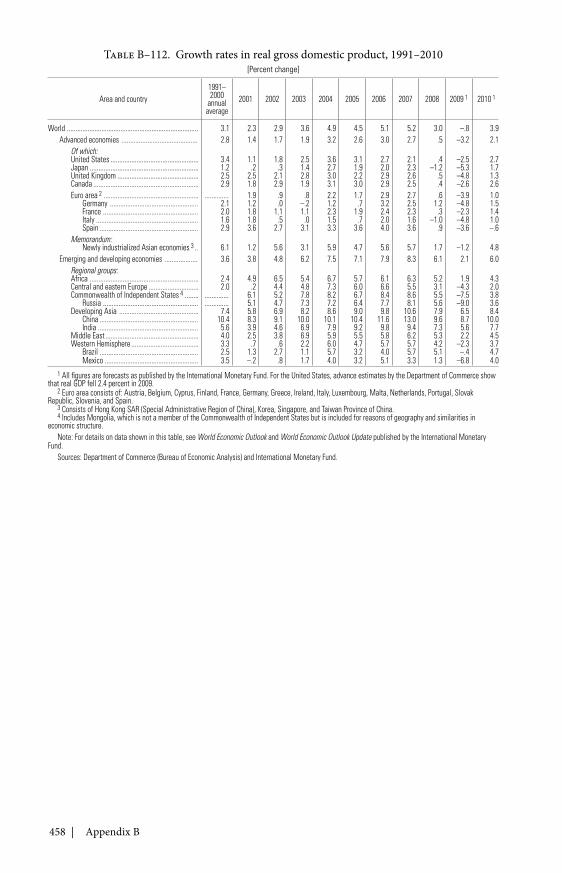
458 | Appendix B
Table B–112. Growth rates in real gross domestic product, 1991–2010[Percent change]
Area and country1991–2000
annualaverage
2001 2002 2003 2004 2005 2006 2007 2008 2009 1 2010 1
World ............................................................................ 3.1 2.3 2.9 3.6 4.9 4.5 5.1 5.2 3.0 –.8 3.9Advanced economies ............................................ 2.8 1.4 1.7 1.9 3.2 2.6 3.0 2.7 .5 –3.2 2.1
Of which:United States ................................................... 3.4 1.1 1.8 2.5 3.6 3.1 2.7 2.1 .4 –2.5 2.7Japan ............................................................... 1.2 .2 .3 1.4 2.7 1.9 2.0 2.3 –1.2 –5.3 1.7United Kingdom ............................................... 2.5 2.5 2.1 2.8 3.0 2.2 2.9 2.6 .5 –4.8 1.3Canada ............................................................. 2.9 1.8 2.9 1.9 3.1 3.0 2.9 2.5 .4 –2.6 2.6Euro area 2 ....................................................... .............. 1.9 .9 .8 2.2 1.7 2.9 2.7 .6 –3.9 1.0
Germany ................................................... 2.1 1.2 .0 –.2 1.2 .7 3.2 2.5 1.2 –4.8 1.5France ....................................................... 2.0 1.8 1.1 1.1 2.3 1.9 2.4 2.3 .3 –2.3 1.4Italy ........................................................... 1.6 1.8 .5 .0 1.5 .7 2.0 1.6 –1.0 –4.8 1.0Spain ......................................................... 2.9 3.6 2.7 3.1 3.3 3.6 4.0 3.6 .9 –3.6 –.6
Memorandum:Newly industrialized Asian economies 3 .. 6.1 1.2 5.6 3.1 5.9 4.7 5.6 5.7 1.7 –1.2 4.8
Emerging and developing economies ................... 3.6 3.8 4.8 6.2 7.5 7.1 7.9 8.3 6.1 2.1 6.0Regional groups:Africa ............................................................... 2.4 4.9 6.5 5.4 6.7 5.7 6.1 6.3 5.2 1.9 4.3Central and eastern Europe ............................. 2.0 .2 4.4 4.8 7.3 6.0 6.6 5.5 3.1 –4.3 2.0Commonwealth of Independent States 4 ........ .............. 6.1 5.2 7.8 8.2 6.7 8.4 8.6 5.5 –7.5 3.8
Russia ....................................................... .............. 5.1 4.7 7.3 7.2 6.4 7.7 8.1 5.6 –9.0 3.6Developing Asia .............................................. 7.4 5.8 6.9 8.2 8.6 9.0 9.8 10.6 7.9 6.5 8.4
China ......................................................... 10.4 8.3 9.1 10.0 10.1 10.4 11.6 13.0 9.6 8.7 10.0India .......................................................... 5.6 3.9 4.6 6.9 7.9 9.2 9.8 9.4 7.3 5.6 7.7
Middle East ...................................................... 4.0 2.5 3.8 6.9 5.9 5.5 5.8 6.2 5.3 2.2 4.5Western Hemisphere ....................................... 3.3 .7 .6 2.2 6.0 4.7 5.7 5.7 4.2 –2.3 3.7
Brazil ......................................................... 2.5 1.3 2.7 1.1 5.7 3.2 4.0 5.7 5.1 –.4 4.7Mexico ...................................................... 3.5 –.2 .8 1.7 4.0 3.2 5.1 3.3 1.3 –6.8 4.0
1 All figures are forecasts as published by the International Monetary Fund. For the United States, advance estimates by the Department of Commerce showthat real GDP fell 2.4 percent in 2009.
2 Euro area consists of: Austria, Belgium, Cyprus, Finland, France, Germany, Greece, Ireland, Italy, Luxembourg, Malta, Netherlands, Portugal, SlovakRepublic, Slovenia, and Spain.
3 Consists of Hong Kong SAR (Special Administrative Region of China), Korea, Singapore, and Taiwan Province of China.4 Includes Mongolia, which is not a member of the Commonwealth of Independent States but is included for reasons of geography and similarities in
economic structure.Note: For details on data shown in this table, see World Economic Outlook and World Economic Outlook Update published by the International Monetary
Fund.Sources: Department of Commerce (Bureau of Economic Analysis) and International Monetary Fund.
Related Documents