Economic Report of the President | i Economic Report of the President For sale by the Superintendent of Documents, U.S. Government Printing Office Internet: bookstore.gpo.gov Phone: toll free (866) 512-1800; DC area (202) 512-1800 Fax: (202) 512-2250 Mail: Stop SSOP, Washington, DC 20402-0001 ISBN 0-16-051539-4 Transmitted to the Congress February 2004 together with THE ANNUAL REPORT of the COUNCIL OF ECONOMIC ADVISERS UNITED STATES GOVERNMENT PRINTING OFFICE WASHINGTON : 2004 108th Congress, 2nd Session..............H. Doc. 108-145

Welcome message from author
This document is posted to help you gain knowledge. Please leave a comment to let me know what you think about it! Share it to your friends and learn new things together.
Transcript

Economic Report of the President | i
Economic Reportof the President
For sale by the Superintendent of Documents, U.S. Government Printing OfficeInternet: bookstore.gpo.gov Phone: toll free (866) 512-1800; DC area (202) 512-1800
Fax: (202) 512-2250 Mail: Stop SSOP, Washington, DC 20402-0001
ISBN 0-16-051539-4
Transmitted to the CongressFebruary 2004
together with
THE ANNUAL REPORTof the
COUNCIL OF ECONOMIC ADVISERS
UNITED STATES GOVERNMENT PRINTING OFFICE
WASHINGTON : 2004
108th Congress, 2nd Session..............H. Doc. 108-145


C O N T E N T S
ECONOMIC REPORT OF THE PRESIDENT...............................................
ANNUAL REPORT OF THE COUNCIL OF ECONOMIC ADVISERS*......
OVERVIEW.......................................................................................................
CHAPTER 1. LESSONS FROM THE RECENT BUSINESS CYCLE .............
CHAPTER 2. THE MANUFACTURING SECTOR........................................
CHAPTER 3. THE YEAR IN REVIEW AND THE YEARS AHEAD ..............
CHAPTER 4. TAX INCIDENCE: WHO BEARS THE TAX BURDEN? .........
CHAPTER 5. DYNAMIC REVENUE AND BUDGET ESTIMATION..........
CHAPTER 6. RESTORING SOLVENCY TO SOCIAL SECURITY ...............
CHAPTER 7. GOVERNMENT REGULATION IN A FREE-MARKET SOCIETY.........................................................................................................
CHAPTER 8. REGULATING ENERGY MARKETS .......................................
CHAPTER 9. PROTECTING THE ENVIRONMENT...................................
CHAPTER 10. HEALTH CARE AND INSURANCE......................................
CHAPTER 11. THE TORT SYSTEM...............................................................
CHAPTER 12. INTERNATIONAL TRADE AND COOPERATION.............
CHAPTER 13. INTERNATIONAL CAPITAL FLOWS ...................................
CHAPTER 14. THE LINK BETWEEN TRADE AND CAPITAL FLOWS......
APPENDIX A. REPORT TO THE PRESIDENT ON THE ACTIVITIESOF THE COUNCIL OF ECONOMIC ADVISERS DURING 2003.............
APPENDIX B. STATISTICAL TABLES RELATING TO INCOME,EMPLOYMENT, AND PRODUCTION........................................................
1
9
17
29
53
83
103
117
129
149
157
173
189
203
223
239
253
265
277
* For a detailed table of contents of the Council’s Report, see page 9
Page
Economic Report of the President | iii


Economic Report of the President | v
ECONOMIC REPORTOF THE PRESIDENT


Economic Report of the President | 3
ECONOMIC REPORT OF THE PRESIDENT
To the Congress of the United States:
As 2004 begins, America’s economy is strong and getting stronger. Over thepast several years, this Nation has faced major economic challenges resultingfrom the decline of the stock market beginning in early 2000, a recession thatbegan shortly after, revelations about corporate governance scandals, slowgrowth among many of our major trading partners, terrorist attacks, and thewar against terror, including in Afghanistan and Iraq. These challenges affectedbusiness and consumer confidence and resulted in hardship for people inmany industries and regions of our Nation. Americans have responded to eachchallenge, and now we have the results: renewed confidence, strong growth,new jobs, and a mounting prosperity that will reach every corner of America.
This Report, prepared by my Council of Economic Advisers, describes theeconomic challenges we faced, the actions we took, and the results we areseeing. It also discusses our plan to continue growing the economy andcreating jobs.
In May 2003, I signed a Jobs and Growth bill that focused on three keygoals. First, we accelerated previously passed tax relief and let American house-holds keep more of their own money to save, invest, and spend. Second, weincreased incentives for small businesses to invest in new equipment and plantexpansions. Third, we enacted important tax relief on dividend income andcapital gains to help investors and businesses. These actions were designed topromote investment, job creation, and income growth. By all three measures ofperformance, we are seeing signs of success.
Since May 2003, we have seen the economy grow at its fastest pace in nearly 20 years. Consumers and businesses have gained confidence. Retail sales arestrong, and Americans are buying, building, and renovating houses at a recordpace. Investment has strengthened, with spending on business equipment the bestin 5 years. The unemployment rate has fallen from its peak of 6.3 percent last Juneto 5.7 percent in December, and employment is beginning to rise as new jobs are

THE WHITE HOUSE
FEBRUARY 2004
4 | Economic Report of the President
created, especially in small business. Productivity growth has been strong, leading tohigher incomes for workers, while the tax relief we passed means that Americanfamilies keep more of their money instead of sending it to Washington.
We are moving in the right direction, but have more to do. I will not be satisfied until every American who wants a job can find one. I have outlined asix-point plan to promote job creation and strong economic growth. This planincludes initiatives to help manage rising health care costs to make health caremore affordable and accessible for American workers and families; reduce theburden of junk lawsuits on the economy; ensure a reliable and affordable energysupply; simplify and streamline government regulations; open foreign marketsfor American goods and services; and allow businesses and families to keep moreof their hard-earned money and plan with confidence by making our tax reliefpermanent. This year, I will work with the Congress to achieve these goals.
I will also continue to work with the Congress on another important sharedgoal: controlling federal spending and reducing the deficit. The federal budget isin deficit, foremost because of the economic slowdown and then recession thatbegan in 2000 and the additional costs of fighting the war on terror andprotecting the homeland. We are continuing to take action to restrain spendingand bring the deficit down. By carefully evaluating priorities and being goodstewards of the taxpayer’s money, we will cut the budget deficit in half over thenext five years.
The task of reducing the deficit will become easier because America’s economy isgrowing. We have taken the actions needed to restore growth, and we are pursuingadditional policies to help create jobs for American workers and families. I’m optimistic about the future of our economy because I know the values of Americaand the decency and entrepreneurial spirit of our people.

Economic Report of the President | 5
THE ANNUAL REPORTOF THE
COUNCIL OF ECONOMIC ADVISERS


Economic Report of the President | 7
LETTER OF TRANSMITTAL
COUNCIL OF ECONOMIC ADVISERS,Washington, D.C., January 30, 2004
MR. PRESIDENT:The Council of Economic Advisers herewith submits its 2004 Annual
Report in accordance with the provisions of the Employment Act of 1946 asamended by the Full Employment and Balanced Growth Act of 1978.
Sincerely,
N. Gregory MankiwChairman
Kristin J. ForbesMember
Harvey S. RosenMember


9
overview ............................................................................................. 17
chapter 1. lessons from the recent business cycle....................... 29Overview of the Recent Business Cycle ............................................ 30Lesson 1: Structural Imbalances Can Take Some Time to Resolve.... 33Lesson 2: Uncertainty Matters for Economic Decisions ................... 37Lesson 3: Aggressive Monetary Policy Can Reduce the Depth of a
Recession........................................................................................ 40Lesson 4: Tax Cuts Can Boost Economic Activity by Raising
After-Tax Income and Enhancing Incentives to Work, Save, and Invest ...................................................................................... 43
Lesson 5: Strong Productivity Growth Raises Standards of Livingbut Means that Much Faster Economic Growth is Needed to Raise Employment.................................................................... 46
Conclusion....................................................................................... 51
chapter 2. the manufacturing sector ............................................ 53Manufacturing and the Recent Business Cycle ................................. 53
The Recent Downturn in Manufacturing Output....................... 54Manufacturing Employment in Recent Years .............................. 56Signs of Recovery in the Manufacturing Sector ........................... 57
Long-Term Trends............................................................................ 59Manufacturing Output over the Long Term................................ 59Manufacturing Productivity and Demand over the Long Term... 60Manufacturing Employment over the Long Term ....................... 69The Effects of Domestic Outsourcing and Temporary
Workers on Measurement of Manufacturing Employment ....... 71Effects of the Shift to Services on Workers’ Compensation ......... 74
The Transition in Context................................................................ 76The Role of Policy............................................................................ 80Conclusion....................................................................................... 82
chapter 3. the year in review and the years ahead....................... 83Developments in 2003 and the Near-Term Outlook........................ 83
Consumer Spending.................................................................... 84Residential Investment ................................................................ 89Business Fixed Investment........................................................... 90Business Inventories .................................................................... 91Government Purchases ................................................................ 92
C O N T E N T S
Page

10 | Economic Report of the President
Exports and Imports ................................................................... 92The Labor Market....................................................................... 94Productivity, Prices, and Wages ................................................... 95Financial Markets ........................................................................ 97
The Long-Term Outlook ................................................................. 97Growth in Real GDP and Productivity over the Long Term ....... 98Interest Rates over the Long Term............................................... 100The Composition of Income over the Long Term....................... 100
Conclusion....................................................................................... 101
chapter 4. tax incidence: who bears the tax burden? .................. 103Theory of Tax Incidence................................................................... 104
Incidence of an Excise Tax........................................................... 104Legal Incidence is Unimportant .................................................. 106Applied Distributional Analysis of Excise Taxes and Subsidies..... 107
Payroll Taxes..................................................................................... 107Taxes on Capital Income .................................................................. 110
Shifting Across Sectors ................................................................ 110Shifting to Workers ..................................................................... 111Applied Distributional Analysis and the Choice of Time Frame.. 113
Estate and Gift Taxes........................................................................ 114Conclusion....................................................................................... 116
chapter 5. dynamic revenue and budget estimation ..................... 117Revenue Estimation and Microeconomic Behavioral Responses ....... 118
An Example of Revenue Implications of MicroeconomicBehavioral Responses ................................................................ 118
Incorporation of Microeconomic Behavioral Responsesin Revenue Estimation .............................................................. 119
Macroeconomic Behavioral Responses to Policy Changes................. 120User’s Guide to Dynamic Revenue and Budget Estimation .............. 122
Guideline 1: Dynamic Estimation Should DistinguishAggregate Demand Effects and Aggregate Supply Effects .......... 122
Guideline 2: Dynamic Estimation Should Include Long-RunEffects ....................................................................................... 123
Guideline 3: Dynamic Estimation Should Be Applied to Spending Changes as well as Tax Changes................................. 124
Guideline 4: Dynamic Estimation Should Reflect the Differing Macroeconomic Effects of Various Tax and Spending Changes..................................................................... 124
Guideline 5: Dynamic Estimation Should Account for the Need to Finance Policy Changes ............................................... 125

Contents | 11
Guideline 6: Dynamic Revenue Estimation Should Use a Variety of Models Until Greater Consensus Develops ............... 126
Conclusion....................................................................................... 127Appendix: The Model Used in the Capital-Tax Example ............ 127
chapter 6. restoring solvency to social security......................... 129The Rationale for Social Security ..................................................... 130Understanding the Financial Crisis................................................... 131Misunderstanding the Financial Crisis.............................................. 137The Nature of a Prefunded Solution ................................................ 139Can We Afford to Reform Entitlements?.......................................... 142Conclusion....................................................................................... 147
chapter 7. government regulation in a free-market society ...... 149How Markets Work.......................................................................... 149Market Imperfections ....................................................................... 151
Regulation and Externalities........................................................ 151Regulation and Market Power ..................................................... 154Regulation in the Absence of a Market Failure ............................ 154
Conclusion....................................................................................... 156
chapter 8. regulating energy markets............................................ 157Market Forces and Regulation in the Market for Natural Gas.......... 158Market Forces and Regulation in Gasoline Markets ......................... 159
Local and Federal Regulations May Conflict ............................... 160Local and State Regulations Lead to Different Market Outcomes................................................................................... 161
Market Forces and Regulation in Electricity Markets ....................... 161The Evolution of the Electric Industry from Local to
Interstate Markets ..................................................................... 162Electricity Regulation in an Evolving Market .............................. 163Demand Response to Electricity Production Costs...................... 165
Energy and Trade ............................................................................. 167U.S. Energy Sources .................................................................... 167Changes in the Oil Market.......................................................... 168Trade in Oil and Price Stability ................................................... 169
The Evolution of Energy Markets .................................................... 169Conclusion....................................................................................... 172
chapter 9. protecting the environment ........................................ 173The Free Market and the Environment ............................................ 173The Role of Government in Regulating the Environment................ 174
Misplaced Reasons for Government Intervention........................ 177Regulations Impose Benefits and Costs ....................................... 178

12 | Economic Report of the President
Using Science to Help Set Regulatory Priorities ............................... 178Overestimating the Risks: The Problem with “Cascading
Conservatism” ........................................................................... 179Population-Weighted Risk Assessments ....................................... 180Objective Versus Perceived Risk .................................................. 180
Achieving Goals Through Cost-Effective Regulations ...................... 181Command-and-Control Regulations ........................................... 182Market-Based Price Regulations: Emission Fees .......................... 183Market-Based Quantity Regulations: Cap-and-Trade .................. 184Emission Fees Versus Cap-and-Trade .......................................... 186The President’s Cap-and-Trade Program ..................................... 187
Conclusion....................................................................................... 188
chapter 10. health care and insurance .......................................... 189The U.S. Health Care System as an Engine of Innovation ............... 190
The Value of Health Care Innovation ......................................... 190U.S. Leadership in Health Care Technology................................ 192
Insurance Reform as a Means of Providing Health Care More Efficiently ............................................................................. 194
The Appropriate Use of Insurance............................................... 194Moral Hazard.............................................................................. 195Adverse Selection......................................................................... 196Health Insurance in the United States ......................................... 196A Brief History of Health Insurance in the United States............ 198
Proposals for Modernizing the Health Care Market ......................... 199Medicare Prescription Drug, Improvement, and
Modernization Act of 2003....................................................... 199Next Steps in Improving Health Care Markets............................ 200
Conclusion....................................................................................... 201
chapter 11. the tort system.............................................................. 203The Changing Role of Tort Law....................................................... 203The Expansion of Tort Costs............................................................ 204
The Economic Effects of the Tort System ................................... 207Torts as Injury Compensation .......................................................... 207
The Principal Injury-Compensation Methods............................. 208Administrative Costs ................................................................... 208Compensation of Noneconomic Losses....................................... 209Extent of Coverage...................................................................... 210
Torts as Deterrence........................................................................... 211General Aviation and Deterrence ................................................ 212Other Evidence on Deterrence .................................................... 215

Contents | 13
The Limits of Tort Deterrence .................................................... 215Potential Tort Reforms ..................................................................... 215
Limiting Noneconomic Damages and Other Potential Reforms .................................................................................... 216
Procedural Reforms ..................................................................... 217Limiting the Scope of Tort Compensation .................................. 217Avoiding the Tort System ............................................................ 220
Conclusion....................................................................................... 221
chapter 12. international trade and cooperation........................ 223Increased Trade Flows: Facts and Trends........................................... 223The Benefits of Free Trade................................................................ 225Comparative Advantage ................................................................... 226Assisting People and Communities Affected by Free Trade............... 227New Facets of Trade ......................................................................... 228
Intellectual Property .................................................................... 228Services ....................................................................................... 228Intra-industry Trade and Intermediate Products .......................... 230
International Cooperation and Disputes .......................................... 231Why Is There a Need for Cooperation?....................................... 231The Benefits of Dispute Settlement............................................. 234
Progress Toward Free Trade .............................................................. 235Conclusion....................................................................................... 237
chapter 13. international capital flows......................................... 239Types of International Capital Flows ................................................ 240
Foreign Direct Investment........................................................... 241Portfolio Investment.................................................................... 241Bank Investment ......................................................................... 242
Benefits of International Capital Flows ............................................ 242Risks of International Capital Flows................................................. 244Constraints Imposed by Free Capital Flows...................................... 247Encouraging Free Capital Flows ....................................................... 250Conclusion....................................................................................... 252
chapter 14. the link between trade and capital flows ................ 253The Basic Accounting Identity ......................................................... 253Trends in the U.S. Balance of Payments ........................................... 258Factors that Influence the Balance of Payments ................................ 260Possible Paths of Balance of Payments Adjustment........................... 263Conclusion....................................................................................... 264

14 | Economic Report of the President
appendixesA. Report to the President on the Activities of the Council of
Economic Advisers During 2003 .............................................. 265B. Statistical Tables Relating to Income, Employment,
and Production ......................................................................... 277
list of tables2-1. Employment in Selected Manufacturing Industries................... 702-2. Compensation in Selected Industries ........................................ 753-1. Administration Forecast ............................................................ 983-2. Accounting for Growth in Real GDP, 1960-2009..................... 999-1. Cost Savings of Tradable-Permit Systems .................................. 18610-1. Important Medical Innovations and Associated Country
of Origin................................................................................. 19211-1. Characteristics of State and Federal Tort Cases Decided by
Trial, 1996 .............................................................................. 20611-2. Compensation for Injury, Illness, and Fatality in the
United States, Selected Methods ............................................. 20912-1. Leading U.S. Net Exports of Goods, 2002................................ 22512-2. Status of Free Trade Agreements (FTAs) with the United States 23614-1. Current and Financial Account ................................................ 259
list of charts1-1. Real GDP ................................................................................. 321-2. Real Investment in Equipment and Software ............................ 341-3. Real Exports.............................................................................. 361-4. The Wilshire 5000 Index of Stock Prices .................................. 381-5. Expected Near-Term S&P 500 Volatility .................................. 391-6. The Effective Federal Funds Rate.............................................. 401-7. Real Residential Investment ...................................................... 411-8. Growth in Personal Income, Before and After Taxes ................. 441-9. Productivity in the Nonfarm Business Sector ............................ 461-10. Total Nonfarm Employment..................................................... 482-1. Real GDP and Manufacturing Industrial Production................ 542-2. Manufacturing Industrial Production and Real Investment....... 552-3. Manufacturing Employment ..................................................... 562-4. Productivity in Manufacturing.................................................. 572-5. Employment in Manufacturing and Temporary-Help Services.. 582-6. Real GDP and Manufacturing Industrial Production................ 592-7. Productivity Growth ................................................................. 612-8. Price Level by Category of Personal Consumption
Expenditures ........................................................................... 622-9. U.S. Imports and Domestic Production of Goods .................... 63

Contents | 15
2-10. Nonagricultural Goods Trade as a Percent of ManufacturingOutput ................................................................................... 64
2-11. Nonagricultural Goods Net Imports as a Percent of Output ..... 642-12. China’s Trade in Goods ............................................................. 672-13. U.S. Trade Deficit in Goods...................................................... 672-14. U.S. Imports of Goods.............................................................. 682-15. U.S. Exports of Goods .............................................................. 682-16. Employment and Relative Productivity ..................................... 692-17. Manufacturing and Professional and Business Services
Employment ........................................................................... 722-18. Outsourcing and Temporary-Help Services Employment.......... 722-19. Employment in Industry as a Percent of Total Employment ..... 772-20. Employment and Real Output in Agriculture ........................... 792-21. Agricultural Productivity........................................................... 792-22. Wholesale Prices........................................................................ 803-1. Wealth-to-Income Ratio and Personal Saving Rate ................... 883-2. National Saving Rate................................................................. 883-3. Growth in Temporary-Help Services and Overall
Employment, 1990-2003........................................................ 954-1. Distribution of Capital Income Tax Burden in the Long Run... 1136-1. Demographic Change and the Cost of Social Security
Through 2080 ........................................................................ 1326-2. Social Security’s Annual Balances Through 2080 ...................... 1336-3. Probability Distribution of Projected Annual Cost Rates .......... 1366-4. The Potential Impact of Commission Model 2 on Deficits
and Debt ................................................................................ 1446-5. Long-Run Budget without Social Security Reform ................... 1456-6. The Long-Run Budget Deficit with Social Security Reform ..... 1468-1. Required Specifications for Gasoline ......................................... 1608-2. Hourly Electricity Consumption, Wholesale Prices, and
Retail Prices in California ....................................................... 1658-3. Production Costs and Reserves of Alternative Transportation
Fuel Sources............................................................................ 1719-1. National Concentrations of Air Pollutants ................................ 1769-2. Particulate Matter Concentrations ............................................ 1769-3. Relationship Between Actual and Perceived Risk of Dying ....... 1819-4. Unit-Level Sulfur Dioxide Emissions Trading in 1997 .............. 18611-1. Tort Costs as a Percent of GDP ................................................ 20511-2. Tort Filings in 16 States ............................................................ 20611-3. General Aviation Liability Payouts and Accident Rates ............. 21311-4. Accident Rate for Small Aircraft................................................ 21311-5. Small-Aircraft Production ......................................................... 214

16 | Economic Report of the President
11-6. International Comparison of Tort Costs, 1998 ......................... 21612-1. World Trade and GDP.............................................................. 22412-2. World Trade in Goods and Services .......................................... 22913-1. Global Capital Flows as a Percent of World GDP..................... 23913-2. World Capital Inflows in 2002 ................................................. 24013-3. “The Impossible Trinity”........................................................... 24714-1. Changes to the Balance of Payments Terminology in 1999 ....... 25514-2. Balance of Payments.................................................................. 25814-3. Exports and Imports of Goods.................................................. 25914-4. Saving, Investment, and the Current Account Balance.............. 26114-5. Budget Deficit and the Current Account Balance ..................... 263
list of boxes1-1. When Did the Recent Recession Begin?.................................... 301-2. Two Surveys of Employment..................................................... 492-1. China and the U.S. Manufacturing Sector ................................ 652-2. What is Manufacturing?............................................................ 732-3. The Evolution of the U.S. Agricultural Sector .......................... 773-1. Personal Saving and National Saving......................................... 864-1. Social Security and Transfer Payments in Distributional Tables. 1096-1. The Retirement of the Baby-Boom Generation ........................ 1346-2. Long-Term Projections and Uncertainty ................................... 1357-1. Market Responses to Unexpected Shortages .............................. 1559-1. Economic Growth Can Improve the Environment ................... 17510-1. Price Regulation and the Introduction of New Drugs............... 19310-2. Who are the Uninsured? ........................................................... 19711-1. Punitive Damages ..................................................................... 21111-2. The Role of Class Actions in the Tort System ........................... 21811-3. Asbestos and the Tort System.................................................... 21912-1. Trade in Financial Services ........................................................ 23012-2. International Cooperation on Intellectual Property Rights........ 23313-1. Capital Controls in Emerging Markets ..................................... 24513-2. Choosing Among a Fixed Exchange Rate, Independent
Monetary Policy, and Free Capital Movements ....................... 24914-1. A New Look for the Balance of Payments ................................. 25414-2. Bilateral Versus Multilateral Balances ........................................ 257

The U.S. economy made notable progress in 2003, propelled forward bypro-growth policies that led to a marked strengthening of activity in the
second half of the year and put the United States on a path for highersustained output growth in the years to come.
The recovery was still tenuous coming into 2003, as continued fallout frompowerful contractionary forces—the capital overhang, corporate scandals, anduncertainty about future economic and geopolitical conditions—was offsetby stimulus from expansionary monetary policy and the Administration’s2001 tax cut and 2002 fiscal package. The contractionary forces dissipatedover the course of 2003, and the expansionary forces were augmented by theJobs and Growth Tax Relief Reconciliation Act (JGTRRA) that was signedinto law at the end of May.
The economy appears to have moved into a full-fledged recovery, with realgross domestic product (GDP), the most comprehensive measure of theoutput of the U.S. economy, expanding at an annual rate of more than 8 percent in the third quarter of the year. Based on data available through themiddle of January, a further solid gain appears likely in the fourth quarter (theGDP estimate for the fourth quarter was released after this Report went topress). Job growth, however, began to pick up only late in 2003.
This Report discusses this turning of the macroeconomic tide, along with anumber of other economic policy issues of continuing importance. The 14 chapters of this Report cover five broad topics: macroeconomic policy,fiscal policy, regulation, reforms of the health care and tort systems, and issuesin international trade and finance. In all of these areas, the Report highlightshow economics can inform the design of public policy and discussesAdministration policies.
The Administration’s pro-growth tax policy, in concert with the dynamism ofthe U.S. free-market economy, has laid the groundwork for sustainable rapidgrowth in the years ahead. Well-timed fiscal stimulus combined with expan-sionary monetary policy to offset and eventually reverse the contractionary forcesimpacting the economy. But there is still much to be done. The tax cuts must bemade permanent to have their full beneficial impact on the economy. A strongereconomy will also result from progress on the other aspects of theAdministration’s economic agenda, including making health care more afford-able; reducing the burden of lawsuits on the economy; ensuring an affordable andreliable energy supply; streamlining regulations; and opening markets to interna-tional trade. These initiatives are discussed in this Economic Report of the President.
17
Overview

18 | Economic Report of the President
Macroeconomic Policy
Chapter 1, Lessons from the Recent Business Cycle, discusses the distinctivefeatures of the recent recession and subsequent recovery, and draws five keylessons for the future. The recent business cycle was unusual in that it wascharacterized by especially weak business investment but robust consumptionand housing investment. This makes clear the first lesson, that structuralimbalances such as the “capital overhang” that developed in the late 1990scan take some time to resolve. A number of events contributed to a climateof uncertainty in 2003, including the terrorist attacks of September 11, 2001,corporate governance and accounting scandals, and geopolitical tensionssurrounding the war with Iraq. The second lesson from the recent businesscycle is that the effects of the uncertainty from these events on household andbusiness confidence can have important effects on asset prices, householdspending, and investment. Resolution of some of the uncertainties appears tohave contributed to the resurgence of growth.
Monetary and fiscal policies played a critical role in moving the economyback toward potential. The third lesson is that aggressive monetary policy canhelp make a recession shorter and milder. The fourth lesson is that tax cutscan likewise boost economic activity. Tax cuts raise after-tax income, while atthe same time promoting long-term growth by enhancing incentives to work,save, and invest. Tax relief enacted in 2001 and 2002 helped lessen theseverity of the recession, while the 2003 tax cut appears to have propelled theeconomy forward into a strong recovery. Job creation has lagged behind, evenas demand has surged. Thus, the fifth lesson of the recent recession is thatstrong productivity growth, as was experienced in 2003, means that muchfaster economic growth is needed to raise employment. This productivitygrowth, however, is not to be lamented, since it ultimately leads to higherstandards of living for both workers and business owners.
Chapter 2, The Manufacturing Sector, examines recent developments andlong-term trends in manufacturing and considers policy responses.Manufacturing was affected by the economic slowdown earlier, longer, andharder than other sectors of the economy and manufacturing employmentlosses have only recently begun to abate. The severity of the recent slowdownin manufacturing was largely due to prolonged weakness in business investment and exports, both of which are heavily tied to manufacturing.
Over the past several decades, the manufacturing sector has experiencedsubstantial output growth, even while manufacturing employment hasdeclined as a share of total employment. The manufacturing employmentdecline over the past half-century primarily reflects striking gains in produc-tivity and increasing consumer demand for services compared tomanufactured goods. International trade has played a relatively small role by

Overview | 19
comparison. Consumers and businesses generally benefit from the lowerprices made possible by increased manufacturing productivity, and strongproductivity growth has led to real compensation growth for workers. Whilethe shift of jobs from manufacturing to services has caused dislocation, it hasnot resulted, on balance, in a shift from “good jobs” to “bad jobs.” The bestpolicy response to recent developments in manufacturing is to focus onstimulating the overall economy and easing restrictions that impede manu-facturing growth. This Administration has actively pursued such measures.
Chapter 3, The Year in Review and the Years Ahead, reviews macroeco-nomic developments in 2003 and discusses the Administration forecast for2004 through 2009. Real GDP growth picked up appreciably in 2003, withgrowth in consumer spending, residential investment, and, particularly,business equipment and software investment increasing noticeably in thesecond half of the year. The labor market began to rebound in the final fivemonths of 2003. Inflation remained well in check, with core consumer infla-tion declining by the end of the year to its lowest level in decades. Theimprovement in the economy over the course of the year stemmed largelyfrom faster growth in household consumption, extraordinary gains in resi-dential investment, and a sharp acceleration of investment in equipment andsoftware by businesses. Payroll employment bottomed out in July andincreased by 278,000 over the remainder of the year. Financial marketsresponded favorably to the strengthening of the economy, with the totalvalue of the stock market rising more than $3 trillion, or 31 percent, overthe course of 2003.
The Administration expects the economic recovery to strengthen furtherin 2004, with real GDP growth running well above its historical average andthe unemployment rate falling. Boosted by pro-growth policies and expan-sionary monetary policy, and on the foundation of the underlying strengthof the free-market society in the United States, the economy is expected tocontinue on a path of strong, sustainable growth.
Fiscal Policy
Chapter 4, Tax Incidence: Who Bears the Tax Burden?, discusses the analysisof how the burden of a tax is distributed among taxpayers. This question isimportant to policy makers, who want to know whether the distribution ofthe tax burden (between rich and poor, capital and labor, consumers andproducers, and so on) meets their criteria for fairness. The key result is thatthe economic incidence of a tax may have little to do with the legal specifi-cation of its incidence. Rather, it depends on the actions of marketparticipants in response to the imposition of the tax.

20 | Economic Report of the President
Distributional tables showing the tax burdens borne by different incomegroups are an important application of incidence analysis. When used prop-erly, distributional tables can contribute to informed decision making on thepart of citizens and policy makers. Unfortunately, mainstream economicanalysis suggests that these tables do not always accurately describe whobears the burden of certain taxes. This problem does not arise from bias orlack of economic knowledge on the part of the economists who preparethese tables. Instead, it reflects resource and data limitations, uncertaintyabout some of the economic effects of taxes, and variations in the time frameconsidered by the analyses. Nevertheless, the shortcomings of distributionaltables can lead to misperceptions of the impact of tax changes.
An important implication of the economic analysis of incidence is that, inthe long run, a large part of the burden of capital taxes is likely to be shiftedto workers through a reduction in wages. Analyses that fail to recognize thisshift can be misleading, suggesting that lower income groups bear an unre-alistically small share of the burden of such taxes and an unrealistically smallshare of the gain when capital income taxes are lowered.
Chapter 5, Dynamic Revenue and Budget Estimation, examines how taxesaffect the behavior of firms, workers, and investors and discusses the impli-cations for the estimated effects of a tax change on revenue. Changes in taxesand spending generally alter incentives for work, investment, and otherproductive activity—a higher tax on an activity tends to discourage thatactivity. Revenue estimation is called dynamic if it incorporates the behav-ioral responses to tax changes and static if it does not incorporate thesebehavioral responses.
To make informed decisions about a policy change, policy makers shouldbe aware of all aspects of its budgetary implications. Currently, officialrevenue estimates of proposed tax changes incorporate the revenue effects ofmany microeconomic behavioral responses. However, these estimates arenot fully dynamic because they exclude the effects of macroeconomic behav-ioral responses. Several obstacles have prevented macroeconomic behavioralresponses from being incorporated in such estimates. This chapter discussesthe ongoing efforts to provide a greater role for fully dynamic revenue andbudget estimation in the analysis of major tax and spending proposals. Atleast in the near term, it may not be practical for macroeconomic effects tobe incorporated in official estimates. But estimates of these effects should beprovided as supplementary information for major tax and spendingproposals. Dynamic estimation of policy changes should distinguish aggre-gate demand effects from aggregate supply effects, include long-run effects,apply to spending as well as tax changes, reflect the differing effects ofvarious policy changes, account for the need to finance policy changes, anduse a variety of models.

Overview | 21
Reform of entitlement programs remains the most pressing fiscal policyissue confronting the Nation. Chapter 6, Restoring Solvency to Social Security,examines the largest entitlement program. Social Security is a pay-as-you-gosystem in which payroll taxes on the wages of current workers finance thebenefits being paid to current retirees. While the program is running a smallsurplus at present, deficits are projected to appear in 15 years; by 2080, theSocial Security deficit is projected to exceed 2.3 percent of GDP. Thesedeficits are driven by two demographic shifts that have been underway forseveral decades: people are having fewer children and are living longer. ThePresident has called for new initiatives to modernize Social Security tocontain costs, expand choice, and make the program secure and financiallyviable for future generations of Americans.
This chapter assesses the need to strengthen Social Security in light of itslong-term financial outlook. The most straightforward way to characterizethe financial imbalance in entitlement programs such as Social Security is byconsidering their long-term annual deficits. Even after the baby-boomgeneration’s effect is no longer felt, Social Security is projected to incurannual deficits greater than 50 percent of payroll tax revenues. These deficitsare so large that they require a meaningful change to Social Security infuture years. Reform should include moderation of the growth of benefitsthat are unfunded and would otherwise require higher taxes in the future.However, the benefits promised to those in or near retirement should bemaintained in full. A new system of personal retirement accounts should beestablished to help pay future benefits. The economic rationale for under-taking this reform in an era of budget deficits is as compelling as it was inan era of budget surpluses.
Regulation
Chapter 7, Government Regulation in a Free-Market Society, discusses therole of the free market in providing for prosperity in the United States andconsiders situations in which government interventions such as regulationswould be beneficial. An important reason for Americans' high standard ofliving is that they rely primarily on markets to allocate resources. Thegovernment enables the system to work by enforcing property rights andcontracts. Typically, free markets allocate resources to their highest-valueduses, avoid waste, prevent shortages, and foster innovation. By providing alegal foundation for transactions, the government makes the market systemreliable: it gives people certainty about what they can trade and keep, and itallows people to establish terms of trade that will be honored by both sellersand buyers. The absence of any one of these elements—competition,

22 | Economic Report of the President
enforceable property rights, or an ability to form mutually advantageouscontracts—can result in inefficiency and lower living standards. In somecases, government intervention in a market, for example through regulation,can create gains for society by remedying shortcomings in the market’s oper-ation. Poorly designed or unnecessary regulations, however, can actuallycreate new problems or make society worse off by damaging the elements ofthe market system that do work.
Chapter 8, Regulating Energy Markets, discusses economic issues relevantto several energy markets, including natural gas, gasoline, electricity, andcrude oil. While energy markets generally function well, some parts of theenergy industry have characteristics associated with market failures. Thesecould stem from the large fixed costs required to construct distributionnetworks for electricity and natural gas that give rise to market power in theform of a natural monopoly. Alternatively, the market may not function wellin the presence of negative externalities, such as when energy producers andconsumers do not fully take into account the fact that burning fossil fuelsmay cause acid rain or smog.
Minimizing disruptions is an important consideration in the design ofregulations to address shortcomings in energy markets. Federal, state, andlocal regulations can have conflicting goals. If the conflicting goals are notbalanced, competing regulations could lead to worse problems than themarket failures the regulations attempt to address. Moreover, regulationsneed to be updated as markets evolve over time to ensure that their originalgoals still apply and that these regulations are still the lowest-cost means ofmeeting those goals.
The chapter also examines global trade in energy products. The UnitedStates benefits from international trade in energy products because meetingall U.S. energy needs from domestic sources would require significant andcostly changes to the U.S. economy, including changes in the types of trans-portation fuels used by Americans. But this leads to the possibility ofoccasional supply disruptions. An important consideration is that the priceof oil is set in global markets, so that disruptions to the supply of oil fromareas that do not supply the United States affect domestic prices of oil evenif U.S. imports are not directly affected. Fortunately, changes in the U.S.economy over the past three decades and the increasing sophistication offinancial markets have diminished the impact of supply disruptions andtemporary price changes on the United States.
Finally, the chapter considers the role for government in subsidizingresearch and development into new energy sources. In general, policymakers should avoid forcing commercialization of new energy sourcesbefore market signals indicate that a shift is required. One potential problemwith forcing this process is that technological breakthroughs may lead to

Overview | 23
alternatives in the future that are hard to imagine today. Premature adoptionof new technologies would raise energy costs before the need arises, causingsociety as a whole to spend more on energy than needed.
Chapter 9, Protecting the Environment, discusses market-orientedapproaches to safeguarding and improving the environment. While the free-market system typically promotes efficiency and economic growth, theabsence of property rights for environmental “goods” such as clean air andwater can lead to negative externalities that reduce societal well-being. Thisproblem can be addressed by establishing and enforcing property rights thatwill lead the interested parties to negotiate mutually beneficial outcomes ina market setting. If such negotiations are expensive, however, the govern-ment can design regulations that consider both the benefits of reducing theenvironmental externality as well as the costs of the regulations.
Regulations should be designed to achieve environmental goals at thelowest possible cost, promoting both environmental protection andcontinued economic growth. Indeed, economic growth can lead to increaseddemand for environmental improvements and provide the resources thatmake it possible to address environmental problems. Some policies aimed atimproving the environment can entail substantial economic costs.Misguided policies might actually achieve less environmental progress thanalternative policies for the same cost. Environmental risks should be evalu-ated using sound scientific methods to avoid possible distortions ofregulatory priorities. Market-based regulations, such as the cap-and-tradeprograms promoted by the Administration to reduce common air pollu-tants, can achieve environmental goals at lower cost than inflexiblecommand-and-control regulations.
Reforms of Health Care and the Legal System
Chapter 10, Health Care and Insurance, discusses the roles of innovation,insurance, and reform in the health care market. U.S. markets provideincentives to develop innovative health care products and services thatbenefit both Americans and the global community. The breadth and pace ofinnovation in the provision of health care in the United States over the pastfew decades have been astounding. New treatment options, however, havealso been associated with higher costs and concerns about affordability.Research suggests that between 50 and 75 percent of the growth in healthexpenditures in the United States is attributable to technological progress inhealth care goods and services. A strong reliance on market mechanisms willensure that incentives for innovation are maintained while providing high-quality care in the most cost-efficient manner.

24 | Economic Report of the President
Health insurance plays a central role in the workings of the U.S. healthcare market. An understanding of the strengths and weaknesses of healthinsurance as a payment mechanism for health care is essential to the designof reforms that retain incentives for innovation while reining in unnecessaryexpenditures. Over-reliance on health insurance as a payment mechanismleads to an inefficient use of resources in providing and utilizing health care.Reforms should provide consumers and health care providers with moreflexibility, more choices, more information, and more control over theirhealth care decisions.
Chapter 11, The Tort System, discusses the role of the U.S. tort system andthe considerable burden it imposes on the U.S. economy. The tort system isintended to compensate accident victims and to deter potential defendantsfrom putting others at risk. Empirical evidence, however, is mixed on whetherthe tort system effectively deters negligent behavior. Moreover, the tort systemis a costly method of providing insurance against a limited number of injuries.Research suggests that tort liability also leads to lower spending on researchand development, higher health care costs, and job losses.
Ways to reduce the burden of the tort system include limits on noneco-nomic damages, class action reforms, trust funds for payments to victimssuch as in asbestos, and allowing parties to avoid the tort system contractu-ally. The Administration has proposed a number of reforms to reduce theburden of the tort system while ensuring that people with legitimate claimscan recover damages.
International Trade and Finance
Chapter 12, International Trade and Cooperation, discusses how growingtrade helps to spur U.S. and global growth. Since the end of the SecondWorld War, international trade has grown steadily relative to overalleconomic activity. Over time, countries that have been more open to inter-national flows of goods, services, and capital have grown faster than countriesthat were less open to the global economy. The United States has been adriving force in constructing an open global trading system. TheAdministration has pursued, and will continue to pursue, an ambitiousagenda of trade liberalization through negotiations at the global, regional,and bilateral levels.
New types of trade deliver new benefits to consumers and firms in openeconomies. Growing international demand for goods such as movies, phar-maceuticals, and recordings offers new opportunities for U.S. exporters. Aburgeoning trade in services provides an important outlet for U.S. expertisein sectors such as banking, engineering, and higher education. The ability to

Overview | 25
buy less expensive goods and services from new producers has made house-hold budgets go further, while the ability of firms to distribute theirproduction around the world has cut costs and thus prices to consumers.The benefits from new forms of trade, such as in services, are no differentfrom the benefits from traditional trade in goods. Outsourcing of profes-sional services is a prominent example of a new type of trade. The gains fromtrade that take place over the Internet or telephone lines are no differentthan the gains from trade in physical goods transported by ship or plane.When a good or service is produced at lower cost in another country, itmakes sense to import it rather than to produce it domestically. This allowsthe United States to devote its resources to more productive purposes.
Although openness to trade provides substantial benefits to nations as awhole, foreign competition can require adjustment on the part of some indi-viduals, businesses, and industries. To help workers adversely affected bytrade develop the skills needed for new jobs, the Administration has workedhard to build upon and develop programs to assist workers and communitiesthat are negatively affected by trade.
The Administration has also worked to strengthen and extend the globaltrading system. International cooperation is essential to realizing the poten-tial gains from trade. International trade agreements have reduced barriersto international commerce, and contributed to the gains from trade. Asystem through which countries can resolve disputes can play an importantrole in realizing these gains.
Chapter 13, International Capital Flows, discusses the economic benefitsand risks associated with the transfer of financial assets, such as cash, stocks,and bonds, across international borders. Capital flows have become anincreasingly significant part of the world economy over the past decade, andan important source of funds to support investment in the United States.Around $2 trillion of capital flowed into all countries in the world in 2002,with around $700 billion flowing into just the United States. Different typesof capital flows—such as foreign direct investment, portfolio investment,and bank lending—are driven by different investor motivations and countrycharacteristics. Countries that permit free capital flows must choose betweenthe stability provided by fixed exchange rates and the flexibility afforded byan independent monetary policy.
Capital flows can have a number of benefits for economies around theworld. For example, foreign direct investment can facilitate the transfer oftechnology, allow for the development of markets and products, andimprove a country’s infrastructure. Portfolio flows can reduce the cost ofcapital, improve competitiveness, and increase investment opportunities.Bank flows can strengthen domestic financial institutions, improve financialintermediation, and reduce vulnerability to crises.
26 | Economic Report of the President
A series of financial crises in emerging market economies, however, hasraised some concerns that financial liberalization can also involve risks. Incountries with weak institutions, poorly regulated banking systems, or highlevels of corruption, capital inflows may not be channeled to their mostproductive uses. One approach to limiting the risks from capital flows whenlegal and financial institutions are poorly developed is to restrict foreigncapital inflows. Experience suggests, however, that capital controls imposesubstantial, and often unexpected, costs. Instead, countries are more likely tobenefit from free capital flows and minimize any related risks, if they adoptprudent fiscal and monetary policies, strengthen financial and corporateinstitutions, and develop sound regulations and supervisory agencies. TheAdministration has promoted policies to help countries reap the benefitsfrom the free flow of international capital.
Chapter 14, The Link Between Trade and Capital Flows, shows that tradeflows and capital flows are inherently intertwined. Changes in a country’s netinternational trade in goods and services, captured by the current account,must be reflected in equal and opposite changes in its net capital flows withthe rest of the world. The large net inflow of foreign capital experienced bythe United States in recent years has funded more investment than could besupported by U.S. national saving. Corresponding to these inflows is the largeU.S. current account deficit. These patterns reflect fundamental economicforces, notably strong growth in the United States that has made investmentin this country attractive compared to opportunities in other countries.
An adjustment of the U.S. current account deficit could come about inseveral ways. Faster growth in other countries relative to the United Statescould increase demand for U.S. net exports. Trade flows could also adjustthrough changes in the relative prices of U.S. goods and services comparedto the prices of foreign goods and services. Any narrowing of the U.S.current account deficit would also require reduced net capital inflows intothe United States. This might occur if U.S. national saving increased,reducing the need for foreign funds to finance U.S. domestic investment, orif U.S. investment declined, so that the United States required less capitalinflows. Lower investment is the least desirable form of balance of paymentsadjustment, however, as it could slow the expansion of U.S. productivecapacity and reduce economic growth.
It is impossible to predict the exact timing or magnitude of any adjustmentin the U.S. current account balance. After a large increase in the U.S. currentaccount deficit in the 1980s, the ensuing adjustments were gradual andbenign. Public policies can facilitate smooth changes in the U.S. currentaccount and net capital flows by creating a stable macroeconomic and finan-cial environment, promoting growth abroad, and encouraging greater savingin the United States.

Overview | 27
Conclusion
The future of the U.S. economy is bright. This is a testament to the institutions and policies that have unleashed the creativity of the Americanpeople and their spirit of entrepreneurship. History teaches that the forcesof free markets are the bedrock of economic prosperity.
In 1776, as the Founding Fathers signed the Declaration of Independence,the great economist Adam Smith wrote: “Little else is requisite to carry a stateto the highest degree of opulence from the lowest barbarism but peace, easytaxes, and a tolerable administration of justice: all the rest being broughtabout by the natural course of things.” The economic analysis presented inthis Report builds on the ideas of Smith and his intellectual descendants bydiscussing the role of the government in creating an environment thatpromotes and sustains economic growth.


Economic conditions in the United States improved substantially during2003, with real gross domestic product (GDP), the most comprehensive
measure of the output of the U.S. economy, expanding at an annual rate ofmore than 8 percent in the third quarter of the year. Based on data availablethrough the middle of January, a further solid gain appears likely in the fourthquarter (the GDP estimate for the fourth quarter was released after this Reportwent to press). The improvement in the economy over the course of the yearstemmed largely from faster growth in household consumption, extraordinarygains in residential investment, and a sharp acceleration of investment in equip-ment and software by businesses. Payroll employment bottomed out in July andincreased 278,000 over the remainder of the year. Financial markets respondedfavorably to the strengthening of the economy, with the total value of the stockmarket rising more than $3 trillion, or 31 percent, over the course of 2003.
Despite this improvement, the U.S. economy has further to go to make upfor the weakness that began showing even before the economy slipped intorecession roughly three years ago. Until recently, the recovery has been slowand uneven. Employment has lagged behind gains in other areas. Strong fiscalpolicy actions by this Administration and the Congress, together with theFederal Reserve’s stimulative monetary policy, have softened the impact of therecession and have also put the economy on an upward trajectory. TheAdministration’s pro-growth tax policy, in particular, has laid the groundworkfor sustainable rapid growth in the years ahead.
This chapter discusses the distinctive features of the recent recession andrecovery, and it draws lessons for the future. The key points in this chapter are:
• Structural imbalances, such as the “capital overhang” that developed inthe late 1990s, can take some time to resolve.
• Uncertainty matters for economic decisions, and was likely a factorweighing on investment in recent years.
• Aggressive monetary policy can reduce the depth of a recession. • Tax cuts can boost economic activity by raising after-tax income and
enhancing incentives to work, save, and invest.• Strong productivity growth raises standards of living but means that
much faster economic growth is needed to raise employment.
29
C H A P T E R 1
Lessons from the Recent Business Cycle

30 | Economic Report of the President
Overview of the Recent Business Cycle
The recent recession and recovery mark the seventh business cycle in theU.S. economy since 1960. This cycle shares some common features withprevious business cycles. According to the National Bureau of EconomicResearch (NBER), the unofficial arbiter of U.S. business cycles, a recession is“a period of falling economic activity spread across the economy, lasting morethan a few months, normally visible in real GDP, real income, employment,industrial production, and wholesale-retail sales.” The recent recession, likeothers, has involved a downturn in economic activity of sufficient depth,duration, and breadth to be judged a recession by the NBER.
The NBER also identifies the peaks and troughs of economic activity thatmark when recessions begin and end. In November 2001, the NBER deter-mined that the economy had peaked in March 2001. However, revisions toeconomic data since the NBER’s initial decision suggest that the peak inactivity was actually months earlier (Box 1-1). In July 2003, the NBERdetermined that the economy had reached a trough in November 2001.
Despite the similarities between the recent business cycle and previousones, this most recent cycle was distinctive in important and instructiveways. One noteworthy difference is that real GDP fell much less in thisrecession than has been typical. Chart 1-1 shows the path of real GDP overthe past several years compared with the average path of the six prior reces-sions, with the level of real GDP at the economy’s peak set equal to 100 ineach case. (All of the charts in this Report assume that the peak for the recentrecession was in the fourth quarter of 2000.) The chart shows that thedecline in real GDP in the recent recession was smaller than the historicalaverage; indeed, it was the second smallest in any recession since 1960.
Box 1-1: When Did the Recent Recession Begin?
The National Bureau of Economic Research (NBER) uses a variety ofeconomic data to determine the dates of business-cycle peaks andtroughs. This task is made more difficult because many of these dataseries are subject to revision. For example, on November 26, 2001, theNBER announced that a recession had begun in March 2001. Sincethen, the four data series that the NBER used to determine the timingof the recession have been revised. The revisions to these seriessuggest that the recent recession began earlier than March 2001.
The four series cited by the NBER in their decision about the recentbusiness-cycle peak were revised as follows:

Chapter 1 | 31
• Real personal income less transfers: When the NBER dated therecession, this series showed a generally steady rise throughout2000 and early 2001. Subsequent revisions reveal that incomepeaked in October 2000.
• Nonfarm payroll employment: The data at the time of the recession announcement showed employment growing at asubstantial pace in early 2001, with 287,000 jobs added fromDecember 2000 to its peak in March 2001. Revised data show thatemployment grew less than one-third of this amount in early 2001and peaked in February 2001.
• Industrial production: The original data used by the NBER showedthat this series peaked in September 2000. Revised data show thatthis peak came even earlier, in June 2000.
• Manufacturing and trade sales: Original data showed a peak inAugust 2000; the most recent data show a peak in June 2000.
Thus, the revised data show that the latest peak among the fourseries was February 2001, with some series peaking considerablyearlier. Moreover, another data series, which the NBER has recentlyannounced it will incorporate into its business-cycle dating process,also shows a peak before March 2001: monthly GDP reached a highpoint in February 2001, according to the most recently available estimates computed by a private economic consulting firm.
While some arbitrariness in determining the date on which a recessionbegan is inevitable, revisions since the NBER made its decision for themost recent recession strongly suggest that the business-cycle peakwas before March 2001. The median date of the peak for the five seriesdiscussed here is October 2000. Other data support the notion thateconomic activity had slowed sharply or even begun to decline by thispoint, including the stock market, business investment, and initialunemployment claims. For these reasons, the analyses throughoutthis chapter (including the charts that compare this recession to pastrecessions) use the fourth quarter of 2000 as the peak of economicactivity and the start of the recession.
In October 2003, the NBER announced that it would defer considerationof whether the latest business-cycle peak should be revised until theresults of the coming comprehensive revision of the National Incomeand Product Accounts were released. The major results of this revisionwere announced in December 2003, but the monthly manufacturingand trade sales data and some of the detail needed to estimate monthlyGDP had not been released at the time this Report went to press.
Box 1-1 — continued

32 | Economic Report of the President
This relatively mild decline in output can be attributed to unusuallyresilient household spending. Consumer spending on goods and servicesheld up well throughout the slowdown, and investment in housing increasedat a fairly steady pace rather than declining as has been typical in past reces-sions. In contrast, business investment in capital equipment and structureshas been quite soft in this cycle. As discussed below, business spendingduring the past few years has likely been held down by overinvestment in thelate 1990s, as well as by heightened business caution owing to terrorism andcorporate scandals. As a result of these forces, investment weakened soonerand has recovered more slowly than in the typical cycle.
Another distinguishing feature of this cycle has been the weakness in labormarkets relative to output. In particular, the recovery in employment—although now under way—lagged the upturn in output by a much longerperiod than in prior recessions. This difference was associated with unusuallylarge productivity gains.
The balance of this chapter draws five distinctive lessons from the recentbusiness cycle in the United States. Chapter 3, The Year in Review and theYears Ahead, presents details about developments over the past year anddiscusses the Administration’s forecast.

Chapter 1 | 33
Lesson 1: Structural Imbalances Can Take Some Time to Resolve
Business investment in equipment and software surged in the late 1990s.Real investment increased at an average annual rate of roughly 13 percentbetween the fourth quarter of 1994 and the fourth quarter of 1999, comparedwith an average annual rate of less than 7 percent over the preceding threedecades. The surge in investment was led by purchases of high-tech capitalgoods—computers, software, and communications equipment—whichincreased at an average annual rate of 20 percent over the period.
Economic theory implies that businesses invest when they believe thatthere are profits to be made from that investment. In the late 1990s, severaldevelopments fed a perception that the expected future return from newlyinstalled capital would be considerably greater than the cost of this capital.Rapid advances in technology had lowered the price of high-tech capitalgoods dramatically throughout the 1990s and especially in the second halfof the decade. For example, the quality-adjusted price index for businesscomputers and peripheral equipment fell at an average annual rate of 22 percent between late 1994 and late 1999. In addition, rapidly growingdemand for business output led firms to believe that newly installed capitalwould be used productively, boosting the expected return to investment.
Moreover, technological progress and legislation provided incentives forstrong investment in high-tech equipment. The development of the WorldWide Web enabled new and established firms to enter e-commerce, andrapidly increasing household and business access to the Internet provided alarge base of potential customers for these firms. The TelecommunicationsAct of 1996 provided for substantial deregulation of the telecommunica-tions industry and may have spurred investment in that sector. In addition,concern that some computer systems might be inoperable after December1999 caused a wave of so-called Y2K-related investment. Some analysis indi-cates that Y2K spending alone boosted the growth rate of real equipmentand software investment by more than 31⁄2 percentage points per year in thelatter part of the 1990s.
Optimism about the potential gains from new capital, and from high-techcapital in particular, was reflected not only in investment decisions but alsoin a sharp rise in stock prices. From late 1994 to late 1999, the Wilshire5000—a broad index of U.S. stock prices—nearly tripled. The Nasdaq stockprice index, which is heavily weighted toward high-tech industries, registeredan even more dramatic ascent, increasing more than fourfold over this period.The increase in stock prices stimulated investment by reducing the cost ofequity capital. In addition, the rise in stock prices fueled a consumptionboom by boosting the wealth of a growing number of Americans and more

34 | Economic Report of the President
generally signaling better future economic conditions. This consumptionboom encouraged further business investment.
In mid-2000, business equipment investment abruptly slowed. After risingat an annual rate of 15 percent in the first half of the year, real spending onbusiness equipment and software inched up at about a 1⁄4 percent annual ratein the second half. The slowdown in high-tech equipment investment wasespecially dramatic. For example, real outlays for computers had skyrocketedat an annual rate of 40 percent in the first half of the year, but grew at less thanone-quarter of that pace in the second half. This stalling of investmentpreceded the downturn in the overall economy; by contrast, in the typicalbusiness cycle, investment has turned down at the same time as overalleconomic activity (Chart 1-2). The unusual timing of the investment slow-down in this recession is the reason that the recent business cycle has beenwidely viewed as an “investment-led” recession.
The sharp break in investment occurred in parallel with an apparentreevaluation of future corporate profitability among financial market partic-ipants. By the end of 2000, the Wilshire 5000 index of stock prices wasdown 13 percent from its peak, and analysts had substantially marked downtheir forecasts for S&P 500 earnings over the coming year. The movementswere even more dramatic in the high-tech sector. The Nasdaq index of stock

Chapter 1 | 35
prices dropped nearly 50 percent from its peak in March 2000 to the end ofthe year. The prices of technology, telecommunications, and Internet sharesfell particularly sharply, along with near-term earnings estimates. Theelevated valuations of many such companies also declined markedly. Indeed,the price-earnings ratio (where “earnings” are those expected over the nextyear) for the technology component of the S&P 500 fell from a peak ofmore than 50 in early 2000 to less than 35 by the end of the year.
These facts and considerable anecdotal evidence suggest that businessmanagers and investors sharply revised downward the expected gains fromnew capital investment during this period. One factor that may havecontributed to the downward revision is a possible slowing of the pace oftechnological advance—the rate at which computer prices were decliningeased (from more than 20 percent in the late 1990s to about half that in2000), and the software industry reportedly developed no new so-called“killer applications” that required or spurred purchases of new hardware. Inaddition, firms may have been disappointed by the response of households toe-commerce opportunities and to new communications technologies such asbroadband. Finally, previous investments had not uniformly translated intohigher profitability, perhaps because the true potential of new forms of capitalcould be realized only by changing other aspects of production processes. Forexample, new computer systems designed to lower inventory managementcosts might have required an expensive reconfiguration of warehouses.
This reassessment of the gains from capital investment also implied thatexisting stocks of some types of equipment exceeded the amount of equip-ment that firms could put to profitable use. Such an excess of the existingcapital stock relative to the desired stock (often called a capital overhang) isone type of structural imbalance that can slow or reverse economic expan-sion. In the case of an excess supply of capital, investment would be expectedto slow until the capital overhang dissipates through a combination ofdepreciation in the existing stock and an increase in the desired stock due tolower costs of capital or stronger final demand.
Resolving the structural imbalance that developed in the late 1990s tookconsiderable time. Real business spending on equipment and softwaredropped more than 9 percent during the four quarters of 2001 and postedless than a 2 percent gain during the four quarters of 2002. The high-techcategories showed especially sharp breaks in their upward trends. In thesecategories, the effects of the capital overhang were likely exacerbated by areduction in normal replacement demand following the Y2K-related invest-ment spurt. The prolonged period of sluggishness in business investment isanother distinctive feature of this business cycle. Real investment in equip-ment and software typically has fallen less and has recovered more quicklythan it did in the current recession and recovery (Chart 1-2).

36 | Economic Report of the President
A similar structural adjustment appears to have taken place overseas,where investment demand was also weak. The global slowdown in invest-ment hampered U.S. export growth, since capital goods traditionallyaccount for about one-third of the value of U.S. exports. Real exports fellsharply in this recession and have recovered only a little of their lost ground.In past recessions, exports have typically leveled off but not declined (Chart 1-3). Soft investment and weak export demand led to a long periodof weakness in manufacturing output, a topic discussed in the next chapter.
Several forces have more recently moved existing capital stocks into betteralignment with desired stocks and thereby set the stage for a renewal ofrobust investment demand. Previously installed capital has depreciated, aprocess that occurs especially quickly for many types of high-tech equip-ment. Rising demand for business output and falling costs for high-techcapital (caused by ongoing technological progress) have increased firms’desired capital stocks. The elimination of capital overhangs, together withimproved business confidence and reductions in tax rates on capital incomediscussed later in this chapter, are consistent with the marked upturn inbusiness investment spending in the second half of 2003.

Chapter 1 | 37
Lesson 2: Uncertainty Matters for Economic Decisions
The U.S. economy has been hit hard in the past few years by a number ofunexpected developments, including the tragic terrorist attacks of September11, 2001, the corporate governance and accounting scandals of 2002, and thegeopolitical tensions surrounding the war with Iraq in 2003. In addition tohaving direct effects on the economy, each of these events contributed to aclimate of uncertainty that weighed on household and business confidenceand thereby affected spending decisions.
The terrorist attacks have had substantial consequences for many aspects ofthe U.S. economy. The heightened focus on security at home, together withthe determined efforts against terrorism around the world, have requiredincreases in some types of government spending. The attacks hurt someindustries directly: for example, fear of new attacks and the inconveniencesassociated with heightened airport security reduced air travel and tourism.Beyond these direct economic effects, the unprecedented attacks on theUnited States also generated uncertainty about future economic conditions.
Another setback for the economy was the series of revelations during 2002regarding incomplete or misleading corporate financial reporting and, in somecases, wrongful conduct by corporate management. The number of financialrestatements—that is, corrections to previous statements of earnings—by U.S.public corporations reached a record high in 2002. Although most of therestatements were not linked to misconduct, they raised questions about thereliability of accounting practices and the credibility of corporate financialdisclosures. The combination of these concerns and allegations of misconductby high-profile executives heightened investors’ uncertainty about the qualityof corporate governance and the reliability of earnings reports and projections.
In early 2003, uncertainty about the economic outlook increased duringthe period leading up to the war with Iraq. One source of this uncertaintywas the potential effect of the conflict on the capacity for producing andtransporting oil in the Persian Gulf, and thus on the future supply and priceof oil. Observers were also concerned about the amount of additional govern-ment spending that would be needed to finance military operations andsubsequent reconstruction, as well as the danger of retaliatory terrorist attackson the United States. Finally, consumer confidence fell sharply in early 2003,raising concerns that the consumer demand that had supported the economyover the previous couple of years might falter. Such concerns were plausible,given that the 1990 Gulf War roughly coincided with a marked drop inconsumer confidence and the start of the 1990-1991 recession.

38 | Economic Report of the President
The uncertainties created by the three developments described above hadsignificant effects on financial markets. Stock prices dipped noticeably inSeptember 2001, recovered subsequently, but moved down during thesummer of 2002 and fell again in early 2003 (Chart 1-4). Risk spreads (thedifference between interest rates on corporate bonds and on comparableTreasury bonds) jumped temporarily after the terrorist attacks and rose againin late 2002 during the peak of concerns about corporate governance.Because risk spreads generally reflect the extra return investors require tohold riskier corporate assets, the rise in spreads in 2002 indicated investors’greater perceived probability of default, lesser willingness to take on risk, orboth. Investor uncertainty also was reflected in measures of the expectedvolatility of stock prices based on option prices, which were elevated duringeach of the episodes noted above (Chart 1-5).
Reductions in share prices and increases in bond yields raised the cost offunding capital expenditures and thus directly discouraged business invest-ment. Increased uncertainty likely also had direct effects on businessdecisions about investment and hiring: uncertainty may cause firms to waituntil they have more information before committing to an investment. Inthis case, firm managers hesitate to respond to a change in demand.Anecdotal evidence from the past few years as well as some statistical analyses

Chapter 1 | 39
suggest that uncertainty has a noticeable damping effect on investment.Anecdotal evidence also suggests that uncertainty has held back hiring in thepast few years.
Household spending may also have been affected by uncertainty.Economic theory and empirical evidence suggest that greater uncertaintyabout future economic conditions may lead households to raise saving andreduce spending. However, such effects are not immediately apparent in therecent cyclical downturn—as will be explained shortly, household spendinghas shown remarkable resiliency over the past few years. A possible explana-tion for the seeming discrepancy between this pattern and empirical workbased on earlier data is that the negative effects of greater uncertainty wereoffset by lower taxes and the effects of lower interest rates.
While the uncertainty created by these unexpected developments hashampered the economic recovery, household and business confidence strength-ened considerably during the second half of 2003. This Administration andthe Congress moved swiftly to address problems with corporate governance.In March 2002, the President proposed a set of reforms aimed at a widerange of corporate governance issues, and in July 2002, Congress passed thelandmark Sarbanes-Oxley Act. As concerns about corporate governancehave abated, and the durability of the recovery has become more apparent,firms have begun to invest and hire.

40 | Economic Report of the President
Lesson 3: Aggressive Monetary Policy CanReduce the Depth of a Recession
When the economy showed signs of weakening three years ago, theFederal Reserve moved decisively to reduce interest rates to stimulate theeconomy. During 2001, the Federal Reserve cut the Federal funds rateeleven times for a total reduction of 43⁄4 percentage points. When theeconomy failed to gain much forward momentum, the Federal Reservereduced the funds rate another 1⁄2 percentage point in November 2002 and afurther 1⁄4 percentage point last June, to 1 percent. The decline in the Federalfunds rate in this economic downturn was larger and occurred more rapidlythan in previous downturns (Chart 1-6). One factor that likely contributedto the Federal Reserve’s willingness to cut the funds rate so sharply was thelow level of inflation. Core consumer price inflation, as measured by the 12-month change in the consumer price index excluding food and energy,was around 23⁄4 percent in early 2001 and fell to just over 1 percent by latelast year. Thus, the Federal Reserve was able to lower the Federal funds rateand keep it low with little apparent risk of triggering an undesirably highinflation rate.

Chapter 1 | 41
Long-term interest rates on government securities and high-grade corporatesecurities began falling in late 2000, likely in part reflecting an anticipateddecline in the Federal funds rate in response to a weaker economic outlook.Throughout 2001, short-term and medium-term interest rates declinedalong with the Federal funds rate. However, long-term rates changed little, onnet, because market participants apparently expected the downturn to beshort-lived and believed that the Federal Reserve would soon begin raisingthe funds rate. Then, in 2002, persistently weak economic conditions,combined with the Federal Reserve’s decisions to hold the funds rate steadyfor much of the year and cut it further in November, persuaded marketparticipants that short-term rates were likely to stay low for some time. As aresult, long-term rates fell substantially, on balance, in 2002. Long-term ratesfluctuated in 2003, but finished the year a little above where they started.
Interest rates on fixed-rate mortgages tracked long-term governmentyields over this period, as they typically have. In 2003, the interest rate on 30-year fixed-rate mortgages averaged more than 2 percentage points belowthe average in 2000. Low and falling mortgage rates have provided strongsupport for housing demand over the past few years. Indeed, residentialinvestment has increased at a fairly steady pace throughout the period ofoverall economic weakness—a stark contrast to the pattern in past recessions,when residential investment tended to fall sharply (Chart 1-7).

42 | Economic Report of the President
Declining mortgage interest rates have also fueled an enormous wave ofmortgage refinancing. (The response has been particularly strong becausetechnological and institutional advances in mortgage markets have reducedthe costs of such transactions.) In many refinancing transactions, home-owners have “cashed out” some of their accumulated home equity by takingout new mortgages that are larger than the remaining balance on theirprevious mortgages. According to a survey of households, more than half ofthe liquefied equity funded either home renovations or household consump-tion and thus may have helped to sustain aggregate demand. Anothersubstantial portion reportedly was used to pay down credit card debt, whichgenerally carries a higher interest rate than mortgage debt and, unlike mort-gage debt, is not tax-deductible. By moving from a high-cost form of debtto a lower-cost one, households have been better able to cope with their debtburdens. In particular, the transition has held down the fraction of theirincome committed to regular debt service payments, and thus has increasedthe amount of income available for spending on discretionary items.
Low long-term interest rates have also reduced the cost of funds tobusinesses. In some cases, this lower cost has been passed directly to house-holds. For example, motor vehicle manufacturers made low-interest-rateloans available to car buyers in late 2001 and have generally maintained ahigh level of financing incentives since then. These incentives have bolsteredconsumer outlays for motor vehicles.
More generally, lower interest rates make it cheaper for firms to financenew investment projects. The aggressive easing of monetary policy sinceearly 2001 has likely helped to support business investment, even thoughthe forces discussed earlier have, on balance, caused investment to be weak.
Firms have also taken advantage of low long-term interest rates to restruc-ture their balance sheets. Net issuance of commercial paper and netborrowing from banks were both negative in each of the past three years,while net bond issuance was strong. By issuing longer-term bonds and payingdown short-term debt, businesses have substantially lengthened the overallmaturity of their debt. This restructuring reduced firms’ near-term repaymentobligations and locked in low rates for longer periods. The strengthening ofbusinesses’ financial positions means that financial constraints are less likelyto restrain a further pickup in hiring and investment.

Chapter 1 | 43
Lesson 4: Tax Cuts Can Boost EconomicActivity by Raising After-Tax Income and
Enhancing Incentives to Work, Save, and Invest
The use of discretionary fiscal policy—explicit changes in taxes and governmentspending, as opposed to those that occur automatically as economic activitychanges—to reduce cyclical fluctuations in the economy has fallen out offavor with many economists over the past several decades. Some havepointed to the difficulties of crafting and implementing discretionary policyquickly enough to provide stimulus while the economy is still weak ratherthan accentuating an upturn that is already under way. It has also been notedthat a temporary reduction in taxes might be mostly saved by householdsand thus encourage relatively little additional spending. Moreover, somehave argued that expansionary fiscal policy can push up interest rates andthereby “crowd out” interest-sensitive spending. All told, before the recentbusiness cycle, many economists believed that monetary policy made the useof discretionary fiscal policy unnecessary to stabilize the economy.
The experience of the past three years, however, shows that well-designedand well-timed tax cuts are a useful complement to expansionary monetarypolicy. Over this period, three bills have made significant changes to thepersonal and corporate tax systems. The President came into office withproposals for permanently reducing taxes on work and saving. With thebudget surplus having reached its highest level relative to GDP in half acentury, the proposals were aimed predominantly at reducing tax-basedimpediments to long-term growth. The proposals resulted in the EconomicGrowth and Tax Relief Reconciliation Act (EGTRRA), which the Presidentsigned into law in June 2001. In the wake of the terrorist attacks ofSeptember 2001 and continuing softness in the economy, the Congresspassed the Job Creation and Worker Assistance Act (JCWAA), which thePresident signed into law in March 2002. And, in early 2003, with the paceof economic growth still falling below its potential and the labor marketlagging behind, the President proposed and the Congress enacted the Jobsand Growth Tax Relief Reconciliation Act (JGTRRA), which the Presidentsigned into law in May.
These three bills provided substantial short-term stimulus to economicactivity and helped put the economy on the road to recovery. One source ofstimulus has been the large boost to after-tax personal income stemmingfrom lower marginal tax rates, a larger child tax credit, reduced tax rates ondividends and capital gains, and other changes in the tax law. Real after-taxincome has increased much more than before-tax income over the past three

44 | Economic Report of the President
years (Chart 1-8). Over the preceding five years, average annual growth inreal after-tax income was more than 1⁄2 percentage point below the growthrate of real before-tax income. Numerous studies have shown that long-termtax cuts foster higher consumer spending. Thus, the additional incomeprovided by the tax cuts is likely to have substantially boosted aggregatedemand since 2000.
The tax cuts provided further stimulus by increasing incentives for businessinvestment. Some of these incentives came in the form of bonus depreciationfor business investment, an expansion in the amount of expensing of invest-ment available for small businesses. The bonus depreciation was introducedin the 2002 tax cut (JCWAA), which specified that 30 percent of the priceof investments made by September 10, 2004 could be treated as an imme-diate expense under the corporate profits tax and the remaining 70 percentdepreciated over time according to the regular depreciation schedules.Moving the depreciation closer to the time of new investment increased thepresent value of depreciation allowances and the net after-tax return oninvestment. The 2003 tax cut (JGTRRA) raised the bonus depreciation to

Chapter 1 | 45
50 percent of the price of new equipment and extended the period of eligibility so that investments made by the end of 2004 would be covered. Italso increased the cap on small-business expensing from $25,000 to$100,000 per year through 2005, effectively lowering the cost of investmentfor small businesses. These tax changes lowered firms’ cost of capital andlikely provided support for investment at a crucial time.
The tax cuts also reduced the cost of capital and increased incentives forbusiness investment by lowering tax rates on personal capital income. The2001 tax cut (EGTRRA) phased out the estate tax and reduced marginal taxrates on all forms of income. These steps lowered the tax burden on capitalincome received from corporations and also on income received throughsole proprietorships, partnerships, and S corporations (corporations forwhich income is taxed through individual tax returns). In addition, the 2003tax cut (JGTRRA) reduced taxes on corporate dividends and capital gains.
Altogether, these three tax bills provided $68 billion in tax stimulus infiscal year 2001, $89 billion in fiscal year 2002, $159 billion in fiscal year2003, and $272 billion in fiscal year 2004. However, the bills were designednot only to provide short-term stimulus, but also to encourage strongereconomic growth over the long run. Lower tax rates on labor incomeprovide an incentive to increase work effort. Lower tax rates on capitalincome—the reward for saving and investment—provide an incentive to domore of these activities. Investment increases the amount of capital for eachworker and also increases the rate at which new technology embodied incapital can be put to use. According to one study, the cut in taxes on capitalincome in the 2003 tax package (JGTRRA) reduced the marginal effectivetotal tax rate on income from corporate investment by 2 to 4 percentagepoints. Lower taxes on dividends and capital gains also move the tax systemtoward a more equal treatment of debt and equity, of dividends and capitalgains, and of corporate and noncorporate capital. This move increaseseconomic efficiency because it promotes the allocation of capital based onbusiness fundamentals rather than a desire for tax avoidance.
In sum, the tax cuts supported by this Administration provided a substantialshort-term stimulus to consumption and investment and promoted strongand sustainable long-term growth. In weighing the merits of countercyclicalmonetary and fiscal policy, the stimulus provided by discretionary fiscalpolicy may be especially important in the low-inflation, low-interest-rateenvironment the country now enjoys. Under these circumstances, theFederal Reserve may have less room to cut interest rates, and direct stimulusto demand from fiscal policy may be needed to ensure that the Nation’sresources are fully utilized in the face of cyclical weakness.

46 | Economic Report of the President
Lesson 5: Strong Productivity Growth RaisesStandards of Living but Means that Much Faster Economic Growth is
Needed to Raise Employment
One distinctive feature of this recession and recovery has been theremarkably fast growth of labor productivity—the amount of goods andservices that a worker with given skills produces from each hour of work.The late 1990s had already witnessed an acceleration of productivity growthfrom an average annual rate of around 11⁄2 percent between the fourth quar-ters of 1972 and 1995 to a roughly 21⁄2 percent rate between the fourthquarters of 1995 and 2000. Productivity growth then picked up further,contrary to the usual experience in which productivity growth has typicallysoftened in the quarters surrounding business-cycle peaks. In the latest reces-sion, productivity growth leveled off for just one quarter before beginningto rise rapidly (Chart 1-9). Since the fourth quarter of 2000, productivityhas increased at an exceptional annual rate of more than 4 percent per year.
Labor productivity growth can be decomposed into the skills of the work-force (labor quality), increases in the amount of capital services perworker-hour (capital deepening), and increases in total factor productivity—a
Chapter 1 | 47
residual category that captures the change in aggregate output not explainedby changes in capital and labor inputs. According to this framework (asdetailed in last year’s Report), productivity growth stepped up in the mid-1990s partly because the rapid pace of business investment generated largeincreases in the amount of capital available to each worker. Yet a larger partof this acceleration owes to faster growth in the unexplained residual category of total factor productivity.
The explanation for faster productivity growth in the past couple of yearsis not clear (especially since the information needed to decompose produc-tivity growth over this period is quite limited). One possibility is that weakerprofits and skepticism about the return to new physical investment haveencouraged firms to make better use of the resources they already had ratherthan investing in new technology and capacity. This effort to increase whatis sometimes called organizational capital might involve, for example,restructuring production processes and retraining workers to take maximumadvantage of new information-technology equipment installed in the late1990s. Another possibility is that firms somehow induced extra work effortfor a time because they were hesitant to hire new workers until they weremore confident that increases in final demand would persist. A third possi-bility is that the slower recent pace of gross investment may have beenaccompanied by slower depreciation of the existing capital stock so thatfirms lengthened replacement cycles and held on to their existing equipmentfor longer periods. If this were the case, net investment and the growth rateof the capital stock would have been stronger than indicated by measuresbased on historical depreciation rates.
In the long run, productivity growth is the key determinant of growth inliving standards. Without labor productivity growth, our nation’s outputand income would grow only at the rate at which the labor force expands; ifthe labor force grows proportionally with population, this would mean thatincome per person would be unchanged. With productivity growth, incomeper person increases. Indeed, U.S. average income is close to eight times ashigh as it was one hundred years ago, similar to the increase in productivityover this period. The recent robust gains in productivity have boosted bothcorporate profits and employees’ compensation. Corporate profits declinedsharply during the recession, but turned around and rose briskly in 2003(based on data through the first three quarters). Average hourly earnings ofproduction workers in private industry have risen at an average annual rateof close to 3 percent over the past three years. Moreover, productivity growthhas reduced inflationary pressures by holding down growth in unit laborcosts. As a result, wage gains after adjusting for inflation have been evenmore impressive by historical standards. In this recession, real average hourlyearnings, published in the Bureau of Labor Statistics employment release,never fell below their pre-recession levels, and increased nearly 3 percent in

48 | Economic Report of the President
the eleven quarters after the recession began. The experiences in past recessionshave been diverse, but many show a net decline in real hourly earnings ormuch weaker growth even eleven quarters after the start of the recession.
By definition, labor productivity multiplied by hours worked equalsoutput. Thus, in an arithmetic sense, faster productivity growth generallyimplies that output must expand more rapidly to generate employmentgains. The same principle explains why the rapid pace of productivitygrowth over the past couple of years has meant that gains in output occurredwithout gains in employment, until recently.
Indeed, the performance of employment over the past couple of years hasbeen appreciably weaker than in past business cycles (Chart 1-10).Employment was slow to pick up in the average previous recovery, perhapsbecause employers delayed hiring until they became confident that theincreases in demand were sustainable. However, such sluggishness typicallyhas been short-lived (a quarter or two) and followed by vigorous expansion.In contrast, in the current business cycle, employment did not begin itsrecovery until nearly two years after the upturn in real GDP. The perform-ance of employment in this cycle has lagged even that of the so-called “joblessrecovery” from the 1990-1991 recession. (Chart 1-10 shows data from theestablishment survey done by the Bureau of Labor Statistics (BLS). The BLShousehold survey can show a different pattern—as it has done over the pastcouple of years. As discussed in Box 1-2, however, the BLS views the estab-lishment survey as a more accurate indicator of labor market conditions.)

Chapter 1 | 49
Nonetheless, one should not conclude that rapid productivity growthcauses low employment growth. Rapid productivity growth means thatoutput must increase faster for employment to expand, but it also means thatthe economy is capable of growing faster. In the long run, the faster rate ofpotential output growth is undoubtedly a good thing for living standards.
Box 1-2:Two Surveys of Employment
Everyone who works is either employed by a firm or is self-employed.Therefore, to count the total number of workers, one could ask eachperson whether he or she is employed, or one could ask each firm howmany workers it employs. The Bureau of Labor Statistics, the agencyresponsible for tracking employment, uses both approaches. When theBLS asks individuals about their employment status, the results aresummarized in the household survey of employment. When the BLS asksfirms, it produces the establishment survey of employment.
Though both surveys ask about employment, they have someimportant differences that can cause their results to diverge. Forexample, the establishment survey obtains data from about 160,000businesses and government agencies that represent about 400,000worksites and employ over 40 million workers. The sample coversabout one-third of all nonfarm payroll jobs in America. The householdsurvey, in contrast, collects data from about 60,000 households,thereby directly covering fewer than 100,000 workers. The establish-ment survey’s larger base of respondents means the calculated marginof error of its estimates is significantly smaller than that associatedwith the household survey estimates. In addition, the establishmentsurvey is revised annually to match complete payroll records from theuniverse of establishments participating in state unemployment insuranceprograms, while the household survey is not.
Furthermore, definitional differences affect the scope of employmentmeasured by the surveys. The establishment survey estimate repre-sents the number of payroll jobs, or the number of jobs for whichfirms pay compensation, while the household survey estimate repre-sents the number of employed persons. Because some people holdmore than one job, the total number of payroll jobs can exceed thetotal number of employed persons. On the other hand, the householdsurvey includes employees working in the agricultural sector, theunincorporated self-employed, unpaid family workers, workers inprivate households, and workers on unpaid leave from their jobs. Theestablishment survey excludes all of these categories because theyare not reported on the nonfarm business payrolls that provide thesource data for the survey.

50 | Economic Report of the President
These differences and other factors create a gap between thehousehold and establishment surveys’ employment estimates,though they tend to display similar long-term trends. The average gapsince 1990 has been about 6 percent, or 8 million workers.
While long-term trends in the two surveys are similar, over shorterperiods of time their trends have sometimes diverged. This has been thecase since late 2001, when employment from the two surveys hastrended in opposite directions. For the first time in the two series’ histo-ries, one showed a large and sustained decrease in employment whilethe other showed a large and sustained increase. In particular, the estab-lishment survey reported a decline in employment of over 1.0 millionfrom the end of the recession in November 2001 to August 2003, whilethe household survey reported an increase of over 1.4 million. In everymonth of 2003, the establishment survey showed employment belowthe November 2001 level, while the household survey showed it abovethis level. Such a sustained string of divergence is unprecedented.
One possible explanation is that the establishment survey missessome new firms and therefore may underestimate employment at thestart of an economic expansion. Past revisions to the establishmentsurvey offer some support for this theory. For the recent data,however, this theory can explain at most the divergence since March2003, because establishment survey data up to that point appearconsistent with unemployment insurance records that cover all estab-lishments. Another possible explanation is that the household surveyresults are overstated because of the way in which the survey resultsare extrapolated to represent the entire population. Specifically, infor-mation from the 2000 Census, together with estimates of how thepopulation is changing over time, are used to determine how manyactual U.S. households correspond to each household in the sample.If, for example, immigration has been unexpectedly low because oftighter border controls and the weaker labor market over the past fewyears, the estimated number of U.S. households corresponding toeach household in the sample may be overstated. As a result, the esti-mates of total employment (and other aggregates based on thepopulation estimates) from the household survey could be too high.
Both surveys contain valuable information about current economicdevelopments, but, as with all economic statistics, the data from bothsurveys are imperfect. The Bureau of Labor Statistics has stated that theestablishment survey is generally the more reliable indicator of currenttrends in employment. Still, the explanation for why these two surveys’results have diverged so markedly over the last few years, and what thismight indicate about the economic recovery, remains a puzzle.
Box 1-2 — continued

Chapter 1 | 51
Conclusion
The U.S. economy is much stronger now than it was a year ago and, aswill be discussed in Chapter 3, prospects for the coming year look solid.Nonetheless, the experiences of the past several years remain relevant for thefuture. Understanding the negative forces that weighed against the economy,as well as the policies that contributed to the recovery, can help policymakers ensure that economic activity maintains a strong upward trend in the years ahead.


The manufacturing sector was affected by the latest economic slowdownearlier, longer, and harder than other sectors of the economy and only
recently have manufacturing employment losses begun to abate. Over the pastseveral decades, the manufacturing sector has experienced substantial outputgrowth, even while manufacturing employment has declined as a share oftotal employment. This chapter examines recent developments and long-termtrends in manufacturing and considers policy responses.
The key points in this chapter are:• The severity of the recent slowdown in manufacturing was largely due to
prolonged weakness in business investment and exports, both of whichare heavily tied to manufacturing.
• The manufacturing employment decline over the past half-centuryprimarily reflects striking gains in productivity and increasing consumerdemand for services compared to manufactured goods. Internationaltrade plays a relatively small role.
• Consumers and businesses generally benefit from the lower prices madepossible by increased manufacturing productivity, and strong produc-tivity growth has led to real compensation growth for workers. The shiftof jobs from manufacturing to services has caused dislocation but has notresulted, on balance, in a shift from “good jobs” to “bad jobs.”
• The best response to recent developments in manufacturing is to focus onstimulating the overall economy and easing restrictions that impede manu-facturing growth. This Administration has actively pursued such measures.
Manufacturing and the Recent Business Cycle
This section looks at the characteristics and causes of the recent economicdownturn with particular focus on the manufacturing sector. Output inmanufacturing held up relatively well in the recent recession, but employmentdeclined sharply. Data released over the past few months are encouragingregarding the prospects for recovery in the manufacturing sector.
53
C H A P T E R 2
The Manufacturing Sector

54 | Economic Report of the President
The Recent Downturn in Manufacturing Output Manufacturing output dropped 6.8 percent from its peak in June 2000 to
its trough in December 2001. This was a larger decline than that for realGDP, which fell only 0.5 percent from its peak in the fourth quarter of 2000to its trough in the third quarter of 2001. This gap is not out of line withhistorical experience: manufacturing output has dropped much more thanreal GDP during past business cycles (Chart 2-1). What is more unusual isthat the recovery in manufacturing output has been far weaker than therecovery in real GDP.
As discussed in Chapter 1, Lessons from the Recent Business Cycle, investmentdemand was especially weak during the recent recession. A slowing ofdemand for equipment investment disproportionately hurts the manufac-turing sector because nearly all business equipment involves manufacturedproducts. The rest of final demand, in contrast, involves a mix of manufac-tured goods, agricultural products, services, and structures. The industrieswithin manufacturing contributing most to the downturn in manufacturingoutput were those primarily associated with the production of businessequipment. In particular, slower growth in production of computers andother electronics, machinery, and metals accounts for nearly two-thirds ofthe swing in manufacturing output from its rapid growth in the late 1990s(an annual rate of 6.9 percent) to its decline in the 18 months after

Chapter 2 | 55
mid-2000 (an annual rate of -4.6 percent). Some parts of manufacturing sawespecially difficult times. The metalworking machinery industry, of whichthe hard-hit tool and die industry makes up 40 percent of employment, hasseen its payrolls decline by almost 25 percent from mid-2000 to the end of2003. Real production in the metalworking machinery industry fell by morethan 35 percent over this period.
The timing of the manufacturing slowdown also strongly suggests a linkto the decline in business investment (Chart 2-2). Manufacturing outputdeclined substantially in the middle of 2000, months before real GDPturned downward around the fourth quarter of 2000. This pattern mirrorsthat of business investment in equipment and software, which also peakedin mid-2000—well before the overall economy. The prolonged period ofweakness in manufacturing output also bears a notable similarity to the sluggish recovery in investment in equipment and software.
Lackluster demand for U.S. exports has been another source of weaknessin the manufacturing sector over the past three years. Exports have beendepressed, in part due to slow growth in other major economies. Since thefourth quarter of 2000, the average annual rates of real GDP growth in theeuro area and Japan have been less than half that of the United States.Industrial supplies and capital goods make up the bulk of U.S. goodsexports. Lower exports of manufactured goods can account for all of thedecline in exports since 2000.
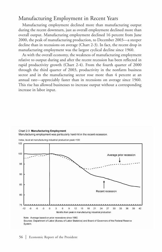
56 | Economic Report of the President
Manufacturing Employment in Recent YearsManufacturing employment declined more than manufacturing output
during the recent downturn, just as overall employment declined more thanoverall output. Manufacturing employment declined 16 percent from June2000, the peak of manufacturing production, to December 2003—a steeperdecline than in recessions on average (Chart 2-3). In fact, the recent drop inmanufacturing employment was the largest cyclical decline since 1960.
As with the overall economy, the weakness of manufacturing employmentrelative to output during and after the recent recession has been reflected inrapid productivity growth (Chart 2-4). From the fourth quarter of 2000through the third quarter of 2003, productivity in the nonfarm businesssector and in the manufacturing sector rose more than 4 percent at anannual rate—appreciably faster than in recessions on average since 1960.This rise has allowed businesses to increase output without a correspondingincrease in labor input.

Chapter 2 | 57
Signs of Recovery in the Manufacturing SectorData for the second half of 2003 suggest a noticeable firming in the
manufacturing sector. Orders and shipments of capital goods began toincrease around the middle of 2003. Industrial production rose at an averageannual rate of 5.9 percent during the second half of the year, the largest six-month gain since the first half of 2000. In addition, the new orders indexfrom the Institute of Supply Management’s monthly survey of purchasingmanagers rose to its highest level in two decades, indicating widespread opti-mism that activity is picking up. Moreover, some of the factors that havehistorically affected firms’ production decisions support a further strength-ening—the cost of capital is low by the standards of the last decade andmanufacturers’ profits are well above their levels of two years ago.
Although manufacturing employment fell throughout 2003, recent develop-ments hint at improving employment conditions for the sector as a whole. Tobe sure, some industries continue to lag—for example, textiles, apparel,printing, and petroleum and coal industries have seen employment fall substan-tially more than overall manufacturing employment since mid-2003. More

58 | Economic Report of the President
broadly, however, the rate of decline in overall manufacturing employmenteased noticeably in the fourth quarter of 2003, with the smallest quarterly lossin three years. In addition, the rise in temporary-help services since the springof 2003 is consistent with a future rebound in permanent employment. Thetemporary-help sector supplies a substantial share of its workers to the manu-facturing sector, and over the past decade has tended to lead movements in thepermanent payrolls of manufacturing firms (Chart 2-5).

Chapter 2 | 59
Long-Term Trends
To place the recent experience of the American manufacturing sector inperspective, this section examines the evolution of the manufacturing sectoras a whole over the 50 years from 1950 to 2000 along three key dimensions:output, productivity and demand, and employment.
Manufacturing Output over the Long TermManufacturing output increased dramatically from 1950 to 2000, with
particularly strong growth in the 1990s (Chart 2-6). Manufacturing indus-trial production, a measure of real manufacturing output, increased more thansixfold from 1950 to 2000 before declining in the recent recession. Over thesame period, annual growth in manufacturing industrial production averaged3.8 percent, faster than real GDP growth of 3.4 percent. From 1990 to 2000,manufacturing industrial production expanded at an annual rate of 4.6percent, outpacing real GDP growth by more than a percentage point. Percapita consumption of manufactured goods has also risen: consumption ofgoods excluding food and fuel more than quadrupled in real 2000 dollarterms from $1,400 per person in 1950 to $6,000 per person in 2000.

60 | Economic Report of the President
In contrast to real manufacturing output, nominal manufacturing output(the dollar value of manufacturing output) has grown more slowly thannominal GDP (the dollar value of GDP). As a result, the share of nominalGDP accounted for by manufacturing roughly halved, from 29 percent in1950 to 15 percent in 2000 (based on GDP by industry data available whenthis Report went to press; that is, prior to the 2003 benchmark revision ofthe National Income and Product Accounts).
Manufacturing Productivity and Demand over theLong Term
Two factors are driving the declining share of manufacturing in U.S.nominal output. First, and most significant, productivity growth in manu-facturing lowered the relative price of manufactured goods, but demand didnot respond proportionately. Second, imported manufactured goodsincreased their market share.
Productivity, as measured by output per hour worked, has grown morerapidly in manufacturing than in the overall nonfarm business sector overthe last three decades. From 1950 to 1973, manufacturing productivity grewat about the same pace as productivity overall. Over the period from 1973to 1995, manufacturing productivity growth exceeded productivity growthoverall by about 1 percentage point per year. The disparity is even wider overthe period from 1995 to 2000, when manufacturing productivity grew at anannual rate nearly 2 percentage points higher than nonfarm businessproductivity (Chart 2-7). An hour of work in manufacturing producedabout four times as much in 2000 as it did in 1950, whereas an hour of workin the nonfarm business sector produced less than three times as much in2000 as it did in 1950.
This dramatic productivity differential has contributed to a decline in theprice of manufactured goods relative to services, which in turn helps toexplain the difference between the behavior of nominal and real manufac-turing output. Increased labor productivity in a sector means that fewer hoursare required to make a given amount of output. This reduces the cost ofproduction and, typically, the relative price of that output. In the same way,relative prices tend to increase in sectors that have experienced less produc-tivity growth, such as services. For example, the falling prices of computersand other electronics have contrasted sharply with the rising costs of services.This example is confirmed by the aggregate data: the average price ofconsumption goods relative to services fell more than 50 percent between1950 and 2000. In contrast to the nearly ninefold increase in the prices for

Chapter 2 | 61
services, prices for durable goods (goods such as cars and refrigerators that areexpected to last, on average, three years or more) rose by a factor of only 21⁄2 and prices for nondurable goods rose by a factor of about 5 from 1950 to2000 (Chart 2-8). Expressed another way, to equal the buying power of $100 worth of durable goods in 1950, a consumer would have spent $250 in2000, while for $100 worth of services in 1950, a consumer would havespent $890 in 2000.
The slower growth of manufactured goods prices has increased thepurchasing power of incomes relative to what it otherwise would have been,but the portion of this increase that Americans have allocated to manufac-tured goods has not been large enough to maintain manufacturing’s share ofnominal output. The boost to real income from the relative price decline ofmanufactured goods has supported demand not only for these goods butalso for services such as health care and financial advice. That is, Americanshave used the resources made available from the relatively slow growth inmanufacturing prices to buy many things, not just manufactured goods.Increased demand for services, combined with rising relative prices for serv-ices, is reflected in the fact that health services and business services each

62 | Economic Report of the President
have increased their share of total nominal output about 4 percentage pointssince 1950. The finance, insurance, and real estate industry has increased itsshare a dramatic 91⁄2 percentage points. The opposite trend has held formanufacturing, in which relative price declines have not been fully offset byincreases in demand. This explains why the share of manufacturing in totalnominal output has roughly halved since 1950. (All calculations of industryshare of nominal GDP are based on the pre-benchmark data available whenthis Report went to press.)
In other words, U.S. demand for manufacturing products has been rela-tively price inelastic. That is, demand has not been very responsive to pricedeclines. For example, a family that purchased a car may have reacted tolower relative car prices (and the increased real income they create) by payingfor college or hiring a home health care aide, rather than by putting thosegains toward the purchase of another car. As a numerical example of inelasticdemand, suppose that people buy 10 compact discs at $20 each (for a totalexpenditure of $200). Now suppose the price falls from $20 to $10. If peoplebuy twice as many compact discs at $10, the value of overall sales will still be$200 (20 compact discs at $10 each). But if people increase their purchasesto 15 compact discs, the value of overall sales will be only $150, a decline of25 percent. This is similar to what has happened in manufacturing.

Chapter 2 | 63
Productivity gains have tempered price increases, and demand has notresponded strongly enough to keep nominal revenues constant as a share ofnominal GDP.
A second factor that has led to a decline in manufacturing’s share of GDPis that Americans are purchasing more goods from abroad. Goods purchasesas a share of total domestic purchases have been declining for about 30 years.The share of domestically produced goods has fallen somewhat faster, partic-ularly in the 1970s and 1990s. Domestically produced goods were 91 percent of overall domestic goods purchases in 1970; by 2000, they hadfallen to 68 percent. In other words, imports have made up an increasedshare of goods bought in the United States (Chart 2-9).
Growth in exports of manufactured goods from the United States over thepast several decades has offset only some of the growth in imports (Chart 2-10).As a result, net imports of nonagricultural goods (imports minus exports)have risen materially, reaching about 30 percent of manufacturing produc-tion in 2000 (based on the pre-benchmark data available when this Reportwent to press) (Chart 2-11). In relation to the overall economy, net nonagri-cultural goods imports have also risen, but remained below 5 percent ofGDP in 2000. China has been a growing source of manufacturing imports,although this growth has not been a major factor in the increase of the U.S.trade deficit (Box 2-1).

64 | Economic Report of the President

Chapter 2 | 65
Box 2-1: China and the U.S. Manufacturing Sector
The recent decline in employment in U.S. manufacturing has coincided with a sizable increase in the overall U.S. trade deficit and asharp increase in the U.S. bilateral trade deficit with China. In partbecause of the high visibility of Chinese imports, which are primarilyeveryday consumer goods, these events have raised concerns that imports of Chinese goods come at the expense of Americanmanufacturing workers.
China’s Trade with the WorldWhile China’s exports and imports grew quickly starting in the early
1990s, China’s trade with the rest of the world has been modest untilvery recently (Chart 2-12). The growth in China’s trade has been wellbalanced in that increased exports to the world have been matched byrising imports from the world. According to data from China’s officialstatistical agency, China has had a trade deficit with the worldexcluding the United States for several years. China recently ran tradedeficits with a number of other countries, including industrial countries such as Germany and Japan.
China’s Trade with the United StatesChina has a significant trade surplus with the United States, its
most important export market and the destination of one-quarter of allChinese goods exports. The U.S. trade deficit with China—about $124 billion through November 2003 at an annual rate—is the singlelargest bilateral goods and services trade deficit for the United States.The next-largest bilateral deficit is with Japan, at $66 billion throughNovember 2003 at an annual rate.
The U.S. trade deficit excluding China has also risen dramaticallysince the mid-1990s and is about 31⁄2 times larger than the bilateraldeficit with China (Chart 2-13). China’s share of the overall U.S. tradedeficit in goods has actually fallen since 1997—exactly the period overwhich trade with China grew rapidly.
Greater trade with China does not appear to have contributed to anincreased overall U.S. trade imbalance, as the higher share of U.S.imports from China has been more than offset by a declining share ofimports from other Asian countries. The share of U.S. imports fromthe Pacific Rim as a whole has fallen since the mid-1990s (Chart 2-14).Restrictions on imports from China would be expected to increaseimports from other low-cost foreign producers, rather than to increaseproduction and employment for American manufacturers. That is, anyjob gains from reduced Chinese imports are more likely to occur inother developing countries rather than the United States.

66 | Economic Report of the President
U.S. exports to China have grown strongly in the last several years,with exports to China up more than 60 percent since 2000. As of thethird quarter of 2003, China was the sixth-largest U.S. export market.Exports to China have grown even while exports to the rest of theworld have stagnated (Chart 2-15).
The Impact of Trade with China on U.S. Manufacturing EmploymentImports from China affect the prospects for domestic firms with
which they compete, and this impact often extends to workers andcommunities associated with these firms. This is especially the casefor firms that make items that are relatively intensive in the use ofless-skilled labor, as these are goods in which China has a compara-tive advantage in production. This may raise the question of whetherimports from China are a primary factor in the displacement ofAmerican manufacturing workers.
A closer look at the data indicates this is not the case. The low levelof U.S. imports from China before the mid-1990s suggests thatdeclines in employment prior to that period were not due to U.S. tradewith China. The data on more-recent job losses in manufacturing indi-cate that China is not a primary factor in these declines, either. Withthe exception of apparel, the largest job losses have occurred inexport-intensive industries for the United States, and job losses inU.S. manufacturing have been mainly in industries in which importsfrom China are small. For example, the computer and electronicequipment industry accounts for 15 percent of all manufacturing joblosses since January 2000, but imports from China were only 8percent of U.S. output in 2002. Other export-intensive industries thathave suffered large job losses include fabricated metal products (9 percent of manufacturing job losses and 2 percent of U.S. output),machinery (10 percent and 2 percent), and transportation equipment(12 percent and 0.4 percent).
Box 2-1 — continued

Chapter 2 | 67

68 | Economic Report of the President

Chapter 2 | 69
Manufacturing Employment over the Long TermEmployment in manufacturing as a share of total employment peaked in
the early 1940s at about one-third of all farm and nonfarm workers. By 2000,it had declined to just below 13 percent (17 million out of 135 millionemployees). Employment in service-providing sectors (including transporta-tion, wholesale and retail trade, finance, insurance, and real estate, andservices) increased from 35 percent of payroll employment in the early 1940sto 65 percent (86 million workers) of all employees in 2000 (Chart 2-16).
The two main reasons for this shift from the manufacturing sector toservice-providing sectors in the labor market are related to the explanationsfor the declining nominal share of manufacturing output. First, increaseddemand for services and relatively slow productivity growth in service-providing sectors have led to rising demand for workers in these sectors. Inmanufacturing, inelastic demand for manufactured goods and faster produc-tivity growth have lowered the relative demand for manufacturing workers.
Second, manufacturing employment likely has fallen in response to thetransfer of manufacturing jobs abroad. The jobs affected have generally beenthose involved in the production of goods requiring relatively low skills.

70 | Economic Report of the President
Indeed, this is part of the explanation for the rapid growth in manufacturingproductivity over the last 50 years (Chart 2-16). The relatively highly-skilledAmerican manufacturing workforce has been increasingly focused onhigher-productivity activities. This shift can be seen by looking at compen-sation for the industries in which employment decreased or increased themost from 1950 to 2000 (Table 2-1). With a few exceptions, employmentfell dramatically in industries with relatively low-skilled jobs and rosedramatically in industries with relatively highly-skilled jobs.
This specialization is a natural outcome of the opening of economies allover the world to trade. As a result of such specialization, world efficiencyincreases and world output goes up as countries focus on the activities inwhich they are relatively more productive. All countries that participate intrade benefit from this increased output.
The effect of long-term productivity improvements on the shift to service-providing jobs is far more important than increased manufacturing imports.Two simple hypothetical exercises can help to illustrate this. In the first exer-cise, imagine that manufacturing productivity was fixed at its value in 1970.To match the actual amount of manufacturing output in 2000, one-third oftotal U.S. nonfarm employment would have been required by manufac-turing, compared with the 13 percent required at 2000 productivity levels.That is, without the increase in manufacturing productivity, manufac-turing’s share of nonfarm employment would have increased 8 percentage
Panel AManufacturing industries with employment that grew the fastest
Rubber and miscellaneous plastics products 213 95Instruments and related products 207 155Printing and publishing 102 113Transportation equipment other than motor vehicles and equipment 83 140Electronic equipment 77 152
Panel BManufacturing industries with employment that declined the fastest
Leather and leather products -82 78Tobacco products -65 195Textile mill products -58 77Apparel and other textile products -50 67Petroleum and coal products -42 177
TABLE 2-1.— Employment in Selected Manufacturing Industries
Industry
Note.—Data relate to full-time equivalent employees and include some definitional changes. Not yet available aredata based on the December 2003 benchmark revision of the National Income and Product Accounts.
Source: Department of Commerce (Bureau of Economic Analysis).
Change in employment, 1950 to 2000
(percent)
Compensation per employee as
percent of average for all sectors, 2000

Chapter 2 | 71
points rather than decreased 12 percentage points from 1970 to 2000. As asecond exercise, imagine that trade in manufactured goods was balanced in2000, so that net exports were zero, but assume that the share of manufac-turing employment in 1970 and productivity growth from 1970 to 2000were their actual values. This would raise the amount of manufacturedgoods produced in the United States. Manufacturing employment as a shareof total nonfarm employment, however, would have been only 1 percentagepoint higher—14 percent, compared with the actual figure of 13 percent—if there had been balanced trade in manufactured goods in 2000.
The Effects of Domestic Outsourcing and TemporaryWorkers on Measurement of ManufacturingEmployment
The decline in manufacturing employment in the official statistics maysomewhat overstate the number of actual manufacturing production jobsthat have been lost. Changing business practices in the manufacturingsector have led to both the outsourcing of nonproduction work that used tobe done “in house” and the increased use of temporary workers.Manufacturing firms that once employed lawyers or accountants in theirlegal or finance departments might now hire outside consultants to performthese services. Counting this outsourcing as a decline in manufacturing jobsis somewhat misleading, because these workers provide services whetherthey are working for a manufacturing firm or an outside firm.
Similarly, manufacturing firms are increasingly using temporary workers,especially during periods of uncertain demand. Such workers, previouslycounted as manufacturing employees, are now counted as service-sectoremployees in the payroll employment data, although many of them stillproduce manufactured goods. The way in which employment statisticscapture the increased use of outsourcing and temporary workers thus over-states the shift from manufacturing to service-providing jobs.
Much of the outsourced work is taken on by industries that make up theemployment category “Professional and Business Services,” which includesthe temporary-help services industry. The professional and business servicescategory covers a rapidly growing sector of the labor market, so it is likelythat the understatement of manufacturing employment has increased overtime. Professional and business services grew from just under 3 millionemployees in 1950 to over 16 million employees in 2000 (Chart 2-17).Employment in subgroups of this category increased substantially in the1990s (Chart 2-18).

72 | Economic Report of the President

Chapter 2 | 73
Results from academic studies can be used to estimate the understatementof employment in the manufacturing sector, bearing in mind that outsourcedjobs are not necessarily comparable to permanent ones (for example, atemporary worker may receive fewer benefits than a permanent employee).One widely-cited study estimates that about one-third of all temporary-helpservices employees work in the manufacturing sector. If the official manufac-turing employment statistics are adjusted by this amount, the decline in thelevel of manufacturing employment in the 1990s is eliminated.
In terms of shares of overall nonfarm employment, adjusted manufacturingshows a decline of 2.8 percentage points over the 1990s, compared with a dropof 3.1 percentage points in the reported data. If outsourcing were alsoincluded, the decline in the actual share of employment in the manufacturingsector would probably be even smaller. In other words, at least one-tenth (andperhaps as much as one-fourth) of the decline in manufacturing’s share ofemployment over the 1990s does not reflect a loss of manufactured goods-producing jobs. Rather, it reflects how measurement conventions used tocalculate employment statistics account for manufacturers’ increased use ofoutsourced workers for tasks previously performed internally. Another exampleof how measurement conventions can affect, and confuse, the evaluation of themanufacturing sector is in the definition of manufacturing (Box 2-2).
Box 2-2: What Is Manufacturing?
The value of the output of the U.S. manufacturing sector as definedin official U.S. statistics is larger than the economies of all but ahandful of other countries. The definition of a manufactured product,however, is not straightforward. When a fast-food restaurant sells ahamburger, for example, is it providing a “service” or is it combininginputs to “manufacture” a product?
The official definition of manufacturing comes from the CensusBureau’s North American Industry Classification System, or NAICS.NAICS classifies all business establishments in the United States intocategories based on how their output is produced. One such categoryis “manufacturing.” NAICS classifies an establishment as in the manu-facturing sector if it is “engaged in the mechanical, physical, orchemical transformation of materials, substances, or components intonew products.”
This definition is somewhat unspecific, as the Census Bureau hasrecognized: “The boundaries of manufacturing and other sectors… canbe somewhat blurry.” Some (perhaps surprising) examples of manufac-turers listed by the Bureau of Labor Statistics are: bakeries, candy stores,

74 | Economic Report of the President
Effects of the Shift to Services on Workers’Compensation
Many workers affected by the structural developments in manufacturinghave experienced difficult transitions. Studies indicate that displacedworkers have a significant chance of being unemployed or employed in apart-time job for some time following their job loss. Many of those who areable to find new jobs suffer earnings declines compared to previous earnings.Furthermore, workers also experience losses in earnings growth relative towhat they would have had if they had remained continuously employed.Because of these effects, an often-voiced concern is that the shift towardemployment in services has meant that more Americans are working in low-paying jobs.
While the shift from the manufacturing sector to service-providing sectorshas been painful for many displaced from the manufacturing sector, theaverage effect on compensation—and in particular on new entrants into the
custom tailors, milk bottling and pasteurizing, fresh fish packaging(oyster shucking, fish filleting), and tire retreading. Sometimes, seem-ingly subtle differences can determine whether an industry is classifiedas manufacturing. For example, mixing water and concentrate toproduce soft drinks is classified as manufacturing. However, if thatactivity is performed at a snack bar, it is considered a service.
The distinction between non-manufacturing and manufacturingindustries may seem somewhat arbitrary but it can play an importantrole in developing policy and assessing its effects. Suppose it wasdecided to offer tax relief to manufacturing firms. Because the manu-facturing category is not well defined, firms would have an incentiveto characterize themselves as in manufacturing. Administering the taxrelief could be difficult, and the tax relief may not extend to the firmsfor which it was enacted.
For policy makers, the blurriness of the definition of manufacturingmeans that policy aimed at manufacturing may inadvertently distortproduction and have unintended and harmful results. Wheneverpossible, policy making should not be based upon this type of arbitrary statistical delineation.
Box 2-2 — continued

Chapter 2 | 75
labor force who have chosen to work in services rather than manufacturing—has been less worrisome. Some service-providing industries pay less thansome manufacturing industries, but much of the employment growth inservice-providing sectors has occurred in industries with higher than averagecompensation. The third column of Panel A in Table 2-2 shows the totalcompensation per full-time equivalent employee in five service-providingindustries relative to the average across industries: for example, compensationin wholesale trade in 2000 was 27 percent higher than the average (whichequals 100 percent). The second column gives the change in employmentfrom 1950 to 2000 for each industry: wholesale trade employment increasedmore than 4 million over this period. As Panel A reveals, four of the fiveservice-providing industries with the largest employment increases paidcompensation roughly at or above the average. Together, these five service-providing industries can explain nearly two-thirds of overall privateemployment growth from 1950 to 2000. Panel B of Table 2-2 shows thatthree of the five manufacturing industries with the highest job-loss rates paidless than the average private-sector job in 2000. For example, apparel employ-ment fell nearly 600,000 from 1950 to 2000, and compensation of workersin the apparel industry in 2000 was only 67 percent of the average. As a resultof the large increases in employment in some of these high-paying service-providing industries, the gap between compensation in service-providingsectors and manufacturing has been closing over the last couple of decades.
Panel A: Service-providingService-providing industries with the largest employment increases
Retail trade 14,248 57Business services 9,079 99Health services 8,482 103Finance, insurance, and real estate 5,406 158Wholesale trade 4,259 127
Panel B: ManufacturingManufacturing industries with the largest employment decreases
Textile mill products -715 77Apparel and other textile products -586 67Primary metal industries -491 124Leather and leather products -321 78Petroleum and coal products -91 177
TABLE 2-2.— Compensation in Selected Industries
Industry
Note.—Data relate to full-time equivalent employees and include some definitional changes. Not yet available aredata based on the December 2003 benchmark revision of the National Income and Product Accounts.
Source: Department of Commerce (Bureau of Economic Analysis).
Change in employment, 1950 to 2000 (thousands)
Compensation per employee as
percent of average for all sectors, 2000

76 | Economic Report of the President
The Transition in Context
Individuals and communities tied to declining industries experience dislocation and distress. While many workers have made the transition frommanufacturing to the service sector, the transition can be difficult. To easeit, the President has supported policies for worker retraining accounts andhas extended unemployment insurance benefits when needed. The appro-priate policy responses to this transition will be discussed in more detail laterin this chapter. Before that, however, it is useful to place the evolution of theU.S. manufacturing sector in a broader context.
First, the shift to a relatively more service-oriented economy has involvedsubstantial benefits for American consumers and producers. Real incomeshave risen, allowing consumers to purchase more goods and services such asfood, health care, transportation, and education, while measures of thequality of life and life expectancy have also increased. In addition, thegrowth of the service-providing sector has generated new opportunities foremployment in industries such as information technology services, financialservices, and entertainment.
Second, the shift of employment away from lower-productivity manufac-turing toward higher-productivity manufacturing and service-providingsectors reflects economic growth and development, just as the shift awayfrom agriculture toward manufacturing did in the last century (Box 2-3).The relative shift from manufacturing toward service-providing sectors hasbeen shared by other advanced economies over the last few decades (Chart2-19). Manufacturing employment declined from the mid-1990s to 2002 ina number of countries whose economies are rapidly developing, includingChina, Brazil, and South Korea. In fact, China, Brazil, South Korea, andJapan had steeper percentage declines in manufacturing employment overthat period than the United States.

Chapter 2 | 77
Box 2-3:The Evolution of the U.S. Agricultural Sector
The evolution of U.S. manufacturing from 1970 to 2000 mirrors, inimportant respects, that of U.S. agriculture from 1940 to 1970. Totalreal farm output increased more than 60 percent from 1940 to 1970.Over the same period, employment in farming declined nearly 6million, or almost two-thirds of the level in 1940 (Chart 2-20). Thistranslated into a decline in agriculture’s share of total employment of15 percentage points, from 19.4 percent in 1940 to 4.4 percent in 1970.
While the histories of agriculture and manufacturing in the UnitedStates differ in some ways, such as the prominent role of subsidies inthe agricultural sector, their similarities help put the long-term storyof the manufacturing sector in context.
In both sectors, a 30-year period of rapid productivity growthsubstantially reduced the share of the American workforce needed tomeet demand for food and manufactured goods. Labor productivity inagriculture nearly quadrupled from 1940 to 1970 (Chart 2-21), a periodthat has been called the “second American agricultural revolution.”

78 | Economic Report of the President
This productivity boom has been attributed to the invention of new technologies, such as hybrid crop varieties, as well as the wide-spread application of existing technologies, such as machinery andconservation practices.
Agricultural productivity growth led to low growth in the price offood, bringing substantial benefits to American consumers and theU.S. economy as a whole and significantly improving U.S. competi-tiveness in world markets. Despite the mid-century expansion in thedemand for agriculture’s output, prices remained essentially flat. Afterthe run-up in demand and prices during World War II and its imme-diate aftermath, agricultural prices increased only 4 percent from 1950to 1970. The average price of all commodities, in comparison,increased 35 percent from 1950 to 1970 (Chart 2-22). The lack of foodprice inflation is mimicked by the low inflation in manufacturing in thelast few decades, with a sizable benefit for American consumers inboth cases.
The evolution of the agricultural sector has been good for theeconomy on the whole, but it meant dislocation for millions of agri-cultural workers—a process that continues today. Displaced farmworkers faced uncertainty regarding their next job and the applica-bility of their skills in different sectors, just as manufacturing workersdo today. The 1940s and 1950s saw the rapid growth of new industriesthat hired workers no longer needed on farms. Manufacturing itselflikely absorbed a substantial percentage of former agriculturalworkers: nearly 8 million new manufacturing jobs were createdbetween 1940 and 1970, 2 million more than the total decline in agri-cultural employment.
In the 1970s and 1980s, service-providing sectors likely absorbedworkers not needed in manufacturing. This continued in the 1990s, ashigh-tech and financial services accounted for new employmentgrowth. Looking forward, it is difficult to predict which industries willgrow and require more workers. The past experience of the adjust-ment in agriculture suggests that market forces will continue toreshape the American workforce.
Box 2-3 — continued

Chapter 2 | 79

80 | Economic Report of the President
The Role of Policy
Markets operating free from government intervention will, in most cases,best allocate the Nation’s resources across sectors. It is generally a mistake totarget government assistance to a particular sector at the expense of othersectors, and manufacturing is no exception. That said, government policycan play a positive role. Policies targeted toward general education andtraining, such as the President’s landmark education reforms and proposedfunding to help displaced workers train for new opportunities, will helppeople adapt to ongoing structural changes. The President’s Jobs for the 21stCentury plan will support students and workers by improving high schooleducation and strengthening post-secondary education and job training.
The short-run performance of the manufacturing sector is closely tied tofluctuations in overall economic activity. Policies that increase aggregateoutput and economic growth will help to improve the near-term outlook forthe manufacturing sector. This Administration put forward a six-point planfor the U.S. economy in September 2003. The plan would help the manu-facturing sector along with the overall economy, and it includes thefollowing components:

Chapter 2 | 81
Making Tax Relief PermanentThe Administration has undertaken several important fiscal measures to
strengthen growth, including the 2001 tax relief program, the March 2002stimulus package, and the May 2003 Jobs and Growth Act. These policieshave already contributed to the current recovery in manufacturing. ThePresident has proposed making provisions of the 2001 and 2003 tax cutspermanent. These include measures that lower the cost of capital andthereby encourage business investment. Capital investment makes up a rela-tively large share of manufacturers’ costs, so a lower cost of capital providesa particularly important benefit to manufacturers. Moreover, manufacturersproduce capital goods, so increased investment demand particularly benefitsmanufacturing firms.
Making Health Care Costs More Affordable and Predictable The President’s proposals aim to reduce frivolous litigation, help individuals
save for future health expenses, and allow small businesses to pool together topurchase health coverage. Health care costs as a share of total compensationare one-third higher in manufacturing than in service-providing industries.The President’s proposals will help manufacturers reduce the burden ofincreasing health care costs.
Reducing the Burden of Lawsuits on the Economy The President seeks to address the burden that lawsuits impose on
American businesses. For example, estimates suggest that roughly 60 compa-nies entangled in asbestos litigation have gone bankrupt primarily becauseof asbestos liabilities, displacing between 52,000 and 60,000 workers.
Ensuring an Affordable, Reliable Energy Supply Initiatives include modernizing the electricity grid and streamlining the
process of acquiring permits for natural gas exploration. This is vital formanufacturing, which makes up about 15 percent of nominal GDP butaccounts for around one-quarter of energy use in the United States.
Streamlining Regulations to Ensure that they are Reasonable andAffordable
Research has shown that manufacturing bore about 30 percent of thecosts of regulation in the United States in 2000—nearly double its share ofnominal output.
Opening International Markets to American Goods and Services This has become particularly important for the manufacturing sector.
While exports accounted for about one-sixth of American manufacturingproduction in 1970, they made up nearly half by 2002.

82 | Economic Report of the President
Conclusion
The manufacturing sector in the United States has undergone significantchange in the last half-century. Productivity and real output in manufac-turing have risen dramatically, and faster than in the economy as a whole.Productivity improvements have boosted real income in the United States.However, because Americans have spent much of their real income gains onservices rather than manufactured goods, manufacturing’s share of employ-ment has declined. In the recent recession, manufacturing output andemployment were hit particularly hard. The President’s policies, aimed atstimulating the overall economy, easing restrictions that impede manufac-turing growth, and ensuring that workers have the skills they need to becompetitive, address the short-term difficulties of the sector and ensure itslong-term health.

The U.S. economy made notable progress in 2003. The recovery was stilltenuous coming into the year, as continued fallout from powerful
contractionary forces—the capital overhang, corporate scandals, and uncer-tainty about future economic and geopolitical conditions discussed inChapter 1, Lessons from the Recent Business Cycle—still weighed against thestimulus from expansionary monetary policy and the Administration’s 2001tax cut and 2002 fiscal package. However, the contractionary forces dissipatedover the course of 2003, and the expansionary forces were augmented by theJobs and Growth Tax Relief Reconciliation Act (JGTRRA) that was signedinto law at the end of May. The economy now appears to have moved into afull-fledged recovery.
This chapter reviews the economic developments of 2003 and discusses theAdministration’s forecast for the years ahead. The key points in this chapter are:
• Real GDP growth picked up appreciably in 2003. Growth in consumerspending, residential investment, and, particularly, business equipmentand software investment appear to have increased noticeably in thesecond half of the year.
• The labor market began to rebound in the final five months of 2003. • Core consumer inflation declined to its lowest level in decades.• The Administration’s forecast calls for the economic recovery to strengthen
further this year, with real GDP growth running well above its historicalaverage and the unemployment rate falling. Looking further ahead, theeconomy is expected to continue on a path of strong, sustainable growth.
Developments in 2003 and the Near-Term Outlook
After rising 2.8 percent during the four quarters of 2002, real GDPexpanded at an average annual rate of 4.4 percent during the first three quar-ters of 2003. The economy appears to have gained momentum as the yearwent on, with annualized real GDP growth averaging close to 21⁄2 percentduring the first half of the year and more than 8 percent in the third quarter.The available data suggest solid further growth in the fourth quarter, thoughnot as spectacular as in the third quarter. (The Report went to print beforeGDP data for the fourth quarter were available.)
83
C H A P T E R 3
The Year in Review and the Years Ahead

84 | Economic Report of the President
The Administration expects real GDP to grow at an annual rate of 4.0 percent during the four quarters of 2004, a figure that is close to thelatest Blue Chip consensus economic forecast (as of January 10, 2004). Theunemployment rate, which peaked at 6.3 percent in June 2003, is projectedto fall to 5.5 percent by the fourth quarter of 2004.
The pace of real GDP growth during the first three quarters of 2003 wassupported by robust gains in consumption, residential investment, anddefense spending. Inventory investment, in contrast, declined over the firstthree quarters of last year. In 2004, the composition of GDP growth isexpected to shift away from government spending and toward business fixedinvestment and net exports. Evidence of emerging momentum in invest-ment accumulated over the course of 2003: businesses began to hire, buildinventories, and increase shipments of nondefense capital goods. In addi-tion, expected faster growth among our trading partners and the recentdecline in the exchange value of the dollar make U.S. exporters well positioned for expansion.
Much of the growth of private demand during 2003 was attributable tothe effects of expansionary fiscal and monetary policy designed to counteractthe lingering effects of the stock market decline, the capital overhang,worries about geopolitical developments, and concern about accountingscandals. Much stimulus remains in the pipeline in the form of refunds on2003 tax liabilities this spring and the ongoing effects of the current lowinterest rates. The fiscal stimulus will not disappear suddenly. The reductionin the tax withholding schedule included in the 2003 fiscal package(JGTRRA) only began in July 2003, and households are still adjusting tothese lower tax rates. Moreover, tax refunds in the first half of 2004 areexpected to be higher than usual: the tax cuts were retroactive to January2003, but last year’s withholding changes generally did not capture taxsavings on income earned in the first half of the year. In addition, becauseof the 2002 and 2003 tax cuts, businesses will be able to cut their tax liabil-ities by expensing 50 percent of their equipment investment (rather thandepreciating the new capital) through the end of 2004. The lower tax rates,higher tax refunds, and investment expensing included in the Jobs andGrowth Tax Relief Reconciliation Act are expected to reduce tax collectionsby about $146 billion in 2004, up from about $49 billion (or about $98 billion at an annual rate) in the second half of 2003.
Consumer SpendingConsumer spending increased briskly in 2003. Real personal consumption
expenditures increased at an average annual pace of 3 percent during the firsthalf of the year, and then surged at an annual rate of 6.9 percent in the thirdquarter. Data on retail sales and motor vehicle purchases through December

Chapter 3 | 85
and services outlays through November are consistent with consumerspending remaining at a high level in the fourth quarter. As a result, realconsumption growth in the second half of the year likely ran noticeablyabove that in the first half.
The pickup in spending growth in the second half of the year correspondedto an increase in the rate of growth of household income. After rising at anannual rate of 3.6 percent in the first half, real disposable personal income(that is, inflation-adjusted household income after taxes) jumped at anannual rate of 6.3 percent in the third quarter, boosted by tax relief, andappears to have held steady in the fourth quarter.
Wages and salaries increased moderately in the second half of the year,bolstered by the emerging recovery in the labor market. Moreover, thepersonal tax cuts included in the 2003 fiscal package (JGTRRA) meant thatU.S. households were able to keep substantially more of their earnings. Thereduction in withholding and the advance rebates of the child tax creditadded $37 billion to disposable income (not at an annual rate) in the secondhalf of the year.
Other factors also likely contributed to the strengthening of consumerspending over the course of 2003. The robust performance of equitymarkets and solid gains in home prices bolstered wealth. Household wealth(net financial resources plus the value of nonfinancial assets such as cars andhomes) increased $21⁄4 trillion during the first three quarters of 2003, and itprobably rose substantially further in the fourth quarter given the solidincrease in broad indexes of stock prices in the last few months of the year.Consumer sentiment was depressed early in the year by the prospect of warwith Iraq. Sentiment jumped in April and May following the successful reso-lution of major combat operations and then was little changed untilNovember, when it picked up noticeably. By the end of the year, householdsentiment was somewhat higher than it had been at the end of 2002 andmuch higher than it was just prior to the war with Iraq.
All told, consumption grew in line with household after-tax incomeduring 2003. Personal saving as a fraction of disposable personal incomeaveraged 2.3 percent in 2002 and remained at this level, on average, in thefirst three quarters of 2003. Swings in personal saving have contributed tomovements in national saving in recent years (Box 3-1).
Growth of real consumption is expected to be lower than that of real GDPin coming years. As explained in Box 3-1, the relative flatness of the personalsaving rate over the past couple of years is likely the result of offsettingforces. On the one hand, capital losses associated with the decline in thestock market from March 2000 to March 2003 probably temperedconsumption (with some lag) and, in turn, caused the personal saving rateto increase. On the other hand, personal saving was likely depressed by the

86 | Economic Report of the President
Box 3-1: Personal Saving and National Saving
One important influence on the personal saving rate (the saving ofthe household sector divided by its after-tax income) over the past 10 years has been changes in households’ wealth, although the pastcouple of years appear to have been an exception.
Driven by movements in stock prices, the ratio of household wealthto personal income climbed dramatically in the second half of the1990s, peaked in early 2000, and then retreated substantially over thenext two years. Economic theory suggests that increases in wealthtend to raise household spending, and decreases in wealth tend tolower household spending. This “wealth effect” often produces anegative correlation between household wealth and the personalsaving rate because personal saving is defined in the nationalaccounts as the difference between income excluding capital gainsand spending (Chart 3-1).
Empirical studies suggest that an additional dollar of wealth leadsto a permanent rise in the level of household consumption of abouttwo to five cents, with the adjustment occurring gradually over aperiod of one to three years (the range depends on the exact specifi-cation—for example, one study found that including the componentsof wealth separately produces lower estimates). Such estimates of thewealth effect can explain the behavior of personal saving in thesecond half of the 1990s fairly well. For example, assuming that adollar of wealth leads to an increase in consumption of three centsand that adjustment lags are typical, one would predict that the rise inwealth in the late 1990s would have caused the saving rate to declineby 4 percentage points between the end of 1994 and the end of 2000—close to the actual decline in the saving rate (ignoring thequarter-to-quarter volatility in the series).
The wealth effect also suggests that the (net) fall in wealth after2000 would have caused a rebound in the personal saving rate ofmore than 2 percentage points. In fact, however, the personal savingrate has not risen materially. One potential explanation for the diver-gence is that households have raised consumption in anticipation thatthe labor market recovery will continue and, in turn, bolster income.Some of the additional consumption may have been funded throughthe wave of cash-out home mortgage refinancing enabled by thecombination of low interest rates and technological advances thathave made such transactions easier. Another possibility is that theavailability of low-interest-rate loans on cars and other items hasspurred households to replace cars and other durable goods earlierthan they otherwise would have.

Chapter 3 | 87
Direct saving by households represents only part of the total savingdone in the United States. Corporations also save in the form ofretained earnings—the difference between after-tax profits and divi-dends. Most of the year-to-year variation in retained earnings stemsfrom profits because dividend payments tend to have a fairly smoothupward trend over time. Profits rose in the early and mid-1990s,boosted by brisk productivity growth. After peaking as a share of GDPin 1997, profits fell over the next few years, owing to the 1998 globalfinancial crisis, a catch-up of wages to productivity gains, and theeconomic slowdown. Retained earnings as a share of GDP alsotrended lower over this period. During the first three quarters of 2003,both profits and retained earnings picked up.
National saving is the sum of private saving (that is, the saving ofhouseholds and corporations) and government saving (equal to theFederal budget surplus plus the state and local government budgetsurpluses). The saving of state and local governments tends to makea small positive contribution to government saving, but in the pastfew years, deteriorating fiscal conditions in states and localities havepushed their overall saving into slightly negative territory. Saving ofthe Federal government has declined sharply since 2000, as the reces-sion and tax cuts have pulled down revenue, and homeland securityand national defense expenditures have increased.
National saving rose (as a fraction of GDP) during the 1990s, but hasfallen sharply since 2000 (Chart 3-2). As a fraction of GDP, it nowstands at the low end of its range since World War II. Although bothgovernment saving and private saving are above their historic lows,the fact that they are both fairly low at the same time has led to thelow level of national saving.
National saving is important because it represents the portion ofour country’s current income that is being set aside for investment innew capital. In particular, national saving plus the net capital inflowfrom abroad equals domestic investment. Greater saving and invest-ment today boost future national income. To increase national saving,the President supports raising Federal saving by restraining Federalspending. He has also proposed Lifetime Savings Accounts andRetirement Savings Accounts, which are designed to increase incentivesfor households to save.
Box 3-1 — continued

88 | Economic Report of the President

Chapter 3 | 89
boost to consumption from low interest rates (both directly through theavailability of low-interest-rate loans on durable goods and indirectlythrough the funds made available by cash-out mortgage refinancings). Asinterest rates and incomes rise over the course of the next several years, thetransitory forces boosting consumption growth should dissipate, and as aresult, real consumption is expected to grow more slowly than real GDPover the forecast period.
An increase in corporate contributions for defined-benefit pension plansis likely to boost the saving rate in the near term from what it might beotherwise. The Pension Benefit Guarantee Corporation (PBGC) has esti-mated that corporate contributions to defined-benefit plans will increasesharply above 2003 levels. Indeed, rapid increases have already begun,according to separate data included in the Employment Cost Index. Thecontributions raise personal income, but because these funds are not placedin the hands of employees until retirement, they seem unlikely to affectcurrent-year consumption. As a result, they should increase the personalsaving rate.
Residential InvestmentThe housing sector continued to show remarkable vigor in 2003, with real
residential investment climbing at an average annual rate of more than 10 percent in the first three quarters of the year. Housing starts moved abovethe already high 2002 level to 1.8 million units in 2003, the largest numberof starts since 1978. In addition, sales of both new and existing single-familyhomes rose to record levels.
Some of the strength in housing demand reflected the same gains inafter-tax income and wealth that bolstered real consumer spending. Thelow levels of mortgage interest rates were another important driving force.The interest rate on new fixed-rate 30-year mortgages slipped from anaverage of 61⁄2 percent in 2002 to an average of 53⁄4 percent in 2003. Thislevel is the lowest in the 32 years for which comparable data are available.Indeed, according to data from the Michigan Survey Research Center,consumers’ assessments of home-buying conditions remained very positivein 2003, largely because of low mortgage interest rates. As a result of thevery favorable conditions in the housing sector, the U.S. home-ownershiprate climbed to 68.2 percent in the third quarter of 2003—equal to itshighest level on record.
During 2004, real residential investment is expected to slip lower ashousing starts edge down to levels determined by long-run demographics.

90 | Economic Report of the President
Business Fixed InvestmentReal business fixed investment (firms’ outlays on equipment, software, and
structures) turned around in 2003, posting an annualized gain of 6.2 percentduring the first three quarters of the year after declines of 10.2 percent duringthe four quarters of 2001 and 2.8 percent during the four quarters of 2002.The acceleration during the year was noteworthy, with real investment risingat an annual rate of 12.8 percent in the third quarter and indications offurther growth in the fourth quarter, compared with an average annual paceof 3.1 percent in the first half of the year. The improvement from 2002 to2003, as well as the pickup over the course of 2003, largely reflected astrengthening in real purchases of equipment and software.
Within the equipment and software category, the largest increasesoccurred for certain high-tech items. Real outlays for computers increased atan annual rate of 43 percent in the first three quarters of 2003, and realspending on communications equipment, which had performed particularlypoorly during the recession, rose almost 15 percent. Shipments data suggestthat spending in these categories remained strong in the fourth quarter.Meanwhile, real investment in software continued its solid upward trend,rising 12 percent during the first three quarters of the year. Outlays fortransportation equipment were held down by further large declines inpurchases of aircraft in the first three quarters of the year. Finally, the avail-able data suggest that real spending on equipment outside of the high-techand transportation categories posted a solid gain over the course of 2003.
The increased momentum in business purchases of capital goods in 2003likely reflects the factors mentioned in Chapter 1. First, with capital over-hangs probably behind them, firms were poised to take advantage of furtherdeclines in prices of high-tech goods stemming from continued technolog-ical advances. Second, striking gains in productivity and falling unit laborcosts bolstered corporate profits. Third, the cost of capital was held down bya number of factors, including falling prices for high-tech capital goods, butalso by low interest rates, rising stock prices, and the investment incentivesintroduced in the Job Creation and Worker Assistance Act of 2002(JCWAA) and expanded in the 2003 fiscal package (JGTRRA).
The Administration expects the recovery in real business investment inequipment to strengthen further this year, reflecting the acceleration inoutput, continued low interest rates, and the investment incentives providedby the 2002 and 2003 tax cuts. Fixed investment in equipment and struc-tures tends to be related to the pace of growth in output (along with the costof capital), and so the pickup in real GDP growth from 2.8 percent duringthe four quarters of 2002 to 4.4 percent during the first three quarters of2003 is projected to lead to an increase in investment during 2004.

Chapter 3 | 91
One reason for the development of a capital overhang was the loweredbusiness expectations of the future level of output that developed just priorto the past recession. As these projections fell, the demand for investmentalso fell. In contrast to that period, current projections of 2004 output havebeen rising since mid-2003 and are expected to lead to increased demand forcapital goods in the initial quarters of the forecast.
Growth in equipment investment in 2004 should be further boosted asfirms pull forward spending in anticipation of the expiration of the periodwhen businesses are able to expense (rather than depreciate) 50 percent of thevalue of their equipment investment. The flip side of some investment beingadvanced into 2004 is that investment may grow more slowly in 2005. Evenso, the growth of equipment investment in 2005 is projected to be solid.
Despite the emerging recovery in spending on equipment and software,business demand for structures remained soft in 2003. High overcapacityseems to have offset the impetus imparted by low interest rates and highercash flow. In the office sector, vacancy rates rose substantially for the thirdconsecutive year. Vacancy rates moved still higher in the industrial sectorand now stand at extremely elevated levels. The good news is that thesubstantial declines in total spending on structures seem to have abated.Indeed, real investment in nonresidential structures was approximately flatover the first three quarters of 2003, in contrast with a plunge of more than25 percent during the preceding two years. Strength in oil and gas drillingand an increase in construction of general merchandise stores during theyear have offset continued softness in some other sectors.
The forces that shape the outlook for business structures—the growth ofoutput and the cost of capital—are much the same as for business equip-ment. However, they operate with a longer lag because of the time it takesto plan and build these structures. Investment in business structures isprojected to post a small gain during 2004.
Business InventoriesBusinesses began 2003 with lean inventories following a massive liquidation
in 2001 and little restocking during 2002. Inventory investment wassubstantially negative over the first three quarters of 2003, as increases inproduction lagged those in final demand. The reasons for this slow responseof production are unclear. Firms may have been surprised by the strength offinal demand, or they may simply have been waiting for compellingevidence that a sustainable recovery was under way.
The net decline in inventories during the first three quarters of 2003 leftstocks in their leanest position relative to final sales of goods and structures inat least 50 years. (This lean position results, at least in part, from efficienciesgenerated by just-in-time inventory-management techniques.) Stockbuilding

92 | Economic Report of the President
seems to have begun in September, however. Inventory investment appearslikely to have made a positive contribution to GDP growth in the fourthquarter of 2003, and the contribution is projected to remain noticeablypositive through the first half of 2004. Inventory investment is expected toplateau thereafter at a level that keeps stocks in line with rising salesthroughout 2004 and 2005.
Government Purchases Real Federal spending (consumption expenditures and gross investment)
climbed at an annual rate of 8 percent during the first three quarters of2003. The available data suggest that 2003 as a whole likely saw the largestincrease in more than 30 years. The gain during the first three quarters wasled by an annualized rise of 10 percent in real defense spending largelyrelated to military operations in Iraq. Real nondefense spending rose at anaverage annual pace about 4 percent. This gain was less than half as large asthe gain during the four quarters of 2002, when outlays were stepped upconsiderably for homeland security.
The defense supplemental appropriations for FY 2004, signed inNovember, allows for some further near-term growth in governmentpurchases. Defense spending is projected to fall during FY 2005, and as aresult, overall Federal spending is projected to edge down.
Like the Federal government, the governments of states and localities sawtheir tax receipts decelerate during the economic slowdown. Budgets havealso deteriorated because of rising health care costs and increased demand forsecurity-related spending. With many of these governments subject tobalanced-budget rules, they have taken a variety of measures to address theirfiscal imbalances, including drawing on accumulated reserves (so-called“rainy day funds”), raising taxes, and restraining spending. Real expendituresof state and local governments were little changed during the first three quar-ters of 2003, in contrast with an average annual gain of around 3 percent overthe preceding five years. With state and local governments still under pres-sure, their real expenditures are projected to increase slowly during thecoming year. Eventually, their fiscal situations should be improved byincreases in tax revenue resulting from the strengthening of the economy.
Exports and ImportsThe U.S. current account deficit as a share of GDP was little changed, on
net, during the first three quarters of 2003, averaging about 5 percent. Thedeficit on trade in goods and services as a share of GDP also moved in anarrow range during the first three quarters. U.S. net investment income (theincome paid to U.S. investors in foreign endeavors less that paid to foreign

Chapter 3 | 93
investors in U.S. projects) was roughly flat, as both receipts from abroad andpayments to foreign investors rose somewhat during the first three quartersof 2003. Real imports of goods and services have likely been restrained inrecent quarters by the decline in the value of the dollar. Real imports rose atan annual rate of 1 percent during the first three quarters of 2003, a substan-tially slower pace than during the four quarters of 2002. Real imports ofcapital goods (other than autos) rose solidly, as would be expected given therecovery in U.S. investment. Real oil imports increased at a faster pace (on anannual basis) than during the four quarters of 2002. Real services imports fellmarkedly in the first half of 2003 but turned up in the third quarter.
America’s major trading partners have recovered from the global slowdownsomewhat more slowly than has the United States. For example, an index ofreal GDP for our G-7 trading partners increased at an average annual pace ofless than 2 percent during the first three quarters of 2003. As a result, foreigndemand for U.S. exports was lackluster in the first half of 2003. Real exportspicked up sharply around the middle of 2003, increasing at an annual paceof 10 percent in the third quarter. The increase was led by a gain in realexports of capital goods. Even so, the level of exports remained well below itspeak in 2000.
Prospects for exports over the next two years look better. Growth amongthe non-U.S. OECD countries is projected by the OECD Secretariat to rise2.6 percent during the four quarters of 2004, up from a pace of 1.6 percentduring 2003. Growth is expected to rise further to 2.8 percent in 2005. Theexpected growth in foreign markets should support growth in U.S. exports.In addition, the effect will likely be augmented by a rise in the U.S. marketshare of world exports owing to the effects of the 23 percent decline in thevalue of the dollar against major currencies from its peak in early 2002through the end of 2003. The effect of the recent dollar decline on exportswill likely take a couple of years to be fully felt.
Real imports are projected to increase along with domestic output, but thegrowth of real imports is likely to be slowed by the recent decline in thedollar’s value relative to other currencies. On balance, real imports areprojected to grow at about the same pace as GDP, on average, during the nexttwo years. Nominal imports will increase faster than real imports becauseimport prices will rise in reaction to the recent dollar decline. Even so, thecurrent account deficit, which rose to about 5 percent of GDP in the firstthree quarters of 2003, is projected to edge up in 2004 and decline thereafter.
Overall, real net exports are expected to be approximately flat during thenext year and are likely to make a positive contribution to real GDP growththereafter. Over the next six years, the returns to foreign owners of U.S.capital are likely to grow faster than the returns to U.S. owners of foreigncapital, a legacy of a long period of strong foreign investment in the United

94 | Economic Report of the President
States during the past decade. As a result, real gross national product (GNP),which includes these net foreign returns to capital, is expected to growslower than real gross domestic product (GDP).
The Labor MarketNonfarm payroll employment fell an average of 50,000 workers per
month in the first seven months of 2003, before increasing 35,000 inAugust, 99,000 in September, and an average of 48,000 per month in thefourth quarter. The strengthening was experienced in most sectors. Job gainsin professional and business services stepped up appreciably from themodest upward pace seen earlier in the year. Construction employmentbegan to expand in the second quarter after two years of modest job losses,and the quarterly averages of employment in the wholesale trade, transporta-tion, and utilities industries turned up at the end of the year. Themanufacturing sector continued to shed jobs through year-end, though thepace of decline slowed, and the factory workweek climbed more than 0.5hour, on balance, in the final five months of 2003.
The unemployment rate increased in the first half of 2003, reaching apeak of 6.3 percent in June, before falling during the second half of the year.In the fourth quarter, the unemployment rate averaged 5.9 percent, thesame as it had been a year earlier. Because the labor force is constantlyexpanding, employment must be growing moderately just to keep theunemployment rate steady. For example, if the labor force is growing at thesame rate as the population (about 1 percent per year), employment wouldhave to rise 110,000 a month just to keep the unemployment rate stable,and larger job gains would be necessary (and are expected) to induce adownward trend in the unemployment rate.
Looking ahead, temporary-help services employment—a leading indicatorfor the labor market—suggests substantial further employment growth.Average growth in temporary-help services employment over a six-monthperiod has a striking positive correlation with growth in overall employmentover the subsequent six months (Chart 3-3). Statistical analysis suggests thatan increase of one job in temporary-help services corresponds to a subsequentrise of seven jobs in overall employment. Employment in temporary-helpservices has expanded 194,000 since last April, suggesting robust growth inoverall employment this year. The unemployment rate is projected to fall to5.5 percent by the fourth quarter of 2004.

Chapter 3 | 95
Productivity, Prices, and WagesThe consumer price index (CPI) increased 1.9 percent over the 12 months
ended in December 2003, a little below the 2.4 percent rise experiencedduring the same period the previous year. Consumer energy prices fluctuatedmarkedly over the course of 2003, but ended the year 6.9 percent above theirlevel at the end of 2002. The core CPI (which excludes food and energy) roseonly 1.1 percent during 2003, considerably below the 1.9 percent increase ofthe previous year. This deceleration likely stems from the slack in labor andproduct markets last year. In addition, unit labor costs were held down by animpressive performance for labor productivity, with output per hour in thenonfarm business sector rising at an annual pace of about 6 percent duringthe first three quarters of the year following an increase of roughly 41⁄2 percentduring the four quarters of 2002. This pace of productivity growth is wellabove the annual average of just over 2 percent experienced since 1960.
Hourly compensation of workers appears to have picked up a little lastyear. During the 12 months of 2003, the employment cost index (ECI) forprivate nonfarm businesses moved up 4 percent following a 3.2 percent gainduring the previous year. The wages and salaries component of the indexrose 3.0 percent during 2003, slightly below the 2.7 percent increaserecorded for 2002. The benefits component of the ECI, however, surged 6.4 percent over the 12 months of 2003, much faster than the 4.7 percent

96 | Economic Report of the President
pace during 2002. The increase in benefits was especially large in the firstquarter of 2003, led by a jump in contributions to defined-benefit pensionplans as employers began making up for losses in the value of pension fundassets. Employer-paid health premiums rose 10.5 percent during 2003,roughly the same pace as in 2002.
Core CPI inflation is expected to continue at a low level in 2004, andoverall inflation is expected to be even lower as energy prices retreat further.Overall CPI inflation is projected to fall to 1.4 percent during the four quar-ters of 2004—close to the past year’s pace of core inflation. With theunemployment rate expected to average 5.6 percent for the year as a whole(above our estimated 5.1 percent midpoint of the range of rates consistentwith stable inflation) the level of slack—although less than in 2003—is stillprojected to hold down inflation during 2004. Also keeping inflation incheck is the recent rapid pace of—and solid near-term prospects for—productivity growth. Offsetting this effect is the somewhat higher pace ofimport-price inflation (resulting from the recent dollar decline) and thequicker pace of GDP growth. Over the next five years, CPI inflation isexpected to edge up, eventually flattening out at 2.5 percent, a level that isidentical to the consensus forecast.
The path of inflation as measured by the GDP price index is similar, buta bit lower throughout the projection period. Inflation as measured by theGDP price index is projected fall to 1.2 percent during the four quarters of2004, the same as the 1.2 percent pace of the core GDP price index duringthe first three quarters of 2003. GDP price inflation is projected to increaseslowly thereafter—roughly parallel to the rise in CPI inflation.
The wedge between the CPI and the GDP measures of inflation hasimportant implications for the Federal budget and budget projections. Alarger wedge reduces the Federal budget surplus because cost-of-livingadjustments for Social Security and other indexed programs rise with theCPI, whereas Federal revenue tends to increase with the GDP price index.For a given level of nominal income, increases in the CPI also cut Federalrevenue because they raise income tax brackets and affect other inflation-indexed features of the tax code. Of the two indexes, the CPI tends toincrease faster in part because it measures the price of a fixed market basket.In contrast, the GDP price index increases less rapidly than the CPI becauseit reflects the choices of households and businesses to shift their purchasesaway from items with increasing relative prices and toward items withdecreasing relative prices. In addition, the GDP price index includes invest-ment goods, such as computers, whose relative prices have been fallingrapidly. Computers, in particular, receive a much larger weight in the GDPprice index (0.8 percent) than in the CPI (0.2 percent).

Chapter 3 | 97
During the eight years ended in 2002, the wedge between inflation inthe CPI-U-RS (a version of the CPI designed to be consistent with currentmethods) and the rate of change in the GDP price index averaged 0.5 percentage point per year. With the core CPI and the core GDP priceindex both increasing at about a 11⁄4 percent pace during the past year,inertia suggests that the near-term wedge will be only about 0.2 percentagepoint in 2004. The wedge is expected to widen eventually to its recentmean of 0.5 percent by 2009.
Financial MarketsStock prices skidded early in the year, but rallied in March and have been
on a solid uptrend since then. During the 12 months of 2003, the Wilshire5000 index—a broad measure of stock prices—rose 29 percent. An increaseof this magnitude has not been seen since 1997. High-tech stocks did evenbetter; for example, the Nasdaq index, which is heavily weighted towardhigh-tech industry, rose 50 percent during 2003. Nearly two-thirds of therise in broad measures of stock prices occurred after the President signed the2003 tax cut (JGTRRA) in late May; the Act reduced marginal tax rates ondividends and capital gains and thus likely contributed to the robustperformance of stock prices.
Following a large decline in 2001, and a smaller one in 2002, the interestrate on 91-day Treasury bills fell an additional 29 basis points in 2003 andended the year at 0.9 percent. These reductions reflected the FederalReserve’s efforts to stimulate the economy, leaving real short-term rates (thatis, nominal rates less expected inflation) slightly negative. Following market-based expectations of interest rates (derived from rates on Eurodollarfutures), the Administration does not expect real rates this low to persistonce the recovery becomes firmly established, and nominal Treasury billrates are projected to increase gradually. Long-term interest rates fell sharplylast spring and then rebounded in the summer. For the year as a whole, long-term Treasury rates were about unchanged, but corporate interest ratesdropped a bit as the spread over Treasury rates narrowed. TheAdministration projects that the yield on 10-year Treasury notes, whichaveraged 4.3 percent in December 2003, will edge up gradually next year,consistent with the path of short-term Treasury rates.
The Long-Term Outlook
The economy could well grow faster than in the projection presentedhere, as the long-run benefits from the full reductions in marginal tax ratesare felt. These should lead to higher labor force participation than would

98 | Economic Report of the President
occur otherwise, more entrepreneurial activity, and greater work effort byhighly productive individuals. The Administration, however, chooses toadopt conservative economic assumptions that are close to the consensus ofprofessional forecasters. As such, the assumptions provide a prudent andcautious basis for the budget projections.
Growth in Real GDP and Productivity over the Long Term
The economy continues to display supply-side characteristics favorable tolong-term growth. Productivity growth has been remarkable, and inflationremains low and stable. As a result of stimulative fiscal and monetary policies,real GDP is expected to grow faster than its 3.1 percent potential rate duringthe next four years. The Administration forecasts that real GDP growth willaverage 3.7 percent at an annual rate during the four years from 2003 to2007—in line with the consensus projection. Because this pace is somewhatabove the assumed rate of increase in productive capacity, the unemploymentrate is projected to decline over this period. In 2008 and 2009, real GDPgrowth is projected to continue at its long-run potential rate of 3.1 percent,and the unemployment rate is projected to be flat at 5.1 percent (Table 3-1).
The growth rate of the economy over the long run is determined by itssupply-side components, which include population, labor force participation,productivity, and the workweek. The Administration’s forecast for the contribu-tion of different supply-side factors to real GDP growth is shown in Table 3-2.
2002 (actual) .... 4.3 2.9 1.3 2.2 5.8 1.6 4.6 130.4
2003 ................. 5.8 4.2 1.5 2.0 6.0 1.0 4.0 130.12004 ................ 5.2 4.0 1.2 1.4 5.6 1.3 4.6 132.72005 ................. 4.9 3.4 1.4 1.6 5.4 2.4 5.0 136.3
2006 ................. 5.0 3.3 1.6 1.9 5.2 3.3 5.4 138.62007 ................. 5.2 3.3 1.8 2.2 5.1 4.0 5.6 140.62008 ................. 5.2 3.1 2.0 2.5 5.1 4.3 5.8 142.52009 ................. 5.2 3.1 2.0 2.5 5.1 4.4 5.8 144.4
TABLE 3-1.— Administration Forecast 1
Year NominalGDP
Real GDP(chain-type)
GDP priceindex
(chain-type)
Consumerpriceindex
(CPI-U)
Interestrate,
91-dayTreasury
bills(percent)
Interestrate,
10-yearTreasury
notes(percent)
Nonfarmpayrollemploy-
ment(millions)
Unemploy-ment rate
(percent)
Percent change, fourth quarter to fourth quarter Level, calendar year
1Based on data available as of December 2, 2003.
Sources: Council of Economic Advisers, Department of Commerce (Bureau of Economic Analysis), Department ofLabor (Bureau of Labor Statistics), Department of the Treasury, and Office of Management and Budget.

Chapter 3 | 99
The Administration expects nonfarm labor productivity to grow at a 2.1 percent average annual pace over the forecast period, virtually the same asthat recorded during the 43 years since the business-cycle peak in 1960. Theprojection is notably more conservative than the roughly 41⁄2 percent averageannual rate of productivity growth since the output peak in the fourth quarterof 2000. After such an extraordinary surge, a period of slower productivitygrowth is likely as firms shed their hesitancy to hire. In addition, the slowerpace of productivity assumed in the forecast reflects the Administration’s viewthat in the absence of a good explanation for the recent acceleration, it is wiserto base the productivity forecast on longer-term averages.
In addition to productivity, growth of the labor force (also shown in Table3-2) is projected to contribute 1.0 percentage point per year to growth ofpotential output on average through 2009. Labor force growth results fromgrowth in the working-age population and changes in the labor force partic-ipation rate. The Bureau of the Census projects that the working-agepopulation will grow at an average annual rate of 1.1 percent through2009—roughly the same pace as during the years between 1990 and 2003.The last year in which the labor force participation rate increased was 1997,
TABLE 3-2.—Accounting for Growth in Real GDP, 1960-2009 1
[Average annual percent change]
Item1960 Q2
to1973 Q4
1973 Q4to
1990 Q3
1990 Q3to
2003 Q3
2003 Q3to
2009 Q4
1) Civilian noninstitutional population aged 16 or over .................... 1.8 1.5 1.2 1.12) Plus: Civilian labor force participation rate .............................. .2 .5 -.1 -.1
3) Equals: Civilian labor force 2 ......................................................... 2.0 2.0 1.1 1.04) Plus: Civilian employment rate 2 ................................................ .0 -.1 .0 .2
5) Equals: Civilian employment 2 ....................................................... 2.0 1.9 1.1 1.26) Plus: Nonfarm business employment as
a share of civilian employment 2 3 .................................... .1 .1 -.1 .6
7) Equals: Nonfarm business employment ........................................ 2.1 2.0 1.0 1.88) Plus: Average weekly hours (nonfarm business) ...................... -.4 -.4 -.1 .0
9) Equals: Hourall persons (nonfarm business) ................................ 1.7 1.7 .9 1.810) Plus: Output per hour (prods of uctivity, nonfarm business) ... 2.8 1.4 2.5 2.1
11) Equals: Nonfarm business output ................................................. 4.6 3.1 3.4 3.912) Plus: Ratio of real GDP to nonfarm business output 4 .............. -.3 -.2 -.4 -.5
13) Equals: Real GDP ........................................................................... 4.2 2.9 3.0 3.4
1 Based on data available as of December 2, 2003.2 Adjusted for 1994 revision of the Current Population Survey.3 Line 6 translates the civilian employment growth rate into the nonfarm business employment growth rate.4 Line 12 translates nonfarm business output back into output for all sectors (GDP), which includes the output of
farms and general government.
Note.— The periods 1960 Q2, 1973 Q4, and 1990 Q3 are business cycle peaks.Detail may not add to totals because of rounding.
Sources: Council of Economic Advisers, Department of Commerce (Bureau of Economic Analysis), and Departmentof Labor (Bureau of Labor Statistics).

100 | Economic Report of the President
so the long-term trend of rising participation appears to have come to anend. Since then, the participation rate has fallen at an average 0.2 percentannual pace—although some of the decline in 2001 and 2002 probablyresulted from the recession-induced decline in job prospects. In 2003, thebaby-boom cohort was 39 to 57 years old, and over the next several years theboomers will be moving into older age brackets with lower participationrates. As a result, the labor force participation rate is projected to edge downan average of 0.1 percent per year through 2009. The decline may be greater,however, after 2008, which is the year that the first baby boomers (thoseborn in 1946) reach the early-retirement age of 62.
In sum, potential real GDP is projected to grow at a 3.1 percent annualpace, slightly above the average actual pace since 1973 of 3.0 percent. Actualreal GDP growth during the six-year forecast period is projected to beslightly higher, at 3.4 percent, because the civilian employment rate (line 4of Table 3-2) makes a small (0.2 percentage point) and transitory contribu-tion to growth through 2007 as the unemployment rate falls. Thiscontribution then ends as the unemployment rate stabilizes at 5.1 percent.
Interest Rates over the Long TermThe gradual increase in the interest rate on 91-day Treasury bills is projected
to continue through 2009. The rate is expected to reach 4.4 percent by 2009,at which date the real interest rate on 91-day Treasury bills will be close to itshistorical average. The projected path of the interest rate on 10-year Treasurynotes is consistent with that on short-term Treasury rates. By 2008, this yieldis projected to be 5.8 percent, 3.3 percentage points above expected CPI infla-tion—a typical real rate by historical standards. By 2009, the projected termpremium (the difference between the 10-year interest rate and the 91-day rate)of 1.4 percentage points is in line with its historical average.
The Composition of Income over the Long TermA primary purpose of the Administration’s economic forecast is to estimate
future government revenue, which requires a projection of the componentsof taxable income. The Administration’s income-side projection is based onthe historical stability of the long-run labor and capital shares of grossdomestic income (GDI). During the first three quarters of 2003, the laborshare of GDI was on the low side of its historical average. From this jump-off point, it is projected to rise to its long-run average and then remain at thislevel over the forecast period. (The income share projections are consistentwith data available through December 2, 2003. They exclude any effects ofthe later comprehensive revision to the National Income and ProductAccounts.) The labor share consists of wages and salaries, which are taxable,employer contributions for employee pension and insurance funds (that is,

Chapter 3 | 101
fringe benefits), which are not taxable, and employer contributions forgovernment social insurance. The Administration forecasts that the wage andsalary share of compensation will decline while employer contributions foremployee pension and insurance funds grow faster than wages. This patternhas generally been in evidence since 1960 except for a few years in the late1990s. During the next five years, the fastest growing components ofemployer contributions for employee pension and insurance funds areexpected to be employer-paid health insurance and contributions for defined-benefit pension plans.
The capital share (the complement of the labor share) of GDI is expectedto fall before leveling off at its historical average. Within the capital share, anear-term decline in depreciation (an echo of the decline in short-livedinvestment during 2001 and 2002) helps boost corporate economic profits,which in the third quarter 2003 were noticeably above their post-1973average of about 8 percent of GDI. The share of corporate economic profitsin GDI is projected to be bolstered in 2004 by the strong recent productivitygrowth together with stable gains in hourly compensation, and an expecteddecline in depreciation. From 2005 forward, the profit share is expected toslowly decline back to its historical average of about 8 percent. The projectedpattern of book profits (known in the national income accounts as “profitsbefore tax”) reflects the 30 percent expensing provisions of the Job Creationand Worker Assistance Act of 2002 and the 50 percent expensing provisionsof the Jobs and Growth Tax Relief Reconciliation Act of 2003. Theseexpensing provisions reduce taxable profits from the third quarter of 2001through the fourth quarter of 2004. The expiration of the expensing provi-sions increases book profits thereafter, however, because those investmentgoods expensed during the three-year expensing window will have lessremaining value to depreciate thereafter. The share of other taxable income(the sum of rent, dividends, proprietors’ income, and personal interestincome) is projected to fall, mainly because of the delayed effects of pastdeclines in long-term interest rates, which reduce personal interest incomeduring the projection period.
Conclusion
The Administration’s policies have been a key force shaping recenteconomic developments and the prospects for economic growth in comingyears. The policies are designed to enhance U.S. economic growth, not justmaintain it. The remaining chapters of this Report illustrate the ways in whichpro-growth economic policies can improve economic performance by strikinga balance between encouragement and regulation of firms, by reducingbarriers to trade, and by reducing tax-based disincentives to economic activity.


The study of tax incidence is the economic study of which taxpayers bearthe burden of a tax. This question is of considerable importance to policy
makers, who want to know whether the distribution of the tax burden(between rich and poor, capital and labor, consumers and producers, and soon) meets their criteria for fairness.
Distributional tables showing the tax burdens borne by different incomegroups are an important application of incidence analysis. The JointCommittee on Taxation (JCT) and the Department of the Treasury preparedistributional tables for the existing tax system and for some proposed andadopted tax changes. The Congressional Budget Office (CBO) prepares suchtables for the existing tax system. In addition to these official analyses, someprivate groups also publish distributional tables.
When used properly, distributional tables can contribute to informed decision making on the part of citizens and policy makers. Unfortunately,mainstream economic analysis suggests that these tables do not always accu-rately describe who bears the long-run burden of certain taxes. This problemdoes not arise from bias or lack of economic knowledge on the part of theeconomists who prepare these tables. Instead, it reflects resource and datalimitations, uncertainty about some of the economic effects of taxes, and vari-ations in the time frame considered by the analyses. Nevertheless, theshortcomings of distributional tables can lead to misperceptions of the impactof tax changes.
This chapter discusses some of the ways in which distributional tables canbe improved. The key points in this chapter are:
• The actual incidence of a tax may have little to do with the legal specifi-cation of its incidence. Official distributional tables recognize this fact inmany contexts, but not in all of them.
• In the long run, a large part of the burden of capital taxes is likely to beshifted to workers through a reduction in wages. Analyses that fail to recog-nize this shift can be misleading, suggesting that higher income groups bearan unrealistically large share of the long-run burden of such taxes.
To begin, it is useful to review the basic economic principles of tax incidenceand apply them to different types of taxes.
103
C H A P T E R 4
Tax Incidence: Who Bears the Tax Burden?

104 | Economic Report of the President
Theory of Tax Incidence
One crucial finding in the study of tax incidence is that the economic incidenceof a tax (the identity of the person who bears the burden of the tax) can becompletely different from its statutory or legal incidence (the identity of theperson upon whom the law officially imposes the tax). In other words, theperson who is legally responsible for paying the tax may not be the one whoactually bears the burden of the tax. As explained below, the incidence of atax depends upon the law of supply and demand, not the laws of Congress.
Another crucial principle is that only people can pay taxes. Businesses andother artificial entities cannot pay taxes. Although the corporate income taxis legally imposed on firms that are organized as corporations, the actualburden of the tax can fall only on people—perhaps the firm’s owners, or itsemployees, or its customers—but certainly not on a legal artifact such as acorporation. Similarly, although the estate tax is legally imposed on the estate,the burden of the tax can fall only on people—perhaps the decedent who leftthe estate, perhaps the heirs, perhaps other people—but not the estate, whichis merely a legal construct established to sort through the ownership of thedecedent’s assets.
It is simplest to first discuss the incidence of a simple excise tax, a tax leviedon a specific good or service. As explained below, the key insights from thisanalysis can be extended to apply to other types of taxes.
Incidence of an Excise Tax Consider a tax on apples. Suppose that when there is no tax, the price of
apples is $1. Now, suppose that the government imposes a 10-cent excise taxon apples and that the producers are legally responsible for paying this tax.Do producers actually bear the economic burden of the tax?
The answer depends on what happens to the price of apples. If the priceremains unchanged, producers bear the economic burden (the economicincidence of the tax is the same as the legal incidence). Consumers pay $1,the same as before, and suffer no burden. Producers, after collecting $1 fromthe consumers, must pay 10 cents to the government, so they clear only 90cents. Alternatively, if the price rises by the amount of the tax, from $1 to$1.10, consumers bear the burden. Although they do not send any moneyto the government, they pay 10 cents more per apple than they did withoutthe tax. The producers bear no economic burden, even though they arelegally responsible for paying the tax. After collecting $1.10 from consumersand sending 10 cents to the government, they still clear $1, as they didwithout the tax. In this case, economists say that the producers shift theburden of the tax to consumers. To consider another possibility, if the priceof apples rises by 5 cents, to $1.05, consumers and producers share the

Chapter 4 | 105
burden equally. Consumers bear a 5-cent burden because they pay $1.05 foreach apple, compared to the $1 that they paid without the tax. Producersbear a 5-cent burden because they clear only 95 cents per apple, comparedto the $1 they cleared without the tax: they collect $1.05 from consumers,but send 10 cents to the government.
As these examples show, the division of the tax burden betweenconsumers and producers depends on what happens to the price of apples.When prices are free to adjust, they are likely to be determined by the lawof supply and demand. If the price of apples was $1 with no tax, then thenumber of apples consumers wanted to buy at that price must have equaledthe number of apples that producers wanted to sell at that price.
What happens when the 10-cent excise tax is imposed? It depends on howresponsive consumers and producers are to changes in the prices they pay orreceive. The relevant questions are: How many fewer apples do producerssell if the amount they clear per apple declines? How many fewer apples doconsumers buy if the amount they pay per apple rises?
For example, suppose that producers are four times more responsive toprice changes than consumers. Then, producers face a price change that isone-fourth as large as that faced by consumers. The 10-cent tax causes theprice to rise from $1 to $1.08, putting an 8-cent burden on consumers anda 2-cent burden on producers. At that price, the number of applesconsumers want to buy falls by the same amount as the number thatproducers want to sell. Alternatively, if consumers were four times moreresponsive than producers, then producers would bear 8 cents of the burdenand consumers would bear only 2 cents.
The group that is less responsive bears more of the burden of the tax. Thegroup that is more responsive escapes much of the burden because itresponds to the tax, abandoning the taxed activity when threatened with atax burden. The price-responsiveness of each group depends upon its flexi-bility. Do producers have good alternatives (in the form of other industriesin which they can produce)? Do consumers have good alternatives (in theform of other products they can buy)?
The answers vary across products, types of producers (such as workers andowners of capital), and time frames. If the excise tax applied only to GrannySmith apples, consumers could switch to other, untaxed, kinds of apples. Ifit applied to all apples, consumers would have somewhat less flexibility.Some workers may have skills specific to the apple industry. Other workersmay be more flexible because their skills are more general; they could avoidbearing the tax burden by finding a job in another industry. The owners ofcapital employed in a taxed industry may bear a significant short-run burdenbecause the buildings and equipment in the industry may be designedspecifically for its use and the owners may have little ability to move those

106 | Economic Report of the President
resources elsewhere. In the long run, though, capital can leave the taxedindustry: as buildings and equipment depreciate in the taxed industry, newbuildings and equipment are constructed in other industries.
A similar logic applies if the product is subsidized rather than taxed. Thegroup that is more responsive receives the smaller benefit because the subsidyprompts new members of that group to enter the market and compete awaythe benefits of the subsidy. Conversely, the group that is less responsivereceives the greater benefit from the subsidy because little entry occurs.
Because the incidence of an excise tax depends upon the relative flexibilityof consumers and producers, the burden may not always fall where theCongress intends. When the Congress imposed a “luxury” tax on yachts in1991, for example, it intended the wealthy purchasers of yachts to bear theburden. Such purchasers, however, may be quite responsive to price becausethere are many alternative goods that they can purchase (expensive cars andjewelry, for example). If this is so, then a significant part of the burden of ayacht tax may fall on workers in the industry, who may be less well-off thanowners of yachts. Indeed, after the tax was introduced, production andemployment in the boat industry fell, leading some observers to claim thatworkers were bearing much of the burden of the tax. Although the validityof this claim cannot be conclusively determined (the industry’s decline mayhave been caused by the 1990-1991 recession rather than the tax), theCongress responded to these concerns by repealing the tax in 1993.
Legal Incidence Is Unimportant As long as prices can freely adjust, the economic incidence of a tax does
not depend on the legal incidence. Suppose that, in the above example, thegovernment imposes the 10-cent excise tax on apple consumers rather thanapple producers. Consumers then must make the tax payment to thegovernment, in addition to the price they pay to producers.
Because producers are four times more price-responsive than consumers,the price received by producers must still fall by 2 cents and the price paidby consumers must still rise by 8 cents. Despite the legislative change, thatis still the only outcome that keeps the number of apples producers want tosell equal to the number that consumers want to buy. If the tax is legallyimposed on producers, they shift 8 cents of the burden to consumers. If it islegally imposed on consumers, they shift 2 cents of the burden to producers.
Given that the price can freely adjust, it should not be surprising that thefinal outcome is unchanged. It is irrelevant whether the tax collector standsnext to consumers and takes 10 cents from them when they buy an apple orstands next to producers and takes 10 cents from them when they sell anapple. It does not matter whether the consumer puts a dime in a bowl marked“taxes” or hands the dime to the producer who puts it in the same bowl.

Chapter 4 | 107
Applied Distributional Analysis of Excise Taxes andSubsidies
The legal incidence of Federal excise taxes is sometimes placed onconsumers, sometimes on manufacturers, and sometimes on otherproducers or importers. In most cases, this legal incidence rightly receiveslittle attention. In accordance with the economic theory of tax incidence,the JCT and Treasury economists preparing distributional tables uniformlyignore the legal incidence of conventional excise taxes. The JCT generallyallocates excise tax burdens to consumers. Treasury follows a similar, butmore elaborate, approach.
These approaches are reasonable, since consumers are likely to bear much ofthe long-run burden of most excise taxes. In the long run, most producers areflexible, or price-responsive, because they can switch to other industries.Consumers are likely to have less flexibility, except in special cases where thereare good substitutes for the product being taxed.
The theory of incidence also applies to more-subtle excise subsidies, suchas those included within the individual income tax. The income tax lawgrants tax reductions for purchasers of various products—for example, anitemized deduction for medical expenses, a credit for electric cars, and theHope and Lifetime Learning credits for the costs of higher education. Theeconomic benefits of these provisions are likely to be divided betweenconsumers and producers, with the greater benefit going to the group thatis less price-responsive. The long-run benefits are likely to go largely toconsumers, because they are likely to be less price-responsive than producers.Official distributional analyses generally allocate these income tax reduc-tions to the consumers.
The basic insight that tax burdens fall more heavily on groups that are lessflexible can be applied to a wide range of taxes. The remainder of thischapter applies this framework to payroll taxes, taxes on capital, and estateand gift taxes.
Payroll Taxes
The largest Federal payroll tax, earmarked to finance Social Security andMedicare Part A, is imposed at a 15.3 percent rate on the first $87,900 ofearnings and at a 2.9 percent rate on earnings above that amount. A muchsmaller Federal payroll tax, earmarked to finance unemployment compensa-tion, is imposed at a 0.8 percent rate on the first $7,000 of earnings. Thelegal incidence of the Social Security-Medicare tax is divided equallybetween employers and employees. The legal incidence of the Federal unem-ployment compensation tax is placed entirely on employers.

108 | Economic Report of the President
With a payroll tax, the product being taxed is labor and its price is thewage rate. Applying the insights obtained from the analysis of excise taxes,the relevant question is whether firms’ demand for labor or workers’ supplyof labor is more responsive to changes in the wage rate. In the long run, it islikely that firms are more responsive, or flexible, particularly in a globaleconomy in which they can relocate abroad. This conclusion implies thatemployees bear most of the payroll tax burden, a result supported by empir-ical studies. In other words, wages paid to employees are lower by an amountroughly equal to the employers’ part of the payroll tax. In accord with thisconclusion, official distributional analyses generally assign the full burden ofpayroll taxes to employees. The primary controversy in this area concernswhether the distributional analysis should also include the Social Securitybenefits that are financed by the payroll tax (Box 4-1).
Much of the individual income tax is also imposed on labor income.Based on the above discussion, the burden of the individual income tax onlabor, like that of payroll taxes, should also fall on workers. Official distrib-utional analyses generally allocate the individual income tax on laborincome to workers.
Some taxes on and subsidies to labor income are more subtle. The incometax laws deny firms their normal business-expense deductions for somepayments of labor income. For example, under certain circumstances, firmscannot deduct salaries greater than $1,000,000 per year paid to senior exec-utives or some “golden-parachute” payments made to executives inconnection with corporate takeovers. Because of this denial of deductibility,the firm pays a tax on these labor income payments, in addition to theregular tax on its owners’ net income. This tax operates as an additionalpayroll tax legally imposed on employers, although of a much narrowerscope than the payroll taxes discussed above. On the other hand, the incometax laws allow firms to claim tax credits for some other payments of laborincome. Examples include the work opportunity tax credit, the welfare-to-work credit, the empowerment zone employment credit, and the Indianemployment credit. (The work opportunity and welfare-to-work creditsexpired on December 31, 2003, but may be reinstated by future legislation.)In economic terms, these credits are subsidies to labor.
The fact that these taxes and subsidies are implemented as changes in theemployer’s (rather than the employee’s) income tax does not change theireconomic incidence. The fact that they apply only to employees in specificjobs or in specific locations or to those receiving specific forms of compensa-tion, however, may change their incidence. Because employees can, to someextent, change their jobs, locations, and forms of compensation, the flexi-bility of the employee may be greater than was assumed in the discussion ofgeneral taxes on labor income. As a consequence, the division of the burdens

Chapter 4 | 109
or benefits between employees and firms is not clear. Official distributionalanalyses generally allocate the burdens and benefits of these provisions in thesame manner as firms’ other income tax payments. (As discussed below, theseanalyses differ in their treatment of the corporate income tax.)
Box 4-1: Social Security and Transfer Payments in
Distributional Tables
In addition to collecting taxes, the government makes transferpayments to households. The net burden that the fiscal systemimposes on households is better measured by looking at tax paymentsminus transfer payments received rather than by looking at taxpayments alone. Official distributional tables, however, usually showonly tax payments. They do not tabulate the distribution of transferpayments, except sometimes the refundable tax credits that areadministered through the individual income tax, such as the EarnedIncome Tax Credit. For example, if a household has $20,000 of wageincome, pays $5,000 in taxes, and receives transfer payments of$2,000, the distributional table would report that the household bearsa $5,000 tax burden, overlooking the fact that its net burden imposedby the fiscal system is only $3,000. In some tables, transfer paymentsare included in the income measure that is used to classify householdsinto different income groups—in this example, the household might beclassified as having income of $22,000 rather than $20,000. But, thetransfer payments are not netted against the taxes in measuring thehousehold’s burden.
This practice induces a potential political bias because policymakers receive “distributional credit” for helping the poor only if theydo so through the tax system rather than through transfer payments.
The omission of government benefits from distributional tablesmay provide a misleading picture of Social Security. Official distribu-tional tables generally show that the Social Security payroll taximposes a smaller burden, as a fraction of income, on high incomegroups than on lower and middle income groups. However, if theanalysis were expanded to include the Social Security benefitsfinanced by the payroll tax, it would likely reveal that high incomegroups bear a larger net burden, as a fraction of income, than someother groups. Thus, distributional tables might be more accurate ifthese benefits were included in some manner. One possibility wouldbe to treat the present value of the future benefits accrued by a workereach year as an offset to his or her payroll tax liability.

110 | Economic Report of the President
Taxes On Capital Income
The Federal tax system imposes taxes on capital income. Capital incomegenerated by corporations is generally subject to the corporate income tax.Capital income received by individuals is generally subject to the individual income tax.
Many observers view capital income taxes as highly progressive becausecapital income is highly concentrated. However, economic analysis suggeststhat capital income taxes are particularly likely to be shifted, especially in thelong run. Taxes imposed on owners of capital in one sector of the economymay be shifted to the owners of capital in other sectors. More importantly,capital income taxes may be partly shifted to workers through a reduction inwages. The extent of shifting differs across time horizons because savers (whoprovide capital and earn capital income) are more flexible in the long runthan in the short run.
Shifting Across Sectors Even if a tax is imposed on capital income in one sector of the economy,
it is likely that owners of capital in all sectors bear the same economicburden in the long run. To see why, note that if capital is mobile acrosssectors, after-tax rates of return must be equalized across sectors, after adjust-ment for risk. Suppose that an economy contains two sectors and that, whenthere are no taxes, capital earns a 6 percent rate of return in each sector.Now, suppose that a 50 percent tax is imposed on capital income in onesector, while no tax applies in the other sector. In the very short run, capitalin the taxed sector earns an after-tax return of only 3 percent, while capitalin the tax-exempt sector earns an after-tax return of 6 percent. At this point,only the owners of capital in the taxed sector bear the burden.
This state of affairs cannot continue. Owners of capital in the taxed sectorwill move their money out of that sector and begin investing in the tax-exempt sector. As they do so, two things happen. First, the before-tax rate ofreturn rises in the taxed sector as capital becomes more scarce. Second, thebefore-tax rate of return falls in the tax-exempt sector as capital becomesmore plentiful. This movement continues until investors are indifferentbetween the two sectors, which happens when after-tax rates of return areonce again in balance. For example, after a certain amount of capital hasrelocated, the before-tax rate of return in the taxed sector may rise from 6 to8 percent, while the before-tax rate of return in the tax-exempt sector mayfall from 6 to 4 percent. At this point, investors in both sectors earn the same4 percent after-tax rate of return. Because all investors initially earned 6 percent and now earn 4 percent, they all bear the same burden from thetax, even though the tax legally applies to only one sector.

Chapter 4 | 111
For example, the corporate income tax is likely to be shifted across sectors.This tax applies only to the corporate sector, but the above analysis suggeststhat the burden is shared by owners of capital in both the corporate andnoncorporate sectors. Similarly, tax provisions that apply to only a singleindustry are likely to ultimately affect owners of capital in all industries.
Shifting to Workers Shifting across sectors may not be the most important way in which the
burden of capital income taxes is shifted. In the long run, much of theburden of capital income taxes (whether imposed at the firm or individuallevel) is likely to be shifted to workers. The reason is that such taxes reduceinvestment, which diminishes the capital stock. With a smaller capital stock,the before-tax rate of return to capital is higher, offsetting part of the burdenthat the owners of capital would otherwise bear. Also, workers are lessproductive because they have a smaller capital stock to work with and earnlower real wages. Part of the tax burden is therefore shifted to workers.
In accordance with the insights obtained by studying the incidence ofexcise taxes, owners of capital bear less of the burden if the supply of capitalis more responsive to changes in its after-tax rate of return. This responsive-ness, and hence the extent to which capital income taxes are shifted, dependsupon several factors, including the amount of time that has elapsed since thetax was imposed, the willingness of consumers to substitute between currentand future consumption, and the extent to which capital can escape the taxby relocating abroad.
The time frame is very important. The shifting of the tax burden toworkers is likely to occur slowly because it takes time for large changes in thecapital stock to occur. In the short run, the tax causes little change in thecapital stock, because most of the capital on hand was already in existencewhen the tax was adopted. With little change in the capital stock, very littleof the burden is shifted from owners of capital to workers. Over time,however, the tax has a greater impact on the capital stock as it discouragesthe accumulation of new capital. As a result, more of the tax burden falls onworkers and less falls on owners of capital.
Under certain assumptions, the entire burden of the capital income tax isshifted to workers in the long run, although owners of capital bear much ofthe burden in the short run. A textbook model of economic growth, calledthe Ramsey model, provides an illustration of this effect. (The Appendix toChapter 5, Dynamic Revenue and Budget Estimation, explains the basicfeatures of this model.) Using plausible values for the key inputs to theRamsey model demonstrates that the economy adjusts only gradually to acapital tax increase. Initially, 100 percent of the burden of a capital taxincrease is borne by the owners of capital, since they have already invested

112 | Economic Report of the President
in the capital currently in place. Five years after the tax increase, about aquarter of the tax burden has shifted to workers. Ten years after the taxincrease, workers have taken on over 40 percent of the burden. It takes 50 years for the burden to shift nearly completely—by that time, capitalowners bear only 6 percent of the burden and workers bear 94 percent.
If consumers are more willing to substitute between present consumptionand the future consumption made possible by their savings, saving is moreresponsive to the after-tax rate of return and more of the capital income taxis shifted. The responsiveness of saving to the after-tax rate of return alsodepends on consumers’ planning horizons. The Ramsey model assumes thatconsumers consider the impact of their saving decisions on their descen-dants. If, instead, consumers plan only for their own lifetimes, saving is lessresponsive to changes in its after-tax rate of return and less of the capitalincome tax burden is shifted to workers.
International capital flows also play a role. If the tax applies only to capitallocated in the United States and capital is mobile across internationalboundaries, the tax is more likely to be shifted to workers. The aboveexample assumes that there are no international capital flows; incorporatingsuch flows would increase the speed at which the tax is shifted.
Empirical work provides some evidence that capital income taxes areshifted to some extent: studies find that the before-tax return to capitalincome is higher when the tax rate on capital income is higher. However, thepicture is not entirely clear, because other factors may cause tax rates andbefore-tax rates of return to move together.
The belief that a large portion of the capital income tax burden is shiftedin the long run is common in the economics profession. In a 1996 survey,public finance economists were asked to state “the percentage of the currentcorporate income tax in the United States that is ultimately borne bycapital.” The average response was 41 percent, and three-quarters of therespondents gave answers of 65 percent or less. This survey indicates that theaverage public finance economist believes that more than half of the tax iseventually shifted from the owners of capital to workers or other groups.
Because labor income is more evenly distributed across taxpayers than capitalincome is, recognizing that part of the burden of capital income taxes is shiftedto workers reveals that high income taxpayers bear a smaller share of the burdenthan is often assumed. Chart 4-1 classifies households by their levels of totalincome and tabulates the share of national labor income and national capitalincome earned by different groups. The chart shows, for example, that the 10percent of households with the highest total incomes receive 37 percent of laborincome and 62 percent of capital income. If half of capital taxes are shifted toworkers in the long run, the fraction of the burden falling on this high-incomegroup is reduced from 62 percent to 49 percent; if all capital taxes are shifted toworkers in the long run, the high-income share of the burden falls to 37 percent.

Chapter 4 | 113
Applied Distributional Analysis and the Choice of Time Frame
Official distributional analyses differ in their treatment of the corporateincome tax. The JCT previously distributed the burden to owners of corpo-rate capital, but now does not distribute it on the grounds that the incidenceof the corporate income tax is uncertain. The CBO and Treasury nowdistribute the corporate tax burden to owners of all capital. None of theseanalyses currently recognizes the shifting of the tax to workers. The CBOpreviously presented analyses that allocated half of the burden to workersand Treasury did the same in its January 1992 corporate integration study.Official analyses generally allocate individual income taxes on capitalincome to the persons who bear the legal incidence of the taxes.
The time frame plays a key role in how tax incidence is treated. When theJCT adopted its former practice of allocating the corporate income tax tocorporate capital, it stated that its analysis was intended to refer to the veryshort run, when little shifting of any kind would occur. Similarly, Treasuryhas justified allocating the burden to owners of all capital by stating that thisis the most reasonable assumption for incidence over a 10-year horizon.These analyses serve the useful objective of informing policy makers of howthe current tax burden is divided between current workers and currentowners of capital.

114 | Economic Report of the President
Nevertheless, presenting estimates only for short time frames leaves anincomplete picture. If a tax change is intended to be permanent, it is impor-tant to also inform policy makers how its long-run burden will be dividedbetween future workers and future owners of capital. Answering that ques-tion requires additional distributional tables that recognize the significantshifting to workers that is likely to occur in the long run.
Estate and Gift Taxes
Capital can also be subject to estate and gift taxes when its ownershipchanges hands due to an inheritance or gift. The lessons from the analysis ofcapital income taxes can therefore be applied to estate and gift taxes.
The estate and gift taxes apply on a cumulative basis to an individual’s lifetime gifts and to the estate the individual bequeaths at his or her death.An individual may make up to $11,000 of gifts to any recipient per year,without counting them against the lifetime total. Bequests to survivingspouses are exempt, as are gifts and bequests to charitable organizations.
The taxes apply only when lifetime gifts plus the estate exceed an exemp-tion amount, which was $675,000 in 2001. Under the laws in place at thebeginning of 2001, the exemption amount was scheduled to increase to$1,000,000 starting in 2006. The taxes applied at rates of up to 55 percent.
The tax law adopted in June 2001 provides for further reductions in theestate and gift taxes for 2002 through 2009. This law increases the exemp-tion amount to $1 million for 2002 and 2003 and gradually increases it to$3.5 million for 2009. The law reduces the top tax rate from 2002 to 2009,with top rates of 50 percent in 2002 and 45 percent in 2007 through 2009.For 2010, the law completely repeals the estate tax, but retains the gift taxwith a top rate of 35 percent. It also increases, in some cases, the capitalgains taxes paid by heirs who sell property that they inherit.
Because the 2001 tax law is scheduled to expire at the end of 2010, theestate and gift taxes are scheduled to return in 2011, at the levels specifiedby the previous laws. The President has proposed permanently extending theprovisions of the 2001 tax law that are in effect in 2010, including the repealof the estate tax.
The issue of who benefits from estate tax repeal has been a prominent one inthe debate over repeal. Treasury allocates the burden of estate and gift taxes tothe decedents (the individuals who have died) and donors. The JCT used to do

Chapter 4 | 115
the same, but has now stopped distributing them due to uncertainty about thetaxes’ incidence. The CBO’s recent distributional analyses have not includedestate and gift taxes. Allocating the estate tax burden to decedents supports thecommon view that the tax is highly progressive, since (at the current exemptionamount) the tax applies to only the largest 2 percent of estates.
It is virtually certain, however, that little of the economic burden of theestate tax is borne by the decedents. The burden of the estate tax is borne bythem only if the tax prompts them to reduce their lifetime consumption andaccumulate a larger estate, so that the tax can be paid without reducing theafter-tax bequests left to their heirs. In other words, the estate tax mustreduce lifetime consumption and promote estate accumulation for it to beborne by the decedents.
This condition is unlikely to hold. Because the estate tax makes estatebuilding less attractive, it probably reduces the size of bequests. Empiricalresearch confirms that the estate tax reduces the amount that decedentsaccumulate and pass on to their heirs. As a first step, it would make moresense to distribute the burden of the tax to heirs rather than to decedents.
Despite what one might expect, the heirs of wealthy decedents are notalways wealthy. Economists have found that the correlation between thelong-term labor earnings of successive generations is around 0.4 or 0.5. Thecorrelation between long-term incomes (which includes the inheritancesthemselves) or between long-term consumption levels of successive genera-tions has been estimated to be around 0.7. (Correlation is a number, rangingfrom -1 to 1, that measures the strength of the relationship between twovariables. A correlation of 0.4 or 0.7 indicates that one variable tends toincrease when the other increases, but that the relationship is not perfect.)Some bequests are left to grandchildren or nephews and nieces where thecorrelation between the incomes of decedents and the incomes of heirs maybe even lower. Because heirs can be less wealthy than decedents, recognizingthat the estate tax burden is more likely to fall on the former reveals that lessof the burden is borne by the very wealthy.
A more important point, however, is that the reduction in estate buildinginduced by the tax is likely to take the form of a reduction in capital accu-mulation. Because the estate and gift taxes are taxes on capital, part of theirlong-run burden is likely to be shifted to workers through a reduction inwage rates, as discussed above. Part of the burden is therefore likely borne byordinary workers who never receive a bequest or taxable gift.

116 | Economic Report of the President
Conclusion
Distributional analysis can be a useful tool for policy makers. It is important,however, to recognize the limitations of existing analyses. Current analysescan be misleading, particularly with respect to the estate and gift taxes andother capital taxes. These taxes are likely to be shifted substantially toworkers in the long run, reducing the extent to which their burden falls onhigh-income groups.

A central conclusion of the study of taxation is that taxes affect behavior anddistort the choices of firms, workers, and investors. In particular, a higher
tax on an activity tends to discourage that activity relative to others. Thesebehavioral responses to a tax change can, among other things, alter the revenueeffect of the tax change, a topic that is the focus of this chapter. Revenue esti-mation is called dynamic if it incorporates the revenue implications ofbehavioral responses to tax changes and static if it does not incorporate theserevenue implications. Like changes in taxes, changes in government spendingcan encourage or discourage certain behavior; budget estimates are dynamic ifthey incorporate the budgetary implications of these behavioral responses.
If policy makers are to make informed decisions about policy changes, allsignificant effects should ideally be included in estimates of the policy’s budg-etary implications. Several obstacles have prevented macroeconomic behavioralresponses from being incorporated in such estimates. This chapter discusses theongoing efforts to provide a greater role for fully dynamic revenue and budgetestimation in the analysis of major tax and spending proposals.
The key points in this chapter are:• Currently, official revenue estimates of proposed tax changes are not fully
static because they incorporate the revenue effects of many microeconomicbehavioral responses. These estimates are not fully dynamic, however,because they exclude the effects of macroeconomic behavioral responses.
• Changes in taxes and spending generally alter incentives for work, invest-ment, and other productive activity. These macroeconomic behavioralresponses have revenue and budgetary implications.
• Steps have recently been taken to provide more information about therevenue effects of macroeconomic behavioral responses. At least in the nearterm, it may not be practical for macroeconomic effects to be incorporatedin official estimates. But estimates of these effects should be provided assupplementary information for major tax and spending proposals.
• Dynamic estimation of policy changes should distinguish aggregatedemand effects from aggregate supply effects, include long-run effects,apply to spending as well as tax changes, reflect the differing effects ofvarious policy changes, account for the need to finance policy changes,and use a variety of models.
117
C H A P T E R 5
Dynamic Revenue and Budget Estimation

118 | Economic Report of the President
Revenue Estimation andMicroeconomic Behavioral Responses
To frame the issues, it is useful to begin with a simple example of how atax change can affect behavior and how the behavioral response then altersthe revenue impact of the tax change.
An Example of Revenue Implications ofMicroeconomic Behavioral Responses
Consider an excise tax on apples (similar to that discussed in Chapter 4,Tax Incidence: Who Bears the Tax Burden?). If the current tax rate is 25 centsper apple and 1,000 apples are produced and consumed at this tax rate, taxrevenue is $250. Now, suppose the tax rate is cut to 20 cents per apple. Ifapple output and consumption don’t change, total tax revenue falls to $200,a decrease of $50. Therefore, a purely static estimate of the revenue losswould be $50.
The actual change in tax revenue is likely to be different, however, becauseconsumers and producers respond to the tax rate change. The tax rate drivesa wedge between the price paid by consumers (including the tax) and theprice that producers receive (net of the tax). When the tax rate is reduced, thiswedge is reduced, meaning that consumers are likely to pay a lower price andproducers are likely to receive a higher price. For example, at the 25-cent taxrate, consumers might pay $1.13 per apple and producers might receive 88 cents per apple; at the 20-cent tax rate, consumers might pay $1.10 andproducers might receive 90 cents. The lower price paid by consumers inducesthem to consume more apples and the higher price received by producersinduces them to produce more apples. As explained in Chapter 4, thechanges in the two prices must be such that consumers’ desired increase inconsumption equals producers’ desired increase in production.
Suppose that 1,100 apples are produced and consumed at the lower tax rate.(The actual increase in the quantity of apples depends on how responsiveconsumers and producers are to their respective prices; the increase is largerwhen both groups are more responsive.) Tax revenue is then $220 (20 centsper apple times 1,100 apples), not $200. Thus, the tax cut lowers revenue by$30, not $50. Of the $50 static revenue loss, $20 is “paid for” by the increasein apple production and consumption caused by the tax cut. In other words,40 percent of the tax cut “pays for itself” through this revenue feedback.
Conversely, increasing the tax from 25 cents to 30 cents yields $50 ofadditional revenue if the quantity of apples remains at 1,000. However, thequantity of apples is likely to fall as the tax rate increases. With the highertax, consumers pay a higher price and producers receive a lower price,

Chapter 5 | 119
prompting a decline in the desired levels of apple production and consump-tion. If the quantity of apples falls from 1,000 to 900, revenue rises from$250 to $270, so that the revenue gain from the tax rate increase is $20rather than the $50 that would occur with no behavioral response.
The actual revenue effects of such a tax change may be more complex thanthis discussion suggests. As the quantity of apples changes, the quantities ofother items produced and consumed also change. If those items are alsosubject to taxes, changes in those quantities also impact revenue. In anyevent, behavioral responses to a tax change can alter its revenue impact.
Incorporation of Microeconomic Behavioral Responsesin Revenue Estimation
The insight that microeconomic behavioral responses to tax changes affectrevenue has been incorporated into the official revenue-estimation process.
The staff of the Joint Committee on Taxation (JCT) prepares the officialrevenue estimates for thousands of proposed tax changes submitted bymembers of Congress each year. Similarly, the Department of the Treasuryprepares official revenue estimates for tax changes proposed by the Presidentand some changes considered by the Congress. Official estimation of therevenue effect of a tax change is commonly called scoring. Each revenue esti-mate presents the estimated change in revenues in the current fiscal year andup to 10 subsequent fiscal years, a period referred to as the “10-year window.”
In preparing their estimates, JCT and Treasury economists routinelyinclude the effects of microeconomic behavioral responses to tax changes. Forexample, when excise taxes change, JCT and Treasury estimates reflect howmuch sales of the taxed item are expected to change. So, official revenue esti-mates for the hypothetical apple tax change described above would reflect anestimate of the change in the quantity of apples. For changes in the tax treat-ment of a particular type of business investment, the revenue estimates reflectshifts between that type of investment and other types.
Changes in the capital gains tax rate provide another example of howbehavioral changes play a prominent role in the scoring process. Economictheory and statistical studies have established that capital gains taxes deterrealization of capital gains—the sale of assets that have risen in value. A cutin the capital gains tax rate, therefore, is likely to spur an increase in capitalgains realizations. Put simply, investors are likely to sell their assets to takeadvantage of the lower tax rate on any gains they have already accrued. Thisincrease in realizations will mean that the capital gains tax will be applied toa larger tax base, partially offsetting the cut in the tax rate itself. Indeed,depending on the timing and structure of the rate cut, it may actually raiserevenue immediately after enactment. JCT and Treasury estimates recognizethese effects.

120 | Economic Report of the President
Economists’ understanding of—and data on—human behavior is incomplete. This makes it difficult to determine the exact magnitude ofbehavioral responses to tax changes and their exact impact on tax revenues.Nevertheless, a revenue estimate that ignores such behavioral responses willbe inaccurate. By taking account of microeconomic behavioral responses,the JCT and Treasury produce estimates that are likely to be more accuratethan strictly static estimates.
Macroeconomic Behavioral Responses to Policy Changes
Despite advances in making revenue estimates more dynamic, the incorporation of behavioral responses has been subject to one fundamentallimitation. The official revenue estimates assume that macroeconomic aggre-gates, such as total investment, total labor supply, and GDP, are not affectedby tax and spending changes. Because the estimates ignore these potentiallyimportant effects, they are not fully dynamic.
Lowering taxes on labor and capital income strengthens incentives towork and invest and is likely to spur increases in these activities. Additionalwork and investment boosts national income, which increases the tax baseand thus partially offsets the revenue loss from lower tax rates.
As an example, suppose that the current income tax rate is 25 percent andthat total national income is $1,000. Total tax revenue is $250. Now,suppose the tax rate is cut to 20 percent. If total income did not change,total tax revenue would be $200. The lower tax rate, however, is likely toencourage work and saving, boosting total income. If income rises to$1,100, total tax revenue will be $220, not $200. Thus, the tax cut lowerstotal tax revenue by $30, not $50. In other words, 40 percent of the tax cut($20 of the $50 static revenue loss) “pays for itself.”
Popular attention is often focused on the possibility that an income taxrate cut could stimulate so much additional income that it would fully payfor itself. Most economists believe that, starting from current U.S. tax rates,such an outcome is unlikely for a broad-based income tax change. It isimportant to realize, however, that any behavioral response alters the size ofthe revenue loss from a tax cut, even if it does not transform the loss into arevenue gain.
Official scoring of income tax rate changes already includes a number ofmicroeconomic behavioral responses. The scoring takes into account a

Chapter 5 | 121
variety of ways in which the rate cut may raise taxable income, such as a shiftfrom tax-exempt fringe benefits to taxable wages. However, the estimates donot recognize that lower income taxes can encourage greater labor supplyand capital accumulation, and thereby raise total income in the economy.
The exclusion of macroeconomic behavioral responses from officialrevenue estimation is not due to ignorance of these responses or disagree-ment about their existence. Instead, it reflects the judgment that accuratelyincluding these effects is impractical, due to the controversy about theirmagnitudes and the complexity of modeling them. Uncertainty about thecorrect model of the economy and the size of behavioral responses to taxchanges, and disagreement about the appropriate time frame for revenueprojections has made consensus difficult to achieve.
Ultimately, it may be possible for macroeconomic effects to become partof the official scoring process for those tax and spending proposals that arelikely to have significant macroeconomic effects. However, given the timeand resource constraints facing revenue estimators and the lack of consensusabout these issues, that goal is not likely to be feasible in the near future. Topromote informed policy making, though, it is essential that fully dynamicrevenue estimates (incorporating macroeconomic as well as microeconomiceffects) be presented as supplementary information for major tax andspending proposals.
Recently, estimators have taken major steps in precisely this direction. InNovember 1997, the JCT compiled and published estimates of the macro-economic effects of fundamental tax reform prepared by nine sets ofeconomists using nine different economic models. The JCT subsequentlybegan developing its own macroeconomic models and formed a blue-ribbonpanel of academic and private-sector economists to further explore dynamicrevenue estimation. In January 2003, the House of Representatives adoptedRule XIII.3(h)(2), which requires the JCT to prepare analyses of the macro-economic effects of major tax bills before such bills can be considered by theHouse. In May 2003, the JCT prepared such an analysis of the Ways andMeans Committee’s version of the Jobs and Growth tax bill. In December2003, the JCT published a description of the methodology it used for thisanalysis. The Congressional Budget Office (CBO) provided a similaranalysis of the President’s 2004 Budget in March 2003 and provided a moredetailed description of its analysis in a July 2003 technical document.Private organizations have also prepared dynamic analyses of proposed taxchanges that reflect macroeconomic behavioral responses

122 | Economic Report of the President
User’s Guide to Dynamic Revenue and Budget Estimation
Recent work suggests six guidelines for dynamic revenue and budget estimation.
Guideline 1: Dynamic Estimation Should DistinguishAggregate Demand Effects and Aggregate Supply Effects
Tax cuts can affect output through two different channels, by changingaggregate demand and by changing aggregate supply. Any aggregate demandeffects are likely to be concentrated in the first few years. Aggregate supplyeffects are likely to occur over a longer time period.
Changes in Aggregate Demand
In the short run, tax cuts may push an underperforming economy backtoward its potential by raising consumers’ disposable incomes and, thus,their demand for goods and services. Tax cuts may also increase firms’demand for investment goods. These effects increase the aggregate demandfor goods and services.
The extent of the increase in aggregate demand depends upon how the taxcut is financed. If the tax cut is accompanied by reductions in governmentspending, little or no stimulus to aggregate demand is likely to occur. If thetax cut is financed by borrowing, then aggregate demand is more likely to be stimulated.
The net effect of a tax cut on aggregate demand also depends upon the reac-tion of the Federal Reserve. If taxes are cut in an under-performing economy,the Federal Reserve may perceive less need for interest-rate reductions. In sucha case, the boost to aggregate demand from a tax cut would, at least in part,be offset by the reduced stimulus provided by the Federal Reserve.
The Federal Reserve is less likely to offset the aggregate demand stimulusfrom tax cuts, however, in a low-interest-rate economy, because interest ratescannot go below zero. Under these circumstances, the fiscal stimulusprovided by a tax cut may reinforce, rather than replace, monetary stimulus.This case seems relevant for the 2003 tax cut; the Federal Reserve’s target forthe Federal funds interest rate was 1.25 percent from November 6, 2002, toJune 25, 2003, and has since remained at 1 percent.
Aggregate demand effects are primarily relevant in the short run. Theseeffects tend to fade over time as prices and wage rates adjust and theeconomy returns to its normal level of output. The bulk of the aggregatedemand stimulus from a policy change is likely to be felt within a few years.

Chapter 5 | 123
Changes in Aggregate Supply
Tax cuts can raise after-tax returns to work and investment, encouragingboth activities. This effect increases aggregate supply because it increases theamount of goods and services that the economy is capable of producing.
Tax changes can also improve the long-run allocation of resources, allowinggreater output to be produced with a given set of resources. One way to dothis is to make tax rates more uniform across different types of income, asexemplified by the reduction in dividend and capital gains tax rates adoptedin the Jobs and Growth Tax Relief Reconciliation Act of 2003. This provisionreduced the tax burden on investment in the corporate sector, which wasmore heavily taxed than investment in the noncorporate sector. Over time,this tax reduction is expected to make the allocation of resources more effi-cient, leading the economy to allocate more resources to the corporate sector.
Because some commercially available forecasting models tend to emphasizeshort-run aggregate demand effects, it may be necessary to develop modelsthat place greater emphasis on long-run aggregate supply effects. In theirrecent dynamic analyses, the CBO and the JCT used a mix of models withvarying emphases on short-run and long-run effects. The time frame overwhich tax revenues are estimated should be long enough to fully capture thelonger-run, supply-side effects, which leads us to the second guideline.
Guideline 2: Dynamic Estimation Should IncludeLong-Run Effects
While official revenue scoring is confined to a 10-year “window,” it isimportant that dynamic revenue estimation provide some information for alonger horizon. Presenting the dynamic revenue estimates as supplementaryinformation, rather than as part of the official revenue estimate, facilitatesthe use of a longer horizon.
The longer horizon is necessary because exclusive use of the 10-yearhorizon skews the emphasis given to different macroeconomic effects. Asdiscussed in guideline 1, aggregate demand effects are likely to be fully real-ized within the 10-year window but have little long-run importance. Incontrast, aggregate supply effects may not fully materialize within the 10-yearwindow: Although changes in labor supply may occur relatively quickly,changes in the capital stock occur more slowly.
Economic analysis indicates that, in a closed economy, such capital accu-mulation takes place over a period of decades. Consider an example in whichthe government cuts taxes slightly on capital income, starting from a 25 percent marginal tax rate. If standard parameter values are assumed for aleading model of economic growth (the Ramsey growth model used inChapter 4 and described in the Appendix to this chapter), only 42 percent

124 | Economic Report of the President
of the long-run increase in the capital stock is put in place within the first10 years. That is, more than half of the increased capital stock accumulatesoutside the conventional 10-year window. In fact, only two-thirds of theincrease takes place within 20 years. In an open economy, internationalcapital flows may allow the capital stock to adjust somewhat more quickly.Still, this analysis indicates the importance of considering a long timehorizon when estimating a tax cut’s effect on aggregate supply.
A longer time horizon would give adequate emphasis to the tax cut’saggregate supply effects. It would also permit policy makers to accuratelycompare the fundamental consequences of different types of tax andspending changes. This leads to the third and fourth guidelines.
Guideline 3: Dynamic Estimation Should Be Appliedto Spending Changes as well as Tax Changes
The logic behind dynamic estimation applies to spending as well as taxchanges. As discussed more fully in guideline 4, spending programs can alsoaffect aggregate demand and aggregate supply. To be sure, dynamic budgetestimation for spending changes can be even more difficult, and has beenless common, than dynamic revenue estimation for tax changes.Nevertheless, including macroeconomic effects only for tax changes wouldlead to an unbalanced and misleading comparison of policies.
Guideline 4: Dynamic Estimation Should Reflect theDiffering Macroeconomic Effects of Various Tax andSpending Changes
Not all types of taxes or spending programs would be expected to have thesame effects on the economy. Moreover, the policies that may have the mostbeneficial effects in the short run (because they provide a powerful boost toaggregate demand) can, in some cases, be the least beneficial, or evenharmful, in the long run (because they fail to boost aggregate supply byincreasing work and investment).
In the short run, the most immediate stimulus may be provided by anincrease in government purchases of goods and services, an increase intransfer payments, or by tax cuts designed to boost consumer spending.These policies, however, are generally not the best ways to boost aggregatesupply. Although some spending programs, such as infrastructure construc-tion and education, may increase economic growth, others, particularlysome transfer payments, would be expected to reduce aggregate supply byweakening incentives to work and invest.
In the long run, the strongest boost to aggregate supply is likely to comefrom tax cuts designed to boost investment. Tax cuts on capital income are
Chapter 5 | 125
most likely to have this effect. Their short-run revenue feedback may besmall (because their aggregate demand effects may be limited), but theirlong-run revenue feedback may be large.
Consider again the example discussed above, in which the governmentcuts capital taxes slightly, starting from a 25 percent marginal tax rate. Usingthe same assumptions as before (as detailed in the Appendix to this chapter),increased growth resulting from the tax cut significantly moderates itsrevenue loss. This is particularly true in the very long run (after 50 years orso), as the economy settles back toward equilibrium. At that point, thereduction in tax revenues is about half of what conventional scoring wouldindicate. The estimated revenue feedback is so large for two reasons: thepolicy being considered is a reduction in the capital tax rate and the estimaterefers to the very long run.
It is also possible for some tax cuts to reduce the incentive to work andsave. In this case, the revenue loss from the tax cut is larger than it wouldhave been without macroeconomic behavioral changes. A prime example isan increase in a tax credit or deduction that is phased out as income rises.Such a phase-out is another form of a higher marginal tax rate on income.For example, married couples filing jointly lose $5 of tax credits per child foreach $100 of additional income above $110,000. For a couple with twochildren, this phase-out increases their effective marginal income tax rate by10 percentage points. Given the existence of the phase-out, any increase inthe size of the credit lengthens the interval of income to which this highermarginal tax rate applies. As with any increase in marginal income tax rates,parents in this income bracket have less incentive to work, save, or otherwiseincrease their income. This outcome does not mean that increasing the childcredit is a bad idea. The President proposed such increases in 2001 and 2003and advocates making the increases permanent. As long as the incomephase-out remains in place, however, revenue estimates for increases in thecredit should include the revenue lost because of the reduction in theparents’ work and saving.
Dynamic estimation is not accurate unless it includes all of the policy changes that are required to support the tax change. This leads to our fifth guideline.
Guideline 5: Dynamic Estimation Should Account Forthe Need to Finance Policy Changes
Because the government is a going concern, it need never actually pay offits outstanding debt. Nevertheless, government debt cannot indefinitelygrow faster than national income. One implication of this constraint is that,over the entire time frame of the economy’s existence, the present value oftax revenue must equal the present value of noninterest government
126 | Economic Report of the President
spending. (Present value takes into account the time value of money—thefact that monetary sums can earn interest over time.) In the long run, therecan be no “unfunded tax cuts” or “unfunded spending increases.” If currenttax revenue is reduced while current spending is left unchanged or if currentspending is increased while current revenue is left unchanged, governmentdebt increases. Servicing this debt requires that future taxes be higher, futurespending be lower, or both.
To be sure, it is infeasible for estimators to accurately predict whichadjustments future Congresses and Presidents may adopt. Nevertheless, toavoid analyzing economically impossible policy specifications, dynamicrevenue estimates should recognize that some such adjustments must occur.To ensure comparability across proposals, it may be best to adopt a few styl-ized assumptions about the nature of the financing. A few benchmark casescould then be considered; perhaps one in which the debt service is financedwith reductions in government purchases, one in which it is financed withreductions in transfer payments, and one in which it is financed with higherincome tax rates.
How a tax cut is financed can alter its effects in the short run and the longrun. If current revenues are reduced through a tax cut while currentspending is held fixed, the government’s budget deficit will get larger. Sucha deficit-financed tax cut has a strong positive effect on aggregate demandbecause consumers are likely to spend part of the tax cut and there is nooffsetting reduction in government spending. It may do somewhat less toboost aggregate supply, however, if the deficit raises interest rates and, as aresult, lowers investment. This effect is often called crowding-out, because agovernment’s deficit spending reduces, or crowds-out, the amount of savingsavailable for private firms to use for funding investment. On the other hand,if current spending is reduced along with current revenue, the aggregatedemand effects of the tax cut are muted, because the spending cuts loweraggregate demand. The boost to aggregate supply is greater, however,because no crowding-out occurs.
To maximize the aggregate supply impact of the recent tax cuts, thePresident has stressed the need to restrain government spending.
Guideline 6: Dynamic Revenue Estimation ShouldUse a Variety of Models Until Greater ConsensusDevelops
One challenge facing estimators is that different models yield differentresults. Comparing the results from different models is the best way toresolve differences between possible approaches and to test the sensitivity ofresults to changes in assumptions. To improve our ability to distinguish

Chapter 5 | 127
among models, a set of models could be applied to clearly defined and rela-tively simple hypothetical policies. This would allow the different models’results to be compared and would make it easier to attribute any variationamong their results to differences in their assumptions. As mentioned above,the JCT did such an exercise in 1997 when exploring the possible effects offundamental tax reform. The CBO and the JCT also used a variety ofmodels in their dynamic analyses in 2003. Presenting dynamic revenue esti-mates as supplementary information rather than as part of the officialrevenue estimates facilitates the use of a variety of models.
One reason that dynamic revenue estimation is subject to so much uncertainty is that fiscal changes may have important effects that are left outof standard models of economic growth. For example, standard growthmodels take the rate of technological progress as given. Some research,however, has suggested that technological progress may be a by-product ofcapital accumulation; if so, changes in capital income taxes can alter the rateof technological progress. As another example, standard models take theeconomy's equilibrium level of unemployment as given. Yet some researchhas indicated that the equilibrium unemployment rate depends on produc-tivity growth, which can also be influenced by changes in capital taxation.Incorporating such nonstandard effects into dynamic revenue estimation isundoubtedly a formidable challenge, but if initial results on these effects areconfirmed by future research, this challenge should not be avoided.
Conclusion
Fully dynamic revenue estimation that incorporates macroeconomicbehavioral changes is an important step forward in applying economicinsights to policy analysis. Significant progress has been made on this front;continued progress is essential to sound policy making.
Appendix: The Model Used in the Capital-TaxExample
The model underlying the capital-tax example is the growth model developed by Frank Ramsey in 1928. It is a leading textbook model, andmost of its assumptions are standard among models of economic growth. Forinstance, output is produced by combining capital and labor, and produc-tivity growth increases how much output a given amount of capital and laborcan produce. Consumers maximize their welfare by deciding how much oftheir income to save. Businesses maximize profit and compete when hiringworkers and selling products. Over the long term, the saving rate determinesthe capital stock and, thus, the level of output in the economy. The Ramsey

128 | Economic Report of the President
model allows consumers to choose their saving rate, while simpler modelsimpose a constant saving rate estimated from historical data.
Unlike some other models, the Ramsey model assumes that consumers aremembers of families comprised of an infinite number of generations and thatthey care about the well-being of their descendants. This means that consumersconsider the effects of their choices on their children and subsequent genera-tions. Some critics of the Ramsey model view this assumption as unreasonable.However, the results presented in the text do not change substantially if weassume that people care less about each successive generation and, for genera-tions far enough into the future, hardly consider their welfare at all.
In the Ramsey model, the long-run equilibrium for the economy can bedescribed by two relationships. Firms invest in capital equipment until thevalue of the output produced by the last unit of capital equipment justequals the interest rate—the cost borne by the firm to invest. The interestrate is, in turn, determined by consumers’ choices about their consumptionand savings. These choices depend on the growth rate of technology, thediscount rate (a measure of how much consumers prefer having a dollartoday compared to a dollar in one year), and consumers’ flexibility withregard to spending in different time periods. To solve the model, we mustmake an assumption about how the government finances policy changes inthe long run. In the capital-tax example, we assume that the governmentadjusts transfer payments accordingly.
Knowing this long-run equilibrium allows us to calculate the impact of acut in tax rates on tax revenue taking into account the aggregate dynamiceffects that this chapter has described. In particular, we can summarize thedifference between a dynamic analysis and a static analysis with a few keyparameters, or inputs, to the model. We assume that the tax rates on laborand capital income are each 25 percent, capital’s share of total income is one-third, and the elasticity of substitution between capital and labor is one.Then, if dynamic effects are considered, a capital tax cut reduces tax revenuein long-run equilibrium by half as much as a static analysis would indicate.

Much of the Federal government’s budget is dedicated to entitlementprograms, in which expenditures are determined not by discretionary
budget allocations but by the number of people who qualify. Reform of enti-tlement programs remains the most pressing fiscal policy issue confrontingthe Nation. With projected expenditures of $478 billion in 2003, SocialSecurity is the largest entitlement program and an appropriate place to begin.Social Security is designed as a pay-as-you-go system in which payroll taxes onthe wages of current workers finance the benefits being paid to currentretirees. While the program is running a small surplus at present, large deficitsloom in the future. Deficits are first projected to appear in 15 years; by 2080,the Social Security deficit is projected to exceed 2.3 percent of GDP.
The coming deficits in Social Security are driven by two demographic shiftsthat have been in progress for several decades: people are having fewer chil-dren and are living longer. The President has called for new initiatives tomodernize Social Security to contain costs, expand choice, and make theprogram secure and financially viable for future generations of Americans.
This chapter assesses the need to strengthen Social Security in light of itslong-term financial outlook. The key points in this chapter are:
• The most straightforward way to characterize the financial imbalance inentitlement programs such as Social Security is by considering their long-term annual deficits. Even after the baby-boom generation’s effect is nolonger felt, Social Security is projected to incur annual deficits greaterthan 50 percent of payroll tax revenues.
• These deficits are so large that they require a meaningful change to SocialSecurity in future years. Reform should include moderation of thegrowth of benefits that are unfunded and can therefore be paid only byassessing taxes in the future. A new system of personal retirementaccounts should be established to help pay future benefits. The benefitspromised to those in or near retirement should be maintained in full.
• The economic rationale for undertaking this reform in an era of budgetdeficits is as compelling as it was in an era of budget surpluses.
129
C H A P T E R 6
Restoring Solvency to Social Security

130 | Economic Report of the President
The Rationale for Social Security
All developed countries and most developing countries have publiclyadministered programs to provide benefits for the elderly, includingprograms to support surviving spouses and the disabled. Governmentinvolvement in markets for goods or services is typically predicated on afailure of private markets to achieve an efficient or equitable result. There arethree main problems in the market for providing support to the elderly thatjustify a government role in old-age entitlement programs.
First, a strictly private market to support old age would require all individualsto choose the level of consumption that they would like in retirement andto save accordingly. Some individuals may not be capable of making the rele-vant calculations themselves and may not be able to enlist the service of afinancial professional to advise them. For these people, Social Securityprovides a minimal level of financial planning. Social Security requirespeople who otherwise would not save for retirement to participate in asystem that makes them pay for insurance against old-age poverty. It alsoprovides a mechanism for everyone to share in the burden of taking care ofthose who are truly in need of assistance.
Second, well-being in retirement is subject to two types of risk that are noteasily insured in private markets. The first risk is low income during workingyears, which can lead to poverty in old age. Low income may be caused bya specific event like disability, and Social Security provides workers withdisability insurance. Private disability insurance plans exist but participationis quite low. Low income may also be caused by other events beyond an indi-vidual’s control. However, these events do not lend themselves to privateinsurance contracts because income can also be low for a variety of reasonsthat are under an individual’s control but that are difficult for an insurer toobserve (such as low work effort). Social Security partially overcomes thisproblem through its progressive benefit formula—retirees with lower earn-ings during their working years get benefits that are higher as a share ofpreretirement earnings.
The other risk to well-being in old age is the possibility that retirees willlive an unusually long time and thereby exhaust their personal savings. Toprotect against this risk, a portion of the retirement wealth that a worker hasaccumulated must be converted to an annuity, a contract that makes sched-uled payments to the individual and his or her dependents for the remainderof their lifetimes. The annuity payments should be indexed to inflation, sothat their purchasing power is not eroded over time. Inflation-indexed annu-ities are a fairly new financial product, and even today, relatively few peopleparticipate in the indexed annuity market. A public system of SocialSecurity, in which the government pays benefits in the form of an annuity

Chapter 6 | 131
that keeps pace with the cost of living, can help protect retirees fromoutliving their means to support themselves.
Third, in other contexts, the government’s fiscal policies are designed toredistribute resources from high- to low-income individuals. In most cases,such as the progressive income tax schedule, income is defined based on anannual measure. Social Security is unusual because it can redistributeincome based on a lifetime average of earnings. By doing so, Social Securitymore accurately targets these transfers to the people who most need the assis-tance. Individuals with higher lifetime average earnings receive benefits fromSocial Security that are higher in dollar terms, but lower as a percentage oftheir earnings, than do those with lower lifetime average earnings.
All of these rationales are legitimate. Whether the U.S. system actuallymeets these goals, and whether it does so in an efficient and equitablemanner, however, should be a subject of continued debate. An essential partof this debate is that none of these rationales require that Social Security beoperated on a pay-as-you-go basis. Long-term solvency can be restored byadvance funding of future obligations through personal retirement accounts.Personal retirement account proposals can be and often have been designedto allow for greater protection for surviving spouses and other vulnerablegroups. The President has taken an important step in this debate by makingthe modernization and long-term solvency of Social Security a prominentfeature of his Administration’s domestic policy agenda.
Understanding the Financial Crisis
In a pay-as-you-go system like Social Security, the benefits paid to currentbeneficiaries are financed largely by the payroll taxes collected from currentworkers. In any given year, the system will be in balance when the incomerate equals the cost rate. The income rate is the total amount of tax revenuecollected (from both the payroll tax and the income taxation of SocialSecurity benefits for moderate- and high-income beneficiaries) divided bythe total amount of payroll on which taxes are levied. The cost rate is thetotal amount of scheduled benefits divided by the total payroll on whichtaxes are levied. The annual balance is the difference between the incomerate and the cost rate in a given year.
The impending financial crisis in Social Security is due to the rapidgrowth in the cost rate relative to the income rate in the future. This growthis attributable to two demographic factors that have become criticallyimportant over the last half century: people are having fewer children andliving longer in old age. As a result of these lower rates of both fertility andmortality, the size of the elderly cohort will expand relative to the youngercohort over time.

132 | Economic Report of the President
Chart 6-1 compares the Social Security cost rate with the dependency ratio,which is the number of beneficiaries per hundred workers. The projectionsare based on the intermediate assumptions made by the Social SecurityTrustees in their 2003 report. The dependency ratio rises from 30.4 in 2003to 55.2 in 2080, an increase of 82 percent. Stated another way, the numberof workers paying payroll taxes to support the payments to each beneficiarywill fall from 3.3 workers per beneficiary in 2003 to 1.8 in 2080. With fewerworkers to support each retiree, it is not surprising that the cost rate isprojected to increase, in this case from 10.89 percent of payroll in 2003 to20.09 percent in 2080. This 84 percent increase is almost identical to the risein the dependency ratio. While changes in productivity, immigration, interestrates, and other factors also affect the long-term solvency of the program,changes in population structure are at the center of the looming crisis.
Chart 6-2 graphs the single-year projections of Social Security’s income andcost rates, along with its annual balances. The solid curve that rises over theperiod represents the cost rate (this is the same curve as in Chart 6-1). Thedashed line is the projected income rate, which reflects revenue received by theSocial Security trust funds from the payroll tax of 12.40 percent plus a portionof the income tax on current benefits. Income taxation on benefits currentlybeing paid generates an amount equal to 0.30 percent of taxable payroll. Thus,

Chapter 6 | 133
the income rate in 2003 was 12.70 percent. Because the income thresholds atwhich Social Security benefits become taxable are not indexed for inflation, agreater share of benefits become taxable over time as the price level rises. In2080, income taxation of benefits is projected to generate 1.03 percent oftaxable payroll, resulting in an income rate of 13.43 percent.
The annual balance, the difference between the income rate and the costrate, is projected to deteriorate. For 2003, the annual balance is 1.81 percentof taxable payroll (12.70 – 10.89). The annual balance is graphed at thebottom of Chart 6-2 as a solid curve that declines over the period. Thesubstantial increase in the cost rate relative to the income rate in the futurecauses this annual balance to change from surplus to deficit by 2018 and towiden considerably thereafter. In 2080, the annual balance will be -6.67 percent of taxable payroll (13.43 – 20.09, as reported in the TrusteesReport, with the small discrepancy due to rounding).
Unless the Social Security system is reformed before that time, the payrolltax would have to rise from 12.40 percent to 19.07 percent to pay all bene-fits scheduled by current law, even with the assumption that benefit taxationcontinues under current law to provide a rising share of program revenues.Such an increase represents an expansion of the payroll taxes associated withthe program of over 50 percent (Box 6-1).

134 | Economic Report of the President
The annual deficit of 6.67 percent of payroll is the most straightforwardway to represent the long-term fiscal challenge confronting the SocialSecurity program. To describe a proposed reform as having restored solvencyto Social Security, the reform must greatly reduce or eliminate these annualdeficits. The only desirable way to restore solvency is to do so without
Box 6-1:The Retirement of the Baby-Boom Generation
It is common in public discussions to associate the financial crisis inSocial Security with the approaching retirement of the baby-boomgeneration, those born between the years 1946 and 1964. This expla-nation, however, is only partly correct. The problems confrontingSocial Security are more fundamental than the aging of an unusuallylarge birth cohort. In 2080, for example, the youngest baby boomerwill be 116 years old, and almost all benefits in that year will be paidto retirees who were born after the baby-boom generation. Even withvirtually no baby boomers among the beneficiaries, Social Security in2080 is projected to have an annual deficit equal to 6.67 percent of itspayroll tax base.
The retirement of the baby-boom generation does have an impor-tant impact on the system’s finances, as can be seen in Chart 6-1. Theperiod of rapid increase in both the dependency ratio and the cost rateoccurs during the two decades starting roughly in 2008 when thebaby-boom generation becomes eligible for retirement benefits.Chart 6-2 shows that over this same period, the annual balance inSocial Security will deteriorate by over 5 percentage points of payroll.If the retirement of the baby-boom generation were the only source ofSocial Security’s financial crisis, then the cost rate would begin todecline as that generation passed away and the dependency ratio fell.
As shown in Chart 6-1, however, the cost rate continues to climbeven as the baby boomers age and pass away. The dramatic increasein the cost rate associated with the retirement of the baby-boomgeneration is, in fact, a permanent transition to an economy in whicha higher ratio of beneficiaries to workers makes pay-as-you-go entitle-ment programs more expensive to maintain. This transition would bemore apparent already were it not for the presence of the baby-boomgeneration in the workforce today. The huge numbers of babyboomers in the workforce have held down the ratio of beneficiaries toworkers over the past several decades. Judged from this pointforward, the retirement of the baby-boom generation does not causethe financial crisis; it simply makes the long-term problem in the pay-as-you-go system appear sooner rather than later.

Chapter 6 | 135
continued reliance on general revenues. While these numbers are only estimates and are revised over time, recent efforts by the actuaries at SocialSecurity to consider the uncertainty in the projections show that there isessentially no chance that the system will be in balance in the long-term(Box 6-2).
Box 6-2: Long-Term Projections and Uncertainty
Recent experience with short-term forecasts has shown that there isconsiderable uncertainty about how the economy will evolve. Thatuncertainty is compounded over the 75-year period that the SocialSecurity actuaries must consider. Traditionally, the Trustees Report hasincluded projections based on three different sets of assumptions—lowcost, intermediate cost, and high cost. The low-cost scenario has higherfertility rates, slower improvements in mortality, faster real wagegrowth, and lower unemployment. All of these changes work to reducethe projected deficits. The high-cost scenario changes the assumptionsin the opposite direction and results in larger projected deficits.
Policy discussions seldom include any mention of the low- andhigh-cost scenarios. Part of the reason is that these alternatives areaccompanied by no information on how likely they are to occur. In the2003 Trustees Report, a new method of dealing with uncertainty wasincluded in an appendix. The method, called stochastic simulation, isbased on the idea that each of the main variables underlying theprojection (like the interest rate or economic growth rate) will fluc-tuate around the value assumed in the intermediate scenario. Thesefluctuations are modeled by an equation that captures the relationshipbetween current and prior years’ values of the variable and introducesyear-by-year random variation, as reflected in the historical period. Astochastic simulation consists of many different combinations ofpossible outcomes for the random variables. Each combination gener-ates a unique path for the key financial measures, each one analogousto the single assumed path generated by the intermediate-costscenario. Taken together, these paths represent a wide range ofpossible outcomes for Social Security.
Chart 6-3 shows the range of outcomes for the cost rate generatedby the simulation model. These simulations are based on the assump-tions and methods in the 2002 Trustees Report, when the deficitsreported in the last year of the projection period (2076) were 1.11, 6.42,and 14.66 percent of taxable payroll in that year for the low-, interme-diate-, and high-cost scenarios, respectively. Each curve, starting withthe lowest, corresponds to a successively higher percentile of thedistribution of outcomes each year. In the last year of the projection

136 | Economic Report of the President
period, the median cost rate is 20.33 percent of taxable payroll, whichis slightly higher than the value of 19.84 percent based on the interme-diate assumptions. Overall, 95 percent of the cost rates are between14.53 and 28.98 percent of payroll. Thus, the low-cost estimate of 14.24and the high-cost estimate of 28.51 correspond to very extremeoutcomes in the overall distribution.
Modeling the uncertainty underlying the demographic andeconomic components of the projection is a large step forward inassessing the future obligations of Social Security. The simulationmodel used in the Trustees Report likely understates the variation thatis possible for future costs of Social Security. Nonetheless, the simula-tions show that based on random year-to-year fluctuations, it is highlyimprobable that the system will have a cost rate below its income ratein the long-term. Uncertainty in the underlying projections onlystrengthens the case for reform.
Box 6-2 — continued

Chapter 6 | 137
Misunderstanding the Financial Crisis
Altough the Social Security program is operated on a largely pay-as-you-gobasis, discussions of the financial condition of the program often focus on thetrust funds out of which benefit payments are made. There are two trustfunds—one for the old-age and survivors benefits and one for the disabilitybenefits—that will be referred to collectively as the “Social Security trustfund.” In a year when the government collects more in payroll taxes than itneeds to pay out in Social Security benefits (net of the income taxes on bene-fits), surplus revenues are allocated to the Social Security trust fund. The trustfund is held in a portfolio that consists of special-issue Treasury bonds. Theinterest rate on the portfolio reflects the yields on long-term Treasury bonds.In a year when Social Security benefit payments exceed revenues, some of thebonds in the trust fund must be redeemed to cover the gap.
In the 2003 Trustees Report, the trust fund ratio for the Social Securityprogram was reported as 288 percent for 2003. The trust fund ratio is theproportion of a year’s benefit payments that could be paid with the fundsavailable at the beginning of the year. Thus, a trust fund ratio of 288 percentmeans that in 2003, the amount of bonds held in the trust fund could havebeen redeemed to cover nearly three years of Social Security benefitpayments. A positive trust fund ratio is the standard way of assessing thesolvency of Social Security at a point in time. A trust fund ratio of 100percent is considered to be an adequate reserve for unforeseen contingencies,such as an unexpected drop in payroll tax collections in a particular year.
When the Trustees Report is released, the reaction in the popular pressalmost always focuses on the date at which the trust fund is projected to goto zero as an indicator of Social Security’s financial health. In the 2003Trustees Report, this date was 2042, and this was widely reported as goodnews because the prior year’s report had projected that date at 2041. Theadditional year before all of the bonds are redeemed reflects higher annualbalances in Social Security through 2042 than were projected in the prioryear’s report.
Focusing on the date of trust fund exhaustion is inadequate as a measureof Social Security’s financial health because this date by itself gives no indi-cation of how dire the fiscal situation becomes after the trust fund hits zero.When the trust fund is projected to be exhausted in 2042, for example, thegap between the income and cost rates on the Social Security program isprojected to be 4.54 percent of taxable payroll (or 37 percent of the revenuescollected by the payroll tax). If such a gap existed in 2003, it would be nearly$200 billion. Reform proposals that are based on pushing back the datewhen the trust fund is exhausted by a few years will be insufficient to addressSocial Security’s long-term financial imbalance.

138 | Economic Report of the President
As a means of providing a longer-range summary of the finances of theprogram, the Trustees Report also projects the 75-year actuarial deficit inSocial Security. Long-range actuarial projections are made over 75 yearsbecause this is approximately the remaining lifetime of the youngest currentSocial Security participants. The 75-year actuarial deficit is equal to thepercentage of taxable payroll that could be added to the income rate for eachof the next 75 years, or subtracted from the cost rate for each year, to leavethe trust fund ratio at 100 percent at the end of the 75-year period.
In the Trustees Report for 2003, this 75-year actuarial deficit was 1.92 percent of taxable payroll using the intermediate assumptions, up from1.87 percent in the prior year’s report. That is, in order to have one year’sworth of benefits left in the trust fund in 2077 (the last year of the 75-yearprojection period starting in 2003), Social Security payroll taxes would haveto be 14.32 percent each year for 75 years.
The 75-year actuarial deficit is a widely used measure of the system’sfinancial condition. However, even this measure understates the long-termchallenge facing Social Security’s finances. Although an increase in theincome rate of 1.92 percentage points in each of the next 75 years leaves thetrust fund with a positive balance at the end of the 75-year period, the trustfund will rapidly decline to zero in the years after 2077. This occurs becausethe payroll tax increase of 1.92 percent does not cover the annual deficits ofover 6.5 percent that are projected for those years.
Relying on the 75-year actuarial deficit as a guide to solvency is onlymarginally better than considering the date of trust fund exhaustion. Areform that purported to close the 75-year actuarial deficit would be suffi-cient only to push the date of trust fund exhaustion to a year just beyondthe projection period.
The actuarial deficit over any finite period, even one as long as 75 years, candramatically understate the financial imbalance in Social Security when theprogram’s annual deficits are getting wider over that period. For example, the2003 Trustees Report estimates that the present value of the unfunded obliga-tions for the program over the next 75 years is $3.5 trillion. In other words, ifthis amount of money were available today and invested at the rate of returnthat is credited to trust fund assets, it would provide just enough to cover theprogram’s deficits over the next 75 years. However, the Trustees Report alsoestimates that the present value of the program’s unfunded obligations over theinfinite horizon—the next 75 years and all years thereafter—is $10.5 trillion.The $7.0 trillion difference reflects the continued annual deficits that persistafter the first 75 years. Thus, the first 75-year period represents only one-thirdof the present value of the total shortfall.
A projection period limited to 75 years also biases the discussion of potentialreforms in favor of those that are based on pay-as-you-go, rather than

Chapter 6 | 139
advanced, funding. Some reform proposals would allow a portion of thepayroll tax to be used to establish voluntary personal retirement accounts(PRAs). People who establish their own personal retirement accounts wouldbe able to direct some of their payroll taxes into their PRAs in exchange foraccepting lower benefits from the pay-as-you-go system in retirement. Theadditional funding requirements to maintain benefits for current retireeswhile allowing some of the payroll tax to be used for personal retirementaccounts for current workers necessarily appear in the first 75 years. However,much of the benefit of advanced funding—in terms of reduced obligations ofthe pay-as-you-go system—occurs outside of the 75-year projection period.
Recognizing that even a 75-year actuarial deficit cannot fully reflect thelong-term financial shortfalls in Social Security, the Trustees have increasedtheir focus on the annual balance in the last year of the 75-year projectionperiod as a guide to the financial shortfalls in the program. If the trust fundratio is to continue to play a role in discussions of solvency, then, at the veryleast, the standard for restoring solvency to the program should be to havenot only a positive trust fund in the terminal year of the projection period,but also a trust fund that is not declining toward zero in that year.
The Nature of a Prefunded Solution
To restore solvency to Social Security on an ongoing basis, the income andcost rates cannot be moving apart over time. If the income and cost rates aremoving together at the same level, then there is no need for a large trust fund,because the program’s annual balance will be roughly zero in each year. Asnoted above, the annual deficit is currently projected to grow to 6.67 percentof taxable payroll by 2080. Only by reducing annual benefits or increasing thepayroll tax (or the income tax on benefits) by a total of 6.67 percent of taxablepayroll can solvency be restored in the long term on a pay-as-you-go basis.
If these benefit cuts or tax increases are not desired, then an alternative isto allow the gap between the cost and income rates to persist (provided thatit is not increasing over time) and rely on the investment income from aportfolio of assets to cover the gap. Such a portfolio would have to be accu-mulated in the intervening years, in order to prefund the difference betweenthe program’s scheduled obligations and revenues.
In 1983, the last time a major reform of Social Security was undertaken,the program was changed to begin accumulating annual surpluses in theSocial Security trust fund. In 2003, the trust fund balance was $1.5 trillion.However, the intervening two decades provide little assurance that the SocialSecurity surpluses during that time have increased the resources available tothe government as a whole to pay future benefits.

140 | Economic Report of the President
The balance in the Social Security trust fund has a clear meaning as anaccounting device. At any point in time, the trust fund balance shows thecumulative amount of additional revenue—plus interest—the Social Securityprogram has made available to the Federal government to spend on otherpurchases. The special-issue Treasury bonds in the trust fund are IOUs fromthe rest of the government to the Social Security program to cover its deficitsin future years. The trust fund balance shows the extent of the legal authorityfor the Social Security program to redeem those IOUs in the future.Administratively, the Social Security program is not authorized to pay bene-fits unless the trust fund ratio is positive; that is, it can only pay benefits tothe extent that it has been a net creditor to the rest of the government.
The question of what the government has done with the revenues madeavailable by past Social Security surpluses has important implications forwhat the trust fund represents in economic terms and for the design ofSocial Security reform. There are two competing conjectures about thegovernment’s actions. The first is that the surpluses in the Social Securityprogram have had no effect on the surpluses or deficits in the rest of thegovernment’s budget. If this is true, every dollar that the governmentreceived from past Social Security surpluses and thus allocated to the trustfund served to reduce the amount of Treasury bonds held by the public bya dollar. In the future, drawing down the trust fund when Social Security isprojected to run annual deficits simply involves selling the debt back to thepublic so that when the trust fund is exhausted, the amount of debt held bythe public in the future will be the same as it would have been had there notbeen any Social Security surpluses. Under this conjecture about governmentbudget policy, the Social Security surpluses have been a source of highernational saving and the trust fund represents real resources available to payfuture benefits.
The second conjecture is that the surpluses in the Social Security programhave encouraged the government to run smaller surpluses or larger deficits inthe rest of its budget. If this conjecture is true, the Social Security surpluseshave not been used to repurchase existing Treasury bonds held by the publicbut instead have been used to pay for government expenditures, such asdefense, health care, or education. Drawing down the trust fund in futureyears will involve selling Treasury debt to the public, as in the first case.However, unless future government spending is reduced, the debt held by thepublic will be higher than it would have been in the absence of Social Securitysurpluses by the time the trust fund is exhausted. Under this conjecture aboutgovernment budget policy, the Social Security surpluses have not resulted inhigher national saving, and the balance in the trust fund does not representadditional real resources available to pay future benefits.
Analysts have argued in favor of both of these conjectures. Determiningwhich one is correct requires making an assumption about what the

Chapter 6 | 141
government would have done in the counterfactual case that Social Securityhad not run annual surpluses. The unified budget deficit (including SocialSecurity) has been the focus of budget discussions for almost all of the lasttwo decades. This provides a strong prima facie case that government expen-ditures outside of Social Security were higher due to the presence of SocialSecurity surpluses during this period.
Allocating Social Security surpluses to special-issue Treasury bonds in thetrust fund provides no guarantee that future Social Security obligations areprefunded. It would therefore not be appropriate to simply accumulategovernment bonds in a trust fund as a way to restore solvency. One way toovercome the vagueness in trust fund accounting is to require that theprefunding occur by allocating a portion of Social Security’s annual revenuesto the purchase of private rather than government securities and to treatthese purchases as annual expenditures of the Federal government. Doing sowould break the link between Social Security surpluses and the issuance ofdebt by the Federal government. This would allow the Social Securityprogram to accumulate a portfolio of financial claims on private sources topay for future obligations.
Some simple arithmetic shows the size of the portfolio of private securitiesthat would be required to close the entire long-term annual deficit in thismanner. Suppose that investments in a portfolio of stocks and corporate bondsearn a 5.2 percent expected return, net of inflation and administrative costs.To obtain an income flow of 6.67 percent of taxable payroll (the annual deficitin 2080) would require a portfolio of assets equal to 6.67/5.2 = 128 percentof taxable payroll. In 2080, taxable payroll is projected to be 34.7 percent ofGDP, so that the required stock of assets would be equal to 44.5 percent ofGDP. If such a fund existed in 2003, when GDP was estimated to be $10.9 trillion, the fund would have a value of $4.9 trillion. This calculationassumes that either taxpayers or beneficiaries will absorb the financial risk asso-ciated with investments in corporate stocks and bonds. Repeating the samearithmetic using a 3 percent real interest rate—the projected return on theTreasury bonds in the Social Security trust fund—shows that the fund wouldhave to be $8.4 trillion.
For portfolios of this magnitude, prefunding by investing in private securitieswould require that individuals establish their own personal retirementaccounts. To put these figures in some perspective, as of November 2003,the net assets of all mutual funds in the United States were estimated to be$7.24 trillion. Thus, in order to cover the annual deficit in 2080 throughprefunding, a portfolio the size of at least two-thirds and possibly more than100 percent of all mutual funds would have to be accumulated. A portfolioof this size is simply too large to be administered centrally without politicalinterference and without disruption to the capital markets.

142 | Economic Report of the President
In light of these issues, a Social Security reform plan should have twocomponents. First, it should restrain the growth of future pay-as-you-gobenefits for those not currently in or near retirement to bring the cost rateof the program in line with the income rate in the long term. Second, itshould establish personal retirement accounts for each worker. The personalretirement accounts serve a dual purpose. First, because the accounts can belocated outside of the government’s budget, the accumulation of assets inthese accounts would not provide any impetus for higher governmentspending in the non-Social Security part of the budget. Second, the personalretirement accounts would provide a way for individual workers to accumu-late assets to offset the reduction in their total retirement income thatotherwise would occur due to the lower benefits in the pay-as-you-go partof the system.
Can We Afford to Reform Entitlements?
While Social Security’s long-term solvency has been an ongoing concernfor over 25 years, the report of the 1994-1996 Advisory Council on SocialSecurity prompted a new round of policy discussions that included seriousproposals to prefund future obligations with private securities. These discus-sions were bolstered by the appearance of surpluses in the Federalgovernment’s budget and budget forecasts during the late 1990s. Shortlyafter the President took office in 2001, a bipartisan commission on SocialSecurity was established. The commission’s final report discusses threereform options that would involve the use of personal retirement accountsto prefund a portion of future benefits.
Some critics of personal retirement accounts have suggested that SocialSecurity reform requires surpluses in the unified budget (including SocialSecurity) or even the non-Social Security portion of the budget to begininvesting in the accounts while maintaining pay-as-you-go benefits to currentretirees. Since the budget surpluses forecasted a few years ago have not mate-rialized, critics argue that adding personal retirement accounts to SocialSecurity is impossible or impractical. In reality, the need to add resources tothe Social Security system is no less pressing now that the surpluses havedisappeared; indeed, it may be even more so. The change in the budgetoutlook makes reform neither less necessary nor less economically feasible.
As an illustration, consider the recent President’s Commission’s Model 2,under the assumption that all eligible workers will voluntarily choose toestablish a personal retirement account (thereby maximizing the transitioncosts to be discussed below). This plan has two main components. First, itslows the growth of benefits from the pay-as-you-go system by indexing

Chapter 6 | 143
future benefits to prices rather than to wages. Prices generally increase moreslowly than wages. Second, the plan allows workers to receive a tax cut now,if they place the tax cut into a personal retirement account, in exchange forspecific reductions in the pay-as-you-go benefits they would receive other-wise. When workers choose this option, private saving is increased. Underthe conjecture that Social Security surpluses are saved rather than spent,government saving is reduced and national saving is essentially unchanged.However, the long-term solvency of the pay-as-you-go system is maintained,and government and national saving increase to the extent that havingresources go into personal retirement accounts rather than the SocialSecurity trust fund prevents the government from using Social Securityrevenues to pay for non-Social Security expenditures.
The economic rationale for undertaking this type of Social Securityreform does not depend on the current budget situation. This is clearly truewith respect to the first component of reform—restraining the growth offuture pay-as-you-go benefits to a level that is commensurate with futurepayroll tax revenues. The value of pursuing this objective does not dependin any important way on whether, due to prior economic and budgetaryevents not related to the reform, future generations will be paying intereston a large or small stock of public debt. If anything, easing the payroll taxburden on future generations is more important if they face a greater interestburden. Relying on personal retirement accounts also remains necessary.Compared to government saving, saving in personal retirement accountsgives workers greater freedom to prepare for their own retirement. Saving inpersonal retirement accounts also ensures that the additional resources beingaccumulated for Social Security are not available to be tapped for additionalgovernment spending.
Even if both components of reform are still necessary, though, are theyfeasible? Chart 6-4 shows the plan’s effect on the unified budget deficit andtotal government debt held by the public assuming that the first contribu-tions to personal retirement accounts are made in 2004. Even under thefavorable conjecture that Social Security surpluses do not facilitate highergovernment spending outside of Social Security, the deficit initially increases,but then falls as the reform is fully phased in. At its maximum, in 2022, theincremental deficit increase is less than 1.6 percent of GDP. The higherdeficits in turn lead to a greater stock of debt in subsequent years, followedby repayment. The maximum increment to the debt is 23.6 percent of GDP, in 2036.
The hump-shaped pattern for the impact of reform on the deficit reflectsthe combined effects of the two parts of the reform. Personal retirementaccounts widen the deficit by design—they refund payroll tax revenues toworkers in the near term while lowering benefit payments from the pay-as-

144 | Economic Report of the President
you-go system in later years. After 2048, an incremental surplus emerges asthe benefit reductions phased in through price indexation begin to outweighthe net effect of the personal retirement accounts on the deficit.
Is this temporary increase in government borrowing a problem? Not froman economic perspective. The increased borrowing does not shift anyburden to future generations. The tax cuts given to today’s workers are paidfor by reductions in the share of their future benefits that must be paid fromfuture tax dollars. Nor are current workers harmed. They save this money intheir own accounts, which can give them retirement income just as surely asif the government were promising it to them.
While the government’s budget situation does not affect the economicnecessity and feasibility of Social Security reform, under some assumptionsabout the political constraints on the budget process, the political feasibilityand desirability of reform may be shaped by the overall budget picture.
Reforms will lead to larger unified budget deficits in the near term butsmaller deficits in the long term. The presence of a deficit in the non-SocialSecurity part of the budget may make it more difficult to persuadelawmakers to reform Social Security, if the transition costs of the reformcause the deficit to eclipse a previous record. However, avoiding SocialSecurity reform will not keep deficits in check. If nothing is done to reformSocial Security, under current projections, the growth of Social Security,

Chapter 6 | 145
Medicare, Medicaid, and the interest on the borrowing required to financetheir growth will lead to unified budget deficits that surpass previous recordsas a share of GDP.
Chart 6-5 shows the projected costs and revenues in the unified budgetunder the assumption that no reforms are made to Social Security. Theprojections are based on the President’s policies in the fiscal year 2004budget, modified to include relief from the alternative minimum tax. Thechart assumes that all scheduled Social Security benefit payments are made,financed through additional debt after the trust fund is exhausted. Thestacked areas represent total scheduled Federal spending as a share of GDP.Even with nonentitlement spending fixed at 8.1 percent of GDP andexcluding interest payments, Federal spending surpasses 20 percent of GDPin 2025, 25 percent in 2050, and 30 percent in 2080. The solid line showstotal revenue. The budget deficit, which is the height of the areas above theblack line, grows sharply in upcoming decades.
The impact of Social Security reform on the baseline deficit is shown inChart 6-6, which graphs the evolution of the deficit under two scenarios: thebaseline from Chart 6-5 in which no reform is implemented and a reformthat includes all of Model 2, with 100 percent participation. Recall fromChart 6-4 that this reform causes the budget deficit to increase temporarilybefore falling to a lower share of GDP as the reform is fully phased in.

146 | Economic Report of the President
With the reform, the unified budget deficit reaches 5 percent of GDP in2019. Without reform, this deficit is reached instead in 2023. The benefitsof the reform appear over time, making a positive impact on the Federalbudget after 2048.
Policy makers concerned about the unified deficit will have to decide howthey will restrain Federal spending over the upcoming decades—they willhave to confront this question even if nothing is done to reform SocialSecurity. The benefit of reforming Social Security is that it alleviates, to someextent, the financial burden that unreformed entitlement programs willplace on future generations.

Chapter 6 | 147
Conclusion
The Nation must act to avert a long-foreseen future crisis in the financingof its old-age entitlement programs. The crisis results mainly from thefundamental demographic shifts to lower birthrates and longer lives ratherthan the impending retirement of the baby-boom generation. However, thescope for enacting meaningful reform will disappear as the baby-boomgeneration begins to retire and an ever greater share of the population seesits current income arrive in the form of a government check. The design ofthe Social Security program has failed to keep pace with emerging demo-graphic realities. The benefits promised to those currently in or nearretirement must be honored, but a new course must be set to ensure thatSocial Security is viable and available to Americans in the future.
To do nothing at this point to restrain the growth of entitlement programswould bequeath to future generations an increasing tax on their income tosupport Social Security. The only way to avoid such an outcome withoutreducing the living standards of future retirees is to save more today. Greatersaving will increase the capital stock and increase the productive capacity ofthe economy so that it can support those higher payments. The combina-tion of reducing the projected cost of taxpayer-financed benefits and shiftingthe revenues into personal retirement accounts provides the best mechanismfor achieving that result.


An important reason for Americans’ high standard of living is that they livein a free-market economy in which competition establishes prices and
the government enforces property rights and contracts. Typically, free marketsallocate resources to their highest-valued uses, avoid waste, prevent shortages,and foster innovation. By providing a legal foundation for transactions, thegovernment makes the market system reliable: it gives people certainty aboutwhat they can trade and keep, and it allows people to establish terms of tradethat will be honored by both sellers and buyers. The absence of any one ofthese elements—competition, enforceable property rights, or an ability toform mutually advantageous contracts—can result in inefficiency and lowerliving standards. In some cases, government intervention in a market, forexample through regulation, can create gains for society by remedying anyshortcomings in the market’s operation. Poorly designed or unnecessary regu-lations, however, can actually create new problems or make society worse offby damaging the elements of the market system that do work.
The key points in this chapter are:• Markets generally allocate resources to their most valuable uses.• Well-designed regulations can address cases where markets fail to accomplish
this goal.• Not all regulations improve market outcomes.
How Markets Work
Free markets work through voluntary exchange. This voluntary natureensures that only trades that benefit both parties take place: people give uptheir property only when someone agrees to exchange it for something thatthey value more highly. In most transactions, sellers receive money rather thangoods in exchange for their property. Sellers then use that money to becomebuyers in other transactions.
What ensures that producers are providing the commodities that consumerswant? Market prices play the critical role of coordinating the activities ofbuyers and sellers. Prices convey information about the strength of consumerdemand for a good, as well as how costly it is to supply. By conveying infor-mation and providing an incentive to act on this information, prices induce
149
C H A P T E R 7
Government Regulation in a Free-Market Society

150 | Economic Report of the President
society to shift its scarce resources to the production of goods that are valuedby consumers. In this way, markets usually allocate resources in a manner thatcreates the greatest net benefits (benefits minus costs) to society. An efficientallocation is one that maximizes the net benefits to society.
In general, efficiency requires that the price of a good reflects the incrementalcost of producing that good, including the cost of inputs and the value ofthe producer's time and effort. In this way, prices induce consumers to econ-omize on goods that are relatively expensive to produce and to increase theirpurchases of goods that are relatively inexpensive to produce. A key advan-tage of free-market competition is that it generally leads to a situation inwhich price equals incremental production cost. This outcome occursbecause in a competitive market environment, a seller who charges a priceabove the cost of production will be undercut by competitors, includingnew entrants. In contrast, if prices are artificially high because of limitedcompetition, consumers will buy less of the good than they would if theyfaced the competitive price. Furthermore, some consumers who wouldbenefit from buying the good at a competitive price may not buy it at all.
When market conditions change, prices usually change as well and signalbuyers and sellers to modify their behavior. For example, if a disruption inthe gasoline supply were to occur and prices and behavior remainedunchanged, there would not be enough gasoline supplied to satisfyconsumer demand at predisruption prices. The result would be a gasshortage. To eliminate this shortage, some form of rationing would berequired to ensure that the quantity of gasoline demanded by consumersmatched the quantity of gasoline provided by suppliers.
In a market economy, rationing is done by prices. As prices of gasolineincrease, two changes in behavior typically occur. First, consumers as awhole reduce their consumption of gasoline, and second, producers as awhole increase the quantity of gasoline available for sale. These aggregatechanges are the result of many individual decisions. For example, someconsumers may carpool, others may cancel trips, and some may be willingto spend more on gasoline to continue on as before. On the supply side,producers may ship gasoline from areas not affected by the supply disrup-tion, refineries may increase production, and firms may lower inventories ofgasoline in storage. Eventually, prices increase to the point at which thereduced quantity of gasoline demanded equals the increased quantity ofgasoline supplied. In a market economy, all of this happens without anycentralized control mechanism.

Chapter 7 | 151
Market Imperfections
Sometimes markets do not allocate resources efficiently. Under suchcircumstances, it may make sense for the government to intervene inmarkets beyond providing a legal foundation for market transactions.Chapters 8 and 9, which deal with energy and the environment, discusssome regulations designed to address two such market failures—externalitiesand market power. These chapters look at both the benefits and potentialproblems that can result from imposition of regulations.
Poorly designed or unnecessary government regulations can actuallyreduce society’s overall well-being. The possible costs of government regula-tion include the costs imposed on consumers and producers, impededinnovation, and unintended negative consequences such as the creation ofunforeseen barriers to competition. It is essential to consider whether thecosts potential regulations impose on society are greater than the benefitssociety receives from fixing any market failures.
Regulation and ExternalitiesExternalities (also known as spillover effects) can lead to a situation in
which the price of a commodity does not reflect its full incremental cost tosociety. A negative externality exists when the voluntary market transactionbetween two parties imposes involuntary costs on a third party. For example,a power plant might produce and sell electricity to consumers to both theiradvantage, but the production process might emit air pollution that nega-tively affects the population. The costs that this pollution imposes on thepopulation might not be considered when the firm decides where to locatea plant, which technologies to use, or how much electricity to produce. Itcould be that if these costs were taken into account in the same way as all ofthe other costs of producing electricity, the plant might be relocated to aplace where its pollution would affect fewer people, the firm might putgreater emphasis on pollution-reducing technologies, or the plant may notproduce as much electricity. The existence of a negative externality can leadto an outcome that is worse for society than one that takes the externalityinto account.
As discussed in Chapter 9, Protecting the Environment, in many cases thebest remedy for externalities is to define property rights and allow theaffected parties to transact privately to achieve a mutually beneficialoutcome. Sometimes, however, establishing property rights can be expen-sive. Even with clearly defined property rights, it may be costly for affectedparties to collectively agree on a mutually beneficial transaction. Under suchcircumstances, other forms of government intervention may be appropriate,including taxes, subsidies, and direct regulation.

152 | Economic Report of the President
Addressing Externalities Through TaxesOne approach to dealing with externalities would be to levy a tax (known
to economists as a Pigouvian tax) on market participants such that theamount of tax collected equals the incremental cost of the externality. Forexample, if a power plant’s emissions are easy to monitor and the costs ofpollution are easy to assess, the tax on each unit of pollution could be setequal to the cost of the externality. Alternatively, if the amount of pollutionis not easily monitored, the tax could apply to each unit of production (eachkilowatt produced by the plant, for example) rather than the pollution itself,and could be set equal to the additional external cost of pollution from eachunit of production.
In general, taxes distort economic activity (see the discussion of theincome tax in Chapter 4, Tax Incidence: Who Bears the Tax Burden?).However, proponents of Pigouvian taxation argue that it can improve theallocation of resources by forcing producers and consumers to confront thefull costs of production. Indeed, some advocates of the use of such taxes gofurther and argue that revenues from Pigouvian taxes could be used tofinance a reduction in the rates on other taxes that do distort behavior, suchas the income tax. This idea is sometimes called the double-dividend hypoth-esis because it increases efficiency in the market with the externality and inthe markets that are distorted by the income tax.
This argument must be viewed with caution. To see why, recall thatPigouvian taxes drive up the prices of the goods that are produced usingtechnologies that involve pollution. The increase in prices reduces thebuying power of households’ incomes. This is effectively a decrease in thereal wage rate because a given dollar amount of wages buys fewer goods andservices. Put another way, Pigouvian taxes are, to some extent, also taxes onearnings. If the labor market is already distorted because of an income tax(as is the case in the United States and other industrial economies), thePigouvian tax makes the distortion worse. In some cases, the added distor-tions in the labor market can actually outweigh the gains from correcting theexternality. The desirability of Pigouvian taxes as a policy instrument mustbe determined on a case-by-case basis.
Addressing Externalities Through Limits on QuantityAnother possible problem with Pigouvian taxes is that determining their
magnitude can be challenging because it may be difficult to measure theamount of pollution, as well as the value of the damage it causes. Moreover,the appropriate tax may change with market conditions. If, for example, thecost of the externality increases with output, the optimal tax would need togo up if output increases.

Chapter 7 | 153
It is also difficult to know beforehand the tax level that will reduce emissionsby the desired amount. Moreover, as the economy changes, the tax will needto be adjusted to maintain the desired amount of emissions reduction. Asystem in which a firm must own a government-issued permit for each unitof pollution addresses these problems because the government determines thenumber of permits to create. A cap-and-trade system, which allows firms totrade these permits, accomplishes the environmental goal at least cost.
Addressing Externalities Through SubsidiesAnother option for dealing with externalities is to subsidize alternative
behaviors that do not produce the negative externality. For example, concernover externalities from fossil fuels has led to government subsidies of somealternative sources of electricity, such as wind and solar power. However,such subsidies have some limitations. First, using the example of electricity,subsidies encourage overconsumption by keeping the cost of electricitybelow the level that market forces would set if the costs of the externalitywere taken into account. Second, subsidies raise some difficult administra-tive issues. In particular, the government needs to identify all the behaviorsthat should qualify for a subsidy. In the case of the power plant that emittedpollution, a fully efficient policy would be to subsidize all other ways ofgenerating electricity and all conservation activities. Such attempts quicklybecome unwieldy in practice.
Addressing Externalities Through Command-and-Control RegulationThe government can also attempt to limit negative externalities with
command-and-control regulations that mandate certain behavior. For example,the government requires automobile producers to meet overall fuel-efficiencystandards. There have also been proposals to mandate that a certain percentageof electricity be generated by renewable fuels such as wind and solar power.
Command-and-control regulations can sometimes be the only way to dealwith an externality. In general, however, they should be avoided because theydiscourage flexible and innovative responses to externalities and can result inhigher costs than alternative policies. For example, mandating use of aparticular technology to lower emissions could lessen firms’ incentives todevelop more effective techniques to reduce pollution. Furthermore, peopleadapt to command-and-control regulations in unintended ways that canlimit their effectiveness over time. For example, one unintended conse-quence of the automobile fuel-efficiency standards was to increase thedemand for light trucks and sport utility vehicles (SUVs), which were not asstringently regulated.

154 | Economic Report of the President
Regulation and Market PowerMarket power, which arises in the presence of impediments to competition,
is another potential source of inefficiency in a free-market system. Firms thathave market power typically have the ability to charge prices above thecompetitive price level and maintain those high prices profitably over aconsiderable period. In some cases, the impediment is a law that makes itdifficult for competitors to enter a market, but market power can also arisefrom the nature of the industry itself. For example, the high cost of wiringresidential neighborhoods for electricity makes it unlikely that multiple firmswould be willing to compete to distribute retail electricity. In these cases,regulation can be useful to prevent firms with market power from chargingconsumers prices that substantially exceed the cost of providing the good.
Policy makers need to recognize, however, that regulations themselvesaffect firms’ and consumers' behavior and incentives. Regulations that donot take these effects into account can result in excessive consumption,misaligned incentives, stunted innovation and investment, and needlesswaste. Even regulations that do account for these effects may be renderedobsolete or counterproductive by changes in the industry that occur overtime. For this reason, it is important to periodically reevaluate regulatorypolicies. Chapter 8, Regulating Energy Markets, discusses opportunities forreevaluation in further detail.
Regulation in the Absence of a Market FailureSome government regulations attempt to reverse what would otherwise be
efficient market outcomes due to beliefs that a particular market-based allo-cation of resources is undesirable. For example, regulations to prevent “pricegouging” might be seen as fair, but the economic consequences of theseregulations must be recognized (Box 7-1). Attempts to circumvent themarket in this way must confront a basic reality—resources are scarce, sothat if market prices are not used to ration commodities, some other mech-anism has to be used instead. For example, resources could be allocated toconsumers using ration coupons, a lottery, or first-come, first-served.Resources could also be allocated based on cronyism or other discriminatorymeans. These nonprice methods cannot guarantee that the scarce resourcesgo to the consumers who value them the most. Furthermore, they reducesuppliers’ incentives to increase production. For example, if prices arecapped, suppliers may not work overtime to increase supplies or pay extratransportation costs to bring in supplies from distant areas. As a result,resources are not put to their best uses.

Chapter 7 | 155
Box 7-1: Market Responses to Unexpected Shortages
When there are large, unexpected increases in demand ordecreases in supply for a good, a normal market response is for pricesto increase by enough to restore balance between supply anddemand. Consumers might accuse sellers of “price gouging” whensuch price increases occur in response to a natural disaster or a failureof supply infrastructure. A number of states have laws that make pricegouging illegal. Even without such laws, some businesses mightchoose not to increase prices during an emergency for fear of aconsumer backlash. If prices do not increase, however, consumers donot receive a signal to cut their consumption and suppliers might nothave the proper incentives to increase supply adequately.
By not allowing market forces to restore the balance betweensupply and demand after the shock, nonprice rationing must be imple-mented instead. For example, after a pipeline break reduced thesupply of gasoline into the Phoenix, Arizona, area in August 2003,press reports indicated that some stations ran out of gasoline,consumers waited in line for hours, and some drivers startedfollowing gasoline tankers as they made their deliveries.
Changes in demand can induce shortages as well. For example, inthe days leading up to the arrival of Hurricane Isabel in the Mid-Atlanticstates in September 2003, press reports indicated that many retailerssold out of flashlights and D batteries. The flashlights and batterieswent to the first people to show up at the store, rather than to thosewho valued them the most. It also meant that people who were able tobuy the goods might have bought more than they would have at thehigher price, leaving fewer for others. Without price increases, therewas no mechanism to allocate the available goods to their highest-valued uses. For example, if prices were higher, early customers mayhave decided not to buy new batteries for their fifth flashlight and latercustomers would not have been forced to sit in the dark.
While allowing prices to increase in the face of a natural disaster ora supply disruption may seem unfair, the alternative would be torestrict the allocation of scarce supplies and to possibly keep suppliesfrom those who need them most. Artificially low prices remove incen-tives for consumers to conserve and for suppliers to meet unfilleddemand, potentially prolonging the shortage. Society must decidewhether the perceived fairness resulting from regulations to holddown prices is more important than allowing the market to provideincentives for resolving the shortage as quickly as possible, whilemaking sure that scarce resources are available for those who valuethem the most.

156 | Economic Report of the President
Conclusion
In general, market systems allocate resources toward their most highlyvalued uses. Importantly, no one directs society to this result. Rather, it is theoutcome of a process in which each consumer and each producer observeprices and privately make the decisions that maximize their well-being. Thecoordination of economic activity is done by prices, which provide signalsof the costs to society of providing various goods. However, in the presenceof market power, externalities, and other types of market failure, market-generated prices may not incorporate all of the relevant information aboutcosts. Under these conditions, there are opportunities for government tointervene and improve the allocation of resources.
The fact that the market-generated allocation of resources is imperfectdoes not mean that the government necessarily can do better. For example,in certain cases the costs of setting up a government agency to deal with anexternality could exceed the cost of the externality itself. Therefore, proposedremedies for market failure must be evaluated on a case-by-case basis.
Energy and the environment are two areas in which government interventionmay play a role in correcting market failures. Such interventions are likely tobe more successful when they harness market forces to the extent possible.The next two chapters illustrate the challenges in properly designing regula-tions in these areas. An important implication of the analysis of bothchapters is that in order to make society better off, regulatory policy must bebased on a solid economic foundation.

Energy is essential to the U.S. economy, both as a final good and as aninput into the production of most other goods. In 2000, energy expendi-
tures equaled $703 billion, or 7.2 percent of GDP. The markets that providethis energy function well and are generally competitive. However, parts of theenergy industry have characteristics that are associated with market failures.For example, the large fixed costs required to construct distribution networksfor electricity and natural gas make it unlikely that more than one firm wouldbe willing to invest in the infrastructure needed to serve residential customersin a particular area. The distribution company, therefore, may have marketpower, the ability to charge prices significantly above the competitive pricelevel and profitably maintain those prices for a considerable period. Anothertype of market failure involves negative externalities, costs that economic trans-actions impose on third parties that the parties to the transaction do not face.For example, energy producers and consumers may not fully take intoaccount the fact that burning fossil fuels may cause acid rain or smog.
This chapter discusses economic issues relevant to several different energymarkets, including natural gas, gasoline, electricity, and crude oil. The use ofthese different types of energy involves different market structures anddifferent potential market failures. An important focus of the chapter is on thedesign of regulations to address market failures in energy markets while mini-mizing disruptions to the market. The key points in this chapter are:
• Markets generally work well for energy products, which in most ways arelike other products in the U.S. economy. While some aspects of energymarkets may require regulation, most segments of these markets func-tion well without regulation.
• Federal, state, and local regulations can have conflicting goals. If theconflicting goals are not balanced, competing regulations could lead toworse problems than the market failures the regulations attempt toaddress.
• Regulations need to be updated as markets evolve over time to ensurethat the original goals still apply and that these regulations are still thelowest-cost means of meeting those goals.
• The United States benefits from international trade in energy products.
157
C H A P T E R 8
Regulating Energy Markets

158 | Economic Report of the President
Market Forces and Regulation in the Market for Natural Gas
Some energy markets require regulation. For example, because of the highcost of natural gas distribution services, the market generally supports onlyone local distribution company. Thus, the delivery infrastructure, includingpipelines and gas meters connected to individual residences, is regulated.However, certain segments of the natural gas industry are amenable tocompetition. They do not require regulation even though the distributionsegment does. Indeed, in many areas of the country parts of the natural gasmarket have been deregulated. For example, producers of natural gas are nolonger subject to price regulation. Furthermore, although prices for trans-porting natural gas to homeowners are regulated, in some states multiplefirms now compete for the right to sell the gas to homeowners. This type ofpartial deregulation has also been applied to electricity markets; in manyareas, local distribution lines are still regulated while generation and retailmarketing are deregulated.
The last year has demonstrated how market forces have worked to allocatescarce resources in the natural gas market. Demand for natural gas is highlyseasonal, with the greatest consumption by far during the winter heatingseason. During the summer, a portion of natural gas production is stored foruse in the following winter. Natural gas inventories in spring 2003 wereunusually low after a colder than normal winter in 2002-2003. This led tolarge increases in natural gas prices in the spot and futures markets. In turn,these high prices encouraged consumers to switch to other fuels or reduceconsumption over the summer, encouraged producers to increase produc-tion, and encouraged importers to bring in additional natural gas fromoutside North America. In combination, these actions resulted in a near-record increase in natural gas inventories in time for the winter heatingseason. As a result, the United States entered the winter of 2003-2004 withslightly above-average natural gas inventories. High prices have also givenfirms an added incentive to invest in new projects, such as liquefied naturalgas (LNG) facilities, to bring additional supplies of natural gas to the marketin the future.

Chapter 8 | 159
Market Forces and Regulation in Gasoline Markets
Recent and past events in the gasoline market have shown how unexpectedshortages affect market prices and how government regulation can make thesituation worse. Wage and price controls imposed in the early 1970s to combatinflation included government regulations that kept gasoline prices below themarket level. As a result, when oil supplies were disrupted in 1973 and 1979by geopolitical events in the Middle East, consumers wanted to buy more gasoline than suppliers were willing to supply at the artificially low prices.
Regulations that prevented suppliers from increasing prices meant thatconsumers had to wait in lines or face limits on the amount of gasoline theycould purchase. As a result, some gasoline likely went to consumers whovalued it less than other consumers because those who would have cutconsumption as prices rose continued to buy gasoline at the artificially lowprice. Keeping gasoline prices artificially low also reduced the incentive foroil companies to refine new sources of crude oil into gasoline—a supplyresponse that would have lessened the shortfall.
Gasoline markets also demonstrate how markets react to unexpectedchanges in supply when prices are not regulated. For example, severalrefinery problems on the West Coast in recent years have, on occasion,temporarily reduced the supply of California Air Resource Board (CARB)gasoline that meets strict California specifications for reducing air pollution.After these disruptions, prices typically increased quickly, and usually stayedhigh for only a matter of weeks. These increased prices led consumers toreduce their gasoline consumption.
During supply disruptions that were expected to last a relatively long time,the high prices also led distant refineries to produce and ship CARB gasolineto California. These refiners had to shift their operations to make CARBgasoline instead of their normal product, find an available tanker, and thenship the gasoline to California—a process that takes three weeks or more.High prices rewarded the refiners that were able to get CARB gasoline toCalifornia quickly, while refiners whose shipments arrived too late (that is, asprices started to come down again) would lose money. The price spikeprovided an incentive for distant refiners to risk making and shipping CARBgasoline to California, thus helping to alleviate California’s gasoline shortage.

160 | Economic Report of the President
Local and Federal Regulations May ConflictAs illustrated in the example above, not all gasoline sold in the United
States is the same. Differences in local specifications are often the result ofhow local and state governments have responded to the Clean Air Act of1990. Chart 8-1 shows which areas of the United States have adopteddifferent fuel specifications. Flexibility in how localities address air pollutionabatement allows them to implement an approach that best meets their needs.However, different local or regional gasoline specifications add complexity tothe national gasoline production and distribution infrastructure, reducing thereliability and availability of gasoline supplies.
The proliferation of fuel varieties produced for various locations (calledboutique fuels) reduces the number of potential suppliers of each particularfuel and slows the industry response when there are local or regional disrup-tions to the gasoline supply. Boutique gasoline specifications likelycontributed to the price spike in the Midwest in 2000, which occurred afterseveral refineries experienced production problems around the same timethat two major pipelines supplying the region went out of service. Chicagoand Milwaukee were particularly hard-hit in part because of their local

Chapter 8 | 161
requirements for reformulated gasoline using ethanol. Nearby cities usingreformulated gasoline had different specifications, so that existing reformu-lated gasoline stocks could not be shipped to the area.
The impact of boutique fuel regulations demonstrates that there may bebenefits from standardizing regulations across geographic areas for goodsthat are sold regionally or nationally. Gasoline markets in the eastern half ofthe United States are interconnected by pipelines, barges, and tankers.Reducing the number of gasoline specifications could allow for increasedflexibility of the gasoline supply system. For example, production lostbecause of a refinery problem in Chicago could be offset by shipments ofgasoline from refiners in other areas. The President’s National Energy Planasked the Environmental Protection Agency (EPA) to study ways to increasethe flexibility of the Nation’s fuel supply.
While there may be benefits from standardizing regulations acrossgeographic areas, standardization may require some areas to use gasoline thatis more expensive than necessary to meet local air-quality standards. Thebenefits of standardization must be weighed against any increased costs.
Local and State Regulations Lead to Different Market Outcomes
State regulations can also increase the cost of marketing and distributinggasoline to consumers. For example, several states and the District ofColumbia have divorcement laws that restrict refiners’ ability to own andoperate retail stations. These regulations have been found to increase pricesat the pump; prices in states with divorcement laws are almost 3 percenthigher than they would be without such laws. Similarly, regulations inOregon and New Jersey ban self-service gasoline sales because of putativesafety and environmental concerns. Economists have estimated that gasolineprices in these states are between 2 and 6 cents per gallon higher than theywould be without the self-service ban (gasoline prices in New Jersey arelower than in surrounding states because of New Jersey’s low gasoline taxes,but prices would be even lower if self-service were allowed).
Market Forces and Regulation in Electricity Markets
While a mix of market forces and well-designed regulation can lead amarket with market failures to perform more effectively and efficiently,improper regulation can lead to worse outcomes than even an imperfectmarket without regulation. The market for electricity is a case in point.

162 | Economic Report of the President
Some existing regulations in the United States have the unintended effect ofmaking the Nation’s electricity supply less reliable and more expensive. Thesame attribute that makes competition in electricity difficult to achieve—provision of electricity over a single network on which the amount ofelectricity supplied must equal the amount of electricity consumed at everymoment—makes the consequences of poorly designed regulation particu-larly costly. For example, California’s rolling blackouts in January 2001appear to have stemmed in part from regulations that fixed retail electricrates. As a result, there was an insufficient supply of electricity during thedaily peak periods of demand. Fixed retail electric rates provided little incen-tive for consumers to reduce their consumption of electricity during thesehigh-usage periods.
The Evolution of the Electric Industry from Local toInterstate Markets
As the electric industry has evolved from local, largely self-containedsystems to a more national, integrated system, the appropriate combinationof state and Federal regulations has changed as well. For many years, elec-tricity was provided by integrated utilities—local monopolies that generatedpower and distributed it to residents and companies in a specific area—thatwere regulated by state public utility commissions.
Over time, a high-voltage transmission network linking the local monop-olies developed. The network was originally designed to boost reliability, butit has also had the effect of reshaping the economics of the electricity market.The existence of this network (called the transmission grid) gave rise to amarket for wholesale electricity through which utilities could buy electricitygenerated elsewhere for use by their own customers.
Regulatory changes complemented the technological and structuralchanges to make the electricity business more competitive. In 1978, newFederal regulations mandated by the Public Utilities Regulatory Policies Act(PURPA) required state-regulated utilities to buy power generated usingrenewable energy sources and cogeneration plants (plants that produce elec-tricity while producing other products such as steam heating). Theseregulations led to an expansion of wholesale markets in which regulated util-ities bought electricity generated by other firms and demonstrated thatindependent electricity generators could coexist with existing state-regulatedutilities. In the late 1980s, Federal regulators began revising regulations toencourage the development of independent producers more generally. In1996, Federal regulators began requiring the public utilities that ownedtransmission lines to make them available to independent electricity gener-ators. Today, more than half of all the electricity generated is exchanged onthe wholesale market before it is sold to consumers.

Chapter 8 | 163
Electricity Regulation in an Evolving MarketWholesale electricity generation will become more efficient over time as
unregulated generating companies add new capacity based on competitivemarket signals. Market signals will influence both the timing of when newgeneration capacity is built and the type of fuel these plants will use. Forfully regulated electric utilities, these decisions are made with the approvalof local or state regulators. Without the discipline of competitive markets,regulated utilities are able to pass increased costs on to consumers regardlessof whether the utilities have made the most efficient choices.
Effects of Regulation on Transmission CapacityRegulations in the electricity market continue to impose barriers to compe-
tition and greater efficiency. Today’s regulatory structure may not encourageregulators in one jurisdiction to take into account the full effects of theiractions on the rest of the transmission grid because the regulatory system isbased on an industry structure that no longer exists. For example, the trans-mission grid crosses state boundaries, so what happens in one state affects theresidents of other states. However, state regulators might not consider thecosts and benefits of their actions on citizens of other states. As a result, regu-lation of the transmission grid has not kept up with changes in the market.
Extensive blackouts in the Northeast and Midwest in August 2003 and inthe West in August 1996 demonstrated the potential costs of not updating andcoordinating Federal, state, and local regulations. Despite the growingdemand for electricity and the growing demand for transmission capacity tosatisfy the wholesale market, construction of new transmission facilities hasdeclined by about 30 percent since 1990. The current mix of regulations hasfacilitated increased use of transmission capacity, but has not done enough toencourage companies to invest in building new capacity. For example, somestate and local regulations have discouraged the construction of new local facil-ities, thus encouraging increased transmission from more distant locations.
State deregulation may also give local utilities the incentive to importlower cost electricity from generators in other states. The growth of inter-state transmission of electricity has increased the need for Federal, state, andlocal governments to coordinate their regulations that affect the interstatetransmission grid.
Another problem with existing regulation is that state and Federal regula-tors approve transmission rates to provide the owners of transmission lines afixed rate of return, but the chosen rate may not be high enough toencourage firms to invest in sufficient new transmission capacity. One factorthat is not fully considered in rate-of-return calculations is the lengthy anduncertain permitting process that requires companies to deal with multipleregulators. Because these costs are not fully accounted for, the effective rate

164 | Economic Report of the President
of return often is too low to attract investment. Such regulatory uncertain-ties are just one of many factors that make investing in new transmissioncapacity risky. Higher rates of return may be needed to spur investment.
Insufficient investment in new transmission capacity is not the onlyproblem stemming from improper regulation of rates of return. Such regu-lation may also prevent investment from being channeled to areas that mostneed new transmission capacity. Higher prices for use of the most congestedparts of the grid would reduce transmission over these parts of the grid andsend a signal to potential investors to expand capacity in those areas. Gridoperators in some parts of the country now use locational marginal pricingto set prices in different locations based on both the cost of generation andthe cost of congestion. Areas that are served by congested transmission linespay higher prices reflecting the cost of such congestion.
Congestion in the transmission grid leads to both lower reliability and lesscompetition. The lack of competition results from the low-cost generators’inability to send power to high-cost areas, forcing the high-cost areas to useless efficient, locally-produced electricity. Adding new transmission capacitybetween low-cost and high-cost areas could increase prices in low-cost areasin the short run. However, these price increases would likely lead to newgenerating capacity being built in low-cost areas, reducing prices backtoward existing levels.
Regulations That Require UpdatingAs electricity markets have become more competitive, Federal regulations
designed to prevent utilities from abusing their government-grantedmonopoly power may have ceased to serve the public interest. For example,the Public Utilities Holding Company Act (PUHCA) was originally passedin the 1930s to limit the size and type of operations in which a public utilitymay engage, including the types of companies that can own utilities. Today,these limits may actually increase prices to consumers by preventing utilitiesfrom engaging in activities that could make their businesses more efficient.These limits also may prevent public utilities from expanding their opera-tions in ways that would increase competition in other parts of the country.
The evolution of the electric power industry from a natural monopoly toan increasingly competitive market calls for regulations that facilitate ratherthan hinder efficiency and innovation. The Federal Energy RegulatoryCommission (FERC) is working on new regulations for wholesale electricitymarkets with the goal of having market forces encourage the lowest-costgenerators to provide electricity.

Chapter 8 | 165
Demand Response to Electricity Production CostsMany residential electric rates today are fixed throughout the day at a level
based on the average cost of generating and delivering electricity to the resi-dential customer. The cost of producing electricity, however, is not fixedthroughout the day. Instead, electricity generators constantly adjust produc-tion to meet demand hour by hour or even minute by minute. As a result,the marginal cost of electricity production—the cost to produce one extraunit of electricity—varies widely over the course of a day. Wholesale pricesreflect this, with lower prices in the middle of the night (a period of lowdemand) and higher prices in late afternoon (a period of peak demand).Under the current regulatory structure, however, many consumers arecharged the same rate regardless of the wholesale cost of electricity so thatutilities cannot raise prices to reflect the true cost of generation. As a result,local regulated utilities must have access to enough generating capacity tomeet peak demand, as well as enough transmission and distribution capacityto get the electricity to all customers. Chart 8-2 illustrates the fluctuations inelectricity consumption and wholesale prices over a week in August 1999.During the week illustrated, the regulated utilities were at times forced to sellelectricity at a loss because wholesale prices rose above the fixed retail rate.
It is not cost-effective to store large quantities of electricity. Therefore, therequirement that electric utilities meet all demand at fixed retail prices

166 | Economic Report of the President
means that they must build enough capacity to meet the highest peakdemand during the year. They also need to maintain reserve capacity tooffset any supply lost due to generation or transmission problems. Some ofthis capacity is only required during the relatively few hours of the year whendemand peaks, for example, on the hottest days in August.
Without the ability to increase retail prices during peak demand toencourage consumers to cut their energy consumption, insufficient genera-tion capacity would lead to a rationing of supply, for example, rollingblackouts. While some electric utilities offer time-of-day pricing, a system inwhich retail rates are higher during periods of peak demand, these prices donot vary with the actual cost of generating electricity on a particular day.These programs reduce the average peak demand but do not provide theneeded incentives to cut power usage on days with extreme peak demand.
Some consumers also receive lower rates in exchange for allowing the electriccompany to interrupt their service if wholesale costs increase above a certainlevel. There are some programs that allow the utility to cut off all of aconsumer’s power, while others simply allow the utility to turn off theconsumer’s air-conditioning. There are also typically limits on how long or howmany times the utility can cut off power. These programs to reduce peak elec-tricity usage thus represent only a partial implementation of variable pricing.
A reduction in peak demand achieved through variable pricing wouldallow regulated utilities to build less generation, transmission, and distribu-tion infrastructure. Because they cannot increase retail prices, these utilitiesuse other means to reduce peak demand, such as rebates to consumers whopurchase energy-efficient appliances or incentives to improve weatherizationof homes. While these programs reduce peak demand by increasing energyefficiency, they do not use the market to determine which ways of cuttingelectricity demand would have the lowest cost. Furthermore, as electricitymarkets evolve, there may no longer be one firm that can capture all of thebenefits from reducing peak demand. As a result, these programs may notbe able to continue because individual companies have less incentive toimplement them.
Current programs that attempt to reduce peak demand still leave customersunaffected by changes in the cost of production until shortages and interrup-tions in service result. If retail prices were allowed to increase, consumers coulddecide to cut their consumption (possibly to zero). This approach couldimprove overall welfare by reducing the number of peaking plants needed; thatis, it may be less costly to curtail demand than to add to supply by buildingexpensive generation capacity that is rarely used. However, for variable pricingto be completely implemented, new meters and smart appliances may beneeded so that consumers can acquire the information and technology neededto adjust their usage as electricity prices change.

Chapter 8 | 167
Energy and Trade
The United States benefits greatly from global trade in energy markets.Gasoline and diesel fuels refined from crude oil are currently the mostwidely used transportation fuels. By importing petroleum, U.S. firms areable to continue to supply gasoline and diesel at real prices comparable tohistorical averages, even as environmental regulations have increased thecosts of refining. Adjusted for inflation, gasoline prices are much lower thanat their peak in 1981. However, this beneficial trade requires reliance onimports that could be subject to supply disruptions.
Because crude oil is traded throughout the world, its price is affected byglobal changes in supply and demand. Disruptions to the supply of oil fromareas that do not supply the United States would affect domestic prices ofoil even if U.S. imports are not directly affected. Indeed, domestic prices ofoil would be affected even if the United States produced all of its oil domes-tically (unless petroleum exports were prohibited). The outcome is the samebecause the price of oil is set in global markets.
Meeting all U.S. energy needs from domestic sources would requiresignificant changes to the U.S. economy, including changes in the types oftransportation fuels used by Americans. The costs of these changes wouldprobably exceed the costs resulting from periodic unexpected increases inthe global price of oil. This is suggested by the fact that prior oil marketdisruptions did not lead to such structural changes in the U.S. economy.Moreover, oil markets have undergone tremendous changes since the 1970sthat likely reduce the risks to the U.S. economy from a disruption in crudeoil production and imports.
U.S. Energy SourcesMost energy consumed in the United States is produced in North
America. In 2002, the main energy sources were petroleum (39 percent),natural gas (24 percent), coal (23 percent), and nuclear power (8 percent).In 2002, roughly 80 percent of U.S. energy needs were met by NorthAmerican sources, including 59 percent of crude oil, 99 percent of naturalgas, 100 percent of coal, and roughly 45 percent of uranium for nuclearpower generation. Petroleum is the main energy source that the UnitedStates imports in significant amounts from outside North America. Hence,discussions of energy security focus on imports of crude oil. In the future,analysts expect the United States to import more natural gas, but there aremany potential suppliers.
The United States also imports a large share of uranium from outside NorthAmerica, but there are sufficient North American reserves of uranium that

168 | Economic Report of the President
could be used if less-expensive foreign sources were not available. Furthermore,uranium fuel represents a relatively small portion of the cost of nuclear elec-tricity generation. Also, most uranium is produced in stable parts of the world,with Canada and Australia producing about half of the world’s total.
Changes in the Oil MarketA disruption in crude oil production in an area that does not supply the
United States would still affect the United States by raising oil prices in theworldwide market. However, the power of the Organization of the PetroleumExporting Countries (OPEC), or of any one country, to affect world oilprices is less today than it was in the past. OPEC’s influence on the markethas fallen with the decline of its market share from 55 percent in 1973 to 39percent in 2002. Other evidence of the diversification of sources of crude oilis that in 1973, the top eight producing countries produced 75 percent of theworld’s oil, while in 2002 the top eight producing countries produced only54 percent. Access to a greater number of sources of oil reduces the impact ofa disruption in any one region on the world oil price. In addition, theincreased sophistication of financial markets for oil and related products hasmade it easier to hedge oil price risks. With financial instruments such asfutures contracts, firms are better able to avoid having potential disruptionsin the crude oil market lead to substantial immediate cost increases from theirenergy inputs.
Another significant difference between today and the 1970s is that theUnited States no longer has price controls on gasoline and oil. During theoil shocks of the 1970s, Federal government mandates kept consumer pricesartificially low and dampened the amount of gasoline conservation thatotherwise would have occurred in response to increased prices. As a result,people wanted to consume more gasoline than suppliers were willing tosupply at the artificially low price leading to shortages in the United States.
When prices are not regulated, large swings in oil prices do not disrupt theeconomy nearly as much. For example, between June 15, 1998, andNovember 27, 2000, the price of West Texas Intermediate (WTI) crude oilmore than tripled from $11.69 to $36.24 per barrel without throwing theeconomy into disarray. These price increases did not cause major economicdisruptions for two main reasons. First, energy consumption per 1996 dollarof real GDP has dropped 43 percent, from 18,360 British thermal units(BTU—a measure of the energy content in fuels) per dollar in 1973 to10,450 BTU per dollar in 2001. Second, market signals have worked toincrease the flexibility of U.S. energy markets, allowing them to adjust andadapt to market changes. This is why market forces work better to allocategoods than command-and-control measures such as price controls.

Chapter 8 | 169
Another change from the 1970s has been the expansion of the strategicreserve of crude oil that can be used during severe disruptions to the oilmarket. Created in 1975, the Strategic Petroleum Reserve held 634.7 millionbarrels as of December 2003—enough oil to replace U.S. crude oil importsfrom the Persian Gulf for approximately 287 days. While maintaining theStrategic Petroleum Reserve entails storage and inventory costs, holdingreserves to increase energy security is less likely to distort the market thanother measures, such as attempting to replace U.S. oil imports with moreexpensive sources of energy.
Trade in Oil and Price StabilityIn considering whether it is worth taking steps to decrease U.S. reliance
on petroleum imports from outside North America, it is useful to comparethe movement of oil prices with the prices of other commodities in whichthe United States is self-sufficient. It turns out that having a supply of acommodity in the United States or North America is not an assurance ofstable prices. Numerous factors affect both the supply and the demand ofgoods so that commodities such as natural gas, wholesale electricity, andmany agricultural goods also exhibit price volatility even when suppliedwholly from North American sources.
Relying on imported oil reduces the United States’ overall expenditures onenergy. Without crude oil imports, the cost of gasoline and other petroleumproducts (or alternative transportation fuels) would be higher. Therefore, theUnited States would have to devote a greater portion of its resources topaying for the costs of energy, especially for transportation, than is the casetoday. Without petroleum imports, it would be necessary to use significantlyless gasoline and more transportation fuels made from corn, soybeans, orother agricultural products, or liquid fuels from coal, natural gas, oil sands,or oil shale. Under current technologies, these substitutes all cost substan-tially more to produce than gasoline from crude oil.
The Evolution of Energy Markets
Energy sources have changed as society’s needs have evolved over time.Wood was replaced by coal, which was replaced by petroleum. Eventually,the energy market may evolve to include substantial energy production fromnew sources, such as renewable energy, hydrogen, or nuclear fusion.Government policy can help move this evolutionary process forward byencouraging research in new energy technologies. However, forcing the tran-sition to new technologies before the market signals that old technologiesshould begin to be phased out could involve tremendous costs to society.

170 | Economic Report of the President
Market signals have already altered U.S. energy consumption. In responseto higher crude oil prices, U.S. crude consumption fell by 21 percentbetween 1978 and 1983 even as real GDP grew by 7.8 percent. Demandshifted towards coal, which experienced the smallest price increase of anymajor fuel, and away from oil and natural gas, which experienced the greatestincreases. Even with the increased consumption of coal, total U.S. energyconsumption declined 1.8 percent annually between 1978 and 1983. Thisdecrease occurred despite the longer-term upward trend of energy consump-tion, which averaged 1.1 percent annually between 1971 and 2001. Energyconservation programs and other nonmarket forces may have been respon-sible for some of the reduced demand for energy. However, at least 80 percent(and probably more) of the demand reduction can be attributed to higherprices and overall changes in the economy.
Market signals have also triggered a great deal of innovation to lower thecost of finding and extracting oil. For example, three-dimensional seismictechnologies have lowered the cost of finding oil, and directional drilling haslowered the cost of extracting oil so that reserves that were not viable in thepast can be extracted profitably today. Similarly, technological advances havelowered the cost of extracting oil from oil sands so that production from oilsands is competitive at today’s oil prices. As a result, at least one industrypublication has classified a portion of Canada’s large oil sand deposits asproved oil reserves; estimates of Canada’s proved oil reserves are now secondonly to those of Saudi Arabia.
The technology exists to convert large North American reserves of oilsands, oil shale, natural gas, coal, wood, and agricultural products intoliquid fuels such as gasoline, diesel, methanol, and ethanol. Some of theseprocesses are now prohibitively expensive, but these fuels could competewith fuels produced from crude oil if oil prices increased or if research anddevelopment lowered their production costs. Chart 8-3 illustrates the rangeof estimated costs of producing synthetic fuels that could compete with oilin the market for liquid fuels. For example, at a price for oil of $20 a barrel,liquid fuels from oil sands and natural gas may be able to cover productioncosts, while oil shale, coal, ethanol, and biodiesel would not be viablesources. Higher prices could eventually make these alternatives commer-cially viable. Note that the extraction process for some of these fuels mayhave adverse environmental consequences that could limit their use and thatsome of these processes yield low-sulfur fuels that may burn more cleanlythan fuels produced from crude oil. The chart does not consider either thecosts of the externalities or the benefits of the cleaner fuels.
There is a role for government in subsidizing research and developmentinto new energy sources. For example, hydrogen shows strong potential as apossible future fuel, though many technological hurdles must be overcome

Chapter 8 | 171
before it becomes practical for everyday use. Even if hydrogen became afeasible energy source, there would be still more problems to be resolvedbefore the technology became economically competitive. Governmentsubsidies for research and development may aid the private market in devel-oping technology to produce, transport, and use hydrogen economically asa fuel. However, market forces should decide when commercial adoption ofhydrogen as an energy source will be competitive.
Policy makers should avoid forcing commercialization of new energysources before market signals indicate that a shift is required. One potentialproblem with forcing this process is that technological breakthroughs maylead to alternatives that are not seriously considered today. Premature adop-tion of new technologies would raise energy costs before the need arises,causing society as a whole to spend more on energy than needed, a misallo-cation of resources that would hurt the U.S. economy. For example, forcingadoption of energy sources other than oil to gain complete energy independ-ence would be prohibitively expensive; it would require tremendousreductions in the use of energy derived from crude oil through the use ofalternative energy sources that are far from competitive.

172 | Economic Report of the President
Conclusion
Regulations can improve the performance of energy markets byaddressing market failures such as externalities and market power. However,it is essential to design regulations to address these potential market failureswithout reducing the benefits from markets. An added complication occurswhen the goals of local and Federal regulators conflict. Regulators shouldadjust the rules as markets evolve and ensure that the regulations’ goals areachieved. Finally, regulators should be careful not to adopt regulations thatcause more harm than the potential market failure.

Economic growth and environmental improvements go hand-in-hand.Economic growth can lead to increased demand for environmental
improvements and can provide the resources that make it possible to addressenvironmental problems. Some policies aimed at promoting environmentalimprovements can entail substantial economic costs. Misguided policies mightactually achieve less environmental progress than alternative policies for thesame economic cost. It is therefore important to weigh the direct benefits ofenvironmental regulations against their economic costs.
While the free-market system typically promotes efficiency and thusenhances economic growth, the absence of property rights for environmental“goods” such as clean air and water can lead to negative externalities that reducesocietal well-being. This can be addressed by establishing and enforcing prop-erty rights that will lead the affected parties to negotiate mutually-beneficialoutcomes in a market setting. If such negotiations are expensive, however, thegovernment can design regulations that consider both the benefits of reducingthe environmental externality as well as the costs the regulations impose onsociety. Regulations should be designed to achieve environmental goals at thelowest cost possible, thus helping to achieve environmental protection andcontinued economic growth.
The key points in this chapter are:• Establishing and enforcing property rights for the environment can
address environmentally-related market failures. Any needed regulationsshould consider both the benefits and the costs.
• Environmental risks should be evaluated using sound scientific methodsto avoid possible distortions of regulatory priorities.
• Market-based regulations, such as the cap-and-trade programs promoted bythe Administration to reduce common air pollutants, can achieve environ-mental goals at lower cost than inflexible command-and-control regulations.
The Free Market and the Environment
In a free-market system, only trades that benefit both parties will take place.Market prices coordinate the activities of buyers and sellers and convey infor-mation about the strength of consumer demand for a good, as well as howcostly it is to supply. In the context of the environment, a market failure may
173
C H A P T E R 9
Protecting the Environment

174 | Economic Report of the President
occur if a voluntary transaction between parties imposes involuntary costson a third party. These involuntary third-party costs are known as negativeexternalities (or spillovers), and their existence in a free market can lead toinefficient outcomes; that is, outcomes that fail to maximize the net benefitsto society. For example, a plant might produce and sell a good to a consumerto both their advantage, but the production process may result in emissionsof air pollutants that negatively affect others not involved in the transaction.The root of the market failure is that there are no clear property rights forthe surrounding air. The interests of the third party—the people affected bythe plant’s emissions—are not represented in the market transaction.
If those affected by the plant’s emissions had a right to demand compensationfor the costs imposed on them by the pollution, then the firm would takethese costs into account when making its production decisions. The plantwould produce only up to the point where the benefit of another unit ofproduction equals the additional cost of producing the good plus the cost tothe people negatively affected by the pollution. Any additional emissions dueto producing more goods would require compensation that is greater than themonetary gain the plant gets from selling the additional goods. Likewise, if theproperty right belonged to the plant, the people negatively affected by theemissions could compensate the plant for reduced emissions. Either way, allthree parties (consumers, the firm, and those affected by the emissions) wouldtransact voluntarily to everyone’s benefit, resulting in an efficient outcome. Ifthe government were to assign and enforce the property right, and if it werecostless for parties to collectively agree on compensation, then an efficient useof resources would result from private bargaining, regardless of which partywas assigned the property right. This insight is known as the Coase theorem.
The Role of Government in Regulating the Environment
The existence of property rights does not always guarantee an efficientoutcome. If there are many sources of pollution or there are many partiesaffected by the emissions, then it might be difficult for the parties collectivelyto agree on the compensation, and an efficient outcome might therefore notbe achieved. This presents an economic justification for government involve-ment and regulation. Government regulation might also be justified in orderto address distributional concerns associated with environmental problems.
Regulations that address negative externalities can therefore improve societal welfare. To improve the environment while still promoting economicgrowth, sound policies must consider both the benefits and the costs of regula-tions. Economic growth itself can contribute to environmental improvements

Chapter 9 | 175
(Box 9-1). As the economy grows, the demand for environmental improvements increases and the greater wealth provides more resources tobetter address environmental concerns. It is therefore important to weigh thedirect environmental benefits of regulations against their economic costs.
Box 9-1: Economic Growth Can Improve the Environment
Much research has shown that economic growth contributes to environmental gains. In the early stages of economic development, envi-ronmental degradation may occur because nations place higher priorityon basic needs such as food and shelter. As wealth increases, however,so does demand for a cleaner environment, and greater wealth providesmore resources to better address these environmental concerns. After acertain level of national income is attained, the balance shifts and envi-ronmental degradation is arrested and then reversed. For severaldecades in the United States, many environmental indicators have beenimproving as the economy has also grown.
From 1975 to 2002, concentrations of five of the six common airpollutants (the pollutants for which there are reliable data) decreasedby an average of 60 percent (Chart 9-1), as real gross domesticproduct (GDP) increased by about 130 percent, energy consumptionincreased by 35 percent, and the population increased by 34 percent.While the Nation’s air quality has improved substantially sincepassage of the Clean Air Act of 1970, air quality was improving priorto 1970, perhaps due to market-induced technological advancements(such as improvements in energy efficiency) that accompanyeconomic growth. The limited air-quality monitoring data availablebefore 1970 indicate that average annual concentrations of particulatematter in urban air dropped 16 percent from 1957 to 1970 and thesetotal suspended particulates (liquid or solid particles in the air) acrossthe country fell by about six percent from 1958 to 1970 (Chart 9-2).
As the Nation’s productive output has increased and environmentalquality has improved, so too has the health and well-being ofAmericans. In the last century, life expectancy at birth increased from48 to 80 years for women and from 46 to 74 years for men. Infantmortality dropped to the lowest level ever recorded in the UnitedStates. The death rates for heart disease, cancer, and stroke are alsodecreasing. This well-documented correlation between wealth andhealth extends across time and nations. More-developed countrieshave higher life expectancy, and globally, life expectancy hasincreased as per capita wealth has increased.
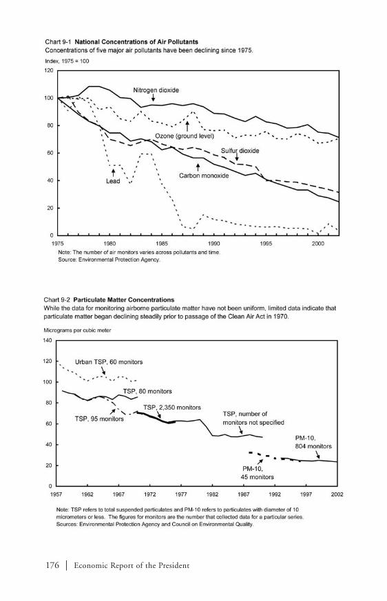
176 | Economic Report of the President

Chapter 9 | 177
Misplaced Reasons for Government InterventionIn making environmental policies, it must be recognized that government
measures themselves might create further inefficiencies. When it is difficultto determine the extent of an environmental externality, an attempt torectify it might end up making matters worse by imposing unintended costson third parties without achieving an efficient outcome.
This inefficiency can arise even from well-intentioned environmentalregulations. Two fallacious arguments are frequently used to justify ineffi-cient regulations. One such misplaced rationale is that regulations improvethe economy and spur job growth. The reasoning goes as follows: environ-mental regulations lead firms to install pollution-control technologies,which they must purchase from other firms. These technologies are built,delivered, installed, and operated by workers who otherwise would not bedoing this work. Similarly, the regulations may promote environmentally-friendly industries that hire people who would not be hired otherwise. Forthese reasons, the regulations are said to “spur” the economy and job growth.By this reasoning, throwing a rock through a window also improves theeconomy, because it necessitates the hiring of someone to repair the window.What this ignores is that the resources spent to comply with an unnecessaryor inefficient regulation are diverted from other uses. The money and peopleinvolved could have been used instead to produce more goods for consumersor to build new factories or machinery. The jobs associated with complyingwith environmental regulations are a cost of regulation, not a benefit.
Another misplaced view of environmental regulation is that the goal ofregulations should be to eliminate or substantially reduce risks withoutconsidering costs. This approach is embodied in some well-intentioned laws.The 1970 Clean Air Act, for example, directs the Environmental ProtectionAgency (EPA) Administrator to set national ambient air quality standards(NAAQS) that achieve “an adequate margin of safety,” and the SupremeCourt has ruled that “the Clean Air Act…unambiguously bars cost consid-erations in the NAAQS setting process.” Similarly, the stated goal of theOccupational Safety and Health Act of 1970 is “to assure so far as possibleevery working man and woman in the Nation safe and healthful workingconditions,” without considering the costs of doing so. While the goals ofthese laws are noble, they do not recognize the inevitable trade-offs involved.Not all environmental laws preclude cost considerations. For example, theSafe Drinking Water Act Amendments of 1996 explicitly acknowledge theimportance of benefit-cost analysis when considering the appropriate levelof regulation for contaminants in drinking water.

178 | Economic Report of the President
Regulations Impose Benefits and CostsThe failure to consider costs inhibits the goal of making regulations that
maximize the difference between benefits and costs. Furthermore, the failureto consider costs can lead to a misallocation of resources, because a regulationthat is made without considering costs might receive more resources thanother regulations that warrant greater attention. While the benefits of manyregulations include both health and non-health related benefits, many regula-tions primarily address fatality risks, and there is a wide range of cost perexpected life saved across such regulations. For example, one survey of cost perlife saved across regulations found that the regulation for childproof cigarettelighters costs approximately $100,000 per life saved (in 2003 dollars) whereasthe formaldehyde regulation costs approximately $80 billion per life saved (in2003 dollars). Shifting resources from regulations where the cost per expectedlife saved is high (for example, formaldehyde regulation) to regulations whereit is low (for example, childproof lighter regulation) would result in more livessaved for the same cost to society. Many of the differences in cost per life savedoccur because legislative mandates only sometimes allow agencies to considercosts when crafting regulations.
Stringent regulations may appear to be good for society because they savelives. However, because the Nation’s ability to bear costs is limited, the widerange of costs per life saved across regulations implies that more lives couldbe saved at the same cost by shifting resources to the regulations with lowercosts per expected life saved. One study found that society could save twiceas many lives with the same budget if it designed regulations in a way thatmaximized lives saved. Some of the more costly health-based regulationsmight actually lead to a net increase in fatality risk because their high costs diminish the resources available for improving other health and environmental outcomes.
Using Science to Help Set Regulatory Priorities
Sound regulatory policy must be based on scientific assessments of environmental and health risks. Scientific assessments involve a carefulexamination of the risks involved and of the expected health outcomes forthe people exposed to the risk at hand. This allows for an unbiased evalua-tion of environmental and health threats in which to target regulatoryactions. Unfortunately, regulatory risk assessments at times overestimatesome threats, or overemphasize risks to “hypothetical” (rather than real)people. These practices can lead to a distortion of regulatory priorities.

Chapter 9 | 179
Overestimating the Risks: The Problem with“Cascading Conservatism”
In a well-intentioned attempt to be prudent, regulatory agencies sometimesrely on scientific assessments of environmental and health risks based onassumptions that overstate actual risks. When estimating chemical toxicity, forexample, risk assessors have at times relied on high-end default assumptionsthat are likely to overestimate the actual risk of a chemical. Toxicity testing isevolving to use information that permits assessors to move away from assump-tions that lead to overstated risks. When more data are available, regulatoryrisk assessors do not need to rely on high-end default assumptions and caninstead attempt to estimate more accurately the expected level of risk. Becausethe EPA’s primary goal is public health protection, however, it still relies onhigh-end default assumptions when there is uncertainty about scientific data.
Similarly, regulatory agencies sometimes use high-end estimates of thelikelihood of people being exposed to a certain risk. These exposure esti-mates are then combined with toxicity estimates that are themselves likely tooverstate risk. The multiplicative impact of combining several high-endcomponent estimates is known as cascading conservatism. This practice canlead to risk estimates that greatly overstate the threat of environmental prob-lems and thus overstate the benefits of regulating those risks. One studyfound that in a sample of hazardous waste sites, over 40 percent of the sitesrequiring cleanup under the Superfund program would shift into the discre-tionary cleanup range if not for the overestimation of risks resulting fromcascading conservatism.
Such high-end risk estimates can lead to several types of problems. First,the practice overstates the risk of all environmental health problems relativeto other types of hazards. This overstatement can cause too many resourcesto be allocated to addressing low-priority concerns. An example of such adistortion is the commonly-held view that synthetic chemical pollutantssuch as insecticides are a leading contributor to cancer. In reality, theevidence suggests that such chemicals account for a low percentage ofhuman cancers. The main contributors to human cancer appear to besmoking and poor diet—each of which accounts for about one-third ofcancers. The result is that regulatory efforts are directed at addressing therisks of synthetic chemicals that may well pose lower risks of causing cancerthan many common natural chemicals.
A second problem with the high-end risk estimates caused by cascadingconservatism is that they can distort the allocation of resources amongdifferent environmental health concerns. If each uncertain component thatgoes into a risk assessment overstates the risk, then the multiplicative impactof cascading conservatism will result in higher risk estimates for threats thathave more uncertain components. For example, if there are two equally

180 | Economic Report of the President
effective pesticides, with one posing a higher threat to the population thanthe other, the safer pesticide might be assessed as more of a threat if there aremore uncertain components involved in its risk assessment. This assessmentcould result in the safer pesticide receiving stronger regulatory emphasis bythe government. It is better to target regulatory dollars to the risks expectedto be higher in a reasonable scenario or range of scenarios than to the risksthat might be higher in a worst-case scenario.
Population-Weighted Risk AssessmentsRegulatory efforts can also be distorted when risk assessments ignore the
number of real people potentially exposed to an environmental risk. Forexample, an environmental hazard at one location might pose a greater riskto any person exposed to the hazard than an environmental hazard at asecond location. However, if no one lives near the first location and manypeople live near the second location, the expected risk to society is higher atthe second location.
The case of United States v. Ottati & Goss offers one example of suchmisplaced regulatory priorities. In this case, a company litigated for relief ofan EPA-required cleanup that would have cost the company $9.3 million toremove small amounts of contaminants from a site that was already mostlydecontaminated. The company had already spent $2.6 million to clean thesite so that small children playing on the site could eat small amounts of dirtdaily for 70 days each year for three and a half years without significantharm. The additional $9.3 million would be used to burn the soil, whichwould allow children to eat a small amount of dirt each day for 245 days peryear without significant harm. However, there was little chance that childrenwould ever be exposed to this site because it was located in a swamp. Thecourts ruled in favor of the private party and refused to enforce the proposedremediation goal.
Objective Versus Perceived RiskRegulatory decisions should be based on scientific assessments of risks
rather than perceived risks. This approach would help properly order priori-ties for regulatory decisions. Perceived risks often differ from expertassessments of risk because laypeople have difficulty assessing the frequencyof low-probability events. Chart 9-3 compares survey respondents’ perceivedrisks of dying from various hazards to the objectively measured risks of dying.In this chart, the dashed line represents where the perceived risk equals theactual risk; if all the points on the chart fell on this line, it would indicate thatsurvey participants precisely estimated the risk of dying from various hazards.All points to the left of the dashed line represent hazards for which the

Chapter 9 | 181
perceived risk of dying is higher than the actual risk, and all points to theright of the line indicate hazards for which people thought the risk of dyingis lower than it actually is. The chart suggests that it is common to overesti-mate fatalities associated with low-probability events and to underestimatefatalities associated with high-probability events. These systematic mispercep-tions may lead to misplaced pressures to overregulate small environmentalrisks at the expense of addressing larger ones.
Achieving Goals Through Cost-Effective Regulations
As discussed in Chapter 7, Government Regulation in a Free-MarketSociety, when the assignment of property rights is insufficient to achieve anefficient outcome, government intervention may help achieve efficiency.Chapter 7 discusses government actions that can, in principle, achieve anefficient outcome by incorporating the costs of externalities into the market’sprice mechanism. It is important that any regulatory mechanism thataddresses externalities do so in the least costly (that is, the most cost-effective) way so that society’s scarce resources are not wasted. This sectionfocuses on how to achieve air-quality goals cost effectively, but many of the

182 | Economic Report of the President
lessons can be applied toward achieving other environmental goals, such asclean water protection and energy-efficiency standards.
Command-and-Control RegulationsAir-quality command-and-control regulations prescribe specific technologies
that individual firms must use to control emissions, or they set specific emis-sion rates for individual firms. The United States currently has many suchenvironmental regulations. These regulations are inherently inflexible and areill-suited to achieving emissions reductions in the least costly manner. Whilesome command-and-control air-quality regulations may be just slightly morecostly than cost-effective regulations, studies show that others are up to 22 times more expensive than the most cost-effective set of controls.
The reason command-and-control regulations are more expensive isstraightforward: suppose the regulatory goal is to halve the emissionsemanating from two firms. A command-and-control regulation mightrequire each firm to cut its emissions by half. However, if it is less costly forone firm to reduce emissions, then—so long as the health effects of the emis-sions depend only on the total from the two emission sources—shifting theburden to the firm with lower abatement costs would result in the same envi-ronmental improvement at a lower cost. In general, the greater the differencesacross firms in their emissions before the regulation, and the greater thedifferences across firms in the rate at which each firm’s costs rise with addi-tional reductions, then the more costly a command-and-control approach iscompared to more flexible approaches. Cost-effective emissions reduction isachieved when the cost of reducing an additional unit of emissions (themarginal abatement cost) is equal across all firms.
An example of an inflexible command-and-control regulation is themechanism by which the Clean Air Act Amendments of 1990 addresshazardous air pollutants (HAPs). The Act specifies that the emissions reduc-tion standards for categories of existing HAP polluters must be set at “theaverage emission limitation achieved by the best performing 12 percent ofthe existing sources.” While some flexibility is allowed in establishing theemission limitations, the command-and-control standard for regulatingHAPs has frequently been interpreted in a way that ignores the differentialcosts of reducing emissions across existing sources within a category. Thislikely results in higher costs than would a more flexible regulation.
Command-and-control regulations also fail to provide market incentivesfor firms to explore less expensive means of reducing emissions. More flex-ible, incentive-based regulations would provide signals to the market of theincreased demand for emissions reductions. With proper incentives in place,markets can respond to such an increase in demand with technological inno-vation and efficient reallocation of their scarce resources to achieve the goal.

Chapter 9 | 183
Command-and-control regulations can also unintentionally lead tooutcomes that are contrary to their environmental goals. An example of this isthe New Source Review component of the 1977 Clean Air Act Amendments.This legislation required a strict control technology for most new industrialfacilities and for facilities that undertook significant modifications, but itexempted existing facilities that did not make major modifications from thesame standards. It was thought at the time to be more efficient to add newpollution control technology when plants were upgrading or when buildingnew plants. This situation is known as new source bias because it provides anincentive for existing sources of emissions to continue their business opera-tions for longer than would have been the case under normal marketconditions without the regulation. It also provides an incentive for existingplants to forgo modifications.
New pollution-causing production sources tend to be cleaner than old oneseven in the absence of regulations, so extending the business operations ofolder plants without making modifications could result in higher emissions.Applying different regulations for “routine” versus “major” modifications alsoleads to ambiguity, litigation delays, and uncertainty in business planning, allof which can harm the economy and may impede environmental improve-ments. The Administration recently addressed this problem by establishingclear rules that remove disincentives for facilities to modify and undertakeroutine maintenance, repair, and replacement activities that could improvethe safety, reliability, and efficiency of the plants.
Market-Based Price Regulations: Emission FeesEnvironmental regulations that provide firms with market-based incentives
for emissions reduction avoid the complications of command-and-controlregulations and achieve the same goals at lower costs. In particular, emissionfees and cap-and-trade programs are usually less expensive than command-and-control approaches at achieving regulatory goals. An emission feeinvolves a charge to polluting sources for each unit of pollution emitted.Because each successive unit of emissions reduction typically involvesincreased costs, each source will reduce emissions until it would cost more toreduce the next unit of emissions than it would to pay the emissions fee. Thisresults in equal marginal abatement costs across all affected firms.
With an emission fee, the total level of emissions reduction will depend onthe per unit fee: a higher rate will achieve more emissions reduction. Theemission fee also provides incentives to reduce emissions, because the bettera firm is at reducing emissions, the lower the total fee the firm must pay. Thissends a market signal that pollution has a price (equal to the emission fee),and any innovative means of reducing emissions will save firms from payingthe fee. This market signal is likely more adept than the government at

184 | Economic Report of the President
spurring technological innovation, adapting to changes in the economy, andshifting resources to reflect the increased demand for emissions reduction.
Market-Based Quantity Regulations: Cap-and-TradeThe main problem with an emission fee is that it is difficult to know
beforehand what fee level will achieve the desired amount of pollutionreduction. A cap-and-trade regulation addresses this issue and providesmarket incentives to reduce emissions in a cost-effective way. Such regula-tions “cap” the amount of allowable emissions and require that a firm owna permit for each unit of pollution emitted in a given period (for example,a year). This permit effectively establishes a legal property right for the airaffected by the pollution, so that any emissions must be paid for by the firm.The government allocates the pollution permits to the emission sources andthen allows the sources to buy and sell permits from each other.
Under a cap-and-trade system, a source with a high cost of reducing anadditional unit of emissions would be willing to purchase a permit from asource with a lower marginal abatement cost. With a well-functioningmarket for the permits, sources will trade permits until the price for thepermits equals the marginal abatement cost. As with the emission fee, themarginal abatement costs will be equal across sources, leading to a cost-effec-tive result. The cap-and-trade system also provides an incentive to reduceemissions because each unit of emissions reduction saves the source the priceof another permit. This regulation sends a market signal that there is a pricefor emissions and any innovative means of reducing emissions will save firmsfrom paying the price. The cap-and-trade system therefore achieves thetarget level of pollution reduction at the lowest cost.
One consideration for a cap-and-trade system is how to allocate thepermits initially. A cap-and-trade system that allocates the permits based onhistoric emissions or other firm characteristics, known as grandfathering, inessence gives away a valuable asset—the permits. A grandfathering systemcould establish a barrier to entry for new firms because any new entrantwould have to purchase permits from existing firms.
One way to avoid these problems is to auction the permits at some regularinterval to the highest bidders. Firms with higher marginal abatement costswould bid more for permits than those that can achieve less-costly emissionsreductions. While auctioning the permits would result in lower profits forthe regulated firms (compared to giving away the permits), it would notaffect the firms’ output decisions. Grandfathering versus auctioning thepermits is primarily a question of distribution, not efficiency—it is a question of whether a public asset should be given to firms for free or soldas a means of generating public revenues.

Chapter 9 | 185
A notable example of a cap-and-trade system is the sulfur dioxide (SO2)trading program created under Title IV of the Clean Air Act Amendmentsof 1990. The program set a goal of reducing emissions by 10 million tonsfrom the 1980 level by 2010. This was to be accomplished in two phases.The first phase, which began in 1995, initially capped the SO2 emissions at263 individual units which were owned by 110 electric utility power plantsin 21 eastern and midwestern states. These plants, which were primarilycoal-fired, emitted the greatest amounts of pollution among power plants inthese regions. From 1995 to 2000, an additional 182 units were allowed intothe program. The second phase, which began in 2000, further decreased theannual emissions of SO2 and required all large fossil fuel-fired power plantsin the contiguous 48 states and the District of Columbia to hold permits tocover their emissions.
In both phases, power plants could purchase permits from other powerplants in order to meet their emissions coverage. The program also allowedplants to carry over (or bank) unused permits to use in later years, whichgives firms even greater flexibility in achieving long-term pollution reduc-tion. In contrast to a command-and-control system, this cap-and-tradesystem allows plants that find it costly to reduce their SO2 emissions topurchase credits from plants that can reduce SO2 at lower cost.
Evidence indicates that such cost-saving trades did indeed take place asfirms took advantage of the system’s inherent flexibility (Chart 9-4). Eachbar in the following chart represents the emissions rate each plant achievedafter trading permits in 1997. The superimposed line in the figure shows thelevel of emissions each plant would have had to achieve in the absence oftrading. Bars below the line indicate plants that reduced their emissions bymore than the required amount and sold their excess permits or bankedthem. Bars above the line indicate plants that purchased permits or usedpreviously banked permits to avoid costly abatement. The figure shows thatalmost every plant took advantage of the flexibility of the system, suggestingthat plant-level costs of reducing SO2 emissions vary greatly.
The trading program has achieved its pollution-reduction goals at greatcost savings. By the end of the first phase, emission reductions were almost30 percent below the required level. The flexibility of this approach has beenestimated to provide cost savings of approximately $0.9 billion to $1.8billion a year compared to costs under a command-and-control regulatoryalternative; other tradable-permit markets have had significant cost savingsas well (Table 9-1).

186 | Economic Report of the President
Emission Fees Versus Cap-and-TradeAs mentioned previously, one problem with emission fees is that it is difficult
to know beforehand at what level to set the fee to achieve the desired pollu-tion reduction. This might require periodic adjustments of the fee level, andsuch adjustments would introduce uncertainty that could interfere withfirms’ planning decisions. The emissions fee does, however, allow thegovernment to set with certainty the marginal cost of emissions reduction.For each emission fee there is a corresponding allocation of permits that
Emissions trading program Criteria air pollutants 1974-present Total, $1-$12 billionLead phasedown Rights for lead in gasoline 1985-1987 Total, $400 millionAcid rain reduction SO2 emission reduction credits 1995-present Annual, $0.9-$1.8 billion
TABLE 9-1.— Cost Savings of Tradable-Permit Systems
Program Traded commodity
1 Base year for values for emissions trading program not specified.
Sources: Robert W. Hahn, “Economic Prescriptions for Environmental Problems: How the Patient Followed theDoctor’s Orders,” Journal of Economic Perspectives, Spring 2000; Curtis Carlson, Dallas Burtraw, Maureen Cropper,and Karen L. Palmer, “Sulfur Dioxide Control by Electric Utilities: What Are the Gains from Trade?” Journal ofPolitical Economy, December 2000; and Environmental Protection Agency.
Cost savings(2003 dollars1)Years of operation

Chapter 9 | 187
would achieve the same results; however, it is difficult to know beforehandwhat the market price for permits will be once trading actually takes place.
One way to reconcile these issues is to offer a cap-and-trade system witha safety valve. The safety valve sets a maximum price for a permit, whichguarantees that the price of reducing emissions does not exceed the expectedbenefits. The regulatory agency issues and sells extra permits on request fromany firm at this fixed safety valve price, thus guaranteeing that the marketpermit price does not exceed this level. A cap-and-trade program with asafety valve achieves the target level of emission reductions in a cost-effectivemanner, while protecting the regulated firms against unexpected short-termprice increases in emissions reduction.
The President’s Cap-and-Trade ProgramAn example of a well-designed incentive-based regulatory approach is the
President’s Clear Skies proposal for reducing emissions of sulfur dioxide,nitrogen oxides, and mercury from electric utility generators by approximately70 percent by 2018. Clear Skies would cost-effectively reduce emissions byestablishing a cap-and-trade system for each of the three pollutants. The EPAhas estimated the benefits of the Clear Skies Act at $113 billion annually by2020, compared with $6 billion in projected annual costs. These include $110 billion in annual health benefits (including the prevention of 14,100premature deaths and 30,000 hospitalizations and emergency room visits) and$3 billion in annual benefits from increased visibility at national parks. Underthe existing Clean Air Act, the EPA issues national air-quality standards forcertain pollutants, including particulate matter and ozone. The EPA projectsthat compared with existing programs, the Clear Skies Act would lead 35 additional eastern U.S. counties to meet the particulate matter standard by2020, leaving only eight counties not meeting the standard. The EPA expectsthat the remaining counties not meeting the standards would move closer toachieving them due to the Clear Skies Act.
To mitigate the effects of market shocks that potentially affect the costs ofemissions reduction, Clear Skies would establish a safety valve price forpermits of each pollutant. It would also provide regulatory certainty byachieving the reductions of all three pollutants in two phases. Firms wouldtherefore plan their reductions of the three pollutants together and over thelong term. Indeed, because the Clear Skies plan allows the banking ofpermits for future use, it provides an incentive for firms to achieve reduc-tions quickly. Additionally, Clear Skies would provide revenue for thegovernment because it phases in an auction system for the permits.
Clear Skies demonstrates the lessons learned from past regulatory experiences:instead of imposing an inflexible, command-and-control regulation to achieve

188 | Economic Report of the President
emissions reduction, it offers a market-based, cost-effective, cap-and-tradeprogram to achieve large reductions in emissions from electric utility generators.
Conclusion
Economic growth and environmental improvements are at times incorrectlyseen as competing aims. Increased economic production can indeed lead togreater environmental degradation. However, an increase in economicresources provides more options (most notably, technological advancements)for addressing environmental problems. Moreover, a growing economy canalso lead to increased demand for environmental improvements. It is thereforeimportant to weigh the direct environmental benefits of a regulation againstits economic costs. The goal should be to maximize the net benefits to society,while also giving due consideration to distributional issues. Maximizing netbenefits is best achieved in a free-market setting unless there are spillover coststo third parties.
Spillover costs are best addressed by establishing property rights that willlead the affected parties to negotiate a mutually-beneficial outcome. If thecosts of such negotiations are prohibitive, however, government shouldrespond carefully and always keep in mind the possible government spillovercosts. To make effective regulations, the government must first assess theenvironmental problems using sound, unbiased estimates of the hazards andthen craft incentive-based regulations to address them. Such regulations canaddress the spillover costs of environmental problems at lower costs tosociety than the traditional command-and-control regulatory methods.These principles, and the lessons learned from our past regulatory experi-ences, as described throughout this chapter, should guide our futureregulatory endeavors to achieve environmental improvements coupled witheconomic growth and efficiency.

The breadth and pace of innovation and change in the provision of healthcare in the United States over the past few decades have been no less than
astounding. Technological progress in the form of new medical knowledge,medicines, treatments, and medical devices has allowed Americans and peopleworldwide to live longer, healthier lives.
As new treatment options become available, it is not surprising that theUnited States and other major industrialized countries continue to shift moreresources to health care. Research suggests that between 50 and 75 percent ofthe growth rate in health expenditures in the United States is attributable totechnological progress in health care goods and services. However, theincrease in resources devoted to health care has led to concern about itsaffordability, both for families worried about tight budgets and for the Nationas a whole. A strong reliance on market mechanisms will ensure that incen-tives for innovation are maintained while providing high-quality care in themost cost-efficient manner. Americans should have more choices, moreinformation, and more control over their health care decisions.
Health insurance plays a central role in the workings of the U.S. health caremarket. An understanding of the strengths and weaknesses of health insuranceas a payment mechanism for health care is essential to the design of reformsthat retain incentives for innovation while reining in unnecessary expenditures.
This chapter discusses the roles of innovation, insurance, and reform in thehealth care market. The key points in this chapter are:
• U.S. markets provide incentives to develop innovative health care prod-ucts and services that benefit both Americans and the global community.
• Over reliance on health insurance as a payment mechanism leads to aninefficient use of resources in providing and utilizing health care.
• Reforms should provide consumers and health care providers with moreflexibility and information.
189
C H A P T E R 1 0
Health Care and Insurance

190 | Economic Report of the President
The U.S. Health Care System as an Engine of Innovation
Innovation and new technology have changed the practice of medicineover the past few decades. Diagnostic tools such as magnetic resonanceimaging and computed tomography scanning have made it possible fordoctors to see otherwise invisible problems. Innovations such as balloonangioplasty treat conditions that previously required extensive surgery.Minimally invasive surgical techniques such as arthroscopy provide treat-ment options that lead to shorter hospital stays and faster recoveries.Restorative surgeries such as hip and knee replacements are now common-place and provide patients with improved mobility and thus improvedquality of life. New pharmaceuticals treat conditions that were previouslyintractable or help to avoid more costly surgeries and lengthy hospital stays.The list of advances is long and impressive.
The Value of Health Care Innovation Innovation in health care goods and services, including advances in
scientific knowledge that have changed many people’s day-to-day behavior,has markedly improved the lives of Americans. Life expectancy at birth inthe United States increased from 68.2 years in 1950 to 77.2 years in 2001.Medical advances have also increased the quality of life through innovationsthat improve mobility, sight, and hearing.
Some might argue that these advances are not unique to the United Statesand that Americans spend too much for health care relative to other coun-tries. The United States expends a higher fraction of GDP on health care thandoes any other industrialized country. According to an international compar-ison released in 2003, the United States spent 13.9 percent of GDP on healthcare in 2001, while the average among industrialized countries was 8.4percent of GDP. Measures of health outcomes such as longevity and infantmortality, however, are not markedly different in the United States than inother advanced economies that spend substantially less on health care.
The argument that the U.S. health care system is overly costly relative toother countries implicitly assumes that if two countries spend differentamounts for health care and get the same health outcomes, then the higher-spending country must be inefficient and wasteful. This argument is notcorrect in the case of health care for two reasons that are related to theleading role of the United States as a source of research and innovation.

Chapter 10 | 191
First, in general terms, while all countries can benefit from research anddevelopment expenditures made by a single country, only the health expen-ditures in the innovating country will include the costs of research anddevelopment. Health expenditures in non-innovating countries will excludethe research and development costs.
Second, free markets incorporate incentives for innovation that generateproducts, services, and knowledge that potentially benefit all countries.Markets naturally encourage and reward innovation. Unfettered by govern-ment price controls or access restrictions, innovative products, talentedhealth care practitioners, and skilled health care professionals are rewardedin the marketplace. This leads to technological advances by encouragingtalented people to participate in the health care industry and by increasinginvestment in new products and research. The financial rewards for innova-tion will be reflected in U.S. health expenditures through a combination ofhigher prices and wages, and higher usage than in other countries. Once aproduct or service is developed through the combination of talent andcapital, however, it becomes available for use outside the United States.Countries in which government regulation has supplanted market forceswill still have the opportunity to take advantage of U.S. innovation withouthaving to pay as much for it.
As an illustration of how U.S. health expenditures reflect the incentivesfor innovation, consider products such as medical devices and pharmaceuti-cals. The patent system exists to encourage innovation for these types ofproducts. The innovator’s incentive in a patent-based system is the opportu-nity to hold a monopoly on a product for a limited period of time.Therefore, the innovator can temporarily charge a higher price and earnmore profits than he would without patent protection. The higher consumerexpenditures that can result from monopoly pricing will be reflected inhealth care expenditures.
Once the patent system has led to the development of a product, it is available for use throughout the world, not just in the United States. Thisleads to an opportunity for other countries with centralized health agenciesto negotiate a price close to production costs, thereby paying lower pricesthan they would in a free market that fully respected patent rights. What thisimplies is that other countries can reap the benefits of U.S. innovations inhealth care goods and services but pay only a fraction of the costs. It followsthat if the United States attempted to reduce health expenditures by adoptingcost-control policies found in other countries, innovation would slow andboth Americans and citizens of other countries would be affected.

192 | Economic Report of the President
U.S. Leadership in Health Care TechnologySeveral pieces of evidence point toward the preeminence of the United
States in providing health care technology. First, since 1975, the Nobel Prizein medicine or physiology has been awarded to more Americans than toresearchers in all other countries combined. Second, according to datacollected through 1993, 15 of the 19 marketed “biotech” drugs used fornondiagnostic purposes were the product of U.S. companies alone. U.S.companies shared credit with companies from other countries for two moreof the 19 drugs. As of 2002, eight of the world’s ten top-selling drugs wereproduced by companies headquartered in the United States.
A third example of U.S. leadership is that many important medical innovations in the past 30 years arguably originated in the United States.This evidence is based on a survey designed to determine the relative impor-tance of a variety of medical innovations developed over approximately thelast 30 years. Starting with a review of the medical literature, researcherscompiled a list of 30 major medical innovations and then surveyed over 300 leading general internists in the United States concerning the relativeimportance to their patients of the innovations. Based on the survey,researchers ranked the innovations in order of importance. The first andsecond columns of Table 10-1 reflect the results for the top ten innovations.
The table also includes countries of origin, a category that was notincluded in the original research. Assignment of country was based on the
1 Magnetic resonance imaging (MRI); Noninvasive methods to view United States, United Kingdom;Computed tomography (CT) internal workings of the body United States, United Kingdom
2 Angiotensin converting enzyme Drugs to treat hypertension and United States(ACE) inhibitors heart failure
3 Balloon angioplasty Minimally invasive surgery to Switzerlandtreat blocked arteries
4 Statins Cholesterol-reducing drugs United States, Japan
5 Mammography Diagnostic tool to detect breast Indeterminate cancer
6 Coronary artery bypass graft Surgery for heart failure United States(CABG) surgery
7 Proton pump inhibitors (PPIs); Antiulcer drugs Sweden; H2-receptor antagonists United States
8 Selective serotonin re-uptake Antidepressant drugs United Statesinhibitors (SSRIs)
9 Cataract extraction and lens Eye surgery United Statesimplants
10 Hip replacement; Joint replacement with United Kingdom; Knee replacement mechanical prosthesis Japan, United Kingdom,
United States
TABLE 10-1.— Important Medical Innovations and Associated Country of Origin
Rank Technology
Sources: Victor R. Fuchs and Harold C. Sox Jr., “Physicians’ Views of the Relative Importance of Thirty MedicalInnovations,” Health Affairs, September/October 2001. Descriptions and countries of origin from various sources.
Description Country of Origin

Chapter 10 | 193
location where the first clinically viable form of the innovation was developedor produced, or where research important to its creation occurred. TheUnited States dominates this chart as the innovating country for these impor-tant medical developments. Of the ten, eight include the United States as akey country. The United Kingdom and Japan, the next closest sources, areassociated with just two of the innovations each.
Table 10-1 should not be misinterpreted. Scientific advances by theirnature are evolutionary, with recent advances building upon prior discov-eries. The process of identifying a single person or team for progress thatrelies upon previous work is necessarily subjective. Nevertheless, such judg-ments are regularly made in selecting awards such as the Nobel Prize. Buteven taking into account the unavoidable limitations of such a list, it doessuggest a dominant role for the United States in the development of newand useful medical technologies.
Box 10-1: Price Regulation and the Introduction of New Drugs
A recent study suggests that pharmaceutical firms tend to avoid ordelay introducing new drugs in countries with price controls. In the study,which includes data from 25 countries on 85 new chemical entities intro-duced in the United States or the United Kingdom between 1994 and1998, the three countries that did not require price approval before launch(the United States, Germany, and the United Kingdom) introduced themost new drugs. Analysis controlling for per capita income and othercountry and firm characteristics shows that countries with lowerexpected prices or smaller expected market size have fewer launches andlonger launch delays. In the European Union, where drugs can beapproved through a centralized procedure for use in the entire region,countries with price controls still experience significant launch delays.
According to the study, the connection between price controls anddelayed access to drugs lies in the tendency for price controls to “spillover” from one country to another. Firms have an incentive to avoidor delay launching drugs in markets with price controls if they fearthat the low prices will “spill over” to other markets. There are twomain mechanisms by which price controls in one country can affectpharmaceutical profits in another: parallel trade and external refer-encing. With parallel trade, one country can take advantage ofregulated low prices in another country through trade. With externalreferencing, countries can incorporate external price controls intodomestic prices through price-setting formulas that depend on pricesin other countries. Overall, the study suggests that there is a tradeoffbetween low prices and rapid access to new drugs.

194 | Economic Report of the President
Insurance Reform as a Means of ProvidingHealth Care More Efficiently
While the U.S. health care market provides excellent incentives for innovation,there are legitimate concerns about cost. Rising health expenditures for fami-lies and firms can lead to difficult decisions over how best to allocate limitedbudgets. Pressure on government budgets continues to increase due to majorhealth care programs such as Medicare (health insurance primarily for theelderly) and Medicaid (health insurance primarily for the poor). Physiciansand hospitals struggle with government regulations, rising liability costs, andgrowing administrative burdens. To craft adequate responses to such challenges, it is important to understand the economic forces at work.
Technological progress in health care has been very beneficial, but it hasled to growth in health care expenditures as the new technology has beenapplied to increase the length and to improve the quality of life. Researchsuggests that between 50 and 75 percent of the growth rate in health expen-ditures in the United States is attributable to technological progress in healthcare goods and services. Potential sources of the remaining 25 to 50 percentof the growth rate include: higher demand for health care due to increasingincomes and the aging of the U.S. population; the increased practice of“defensive medicine” (that is, medical procedures with limited therapeuticvalue that are performed by physicians to avoid lawsuits); and increased useof health insurance plans as a payment mechanism for health care.
There are various ways to reduce health care costs. Reducing the incentiveto practice defensive medicine has the potential to lower the level of healthcare costs and is therefore an important objective. Modifying the health insur-ance system offers an especially attractive target for cost-saving reform becauseit would affect both the level and the growth rate of health expenditures.Reforms could be targeted to reduce administrative costs and the incentive tooveruse health insurance as a payment mechanism. Understanding thestrengths and the weaknesses of the health insurance system is central to devel-oping policies that will lead to more cost-effective health care and to greateraccess to health care for those underserved by the current market.
The Appropriate Use of InsuranceInsurance is an indispensable tool in modern economies. Individuals
insure automobiles against the possibility of an accident and homes againstthe possibility of a fire. Life insurance provides financial security to lovedones in case of an untimely demise. In each of these examples, the basic principle is the same: for a fee—the insurance premium—the insurer promises that some financial benefit will be forthcoming if a well-definedevent takes place such as a car accident, a house fire, or a death.

Chapter 10 | 195
Insurance is a valuable economic commodity. By giving up some incomein the form of a premium, a consumer can avoid the large decline in wealthassociated with an unfortunate event. Even if the event does not occur, aconsumer benefits from the reduced uncertainty provided by insurance.
Insurance is generally not needed when there is little uncertainty or whenfinancial risks are small. For example, insurance policies usually do not payfor items such as groceries, clothing, or gasoline, although it would certainlybe possible to create such policies. Suppose, for example, that an individualcould purchase a clothing insurance policy with a “coinsurance” rate of 20 percent, meaning that after paying the insurance premium, the holder ofthe insurance policy would have to pay only 20 cents on the dollar for allclothing purchases. An individual with such a policy would be expected tospend substantially more on clothes—due to larger quantity and higherquality purchases—with the 80 percent discount than he would at the fullprice. However, the insurance company would need to charge a highpremium to cover expenses. The premium would need to cover the 80 percent discount on the clothing that the individual would have boughthad he or she been paying full price. Additionally, the premium would needto cover the insurer’s expense for clothes purchased because the individualbuys clothes as if they cost only 20 cents on the dollar. Few individualswould find such an expensive policy cost-effective.
Moral HazardThe clothing insurance example suggests an inherent inefficiency in the
use of insurance to pay for things that have little intrinsic risk or uncertainty.It also illustrates the broader problem in insurance markets known as moralhazard. Moral hazard refers to the idea that policy holders will makedifferent choices when they are covered by an insurance policy than whenthey are not, but the insurer cannot fully monitor or restrict their actions. Inthe clothing example, moral hazard results in insured individuals spendingmore on clothing than they would without insurance.
Optimal insurance contracts must balance the value that consumers placeon reducing their exposure to risk against the inefficiency arising from moralhazard. In the absence of uncertainty, insurance is wasteful because moralhazard will lead to excessive use and there is no benefit to the consumer fromrisk-reduction. Inefficient use of insurance will be reflected in an unneces-sarily high cost for insurance. Standard features of insurance contracts suchas coinsurance rates, copayments, and deductibles are attempts to mitigatethe moral hazard problem. Even so, inefficiencies of this sort are pervasivein the U.S. health care system.

196 | Economic Report of the President
Adverse SelectionAnother issue that arises in discussions of insurance markets is adverse
selection. Adverse selection occurs when an insurance policy attracts certaintypes of people, and the insurer cannot identify these people before theyenroll. If the premium is based on the average individual, but the policydisproportionately attracts those who spend more than the average person(in the clothing example, individuals with particularly expensive tastes inclothes), the policy will lose money for the insurer. The policy will theneither increase in price or not last in the marketplace.
Adverse selection illustrates a problem that exists when the consumerknows more about his or her characteristics than the insurer. As a result thereis a market inefficiency where, in the extreme, some consumers do notpurchase insurance because the only policy available to them is priced for themost expensive consumers. If insurers could distinguish among differenttypes of consumers, policies could be tailored to specific types and pricedaccordingly. With better information, an efficiently functioning insurancemarket would be able to provide insurance in a way that would maximizeindividual consumer welfare.
Health Insurance in the United StatesHealth insurance in the United States has several unique features. First,
the employer portion of premiums for employer-provided health insuranceis generally exempt from income and payroll taxes. The employee portion ofpremiums is similarly tax-exempt for the roughly one-half of workerscovered by tax-advantaged health plans. This leads to the second, and unsur-prising, feature, which is that most health insurance is provided throughemployers. Over 60 percent of all individuals in the United States haveemployer-provided health insurance. The central role of employer provisionmakes health insurance very different from other types of insurance, such asfire and car insurance.
Third, health insurance policies in the United States also tend to covermany events that have little uncertainty, such as routine dental care, annualmedical exams, and vaccinations. For these types of predictable expenses,health insurance is more like prepaid preventative care than true insurance. Ifautomobile insurance were structured like the typical health policy, it wouldcover annual maintenance, tire replacement, and possibly even car washes.
Fourth, health insurance tends to cover relatively low-expense items, suchas an office visit to the doctor for a sore throat. Although often unforeseeable,this expense would not have a major financial impact on most people. Tocontinue the analogy, it would be similar to car insurance covering relativelysmall expenses such as replacing worn brakes.

Chapter 10 | 197
Box 10-2: Who are the Uninsured?
The U.S. Census Bureau estimates that in 2002, 242.4 millionpeople in the United States had health insurance for the entire year,while the remaining 43.6 million people were uninsured.Uninsurance persists in the face of public programs such as Medicare,Medicaid, and the State Children’s Health Insurance Program. Ingeneral, these programs provide health insurance to the elderly, thevery poor, and the children of the moderately poor, respectively.
The uninsured are a diverse and perpetually changing group. TheCongressional Budget Office claims that due to sampling techniques,the U.S. Census Bureau estimate of 43.6 million (15.2 percent of thepopulation) more closely represents the number of people who areuninsured at a point in time than the number of people who are unin-sured for an entire year. Just under half of all new spells ofuninsurance end within four months. The number of people who wereuninsured for all of 1998 (the most recent year for which comparativesurvey data are available) is estimated to have been 21 million to 31 million (7.6 to 11.2 percent of the population).
Some individuals included in survey-based counts of the uninsuredmay in fact have access to public coverage. For instance, the numberof people who report having Medicaid is smaller than the numberdetermined to be enrolled based on the program’s administrativedata. The reasons for this discrepancy are not well understood.People might fail to report this coverage because of a possible stigmaassociated with being on Medicaid or because the survey questionsare confusing. In addition, some individuals who are uninsured areeligible for Medicaid but have not enrolled. These people are countedas uninsured in surveys, but they are effectively insured because theycan enroll in Medicaid should they require medical treatment.
Others who lack insurance coverage possess economic or demographic characteristics that suggest many of them may remainuninsured as a matter of choice. For example, some have levels ofhousehold income that are above the median for the population.Over 32 percent of uninsured individuals report a household incomeof $50,000 or more. Others have access to employer-providedcoverage but do not opt to participate. Researchers believe that asmany as one-quarter of those without health insurance had coverageavailable through an employer but declined the coverage. Still othersmay remain uninsured because they are young and healthy and do not see the need for insurance. In fact, more than two-fifths of uninsured individuals are between the ages of 18 and 34.

198 | Economic Report of the President
A Brief History of Health Insurance in the United States
The historical background of health insurance coverage in the United Stateshelps explain why health insurance is different from other types of insurance.In the early twentieth century, health insurance tended to cover wage lossrather than payment for medical services. This insurance is comparable topresent-day disability insurance or workers’ compensation. Limited health carecoverage reflected the small number of options available to the medical profes-sion for improving health—there were few costly treatments to insure against.
The first modern health insurance policy appears to have been started in1929 when a group of teachers contracted with Baylor University Hospital.For an annual premium of $6, the policy guaranteed up to three weeks ofhospital coverage. Providing insurance through employers, rather than toindividuals, lowered administrative costs for insurers. It also mitigated theproblems from adverse selection because the insured group was formedwithout regard to health status.
Employer-based coverage was encouraged by legal provisions during WorldWar II that allowed employers to compete for employees by offering healthbenefits during a period of wage and price controls. Separately, a 1943 admin-istrative tax court ruled that some employers’ payments for group medicalcoverage on behalf of employees were not taxable as employee income.
A consequence of exempting premiums paid on employer-provided insurance is that tax receipts to the Federal government are lower than theyotherwise would be. It has been estimated that Federal tax receipts in 2001 wereabout $120 billion lower as a result of the tax exemption. Research suggests thatthe tax preference for insurance induces people to buy more expansive healthinsurance—for example, people buy policies that cover a broad array of healthservices—and policies that have low deductibles and low coinsurance rates,which lead to the associated inefficiencies from moral hazard.
Finally, many of the people included in domestic estimates of uninsurance are citizens of other countries. Over 8.9 million of the 43.6 million people included in the U.S. Census Bureau estimate of theuninsured are not U.S. citizens. This includes both legal immigrantsand foreign-born individuals with non-immigrant status, such asstudents, diplomats, and undocumented individuals.
Box 10-2 — continued

Chapter 10 | 199
To summarize, health insurance markets can be improved in at least threeways. The first is to encourage contracts that focus on large expendituresthat are truly the result of unforeseen circumstances. The second is tostrengthen health insurance markets outside the traditional employer-basedgroup markets. The third is to provide a more standardized tax treatment ofall health care expenditures.
Proposals for Modernizing the Health Care Market
Health insurance reforms have the potential to increase the cost-effectiveness of health care markets without sacrificing the incentives that areessential to continued innovation. Reforms that lead to more direct interac-tion between consumers and health care providers, relying less onthird-party payers such as insurance companies, have the potential toincrease the efficiency and therefore the cost-effectiveness of health caremarkets. Coupled with changes that provide consumers with more flexibilityand more information, such reforms would continue to provide the marketsignals important for developing new and useful health care innovations.The President has proposed several reforms that promise to move the Nationin the direction of achieving these goals. Taken together, these reforms willhelp preserve the innovative strengths that have proven so valuable toAmericans and will improve the efficiency of the U.S. health care system.
Medicare Prescription Drug, Improvement, and Modernization Act of 2003
The Medicare Prescription Drug, Improvement, and Modernization Act of2003, enacted in December, adds a prescription drug benefit to the Medicareprogram. The new drug benefit will give more Medicare beneficiaries accessto prescription drug coverage and will provide benefits for individuals withlimited means and low incomes. A prescription drug discount card will beavailable for beneficiaries until the full drug benefit is available nationwide.
The Act also establishes another key element of the President’s health careagenda, Health Savings Accounts (HSAs). With an HSA, individuals andtheir employers may contribute pretax dollars to fund an account that canthen be used to pay for medical expenses. Once established, this moneybelongs to the individual and can accumulate over time. The accountremains with the individual if he or she changes employers. With suchaccounts, there is an increased incentive to purchase insurance that only

200 | Economic Report of the President
covers events that are truly random and large, and to pay for other expensesusing an HSA. Indeed, the law requires that such accounts be coupled witha high-deductible insurance plan.
With less reliance on insurance for routine health expenses, consumerswould place a greater value on information about health care options andproviders. More prudent use of insurance would also reduce “middle-man”costs of involving an insurance company in what could otherwise be asimple transaction between the patient and the caregiver.
Next Steps in Improving Health Care MarketsThe passage of the Medicare bill was a major accomplishment, but much
remains to be done. A number of proposals on the President’s agenda forhealth care reform would lead to improvements in the health care market.
Association Health Plans (AHPs) The AHP proposal enables small businesses and associations to purchase
health insurance for employees and their families. These plans offer smallbusinesses and self-employed individuals the potential for lower healthinsurance premiums resulting from decreased administrative costs andincreased bargaining power with insurers and medical providers.
New Tax Deduction for Health Insurance PremiumsThe President has proposed a new tax deduction for health insurance
premiums. Individuals who purchase a high-deductible insurance policycoupled with an HSA would be able to deduct the value of the insurancepremium from their income taxes even if they do not itemize their deduc-tions. This would encourage the use of high-deductible insurance byproviding a tax benefit similar to that given to employer-provided insurance.
Refundable Health CreditMany workers do not have the option to obtain insurance through their
employment. The President has proposed a refundable health credit thatcould be used to purchase insurance. This credit will help expand health careaccess for low- and middle-income workers who do not have good employer-based coverage options.

Chapter 10 | 201
Reducing the Cost of Medical Care Through Liability ReformMalpractice premiums are a significant cost for physicians and hospitals.
The President has proposed the national adoption of standards to make themedical liability system more fair, predictable, and timely. Adoption of theseproposals would lower the cost of providing health care (see the discussionof this subject in Chapter 11, The Tort System). Similarly, fear of litigationkeeps health care providers from sharing vital information on quality prob-lems and medical errors. The President has called for legislation to allay thesefears and make it possible for health professionals to share information toreduce errors and complications.
Improving Efficiency Through the Use of Health InformationTechnology
The use of information technology in health care holds the promise ofreducing medical errors, facilitating communication between care providersand patients, and reducing administrative costs. Computerized physicianorder entry, a type of technology that allows physicians to write medicationorders electronically, has been shown to reduce significantly the rate ofserious medication errors. Intensive care telemedicine, a type of technologythat allows remote specialists to monitor patients continuously with video-conferencing and computer-based data transmission tools, has been foundto decrease intensive care costs substantially in certain settings. ThePresident is proposing to double the funding (for a total of $100 million) forthe Department of Health and Human Services to increase the use of thesenew technologies through demonstration projects.
Conclusion
The U.S. health care system has provided tremendous benefits for bothAmerican citizens and the global community. New knowledge, innovativeproducts, and life-saving medical procedures are the results of the U.S. marketfor health care. The proposed policies will help preserve the strengths of theU.S. market and will improve the efficiency and affordability of health care.


T ort is the civil law through which injured individuals seek compensationfrom another party alleged to have caused or contributed to their
injury. The tort system in the United States is intended to compensate acci-dent victims and to deter potential defendants from putting others at risk.Expenditures in the U.S. tort system were $233.4 billion in 2002, equal to2.2 percent of gross domestic product (GDP), more than twice the amountspent on new automobiles in 2002. The expansive tort system has a consid-erable impact on the U.S. economy. Tort liability leads to lower spending onresearch and development, higher health care costs, and job losses. Thischapter examines the growth of the tort system, the benefits the United Statesreceives from it, and how alternative injury-compensation systems comparewith the present tort system in terms of costs.
The key points of the chapter are:• The evidence is mixed on whether the tort system serves to deter
negligent behavior.• The tort system is a costly method of providing insurance against
injuries, and has a number of adverse effects on the economy.• Possible ways of reducing the burden of the tort system include limiting
noneconomic damages, reforming class action procedures, setting uptrust funds for payments to victims, and allowing parties to avoid thetort system contractually.
The Changing Role of Tort Law
Until the 1960s, tort law covered injuries involving strangers, such as thosecaused by automobile accidents. Injuries resulting from the interactionbetween individuals with a prior relationship, such as physicians and patients,were covered by contract law instead of torts, which enabled individuals todefine the terms the court would use to resolve any injury disputes in advance.This division between the tort system and contracts limited the courts’ role tohearing cases involving injuries in which one person had harmed another withno predetermined specification of damages by the parties—either because nocontract existed or because the existing contract did not cover a particular setof circumstances. In essence, the courts’ job was to decide if the defendant was
203
C H A P T E R 1 1
The Tort System

204 | Economic Report of the President
liable (at fault) and to determine compensation for the plaintiff (the victim).An important feature of the legal environment was that courts assignedliability for an injury by applying the negligence standard, under which thecourt assessed whether the injury had occurred because the defendant hadfailed to exercise the caution of a reasonable person under the circumstancesof the accident. Changes to tort law since the 1960s have altered the stan-dard of care courts apply in considering claims for compensation. Althoughsome tort cases, such as those alleging medical liability, still use the negli-gence standard, others, such as product liability, are now generally decidedusing strict liability. Under this standard, defendants are held responsible forany product-related injuries even if they were not negligent. More injurieshave become eligible for compensation as a result of this change, thusincreasing the number of injuries litigated in the tort system.
Another change since the 1960s is that the tort system now serves toprovide insurance against harms relating to any goods or services consumersor businesses purchase. This function is in addition to the original purposeof punishing negligence in order to deter future injuries. The right to sue fordamages means that the tort system today effectively obligates suppliers ofgoods and services to provide this insurance along with their products. Asrecently as the late 1950s, ladder manufacturers would not have been liablefor falls from ladders, doctors would not have been liable for birth defects,and diving-board manufacturers would not have been liable for injuriesresulting from diving; in today’s tort system, they are. Courts used topresume that falls from ladders were caused by deviations from normal useand not, as is currently the case, that ladder manufacturers were potentiallyliable for not warning consumers about the dangers of their product.
The Expansion of Tort Costs
Expenditures associated with the tort system have risen along with itsincreased role in society. One estimate based on insurance industry datafinds that aggregate expenditures in the tort system were $233.4 billion in2002. This estimate includes the legal costs of defending policyholders,benefits paid to parties injured by policyholders, insurance companies’administrative costs, and estimates of medical liability and self-insurancecosts. Tort costs as a percentage of GDP increased after 1974 and peaked in1987 (Chart 11-1).
The number of injuries handled in the tort system has increased alongwith expenditures. The number of filings per capita started to rise in theearly 1980s and peaked in the mid-1980s, at least in the 16 states for whichdata on lawsuit filings are available between 1975 and 2000 (Chart 11-2).

Chapter 11 | 205
Much of the decline in filings since 1985 appears to have occurred inCalifornia, where medical liability reforms included a $250,000 limit fornoneconomic damages that was found constitutional in 1985. Althoughthere has been a decline in cases per capita since the 1980s, some types oftort awards have increased. For example, between 1990 and 2001, themedian award in medical liability cases increased from about $100,000 tomore than $300,000.
Expenditures in the tort system vary by the type of dispute (Table 11-1). Inauto cases plaintiffs received a median award of $18,000 (in 57.5 percent ofthe cases). The most expensive cases tended to be those in which plaintiffs anddefendants had preexisting relationships, such as product liability and medicalliability. Plaintiffs won 23.4 percent of the time in medical liability cases andreceived a median award of $286,000. The median award in asbestos casestried in state courts was $309,000, with 56 percent of plaintiffs receivingcompensation. Large awards are relatively rare. In the 75 largest counties in theUnited States in 1992, 73 percent of the 377,421 tort cases disposed in statecourts concerned auto accidents, which tend to result in relatively smallawards at trial.

206 | Economic Report of the President
All tort casesState 48.2 $31,000 16.9 5.8Federal 45.8 139,000 38.1 14.6
Automobile casesState 57.5 18,000 8.7 3.4Federal 59.7 100,000 37.4 11.6
Medical liabilityState 23.4 286,000 51.0 20.2Federal 39.8 252,000 54.3 22.9
AsbestosState 55.6 309,000 50.6 12.1Federal 40.0 465,000 50.0 0.0
Product liability other than asbestosState 37.1 177,000 41.2 16.3Federal 26.6 368,500 62.0 24.0
TABLE 11-1.— Characteristics of State and Federal Tort Cases Decided by Trial, 1996
Tort cases by type Cases won byplaintiff (percent)
Source: Congressional Budget Office.
$1 million or moreMedianaward Total
Percent of awards $250,000 or more

Chapter 11 | 207
The Economic Effects of the Tort System The economic effects of the tort system go beyond their direct impact in
terms of expenditures. Resources that could be directed toward productiveuses are diverted instead to the tort system or dissipated as firms and individ-uals take actions not needed for actual safety concerns but rather to avoidexposure to tort liability. Studies suggest that the gains to society from tortcompensation and deterrence do not make up for these losses. A study of theimpact of tort reform on productivity finds that limitations on the size of tortclaims (for example, caps on punitive damages) enacted by states from 1972to 1990 increased productivity by 1 to 2 percent a year, an amount equal to$955 per worker per year in 2002 dollars. Limitations on tort awards movedsome injury payments out of the tort system so that the $955 figure represents an estimate of the cost of the tort system over alternative systems.
The gains from limits on the tort system come about because torts causefirms and individuals such as medical professionals to change the way theydo business. Firms choose not to sell certain products so that they can avoidpotential liability or they take costly extra precautions in the delivery of theirproducts and services—precautions beyond the level that would reasonablybalance costs and benefits to society. For example, torts cause doctors topractice defensive medicine, such as ordering extra tests that are a waste oftime and resources. Some expenditures in the tort system, such as compen-sation for damages, are transfers of money from defendants to plaintiffs anddo not consume resources. Other expenditures involve true economic costsin that the resources involved are not available for more productive uses;attorney’s fees are an example. Additional costs include the profits andconsumer benefits forgone by society when a potential defendant removes aproduct or service from the market or does not produce it in the first placein order to avoid frivolous lawsuits.
Torts as Injury Compensation
The tort system is not the only way in which society can deter injuries andcompensate victims. There is an extensive system of regulations to improvethe safety of products, medicines, and many other goods and services.Consumers have access to numerous publications and Internet Web sitesthat offer reviews and facilitate discussions of products. The availability ofthis information on product safety provides producers with a powerfulfinancial incentive to make their products safer.
The question then becomes whether another system could provide thesame benefits in terms of compensation and deterrence as the tort systembut at lower cost. There is not enough evidence to determine the answer to

208 | Economic Report of the President
this broad question. Nevertheless, some evidence indicates that in certainareas, such as product liability and medical liability, the tort system does notdeliver enough deterrence benefits to justify the associated administrativecosts (such as legal fees, overhead to process insurance claims, and the costof running the tort system itself ).
The Principal Injury-Compensation MethodsInjury-compensation systems can be broadly classified by the type of act
that leads to the compensation being provided. A fault-based system compen-sates the injured party on the basis of negligent action, intentional harm, orstrict liability. In contrast, a cause-based system is one in which the specificcause of the injury entitles an individual to compensation. The most wide-spread cause-based program in the United States is workers’ compensation,which pays for many workplace injuries regardless of whether the employerwas negligent with regard to the worker’s injury. Finally, loss-based systems paycompensation based only on injury or illness. Loss-based systems includeprivate systems like health insurance and public systems like Medicare.
The tort system is not the principal means by which injuries are compen-sated. Private health insurance, Medicaid, and Medicare are all substantiallylarger providers of compensation than the tort system (Table 11-2). Theportion of tort expenditures that covers only economic damages such ascurrent and future lost wages (that is, not including noneconomic damagessuch as for pain and suffering) is comparable in size to either the workers’compensation system or payments for life insurance.
Administrative Costs The tort system is one of the most expensive compensation systems to
run, with administrative costs equal to 54 percent of benefits. Sixty-onepercent of these administrative costs (about a third of every dollar spent inthe tort system) are the legal fees generated by attorneys for plaintiffs anddefendants. In 2001, administrative costs of the health insurance industrywere around 14 percent of benefits paid. The overhead for the SocialSecurity disability system was around 3 percent of benefits in 2003; a studyfrom the mid-1980s found that workers’ compensation had overhead costsof around 20 percent of benefits. Some of the high cost of the tort systemmay arise because it deals with accidents that are more difficult to evaluatethan those of other injury-compensation mechanisms.

Chapter 11 | 209
Compensation of Noneconomic Losses Another way in which the tort system differs from other compensation
methods is that it forces consumers to accept not only coverage for economiclosses such as current and future lost wages and medical costs, but also nonpe-cuniary losses such as pain and suffering. Of the 46 cents of each dollar spentin the tort system that goes to plaintiffs, on average, 22 cents compensates themfor economic losses and 24 cents compensates them for noneconomic damages.
Damages paid through the tort system are costs to firms—and higher costsultimately translate into higher prices for goods and services. Tort awards canthus be seen as a form of insurance: consumers pay “premiums” in the form ofhigher prices for goods and services and receive compensation if injured. Tortscover only a limited set of possible injuries, however, so a consumer seekingcomprehensive insurance against all possible economic and noneconomic losseswould still have to purchase additional insurance. In reality, few people buyinsurance against noneconomic losses such as pain and suffering; people do buyinsurance against economic losses such as lost wages, medical expenses, or coststo rebuild a damaged house. This suggests that insurance policies againstnoneconomic losses are not worth their cost to potential buyers.
Fault-basedTort economic payment1 ......................................................................................... 51.3Tort noneconomic payment1 ................................................................................... 55.9
Cause-basedWorkers’ compensation2 ......................................................................................... 48.0Veterans’ benefits2 ................................................................................................. 26.0
Loss-basedHealth insurance (private first-party)2................................................................... 408.2Life insurance (private first-party)2 ....................................................................... 46.1
Social/public insuranceHealth:
Medicaid3 and Medicare2 ............................................................................. 362.1Medicaid prescription drug4 ........................................................................ 13.1
Disability:Social Security Disability1 and Supplemental Security Income2.................. 94.1
TABLE 11-2.— Compensation for Injury, Illness, and Fatality in the United States, Selected Methods
Type of injury or illness compensation system Compensation(billions of 2002 dollars)
1Data are for 2002.2Data are for 2000.3Data are for 1999.4Data are for 1998
Sources: Department of Commerce (Bureau of Economic Analysis); Social Security Administration; Centers forMedicare and Medicaid Services; American Council of Life Insurers, “Life Insurers Fact Book,” annual; andTillinghast-Towers Perrin, “U.S. Tort Costs: 2000, Trends and Findings on the Costs of the U.S. Tort System,”February 2002.

210 | Economic Report of the President
Extent of Coverage Despite the expansion of the tort system, torts still provide compensation
for a relatively limited number of injuries compared to other systems suchas health insurance. For example, injuries that are the sole fault of the victimdo not give rise to a legal claim for compensation and hence do not fallunder the purview of the tort system. Many injuries are too small ineconomic terms to justify litigation. The long delays inherent before the tortsystem delivers monetary compensation likely also dissuade many potentiallawsuits from being filed. In tort cases resolved in the 75 largest counties inthe United States in 1992, the median time from filing to disposition wasjust over two years, with nearly one out of six cases taking more than fouryears. For medical liability, the median time to resolution was nearly threeyears with almost three out of ten cases taking longer than four years.
There is evidence that the eventual compensation does not match theinjury well. In medical liability cases, the tort system appears to overcom-pensate minor injuries relative to the compensation that would have beenprovided by private insurance, while more serious injuries are undercompen-sated. This discrepancy may exist because factors other than the medicalspecifics of the injury could affect the compensation received by the plain-tiff. For example, the location of the trial and the composition of the jurypool appear to affect the verdicts of some tort lawsuits and the size of thecompensation. In addition, compensation may be tied more to the ability ofthe defendant to pay than to the actual injury suffered by the plaintiff. Thisis particularly a concern for punitive damages (Box 11-1).
Moreover, the tort system does a poor job of identifying which injuries areentitled to compensation and which are not. Many injuries that would meet thelegal definition of negligence are never pursued, and the majority of those thatare pursued appear not to merit compensation. A 1984 study of the outcomesof hospitalizations in New York City found that 3 to 4 percent of hospitaliza-tions gave rise to adverse events such as drug reactions, with just overone-quarter of these due to negligent actions. However, more than half of themedical liability claims actually filed in the tort system arose from circumstancesin which neither negligence nor any identifiable injury was present. One-thirdarose from instances in which the patient was injured but the doctor was notnegligent (for example, for injuries resulting from a previously unknown drugallergy). Only one-sixth of the cases identified instances of true negligence andinjury. Moreover, in this study, these claims represented a small fraction ofinjuries that actually arose due to negligence. Consequently, the majority of thecompensation went to people who were not injured or were not injured by thedoctor accused of malpractice, while the majority of those actually injured bydoctor error were not compensated at all. Only in a minority of cases did thoselegally entitled to compensation receive it through the legal system.

Chapter 11 | 211
Torts As Deterrence
The threat of a lawsuit can create and enforce appropriate standards ofbehavior. If the tort system made products and services in the United Statessafer, fewer accidents would occur and the higher administrative cost of tortswould provide benefits to society in terms of reduced injury rates and associ-ated health care costs. For example, the move by a number of states tono-fault automobile insurance in the 1970s appears to have led to as much asa 15 percent increase in the highway fatality rate. Such no-fault auto insur-ance laws eliminate or restrict liability for auto accidents so that each driver’sown insurer typically pays for his or her own accident costs regardless of how
Box 11-1: Punitive Damages
Compensatory damages are intended to “make the plaintiff whole”by offsetting an injured victim’s losses. Punitive damages, on theother hand, are intended to punish the party whose negligent actioncaused the injury. Defendants may be liable for punitive damages if ajury finds that their actions were malicious, oppressive, gross, willfuland wanton, or fraudulent. The Department of Justice studied civil trialcases in the country’s 75 largest counties and found that punitivedamages were awarded in 4.5 percent of cases that plaintiffs won (or2.3 percent of all cases), but represented 21 percent of all damagesawarded to plaintiffs. The median punitive award was $40,000 in thosecases in which the plaintiff received an award. The threat posed bylarge punitive damages is that they may encourage more frequentand larger settlements.
Some are concerned that punitive damages are awarded againstcompanies because they have deep pockets rather than because theyhave behaved egregiously. Indeed, the Supreme Court has expressedunease over the fact that the size of certain punitive awards hasseemed out of proportion to the wrongfulness of the defendant’sactions. This capriciousness also has implications for the deterrenceeffect of punitive damages, because a deterrence effect can be real-ized only if firms are able to take specific actions to avoid liability. Iffirms cannot tell which actions will likely incur liability, they cannotavoid them. Anecdotal evidence suggests that punitive-damageawards can indeed be unpredictable. Two identical allegations of fraudagainst BMW were heard in the same Alabama court and before thesame judge. One purchaser was awarded $4 million in punitivedamages; the second purchaser received no punitive damages.

212 | Economic Report of the President
the accident happened. Drivers who know that they will not be financiallyliable for other drivers’ injuries in the event of an accident might be expectedto take fewer safety precautions than if they were responsible for the financialconsequences of their actions. In other areas of tort law such as medicalliability and product liability, there is not consistent evidence that deterrenceeffects are large enough to justify the considerable administrative costs of thetort system. This suggests that alternatives to the tort system provide deter-rence. For example, the possibility of losing a medical license could providean adequate incentive for doctors to take steps to avoid negligence beyond thesteps doctors take in the interests of their patients.
General Aviation and DeterrenceThe experience of the general aviation industry over the past several
decades provides an example of the role of tort liability in affecting productsafety, firm profits, and the availability of goods to consumers. General avia-tion is the segment of the aviation industry composed of all civil aircraft notflown by commercial airlines or the military. General aviation manufacturerswere the targets of a large volume of litigation in the 1970s and 1980s.
The general aviation accident rate has been declining for 50 years (Chart11-3). In 1963, court rulings made lawsuits alleging manufacturing defectsin the design of private and commercial aircraft subject to strict liability. Inthe most extreme cases, this meant that firms were responsible for accidentseven if the accidents were caused by product defects that were not known orknowable at the time of manufacture. By the mid-1970s, this change in thelaw had led to a sharp rise in the number of product-liability cases andincreased liability costs for the general aviation industry, with liabilityawards increasing nearly ninefold from 1977 to 1985.
The merits of these product-liability claims against airplane manufacturerswere subject to question. A study of a sample of general aviation lawsuits filedbetween 1983 and 1986 showed that none of the accidents that led tolawsuits was caused by a design or manufacturing defect, as each suit hadclaimed. Thus, these lawsuits did not give manufacturers any additionalincentives to produce safer aircraft, since the allegations of design defectsappear to have been specious in the first place.
Indeed, the rise in tort claims had no discernible effect on the accidentrate. An examination of the trends in the accident rate calculated overvarious periods shows that the steepest decline in general aviation accidentsoccurred between 1950 and 1969—before the dramatic rise in tort costs inthe 1970s and 1980s (Chart 11-4). If liability exposure were driving thegeneral aviation industry to build safer products, accident rates would havedeclined more rapidly as the increased likelihood of tort litigation pushedaircraft manufacturers to add safety features to their aircraft.

Chapter 11 | 213

214 | Economic Report of the President
The rise in liability expenses did, however, cause great harm to the generalaviation industry. During the period of expanding liability costs from 1977to 1985, the financial health of the general aviation industry deterioratedmarkedly, with a number of firms shutting down production lines and onegoing bankrupt. As a result, small-aircraft production fell precipitously(Chart 11-5). By discouraging the production of new planes, tort law hascreated a situation in which the mix of planes in use actually presents a higherrisk than would have been the case had older planes been retired and replacedby new ones. The General Aviation Revitalization Act of 1994, whichexempted some general aviation aircraft older than 18 years from product-liability claims, appears to have led to a small resurgence in the industry.
Chapter 11 | 215
Other Evidence on DeterrenceIt is difficult to find deterrence effects in other contexts. For example,
studies examining injury rates for consumers and workers as well as deathrates from workplace injuries show that such injuries did not decline morerapidly following a steep increase in litigation. Other research has examinedthe deterrence effect of medical liability by estimating the impact on treat-ment outcomes of state-imposed limits on damage awards at trial (such asCalifornia’s $250,000 limit on noneconomic damages). Studies have foundno appreciable impact on treatment outcomes—the lower threat of torts didnot lead to more medical injuries. These findings suggest that there is at bestlimited deterrence from such cases.
The Limits of Tort DeterrenceWhy does the tort system appear to be ineffective in improving product
safety? One major reason is that market incentives already provide an impor-tant form of deterrence against unsafe products. Firms whose products causeinjuries lose customers and suffer economic losses. In addition, many prod-ucts and services face government regulation. The producers of such itemsare required to undertake investments in safety, and the tort system mayhave no incremental effect on safety. Similarly, medical services also facemarket incentives and regulation by governmental and professional bodies.
The current tort system makes it hard to predict which actions will bedeemed negligent during litigation. Thus, the system does not provide muchdeterrence because people do not know what steps to take to avoid a lawsuitor an adverse judgment.
Potential Tort Reforms
One way to consider the effects of changes in the U.S. tort system is tocompare the U.S. system with those in other advanced economies, such asCanada, Japan and the United Kingdom. Like the United States, many ofthese countries use a negligence standard for medical liability and strictliability for product-related injuries, yet they expend fewer resources in theirtort systems than the United States (Chart 11-6). Possible explanations forthis divergence are discussed in the following sections.

216 | Economic Report of the President
Limiting Noneconomic Damages and Other PotentialReforms
One important reason for the divergence in tort costs between the UnitedStates and other countries is that awards for noneconomic damages, such aspain and suffering, appear to be much higher in the United States.Noneconomic damages account for half of all compensation awarded in theUnited States, but in other countries are either capped (as in Canada) orotherwise restricted (as in Germany). Reforms aimed at reducing or elimi-nating pain and suffering awards, such as the President’s proposed $250,000limitation on noneconomic damages in health-related cases, have the poten-tial to reduce the cost of the U.S. tort system.
Several other differences appear to be less important in explaining thedivergence than compensation for noneconomic damages. One difference isthat in other countries, judges decide the vast majority of tort claims, whilejuries typically decide cases in the United States. Empirical evidence suggeststhat U.S. judges and juries decide cases in approximately the same way,suggesting this is not a major factor in explaining the divergence. Anotherdifference is that in the United States each side pays its own legal costs,whereas in many other nations the losing side pays both sides’ legal costs. Astudy of Florida’s temporary use of a “loser-pays” method in medical liability

Chapter 11 | 217
cases found that when the losing side paid legal expenses, plaintiffs weremore likely to receive compensation either at trial or in a settlement.Furthermore, the compensation was higher. This finding suggests thatapportioning legal costs to the losers discourages plaintiffs from pursuinglow-quality (nuisance) cases because they would have to pay all legal costs ifthe case went against them.
Procedural ReformsSome of the costs of the tort system arise because there are incentives that
encourage state judges and juries to extract financial compensation from out-of-town defendants. The vast majority of tort cases are litigated in state courts.Tort cases tried before elected state judges have been found to result in higherawards when the defendant is a corporation headquartered outside of the statethan when the defendant is local. By removing national class action suits fromstate courts, the Federal government could reduce the ability of entrepre-neurial lawyers to forum shop, that is, to file cases in a sympathetic state court.Some evidence on asbestos tort litigation suggests that forum shopping isindeed a problem. Research also suggests that certain small counties tend to bemagnets for national class actions in the sense that they attract many morecases than would be expected on the basis of their populations.
The Class Action Fairness Act of 2003 would allow removal of some classactions to Federal court if any plaintiff is from a different state than anydefendant (Box 11-2). Under current law, a plaintiff ’s attorney who does notlike a particular judge’s limitations in a class action can seek a less restrictivejudge in a different jurisdiction. The proposed Act would make this moredifficult by reducing the ability of plaintiffs’ attorneys to file national classactions in state court.
Limiting the Scope of Tort CompensationAn alternative approach to the current system would be to resolve disputes
and compensate victims outside the tort system. An example of thisapproach is the case of compensation for individuals exposed to asbestos.The proposed Fairness in Asbestos Injury Resolution Act of 2003 wouldcreate a trust fund to compensate those injured by asbestos exposure.Disbursements from the fund would be restricted to those who are actuallysuffering from asbestos-related illnesses. The use of asbestos has been all butabandoned in the United States, so the focus in resolving claims is nowappropriately placed on compensating injured workers rather than deterringnew instances of future liability (Box 11-3).

218 | Economic Report of the President
Box 11-2:The Role of Class Actions in the Tort System
A class action is a legal procedure in which individuals are joinedtogether to litigate a single case (the class refers to the group of suchindividuals). Class actions are used in a variety of contexts, includingcases involving securities fraud, consumer protection, employment,civil rights, and exposure to toxic chemicals or other pollutants. Classactions are intended to secure compensation in cases that involvesubstantial aggregate losses but relatively small individual losses. Inpractice, private attorneys often initiate these cases, each one in effectbecoming a “Private Attorney General.” In this role, lawyers identifyboth the legal violations and a number of individuals harmed by theviolations and bring an action on these individuals’ behalf. To induceattorneys to take on this role, they are compensated out of the settle-ment fund. In many cases, this compensation is based on a contingentfee, a percentage of the settlement or award.
An important concern about class action suits is that many of themare filed more for the benefit of the plaintiffs’ attorneys than for theplaintiffs. In individual litigation, plaintiffs enter a contract with anattorney and have an incentive to monitor the attorney’s effort toensure a favorable outcome. In class action suits, most individualplaintiffs have only a small stake in the case’s outcome and thus havelittle incentive to monitor the activities of their lawyers. In principle,judges are expected to monitor payments to plaintiffs’ attorneys andthe nature of settlements. With growing caseloads, however, manyjudges face pressure to clear their dockets as rapidly as possible.Accepting a settlement and associated attorneys’ fees is one way toaccomplish this.
Without the active scrutiny of clients or judges, plaintiffs’ lawyershave an incentive to collude with defendants to set higher attorney’sfees in exchange for lower overall payouts from defendants to plain-tiffs. One study of a small number of class action cases found that ina substantial fraction of them, class counsel received more in fees andexpenses than all of the plaintiffs combined.
Chapter 11 | 219
Box 11-3: Asbestos and the Tort System
The tort system’s treatment of asbestos cases demonstrates how thesystem can fall short of its purported objectives of deterring harmfulbehavior and funding compensation. Beginning in the 1970s, increasedpublic awareness and concern about the health effects of asbestos ledto regulations limiting exposure to asbestos. By 1989, all new uses werebanned, and strict regulations have limited remaining asbestos use.Between 1973 and 2001, asbestos use in the United States fell by 98percent. With extensive regulations in place and minimal use, the tortsystem’s role in deterring harmful behavior has been substantiallyreduced simply because there is little activity to deter.
Yet even as the use of asbestos declined, the number of claims rosesubstantially. The total number of claimants is estimated to have grownfrom 21,000 in 1982 to over 600,000 by the end of 2000. To be sure,some additional claims are warranted because cancers caused byasbestos can take years to develop. An estimated 90 percent of the newclaims, however, are by people who have no cancers and may neverdevelop cancer. Claims by individuals without a diagnosed asbestos-related cancer account for almost all of the growth in asbestos caseloads during the 1990s and most of the compensation received byclaimants goes to those without malignant cancers. Only 43 percent ofthe money spent on asbestos litigation is recovered by claimants—therest goes to lawyers and administrative costs. In short, the currentsystem neither achieves deterrence in the use of this dangeroussubstance nor directs appropriate compensation to its victims.
Instead, asbestos litigation has imposed costs on workers, share-holders, and those who in the future will become ill from their previousexposure to asbestos. Estimates suggest that roughly 60 companiesentangled in asbestos litigation have gone bankrupt primarily becauseof asbestos liabilities, with most of the bankruptcies occurring since1990. One study estimated that between 52,000 and 60,000 workerswere displaced because of these bankruptcies. Moreover, bankruptcyresults in a shrinking pool of money to be divided up among futureclaimants. The growing number of bankruptcies raises concerns thatthose who become ill in the future will receive little or no compensation.

220 | Economic Report of the President
For other injuries, a possible approach to compensating accident victimswould be a system akin to workers’ compensation, in which compensationwould be provided by an insurance system. New Zealand has replaced thepersonal injury and medical liability aspects of its tort system with a govern-ment-run compensation system. Such a system, however, can increase theprevalence of accidents because fully-insured individuals may not take suffi-cient care against a loss. This is not a concern in cases where accidents havealready occurred, such as asbestos exposure. In other cases, such as productliability or medical liability, the effect of changes in the system on thebehavior of potential victims is an important consideration. Moreover, likethe tort system, workers’ compensation systems tend to be costly to admin-ister and may encourage frivolous claims. Replacing the tort system with amore general workers’ compensation system could well mean replacing onecostly and inefficient system with another.
Avoiding the Tort SystemRecontractualization is an alternative approach to reform that has been the
subject of considerable academic discussion. According to this idea, individ-uals and firms would be allowed to specify by contract the types of damagesfor which injurers would be liable. For example, consumers or their insurerscould determine individual caps on damages in exchange for lower prices forgoods and services. In principle, potential defendants would enter into suchcontracts if they reduced the expected costs of dealing with injuries. Such asystem would be voluntary, so that individuals could refuse to participate ifoffered a contract by a potential defendant that was inferior to the insuranceassociated with the tort system.
A possible drawback to this approach is that the courts currently viewcontracts limiting damages or defining negligence with suspicion. Courtshave held that warranties that limit liability are not enforceable because theyare contracts of adhesion—agreements that the purchaser of a product orservice has no choice but to accept. Hence, it is likely that any steps towardrecontractualization would require substantial institutional and legal changes.This could explain why this approach has not received much attention frompolicy makers.

Chapter 11 | 221
Conclusion
The tort system has expanded in the last 30 years. By expanding thenumber of accidents for which accident victims receive compensation, thecurrent tort system in effect requires the suppliers of goods and services toprovide insurance to their customers. This tort-based insurance against acci-dents appears to be more expensive than other methods of compensatingvictims. At least in the cases of product liability and medical liability, theexpansion of the tort system does not appear to have had an appreciableeffect in deterring negligent behavior.
The President has proposed several initiatives to reduce the burden oftorts on the economy. These include placing limits on noneconomicdamages, reforming class action procedures, and finding alternative methodsto compensate injuries such as those that have been proposed for peoplesuffering from asbestos-related ailments. These steps would focus the tortsystem on those cases it can deal with most effectively and lessen the coststo society of frivolous lawsuits and awards.


Since the end of the Second World War, international trade has grownsteadily relative to overall economic activity. Countries that have been
more open to international flows of goods, services, and capital grew fasterthan countries that were less open to the global economy. The United Stateshas been a driving force in constructing an open global trading system. Aseries of international trade agreements has reduced barriers to trade in goodsand services and has been an important element in U.S. and global growth.
During this period, new types of trade emerged and delivered new benefitsto consumers and firms in trading countries. Growing international demandfor goods such as movies, pharmaceuticals, and recordings offered new oppor-tunities for U.S. exporters. A burgeoning trade in services provided animportant outlet for U.S. expertise in sectors such as banking, engineering,and higher education. The ability to buy goods and services from new placeshas made household budgets go farther, while the ability of firms to distributetheir production around the globe has cut costs and thus prices to consumers.
The key points in this chapter are:• Trade has grown significantly since World War II. The benefits from new
forms of trade, such as trade in services, are no different from the benefits of traditional trade in goods.
• The benefits of integration are substantial.• International cooperation is an essential part of realizing the potential
gains from international trade. A system through which countries canresolve disputes can play an important role in realizing these gains.
Increased Trade Flows: Facts and Trends
One way to measure the relative importance of international trade is tocompare the value of trade flows to overall economic activity. In the latter halfof the twentieth century and into the twenty-first, growth in world trade hasoutpaced growth in world output (Chart 12-1). As recently as 1950, the sumof merchandise exports of all countries equaled only 8 percent of world GDP.In 2002, the most recent year for which data are available, exports hadincreased to 19 percent of world output. For the United States, the sum ofmerchandise exports and imports rose from 7 percent to 18 percent of GDPover the same period.
223
C H A P T E R 1 2
International Trade and Cooperation

224 | Economic Report of the President
Increased trade has been accompanied by increased output growth, whichcan be attributed, at least in part, to the opening of markets and to the bene-fits derived from the international trading system. The growth in worldtrade also reflects lower transportation costs, which facilitate trade; newproduction processes, which allow companies to produce and assemblegoods in different countries; and information technology, which facilitatescommunication between buyers and sellers. These allow trading countries totake advantage of variations in resource endowments and sectoral productiv-ities across countries.
The United States is the largest importer and exporter of goods and services in the world, although its prowess at exporting is sometimes lessapparent to the casual observer than the country’s demand for imports. Thisis because many of the products that U.S. firms export are capital goods usedin production and are not sold at the retail level to consumers (Table 12-1).The composition of U.S. exports reflects its abundance of skilled labor andhigh-technology expertise relative to other countries. This relative abun-dance explains why the United States is more likely to export aircraft andsemiconductors and import footwear and clothing.
U.S. export levels depend partly on the vitality of export markets. WhenU.S. trading partners such as Europe and Japan experience slow growth, ashas occurred in recent years, they import fewer goods from the UnitedStates. The developed countries of North America, Europe, and Japan stillaccount for roughly two-thirds of world imports and exports of goods, andover 70 percent of world trade in services.

Chapter 12 | 225
The Benefits of Free Trade
The benefits of free trade are often misunderstood. Discussions of thegains from trade often focus on the jobs created in industries that exportgoods and services rather than the benefits to consumers and producers fromimporting. The jobs created by exports are important—indeed, someresearch suggests that workers in export industries tend to have higher wagesthan those in other industries. The benefits of trade, however, are muchgreater. In fact, the claim that free trade is good mainly because it allows usto export misses much of the story. Free trade is good not just because itallows us to export, but also because it allows us to import. Providing goodsand services to people in other countries is worthwhile because it allowsAmericans to consume the goods and services made in other countries. Thisis analogous to why most people work at their jobs—to earn the incomewith which to buy goods and services. That is, people “export” the productof their efforts and in return receive income with which to buy goods andservices made by other people.
The benefits of exports are similar. The advantage of selling goods andservices abroad is that U.S. exporters receive funds that can be spent onimports for Americans to consume. Imports allow Americans to purchasemore varieties of goods and services at lower cost than if the same items wereobtained from domestic producers. These cost savings free up resources tobe used to produce other products. In this way, imports raise the standard ofliving in the United States.
1 Aircraft ........................................................................................................................ 15,6752 Semiconductors and related devices .......................................................................... 15,2333 Aircraft parts and auxiliary equipment ...................................................................... 9,4824 Plastics materials and resins ..................................................................................... 6,8195 Soybeans ..................................................................................................................... 5,5976 Oil and gas field machinery and equipment............................................................... 5,2967 Corn............................................................................................................................. 4,9888 Aircraft engines and engine parts .............................................................................. 4,6249 Motor vehicle parts ..................................................................................................... 3,976
TABLE 12-1.— Leading U.S. Net Exports of Goods, 2002
Rank Category
Source: Department of Commerce (International Trade Administration).
Millions of dollars

226 | Economic Report of the President
Comparative Advantage
Free trade does not require that one country gains at another country’sexpense. Free trade is win-win. Just as the United States benefits from goodsproduced more cheaply abroad, other countries benefit from goods builtmore efficiently here. Each country gains from these exchanges because eachhas different capabilities. Free trade encourages countries to specialize inwhat they do best. Such a division of tasks raises economic well-beingaround the world, just as the specialization of individual workers intodifferent jobs makes a company more productive.
Free trade also pushes American businesses to become as efficient aspossible by exposing them to competition from foreign firms. For example,foreign competition over the past several decades has spurred improvementson the part of U.S. automakers. American firms and workers responded tothe challenge of international competition by improving American cars andmaking them less expensive. American consumers are better off as a result ofincreased choice and better value.
Barriers to trade, in contrast, tend to help a relatively small number offirms and their workers at the expense of harming a much larger number ofconsumers who pay more for their goods as a result of protection. Eachconsumer might pay only modestly more while the beneficiaries of theprotection gain substantially. The total financial costs of protection borne byconsumers, however, are typically larger than the benefits that accrue toproducers and workers.
The effects of trade policy on economic growth and the mechanisms bywhich trade affects growth have been controversial. In part, this is because itis difficult to disentangle the effects of trade liberalization on economic growthfrom the effects of the multitude of other policies that countries adopt. As lateas the 1950s and 1960s, the idea that open markets spur economic growth wassomewhat unconventional. The more common belief was that developingcountries should close their borders to imports in order to support andencourage the growth of their own firms. This approach became known as“import substitution” because countries sought to develop home industries inplace of imports. This was believed to be particularly important for the manu-facturing sector. Advocates of this view pointed to positive past experienceswith protection among currently developed countries. Developing countriesthat followed this strategy and tried to substitute domestic production forimports often found initial success, but subsequently encountered seriouseconomic difficulties.
Broad comparisons of countries’ experiences support the assessment thatopenness to trade is significantly correlated with economic growth. Onestudy examined the experience of 133 countries from 1950 to 1998.Countries’ annual real incomes per capita grew about 1⁄2 percentage point

Chapter 12 | 227
faster after liberalizing trade policies than under their closed regimes.Further, the income gains from opening up to free trade have becomeincreasingly significant; countries that removed trade barriers in the 1990sraised their growth rates 21⁄2 percentage points, an additional 2 percentagepoints per year. While the results of these cross-country studies are notirrefutable, their findings are bolstered by studies of individual countries’ problems with trade protection and successes with liberalization.
Assisting People and Communities Affected by Free Trade
Although openness to trade provides substantial benefits to the Nation asa whole, foreign competition can require adjustment on the part of someindividuals, businesses, and industries. To help workers affected by tradedevelop the skills needed for new jobs, the Administration has built uponand developed programs to assist workers and communities that are nega-tively affected by trade. The Administration has reformed existing programsto make them more responsive and flexible. For example, the long-standingTrade Adjustment Assistance program offered training and income supportto workers directly hurt by greater imports. This program was significantlyenhanced by new legislation signed by the President in 2002 to extend eligi-bility to workers indirectly affected, such as upstream suppliers of the firmshurt by imports. The new legislation also expanded the benefits to includea health insurance tax credit and a wage supplement for older workers whofound new jobs that did not pay as well as the jobs they had lost. This assis-tance, which will total $12 billion over 10 years, helps ease the adjustmentfor displaced workers and helps them move into jobs where they are mostneeded. In addition, the President has proposed a pilot program for PersonalReemployment Accounts, which would offer an innovative approach toworker adjustment. These accounts would provide unemployed individualsfunds they can use for training, for job-search assistance, or as a cash reemployment bonus if they find new work quickly.
The creation and destruction of jobs is part of the way in which people andmaterials move from less-productive to more-productive functions in a free-market economy. Businesses fail and jobs are lost for many reasons; forexample, changes in technology or new domestic competition can shake upindustries and communities. In the 1980s, 70 percent of the changes inemployment in U.S. manufacturing resulted from less demand for relativelylow-skilled workers and greater demand for high-skilled workers within thesame industry. This indicates that the job losses in the 1980s were not prima-rily due to foreign trade pushing workers out of a sector, but to the changingnature of manufacturing. Import competition, however, often receives a

228 | Economic Report of the President
disproportionate share of the blame. This may be because there is less that canbe done to prevent the dislocations associated with technological change.
New Facets of Trade
The nature of U.S. trade has changed dramatically over the last severaldecades. Whereas the United States once would have exported your father’sOldsmobile in exchange for foreign-made food or clothing, the UnitedStates is now as likely to export financial or educational services, Hollywoodblockbusters, or life-saving medicines. The United States still imports foodand apparel, but it also imports components that go into sophisticated prod-ucts (such as computer hard drives). This section explores several ways inwhich modern trade has evolved from the classic exchange of manufacturedand agricultural goods.
Intellectual PropertyThe kinds of goods that have been traded for centuries, such as wine or
clothing, have two important attributes: the value of the good is linked tothe physical object, and it costs roughly the same to produce the second unitof the good as the first. Many of the goods in which the United States nowexcels—movies, books, music, software, and pharmaceuticals—are dramat-ically different from traditional goods. The value of a book, movie, orcomputer software program lies in the ideas contained within, more than inthe paper and binding or disk. The cost of producing the first book includesnot just the paper and ink, but the intellectual contribution of the author.To produce the second copy of the book, however, only the raw materials arerequired, which makes it significantly less expensive. As discussed later in thechapter, trade in goods with valuable intellectual property raises differentpolicy questions than does more-traditional trade.
ServicesServices trade is growing in importance in the world economy (Chart 12-2).
The services sector, for trade purposes, includes travel and transportation-related services, royalties and license fees, and other private services, such asfinance, insurance and telecommunications. The service-providing sector is thelargest component of the private economy in the United States, providing morethan 86 million jobs in 2003 and accounting for over half of total GDP. In2002, the United States exported services worth almost $300 billion, about 30percent of total exports of goods and services.
Worldwide services trade totaled $1.5 trillion in 2002, compared to goodstrade of over $6 trillion, but services trade has been growing faster. Unlike

Chapter 12 | 229
goods trade, in which a product can be loaded on a ship at one port and off-loaded anywhere in the world with little need for the exporter andimporter to interact, services trade generally requires extensive interaction.Some services can be provided at a distance, such as software services. Forothers, such as tourism, the customer must come to the location of theservice provider. For others, such as some consulting work, the serviceprovider must come to the customer. The liberalization of services tradeinvolves the movement of individuals as well as the regulation of investmentand other business activity. For American banks to sell many of their serv-ices abroad, they must open branches in their target markets (Box 12-1). Asa result, negotiations to liberalize trade in services have moved beyondborder measures such as tariffs (taxes on imports) to deal with subjects thathave traditionally been the domain of domestic regulation.
One facet of increased services trade is the increased use of offshoreoutsourcing in which a company relocates labor-intensive service industryfunctions to another country. For example, a U.S. firm might use a call-center in India to handle customer service-related questions. The principalnovelty of outsourcing services is the means by which foreign purchases aredelivered. Whereas imported goods might arrive by ship, outsourced servicesare often delivered using telephone lines or the Internet. The basic economicforces behind the transactions are the same, however. When a good orservice is produced more cheaply abroad, it makes more sense to import itthan to make or provide it domestically.

230 | Economic Report of the President
Intra-industry Trade and Intermediate ProductsIn classical descriptions of trade, a country with abundant land sends corn
to a country with abundant capital in exchange for automobiles. In moderntrade, it is common for two countries to send machine tools back and forthto each other. While the items traveling in both directions might all bemachine tools, they are distinct products that draw on similar productioncapabilities. Even when a country is technologically capable of producing allvarieties of a product, it is cost-effective to specialize in producing particularvarieties and then trade with partner countries to obtain other types of theproduct. This type of trade is referred to as intra-industry trade.
Modern trade also differs from classical trade because the production ofany given product may be spread across several countries. Final assemblymight occur in the United States, for example, using parts (intermediateinputs) that were built in Canada and Brazil. In fact, a good deal of U.S.trade involves flows of intermediate inputs used for domestic production.
Box 12-1:Trade in Financial Services
The United States is the world's top producer and exporter of finan-cial services, with exports of roughly $16 billion in 2002. Foreignclients rely on U.S. firms for financial advice, fund management,credit-card services, credit-rating services, and housing finance. Indeveloping countries that suffer from a shortage of capital or qualifiedhuman resources, foreign-provided services can offer vital support foreconomic development. Financial services can introduce new tech-nologies, promote better business practices, and provide access tothe global capital market.
The experience of foreign financial services firms in Mexico providesan example of the benefits of trade in financial services. In the after-math of the peso devaluation in 1994, thousands of business wentbankrupt. As a result, a number of Mexican banks failed and the govern-ment was forced to purchase $100 billion worth of nonperforming loansto prevent a systemic banking crisis. The Mexican government alsoencouraged foreign banks to invest in Mexican banks. The governmenthoped that foreign banks would inject much-needed liquidity into thefinancial system. U.S. and other foreign financial service companies arecredited with helping to stabilize Mexico’s financial sector. Together,foreign firms now manage a significant fraction of the assets of theMexican banking system.

Chapter 12 | 231
This kind of trade can have very different economic effects. In the conventional trade model, an increase in imports would drive out domesticproduction and jobs in the import-competing sectors. Evidence indicates,however, that increases in imports are correlated with increases in domesticemployment in the same product category. One explanation for this resultis that when production is integrated across countries, an increase indemand can stimulate both domestic and foreign production.
International Cooperation and Disputes
Countries can benefit from cooperation that increases trade. This hasalways been true for the shipment of goods across borders, but it is evenmore essential for the new types of trade described above. Trade in servicesand goods with high intellectual-property content often requires a deeperinvolvement on the part of the exporter in the importing country, as in thecase of U.S. bank branches overseas.
Why Is There a Need for Cooperation?Even if a nation understands and accepts the benefits of importing, there
may still be an incentive to intervene in trade through policies such as tariffs.Countries that are large enough to affect world prices can potentially benefitby limiting their demand for imports and moving the terms of trade (the rela-tive price of exports to imports) in their favor. If two large countries try todo this to each other, however, they can make their situations worse thanunder free trade.
One reminder of this lesson was the aftermath of the Smoot-Hawley TariffAct of 1930. Though the United States had a trade surplus before 1930, thepressures of the nascent Great Depression led Congress to raise tariffs in anill-conceived attempt to protect American jobs. Trading partners around theworld responded by raising their own trade barriers. This was an importantfactor in the ensuing breakdown of international commerce, contributing tolower employment worldwide.
Many of the post-World War II international economic institutions established under U.S. leadership, such as the World Bank and theInternational Monetary Fund, were responses to perceived failures in inter-national economic policy in the prewar period. The plan under which thesetwo institutions were created also included a proposal for an organization,the International Trade Organization (ITO), to oversee cooperation in international trade. The ITO was never established due to political disputes.
For more than four decades the trading system was governed instead by aseries of agreements known as the General Agreement on Tariffs and Trade

232 | Economic Report of the President
(GATT). GATT only became part of a formal organization, the World TradeOrganization (WTO), in 1995. Despite the absence of a standing interna-tional body, substantial progress was made in global trade liberalization.
In the first GATT negotiations in the late 1940s, a relatively small groupof countries, including the United States, looked for opportunities in whichthey could all benefit from reciprocally lowering barriers. This gathering toseek mutual gains from cooperation was known as a “round.” The currentmultilateral trade talks were launched by well over 100 countries in Doha,Qatar, in 2001.
Early trade talks were primarily devoted to cutting tariffs. This era ofimport liberalization coincided with and contributed to an era of rapidworldwide economic growth. While tariff cuts could be painful for indus-tries that faced new competition from imports, the United States gainedbetter market access for exports, while consumers and firms benefited fromlower prices of imports. At a practical level, tariff cutting was relatively easy.If the United States and France each had 40 percent tariffs in sensitivesectors, they could agree to cut those tariffs to 20 percent. Because of thissimplicity, as well as the limited number of participating countries, the earlyGATT trade rounds were brief. Over time, however, GATT negotiationsbecame more comprehensive and more complex. The negotiations were heldless frequently and lasted much longer. Nonetheless, a good deal of progresswas made in liberalizing world trade. Among developed countries, successivetariff cuts on manufactured goods lowered average tariff levels to below 5 percent. Barriers remained higher in developing countries.
Nontariff barriers to trade remain, but they are often more difficult toaddress. For example, countries’ policies on protecting intellectual propertycan constitute a nontariff barrier with important trade consequences (Box12-2). Other types of regulations could, if misused, also constitute a barrierto trade. For example, “sanitary and phytosanitary regulations” are rulesdesigned to protect the health of people, plants, and animals. A foreigngovernment seeking to block competition in a sensitive agricultural sectorcould seek to ban imports on the basis of a product-safety claim that iswithout a sound basis in science. The standard that was agreed upon in theUruguay Round of trade talks in 1994 was that such claims must be basedon sound scientific evidence. What constitutes such evidence has been thesubject of dispute. This circumstance poses a challenge: trade restrictionsbased on sound science must be allowed and claims not founded on soundscience must be avoided or dismissed, but determining the difference isfrequently not an easy process.

Chapter 12 | 233
Box 12-2: International Cooperation on Intellectual Property
Rights
The protection of intellectual property is an important new tradeissue. The United States has worked to ensure that copyrights, trade-marks, and patents given to authors, companies, programmers, orother inventors are protected in other countries.
One implication of the high development and low production costs ofgoods with high intellectual property content is that they are relativelyeasy to steal. While it may cost $80 million to create a feature film, theblank videotape or DVD used to copy that film may cost just a fewdollars. It is a fairly straightforward matter for the United States toprevent other countries from taking U.S. wheat without paying. It ismore difficult to prevent an exported copy of a movie, recording, or drugfrom being reproduced, though the loss to the United States in forgoneexports would be just as significant. These losses can occur not onlythrough unauthorized duplication, but also through foreign governmentpolicies such as controls on drug prices. These price controls reduce thereturn that U.S. producers can earn from abroad and shift the burden ofpaying for development costs to the American consumer.
As trade in goods embodying valuable intellectual property hasgrown, the protection of intellectual property has emerged as animportant policy concern. In the Uruguay Round of trade talks, whichconcluded in 1994, participating countries agreed to adopt high stan-dards of intellectual property protection in the accord onTrade-Related Aspects of Intellectual Property Rights (TRIPS). Somehave misconstrued it as preventing developing nations fromaddressing health emergencies such as the spread of AIDS in Africa.At Doha in 2001, WTO members agreed that the TRIPS Agreementdoes not and should not prevent members from taking measures toprotect public health. Furthermore, in 2003, the United States andother WTO members agreed that developing countries that lackdomestic manufacturing capacities in the pharmaceutical sectorsshould be able to override patent rights to import needed medicinesfrom abroad in order to deal with domestic health problems.
The Administration has actively pursued measures in trade agree-ments to ensure the security of U.S. intellectual property rights. Theinclusion of these measures in trade agreements illustrates a new wayin which international cooperation benefits the United States. If coun-tries are found to be in violation of their obligations under a tradeagreement, the United States could retaliate against those countriesacross the entire range of transactions covered by the agreement.

234 | Economic Report of the President
The Benefits of Dispute SettlementAnother issue that arises with international cooperation in trade is the
need for some way of solving disagreements among trading partners.Disputes might occur when one country disregards a commitment it madein negotiations, or when there is a disagreement over the interpretation ofan agreement.
If one WTO member has a complaint about the behavior of anothermember, there is an established process for addressing the concern. First, thetwo countries are required to consult and determine whether the dispute canbe resolved amicably. If this is not possible, a dispute settlement panel isestablished at the WTO. This panel consists of experts, generally selectedfrom countries not involved in the dispute, who hear evidence from thecomplaining and responding countries and then issue findings. The paneldetermines whether a country has failed to follow through on commitmentspreviously made in its trade agreements. Panel findings can be appealed to astanding body, which issues its own report and findings on the issues onappeal. Panel and Appellate Body reports are then submitted to the DisputeSettlement Body (DSB), also a standing body, for adoption. Once adopted,these findings become DSB recommendations and rulings.
After the conclusion of the dispute process, the difference between theWTO system and the domestic legal system becomes apparent. All WTOmembers have agreed that when a country loses a dispute settlement case atthe WTO, the first preference is to bring the domestic law into compliancewith the DSB recommendations and rulings. However, if the losing countrychooses to maintain its initial policies, it must either negotiate compensa-tion to the complaining country or else the complaining country can getauthorization from the WTO to retaliate by withdrawing concessions ofcomparable value. If the latter happens, the net effect is the unwinding ofthe reciprocal liberalization that the countries had undertaken.
The virtue of an orderly dispute-settlement system that has the confidenceof all participants is that the unraveling of cooperation is limited. Parties notinvolved in the dispute handle the facts and interpretation of the dispute,reducing the scope for disagreement over whether retaliation is legitimate.
The United States has had much success in complaints it has initiatedagainst other countries’ trade practices. As of September 2003, the UnitedStates had filed 63 complaints against other countries. Of the 39 that havebeen resolved through panel proceedings, the United States lost only 3 inlitigation. In turn, the United States was a respondent in 77 cases over thesame time period and successfully defended its practices in 4 of the resulting38 panel proceedings. These statistics suggest that WTO complaints are notbrought frivolously, in the sense that complaints, whether by or against theUnited States, have a high probability of success.

Chapter 12 | 235
An effective dispute-settlement mechanism that has the confidence of allparticipants is an important part of the cooperative trading system. Adispute-settlement system can help to ensure that all parties to trade agreements receive the benefits on which they agreed.
Progress Toward Free Trade
The United States has pursued trade liberalization through negotiations atthe global, regional, and bilateral levels. This multipronged approach allowsfor continuing progress even when one avenue for liberalization is blockedor stalled. Due to its global reach, the broadest and most important forumfor liberalization is the World Trade Organization. This body now has 148 members. Among the central principles of the WTO is the requirementthat the lowest tariff offered to one WTO member must be offered to allmembers. This principle, known as most-favored-nation (MFN) treatment,ensures that even if cooperative agreements are reached among a smallergroup of countries, those countries will extend the benefits broadly to otherWTO members. Although WTO rules permit important exceptions to theMFN principle, such as allowing countries to lower barriers with trade-agreement partners and as part of trade preference programs for poorcountries, when the MFN principle is observed it creates a “level playingfield” of equal tariffs on all trading partners so that countries will buy goodsfrom the most-efficient producer.
The WTO encompasses agreements made under the GATT, as well asagreements on trade in services, intellectual property, and other issues. TheWTO is driven by its members. It does not serve as a legislative body andpasses no laws. What the WTO provides is a forum for countries to cometogether to negotiate. When there are decisions to be made, they are reachedby consensus of the members rather than by majority vote. The principaltask of the WTO Secretariat is to support the work of member countries asthey pursue the goal of trade liberalization.
The Administration played a critical role in launching the DohaDevelopment Agenda negotiations in 2001, following the failure of the 1999Seattle ministerial meeting to initiate new multilateral trade negotiations.Participating nations agreed that the negotiations would focus on the needsof developing countries and their integration into the global trading system.The United States has put forward proposals for liberalization of trade inagriculture, consumer and industrial goods, and services—the three majorareas for market access under negotiation. The Administration is committedto a successful completion of the Doha Development Agenda. This wouldsubstantially lower barriers to trade in all countries and provide expanded

236 | Economic Report of the President
market access for American goods and services, while boosting economicprospects for developing countries. One study estimates that removal of tariffbarriers, production subsidies, and export subsidies could raise annual worldincome by over $355 billion by 2015. According to another study, asuccessful round that lowered trade barriers around the world could raise thelevel of U.S. GDP by $144 billion each year, which translates into additionalannual income of $2,000 or more for a family of four.
The WTO operates by consensus, so it takes little to halt progress. Whilethe Administration seeks to continue work on global trade negotiationsthrough the WTO, it has also independently pursued trade liberalizationwith developed and developing nations through far-reaching bilateral andregional agreements (Table 12-2). These free trade agreements (FTAs)remove substantially all barriers to trade between participants and allow forcooperation in other areas of concern, such as regulation of investments andthe protection of intellectual property, the environment, and labor rights.Under WTO rules, countries may undertake preferential liberalization in afree trade agreement, as long as the accord is comprehensive and the liberalization is completed in a reasonable period of time.
Israel ................................................................................................ In effect since April 22, 1985Mexico and Canada (NAFTA) ............................................................ In effect since January 1, 1994Jordan............................................................................................... In effect since December 17, 2001Singapore ......................................................................................... In effect since January 1, 2004Chile ................................................................................................. In effect since January 1, 2004
Australia........................................................................................... In negotiation as of January 2004Morocco ............................................................................................ In negotiation as of January 2004Central America (CAFTA)
El Salvador, Guatemala, Honduras and Nicaragua .................... Negotiations concluded on December 17, 2003Costa Rica................................................................................... Negotiations concluded on January 25, 2004Dominican Republic .................................................................... In negotiation
Southern African Customs Union (Botswana, Lesotho,Namibia, South Africa, and Swaziland)...................................... In negotiation
34 Western Hemisphere Countries (FTAA) ....................................... In negotiationBahrain............................................................................................. In negotiationThailand ........................................................................................... Intentions to negotiate announcedPanama ............................................................................................ Intentions to negotiate announcedColumbia, Peru, Bolivia, and Ecuador.............................................. Intentions to negotiate announced
TABLE 12-2.— Status of Free Trade Agreements (FTAs) with the United States
Country or Region Status
Source: U.S. Trade Representative.

Chapter 12 | 237
For each potential trading partner in a free trade agreement, the UnitedStates assesses the economic benefits such an agreement would bring to theUnited States, the extent to which the country is ready to undertake freetrade obligations, and the role that the agreement would play in furtheringthe broader, worldwide trade-liberalization agenda. Throughout the processof selecting and negotiating with FTA partners, the Administration consultswith members of Congress, public-interest groups, and industry representa-tives. The United States has demonstrated its willingness to liberalize tradewith countries from around the world, both developing and developed.These agreements offer the benefits of trade and investment to the UnitedStates and our partner countries and help build a coalition of nations interested in achieving progress in multilateral talks.
The United States has worked to rapidly expand its set of FTA partners,while maintaining low trade barriers to goods and services from all countriesthrough our global commitments.
Conclusion
The United States has benefited and continues to benefit enormouslyfrom the international exchange of goods and services. Trade allows coun-tries to specialize in those activities that make the best use of their skills andresources, as well as to reap the benefits in terms of imported goods. Thesegains have increased as lower barriers, better transportation, and easiercommunication have expanded existing international markets and creatednew ones.
Another important but often overlooked benefit to the expansion of freetrade is the expansion of freedom and democracy. Involvement in the globaleconomy provides incentives for nations to ensure a degree of transparencyand stability in order to attract investors and trading partners. It also encour-ages countries to embrace a more democratic and less corrupt system ofgovernment. Economic freedoms can lead to greater political freedoms.
As the complexity of international trade has increased, so too has thecomplexity of the agreements that govern it. The dispute-settlement mech-anism in the WTO has been useful for resolving disagreements betweenWTO members. The United States has been challenged on certain tradepractices, but in turn has used the dispute settlement system to assert itsrights and challenge the practices of other countries.
The Administration is committed to an open and unfettered trading systemto promote economic growth in the United States and around the world.


International capital flows are the transfer of financial assets, such as cash,stocks, or bonds, across international borders. They have become an
increasingly significant part of the world economy over the past decade andan important source of funds to support investment in the United States. In2002, around $700 billion flowed into the United States. Inflows of interna-tional capital help to finance U.S. factories, support U.S. medical research,and fund U.S. companies. At the same time, U.S. investors provided nearly$200 billion in capital to other countries for a wide range of purposes.
Around $2 trillion flowed into countries around the world in 2002, equivalent to roughly 6 percent of global GDP (Chart 13-1). Although theseworld capital flows have dropped from a peak of over 13 percent of GDP in2000, largely reflecting a global economic slowdown, they remain above thelevel of the early 1990s.
239
C H A P T E R 1 3
International Capital Flows

240 | Economic Report of the President
This chapter describes the various types of international capital flows anddiscusses their benefits, as well as their risks. The key points in this chapter are:
• Capital flows have significant potential benefits for economies aroundthe world.
• Countries with sound macroeconomic policies and well-functioninginstitutions are in the best position to reap the benefits of capital flowsand minimize the risks.
• Countries that permit free capital flows must choose between thestability provided by fixed exchange rates and the flexibility afforded byan independent monetary policy.
Types of International Capital Flows
Not all capital flows are alike, and there is evidence that the motivationfor capital flows and their impact vary by the type of investment. Capitalflows can be grouped into three broad categories: foreign direct investment,portfolio investment, and bank and other investment (Chart 13-2).

Chapter 13 | 241
Foreign Direct Investment Foreign direct investment occurs when an investor, in many cases a firm
rather than an individual, gains some control over the functioning of anenterprise in another country. This typically takes place through a directpurchase of a business enterprise or when the purchaser acquires more than10 percent of the shares of the target asset.
A number of factors affect the flow of foreign direct investment. Tradelinks between investor and recipient countries tend to increase foreign directinvestment, as demonstrated by the establishment of Japanese auto plants inthe United States starting in the 1980s. Proximity to foreign markets alsoplays a role, as shown by the investment of U.S. companies in China toservice Chinese consumers and firms. The political, economic, and legalstability of the recipient country also matters. Investors are reluctant toestablish ownership of foreign companies or set up businesses abroad ifcorruption or political or social instability are likely to jeopardize operations.
In 2002, foreign direct investment made up roughly one quarter of worldcapital inflows. About 40 percent of these flows went to the major industrialcountries—the United States, Canada, the United Kingdom, Japan, andcountries in the euro zone. During much of the 1990s, the United States wasthe largest single recipient of foreign direct investment. Foreign direct invest-ment flows to industrialized countries are driven largely by the desire for betterdistribution networks and market access. Another 30 percent of total foreigndirect investment went to emerging markets. Relative to flows to industrialcountries, these investments were driven more by the low production costsand growing markets of Asia, as well as the privatization of state-owned enterprises in many countries in Latin America and Eastern Europe.
Portfolio InvestmentPortfolio investment occurs when investors purchase noncontrolling
interests in foreign companies or buy foreign corporate or governmentbonds, short-term securities, or notes. This type of investment accounted foralmost half of world capital inflows in 2002.
Economic and financial conditions in the recipient and investor countriesare important influences on portfolio investment flows. The market for theseassets is typically more liquid than that for direct investments; it is usuallyeasier to sell a stock or bond than a factory. As a result, investors can quicklyreshuffle portfolio investments if they lose confidence in their purchases. Notsurprisingly, portfolio investment is far more volatile than foreign directinvestment. Countries that receive large capital inflows in one year can see aquick reversal of these inflows if economic or political developments causeinvestors to reevaluate the expected return on their assets.

242 | Economic Report of the President
Sudden and destabilizing reversals of portfolio investment took place incountries such as Korea, Mexico, Russia, Brazil, and Argentina during thesecond half of the 1990s and early 2000s. These reversals partly reflected theconcern that private-sector and government borrowers in emerging marketeconomies might be unable to meet their financial obligations.
In the United States, portfolio investment in U.S. government securitieshas played an increasingly important role since 2001. Foreign purchases ofU.S. government securities rose from 3 percent of total capital inflows in2001 to 33 percent in the first three quarters of 2003. One of the mostimportant factors explaining this change is a shift in the share of U.S. secu-rity purchases by foreign investors from equities into lower-risk assets, suchas U.S. government obligations. Another important factor is increasedpurchases of U.S. government securities by foreign central banks. A declinein the number of mergers and acquisitions in the United States has also ledto lower foreign purchases of private assets.
Bank InvestmentBank investment is the third major type of capital flow. Bank-related
international investment includes deposit holdings by foreigners and loansto foreign individuals, businesses, and governments. These investments,grouped with a few other miscellaneous types of investments, accounted forover one quarter of total international capital inflows in 2002. For emergingmarkets, the importance of these bank-related and other investment flowshas declined dramatically in the past decade. While these flows representedan average of 28 percent of capital inflows to emerging economies from1992 to 1996, they represented an average of only 3 percent of inflows from1997 to 2002. Economic crises in a number of Asian and Latin Americancountries since the mid-1990s have contributed to reduced bank lending tothese regions since 1997, notably from banks in Japan and Europe.
Benefits of International Capital Flows
Capital flows can have a number of important benefits:• International capital allows countries to finance more investment than
can be supported by domestic saving, thereby increasing output andemployment.
• Greater access to foreign markets can provide new opportunities forforeign and domestic investors to increase the return and reduce therisk of their portfolios.

Chapter 13 | 243
• Foreign direct investment can facilitate the transfer of technology and managerial expertise to developing countries, thus improving productivity.
• Better risk management and other management techniques associatedwith foreign direct investment can help recipients modify their production processes to lower costs and raise productivity.
• Exposure to international capital markets and the resulting increasedcompetition may induce governments and firms issuing assets toimprove macroeconomic policy, management, and profitability. Theseimprovements may, in turn, encourage additional foreign investment.
• Improved international access to investment opportunities in thecountry receiving capital inflows expands the number of potentialinvestors in any domestic project. This will tend to reduce the cost ofraising capital.
• Increased capital inflows can spur the development of domestic financial sectors. A well-developed financial sector can lead to greaterinvestment and reduced financial-sector vulnerability.
Empirical evidence suggests that countries that are open to capital flowscan enjoy many of these benefits. In the case of foreign direct investment,studies indicate that industries and some developing countries with moreforeign direct investment grow faster than those with less foreign directinvestment. In addition, extensive research has found that foreign-ownedfirms tend to have higher productivity and wages than do their domesticcounterparts. Finally, for some developing countries, foreign direct invest-ment can help catalyze the adoption of more-advanced technologies andmanagement practices.
Foreign portfolio investment has played a key role in furthering the development of domestic equity and bond markets. In the case of equitymarkets, one report estimates that opening up to foreign shareholders leadsto an almost 40 percent increase in the real dollar value of the stock market.This lowers the cost of equity capital for domestic firms, as a higher stockprice means that a smaller portion of a company needs to be sold to raise agiven amount of capital. Developing equity markets can help restrain theability of corporate managers to pursue their own goals and can help alignmanagerial incentives with earnings growth. In the case of debt markets,evidence indicates that foreign investment can widen the investor base andhelp businesses raise capital. Moreover, developing countries that lack debtmarkets may rely excessively on bank lending. Studies suggest that this mayleave economies more vulnerable to financial crises because banks are lesslikely to hold well-diversified portfolios than are participants in developedbond markets.

244 | Economic Report of the President
For all of these reasons, financial market liberalization has been linked togreater investment and higher output growth. One study found that equitymarket liberalization raised annual economic growth by about 1 percentagepoint per year in the five years following liberalization. In a related study, thesame researchers showed that 17 out of a set of 21 countries that openedtheir equity markets to foreign participation experienced faster average-growth rates than before liberalization.
A foreign banking presence can also have substantial benefits for the hosteconomy. Foreign-owned financial institutions have been shown to improvethe standards and efficiency of the domestic banking sector. This can raisethe net yield on saving and enhance capital accumulation and growth. InLatin America, studies have shown that foreign banks in the latter half of the1990s had higher and less-volatile loan growth than the average domesticbank. Foreign banks may also be a stabilizing force during periods of finan-cial stress. This is partly because foreign banks are often better capitalizedand have access to financing through their parent companies at times whendomestic banks might be unable to raise capital. Because foreign banks areoften better managed and less exposed to domestic downturns, they can alsoprovide citizens some insurance against a collapse of the domestic bankingsector. Drawing on the experiences of the Asian crises, academic worksuggests that the greater the foreign bank presence in a developing country,the less likely the country was to experience a banking crisis. The ability tohold bank accounts in other countries and borrow from overseas financialinstitutions can also facilitate trade.
Risks of International Capital Flows
Many countries that reduced barriers to capital flows in the 1990s experiencedlarge capital inflows, increased investment, and strong growth. Several ofthese countries, however, subsequently experienced economic crises. In themajority of these crises, capital outflows were associated with currencydepreciations. The governments, firms, and citizens of many of theseemerging markets had significant amounts of debt denominated in foreigncurrency but received income denominated in domestic currency. Thecurrency depreciations therefore greatly impaired the capacity of theseborrowers to service their debts. The resulting increase in bankruptcies and,in some cases, government defaults, weakened the banking sectors and otherfinancial institutions in these countries. All of these factors contributed tosharp contractions in output and high unemployment rates. Such “currencycrises” occurred in Mexico, Thailand, Korea, Russia, and Argentina from themid-1990s through 2001. These experiences have led to a more guardedview of the advantages of capital flows.

Chapter 13 | 245
One lesson learned from these crises is that a strong institutional frameworkis important if a country is to benefit fully from openness to capital flows. Inother words, capital flows are more likely to yield substantial benefits and carryfewer risks in countries where the financial system is strong and well devel-oped; laws and regulations are clear, reasonable, and enforced by the courtsand public institutions; and the reporting of financial information is timelyand accurate so that investors have a clear understanding of the conditions andstrength of the assets in which they are investing. Corruption is also associatedwith lower foreign investment and weaker growth.
In countries with weak institutions or high levels of corruption, capitalinflows may not be channeled to their most-productive uses, dissipatingtheir potential benefits. In these cases, improved access to capital can allowfirms and sovereigns to accumulate high levels of debt through purchases ofunproductive assets. This can ultimately leave firms and countries vulnerableto changes in investor sentiment, possibly contributing to economic crises.
One approach to limiting these risks when legal and financial institutionsare poorly developed is to restrict foreign capital flows. Experience, however,suggests that capital controls impose substantial costs. Controls on themovement of capital can distort firms’ investment decisions, increase oppor-tunities for corruption, and discourage foreign direct investment. All ofthese effects can depress growth (Box 13-1).
Box 13-1: Capital Controls in Emerging Markets
Recent economic crises in several emerging economies thatopened their markets to capital flows have renewed debate on thedesirability of capital controls. Any benefits of restrictions on capitalflows, however, must be weighed against the costs and distortionsthey impose.
Capital controls can take various forms and can target either capitalinflows or capital outflows. Countries may adopt controls on capitalinflows in an attempt to prevent an appreciation of their currency orto direct foreign investments to longer-term ventures. Experienceshows that these controls, regardless of whether they achieve theirobjective, can create problems, including economic distortions andlarge administrative fees. For example, in the 1990s, the Chileangovernment required that a portion of capital inflows be temporarilydeposited in a non-interest-bearing central bank account. Theserestrictions lowered the risk of rapid capital flight, and some analysesshow that they lengthened the average period of time that capitalinflows remained in Chile. These restrictions, however, also increasedadministrative costs, especially because the government had to

246 | Economic Report of the President
Another approach for developing countries to minimize the risks fromopening up to capital movements involves the careful timing, or sequencing,of policies designed to “liberalize” financial markets. One variant of thisapproach suggests that countries should first achieve macroeconomicstability, in part by implementing sound fiscal and monetary policies.Countries should next strengthen financial market institutions, and onlythen allow for free capital flows. While this approach may work for somecountries under specific economic conditions, the pace and timing ofreforms appear to be less important than the consistency of the reforms andthe government’s commitment to them.
modify them frequently to close numerous loopholes. Research alsoshows that these controls on capital inflows caused smaller, publicfirms to face greater financing constraints than they did before the restrictions. These higher financing costs may have stifled animportant source of growth and innovation in Chile.
Countries’ experiences with controls on capital outflows reinforcethe view that controls are difficult to implement and often carry unex-pected costs. Controls on capital outflows also take a variety offorms, such as limitations on the amount of domestic holdings offoreign currency and restrictions on the ability of foreign investors torepatriate their earnings. The potential to avert financial crises trig-gered by capital outflows can make controls appealing in theory. Inpractice, however, any such benefits tend to be eroded over time asfirms and individuals find ways to circumvent the restrictions. Suchevasive activity can create additional problems, such as reducedfinancial transparency and tax compliance, distortions from theunequal impact of the controls (as not all sectors have equal access tothe evasive measures), and a general reduction in respect for the law.For example, studies indicate that controls on capital outflows inRussia in the mid-1990s were evaded by exporters, particularly in theenergy sector, through the underreporting of earnings.
Finally, capital controls can also distort the behavior of foreigninvestors. For example, research indicates that American multina-tional firms invest less in their local affiliates in countries with capitalcontrols. In addition, multinationals tend to alter their investment andpayment structure in order to minimize the effect of the restrictions.This distortion is yet another way capital controls can reduce theproductivity of the world’s stock of capital.
Box 13-1 — continued

Chapter 13 | 247
Policy makers increasingly realize that there is no simple rule to bestachieve free capital flows, and that country characteristics should be considered. There is some consensus, however, that the benefits of interna-tional capital mobility can be substantial and that to best achieve thesebenefits, countries should implement reforms of domestic financial and legal institutions.
Constraints Imposed by Free Capital Flows
One consequence of allowing capital to flow freely in and out of a countryis that this constrains a nation’s choice of monetary policy and exchange-rateregime. For important but subtle reasons related to the tendency for capitalto flow to where returns are the highest, countries can maintain only two ofthe following three policies—free capital flows, a fixed exchange rate, and anindependent monetary policy. Economists refer to this restriction as theimpossible trinity. As illustrated by Chart 13-3, countries must choose to beon one side of the triangle, adopting the policies at each end, but forgoingthe policy on the opposite corner.

248 | Economic Report of the President
The easiest way to understand this restriction is through specific examples. The United States allows free capital flows and has an inde-pendent monetary policy, but it has a flexible exchange rate. (The U.S.government does not attempt to fix, or “peg,” the exchange value of thedollar at any particular level against other currencies.) As a simplifiedexample, if the Federal Reserve Board raised its target interest rate relative toforeign interest rates, capital would flow into the United States. Byincreasing the demand for U.S. dollars relative to other currencies, thesecapital inflows would increase the price of the dollar against other curren-cies. This would cause the exchange rate to adjust and the U.S. dollar toappreciate. In the opposite case, if the Federal Reserve Board lowered itstarget interest rate, net capital outflows would reduce the demand fordollars, thereby causing the dollar to depreciate against foreign currencies.
In contrast, Hong Kong essentially pegs the value of its currency to theU.S. dollar and allows free capital flows. (Hong Kong is a SpecialAdministrative Region of China, but maintains its own currency.) Thetrade-off is that Hong Kong loses the ability to use monetary policy to influ-ence domestic interest rates. Unlike the United States, Hong Kong cannotcut interest rates to stimulate a weak economy. If Hong Kong’s interest rateswere to deviate from world rates, capital would flow in or out of the HongKong economy, just as in the U.S. case above. Under a flexible exchangerate, these flows would cause the price of the Hong Kong dollar to changerelative to that of other currencies. Under a fixed exchange rate, however, themonetary authority must offset these flows by purchasing domestic orforeign currency in order to keep the supply and demand for its currencyfixed, and therefore the exchange rate unchanged. The capacity of thegovernment to sustain large purchases and sales of its currency is ultimatelylimited by several factors, including the amount of foreign exchange reservesheld by the government and its willingness to accumulate stocks of relativelylow-return foreign currency assets.
Just as in the case of Hong Kong, China pegs its exchange rate to the U.S.dollar. China can operate an independent monetary policy, however, as itmaintains restrictions on capital flows. In China’s case, world and domesticinterest rates can differ, because controls on the transfer of funds in and outof the country limit the resulting changes in the money supply and thecorresponding pressures on the exchange rate.
As these three examples show, if a country chooses to allow capital to flowfreely, it must also decide between having an independent monetary policyor a fixed exchange rate. Many factors affect how a country makes thiscrucial decision (Box 13-2).

Chapter 13 | 249
Box 13-2: Choosing Among a Fixed Exchange Rate,
Independent Monetary Policy, and Free Capital Movements
How does a country choose whether to give up a fixed exchangerate, independent monetary policy, or free capital movements? Whilecountry-specific factors play a role, experience has shown that thesedecisions also reflect global trends.
In the late 1920s, many countries, including the United States,adopted an exchange-rate system in which they pegged their currenciesto a fixed quantity of gold. This system, which was used previously butwas abandoned during World War I, was known as the gold standard. Iteffectively fixed the exchange rates of the currencies for all participatingcountries. Countries generally coupled this fixed exchange rate with thefree movement of capital, relinquishing the ability to influence economicactivity at home through the use of independent monetary policy.
This system proved sustainable until the Great Depression of the1930s, when many governments abandoned exchange-rate stability inorder to expand domestic demand by increasing the money supply andlowering interest rates. Following the economic recoveries under thisregime, the choice of free capital flows and independent monetarypolicy remained popular through the end of World War II.
The postwar era, however, saw substantial international integrationof markets and increasing cross-border trade. Countries such as theUnited States wanted to facilitate this increase in trade by eliminatingthe risks of exchange-rate fluctuations. At a summit held in BrettonWoods, New Hampshire, in 1944, representatives from the majorindustrial economies designed and implemented a plan that encour-aged exchange-rate stability while maintaining autonomous monetarypolicies. The Bretton Woods system, as it became known, offered coun-tries greater monetary independence while fixing the value of thedollar, yen, deutsche mark, and other currencies. Just as with theprevious systems, however, something had to be sacrificed—theBretton Woods arrangement required capital controls. Capital controlsincluded caps on the interest rates that banks could offer to depositorsand limitations on the types of assets in which banks could invest.Further, governments frequently intervened in financial markets todirect capital toward strategic domestic sectors. Though none of thesecontrols alone prevented international capital flows, in combinationthey allowed governments to restrain the amount of cross-bordercapital transactions.

250 | Economic Report of the President
Encouraging Free Capital Flows
The Administration supports the free flow of capital between the UnitedStates and other countries and encourages countries to take steps to opentheir markets to international investment. Such efforts include the negotia-tion of Bilateral Investment Treaties, as well as Trade and InvestmentFramework Agreements. Under these agreements, foreign countries committo treating U.S. investors fairly and to allowing U.S. corporations to operatein foreign countries in closer accordance with standard U.S. practices andprocedures. This protection reduces the risks associated with investingabroad and encourages U.S. multinational companies to expand throughforeign direct investment.
Investment measures and protections have also played a central role in freetrade agreements negotiated by the United States (these are discussed inChapter 12, International Trade and Cooperation). Recent trade agreements,such as that with Chile, have included investment provisions that protectAmerican investors and ensure their access to foreign investment opportunities.
In the early 1970s, the Bretton Woods system gave way to a more-diverse set of regimes. Ultimately, as growth in other countriesoutstripped growth in the United States, demand shifted from the U.S.dollar to foreign currencies, putting downward pressure on the dollar’svalue. After several negotiated devaluations of the dollar, governmentsagreed to abandon the system rather than continue to be forced tochange domestic interest and inflation rates to keep the dollar’s valueconstant. Furthermore, greater financial sophistication and increasingcapital mobility made it more difficult and costly to sustain capitalcontrols in the advanced economies.
Since the end of the Bretton Woods system, countries have chosena variety of exchange-rate regimes. Countries in the euro zone, forinstance, have adopted the euro as a common currency. This is equiv-alent to fixing the exchange rates among the participating countries.The euro, however, is allowed to move freely against other currenciessuch as the dollar. Each of the countries within the euro zone has hadto give up its own independent monetary policy. The value of the U.S.dollar, on the other hand, floats freely against other currencies. Thefree movement of capital has been uniformly embraced by theadvanced industrial economies and is increasingly being adopted bydeveloping economies.
Box 13-2 — continued

Chapter 13 | 251
The United States also encourages countries to undertake the reforms thatwill help them best reap the benefits of greater investment and capital flows.These reforms include improvements in corporate governance and thedistribution of accurate, timely, and complete information on economicconditions, government regulations, and corporate performance. TheAdministration has focused on reducing the risks of destabilizing capitalflows in a number of ways.
One important development in this regard has been the increased inclusionof “collective action clauses” in international bonds issued by emerging marketcountries—a practice that has been supported and encouraged by the UnitedStates. These clauses allow a majority of creditors to bind a minority to keyfinancial terms in the event of a debt restructuring. They also help facilitateongoing discussions and negotiations between a sovereign and its creditors. Bymaking it easier for issuers and bondholders to agree to changes in bond termsin the event of a default or restructuring, collective action clauses provide acontractual method for improving the resolution of situations where sovereigndebt levels are unsustainable. Such improvements to the debt-resolutionprocess should reduce the unnecessary loss of value to creditors and therebylessen the risk of lending to emerging market countries.
The United States has also endorsed the efforts of the InternationalMonetary Fund and the World Bank to increase the availability, frequency,scope, and quality of the reported data of their member countries. Betterand more timely information can assist policy makers and investors to makeappropriate decisions. Some of these efforts include:
• The Financial Sector Assessment Program, which involves a rigorousand in-depth analysis of a country’s financial system.
• The Special Data Dissemination Standard, which sets certain standardsof timeliness and quality for economic and financial statistics to guidecountries that have (or desire) access to foreign capital markets.
• The implementation of agreed-upon norms, such as the Code of GoodPractices and Fiscal Transparency, which emphasize adherence tocertain standards of good practice and promote quality accountingprocedures and fiscal transparency.
These programs help investors, public-sector lenders, and governmentsidentify weaknesses and vulnerabilities in firms, sectors, and the economy ingeneral. They also target areas for reform in a country’s macroeconomicpolicy, financial sector, and supervisory systems. This combination of poli-cies should help developed and developing countries take advantage ofgreater capital market integration, while minimizing the risks.
Finally, the Millennium Challenge Account, a Presidential initiative enactedin January 2004, provides incentives for developing countries to adopt poli-cies that spur economic growth and reduce poverty. First-year funding for the

252 | Economic Report of the President
Millennium Challenge Account is $1 billion. The Administration hasrequested that this amount rise to $5 billion per year by fiscal year 2006. TheMillennium Challenge Corporation, which administers the MillenniumChallenge Account, will direct development grants to poor countries thathave appropriate economic, political, and structural conditions to benefitfrom foreign assistance. The Millennium Challenge Corporation will partnerwith countries that demonstrate a strong commitment to ruling justly,investing in their people, and encouraging economic freedom in order todevelop their own strategies for catalyzing economic growth and reducingpoverty. The Millennium Challenge Account is designed to provide fundingfor programs that have clear objectives, a sound financial plan, and measuredbenchmarks for demonstrating progress in overcoming major obstacles tosustained economic growth. The Millennium Challenge Account will not onlyimprove the ability of recipient countries to fight poverty and to grow morequickly, but will also encourage the international investment that helps tostrengthen growth.
Conclusion
Underlying each of the policies promoted by the Administration is thegoal of helping countries reap the substantial benefits of the free flow ofinternational capital. Foreign direct investment can facilitate the transfer oftechnology, allow for the development of markets and products, andimprove a country’s infrastructure. Portfolio flows can reduce the cost ofcapital, improve competitiveness, and increase investment opportunities.Bank flows can strengthen domestic financial institutions, improve financialintermediation, and reduce vulnerability to crises. These flows are notwithout their risks, but such risks can be reduced if countries adopt prudentfiscal and monetary policies, strengthen financial and corporate institutions,and develop the regulations and agencies that supervise such institutions.Such steps allow countries to fully gain from free capital flows.

Movements of goods and services across borders are often thought of asdistinct from international capital flows. For example, an individual
who allocates part of his or her retirement savings to a mutual fund that investsin an international portfolio might not think that this cross-border transactionhas an impact on the price of imports, such as foreign cars or food at the super-market. Yet, for important but subtle reasons, trade flows and capital flows areclosely intertwined—indeed, they are two sides of the same coin.
This chapter explores the linkages between trade and capital flows. The keypoints in this chapter are:
• Changes in a country’s net international trade in goods and services,captured by the current account, must be reflected in equal and oppositechanges in its net capital flows with the rest of the world.
• The United States has experienced a large net inflow of foreign capital inrecent years. Any such inflow must be accompanied by an equally largecurrent account deficit.
• The size and movement of current and capital accounts reflect fundamentaleconomic forces, including saving and investment rates, and relativerates of growth across countries.
The Basic Accounting Identity
The balance of payments is the accounting system by which countries reportdata on their international borrowing and lending, as well as on the flow ofgoods and services in and out of the country. The balance of paymentsincludes a number of different accounts (Box 14-1). The central relationshipof the balance of payments is that the net flow of capital into a country, asmeasured by the financial and capital accounts, must balance the net flow ofgoods, services, transfer payments, and income receipts out of the country, asmeasured by the current account.
When the current account balance is negative, this means that purchases offoreign goods and services (and other outflows) exceed sales of goods andservices to foreigners (and other inflows). This situation is referred to as acurrent account deficit. The trade balance is generally the largest component ofthe current account and captures the net inflows of goods and services. A
253
C H A P T E R 1 4
The Link Between Trade and Capital Flows

254 | Economic Report of the President
positive net flow of capital into the United States means that foreigners arepurchasing more U.S. assets than U.S. citizens are purchasing foreign assets.According to the balance of payments, a positive net flow of capital into theUnited States must be balanced by a current account deficit.
Box 14-1: A New Look for the Balance of Payments
Just as a country’s national accounts keep track of macroeconomicvariables such as GDP, saving, and investment, a country’s balance ofpayments accounts serve as the bookkeeping for its internationaltransactions, such as exports, imports, and international investmentflows. In 1999, the Bureau of Economic Analysis announced that itwould adopt new terminology to be consistent with international bestpractices for balance of payments accounting, as outlined by theInternational Monetary Fund.
The old balance of payments system used two accounts: the capitalaccount and the current account. The new system uses three accounts(Chart 14-1). The new current account includes the trade balance ingoods and services, net income receipts, and the balance of mostunilateral transfers (one-way transfers of assets, such as pensionpayments to foreign residents). Some unilateral transfers, includingdebt forgiveness and the transfer of bank accounts by foreign citizenswhen immigrating to the United States, have been removed from theold current account and are now in a separate account, the newcapital account. The new capital account represents a very smallportion of overall capital flows. Private capital flows and changes inforeign and domestic reserves (formerly in the old capital account) arenow in the financial account. This new treatment preserves thebalance of payments identity that the sum of all the accounts is zero.
To simplify terminology, this Economic Report of the Presidentrefers to the new capital and financial accounts as net capital flows—that is, inflows of capital from foreign countries minus outflows fromthe United States. Positive net capital flows indicate that more capitalis flowing into the United States than out.

Chapter 14 | 255
To understand how the balance of payments works in practice, consider aconsumer in the United States who purchases a scarf from a foreign seller forone dollar. This transaction is recorded as an import and reduces the U.S.current account balance by one dollar. The foreign seller could spend thedollar on U.S. goods or on U.S assets, such as stocks or bonds. If theforeigner purchases U.S. goods, this would be recorded in the balance ofpayments as a U.S. export in the current account. The U.S. purchase of theforeign scarf and the foreign purchase of U.S. goods would cancel each otherout, so there would be no change in the current account and no change innet capital flows. Alternatively, if the foreigner decided to purchase U.S.assets, this would be recorded as a capital inflow into the United States. Theincrease in net capital flows would balance the decrease in the U.S. currentaccount. In both examples, the resulting change in the current account, ifany, exactly balances any change in net capital flows.
Trade in goods can lead to changes in financial balances (such as with thepayment for the scarf in the example above), or financial transactions canlead to changes in trade balances. The latter case would occur if a foreignerpurchased a U.S. asset, such as a bond, and the American seller of the bondused the proceeds to purchase foreign goods. In both cases, the balancebetween the current account and net capital flows still holds.
To understand how financial flows can affect trade balances, suppose thatat the prevailing rate of return, investors in the United States seek to under-take $200 billion worth of projects. If U.S. savers were willing to provideonly $150 billion in capital through saving, then the other $50 billion could come from the rest of the world as $50 billion in capital

256 | Economic Report of the President
inflows. If the U.S. investors choose to spend this capital inflow on foreigngoods (perhaps imports of new computers), then net purchases of foreigngoods would increase by $50 billion. The resulting $50 billion currentaccount deficit would balance the $50 billion capital inflow. If investors inthe United States were not able to obtain the initial $50 billion from abroad,both net capital flows and the current account would equal zero. There wouldbe no current account deficit. Would this be good or bad? One immediateeffect would be that the $50 billion gap between desired investment andsaving would need to be closed by scaling back investment projects or raisingnational saving. These changes should be evaluated on their own merits; thereis nothing particularly beneficial about having a trade balance or net capitalflows exactly equal to zero.
A country’s saving and investment decisions are critical to evaluating theimplication of any given level of its current account balance. In a worldwithout capital flows, the only funds available for investment come fromdomestic saving. Capital flows allow a country to finance higher levels ofinvestment by drawing on funds from abroad. This net inflow of fundscorresponds to greater net purchases from the world and a decline in thecurrent account balance.
The desirability of positive net capital flows and a current account deficitdepend on what the capital inflows are used for. Household borrowing—anexcess of household spending or investment over saving—provides a usefulanalogy. Household debt could reflect borrowing to finance an extravagantvacation, a mortgage to buy a home, or a loan to finance education. Withoutknowing its purpose, the appropriateness of the borrowing cannot bejudged. Similarly for countries, borrowing from abroad can be productive orunproductive. Borrowing from abroad can be justified if it raises the poten-tial output of the economy and this, in turn, generates the resources neededto repay the foreign lenders.
This entire discussion has focused on trade balances and net capital flowswith the world as a whole, and not with any individual country. There is noeconomic basis for concern about trade deficits and the corresponding netcapital flows with an individual trading partner when there are many countriesin the world (Box 14-2).

Chapter 14 | 257
Box 14-2: Bilateral Versus Multilateral Balances
A country’s aggregate trade deficit matters only to the extent that itreveals information about underlying economic forces, such as relativeinternational growth rates or national saving and investment patterns.In contrast, bilateral deficits, such as the U.S. trade deficit with China,reveal nothing about underlying economic forces in either country.While trade barriers are a cause for concern, there is no economicsense in which a bilateral deficit is either good or bad. It would be anextraordinary coincidence if all countries had balanced trade with eachof their partners. One of the benefits of the international financialsystem is that it frees countries from these bilateral constraints.
For example, imagine a simplified world that consisted of only theUnited States, Australia, and China. Suppose the United States ships$100 billion of machine tools to Australia and imports no goods inreturn. Australia ships $100 billion of wheat to China with no recip-rocal goods imports, and China ships $100 billion of toys to the UnitedStates. Each country would have $100 billion of exports and $100billion of imports, so that each would have balanced trade overall. Yetsome Americans might complain about their bilateral deficit withChina. Some Chinese might complain about their deficit withAustralia, and some Australians about their deficit with the UnitedStates. All of these complaints would be unfounded; bilateral deficitsand surpluses are a natural consequence of a trading worldcomposed of many countries.
Domestic transactions provide a useful analogy. A plumber whospends no more than he earns can still run a bilateral deficit with thelocal grocer. The plumber can earn money from other sources to paythe grocer and is not constrained to buying only from grocers whohave plumbing problems. The bilateral imbalance that exists betweenthe plumber and the grocer is an entirely natural feature of a well-functioning economy with a strong payments system and specialization.

258 | Economic Report of the President
Trends in the U.S. Balance of PaymentsThe decrease in the U.S. current account balance, from nearly zero in the
early 1990s to a deficit of about 5 percent of GDP in the first three quartersof 2003, has been mirrored by a similar increase in net capital flows (Chart14-2). (The two series in Chart 14-2 are not exact mirror images due toimprecision in the measurement of trade and capital flows.)
Examining the components of the current and financial accounts providesinformation on the causes of these recent trends in the U.S. balance ofpayments (Table 14-1). Over the 1990s, a major contributor to the rise in thecurrent account deficit was the increase in imports of foreign goods. The tradebalance in goods moved from a deficit of 1.9 percent of GDP in 1990 to adeficit of 4.6 percent of GDP in 2000. Exports of goods increased from 6.7percent of GDP in 1990 to 7.9 percent of GDP in 2000, but goods importsincreased by much more, from 8.6 percent of GDP to 12.5 percent of GDPover the same period. The increase in the current account deficit since 2000 hasresulted mainly from lower exports of goods (which fell from 7.9 percent to 6.4percent of GDP between 2000 and the first three quarters of 2003), rather thanincreased imports. Imports as a share of GDP actually fell 1 percentage pointover the same period (Chart 14-3 and Table 14-1). Most recently, the currentaccount deficit has narrowed from 5.2 percent of GDP in the first quarter of2003 to 4.9 percent of GDP in the third, reflecting stronger export growth.

Chapter 14 | 259
Current account balance........................................................... -1.4 -4.2 -4.6 -5.1Trade balance in goods ....................................................... -1.9 -4.6 -4.6 -5.0
Exports............................................................................ 6.7 7.9 6.5 6.4Imports ........................................................................... -8.6 -12.5 -11.1 -11.5
Services (net) ...................................................................... .5 .8 .6 .5Other (net) ........................................................................... .0 -.4 -.6 -.6
Net capital flows ....................................................................... .9 4.6 5.0 5.0Financial account balance ........................................................ 1.0 4.6 5.0 5.1
Direct investment (net) ....................................................... .2 1.7 -.9 -.5Portfolio (net) ...................................................................... -.1 3.0 4.2 3.7
Equity securities (net) .................................................... -.4 .9 .3 -.8Debt securities (net) ...................................................... .3 2.2 3.8 4.5
Other.................................................................................... 1.0 .0 1.8 1.8Capital account balance ........................................................... -.1 .0 .0 .0
Memo:Foreign purchases of U.S. Government securities .............. .5 -.5 1.6 2.6
TABLE 14-1.— Current and Financial Account [Percent of GDP]
Accounts
Note: Detail may not add to totals because of rounding and seasonal adjustment.
Source: Department of Commerce (Bureau of Economic Analysis).
1990 2003: Q1-Q32000 2002

260 | Economic Report of the President
U.S. net capital flows grew from about 1 percent of GDP in 1990 to over41⁄2 percent of GDP in 2000. This resulted from roughly equal increases inforeign purchases of debt securities, equity securities, and direct investment.This increase in net capital flows into the United States largely reflected thedesire of foreigners to participate in higher-return investment opportunitiesin the United States. The global economic downturn and the collapse ofhigh-tech stock prices and broader equity indices that began in 2000contributed to a shift in the composition of capital flows in the UnitedStates. Foreign investors moved away from foreign direct investment andprivate equity assets and toward government and corporate bonds. In addi-tion, foreign governments increased their share of these capital flows,although the foreign private sector still accounts for a far greater proportion.
Over the latter half of the 1990s and the early 2000s, the counterpart to therising U.S. current account deficit has been a growing wedge between U.S.investment rates and U.S. national saving rates (Chart 14-4). The nationalsaving rate in the United States began to decline in 1999, but increased capitalinflows allowed U.S. investment rates to remain at a high level through 2000.As discussed in Chapter 1, Lessons from the Recent Business Cycle, investmentfell substantially after the collapse of the stock market bubble of the late1990s. In 2001, the decline in investment outpaced a contemporaneousdecline in U.S. saving, so that the current account deficit narrowed. U.S.investment has since leveled off while saving remains low, causing a widerU.S. current account deficit. Over the entire period, the availability of foreigninvestment permitted the United States to maintain higher investment ratesthan it could have funded relying solely on domestic financing. These capitalinflows have helped finance U.S. investments, expand U.S. productivecapacity, and strengthen U.S. economic performance.
Factors that Influence the Balance of Payments
A number of underlying economic factors influence the level of andchanges in the balance of payments. One of the most important factors isthe differential rate of GDP growth across countries. During the late 1990s,the United States grew faster than many of its major trading partners, suchas Japan and a number of major European countries. As a result, capitalflowed into the United States, leading to a corresponding trade deficit. Evenduring the recent business-cycle downturn and recovery, U.S. growth rateshave exceeded those of many of our major trading partners. This hascontributed to the slow recovery in U.S. exports and has helped to maintaincontinued capital inflows into the United States.

Chapter 14 | 261
A second determinant of trade and capital flows is the price of domesticgoods relative to foreign goods. Relative prices are influenced by a numberof factors, including labor and production costs, labor productivity, andexchange rates. For many manufactured products, for example, labor andproduction costs in developing countries are often below such costs in theUnited States. As a result, the prices of these goods produced in developingcountries may be substantially lower than the price of similar goodsproduced in the United States. For other products and projects, such asairplanes and the development of new drugs, the availability of factors ofproduction such as skilled engineers may be more important than the avail-ability of low-skilled workers. Exchange rates can also influence relativeprices. A depreciation of a country’s currency can make its products cheaperand thus more competitive abroad, even if domestic prices do not change.When a country’s currency appreciates, domestically produced goodsbecome relatively more expensive in foreign markets.
A third determinant of the direction and size of capital flows is the relativereturn that investors expect to make in one country compared with another.This return differential can reflect factors discussed earlier, such as relativeoutput growth, labor costs, or exchange rates. This differential can also

262 | Economic Report of the President
depend on a country’s legal framework, accounting and tax systems, infrastructure, culture, and institutions. The flow of capital into the UnitedStates likely reflects a view that the expected risk-adjusted, after-tax return onU.S. assets is higher than the return on similar foreign investments.
These factors—growth rates, relative prices, and rates of return—all drivenational saving and investment decisions. Those decisions most directlydetermine the balance of payments. National saving is the sum of privatesaving (saving of households and corporations) and public saving (the totalsaving of Federal, State, and local governments, as reflected in their budgetbalances). When national saving is less than domestic investment, a countrymust be borrowing from abroad. This borrowing will be reflected in positivenet capital flows and a current account deficit.
Although this suggests that the recent increase in the U.S. budget deficitmay be related to the recent increase in the U.S. current account deficit, thehistorical evidence for a relationship between government deficits and tradedeficits is mixed. A number of academic studies suggest that other domesticand international factors are more important influences on current accountbalances than government deficits. The recent U.S. experience supports this.In the 1990s, the large increase in the U.S. current account deficit occurredwhile the Federal budget surplus was growing (Chart 14-5). From 1997 to2000, the U.S. current account deficit increased by almost 3 percentagepoints. Over the same period, the U.S. budget balance went from a slightdeficit to a surplus of 21⁄2 percent of GDP. Since 2000, the U.S. budget hasmoved into deficit by several percentage points of GDP, but the currentaccount deficit has widened by only about 1 percentage point of GDP. Thesefigures show that the current account and Federal budget do not move inlockstep, and that the government deficit is only one of several factorsbehind the widening of the current account deficit since the mid-1990s.

Chapter 14 | 263
Possible Paths of Balance of Payments Adjustment
The U.S. current account deficit reached about 5 percent of GDP in thefirst three quarters of 2003. Historically, many countries with sizable currentaccount deficits have experienced reductions in capital flows and correspon-ding reductions in their current account deficits. Because the U.S. currentaccount deficit and U.S. capital inflows are balanced by trade and capitalflows in other countries, any change in the U.S. balance of payments wouldinvolve corresponding changes in other countries’ flows of trade and capital.The economic implications of any adjustments depend on how it occurs.
An adjustment in the U.S. trade balance could involve a number ofdomestic and global factors. For example, faster growth in other countrieswould be expected to increase demand for U.S. exports and narrow the U.S.current account deficit. Slower growth in the United States relative to itsmajor trading partners would dampen U.S. demand for imports and reducethe U.S. trade deficit. Trade flows could also adjust through changes in therelative prices of U.S. goods and services compared to the prices of foreigngoods and services. This relative-price adjustment could occur throughchanges in nominal exchange rates or through different inflation rates indifferent countries.

264 | Economic Report of the President
An adjustment in the U.S. balance of payments would also require achange in international capital flows. To reduce net capital flows, foreigninvestors could buy fewer U.S. assets and/or U.S. investors could buy moreforeign assets. This might occur if U.S. national saving were to increase,thereby reducing the need for foreign funds to finance U.S. domestic invest-ment. The U.S. investment rate could also fall, so that the United Statesrequired less capital inflow. Lower investment is the least desirable form ofadjustment for the balance of payments, however, as it would reduce U.S.productive capacity and lead to slower growth.
It is impossible to predict the exact timing or magnitude of any adjustmentin the U.S. current account balance. After a large increase in the U.S. currentaccount deficit in the 1980s, the ensuing adjustments were gradual andbenign. Public policies can facilitate changes in the U.S. current account andnet capital flows by creating a stable macroeconomic and financial environ-ment, encouraging foreign growth, and spurring increased saving in theUnited States.
Conclusion
Flows of goods and services across borders are linked to internationalcapital flows through the balance of payments. Changes in the currentaccount (which includes international trade in goods and services) must bebalanced by equal and opposite changes in net capital flows with the rest ofthe world. Similarly, movements in net capital flows require offsetting movements in the current account.
In recent years, the United States has received large net inflows of foreigncapital, which have been balanced by large U.S. current account deficits.The U.S. balance of payments is mirrored by trade and capital flows in othercountries. Thus, over the same period, the rest of the world as a whole hasexperienced a current account surplus and capital outflows.
The United States’ sizable positive net capital flows and the correspondingtrade deficits are neither good nor bad in and of themselves. Instead, theyrepresent underlying economic forces, such as relative GDP growth rates,relative prices of domestic and foreign goods, relative returns on investment,and national saving and investment decisions. Changes in these underlyingfactors would lead to changes in the U.S. balance of payments and corresponding changes in the international flows of trade and capital.

Appendix A
REPORT TO THE PRESIDENT ON THE ACTIVITIESOF THE
COUNCIL OF ECONOMIC ADVISERS DURING 2003

266 | Economic Report of the President

Appendix A | 267
LETTER OF TRANSMITTAL
COUNCIL OF ECONOMIC ADVISERS,Washington, D.C., December 31, 2003.
MR. PRESIDENT:The Council of Economic Advisers submits this report on its activities
during the calendar year 2002 in accordance with the requirements of theCongress, as set forth in section 10(d) of the Employment Act of 1946 asamended by the Full Employment and Balanced Growth Act of 1978.
Sincerely,
N. Gregory Mankiw, ChairmanKristin J. Forbes, MemberHarvey S. Rosen, Member

Edwin G. Nourse ............................ Chairman ..................................... August 9, 1946......................... November 1, 1949. Leon H. Keyserling......................... Vice Chairman ............................. August 9, 1946.........................
Acting Chairman.......................... November 2, 1949 ....................Chairman ..................................... May 10, 1950 ........................... January 20, 1953.
John D. Clark ................................. Member........................................ August 9, 1946.........................Vice Chairman ............................. May 10, 1950 ........................... February 11, 1953.
Roy Blough .................................... Member........................................ June 29, 1950........................... August 20, 1952. Robert C. Turner............................ Member........................................ September 8, 1952................... January 20, 1953. Arthur F. Burns.............................. Chairman ..................................... March 19, 1953 ........................ December 1, 1956. Neil H. Jacoby ................................ Member........................................ September 15, 1953................. February 9, 1955. Walter W. Stewart ......................... Member........................................ December 2, 1953 .................... April 29, 1955. Raymond J. Saulnier...................... Member........................................ April 4, 1955.............................
Chairman ..................................... December 3, 1956 .................... January 20, 1961. Joseph S. Davis.............................. Member........................................ May 2, 1955 ............................. October 31, 1958. Paul W. McCracken ....................... Member........................................ December 3, 1956 .................... January 31, 1959. Karl Brandt.................................... Member........................................ November 1, 1958 .................... January 20, 1961. Henry C. Wallich ............................ Member........................................ May 7, 1959 ............................. January 20, 1961. Walter W. Heller............................. Chairman ..................................... January 29, 1961...................... November 15, 1964.James Tobin .................................. Member........................................ January 29, 1961...................... July 31, 1962.Kermit Gordon ............................... Member........................................ January 29, 1961...................... December 27, 1962. Gardner Ackley .............................. Member........................................ August 3, 1962.........................
Chairman ..................................... November 16, 1964 .................. February 15, 1968. John P. Lewis ................................. Member........................................ May 17, 1963 ........................... August 31, 1964.Otto Eckstein ................................. Member........................................ September 2, 1964................... February 1, 1966. Arthur M. Okun .............................. Member........................................ November 16, 1964 ..................
Chairman ..................................... February 15, 1968 .................... January 20, 1969. James S. Duesenberry ................... Member........................................ February 2, 1966 ...................... June 30, 1968. Merton J. Peck............................... Member........................................ February 15, 1968 .................... January 20, 1969. Warren L. Smith............................. Member........................................ July 1, 1968.............................. January 20, 1969. Paul W. McCracken ....................... Chairman ..................................... February 4, 1969 ...................... December 31, 1971. Hendrik S. Houthakker................... Member........................................ February 4, 1969 ...................... July 15, 1971. Herbert Stein ................................. Member........................................ February 4, 1969 ......................
Chairman ..................................... January 1, 1972........................ August 31, 1974. Ezra Solomon................................. Member........................................ September 9, 1971................... March 26, 1973. Marina v.N. Whitman..................... Member........................................ March 13, 1972 ........................ August 15, 1973. Gary L. Seevers.............................. Member........................................ July 23, 1973............................ April 15, 1975. William J. Fellner ........................... Member........................................ October 31, 1973...................... February 25, 1975. Alan Greenspan ............................. Chairman ................................... September 4, 1974................... January 20, 1977. Paul W. MacAvoy ........................... Member........................................ June 13, 1975........................... November 15, 1976. Burton G. Malkiel........................... Member........................................ July 22, 1975............................ January 20, 1977. Charles L. Schultze........................ Chairman ..................................... January 22, 1977...................... January 20, 1981. William D. Nordhaus...................... Member........................................ March 18, 1977 ........................ February 4, 1979. Lyle E. Gramley.............................. Member........................................ March 18, 1977 ........................ May 27, 1980.George C. Eads .............................. Member........................................ June 6, 1979............................. January 20, 1981. Stephen M. Goldfeld ...................... Member........................................ August 20, 1980....................... January 20, 1981.Murray L. Weidenbaum.................. Chairman ..................................... February 27, 1981 .................... August 25, 1982. William A. Niskanen ...................... Member........................................ June 12, 1981........................... March 30, 1985.Jerry L. Jordan ............................... Member........................................ July 14, 1981............................ July 31, 1982.Martin Feldstein ............................ Chairman ..................................... October 14, 1982...................... July 10, 1984. William Poole................................. Member........................................ December 10, 1982 .................. January 20, 1985. Beryl W. Sprinkel ........................... Chairman ..................................... April 18, 1985........................... January 20, 1989. Thomas Gale Moore....................... Member........................................ July 1, 1985.............................. May 1, 1989.Michael L. Mussa........................... Member........................................ August 18, 1986....................... September 19, 1988.Michael J. Boskin........................... Chairman ..................................... February 2, 1989 ...................... January 12, 1993.John B. Taylor................................ Member........................................ June 9, 1989............................. August 2, 1991.Richard L. Schmalensee ................ Member........................................ October 3, 1989........................ June 21, 1991.David F. Bradford .......................... Member........................................ November 13, 1991 .................. January 20, 1993.Paul Wonnacott ............................. Member........................................ November 13, 1991 .................. January 20, 1993.Laura D’Andrea Tyson ................... Chair ............................................ February 5, 1993 ...................... April 22, 1995.Alan S. Blinder............................... Member........................................ July 27, 1993............................ June 26, 1994.Joseph E. Stiglitz ........................... Member........................................ July 27, 1993............................
Chairman ..................................... June 28, 1995........................... February 10, 1997.Martin N. Baily .............................. Member........................................ June 30, 1995........................... August 30, 1996.Alicia H. Munnell ........................... Member........................................ January 29, 1996...................... August 1, 1997.Janet L. Yellen ............................... Chair ............................................ February 18, 1997 .................... August 3, 1999.Jeffrey A. Frankel........................... Member........................................ April 23, 1997........................... March 2, 1999.Rebecca M. Blank.......................... Member........................................ October 22, 1998...................... July 9, 1999.Martin N. Baily .............................. Chairman ..................................... August 12, 1999....................... January 19, 2001Robert Z. Lawrence........................ Member........................................ August 12, 1999....................... January 12, 2001Kathryn L. Shaw ............................ Member........................................ May 31, 2000 ........................... January 19, 2001R. Glenn Hubbard .......................... Chairman ..................................... May 11, 2001 ........................... February 28, 2003.Mark B. McClellan ......................... Member........................................ July 25, 2001............................ November 13, 2002.Randall S. Kroszner ....................... Member........................................ November 30, 2001 .................. July 1, 2003.N. Gregory Mankiw ........................ Chairman ..................................... May 29, 2003Kristin J. Forbes............................. Member........................................ November 21, 2003Harvey S. Rosen............................. Member........................................ November 21, 2003
268 | Economic Report of the President
Name Position Oath of office date Separation date
Council Members and Their Dates of Service

The Council of Economic Advisers was established by the Employment Actof 1946 to provide the President with objective economic analysis and adviceon the development and implementation of a wide range of domestic andinternational economic policy issues.
The Chairman of the Council
N. Gregory Mankiw was appointed by the President as Chairman on May 29,2003. Dr. Mankiw replaced R. Glenn Hubbard, who returned to ColumbiaUniversity where he is the Russell L. Carson Professor of Economics and Financeand Co-Director of the Entrepreneurship Program in the Graduate School ofBusiness and Professor of Economics in the Faculty of Arts and Sciences. Dr.Mankiw is on leave from Harvard University, where he is the Allie S. FreedProfessor of Economics.
Dr. Mankiw is responsible for communicating the Council’s views oneconomic matters directly to the President through personal discussions andwritten reports. He represents the Council at Cabinet meetings, meetings ofthe National Economic Council, daily White House senior staff meetings,budget team meetings with the President, and other formal and informalmeetings with the President. He also travels within the United States and over-seas to present the Administration’s views on the economy. Dr. Mankiw is theCouncil's chief public spokesperson. He directs the work of the Council andexercises ultimate responsibility for the work of the professional staff.
The Members of the Council
Kristin J. Forbes is a Member of the Council of Economic Advisers. Dr. Forbes is on leave from the Massachusetts Institute of Technology SloanSchool of Management where she is the Mitsubishi Career DevelopmentChair of International Management and Associate Professor of International Management in the Applied Economics Group. She previously served asDeputy Assistant Secretary for Quantitative Policy Analysis and Latin American and Caribbean Nations at the U.S. Department of the Treasury.
Appendix A | 269
Report to the President on the Activities of the Council of Economic
Advisers During 2003

Harvey S. Rosen is also a Member of the Council of Economic Advisers. Dr.Rosen is on leave from Princeton University, where he is the John L. WeinbergProfessor of Economics and Business Policy. Dr. Rosen previously served as DeputyAssistant Secretary for Tax Analysis at the U.S. Department of the Treasury.
The Chairman and the Members work as a team on most economic policyissues. Dr. Mankiw is primarily responsible for the Council’s macroeconomicanalysis including the Administration’s economic forecast. Dr. Forbes’ respon-sibilities include international finance and trade issues, with a particular focuson emerging markets and developing economies. Dr. Rosen’s responsibilitiesinclude policy analysis relating to taxation and microeconomic issuesincluding labor markets, health care, and regulation.
Macroeconomic PoliciesAs is its tradition, the Council devoted much time during 2003 to assisting
the President in formulating economic policy objectives and designingprograms to implement them. In this regard the Chairman kept the Presidentinformed, on a continuing basis, of important macroeconomic developmentsand other major policy issues through regular macroeconomic briefings. TheCouncil prepares for the President, the Vice President, and the White Housesenior staff almost daily memoranda that report key economic data and analyzecurrent economic events. In addition, they prepare weekly discussion and datamemos for the President, Vice President and senior White House staff.
The Council, the Department of the Treasury, and the Office of Managementand Budget (OMB)—the Administration’s economic “troika”—are responsiblefor producing the economic forecasts that underlie the Administration’sbudget proposals. The Council, under the leadership of the Chairman and theChief Economist, initiates the forecasting process twice each year. In preparingthese forecasts, the Council consults with a variety of outside sources,including leading private sector forecasters.
In 2003, the Council took part in discussions on a range of macroeconomicissues. An important concern in the first half of the year was in providinganalysis related to the President’s Jobs and Growth proposal, which took effectin midyear. An important subsequent interest was then in assessing the responseof the economy, and the labor market in particular, to fiscal and monetary poli-cies. The Council works closely with the Treasury, the Federal Reserve, andother government agencies in providing analyses to the Administration on thesetopics of concern. In 2003, the Council worked closely with the NationalEconomic Council, the Office of Management and Budget, and other officeswithin the Executive Office of the President in assessing the economy andeconomic policy proposals.
270 | Economic Report of the President

The Council continued its efforts to improve the public’s understanding ofeconomic issues and of the Administration’s economic agenda through regularbriefings with the economic and financial press, frequent discussions withoutside economists, and presentations to outside organizations. The Chairmanalso regularly exchanged views on the economy with the Chairman andGovernors of the Federal Reserve System.
International Economic PoliciesThe Council was involved in a range of international trade issues, including
discussions on trade liberalization at the global, regional, and bilateral levels.The Council contributed to the development of U.S. positions in talks on freetrade agreements with Australia, Central America, Morocco, the SouthernAfrican Customs Union, and to the development of positions for the ongoing negotiations on the Doha Development Agenda at the World Trade Organization and for the Free Trade Agreement of the Americas. The Councilparticipated in deliberations concerning trade policy in a number of indus-tries, including steel and softwood lumber. The Council also provided analysisrelated to U.S. economic interaction with China and the impact of trade onthe manufacturing sector.
The Council participated in discussions concerning international financialpolicy involving many countries, including Argentina, Bolivia, Brazil, China,the Dominican Republic, Iraq, Japan, the Philippines, and Turkey. TheCouncil participated in the development of U.S. proposals for a number ofheads of state summits, including the leaders of the G8 nations and the SpecialSummit of the Americas in early 2004. The Council also provided analysis insupport of efforts to promote economic stability and growth in Iraq.
The Council is a leading participant in the Organization for EconomicCooperation and Development (OECD), the principal forum for economiccooperation among the high-income industrial countries. The Chairmanheads the U.S. delegation to the semiannual meetings of the OECD’sEconomic Policy Committee (EPC) and serves as the EPC Chairman. Dr. Kroszner and Dr. Forbes participated in meetings of the OECD’s WorkingParty 3 on macroeconomic policy and coordination. Council staff participatedin the OECD’s Working Party 1 on microeconomic policy, in the annualOECD review of U.S. economic policy, and in the OECD Ad Hoc Group onSustainable Development.
Council members regularly met with representatives of the Council’s counterpart agencies in foreign countries, as well as with foreign trade ministers,other government officials, and members of the private sector. During the yearthe Council represented the United States at other international forums as well,including meetings of the Asian-Pacific Economic Cooperation forum (APEC).
Appendix A | 271

Microeconomic PoliciesA wide variety of microeconomic issues received Council attention during
2003. The Council actively participated in the Cabinet-level NationalEconomic Council, dealing with issues including energy policy, the environ-ment, international tax policy, reform of Medicare, pensions, transportation,homeland security, technology, and financial markets. Dr. Rosen was involvedin formulating policy concerning the supervisory regime for government-sponsored enterprises in the home mortgage system.
The Council worked on a variety of environmental issues in 2003. TheCouncil played a role in the development of proposed mercury standards, aswell as in the proposed Inter-State Air Quality Rule, which seeks to regulatesulfur dioxide and nitrogen oxides emissions from power plants. The Councilparticipated in discussions on the final rule to clarify the routine maintenance,repair and replacement exclusion under EPA’s New Source Review program.The Council also helped in the revision of the OMB Guidelines for theConduct of Regulatory Analysis and the Format of Accounting Statements. TheCouncil analyzed proposed revisions to the voluntary registry for greenhousegases, and aided in the review and updating of models concerning the Administration’s Clear Skies legislative proposal.
Energy policy was an important focus of the Council’s efforts in 2003, withanalysis on topics including the impact of high natural gas prices and problemswith the electricity transmission grid. The Council also played a role in thederegulation of computer reservation systems, as well as a number of other tech-nology issues including the exploration of space, telecommunications andbroadband, spectrum allocation, and spam. The Council also participated indiscussions concerning reforms to corporate governance, government-sponsoredenterprises, financial privacy rules, pensions, the Postal Service, and tort reform.
During 2003, the Council participated in discussions on a number of issuesrelated to labor markets and social policies. These issues included Medicarereform and the provision of prescription drug benefits within Medicare, healthinformation technology, medical malpractice liability, unemployment insur-ance, workers’ compensation, immigration, college financial aid, and thePresident’s proposal for re-employment accounts. The Council was alsoinvolved in discussions on agriculture, transportation, and homeland security.
272 | Economic Report of the President

The Staff of the Council of Economic Advisers
The professional staff of the Council consists of the Chief of Staff, theSenior Statistician, the Chief Economist, the Director of MacroeconomicForecasting, eight senior economists, five staff economists, and five researchassistants. The professional staff and their areas of concentration at the end of 2003 were:
Chief of StaffPhillip L. Swagel
Chief EconomistAndrew A. Samwick
Directorof
Senior Statistician Macroeconomic ForecastingCatherine H. Furlong Steven N. Braun
Senior EconomistsKaren E. Dynan ........................... Macroeconomics Ted Gayer .................................... Environment and RegulationEric A. Helland............................. Finance, Regulation, and TechnologyPhilip I. Levy ................................ International TradeDavid W. Meyer ........................... Energy, Regulation, and TransportationMark H. Showalter ....................... Labor, Health Care, and EducationAlan D. Viard ............................... Public Finance and MacroeconomicsBeth Anne Wilson ........................ International Finance
Staff Economists
Anne L. Berry ............................... Finance, Regulation, and TechnologyCarol L. Cohen............................. International TradeWilliam J. Congdon ..................... Education and Labor Brent I. Neiman............................ International FinanceMatthew C. Weinzierl................... Macroeconomics
Appendix A | 273

Research AssistantsChristine L. Dobridge................... Environment and RegulationNamita K. Kalyan ......................... Macroeconomics and Public FinanceAmanda E. Kowalski..................... Health Care and LaborTherese C. Scharlemann ............... Macroeconomics and Public FinanceJulia A. Stahl ................................. Public Finance
Statistical OfficeMrs. Furlong directs the Statistical Office. The Statistical Office maintainsand updates the Council’s statistical information, oversees the publication ofthe monthly Economic Indicators and the statistical appendix to the EconomicReport of the President, and verifies statistics in Presidential and Councilmemoranda, testimony, and speeches.
Linda A. Reilly.............................. StatisticianBrian A. Amorosi .......................... Program Analyst (Statistical)Dagmara A. Mocala ...................... Research Assistant
Administrative OfficeThe Administrative Office provides general support for the Council’s activities.This includes financial management, human resource management, and travel,facility, security, information, and telecommunications management support.
Rosemary M. Rogers..................... Acting Administrative AssistantBrandon L. Schwartz..................... Information Management Assistant
Office of the ChairmanAlice H. Williams ......................... Executive Assistant to the Chairman Sandra F. Daigle............................ Executive Assistant to the Chairman
and Assistant to the Chief of Staff and Chief Economist
Lisa D. Branch.............................. Executive Assistant to Dr. ForbesMary E. Jones ............................... Executive Assistant to Dr. Rosen
Staff SupportSharon K. Thomas ........................ Administrative Support Assistant
Jane Tufts and Barbara Pendergast provided editorial assistance in the preparation of the 2004 Economic Report of the President.
John P. Cogbill, Jamie Hall, Joseph J. Prusacki, and John L. Staub served atthe Council in 2003 on detail from other government agencies.
John A. List, Michael Moore, and Peter H. Woodward provided consultingservices to the Council during 2003.
274 | Economic Report of the President

Student Interns during the year were Jose G. Asturias, Jeffrey P. Clemens,James B. Hargrave, Angela B. Howard, James R. Larson, Yoon-Ho Lee, EvanM. Newman, Christina A. Norair, Michael K. Price, Nirupama S. Rao, MarkT. Silvestri, Richard R. Townsend, Diane T. Tran and Clint W. Wood. ElaineL. Hill joined the staff of the Council in January as a student intern.
DeparturesThe Council's senior economists, in most cases, are on leave of absence from
faculty positions at academic institutions or from other government agenciesor research institutions. Their tenure with the Council is usually limited to 1 or 2 years. Some of the senior economists who resigned during the yearreturned to their previous affiliations. They are Robert N. Collender, (U.S.Department of Agriculture), John L. List (University of Maryland), MichaelO. Moore (George Washington University), Robert J. Carroll returned to theDepartment of the Treasury as Deputy Assistant Secretary for Tax Analysisafter joining the Congressional Budget Office as a Visiting Scholar.
Others went on to new positions. Cindy R. Alexander accepted a positionat the Securities and Exchange Commission, S. Brock Blomberg accepted aposition at Claremont McKenna College, Thomas C. DeLeire went on to aposition at Harvard University, and Christopher L. Foote accepted a positionwith the Federal Reserve Bank of Boston.
Several staff economists went on to new positions. D. Clay Ackerly accepted aposition with the Food and Drug Administration. Catherine L. Downardaccepted a position with the Department of the Treasury. Brian H. Jenn accepteda position with the Joint Economic Committee. Those who served as researchassistants at the Council and resigned during 2003 are Adam R. Saunders (MITSloan School of Management), Leandra T. de Silva (University of Pennsylvania),Shelley D. de Alth (Public Policy Institute of California), Paul Landefeld (FederalReserve Board), and Jeff Lee.
John W. Arnold, Information Management Assistant, resigned to pursue graduate studies. Stephen M. Lineberry, Confidential Assistant to Dr. McClellanaccepted a position with the White House Office of Public Liaison. Administra-tive Officer, Mary C. Fibich, retired after 37 years of Federal service, most ofwhich were with the Council.
Appendix A | 275

Public Information
The Council’s annual Economic Report of the President is an importantvehicle for presenting the Administration's domestic and internationaleconomic policies. It is now available for distribution as a bound volume andon the Internet, where it is accessible at www.gpoaccess.gov/eop. The Councilalso has primary responsibility for compiling the monthly Economic Indicators,which is issued by the Joint Economic Committee of the Congress. TheInternet address for the Economic Indicators is www.gpoaccess.gov/indicators.The Council’s home page is located at www.whitehouse.gov/cea.
276 | Economic Report of the President

Appendix B
STATISTICAL TABLES RELATING TO INCOME, EMPLOYMENT, AND PRODUCTION
VerDate jul 14 2003 09:04 Jan 31, 2004 Jkt 198929 PO 00000 Frm 00001 Fmt 0803 Sfmt 0803 E:\2004_EOP\198929P2.XXX 198929P2

VerDate jul 14 2003 09:04 Jan 31, 2004 Jkt 198929 PO 00000 Frm 00002 Fmt 0803 Sfmt 0803 E:\2004_EOP\198929P2.XXX 198929P2

279
C O N T E N T S
NATIONAL INCOME OR EXPENDITURE: Page
B–1. Gross domestic product, 1959–2003 ................................................. 284B–2. Real gross domestic product, 1959–2003 .......................................... 286B–3. Quantity and price indexes for gross domestic product, and per-
cent changes, 1959–2003 ................................................................ 288B–4. Percent changes in real gross domestic product, 1959–2003 .......... 289B–5. Contributions to percent change in real gross domestic product,
1959–2003 ....................................................................................... 290B–6. Chain-type quantity indexes for gross domestic product, 1959–
2003 ................................................................................................. 292B–7. Chain-type price indexes for gross domestic product, 1959–2003 294B–8. Gross domestic product by major type of product, 1959–2003 ....... 296B–9. Real gross domestic product by major type of product, 1959–2003 297B–10. Gross value added by sector, 1959–2003 .......................................... 298B–11. Real gross value added by sector, 1959–2003 .................................. 299B–12. Gross domestic product by industry, 1959–2002 ............................. 300B–13. Real gross domestic product by industry, 1987–2002 ..................... 301B–14. Gross value added of nonfinancial corporate business, 1959–2003 302B–15. Gross value added and price, costs, and profits of nonfinancial
corporate business, 1959–2003 ...................................................... 303B–16. Personal consumption expenditures, 1959–2003 ............................. 304B–17. Real personal consumption expenditures, 1990–2003 .................... 305B–18. Private fixed investment by type, 1959–2003 .................................. 306B–19. Real private fixed investment by type, 1990–2003 ......................... 307B–20. Government consumption expenditures and gross investment by
type, 1959–2003 .............................................................................. 308B–21. Real government consumption expenditures and gross invest-
ment by type, 1990–2003 ............................................................... 309B–22. Private inventories and domestic final sales by industry, 1959–
2003 ................................................................................................. 310B–23. Real private inventories and domestic final sales by industry,
1990–2003 ....................................................................................... 311B–24. Foreign transactions in the national income and product ac-
counts, 1959–2003 .......................................................................... 312B–25. Real exports and imports of goods and services, 1990–2003 .......... 313B–26. Relation of gross domestic product, gross national product, net
national product, and national income, 1959–2003 ..................... 314B–27. Relation of national income and personal income, 1959–2003 ....... 315B–28. National income by type of income, 1959–2003 ............................... 316B–29. Sources of personal income, 1959–2003 ........................................... 318B–30. Disposition of personal income, 1959–2003 ..................................... 320B–31. Total and per capita disposable personal income and personal
consumption expenditures, and per capita gross domestic prod-uct, in current and real dollars, 1959–2003 ................................. 321
B–32. Gross saving and investment, 1959–2003 ........................................ 322
VerDate jul 14 2003 09:04 Jan 31, 2004 Jkt 198929 PO 00000 Frm 00003 Fmt 0803 Sfmt 0803 E:\2004_EOP\198929P2.XXX 198929P2

280
Page B–33. Median money income (in 2002 dollars) and poverty status of
families and persons, by race, selected years, 1988–2002 ........... 324
POPULATION, EMPLOYMENT, WAGES, AND PRODUCTIVITY: B–34. Population by age group, 1929–2003 ................................................ 325B–35. Civilian population and labor force, 1929–2003 .............................. 326B–36. Civilian employment and unemployment by sex and age, 1959–
2003 ................................................................................................. 328B–37. Civilian employment by demographic characteristic, 1959–2003 .. 329B–38. Unemployment by demographic characteristic, 1959–2003 ........... 330B–39. Civilian labor force participation rate and employment/popu-
lation ratio, 1959–2003 .................................................................. 331B–40. Civilian labor force participation rate by demographic char-
acteristic, 1965–2003 ...................................................................... 332B–41. Civilian employment/population ratio by demographic char-
acteristic, 1965–2003 ...................................................................... 333B–42. Civilian unemployment rate, 1959–2003 ......................................... 334B–43. Civilian unemployment rate by demographic characteristic,
1965–2003 ....................................................................................... 335B–44. Unemployment by duration and reason, 1959–2003 ....................... 336B–45. Unemployment insurance programs, selected data, 1978–2003 .... 337B–46. Employees on nonagricultural payrolls, by major industry, 1959–
2003 ................................................................................................. 338B–47. Hours and earnings in private nonagricultural industries, 1959–
2003 ................................................................................................. 340B–48. Employment cost index, private industry, 1982–2003 .................... 341B–49. Productivity and related data, business sector, 1959–2003 ........... 342B–50. Changes in productivity and related data, business sector, 1959–
2003 ................................................................................................. 343
PRODUCTION AND BUSINESS ACTIVITY: B–51. Industrial production indexes, major industry divisions, 1959–
2003 ................................................................................................. 344B–52. Industrial production indexes, market groupings, 1959–2003 ....... 345B–53. Industrial production indexes, selected manufacturing industries,
1967–2003 ....................................................................................... 346B–54. Capacity utilization rates, 1959–2003 .............................................. 347B–55. New construction activity, 1964–2003 .............................................. 348B–56. New private housing units started, authorized, and completed,
and houses sold, 1959–2003 ........................................................... 349B–57. Manufacturing and trade sales and inventories, 1965–2003 ......... 350B–58. Manufacturers’ shipments and inventories, 1965–2003 ................. 351B–59. Manufacturers’ new and unfilled orders, 1965–2003 ...................... 352
PRICES: B–60. Consumer price indexes for major expenditure classes, 1959–
2003 ................................................................................................. 353B–61. Consumer price indexes for selected expenditure classes, 1959–
2003 ................................................................................................. 354B–62. Consumer price indexes for commodities, services, and special
groups, 1960–2003 .......................................................................... 356B–63. Changes in special consumer price indexes, 1960–2003 ................. 357B–64. Changes in consumer price indexes for commodities and services,
1929–2003 ....................................................................................... 358B–65. Producer price indexes by stage of processing, 1959–2003 ............. 359
VerDate jul 14 2003 09:04 Jan 31, 2004 Jkt 198929 PO 00000 Frm 00004 Fmt 0803 Sfmt 0803 E:\2004_EOP\198929P2.XXX 198929P2

281
Page B–66. Producer price indexes by stage of processing, special groups,
1974–2003 ....................................................................................... 361B–67. Producer price indexes for major commodity groups, 1959–2003 362B–68. Changes in producer price indexes for finished goods, 1965–2003 364
MONEY STOCK, CREDIT, AND FINANCE: B–69. Money stock and debt measures, 1959–2003 ................................... 365B–70. Components of money stock measures, 1959–2003 ......................... 366B–71. Aggregate reserves of depository institutions and the monetary
base, 1959–2003 .............................................................................. 368B–72. Bank credit at all commercial banks, 1959–2003 ............................ 369B–73. Bond yields and interest rates, 1929–2003 ...................................... 370B–74. Credit market borrowing, 1994–2003 ............................................... 372B–75. Mortgage debt outstanding by type of property and of financing,
1949–2003 ....................................................................................... 374B–76. Mortgage debt outstanding by holder, 1949–2003 .......................... 375B–77. Consumer credit outstanding, 1955–2003 ........................................ 376
GOVERNMENT FINANCE: B–78. Federal receipts, outlays, surplus or deficit, and debt, selected
fiscal years, 1939–2005 .................................................................. 377B–79. Federal receipts, outlays, surplus or deficit, and debt, as percent
of gross domestic product, fiscal years 1934–2005 ...................... 378B–80. Federal receipts and outlays, by major category, and surplus or
deficit, fiscal years 1940–2005 ....................................................... 379B–81. Federal receipts, outlays, surplus or deficit, and debt, fiscal years
2000–2005 ....................................................................................... 380B–82. Federal and State and local government current receipts and ex-
penditures, national income and product accounts (NIPA), 1959–2003 ....................................................................................... 381
B–83. Federal and State and local government current receipts and ex-penditures, national income and product accounts (NIPA), by major type, 1959–2003 ................................................................... 382
B–84. Federal Government current receipts and expenditures, national income and product accounts (NIPA), 1959–2003 ....................... 383
B–85. State and local government current receipts and expenditures, national income and product accounts (NIPA), 1959–2003 ........ 384
B–86. State and local government revenues and expenditures, selected fiscal years, 1927–2001 .................................................................. 385
B–87. U.S. Treasury securities outstanding by kind of obligation, 1967–2003 ................................................................................................. 386
B–88. Maturity distribution and average length of marketable interest-bearing public debt securities held by private investors, 1967–2003 ................................................................................................. 387
B–89. Estimated ownership of U.S. Treasury securities, 1992–2003 ....... 388
CORPORATE PROFITS AND FINANCE: B–90. Corporate profits with inventory valuation and capital consump-
tion adjustments, 1959–2003 ......................................................... 389B–91. Corporate profits by industry, 1959–2003 ........................................ 390B–92. Corporate profits of manufacturing industries, 1959–2003 ............ 391B–93. Sales, profits, and stockholders’ equity, all manufacturing cor-
porations, 1965–2003 ..................................................................... 392B–94. Relation of profits after taxes to stockholders’ equity and to sales,
all manufacturing corporations, 1955–2003 ................................. 393
VerDate jul 14 2003 09:04 Jan 31, 2004 Jkt 198929 PO 00000 Frm 00005 Fmt 0803 Sfmt 0803 E:\2004_EOP\198929P2.XXX 198929P2

282
Page B–95. Common stock prices and yields, 1969–2003 ................................... 394B–96. Business formation and business failures, 1955–97 ....................... 395
AGRICULTURE: B–97. Farm income, 1945–2003 ................................................................... 396B–98. Farm business balance sheet, 1950–2002 ........................................ 397B–99. Farm output and productivity indexes, 1948–99 ............................. 398B–100. Farm input use, selected inputs, 1948–2003 ................................... 399B–101. Agricultural price indexes and farm real estate value, 1975–2003 400B–102. U.S. exports and imports of agricultural commodities, 1945–2003 401
INTERNATIONAL STATISTICS: B–103. U.S. international transactions, 1946–2003 ..................................... 402B–104. U.S. international trade in goods by principal end-use category,
1965–2003 ....................................................................................... 404B–105. U.S. international trade in goods by area, 1994–2003 .................... 405B–106. U.S. international trade in goods on balance of payments (BOP)
and Census basis, and trade in services on BOP basis, 1979–2003 ................................................................................................. 406
B–107. International investment position of the United States at year-end, 1994–2002 ............................................................................... 407
B–108. Industrial production and consumer prices, major industrial countries, 1979–2003 ...................................................................... 408
B–109. Civilian unemployment rate, and hourly compensation, major in-dustrial countries, 1979–2003 ....................................................... 409
B–110. Foreign exchange rates, 1983–2003 .................................................. 410B–111. International reserves, selected years, 1962–2003 .......................... 411B–112. Growth rates in real gross domestic product, 1985–2003 ............... 412
VerDate jul 14 2003 09:04 Jan 31, 2004 Jkt 198929 PO 00000 Frm 00006 Fmt 0803 Sfmt 0803 E:\2004_EOP\198929P2.XXX 198929P2

283
General Notes
Detail in these tables may not add to totals because of rounding.
Because of the formula used for calculating real gross domestic product (GDP), the chained (2000) dollar estimates for the detailed components do not add to the chained-dollar value of GDP or to any intermediate aggregate. The Department of Commerce (Bureau of Economic Analysis) no longer publishes chained-dollar esti-mates prior to 1990, except for selected series.
Unless otherwise noted, all dollar figures are in current dollars.
Symbols used: p Preliminary. ... Not available (also, not applicable).
Data in these tables reflect revisions made by the source agencies through Janu-ary 28, 2004. In particular, tables containing national income and product ac-counts (NIPA) estimates reflect the comprehensive (benchmark) revision released by the Department of Commerce in December 2003.
VerDate jul 14 2003 09:04 Jan 31, 2004 Jkt 198929 PO 00000 Frm 00007 Fmt 0803 Sfmt 0803 E:\2004_EOP\198929P2.XXX 198929P2

284
NATIONAL INCOME OR EXPENDITURE
TABLE B–1.—Gross domestic product, 1959–2003[Billions of dollars, except as noted; quarterly data at seasonally adjusted annual rates]
Year orquarter
Grossdomesticproduct
Personal consumption expenditures Gross private domestic investment
Total Durablegoods
Non-durablegoods
Serv-ices Total
Fixed investment Change
inpri-vate
inven-tories
Total
Nonresidential
Resi-dential Total Struc-
tures
Equip-mentandsoft-ware
1959 ................... 506.6 317.6 42.7 148.5 126.5 78.5 74.6 46.5 18.1 28.4 28.1 3.9
1960 ................... 526.4 331.7 43.3 152.8 135.6 78.9 75.7 49.4 19.6 29.8 26.3 3.21961 ................... 544.7 342.1 41.8 156.6 143.8 78.2 75.2 48.8 19.7 29.1 26.4 3.01962 ................... 585.6 363.3 46.9 162.8 153.6 88.1 82.0 53.1 20.8 32.3 29.0 6.11963 ................... 617.7 382.7 51.6 168.2 162.9 93.8 88.1 56.0 21.2 34.8 32.1 5.61964 ................... 663.6 411.4 56.7 178.6 176.1 102.1 97.2 63.0 23.7 39.2 34.3 4.81965 ................... 719.1 443.8 63.3 191.5 189.0 118.2 109.0 74.8 28.3 46.5 34.2 9.21966 ................... 787.8 480.9 68.3 208.7 203.8 131.3 117.7 85.4 31.3 54.0 32.3 13.61967 ................... 832.6 507.8 70.4 217.1 220.3 128.6 118.7 86.4 31.5 54.9 32.4 9.91968 ................... 910.0 558.0 80.8 235.7 241.6 141.2 132.1 93.4 33.6 59.9 38.7 9.11969 ................... 984.6 605.2 85.9 253.1 266.1 156.4 147.3 104.7 37.7 67.0 42.6 9.2
1970 ................... 1,038.5 648.5 85.0 272.0 291.5 152.4 150.4 109.0 40.3 68.7 41.4 2.01971 ................... 1,127.1 701.9 96.9 285.5 319.5 178.2 169.9 114.1 42.7 71.5 55.8 8.31972 ................... 1,238.3 770.6 110.4 308.0 352.2 207.6 198.5 128.8 47.2 81.7 69.7 9.11973 ................... 1,382.7 852.4 123.5 343.1 385.8 244.5 228.6 153.3 55.0 98.3 75.3 15.91974 ................... 1,500.0 933.4 122.3 384.5 426.6 249.4 235.4 169.5 61.2 108.2 66.0 14.01975 ................... 1,638.3 1,034.4 133.5 420.7 480.2 230.2 236.5 173.7 61.4 112.4 62.7 −6.31976 ................... 1,825.3 1,151.9 158.9 458.3 534.7 292.0 274.8 192.4 65.9 126.4 82.5 17.11977 ................... 2,030.9 1,278.6 181.2 497.1 600.2 361.3 339.0 228.7 74.6 154.1 110.3 22.31978 ................... 2,294.7 1,428.5 201.7 550.2 676.6 438.0 412.2 280.6 93.6 187.0 131.6 25.81979 ................... 2,563.3 1,592.2 214.4 624.5 753.3 492.9 474.9 333.9 117.7 216.2 141.0 18.0
1980 ................... 2,789.5 1,757.1 214.2 696.1 846.9 479.3 485.6 362.4 136.2 226.2 123.2 −6.31981 ................... 3,128.4 1,941.1 231.3 758.9 950.8 572.4 542.6 420.0 167.3 252.7 122.6 29.81982 ................... 3,255.0 2,077.3 240.2 787.6 1,049.4 517.2 532.1 426.5 177.6 248.9 105.7 −14.91983 ................... 3,536.7 2,290.6 280.8 831.2 1,178.6 564.3 570.1 417.2 154.3 262.9 152.9 −5.81984 ................... 3,933.2 2,503.3 326.5 884.6 1,292.2 735.6 670.2 489.6 177.4 312.2 180.6 65.41985 ................... 4,220.3 2,720.3 363.5 928.7 1,428.1 736.2 714.4 526.2 194.5 331.7 188.2 21.81986 ................... 4,462.8 2,899.7 403.0 958.4 1,538.3 746.5 739.9 519.8 176.5 343.3 220.1 6.61987 ................... 4,739.5 3,100.2 421.7 1,015.3 1,663.3 785.0 757.8 524.1 174.2 349.9 233.7 27.11988 ................... 5,103.8 3,353.6 453.6 1,083.5 1,816.5 821.6 803.1 563.8 182.8 381.0 239.3 18.51989 ................... 5,484.4 3,598.5 471.8 1,166.7 1,960.0 874.9 847.3 607.7 193.7 414.0 239.5 27.7
1990 ................... 5,803.1 3,839.9 474.2 1,249.9 2,115.9 861.0 846.4 622.4 202.9 419.5 224.0 14.51991 ................... 5,995.9 3,986.1 453.9 1,284.8 2,247.4 802.9 803.3 598.2 183.6 414.6 205.1 −.41992 ................... 6,337.7 4,235.3 483.6 1,330.5 2,421.2 864.8 848.5 612.1 172.6 439.6 236.3 16.31993 ................... 6,657.4 4,477.9 526.7 1,379.4 2,571.8 953.4 932.5 666.6 177.2 489.4 266.0 20.81994 ................... 7,072.2 4,743.3 582.2 1,437.2 2,723.9 1,097.1 1,033.3 731.4 186.8 544.6 301.9 63.81995 ................... 7,397.7 4,975.8 611.6 1,485.1 2,879.1 1,144.0 1,112.9 810.0 207.3 602.8 302.8 31.11996 ................... 7,816.9 5,256.8 652.6 1,555.5 3,048.7 1,240.3 1,209.5 875.4 224.6 650.8 334.1 30.81997 ................... 8,304.3 5,547.4 692.7 1,619.0 3,235.8 1,389.8 1,317.8 968.7 250.3 718.3 349.1 72.01998 ................... 8,747.0 5,879.5 750.2 1,683.6 3,445.7 1,509.1 1,438.4 1,052.6 275.2 777.3 385.8 70.81999 ................... 9,268.4 6,282.5 817.6 1,804.8 3,660.0 1,625.7 1,558.8 1,133.9 282.2 851.7 424.9 66.9
2000 ................... 9,817.0 6,739.4 863.3 1,947.2 3,928.8 1,735.5 1,679.0 1,232.1 313.2 918.9 446.9 56.52001 ................... 10,100.8 7,045.4 881.9 2,013.6 4,149.8 1,607.2 1,643.4 1,174.1 322.1 852.0 469.2 −36.12002 ................... 10,480.8 7,385.3 911.3 2,086.0 4,388.0 1,589.2 1,583.9 1,080.2 266.3 813.9 503.7 5.4
1999: I ................ 9,066.6 6,101.7 785.2 1,748.5 3,568.0 1,596.7 1,514.6 1,101.0 278.3 822.7 413.5 82.2II ............... 9,174.1 6,237.2 818.5 1,789.2 3,629.6 1,589.9 1,551.7 1,130.1 282.0 848.1 421.7 38.1III .............. 9,313.5 6,337.2 832.8 1,812.5 3,691.9 1,628.3 1,579.2 1,151.5 281.6 869.8 427.8 49.1IV .............. 9,519.5 6,453.7 834.1 1,869.0 3,750.7 1,687.7 1,589.5 1,153.0 286.9 866.1 436.5 98.2
2000: I ................ 9,629.4 6,613.9 876.9 1,894.2 3,842.8 1,672.3 1,642.4 1,193.9 295.2 898.7 448.5 29.9II ............... 9,822.8 6,688.1 854.2 1,938.3 3,895.6 1,781.7 1,685.4 1,236.5 310.4 926.1 448.8 96.3III .............. 9,862.1 6,783.9 861.3 1,965.8 3,956.7 1,749.0 1,690.6 1,247.5 321.1 926.5 443.1 58.4IV .............. 9,953.6 6,871.6 860.9 1,990.5 4,020.3 1,738.9 1,697.5 1,250.3 326.0 924.2 447.2 41.4
2001: I ................ 10,024.8 6,934.3 862.0 1,998.6 4,073.8 1,688.3 1,686.2 1,230.3 326.4 903.9 455.9 2.0II ............... 10,088.2 7,017.4 875.3 2,011.5 4,130.5 1,620.3 1,652.7 1,186.9 327.2 859.6 465.8 −32.4III .............. 10,096.2 7,058.1 870.6 2,021.8 4,165.7 1,594.3 1,640.3 1,162.9 334.1 828.8 477.4 −46.0IV .............. 10,193.9 7,171.6 919.6 2,022.6 4,229.4 1,526.1 1,594.2 1,116.4 300.6 815.8 477.8 −68.1
2002: I ................ 10,329.3 7,256.5 914.9 2,051.8 4,289.7 1,553.1 1,580.8 1,092.7 280.0 812.7 488.2 −27.8II ............... 10,428.3 7,355.5 909.3 2,082.5 4,363.6 1,580.9 1,580.4 1,080.4 269.6 810.8 500.0 .5III .............. 10,542.0 7,428.2 913.6 2,090.5 4,424.1 1,608.2 1,579.7 1,073.4 259.4 814.0 506.3 28.6IV .............. 10,623.7 7,501.2 907.3 2,119.2 4,474.7 1,614.7 1,594.6 1,074.3 256.3 817.9 520.3 20.2
2003: I ................ 10,735.8 7,600.7 898.2 2,175.7 4,526.8 1,605.3 1,606.2 1,071.8 256.1 815.8 534.4 −.9II ............... 10,846.7 7,673.6 926.2 2,170.8 4,576.6 1,624.3 1,630.1 1,086.9 259.2 827.7 543.2 −5.8III .............. 11,107.0 7,836.3 975.1 2,230.0 4,631.2 1,689.1 1,699.5 1,124.4 259.8 864.6 575.1 −10.5
See next page for continuation of table.
VerDate jul 14 2003 09:04 Jan 31, 2004 Jkt 198929 PO 00000 Frm 00008 Fmt 0808 Sfmt 0808 E:\2004_EOP\B1.ER4 198929P2

285
TABLE B–1.—Gross domestic product, 1959–2003—Continued[Billions of dollars, except as noted; quarterly data at seasonally adjusted annual rates]
Year orquarter
Net exports of goodsand services
Government consumption expendituresand gross investment
Finalsales ofdomes-
ticproduct
Grossdomes-
ticpur-
chases 1
Adden-dum:Gross
nationalprod-uct 2
Percent changefrom preceding
period
Netexports Exports Imports Total
Federal Stateandlocal
Grossdomes-
ticprod-uct
Grossdomes-
ticpur-
chases 1
Total Nation-
alde-
fense
Non-de-
fense
1959 .......... 0.4 22.7 22.3 110.0 65.4 53.8 11.5 44.7 502.7 506.2 509.3 8.4 8.5
1960 .......... 4.2 27.0 22.8 111.6 64.1 53.4 10.7 47.5 523.2 522.2 529.5 3.9 3.21961 .......... 4.9 27.6 22.7 119.5 67.9 56.5 11.4 51.6 541.7 539.8 548.2 3.5 3.41962 .......... 4.1 29.1 25.0 130.1 75.3 61.1 14.2 54.9 579.5 581.5 589.7 7.5 7.71963 .......... 4.9 31.1 26.1 136.4 76.9 61.0 15.9 59.5 612.1 612.8 622.2 5.5 5.41964 .......... 6.9 35.0 28.1 143.2 78.5 60.3 18.2 64.8 658.8 656.7 668.5 7.4 7.21965 .......... 5.6 37.1 31.5 151.5 80.4 60.6 19.8 71.0 709.9 713.5 724.4 8.4 8.61966 .......... 3.9 40.9 37.1 171.8 92.5 71.7 20.8 79.2 774.2 783.9 792.9 9.5 9.91967 .......... 3.6 43.5 39.9 192.7 104.8 83.5 21.3 87.9 822.7 829.0 838.0 5.7 5.81968 .......... 1.4 47.9 46.6 209.4 111.4 89.3 22.1 98.0 900.9 908.6 916.1 9.3 9.61969 .......... 1.4 51.9 50.5 221.5 113.4 89.5 23.8 108.2 975.4 983.2 990.7 8.2 8.2
1970 .......... 4.0 59.7 55.8 233.8 113.5 87.6 25.8 120.3 1,036.5 1,034.6 1,044.9 5.5 5.21971 .......... .6 63.0 62.3 246.5 113.7 84.6 29.1 132.8 1,118.9 1,126.5 1,134.7 8.5 8.91972 .......... −3.4 70.8 74.2 263.5 119.7 87.0 32.7 143.8 1,229.2 1,241.7 1,246.8 9.9 10.21973 .......... 4.1 95.3 91.2 281.7 122.5 88.2 34.3 159.2 1,366.8 1,378.6 1,395.3 11.7 11.01974 .......... −.8 126.7 127.5 317.9 134.6 95.6 39.0 183.4 1,486.0 1,500.8 1,515.5 8.5 8.91975 .......... 16.0 138.7 122.7 357.7 149.1 103.9 45.1 208.7 1,644.6 1,622.4 1,651.3 9.2 8.11976 .......... −1.6 149.5 151.1 383.0 159.7 111.1 48.6 223.3 1,808.2 1,826.9 1,842.1 11.4 12.61977 .......... −23.1 159.4 182.4 414.1 175.4 120.9 54.5 238.7 2,008.6 2,054.0 2,051.2 11.3 12.41978 .......... −25.4 186.9 212.3 453.6 190.9 130.5 60.4 262.6 2,268.9 2,320.1 2,316.3 13.0 13.01979 .......... −22.5 230.1 252.7 500.8 210.6 145.2 65.4 290.2 2,545.3 2,585.9 2,595.3 11.7 11.5
1980 .......... −13.1 280.8 293.8 566.2 243.8 168.0 75.8 322.4 2,795.8 2,802.6 2,823.7 8.8 8.41981 .......... −12.5 305.2 317.8 627.5 280.2 196.3 84.0 347.3 3,098.6 3,141.0 3,161.4 12.2 12.11982 .......... −20.0 283.2 303.2 680.5 310.8 225.9 84.9 369.7 3,269.9 3,275.0 3,291.5 4.0 4.31983 .......... −51.7 277.0 328.6 733.5 342.9 250.7 92.3 390.5 3,542.4 3,588.3 3,573.8 8.7 9.61984 .......... −102.7 302.4 405.1 797.0 374.4 281.6 92.8 422.6 3,867.8 4,035.9 3,969.5 11.2 12.51985 .......... −115.2 302.0 417.2 879.0 412.8 311.2 101.6 466.2 4,198.4 4,335.5 4,246.8 7.3 7.41986 .......... −132.7 320.5 453.3 949.3 438.6 330.9 107.8 510.7 4,456.3 4,595.6 4,480.6 5.7 6.01987 .......... −145.2 363.9 509.1 999.5 460.1 350.0 110.0 539.4 4,712.3 4,884.7 4,757.4 6.2 6.31988 .......... −110.4 444.1 554.5 1,039.0 462.3 354.9 107.4 576.7 5,085.3 5,214.2 5,127.4 7.7 6.71989 .......... −88.2 503.3 591.5 1,099.1 482.2 362.2 120.0 616.9 5,456.7 5,572.5 5,510.6 7.5 6.9
1990 .......... −78.0 552.4 630.3 1,180.2 508.3 374.0 134.3 671.9 5,788.5 5,881.1 5,837.9 5.8 5.51991 .......... −27.5 596.8 624.3 1,234.4 527.7 383.2 144.5 706.7 5,996.3 6,023.4 6,026.3 3.3 2.41992 .......... −33.2 635.3 668.6 1,271.0 533.9 376.9 157.0 737.0 6,321.4 6,371.0 6,367.4 5.7 5.81993 .......... −65.0 655.8 720.9 1,291.2 525.2 362.9 162.4 766.0 6,636.6 6,722.4 6,689.3 5.0 5.51994 .......... −93.6 720.9 814.5 1,325.5 519.1 353.7 165.5 806.3 7,008.4 7,165.8 7,098.4 6.2 6.61995 .......... −91.4 812.2 903.6 1,369.2 519.2 348.7 170.5 850.0 7,366.5 7,489.0 7,433.4 4.6 4.51996 .......... −96.2 868.6 964.8 1,416.0 527.4 354.6 172.8 888.6 7,786.1 7,913.1 7,851.9 5.7 5.71997 .......... −101.6 955.3 1,056.9 1,468.7 530.9 349.6 181.3 937.8 8,232.3 8,405.9 8,337.3 6.2 6.21998 .......... −159.9 955.9 1,115.9 1,518.3 530.4 345.7 184.7 987.9 8,676.2 8,906.9 8,768.3 5.3 6.01999 .......... −260.5 991.2 1,251.7 1,620.8 555.8 360.6 195.2 1,065.0 9,201.5 9,528.9 9,302.2 6.0 7.0
2000 .......... −379.5 1,096.3 1,475.8 1,721.6 578.8 370.3 208.5 1,142.8 9,760.5 10,196.4 9,855.9 5.9 7.02001 .......... −366.5 1,035.1 1,401.7 1,814.7 612.9 393.0 219.9 1,201.8 10,136.9 10,467.3 10,135.9 2.9 2.72002 .......... −426.3 1,006.8 1,433.1 1,932.5 679.5 438.3 241.2 1,253.1 10,475.5 10,907.1 10,502.3 3.8 4.2
1999: I ....... −207.5 960.1 1,167.6 1,575.6 540.6 350.2 190.4 1,035.0 8,984.4 9,274.1 9,097.2 5.1 6.6II ...... −252.1 972.8 1,224.9 1,599.1 545.9 351.7 194.2 1,053.2 9,136.0 9,426.2 9,209.9 4.8 6.7III ..... −285.2 1,000.5 1,285.7 1,633.2 560.0 364.9 195.1 1,073.2 9,264.4 9,598.7 9,343.4 6.2 7.5IV ..... −297.2 1,031.6 1,328.8 1,675.3 576.8 375.7 201.0 1,098.5 9,421.3 9,816.7 9,558.3 9.1 9.4
2000: I ....... −346.4 1,055.1 1,401.5 1,689.6 565.3 360.9 204.4 1,124.3 9,599.6 9,975.8 9,661.9 4.7 6.6II ...... −366.9 1,091.8 1,458.7 1,720.0 586.6 375.2 211.4 1,133.4 9,726.5 10,189.7 9,859.6 8.3 8.9III ..... −400.7 1,122.4 1,523.1 1,729.9 581.2 371.3 209.9 1,148.6 9,803.7 10,262.8 9,893.6 1.6 2.9IV ..... −403.9 1,115.8 1,519.7 1,746.9 582.0 373.8 208.2 1,164.9 9,912.2 10,357.5 10,008.4 3.8 3.7
2001: I ....... −381.3 1,103.1 1,484.4 1,783.5 597.5 384.1 213.4 1,185.9 10,022.8 10,406.1 10,052.1 2.9 1.9II ...... −368.2 1,061.1 1,429.3 1,818.8 609.8 388.2 221.6 1,209.0 10,120.6 10,456.4 10,115.5 2.6 1.9III ..... −364.9 1,005.4 1,370.4 1,808.8 613.3 392.8 220.5 1,195.4 10,142.2 10,461.2 10,107.8 .3 .2IV ..... −351.7 970.8 1,322.5 1,847.8 630.8 406.9 223.9 1,217.1 10,262.0 10,545.5 10,268.3 3.9 3.3
2002: I ....... −365.6 978.5 1,344.1 1,885.4 652.9 420.3 232.6 1,232.5 10,357.1 10,694.9 10,351.3 5.4 5.8II ...... −427.3 1,006.3 1,433.6 1,919.3 673.2 432.5 240.7 1,246.1 10,427.8 10,855.6 10,435.9 3.9 6.1III ..... −435.9 1,025.3 1,461.3 1,941.5 681.8 439.3 242.5 1,259.7 10,513.4 10,977.9 10,560.5 4.4 4.6IV ..... −476.1 1,017.2 1,493.3 1,983.9 710.0 461.1 248.9 1,273.9 10,603.6 11,099.9 10,661.6 3.1 4.5
2003: I ....... −487.6 1,021.0 1,508.5 2,017.4 723.0 463.3 259.7 1,294.5 10,736.7 11,223.4 10,763.7 4.3 4.5II ...... −505.5 1,020.2 1,525.7 2,054.2 764.7 507.3 257.4 1,289.6 10,852.4 11,352.2 10,880.0 4.2 4.7III ..... −490.6 1,048.5 1,539.0 2,072.1 769.6 507.2 262.4 1,302.5 11,117.4 11,597.5 11,144.8 10.0 8.9
1 Gross domestic product (GDP) less exports of goods and services plus imports of goods and services. 2 GDP plus net income receipts from rest of the world.Source: Department of Commerce, Bureau of Economic Analysis.
VerDate jul 14 2003 09:04 Jan 31, 2004 Jkt 198929 PO 00000 Frm 00009 Fmt 0808 Sfmt 0808 E:\2004_EOP\B1.ER4 198929P2

286
TABLE B–2.—Real gross domestic product, 1959–2003 [Billions of chained (2000) dollars, except as noted; quarterly data at seasonally adjusted annual rates]
Year orquarter
Grossdomesticproduct
Personal consumption expenditures Gross private domestic investment
Total Durablegoods
Non-durablegoods
Services Total
Fixed investment Change
inpri-vate
inven-tories
Total
Nonresidential
Resi-dential Total Struc-
tures
Equip-mentandsoft-ware
1959 ............... 2,441.3 1,554.6 .............. ................ .............. 266.7 .............. .............. .............. .............. ............ ..............
1960 ............... 2,501.8 1,597.4 .............. ................ .............. 266.6 .............. .............. .............. .............. ............ ..............1961 ............... 2,560.0 1,630.3 .............. ................ .............. 264.9 .............. .............. .............. .............. ............ ..............1962 ............... 2,715.2 1,711.1 .............. ................ .............. 298.4 .............. .............. .............. .............. ............ ..............1963 ............... 2,834.0 1,781.6 .............. ................ .............. 318.5 .............. .............. .............. .............. ............ ..............1964 ............... 2,998.6 1,888.4 .............. ................ .............. 344.7 .............. .............. .............. .............. ............ ..............1965 ............... 3,191.1 2,007.7 .............. ................ .............. 393.1 .............. .............. .............. .............. ............ ..............1966 ............... 3,399.1 2,121.8 .............. ................ .............. 427.7 .............. .............. .............. .............. ............ ..............1967 ............... 3,484.6 2,185.0 .............. ................ .............. 408.1 .............. .............. .............. .............. ............ ..............1968 ............... 3,652.7 2,310.5 .............. ................ .............. 431.9 .............. .............. .............. .............. ............ ..............1969 ............... 3,765.4 2,396.4 .............. ................ .............. 457.1 .............. .............. .............. .............. ............ ..............1970 ............... 3,771.9 2,451.9 .............. ................ .............. 427.1 .............. .............. .............. .............. ............ ..............1971 ............... 3,898.6 2,545.5 .............. ................ .............. 475.7 .............. .............. .............. .............. ............ ..............1972 ............... 4,105.0 2,701.3 .............. ................ .............. 532.1 .............. .............. .............. .............. ............ ..............1973 ............... 4,341.5 2,833.8 .............. ................ .............. 594.4 .............. .............. .............. .............. ............ ..............1974 ............... 4,319.6 2,812.3 .............. ................ .............. 550.6 .............. .............. .............. .............. ............ ..............1975 ............... 4,311.2 2,876.9 .............. ................ .............. 453.1 .............. .............. .............. .............. ............ ..............1976 ............... 4,540.9 3,035.5 .............. ................ .............. 544.7 .............. .............. .............. .............. ............ ..............1977 ............... 4,750.5 3,164.1 .............. ................ .............. 627.0 .............. .............. .............. .............. ............ ..............1978 ............... 5,015.0 3,303.1 .............. ................ .............. 702.6 .............. .............. .............. .............. ............ ..............1979 ............... 5,173.4 3,383.4 .............. ................ .............. 725.0 .............. .............. .............. .............. ............ ..............1980 ............... 5,161.7 3,374.1 .............. ................ .............. 645.3 .............. .............. .............. .............. ............ ..............1981 ............... 5,291.7 3,422.2 .............. ................ .............. 704.9 .............. .............. .............. .............. ............ ..............1982 ............... 5,189.3 3,470.3 .............. ................ .............. 606.0 .............. .............. .............. .............. ............ ..............1983 ............... 5,423.8 3,668.6 .............. ................ .............. 662.5 .............. .............. .............. .............. ............ ..............1984 ............... 5,813.6 3,863.3 .............. ................ .............. 857.7 .............. .............. .............. .............. ............ ..............1985 ............... 6,053.7 4,064.0 .............. ................ .............. 849.7 .............. .............. .............. .............. ............ ..............1986 ............... 6,263.6 4,228.9 .............. ................ .............. 843.9 .............. .............. .............. .............. ............ ..............1987 ............... 6,475.1 4,369.8 .............. ................ .............. 870.0 .............. .............. .............. .............. ............ ..............1988 ............... 6,742.7 4,546.9 .............. ................ .............. 890.5 .............. .............. .............. .............. ............ ..............1989 ............... 6,981.4 4,675.0 .............. ................ .............. 926.2 .............. .............. .............. .............. ............ ..............1990 ............... 7,112.5 4,770.3 453.5 1,484.0 2,851.7 895.1 886.6 595.1 275.2 355.0 298.9 15.4 1991 ............... 7,100.5 4,778.4 427.9 1,480.5 2,900.0 822.2 829.1 563.2 244.6 345.9 270.2 −.5 1992 ............... 7,336.6 4,934.8 453.0 1,510.1 3,000.8 889.0 878.3 581.3 229.9 371.1 307.6 16.5 1993 ............... 7,532.7 5,099.8 488.4 1,550.4 3,085.7 968.3 953.5 631.9 228.3 417.4 332.7 20.6 1994 ............... 7,835.5 5,290.7 529.4 1,603.9 3,176.6 1,099.6 1,042.3 689.9 232.3 467.2 364.8 63.6 1995 ............... 8,031.7 5,433.5 552.6 1,638.6 3,259.9 1,134.0 1,109.6 762.5 247.1 523.1 353.1 29.9 1996 ............... 8,328.9 5,619.4 595.9 1,680.4 3,356.0 1,234.3 1,209.2 833.6 261.1 578.7 381.3 28.7 1997 ............... 8,703.5 5,831.8 646.9 1,725.3 3,468.0 1,387.7 1,320.6 934.2 280.1 658.3 388.6 71.2 1998 ............... 9,066.9 6,125.8 720.3 1,794.4 3,615.0 1,524.1 1,455.0 1,037.8 294.5 745.6 418.3 72.6 1999 .............. 9,470.3 6,438.6 804.6 1,876.6 3,758.0 1,642.6 1,576.3 1,133.3 293.2 840.2 443.6 68.9
2000 ............... 9,817.0 6,739.4 863.3 1,947.2 3,928.8 1,735.5 1,679.0 1,232.1 313.2 918.9 446.9 56.5 2001 ............... 9,866.6 6,904.6 899.1 1,983.3 4,022.4 1,590.6 1,625.7 1,176.8 305.2 871.3 448.5 −36.02002 ............... 10,083.0 7,140.4 957.2 2,043.6 4,141.8 1,572.0 1,565.8 1,092.6 249.0 846.7 470.3 5.7
1999: I ............ 9,315.5 6,311.3 767.4 1,849.2 3,696.4 1,606.6 1,531.0 1,094.0 292.0 802.7 438.1 79.5 II .......... 9,392.6 6,409.7 803.6 1,867.9 3,738.5 1,607.8 1,568.6 1,127.3 294.1 833.5 441.8 41.7 III ......... 9,502.2 6,476.7 820.7 1,873.7 3,782.3 1,647.4 1,598.6 1,154.4 291.8 862.4 444.5 50.8 IV ......... 9,671.1 6,556.8 826.4 1,915.7 3,815.0 1,708.4 1,606.9 1,157.3 294.8 862.3 449.9 103.5
2000: I ............ 9,695.6 6,661.3 872.8 1,917.2 3,871.1 1,678.0 1,651.1 1,196.7 299.9 896.7 454.5 26.9II .......... 9,847.9 6,703.3 851.3 1,944.0 3,908.2 1,788.6 1,689.1 1,238.6 312.5 926.0 450.4 99.3III ......... 9,836.6 6,768.0 863.8 1,955.0 3,949.3 1,742.6 1,686.4 1,245.2 319.7 925.5 441.2 56.2IV ......... 9,887.7 6,825.0 865.4 1,972.7 3,986.8 1,732.7 1,689.4 1,247.9 320.6 927.3 441.6 43.5
2001: I ............ 9,882.2 6,833.7 869.1 1,974.5 3,989.6 1,682.2 1,677.8 1,233.6 315.8 917.8 444.4 4.3II .......... 9,866.3 6,872.2 889.6 1,969.1 4,013.3 1,608.5 1,638.0 1,189.4 311.3 877.6 448.5 −28.8III ......... 9,834.6 6,904.2 891.1 1,983.4 4,029.3 1,573.1 1,616.1 1,163.7 313.1 849.4 451.9 −44.0IV ......... 9,883.6 7,008.2 946.6 2,006.2 4,057.4 1,498.4 1,570.7 1,120.6 280.8 840.5 449.0 −75.5
2002: I ............ 9,997.9 7,079.2 950.3 2,035.9 4,095.3 1,538.2 1,560.9 1,100.4 262.2 840.0 458.5 −23.5II .......... 10,045.1 7,124.5 951.4 2,037.8 4,137.0 1,555.8 1,563.2 1,092.1 252.2 842.6 468.4 −8.0III ......... 10,128.4 7,159.2 963.1 2,038.8 4,159.4 1,598.2 1,565.4 1,089.1 242.4 850.3 473.2 32.8IV ......... 10,160.8 7,198.9 963.8 2,061.8 4,175.4 1,595.8 1,573.5 1,088.9 239.0 853.9 481.0 21.5
2003: I ............ 10,210.4 7,244.1 965.0 2,090.5 4,190.7 1,581.6 1,577.7 1,087.3 236.5 855.0 486.4 1.6II .......... 10,288.3 7,304.0 1,005.1 2,096.9 4,208.4 1,599.9 1,601.4 1,105.8 238.8 871.6 491.7 −4.5III ......... 10,493.1 7,426.6 1,069.1 2,134.3 4,237.2 1,656.1 1,661.0 1,139.5 237.7 907.7 516.7 −9.1
See next page for continuation of table.
VerDate jul 14 2003 09:04 Jan 31, 2004 Jkt 198929 PO 00000 Frm 00010 Fmt 0808 Sfmt 0808 E:\2004_EOP\B2.ER4 198929P2

287
TABLE B–2.—Real gross domestic product, 1959–2003—Continued[Billions of chained (2000) dollars, except as noted; quarterly data at seasonally adjusted annual rates]
Year orquarter
Net exports of goodsand services
Government consumption expendituresand gross investment
Finalsales ofdomes-
ticproduct
Grossdomes-
ticpur-
chases 1
Adden-dum:Gross
nationalprod-uct 2
Percent changefrom preceding
period
Netexports Exports Imports Total
Federal Stateandlocal
Grossdomes-
ticprod-uct
Grossdomes-
ticpur-
chases 1 Total
Nation-al
de-fense
Non-de-
fense
1959 ......... .............. 77.2 101.9 714.3 ............ .............. ............ .............. 2,442.7 2,485.9 2,457.4 7.1 7.11960 ......... .............. 90.6 103.3 715.4 ............ .............. ............ .............. 2,506.8 2,529.6 2,519.4 2.5 1.8 1961 ......... .............. 91.1 102.6 751.3 ............ .............. ............ .............. 2,566.8 2,587.6 2,579.3 2.3 2.3 1962 ......... .............. 95.7 114.3 797.6 ............ .............. ............ .............. 2,708.5 2,751.4 2,736.9 6.1 6.3 1963 ......... .............. 102.5 117.3 818.1 ............ .............. ............ .............. 2,830.3 2,866.0 2,857.2 4.4 4.2 1964 ......... .............. 114.6 123.6 836.1 ............ .............. ............ .............. 2,999.9 3,023.2 3,023.6 5.8 5.5 1965 ......... .............. 117.8 136.7 861.3 ............ .............. ............ .............. 3,173.8 3,228.6 3,217.3 6.4 6.8 1966 ......... .............. 126.0 157.1 937.1 ............ .............. ............ .............. 3,364.8 3,450.3 3,423.7 6.5 6.9 1967 ......... .............. 128.9 168.5 1,008.9 ............ .............. ............ .............. 3,467.6 3,545.1 3,510.1 2.5 2.7 1968 ......... .............. 139.0 193.6 1,040.5 ............ .............. ............ .............. 3,640.3 3,727.5 3,680.0 4.8 5.1 1969 ......... .............. 145.7 204.6 1,038.0 ............ .............. ............ .............. 3,753.7 3,844.1 3,792.0 3.1 3.1
1970 ......... .............. 161.4 213.4 1,012.9 ............ .............. ............ .............. 3,787.7 3,837.4 3,798.2 .2 −.2 1971 ......... .............. 164.1 224.7 990.8 ............ .............. ............ .............. 3,893.4 3,974.2 3,927.8 3.4 3.6 1972 ......... .............. 176.5 250.0 983.5 ............ .............. ............ .............. 4,098.6 4,192.8 4,136.2 5.3 5.5 1973 ......... .............. 209.7 261.6 980.0 ............ .............. ............ .............. 4,315.9 4,399.1 4,383.6 5.8 4.9 1974 ......... .............. 226.3 255.7 1,004.7 ............ .............. ............ .............. 4,305.5 4,343.8 4,367.5 −.5 −1.3 1975 ......... .............. 224.9 227.3 1,027.4 ............ .............. ............ .............. 4,352.5 4,297.0 4,348.4 −.2 −1.1 1976 ......... .............. 234.7 271.7 1,031.9 ............ .............. ............ .............. 4,522.3 4,575.0 4,585.3 5.3 6.5 1977 ......... .............. 240.3 301.4 1,043.3 ............ .............. ............ .............. 4,721.6 4,818.5 4,800.3 4.6 5.3 1978 ......... .............. 265.7 327.6 1,074.0 ............ .............. ............ .............. 4,981.6 5,081.5 5,064.4 5.6 5.5 1979 ......... .............. 292.0 333.0 1,094.1 ............ .............. ............ .............. 5,161.2 5,206.8 5,240.1 3.2 2.5
1980 ......... .............. 323.5 310.9 1,115.4 ............ .............. ............ .............. 5,196.7 5,108.9 5,227.6 −.2 −1.9 1981 ......... .............. 327.4 319.1 1,125.6 ............ .............. ............ .............. 5,265.1 5,244.7 5,349.7 2.5 2.7 1982 ......... .............. 302.4 315.0 1,145.4 ............ .............. ............ .............. 5,233.4 5,175.1 5,249.7 −1.9 −1.3 1983 ......... .............. 294.6 354.8 1,187.3 ............ .............. ............ .............. 5,454.0 5,477.6 5,482.5 4.5 5.8 1984 ......... .............. 318.7 441.1 1,227.0 ............ .............. ............ .............. 5,739.2 5,951.6 5,869.3 7.2 8.7 1985 ......... .............. 328.3 469.8 1,312.5 ............ .............. ............ .............. 6,042.1 6,215.8 6,093.4 4.1 4.4 1986 ......... .............. 353.7 510.0 1,392.5 ............ .............. ............ .............. 6,271.8 6,443.6 6,290.6 3.5 3.7 1987 ......... .............. 391.8 540.2 1,426.7 ............ .............. ............ .............. 6,457.2 6,644.1 6,500.9 3.4 3.1 1988 ......... .............. 454.6 561.4 1,445.1 ............ .............. ............ .............. 6,734.5 6,857.9 6,775.2 4.1 3.2 1989 ......... .............. 506.8 586.0 1,482.5 ............ .............. ............ .............. 6,962.2 7,060.8 7,015.4 3.5 3.0
1990 ......... −54.7 552.5 607.1 1,530.0 659.1 479.4 178.6 868.4 7,108.5 7,161.6 7,155.2 1.9 1.4 1991 ......... −14.6 589.1 603.7 1,547.2 658.0 474.2 182.8 886.8 7,115.0 7,101.2 7,136.8 −.2 −.8 1992 ......... −15.9 629.7 645.6 1,555.3 646.6 450.7 195.4 906.5 7,331.1 7,338.9 7,371.8 3.3 3.3 1993 ......... −52.1 650.0 702.1 1,541.1 619.6 425.3 194.1 919.5 7,522.3 7,577.2 7,568.6 2.7 3.2 1994 ......... −79.4 706.5 785.9 1,541.3 596.4 404.6 191.7 943.3 7,777.8 7,911.3 7,864.2 4.0 4.4 1995 ......... −71.0 778.2 849.1 1,549.7 580.3 389.2 191.0 968.3 8,010.2 8,098.4 8,069.8 2.5 2.4 1996 ......... −79.6 843.4 923.0 1,564.9 573.5 383.8 189.6 990.5 8,306.5 8,405.7 8,365.3 3.7 3.8 1997 ......... −104.6 943.7 1,048.3 1,594.0 567.6 373.0 194.5 1,025.9 8,636.6 8,807.6 8,737.5 4.5 4.8 1998 ......... −203.7 966.5 1,170.3 1,624.4 561.2 365.3 195.9 1,063.0 8,997.6 9,272.5 9,088.7 4.2 5.3 1999 ......... −296.2 1,008.2 1,304.4 1,686.9 573.7 372.2 201.5 1,113.2 9,404.0 9,767.7 9,504.7 4.5 5.3
2000 ......... −379.5 1,096.3 1,475.8 1,721.6 578.8 370.3 208.5 1,142.8 9,760.5 10,196.4 9,855.9 3.7 4.42001 ......... −398.1 1,039.0 1,437.1 1,768.9 600.5 384.7 215.8 1,168.5 9,901.1 10,265.0 9,901.4 .5 .7 2002 ......... −470.6 1,014.2 1,484.7 1,836.9 648.0 418.8 229.2 1,189.1 10,076.9 10,551.5 10,105.0 2.2 2.8
1999: I ...... −262.1 980.1 1,242.2 1,662.2 562.9 364.1 198.8 1,099.3 9,239.7 9,579.6 9,346.7 3.4 5.1 II ..... −295.2 991.2 1,286.4 1,672.3 565.3 363.9 201.4 1,107.0 9,353.7 9,689.1 9,429.1 3.4 4.7 III .... −313.9 1,017.4 1,331.3 1,693.1 576.7 375.9 200.8 1,116.3 9,453.5 9,816.7 9,532.7 4.8 5.4 IV .... −313.7 1,044.1 1,357.9 1,720.2 589.9 385.0 204.9 1,130.2 9,569.3 9,985.4 9,710.4 7.3 7.1
2000: I ...... −350.6 1,060.9 1,411.5 1,707.3 568.2 362.6 205.6 1,139.2 9,668.8 10,046.5 9,729.0 1.0 2.5 II ..... −374.5 1,092.0 1,466.5 1,730.5 591.2 377.1 214.0 1,139.3 9,748.4 10,222.4 9,885.3 6.4 7.2 III .... −395.6 1,120.0 1,515.6 1,721.5 578.6 369.9 208.7 1,142.9 9,780.4 10,232.1 9,867.8 −.5 .4IV ... −397.2 1,112.3 1,509.5 1,727.1 577.2 371.5 205.6 1,149.9 9,844.3 10,284.7 9,941.6 2.1 2.1
2001: I ...... −385.9 1,099.6 1,485.5 1,751.6 589.7 378.5 211.2 1,161.9 9,877.5 10,267.7 9,908.7 −.2 −.7 II ..... −391.7 1,060.9 1,452.7 1,776.4 599.3 380.9 218.4 1,177.1 9,895.3 10,258.0 9,893.5 −.6 −.4 III ... −401.3 1,010.6 1,411.9 1,758.1 599.3 383.2 216.0 1,158.9 9,876.9 10,236.3 9,846.5 −1.3 −.8 IV ... −413.4 984.8 1,398.2 1,789.7 613.6 396.2 217.4 1,176.1 9,954.9 10,298.0 9,956.8 2.0 2.4
2002: I ...... −431.2 995.4 1,426.7 1,810.1 626.1 404.1 222.0 1,184.1 10,020.1 10,429.5 10,020.3 4.7 5.2 II ..... −467.6 1,016.5 1,484.1 1,827.8 641.9 413.4 228.5 1,186.0 10,052.3 10,510.4 10,053.4 1.9 3.1 III ... −471.9 1,027.3 1,499.2 1,838.9 648.2 418.1 230.1 1,190.9 10,096.4 10,598.0 10,147.5 3.4 3.4IV ... −511.5 1,017.5 1,529.0 1,870.8 675.8 439.5 236.4 1,195.3 10,138.9 10,668.0 10,198.5 1.3 2.7
2003: I ...... −490.0 1,012.4 1,502.5 1,869.0 675.5 433.2 242.4 1,193.8 10,206.4 10,697.6 10,237.6 2.0 1.1 II ..... −526.0 1,009.6 1,535.7 1,902.8 712.0 472.8 239.3 1,191.4 10,289.5 10,809.9 10,320.2 3.1 4.3 III ... −505.2 1,033.7 1,538.9 1,911.1 714.3 471.2 243.1 1,197.4 10,497.7 10,995.4 10,528.6 8.2 7.0
1 Gross domestic product (GDP) less exports of goods and services plus imports of goods and services. 2 GDP plus net income receipts from rest of the world.
Source: Department of Commerce, Bureau of Economic Analysis.
VerDate jul 14 2003 09:04 Jan 31, 2004 Jkt 198929 PO 00000 Frm 00011 Fmt 0808 Sfmt 0808 E:\2004_EOP\B2.ER4 198929P2

288
TABLE B–3.—Quantity and price indexes for gross domestic product, and percent changes, 1959–2003 [Quarterly data are seasonally adjusted]
Year or quarter
Gross domestic product (GDP)
Index numbers, 2000=100 Percent change from preceding period 1
Real GDP(chain-type
quantityindex)
GDPchain-type
priceindex
GDPimplicit
pricedeflator
GDP(currentdollars)
Real GDP(chain-type
quantityindex)
GDPchain-type
priceindex
GDPimplicit
pricedeflator
1959 ............................................................ 24.868 20.754 20.751 8.4 7.1 1.2 1.2
1960 ............................................................ 25.484 21.044 21.041 3.9 2.5 1.4 1.4 1961 ............................................................ 26.077 21.281 21.278 3.5 2.3 1.1 1.1 1962 ............................................................ 27.658 21.572 21.569 7.5 6.1 1.4 1.4 1963 ............................................................ 28.868 21.801 21.798 5.5 4.4 1.1 1.1 1964 ............................................................ 30.545 22.134 22.131 7.4 5.8 1.5 1.5 1965 ............................................................ 32.506 22.538 22.535 8.4 6.4 1.8 1.8 1966 ............................................................ 34.625 23.180 23.176 9.5 6.5 2.8 2.8 1967 ............................................................ 35.496 23.897 23.893 5.7 2.5 3.1 3.1 1968 ............................................................ 37.208 24.916 24.913 9.3 4.8 4.3 4.3 1969 ............................................................ 38.356 26.153 26.149 8.2 3.1 5.0 5.0
1970 ............................................................ 38.422 27.538 27.534 5.5 .2 5.3 5.3 1971 ............................................................ 39.713 28.916 28.911 8.5 3.4 5.0 5.0 1972 ............................................................ 41.815 30.171 30.166 9.9 5.3 4.3 4.3 1973 ............................................................ 44.224 31.854 31.849 11.7 5.8 5.6 5.6 1974 ............................................................ 44.001 34.721 34.725 8.5 −.5 9.0 9.0 1975 ............................................................ 43.916 38.007 38.002 9.2 −.2 9.5 9.4 1976 ............................................................ 46.256 40.202 40.196 11.4 5.3 5.8 5.8 1977 ............................................................ 48.391 42.758 42.752 11.3 4.6 6.4 6.4 1978 ............................................................ 51.085 45.762 45.757 13.0 5.6 7.0 7.0 1979 ............................................................ 52.699 49.553 49.548 11.7 3.2 8.3 8.3
1980 ............................................................ 52.579 54.062 54.043 8.8 −.2 9.1 9.1 1981 ............................................................ 53.904 59.128 59.119 12.2 2.5 9.4 9.4 1982 ............................................................ 52.860 62.738 62.726 4.0 −1.9 6.1 6.1 1983 ............................................................ 55.249 65.214 65.207 8.7 4.5 3.9 4.0 1984 ............................................................ 59.220 67.664 67.655 11.2 7.2 3.8 3.8 1985 ............................................................ 61.666 69.724 69.713 7.3 4.1 3.0 3.0 1986 ............................................................ 63.804 71.269 71.250 5.7 3.5 2.2 2.2 1987 ............................................................ 65.958 73.204 73.196 6.2 3.4 2.7 2.7 1988 ............................................................ 68.684 75.706 75.694 7.7 4.1 3.4 3.4 1989 ............................................................ 71.116 78.569 78.556 7.5 3.5 3.8 3.8
1990 ............................................................ 72.451 81.614 81.590 5.8 1.9 3.9 3.9 1991 ............................................................ 72.329 84.457 84.444 3.3 −.2 3.5 3.5 1992 ............................................................ 74.734 86.402 86.385 5.7 3.3 2.3 2.3 1993 ............................................................ 76.731 88.390 88.381 5.0 2.7 2.3 2.3 1994 ............................................................ 79.816 90.265 90.259 6.2 4.0 2.1 2.1 1995 ............................................................ 81.814 92.115 92.106 4.6 2.5 2.0 2.0 1996 ............................................................ 84.842 93.859 93.852 5.7 3.7 1.9 1.9 1997 ............................................................ 88.658 95.415 95.414 6.2 4.5 1.7 1.7 1998 ............................................................ 92.359 96.475 96.472 5.3 4.2 1.1 1.1 1999 ............................................................ 96.469 97.868 97.868 6.0 4.5 1.4 1.4
2000 ............................................................ 100.000 100.000 100.000 5.9 3.7 2.2 2.2 2001 ............................................................ 100.506 102.376 102.373 2.9 .5 2.4 2.42002 ............................................................ 102.710 103.949 103.945 3.8 2.2 1.5 1.5
1999: I .......................................................... 94.892 97.274 97.328 5.1 3.4 1.5 1.6 II ........................................................ 95.677 97.701 97.674 4.8 3.4 1.8 1.4 III ....................................................... 96.794 98.022 98.013 6.2 4.8 1.3 1.4 IV ....................................................... 98.514 98.475 98.432 9.1 7.3 1.9 1.7
2000: I .......................................................... 98.764 99.292 99.317 4.7 1.0 3.4 3.6 II ........................................................ 100.315 99.780 99.745 8.3 6.4 2.0 1.7 III ....................................................... 100.200 100.241 100.259 1.6 −.5 1.9 2.1IV ....................................................... 100.721 100.687 100.666 3.8 2.1 1.8 1.6
2001: I .......................................................... 100.664 101.478 101.443 2.9 −.2 3.2 3.1II ........................................................ 100.503 102.273 102.248 2.6 −.6 3.2 3.2III ....................................................... 100.180 102.676 102.660 .3 −1.3 1.6 1.6IV ....................................................... 100.679 103.078 103.139 3.9 2.0 1.6 1.9
2002: I .......................................................... 101.843 103.364 103.315 5.4 4.7 1.1 .7 II ........................................................ 102.324 103.738 103.814 3.9 1.9 1.5 1.9 III ....................................................... 103.172 104.123 104.084 4.4 3.4 1.5 1.0 IV ....................................................... 103.502 104.571 104.556 3.1 1.3 1.7 1.8
2003: I .......................................................... 104.008 105.163 105.146 4.3 2.0 2.3 2.3II ........................................................ 104.801 105.440 105.427 4.2 3.1 1.1 1.1 III ....................................................... 106.887 105.870 105.851 10.0 8.2 1.6 1.6
1 Quarterly percent changes are at annual rates.
Source: Department of Commerce, Bureau of Economic Analysis.
VerDate jul 14 2003 09:04 Jan 31, 2004 Jkt 198929 PO 00000 Frm 00012 Fmt 0808 Sfmt 0808 E:\2004_EOP\B3.ER4 198929P2

289
TABLE B–4.—Percent changes in real gross domestic product, 1959–2003[Percent change from preceding period; quarterly data at seasonally adjusted annual rates]
Year orquarter
Grossdomes-
ticproduct
Personal consumptionexpenditures
Gross private domesticinvestment
Exports and im- ports of goods and services
Government consump-tion expenditures and
gross investment
Total Dura-
blegoods
Non-dura-
blegoods
Serv-ices
Nonresidential fixed
Resi-dentialfixed
Ex-ports
Im-ports Total Fed-
eral State and local Total Struc-
tures
Equip-mentandsoft-ware
1959 ............ 7.1 5.6 12.1 4.1 5.3 8.0 2.4 11.9 25.4 10.3 10.5 3.4 3.1 3.8
1960 ............ 2.5 2.8 2.0 1.5 4.5 5.7 7.9 4.2 −7.1 17.4 1.3 .2 −2.7 4.41961 ............ 2.3 2.1 −3.8 1.8 4.2 −.6 1.4 −1.9 .3 .5 −.7 5.0 4.2 6.21962 ............ 6.1 5.0 11.7 3.1 5.0 8.7 4.5 11.6 9.6 5.1 11.3 6.2 8.5 3.11963 ............ 4.4 4.1 9.7 2.1 4.6 5.6 1.1 8.4 11.8 7.1 2.7 2.6 .1 6.01964 ............ 5.8 6.0 9.3 4.9 6.1 11.9 10.4 12.8 5.8 11.8 5.3 2.2 −1.3 6.81965 ............ 6.4 6.3 12.7 5.3 5.3 17.4 15.9 18.3 −2.9 2.8 10.6 3.0 .0 6.71966 ............ 6.5 5.7 8.4 5.5 5.0 12.5 6.8 16.0 −8.9 6.9 14.9 8.8 11.0 6.31967 ............ 2.5 3.0 1.6 1.6 4.9 −1.4 −2.5 −.7 −3.1 2.3 7.3 7.7 9.9 5.01968 ............ 4.8 5.7 11.0 4.6 5.2 4.5 1.5 6.2 13.6 7.9 14.9 3.1 .8 5.91969 ............ 3.1 3.7 3.5 2.7 4.8 7.6 5.4 8.8 3.0 4.8 5.7 −.2 −3.4 3.4
1970 ............ .2 2.3 −3.2 2.4 4.0 −.5 .3 −1.0 −6.0 10.7 4.3 −2.4 −7.4 2.81971 ............ 3.4 3.8 10.0 1.8 3.9 .0 −1.6 1.0 27.4 1.7 5.3 −2.2 −7.7 3.11972 ............ 5.3 6.1 12.7 4.4 5.7 9.2 3.1 12.9 17.8 7.5 11.3 −.7 −4.1 2.21973 ............ 5.8 4.9 10.3 3.3 4.7 14.6 8.2 18.3 −.6 18.9 4.6 −.4 −4.2 2.81974 ............ −.5 −.8 −6.9 −2.0 2.3 .8 −2.1 2.6 −20.6 7.9 −2.3 2.5 .9 3.81975 ............ −.2 2.3 .0 1.5 3.7 −9.9 −10.5 −9.5 −13.0 −.6 −11.1 2.3 .3 3.71976 ............ 5.3 5.5 12.8 4.9 4.1 4.9 2.4 6.2 23.6 4.4 19.5 .4 .0 .71977 ............ 4.6 4.2 9.3 2.4 4.3 11.3 4.1 15.1 21.5 2.4 10.9 1.1 2.1 .41978 ............ 5.6 4.4 5.3 3.7 4.7 15.0 14.4 15.2 6.3 10.5 8.7 2.9 2.5 3.31979 ............ 3.2 2.4 −.3 2.7 3.1 10.1 12.7 8.7 −3.7 9.9 1.7 1.9 2.4 1.5
1980 ............ −.2 −.3 −7.8 −.2 1.8 −.3 5.8 −3.6 −21.2 10.8 −6.6 2.0 4.7 −.11981 ............ 2.5 1.4 1.2 1.2 1.7 5.7 8.0 4.3 −8.0 1.2 2.6 .9 4.8 −2.11982 ............ −1.9 1.4 −.1 1.0 2.1 −3.8 −1.7 −5.2 −18.2 −7.6 −1.3 1.8 3.9 .11983 ............ 4.5 5.7 14.6 3.3 5.5 −1.3 −10.8 5.4 41.4 −2.6 12.6 3.7 6.6 1.21984 ............ 7.2 5.3 14.6 4.0 4.1 17.7 14.0 19.8 14.8 8.2 24.3 3.3 3.1 3.61985 ............ 4.1 5.2 10.1 2.7 5.6 6.6 7.1 6.4 1.6 3.0 6.5 7.0 7.8 6.21986 ............ 3.5 4.1 9.7 3.6 2.9 −2.9 −11.0 1.9 12.3 7.7 8.6 6.1 5.7 6.41987 ............ 3.4 3.3 1.7 2.4 4.3 −.1 −2.9 1.4 2.0 10.8 5.9 2.5 3.6 1.51988 ............ 4.1 4.1 6.0 3.3 4.0 5.2 .6 7.5 −1.0 16.0 3.9 1.3 −1.6 3.71989 ............ 3.5 2.8 2.2 2.8 3.0 5.6 2.0 7.3 −3.0 11.5 4.4 2.6 1.5 3.4
1990 ............ 1.9 2.0 −.3 1.6 2.9 .5 1.5 .0 −8.6 9.0 3.6 3.2 2.0 4.11991 ............ −.2 .2 −5.6 −.2 1.7 −5.4 −11.1 −2.6 −9.6 6.6 −.6 1.1 −.2 2.21992 ............ 3.3 3.3 5.9 2.0 3.5 3.2 −6.0 7.3 13.8 6.9 7.0 .5 −1.7 2.21993 ............ 2.7 3.3 7.8 2.7 2.8 8.7 −.7 12.5 8.2 3.2 8.8 −.9 −4.2 1.41994 ............ 4.0 3.7 8.4 3.5 2.9 9.2 1.8 11.9 9.6 8.7 11.9 .0 −3.7 2.61995 ............ 2.5 2.7 4.4 2.2 2.6 10.5 6.4 12.0 −3.2 10.1 8.0 .5 −2.7 2.61996 ............ 3.7 3.4 7.8 2.6 2.9 9.3 5.6 10.6 8.0 8.4 8.7 1.0 −1.2 2.31997 ............ 4.5 3.8 8.6 2.7 3.3 12.1 7.3 13.8 1.9 11.9 13.6 1.9 −1.0 3.61998 ............ 4.2 5.0 11.3 4.0 4.2 11.1 5.1 13.3 7.6 2.4 11.6 1.9 −1.1 3.61999 ............ 4.5 5.1 11.7 4.6 4.0 9.2 −.4 12.7 6.0 4.3 11.5 3.9 2.2 4.7
2000 ............ 3.7 4.7 7.3 3.8 4.5 8.7 6.8 9.4 .8 8.7 13.1 2.1 .9 2.72001 ............ .5 2.5 4.1 1.9 2.4 −4.5 −2.5 −5.2 .4 −5.2 −2.6 2.8 3.7 2.22002 ............ 2.2 3.4 6.5 3.0 3.0 −7.2 −18.4 −2.8 4.9 −2.4 3.3 3.8 7.9 1.8
1999: I ......... 3.4 4.1 −1.5 5.3 4.7 7.4 −7.4 12.9 3.5 −3.4 10.7 2.7 −2.3 5.4II ........ 3.4 6.4 20.3 4.1 4.6 12.8 2.9 16.2 3.5 4.6 15.0 2.4 1.7 2.8III ....... 4.8 4.3 8.8 1.2 4.8 10.0 −3.1 14.6 2.4 11.0 14.7 5.1 8.3 3.4IV ...... 7.3 5.0 2.8 9.3 3.5 1.0 4.2 .0 5.0 10.9 8.2 6.6 9.5 5.1
2000: I ......... 1.0 6.5 24.4 .3 6.0 14.3 7.0 16.9 4.1 6.6 16.7 −3.0 −13.9 3.2II ........ 6.4 2.5 −9.5 5.7 3.9 14.8 18.0 13.7 −3.5 12.3 16.5 5.5 17.2 .1III ...... −.5 3.9 6.0 2.3 4.3 2.2 9.6 −.2 −8.0 10.7 14.1 −2.1 −8.2 1.3IV ....... 2.1 3.4 .7 3.7 3.9 .9 1.2 .8 .4 −2.7 −1.6 1.3 −1.0 2.5
2001: I ......... −.2 .5 1.7 .4 .3 −4.5 −5.9 −4.0 2.6 −4.5 −6.2 5.8 8.9 4.3II ........ −.6 2.3 9.8 −1.1 2.4 −13.6 −5.6 −16.4 3.7 −13.4 −8.6 5.8 6.7 5.3III ....... −1.3 −1.9 .7 2.9 1.6 −8.4 2.2 −12.2 3.1 −17.7 −10.8 −4.1 .0 −6.1IV ....... 2.0 6.2 27.3 4.7 2.8 −14.0 −35.3 −4.1 −2.5 −9.8 −3.8 7.4 9.9 6.1
2002: I ......... 4.7 4.1 1.6 6.1 3.8 −7.0 −23.9 −.2 8.7 4.4 8.4 4.6 8.4 2.7II ........ 1.9 2.6 .5 .4 4.1 −3.0 −14.5 1.2 8.9 8.7 17.1 4.0 10.5 .7III ....... 3.4 2.0 5.0 .2 2.2 −1.1 −14.6 3.7 4.2 4.3 4.1 2.5 3.9 1.7IV ....... 1.3 2.2 .3 4.6 1.5 −.1 −5.6 1.7 6.8 −3.7 8.2 7.1 18.2 1.5
2003: I ......... 2.0 2.5 .5 5.7 1.5 −.6 −4.0 .5 4.5 −2.0 −6.8 −.4 −.2 −.5II ........ 3.1 3.3 17.7 1.2 1.7 7.0 3.9 8.0 4.5 −1.1 9.1 7.4 23.5 −.8III ....... 8.2 6.9 28.0 7.3 2.8 12.8 −1.8 17.6 21.9 9.9 .8 1.8 1.2 2.1
Note.—Percent changes based on unrounded data.Source: Department of Commerce, Bureau of Economic Analysis.
VerDate jul 14 2003 09:04 Jan 31, 2004 Jkt 198929 PO 00000 Frm 00013 Fmt 0808 Sfmt 0808 E:\2004_EOP\B4.ER4 198929P2

290
TABLE B–5.—Contributions to percent change in real gross domestic product, 1959–2003[Percentage points, except as noted; quarterly data at seasonally adjusted annual rates]
Year orquarter
Grossdomes-
ticproduct
(per-cent
change)
Personal consumption expenditures Gross private domestic investment
Total Durablegoods
Non-durablegoods
Serv-ices Total
Fixed investment Change
inpri-vate
inven-tories
Total
Nonresidential
Resi-dential Total Struc-
tures
Equip-mentandsoft-ware
1959 ....................................... 7.1 3.55 0.97 1.25 1.33 2.80 1.94 0.73 0.09 0.64 1.21 0.86
1960 ....................................... 2.5 1.73 .17 .44 1.12 .00 .13 .52 .28 .24 −.39 −.131961 ....................................... 2.3 1.30 −.31 .53 1.08 −.10 −.04 −.06 .05 −.11 .01 −.051962 ....................................... 6.1 3.11 .89 .90 1.31 1.81 1.24 .78 .16 .61 .46 .571963 ....................................... 4.4 2.56 .77 .59 1.20 1.00 1.08 .50 .04 .46 .58 −.081964 ....................................... 5.8 3.71 .77 1.33 1.61 1.25 1.37 1.07 .36 .71 .30 −.131965 ....................................... 6.4 3.91 1.07 1.43 1.42 2.16 1.50 1.65 .57 1.07 −.15 .661966 ....................................... 6.5 3.50 .73 1.46 1.31 1.44 .87 1.29 .27 1.02 −.43 .581967 ....................................... 2.5 1.81 .13 .42 1.26 −.76 −.28 −.15 −.10 −.05 −.13 −.491968 ....................................... 4.8 3.50 .93 1.19 1.38 .90 1.00 .46 .06 .41 .53 −.101969 ....................................... 3.1 2.27 .31 .69 1.28 .90 .90 .78 .20 .58 .13 .00
1970 ....................................... .2 1.42 −.28 .61 1.08 −1.04 −.31 −.06 .01 −.07 −.26 −.731971 ....................................... 3.4 2.38 .81 .47 1.09 1.67 1.10 .00 −.06 .07 1.10 .581972 ....................................... 5.3 3.80 1.07 1.11 1.61 1.87 1.81 .92 .12 .81 .89 .061973 ....................................... 5.8 3.05 .90 .82 1.33 1.96 1.46 1.50 .31 1.19 −.04 .501974 ....................................... −.5 −.47 −.61 −.51 .65 −1.30 −1.04 .09 −.09 .18 −1.13 −.271975 ....................................... −.2 1.42 .00 .37 1.05 −2.98 −1.71 −1.14 −.43 −.70 −.57 −1.271976 ....................................... 5.3 3.48 1.04 1.24 1.19 2.84 1.42 .52 .09 .43 .90 1.411977 ....................................... 4.6 2.68 .80 .60 1.27 2.43 2.18 1.19 .15 1.04 .99 .251978 ....................................... 5.6 2.76 .47 .91 1.38 2.16 2.04 1.69 .54 1.15 .35 .121979 ....................................... 3.2 1.52 −.03 .65 .90 .61 1.02 1.23 .52 .71 −.21 −.41
1980 ....................................... −.2 −.17 −.65 −.04 .52 −2.12 −1.21 −.04 .27 −.30 −1.17 −.911981 ....................................... 2.5 .90 .09 .29 .51 1.59 .39 .74 .40 .34 −.35 1.201982 ....................................... −1.9 .87 .00 .23 .65 −2.55 −1.22 −.51 −.09 −.42 −.71 −1.341983 ....................................... 4.5 3.65 1.07 .80 1.79 1.45 1.17 −.16 −.57 .41 1.33 .291984 ....................................... 7.2 3.44 1.15 .93 1.36 4.63 2.68 2.05 .60 1.44 .64 1.951985 ....................................... 4.1 3.31 .83 .61 1.87 −.17 .89 .82 .32 .50 .07 −1.061986 ....................................... 3.5 2.62 .83 .78 1.01 −.12 .20 −.36 −.50 .15 .55 −.321987 ....................................... 3.4 2.17 .16 .52 1.50 .51 .09 −.01 −.11 .10 .10 .421988 ....................................... 4.1 2.66 .53 .70 1.43 .39 .52 .57 .02 .55 −.05 −.141989 ....................................... 3.5 1.86 .19 .59 1.07 .64 .47 .61 .07 .54 −.14 .17
1990 ....................................... 1.9 1.34 −.02 .33 1.03 −.53 −.32 .05 .05 .00 −.37 −.211991 ....................................... −.2 .11 −.46 −.05 .62 −1.20 −.94 −.57 −.39 −.18 −.37 −.261992 ....................................... 3.3 2.18 .44 .43 1.31 1.07 .79 .32 −.18 .50 .47 .291993 ....................................... 2.7 2.23 .59 .56 1.09 1.21 1.14 .83 −.02 .85 .31 .071994 ....................................... 4.0 2.52 .66 .71 1.14 1.93 1.30 .91 .05 .87 .39 .631995 ....................................... 2.5 1.81 .36 .44 1.01 .48 .94 1.08 .17 .91 −.14 −.461996 ....................................... 3.7 2.31 .64 .51 1.15 1.35 1.34 1.01 .16 .85 .33 .021997 ....................................... 4.5 2.54 .70 .53 1.31 1.95 1.42 1.33 .21 1.12 .08 .541998 ....................................... 4.2 3.36 .93 .78 1.66 1.63 1.60 1.28 .16 1.12 .32 .031999 ...................................... 4.5 3.44 .99 .89 1.56 1.33 1.36 1.09 −.01 1.11 .27 −.03
2000 ...................................... 3.7 3.17 .63 .74 1.80 .99 1.09 1.06 .21 .85 .03 −.102001 ...................................... .5 1.68 .36 .37 .96 −1.47 −.54 −.56 −.08 −.47 .02 −.932002 ...................................... 2.2 2.38 .55 .60 1.23 −.18 −.60 −.82 −.59 −.23 .23 .41
1999: I .................................... 3.4 2.68 −.14 1.00 1.82 1.96 1.02 .87 −.24 1.11 .16 .93II .................................. 3.4 4.23 1.64 .79 1.81 .05 1.63 1.47 .09 1.38 .16 −1.57III ................................. 4.8 2.90 .76 .24 1.89 1.72 1.30 1.19 −.10 1.28 .11 .42IV ................................. 7.3 3.47 .25 1.80 1.43 2.65 .36 .12 .13 .00 .23 2.30
2000: I .................................... 1.0 4.38 1.96 .06 2.36 −1.30 1.83 1.64 .21 1.44 .19 −3.13II .................................. 6.4 1.78 −.89 1.11 1.55 4.65 1.60 1.76 .53 1.23 −.16 3.05III ................................. −.5 2.62 .50 .44 1.67 −1.84 −.10 .28 .29 −.02 −.38 −1.74IV ................................. 2.1 2.29 .06 .72 1.51 −.36 .13 .11 .04 .07 .02 −.49
2001: I .................................... −.2 .28 .15 .06 .07 −1.96 −.45 −.56 −.20 −.37 .12 −1.51II .................................. −.6 1.52 .80 −.22 .94 −2.92 −1.60 −1.76 −.19 −1.57 .16 −1.32III ................................. −1.3 1.27 .06 .57 .64 −1.39 −.88 −1.02 .07 −1.09 .14 −.51IV ................................. 2.0 4.20 2.14 .91 1.15 −2.98 −1.83 −1.71 −1.36 −.35 −.12 −1.15
2002: I .................................... 4.7 2.92 .14 1.19 1.58 1.60 −.41 −.81 −.77 −.03 .40 2.01II .................................. 1.9 1.81 .04 .07 1.70 .69 .08 −.33 −.41 .09 .41 .61III ................................. 3.4 1.39 .43 .04 .92 1.66 .08 −.12 −.40 .28 .20 1.58IV ................................. 1.3 1.57 .02 .90 .65 −.09 .31 −.01 −.14 .13 .32 −.40
2003: I .................................... 2.0 1.80 .04 1.13 .63 −.57 .16 −.06 −.10 .04 .22 −.74II .................................. 3.1 2.34 1.38 .25 .71 .73 .90 .68 .09 .59 .22 −.17III ................................. 8.2 4.89 2.23 1.48 1.19 2.17 2.30 1.25 −.04 1.30 1.05 −.13
See next page for continuation of table.
VerDate jul 14 2003 09:04 Jan 31, 2004 Jkt 198929 PO 00000 Frm 00014 Fmt 0808 Sfmt 0808 E:\2004_EOP\B5.ER4 198929P2

291
TABLE B–5.—Contributions to percent change in real gross domestic product, 1959–2003—Continued[Percentage points, except as noted; quarterly data at seasonally adjusted annual rates]
Year orquarter
Net exports ofgoods and services
Government consumption expendituresand gross investment
Netexports
Exports Imports
Total
Federal Stateandlocal Total Goods Serv-
ices Total Goods Serv-ices Total
Na-tional
defense Non-
defense
1959 ....................................... 0.00 0.45 −0.02 0.48 −0.45 −0.48 0.03 0.76 0.42 −0.23 0.65 0.34
1960 ....................................... .72 .78 .76 .02 −.06 .05 −.11 .03 −.35 −.17 −.18 .391961 ....................................... .06 .03 .02 .01 .03 .00 .02 1.07 .51 .45 .06 .561962 ....................................... −.21 .25 .17 .08 −.47 −.40 −.07 1.36 1.07 .63 .44 .291963 ....................................... .24 .35 .29 .06 −.12 −.12 .00 .58 .01 −.25 .26 .571964 ....................................... .36 .59 .52 .07 −.23 −.19 −.04 .49 −.17 −.40 .23 .651965 ....................................... −.30 .15 .02 .13 −.45 −.41 −.04 .65 .00 −.19 .19 .661966 ....................................... −.29 .36 .27 .09 −.65 −.49 −.16 1.87 1.24 1.21 .03 .631967 ....................................... −.22 .12 .02 .10 −.34 −.17 −.16 1.68 1.17 1.19 −.02 .511968 ....................................... −.30 .41 .30 .10 −.70 −.68 −.03 .73 .10 .16 −.06 .631969 ....................................... −.04 .25 .20 .05 −.29 −.20 −.09 −.06 −.42 −.49 .06 .37
1970 ....................................... .34 .56 .44 .12 −.22 −.15 −.07 −.55 −.86 −.83 −.03 .311971 ....................................... −.19 .10 −.02 .11 −.29 −.33 .04 −.50 −.85 −.97 .12 .361972 ....................................... −.21 .42 .43 −.01 −.63 −.57 −.06 −.16 −.42 −.61 .18 .261973 ....................................... .82 1.12 1.01 .11 −.29 −.34 .05 −.08 −.41 −.39 −.02 .331974 ....................................... .75 .58 .46 .12 .18 .17 .00 .52 .08 −.05 .13 .441975 ....................................... .89 −.05 −.16 .10 .94 .87 .07 .48 .03 −.06 .09 .451976 ....................................... −1.08 .37 .31 .05 −1.45 −1.35 −.10 .10 .00 −.02 .03 .091977 ....................................... −.72 .20 .08 .11 −.92 −.84 −.07 .23 .19 .07 .12 .041978 ....................................... .05 .82 .68 .15 −.78 −.67 −.11 .60 .22 .05 .16 .381979 ....................................... .66 .82 .77 .06 −.16 −.14 −.02 .37 .20 .17 .03 .17
1980 ....................................... 1.68 .97 .86 .11 .71 .67 .04 .38 .39 .25 .14 −.011981 ....................................... −.15 .12 −.09 .21 −.27 −.18 −.09 .19 .42 .38 .04 −.231982 ....................................... −.60 −.73 −.67 −.06 .12 .20 −.08 .35 .35 .48 −.13 .011983 ....................................... −1.35 −.22 −.19 −.03 −1.13 −1.00 −.13 .77 .63 .50 .13 .131984 ....................................... −1.58 .63 .46 .17 −2.21 −1.83 −.39 .70 .30 .35 −.05 .401985 ....................................... −.42 .23 .20 .02 −.65 −.52 −.13 1.41 .74 .60 .14 .671986 ....................................... −.30 .54 .26 .28 −.84 −.82 −.02 1.27 .55 .47 .08 .711987 ....................................... .17 .78 .56 .21 −.61 −.39 −.22 .52 .36 .35 .01 .171988 ....................................... .82 1.24 1.04 .20 −.42 −.36 −.07 .27 −.15 −.03 −.12 .421989 ....................................... .52 .99 .75 .24 −.47 −.38 −.10 .52 .14 −.03 .17 .39
1990 ....................................... .43 .81 .56 .26 −.39 −.26 −.13 .64 .18 .00 .18 .461991 ....................................... .69 .63 .46 .16 .06 .01 .05 .23 −.02 −.07 .06 .241992 ....................................... −.04 .68 .52 .16 −.72 −.77 .05 .11 −.15 −.32 .17 .261993 ....................................... −.59 .32 .23 .09 −.91 −.85 −.06 −.18 −.35 −.33 −.02 .171994 ....................................... −.43 .85 .67 .18 −1.29 −1.18 −.11 .00 −.30 −.27 −.03 .301995 ....................................... .11 1.04 .85 .19 −.93 −.87 −.06 .10 −.20 −.19 −.01 .301996 ....................................... −.14 .91 .68 .22 −1.05 −.94 −.11 .18 −.08 −.07 −.02 .261997 ....................................... −.34 1.30 1.11 .19 −1.64 −1.45 −.19 .34 −.07 −.13 .06 .411998 ....................................... −1.16 .27 .18 .09 −1.43 −1.20 −.23 .34 −.07 −.09 .02 .411999 ....................................... −.99 .47 .29 .18 −1.46 −1.31 −.15 .67 .14 .08 .06 .54
2000 ....................................... −.86 .93 .84 .09 −1.79 −1.55 −.25 .36 .05 −.02 .07 .312001 ....................................... −.19 −.58 −.48 −.10 .39 .39 −.01 .48 .22 .15 .07 .262002 ....................................... −.70 −.24 −.29 .04 −.45 −.42 −.03 .69 .48 .35 .14 .21
1999: I .................................... −1.67 −.39 −.63 .24 −1.28 −1.16 −.13 .46 −.14 −.22 .08 .60II ................................... −1.35 .48 .33 .14 −1.83 −1.69 −.14 .41 .09 −.01 .09 .32III .................................. −.75 1.12 .98 .14 −1.87 −1.67 −.19 .88 .49 .51 −.02 .39IV .................................. .01 1.13 1.01 .12 −1.11 −1.01 −.11 1.17 .58 .39 .18 .59
2000: I .................................... −1.53 .70 .65 .05 −2.23 −1.79 −.44 −.56 −.93 −.92 −.01 .36II ................................... −.98 1.30 1.03 .26 −2.27 −2.03 −.24 .96 .96 .61 .35 .01III .................................. −.87 1.14 1.36 −.22 −2.01 −1.70 −.32 −.37 −.51 −.29 −.22 .15IV .................................. −.07 −.31 −.45 .14 .24 .19 .04 .22 −.07 .06 −.13 .29
2001: I .................................... .46 −.50 −.44 −.06 .96 .88 .08 .99 .50 .27 .23 .49II ................................... −.25 −1.54 −1.52 −.02 1.29 1.57 −.28 1.00 .38 .10 .28 .62III .................................. −.42 −1.99 −1.50 −.48 1.57 1.10 .47 −.74 .00 .09 −.09 −.74IV .................................. −.50 −1.02 −.54 −.47 .52 .35 .16 1.28 .57 .53 .04 .71
2002: I .................................... −.65 .40 −.19 .59 −1.05 −.66 −.39 .85 .52 .33 .20 .33II ................................... −1.32 .80 .75 .05 −2.12 −2.20 .09 .72 .64 .38 .27 .08III .................................. −.15 .41 .28 .13 −.56 −.55 −.02 .46 .26 .19 .07 .20IV .................................. −1.47 −.37 −.64 .27 −1.10 −.83 −.27 1.29 1.11 .85 .26 .18
2003: I .................................... .81 −.19 .13 −.31 1.00 .81 .19 −.07 −.01 −.25 .24 −.06II ................................... −1.34 −.11 −.11 .01 −1.24 −1.51 .27 1.36 1.46 1.58 −.12 −.10III .................................. .80 .92 .56 .36 −.12 .18 −.30 .34 .09 −.06 .15 .25
Source: Department of Commerce, Bureau of Economic Analysis.
VerDate jul 14 2003 09:04 Jan 31, 2004 Jkt 198929 PO 00000 Frm 00015 Fmt 0808 Sfmt 0808 E:\2004_EOP\B5.ER4 198929P2

292
TABLE B–6.—Chain-type quantity indexes for gross domestic product, 1959–2003[Index numbers, 2000=100; quarterly data seasonally adjusted]
Year orquarter
Grossdomes-
ticproduct
Personal consumption expenditures Gross private domestic investment
Total Durablegoods
Non-durablegoods
Services Total
Fixed investment
Total
Nonresidential
Resi-dential Total Struc-
tures
Equip-mentandsoft-ware
1959 ........................ 24.868 23.067 10.822 33.491 20.794 15.367 15.736 10.760 36.530 6.065 37.8201960 ........................ 25.484 23.702 11.041 33.994 21.720 15.362 15.870 11.371 39.433 6.322 35.1291961 ........................ 26.077 24.191 10.622 34.621 22.626 15.261 15.820 11.299 39.966 6.200 35.2271962 ........................ 27.658 25.389 11.865 35.710 23.747 17.197 17.248 12.284 41.775 6.917 38.6041963 ........................ 28.868 26.436 13.017 36.463 24.830 18.351 18.584 12.966 42.239 7.500 43.1541964 ........................ 30.545 28.020 14.222 38.248 26.345 19.863 20.378 14.504 46.626 8.457 45.6621965 ........................ 32.506 29.791 16.025 40.277 27.749 22.650 22.459 17.031 54.058 10.007 44.3291966 ........................ 34.625 31,484 17.377 42.487 29.129 24.644 23.745 19.160 57.751 11.609 40.3621967 ........................ 35.496 32.422 17.648 43.157 30.552 23.517 23.306 18.900 56.284 11.532 39.0921968 ........................ 37.208 34.284 19.594 45.126 32.148 24.887 24.935 19.746 57.102 12.250 44.4211969 ........................ 38.356 35.558 20.289 46.326 33.691 26.338 26.486 21.246 60.189 13.334 45.7331970 ........................ 38.422 36.381 19.631 47.436 35.038 24.608 25.931 21.134 60.364 13.201 42.9981971 ........................ 39.713 37.770 21.593 48.294 36.400 27.413 27.894 21.135 59.370 13.332 54.7891972 ........................ 41.815 40.082 24.336 50.422 38.469 30.658 31.246 23.072 61.201 15.052 64.5261973 ........................ 44.224 42.048 26.849 52.068 40.274 34.249 34.101 26.429 66.200 17.812 64.1121974 ........................ 44.001 41.729 25.001 51.020 41.216 31.729 31.971 26.653 64.785 18.268 50.8771975 ........................ 43.916 42.688 24.996 51.771 42.743 26.111 28.541 24.022 57.984 16.529 44.2711976 ........................ 46.256 45.041 28.187 54.301 44.475 31.387 31.356 25.200 59.390 17.562 54.6981977 ........................ 48.391 46.950 30.809 55.609 46.392 36.130 35.863 28.045 61.841 20.208 66.4401978 ........................ 51.085 49.012 32.435 57.687 48.558 40.486 40.205 32.243 70.769 23.284 70.6231979 ........................ 52.699 50.204 32.325 59.226 50.044 41.776 42.473 35.489 79.731 25.318 68.0321980 ........................ 52.579 50.065 29.788 59.137 50.921 37.182 39.708 35.388 84.350 24.407 53.6361981 ........................ 53.904 50.779 30.149 59.839 51.773 40.615 40.591 37.398 91.074 25.445 49.3361982 ........................ 52.860 51.493 30.128 60.409 52.865 34.918 37.737 35.981 89.528 24.122 40.3781983 ........................ 55.249 54.436 34.535 62.417 55.760 38.172 40.491 35.518 79.865 25.420 57.0931984 ........................ 59.220 57.325 39.577 64.898 58.026 49.420 47.331 41.788 91.016 30.462 65.5661985 ........................ 61.666 60.303 43.577 66.665 61.303 48.963 49.823 44.561 97.502 32.397 66.6041986 ........................ 63.804 62.749 47.785 69.060 63.111 48.629 50.403 43.287 86.817 33.011 74.7761987 ........................ 65.958 64.840 48.616 70.715 65.843 50.130 50.682 43.259 84.340 33.463 76.2691988 ........................ 68.684 67.468 51.549 73.016 68.506 51.309 52.352 45.520 84.885 35.987 75.4961989 ........................ 71.116 69.369 52.686 75.044 70.555 53.369 53.928 48.063 86.583 38.624 73.2041990 ........................ 72.451 70.782 52.532 76.209 72.583 51.574 52.803 48.302 87.867 38.636 66.8871991 ........................ 72.329 70.903 49.564 76.033 73.812 47.378 49.379 45.712 78.091 37.643 60.4601992 ........................ 74.734 73.224 52.470 77.553 76.379 51.223 52.312 47.179 73.423 40.387 68.8251993 ........................ 76.731 75.672 56.577 79.619 78.540 55.795 56.788 51.287 72.891 45.428 74.4461994 ........................ 79.816 78.504 61.321 82.369 80.854 63.358 62.079 55.999 74.180 50.846 81.6211995 ........................ 81.814 80.623 64.011 84.152 82.973 65.340 66.090 61.885 78.903 56.930 79.0051996 ........................ 84.842 83.382 69.025 86.300 85.420 71.123 72.018 67.661 83.354 62.981 85.3311997 ....................... 88.658 86.533 74.935 88.605 88.270 79.961 78.657 75.820 89.432 71.641 86.9471998 ........................ 92.359 90.896 83.432 92.154 92.011 87.821 86.657 84.232 94.019 81.137 93.5971999 ....................... 96.469 95.537 93.192 96.374 95.652 94.647 93.884 91.980 93.619 91.437 99.2542000 ....................... 100.000 100.000 100.000 100.000 100.000 100.000 100.000 100.000 100.000 100.000 100.0002001 ....................... 100.506 102.452 104.144 101.852 102.382 91.650 96.826 95.517 97.465 94.825 100.3512002 ....................... 102.710 105.951 110.868 104.949 105.420 90.580 93.258 88.683 79.492 92.144 105.2281999: I ..................... 94.892 93.648 88.891 94.967 94.083 92.577 91.189 88.792 93.238 87.352 98.024
II .................... 95.677 95.108 93.085 95.925 95.155 92.646 93.426 91.499 93.915 90.702 98.869III ................... 96.794 96.103 95.066 96.223 96.269 94.923 95.212 93.697 93.179 93.848 99.452IV ................... 98.514 97.291 95.725 98.383 97.103 98.442 95.707 93.931 94.144 93.846 100.672
2000; I ..................... 98.764 98.841 101.097 98.458 98.530 96.691 98.339 97.126 95.744 97.587 101.689II .................... 100.315 99.465 98.609 99.835 99.474 103.060 100.600 100.526 99.785 100.778 100.786III ................... 100.200 100.424 100.056 100.398 100.521 100.411 100.443 101.066 102.088 100.723 98.718IV ................... 100.721 101.270 100.238 101.309 101.475 99.838 100.619 101.282 102.383 100.912 98.807
2001: I ..................... 100.664 101.400 100.669 101.400 101.547 96.933 99.932 100.125 100.843 99.885 99.451II .................... 100.503 101.971 103.039 101.124 102.150 92.686 97.560 96.535 99.406 95.506 100.354III ................... 100.180 102.446 103.219 101.857 102.558 90.646 96.258 94.453 99.958 92.437 101.120IV ................... 100.679 103.989 109.648 103.029 103.273 86.337 93.554 90.955 89.654 91.470 100.480
2002: I ..................... 101.843 105.043 110.076 104.556 104.236 88.634 92.969 89.314 83.728 91.420 102.596II .................... 102.324 105.715 110.202 104.652 105.298 89.645 93.106 88.641 80.523 91.693 104.805III ................... 103.172 106.229 111.557 104.703 105.869 92.090 93.238 88.399 77.412 92.536 105.884IV ................... 103.502 106.819 111.638 105.885 106.276 91.953 93.718 88.378 76.304 92.927 107.629
2003: I ..................... 104.008 107.489 111.779 107.358 106.664 91.135 93.968 88.248 75.523 93.047 108.828II .................... 104.801 108.378 116.420 107.685 107.115 92.186 95.378 89.751 76.244 94.851 110.021III ................... 106.887 110.197 123.834 109.607 107.849 95.424 98.932 92.485 75.906 98.779 115.616
See next page for continuation of table.
VerDate jul 14 2003 09:04 Jan 31, 2004 Jkt 198929 PO 00000 Frm 00016 Fmt 0808 Sfmt 0808 E:\2004_EOP\B6.ER4 198929P2

293
TABLE B–6.—Chain-type quantity indexes for gross domestic product, 1959–2003—Continued[Index numbers, 2000=100; quarterly data seasonally adjusted]
Year orquarter
Exports of goods andservices
Imports of goods andservices
Government consumption expendituresand gross investment
Total Goods Services Total Goods Services Total Federal State
andlocal Total National
defense Non-
defense
1959 ........................ 7.043 6.198 9.641 6.908 5.403 15.462 41.489 68.666 89.447 33.305 26.9991960 ........................ 8.266 7.651 9.797 7.000 5.314 16.669 41.553 66.779 87.977 30.672 28.1821961 ........................ 8.309 7.689 9.857 6.953 5.307 16.385 43.639 69.564 91.851 31.599 29.9181962 ........................ 8.729 8.031 10.535 7.742 6.092 17.150 46.329 75.492 97.412 38.144 30.8391963 ........................ 9.353 8.662 11.070 7.951 6.339 17.137 47.522 75.540 95.085 42.217 32.6961964 ........................ 10.454 9.849 11.733 8.374 6.757 17.579 48.563 74.530 91.304 45.880 34.9131965 ........................ 10.747 9.901 12.926 9.265 7.714 18.096 50.028 74.508 89.403 48.995 37.2521966 ........................ 11.492 10.589 13.814 10.642 8.930 20.395 54.430 82.737 102.205 49.501 39.5901967 ........................ 11.757 10.638 14.905 11.417 9.400 22.887 58.604 90.960 115.571 49.059 41.5891968 ........................ 12.681 11.481 16.049 13.118 11.342 23.298 60.436 91.681 117.416 47.912 44.0481969 ........................ 13.294 12.082 16.646 13.866 11.963 24.767 60.290 88.525 111.604 49.186 45.5341970 ........................ 14.723 13.460 18.128 14.457 12.432 26.059 58.833 81.997 101.477 48.674 46.7971971 ........................ 14.973 13.408 19.527 15.229 13.474 25.317 57.553 75.686 89.980 50.961 48.2321972 ........................ 16.096 14.849 19.404 16.943 15.307 26.390 57.128 72.574 82.921 54.551 49.2911973 ........................ 19.131 18.259 20.775 17.729 16.388 25.500 56.926 69.519 78.322 54.213 50.6941974 ........................ 20.643 19.709 22.396 17.327 15.932 25.472 58.360 70.134 77.714 57.023 52.6031975 ........................ 20.512 19.252 23.773 15.402 13.924 24.367 59.675 70.360 76.977 58.965 54.5361976 ........................ 21.408 20.165 24.476 18.413 17.073 26.049 59.940 70.388 76.706 59.523 54.9371977 ........................ 21.923 20.429 26.055 20.426 19.153 27.347 60.598 71.880 77.597 62.089 55.1371978 ........................ 24.234 22.712 28.234 22.196 20.871 29.297 62.383 73.681 78.259 65.947 56.9381979 ........................ 26.637 25.396 29.103 22.565 21.229 29.700 63.549 75.465 80.648 66.640 57.7751980 ........................ 29.506 28.422 30.919 21.066 19.653 29.037 64.790 79.043 84.160 70.373 57.7361981 ........................ 29.868 28.114 34.211 21.620 20.058 30.711 65.381 82.818 89.486 71.310 56.5771982 ........................ 27.586 25.573 33.263 21.348 19.544 32.346 66.530 86.018 96.244 67.888 56.6071983 ........................ 26.875 24.838 32.710 24.041 22.210 34.958 68.964 91.726 103.158 71.398 57.2681984 ........................ 29.068 26.801 35.627 29.893 27.584 43.724 71.273 94.550 108.186 70.035 59.3221985 ........................ 29.951 27.790 36.051 31.833 29.310 47.050 76.240 101.957 117.355 74.169 63.0031986 ........................ 32.259 29.217 41.325 34.561 32.314 47.638 80.885 107.754 124.871 76.764 67.0641987 ........................ 35.742 32.456 45.502 36.602 33.812 53.205 82.873 111.674 130.779 76.984 68.0411988 ........................ 41.469 38.572 49.616 38.039 35.181 55.010 83.940 109.898 130.161 73.037 70.5821989 ........................ 46.233 43.172 54.723 39.706 36.686 57.678 86.110 111.594 129.518 79.075 72.9941990 ........................ 50.394 46.810 60.480 41.139 37.770 61.430 88.869 113.873 129.472 85.651 75.9911991 ........................ 53.736 50.042 64.082 40.905 37.741 59.849 89.872 113.679 128.050 87.700 77.6001992 ........................ 57.439 53.785 67.590 43.748 41.263 58.321 90.342 111.713 121.708 93.749 79.3181993 ........................ 59.291 55.534 69.726 47.576 45.423 60.026 89.513 107.056 114.860 93.087 80.4591994 ........................ 64.447 60.937 74.097 53.256 51.466 63.421 89.525 103.050 109.259 91.957 82.5431995 ........................ 70.982 68.070 78.793 57.539 56.104 65.492 90.015 100.254 105.093 91.613 84.7281996 ........................ 76.930 74.086 84.483 62.544 61.337 69.094 90.896 99.091 103.648 90.955 86.6681997 ........................ 86.082 84.717 89.509 71.037 70.172 75.600 92.588 98.066 100.733 93.320 89.7701998 ........................ 88.164 86.614 92.077 79.299 78.364 84.222 94.354 96.970 98.650 93.985 93.0141999 ....................... 91.969 89.907 97.207 88.391 88.078 90.038 97.987 99.122 100.515 96.646 97.4092000 ....................... 100.000 100.000 100.000 100.000 100.000 100.000 100.000 100.000 100.000 100.000 100.0002001 ....................... 94.773 93.903 96.950 97.377 96.802 100.404 102.750 103.746 103.890 103.490 102.2482002 ....................... 92.512 90.163 98.348 100.609 100.400 101.787 106.697 111.958 113.086 109.956 104.047 1999: I ..................... 89.406 86.963 95.629 84.174 83.489 87.759 96.550 97.248 98.313 95.355 96.195
II .................... 90.419 87.946 96.712 87.170 86.793 89.157 97.136 97.670 98.276 96.595 96.865III ................... 92.807 90.846 97.786 90.210 90.044 91.091 98.343 99.642 101.501 96.338 97.679IV ................... 95.243 93.874 98.703 92.011 91.987 92.144 99.920 101.926 103.969 98.297 98.896
2000: I ..................... 96.770 95.861 99.055 95.643 95.465 96.598 99.169 98.169 97.925 98.601 99.679II .................... 99.608 99.017 101.092 99.371 99.427 99.076 100.517 102.139 101.841 102.669 99.696III ................... 102.163 103.270 99.384 102.700 102.756 102.402 99.995 99.970 99.901 100.091 100.007IV ................... 101.458 101.852 100.469 102.286 102.352 101.924 100.318 99.722 100.334 98.639 100.618
2001: I ..................... 100.304 100.443 99.956 100.659 100.570 101.118 101.742 101.878 102.202 101.300 101.672II .................... 96.774 95.558 99.810 98.434 97.346 104.151 103.185 103.549 102.871 104.757 103.000III ................... 92.188 90.691 95.924 95.673 95.032 99.054 102.119 103.539 103.491 103.622 101.404IV ................... 89.829 88.918 92.111 94.741 94.260 97.293 103.955 106.019 106.995 104.282 102.916
2002: I ..................... 90.802 88.323 96.959 96.674 95.704 101.670 105.138 108.175 109.132 106.477 103.610II .................... 92.721 90.863 97.347 100.567 100.561 100.730 106.168 110.907 111.647 109.592 103.779III ................... 93.709 91.814 98.426 101.587 101.748 100.906 106.814 111.986 112.894 110.374 104.207IV ................... 92.818 89.651 100.660 103.610 103.586 103.842 108.666 116.764 118.672 113.381 104.593
2003: I ..................... 92.353 90.076 98.010 101.810 101.829 101.828 108.563 116.713 116.972 116.252 104.463II .................... 92.097 89.693 98.068 104.059 105.144 98.938 110.527 123.025 127.675 114.781 104.248III ................... 94.290 91.572 101.033 104.277 104.739 102.100 111.008 123.406 127.247 116.596 104.779
Source: Department of Commerce, Bureau of Economic Analysis.
VerDate jul 14 2003 09:04 Jan 31, 2004 Jkt 198929 PO 00000 Frm 00017 Fmt 0808 Sfmt 0808 E:\2004_EOP\B6.ER4 198929P2

294
TABLE B–7.—Chain-type price indexes for gross domestic product, 1959–2003[Index numbers, 2000=100, except as noted; quarterly data seasonally adjusted]
Year orquarter
Grossdomesticproduct
Personal consumption expenditures Gross private domestic investment
Total Durablegoods
Non-durablegoods
Services Total
Fixed investment
Total
Nonresidential
Resi-dential Total Struc-
tures
Equip-mentandsoft-ware
1959 ........... 20.754 20.432 45.662 22.765 15.485 29.474 28.262 35.114 15.923 50.882 16.630
1960 ........... 21.044 20.767 45.444 23.089 15.887 29.619 28.414 35.275 15.904 51.305 16.7431961 ........... 21.281 20.985 45.551 23.227 16.173 29.538 28.325 35.076 15.810 51.025 16.7691962 ........... 21.572 21.232 45.755 23.412 16.466 29.558 28.346 35.087 15.941 50.774 16.7951963 ........... 21.801 21.479 45.915 23.683 16.701 29.467 28.267 35.088 16.085 50.495 16.6631964 ........... 22.134 21.786 46.142 23.986 17.016 29.634 28.440 35.268 16.316 50.474 16.7961965 ........... 22.538 22.103 45.721 24.423 17.334 30.107 28.926 35.672 16.791 50.520 17.2721966 ........... 23.180 22.662 45.517 25.232 17.810 30.726 29.536 36.206 17.398 50.654 17.8991967 ........... 23.897 23.237 46.228 25.830 18.349 31.538 30.364 37.129 17.943 51.776 18.5211968 ........... 24.916 24.151 47.749 26.820 19.128 32.714 31.582 38.431 18.835 53.167 19.5041969 ........... 26.153 25.255 49.067 28.062 20.106 34.264 33.140 40.018 20.074 54.645 20.853
1970 ........... 27.538 26.448 50.148 29.446 21.175 35.713 34.565 41.908 21.390 56.657 21.5261971 ........... 28.916 27.574 51.975 30.359 22.340 37.493 36.306 43.880 23.040 58.340 22.7751972 ........... 30.171 28.528 52.531 31.373 23.304 39.062 37.865 45.367 24.704 59.044 24.1581973 ........... 31.854 30.081 53.301 33.838 24.381 41.172 39.958 47.115 26.619 60.047 26.2971974 ........... 34.721 33.191 56.676 38.702 26.345 45.263 43.890 51.658 30.295 64.474 29.0111975 ........... 38.007 35.955 61.844 41.735 28.595 50.847 49.384 58.763 33.911 74.001 31.7061976 ........... 40.202 37.948 65.278 43.346 30.603 53.654 52.244 62.018 35.571 78.355 33.7431977 ........... 42.758 40.410 68.129 45.911 32.933 57.677 56.342 66.258 38.651 83.011 37.1471978 ........... 45.762 43.248 72.038 48.985 35.464 62.381 61.101 70.695 42.382 87.391 41.6961979 ........... 49.553 47.059 76.830 54.148 38.316 68.027 66.642 76.440 47.313 92.932 46.374
1980 ........... 54.062 52.078 83.277 60.449 42.332 74.424 72.887 83.198 51.740 100.868 51.3941981 ........... 59.128 56.720 88.879 65.130 46.746 81.278 79.670 91.245 58.880 108.077 55.5871982 ........... 62.738 59.859 92.358 66.955 50.528 85.455 84.047 96.295 63.566 112.293 58.5641983 ........... 65.214 62.436 94.181 68.386 53.799 85.237 83.912 95.432 61.939 112.530 59.9081984 ........... 67.664 64.795 95.550 70.004 56.680 85.845 84.399 95.195 62.468 111.547 61.6301985 ........... 69.724 66.936 96.620 71.543 59.295 86.720 85.457 95.936 63.940 111.413 63.2191986 ........... 71.269 68.569 97.685 71.273 62.040 88.599 87.501 97.566 65.168 113.178 65.8681987 ........... 73.204 70.947 100.465 73.731 64.299 90.289 89.118 98.435 66.199 113.796 68.5611988 ........... 75.706 73.755 101.921 76.206 67.493 92.354 91.431 100.625 69.016 115.216 70.9281989 ........... 78.569 76.972 103.717 79.842 70.708 94.559 93.641 102.731 71.707 116.657 73.211
1990 ........... 81.614 80.498 104.561 84.226 74.197 96.379 95.542 104.695 74.015 118.168 74.9301991 ........... 84.457 83.419 106.080 86.779 77.497 97.749 96.960 106.314 75.355 119.854 75.9121992 ........... 86.402 85.824 106.756 88.105 80.684 97.395 96.670 105.411 75.330 118.444 76.8361993 ........... 88.390 87.804 107.840 88.973 83.345 98.521 97.805 105.487 77.602 117.243 79.9411994 ........... 90.265 89.654 109.978 89.605 85.748 99.813 99.133 106.008 80.388 116.572 82.7541995 ........... 92.115 91.577 110.672 90.629 88.320 100.941 100.292 106.239 83.879 115.224 85.7691996 ........... 93.859 93.547 109.507 92.567 90.844 100.520 100.028 105.011 86.045 112.451 87.6101997 ........... 95.415 95.124 107.068 93.835 93.305 100.157 99.785 103.696 89.381 109.120 89.843 1998 ........... 96.475 95.978 104.152 93.821 95.319 99.035 98.861 101.421 93.474 104.259 92.2391999 ........... 97.868 97.575 101.626 96.173 97.393 98.972 98.888 100.057 96.257 101.366 95.780
2000 ........... 100.000 100.000 100.000 100.000 100.000 100.000 100.000 100.000 100.000 100.000 100.0002001 ........... 102.376 102.039 98.086 101.530 103.168 101.070 101.087 99.770 105.518 97.786 104.6282002 ........... 103.949 103.429 95.208 102.075 105.946 101.119 101.155 98.859 106.974 96.121 107.105
1999: I ......... 97.274 96.687 102.292 94.566 96.535 99.036 98.922 100.632 95.302 102.476 94.415II ....... 97.701 97.319 101.833 95.801 97.094 99.003 98.925 100.235 95.880 101.732 95.442III ...... 98.022 97.855 101.455 96.751 97.620 98.855 98.790 99.737 96.513 100.844 96.253IV ...... 98.475 98.438 100.923 97.575 98.322 98.993 98.916 99.625 97.331 100.413 97.010
2000: I ......... 99.292 99.296 100.471 98.816 99.276 99.496 99.481 99.772 98.482 100.212 98.683II ....... 99.780 99.777 100.337 99.717 99.685 99.788 99.788 99.841 99.366 100.005 99.635III ...... 100.241 100.239 99.715 100.562 100.194 100.253 100.252 100.191 100.455 100.102 100.418IV ...... 100.687 100.687 99.477 100.905 100.845 100.463 100.479 100.195 101.697 99.681 101.263
2001: I ......... 101.478 101.475 99.163 101.220 102.114 100.542 100.492 99.731 103.322 98.499 102.587II ....... 102.273 102.115 98.379 102.152 102.925 100.865 100.855 99.790 105.068 97.973 103.868III ...... 102.676 102.231 97.678 101.933 103.388 101.433 101.486 99.933 106.686 97.591 105.652IV ...... 103.078 102.334 97.124 100.815 104.243 101.441 101.484 99.626 106.997 97.079 106.407
2002: I ......... 103.364 102.507 96.268 100.780 104.754 101.266 101.274 99.300 106.759 96.746 106.478II ....... 103.738 103.245 95.574 102.194 105.485 101.097 101.096 98.925 106.888 96.228 106.762III ...... 104.123 103.761 94.855 102.538 106.371 100.852 100.908 98.554 106.975 95.730 106.998IV ...... 104.571 104.203 94.136 102.789 107.174 101.259 101.341 98.658 107.274 95.781 108.184
2003: I ......... 105.163 104.927 93.074 104.079 108.028 101.586 101.808 98.579 108.268 95.404 109.881II ....... 105.440 105.065 92.147 103.529 108.758 101.589 101.796 98.293 108.559 94.961 110.485III ...... 105.870 105.522 91.207 104.488 109.306 102.093 102.319 98.678 109.288 95.251 111.321
See next page for continuation of table,
VerDate jul 14 2003 09:04 Jan 31, 2004 Jkt 198929 PO 00000 Frm 00018 Fmt 0808 Sfmt 0808 E:\2004_EOP\B7.ER4 198929P2

295
TABLE B–7.—Chain-type price indexes for gross domestic product, 1959–2003—Continued[Index numbers, 2000=100, except as noted; quarterly data seasonally adjusted]
Year orquarter
Exports andimports
of goods andservices
Government consumption expendituresand gross investment
Finalsales ofdomesticproduct
Gross domestic purchases 1
Percent change 2
Exports ImportsTotal
Federal Stateandlocal
Total Less
food and energy
Gross domestic product
Gross domestic purchases 1
Total Nationaldefense
Non-defense Total
Less food and energy
1959 ................ 29.433 21.901 15.404 16.450 16.257 16.591 14.475 20.581 20.365 .............. 1.2 1.2 ..............
1960 ................ 29.846 22.110 15.597 16.590 16.383 16.798 14.738 20.872 20.646 .............. 1.4 1.4 ..............1961 ................ 30.300 22.110 15.909 16.871 16.619 17.296 15.093 21.108 20.865 .............. 1.1 1.1 ..............1962 ................ 30.375 21.849 16.314 17.228 16.940 17.808 15.564 21.398 21.139 .............. 1.4 1.3 ..............1963 ................ 30.307 22.273 16.669 17.597 17.320 18.116 15.911 21.629 21.385 .............. 1.1 1.2 ..............1964 ................ 30.556 22.743 17.132 18.191 17.822 19.036 16.234 21.963 21.725 .............. 1.5 1.6 ..............1965 ................ 31.529 23.059 17.588 18.658 18.314 19.408 16.685 22.368 22.102 .............. 1.8 1.7 ..............1966 ................ 32.481 23.596 18.330 19.330 18.950 20.190 17.507 23.010 22.724 .............. 2.8 2.8 ..............1967 ................ 33.725 23.688 19.099 19.913 19.518 20.815 18.488 23.729 23.389 .............. 3.1 2.9 ..............1968 ................ 34.461 24.048 20.128 20.995 20.539 22.116 19.475 24.752 24.380 .............. 4.3 4.2 ..............1969 ................ 35.627 24.675 21.341 22.130 21.664 23.251 20.780 25.988 25.580 .............. 5.0 4.9 ..............
1970 ................ 36.993 26.135 23.079 23.915 23.321 25.478 22.488 27.369 26.964 .............. 5.3 5.4 ..............1971 ................ 38.358 27.739 24.875 25.957 25.387 27.400 24.087 28.741 28.351 .............. 5.0 5.1 ..............1972 ................ 40.146 29.682 26.788 28.495 28.319 28.780 25.524 29.994 29.619 .............. 4.3 4.5 ..............1973 ................ 45.425 34.841 28.743 30.449 30.396 30.394 27.477 31.673 31.343 .............. 5.6 5.8 ..............1974 ................ 55.965 49.847 31.646 33.162 33.217 32.819 30.500 34.517 34.546 .............. 9.0 10.2 ..............1975 ................ 61.682 53.997 34.824 36.615 36.460 36.746 33.481 37.789 37.761 .............. 9.5 9.3 ..............1976 ................ 63.707 55.622 37.118 39.217 39.117 39.209 35.563 39.987 39.938 .............. 5.8 5.8 ..............1977 ................ 66.302 60.523 39.694 42.180 42.079 42.152 37.872 42.546 42.634 .............. 6.4 6.8 ..............1978 ................ 70.342 64.798 42.235 44.785 45.035 43.983 40.359 45.551 45.663 .............. 7.0 7.1 ..............1979 ................ 78.808 75.879 45.775 48.231 48.628 47.099 43.944 49.322 49.669 .............. 8.3 8.8 ..............
1980 ................ 86.801 94.513 50.761 53.299 53.908 51.683 48.858 53.806 54.876 .............. 9.1 10.5 ..............1981 ................ 93.217 99.594 55.752 58.476 59.229 56.516 53.709 58.859 59.896 .............. 9.4 9.1 ..............1982 ................ 93.645 96.235 59.414 62.446 63.392 60.020 57.140 62.489 63.296 62.221 6.1 5.7 ..............1983 ................ 94.015 92.629 61.778 64.612 65.617 62.038 59.666 64.958 65.515 64.685 3.9 3.5 4.01984 ................ 94.887 91.829 64.955 68.426 70.290 63.577 62.336 67.399 67.822 67.106 3.8 3.5 3.71985 ................ 91.983 88.813 66.970 69.974 71.621 65.740 64.739 69.494 69.760 69.232 3.0 2.9 3.21986 ................ 90.639 88.871 68.175 70.352 71.554 67.395 66.624 71.060 71.338 71.474 2.2 2.3 3.21987 ................ 92.874 94.251 70.056 71.200 72.281 68.616 69.361 72.985 73.527 73.716 2.7 3.1 3.11988 ................ 97.687 98.774 71.899 72.704 73.631 70.609 71.485 75.519 76.043 76.429 3.4 3.4 3.71989 ................ 99.310 100.944 74.139 74.677 75.528 72.826 73.940 78.383 78.934 79.151 3.8 3.8 3.6
1990 ................ 99.982 103.826 77.139 77.142 78.010 75.260 77.357 81.440 82.144 82.109 3.9 4.1 3.71991 ................ 101.313 103.420 79.787 80.232 80.821 79.100 79.681 84.286 84.836 84.942 3.5 3.3 3.51992 ................ 100.892 103.552 81.719 82.602 83.628 80.411 81.300 86.237 86.828 87.169 2.3 2.3 2.61993 ................ 100.898 102.671 83.789 84.788 85.313 83.728 83.294 88.226 88.730 89.211 2.3 2.2 2.31994 ................ 102.033 103.634 86.002 87.061 87.412 86.375 85.472 90.108 90.583 91.213 2.1 2.1 2.21995 ................ 104.376 106.412 88.358 89.503 89.598 89.351 87.778 91.965 92.483 93.176 2.0 2.1 2.21996 ................ 102.988 104.529 90.491 91.982 92.379 91.216 89.709 93.736 94.145 94.616 1.9 1.8 1.51997 ................ 101.232 100.816 92.139 93.533 93.716 93.192 91.414 95.320 95.440 95.865 1.7 1.4 1.31998 ................ 98.905 95.353 93.469 94.511 94.643 94.268 92.934 96.428 96.060 96.797 1.1 .6 1.01999 ................ 98.313 95.960 96.079 96.884 96.886 96.880 95.667 97.847 97.556 98.165 1.4 1.6 1.4
2000 ................ 100.000 100.000 100.000 100.000 100.000 100.000 100.000 100.000 100.000 100.000 2.2 2.5 1.92001 ................ 99.628 97.537 102.587 102.065 102.158 101.900 102.853 102.381 101.974 101.864 2.4 2.0 1.92002 ................ 99.273 96.519 105.207 104.858 104.666 105.208 105.382 103.955 103.374 103.557 1.5 1.4 1.7
1999: I ............. 97.956 94.023 94.803 96.055 96.199 95.791 94.162 97.244 96.761 97.618 1.5 1.3 1.5II ........... 98.145 95.268 95.639 96.583 96.658 96.443 95.157 97.679 97.317 97.989 1.8 2.3 1.5III .......... 98.345 96.634 96.475 97.120 97.091 97.172 96.146 98.005 97.790 98.296 1.3 2.0 1.3IV .......... 98.807 97.914 97.397 97.777 97.595 98.114 97.205 98.459 98.356 98.756 1.9 2.3 1.9
2000: I ............. 99.461 99.321 98.970 99.489 99.527 99.421 98.707 99.288 99.275 99.466 3.4 3.8 2.9II ........... 99.989 99.487 99.395 99.223 99.482 98.765 99.483 99.779 99.714 99.793 2.0 1.8 1.3III .......... 100.223 100.506 100.486 100.449 100.377 100.576 100.504 100.241 100.283 100.191 1.9 2.3 1.6IV .......... 100.327 100.686 101.149 100.838 100.614 101.238 101.306 100.691 100.727 100.549 1.8 1.8 1.4
2001: I ............. 100.344 99.967 101.822 101.343 101.504 101.053 102.068 101.473 101.381 101.110 3.2 2.6 2.3II ........... 100.043 98.439 102.385 101.756 101.903 101.494 102.707 102.279 101.958 101.602 3.2 2.3 2.0III .......... 99.513 97.106 102.887 102.359 102.516 102.079 103.156 102.687 102.211 102.078 1.6 1.0 1.9IV .......... 98.610 94.637 103.253 102.803 102.710 102.974 103.481 103.086 102.346 102.663 1.6 .5 2.3
2002: I ............. 98.309 94.249 104.169 104.292 104.014 104.796 104.091 103.365 102.592 102.976 1.1 1.0 1.2II ........... 99.007 96.631 105.013 104.876 104.618 105.345 105.071 103.737 103.213 103.364 1.5 2.4 1.5III .......... 99.812 97.503 105.590 105.199 105.090 105.397 105.785 104.132 103.625 103.755 1.5 1.6 1.5IV .......... 99.964 97.694 106.055 105.066 104.941 105.293 106.580 104.585 104.065 104.132 1.7 1.7 1.5
2003: I ............. 100.842 100.435 107.951 107.032 106.968 107.148 108.435 105.198 104.934 104.585 2.3 3.4 1.8II ........... 101.044 99.381 107.966 107.399 107.300 107.581 108.246 105.474 105.031 104.811 1.1 .4 .9III .......... 101.434 100.042 108.433 107.755 107.654 107.942 108.778 105.906 105.496 105.151 1.6 1.8 1.3
1 Gross domestic product (GDP) less exports of goods and services plus imports of goods and services. 2 Quarterly percent changes are at annual rates.Source: Department of Commerce. Bureau of Economic Analysis.
VerDate jul 14 2003 09:04 Jan 31, 2004 Jkt 198929 PO 00000 Frm 00019 Fmt 0808 Sfmt 0808 E:\2004_EOP\B7.ER4 198929P2

296
TABLE B–8.—Gross domestic product by major type of product, 1959–2003 [Billions of dollars; quarterly data at seasonally adjusted annual rates]
Year orquarter
Grossdomesticproduct
Finalsales ofdomes-
ticproduct
Changein
pri-vate
inven-tories
Goods
Serv-ices 2
Struc-tures
Total Durable goods Nondurable goods
Total Finalsales
Changein
pri-vate
inven-tories
Finalsales
Changein
pri-vate
inven-tories 1
Finalsales
Changein
pri-vate
inven-tories 1
1959 ............................ 506.6 502.7 3.9 237.6 233.6 3.9 86.3 2.9 147.3 1.1 206.5 62.5
1960 ............................ 526.4 523.2 3.2 246.6 243.4 3.2 90.2 1.7 153.2 1.6 217.9 61.9 1961 ............................ 544.7 541.7 3.0 250.1 247.2 3.0 90.2 −.1 157.0 3.0 231.0 63.6 1962 ............................ 585.6 579.5 6.1 268.1 262.0 6.1 99.4 3.4 162.6 2.7 249.7 67.81963 ............................ 617.7 612.1 5.6 280.1 274.5 5.6 106.0 2.6 168.5 3.0 265.0 72.71964 ............................ 663.6 658.8 4.8 300.9 296.0 4.8 116.4 3.8 179.7 1.0 284.3 78.41965 ............................ 719.1 709.9 9.2 329.4 320.2 9.2 128.4 6.2 191.8 3.0 305.0 84.71966 ............................ 787.8 774.2 13.6 364.5 350.9 13.6 142.0 10.0 208.9 3.6 335.3 88.0 1967 ............................ 832.6 822.7 9.9 373.9 364.0 9.9 146.4 4.8 217.6 5.0 369.1 89.61968 ............................ 910.0 900.9 9.1 402.6 393.6 9.1 158.7 4.5 234.8 4.5 407.4 100.01969 ............................ 984.6 975.4 9.2 432.0 422.8 9.2 171.1 6.0 251.7 3.2 444.4 108.3
1970 ............................ 1,038.5 1,036.5 2.0 446.9 444.9 2.0 173.6 −.2 271.3 2.2 481.9 109.7 1971 ............................ 1,127.1 1,118.9 8.3 472.9 464.7 8.3 181.1 2.9 283.6 5.3 525.8 128.4 1972 ............................ 1,238.3 1,229.2 9.1 516.6 507.5 9.1 202.4 6.4 305.1 2.7 574.8 146.9 1973 ............................ 1,382.7 1,366.8 15.9 597.1 581.2 15.9 236.6 13.0 344.6 2.9 622.7 162.9 1974 ............................ 1,500.0 1,486.0 14.0 643.3 629.3 14.0 254.5 10.9 374.8 3.1 691.0 165.6 1975 ............................ 1,638.3 1,644.6 −6.3 691.4 697.7 −6.3 284.5 −7.5 413.2 1.2 780.2 166.7 1976 ............................ 1,825.3 1,808.2 17.1 777.5 760.4 17.1 321.2 10.8 439.2 6.3 856.6 191.2 1977 ............................ 2,030.9 2,008.6 22.3 851.5 829.1 22.3 363.8 9.5 465.3 12.8 952.7 226.8 1978 ............................ 2,294.7 2,268.9 25.8 961.0 935.2 25.8 413.2 18.2 522.0 7.6 1,059.7 273.9 1979 ............................ 2,563.3 2,545.3 18.0 1,078.1 1,060.1 18.0 472.0 12.8 588.1 5.2 1,171.9 313.3
1980 ............................ 2,789.5 2,795.8 −6.3 1,145.7 1,152.0 −6.3 500.1 −2.3 651.9 −4.0 1,322.5 321.3 1981 ............................ 3,128.4 3,098.6 29.8 1,288.2 1,258.3 29.8 542.2 7.3 716.1 22.5 1,487.7 352.6 1982 ............................ 3,255.0 3,269.9 −14.9 1,277.3 1,292.2 −14.9 539.7 −16.0 752.5 1.1 1,633.2 344.5 1983 ............................ 3,536.7 3,542.4 −5.8 1,365.0 1,370.8 −5.8 578.1 2.5 792.7 −8.2 1,802.9 368.7 1984 ............................ 3,933.2 3,867.8 65.4 1,549.6 1,484.2 65.4 650.2 41.4 834.0 24.0 1,957.8 425.8 1985 ............................ 4,220.3 4,198.4 21.8 1,607.4 1,585.6 21.8 711.0 4.4 874.6 17.4 2,154.1 458.7 1986 ............................ 4,462.8 4,456.3 6.6 1,657.0 1,650.5 6.6 739.9 −1.9 910.6 8.4 2,325.7 480.1 1987 ............................ 4,739.5 4,712.3 27.1 1,751.3 1,724.2 27.1 764.9 22.9 959.3 4.2 2,490.5 497.6 1988 ............................ 5,103.8 5,085.3 18.5 1,903.4 1,884.9 18.5 841.8 22.7 1,043.1 −4.3 2,685.3 515.0 1989 ............................ 5,484.4 5,456.7 27.7 2,066.6 2,038.9 27.7 917.1 20.0 1,121.9 7.7 2,888.7 529.0
1990 ............................ 5,803.1 5,788.5 14.5 2,155.8 2,141.3 14.5 950.2 7.7 1,191.1 6.8 3,113.7 533.5 1991 ............................ 5,995.9 5,996.3 −.4 2,184.7 2,185.1 −.4 944.1 −13.6 1,241.0 13.2 3,311.3 499.9 1992 ............................ 6,337.7 6,321.4 16.3 2,282.3 2,266.0 16.3 986.1 −3.0 1,279.8 19.3 3,532.7 522.7 1993 ............................ 6,657.4 6,636.6 20.8 2,387.8 2,367.0 20.8 1,047.9 17.1 1,319.1 3.7 3,711.7 557.8 1994 ............................ 7,072.2 7,008.4 63.8 2,563.8 2,500.0 63.8 1,125.0 35.7 1,375.0 28.1 3,901.2 607.3 1995 ............................ 7,397.7 7,366.5 31.1 2,661.1 2,630.0 31.1 1,202.2 33.6 1,427.8 −2.4 4,098.4 638.1 1996 ............................ 7,816.9 7,786.1 30.8 2,807.0 2,776.3 30.8 1,298.0 19.1 1,478.3 11.7 4,312.7 697.1 1997 ............................ 8,304.3 8,232.3 72.0 3,007.7 2,935.7 72.0 1,409.1 39.9 1,526.6 32.1 4,548.4 748.2 1998 ............................ 8,747.0 8,676.2 70.8 3,143.4 3,072.6 70.8 1,487.8 42.8 1,584.8 28.0 4,789.8 813.8 1999 ............................ 9,268.4 9,201.5 66.9 3,311.3 3,244.4 66.9 1,576.5 40.0 1,667.9 26.9 5,081.8 875.3
2000 ............................ 9,817.0 9,760.5 56.5 3,449.3 3,392.8 56.5 1,653.3 36.1 1,739.5 20.4 5,425.6 942.1 2001 ............................ 10,100.8 10,136.9 −36.1 3,400.5 3,436.6 −36.1 1,626.0 −44.2 1,810.6 8.1 5,717.6 982.7 2002 ............................ 10,480.8 10,475.5 5.4 3,456.2 3,450.9 5.4 1,576.8 6.1 1,874.1 −.7 6,049.8 974.8
1999: I ......................... 9,066.6 8,984.4 82.2 3,251.3 3,169.1 82.2 1,529.0 48.0 1,640.2 34.1 4,958.6 856.7 II ........................ 9,174.1 9,136.0 38.1 3,272.6 3,234.5 38.1 1,574.5 14.1 1,660.0 24.0 5,033.0 868.5 III ....................... 9,313.5 9,264.4 49.1 3,314.1 3,265.0 49.1 1,603.2 32.0 1,661.8 17.1 5,123.0 876.4 IV ...................... 9,519.5 9,421.3 98.2 3,407.1 3,308.9 98.2 1,599.4 65.8 1,709.5 32.4 5,212.7 899.7
2000: I ......................... 9,629.4 9,599.6 29.9 3,392.9 3,363.1 29.9 1,651.8 18.0 1,711.3 11.9 5,310.5 926.0 II ........................ 9,822.8 9,726.5 96.3 3,486.1 3,389.8 96.3 1,654.9 67.1 1,734.9 29.2 5,397.4 939.4 III ....................... 9,862.1 9,803.7 58.4 3,461.0 3,402.6 58.4 1,656.2 29.3 1,746.4 29.1 5,454.8 946.3 IV ....................... 9,953.6 9,912.2 41.4 3,457.4 3,416.0 41.4 1,650.5 29.8 1,765.5 11.6 5,539.6 956.6
2001: I ......................... 10,024.8 10,022.8 2.0 3,430.3 3,428.3 2.0 1,654.3 −12.3 1,774.0 14.3 5,622.4 972.1 II ........................ 10,088.2 10,120.6 −32.4 3,401.8 3,434.2 −32.4 1,637.8 −45.9 1,796.4 13.4 5,692.4 994.0 III ....................... 10,096.2 10,142.2 −46.0 3,367.2 3,413.2 −46.0 1,591.4 −52.2 1,821.8 6.2 5,737.4 991.6IV ....................... 10,193.9 10,262.0 −68.1 3,402.7 3,470.8 −68.1 1,620.5 −66.6 1,850.3 −1.5 5,818.0 973.2
2002: I ......................... 10,329.3 10,357.1 −27.8 3,448.4 3,476.1 −27.8 1,595.4 −23.6 1,880.7 −4.1 5,909.0 972.0 II ........................ 10,428.3 10,427.8 .5 3,443.3 3,442.8 .5 1,573.6 −4.3 1,869.2 4.8 6,012.5 972.5III ...................... 10,542.0 10,513.4 28.6 3,478.7 3,450.1 28.6 1,583.7 19.8 1,866.4 8.8 6,091.7 971.5IV ...................... 10,623.7 10,603.6 20.2 3,454.5 3,434.4 20.2 1,554.4 32.3 1,880.0 −12.1 6,185.9 983.3
2003: I ......................... 10,735.8 10,736.7 −.9 3,472.6 3,473.5 −.9 1,558.0 10.9 1,915.5 −11.8 6,267.5 995.7II ........................ 10,846.7 10,852.4 −5.8 3,492.8 3,498.5 −5.8 1,588.7 −1.1 1,909.8 −4.7 6,345.6 1,008.3 III ....................... 11,107.0 11,117.4 −10.5 3,646.0 3,656.5 −10.5 1,688.3 −15.8 1,968.2 5.4 6,412.8 1,048.1
1 Estimates for durable and nondurable goods for 1996 and earlier periods are based on the Standard Industrial Classification (SIC); later estimates are based on the North American Industry Classification System (NAICS).
2 Includes government consumption expenditures, which are for services (such as education and national defense) produced by government. In current dollars, these services are valued at their cost of production.
Source: Department of Commerce, Bureau of Economic Analysis.
VerDate jul 14 2003 09:04 Jan 31, 2004 Jkt 198929 PO 00000 Frm 00020 Fmt 0808 Sfmt 0808 E:\2004_EOP\B8.ER4 198929P2

297
TABLE B–9.—Real gross domestic product by major type of product, 1959–2003[Billions of chained (2000) dollars; quarterly data at seasonally adjusted annual rates]
Year orquarter
Grossdomesticproduct
Finalsales ofdomes-
ticproduct
Changein
pri-vate
inven-tories
Goods
Serv-ices 2
Struc-tures
Total Durable goods Nondurable goods
Total Finalsales
Changein
pri-vate
inven-tories
Finalsales
Changein
pri-vate
inven-tories 1
Finalsales
Changein
pri-vate
inven-tories 1
1959 ........................ 2,441.3 2,442.7 12.3 700.7 .............. ............ .............. ............ .............. ............ 1,391.1 392.8
1960 ........................ 2,501.8 2,506.8 10.4 721.1 .............. ............ .............. ............ .............. ............ 1,433.0 389.11961 ........................ 2,560.0 2,566.8 9.4 726.7 .............. ............ .............. ............ .............. ............ 1,489.4 399.91962 ........................ 2,715.2 2,708.5 19.5 773.8 .............. ............ .............. ............ .............. ............ 1,574.3 422.81963 ........................ 2,834.0 2,830.3 18.0 803.4 .............. ............ .............. ............ .............. ............ 1,642.4 451.31964 ........................ 2,998.6 2,999.9 15.4 856.4 .............. ............ .............. ............ .............. ............ 1,720.1 481.71965 ........................ 3,191.1 3,173.8 29.3 927.3 .............. ............ .............. ............ .............. ............ 1,803.6 505.81966 ........................ 3,399.1 3,364.8 42.1 1,005.2 .............. ............ .............. ............ .............. ............ 1,916.7 506.41967 ........................ 3,484.6 3,467.6 30.3 1,006.4 .............. ............ .............. ............ .............. ............ 2,034.8 499.01968 ........................ 3,652.7 3,640.3 27.4 1,047.9 .............. ............ .............. ............ .............. ............ 2,140.4 529.71969 ........................ 3,765.4 3,753.7 27.0 1,082.2 .............. ............ .............. ............ .............. ............ 2,212.2 536.5
1970 ........................ 3,771.9 3,787.7 5.0 1,076.3 .............. ............ .............. ............ .............. ............ 2,255.4 513.41971 ........................ 3,898.6 3,893.4 22.3 1,105.7 .............. ............ .............. ............ .............. ............ 2,313.6 561.01972 ........................ 4,105.0 4,098.6 23.1 1,180.5 .............. ............ .............. ............ .............. ............ 2,393.7 602.71973 ........................ 4,341.5 4,315.9 35.0 1,299.5 .............. ............ .............. ............ .............. ............ 2,461.3 615.61974 ........................ 4,319.6 4,305.5 25.9 1,288.1 .............. ............ .............. ............ .............. ............ 2,522.8 551.81975 ........................ 4,311.2 4,352.5 −11.3 1,263.7 .............. ............ .............. ............ .............. ............ 2,612.1 501.71976 ........................ 4,540.9 4,522.3 30.7 1,359.8 .............. ............ .............. ............ .............. ............ 2,676.9 548.71977 ........................ 4,750.5 4,721.6 38.5 1,423.2 .............. ............ .............. ............ .............. ............ 2,770.5 600.61978 ........................ 5,015.0 4,981.6 41.1 1,515.6 .............. ............ .............. ............ .............. ............ 2,874.9 658.31979 ........................ 5,173.4 5,161.2 25.1 1,577.9 .............. ............ .............. ............ .............. ............ 2,943.3 677.0
1980 ........................ 5,161.7 5,196.7 −8.0 1,567.1 .............. ............ .............. ............ .............. ............ 3,004.2 627.81981 ........................ 5,291.7 5,265.1 34.9 1,634.5 .............. ............ .............. ............ .............. ............ 3,062.5 619.21982 ........................ 5,189.3 5,233.4 −17.5 1,559.7 .............. ............ .............. ............ .............. ............ 3,120.0 566.11983 ........................ 5,423.8 5,454.0 −6.4 1,625.4 .............. ............ .............. ............ .............. ............ 3,251.0 607.11984 ........................ 5,813.6 5,739.2 71.3 1,810.9 .............. ............ .............. ............ .............. ............ 3,341.1 689.21985 ........................ 6,053.7 6,042.1 23.7 1,851.3 .............. ............ .............. ............ .............. ............ 3,520.8 725.11986 ........................ 6,263.6 6,271.8 8.3 1,906.0 .............. ............ .............. ............ .............. ............ 3,671.0 735.91987 ........................ 6,475.1 6,457.2 30.3 1,984.9 .............. ............ .............. ............ .............. ............ 3,797.3 739.21988 ........................ 6,742.7 6,734.5 20.3 2,108.9 .............. ............ .............. ............ .............. ............ 3,930.9 737.91989 ........................ 6,981.4 6,962.2 28.3 2,223.3 .............. ............ .............. ............ .............. ............ 4,049.5 732.8
1990 ........................ 7,112.5 7,108.5 15.4 2,252.7 2,244.3 15.4 872.8 7.2 1,402.1 3.5 4,170.0 718.31991 ........................ 7,100.5 7,115.0 −.5 2,221.5 2,228.9 −.5 852.7 −13.6 1,410.3 6.1 4,251.2 662.81992 ........................ 7,336.6 7,331.1 16.5 2,307.8 2,297.7 16.5 894.7 −3.0 1,434.3 8.7 4,373.7 688.31993 ........................ 7,532.7 7,522.3 20.6 2,394.8 2,380.3 20.6 949.8 16.4 1,457.7 1.5 4,457.5 709.31994 ........................ 7,835.5 7,777.8 63.6 2,550.6 2,493.9 63.6 1,016.4 33.4 1,501.4 12.6 4,558.3 746.01995 ........................ 8,031.7 8,010.2 29.9 2,639.0 2,614.9 29.9 1,096.9 31.0 1,536.9 −1.2 4,654.7 753.51996 ........................ 8,328.9 8,306.5 28.7 2,772.4 2,747.4 28.7 1,193.8 17.8 1,566.5 4.5 4,765.6 803.11997 ........................ 8,703.5 8,636.6 71.2 2,971.3 2,904.6 71.2 1,317.4 38.5 1,593.4 32.4 4,901.1 835.71998 ........................ 9,066.9 8,997.6 72.6 3,132.7 3,063.7 72.6 1,431.8 42.4 1,634.2 29.8 5,057.5 879.11999 ........................ 9,470.3 9,404.0 68.9 3,312.6 3,246.4 68.9 1,554.3 40.4 1,692.6 28.1 5,245.1 913.0
2000 ........................ 9,817.0 9,760.5 56.5 3,449.3 3,392.8 56.5 1,653.3 36.1 1,739.5 20.4 5,425.6 942.12001 ........................ 9,866.6 9,901.1 −36.0 3,378.7 3,414.0 −36.0 1,650.4 −44.8 1,763.3 8.4 5,548.5 938.52002 ........................ 10,083.0 10,076.9 5.7 3,450.5 3,444.1 5.7 1,631.6 6.2 1,810.5 −.4 5,721.3 910.8
1999: I ..................... 9,315.5 9,239.7 79.5 3,241.2 3,165.8 79.5 1,496.3 48.7 1,670.6 30.2 5,169.7 905.7II .................... 9,392.6 9,353.7 41.7 3,270.7 3,231.3 41.7 1,547.3 14.5 1,684.4 27.4 5,213.3 909.4III ................... 9,502.2 9,453.5 50.8 3,318.5 3,269.6 50.8 1,585.5 32.4 1,684.0 18.1 5,273.5 910.6IV .................. 9,671.1 9,569.3 103.5 3,420.2 3,319.0 103.5 1,588.0 66.1 1,731.3 36.9 5,323.8 926.5
2000: I ..................... 9,695.6 9,668.8 26.9 3,399.3 3,372.3 26.9 1,648.8 18.0 1,723.4 8.9 5,356.6 939.9II .................... 9,847.9 9,748.4 99.3 3,484.9 3,385.6 99.3 1,654.4 67.2 1,731.2 32.0 5,419.3 943.6III ................... 9,836.6 9,780.4 56.2 3,455.7 3,399.5 56.2 1,656.9 29.2 1,742.6 27.0 5,439.1 941.9IV .................. 9,887.7 9,844.3 43.5 3,457.5 3,414.1 43.5 1,653.2 29.8 1,761.0 13.8 5,487.3 942.8
2001: I ..................... 9,882.2 9,877.5 4.3 3,427.3 3,422.9 4.3 1,670.0 −12.4 1,753.2 16.5 5,509.2 945.2II .................... 9,866.3 9,895.3 −28.8 3,374.8 3,404.3 −28.8 1,659.8 −46.3 1,744.9 16.6 5,535.7 954.6III .................. 9,834.6 9,876.9 −44.0 3,339.3 3,382.5 −44.0 1,618.2 −52.8 1,763.2 8.3 5,554.9 938.8IV .................. 9,883.6 9,954.9 −75.5 3,373.3 3,446.1 −75.5 1,653.5 −67.7 1,791.8 −7.7 5,594.3 915.4
2002: I ..................... 9,997.9 10,020.1 −23.5 3,436.8 3,459.5 −23.5 1,635.0 −24.0 1,822.2 .4 5,648.3 913.1II .................... 10,045.1 10,052.3 −8.0 3,426.9 3,434.3 −8.0 1,624.9 −4.3 1,807.2 −3.8 5,706.7 910.6III .................. 10,128.4 10,096.4 32.8 3,481.4 3,448.2 32.8 1,646.5 20.2 1,800.6 12.5 5,740.2 907.4IV .................. 10,160.8 10,138.9 21.5 3,457.0 3,434.4 21.5 1,619.9 32.8 1,811.9 −10.6 5,790.1 912.0
2003: I ..................... 10,210.4 10,206.4 1.6 3,493.7 3,489.8 1.6 1,636.9 11.1 1,849.5 −8.9 5,805.1 911.4II .................... 10,288.3 10,289.5 −4.5 3,512.9 3,514.7 −4.5 1,682.7 −1.0 1,831.5 −3.4 5,856.8 917.8III .................. 10,493.1 10,497.7 −9.1 3,663.3 3,668.6 −9.1 1,799.3 −16.0 1,873.1 6.1 5,887.3 948.2
1 Estimates for durable and nondurable goods for 1996 and earlier periods are based on the Standard Industrial Classification (SIC); later estimates are based on the North American Industry Classification System (NAICS).
2 Includes government consumption expenditures, which are for services (such as education and national defense) produced by government. In current dollars, these services are valued at their cost of production.
Source: Department of Commerce, Bureau of Economic Analysis.
VerDate jul 14 2003 09:04 Jan 31, 2004 Jkt 198929 PO 00000 Frm 00021 Fmt 0808 Sfmt 0808 E:\2004_EOP\B9.ER4 198929P2

298
TABLE B–10.—Gross value added by sector, 1959–2003[Billions of dollars; quarterly data at seasonally adjusted annual rates]
Year orquarter
Grossdomesticproduct
Business 1 Households and institutions General government 3
Adden-dum:Gross
housing value added
Total Non-farm 1 Farm Total House-
holds
Non-profit
institu-tions
serving house-holds 2
Total Federal State and local
1959 .................................... 506.6 408.2 390.9 17.3 40.1 29.8 10.3 58.3 31.9 26.5 36.9
1960 .................................... 526.4 420.4 402.3 18.2 43.9 32.3 11.7 62.0 33.1 28.9 39.91961 .................................... 544.7 432.0 413.7 18.3 46.7 34.3 12.4 66.0 34.4 31.6 42.81962 .................................... 585.6 464.5 446.1 18.4 50.4 36.7 13.6 70.7 36.5 34.2 46.0 1963 .................................... 617.7 488.7 470.2 18.5 53.6 38.8 14.8 75.5 38.4 37.1 48.9 1964 .................................... 663.6 525.6 508.2 17.3 56.9 40.8 16.1 81.1 40.7 40.4 51.61965 .................................... 719.1 571.4 551.5 19.9 61.0 43.3 17.7 86.7 42.4 44.2 54.9 1966 .................................... 787.8 625.1 604.3 20.8 65.8 45.9 19.9 96.9 47.3 49.6 58.2 1967 .................................... 832.6 654.5 634.4 20.1 70.9 48.8 22.1 107.2 51.7 55.5 62.1 1968 .................................... 910.0 714.5 694.0 20.5 76.5 51.6 25.0 119.0 56.4 62.5 65.9 1969 .................................... 984.6 770.3 747.5 22.8 84.3 55.6 28.7 130.0 60.0 70.0 71.3
1970 .................................... 1,038.5 803.6 779.9 23.7 91.4 59.4 32.0 143.6 64.1 79.5 76.7 1971 .................................... 1,127.1 869.9 844.5 25.4 100.9 65.1 35.7 156.4 67.8 88.6 83.91972 .................................... 1,238.3 959.0 929.4 29.7 109.9 70.3 39.5 169.4 71.6 97.9 91.11973 .................................... 1,382.7 1,079.4 1,032.7 46.8 120.0 76.0 44.0 183.3 74.0 109.3 98.31974 .................................... 1,500.0 1,166.9 1,122.6 44.2 131.7 82.5 49.2 201.4 79.6 121.8 106.81975 .................................... 1,638.3 1,268.5 1,222.8 45.6 145.4 90.3 55.1 224.5 87.3 137.1 117.21976 .................................... 1,825.3 1,423.7 1,380.7 43.0 158.1 98.1 60.0 243.5 93.8 149.7 126.61977 .................................... 2,030.9 1,593.5 1,549.9 43.5 172.8 107.3 65.6 264.6 102.1 162.6 140.3 1978 .................................... 2,294.7 1,813.4 1,762.7 50.7 193.8 120.4 73.4 287.5 109.7 177.8 155.2 1979 .................................... 2,563.3 2,032.9 1,972.8 60.1 217.4 135.0 82.5 313.0 117.6 195.4 172.5
1980 .................................... 2,789.5 2,191.1 2,139.7 51.4 249.9 155.5 94.4 348.6 131.3 217.3 199.4 1981 .................................... 3,128.4 2,459.4 2,394.5 65.0 283.7 176.8 106.9 385.3 147.4 237.9 228.4 1982 .................................... 3,255.0 2,520.7 2,460.3 60.4 315.3 195.7 119.6 419.0 161.3 257.7 255.4 1983 .................................... 3,536.7 2,747.2 2,702.3 44.9 344.0 211.7 132.4 445.4 171.3 274.1 277.41984 .................................... 3,933.2 3,071.8 3,007.7 64.2 376.2 230.2 146.0 485.2 192.1 293.1 301.1 1985 .................................... 4,220.3 3,290.8 3,227.4 63.4 406.0 249.6 156.4 523.5 205.1 318.4 332.9 1986 .................................... 4,462.8 3,468.8 3,409.4 59.4 438.0 267.4 170.6 556.1 212.6 343.5 359.5 1987 .................................... 4,739.5 3,669.9 3,608.4 61.6 478.4 287.6 190.8 591.2 223.4 367.8 385.51988 .................................... 5,103.8 3,948.6 3,887.2 61.3 525.1 312.8 212.4 630.1 234.9 395.2 415.5 1989 .................................... 5,484.4 4,243.2 4,169.7 73.6 569.6 337.0 232.6 671.5 246.6 424.9 443.8
1990 .................................... 5,803.1 4,462.6 4,386.0 76.6 618.9 362.9 256.0 721.6 258.9 462.6 478.1 1991 .................................... 5,995.9 4,569.3 4,499.5 69.9 660.7 383.4 277.3 765.9 275.0 490.9 508.51992 .................................... 6,337.7 4,840.4 4,761.7 78.7 697.9 397.2 300.7 799.4 282.1 517.3 531.01993 .................................... 6,657.4 5,096.2 5,025.6 70.6 732.0 413.7 318.3 829.3 286.3 543.0 549.1 1994 .................................... 7,072.2 5,444.0 5,362.4 81.6 771.3 439.5 331.7 857.0 286.2 570.7 582.0 1995 .................................... 7,397.7 5,700.6 5,632.0 68.5 815.5 463.3 352.1 881.6 284.7 596.9 613.3 1996 .................................... 7,816.9 6,056.7 5,966.0 90.7 852.2 484.7 367.5 908.0 288.6 619.3 638.0 1997 ................................... 8,304.3 6,471.9 6,383.8 88.1 895.8 509.6 386.2 936.7 290.9 645.8 667.7 1998 .................................... 8,747.0 6,827.1 6,748.2 78.9 949.7 538.0 411.7 970.3 293.1 677.2 700.2 1999 .................................... 9,268.4 7,243.4 7,174.7 68.8 1,012.3 576.4 435.9 1,012.7 300.9 711.8 747.8
2000 .................................... 9,817.0 7,666.7 7,595.1 71.5 1,080.7 615.6 465.1 1,069.6 315.4 754.2 794.3 2001 .................................... 10,100.8 7,822.5 7,747.0 75.5 1,153.1 661.5 491.6 1,125.1 325.2 799.9 850.3 2002 .................................... 10,480.8 8,065.6 7,994.9 70.7 1,226.4 704.3 522.2 1,188.8 345.3 843.5 904.0
1999: I ................................. 9,066.6 7,081.9 7,001.3 80.6 987.0 561.3 425.7 997.7 300.2 697.5 728.8 II ................................ 9,174.1 7,162.6 7,093.1 69.4 1,005.7 570.6 435.1 1,005.9 299.8 706.0 740.7 III ............................... 9,313.5 7,280.3 7,216.2 64.1 1,016.5 580.6 435.9 1,016.7 300.9 715.9 753.0 IV ............................... 9,519.5 7,449.0 7,388.1 60.9 1,040.0 593.2 446.8 1,030.5 302.7 727.8 768.6
2000: I ................................. 9,629.4 7,517.6 7,446.1 71.6 1,059.1 604.3 454.8 1,052.7 312.8 739.9 780.4 II ................................ 9,822.8 7,688.0 7,615.2 72.9 1,069.4 609.0 460.4 1,065.4 316.8 748.6 786.1 III ............................... 9,862.1 7,698.3 7,626.2 72.2 1,087.9 618.7 469.2 1,075.9 316.4 759.5 798.1 IV ............................... 9,953.6 7,762.7 7,693.2 69.5 1,106.5 630.6 475.8 1,084.4 315.5 768.9 812.6
2001: I ................................. 10,024.8 7,797.4 7,725.6 71.8 1,125.9 640.4 485.4 1,101.6 321.1 780.4 823.3 II ................................ 10,088.2 7,834.3 7,761.5 72.8 1,138.1 649.5 488.6 1,115.8 323.0 792.8 835.6 III .............................. 10,096.2 7,797.4 7,723.4 73.9 1,166.1 673.1 493.0 1,132.8 326.4 806.4 865.4 IV ............................... 10,193.9 7,861.1 7,777.5 83.6 1,182.3 682.8 499.5 1,150.5 330.3 820.2 876.7
2002: I ................................. 10,329.3 7,955.2 7,890.1 65.1 1,205.5 693.6 511.9 1,168.6 341.2 827.4 891.0 II ................................ 10,428.3 8,015.1 7,942.5 72.6 1,230.9 711.1 519.8 1,182.2 344.3 838.0 912.3 III .............................. 10,542.0 8,110.7 8,040.0 70.7 1,236.4 710.0 526.4 1,194.9 346.7 848.1 910.5 IV ............................... 10,623.7 8,181.3 8,106.7 74.6 1,233.0 702.4 530.6 1,209.5 349.1 860.4 902.2
2003: I ................................. 10,735.8 8,254.3 8,185.4 69.0 1,248.9 711.8 537.1 1,232.6 363.1 869.4 914.6 II ................................ 10,846.7 8,357.5 8,275.8 81.7 1,245.5 701.7 543.8 1,243.7 369.2 874.5 902.7 III ............................... 11,107.0 8,592.4 8,506.5 85.9 1,263.4 710.8 552.6 1,251.1 369.8 881.3 912.8
1 Gross domestic business product equals gross domestic product excluding gross value added of households and institutions and of gen-eral government. Nonfarm product equals gross domestic business value added excluding gross farm value added.
2 Equals compensation of employees of nonprofit institutions, the rental value of nonresidential fixed assets owned and used by nonprofit institutions serving households, and rental income of persons for tenant-occupied housing owned by nonprofit institutions.
3 Equals compensation of general government employees plus general government consumption of fixed capital.Source: Department of Commerce, Bureau of Economic Analysis.
VerDate jul 14 2003 09:04 Jan 31, 2004 Jkt 198929 PO 00000 Frm 00022 Fmt 0808 Sfmt 0808 E:\2004_EOP\B10.ER4 198929P2

299
TABLE B–11.—Real gross value added by sector, 1959–2003[Billions of chained (2000) dollars; quarterly data at seasonally adjusted annual rates]
Year orquarter
Grossdomesticproduct
Business 1 Households and institutions General government 3
Adden-dum:Gross
housing value added
Total Non-farm 1 Farm Total House-
holds
Non-profit
institu-tions
serving house-holds 2
Total Federal State and local
1959 ................................ 2,441.3 1,716.0 1,684.1 21.2 261.7 161.6 97.8 514.5 279.4 236.7 195.0
1960 ................................ 2,501.8 1,748.8 1,713.5 22.4 279.6 171.4 106.6 532.2 284.6 249.3 207.31961 ................................ 2,560.0 1,782.8 1,747.8 22.6 291.5 179.6 109.6 550.9 290.5 262.1 219.21962 ................................ 2,715.2 1,897.7 1,867.0 22.1 307.7 189.8 115.4 572.5 302.5 271.8 232.81963 ................................ 2,834.0 1,985.4 1,954.3 22.8 320.4 197.7 120.0 589.5 305.2 285.9 244.31964 ................................ 2,998.6 2,111.7 2,086.0 22.1 333.7 205.7 125.4 609.7 308.2 303.1 255.41965 ................................ 3,191.1 2,260.6 2,233.5 23.5 350.2 215.2 132.6 630.3 310.4 321.5 268.91966 ................................ 3,399.1 2,413.6 2,393.2 22.7 366.3 224.0 140.2 669.7 330.7 340.6 281.01967 ................................ 3,484.6 2,459.5 2,434.1 24.5 381.6 233.1 146.5 705.2 352.2 354.9 294.01968 ................................ 3,652.7 2,581.7 2,561.5 23.6 400.4 239.3 161.0 732.7 358.1 376.2 304.61969 ................................ 3,765.4 2,660.3 2,639.1 24.5 417.8 249.1 168.8 751.3 359.0 393.4 318.7
1970 ................................ 3,771.9 2,659.3 2,636.0 25.1 425.0 254.7 170.0 754.1 343.6 410.8 328.91971 ................................ 3,898.6 2,761.5 2,736.2 26.4 443.0 266.5 176.1 755.3 327.8 427.5 343.81972 ................................ 4,105.0 2,939.8 2,918.4 26.4 460.7 277.7 182.4 753.8 311.8 442.3 360.11973 ................................ 4,341.5 3,145.0 3,131.5 26.2 476.3 287.5 188.2 757.2 300.1 457.8 373.01974 ................................ 4,319.6 3,101.3 3,089.1 25.6 493.9 299.9 193.1 772.6 299.2 474.4 390.71975 ................................ 4,311.2 3,071.2 3,037.5 30.5 513.7 308.0 205.2 785.1 297.5 488.9 402.71976 ................................ 4,540.9 3,272.9 3,249.1 29.1 521.5 313.3 207.5 791.8 297.9 495.3 408.31977 ................................ 4,750.5 3,456.2 3,431.1 30.7 528.3 316.2 211.6 800.1 298.8 502.9 418.31978 ................................ 5,015.0 3,673.3 3,656.8 29.6 552.4 335.1 216.3 815.5 302.5 514.6 436.81979 ................................ 5,173.4 3,796.7 3,774.2 32.2 576.7 350.4 225.3 824.2 302.3 523.7 453.9
1980 ................................ 5,161.7 3,756.1 3,736.1 31.1 606.9 372.9 232.8 836.0 307.0 530.8 481.91981 ................................ 5,291.7 3,859.5 3,814.7 41.0 626.5 384.7 240.5 840.6 311.7 530.6 501.01982 ................................ 5,189.3 3,743.1 3,691.9 43.1 647.2 391.8 254.4 849.2 316.8 534.0 514.71983 ................................ 5,423.8 3,944.3 3,932.8 26.9 665.9 399.4 265.7 854.6 324.2 531.8 526.21984 ................................ 5,813.6 4,286.3 4,254.3 37.2 687.8 413.3 273.6 865.2 331.5 535.0 543.01985 ................................ 6,053.7 4,484.5 4,434.2 46.7 700.1 423.2 275.9 890.0 341.0 550.3 564.41986 ................................ 6,263.6 4,652.0 4,606.2 44.9 718.5 428.7 289.1 911.9 347.0 566.3 574.91987 ................................ 6,475.1 4,815.5 4,769.8 45.5 745.7 440.3 304.8 931.8 356.1 577.2 588.81988 ................................ 6,742.7 5,023.0 4,987.7 40.9 780.6 457.1 323.1 956.0 360.5 596.9 606.21989 ................................ 6,981.4 5,206.6 5,162.3 46.4 812.3 471.5 340.6 978.8 364.9 615.3 620.3
1990 ................................ 7,112.5 5,287.0 5,237.9 49.3 841.2 483.2 357.9 1,003.9 371.6 633.6 635.71991 ................................ 7,100.5 5,245.4 5,194.7 50.0 865.3 497.8 367.5 1,014.3 373.8 641.7 657.21992 ................................ 7,336.6 5,456.5 5,395.2 57.5 882.6 502.6 379.9 1,017.7 366.0 652.6 666.21993 ................................ 7,532.7 5,625.9 5,576.0 50.6 904.8 507.9 396.9 1,019.8 358.9 661.6 669.91994 ................................ 7,835.5 5,905.3 5,841.4 60.9 923.1 524.7 398.4 1,019.9 347.2 673.1 690.81995 ................................ 8,031.7 6,076.8 6,030.2 49.6 945.1 534.3 410.8 1,020.6 334.1 686.5 705.71996 ................................ 8,328.9 6,356.0 6,300.4 56.1 957.8 540.8 417.0 1,022.1 325.0 697.2 712.11997 ................................ 8,703.5 6,693.8 6,627.2 64.4 983.5 554.0 429.5 1,030.0 318.8 711.2 726.51998 ................................ 9,066.9 7,017.1 6,955.3 61.6 1,010.4 563.8 446.9 1,041.0 315.2 725.8 735.51999 ............................... 9,470.3 7,376.8 7,314.2 62.9 1,042.3 590.7 451.6 1,051.4 312.7 738.7 767.2
2000 ............................... 9,817.0 7,666.7 7,595.1 71.5 1,080.7 615.6 465.1 1,069.6 315.4 754.2 794.32001 ............................... 9,866.6 7,673.6 7,605.2 68.5 1,104.8 634.5 470.3 1,088.0 316.1 771.9 815.52002 ................................ 10,083.0 7,848.7 7,779.0 69.8 1,128.8 649.9 478.9 1,105.4 321.4 783.9 835.3
1999: I ............................. 9,315.5 7,239.5 7,177.5 62.3 1,028.2 579.1 449.1 1,048.4 315.0 733.4 753.0II ............................ 9,392.6 7,307.9 7,243.3 64.7 1,036.2 586.1 450.2 1,048.8 312.4 736.4 761.8III ........................... 9,502.2 7,404.4 7,343.2 61.6 1,046.2 594.2 452.0 1,051.7 311.7 740.1 771.5IV ........................... 9,671.1 7,555.4 7,492.8 62.9 1,058.8 603.5 455.3 1,056.8 311.7 745.1 782.4
2000: I ............................. 9,695.6 7,561.7 7,490.6 71.3 1,070.9 608.9 462.0 1,063.0 313.9 749.1 787.1II ............................ 9,847.9 7,699.1 7,626.9 72.2 1,075.7 610.9 464.8 1,073.0 320.3 752.7 789.1III ........................... 9,836.6 7,683.8 7,610.6 73.1 1,083.2 617.8 465.4 1,069.7 314.5 755.2 796.6IV .......................... 9,887.7 7,722.1 7,652.5 69.5 1,093.0 625.0 468.0 1,072.7 312.8 759.8 804.4
2001: I ............................. 9,882.2 7,705.7 7,636.7 69.1 1,095.4 627.4 467.9 1,081.1 315.8 765.3 805.8II ............................ 9,866.3 7,682.8 7,616.9 66.2 1,097.2 627.6 469.6 1,086.3 316.0 770.3 807.0III .......................... 9,834.6 7,631.8 7,569.0 63.3 1,112.3 641.7 470.6 1,089.9 316.2 773.7 825.1IV .......................... 9,883.6 7,674.0 7,598.2 75.3 1,114.4 641.3 473.1 1,094.6 316.3 778.2 824.1
2002: I ............................. 9,997.9 7,779.6 7,721.7 58.2 1,119.8 644.6 475.3 1,098.2 318.4 779.8 829.1II ............................ 10,045.1 7,806.3 7,737.4 68.8 1,135.2 657.1 478.1 1,102.8 320.0 782.8 844.1III .......................... 10,128.4 7,889.2 7,813.2 76.2 1,132.3 652.2 480.1 1,107.0 321.8 785.2 837.8IV .......................... 10,160.8 7,919.7 7,844.0 75.9 1,127.9 645.9 482.0 1,113.5 325.6 787.9 830.1
2003: I ............................. 10,210.4 7,957.9 7,891.0 67.0 1,134.8 651.5 483.3 1,118.1 329.1 789.0 837.3II ............................ 10,288.3 8,039.3 7,964.0 75.2 1,129.4 644.8 484.4 1,121.1 333.1 788.0 828.2III .......................... 10,493.1 8,238.4 8,163.8 74.6 1,137.4 651.4 486.0 1,121.3 333.2 788.2 835.0
1 Gross domestic business product equals gross domestic product excluding gross value added of households and institutions and of gen-eral government. Nonfarm product equals gross domestic business value added excluding gross farm value added.
2 Equals compensation of employees of nonprofit institutions, the rental value of nonresidential fixed assets owned and used by nonprofit institutions serving households, and rental income of persons for tenant-occupied housing owned by nonprofit institutions.
3 Equals compensation of general government employees plus general government consumption of fixed capital. Source: Department of Commerce, Bureau of Economic Analysis.
VerDate jul 14 2003 09:04 Jan 31, 2004 Jkt 198929 PO 00000 Frm 00023 Fmt 0808 Sfmt 0808 E:\2004_EOP\B11.ER4 198929P2

300
TABLE B–12.—Gross domestic product by industry, 1959–2002[Billions of dollars]
Year
Grossdomes-
ticprod-uct
Private industries
Govern-ment
Totalprivateindus-tries
Agri-cul-ture,for-
estry,andfish-ing
Min-ing
Con-struc-tion
Manu-fac-
turing
Trans-porta-tionand
publicutili-ties
Whole-saletrade
Retailtrade
Fi-nance,insur-ance,andreal
estate
Serv-ices
Sta-tis-ticaldis-
crep-ancy 1
Based on 1972 SIC:1959 ......................... 507.4 442.1 20.3 12.6 23.6 140.3 45.3 35.7 49.5 65.5 48.4 0.8 65.3
1960 ......................... 527.4 457.9 21.4 13.0 24.1 142.5 47.5 37.4 50.7 70.3 51.6 −.6 69.51961 ......................... 545.7 472.0 21.7 13.1 25.1 143.0 49.1 38.4 52.0 74.7 55.0 −.2 73.7 1962 ......................... 586.5 507.6 22.1 13.3 26.9 156.8 52.2 41.0 55.7 79.5 59.4 .7 79.0 1963 ......................... 618.7 533.9 22.3 13.6 28.8 166.2 55.1 42.8 58.2 83.8 63.5 −.4 84.8 1964 ......................... 664.4 573.4 21.4 14.0 31.4 178.1 58.6 46.0 63.9 89.5 69.2 1.2 90.9
1965 ......................... 720.1 623.0 24.2 14.2 34.5 196.6 62.7 49.7 68.4 96.0 74.8 1.9 97.1 1966 ......................... 789.3 681.6 25.4 14.8 37.6 215.8 67.6 54.1 73.1 103.9 82.8 6.4 107.7 1967 ......................... 834.1 715.5 24.9 15.3 39.4 221.3 70.9 57.5 78.7 111.6 91.0 4.8 118.6 1968 ......................... 911.5 779.4 25.7 16.4 43.1 241.8 76.8 63.1 87.1 121.5 99.7 4.3 132.0 1969 ......................... 985.3 841.1 28.5 17.3 48.3 254.6 83.1 68.3 94.6 132.3 111.1 2.9 144.3
1970 ......................... 1,039.7 880.7 29.8 18.9 50.9 249.8 88.7 72.0 100.7 142.1 120.9 6.9 158.9 1971 ......................... 1,128.6 955.4 32.1 19.1 55.9 263.2 97.8 77.7 109.7 157.6 130.8 11.3 173.2 1972 ......................... 1,240.4 1,051.1 37.3 20.0 62.1 290.5 109.0 86.9 119.2 172.0 145.4 8.7 189.3 1973 ......................... 1,385.5 1,180.9 55.0 24.0 70.2 321.9 119.7 97.8 131.1 189.5 163.7 8.0 204.6 1974 ......................... 1,501.0 1,276.4 53.2 37.1 75.0 337.1 130.1 111.1 137.0 206.1 179.6 10.0 224.7
1975 ......................... 1,635.2 1,386.5 54.9 42.8 75.5 354.8 142.4 121.1 153.2 224.6 199.5 17.7 248.7 1976 ......................... 1,823.9 1,553.1 53.7 47.5 85.8 405.8 161.4 129.1 172.7 248.0 224.4 24.5 270.8 1977 ......................... 2,031.4 1,738.3 54.3 54.0 94.8 462.8 179.4 142.2 190.9 282.2 256.2 21.6 293.1 1978 ......................... 2,295.9 1,976.8 63.3 61.7 112.0 517.5 202.3 162.1 214.8 327.0 295.1 21.0 319.1 1979 ......................... 2,566.4 2,219.5 74.5 71.5 126.5 571.0 219.0 183.8 233.5 369.7 334.3 35.7 346.8
1980 ......................... 2,795.6 2,410.8 66.7 113.1 129.8 587.5 242.4 196.9 245.4 416.2 378.9 33.9 384.81981 ......................... 3,131.3 2,704.3 81.1 152.6 131.5 652.2 274.6 218.5 270.6 467.5 428.1 27.5 427.0 1982 ......................... 3,259.2 2,794.8 77.1 150.4 130.8 650.7 295.4 224.2 288.1 500.7 474.9 2.5 464.5 1983 ......................... 3,534.9 3,039.7 62.6 129.1 139.8 693.3 324.0 236.9 322.4 559.0 525.5 47.0 495.3 1984 ......................... 3,932.7 3,392.3 83.8 135.9 166.1 782.5 357.5 271.1 361.9 619.6 595.3 18.6 540.5
1985 ......................... 4,213.0 3,627.9 84.7 135.3 186.3 804.4 379.0 289.1 394.4 686.5 656.5 11.7 585.1 1986 ......................... 4,452.9 3,830.8 82.4 88.2 207.9 829.5 395.5 301.2 415.2 750.9 716.3 43.9 622.0
Based on 1987 SIC:1987 ......................... 4,742.5 4,081.4 88.9 92.2 219.3 888.6 426.2 308.9 434.5 829.7 789.9 3.3 661.0 1988 ......................... 5,108.3 4,401.8 89.1 99.2 237.2 979.9 449.0 346.6 461.5 893.7 887.9 −42.2 706.5 1989 ......................... 5,489.1 4,735.5 102.0 97.1 245.8 1,017.7 468.7 364.7 492.7 954.5 976.0 16.3 753.6
1990 ......................... 5,803.2 4,996.7 108.3 111.9 248.7 1,040.6 490.9 376.1 507.8 1,010.3 1,071.5 30.6 806.6 1991 ......................... 5,986.2 5,129.1 102.9 96.7 232.7 1,043.5 518.3 395.6 523.7 1,072.2 1,123.8 19.6 857.1 1992 ......................... 6,318.9 5,424.5 111.7 87.6 234.4 1,082.0 538.5 414.6 551.7 1,140.9 1,219.4 43.7 894.4 1993 ......................... 6,642.3 5,717.5 108.3 88.4 248.9 1,131.4 573.3 432.5 578.0 1,205.3 1,287.7 63.8 924.8 1994 ......................... 7,054.3 6,096.7 118.5 90.2 275.3 1,223.2 611.4 479.2 620.6 1,254.8 1,365.0 58.5 957.6
1995 ......................... 7,400.5 6,411.1 109.8 95.7 290.3 1,289.1 642.6 500.6 646.8 1,347.2 1,462.4 26.5 989.5 1996 ......................... 7,813.2 6,792.8 130.4 113.0 316.4 1,316.0 666.3 529.6 687.1 1,436.8 1,564.2 32.8 1,020.4 1997 ......................... 8,318.4 7,253.6 130.0 118.9 338.2 1,379.6 688.4 566.8 740.5 1,569.9 1,691.5 29.7 1,064.8 1998 ......................... 8,781.5 7,678.2 128.0 100.2 380.8 1,431.5 732.0 607.9 790.4 1,708.5 1,829.9 −31.0 1,103.31999 ......................... 9,274.3 8,123.0 127.7 104.1 425.4 1,481.3 770.1 645.3 831.7 1,798.8 1,977.2 −38.8 1,151.3
2000 ......................... 9,824.6 8,606.9 134.3 133.1 461.3 1,520.3 809.3 696.8 887.3 1,976.7 2,116.4 −128.5 1,217.72001 ......................... 10,082.2 8,800.8 140.7 139.0 480.0 1,423.0 819.5 680.7 931.8 2,076.9 2,226.6 −117.3 1,281.32002 ......................... 10,446.2 9,101.1 142.1 123.2 490.3 1,448.4 839.3 707.7 970.8 2,183.8 2,312.2 −116.7 1,345.2
1 Equals gross domestic product (GDP) measured as the sum of expenditures less gross domestic income.Note.—Data shown in Tables B–12 and B–13 do not reflect the benchmark revision of the National Income and Product Accounts released
in early December 2003. Data shown here are for information only. For details regarding these data, see Survey of Current Business, June 2000 and May 2003.
Source: Department of Commerce, Bureau of Economic Analysis.
VerDate jul 14 2003 09:04 Jan 31, 2004 Jkt 198929 PO 00000 Frm 00024 Fmt 0808 Sfmt 0808 E:\2004_EOP\B12.ER4 198929P2

301
TABLE B–13.—Real gross domestic product by industry, 1987–2002
[Billions of chained (1996) dollars]
Year
Grossdomes-
ticprod-uct
Private industries
Govern-ment
Totalprivateindus-tries
Agri-cul-ture,for-
estry,andfish-ing
Min-ing
Con-struc-tion
Manu-fac-
turing
Trans-porta-tionand
publicutili-ties
Whole-saletrade
Retailtrade
Fi-nance,insur-ance,andreal
estate
Serv-ices
Sta-tis-ticaldis-
crep-ancy 1
Based on1987 SIC:
1987 .............................. 6,113.3 5,212.0 110.3 98.5 278.4 1,046.3 460.4 353.5 512.1 1,169.1 1,181.0 4.2 938.0 1988 .............................. 6,368.4 5,445.6 101.2 114.5 294.1 1,120.2 479.0 379.4 544.6 1,209.1 1,255.1 −51.8 961.0 1989 .............................. 6,591.8 5,648.2 111.4 102.8 296.3 1,111.6 500.4 399.3 562.5 1,234.3 1,313.8 19.3 984.3
1990 .............................. 6,707.9 5,736.8 118.5 105.8 290.7 1,102.3 525.0 395.1 559.5 1,250.6 1,361.9 34.9 1,008.2 1991 .............................. 6,676.4 5,707.8 121.3 101.1 268.8 1,066.3 543.1 416.6 554.6 1,270.6 1,352.4 21.7 1,012.1 1992 .............................. 6,880.0 5,880.3 130.7 95.7 271.7 1,085.0 555.7 444.9 569.7 1,297.4 1,391.4 47.3 1,015.3 1993 .............................. 7,062.6 6,043.2 122.6 101.1 279.2 1,122.9 576.3 452.4 581.8 1,328.9 1,418.0 67.5 1,013.1 1994 .............................. 7,347.7 6,314.4 135.8 108.1 297.2 1,206.0 606.1 481.6 617.2 1,347.6 1,458.1 60.7 1,016.0
1995 .............................. 7,543.8 6,508.7 123.1 113.0 299.6 1,284.7 634.5 483.0 641.4 1,393.0 1,510.4 27.0 1,017.1 1996 .............................. 7,813.2 6,792.8 130.4 113.0 316.4 1,316.0 666.3 529.6 687.1 1,436.8 1,564.2 32.8 1,020.4 1997 .............................. 8,159.5 7,151.2 143.7 117.0 324.6 1,387.2 668.7 584.1 745.3 1,520.8 1,632.2 29.2 1,035.5 1998 .............................. 8,508.9 7,490.6 145.5 119.7 348.9 1,444.3 683.1 663.3 800.0 1,622.1 1,699.0 −30.1 1,047.31999 .............................. 8,859.0 7,851.0 154.6 114.7 367.8 1,513.9 732.2 708.6 846.2 1,688.3 1,768.4 −37.3 1,061.1
2000 .............................. 9,191.4 8,157.8 166.7 101.9 378.0 1,585.4 781.9 750.2 909.2 1,793.5 1,826.0 −121.3 1,088.82001 .............................. 9,214.5 8,189.4 163.9 106.8 371.9 1,490.3 780.5 748.7 951.2 1,843.5 1,843.3 −108.3 1,107.52002 .............................. 9,439.9 8,390.8 164.0 108.3 372.4 1,516.9 810.8 786.1 1,007.1 1,872.5 1,871.9 −107.0 1,128.2
1 Equals the current-dollar statistical discrepancy deflated by the implicit price deflator for gross domestic business product.Note.—Data shown in Tables B–12 and B–13 do not reflect the benchmark revision of the National Income and Product Accounts released
in early December 2003. Data shown here are for information only. For details regarding these data, see Survey of Current Business, June 2000 and May 2003.
Source: Department of Commerce, Bureau of Economic Analysis.
VerDate jul 14 2003 09:04 Jan 31, 2004 Jkt 198929 PO 00000 Frm 00025 Fmt 0808 Sfmt 0808 E:\2004_EOP\B13.ER4 198929P2

302
TABLE B–14.—Gross value added of nonfinancial corporate business, 1959–2003 [Billions of dollars; quarterly data at seasonally adjusted annual rates]
Year orquarter
Grossvalueadded
ofnon-
finan-cial
corpo-ratebusi-ness 1
Con-sump-
tionof
fixedcap-ital
Net value added Addenda:
Total
Com-pen-sa-tionof
employ-ees
Taxeson
prod-uctionand
importsless
subsi-dies
Net operating surplus
Profitsbefore
tax
In-ven-tory
valua-tionad-
just-ment
Capi-tal
con-sump-
tionad-
just-ment
Total
Netinterest
andmis-cel-la-
neouspay-
ments
Busi-nesscur-rent
trans-fer
pay-ments
Corporate profits with inventory valuation and capital consumption ad-
justments
Total
Taxeson
corpo-ratein-
come
Profitsaftertax 2
1959 .................... 266.0 21.1 244.9 170.8 24.4 49.7 2.9 1.3 45.5 20.7 24.8 43.4 −0.3 2.3
1960 .................... 276.4 22.6 253.8 180.4 26.6 46.8 3.2 1.4 42.2 19.1 23.1 40.1 −.2 2.31961 .................... 283.7 23.2 260.5 184.5 27.6 48.4 3.7 1.5 43.2 19.4 23.8 39.9 .3 3.01962 .................... 309.8 23.9 285.9 199.3 29.9 56.8 4.3 1.7 50.8 20.6 30.2 44.6 .0 6.11963 .................... 329.9 25.2 304.7 210.1 31.7 62.9 4.7 1.7 56.5 22.8 33.8 49.7 .1 6.81964 .................... 356.1 26.4 329.7 225.7 33.9 70.2 5.2 2.0 63.0 23.9 39.2 55.9 −.5 7.71965 .................... 391.2 28.4 362.8 245.4 36.0 81.4 5.8 2.2 73.3 27.1 46.2 66.1 −1.2 8.41966 .................... 429.0 31.5 397.4 272.9 37.0 87.6 7.0 2.7 77.9 29.5 48.4 71.4 −2.1 8.51967 .................... 451.2 34.3 416.8 291.1 39.3 86.4 8.4 2.8 75.2 27.8 47.3 67.6 −1.6 9.11968 .................... 497.8 37.6 460.2 321.9 45.5 92.8 9.7 3.1 80.0 33.5 46.5 74.0 −3.7 9.71969 .................... 540.5 42.4 498.1 357.1 50.2 90.8 12.7 3.2 74.9 33.3 41.6 71.2 −5.9 9.6
1970 .................... 558.3 46.8 511.5 376.5 54.2 80.7 16.6 3.3 60.9 27.3 33.6 58.5 −6.6 8.91971 .................... 603.0 50.7 552.4 339.4 59.5 93.4 17.6 3.7 72.1 30.0 42.1 67.4 −4.6 9.31972 .................... 669.5 56.4 613.2 443.9 63.7 105.6 18.6 4.0 83.0 33.8 49.2 79.2 −6.6 10.51973 .................... 750.8 62.7 688.1 502.2 70.1 115.8 21.8 4.7 89.4 40.4 49.0 99.4 −19.6 9.51974 .................... 809.8 74.1 735.7 552.2 74.4 109.1 27.5 4.1 77.5 42.8 34.7 110.1 −38.2 5.61975 .................... 876.7 87.9 788.7 575.5 80.2 133.1 28.4 5.0 99.6 41.9 57.7 110.7 −10.5 −.51976 .................... 989.7 97.0 892.7 651.4 86.7 154.7 26.0 7.0 121.7 53.5 68.2 138.2 −14.1 −2.41977 .................... 1,119.4 110.5 1,008.8 735.3 94.6 178.9 28.5 9.0 141.4 60.6 80.9 159.4 −15.7 −2.21978 .................... 1,272.9 127.8 1,145.1 845.3 102.7 197.0 33.4 9.5 154.1 67.6 86.6 183.7 −23.7 −5.91979 .................... 1,415.9 147.3 1,268.6 959.9 108.8 200.0 41.8 9.5 148.8 70.6 78.1 197.0 −40.1 −8.1
1980 .................... 1,537.1 168.2 1,368.9 1,049.8 121.5 197.6 54.2 10.2 133.2 68.2 65.0 184.0 −42.1 −8.71981 .................... 1,746.0 191.5 1,554.5 1,161.5 146.7 246.4 67.2 11.4 167.7 66.0 101.7 185.0 −24.6 7.41982 .................... 1,806.2 211.2 1,594.9 1,203.9 152.9 238.1 77.4 8.8 151.9 48.8 103.1 139.9 −7.5 19.51983 .................... 1,933.0 217.6 1,715.4 1,266.9 168.0 280.5 77.0 10.5 192.9 61.7 131.2 163.3 −7.4 37.11984 .................... 2,167.5 230.7 1,936.8 1,406.1 185.0 345.7 86.0 11.7 248.0 75.9 172.0 197.6 −4.0 54.31985 .................... 2,302.0 247.4 2,054.6 1,504.2 196.6 353.8 91.5 16.1 246.3 71.1 175.2 173.4 .0 72.81986 .................... 2,387.5 255.3 2,132.2 1,583.1 204.6 344.5 95.1 27.3 222.1 76.2 145.9 149.7 7.1 65.31987 .................... 2,557.1 266.5 2,290.6 1,687.8 216.8 386.0 96.4 29.9 259.7 94.2 165.5 209.8 −16.2 66.21988 .................... 2,771.6 281.6 2,490.0 1,812.8 233.8 443.4 109.8 27.4 306.2 104.0 202.3 260.4 −22.2 68.01989 .................... 2,912.3 301.6 2,610.7 1,914.7 248.2 447.9 142.0 23.0 282.9 101.2 181.7 238.7 −16.3 60.6
1990 .................... 3,041.5 319.2 2,722.3 2,012.9 263.5 445.8 146.2 25.4 274.3 98.5 175.8 239.0 −12.9 48.21991 .................... 3,099.7 341.4 2,758.3 2,048.4 285.7 424.2 135.9 26.7 261.5 88.6 172.9 222.4 4.9 34.21992 .................... 3,236.0 353.6 2,882.3 2,154.1 302.5 425.7 111.3 25.2 289.2 94.4 194.8 258.2 −2.8 33.81993 .................... 3,397.8 363.4 3,034.4 2,244.8 318.8 470.8 102.0 29.6 339.2 108.0 231.2 303.3 −4.0 39.91994 .................... 3,669.5 391.5 3,278.0 2,381.5 349.6 546.9 101.0 30.0 415.9 132.9 283.1 380.1 −12.4 48.31995 .................... 3,879.5 415.0 3,464.5 2,509.8 356.9 597.8 115.2 30.2 452.5 141.0 311.4 419.3 −18.3 51.51996 .................... 4,109.5 436.5 3,673.0 2,630.8 369.1 673.1 111.9 38.0 523.2 153.1 370.1 458.5 3.1 61.61997 .................... 4,401.8 467.1 3,934.7 2,812.9 385.5 736.3 124.0 39.0 573.4 161.9 411.5 494.2 14.1 65.01998 .................... 4,655.0 493.3 4,161.7 3,045.6 398.7 717.4 143.8 35.2 538.3 158.6 379.7 449.4 20.2 68.71999 .................... 4,950.8 523.8 4,427.0 3,267.7 416.6 742.7 160.2 45.0 537.6 171.2 366.3 457.9 1.0 78.7
2000 .................... 5,272.2 567.8 4,704.3 3,544.4 443.4 716.5 191.7 48.4 476.4 170.2 306.2 423.9 −14.1 66.62001 .................... 5,299.3 610.5 4,688.9 3,597.0 440.3 651.5 205.8 50.0 395.6 108.7 286.9 309.6 9.1 76.82002 .................... 5,410.6 618.2 4,792.4 3,570.1 464.5 757.7 206.9 59.1 491.7 101.6 390.2 336.5 −2.2 157.5
1999: I .................. 4,868.1 510.2 4,357.9 3,209.4 408.6 739.9 150.3 43.6 546.0 167.6 378.4 448.6 20.9 76.5II ................ 4,921.5 517.2 4,404.3 3,236.2 413.2 754.9 155.7 46.0 553.3 174.5 378.8 466.6 6.6 80.1III ............... 4,961.8 531.4 4,430.3 3,279.5 418.9 731.9 163.1 42.1 526.8 171.0 355.8 455.3 −8.5 79.9IV ............... 5,052.0 536.6 4,515.4 3,345.5 425.6 744.2 171.9 48.2 524.1 171.9 352.2 461.3 −15.3 78.1
2000: I .................. 5,196.5 549.6 4,647.0 3,485.0 432.0 730.0 183.5 48.5 498.0 183.6 314.4 454.8 −28.6 71.8II ................ 5,252.7 562.2 4,690.5 3,506.0 440.3 744.2 189.7 47.9 506.6 181.4 325.2 451.3 −11.3 66.6III ............... 5,316.9 574.3 4,742.6 3,577.5 447.6 717.5 196.0 48.1 473.5 165.9 307.6 415.8 −6.3 64.0IV ............... 5,322.4 585.3 4,737.1 3,608.9 453.9 674.4 197.6 49.3 427.5 150.0 277.5 373.7 −10.1 63.9
2001: I .................. 5,300.3 592.1 4,708.2 3,611.9 444.0 652.3 204.9 51.2 396.2 124.2 272.1 357.9 −4.9 43.3II ................ 5,301.0 602.3 4,698.7 3,604.0 438.5 656.2 205.8 55.8 394.6 126.2 268.4 360.4 −1.6 35.8III ............... 5,284.8 640.8 4,644.0 3,596.3 427.9 619.8 207.0 37.3 375.5 111.1 264.4 316.3 14.3 44.9IV ............... 5,311.1 606.6 4,704.5 3,576.0 450.8 677.7 205.7 55.8 416.1 73.4 342.8 204.1 28.7 183.4
2002: I .................. 5,322.9 609.2 4,713.7 3,534.2 458.3 721.1 207.1 56.9 457.2 83.5 373.7 271.7 12.1 173.3II ................ 5,408.0 617.8 4,790.2 3,568.9 462.9 758.4 205.9 58.2 494.3 101.1 393.2 333.3 .9 160.1III ............... 5,432.0 622.4 4,809.6 3,580.5 465.4 763.6 207.8 59.7 496.1 107.3 388.9 356.2 −11.1 151.1IV ............... 5,479.3 623.4 4,856.0 3,596.8 471.5 787.6 207.0 61.4 519.3 114.5 404.8 384.7 −10.8 145.4
2003: I .................. 5,479.2 622.9 4,856.3 3,612.6 474.1 769.6 204.5 55.1 510.0 119.8 390.2 398.4 −28.1 139.7II ................ 5,581.7 619.4 4,962.3 3,640.5 469.0 852.8 201.4 56.7 594.7 117.7 477.0 383.4 1.2 210.1III ............... 5,708.8 621.3 5,087.4 3,671.7 486.0 929.7 202.9 59.6 667.3 133.6 533.7 433.6 −1.8 235.5
1 Estimates for nonfinancial corporate business for 2000 and earlier periods are based on the Standard Industrial Classification (SIC); later estimates are based on the North American Industry Classification System (NAICS).
2 With inventory valuation and capital consumption adjustments.Source: Department of Commerce, Bureau of Economic Analysis.
VerDate jul 14 2003 09:04 Jan 31, 2004 Jkt 198929 PO 00000 Frm 00026 Fmt 0808 Sfmt 0808 E:\2004_EOP\B14.ER4 198929P2

303
TABLE B–15.—Gross value added and price, costs, and profits of nonfinancial corporate business, 1959–2003
[Quarterly data at seasonally adjusted annual rates]
Year or quarter
Grossvalue added
ofnonfinancial
corporatebusiness
(billions ofdollars) 1
Price per unit of real gross value added of nonfinancial corporate business (dollars) 1 2
Currentdollars
Chained(2000)dollars
Total 2
Com-pen-
sationof
employ-ees
(unitlaborcost)
Unit nonlabor cost Corporate profits withinventory valuation and
capital consumptionadjustments 4
Total
Con-sump-
tionof
fixedcapital
Taxeson
produc-tionandim-
ports 3
Netinterest
andmiscel-laneous
pay-ments
Total
Taxeson
corpo-rate
income
Profitsaftertax 5
1959 .................................. 266.0 1,000.7 0.266 0.171 0.050 0.021 0.026 0.003 0.045 0.021 0.0251960 .................................. 276.4 1,032.4 .268 .175 .052 .022 .027 .003 .041 .019 .0221961 .................................. 283.7 1,054.8 .269 .175 .053 .022 .028 .003 .041 .018 .0231962 .................................. 309.8 1,143.4 .271 .174 .053 .021 .028 .004 .044 .018 .0261963 .................................. 329.9 1,211.1 .272 .173 .053 .021 .028 .004 .047 .019 .0281964 .................................. 356.1 1,296.2 .275 .174 .052 .020 .028 .004 .049 .018 .0301965 .................................. 391.2 1,403.3 .279 .175 .051 .020 .027 .004 .052 .019 .0331966 .................................. 429.0 1,502.6 .285 .182 .052 .021 .026 .005 .052 .020 .0321967 .................................. 451.2 1,539.8 .293 .189 .054 .022 .027 .005 .049 .018 .0311968 .................................. 497.8 1,637.5 .304 .197 .059 .023 .030 .006 .049 .020 .0281969 .................................. 540.5 1,701.2 .318 .210 .063 .025 .031 .007 .044 .020 .0241970 .................................. 558.3 1,683.7 .332 .224 .072 .028 .034 .010 .036 .016 .0201971 .................................. 603.0 1,751.5 .344 .228 .075 .029 .036 .010 .041 .017 .0241972 .................................. 669.5 1,883.8 .355 .236 .076 .030 .036 .010 .044 .018 .0261973 .................................. 750.8 1,997.8 .376 .251 .079 .031 .037 .011 .045 .020 .0251974 .................................. 809.8 1,964.7 .412 .281 .092 .038 .040 .014 .039 .022 .0181975 .................................. 876.7 1,937.8 .452 .297 .104 .045 .044 .015 .051 .022 .0301976 .................................. 989.7 2,091.6 .473 .311 .103 .046 .045 .012 .058 .026 .0331977 .................................. 1,119.4 2,245.0 .499 .328 .108 .049 .046 .013 .063 .027 .0361978 .................................. 1,272.9 2,390.4 .533 .354 .114 .053 .047 .014 .064 .028 .0361979 .................................. 1,415.9 2,462.1 .575 .390 .125 .060 .048 .017 .060 .029 .0321980 .................................. 1,537.1 2,423.3 .634 .433 .145 .069 .054 .022 .055 .028 .0271981 .................................. 1,746.0 2,500.0 .698 .465 .167 .077 .063 .027 .067 .026 .0411982 .................................. 1,806.2 2,447.0 .738 .492 .184 .086 .066 .032 .062 .020 .0421983 .................................. 1,933.0 2,572.8 .751 .492 .184 .085 .069 .030 .075 .024 .0511984 .................................. 2,167.5 2,810.2 .771 .500 .183 .082 .070 .031 .088 .027 .0611985 .................................. 2,302.0 2,940.0 .783 .512 .187 .084 .072 .031 .084 .024 .0601986 .................................. 2,387.5 3,012.6 .792 .525 .194 .085 .077 .032 .074 .025 .0481987 .................................. 2,557.1 3,172.2 .806 .532 .192 .084 .078 .030 .082 .030 .0521988 .................................. 2,771.6 3,348.6 .828 .541 .195 .084 .078 .033 .091 .031 .0601989 .................................. 2,912.3 3,401.5 .856 .563 .211 .089 .080 .042 .083 .030 .0531990 .................................. 3,041.5 3,431.3 .886 .587 .220 .093 .084 .043 .080 .029 .0511991 .................................. 3,099.7 3,408.1 .910 .601 .232 .100 .092 .040 .077 .026 .0511992 .................................. 3,236.0 3,499.5 .925 .616 .227 .101 .094 .032 .083 .027 .0561993 .................................. 3,397.8 3,604.4 .943 .623 .226 .101 .097 .028 .094 .030 .0641994 .................................. 3,669.5 3,832.0 .958 .621 .227 .102 .099 .026 .109 .035 .0741995 .................................. 3,879.5 3,999.1 .970 .628 .230 .104 .097 .029 .113 .035 .0781996 .................................. 4,109.5 4,222.3 .973 .623 .225 .103 .096 .026 .124 .036 .0881997 .................................. 4,401.8 4,493.0 .980 .626 .226 .104 .094 .028 .128 .036 .0921998 .................................. 4,655.0 4,735.5 .983 .643 .226 .104 .092 .030 .114 .033 .0801999 .................................. 4,950.8 5,009.9 .988 .652 .229 .105 .092 .032 .107 .034 .0732000 .................................. 5,272.2 5,272.2 1.000 .672 .237 .108 .093 .036 .090 .032 .0582001 .................................. 5,299.3 5,235.4 1.012 .687 .250 .117 .094 .039 .076 .021 .0552002 .................................. 5,410.6 5,339.0 1.013 .669 .253 .116 .098 .039 .092 .019 .0731999: I ............................... 4,868.1 4,927.8 .988 .651 .226 .104 .092 .030 .111 .034 .077
II .............................. 4,921.5 4,982.3 .988 .650 .227 .104 .092 .031 .111 .035 .076III ............................. 4,961.8 5,020.7 .988 .653 .230 .106 .092 .032 .105 .034 .071IV ............................. 5,052.0 5,108.9 .989 .655 .232 .105 .093 .034 .103 .034 .069
2000: I ............................... 5,196.5 5,227.0 .994 .667 .232 .105 .092 .035 .095 .035 .060II .............................. 5,252.7 5,257.7 .999 .667 .236 .107 .093 .036 .096 .035 .062III ............................. 5,316.9 5,302.7 1.003 .675 .238 .108 .093 .037 .089 .031 .058IV ............................. 5,322.4 5,301.2 1.004 .681 .242 .110 .095 .037 .081 .028 .052
2001: I ............................... 5,300.3 5,272.5 1.005 .685 .245 .112 .094 .039 .075 .024 .052II .............................. 5,301.0 5,237.1 1.012 .688 .248 .115 .094 .039 .075 .024 .051III ............................. 5,284.8 5,207.1 1.015 .691 .252 .123 .089 .040 .072 .021 .051IV ............................. 5,311.1 5,225.1 1.016 .684 .252 .116 .097 .039 .080 .014 .066
2002: I ............................... 5,322.9 5,255.0 1.013 .673 .253 .116 .098 .039 .087 .016 .071II .............................. 5,408.0 5,326.6 1.015 .670 .253 .116 .098 .039 .093 .019 .074III ............................. 5,432.0 5,368.7 1.012 .667 .253 .116 .098 .039 .092 .020 .072IV ............................. 5,479.3 5,405.7 1.014 .665 .252 .115 .099 .038 .096 .021 .075
2003: I ............................... 5,479.2 5,412.1 1.012 .668 .251 .115 .098 .038 .094 .022 .072II .............................. 5,581.7 5,505.2 1.014 .661 .245 .113 .095 .037 .108 .021 .087III ............................. 5,708.8 5,618.3 1.016 .654 .244 .111 .097 .036 .119 .024 .095
1 Estimates for nonfinancial corporate business for 2000 and earlier periods are based on the Standard Industrial Classification (SIC); later estimates are based on the North American Industry Classification System (NAICS).
2 The implicit price deflator for gross value added of nonfinancial corporate business divided by 100. 3 Less subsidies plus business current transfer payments. 4 Unit profits from current production. 5 With inventory valuation and capital consumption adjustments. Source: Department of Commerce, Bureau of Economic Analysis.
VerDate jul 14 2003 09:04 Jan 31, 2004 Jkt 198929 PO 00000 Frm 00027 Fmt 0808 Sfmt 0808 E:\2004_EOP\B15.ER4 198929P2

304
TABLE B–16.—Personal consumption expenditures, 1959–2003[Billions of dollars; quarterly data at seasonally adjusted annual rates]
Year orquarter
Personalcon-
sumptionexpendi-
tures
Durable goods Nondurable goods Services
Total 1
Motorvehi-clesand
parts
Furni-tureand
house-hold
equip-ment
Total 1 Food Cloth-
ingand
shoes
Gaso-lineandoil
Fueloil
andcoal
Total 1 Hous-ing 2
Householdoperation Trans-
por-ta-tion
Medi-cal
care Total 1
Elec-tricityandgas
1959 ............... 317.6 42.7 18.9 18.1 148.5 80.6 26.4 11.3 4.0 126.5 45.0 18.7 7.6 10.6 16.41960 ............... 331.7 43.3 19.7 18.0 152.8 82.3 27.0 12.0 3.8 135.6 48.2 20.3 8.3 11.2 17.71961 ............... 342.1 41.8 17.8 18.3 156.6 84.0 27.6 12.0 3.8 143.8 51.2 21.2 8.8 11.6 19.01962 ............... 363.3 46.9 21.5 19.3 162.8 86.1 29.0 12.6 3.8 153.6 54.7 22.4 9.4 12.3 21.21963 ............... 382.7 51.6 24.4 20.7 168.2 88.2 29.8 13.0 4.0 162.9 58.0 23.6 9.9 12.9 23.01964 ............... 411.4 56.7 26.0 23.2 178.6 93.5 32.4 13.6 4.1 176.1 61.4 25.0 10.4 13.8 26.41965 ............... 443.8 63.3 29.9 25.1 191.5 100.7 34.1 14.8 4.4 189.0 65.4 26.5 10.9 14.7 28.61966 ............... 480.9 68.3 30.3 28.2 208.7 109.3 37.4 16.0 4.7 203.8 69.5 28.1 11.5 15.9 31.51967 ............... 507.8 70.4 30.0 30.0 217.1 112.4 39.2 17.1 4.8 220.3 74.1 30.0 12.2 17.4 34.71968 ............... 558.0 80.8 36.1 32.9 235.7 122.2 43.2 18.6 4.7 241.6 79.8 32.3 13.0 19.3 40.11969 ............... 605.2 85.9 38.4 34.7 253.1 131.5 46.5 20.5 4.6 266.1 86.9 35.0 14.1 21.6 45.81970 ............... 648.5 85.0 35.5 35.7 272.0 143.8 47.8 21.9 4.4 291.5 94.1 37.8 15.3 24.0 51.71971 ............... 701.9 96.9 44.5 37.8 285.5 149.7 51.7 23.2 4.6 319.5 102.8 41.1 16.9 26.8 58.41972 ............... 770.6 110.4 51.1 42.4 308.0 161.4 56.4 24.4 5.1 352.2 112.6 45.4 18.8 29.6 65.61973 ............... 852.4 123.5 56.1 47.9 343.1 179.6 62.5 28.1 6.3 385.8 123.3 49.9 20.4 31.6 73.31974 ............... 933.4 122.3 49.5 51.5 384.5 201.8 66.0 36.1 7.8 426.6 134.8 55.8 24.0 34.1 82.31975 ............... 1,034.4 133.5 54.8 54.5 420.7 223.2 70.8 39.7 8.4 480.2 147.7 64.0 29.2 37.9 95.61976 ............... 1,151.9 158.9 71.3 60.2 458.3 242.5 76.6 43.0 10.1 534.7 162.2 72.5 33.2 42.5 109.11977 ............... 1,278.6 181.2 83.5 67.2 497.1 262.6 84.1 46.9 11.1 600.2 180.2 81.8 38.5 48.7 125.31978 ............... 1,428.5 201.7 93.1 74.3 550.2 289.6 94.3 50.1 11.5 676.6 202.4 91.2 43.0 53.4 143.11979 ............... 1,592.2 214.4 93.5 82.7 624.5 324.7 101.2 66.2 14.4 753.3 227.3 100.3 47.8 59.9 161.01980 ............... 1,757.1 214.2 87.0 86.7 696.1 356.0 107.3 86.7 15.4 846.9 256.2 113.7 57.5 65.2 184.41981 ............... 1,941.1 231.3 95.8 92.1 758.9 383.5 117.2 97.9 15.8 950.8 289.7 126.8 64.8 70.3 216.71982 ............... 2,077.3 240.2 102.9 93.4 787.6 403.4 120.5 94.1 14.5 1,049.4 315.2 142.5 74.2 72.9 243.31983 ............... 2,290.6 280.8 126.5 106.6 831.2 423.8 130.9 93.1 13.6 1,178.6 341.0 157.0 82.4 81.1 274.31984 ............... 2,503.3 326.5 152.1 119.0 884.6 447.4 142.5 94.6 13.9 1,292.2 374.5 169.4 86.5 93.2 303.21985 ............... 2,720.3 363.5 175.9 128.5 928.7 467.6 152.1 97.2 13.6 1,428.1 412.7 181.8 90.8 104.5 331.51986 ............... 2,899.7 403.0 194.1 143.0 958.4 492.0 163.1 80.1 11.3 1,538.3 448.4 187.7 89.2 111.1 357.51987 ............... 3,100.2 421.7 195.0 153.4 1,015.3 515.2 174.4 85.4 11.2 1,663.3 483.7 195.4 90.9 120.9 392.21988 ............... 3,353.6 453.6 209.4 163.7 1,083.5 553.5 185.5 88.3 11.7 1,816.5 521.5 207.3 96.3 133.4 442.81989 ............... 3,598.5 471.8 215.3 171.6 1,166.7 591.6 198.9 98.6 11.9 1,960.0 557.4 221.1 101.0 142.0 492.51990 ............... 3,839.9 474.2 212.8 171.6 1,249.9 636.8 204.1 111.2 12.9 2,115.9 597.9 227.3 101.0 147.7 556.01991 ............... 3,986.1 453.9 193.5 171.7 1,284.8 657.5 208.7 108.5 12.4 2,247.4 631.1 238.6 107.4 145.3 608.91992 ............... 4,235.3 483.6 213.0 178.7 1,330.5 669.3 221.9 112.4 12.2 2,421.2 658.5 250.7 108.9 157.7 672.21993 ............... 4,477.9 526.7 234.0 193.4 1,379.4 691.9 229.9 114.1 12.4 2,571.8 683.9 269.9 118.2 172.7 715.11994 ............... 4,743.3 582.2 260.5 213.4 1,437.2 720.6 238.1 116.2 12.8 2,723.9 726.1 286.2 120.7 190.6 752.91995 ............... 4,975.8 611.6 266.7 228.6 1,485.1 740.9 241.7 120.2 13.1 2,879.1 764.4 298.7 122.2 207.7 797.91996 ............... 5,256.8 652.6 284.9 242.9 1,555.5 768.7 250.2 130.4 14.3 3,048.7 800.1 318.5 129.4 226.5 833.51997 ............... 5,547.4 692.7 305.1 256.2 1,619.0 796.2 258.1 134.4 13.3 3,235.8 842.6 337.0 131.3 245.7 873.01998 ............... 5,879.5 750.2 336.1 273.1 1,683.6 829.8 270.9 122.4 11.5 3,445.7 894.6 350.5 129.8 259.5 921.41999 ............... 6,282.5 817.6 370.8 293.9 1,804.8 873.1 286.3 137.9 11.9 3,660.0 948.4 364.8 130.6 276.4 961.1
2000 ............... 6,739.4 863.3 386.5 312.9 1,947.2 925.2 297.7 175.7 15.8 3,928.8 1,006.5 390.1 143.3 291.3 1,026.82001 ............... 7,045.4 881.9 406.9 312.0 2,013.6 964.6 297.5 173.1 15.4 4,149.8 1,073.7 407.4 156.2 294.0 1,109.92002 ............... 7,385.3 911.3 418.1 323.7 2,086.0 1,005.6 304.4 165.8 14.6 4,388.0 1,144.6 408.2 152.3 292.8 1,202.7
1999: I ............ 6,101.7 785.2 352.1 285.0 1,748.5 852.7 281.7 119.8 10.8 3,568.0 930.2 355.6 127.4 269.7 941.8 II ........... 6,237.2 818.5 377.0 290.5 1,789.2 866.3 286.8 134.6 11.9 3,629.6 942.3 362.9 130.3 274.4 952.5 III .......... 6,337.2 832.8 382.0 297.0 1,812.5 875.4 287.8 142.1 12.4 3,691.9 954.5 372.2 135.6 279.1 967.2 IV .......... 6,453.7 834.1 372.1 303.0 1,869.0 898.1 288.9 154.9 12.6 3,750.7 966.7 368.4 129.2 282.4 983.2
2000: I ............ 6,613.9 876.9 402.3 311.4 1,894.2 906.9 292.8 168.6 14.3 3,842.8 983.8 372.0 128.6 286.8 998.1II ........... 6,688.1 854.2 376.9 313.4 1,938.3 922.1 296.1 173.7 14.9 3,895.6 998.8 385.4 138.7 290.9 1,017.0III .......... 6,783.9 861.3 382.6 314.7 1,965.8 932.0 300.3 177.5 16.2 3,956.7 1,013.6 393.7 145.4 292.5 1,036.9IV ......... 6,871.6 860.9 384.3 312.2 1,990.5 939.7 301.6 182.8 18.0 4,020.3 1,029.6 409.4 160.6 294.7 1,055.2
2001: I ............ 6,934.3 862.0 387.4 311.3 1,998.6 953.1 299.5 181.4 17.5 4,073.8 1,047.4 417.0 170.3 296.6 1,077.7II ........... 7,017.4 875.3 403.5 309.5 2,011.5 959.5 295.5 185.3 15.0 4,130.5 1,065.6 409.5 157.6 296.3 1,098.5III .......... 7,058.1 870.6 398.5 310.8 2,021.8 968.3 296.3 172.2 15.1 4,165.7 1,082.1 406.7 153.4 293.0 1,120.7IV .......... 7,171.6 919.6 438.1 316.4 2,022.6 977.5 298.7 153.2 14.0 4,229.4 1,099.8 396.5 143.5 290.3 1,142.9
2002: I ............ 7,256.5 914.9 425.2 321.7 2,051.8 996.0 305.0 151.6 12.8 4,289.7 1,120.0 400.5 146.5 293.3 1,167.5II ........... 7,355.5 909.3 415.7 324.6 2,082.5 1,003.6 304.5 166.8 14.1 4,363.6 1,137.7 409.7 153.8 294.8 1,191.2III .......... 7,428.2 913.6 421.1 323.3 2,090.5 1,006.3 301.9 168.4 14.8 4,424.1 1,152.9 409.9 152.8 291.7 1,212.3IV .......... 7,501.2 907.3 410.4 325.3 2,119.2 1,016.4 306.4 176.3 16.7 4,474.7 1,167.7 412.9 156.0 291.5 1,239.8
2003: I ............ 7,600.7 898.2 402.1 321.8 2,175.7 1,037.4 304.8 203.6 18.9 4,526.8 1,181.5 422.6 163.1 292.3 1,263.1II ........... 7,673.6 926.2 414.5 329.9 2,170.8 1,049.7 307.5 180.4 16.5 4,576.6 1,191.4 424.2 163.9 292.8 1,289.2III .......... 7,836.3 975.1 447.2 339.9 2,230.0 1,074.9 315.1 191.7 17.4 4,631.2 1,204.9 428.5 165.8 295.3 1,315.1
1 Includes other items not shown separately. 2 Includes imputed rental value of owner-occupied housing.Source: Department of Commerce, Bureau of Economic Analysis.
VerDate jul 14 2003 09:04 Jan 31, 2004 Jkt 198929 PO 00000 Frm 00028 Fmt 0808 Sfmt 0808 E:\2004_EOP\B16.ER4 198929P2

305
TABLE B–17.—Real personal consumption expenditures, 1990–2003 [Billions of chained (2000) dollars; quarterly data at seasonally adjusted annual rates]
Year orquarter
Personalcon-
sumptionexpendi-
tures
Durable goods Nondurable goods Services
Total 1
Motorvehi-clesand
parts
Furni-tureand
house-hold
equip-ment
Total 1 Food Cloth-
ingand
shoes
Gaso-lineandoil
Fueloil
andcoal
Total 1 Hous-ing 2
Householdoperation
Trans-porta-tion
Medi-cal
care Total 1
Elec-tricityandgas
1990 ..... 4,770.3 453.5 256.1 119.9 1,484.0 784.4 188.2 141.8 16.7 2,851.7 802.2 266.4 117.4 195.7 797.61991 ..... 4,778.4 427.9 226.6 121.1 1,480.5 783.3 188.8 140.3 16.6 2,900.0 820.1 269.9 121.1 186.3 824.51992 ..... 4,934.8 453.0 244.9 127.8 1,510.1 787.9 199.2 146.0 17.0 3,000.8 832.7 277.4 120.4 194.2 863.61993 ..... 5,099.8 488.4 259.2 141.1 1,550.4 802.2 207.4 149.7 17.4 3,085.7 841.8 291.1 126.8 202.5 877.21994 ..... 5,290.7 529.4 276.2 156.8 1603.9 821.8 218.5 151.7 18.2 3,176.6 869.3 303.3 128.8 218.4 887.11995 ..... 5,433.5 552.6 272.3 173.3 1,638.6 827.1 227.4 154.5 18.7 3,259.9 887.5 312.9 130.2 231.8 906.41996 ..... 5,619.4 595.9 285.4 193.4 1,680.4 834.7 238.7 157.9 18.4 3,356.0 901.1 327.3 134.7 247.5 922.51997 ..... 5,831.8 646.9 304.7 216.3 1,725.3 845.2 246.0 162.8 16.9 3,468.0 922.5 340.4 133.7 263.2 942.81998 ..... 6,125.8 720.3 339.0 244.7 1794.4 865.6 263.1 170.3 16.0 3,615.0 948.8 357.1 136.7 272.0 970.71999 ..... 6,438.6 804.6 372.4 280.7 1,876.6 893.6 282.7 176.3 16.4 3,758.0 978.6 371.9 138.1 283.4 989.0
2000 ..... 6,739.4 863.3 386.5 312.9 1,947.2 925.2 297.7 175.7 15.8 3,928.8 1,006.5 390.1 143.3 291.3 1,026.8 2001 ..... 6,904.6 899.1 405.4 331.4 1,983.3 937.0 303.5 179.6 15.2 4,022.4 1,033.9 390.2 141.2 289.6 1,070.92002 ..... 7,140.4 957.2 423.3 364.7 2,043.6 958.2 319.1 183.3 15.9 4,141.8 1,061.9 394.5 145.2 284.8 1,132.1
1999: I .. 6,311.3 767.4 355.1 266.1 1,849.2 878.4 278.9 177.0 16.1 3,696.4 969.4 362.8 135.5 279.3 978.0II 6,409.7 803.6 380.2 275.1 1,867.9 889.0 282.3 176.5 17.1 3,738.5 975.2 371.1 138.5 281.9 983.7III 6,476.7 820.7 382.5 285.7 1,873.7 894.5 284.7 172.3 16.6 3,782.3 981.8 379.9 143.2 285.5 992.5IV 6,556.8 826.4 371.9 296.1 1,915.7 912.4 284.9 179.2 15.8 3,815.0 987.9 373.7 135.4 287.0 1,001.8
2000: I .. 6,661.3 872.8 403.3 306.7 1,917.2 916.1 291.3 176.7 14.8 3,871.1 995.7 376.3 133.9 289.9 1,010.7II 6,703.3 851.3 376.1 311.3 1,944.0 925.6 296.4 174.4 15.7 3,908.2 1,003.3 388.6 142.0 291.9 1,022.0III 6,768.0 863.8 383.2 315.9 1,955.0 927.8 301.1 173.0 16.1 3,949.3 1,009.9 392.5 143.8 291.6 1,032.1IV 6,825.0 865.4 383.5 317.8 1,972.7 931.2 302.1 178.5 16.7 3,986.8 1,016.9 403.0 153.6 291.7 1,042.5
2001: I .. 6,833.7 869.1 384.5 322.5 1,974.5 936.5 300.2 182.3 15.9 3,989.6 1,025.0 397.1 150.4 292.4 1,051.1II 6,872.2 889.6 401.3 326.7 1,969.1 935.7 300.5 174.5 14.6 4,013.3 1,031.4 389.9 139.7 292.2 1,062.5III 6,904.2 891.1 397.9 332.9 1,983.4 936.3 304.2 176.4 15.0 4,029.3 1,036.5 389.0 138.8 288.6 1,077.6IV 7,008.2 946.6 437.8 343.7 2,006.2 939.6 309.1 185.4 15.1 4,057.4 1,042.7 384.9 135.8 285.1 1,092.5
2002: I .. 7,079.2 950.3 426.5 356.2 2,035.9 952.9 317.6 188.7 14.8 4,095.3 1,051.1 389.2 140.4 287.7 1,110.4II 7,124.5 951.4 420.1 362.8 2,037.8 957.7 317.9 181.9 15.7 4,137.0 1,059.0 398.3 147.0 286.5 1,125.3III 7,159.2 963.1 427.8 366.2 2,038.8 958.4 317.6 179.1 15.9 4,159.4 1,065.7 394.7 145.7 283.6 1,137.8IV 7,198.9 963.8 419.0 373.5 2,061.8 963.9 323.4 183.6 17.4 4,175.4 1,071.7 395.6 147.9 281.3 1,154.8
2003: I .. 7,244.1 965.0 414.5 374.7 2,090.5 979.6 325.7 186.8 16.3 4,190.7 1,078.0 396.6 148.0 281.6 1,169.3II 7,304.0 1,005.1 429.5 391.7 2,096.9 985.4 331.9 177.9 15.1 4,208.4 1,082.8 393.4 143.1 278.8 1,182.4III 7,426.6 1,069.1 466.9 412.4 2,134.3 1,002.8 339.5 178.5 16.2 4,237.2 1,088.7 396.8 144.5 277.2 1,196.9
1 Includes other items not shown separately. 2 Includes imputed rental value of owner-occupied housing.Note.—See Table B-2 for data for total personal consumption expenditures for 1959-89.Source: Department of Commerce, Bureau of Economic Analysis.
VerDate jul 14 2003 09:04 Jan 31, 2004 Jkt 198929 PO 00000 Frm 00029 Fmt 0808 Sfmt 0808 E:\2004_EOP\B17.ER4 198929P2

306
TABLE B–18.—Private fixed investment by type, 1959–2003[Billions of dollars; quarterly data at seasonally adjusted annual rates]
Year or quarter
Private fixed
invest-ment
Nonresidential Residential
Totalnon-resi-den-tial
Struc-tures
Equipment and software
Total resi-den-tial 1
Structures
Total
Information processing equipment and software
Indus-trial
equip-ment
Trans-porta-tion
equip-ment
Otherequip-ment
Total 1 Singlefamily
Total
Com-puters
and pe-ripheralequip-ment
Soft-ware Other
1959 ....... 74.6 46.5 18.1 28.4 4.0 0.0 0.0 4.0 8.5 8.3 7.6 28.1 27.5 16.7
1960 ....... 75.7 49.4 19.6 29.8 4.9 .2 .1 4.6 9.4 8.5 7.1 26.3 25.8 14.91961 ....... 75.2 48.8 19.7 29.1 5.3 .3 .2 4.8 8.8 8.0 7.0 26.4 25.9 14.11962 ....... 82.0 53.1 20.8 32.3 5.7 .3 .2 5.1 9.3 9.8 7.5 29.0 28.4 15.11963 ....... 88.1 56.0 21.2 34.8 6.5 .7 .4 5.4 10.0 9.4 8.8 32.1 31.5 16.01964 ....... 97.2 63.0 23.7 39.2 7.4 .9 .5 5.9 11.4 10.6 9.9 34.3 33.6 17.61965 ....... 109.0 74.8 28.3 46.5 8.5 1.2 .7 6.7 13.7 13.2 11.0 34.2 33.5 17.81966 ....... 117.7 85.4 31.3 54.0 10.7 1.7 1.0 8.0 16.2 14.5 12.7 32.3 31.6 16.61967 ....... 118.7 86.4 31.5 54.9 11.3 1.9 1.2 8.2 16.9 14.3 12.4 32.4 31.6 16.81968 ....... 132.1 93.4 33.6 59.9 11.9 1.9 1.3 8.7 17.3 17.6 13.0 38.7 37.9 19.51969 ....... 147.3 104.7 37.7 67.0 14.6 2.4 1.8 10.4 19.1 18.9 14.4 42.6 41.6 19.7
1970 ....... 150.4 109.0 40.3 68.7 16.6 2.7 2.3 11.6 20.3 16.2 15.6 41.4 40.2 17.51971 ....... 169.9 114.1 42.7 71.5 17.3 2.8 2.4 12.2 19.5 18.4 16.3 55.8 54.5 25.81972 ....... 198.5 128.8 47.2 81.7 19.5 3.5 2.8 13.2 21.4 21.8 19.0 69.7 68.1 32.81973 ....... 228.6 153.3 55.0 98.3 23.1 3.5 3.2 16.3 26.0 26.6 22.6 75.3 73.6 35.21974 ....... 235.4 169.5 61.2 108.2 27.0 3.9 3.9 19.2 30.7 26.3 24.3 66.0 64.1 29.71975 ....... 236.5 173.7 61.4 112.4 28.5 3.6 4.8 20.2 31.3 25.2 27.4 62.7 60.8 29.61976 ....... 274.8 192.4 65.9 126.4 32.7 4.4 5.2 23.1 34.1 30.0 29.6 82.5 80.4 43.91977 ....... 339.0 228.7 74.6 154.1 39.2 5.7 5.5 28.0 39.4 39.3 36.3 110.3 107.9 62.21978 ....... 412.2 280.6 93.6 187.0 48.7 7.6 6.3 34.8 47.7 47.3 43.2 131.6 128.9 72.81979 ....... 474.9 333.9 117.7 216.2 58.5 10.2 8.1 40.2 56.2 53.6 47.9 141.0 137.8 72.3
1980 ....... 485.6 362.4 136.2 226.2 68.8 12.5 9.8 46.4 60.7 48.4 48.3 123.2 119.8 52.91981 ....... 542.6 420.0 167.3 252.7 81.5 17.1 11.8 52.5 65.5 50.6 55.2 122.6 118.9 52.01982 ....... 532.1 426.5 177.6 248.9 88.3 18.9 14.0 55.3 62.7 46.8 51.2 105.7 102.0 41.51983 ....... 570.1 417.2 154.3 262.9 100.1 23.9 16.4 59.8 58.9 53.5 50.4 152.9 148.6 72.51984 ....... 670.2 489.6 177.4 312.2 121.5 31.6 20.4 69.6 68.1 64.4 58.1 180.6 175.9 86.4 1985 ....... 714.4 526.2 194.5 331.7 130.3 33.7 23.8 72.9 72.5 69.0 59.9 188.2 183.1 87.41986 ....... 739.9 519.8 176.5 343.3 136.8 33.4 25.6 77.7 75.4 70.5 60.7 220.1 214.6 104.11987 ....... 757.8 524.1 174.2 349.9 141.2 35.8 29.0 76.4 76.7 68.1 63.9 233.7 227.9 117.21988 ....... 803.1 563.8 182.8 381.0 154.9 38.0 34.2 82.8 84.2 72.9 69.0 239.3 233.2 120.11989 ....... 847.3 607.7 193.7 414.0 172.6 43.1 41.9 87.6 93.3 67.9 80.2 239.5 233.4 120.9
1990 ....... 846.4 622.4 202.9 419.5 177.2 38.6 47.6 90.9 92.1 70.0 80.2 224.0 218.0 112.91991 ....... 803.3 598.2 183.6 414.6 182.9 37.7 53.7 91.5 89.3 71.5 70.8 205.1 199.4 99.41992 ....... 848.5 612.1 172.6 439.6 199.9 44.0 57.9 98.1 93.0 74.7 72.0 236.3 230.4 122.01993 ....... 932.5 666.6 177.2 489.4 217.6 47.9 64.3 105.4 102.2 89.4 80.2 266.0 259.9 140.11994 ....... 1,033.3 731.4 186.8 544.6 235.2 52.4 68.3 114.6 113.6 107.7 88.1 301.9 295.6 162.31995 ....... 1,112.9 810.0 207.3 602.8 263.0 66.1 74.6 122.3 129.0 116.1 94.7 302.8 296.5 153.51996 ....... 1,209.5 875.4 224.6 650.8 290.1 72.8 85.5 131.9 136.5 123.2 101.0 334.1 327.8 170.81997 ....... 1,317.8 968.7 250.3 718.3 330.3 81.4 107.5 141.4 140.4 135.5 112.1 349.1 342.8 175.21998 ....... 1,438.4 1,052.6 275.2 777.3 363.4 87.2 124.0 152.2 146.4 144.0 123.5 385.8 379.3 199.41999 ...... 1,558.8 1,133.9 282.2 851.7 411.0 96.0 152.6 162.4 147.0 167.6 126.0 424.9 417.8 223.8
2000 ....... 1,679.0 1,232.1 313.2 918.9 467.6 101.4 176.2 190.0 159.2 160.8 131.2 446.9 439.5 236.82001 ....... 1,643.4 1,174.1 322.1 852.0 436.4 85.2 173.4 177.7 146.2 141.3 128.2 469.2 461.8 249.12002 ....... 1,583.9 1,080.2 266.3 813.9 421.3 83.3 167.9 170.1 137.5 128.0 127.1 503.7 496.1 265.9
1999: I .... 1,514.6 1,101.0 278.3 822.7 389.2 93.4 139.5 156.2 144.6 162.3 126.7 413.5 406.7 218.6II ... 1,551.7 1,130.1 282.0 848.1 410.5 98.7 149.6 162.3 146.3 166.7 124.5 421.7 414.7 220.7III .. 1,579.2 1,151.5 281.6 869.8 422.7 98.2 157.9 166.6 148.3 173.4 125.5 427.8 420.6 223.8IV .. 1,589.5 1,153.0 286.9 866.1 421.6 93.6 163.3 164.7 148.8 168.1 127.5 436.5 429.3 232.3
2000: I .... 1,642.4 1,193.9 295.2 898.7 446.4 96.2 168.7 181.5 156.0 165.6 130.7 448.5 441.2 240.6II ... 1,685.4 1,236.5 310.4 926.1 466.5 103.5 174.8 188.1 159.5 166.7 133.4 448.8 441.5 238.9III .. 1,690.6 1,247.5 321.1 926.5 473.6 103.8 177.9 191.9 162.1 160.3 130.6 443.1 435.7 233.3IV .. 1,697.5 1,250.3 326.0 924.2 484.0 102.2 183.2 198.5 159.3 150.8 130.1 447.2 439.8 234.3
2001: I .... 1,686.2 1,230.3 326.4 903.9 468.3 97.1 181.3 189.8 160.9 142.3 132.4 455.9 448.5 241.7II ... 1,652.7 1,186.9 327.2 859.6 442.3 88.1 175.9 178.3 148.1 141.7 127.5 465.8 458.5 247.6III .. 1,640.3 1,162.9 334.1 828.8 421.6 77.4 170.9 173.3 140.5 137.8 128.8 477.4 470.0 254.4IV .. 1,594.2 1,116.4 300.6 815.8 413.3 78.3 165.6 169.4 135.1 143.2 124.2 477.8 470.3 252.7
2002: I .... 1,580.8 1,092.7 280.0 812.7 413.0 81.5 164.5 167.0 141.5 134.9 123.3 488.2 480.6 256.7II ... 1,580.4 1,080.4 269.6 810.8 418.8 81.2 165.9 171.6 136.1 128.3 127.6 500.0 492.4 263.6III .. 1,579.7 1,073.4 259.4 814.0 429.4 85.4 171.6 172.4 136.6 119.9 128.1 506.3 498.8 267.1IV .. 1,594.6 1,074.3 256.3 817.9 424.1 84.9 169.8 169.3 135.6 128.8 129.4 520.3 512.7 276.1
2003: I .... 1,606.2 1,071.8 256.1 815.8 436.2 86.8 173.4 175.9 133.4 119.8 126.3 534.4 526.7 287.2II ... 1,630.1 1,086.9 259.2 827.7 451.2 93.5 177.6 180.1 133.2 115.3 128.1 543.2 535.3 288.4III .. 1,699.5 1,124.4 259.8 864.6 477.0 101.8 185.1 190.2 134.1 117.8 135.7 575.1 566.9 304.7
1 Includes other items, not shown separately.
Source: Department of Commerce, Bureau of Economic Analysis.
VerDate jul 14 2003 09:04 Jan 31, 2004 Jkt 198929 PO 00000 Frm 00030 Fmt 0808 Sfmt 0808 E:\2004_EOP\B18.ER4 198929P2

307
TABLE B–19.—Real private fixed investment by type, 1990–2003[Billions of chained (2000) dollars; quarterly data at seasonally adjusted annual rates]
Year or quarter
Private fixed
invest-ment
Nonresidential Residential
Totalnon- resi-den-tial
Struc-tures
Equipment and software
Total resi-den-tial 2
Structures
Total
Information processing equipment and software
Indus-trial
equip-ment
Trans-porta-tion
equip-ment
Other equip-ment
Total 2 Single family
Total
Com-puters
and periph-
eral equip-ment1
Soft-ware Other
1990 ....... 886.6 595.1 275.2 355.0 100.7 ............ 39.9 80.1 109.2 81.0 96.0 298.9 292.6 154.2 1991 ....... 829.1 563.2 244.6 345.9 105.9 ............ 45.1 79.6 102.2 78.8 82.0 270.2 264.0 135.11992 ....... 878.3 581.3 229.9 371.1 122.2 ............ 53.0 84.4 104.0 80.2 81.6 307.6 301.4 164.11993 ....... 953.5 631.9 228.3 417.4 138.2 ............ 59.3 90.9 112.9 95.1 89.3 332.7 326.4 179.7 1994 ....... 1,042.3 689.9 232.3 467.2 155.7 ............ 65.1 99.4 122.9 111.4 96.5 364.8 358.6 198.9 1995 ....... 1,109.6 762.5 247.1 523.1 182.7 ............ 71.6 107.0 134.9 120.6 101.7 353.1 346.8 180.6 1996 ....... 1,209.2 833.6 261.1 578.7 218.9 ............ 84.1 117.2 139.9 125.4 105.6 381.3 375.1 197.3 1997 ....... 1,320.6 934.2 280.1 658.3 269.9 ............ 108.8 127.3 143.0 135.9 115.8 388.6 382.4 196.61998 ....... 1,455.0 1,037.8 294.5 745.6 328.9 ............ 129.4 143.2 148.1 145.4 125.7 418.3 411.9 218.11999 ....... 1,576.3 1,133.3 293.2 840.2 398.5 ............ 157.2 158.0 147.9 167.7 126.7 443.6 436.6 234.2
2000 ....... 1,679.0 1,232.1 313.2 918.9 467.6 ............ 176.2 190.0 159.2 160.8 131.2 446.9 439.5 236.82001 ....... 1,625.7 1,176.8 305.2 871.3 457.6 ............ 171.8 182.3 145.0 142.6 126.4 448.5 441.1 237.22002 ....... 1,565.8 1,092.6 249.0 846.7 459.3 ............ 167.5 177.1 136.1 128.2 124.3 470.3 462.7 246.9
1999: I .... 1,531.0 1,094.0 292.0 802.7 369.5 ............ 144.9 149.8 145.6 161.4 127.5 438.1 431.3 232.5II ... 1,568.6 1,127.3 294.1 833.5 395.8 ............ 154.5 157.0 147.4 165.7 125.1 441.8 434.9 231.8III .. 1,598.6 1,154.4 291.8 862.4 412.8 ............ 162.2 162.8 149.2 174.6 126.1 444.5 437.3 232.8IV .. 1,606.9 1,157.3 294.8 862.3 415.8 ............ 167.2 162.4 149.3 169.1 128.2 449.9 442.7 239.6
2000: I .... 1,651.1 1,196.7 299.9 896.7 442.9 ............ 171.4 179.9 156.3 166.1 131.3 454.5 447.1 243.5II ... 1,689.1 1,238.6 312.5 926.0 465.7 ............ 175.8 187.7 159.7 167.0 133.6 450.4 443.1 239.7III .. 1,686.4 1,245.2 319.7 925.5 473.8 ............ 176.2 192.3 161.9 159.5 130.4 441.2 433.8 232.4IV .. 1,689.4 1,247.9 320.6 927.3 488.1 ............ 181.2 200.2 159.0 150.7 129.6 441.6 434.2 231.5
2001: I .... 1,677.8 1,233.6 315.8 917.8 482.8 ............ 179.5 192.9 160.0 144.2 131.1 444.4 437.1 235.4II .. 1,638.0 1,189.4 311.3 877.6 460.8 ............ 173.7 182.8 146.9 144.3 125.9 448.5 441.2 238.3III .. 1,616.1 1,163.7 313.1 849.4 445.4 ............ 169.7 178.5 139.4 137.9 126.9 451.9 444.5 239.6IV .. 1,570.7 1,120.6 280.8 840.5 441.4 ............ 164.4 175.0 133.8 143.9 121.7 449.0 441.6 235.3
2002: I .... 1,560.9 1,100.4 262.2 840.0 444.2 ............ 163.3 172.9 140.3 135.0 120.8 458.5 451.0 239.4II ... 1,563.2 1,092.1 252.2 842.6 454.7 ............ 165.7 178.5 135.0 128.7 125.1 468.4 460.8 245.6III .. 1,565.4 1,089.1 242.4 850.3 470.0 ............ 171.2 179.8 135.0 122.0 125.1 473.2 465.6 248.7IV .. 1,573.5 1,088.9 239.0 853.9 468.2 ............ 169.7 177.1 133.9 127.2 126.1 481.0 473.3 253.7
2003: I .... 1,577.7 1,087.3 236.5 855.0 487.2 ............ 174.4 184.3 131.4 117.4 122.6 486.4 478.5 259.0II ... 1,601.4 1,105.8 238.8 871.6 506.4 ............ 178.6 188.6 131.0 115.1 123.9 491.7 483.5 259.0III .. 1,661.0 1,139.5 237.7 907.7 537.7 ............ 185.0 200.2 131.4 113.7 131.1 516.7 508.2 271.9
1 For details on this component see Survey of Current Business, Table 5.3.6, Table 5.3.1 for growth rates, Table 5.3.2 for contributions, and Table 5.3.3 for quantity indexes.
2 Includes other items, not shown separately.Source: Department of Commerce, Bureau of Economic Analysis.
VerDate jul 14 2003 09:04 Jan 31, 2004 Jkt 198929 PO 00000 Frm 00031 Fmt 0808 Sfmt 0808 E:\2004_EOP\B19.ER4 198929P2

308
TABLE B–20.—Government consumption expenditures and gross investment by type, 1959–2003[Billions of dollars; quarterly data at seasonally adjusted annual rates]
Year or quarter
Government consumption expenditures and gross investment
Total
Federal State and local
Total
National defense Nondefense
Total
Con-sump-
tionexpend-itures
Grossinvestment
Total
Con-sump-
tionexpend-itures
Grossinvestment
Total
Con-sump-
tionexpend-itures
Grossinvestment
Struc-tures
Equip-mentand soft-ware
Struc-tures
Equip-mentand soft-ware
Struc-tures
Equip-mentand soft-ware
1959 ....... 110.0 65.4 53.8 40.1 2.5 11.2 11.5 9.8 1.5 0.2 44.7 30.7 12.8 1.1
1960 ....... 111.6 64.1 53.4 41.0 2.2 10.1 10.7 8.7 1.7 .3 47.5 33.5 12.7 1.21961 ....... 119.5 67.9 56.5 42.7 2.4 11.5 11.4 9.0 1.9 .6 51.6 36.6 13.8 1.31962 ....... 130.1 75.3 61.1 46.6 2.0 12.5 14.2 11.3 2.1 .8 54.9 39.0 14.5 1.31963 ....... 136.4 76.9 61.0 48.3 1.6 11.0 15.9 12.4 2.3 1.2 59.5 41.9 16.0 1.51964 ....... 143.2 78.5 60.3 48.8 1.3 10.2 18.2 14.0 2.5 1.6 64.8 45.8 17.2 1.81965 ....... 151.5 80.4 60.6 50.6 1.1 8.9 19.8 15.1 2.8 1.9 71.0 50.2 19.0 1.91966 ....... 171.8 92.5 71.7 60.0 1.3 10.5 20.8 15.9 2.8 2.1 79.2 56.1 21.0 2.11967 ....... 192.7 104.8 83.5 70.0 1.2 12.3 21.3 17.1 2.2 1.9 87.9 62.6 23.0 2.31968 ....... 209.4 111.4 89.3 77.2 1.2 10.9 22.1 18.3 2.1 1.7 98.0 70.4 25.2 2.41969 ....... 221.5 113.4 89.5 78.2 1.5 9.9 23.8 20.2 1.9 1.7 108.2 79.9 25.6 2.7
1970 ....... 233.8 113.5 87.6 76.6 1.3 9.8 25.8 22.1 2.1 1.7 120.3 91.5 25.8 3.01971 ....... 246.5 113.7 84.6 77.1 1.8 5.7 29.1 24.9 2.5 1.7 132.8 102.7 27.0 3.11972 ....... 263.5 119.7 87.0 79.5 1.8 5.7 32.7 28.2 2.7 1.8 143.8 113.2 27.1 3.51973 ....... 281.7 122.5 88.2 79.4 2.1 6.6 34.3 29.4 3.1 1.8 159.2 126.0 29.1 4.11974 ....... 317.9 134.6 95.6 84.5 2.2 8.9 39.0 33.4 3.4 2.2 183.4 143.7 34.7 4.91975 ....... 357.7 149.1 103.9 90.9 2.3 10.7 45.1 38.7 4.1 2.4 208.7 165.1 38.1 5.51976 ....... 383.0 159.7 111.1 95.8 2.1 13.2 48.6 41.4 4.6 2.7 223.3 179.5 38.1 5.71977 ....... 414.1 175.4 120.9 104.2 2.4 14.4 54.5 46.5 5.0 3.0 238.7 195.9 36.9 5.91978 ....... 453.6 190.9 130.5 112.7 2.5 15.3 60.4 50.6 6.1 3.7 262.6 213.2 42.8 6.61979 ....... 500.8 210.6 145.2 123.8 2.5 18.9 65.4 55.1 6.3 4.0 290.2 233.3 49.0 7.8
1980 ....... 566.2 243.8 168.0 143.7 3.2 21.1 75.8 63.8 7.1 4.9 322.4 258.4 55.1 8.91981 ....... 627.5 280.2 196.3 167.3 3.2 25.7 84.0 71.0 7.7 5.3 347.3 282.3 55.4 9.51982 ....... 680.5 310.8 225.9 191.2 4.0 30.8 84.9 72.1 6.8 6.0 369.7 304.9 54.2 10.61983 ....... 733.5 342.9 250.7 208.8 4.8 37.1 92.3 77.7 6.7 7.8 390.5 324.1 54.2 12.21984 ....... 797.0 374.4 281.6 232.9 4.9 43.8 92.8 77.1 7.0 8.7 422.6 347.7 60.5 14.41985 ....... 879.0 412.8 311.2 253.7 6.2 51.3 101.6 84.7 7.3 9.6 466.2 381.8 67.6 16.81986 ....... 949.3 438.6 330.9 268.0 6.8 56.1 107.8 90.3 8.0 9.5 510.7 417.9 74.2 18.61987 ....... 999.5 460.1 350.0 283.6 7.7 58.8 110.0 90.6 9.0 10.4 539.4 440.9 78.8 19.61988 ....... 1,039.0 462.3 354.9 293.6 7.4 53.9 107.4 88.9 6.8 11.7 576.7 470.4 84.8 21.51989 ....... 1,099.1 482.2 362.2 299.5 6.4 56.3 120.0 99.7 6.9 13.4 616.9 502.1 88.7 26.0
1990 ....... 1,180.2 508.3 374.0 308.1 6.1 59.8 134.3 111.7 8.0 14.6 671.9 544.6 98.5 28.71991 ....... 1,234.4 527.7 383.2 319.8 4.6 58.8 144.5 119.7 9.2 15.7 706.7 574.6 103.2 28.91992 ....... 1,271.0 533.9 376.9 315.3 5.2 56.3 157.0 129.8 10.3 16.9 737.0 602.7 104.2 30.11993 ....... 1,291.2 525.2 362.9 307.6 5.1 50.1 162.4 134.2 11.2 16.9 766.0 630.3 104.5 31.21994 ....... 1,325.5 519.1 353.7 300.7 5.7 47.2 165.5 140.1 10.5 14.9 806.3 663.3 108.7 34.31995 ....... 1,369.2 519.2 348.7 297.3 6.3 45.1 170.5 143.2 10.8 16.5 850.0 696.1 117.3 36.71996 ....... 1,416.0 527.4 354.6 302.5 6.7 45.4 172.8 143.8 11.2 17.9 888.6 724.8 126.8 36.91997 ...... 1,468.7 530.9 349.6 304.7 5.7 39.2 181.3 153.0 9.8 18.5 937.8 758.9 139.5 39.41998 ....... 1,518.3 530.4 345.7 300.7 5.1 39.9 184.7 153.9 10.6 20.2 987.9 801.4 143.6 43.01999 ...... 1,620.8 555.8 360.6 312.9 5.0 42.8 195.2 162.2 10.6 22.4 1,065.0 858.9 159.7 46.4
2000 ...... 1,721.6 578.8 370.3 321.5 5.0 43.8 208.5 177.8 8.3 22.3 1,142.8 917.8 176.0 49.02001 ...... 1,814.7 612.9 393.0 342.8 4.6 45.6 219.9 188.8 8.4 22.6 1,201.8 966.1 185.8 50.02002 ....... 1,932.5 679.5 438.3 382.7 4.4 51.2 241.2 208.1 9.9 23.2 1,253.1 1,004.6 198.1 50.31999: I .... 1,575.6 540.6 350.2 307.1 5.1 37.9 190.4 159.9 10.9 19.7 1,035.0 834.3 155.6 45.1
II ... 1,599.1 545.9 351.7 304.3 5.2 42.3 194.2 159.7 10.5 24.0 1,053.2 850.8 156.1 46.3III .. 1,633.2 560.0 364.9 314.5 4.8 45.6 195.1 163.0 10.4 21.7 1,073.2 867.3 159.0 46.9IV .. 1,675.3 576.8 375.7 325.8 4.7 45.2 201.0 166.1 10.8 24.2 1,098.5 883.3 168.0 47.2
2000: I .... 1,689.6 565.3 360.9 311.9 4.5 44.5 204.4 173.8 9.2 21.5 1,124.3 900.6 176.0 47.8II ... 1,720.0 586.6 375.2 326.2 5.2 43.8 211.4 178.9 8.6 24.0 1,133.4 910.8 173.8 48.8III .. 1,729.9 581.2 371.3 322.1 5.4 43.8 209.9 179.4 8.1 22.4 1,148.6 923.4 175.9 49.4IV .. 1,746.9 582.0 373.8 325.7 4.8 43.3 208.2 179.2 7.5 21.5 1,164.9 936.3 178.5 50.1
2001: I .... 1,783.5 597.5 384.1 336.6 4.8 42.8 213.4 183.4 7.9 22.0 1,185.9 951.1 184.4 50.4II ... 1,818.8 609.8 388.2 338.1 4.7 45.5 221.6 189.0 8.1 24.6 1,209.0 963.3 195.5 50.1III .. 1,808.8 613.3 392.8 341.3 4.3 47.3 220.5 189.8 8.7 22.0 1,195.4 971.1 174.5 49.8IV .. 1,847.8 630.8 406.9 355.5 4.6 46.8 223.9 193.1 9.1 21.7 1,217.1 978.8 188.6 49.7
2002: I .... 1,885.4 652.9 420.3 368.5 4.4 47.4 232.6 200.8 9.6 22.2 1,232.5 984.8 197.4 50.3II ... 1,919.3 673.2 432.5 376.6 4.4 51.5 240.7 206.0 9.8 24.9 1,246.1 999.5 196.3 50.3III .. 1,941.5 681.8 439.3 380.9 4.5 53.9 242.5 209.5 9.9 23.1 1,259.7 1,010.1 199.0 50.6IV .. 1,983.9 710.0 461.1 404.6 4.5 52.1 248.9 216.1 10.2 22.6 1,273.9 1,024.2 199.6 50.1
2003: I .... 2,017.4 723.0 463.3 408.6 4.6 50.2 259.7 227.3 9.8 22.5 1,294.5 1,045.8 198.6 50.1II ... 2,054.2 764.7 507.3 447.5 4.5 55.3 257.4 221.4 10.6 25.4 1,289.6 1,040.9 198.7 50.0III .. 2,072.1 769.6 507.2 443.7 5.1 58.4 262.4 228.5 10.6 23.3 1,302.5 1,046.3 205.8 50.4
Source: Department of Commerce, Bureau of Economic Analysis.
VerDate jul 14 2003 09:04 Jan 31, 2004 Jkt 198929 PO 00000 Frm 00032 Fmt 0808 Sfmt 0808 E:\2004_EOP\B20.ER4 198929P2

309
TABLE B–21.—Real government consumption expenditures and gross investment by type, 1990–2003[Billions of chained (2000) dollars; quarterly data at seasonally adjusted annual rates]
Year or quarter
Government consumption expenditures and gross investment
Total
Federal State and local
Total
National defense Nondefense
Total
Con-sump-
tionexpend-itures
Grossinvestment
Total
Con-sump-
tionexpend-itures
Grossinvestment
Total
Con-sump-
tionexpend-itures
Grossinvestment
Struc-tures
Equip-mentandsoft-ware
Struc-tures
Equip-mentandsoft-ware
Struc-tures
Equip-mentandsoft-ware
1990 ......... 1,530.0 659.1 479.4 404.9 8.6 64.2 178.6 156.5 10.6 12.9 868.4 714.2 132.1 25.01991 ......... 1,547.2 658.0 474.2 404.4 6.4 61.8 182.8 158.4 11.8 13.7 886.8 729.0 136.5 24.81992 ......... 1,555.3 646.6 450.7 383.5 7.0 58.7 195.4 168.2 13.2 15.0 906.5 746.5 137.0 25.91993 ......... 1,541.1 619.6 425.3 367.2 6.4 51.1 194.1 166.0 14.1 15.0 919.5 761.4 133.9 26.81994 ......... 1,541.3 596.4 404.6 350.6 7.1 46.8 191.7 167.3 12.7 13.3 943.3 780.6 134.9 29.51995 ......... 1,549.7 580.3 389.2 338.1 7.4 43.7 191.0 164.7 12.6 14.7 968.3 798.4 139.5 31.71996 ......... 1,564.9 573.5 383.8 332.2 7.7 43.8 189.6 161.1 12.7 16.4 990.5 812.8 146.3 32.71997 ......... 1,594.0 567.6 373.0 328.1 6.4 38.9 194.5 166.6 10.9 17.5 1,025.9 834.9 155.8 36.11998 ......... 1,624.4 561.2 365.3 319.8 5.5 40.1 195.9 164.8 11.5 19.8 1,063.0 866.4 155.6 41.21999 ......... 1,686.9 573.7 372.2 324.6 5.2 42.5 201.5 168.1 11.1 22.3 1,113.2 900.3 167.0 45.92000 ......... 1,721.6 578.8 370.3 321.5 5.0 43.8 208.5 177.8 8.3 22.3 1,142.8 917.8 176.0 49.02001 ......... 1,768.9 600.5 384.7 334.0 4.4 46.3 215.8 185.0 8.1 22.6 1,168.5 937.7 179.7 51.12002 ......... 1,836.9 648.0 418.8 362.2 4.2 52.5 229.2 196.3 9.3 23.6 1,189.1 950.5 186.0 52.6
1999: I ...... 1,662.2 562.9 364.1 321.3 5.4 37.6 198.8 167.9 11.5 19.5 1,099.3 889.8 165.4 44.3II ..... 1,672.3 565.3 363.9 316.5 5.4 42.0 201.4 166.4 11.0 23.9 1,107.0 897.3 164.0 45.7III .... 1,693.1 576.7 375.9 325.5 5.0 45.4 200.8 168.3 10.9 21.7 1,116.3 904.0 165.7 46.6IV ... 1,720.2 589.9 385.0 335.2 4.8 44.9 204.9 169.6 11.1 24.2 1,130.2 910.2 173.0 47.1
2000: I ...... 1,707.3 568.2 362.6 313.8 4.5 44.3 205.6 174.8 9.3 21.5 1,139.2 912.4 179.1 47.7II ..... 1,730.5 591.2 377.1 328.1 5.2 43.8 214.0 181.5 8.6 24.0 1,139.3 916.3 174.2 48.8III .... 1,721.5 578.6 369.9 320.7 5.4 43.9 208.7 178.2 8.1 22.4 1,142.9 918.7 174.9 49.3IV .... 1,727.1 577.2 371.5 323.4 4.7 43.4 205.6 176.8 7.3 21.5 1,149.9 923.7 175.9 50.2
2001: I ...... 1,751.6 589.7 378.5 330.6 4.6 43.2 211.2 181.3 7.8 22.1 1,161.9 930.9 179.9 51.2II ..... 1,776.4 599.3 380.9 330.6 4.5 45.9 218.4 186.0 7.8 24.6 1,177.1 936.2 189.9 51.0III ... 1,758.1 599.3 383.2 331.3 4.1 47.9 216.0 185.6 8.3 22.1 1,158.9 939.4 168.6 50.9IV .... 1,789.7 613.6 396.2 343.6 4.3 48.2 217.4 186.9 8.7 21.8 1,176.1 944.5 180.3 51.4
2002: I ...... 1,810.1 626.1 404.1 351.2 4.1 48.8 222.0 190.4 9.1 22.5 1,184.1 944.9 187.0 52.2II ..... 1,827.8 641.9 413.4 356.7 4.1 52.8 228.5 194.1 9.3 25.2 1,186.0 949.0 184.5 52.5III ... 1,838.9 648.2 418.1 358.9 4.2 55.3 230.1 197.2 9.3 23.5 1,190.9 951.8 186.1 53.1IV .... 1,870.8 675.8 439.5 382.0 4.2 53.3 236.4 203.6 9.5 23.1 1,195.3 956.4 186.3 52.7
2003: I ...... 1,869.0 675.5 433.2 377.3 4.2 51.6 242.4 209.9 9.1 23.2 1,193.8 957.8 183.2 52.9II ..... 1,902.8 712.0 472.8 411.8 4.1 56.9 239.3 203.4 9.8 26.2 1,191.4 956.6 181.7 53.2III ... 1,911.1 714.3 471.2 406.9 4.7 59.9 243.1 209.3 9.7 24.0 1,197.4 956.0 187.9 53.7
Note.—See Table B-2 for data for total government consumption expenditures and gross investment for 1959-89.
Source: Department of Commerce, Bureau of Economic Analysis.
VerDate jul 14 2003 09:04 Jan 31, 2004 Jkt 198929 PO 00000 Frm 00033 Fmt 0808 Sfmt 0808 E:\2004_EOP\B21.ER4 198929P2
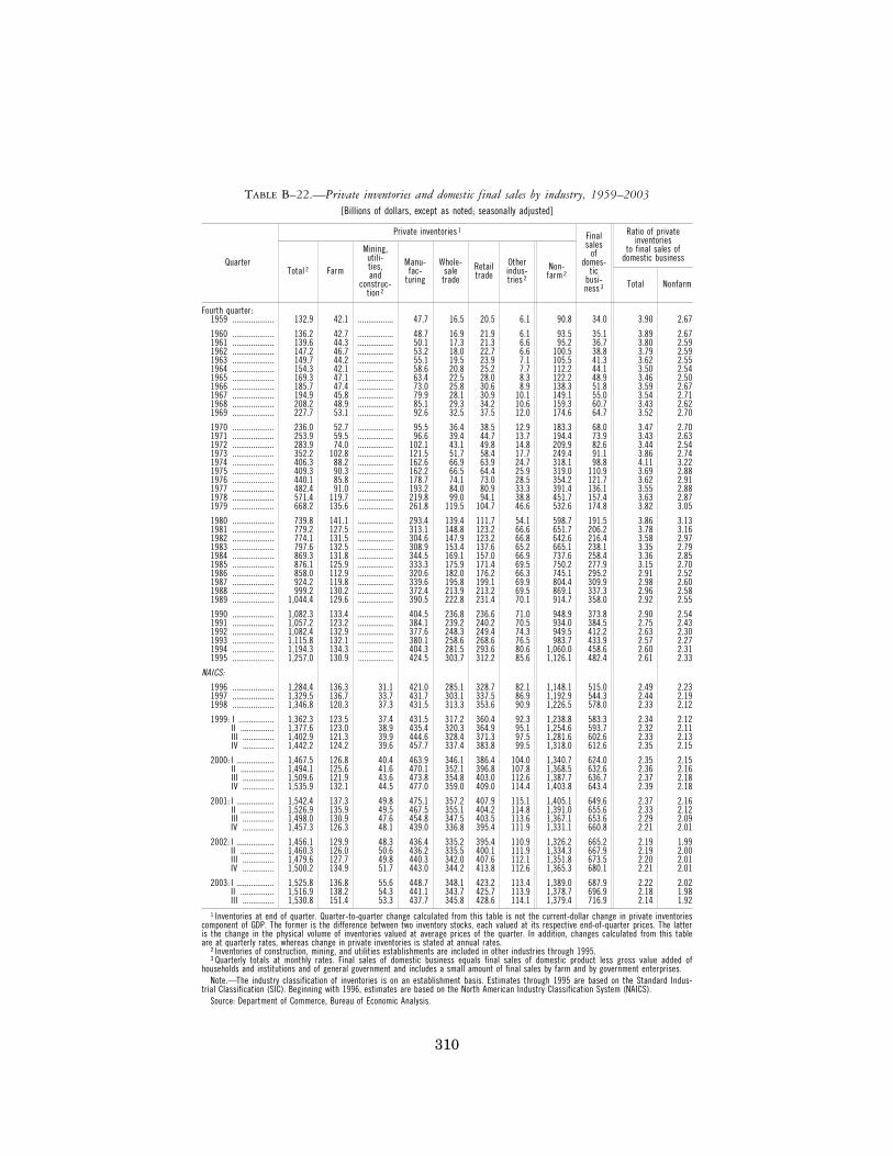
310
TABLE B–22.—Private inventories and domestic final sales by industry, 1959–2003[Billions of dollars, except as noted; seasonally adjusted]
Quarter
Private inventories 1 Finalsales
ofdomes-
ticbusi-ness 3
Ratio of privateinventories
to final sales ofdomestic business
Total 2 Farm
Mining,utili-ties,and
construc-tion 2
Manu-fac-
turing
Whole-saletrade
Retailtrade
Other indus-tries 2
Non-farm 2
Total Nonfarm
Fourth quarter: 1959 .................... 132.9 42.1 ................. 47.7 16.5 20.5 6.1 90.8 34.0 3.90 2.67
1960 .................... 136.2 42.7 ................. 48.7 16.9 21.9 6.1 93.5 35.1 3.89 2.671961 .................... 139.6 44.3 ................. 50.1 17.3 21.3 6.6 95.2 36.7 3.80 2.59 1962 .................... 147.2 46.7 ................. 53.2 18.0 22.7 6.6 100.5 38.8 3.79 2.59 1963 .................... 149.7 44.2 ................. 55.1 19.5 23.9 7.1 105.5 41.3 3.62 2.55 1964 .................... 154.3 42.1 ................. 58.6 20.8 25.2 7.7 112.2 44.1 3.50 2.541965 .................... 169.3 47.1 ................. 63.4 22.5 28.0 8.3 122.2 48.9 3.46 2.50 1966 .................... 185.7 47.4 ................. 73.0 25.8 30.6 8.9 138.3 51.8 3.59 2.67 1967 .................... 194.9 45.8 ................. 79.9 28.1 30.9 10.1 149.1 55.0 3.54 2.71 1968 .................... 208.2 48.9 ................. 85.1 29.3 34.2 10.6 159.3 60.7 3.43 2.62 1969 .................... 227.7 53.1 ................. 92.6 32.5 37.5 12.0 174.6 64.7 3.52 2.70
1970 .................... 236.0 52.7 ................. 95.5 36.4 38.5 12.9 183.3 68.0 3.47 2.70 1971 .................... 253.9 59.5 ................. 96.6 39.4 44.7 13.7 194.4 73.9 3.43 2.63 1972 .................... 283.9 74.0 ................. 102.1 43.1 49.8 14.8 209.9 82.6 3.44 2.54 1973 .................... 352.2 102.8 ................. 121.5 51.7 58.4 17.7 249.4 91.1 3.86 2.74 1974 .................... 406.3 88.2 ................. 162.6 66.9 63.9 24.7 318.1 98.8 4.11 3.221975 .................... 409.3 90.3 ................. 162.2 66.5 64.4 25.9 319.0 110.9 3.69 2.88 1976 .................... 440.1 85.8 ................. 178.7 74.1 73.0 28.5 354.2 121.7 3.62 2.91 1977 .................... 482.4 91.0 ................. 193.2 84.0 80.9 33.3 391.4 136.1 3.55 2.88 1978 .................... 571.4 119.7 ................. 219.8 99.0 94.1 38.8 451.7 157.4 3.63 2.87 1979 .................... 668.2 135.6 ................. 261.8 119.5 104.7 46.6 532.6 174.8 3.82 3.05
1980 .................... 739.8 141.1 ................. 293.4 139.4 111.7 54.1 598.7 191.5 3.86 3.13 1981 .................... 779.2 127.5 ................. 313.1 148.8 123.2 66.6 651.7 206.2 3.78 3.16 1982 .................... 774.1 131.5 ................. 304.6 147.9 123.2 66.8 642.6 216.4 3.58 2.97 1983 .................... 797.6 132.5 ................. 308.9 153.4 137.6 65.2 665.1 238.1 3.35 2.79 1984 .................... 869.3 131.8 ................. 344.5 169.1 157.0 66.9 737.6 258.4 3.36 2.85 1985 .................... 876.1 125.9 ................. 333.3 175.9 171.4 69.5 750.2 277.9 3.15 2.70 1986 .................... 858.0 112.9 ................. 320.6 182.0 176.2 66.3 745.1 295.2 2.91 2.521987 .................... 924.2 119.8 ................. 339.6 195.8 199.1 69.9 804.4 309.9 2.98 2.60 1988 .................... 999.2 130.2 ................. 372.4 213.9 213.2 69.5 869.1 337.3 2.96 2.58 1989 .................... 1,044.4 129.6 ................. 390.5 222.8 231.4 70.1 914.7 358.0 2.92 2.55
1990 .................... 1,082.3 133.4 ................. 404.5 236.8 236.6 71.0 948.9 373.8 2.90 2.54 1991 .................... 1,057.2 123.2 ................. 384.1 239.2 240.2 70.5 934.0 384.5 2.75 2.43 1992 .................... 1,082.4 132.9 ................. 377.6 248.3 249.4 74.3 949.5 412.2 2.63 2.301993 .................... 1,115.8 132.1 ................. 380.1 258.6 268.6 76.5 983.7 433.9 2.57 2.271994 .................... 1,194.3 134.3 ................. 404.3 281.5 293.6 80.6 1,060.0 458.6 2.60 2.311995 .................... 1,257.0 130.9 ................. 424.5 303.7 312.2 85.6 1,126.1 482.4 2.61 2.33
NAICS:
1996 .................... 1,284.4 136.3 31.1 421.0 285.1 328.7 82.1 1,148.1 515.0 2.49 2.231997 .................... 1,329.5 136.7 33.7 431.7 303.1 337.5 86.9 1,192.9 544.3 2.44 2.191998 .................... 1,346.8 120.3 37.3 431.5 313.3 353.6 90.9 1,226.5 578.0 2.33 2.12
1999: I ................. 1,362.3 123.5 37.4 431.5 317.2 360.4 92.3 1,238.8 583.3 2.34 2.12II ................ 1,377.6 123.0 38.9 435.4 320.3 364.9 95.1 1,254.6 593.7 2.32 2.11III ............... 1,402.9 121.3 39.9 444.6 328.4 371.3 97.5 1,281.6 602.6 2.33 2.13IV ............... 1,442.2 124.2 39.6 457.7 337.4 383.8 99.5 1,318.0 612.6 2.35 2.15
2000: I .................. 1,467.5 126.8 40.4 463.9 346.1 386.4 104.0 1,340.7 624.0 2.35 2.15II ................ 1,494.1 125.6 41.6 470.1 352.1 396.8 107.8 1,368.5 632.6 2.36 2.16III ............... 1,509.6 121.9 43.6 473.8 354.8 403.0 112.6 1,387.7 636.7 2.37 2.18IV ............... 1,535.9 132.1 44.5 477.0 359.0 409.0 114.4 1,403.8 643.4 2.39 2.18
2001: I .................. 1,542.4 137.3 49.8 475.1 357.2 407.9 115.1 1,405.1 649.6 2.37 2.16II ................ 1,526.9 135.9 49.5 467.5 355.1 404.2 114.8 1,391.0 655.6 2.33 2.12III ............... 1,498.0 130.9 47.6 454.8 347.5 403.5 113.6 1,367.1 653.6 2.29 2.09IV ............... 1,457.3 126.3 48.1 439.0 336.8 395.4 111.9 1,331.1 660.8 2.21 2.01
2002: I .................. 1,456.1 129.9 48.3 436.4 335.2 395.4 110.9 1,326.2 665.2 2.19 1.99II ................ 1,460.3 126.0 50.6 436.2 335.5 400.1 111.9 1,334.3 667.9 2.19 2.00III ............... 1,479.6 127.7 49.8 440.3 342.0 407.6 112.1 1,351.8 673.5 2.20 2.01IV ............... 1,500.2 134.9 51.7 443.0 344.2 413.8 112.6 1,365.3 680.1 2.21 2.01
2003: I .................. 1,525.8 136.8 55.6 448.7 348.1 423.2 113.4 1,389.0 687.9 2.22 2.02II ................ 1,516.9 138.2 54.3 441.1 343.7 425.7 113.9 1,378.7 696.9 2.18 1.98III ............... 1,530.8 151.4 53.3 437.7 345.8 428.6 114.1 1,379.4 716.9 2.14 1.92
1 Inventories at end of quarter. Quarter-to-quarter change calculated from this table is not the current-dollar change in private inventories component of GDP. The former is the difference between two inventory stocks, each valued at its respective end-of-quarter prices. The latter is the change in the physical volume of inventories valued at average prices of the quarter. In addition, changes calculated from this table are at quarterly rates, whereas change in private inventories is stated at annual rates.
2 Inventories of construction, mining, and utilities establishments are included in other industries through 1995. 3 Quarterly totals at monthly rates. Final sales of domestic business equals final sales of domestic product less gross value added of
households and institutions and of general government and includes a small amount of final sales by farm and by government enterprises.Note.—The industry classification of inventories is on an establishment basis. Estimates through 1995 are based on the Standard Indus-
trial Classification (SIC). Beginning with 1996, estimates are based on the North American Industry Classification System (NAICS).Source: Department of Commerce, Bureau of Economic Analysis.
VerDate jul 14 2003 09:04 Jan 31, 2004 Jkt 198929 PO 00000 Frm 00034 Fmt 0808 Sfmt 0808 E:\2004_EOP\B22.ER4 198929P2

311
TABLE B–23.—Real private inventories and domestic final sales by industry, 1990–2003[Billions of chained (2000) dollars, except as noted; seasonally adjusted]
Quarter
Private inventories 1 Finalsales
ofdomes-
ticbusi-ness 3
Ratio of privateinventories
to final sales ofdomestic business
Total 2 Farm
Mining,utili-ties,and, con-
struc-tion 2
Manu-fac-
turing
Whole-saletrade
Retailtrade
Otherindus-tries 2
Non-farm 2
Total Nonfarm
Fourth quarter:1990 ............................ 1,092.8 120.9 ............ 390.0 242.0 258.9 78.3 971.2 394.0 2.77 2.461991 ............................ 1,092.3 119.4 ............ 383.5 246.4 259.5 81.4 972.2 394.6 2.77 2.461992 ............................ 1,108.7 125.1 ............ 378.9 254.8 264.1 83.9 982.5 415.7 2.67 2.361993 ............................ 1,129.4 119.1 ............ 382.4 261.0 279.4 86.9 1,010.2 429.8 2.63 2.351994 ............................ 1,193.0 130.3 ............ 394.1 276.7 299.9 91.1 1,062.2 447.2 2.67 2.381995 ............................ 1,222.8 119.6 ............ 407.8 289.9 312.0 93.3 1,103.5 464.2 2.63 2.38
NAICS:1996 ............................ 1,251.6 126.4 33.6 409.9 273.3 325.9 82.7 1,125.2 488.3 2.56 2.301997 ............................ 1,322.7 129.3 36.1 430.7 298.3 340.6 88.1 1,193.7 509.2 2.60 2.341998 ............................ 1,395.3 130.7 43.3 449.3 320.9 357.9 94.0 1,264.9 538.0 2.59 2.35
1999: I ......................... 1,415.2 130.9 44.0 452.7 325.9 366.3 96.0 1,284.6 541.5 2.61 2.37II ........................ 1,425.6 131.2 44.2 454.8 328.1 369.5 98.3 1,294.7 549.9 2.59 2.35III ....................... 1,438.3 128.3 43.6 458.8 334.1 373.7 100.1 1,310.1 556.0 2.59 2.36IV ....................... 1,464.2 127.8 42.7 466.3 340.6 385.5 101.3 1,336.4 563.4 2.60 2.37
2000: I ......................... 1,470.9 124.2 43.7 465.6 345.4 387.6 104.6 1,346.8 571.2 2.58 2.36II ........................ 1,495.7 125.7 43.0 470.6 351.6 396.7 108.1 1,370.1 575.0 2.60 2.38III ...................... 1,509.8 125.0 43.1 471.5 355.3 402.4 112.5 1,384.8 577.5 2.61 2.40IV ...................... 1,520.7 126.4 41.1 474.2 358.2 407.1 113.7 1,394.3 581.0 2.62 2.40
2001: I ......................... 1,521.7 128.0 43.3 471.9 358.2 406.0 114.1 1,393.7 581.5 2.62 2.40II ........................ 1,514.5 127.5 47.3 465.1 357.9 402.3 113.9 1,387.0 581.2 2.61 2.39III ...................... 1,503.5 127.9 50.0 457.2 352.6 401.8 113.6 1,375.5 578.5 2.60 2.38IV ...................... 1,484.7 126.6 52.2 450.7 345.5 396.0 113.2 1,358.0 582.4 2.55 2.33
2002: I ......................... 1,478.8 127.9 52.1 446.4 342.3 396.9 112.8 1,350.8 586.3 2.52 2.30II ........................ 1,476.8 124.9 51.5 443.5 341.2 401.7 113.6 1,351.9 587.2 2.52 2.30III ...................... 1,485.0 124.2 50.9 444.1 343.2 408.6 113.7 1,360.9 589.1 2.52 2.31IV ...................... 1,490.4 123.3 50.1 443.2 344.8 415.2 113.5 1,367.2 589.2 2.53 2.32
2003: I ......................... 1,490.8 123.6 48.3 440.2 343.6 422.0 113.0 1,367.3 594.0 2.51 2.30II ........................ 1,489.6 123.1 47.8 436.4 342.5 425.8 114.1 1,366.7 597.8 2.49 2.29III ...................... 1,487.4 122.4 47.7 432.4 342.1 428.6 114.3 1,365.2 614.8 2.42 2.22
1 Inventories at end of quarter. Quarter-to-quarter changes calculated from this table are at quarterly rates, whereas the change in private inventories component of GDP is stated at annual rates.
2 Inventories of construction, mining, and utilities establishments are included in other industries through 1995. 3 Quarterly totals at monthly rates. Final sales of domestic business equals final sales of domestic product less gross value added of
households and institutions and of general government and includes a small amount of final sales by farm and by government enterprises.Note.—The industry classification of inventories is on an establishment basis. Estimates for 1990 through 1995 are based on the 1987
Standard Industrial Classification (SIC). Beginning with 1996, estimates are based on the North American Industry Classification System (NAICS).
See Survey of Current Business, Table 5.7.6A and 5.7.6B, for detailed information on calculation of the chained (2000) dollar inventory se-ries.
Source: Department of Commerce, Bureau of Economic Analysis.
VerDate jul 14 2003 09:04 Jan 31, 2004 Jkt 198929 PO 00000 Frm 00035 Fmt 0808 Sfmt 0808 E:\2004_EOP\B23.ER4 198929P2

312
TABLE B–24.—Foreign transactions in the national income and product accounts, 1959–2003
[Billions of dollars; quarterly data at seasonally adjusted annual rates]
Year orquarter
Current receipts from rest of the world Current payments to rest of the world
Total
Exports of goods andservices
In-comere-
ceipts Total
Imports of goods andservices In-
comepay-
ments
Current taxes andtransfer payments
to rest of the world (net) Balanceon
currentaccount,
NIPA Total Goods 1 Serv-ices 1 Total Goods 1 Serv-
ices 1 Total From
persons(net)
Fromgovern-
ment(net)
Frombusi-ness(net)
1959 ............. 27.0 22.7 16.5 6.3 4.3 28.2 22.3 15.3 7.0 1.5 4.3 0.5 3.8 0.1 −1.2
1960 ............. 31.9 27.0 20.5 6.6 4.9 28.7 22.8 15.2 7.6 1.8 4.1 .5 3.5 .1 3.21961 ............. 32.9 27.6 20.9 6.7 5.3 28.6 22.7 15.1 7.6 1.8 4.2 .5 3.6 .1 4.31962 ............. 35.0 29.1 21.7 7.4 5.9 31.1 25.0 16.9 8.1 1.8 4.3 .5 3.6 .1 3.91963 ............. 37.6 31.1 23.3 7.7 6.5 32.6 26.1 17.7 8.4 2.1 4.4 .7 3.6 .1 5.01964 ............. 42.3 35.0 26.7 8.3 7.2 34.7 28.1 19.4 8.7 2.3 4.3 .7 3.4 .2 7.51965 ............. 45.0 37.1 27.8 9.4 7.9 38.8 31.5 22.2 9.3 2.6 4.7 .8 3.7 .2 6.21966 ............. 49.0 40.9 30.7 10.2 8.1 45.1 37.1 26.3 10.7 3.0 5.0 .8 4.0 .2 3.91967 ............. 52.1 43.5 32.2 11.3 8.7 48.6 39.9 27.8 12.2 3.3 5.4 1.0 4.1 .2 3.61968 ............. 58.0 47.9 35.3 12.6 10.1 56.3 46.6 33.9 12.6 4.0 5.7 1.0 4.4 .3 1.71969 ............. 63.7 51.9 38.3 13.7 11.8 61.9 50.5 36.8 13.7 5.7 5.8 1.1 4.4 .3 1.8
1970 ............. 72.5 59.7 44.5 15.2 12.8 68.5 55.8 40.9 14.9 6.4 6.3 1.3 4.7 .4 4.01971 ............. 77.0 63.0 45.6 17.4 14.0 76.4 62.3 46.6 15.8 6.4 7.6 1.3 5.9 .4 .61972 ............. 87.1 70.8 51.8 19.0 16.3 90.7 74.2 56.9 17.3 7.7 8.8 1.4 7.0 .5 −3.61973 ............. 118.8 95.3 73.9 21.3 23.5 109.5 91.2 71.8 19.3 10.9 7.4 1.5 5.2 .7 9.31974 ............. 156.5 126.7 101.0 25.7 29.8 149.8 127.5 104.5 22.9 14.3 8.1 1.3 5.8 1.0 6.61975 ............. 166.7 138.7 109.6 29.1 28.0 145.4 122.7 99.0 23.7 15.0 7.6 1.3 5.6 .7 21.41976 ............. 181.9 149.5 117.8 31.7 32.4 173.0 151.1 124.6 26.5 15.5 6.3 1.3 3.9 1.1 8.91977 ............. 196.6 159.4 123.7 35.7 37.2 205.6 182.4 152.6 29.8 16.9 6.2 1.3 3.5 1.4 −9.01978 ............. 233.1 186.9 145.4 41.5 46.3 243.6 212.3 177.4 34.8 24.7 6.7 1.5 3.8 1.4 −10.41979 ............. 298.5 230.1 184.0 46.1 68.3 297.0 252.7 212.8 39.9 36.4 8.0 1.6 4.3 2.0 1.4
1980 ............. 359.9 280.8 225.8 55.0 79.1 348.5 293.8 248.6 45.3 44.9 9.8 1.8 5.5 2.4 11.4 1981 ............. 397.3 305.2 239.1 66.1 92.0 390.9 317.8 267.8 49.9 59.1 14.1 5.5 5.4 3.2 6.31982 ............. 384.2 283.2 215.0 68.2 101.0 384.4 303.2 250.5 52.6 64.5 16.7 6.6 6.7 3.4 −.21983 ............. 378.9 277.0 207.3 69.7 101.9 410.9 328.6 272.7 56.0 64.8 17.5 6.9 7.2 3.4 −32.1 1984 ............. 424.2 302.4 225.6 76.7 121.9 511.2 405.1 336.3 68.8 85.6 20.5 7.8 9.2 3.5 −86.9 1985 ............. 414.5 302.0 222.2 79.8 112.4 525.3 417.2 343.3 73.9 85.9 22.2 8.2 11.1 2.9 −110.8 1986 ............. 431.9 320.5 226.0 94.5 111.4 571.2 453.3 370.0 83.3 93.6 24.3 9.0 12.2 3.2 −139.2 1987 ............. 487.1 363.9 257.5 106.4 123.2 637.9 509.1 414.8 94.3 105.3 23.5 9.9 10.3 3.4 −150.8 1988 ............. 596.2 444.1 325.8 118.3 152.1 708.4 554.5 452.1 102.4 128.5 25.5 10.6 10.4 4.5 −112.2 1989 ............. 681.0 503.3 369.4 134.0 177.7 769.3 591.5 484.8 106.7 151.5 26.4 11.4 10.4 4.6 −88.3
1990 ............. 741.5 552.4 396.6 155.7 189.1 811.5 630.3 508.1 122.3 154.3 26.9 12.0 10.0 4.8 −70.1 1991 ............. 765.7 596.8 423.5 173.3 168.9 752.3 624.3 500.7 123.6 138.5 −10.6 13.0 −28.6 5.0 13.5 1992 ............. 788.0 635.3 448.0 187.4 152.7 824.9 668.6 544.9 123.6 123.0 33.4 12.3 17.1 3.9 −36.9 1993 ............. 812.1 655.8 459.9 195.9 156.2 882.5 720.9 592.8 128.1 124.3 37.3 14.2 17.8 5.4 −70.4 1994 ............. 907.3 720.9 510.1 210.8 186.4 1,012.5 814.5 676.8 137.7 160.2 37.8 15.4 15.8 6.6 −105.2 1995 ............. 1,046.1 812.2 583.3 228.9 233.9 1,137.1 903.6 757.4 146.1 198.1 35.4 16.2 10.1 9.1 −91.01996 ............. 1,117.3 868.6 618.3 250.2 248.7 1,217.6 964.8 807.4 157.4 213.7 39.1 18.0 14.1 7.1 −100.31997 ............ 1,242.0 955.3 687.7 267.6 286.7 1,352.2 1,056.9 885.3 171.5 253.7 41.6 21.0 10.9 9.7 −110.2 1998 ............ 1,243.1 955.9 680.9 275.1 287.1 1,430.5 1,115.9 929.0 186.9 265.8 48.8 24.6 11.2 12.9 −187.4 1999 ............ 1,312.1 991.2 697.2 294.0 320.8 1,585.9 1,251.7 1,045.5 206.3 287.0 47.2 28.3 11.6 7.3 −273.9
2000 ............ 1,478.9 1,096.3 784.3 311.9 382.7 1,875.6 1,475.8 1,243.5 232.3 343.7 56.1 31.5 13.5 11.2 −396.62001 ............ 1,354.1 1,035.1 731.5 303.6 319.0 1,732.5 1,401.7 1,168.0 233.6 283.8 47.0 33.1 9.5 4.5 −378.42002 ............ 1,306.0 1,006.8 697.8 309.1 299.1 1,770.1 1,433.1 1,190.3 242.7 277.6 59.3 35.4 14.3 9.6 −464.1
1999: I .......... 1,254.7 960.1 673.2 286.8 294.6 1,475.5 1,167.6 970.1 197.5 264.0 44.0 27.2 8.6 8.2 −220.8II ......... 1,283.2 972.8 680.3 292.5 310.4 1,545.2 1,224.9 1,021.1 203.8 274.6 45.7 28.8 10.1 6.8 −262.0III ........ 1,330.4 1,000.5 703.9 296.6 329.9 1,630.5 1,285.7 1,075.3 210.4 300.0 44.8 28.7 8.8 7.3 −300.1IV ........ 1,379.9 1,031.6 731.3 300.3 348.4 1,692.6 1,328.8 1,115.3 213.4 309.6 54.2 28.4 19.1 6.7 −312.6
2000: I .......... 1,418.0 1,055.1 749.2 305.9 362.9 1,780.8 1,401.5 1,177.0 224.5 330.4 48.9 31.9 8.7 8.3 −362.8II ......... 1,477.8 1,091.8 776.9 315.0 386.0 1,858.9 1,458.7 1,229.6 229.1 349.2 51.0 31.6 9.1 10.3 −381.1III ........ 1,502.1 1,122.4 810.9 311.5 379.7 1,925.6 1,523.1 1,284.9 238.3 348.1 54.3 31.3 11.4 11.6 −423.5IV ........ 1,517.8 1,115.8 800.4 315.4 402.1 1,937.0 1,519.7 1,282.3 237.3 347.2 70.1 31.2 24.6 14.4 −419.2
2001: I .......... 1,458.9 1,103.1 788.9 314.2 355.8 1,859.3 1,484.4 1,247.8 236.6 328.5 46.4 22.4 7.0 16.9 −400.4II ......... 1,392.9 1,061.1 747.6 313.5 331.8 1,779.5 1,429.3 1,187.4 241.9 304.5 45.7 18.9 8.0 18.9 −386.7III ........ 1,310.3 1,005.4 704.9 300.5 304.9 1,709.2 1,370.4 1,139.5 230.9 293.3 45.5 71.6 8.7 −34.8 −398.8IV ........ 1,254.2 970.8 684.5 286.4 283.3 1,582.0 1,322.5 1,097.4 225.1 208.9 50.6 19.7 14.1 16.9 −327.8
2002: I .......... 1,262.9 978.5 677.7 300.8 284.4 1,670.7 1,344.1 1,108.5 235.6 262.4 64.2 28.5 22.7 13.0 −407.8II ......... 1,305.3 1,006.3 700.9 305.4 299.0 1,779.5 1,433.6 1,194.9 238.7 291.4 54.4 34.5 9.8 10.1 −474.1III ........ 1,333.7 1,025.3 714.1 311.2 308.3 1,807.6 1,461.3 1,217.1 244.1 289.9 56.5 38.6 9.7 8.2 −473.9IV ........ 1,322.0 1,017.2 698.3 318.8 304.8 1,822.5 1,493.3 1,240.8 252.5 266.9 62.2 40.2 15.1 6.9 −500.5
2003: I .......... 1,317.8 1,021.0 707.6 313.3 296.8 1,847.1 1,508.5 1,254.2 254.3 269.0 69.6 40.1 21.1 8.5 −529.3II ......... 1,319.7 1,020.2 707.7 312.5 299.5 1,859.9 1,525.7 1,272.4 253.3 266.2 68.1 37.5 20.2 10.4 −540.2III ........ 1,360.6 1,048.5 722.1 326.4 312.1 1,879.0 1,539.0 1,275.6 263.5 274.3 65.7 33.9 19.1 12.7 −518.4
1 Certain goods, primarily military equipment purchased and sold by the Federal Government, are included in services. Beginning with 1986, repairs and alterations of equipment were reclassified from goods to services.
Source: Department of Commerce, Bureau of Economic Analysis.
VerDate jul 14 2003 09:04 Jan 31, 2004 Jkt 198929 PO 00000 Frm 00036 Fmt 0808 Sfmt 0808 E:\2004_EOP\B24.ER4 198929P2

313
TABLE B–25.—Real exports and imports of goods and services, 1990–2003[Billions of chained (2000) dollars; quarterly data at seasonally adjusted annual rates]
Year or quarter
Exports of goods and services Imports of goods and services
Total
Goods 1
Serv-ices 1 Total
Goods 1
Serv-ices 1
Total Dura-
blegoods
Non-dura-
blegoods
Total Dura-
blegoods
Non-dura-
blegoods
1990 ...................................................................... 552.5 367.2 226.3 145.1 188.7 607.1 469.7 264.7 218.4 142.71991 ...................................................................... 589.1 392.5 243.1 153.7 199.9 603.7 469.3 266.1 215.9 139.01992 ...................................................................... 629.7 421.9 262.5 163.6 210.8 645.6 513.1 294.0 231.9 135.51993 ...................................................................... 650.0 435.6 276.1 162.4 217.5 702.1 564.8 328.8 248.0 139.41994 ...................................................................... 706.5 478.0 309.6 170.1 231.1 785.9 640.0 383.1 266.0 147.31995 ...................................................................... 778.2 533.9 353.6 181.1 245.8 849.1 697.6 427.1 277.0 152.11996 ...................................................................... 843.4 581.1 394.9 186.7 263.5 923.0 762.7 472.8 295.2 160.51997 ...................................................................... 943.7 664.5 466.2 198.7 279.2 1,048.3 872.6 550.3 326.4 175.61998 ...................................................................... 966.5 679.4 481.2 198.5 287.2 1,170.3 974.4 621.8 355.7 195.61999 ...................................................................... 1,008.2 705.2 503.6 201.7 303.2 1,304.4 1,095.2 711.7 384.3 209.1
2000 ...................................................................... 1,096.3 784.3 569.2 215.1 311.9 1,475.8 1,243.5 820.7 422.8 232.32001 ...................................................................... 1,039.0 736.5 522.2 214.4 302.4 1,437.1 1,203.7 769.4 434.6 233.22002 ...................................................................... 1,014.2 707.2 493.7 213.7 306.8 1,484.7 1,248.4 801.4 447.4 236.4
1999: I ................................................................... 980.1 682.1 486.3 195.9 298.3 1,242.2 1,038.2 668.0 372.1 203.9II .................................................................. 991.2 689.8 490.6 199.5 301.7 1,286.4 1,079.2 698.9 381.3 207.1III ................................................................. 1,017.4 712.5 509.5 203.1 305.0 1,331.3 1,119.7 727.9 392.4 211.6IV ................................................................. 1,044.1 736.3 528.1 208.3 307.9 1,357.9 1,143.8 752.1 391.6 214.0
2000: I ................................................................... 1,060.9 751.9 543.7 208.2 309.0 1,411.5 1,187.1 785.3 401.5 224.4II .................................................................. 1,092.0 776.6 566.9 209.8 315.3 1,466.5 1,236.3 813.7 422.5 230.1III ................................................................. 1,120.0 810.0 586.7 223.3 310.0 1,515.6 1,277.7 842.0 435.8 237.9IV ................................................................ 1,112.3 798.9 579.7 219.1 313.4 1,509.5 1,272.7 841.8 431.3 236.8
2001: I ................................................................... 1,099.6 787.8 569.8 218.0 311.8 1,485.5 1,250.6 810.7 439.9 234.9II .................................................................. 1,060.9 749.5 533.7 215.8 311.3 1,452.7 1,210.5 769.9 440.9 241.9III ................................................................. 1,010.6 711.3 500.9 210.5 299.2 1,411.9 1,181.7 751.2 431.0 230.1IV ................................................................ 984.8 697.4 484.6 213.1 287.3 1,398.2 1,172.1 746.0 426.8 226.0
2002: I ................................................................... 995.4 692.8 481.4 211.7 302.5 1,426.7 1,190.1 766.5 423.6 236.2II .................................................................. 1,016.5 712.7 497.9 215.0 303.7 1,484.1 1,250.4 804.4 446.3 234.0III ................................................................ 1,027.3 720.1 506.5 213.8 307.0 1,499.2 1,265.2 812.2 453.4 234.4IV ................................................................ 1,017.5 703.2 489.1 214.3 314.0 1,529.0 1,288.1 822.3 466.2 241.2
2003: I ................................................................... 1,012.4 706.5 487.9 218.7 305.7 1,502.5 1,266.2 805.1 461.4 236.5II .................................................................. 1,009.6 703.5 488.6 215.1 305.9 1,535.7 1,307.4 824.8 482.5 229.8III ................................................................ 1,033.7 718.2 500.5 218.0 315.2 1,538.9 1,302.4 821.4 480.8 237.2
1 Certain goods, primarily military equipment purchased and sold by the Federal Government, are included in services. Beginning with 1986, repairs and alterations of equipment were reclassified from goods to services.
Note.—See Table B-2 for data for total exports of goods and services and total imports of goods and services for 1959-89.Source: Department of Commerce, Bureau of Economic Analysis.
VerDate jul 14 2003 09:04 Jan 31, 2004 Jkt 198929 PO 00000 Frm 00037 Fmt 0808 Sfmt 0808 E:\2004_EOP\B25.ER4 198929P2

314
TABLE B–26.—Relation of gross domestic product, gross national product, net national product, andnational income, 1959–2003
[Billions of dollars; quarterly data at seasonally adjusted annual rates]
Year orquarter
Grossdomesticproduct
Plus:Incomereceipts
from rest of the world
Less:Income
paymentsto
rest ofthe
world
Equals:Gross
nationalproduct
Less: Consumption of fixed capital Equals:
Netnationalproduct
Less:Statisticaldiscrep-
ancy
Equals: National income Total Private Govern-
ment
1959 ........... 506.6 4.3 1.5 509.3 53.0 38.6 14.5 456.3 0.5 455.8
1960 ........... 526.4 4.9 1.8 529.5 55.6 40.5 15.0 473.9 −.9 474.9 1961 ........... 544.7 5.3 1.8 548.2 57.2 41.6 15.6 491.0 −.6 491.6 1962 ........... 585.6 5.9 1.8 589.7 59.3 42.8 16.5 530.5 .4 530.1 1963 ........... 617.7 6.5 2.1 622.2 62.4 44.9 17.5 559.8 −.8 560.6 1964 ........... 663.6 7.2 2.3 668.5 65.0 46.9 18.1 603.5 .8 602.7 1965 ........... 719.1 7.9 2.6 724.4 69.4 50.5 18.9 655.0 1.6 653.4 1966 ........... 787.8 8.1 3.0 792.9 75.6 55.5 20.1 717.3 6.3 711.0 1967 ........... 832.6 8.7 3.3 838.0 81.5 59.9 21.6 756.5 4.6 751.9 1968 ........... 910.0 10.1 4.0 916.1 88.4 65.2 23.1 827.7 4.6 823.2 1969 ........... 984.6 11.8 5.7 990.7 97.9 73.1 24.8 892.8 3.2 889.7
1970 ........... 1,038.5 12.8 6.4 1,044.9 106.7 80.0 26.7 938.2 7.3 930.91971 ........... 1,127.1 14.0 6.4 1,134.7 115.0 86.7 28.3 1,019.7 11.6 1,008.1 1972 ........... 1,238.3 16.3 7.7 1,246.8 126.5 97.1 29.5 1,120.3 9.1 1,111.2 1973 ........... 1,382.7 23.5 10.9 1,395.3 139.3 107.9 31.4 1,256.0 8.6 1,247.4 1974 ........... 1,500.0 29.8 14.3 1,515.5 162.5 126.6 35.9 1,353.0 10.9 1,342.1 1975 ........... 1,638.3 28.0 15.0 1,651.3 187.7 147.8 40.0 1,463.6 17.7 1,445.9 1976 ........... 1,825.3 32.4 15.5 1,842.1 205.2 162.5 42.6 1,637.0 25.1 1,611.81977 ........... 2,030.9 37.2 16.9 2,051.2 230.0 184.3 45.7 1,821.2 22.3 1,798.9 1978 ........... 2,294.7 46.3 24.7 2,316.3 262.3 212.8 49.5 2,054.0 26.6 2,027.4 1979 ........... 2,563.3 68.3 36.4 2,595.3 300.1 245.7 54.5 2,295.1 46.0 2,249.1
1980 ........... 2,789.5 79.1 44.9 2,823.7 343.0 281.1 61.8 2,480.7 41.4 2,439.3 1981 ........... 3,128.4 92.0 59.1 3,161.4 388.1 317.9 70.1 2,773.3 30.9 2,742.4 1982 ........... 3,255.0 101.0 64.5 3,291.5 426.9 349.8 77.1 2,864.6 .3 2,864.3 1983 ........... 3,536.7 101.9 64.8 3,573.8 443.8 362.1 81.7 3,130.0 45.7 3,084.2 1984 ........... 3,933.2 121.9 85.6 3,969.5 472.6 385.6 87.0 3,496.9 14.6 3,482.3 1985 ........... 4,220.3 112.4 85.9 4,246.8 506.7 414.0 92.7 3,740.1 16.7 3,723.4 1986 ........... 4,462.8 111.4 93.6 4,480.6 531.3 431.8 99.5 3,949.3 47.0 3,902.3 1987 ........... 4,739.5 123.2 105.3 4,757.4 561.9 455.3 106.7 4,195.4 21.7 4,173.7 1988 ........... 5,103.8 152.1 128.5 5,127.4 597.6 483.5 114.1 4,529.8 −19.5 4,549.4 1989 ........... 5,484.4 177.7 151.5 5,510.6 644.3 522.1 122.2 4,866.3 39.7 4,826.6
1990 ........... 5,803.1 189.1 154.3 5,837.9 682.5 551.6 130.9 5,155.4 66.2 5,089.1 1991 ........... 5,995.9 168.9 138.5 6,026.3 725.9 586.9 139.1 5,300.4 72.5 5,227.9 1992 ........... 6,337.7 152.7 123.0 6,367.4 751.9 607.3 144.6 5,615.5 102.7 5,512.8 1993 ........... 6,657.4 156.2 124.3 6,689.3 776.4 624.7 151.8 5,912.9 139.5 5,773.4 1994 ........... 7,072.2 186.4 160.2 7,098.4 833.7 675.1 158.6 6,264.7 142.5 6,122.3 1995 ........... 7,397.7 233.9 198.1 7,433.4 878.4 713.4 165.0 6,555.1 101.2 6,453.9 1996 ........... 7,816.9 248.7 213.7 7,851.9 918.1 748.8 169.3 6,933.8 93.7 6,840.1 1997 ........... 8,304.3 286.7 253.7 8,337.3 974.4 800.3 174.1 7,362.8 70.7 7,292.2 1998 ........... 8,747.0 287.1 265.8 8,768.3 1,030.2 851.2 179.0 7,738.2 −14.6 7,752.8 1999 ........... 9,268.4 320.8 287.0 9,302.2 1,101.3 914.3 187.0 8,200.9 −35.7 8,236.7
2000 ........... 9,817.0 382.7 343.7 9,855.9 1,187.8 990.8 197.0 8,668.1 −127.2 8,795.2 2001 ........... 10,100.8 319.0 283.8 10,135.9 1,266.9 1,061.0 205.9 8,869.0 −112.2 8,981.2 2002 ........... 10,480.8 299.1 277.6 10,502.3 1,288.6 1,077.8 210.8 9,213.7 −77.2 9,290.8
1999: I ......... 9,066.6 294.6 264.0 9,097.2 1,069.5 886.1 183.4 8,027.7 −46.5 8,074.2 II ....... 9,174.1 310.4 274.6 9,209.9 1,087.0 901.2 185.8 8,122.9 −38.4 8,161.3 III ...... 9,313.5 329.9 300.0 9,343.4 1,120.3 932.3 188.0 8,223.1 −31.6 8,254.7 IV ...... 9,519.5 348.4 309.6 9,558.3 1,128.3 937.6 190.6 8,430.0 −26.4 8,456.4
2000: I ......... 9,629.4 362.9 330.4 9,661.9 1,153.1 959.6 193.4 8,508.8 −171.7 8,680.5 II ....... 9,822.8 386.0 349.2 9,859.6 1,177.0 981.0 196.0 8,682.6 −67.8 8,750.4III ...... 9,862.1 379.7 348.1 9,893.6 1,199.9 1,001.6 198.3 8,693.7 −164.6 8,858.3IV ...... 9,953.6 402.1 347.2 10,008.4 1,221.3 1,021.1 200.2 8,787.2 −104.6 8,891.7
2001: I ......... 10,024.8 355.8 328.5 10,052.1 1,230.4 1,028.4 202.0 8,821.7 −120.6 8,942.2 II ....... 10,088.2 331.8 304.5 10,115.5 1,257.0 1,053.2 203.8 8,858.5 −87.7 8,946.2 III ..... 10,096.2 304.9 293.3 10,107.8 1,317.3 1,106.0 211.3 8,790.6 −104.1 8,894.7 IV ...... 10,193.9 283.3 208.9 10,268.3 1,263.1 1,056.6 206.5 9,005.2 −136.5 9,141.8
2002: I ......... 10,329.3 284.4 262.4 10,351.3 1,271.6 1,063.2 208.4 9,079.8 −110.7 9,190.5 II ....... 10,428.3 299.0 291.4 10,435.9 1,286.8 1,076.7 210.1 9,149.1 −132.0 9,281.1 III ..... 10,542.0 308.3 289.9 10,560.5 1,295.8 1,084.2 211.6 9,264.7 −50.3 9,314.9 IV ...... 10,623.7 304.8 266.9 10,661.6 1,300.4 1,087.1 213.3 9,361.2 −15.7 9,376.9
2003: I ......... 10,735.8 296.8 269.0 10,763.7 1,305.7 1,090.4 215.3 9,457.9 23.2 9,434.8II ....... 10,846.7 299.5 266.2 10,880.0 1,303.4 1,086.0 217.4 9,576.6 −8.3 9,584.9 III ...... 11,107.0 312.1 274.3 11,144.8 1,309.1 1,089.9 219.2 9,835.7 54.0 9,781.7
Source: Department of Commerce, Bureau of Economic Analysis.
VerDate jul 14 2003 09:04 Jan 31, 2004 Jkt 198929 PO 00000 Frm 00038 Fmt 0808 Sfmt 0808 E:\2004_EOP\B26.ER4 198929P2

315
TABLE B–27.—Relation of national income and personal income, 1959–2003[Billions of dollars; quarterly data at seasonally adjusted annual rates]
Year or quarter Nationalincome
Less: Plus: Equals:
Corporateprofitswith
inventoryvaluation
andcapital
consump-tion
adjust-ments
Taxes on pro-duction
and imports
lesssubsi-dies
Contri-bu-
tionsfor
govern-mentsocialinsur-ance
Netinterest
and mis-cellane-ous pay-
ments on
assets
Business current transfer
pay-ments (net)
Current surplus of gov-ernment enter-prises
Wageaccruals
less disburse-
ments
Personalincome receipts on as-sets
Personalcurrent transfer receipts
Personalincome
1959 ....................... 455.8 55.7 40.0 13.8 9.6 1.8 1.0 0.0 34.6 24.2 392.8
1960 ....................... 474.9 53.8 43.4 16.4 10.6 1.9 .9 .0 37.9 25.7 411.51961 ....................... 491.6 54.9 45.0 17.0 12.5 2.0 .8 .0 40.1 29.5 429.01962 ....................... 530.1 63.3 48.2 19.1 14.2 2.2 .9 .0 44.1 30.4 456.71963 ....................... 560.6 69.0 51.2 21.7 15.2 2.7 1.4 .0 47.9 32.2 479.61964 ....................... 602.7 76.5 54.6 22.4 17.4 3.1 1.3 .0 53.8 33.5 514.61965 ....................... 653.4 87.5 57.8 23.4 19.6 3.6 1.3 .0 59.4 36.2 555.71966 ....................... 711.0 93.2 59.3 31.3 22.4 3.5 1.0 .0 64.1 39.6 603.91967 ....................... 751.9 91.3 64.2 34.9 25.5 3.8 .9 .0 69.0 48.0 648.31968 ....................... 823.2 98.8 72.3 38.7 27.1 4.3 1.2 .0 75.2 56.1 712.01969 ....................... 889.7 95.4 79.4 44.1 32.7 4.9 1.0 .0 84.1 62.3 778.5
1970 ....................... 930.9 83.6 86.7 46.4 39.1 4.5 .0 .0 93.5 74.7 838.81971 ....................... 1,008.1 98.0 95.9 51.2 43.9 4.3 −.2 .6 101.0 88.1 903.51972 ....................... 1,111.2 112.1 101.4 59.2 47.9 4.9 .5 .0 109.6 97.9 992.71973 ....................... 1,247.4 125.5 112.1 75.5 55.2 6.0 −.4 −.1 124.7 112.6 1,110.71974 ....................... 1,342.1 115.8 121.7 85.2 70.8 7.1 −.9 −.5 146.4 133.3 1,222.61975 ....................... 1,445.9 134.8 131.0 89.3 81.6 9.4 −3.2 .1 162.2 170.0 1,335.01976 ....................... 1,611.8 163.3 141.5 101.3 85.5 9.5 −1.8 .1 178.4 184.0 1,474.81977 ....................... 1,798.9 192.4 152.8 113.1 101.1 8.4 −2.6 .1 205.3 194.2 1,633.21978 ....................... 2,027.4 216.6 162.2 131.3 115.0 10.6 −1.9 .3 234.8 209.6 1,837.71979 ....................... 2,249.1 223.2 171.9 152.7 138.9 13.0 −2.6 −.2 274.7 235.3 2,062.2
1980 ....................... 2,439.3 201.1 190.9 166.2 181.8 14.4 −4.8 .0 338.7 279.5 2,307.91981 ....................... 2,742.4 226.1 224.5 195.7 232.3 17.6 −4.9 .1 421.9 318.4 2,591.31982 ....................... 2,864.3 209.7 226.4 208.9 271.1 20.1 −4.0 .0 488.4 354.8 2,775.31983 ....................... 3,084.2 264.2 242.5 226.0 285.3 22.5 −3.1 −.4 529.6 383.7 2,960.71984 ....................... 3,482.3 318.6 269.3 257.5 327.1 30.1 −1.9 .2 607.9 400.1 3,289.51985 ....................... 3,723.4 330.3 287.3 281.4 341.3 34.8 .8 −.2 654.0 424.9 3,526.71986 ....................... 3,902.3 319.5 298.9 303.4 366.8 36.6 1.3 .0 695.5 451.0 3,722.41987 ....................... 4,173.7 368.8 317.7 323.1 366.4 33.8 1.2 .0 717.0 467.6 3,947.41988 ....................... 4,549.4 432.6 345.5 361.5 385.3 34.0 2.5 .0 769.3 496.6 4,253.71989 ....................... 4,826.6 426.6 372.1 385.2 432.1 39.2 4.9 .0 878.0 543.4 4,587.8
1990 ....................... 5,089.1 437.8 398.7 410.1 442.2 39.4 1.6 .1 924.0 595.2 4,878.61991 ....................... 5,227.9 451.2 430.2 430.2 418.2 39.9 5.7 −.1 932.0 666.4 5,051.01992 ....................... 5,512.8 479.3 453.9 455.0 388.5 42.4 7.6 −15.8 910.9 749.4 5,362.01993 ....................... 5,773.4 541.9 467.0 477.7 365.7 40.7 7.2 6.4 901.8 790.1 5,558.51994 ....................... 6,122.3 600.3 513.5 508.2 366.4 43.3 8.6 17.6 950.8 827.3 5,842.51995 ....................... 6,453.9 696.7 524.2 532.8 367.1 46.9 11.4 16.4 1,016.4 877.4 6,152.31996 ....................... 6,840.1 786.2 546.8 555.2 376.2 53.1 12.7 3.6 1,089.2 925.0 6,520.61997 ....................... 7,292.2 868.5 579.1 587.2 415.6 49.9 12.6 −2.9 1,181.7 951.2 6,915.11998 ....................... 7,752.8 801.6 604.4 624.2 487.1 64.7 10.3 −.7 1,283.2 978.6 7,423.01999 ....................... 8,236.7 851.3 629.8 661.4 495.4 67.4 10.1 5.2 1,264.2 1,022.1 7,802.4
2000 ....................... 8,795.2 817.9 664.6 702.7 559.0 87.1 5.3 .0 1,387.0 1,084.0 8,429.72001 ....................... 8,981.2 770.4 674.5 728.5 568.4 92.5 1.2 .0 1,374.9 1,192.6 8,713.12002 ....................... 9,290.8 904.2 721.8 750.3 582.4 89.8 2.8 .0 1,378.5 1,292.2 8,910.3
1999: I .................... 8,074.2 844.2 616.6 652.8 480.6 64.2 11.2 5.2 1,249.4 1,009.5 7,658.4II ................... 8,161.3 849.3 623.5 656.8 490.6 65.4 10.5 5.2 1,255.4 1,013.3 7,728.8III .................. 8,254.7 842.3 634.0 662.4 498.8 68.1 10.0 5.2 1,262.3 1,027.4 7,823.7IV .................. 8,456.4 869.3 645.3 673.8 511.5 71.8 8.6 5.2 1,289.7 1,038.1 7,998.8
2000: I .................... 8,680.5 832.6 653.2 695.5 548.3 81.3 7.9 .0 1,349.9 1,054.6 8,266.2II ................... 8,750.4 833.0 662.6 696.3 560.6 85.0 7.1 .0 1,385.6 1,080.8 8,372.3III .................. 8,858.3 811.8 667.9 707.7 564.3 88.9 4.2 .0 1,406.2 1,094.8 8,514.4IV ................. 8,891.7 794.3 674.6 711.2 563.0 93.1 2.2 .0 1,406.5 1,106.0 8,565.8
2001: I .................... 8,942.2 755.8 672.6 726.3 563.9 97.0 3.0 .0 1,391.8 1,148.0 8,663.5II ................... 8,946.2 748.6 668.9 727.6 566.7 102.4 1.6 .0 1,378.1 1,181.9 8,690.2III ................. 8,894.7 713.6 660.3 729.2 568.0 71.1 .6 .0 1,367.4 1,208.0 8,727.4 IV ................. 9,141.8 863.6 696.2 731.1 575.2 99.5 −.3 .0 1,362.3 1,232.3 8,771.2
2002: I .................... 9,190.5 880.1 705.7 743.7 581.2 94.7 1.2 .0 1,359.3 1,260.5 8,803.6II ................... 9,281.1 901.9 719.7 749.6 572.8 90.6 .6 .0 1,375.4 1,291.1 8,912.2III ................. 9,314.9 899.8 729.1 752.1 585.7 87.8 5.4 .0 1,387.5 1,301.6 8,944.0IV ................. 9,376.9 934.9 732.8 755.5 589.7 86.2 4.1 .0 1,392.0 1,315.6 8,981.3
2003: I .................... 9,434.8 927.1 729.4 768.7 589.3 90.1 6.3 1.4 1,388.6 1,337.6 9,048.7II ................... 9,584.9 1,022.8 725.2 772.3 581.7 92.5 5.8 −1.4 1,390.2 1,369.7 9,145.9III .................. 9,781.7 1,124.2 745.2 776.9 579.9 97.1 3.7 .0 1,389.2 1,398.7 9,242.5
Source: Department of Commerce, Bureau of Economic Analysis.
VerDate jul 14 2003 09:04 Jan 31, 2004 Jkt 198929 PO 00000 Frm 00039 Fmt 0808 Sfmt 0808 E:\2004_EOP\B27.ER4 198929P2

316
TABLE B–28.—National income by type of income, 1959–2003[Billions of dollars; quarterly data at seasonally adjusted annual rates]
Year orquarter
Nationalincome
Compensation of employees Proprietors’ income with inventory valuation and capital consump-
tion adjustments Rentalincome
of personswith
capitalconsump-
tionadjust-ment
Total
Wage and salary accruals Supplements to wages andsalaries
Total Farm Non-farm Total
Gov-ern-ment
Other Total
Employercontribu-tions foremployeepension
and insur-ancefunds
Employercontribu-tions forgovern-
mentsocialinsur-ance
1959 ........ 455.8 281.0 259.8 46.1 213.8 21.1 13.3 7.9 50.7 10.0 40.6 16.2
1960 ........ 474.9 296.4 272.9 49.2 223.7 23.6 14.3 9.3 50.8 10.5 40.3 17.11961 ........ 491.6 305.3 280.5 52.5 228.0 24.8 15.2 9.6 53.2 11.0 42.2 17.91962 ........ 530.1 327.1 299.4 56.3 243.0 27.8 16.6 11.2 55.4 11.0 44.4 18.81963 ........ 560.6 345.2 314.9 60.0 254.8 30.4 18.0 12.4 56.5 10.8 45.7 19.51964 ........ 602.7 370.7 337.8 64.9 272.9 32.9 20.3 12.6 59.4 9.6 49.8 19.61965 ........ 653.4 399.5 363.8 69.9 293.8 35.7 22.7 13.1 63.9 11.8 52.1 20.21966 ........ 711.0 442.7 400.3 78.4 321.9 42.3 25.5 16.8 68.2 12.8 55.4 20.81967 ........ 751.9 475.1 429.0 86.5 342.5 46.1 28.1 18.0 69.8 11.5 58.4 21.21968 ........ 823.2 524.3 472.0 96.7 375.3 52.3 32.4 20.0 74.3 11.5 62.8 20.91969 ........ 889.7 577.6 518.3 105.6 412.7 59.3 36.5 22.8 77.4 12.6 64.7 21.2
1970 ........ 930.9 617.2 551.6 117.2 434.3 65.7 41.8 23.8 78.4 12.7 65.7 21.41971 ........ 1,008.1 658.9 584.5 126.8 457.8 74.4 47.9 26.4 84.8 13.2 71.6 22.41972 ........ 1,111.2 725.1 638.8 137.9 500.9 86.4 55.2 31.2 95.9 16.8 79.1 23.41973 ........ 1,247.4 811.2 708.8 148.8 560.0 102.5 62.7 39.8 113.5 28.9 84.6 24.31974 ........ 1,342.1 890.2 772.3 160.5 611.8 118.0 73.3 44.7 113.1 23.2 89.9 24.31975 ........ 1,445.9 949.1 814.8 176.2 638.6 134.3 87.6 46.7 119.5 21.7 97.8 23.71976 ........ 1,611.8 1,059.3 899.7 188.9 710.8 159.6 105.2 54.4 132.2 17.0 115.2 22.31977 ........ 1,798.9 1,180.5 994.2 202.6 791.6 186.4 125.3 61.1 145.7 15.7 130.0 20.71978 ........ 2,027.4 1,336.1 1,121.2 220.0 901.2 214.9 143.4 71.5 166.6 19.6 147.1 22.11979 ........ 2,249.1 1,500.8 1,255.8 237.1 1,018.7 245.0 162.4 82.6 180.1 21.8 158.3 23.8
1980 ........ 2,439.3 1,651.8 1,377.6 261.5 1,116.2 274.2 185.2 88.9 174.1 11.3 162.8 30.01981 ........ 2,742.4 1,825.8 1,517.5 285.8 1,231.7 308.3 204.7 103.6 183.0 18.7 164.3 38.01982 ........ 2,864.3 1,925.8 1,593.7 307.5 1,286.2 332.1 222.4 109.8 176.3 13.1 163.3 38.81983 ........ 3,084.2 2,042.6 1,684.6 324.8 1,359.8 358.0 238.1 119.9 192.5 6.0 186.5 37.81984 ........ 3,482.3 2,255.6 1,855.1 348.1 1,507.0 400.5 261.5 139.0 243.3 20.6 222.7 40.21985 ........ 3,723.4 2,424.7 1,995.5 373.9 1,621.6 429.2 281.5 147.7 262.3 20.8 241.5 41.91986 ........ 3,902.3 2,570.1 2,114.8 397.0 1,717.9 455.3 297.5 157.9 275.7 22.6 253.1 33.51987 ........ 4,173.7 2,750.2 2,270.7 422.6 1,848.1 479.5 313.2 166.3 302.2 28.7 273.5 33.51988 ........ 4,549.4 2,967.2 2,452.9 451.3 2,001.6 514.2 329.6 184.6 341.6 26.8 314.7 40.61989 ........ 4,826.6 3,145.2 2,596.3 480.2 2,116.2 548.9 355.2 193.7 363.3 33.0 330.3 43.1
1990 ........ 5,089.1 3,338.2 2,754.0 517.7 2,236.3 584.2 377.8 206.5 380.6 31.9 348.7 50.71991 ........ 5,227.9 3,445.2 2,823.0 546.8 2,276.2 622.3 407.1 215.1 377.1 26.7 350.4 60.31992 ........ 5,512.8 3,635.4 2,964.5 569.2 2,395.3 670.9 442.5 228.4 427.6 34.5 393.0 78.01993 ........ 5,773.4 3,801.4 3,089.2 586.8 2,502.4 712.2 472.4 239.8 453.8 31.2 422.6 95.61994 ........ 6,122.3 3,997.2 3,249.8 606.2 2,643.5 747.5 493.3 254.1 473.3 33.9 439.4 119.71995 ........ 6,453.9 4,193.3 3,435.7 625.5 2,810.2 757.7 493.6 264.0 492.1 22.7 469.5 122.11996 ........ 6,840.1 4,390.5 3,623.2 644.4 2,978.8 767.3 492.5 274.9 543.2 37.3 505.9 131.51997 ........ 7,292.2 4,661.7 3,874.7 668.1 3,206.6 787.0 497.5 289.5 576.0 34.2 541.8 128.81998 ........ 7,752.8 5,019.4 4,182.7 697.3 3,485.5 836.7 529.7 307.0 627.8 29.4 598.4 137.51999 ........ 8,236.7 5,357.1 4,471.4 729.3 3,742.1 885.7 562.4 323.3 678.3 28.6 649.7 147.3
2000 ........ 8,795.2 5,782.7 4,829.2 774.7 4,054.5 953.4 609.9 343.5 728.4 22.7 705.7 150.32001 ........ 8,981.2 5,940.4 4,942.9 815.8 4,127.1 997.6 642.6 354.9 770.6 25.0 745.6 163.12002 ........ 9,290.8 6,019.1 4,974.6 859.9 4,114.7 1,044.5 680.4 364.1 797.7 14.3 783.4 173.0
1999: I ..... 8,074.2 5,248.0 4,380.9 718.2 3,662.7 867.0 547.7 319.3 664.3 34.9 629.4 145.2II .... 8,161.3 5,302.5 4,425.4 724.3 3,701.1 877.1 556.0 321.1 672.0 29.3 642.7 147.6III ... 8,254.7 5,376.3 4,486.1 732.3 3,753.8 890.2 566.5 323.7 680.6 25.6 655.1 144.5IV ... 8,456.4 5,501.7 4,593.2 742.5 3,850.7 908.5 579.3 329.3 696.1 24.6 671.5 152.1
2000: I ..... 8,680.5 5,694.1 4,760.0 762.0 3,998.0 934.1 593.9 340.2 709.3 23.2 686.1 153.8II .... 8,750.4 5,727.2 4,783.2 772.8 4,010.5 944.0 603.7 340.3 726.5 23.8 702.7 148.5III .. 8,858.3 5,837.4 4,874.9 779.2 4,095.8 962.5 616.5 346.0 735.6 23.0 712.6 148.2IV .. 8,891.7 5,871.9 4,898.8 784.9 4,113.9 973.1 625.6 347.6 742.1 20.7 721.4 150.5
2001: I ..... 8,942.2 5,935.6 4,951.9 798.8 4,153.2 983.7 629.6 354.1 761.3 24.9 736.5 153.0II .... 8,946.2 5,936.0 4,945.0 809.1 4,135.9 991.0 636.5 354.5 766.4 24.8 741.5 155.6III .. 8,894.7 5,940.8 4,938.8 821.4 4,117.4 1,002.1 647.0 355.1 769.2 23.5 745.7 171.1IV .. 9,141.8 5,949.3 4,935.8 833.8 4,102.1 1,013.5 657.5 356.0 785.7 26.8 758.9 172.6
2002: I ..... 9,190.5 5,972.4 4,945.1 846.6 4,098.5 1,027.3 666.6 360.7 779.3 12.1 767.2 175.9II .... 9,281.1 6,014.8 4,973.1 856.0 4,117.1 1,041.7 677.9 363.9 796.2 15.2 780.9 184.4III .. 9,314.9 6,031.1 4,980.9 863.2 4,117.7 1,050.2 685.2 365.1 803.2 13.5 789.7 172.7IV .. 9,376.9 6,058.0 4,999.1 873.8 4,125.4 1,058.8 692.1 366.7 812.2 16.3 795.9 159.0
2003: I ..... 9,434.8 6,115.8 5,034.6 891.4 4,143.3 1,081.2 706.3 374.9 813.5 13.0 800.5 163.2II .... 9,584.9 6,164.8 5,070.8 898.1 4,172.7 1,093.9 717.3 376.6 838.8 20.0 818.8 153.4III .. 9,781.7 6,213.6 5,104.1 900.0 4,204.1 1,109.6 730.7 378.8 860.9 21.5 839.4 157.0
See next page for continuation of table.
VerDate jul 14 2003 09:04 Jan 31, 2004 Jkt 198929 PO 00000 Frm 00040 Fmt 0808 Sfmt 0808 E:\2004_EOP\B28.ER4 198929P2

317
TABLE B–28.—National income by type of income, 1959–2003—Continued[Billions of dollars; quarterly data at seasonally adjusted annual rates]
Year orquarter
Corporate profits with inventory valuation and capital consumption adjustments
Netinterest
andmiscel-laneous
pay-ments
Taxeson
produc-tionand
imports
Less:Subsi-dies
Busi-ness
currenttrans-
ferpay-
ments
Cur-rent
surplusof
govern-mententer-prises
Total
Profits with inventory valuation adjustment and withoutcapital consumption adjustment
Capitalcon-
sump-tion
adjust-ment
Total
Profits Inven-tory
valu-ation
adjust-ment
Profitsbefore
tax
Taxes oncorpo-rate
income
Profits after tax
Total Netdivi-
dends
Undis-tributedprofits
1959 ...... 55.7 53.5 53.8 23.7 30.0 12.6 17.5 −0.3 2.2 9.6 41.1 1.1 1.8 1.0
1960 ...... 53.8 51.5 51.6 22.8 28.8 13.4 15.5 −.2 2.3 10.6 44.6 1.1 1.9 .91961 ...... 54.9 51.8 51.6 22.9 28.7 13.9 14.8 .3 3.0 12.5 47.0 2.0 2.0 .81962 ...... 63.3 57.0 57.0 24.1 32.9 15.0 17.9 .0 6.2 14.2 50.4 2.3 2.2 .91963 ...... 69.0 62.1 62.1 26.4 35.7 16.2 19.5 .1 6.8 15.2 53.4 2.2 2.7 1.41964 ...... 76.5 68.6 69.1 28.2 40.9 18.2 22.7 −.5 7.9 17.4 57.3 2.7 3.1 1.31965 ...... 87.5 78.9 80.2 31.1 49.1 20.2 28.9 −1.2 8.6 19.6 60.8 3.0 3.6 1.31966 ...... 93.2 84.6 86.7 33.9 52.8 20.7 32.1 −2.1 8.6 22.4 63.3 3.9 3.5 1.01967 ...... 91.3 82.0 83.5 32.9 50.6 21.5 29.1 −1.6 9.3 25.5 68.0 3.8 3.8 .91968 ...... 98.8 88.8 92.4 39.6 52.8 23.5 29.3 −3.7 10.0 27.1 76.5 4.2 4.3 1.21969 ...... 95.4 85.5 91.4 40.0 51.4 24.2 27.2 −5.9 9.9 32.7 84.0 4.5 4.9 1.0
1970 ...... 83.6 74.4 81.0 34.8 46.2 24.3 21.9 −6.6 9.2 39.1 91.5 4.8 4.5 .01971 ...... 98.0 88.3 92.9 38.2 54.7 25.0 29.7 −4.6 9.7 43.9 100.6 4.7 4.3 −.21972 ...... 112.1 101.2 107.8 42.3 65.5 26.8 38.6 −6.6 10.9 47.9 108.1 6.6 4.9 .51973 ...... 125.5 115.3 134.8 50.0 84.9 29.9 55.0 −19.6 10.2 55.2 117.3 5.2 6.0 −.41974 ...... 115.8 109.5 147.8 52.8 95.0 33.2 61.8 −38.2 6.2 70.8 125.0 3.3 7.1 −.91975 ...... 134.8 135.0 145.5 51.6 93.9 33.0 60.9 −10.5 −.2 81.6 135.5 4.5 9.4 −3.21976 ...... 163.3 165.6 179.7 65.3 114.4 39.0 75.4 −14.1 −2.3 85.5 146.6 5.1 9.5 −1.81977 ...... 192.4 194.7 210.4 74.4 136.0 44.8 91.2 −15.7 −2.3 101.1 159.9 7.1 8.4 −2.61978 ...... 216.6 222.4 246.1 84.9 161.3 50.8 110.5 −23.7 −5.8 115.0 171.2 8.9 10.6 −1.91979 ...... 223.2 231.8 271.9 90.0 181.9 57.5 124.4 −40.1 −8.5 138.9 180.4 8.5 13.0 −2.6
1980 ...... 201.1 211.4 253.5 87.2 166.3 64.1 102.2 −42.1 −10.2 181.8 200.7 9.8 14.4 −4.81981 ...... 226.1 219.1 243.7 84.3 159.4 73.8 85.6 −24.6 7.0 232.3 236.0 11.5 17.6 −4.91982 ...... 209.7 191.0 198.5 66.5 132.0 77.7 54.3 −7.5 18.6 271.1 241.3 15.0 20.1 −4.01983 ...... 264.2 226.5 233.9 80.6 153.3 83.5 69.8 −7.4 37.8 285.3 263.7 21.2 22.5 −3.11984 ...... 318.6 264.6 268.6 97.5 171.1 90.8 80.3 −4.0 54.0 327.1 290.2 21.0 30.1 −1.91985 ...... 330.3 257.5 257.4 99.4 158.0 97.6 60.5 .0 72.9 341.3 308.5 21.3 34.8 .81986 ...... 319.5 253.0 246.0 109.7 136.3 106.2 30.1 7.1 66.5 366.8 323.7 24.8 36.6 1.31987 ...... 368.8 301.4 317.6 130.4 187.2 112.3 74.9 −16.2 67.5 366.4 347.9 30.2 33.8 1.21988 ...... 432.6 363.9 386.1 141.6 244.4 129.9 114.5 −22.2 68.7 385.3 374.9 29.4 34.0 2.51989 ...... 426.6 367.4 383.7 146.1 237.7 158.0 79.7 −16.3 59.2 432.1 399.3 27.2 39.2 4.9
1990 ...... 437.8 396.6 409.5 145.4 264.1 169.1 95.0 −12.9 41.2 442.2 425.5 26.8 39.4 1.61991 ...... 451.2 427.9 423.0 138.6 284.4 180.7 103.7 4.9 23.3 418.2 457.5 27.3 39.9 5.71992 ...... 479.3 458.3 461.1 148.7 312.4 187.9 124.5 −2.8 21.1 388.5 483.8 29.9 42.4 7.61993 ...... 541.9 513.1 517.1 171.0 346.1 202.8 143.3 −4.0 28.8 365.7 503.4 36.4 40.7 7.21994 ...... 600.3 564.6 577.1 193.7 383.3 234.7 148.6 −12.4 35.7 366.4 545.6 32.2 43.3 8.61995 ...... 696.7 656.0 674.3 218.7 455.6 254.2 201.4 −18.3 40.7 367.1 558.2 34.0 46.9 11.41996 ...... 786.2 736.1 733.0 231.7 501.4 297.6 203.8 3.1 50.1 376.2 581.1 34.3 53.1 12.71997 ...... 868.5 812.3 798.2 246.1 552.1 334.5 217.6 14.1 56.2 415.6 612.0 32.9 49.9 12.61998 ...... 801.6 738.5 718.3 248.3 470.0 351.6 118.3 20.2 63.1 487.1 639.8 35.4 64.7 10.31999 ...... 851.3 776.8 775.9 258.6 517.2 337.4 179.9 1.0 74.5 495.4 674.0 44.2 67.4 10.1
2000 ...... 817.9 759.3 773.4 265.2 508.2 377.9 130.3 −14.1 58.6 559.0 708.9 44.3 87.1 5.32001 ...... 770.4 705.9 696.8 201.1 495.6 373.2 122.4 9.1 64.5 568.4 729.8 55.3 92.5 1.22002 ...... 904.2 742.7 745.0 195.0 549.9 398.3 151.6 −-2.2 161.5 582.4 760.1 38.2 89.8 2.8
1999: I ... 844.2 771.3 750.3 251.0 499.3 339.9 159.4 20.9 72.9 480.6 657.9 41.3 64.2 11.2II .. 849.3 773.2 766.5 256.5 510.0 333.4 176.6 6.6 76.2 490.6 667.5 44.0 65.4 10.5III 842.3 766.8 775.3 260.2 515.1 334.2 180.9 −8.5 75.5 498.8 679.6 45.6 68.1 10.0IV 869.3 796.1 811.4 266.8 544.5 342.0 202.6 −15.3 73.2 511.5 691.2 45.8 71.8 8.6
2000: I ... 832.6 766.8 795.4 280.8 514.6 360.3 154.4 −28.6 65.8 548.3 697.6 44.4 81.3 7.9II .. 833.0 773.5 784.8 272.5 512.2 377.3 135.0 −11.3 59.6 560.6 706.9 44.4 85.0 7.1III 811.8 756.3 762.6 260.3 502.3 386.6 115.7 −6.3 55.5 564.3 712.2 44.3 88.9 4.2IV 794.3 740.7 750.8 247.1 503.7 387.6 116.1 −10.1 53.6 563.0 718.7 44.1 93.1 2.2
2001: I ... 755.8 730.7 735.5 219.1 516.4 380.0 136.4 −4.9 25.1 563.9 752.2 52.5 97.0 3.0II .. 748.6 731.4 733.0 217.2 515.8 371.5 144.3 −1.6 17.2 566.7 727.2 58.3 102.4 1.6III 713.6 685.8 671.5 198.2 473.3 368.7 104.6 14.3 27.8 568.0 727.5 67.2 71.1 .6IV 863.6 675.7 647.0 170.1 477.0 372.6 104.4 28.7 187.9 575.2 739.4 43.2 99.5 −.3
2002: I ... 880.1 702.7 690.6 181.6 509.0 382.3 126.7 12.1 177.4 581.2 745.8 40.1 94.7 1.2II .. 901.9 738.9 738.0 197.1 540.9 393.5 147.4 .9 163.0 572.8 757.6 37.9 90.6 .6III 899.8 745.1 756.3 198.6 557.7 404.3 153.4 −11.1 154.7 585.7 767.4 38.2 87.8 5.4IV 934.9 784.2 795.0 202.9 592.1 413.1 179.1 −10.8 150.7 589.7 769.5 36.7 86.2 4.1
2003: I ... 927.1 780.9 809.0 213.9 595.0 420.3 174.7 −28.1 146.3 589.3 774.2 44.7 90.1 6.3II .. 1,022.8 793.6 792.5 211.4 581.0 427.5 153.5 1.2 229.2 581.7 782.1 56.9 92.5 5.8III 1,124.2 864.2 865.9 230.6 635.4 434.3 201.1 −1.8 260.1 579.9 791.5 46.3 97.1 3.7
Source: Department of Commerce, Bureau of Economic Analysis.
VerDate jul 14 2003 09:04 Jan 31, 2004 Jkt 198929 PO 00000 Frm 00041 Fmt 0808 Sfmt 0808 E:\2004_EOP\B28.ER4 198929P2

318
TABLE B–29.—Sources of personal income, 1959–2003[Billions of dollars; quarterly data at seasonally adjusted annual rates]
Year or quarter Personalincome
Compensation of employees, received Proprietors’ incomewith inventoryvaluation and
capitalconsumptionadjustments
Rentalincome
ofpersons
withcapitalcon-
sumptionadjust-ment
Total
Wage and salary disburse-ments
Supplements to wages and sala-ries
Total Farm Non-farm
Total Private indus-tries
Govern-ment Total
Employer contribu-tions for employee pension
and insur-ance funds
Employer contribu-tions for govern-
ment so-cial insur-
ance
1959 .................... 392.8 281.0 259.8 213.8 46.1 21.1 13.3 7.9 50.7 10.0 40.6 16.2
1960 .................... 411.5 296.4 272.9 223.7 49.2 23.6 14.3 9.3 50.8 10.5 40.3 17.11961 .................... 429.0 305.3 280.5 228.0 52.5 24.8 15.2 9.6 53.2 11.0 42.2 17.91962 .................... 456.7 327.1 299.4 243.0 56.3 27.8 16.6 11.2 55.4 11.0 44.4 18.81963 .................... 479.6 345.2 314.9 254.8 60.0 30.4 18.0 12.4 56.5 10.8 45.7 19.51964 .................... 514.6 370.7 337.8 272.9 64.9 32.9 20.3 12.6 59.4 9.6 49.8 19.61965 .................... 555.7 399.5 363.8 293.8 69.9 35.7 22.7 13.1 63.9 11.8 52.1 20.21966 .................... 603.9 442.7 400.3 321.9 78.4 42.3 25.5 16.8 68.2 12.8 55.4 20.81967 .................... 648.3 475.1 429.0 342.5 86.5 46.1 28.1 18.0 69.8 11.5 58.4 21.21968 .................... 712.0 524.3 472.0 375.3 96.7 52.3 32.4 20.0 74.3 11.5 62.8 20.91969 .................... 778.5 577.6 518.3 412.7 105.6 59.3 36.5 22.8 77.4 12.6 64.7 21.2
1970 .................... 838.8 617.2 551.6 434.3 117.2 65.7 41.8 23.8 78.4 12.7 65.7 21.41971 .................... 903.5 658.3 584.0 457.4 126.6 74.4 47.9 26.4 84.8 13.2 71.6 22.41972 .................... 992.7 725.1 638.8 501.2 137.6 86.4 55.2 31.2 95.9 16.8 79.1 23.41973 .................... 1,110.7 811.3 708.8 560.0 148.8 102.5 62.7 39.8 113.5 28.9 84.6 24.31974 .................... 1,222.6 890.7 772.8 611.8 161.0 118.0 73.3 44.7 113.1 23.2 89.9 24.31975 .................... 1,335.0 949.0 814.7 638.6 176.1 134.3 87.6 46.7 119.5 21.7 97.8 23.71976 .................... 1,474.8 1,059.2 899.6 710.8 188.8 159.6 105.2 54.4 132.2 17.0 115.2 22.31977 .................... 1,633.2 1,180.4 994.1 791.6 202.5 186.4 125.3 61.1 145.7 15.7 130.0 20.71978 .................... 1,837.7 1,335.8 1,120.9 901.2 219.7 214.9 143.4 71.5 166.6 19.6 147.1 22.11979 .................... 2,062.2 1,501.0 1,256.0 1,018.7 237.3 245.0 162.4 82.6 180.1 21.8 158.3 23.8
1980 .................... 2,307.9 1,651.8 1,377.7 1,116.2 261.5 274.2 185.2 88.9 174.1 11.3 162.8 30.01981 .................... 2,591.3 1,825.7 1,517.5 1,231.7 285.8 308.3 204.7 103.6 183.0 18.7 164.3 38.01982 .................... 2,775.3 1,925.9 1,593.7 1,286.2 307.5 332.1 222.4 109.8 176.3 13.1 163.3 38.81983 .................... 2,960.7 2,043.0 1,685.0 1,359.8 325.2 358.0 238.1 119.9 192.5 6.0 186.5 37.81984 .................... 3,289.5 2,255.4 1,854.9 1,507.0 347.9 400.5 261.5 139.0 243.3 20.6 222.7 40.21985 .................... 3,526.7 2,424.9 1,995.7 1,621.6 374.1 429.2 281.5 147.7 262.3 20.8 241.5 41.91986 .................... 3,722.4 2,570.1 2,114.8 1,717.9 397.0 455.3 297.5 157.9 275.7 22.6 253.1 33.51987 .................... 3,947.4 2,750.2 2,270.7 1,848.1 422.6 479.5 313.2 166.3 302.2 28.7 273.5 33.51988 .................... 4,253.7 2,967.2 2,452.9 2,001.6 451.3 514.2 329.6 184.6 341.6 26.8 314.7 40.61989 .................... 4,587.8 3,145.2 2,596.3 2,116.2 480.2 548.9 355.2 193.7 363.3 33.0 330.3 43.1
1990 .................... 4,878.6 3,338.2 2,754.0 2,236.3 517.7 584.2 377.8 206.5 380.6 31.9 348.7 50.71991 .................... 5,051.0 3,445.3 2,823.0 2,276.2 546.8 622.3 407.1 215.1 377.1 26.7 350.4 60.31992 .................... 5,362.0 3,651.2 2,980.3 2,411.1 569.2 670.9 442.5 228.4 427.6 34.5 393.0 78.01993 .................... 5,558.5 3,794.9 3,082.7 2,496.0 586.8 712.2 472.4 239.8 453.8 31.2 422.6 95.61994 .................... 5,842.5 3,979.6 3,232.1 2,625.9 606.2 747.5 493.3 254.1 473.3 33.9 439.4 119.71995 .................... 6,152.3 4,177.0 3,419.3 2,793.8 625.5 757.7 493.6 264.0 492.1 22.7 469.5 122.11996 .................... 6,520.6 4,386.9 3,619.6 2,975.2 644.4 767.3 492.5 274.9 543.2 37.3 505.9 131.51997 .................... 6,915.1 4,664.6 3,877.6 3,209.5 668.1 787.0 497.5 289.5 576.0 34.2 541.8 128.81998 .................... 7,423.0 5,020.1 4,183.4 3,486.2 697.3 836.7 529.7 307.0 627.8 29.4 598.4 137.51999 .................... 7,802.4 5,352.0 4,466.3 3,736.9 729.3 885.7 562.4 323.3 678.3 28.6 649.7 147.3
2000 .................... 8,429.7 5,782.7 4,829.2 4,054.5 774.7 953.4 609.9 343.5 728.4 22.7 705.7 150.32001 .................... 8,713.1 5,940.4 4,942.9 4,127.1 815.8 997.6 642.6 354.9 770.6 25.0 745.6 163.12002 .................... 8,910.3 6,019.1 4,974.6 4,114.7 859.9 1,044.5 680.4 364.1 797.7 14.3 783.4 173.0
1999: I ................. 7,658.4 5,242.8 4,375.8 3,657.6 718.2 867.0 547.7 319.3 664.3 34.9 629.4 145.2II ................ 7,728.8 5,297.3 4,420.2 3,696.0 724.3 877.1 556.0 321.1 672.0 29.3 642.7 147.6III ............... 7,823.7 5,371.2 4,481.0 3,748.7 732.3 890.2 566.5 323.7 680.6 25.6 655.1 144.5IV ............... 7,998.8 5,496.5 4,588.0 3,845.5 742.5 908.5 579.3 329.3 696.1 24.6 671.5 152.1
2000: I ................. 8,266.2 5,694.1 4,760.0 3,998.0 762.0 934.1 593.9 340.2 709.3 23.2 686.1 153.8II ................ 8,372.3 5,727.2 4,783.2 4,010.5 772.8 944.0 603.7 340.3 726.5 23.8 702.7 148.5III ............... 8,514.4 5,837.4 4,874.9 4,095.8 779.2 962.5 616.5 346.0 735.6 23.0 712.6 148.2IV ............... 8,565.8 5,871.9 4,898.8 4,113.9 784.9 973.1 625.6 347.6 742.1 20.7 721.4 150.5
2001: I ................. 8,663.5 5,935.6 4,951.9 4,153.2 798.8 983.7 629.6 354.1 761.3 24.9 736.5 153.0II ................ 8,690.2 5,936.0 4,945.0 4,135.9 809.1 991.0 636.5 354.5 766.4 24.8 741.5 155.6III .............. 8,727.4 5,940.8 4,938.8 4,117.4 821.4 1,002.1 647.0 355.1 769.2 23.5 745.7 171.1IV .............. 8,771.2 5,949.3 4,935.8 4,102.1 833.8 1,013.5 657.5 356.0 785.7 26.8 758.9 172.6
2002: I ................. 8,803.6 5,972.4 4,945.1 4,098.5 846.6 1,027.3 666.6 360.7 779.3 12.1 767.2 175.9II ................ 8,912.2 6,014.8 4,973.1 4,117.1 856.0 1,041.7 677.9 363.9 796.2 15.2 780.9 184.4III .............. 8,944.0 6,031.1 4,980.9 4,117.7 863.2 1,050.2 685.2 365.1 803.2 13.5 789.7 172.7IV .............. 8,981.3 6,058.0 4,999.1 4,125.4 873.8 1,058.8 692.1 366.7 812.2 16.3 795.9 159.0
2003: I ................. 9,048.7 6,114.4 5,033.2 4,143.3 890.0 1,081.2 706.3 374.9 813.5 13.0 800.5 163.2II ................ 9,145.9 6,166.2 5,072.2 4,172.7 899.5 1,093.9 717.3 376.6 838.8 20.0 818.8 153.4III .............. 9,242.5 6,213.6 5,104.1 4,204.1 900.0 1,109.6 730.7 378.8 860.9 21.5 839.4 157.0
1 Consists of aid to families with dependent children and, beginning with 1996, assistance programs operating under the Personal Respon-sibility and Work Opportunity Reconciliation Act of 1996.
See next page for continuation of table.
VerDate jul 14 2003 09:04 Jan 31, 2004 Jkt 198929 PO 00000 Frm 00042 Fmt 0808 Sfmt 0808 E:\2004_EOP\B29.ER4 198929P2

319
TABLE B–29.—Sources of personal income, 1959–2003—Continued[Billions of dollars; quarterly data at seasonally adjusted annual rates]
Year orquarter
Personal income receipts onassets
Personal current transfer receipts
Less:Contribu-
tionsfor
govern-mentsocial
insurance
Total Personalinterestincome
Personaldividendincome
Total
Government social benefits to persons Other
current transfer receipts,
from business
(net)
Total
Old-age, survivors, disability,
andhealthinsur-
ance ben-efits
Govern-ment
unem-ployment
insur-ance
benefits
Veterans benefits
Familyassis-tance 1
Other
1959 .................. 34.6 22.0 12.6 24.2 22.9 10.2 2.8 4.6 0.9 4.5 1.3 13.8
1960 .................. 37.9 24.5 13.4 25.7 24.4 11.1 3.0 4.6 1.0 4.7 1.3 16.41961 .................. 40.1 26.2 13.9 29.5 28.1 12.6 4.3 5.0 1.1 5.1 1.4 17.01962 .................. 44.1 29.1 15.0 30.4 28.8 14.3 3.1 4.7 1.3 5.5 1.5 19.11963 .................. 47.9 31.7 16.2 32.2 30.3 15.2 3.0 4.8 1.4 5.9 1.9 21.71964 .................. 53.8 35.6 18.2 33.5 31.3 16.0 2.7 4.7 1.5 6.4 2.2 22.41965 .................. 59.4 39.2 20.2 36.2 33.9 18.1 2.3 4.9 1.7 7.0 2.3 23.41966 .................. 64.1 43.4 20.7 39.6 37.5 20.8 1.9 4.9 1.9 8.1 2.1 31.31967 .................. 69.0 47.5 21.5 48.0 45.8 25.8 2.2 5.6 2.3 9.9 2.3 34.91968 .................. 75.2 51.6 23.5 56.1 53.3 30.5 2.1 5.9 2.8 11.9 2.8 38.71969 .................. 84.1 59.9 24.2 62.3 59.0 33.1 2.2 6.7 3.5 13.4 3.3 44.1
1970 .................. 93.5 69.2 24.3 74.7 71.7 38.6 4.0 7.7 4.8 16.6 2.9 46.41971 .................. 101.0 75.9 25.0 88.1 85.4 44.7 5.8 8.8 6.2 20.0 2.7 51.21972 .................. 109.6 82.8 26.8 97.9 94.8 49.8 5.7 9.7 6.9 22.7 3.1 59.21973 .................. 124.7 94.8 29.9 112.6 108.6 60.9 4.4 10.4 7.2 25.7 3.9 75.51974 .................. 146.4 113.2 33.2 133.3 128.6 70.3 6.8 11.8 8.0 31.7 4.7 85.21975 .................. 162.2 129.3 32.9 170.0 163.1 81.5 17.6 14.5 9.3 40.2 6.8 89.31976 .................. 178.4 139.5 39.0 184.0 177.3 93.3 15.8 14.4 10.1 43.7 6.7 101.31977 .................. 205.3 160.6 44.7 194.2 189.1 105.3 12.7 13.8 10.6 46.7 5.1 113.11978 .................. 234.8 184.0 50.7 209.6 203.2 116.9 9.1 13.9 10.8 52.5 6.5 131.31979 .................. 274.7 217.3 57.4 235.3 227.1 132.5 9.4 14.4 11.1 59.6 8.2 152.7
1980 .................. 338.7 274.7 64.0 279.5 270.8 154.8 15.7 15.0 12.5 72.8 8.6 166.21981 .................. 421.9 348.3 73.6 318.4 307.2 182.1 15.6 16.1 13.1 80.2 11.2 195.71982 .................. 488.4 410.8 77.6 354.8 342.4 204.6 25.1 16.4 12.9 83.4 12.4 208.91983 .................. 529.6 446.3 83.3 383.7 369.9 222.2 26.2 16.6 13.8 91.0 13.8 226.01984 .................. 607.9 517.2 90.6 400.1 380.4 237.8 15.9 16.4 14.5 95.9 19.7 257.51985 .................. 654.0 556.6 97.4 424.9 402.6 253.0 15.7 16.7 15.2 102.0 22.3 281.41986 .................. 695.5 589.5 106.0 451.0 428.0 268.9 16.3 16.7 16.1 109.9 22.9 303.41987 .................. 717.0 604.9 112.2 467.6 447.4 282.6 14.5 16.6 16.4 117.3 20.2 323.11988 .................. 769.3 639.5 129.7 496.6 476.0 300.2 13.2 16.9 16.9 128.8 20.6 361.51989 .................. 878.0 720.2 157.8 543.4 519.9 325.6 14.3 17.3 17.5 145.3 23.5 385.2
1990 .................. 924.0 755.2 168.8 595.2 573.1 351.8 18.0 17.8 19.2 166.2 22.2 410.11991 .................. 932.0 751.7 180.3 666.4 648.5 381.7 26.6 18.3 21.1 200.8 17.9 430.21992 .................. 910.9 723.4 187.4 749.4 729.8 414.4 38.9 19.3 22.2 234.9 19.6 455.01993 .................. 901.8 699.6 202.2 790.1 775.7 443.4 34.1 20.1 22.8 255.3 14.4 477.71994 .................. 950.8 716.8 234.0 827.3 812.2 475.4 23.5 20.1 23.2 270.0 15.1 508.21995 .................. 1,016.4 763.2 253.2 877.4 858.4 506.8 21.4 20.9 22.6 286.7 19.0 532.81996 .................. 1,089.2 793.0 296.2 925.0 902.1 537.7 22.0 21.7 20.3 300.4 22.9 555.21997 .................. 1,181.7 848.7 333.0 951.2 931.8 563.2 19.9 22.5 17.9 308.3 19.4 587.21998 .................. 1,283.2 933.2 349.9 978.6 952.6 575.1 19.5 23.4 17.4 317.3 26.0 624.21999 .................. 1,264.2 928.6 335.6 1,022.1 988.0 588.9 20.3 24.3 17.9 336.7 34.1 661.4
2000 .................. 1,387.0 1,011.0 376.1 1,084.0 1,041.6 620.8 20.3 25.1 18.4 357.0 42.4 702.72001 .................. 1,374.9 1,003.7 371.2 1,192.6 1,142.6 668.4 31.7 26.7 18.6 397.2 49.9 728.52002 .................. 1,378.5 982.4 396.2 1,292.2 1,249.5 710.3 53.4 29.9 19.7 436.2 42.6 750.3
1999: I ............... 1,249.4 911.2 338.2 1,009.5 978.7 583.9 20.6 24.1 17.7 332.5 30.8 652.8II .............. 1,255.4 923.7 331.6 1,013.3 980.5 587.0 20.7 24.2 17.8 330.8 32.8 656.8III ............. 1,262.3 930.0 332.4 1,027.4 992.0 590.4 20.2 24.3 18.0 339.2 35.4 662.4IV ............. 1,289.7 949.6 340.1 1,038.1 1,000.8 594.2 19.8 24.4 18.2 344.2 37.2 673.8
2000: I ............... 1,349.9 991.5 358.4 1,054.6 1,014.0 605.7 20.1 25.0 18.3 345.0 40.6 695.5II .............. 1,385.6 1,010.2 375.4 1,080.8 1,038.9 621.5 19.5 25.0 18.4 354.6 41.8 696.3III ............. 1,406.2 1,021.4 384.7 1,094.8 1,051.6 625.2 20.1 25.1 18.5 362.8 43.1 707.7IV ............. 1,406.5 1,020.8 385.7 1,106.0 1,061.8 631.0 21.3 25.4 18.5 365.6 44.1 711.2
2001: I ............... 1,391.8 1,013.7 378.1 1,148.0 1,104.7 655.1 25.3 26.0 18.4 380.0 43.3 726.3II .............. 1,378.1 1,008.5 369.6 1,181.9 1,135.6 663.3 28.2 26.4 18.5 399.2 46.2 727.6III ............ 1,367.4 1,000.7 366.7 1,208.0 1,142.7 674.7 33.0 26.7 18.7 389.6 65.3 729.2IV ............ 1,362.3 991.7 370.6 1,232.3 1,187.5 680.4 40.4 27.8 18.9 420.0 44.9 731.1
2002: I ............... 1,359.3 979.1 380.2 1,260.5 1,216.2 699.4 42.3 28.7 19.4 426.5 44.3 743.7II .............. 1,375.4 984.0 391.4 1,291.1 1,247.9 707.0 60.2 29.6 19.6 431.4 43.2 749.6III ............ 1,387.5 985.3 402.2 1,301.6 1,259.4 713.8 57.3 30.4 19.9 438.1 42.1 752.1IV ............ 1,392.0 981.2 410.8 1,315.6 1,274.6 721.1 53.8 30.9 20.1 448.8 41.0 755.5
2003: I ............... 1,388.6 970.6 418.0 1,337.6 1,292.4 732.3 51.9 31.8 20.2 456.3 45.3 768.7II .............. 1,390.2 964.9 425.3 1,369.7 1,325.3 741.8 56.3 32.4 20.3 474.5 44.5 772.3III ............ 1,389.2 957.0 432.2 1,398.7 1,352.6 745.6 58.6 33.0 20.3 495.1 46.1 776.9
Source: Department of Commerce, Bureau of Economic Analysis.
VerDate jul 14 2003 09:04 Jan 31, 2004 Jkt 198929 PO 00000 Frm 00043 Fmt 0808 Sfmt 0808 E:\2004_EOP\B29.ER4 198929P2

320
TABLE B–30.—Disposition of personal income, 1959–2003 [Billions of dollars, except as noted; quarterly data at seasonally adjusted annual rates]
Year or quarter Personal income
Less: Personalcurrenttaxes
Equals:Dispos-
able personalincome
Less: Personal outlays
Equals: Personal saving
Percent of disposablepersonal income 2
Total
Personalcon-
sumptionexpendi-
tures
Personal interest
pay-ments 1
Per-sonalcur-rent
trans-fer
pay-ments
Personal outlays
Personal saving Total
Personalcon-
sumptionexpendi-
tures
1959 ..................... 392.8 42.3 350.5 323.9 317.6 5.5 0.8 26.7 92.4 90.6 7.6
1960 ..................... 411.5 46.1 365.4 338.8 331.7 6.2 .8 26.7 92.7 90.8 7.31961 ..................... 429.0 47.3 381.8 349.6 342.1 6.5 1.0 32.2 91.6 89.6 8.41962 ..................... 456.7 51.6 405.1 371.3 363.3 7.0 1.1 33.8 91.7 89.7 8.31963 ..................... 479.6 54.6 425.1 391.8 382.7 7.9 1.2 33.3 92.2 90.0 7.81964 ..................... 514.6 52.1 462.5 421.7 411.4 8.9 1.3 40.8 91.2 89.0 8.81965 ..................... 555.7 57.7 498.1 455.1 443.8 9.9 1.4 43.0 91.4 89.1 8.61966 ..................... 603.9 66.4 537.5 493.1 480.9 10.7 1.6 44.4 91.7 89.5 8.31967 ..................... 648.3 73.0 575.3 520.9 507.8 11.1 2.0 54.4 90.5 88.3 9.51968 ..................... 712.0 87.0 625.0 572.2 558.0 12.2 2.0 52.8 91.6 89.3 8.41969 ..................... 778.5 104.5 674.0 621.4 605.2 14.0 2.2 52.5 92.2 89.8 7.8
1970 ..................... 838.8 103.1 735.7 666.2 648.5 15.2 2.6 69.5 90.6 88.1 9.41971 ..................... 903.5 101.7 801.8 721.2 701.9 16.6 2.8 80.6 89.9 87.5 10.11972 ..................... 992.7 123.6 869.1 791.9 770.6 18.1 3.1 77.2 91.1 88.7 8.91973 ..................... 1,110.7 132.4 978.3 875.6 852.4 19.8 3.4 102.7 89.5 87.1 10.51974 ..................... 1,222.6 151.0 1,071.6 958.0 933.4 21.2 3.4 113.6 89.4 87.1 10.6 1975 ..................... 1,335.0 147.6 1,187.4 1,061.9 1,034.4 23.7 3.8 125.6 89.4 87.1 10.61976 ..................... 1,474.8 172.3 1,302.5 1,180.2 1,151.9 23.9 4.4 122.3 90.6 88.4 9.41977 ..................... 1,633.2 197.5 1,435.7 1,310.4 1,278.6 27.0 4.8 125.3 91.3 89.1 8.71978 ..................... 1,837.7 229.4 1,608.3 1,465.8 1,428.5 31.9 5.4 142.5 91.1 88.8 8.91979 ..................... 2,062.2 268.7 1,793.5 1,634.4 1,592.2 36.2 5.9 159.1 91.1 88.8 8.9
1980 ..................... 2,307.9 298.9 2,009.0 1,807.5 1,757.1 43.6 6.8 201.4 90.0 87.5 10.01981 ..................... 2,591.3 345.2 2,246.1 2,001.8 1,941.1 49.3 11.4 244.3 89.1 86.4 10.91982 ..................... 2,775.3 354.1 2,421.2 2,150.4 2,077.3 59.5 13.6 270.8 88.8 85.8 11.21983 ..................... 2,960.7 352.3 2,608.4 2,374.8 2,290.6 69.2 15.0 233.6 91.0 87.8 9.01984 ..................... 3,289.5 377.4 2,912.0 2,597.3 2,503.3 77.0 16.9 314.8 89.2 86.0 10.81985 ..................... 3,526.7 417.4 3,109.3 2,829.3 2,720.3 90.4 18.6 280.0 91.0 87.5 9.01986 ..................... 3,722.4 437.3 3,285.1 3,016.7 2,899.7 96.1 20.9 268.4 91.8 88.3 8.21987 ..................... 3,947.4 489.1 3,458.3 3,216.9 3,100.2 93.6 23.1 241.4 93.0 89.6 7.01988 ..................... 4,253.7 505.0 3,748.7 3,475.8 3,353.6 96.8 25.4 272.9 92.7 89.5 7.31989 ..................... 4,587.8 566.1 4,021.7 3,734.5 3,598.5 108.2 27.8 287.1 92.9 89.5 7.1
1990 ..................... 4,878.6 592.8 4,285.8 3,986.4 3,839.9 116.1 30.4 299.4 93.0 89.6 7.01991 ..................... 5,051.0 586.7 4,464.3 4,140.1 3,986.1 118.5 35.6 324.2 92.7 89.3 7.31992 ..................... 5,362.0 610.6 4,751.4 4,385.4 4,235.3 111.8 38.3 366.0 92.3 89.1 7.71993 ..................... 5,558.5 646.6 4,911.9 4,627.9 4,477.9 107.3 42.7 284.0 94.2 91.2 5.81994 ..................... 5,842.5 690.7 5,151.8 4,902.4 4,743.3 112.8 46.3 249.5 95.2 92.1 4.81995 ..................... 6,152.3 744.1 5,408.2 5,157.3 4,975.8 132.7 48.9 250.9 95.4 92.0 4.61996 ..................... 6,520.6 832.1 5,688.5 5,460.0 5,256.8 150.3 52.9 228.4 96.0 92.4 4.01997 ..................... 6,915.1 926.3 5,988.8 5,770.5 5,547.4 163.9 59.2 218.3 96.4 92.6 3.61998 ..................... 7,423.0 1,027.0 6,395.9 6,119.1 5,879.5 174.5 65.2 276.8 95.7 91.9 4.31999 ..................... 7,802.4 1,107.5 6,695.0 6,536.4 6,282.5 181.0 73.0 158.6 97.6 93.8 2.4
2000 ..................... 8,429.7 1,235.7 7,194.0 7,025.6 6,739.4 204.7 81.5 168.5 97.7 93.7 2.32001 ..................... 8,713.1 1,243.7 7,469.4 7,342.2 7,045.4 209.1 87.7 127.2 98.3 94.3 1.72002 ..................... 8,910.3 1,053.1 7,857.2 7,674.0 7,385.3 194.7 94.0 183.2 97.7 94.0 2.3
1999: I .................. 7,658.4 1,071.7 6,586.7 6,346.3 6,101.7 174.6 70.0 240.4 96.4 92.6 3.6II ................. 7,728.8 1,090.2 6,638.6 6,489.5 6,237.2 179.4 72.8 149.1 97.8 94.0 2.2III ................ 7,823.7 1,115.5 6,708.2 6,593.2 6,337.2 182.0 74.0 115.0 98.3 94.5 1.7IV ............... 7,998.8 1,152.5 6,846.2 6,716.6 6,453.7 187.8 75.0 129.7 98.1 94.3 1.9
2000: I .................. 8,266.2 1,207.0 7,059.2 6,888.0 6,613.9 194.1 79.9 171.2 97.6 93.7 2.4II ................. 8,372.3 1,231.1 7,141.2 6,970.0 6,688.1 201.0 81.0 171.3 97.6 93.7 2.4III ................ 8,514.4 1,248.0 7,266.4 7,076.3 6,783.9 210.4 82.0 190.1 97.4 93.4 2.6IV ................ 8,565.8 1,256.6 7,309.3 7,168.1 6,871.6 213.3 83.1 141.2 98.1 94.0 1.9
2001: I .................. 8,663.5 1,302.1 7,361.3 7,219.7 6,934.3 209.9 75.4 141.7 98.1 94.2 1.9II ................. 8,690.2 1,308.7 7,381.6 7,302.3 7,017.4 211.9 73.0 79.3 98.9 95.1 1.1III ................ 8,727.4 1,120.9 7,606.4 7,395.7 7,058.1 211.0 126.7 210.7 97.2 92.8 2.8IV ................ 8,771.2 1,243.0 7,528.1 7,451.0 7,171.6 203.6 75.8 77.1 99.0 95.3 1.0
2002: I .................. 8,803.6 1,069.9 7,733.7 7,538.1 7,256.5 196.1 85.5 195.6 97.5 93.8 2.5II ................. 8,912.2 1,043.7 7,868.6 7,646.8 7,355.5 198.9 92.5 221.7 97.2 93.5 2.8III ................ 8,944.0 1,053.0 7,891.0 7,722.0 7,428.2 196.2 97.6 169.0 97.9 94.1 2.1IV ................ 8,981.3 1,045.6 7,935.6 7,789.2 7,501.2 187.7 100.3 146.4 98.2 94.5 1.8
2003: I .................. 9,048.7 1,009.4 8,039.2 7,888.3 7,600.7 186.2 101.3 151.0 98.1 94.5 1.9II ................. 9,145.9 1,000.2 8,145.8 7,956.7 7,673.6 183.2 100.0 189.0 97.7 94.2 2.3III ................ 9,242.5 936.0 8,306.6 8,118.5 7,836.3 184.6 97.6 188.1 97.7 94.3 2.3
1 Consists of nonmortgage interest paid by households. 2 Percents based on data in millions of dollars. Source: Department of Commerce, Bureau of Economic Analysis.
VerDate jul 14 2003 09:04 Jan 31, 2004 Jkt 198929 PO 00000 Frm 00044 Fmt 0808 Sfmt 0808 E:\2004_EOP\B30.ER4 198929P2

321
TABLE B–31.—Total and per capita disposable personal income and personal consumption expenditures,and per capita gross domestic product, in current and real dollars, 1959–2003
[Quarterly data at seasonally adjusted annual rates, except as noted]
Year orquarter
Disposable personal income Personal consumption expenditures Gross domesticproduct
per capita(dollars)
Popula-tion
(thou-sands) 1
Total (billions ofdollars)
Per capita(dollars)
Total (billions ofdollars)
Per capita(dollars)
Currentdollars
Chained(2000)dollars
Currentdollars
Chained(2000)dollars
Currentdollars
Chained(2000)dollars
Currentdollars
Chained(2000)dollars
Currentdollars
Chained(2000)dollars
1959 ........ 350.5 1,715.5 1,979 9,685 317.6 1,554.6 1,793 8,776 2,860 13,782 177,130
1960 ........ 365.4 1,759.7 2,022 9,735 331.7 1,597.4 1,835 8,837 2,912 13,840 180,7601961 ........ 381.8 1,819.2 2,078 9,901 342.1 1,630.3 1,862 8,873 2,965 13,932 183,7421962 ........ 405.1 1,908.2 2,171 10,227 363.3 1,711.1 1,947 9,170 3,139 14,552 186,5901963 ........ 425.1 1,979.1 2,246 10,455 382.7 1,781.6 2,022 9,412 3,263 14,971 189,3001964 ........ 462.5 2,122.8 2,410 11,061 411.4 1,888.4 2,144 9,839 3,458 15,624 191,9271965 ........ 498.1 2,253.3 2,563 11,594 443.8 2,007.7 2,283 10,331 3,700 16,420 194,3471966 ........ 537.5 2,371.9 2,734 12,065 480.9 2,121.8 2,446 10,793 4,007 17,290 196,5991967 ........ 575.3 2,475.9 2,895 12,457 507.8 2,185.0 2,555 10,994 4,189 17,533 198,752 1968 ........ 625.0 2,588.0 3,114 12,892 558.0 2,310.5 2,780 11,510 4,533 18,196 200,7451969 ........ 674.0 2,668.7 3,324 13,163 605.2 2,396.4 2,985 11,820 4,857 18,573 202,736
1970 ........ 735.7 2,781.7 3,587 13,563 648.5 2,451.9 3,162 11,955 5,064 18,391 205,0891971 ........ 801.8 2,907.9 3,860 14,001 701.9 2,545.5 3,379 12,256 5,427 18,771 207,6921972 ........ 869.1 3,046.5 4,140 14,512 770.6 2,701.3 3,671 12,868 5,899 19,555 209,9241973 ........ 978.3 3,252.3 4,616 15,345 852.4 2,833.8 4,022 13,371 6,524 20,484 211,9391974 ........ 1,071.6 3,228.5 5,010 15,094 933.4 2,812.3 4,364 13,148 7,013 20,195 213,8981975 ........ 1,187.4 3,302.6 5,498 15,291 1,034.4 2,876.9 4,789 13,320 7,586 19,961 215,9811976 ........ 1,302.5 3,432.2 5,972 15,738 1,151.9 3,035.5 5,282 13,919 8,369 20,822 218,0861977 ........ 1,435.7 3,552.9 6,517 16,128 1,278.6 3,164.1 5,804 14,364 9,219 21,565 220,2891978 ........ 1,608.3 3,718.8 7,224 16,704 1,428.5 3,303.1 6,417 14,837 10,307 22,526 222,6291979 ........ 1,793.5 3,811.2 7,967 16,931 1,592.2 3,383.4 7,073 15,030 11,387 22,982 225,106
1980 ........ 2,009.0 3,857.7 8,822 16,940 1,757.1 3,374.1 7,716 14,816 12,249 22,666 227,7261981 ........ 2,246.1 3,960.0 9,765 17,217 1,941.1 3,422.2 8,439 14,879 13,601 23,007 230,0081982 ........ 2,421.2 4,044.9 10,426 17,418 2,077.3 3,470.3 8,945 14,944 14,017 22,346 232,2181983 ........ 2,608.4 4,177.7 11,131 17,828 2,290.6 3,668.6 9,775 15,656 15,092 23,146 234,3331984 ........ 2,912.0 4,494.1 12,319 19,011 2,503.3 3,863.3 10,589 16,343 16,638 24,593 236,3941985 ........ 3,109.3 4,645.2 13,037 19,476 2,720.3 4,064.0 11,406 17,040 17,695 25,382 238,5061986 ........ 3,285.1 4,791.0 13,649 19,906 2,899.7 4,228.9 12,048 17,570 18,542 26,024 240,6831987 ........ 3,458.3 4,874.5 14,241 20,072 3,100.2 4,369.8 12,766 17,994 19,517 26,664 242,8431988 ........ 3,748.7 5,082.6 15,297 20,740 3,353.6 4,546.9 13,685 18,554 20,827 27,514 245,0611989 ........ 4,021.7 5,224.8 16,257 21,120 3,598.5 4,675.0 14,546 18,898 22,169 28,221 247,387
1990 ........ 4,285.8 5,324.2 17,131 21,281 3,839.9 4,770.3 15,349 19,067 23,195 28,429 250,1811991 ........ 4,464.3 5,351.7 17,609 21,109 3,986.1 4,778.4 15,722 18,848 23,650 28,007 253,5301992 ........ 4,751.4 5,536.3 18,494 21,548 4,235.3 4,934.8 16,485 19,208 24,668 28,556 256,9221993 ........ 4,911.9 5,594.2 18,872 21,493 4,477.9 5,099.8 17,204 19,593 25,578 28,940 260,2821994 ........ 5,151.8 5,746.4 19,555 21,812 4,743.3 5,290.7 18,004 20,082 26,844 29,741 263,4551995 ........ 5,408.2 5,905.7 20,287 22,153 4,975.8 5,433.5 18,665 20,382 27,749 30,128 266,5881996 ........ 5,688.5 6,080.9 21,091 22,546 5,256.8 5,619.4 19,490 20,835 28,982 30,881 269,7141997 ........ 5,988.8 6,295.8 21,940 23,065 5,547.4 5,831.8 20,323 21,365 30,424 31,886 272,958 1998 ........ 6,395.9 6,663.9 23,161 24,131 5,879.5 6,125.8 21,291 22,183 31,674 32,833 276,1541999 ........ 6,695.0 6,861.3 23,968 24,564 6,282.5 6,438.6 22,491 23,050 33,181 33,904 279,328
2000 ....... 7,194.0 7,194.0 25,467 25,467 6,739.4 6,739.4 23,858 23,858 34,753 34,753 282,4792001 ....... 7,469.4 7,320.2 26,156 25,633 7,045.4 6,904.6 24,671 24,178 35,370 34,550 285,5742002 ....... 7,857.2 7,596.7 27,223 26,320 7,385.3 7,140.4 25,588 24,739 36,313 34,934 288,627
1999: I ..... 6,586.7 6,812.9 23,684 24,498 6,101.7 6,311.3 21,941 22,694 32,602 33,497 278,103II .... 6,638.6 6,822.1 23,806 24,464 6,237.2 6,409.7 22,367 22,985 32,898 33,682 278,864III ... 6,708.2 6,856.0 23,979 24,507 6,337.2 6,476.7 22,653 23,152 33,292 33,967 279,751IV .. 6,846.2 6,955.6 24,399 24,789 6,453.7 6,556.8 23,000 23,368 33,926 34,467 280,592
2000: I ..... 7,059.2 7,109.7 25,094 25,274 6,613.9 6,661.3 23,511 23,680 34,231 34,466 281,308II .... 7,141.2 7,157.5 25,320 25,378 6,688.1 6,703.3 23,713 23,768 34,828 34,917 282,037III ... 7,266.4 7,249.3 25,688 25,627 6,783.9 6,768.0 23,982 23,926 34,864 34,774 282,873IV .. 7,309.3 7,259.6 25,764 25,589 6,871.6 6,825.0 24,222 24,057 35,085 34,853 283,699
2001: I ..... 7,361.3 7,254.6 25,884 25,508 6,934.3 6,833.7 24,382 24,028 35,249 34,747 284,402II .... 7,381.6 7,228.8 25,887 25,352 7,017.4 6,872.2 24,610 24,101 35,380 34,602 285,142III .. 7,606.4 7,440.6 26,599 26,019 7,058.1 6,904.2 24,681 24,143 35,305 34,390 285,970IV .. 7,528.1 7,356.6 26,250 25,652 7,171.6 7,008.2 25,007 24,438 35,546 34,464 286,781
2002: I ..... 7,733.7 7,544.8 26,903 26,246 7,256.5 7,079.2 25,243 24,626 35,932 34,779 287,468II .... 7,868.6 7,621.5 27,302 26,445 7,355.5 7,124.5 25,522 24,721 36,184 34,854 288,202III .. 7,891.0 7,605.2 27,303 26,314 7,428.2 7,159.2 25,701 24,771 36,475 35,044 289,019IV .. 7,935.6 7,615.8 27,381 26,278 7,501.2 7,198.9 25,882 24,840 36,657 35,059 289,818
2003: I ..... 8,039.2 7,662.0 27,675 26,376 7,600.7 7,244.1 26,165 24,937 36,957 35,149 290,492II ... 8,145.8 7,753.5 27,971 26,624 7,673.6 7,304.0 26,350 25,081 37,245 35,328 291,221III .. 8,306.6 7,872.3 28,443 26,956 7,836.3 7,426.6 26,833 25,430 38,032 35,930 292,043
1 Population of the United States including Armed Forces overseas; includes Alaska and Hawaii beginning 1960. Annual data are averages of quarterly data. Quarterly data are averages for the period.
Source: Department of Commerce (Bureau of Economic Analysis and Bureau of the Census).
VerDate jul 14 2003 09:04 Jan 31, 2004 Jkt 198929 PO 00000 Frm 00045 Fmt 0808 Sfmt 0808 E:\2004_EOP\B31.ER4 198929P2

322
TABLE B–32.—Gross saving and investment, 1959–2003[Billions of dollars, except as noted; quarterly data at seasonally adjusted annual rates]
Year or quarter
Gross saving
Total gross saving
Net saving Consumption of fixed
capital
Totalnet
saving
Net private saving Net government saving
Total Private Govern-ment
Total Personal saving
Undis-tributed
cor-porate
profits 1
Wage accruals less dis-burse-ments
Total Federal State and local
1959 ............................. 106.2 53.2 46.0 26.7 19.4 0.0 7.1 3.3 3.8 53.0 38.6 14.5
1960 ............................. 111.3 55.8 44.3 26.7 17.6 .0 11.5 7.2 4.3 55.6 40.5 15.01961 ............................. 114.3 57.1 50.2 32.2 18.1 .0 6.9 2.6 4.3 57.2 41.6 15.61962 ............................. 124.9 65.7 57.9 33.8 24.1 .0 7.8 2.5 5.2 59.3 42.8 16.51963 ............................. 133.2 70.8 59.7 33.3 26.4 .0 11.1 5.4 5.7 62.4 44.9 17.51964 ............................. 143.4 78.4 71.0 40.8 30.1 .0 7.4 1.0 6.4 65.0 46.9 18.11965 ............................. 158.5 89.1 79.2 43.0 36.2 .0 9.9 3.3 6.5 69.4 50.5 18.91966 ............................. 168.7 93.1 83.1 44.4 38.7 .0 10.0 2.3 7.8 75.6 55.5 20.11967 ............................. 170.5 89.0 91.4 54.4 36.9 .0 −2.4 −9.4 7.0 81.5 59.9 21.61968 ............................. 182.0 93.6 88.4 52.8 35.6 .0 5.2 −2.3 7.5 88.4 65.2 23.11969 ............................. 198.3 100.4 83.7 52.5 31.2 .0 16.7 8.7 8.0 97.9 73.1 24.8
1970 ............................. 192.7 86.0 94.0 69.5 24.6 .0 −8.1 −15.2 7.1 106.7 80.0 26.71971 ............................. 208.9 93.9 115.8 80.6 34.8 .4 −21.9 −28.4 6.5 115.0 86.7 28.31972 ............................. 237.5 111.0 119.8 77.2 42.9 −.3 −8.8 −24.4 15.6 126.5 97.1 29.51973 ............................. 292.0 152.7 148.3 102.7 45.6 .0 4.4 −11.3 15.7 139.3 107.9 31.41974 ............................. 301.5 139.0 143.4 113.6 29.8 .0 −4.4 −13.8 9.3 162.5 126.6 35.91975 ............................. 297.0 109.2 175.8 125.6 50.2 .0 −66.6 −69.0 2.5 187.7 147.8 40.01976 ............................. 342.1 137.0 181.3 122.3 59.0 .0 −44.4 −51.7 7.4 205.2 162.5 42.61977 ............................. 397.5 167.5 198.5 125.3 73.2 .0 −31.0 −44.1 13.1 230.0 184.3 45.71978 ............................. 478.0 215.7 223.5 142.5 81.0 .0 −7.8 −26.5 18.7 262.3 212.8 49.51979 ............................. 536.7 236.6 234.9 159.1 75.7 .0 1.7 −11.3 13.0 300.1 245.7 54.5
1980 ............................. 549.4 206.5 251.3 201.4 49.9 .0 −44.8 −53.6 8.8 343.0 281.1 61.81981 ............................. 654.7 266.6 312.3 244.3 68.0 .0 −45.7 −53.3 7.6 388.1 317.9 70.11982 ............................. 629.1 202.2 336.2 270.8 65.4 .0 −134.1 −131.9 −2.2 426.9 349.8 77.11983 ............................. 609.4 165.6 333.7 233.6 100.1 .0 −168.1 −173.0 4.9 443.8 362.1 81.71984 ............................. 773.4 300.9 445.0 314.8 130.3 .0 −144.1 −168.1 23.9 472.6 385.6 87.01985 ............................. 767.5 260.7 413.4 280.0 133.4 .0 −152.6 −175.0 22.3 506.7 414.0 92.71986 ............................. 733.5 202.2 372.0 268.4 103.7 .0 −169.9 −190.8 21.0 531.3 431.8 99.51987 ............................. 796.8 234.9 367.4 241.4 126.1 .0 −132.6 −145.0 12.4 561.9 455.3 106.71988 ............................. 915.0 317.4 434.0 272.9 161.1 .0 −116.6 −134.5 17.9 597.6 483.5 114.11989 ............................. 944.7 300.4 409.7 287.1 122.6 .0 −109.3 −130.1 20.8 644.3 522.1 122.2
1990 ............................. 940.4 258.0 422.7 299.4 123.3 .0 −164.8 −172.0 7.2 682.5 551.6 130.91991 ............................. 964.1 238.2 456.1 324.2 131.9 .0 −217.9 −213.7 −4.2 725.9 586.9 139.11992 ............................. 948.2 196.3 493.0 366.0 142.7 −15.8 −296.7 −297.4 .7 751.9 607.3 144.61993 ............................. 962.4 186.0 458.6 284.0 168.1 6.4 −272.6 −273.5 .9 776.4 624.7 151.81994 ............................. 1,070.7 237.1 438.9 249.5 171.8 17.6 −201.9 −212.3 10.5 833.7 675.1 158.61995 ............................. 1,184.5 306.2 491.1 250.9 223.8 16.4 −184.9 −197.0 12.0 878.4 713.4 165.01996 ............................. 1,291.1 373.0 489.0 228.4 256.9 3.6 −116.0 −141.8 25.8 918.1 748.8 169.31997 ............................. 1,461.1 486.6 503.3 218.3 287.9 −2.9 −16.7 −55.8 39.1 974.4 800.3 174.11998 ............................. 1,598.7 568.6 477.8 276.8 201.7 −.7 90.8 38.8 52.0 1,030.2 851.2 179.01999 ............................ 1,674.3 573.0 419.0 158.6 255.3 5.2 154.0 103.6 50.4 1,101.3 914.3 187.0
2000 ............................ 1,770.5 582.7 343.3 168.5 174.8 .0 239.4 189.5 50.0 1,187.8 990.8 197.02001 ............................. 1,658.0 391.1 323.2 127.2 196.0 .0 67.8 50.5 17.3 1,266.9 1,061.0 205.92002 ............................. 1,539.4 250.8 494.0 183.2 310.8 .0 −243.3 −240.0 −3.2 1,288.6 1,077.8 210.8
1999: I .......................... 1,696.7 627.2 498.8 240.4 253.2 5.2 128.4 79.4 49.0 1,069.5 886.1 183.4II ......................... 1,650.6 563.6 413.7 149.1 259.4 5.2 149.9 104.6 45.3 1,087.0 901.2 185.8III ........................ 1,648.1 527.9 368.1 115.0 247.9 5.2 159.8 107.8 52.0 1,120.3 932.3 188.0IV ....................... 1,701.6 573.3 395.3 129.7 260.5 5.2 178.0 122.7 55.3 1,128.3 937.6 190.6
2000: I .......................... 1,784.5 631.4 362.8 171.2 191.6 .0 268.7 212.7 55.9 1,153.1 959.6 193.4II ......................... 1,772.4 595.4 354.5 171.3 183.2 .0 240.9 181.4 59.5 1,177.0 981.0 196.0III ....................... 1,795.1 595.2 355.0 190.1 164.9 .0 240.2 191.2 49.0 1,199.9 1,001.6 198.3IV ....................... 1,730.0 508.7 300.8 141.2 159.6 .0 207.9 172.5 35.4 1,221.3 1,021.1 200.2
2001: I .......................... 1,720.8 490.4 298.3 141.7 156.6 .0 192.2 156.1 36.1 1,230.4 1,028.4 202.0II ......................... 1,649.7 392.7 239.2 79.3 159.9 .0 153.6 128.9 24.6 1,257.0 1,053.2 203.8III ........................ 1,606.3 289.0 357.5 210.7 146.8 .0 −68.5 −80.1 11.6 1,317.3 1,106.0 211.3IV ........................ 1,655.2 392.1 398.0 77.1 320.9 .0 −5.9 −2.8 −3.0 1,263.1 1,056.6 206.5
2002: I .......................... 1,587.2 315.7 511.8 195.6 316.3 .0 −196.2 −188.8 −7.4 1,271.6 1,063.2 208.4II ......................... 1,575.8 289.1 533.0 221.7 311.3 .0 −244.0 −232.0 −11.9 1,286.8 1,076.7 210.1III ........................ 1,525.6 229.7 465.9 169.0 296.9 .0 −236.1 −242.9 6.8 1,295.8 1,084.2 211.6IV ........................ 1,469.0 168.5 465.3 146.4 318.9 .0 −296.8 −296.3 −.4 1,300.4 1,087.1 213.3
2003: I .......................... 1,388.5 82.8 443.9 151.0 292.9 .0 −361.0 −320.4 −40.6 1,305.7 1,090.4 215.3II ......................... 1,436.9 133.5 572.9 189.0 383.8 .0 −439.3 −424.7 −14.7 1,303.4 1,086.0 217.4III ........................ 1,470.2 161.1 647.4 188.1 459.3 .0 −486.3 −499.4 13.1 1,309.1 1,089.9 219.2
1 With inventory valuation and capital consumption adjustments.See next page for continuation of table.
VerDate jul 14 2003 09:04 Jan 31, 2004 Jkt 198929 PO 00000 Frm 00046 Fmt 0808 Sfmt 0808 E:\2004_EOP\B32.ER4 198929P2

323
TABLE B–32.—Gross saving and investment, 1959–2003—Continued[Billions of dollars, except as noted; quarterly data at seasonally adjusted annual rates]
Year or quarter
Gross domestic investment, capital account trans-actions, and net lending, NIPA
Statis-tical
discrep-ancy
Addenda:
Total
Gross domestic investment Cap-ital ac-
count trans-
ac-tions (net)
Net lending or net bor-
rowing (–),
NIPA 3
Gross private saving
Gross government saving
Netdomes-
ticinvest-ment
Gross saving as a per-cent of
gross na-
tional in-
come
Net saving as a per-cent of
gross na-
tional in-
come
TotalGross
privatedomes-
ticinvest-ment
Gross govern-
mentinvest-ment 2
Total Federal Stateandlocal
1959 .......... 106.7 107.8 78.5 29.3 .......... −1.2 0.5 84.6 21.6 13.6 8.0 54.8 20.9 10.4
1960 .......... 110.4 107.2 78.9 28.3 .......... 3.2 −.9 84.8 26.5 17.8 8.7 51.6 21.0 10.51961 .......... 113.8 109.5 78.2 31.3 .......... 4.3 −.6 91.8 22.5 13.5 9.0 52.3 20.8 10.41962 .......... 125.3 121.4 88.1 33.3 .......... 3.9 .4 100.7 24.3 14.0 10.3 62.2 21.2 11.11963 .......... 132.4 127.4 93.8 33.6 .......... 5.0 −.8 104.6 28.6 17.5 11.1 65.0 21.4 11.41964 .......... 144.2 136.7 102.1 34.6 .......... 7.5 .8 117.9 25.5 13.4 12.1 71.7 21.5 11.71965 .......... 160.0 153.8 118.2 35.6 .......... 6.2 1.6 129.7 28.8 16.0 12.8 84.4 21.9 12.31966 .......... 175.0 171.1 131.3 39.8 .......... 3.9 6.3 138.6 30.1 15.5 14.6 95.5 21.4 11.81967 .......... 175.1 171.6 128.6 43.0 .......... 3.6 4.6 151.3 19.2 4.7 14.5 90.1 20.5 10.71968 .......... 186.6 184.8 141.2 43.6 .......... 1.7 4.6 153.7 28.3 12.5 15.8 96.5 20.0 10.31969 .......... 201.5 199.7 156.4 43.3 .......... 1.8 3.2 156.8 41.5 24.2 17.3 101.8 20.1 10.2
1970 .......... 200.0 196.0 152.4 43.6 .......... 4.0 7.3 174.1 18.6 .9 17.7 89.3 18.6 8.31971 .......... 220.5 219.9 178.2 41.8 .......... .6 11.6 202.5 6.4 −11.9 18.3 104.9 18.6 8.41972 .......... 246.6 250.2 207.6 42.6 .......... −3.6 9.1 216.8 20.7 −7.7 28.5 123.7 19.2 9.01973 .......... 300.7 291.3 244.5 46.8 .......... 9.3 8.6 256.3 35.8 5.8 30.0 152.1 21.1 11.01974 .......... 312.3 305.7 249.4 56.3 .......... 6.6 10.9 270.0 31.5 4.5 27.0 143.2 20.0 9.21975 .......... 314.7 293.3 230.2 63.1 .......... 21.4 17.7 323.6 −26.6 −49.3 22.7 105.6 18.2 6.71976 .......... 367.2 358.4 292.0 66.4 .......... 8.9 25.1 343.8 −1.7 −30.3 28.6 153.2 18.8 7.51977 .......... 419.8 428.8 361.3 67.5 .......... −9.0 22.3 382.8 14.7 −21.0 35.7 198.8 19.6 8.31978 .......... 504.6 515.0 438.0 77.1 .......... −10.4 26.6 436.3 41.7 −1.5 43.2 252.7 20.9 9.41979 .......... 582.8 581.4 492.9 88.5 .......... 1.4 46.0 480.5 56.2 15.7 40.5 281.2 21.1 9.3
1980 .......... 590.9 579.5 479.3 100.3 .......... 11.4 41.4 532.4 17.0 −23.6 40.6 236.6 19.7 7.41981 .......... 685.6 679.3 572.4 106.9 .......... 6.3 30.9 630.3 24.4 −19.4 43.9 291.2 20.9 8.51982 .......... 629.4 629.5 517.2 112.3 −0.2 .0 .3 686.0 −56.9 −94.2 37.3 202.6 19.1 6.11983 .......... 655.1 687.2 564.3 122.9 −.2 −31.8 45.7 695.8 −86.5 −132.3 45.8 243.4 17.3 4.71984 .......... 788.0 875.0 735.6 139.4 −.2 −86.7 14.6 830.6 −57.2 −123.5 66.3 402.4 19.6 7.61985 .......... 784.1 895.0 736.2 158.8 −.3 −110.5 16.7 827.3 −59.9 −126.9 67.0 388.3 18.1 6.21986 .......... 780.5 919.7 746.5 173.2 −.3 −138.9 47.0 803.9 −70.4 −139.2 68.8 388.4 16.5 4.61987 .......... 818.5 969.2 785.0 184.3 −.4 −150.4 21.7 822.7 −25.9 −89.8 63.9 407.3 16.8 5.01988 .......... 895.5 1,007.7 821.6 186.1 −.5 −111.7 −19.5 917.5 −2.5 −75.2 72.7 410.1 17.8 6.21989 .......... 984.3 1,072.6 874.9 197.7 −.3 −88.0 39.7 931.8 12.9 −66.7 79.6 428.4 17.3 5.5
1990 .......... 1,006.7 1,076.7 861.0 215.7 6.6 −76.6 66.2 974.3 −33.8 −104.1 70.3 394.2 16.3 4.51991 .......... 1,036.6 1,023.2 802.9 220.3 4.5 9.0 72.5 1,042.9 −78.8 −141.5 62.7 297.3 16.2 4.01992 .......... 1,051.0 1,087.9 864.8 223.1 .6 −37.5 102.7 1,100.4 −152.1 −222.7 70.6 336.0 15.1 3.11993 .......... 1,102.0 1,172.4 953.4 219.0 1.3 −71.7 139.5 1,083.3 −120.8 −195.5 74.7 395.9 14.7 2.81994 .......... 1,213.2 1,318.4 1,097.1 221.4 1.7 −106.9 142.5 1,114.0 −43.2 −132.2 88.9 484.7 15.4 3.41995 .......... 1,285.7 1,376.7 1,144.0 232.7 .9 −91.9 101.2 1,204.5 −19.9 −115.1 95.2 498.4 16.2 4.21996 .......... 1,384.8 1,485.2 1,240.3 244.9 .7 −101.0 93.7 1,237.8 53.3 −59.7 113.0 567.1 16.6 4.81997 .......... 1,531.7 1,641.9 1,389.8 252.2 1.0 −111.3 70.7 1,303.6 157.5 26.7 130.7 667.5 17.7 5.91998 .......... 1,584.1 1,771.5 1,509.1 262.4 .7 −188.1 −14.6 1,328.9 269.8 121.6 148.2 741.3 18.2 6.51999 ......... 1,638.5 1,912.4 1,625.7 286.8 4.8 −278.7 −35.7 1,333.3 341.0 188.5 152.5 811.2 17.9 6.1
2000 ......... 1,643.3 2,040.0 1,735.5 304.5 .8 −397.4 −127.2 1,334.1 436.4 276.6 159.8 852.1 17.7 5.82001 .......... 1,545.8 1,924.2 1,607.2 317.0 1.1 −379.5 −112.2 1,384.3 273.7 138.8 135.0 657.3 16.2 3.82002 .......... 1,462.2 1,926.3 1,589.2 337.1 1.3 −465.4 −77.2 1,571.8 −32.4 −150.9 118.5 637.7 14.6 2.4
1999: I ....... 1,650.3 1,871.1 1,596.7 274.4 .8 −221.6 −46.5 1,384.9 311.9 163.3 148.6 801.6 18.6 6.9II ...... 1,612.2 1,874.2 1,589.9 284.4 .7 −262.7 −38.4 1,314.9 335.7 189.1 146.6 787.2 17.8 6.1III ..... 1,616.5 1,916.6 1,628.3 288.3 .7 −300.8 −31.6 1,300.4 347.7 192.9 154.8 796.4 17.6 5.6IV ..... 1,675.2 1,987.8 1,687.7 300.1 17.2 −329.9 −26.4 1,333.0 368.6 208.5 160.1 859.5 17.8 6.0
2000: I ....... 1,612.8 1,975.6 1,672.3 303.3 .8 −363.6 −171.7 1,322.4 462.1 299.4 162.7 822.6 18.1 6.4II ...... 1,704.6 2,085.7 1,781.7 304.0 .8 −381.9 −67.8 1,335.5 437.0 268.4 168.6 908.7 17.9 6.0III ..... 1,630.6 2,054.0 1,749.0 305.0 .9 −424.3 −164.6 1,356.6 438.5 278.7 159.8 854.1 17.8 5.9IV .... 1,625.4 2,044.5 1,738.9 305.6 .8 −419.9 −104.6 1,321.9 408.1 260.1 147.9 823.3 17.1 5.0
2001: I ....... 1,600.3 2,000.7 1,688.3 312.4 1.1 −401.5 −120.6 1,326.7 394.2 244.0 150.2 770.3 16.9 4.8II ...... 1,562.0 1,948.7 1,620.3 328.4 1.0 −387.7 −87.7 1,292.4 357.3 217.2 140.1 691.7 16.2 3.8III .... 1,502.1 1,901.0 1,594.3 306.6 1.1 −400.0 −104.1 1,463.5 142.8 8.3 134.5 583.7 15.7 2.8IV .... 1,518.7 1,846.6 1,526.1 320.5 1.0 −328.8 −136.5 1,454.6 200.7 85.5 115.2 583.5 15.9 3.8
2002: I ....... 1,476.5 1,884.3 1,553.1 331.3 1.1 −408.9 −110.7 1,575.0 12.2 −100.2 112.4 612.8 15.2 3.0II ...... 1,443.9 1,918.0 1,580.9 337.1 1.1 −475.3 −132.0 1,609.7 −33.9 −143.2 109.3 631.2 14.9 2.7III .... 1,475.3 1,949.2 1,608.2 341.0 1.5 −475.4 −50.3 1,550.1 −24.6 −153.8 129.2 653.4 14.4 2.2IV .... 1,453.3 1,953.8 1,614.7 339.0 1.4 −501.9 −15.7 1,552.4 −83.4 −206.5 123.1 653.3 13.8 1.6
2003: I ....... 1,411.7 1,941.0 1,605.3 335.8 1.6 −530.9 23.2 1,534.3 −145.7 −230.4 84.7 635.3 12.9 .8II ...... 1,428.6 1,968.8 1,624.3 344.5 1.3 −541.5 −8.3 1,658.9 −222.0 −334.1 112.2 665.4 13.2 1.2III ..... 1,524.1 2,042.6 1,689.1 353.5 3.2 −521.6 54.0 1,737.3 −267.1 −408.2 141.0 733.5 13.3 1.5
2 For details on government investment, see Table B–20. 3 Prior to 1982, equals the balance on current account, NIPA (see Table B–24).Source: Department of Commerce, Bureau of Economic Analysis.
VerDate jul 14 2003 09:04 Jan 31, 2004 Jkt 198929 PO 00000 Frm 00047 Fmt 0808 Sfmt 0808 E:\2004_EOP\B32.ER4 198929P2

324
TABLE B–33.—Median money income (in 2002 dollars) and poverty status of families and persons, by race, selected years, 1988–2002
Year
Families 1 Personsbelow
poverty level
Median money income (in 2002 dollars)of persons 15 years old and over with
income 2
Num-ber
(mil-lions)
Medianmoneyincome
(in2002dol-
lars) 2
Below poverty level
Num-ber
(mil-lions)
Per-cent
Males Females Total Femalehouseholder
Allpersons
Year-round
full-timeworkers
Allpersons
Year-round
full-timeworkers
Num-ber
(mil-lions)
Per-cent
Num-ber
(mil-lions)
Per-cent
ALL RACES1988 ......................... 65.8 $47,021 6.9 10.4 3.6 33.4 31.7 13.0 $27,619 $39,938 $12,977 $27,0881989 ......................... 66.1 47,916 6.8 10.3 3.5 32.2 31.5 12.8 27,861 39,802 13,479 27,5041990 ......................... 66.3 47,167 7.1 10.7 3.8 33.4 33.6 13.5 27,075 38,663 13,435 27,4721991 ......................... 67.2 46,275 7.7 11.5 4.2 35.6 35.7 14.2 26,356 39,055 13,489 27,3551992 3 ....................... 68.2 45,940 8.1 11.9 4.3 35.4 38.0 14.8 25,694 38,729 13,458 27,7511993 ......................... 68.5 45,295 8.4 12.3 4.4 35.6 39.3 15.1 25,862 38,086 13,537 27,5371994 ......................... 69.3 46,549 8.1 11.6 4.2 34.6 38.1 14.5 26,070 37,943 13,762 27,9241995 ......................... 69.6 47,588 7.5 10.8 4.1 32.4 36.4 13.8 26,438 37,731 14,214 27,8621996 ......................... 70.2 48,272 7.7 11.0 4.2 32.6 36.5 13.7 27,199 38,273 14,624 28,4551997 ......................... 70.9 49,797 7.3 10.3 4.0 31.6 35.6 13.3 28,170 39,383 15,311 29,0831998 ......................... 71.6 51,495 7.2 10.0 3.8 29.9 34.5 12.7 29,189 39,943 15,899 29,5891999 4 ....................... 73.2 52,694 6.8 9.3 3.6 27.8 32.8 11.9 29,452 40,413 16,515 29,5312000 5 ....................... 73.8 52,977 6.4 8.7 3.3 25.4 31.6 11.3 29,597 40,612 16,774 30,4122001 ......................... 74.3 52,225 6.8 9.2 3.5 26.4 32.9 11.7 29,564 40,774 16,878 30,9042002 ......................... 75.6 51,680 7.2 9.6 3.6 26.5 34.6 12.1 29,238 40,507 16,812 30,970WHITE1988 ......................... 56.5 49,539 4.5 7.9 1.9 26.5 20.7 10.1 29,154 41,282 13,297 27,4941989 ......................... 56.6 50,384 4.4 7.8 1.9 25.4 20.8 10.0 29,219 41,557 13,742 27,8301990 ......................... 56.8 49,251 4.6 8.1 2.0 26.8 22.3 10.7 28,245 40,134 13,765 27,8031991 ......................... 57.2 48,650 5.0 8.8 2.2 28.4 23.7 11.3 27,548 39,855 13,804 27,7541992 3 ....................... 57.7 48,574 5.3 9.1 2.2 28.5 25.3 11.9 26,888 39,649 13,771 28,0731993 ......................... 57.9 48,164 5.5 9.4 2.4 29.2 26.2 12.2 26,939 39,012 13,807 28,1621994 ......................... 58.4 49,072 5.3 9.1 2.3 29.0 25.4 11.7 27,209 38,937 13,959 28,6791995 ......................... 58.9 49,973 5.0 8.5 2.2 26.6 24.4 11.2 28,000 39,273 14,432 28,4331996 ......................... 58.9 51,074 5.1 8.6 2.3 27.3 24.7 11.2 28,471 39,646 14,791 28,9381997 ......................... 59.5 52,239 5.0 8.4 2.3 27.7 24.4 11.0 29,179 40,355 15,410 29,5751998 ......................... 60.1 54,014 4.8 8.0 2.1 24.9 23.5 10.5 30,461 40,983 16,105 30,0841999 4 ....................... 61.1 55,120 4.4 7.3 1.9 22.5 22.2 9.8 30,932 42,314 16,566 30,2152000 5 ....................... 61.3 55,376 4.3 7.1 1.8 21.2 21.6 9.5 31,116 42,035 16,791 31,2772001 ......................... 61.6 54,927 4.6 7.4 1.9 22.4 22.7 9.9 30,721 41,439 16,917 31,3402002 Alone 6 ............ 62.3 54,633 4.9 7.8 2.0 22.6 23.5 10.2 30,383 41,375 16,838 31,4002002 Alone or in
combination 6 ....... 63.0 54,449 5.0 7.9 2.1 22.6 24.1 10.3 30,316 41,316 16,805 31,388BLACK1988 ......................... 7.4 28,233 2.1 28.2 1.6 49.0 9.4 31.3 17,592 30,259 10,735 24,6371989 ......................... 7.5 28,303 2.1 27.8 1.5 46.5 9.3 30.7 17,659 28,997 11,029 25,0291990 ......................... 7.5 28,582 2.2 29.3 1.6 48.1 9.8 31.9 17,168 28,660 11,111 24,7411991 ......................... 7.7 27,745 2.3 30.4 1.8 51.2 10.2 32.7 16,690 29,136 11,352 24,6371992 3 ....................... 8.0 26,508 2.5 31.1 1.9 50.2 10.8 33.4 16,410 28,879 11,163 25,4461993 ......................... 8.0 26,401 2.5 31.3 1.9 49.9 10.9 33.1 17,899 28,881 11,653 24,8971994 ......................... 8.1 29,644 2.2 27.3 1.7 46.2 10.2 30.6 17,983 29,293 12,656 24,7591995 ......................... 8.1 30,432 2.1 26.4 1.7 45.1 9.9 29.3 18,756 29,059 12,844 24,7011996 ......................... 8.5 30,266 2.2 26.1 1.7 43.7 9.7 28.4 18,819 30,967 13,434 25,0941997 ......................... 8.4 31,958 2.0 23.6 1.6 39.8 9.1 26.5 20,219 30,053 14,579 25,4351998 ......................... 8.5 32,398 2.0 23.4 1.6 40.8 9.1 26.1 21,288 30,269 14,474 26,2941999 4 ....................... 8.7 34,370 1.9 21.8 1.5 39.2 8.4 23.6 22,058 32,539 15,945 27,1302000 5 ....................... 8.7 35,166 1.7 19.3 1.3 34.3 8.0 22.5 22,288 31,838 16,584 26,8902001 ......................... 8.8 34,132 1.8 20.7 1.4 35.2 8.1 22.7 21,807 32,429 16,541 27,7312002 Alone 6 ............ 8.9 33,525 1.9 21.5 1.4 35.8 8.6 24.1 21,561 31,932 16,729 27,6252002 Alone or in
combination 6 ....... 9.1 33,634 2.0 21.4 1.5 35.7 8.9 23.9 21,509 31,966 16,671 27,7031 The term ‘‘family’’ refers to a group of two or more persons related by birth, marriage, or adoption and residing together. Every family
must include a reference person. 2 Current dollar median money income adjusted by CPI–U–RS. 3 Based on 1990 census adjusted population controls; comparable with succeeding years. 4 Reflects implementation of Census 2000-based population controls comparable with succeeding years. 5 Reflects household sample expansion. 6 Data are for white alone; for white alone or in combination; for black alone; and, for black alone or in combination. Beginning with data
for 2002 the Current Population Survey allowed respondents to choose more than one race; for earlier years respondents could report only one race group.
Note.—Poverty rates (percent of persons below poverty level) for all races for years not shown above are: 1959, 22.4; 1960, 22.2; 1961, 21.9; 1962, 21.0; 1963, 19.5; 1964, 19.0; 1965, 17.3; 1966, 14.7; 1967, 14.2; 1968, 12.8; 1969, 12.1; 1970, 12.6; 1971, 12.5; 1972, 11.9; 1973, 11.1; 1974, 11.2; 1975, 12.3; 1976, 11.8; 1977, 11.6; 1978, 11.4; 1979, 11.7; 1980, 13.0; 1981, 14.0; 1982, 15.0; 1983, 15.2; 1984, 14.4; 1985, 14.0; 1986, 13.6; and 1987, 13.4.
Poverty thresholds are updated each year to reflect changes in the consumer price index (CPI–U).For details see ‘‘Current Population Reports,’’ Series P–60.
Source: Department of Commerce, Bureau of the Census.
VerDate jul 14 2003 09:04 Jan 31, 2004 Jkt 198929 PO 00000 Frm 00048 Fmt 0808 Sfmt 0808 E:\2004_EOP\B33.ER4 198929P2

325
POPULATION, EMPLOYMENT, WAGES, AND PRODUCTIVITY
TABLE B–34.—Population by age group, 1929–2003[Thousands of persons]
July 1 Total Age (years)
Under 5 5-15 16-19 20-24 25-44 45-64 65 andover
1929 .......................... 121,767 11,734 26,800 9,127 10,694 35,862 21,076 6,4741933 .......................... 125,579 10,612 26,897 9,302 11,152 37,319 22,933 7,3631939 .......................... 130,880 10,418 25,179 9,822 11,519 39,354 25,823 8,764
1940 .......................... 132,122 10,579 24,811 9,895 11,690 39,868 26,249 9,0311941 .......................... 133,402 10,850 24,516 9,840 11,807 40,383 26,718 9,2881942 .......................... 134,860 11,301 24,231 9,730 11,955 40,861 27,196 9,5841943 .......................... 136,739 12,016 24,093 9,607 12,064 41,420 27,671 9,8671944 .......................... 138,397 12,524 23,949 9,561 12,062 42,016 28,138 10,147
1945 .......................... 139,928 12,979 23,907 9,361 12,036 42,521 28,630 10,4941946 .......................... 141,389 13,244 24,103 9,119 12,004 43,027 29,064 10,8281947 .......................... 144,126 14,406 24,468 9,097 11,814 43,657 29,498 11,1851948 .......................... 146,631 14,919 25,209 8,952 11,794 44,288 29,931 11,5381949 .......................... 149,188 15,607 25,852 8,788 11,700 44,916 30,405 11,921
1950 .......................... 152,271 16,410 26,721 8,542 11,680 45,672 30,849 12,3971951 .......................... 154,878 17,333 27,279 8,446 11,552 46,103 31,362 12,8031952 .......................... 157,553 17,312 28,894 8,414 11,350 46,495 31,884 13,2031953 .......................... 160,184 17,638 30,227 8,460 11,062 46,786 32,394 13,6171954 .......................... 163,026 18,057 31,480 8,637 10,832 47,001 32,942 14,076
1955 .......................... 165,931 18,566 32,682 8,744 10,714 47,194 33,506 14,5251956 .......................... 168,903 19,003 33,994 8,916 10,616 47,379 34,057 14,9381957 .......................... 171,984 19,494 35,272 9,195 10,603 47,440 34,591 15,3881958 .......................... 174,882 19,887 36,445 9,543 10,756 47,337 35,109 15,8061959 .......................... 177,830 20,175 37,368 10,215 10,969 47,192 35,663 16,248
1960 .......................... 180,671 20,341 38,494 10,683 11,134 47,140 36,203 16,6751961 .......................... 183,691 20,522 39,765 11,025 11,483 47,084 36,722 17,0891962 .......................... 186,538 20,469 41,205 11,180 11,959 47,013 37,255 17,4571963 .......................... 189,242 20,342 41,626 12,007 12,714 46,994 37,782 17,7781964 .......................... 191,889 20,165 42,297 12,736 13,269 46,958 38,338 18,127
1965 .......................... 194,303 19,824 42,938 13,516 13,746 46,912 38,916 18,4511966 .......................... 196,560 19,208 43,702 14,311 14,050 47,001 39,534 18,7551967 .......................... 198,712 18,563 44,244 14,200 15,248 47,194 40,193 19,0711968 .......................... 200,706 17,913 44,622 14,452 15,786 47,721 40,846 19,3651969 .......................... 202,677 17,376 44,840 14,800 16,480 48,064 41,437 19,680
1970 .......................... 205,052 17,166 44,816 15,289 17,202 48,473 41,999 20,1071971 .......................... 207,661 17,244 44,591 15,688 18,159 48,936 42,482 20,5611972 .......................... 209,896 17,101 44,203 16,039 18,153 50,482 42,898 21,0201973 .......................... 211,909 16,851 43,582 16,446 18,521 51,749 43,235 21,5251974 .......................... 213,854 16,487 42,989 16,769 18,975 53,051 43,522 22,061
1975 .......................... 215,973 16,121 42,508 17,017 19,527 54,302 43,801 22,6961976 .......................... 218,035 15,617 42,099 17,194 19,986 55,852 44,008 23,2781977 .......................... 220,239 15,564 41,298 17,276 20,499 57,561 44,150 23,8921978 .......................... 222,585 15,735 40,428 17,288 20,946 59,400 44,286 24,5021979 .......................... 225,055 16,063 39,552 17,242 21,297 61,379 44,390 25,134
1980 .......................... 227,726 16,451 38,838 17,167 21,590 63,470 44,504 25,7071981 .......................... 229,966 16,893 38,144 16,812 21,869 65,528 44,500 26,2211982 .......................... 232,188 17,228 37,784 16,332 21,902 67,692 44,462 26,7871983 .......................... 234,307 17,547 37,526 15,823 21,844 69,733 44,474 27,3611984 .......................... 236,348 17,695 37,461 15,295 21,737 71,735 44,547 27,878
1985 .......................... 238,466 17,842 37,450 15,005 21,478 73,673 44,602 28,4161986 .......................... 240,651 17,963 37,404 15,024 20,942 75,651 44,660 29,0081987 .......................... 242,804 18,052 37,333 15,215 20,385 77,338 44,854 29,6261988 .......................... 245,021 18,195 37,593 15,198 19,846 78,595 45,471 30,1241989 .......................... 247,342 18,508 37,972 14,913 19,442 79,943 45,882 30,682
1990 .......................... 250,132 18,856 38,632 14,466 19,323 81,291 46,316 31,247 1991 .......................... 253,493 19,208 39,349 13,992 19,414 82,844 46,874 31,812 1992 .......................... 256,894 19,528 40,161 13,781 19,314 83,201 48,553 32,356 1993 .......................... 260,255 19,729 40,904 13,953 19,101 83,766 49,899 32,902 1994 .......................... 263,436 19,777 41,689 14,228 18,758 84,334 51,318 33,331
1995 .......................... 266,557 19,627 42,510 14,522 18,391 84,933 52,806 33,769 1996 .......................... 269,667 19,408 43,172 15,057 17,965 85,527 54,396 34,143 1997 .......................... 272,912 19,233 43,833 15,433 17,992 85,737 56,283 34,402 1998 .......................... 276,115 19,145 44,332 15,856 18,250 85,663 58,249 34,619 1999 .......................... 279,295 19,136 44,755 16,164 18,672 85,408 60,362 34,798
2000 1 ........................ 282,434 19,212 45,108 16,198 19,204 85,138 62,494 35,0802001 .......................... 285,545 19,364 45,179 16,226 19,787 85,086 64,550 35,3532002 .......................... 288,600 19,609 45,128 16,299 20,292 84,978 66,692 35,6022003 .......................... 291,049 ................ ................ ................ ................ ................ ................ ................
1 Revised total population data for 2000, 2001 and 2002 are available as follows: 2000, 282,388; 2001, 285,321; and 2002, 288,205.Note.—Includes Armed Forces overseas beginning 1940. Includes Alaska and Hawaii beginning 1950.All estimates are consistent with decennial census enumerations.Source: Department of Commerce, Bureau of the Census.
VerDate jul 14 2003 09:04 Jan 31, 2004 Jkt 198929 PO 00000 Frm 00049 Fmt 0808 Sfmt 0808 E:\2004_EOP\B34.ER4 198929P2

326
TABLE B–35.—Civilian population and labor force, 1929–2003[Monthly data seasonally adjusted, except as noted]
Year or month
Civilian noninsti-tutional popula-
tion 1
Civilian labor force
Not in labor force
Civil- ian
labor force par- tici-
pation rate 2
Civil- ian em- ploy- ment/ pop- ula- tion
ratio 3
Unem- ploy- ment rate, civil- ian
work- ers 4
Total
Employment
Un- employ-
ment Total Agri- cul- tural
Non- agri-
cultural
Thousands of persons 14 years of age and over Percent
1929 .............................................................. ................ 49,180 47,630 10,450 37,180 1,550 ............ .......... .......... 3.21933 .............................................................. ................ 51,590 38,760 10,090 28,670 12,830 ............ .......... .......... 24.91939 .............................................................. ................ 55,230 45,750 9,610 36,140 9,480 ............ .......... .......... 17.21940 .............................................................. 99,840 55,640 47,520 9,540 37,980 8,120 44,200 55.7 47.6 14.61941 .............................................................. 99,900 55,910 50,350 9,100 41,250 5,560 43,990 56.0 50.4 9.91942 .............................................................. 98,640 56,410 53,750 9,250 44,500 2,660 42,230 57.2 54.5 4.71943 .............................................................. 94,640 55,540 54,470 9,080 45,390 1,070 39,100 58.7 57.6 1.91944 .............................................................. 93,220 54,630 53,960 8,950 45,010 670 38,590 58.6 57.9 1.21945 .............................................................. 94,090 53,860 52,820 8,580 44,240 1,040 40,230 57.2 56.1 1.91946 .............................................................. 103,070 57,520 55,250 8,320 46,930 2,270 45,550 55.8 53.6 3.91947 .............................................................. 106,018 60,168 57,812 8,256 49,557 2,356 45,850 56.8 54.5 3.9
Thousands of persons 16 years of age and over
1947 .............................................................. 101,827 59,350 57,038 7,890 49,148 2,311 42,477 58.3 56.0 3.91948 .............................................................. 103,068 60,621 58,343 7,629 50,714 2,276 42,447 58.8 56.6 3.81949 .............................................................. 103,994 61,286 57,651 7,658 49,993 3,637 42,708 58.9 55.4 5.91950 .............................................................. 104,995 62,208 58,918 7,160 51,758 3,288 42,787 59.2 56.1 5.31951 .............................................................. 104,621 62,017 59,961 6,726 53,235 2,055 42,604 59.2 57.3 3.31952 .............................................................. 105,231 62,138 60,250 6,500 53,749 1,883 43,093 59.0 57.3 3.01953 5 ............................................................ 107,056 63,015 61,179 6,260 54,919 1,834 44,041 58.9 57.1 2.91954 .............................................................. 108,321 63,643 60,109 6,205 53,904 3,532 44,678 58.8 55.5 5.51955 .............................................................. 109,683 65,023 62,170 6,450 55,722 2,852 44,660 59.3 56.7 4.41956 .............................................................. 110,954 66,552 63,799 6,283 57,514 2,750 44,402 60.0 57.5 4.11957 .............................................................. 112,265 66,929 64,071 5,947 58,123 2,859 45,336 59.6 57.1 4.31958 .............................................................. 113,727 67,639 63,036 5,586 57,450 4,602 46,088 59.5 55.4 6.81959 .............................................................. 115,329 68,369 64,630 5,565 59,065 3,740 46,960 59.3 56.0 5.51960 5 ............................................................ 117,245 69,628 65,778 5,458 60,318 3,852 47,617 59.4 56.1 5.51961 .............................................................. 118,771 70,459 65,746 5,200 60,546 4,714 48,312 59.3 55.4 6.71962 5 ............................................................ 120,153 70,614 66,702 4,944 61,759 3,911 49,539 58.8 55.5 5.51963 .............................................................. 122,416 71,833 67,762 4,687 63,076 4,070 50,583 58.7 55.4 5.71964 .............................................................. 124,485 73,091 69,305 4,523 64,782 3,786 51,394 58.7 55.7 5.21965 .............................................................. 126,513 74,455 71,088 4,361 66,726 3,366 52,058 58.9 56.2 4.51966 .............................................................. 128,058 75,770 72,895 3,979 68,915 2,875 52,288 59.2 56.9 3.81967 .............................................................. 129,874 77,347 74,372 3,844 70,527 2,975 52,527 59.6 57.3 3.81968 .............................................................. 132,028 78,737 75,920 3,817 72,103 2,817 53,291 59.6 57.5 3.61969 .............................................................. 134,335 80,734 77,902 3,606 74,296 2,832 53,602 60.1 58.0 3.51970 .............................................................. 137,085 82,771 78,678 3,463 75,215 4,093 54,315 60.4 57.4 4.91971 .............................................................. 140,216 84,382 79,367 3,394 75,972 5,016 55,834 60.2 56.6 5.91972 5 ............................................................ 144,126 87,034 82,153 3,484 78,669 4,882 57,091 60.4 57.0 5.61973 5 ............................................................ 147,096 89,429 85,064 3,470 81,594 4,365 57,667 60.8 57.8 4.91974 .............................................................. 150,120 91,949 86,794 3,515 83,279 5,156 58,171 61.3 57.8 5.61975 .............................................................. 153,153 93,775 85,846 3,408 82,438 7,929 59,377 61.2 56.1 8.51976 .............................................................. 156,150 96,158 88,752 3,331 85,421 7,406 59,991 61.6 56.8 7.71977 .............................................................. 159,033 99,009 92,017 3,283 88,734 6,991 60,025 62.3 57.9 7.11978 5 ............................................................ 161,910 102,251 96,048 3,387 92,661 6,202 59,659 63.2 59.3 6.11979 .............................................................. 164,863 104,962 98,824 3,347 95,477 6,137 59,900 63.7 59.9 5.81980 .............................................................. 167,745 106,940 99,303 3,364 95,938 7,637 60,806 63.8 59.2 7.11981 .............................................................. 170,130 108,670 100,397 3,368 97,030 8,273 61,460 63.9 59.0 7.61982 .............................................................. 172,271 110,204 99,526 3,401 96,125 10,678 62,067 64.0 57.8 9.71983 .............................................................. 174,215 111,550 100,834 3,383 97,450 10,717 62,665 64.0 57.9 9.61984 .............................................................. 176,383 113,544 105,005 3,321 101,685 8,539 62,839 64.4 59.5 7.51985 .............................................................. 178,206 115,461 107,150 3,179 103,971 8,312 62,744 64.8 60.1 7.21986 5 ............................................................ 180,587 117,834 109,597 3,163 106,434 8,237 62,752 65.3 60.7 7.01987 .............................................................. 182,753 119,865 112,440 3,208 109,232 7,425 62,888 65.6 61.5 6.21988 .............................................................. 184,613 121,669 114,968 3,169 111,800 6,701 62,944 65.9 62.3 5.5 1989 .............................................................. 186,393 123,869 117,342 3,199 114,142 6,528 62,523 66.5 63.0 5.31990 5 ............................................................ 189,164 125,840 118,793 3,223 115,570 7,047 63,324 66.5 62.8 5.61991 .............................................................. 190,925 126,346 117,718 3,269 114,449 8,628 64,578 66.2 61.7 6.81992 .............................................................. 192,805 128,105 118,492 3,247 115,245 9,613 64,700 66.4 61.5 7.51993 .............................................................. 194,838 129,200 120,259 3,115 117,144 8,940 65,638 66.3 61.7 6.91994 5 ............................................................ 196,814 131,056 123,060 3,409 119,651 7,996 65,758 66.6 62.5 6.11995 .............................................................. 198,584 132,304 124,900 3,440 121,460 7,404 66,280 66.6 62.9 5.61996 .............................................................. 200,591 133,943 126,708 3,443 123,264 7,236 66,647 66.8 63.2 5.41997 5 ............................................................ 203,133 136,297 129,558 3,399 126,159 6,739 66,837 67.1 63.8 4.9 1998 5 ............................................................ 205,220 137,673 131,463 3,378 128,085 6,210 67,547 67.1 64.1 4.51999 5 ............................................................ 207,753 139,368 133,488 3,281 130,207 5,880 68,385 67.1 64.3 4.2
1 Not seasonally adjusted. 2 Civilian labor force as percent of civilian noninstitutional population. 3 Civilian employment as percent of civilian noninstitutional population. 4 Unemployed as percent of civilian labor force.See next page for continuation of table.
VerDate jul 14 2003 09:04 Jan 31, 2004 Jkt 198929 PO 00000 Frm 00050 Fmt 0808 Sfmt 0808 E:\2004_EOP\B35.ER4 198929P2

327
TABLE B–35.—Civilian population and labor force, 1929–2003—Continued[Monthly data seasonally adjusted, except as noted]
Year or month
Civilian noninsti-tutional popula-
tion 1
Civilian labor force
Not in labor force
Civil- ian
labor force par- tici-
pation rate 2
Civil- ian em- ploy- ment/ pop- ula- tion
ratio 3
Unem- ploy- ment rate, civil- ian
work- ers 4
Total
Employment
Un- employ-
ment Total Agri- cul- tural
Non- agri-
cultural
Thousands of persons 16 years of age and over Percent
2000 5 6 ......................................................... 212,577 142,583 136,891 2,464 134,427 5,692 69,994 67.1 64.4 4.02001 .............................................................. 215,092 143,734 136,933 2,299 134,635 6,801 71,359 66.8 63.7 4.72002 .............................................................. 217,570 144,863 136,485 2,311 134,174 8,378 72,707 66.6 62.7 5.82003 .............................................................. 221,168 146,510 137,736 2,275 135,461 8,774 74,658 66.2 62.3 6.02000: Jan 5 6 ................................................. 211,410 142,258 136,561 2,611 133,912 5,698 69,151 67.3 64.6 4.0
Feb ...................................................... 211,576 142,452 136,599 2,728 133,901 5,853 69,125 67.3 64.6 4.1Mar ..................................................... 211,772 142,398 136,668 2,578 134,004 5,730 69,374 67.2 64.5 4.0Apr ...................................................... 212,018 142,747 137,264 2,505 134,778 5,483 69,271 67.3 64.7 3.8May ..................................................... 212,242 142,369 136,611 2,481 134,118 5,758 69,873 67.1 64.4 4.0June .................................................... 212,466 142,571 136,923 2,446 134,515 5,648 69,895 67.1 64.4 4.0July ...................................................... 212,677 142,265 136,516 2,401 134,217 5,749 70,412 66.9 64.2 4.0Aug ...................................................... 212,916 142,562 136,701 2,437 134,309 5,861 70,354 67.0 64.2 4.1Sept ..................................................... 213,163 142,539 136,908 2,388 134,483 5,631 70,624 66.9 64.2 4.0Oct ...................................................... 213,405 142,663 137,124 2,316 134,820 5,540 70,741 66.9 64.3 3.9Nov ...................................................... 213,540 142,959 137,316 2,342 134,942 5,643 70,582 66.9 64.3 3.9Dec ...................................................... 213,736 143,273 137,632 2,389 135,205 5,641 70,463 67.0 64.4 3.9
2001: Jan ...................................................... 213,888 143,787 137,790 2,349 135,407 5,997 70,101 67.2 64.4 4.2Feb ...................................................... 214,110 143,652 137,581 2,359 135,249 6,072 70,458 67.1 64.3 4.2Mar ..................................................... 214,305 143,873 137,738 2,340 135,320 6,136 70,432 67.1 64.3 4.3Apr ...................................................... 214,525 143,549 137,275 2,335 134,989 6,274 70,976 66.9 64.0 4.4May ..................................................... 214,732 143,290 137,063 2,357 134,699 6,227 71,442 66.7 63.8 4.3June .................................................... 214,950 143,323 136,842 2,092 134,725 6,481 71,627 66.7 63.7 4.5July ...................................................... 215,180 143,674 137,091 2,297 134,859 6,583 71,505 66.8 63.7 4.6Aug ...................................................... 215,420 143,372 136,314 2,314 133,967 7,057 72,048 66.6 63.3 4.9Sept ..................................................... 215,665 144,020 136,869 2,327 134,565 7,151 71,646 66.8 63.5 5.0Oct ...................................................... 215,903 144,171 136,447 2,315 134,141 7,723 71,732 66.8 63.2 5.4Nov ...................................................... 216,117 144,254 136,234 2,228 134,011 8,020 71,863 66.7 63.0 5.6 Dec ...................................................... 216,315 144,369 136,078 2,289 133,770 8,291 71,946 66.7 62.9 5.7
2002: Jan ...................................................... 216,506 143,842 135,715 2,360 133,359 8,126 72,664 66.4 62.7 5.6Feb ...................................................... 216,663 144,546 136,362 2,373 134,046 8,184 72,117 66.7 62.9 5.7Mar ..................................................... 216,823 144,384 136,106 2,348 133,710 8,278 72,440 66.6 62.8 5.7Apr ...................................................... 217,006 144,675 136,096 2,375 133,782 8,578 72,331 66.7 62.7 5.9May ..................................................... 217,198 144,902 136,505 2,270 134,236 8,397 72,296 66.7 62.8 5.8June .................................................... 217,407 144,738 136,353 2,191 134,087 8,384 72,670 66.6 62.7 5.8July ...................................................... 217,630 144,879 136,478 2,341 134,094 8,400 72,751 66.6 62.7 5.8Aug ...................................................... 217,866 145,146 136,811 2,146 134,639 8,335 72,720 66.6 62.8 5.7Sept ..................................................... 218,107 145,606 137,337 2,288 135,127 8,269 72,500 66.8 63.0 5.7Oct ...................................................... 218,340 145,442 137,079 2,421 134,666 8,363 72,898 66.6 62.8 5.7Nov ...................................................... 218,548 145,109 136,545 2,296 134,269 8,565 73,439 66.4 62.5 5.9Dec ...................................................... 218,741 145,157 136,459 2,345 134,098 8,698 73,584 66.4 62.4 6.0
2003: Jan 5 .................................................... 219,897 145,875 137,447 2,301 135,176 8,428 74,022 66.3 62.5 5.8Feb 5 .................................................... 220,114 145,898 137,318 2,205 135,166 8,581 74,216 66.3 62.4 5.9Mar ..................................................... 220,317 145,818 137,300 2,235 135,054 8,519 74,499 66.2 62.3 5.8Apr ...................................................... 220,540 146,377 137,578 2,162 135,486 8,799 74,163 66.4 62.4 6.0May ..................................................... 220,768 146,462 137,505 2,194 135,311 8,957 74,306 66.3 62.3 6.1June .................................................... 221,014 146,917 137,673 2,229 135,348 9,245 74,097 66.5 62.3 6.3July ...................................................... 221,252 146,652 137,604 2,217 135,240 9,048 74,600 66.3 62.2 6.2Aug ...................................................... 221,507 146,622 137,693 2,327 135,282 8,929 74,884 66.2 62.2 6.1Sept ..................................................... 221,779 146,610 137,644 2,341 135,401 8,966 75,168 66.1 62.1 6.1Oct ...................................................... 222,039 146,892 138,095 2,410 135,722 8,797 75,147 66.2 62.2 6.0Nov ...................................................... 222,279 147,187 138,533 2,418 136,172 8,653 75,093 66.2 62.3 5.9Dec ...................................................... 222,509 146,878 138,479 2,245 136,180 8,398 75,631 66.0 62.2 5.7
5 Not strictly comparable with earlier data due to population adjustments or other changes. See Employment and Earnings for details on breaks in series.
6 Beginning in 2000, data for agricultural employment are for agricultural and related industries; data for this series and for non-agricultural employment are not strictly comparable with data for earlier years. Because of independent seasonal adjustment for these two series, monthly data will not add to total civilian employment.
Note.—Labor force data in Tables B-35 through B-44 are based on household interviews and relate to the calendar week including the 12th of the month. For definitions of terms, area samples used, historical comparability of the data, comparability with other series, etc., see Employment and Earnings.
Source: Department of Labor, Bureau of Labor Statistics.
VerDate jul 14 2003 09:04 Jan 31, 2004 Jkt 198929 PO 00000 Frm 00051 Fmt 0808 Sfmt 0808 E:\2004_EOP\B35.ER4 198929P2

328
TABLE B–36.—Civilian employment and unemployment by sex and age, 1959–2003[Thousands of persons 16 years of age and over; monthly data seasonally adjusted]
Year or month
Civilian employment Unemployment
Total
Males Females
Total
Males Females
Total 16-19years
20yearsandover
Total 16-19years
20yearsandover
Total 16-19years
20yearsandover
Total 16-19years
20yearsandover
1959 .................... 64,630 43,466 2,198 41,267 21,164 1,640 19,524 3,740 2,420 398 2,022 1,320 256 1,063
1960 .................... 65,778 43,904 2,361 41,543 21,874 1,768 20,105 3,852 2,486 426 2,060 1,366 286 1,0801961 .................... 65,746 43,656 2,315 41,342 22,090 1,793 20,296 4,714 2,997 479 2,518 1,717 349 1,3681962 .................... 66,702 44,177 2,362 41,815 22,525 1,833 20,693 3,911 2,423 408 2,016 1,488 313 1,1751963 .................... 67,762 44,657 2,406 42,251 23,105 1,849 21,257 4,070 2,472 501 1,971 1,598 383 1,2161964 .................... 69,305 45,474 2,587 42,886 23,831 1,929 21,903 3,786 2,205 487 1,718 1,581 385 1,1951965 .................... 71,088 46,340 2,918 43,422 24,748 2,118 22,630 3,366 1,914 479 1,435 1,452 395 1,0561966 .................... 72,895 46,919 3,253 43,668 25,976 2,468 23,510 2,875 1,551 432 1,120 1,324 405 9211967 .................... 74,372 47,479 3,186 44,294 26,893 2,496 24,397 2,975 1,508 448 1,060 1,468 391 1,0781968 .................... 75,920 48,114 3,255 44,859 27,807 2,526 25,281 2,817 1,419 426 993 1,397 412 9851969 .................... 77,902 48,818 3,430 45,388 29,084 2,687 26,397 2,832 1,403 440 963 1,429 413 1,015
1970 .................... 78,678 48,990 3,409 45,581 29,688 2,735 26,952 4,093 2,238 599 1,638 1,855 506 1,3491971 .................... 79,367 49,390 3,478 45,912 29,976 2,730 27,246 5,016 2,789 693 2,097 2,227 568 1,6581972 .................... 82,153 50,896 3,765 47,130 31,257 2,980 28,276 4,882 2,659 711 1,948 2,222 598 1,6251973 .................... 85,064 52,349 4,039 48,310 32,715 3,231 29,484 4,365 2,275 653 1,624 2,089 583 1,5071974 .................... 86,794 53,024 4,103 48,922 33,769 3,345 30,424 5,156 2,714 757 1,957 2,441 665 1,7771975 .................... 85,846 51,857 3,839 48,018 33,989 3,263 30,726 7,929 4,442 966 3,476 3,486 802 2,6841976 .................... 88,752 53,138 3,947 49,190 35,615 3,389 32,226 7,406 4,036 939 3,098 3,369 780 2,5881977 .................... 92,017 54,728 4,174 50,555 37,289 3,514 33,775 6,991 3,667 874 2,794 3,324 789 2,5351978 .................... 96,048 56,479 4,336 52,143 39,569 3,734 35,836 6,202 3,142 813 2,328 3,061 769 2,2921979 .................... 98,824 57,607 4,300 53,308 41,217 3,783 37,434 6,137 3,120 811 2,308 3,018 743 2,276
1980 .................... 99,303 57,186 4,085 53,101 42,117 3,625 38,492 7,637 4,267 913 3,353 3,370 755 2,6151981 .................... 100,397 57,397 3,815 53,582 43,000 3,411 39,590 8,273 4,577 962 3,615 3,696 800 2,8951982 .................... 99,526 56,271 3,379 52,891 43,256 3,170 40,086 10,678 6,179 1,090 5,089 4,499 886 3,6131983 .................... 100,834 56,787 3,300 53,487 44,047 3,043 41,004 10,717 6,260 1,003 5,257 4,457 825 3,6321984 .................... 105,005 59,091 3,322 55,769 45,915 3,122 42,793 8,539 4,744 812 3,932 3,794 687 3,1071985 .................... 107,150 59,891 3,328 56,562 47,259 3,105 44,154 8,312 4,521 806 3,715 3,791 661 3,1291986 .................... 109,597 60,892 3,323 57,569 48,706 3,149 45,556 8,237 4,530 779 3,751 3,707 675 3,0321987 .................... 112,440 62,107 3,381 58,726 50,334 3,260 47,074 7,425 4,101 732 3,369 3,324 616 2,7091988 .................... 114,968 63,273 3,492 59,781 51,696 3,313 48,383 6,701 3,655 667 2,987 3,046 558 2,4871989 .................... 117,342 64,315 3,477 60,837 53,027 3,282 49,745 6,528 3,525 658 2,867 3,003 536 2,467
1990 .................... 118,793 65,104 3,427 61,678 53,689 3,154 50,535 7,047 3,906 667 3,239 3,140 544 2,5961991 .................... 117,718 64,223 3,044 61,178 53,496 2,862 50,634 8,628 4,946 751 4,195 3,683 608 3,074 1992 .................... 118,492 64,440 2,944 61,496 54,052 2,724 51,328 9,613 5,523 806 4,717 4,090 621 3,4691993 .................... 120,259 65,349 2,994 62,355 54,910 2,811 52,099 8,940 5,055 768 4,287 3,885 597 3,2881994 .................... 123,060 66,450 3,156 63,294 56,610 3,005 53,606 7,996 4,367 740 3,627 3,629 580 3,0491995 .................... 124,900 67,377 3,292 64,085 57,523 3,127 54,396 7,404 3,983 744 3,239 3,421 602 2,8191996 .................... 126,708 68,207 3,310 64,897 58,501 3,190 55,311 7,236 3,880 733 3,146 3,356 573 2,7831997 .................... 129,558 69,685 3,401 66,284 59,873 3,260 56,613 6,739 3,577 694 2,882 3,162 577 2,5851998 .................... 131,463 70,693 3,558 67,135 60,771 3,493 57,278 6,210 3,266 686 2,580 2,944 519 2,4241999 .................... 133,488 71,446 3,685 67,761 62,042 3,487 58,555 5,880 3,066 633 2,433 2,814 529 2,285
2000 .................... 136,891 73,305 3,671 69,634 63,586 3,519 60,067 5,692 2,975 599 2,376 2,717 483 2,2352001 .................... 136,933 73,196 3,420 69,776 63,737 3,320 60,417 6,801 3,690 650 3,040 3,111 512 2,5992002 .................... 136,485 72,903 3,169 69,734 63,582 3,162 60,420 8,378 4,597 700 3,896 3,781 553 3,2282003 .................... 137,736 73,332 2,917 70,415 64,404 3,002 61,402 8,774 4,906 697 4,209 3,868 554 3,314
2002: Jan ............ 135,715 72,526 3,203 69,323 63,189 3,171 60,019 8,126 4,458 668 3,790 3,668 584 3,084Feb ............ 136,362 72,724 3,235 69,490 63,638 3,182 60,456 8,184 4,456 671 3,785 3,728 552 3,175Mar ............ 136,106 72,679 3,227 69,451 63,427 3,275 60,151 8,278 4,549 726 3,824 3,729 558 3,170Apr ............. 136,096 72,745 3,190 69,555 63,351 3,162 60,189 8,578 4,607 702 3,905 3,971 578 3,393May ........... 136,505 73,158 3,203 69,955 63,347 3,123 60,224 8,397 4,557 726 3,832 3,840 544 3,295June ........... 136,353 72,939 3,150 69,789 63,414 3,189 60,225 8,384 4,606 713 3,893 3,778 554 3,224
July ............ 136,478 73,019 3,165 69,854 63,459 3,160 60,299 8,400 4,579 718 3,861 3,822 555 3,267Aug ............ 136,811 73,080 3,075 70,004 63,731 3,159 60,572 8,335 4,639 772 3,867 3,696 525 3,171Sept ........... 137,337 73,405 3,199 70,206 63,932 3,215 60,717 8,269 4,578 709 3,869 3,691 531 3,160Oct ............. 137,079 73,207 3,229 69,978 63,872 3,169 60,704 8,363 4,559 616 3,943 3,804 523 3,281Nov ............ 136,545 72,740 3,128 69,612 63,804 3,050 60,754 8,565 4,764 698 4,066 3,801 574 3,226Dec ............ 136,459 72,615 3,046 69,569 63,844 3,094 60,750 8,698 4,832 675 4,157 3,866 560 3,306
2003: Jan ............ 137,447 72,958 3,018 69,940 64,489 3,098 61,391 8,428 4,764 689 4,075 3,665 565 3,100Feb ............ 137,318 73,132 2,959 70,174 64,186 3,080 61,106 8,581 4,783 715 4,068 3,798 545 3,253Mar ............ 137,300 73,015 2,801 70,213 64,285 3,066 61,219 8,519 4,716 720 3,995 3,803 532 3,271Apr ............. 137,578 73,150 2,860 70,290 64,427 3,084 61,343 8,799 4,945 725 4,220 3,854 565 3,289May ........... 137,505 73,049 2,867 70,182 64,456 3,059 61,397 8,957 5,072 731 4,341 3,885 583 3,302June ........... 137,673 73,124 2,935 70,190 64,548 2,938 61,610 9,245 5,214 729 4,485 4,031 652 3,379
July ............ 137,604 73,149 2,880 70,269 64,455 2,976 61,479 9,048 5,128 737 4,391 3,920 563 3,356Aug ............ 137,693 73,263 2,939 70,324 64,431 2,963 61,467 8,929 4,988 630 4,358 3,941 572 3,369Sept ........... 137,644 73,488 2,893 70,596 64,155 2,964 61,191 8,966 5,016 707 4,309 3,951 533 3,417Oct ............. 138,095 73,643 2,917 70,726 64,452 2,928 61,524 8,797 4,887 671 4,216 3,910 535 3,375Nov ............ 138,533 73,915 2,951 70,964 64,618 3,021 61,597 8,653 4,883 660 4,224 3,770 450 3,320Dec ............ 138,479 74,085 2,986 71,099 64,394 2,873 61,521 8,398 4,576 631 3,945 3,823 497 3,326
Note.—See footnote 5 and Note, Table B–35.Source: Department of Labor, Bureau of Labor Statistics.
VerDate jul 14 2003 09:04 Jan 31, 2004 Jkt 198929 PO 00000 Frm 00052 Fmt 0808 Sfmt 0808 E:\2004_EOP\B36.ER4 198929P2

329
TABLE B–37.—Civilian employment by demographic characteristic, 1959–2003[Thousands of persons 16 years of age and over; monthly data seasonally adjusted]
Year ormonth
Allcivilianworkers
White 1 Black and other 1 Black or African American 1
Total Males Fe-males
Bothsexes16-19
Total Males Fe-males
Bothsexes16-19
Total Males Fe-males
Bothsexes16-19
1959 .......................................... 64,630 58,006 39,494 18,512 3,475 6,623 3,971 2,652 362 ............ .......... .......... ..........
1960 .......................................... 65,778 58,850 39,755 19,095 3,700 6,928 4,149 2,779 430 ............ .......... .......... ..........1961 .......................................... 65,746 58,913 39,588 19,325 3,693 6,833 4,068 2,765 414 ............ .......... .......... ..........1962 .......................................... 66,702 59,698 40,016 19,682 3,774 7,003 4,160 2,843 420 ............ .......... .......... ..........1963 .......................................... 67,762 60,622 40,428 20,194 3,851 7,140 4,229 2,911 404 ............ .......... .......... ..........1964 .......................................... 69,305 61,922 41,115 20,807 4,076 7,383 4,359 3,024 440 ............ .......... .......... ..........1965 .......................................... 71,088 63,446 41,844 21,602 4,562 7,643 4,496 3,147 474 ............ .......... .......... ..........1966 .......................................... 72,895 65,021 42,331 22,690 5,176 7,877 4,588 3,289 545 ............ .......... .......... ..........1967 .......................................... 74,372 66,361 42,833 23,528 5,114 8,011 4,646 3,365 568 ............ .......... .......... ..........1968 .......................................... 75,920 67,750 43,411 24,339 5,195 8,169 4,702 3,467 584 ............ .......... .......... ..........1969 .......................................... 77,902 69,518 44,048 25,470 5,508 8,384 4,770 3,614 609 ............ .......... .......... ..........
1970 .......................................... 78,678 70,217 44,178 26,039 5,571 8,464 4,813 3,650 574 ............ .......... .......... ..........1971 .......................................... 79,367 70,878 44,595 26,283 5,670 8,488 4,796 3,692 538 ............ .......... .......... ..........1972 .......................................... 82,153 73,370 45,944 27,426 6,173 8,783 4,952 3,832 573 7,802 4,368 3,433 5091973 .......................................... 85,064 75,708 47,085 28,623 6,623 9,356 5,265 4,092 647 8,128 4,527 3,601 5701974 .......................................... 86,794 77,184 47,674 29,511 6,796 9,610 5,352 4,258 652 8,203 4,527 3,677 5541975 .......................................... 85,846 76,411 46,697 29,714 6,487 9,435 5,161 4,275 615 7,894 4,275 3,618 5071976 .......................................... 88,752 78,853 47,775 31,078 6,724 9,899 5,363 4,536 611 8,227 4,404 3,823 5081977 .......................................... 92,017 81,700 49,150 32,550 7,068 10,317 5,579 4,739 619 8,540 4,565 3,975 5081978 .......................................... 96,048 84,936 50,544 34,392 7,367 11,112 5,936 5,177 703 9,102 4,796 4,307 5711979 .......................................... 98,824 87,259 51,452 35,807 7,356 11,565 6,156 5,409 727 9,359 4,923 4,436 579
1980 .......................................... 99,303 87,715 51,127 36,587 7,021 11,588 6,059 5,529 689 9,313 4,798 4,515 5471981 .......................................... 100,397 88,709 51,315 37,394 6,588 11,688 6,083 5,606 637 9,355 4,794 4,561 5051982 .......................................... 99,526 87,903 50,287 37,615 5,984 11,624 5,983 5,641 565 9,189 4,637 4,552 4281983 .......................................... 100,834 88,893 50,621 38,272 5,799 11,941 6,166 5,775 543 9,375 4,753 4,622 4161984 .......................................... 105,005 92,120 52,462 39,659 5,836 12,885 6,629 6,256 607 10,119 5,124 4,995 4741985 .......................................... 107,150 93,736 53,046 40,690 5,768 13,414 6,845 6,569 666 10,501 5,270 5,231 5321986 .......................................... 109,597 95,660 53,785 41,876 5,792 13,937 7,107 6,830 681 10,814 5,428 5,386 5361987 .......................................... 112,440 97,789 54,647 43,142 5,898 14,652 7,459 7,192 742 11,309 5,661 5,648 5871988 .......................................... 114,968 99,812 55,550 44,262 6,030 15,156 7,722 7,434 774 11,658 5,824 5,834 6011989 .......................................... 117,342 101,584 56,352 45,232 5,946 15,757 7,963 7,795 813 11,953 5,928 6,025 625
1990 .......................................... 118,793 102,261 56,703 45,558 5,779 16,533 8,401 8,131 801 12,175 5,995 6,180 5981991 .......................................... 117,718 101,182 55,797 45,385 5,216 16,536 8,426 8,110 690 12,074 5,961 6,113 4941992 .......................................... 118,492 101,669 55,959 45,710 4,985 16,823 8,482 8,342 684 12,151 5,930 6,221 4921993 .......................................... 120,259 103,045 56,656 46,390 5,113 17,214 8,693 8,521 691 12,382 6,047 6,334 4941994 .......................................... 123,060 105,190 57,452 47,738 5,398 17,870 8,998 8,872 763 12,835 6,241 6,595 5521995 .......................................... 124,900 106,490 58,146 48,344 5,593 18,409 9,231 9,179 826 13,279 6,422 6,857 5861996 .......................................... 126,708 107,808 58,888 48,920 5,667 18,900 9,319 9,580 832 13,542 6,456 7,086 6131997 .......................................... 129,558 109,856 59,998 49,859 5,807 19,701 9,687 10,014 853 13,969 6,607 7,362 6311998 .......................................... 131,463 110,931 60,604 50,327 6,089 20,532 10,089 10,443 962 14,556 6,871 7,685 7361999 .......................................... 133,488 112,235 61,139 51,096 6,204 21,253 10,307 10,945 968 15,056 7,027 8,029 691
2000 .......................................... 136,891 114,424 62,289 52,136 6,160 ............ ............ ............ ............ 15,156 7,082 8,073 7112001 .......................................... 136,933 114,430 62,212 52,218 5,817 ............ ............ ............ ............ 15,006 6,938 8,068 6372002 .......................................... 136,485 114,013 61,849 52,164 5,441 ............ ............ ............ ............ 14,872 6,959 7,914 6112003 .......................................... 137,736 114,235 61,866 52,369 5,064 ............ ............ ............ ............ 14,739 6,820 7,919 516
2002: Jan ................................... 135,715 113,433 61,625 51,808 5,499 ............ ............ ............ ............ 14,876 7,004 7,871 589Feb ................................... 136,362 114,084 61,856 52,228 5,496 ............ ............ ............ ............ 14,872 6,974 7,898 636Mar .................................. 136,106 113,853 61,700 52,153 5,598 ............ ............ ............ ............ 14,782 6,981 7,801 606Apr ................................... 136,096 113,772 61,678 52,095 5,477 ............ ............ ............ ............ 14,855 6,992 7,863 608May .................................. 136,505 114,088 61,986 52,102 5,407 ............ ............ ............ ............ 14,951 7,093 7,858 623June ................................. 136,353 113,971 61,882 52,089 5,444 ............ ............ ............ ............ 14,799 6,917 7,882 630
July .................................. 136,478 114,051 61,902 52,149 5,432 ............ ............ ............ ............ 14,784 6,939 7,845 589Aug .................................. 136,811 114,283 61,983 52,300 5,356 ............ ............ ............ ............ 14,897 6,965 7,933 597Sept ................................. 137,337 114,434 62,094 52,341 5,486 ............ ............ ............ ............ 15,100 7,041 8,059 635Oct ................................... 137,079 114,264 61,971 52,293 5,419 ............ ............ ............ ............ 15,032 7,037 7,995 659Nov .................................. 136,545 114,047 61,807 52,241 5,359 ............ ............ ............ ............ 14,720 6,776 7,944 587Dec .................................. 136,459 113,876 61,700 52,176 5,330 ............ ............ ............ ............ 14,799 6,791 8,009 572
2003: Jan ................................... 137,447 113,985 61,656 52,329 5,243 ............ ............ ............ ............ 14,717 6,749 7,968 563Feb ................................... 137,318 114,118 61,830 52,288 5,167 ............ ............ ............ ............ 14,665 6,800 7,865 553Mar .................................. 137,300 114,057 61,713 52,344 5,019 ............ ............ ............ ............ 14,678 6,743 7,936 523Apr ................................... 137,578 114,220 61,769 52,451 5,079 ............ ............ ............ ............ 14,739 6,773 7,966 527May .................................. 137,505 113,978 61,621 52,357 5,068 ............ ............ ............ ............ 14,838 6,758 8,080 514June ................................. 137,673 114,222 61,653 52,569 5,062 ............ ............ ............ ............ 14,729 6,815 7,914 473
July .................................. 137,604 114,086 61,690 52,396 5,028 ............ ............ ............ ............ 14,727 6,826 7,901 499Aug .................................. 137,693 114,156 61,753 52,403 5,057 ............ ............ ............ ............ 14,771 6,832 7,939 512Sept ................................. 137,644 114,015 61,900 52,115 5,020 ............ ............ ............ ............ 14,826 6,869 7,957 543Oct ................................... 138,095 114,535 62,115 52,420 5,020 ............ ............ ............ ............ 14,696 6,853 7,843 489Nov .................................. 138,533 114,783 62,324 52,459 5,074 ............ ............ ............ ............ 14,812 6,890 7,921 505Dec .................................. 138,479 114,678 62,355 52,323 4,942 ............ ............ ............ ............ 14,679 6,924 7,755 514
1 Beginning in 2003, persons who selected this race group only. Prior to 2003, persons who selected more than one race were included in the group they identified as the main race. Data for black or African American were for black prior to 2003. Data discontinued for black and other series. See Employment and Earnings, for details.
Note.—Beginning with data for 2000, since data for all race groups are not shown here, detail will not sum to total. See footnote 5 and Note, Table B–35.Source: Department of Labor, Bureau of Labor Statistics.
VerDate jul 14 2003 09:04 Jan 31, 2004 Jkt 198929 PO 00000 Frm 00053 Fmt 0808 Sfmt 0808 E:\2004_EOP\B37.ER4 198929P2

330
TABLE B–38.—Unemployment by demographic characteristic, 1959–2003[Thousands of persons 16 years of age and over; monthly data seasonally adjusted]
Year ormonth
Allcivilianworkers
White 1 Black and other 1 Black or African American 1
Total Males Fe-males
Bothsexes16-19
Total Males Fe-males
Bothsexes16-19
Total Males Fe-males
Bothsexes16-19
1959 .............. 3,740 2,946 1,903 1,043 525 793 517 276 128 ............ ........... ........... ..........
1960 .............. 3,852 3,065 1,988 1,077 575 788 498 290 138 ............ ........... ........... ..........1961 .............. 4,714 3,743 2,398 1,345 669 971 599 372 159 ............ ........... ........... ..........1962 .............. 3,911 3,052 1,915 1,137 580 861 509 352 142 ............ ........... ........... ..........1963 .............. 4,070 3,208 1,976 1,232 708 863 496 367 176 ............ ........... ........... ..........1964 .............. 3,786 2,999 1,779 1,220 708 787 426 361 165 ............ ........... ........... ..........1965 .............. 3,366 2,691 1,556 1,135 705 678 360 318 171 ............ ........... ........... ..........1966 .............. 2,875 2,255 1,241 1,014 651 622 310 312 186 ............ ........... ........... ..........1967 .............. 2,975 2,338 1,208 1,130 635 638 300 338 203 ............ ........... ........... ..........1968 .............. 2,817 2,226 1,142 1,084 644 590 277 313 194 ............ ........... ........... ..........1969 .............. 2,832 2,260 1,137 1,123 660 571 267 304 193 ............ ........... ........... ..........
1970 .............. 4,093 3,339 1,857 1,482 871 754 380 374 235 ............ ........... ........... ..........1971 .............. 5,016 4,085 2,309 1,777 1,011 930 481 450 249 ............ ........... ........... ..........1972 .............. 4,882 3,906 2,173 1,733 1,021 977 486 491 288 906 448 458 279 1973 .............. 4,365 3,442 1,836 1,606 955 924 440 484 280 846 395 451 262 1974 .............. 5,156 4,097 2,169 1,927 1,104 1,058 544 514 318 965 494 470 297 1975 .............. 7,929 6,421 3,627 2,794 1,413 1,507 815 692 355 1,369 741 629 330 1976 .............. 7,406 5,914 3,258 2,656 1,364 1,492 779 713 355 1,334 698 637 330 1977 .............. 6,991 5,441 2,883 2,558 1,284 1,550 784 766 379 1,393 698 695 354 1978 .............. 6,202 4,698 2,411 2,287 1,189 1,505 731 774 394 1,330 641 690 360 1979 .............. 6,137 4,664 2,405 2,260 1,193 1,473 714 759 362 1,319 636 683 333
1980 .............. 7,637 5,884 3,345 2,540 1,291 1,752 922 830 377 1,553 815 738 343 1981 .............. 8,273 6,343 3,580 2,762 1,374 1,930 997 933 388 1,731 891 840 357 1982 .............. 10,678 8,241 4,846 3,395 1,534 2,437 1,334 1,104 443 2,142 1,167 975 396 1983 .............. 10,717 8,128 4,859 3,270 1,387 2,588 1,401 1,187 441 2,272 1,213 1,059 392 1984 .............. 8,539 6,372 3,600 2,772 1,116 2,167 1,144 1,022 384 1,914 1,003 911 353 1985 .............. 8,312 6,191 3,426 2,765 1,074 2,121 1,095 1,026 394 1,864 951 913 357 1986 .............. 8,237 6,140 3,433 2,708 1,070 2,097 1,097 999 383 1,840 946 894 347 1987 .............. 7,425 5,501 3,132 2,369 995 1,924 969 955 353 1,684 826 858 312 1988 .............. 6,701 4,944 2,766 2,177 910 1,757 888 869 316 1,547 771 776 288 1989 .............. 6,528 4,770 2,636 2,135 863 1,757 889 868 331 1,544 773 772 300
1990 .............. 7,047 5,186 2,935 2,251 903 1,860 971 889 308 1,565 806 758 268 1991 .............. 8,628 6,560 3,859 2,701 1,029 2,068 1,087 981 330 1,723 890 833 280 1992 .............. 9,613 7,169 4,209 2,959 1,037 2,444 1,314 1,130 390 2,011 1,067 944 3241993 .............. 8,940 6,655 3,828 2,827 992 2,285 1,227 1,058 373 1,844 971 872 3131994 .............. 7,996 5,892 3,275 2,617 960 2,104 1,092 1,011 360 1,666 848 818 3001995 .............. 7,404 5,459 2,999 2,460 952 1,945 984 961 394 1,538 762 777 3251996 .............. 7,236 5,300 2,896 2,404 939 1,936 984 952 367 1,592 808 784 3101997 .............. 6,739 4,836 2,641 2,195 912 1,903 935 967 359 1,560 747 813 3021998 .............. 6,210 4,484 2,431 2,053 876 1,726 835 891 329 1,426 671 756 2811999 .............. 5,880 4,273 2,274 1,999 844 1,606 792 814 318 1,309 626 684 268
2000 .............. 5,692 4,121 2,177 1,944 795 ............ ........... ........... .......... 1,241 620 621 2302001 .............. 6,801 4,969 2,754 2,215 845 ............ ........... ........... .......... 1,416 709 706 2602002 ............. 8,378 6,137 3,459 2,678 925 ............ ........... ........... .......... 1,693 835 858 2602003 ............. 8,774 6,311 3,643 2,668 909 ............ ........... ........... .......... 1,787 891 895 255
2002: Jan ....... 8,126 6,045 3,355 2,690 936 ............ ........... ........... .......... 1,645 803 842 269Feb ....... 8,184 6,014 3,320 2,694 907 ............ ........... ........... .......... 1,617 785 832 260Mar ...... 8,278 6,030 3,396 2,634 940 ............ ........... ........... .......... 1,730 871 859 280Apr ....... 8,578 6,232 3,474 2,759 905 ............ ........... ........... .......... 1,784 835 948 325May ...... 8,397 6,166 3,446 2,720 931 ............ ........... ........... .......... 1,665 808 857 254June ..... 8,384 6,135 3,446 2,689 929 ............ ........... ........... .......... 1,723 881 843 265
July ...... 8,400 6,225 3,515 2,709 991 ............ ........... ........... .......... 1,626 767 859 212Aug ...... 8,335 6,150 3,506 2,644 942 ............ ........... ........... .......... 1,624 806 818 256Sept ..... 8,269 6,118 3,487 2,631 908 ............ ........... ........... .......... 1,621 839 781 248Oct ....... 8,363 6,195 3,485 2,710 890 ............ ........... ........... .......... 1,629 838 792 211Nov ...... 8,565 6,170 3,554 2,616 933 ............ ........... ........... .......... 1,797 902 895 268Dec ...... 8,698 6,195 3,561 2,634 870 ............ ........... ........... .......... 1,902 914 988 301
2003: Jan ....... 8,428 6,132 3,537 2,595 927 ............ ........... ........... .......... 1,727 884 843 249Feb ....... 8,581 6,129 3,500 2,629 939 ............ ........... ........... .......... 1,751 907 845 243Mar ...... 8,519 6,166 3,503 2,663 918 ............ ........... ........... .......... 1,681 848 833 261Apr ....... 8,799 6,294 3,663 2,631 918 ............ ........... ........... .......... 1,782 893 889 259May ...... 8,957 6,491 3,730 2,762 917 ............ ........... ........... .......... 1,776 960 815 287June ..... 9,245 6,594 3,860 2,734 981 ............ ........... ........... .......... 1,926 947 979 296
July ...... 9,048 6,559 3,886 2,673 933 ............ ........... ........... .......... 1,836 893 943 271Aug ...... 8,929 6,502 3,808 2,694 903 ............ ........... ........... .......... 1,813 871 942 217Sept ..... 8,966 6,397 3,671 2,726 896 ............ ........... ........... .......... 1,851 945 906 264Oct ....... 8,797 6,200 3,544 2,657 838 ............ ........... ........... .......... 1,893 941 952 290Nov ...... 8,653 6,258 3,652 2,607 843 ............ ........... ........... .......... 1,712 853 860 205Dec ...... 8,398 6,073 3,455 2,617 857 ............ ........... ........... .......... 1,686 778 908 193
1 See footnote 1 and Note, Table B–37.
Note.—See footnote 5 and Note, Table B–35.Source: Department of Labor, Bureau of Labor Statistics.
VerDate jul 14 2003 09:04 Jan 31, 2004 Jkt 198929 PO 00000 Frm 00054 Fmt 0808 Sfmt 0808 E:\2004_EOP\B38.ER4 198929P2

331
TABLE B–39.—Civilian labor force participation rate and employment/population ratio, 1959–2003[Percent;1 monthly data seasonally adjusted]
Year ormonth
Labor force participation rate Employment/population ratio
Allcivil-ian
work-ers
Males Fe-males
Bothsexes16–19years
White2Blackand
other2
Black or
AfricanAmeri-can2
Allcivil-ian
work-ers
Males Fe-males
Bothsexes16–19years
White2Blackand
other2
Black or
AfricanAmeri-can2
1959 ....................... 59.3 83.7 37.1 46.7 58.7 64.3 ............ 56.0 79.3 35.0 39.9 55.9 57.5 ............1960 ....................... 59.4 83.3 37.7 47.5 58.8 64.5 ............ 56.1 78.9 35.5 40.5 55.9 57.9 ............1961 ....................... 59.3 82.9 38.1 46.9 58.8 64.1 ............ 55.4 77.6 35.4 39.1 55.3 56.2 ............1962 ....................... 58.8 82.0 37.9 46.1 58.3 63.2 ............ 55.5 77.7 35.6 39.4 55.4 56.3 ............1963 ....................... 58.7 81.4 38.3 45.2 58.2 63.0 ............ 55.4 77.1 35.8 37.4 55.3 56.2 ............1964 ....................... 58.7 81.0 38.7 44.5 58.2 63.1 ............ 55.7 77.3 36.3 37.3 55.5 57.0 ............1965 ....................... 58.9 80.7 39.3 45.7 58.4 62.9 ............ 56.2 77.5 37.1 38.9 56.0 57.8 ............1966 ....................... 59.2 80.4 40.3 48.2 58.7 63.0 ............ 56.9 77.9 38.3 42.1 56.8 58.4 ............1967 ....................... 59.6 80.4 41.1 48.4 59.2 62.8 ............ 57.3 78.0 39.0 42.2 57.2 58.2 ............1968 ....................... 59.6 80.1 41.6 48.3 59.3 62.2 ............ 57.5 77.8 39.6 42.2 57.4 58.0 ............1969 ....................... 60.1 79.8 42.7 49.4 59.9 62.1 ............ 58.0 77.6 40.7 43.4 58.0 58.1 ............1970 ....................... 60.4 79.7 43.3 49.9 60.2 61.8 ............ 57.4 76.2 40.8 42.3 57.5 56.8 ............1971 ....................... 60.2 79.1 43.4 49.7 60.1 60.9 ............ 56.6 74.9 40.4 41.3 56.8 54.9 ............1972 ....................... 60.4 78.9 43.9 51.9 60.4 60.2 59.9 57.0 75.0 41.0 43.5 57.4 54.1 53.71973 ....................... 60.8 78.8 44.7 53.7 60.8 60.5 60.2 57.8 75.5 42.0 45.9 58.2 55.0 54.51974 ....................... 61.3 78.7 45.7 54.8 61.4 60.3 59.8 57.8 74.9 42.6 46.0 58.3 54.3 53.51975 ....................... 61.2 77.9 46.3 54.0 61.5 59.6 58.8 56.1 71.7 42.0 43.3 56.7 51.4 50.11976 ....................... 61.6 77.5 47.3 54.5 61.8 59.8 59.0 56.8 72.0 43.2 44.2 57.5 52.0 50.81977 ....................... 62.3 77.7 48.4 56.0 62.5 60.4 59.8 57.9 72.8 44.5 46.1 58.6 52.5 51.41978 ....................... 63.2 77.9 50.0 57.8 63.3 62.2 61.5 59.3 73.8 46.4 48.3 60.0 54.7 53.61979 ....................... 63.7 77.8 50.9 57.9 63.9 62.2 61.4 59.9 73.8 47.5 48.5 60.6 55.2 53.81980 ....................... 63.8 77.4 51.5 56.7 64.1 61.7 61.0 59.2 72.0 47.7 46.6 60.0 53.6 52.31981 ....................... 63.9 77.0 52.1 55.4 64.3 61.3 60.8 59.0 71.3 48.0 44.6 60.0 52.6 51.31982 ....................... 64.0 76.6 52.6 54.1 64.3 61.6 61.0 57.8 69.0 47.7 41.5 58.8 50.9 49.41983 ....................... 64.0 76.4 52.9 53.5 64.3 62.1 61.5 57.9 68.8 48.0 41.5 58.9 51.0 49.51984 ....................... 64.4 76.4 53.6 53.9 64.6 62.6 62.2 59.5 70.7 49.5 43.7 60.5 53.6 52.31985 ....................... 64.8 76.3 54.5 54.5 65.0 63.3 62.9 60.1 70.9 50.4 44.4 61.0 54.7 53.41986 ....................... 65.3 76.3 55.3 54.7 65.5 63.7 63.3 60.7 71.0 51.4 44.6 61.5 55.4 54.11987 ....................... 65.6 76.2 56.0 54.7 65.8 64.3 63.8 61.5 71.5 52.5 45.5 62.3 56.8 55.61988 ....................... 65.9 76.2 56.6 55.3 66.2 64.0 63.8 62.3 72.0 53.4 46.8 63.1 57.4 56.3 1989 ....................... 66.5 76.4 57.4 55.9 66.7 64.7 64.2 63.0 72.5 54.3 47.5 63.8 58.2 56.91990 ....................... 66.5 76.4 57.5 53.7 66.9 64.4 64.0 62.8 72.0 54.3 45.3 63.7 57.9 56.71991 ....................... 66.2 75.8 57.4 51.6 66.6 63.8 63.3 61.7 70.4 53.7 42.0 62.6 56.7 55.41992 ....................... 66.4 75.8 57.8 51.3 66.8 64.6 63.9 61.5 69.8 53.8 41.0 62.4 56.4 54.9 1993 ....................... 66.3 75.4 57.9 51.5 66.8 63.8 63.2 61.7 70.0 54.1 41.7 62.7 56.3 55.0 1994 ....................... 66.6 75.1 58.8 52.7 67.1 63.9 63.4 62.5 70.4 55.3 43.4 63.5 57.2 56.11995 ....................... 66.6 75.0 58.9 53.5 67.1 64.3 63.7 62.9 70.8 55.6 44.2 63.8 58.1 57.1 1996 ....................... 66.8 74.9 59.3 52.3 67.2 64.6 64.1 63.2 70.9 56.0 43.5 64.1 58.6 57.4 1997 ....................... 67.1 75.0 59.8 51.6 67.5 65.2 64.7 63.8 71.3 56.8 43.4 64.6 59.4 58.21998 ....................... 67.1 74.9 59.8 52.8 67.3 66.0 65.6 64.1 71.6 57.1 45.1 64.7 60.9 59.71999 ....................... 67.1 74.7 60.0 52.0 67.3 65.9 65.8 64.3 71.6 57.4 44.7 64.8 61.3 60.62000 ....................... 67.1 74.8 59.9 52.0 67.3 .......... 65.8 64.4 71.9 57.5 45.2 64.9 .......... 60.92001 ....................... 66.8 74.4 59.8 49.6 67.0 .......... 65.3 63.7 70.9 57.0 42.3 64.2 .......... 59.72002 ....................... 66.6 74.1 59.6 47.4 66.8 .......... 64.8 62.7 69.7 56.3 39.6 63.4 .......... 58.12003 ....................... 66.2 73.5 59.5 44.5 66.5 .......... 64.3 62.3 68.9 56.1 36.8 63.0 .......... 57.42002: Jan ............... 66.4 74.0 59.4 47.4 66.7 .......... 65.1 62.7 69.7 56.2 39.6 63.3 .......... 58.6
Feb ............... 66.7 74.1 59.9 47.6 67.0 .......... 64.9 62.9 69.9 56.5 39.9 63.7 .......... 58.5Mar .............. 66.6 74.1 59.6 48.4 66.9 .......... 64.9 62.8 69.8 56.3 40.5 63.5 .......... 58.1Apr ............... 66.7 74.2 59.7 47.7 66.9 .......... 65.3 62.7 69.8 56.2 39.7 63.4 .......... 58.3May .............. 66.7 74.4 59.6 47.4 67.0 .......... 65.1 62.8 70.1 56.2 39.5 63.6 .......... 58.6June ............. 66.6 74.2 59.5 47.7 66.8 .......... 64.7 62.7 69.8 56.2 39.8 63.4 .......... 57.9July ............... 66.6 74.2 59.5 47.6 66.9 .......... 64.1 62.7 69.8 56.2 39.6 63.4 .......... 57.8Aug ............... 66.6 74.2 59.6 47.1 66.9 .......... 64.5 62.8 69.8 56.3 39.0 63.5 .......... 58.1Sept .............. 66.8 74.4 59.7 48.0 66.9 .......... 65.1 63.0 70.0 56.5 40.2 63.5 .......... 58.8Oct ............... 66.6 74.1 59.7 47.2 66.8 .......... 64.8 62.8 69.7 56.3 40.1 63.4 .......... 58.5Nov ............... 66.4 73.7 59.6 46.8 66.6 .......... 64.1 62.5 69.2 56.2 38.8 63.2 .......... 57.2Dec ............... 66.4 73.6 59.6 46.3 66.5 .......... 64.8 62.4 69.0 56.2 38.6 63.1 .......... 57.4
2003: Jan ............... 66.3 73.5 59.7 46.0 66.6 .......... 64.5 62.5 69.0 56.5 38.2 63.2 .......... 57.8Feb ............... 66.3 73.6 59.5 45.5 66.6 .......... 64.3 62.4 69.1 56.2 37.7 63.2 .......... 57.5Mar .............. 66.2 73.3 59.6 44.4 66.5 .......... 64.0 62.3 68.9 56.2 36.6 63.1 .......... 57.4Apr ............... 66.4 73.6 59.7 45.1 66.6 .......... 64.6 62.4 68.9 56.3 37.0 63.1 .......... 57.6May .............. 66.3 73.5 59.7 45.0 66.6 .......... 64.8 62.3 68.8 56.3 36.9 63.0 .......... 57.9June ............. 66.5 73.7 59.8 45.1 66.7 .......... 64.9 62.3 68.8 56.3 36.5 63.0 .......... 57.4July ............... 66.3 73.5 59.6 44.4 66.5 .......... 64.4 62.2 68.7 56.2 36.4 62.9 .......... 57.3Aug ............... 66.2 73.4 59.5 44.1 66.5 .......... 64.4 62.2 68.7 56.1 36.6 62.9 .......... 57.4Sept .............. 66.1 73.5 59.2 44.0 66.3 .......... 64.7 62.1 68.8 55.8 36.3 62.8 .......... 57.5Oct ............... 66.2 73.5 59.4 43.7 66.4 .......... 64.2 62.2 68.9 56.0 36.2 63.0 .......... 56.9Nov ............... 66.2 73.6 59.3 43,8 66.5 .......... 63.9 62.3 69.1 56.1 37.0 63.1 .......... 57.3Dec ............... 66.0 73.4 59.1 43.2 66.3 .......... 63.2 62.2 69.2 55.8 36.2 62.9 .......... 56.7
1 Civilian labor force or civilian employment as percent of civilian noninstitutional population in group specified. 2 See footnote 1, Table B–37.Note.—Data relate to persons 16 years of age and over. See footnote 5 and Note, Table B-35.Source: Department of Labor, Bureau of Labor Statistics.
VerDate jul 14 2003 09:04 Jan 31, 2004 Jkt 198929 PO 00000 Frm 00055 Fmt 0808 Sfmt 0808 E:\2004_EOP\B39.ER4 198929P2

332
TABLE B–40.—Civilian labor force participation rate by demographic characteristic, 1965–2003[Percent;1 monthly data seasonally adjusted]
Year or month
Allcivil-ian
work-ers
White 2 Black and other or black or African American 2
Total
Males Females
Total
Males Females
Total 16-19years
20yearsandover
Total 16-19years
20yearsandover
Total 16-19years
20yearsandover
Total 16-19years
20yearsandover
Black and other
1965 ............. 58.9 58.4 80.8 54.1 83.9 38.1 39.2 38.0 62.9 79.6 51.3 83.7 48.6 29.5 51.11966 ............. 59.2 58.7 80.6 55.9 83.6 39.2 42.6 38.8 63.0 79.0 51.4 83.3 49.4 33.5 51.61967 ............. 59.6 59.2 80.6 56.3 83.5 40.1 42.5 39.8 62.8 78.5 51.1 82.9 49.5 35.2 51.61968 ............. 59.6 59.3 80.4 55.9 83.2 40.7 43.0 40.4 62.2 77.7 49.7 82.2 49.3 34.8 51.41969 ............. 60.1 59.9 80.2 56.8 83.0 41.8 44.6 41.5 62.1 76.9 49.6 81.4 49.8 34.6 52.01970 ............. 60.4 60.2 80.0 57.5 82.8 42.6 45.6 42.2 61.8 76.5 47.4 81.4 49.5 34.1 51.81971 ............. 60.2 60.1 79.6 57.9 82.3 42.6 45.4 42.3 60.9 74.9 44.7 80.0 49.2 31.2 51.81972 ............. 60.4 60.4 79.6 60.1 82.0 43.2 48.1 42.7 60.2 73.9 46.0 78.6 48.8 32.3 51.2
Black or African American 2
1972 ............. 60.4 60.4 79.6 60.1 82.0 43.2 48.1 42.7 59.9 73.6 46.3 78.5 48.7 32.2 51.21973 ............. 60.8 60.8 79.4 62.0 81.6 44.1 50.1 43.5 60.2 73.4 45.7 78.4 49.3 34.2 51.61974 ............. 61.3 61.4 79.4 62.9 81.4 45.2 51.7 44.4 59.8 72.9 46.7 77.6 49.0 33.4 51.41975 ............. 61.2 61.5 78.7 61.9 80.7 45.9 51.5 45.3 58.8 70.9 42.6 76.0 48.8 34.2 51.11976 ............. 61.6 61.8 78.4 62.3 80.3 46.9 52.8 46.2 59.0 70.0 41.3 75.4 49.8 32.9 52.51977 ............. 62.3 62.5 78.5 64.0 80.2 48.0 54.5 47.3 59.8 70.6 43.2 75.6 50.8 32.9 53.61978 ............. 63.2 63.3 78.6 65.0 80.1 49.4 56.7 48.7 61.5 71.5 44.9 76.2 53.1 37.3 55.51979 ............. 63.7 63.9 78.6 64.8 80.1 50.5 57.4 49.8 61.4 71.3 43.6 76.3 53.1 36.8 55.41980 ............. 63.8 64.1 78.2 63.7 79.8 51.2 56.2 50.6 61.0 70.3 43.2 75.1 53.1 34.9 55.61981 ............. 63.9 64.3 77.9 62.4 79.5 51.9 55.4 51.5 60.8 70.0 41.6 74.5 53.5 34.0 56.01982 ............. 64.0 64.3 77.4 60.0 79.2 52.4 55.0 52.2 61.0 70.1 39.8 74.7 53.7 33.5 56.21983 ............. 64.0 64.3 77.1 59.4 78.9 52.7 54.5 52.5 61.5 70.6 39.9 75.2 54.2 33.0 56.81984 ............. 64.4 64.6 77.1 59.0 78.7 53.3 55.4 53.1 62.2 70.8 41.7 74.8 55.2 35.0 57.61985 ............. 64.8 65.0 77.0 59.7 78.5 54.1 55.2 54.0 62.9 70.8 44.6 74.4 56.5 37.9 58.61986 ............. 65.3 65.5 76.9 59.3 78.5 55.0 56.3 54.9 63.3 71.2 43.7 74.8 56.9 39.1 58.91987 ............. 65.6 65.8 76.8 59.0 78.4 55.7 56.5 55.6 63.8 71.1 43.6 74.7 58.0 39.6 60.01988 ............. 65.9 66.2 76.9 60.0 78.3 56.4 57.2 56.3 63.8 71.0 43.8 74.6 58.0 37.9 60.11989 ............. 66.5 66.7 77.1 61.0 78.5 57.2 57.1 57.2 64.2 71.0 44.6 74.4 58.7 40.4 60.61990 ............. 66.5 66.9 77.1 59.6 78.5 57.4 55.3 57.6 64.0 71.0 40.7 75.0 58.3 36.8 60.61991 ............. 66.2 66.6 76.5 57.3 78.0 57.4 54.1 57.6 63.3 70.4 37.3 74.6 57.5 33.5 60.01992 ............. 66.4 66.8 76.5 56.9 78.0 57.7 52.5 58.1 63.9 70.7 40.6 74.3 58.5 35.2 60.81993 ............. 66.3 66.8 76.2 56.6 77.7 58.0 53.5 58.3 63.2 69.6 39.5 73.2 57.9 34.6 60.21994 ............. 66.6 67.1 75.9 57.7 77.3 58.9 55.1 59.2 63.4 69.1 40.8 72.5 58.7 36.3 60.91995 ............. 66.6 67.1 75.7 58.5 77.1 59.0 55.5 59.2 63.7 69.0 40.1 72.5 59.5 39.8 61.41996 ............. 66.8 67.2 75.8 57.1 77.3 59.1 54.7 59.4 64.1 68.7 39.5 72.3 60.4 38.9 62.61997 ............. 67.1 67.5 75.9 56.1 77.5 59.5 54.1 59.9 64.7 68.3 37.4 72.2 61.7 39.9 64.01998 ............. 67.1 67.3 75.6 56.6 77.2 59.4 55.4 59.7 65.6 69.0 40.7 72.5 62.8 42.5 64.81999 ............. 67.1 67.3 75.6 56.4 77.2 59.6 54.5 59.9 65.8 68.7 38.6 72.4 63.5 38.8 66.12000 ............. 67.1 67.3 75.5 56.5 77.1 59.5 54.5 59.9 65.8 69.2 39.2 72.8 63.1 39.6 65.42001 ............. 66.8 67.0 75.1 53.7 76.9 59.4 52.4 59.9 65.3 68.4 37.9 72.1 62.8 37.3 65.22002 ............. 66.6 66.8 74.8 50.3 76.7 59.3 50.8 60.0 64.8 68.4 37.3 72.1 61.8 34.7 64.42003 ............. 66.2 66.5 74.2 47.5 76.3 59.2 47.9 59.9 64.3 67.3 31.1 71.5 61.9 33.7 64.6
2002: Jan ...... 66.4 66.7 74.7 50.1 76.7 59.2 52.1 59.7 65.1 69.1 38.8 72.7 61.8 32.5 64.6Feb ...... 66.7 67.0 74.9 50.5 76.8 59.6 51.1 60.2 64.9 68.6 39.3 72.0 61.9 35.1 64.4Mar ..... 66.6 66.9 74.7 51.2 76.6 59.4 52.6 59.9 64.9 69.3 39.0 72.9 61.3 34.7 63.8Apr ...... 66.7 66.9 74.8 50.5 76.7 59.5 50.8 60.1 65.3 69.0 39.5 72.5 62.3 37.9 64.6May ..... 66.7 67.0 75.0 50.2 77.0 59.4 50.4 60.0 65.1 69.6 41.1 72.9 61.6 31.7 64.4June .... 66.6 66.8 74.8 50.3 76.8 59.3 51.0 59.9 64.7 68.5 38.8 72.0 61.6 35.3 64.0
July ..... 66.6 66.9 74.9 51.1 76.8 59.3 50.9 59.9 64.1 67.6 32.8 71.7 61.3 33.4 64.0Aug ..... 66.6 66.9 74.9 49.7 76.9 59.4 50.4 60.0 64.5 68.1 35.6 71.9 61.6 34.9 64.1Sept .... 66.8 66.9 74.9 50.8 76.8 59.4 50.7 60.0 65.1 68.9 36.9 72.6 62.1 36.1 64.5Oct ...... 66.6 66.8 74.7 50.1 76.6 59.4 50.1 60.0 64.8 68.7 37.8 72.3 61.6 34.1 64.2Nov ..... 66.4 66.6 74.5 50.3 76.4 59.2 49.6 59.8 64.1 66.9 36.9 70.4 61.9 33.7 64.6Dec ..... 66.4 66.5 74.3 49.2 76.3 59.1 49.2 59.8 64.8 67.0 33.7 70.9 63.0 38.2 65.3
2003: Jan ...... 66.3 66.6 74.3 48.8 76.2 59.3 50.0 59.9 64.5 67.2 32.6 71.2 62.4 36.0 64.8Feb ...... 66.3 66.6 74.3 48.4 76.4 59.2 49.4 59.9 64.3 67.8 34.1 71.6 61.6 33.2 64.2Mar ..... 66.2 66.5 74.1 46.5 76.3 59.3 48.6 60.0 64.0 66.6 31.6 70.7 61.9 34.7 64.4Apr ...... 66.4 66.6 74.3 46.9 76.5 59.3 49.1 60.1 64.6 67.2 30.9 71.4 62.4 35.4 65.0May ..... 66.3 66.6 74.2 47.1 76.3 59.3 48.6 60.1 64.8 67.6 31.5 71.7 62.6 35.9 65.1June .... 66.5 66.7 74.3 48.1 76.3 59.5 48.4 60.3 64.9 67.8 30.7 72.1 62.5 33.9 65.2
July ..... 66.3 66.5 74.3 47.7 76.4 59.2 47.4 60.0 64.4 67.3 31.0 71.5 62.1 33.5 64.8Aug ..... 66.2 66.5 74.2 47.2 76.3 59.1 47.9 59.9 64.4 67.1 29.0 71.5 62.3 32.0 65.1Sept .... 66.1 66.3 74.1 47.2 76.2 58.8 47.1 59.6 64.7 67.9 32.2 72.0 62.1 35.3 64.5Oct ...... 66.2 66.4 74.1 46.3 76.3 59.0 47.0 59.9 64.2 67.6 34.6 71.4 61.5 30.5 64.4Nov ..... 66.2 66.5 74.4 47.8 76.5 59.0 46.3 59.9 63.9 67.1 27.9 71.6 61.3 31.3 64.1Dec ..... 66.0 66.3 74.2 47.7 76.2 58.8 44.4 59.8 63.2 66.7 27.0 71.2 60.4 31.8 63.1
1Civilian labor force as percent of civilian noninstitutional population in group specified. 2 See footnote 1, Table B–37. Note.—Data relate to persons 16 years of age and over. See footnote 5 and Note, Table B–35.Source: Department of Labor, Bureau of Labor Statistics.
VerDate jul 14 2003 09:04 Jan 31, 2004 Jkt 198929 PO 00000 Frm 00056 Fmt 0808 Sfmt 0808 E:\2004_EOP\B40.ER4 198929P2

333
TABLE B–41.—Civilian employment/population ratio by demographic characteristic, 1965–2003[Percent;1 monthly data seasonally adjusted]
Year or month
Allcivil-ian
work-ers
White 2 Black and other or black or African American 2
Total
Males Females
Total
Males Females
Total 16-19years
20yearsandover
Total 16-19years
20yearsandover
Total 16-19years
20yearsandover
Total 16-19years
20yearsandover
Black and other
1965 ..................... 56.2 56.0 77.9 47.1 81.5 36.2 33.7 36.5 57.8 73.7 39.4 78.7 44.1 20.2 47.31966 ..................... 56.9 56.8 78.3 50.1 81.7 37.5 37.5 37.5 58.4 74.0 40.5 79.2 45.1 23.1 48.21967 ..................... 57.3 57.2 78.4 50.2 81.7 38.3 37.7 38.3 58.2 73.8 38.8 79.4 45.0 24.8 47.91968 ..................... 57.5 57.4 78.3 50.3 81.6 38.9 37.8 39.1 58.0 73.3 38.7 78.9 45.2 24.7 48.21969 ..................... 58.0 58.0 78.2 51.1 81.4 40.1 39.5 40.1 58.1 72.8 39.0 78.4 45.9 25.1 48.91970 ..................... 57.4 57.5 76.8 49.6 80.1 40.3 39.5 40.4 56.8 70.9 35.5 76.8 44.9 22.4 48.21971 ..................... 56.6 56.8 75.7 49.2 79.0 39.9 38.6 40.1 54.9 68.1 31.8 74.2 43.9 20.2 47.31972 ..................... 57.0 57.4 76.0 51.5 79.0 40.7 41.3 40.6 54.1 67.3 32.4 73.2 43.3 19.9 46.7
Black or African American 2
1972 ..................... 57.0 57.4 76.0 51.5 79.0 40.7 41.3 40.6 53.7 66.8 31.6 73.0 43.0 19.2 46.51973 ..................... 57.8 58.2 76.5 54.3 79.2 41.8 43.6 41.6 54.5 67.5 32.8 73.7 43.8 22.0 47.21974 ..................... 57.8 58.3 75.9 54.4 78.6 42.4 44.3 42.2 53.5 65.8 31.4 71.9 43.5 20.9 46.91975 ..................... 56.1 56.7 73.0 50.6 75.7 42.0 42.5 41.9 50.1 60.6 26.3 66.5 41.6 20.2 44.91976 ..................... 56.8 57.5 73.4 51.5 76.0 43.2 44.2 43.1 50.8 60.6 25.8 66.8 42.8 19.2 46.41977 ..................... 57.9 58.6 74.1 54.4 76.5 44.5 45.9 44.4 51.4 61.4 26.4 67.5 43.3 18.5 47.01978 ..................... 59.3 60.0 75.0 56.3 77.2 46.3 48.5 46.1 53.6 63.3 28.5 69.1 45.8 22.1 49.31979 ..................... 59.9 60.6 75.1 55.7 77.3 47.5 49.4 47.3 53.8 63.4 28.7 69.1 46.0 22.4 49.31980 ..................... 59.2 60.0 73.4 53.4 75.6 47.8 47.9 47.8 52.3 60.4 27.0 65.8 45.7 21.0 49.11981 ..................... 59.0 60.0 72.8 51.3 75.1 48.3 46.2 48.5 51.3 59.1 24.6 64.5 45.1 19.7 48.51982 ..................... 57.8 58.8 70.6 47.0 73.0 48.1 44.6 48.4 49.4 56.0 20.3 61.4 44.2 17.7 47.51983 ..................... 57.9 58.9 70.4 47.4 72.6 48.5 44.5 48.9 49.5 56.3 20.4 61.6 44.1 17.0 47.41984 ..................... 59.5 60.5 72.1 49.1 74.3 49.8 47.0 50.0 52.3 59.2 23.9 64.1 46.7 20.1 49.81985 ..................... 60.1 61.0 72.3 49.9 74.3 50.7 47.1 51.0 53.4 60.0 26.3 64.6 48.1 23.1 50.91986 ..................... 60.7 61.5 72.3 49.6 74.3 51.7 47.9 52.0 54.1 60.6 26.5 65.1 48.8 23.8 51.61987 ..................... 61.5 62.3 72.7 49.9 74.7 52.8 49.0 53.1 55.6 62.0 28.5 66.4 50.3 25.8 53.01988 ..................... 62.3 63.1 73.2 51.7 75.1 53.8 50.2 54.0 56.3 62.7 29.4 67.1 51.2 25.8 53.91989 ..................... 63.0 63.8 73.7 52.6 75.4 54.6 50.5 54.9 56.9 62.8 30.4 67.0 52.0 27.1 54.61990 ..................... 62.8 63.7 73.3 51.0 75.1 54.7 48.3 55.2 56.7 62.6 27.7 67.1 51.9 25.8 54.71991 ..................... 61.7 62.6 71.6 47.2 73.5 54.2 45.9 54.8 55.4 61.3 23.8 65.9 50.6 21.5 53.61992 ..................... 61.5 62.4 71.1 46.4 73.1 54.2 44.2 54.9 54.9 59.9 23.6 64.3 50.8 22.1 53.61993 ..................... 61.7 62.7 71.4 46.6 73.3 54.6 45.7 55.2 55.0 60.0 23.6 64.3 50.9 21.6 53.81994 ..................... 62.5 63.5 71.8 48.3 73.6 55.8 47.5 56.4 56.1 60.8 25.4 65.0 52.3 24.5 55.0 1995 ..................... 62.9 63.8 72.0 49.4 73.8 56.1 48.1 56.7 57.1 61.7 25.2 66.1 53.4 26.1 56.1 1996 ..................... 63.2 64.1 72.3 48.2 74.2 56.3 47.6 57.0 57.4 61.1 24.9 65.5 54.4 27.1 57.11997 ..................... 63.8 64.6 72.7 48.1 74.7 57.0 47.2 57.8 58.2 61.4 23.7 66.1 55.6 28.5 58.41998 ..................... 64.1 64.7 72.7 48.6 74.7 57.1 49.3 57.7 59.7 62.9 28.4 67.1 57.2 31.8 59.71999 ..................... 64.3 64.8 72.8 49.3 74.8 57.3 48.3 58.0 60.6 63.1 26.7 67.5 58.6 29.0 61.52000 ..................... 64.4 64.9 73.0 49.5 74.9 57.4 48.8 58.0 60.9 63.6 28.9 67.7 58.6 30.6 61.32001 ..................... 63.7 64.2 72.0 46.2 74.0 57.0 46.5 57.7 59.7 62.1 26.4 66.3 57.8 27.0 60.72002 ..................... 62.7 63.4 70.8 42.3 73.1 56.4 44.1 57.3 58.1 61.1 25.6 65.2 55.8 24.9 58.72003 ..................... 62.3 63.0 70.1 39.4 72.5 56.3 41.5 57.3 57.4 59.5 19.9 64.1 55.6 23.4 58.6
2002: Jan .............. 62.7 63.3 70.8 42.8 73.1 56.3 44.5 57.1 58.6 62.0 26.1 66.3 55.9 22.9 59.0Feb .............. 62.9 63.7 71.1 42.7 73.3 56.7 44.6 57.5 58.5 61.7 27.5 65.7 56.0 25.3 58.9Mar ............. 62.8 63.5 70.8 43.0 73.1 56.6 46.0 57.3 58.1 61.6 25.5 65.9 55.2 24.8 58.1Apr .............. 62.7 63.4 70.8 42.7 73.0 56.5 44.3 57.3 58.3 61.7 25.8 65.9 55.6 24.6 58.5May ............. 62.8 63.6 71.1 42.4 73.4 56.4 43.5 57.4 58.6 62.4 26.9 66.6 55.5 24.8 58.4June ............ 62.7 63.4 70.9 42.0 73.2 56.4 44.5 57.2 57.9 60.8 26.9 64.8 55.6 25.3 58.5
July ............. 62.7 63.4 70.8 42.1 73.1 56.4 44.3 57.3 57.8 60.9 25.5 65.0 55.3 23.3 58.3Aug ............. 62.8 63.5 70.9 41.0 73.2 56.5 44.2 57.4 58.1 61.0 24.2 65.3 55.8 25.1 58.7Sept ............ 63.0 63.5 70.9 43.0 73.1 56.5 44.2 57.4 58.8 61.6 24.0 65.9 56.6 28.4 59.3Oct .............. 62.8 63.4 70.7 42.7 72.9 56.4 43.4 57.4 58.5 61.4 28.1 65.3 56.1 26.3 58.9Nov ............. 62.5 63.2 70.5 42.3 72.7 56.3 42.8 57.3 57.2 59.0 25.6 62.9 55.7 22.9 58.7Dec ............. 62.4 63.1 70.3 41.7 72.5 56.2 42.9 57.2 57.4 59.1 21.8 63.4 56.0 25.3 58.9
2003: Jan .............. 62.5 63.2 70.2 40.9 72.5 56.5 43.1 57.4 57.8 59.4 21.5 63.8 56.4 26.1 59.2Feb .............. 62.4 63.2 70.4 40.1 72.7 56.4 42.7 57.4 57.5 59.8 21.1 64.2 55.6 25.5 58.4Mar ............. 62.3 63.1 70.2 38.2 72.7 56.4 42.2 57.4 57.4 59.2 18.0 63.9 56.0 26.2 58.8Apr .............. 62.4 63.1 70.2 38.8 72.6 56.5 42.6 57.5 57.6 59.4 19.4 63.9 56.2 25.0 59.1May ............. 62.3 63.0 69.9 39.0 72.4 56.4 42.0 57.4 57.9 59.1 18.5 63.8 56.9 24.7 59.9June ............ 62.3 63.0 69.9 39.6 72.3 56.5 41.2 57.6 57.4 59.6 19.5 64.1 55.7 20.2 58.9
July ............. 62.2 62.9 69.9 39.2 72.3 56.3 41.1 57.4 57.3 59.6 19.5 64.1 55.5 22.3 58.6Aug ............. 62.2 62.9 69.9 39.4 72.3 56.3 41.3 57.3 57.4 59.5 21.0 63.9 55.7 21.9 58.8Sept ............ 62.1 62.8 70.0 38.9 72.4 55.9 41.2 56.9 57.5 59.7 21.2 64.1 55.7 24.2 58.6Oct .............. 62.2 63.0 70.1 38.9 72.6 56.2 41.1 57.2 56.9 59.5 20.4 63.9 54.8 20.4 58.0Nov ............. 62.3 63.1 70.3 39.8 72.7 56.2 41.0 57.2 57.3 59.7 18.8 64.4 55.3 23.2 58.3Dec ............. 62.2 62.9 70.3 40.0 72.6 56.0 38.6 57.2 56.7 59.9 19.3 64.6 54.1 23.3 56.9
1 Civilian employment as percent of civilian noninstitutional population in group specified. 2 See footnote 1, Table B–37.Note.—Data relate to persons 16 years of age and over. See footnote 5 and Note, Table B–35.Source: Department of Labor, Bureau of Labor Statistics.
VerDate jul 14 2003 09:04 Jan 31, 2004 Jkt 198929 PO 00000 Frm 00057 Fmt 0808 Sfmt 0808 E:\2004_EOP\B41.ER4 198929P2

334
TABLE B–42.—Civilian unemployment rate, 1959–2003[Percent;1 monthly data seasonally adjusted, except as noted by NSA]
Year or month
Allcivil-ian
work-ers
Males Females
Bothsexes16–19years
By race His-panic
orLatinoeth-ni-
city 3
Marriedmen,
spousepresent
Womenwho
main-tain
fami-lies
(NSA)
Total 16–19
years
20yearsandover
Total 16–19
years
20yearsandover
White 2Blackand
other 2
Blackor
Afri-can
Ameri-can 2
Asian (NSA) 2
1959 ................ 5.5 5.2 15.3 4.7 5.9 13.5 5.2 14.6 4.8 10.7 ............. ............ .......... 3.6 ............1960 ................ 5.5 5.4 15.3 4.7 5.9 13.9 5.1 14.7 5.0 10.2 ............. ............ .......... 3.7 ............1961 ................ 6.7 6.4 17.1 5.7 7.2 16.3 6.3 16.8 6.0 12.4 ............. ............ .......... 4.6 ............1962 ................ 5.5 5.2 14.7 4.6 6.2 14.6 5.4 14.7 4.9 10.9 ............. ............ .......... 3.6 ............1963 ................ 5.7 5.2 17.2 4.5 6.5 17.2 5.4 17.2 5.0 10.8 ............. ............ .......... 3.4 ............1964 ................ 5.2 4.6 15.8 3.9 6.2 16.6 5.2 16.2 4.6 9.6 ............. ............ .......... 2.8 ............1965 ................ 4.5 4.0 14.1 3.2 5.5 15.7 4.5 14.8 4.1 8.1 ............. ............ .......... 2.4 ............1966 ................ 3.8 3.2 11.7 2.5 4.8 14.1 3.8 12.8 3.4 7.3 ............. ............ .......... 1.9 ............1967 ................ 3.8 3.1 12.3 2.3 5.2 13.5 4.2 12.9 3.4 7.4 ............. ............ .......... 1.8 4.91968 ................ 3.6 2.9 11.6 2.2 4.8 14.0 3.8 12.7 3.2 6.7 ............. ............ .......... 1.6 4.41969 ................ 3.5 2.8 11.4 2.1 4.7 13.3 3.7 12.2 3.1 6.4 ............. ............ .......... 1.5 4.41970 ................ 4.9 4.4 15.0 3.5 5.9 15.6 4.8 15.3 4.5 8.2 ............. ............ .......... 2.6 5.41971 ................ 5.9 5.3 16.6 4.4 6.9 17.2 5.7 16.9 5.4 9.9 ............. ............ .......... 3.2 7.31972 ................ 5.6 5.0 15.9 4.0 6.6 16.7 5.4 16.2 5.1 10.0 10.4 ............ .......... 2.8 7.21973 ................ 4.9 4.2 13.9 3.3 6.0 15.3 4.9 14.5 4.3 9.0 9.4 ............ 7.5 2.3 7.11974 ................ 5.6 4.9 15.6 3.8 6.7 16.6 5.5 16.0 5.0 9.9 10.5 ............ 8.1 2.7 7.01975 ................ 8.5 7.9 20.1 6.8 9.3 19.7 8.0 19.9 7.8 13.8 14.8 ............ 12.2 5.1 10.01976 ................ 7.7 7.1 19.2 5.9 8.6 18.7 7.4 19.0 7.0 13.1 14.0 ............ 11.5 4.2 10.11977 ................ 7.1 6.3 17.3 5.2 8.2 18.3 7.0 17.8 6.2 13.1 14.0 ............ 10.1 3.6 9.41978 ................ 6.1 5.3 15.8 4.3 7.2 17.1 6.0 16.4 5.2 11.9 12.8 ............ 9.1 2.8 8.51979 ................ 5.8 5.1 15.9 4.2 6.8 16.4 5.7 16.1 5.1 11.3 12.3 ............ 8.3 2.8 8.31980 ................ 7.1 6.9 18.3 5.9 7.4 17.2 6.4 17.8 6.3 13.1 14.3 ............ 10.1 4.2 9.21981 ................ 7.6 7.4 20.1 6.3 7.9 19.0 6.8 19.6 6.7 14.2 15.6 ............ 10.4 4.3 10.41982 ................ 9.7 9.9 24.4 8.8 9.4 21.9 8.3 23.2 8.6 17.3 18.9 ............ 13.8 6.5 11.71983 ................ 9.6 9.9 23.3 8.9 9.2 21.3 8.1 22.4 8.4 17.8 19.5 ............ 13.7 6.5 12.21984 ................ 7.5 7.4 19.6 6.6 7.6 18.0 6.8 18.9 6.5 14.4 15.9 ............ 10.7 4.6 10.31985 ................ 7.2 7.0 19.5 6.2 7.4 17.6 6.6 18.6 6.2 13.7 15.1 ............ 10.5 4.3 10.41986 ................ 7.0 6.9 19.0 6.1 7.1 17.6 6.2 18.3 6.0 13.1 14.5 ............ 10.6 4.4 9.81987 ................ 6.2 6.2 17.8 5.4 6.2 15.9 5.4 16.9 5.3 11.6 13.0 ............ 8.8 3.9 9.2 1988 ................ 5.5 5.5 16.0 4.8 5.6 14.4 4.9 15.3 4.7 10.4 11.7 ............ 8.2 3.3 8.11989 ................ 5.3 5.2 15.9 4.5 5.4 14.0 4.7 15.0 4.5 10.0 11.4 ............ 8.0 3.0 8.11990 ................ 5.6 5.7 16.3 5.0 5.5 14.7 4.9 15.5 4.8 10.1 11.4 ............ 8.2 3.4 8.31991 ................ 6.8 7.2 19.8 6.4 6.4 17.5 5.7 18.7 6.1 11.1 12.5 ............ 10.0 4.4 9.31992 ................ 7.5 7.9 21.5 7.1 7.0 18.6 6.3 20.1 6.6 12.7 14.2 ............ 11.6 5.1 10.01993 ................ 6.9 7.2 20.4 6.4 6.6 17.5 5.9 19.0 6.1 11.7 13.0 ............ 10.8 4.4 9.7 1994 ................ 6.1 6.2 19.0 5.4 6.0 16.2 5.4 17.6 5.3 10.5 11.5 ............ 9.9 3.7 8.9 1995 ................ 5.6 5.6 18.4 4.8 5.6 16.1 4.9 17.3 4.9 9.6 10.4 ............ 9.3 3.3 8.01996 ................ 5.4 5.4 18.1 4.6 5.4 15.2 4.8 16.7 4.7 9.3 10.5 ............ 8.9 3.0 8.21997 ................ 4.9 4.9 16.9 4.2 5.0 15.0 4.4 16.0 4.2 8.8 10.0 ............ 7.7 2.7 8.11998 ................ 4.5 4.4 16.2 3.7 4.6 12.9 4.1 14.6 3.9 7.8 8.9 ............ 7.2 2.4 7.21999 ................ 4.2 4.1 14.7 3.5 4.3 13.2 3.8 13.9 3.7 7.0 8.0 ............ 6.4 2.2 6.42000 ................ 4.0 3.9 14.0 3.3 4.1 12.1 3.6 13.1 3.5 ........... 7.6 3.6 5.7 2.0 5.92001 ................ 4.7 4.8 16.0 4.2 4.7 13.4 4.1 14.7 4.2 ........... 8.6 4.5 6.6 2.7 6.62002 ................ 5.8 5.9 18.1 5.3 5.6 14.9 5.1 16.5 5.1 ........... 10.2 5.9 7.5 3.6 8.02003 ................ 6.0 6.3 19.3 5.6 5.7 15.6 5.1 17.5 5.2 ........... 10.8 6.0 7.7 3.8 8.52002: Jan ........ 5.6 5.8 17.3 5.2 5.5 15.6 4.9 16.4 5.1 ........... 10.0 5.6 7.8 3.5 8.2
Feb ........ 5.7 5.8 17.2 5.2 5.5 14.8 5.0 16.0 5.0 ........... 9.8 5.6 7.0 3.5 8.3Mar ....... 5.7 5.9 18.4 5.2 5.6 14.6 5.0 16.5 5.0 ........... 10.5 5.6 7.4 3.5 7.9Apr ........ 5.9 6.0 18.0 5.3 5.9 15.5 5.3 16.8 5.2 ........... 10.7 5.9 8.0 3.9 8.2May ....... 5.8 5.9 18.5 5.2 5.7 14.8 5.2 16.7 5.1 ........... 10.0 5.9 7.0 3.6 8.1June ...... 5.8 5.9 18.5 5.3 5.6 14.8 5.1 16.7 5.1 ........... 10.4 6.9 7.2 3.9 8.2July ........ 5.8 5.9 18.5 5.2 5.7 14.9 5.1 16.8 5.2 ........... 9.9 6.2 7.4 3.5 8.6Aug ........ 5.7 6.0 20.1 5.2 5.5 14.3 5.0 17.2 5.1 ........... 9.8 6.5 7.5 3.5 7.6Sept ...... 5.7 5.9 18.1 5.2 5.5 14.2 4.9 16.2 5.1 ........... 9.7 5.4 7.5 3.6 7.0Oct ........ 5.7 5.9 16.0 5.3 5.6 14.2 5.1 15.1 5.1 ........... 9.8 5.6 7.8 3.5 7.7Nov ........ 5.9 6.1 18.2 5.5 5.6 15.8 5.0 17.1 5.1 ........... 10.9 5.6 7.8 3.6 8.0Dec ........ 6.0 6.2 18.1 5.6 5.7 15.3 5.2 16.7 5.2 ........... 11.4 5.9 8.0 3.7 7.9
2003: Jan ........ 5.8 6.1 18.6 5.5 5.4 15.4 4.8 17.0 5.1 ........... 10.5 5.6 7.9 3.6 8.0 Feb ........ 5.9 6.1 19.5 5.5 5.6 15.0 5.1 17.3 5.1 ........... 10.7 6.0 7.7 3.7 9.0Mar ....... 5.8 6.1 20.5 5.4 5.6 14.8 5.1 17.6 5.1 ........... 10.3 6.5 7.7 3.8 8.4Apr ........ 6.0 6.3 20.2 5.7 5.6 15.5 5.1 17.8 5.2 ........... 10.8 5.8 7.6 3.8 8.5May ....... 6.1 6.5 20.3 5.8 5.7 16.0 5.1 18.1 5.4 ........... 10.7 5.1 8.1 3.9 8.3June ...... 6.3 6.7 19.9 6.0 5.9 18.2 5.2 19.0 5.5 ........... 11.6 7.8 8.2 4.3 8.7July ........ 6.2 6.6 20.4 5.9 5.7 15.9 5.2 18.2 5.4 ........... 11.1 6.2 8.1 3.9 9.0Aug ........ 6.1 6.4 17.6 5.8 5.8 16.2 5.2 16.9 5.4 ........... 10.9 5.9 7.8 3.9 8.4Sept ...... 6.1 6.4 19.6 5.8 5.8 15.2 5.3 17.5 5.3 ........... 11.1 6.2 7.5 3.8 8.5Oct ........ 6.0 6.2 18.7 5.6 5.7 15.4 5.2 17.1 5.1 ........... 11.4 6.1 7.3 3.8 8.4Nov ........ 5.9 6.2 18.3 5.6 5.5 13.0 5.1 15.7 5.2 ........... 10.4 5.2 7.4 3.7 8.3Dec ........ 5.7 5.8 17.4 5.3 5.6 14.7 5.1 16.1 5.0 ........... 10.3 5.3 6.6 3.3 8.4
1 Unemployed as percent of civilian labor force in group specified. 2 See footnote 1, Table B-37. 3 Persons whose ethnicity is identified as Hispanic or Latino may be of any race.Note.—Data relate to persons 16 years of age and over. See footnote 5 and Note, Table B-35.NSA indicates data are not seasonally adjusted.Source: Department of Labor, Bureau of Labor Statistics.
VerDate jul 14 2003 09:04 Jan 31, 2004 Jkt 198929 PO 00000 Frm 00058 Fmt 0808 Sfmt 0808 E:\2004_EOP\B42.ER4 198929P2

335
TABLE B–43.—Civilian unemployment rate by demographic characteristic, 1965–2003[Percent; 1 monthly data seasonally adjusted]
Year or month
Allcivil-ian
work-ers
White 2 Black and other or black or African American 2
Total
Males Females
Total
Males Females
Total 16-19years
20yearsandover
Total 16-19years
20yearsandover
Total 16-19years
20yearsandover
Total 16-19years
20yearsandover
Black and other
1965 ..................... 4.5 4.1 3.6 12.9 2.9 5.0 14.0 4.0 8.1 7.4 23.3 6.0 9.2 31.7 7.51966 ..................... 3.8 3.4 2.8 10.5 2.2 4.3 12.1 3.3 7.3 6.3 21.3 4.9 8.7 31.3 6.61967 ..................... 3.8 3.4 2.7 10.7 2.1 4.6 11.5 3.8 7.4 6.0 23.9 4.3 9.1 29.6 7.11968 ..................... 3.6 3.2 2.6 10.1 2.0 4.3 12.1 3.4 6.7 5.6 22.1 3.9 8.3 28.7 6.31969 ..................... 3.5 3.1 2.5 10.0 1.9 4.2 11.5 3.4 6.4 5.3 21.4 3.7 7.8 27.6 5.81970 ..................... 4.9 4.5 4.0 13.7 3.2 5.4 13.4 4.4 8.2 7.3 25.0 5.6 9.3 34.5 6.91971 ..................... 5.9 5.4 4.9 15.1 4.0 6.3 15.1 5.3 9.9 9.1 28.8 7.3 10.9 35.4 8.71972 ..................... 5.6 5.1 4.5 14.2 3.6 5.9 14.2 4.9 10.0 8.9 29.7 6.9 11.4 38.4 8.8
Black or African American 2
1972 ..................... 5.6 5.1 4.5 14.2 3.6 5.9 14.2 4.9 10.4 9.3 31.7 7.0 11.8 40.5 9.01973 ..................... 4.9 4.3 3.8 12.3 3.0 5.3 13.0 4.3 9.4 8.0 27.8 6.0 11.1 36.1 8.61974 ..................... 5.6 5.0 4.4 13.5 3.5 6.1 14.5 5.1 10.5 9.8 33.1 7.4 11.3 37.4 8.81975 ..................... 8.5 7.8 7.2 18.3 6.2 8.6 17.4 7.5 14.8 14.8 38.1 12.5 14.8 41.0 12.21976 ..................... 7.7 7.0 6.4 17.3 5.4 7.9 16.4 6.8 14.0 13.7 37.5 11.4 14.3 41.6 11.71977 ..................... 7.1 6.2 5.5 15.0 4.7 7.3 15.9 6.2 14.0 13.3 39.2 10.7 14.9 43.4 12.31978 ..................... 6.1 5.2 4.6 13.5 3.7 6.2 14.4 5.2 12.8 11.8 36.7 9.3 13.8 40.8 11.21979 ..................... 5.8 5.1 4.5 13.9 3.6 5.9 14.0 5.0 12.3 11.4 34.2 9.3 13.3 39.1 10.91980 ..................... 7.1 6.3 6.1 16.2 5.3 6.5 14.8 5.6 14.3 14.5 37.5 12.4 14.0 39.8 11.91981 ..................... 7.6 6.7 6.5 17.9 5.6 6.9 16.6 5.9 15.6 15.7 40.7 13.5 15.6 42.2 13.41982 ..................... 9.7 8.6 8.8 21.7 7.8 8.3 19.0 7.3 18.9 20.1 48.9 17.8 17.6 47.1 15.41983 ..................... 9.6 8.4 8.8 20.2 7.9 7.9 18.3 6.9 19.5 20.3 48.8 18.1 18.6 48.2 16.51984 ..................... 7.5 6.5 6.4 16.8 5.7 6.5 15.2 5.8 15.9 16.4 42.7 14.3 15.4 42.6 13.51985 ..................... 7.2 6.2 6.1 16.5 5.4 6.4 14.8 5.7 15.1 15.3 41.0 13.2 14.9 39.2 13.11986 ..................... 7.0 6.0 6.0 16.3 5.3 6.1 14.9 5.4 14.5 14.8 39.3 12.9 14.2 39.2 12.41987 ..................... 6.2 5.3 5.4 15.5 4.8 5.2 13.4 4.6 13.0 12.7 34.4 11.1 13.2 34.9 11.61988 ..................... 5.5 4.7 4.7 13.9 4.1 4.7 12.3 4.1 11.7 11.7 32.7 10.1 11.7 32.0 10.41989 ..................... 5.3 4.5 4.5 13.7 3.9 4.5 11.5 4.0 11.4 11.5 31.9 10.0 11.4 33.0 9.8 1990 ..................... 5.6 4.8 4.9 14.3 4.3 4.7 12.6 4.1 11.4 11.9 31.9 10.4 10.9 29.9 9.71991 ..................... 6.8 6.1 6.5 17.6 5.8 5.6 15.2 5.0 12.5 13.0 36.3 11.5 12.0 36.0 10.6 1992 ..................... 7.5 6.6 7.0 18.5 6.4 6.1 15.8 5.5 14.2 15.2 42.0 13.5 13.2 37.2 11.81993 ..................... 6.9 6.1 6.3 17.7 5.7 5.7 14.7 5.2 13.0 13.8 40.1 12.1 12.1 37.4 10.71994 ..................... 6.1 5.3 5.4 16.3 4.8 5.2 13.8 4.6 11.5 12.0 37.6 10.3 11.0 32.6 9.81995 ..................... 5.6 4.9 4.9 15.6 4.3 4.8 13.4 4.3 10.4 10.6 37.1 8.8 10.2 34.3 8.61996 ..................... 5.4 4.7 4.7 15.5 4.1 4.7 12.9 4.1 10.5 11.1 36.9 9.4 10.0 30.3 8.71997 ..................... 4.9 4.2 4.2 14.3 3.6 4.2 12.8 3.7 10.0 10.2 36.5 8.5 9.9 28.7 8.81998 ..................... 4.5 3.9 3.9 14.1 3.2 3.9 10.9 3.4 8.9 8.9 30.1 7.4 9.0 25.3 7.91999 ..................... 4.2 3.7 3.6 12.6 3.0 3.8 11.3 3.3 8.0 8.2 30.9 6.7 7.8 25.1 6.82000 ..................... 4.0 3.5 3.4 12.3 2.8 3.6 10.4 3.1 7.6 8.0 26.2 6.9 7.1 22.8 6.22001 ..................... 4.7 4.2 4.2 13.9 3.7 4.1 11.4 3.6 8.6 9.3 30.4 8.0 8.1 27.5 7.02002 ..................... 5.8 5.1 5.3 15.9 4.7 4.9 13.1 4.4 10.2 10.7 31.3 9.5 9.8 28.3 8.82003 ..................... 6.0 5.2 5.6 17.1 5.0 4.8 13.3 4.4 10.8 11.6 36.0 10.3 10.2 30.3 9.2
2002: Jan ............. 5.6 5.1 5.2 14.6 4.7 4.9 14.5 4.3 10.0 10.3 32.9 8.9 9.7 29.5 8.7Feb .............. 5.7 5.0 5.1 15.4 4.5 4.9 12.8 4.4 9.8 10.1 29.9 8.8 9.5 28.1 8.6Mar ............. 5.7 5.0 5.2 16.1 4.6 4.8 12.7 4.3 10.5 11.1 34.4 9.6 9.9 28.5 9.0Apr .............. 5.9 5.2 5.3 15.5 4.8 5.0 12.8 4.6 10.7 10.7 34.8 9.1 10.8 35.0 9.4May ............. 5.8 5.1 5.3 15.6 4.7 5.0 13.8 4.4 10.0 10.2 34.5 8.6 9.8 21.8 9.3June ............ 5.8 5.1 5.3 16.4 4.7 4.9 12.7 4.4 10.4 11.3 30.8 10.1 9.7 28.4 8.7July ............. 5.8 5.2 5.4 17.7 4.7 4.9 13.0 4.4 9.9 10.0 22.4 9.3 9.9 30.2 8.9Aug ............. 5.7 5.1 5.4 17.6 4.7 4.8 12.3 4.4 9.8 10.4 31.9 9.1 9.3 28.0 8.4Sept ............ 5.7 5.1 5.3 15.5 4.8 4.8 12.9 4.3 9.7 10.7 34.8 9.2 8.8 21.4 8.2Oct .............. 5.7 5.1 5.3 14.9 4.8 4.9 13.3 4.4 9.8 10.6 25.5 9.7 9.0 22.8 8.3Nov ............. 5.9 5.1 5.4 16.0 4.9 4.8 13.6 4.2 10.9 11.7 30.7 10.6 10.1 32.1 9.1Dec ............. 6.0 5.2 5.5 15.2 5.0 4.8 12.8 4.3 11.4 11.9 35.3 10.6 11.0 33.7 9.7
2003: Jan ............. 5.8 5.1 5.4 16.3 4.9 4.7 13.8 4.2 10.5 11.6 34.1 10.4 9.6 27.6 8.6Feb .............. 5.9 5.1 5.4 17.1 4.8 4.8 13.6 4.3 10.7 11.8 38.0 10.3 9.7 23.1 9.1Mar ............. 5.8 5.1 5.4 17.8 4.8 4.8 13.1 4.4 10.3 11.2 43.1 9.5 9.5 24.5 8.8Apr .............. 6.0 5.2 5.6 17.4 5.0 4.8 13.2 4.3 10.8 11.6 37.1 10.4 10.0 29.3 9.1May ............. 6.1 5.4 5.7 17.1 5.2 5.0 13.6 4.5 10.7 12.4 41.1 11.0 9.2 31.3 8.0June ............ 6.3 5.5 5.9 17.6 5.3 4.9 14.8 4.4 11.6 12.2 36.5 11.0 11.0 40.3 9.6
July ............. 6.2 5.4 5.9 17.9 5.3 4.9 13.3 4.4 11.1 11.6 37.1 10.3 10.7 33.4 9.6Aug ............. 6.1 5.4 5.8 16.5 5.3 4.9 13.7 4.4 10.9 11.3 27.8 10.5 10.6 31.5 9.7Sept ............ 6.1 5.3 5.6 17.6 5.0 5.0 12.6 4.5 11.1 12.1 34.2 11.0 10.2 31.4 9.2Oct .............. 6.0 5.1 5.4 15.9 4.9 4.8 12.6 4.4 11.4 12.1 40.9 10.5 10.8 33.2 9.8Nov ............. 5.9 5.2 5.5 16.8 5.0 4.7 11.5 4.4 10.4 11.0 32.5 10.1 9.8 25.7 9.1Dec ............. 5.7 5.0 5.3 16.3 4.7 4.8 13.1 4.3 10.3 10.1 28.4 9.3 10.5 26.5 9.7
1 Unemployed as percent of civilian labor force in group specified. 2 See footnote 1, Table B–37.Note.—Data relate to persons 16 years of age and over. See footnote 5 and Note, Table B–35.Source: Department of Labor, Bureau of Labor Statistics.
VerDate jul 14 2003 09:04 Jan 31, 2004 Jkt 198929 PO 00000 Frm 00059 Fmt 0808 Sfmt 0808 E:\2004_EOP\B43.ER4 198929P2

336
TABLE B–44.—Unemployment by duration and reason, 1959–2003[ Thousands of persons, except as noted; monthly data seasonally adjusted 1 ]
Year or month Unem-ploy-ment
Duration of unemployment Reason for unemployment
Lessthan
5weeks
5-14weeks
15-26weeks
27weeksandover
Average(mean)dura-tion
(weeks)
Mediandura-tion
(weeks)
Job losers 3
Jobleav-ers
Reen-trants
Newen-
trants Total Onlayoff Other
1959 ......................... 3,740 1,585 1,114 469 571 14.4 ............ .......... .......... .......... .......... .......... ..........1960 ......................... 3,852 1,719 1,176 503 454 12.8 ............ .......... .......... .......... .......... .......... ..........1961 ......................... 4,714 1,806 1,376 728 804 15.6 ............ .......... .......... .......... .......... .......... ..........1962 ......................... 3,911 1,663 1,134 534 585 14.7 ............ .......... .......... .......... .......... .......... ..........1963 ......................... 4,070 1,751 1,231 535 553 14.0 ............ .......... .......... .......... .......... .......... ..........1964 ......................... 3,786 1,697 1,117 491 482 13.3 ............ .......... .......... .......... .......... .......... ..........1965 ......................... 3,366 1,628 983 404 351 11.8 ............ .......... .......... .......... .......... .......... ..........1966 ......................... 2,875 1,573 779 287 239 10.4 ............ .......... .......... .......... .......... .......... ..........1967 2 ....................... 2,975 1,634 893 271 177 8.7 2.3 1,229 394 836 438 945 3961968 ......................... 2,817 1,594 810 256 156 8.4 4.5 1,070 334 736 431 909 4071969 ......................... 2,832 1,629 827 242 133 7.8 4.4 1,017 339 678 436 965 4131970 ......................... 4,093 2,139 1,290 428 235 8.6 4.9 1,811 675 1,137 550 1,228 5041971 ......................... 5,016 2,245 1,585 668 519 11.3 6.3 2,323 735 1,588 590 1,472 6301972 ......................... 4,882 2,242 1,472 601 566 12.0 6.2 2,108 582 1,526 641 1,456 6771973 ......................... 4,365 2,224 1,314 483 343 10.0 5.2 1,694 472 1,221 683 1,340 6491974 ......................... 5,156 2,604 1,597 574 381 9.8 5.2 2,242 746 1,495 768 1,463 6811975 ......................... 7,929 2,940 2,484 1,303 1,203 14.2 8.4 4,386 1,671 2,714 827 1,892 8231976 ......................... 7,406 2,844 2,196 1,018 1,348 15.8 8.2 3,679 1,050 2,628 903 1,928 8951977 ......................... 6,991 2,919 2,132 913 1,028 14.3 7.0 3,166 865 2,300 909 1,963 9531978 ......................... 6,202 2,865 1,923 766 648 11.9 5.9 2,585 712 1,873 874 1,857 8851979 ......................... 6,137 2,950 1,946 706 535 10.8 5.4 2,635 851 1,784 880 1,806 8171980 ......................... 7,637 3,295 2,470 1,052 820 11.9 6.5 3,947 1,488 2,459 891 1,927 8721981 ......................... 8,273 3,449 2,539 1,122 1,162 13.7 6.9 4,267 1,430 2,837 923 2,102 9811982 ......................... 10,678 3,883 3,311 1,708 1,776 15.6 8.7 6,268 2,127 4,141 840 2,384 1,1851983 ......................... 10,717 3,570 2,937 1,652 2,559 20.0 10.1 6,258 1,780 4,478 830 2,412 1,2161984 ......................... 8,539 3,350 2,451 1,104 1,634 18.2 7.9 4,421 1,171 3,250 823 2,184 1,1101985 ......................... 8,312 3,498 2,509 1,025 1,280 15.6 6.8 4,139 1,157 2,982 877 2,256 1,0391986 ......................... 8,237 3,448 2,557 1,045 1,187 15.0 6.9 4,033 1,090 2,943 1,015 2,160 1,0291987 ......................... 7,425 3,246 2,196 943 1,040 14.5 6.5 3,566 943 2,623 965 1,974 9201988 ......................... 6,701 3,084 2,007 801 809 13.5 5.9 3,092 851 2,241 983 1,809 816 1989 ......................... 6,528 3,174 1,978 730 646 11.9 4.8 2,983 850 2,133 1,024 1,843 6771990 ......................... 7,047 3,265 2,257 822 703 12.0 5.3 3,387 1,028 2,359 1,041 1,930 6881991 ......................... 8,628 3,480 2,791 1,246 1,111 13.7 6.8 4,694 1,292 3,402 1,004 2,139 7921992 ......................... 9,613 3,376 2,830 1,453 1,954 17.7 8.7 5,389 1,260 4,129 1,002 2,285 9371993 ......................... 8,940 3,262 2,584 1,297 1,798 18.0 8.3 4,848 1,115 3,733 976 2,198 9191994 ......................... 7,996 2,728 2,408 1,237 1,623 18.8 9.2 3,815 977 2,838 791 2,786 6041995 ......................... 7,404 2,700 2,342 1,085 1,278 16.6 8.3 3,476 1,030 2,446 824 2,525 5791996 ......................... 7,236 2,633 2,287 1,053 1,262 16.7 8.3 3,370 1,021 2,349 774 2,512 5801997 ......................... 6,739 2,538 2,138 995 1,067 15.8 8.0 3,037 931 2,106 795 2,338 5691998 ......................... 6,210 2,622 1,950 763 875 14.5 6.7 2,822 866 1,957 734 2,132 520 1999 ......................... 5,880 2,568 1,832 755 725 13.4 6.4 2,622 848 1,774 783 2,005 4692000 ......................... 5,692 2,558 1,815 669 649 12.6 5.9 2,517 852 1,664 780 1,961 4342001 ......................... 6,801 2,853 2,196 951 801 13.1 6.8 3,476 1,067 2,409 835 2,031 4592002 ......................... 8,378 2,893 2,580 1,369 1,535 16.6 9.1 4,607 1,124 3,483 866 2,368 5362003 ......................... 8,774 2,785 2,612 1,442 1,936 19.2 10.1 4,838 1,121 3,717 818 2,477 641
2002: Jan ................. 8,126 3,011 2,595 1,405 1,182 14.6 8.5 4,446 1,155 3,291 881 2,266 488Feb ................. 8,184 2,963 2,561 1,408 1,215 15.1 8.3 4,457 1,135 3,322 891 2,314 508Mar ................. 8,278 3,051 2,535 1,385 1,342 15.5 8.4 4,454 1,099 3,355 881 2,459 533Apr .................. 8,578 2,940 2,848 1,373 1,459 16.2 8.8 4,665 1,128 3,536 991 2,373 524May ................ 8,397 2,887 2,573 1,375 1,573 16.9 9.6 4,604 1,091 3,513 900 2,409 502June ................ 8,384 2,727 2,684 1,389 1,608 16.9 11.1 4,624 1,086 3,539 840 2,350 540July ................. 8,400 2,905 2,498 1,344 1,579 16.7 8.9 4,594 1,216 3,378 842 2,377 541Aug ................. 8,335 2,894 2,546 1,306 1,566 16.4 8.9 4,567 1,166 3,402 845 2,314 610Sept ................ 8,269 2,795 2,511 1,353 1,623 17.7 9.5 4,538 1,042 3,497 798 2,333 534Oct .................. 8,363 2,779 2,514 1,376 1,695 17.8 9.6 4,733 1,098 3,635 850 2,365 487Nov ................. 8,565 2,930 2,534 1,339 1,765 17.7 9.4 4,784 1,081 3,703 826 2,399 610Dec ................. 8,698 2,873 2,591 1,420 1,891 18.5 9.6 4,839 1,122 3,716 866 2,475 534
2003: Jan ................. 8,428 2,795 2,573 1,444 1,731 18.5 9.7 4,631 1,094 3,536 825 2,374 605Feb ................. 8,581 2,782 2,586 1,292 1,884 18.7 9.5 4,806 1,141 3,665 783 2,418 589Mar ................. 8,519 2,788 2,531 1,340 1,829 18.1 9.7 4,774 1,151 3,623 802 2,410 620Apr .................. 8,799 2,815 2,625 1,399 1,919 19.4 10.1 4,851 1,112 3,739 818 2,517 633May ................ 8,957 3,033 2,617 1,380 1,914 19.2 10.1 5,021 1,197 3,824 778 2,506 635June ................ 9,245 2,937 2,787 1,500 2,010 19.6 11.7 4,972 1,177 3,795 890 2,646 642July ................. 9,048 2,739 2,698 1,598 1,961 19.3 10.1 4,947 1,173 3,774 798 2,522 661Aug ................. 8,929 2,735 2,630 1,561 2,001 19.2 10.0 4,939 1,092 3,847 790 2,530 650Sept ................ 8,966 2,749 2,736 1,438 2,073 19.6 10.1 4,947 1,110 3,837 836 2,436 684Oct .................. 8,797 2,733 2,585 1,460 2,018 19.4 10.3 4,877 1,097 3,780 789 2,518 653Nov ................. 8,653 2,622 2,556 1,448 2,036 20.0 10.4 4,719 1,055 3,664 931 2,440 619Dec ................. 8,398 2,627 2,450 1,513 1,890 19.6 10.4 4,618 1,060 3,558 783 2,366 694
1 Because of independent seasonal adjustment of the various series, detail will not add to totals. 2 Data for 1967 by reason for unemployment are not equal to total unemployment. 3 Beginning January 1994, job losers and persons who completed temporary jobs.Note.—Data relate to persons 16 years of age and over. See footnote 5 and Note, Table B-35.Source: Department of Labor, Bureau of Labor Statistics.
VerDate jul 14 2003 09:04 Jan 31, 2004 Jkt 198929 PO 00000 Frm 00060 Fmt 0808 Sfmt 0808 E:\2004_EOP\B44.ER4 198929P2

337
TABLE B–45.—Unemployment insurance programs, selected data, 1978–2003
Year or month
All programs State programs
Covered employ-ment 1
Insured unemploy-
ment(weeklyaver-
age) 2 3
Totalbenefits
paid(millions
ofdollars) 2 4
Insuredunem-ploy-
ment 3
Initialclaims
Exhaus-tions 5
Insuredunemploy-ment aspercent
ofcoveredemploy-
ment
Benefits paid
Total (millions
ofdollars) 4
Average weekly check
(dollars) 6
Thousands Weekly average; thousands
1978 .................................. 88,804 2,645 9,007 2,359 346 39 3.3 7,717 83.671979 .................................. 92,062 2,592 9,401 2,434 388 39 2.9 8,613 89.671980 .................................. 92,659 3,837 16,175 3,350 488 59 3.9 13,761 98.951981 .................................. 93,300 3,410 15,287 3,047 460 57 3.5 13,262 106.701982 .................................. 91,628 4,592 24,491 4,059 583 80 4.6 20,649 119.341983 .................................. 91,898 3,774 20,968 3,395 438 80 3.9 18,549 123.591984 .................................. 96,474 2,560 13,739 2,475 377 50 2.8 13,237 123.471985 .................................. 99,186 2,699 15,217 2,617 397 49 2.9 14,707 128.111986 .................................. 101,099 2,739 16,563 2,643 378 52 2.8 15,950 135.651987 .................................. 103,936 2,369 14,684 2,300 328 46 2.4 14,211 140.391988 .................................. 107,156 2,135 13,481 2,081 310 38 2.0 13,086 144.741989 .................................. 109,929 2,205 14,569 2,158 330 37 2.1 14,205 151.431990 .................................. 111,500 2,575 18,387 2,522 388 45 2.4 17,932 161.201991 .................................. 109,606 3,406 26,327 3,342 447 67 3.2 25,479 169.561992 .................................. 110,167 3,348 7 26,035 3,245 408 74 3.1 25,056 173.381993 .................................. 112,146 2,845 7 22,629 2,751 341 62 2.6 21,661 179.411994 .................................. 115,255 2,746 22,508 2,670 340 57 2.4 21,537 181.911995 .................................. 118,068 2,639 21,991 2,572 357 51 2.3 21,226 187.041996 .................................. 120,567 2,656 22,495 2,595 356 53 2.2 21,820 189.271997 ................................. 121,044 2,370 20,324 2,323 323 48 1.9 19,735 192.841998 ................................. 124,184 2,260 19,941 2,222 321 44 1.8 19,431 200.581999 ................................. 127,042 2,223 21,024 2,188 298 44 1.7 20,563 212.102000 .................................. 129,877 2,146 20,983 2,110 301 41 1.6 20,507 221.012001 ................................. 129,636 3,012 32,228 2,974 404 54 2.3 31,680 238.072002 ................................. 128,234 3,624 8 42,978 3,585 407 85 2.8 42,130 256.792003 p ................................ .................. 3,575 8 38,615 3,533 402 85 2.8 37,680 261.61
** ** **2002: Jan .......................... .................. 4,321 4,398.6 3,513 401 81 2.7 4,318.9 251.13
Feb .......................... .................. 4,308 3,948.1 3,522 389 77 2.7 3,860.9 254.62Mar ......................... .................. 4,151 3,973.6 3,583 419 89 2.8 3,900.8 256.57Apr ......................... .................. 3,953 3,887.1 3,669 430 101 2.9 3,838.8 256.85May ........................ .................. 3,254 3,442.9 3,705 409 85 2.9 3,401.7 259.10June ........................ .................. 3,542 3,105.7 3,651 392 85 2.8 3,068.8 257.89July ......................... .................. 3,526 3,595.9 3,515 387 94 2.7 3,551.2 255.57Aug ......................... .................. 3,125 3,188.7 3,549 397 82 2.8 3,144.2 254.91Sept ........................ .................. 3,269 3,009.3 3,608 417 82 2.8 2,952.1 259.49Oct .......................... .................. 2,938 3,258.3 3,601 411 79 2.8 3,191.3 260.97Nov ......................... .................. 3,085 2,860.0 3,486 390 75 2.7 2,790.1 258.35Dec ......................... .................. 3,911 3,812.4 3,478 409 85 2.7 3,725.0 259.05
2003: Jan .......................... .................. 3,977 4,130.1 3,361 388 84 2.6 4,035.1 261.09Feb .......................... .................. 4,179 3,889.6 3,429 409 83 2.7 3,806.3 263.60Mar ......................... .................. 4,354 4,204.7 3,514 423 88 2.8 4,125.6 264.74Apr ......................... .................. 3,712 3,862.7 3,622 443 92 2.9 3,792.9 263.66May ........................ .................. 3,273 3,305.1 3,716 432 84 2.9 3,244.9 262.72June ........................ .................. 3,676 3,387.0 3,726 427 85 2.9 3,323.9 261.15July ......................... .................. 3,452 3,615.3 3,625 406 89 2.9 3,551.2 258.74Aug ......................... .................. 3,382 3,174.1 3,630 402 84 2.9 3,099.1 257.23Sept ........................ .................. 3,226 3,212.8 3,626 403 83 2.9 3,116.8 261.06Oct .......................... .................. 2,810 2,978.8 3,515 382 78 2.8 2,887.6 262.17Nov ......................... .................. 3,216 2,810.5 3,367 363 81 2.7 2,719.4 260.60Dec p ....................... .................. 3,559 3,701.4 3,259 356 86 2.6 3,600.9 261.35
** Monthly data are seasonally adjusted. 1 Through 1996 includes persons under the State, UCFE (Federal employee, effective January 1955), RRB (Railroad Retirement Board) pro-
grams, and UCX (unemployment compensation for ex-servicemembers, effective October 1958) programs. Beginning 1997, covered employ-ment data are State and UCFE programs only. Workers covered by State programs account for about 97 percent of wage and salary earners.
Covered employment data beginning 2001 are based on the North American Industry Classification System (NAICS). Prior data are based on the Standard Industrial Classification (SIC).
2 Includes State, UCFE, RR, and UCX. Also includes Federal and State extended benefit programs. Does not include FSB (Federal supple-mental benefits), SUA (special unemployment assistance), Federal Supplemental Compensation, Emergency Unemployment Compensation, and TEUC (Temporary Extended Unemployment Compensation) programs.
3 Covered workers who have completed at least 1 week of unemployment. 4 Annual data are net amounts and monthly data are gross amounts. 5 Individuals receiving final payments in benefit year. 6 For total unemployment only. 7 Including Emergency Unemployment Compensation, total benefits paid for 1992 and 1993 would be approximately (in millions of dollars):
for 1992, 39,990 and for 1993, 34,876.8 Including Temporary Extended Unemployment Compensation, total benefits paid for 2002 and 2003 (not including RRB program) would be
approximately (in millions of dollars): for 2002, 53,800 and for 2003, 51,326.Note.—Insured unemployment and initial claims programs include Puerto Rican sugar cane workers.Source: Department of Labor, Employment and Training Administration.
VerDate jul 14 2003 09:04 Jan 31, 2004 Jkt 198929 PO 00000 Frm 00061 Fmt 0808 Sfmt 0808 E:\2004_EOP\B45.ER4 198929P2

338
TABLE B–46.—Employees on nonagricultural payrolls, by major industry, 1959–2003[Thousands of persons; monthly data seasonally adjusted]
Year or month Total
Goods-producing industries Service-providing industries
Total
Naturalre-
sourcesand
mining
Con-struc-tion
Manufacturing
Total
Trade, transpor-tation, andutilities 1
Total Durable
goods
Non-dura-
blegoods Total Retail
trade
1959 ..................................... 53,374 19,163 789 3,050 15,325 8,988 6,337 34,211 10,960 5,453
1960 ..................................... 54,296 19,182 771 2,973 15,438 9,071 6,367 35,114 11,147 5,5891961 ..................................... 54,105 18,647 728 2,908 15,011 8,711 6,300 35,458 11,040 5,560 1962 ..................................... 55,659 19,203 709 2,997 15,498 9,099 6,399 36,455 11,215 5,672 1963 ..................................... 56,764 19,385 694 3,060 15,631 9,226 6,405 37,379 11,367 5,781 1964 ..................................... 58,391 19,733 697 3,148 15,888 9,414 6,474 38,658 11,677 5,977 1965 ..................................... 60,874 20,595 694 3,284 16,617 9,973 6,644 40,279 12,139 6,262 1966 ..................................... 64,020 21,740 690 3,371 17,680 10,803 6,878 42,280 12,611 6,530 1967 ..................................... 65,931 21,882 679 3,305 17,897 10,952 6,945 44,049 12,950 6,711 1968 ..................................... 68,023 22,292 671 3,410 18,211 11,137 7,074 45,731 13,334 6,977 1969 ..................................... 70,512 22,893 683 3,637 18,573 11,396 7,177 47,619 13,853 7,2951970 ..................................... 71,006 22,179 677 3,654 17,848 10,762 7,086 48,827 14,144 7,463 1971 ..................................... 71,335 21,602 658 3,770 17,174 10,229 6,944 49,734 14,318 7,657 1972 ..................................... 73,798 22,299 672 3,957 17,669 10,630 7,039 51,499 14,788 8,038 1973 ..................................... 76,912 23,450 693 4,167 18,589 11,414 7,176 53,462 15,349 8,371 1974 ..................................... 78,389 23,364 755 4,095 18,514 11,432 7,082 55,025 15,693 8,536 1975 ..................................... 77,069 21,318 802 3,608 16,909 10,266 6,643 55,751 15,606 8,600 1976 ..................................... 79,502 22,025 832 3,662 17,531 10,640 6,891 57,477 16,128 8,966 1977 ..................................... 82,593 22,972 865 3,940 18,167 11,132 7,035 59,620 16,765 9,359 1978 ..................................... 86,826 24,156 902 4,322 18,932 11,770 7,162 62,670 17,658 9,879 1979 ..................................... 89,932 24,997 1,008 4,562 19,426 12,220 7,206 64,935 18,303 10,1801980 ..................................... 90,528 24,263 1,077 4,454 18,733 11,679 7,054 66,265 18,413 10,244 1981 ..................................... 91,289 24,118 1,180 4,304 18,634 11,611 7,023 67,172 18,604 10,364 1982 ..................................... 89,677 22,550 1,163 4,024 17,363 10,610 6,753 67,127 18,457 10,372 1983 ..................................... 90,280 22,110 997 4,065 17,048 10,326 6,722 68,171 18,668 10,635 1984 ..................................... 94,530 23,435 1,014 4,501 17,920 11,050 6,870 71,095 19,653 11,223 1985 ..................................... 97,511 23,585 974 4,793 17,819 11,034 6,784 73,926 20,379 11,733 1986 ..................................... 99,474 23,318 829 4,937 17,552 10,795 6,757 76,156 20,795 12,078 1987 ..................................... 102,088 23,470 771 5,090 17,609 10,767 6,842 78,618 21,302 12,419 1988 ..................................... 105,345 23,909 770 5,233 17,906 10,969 6,938 81,436 21,974 12,808 1989 ..................................... 108,014 24,045 750 5,309 17,985 11,004 6,981 83,969 22,510 13,1081990 ..................................... 109,487 23,723 765 5,263 17,695 10,736 6,959 85,764 22,666 13,182 1991 ..................................... 108,374 22,588 739 4,780 17,068 10,219 6,849 85,787 22,281 12,8961992 ..................................... 108,726 22,095 689 4,608 16,799 9,945 6,854 86,631 22,125 12,828 1993 ..................................... 110,844 22,219 666 4,779 16,774 9,900 6,873 88,625 22,378 13,021 1994 ..................................... 114,291 22,774 659 5,095 17,021 10,131 6,890 91,517 23,128 13,491 1995 ..................................... 117,298 23,156 641 5,274 17,241 10,372 6,869 94,142 23,834 13,897 1996 ..................................... 119,708 23,410 637 5,536 17,237 10,485 6,752 96,299 24,239 14,143 1997 ..................................... 122,776 23,886 654 5,813 17,419 10,704 6,716 98,890 24,700 14,389 1998 ..................................... 125,930 24,354 645 6,149 17,560 10,910 6,650 101,576 25,186 14,609 1999 .................................... 128,993 24,465 598 6,545 17,322 10,830 6,492 104,528 25,771 14,9702000 ..................................... 131,785 24,649 599 6,787 17,263 10,876 6,388 107,136 26,225 15,280 2001 .................................... 131,826 23,873 606 6,826 16,441 10,335 6,107 107,952 25,983 15,239 2002 .................................... 130,376 22,619 581 6,732 15,306 9,517 5,789 107,757 25,493 15,047 2003 p .................................. 130,045 22,064 566 6,797 14,701 9,093 5,608 107,981 25,266 14,9762002: Jan ............................. 130,578 22,960 598 6,777 15,585 9,707 5,878 107,618 25,564 15,050
Feb ............................. 130,510 22,887 594 6,776 15,517 9,666 5,851 107,623 25,570 15,069 Mar ............................ 130,481 22,792 589 6,753 15,450 9,617 5,833 107,689 25,565 15,081 Apr ............................. 130,415 22,713 588 6.719 15,406 9,590 5,816 107,702 25,560 15,087May ............................ 130,411 22,667 584 6,716 15,367 9,567 5,800 107,744 25,536 15,069 June ........................... 130,383 22,639 580 6,725 15,334 9,541 5,793 107,744 25,530 15,065July ............................ 130,204 22,588 576 6,703 15,309 9,516 5,793 107,616 25,513 15,062 Aug ............................ 130,224 22,527 575 6,719 15,233 9,472 5,761 107,697 25,458 15,033 Sept ........................... 130,289 22,497 573 6,728 15,196 9,435 5,761 107,792 25,430 15,016 Oct ............................. 130,408 22,435 572 6,720 15,143 9,400 5,743 107,973 25,439 15,025 Nov ............................. 130,409 33,409 573 6,745 15,091 9,362 5,729 108,000 25,406 15,014 Dec ............................. 130,198 22,323 572 6,731 15,020 9,316 5,704 107,875 25,378 15,006
2003: Jan ............................. 130,356 22,288 568 6,738 14,982 9,282 5,700 108,068 25,376 15,009 Feb ............................. 130,235 22,191 569 6,700 14,922 9,236 5,686 108,044 25,346 14,987Mar ............................ 130,084 22,159 565 6,720 14,874 9,203 5,671 107,925 25,338 14,995Apr ............................. 130,062 22,119 564 6,760 14,795 9,147 5,648 107,943 25,321 15,000May ............................ 129,986 22,098 566 6,786 14,746 9,114 5,632 107,888 25,282 14,979June ........................... 129,903 22,061 569 6,800 14,692 9,081 5,611 107,842 25,238 14,964July ............................ 129,846 22,001 566 6,804 14,631 9,034 5,597 107,845 25,211 14,958Aug ............................ 129,881 21,982 565 6,825 14,592 9,018 5,574 107,899 25,217 14,975Sept ........................... 129,980 21,978 564 6,841 14,573 9,010 5,563 108,002 25,243 14,987Oct ............................. 130,080 21,966 565 6,845 14,556 9,004 5,552 108,114 25,256 14,996Nov p .......................... 130,123 21,954 565 6,859 14,530 9,001 5,529 108,169 25,236 14,969Dec p .......................... 130,124 21,942 565 6,873 14,504 8,993 5,511 108,182 25,201 14,931
1 Includes wholesale trade, transportation and warehousing, and utilities, not shown separately.
Note.—Data in Tables B–46 and B–47 are based on reports from employing establishments and relate to full- and part-time wage and sal-ary workers in nonagricultural establishments who received pay for any part of the pay period that includes the 12th of the month. Not com-parable with labor force data (Tables B–35 through B–44), which include proprietors, self-employed persons, unpaid family workers, and
See next page for continuation of table.
VerDate jul 14 2003 09:04 Jan 31, 2004 Jkt 198929 PO 00000 Frm 00062 Fmt 0808 Sfmt 0808 E:\2004_EOP\B46.ER4 198929P2

339
TABLE B–46.—Employees on nonagricultural payrolls, by major industry, 1959–2003—Continued [Thousands of persons; monthly data seasonally adjusted]
Year or month
Service-providing industries—Continued
Infor-ma-tion
Finan-cial
activi-ties
Profes-sionaland
busi-ness
services
Educa-tion andhealth
services
Leisure and hos-pitality
Other services
Government
Total Federal State Local
1959 ..................................... 1,718 2,454 3,591 2,822 3,365 1,107 8,192 2,342 1,484 4,366
1960 ..................................... 1,728 2,532 3,694 2,937 3,460 1,152 8,464 2,381 1,536 4,5471961 ..................................... 1,693 2,590 3,744 3,030 3,468 1,188 8,706 2,391 1,607 4,7081962 ..................................... 1,723 2,656 3,885 3,172 3,557 1,243 9,004 2,455 1,669 4,8811963 ..................................... 1,735 2,731 3,990 3,288 3,639 1,288 9,341 2,473 1,747 5,1211964 ..................................... 1,766 2,811 4,137 3,438 3,772 1,346 9,711 2,463 1,856 5,3921965 ..................................... 1,824 2,878 4,306 3,587 3,951 1,404 10,191 2,495 1,996 5,7001966 ..................................... 1,908 2,961 4,517 3,770 4,127 1,475 10,910 2,690 2,141 6,0801967 ..................................... 1,955 3,087 4,720 3,986 4,269 1,558 11,525 2,852 2,302 6,371 1968 ..................................... 1,991 3,234 4,918 4,191 4,453 1,638 11,972 2,871 2,442 6,6601969 ..................................... 2,048 3,404 5,156 4,428 4,670 1,731 12,330 2,893 2,533 6,9041970 ..................................... 2,041 3,532 5,267 4,577 4,789 1,789 12,687 2,865 2,664 7,1581971 ..................................... 2,009 3,651 5,328 4,675 4,914 1,827 13,012 2,828 2,747 7,4371972 ..................................... 2,056 3,784 5,523 4,863 5,121 1,900 13,465 2,815 2,859 7,7901973 ..................................... 2,135 3,920 5,774 5,092 5,341 1,990 13,862 2,794 2,923 8,1461974 ..................................... 2,160 4,023 5,974 5,322 5,471 2,078 14,303 2,858 3,039 8,4071975 ..................................... 2,061 4,047 6,034 5,497 5,544 2,144 14,820 2,882 3,179 8,7581976 ..................................... 2,111 4,155 6,287 5,756 5,794 2,244 15,001 2,863 3,273 8,8651977 ..................................... 2,185 4,348 6,587 6,052 6,065 2,359 15,258 2,859 3,377 9,0231978 ..................................... 2,287 4,599 6,972 6,427 6,411 2,505 15,812 2,893 3,474 9,4461979 ..................................... 2,375 4,843 7,312 6,767 6,631 2,637 16,068 2,894 3,541 9,6331980 ..................................... 2,361 5,025 7,544 7,072 6,721 2,755 16,375 3,000 3,610 9,7651981 ..................................... 2,382 5,163 7,782 7,357 6,840 2,865 16,180 2,922 3,640 9,6191982 ..................................... 2,317 5,209 7,848 7,515 6,874 2,924 15,982 2,884 3,640 9,4581983 ..................................... 2,253 5,334 8,039 7,766 7,078 3,021 16,011 2,915 3,662 9,4341984 ..................................... 2,398 5,553 8,464 8,193 7,489 3,186 16,159 2,943 3,734 9,482 1985 ..................................... 2,437 5,815 8,871 8,657 7,869 3,366 16,533 3,014 3,832 9,687 1986 ..................................... 2,445 6,128 9,211 9,061 8,156 3,523 16,838 3,044 3,893 9,9011987 ..................................... 2,507 6,385 9,608 9,515 8,446 3,699 17,156 3,089 3,967 10,1001988 ..................................... 2,585 6,500 10,090 10,063 8,778 3,907 17,540 3,124 4,076 10,3391989 ..................................... 2,622 6,562 10,555 10,616 9,062 4,116 17,927 3,136 4,182 10,6091990 ..................................... 2,688 6,614 10,848 10,984 9,288 4,261 18,415 3,196 4,305 10,9141991 ..................................... 2,677 6,558 10,714 11,506 9,256 4,249 18,545 3,110 4,355 11,0811992 ..................................... 2,641 6,540 10,970 11,891 9,437 4,240 18,787 3,111 4,408 11,2671993 ..................................... 2,668 6,709 11,495 12,303 9,732 4,350 18,989 3,063 4,488 11,4381994 ..................................... 2,738 6,867 12,174 12,807 10,100 4,428 19,275 3,018 4,576 11,6821995 ..................................... 2,843 6,827 12,844 13,289 10,501 4,572 19,432 2,949 4,635 11,8491996 ..................................... 2,940 6,969 13,462 13,683 10,777 4,690 19,539 2,877 4,606 12,0561997 ..................................... 3,084 7,178 14,335 14,087 11,018 4,825 19,664 2,806 4,582 12,2761998 ..................................... 3,218 7,462 15,147 14,446 11,232 4,976 19,909 2,772 4,612 12,5251999 .................................... 3,419 7,648 15,957 14,798 11,543 5,087 20,307 2,769 4,709 12,8292000 .................................... 3,631 7,687 16,666 15,109 11,862 5,168 20,790 2,865 4,786 13,1392001 .................................... 3,629 7,807 16,476 15,645 12,036 5,258 21,118 2,764 4,905 13,4492002 .................................... 3,420 7,843 16,010 16,184 11,969 5,348 21,489 2,767 5,006 13,7162003 p .................................. 3,286 7,959 16,063 16,526 12,062 5,319 21,500 2,755 4,949 13,7962002: Jan ............................. 3,492 7,836 16,030 15,968 12,002 5,341 21,385 2,755 5,009 13,621
Feb ............................. 3,470 7,826 15,995 16,017 11,969 5,355 21,421 2,758 5,012 13,651Mar ............................ 3,454 7,823 16,013 16,057 11,966 5,364 21,447 2,755 5,019 13,673Apr ............................. 3,443 7,828 16,023 16,100 11,929 5,361 21,458 2,753 5,020 13,685May ............................ 3,434 7,825 16,035 16,130 11,922 5,358 21,504 2,780 5,023 13,701June ........................... 3,424 7,830 16,026 16,183 11,904 5,355 21,492 2,779 5,019 13,694July ............................ 3,410 7,830 15,973 16,194 11,918 5,330 21,448 2,761 5,015 13,672Aug ............................ 3,401 7,830 16,008 16,241 11,940 5,340 21,479 2,765 5,013 13,701Sept ........................... 3,383 7,851 16,008 16,273 11,975 5,346 21,526 2,774 4,993 13,759Oct ............................. 3,392 7,872 16,036 16,315 12,032 5,343 21,544 2,781 4,984 13,779Nov ............................. 3,382 7,880 16,014 16,357 12,069 5,352 21,540 2,782 4,983 13,775Dec ............................. 3,353 7,889 15,972 16,373 12,019 5,335 21,556 2,778 4,984 13,794
2003: Jan ............................. 3,328 7,902 16,015 16,405 12,132 5,334 21,576 2,786 4,974 13,816Feb ............................. 3,308 7,916 16,043 16,430 12,084 5,329 21,588 2,791 4,979 13,818Mar ............................ 3,305 7,930 15,980 16,452 12,050 5,323 21,547 2,789 4,958 13,800Apr ............................. 3,303 7,956 15,989 16,483 12,043 5,322 21,526 2,769 4,952 13,805 May ............................ 3,294 7,971 16,002 16,509 12,026 5,320 21,484 2,761 4,941 13,782June ........................... 3,285 7,972 16,006 16,503 12,039 5,323 21,476 2,749 4,925 13,802July ............................ 3,278 7,981 16,063 16,487 12,051 5,316 21,458 2,747 4,920 13,791Aug ............................ 3,267 7,980 16,054 16,541 12,051 5,319 21,470 2,745 4,928 13,797Sept ........................... 3,270 7,986 16,107 16,570 12,056 5,314 21,456 2,742 4,948 13,766Oct ............................. 3,266 7,971 16,142 16,625 12,071 5,310 21,473 2,730 4,952 13,791Nov p .......................... 3,265 7,964 16,179 16,653 12,091 5,309 21,472 2,720 4,954 13,798Dec p .......................... 3,270 7,952 16,224 16,674 12,087 5,306 21,468 2,710 4,951 13,807
Note (cont’d).—private household workers; which count persons as employed when they are not at work because of industrial disputes, bad weather, etc., even if they are not paid for the time off; which are based on a sample of the working-age population; and which count per-sons only once—as employed, unemployed, or not in the labor force. In the data shown here, persons who work at more than one job are counted each time they appear on a payroll.
Establishment data for employment, hours, and earnings are classified based on the 2002 North American Industry Classification System (NAICS).
For further description and details see Employment and Earnings.Source: Department of Labor, Bureau of Labor Statistics.
VerDate jul 14 2003 09:04 Jan 31, 2004 Jkt 198929 PO 00000 Frm 00063 Fmt 0808 Sfmt 0808 E:\2004_EOP\B46.ER4 198929P2

340
TABLE B–47.—Hours and earnings in private nonagricultural industries, 1959–2003 1 [Monthly data seasonally adjusted]
Year or month
Average weekly hours Average hourly earnings Average weekly earnings, total private
Total private
Manufacturing Total private Manu-fac-
turing(currentdollars)
Level Percent change
from yearearlier
Total Over-time
Currentdollars
1982 dollars 2
Currentdollars
1982dollars 2
Currentdollars
1982dollars 2
1959 .................................................. ............ 40.3 2.7 ............ ............. $2.08 .............. .............. ............ .............
1960 .................................................. ............ 39.8 2.5 ............ ............. 2.15 .............. .............. ............ .............1961 .................................................. ............ 39.9 2.4 ............ ............. 2.20 .............. .............. ............ .............1962 .................................................. ............ 40.5 2.8 ............ ............. 2.27 .............. .............. ............ .............1963 .................................................. ............ 40.6 2.8 ............ ............. 2.34 .............. .............. ............ .............1964 .................................................. 38.5 40.8 3.1 $2.53 $7.86 2.41 $97.41 $302.52 ............ .............1965 .................................................. 38.6 41.2 3.6 2.63 8.04 2.49 101.52 310.46 4.2 2.6 1966 .................................................. 38.5 41.4 3.9 2.73 8.13 2.60 105.11 312.83 3.5 .8 1967 .................................................. 37.9 40.6 3.3 2.85 8.21 2.71 108.02 311.30 2.8 −.5 1968 .................................................. 37.7 40.7 3.5 3.02 8.37 2.89 113.85 315.37 5.4 1.3 1969 .................................................. 37.5 40.6 3.6 3.22 8.45 3.07 120.75 316.93 6.1 .5
1970 .................................................. 37.0 39.8 2.9 3.40 8.46 3.23 125.80 312.94 4.2 −1.3 1971 .................................................. 36.8 39.9 2.9 3.63 8.64 3.45 133.58 318.05 6.2 1.6 1972 .................................................. 36.9 40.6 3.4 3.90 8.99 3.70 143.91 331.59 7.7 4.3 1973 .................................................. 36.9 40.7 3.8 4.14 8.98 3.97 152.77 331.39 6.2 −.1 1974 .................................................. 36.4 40.0 3.2 4.43 8.65 4.31 161.25 314.94 5.6 −5.0 1975 .................................................. 36.0 39.5 2.6 4.73 8.48 4.71 170.28 305.16 5.6 −3.1 1976 .................................................. 36.1 40.1 3.1 5.06 8.58 5.09 182.67 309.61 7.3 1.5 1977 .................................................. 35.9 40.3 3.4 5.44 8.66 5.55 195.30 310.99 6.9 .4 1978 .................................................. 35.8 40.4 3.6 5.87 8.67 6.05 210.15 310.41 7.6 −.2 1979 .................................................. 35.6 40.2 3.3 6.33 8.40 6.57 225.35 298.87 7.2 −3.7
1980 .................................................. 35.2 39.7 2.8 6.84 7.99 7.15 240.77 281.27 6.8 −5.9 1981 .................................................. 35.2 39.8 2.8 7.43 7.88 7.86 261.54 277.35 8.6 −1.4 1982 .................................................. 34.7 38.9 2.3 7.86 7.86 8.36 272.74 272.74 4.3 −1.7 1983 .................................................. 34.9 40.1 2.9 8.19 7.95 8.70 285.83 277.50 4.8 1.7 1984 .................................................. 35.1 40.7 3.4 8.48 7.95 9.05 297.65 279.22 4.1 .6 1985 .................................................. 34.9 40.5 3.3 8.73 7.91 9.40 304.68 276.23 2.4 −1.1 1986 .................................................. 34.7 40.7 3.4 8.92 7.96 9.59 309.52 276.11 1.6 −.0 1987 .................................................. 34.7 40.9 3.7 9.13 7.86 9.77 316.81 272.88 2.4 −1.2 1988 .................................................. 34.6 41.0 3.8 9.43 7.81 10.05 326.28 270.32 3.0 −.91989 .................................................. 34.5 40.9 3.8 9.80 7.75 10.35 338.10 267.27 3.6 −1.1
1990 .................................................. 34.3 40.5 3.8 10.19 7.66 10.78 349.29 262.43 3.3 −1.81991 .................................................. 34.1 40.4 3.8 10.50 7.58 11.13 358.06 258.34 2.5 −1.6 1992 .................................................. 34.2 40.7 4.0 10.76 7.55 11.40 367.83 257.95 2.7 −.2 1993 .................................................. 34.3 41.1 4.4 11.03 7.52 11.70 378.40 258.12 2.9 .1 1994 .................................................. 34.5 41.7 5.0 11.32 7.53 12.04 390.73 259.97 3.3 .7 1995 .................................................. 34.3 41.3 4.7 11.64 7.53 12.34 399.53 258.43 2.3 −.6 1996 .................................................. 34.3 41.3 4.8 12.03 7.57 12.75 412.74 259.58 3.3 .4 1997 .................................................. 34.5 41.7 5.1 12.49 7.68 13.14 431.25 265.22 4.5 2.21998 .................................................. 34.5 41.4 4.8 13.00 7.89 13.45 448.04 271.87 3.9 2.51999 ................................................. 34.3 41.4 4.8 13.47 8.00 13.85 462.49 274.64 3.2 1.0
2000 ................................................. 34.3 41.3 4.7 14.00 8.03 14.32 480.41 275.62 3.9 .42001 ................................................. 34.0 40.3 4.0 14.53 8.11 14.76 493.20 275.38 2.7 −.12002 ................................................. 33.9 40.5 4.2 14.95 8.24 15.29 506.22 278.91 2.6 1.32003 p ................................................ 33.8 40.4 4.2 15.38 8.29 15.74 519.56 279.94 2.6 .4
2002: Jan ........................................... 33.8 40.2 3.9 14.74 8.23 15.05 498.21 278.17 2.0 1.2Feb ........................................... 33.9 40.3 4.0 14.77 8.23 15.12 500.70 278.94 2.3 1.5Mar .......................................... 33.9 40.6 4.1 14.80 8.22 15.15 501.72 278.58 2.2 1.0Apr ........................................... 33.9 40.5 4.1 14.81 8.18 15.17 502.06 277.38 2.3 .9May .......................................... 33.9 40.6 4.2 14.86 8.21 15.23 503.75 278.16 2.3 1.5June ......................................... 34.0 40.7 4.2 14.93 8.23 15.27 507.62 279.83 2.8 2.0
July .......................................... 33.8 40.4 4.2 14.97 8.23 15.27 505.99 278.32 2.3 1.0Aug .......................................... 33.9 40.5 4.2 15.02 8.24 15.34 509.18 279.46 3.0 1.4Sept ......................................... 33.9 40.5 4.2 15.05 8.24 15.38 510.20 279.41 3.2 1.9Oct ........................................... 33.8 40.3 4.2 15.10 8.26 15.45 510.38 279.05 3.4 1.5Nov .......................................... 33.8 40.4 4.3 15.14 8.27 15.48 511.73 279.63 3.0 .9Dec .......................................... 33.8 40.5 4.3 15.20 8.30 15.55 513.76 280.44 2.9 .4
2003: Jan ........................................... 33.8 40.4 4.4 15.22 8.28 15.59 514.44 279.89 3.3 .6Feb ........................................... 33.7 40.4 4.3 15.29 8.26 15.63 515.27 278.52 2.9 −.2Mar .......................................... 33.8 40.4 4.1 15.29 8.22 15.64 516.80 277.85 3.0 −.3Apr ........................................... 33.7 40.1 4.0 15.30 8.27 15.63 515.61 278.56 2.7 .4May .......................................... 33.7 40.2 4.1 15.35 8.31 15.68 517.30 279.92 2.7 .6June ......................................... 33.7 40.3 4.0 15.38 8.30 15.72 518.31 279.87 2.1 .0
July .......................................... 33.6 40.1 4.1 15.43 8.32 15.73 518.45 279.64 2.5 .5Aug .......................................... 33.7 40.2 4.1 15.45 8.30 15.79 520.67 279.63 2.3 .1Sept ......................................... 33.7 40.5 4.2 15.44 8.27 15.83 520.33 278.70 2.0 −.3Oct .......................................... 33.8 40.6 4.3 15.46 8.29 15.83 522.55 280.34 2.4 .5Nov p ........................................ 33.9 40.8 4.5 15.47 8.32 15.85 524.43 282.10 2.5 .9Dec p ........................................ 33.7 40.7 4.6 15.50 8.32 15.90 522.35 280.53 1.7 .0
1 For production or nonsupervisory workers; total includes private industry groups shown in Table B-46. 2 Current dollars divided by the consumer price index for urban wage earners and clerical workers on a 1982=100 base.
Note.—See Note, Table B-46.
Source: Department of Labor, Bureau of Labor Statistics.
VerDate jul 14 2003 09:04 Jan 31, 2004 Jkt 198929 PO 00000 Frm 00064 Fmt 0808 Sfmt 0808 E:\2004_EOP\B47.ER4 198929P2

341
TABLE B–48.—Employment cost index, private industry, 1982–2003
Year and month
Total private Goods-producing Service-producing Manufacturing Nonmanufacturing
Total com-pen-
sation
Wagesand
sala-ries
Bene-fits 1
Totalcom-pen-
sation
Wagesand
sala-ries
Bene-fits 1
Totalcom-pen-
sation
Wagesand
sala-ries
Bene-fits 1
Totalcom-pen-
sation
Wagesand
sala-ries
Bene-fits 1
Totalcom-pen-
sation
Wagesand
sala-ries
Bene-fits 1
Index, June 1989=100; not seasonally adjusted
December: 1982 .............. 75.8 77.6 71.4 77.8 80.0 73.2 74.1 75.9 69.6 76.9 79.1 72.4 75.1 76.8 70.61983 .............. 80.1 81.4 76.7 81.6 83.2 78.3 78.9 80.2 75.2 80.8 82.5 77.5 79.6 81.0 76.21984 .............. 84.0 84.8 81.7 85.4 86.4 83.2 82.9 83.7 80.4 85.0 86.1 82.7 83.4 84.2 81.11985 .............. 87.3 88.3 84.6 88.2 89.4 85.7 86.6 87.7 83.6 87.8 89.2 85.0 87.0 88.0 84.41986 .............. 90.1 91.1 87.5 91.0 92.3 88.3 89.3 90.3 86.8 90.7 92.1 87.5 89.7 90.6 87.51987 .............. 93.1 94.1 90.5 93.8 95.2 90.9 92.6 93.4 90.2 93.4 95.2 89.8 92.9 93.7 91.01988 .............. 97.6 98.0 96.7 97.9 98.2 97.3 97.3 97.8 96.1 97.6 98.1 96.6 97.5 97.8 96.81989 .............. 102.3 102.0 102.6 102.1 102.0 102.6 102.3 102.2 102.6 102.0 101.9 102.3 102.3 102.2 102.81990 .............. 107.0 106.1 109.4 107.0 105.8 109.9 107.0 106.3 109.0 107.2 106.2 109.5 106.9 106.1 109.31991 .............. 111.7 110.0 116.2 111.9 109.7 116.7 111.6 110.2 115.7 112.2 110.3 116.1 111.5 109.8 116.21992 .............. 115.6 112.9 122.2 116.1 112.8 123.4 115.2 113.0 121.2 116.5 113.7 122.6 115.1 112.6 122.0 1993 .............. 119.8 116.4 128.3 120.6 116.1 130.3 119.3 116.6 126.7 121.3 117.3 130.0 119.0 116.0 127.41994 .............. 123.5 119.7 133.0 124.3 119.6 134.8 122.8 119.7 131.5 125.1 120.8 134.3 122.6 119.1 132.31995 .............. 126.7 123.1 135.9 127.3 122.9 137.1 126.2 123.2 134.7 128.3 124.3 136.7 125.9 122.5 135.31996 .............. 130.6 127.3 138.6 130.9 126.8 139.7 130.2 127.5 137.4 132.1 128.4 139.8 129.8 126.8 137.91997 .............. 135.1 132.3 141.8 134.1 130.6 141.5 135.3 133.1 141.4 135.3 132.2 141.7 134.7 132.1 141.51998 .............. 139.8 137.4 145.2 137.8 135.2 143.2 140.5 138.4 145.7 138.9 136.8 142.7 139.7 137.4 145.81999 .............. 144.6 142.2 150.2 142.5 139.7 148.2 145.3 143.3 150.7 143.6 141.5 147.8 144.5 142.1 150.72000 .............. 150.9 147.7 158.6 148.8 145.2 156.2 151.7 148.9 159.4 149.3 146.5 154.8 151.1 147.9 159.72001 .............. 157.2 153.3 166.7 154.4 150.5 162.6 158.2 154.5 168.4 154.6 151.7 160.4 157.6 153.5 168.82002 .............. 162.3 157.5 174.6 160.1 155.0 171.0 163.1 158.6 175.9 160.5 156.5 168.9 162.5 157.5 176.3
2003: Mar ........... 165.0 159.3 179.6 163.0 156.3 178.0 165.6 160.6 179.9 164.0 158.0 176.9 164.9 159.4 180.3June ......... 166.4 160.4 182.0 164.5 157.4 180.2 167.0 161.7 182.3 165.4 159.0 179.0 166.4 160.5 182.8Sept ......... 168.1 161.7 184.3 165.7 158.3 182.3 168.8 163.3 184.7 166.5 159.7 181.1 168.1 162.1 185.1
Index, June 1989=100; seasonally adjusted
2002: Mar ........... 158.8 154.8 168.6 156.3 151.7 165.2 160.1 156.1 170.5 156.3 153.1 163.2 159.2 155.0 171.0June ......... 160.5 156.2 170.8 157.8 153.1 167.1 161.8 157.5 173.0 157.8 154.5 165.1 160.9 156.3 173.2Sept ......... 161.5 156.9 172.6 159.0 153.9 169.1 162.7 158.3 174.7 159.1 155.4 167.2 161.9 157.1 175.0Dec ........... 162.7 157.7 174.7 160.6 155.0 171.6 163.7 158.9 176.5 160.8 156.5 169.5 162.9 157.8 176.9
2003: Mar ........... 164.9 159.3 178.9 163.1 156.3 177.4 165.7 160.6 179.7 163.7 158.0 176.3 164.8 159.4 180.2June ......... 166.3 160.3 181.3 164.7 157.4 179.9 167.0 161.5 182.0 165.1 159.0 178.6 166.2 160.3 182.5Sept ......... 168.0 161.7 183.8 166.2 158.3 182.6 168.8 163.2 184.5 166.5 159.7 181.5 168.0 162.0 184.9
Percent change from 12 months earlier, not seasonally adjusted
December: 1982 .............. 6.5 6.3 7.2 6.1 5.7 7.3 6.6 6.8 6.9 6.1 5.6 7.3 6.7 6.5 6.81983 .............. 5.7 4.9 7.4 4.9 4.0 7.0 6.5 5.7 8.0 5.1 4.3 7.0 6.0 5.5 7.91984 .............. 4.9 4.2 6.5 4.7 3.8 6.3 5.1 4.4 6.9 5.2 4.4 6.7 4.8 4.0 6.41985 .............. 3.9 4.1 3.5 3.3 3.5 3.0 4.5 4.8 4.0 3.3 3.6 2.8 4.3 4.5 4.11986 .............. 3.2 3.2 3.4 3.2 3.2 3.0 3.1 3.0 3.8 3.3 3.3 2.9 3.1 3.0 3.71987 .............. 3.3 3.3 3.4 3.1 3.1 2.9 3.7 3.4 3.9 3.0 3.4 2.6 3.6 3.4 4.01988 .............. 4.8 4.1 6.9 4.4 3.2 7.0 5.1 4.7 6.5 4.5 3.0 7.6 5.0 4.4 6.41989 .............. 4.8 4.1 6.1 4.3 3.9 5.4 5.1 4.5 6.8 4.5 3.9 5.9 4.9 4.5 6.21990 .............. 4.6 4.0 6.6 4.8 3.7 7.1 4.6 4.0 6.2 5.1 4.2 7.0 4.5 3.8 6.31991 .............. 4.4 3.7 6.2 4.6 3.7 6.2 4.3 3.7 6.1 4.7 3.9 6.0 4.3 3.5 6.31992 .............. 3.5 2.6 5.2 3.8 2.8 5.7 3.2 2.5 4.8 3.8 3.1 5.6 3.2 2.6 5.0 1993 .............. 3.6 3.1 5.0 3.9 2.9 5.6 3.6 3.2 4.5 4.1 3.2 6.0 3.4 3.0 4.41994 .............. 3.1 2.8 3.7 3.1 3.0 3.5 2.9 2.7 3.8 3.1 3.0 3.3 3.0 2.7 3.81995 .............. 2.6 2.8 2.2 2.4 2.8 1.7 2.8 2.9 2.4 2.6 2.9 1.8 2.7 2.9 2.31996 .............. 3.1 3.4 2.0 2.8 3.2 1.9 3.2 3.5 2.0 3.0 3.3 2.3 3.1 3.5 1.91997 .............. 3.4 3.9 2.3 2.4 3.0 1.3 3.9 4.4 2.9 2.4 3.0 1.4 3.8 4.2 2.61998 .............. 3.5 3.9 2.4 2.8 3.5 1.2 3.8 4.0 3.0 2.7 3.5 .7 3.7 4.0 3.01999 .............. 3.4 3.5 3.4 3.4 3.3 3.4 3.4 3.5 3.4 3.4 3.4 3.4 3.4 3.4 3.42000 .............. 4.4 3.9 5.6 4.4 3.9 5.4 4.4 3.9 5.8 4.0 3.5 4.7 4.6 4.1 6.02001 .............. 4.2 3.8 5.1 3.8 3.7 4.1 4.3 3.8 5.6 3.5 3.5 3.6 4.3 3.8 5.72002 .............. 3.2 2.7 4.7 3.7 3.0 5.2 3.1 2.7 4.5 3.8 3.2 5.3 3.1 2.6 4.4
2003: Mar ........... 3.8 3.0 6.1 4.4 3.0 7.4 3.6 2.9 5.4 4.7 3.2 8.1 3.5 2.8 5.4June ......... 3.5 2.6 6.1 4.4 2.8 7.6 3.2 2.5 5.2 4.6 2.9 8.2 3.3 2.6 5.4Sept ......... 4.0 3.0 6.5 4.5 2.9 8.0 3.7 3.1 5.6 4.7 2.8 8.6 3.8 3.1 5.7
Percent change from 3 months earlier, seasonally adjusted
2002: Mar ........... 0.9 0.9 1.1 1.0 0.8 1.2 0.9 0.9 0.9 1.0 0.9 1.4 0.8 0.8 1.0June ......... 1.1 .9 1.3 1.0 .9 1.2 1.1 .9 1.5 1.0 .9 1.2 1.1 .8 1.3Sept ......... .6 .4 1.1 .8 .5 1.2 .6 .5 1.0 .8 .6 1.3 .6 .5 1.0Dec ........... .7 .5 1.2 1.0 .7 1.5 .6 .4 1.0 1.1 .7 1.4 .6 .4 1.1
2003: Mar ........... 1.4 1.0 2.4 1.6 .8 3.4 1.2 1.1 1.8 1.8 1.0 4.0 1.2 1.0 1.9June ......... .8 .6 1.3 1.0 .7 1.4 .8 .6 1.3 .9 .6 1.3 .8 .6 1.3Sept ......... 1.0 .9 1.4 .9 .6 1.5 1.1 1.1 1.4 .8 .4 1.6 1.1 1.1 1.3
1 Employer costs for employee benefits.Note.—The employment cost index is a measure of the change in the cost of labor, free from the influence of employment shifts among
occupations and industries. Data exclude farm and household workers.Source: Department of Labor, Bureau of Labor Statistics.
VerDate jul 14 2003 09:04 Jan 31, 2004 Jkt 198929 PO 00000 Frm 00065 Fmt 0808 Sfmt 0808 E:\2004_EOP\B48.ER4 198929P2

342
TABLE B–49.—Productivity and related data, business sector, 1959–2003[Index numbers, 1992=100; quarterly data seasonally adjusted]
Year orquarter
Output per hourof all persons
Output 1 Hours of allpersons 2
Compensationper hour 3
Real compensationper hour 4
Unit laborcosts
Implicit pricedeflator 5
Busi-ness
sector
Nonfarm business
sector
Busi-ness
sector
Nonfarm business
sector
Busi-ness
sector
Nonfarm business
sector
Busi-ness
sector
Nonfarm business
sector
Busi-ness
sector
Nonfarm business
sector
Busi-ness
sector
Nonfarm business
sector
Busi-ness
sector
Nonfarm business
sector
1959 .......... 48.6 51.8 31.9 31.6 65.5 61.0 13.3 13.8 59.2 61.6 27.4 26.7 26.7 26.2
1960 .......... 49.5 52.4 32.5 32.1 65.6 61.3 13.9 14.5 60.7 63.2 28.0 27.6 27.0 26.51961 .......... 51.3 54.2 33.1 32.8 64.5 60.5 14.4 15.0 62.5 64.8 28.1 27.6 27.2 26.71962 .......... 53.6 56.6 35.2 35.0 65.7 61.9 15.1 15.6 64.6 66.7 28.1 27.5 27.4 26.91963 .......... 55.7 58.6 36.8 36.6 66.1 62.6 15.6 16.1 66.1 68.1 28.0 27.5 27.6 27.11964 .......... 57.6 60.4 39.2 39.1 68.0 64.8 16.2 16.6 67.7 69.4 28.1 27.5 27.9 27.5
1965 .......... 59.7 62.2 41.9 41.9 70.3 67.3 16.8 17.2 69.1 70.6 28.2 27.6 28.4 27.81966 .......... 62.1 64.5 44.8 44.9 72.1 69.6 17.9 18.2 71.7 72.6 28.9 28.2 29.1 28.51967 .......... 63.5 65.6 45.6 45.7 71.9 69.6 19.0 19.3 73.6 74.7 29.9 29.3 29.9 29.41968 .......... 65.5 67.7 47.9 48.1 73.2 71.1 20.4 20.7 76.0 76.9 31.2 30.5 31.0 30.51969 .......... 65.8 67.8 49.4 49.5 75.1 73.1 21.9 22.1 77.2 77.9 33.2 32.6 32.4 31.9
1970 .......... 67.1 68.8 49.4 49.5 73.6 71.9 23.6 23.7 78.6 79.0 35.1 34.4 33.9 33.31971 .......... 70.0 71.6 51.3 51.4 73.3 71.7 25.0 25.2 80.1 80.6 35.8 35.2 35.3 34.71972 .......... 72.2 74.0 54.7 54.9 75.7 74.2 26.6 26.8 82.3 82.9 36.8 36.2 36.5 35.81973 .......... 74.5 76.3 58.5 58.9 78.6 77.2 28.8 29.0 84.1 84.5 38.7 37.9 38.4 37.01974 .......... 73.2 75.1 57.6 58.0 78.7 77.2 31.6 31.8 83.1 83.5 43.2 42.3 42.1 40.8
1975 .......... 75.8 77.1 57.0 57.0 75.3 73.9 34.8 35.0 83.9 84.3 46.0 45.4 46.1 45.11976 .......... 78.4 79.9 60.9 61.1 77.7 76.5 37.9 38.0 86.2 86.5 48.3 47.5 48.5 47.61977 .......... 79.7 81.2 64.3 64.6 80.7 79.5 40.9 41.1 87.4 87.8 51.3 50.6 51.4 50.61978 .......... 80.6 82.2 68.3 68.8 84.8 83.6 44.5 44.7 88.9 89.4 55.2 54.4 55.1 54.11979 .......... 80.5 81.9 70.6 70.9 87.7 86.6 48.8 49.0 89.1 89.5 60.6 59.8 59.8 58.7
1980 .......... 80.3 81.7 69.8 70.2 86.9 85.9 54.1 54.3 88.9 89.3 67.3 66.4 65.2 64.31981 .......... 81.9 82.7 71.7 71.6 87.6 86.6 59.2 59.5 89.0 89.6 72.3 72.0 71.2 70.51982 .......... 81.6 82.3 69.6 69.4 85.2 84.3 63.7 64.0 90.5 91.0 78.1 77.8 75.3 74.81983 .......... 84.5 85.9 73.3 73.8 86.7 85.9 66.3 66.7 90.4 91.0 78.5 77.7 77.8 77.21984 .......... 86.8 87.7 79.7 80.0 91.8 91.1 69.2 69.5 90.7 91.2 79.7 79.3 80.0 79.4
1985 .......... 88.5 88.9 83.1 83.0 93.8 93.4 72.6 72.8 92.1 92.4 82.0 81.9 82.2 81.91986 .......... 91.2 91.6 86.1 86.2 94.4 94.1 76.4 76.6 95.2 95.5 83.8 83.6 83.5 83.21987 .......... 91.6 91.9 89.2 89.3 97.3 97.1 79.3 79.5 95.6 95.8 86.6 86.5 85.6 85.41988 .......... 93.0 93.4 92.9 93.3 99.9 99.9 83.4 83.4 97.0 97.0 89.7 89.3 88.3 87.91989 .......... 93.9 94.1 96.2 96.5 102.5 102.5 85.7 85.6 95.5 95.4 91.2 91.0 91.5 91.2
1990 .......... 95.3 95.3 97.6 97.8 102.5 102.6 90.7 90.5 96.3 96.1 95.2 94.9 94.8 94.51991 .......... 96.4 96.5 96.5 96.6 100.1 100.1 95.0 95.0 97.4 97.4 98.6 98.4 98.1 98.01992 .......... 100.0 100.0 100.0 100.0 100.0 100.0 100.0 100.0 100.0 100.0 100.0 100.0 100.0 100.01993 .......... 100.5 100.5 103.1 103.3 102.6 102.9 102.4 102.2 99.9 99.7 101.9 101.7 102.2 102.21994 .......... 101.7 101.8 108.1 108.2 106.3 106.3 104.4 104.3 99.7 99.6 102.6 102.5 104.0 104.1
1995 .......... 102.3 102.7 111.5 111.8 108.9 108.9 106.5 106.5 99.4 99.4 104.1 103.7 106.0 106.11996 .......... 105.1 105.3 116.4 116.7 110.7 110.8 109.9 109.8 99.8 99.7 104.6 104.3 107.7 107.61997 .......... 107.4 107.4 122.5 122.7 114.0 114.2 113.2 113.0 100.7 100.5 105.4 105.2 109.7 109.81998 .......... 110.2 110.2 128.5 128.8 116.6 116.9 119.4 119.1 104.8 104.5 108.4 108.1 110.6 110.81999 .......... 113.0 112.8 134.5 134.8 119.0 119.6 124.8 124.3 107.2 106.8 110.4 110.3 111.6 112.1
2000 .......... 116.5 116.1 140.0 140.2 120.1 120.7 133.5 133.0 111.0 110.6 114.6 114.6 113.5 114.12001 .......... 118.8 118.3 139.8 140.1 117.6 118.4 138.6 137.8 112.1 111.4 116.7 116.5 115.8 116.32002 .......... 125.1 124.7 143.5 143.9 114.7 115.4 142.5 141.7 113.5 112.8 113.9 113.6 116.3 116.9
2000: I ....... 114.8 114.6 138.4 138.7 120.6 121.0 131.1 130.8 110.3 110.1 114.1 114.2 112.8 113.4II ...... 116.6 116.1 140.3 140.5 120.3 121.0 131.9 131.4 110.1 109.7 113.1 113.1 113.4 113.9III ..... 116.8 116.4 140.4 140.6 120.2 120.8 134.6 134.2 111.4 111.0 115.3 115.3 113.7 114.3IV ..... 117.5 117.0 140.7 141.0 119.7 120.5 135.9 135.3 111.7 111.2 115.6 115.6 114.3 114.8
2001: I ....... 117.4 116.9 140.4 140.7 119.6 120.3 137.4 136.7 111.9 111.3 117.1 117.0 115.2 115.7II ...... 117.8 117.4 139.4 139.7 118.3 119.0 138.2 137.4 111.6 111.0 117.3 117.1 115.8 116.3III ..... 118.8 118.3 139.1 139.4 117.1 117.8 139.1 138.2 112.1 111.4 117.1 116.8 116.4 116.8IV ..... 121.3 120.7 140.3 140.4 115.6 116.3 139.8 138.9 112.8 112.1 115.2 115.1 115.9 116.5
2002: I ....... 123.9 123.4 142.3 142.5 114.9 115.5 141.0 140.2 113.4 112.8 113.8 113.6 116.0 116.4II ...... 124.1 123.7 142.5 142.9 114.8 115.5 142.4 141.5 113.5 112.9 114.7 114.4 116.2 116.8III ..... 125.9 125.5 144.4 144.7 114.6 115.3 143.1 142.2 113.5 112.8 113.6 113.3 116.3 116.9IV ..... 126.4 126.0 145.0 145.3 114.7 115.3 143.7 142.8 113.4 112.7 113.7 113.3 116.8 117.3
2003: I ....... 127.2 126.7 145.5 145.8 114.3 115.1 144.8 143.7 113.3 112.4 113.8 113.4 117.2 117.7II ...... 129.5 128.9 147.1 147.5 113.6 114.4 146.3 145.0 114.2 113.2 112.9 112.5 117.5 117.9III ..... 132.2 131.8 150.7 151.1 114.0 114.7 147.1 146.1 114.2 113.4 111.3 110.8 118.0 118.3
1 Output refers to real gross domestic product in the sector. 2 Hours at work of all persons engaged in the sector, including hours of proprietors and unpaid family workers. Estimates based primarily
on establishment data. 3 Wages and salaries of employees plus employers’ contributions for social insurance and private benefit plans. Also includes an estimate
of wages, salaries, and supplemental payments for the self-employed. 4 Hourly compensation divided by the consumer price index for all urban consumers for recent quarters. The trend from 1978–2002 is
based on the consumer price index research series (CPI–U–RS). 5 Current dollar output divided by the output index.Note.—Data shown in Tables B–49 and B–50 are based on pre-benchmark GDP data released in late November 2003 and do not reflect ei-
ther the benchmark revision of the National Income and Product Accounts released in early December or revised GDP data for 2003:III re-leased in late December 2003.
Source: Department of Labor, Bureau of Labor Statistics.
VerDate jul 14 2003 09:04 Jan 31, 2004 Jkt 198929 PO 00000 Frm 00066 Fmt 0808 Sfmt 0808 E:\2004_EOP\B49.ER4 198929P2

343
TABLE B–50.—Changes in productivity and related data, business sector, 1959–2003[Percent change from preceding period; quarterly data at seasonally adjusted annual rates]
Year orquarter
Output per hourof all persons Output 1 Hours of all
persons 2 Compensation
per hour 3 Real compensation
per hour 4Unit labor
costs Implicit price
deflator 5
Busi-ness
sector
Nonfarmbusiness
sector
Busi-ness
sector
Nonfarmbusiness
sector
Busi-ness
sector
Nonfarmbusiness
sector
Busi-ness
sector
Nonfarmbusiness
sector
Busi-ness
sector
Nonfarmbusiness
sector
Busi-ness
sector
Nonfarm business
sector
Busi-ness
sector
Nonfarmbusiness
sector
1959 ............... 4.0 4.0 8.3 8.8 4.2 4.6 4.1 3.9 3.4 3.2 0.1 0.0 0.7 1.2
1960 ............... 1.8 1.2 1.9 1.7 .1 .5 4.2 4.4 2.5 2.6 2.4 3.1 1.1 1.21961 ............... 3.7 3.3 2.0 2.0 −1.6 −1.2 4.0 3.5 3.0 2.5 .4 .2 .8 .81962 ............... 4.5 4.5 6.4 6.8 1.8 2.2 4.4 4.0 3.4 2.9 −.1 −.5 1.0 1.01963 ............... 3.9 3.5 4.6 4.6 .7 1.1 3.6 3.4 2.2 2.1 −.3 .0 .6 .71964 ............... 3.4 3.0 6.4 6.7 2.8 3.6 3.8 3.2 2.5 1.9 .4 .2 1.1 1.2
1965 ............... 3.5 3.1 7.0 7.1 3.4 3.8 3.7 3.3 2.1 1.7 .2 .2 1.6 1.41966 ............... 4.1 3.6 6.8 7.2 2.6 3.5 6.7 5.9 3.7 2.9 2.5 2.2 2.5 2.31967 ............... 2.2 1.8 1.9 1.7 −.3 −.1 5.8 5.9 2.6 2.8 3.5 4.1 2.7 3.21968 ............... 3.1 3.1 5.0 5.3 1.9 2.2 7.6 7.4 3.3 3.1 4.4 4.2 3.9 3.81969 ............... .5 .2 3.0 3.0 2.5 2.9 7.0 6.8 1.5 1.3 6.5 6.7 4.5 4.4
1970 ............... 2.0 1.5 .0 −.1 −2.0 −1.6 7.7 7.2 1.9 1.4 5.6 5.6 4.4 4.51971 ............... 4.3 4.1 3.9 3.8 −.4 −.3 6.3 6.4 1.9 1.9 1.9 2.2 4.3 4.41972 ............... 3.2 3.3 6.6 6.9 3.4 3.4 6.1 6.3 2.8 3.0 2.8 2.9 3.3 2.91973 ............... 3.1 3.1 7.0 7.3 3.7 4.0 8.5 8.2 2.1 1.8 5.2 4.9 5.2 3.61974 ............... −1.7 −1.6 −1.5 −1.5 .1 .1 9.7 9.8 −1.2 −1.1 11.6 11.6 9.6 10.2
1975 ............... 3.5 2.7 −1.0 −1.7 −4.3 −4.3 10.2 10.1 1.0 .9 6.5 7.2 9.6 10.61976 ............... 3.5 3.6 6.8 7.2 3.2 3.5 8.7 8.5 2.8 2.6 5.1 4.7 5.2 5.41977 ............... 1.7 1.6 5.6 5.6 3.8 3.9 7.9 8.1 1.4 1.5 6.1 6.4 6.1 6.41978 ............... 1.1 1.3 6.2 6.5 5.1 5.2 8.8 8.9 1.8 1.9 7.6 7.6 7.2 6.81979 ............... −.1 −.4 3.3 3.2 3.4 3.6 9.7 9.5 .3 .1 9.8 10.0 8.5 8.5
1980 ............... −.3 −.3 −1.1 −1.1 −.9 −.8 10.8 10.8 −.2 −.2 11.1 11.1 9.1 9.71981 ............... 1.9 1.2 2.7 2.0 .7 .8 9.5 9.7 .1 .3 7.4 8.3 9.2 9.51982 ............... −.3 −.5 −2.9 −3.1 −2.6 −2.6 7.6 7.6 1.6 1.6 8.0 8.1 5.7 6.21983 ............... 3.5 4.4 5.4 6.4 1.7 1.9 4.1 4.2 .0 .0 .5 −.2 3.4 3.21984 ............... 2.8 2.1 8.8 8.3 5.9 6.1 4.3 4.2 .3 .2 1.5 2.1 2.9 2.8
1985 ............... 2.0 1.3 4.2 3.9 2.2 2.5 4.9 4.7 1.6 1.3 2.9 3.3 2.7 3.21986 ............... 3.0 3.0 3.7 3.8 .7 .8 5.2 5.2 3.3 3.3 2.1 2.1 1.6 1.71987 ............... .5 .3 3.5 3.5 3.0 3.2 3.9 3.8 .4 .4 3.4 3.4 2.5 2.51988 ............... 1.5 1.6 4.3 4.5 2.7 2.9 5.1 4.9 1.4 1.2 3.6 3.2 3.1 3.01989 ............... 1.0 .7 3.5 3.4 2.6 2.6 2.7 2.6 −1.5 −1.6 1.7 1.9 3.7 3.7
1990 ............... 1.5 1.3 1.5 1.4 .0 .1 5.9 5.7 .8 .7 4.3 4.3 3.5 3.61991 ............... 1.1 1.2 −1.2 −1.3 −2.3 −2.5 4.8 5.0 1.1 1.3 3.6 3.7 3.5 3.71992 ............... 3.8 3.6 3.7 3.5 −.1 −.1 5.2 5.3 2.7 2.7 1.4 1.6 2.0 2.11993 ............... .5 .5 3.1 3.3 2.6 2.9 2.4 2.2 −.1 −.3 1.9 1.7 2.2 2.21994 ............... 1.2 1.3 4.9 4.7 3.6 3.3 1.9 2.1 −.2 .0 .7 .8 1.8 1.9
1995 ............... .6 .9 3.1 3.4 2.5 2.4 2.1 2.2 −.3 −.3 1.5 1.2 2.0 2.01996 ............... 2.7 2.5 4.4 4.3 1.6 1.7 3.1 3.1 .4 .4 .4 .5 1.6 1.41997 ............... 2.2 2.0 5.2 5.1 3.0 3.1 3.0 2.9 .9 .8 .8 1.0 1.8 2.11998 ............... 2.6 2.6 4.9 5.0 2.2 2.4 5.5 5.4 4.0 3.9 2.8 2.7 .8 .91999 ............... 2.5 2.3 4.7 4.6 2.1 2.3 4.5 4.3 2.4 2.2 1.9 2.0 1.0 1.2
2000 ............... 3.1 3.0 4.1 4.0 .9 1.0 6.9 7.0 3.5 3.6 3.7 3.9 1.7 1.82001 ............... 2.0 1.9 −.2 −.1 −2.1 −2.0 3.8 3.6 1.0 .8 1.8 1.7 2.0 1.92002 ............... 5.3 5.4 2.7 2.7 −2.5 −2.5 2.8 2.8 1.2 1.2 −2.3 −2.4 .4 .5
2000: I ............. .5 .3 2.2 1.9 1.7 1.6 15.2 15.4 11.0 11.3 14.6 15.1 2.4 2.7II ........... 6.3 5.7 5.4 5.4 −.8 −.2 2.6 1.9 −.8 −1.4 −3.5 −3.6 2.2 1.9III .......... .7 .8 .4 .2 −.3 −.6 8.5 8.8 4.7 5.0 7.8 7.9 1.1 1.4IV .......... 2.6 2.2 .9 1.1 −1.7 −1.0 3.9 3.3 .9 .4 1.2 1.1 1.9 1.6
2001: I ............. −.5 −.4 −1.0 −.9 −.5 −.5 4.6 4.3 .8 .5 5.1 4.7 3.4 3.3II ........... 1.5 1.6 −2.8 −2.7 −4.3 −4.3 2.3 2.0 −.9 −1.2 .8 .3 2.2 2.0III .......... 3.3 3.4 −.9 −.8 −4.1 −4.1 2.5 2.4 1.6 1.5 −.8 −.9 1.8 1.7IV .......... 8.7 8.3 3.5 2.9 −4.8 −5.0 2.1 2.1 2.7 2.7 −6.1 −5.7 −1.6 −1.0
2002: I ............. 8.7 9.3 5.9 6.2 −2.6 −2.9 3.5 3.7 2.2 2.4 −4.8 −5.2 .3 −.2II ........... .8 1.0 .6 .9 −.2 .0 4.0 3.9 .4 .3 3.1 2.9 .7 1.4III .......... 5.9 5.9 5.3 5.2 −.6 −.6 2.1 2.0 .0 −.2 −3.6 −3.7 .5 .1IV .......... 1.5 1.7 1.7 1.7 .2 .0 1.6 1.6 −.4 −.4 .1 −.1 1.5 1.4
2003: I ............. 2.7 2.1 1.4 1.4 −1.2 −.7 3.2 2.6 −.6 −1.2 .5 .4 1.6 1.4II ........... 7.4 7.0 4.5 4.6 −2.7 −2.2 4.1 3.6 3.5 3.0 −3.1 −3.2 1.0 .8III .......... 8.6 9.4 10.2 10.3 1.4 .8 2.3 3.0 .0 .7 −5.8 −5.8 1.7 1.5
1 Output refers to real gross domestic product in the sector. 2 Hours at work of all persons engaged in the sector. See footnote 2, Table B-49. 3 Wages and salaries of employees plus employers’ contributions for social insurance and private benefit plans. Also includes an estimate
of wages, salaries, and supplemental payments for the self-employed. 4 Hourly compensation divided by the consumer price index. See footnote 4, Table B-49. 5 Current dollar output divided by the output index.Note.—Percent changes are based on original data and may differ slightly from percent changes based on indexes in Table B-49.Data shown in Tables B–49 and B–50 are based on pre-benchmark GDP data released in late November 2003 and do not reflect either the
benchmark revision of the National Income and Product Accounts released in early December or revised GDP data for 2003:III released in late December 2003.
Source: Department of Labor, Bureau of Labor Statistics.
VerDate jul 14 2003 09:04 Jan 31, 2004 Jkt 198929 PO 00000 Frm 00067 Fmt 0808 Sfmt 0808 E:\2004_EOP\B50.ER4 198929P2

344
PRODUCTION AND BUSINESS ACTIVITY
TABLE B–51.—Industrial production indexes, major industry divisions, 1959–2003[1997=100; monthly data seasonally adjusted]
Year or month Total industrial
production 1
Manufacturing Mining Utilities
Total 1 Durable Nondurable Other(non-NAICS) 1
1959 ......................... 28.4 26.1 ....................... ....................... ........................... ....................... .......................1960 ......................... 29.0 26.6 ....................... ....................... ........................... ....................... .......................1961 ......................... 29.2 26.7 ....................... ....................... ........................... ....................... .......................1962 ......................... 31.6 29.1 ....................... ....................... ........................... ....................... .......................1963 ......................... 33.5 30.9 ....................... ....................... ........................... ....................... .......................1964 ......................... 35.8 33.0 ....................... ....................... ........................... ....................... .......................1965 ......................... 39.3 36.5 ....................... ....................... ........................... ....................... .......................1966 ......................... 42.8 39.9 ....................... ....................... ........................... ....................... .......................1967 ......................... 43.7 40.6 ....................... ....................... ........................... ....................... .......................1968 ......................... 46.2 42.9 ....................... ....................... ........................... ....................... .......................1969 ......................... 48.3 44.8 ....................... ....................... ........................... ....................... .......................1970 ......................... 46.7 42.8 ....................... ....................... ........................... ....................... .......................1971 ......................... 47.4 43.5 ....................... ....................... ........................... ....................... .......................1972 ......................... 51.9 48.0 38.8 61.3 66.9 98.7 56.51973 ......................... 56.1 52.3 43.6 64.1 69.1 99.2 59.71974 ......................... 55.9 52.1 43.3 64.4 69.6 97.8 59.41975 ......................... 50.9 46.6 37.5 59.8 66.0 95.4 60.41976 ......................... 54.9 50.8 41.0 65.2 68.1 96.1 63.11977 ......................... 59.1 55.2 45.1 69.7 74.7 98.3 65.51978 ......................... 62.4 58.6 48.6 72.1 77.4 101.4 67.31979 ......................... 64.2 60.4 51.0 72.6 79.0 104.4 68.81980 ......................... 62.5 58.2 48.7 70.3 81.8 106.4 69.31981 ......................... 63.4 58.8 49.2 71.0 83.8 109.2 70.21982 ......................... 60.1 55.6 45.1 69.9 84.7 103.8 68.01983 ......................... 61.7 58.2 47.2 73.2 87.0 98.3 68.51984 ......................... 67.3 64.0 54.0 76.6 91.1 104.6 72.51985 ......................... 68.1 65.1 55.3 77.0 94.6 102.6 74.01986 ......................... 68.8 66.5 56.2 79.2 96.7 95.2 74.61987 ......................... 72.3 70.2 59.4 83.5 102.1 96.0 78.21988 ......................... 75.9 73.8 63.6 86.3 101.7 98.4 82.61989 ......................... 76.6 74.4 64.2 86.8 100.2 97.3 85.21990 ......................... 77.2 74.9 64.4 88.2 99.0 98.8 86.81991 ......................... 76.1 73.4 62.4 87.9 94.9 96.5 88.91992 ......................... 78.2 76.1 65.6 90.1 92.8 94.4 88.91993 ......................... 80.8 78.8 69.3 91.4 93.5 94.4 92.01994 ......................... 85.2 83.6 75.4 94.6 92.8 96.6 93.91995 ......................... 89.3 88.0 81.9 96.2 92.9 96.4 97.21996 ......................... 93.1 92.1 89.0 96.5 92.1 98.1 100.01997 ......................... 100.0 100.0 100.0 100.0 100.0 100.0 100.01998 ......................... 105.9 106.8 110.7 101.5 106.5 98.2 102.51999 ......................... 110.6 112.1 119.9 102.2 109.9 94.0 105.52000 ......................... 115.4 117.4 129.5 102.8 112.2 96.3 108.62001 ......................... 111.5 112.7 123.5 99.8 105.6 96.8 108.12002 ......................... 110.9 111.8 122.9 99.2 102.0 93.0 111.32003 p ....................... 111.2 112.2 125.4 97.0 105.9 93.2 110.92002: Jan .................. 109.7 111.0 120.8 99.2 103.2 93.5 106.6
Feb .................. 109.9 111.0 121.1 99.0 102.9 93.7 107.7Mar ................. 110.3 111.4 121.4 99.5 103.1 93.0 109.9Apr .................. 110.8 111.6 122.0 99.6 101.6 92.8 112.3May ................. 110.9 111.9 122.7 99.5 101.6 93.1 111.4June ................ 111.7 112.6 123.5 100.2 101.2 93.6 112.5July ................. 111.5 112.4 123.3 100.0 101.1 92.8 113.4Aug ................. 111.5 112.6 124.1 99.7 101.4 93.0 110.9Sept ................ 111.3 112.5 123.8 99.5 102.5 91.3 111.6Oct .................. 111.0 111.9 123.5 98.5 102.8 91.8 113.4Nov .................. 111.2 111.9 124.5 97.8 101.6 93.8 112.8Dec .................. 110.6 111.3 123.6 97.4 100.5 94.2 112.8
2003: Jan .................. 111.2 112.0 124.8 97.5 103.7 93.4 112.3Feb .................. 111.6 112.1 124.5 97.5 106.0 93.3 116.4Mar ................. 110.8 111.8 123.6 97.5 107.0 93.1 110.8Apr .................. 110.1 111.1 122.8 97.0 106.0 93.4 109.4May ................. 110.0 111.0 122.8 96.8 106.1 92.7 110.2June ................ 110.0 111.2 123.6 96.3 107.0 93.2 107.9July ................. 110.8 111.8 124.8 96.7 105.0 93.4 111.3Aug ................. 110.9 111.8 124.9 96.5 105.2 93.1 111.8Sept ................ 111.5 112.7 127.1 96.6 104.7 93.5 109.9Oct p ................ 111.9 113.0 127.4 96.7 106.2 93.7 112.0Nov p ............... 113.1 114.2 128.9 97.5 107.1 94.2 113.5Dec p ............... 113.2 114.5 129.7 97.5 106.7 94.2 112.0
1 Total industry and total manufacturing series include manufacturing as defined in the North American Industry Classification System (NAICS) plus those industries—logging, and newspaper, periodical, book and directory-publishing—that have traditionally been considered to be manufacturing and included in the industrial sector.
Note.—Data based on the North American Industry Classification System; see footnote 1.Source: Board of Governors of the Federal Reserve System.
VerDate jul 14 2003 09:04 Jan 31, 2004 Jkt 198929 PO 00000 Frm 00068 Fmt 0808 Sfmt 0808 E:\2004_EOP\B51.ER4 198929P2

345
TABLE B–52.—Industrial production indexes, market groupings, 1959–2003[1997=100; monthly data seasonally adjusted]
Year or month
Totalindus-trialpro-duc-tion
Final products Nonindustrial supplies Materials
Total
Consumer goods Equipment
Total Con-
struc-tion
Busi-ness Total
Non-en-ergy
Ener-gy Total
Auto-motiveprod-ucts
Otherdura-
blegoods
Non-durablegoods
Total 1 Busi-ness
De-fenseand
space
1959 ............. 28.4 27.1 33.3 23.6 21.6 38.7 19.0 14.2 48.6 28.7 39.9 23.7 28.9 .......... 51.41960 ............. 29.0 28.0 34.6 27.1 21.8 39.9 19.5 14.5 49.9 28.9 39.0 24.5 29.3 .......... 52.21961 ............. 29.2 28.2 35.3 24.7 22.4 41.3 19.3 14.1 50.7 29.5 39.4 25.3 29.3 .......... 52.51962 ............. 31.6 30.6 37.7 29.9 24.4 43.2 21.4 15.3 58.7 31.3 41.7 26.8 31.9 .......... 54.41963 ............. 33.5 32.3 39.7 32.8 26.3 45.1 22.7 16.1 63.3 33.0 43.7 28.6 34.0 .......... 57.61964 ............. 35.8 34.2 42.0 34.4 28.7 47.4 24.0 18.0 61.3 35.2 46.3 30.6 36.7 .......... 59.91965 ............. 39.3 37.5 45.3 42.3 32.6 49.4 27.2 20.6 67.8 37.5 49.2 32.6 41.0 .......... 62.61966 ............. 42.8 41.1 47.6 42.2 35.9 51.8 31.6 23.9 79.7 39.8 51.3 35.1 44.6 .......... 66.61967 ............. 43.7 42.8 48.7 37.0 36.4 54.4 33.6 24.4 90.9 41.4 52.6 37.0 44.2 37.6 68.91968 ............. 46.2 44.8 51.7 44.1 38.9 56.6 34.6 25.4 91.1 43.8 55.3 39.2 47.1 40.3 72.11969 ............. 48.3 46.2 53.6 44.3 41.5 58.5 35.5 27.1 86.7 46.1 57.7 41.7 49.9 42.8 75.71970 ............. 46.7 44.6 53.0 37.3 40.2 59.5 33.0 26.1 73.4 45.5 55.7 41.9 48.1 40.3 79.51971 ............. 47.4 45.0 56.0 47.5 42.6 61.2 30.9 24.8 66.0 46.8 57.5 43.2 48.9 41.0 80.21972 ............. 51.9 48.8 60.5 51.3 48.8 65.1 33.8 28.3 64.2 52.3 65.2 47.5 53.8 46.0 83.21973 ............. 56.1 52.6 63.3 55.5 52.1 67.1 38.5 32.7 69.9 55.9 70.7 50.4 58.7 50.9 85.21974 ............. 55.9 52.4 61.4 48.0 48.9 67.1 40.3 34.5 72.0 55.4 69.0 50.3 58.5 50.8 84.91975 ............. 50.9 49.3 59.0 46.1 42.8 66.0 36.5 30.5 73.2 49.7 58.5 46.4 52.1 43.7 84.01976 ............. 54.9 52.7 63.8 52.4 48.1 70.1 38.3 32.3 70.9 53.1 63.1 49.4 56.7 48.6 85.81977 ............. 59.1 57.0 67.7 59.1 53.8 72.6 42.9 37.4 63.4 57.6 68.7 53.5 60.7 52.7 88.51978 ............. 62.4 60.5 69.8 58.4 56.3 75.2 47.7 42.3 63.9 60.8 72.6 56.4 63.7 56.1 89.61979 ............. 64.2 62.5 68.8 52.6 56.6 74.8 53.2 47.6 68.7 62.7 74.4 58.4 65.4 57.7 92.01980 ............. 62.5 62.1 66.3 41.2 52.5 74.8 55.3 48.2 81.8 60.2 68.8 57.0 63.0 54.3 92.71981 ............. 63.4 63.6 66.8 42.5 52.8 75.2 57.8 49.5 88.7 60.8 67.6 58.4 63.3 54.5 93.61982 ............. 60.1 62.2 66.6 41.2 49.0 76.5 55.1 45.4 106.2 58.7 61.4 57.7 58.5 49.1 89.61983 ............. 61.7 63.3 69.0 47.3 53.1 77.3 54.5 45.3 107.0 61.8 65.7 60.4 60.0 52.4 86.81984 ............. 67.3 68.6 72.1 52.4 59.3 78.9 62.6 52.5 122.3 67.2 71.6 65.7 65.8 58.6 92.31985 ............. 68.1 70.4 72.7 52.2 59.4 79.9 65.8 54.6 136.9 69.0 73.4 67.4 65.7 58.6 91.71986 ............. 68.8 71.4 75.1 55.3 62.8 81.8 65.0 53.9 145.5 71.3 75.9 69.6 65.7 59.8 88.11987 ............. 72.3 74.6 78.1 58.5 66.1 84.7 68.3 57.3 148.3 75.6 80.5 73.8 69.2 63.8 90.21988 ............. 75.9 78.3 81.2 62.0 69.6 87.5 73.0 62.4 148.3 78.1 82.3 76.6 73.0 67.8 93.31989 ............. 76.6 79.1 81.4 64.1 70.3 87.2 74.6 64.4 148.3 78.8 81.9 77.7 73.5 68.2 94.21990 ............. 77.2 79.8 82.0 61.2 70.2 88.7 75.5 66.1 142.6 80.0 81.1 79.6 74.0 68.3 96.11991 ............. 76.1 78.8 82.0 57.9 68.2 90.0 72.7 64.6 131.6 78.0 76.6 78.5 72.9 66.9 96.21992 ............. 78.2 80.6 84.5 67.8 71.3 90.6 73.5 67.1 122.3 80.2 79.8 80.3 75.4 70.2 95.31993 ............. 80.8 83.2 87.4 75.3 77.7 91.9 75.3 69.7 115.6 83.0 83.4 82.9 77.9 73.4 95.51994 ............. 85.2 86.8 91.6 85.7 85.2 94.2 78.0 73.5 108.9 87.0 89.5 86.2 83.0 79.4 97.01995 ............. 89.3 90.4 94.5 89.1 90.2 96.5 82.8 79.4 106.0 90.3 91.4 89.9 87.9 85.1 98.51996 ............. 93.1 93.9 96.5 92.7 94.3 97.8 88.9 86.9 102.0 93.8 95.5 93.2 92.2 90.1 100.01997 ............. 100.0 100.0 100.0 100.0 100.0 100.0 100.0 100.0 100.0 100.0 100.0 100.0 100.0 100.0 100.01998 ............. 105.9 105.7 103.6 106.6 107.3 102.2 110.0 111.2 104.1 105.7 105.2 105.9 106.2 107.8 100.21999 ............. 110.6 108.3 105.3 116.5 110.8 102.1 114.2 117.1 101.4 109.9 107.9 110.7 113.1 116.7 100.22000 ............. 115.4 111.6 107.5 119.4 115.8 103.7 119.7 125.5 91.0 114.4 110.3 116.0 119.8 124.9 101.62001 ............ 111.5 109.1 105.9 113.9 107.4 104.0 115.1 117.6 102.6 109.8 105.2 111.6 114.6 118.2 100.42002 ............ 110.9 107.6 106.8 124.1 108.3 103.4 108.1 109.5 105.7 108.6 103.1 110.7 115.1 118.9 100.52003 p ........... 111.2 107.5 106.0 129.4 108.5 101.6 109.7 110.4 112.0 109.0 102.0 111.7 115.8 119.9 100.52002: Jan ...... 109.7 107.3 106.3 118.1 108.1 103.6 108.5 110.0 103.7 107.1 101.9 109.2 113.0 116.6 99.3
Feb ...... 109.9 107.3 106.3 119.6 108.6 103.4 108.2 109.8 103.3 107.4 102.7 109.2 113.4 116.8 100.1Mar ..... 110.3 107.6 106.8 119.9 108.6 104.0 107.9 109.5 103.9 108.1 103.9 109.8 113.9 117.4 100.4Apr ...... 110.8 107.6 107.0 122.3 107.5 104.1 107.7 109.4 104.3 108.7 103.5 110.7 114.8 118.4 100.7May ..... 110.9 107.4 106.5 122.7 108.1 103.2 108.0 109.7 104.5 109.2 103.9 111.3 115.3 119.2 100.6June .... 111.7 108.3 107.6 125.2 108.2 104.4 108.5 110.1 105.3 109.1 104.0 111.1 116.0 120.0 101.2July ..... 111.5 108.0 107.5 127.4 107.5 103.9 107.6 109.0 105.0 109.0 102.6 111.6 116.2 120.0 101.6Aug ..... 111.5 107.9 107.1 128.0 106.9 103.5 108.3 109.7 106.1 109.0 103.3 111.2 116.1 120.3 100.5Sept .... 111.3 108.0 107.3 127.1 108.2 103.6 108.2 109.3 107.2 108.9 103.4 111.1 115.7 120.0 99.7Oct ...... 111.0 107.5 106.7 124.9 108.0 103.2 107.9 108.8 107.9 109.3 103.2 111.7 115.3 119.5 99.8Nov ..... 111.2 107.5 106.6 129.5 109.5 102.1 108.3 109.6 107.1 108.7 102.8 111.0 115.9 119.8 100.9Dec ..... 110.6 106.9 105.6 124.9 109.8 101.5 108.4 109.2 109.7 108.4 102.1 110.9 115.3 119.0 101.0
2003: Jan ...... 111.2 107.7 106.6 129.5 110.5 101.9 108.9 109.8 110.3 109.2 102.7 111.8 115.5 119.4 100.6Feb ...... 111.6 108.2 107.0 127.1 108.6 103.2 109.7 110.6 111.0 109.5 101.9 112.6 115.8 119.3 101.7Mar ..... 110.8 107.6 106.3 125.7 108.2 102.6 109.1 110.0 111.0 108.8 101.2 111.9 114.7 118.7 99.8Apr ...... 110.1 106.5 105.3 124.4 107.7 101.4 108.0 108.7 110.3 108.1 100.6 111.1 114.5 118.3 100.2May ..... 110.0 106.7 105.5 123.5 108.1 101.8 108.3 108.6 111.8 108.1 100.8 111.0 114.1 117.9 99.6June .... 110.0 106.5 105.0 125.7 108.0 100.9 108.5 109.0 111.8 107.8 100.8 110.6 114.4 118.3 99.6July ..... 110.8 107.1 105.8 129.1 108.6 101.3 108.9 109.3 112.1 108.7 101.5 111.5 115.4 119.2 100.9Aug ..... 110.9 107.2 105.7 127.3 108.8 101.4 109.6 110.0 113.0 108.6 101.9 111.2 115.5 119.2 101.0Sept ... 111.5 107.8 106.1 135.0 108.3 100.9 110.6 111.2 113.7 108.7 102.3 111.3 116.4 120.8 100.4Oct p ... 111.9 107.8 106.2 131.7 109.3 101.3 110.5 111.1 113.8 109.7 103.1 112.4 117.0 121.5 101.0Nov p ... 113.1 109.0 107.1 131.6 110.9 102.2 112.3 113.2 113.8 110.8 104.2 113.5 118.2 122.9 101.6Dec p ... 113.2 108.8 106.9 132.2 110.9 101.9 112.2 113.1 113.9 110.6 104.1 113.2 118.7 123.9 101.2
1 Includes other items, not shown separately.Note.—See footnote 1 and Note, Table B–51.Source: Board of Governors of the Federal Reserve System.
VerDate jul 14 2003 09:04 Jan 31, 2004 Jkt 198929 PO 00000 Frm 00069 Fmt 0808 Sfmt 0808 E:\2004_EOP\B52.ER4 198929P2

346
TABLE B–53.—Industrial production indexes, selected manufacturing industries, 1967–2003 [1997=100; monthly data seasonally adjusted]
Year or month
Durable manufacturing Nondurable manufacturing
Primarymetal Fabri-
catedmetalprod-ucts
Ma-chin-ery
Computer andelectronicproducts
Transportationequipment
Ap-parel Paper
Print-ingandsup-port
Chem-ical
Plas-ticsandrub-ber
prod-ucts
Food
Total
Ironandsteelprod-ucts
Total
Se-lectedhigh-tech-
nology 1
Total
Motor vehicles
andparts
1967 ........... .......... .......... .......... .......... .......... 0.8 .......... ............. .......... .......... .......... ............ .......... ..........1968 ........... .......... .......... .......... .......... .......... .8 .......... ............. .......... .......... .......... ............ .......... ..........1969 ........... .......... .......... .......... .......... .......... .9 .......... ............. .......... .......... .......... ............ .......... ..........1970 ........... .......... .......... .......... .......... .......... .9 .......... ............. .......... .......... .......... ............ .......... ..........1971 ........... .......... .......... .......... .......... .......... .9 .......... ............. .......... .......... .......... ............ .......... ..........1972 ........... 108.3 115.9 67.4 60.7 3.2 1.0 58.9 51.6 98.9 62.6 46.8 53.1 37.5 64.41973 ........... 126.0 139.0 74.4 70.2 3.8 1.3 67.2 59.0 101.9 67.7 49.2 58.1 42.2 64.61974 ........... 129.1 148.4 73.1 73.6 4.1 1.5 62.0 50.7 94.8 70.6 47.7 60.3 41.0 65.21975 ........... 100.2 110.2 63.2 64.2 3.7 1.3 56.2 44.2 92.8 61.1 44.5 53.1 35.1 64.01976 ........... 106.3 114.1 67.7 67.0 4.3 1.6 62.9 56.4 98.0 67.5 47.8 59.4 38.8 69.11977 ........... 107.3 111.5 73.5 73.2 5.5 2.2 68.3 64.2 104.2 70.4 51.8 64.6 45.8 70.41978 ........... 114.1 119.8 77.1 78.9 6.8 2.7 72.7 66.9 107.2 73.6 54.8 67.9 47.3 72.61979 ........... 116.7 123.9 80.5 83.2 8.4 3.6 73.4 61.2 101.6 74.7 56.4 69.4 46.5 71.91980 ........... 102.3 104.9 75.9 79.2 10.1 4.3 65.1 45.0 103.1 74.5 56.8 65.6 41.4 73.21981 ........... 102.6 109.0 75.4 78.5 11.6 5.1 62.6 43.9 102.5 75.5 58.3 66.7 43.9 74.21982 ........... 72.7 67.3 67.6 65.7 13.1 5.9 57.6 39.6 103.9 74.2 62.7 62.4 43.1 77.01983 ........... 74.2 67.5 68.2 59.3 15.0 7.0 63.6 50.5 106.9 79.1 67.4 66.7 46.9 77.91984 ........... 81.5 74.5 74.3 69.3 18.7 9.3 72.2 60.6 108.5 83.1 73.4 70.6 54.2 79.41985 ........... 75.2 69.2 75.2 69.5 20.0 9.9 76.0 62.9 104.2 81.4 76.3 70.1 56.3 82.31986 ........... 73.4 67.4 74.7 68.4 20.8 10.2 77.8 62.8 105.4 84.8 80.2 73.2 58.6 83.51987 ........... 79.2 77.0 76.1 69.7 23.5 12.3 80.6 65.1 106.1 87.6 86.1 78.9 64.9 85.31988 ........... 88.6 89.5 80.1 76.8 25.8 14.2 85.2 69.6 104.2 91.1 88.8 83.4 67.9 87.51989 ........... 86.7 86.4 79.4 79.6 26.5 15.0 86.7 68.8 99.1 92.1 89.2 85.0 70.2 87.7 1990 ........... 85.5 85.3 78.3 77.6 28.7 16.8 84.0 64.7 97.1 92.0 92.5 87.0 72.0 90.41991 ........... 80.3 78.0 74.8 72.9 29.8 18.0 80.5 61.8 97.6 92.2 89.7 86.8 71.3 92.01992 ........... 82.2 81.6 77.1 72.6 33.6 21.8 83.5 70.4 99.5 94.5 94.6 88.0 76.7 93.81993 ........... 86.2 86.5 80.0 78.1 37.1 25.6 85.9 77.8 102.0 95.6 94.9 89.0 82.2 96.31994 ........... 92.6 93.3 87.0 85.5 44.2 33.2 89.9 89.4 104.1 99.7 95.9 91.3 89.0 96.81995 ........... 93.7 94.8 92.3 91.5 57.5 47.3 90.1 92.0 104.1 101.1 97.3 92.7 91.1 99.31996 ........... 95.9 97.1 95.8 94.9 73.8 66.7 91.7 92.7 101.3 98.0 98.0 94.6 94.3 97.41997 ........... 100.0 100.0 100.0 100.0 100.0 100.0 100.0 100.0 100.0 100.0 100.0 100.0 100.0 100.01998 ........... 102.3 100.3 103.0 102.6 129.1 140.2 108.8 105.2 94.6 101.1 101.0 101.8 103.4 104.31999 ........... 101.7 99.9 103.8 100.4 169.0 201.3 114.5 116.4 90.7 102.2 101.9 103.8 108.7 105.22000 ........... 98.5 99.0 107.9 105.8 224.0 286.7 109.5 116.2 87.3 99.9 102.3 105.5 110.5 106.82001 .......... 89.0 87.7 100.1 93.8 226.1 291.1 105.9 105.6 77.9 94.3 96.9 103.9 104.0 106.92002 .......... 86.5 89.5 97.4 86.8 234.7 311.4 108.0 114.5 70.8 93.5 93.7 105.3 104.3 107.12003 p ......... 84.7 89.9 94.6 86.7 267.6 370.7 108.6 117.4 62.4 92.3 89.7 105.6 103.2 106.12002: Jan .... 84.8 84.7 96.5 86.8 224.3 291.3 106.4 108.8 70.7 91.5 95.3 105.7 101.7 108.4
Feb ... 85.2 85.8 96.8 86.9 225.1 294.1 106.9 110.8 70.0 91.6 94.2 104.6 102.0 107.6Mar ... 86.7 87.8 96.8 87.0 226.1 295.8 106.7 110.7 70.3 90.8 93.7 105.4 103.8 107.4Apr .... 85.7 86.1 97.4 87.0 226.9 298.9 107.9 113.4 69.4 92.6 94.0 104.9 104.6 107.3May .. 86.6 89.8 98.2 87.6 229.2 302.3 107.4 113.5 70.6 94.0 94.4 105.6 105.2 107.3June .. 87.3 89.4 98.3 87.8 233.0 308.3 108.6 115.8 72.2 94.0 93.5 106.2 106.1 107.5July ... 85.7 88.0 98.1 86.4 233.9 311.2 109.2 117.8 72.2 94.3 94.3 106.8 105.6 107.0Aug ... 88.6 93.8 98.0 87.5 238.3 318.9 109.7 117.9 71.6 94.4 93.8 105.9 105.4 106.7Sept .. 86.7 91.3 97.4 86.8 241.2 323.2 109.1 117.0 72.2 94.7 92.9 105.9 105.1 107.0Oct .... 87.9 93.9 97.7 86.1 242.4 325.8 107.7 115.1 70.2 94.2 92.6 104.7 104.7 106.8Nov ... 88.8 96.7 96.5 86.5 246.5 332.5 109.6 118.9 71.1 95.3 92.7 104.3 103.9 105.9Dec ... 84.3 86.4 96.6 85.6 248.9 334.7 107.0 114.6 69.2 94.2 93.0 104.0 103.4 106.3
2003: Jan .... 88.3 97.2 96.2 85.2 251.1 335.7 109.6 118.7 67.6 92.4 92.7 104.5 103.4 106.5Feb ... 88.0 93.1 95.7 86.5 253.6 344.0 107.6 116.0 66.2 92.5 92.3 105.3 103.8 106.2Mar ... 83.5 84.4 95.0 86.3 254.6 345.9 106.7 114.4 65.2 93.4 90.3 105.0 103.9 106.5Apr .... 83.8 91.2 94.0 85.4 254.6 348.3 105.6 113.0 63.4 92.2 90.3 105.6 102.2 106.1May .. 82.2 83.8 93.2 86.2 258.0 352.9 105.2 112.0 63.6 92.7 88.8 104.4 103.0 106.1June .. 82.7 87.3 93.3 86.3 260.5 359.6 106.3 113.8 61.8 93.1 88.8 103.5 102.5 106.4July ... 82.9 87.2 94.2 85.9 266.7 369.1 107.9 116.6 60.9 93.0 89.0 104.5 102.8 106.5Aug ... 82.5 84.5 93.2 86.7 273.7 382.6 107.2 114.9 59.1 91.6 88.5 105.5 103.1 105.4Sept .. 83.0 88.5 94.4 87.3 277.1 388.1 112.1 122.7 59.1 91.3 88.7 106.1 103.0 105.9Oct p 85.2 91.9 94.9 86.4 284.2 399.6 110.2 119.8 60.7 91.2 88.7 106.5 103.7 105.4Nov p 87.1 93.9 96.0 89.6 289.2 409.1 110.3 119.8 61.2 92.1 89.3 108.2 103.6 106.0Dec p 88.8 97.0 96.1 90.0 290.6 416.8 111.1 120.5 60.0 92.0 88.9 108.9 103.6 106.1
1 Computers and office equipment, communications equipment, and semiconductors and related electronic components.Note.—See footnote 1 and Note, Table B–51.Source: Board of Governors of the Federal Reserve System.
VerDate jul 14 2003 09:04 Jan 31, 2004 Jkt 198929 PO 00000 Frm 00070 Fmt 0808 Sfmt 0808 E:\2004_EOP\B53.ER4 198929P2

347
TABLE B–54.—Capacity utilization rates, 1959–2003[Percent 1; monthly data seasonally adjusted]
Year or month Totalindustry 2
Manufacturing
Mining Utilities
Stage-of-process
Total 2 Durablegoods
Non-durablegoods
Other(non-
NAICS) 2Crude
Primaryand
semi-finished
Finished
1959 ............... ................ 81.6 ................ ................ ................ ................ ................ ................ 83.0 81.1
1960 ............... ................ 80.1 ................ ................ ................ ................ ................ ................ 79.8 80.51961 ............... ................ 77.3 ................ ................ ................ ................ ................ ................ 77.9 77.21962 ............... ................ 81.4 ................ ................ ................ ................ ................ ................ 81.5 81.61963 ............... ................ 83.5 ................ ................ ................ ................ ................ ................ 83.8 83.41964 ............... ................ 85.6 ................ ................ ................ ................ ................ ................ 87.8 84.61965 ............... ................ 89.5 ................ ................ ................ ................ ................ ................ 91.0 88.81966 ............... ................ 91.1 ................ ................ ................ ................ ................ ................ 91.4 91.11967 ............... 87.0 87.2 87.5 86.3 ................ 81.2 94.5 81.1 85.0 88.2 1968 ............... 87.3 87.1 87.3 86.4 ................ 83.6 95.1 83.4 86.8 87.11969 ............... 87.3 86.5 87.0 86.0 ................ 86.8 96.8 85.6 88.0 85.5
1970 ............... 81.1 79.3 77.6 82.0 ................ 89.3 96.2 85.1 81.3 78.01971 ............... 79.4 77.7 75.2 81.6 ................ 87.9 94.7 84.2 81.4 75.51972 ............... 84.5 83.2 81.8 85.1 85.2 90.8 95.2 88.5 87.9 79.51973 ............... 88.3 87.5 88.4 86.5 84.3 91.9 94.4 90.6 92.1 83.01974 ............... 84.9 84.1 84.3 84.1 82.6 91.1 87.7 91.2 87.1 80.11975 ............... 75.5 73.4 71.4 76.0 76.8 89.2 84.6 83.9 74.9 73.41976 ............... 79.5 77.9 76.0 80.9 77.1 90.2 85.3 87.4 79.9 76.21977 ............... 83.2 82.3 81.0 84.1 83.1 90.4 85.5 89.6 84.5 79.31978 ............... 85.0 84.5 84.3 84.9 84.8 90.1 84.2 88.8 86.1 82.21979 ............... 85.1 84.3 84.7 83.7 85.1 91.1 85.5 89.4 86.0 82.1
1980 ............... 80.9 78.8 77.9 79.5 87.0 91.7 85.3 89.2 78.9 79.71981 ............... 79.9 77.3 75.6 78.9 87.6 91.6 84.4 89.6 77.2 78.31982 ............... 73.9 71.3 66.9 76.8 86.7 83.8 80.5 81.9 70.5 74.11983 ............... 74.8 73.6 68.7 79.9 87.1 78.4 79.6 78.5 74.2 73.81984 ............... 80.5 79.5 76.9 82.6 89.3 84.5 83.0 84.7 81.0 78.01985 ............... 79.5 78.5 75.9 81.1 91.2 83.4 83.2 83.4 80.1 77.31986 ............... 78.8 78.5 75.4 82.1 89.3 76.7 82.3 79.0 79.9 77.41987 ............... 81.3 81.2 77.8 85.1 90.1 79.5 84.0 83.0 82.8 79.01988 ............... 84.3 84.1 82.1 86.5 88.2 83.5 86.1 86.7 85.7 81.81989 ............... 83.6 83.2 81.3 85.3 86.1 84.3 86.7 87.5 84.5 81.3
1990 ............... 82.4 81.6 79.1 84.6 84.3 86.5 86.1 88.8 82.3 80.71991 ............... 79.6 78.3 74.8 82.6 80.0 84.8 86.8 86.0 79.4 77.91992 ............... 80.3 79.4 76.8 82.9 78.6 84.4 85.2 85.7 80.9 78.21993 ............... 81.3 80.3 78.5 82.5 80.8 85.7 87.7 85.5 83.0 78.21994 ............... 83.4 82.6 81.5 84.1 81.5 87.3 88.9 87.2 86.3 79.11995 ............... 83.6 82.7 82.0 83.9 80.8 87.1 90.0 87.9 86.4 79.21996 ............... 82.4 81.1 80.7 82.2 78.1 89.6 90.5 87.6 85.1 78.01997 ............... 83.6 82.6 82.6 83.0 79.9 90.8 89.1 89.0 85.7 79.81998 ............... 83.0 82.0 81.9 82.2 81.3 88.1 91.0 86.1 84.4 80.61999 .............. 82.4 81.4 81.5 80.9 83.1 85.7 92.5 85.9 84.8 78.8
2000 .............. 82.6 81.1 81.5 80.1 84.8 89.9 92.9 87.4 85.3 78.22001 .............. 77.4 75.4 73.2 77.8 80.4 89.0 89.8 85.1 78.6 74.32002 .............. 75.6 73.9 70.6 77.6 78.6 84.3 87.8 82.9 77.5 71.92003 p ............ 74.9 73.4 70.2 76.4 83.0 85.0 83.7 83.7 76.8 71.0
2002: Jan ........ 75.4 73.7 70.3 77.5 79.0 84.8 86.4 82.6 76.4 72.7Feb ....... 75.4 73.7 70.3 77.4 78.8 84.9 86.9 82.7 76.7 72.4Mar ....... 75.6 73.8 70.3 77.8 79.1 84.2 88.2 82.2 77.2 72.4Apr ....... 75.8 73.9 70.5 77.9 78.0 84.0 89.8 82.8 77.7 72.2May ...... 75.8 74.1 70.8 77.9 78.1 84.2 88.6 83.5 77.9 71.9June ...... 76.2 74.4 71.1 78.4 77.9 84.7 89.0 83.6 78.2 72.5
July ....... 76.0 74.3 70.8 78.3 77.9 84.0 89.2 83.6 78.2 72.1Aug ....... 75.9 74.3 71.1 78.1 78.3 84.2 86.8 83.1 77.9 72.1Sept ..... 75.7 74.2 70.8 77.9 79.3 82.7 86.9 82.0 77.7 72.1Oct ....... 75.4 73.7 70.5 77.2 79.7 83.2 87.9 82.1 77.8 71.3Nov ...... 75.4 73.6 70.9 76.7 78.9 85.1 87.1 83.3 77.7 71.1Dec ...... 74.9 73.1 70.2 76.4 78.1 85.4 86.7 83.8 77.0 70.8
2003: Jan ........ 75.2 73.6 70.7 76.5 80.7 84.8 85.9 82.9 77.2 71.4Feb ....... 75.4 73.5 70.4 76.5 82.7 84.7 88.7 83.4 77.8 71.1Mar ....... 74.8 73.3 69.7 76.6 83.5 84.6 84.1 83.5 76.6 71.0Apr ....... 74.2 72.7 69.1 76.2 82.8 84.9 82.8 83.5 76.0 70.5May ...... 74.1 72.6 69.0 76.1 83.0 84.3 83.1 83.0 75.9 70.4June ...... 74.0 72.7 69.3 75.8 83.8 84.8 81.1 83.6 75.6 70.4
July ....... 74.5 73.0 69.8 76.2 82.3 85.0 83.4 83.9 76.3 70.8Aug ....... 74.5 73.0 69.8 76.1 82.5 84.8 83.5 83.4 76.4 70.6Sept ...... 74.9 73.6 70.8 76.2 82.3 85.2 81.8 83.8 76.6 71.2Oct p ..... 75.1 73.7 70.9 76.3 83.5 85.3 83.1 83.9 77.2 71.1Nov p ..... 75.8 74.4 71.6 77.0 84.4 85.9 84.0 84.5 77.9 71.9Dec p ..... 75.8 74.5 71.9 77.0 84.1 85.9 82.6 84.6 77.9 71.8
1 Output as percent of capacity. 2 See footnote 1 and Note, Table B–51.Source: Board of Governors of the Federal Reserve System.
VerDate jul 14 2003 09:04 Jan 31, 2004 Jkt 198929 PO 00000 Frm 00071 Fmt 0808 Sfmt 0808 E:\2004_EOP\B54.ER4 198929P2

348
TABLE B–55.—New construction activity, 1964–2003[Value put in place, billions of dollars; monthly data at seasonally adjusted annual rates]
Year or month Totalnew
construc-tion
Private construction Public construction
Total
Residentialbuildings 1
Nonresidential buildings and otherconstruction
Total Federal Stateandlocal Total 2
Newhousingunits 3
Total Lodg-ing Office
Com-mer-cial 4
Manu-fac-
turing Other 5
1964 ..................... 75.1 54.9 30.5 24.1 24.4 ............ .......... ............ ............ .............. 20.2 3.7 16.51965 ..................... 81.9 60.0 30.2 23.8 29.7 ............ .......... ............ ............ .............. 21.9 3.9 18.01966 ..................... 85.8 61.9 28.6 21.8 33.3 ............ .......... ............ ............ .............. 23.8 3.8 20.01967 ..................... 87.2 61.8 28.7 21.5 33.1 ............ .......... ............ ............ .............. 25.4 3.3 22.11968 ..................... 96.8 69.4 34.2 26.7 35.2 ............ .......... ............ ............ .............. 27.4 3.2 24.21969 ..................... 104.9 77.2 37.2 29.2 39.9 ............ .......... ............ ............ .............. 27.8 3.2 24.6
1970 ..................... 105.9 78.0 35.9 27.1 42.1 ............ .......... ............ ............ .............. 27.9 3.1 24.81971 ..................... 122.4 92.7 48.5 38.7 44.2 ............ .......... ............ ............ .............. 29.7 3.8 25.91972 ..................... 139.1 109.1 60.7 50.1 48.4 ............ .......... ............ ............ .............. 30.0 4.2 25.81973 ..................... 153.8 121.4 65.1 54.6 56.3 ............ .......... ............ ............ .............. 32.3 4.7 27.61974 ..................... 155.2 117.0 56.0 43.4 61.1 ............ .......... ............ ............ .............. 38.1 5.1 33.01975 ..................... 152.6 109.3 51.6 36.3 57.8 ............ .......... ............ ............ .............. 43.3 6.1 37.21976 ..................... 172.1 128.2 68.3 50.8 59.9 ............ .......... ............ ............ .............. 44.0 6.8 37.21977 ..................... 200.5 157.4 92.0 72.2 65.4 ............ .......... ............ ............ .............. 43.1 7.1 36.01978 ..................... 239.9 189.7 109.8 85.6 79.9 ............ .......... ............ ............ .............. 50.1 8.1 42.01979 ..................... 272.9 216.2 116.4 89.3 99.8 ............ .......... ............ ............ .............. 56.6 8.6 48.1
1980 ..................... 273.9 210.3 100.4 69.6 109.9 ............ .......... ............ ............ .............. 63.6 9.6 54.01981 ..................... 289.1 224.4 99.2 69.4 125.1 ............ .......... ............ ............ .............. 64.7 10.4 54.31982 ..................... 279.3 216.3 84.7 57.0 131.6 ............ .......... ............ ............ .............. 63.1 10.0 53.11983 ..................... 311.9 248.4 125.8 95.0 122.6 ............ .......... ............ ............ .............. 63.5 10.6 52.91984 ..................... 370.2 300.0 155.0 114.6 144.9 ............ .......... ............ ............ .............. 70.2 11.2 59.01985 ..................... 403.4 325.6 160.5 115.9 165.1 ............ .......... ............ ............ .............. 77.8 12.0 65.81986 ..................... 433.5 348.9 190.7 135.2 158.2 ............ .......... ............ ............ .............. 84.6 12.4 72.21987 ..................... 446.6 356.0 199.7 142.7 156.3 ............ .......... ............ ............ .............. 90.6 14.1 76.61988 ..................... 462.0 367.3 204.5 142.4 162.8 ............ .......... ............ ............ .............. 94.7 12.3 82.51989 ..................... 477.5 379.3 204.3 143.2 175.1 ............ .......... ............ ............ .............. 98.2 12.2 86.0
1990 ..................... 476.8 369.3 191.1 132.1 178.2 ............ .......... ............ ............ .............. 107.5 12.1 95.41991 ..................... 432.6 322.5 166.3 114.6 156.2 ............ .......... ............ ............ .............. 110.1 12.8 97.31992 ..................... 463.7 347.8 199.4 135.1 148.4 ............ .......... ............ ............ .............. 115.8 14.4 101.5 1993 ..................... 491.0 375.1 225.1 150.9 150.0 4.6 20.0 34.4 23.4 67.7 116.0 14.4 101.51994 ..................... 539.2 419.0 258.6 176.4 160.4 4.7 20.4 39.6 28.8 66.9 120.2 14.4 105.81995 ..................... 557.8 427.9 247.4 171.4 180.5 7.1 23.0 44.1 35.4 70.9 129.9 15.8 114.21996 ..................... 615.9 476.6 281.1 191.1 195.5 10.9 26.5 49.4 38.1 70.6 139.3 15.3 123.91997 ..................... 653.4 502.7 289.0 198.1 213.7 12.9 32.8 53.1 37.6 77.3 150.7 14.1 136.61998 ..................... 705.7 551.4 314.6 224.0 236.8 14.8 40.4 55.7 40.5 85.4 154.3 14.3 140.01999 ..................... 766.1 596.3 350.6 251.3 245.8 16.0 45.1 59.4 32.6 92.8 169.7 14.0 155.7
2000 ..................... 828.8 642.6 374.5 265.0 268.2 16.3 52.4 64.1 31.8 103.6 186.1 14.2 172.02001 ..................... 852.6 652.5 388.3 279.4 264.2 14.5 49.7 63.6 29.5 106.8 200.1 15.1 185.02002 ..................... 860.9 650.5 421.5 298.5 229.0 10.3 35.1 58.2 16.6 108.7 210.4 16.3 194.1
2002: Jan ............. 863.7 653.0 399.2 281.2 253.8 11.6 39.7 63.4 21.4 117.7 210.7 15.1 195.6Feb .............. 868.7 654.6 409.5 287.4 245.0 10.8 37.9 60.6 19.8 116.0 214.2 16.7 197.4Mar ............. 858.1 655.1 411.7 292.0 243.4 10.7 36.3 62.3 18.5 115.6 203.0 16.1 186.9Apr .............. 863.6 657.8 415.4 293.5 242.4 11.8 37.5 61.4 17.9 113.8 205.7 16.1 189.6May ............. 861.5 650.1 417.3 294.9 232.8 11.5 35.8 58.8 17.7 108.9 211.5 16.5 195.0June ............ 855.0 646.9 420.1 297.0 226.8 10.5 34.3 57.7 17.0 107.2 208.1 16.1 192.0
July ............. 858.7 648.2 423.9 299.5 224.3 10.0 34.7 55.4 16.1 108.1 210.5 16.5 194.0 Aug ............. 848.6 638.1 423.6 298.7 214.6 9.5 33.9 56.6 15.1 99.5 210.5 16.4 194.0Sept ............ 854.9 641.5 425.7 302.1 215.8 9.4 33.6 57.8 14.2 100.8 213.3 16.0 197.3Oct .............. 861.9 651.1 429.9 305.7 221.2 9.7 33.5 57.4 14.6 106.1 210.8 17.0 193.8Nov ............. 870.0 656.4 434.4 310.0 222.0 9.0 33.2 56.9 14.6 108.2 213.6 16.6 197.0Dec ............. 872.1 658.2 441.5 315.6 216.8 8.9 32.1 52.3 13.9 109.6 213.8 16.7 197.2
2003: Jan ............. 883.2 667.6 450.0 323.6 217.6 9.2 30.8 56.8 14.0 106.7 215.6 16.8 198.8Feb .............. 876.5 665.1 448.5 322.8 216.5 9.3 29.7 54.8 13.6 109.2 211.4 16.7 194.7Mar ............. 875.2 668.8 447.1 321.7 221.6 10.1 29.7 55.6 14.0 112.2 206.5 16.1 190.4Apr .............. 871.9 662.8 443.9 320.3 218.9 10.4 29.3 54.7 13.9 110.6 209.1 17.6 191.5May ............. 871.9 660.9 444.9 324.2 216.1 10.8 28.6 55.3 14.2 107.2 210.9 17.7 193.2June ............ 878.8 661.5 444.4 326.3 217.1 10.3 29.3 56.9 14.5 106.0 217.2 17.8 199.5
July ............. 892.6 674.3 457.1 333.4 217.2 9.2 28.5 58.2 13.6 107.6 218.3 17.6 200.7Aug ............. 901.4 681.2 466.8 342.1 214.4 9.5 29.1 58.4 14.1 103.4 220.2 18.5 201.7Sept ............ 913.8 692.5 475.7 350.5 216.7 9.4 29.8 57.0 14.0 106.5 221.4 18.6 202.8Oct .............. 923.8 702.4 486.2 358.9 216.2 9.7 30.3 56.3 14.0 105.9 221.4 18.1 203.4Nov p ........... 934.5 710.8 495.7 368.4 215.1 9.6 31.1 56.7 13.8 104.0 223.7 18.0 205.7
1 Includes farm residential buildings. 2 Includes residential improvements, not shown separately. 3 New single- and multi-family units. 4 Including farm. 5 Health care, educational, religious, public safety, amusement and recreation, transportation, communication, power, highway and street,
sewage and waste disposal, water supply, and conservation and development.
Note.—Data beginning 1993 reflect reclassification.
Source: Department of Commerce, Bureau of the Census.
VerDate jul 14 2003 09:04 Jan 31, 2004 Jkt 198929 PO 00000 Frm 00072 Fmt 0808 Sfmt 0808 E:\2004_EOP\B55.ER4 198929P2

349
TABLE B–56.—New private housing units started, authorized, and completed, and houses sold, 1959–2003
[Thousands; monthly data at seasonally adjusted annual rates]
Year or month
New housing units started New housing units authorized 1 New
housing units
completed
New houses
sold Type of structure Type of structure
Total 1 unit 2 to 4units 2
5 unitsor more Total 1 unit 2 to 4
units 5 unitsor more
1959 .............................. 1,517.0 1,234.0 283.0 1,208.3 938.3 77.1 192.9 ................ ................1960 .............................. 1,252.2 994.7 257.5 998.0 746.1 64.6 187.4 ................ ................1961 .............................. 1,313.0 974.3 338.7 1,064.2 722.8 67.6 273.8 ................ ................1962 .............................. 1,462.9 991.4 471.5 1,186.6 716.2 87.1 383.3 ................ ................1963 .............................. 1,603.2 1,012.4 590.8 1,334.7 750.2 118.9 465.6 ................ 5601964 .............................. 1,528.8 970.5 108.3 450.0 1,285.8 720.1 100.8 464.9 ................ 5651965 .............................. 1,472.8 963.7 86.7 422.5 1,240.6 709.9 84.8 445.9 ................ 5751966 .............................. 1,164.9 778.6 61.2 325.1 971.9 563.2 61.0 347.7 ................ 4611967 .............................. 1,291.6 843.9 71.7 376.1 1,141.0 650.6 73.0 417.5 ................ 4871968 .............................. 1,507.6 899.4 80.7 527.3 1,353.4 694.7 84.3 574.4 1,319.8 4901969 .............................. 1,466.8 810.6 85.1 571.2 1,322.3 624.8 85.2 612.4 1,399.0 448
1970 .............................. 1,433.6 812.9 84.9 535.9 1,351.5 646.8 88.1 616.7 1,418.4 4851971 .............................. 2,052.2 1,151.0 120.5 780.9 1,924.6 906.1 132.9 885.7 1,706.1 6561972 .............................. 2,356.6 1,309.2 141.2 906.2 2,218.9 1,033.1 148.6 1,037.2 2,003.9 7181973 .............................. 2,045.3 1,132.0 118.2 795.0 1,819.5 882.1 117.0 820.5 2,100.5 6341974 .............................. 1,337.7 888.1 68.0 381.6 1,074.4 643.8 64.3 366.2 1,728.5 5191975 .............................. 1,160.4 892.2 64.0 204.3 939.2 675.5 63.9 199.8 1,317.2 5491976 .............................. 1,537.5 1,162.4 85.8 289.2 1,296.2 893.6 93.1 309.5 1,377.2 6461977 .............................. 1,987.1 1,450.9 121.7 414.4 1,690.0 1,126.1 121.3 442.7 1,657.1 8191978 .............................. 2,020.3 1,433.3 125.1 462.0 1,800.5 1,182.6 130.6 487.3 1,867.5 8171979 .............................. 1,745.1 1,194.1 122.0 429.0 1,551.8 981.5 125.4 444.8 1,870.8 709
1980 .............................. 1,292.2 852.2 109.5 330.5 1,190.6 710.4 114.5 365.7 1,501.6 5451981 .............................. 1,084.2 705.4 91.2 287.7 985.5 564.3 101.8 319.4 1,265.7 4361982 .............................. 1,062.2 662.6 80.1 319.6 1,000.5 546.4 88.3 365.8 1,005.5 4121983 .............................. 1,703.0 1,067.6 113.5 522.0 1,605.2 901.5 133.6 570.1 1,390.3 6231984 .............................. 1,749.5 1,084.2 121.4 543.9 1,681.8 922.4 142.6 616.8 1,652.2 6391985 .............................. 1,741.8 1,072.4 93.5 576.0 1,733.3 956.6 120.1 656.6 1,703.3 6881986 .............................. 1,805.4 1,179.4 84.0 542.0 1,769.4 1,077.6 108.4 583.5 1,756.4 7501987 .............................. 1,620.5 1,146.4 65.1 408.7 1,534.8 1,024.4 89.3 421.1 1,668.8 6711988 .............................. 1,488.1 1,081.3 58.7 348.0 1,455.6 993.8 75.7 386.1 1,529.8 6761989 .............................. 1,376.1 1,003.3 55.3 317.6 1,338.4 931.7 67.0 339.8 1,422.8 650
1990 .............................. 1,192.7 894.8 37.6 260.4 1,110.8 793.9 54.3 262.6 1,308.0 5341991 .............................. 1,013.9 840.4 35.6 137.9 948.8 753.5 43.1 152.1 1,090.8 5091992 .............................. 1,199.7 1,029.9 30.9 139.0 1,094.9 910.7 45.8 138.4 1,157.5 6101993 .............................. 1,287.6 1,125.7 29.4 132.6 1,199.1 986.5 52.3 160.2 1,192.7 6661994 .............................. 1,457.0 1,198.4 35.2 223.5 1,371.6 1,068.5 62.2 241.0 1,346.9 6701995 .............................. 1,354.1 1,076.2 33.8 244.1 1,332.5 997.3 63.7 271.5 1,312.6 6671996 .............................. 1,476.8 1,160.9 45.3 270.8 1,425.6 1,069.5 65.8 290.3 1,412.9 7571997 .............................. 1,474.0 1,133.7 44.5 295.8 1,441.1 1,062.4 68.5 310.3 1,400.5 8041998 .............................. 1,616.9 1,271.4 42.6 302.9 1,612.3 1,187.6 69.2 355.5 1,474.2 8861999 .............................. 1,640.9 1,302.4 31.9 306.6 1,663.5 1,246.7 65.8 351.1 1,604.9 8802000 .............................. 1,568.7 1,230.9 38.7 299.1 1,592.3 1,198.1 64.9 329.3 1,573.7 8772001 ............................. 1,602.7 1,273.3 36.6 292.8 1,636.7 1,235.6 66.0 335.2 1,570.8 9082002 ............................. 1,704.9 1,358.6 38.5 307.9 1,747.7 1,332.6 73.7 341.4 1,648.4 9732003 p ........................... 1,848.4 1,498.5 33.3 316.6 1,862.4 1,443.6 82.7 336.0 1,677.7 1,0852002: Jan ...................... 1,681 1,307 68 306 1,679 1,294 72 313 1,631 876
Feb ...................... 1,817 1,491 44 282 1,773 1,391 66 316 1,666 949Mar ..................... 1,651 1,284 48 319 1,681 1,281 71 329 1,563 917Apr ...................... 1,587 1,275 27 285 1,662 1,279 70 313 1,643 916May ..................... 1,752 1,389 37 326 1,721 1,286 69 366 1,713 981June .................... 1,709 1,359 47 303 1,746 1,309 82 355 1,591 959July ...................... 1,666 1,329 31 306 1,742 1,312 70 360 1,612 961Aug ...................... 1,630 1,249 31 350 1,704 1,319 73 312 1,705 1,025Sept ..................... 1,810 1,449 37 324 1,803 1,372 91 340 1,655 1,057Oct ...................... 1,653 1,366 33 254 1,813 1,390 71 352 1,591 1,005Nov ...................... 1,760 1,403 34 323 1,764 1,377 70 317 1,706 1,022Dec ...................... 1,815 1,462 35 318 1,907 1,420 77 410 1,674 1,052
2003: Jan ...................... 1,828 1,509 41 278 1,777 1,406 87 284 1,647 1,009Feb ...................... 1,640 1,312 30 298 1,786 1,319 78 389 1,672 935Mar ..................... 1,742 1,393 36 313 1,688 1,311 71 306 1,621 1,008Apr ...................... 1,627 1,357 31 239 1,724 1,332 82 310 1,680 1,004May ..................... 1,745 1,389 27 329 1,803 1,349 84 370 1,742 1,081June .................... 1,844 1,499 28 317 1,823 1,427 77 319 1,663 1,200July ...................... 1,890 1,533 36 321 1,800 1,434 77 289 1,678 1,145Aug ...................... 1,831 1,490 32 309 1,901 1,484 84 333 1,573 1,190Sept ..................... 1,931 1,547 45 339 1,875 1,487 88 300 1,709 1,129Oct ...................... 1,977 1,640 29 308 1,981 1,539 81 361 1,717 1,149Nov p ................... 2,054 1,674 37 343 1,863 1,473 88 302 1,707 1,117Dec p ................... 2,088 1,664 27 397 1,953 1,530 77 346 1,710 1,060
1 Authorized by issuance of local building permits in: 19,000 permit-issuing places beginning 1994; 17,000 places for 1984–93; 16,000 places for 1978–83; 14,000 places for 1972–77; 13,000 places for 1967–71; 12,000 places for 1963–66; and 10,000 places prior to 1963.
2 Monthly data derived.Note.—Data beginning 1999 for new housing units started and completed and for new houses sold are based on new estimation methods
and are not directly comparable with earlier data.Source: Department of Commerce, Bureau of the Census.
VerDate jul 14 2003 09:04 Jan 31, 2004 Jkt 198929 PO 00000 Frm 00073 Fmt 0808 Sfmt 0808 E:\2004_EOP\B56.ER4 198929P2

350
TABLE B–57.—Manufacturing and trade sales and inventories, 1965–2003[Amounts in millions of dollars; monthly data seasonally adjusted]
Yearor
month
Total manufacturing andtrade
Manufac-turing
Merchantwholesalers
Retailtrade Retail
and foodservices
sales Sales 1 Inven-tories 2 Ratio 3 Sales 1 Inven-
tories 2 Ratio 3 Sales 1 Inven-tories 2 Ratio 3 Sales 1 4 Inven-
tories 2 Ratio 3
SIC: 5
1965 ................... 80,283 120,929 1.51 40,995 68,207 1.66 15,611 18,317 1.17 23,677 34,405 1.45 ..............1966 ................... 87,187 136,824 1.57 44,870 77,986 1.74 16,987 20,765 1.22 25,330 38,073 1.50 ..............1967 ................... 90,820 145,681 1.60 46,486 84,646 1.82 19,576 25,786 1.32 24,757 35,249 1.42 ..............1968 ................... 98,685 156,611 1.59 50,229 90,560 1.80 21,012 27,166 1.29 27,445 38,885 1.42 ..............1969 ................... 105,690 170,400 1.61 53,501 98,145 1.83 22,818 29,800 1.31 29,371 42,455 1.45 ..............1970 ................... 108,221 178,594 1.65 52,805 101,599 1.92 24,167 33,354 1.38 31,249 43,641 1.40 ..............1971 ................... 116,895 188,991 1.62 55,906 102,567 1.83 26,492 36,568 1.38 34,497 49,856 1.45 ..............1972 ................... 131,081 203,227 1.55 63,027 108,121 1.72 29,866 40,297 1.35 38,189 54,809 1.44 ..............1973 ................... 153,677 234,406 1.53 72,931 124,499 1.71 38,115 46,918 1.23 42,631 62,989 1.48 ..............1974 ................... 177,912 287,144 1.61 84,790 157,625 1.86 47,982 58,667 1.22 45,141 70,852 1.57 ..............1975 ................... 182,198 288,992 1.59 86,589 159,708 1.84 46,634 57,774 1.24 48,975 71,510 1.46 ..............1976 ................... 204,150 318,345 1.56 98,797 174,636 1.77 50,698 64,622 1.27 54,655 79,087 1.45 ..............1977 ................... 229,513 350,706 1.53 113,201 188,378 1.66 56,136 73,179 1.30 60,176 89,149 1.48 ..............1978 ................... 260,320 400,931 1.54 126,905 211,691 1.67 66,413 86,934 1.31 67,002 102,306 1.53 ..............1979 ................... 297,701 452,640 1.52 143,936 242,157 1.68 79,051 99,679 1.26 74,713 110,804 1.48 ..............1980 ................... 327,233 508,924 1.56 154,391 265,215 1.72 93,099 122,631 1.32 79,743 121,078 1.52 ..............1981 ................... 355,822 545,786 1.53 168,129 283,413 1.69 101,180 129,654 1.28 86,514 132,719 1.53 ..............1982 ................... 347,625 573,908 1.67 163,351 311,852 1.95 95,211 127,428 1.36 89,062 134,628 1.49 ..............1983 ................... 369,286 590,287 1.56 172,547 312,379 1.78 99,225 130,075 1.28 97,514 147,833 1.44 ..............1984 ................... 410,124 649,780 1.53 190,682 339,516 1.73 112,199 142,452 1.23 107,243 167,812 1.49 ..............1985 ................... 422,583 664,039 1.56 194,538 334,749 1.73 113,459 147,409 1.28 114,586 181,881 1.52 ..............1986 ................... 430,419 662,738 1.55 194,657 322,654 1.68 114,960 153,574 1.32 120,803 186,510 1.56 ..............1987 ................... 457,735 709,848 1.50 206,326 338,109 1.59 122,968 163,903 1.29 128,442 207,836 1.55 ..............1988 ................... 497,157 767,222 1.49 224,619 369,374 1.57 134,521 178,801 1.30 138,017 219,047 1.54 ..............1989 ................... 527,039 815,455 1.52 236,698 391,212 1.63 143,760 187,009 1.28 146,581 237,234 1.58 ..............1990 ................... 545,909 840,594 1.52 242,686 405,073 1.65 149,506 195,833 1.29 153,718 239,688 1.56 ..............1991 ................... 542,815 834,609 1.53 239,847 390,950 1.65 148,306 200,448 1.33 154,661 243,211 1.54 ..............1992 ................... 567,176 842,809 1.48 250,394 382,510 1.54 154,150 208,302 1.32 162,632 251,997 1.52 ..............NAICS: 5
1992 ................... 541,227 840,820 1.53 242,002 379,183 1.57 144,302 193,706 1.31 154,923 267,931 1.67 171,8751993 ................... 568,073 868,067 1.50 251,708 380,102 1.51 150,833 201,939 1.31 165,533 286,026 1.68 183,5371994 ................... 610,669 931,353 1.47 269,843 400,335 1.44 161,133 218,856 1.30 179,693 312,162 1.66 198,4961995 ................... 655,227 989,989 1.48 289,973 425,217 1.44 176,227 235,128 1.30 189,028 329,644 1.72 208,4961996 ................... 687,472 1,009,196 1.46 299,766 430,816 1.43 186,649 237,828 1.28 201,058 340,552 1.67 221,2991997 ................... 724,126 1,050,132 1.42 319,558 443,804 1.37 194,541 255,427 1.27 210,027 350,901 1.64 231,5301998 ................... 743,716 1,082,701 1.44 324,984 499,231 1.39 198,319 268,385 1.32 220,413 365,085 1.62 243,1331999 ................... 787,656 1,143,124 1.41 335,991 463,646 1.35 211,797 285,167 1.31 239,869 394,311 1.59 263,6962000 ................... 835,239 1,201,677 1.41 350,715 481,396 1.35 228,549 302,495 1.30 255,974 417,786 1.59 281,4972001 ................... 819,373 1,145,363 1.44 330,875 452,236 1.42 225,722 287,556 1.32 262,776 405,571 1.58 289,3002002 ................... 824,013 1,169,352 1.40 324,313 444,188 1.37 229,250 288,847 1.25 270,451 436,317 1.56 298,334
2002: Jan ........... 810,748 1,144,083 1.41 323,837 448,919 1.39 222,112 286,905 1.29 264,799 408,259 1.54 292,393Feb ............ 810,406 1,141,534 1.41 320,087 446,363 1.39 224,199 284,463 1.27 266,120 410,708 1.54 293,878Mar ........... 807,958 1,140,487 1.41 318,481 445,444 1.40 223,530 284,642 1.27 265,947 410,401 1.54 293,579Apr ............ 823,133 1,139,091 1.38 325,938 444,605 1.36 227,173 282,779 1.24 270,022 411,707 1.52 297,827May ........... 819,673 1,142,364 1.39 325,999 442,917 1.36 227,446 282,853 1.24 266,228 416,594 1.56 293,870June .......... 821,495 1,144,988 1.39 322,827 442,415 1.37 228,575 283,920 1.24 270,093 418,653 1.55 298,026July ........... 831,022 1,152,039 1.39 328,367 442,605 1.35 229,714 286,083 1.25 272,941 423,351 1.55 300,842Aug ........... 833,117 1,153,106 1.38 326,168 442,827 1.36 232,373 286,685 1.23 274,576 423,594 1.54 302,449Sept .......... 828,278 1,159,217 1.40 326,165 443,595 1.36 231,752 287,186 1.24 270,361 428,436 1.58 298,239Oct ............ 833,161 1,160,528 1.39 329,349 443,545 1.35 231,615 285,890 1.23 272,197 431,093 1.58 299,924Nov ........... 834,536 1,163,281 1.39 326,527 442,499 1.36 234,619 286,317 1.22 273,390 434,465 1.59 301,469Dec ........... 833,037 1,169,352 1.40 323,362 444,188 1.37 233,732 288,847 1.24 275,943 436,317 1.58 304,659
2003: Jan ........... 844,999 1,172,045 1.39 329,665 444,220 1.35 236,978 288,705 1.22 278,356 439,120 1.58 307,045Feb ............ 837,850 1,179,647 1.41 325,591 446,088 1.37 238,193 289,680 1.22 274,066 443,879 1.62 302,741Mar ........... 851,680 1,183,281 1.39 330,764 445,180 1.35 240,547 290,938 1.21 280,369 447,163 1.59 309,567Apr ............ 836,843 1,183,557 1.41 322,608 445,207 1.38 234,634 290,092 1.24 279,601 448,258 1.60 308,675May ........... 838,547 1,179,925 1.41 323,920 444,049 1.37 234,049 288,962 1.23 280,578 446,914 1.59 310,214June .......... 849,696 1,180,343 1.39 328,643 442,666 1.35 237,735 288,919 1.22 283,318 448,758 1.58 313,142July ........... 863,732 1,178,142 1.36 337,248 440,767 1.31 238,919 289,061 1.21 287,565 448,314 1.56 317,512Aug ........... 861,312 1,173,573 1.36 331,676 439,632 1.33 239,515 288,717 1.21 290,121 445,224 1.53 320,703Sept .......... 869,199 1,178,322 1.36 337,598 438,294 1.30 242,007 289,691 1.20 289,594 450,337 1.56 319,621Oct ............ 875,497 1,183,298 1.35 339,825 438,680 1.29 246,732 291,224 1.18 288,940 453,394 1.57 319,705Nov p ......... 879,768 1,187,426 1.35 339,899 437,904 1.29 247,448 292,743 1.18 292,421 456,779 1.56 323,541
1 Annual data are averages of monthly not seasonally adjusted figures. 2 Seasonally adjusted, end of period. Inventories beginning January 1982 for manufacturing and December 1980 for wholesale and retail
trade are not comparable with earlier periods. 3 Inventory/sales ratio. Annual data are: beginning 1982, averages of monthly ratios; for 1965–81, ratio of December inventories to monthly
average sales for the year; and for earlier years, weighted averages. Monthly ratios are inventories at end of month to sales for month. 4 Food services included on SIC basis and excluded on NAICS basis. See last column for retail and food services sales. 5 Effective in 2001, data classified based on North American Industry Classification System (NAICS). Data on NAICS basis available begin-
ning 1992. Earlier data based on Standard Industrial Classification (SIC). Data include semiconductors.Note.—Earlier data are not strictly comparable with data beginning 1967 for wholesale and retail trade.Source: Department of Commerce, Bureau of the Census.
VerDate jul 14 2003 09:04 Jan 31, 2004 Jkt 198929 PO 00000 Frm 00074 Fmt 0808 Sfmt 0808 E:\2004_EOP\B57.ER4 198929P2

351
TABLE B–58.—Manufacturers’ shipments and inventories, 1965–2003[Millions of dollars; monthly data seasonally adjusted]
Year or month
Shipments 1 Inventories 2
Total Durablegoodsindus-tries
Nondur-able
goodsindus-tries
Total
Durable goods industries Nondurable goods industries
Total Mate-rialsand
supplies
Workin
proc-ess
Finished goods Total
Mate-rialsand
supplies
Workin
proc-ess
Finished goods
SIC: 3
1965 .................. 40,995 22,193 18,802 68,207 42,189 13,298 18,055 10,836 26,018 10,487 3,825 11,7061966 .................. 44,870 24,617 20,253 77,986 49,852 15,464 21,908 12,480 28,134 11,197 4,226 12,711 1967 .................. 46,486 25,233 21,253 84,646 54,896 16,423 24,933 13,540 29,750 11,760 4,431 13,5591968 .................. 50,229 27,624 22,605 90,560 58,732 17,344 27,213 14,175 31,828 12,328 4,852 14,648 1969 .................. 53,501 29,403 24,098 98,145 64,598 18,636 30,282 15,680 33,547 12,753 5,120 15,674
1970 .................. 52,805 28,156 24,649 101,599 66,651 19,149 29,745 17,757 34,948 13,168 5,271 16,5091971 .................. 55,906 29,924 25,982 102,567 66,136 19,679 28,550 17,907 36,431 13,686 5,678 17,0671972 .................. 63,027 33,987 29,040 108,121 70,067 20,807 30,713 18,547 38,054 14,677 5,998 17,3791973 .................. 72,931 39,635 33,296 124,499 81,192 25,944 35,490 19,758 43,307 18,147 6,729 18,4311974 .................. 84,790 44,173 40,617 157,625 101,493 35,070 42,530 23,893 56,132 23,744 8,189 24,1991975 .................. 86,589 43,598 42,991 159,708 102,590 33,903 43,227 25,460 57,118 23,565 8,834 24,7191976 .................. 98,797 50,623 48,174 174,636 111,988 37,457 46,074 28,457 62,648 25,847 9,929 26,8721977 .................. 113,201 59,168 54,033 188,378 120,877 40,186 50,226 30,465 67,501 27,387 10,961 29,153 1978 .................. 126,905 67,731 59,174 211,691 138,181 45,198 58,848 34,135 73,510 29,619 12,085 31,8061979 .................. 143,936 75,927 68,009 242,157 160,734 52,670 69,325 38,739 81,423 32,814 13,910 34,699
1980 .................. 154,391 77,419 76,972 265,215 174,788 55,173 76,945 42,670 90,427 36,606 15,884 37,9371981 .................. 168,129 83,727 84,402 283,413 186,443 57,998 80,998 47,447 96,970 38,165 16,194 42,6111982 .................. 163,351 79,212 84,139 311,852 200,444 59,136 86,707 54,601 111,408 44,039 18,612 48,7571983 .................. 172,547 85,481 87,066 312,379 199,854 60,325 86,899 52,630 112,525 44,816 18,691 49,0181984 .................. 190,682 97,940 92,742 339,516 221,330 66,031 98,251 57,048 118,186 45,692 19,328 53,1661985 .................. 194,538 101,279 93,259 334,749 218,193 63,904 98,162 56,127 116,556 44,106 19,442 53,0081986 .................. 194,657 103,238 91,419 322,654 211,997 61,331 97,000 53,666 110,657 42,335 18,124 50,1981987 .................. 206,326 108,128 98,198 338,109 220,799 63,562 102,393 54,844 117,310 45,319 19,270 52,7211988 .................. 224,619 118,458 106,161 369,374 242,468 69,611 112,958 59,899 126,906 49,396 20,559 56,9511989 .................. 236,698 123,158 113,540 391,212 257,513 72,435 122,251 62,827 133,699 50,674 21,653 61,372
1990 .................. 242,686 123,776 118,910 405,073 263,209 73,559 124,130 65,520 141,864 52,645 22,817 66,4021991 .................. 239,847 121,000 118,847 390,950 250,019 70,834 114,960 64,225 140,931 53,011 22,815 65,1051992 .................. 250,394 128,489 121,905 382,510 238,105 69,459 104,424 64,222 144,405 54,007 23,532 66,866NAICS: 3 1992 .................. 242,002 126,572 115,430 379,183 238,416 69,823 104,341 64,252 140,767 53,126 23,438 64,2031993 .................. 251,708 133,712 117,996 380,102 239,040 72,752 102,114 64,174 141,062 54,231 23,426 63,4051994 .................. 269,843 147,005 122,838 400,335 253,444 78,680 106,676 68,088 146,891 57,114 24,491 65,2861995 .................. 289,973 158,568 131,405 425,217 267,696 85,612 106,777 75,307 157,521 60,699 25,842 70,980 1996 .................. 299,766 164,883 134,883 430,816 272,787 86,365 110,651 75,771 158,029 59,066 26,500 72,463 1997 .................. 319,558 178,949 140,610 443,804 281,249 92,364 109,991 78,894 162,555 60,121 28,527 73,907 1998 .................. 324,984 185,966 139,019 449,231 290,874 93,614 115,328 81,932 158,357 58,139 27,075 73,143 1999 .................. 335,991 193,895 142,096 463,646 296,645 97,835 114,230 84,580 167,001 60,951 28,786 77,264
2000 .................. 350,715 197,807 152,908 481,396 306,682 106,018 111,270 89,394 174,714 61,268 30,065 83,3812001 .................. 330,875 181,201 149,674 452,236 283,722 96,251 102,304 85,167 168,514 59,499 28,503 80,5122002 .................. 324,313 177,617 146,696 444,188 271,789 89,408 97,383 84,998 172,399 59,071 30,418 82,910
2002: Jan ........... 323,837 178,520 145,317 448,919 281,384 95,378 101,949 84,057 167,535 58,873 28,831 79,831 Feb .......... 320,087 177,021 143,066 446,363 279,546 94,427 101,379 83,740 166,817 58,996 28,834 78,987 Mar .......... 318,481 174,615 143,866 445,444 276,976 94,673 98,423 83,880 168,468 59,355 29,123 79,990 Apr .......... 325,938 180,692 145,246 444,605 275,800 94,461 97,285 84,054 168,805 59,557 29,170 80,078 May ......... 325,999 179,898 146,101 442,917 274,439 93,277 97,207 83,955 168,478 59,308 29,426 79,744 June ......... 322,827 176,479 146,348 442,415 273,396 92,365 97,240 83,791 169,019 59,234 29,761 80,024
July .......... 328,367 181,527 146,840 442,605 272,636 91,752 96,624 84,260 169,969 59,509 30,216 80,244 Aug .......... 326,168 178,881 147,287 442,827 271,941 91,445 96,186 84,310 170,866 59,390 30,996 80,500 Sept ......... 326,165 178,199 147,966 443,595 271,364 90,965 95,875 84,524 172,231 59,560 31,158 81,513 Oct .......... 329,349 179,936 149,413 443,545 270,836 90,730 95,397 84,709 172,709 59,597 31,037 82,075 Nov .......... 326,527 177,483 149,044 442,499 269,774 89,740 95,051 84,983 172,725 60,036 30,831 81,858 Dec .......... 323,362 172,894 150,468 444,188 271,789 89,408 97,383 84,998 172,399 59,071 30,418 82,910
2003: Jan ........... 329,665 177,331 152,334 444,220 270,964 88,916 97,287 84,761 173,256 60,248 30,606 82,402 Feb .......... 325,591 173,992 151,599 446,088 270,765 88,703 97,432 84,630 175,323 60,758 30,994 83,571 Mar .......... 330,764 175,475 155,289 445,180 269,454 87,948 97,009 84,497 175,726 60,258 31,422 84,046 Apr .......... 322,608 173,512 149,096 445,207 269,285 87,443 97,851 83,991 175,922 60,741 30,859 84,322 May ......... 323,920 173,783 150,137 444,049 268,449 87,129 97,810 83,510 175,600 60,539 30,596 84,465 June ......... 328,643 176,782 151,861 442,666 266,154 86,243 96,243 83,668 176,512 59,786 31,166 85,560
July .......... 337,248 181,761 155,487 440,767 264,638 85,203 96,383 83,052 176,129 58,920 31,502 85,707Aug .......... 331,676 177,187 154,489 439,632 262,949 84,068 96,258 82,623 176,683 59,117 31,452 86,114 Sept ......... 337,598 182,379 155,219 438,294 261,678 83,637 95,533 82,508 176,616 59,396 31,293 85,927 Oct .......... 339,825 183,740 156,085 438,680 262,351 84,013 96,225 82,113 176,329 59,121 31,655 85,553Nov p ........ 339,899 184,158 155,741 437,904 261,721 83,513 95,905 82,303 176,183 59,163 31,972 85,048
1 Annual data are averages of monthly not seasonally adjusted figures. 2 Seasonally adjusted, end of period. Data beginning 1982 are not comparable with data for earlier data. 3 Effective in 2001, data classified based on North American Industry Classification System (NAICS). Data on NAICS basis available begin-
ning 1992. Earlier data based on Standard Industrial Classification (SIC). Data include semiconductors.Source: Department of Commerce, Bureau of the Census.
VerDate jul 14 2003 09:04 Jan 31, 2004 Jkt 198929 PO 00000 Frm 00075 Fmt 0808 Sfmt 0808 E:\2004_EOP\B58.ER4 198929P2

352
TABLE B–59.—Manufacturers’ new and unfilled orders, 1965–2003[Amounts in millions of dollars; monthly data seasonally adjusted]
Year or month
Neworders 1
Unfilledorders 2
Unfilled orders—shipmentsratio 2
Total
Durable goodsindustries Non-
durablegoods
industries Total
Durablegoods
industries
Non-durablegoods
industries Total
Durablegoods
industries
Non-durablegoodsindus-tries Total
Capitalgoods,non-
defense
SIC: 3
1965 ................ 42,137 23,286 .................. 18,851 78,249 74,459 3,790 3.25 3.86 0.791966 ................ 46,420 26,163 .................. 20,258 96,846 93,002 3,844 3.74 4.48 .75 1967 ................ 47,067 25,803 .................. 21,265 103,711 99,735 3,976 3.66 4.37 .731968 ................ 50,657 28,051 6,314 22,606 108,377 104,393 3,984 3.79 4.58 .691969 ................ 53,990 29,876 7,046 24,114 114,341 110,161 4,180 3.71 4.45 .691970 ................ 52,022 27,340 6,072 24,682 105,008 100,412 4,596 3.61 4.36 .761971 ................ 55,921 29,905 6,682 26,016 105,247 100,225 5,022 3.32 4.00 .761972 ................ 64,182 35,038 7,745 29,144 119,349 113,034 6,315 3.26 3.85 .861973 ................ 76,003 42,627 9,926 33,376 156,561 149,204 7,357 3.80 4.51 .911974 ................ 87,327 46,862 11,594 40,465 187,043 181,519 5,524 4.09 4.93 .621975 ................ 85,139 41,957 9,886 43,181 169,546 161,664 7,882 3.69 4.45 .821976 ................ 99,513 51,307 11,490 48,206 178,128 169,857 8,271 3.24 3.88 .741977 ................ 115,109 61,035 13,681 54,073 202,024 193,323 8,701 3.24 3.85 .711978 ................ 131,629 72,278 17,588 59,351 259,169 248,281 10,888 3.57 4.20 .811979 ................ 147,604 79,483 21,154 68,121 303,593 291,321 12,272 3.89 4.62 .821980 ................ 156,359 79,392 21,135 76,967 327,416 315,202 12,214 3.85 4.58 .751981 ................ 168,025 83,654 21,806 84,371 326,547 314,707 11,840 3.87 4.68 .691982 ................ 162,140 78,064 19,213 84,077 311,887 300,798 11,089 3.84 4.74 .621983 ................ 175,451 88,140 19,624 87,311 347,273 333,114 14,159 3.53 4.29 .691984 ................ 192,879 100,164 23,669 92,715 373,529 359,651 13,878 3.60 4.37 .641985 ................ 195,706 102,356 24,545 93,351 387,196 372,097 15,099 3.67 4.47 .681986 ................ 195,204 103,647 23,982 91,557 393,515 376,699 16,816 3.59 4.41 .701987 ................ 209,389 110,809 26,094 98,579 430,426 408,688 21,738 3.63 4.43 .831988 ................ 228,270 122,076 31,108 106,194 474,154 452,150 22,004 3.64 4.46 .76 1989 ................ 239,572 126,055 32,988 113,516 508,849 487,098 21,751 3.96 4.85 .771990 ................ 244,507 125,583 33,331 118,924 531,131 509,124 22,007 4.15 5.15 .761991 ................ 238,805 119,849 30,471 118,957 519,199 495,802 23,397 4.08 5.07 .79 1992 ................ 248,212 126,308 31,524 121,905 492,893 469,381 23,512 3.51 4.30 .75NAICS: 3
1992 ................ ................ .................. .................. .................. ................ 450,965 ................ .............. 4.90 ............1993 ................ 246,668 128,672 40,681 .................. ................ 425,665 ................ .............. 4.40 ............1994 ................ 266,641 143,803 45,175 .................. ................ 434,594 ................ .............. 4.06 ............1995 ................ 285,542 154,137 51,011 .................. ................ 447,338 ................ .............. 3.89 ............1996 ................ 297,282 162,399 54,066 .................. ................ 488,815 ................ .............. 4.18 ............1997 ................ 314,986 174,377 60,697 .................. ................ 513,166 ................ .............. 4.06 ............1998 ................ 317,345 178,327 62,133 .................. ................ 496,471 ................ .............. 3.81 ............1999 ................ 329,770 187,674 64,392 .................. ................ 505,941 ................ .............. 3.77 ............2000 ................ 346,789 193,881 69,278 .................. ................ 550,005 ................ .............. 4.08 ............2001 ................ 322,944 173,270 58,336 .................. ................ 517,590 ................ .............. 4.25 ............2002 ................ 316,744 170,048 53,991 .................. ................ 485,816 ................ .............. 4.12 ............2002: Jan ......... 311,730 166,413 52,933 .................. ................ 510,293 ................ .............. 4.15 ............
Feb ......... 317,675 174,609 56,194 .................. ................ 512,426 ................ .............. 4.20 ............Mar ........ 313,271 169,405 51,840 .................. ................ 512,007 ................ .............. 4.22 ............Apr ......... 317,606 172,360 54,128 .................. ................ 508,336 ................ .............. 4.09 ............May ........ 318,297 172,196 55,528 .................. ................ 505,261 ................ .............. 4.08 ............June ....... 310,680 164,332 50,855 .................. ................ 497,705 ................ .............. 4.08 ............July ........ 324,427 177,587 56,065 .................. ................ 498,562 ................ .............. 4.01 ............Aug ........ 323,955 176,668 58,967 .................. ................ 501,299 ................ .............. 4.09 ............Sept ....... 313,949 165,983 51,702 .................. ................ 494,297 ................ .............. 4.03 ............Oct ......... 320,000 170,587 54,829 .................. ................ 490,267 ................ .............. 3.98 ............Nov ........ 317,869 168,825 54,439 .................. ................ 487,009 ................ .............. 4.00 ............Dec ........ 316,944 166,476 53,807 .................. ................ 485,816 ................ .............. 4.12 ............
2003: Jan ......... 322,157 169,823 55,261 .................. ................ 483,871 ................ .............. 4.01 ............Feb ......... 320,664 169,065 53,417 .................. ................ 484,649 ................ .............. 4.09 ............Mar ........ 325,614 170,325 54,838 .................. ................ 485,178 ................ .............. 4.07 ............Apr ......... 317,095 167,999 55,845 .................. ................ 485,534 ................ .............. 4.11 ............May ........ 318,144 168,007 55,367 .................. ................ 485,829 ................ .............. 4.11 ............June ....... 324,098 172,237 57,351 .................. ................ 487,360 ................ .............. 4.07 ............July ........ 330,551 175,064 58,188 .................. ................ 485,959 ................ .............. 3.94 ............Aug ........ 329,401 174,912 57,229 .................. ................ 490,036 ................ .............. 4.09 ............Sept ....... 333,957 178,738 60,225 .................. ................ 492,006 ................ .............. 4.00 ............Oct ......... 341,856 185,771 61,672 .................. ................ 500,307 ................ .............. 4.05 ............Nov p ...... 336,909 181,168 58,164 .................. ................ 503,633 ................ .............. 4.05 ............
1 Annual data are averages of monthly not seasonally adjusted figures. 2 Unfilled orders are seasonally adjusted, end of period. Ratios are unfilled orders at end of period to shipments for period (excludes indus-
tries with no unfilled orders). Annual ratios relate to seasonally adjusted data for December. 3 Effective in 2001, data classified based on North American Industry Classification System (NAICS). Data on NAICS basis available begin-
ning 1992. Earlier data based on the Standard Industrial Classification (SIC). Data on SIC basis include semiconductors. Data on NAICS basis do not include semiconductors.
Note.—Since there are no unfilled orders for manufacturers’ nondurable goods, manufacturers’ nondurable new orders and nondurable shipments are the same (see Table B–58).
Source: Department of Commerce, Bureau of the Census.
VerDate jul 14 2003 09:04 Jan 31, 2004 Jkt 198929 PO 00000 Frm 00076 Fmt 0808 Sfmt 0808 E:\2004_EOP\B59.ER4 198929P2

353
PRICES
TABLE B–60.—Consumer price indexes for major expenditure classes, 1959–2003[For all urban consumers; 1982-84=100, except as noted]
Year or month All items(CPI-U)
Food andbeverages
Apparel Hous-ing
Trans-por-ta-tion
Medicalcare
Enter-tain-ment
Recrea-tion 2
Educa-tion and
communi-cation 2
Othergoodsand
services
Ener-gy 3
Total 1 Food
1959 ........................... 29.1 ............ 29.7 45.0 ............ 29.8 21.5 ............ .............. ................. .............. 21.91960 ........................... 29.6 ............ 30.0 45.7 ............ 29.8 22.3 ............ .............. ................. .............. 22.41961 ........................... 29.9 ............ 30.4 46.1 ............ 30.1 22.9 ............ .............. ................. .............. 22.51962 ........................... 30.2 ............ 30.6 46.3 ............ 30.8 23.5 ............ .............. ................. .............. 22.61963 ........................... 30.6 ............ 31.1 46.9 ............ 30.9 24.1 ............ .............. ................. .............. 22.61964 ........................... 31.0 ............ 31.5 47.3 ............ 31.4 24.6 ............ .............. ................. .............. 22.51965 ........................... 31.5 ............ 32.2 47.8 ............ 31.9 25.2 ............ .............. ................. .............. 22.91966 ........................... 32.4 ............ 33.8 49.0 ............ 32.3 26.3 ............ .............. ................. .............. 23.31967 ........................... 33.4 35.0 34.1 51.0 30.8 33.3 28.2 40.7 .............. ................. 35.1 23.81968 ........................... 34.8 36.2 35.3 53.7 32.0 34.3 29.9 43.0 .............. ................. 36.9 24.21969 ........................... 36.7 38.1 37.1 56.8 34.0 35.7 31.9 45.2 .............. ................. 38.7 24.81970 ........................... 38.8 40.1 39.2 59.2 36.4 37.5 34.0 47.5 .............. ................. 40.9 25.51971 ........................... 40.5 41.4 40.4 61.1 38.0 39.5 36.1 50.0 .............. ................. 42.9 26.51972 ........................... 41.8 43.1 42.1 62.3 39.4 39.9 37.3 51.5 .............. ................. 44.7 27.21973 ........................... 44.4 48.8 48.2 64.6 41.2 41.2 38.8 52.9 .............. ................. 46.4 29.41974 ........................... 49.3 55.5 55.1 69.4 45.8 45.8 42.4 56.9 .............. ................. 49.8 38.11975 ........................... 53.8 60.2 59.8 72.5 50.7 50.1 47.5 62.0 .............. ................. 53.9 42.11976 ........................... 56.9 62.1 61.6 75.2 53.8 55.1 52.0 65.1 .............. ................. 57.0 45.11977 ........................... 60.6 65.8 65.5 78.6 57.4 59.0 57.0 68.3 .............. ................. 60.4 49.41978 ........................... 65.2 72.2 72.0 81.4 62.4 61.7 61.8 71.9 .............. ................. 64.3 52.51979 ........................... 72.6 79.9 79.9 84.9 70.1 70.5 67.5 76.7 .............. ................. 68.9 65.71980 ........................... 82.4 86.7 86.8 90.9 81.1 83.1 74.9 83.6 .............. ................. 75.2 86.01981 ........................... 90.9 93.5 93.6 95.3 90.4 93.2 82.9 90.1 .............. ................. 82.6 97.71982 ........................... 96.5 97.3 97.4 97.8 96.9 97.0 92.5 96.0 .............. ................. 91.1 99.21983 ........................... 99.6 99.5 99.4 100.2 99.5 99.3 100.6 100.1 .............. ................. 101.1 99.91984 ........................... 103.9 103.2 103.2 102.1 103.6 103.7 106.8 103.8 .............. ................. 107.9 100.91985 ........................... 107.6 105.6 105.6 105.0 107.7 106.4 113.5 107.9 .............. ................. 114.5 101.61986 ........................... 109.6 109.1 109.0 105.9 110.9 102.3 122.0 111.6 .............. ................. 121.4 88.21987 ........................... 113.6 113.5 113.5 110.6 114.2 105.4 130.1 115.3 .............. ................. 128.5 88.61988 ........................... 118.3 118.2 118.2 115.4 118.5 108.7 138.6 120.3 .............. ................. 137.0 89.31989 ........................... 124.0 124.9 125.1 118.6 123.0 114.1 149.3 126.5 .............. ................. 147.7 94.31990 ........................... 130.7 132.1 132.4 124.1 128.5 120.5 162.8 132.4 .............. ................. 159.0 102.1 1991 ........................... 136.2 136.8 136.3 128.7 133.6 123.8 177.0 138.4 .............. ................. 171.6 102.51992 ........................... 140.3 138.7 137.9 131.9 137.5 126.5 190.1 142.3 .............. ................. 183.3 103.01993 ........................... 144.5 141.6 140.9 133.7 141.2 130.4 201.4 145.8 90.7 85.5 192.9 104.21994 ........................... 148.2 144.9 144.3 133.4 144.8 134.3 211.0 150.1 92.7 88.8 198.5 104.61995 ........................... 152.4 148.9 148.4 132.0 148.5 139.1 220.5 153.9 94.5 92.2 206.9 105.21996 ........................... 156.9 153.7 153.3 131.7 152.8 143.0 228.2 159.1 97.4 95.3 215.4 110.1 1997 ........................... 160.5 157.7 157.3 132.9 156.8 144.3 234.6 162.5 99.6 98.4 224.8 111.51998 ........................... 163.0 161.1 160.7 133.0 160.4 141.6 242.1 ............ 101.1 100.3 237.7 102.91999 ........................... 166.6 164.6 164.1 131.3 163.9 144.4 250.6 ............ 102.0 101.2 258.3 106.62000 ........................... 172.2 168.4 167.8 129.6 169.6 153.3 260.8 ............ 103.3 102.5 271.1 124.6 2001 ........................... 177.1 173.6 173.1 127.3 176.4 154.3 272.8 ............ 104.9 105.2 282.6 129.3 2002 ........................... 179.9 176.8 176.2 124.0 180.3 152.9 285.6 ............ 106.2 107.9 293.2 121.72003 ........................... 184.0 180.5 180.0 120.9 184.8 157.6 297.1 ............ 107.5 109.8 298.7 136.52002: Jan .................... 177.1 176.2 175.8 120.4 177.6 148.6 279.6 ............ 105.7 107.2 287.2 111.7
Feb ................... 177.8 176.4 175.9 123.5 178.5 148.4 281.0 ............ 105.9 107.3 290.2 111.0Mar ................... 178.8 176.6 176.1 128.2 179.1 150.5 282.0 ............ 106.1 106.6 288.5 115.6Apr ................... 179.8 176.7 176.2 128.8 179.5 153.7 283.2 ............ 106.5 106.2 292.9 122.2May .................. 179.8 176.4 175.8 127.1 179.7 153.8 284.1 ............ 106.4 106.6 291.5 122.9June .................. 179.9 176.4 175.8 122.7 180.7 153.4 284.7 ............ 106.2 106.9 294.4 124.9
July ................... 180.1 176.6 176.0 118.7 181.2 153.7 286.6 ............ 106.2 107.6 294.5 125.5Aug ................... 180.7 176.6 176.0 120.5 181.7 153.9 287.3 ............ 106.3 108.9 295.9 125.8Sept .................. 181.0 176.9 176.4 124.6 181.5 154.0 287.7 ............ 106.2 109.5 297.0 126.1Oct .................... 181.3 177.1 176.5 126.8 181.4 154.9 289.2 ............ 106.4 109.4 295.4 125.8Nov ................... 181.3 177.4 176.8 125.5 181.2 155.2 290.5 ............ 106.4 109.3 295.6 125.3Dec ................... 180.9 177.8 177.3 121.5 181.1 154.2 291.3 ............ 106.5 109.2 295.8 123.3
2003: Jan .................... 181.7 178.1 177.5 118.1 182.3 155.5 292.6 ............ 106.9 109.7 296.5 127.5Feb ................... 183.1 178.9 178.3 120.6 183.2 158.9 293.7 ............ 107.2 109.7 297.5 135.4Mar ................... 184.2 179.2 178.6 123.6 184.3 161.0 294.2 ............ 107.4 109.4 297.3 142.6Apr ................... 183.8 179.0 178.4 123.9 184.1 159.3 294.6 ............ 107.4 109.0 298.1 138.1May .................. 183.5 179.4 178.8 122.5 184.5 157.2 295.5 ............ 107.6 108.6 298.1 134.0June .................. 183.7 180.2 179.6 119.5 185.3 156.8 296.3 ............ 107.6 108.5 298.1 136.5
July ................... 183.9 180.3 179.7 116.2 185.9 156.8 297.6 ............ 107.7 108.9 299.2 136.8Aug ................... 184.6 180.9 180.4 117.2 186.1 158.3 298.4 ............ 107.7 110.1 299.6 140.6Sept .................. 185.2 181.3 180.7 122.0 185.8 159.4 299.2 ............ 107.7 110.9 299.9 144.6Oct .................... 185.0 182.2 181.7 124.8 185.7 157.1 299.9 ............ 107.6 110.9 300.2 136.9Nov ................... 184.5 182.9 182.4 123.1 185.1 155.7 300.8 ............ 107.8 110.8 300.0 133.1Dec ................... 184.3 184.1 183.6 119.0 185.1 154.7 302.1 ............ 107.7 110.9 300.2 131.8
1 Includes alcoholic beverages, not shown separately. 2 December 1997=100. 3 Household fuels—gas (piped), electricity, fuel oil, etc.—and motor fuel. Motor oil, coolant, etc. also included through 1982.Note.—Data beginning 1983 incorporate a rental equivalence measure for homeowners’ costs. Series reflect changes in composition and renaming beginning in 1998, and formula and methodology changes beginning in 1999.Source: Department of Labor, Bureau of Labor Statistics.
VerDate jul 14 2003 09:04 Jan 31, 2004 Jkt 198929 PO 00000 Frm 00077 Fmt 0808 Sfmt 0808 E:\2004_EOP\B60.ER4 198929P2

354
TABLE B–61.—Consumer price indexes for selected expenditure classes, 1959–2003[For all urban consumers; 1982-84=100, except as noted]
Year ormonth
Food and beverages Housing
Total 1
Food
Total
Shelter Fuels and utilities
Furnish-ingsand
opera-tions
Total Athome
Awayfromhome
Total 2
Rent ofprimary
resi-dence
Owners’equiva-
lent rentof pri-maryresi-
dence 3
Total 2
Fuels
Total
Fuel oil
andotherfuels
Gas(piped)
and elec-tricity
1959 ....................... .............. 29.7 31.2 24.8 .............. 24.7 38.2 .............. 25.4 .......... 13.9 22.4 ...............
1960 ....................... .............. 30.0 31.5 25.4 .............. 25.2 38.7 .............. 26.0 .......... 13.8 23.3 ...............1961 ....................... .............. 30.4 31.8 26.0 .............. 25.4 39.2 .............. 26.3 .......... 14.1 23.5 ...............1962 ....................... .............. 30.6 32.0 26.7 .............. 25.8 39.7 .............. 26.3 .......... 14.2 23.5 ...............1963 ....................... .............. 31.1 32.4 27.3 .............. 26.1 40.1 .............. 26.6 .......... 14.4 23.5 ...............1964 ....................... .............. 31.5 32.7 27.8 .............. 26.5 40.5 .............. 26.6 .......... 14.4 23.5 ...............1965 ....................... .............. 32.2 33.5 28.4 .............. 27.0 40.9 .............. 26.6 .......... 14.6 23.5 ...............1966 ....................... .............. 33.8 35.2 29.7 .............. 27.8 41.5 .............. 26.7 .......... 15.0 23.6 ...............1967 ....................... 35.0 34.1 35.1 31.3 30.8 28.8 42.2 .............. 27.1 21.4 15.5 23.7 42.01968 ....................... 36.2 35.3 36.3 32.9 32.0 30.1 43.3 .............. 27.4 21.7 16.0 23.9 43.61969 ....................... 38.1 37.1 38.0 34.9 34.0 32.6 44.7 .............. 28.0 22.1 16.3 24.3 45.2
1970 ....................... 40.1 39.2 39.9 37.5 36.4 35.5 46.5 .............. 29.1 23.1 17.0 25.4 46.81971 ....................... 41.4 40.4 40.9 39.4 38.0 37.0 48.7 .............. 31.1 24.7 18.2 27.1 48.61972 ....................... 43.1 42.1 42.7 41.0 39.4 38.7 50.4 .............. 32.5 25.7 18.3 28.5 49.71973 ....................... 48.8 48.2 49.7 44.2 41.2 40.5 52.5 .............. 34.3 27.5 21.1 29.9 51.11974 ....................... 55.5 55.1 57.1 49.8 45.8 44.4 55.2 .............. 40.7 34.4 33.2 34.5 56.81975 ....................... 60.2 59.8 61.8 54.5 50.7 48.8 58.0 .............. 45.4 39.4 36.4 40.1 63.41976 ....................... 62.1 61.6 63.1 58.2 53.8 51.5 61.1 .............. 49.4 43.3 38.8 44.7 67.31977 ....................... 65.8 65.5 66.8 62.6 57.4 54.9 64.8 .............. 54.7 49.0 43.9 50.5 70.41978 ....................... 72.2 72.0 73.8 68.3 62.4 60.5 69.3 .............. 58.5 53.0 46.2 55.0 74.71979 ....................... 79.9 79.9 81.8 75.9 70.1 68.9 74.3 .............. 64.8 61.3 62.4 61.0 79.9
1980 ....................... 86.7 86.8 88.4 83.4 81.1 81.0 80.9 .............. 75.4 74.8 86.1 71.4 86.31981 ....................... 93.5 93.6 94.8 90.9 90.4 90.5 87.9 .............. 86.4 87.2 104.6 81.9 93.01982 ....................... 97.3 97.4 98.1 95.8 96.9 96.9 94.6 .............. 94.9 95.6 103.4 93.2 98.01983 ....................... 99.5 99.4 99.1 100.0 99.5 99.1 100.1 102.5 100.2 100.5 97.2 101.5 100.21984 ....................... 103.2 103.2 102.8 104.2 103.6 104.0 105.3 107.3 104.8 104.0 99.4 105.4 101.91985 ....................... 105.6 105.6 104.3 108.3 107.7 109.8 111.8 113.2 106.5 104.5 95.9 107.1 103.81986 ....................... 109.1 109.0 107.3 112.5 110.9 115.8 118.3 119.4 104.1 99.2 77.6 105.7 105.21987 ....................... 113.5 113.5 111.9 117.0 114.2 121.3 123.1 124.8 103.0 97.3 77.9 103.8 107.11988 ....................... 118.2 118.2 116.6 121.8 118.5 127.1 127.8 131.1 104.4 98.0 78.1 104.6 109.41989 ....................... 124.9 125.1 124.2 127.4 123.0 132.8 132.8 137.4 107.8 100.9 81.7 107.5 111.2
1990 ....................... 132.1 132.4 132.3 133.4 128.5 140.0 138.4 144.8 111.6 104.5 99.3 109.3 113.31991 ....................... 136.8 136.3 135.8 137.9 133.6 146.3 143.3 150.4 115.3 106.7 94.6 112.6 116.01992 ....................... 138.7 137.9 136.8 140.7 137.5 151.2 146.9 155.5 117.8 108.1 90.7 114.8 118.01993 ....................... 141.6 140.9 140.1 143.2 141.2 155.7 150.3 160.5 121.3 111.2 90.3 118.5 119.31994 ....................... 144.9 144.3 144.1 145.7 144.8 160.5 154.0 165.8 122.8 111.7 88.8 119.2 121.01995 ....................... 148.9 148.4 148.8 149.0 148.5 165.7 157.8 171.3 123.7 111.5 88.1 119.2 123.01996 ....................... 153.7 153.3 154.3 152.7 152.8 171.0 162.0 176.8 127.5 115.2 99.2 122.1 124.71997 ....................... 157.7 157.3 158.1 157.0 156.8 176.3 166.7 181.9 130.8 117.9 99.8 125.1 125.41998 ....................... 161.1 160.7 161.1 161.1 160.4 182.1 172.1 187.8 128.5 113.7 90.0 121.2 126.61999 ....................... 164.6 164.1 164.2 165.1 163.9 187.3 177.5 192.9 128.8 113.5 91.4 120.9 126.7
2000 ....................... 168.4 167.8 167.9 169.0 169.6 193.4 183.9 198.7 137.9 122.8 129.7 128.0 128.22001 ....................... 173.6 173.1 173.4 173.9 176.4 200.6 192.1 206.3 150.2 135.4 129.3 142.4 129.12002 ....................... 176.8 176.2 175.6 178.3 180.3 208.1 199.7 214.7 143.6 127.2 115.5 134.4 128.32003 ....................... 180.5 180.0 179.4 182.1 184.8 213.1 205.5 219.9 154.5 138.2 139.5 145.0 126.1
2002: Jan ............... 176.2 175.8 176.2 176.4 177.6 204.5 197.0 211.6 141.5 125.3 112.9 132.4 128.7Feb ................ 176.4 175.9 176.0 177.0 178.5 206.1 197.7 212.2 140.0 123.7 112.3 130.6 128.6Mar ............... 176.6 176.1 176.3 177.1 179.1 207.0 198.2 212.8 140.2 123.8 112.8 130.7 128.7Apr ................ 176.7 176.2 176.4 177.2 179.5 207.5 198.5 213.3 140.3 123.8 115.1 130.6 128.9May ............... 176.4 175.8 175.5 177.6 179.7 207.5 198.8 213.7 141.5 125.1 114.4 132.1 128.9June .............. 176.4 175.8 175.0 178.2 180.7 208.1 199.3 214.3 146.2 130.3 112.7 138.0 128.7July ............... 176.6 176.0 175.2 178.5 181.2 208.8 199.8 214.9 146.8 130.8 111.6 138.6 128.6Aug ............... 176.6 176.0 174.9 178.8 181.7 209.6 200.2 215.4 146.8 130.7 112.1 138.5 128.1Sept .............. 176.9 176.4 175.2 179.2 181.5 209.2 200.7 216.2 147.2 131.0 115.2 138.7 128.1Oct ................ 177.1 176.5 175.1 179.6 181.4 209.7 201.3 216.8 144.4 127.9 119.3 134.9 128.0Nov ............... 177.4 176.8 175.5 179.8 181.2 209.6 202.0 217.3 143.6 127.0 121.8 133.7 127.8Dec ............... 177.8 177.3 176.1 180.1 181.1 209.5 202.5 217.9 144.2 127.5 125.6 134.1 127.0
2003: Jan ............... 178.1 177.5 176.7 179.9 182.3 210.9 203.3 218.5 146.1 129.5 136.6 135.6 127.4Feb ................ 178.9 178.3 177.6 180.7 183.2 211.6 203.7 218.7 148.3 131.9 156.3 136.9 127.7Mar ............... 179.2 178.6 177.7 181.0 184.3 212.1 204.1 218.9 154.5 138.5 169.0 143.5 127.1Apr ................ 179.0 178.4 177.3 181.1 184.1 212.1 204.5 218.9 153.1 136.8 147.9 143.0 127.2May ............... 179.4 178.8 177.8 181.5 184.5 212.8 204.9 219.1 153.7 137.5 137.0 144.5 126.3June .............. 180.2 179.6 178.9 181.9 185.3 213.0 205.1 219.1 159.1 143.4 132.2 151.3 126.2July ............... 180.3 179.7 178.9 182.3 185.9 213.8 205.6 219.6 159.4 143.6 130.5 151.6 126.1Aug ............... 180.9 180.4 179.7 182.6 186.1 214.3 206.1 220.1 159.2 143.0 130.7 151.0 125.5Sept .............. 181.3 180.7 180.1 182.8 185.8 213.8 206.6 220.7 159.6 143.4 130.5 151.5 125.2Oct ................ 182.2 181.7 181.5 183.3 185.7 214.7 206.9 221.4 155.0 138.2 131.4 145.6 125.1Nov ............... 182.9 182.4 182.4 183.8 185.1 214.2 207.5 221.9 152.9 135.7 134.8 142.6 124.9Dec ............... 184.1 183.6 184.1 184.3 185.1 214.1 207.9 222.2 153.6 136.5 137.0 143.3 124.7
1 Includes alcoholic beverages, not shown separately. 2 Includes other items, not shown separately. 3 December 1982=100.
See next page for continuation of table.
VerDate jul 14 2003 09:04 Jan 31, 2004 Jkt 198929 PO 00000 Frm 00078 Fmt 0808 Sfmt 0808 E:\2004_EOP\B61.ER4 198929P2

355
TABLE B–61.—Consumer price indexes for selected expenditure classes, 1959–2003—Continued[For all urban consumers; 1982-84=100, except as noted]
Year or month
Transportation Medical care
Total
Private transportation
Publictrans-porta-tion
Total Medical
care com-
modities
Medicalcare
services Total 2
New vehicles Usedcarsand
trucks
Motor fuel
Motor vehiclemainte-nanceand
repair Total 2 New cars
1959 ................................ 29.8 30.8 52.3 52.2 26.8 23.7 26.0 21.5 21.5 46.8 18.7
1960 ................................ 29.8 30.6 51.6 51.5 25.0 24.4 26.5 22.2 22.3 46.9 19.51961 ................................ 30.1 30.8 51.6 51.5 26.0 24.1 27.1 23.2 22.9 46.3 20.21962 ................................ 30.8 31.4 51.4 51.3 28.4 24.3 27.5 24.0 23.5 45.6 20.91963 ................................ 30.9 31.6 51.1 51.0 28.7 24.2 27.8 24.3 24.1 45.2 21.51964 ................................ 31.4 32.0 50.9 50.9 30.0 24.1 28.2 24.7 24.6 45.1 22.01965 ................................ 31.9 32.5 49.8 49.7 29.8 25.1 28.7 25.2 25.2 45.0 22.71966 ................................ 32.3 32.9 48.9 48.8 29.0 25.6 29.2 26.1 26.3 45.1 23.91967 ................................ 33.3 33.8 49.3 49.3 29.9 26.4 30.4 27.4 28.2 44.9 26.01968 ................................ 34.3 34.8 50.7 50.7 .............. 26.8 32.1 28.7 29.9 45.0 27.91969 ................................ 35.7 36.0 51.5 51.5 30.9 27.6 34.1 30.9 31.9 45.4 30.2
1970 ................................ 37.5 37.5 53.1 53.0 31.2 27.9 36.6 35.2 34.0 46.5 32.31971 ................................ 39.5 39.4 55.3 55.2 33.0 28.1 39.3 37.8 36.1 47.3 34.71972 ................................ 39.9 39.7 54.8 54.7 33.1 28.4 41.1 39.3 37.3 47.4 35.91973 ................................ 41.2 41.0 54.8 54.8 35.2 31.2 43.2 39.7 38.8 47.5 37.51974 ................................ 45.8 46.2 58.0 57.9 36.7 42.2 47.6 40.6 42.4 49.2 41.41975 ................................ 50.1 50.6 63.0 62.9 43.8 45.1 53.7 43.5 47.5 53.3 46.61976 ................................ 55.1 55.6 67.0 66.9 50.3 47.0 57.6 47.8 52.0 56.5 51.31977 ................................ 59.0 59.7 70.5 70.4 54.7 49.7 61.9 50.0 57.0 60.2 56.41978 ................................ 61.7 62.5 75.9 75.8 55.8 51.8 67.0 51.5 61.8 64.4 61.21979 ................................ 70.5 71.7 81.9 81.8 60.2 70.1 73.7 54.9 67.5 69.0 67.2
1980 ................................ 83.1 84.2 88.5 88.4 62.3 97.4 81.5 69.0 74.9 75.4 74.81981 ................................ 93.2 93.8 93.9 93.7 76.9 108.5 89.2 85.6 82.9 83.7 82.81982 ................................ 97.0 97.1 97.5 97.4 88.8 102.8 96.0 94.9 92.5 92.3 92.61983 ................................ 99.3 99.3 99.9 99.9 98.7 99.4 100.3 99.5 100.6 100.2 100.71984 ................................ 103.7 103.6 102.6 102.8 112.5 97.9 103.8 105.7 106.8 107.5 106.71985 ................................ 106.4 106.2 106.1 106.1 113.7 98.7 106.8 110.5 113.5 115.2 113.21986 ................................ 102.3 101.2 110.6 110.6 108.8 77.1 110.3 117.0 122.0 122.8 121.91987 ................................ 105.4 104.2 114.4 114.6 113.1 80.2 114.8 121.1 130.1 131.0 130.01988 ................................ 108.7 107.6 116.5 116.9 118.0 80.9 119.7 123.3 138.6 139.9 138.31989 ................................ 114.1 112.9 119.2 119.2 120.4 88.5 124.9 129.5 149.3 150.8 148.9
1990 ................................ 120.5 118.8 121.4 121.0 117.6 101.2 130.1 142.6 162.8 163.4 162.71991 ................................ 123.8 121.9 126.0 125.3 118.1 99.4 136.0 148.9 177.0 176.8 177.11992 ................................ 126.5 124.6 129.2 128.4 123.2 99.0 141.3 151.4 190.1 188.1 190.51993 ................................ 130.4 127.5 132.7 131.5 133.9 98.0 145.9 167.0 201.4 195.0 202.91994 ................................ 134.3 131.4 137.6 136.0 141.7 98.5 150.2 172.0 211.0 200.7 213.41995 ................................ 139.1 136.3 141.0 139.0 156.5 100.0 154.0 175.9 220.5 204.5 224.21996 ................................ 143.0 140.0 143.7 141.4 157.0 106.3 158.4 181.9 228.2 210.4 232.4 1997 ................................ 144.3 141.0 144.3 141.7 151.1 106.2 162.7 186.7 234.6 215.3 239.1 1998 ................................ 141.6 137.9 143.4 140.7 150.6 92.2 167.1 190.3 242.1 221.8 246.81999 ................................ 144.4 140.5 142.9 139.6 152.0 100.7 171.9 197.7 250.6 230.7 255.1
2000 ................................ 153.3 149.1 142.8 139.6 155.8 129.3 177.3 209.6 260.8 238.1 266.02001 ................................ 154.3 150.0 142.1 138.9 158.7 124.7 183.5 210.6 272.8 247.6 278.82002 ................................ 152.9 148.8 140.0 137.3 152.0 116.6 190.2 207.4 285.6 256.4 292.92003 ................................ 157.6 153.6 137.9 134.7 142.9 135.8 195.6 209.3 297.1 262.8 306.0
2002: Jan ........................ 148.6 144.4 142.7 139.7 155.6 97.9 187.1 205.8 279.6 252.6 286.2Feb ........................ 148.4 144.1 141.2 138.6 153.9 98.2 188.0 207.3 281.0 253.7 287.7Mar ........................ 150.5 146.3 140.7 138.2 152.1 107.7 188.5 207.9 282.0 254.1 288.9Apr ......................... 153.7 149.6 140.4 137.8 151.8 121.4 189.0 209.7 283.2 254.8 290.2May ........................ 153.8 149.5 139.8 137.2 151.8 121.4 189.9 211.9 284.1 255.4 291.2June ....................... 153.4 149.1 139.2 136.6 152.2 120.1 190.0 211.3 284.7 256.4 291.7July ........................ 153.7 149.5 138.7 136.1 152.7 120.8 189.8 209.7 286.6 257.5 293.8Aug ........................ 153.9 149.7 138.1 135.4 153.4 121.5 191.0 209.4 287.3 257.7 294.7Sept ....................... 154.0 150.0 138.7 135.8 152.2 121.7 191.4 206.5 287.7 257.9 295.2Oct ......................... 154.9 151.1 139.5 136.7 150.7 124.5 191.8 203.4 289.2 258.3 297.1Nov ........................ 155.2 151.5 140.4 137.6 148.8 124.4 192.8 202.3 290.5 259.1 298.5Dec ........................ 154.2 150.4 140.6 137.7 148.5 119.7 193.3 203.0 291.3 259.5 299.4
2003: Jan ........................ 155.5 151.8 139.7 136.7 148.3 126.3 193.7 202.2 292.6 260.3 300.8Feb ........................ 158.9 155.3 139.2 136.0 148.4 140.4 194.5 203.6 293.7 260.4 302.3Mar ........................ 161.0 157.3 139.3 136.1 148.5 148.1 194.3 206.1 294.2 261.4 302.6Apr ......................... 159.3 155.5 138.7 135.5 148.4 140.6 194.6 207.2 294.6 261.6 303.1May ........................ 157.2 153.1 138.1 134.9 147.9 131.3 194.9 211.6 295.5 261.8 304.2June ....................... 156.8 152.6 137.3 134.2 147.4 130.1 195.1 214.4 296.3 262.1 305.2July ........................ 156.8 152.4 136.7 133.5 145.7 130.6 196.0 216.7 297.6 263.6 306.4Aug ........................ 158.3 154.1 136.8 133.6 143.3 139.0 195.7 213.8 298.4 264.1 307.2Sept ....................... 159.4 155.4 136.4 133.1 139.0 147.1 196.2 211.2 299.2 264.9 308.2Oct ......................... 157.1 153.0 136.5 133.5 135.1 136.6 196.9 211.3 299.9 264.7 309.1Nov ........................ 155.7 151.7 137.5 134.3 132.0 131.2 197.2 207.9 300.8 264.0 310.6Dec ........................ 154.7 150.8 138.0 134.8 131.0 127.8 198.0 205.6 302.1 265.0 311.9
Note.—See Note, Table B-60.
Source: Department of Labor, Bureau of Labor Statistics.
VerDate jul 14 2003 09:04 Jan 31, 2004 Jkt 198929 PO 00000 Frm 00079 Fmt 0808 Sfmt 0808 E:\2004_EOP\B61.ER4 198929P2

356
TABLE B–62.—Consumer price indexes for commodities, services, and special groups, 1960–2003[For all urban consumers; 1982-84=100, except as noted]
Year or month All
items (CPI-U)
Commodities Services Special indexes All items
Allcom
modities
Com-modi-ties less food
All services
Servicesless
medicalcare
services
All items less food
All items less
energy
All items less food and
energy
All items less
medical care
CPI-U-X1
(Dec. 1982= 97.6) 1
CPI-U-RS
(Dec. 1977=100) 2
C-CPI-U
(Dec. 1999=100) 3
1960 ............................... 29.6 33.6 36.0 24.1 25.0 29.7 30.4 30.6 30.2 32.2 ........... ...........1961 ............................... 29.9 33.8 36.1 24.5 25.4 30.0 30.7 31.0 30.5 32.5 ........... ...........1962 ............................... 30.2 34.1 36.3 25.0 25.9 30.3 31.1 31.4 30.8 32.8 ........... ...........1963 ............................... 30.6 34.4 36.6 25.5 26.3 30.7 31.5 31.8 31.1 33.3 ........... ...........1964 ............................... 31.0 34.8 36.9 26.0 26.8 31.1 32.0 32.3 31.5 33.7 ........... ...........1965 ............................... 31.5 35.2 37.2 26.6 27.4 31.6 32.5 32.7 32.0 34.2 ........... ...........1966 ............................... 32.4 36.1 37.7 27.6 28.3 32.3 33.5 33.5 33.0 35.2 ........... ...........1967 ............................... 33.4 36.8 38.6 28.8 29.3 33.4 34.4 34.7 33.7 36.3 ........... ...........1968 ............................... 34.8 38.1 40.0 30.3 30.8 34.9 35.9 36.3 35.1 37.7 ........... ...........1969 ............................... 36.7 39.9 41.7 32.4 32.9 36.8 38.0 38.4 37.0 39.4 ........... ...........1970 ............................... 38.8 41.7 43.4 35.0 35.6 39.0 40.3 40.8 39.2 41.3 ........... ...........1971 ............................... 40.5 43.2 45.1 37.0 37.5 40.8 42.0 42.7 40.8 43.1 ........... ...........1972 ............................... 41.8 44.5 46.1 38.4 38.9 42.0 43.4 44.0 42.1 44.4 ........... ...........1973 ............................... 44.4 47.8 47.7 40.1 40.6 43.7 46.1 45.6 44.8 47.2 ........... ...........1974 ............................... 49.3 53.5 52.8 43.8 44.3 48.0 50.6 49.4 49.8 51.9 ........... ...........1975 ............................... 53.8 58.2 57.6 48.0 48.3 52.5 55.1 53.9 54.3 56.2 ........... ...........1976 ............................... 56.9 60.7 60.5 52.0 52.2 56.0 58.2 57.4 57.2 59.4 ........... ...........1977 ............................... 60.6 64.2 63.8 56.0 55.9 59.6 61.9 61.0 60.8 63.2 ........... ...........1978 ............................... 65.2 68.8 67.5 60.8 60.7 63.9 66.7 65.5 65.4 67.5 104.3 ...........1979 ............................... 72.6 76.6 75.3 67.5 67.5 71.2 73.4 71.9 72.9 74.0 114.1 ...........1980 ............................... 82.4 86.0 85.7 77.9 78.2 81.5 81.9 80.8 82.8 82.3 126.7 ...........1981 ............................... 90.9 93.2 93.1 88.1 88.7 90.4 90.1 89.2 91.4 90.1 138.6 ...........1982 ............................... 96.5 97.0 96.9 96.0 96.4 96.3 96.1 95.8 96.8 95.6 146.8 ...........1983 ............................... 99.6 99.8 100.0 99.4 99.2 99.7 99.6 99.6 99.6 99.6 152.9 ...........1984 ............................... 103.9 103.2 103.1 104.6 104.4 104.0 104.3 104.6 103.7 103.9 159.0 ...........1985 ............................... 107.6 105.4 105.2 109.9 109.6 108.0 108.4 109.1 107.2 107.6 164.3 ...........1986 ............................... 109.6 104.4 101.7 115.4 114.6 109.8 112.6 113.5 108.8 109.6 167.3 ...........1987 ............................... 113.6 107.7 104.3 120.2 119.1 113.6 117.2 118.2 112.6 113.6 173.0 ...........1988 ............................... 118.3 111.5 107.7 125.7 124.3 118.3 122.3 123.4 117.0 118.3 179.3 ...........1989 ............................... 124.0 116.7 112.0 131.9 130.1 123.7 128.1 129.0 122.4 124.0 187.0 ...........1990 ............................... 130.7 122.8 117.4 139.2 136.8 130.3 134.7 135.5 128.8 130.7 196.3 ...........1991 ............................... 136.2 126.6 121.3 146.3 143.3 136.1 140.9 142.1 133.8 136.2 203.4 ...........1992 ............................... 140.3 129.1 124.2 152.0 148.4 140.8 145.4 147.3 137.5 140.3 208.5 ...........1993 ............................... 144.5 131.5 126.3 157.9 153.6 145.1 150.0 152.2 141.2 144.5 213.7 ...........1994 ............................... 148.2 133.8 127.9 163.1 158.4 149.0 154.1 156.5 144.7 148.2 218.2 ...........1995 ............................... 152.4 136.4 129.8 168.7 163.5 153.1 158.7 161.2 148.6 152.4 223.5 ...........1996 ............................... 156.9 139.9 132.6 174.1 168.7 157.5 163.1 165.6 152.8 156.9 229.5 ...........1997 ............................... 160.5 141.8 133.4 179.4 173.9 161.1 167.1 169.5 156.3 160.5 234.4 ...........1998 ............................... 163.0 141.9 132.0 184.2 178.4 163.4 170.9 173.4 158.6 163.0 237.7 ...........1999 ............................... 166.6 144.4 134.0 188.8 182.7 167.0 174.4 177.0 162.0 166.6 242.7 ...........2000 ............................... 172.2 149.2 139.2 195.3 188.9 173.0 178.6 181.3 167.3 172.2 250.8 102.02001 ............................... 177.1 150.7 138.9 203.4 196.6 177.8 183.5 186.1 171.9 177.1 257.8 104.32002 ............................... 179.9 149.7 136.0 209.8 202.5 180.5 187.7 190.5 174.3 179.9 261.9 105.62003 ............................... 184.0 151.2 136.5 216.5 208.7 184.7 190.6 193.2 178.1 184.0 267.9 107.62002: Jan ........................ 177.1 147.8 133.5 206.3 199.2 177.4 185.7 188.2 171.7 177.1 257.9 104.1
Feb ....................... 177.8 148.1 133.9 207.3 200.2 178.2 186.5 189.2 172.4 177.8 258.9 104.5Mar ....................... 178.8 149.4 135.6 208.0 200.8 179.2 187.1 189.8 173.3 178.8 260.3 105.1Apr ....................... 179.8 151.0 137.8 208.4 201.2 180.4 187.5 190.3 174.3 179.8 261.8 105.7May ...................... 179.8 150.5 137.3 208.8 201.6 180.4 187.4 190.2 174.2 179.8 261.7 105.7June ...................... 179.9 149.8 136.3 209.8 202.6 180.6 187.3 190.1 174.4 179.9 262.0 105.7July ....................... 180.1 149.3 135.5 210.7 203.3 180.8 187.5 190.3 174.5 180.1 262.3 105.7Aug ....................... 180.7 149.6 135.9 211.5 204.2 181.5 188.1 191.0 175.0 180.7 263.1 106.0Sept ...................... 181.0 150.2 136.7 211.5 204.1 181.8 188.4 191.3 175.3 181.0 263.5 106.2Oct ....................... 181.3 150.7 137.3 211.7 204.2 182.2 188.8 191.8 175.6 181.3 264.0 106.4Nov ....................... 181.3 150.6 137.0 211.8 204.3 182.1 188.9 191.8 175.6 181.3 264.0 106.3Dec ....................... 180.9 149.7 135.6 211.9 204.3 181.6 188.6 191.4 175.1 180.9 263.4 106.0
2003: Jan ........................ 181.7 150.0 135.8 213.1 205.5 182.4 189.0 191.8 175.9 181.7 264.6 106.4Feb ....................... 183.1 152.0 138.3 214.0 206.4 183.9 189.7 192.5 177.3 183.1 266.6 107.2Mar ....................... 184.2 153.1 139.8 215.1 207.4 185.2 190.2 193.0 178.4 184.2 268.2 107.8Apr ....................... 183.8 152.2 138.6 215.1 207.5 184.7 190.2 193.1 178.0 183.8 267.6 107.6May ...................... 183.5 150.9 136.5 215.9 208.2 184.3 190.3 193.2 177.7 183.5 267.2 107.4June ...................... 183.7 150.4 135.5 216.8 209.1 184.5 190.3 193.0 177.9 183.7 267.5 107.5July ....................... 183.9 150.0 134.9 217.6 209.8 184.6 190.5 193.2 178.0 183.9 267.8 107.5Aug ....................... 184.6 150.9 135.9 218.0 210.3 185.3 190.8 193.5 178.7 184.6 268.8 107.8Sept ...................... 185.2 152.0 137.3 218.1 210.3 186.0 191.0 193.6 179.2 185.2 269.7 108.1Oct ....................... 185.0 151.4 136.1 218.4 210.5 185.6 191.7 194.3 179.1 185.0 269.4 108.1Nov ....................... 184.5 150.9 135.0 217.9 209.9 184.9 191.6 193.9 178.5 184.5 268.6 107.7Dec ....................... 184.3 150.4 133.8 217.9 209.9 184.4 191.5 193.6 178.2 184.3 268.4 107.5
1 CPI-U-X1 is a rental equivalence approach to homeowners’ costs for the CPI-U for years prior to 1983, the first year for which the official index incorporates such a measure. CPI-U-X1 is rebased to the December 1982 value of the CPI-U (1982-84=100) and is identical with CPI-U data from December 1982 forward. Data prior to 1967 estimated by moving the series at the same rate as the CPI-U for each year.
2 CPI research series using current methods (CPI-U-RS) introduced in June 1999. Data for 2003 are preliminary. All data are subject to re-vision annually.
3 Chained consumer price index introduced in August 2002. Data for 2002 and 2003 are subject to revision.Note.—See Note, Table B-60.Source: Department of Labor, Bureau of Labor Statistics.
VerDate jul 14 2003 09:04 Jan 31, 2004 Jkt 198929 PO 00000 Frm 00080 Fmt 0808 Sfmt 0808 E:\2004_EOP\B62.ER4 198929P2

357
TABLE B–63.—Changes in special consumer price indexes, 1960–2003[For all urban consumers; percent change]
Year or month
All items(CPI-U)
All items lessfood
All items lessenergy
All items less foodand energy
All items lessmedical care
Dec.to
Dec.1
Yearto
year
Dec.to
Dec.1
Yearto
year
Dec.to
Dec.1
Yearto
year
Dec.to
Dec.1
Yearto
year
Dec.to
Dec.1
Yearto
year
1960 ........................ 1.4 1.7 1.0 1.7 1.3 1.7 1.0 1.3 1.3 1.31961 ........................ .7 1.0 1.3 1.0 .7 1.0 1.3 1.3 .3 1.01962 ........................ 1.3 1.0 1.0 1.0 1.3 1.3 1.3 1.3 1.3 1.01963 ........................ 1.6 1.3 1.6 1.3 1.9 1.3 1.6 1.3 1.6 1.01964 ........................ 1.0 1.3 1.0 1.3 1.3 1.6 1.2 1.6 1.0 1.31965 ........................ 1.9 1.6 1.6 1.6 1.9 1.6 1.5 1.2 1.9 1.61966 ........................ 3.5 2.9 3.5 2.2 3.4 3.1 3.3 2.4 3.4 3.11967 ........................ 3.0 3.1 3.3 3.4 3.2 2.7 3.8 3.6 2.7 2.11968 ........................ 4.7 4.2 5.0 4.5 4.9 4.4 5.1 4.6 4.7 4.21969 ........................ 6.2 5.5 5.6 5.4 6.5 5.8 6.2 5.8 6.1 5.41970 ........................ 5.6 5.7 6.6 6.0 5.4 6.1 6.6 6.3 5.2 5.91971 ........................ 3.3 4.4 3.0 4.6 3.4 4.2 3.1 4.7 3.2 4.11972 ........................ 3.4 3.2 2.9 2.9 3.5 3.3 3.0 3.0 3.4 3.21973 ........................ 8.7 6.2 5.6 4.0 8.2 6.2 4.7 3.6 9.1 6.41974 ........................ 12.3 11.0 12.2 9.8 11.7 9.8 11.1 8.3 12.2 11.21975 ........................ 6.9 9.1 7.3 9.4 6.6 8.9 6.7 9.1 6.7 9.01976 ........................ 4.9 5.8 6.1 6.7 4.8 5.6 6.1 6.5 4.5 5.31977 ........................ 6.7 6.5 6.4 6.4 6.7 6.4 6.5 6.3 6.7 6.31978 ........................ 9.0 7.6 8.3 7.2 9.1 7.8 8.5 7.4 9.1 7.61979 ........................ 13.3 11.3 14.0 11.4 11.1 10.0 11.3 9.8 13.4 11.51980 ........................ 12.5 13.5 13.0 14.5 11.7 11.6 12.2 12.4 12.5 13.61981 ........................ 8.9 10.3 9.8 10.9 8.5 10.0 9.5 10.4 8.8 10.41982 ........................ 3.8 6.2 4.1 6.5 4.2 6.7 4.5 7.4 3.6 5.91983 ........................ 3.8 3.2 4.1 3.5 4.5 3.6 4.8 4.0 3.6 2.91984 ........................ 3.9 4.3 3.9 4.3 4.4 4.7 4.7 5.0 3.9 4.11985 ........................ 3.8 3.6 4.1 3.8 4.0 3.9 4.3 4.3 3.5 3.41986 ........................ 1.1 1.9 .5 1.7 3.8 3.9 3.8 4.0 .7 1.51987 ........................ 4.4 3.6 4.6 3.5 4.1 4.1 4.2 4.1 4.3 3.51988 ........................ 4.4 4.1 4.2 4.1 4.7 4.4 4.7 4.4 4.2 3.91989 ........................ 4.6 4.8 4.5 4.6 4.6 4.7 4.4 4.5 4.5 4.61990 ........................ 6.1 5.4 6.3 5.3 5.2 5.2 5.2 5.0 5.9 5.21991 ........................ 3.1 4.2 3.3 4.5 3.9 4.6 4.4 4.9 2.7 3.91992 ........................ 2.9 3.0 3.2 3.5 3.0 3.2 3.3 3.7 2.7 2.81993 ........................ 2.7 3.0 2.7 3.1 3.1 3.2 3.2 3.3 2.6 2.71994 ........................ 2.7 2.6 2.6 2.7 2.6 2.7 2.6 2.8 2.5 2.51995 ........................ 2.5 2.8 2.7 2.8 2.9 3.0 3.0 3.0 2.5 2.7 1996 ........................ 3.3 3.0 3.1 2.9 2.9 2.8 2.6 2.7 3.3 2.81997 ........................ 1.7 2.3 1.8 2.3 2.1 2.5 2.2 2.4 1.6 2.31998 ........................ 1.6 1.6 1.5 1.4 2.4 2.3 2.4 2.3 1.5 1.51999 ........................ 2.7 2.2 2.8 2.2 2.0 2.0 1.9 2.1 2.6 2.1
2000 ........................ 3.4 3.4 3.5 3.6 2.6 2.4 2.6 2.4 3.3 3.32001 ........................ 1.6 2.8 1.3 2.8 2.8 2.7 2.7 2.6 1.4 2.7 2002 ........................ 2.4 1.6 2.6 1.5 1.8 2.3 1.9 2.4 2.2 1.4 2003 ........................ 1.9 2.3 1.5 2.3 1.5 1.5 1.1 1.4 1.8 2.2
Percent change from preceding month
Unad-justed
Sea-sonally
ad-justed
Unad-justed
Sea-sonally
ad-justed
Unad-justed
Sea-sonally
ad-justed
Unad-justed
Sea-sonally
ad-justed
Unad-justed
Sea-sonally
ad-justed
2002: Jan ................. 0.2 0.2 0.2 0.2 0.3 0.2 0.2 0.2 0.2 0.2Feb ................ .4 .2 .5 .1 .4 .2 .5 .2 .4 .2Mar ................ .6 .3 .6 .3 .3 .1 .3 .1 .5 .3Apr ................. .6 .4 .7 .6 .2 .2 .3 .3 .6 .5May ................ 0 .1 0 .2 −.1 .1 −.1 .2 −.1 .1June ............... .1 .2 .1 .2 −.1 .1 −.1 .1 .1 .1July ................ .1 .2 .1 .2 .1 .2 .1 .2 .1 .2Aug ................ .3 .2 .4 .3 .3 .3 .4 .3 .3 .2Sept ............... .2 .2 .2 .2 .2 .1 .2 .2 .2 .2Oct ................. .2 .2 .2 .3 .2 .2 .3 .1 .2 .2Nov ................ 0 .1 −.1 .1 .1 .1 0 .1 0 .1Dec ................ −.2 .1 −.3 .1 −.2 .2 −.2 .2 −.3 .1
2003: Jan ................. .4 .3 .4 .4 .2 .1 .2 .1 .5 .3 Feb ................ .8 .6 .8 .6 .4 .2 .4 .1 .8 .6Mar ................ .6 .3 .7 .4 .3 0 .3 0 .6 .4Apr ................. −.2 −.3 −.3 −.4 0 0 .1 0 −.2 −.4May ................ −.2 0 −.2 −.1 .1 .3 .1 .3 −.2 −.1June ............... .1 .2 .1 .1 0 .1 −.1 0 .1 .2July ................ .1 .2 .1 .2 .1 .2 .1 .2 .1 .2Aug ................ .4 .3 .4 .3 .2 .1 .2 .1 .4 .3Sept ............... .3 .3 .4 .3 .1 .1 .1 .1 .3 .3Oct ................. −.1 0 −.2 −.2 .4 .3 .4 .2 −.1 −.1Nov ................ −.3 −.2 −.4 −.3 −.1 0 −.2 −.1 −.3 −.3Dec ................ −.1 .2 −.3 .2 −.1 .2 −.2 .1 −.2 .2
1 Changes from December to December are based on unadjusted indexes. Note.—See Note, Table B-60.Source: Department of Labor, Bureau of Labor Statistics.
VerDate jul 14 2003 09:04 Jan 31, 2004 Jkt 198929 PO 00000 Frm 00081 Fmt 0808 Sfmt 0808 E:\2004_EOP\B63.ER4 198929P2

358
TABLE B–64.—Changes in consumer price indexes for commodities and services, 1929–2003[For all urban consumers; percent change]
Year
All items(CPI-U) Commodities Services Medical
care 2 Energy 3
Dec.to
Dec.1
Yearto
year
Total Food Total Medical care Dec.to
Dec. 1
Yearto
year
Dec.to
Dec. 1
Yearto
year Dec.to
Dec.1
Yearto
year
Dec.to
Dec.1
Yearto
year
Dec.to
Dec. 1
Yearto
year
Dec.to
Dec. 1
Yearto
year
1929 ....................... 0.6 0 ........... ........... 2.5 1.2 ........... ........... ........... ........... ........... ........... ........... ...........
1933 ....................... .8 −5.1 ........... ........... 6.9 −2.8 ........... ........... ........... ........... ........... ........... ........... ...........
1939 ....................... 0 −1.4 −0.7 −2.0 −2.5 −2.5 0 0 1.2 1.2 1.0 0 ........... ...........
1940 ....................... .7 .7 1.4 .7 2.5 1.7 .8 .8 0 0 0 1.0 ........... ...........1941 ....................... 9.9 5.0 13.3 6.7 15.7 9.2 2.4 .8 1.2 0 1.0 0 ........... ...........1942 ....................... 9.0 10.9 12.9 14.5 17.9 17.6 2.3 3.1 3.5 3.5 3.8 2.9 ........... ...........1943 ....................... 3.0 6.1 4.2 9.3 3.0 11.0 2.3 2.3 5.6 4.5 4.6 4.7 ........... ...........1944 ....................... 2.3 1.7 2.0 1.0 0 −1.2 2.2 2.2 3.2 4.3 2.6 3.6 ........... ...........1945 ....................... 2.2 2.3 2.9 3.0 3.5 2.4 .7 1.5 3.1 3.1 2.6 2.6 ........... ...........1946 ....................... 18.1 8.3 24.8 10.6 31.3 14.5 3.6 1.4 9.0 5.1 8.3 5.0 ........... ...........1947 ....................... 8.8 14.4 10.3 20.5 11.3 21.7 5.6 4.3 6.4 8.7 6.9 8.0 ........... ...........1948 ....................... 3.0 8.1 1.7 7.2 −.8 8.3 5.9 6.1 6.9 7.1 5.8 6.7 ........... ...........1949 ....................... −2.1 −1.2 −4.1 −2.7 −3.9 −4.2 3.7 5.1 1.6 3.3 1.4 2.8 ........... ...........
1950 ....................... 5.9 1.3 7.8 .7 9.8 1.6 3.6 3.0 4.0 2.4 3.4 2.0 ........... ...........1951 ....................... 6.0 7.9 5.9 9.0 7.1 11.0 5.2 5.3 5.3 4.7 5.8 5.3 ........... ...........1952 ....................... .8 1.9 −.9 1.3 −1.0 1.8 4.4 4.5 5.8 6.7 4.3 5.0 ........... ...........1953 ....................... .7 .8 −.3 −.3 −1.1 −1.4 4.2 4.3 3.4 3.5 3.5 3.6 ........... ...........1954 ....................... −.7 .7 −1.6 −.9 −1.8 −.4 2.0 3.1 2.6 3.4 2.3 2.9 ........... ...........1955 ....................... .4 −.4 −.3 −.9 −.7 −1.4 2.0 2.0 3.2 2.6 3.3 2.2 ........... ...........1956 ....................... 3.0 1.5 2.6 1.0 2.9 .7 3.4 2.5 3.8 3.8 3.2 3.8 ........... ...........1957 ....................... 2.9 3.3 2.8 3.2 2.8 3.2 4.2 4.3 4.8 4.3 4.7 4.2 ........... ...........1958 ....................... 1.8 2.8 1.2 2.1 2.4 4.5 2.7 3.7 4.6 5.3 4.5 4.6 −0.9 01959 ....................... 1.7 .7 .6 0 −1.0 −1.7 3.9 3.1 4.9 4.5 3.8 4.4 4.7 1.9
1960 ....................... 1.4 1.7 1.2 .9 3.1 1.0 2.5 3.4 3.7 4.3 3.2 3.7 1.3 2.31961 ....................... .7 1.0 0 .6 −.7 1.3 2.1 1.7 3.5 3.6 3.1 2.7 −1.3 .41962 ....................... 1.3 1.0 .9 .9 1.3 .7 1.6 2.0 2.9 3.5 2.2 2.6 2.2 .41963 ....................... 1.6 1.3 1.5 .9 2.0 1.6 2.4 2.0 2.8 2.9 2.5 2.6 −.9 01964 ....................... 1.0 1.3 .9 1.2 1.3 1.3 1.6 2.0 2.3 2.3 2.1 2.1 0 −.41965 ....................... 1.9 1.6 1.4 1.1 3.5 2.2 2.7 2.3 3.6 3.2 2.8 2.4 1.8 1.81966 ....................... 3.5 2.9 2.5 2.6 4.0 5.0 4.8 3.8 8.3 5.3 6.7 4.4 1.7 1.71967 ....................... 3.0 3.1 2.5 1.9 1.2 .9 4.3 4.3 8.0 8.8 6.3 7.2 1.7 2.11968 ....................... 4.7 4.2 4.0 3.5 4.4 3.5 5.8 5.2 7.1 7.3 6.2 6.0 1.7 1.71969 ....................... 6.2 5.5 5.4 4.7 7.0 5.1 7.7 6.9 7.3 8.2 6.2 6.7 2.9 2.5
1970 ....................... 5.6 5.7 3.9 4.5 2.3 5.7 8.1 8.0 8.1 7.0 7.4 6.6 4.8 2.81971 ....................... 3.3 4.4 2.8 3.6 4.3 3.1 4.1 5.7 5.4 7.4 4.6 6.2 3.1 3.91972 ....................... 3.4 3.2 3.4 3.0 4.6 4.2 3.4 3.8 3.7 3.5 3.3 3.3 2.6 2.61973 ....................... 8.7 6.2 10.4 7.4 20.3 14.5 6.2 4.4 6.0 4.5 5.3 4.0 17.0 8.11974 ....................... 12.3 11.0 12.8 11.9 12.0 14.3 11.4 9.2 13.2 10.4 12.6 9.3 21.6 29.61975 ....................... 6.9 9.1 6.2 8.8 6.6 8.5 8.2 9.6 10.3 12.6 9.8 12.0 11.4 10.51976 ....................... 4.9 5.8 3.3 4.3 .5 3.0 7.2 8.3 10.8 10.1 10.0 9.5 7.1 7.11977 ....................... 6.7 6.5 6.1 5.8 8.1 6.3 8.0 7.7 9.0 9.9 8.9 9.6 7.2 9.51978 ....................... 9.0 7.6 8.8 7.2 11.8 9.9 9.3 8.6 9.3 8.5 8.8 8.4 7.9 6.31979 ....................... 13.3 11.3 13.0 11.3 10.2 11.0 13.6 11.0 10.5 9.8 10.1 9.2 37.5 25.1
1980 ....................... 12.5 13.5 11.0 12.3 10.2 8.6 14.2 15.4 10.1 11.3 9.9 11.0 18.0 30.91981 ....................... 8.9 10.3 6.0 8.4 4.3 7.8 13.0 13.1 12.6 10.7 12.5 10.7 11.9 13.61982 ....................... 3.8 6.2 3.6 4.1 3.1 4.1 4.3 9.0 11.2 11.8 11.0 11.6 1.3 1.51983 ....................... 3.8 3.2 2.9 2.9 2.7 2.1 4.8 3.5 6.2 8.7 6.4 8.8 −.5 .71984 ....................... 3.9 4.3 2.7 3.4 3.8 3.8 5.4 5.2 5.8 6.0 6.1 6.2 .2 1.01985 ....................... 3.8 3.6 2.5 2.1 2.6 2.3 5.1 5.1 6.8 6.1 6.8 6.3 1.8 .71986 ....................... 1.1 1.9 −2.0 −.9 3.8 3.2 4.5 5.0 7.9 7.7 7.7 7.5 −19.7 −13.21987 ....................... 4.4 3.6 4.6 3.2 3.5 4.1 4.3 4.2 5.6 6.6 5.8 6.6 8.2 .51988 ....................... 4.4 4.1 3.8 3.5 5.2 4.1 4.8 4.6 6.9 6.4 6.9 6.5 .5 .81989 ....................... 4.6 4.8 4.1 4.7 5.6 5.8 5.1 4.9 8.6 7.7 8.5 7.7 5.1 5.6
1990 ....................... 6.1 5.4 6.6 5.2 5.3 5.8 5.7 5.5 9.9 9.3 9.6 9.0 18.1 8.31991 ....................... 3.1 4.2 1.2 3.1 1.9 2.9 4.6 5.1 8.0 8.9 7.9 8.7 −7.4 .41992 ....................... 2.9 3.0 2.0 2.0 1.5 1.2 3.6 3.9 7.0 7.6 6.6 7.4 2.0 .51993 ....................... 2.7 3.0 1.5 1.9 2.9 2.2 3.8 3.9 5.9 6.5 5.4 5.9 −1.4 1.2 1994 ....................... 2.7 2.6 2.3 1.7 2.9 2.4 2.9 3.3 5.4 5.2 4.9 4.8 2.2 .41995 ....................... 2.5 2.8 1.4 1.9 2.1 2.8 3.5 3.4 4.4 5.1 3.9 4.5 −1.3 .61996 ....................... 3.3 3.0 3.2 2.6 4.3 3.3 3.3 3.2 3.2 3.7 3.0 3.5 8.6 4.71997 ....................... 1.7 2.3 .2 1.4 1.5 2.6 2.8 3.0 2.9 2.9 2.8 2.8 −3.4 1.31998 ....................... 1.6 1.6 .4 .1 2.3 2.2 2.6 2.7 3.2 3.2 3.4 3.2 −8.8 −7.71999 ....................... 2.7 2.2 2.7 1.8 1.9 2.1 2.6 2.5 3.6 3.4 3.7 3.5 13.4 3.6
2000 ....................... 3.4 3.4 2.7 3.3 2.8 2.3 3.9 3.4 4.6 4.3 4.2 4.1 14.2 16.92001 ....................... 1.6 2.8 −1.4 1.0 2.8 3.2 3.7 4.1 4.8 4.8 4.7 4.6 −13.0 3.82002 ....................... 2.4 1.6 1.2 −.7 1.5 1.8 3.2 3.1 5.6 5.1 5.0 4.7 10.7 −5.9 2003 ....................... 1.9 2.3 .5 1.0 3.6 2.2 2.8 3.2 4.2 4.5 3.7 4.0 6.9 12.2
1 Changes from December to December are based on unadjusted indexes. 2 Commodities and services. 3 Household fuels—gas (piped), electricity, fuel oil, etc.,—and motor fuel. Motor oil, coolant, etc., also included through 1982.
Note.—See Note, Table B-60.
Source: Department of Labor, Bureau of Labor Statistics.
VerDate jul 14 2003 09:04 Jan 31, 2004 Jkt 198929 PO 00000 Frm 00082 Fmt 0808 Sfmt 0808 E:\2004_EOP\B64.ER4 198929P2

359
TABLE B–65.—Producer price indexes by stage of processing, 1959–2003[1982=100]
Year or month
Finished goods
Total finished goods
Consumer foods Finished goods excluding consumer foods Total
finished consumer
goods Total Crude Proc-essed Total
Consumer goods Capital
equipment Total Durable Non-durable
1959 ....................................................... 33.1 34.8 37.3 34.7 .......... 33.3 43.9 28.2 32.7 33.31960 ....................................................... 33.4 35.5 39.8 35.2 .......... 33.5 43.8 28.4 32.8 33.61961 ....................................................... 33.4 35.4 38.0 35.3 .......... 33.4 43.6 28.4 32.9 33.61962 ....................................................... 33.5 35.7 38.4 35.6 .......... 33.4 43.4 28.4 33.0 33.71963 ....................................................... 33.4 35.3 37.8 35.2 .......... 33.4 43.1 28.5 33.1 33.51964 ....................................................... 33.5 35.4 38.9 35.2 .......... 33.3 43.3 28.4 33.4 33.61965 ....................................................... 34.1 36.8 39.0 36.8 .......... 33.6 43.2 28.8 33.8 34.21966 ....................................................... 35.2 39.2 41.5 39.2 .......... 34.1 43.4 29.3 34.6 35.41967 ....................................................... 35.6 38.5 39.6 38.8 35.0 34.7 44.1 30.0 35.8 35.61968 ....................................................... 36.6 40.0 42.5 40.0 35.9 35.5 45.1 30.6 37.0 36.51969 ....................................................... 38.0 42.4 45.9 42.3 36.9 36.3 45.9 31.5 38.3 37.91970 ....................................................... 39.3 43.8 46.0 43.9 38.2 37.4 47.2 32.5 40.1 39.11971 ....................................................... 40.5 44.5 45.8 44.7 39.6 38.7 48.9 33.5 41.7 40.21972 ....................................................... 41.8 46.9 48.0 47.2 40.4 39.4 50.0 34.1 42.8 41.51973 ....................................................... 45.6 56.5 63.6 55.8 42.0 41.2 50.9 36.1 44.2 46.01974 ....................................................... 52.6 64.4 71.6 63.9 48.8 48.2 55.5 44.0 50.5 53.11975 ....................................................... 58.2 69.8 71.7 70.3 54.7 53.2 61.0 48.9 58.2 58.21976 ....................................................... 60.8 69.6 76.7 69.0 58.1 56.5 63.7 52.4 62.1 60.41977 ....................................................... 64.7 73.3 79.5 72.7 62.2 60.6 67.4 56.8 66.1 64.31978 ....................................................... 69.8 79.9 85.8 79.4 66.7 64.9 73.6 60.0 71.3 69.41979 ....................................................... 77.6 87.3 92.3 86.8 74.6 73.5 80.8 69.3 77.5 77.51980 ....................................................... 88.0 92.4 93.9 92.3 86.7 87.1 91.0 85.1 85.8 88.61981 ....................................................... 96.1 97.8 104.4 97.2 95.6 96.1 96.4 95.8 94.6 96.61982 ....................................................... 100.0 100.0 100.0 100.0 100.0 100.0 100.0 100.0 100.0 100.01983 ....................................................... 101.6 101.0 102.4 100.9 101.8 101.2 102.8 100.5 102.8 101.31984 ....................................................... 103.7 105.4 111.4 104.9 103.2 102.2 104.5 101.1 105.2 103.31985 ....................................................... 104.7 104.6 102.9 104.8 104.6 103.3 106.5 101.7 107.5 103.81986 ....................................................... 103.2 107.3 105.6 107.4 101.9 98.5 108.9 93.3 109.7 101.41987 ....................................................... 105.4 109.5 107.1 109.6 104.0 100.7 111.5 94.9 111.7 103.61988 ....................................................... 108.0 112.6 109.8 112.7 106.5 103.1 113.8 97.3 114.3 106.21989 ....................................................... 113.6 118.7 119.6 118.6 111.8 108.9 117.6 103.8 118.8 112.11990 ....................................................... 119.2 124.4 123.0 124.4 117.4 115.3 120.4 111.5 122.9 118.21991 ....................................................... 121.7 124.1 119.3 124.4 120.9 118.7 123.9 115.0 126.7 120.51992 ....................................................... 123.2 123.3 107.6 124.4 123.1 120.8 125.7 117.3 129.1 121.71993 ....................................................... 124.7 125.7 114.4 126.5 124.4 121.7 128.0 117.6 131.4 123.01994 ....................................................... 125.5 126.8 111.3 127.9 125.1 121.6 130.9 116.2 134.1 123.31995 ....................................................... 127.9 129.0 118.8 129.8 127.5 124.0 132.7 118.8 136.7 125.61996 ....................................................... 131.3 133.6 129.2 133.8 130.5 127.6 134.2 123.3 138.3 129.51997 ....................................................... 131.8 134.5 126.6 135.1 130.9 128.2 133.7 124.3 138.2 130.21998 ....................................................... 130.7 134.3 127.2 134.8 129.5 126.4 132.9 122.2 137.6 128.91999 ....................................................... 133.0 135.1 125.5 135.9 132.3 130.5 133.0 127.9 137.6 132.02000 ....................................................... 138.0 137.2 123.5 138.3 138.1 138.4 133.9 138.7 138.8 138.22001 ....................................................... 140.7 141.3 127.7 142.4 140.4 141.4 134.0 142.8 139.7 141.52002 ....................................................... 138.9 140.1 128.5 141.0 138.3 138.8 133.0 139.8 139.1 139.42003 ....................................................... 143.3 146.0 130.1 147.3 142.4 144.6 133.1 148.3 139.6 145.2
2002: Jan ................................................ 137.4 141.1 139.4 141.1 136.3 135.4 133.9 134.4 139.7 137.2Feb ................................................ 137.7 142.3 146.4 141.9 136.3 135.4 134.1 134.3 139.8 137.5Mar ............................................... 138.7 143.4 160.3 141.9 137.2 136.9 133.6 136.7 139.5 138.9Apr ................................................ 138.8 139.2 115.1 141.2 138.5 138.9 133.5 139.8 139.3 139.2May ............................................... 138.6 139.4 124.4 140.6 138.2 138.6 133.0 139.5 139.1 139.1June .............................................. 139.0 139.8 126.2 140.9 138.6 139.3 132.8 140.6 139.0 139.6July ............................................... 138.8 139.8 125.8 140.9 138.3 139.1 131.5 141.0 138.4 139.6Aug ............................................... 138.8 139.3 125.4 140.4 138.4 139.3 131.0 141.5 138.2 139.6Sept .............................................. 139.1 138.7 119.0 140.3 139.0 140.2 131.1 142.8 138.3 140.0Oct ................................................ 140.7 139.2 123.8 140.4 140.8 142.2 134.8 143.8 139.9 141.6Nov ............................................... 139.7 139.2 123.2 140.5 139.6 140.5 133.6 142.0 139.5 140.4Dec ............................................... 139.0 139.5 112.7 141.8 138.7 139.3 132.8 140.6 139.1 139.6
2003: Jan ................................................ 140.8 142.0 123.3 143.5 140.3 141.6 133.2 143.8 139.3 141.9Feb ................................................ 142.3 142.3 117.5 144.3 142.1 144.4 133.1 147.9 139.2 144.0Mar ............................................... 144.2 142.8 123.7 144.4 144.3 147.4 134.4 151.7 139.9 146.3Apr ................................................ 142.1 144.0 133.7 144.8 141.5 143.5 132.5 146.9 139.1 143.8May ............................................... 142.0 144.6 133.1 145.5 141.1 143.0 132.4 146.3 139.0 143.7June .............................................. 143.0 145.2 121.5 147.2 142.2 144.6 131.8 148.9 138.9 145.0July ............................................... 143.0 144.9 120.4 146.9 142.2 144.8 131.7 149.2 138.9 145.1Aug 1 ............................................. 143.7 146.3 128.2 147.8 142.7 145.4 131.8 150.0 139.2 145.9Sept .............................................. 143.9 147.9 136.8 148.8 142.6 145.3 131.1 150.2 139.1 146.3Oct ................................................ 145.5 151.0 135.0 152.3 143.8 146.1 135.5 149.2 141.1 147.7Nov ............................................... 144.5 150.2 137.0 151.3 142.8 144.7 135.1 147.4 140.7 146.5Dec ............................................... 144.5 150.3 150.8 150.2 142.8 144.8 134.4 147.9 140.4 146.6
1 Data have been revised through August 2003; data are subject to revision 4 months after date of original publication.
See next page for continuation of table.
VerDate jul 14 2003 09:04 Jan 31, 2004 Jkt 198929 PO 00000 Frm 00083 Fmt 0808 Sfmt 0808 E:\2004_EOP\B65.ER4 198929P2

360
TABLE B–65.—Producer price indexes by stage of processing, 1959–2003—Continued[1982=100]
Year or month
Intermediate materials, supplies, and components Crude materials for further processing
Total Foods and
feeds 2Other
Materials andcomponents
Proc-essed fuels and
lubri-cants
Con-tainers Supplies Total
Food-stuffs and
feed-stuffs
Other
Formanufac-
turing
Forconstruc-
tion Total Fuel Other
1959 ............. 30.8 ........... 30.5 33.3 32.9 16.2 33.0 33.5 31.1 38.8 .......... 10.4 28.1
1960 ............. 30.8 ........... 30.7 33.3 32.7 16.6 33.4 33.3 30.4 38.4 .......... 10.5 26.91961 ............. 30.6 ........... 30.3 32.9 32.2 16.8 33.2 33.7 30.2 37.9 .......... 10.5 27.21962 ............. 30.6 ........... 30.2 32.7 32.1 16.7 33.6 34.5 30.5 38.6 .......... 10.4 27.11963 ............. 30.7 ........... 30.1 32.7 32.2 16.6 33.2 35.0 29.9 37.5 .......... 10.5 26.71964 ............. 30.8 ........... 30.3 33.1 32.5 16.2 32.9 34.7 29.6 36.6 .......... 10.5 27.21965 ............. 31.2 ........... 30.7 33.6 32.8 16.5 33.5 35.0 31.1 39.2 .......... 10.6 27.71966 ............. 32.0 ........... 31.3 34.3 33.6 16.8 34.5 36.5 33.1 42.7 .......... 10.9 28.31967 ............. 32.2 41.8 31.7 34.5 34.0 16.9 35.0 36.8 31.3 40.3 21.1 11.3 26.51968 ............. 33.0 41.5 32.5 35.3 35.7 16.5 35.9 37.1 31.8 40.9 21.6 11.5 27.11969 ............. 34.1 42.9 33.6 36.5 37.7 16.6 37.2 37.8 33.9 44.1 22.5 12.0 28.4
1970 ............. 35.4 45.6 34.8 38.0 38.3 17.7 39.0 39.7 35.2 45.2 23.8 13.8 29.11971 ............. 36.8 46.7 36.2 38.9 40.8 19.5 40.8 40.8 36.0 46.1 24.7 15.7 29.41972 ............. 38.2 49.5 37.7 40.4 43.0 20.1 42.7 42.5 39.9 51.5 27.0 16.8 32.31973 ............. 42.4 70.3 40.6 44.1 46.5 22.2 45.2 51.7 54.5 72.6 34.3 18.6 42.91974 ............. 52.5 83.6 50.5 56.0 55.0 33.6 53.3 56.8 61.4 76.4 44.1 24.8 54.51975 ............. 58.0 81.6 56.6 61.7 60.1 39.4 60.0 61.8 61.6 77.4 43.7 30.6 50.01976 ............. 60.9 77.4 60.0 64.0 64.1 42.3 63.1 65.8 63.4 76.8 48.2 34.5 54.91977 ............. 64.9 79.6 64.1 67.4 69.3 47.7 65.9 69.3 65.5 77.5 51.7 42.0 56.31978 ............. 69.5 84.8 68.6 72.0 76.5 49.9 71.0 72.9 73.4 87.3 57.5 48.2 61.91979 ............. 78.4 94.5 77.4 80.9 84.2 61.6 79.4 80.2 85.9 100.0 69.6 57.3 75.5
1980 ............. 90.3 105.5 89.4 91.7 91.3 85.0 89.1 89.9 95.3 104.6 84.6 69.4 91.81981 ............. 98.6 104.6 98.2 98.7 97.9 100.6 96.7 96.9 103.0 103.9 101.8 84.8 109.81982 ............. 100.0 100.0 100.0 100.0 100.0 100.0 100.0 100.0 100.0 100.0 100.0 100.0 100.01983 ............. 100.6 103.6 100.5 101.2 102.8 95.4 100.4 101.8 101.3 101.8 100.7 105.1 98.81984 ............. 103.1 105.7 103.0 104.1 105.6 95.7 105.9 104.1 103.5 104.7 102.2 105.1 101.01985 ............. 102.7 97.3 103.0 103.3 107.3 92.8 109.0 104.4 95.8 94.8 96.9 102.7 94.31986 ............. 99.1 96.2 99.3 102.2 108.1 72.7 110.3 105.6 87.7 93.2 81.6 92.2 76.01987 ............. 101.5 99.2 101.7 105.3 109.8 73.3 114.5 107.7 93.7 96.2 87.9 84.1 88.51988 ............. 107.1 109.5 106.9 113.2 116.1 71.2 120.1 113.7 96.0 106.1 85.5 82.1 85.91989 ............. 112.0 113.8 111.9 118.1 121.3 76.4 125.4 118.1 103.1 111.2 93.4 85.3 95.8
1990 ............. 114.5 113.3 114.5 118.7 122.9 85.9 127.7 119.4 108.9 113.1 101.5 84.8 107.31991 ............. 114.4 111.1 114.6 118.1 124.5 85.3 128.1 121.4 101.2 105.5 94.6 82.9 97.51992 ............. 114.7 110.7 114.9 117.9 126.5 84.5 127.7 122.7 100.4 105.1 93.5 84.0 94.21993 ............. 116.2 112.7 116.4 118.9 132.0 84.7 126.4 125.0 102.4 108.4 94.7 87.1 94.11994 ............. 118.5 114.8 118.7 122.1 136.6 83.1 129.7 127.0 101.8 106.5 94.8 82.4 97.01995 ............. 124.9 114.8 125.5 130.4 142.1 84.2 148.8 132.1 102.7 105.8 96.8 72.1 105.81996 ............. 125.7 128.1 125.6 128.6 143.6 90.0 141.1 135.9 113.8 121.5 104.5 92.6 105.7 1997 ............. 125.6 125.4 125.7 128.3 146.5 89.3 136.0 135.9 111.1 112.2 106.4 101.3 103.51998 ............. 123.0 116.2 123.4 126.1 146.8 81.1 140.8 134.8 96.8 103.9 88.4 86.7 84.51999 ............. 123.2 111.1 123.9 124.6 148.9 84.6 142.5 134.2 98.2 98.7 94.3 91.2 91.1
2000 ............. 129.2 111.7 130.1 128.1 150.7 102.0 151.6 136.9 120.6 100.2 130.4 136.9 118.02001 ............. 129.7 115.9 130.5 127.4 150.6 104.5 153.1 138.7 121.0 106.1 126.8 151.4 101.52002 ............. 127.8 115.5 128.5 126.1 151.3 96.3 152.1 138.9 108.1 99.5 111.4 117.3 101.02003 ............. 133.7 125.8 134.2 129.7 153.6 112.6 153.7 141.5 135.3 113.5 148.2 186.1 116.8
2002: Jan ...... 125.5 113.6 126.1 124.5 150.2 90.0 152.6 138.2 98.9 99.6 95.0 100.5 86.0Feb ...... 125.2 113.6 125.9 124.6 150.2 88.8 151.9 138.1 98.0 102.0 91.4 85.0 89.5Mar ..... 126.1 114.3 126.8 125.1 150.7 91.3 151.7 138.3 103.7 102.8 100.9 98.0 96.4Apr ...... 127.2 113.6 127.9 125.5 151.1 95.3 151.2 138.5 108.3 96.5 114.0 124.4 100.8 May ..... 127.1 112.9 127.9 125.5 151.4 94.8 151.0 138.4 109.9 98.2 115.6 120.1 105.8June .... 127.7 114.2 128.4 125.9 151.5 96.4 151.3 138.7 105.7 96.8 109.2 113.7 99.9July ..... 128.1 115.8 128.8 126.3 151.7 97.3 151.4 139.1 106.8 98.0 110.2 109.8 103.5Aug .... 128.4 116.8 129.0 126.5 152.1 97.6 151.5 139.3 108.7 99.7 112.1 111.1 105.8Sept .... 129.3 118.0 130.0 126.9 152.1 100.6 152.5 139.6 110.9 100.7 115.4 115.4 108.3Oct ...... 129.7 117.4 130.4 127.4 151.7 101.6 153.3 139.5 112.6 99.9 119.0 126.0 107.5Nov ..... 129.7 117.5 130.3 127.6 151.2 101.2 153.4 139.6 116.1 99.7 125.3 150.6 102.6Dec ..... 129.4 118.8 130.0 127.2 151.1 100.9 153.2 139.6 118.1 100.5 128.2 153.0 105.7
2003: Jan ...... 131.1 120.4 131.7 127.9 151.4 106.9 153.4 140.1 127.3 105.6 140.4 169.9 114.5Feb ...... 133.5 121.2 134.2 129.5 152.1 113.6 153.7 140.7 134.0 106.3 151.7 186.6 121.9Mar ..... 136.2 121.0 137.0 130.1 152.3 124.8 153.8 141.2 152.2 105.7 184.4 271.5 121.8Apr ...... 133.0 121.2 133.7 129.4 152.9 110.8 154.0 141.3 128.0 107.0 140.6 176.9 110.5May ..... 132.5 122.8 133.1 129.3 152.9 108.0 153.9 141.5 130.9 111.0 142.4 183.7 109.2June .... 133.5 125.1 134.0 129.6 153.0 112.1 154.1 141.5 136.5 110.4 152.8 203.0 113.8July ..... 133.7 124.4 134.2 129.2 153.6 113.7 153.8 141.5 132.6 107.6 148.2 189.1 115.0Aug 1 ... 134.1 125.0 134.6 129.8 153.7 114.5 153.6 141.2 131.3 111.5 142.7 171.2 117.1Sept .... 134.1 128.0 134.5 129.8 155.1 113.3 153.6 141.7 135.6 118.7 144.5 180.1 114.6Oct ...... 134.1 131.7 134.4 130.5 155.2 111.9 153.2 141.8 138.3 127.9 141.9 165.8 119.1Nov ..... 134.0 134.8 134.1 130.7 155.6 109.7 153.5 142.6 137.4 126.1 141.9 163.8 120.2Dec ..... 134.5 133.9 134.7 131.0 155.6 111.7 153.4 142.7 139.9 124.6 147.4 172.1 123.8
2 Intermediate materials for food manufacturing and feeds.
Source: Department of Labor, Bureau of Labor Statistics.
VerDate jul 14 2003 09:04 Jan 31, 2004 Jkt 198929 PO 00000 Frm 00084 Fmt 0808 Sfmt 0808 E:\2004_EOP\B65.ER4 198929P2

361
TABLE B–66.—Producer price indexes by stage of processing, special groups, 1974–2003[1982=100]
Year or month
Finishedgoods
Intermediate materials, supplies, and components
Crude materials for further processing
Total Foods Energy
Excluding foods andenergy
Total Foods and
feeds1 Energy Other Total
Food- stuffs and
feed- stuffs
Energy Other Total
Capital equip-ment
Con- sumergoods
exclud- ing
foodsand
energy
1974 ................. 52.6 64.4 26.2 53.6 50.5 55.5 52.5 83.6 33.1 54.0 61.4 76.4 27.8 83.3
1975 ................. 58.2 69.8 30.7 59.7 58.2 60.6 58.0 81.6 38.7 60.2 61.6 77.4 33.3 69.31976 ................. 60.8 69.6 34.3 63.1 62.1 63.7 60.9 77.4 41.5 63.8 63.4 76.8 35.3 80.21977 ................. 64.7 73.3 39.7 66.9 66.1 67.3 64.9 79.6 46.8 67.6 65.5 77.5 40.4 79.81978 ................. 69.8 79.9 42.3 71.9 71.3 72.2 69.5 84.8 49.1 72.5 73.4 87.3 45.2 87.81979 ................. 77.6 87.3 57.1 78.3 77.5 78.8 78.4 94.5 61.1 80.7 85.9 100.0 54.9 106.2
1980 ................. 88.0 92.4 85.2 87.1 85.8 87.8 90.3 105.5 84.9 90.3 95.3 104.6 73.1 113.11981 ................. 96.1 97.8 101.5 94.6 94.6 94.6 98.6 104.6 100.5 97.7 103.0 103.9 97.7 111.71982 ................. 100.0 100.0 100.0 100.0 100.0 100.0 100.0 100.0 100.0 100.0 100.0 100.0 100.0 100.01983 ................. 101.6 101.0 95.2 103.0 102.8 103.1 100.6 103.6 95.3 101.6 101.3 101.8 98.7 105.31984 ................. 103.7 105.4 91.2 105.5 105.2 105.7 103.1 105.7 95.5 104.7 103.5 104.7 98.0 111.7
1985 ................. 104.7 104.6 87.6 108.1 107.5 108.4 102.7 97.3 92.6 105.2 95.8 94.8 93.3 104.91986 ................. 103.2 107.3 63.0 110.6 109.7 111.1 99.1 96.2 72.6 104.9 87.7 93.2 71.8 103.11987 ................. 105.4 109.5 61.8 113.3 111.7 114.2 101.5 99.2 73.0 107.8 93.7 96.2 75.0 115.71988 ................. 108.0 112.6 59.8 117.0 114.3 118.5 107.1 109.5 70.9 115.2 96.0 106.1 67.7 133.01989 ................. 113.6 118.7 65.7 122.1 118.8 124.0 112.0 113.8 76.1 120.2 103.1 111.2 75.9 137.9
1990 ................. 119.2 124.4 75.0 126.6 122.9 128.8 114.5 113.3 85.5 120.9 108.9 113.1 85.9 136.31991 ................. 121.7 124.1 78.1 131.1 126.7 133.7 114.4 111.1 85.1 121.4 101.2 105.5 80.4 128.21992 ................. 123.2 123.3 77.8 134.2 129.1 137.3 114.7 110.7 84.3 122.0 100.4 105.1 78.8 128.41993 ................. 124.7 125.7 78.0 135.8 131.4 138.5 116.2 112.7 84.6 123.8 102.4 108.4 76.7 140.21994 ................. 125.5 126.8 77.0 137.1 134.1 139.0 118.5 114.8 83.0 127.1 101.8 106.5 72.1 156.2
1995 ................. 127.9 129.0 78.1 140.0 136.7 141.9 124.9 114.8 84.1 135.2 102.7 105.8 69.4 173.61996 ................. 131.3 133.6 83.2 142.0 138.3 144.3 125.7 128.1 89.8 134.0 113.8 121.5 85.0 155.81997 ................. 131.8 134.5 83.4 142.4 138.2 145.1 125.6 125.4 89.0 134.2 111.1 112.2 87.3 156.5 1998 ................. 130.7 134.3 75.1 143.7 137.6 147.7 123.0 116.2 80.8 133.5 96.8 103.9 68.6 142.1 1999 ................. 133.0 135.1 78.8 146.1 137.6 151.7 123.2 111.1 84.3 133.1 98.2 98.7 78.5 135.2
2000 ................. 138.0 137.2 94.1 148.0 138.8 154.0 129.2 111.7 101.7 136.6 120.6 100.2 122.1 145.22001 ................. 140.7 141.3 96.7 150.0 139.7 156.9 129.7 115.9 104.1 136.4 121.0 106.1 122.3 130.72002 ................. 138.9 140.1 88.8 150.2 139.1 157.6 127.8 115.5 95.9 135.8 108.1 99.5 102.0 135.7 2003 ................. 143.3 146.0 102.0 150.5 139.6 157.8 133.7 125.8 111.9 138.5 135.3 113.5 147.4 152.2
2002: Jan .......... 137.4 141.1 81.3 150.4 139.7 157.6 125.5 113.6 89.6 134.6 98.9 99.6 82.8 126.1Feb .......... 137.7 142.3 81.3 150.4 139.8 157.6 125.2 113.6 88.4 134.6 98.0 102.0 76.9 128.1Mar ......... 138.7 143.4 85.0 150.2 139.5 157.4 126.1 114.3 90.9 135.0 103.7 102.8 89.9 129.0Apr .......... 138.8 139.2 88.8 150.4 139.3 157.9 127.2 113.6 94.9 135.4 108.3 96.5 107.3 131.8May ......... 138.6 139.4 88.4 150.2 139.1 157.7 127.1 112.9 94.6 135.4 109.9 98.2 108.3 134.9June ........ 139.0 139.8 89.8 150.2 139.0 157.8 127.7 114.2 96.2 135.7 105.7 96.8 97.8 138.6July ......... 138.8 139.8 90.5 149.5 138.4 157.1 128.1 115.8 96.7 136.0 106.8 98.0 98.1 141.0Aug ......... 138.8 139.3 91.3 149.3 138.2 156.8 128.4 116.8 97.0 136.2 108.7 99.7 101.2 140.3Sept ........ 139.1 138.7 93.0 149.5 138.3 157.1 129.3 118.0 100.4 136.5 110.9 100.7 105.9 140.0Oct .......... 140.7 139.2 94.5 151.3 139.9 159.1 129.7 117.4 101.6 136.6 112.6 99.9 111.3 139.3Nov ......... 139.7 139.2 91.3 150.9 139.5 158.6 129.7 117.5 101.0 136.7 116.1 99.7 120.0 139.8Dec ......... 139.0 139.5 90.7 149.9 139.1 157.2 129.4 118.8 100.0 136.6 118.1 100.5 124.0 139.9
2003: Jan .......... 140.8 142.0 95.3 150.3 139.3 157.7 131.1 120.4 105.8 137.1 127.3 105.6 140.1 143.0Feb .......... 142.3 142.3 101.7 150.2 139.2 157.6 133.5 121.2 113.2 138.1 134.0 106.3 153.9 148.3Mar ......... 144.2 142.8 107.4 151.0 139.9 158.4 136.2 121.0 124.2 138.7 152.2 105.7 200.2 148.1Apr .......... 142.1 144.0 100.0 150.0 139.1 157.4 133.0 121.2 110.1 138.4 128.0 107.0 138.8 146.7May ......... 142.0 144.6 98.9 150.0 139.0 157.4 132.5 122.8 107.1 138.5 130.9 111.0 141.4 146.5June ........ 143.0 145.2 103.1 149.8 138.9 157.1 133.5 125.1 111.3 138.4 136.5 110.4 156.2 146.3July ......... 143.0 144.9 103.4 149.8 138.9 157.1 133.7 124.4 113.0 138.3 132.6 107.6 148.7 148.8Aug 2 ....... 143.7 146.3 104.7 149.9 139.2 157.2 134.1 125.0 114.3 138.4 131.3 111.5 139.7 151.8Sept ........ 143.9 147.9 105.0 149.7 139.1 156.9 134.1 128.0 112.4 138.8 135.6 118.7 140.7 155.5Oct .......... 145.5 151.0 103.2 152.0 141.1 159.2 134.1 131.7 111.1 139.0 138.3 127.9 135.7 158.8Nov ......... 144.5 150.2 100.3 151.7 140.7 159.0 134.0 134.8 109.0 139.2 137.4 126.1 133.6 163.7Dec ......... 144.5 150.3 101.1 151.4 140.4 158.8 134.5 133.9 110.9 139.5 139.9 124.6 139.3 169.0
1 Intermediate materials for food manufacturing and feeds. 2 Data have been revised through August 2003; data are subject to revision 4 months after date of original publication.
Source: Department of Labor, Bureau of Labor Statistics.
VerDate jul 14 2003 09:04 Jan 31, 2004 Jkt 198929 PO 00000 Frm 00085 Fmt 0808 Sfmt 0808 E:\2004_EOP\B66.ER4 198929P2

362
TABLE B–67.—Producer price indexes for major commodity groups, 1959–2003[1982=100]
Year or month
Farm products and processed foods and feeds
Industrialcommodities
Total Farm products
Processed foods and
feeds Total
Textile products
and apparel
Hides, skins,
leather, and
related products
Fuels and related
products and
power
Chemicals and allied products 1
1959 ..................................................... 37.6 40.2 35.6 30.5 48.1 35.9 13.7 34.8
1960 ..................................................... 37.7 40.1 35.6 30.5 48.6 34.6 13.9 34.81961 ..................................................... 37.7 39.7 36.2 30.4 47.8 34.9 14.0 34.51962 ..................................................... 38.1 40.4 36.5 30.4 48.2 35.3 14.0 33.91963 ..................................................... 37.7 39.6 36.8 30.3 48.2 34.3 13.9 33.51964 ..................................................... 37.5 39.0 36.7 30.5 48.5 34.4 13.5 33.61965 ..................................................... 39.0 40.7 38.0 30.9 48.8 35.9 13.8 33.91966 ..................................................... 41.6 43.7 40.2 31.5 48.9 39.4 14.1 34.01967 ..................................................... 40.2 41.3 39.8 32.0 48.9 38.1 14.4 34.21968 ..................................................... 41.1 42.3 40.6 32.8 50.7 39.3 14.3 34.11969 ..................................................... 43.4 45.0 42.7 33.9 51.8 41.5 14.6 34.2
1970 ..................................................... 44.9 45.8 44.6 35.2 52.4 42.0 15.3 35.01971 ..................................................... 45.8 46.6 45.5 36.5 53.3 43.4 16.6 35.61972 ..................................................... 49.2 51.6 48.0 37.8 55.5 50.0 17.1 35.61973 ..................................................... 63.9 72.7 58.9 40.3 60.5 54.5 19.4 37.61974 ..................................................... 71.3 77.4 68.0 49.2 68.0 55.2 30.1 50.21975 ..................................................... 74.0 77.0 72.6 54.9 67.4 56.5 35.4 62.01976 ..................................................... 73.6 78.8 70.8 58.4 72.4 63.9 38.3 64.01977 ..................................................... 75.9 79.4 74.0 62.5 75.3 68.3 43.6 65.91978 ..................................................... 83.0 87.7 80.6 67.0 78.1 76.1 46.5 68.01979 ..................................................... 92.3 99.6 88.5 75.7 82.5 96.1 58.9 76.0
1980 ..................................................... 98.3 102.9 95.9 88.0 89.7 94.7 82.8 89.01981 ..................................................... 101.1 105.2 98.9 97.4 97.6 99.3 100.2 98.41982 ..................................................... 100.0 100.0 100.0 100.0 100.0 100.0 100.0 100.01983 ..................................................... 102.0 102.4 101.8 101.1 100.3 103.2 95.9 100.31984 ..................................................... 105.5 105.5 105.4 103.3 102.7 109.0 94.8 102.91985 ..................................................... 100.7 95.1 103.5 103.7 102.9 108.9 91.4 103.71986 ..................................................... 101.2 92.9 105.4 100.0 103.2 113.0 69.8 102.61987 ..................................................... 103.7 95.5 107.9 102.6 105.1 120.4 70.2 106.41988 ..................................................... 110.0 104.9 112.7 106.3 109.2 131.4 66.7 116.31989 ..................................................... 115.4 110.9 117.8 111.6 112.3 136.3 72.9 123.0
1990 ..................................................... 118.6 112.2 121.9 115.8 115.0 141.7 82.3 123.61991 ..................................................... 116.4 105.7 121.9 116.5 116.3 138.9 81.2 125.61992 ..................................................... 115.9 103.6 122.1 117.4 117.8 140.4 80.4 125.91993 ..................................................... 118.4 107.1 124.0 119.0 118.0 143.7 80.0 128.21994 ..................................................... 119.1 106.3 125.5 120.7 118.3 148.5 77.8 132.11995 ..................................................... 120.5 107.4 127.0 125.5 120.8 153.7 78.0 142.51996 ..................................................... 129.7 122.4 133.3 127.3 122.4 150.5 85.8 142.11997 ..................................................... 127.0 112.9 134.0 127.7 122.6 154.2 86.1 143.61998 ..................................................... 122.7 104.6 131.6 124.8 122.9 148.0 75.3 143.91999 ..................................................... 120.3 98.4 131.1 126.5 121.1 146.0 80.5 144.2
2000 ..................................................... 122.0 99.5 133.1 134.8 121.4 151.5 103.5 151.02001 ..................................................... 126.2 103.8 137.3 135.7 121.3 158.4 105.3 151.82002 ..................................................... 123.9 99.0 136.2 132.4 119.9 157.6 93.2 151.92003 ..................................................... 132.9 111.5 143.3 139.1 119.7 162.3 112.9 161.8
2002: Jan .............................................. 123.9 99.9 135.7 129.4 120.3 152.4 84.0 147.1Feb .............................................. 125.1 101.8 136.5 129.1 119.9 152.5 82.5 147.3Mar ............................................. 125.9 104.4 136.4 130.5 120.0 154.3 87.4 148.8Apr .............................................. 122.0 94.3 135.8 132.4 119.8 154.4 93.7 150.5May ............................................. 122.5 96.6 135.3 132.3 119.8 156.5 93.4 150.6June ............................................ 122.6 96.2 135.6 132.4 119.9 158.0 92.9 151.3July ............................................. 123.5 97.9 136.2 132.6 119.9 158.5 93.5 152.9Aug ............................................ 124.0 99.7 136.0 132.8 119.8 160.4 94.5 153.6Sept ............................................ 124.2 99.8 136.3 133.7 119.8 161.0 97.5 154.1Oct .............................................. 124.1 99.1 136.4 134.8 119.7 160.9 99.7 155.3Nov ............................................. 124.1 99.1 136.5 134.7 119.8 160.9 99.5 155.6Dec ............................................. 124.8 99.1 137.5 134.4 120.0 161.0 99.4 155.1
2003: Jan .............................................. 127.5 104.1 139.2 136.7 119.7 160.8 106.5 158.0Feb .............................................. 128.2 104.6 139.9 139.3 119.6 162.2 114.9 162.2Mar ............................................. 128.1 104.0 140.1 143.6 119.7 162.3 129.6 164.5Apr .............................................. 129.0 105.6 140.7 138.2 119.7 162.8 110.0 162.2May ............................................. 130.7 109.2 141.4 137.8 119.9 161.0 108.5 162.1June ............................................ 131.2 107.3 143.2 139.2 119.7 160.8 114.3 162.2July ............................................. 130.3 105.5 142.7 139.1 119.6 160.8 114.0 160.9Aug 2 ........................................... 132.1 109.0 143.6 139.1 119.9 161.9 113.7 161.2Sep ............................................. 136.1 116.1 145.0 139.2 119.5 162.8 113.1 161.2Oct .............................................. 141.1 124.1 148.5 139.3 119.7 163.8 111.1 161.9Nov ............................................. 140.3 124.0 148.3 138.7 119.7 163.9 108.5 162.2Dec ............................................. 139.8 124.2 147.3 139.4 119.5 164.6 110.6 163.3
1 Prices for some items in this grouping are lagged and refer to 1 month earlier than the index month. 2 Data have been revised through August 2003; data are subject to revision 4 months after date of original publication.
See next page for continuation of table.
VerDate jul 14 2003 09:04 Jan 31, 2004 Jkt 198929 PO 00000 Frm 00086 Fmt 0808 Sfmt 0808 E:\2004_EOP\B67.ER4 198929P2

363
TABLE B–67.—Producer price indexes for major commodity groups, 1959–2003—Continued[1982=100]
Year or month
Industrial commodities—Continued
Rubber and
plastic products
Lumber and
wood products
Pulp, paper,
andallied
products
Metals and
metal products
Machinery and
equipment
Furniture and
household durables
Non-metallic mineral products
Transportation equipment
Miscel-laneousprod-ucts Total
Motor vehicles
and equip-ment
1959 ................................ 42.6 34.7 33.7 30.6 32.8 48.0 30.3 .............. 39.9 33.4
1960 ................................ 42.7 33.5 34.0 30.6 33.0 47.8 30.4 .............. 39.3 33.61961 ................................ 41.1 32.0 33.0 30.5 33.0 47.5 30.5 .............. 39.2 33.71962 ................................ 39.9 32.2 33.4 30.2 33.0 47.2 30.5 .............. 39.2 33.91963 ................................ 40.1 32.8 33.1 30.3 33.1 46.9 30.3 .............. 38.9 34.21964 ................................ 39.6 33.5 33.0 31.1 33.3 47.1 30.4 .............. 39.1 34.41965 ................................ 39.7 33.7 33.3 32.0 33.7 46.8 30.4 .............. 39.2 34.71966 ................................ 40.5 35.2 34.2 32.8 34.7 47.4 30.7 .............. 39.2 35.31967 ................................ 41.4 35.1 34.6 33.2 35.9 48.3 31.2 .............. 39.8 36.21968 ................................ 42.8 39.8 35.0 34.0 37.0 49.7 32.4 .............. 40.9 37.01969 ................................ 43.6 44.0 36.0 36.0 38.2 50.7 33.6 40.4 41.7 38.1
1970 ................................ 44.9 39.9 37.5 38.7 40.0 51.9 35.3 41.9 43.3 39.81971 ................................ 45.2 44.7 38.1 39.4 41.4 53.1 38.2 44.2 45.7 40.81972 ................................ 45.3 50.7 39.3 40.9 42.3 53.8 39.4 45.5 47.0 41.51973 ................................ 46.6 62.2 42.3 44.0 43.7 55.7 40.7 46.1 47.4 43.31974 ................................ 56.4 64.5 52.5 57.0 50.0 61.8 47.8 50.3 51.4 48.11975 ................................ 62.2 62.1 59.0 61.5 57.9 67.5 54.4 56.7 57.6 53.41976 ................................ 66.0 72.2 62.1 65.0 61.3 70.3 58.2 60.5 61.2 55.61977 ................................ 69.4 83.0 64.6 69.3 65.2 73.2 62.6 64.6 65.2 59.41978 ................................ 72.4 96.9 67.7 75.3 70.3 77.5 69.6 69.5 70.0 66.71979 ................................ 80.5 105.5 75.9 86.0 76.7 82.8 77.6 75.3 75.8 75.5
1980 ................................ 90.1 101.5 86.3 95.0 86.0 90.7 88.4 82.9 83.1 93.61981 ................................ 96.4 102.8 94.8 99.6 94.4 95.9 96.7 94.3 94.6 96.11982 ................................ 100.0 100.0 100.0 100.0 100.0 100.0 100.0 100.0 100.0 100.01983 ................................ 100.8 107.9 103.3 101.8 102.7 103.4 101.6 102.8 102.2 104.81984 ................................ 102.3 108.0 110.3 104.8 105.1 105.7 105.4 105.2 104.1 107.01985 ................................ 101.9 106.6 113.3 104.4 107.2 107.1 108.6 107.9 106.4 109.41986 ................................ 101.9 107.2 116.1 103.2 108.8 108.2 110.0 110.5 109.1 111.61987 ................................ 103.0 112.8 121.8 107.1 110.4 109.9 110.0 112.5 111.7 114.91988 ................................ 109.3 118.9 130.4 118.7 113.2 113.1 111.2 114.3 113.1 120.21989 ................................ 112.6 126.7 137.8 124.1 117.4 116.9 112.6 117.7 116.2 126.5
1990 ................................ 113.6 129.7 141.2 122.9 120.7 119.2 114.7 121.5 118.2 134.21991 ................................ 115.1 132.1 142.9 120.2 123.0 121.2 117.2 126.4 122.1 140.81992 ................................ 115.1 146.6 145.2 119.2 123.4 122.2 117.3 130.4 124.9 145.31993 ................................ 116.0 174.0 147.3 119.2 124.0 123.7 120.0 133.7 128.0 145.41994 ................................ 117.6 180.0 152.5 124.8 125.1 126.1 124.2 137.2 131.4 141.91995 ................................ 124.3 178.1 172.2 134.5 126.6 128.2 129.0 139.7 133.0 145.41996 ................................ 123.8 176.1 168.7 131.0 126.5 130.4 131.0 141.7 134.1 147.71997 ................................ 123.2 183.8 167.9 131.8 125.9 130.8 133.2 141.6 132.7 150.91998 ................................ 122.6 179.1 171.7 127.8 124.9 131.3 135.4 141.2 131.4 156.01999 ................................ 122.5 183.6 174.1 124.6 124.3 131.7 138.9 141.8 131.7 166.6
2000 ................................ 125.5 178.2 183.7 128.1 124.0 132.6 142.5 143.8 132.3 170.82001 ................................ 127.2 174.4 184.8 125.4 123.7 133.2 144.3 145.2 131.5 181.32002 ................................ 126.8 173.3 185.9 125.9 122.9 133.5 146.2 144.6 129.9 182.42003 ................................ 130.1 177.5 190.0 129.2 122.0 133.8 148.1 145.6 129.5 179.7
2002: Jan ......................... 126.4 171.7 184.7 123.7 123.3 133.5 145.7 145.4 131.1 182.0Feb ........................ 125.8 173.0 184.4 124.0 123.3 133.4 145.3 145.8 131.7 181.8 Mar ........................ 126.0 175.3 184.4 124.5 123.4 133.2 145.1 145.3 131.0 181.4Apr ........................ 126.2 175.6 184.9 125.0 123.2 133.2 145.7 145.1 130.6 183.0May ....................... 126.6 174.4 184.9 125.6 123.0 133.1 146.4 144.5 130.0 182.9June ....................... 127.1 173.3 185.6 126.4 122.9 133.4 146.5 144.4 129.7 183.0July ........................ 126.7 173.3 186.2 126.8 122.7 133.8 146.4 143.0 127.8 183.0Aug ........................ 127.1 173.8 186.6 126.6 122.7 133.7 146.6 142.5 127.0 182.9Sept ....................... 127.8 173.0 186.8 127.1 122.7 133.8 146.7 142.5 127.0 183.2Oct ........................ 127.8 172.3 187.2 127.0 122.5 133.9 146.7 146.4 132.0 183.2Nov ........................ 127.3 171.8 187.5 127.3 122.5 133.9 146.5 145.5 130.7 183.1Dec ........................ 127.3 171.8 187.4 127.2 122.3 133.5 146.3 144.8 129.8 179.1
2003: Jan ......................... 127.8 171.7 188.5 127.6 122.3 133.7 146.8 145.3 129.9 179.5Feb ........................ 128.7 173.2 188.8 128.3 122.1 133.6 147.5 145.5 130.0 179.5Mar ........................ 129.9 172.6 189.1 128.5 122.1 133.6 147.8 146.9 131.7 179.9Apr ........................ 130.9 172.9 189.6 128.2 122.1 133.8 148.5 144.9 128.9 179.1May ....................... 131.0 173.1 189.9 128.3 122.1 133.9 148.4 144.8 128.8 179.1June ....................... 130.5 173.8 190.2 128.3 122.0 134.0 148.2 144.3 127.8 179.3July ........................ 130.4 176.9 190.3 128.4 121.9 134.1 148.2 144.3 127.5 179.0Aug 2 ..................... 130.5 177.8 190.4 129.0 121.8 133.9 148.3 144.6 127.7 179.3Sept ....................... 130.5 184.4 190.7 129.6 122.0 133.7 148.4 144.0 126.8 179.7Oct ........................ 130.4 184.3 190.8 130.2 121.9 134.1 148.1 148.3 132.6 180.4Nov ........................ 130.3 185.2 191.1 131.2 121.7 134.0 148.6 147.8 131.9 180.7Dec ........................ 130.8 184.0 190.9 132.8 121.6 133.8 148.8 147.2 131.0 180.7
Source: Department of Labor, Bureau of Labor Statistics.
VerDate jul 14 2003 09:04 Jan 31, 2004 Jkt 198929 PO 00000 Frm 00087 Fmt 0808 Sfmt 0808 E:\2004_EOP\B67.ER4 198929P2

364
TABLE B–68.—Changes in producer price indexes for finished goods, 1965–2003[Percent change]
Year or month
Totalfinishedgoods
Finishedconsumer
foods
Finished goods excluding consumer foods Finishedenergygoods
Finished goodsexcluding foods
and energy
Dec. toDec. 1
Year toyear
Dec. toDec. 1
Year toyear
Total Consumergoods
Capitalequipment
Dec.to
Dec. 1
Yearto
year Dec. toDec. 1
Year toyear Dec. to
Dec. 1Year to
year Dec. toDec. 1
Year toyear
Dec. toDec. 1
Year toyear
1965 ........... 3.3 1.8 9.1 4.0 ............. ............. 0.9 0.9 1.5 1.2 ........... ........... ............. .............1966 ........... 2.0 3.2 1.3 6.5 ............. ............. 1.8 1.5 3.8 2.4 ........... ........... ............. .............1967 ........... 1.7 1.1 −.3 −1.8 ............. ............. 2.0 1.8 3.1 3.5 ........... ........... ............. .............1968 ........... 3.1 2.8 4.6 3.9 2.5 2.6 2.0 2.3 3.0 3.4 ........... ........... ............. .............1969 ........... 4.9 3.8 8.1 6.0 3.3 2.8 2.8 2.3 4.8 3.5 ........... ........... ............. .............
1970 ........... 2.1 3.4 −2.3 3.3 4.3 3.5 3.8 3.0 4.8 4.7 ........... ........... ............. .............1971 ........... 3.3 3.1 5.8 1.6 2.0 3.7 2.1 3.5 2.4 4.0 ........... ........... ............. .............1972 ........... 3.9 3.2 7.9 5.4 2.3 2.0 2.1 1.8 2.1 2.6 ........... ........... ............. .............1973 ........... 11.7 9.1 22.7 20.5 6.6 4.0 7.5 4.6 5.1 3.3 ........... ........... ............. .............1974 ........... 18.3 15.4 12.8 14.0 21.1 16.2 20.3 17.0 22.7 14.3 ........... ........... 17.7 11.41975 ........... 6.6 10.6 5.6 8.4 7.2 12.1 6.8 10.4 8.1 15.2 16.3 17.2 6.0 11.41976 ........... 3.8 4.5 −2.5 −.3 6.2 6.2 6.0 6.2 6.5 6.7 11.6 11.7 5.7 5.71977 ........... 6.7 6.4 6.9 5.3 6.8 7.1 6.7 7.3 7.2 6.4 12.0 15.7 6.2 6.01978 ........... 9.3 7.9 11.7 9.0 8.3 7.2 8.5 7.1 8.0 7.9 8.5 6.5 8.4 7.51979 ........... 12.8 11.2 7.4 9.3 14.8 11.8 17.6 13.3 8.8 8.7 58.1 35.0 9.4 8.9
1980 ........... 11.8 13.4 7.5 5.8 13.4 16.2 14.1 18.5 11.4 10.7 27.9 49.2 10.8 11.21981 ........... 7.1 9.2 1.5 5.8 8.7 10.3 8.6 10.3 9.2 10.3 14.1 19.1 7.7 8.61982 ........... 3.6 4.1 2.0 2.2 4.2 4.6 4.2 4.1 3.9 5.7 −.1 −1.5 4.9 5.71983 ........... .6 1.6 2.3 1.0 0 1.8 −.9 1.2 2.0 2.8 −9.2 −4.8 1.9 3.01984 ........... 1.7 2.1 3.5 4.4 1.1 1.4 .8 1.0 1.8 2.3 −4.2 −4.2 2.0 2.41985 ........... 1.8 1.0 .6 −.8 2.2 1.4 2.1 1.1 2.7 2.2 −.2 −3.9 2.7 2.51986 ........... −2.3 −1.4 2.8 2.6 −4.0 −2.6 −6.6 −4.6 2.1 2.0 −38.1 −28.1 2.7 2.31987 ........... 2.2 2.1 −.2 2.1 3.2 2.1 4.1 2.2 1.3 1.8 11.2 −1.9 2.1 2.41988 ........... 4.0 2.5 5.7 2.8 3.2 2.4 3.1 2.4 3.6 2.3 −3.6 −3.2 4.3 3.31989 ........... 4.9 5.2 5.2 5.4 4.8 5.0 5.3 5.6 3.8 3.9 9.5 9.9 4.2 4.4
1990 ........... 5.7 4.9 2.6 4.8 6.9 5.0 8.7 5.9 3.4 3.5 30.7 14.2 3.5 3.71991 ........... −.1 2.1 −1.5 −.2 .3 3.0 −.7 2.9 2.5 3.1 −9.6 4.1 3.1 3.61992 ........... 1.6 1.2 1.6 −.6 1.6 1.8 1.6 1.8 1.7 1.9 −.3 −.4 2.0 2.41993 ........... .2 1.2 2.4 1.9 −.4 1.1 −1.4 .7 1.8 1.8 −4.1 .3 .4 1.21994 ........... 1.7 .6 1.1 .9 1.9 .6 2.0 −.1 2.0 2.1 3.5 −1.3 1.6 1.01995 ........... 2.3 1.9 1.9 1.7 2.3 1.9 2.3 2.0 2.2 1.9 1.1 1.4 2.6 2.11996 ........... 2.8 2.7 3.4 3.6 2.6 2.4 3.7 2.9 .4 1.2 11.7 6.5 .6 1.41997 ........... −1.2 .4 −.8 .7 −1.2 .3 −1.5 .5 −.6 −.1 −6.4 .2 0 .31998 ........... 0 −.8 .1 −.1 −.1 −1.1 −.1 −1.4 0 −.4 −11.7 −10.0 2.5 .9 1999 ........... 2.9 1.8 .8 .6 3.5 2.2 5.1 3.2 .3 0 18.1 4.9 .9 1.7
2000 ........... 3.6 3.8 1.7 1.6 4.1 4.4 5.5 6.1 1.2 .9 16.6 19.4 1.3 1.32001 ........... −1.6 2.0 1.8 3.0 −2.6 1.7 −3.9 2.2 0 .6 −17.1 2.8 .9 1.42002 ........... 1.2 −1.3 −.6 −.8 1.7 −1.5 2.9 −1.8 −.6 −.4 12.3 −8.2 −.5 .12003 ........... 4.0 3.2 7.7 4.2 3.0 3.0 3.9 4.2 .9 .4 11.5 14.9 1.0 .2
Percent change from preceding month
Unad-justed
Sea-son-
ally ad-justed
Unad-justed
Sea-son-
ally ad-justed
Unad-justed
Sea-son-
ally ad-justed
Unad-justed
Sea-son-
ally ad-justed
Unad-justed
Sea-son-
ally ad-justed
Unad-justed
Sea-son-ally ad-
justed
Unad-justed
Sea-son-
ally ad-justed
2002: Jan .... 0 0 0.5 0.5 −0.1 −0.1 0 −0.1 −0.1 −0.1 0.6 −0.2 −0.2 −0.1Feb .... .2 .3 .9 1.1 0 .1 0 .1 .1 0 0 .6 0 0Mar ... .7 .8 .8 .6 .7 .8 1.1 1.3 −.2 0 4.6 4.6 −.1 −.1Apr .... .1 −.1 −2.9 −2.9 .9 .7 1.5 1.1 −.1 −.2 4.5 3.1 .1 .1May ... −.1 −.4 .1 −.3 −.2 −.5 −.2 −.7 −.1 −.1 −.5 −2.3 −.1 0June .. .3 .1 .3 .2 .3 .1 .5 .2 −.1 .1 1.6 .1 0 .1
July ... −.1 0 0 −.1 −.2 −.1 −.1 .1 −.4 −.3 .8 1.1 −.5 −.3Aug ... 0 0 −.4 −.4 .1 .2 .1 .3 −.1 −.1 .9 1.4 −.1 −.1Sep .... .2 .3 −.4 −.4 .4 .4 .6 .6 .1 .3 1.9 1.2 .1 .3Oct .... 1.2 .8 .4 .4 1.3 .9 1.4 1.2 1.2 .2 1.6 3.4 1.2 .3Nov .... −.7 −.3 0 .4 −.9 −.4 −1.2 −.6 −.3 −.1 −3.4 −1.6 −.3 −.1Dec .... −.5 −.3 .2 .4 −.6 −.4 −.9 −.6 −.3 −.2 −.7 .2 −.7 −.6
2003: Jan .... 1.3 1.4 1.8 1.9 1.2 1.2 1.7 1.6 .1 .3 5.1 4.6 .3 .3Feb .... 1.1 1.1 .2 .4 1.3 1.4 2.0 2.2 −.1 −.1 6.7 7.4 −.1 −.1Mar ... 1.3 1.4 .4 .2 1.5 1.6 2.1 2.1 .5 .6 5.6 5.4 .5 .7Apr .... −1.5 −1.7 .8 .8 −1.9 −2.3 −2.6 −3.1 −.6 −.6 −6.9 −8.1 −.7 −.7May ... −.1 −.4 .4 .1 −.3 −.5 −.3 −.8 −.1 .1 −1.1 −2.9 0 .1June .. .7 .5 .4 .3 .8 .6 1.1 .8 −.1 0 4.2 2.9 −.1 −.1
July ... 0 .1 −.2 −.3 0 .2 .1 .3 0 .1 .3 .7 0 .1Aug 2 .5 .6 1.0 .9 .4 .5 .4 .6 .2 .3 1.3 1.6 .1 .2Sept .. .1 .2 1.1 1.0 −.1 −.1 −.1 −.1 −.1 0 .3 −.3 −.1 0Oct .... 1.1 .8 2.1 2.2 .8 .4 .6 .3 1.4 .6 −1.7 −.1 1.5 .5Nov .... −.7 −.3 −.5 −.3 −.7 −.3 −1.0 −.3 −.3 −.1 −2.8 −1.2 −.2 −.1Dec .... 0 .3 .1 .2 0 .3 .1 .5 −.2 −.1 .8 1.8 −.2 −.1
1 Changes from December to December are based on unadjusted indexes. 2 Data have been revised through August 2003; data are subject to revision 4 months after date of original publication.
Source: Department of Labor, Bureau of Labor Statistics.
VerDate jul 14 2003 09:04 Jan 31, 2004 Jkt 198929 PO 00000 Frm 00088 Fmt 0808 Sfmt 0808 E:\2004_EOP\B68.ER4 198929P2

365
MONEY STOCK, CREDIT, AND FINANCE
TABLE B–69.—Money stock and debt measures, 1959–2003[Averages of daily figures, except debt end-of-period basis; billions of dollars, seasonally adjusted]
Yearand
month
M1 M2 M3 Debt 1 Percent change
Sum of currency, demand deposits, travelers checks,
and other checkable depos-
its (OCDs)
M1 plus retail MMMF balances, savings deposits
(including MMDAs), and small timedeposits
M2 plus large time deposits,
RPs, Euro-dollars, and in-stitution-only
MMMF balances
Debt ofdomestic
nonfinancialsectors
From year or 6 months earlier 2
From previous period 3
M1 M2 M3 Debt
December: 1959 ....................... 140.0 297.8 299.7 689.5 .......... .......... .......... 7.81960 ....................... 140.7 312.4 315.2 724.3 0.5 4.9 5.2 5.01961 ....................... 145.2 335.5 340.8 767.8 3.2 7.4 8.1 6.01962 ....................... 147.8 362.7 371.3 820.6 1.8 8.1 8.9 6.91963 ....................... 153.3 393.2 405.9 876.1 3.7 8.4 9.3 6.81964 ....................... 160.3 424.7 442.4 940.0 4.6 8.0 9.0 7.31965 ....................... 167.8 459.2 482.1 1,007.2 4.7 8.1 9.0 7.11966 ....................... 172.0 480.2 505.4 1,074.7 2.5 4.6 4.8 6.71967 ....................... 183.3 524.8 557.9 1,152.7 6.6 9.3 10.4 7.31968 ....................... 197.4 566.8 607.2 1,242.8 7.7 8.0 8.8 7.91969 ....................... 203.9 587.9 615.9 1,332.3 3.3 3.7 1.4 7.21970 ....................... 214.3 626.4 677.0 1,422.5 5.1 6.5 9.9 6.91971 ....................... 228.2 710.1 775.9 1,557.7 6.5 13.4 14.6 9.51972 ....................... 249.1 802.1 885.8 1,713.7 9.2 13.0 14.2 10.01973 ....................... 262.7 855.3 984.9 1,898.2 5.5 6.6 11.2 10.71974 ....................... 274.0 901.9 1,069.7 2,073.1 4.3 5.4 8.6 9.21975 ....................... 286.8 1,016.0 1,169.9 2,264.7 4.7 12.7 9.4 9.3 1976 ....................... 305.9 1,151.7 1,309.7 2,508.3 6.7 13.4 11.9 10.81977 ....................... 330.5 1,269.9 1,470.1 2,829.6 8.0 10.3 12.2 12.8 1978 ....................... 356.9 1,365.6 1,644.2 3,214.5 8.0 7.5 11.8 13.81979 ....................... 381.4 1,473.3 1,808.3 3,606.5 6.9 7.9 10.0 12.21980 ....................... 408.1 1,599.4 1,995.1 3,957.9 7.0 8.6 10.3 9.51981 ....................... 436.2 1,754.9 2,254.0 4,366.4 6.9 9.7 13.0 10.41982 ....................... 474.3 1,909.8 2,460.2 4,788.3 8.7 8.8 9.1 10.11983 ....................... 520.8 2,125.9 2,697.0 5,364.8 9.8 11.3 9.6 12.01984 ....................... 551.2 2,309.6 2,990.5 6,151.2 5.8 8.6 10.9 14.7 1985 ....................... 619.1 2,494.9 3,207.6 7,132.3 12.3 8.0 7.3 15.71986 ....................... 724.0 2,731.6 3,498.7 7,975.1 16.9 9.5 9.1 11.91987 ....................... 749.4 2,830.6 3,685.9 8,677.6 3.5 3.6 5.4 9.01988 ....................... 786.0 2,993.8 3,928.3 9,461.7 4.9 5.8 6.6 9.11989 ....................... 792.1 3,157.4 4,076.0 10,166.2 .8 5.5 3.8 7.31990 ....................... 824.1 3,277.2 4,152.1 10,850.4 4.0 3.8 1.9 6.51991 ....................... 896.3 3,376.7 4,204.8 11,313.1 8.8 3.0 1.3 4.31992 ....................... 1,024.3 3,430.8 4,215.8 11,831.7 14.3 1.6 .3 4.61993 ....................... 1,129.3 3,483.3 4,277.6 12,413.5 10.3 1.5 1.5 4.81994 ....................... 1,149.9 3,496.2 4,360.0 12,993.3 1.8 .4 1.9 4.61995 ....................... 1,126.7 3,640.0 4,625.2 13,682.8 −2.0 4.1 6.1 5.31996 ....................... 1,078.4 3,815.3 4,972.0 14,412.5 −4.3 4.8 7.5 5.31997 ....................... 1,071.4 4,031.5 5,446.5 15,199.1 −.6 5.7 9.5 5.51998 ....................... 1,094.8 4,384.4 6,036.6 16,241.1 2.2 8.8 10.8 6.91999 ...................... 1,121.5 4,650.2 6,535.4 17,302.3 2.4 6.1 8.3 6.32000 ....................... 1,084.7 4,932.1 7,100.5 18,165.7 −3.3 6.1 8.6 4.92001 ...................... 1,172.9 5,445.1 8,006.2 19,302.2 8.1 10.4 12.8 6.32002 ...................... 1,210.4 5,792.9 8,525.9 20,677.1 3.2 6.4 6.5 7.12003 p ..................... 1,287.1 6,044.6 8,806.9 ............................ 6.3 4.3 3.3 ..............
2002: Jan .................... 1,179.0 5,469.1 8,017.9 ............................ 7.2 9.0 9.1 ..............Feb .................... 1,185.2 5,507.4 8,069.6 ............................ 6.3 9.1 10.2 ..............Mar ................... 1,187.1 5,508.3 8,082.8 19,571.9 −2.3 4.9 6.3 5.6Apr .................... 1,172.6 5,494.8 8,085.0 ............................ 1.5 4.9 5.4 ..............May ................... 1,183.3 5,557.5 8,152.4 ............................ 3.1 5.7 5.2 ..............June .................. 1,188.9 5,587.7 8,180.9 19,939.4 2.7 5.2 4.4 7.5July ................... 1,195.7 5,635.5 8,227.1 ............................ 2.8 6.1 5.2 ..............Aug ................... 1,184.5 5,673.4 8,293.7 ............................ −.1 6.0 5.6 ..............Sept .................. 1,191.3 5,699.1 8,335.3 20,261.4 .7 6.9 6.2 6.5Oct .................... 1,202.6 5,737.0 8,346.9 ............................ 5.1 8.8 6.5 ..............Nov ................... 1,202.2 5,777.3 8,470.0 ............................ 3.2 7.9 7.8 ..............Dec ................... 1,210.4 5,792.9 8,525.9 20,677.1 3.6 7.3 8.4 8.2
2003: Jan .................... 1,212.8 5,821.8 8,526.0 ............................ 2.9 6.6 7.3 ..............Feb .................... 1,233.4 5,875.0 8,572.9 ............................ 8.3 7.1 6.7 ..............Mar ................... 1,236.7 5,887.1 8,599.4 21,011.9 7.6 6.6 6.3 6.5Apr .................... 1,236.9 5,910.0 8,617.6 ............................ 5.7 6.0 6.5 ..............May ................... 1,257.8 5,998.6 8,711.7 ............................ 9.2 7.7 5.7 ..............June .................. 1,271.9 6,047.5 8,780.2 21,595.3 10.2 8.8 6.0 11.1July ................... 1,277.8 6,099.5 8,916.9 ............................ 10.7 9.5 9.2 ..............Aug ................... 1,285.8 6,143.6 8,956.5 ............................ 8.5 9.1 8.9 ..............Sept .................. 1,288.1 6,122.4 8,953.7 21,997.0 8.3 8.0 8.2 7.4Oct .................... 1,286.9 6,092.1 8,896.0 ............................ 8.1 6.2 6.5 ..............Nov ................... 1,281.8 6,071.5 8,856.1 ............................ 3.8 2.4 3.3 ..............Dec p ................. 1,287.1 6,044.6 8,806.9 ............................ 2.4 −.1 .6 ..............
1 Consists of outstanding credit market debt of the U.S. Government, State and local governments, and private nonfinancial sectors. 2 Annual changes are from December to December; monthly changes are from 6 months earlier at a simple annual rate. 3 Annual changes are from fourth quarter to fourth quarter. Quarterly changes are from previous quarter at annual rate. Note.—See Table B-70, for components.Source: Board of Governors of the Federal Reserve System.
VerDate jul 14 2003 09:04 Jan 31, 2004 Jkt 198929 PO 00000 Frm 00089 Fmt 0808 Sfmt 0808 E:\2004_EOP\B69.ER4 198929P2

366
TABLE B–70.—Components of money stock measures, 1959–2003[Averages of daily figures; billions of dollars, seasonally adjusted]
Yearand
month Currency
Nonbank travelers checks
Demand deposits
Other checkable deposits (OCDs)
Smalldenomi-nationtime
deposits 1
Savings deposits, including
money market deposit
accounts (MMDAs) 2
December: 1959 ............................................................................................... 28.8 0.3 110.8 0.0 11.4 146.5
1960 ............................................................................................... 28.7 .3 111.6 .0 12.5 159.1 1961 ............................................................................................... 29.3 .4 115.5 .0 14.8 175.5 1962 ............................................................................................... 30.3 .4 117.1 .0 20.1 194.8 1963 ............................................................................................... 32.2 .4 120.6 .1 25.5 214.4 1964 ............................................................................................... 33.9 .5 125.8 .1 29.2 235.2 1965 ............................................................................................... 36.0 .5 131.3 .1 34.5 256.9 1966 ............................................................................................... 38.0 .6 133.4 .1 55.0 253.1 1967 ............................................................................................... 40.0 .6 142.5 .1 77.8 263.7 1968 ............................................................................................... 43.0 .7 153.6 .1 100.5 268.9 1969 ............................................................................................... 45.7 .8 157.3 .2 120.4 263.7
1970 ............................................................................................... 48.6 .8 164.7 .1 151.2 261.0 1971 ............................................................................................... 52.0 .9 175.1 .2 189.7 292.2 1972 ............................................................................................... 56.2 1.1 191.6 .2 231.6 321.4 1973 ............................................................................................... 60.8 1.2 200.3 .3 265.8 326.8 1974 ............................................................................................... 67.0 1.5 205.1 .4 287.9 338.6 1975 ............................................................................................... 72.8 1.9 211.3 .9 337.9 388.9 1976 ............................................................................................... 79.5 2.3 221.5 2.7 390.7 453.2 1977 ............................................................................................... 87.4 2.6 236.4 4.2 445.5 492.2 1978 ............................................................................................... 96.0 2.9 249.5 8.5 521.0 481.9 1979 ............................................................................................... 104.8 3.1 256.6 16.8 634.3 423.8
1980 ............................................................................................... 115.3 3.5 261.2 28.1 728.5 400.3 1981 ............................................................................................... 122.5 3.6 231.4 78.7 823.1 343.9 1982 ............................................................................................... 132.5 3.6 234.1 104.1 850.9 400.1 1983 ............................................................................................... 146.2 4.0 238.5 132.1 784.1 684.9 1984 ............................................................................................... 156.1 4.3 243.4 147.4 888.8 704.7 1985 ............................................................................................... 167.7 4.8 266.7 179.8 885.7 815.3 1986 ............................................................................................... 180.4 5.2 302.7 235.6 858.4 940.9 1987 ............................................................................................... 196.7 5.7 287.5 259.5 921.0 937.4 1988 ............................................................................................... 212.0 6.1 287.0 280.9 1,037.1 926.4 1989 ............................................................................................... 222.2 6.1 278.6 285.1 1,151.3 893.7
1990 ............................................................................................... 246.5 7.0 276.9 293.7 1,173.4 922.9 1991 ............................................................................................... 267.1 7.1 289.7 332.4 1,065.6 1,043.6 1992 ............................................................................................... 292.2 7.6 340.0 384.6 868.1 1,186.8 1993 ............................................................................................... 321.6 7.5 385.5 414.8 782.0 1,219.4 1994 ............................................................................................... 354.0 8.0 383.6 404.2 816.4 1,149.8 1995 ............................................................................................... 372.1 8.5 389.3 356.8 931.4 1,134.1 1996 ............................................................................................... 394.1 8.3 400.3 275.7 946.8 1,273.9 1997 ............................................................................................... 424.6 8.1 393.1 245.7 968.0 1,400.61998 ............................................................................................... 459.9 8.2 377.1 249.5 951.6 1,605.2 1999 ............................................................................................... 517.7 8.3 352.2 243.4 954.1 1,740.7
2000 ............................................................................................... 531.5 8.0 306.9 238.2 1,044.2 1,877.22001 ............................................................................................... 581.9 7.8 326.1 257.2 973.2 2,307.02002 ............................................................................................... 627.3 7.5 297.0 278.6 893.2 2,762.82003 p ............................................................................................. 664.0 7.5 306.5 309.1 805.8 3,144.9
2002: Jan ............................................................................................ 587.5 7.9 325.4 258.3 961.0 2,348.4 Feb ............................................................................................ 592.2 7.8 325.7 259.5 950.0 2,398.6 Mar ........................................................................................... 595.9 7.8 323.9 259.5 940.9 2,421.5 Apr ............................................................................................ 600.0 7.7 305.8 259.1 933.3 2,450.6 May ........................................................................................... 605.0 7.8 307.1 263.4 927.5 2,499.2 June .......................................................................................... 609.5 8.2 306.2 265.0 923.5 2,531.4 July ............................................................................................ 613.7 8.5 305.1 268.4 919.3 2,568.5 Aug ............................................................................................ 616.4 8.3 290.0 269.8 914.4 2,625.8 Sept .......................................................................................... 618.3 7.9 292.7 272.4 907.3 2,664.5 Oct ............................................................................................ 620.9 7.7 299.7 274.4 902.2 2,699.6 Nov ............................................................................................ 623.6 7.5 294.5 276.6 898.1 2,743.6 Dec ............................................................................................ 627.3 7.5 297.0 278.6 893.2 2,762.8
2003: Jan ............................................................................................ 631.0 7.6 295.6 278.6 888.3 2,807.4 Feb ............................................................................................ 636.2 7.6 305.9 283.7 882.1 2,851.6 Mar ........................................................................................... 640.3 7.5 304.1 284.8 877.2 2,871.4 Apr ............................................................................................ 643.2 7.4 304.0 282.3 871.6 2,914.1 May ........................................................................................... 645.8 7.5 315.0 289.6 863.6 2,981.8 June .......................................................................................... 646.5 7.9 322.2 295.3 854.9 3,029.7July ............................................................................................ 646.2 8.2 322.5 301.0 843.0 3,096.7 Aug ............................................................................................ 649.2 8.0 322.3 306.2 832.0 3,148.2 Sept .......................................................................................... 653.0 7.8 317.3 310.0 823.9 3,142.2 Oct ............................................................................................ 658.2 7.6 313.9 307.2 817.2 3,147.6 Nov ........................................................................................... 661.4 7.4 306.9 306.1 810.4 3,155.3Dec p ......................................................................................... 664.0 7.5 306.5 309.1 805.8 3,144.9
1 Small denomination deposits are those issued in amounts of less than $100,000. 2 Data prior to 1982 are savings deposits only; MMDA data begin December 1982.
See next page for continuation of table.
VerDate jul 14 2003 09:04 Jan 31, 2004 Jkt 198929 PO 00000 Frm 00090 Fmt 0808 Sfmt 0808 E:\2004_EOP\B70.ER4 198929P2

367
TABLE B–70.—Components of money stock measures, 1959–2003—Continued[Averages of daily figures; billions of dollars, seasonally adjusted]
Yearand
month
Money marketmutual fund
(MMMF) balances Largedenomi-nationtime
deposits 3
Over-night
and termrepur-chaseagree-ments(RPs)(net)
Over-night
and termEuro-
dollars(net) Retail
Institu-tiononly
December: 1959 ..................................................................................................................... 0.0 0.0 1.2 0.0 0.7
1960 ..................................................................................................................... .0 .0 2.0 .0 .8 1961 ..................................................................................................................... .0 .0 3.9 .0 1.5 1962 ..................................................................................................................... .0 .0 7.0 .0 1.6 1963 ..................................................................................................................... .0 .0 10.8 .0 1.9 1964 ..................................................................................................................... .0 .0 15.2 .0 2.4 1965 ..................................................................................................................... .0 .0 21.2 .0 1.8 1966 ..................................................................................................................... .0 .0 23.1 .0 2.2 1967 ..................................................................................................................... .0 .0 30.9 .0 2.2 1968 ..................................................................................................................... .0 .0 37.4 .0 2.9 1969 ..................................................................................................................... .0 .0 20.4 4.9 2.7
1970 ..................................................................................................................... .0 .0 45.2 3.0 2.4 1971 ..................................................................................................................... .0 .0 57.7 5.2 2.9 1972 ..................................................................................................................... .0 .0 73.3 6.6 3.81973 ..................................................................................................................... .1 .0 110.9 12.8 5.8 1974 ..................................................................................................................... 1.4 .2 144.7 14.5 8.5 1975 ..................................................................................................................... 2.4 .5 129.7 13.8 10.0 1976 ..................................................................................................................... 1.8 .6 118.1 24.0 15.2 1977 ..................................................................................................................... 1.8 1.0 145.2 32.2 21.7 1978 ..................................................................................................................... 5.8 3.5 195.6 44.4 35.1 1979 ..................................................................................................................... 33.9 10.4 223.1 48.8 52.7
1980 ..................................................................................................................... 62.5 16.0 260.2 58.1 61.4 1981 ..................................................................................................................... 151.7 38.2 304.3 67.8 88.8 1982 ..................................................................................................................... 184.5 48.8 325.6 71.8 104.2 1983 ..................................................................................................................... 136.1 40.9 316.1 97.5 116.6 1984 ..................................................................................................................... 164.9 62.3 402.2 107.6 108.9 1985 ..................................................................................................................... 174.9 65.3 421.7 121.5 104.2 1986 ..................................................................................................................... 208.4 86.3 419.0 146.2 115.7 1987 ..................................................................................................................... 222.8 93.7 461.9 178.3 121.5 1988 ..................................................................................................................... 244.3 93.8 512.4 196.7 131.7 1989 ..................................................................................................................... 320.3 112.3 527.9 169.0 109.4
1990 ..................................................................................................................... 356.8 140.5 479.6 151.5 103.3 1991 ..................................................................................................................... 370.9 189.8 414.8 131.2 92.3 1992 ..................................................................................................................... 351.6 213.8 350.1 141.6 79.5 1993 ..................................................................................................................... 352.6 217.0 331.8 172.6 72.8 1994 ..................................................................................................................... 380.1 211.3 369.8 196.4 86.31995 ..................................................................................................................... 447.7 264.6 428.1 198.5 94.0 1996 ..................................................................................................................... 516.2 322.9 508.6 210.5 114.7 1997 ..................................................................................................................... 591.5 395.8 617.7 254.0 147.5 1998 ..................................................................................................................... 732.7 539.3 669.4 293.4 150.2 1999 .................................................................................................................... 833.9 634.8 744.2 335.7 170.5
2000 .................................................................................................................... 926.0 789.4 821.2 363.5 194.32001 ................................................................................................................... 992.0 1,191.7 785.8 375.0 208.62002 ................................................................................................................... 926.5 1,236.8 793.6 474.6 227.92003 p .................................................................................................................. 806.8 1,102.6 884.7 493.8 281.1
2002: Jan .................................................................................................................. 980.6 1,176.6 790.6 373.0 208.6Feb .................................................................................................................. 973.6 1,181.8 793.3 372.8 214.3Mar ................................................................................................................. 958.8 1,186.9 797.0 374.5 216.1Apr .................................................................................................................. 938.4 1,191.0 808.5 375.3 215.5May ................................................................................................................. 947.5 1,190.7 821.1 371.3 211.8June ................................................................................................................ 943.9 1,199.3 813.4 371.7 208.8July ................................................................................................................. 952.0 1,195.0 815.2 373.3 208.1Aug ................................................................................................................. 948.8 1,194.3 815.6 400.9 209.6Sept ................................................................................................................ 936.0 1,186.2 812.9 424.3 212.8Oct .................................................................................................................. 932.5 1,145.8 818.8 423.4 221.8 Nov ................................................................................................................. 933.4 1,211.4 811.6 443.4 226.4 Dec ................................................................................................................. 926.5 1,236.8 793.6 474.6 227.9
2003: Jan .................................................................................................................. 913.3 1,201.0 802.9 466.3 234.0 Feb .................................................................................................................. 907.8 1,181.2 800.6 480.9 235.2Mar ................................................................................................................. 901.7 1,168.5 805.2 499.4 239.3 Apr .................................................................................................................. 887.4 1,146.8 804.9 509.3 246.6 May ................................................................................................................. 895.4 1,127.9 808.2 517.5 259.5 June ................................................................................................................ 890.9 1,147.6 805.8 520.2 259.1 July ................................................................................................................. 882.0 1,188.4 865.7 496.2 267.1 Aug ................................................................................................................. 877.7 1,170.4 871.1 494.3 277.2 Sept ................................................................................................................ 868.2 1,179.6 876.5 498.5 276.7 Oct .................................................................................................................. 840.4 1,149.1 865.4 505.9 283.4 Nov ................................................................................................................. 824.0 1,125.1 869.8 507.7 281.9Dec p ............................................................................................................... 806.8 1,102.6 884.7 493.8 281.1
3 Large denomination deposits are those issued in amounts of more than $100,000.
Note.—See also Table B-69.
Source: Board of Governors of the Federal Reserve System.
VerDate jul 14 2003 09:04 Jan 31, 2004 Jkt 198929 PO 00000 Frm 00091 Fmt 0808 Sfmt 0808 E:\2004_EOP\B70.ER4 198929P2

368
TABLE B–71.—Aggregate reserves of depository institutions and the monetary base, 1959–2003[Averages of daily figures 1; millions of dollars; seasonally adjusted, except as noted]
Year and month
Adjusted for changes in reserve requirements 2 Borrowings of depositoryinstitutions from the
Federal Reserve (NSA) Reserves of depository institutions Mone-tarybase Total Primary Secondary Seasonal Adjust-
ment Total Nonbor-rowed Required Execess
(NSA)
December: 1959 ........... 11,109 10,168 10,603 506 40,880 941 ................ ................ ................ 9411960 ........... 11,247 11,172 10,503 743 40,977 74 ................ ................ ................ 741961 ........... 11,499 11,366 10,915 584 41,853 133 ................ ................ ................ 1331962 ........... 11,604 11,344 11,033 572 42,957 260 ................ ................ ................ 2601963 ........... 11,730 11,397 11,239 490 45,003 332 ................ ................ ................ 3321964 ........... 12,011 11,747 11,605 406 47,161 264 ................ ................ ................ 2641965 ........... 12,316 11,872 11,892 423 49,620 444 ................ ................ ................ 4441966 ........... 12,223 11,690 11,884 339 51,565 532 ................ ................ ................ 5321967 ........... 13,180 12,952 12,805 375 54,579 228 ................ ................ ................ 2281968 ........... 13,767 13,021 13,341 426 58,357 746 ................ ................ ................ 7461969 ........... 14,168 13,049 13,882 286 61,569 1,119 ................ ................ ................ 1,1191970 ........... 14,558 14,225 14,309 249 65,013 332 ................ ................ ................ 3321971 ........... 15,230 15,104 15,049 182 69,108 126 ................ ................ ................ 1261972 ........... 16,645 15,595 16,361 284 75,167 1,050 ................ ................ ................ 1,0501973 ........... 17,021 15,723 16,717 304 81,073 1,298 ................ ................ 41 1,2571974 ........... 17,550 16,823 17,292 258 87,535 727 ................ ................ 32 5481975 ........... 17,822 17,692 17,556 266 93,887 130 ................ ................ 14 1041976 ........... 18,388 18,335 18,115 274 101,515 53 ................ ................ 13 401977 ........... 18,990 18,420 18,800 190 110,324 569 ................ ................ 55 5141978 ........... 19,753 18,885 19,521 232 120,445 868 ................ ................ 135 7341979 ........... 20,720 19,248 20,279 442 131,143 1,473 ................ ................ 82 1,3901980 ........... 22,015 20,325 21,501 514 142,004 1,690 ................ ................ 116 1,5711981 ........... 22,443 21,807 22,124 319 149,021 636 ................ ................ 54 4331982 ........... 23,600 22,966 23,100 500 160,127 634 ................ ................ 33 4151983 ........... 25,367 24,593 24,806 561 175,467 774 ................ ................ 96 6761984 ........... 26,896 23,710 26,061 835 187,241 3,186 ................ ................ 113 4691985 ........... 31,541 30,223 30,478 1,063 203,540 1,318 ................ ................ 56 7631986 ........... 38,841 38,015 37,668 1,173 223,430 827 ................ ................ 38 4861987 ........... 38,918 38,141 37,899 1,019 239,846 777 ................ ................ 93 2011988 ........... 40,428 38,712 39,366 1,061 256,866 1,716 ................ ................ 130 3421989 ........... 40,430 40,164 39,489 941 267,669 265 ................ ................ 84 1621990 ........... 41,699 41,374 40,035 1,664 293,267 326 ................ ................ 76 2271991 ........... 45,451 45,258 44,461 989 317,507 192 ................ ................ 38 1531992 ........... 54,332 54,208 53,178 1,154 350,754 124 ................ ................ 18 1051993 ........... 60,460 60,378 59,390 1,070 386,462 82 ................ ................ 31 511994 ........... 59,369 59,160 58,209 1,159 418,194 209 ................ ................ 100 1091995 ........... 56,430 56,173 55,140 1,290 434,400 257 ................ ................ 40 2171996 ........... 50,149 49,994 48,733 1,416 451,921 155 ................ ................ 68 871997 ........... 46,848 46,523 45,163 1,685 479,838 324 ................ ................ 79 2451998 ........... 45,141 45,024 43,627 1,514 513,708 117 ................ ................ 15 1011999 ........... 41,809 41,488 40,512 1,297 593,155 3 320 ................ ................ 67 1792000 ........... 38,537 38,327 37,110 1,427 584,765 210 ................ ................ 111 992001 ........... 41,243 41,177 39,595 1,649 635,617 67 ................ ................ 33 342002 ........... 40,217 40,138 38,208 2,009 681,899 80 ................ ................ 45 352003 .......... 43,020 42,974 41,359 1,661 721,040 46 17 0 29 ................
2002: Jan ........ 41,576 41,526 40,181 1,395 641,597 50 ................ ................ 17 33Feb ....... 41,335 41,305 39,964 1,371 646,583 30 ................ ................ 17 12 Mar ....... 40,768 40,689 39,347 1,421 649,991 79 ................ ................ 20 59Apr ....... 40,635 40,565 39,424 1,211 654,077 71 ................ ................ 50 21May ...... 39,406 39,294 38,145 1,261 657,784 112 ................ ................ 105 7June ...... 39,469 39,327 38,231 1,238 662,317 142 ................ ................ 136 6July ....... 39,679 39,487 38,301 1,377 666,838 191 ................ ................ 176 16Aug ....... 39,961 39,628 38,353 1,608 669,833 333 ................ ................ 185 148Sept ...... 39,209 38,980 37,722 1,486 671,399 229 ................ ................ 169 60Oct ........ 39,171 39,028 37,636 1,535 674,250 143 ................ ................ 120 23Nov ....... 39,760 39,489 38,122 1,638 677,611 272 ................ ................ 60 211Dec ....... 40,217 40,138 38,208 2,009 681,899 80 ................ ................ 45 35
2003: Jan ........ 40,731 40,704 39,024 1,707 685,725 27 12 0 13 2Feb ....... 40,820 40,795 38,855 1,965 691,300 25 21 0 5 ................Mar ....... 40,973 40,951 39,337 1,636 695,141 22 14 0 8 ................Apr ....... 40,806 40,777 39,274 1,532 698,221 29 8 0 21 ................May ...... 40,986 40,931 39,367 1,619 701,177 55 3 0 53 ................June ...... 42,795 42,634 40,942 1,854 703,172 161 87 0 74 ................July ....... 43,927 43,796 42,003 1,924 703,534 130 21 0 110 ................Aug ....... 46,282 45,954 42,519 3,763 709,233 329 168 15 146 ................Sept ...... 44,963 44,783 43,458 1,505 711,231 181 23 0 158 ................Oct ........ 43,992 43,884 42,525 1,467 715,778 107 13 0 94 ................Nov ....... 43,430 43,362 41,882 1,548 719,012 68 25 0 43 ................Dec ....... 43,020 42,974 41,359 1,661 721,040 46 17 0 29 ................
1 Data are prorated averages of biweekly (maintenance period) averages of daily figures. 2 Aggregate reserves incorporate adjustments for discontinuities associated with regulatory changes to reserve requirements. For details on
aggregate reserves series see Federal Reserve Bulletin. 3 Total includes borrowing under the terms and conditions established for the Century Date Change Special Liquidity Facility in effect from
October 1, 1999 through April 7, 2000.Note.—NSA indicates data are not seasonally adjusted.Source: Board of Governors of the Federal Reserve System.
VerDate jul 14 2003 09:04 Jan 31, 2004 Jkt 198929 PO 00000 Frm 00092 Fmt 0808 Sfmt 0808 E:\2004_EOP\B71.ER4 198929P2

369
TABLE B–72.—Bank credit at all commercial banks, 1959–2003[Monthly average; billions of dollars, seasonally adjusted 1]
Year and month Total bank credit
Securities in bank credit Loans and leases in bank credit
Total secu-rities
U.S. Treasury
and agency
securities
Other secu-rities
Totalloansand
leases 2
Com-mercial
and indus-trial
Real estate
Con- sumer
Secu-rity Other
Total
Re- volv- ing
home equity
Other
December: 1959 ..................... 189.5 77.4 61.9 15.5 112.1 39.5 28.1 .......... ................ 24.1 5.0 15.4
1960 ..................... 197.6 79.5 63.9 15.6 118.1 42.4 28.7 .......... ................ 26.3 5.2 15.6 1961 ..................... 213.1 88.2 70.4 17.9 124.8 44.1 30.2 .......... ................ 27.6 6.1 16.8 1962 ..................... 231.0 92.2 70.7 21.5 138.8 47.7 34.0 .......... ................ 30.3 6.6 20.21963 ..................... 250.7 92.6 67.4 25.2 158.1 52.5 38.9 .......... ................ 34.2 7.9 24.6 1964 ..................... 270.4 94.7 66.7 28.1 175.6 58.7 43.5 .......... ................ 39.5 8.3 25.7 1965 ..................... 297.1 96.1 64.3 31.9 201.0 69.5 48.9 .......... ................ 45.0 8.0 29.71966 ..................... 318.6 97.2 61.0 36.2 221.4 79.3 53.8 .......... ................ 47.7 8.3 32.4 1967 ..................... 350.5 111.4 70.7 40.6 239.2 86.5 58.2 .......... ................ 51.2 9.6 33.8 1968 ..................... 390.5 121.9 73.8 48.1 268.6 96.5 64.8 .......... ................ 57.7 10.5 39.21969 ..................... 401.6 112.4 64.2 48.2 289.2 106.9 69.9 .......... ................ 62.6 10.0 39.8
1970 ..................... 434.4 129.7 73.4 56.3 304.6 111.6 72.9 .......... ................ 65.3 10.4 44.5 1971 ..................... 485.2 147.5 79.8 67.7 337.6 118.0 81.7 .......... ................ 73.3 10.9 53.9 1972 ..................... 555.3 160.6 85.4 75.2 394.7 133.6 98.8 .......... ................ 85.4 14.4 62.5 1973 ..................... 638.6 168.4 89.7 78.7 470.1 162.8 119.4 .......... 119.4 98.3 11.2 78.4 1974 ..................... 701.7 173.8 87.9 85.9 527.9 193.0 132.5 .......... 132.5 102.1 10.6 89.6 1975 ..................... 732.9 206.7 117.9 88.9 526.2 184.3 137.2 .......... 137.2 104.6 12.7 87.51976 ..................... 790.7 228.6 137.3 91.3 562.1 186.3 151.3 .......... 151.3 115.9 17.7 91.01977 ..................... 876.0 236.3 137.4 98.9 639.7 205.8 178.0 .......... 178.0 138.1 20.7 97.2 1978 ..................... 989.4 242.2 138.4 103.8 747.2 239.0 213.5 .......... 213.5 164.6 19.1 110.9 1979 ..................... 1,111.4 260.7 147.2 113.4 850.7 282.2 245.0 .......... 245.0 184.5 17.4 121.6
1980 ..................... 1,207.1 296.8 173.2 123.6 910.3 314.5 265.7 .......... 265.7 179.2 17.2 133.6 1981 ..................... 1,302.7 311.1 181.8 129.3 991.6 353.3 287.5 .......... 287.5 182.7 20.2 148.0 1982 ..................... 1,412.3 338.6 204.7 133.9 1,073.7 396.4 303.8 .......... 303.8 188.2 23.6 161.7 1983 ..................... 1,566.7 403.8 263.4 140.4 1,163.0 419.1 334.8 .......... 334.8 213.2 26.5 169.4 1984 ..................... 1,733.4 406.6 262.9 143.7 1,326.9 479.4 380.8 .......... 380.8 253.6 34.1 179.0 1985 ..................... 1,922.2 455.9 273.8 182.2 1,466.3 506.5 431.0 .......... 431.0 294.5 42.9 191.4 1986 ..................... 2,106.6 510.0 312.8 197.2 1,596.5 544.0 499.9 .......... 499.9 314.5 38.6 199.5 1987 ..................... 2,255.3 535.0 338.9 196.1 1,720.2 575.0 595.7 32.2 563.5 327.7 34.8 187.0 1988 ..................... 2,434.7 562.2 366.6 195.6 1,872.5 611.6 678.0 42.6 635.5 354.8 40.3 187.7 1989 ..................... 2,604.2 585.1 400.0 185.1 2,019.1 642.6 771.0 53.5 717.5 375.4 40.9 189.3
1990 ..................... 2,751.5 635.1 456.3 178.8 2,116.4 645.5 858.2 66.3 791.9 380.9 44.6 187.2 1991 ..................... 2,857.7 747.0 566.8 180.3 2,110.7 623.3 884.3 74.3 810.0 364.1 53.9 185.0 1992 ..................... 2,956.7 843.1 666.2 176.9 2,113.6 599.4 907.3 78.4 828.9 356.4 63.4 187.1 1993 ..................... 3,116.0 917.9 733.1 184.8 2,198.0 590.3 948.3 78.0 870.3 387.6 86.5 185.3 1994 ..................... 3,322.4 942.6 724.2 218.4 2,379.8 650.3 1,012.1 80.5 931.7 448.3 75.9 193.3 1995 ..................... 3,605.1 986.7 703.7 283.0 2,618.3 723.8 1,091.0 84.4 1,006.5 491.5 83.3 228.7 1996 ..................... 3,757.2 981.9 701.8 280.1 2,775.3 784.9 1,142.4 90.8 1,051.6 513.2 75.4 259.5 1997 ..................... 4,101.3 1,096.6 755.2 341.4 3,004.7 854.5 1,245.5 104.9 1,140.6 503.0 94.6 307.2 1998 ..................... 4,537.4 1,236.1 797.6 438.5 3,301.3 948.0 1,336.3 103.8 1,232.5 497.3 145.8 373.9 1999 ..................... 4,769.2 1,281.4 814.6 466.8 3,487.8 999.8 1,475.5 101.5 1,374.0 491.2 150.4 370.8
2000 ..................... 5,223.8 1,346.8 791.8 555.0 3,877.0 1,088.4 1,656.0 130.0 1,526.1 540.1 177.2 415.3 2001 ..................... 5,434.1 1,491.8 852.4 639.4 3,942.4 1,029.0 1,784.4 155.5 1,628.8 557.5 145.6 426.0 2002 ..................... 5,889.4 1,718.4 1,028.1 690.4 4,171.0 964.0 2,028.5 213.4 1,815.1 588.0 188.8 401.7 2003 ..................... 6,247.6 1,850.6 1,100.5 750.1 4,397.0 897.7 2,217.0 280.9 1,936.1 635.1 196.6 450.6
2002: Jan .................. 5,413.9 1,482.8 835.4 647.4 3,931.0 1,019.2 1,782.4 158.6 1,623.8 560.3 151.8 417.3 Feb .................. 5,420.2 1,480.2 829.8 650.4 3,940.0 1,023.3 1,790.2 161.7 1,628.5 562.3 154.0 410.2 Mar ................. 5,411.2 1,479.8 846.7 633.1 3,931.4 1,016.4 1,792.3 167.0 1,625.2 560.8 161.7 400.3 Apr .................. 5,435.6 1,499.4 868.4 630.9 3,936.2 1,005.6 1,796.8 171.1 1,625.6 565.3 168.3 400.3 May ................. 5,484.3 1,529.1 889.7 639.4 3,955.2 998.4 1,819.6 178.6 1,641.1 568.5 170.0 398.7 June ................ 5,528.9 1,559.6 908.7 650.9 3,969.4 990.0 1,842.6 185.2 1,657.4 567.8 169.6 399.4
July ................. 5,580.9 1,591.7 917.4 674.3 3,989.2 978.6 1,874.7 192.3 1,682.4 564.1 178.1 393.7 Aug ................. 5,662.9 1,629.4 943.6 685.7 4,033.5 978.5 1,906.7 197.3 1,709.4 574.5 177.0 396.9Sept ................ 5,722.4 1,642.5 962.6 679.9 4,079.9 972.8 1,940.0 200.7 1,739.3 583.0 181.0 403.1Oct .................. 5,755.0 1,645.2 981.6 663.6 4,109.8 967.4 1,971.5 204.7 1,766.8 584.7 183.1 403.2Nov ................. 5,835.3 1,687.3 1,012.3 675.0 4,148.0 966.3 2,006.5 208.7 1,797.8 585.5 185.9 403.9Dec ................. 5,889.4 1,718.4 1,028.1 690.4 4,171.0 964.0 2,028.5 213.4 1,815.1 588.0 188.8 401.7
2003: Jan .................. 5,881.2 1,713.6 1,029.7 683.8 4,167.6 957.4 2,046.8 217.6 1,829.2 591.9 171.5 399.9Feb .................. 5,957.2 1,756.2 1,058.4 697.8 4,201.0 951.2 2,080.0 222.7 1,857.3 591.9 177.9 400.0 Mar ................. 5,988.8 1,769.0 1,071.1 697.9 4,219.8 945.6 2,095.2 230.5 1,864.7 587.0 190.0 402.0Apr .................. 6,028.1 1,782.9 1,103.5 679.4 4,245.2 945.4 2,111.1 234.8 1,876.4 584.6 187.1 416.9May ................. 6,140.7 1,841.4 1,134.5 706.9 4,299.3 937.2 2,134.1 238.4 1,895.7 594.5 207.8 425.9June ................ 6,196.6 1,868.2 1,152.1 716.2 4,328.3 924.4 2,156.9 244.8 1,912.2 600.5 209.9 436.6
July ................. 6,201.1 1,828.6 1,116.7 711.9 4,372.5 923.7 2,195.6 249.0 1,946.6 602.2 211.3 439.7Aug ................. 6,190.6 1,785.6 1,079.6 706.0 4,405.0 917.1 2,242.3 253.4 1,988.9 603.4 203.7 438.4Sept ................ 6,198.2 1,789.7 1,064.5 725.3 4,408.5 907.2 2,259.5 258.8 2,000.8 607.9 199.1 434.7Oct .................. 6,178.1 1,809.6 1,080.8 728.8 4,368.5 896.8 2,238.3 265.6 1,972.6 603.0 206.7 423.8Nov ................. 6,217.9 1,839.2 1,101.3 738.0 4,378.7 893.0 2,222.7 273.4 1,949.3 631.7 212.4 418.8Dec ................. 6,247.6 1,850.6 1,100.5 750.1 4,397.0 897.7 2,217.0 280.9 1,936.1 635.1 196.6 450.6
1 Data are prorated averages of Wednesday values for domestically chartered commercial banks, branches and agencies of foreign banks, New York State investment companies (through September 1996), and Edge Act and agreement corporations.
2 Excludes Federal funds sold to, reverse repurchase agreements (RPs) with, and loans to commercial banks in the United States. Source: Board of Governors of the Federal Reserve System.
VerDate jul 14 2003 09:04 Jan 31, 2004 Jkt 198929 PO 00000 Frm 00093 Fmt 0808 Sfmt 0808 E:\2004_EOP\B72.ER4 198929P2

370
TABLE B–73.—Bond yields and interest rates, 1929–2003[Percent per annum]
Year andmonth
U.S. Treasury securities Corporate bonds
(Moody’s)
High-grademunici-
palbonds
(Stand-ard &Poor’s)
New-homemort-gage
yields 4
Primerate
chargedby
banks 5
Discount window(Federal Reserve Bank
of New York) 5 6 Federalfundsrate 7
Bills(new issues) 1
Constantmaturities 2
Aaa 3 Baa Primarycredit
Discountrate 3-
month 6-
month 3-
year 10-year
30-year
1929 ....... .............. .............. .......... .......... .......... 4.73 5.90 4.27 ............ 5.50-6.00 ................ 5.16 ............1933 ....... 0.515 .............. .......... .......... .......... 4.49 7.76 4.71 ............ 1.50-4.00 ................ 2.56 ............1939 ....... .023 .............. .......... .......... .......... 3.01 4.96 2.76 ............ 1.50 ................ 1.00 ............1940 ....... .014 .............. .......... .......... .......... 2.84 4.75 2.50 ............ 1.50 ................ 1.00 ............1941 ....... .103 .............. .......... .......... .......... 2.77 4.33 2.10 ............ 1.50 ................ 1.00 ............1942 ....... .326 .............. .......... .......... .......... 2.83 4.28 2.36 ............ 1.50 ................ 8 1.00 ............1943 ....... .373 .............. .......... .......... .......... 2.73 3.91 2.06 ............ 1.50 ................ 8 1.00 ............1944 ....... .375 .............. .......... .......... .......... 2.72 3.61 1.86 ............ 1.50 ................ 8 1.00 ............1945 ....... .375 .............. .......... .......... .......... 2.62 3.29 1.67 ............ 1.50 ................ 8 1.00 ............1946 ....... .375 .............. .......... .......... .......... 2.53 3.05 1.64 ............ 1.50 ................ 8 1.00 ............1947 ....... .594 .............. .......... .......... .......... 2.61 3.24 2.01 ............ 1.50-1.75 ................ 1.00 ............1948 ....... 1.040 .............. .......... .......... .......... 2.82 3.47 2.40 ............ 1.75-2.00 ................ 1.34 ............1949 ....... 1.102 .............. .......... .......... .......... 2.66 3.42 2.21 ............ 2.00 ................ 1.50 ............1950 ....... 1.218 .............. .......... .......... .......... 2.62 3.24 1.98 ............ 2.07 ................ 1.59 ............1951 ....... 1.552 .............. .......... .......... .......... 2.86 3.41 2.00 ............ 2.56 ................ 1.75 ............1952 ....... 1.766 .............. .......... .......... .......... 2.96 3.52 2.19 ............ 3.00 ................ 1.75 ............1953 ....... 1.931 .............. 2.47 2.85 .......... 3.20 3.74 2.72 ............ 3.17 ................ 1.99 ............1954 ....... .953 .............. 1.63 2.40 .......... 2.90 3.51 2.37 ............ 3.05 ................ 1.60 ............1955 ....... 1.753 .............. 2.47 2.82 .......... 3.06 3.53 2.53 ............ 3.16 ................ 1.89 1.781956 ....... 2.658 .............. 3.19 3.18 .......... 3.36 3.88 2.93 ............ 3.77 ................ 2.77 2.731957 ....... 3.267 .............. 3.98 3.65 .......... 3.89 4.71 3.60 ............ 4.20 ................ 3.12 3.111958 ....... 1.839 .............. 2.84 3.32 .......... 3.79 4.73 3.56 ............ 3.83 ................ 2.15 1.571959 ....... 3.405 3.832 4.46 4.33 .......... 4.38 5.05 3.95 ............ 4.48 ................ 3.36 3.301960 ....... 2.928 3.247 3.98 4.12 .......... 4.41 5.19 3.73 ............ 4.82 ................ 3.53 3.221961 ....... 2.378 2.605 3.54 3.88 .......... 4.35 5.08 3.46 ............ 4.50 ................ 3.00 1.961962 ....... 2.778 2.908 3.47 3.95 .......... 4.33 5.02 3.18 ............ 4.50 ................ 3.00 2.681963 ....... 3.157 3.253 3.67 4.00 .......... 4.26 4.86 3.23 5.89 4.50 ................ 3.23 3.181964 ....... 3.549 3.686 4.03 4.19 .......... 4.40 4.83 3.22 5.83 4.50 ................ 3.55 3.501965 ....... 3.954 4.055 4.22 4.28 .......... 4.49 4.87 3.27 5.81 4.54 ................ 4.04 4.071966 ....... 4.881 5.082 5.23 4.92 .......... 5.13 5.67 3.82 6.25 5.63 ................ 4.50 5.111967 ....... 4.321 4.630 5.03 5.07 .......... 5.51 6.23 3.98 6.46 5.61 ................ 4.19 4.221968 ....... 5.339 5.470 5.68 5.65 .......... 6.18 6.94 4.51 6.97 6.30 ................ 5.16 5.661969 ....... 6.677 6.853 7.02 6.67 .......... 7.03 7.81 5.81 7.81 7.96 ................ 5.87 8.201970 ....... 6.458 6.562 7.29 7.35 .......... 8.04 9.11 6.51 8.45 7.91 ................ 5.95 7.181971 ....... 4.348 4.511 5.65 6.16 .......... 7.39 8.56 5.70 7.74 5.72 ................ 4.88 4.661972 ....... 4.071 4.466 5.72 6.21 .......... 7.21 8.16 5.27 7.60 5.25 ................ 4.50 4.431973 ....... 7.041 7.178 6.95 6.84 .......... 7.44 8.24 5.18 7.96 8.03 ................ 6.44 8.731974 ....... 7.886 7.926 7.82 7.56 .......... 8.57 9.50 6.09 8.92 10.81 ................ 7.83 10.501975 ....... 5.838 6.122 7.49 7.99 .......... 8.83 10.61 6.89 9.00 7.86 ................ 6.25 5.821976 ....... 4.989 5.266 6.77 7.61 .......... 8.43 9.75 6.49 9.00 6.84 ................ 5.50 5.041977 ....... 5.265 5.510 6.69 7.42 7.75 8.02 8.97 5.56 9.02 6.83 ................ 5.46 5.541978 ....... 7.221 7.572 8.29 8.41 8.49 8.73 9.49 5.90 9.56 9.06 ................ 7.46 7.931979 ....... 10.041 10.017 9.71 9.44 9.28 9.63 10.69 6.39 10.78 12.67 ................ 10.28 11.191980 ....... 11.506 11.374 11.55 11.46 11.27 11.94 13.67 8.51 12.66 15.27 ................ 11.77 13.361981 ....... 14.029 13.776 14.44 13.91 13.45 14.17 16.04 11.23 14.70 18.87 ................ 13.42 16.381982 ....... 10.686 11.084 12.92 13.00 12.76 13.79 16.11 11.57 15.14 14.86 ................ 11.02 12.261983 ....... 8.63 8.75 10.45 11.10 11.18 12.04 13.55 9.47 12.57 10.79 ................ 8.50 9.091984 ....... 9.58 9.80 11.89 12.44 12.41 12.71 14.19 10.15 12.38 12.04 ................ 8.80 10.231985 ....... 7.48 7.66 9.64 10.62 10.79 11.37 12.72 9.18 11.55 9.93 ................ 7.69 8.101986 ....... 5.98 6.03 7.06 7.68 7.78 9.02 10.39 7.38 10.17 8.33 ................ 6.33 6.811987 ....... 5.82 6.05 7.68 8.39 8.59 9.38 10.58 7.73 9.31 8.21 ................ 5.66 6.661988 ....... 6.69 6.92 8.26 8.85 8.96 9.71 10.83 7.76 9.19 9.32 ................ 6.20 7.571989 ....... 8.12 8.04 8.55 8.49 8.45 9.26 10.18 7.24 10.13 10.87 ................ 6.93 9.211990 ....... 7.51 7.47 8.26 8.55 8.61 9.32 10.36 7.25 10.05 10.01 ................ 6.98 8.101991 ....... 5.42 5.49 6.82 7.86 8.14 8.77 9.80 6.89 9.32 8.46 ................ 5.45 5.691992 ....... 3.45 3.57 5.30 7.01 7.67 8.14 8.98 6.41 8.24 6.25 ................ 3.25 3.521993 ....... 3.02 3.14 4.44 5.87 6.59 7.22 7.93 5.63 7.20 6.00 ................ 3.00 3.021994 ....... 4.29 4.66 6.27 7.09 7.37 7.96 8.62 6.19 7.49 7.15 ................ 3.60 4.211995 ....... 5.51 5.59 6.25 6.57 6.88 7.59 8.20 5.95 7.87 8.83 ................ 5.21 5.831996 ....... 5.02 5.09 5.99 6.44 6.71 7.37 8.05 5.75 7.80 8.27 ................ 5.02 5.301997 ....... 5.07 5.18 6.10 6.35 6.61 7.26 7.86 5.55 7.71 8.44 ................ 5.00 5.461998 ....... 4.81 4.85 5.14 5.26 5.58 6.53 7.22 5.12 7.07 8.35 ................ 4.92 5.351999 ....... 4.66 4.76 5.49 5.65 5.87 7.04 7.87 5.43 7.04 8.00 ................ 4.62 4.972000 ....... 5.85 5.92 6.22 6.03 5.94 7.62 8.36 5.77 7.52 9.23 ................ 5.73 6.242001 ....... 3.45 3.39 4.09 5.02 5.49 7.08 7.95 5.19 7.00 6.91 ................ 3.40 3.882002 ....... 1.62 1.69 3.10 4.61 .......... 6.49 7.80 5.05 6.43 4.67 ................ 1.17 1.672003 ....... 1.02 1.06 2.10 4.01 .......... 5.67 6.77 4.73 5.80 4.12 2.12 .................. 1.13
1 Rate on new issues within period; bank-discount basis. 2 Yields on the more actively traded issues adjusted to constant maturities by the Department of the Treasury. In February 2002, the De-
partment of the Treasury discontinued publication of the 30-year series. 3 Beginning December 7, 2001, data for corporate Aaa series are industrial bonds only. 4 Effective rate (in the primary market) on conventional mortgages, reflecting fees and charges as well as contract rate and assuming, on
the average, repayment at end of 10 years. Rates beginning January 1973 not strictly comparable with prior rates.See next page for continuation of table.
VerDate jul 14 2003 09:04 Jan 31, 2004 Jkt 198929 PO 00000 Frm 00094 Fmt 0808 Sfmt 0808 E:\2004_EOP\B73.ER4 198929P2

371
TABLE B–73.—Bond yields and interest rates, 1929–2003—Continued[Percent per annum]
Year andmonth
U.S. Treasury securities Corporate bonds
(Moody’s)
High-grade
munici-pal
bonds(Stand-ard &Poor’s)
New-homemort-gage
yields 4
Primerate
chargedby
banks 5
Discount window(Federal Reserve Bank
of New York) 5 6Federalfundsrate 7
Bills(new issues) 1
Constantmaturities 2
Aaa 3 Baa Primarycredit
Discountrate 3-
month 6-
month 3-
year 10-year
30-year
High-low High-low High-low
1999: Jan ........ 4.34 4.36 4.61 4.72 5.16 6.24 7.29 5.04 6.96 7.75-7.75 .................. 4.50-4.50 4.63 Feb ........ 4.45 4.43 4.90 5.00 5.37 6.40 7.39 5.03 6.92 7.75-7.75 .................. 4.50-4.50 4.76 Mar ........ 4.48 4.52 5.11 5.23 5.58 6.62 7.53 5.10 6.86 7.75-7.75 .................. 4.50-4.50 4.81 Apr ........ 4.28 4.36 5.03 5.18 5.55 6.64 7.48 5.07 6.85 7.75-7.75 .................. 4.50-4.50 4.74 May ....... 4.51 4.55 5.33 5.54 5.81 6.93 7.72 5.17 6.89 7.75-7.75 .................. 4.50-4.50 4.74 June ....... 4.59 4.81 5.70 5.90 6.04 7.23 8.02 5.34 7.03 7.75-7.75 .................. 4.50-4.50 4.76 July ........ 4.60 4.62 5.62 5.79 5.98 7.19 7.95 5.36 7.29 8.00-8.00 .................. 4.50-4.50 4.99 Aug ........ 4.76 4.88 5.77 5.94 6.07 7.40 8.15 5.59 7.09 8.25-8.00 .................. 4.75-4.50 5.07 Sept ....... 4.73 4.91 5.75 5.92 6.07 7.39 8.20 5.70 7.09 8.25-8.25 .................. 4.75-4.75 5.22Oct ......... 4.88 4.98 5.94 6.11 6.26 7.55 8.38 5.92 7.17 8.25-8.25 .................. 4.75-4.75 5.20 Nov ........ 5.07 5.17 5.92 6.03 6.15 7.36 8.15 5.85 7.24 8.50-8.25 .................. 5.00-4.75 5.42 Dec ........ 5.23 5.43 6.14 6.28 6.35 7.55 8.19 5.93 7.28 8.50-8.50 .................. 5.00-5.00 5.30
2000: Jan ........ 5.34 5.52 6.49 6.66 6.63 7.78 8.33 6.10 7.45 8.50-8.50 .................. 5.00-5.00 5.45Feb ........ 5.57 5.75 6.65 6.52 6.23 7.68 8.29 6.06 7.54 8.75-8.50 .................. 5.25-5.00 5.73Mar ........ 5.72 5.85 6.53 6.26 6.05 7.68 8.37 5.89 7.60 9.00-8.75 .................. 5.50-5.25 5.85Apr ........ 5.67 5.82 6.36 5.99 5.85 7.64 8.40 5.76 7.63 9.00-9.00 .................. 5.50-5.50 6.02May ....... 5.92 6.12 6.77 6.44 6.15 7.99 8.90 6.04 7.55 9.50-9.00 .................. 6.00-5.50 6.27June ....... 5.74 6.02 6.43 6.10 5.93 7.67 8.48 5.84 7.50 9.50-9.50 .................. 6.00-6.00 6.53July ........ 5.93 5.99 6.28 6.05 5.85 7.65 8.35 5.72 7.51 9.50-9.50 .................. 6.00-6.00 6.54Aug ........ 6.11 6.09 6.17 5.83 5.72 7.55 8.26 5.63 7.54 9.50-9.50 .................. 6.00-6.00 6.50Sept ....... 6.00 5.98 6.02 5.80 5.83 7.62 8.35 5.64 7.52 9.50-9.50 .................. 6.00-6.00 6.52Oct ......... 6.10 6.04 5.85 5.74 5.80 7.55 8.34 5.65 7.53 9.50-9.50 .................. 6.00-6.00 6.51Nov ........ 6.19 6.07 5.79 5.72 5.78 7.45 8.28 5.60 7.47 9.50-9.50 .................. 6.00-6.00 6.51Dec ........ 5.83 5.70 5.26 5.24 5.49 7.21 8.02 5.30 7.40 9.50-9.50 .................. 6.00-6.00 6.40
2001: Jan ........ 5.27 5.04 4.77 5.16 5.54 7.15 7.93 5.15 7.20 9.50-9.00 .................. 6.00-5.00 5.98Feb ........ 4.93 4.78 4.71 5.10 5.45 7.10 7.87 5.21 7.10 8.50-8.50 .................. 5.00-5.00 5.49Mar ........ 4.50 4.36 4.43 4.89 5.34 6.98 7.84 5.19 7.04 8.50-8.00 .................. 5.00-4.50 5.31Apr ........ 3.92 3.89 4.42 5.14 5.65 7.20 8.07 5.33 7.07 8.00-7.50 .................. 4.50-4.00 4.80May ....... 3.67 3.66 4.51 5.39 5.78 7.29 8.07 5.35 7.12 7.50-7.00 .................. 4.00-3.50 4.21June ....... 3.48 3.44 4.35 5.28 5.67 7.18 7.97 5.24 7.12 7.00-6.75 .................. 3.50-3.25 3.97July ........ 3.54 3.48 4.31 5.24 5.61 7.13 7.97 5.22 7.11 6.75-6.75 .................. 3.25-3.25 3.77Aug ........ 3.39 3.31 4.04 4.97 5.48 7.02 7.85 5.06 7.15 6.75-6.50 .................. 3.25-3.00 3.65Sept ....... 2.87 2.84 3.45 4.73 5.48 7.17 8.03 5.09 6.89 6.50-6.00 .................. 3.00-2.50 3.07Oct ......... 2.22 2.19 3.14 4.57 5.32 7.03 7.91 5.07 6.73 6.00-5.50 .................. 2.50-2.00 2.49Nov ........ 1.93 1.94 3.22 4.65 5.12 6.97 7.81 5.06 6.63 5.50-5.00 .................. 2.00-1.50 2.09Dec ........ 1.72 1.81 3.62 5.09 5.48 6.76 8.05 5.28 6.79 5.00-4.75 .................. 1.50-1.25 1.82
2002: Jan ........ 1.66 1.74 3.56 5.04 5.45 6.55 7.87 5.19 6.87 4.75-4.75 .................. 1.25-1.25 1.73Feb ........ 1.73 1.83 3.55 4.91 .......... 6.51 7.89 5.14 6.82 4.75-4.75 .................. 1.25-1.25 1.74Mar ........ 1.81 2.02 4.14 5.28 .......... 6.81 8.11 5.27 6.76 4.75-4.75 .................. 1.25-1.25 1.73Apr ........ 1.72 1.97 4.01 5.21 .......... 6.76 8.03 5.27 6.74 4.75-4.75 .................. 1.25-1.25 1.75May ....... 1.74 1.88 3.80 5.16 .......... 6.75 8.09 5.22 6.59 4.75-4.75 .................. 1.25-1.25 1.75June ....... 1.71 1.83 3.49 4.93 .......... 6.63 7.95 5.11 6.47 4.75-4.75 .................. 1.25-1.25 1.75July ........ 1.68 1.71 3.01 4.65 .......... 6.53 7.90 5.01 6.37 4.75-4.75 .................. 1.25-1.25 1.73Aug ........ 1.63 1.62 2.52 4.26 .......... 6.37 7.58 4.92 6.26 4.75-4.75 .................. 1.25-1.25 1.74Sept ....... 1.63 1.61 2.32 3.87 .......... 6.15 7.40 4.73 6.17 4.75-4.75 .................. 1.25-1.25 1.75Oct ......... 1.60 1.57 2.25 3.94 .......... 6.32 7.73 4.85 6.09 4.75-4.75 .................. 1.25-1.25 1.75Nov ........ 1.26 1.29 2.32 4.05 .......... 6.31 7.62 4.98 6.08 4.75-4.25 .................. 1.25-0.75 1.34Dec ........ 1.20 1.26 2.23 4.03 .......... 6.21 7.45 4.91 6.04 4.25-4.25 .................. 0.75-0.75 1.24
2003: Jan ........ 1.17 1.21 2.18 4.05 .......... 6.17 7.35 4.88 6.12 4.25-4.25 2.25-2.25 0.75-0.75 1.24Feb ........ 1.16 1.18 2.05 3.90 .......... 5.95 7.06 4.80 5.82 4.25-4.25 2.25-2.25 .................. 1.26Mar ........ 1.13 1.12 1.98 3.81 .......... 5.89 6.95 4.72 5.75 4.25-4.25 2.25-2.25 .................. 1.25Apr ........ 1.14 1.15 2.06 3.96 .......... 5.74 6.85 4.71 5.92 4.25-4.25 2.25-2.25 .................. 1.26May ....... 1.08 1.09 1.75 3.57 .......... 5.22 6.38 4.35 5.75 4.25-4.25 2.25-2.25 .................. 1.26June ....... 0.95 0.94 1.51 3.33 .......... 4.97 6.19 4.32 5.51 4.25-4.00 2.25-2.00 .................. 1.22July ........ 0.90 0.95 1.93 3.98 .......... 5.49 6.62 4.71 5.53 4.00-4.00 2.00-2.00 .................. 1.01Aug ........ 0.96 1.04 2.44 4.45 .......... 5.88 7.01 5.08 5.77 4.00-4.00 2.00-2.00 .................. 1.03Sept ....... 0.95 1.02 2.23 4.27 .......... 5.72 6.79 4.91 5.97 4.00-4.00 2.00-2.00 .................. 1.01Oct ......... 0.93 1.01 2.26 4.29 .......... 5.70 6.73 4.84 5.92 4.00-4.00 2.00-2.00 .................. 1.01Nov ........ 0.94 1.02 2.45 4.30 .......... 5.65 6.66 4.74 5.92 4.00-4.00 2.00-2.00 .................. 1.00Dec ........ 0.90 1.00 2.44 4.27 .......... 5.62 6.60 4.65 5.59 4.00-4.00 2.00-2.00 .................. 0.985 For monthly data, high and low for the period. Prime rate for 1929–33 and 1947–48 are ranges of the rate in effect during the period. 6 Discount window borrowing for primary credit and discount rate (adjustment credit). The rate for primary credit replaced the rate for ad-
justment credit under an amendment to the Federal Reserve Board’s Regulation A, effective January 9, 2003. 7 Since July 19, 1975, the daily effective rate is an average of the rates on a given day weighted by the volume of transactions at these
rates. Prior to that date, the daily effective rate was the rate considered most representative of the day’s transactions, usually the one at which most transactions occurred.
8 From October 30, 1942, to April 24, 1946, a preferential rate of 0.50 percent was in effect for advances secured by Government securi-ties maturing in 1 year or less.
Sources: Department of the Treasury, Board of Governors of the Federal Reserve System, Federal Housing Finance Board, Moody’s Investors Service, and Standard & Poor’s.
VerDate jul 14 2003 09:04 Jan 31, 2004 Jkt 198929 PO 00000 Frm 00095 Fmt 0808 Sfmt 0808 E:\2004_EOP\B73.ER4 198929P2

372
TABLE B–74.—Credit market borrowing, 1994–2003[Billions of dollars; quarterly data at seasonally adjusted annual rates]
Item 1994 1995 1996 1997 1998 1999 2000 2001 2002
NONFINANCIAL SECTORS
DOMESTIC .................................................... 573.6 690.0 729.7 788.1 1,042.0 1,026.0 852.2 1,135.9 1,374.9
FEDERAL GOVERNMENT ....................... 155.9 144.4 144.9 23.1 −52.6 −71.2 −295.9 −5.6 257.5
Treasury securities ..................... 155.7 142.9 146.6 23.2 −54.6 −71.0 −294.9 −5.0 257.0Budget agency securities and
mortgages ............................... .2 1.5 −1.6 −.1 2.0 −.2 −1.0 −.5 .5
NONFEDERAL, BY INSTRUMENT .......... 417.7 545.6 584.7 765.0 1,094.6 1,097.8 1,148.1 1,141.5 1,117.4
Commercial paper ...................... 21.4 18.1 −.9 13.7 24.4 37.4 48.1 −88.3 −64.2Municipal securities and loans .. −35.9 −57.6 −6.5 56.9 84.2 54.4 23.6 122.9 161.0Corporate bonds ......................... 23.3 91.1 116.3 150.5 235.2 221.7 162.6 348.5 132.3Bank loans n.e.c. ........................ 75.2 103.7 70.4 106.4 109.8 82.9 101.8 −82.0 −87.1 Other loans and advances ......... 36.3 52.6 22.2 43.1 68.5 26.1 84.5 5.6 18.6
Mortgages ................................... 162.6 190.6 279.7 322.4 485.5 563.3 562.4 697.1 875.5 Home ................................... 182.1 176.8 241.7 258.3 384.6 424.4 418.2 533.2 724.0Multifamily residential ....... −2.7 4.6 9.9 7.2 23.1 35.2 30.1 44.4 41.1Commercial ......................... −19.1 7.8 25.4 53.8 71.3 98.0 107.5 112.1 101.9 Farm .................................... 2.3 1.4 2.7 3.1 6.5 5.8 6.5 7.5 8.4
Consumer credit ......................... 134.8 147.0 103.6 71.9 87.0 112.1 165.2 137.7 81.4
NONFEDERAL, BY SECTOR ................... 417.7 545.6 584.7 765.0 1,094.6 1,097.8 1,148.1 1,141.5 1,117.4
Household sector ........................ 325.1 330.5 345.7 330.7 451.1 490.5 565.5 637.8 771.1 Nonfinancial business ................ 138.9 276.0 254.9 392.7 575.8 568.8 567.1 397.9 200.9
Corporate ............................ 126.5 227.1 182.8 291.8 408.1 381.0 372.2 233.6 61.0 Nonfarm noncorporate ....... 8.0 46.1 67.3 94.7 159.7 182.4 184.1 156.8 132.0 Farm .................................... 4.4 2.7 4.9 6.2 8.0 5.5 10.9 7.5 7.9
State and local governments ..... −46.3 −60.9 −15.9 41.5 67.7 38.5 15.5 105.8 145.5
FOREIGN BORROWING IN THE UNITED STATES ..................................................... −13.9 78.5 88.4 71.8 31.2 13.0 57.0 −49.7 6.0
Commercial paper ............................... −26.1 13.5 11.3 3.7 7.8 16.3 31.7 −14.2 36.1Bonds ................................................... 12.2 57.1 67.0 61.4 22.8 1.9 15.2 −24.5 −33.5 Bank loans n.e.c. ................................ 1.4 8.5 9.1 8.5 6.6 .5 11.4 −7.3 5.3 Other loans and advances .................. −1.4 −.5 1.0 −1.8 −6.0 −5.7 −1.3 −3.8 −1.9
NONFINANCIAL DOMESTIC AND FOREIGN BORROWING ............................................. 559.6 768.5 818.1 859.9 1,073.2 1,039.6 909.2 1,086.2 1,381.0
FINANCIAL SECTORS
BY INSTRUMENT .......................................... 468.3 454.0 550.1 662.2 1,084.6 1,068.5 815.3 935.4 911.2
Federal Government related ............... 287.4 204.2 231.4 212.9 470.9 592.0 433.5 629.3 554.0 Government-sponsored enter-
prises securities ..................... 176.9 105.9 90.4 98.4 278.3 318.2 234.1 290.8 225.9 Mortgage pool securities ............ 115.3 98.3 141.0 114.6 192.6 273.8 199.4 338.5 328.1 U.S. Government loans ............... −4.8 0 0 0 0 0 0 0 0
Private financial sectors ..................... 180.9 249.8 318.7 449.3 613.7 476.5 381.8 306.1 357.2 Open market paper ..................... 40.5 42.7 92.2 166.7 161.0 176.2 131.7 −45.3 −63.5 Corporate bonds ......................... 121.8 195.9 178.1 218.9 309.2 202.4 201.8 302.1 397.0 Bank loans n.e.c. ........................ −13.7 2.5 12.6 13.3 28.5 −14.4 −.4 13.1 1.1 Other loans and advances ......... 22.6 3.4 27.9 35.6 90.2 107.1 42.5 34.9 16.6 Mortgages ................................... 9.8 5.3 7.9 14.9 24.8 5.1 6.2 1.3 5.9
BY SECTOR ................................................... 468.3 454.0 550.1 662.2 1,084.6 1,068.5 815.3 935.4 911.2
Commercial banking ........................... 20.1 22.5 13.0 46.1 72.9 67.2 60.0 52.9 49.9 Savings institutions ............................ 12.8 2.6 25.5 19.7 52.2 48.0 27.3 7.4 −13.7 Government-sponsored enterprises .... 172.1 105.9 90.4 98.4 278.3 318.2 234.1 290.8 225.9 Federally related mortgage pools ....... 115.3 98.3 141.0 114.6 192.6 273.8 199.4 338.5 328.1 Asset-backed securities issuers ......... 76.5 142.4 150.8 202.2 320.4 207.2 195.3 293.5 256.4 Finance companies .............................. 48.7 50.2 50.6 57.8 57.1 70.7 82.0 1.5 43.1Funding corporations .......................... 23.1 34.9 63.8 79.9 40.0 91.5 −.4 −55.2 −.6 Other 1 .................................................. −.2 −2.8 15.1 43.5 71.1 −8.0 17.6 6.0 22.0
ALL SECTORS
BY INSTRUMENT .......................................... 1,028.0 1,222.6 1,368.1 1,522.1 2,157.8 2,108.0 1,724.5 2,021.6 2,292.2
Open market paper ............................. 35.7 74.3 102.6 184.1 193.1 229.9 211.6 −147.8 −91.5 U.S. Government securities ................. 448.0 348.6 376.3 236.0 418.3 520.7 137.6 623.8 811.5 Municipal securities and loans .......... −35.9 −57.6 −6.5 56.9 84.2 54.4 23.6 122.9 161.0 Corporate and foreign bonds .............. 157.3 344.1 361.3 430.8 567.2 426.1 379.5 626.2 495.8 Bank loans n.e.c. ................................ 62.9 114.7 92.1 128.2 145.0 69.0 112.8 −76.2 −80.6 Other loans and advances .................. 52.7 55.6 51.1 76.9 152.7 127.5 125.6 36.7 33.3 Mortgages ............................................ 172.4 195.9 287.6 337.3 510.3 568.4 568.6 698.4 881.3 Consumer credit .................................. 134.8 147.0 103.6 71.9 87.0 112.1 165.2 137.7 81.4
1 Credit unions, life insurance companies, mortgage companies, real estate investment trusts, and brokers and dealers.
See next page for continuation of table.
VerDate jul 14 2003 09:04 Jan 31, 2004 Jkt 198929 PO 00000 Frm 00096 Fmt 0808 Sfmt 0808 E:\2004_EOP\B74.ER4 198929P2

373
TABLE B–74.—Credit market borrowing, 1994–2003—Continued [Billions of dollars; quarterly data at seasonally adjusted annual rates]
Item 2002 2003
I II III IV I II III
NONFINANCIAL SECTORS
DOMESTIC ......................................................................................... 1,078.9 1,470.2 1,287.8 1,662.8 1,339.3 2,333.6 1,606.5
FEDERAL GOVERNMENT ........................................................... 102.8 421.4 261.5 244.4 164.2 749.0 317.5
Treasury securities ......................................................... 104.6 419.6 259.9 244.0 165.8 748.5 317.5 Budget agency securities and mortgages ..................... −1.8 1.8 1.6 .4 −1.6 .5 .1
NONFEDERAL, BY INSTRUMENT .............................................. 976.1 1,048.8 1,026.3 1,418.4 1,175.1 1,584.6 1,289.0
Commercial paper ........................................................... −144.4 −81.7 −17.4 −13.2 −15.2 −87.3 −1.1Municipal securities and loans ...................................... 87.4 177.2 162.1 217.3 103.1 187.2 156.7Corporate bonds .............................................................. 264.4 185.1 −20.3 99.8 185.9 292.6 85.5 Bank loans n.e.c. ............................................................ −38.1 −175.6 −106.2 −28.4 −83.1 −43.3 −104.8 Other loans and advances .............................................. −39.6 39.8 38.7 35.4 −24.1 −3.8 −6.3
Mortgages ....................................................................... 731.2 799.9 889.5 1,081.3 925.4 1,125.8 1,037.7 Home ....................................................................... 631.7 633.9 750.3 880.3 792.3 937.9 826.8 Multifamily residential ........................................... 27.6 40.4 31.0 65.5 35.2 50.0 67.7 Commercial ............................................................. 65.0 116.5 95.2 130.8 89.2 127.0 137.4 Farm ........................................................................ 6.9 9.1 13.0 4.7 8.7 10.9 5.9
Consumer credit .............................................................. 115.2 104.1 79.9 26.2 83.0 113.4 121.3
NONFEDERAL, BY SECTOR ....................................................... 976.1 1,048.8 1,026.3 1,418.4 1,175.1 1,584.6 1,289.0
Household sector ............................................................. 734.6 679.6 753.3 916.7 844.9 1,032.5 906.5 Nonfinancial business ..................................................... 166.7 203.0 125.3 308.4 248.7 378.1 245.2
Corporate ................................................................ 51.0 61.8 −17.1 148.3 128.1 229.9 58.4 Nonfarm noncorporate ............................................ 110.2 132.0 128.0 158.0 113.2 145.2 180.2 Farm ........................................................................ 5.6 9.2 14.4 2.2 7.4 2.9 6.6
State and local governments ......................................... 74.8 166.2 147.7 193.2 81.5 174.1 137.3
FOREIGN BORROWING IN THE UNITED STATES ............................... 65.2 3.1 −45.9 1.8 20.0 −62.9 −68.8
Commercial paper ................................................................... 66.8 36.5 3.9 37.3 52.6 73.5 −55.4 Bonds ....................................................................................... −14.5 −54.0 −35.3 −30.1 −28.9 −102.2 −4.9 Bank loans n.e.c. ..................................................................... 13.9 22.0 −11.7 −2.9 −4.0 −31.4 −3.1 Other loans and advances ...................................................... −1.0 −1.3 −2.9 −2.5 .2 −2.7 −5.4
NONFINANCIAL DOMESTIC AND FOREIGN BORROWING .................. 1,144.1 1,473.3 1,241.8 1,664.6 1,359.3 2,270.7 1,537.7
FINANCIAL SECTORS
BY INSTRUMENT ............................................................................... 918.9 862.4 823.2 1,040.4 1,195.1 909.3 1,177.8
Federal Government related .................................................... 703.1 484.0 425.6 603.3 531.0 502.0 831.1 Government-sponsored enterprise securities ................. 191.3 141.7 249.1 321.5 247.5 255.8 497.4 Mortgage pool securities ................................................ 511.8 342.3 176.5 281.8 283.5 246.2 333.7 U.S. Government loans .................................................... 0 0 0 0 0 0 0
Private financial sectors ......................................................... 215.7 378.4 397.6 437.1 664.1 407.3 346.6 Open market paper ......................................................... −117.7 −85.0 32.7 −83.9 1.3 −67.5 −30.4 Corporate bonds .............................................................. 322.8 400.9 226.5 638.0 593.2 457.7 386.0 Bank loans n.e.c. ............................................................ 5.8 26.2 76.2 −103.7 −35.3 15.4 13.1 Other loans and advances .............................................. −1.7 29.3 57.0 −18.1 108.4 −1.7 −28.9 Mortgages ....................................................................... 6.6 7.0 5.3 4.7 −3.5 3.3 6.8
BY SECTOR ....................................................................................... 918.9 862.4 823.2 1,040.4 1,195.1 909.3 1,177.8
Commercial banking ................................................................ 26.5 22.1 68.7 82.3 78.6 30.5 1.5 Savings institutions ................................................................. −33.0 −8.0 15.8 −29.6 48.8 −25.6 −28.1 Government-sponsored enterprises ........................................ 191.3 141.7 249.1 321.5 247.5 255.8 497.4 Federally related mortgage pools ........................................... 511.8 342.3 176.5 281.8 283.5 246.2 333.7Asset-backed securities issuers ............................................. 248.4 219.3 204.7 353.3 334.9 302.3 233.2Finance companies .................................................................. −24.0 86.7 80.4 29.6 37.7 192.3 108.5Funding corporations ............................................................... 1.4 12.4 −20.0 4.0 101.0 −92.0 −19.8Other 1 ...................................................................................... −3.5 46.1 48.1 −2.5 63.2 −.3 51.3
ALL SECTORS
BY INSTRUMENT ............................................................................... 2,063.0 2,335.7 2,065.1 2,705.0 2,554.4 3,180.0 2,715.5
Open market paper ................................................................. −195.3 −130.2 19.2 −59.8 38.7 −81.4 −86.9U.S. Government securities ..................................................... 805.9 905.3 687.1 847.7 695.2 1,251.0 1,148.7Municipal securities and loans ............................................... 87.4 177.2 162.1 217.3 103.1 187.2 156.7Corporate and foreign bonds .................................................. 572.7 532.0 170.9 707.7 750.2 648.1 466.6Bank loans n.e.c. ..................................................................... −18.3 −127.4 −41.7 −134.9 −122.4 −59.3 −94.8Other loans and advances ...................................................... −42.4 67.8 92.8 14.8 84.6 −8.2 −40.5Mortgages ................................................................................ 737.8 806.9 894.7 1,085.9 922.0 1,129.2 1,044.5Consumer credit ...................................................................... 115.2 104.1 79.9 26.2 83.0 113.4 121.3
Source: Board of Governors of the Federal Reserve System.
VerDate jul 14 2003 09:04 Jan 31, 2004 Jkt 198929 PO 00000 Frm 00097 Fmt 0808 Sfmt 0808 E:\2004_EOP\B74.ER4 198929P2

374
TABLE B–75.—Mortgage debt outstanding by type of property and of financing, 1949–2003[Billions of dollars]
End of year or quarter
All proper-
ties
Farm proper-
ties
Nonfarm properties Nonfarm properties by type of mortgage
Total 1- to 4-family houses
Multi-familyproper-
ties
Com-mercialproper-
ties
Government underwritten Conventional 2
Total 1
1- to 4-family houses
Total 1- to 4-family housesTotal FHA
insured VA
guar-anteed
1949 .............. 62.3 5.6 56.7 37.3 8.6 10.8 17.1 15.0 6.9 8.1 39.6 22.3
1950 .............. 72.7 6.0 66.6 45.1 10.1 11.5 22.1 18.8 8.5 10.3 44.6 26.21951 .............. 82.1 6.6 75.6 51.6 11.5 12.5 26.6 22.9 9.7 13.2 49.0 28.81952 .............. 91.4 7.2 84.2 58.6 12.3 13.4 29.3 25.4 10.8 14.6 55.0 33.21953 .............. 101.2 7.7 93.5 66.1 12.9 14.6 32.1 28.1 12.0 16.1 61.4 38.01954 .............. 113.7 8.1 105.6 75.8 13.5 16.3 36.2 32.1 12.8 19.3 69.4 43.71955 .............. 130.1 9.0 121.1 88.4 14.3 18.4 42.9 38.9 14.3 24.6 78.1 49.51956 .............. 144.7 9.8 134.8 99.2 14.9 20.8 47.8 43.9 15.5 28.4 87.0 55.31957 .............. 156.7 10.4 146.3 107.8 15.3 23.2 51.6 47.2 16.5 30.7 94.8 60.61958 .............. 172.0 11.1 160.9 117.9 16.8 26.2 55.2 50.1 19.7 30.4 105.8 67.81959 .............. 190.9 12.1 178.8 130.9 18.7 29.2 59.3 53.8 23.8 30.0 119.5 77.1
1960 .............. 207.5 12.8 194.7 141.9 20.3 32.4 62.3 56.4 26.7 29.7 132.3 85.51961 .............. 228.1 13.9 214.2 154.7 23.0 36.5 65.6 59.1 29.5 29.6 148.6 95.51962 .............. 251.6 15.2 236.4 169.4 25.8 41.2 69.4 62.2 32.3 29.9 167.1 107.31963 .............. 278.7 16.8 261.9 186.6 29.0 46.3 73.4 65.9 35.0 30.9 188.5 120.71964 .............. 306.2 18.9 287.3 203.6 33.6 50.1 77.2 69.2 38.3 30.9 210.1 134.31965 .............. 333.7 21.2 312.5 220.8 37.2 54.5 81.2 73.1 42.0 31.1 231.3 147.61966 .............. 356.9 23.1 333.8 233.3 40.3 60.3 84.1 76.1 44.8 31.3 249.7 157.21967 .............. 381.6 25.1 356.5 247.7 43.9 64.8 88.2 79.9 47.4 32.5 268.3 167.81968 .............. 411.5 27.5 383.9 265.2 47.3 71.4 93.4 84.4 50.6 33.8 290.5 180.81969 .............. 442.3 29.4 412.9 283.6 52.2 77.1 100.2 90.2 54.5 35.7 312.7 193.4
1970 .............. 474.4 30.5 443.9 297.8 60.1 86.0 109.2 97.3 59.9 37.3 334.7 200.61971 .............. 525.1 32.4 492.7 326.2 70.1 96.4 120.7 105.2 65.7 39.5 372.0 221.01972 .............. 598.1 35.4 562.8 366.7 82.8 113.3 131.1 113.0 68.2 44.7 431.7 253.81973 .............. 673.4 39.8 633.6 407.9 93.2 132.6 135.0 116.2 66.2 50.0 498.6 291.61974 .............. 734.0 44.9 689.1 440.7 100.0 148.3 140.2 121.3 65.1 56.2 548.8 319.41975 .............. 793.5 49.9 743.7 482.0 100.7 161.0 147.0 127.7 66.1 61.6 596.7 354.21976 .............. 880.3 55.4 824.9 544.8 105.9 174.2 154.0 133.5 66.5 67.0 670.9 411.31977 .............. 1,012.0 63.8 948.2 640.6 114.3 193.3 161.7 141.6 68.0 73.6 786.4 499.01978 .............. 1,164.6 72.8 1,091.9 752.2 125.2 214.5 176.4 153.4 71.4 82.0 915.5 598.81979 .............. 1,330.0 86.8 1,243.3 868.8 135.0 239.4 199.0 172.9 81.0 92.0 1,044.3 695.9
1980 .............. 1,464.8 97.5 1,367.3 966.2 141.1 259.9 225.1 195.2 93.6 101.6 1,142.2 771.11981 .............. 1,590.1 107.2 1,482.9 1,044.1 139.2 299.7 238.9 207.6 101.3 106.2 1,244.0 836.51982 .............. 1,675.5 111.3 1,564.2 1,089.5 141.1 333.6 248.9 217.9 108.0 109.9 1,315.3 871.61983 .............. 1,869.1 113.7 1,755.3 1,211.6 154.3 389.4 279.8 248.8 127.4 121.4 1,475.5 962.81984 .............. 2,113.1 112.4 2,000.7 1,351.4 177.4 471.9 294.8 265.9 136.7 129.1 1,705.8 1,085.51985 .............. 2,376.8 105.9 2,271.0 1,523.5 205.9 541.6 328.3 288.8 153.0 135.8 1,942.7 1,234.71986 .............. 2,663.3 95.1 2,568.3 1,726.4 239.3 602.5 370.5 328.6 185.5 143.1 2,197.8 1,397.81987 .............. 3,001.5 87.7 2,913.7 1,953.6 262.1 698.0 431.4 387.9 235.5 152.4 2,482.3 1,565.71988 .............. 3,319.6 83.0 3,236.6 2,188.1 279.0 769.6 459.7 414.2 258.8 155.4 2,776.9 1,773.91989 .............. 3,591.3 80.5 3,510.8 2,421.5 289.9 799.5 486.8 440.1 282.8 157.3 3,024.0 1,981.4
1990 .............. 3,807.8 78.9 3,728.9 2,619.9 288.3 820.7 517.9 470.9 310.9 160.0 3,210.9 2,149.01991 .............. 3,959.8 79.2 3,880.6 2,788.6 284.9 807.1 537.2 493.3 330.6 162.7 3,343.4 2,295.31992 .............. 4,072.3 79.7 3,992.5 2,957.1 272.0 763.4 533.3 489.8 326.0 163.8 3,459.2 2,467.41993 .............. 4,208.8 80.7 4,128.1 3,119.1 269.1 739.9 513.4 469.5 303.2 166.2 3,614.7 2,649.71994 .............. 4,381.2 83.0 4,298.3 3,301.5 269.6 727.2 559.3 514.2 336.8 177.3 3,738.9 2,787.31995 .............. 4,576.8 84.6 4,492.3 3,478.2 275.5 738.5 584.3 537.1 352.3 184.7 3,908.0 2,941.21996 .............. 4,864.3 87.1 4,777.2 3,719.9 288.0 769.2 620.3 571.2 379.2 192.0 4,156.8 3,148.81997 .............. 5,201.8 90.3 5,111.5 3,978.7 301.1 831.7 656.7 605.7 405.7 200.0 4,454.8 3,373.01998 .............. 5,711.7 96.5 5,615.2 4,362.9 331.3 921.0 674.1 623.8 417.9 205.9 4,941.1 3,739.11999 .............. 6,315.1 103.0 6,212.2 4,787.2 368.4 1,056.5 731.5 678.8 462.3 216.5 5,480.7 4,108.4
2000 .............. 6,883.1 108.9 6,774.2 5,205.4 400.6 1,168.2 773.1 720.0 499.9 220.1 6,001.1 4,485.52001 .............. 7,581.0 116.3 7,464.7 5,738.1 445.4 1,281.2 772.7 718.5 497.4 221.2 6,692.0 5,019.62002 .............. 8,463.0 124.8 8,338.2 6,462.7 488.4 1,387.1 759.3 704.0 486.2 217.7 7,578.9 5,758.7
2001: I ........... 7,010.2 110.0 6,900.2 5,301.1 409.6 1,189.5 776.6 723.1 502.8 220.3 6,123.6 4,578.0II ......... 7,210.0 113.0 7,097.0 5,460.8 420.6 1,215.7 772.3 718.2 497.8 220.4 6,324.7 4,742.5III ........ 7,400.5 114.6 7,285.9 5,605.0 432.4 1,248.5 773.7 719.7 499.3 220.4 6,512.2 4,885.3IV ........ 7,581.0 116.3 7,464.7 5,738.1 445.4 1,281.2 772.7 718.5 497.4 221.2 6,692.0 5,019.6
2002: I ........... 7,747.8 118.1 7,629.7 5,877.2 452.8 1,299.6 778.5 723.9 503.5 220.4 6,851.2 5,153.4II ......... 7,962.6 120.5 7,842.2 6,049.6 463.5 1,329.1 781.0 726.2 508.7 217.5 7,061.2 5,323.4III ........ 8,196.7 123.6 8,073.1 6,247.7 471.7 1,353.7 778.3 723.7 505.9 217.8 7,294.8 5,524.1IV ........ 8,463.0 124.8 8,338.2 6,462.7 488.4 1,387.1 759.3 704.0 486.2 217.7 7,578.9 5,758.7
2003: I ........... 8,672.7 126.9 8,545.8 6,640.4 496.9 1,408.5 749.9 694.3 477.8 216.5 7,795.9 5,946.1II ......... 8,970.6 129.7 8,841.0 6,890.4 509.6 1,440.9 730.1 673.3 457.5 215.9 8,110.8 6,217.1III p ...... 9,241.9 131.0 9,110.9 7,107.5 527.1 1,476.2 709.2 653.1 438.3 214.8 8,401.6 6,454.4
1 Includes FHA insured multifamily properties, not shown separately. 2 Derived figures. Total includes commercial properties, and multifamily properties, not shown separately.
Source: Board of Governors of the Federal Reserve System, based on data from various Government and private organizations.
VerDate jul 14 2003 09:04 Jan 31, 2004 Jkt 198929 PO 00000 Frm 00098 Fmt 0808 Sfmt 0808 E:\2004_EOP\B75.ER4 198929P2

375
TABLE B–76.—Mortgage debt outstanding by holder, 1949–2003[Billions of dollars]
End of yearor quarter Total
Major financial institutions Other holders
Total Savings institu-tions 1
Commer-cial
banks 2
Life insur-ance com-
panies
Federal and
related agen-cies 3
Indi-viduals
andothers 4
1949 ............................................... 62.3 42.9 18.3 11.6 12.9 2.0 17.51950 ............................................... 72.7 51.7 21.9 13.7 16.1 2.6 18.41951 ............................................... 82.1 59.5 25.5 14.7 19.3 3.3 19.31952 ............................................... 91.4 67.0 29.8 16.0 21.3 3.9 20.41953 ............................................... 101.2 75.1 34.8 17.0 23.3 4.4 21.71954 ............................................... 113.7 85.8 41.1 18.7 26.0 4.7 23.21955 ............................................... 130.1 99.5 48.9 21.2 29.4 5.3 25.31956 ............................................... 144.7 111.4 55.5 22.9 33.0 6.2 27.11957 ............................................... 156.7 120.0 61.2 23.6 35.2 7.7 29.11958 ............................................... 172.0 131.7 68.9 25.8 37.1 8.0 32.31959 ............................................... 190.9 145.6 78.1 28.2 39.2 10.2 35.11960 ............................................... 207.5 157.6 86.9 28.9 41.8 11.5 38.41961 ............................................... 228.1 172.7 98.0 30.6 44.2 12.2 43.11962 ............................................... 251.6 192.6 111.1 34.7 46.9 12.6 46.31963 ............................................... 278.7 217.4 127.2 39.6 50.5 11.8 49.51964 ............................................... 306.2 241.3 141.9 44.3 55.2 12.2 52.71965 ............................................... 333.7 265.0 154.9 50.0 60.0 13.5 55.21966 ............................................... 356.9 281.2 161.8 54.8 64.6 17.5 58.21967 ............................................... 381.6 299.2 172.3 59.5 67.4 20.9 61.41968 ............................................... 411.5 320.3 184.3 66.1 70.0 25.1 66.11969 ............................................... 442.3 339.8 196.4 71.4 72.0 31.1 71.41970 ............................................... 474.4 356.7 208.3 74.1 74.4 38.3 79.41971 ............................................... 525.1 395.2 236.2 83.4 75.5 46.3 83.61972 ............................................... 598.1 450.8 273.6 100.2 76.9 54.5 92.81973 ............................................... 673.4 506.3 305.0 120.1 81.3 64.7 102.41974 ............................................... 734.0 544.1 324.2 133.6 86.2 82.2 107.71975 ............................................... 793.5 582.9 355.8 137.9 89.2 101.1 109.61976 ............................................... 880.3 649.3 404.6 153.1 91.6 116.7 114.41977 ............................................... 1,012.0 747.0 469.4 180.8 96.8 140.5 124.61978 ............................................... 1,164.6 849.8 528.0 215.7 106.2 170.6 144.31979 ............................................... 1,330.0 939.9 574.6 246.9 118.4 216.0 174.21980 ............................................... 1,464.8 998.6 603.1 264.5 131.1 256.8 209.41981 ............................................... 1,590.1 1,042.8 618.5 286.5 137.7 289.4 257.91982 ............................................... 1,675.5 1,023.4 578.1 303.4 142.0 355.4 296.71983 ............................................... 1,869.1 1,109.9 626.6 332.3 151.0 433.3 325.81984 ............................................... 2,113.1 1,247.8 709.7 381.4 156.7 490.6 374.71985 ............................................... 2,376.8 1,363.5 760.5 431.2 171.8 580.9 432.41986 ............................................... 2,663.3 1,476.5 778.0 504.7 193.8 733.7 453.11987 ............................................... 3,001.5 1,667.6 860.5 594.8 212.4 857.9 475.91988 ............................................... 3,319.6 1,834.3 924.5 676.9 232.9 937.8 547.61989 ............................................... 3,591.3 1,935.2 910.3 770.7 254.2 1,067.3 588.81990 ............................................... 3,807.8 1,918.8 801.6 849.3 267.9 1,258.9 630.11991 ............................................... 3,959.8 1,846.2 705.4 881.3 259.5 1,422.5 691.21992 ............................................... 4,072.3 1,770.4 627.9 900.5 242.0 1,558.1 743.71993 ............................................... 4,208.8 1,770.1 598.4 947.8 223.9 1,682.8 755.91994 ............................................... 4,381.2 1,824.7 596.2 1,012.7 215.8 1,787.6 768.91995 ............................................... 4,576.8 1,900.1 596.8 1,090.2 213.1 1,878.2 798.51996 ............................................... 4,864.3 1,981.9 628.3 1,145.4 208.2 2,005.6 876.81997 ............................................... 5,201.8 2,084.0 631.8 1,245.3 206.8 2,111.0 1,006.81998 ............................................... 5,711.7 2,194.6 644.0 1,337.0 213.6 2,310.1 1,207.01999 ............................................... 6,315.1 2,394.3 668.1 1,495.4 230.8 2,612.0 1,308.92000 ............................................... 6,883.1 2,619.0 723.0 1,660.1 235.9 2,832.7 1,431.42001 ............................................... 7,581.0 2,791.1 758.2 1,789.8 243.0 3,202.8 1,587.12002 ............................................... 8,463.0 3,089.8 781.4 2,058.4 250.0 3,594.4 1,778.82001: I ............................................ 7,010.2 2,663.2 740.5 1,687.7 235.1 2,878.4 1,468.6
II .......................................... 7,210.0 2,711.3 751.6 1,722.4 237.2 2,989.1 1,509.7III ......................................... 7,400.5 2,734.2 758.3 1,736.6 239.2 3,117.9 1,548.4IV ......................................... 7,581.0 2,791.1 758.2 1,789.8 243.0 3,202.8 1,587.1
2002: I ............................................ 7,747.8 2,790.9 748.3 1,799.1 243.4 3,335.6 1,621.4II .......................................... 7,962.6 2,861.2 742.7 1,873.4 245.1 3,432.8 1,668.6III ......................................... 8,196.7 2,981.8 773.7 1,962.2 245.9 3,491.5 1,723.4IV ......................................... 8,463.0 3,089.8 781.4 2,058.4 250.0 3,594.4 1,778.8
2003: I ............................................ 8,672.7 3,166.4 815.9 2,099.4 251.1 3,681.9 1,824.4II .......................................... 8,970.6 3,281.1 833.6 2,193.0 254.5 3,778.5 1,911.0III p ....................................... 9,241.9 3,373.2 852.1 2,263.9 257.3 3,900.6 1,968.0
1 Includes savings banks and savings and loan associations. Data reported by Federal Savings and Loan Insurance Corporation-insured institutions include loans in process for 1987 and exclude loans in process beginning 1988.
2 Includes loans held by nondeposit trust companies, but not by bank trust departments. 3 Includes Government National Mortgage Association (GNMA), Federal Housing Administration, Veterans Administration, Farmers Home
Administration (FmHA), Federal Deposit Insurance Corporation, Resolution Trust Corporation (through 1995), and in earlier years Reconstruc-tion Finance Corporation, Homeowners Loan Corporation, Federal Farm Mortgage Corporation, and Public Housing Administration. Also includes U.S.-sponsored agencies such as Federal National Mortgage Association (FNMA), Federal Land Banks, Federal Home Loan Mortgage Corpora-tion (FHLMC), Federal Home Loan Banks (beginning 1997), and mortgage pass-through securities issued or guaranteed by GNMA, FHLMC, FNMA or FmHA. Other U.S. agencies (amounts small or current separate data not readily available) included with ‘‘individuals and others.’’
4 Includes private mortgage pools.Source: Board of Governors of the Federal Reserve System, based on data from various Government and private organizations.
VerDate jul 14 2003 09:04 Jan 31, 2004 Jkt 198929 PO 00000 Frm 00099 Fmt 0808 Sfmt 0808 E:\2004_EOP\B76.ER4 198929P2

376
TABLE B–77.—Consumer credit outstanding, 1955–2003[Amount outstanding (end of month); millions of dollars, seasonally adjusted]
Year and month Total
consumercredit 1
Revolving Nonrevolving 2
December: 1955 .......................................................................................................................... 41,869.0 ............................ 41,869.0 1956 .......................................................................................................................... 45,448.2 ............................ 45,448.21957 .......................................................................................................................... 48,078.3 ............................ 48,078.3 1958 .......................................................................................................................... 48,394.3 ............................ 48,394.3 1959 .......................................................................................................................... 56,010.7 ............................ 56,010.7
1960 .......................................................................................................................... 60,025.3 ............................ 60,025.3 1961 .......................................................................................................................... 62,248.5 ............................ 62,248.5 1962 .......................................................................................................................... 68,126.7 ............................ 68,126.7 1963 .......................................................................................................................... 76,581.4 ............................ 76,581.41964 .......................................................................................................................... 85,959.6 ............................ 85,959.6 1965 .......................................................................................................................... 95,954.7 ............................ 95,954.7 1966 .......................................................................................................................... 101,788.2 ............................ 101,788.2 1967 .......................................................................................................................... 106,842.6 ............................ 106,842.6 1968 .......................................................................................................................... 117,399.1 2,041.5 115,357.51969 .......................................................................................................................... 127,156.2 3,604.8 123,551.3
1970 .......................................................................................................................... 131,551.6 4,961.5 126,590.11971 .......................................................................................................................... 146,930.2 8,245.3 138,684.81972 .......................................................................................................................... 166,189.1 9,379.2 156,809.91973 .......................................................................................................................... 190,086.3 11,342.2 178,744.11974 .......................................................................................................................... 198,917.8 13,241.3 185,676.61975 .......................................................................................................................... 204,002.0 14,495.3 189,506.71976 .......................................................................................................................... 225,721.6 16,489.1 209,232.51977 .......................................................................................................................... 260,562.7 37,414.8 223,147.9 1978 .......................................................................................................................... 306,100.4 45,691.0 260,409.41979 .......................................................................................................................... 348,589.1 53,596.4 294,992.7
1980 .......................................................................................................................... 351,920.1 54,970.1 296,950.01981 .......................................................................................................................... 371,301.4 60,928.0 310,373.4 1982 .......................................................................................................................... 389,848.7 66,348.3 323,500.41983 .......................................................................................................................... 437,068.9 79,027.3 358,041.61984 .......................................................................................................................... 517,279.0 100,385.6 416,893.41985 .......................................................................................................................... 599,711.2 124,465.8 475,245.41986 .......................................................................................................................... 654,750.2 141,068.2 513,682.11987 .......................................................................................................................... 686,318.8 160,853.9 525,464.919883 ........................................................................................................................ 731,917.8 184,593.1 547,324.61989 .......................................................................................................................... 794,612.2 211,229.8 583,382.3
1990 .......................................................................................................................... 808,230.6 238,642.6 569,588.01991 .......................................................................................................................... 798,029.0 263,768.6 534,260.41992 .......................................................................................................................... 806,118.7 278,449.7 527,669.01993 .......................................................................................................................... 865,650.6 309,908.0 555,742.61994 .......................................................................................................................... 997,126.9 365,569.6 631,557.31995 .......................................................................................................................... 1,140,629.6 443,126.9 697,502.71996 .......................................................................................................................... 1,242,168.9 498,931.0 743,238.01997 .......................................................................................................................... 1,305,033.3 521,663.0 783,370.31998 .......................................................................................................................... 1,400,260.7 562,807.8 837,452.91999 .......................................................................................................................... 1,512,769.0 590,496.8 922,272.2
2000 .......................................................................................................................... 1,686,221.8 658,855.3 1,027,366.52001 .......................................................................................................................... 1,822,183.3 703,881.7 1,118,301.72002 .......................................................................................................................... 1,902,731.3 716,702.3 1,186,029.0
2002: Jan ....................................................................................................................... 1,828,402.9 705,862.5 1,122,540.5Feb ....................................................................................................................... 1,838,334.2 705,576.2 1,132,758.0Mar ...................................................................................................................... 1,850,775.7 708,504.1 1,142,271.6 Apr ....................................................................................................................... 1,858,954.3 710,792.0 1,148,162.3 May ...................................................................................................................... 1,867,701.5 712,684.9 1,155,016.7 June ..................................................................................................................... 1,876,605.9 716,176.9 1,160,429.0
July ...................................................................................................................... 1,886,143.4 718,453.6 1,167,689.8Aug ...................................................................................................................... 1,892,855.7 722,183.8 1,170,671.9 Sept ..................................................................................................................... 1,896,378.2 721,410.9 1,174,967.2 Oct ....................................................................................................................... 1,901,407.1 721,764.5 1,179,642.6Nov ...................................................................................................................... 1,902,586.2 721,743.9 1,180,842.4 Dec ...................................................................................................................... 1,902,731.3 716,702.3 1,186,029.0
2003: Jan ....................................................................................................................... 1,915,183.1 719,709.2 1,195,473.9 Feb ....................................................................................................................... 1,924,581.9 723,200.3 1,201,381.6 Mar ...................................................................................................................... 1,923,487.5 724,801.3 1,198,686.2 Apr ....................................................................................................................... 1,933,140.1 726,911.6 1,206,228.5 May ...................................................................................................................... 1,951,072.1 731,017.8 1,220,054.4 June ..................................................................................................................... 1,951,846.9 729,744.5 1,222,102.4
July ...................................................................................................................... 1,959,267.8 730,979.5 1,228,288.3 Aug ...................................................................................................................... 1,970,829.3 733,160.9 1,237,668.5 Sept ..................................................................................................................... 1,982,178.8 737,330.1 1,244,848.8 Oct ....................................................................................................................... 1,990,515.0 739,960.2 1,250,554.9Nov p .................................................................................................................... 1,994,554.9 739,396.6 1,255,158.4
1 Covers most short- and intermediate-term credit extended to individuals. Credit secured by real estate is excluded. 2 Includes automobile loans and all other loans not included in revolving credit, such as loans for mobile homes, education, boats, trailers,
or vacations. These loans may be secured or unsecured. Beginning 1977 includes student loans extended by the Federal Government and by SLM Holding Corporation, the parent company of Sallie Mae.
3 Data newly available in January 1989 result in breaks in these series between December 1988 and subsequent months.
Source: Board of Governors of the Federal Reserve System.
VerDate jul 14 2003 09:04 Jan 31, 2004 Jkt 198929 PO 00000 Frm 00100 Fmt 0808 Sfmt 0808 E:\2004_EOP\B77.ER4 198929P2

377
GOVERNMENT FINANCE
TABLE B–78.—Federal receipts, outlays, surplus or deficit, and debt, selected fiscal years, 1939–2005[Billions of dollars; fiscal years]
Fiscal year or period
Total On-budget Off-budget Federal debt(end of period)
Adden-dum:Gross
domes-tic
prod-uct
Re-ceipts Outlays
Surplus or
deficit(−)
Re-ceipts Outlays
Surplus or
deficit(−)
Re-ceipts Outlays
Surplus or
deficit(−)
GrossFederal
Held by the
public
1939 ......................... 6.3 9.1 −2.8 5.8 9.2 −3.4 0.5 −0.0 0.5 48.2 41.4 89.1
1940 ......................... 6.5 9.5 −2.9 6.0 9.5 −3.5 .6 −.0 .6 50.7 42.8 96.81941 ......................... 8.7 13.7 −4.9 8.0 13.6 −5.6 .7 .0 .7 57.5 48.2 114.1 1942 ......................... 14.6 35.1 −20.5 13.7 35.1 −21.3 .9 .1 .8 79.2 67.8 144.31943 ......................... 24.0 78.6 −54.6 22.9 78.5 −55.6 1.1 .1 1.0 142.6 127.8 180.31944 ......................... 43.7 91.3 −47.6 42.5 91.2 −48.7 1.3 .1 1.2 204.1 184.8 209.21945 ......................... 45.2 92.7 −47.6 43.8 92.6 −48.7 1.3 .1 1.2 260.1 235.2 221.41946 ......................... 39.3 55.2 −15.9 38.1 55.0 −17.0 1.2 .2 1.0 271.0 241.9 222.71947 ......................... 38.5 34.5 4.0 37.1 34.2 2.9 1.5 .3 1.2 257.1 224.3 233.21948 ......................... 41.6 29.8 11.8 39.9 29.4 10.5 1.6 .4 1.2 252.0 216.3 256.71949 ......................... 39.4 38.8 .6 37.7 38.4 −.7 1.7 .4 1.3 252.6 214.3 271.3
1950 ......................... 39.4 42.6 −3.1 37.3 42.0 −4.7 2.1 .5 1.6 256.9 219.0 273.21951 ......................... 51.6 45.5 6.1 48.5 44.2 4.3 3.1 1.3 1.8 255.3 214.3 320.31952 ......................... 66.2 67.7 −1.5 62.6 66.0 −3.4 3.6 1.7 1.9 259.1 214.8 348.71953 ......................... 69.6 76.1 −6.5 65.5 73.8 −8.3 4.1 2.3 1.8 266.0 218.4 372.61954 ......................... 69.7 70.9 −1.2 65.1 67.9 −2.8 4.6 2.9 1.7 270.8 224.5 377.11955 ......................... 65.5 68.4 −3.0 60.4 64.5 −4.1 5.1 4.0 1.1 274.4 226.6 395.91956 ......................... 74.6 70.6 3.9 68.2 65.7 2.5 6.4 5.0 1.5 272.7 222.2 427.01957 ......................... 80.0 76.6 3.4 73.2 70.6 2.6 6.8 6.0 .8 272.3 219.3 450.91958 ......................... 79.6 82.4 −2.8 71.6 74.9 −3.3 8.0 7.5 .5 279.7 226.3 460.01959 ......................... 79.2 92.1 −12.8 71.0 83.1 −12.1 8.3 9.0 −.7 287.5 234.7 490.2
1960 ......................... 92.5 92.2 .3 81.9 81.3 .5 10.6 10.9 −.2 290.5 236.8 518.91961 ......................... 94.4 97.7 −3.3 82.3 86.0 −3.8 12.1 11.7 .4 292.6 238.4 529.91962 ......................... 99.7 106.8 −7.1 87.4 93.3 −5.9 12.3 13.5 −1.3 302.9 248.0 567.81963 ......................... 106.6 111.3 −4.8 92.4 96.4 −4.0 14.2 15.0 −.8 310.3 254.0 599.21964 ......................... 112.6 118.5 −5.9 96.2 102.8 −6.5 16.4 15.7 .6 316.1 256.8 641.41965 ......................... 116.8 118.2 −1.4 100.1 101.7 −1.6 16.7 16.5 .2 322.3 260.8 687.51966 ......................... 130.8 134.5 −3.7 111.7 114.8 −3.1 19.1 19.7 −.6 328.5 263.7 755.81967 ......................... 148.8 157.5 −8.6 124.4 137.0 −12.6 24.4 20.4 4.0 340.4 266.6 810.21968 ......................... 153.0 178.1 −25.2 128.1 155.8 −27.7 24.9 22.3 2.6 368.7 289.5 868.51969 ......................... 186.9 183.6 3.2 157.9 158.4 −.5 29.0 25.2 3.7 365.8 278.1 948.3
1970 ......................... 192.8 195.6 −2.8 159.3 168.0 −8.7 33.5 27.6 5.9 380.9 283.2 1,012.91971 ......................... 187.1 210.2 −23.0 151.3 177.3 −26.1 35.8 32.8 3.0 408.2 303.0 1,080.31972 ......................... 207.3 230.7 −23.4 167.4 193.8 −26.4 39.9 36.9 3.1 435.9 322.4 1,176.91973 ......................... 230.8 245.7 −14.9 184.7 200.1 −15.4 46.1 45.6 .5 466.3 340.9 1,311.01974 ......................... 263.2 269.4 −6.1 209.3 217.3 −8.0 53.9 52.1 1.8 483.9 343.7 1,438.91975 ......................... 279.1 332.3 −53.2 216.6 271.9 −55.3 62.5 60.4 2.0 541.9 394.7 1,560.81976 ......................... 298.1 371.8 −73.7 231.7 302.2 −70.5 66.4 69.6 −3.2 629.0 477.4 1,738.8Transition quarter ... 81.2 96.0 −14.7 63.2 76.6 −13.3 18.0 19.4 −1.4 643.6 495.5 459.61977 ......................... 355.6 409.2 −53.7 278.7 328.5 −49.8 76.8 80.7 −3.9 706.4 549.1 1,974.41978 ......................... 399.6 458.7 −59.2 314.2 369.1 −54.9 85.4 89.7 −4.3 776.6 607.1 2,218.31979 ......................... 463.3 504.0 −40.7 365.3 404.1 −38.7 98.0 100.0 −2.0 829.5 640.3 2,502.4
1980 ......................... 517.1 590.9 −73.8 403.9 476.6 −72.7 113.2 114.3 −1.1 909.0 711.9 2,725.41981 ......................... 599.3 678.2 −79.0 469.1 543.0 −73.9 130.2 135.2 −5.0 994.8 789.4 3,058.61982 ......................... 617.8 745.7 −128.0 474.3 594.3 −120.0 143.5 151.4 −7.9 1,137.3 924.6 3,225.51983 ......................... 600.6 808.4 −207.8 453.2 661.3 −208.0 147.3 147.1 .2 1,371.7 1,137.3 3,442.71984 ......................... 666.5 851.9 −185.4 500.4 686.0 −185.6 166.1 165.8 .3 1,564.6 1,307.0 3,846.71985 ......................... 734.1 946.4 −212.3 547.9 769.6 −221.7 186.2 176.8 9.4 1,817.4 1,507.3 4,148.91986 ......................... 769.2 990.4 −221.2 569.0 806.9 −237.9 200.2 183.5 16.7 2,120.5 1,740.6 4,406.71987 ......................... 854.4 1,004.1 −149.7 641.0 810.2 −169.3 213.4 193.8 19.6 2,346.0 1,889.8 4,654.41988 ......................... 909.3 1,064.5 −155.2 667.8 861.8 −194.0 241.5 202.7 38.8 2,601.1 2,051.6 5,011.91989 ......................... 991.2 1,143.6 −152.5 727.5 932.7 −205.2 263.7 210.9 52.8 2,867.8 2,190.7 5,401.7
1990 ......................... 1,032.0 1,253.2 −221.2 750.3 1,028.1 −277.8 281.7 225.1 56.6 3,206.3 2,411.6 5,737.01991 ......................... 1,055.0 1,324.4 −269.3 761.2 1,082.7 −321.5 293.9 241.7 52.2 3,598.2 2,689.0 5,934.21992 ......................... 1,091.3 1,381.7 −290.4 788.9 1,129.3 −340.5 302.4 252.3 50.1 4,001.8 2,999.7 6,240.61993 ......................... 1,154.4 1,409.5 −255.1 842.5 1,142.9 −300.4 311.9 266.6 45.3 4,351.0 3,248.4 6,578.41994 ......................... 1,258.6 1,461.9 −203.3 923.6 1,182.5 −258.9 335.0 279.4 55.7 4,643.3 3,433.1 6,964.21995 ......................... 1,351.8 1,515.8 −164.0 1,000.8 1,227.1 −226.4 351.1 288.7 62.4 4,920.6 3,604.4 7,325.11996 ......................... 1,453.1 1,560.5 −107.5 1,085.6 1,259.6 −174.1 367.5 300.9 66.6 5,181.5 3,734.1 7,697.41997 ......................... 1,579.3 1,601.3 −22.0 1,187.3 1,290.6 −103.3 392.0 310.6 81.4 5,369.2 3,772.3 8,186.61998 ......................... 1,721.8 1,652.6 69.2 1,306.0 1,336.0 −30.0 415.8 316.6 99.2 5,478.2 3,721.1 8,626.31999 ......................... 1,827.5 1,701.9 125.6 1,383.0 1,381.1 1.9 444.5 320.8 123.7 5,605.5 3,632.4 9,127.0
2000 ......................... 2,025.2 1,788.8 236.4 1,544.6 1,458.0 86.6 480.6 330.8 149.8 5,628.7 3,409.8 9,708.42001 ......................... 1,991.2 1,863.8 127.4 1,483.7 1,516.9 −33.3 507.5 346.8 160.7 5,769.9 3,319.6 10,040.7 2002 ......................... 1,853.2 2,011.0 −157.8 1,337.9 1,655.3 −317.5 515.3 355.7 159.7 6,198.4 3,540.4 10,373.4 2003 ......................... 1,782.3 2,157.6 −375.3 1,258.5 1,794.6 −536.1 523.8 363.0 160.8 6,760.0 3,913.6 10,828.32004 1 ...................... 1,798.1 2,318.8 −520.7 1,264.1 1,938.9 −674.8 534.0 380.0 154.0 7,486.4 4,420.8 11,466.02005 1 ...................... 2,036.3 2,399.8 −363.6 1,461.2 2,004.1 −542.9 575.1 395.7 179.4 8,132.9 4,791.9 12,042.4
1 Estimates. Note.—Through fiscal year 1976, the fiscal year was on a July 1-June 30 basis; beginning October 1976 (fiscal year 1977), the fiscal year
is on an October 1-September 30 basis. The transition quarter is the 3-month period from July 1, 1976 through September 30, 1976. Refunds of receipts are excluded from receipts and outlays. See Budget of the United States Government, Fiscal Year 2005, for additional information.
Sources: Department of Commerce (Bureau of Economic Analysis), Department of the Treasury, and Office of Management and Budget.
VerDate jul 14 2003 09:04 Jan 31, 2004 Jkt 198929 PO 00000 Frm 00101 Fmt 0808 Sfmt 0808 E:\2004_EOP\B78.ER4 198929P2

378
TABLE B–79.—Federal receipts, outlays, surplus or deficit, and debt, as percent of gross domestic product, fiscal years 1934–2005
[Percent; fiscal years]
Fiscal year or period Receipts Outlays
Surplus ordeficit (−)
Federal debt (end of period)
Total Nationaldefense
GrossFederal
Held bypublic
1934 .................................................. 4.8 10.7 ........................ −5.9 ........................ ........................1935 .................................................. 5.2 9.2 ........................ −4.0 ........................ ........................1936 .................................................. 5.0 10.5 ........................ −5.5 ........................ ........................1937 .................................................. 6.1 8.6 ........................ −2.5 ........................ ........................1938 .................................................. 7.6 7.7 ........................ −.1 ........................ ........................1939 .................................................. 7.1 10.3 ........................ −3.2 54.2 46.6
1940 .................................................. 6.8 9.8 1.7 −3.0 52.4 44.21941 .................................................. 7.6 12.0 5.6 −4.3 50.4 42.31942 .................................................. 10.1 24.3 17.8 −14.2 54.9 47.01943 .................................................. 13.3 43.6 37.0 −30.3 79.1 70.91944 .................................................. 20.9 43.6 37.8 −22.7 97.6 88.31945 .................................................. 20.4 41.9 37.5 −21.5 117.5 106.21946 .................................................. 17.6 24.8 19.2 −7.2 121.7 108.61947 .................................................. 16.5 14.8 5.5 1.7 110.3 96.21948 .................................................. 16.2 11.6 3.5 4.6 98.2 84.31949 .................................................. 14.5 14.3 4.8 .2 93.1 79.0
1950 .................................................. 14.4 15.6 5.0 −1.1 94.0 80.21951 .................................................. 16.1 14.2 7.4 1.9 79.7 66.91952 .................................................. 19.0 19.4 13.2 −.4 74.3 61.61953 .................................................. 18.7 20.4 14.2 −1.7 71.4 58.61954 .................................................. 18.5 18.8 13.1 −.3 71.8 59.51955 .................................................. 16.5 17.3 10.8 −.8 69.3 57.21956 .................................................. 17.5 16.5 10.0 .9 63.9 52.01957 .................................................. 17.7 17.0 10.1 .8 60.4 48.61958 .................................................. 17.3 17.9 10.2 −.6 60.8 49.21959 .................................................. 16.2 18.8 10.0 −2.6 58.6 47.9
1960 .................................................. 17.8 17.8 9.3 .1 56.0 45.61961 .................................................. 17.8 18.4 9.4 −.6 55.2 45.01962 .................................................. 17.6 18.8 9.2 −1.3 53.4 43.71963 .................................................. 17.8 18.6 8.9 −.8 51.8 42.41964 .................................................. 17.6 18.5 8.5 −.9 49.3 40.01965 .................................................. 17.0 17.2 7.4 −.2 46.9 37.91966 .................................................. 17.3 17.8 7.7 −.5 43.5 34.91967 .................................................. 18.4 19.4 8.8 −1.1 42.0 32.91968 .................................................. 17.6 20.5 9.4 −2.9 42.5 33.31969 .................................................. 19.7 19.4 8.7 .3 38.6 29.3
1970 .................................................. 19.0 19.3 8.1 −.3 37.6 28.01971 .................................................. 17.3 19.5 7.3 −2.1 37.8 28.11972 .................................................. 17.6 19.6 6.7 −2.0 37.0 27.41973 .................................................. 17.6 18.7 5.8 −1.1 35.6 26.01974 .................................................. 18.3 18.7 5.5 −.4 33.6 23.91975 .................................................. 17.9 21.3 5.5 −3.4 34.7 25.31976 .................................................. 17.1 21.4 5.2 −4.2 36.2 27.5Transition quarter ............................ 17.7 20.9 4.8 −3.2 35.0 27.01977 .................................................. 18.0 20.7 4.9 −2.7 35.8 27.81978 .................................................. 18.0 20.7 4.7 −2.7 35.0 27.41979 .................................................. 18.5 20.1 4.6 −1.6 33.1 25.6
1980 .................................................. 19.0 21.7 4.9 −2.7 33.4 26.11981 .................................................. 19.6 22.2 5.1 −2.6 32.5 25.81982 .................................................. 19.2 23.1 5.7 −4.0 35.3 28.71983 .................................................. 17.4 23.5 6.1 −6.0 39.8 33.01984 .................................................. 17.3 22.1 5.9 −4.8 40.7 34.01985 .................................................. 17.7 22.8 6.1 −5.1 43.8 36.31986 .................................................. 17.5 22.5 6.2 −5.0 48.1 39.51987 .................................................. 18.4 21.6 6.1 −3.2 50.4 40.61988 .................................................. 18.1 21.2 5.8 −3.1 51.9 40.91989 .................................................. 18.3 21.2 5.6 −2.8 53.1 40.6
1990 .................................................. 18.0 21.8 5.2 −3.9 55.9 42.01991 .................................................. 17.8 22.3 4.6 −4.5 60.6 45.31992 .................................................. 17.5 22.1 4.8 −4.7 64.1 48.11993 .................................................. 17.5 21.4 4.4 −3.9 66.1 49.41994 .................................................. 18.1 21.0 4.0 −2.9 66.7 49.31995 .................................................. 18.5 20.7 3.7 −2.2 67.2 49.21996 .................................................. 18.9 20.3 3.5 −1.4 67.3 48.51997 .................................................. 19.3 19.6 3.3 −.3 65.6 46.11998 .................................................. 20.0 19.2 3.1 .8 63.5 43.11999 .................................................. 20.0 18.6 3.0 1.4 61.4 39.8
2000 .................................................. 20.9 18.4 3.0 2.4 58.0 35.12001 .................................................. 19.8 18.6 3.0 1.3 57.5 33.12002 .................................................. 17.9 19.4 3.4 −1.5 59.8 34.12003 .................................................. 16.5 19.9 3.7 −3.5 62.4 36.12004 1 ............................................... 15.7 20.2 4.0 −4.5 65.3 38.62005 1 ............................................... 16.9 19.9 3.7 −3.0 67.5 39.8
1 Estimates.
Note.—See Note, Table B-78.
Sources: Department of the Treasury and Office of Management and Budget.
VerDate jul 14 2003 09:04 Jan 31, 2004 Jkt 198929 PO 00000 Frm 00102 Fmt 0808 Sfmt 0808 E:\2004_EOP\B79.ER4 198929P2

379
TABLE B–80.—Federal receipts and outlays, by major category, and surplus or deficit, fiscal years 1940–2005
[Billions of dollars; fiscal years]
Fiscal year or
period
Receipts (on-budget and off-budget) Outlays (on-budget and off-budget) Surplusor
deficit(−)(on-
budgetandoff-
budget)
Total
Indi-vid-ualin-
cometaxes
Cor-pora-tionin-
cometaxes
Socialinsur-anceand
retire-mentre-
ceipts
Other Total
Nationaldefense Inter-
na-tion-
alaf-
fairs
Health Medi-care
In-come secu-rity
Social secu-rity
Net inter-
est Other
Total Depart-ment of Defense, military
1940 ........... 6.5 0.9 1.2 1.8 2.7 9.5 1.7 .............. 0.1 0.1 .......... 1.5 0.0 0.9 5.3 −2.91941 ........... 8.7 1.3 2.1 1.9 3.3 13.7 6.4 .............. .1 .1 .......... 1.9 .1 .9 4.1 −4.91942 ........... 14.6 3.3 4.7 2.5 4.2 35.1 25.7 .............. 1.0 .1 .......... 1.8 .1 1.1 5.4 −20.51943 ........... 24.0 6.5 9.6 3.0 4.9 78.6 66.7 .............. 1.3 .1 .......... 1.7 .2 1.5 7.0 −54.61944 ........... 43.7 19.7 14.8 3.5 5.7 91.3 79.1 .............. 1.4 .2 .......... 1.5 .2 2.2 6.6 −47.61945 ........... 45.2 18.4 16.0 3.5 7.3 92.7 83.0 .............. 1.9 .2 .......... 1.1 .3 3.1 3.1 −47.61946 ........... 39.3 16.1 11.9 3.1 8.2 55.2 42.7 .............. 1.9 .2 .......... 2.4 .4 4.1 3.6 −15.91947 ........... 38.5 17.9 8.6 3.4 8.5 34.5 12.8 .............. 5.8 .2 .......... 2.8 .5 4.2 8.2 4.01948 ........... 41.6 19.3 9.7 3.8 8.8 29.8 9.1 .............. 4.6 .2 .......... 2.5 .6 4.3 8.5 11.81949 ........... 39.4 15.6 11.2 3.8 8.9 38.8 13.2 .............. 6.1 .2 .......... 3.2 .7 4.5 11.1 .6
1950 ........... 39.4 15.8 10.4 4.3 8.9 42.6 13.7 .............. 4.7 .3 .......... 4.1 .8 4.8 14.2 −3.11951 ........... 51.6 21.6 14.1 5.7 10.2 45.5 23.6 .............. 3.6 .3 .......... 3.4 1.6 4.7 8.4 6.11952 ........... 66.2 27.9 21.2 6.4 10.6 67.7 46.1 .............. 2.7 .3 .......... 3.7 2.1 4.7 8.1 −1.51953 ........... 69.6 29.8 21.2 6.8 11.7 76.1 52.8 .............. 2.1 .3 .......... 3.8 2.7 5.2 9.1 −6.51954 ........... 69.7 29.5 21.1 7.2 11.9 70.9 49.3 .............. 1.6 .3 .......... 4.4 3.4 4.8 7.1 −1.21955 ........... 65.5 28.7 17.9 7.9 11.0 68.4 42.7 .............. 2.2 .3 .......... 5.1 4.4 4.9 8.9 −3.01956 ........... 74.6 32.2 20.9 9.3 12.2 70.6 42.5 .............. 2.4 .4 .......... 4.7 5.5 5.1 10.1 3.91957 ........... 80.0 35.6 21.2 10.0 13.2 76.6 45.4 .............. 3.1 .5 .......... 5.4 6.7 5.4 10.1 3.41958 ........... 79.6 34.7 20.1 11.2 13.6 82.4 46.8 .............. 3.4 .5 .......... 7.5 8.2 5.6 10.3 −2.81959 ........... 79.2 36.7 17.3 11.7 13.5 92.1 49.0 .............. 3.1 .7 .......... 8.2 9.7 5.8 15.5 −12.8
1960 ........... 92.5 40.7 21.5 14.7 15.6 92.2 48.1 .............. 3.0 .8 .......... 7.4 11.6 6.9 14.4 .31961 ........... 94.4 41.3 21.0 16.4 15.7 97.7 49.6 .............. 3.2 .9 .......... 9.7 12.5 6.7 15.2 −3.31962 ........... 99.7 45.6 20.5 17.0 16.5 106.8 52.3 50.1 5.6 1.2 .......... 9.2 14.4 6.9 17.2 −7.11963 ........... 106.6 47.6 21.6 19.8 17.6 111.3 53.4 51.1 5.3 1.5 .......... 9.3 15.8 7.7 18.3 −4.81964 ........... 112.6 48.7 23.5 22.0 18.5 118.5 54.8 52.6 4.9 1.8 .......... 9.7 16.6 8.2 22.6 −5.91965 ........... 116.8 48.8 25.5 22.2 20.3 118.2 50.6 48.8 5.3 1.8 .......... 9.5 17.5 8.6 25.0 −1.41966 ........... 130.8 55.4 30.1 25.5 19.8 134.5 58.1 56.6 5.6 2.5 0.1 9.7 20.7 9.4 28.5 −3.71967 ........... 148.8 61.5 34.0 32.6 20.7 157.5 71.4 70.1 5.6 3.4 2.7 10.3 21.7 10.3 32.1 −8.61968 ........... 153.0 68.7 28.7 33.9 21.7 178.1 81.9 80.4 5.3 4.4 4.6 11.8 23.9 11.1 35.1 −25.21969 ........... 186.9 87.2 36.7 39.0 23.9 183.6 82.5 80.8 4.6 5.2 5.7 13.1 27.3 12.7 32.6 3.2
1970 ........... 192.8 90.4 32.8 44.4 25.2 195.6 81.7 80.1 4.3 5.9 6.2 15.7 30.3 14.4 37.2 −2.81971 ........... 187.1 86.2 26.8 47.3 26.8 210.2 78.9 77.5 4.2 6.8 6.6 22.9 35.9 14.8 40.0 −23.01972 ........... 207.3 94.7 32.2 52.6 27.8 230.7 79.2 77.6 4.8 8.7 7.5 27.7 40.2 15.5 47.3 −23.41973 ........... 230.8 103.2 36.2 63.1 28.3 245.7 76.7 75.0 4.1 9.4 8.1 28.3 49.1 17.3 52.8 −14.91974 ........... 263.2 119.0 38.6 75.1 30.6 269.4 79.3 77.9 5.7 10.7 9.6 33.7 55.9 21.4 52.9 −6.11975 ........... 279.1 122.4 40.6 84.5 31.5 332.3 86.5 84.9 7.1 12.9 12.9 50.2 64.7 23.2 74.8 −53.21976 ........... 298.1 131.6 41.4 90.8 34.3 371.8 89.6 87.9 6.4 15.7 15.8 60.8 73.9 26.7 82.7 −73.7Transition
quarter ... 81.2 38.8 8.5 25.2 8.8 96.0 22.3 21.8 2.5 3.9 4.3 15.0 19.8 6.9 21.4 −14.71977 ........... 355.6 157.6 54.9 106.5 36.6 409.2 97.2 95.1 6.4 17.3 19.3 61.1 85.1 29.9 93.0 −53.71978 ........... 399.6 181.0 60.0 121.0 37.7 458.7 104.5 102.3 7.5 18.5 22.8 61.5 93.9 35.5 114.7 −59.21979 ........... 463.3 217.8 65.7 138.9 40.8 504.0 116.3 113.6 7.5 20.5 26.5 66.4 104.1 42.6 120.2 −40.7
1980 ........... 517.1 244.1 64.6 157.8 50.6 590.9 134.0 130.9 12.7 23.2 32.1 86.6 118.5 52.5 131.3 −73.81981 ........... 599.3 285.9 61.1 182.7 69.5 678.2 157.5 153.9 13.1 26.9 39.1 100.3 139.6 68.8 133.0 −79.01982 ........... 617.8 297.7 49.2 201.5 69.3 745.7 185.3 180.7 12.3 27.4 46.6 108.2 156.0 85.0 125.0 −128.01983 ........... 600.6 288.9 37.0 209.0 65.6 808.4 209.9 204.4 11.8 28.6 52.6 123.0 170.7 89.8 121.8 −207.81984 ........... 666.5 298.4 56.9 239.4 71.8 851.9 227.4 220.9 15.9 30.4 57.5 113.4 178.2 111.1 117.9 −185.41985 ........... 734.1 334.5 61.3 265.2 73.1 946.4 252.7 245.1 16.2 33.5 65.8 129.0 188.6 129.5 131.0 −212.31986 ........... 769.2 349.0 63.1 283.9 73.2 990.4 273.4 265.4 14.2 35.9 70.2 120.6 198.8 136.0 141.4 −221.21987 ........... 854.4 392.6 83.9 303.3 74.6 1,004.1 282.0 273.9 11.6 40.0 75.1 124.1 207.4 138.6 125.3 −149.71988 ........... 909.3 401.2 94.5 334.3 79.3 1,064.5 290.4 281.9 10.5 44.5 78.9 130.4 219.3 151.8 138.7 −155.21989 ........... 991.2 445.7 103.3 359.4 82.8 1,143.6 303.6 294.8 9.6 48.4 85.0 137.4 232.5 169.0 158.2 −152.5
1990 ........... 1,032.0 466.9 93.5 380.0 91.5 1,253.2 299.3 289.7 13.8 57.7 98.1 148.7 248.6 184.3 202.6 −221.21991 ........... 1,055.0 467.8 98.1 396.0 93.1 1,324.4 273.3 262.3 15.9 71.2 104.5 172.4 269.0 194.4 223.7 −269.31992 ........... 1,091.3 476.0 100.3 413.7 101.4 1,381.7 298.4 286.8 16.1 89.5 119.0 199.5 287.6 199.3 172.2 −290.41993 ........... 1,154.4 509.7 117.5 428.3 98.9 1,409.5 291.1 278.5 17.2 99.4 130.6 209.9 304.6 198.7 158.0 −255.11994 ........... 1,258.6 543.1 140.4 461.5 113.7 1,461.9 281.6 268.6 17.1 107.1 144.7 217.1 319.6 202.9 171.7 −203.31995 ........... 1,351.8 590.2 157.0 484.5 120.1 1,515.8 272.1 259.4 16.4 115.4 159.9 223.7 335.8 232.1 160.3 −164.01996 ........... 1,453.1 656.4 171.8 509.4 115.4 1,560.5 265.8 253.1 13.5 119.4 174.2 229.7 349.7 241.1 167.3 −107.51997 ........... 1,579.3 737.5 182.3 539.4 120.2 1,601.3 270.5 258.3 15.2 123.8 190.0 235.0 365.3 244.0 157.5 −22.01998 ........... 1,721.8 828.6 188.7 571.8 132.7 1,652.6 268.5 256.1 13.1 131.4 192.8 237.7 379.2 241.1 188.8 69.21999 ........... 1,827.5 879.5 184.7 611.8 151.5 1,701.9 274.9 261.3 15.2 141.1 190.4 242.4 390.0 229.8 218.1 125.6
2000 ........... 2,025.2 1,004.5 207.3 652.9 160.6 1,788.8 294.5 281.2 17.2 154.5 197.1 253.6 409.4 223.0 239.5 236.42001 ........... 1,991.2 994.3 151.1 694.0 151.8 1,863.8 305.5 291.0 16.5 172.3 217.4 269.6 433.0 206.2 243.4 127.42002 ........... 1,853.2 858.3 148.0 700.8 146.0 2,011.0 348.6 332.0 22.4 196.5 230.9 312.5 456.0 171.0 273.2 −157.82003 ........... 1,782.3 793.7 131.8 713.0 143.9 2,157.6 404.9 387.3 21.2 219.6 249.4 334.4 474.7 153.1 300.3 −375.32004 1 ......... 1,798.1 765.4 168.7 732.4 131.6 2,318.8 453.7 434.8 34.2 243.5 270.5 339.5 496.2 156.3 325.0 −520.72005 1 ......... 2,036.3 873.8 230.2 793.9 138.3 2,399.8 450.6 429.6 37.8 252.6 294.2 348.1 515.0 177.9 323.5 −363.6
1 Estimates.
Note.—See Note, Table B-78.
Sources: Department of the Treasury and Office of Management and Budget.
VerDate jul 14 2003 09:04 Jan 31, 2004 Jkt 198929 PO 00000 Frm 00103 Fmt 0808 Sfmt 0808 E:\2004_EOP\B80.ER4 198929P2

380
TABLE B–81.—Federal receipts, outlays, surplus or deficit, and debt, fiscal years 2000–2005[Millions of dollars; fiscal years]
Description Actual Estimates
2000 2001 2002 2003 2004 2005
RECEIPTS AND OUTLAYS: Total receipts .......................................................................... 2,025,218 1,991,194 1,853,173 1,782,342 1,798,093 2,036,273Total outlays ........................................................................... 1,788,773 1,863,770 2,010,970 2,157,637 2,318,834 2,399,843
Total surplus or deficit (−) ............................................ 236,445 127,424 −157,797 −375,295 −520,741 −363,570
On-budget receipts ................................................................. 1,544,634 1,483,675 1,337,852 1,258,500 1,264,089 1,461,172On-budget outlays .................................................................. 1,458,008 1,516,932 1,655,308 1,794,628 1,938,855 2,004,104
On-budget surplus or deficit (−) ................................... 86,626 −33,257 −317,456 −536,128 −674,766 −542,932
Off-budget receipts ................................................................ 480,584 507,519 515,321 523,842 534,004 575,101Off-budget outlays ................................................................. 330,765 346,838 355,662 363,009 379,979 395,739
Off-budget surplus or deficit (−) .................................. 149,819 160,681 159,659 160,833 154,025 179,362
OUTSTANDING DEBT, END OF PERIOD: Gross Federal debt ................................................................. 5,628,700 5,769,881 6,198,401 6,760,014 7,486,447 8,132,945
Held by Federal Government accounts .......................... 2,218,896 2,450,266 2,658,006 2,846,407 3,065,659 3,341,083Held by the public .......................................................... 3,409,804 3,319,615 3,540,395 3,913,607 4,420,788 4,791,862
Federal Reserve System ........................................ 511,413 534,135 604,191 656,116 .................. ..................Other ...................................................................... 2,898,391 2,785,480 2,936,203 3,257,491 .................. ..................
RECEIPTS: ON-BUDGET AND OFF-BUDGET ............................. 2,025,218 1,991,194 1,853,173 1,782,342 1,798,093 2,036,273
Individual income taxes ......................................................... 1,004,462 994,339 858,345 793,699 765,399 873,837Corporation income taxes ...................................................... 207,289 151,075 148,044 131,778 168,741 230,196Social insurance and retirement receipts ............................. 652,852 693,967 700,760 712,978 732,392 793,948
On-budget ....................................................................... 172,268 186,448 185,439 189,136 198,388 218,847Off-budget ...................................................................... 480,584 507,519 515,321 523,842 534,004 575,101
Excise taxes ............................................................................ 68,865 66,232 66,989 67,524 70,776 73,210Estate and gift taxes ............................................................. 29,010 28,400 26,507 21,959 23,909 21,442Customs duties and fees ....................................................... 19,914 19,369 18,602 19,862 22,595 22,095Miscellaneous receipts ........................................................... 42,826 37,812 33,926 34,542 34,281 36,545
Deposits of earnings by Federal Reserve System .......................................................... 32,293 26,124 23,683 21,878 22,880 25,262
All other 1 ....................................................................... 10,533 11,688 10,243 12,664 11,401 11,283Adjustment for revenue uncertainty ...................................... .................. .................. .................. .................. −20,000 −15,000
OUTLAYS: ON-BUDGET AND OFF-BUDGET .............................. 1,788,773 1,863,770 2,010,970 2,157,637 2,318,834 2,399,843
National defense .................................................................... 294,495 305,500 348,555 404,920 453,684 450,586International affairs ............................................................... 17,216 16,493 22,351 21,208 34,236 37,838General science, space and technology ................................ 18,633 19,784 20,767 20,873 22,291 24,353Energy ..................................................................................... −1,061 38 482 −775 957 1,774Natural resources and environment ...................................... 25,031 25,623 29,454 29,703 31,665 30,899Agriculture .............................................................................. 36,465 26,204 21,957 22,600 20,121 22,322Commerce and housing credit ............................................... 3,207 5,878 −391 −1,607 7,723 2,714
On-budget ....................................................................... 1,178 3,576 260 3,638 12,679 2,964Off-budget ...................................................................... 2,029 2,302 −651 −5,245 −4,956 −250
Transportation ........................................................................ 46,853 54,447 61,833 67,069 68,144 69,899Community and regional development .................................. 10,623 11,773 12,981 18,850 18,757 17,017Education, training, employment, and social services 53,754 57,143 70,544 82,568 87,211 89,020Health ...................................................................................... 154,533 172,270 196,544 219,576 243,501 252,597Medicare ................................................................................. 197,113 217,384 230,855 249,433 270,451 294,249Income security ...................................................................... 253,575 269,615 312,530 334,432 339,495 348,149Social security ........................................................................ 409,423 432,958 455,980 474,680 496,174 514,989
On-budget ....................................................................... 13,254 11,701 13,969 13,279 14,299 15,124Off-budget ...................................................................... 396,169 421,257 442,011 461,401 481,875 499,865
Veterans benefits and services ............................................. 47,083 45,039 50,984 57,018 60,454 67,473Administration of justice ....................................................... 28,501 30,205 35,171 35,408 41,603 42,782General government ............................................................... 12,959 14,259 16,814 22,987 25,424 19,148Net interest ............................................................................. 222,951 206,168 170,951 153,076 156,264 177,909
On-budget ....................................................................... 282,747 274,979 247,771 236,621 242,550 269,827Off-budget ...................................................................... −59,796 −68,811 −76,820 −83,545 −86,286 −91,918
Allowances .............................................................................. .................. .................. .................. .................. .................. −767Undistributed offsetting receipts ........................................... −42,581 −47,011 −47,392 −54,382 −59,321 −63,108
On-budget ....................................................................... −34,944 −39,101 −38,514 −44,780 −48,667 −51,150Off-budget ...................................................................... −7,637 −7,910 −8,878 −9,602 −10,654 −11,958
1 Beginning 1984, includes universal service fund receipts.Note.—See Note, Table B-78.Sources: Department of the Treasury and Office of Management and Budget.
VerDate jul 14 2003 09:04 Jan 31, 2004 Jkt 198929 PO 00000 Frm 00104 Fmt 0808 Sfmt 0808 E:\2004_EOP\B81.ER4 198929P2

381
TABLE B–82.—Federal and State and local government current receipts and expenditures, national income and product accounts (NIPA), 1959–2003
[Billions of dollars; quarterly data at seasonally adjusted annual rates]
Year orquarter
Total government Federal Government State and local Government Adden-dum:
Grants-in-aid
toStateandlocal
govern-ments
Currentreceipts
Current expendi-
tures
Netgovern-
mentsaving(NIPA)
Currentreceipts
Current expendi-
tures
NetFederalGovern-
mentsaving(NIPA)
Currentreceipts
Current expendi-
tures
NetState and
localgovern-
mentsaving(NIPA)
1959 ........................... 123.0 115.8 7.1 87.0 83.6 3.3 40.6 36.9 3.8 3.8
1960 ........................... 134.4 122.9 11.5 93.9 86.7 7.2 44.5 40.2 4.3 4.01961 ........................... 139.0 132.1 6.9 95.5 92.8 2.6 48.1 43.8 4.3 4.51962 ........................... 150.6 142.8 7.8 103.6 101.1 2.5 52.0 46.8 5.2 5.01963 ........................... 162.2 151.1 11.1 111.8 106.4 5.4 56.0 50.3 5.7 5.61964 ........................... 166.6 159.2 7.4 111.8 110.8 1.0 61.3 54.9 6.4 6.51965 ........................... 180.3 170.4 9.9 120.9 117.6 3.3 66.5 60.0 6.5 7.21966 ........................... 202.8 192.8 10.0 137.9 135.7 2.3 74.9 67.2 7.8 10.11967 ........................... 217.6 220.0 −2.4 146.9 156.2 −9.4 82.5 75.5 7.0 11.71968 ........................... 252.0 246.8 5.2 171.2 173.5 −2.3 93.5 86.0 7.5 12.71969 ........................... 283.4 266.7 16.7 192.5 183.8 8.7 105.5 97.5 8.0 14.6
1970 ........................... 286.7 294.8 −8.1 186.0 201.1 −15.2 120.1 113.0 7.1 19.31971 ........................... 303.4 325.3 −21.9 191.7 220.0 −28.4 134.9 128.5 6.5 23.21972 ........................... 346.8 355.5 −8.8 220.1 244.4 −24.4 158.4 142.8 15.6 31.71973 ........................... 390.0 385.6 4.4 250.4 261.7 −11.3 174.3 158.6 15.7 34.81974 ........................... 431.3 435.8 −4.4 279.5 293.3 −13.8 188.1 178.7 9.3 36.31975 ........................... 441.6 508.2 −66.6 277.2 346.2 −69.0 209.6 207.1 2.5 45.11976 ........................... 505.5 549.9 −44.4 322.5 374.3 −51.7 233.7 226.3 7.4 50.71977 ........................... 566.8 597.7 −31.0 363.4 407.5 −44.1 259.9 246.8 13.1 56.61978 ........................... 645.6 653.4 −7.8 423.5 450.0 −26.5 287.6 268.9 18.7 65.51979 ........................... 728.2 726.5 1.7 486.2 497.5 −11.3 308.4 295.4 13.0 66.3
1980 ........................... 798.0 842.8 −44.8 532.1 585.7 −53.6 338.2 329.4 8.8 72.31981 ........................... 917.2 962.9 −45.7 619.4 672.7 −53.3 370.2 362.7 7.6 72.51982 ........................... 938.5 1,072.6 −134.1 616.6 748.5 −131.9 391.4 393.6 −2.2 69.51983 ........................... 999.4 1,167.5 −168.1 642.3 815.4 −173.0 428.6 423.7 4.9 71.61984 ........................... 1,112.5 1,256.6 −144.1 709.0 877.1 −168.1 480.2 456.2 23.9 76.71985 ........................... 1,213.5 1,366.1 −152.6 773.3 948.2 −175.0 521.1 498.7 22.3 80.91986 ........................... 1,289.3 1,459.1 −169.9 815.2 1,006.0 −190.8 561.6 540.7 21.0 87.61987 ........................... 1,403.2 1,535.8 −132.6 896.6 1,041.6 −145.0 590.6 578.1 12.4 83.91988 ........................... 1,502.2 1,618.7 −116.6 958.2 1,092.7 −134.5 635.5 617.6 17.9 91.61989 ........................... 1,626.3 1,735.6 −109.3 1,037.4 1,167.5 −130.1 687.3 666.5 20.8 98.3
1990 ........................... 1,707.8 1,872.6 −164.8 1,081.5 1,253.5 −172.0 737.8 730.5 7.2 111.41991 ........................... 1,758.8 1,976.7 −217.9 1,101.3 1,315.0 −213.7 789.2 793.3 −4.2 131.61992 ........................... 1,843.7 2,140.4 −296.7 1,147.2 1,444.6 −297.4 845.7 845.0 .7 149.11993 ........................... 1,945.8 2,218.4 −272.6 1,222.5 1,496.0 −273.5 886.9 886.0 .9 163.71994 ........................... 2,089.0 2,290.8 −201.9 1,320.8 1,533.1 −212.3 942.9 932.4 10.5 174.71995 ........................... 2,212.6 2,397.6 −184.9 1,406.5 1,603.5 −197.0 990.2 978.2 12.0 184.11996 ........................... 2,376.1 2,492.1 −116.0 1,524.0 1,665.8 −141.8 1,043.3 1,017.5 25.8 191.21997 ........................... 2,551.9 2,568.6 −16.7 1,653.1 1,708.9 −55.8 1,097.4 1,058.3 39.1 198.6 1998 ........................... 2,724.2 2,633.4 90.8 1,773.8 1,734.9 38.8 1,163.2 1,111.2 52.0 212.81999 ........................... 2,895.0 2,741.0 154.0 1,891.2 1,787.6 103.6 1,236.7 1,186.3 50.4 232.9
2000 ........................... 3,125.9 2,886.5 239.4 2,053.8 1,864.4 189.5 1,319.5 1,269.5 50.0 247.32001 ........................... 3,124.2 3,056.4 67.8 2,017.8 1,967.3 50.5 1,382.7 1,365.4 17.3 276.32002 ........................... 2,980.7 3,224.0 −243.3 1,860.7 2,100.7 −240.0 1,424.7 1,427.9 −3.2 304.6
1999: I ........................ 2,821.8 2,693.3 128.4 1,843.6 1,764.2 79.4 1,205.1 1,156.1 49.0 227.0II ....................... 2,862.8 2,712.9 149.9 1,869.5 1,764.8 104.6 1,217.1 1,171.8 45.3 223.7III ...................... 2,912.2 2,752.5 159.8 1,900.2 1,792.4 107.8 1,249.6 1,197.6 52.0 237.6 IV ...................... 2,983.3 2,805.3 178.0 1,951.6 1,828.9 122.7 1,275.0 1,219.7 55.3 243.2
2000: I ........................ 3,091.1 2,822.4 268.7 2,035.7 1,823.0 212.7 1,294.4 1,238.5 55.9 239.0II ....................... 3,121.1 2,880.2 240.9 2,044.9 1,863.5 181.4 1,319.0 1,259.5 59.5 242.8III ...................... 3,142.3 2,902.1 240.2 2,066.8 1,875.5 191.2 1,330.5 1,281.6 49.0 255.0IV ...................... 3,149.3 2,941.4 207.9 2,068.0 1,895.5 172.5 1,333.9 1,298.5 35.4 252.6
2001: I ........................ 3,193.3 3,001.2 192.2 2,088.5 1,932.4 156.1 1,370.5 1,334.4 36.1 265.7II ....................... 3,200.8 3,047.2 153.6 2,082.9 1,953.9 128.9 1,396.5 1,371.8 24.6 278.5III ...................... 2,999.4 3,067.9 −68.5 1,901.8 1,981.9 −80.1 1,371.4 1,359.7 11.6 273.7IV ...................... 3,103.5 3,109.4 −5.9 1,998.2 2,001.1 −2.8 1,392.6 1,395.6 −3.0 287.3
2002: I ........................ 2,960.1 3,156.3 −196.2 1,857.7 2,046.5 −188.8 1,393.0 1,400.3 −7.4 290.6II ....................... 2,967.0 3,211.0 −244.0 1,865.4 2,097.4 −232.0 1,406.2 1,418.2 −11.9 304.6III ...................... 2,995.9 3,232.1 −236.1 1,859.9 2,102.8 −242.9 1,442.8 1,436.1 6.8 306.8IV ...................... 2,999.9 3,296.7 −296.8 1,859.7 2,156.1 −296.3 1,456.6 1,457.0 −.4 316.4
2003: I ........................ 2,993.9 3,354.9 −361.0 1,863.5 2,184.0 −320.4 1,441.2 1,481.8 −40.6 310.8II ....................... 2,996.3 3,435.7 −439.3 1,863.9 2,288.5 −424.7 1,477.9 1,492.6 −14.7 345.5III ...................... 2,966.0 3,452.3 −486.3 1,784.3 2,283.7 −499.4 1,528.0 1,514.9 13.1 346.3
Note.—Federal grants-in-aid to State and local governments are reflected in Federal current expenditures and State and local current re-ceipts. Total government current receipts and expenditures have been adjusted to eliminate this duplication.
Source: Department of Commerce, Bureau of Economic Analysis.
VerDate jul 14 2003 09:04 Jan 31, 2004 Jkt 198929 PO 00000 Frm 00105 Fmt 0808 Sfmt 0808 E:\2004_EOP\B82.ER4 198929P2

382
TABLE B–83.—Federal and State and local government current receipts and expenditures, national income and product accounts (NIPA), by major type, 1959–2003
[Billions of dollars; quarterly data at seasonally adjusted annual rates]
Year orquarter
Current receipts Current expenditures
Netgovern-
mentsaving Total
Current tax receipts Con-tribu-tionsfor
govern-mentsocialinsur-ance
In-comere-
ceiptson
assets
Currenttrans-
ferre-
ceipts
Currentsurplus
ofgovern-
mententer-prises
Total 2
Con-sump-
tionexpendi-
tures
Currenttrans-
ferpay-
ments
Inter-est
pay-ments
Sub-si-
dies Total 1
Per-sonal
currenttaxes
Taxeson
produc-tionand
imports
Taxeson
corpo-rate
income
1959 ........ 123.0 107.1 42.3 41.1 23.6 13.8 0.3 0.8 1.0 115.8 80.7 26.8 7.3 1.1 7.1
1960 ........ 134.4 113.4 46.1 44.6 22.7 16.4 2.7 .9 .9 122.9 83.3 28.0 10.4 1.1 11.51961 ........ 139.0 117.1 47.3 47.0 22.8 17.0 2.9 1.1 .8 132.1 88.2 31.8 10.2 2.0 6.91962 ........ 150.6 126.1 51.6 50.4 24.0 19.1 3.2 1.2 .9 142.8 96.8 32.6 11.1 2.3 7.81963 ........ 162.2 134.4 54.6 53.4 26.2 21.7 3.4 1.3 1.4 151.1 102.7 34.1 12.0 2.2 11.11964 ........ 166.6 137.6 52.1 57.3 28.0 22.4 3.7 1.6 1.3 159.2 108.6 34.9 12.9 2.7 7.41965 ........ 180.3 149.5 57.7 60.8 30.9 23.4 4.1 1.9 1.3 170.4 115.9 37.8 13.7 3.0 9.91966 ........ 202.8 163.5 66.4 63.3 33.7 31.3 4.7 2.2 1.0 192.8 132.0 41.8 15.1 3.9 10.01967 ........ 217.6 173.9 73.0 68.0 32.7 34.9 5.5 2.5 .9 220.0 149.7 50.1 16.4 3.8 −2.41968 ........ 252.0 203.2 87.0 76.5 39.4 38.7 6.4 2.6 1.2 246.8 165.8 58.1 18.8 4.2 5.21969 ........ 283.4 228.5 104.5 84.0 39.7 44.1 7.0 2.7 1.0 266.7 178.2 63.7 20.2 4.5 16.7
1970 ........ 286.7 229.3 103.1 91.5 34.4 46.4 8.2 2.9 .0 294.8 190.2 76.8 23.1 4.8 −8.11971 ........ 303.4 240.4 101.7 100.6 37.7 51.2 9.0 3.1 −.2 325.3 204.7 91.6 24.5 4.7 −21.9 1972 ........ 346.8 274.0 123.6 108.1 41.9 59.2 9.5 3.6 .5 355.5 220.8 102.2 26.3 6.6 −8.81973 ........ 390.0 299.4 132.4 117.3 49.3 75.5 11.6 3.9 −.4 385.6 234.8 114.2 31.3 5.2 4.41974 ........ 431.3 328.3 151.0 125.0 51.8 85.2 14.4 4.5 −.9 435.8 261.7 134.7 35.6 3.3 −4.41975 ........ 441.6 334.4 147.6 135.5 50.9 89.3 16.1 5.1 −3.2 508.2 294.6 169.2 40.0 4.5 −66.6 1976 ........ 505.5 383.8 172.3 146.6 64.2 101.3 16.3 5.8 −1.8 549.9 316.6 181.9 46.3 5.1 −44.4 1977 ........ 566.8 431.2 197.5 159.9 73.0 113.1 18.4 6.8 −2.6 597.7 346.6 193.3 50.8 7.1 −31.01978 ........ 645.6 485.0 229.4 171.2 83.5 131.3 23.2 8.0 −1.9 653.4 376.5 207.9 60.2 8.9 −7.81979 ........ 728.2 538.2 268.7 180.4 88.0 152.7 30.8 9.1 −2.6 726.5 412.3 232.6 72.9 8.5 1.7
1980 ........ 798.0 586.0 298.9 200.7 84.8 166.2 39.9 10.7 −4.8 842.8 465.9 278.0 89.1 9.8 −44.81981 ........ 917.2 663.9 345.2 236.0 81.1 195.7 50.2 12.3 −4.9 962.9 520.6 314.2 116.7 11.5 −45.71982 ........ 938.5 659.9 354.1 241.3 63.1 208.9 58.9 14.8 −4.0 1,072.6 568.2 350.5 138.9 15.0 −134.11983 ........ 999.4 694.5 352.3 263.7 77.2 226.0 65.3 16.8 −3.1 1,167.5 610.6 378.4 156.9 21.2 −168.11984 ........ 1,112.5 763.0 377.4 290.2 94.0 257.5 74.3 19.6 −1.9 1,256.6 657.6 390.9 187.3 21.0 −144.11985 ........ 1,213.5 824.3 417.4 308.5 96.5 281.4 84.0 23.0 .8 1,366.1 720.2 415.7 208.8 21.3 −152.6 1986 ........ 1,289.3 869.2 437.3 323.7 106.5 303.4 89.8 25.6 1.3 1,459.1 776.1 441.9 216.3 24.8 −169.9 1987 ........ 1,403.2 966.1 489.1 347.9 127.1 323.1 86.1 26.8 1.2 1,535.8 815.2 459.7 230.8 30.2 −132.6 1988 ........ 1,502.2 1,019.4 505.0 374.9 137.2 361.5 90.5 28.2 2.5 1,618.7 852.8 488.8 247.7 29.4 −116.61989 ........ 1,626.3 1,109.7 566.1 399.3 141.5 385.2 94.3 32.2 4.9 1,735.6 901.4 533.1 274.0 27.2 −109.3
1990 ........ 1,707.8 1,161.9 592.8 425.5 140.6 410.1 98.7 35.6 1.6 1,872.6 964.4 586.1 295.3 26.8 −164.81991 ........ 1,758.8 1,180.3 586.7 457.5 133.6 430.2 98.1 44.6 5.7 1,976.7 1,014.1 622.5 312.7 27.3 −217.91992 ........ 1,843.7 1,240.2 610.6 483.8 143.1 455.0 90.5 50.5 7.6 2,140.4 1,047.8 749.5 313.2 29.9 −296.71993 ........ 1,945.8 1,318.2 646.6 503.4 165.4 477.7 87.6 55.1 7.2 2,218.4 1,072.2 796.3 313.6 36.4 −272.61994 ........ 2,089.0 1,426.1 690.7 545.6 186.7 508.2 86.6 59.5 8.6 2,290.8 1,104.1 831.2 323.4 32.2 −201.91995 ........ 2,212.6 1,517.2 744.1 558.2 211.0 532.8 92.1 59.1 11.4 2,397.6 1,136.5 872.5 354.6 34.0 −184.9 1996 ........ 2,376.1 1,642.0 832.1 581.1 223.6 555.2 100.2 66.0 12.7 2,492.1 1,171.1 921.4 365.3 34.3 −116.0 1997 ........ 2,551.9 1,780.5 926.3 612.0 237.1 587.2 103.7 67.9 12.6 2,568.6 1,216.6 947.8 371.4 32.9 −16.71998 ........ 2,724.2 1,911.7 1,027.0 639.8 239.2 624.2 102.4 75.5 10.3 2,633.4 1,256.0 969.6 372.4 35.4 90.81999 ........ 2,895.0 2,036.2 1,107.5 674.0 248.8 661.4 106.8 80.6 10.1 2,741.0 1,334.0 1,005.5 357.3 44.2 154.0
2000 ........ 3,125.9 2,206.8 1,235.7 708.9 255.0 702.7 117.4 93.7 5.3 2,886.5 1,417.1 1,062.4 362.8 44.3 239.42001 ........ 3,124.2 2,172.6 1,243.7 729.8 192.0 728.5 120.0 101.9 1.2 3,056.4 1,497.7 1,159.2 344.1 55.3 67.8 2002 ........ 2,980.7 2,006.2 1,053.1 760.1 185.9 750.3 116.1 105.3 2.8 3,224.0 1,595.4 1,271.1 319.3 38.2 −243.3
1999: I ..... 2,821.8 1,976.1 1,071.7 657.9 241.2 652.8 103.9 77.8 11.2 2,693.3 1,301.2 992.6 358.2 41.3 128.4II .... 2,862.8 2,010.6 1,090.2 667.5 247.0 656.8 105.7 79.3 10.5 2,712.9 1,314.8 996.5 357.6 44.0 149.9III ... 2,912.2 2,051.3 1,115.5 679.6 249.8 662.4 107.5 81.0 10.0 2,752.5 1,344.9 1,007.1 354.9 45.6 159.8IV ... 2,983.3 2,106.7 1,152.5 691.2 257.0 673.8 110.0 84.3 8.6 2,805.3 1,375.2 1,025.9 358.4 45.8 178.0
2000: I ..... 3,091.1 2,182.2 1,207.0 697.6 270.8 695.5 114.9 90.5 7.9 2,822.4 1,386.3 1,029.6 362.2 44.4 268.7II .... 3,121.1 2,207.8 1,231.1 706.9 262.2 696.3 117.4 92.6 7.1 2,880.2 1,416.0 1,055.7 364.2 44.4 240.9III .. 3,142.3 2,218.0 1,248.0 712.2 250.5 707.7 117.8 94.6 4.2 2,902.1 1,424.8 1,070.2 362.8 44.3 240.2IV ... 3,149.3 2,219.2 1,256.6 718.7 236.4 711.2 119.6 97.1 2.2 2,941.4 1,441.3 1,093.9 362.0 44.1 207.9
2001: I ..... 3,193.3 2,244.2 1,302.1 725.2 209.7 726.3 120.6 99.2 3.0 3,001.2 1,471.1 1,119.0 358.6 52.5 192.2II .... 3,200.8 2,250.2 1,308.7 727.2 207.8 727.6 120.6 100.8 1.6 3,047.2 1,490.4 1,150.0 348.6 58.3 153.6III ... 2,999.4 2,045.1 1,120.9 727.5 189.5 729.2 120.1 104.4 .6 3,067.9 1,502.1 1,158.7 339.9 67.2 −68.5IV ... 3,103.5 2,151.0 1,243.0 739.4 160.9 731.1 118.6 103.0 −.3 3,109.4 1,527.4 1,209.3 329.5 43.2 −5.9
2002: I ..... 2,960.1 1,995.4 1,069.9 745.8 172.4 743.7 116.2 103.6 1.2 3,156.3 1,554.1 1,246.2 315.8 40.1 −196.2II .... 2,967.0 1,996.8 1,043.7 757.6 187.8 749.6 115.3 104.7 .6 3,211.0 1,582.1 1,265.5 325.5 37.9 −244.0III ... 2,995.9 2,016.6 1,053.0 767.4 189.2 752.1 115.9 106.0 5.4 3,232.1 1,600.5 1,276.2 317.1 38.2 −236.1IV ... 2,999.9 2,016.0 1,045.6 769.5 194.2 755.5 117.1 107.2 4.1 3,296.7 1,644.9 1,296.5 318.6 36.7 −296.8
2003: I ..... 2,993.9 1,995.3 1,009.4 774.2 204.9 768.7 116.9 106.7 6.3 3,354.9 1,681.7 1,320.2 309.7 44.7 −361.0II .... 2,996.3 1,992.0 1,000.2 782.1 202.9 772.3 117.5 108.7 5.8 3,435.7 1,709.8 1,352.4 315.3 56.9 −439.3III ... 2,966.0 1,955.7 936.0 791.5 221.6 776.9 118.7 111.0 3.7 3,452.3 1,718.6 1,378.3 309.1 46.3 −486.3
1 Includes taxes from the rest of the world, not shown separately. 2 Includes an item for the difference between wage accruals and disbursements, not shown separately.
Source: Department of Commerce, Bureau of Economic Analysis.
VerDate jul 14 2003 09:04 Jan 31, 2004 Jkt 198929 PO 00000 Frm 00106 Fmt 0808 Sfmt 0808 E:\2004_EOP\B83.ER4 198929P2

383
TABLE B–84.—Federal Government current receipts and expenditures, national income and product accounts (NIPA), 1959–2003
[Billions of dollars; quarterly data at seasonally adjusted annual rates]
Year orquarter
Current receipts Current expenditures
Net Federal Govern-
ment saving
Total
Current tax receipts Con-tribu-tionsfor
govern-mentsocial insur-ance
In-comere-
ceiptson
assets
Currenttrans-
ferre-
ceipts
Current surplus
ofgovern-
ment enter-prises
Total 2
Con-sump-
tion ex-
pendi-tures
Currenttrans-
ferpay-
ments 3
Inter-est
pay-ments
Sub-si-
dies Total 1 Per-sonal
current taxes
Taxeson
produc-tionandim-
ports
Taxes on
corpo-rate
income
1959 ........ 87.0 73.3 38.5 12.2 22.5 13.4 0.0 0.4 −0.1 83.6 50.0 26.2 6.3 1.1 3.3
1960 ........ 93.9 76.5 41.8 13.1 21.4 16.0 1.4 .4 −.3 86.7 49.8 27.5 8.4 1.1 7.21961 ........ 95.5 77.5 42.7 13.2 21.5 16.5 1.5 .5 −.5 92.8 51.6 31.3 7.9 2.0 2.61962 ........ 103.6 83.3 46.5 14.2 22.5 18.6 1.7 .5 −.5 101.1 57.8 32.3 8.6 2.3 2.51963 ........ 111.8 88.6 49.1 14.7 24.6 21.0 1.8 .6 −.3 106.4 60.8 34.1 9.3 2.2 5.41964 ........ 111.8 87.8 46.0 15.5 26.1 21.7 1.8 .7 −.3 110.8 62.8 35.2 10.0 2.7 1.01965 ........ 120.9 95.7 51.1 15.5 28.9 22.7 1.9 1.1 −.3 117.6 65.7 38.3 10.6 3.0 3.31966 ........ 137.9 104.8 58.6 14.5 31.4 30.5 2.1 1.2 −.6 135.7 75.9 44.2 11.6 3.9 2.31967 ........ 146.9 109.9 64.4 15.2 30.0 34.0 2.5 1.1 −.6 156.2 87.1 52.6 12.7 3.8 −9.41968 ........ 171.2 129.8 76.4 17.0 36.1 37.8 2.9 1.1 −.3 173.5 95.4 59.3 14.6 4.1 −2.31969 ........ 192.5 146.1 91.7 17.9 36.1 43.1 2.7 1.1 −.5 183.8 98.4 65.1 15.8 4.5 8.7
1970 ........ 186.0 138.0 88.9 18.2 30.6 45.3 3.1 1.1 −1.5 201.1 98.6 80.0 17.7 4.8 −15.21971 ........ 191.7 138.7 85.8 19.1 33.5 50.0 3.5 1.1 −1.6 220.0 102.0 95.5 17.9 4.6 −28.41972 ........ 220.1 158.4 102.8 18.6 36.6 57.9 3.6 1.3 −1.1 244.4 107.7 111.9 18.8 6.6 −24.41973 ........ 250.4 173.1 109.6 19.9 43.3 74.0 3.8 1.3 −1.8 261.7 108.9 124.9 22.8 5.1 −11.31974 ........ 279.5 192.2 126.5 20.2 45.1 83.5 4.2 1.4 −1.8 293.3 118.0 145.7 26.0 3.2 −13.81975 ........ 277.2 187.0 120.7 22.2 43.6 87.5 4.9 1.5 −3.6 346.2 129.6 183.5 28.9 4.3 −69.01976 ........ 322.5 218.1 141.2 21.6 54.6 99.1 5.9 1.6 −2.2 374.3 137.2 198.5 33.8 4.9 −51.71977 ........ 363.4 247.4 162.2 22.9 61.6 110.3 6.7 1.9 −2.9 407.5 150.7 212.9 37.1 6.9 −44.11978 ........ 423.5 286.9 188.9 25.6 71.4 127.9 8.5 2.4 −2.1 450.0 163.3 232.7 45.3 8.7 −26.51979 ........ 486.2 326.2 224.6 26.0 74.4 148.9 10.7 2.8 −2.3 497.5 179.0 254.6 55.7 8.2 −11.3
1980 ........ 532.1 355.9 250.0 34.0 70.3 162.6 13.7 3.5 −3.6 585.7 207.5 299.1 69.7 9.4 −53.61981 ........ 619.4 408.1 290.6 50.3 65.7 191.8 18.3 3.8 −2.5 672.7 238.3 329.5 93.9 11.1 −53.31982 ........ 616.6 386.8 295.0 41.4 49.0 204.9 22.2 5.2 −2.4 748.5 263.3 358.8 111.8 14.5 −131.91983 ........ 642.3 393.6 286.2 44.8 61.3 221.8 23.8 6.0 −2.9 815.4 286.5 383.0 124.6 20.8 −173.01984 ........ 709.0 425.7 301.4 47.8 75.2 252.8 26.6 7.3 −3.4 877.1 310.0 396.5 150.3 20.6 −168.11985 ........ 773.3 460.6 336.0 46.4 76.3 276.5 29.1 9.4 −2.4 948.2 338.4 419.3 169.4 20.9 −175.01986 ........ 815.2 479.6 350.1 44.0 83.8 297.5 31.4 8.2 −1.5 1,006.0 358.2 445.1 178.2 24.5 −190.81987 ........ 896.6 544.0 392.5 46.3 103.2 315.9 27.9 10.7 −2.0 1,041.6 374.3 452.9 184.6 29.9 −145.01988 ........ 958.2 566.7 402.9 50.3 111.1 353.1 30.0 10.8 −2.3 1,092.7 382.5 481.9 199.3 29.0 −134.51989 ........ 1,037.4 621.7 451.5 50.2 117.2 376.3 28.6 12.4 −1.6 1,167.5 399.2 522.0 219.3 26.8 −130.1
1990 ........ 1,081.5 642.8 470.2 51.4 118.1 400.1 30.2 13.5 −5.1 1,253.5 419.8 569.9 237.5 26.4 −172.01991 ........ 1,101.3 636.1 461.3 62.2 109.9 418.6 30.1 17.9 −1.4 1,315.0 439.5 597.6 250.9 26.9 −213.71992 ........ 1,147.2 660.4 475.3 63.7 118.8 441.8 25.7 19.4 −.1 1,444.6 445.2 718.7 251.3 29.5 −297.41993 ........ 1,222.5 713.4 505.5 66.7 138.5 463.6 26.2 21.1 −1.8 1,496.0 441.9 764.7 253.4 36.0 −273.51994 ........ 1,320.8 781.9 542.7 79.4 156.7 493.7 23.4 22.3 −.4 1,533.1 440.8 799.2 261.3 31.8 −212.31995 ........ 1,406.5 845.1 586.0 75.9 179.3 519.2 23.7 19.1 −.6 1,603.5 440.5 839.0 290.4 33.7 −197.01996 ........ 1,524.0 932.4 663.4 73.2 190.6 542.8 26.9 23.1 −1.2 1,665.8 446.3 888.3 297.3 34.0 −141.81997 ........ 1,653.1 1,030.6 744.3 78.2 203.0 576.4 25.9 19.9 .3 1,708.9 457.7 918.8 300.0 32.4 −55.81998 ........ 1,773.8 1,116.8 825.8 81.1 204.2 613.8 21.5 21.5 .1 1,734.9 454.6 946.5 298.8 35.0 38.81999 ....... 1,891.2 1,195.7 893.0 83.9 213.0 651.6 21.5 22.7 −.3 1,787.6 475.1 986.1 282.7 43.8 103.6
2000 ........ 2,053.8 1,313.6 999.1 87.8 219.4 691.7 25.2 25.7 −2.3 1,864.4 499.3 1,038.1 283.3 43.8 189.52001 ....... 2,017.8 1,254.9 1,000.0 86.0 161.8 715.4 24.4 27.4 −4.1 1,967.3 531.7 1,130.5 257.5 47.6 50.52002 ........ 1,860.7 1,080.7 831.1 87.6 154.8 736.7 20.6 25.8 −3.1 2,100.7 590.8 1,243.4 229.3 37.2 −240.0
1999: I ..... 1,843.6 1,157.5 864.1 81.7 206.3 643.0 20.8 21.9 .4 1,764.2 467.0 971.9 284.4 40.9 79.4II .... 1,869.5 1,179.2 879.7 82.1 211.4 647.1 21.2 22.1 −.2 1,764.8 463.9 973.9 283.3 43.6 104.6III ... 1,900.2 1,203.9 899.5 84.2 213.9 652.6 21.5 22.5 −.4 1,792.4 477.6 989.5 280.1 45.2 107.8IV ... 1,951.6 1,242.4 928.7 87.5 220.2 663.9 22.3 24.2 −1.2 1,828.9 491.8 1,008.9 282.8 45.4 122.7
2000: I ..... 2,035.7 1,301.9 975.4 86.7 233.0 685.3 24.5 24.8 −.8 1,823.0 485.7 1,008.2 285.1 43.9 212.7II .... 2,044.9 1,309.4 987.4 88.9 225.5 685.6 25.5 25.3 −.9 1,863.5 505.1 1,028.8 285.7 43.8 181.4III ... 2,066.8 1,322.6 1,011.7 88.1 215.6 696.5 25.0 25.8 −3.1 1,875.5 501.5 1,047.8 282.5 43.7 191.2IV .. 2,068.0 1,320.4 1,021.7 87.5 203.7 699.4 25.9 26.7 −4.5 1,895.5 505.0 1,067.4 279.6 43.5 172.5
2001: I ..... 2,088.5 1,324.4 1,051.2 87.9 178.1 713.7 26.1 27.4 −3.1 1,932.4 520.0 1,094.2 273.7 44.5 156.1II .... 2,082.9 1,319.9 1,050.2 86.8 176.5 714.5 25.0 27.5 −4.1 1,953.9 527.0 1,120.6 262.4 43.9 128.9III .. 1,901.8 1,138.9 887.0 84.4 160.2 715.7 24.0 27.5 −4.3 1,981.9 531.1 1,135.8 252.7 62.3 −80.1IV ... 1,998.2 1,236.5 1,011.5 84.9 132.4 717.5 22.3 27.1 −5.1 2,001.1 548.6 1,171.3 241.4 39.8 −2.8
2002: I ..... 1,857.7 1,085.2 849.0 85.4 143.4 730.3 20.2 26.1 −4.0 2,046.5 569.4 1,211.9 227.1 38.2 −188.8II .... 1,865.4 1,088.8 836.6 88.1 156.4 736.1 19.7 25.8 −5.2 2,097.4 582.6 1,241.6 235.9 37.2 −232.0III ... 1,859.9 1,076.1 823.6 87.9 157.5 738.6 20.5 25.7 −1.0 2,102.8 590.4 1,249.2 226.7 36.5 −242.9IV ... 1,859.7 1,072.7 815.4 89.0 161.7 741.9 22.0 25.4 −2.3 2,156.1 620.7 1,270.8 227.6 37.0 −296.3
2003: I ..... 1,863.5 1,060.3 794.3 88.3 171.0 755.1 22.5 26.0 −.4 2,184.0 635.9 1,287.3 217.7 44.5 −320.4II .... 1,863.9 1,057.1 794.6 87.7 167.9 758.5 23.6 26.3 −1.6 2,288.5 668.9 1,339.5 222.5 56.3 −424.7III ... 1,784.3 972.1 696.3 86.3 182.8 763.1 24.9 26.9 −2.5 2,283.7 672.3 1,348.9 215.6 47.0 −499.4
1 Includes taxes from the rest of the world, not shown separately. 2 Includes an item for the difference between wage accruals and disbursements, not shown separately. 3 Includes Federal grants-in-aid.Source: Department of Commerce, Bureau of Economic Analysis.
VerDate jul 14 2003 09:04 Jan 31, 2004 Jkt 198929 PO 00000 Frm 00107 Fmt 0808 Sfmt 0808 E:\2004_EOP\B84.ER4 198929P2

384
TABLE B–85.—State and local government current receipts and expenditures, national income and product accounts (NIPA), 1959–2003
[Billions of dollars; quarterly data at seasonally adjusted annual rates]
Year orquarter
Current receipts Current expenditures
Net State and local
govern-ment
saving
Total
Current tax receipts Con-tribu-tions for
govern-ment social insur-ance
Income re-
ceipts on as-sets
Current trans-fer-re-
ceipts 1
Current surplus of gov-
ern-ment enter-prises
Total 2
Con-sump-
tion ex-pendi-tures
Govern-mentsocialbenefit
pay-ments
topersons
Inter-est
pay-ments
Sub-si-
dies Total Per-sonal
current taxes
Taxes on produc-tion and imports
Taxes on
cor-porate
in-come
1959 .......... 40.6 33.8 3.8 28.8 1.2 0.4 1.1 4.2 1.1 36.9 30.7 4.3 1.8 0.0 3.8
1960 .......... 44.5 37.0 4.2 31.5 1.2 .5 1.3 4.5 1.2 40.2 33.5 4.6 2.1 .0 4.31961 .......... 48.1 39.7 4.6 33.8 1.3 .5 1.4 5.2 1.3 43.8 36.6 5.0 2.2 .0 4.31962 .......... 52.0 42.8 5.0 36.3 1.5 .5 1.5 5.8 1.4 46.8 39.0 5.3 2.4 .0 5.21963 .......... 56.0 45.8 5.4 38.7 1.7 .6 1.6 6.4 1.6 50.3 41.9 5.7 2.7 .0 5.71964 .......... 61.3 49.8 6.1 41.8 1.8 .7 1.9 7.3 1.6 54.9 45.8 6.2 2.9 .0 6.41965 .......... 66.5 53.9 6.6 45.3 2.0 .8 2.2 8.0 1.7 60.0 50.2 6.7 3.1 .0 6.51966 .......... 74.9 58.8 7.8 48.8 2.2 .8 2.6 11.1 1.6 67.2 56.1 7.6 3.4 .0 7.81967 .......... 82.5 64.0 8.6 52.8 2.6 .9 3.0 13.1 1.5 75.5 62.6 9.2 3.7 .0 7.01968 .......... 93.5 73.4 10.6 59.5 3.3 .9 3.5 14.2 1.5 86.0 70.4 11.4 4.2 .0 7.51969 .......... 105.5 82.5 12.8 66.0 3.6 1.0 4.3 16.2 1.5 97.5 79.9 13.2 4.4 .0 8.0
1970 .......... 120.1 91.3 14.2 73.3 3.7 1.1 5.2 21.1 1.5 113.0 91.5 16.1 5.3 .0 7.11971 .......... 134.9 101.7 15.9 81.5 4.3 1.2 5.5 25.2 1.4 128.5 102.7 19.3 6.5 .0 6.51972 .......... 158.4 115.6 20.9 89.4 5.3 1.3 5.9 34.0 1.6 142.8 113.2 22.0 7.5 .1 15.61973 .......... 174.3 126.3 22.8 97.4 6.0 1.5 7.8 37.3 1.5 158.6 126.0 24.1 8.5 .1 15.71974 .......... 188.1 136.0 24.5 104.8 6.7 1.7 10.2 39.3 .9 178.7 143.7 25.3 9.6 .1 9.31975 .......... 209.6 147.4 26.9 113.2 7.3 1.8 11.2 48.7 .4 207.1 165.1 30.8 11.1 .2 2.51976 .......... 233.7 165.7 31.1 125.0 9.6 2.2 10.4 55.0 .4 226.3 179.5 34.1 12.5 .2 7.41977 .......... 259.9 183.7 35.4 136.9 11.4 2.8 11.7 61.4 .3 246.8 195.9 37.0 13.7 .2 13.11978 .......... 287.6 198.2 40.5 145.6 12.1 3.4 14.7 71.1 .3 268.9 213.2 40.8 14.9 .2 18.71979 .......... 308.4 212.0 44.0 154.4 13.6 3.9 20.1 72.7 −.3 295.4 233.3 44.3 17.2 .3 13.0
1980 .......... 338.2 230.0 48.9 166.7 14.5 3.6 26.3 79.5 −1.2 329.4 258.4 51.2 19.4 .4 8.81981 .......... 370.2 255.8 54.6 185.7 15.4 3.9 32.0 81.0 −2.4 362.7 282.3 57.1 22.8 .4 7.61982 .......... 391.4 273.2 59.1 200.0 14.0 4.0 36.7 79.1 −1.6 393.6 304.9 61.2 27.1 .5 −2.21983 .......... 428.6 300.9 66.1 218.9 15.9 4.1 41.4 82.4 −.2 423.7 324.1 66.9 32.3 .4 4.91984 .......... 480.2 337.3 76.0 242.5 18.8 4.7 47.7 89.0 1.5 456.2 347.7 71.2 37.0 .4 23.91985 .......... 521.1 363.7 81.4 262.1 20.2 4.9 54.9 94.5 3.2 498.7 381.8 77.3 39.4 .3 22.31986 .......... 561.6 389.5 87.2 279.7 22.7 6.0 58.4 105.0 2.8 540.7 417.9 84.3 38.2 .3 21.01987 .......... 590.6 422.1 96.6 301.6 23.9 7.2 58.1 100.0 3.1 578.1 440.9 90.7 46.2 .3 12.41988 .......... 635.5 452.8 102.1 324.6 26.0 8.4 60.5 109.0 4.8 617.6 470.4 98.5 48.4 .4 17.91989 .......... 687.3 488.0 114.6 349.1 24.2 9.0 65.7 118.1 6.5 666.5 502.1 109.3 54.6 .4 20.8
1990 .......... 737.8 519.1 122.6 374.1 22.5 10.0 68.4 133.5 6.7 730.5 544.6 127.7 57.9 .4 7.21991 .......... 789.2 544.3 125.3 395.3 23.6 11.6 68.0 158.2 7.1 793.3 574.6 156.5 61.7 .4 −4.21992 .......... 845.7 579.8 135.3 420.1 24.4 13.1 64.8 180.3 7.7 845.0 602.7 180.0 61.9 .4 .71993 .......... 886.9 604.7 141.1 436.8 26.9 14.1 61.4 197.7 9.0 886.0 630.3 195.2 60.2 .4 .91994 .......... 942.9 644.2 148.0 466.3 30.0 14.5 63.2 211.9 9.0 932.4 663.3 206.7 62.0 .3 10.51995 .......... 990.2 672.1 158.1 482.4 31.7 13.6 68.4 224.1 12.0 978.2 696.1 217.6 64.2 .3 12.01996 .......... 1,043.3 709.6 168.7 507.9 33.0 12.5 73.3 234.1 13.9 1,017.5 724.8 224.3 68.1 .3 25.81997 .......... 1,097.4 749.9 182.0 533.8 34.1 10.8 77.8 246.6 12.3 1,058.3 758.9 227.6 71.4 .4 39.11998 .......... 1,163.2 794.9 201.2 558.8 34.9 10.4 80.9 266.8 10.2 1,111.2 801.4 235.8 73.6 .4 52.01999 .......... 1,236.7 840.4 214.5 590.2 35.8 9.8 85.3 290.8 10.4 1,186.3 858.9 252.4 74.6 .4 50.4
2000 .......... 1,319.5 893.2 236.6 621.1 35.5 11.0 92.2 315.4 7.7 1,269.5 917.8 271.7 79.5 .5 50.02001 .......... 1,382.7 917.7 243.7 643.8 30.2 13.2 95.6 350.8 5.4 1,365.4 966.1 305.1 86.6 7.7 17.32002 .......... 1,424.7 925.5 221.9 672.5 31.1 13.5 95.5 384.2 5.9 1,427.9 1,004.6 332.3 89.9 1.0 −3.2
1999: I ....... 1,205.1 818.6 207.6 576.1 34.9 9.8 83.0 282.8 10.8 1,156.1 834.3 247.7 73.8 .4 49.0II ...... 1,217.1 831.4 210.4 585.4 35.6 9.7 84.4 280.9 10.7 1,171.8 850.8 246.3 74.2 .4 45.3III ..... 1,249.6 847.3 216.0 595.4 35.9 9.7 86.0 296.1 10.4 1,197.6 867.3 255.1 74.8 .4 52.0IV ..... 1,275.0 864.3 223.8 603.7 36.8 9.9 87.7 303.3 9.8 1,219.7 883.3 260.3 75.6 .4 55.3
2000: I ....... 1,294.4 880.3 231.6 610.9 37.8 10.3 90.4 304.7 8.8 1,238.5 900.6 260.4 77.0 .5 55.9II ...... 1,319.0 898.4 243.7 618.0 36.7 10.7 91.9 310.0 8.0 1,259.5 910.8 269.6 78.5 .5 59.5III ..... 1,330.5 895.4 236.3 624.1 35.0 11.2 92.8 323.8 7.3 1,281.6 923.4 277.4 80.3 .6 49.0IV ..... 1,333.9 898.8 234.8 631.2 32.8 11.8 93.7 323.0 6.6 1,298.5 936.3 279.2 82.4 .6 35.4
2001: I ....... 1,370.5 919.8 250.9 637.3 31.6 12.6 94.5 337.5 6.0 1,334.4 951.1 290.4 84.9 8.0 36.1II ...... 1,396.5 930.2 258.4 640.5 31.3 13.1 95.6 351.8 5.7 1,371.8 963.3 307.9 86.2 14.4 24.6III .... 1,371.4 906.3 233.9 643.1 29.3 13.4 96.1 350.7 4.9 1,359.7 971.1 296.6 87.2 4.8 11.6IV .... 1,392.6 914.5 231.6 654.5 28.5 13.6 96.3 363.3 4.8 1,395.6 978.8 325.4 88.1 3.4 −3.0
2002: I ....... 1,393.0 910.2 220.9 660.3 29.0 13.5 96.1 368.0 5.2 1,400.3 984.8 324.9 88.8 1.9 −7.4II ...... 1,406.2 908.0 207.1 669.5 31.3 13.5 95.6 383.4 5.7 1,418.2 999.5 328.4 89.6 .7 −11.9III .... 1,442.8 940.5 229.4 679.5 31.6 13.5 95.4 387.1 6.3 1,436.1 1,010.1 333.8 90.4 1.8 6.8IV .... 1,456.6 943.3 230.3 680.5 32.5 13.6 95.0 398.2 6.5 1,457.0 1,024.2 342.1 91.0 −.3 −.4
2003: I ....... 1,441.2 935.0 215.1 685.9 33.9 13.7 94.4 391.5 6.6 1,481.8 1,045.8 343.7 92.0 .3 −40.6II ...... 1,477.9 934.9 205.6 694.4 35.0 13.8 93.9 427.9 7.4 1,492.6 1,040.9 358.4 92.7 .6 −14.7III .... 1,528.0 983.6 239.7 705.1 38.8 13.9 93.9 430.4 6.2 1,514.9 1,046.3 375.7 93.5 −.7 13.1
1 Includes Federal grants-in-aid. 2 Includes an item for the difference between wage accruals and disbursements, not shown separately.Source: Department of Commerce, Bureau of Economic Analysis.
VerDate jul 14 2003 09:04 Jan 31, 2004 Jkt 198929 PO 00000 Frm 00108 Fmt 0808 Sfmt 0808 E:\2004_EOP\B85.ER4 198929P2

385
TABLE B–86.—State and local government revenues and expenditures, selected fiscal years, 1927–2001[Millions of dollars]
Fiscal year 1
General revenues by source 2 General expenditures by function 2
Total Property taxes
Sales and
gross receipts
taxes
Indi-vidual income taxes
Corpo-ration
net income taxes
Revenue from
Federal Govern-
ment
Allother 3 Total Edu-
cation High-ways
Public welfare
Allother 4
1927 ............... 7,271 4,730 470 70 92 116 1,793 7,210 2,235 1,809 151 3,0151932 ............... 7,267 4,487 752 74 79 232 1,643 7,765 2,311 1,741 444 3,2691934 ............... 7,678 4,076 1,008 80 49 1,016 1,449 7,181 1,831 1,509 889 2,9521936 ............... 8,395 4,093 1,484 153 113 948 1,604 7,644 2,177 1,425 827 3,2151938 ............... 9,228 4,440 1,794 218 165 800 1,811 8,757 2,491 1,650 1,069 3,5471940 ............... 9,609 4,430 1,982 224 156 945 1,872 9,229 2,638 1,573 1,156 3,8621942 ............... 10,418 4,537 2,351 276 272 858 2,123 9,190 2,586 1,490 1,225 3,8891944 ............... 10,908 4,604 2,289 342 451 954 2,269 8,863 2,793 1,200 1,133 3,7371946 ............... 12,356 4,986 2,986 422 447 855 2,661 11,028 3,356 1,672 1,409 4,5911948 ............... 17,250 6,126 4,442 543 592 1,861 3,685 17,684 5,379 3,036 2,099 7,1701950 ............... 20,911 7,349 5,154 788 593 2,486 4,541 22,787 7,177 3,803 2,940 8,8671952 ............... 25,181 8,652 6,357 998 846 2,566 5,763 26,098 8,318 4,650 2,788 10,3421953 ............... 27,307 9,375 6,927 1,065 817 2,870 6,252 27,910 9,390 4,987 2,914 10,6191954 ............... 29,012 9,967 7,276 1,127 778 2,966 6,897 30,701 10,557 5,527 3,060 11,5571955 ............... 31,073 10,735 7,643 1,237 744 3,131 7,584 33,724 11,907 6,452 3,168 12,1971956 ............... 34,667 11,749 8,691 1,538 890 3,335 8,465 36,711 13,220 6,953 3,139 13,3991957 ............... 38,164 12,864 9,467 1,754 984 3,843 9,252 40,375 14,134 7,816 3,485 14,9401958 ............... 41,219 14,047 9,829 1,759 1,018 4,865 9,699 44,851 15,919 8,567 3,818 16,5471959 ............... 45,306 14,983 10,437 1,994 1,001 6,377 10,516 48,887 17,283 9,592 4,136 17,8761960 ............... 50,505 16,405 11,849 2,463 1,180 6,974 11,634 51,876 18,719 9,428 4,404 19,3251961 ............... 54,037 18,002 12,463 2,613 1,266 7,131 12,563 56,201 20,574 9,844 4,720 21,0631962 ............... 58,252 19,054 13,494 3,037 1,308 7,871 13,489 60,206 22,216 10,357 5,084 22,5491963 ............... 62,890 20,089 14,456 3,269 1,505 8,722 14,850 64,816 23,776 11,136 5,481 24,4231962-63 ......... 62,269 19,833 14,446 3,267 1,505 8,663 14,556 63,977 23,729 11,150 5,420 23,6781963-64 ......... 68,443 21,241 15,762 3,791 1,695 10,002 15,951 69,302 26,286 11,664 5,766 25,5861964-65 ......... 74,000 22,583 17,118 4,090 1,929 11,029 17,250 74,678 28,563 12,221 6,315 27,5791965-66 ......... 83,036 24,670 19,085 4,760 2,038 13,214 19,269 82,843 33,287 12,770 6,757 30,0291966-67 ......... 91,197 26,047 20,530 5,825 2,227 15,370 21,198 93,350 37,919 13,932 8,218 33,2811967-68 ......... 101,264 27,747 22,911 7,308 2,518 17,181 23,599 102,411 41,158 14,481 9,857 36,9151968-69 ......... 114,550 30,673 26,519 8,908 3,180 19,153 26,117 116,728 47,238 15,417 12,110 41,9631969-70 ......... 130,756 34,054 30,322 10,812 3,738 21,857 29,973 131,332 52,718 16,427 14,679 47,5081970-71 ......... 144,927 37,852 33,233 11,900 3,424 26,146 32,372 150,674 59,413 18,095 18,226 54,9401971-72 ......... 167,535 42,877 37,518 15,227 4,416 31,342 36,156 168,549 65,813 19,021 21,117 62,5981972-73 ......... 190,222 45,283 42,047 17,994 5,425 39,264 40,210 181,357 69,713 18,615 23,582 69,4471973-74 ......... 207,670 47,705 46,098 19,491 6,015 41,820 46,542 198,959 75,833 19,946 25,085 78,0951974-75 ......... 228,171 51,491 49,815 21,454 6,642 47,034 51,735 230,722 87,858 22,528 28,156 92,1801975-76 ......... 256,176 57,001 54,547 24,575 7,273 55,589 57,191 256,731 97,216 23,907 32,604 103,0041976-77 ......... 285,157 62,527 60,641 29,246 9,174 62,444 61,125 274,215 102,780 23,058 35,906 112,4721977-78 ......... 315,960 66,422 67,596 33,176 10,738 69,592 68,435 296,984 110,758 24,609 39,140 122,4781978-79 ......... 343,236 64,944 74,247 36,932 12,128 75,164 79,822 327,517 119,448 28,440 41,898 137,7311979-80 ......... 382,322 68,499 79,927 42,080 13,321 83,029 95,467 369,086 133,211 33,311 47,288 155,2761980-81 ......... 423,404 74,969 85,971 46,426 14,143 90,294 111,599 407,449 145,784 34,603 54,105 172,9571981-82 ......... 457,654 82,067 93,613 50,738 15,028 87,282 128,925 436,733 154,282 34,520 57,996 189,9351982-83 ......... 486,753 89,105 100,247 55,129 14,258 90,007 138,008 466,516 163,876 36,655 60,906 205,0801983-84 ......... 542,730 96,457 114,097 64,529 17,141 96,935 153,571 505,008 176,108 39,419 66,414 223,0681984-85 ......... 598,121 103,757 126,376 70,361 19,152 106,158 172,317 553,899 192,686 44,989 71,479 244,7451985-86 ......... 641,486 111,709 135,005 74,365 19,994 113,099 187,314 605,623 210,819 49,368 75,868 269,5681986-87 ......... 686,860 121,203 144,091 83,935 22,425 114,857 200,350 657,134 226,619 52,355 82,650 295,5101987-88 ......... 726,762 132,212 156,452 88,350 23,663 117,602 208,482 704,921 242,683 55,621 89,090 317,5271988-89 ......... 786,129 142,400 166,336 97,806 25,926 125,824 227,838 762,360 263,898 58,105 97,879 342,4791989-90 ......... 849,502 155,613 177,885 105,640 23,566 136,802 249,996 834,818 288,148 61,057 110,518 375,0941990-91 ......... 902,207 167,999 185,570 109,341 22,242 154,099 262,955 908,108 309,302 64,937 130,402 403,4671991-92 ......... 979,137 180,337 197,731 115,638 23,880 179,174 282,376 981,253 324,652 67,351 158,723 430,5261992-93 ......... 1,041,643 189,744 209,649 123,235 26,417 198,663 293,935 1,030,434 342,287 68,370 170,705 449,0721993-94 ......... 1,100,490 197,141 223,628 128,810 28,320 215,492 307,099 1,077,665 353,287 72,067 183,394 468,9161994-95 ......... 1,169,505 203,451 237,268 137,931 31,406 228,771 330,677 1,149,863 378,273 77,109 196,703 497,7791995-96 ......... 1,222,821 209,440 248,993 146,844 32,009 234,891 350,645 1,193,276 398,859 79,092 197,354 517,9711996-97 ......... 1,289,237 218,877 261,418 159,042 33,820 244,847 371,233 1,249,984 418,416 82,062 203,779 545,7271997-98 ......... 1,365,762 230,150 274,883 175,630 34,412 255,048 395,639 1,318,042 450,365 87,214 208,120 572,3431998-99 ......... 1,434,464 240,107 290,993 189,309 33,922 270,628 409,505 1,402,369 483,259 93,018 218,957 607,1341999-2000 ..... 1,541,322 249,178 309,290 211,661 36,059 291,950 443,186 1,506,797 521,612 101,336 237,336 646,5122000-01 ......... 1,647,161 263,689 320,217 226,334 35,296 324,033 477,592 1,626,063 563,572 107,235 257,380 697,876
1 Fiscal years not the same for all governments. See Note. 2 Excludes revenues or expenditures of publicly owned utilities and liquor stores, and of insurance-trust activities. Intergovernmental
receipts and payments between State and local governments are also excluded. 3 Includes other taxes and charges and miscellaneous revenues. 4 Includes expenditures for libraries, hospitals, health, employment security administration, veterans’ services, air transportation, water
transport and terminals, parking facilities, transit subsidies, police protection, fire protection, correction, protective inspection and regulation, sewerage, natural resources, parks and recreation, housing and community development, solid waste management, financial administration, judicial and legal, general public buildings, other government administration, interest on general debt, and general expenditures, n.e.c.
Note.—Except for States listed, data for fiscal years listed from 1962-63 to 2000-01 are the aggregation of data for government fiscal years that ended in the 12-month period from July 1 to June 30 of those years (Texas used August and Alabama and Michigan used Sep-tember). Data for 1963 and earlier years include data for governments fiscal years ending during that particular calendar year.
Data are not available for intervening years. Source: Department of Commerce, Bureau of the Census.
VerDate jul 14 2003 09:04 Jan 31, 2004 Jkt 198929 PO 00000 Frm 00109 Fmt 0808 Sfmt 0808 E:\2004_EOP\B86.ER4 198929P2

386
TABLE B–87.—U.S. Treasury securities outstanding by kind of obligation, 1967–2003[Billions of dollars]
End of yearor month
TotalTreasurysecurities
out-stand-ing 1
Marketable Nonmarketable
Total 2Treas-
ury bills
Treasury notes
Treas-ury
bonds
Treasuryinflation-indexed Total
U.S. savings securi-ties 3
Foreign series 4
Govern-ment
accountseries
Other 5
Notes Bonds
Fiscal year: 1967 .......................... 322.3 6 210.7 58.5 49.1 97.4 .......... .......... 111.6 51.2 1.5 56.2 2.71968 .......................... 344.4 226.6 64.4 71.1 91.1 .......... .......... 117.8 51.7 3.7 59.5 2.81969 .......................... 351.7 226.1 68.4 78.9 78.8 .......... .......... 125.6 51.7 4.1 66.8 3.11970 .......................... 369.0 232.6 76.2 93.5 63.0 .......... .......... 136.4 51.3 4.8 76.3 4.11971 .......................... 396.3 245.5 86.7 104.8 54.0 .......... .......... 150.8 53.0 9.3 82.8 5.81972 .......................... 425.4 257.2 94.6 113.4 49.1 .......... .......... 168.2 55.9 19.0 89.6 3.71973 .......................... 456.4 263.0 100.1 117.8 45.1 .......... .......... 193.4 59.4 28.5 101.7 3.71974 .......................... 473.2 266.6 105.0 128.4 33.1 .......... .......... 206.7 61.9 25.0 115.4 4.31975 .......................... 532.1 315.6 128.6 150.3 36.8 .......... .......... 216.5 65.5 23.2 124.2 3.61976 .......................... 619.3 392.6 161.2 191.8 39.6 .......... .......... 226.7 69.7 21.5 130.6 4.91977 .......................... 697.6 443.5 156.1 241.7 45.7 .......... .......... 254.1 75.4 21.8 140.1 16.81978 .......................... 767.0 485.2 160.9 267.9 56.4 .......... .......... 281.8 79.8 21.7 153.3 27.11979 .......................... 819.0 506.7 161.4 274.2 71.1 .......... .......... 312.3 80.4 28.1 176.4 27.41980 .......................... 906.4 594.5 199.8 310.9 83.8 .......... .......... 311.9 72.7 25.2 189.8 24.21981 .......................... 996.5 683.2 223.4 363.6 96.2 .......... .......... 313.3 68.0 20.5 201.1 23.71982 .......................... 1,140.9 824.4 277.9 442.9 103.6 .......... .......... 316.5 67.3 14.6 210.5 24.11983 .......................... 1,375.8 1,024.0 340.7 557.5 125.7 .......... .......... 351.8 70.0 11.5 234.7 35.61984 .......................... 1,559.6 1,176.6 356.8 661.7 158.1 .......... .......... 383.0 72.8 8.8 259.5 41.81985 .......................... 1,821.0 1,360.2 384.2 776.4 199.5 .......... .......... 460.8 77.0 6.6 313.9 63.31986 .......................... 2,122.7 2 1,564.3 410.7 896.9 241.7 .......... .......... 558.4 85.6 4.1 365.9 102.81987 .......................... 2,347.8 2 1,676.0 378.3 1,005.1 277.6 .......... .......... 671.8 97.0 4.4 440.7 129.81988 .......................... 2,599.9 2 1,802.9 398.5 1,089.6 299.9 .......... .......... 797.0 106.2 6.3 536.5 148.01989 .......................... 2,836.3 2 1,892.8 406.6 1,133.2 338.0 .......... .......... 943.5 114.0 6.8 663.7 159.01990 .......................... 3,210.9 2 2,092.8 482.5 1,218.1 377.2 .......... .......... 1,118.2 122.2 36.0 779.4 180.61991 .......................... 3,662.8 2 2,390.7 564.6 1,387.7 423.4 .......... .......... 1,272.1 133.5 41.6 908.4 188.5 1992 .......................... 4,061.8 2 2,677.5 634.3 1,566.3 461.8 .......... .......... 1,384.3 148.3 37.0 1,011.0 188.01993 .......................... 4,408.6 2 2,904.9 658.4 1,734.2 497.4 .......... .......... 1,503.7 167.0 42.5 1,114.3 179.91994 .......................... 4,689.5 2 3,091.6 697.3 1,867.5 511.8 .......... .......... 1,597.9 176.4 42.0 1,211.7 167.81995 .......................... 4,950.6 2 3,260.4 742.5 1,980.3 522.6 .......... .......... 1,690.2 181.2 41.0 1,324.3 143.8 1996 .......................... 5,220.8 2 3,418.4 761.2 2,098.7 543.5 .......... .......... 1,802.4 184.1 37.5 1,454.7 126.11997 .......................... 5,407.5 2 3,439.6 701.9 2,122.2 576.2 24.4 .......... 1,967.9 182.7 34.9 1,608.5 141.91998 .......................... 5,518.7 2 3,331.0 637.6 2,009.1 610.4 41.9 17.0 2,187.7 180.8 35.1 1,777.3 194.41999 .......................... 5,647.2 2 3,233.0 653.2 1,828.8 643.7 67.6 24.8 2,414.2 180.0 31.0 2,005.2 198.12000 .......................... 5,622.1 2 2,992.8 616.2 1,611.3 635.3 81.6 33.4 2,629.3 177.7 25.4 2,242.9 183.32001 1 ....................... 5,807.5 2 2,930.7 734.9 1,433.0 613.0 95.1 39.7 2,876.7 186.5 18.3 2,492.1 179.92002 ......................... 6,228.2 2 3,136.7 868.3 1,521.6 593.0 93.7 45.1 3,091.5 193.3 12.5 2,707.3 178.42003 ......................... 6,783.2 3,460.7 918.2 1,799.5 576.9 120.0 46.1 3,322.5 201.6 11.0 2,912.2 197.7
2002: Jan ....................... 5,937.2 2 2,968.2 792.7 1,411.9 602.7 101.1 44.7 2,969.0 190.9 16.4 2,584.8 176.9Feb ...................... 6,003.5 2 3,033.6 833.2 1,443.2 596.8 100.7 44.6 2,969.8 191.5 14.8 2,588.1 175.5Mar ...................... 6,006.0 2 3,035.0 834.4 1,443.3 596.8 100.9 44.7 2,971.0 192.0 14.6 2,589.7 174.8Apr ....................... 5,984.7 2 2,992.7 793.5 1,445.4 593.0 101.3 44.6 2,991.9 192.4 14.8 2,610.5 174.2May ..................... 6,019.3 2 3,045.1 816.1 1,474.3 593.0 101.9 44.8 2,974.2 192.6 14.4 2,587.0 180.2June ..................... 6,126.5 2 3,052.3 822.5 1,474.3 593.0 102.4 45.1 3,074.2 192.8 13.3 2,691.4 176.7July ...................... 6,159.7 2 3,095.9 862.3 1,487.0 593.0 93.6 45.1 3,063.8 193.0 12.9 2,689.2 168.8Aug ...................... 6,210.5 2 3,145.6 890.7 1,508.2 593.0 93.6 45.1 3,064.9 193.1 12.7 2,683.5 175.6Sept ..................... 6,228.2 2 3,136.7 868.3 1,521.6 593.0 93.7 45.1 3,091.5 193.3 12.5 2,707.3 178.4Oct ....................... 6,282.5 3,148.7 881.9 1,527.4 593.0 101.1 45.3 3,133.9 193.9 12.7 2,743.6 183.7Nov ...................... 6,343.5 3,205.7 901.4 1,568.9 588.8 101.3 45.4 3,137.8 194.4 12.5 2,742.6 188.2Dec ...................... 6,405.7 3,205.3 888.8 1,580.9 588.8 101.4 45.4 3,200.4 194.9 11.2 2,806.9 187.4
2003: Jan ....................... 6,401.4 3,197.2 869.3 1,586.2 588.8 107.5 45.4 3,204.2 195.8 11.2 2,814.6 182.5Feb ...................... 6,445.8 3,273.7 918.8 1,616.6 585.8 107.2 45.3 3,172.1 196.4 11.6 2,780.5 183.5Mar ...................... 6,460.8 2 3,332.0 955.0 1,622.9 585.8 107.7 45.5 3,128.8 196.9 12.2 2,736.8 182.9Apr ....................... 6,460.4 2 3,316.4 929.9 1,631.3 585.7 108.5 45.9 3,144.0 197.7 12.2 2,754.2 179.9May ..................... 6,558.1 2 3,353.9 910.8 1,690.3 582.5 109.2 46.2 3,204.2 198.5 11.8 2,819.2 174.8June ..................... 6,670.1 3,379.1 927.8 1,713.8 582.5 109.0 46.1 3,291.0 199.2 11.7 2,905.5 174.7July ...................... 6,751.2 3,413.1 937.0 1,727.8 582.5 119.8 46.0 3,338.1 200.0 11.6 2,900.9 225.6Aug ...................... 6,790.0 3,454.2 961.7 1,749.7 576.9 119.9 46.0 3,335.8 200.8 11.1 2,895.2 228.8Sept ..................... 6,783.2 3,460.7 918.2 1,799.5 576.9 120.0 46.1 3,322.5 201.6 11.0 2,912.2 197.7Oct ....................... 6,872.7 3,519.3 943.9 1,822.7 576.9 129.5 46.3 3,353.4 203.0 11.0 2,935.2 204.1Nov ...................... 6,925.1 3,563.0 954.8 1,867.4 564.4 130.0 46.4 3,362.1 203.6 9.9 2,945.4 203.3Dec ...................... 6,998.0 3,575.2 928.8 1,905.8 564.4 129.8 46.4 3,422.8 203.9 9.7 3,007.0 202.2
1 Data beginning January 2001 are interest-bearing and noninterest-bearing securities; prior data are interest-bearing securities only. 2 Includes Federal Financing Bank securities, not shown separately, in the amount of $15 billion. 3 Through 1996, series is U.S. savings bonds. Beginning 1997, includes U.S. retirement plan bonds, U.S. individual retirement bonds, and
U.S. savings notes previously included in ‘‘other’’ nonmarketable securities. 4 Nonmarketable certificates of indebtedness, notes, bonds, and bills in the Treasury foreign series of dollar-denominated and foreign-
currency denominated issues. 5 Includes depository bonds, retirement plan bonds, Rural Electrification Administration bonds, State and local bonds, special issues held
only by U.S. Government agencies and trust funds and the Federal home loan banks and, beginning in July 2003, depositary compensation se-curities.
6 Includes $5,610 million in certificates not shown separately.Note.—Through fiscal year 1976, the fiscal year was on a July 1-June 30 basis; beginning October 1976 (fiscal year 1977), the fiscal year
is on an October 1-September 30 basis.Source: Department of the Treasury.
VerDate jul 14 2003 09:04 Jan 31, 2004 Jkt 198929 PO 00000 Frm 00110 Fmt 0808 Sfmt 0808 E:\2004_EOP\B87.ER4 198929P2

387
TABLE B–88.—Maturity distribution and average length of marketable interest-bearing public debt securities held by private investors, 1967–2003
End of year or month
Amountout-
standing,privately
held
Maturity class
Average length 1Within1 year
1 to 5years
5 to 10years
10 to 20years
20 yearsand over
Millions of dollars Years Months
Fiscal year: 1967 ................................................. 150,321 56,561 53,584 21,057 6,153 12,968 5 11968 ................................................. 159,671 66,746 52,295 21,850 6,110 12,670 4 51969 ................................................. 156,008 69,311 50,182 18,078 6,097 12,337 4 2
1970 ................................................. 157,910 76,443 57,035 8,286 7,876 8,272 3 81971 ................................................. 161,863 74,803 58,557 14,503 6,357 7,645 3 61972 ................................................. 165,978 79,509 57,157 16,033 6,358 6,922 3 31973 ................................................. 167,869 84,041 54,139 16,385 8,741 4,564 3 11974 ................................................. 164,862 87,150 50,103 14,197 9,930 3,481 2 11
1975 ................................................. 210,382 115,677 65,852 15,385 8,857 4,611 2 81976 ................................................. 279,782 150,296 90,578 24,169 8,087 6,652 2 71977 ................................................. 326,674 161,329 113,319 33,067 8,428 10,531 2 111978 ................................................. 356,501 163,819 132,993 33,500 11,383 14,805 3 31979 ................................................. 380,530 181,883 127,574 32,279 18,489 20,304 3 7
1980 ................................................. 463,717 220,084 156,244 38,809 25,901 22,679 3 91981 ................................................. 549,863 256,187 182,237 48,743 32,569 30,127 4 01982 ................................................. 682,043 314,436 221,783 75,749 33,017 37,058 3 111983 ................................................. 862,631 379,579 294,955 99,174 40,826 48,097 4 11984 ................................................. 1,017,488 437,941 332,808 130,417 49,664 66,658 4 6
1985 ................................................. 1,185,675 472,661 402,766 159,383 62,853 88,012 4 111986 ................................................. 1,354,275 506,903 467,348 189,995 70,664 119,365 5 31987 ................................................. 1,445,366 483,582 526,746 209,160 72,862 153,016 5 91988 ................................................. 1,555,208 524,201 552,993 232,453 74,186 171,375 5 91989 ................................................. 1,654,660 546,751 578,333 247,428 80,616 201,532 6 0
1990 ................................................. 1,841,903 626,297 630,144 267,573 82,713 235,176 6 11991 ................................................. 2,113,799 713,778 761,243 280,574 84,900 273,304 6 01992 ................................................. 2,363,802 808,705 866,329 295,921 84,706 308,141 5 111993 ................................................. 2,562,336 858,135 978,714 306,663 94,345 324,479 5 101994 ................................................. 2,719,861 877,932 1,128,322 289,998 88,208 335,401 5 8
1995 ................................................. 2,870,781 1,002,875 1,157,492 290,111 87,297 333,006 5 41996 ................................................. 3,011,185 1,058,558 1,212,258 306,643 111,360 322,366 5 31997 ................................................. 2,998,846 1,017,913 1,206,993 321,622 154,205 298,113 5 51998 ................................................. 2,856,637 940,572 1,105,175 319,331 157,347 334,212 5 101999 ................................................. 2,728,011 915,145 962,644 378,163 149,703 322,356 6 0
2000 ................................................. 2,469,152 858,903 791,540 355,382 167,082 296,246 6 22001 ................................................. 2,328,302 900,178 650,522 329,247 174,653 273,702 6 12002 ................................................. 2,492,821 939,986 802,032 311,176 203,816 235,811 5 62003 ................................................. 2,804,092 1,057,049 955,239 351,552 243,755 196,497 5 1
2002: Jan ................................................... 2,371,510 906,466 712,370 307,869 197,484 247,321 5 10Feb .................................................. 2,430,599 959,624 719,279 308,109 197,408 246,179 5 9Mar .................................................. 2,400,776 953,703 696,282 307,424 197,398 245,968 5 9Apr .................................................. 2,375,274 904,061 725,849 306,097 195,227 244,040 5 9May ................................................. 2,419,549 912,351 761,718 305,994 195,227 244,258 5 8June ................................................. 2,402,091 916,256 740,340 305,792 195,227 244,478 5 8
July .................................................. 2,457,756 922,600 781,212 314,301 195,227 244,416 5 7Aug .................................................. 2,483,538 968,597 764,257 311,100 203,816 235,768 5 7Sept ................................................. 2,492,821 939,986 802,032 311,176 203,816 235,811 5 6Oct .................................................. 2,519,727 951,452 810,083 318,435 203,816 235,940 5 5Nov .................................................. 2,555,144 992,371 794,585 328,363 209,639 230,186 5 5Dec .................................................. 2,575,371 981,309 825,882 328,290 209,639 230,251 5 4
2003: Jan ................................................... 2,567,292 964,715 845,144 317,542 209,639 230,253 5 4Feb .................................................. 2,636,316 995,366 878,201 322,940 222,785 217,023 5 4Mar .................................................. 2,675,019 1,031,783 880,646 322,672 222,785 217,132 5 2Apr .................................................. 2,653,534 1,007,588 882,574 323,174 222,785 217,412 5 2May ................................................. 2,666,851 1,020,653 885,966 319,770 222,785 217,678 5 3June ................................................. 2,726,476 1,042,539 923,907 319,643 222,785 217,602 5 1
July .................................................. 2,759,673 1,066,487 922,326 330,539 222,785 217,536 5 1Aug .................................................. 2,786,706 1,090,480 916,129 339,736 243,835 196,526 5 1Sept ................................................. 2,804,092 1,057,049 955,239 351,552 243,755 196,497 5 1Oct .................................................. 2,859,992 1,090,086 968,750 360,755 243,755 196,646 5 0Nov .................................................. 2,877,933 1,127,794 953,987 355,619 243,755 196,778 5 0
1 In 2002, the average length calculation was revised to include Treasury inflation-indexed notes (first offered in 1997) and bonds (first offered in 1998).
Note.—Through fiscal year 1976, the fiscal year was on a July 1-June 30 basis; beginning October 1976 (fiscal year 1977), the fiscal year is on an October 1-September 30 basis.
Source: Department of the Treasury.
VerDate jul 14 2003 09:04 Jan 31, 2004 Jkt 198929 PO 00000 Frm 00111 Fmt 0808 Sfmt 0808 E:\2004_EOP\B88.ER4 198929P2

388
TABLE B–89.—Estimated ownership of U.S. Treasury securities, 1992–2003[Billions of dollars]
End of month Total public debt 1
Federal Reserve
and Govern-
ment ac-
counts 2
Held by private investors
Total privately
held
De-posi-tory
insti-tu-
tions 3
U.S. savings bonds 4
Pension funds Insur-ance
compa-nies
Mutual funds 6
State and local
govern-ments
Foreign and inter-
nation-al 7
Other inves-tors 8Pri-
vate 5
State and local
govern-ments
1992: Mar ................ 3,881.3 1,215.5 2,665.8 300.5 142.0 116.9 141.7 188.4 193.8 460.0 536.4 586.0June .............. 3,984.7 1,272.3 2,712.4 315.1 145.4 116.8 146.7 192.8 193.7 435.6 558.2 608.1Sept .............. 4,064.6 1,282.4 2,782.2 337.2 150.3 120.1 166.4 194.8 195.9 429.3 562.8 625.4Dec ................ 4,177.0 1,329.7 2,847.3 348.3 157.3 121.2 172.3 197.5 200.4 418.2 576.7 655.3
1993: Mar ................ 4,230.6 1,328.6 2,902.0 362.6 163.6 112.3 171.2 208.0 202.0 434.0 585.9 662.5June .............. 4,352.0 1,400.6 2,951.4 360.9 166.5 111.8 176.9 217.8 207.5 441.2 596.8 672.0Sept .............. 4,411.5 1,422.2 2,989.3 366.2 169.1 125.3 189.2 229.4 217.6 434.0 619.1 639.4Dec ................ 4,535.7 1,476.1 3,059.6 373.0 171.9 119.6 186.6 234.5 227.1 447.8 650.3 648.9
1994: Mar ................ 4,575.9 1,476.0 3,099.9 397.4 175.0 119.9 195.3 233.4 212.8 443.4 661.1 661.6June .............. 4,645.8 1,547.5 3,098.3 383.8 177.1 129.2 193.4 238.0 204.6 425.2 659.9 687.1Sept .............. 4,692.8 1,562.8 3,130.0 364.0 178.6 136.2 191.9 243.7 201.6 398.2 682.0 733.8Dec ................ 4,800.2 1,622.6 3,177.6 339.6 179.9 139.9 191.9 240.1 209.4 370.0 667.3 839.5
1995: Mar ................ 4,864.1 1,619.3 3,244.8 353.0 181.4 141.6 203.1 244.2 210.6 350.5 707.0 853.5June .............. 4,951.4 1,690.1 3,261.3 340.0 182.6 142.5 197.2 245.0 202.5 313.7 762.5 875.5Sept .............. 4,974.0 1,688.0 3,286.0 330.8 183.5 141.9 193.0 245.2 211.6 304.3 820.4 855.4Dec ................ 4,988.7 1,681.0 3,307.7 315.4 185.0 142.6 191.7 241.5 225.1 289.8 835.2 881.4
1996: Mar ................ 5,117.8 1,731.1 3,386.7 322.1 185.8 144.2 198.9 239.4 240.9 283.6 908.1 863.6June .............. 5,161.1 1,806.7 3,354.4 318.7 186.5 144.5 208.2 229.5 230.6 283.3 929.7 823.4Sept .............. 5,224.8 1,831.6 3,393.2 310.9 186.8 141.1 202.4 226.8 226.8 263.7 993.4 841.3Dec ................ 5,323.2 1,892.0 3,431.2 296.6 187.0 139.9 203.5 214.1 227.4 257.0 1,102.1 803.6
1997: Mar ................ 5,380.9 1,928.7 3,452.2 317.3 186.5 141.4 203.7 181.8 221.9 248.1 1,157.6 793.9June .............. 5,376.2 1,998.9 3,377.3 300.1 186.3 141.9 209.3 183.1 216.8 243.3 1,182.7 713.7Sept .............. 5,413.1 2,011.5 3,401.6 292.8 186.2 142.9 219.7 186.8 221.6 235.2 1,230.5 685.8Dec ................ 5,502.4 2,087.8 3,414.6 300.3 186.5 144.1 216.9 176.6 232.4 239.3 1,241.6 677.0
1998: Mar ................ 5,542.4 2,104.9 3,437.5 308.3 186.2 136.5 211.9 169.4 234.7 238.1 1,250.5 701.8June .............. 5,547.9 2,198.6 3,349.3 290.9 186.0 129.6 214.8 160.6 230.7 258.5 1,256.0 622.2Sept .............. 5,526.2 2,213.0 3,313.2 244.4 186.0 121.1 211.2 151.3 231.8 266.4 1,224.2 676.8Dec ................ 5,614.2 2,280.2 3,334.0 237.4 186.6 113.2 217.7 141.7 253.5 269.3 1,278.7 635.9
1999: Mar ................ 5,651.6 2,324.1 3,327.5 247.4 186.5 109.5 218.4 137.5 254.0 272.5 1,272.3 629.4June .............. 5,638.8 2,439.6 3,199.2 240.6 186.5 111.0 222.5 133.6 227.9 279.1 1,258.8 539.2Sept .............. 5,656.3 2,480.9 3,175.4 241.2 186.2 110.8 215.3 128.0 224.4 271.6 1,281.4 516.5Dec ................ 5,776.1 2,542.2 3,233.9 248.6 186.4 110.5 211.2 123.4 228.7 266.8 1,268.7 589.6
2000: Mar ................ 5,773.4 2,590.6 3,182.8 237.7 185.3 108.5 211.1 120.0 222.0 260.0 1,106.9 731.2June .............. 5,685.9 2,698.6 2,987.3 222.1 184.6 110.0 210.5 116.5 204.9 262.9 1,082.0 593.9Sept .............. 5,674.2 2,737.9 2,936.3 220.5 184.3 110.3 200.7 113.7 207.4 251.4 1,057.9 590.0Dec ................ 5,662.2 2,781.8 2,880.4 201.4 184.8 109.1 195.7 110.2 220.8 247.7 1,034.2 576.5
2001: Mar ................ 5,773.7 2,880.9 2,892.8 188.0 184.8 106.7 195.3 109.1 220.7 259.3 1,029.9 599.0June .............. 5,726.8 3,004.2 2,722.6 188.1 185.5 106.9 204.4 108.1 217.4 272.0 1,000.5 439.8Sept .............. 5,807.5 3,027.8 2,779.7 189.1 186.4 104.7 187.7 106.8 231.5 286.8 1,005.5 481.2Dec ................ 5,943.4 3,123.9 2,819.5 181.5 190.3 105.8 177.4 105.7 257.5 295.4 1,051.2 454.7
2002: Mar ................ 6,006.0 3,156.8 2,849.2 187.6 192.0 107.9 187.0 114.0 264.8 298.9 1,067.1 430.1June .............. 6,126.5 3,276.7 2,849.8 204.6 192.8 110.5 177.2 122.0 252.1 311.8 1,134.3 344.6Sept .............. 6,228.2 3,303.5 2,924.8 210.4 193.3 112.9 174.1 130.4 255.7 308.9 1,199.6 339.5Dec ................ 6,405.7 3,387.2 3,018.5 222.8 194.9 116.4 176.3 139.7 279.0 315.0 1,245.3 329.1
2003: Mar ................ 6,460.8 3,390.9 3,069.8 153.1 196.9 120.3 177.2 151.2 296.3 306.2 1,287.4 381.4June .............. 6,670.1 3,505.4 3,164.7 144.8 199.1 123.0 185.4 161.7 298.5 318.5 1,384.0 349.7Sept .............. 6,783.2 3,515.3 3,268.0 .......... 201.6 ............ ............ .............. ............ .............. 1,458.5 ..............
1 Face value. 2 Federal Reserve holdings exclude Treasury securities held under repurchase agreements. 3 Includes commercial banks, savings institutions, and credit unions. 4 Current accrual value. 5 Includes Treasury securities held by the Federal Employees Retirement System Thrift Savings Plan ‘‘G Fund.’’6 Includes money market mutual funds, mutual funds, and closed-end investment companies. 7 Includes nonmarketable foreign series Treasury securities and Treasury deposit funds. Excludes Treasury securities held under repurchase
agreements in custody accounts at the Federal Reserve Bank of New York. Estimates reflect the 1989 benchmark to December 1994, the 1994 benchmark to March 2000, the March 2000 benchmark to June
2002, and the June 2002 benchmark (released in December 2003) to date. 8 Includes individuals, Government-sponsored enterprises, brokers and dealers, bank personal trusts and estates, corporate and noncor-
porate businesses, and other investors.
Note.—Data shown in this table are as of December 2003.
Source: Department of the Treasury.
VerDate jul 14 2003 09:04 Jan 31, 2004 Jkt 198929 PO 00000 Frm 00112 Fmt 0808 Sfmt 0808 E:\2004_EOP\B89.ER4 198929P2

389
CORPORATE PROFITS AND FINANCE
TABLE B–90.—Corporate profits with inventory valuation and capital consumption adjustments, 1959–2003
[Billions of dollars; quarterly data at seasonally adjusted annual rates]
Year or quarter
Corporate profits with
inventory valuation
and capital consumption adjustments
Taxes on corporate income
Corporate profits after tax with inventory valuation and capital consumption adjust-
ments
Total Netdividends
Undistrib-uted prof-
its with inventory valuation and cap-ital con-sumption adjust-ments
1959 ........................................................ 55.7 23.7 32.0 12.6 19.4
1960 ........................................................ 53.8 22.8 31.0 13.4 17.61961 ........................................................ 54.9 22.9 32.0 13.9 18.11962 ........................................................ 63.3 24.1 39.2 15.0 24.11963 ........................................................ 69.0 26.4 42.6 16.2 26.41964 ........................................................ 76.5 28.2 48.3 18.2 30.11965 ........................................................ 87.5 31.1 56.4 20.2 36.21966 ........................................................ 93.2 33.9 59.3 20.7 38.71967 ........................................................ 91.3 32.9 58.4 21.5 36.91968 ........................................................ 98.8 39.6 59.2 23.5 35.61969 ........................................................ 95.4 40.0 55.4 24.2 31.2
1970 ........................................................ 83.6 34.8 48.9 24.3 24.61971 ........................................................ 98.0 38.2 59.9 25.0 34.81972 ........................................................ 112.1 42.3 69.7 26.8 42.91973 ........................................................ 125.5 50.0 75.5 29.9 45.61974 ........................................................ 115.8 52.8 63.0 33.2 29.81975 ........................................................ 134.8 51.6 83.2 33.0 50.21976 ........................................................ 163.3 65.3 98.1 39.0 59.01977 ........................................................ 192.4 74.4 118.0 44.8 73.21978 ........................................................ 216.6 84.9 131.8 50.8 81.01979 ........................................................ 223.2 90.0 133.2 57.5 75.7
1980 ........................................................ 201.1 87.2 113.9 64.1 49.91981 ........................................................ 226.1 84.3 141.8 73.8 68.01982 ........................................................ 209.7 66.5 143.2 77.7 65.41983 ........................................................ 264.2 80.6 183.6 83.5 100.11984 ........................................................ 318.6 97.5 221.1 90.8 130.31985 ........................................................ 330.3 99.4 230.9 97.6 133.41986 ........................................................ 319.5 109.7 209.8 106.2 103.71987 ........................................................ 368.8 130.4 238.4 112.3 126.11988 ........................................................ 432.6 141.6 291.0 129.9 161.11989 ........................................................ 426.6 146.1 280.5 158.0 122.6
1990 ........................................................ 437.8 145.4 292.4 169.1 123.31991 ........................................................ 451.2 138.6 312.6 180.7 131.91992 ........................................................ 479.3 148.7 330.6 187.9 142.71993 ........................................................ 541.9 171.0 370.9 202.8 168.11994 ........................................................ 600.3 193.7 406.5 234.7 171.81995 ........................................................ 696.7 218.7 478.0 254.2 223.81996 ........................................................ 786.2 231.7 554.5 297.6 256.91997 ........................................................ 868.5 246.1 622.4 334.5 287.91998 ........................................................ 801.6 248.3 553.3 351.6 201.71999 ........................................................ 851.3 258.6 592.6 337.4 255.3
2000 ........................................................ 817.9 265.2 552.7 377.9 174.82001 ........................................................ 770.4 201.1 569.3 373.2 196.02002 ........................................................ 904.2 195.0 709.1 398.3 310.8
1999: I ..................................................... 844.2 251.0 593.2 339.9 253.2II .................................................... 849.3 256.5 592.9 333.4 259.4III ................................................... 842.3 260.2 582.1 334.2 247.9IV ................................................... 869.3 266.8 602.5 342.0 260.5
2000: I ..................................................... 832.6 280.8 551.8 360.3 191.6II .................................................... 833.0 272.5 560.5 377.3 183.2III ................................................... 811.8 260.3 551.5 386.6 164.9IV ................................................... 794.3 247.1 547.2 387.6 159.6
2001: I ..................................................... 755.8 219.1 536.7 380.0 156.6II .................................................... 748.6 217.2 531.4 371.5 159.9III ................................................... 713.6 198.2 515.5 368.7 146.8IV ................................................... 863.6 170.1 693.5 372.6 320.9
2002: I ..................................................... 880.1 181.6 698.6 382.3 316.3II .................................................... 901.9 197.1 704.8 393.5 311.3III ................................................... 899.8 198.6 701.2 404.3 296.9IV ................................................... 934.9 202.9 732.0 413.1 318.9
2003: I ..................................................... 927.1 213.9 713.2 420.3 292.9II .................................................... 1,022.8 211.4 811.3 427.5 383.8III ................................................... 1,124.2 230.6 893.7 434.3 459.3
Source: Department of Commerce, Bureau of Economic Analysis.
VerDate jul 14 2003 09:04 Jan 31, 2004 Jkt 198929 PO 00000 Frm 00113 Fmt 0808 Sfmt 0808 E:\2004_EOP\B90.ER4 198929P2

390
TABLE B–91.—Corporate profits by industry, 1959–2003 [Billions of dollars; quarterly data at seasonally adjusted annual rates]
Year orquarter
Corporate profits with inventory valuation adjustment and without capital consumption adjustment
Total
Domestic industries
Restof theworld Total
Financial Nonfinancial
Total FederalReservebanks
Other Total 1 Manu-fac-tur
ing 2
Trans-porta-tionand
publicutilities
Utili-ties
Whole-saletrade
Retailtrade Other
SIC: 3
1959 ............. 53.5 50.8 7.6 0.7 6.9 43.2 26.5 7.1 ............ 2.9 3.3 3.4 2.7 1960 ............. 51.5 48.3 8.4 .9 7.5 39.9 23.8 7.5 ............ 2.5 2.8 3.3 3.1 1961 ............. 51.8 48.5 8.3 .8 7.6 40.2 23.4 7.9 ............ 2.5 3.0 3.4 3.3 1962 ............. 57.0 53.3 8.6 .9 7.7 44.7 26.3 8.5 ............ 2.8 3.4 3.6 3.8 1963 ............. 62.1 58.1 8.3 1.0 7.3 49.8 29.7 9.5 ............ 2.8 3.6 4.1 4.1 1964 ............. 68.6 64.1 8.8 1.1 7.6 55.4 32.6 10.2 ............ 3.4 4.5 4.7 4.5 1965 ............. 78.9 74.2 9.3 1.3 8.0 64.9 39.8 11.0 ............ 3.8 4.9 5.4 4.7 1966 ............. 84.6 80.1 10.7 1.7 9.1 69.3 42.6 12.0 ............ 4.0 4.9 5.9 4.5 1967 ............. 82.0 77.2 11.2 2.0 9.2 66.0 39.2 10.9 ............ 4.1 5.7 6.1 4.8 1968 ............. 88.8 83.2 12.8 2.5 10.3 70.4 41.9 11.0 ............ 4.6 6.4 6.6 5.6 1969 ............. 85.5 78.9 13.6 3.1 10.5 65.3 37.3 10.7 ............ 4.9 6.4 6.1 6.61970 ............. 74.4 67.3 15.4 3.5 11.9 52.0 27.5 8.3 ............ 4.4 6.0 5.8 7.1 1971 ............. 88.3 80.4 17.6 3.3 14.3 62.8 35.1 8.9 ............ 5.2 7.2 6.4 7.91972 ............. 101.2 91.7 19.1 3.3 15.8 72.6 41.9 9.5 ............ 6.9 7.4 7.0 9.5 1973 ............. 115.3 100.4 20.5 4.5 16.0 79.9 47.2 9.1 ............ 8.2 6.6 8.7 14.9 1974 ............. 109.5 92.1 20.2 5.7 14.5 71.9 41.4 7.6 ............ 11.5 2.3 9.1 17.5 1975 ............. 135.0 120.4 20.2 5.6 14.6 100.2 55.2 11.0 ............ 13.8 8.2 12.0 14.6 1976 ............. 165.6 149.0 25.0 5.9 19.1 124.1 71.3 15.3 ............ 12.9 10.5 14.0 16.5 1977 ............. 194.7 175.6 31.9 6.1 25.8 143.7 79.3 18.6 ............ 15.6 12.4 17.8 19.1 1978 ............. 222.4 199.6 39.5 7.6 31.9 160.0 90.5 21.8 ............ 15.6 12.3 19.8 22.9 1979 ............. 231.8 197.2 40.3 9.4 30.9 156.8 89.6 17.0 ............ 18.8 9.8 21.6 34.61980 ............. 211.4 175.9 34.0 11.8 22.2 141.9 78.3 18.4 ............ 17.2 6.2 21.8 35.5 1981 ............. 219.1 189.4 29.1 14.4 14.7 160.3 91.1 20.3 ............ 22.4 9.9 16.7 29.7 1982 ............. 191.0 158.5 26.0 15.2 10.8 132.4 67.1 23.1 ............ 19.6 13.4 9.2 32.61983 ............. 226.5 191.4 35.5 14.6 20.9 155.9 76.2 29.5 ............ 21.0 18.7 10.4 35.1 1984 ............. 264.6 228.1 34.4 16.4 18.0 193.7 91.8 40.1 ............ 29.5 21.1 11.1 36.6 1985 ............. 257.5 219.4 45.9 16.3 29.5 173.5 84.3 33.8 ............ 23.9 22.2 9.2 38.1 1986 ............. 253.0 213.5 56.8 15.5 41.2 156.8 57.9 35.8 ............ 24.1 23.5 15.5 39.5 1987 ............. 301.4 253.4 59.8 15.7 44.1 193.5 86.3 41.9 ............ 18.6 23.4 23.4 48.0 1988 ............. 363.9 306.9 68.7 17.6 51.1 238.2 121.2 48.4 ............ 20.1 20.3 28.3 57.0 1989 ............. 367.4 300.3 77.9 20.2 57.8 222.3 110.9 43.3 ............ 21.8 20.8 25.5 67.11990 ............. 396.6 320.5 94.4 21.4 73.0 226.1 113.1 44.2 ............ 19.2 20.7 29.0 76.1 1991 ............. 427.9 351.4 124.2 20.3 103.9 227.3 98.0 53.3 ............ 21.7 26.7 27.5 76.5 1992 ............. 458.3 385.2 129.8 17.8 111.9 255.4 99.5 58.4 ............ 25.1 32.6 39.7 73.1 1993 ............. 513.1 436.1 136.8 16.2 120.6 299.3 115.6 69.5 ............ 26.3 39.1 48.9 76.9 1994 ............. 564.6 487.6 119.9 18.1 101.8 367.7 147.0 83.2 ............ 30.9 46.2 60.4 77.1 1995 ............. 656.0 563.2 162.2 22.5 139.7 401.0 173.7 85.8 ............ 27.3 43.1 71.2 92.8 1996 ............. 736.1 634.2 172.6 22.1 150.5 461.6 188.8 91.3 ............ 39.8 51.9 89.7 101.91997 ............. 812.3 701.4 193.0 23.8 169.2 508.4 209.0 84.2 ............ 47.6 64.2 103.4 110.9 1998 ............. 738.5 635.5 165.9 25.2 140.7 469.6 173.5 78.9 ............ 52.3 73.4 91.5 103.01999 ............. 776.8 655.3 196.4 26.3 170.1 458.9 175.2 56.8 ............ 52.6 74.6 99.7 121.52000 ............. 759.3 613.6 203.8 30.8 173.0 409.8 166.3 43.8 ............ 56.9 70.1 72.8 145.7
NAICS: 3
1998 ............. 738.5 635.5 165.4 25.2 140.2 470.1 157.0 ............ 32.7 53.2 66.4 119.8 103.01999 ............. 776.8 655.3 194.3 26.3 168.0 461.1 150.6 ............ 33.1 55.5 65.2 130.1 121.52000 ............. 759.3 613.6 200.2 30.8 169.4 413.4 144.3 ............ 24.4 59.7 59.6 128.2 145.72001 ............. 705.9 544.4 225.6 28.3 197.3 318.8 54.0 ............ 24.1 51.6 71.1 145.3 161.52002 ............. 742.7 589.4 255.1 22.9 232.2 334.3 73.3 ............ 22.0 49.1 76.7 135.5 153.42001: I ........... 730.7 581.3 228.3 31.3 197.0 353.0 86.8 ............ 26.0 46.1 64.2 149.2 149.3
II ......... 731.4 578.6 219.9 29.2 190.6 358.8 79.3 ............ 27.1 47.7 66.8 156.2 152.8III ........ 685.8 541.7 211.1 27.4 183.7 330.6 50.1 ............ 25.0 54.1 74.3 152.4 144.1IV ........ 675.7 476.0 243.2 25.2 218.0 232.7 −.2 ............ 18.4 58.5 79.1 123.3 199.7
2002: I ........... 702.7 551.4 267.5 23.8 243.8 283.8 42.0 ............ 18.5 48.8 75.8 127.5 151.3II ......... 738.9 594.8 260.6 23.9 236.7 334.2 69.2 ............ 25.3 53.9 79.7 135.5 144.1III ........ 745.1 594.0 249.0 22.6 226.4 345.0 87.2 ............ 21.5 45.7 77.5 136.7 151.1IV ........ 784.2 617.2 243.4 21.2 222.1 373.9 95.1 ............ 22.8 47.9 73.9 144.4 166.9
2003: I ........... 780.9 632.1 261.8 21.2 240.7 370.3 87.1 ............ 28.1 39.8 72.9 148.1 148.7II ......... 793.6 645.1 260.6 20.5 240.1 384.5 80.3 ............ 21.1 42.6 85.0 150.7 148.5III ........ 864.2 706.4 274.6 18.9 255.7 431.8 97.7 ............ 21.5 51.0 84.3 160.2 157.7
1 Data on NAICS basis include transportation and warehousing, and information, not shown separately. 2 See Table B-92 for industry detail. 3 Industry data based on the Standard Industrial Classification (SIC) are based on the 1987 SIC for data beginning 1987 and on the 1972
SIC for earlier data shown. Data on the North American Industry Classification System (NAICS) are based on the 1997 NAICS. Industry groups shown on SIC and NAICS basis are not necessarily the same and are not strictly comparable.Source: Department of Commerce, Bureau of Economic Analysis.
VerDate jul 14 2003 09:04 Jan 31, 2004 Jkt 198929 PO 00000 Frm 00114 Fmt 0808 Sfmt 0808 E:\2004_EOP\B91.ER4 198929P2

391
TABLE B–92.—Corporate profits of manufacturing industries, 1959–2003[Billions of dollars; quarterly data at seasonally adjusted annual rates]
Year or quarter
Corporate profits with inventory valuation adjustment and without capital consumption adjustment
Totalmanu-fac-
turing
Durable goods 2 Nondurable goods 2
Total 1
Fabri-catedmetalprod-ucts
Ma-chinery
Compu-terandelec-tronicprod-ucts
Elec-tricalequip-ment,appli-ances,
andcompo-nents
Motorvehi-cles,
bodies and
trail-ers,and
parts
Other Total
Foodandbev-
erageand
tobaccoprod-ucts
Chem-ical
prod-ucts
Petro-leumandcoal
prod-ucts
Other
SICS: 3
1959 ........... 26.5 13.7 1.1 2.2 .............. 1.7 3.0 3.5 12.9 2.5 3.5 2.6 4.3
1960 ........... 23.8 11.6 .8 1.8 .............. 1.3 3.0 2.7 12.2 2.2 3.1 2.6 4.21961 ........... 23.4 11.3 1.0 1.9 .............. 1.3 2.5 2.9 12.1 2.4 3.3 2.3 4.21962 ........... 26.3 14.1 1.2 2.4 .............. 1.5 4.0 3.4 12.3 2.4 3.2 2.2 4.41963 ........... 29.7 16.4 1.3 2.6 .............. 1.6 4.9 4.0 13.3 2.7 3.7 2.2 4.71964 ........... 32.6 18.1 1.5 3.3 .............. 1.7 4.6 4.4 14.5 2.7 4.1 2.4 5.31965 ........... 39.8 23.3 2.1 4.0 .............. 2.7 6.2 5.2 16.5 2.9 4.6 2.9 6.11966 ........... 42.6 24.1 2.4 4.6 .............. 3.0 5.2 5.2 18.6 3.3 4.9 3.4 6.91967 ........... 39.2 21.3 2.5 4.2 .............. 3.0 4.0 4.9 18.0 3.3 4.3 4.0 6.41968 ........... 41.9 22.5 2.3 4.2 .............. 2.9 5.5 5.6 19.4 3.2 5.3 3.8 7.11969 ........... 37.3 19.2 2.0 3.8 .............. 2.3 4.8 4.9 18.1 3.1 4.6 3.4 7.0
1970 ........... 27.5 10.5 1.1 3.1 .............. 1.3 1.3 2.9 17.0 3.2 3.9 3.7 6.11971 ........... 35.1 16.6 1.5 3.1 .............. 2.0 5.2 4.1 18.5 3.6 4.5 3.8 6.61972 ........... 41.9 22.7 2.2 4.5 .............. 2.9 6.0 5.6 19.2 3.0 5.3 3.3 7.61973 ........... 47.2 25.1 2.7 4.9 .............. 3.2 5.9 6.2 22.0 2.5 6.2 5.4 7.91974 ........... 41.4 15.3 1.8 3.3 .............. .6 .7 4.0 26.1 2.6 5.3 10.9 7.31975 ........... 55.2 20.6 3.3 5.1 .............. 2.6 2.3 4.7 34.5 8.6 6.4 10.1 9.51976 ........... 71.3 31.4 3.9 6.9 .............. 3.8 7.4 7.3 39.9 7.1 8.2 13.5 11.11977 ........... 79.3 37.9 4.5 8.6 .............. 5.9 9.4 8.5 41.4 6.9 7.8 13.1 13.61978 ........... 90.5 45.4 5.0 10.7 .............. 6.7 9.0 10.5 45.1 6.2 8.3 15.8 14.81979 ........... 89.6 37.1 5.3 9.5 .............. 5.6 4.7 8.5 52.5 5.8 7.2 24.8 14.7
1980 ........... 78.3 18.9 4.4 8.0 .............. 5.2 −4.3 2.7 59.5 6.1 5.7 34.7 13.11981 ........... 91.1 19.5 4.5 9.0 .............. 5.2 .3 −2.6 71.6 9.2 8.0 40.0 14.51982 ........... 67.1 5.0 2.7 3.1 .............. 1.7 .0 2.1 62.1 7.3 5.1 34.7 15.01983 ........... 76.2 19.5 3.1 4.0 .............. 3.5 5.3 8.4 56.7 6.3 7.4 23.9 19.11984 ........... 91.8 39.3 4.7 6.0 .............. 5.1 9.2 14.6 52.6 6.8 8.2 17.6 20.11985 ........... 84.3 29.7 4.9 5.7 .............. 2.6 7.4 10.1 54.6 8.8 6.6 18.7 20.51986 ........... 57.9 26.3 5.2 .8 .............. 2.7 4.6 12.1 31.7 7.5 7.5 −4.7 21.31987 ........... 86.3 40.7 5.5 5.4 .............. 5.9 3.7 17.6 45.6 11.4 14.4 −1.5 21.31988 ........... 121.2 54.1 6.5 11.1 .............. 7.7 6.2 16.5 67.1 12.0 18.6 12.7 23.71989 ........... 110.9 51.2 6.4 12.2 .............. 9.3 2.7 14.2 59.7 11.1 18.2 6.5 23.9
1990 ........... 113.1 43.8 6.0 11.8 .............. 8.5 −1.9 15.9 69.2 14.3 16.8 16.4 21.71991 ........... 98.0 34.4 5.3 5.7 .............. 10.0 −5.4 17.3 63.6 18.1 16.2 7.3 22.01992 ........... 99.5 40.6 6.2 7.5 .............. 10.4 −1.0 17.4 59.0 18.2 16.0 −.9 25.61993 ........... 115.6 55.8 7.4 7.5 .............. 15.2 6.0 19.4 59.7 16.4 15.9 2.7 24.71994 ........... 147.0 74.4 11.1 9.1 .............. 22.8 7.8 21.3 72.6 19.9 23.2 1.2 28.31995 ........... 173.7 80.9 11.8 14.8 .............. 21.5 .0 25.8 92.8 27.1 27.9 7.1 30.61996 ........... 188.8 90.6 14.5 16.9 .............. 20.1 4.2 29.2 98.2 22.1 26.4 15.0 34.71997 ........... 209.0 103.1 17.0 16.7 .............. 25.3 4.8 33.0 105.9 24.6 32.3 17.3 31.71998 ........... 173.5 87.3 16.4 19.5 .............. 8.9 5.9 30.1 86.2 21.9 26.5 6.7 31.11999 ........... 175.2 78.8 16.2 12.4 .............. 5.3 7.3 35.3 96.4 28.1 25.2 4.3 38.92000 ........... 166.3 64.8 15.4 16.3 .............. 4.7 −1.5 28.2 101.5 25.7 16.0 29.1 30.7
NAICS: 3
1998 ........... 157.0 83.4 16.7 15.6 3.9 6.1 6.4 34.6 73.6 21.8 25.1 4.9 21.81999 ........... 150.6 72.3 16.5 12.4 −6.5 6.3 7.3 36.4 78.3 30.7 23.0 1.8 22.7
2000 ........... 144.3 60.0 15.5 8.2 4.0 5.6 −1.0 27.7 84.3 25.4 14.2 26.9 17.82001 ........... 54.0 −24.9 9.7 3.2 −49.4 2.0 −7.2 16.7 78.9 27.5 13.8 29.9 7.72002 ........... 73.3 8.8 9.7 1.5 −18.4 1.7 −1.0 15.3 64.6 32.8 17.5 6.4 7.9
2001: I ........ 86.8 13.9 11.4 9.6 −19.3 3.0 −5.8 15.0 72.8 23.0 5.8 34.1 9.8II ....... 79.3 −4.4 10.5 5.8 −38.3 2.7 −8.2 22.9 83.7 27.6 14.6 33.4 8.1III ...... 50.1 −37.6 9.9 −5.2 −60.9 2.2 −4.0 20.4 87.7 28.5 16.7 32.5 10.0IV ...... −.2 −71.7 6.9 2.5 −79.0 .3 −10.9 8.5 71.4 31.0 18.1 19.6 2.7
2002: I ........ 42.0 −16.4 8.8 2.0 −40.1 3.1 −5.7 15.5 58.3 31.4 16.2 4.1 6.6II ....... 69.2 5.8 9.3 2.6 −23.6 1.5 2.3 13.7 63.3 32.9 16.6 5.1 8.7III ...... 87.2 20.4 8.4 2.6 −8.7 1.6 1.1 15.3 66.8 34.4 17.7 7.7 7.0IV ...... 95.1 25.2 12.1 −1.3 −1.2 .7 −1.7 16.6 69.9 32.4 19.4 8.7 9.4
2003: I ........ 87.1 17.1 8.9 −2.8 −5.6 .7 7.3 8.6 70.0 32.4 18.9 20.2 −1.5II ....... 80.3 13.9 12.1 −2.7 −1.8 −.9 −1.9 9.1 66.4 30.6 15.8 20.6 −.5III ...... 97.7 19.4 12.6 −2.4 −1.5 −1.5 −3.5 15.7 78.4 31.8 23.7 19.5 3.4
1 For SIC data, includes primary metal industries, not shown separately. 2 Industry groups shown in column headings reflect NAICS classification for data beginning 1998. For data on SIC basis, the industry
groups would be, machinery—industrial machinery and equipment; electrical equipment, appliances, and components—electronic and other electric equipment; motor vehicles, bodies and trailers, and parts—motor vehicles and equipment; food and beverage and tobacco products—food and kindred products; and chemical products—chemicals and allied products.
3 Industry data based on the Standard Industrial Classification (SIC) are based on the 1987 SIC for data beginning 1987 and on the 1972 SIC for earlier data shown. Data on the North American Industry Classification System (NAICS) are based on the 1997 NAICS.
Industry groups shown on SIC and NAICS basis are not necessarily the same and are not strictly comparable.Source: Department of Commerce, Bureau of Economic Analysis.
VerDate jul 14 2003 09:04 Jan 31, 2004 Jkt 198929 PO 00000 Frm 00115 Fmt 0808 Sfmt 0808 E:\2004_EOP\B92.ER4 198929P2

392
TABLE B–93.—Sales, profits, and stockholders’ equity, all manufacturing corporations, 1965–2003[Billions of dollars]
Year orquarter
All manufacturing corporations Durable goods industries Nondurable goods industries
Sales (net)
Profits Stock-
holders’ equity 2
Sales (net)
Profits Stock-
holders’ equity 2
Sales (net)
Profits Stock-
holders’ equity 2
Before income taxes 1
After income taxes
Before income taxes 1
After income taxes
Before income taxes 1
After income taxes
1965 ............ 492.2 46.5 27.5 211.7 257.0 26.2 14.5 105.4 235.2 20.3 13.0 106.31966 ............ 554.2 51.8 30.9 230.3 291.7 29.2 16.4 115.2 262.4 22.6 14.6 115.11967 ............ 575.4 47.8 29.0 247.6 300.6 25.7 14.6 125.0 274.8 22.0 14.4 122.61968 ............ 631.9 55.4 32.1 265.9 335.5 30.6 16.5 135.6 296.4 24.8 15.5 130.31969 ............ 694.6 58.1 33.2 289.9 366.5 31.5 16.9 147.6 328.1 26.6 16.4 142.31970 ............ 708.8 48.1 28.6 306.8 363.1 23.0 12.9 155.1 345.7 25.2 15.7 151.71971 ............ 751.1 52.9 31.0 320.8 381.8 26.5 14.5 160.4 369.3 26.5 16.5 160.51972 ............ 849.5 63.2 36.5 343.4 435.8 33.6 18.4 171.4 413.7 29.6 18.0 172.01973 ............ 1,017.2 81.4 48.1 374.1 527.3 43.6 24.8 188.7 489.9 37.8 23.3 185.41973: IV ...... 275.1 21.4 13.0 386.4 140.1 10.8 6.3 194.7 135.0 10.6 6.7 191.7New series:
1973: IV ...... 236.6 20.6 13.2 368.0 122.7 10.1 6.2 185.8 113.9 10.5 7.0 182.11974 ............ 1,060.6 92.1 58.7 395.0 529.0 41.1 24.7 196.0 531.6 51.0 34.1 199.01975 ............ 1,065.2 79.9 49.1 423.4 521.1 35.3 21.4 208.1 544.1 44.6 27.7 215.31976 ............ 1,203.2 104.9 64.5 462.7 589.6 50.7 30.8 224.3 613.7 54.3 33.7 238.41977 ............ 1,328.1 115.1 70.4 496.7 657.3 57.9 34.8 239.9 670.8 57.2 35.5 256.81978 ............ 1,496.4 132.5 81.1 540.5 760.7 69.6 41.8 262.6 735.7 62.9 39.3 277.91979 ............ 1,741.8 154.2 98.7 600.5 865.7 72.4 45.2 292.5 876.1 81.8 53.5 308.01980 ............ 1,912.8 145.8 92.6 668.1 889.1 57.4 35.6 317.7 1,023.7 88.4 56.9 350.41981 ............ 2,144.7 158.6 101.3 743.4 979.5 67.2 41.6 350.4 1,165.2 91.3 59.6 393.01982 ............ 2,039.4 108.2 70.9 770.2 913.1 34.7 21.7 355.5 1,126.4 73.6 49.3 414.71983 ............ 2,114.3 133.1 85.8 812.8 973.5 48.7 30.0 372.4 1,140.8 84.4 55.8 440.41984 ............ 2,335.0 165.6 107.6 864.2 1,107.6 75.5 48.9 395.6 1,227.5 90.0 58.8 468.51985 ............ 2,331.4 137.0 87.6 866.2 1,142.6 61.5 38.6 420.9 1,188.8 75.6 49.1 445.31986 ............ 2,220.9 129.3 83.1 874.7 1,125.5 52.1 32.6 436.3 1,095.4 77.2 50.5 438.41987 ............ 2,378.2 173.0 115.6 900.9 1,178.0 78.0 53.0 444.3 1,200.3 95.1 62.6 456.61988 3 ......... 2,596.2 215.3 153.8 957.6 1,284.7 91.6 66.9 468.7 1,311.5 123.7 86.8 488.9 1989 ............ 2,745.1 187.6 135.1 999.0 1,356.6 75.1 55.5 501.3 1,388.5 112.6 79.6 497.71990 ............ 2,810.7 158.1 110.1 1,043.8 1,357.2 57.3 40.7 515.0 1,453.5 100.8 69.4 528.9 1991 ............ 2,761.1 98.7 66.4 1,064.1 1,304.0 13.9 7.2 506.8 1,457.1 84.8 59.3 557.41992 4 ......... 2,890.2 31.4 22.1 1,034.7 1,389.8 −33.7 −24.0 473.9 1,500.4 65.1 46.0 560.81993 ............ 3,015.1 117.9 83.2 1,039.7 1,490.2 38.9 27.4 482.7 1,524.9 79.0 55.7 557.1 1994 ............ 3,255.8 243.5 174.9 1,110.1 1,657.6 121.0 87.1 533.3 1,598.2 122.5 87.8 576.81995 ............ 3,528.3 274.5 198.2 1,240.6 1,807.7 130.6 94.3 613.7 1,720.6 143.9 103.9 627.01996 ............ 3,757.6 306.6 224.9 1,348.0 1,941.6 146.6 106.1 673.9 1,816.0 160.0 118.8 674.2 1997 ............ 3,920.0 331.4 244.5 1,462.7 2,075.8 167.0 121.4 743.4 1,844.2 164.4 123.1 719.31998 ............ 3,949.4 314.7 234.4 1,482.9 2,168.8 175.1 127.8 779.9 1,780.7 139.6 106.5 703.01999 ............ 4,148.9 355.3 257.8 1,569.3 2,314.2 198.8 140.3 869.6 1,834.6 156.5 117.5 699.72000 ............ 4,548.2 381.1 275.3 1,823.1 2,457.4 190.7 131.8 1,054.3 2,090.8 190.5 143.5 768.72000: IV ...... 1,163.6 69.2 46.8 1,892.4 620.4 31.2 19.3 1,101.5 543.2 38.0 27.4 790.9NAICS: 5
2000: IV ...... 1,128.8 62.1 41.7 1,833.8 623.0 26.9 15.4 1,100.0 505.8 35.2 26.3 733.82001 ............ 4,295.0 83.2 36.2 1,843.0 2,321.2 −69.0 −76.1 1,080.5 1,973.8 152.2 112.3 762.52002 ............ 4,220.7 196.8 136.0 1,805.2 2,262.4 47.1 22.8 1,025.6 1,958.3 149.7 113.2 779.62001: I ......... 1,082.2 12.0 −.2 1,846.3 591.6 −28.0 −31.6 1,101.7 490.6 40.0 31.4 744.6
II ....... 1,116.6 39.6 24.0 1,858.2 600.6 −8.3 −12.2 1,100.5 516.0 47.9 36.3 757.7III ...... 1,062.4 20.1 9.8 1,840.8 567.4 −18.9 −18.1 1,068.6 495.0 39.0 27.9 772.2IV ...... 1,033.7 11.5 2.5 1,826.6 561.5 −13.8 −14.2 1,051.2 472.2 25.3 16.6 775.5
2002: I ......... 994.1 36.1 24.7 1,796.5 546.4 .8 −1.8 1,035.9 447.6 35.2 26.6 760.5II ....... 1,071.6 64.6 46.2 1,819.3 583.4 22.4 15.1 1,046.8 488.1 42.2 31.2 772.5III ...... 1,068.7 59.3 40.1 1,830.0 564.8 16.4 8.5 1,029.9 503.8 42.9 31.6 800.1IV ...... 1,086.4 36.9 25.0 1,775.1 567.7 7.5 1.1 989.8 518.7 29.4 23.8 785.3
2003: I ......... 1,069.3 72.7 54.1 1,801.5 548.0 21.1 14.0 1,000.9 521.3 51.6 40.1 800.7II ....... 1,097.8 77.0 57.3 1,854.9 573.3 29.4 21.4 1,029.1 524.5 47.6 35.9 825.8III ...... 1,107.3 74.3 54.4 1,878.0 571.3 31.0 23.6 1,041.1 536.0 43.3 30.8 836.9
1 In the old series, ‘‘income taxes’’ refers to Federal income taxes only, as State and local income taxes had already been deducted. In the new series, no income taxes have been deducted.
2 Annual data are average equity for the year (using four end-of-quarter figures). 3 Beginning 1988, profits before and after income taxes reflect inclusion of minority stockholders’ interest in net income before and after
income taxes. 4 Data for 1992 (most significantly 1992:I) reflect the early adoption of Financial Accounting Standards Board Statement 106 (Employer’s
Accounting for Post-Retirement Benefits Other Than Pensions) by a large number of companies during the fourth quarter of 1992. Data for 1993 (1993:I) also reflect adoption of Statement 106. Corporations must show the cumulative effect of a change in accounting principle in the first quarter of the year in which the change is adopted.
5 Data based on the North American Industry Classification System (NAICS). Other data shown are based on the Standard Industrial Classi-fication (SIC).
Note.—Data are not necessarily comparable from one period to another due to changes in accounting principles, industry classifications, sampling procedures, etc. For explanatory notes concerning compilation of the series, see ‘‘Quarterly Financial Report for Manufacturing, Mining, and Trade Corporations,’’ Department of Commerce, Bureau of the Census.
Source: Department of Commerce, Bureau of the Census.
VerDate jul 14 2003 09:04 Jan 31, 2004 Jkt 198929 PO 00000 Frm 00116 Fmt 0808 Sfmt 0808 E:\2004_EOP\B93.ER4 198929P2

393
TABLE B–94.—Relation of profits after taxes to stockholders’ equity and to sales, all manufacturingcorporations, 1955–2003
Year or quarter
Ratio of profits after income taxes (annual rate) to stockholders’ equity—percent 1
Profits after income taxes per dollar of sales—cents
All manufacturing corporations
Durable goods
industries
Nondurable goods
industries
All manufacturing corporations
Durable goods
industries
Nondurable goods
industries
1955 ................................................... 12.6 13.8 11.4 5.4 5.7 5.11956 ................................................... 12.3 12.8 11.8 5.3 5.2 5.31957 ................................................... 10.9 11.3 10.6 4.8 4.8 4.91958 ................................................... 8.6 8.0 9.2 4.2 3.9 4.41959 ................................................... 10.4 10.4 10.4 4.8 4.8 4.9
1960 ................................................... 9.2 8.5 9.8 4.4 4.0 4.81961 ................................................... 8.9 8.1 9.6 4.3 3.9 4.71962 ................................................... 9.8 9.6 9.9 4.5 4.4 4.71963 ................................................... 10.3 10.1 10.4 4.7 4.5 4.91964 ................................................... 11.6 11.7 11.5 5.2 5.1 5.41965 ................................................... 13.0 13.8 12.2 5.6 5.7 5.51966 ................................................... 13.4 14.2 12.7 5.6 5.6 5.61967 ................................................... 11.7 11.7 11.8 5.0 4.8 5.31968 ................................................... 12.1 12.2 11.9 5.1 4.9 5.21969 ................................................... 11.5 11.4 11.5 4.8 4.6 5.0
1970 ................................................... 9.3 8.3 10.3 4.0 3.5 4.51971 ................................................... 9.7 9.0 10.3 4.1 3.8 4.51972 ................................................... 10.6 10.8 10.5 4.3 4.2 4.41973 ................................................... 12.8 13.1 12.6 4.7 4.7 4.8
1973: IV ............................................. 13.4 12.9 14.0 4.7 4.5 5.0
New series:
1973: IV ............................................. 14.3 13.3 15.3 5.6 5.0 6.1
1974 ................................................... 14.9 12.6 17.1 5.5 4.7 6.41975 ................................................... 11.6 10.3 12.9 4.6 4.1 5.11976 ................................................... 13.9 13.7 14.2 5.4 5.2 5.51977 ................................................... 14.2 14.5 13.8 5.3 5.3 5.31978 ................................................... 15.0 16.0 14.2 5.4 5.5 5.31979 ................................................... 16.4 15.4 17.4 5.7 5.2 6.1
1980 ................................................... 13.9 11.2 16.3 4.8 4.0 5.61981 ................................................... 13.6 11.9 15.2 4.7 4.2 5.11982 ................................................... 9.2 6.1 11.9 3.5 2.4 4.41983 ................................................... 10.6 8.1 12.7 4.1 3.1 4.91984 ................................................... 12.5 12.4 12.5 4.6 4.4 4.81985 ................................................... 10.1 9.2 11.0 3.8 3.4 4.11986 ................................................... 9.5 7.5 11.5 3.7 2.9 4.61987 ................................................... 12.8 11.9 13.7 4.9 4.5 5.21988 2 ................................................ 16.1 14.3 17.8 5.9 5.2 6.61989 ................................................... 13.5 11.1 16.0 4.9 4.1 5.7
1990 ................................................... 10.6 7.9 13.1 3.9 3.0 4.81991 ................................................... 6.2 1.4 10.6 2.4 .5 4.11992 3 ................................................ 2.1 −5.1 8.2 .8 −1.7 3.11993 ................................................... 8.0 5.7 10.0 2.8 1.8 3.71994 ................................................... 15.8 16.3 15.2 5.4 5.3 5.51995 ................................................... 16.0 15.4 16.6 5.6 5.2 6.01996 ................................................... 16.7 15.7 17.6 6.0 5.5 6.51997 ................................................... 16.7 16.3 17.1 6.2 5.8 6.71998 ................................................... 15.8 16.4 15.2 5.9 5.9 6.0 1999 ................................................... 16.4 16.1 16.8 6.2 6.1 6.4 2000 ................................................... 15.1 12.5 18.7 6.1 5.4 6.9
2000: IV .............................................. 9.9 7.0 13.9 4.0 3.1 5.1
NAICS: 4
2000: IV .............................................. 9.1 5.6 14.3 3.7 2.5 5.2
2001 ................................................... 2.0 −7.0 14.7 .8 −3.3 5.72002 ................................................... 7.5 2.2 14.5 3.2 1.0 5.8
2001: I ................................................ .0 −11.5 16.9 .0 −5.3 6.4II .............................................. 5.2 −4.5 19.2 2.2 −2.0 7.0III ............................................. 2.1 −6.8 14.5 .9 −3.2 5.6IV ............................................. .5 −5.4 8.6 .2 −2.5 3.5
2002: I ................................................ 5.5 −.7 14.0 2.5 −.3 5.9II .............................................. 10.2 5.8 16.1 4.3 2.6 6.4III ............................................. 8.8 3.3 15.8 3.7 1.5 6.3IV ............................................. 5.6 .5 12.1 2.3 .2 4.6
2003: I ................................................ 12.0 5.6 20.0 5.1 2.6 7.7II .............................................. 12.4 8.3 17.4 5.2 3.7 6.9III ............................................. 11.6 9.1 14.7 4.9 4.1 5.7
1 Annual ratios based on average equity for the year (using four end-of-quarter figures). Quarterly ratios based on equity at end of quarter. 2 See footnote 3, Table B-93. 3 See footnote 4, Table B-93. 4 See footnote 5, Table B-93.Note.—Based on data in millions of dollars. See Note, Table B-93.Source: Department of Commerce, Bureau of the Census.
VerDate jul 14 2003 09:04 Jan 31, 2004 Jkt 198929 PO 00000 Frm 00117 Fmt 0808 Sfmt 0808 E:\2004_EOP\B94.ER4 198929P2

394
TABLE B–95.—Common stock prices and yields, 1969–2003
Year or month
Common stock prices 1 Common stock yields (S&P) (percent) 4
New York Stock Exchange indexes 2 Dow Jones industrial average 2
Standard & Poor’s
composite index
(1941-43=10) 2
Nasdaq composite
index (Feb. 5, 1971= 100) 2
Dividend- price ratio 5
Earnings- price ratio 6
Composite (Dec. 31,
2002=5,000)
December 31, 1965=50
Industrial Transpor- tation Utility 3 Finance
1969 .................. 578.01 57.44 46.96 85.60 70.49 876.72 97.84 ................ 3.24 6.081970 .................. 483.39 48.03 32.14 74.47 60.00 753.19 83.22 ................ 3.83 6.451971 .................. 573.33 57.92 44.35 79.05 70.38 884.76 98.29 107.44 3.14 5.411972 .................. 637.52 65.73 50.17 76.95 78.35 950.71 109.20 128.52 2.84 5.501973 .................. 607.11 63.08 37.74 75.38 70.12 923.88 107.43 109.90 3.06 7.121974 .................. 463.54 48.08 31.89 59.58 49.67 759.37 82.85 76.29 4.47 11.591975 .................. 483.55 50.52 31.10 63.00 47.14 802.49 86.16 77.20 4.31 9.151976 .................. 575.85 60.44 39.57 73.94 52.94 974.92 102.01 89.90 3.77 8.901977 .................. 567.66 57.86 41.09 81.84 55.25 894.63 98.20 98.71 4.62 10.791978 .................. 567.81 58.23 43.50 78.44 56.65 820.23 96.02 117.53 5.28 12.031979 .................. 616.68 64.76 47.34 76.41 61.42 844.40 103.01 136.57 5.47 13.461980 .................. 720.15 78.70 60.61 74.69 64.25 891.41 118.78 168.61 5.26 12.661981 .................. 782.62 85.44 72.61 77.81 73.52 932.92 128.05 203.18 5.20 11.961982 .................. 728.84 78.18 60.41 79.49 71.99 884.36 119.71 188.97 5.81 11.601983 .................. 979.52 107.45 89.36 93.99 95.34 1,190.34 160.41 285.43 4.40 8.031984 .................. 977.33 108.01 85.63 92.89 89.28 1,178.48 160.46 248.88 4.64 10.021985 .................. 1,142.97 123.79 104.11 113.49 114.21 1,328.23 186.84 290.19 4.25 8.121986 .................. 1,438.02 155.85 119.87 142.72 147.20 1,792.76 236.34 366.96 3.49 6.091987 .................. 1,709.79 195.31 140.39 148.59 146.48 2,275.99 286.83 402.57 3.08 5.481988 .................. 1,585.14 180.95 134.12 143.53 127.26 2,060.82 265.79 374.43 3.64 8.011989 .................. 1,903.36 216.23 175.28 174.87 151.88 2,508.91 322.84 437.81 3.45 7.421990 .................. 1,939.47 225.78 158.62 181.20 133.26 2,678.94 334.59 409.17 3.61 6.471991 .................. 2,181.72 258.14 173.99 185.32 150.82 2,929.33 376.18 491.69 3.24 4.79 1992 .................. 2,421.51 284.62 201.09 198.91 179.26 3,284.29 415.74 599.26 2.99 4.221993 .................. 2,638.96 299.99 242.49 228.90 216.42 3,522.06 451.41 715.16 2.78 4.461994 .................. 2,687.02 315.25 247.29 209.06 209.73 3,793.77 460.42 751.65 2.82 5.831995 .................. 3,078.56 367.34 269.41 220.30 238.45 4,493.76 541.72 925.19 2.56 6.091996 .................. 3,787.20 453.98 327.33 249.77 303.89 5,742.89 670.50 1,164.96 2.19 5.241997 .................. 4,827.35 574.52 414.60 283.82 424.48 7,441.15 873.43 1,469.49 1.77 4.571998 .................. 5,818.26 681.57 468.69 378.12 516.35 8,625.52 1,085.50 1,794.91 1.49 3.461999 .................. 6,546.81 774.78 491.60 473.73 530.86 10,464.88 1,327.33 2,728.15 1.25 3.172000 .................. 6,805.89 810.63 413.60 477.65 553.13 10,734.90 1,427.22 3,783.67 1.15 3.632001 .................. 6,397.85 748.26 443.59 377.30 595.61 10,189.13 1,194.18 2,035.00 1.32 2.952002 .................. 5,578.89 657.37 431.10 260.85 555.27 9,226.43 993.94 1,539.73 1.61 2.922003 .................. 5,447.93 633.18 436.51 237.77 565.75 8,993.59 965.23 1,647.17 1.77 .................2002: Jan ........... 6,151.15 723.56 446.13 322.49 591.94 9,923.80 1,140.21 1,976.77 1.38 .................
Feb .......... 6,022.23 715.80 453.51 301.32 570.18 9,891.05 1,100.67 1,799.72 1.43 .................Mar .......... 6,352.08 751.79 490.51 316.27 609.72 10,500.95 1,153.79 1,863.05 1.37 2.15Apr .......... 6,212.88 732.71 470.00 300.66 610.24 10,165.18 1,112.03 1,758.80 1.42 .................May ......... 6,087.85 718.12 459.55 287.10 603.15 10,080.48 1,079.27 1,660.31 1.47 .................June ......... 5,755.89 677.58 449.42 265.21 577.05 9,492.44 1,014.05 1,505.49 1.58 2.70July .......... 5,139.94 603.04 416.10 230.19 524.01 8,616.52 903.59 1,346.09 1.76 .................Aug .......... 5,200.62 611.34 409.96 225.52 533.60 8,685.48 912.55 1,327.36 1.72 .................Sept ......... 4,980.65 589.14 388.19 210.76 506.05 8,160.78 867.81 1,251.07 1.80 3.68Oct ........... 4,862.70 574.45 383.41 207.83 494.06 8,048.12 854.63 1,241.91 1.86 .................Nov .......... 5,104.89 597.75 405.03 229.41 523.50 8,625.72 909.93 1,409.15 1.73 .................Dec .......... 5,075.76 593.15 401.39 233.38 519.72 8,526.66 899.18 1,387.15 1.77 3.14
2003: Jan ........... 5,055.78 587.78 394.84 236.43 522.51 8,474.59 895.84 1,389.56 1.80 .................Feb .......... 4,738.56 553.90 367.55 214.63 485.33 7,916.18 837.62 1,313.26 1.95 .................Mar .......... 4,724.22 558.10 366.90 211.45 486.71 7,977.73 846.62 1,348.50 1.93 3.57Apr .......... 4,977.45 583.74 395.85 221.06 522.05 8,332.09 890.03 1,409.83 1.83 .................May ......... 5,269.96 613.26 425.12 238.33 549.91 8,623.41 935.96 1,524.18 1.75 .................June ......... 5,583.42 649.25 441.81 254.16 579.48 9,098.07 988.00 1,631.75 1.66 3.55July .......... 5,567.94 648.00 445.29 244.67 588.81 9,154.39 992.54 1,716.85 1.71 .................Aug .......... 5,580.87 651.19 451.31 238.06 582.20 9,284.78 989.53 1,724.82 1.78 .................Sept ......... 5,748.42 670.18 464.61 243.37 593.10 9,492.54 1,019.44 1,856.22 1.73 3.88Oct ........... 5,894.39 678.51 477.99 245.96 616.46 9,682.46 1,038.73 1,907.89 1.71 .................Nov .......... 5,989.42 689.30 497.44 248.01 624.02 9,762.20 1,049.90 1,939.25 1.69 .................Dec .......... 6,244.68 714.93 509.35 257.12 638.41 10,124.66 1,080.64 1,956.98 1.67 .................
1 Averages of daily closing prices. 2 Includes stocks as follows: for NYSE, all stocks listed (nearly 3,000); for Dow Jones industrial average, 30 stocks; for S&P composite
index, 500 stocks; and for Nasdaq composite index, over 5,000. 3 Effective April 1993, the NYSE doubled the value of the utility index to facilitate trading of options and futures on the index. Annual
indexes prior to 1993 reflect the doubling. 4 Based on 500 stocks in the S&P composite index. 5 Aggregate cash dividends (based on latest known annual rate) divided by aggregate market value based on Wednesday closing prices.
Monthly data are averages of weekly figures; annual data are averages of monthly figures. 6 Quarterly data are ratio of earnings (after taxes) for 4 quarters ending with particular quarter to price index for last day of that quarter.
Annual data are averages of quarterly ratios.Note.—Data for NYSE composite index reflect the new composite index, released on January 9, 2003 by the NYSE, incorporating new meth-
odology, definitions and base value.Sources: New York Stock Exchange (NYSE), Dow Jones & Co., Inc., Standard & Poor’s (S&P), and Nasdaq Stock Market.
VerDate jul 14 2003 09:04 Jan 31, 2004 Jkt 198929 PO 00000 Frm 00118 Fmt 0808 Sfmt 0808 E:\2004_EOP\B95.ER4 198929P2

395
TABLE B–96.—Business formation and business failures, 1955–97
Year or month
Indexof net
business formation (1967=
100)
New business incorpo-rations
(number)
Business failures 1
Business failure rate 2
Number offailures
Amount of current liabilities (millions of dollars)
Total Liability size class
Total Liability size class
Under $100,000
$100,000 and over
Under $100,000
$100,000 and over
1955 ........................ 96.6 139,915 42 10,969 10,113 856 449.4 206.4 243.01956 ........................ 94.6 141,163 48 12,686 11,615 1,071 562.7 239.8 322.91957 ........................ 90.3 137,112 52 13,739 12,547 1,192 615.3 267.1 348.21958 ........................ 90.2 150,781 56 14,964 13,499 1,465 728.3 297.6 430.71959 ........................ 97.9 193,067 52 14,053 12,707 1,346 692.8 278.9 413.91960 ........................ 94.5 182,713 57 15,445 13,650 1,795 938.6 327.2 611.41961 ........................ 90.8 181,535 64 17,075 15,006 2,069 1,090.1 370.1 720.01962 ........................ 92.6 182,057 61 15,782 13,772 2,010 1,213.6 346.5 867.11963 ........................ 94.4 186,404 56 14,374 12,192 2,182 1,352.6 321.0 1,031.61964 ........................ 98.2 197,724 53 13,501 11,346 2,155 1,329.2 313.6 1,015.61965 ........................ 99.8 203,897 53 13,514 11,340 2,174 1,321.7 321.7 1,000.01966 ........................ 99.3 200,010 52 13,061 10,833 2,228 1,385.7 321.5 1,064.11967 ........................ 100.0 206,569 49 12,364 10,144 2,220 1,265.2 297.9 967.31968 ........................ 108.3 233,635 39 9,636 7,829 1,807 941.0 241.1 699.91969 ........................ 115.8 274,267 37 9,154 7,192 1,962 1,142.1 231.3 910.81970 ........................ 108.8 264,209 44 10,748 8,019 2,729 1,887.8 269.3 1,618.41971 ........................ 111.1 287,577 42 10,326 7,611 2,715 1,916.9 271.3 1,645.61972 ........................ 119.3 316,601 38 9,566 7,040 2,526 2,000.2 258.8 1,741.51973 ........................ 119.1 329,358 36 9,345 6,627 2,718 2,298.6 235.6 2,063.01974 ........................ 113.2 319,149 38 9,915 6,733 3,182 3,053.1 256.9 2,796.31975 ........................ 109.9 326,345 43 11,432 7,504 3,928 4,380.2 298.6 4,081.61976 ........................ 120.4 375,766 35 9,628 6,176 3,452 3,011.3 257.8 2,753.41977 ........................ 130.8 436,170 28 7,919 4,861 3,058 3,095.3 208.3 2,887.01978 ........................ 138.1 478,019 24 6,619 3,712 2,907 2,656.0 164.7 2,491.31979 ........................ 138.3 524,565 28 7,564 3,930 3,634 2,667.4 179.9 2,487.51980 ........................ 129.9 533,520 42 11,742 5,682 6,060 4,635.1 272.5 4,362.6 1981 ........................ 124.8 581,242 61 16,794 8,233 8,561 6,955.2 405.8 6,549.31982 ........................ 116.4 566,942 88 24,908 11,509 13,399 15,610.8 541.7 15,069.11983 ........................ 117.5 600,420 110 31,334 15,572 15,762 16,072.9 635.1 15,437.81984 ........................ 121.3 634,991 107 52,078 33,527 18,551 29,268.6 409.8 28,858.81985 ........................ 120.9 664,235 115 57,253 36,551 20,702 36,937.4 423.9 36,513.51986 ........................ 120.4 702,738 120 61,616 38,908 22,708 44,724.0 838.3 43,885.71987 ........................ 121.2 685,572 102 61,111 38,949 22,162 34,723.8 746.0 33,977.81988 ........................ 124.1 685,095 98 57,097 38,300 18,797 39,573.0 686.9 38,886.11989 ........................ 124.8 676,565 65 50,361 33,312 17,049 42,328.8 670.5 41,658.21990 ........................ 120.7 647,366 74 60,747 40,833 19,914 56,130.1 735.6 55,394.51991 ........................ 115.2 628,604 107 88,140 60,617 27,523 96,825.3 1,044.9 95,780.41992 ........................ 116.3 666,800 110 97,069 68,264 28,805 94,317.5 1,096.7 93,220.81993 ........................ 121.1 706,537 109 86,133 61,188 24,945 47,755.5 947.6 46,807.91994 ........................ 125.5 741,778 86 71,558 50,814 20,744 28,977.9 845.0 28,132.91995 ........................ (3) 766,988 82 71,128 49,495 21,633 37,283.6 866.1 36,417.41996 ........................ (3) 786,482 80 71,931 49,667 22,264 29,568.7 914.9 28,653.81997 ........................ (3) 798,779 88 83,384 56,050 27,334 37,436.9 1,111.3 36,325.6
1 Commercial and industrial failures only through 1983, excluding failures of banks, railroads, real estate, insurance, holding, and financial companies, steamship lines, travel agencies, etc.
Data beginning 1984 are based on expanded coverage and new methodology and are therefore not generally comparable with earlier data. 2 Failure rate per 10,000 listed enterprises. 3 Series discontinued in 1995.Note.—Data are no longer published.Sources: Department of Commerce (Bureau of Economic Analysis) and The Dun & Bradstreet Corporation.
VerDate jul 14 2003 09:04 Jan 31, 2004 Jkt 198929 PO 00000 Frm 00119 Fmt 0808 Sfmt 0808 E:\2004_EOP\B96.ER4 198929P2

396
AGRICULTURE
TABLE B–97.—Farm income, 1945–2003[Billions of dollars]
Year
Income of farm operators from farming
Gross farm income
Produc-tion
expenses Net farmincome Total 1
Cash marketing receipts Value of inventory changes 3
DirectGovernmentpayments 4Total
Livestockand
products Crops 2
1945 ....................................................... 25.4 21.7 12.0 9.7 −0.4 0.7 13.1 12.31946 ....................................................... 29.6 24.8 13.8 11.0 .0 .8 14.5 15.11947 ....................................................... 32.4 29.6 16.5 13.1 −1.8 .3 17.0 15.41948 ....................................................... 36.5 30.2 17.1 13.1 1.7 .3 18.8 17.71949 ....................................................... 30.8 27.8 15.4 12.4 −.9 .2 18.0 12.81950 ....................................................... 33.1 28.4 16.1 12.4 .8 .3 19.5 13.61951 ....................................................... 38.3 32.8 19.6 13.2 1.2 .3 22.3 15.91952 ....................................................... 37.7 32.5 18.2 14.3 .9 .3 22.8 14.91953 ....................................................... 34.4 31.0 16.9 14.1 −.6 .2 21.5 13.01954 ....................................................... 34.2 29.8 16.3 13.6 .5 .3 21.8 12.41955 ....................................................... 33.4 29.5 16.0 13.5 .2 .2 22.2 11.31956 ....................................................... 33.9 30.4 16.4 14.0 −.5 .6 22.7 11.21957 ....................................................... 34.8 29.7 17.4 12.3 .6 1.0 23.7 11.11958 ....................................................... 39.0 33.5 19.2 14.2 .8 1.1 25.8 13.21959 ....................................................... 37.9 33.6 18.9 14.7 .0 .7 27.2 10.71960 ....................................................... 38.6 34.0 19.0 15.0 .4 .7 27.4 11.21961 ....................................................... 40.5 35.2 19.5 15.7 .3 1.5 28.6 12.01962 ....................................................... 42.3 36.5 20.2 16.3 .6 1.7 30.3 12.11963 ....................................................... 43.4 37.5 20.0 17.4 .6 1.7 31.6 11.81964 ....................................................... 42.3 37.3 19.9 17.4 −.8 2.2 31.8 10.5 1965 ....................................................... 46.5 39.4 21.9 17.5 1.0 2.5 33.6 12.91966 ....................................................... 50.5 43.4 25.0 18.4 −.1 3.3 36.5 14.01967 ....................................................... 50.5 42.8 24.4 18.4 .7 3.1 38.2 12.31968 ....................................................... 51.8 44.2 25.5 18.7 .1 3.5 39.5 12.31969 ....................................................... 56.4 48.2 28.6 19.6 .1 3.8 42.1 14.31970 ....................................................... 58.8 50.5 29.5 21.0 .0 3.7 44.5 14.41971 ....................................................... 62.1 52.7 30.5 22.3 1.4 3.1 47.1 15.01972 ....................................................... 71.1 61.1 35.6 25.5 .9 4.0 51.7 19.51973 ....................................................... 98.9 86.9 45.8 41.1 3.4 2.6 64.6 34.41974 ....................................................... 98.2 92.4 41.3 51.1 −1.6 .5 71.0 27.31975 ....................................................... 100.6 88.9 43.1 45.8 3.4 .8 75.0 25.51976 ....................................................... 102.9 95.4 46.3 49.0 −1.5 .7 82.7 20.21977 ....................................................... 108.8 96.2 47.6 48.6 1.1 1.8 88.9 19.91978 ....................................................... 128.4 112.4 59.2 53.2 1.9 3.0 103.2 25.21979 ....................................................... 150.7 131.5 69.2 62.3 5.0 1.4 123.3 27.41980 ....................................................... 149.3 139.7 68.0 71.7 −6.3 1.3 133.1 16.11981 ....................................................... 166.3 141.6 69.2 72.5 6.5 1.9 139.4 26.91982 ....................................................... 164.1 142.6 70.3 72.3 −1.4 3.5 140.3 23.8 1983 ....................................................... 153.9 136.8 69.6 67.2 −10.9 9.3 139.6 14.3 1984 ....................................................... 168.0 142.8 72.9 69.9 6.0 8.4 142.0 26.01985 ....................................................... 161.1 144.0 70.1 73.9 −2.3 7.7 132.6 28.5 1986 ....................................................... 156.1 135.4 71.6 63.8 −2.2 11.8 125.0 31.1 1987 ....................................................... 168.4 141.8 76.0 65.8 −2.3 16.7 130.4 38.0 1988 ....................................................... 177.8 151.1 79.5 71.6 −4.1 14.5 138.3 39.51989 ....................................................... 191.6 160.5 83.6 76.9 3.8 10.9 145.1 46.51990 ....................................................... 197.9 169.4 89.1 80.3 3.3 9.3 151.5 46.3 1991 ....................................................... 192.0 167.9 85.8 82.1 −.2 8.2 151.8 40.21992 ....................................................... 200.7 171.5 85.8 85.8 4.2 9.2 151.2 49.51993 ....................................................... 205.1 178.3 90.5 87.7 −4.2 13.4 158.3 46.8 1994 ....................................................... 216.2 181.4 88.3 93.1 8.3 7.9 164.8 51.41995 ....................................................... 210.9 188.2 87.2 101.0 −5.0 7.3 171.2 39.7 1996 ....................................................... 235.9 199.5 92.9 106.5 7.9 7.3 178.1 57.8 1997 ....................................................... 238.3 207.9 96.5 111.4 .6 7.5 187.1 51.3 1998 ....................................................... 232.3 196.2 94.1 102.1 −.6 12.4 186.0 46.2 1999 ....................................................... 234.5 187.6 95.6 92.0 −.2 21.5 187.7 46.82000 ....................................................... 241.4 192.0 99.5 92.4 1.6 22.9 193.6 47.82001 ....................................................... 248.4 199.8 106.4 93.4 1.2 20.7 197.8 50.62002 ....................................................... 228.2 192.9 93.5 99.5 −3.1 11.0 192.8 35.32003 p ..................................................... 259.2 209.9 104.3 105.6 1.0 19.7 203.5 55.8
1 Cash marketing receipts, Government payments, value of changes in inventories, other farm related cash income, and nonmoney income produced by farms including imputed rent of operator residences.
2 Crop receipts include proceeds received from commodities placed under Commodity Credit Corporation loans. 3 Physical changes in beginning and ending year inventories of crop and livestock commodities valued at weighted average market prices
during the year. 4 Includes only Government payments made directly to farmers.Note.—Data for 2003 are forecasts.Source: Department of Agriculture, Economic Research Service.
VerDate jul 14 2003 09:04 Jan 31, 2004 Jkt 198929 PO 00000 Frm 00120 Fmt 0808 Sfmt 0808 E:\2004_EOP\B97.ER4 198929P2

397
TABLE B–98.—Farm business balance sheet, 1950–2002[Billions of dollars]
End of year
Assets Claims
Totalassets
Physical assets Financial assets
Totalclaims
Realestatedebt 5
Non-real
estatedebt 6
Propri-etors’equity Real
estate
Nonreal estate Invest-ments
incooper-atives
Other 4Live-stockand
poul-try 1
Machin-ery andmotor
vehicles Crops 2
Pur-chased
in-puts 3
1950 ........................... 121.6 75.4 17.1 12.3 7.1 ........... 2.7 7.0 121.6 5.2 5.7 110.71951 ........................... 136.0 83.8 19.5 14.3 8.2 ........... 2.9 7.3 136.0 5.7 6.9 123.41952 ........................... 133.1 85.1 14.8 15.0 7.9 ........... 3.2 7.1 133.1 6.2 7.1 119.81953 ........................... 128.7 84.3 11.7 15.6 6.8 ........... 3.3 7.0 128.7 6.6 6.3 115.81954 ........................... 132.6 87.8 11.2 15.7 7.5 ........... 3.5 6.9 132.6 7.1 6.7 118.8
1955 ........................... 137.0 93.0 10.6 16.3 6.5 ........... 3.7 6.9 137.0 7.8 7.3 121.91956 ........................... 145.7 100.3 11.0 16.9 6.8 ........... 4.0 6.7 145.7 8.5 7.4 129.81957 ........................... 154.5 106.4 13.9 17.0 6.4 ........... 4.2 6.6 154.5 9.0 8.2 137.31958 ........................... 168.7 114.6 17.7 18.1 6.9 ........... 4.5 6.9 168.7 9.7 9.4 149.61959 ........................... 172.9 121.2 15.2 19.3 6.2 ........... 4.8 6.2 172.9 10.6 10.7 151.6
1960 ........................... 174.4 123.3 15.6 19.1 6.4 ........... 4.2 5.8 174.4 11.3 11.1 151.91961 ........................... 181.6 129.1 16.4 19.3 6.5 ........... 4.5 5.9 181.6 12.3 11.8 157.51962 ........................... 188.9 134.6 17.3 19.9 6.5 ........... 4.6 5.9 188.9 13.5 13.2 162.21963 ........................... 196.7 142.4 15.9 20.4 7.4 ........... 5.0 5.7 196.7 15.0 14.6 167.11964 ........................... 204.2 150.5 14.5 21.2 7.0 ........... 5.2 5.8 204.2 16.9 15.3 172.1
1965 ........................... 220.8 161.5 17.6 22.4 7.9 ........... 5.4 6.0 220.8 18.9 16.9 185.01966 ........................... 234.0 171.2 19.0 24.1 8.1 ........... 5.7 6.0 234.0 20.7 18.5 194.81967 ........................... 246.1 180.9 18.8 26.3 8.0 ........... 5.8 6.1 246.1 22.6 19.6 203.91968 ........................... 257.2 189.4 20.2 27.7 7.4 ........... 6.1 6.3 257.2 24.7 19.2 213.21969 ........................... 267.8 195.3 22.8 28.6 8.3 ........... 6.4 6.4 267.8 26.4 20.0 221.4
1970 ........................... 278.8 202.4 23.7 30.4 8.7 ........... 7.2 6.5 278.8 27.2 21.3 230.31971 ........................... 301.8 217.6 27.3 32.4 10.0 ........... 7.9 6.7 301.8 28.8 24.0 248.91972 ........................... 339.9 243.0 33.7 34.6 12.9 ........... 8.7 6.9 339.9 31.4 26.7 281.81973 ........................... 418.5 298.3 42.4 39.7 21.4 ........... 9.7 7.1 418.5 35.2 31.6 351.71974 7 ......................... 449.2 335.6 24.6 48.5 22.5 ........... 11.2 6.9 449.2 39.6 35.1 374.5
1975 ........................... 510.8 383.6 29.4 57.4 20.5 ........... 13.0 6.9 510.8 43.8 39.8 427.31976 ........................... 590.7 456.5 29.0 63.3 20.6 ........... 14.3 6.9 590.7 48.5 45.7 496.51977 ........................... 651.5 509.3 31.9 69.3 20.4 ........... 13.5 7.0 651.5 55.8 52.6 543.11978 ........................... 777.7 601.8 50.1 78.8 23.8 ........... 16.1 7.1 777.7 63.4 60.4 653.91979 ........................... 914.7 706.1 61.4 91.9 29.9 ........... 18.1 7.3 914.7 75.8 71.7 767.2
1980 ........................... 1,000.4 782.8 60.6 97.5 32.8 ........... 19.3 7.4 1,000.4 85.3 77.2 838.01981 ........................... 997.9 785.6 53.5 101.1 29.5 ........... 20.6 7.6 997.9 93.9 83.8 820.21982 ........................... 962.5 750.0 53.0 103.9 25.9 ........... 21.9 7.8 962.5 96.8 87.2 778.51983 ........................... 959.3 753.4 49.5 101.7 23.7 ........... 22.8 8.1 959.3 98.1 88.1 773.11984 ........................... 897.8 661.8 49.5 125.8 26.1 2.0 24.3 8.3 897.8 101.4 87.4 709.0
1985 ........................... 775.9 586.2 46.3 86.1 22.9 1.2 24.3 9.0 775.9 94.1 78.1 603.81986 ........................... 722.0 542.4 47.8 79.0 16.3 2.1 24.4 10.0 722.0 84.1 67.2 570.71987 ........................... 756.5 563.7 58.0 78.7 17.8 3.2 25.3 9.9 756.5 75.8 62.7 618.01988 ........................... 788.5 582.3 62.2 81.0 23.7 3.5 25.6 10.4 788.5 70.8 62.3 655.41989 ........................... 813.7 600.1 66.2 84.1 23.9 2.6 26.3 10.4 813.7 68.8 62.3 682.7
1990 ........................... 840.6 619.1 70.9 86.3 23.2 2.8 27.5 10.9 840.6 67.6 63.5 709.51991 ........................... 844.2 624.8 68.1 85.9 22.2 2.6 28.7 11.8 844.2 67.4 64.4 712.31992 ........................... 867.8 640.8 71.0 84.8 24.2 3.9 29.4 13.6 867.8 67.9 63.7 736.21993 ........................... 909.2 677.6 72.8 85.4 23.3 3.8 31.0 15.3 909.2 68.4 65.9 774.91994 ........................... 934.7 704.1 67.9 86.8 23.3 5.0 32.1 15.5 934.7 69.9 69.0 795.8
1995 ........................... 965.7 740.5 57.8 87.6 27.4 3.4 34.1 15.0 965.7 71.7 71.3 822.81996 ........................... 1,002.9 769.5 60.3 88.0 31.7 4.4 34.9 14.1 1,002.9 74.4 74.2 854.31997 ........................... 1,051.3 808.2 67.1 88.7 32.7 4.9 35.7 13.9 1,051.3 78.5 78.4 894.4 1998 ........................... 1,083.1 840.4 63.4 89.8 29.7 5.0 40.5 14.2 1,083.1 83.1 81.5 918.5 1999 ........................... 1,138.8 887.0 73.2 89.8 28.3 4.0 41.9 14.6 1,138.8 87.2 80.5 971.1
2000 ........................... 1,203.2 946.4 76.8 90.1 27.9 4.9 43.0 14.1 1,203.2 91.1 86.5 1,025.62001 ........................... 1,255.9 996.2 78.5 92.8 25.2 4.2 43.6 15.3 1,255.9 96.0 89.7 1,070.22002 ........................... 1,304.0 1,045.7 75.6 93.6 23.1 5.6 44.7 15.8 1,304.0 103.4 90.0 1,110.7
1 Excludes commercial broilers; excludes horses and mules beginning 1959; excludes turkeys beginning 1986. 2 Non-Commodity Credit Corporation (CCC) crops held on farms plus value above loan rate for crops held under CCC.3 Includes fertilizer, chemicals, fuels, parts, feed, seed, and other supplies. 4 Currency and demand deposits. 5 Includes CCC storage and drying facilities loans. 6 Does not include CCC crop loans. 7 Beginning 1974, data are for farms included in the new farm definition, that is, places with sales of $1,000 or more annually.
Note.—Data exclude operator households. Beginning 1959, data include Alaska and Hawaii.
Source: Department of Agriculture, Economic Research Service.
VerDate jul 14 2003 09:04 Jan 31, 2004 Jkt 198929 PO 00000 Frm 00121 Fmt 0808 Sfmt 0808 E:\2004_EOP\B98.ER4 198929P2

398
TABLE B–99.—Farm output and productivity indexes, 1948–99[1996=100]
Year
Farm output Productivityindicators
Total
Primary output
Secondaryoutput
Farmoutput
per unitof totalfactorinput
Farmoutput
per unitof
laborinput
Livestockand
products Crops
1948 .................................................................................................... 43 49 41 27 43 131949 .................................................................................................... 42 50 39 25 40 13
1950 .................................................................................................... 42 52 37 22 39 131951 .................................................................................................... 44 54 39 23 41 141952 .................................................................................................... 45 55 41 23 42 151953 .................................................................................................... 45 55 41 22 43 161954 .................................................................................................... 46 58 40 22 44 17
1955 .................................................................................................... 47 59 42 22 44 171956 .................................................................................................... 48 62 41 23 44 181957 .................................................................................................... 47 61 41 27 44 191958 .................................................................................................... 50 62 45 31 46 211959 .................................................................................................... 52 64 45 38 46 22
1960 .................................................................................................... 53 65 48 42 48 231961 .................................................................................................... 54 68 48 42 50 241962 .................................................................................................... 55 69 48 41 50 251963 .................................................................................................... 57 71 50 43 51 271964 .................................................................................................... 56 72 49 37 51 28
1965 .................................................................................................... 58 70 52 36 53 291966 .................................................................................................... 58 72 51 35 52 311967 .................................................................................................... 59 74 53 35 54 341968 .................................................................................................... 60 74 54 34 56 361969 .................................................................................................... 62 74 56 32 56 37
1970 .................................................................................................... 61 76 54 28 55 371971 .................................................................................................... 66 79 60 31 60 411972 .................................................................................................... 66 81 60 30 59 421973 .................................................................................................... 69 81 64 32 61 431974 .................................................................................................... 64 78 59 30 58 44
1975 .................................................................................................... 68 75 67 31 63 461976 .................................................................................................... 69 79 66 30 61 471977 .................................................................................................... 73 80 72 31 66 521978 .................................................................................................... 74 80 74 33 63 561979 .................................................................................................... 79 81 81 33 66 60
1980 .................................................................................................... 75 82 74 29 63 601981 .................................................................................................... 81 83 85 21 70 641982 .................................................................................................... 83 83 86 51 73 681983 .................................................................................................... 72 84 66 59 64 601984 .................................................................................................... 82 83 83 47 75 69
1985 .................................................................................................... 85 85 87 55 80 771986 .................................................................................................... 82 86 82 56 80 801987 .................................................................................................... 84 87 83 74 82 811988 .................................................................................................... 80 88 73 99 79 751989 .................................................................................................... 86 88 83 105 86 82
1990 .................................................................................................... 90 90 89 99 89 861991 .................................................................................................... 91 92 89 105 89 841992 .................................................................................................... 96 95 96 98 96 941993 .................................................................................................... 91 96 87 101 91 931994 .................................................................................................... 102 101 103 98 101 103
1995 .................................................................................................... 97 102 92 105 93 941996 .................................................................................................... 100 100 100 100 100 1001997 .................................................................................................... 104 103 104 115 102 1041998 .................................................................................................... 105 104 103 121 101 1071999 .................................................................................................... 107 108 104 129 101 106
Note.—Farm output includes primary agricultural activities and certain secondary activities that are closely linked to agricultural produc-tion for which information on production and input use cannot be separately observed.
See Table B–100 for farm inputs.
Source: Department of Agriculture, Economic Research Service.
VerDate jul 14 2003 09:04 Jan 31, 2004 Jkt 198929 PO 00000 Frm 00122 Fmt 0808 Sfmt 0808 E:\2004_EOP\B99.ER4 198929P2

399
TABLE B–100.—Farm input use, selected inputs, 1948–2003
Year
Farm population, April 1
Farm employment(thousands) 3
Cropshar-
vested(mil-
lions ofacres) 5
Selected indexes ofinput use (1996=100)
Number (thou-sands)
Aspercentof totalpopula-
tion 2
Total
Self- em-
ployed and
unpaid work- ers 4
Hired workers Total Farm
labor Farm real
estate
Durable equip-ment
Ener-gy
Agri-culturalchemi-
cals
Feed,seed,andpur-
chasedlive-stock
Other pur-
chased inputs
1948 .... 24,383 16.6 10,363 8,026 2,337 356 101 341 116 70 66 22 55 141949 .... 24,194 16.2 9,964 7,712 2,252 360 106 334 116 82 73 24 59 31
1950 .... 23,048 15.2 9,926 7,597 2,329 345 106 321 117 94 75 29 59 321951 .... 21,890 14.2 9,546 7,310 2,236 344 108 308 117 105 77 28 62 341952 .... 21,748 13.9 9,149 7,005 2,144 349 107 298 118 114 81 29 61 351953 .... 19,874 12.5 8,864 6,775 2,089 348 106 282 118 119 83 29 62 381954 .... 19,019 11.7 8,651 6,570 2,081 346 104 275 117 125 82 30 59 36
1955 .... 19,078 11.5 8,381 6,345 2,036 340 108 279 117 127 85 31 65 411956 .... 18,712 11.1 7,852 5,900 1,952 324 109 264 116 129 85 33 68 461957 .... 17,656 10.3 7,600 5,660 1,940 324 108 246 116 127 83 31 72 521958 .... 17,128 9.8 7,503 5,521 1,982 324 109 235 115 125 81 32 76 511959 .... 16,592 9.3 7,342 5,390 1,952 324 111 234 115 125 82 38 77 59
1960 .... 15,635 8.7 7,057 5,172 1,885 324 111 228 115 127 83 45 77 601961 .... 14,803 8.1 6,919 5,029 1,890 302 110 222 115 124 85 48 76 581962 .... 14,313 7.7 6,700 4,873 1,827 295 111 220 115 122 87 46 80 571963 .... 13,367 7.1 6,518 4,738 1,780 298 112 214 116 122 88 50 82 561964 .... 12,954 6.7 6,110 4,506 1,604 298 109 202 116 124 89 56 80 57
1965 .... 12,363 6.4 5,610 4,128 1,482 298 109 196 116 126 91 60 80 581966 .... 11,595 5.9 5,214 3,854 1,360 294 110 183 116 129 92 69 86 551967 .... 10,875 5.5 4,903 3,650 1,253 306 110 174 115 134 92 70 86 601968 .... 10,454 5.2 4,749 3,535 1,213 300 108 168 115 139 92 60 87 621969 .... 10,307 5.1 4,596 3,419 1,176 290 109 165 115 142 94 61 91 60
1970 .... 9,712 4.7 4,523 3,348 1,175 293 110 163 114 143 94 72 93 581971 .... 9,425 4.5 4,436 3,275 1,161 305 110 160 113 144 92 72 94 601972 .... 9,610 4.6 4,373 3,228 1,146 294 112 158 112 145 91 77 99 581973 .... 9,472 4.5 4,337 3,169 1,168 321 112 159 111 147 92 80 98 491974 .... 9,264 4.3 4,389 3,075 1,314 328 110 147 111 156 88 86 94 48
1975 .... 8,864 4.1 4,331 3,021 1,310 336 109 147 112 162 103 77 91 531976 .... 8,253 3.8 4,363 2,992 1,371 337 113 145 112 166 116 91 95 581977 .... 6 6,194 6 2.8 4,143 2,852 1,291 345 111 140 113 171 122 80 94 621978 .... 6 6,501 6 2.9 3,937 2,680 1,256 338 117 133 114 175 127 87 106 771979 .... 6 6,241 6 2.8 3,765 2,495 1,270 348 119 130 113 180 116 95 109 78
1980 .... 6 6,051 6 2.7 3,699 2,401 1,298 352 120 126 115 186 113 112 109 731981 .... 6 5,850 6 2.5 7 3,582 7 2,324 7 1,258 366 115 128 114 186 108 101 103 711982 .... 6 5,628 6 2.4 7 3,466 7 2,248 7 1,218 362 113 122 110 183 102 82 107 791983 .... 6 5,787 6 2.5 7 3,349 7 2,171 7 1,178 306 113 121 110 174 99 81 107 791984 .... 5,754 2.4 7 3,233 7 2,095 7 1,138 348 109 119 111 166 103 88 99 74
1985 .... 5,355 2.2 3,116 2,018 1,098 342 106 111 111 158 92 90 100 811986 .... 5,226 2.2 2,912 1,873 1,039 325 104 103 109 147 86 105 101 811987 .... 4,986 2.1 2,897 1,846 1,051 302 102 103 107 136 95 96 100 841988 .... 4,951 2.1 2,954 1,967 1,037 297 102 106 107 129 95 80 99 831989 .... 4,801 2.0 2,863 1,935 928 318 100 105 107 123 94 82 95 86
1990 .... 4,591 1.9 2,891 2,000 892 322 102 105 106 119 94 95 101 871991 .... 4,632 1.9 2,877 1,968 910 318 102 108 105 116 94 96 101 901992 .... .............. .............. 2,810 1,944 866 319 100 102 104 113 94 98 101 891993 .... .............. .............. 2,800 1,942 857 308 100 98 103 109 94 94 103 991994 .... .............. .............. 2,767 1,925 842 321 101 99 102 106 97 101 103 104
1995 .... .............. .............. 2,836 1,967 869 314 104 103 101 103 102 92 109 1101996 .... .............. .............. 2,842 2,010 832 326 100 100 100 100 100 100 100 1001997 .... .............. .............. 2,867 1,990 877 333 103 101 99 98 102 108 105 1081998 .... .............. .............. 2,827 1,947 880 327 103 98 98 98 104 105 111 1191999 ... .............. .............. 2,977 2,048 929 327 106 101 97 99 105 104 117 1272000 ... .............. .............. 2,952 2,062 890 324 .......... .......... .......... ............ .......... .............. .............. ...........2001 ... .............. .............. 2,923 2,050 873 321 .......... .......... .......... ............ .......... .............. .............. ...........2002 ... .............. .............. ............ ............ 886 317 .......... .......... .......... ............ .......... .............. .............. ...........2003 p .............. .............. ............ ............ 836 324 .......... .......... .......... ............ .......... .............. .............. ...........
1 Farm population as defined by Department of Agriculture and Department of Commerce, i.e., civilian population living on farms in rural areas, regardless of occupation. Series discontinued in 1992.
2 Total population of United States including Armed Forces overseas, as of July 1. 3 Includes persons doing farmwork on all farms. These data, published by the Department of Agriculture, differ from those on agricultural
employment by the Department of Labor (see Table B-35) because of differences in the method of approach, in concepts of employment, and in time of month for which the data are collected.
4 Prior to 1982 this category was termed ‘‘family workers’’ and did not include nonfamily unpaid workers. Series discontinued in 2002. 5 Acreage harvested plus acreages in fruits, tree nuts, and vegetables and minor crops. 6 Based on new definition of a farm. Under old definition of a farm, farm population (in thousands and as percent of total population) for
1977, 1978, 1979, 1980, 1981, 1982, and 1983 is 7,806 and 3.6; 8,005 and 3.6; 7,553 and 3.4; 7,241 and 3.2; 7,014 and 3.1; 6,880 and 3.0; 7,029 and 3.0, respectively.
7 Basis for farm employment series was discontinued for 1981 through 1984. Employment is estimated for these years.
Note.—Population includes Alaska and Hawaii beginning 1960.
Sources: Department of Agriculture (Economic Research Service) and Department of Commerce (Bureau of the Census).
VerDate jul 14 2003 09:04 Jan 31, 2004 Jkt 198929 PO 00000 Frm 00123 Fmt 0808 Sfmt 0808 E:\2004_EOP\B100.ER4 198929P2

400
TABLE B–101.—Agricultural price indexes and farm real estate value, 1975–2003[1990-92=100, except as noted]
Year ormonth
Prices received byfarmers
Prices paid by farmers Adden-dum:
Averagefarmreal
estatevalueper acre(dol-lars) 3
Allfarm prod-ucts
Crops
Live-stockand
prod-ucts
Allcommod-
ities,services,interest,taxes,and
wagerates 1
Production items
Wage rates Total 2 Feed
Live-stockand
poul-try
Fertil-izer
Agri-cul-tural
chemi-cals
Fuels Farmma-chin-ery
Farm serv-ices
Rent
1975 ........... 73 88 62 47 55 83 39 87 72 40 38 48 44 340 1976 ........... 75 87 64 50 59 83 47 74 78 43 43 52 48 397 1977 ........... 73 83 64 53 61 82 48 72 71 46 47 57 51 474 1978 ........... 83 89 78 58 67 80 65 72 66 48 51 60 55 531 1979 ........... 94 98 90 66 76 89 88 77 67 61 56 66 60 628
1980 ........... 98 107 89 75 85 98 85 96 71 86 63 81 65 737 1981 ........... 100 111 89 82 92 110 80 104 77 98 70 89 70 819 1982 ........... 94 98 90 86 94 99 78 105 83 97 76 96 74 823 1983 ........... 98 108 88 86 92 107 76 100 87 94 81 82 76 788 1984 ........... 101 111 91 89 94 112 73 103 90 93 85 86 77 801
1985 ........... 91 97 86 86 91 95 74 98 90 93 85 85 78 713 1986 ........... 87 87 88 85 86 88 73 90 89 76 83 83 81 640 1987 ........... 89 86 91 87 87 83 85 86 87 76 85 84 85 599 1988 ........... 99 105 93 91 90 104 91 94 89 77 89 85 87 632 1989 ........... 104 109 100 96 95 110 93 99 93 83 94 91 95 668
1990 ........... 104 103 105 99 99 103 102 97 95 100 96 96 96 96 683 1991 ........... 100 101 99 100 100 98 102 103 101 104 100 98 100 100 703 1992 ........... 99 101 97 101 101 99 96 100 103 96 104 103 104 105 713 1993 ........... 101 102 100 104 104 102 104 96 109 93 107 110 100 108 736 1994 ........... 100 105 95 106 106 106 94 105 112 89 113 110 108 111 798
1995 ........... 102 112 92 109 108 103 82 121 116 89 120 115 117 114 844 1996 ........... 112 127 99 115 115 129 75 125 119 102 125 116 128 117 887 1997 ........... 107 115 98 118 119 125 94 121 121 106 128 116 136 123 926 1998 ........... 101 107 97 115 113 111 88 112 122 84 132 115 120 129 974 1999 ........... 96 97 95 115 111 100 95 105 121 93 135 116 113 135 1,020
2000 ........... 96 96 97 120 116 102 110 110 120 134 139 119 110 140 1,0802001 ........... 102 99 106 123 120 109 111 123 121 119 144 121 117 146 1,1502002 ........... 98 105 90 124 119 112 102 108 119 112 148 120 119 153 1,2102003 ........... 107 111 103 128 124 116 109 124 121 144 149 122 120 157 1,270
2002: Jan ... 95 94 96 122 117 108 109 108 120 83 146 120 119 155 1,210 Feb .... 98 101 96 122 117 107 110 108 118 86 146 120 119 155 .............Mar ... 105 117 94 123 118 109 106 107 119 101 147 120 119 155 .............Apr .... 94 100 89 123 118 109 102 107 119 114 147 119 119 153 .............May ... 96 104 89 123 118 108 98 107 119 110 148 120 119 153 .............June .. 97 105 90 123 118 110 95 108 119 108 147 121 119 153 .............
July ... 98 109 88 123 119 114 96 107 119 112 148 121 119 148 .............Aug ... 100 113 87 124 120 116 97 107 120 117 148 121 119 148 .............Sept .. 98 109 85 124 121 118 99 107 120 129 148 121 119 148 .............Oct .... 95 101 87 125 121 116 101 107 119 139 148 120 119 155 .............Nov ... 97 104 89 125 120 114 105 109 119 123 149 120 119 155 .............Dec ... 100 107 91 125 121 114 109 109 121 123 149 120 119 155 .............
2003: Jan ... 100 103 96 126 122 114 105 112 122 140 149 121 120 161 1,270 Feb .... 99 103 95 127 123 114 101 117 122 171 149 121 120 161 .............Mar ... 99 106 93 128 124 114 98 126 120 178 149 121 120 161 .............Apr .... 101 111 94 128 124 114 102 129 121 143 149 122 120 158 .............May ... 106 116 97 127 123 116 102 127 121 129 149 122 120 158 .............June .. 107 117 99 128 123 115 103 124 121 134 149 123 120 158 .............
July ... 105 109 101 127 123 113 106 122 121 136 149 123 120 153 .............Aug ... 109 113 106 127 123 110 107 123 121 141 149 123 120 153 .............Sept .. 110 111 110 129 125 114 117 124 121 138 149 124 120 153 .............Oct .... 113 111 116 130 126 115 125 125 122 144 150 123 120 156 .............Nov ... 117 117 117 130 127 121 122 126 122 137 150 122 120 156 .............Dec ... 115 117 113 130 128 129 119 127 122 137 150 122 120 156 .............
1 Includes items used for family living, not shown separately. 2 Includes other production items not shown separately. 3 Average for 48 States. Annual data are: March 1 for 1975, February 1 for 1976-81, April 1 for 1982-85, February 1 for 1986-89, and Jan-
uary 1 for 1990-2003.
Note.—Data on a 1990-92 base prior to 1975 have not been calculated by Department of Agriculture.
Source: Department of Agriculture, National Agricultural Statistics Service.
VerDate jul 14 2003 09:04 Jan 31, 2004 Jkt 198929 PO 00000 Frm 00124 Fmt 0808 Sfmt 0808 E:\2004_EOP\B101.ER4 198929P2

401
TABLE B–102.—U.S. exports and imports of agricultural commodities, 1945–2003[Billions of dollars]
Year
Exports Imports Agri-
culturaltrade
balance Total 1 Feedgrains
Foodgrains 2
Oil-seedsand
prod-ucts
Cot-ton
To-bacco
Ani-malsand
prod-ucts
Total 1
Fruits,nuts,and
vege-tables 3
Ani-malsand
prod-ucts
Cof-fee
Cocoabeansand
prod-ucts
1945 ...................... 2.3 (4) 0.4 (4) 0.3 0.2 0.9 1.7 0.1 0.4 0.3 (4) 0.51946 ...................... 3.1 0.1 .7 (4) .5 .4 .9 2.3 .2 .4 .5 0.1 .81947 ...................... 4.0 .4 1.4 0.1 .4 .3 .7 2.8 .1 .4 .6 .2 1.21948 ...................... 3.5 .1 1.5 .2 .5 .2 .5 3.1 .2 .6 .7 .2 .31949 ...................... 3.6 .3 1.1 .3 .9 .3 .4 2.9 .2 .4 .8 .1 .7
1950 ...................... 2.9 .2 .6 .2 1.0 .3 .3 4.0 .2 .7 1.1 .2 −1.11951 ...................... 4.0 .3 1.1 .3 1.1 .3 .5 5.2 .2 1.1 1.4 .2 −1.11952 ...................... 3.4 .3 1.1 .2 .9 .2 .3 4.5 .2 .7 1.4 .2 −1.11953 ...................... 2.8 .3 .7 .2 .5 .3 .4 4.2 .2 .6 1.5 .2 −1.31954 ...................... 3.1 .2 .5 .3 .8 .3 .5 4.0 .2 .5 1.5 .3 −.9
1955 ...................... 3.2 .3 .6 .4 .5 .4 .6 4.0 .2 .5 1.4 .2 −.81956 ...................... 4.2 .4 1.0 .5 .7 .3 .7 4.0 .2 .4 1.4 .2 .21957 ...................... 4.5 .3 1.0 .5 1.0 .4 .7 4.0 .2 .5 1.4 .2 .61958 ...................... 3.9 .5 .8 .4 .7 .4 .5 3.9 .2 .7 1.2 .2 (4) 1959 ...................... 4.0 .6 .9 .6 .4 .3 .6 4.1 .2 .8 1.1 .2 −.1
1960 ...................... 4.8 .5 1.2 .6 1.0 .4 .6 3.8 .2 .6 1.0 .2 1.01961 ...................... 5.0 .5 1.4 .6 .9 .4 .6 3.7 .2 .7 1.0 .2 1.31962 ...................... 5.0 .8 1.3 .7 .5 .4 .6 3.9 .2 .9 1.0 .2 1.21963 ...................... 5.6 .8 1.5 .8 .6 .4 .7 4.0 .3 .9 1.0 .2 1.61964 ...................... 6.3 .9 1.7 1.0 .7 .4 .8 4.1 .3 .8 1.2 .2 2.3
1965 ...................... 6.2 1.1 1.4 1.2 .5 .4 .8 4.1 .3 .9 1.1 .1 2.11966 ...................... 6.9 1.3 1.8 1.2 .4 .5 .7 4.5 .4 1.2 1.1 .1 2.41967 ...................... 6.4 1.1 1.5 1.3 .5 .5 .7 4.5 .4 1.1 1.0 .2 1.91968 ...................... 6.3 .9 1.4 1.3 .5 .5 .7 5.0 .5 1.3 1.2 .2 1.31969 ...................... 6.0 .9 1.2 1.3 .3 .6 .8 5.0 .5 1.4 .9 .2 1.1
1970 ...................... 7.3 1.1 1.4 1.9 .4 .5 .9 5.8 .5 1.6 1.2 .3 1.51971 ...................... 7.7 1.0 1.3 2.2 .6 .5 1.0 5.8 .6 1.5 1.2 .2 1.91972 ...................... 9.4 1.5 1.8 2.4 .5 .7 1.1 6.5 .7 1.8 1.3 .2 2.91973 ...................... 17.7 3.5 4.7 4.3 .9 .7 1.6 8.4 .8 2.6 1.7 .3 9.31974 ...................... 21.9 4.6 5.4 5.7 1.3 .8 1.8 10.2 .8 2.2 1.6 .5 11.7
1975 ...................... 21.9 5.2 6.2 4.5 1.0 .9 1.7 9.3 .8 1.8 1.7 .5 12.61976 ...................... 23.0 6.0 4.7 5.1 1.0 .9 2.4 11.0 .9 2.3 2.9 .6 12.01977 ...................... 23.6 4.9 3.6 6.6 1.5 1.1 2.7 13.4 1.2 2.3 4.2 1.0 10.21978 ...................... 29.4 5.9 5.5 8.2 1.7 1.4 3.0 14.8 1.5 3.1 4.0 1.4 14.61979 ...................... 34.7 7.7 6.3 8.9 2.2 1.2 3.8 16.7 1.7 3.9 4.2 1.2 18.0
1980 ...................... 41.2 9.8 7.9 9.4 2.9 1.3 3.8 17.4 1.7 3.8 4.2 .9 23.81981 ...................... 43.3 9.4 9.6 9.6 2.3 1.5 4.2 16.9 2.0 3.5 2.9 .9 26.41982 ...................... 36.6 6.4 7.9 9.1 2.0 1.5 3.9 15.3 2.3 3.7 2.9 .7 21.31983 ...................... 36.1 7.3 7.4 8.7 1.8 1.5 3.8 16.5 2.3 3.8 2.8 .8 19.61984 ...................... 37.8 8.1 7.5 8.4 2.4 1.5 4.2 19.3 3.1 4.1 3.3 1.1 18.5
1985 ...................... 29.0 6.0 4.5 5.8 1.6 1.5 4.1 20.0 3.5 4.2 3.3 1.4 9.11986 ...................... 26.2 3.1 3.8 6.5 .8 1.2 4.5 21.5 3.6 4.5 4.6 1.1 4.71987 ...................... 28.7 3.8 3.8 6.4 1.6 1.1 5.2 20.4 3.6 4.9 2.9 1.2 8.3 1988 ...................... 37.1 5.9 5.9 7.7 2.0 1.3 6.4 21.0 3.8 5.2 2.5 1.0 16.11989 ...................... 40.1 7.7 7.1 6.4 2.2 1.3 6.4 21.9 4.2 5.0 2.4 1.0 18.2
1990 ...................... 39.5 7.0 4.8 5.7 2.8 1.4 6.6 22.9 4.9 5.6 1.9 1.1 16.61991 ...................... 39.3 5.7 4.2 6.4 2.5 1.4 7.1 22.9 4.8 5.5 1.9 1.1 16.51992 ...................... 43.1 5.7 5.4 7.2 2.0 1.7 8.0 24.8 4.9 5.7 1.7 1.1 18.31993 ...................... 42.9 5.0 5.6 7.3 1.5 1.3 8.0 25.1 5.0 5.9 1.5 1.0 17.71994 ...................... 46.2 4.7 5.3 7.2 2.7 1.3 9.2 27.0 5.4 5.7 2.5 1.0 19.2
1995 ...................... 56.3 8.2 6.7 9.0 3.7 1.4 10.9 30.3 5.9 6.0 3.3 1.1 26.01996 ...................... 60.3 9.4 7.4 10.8 2.7 1.4 11.1 33.5 6.9 6.1 2.8 1.4 26.81997 ...................... 57.2 6.0 5.2 12.1 2.7 1.6 11.3 36.1 7.2 6.5 3.9 1.5 21.01998 ...................... 51.8 5.0 5.0 9.5 2.5 1.5 10.6 36.9 7.9 6.9 3.4 1.7 14.91999 ...................... 48.4 5.5 4.7 8.1 1.0 1.3 10.4 37.7 8.9 7.3 2.9 1.5 10.7
2000 ...................... 51.2 5.2 4.3 8.6 1.9 1.2 11.6 39.0 9.0 8.3 2.7 1.4 12.32001 ...................... 53.7 5.2 4.2 9.2 2.2 1.3 12.4 39.4 9.3 9.1 1.7 1.5 14.32002 ...................... 53.1 5.5 4.5 9.6 2.0 1.0 11.1 41.9 10.1 9.0 1.7 1.8 11.2
Jan-Nov: 2002 .................. 48.2 5.0 3.9 8.6 1.8 1.0 10.2 38.2 8.5 8.2 1.5 1.6 10.02003 .................. 53.5 4.8 4.5 10.2 2.7 .9 11.4 42.9 9.6 8.0 1.8 2.2 10.61 Total includes items not shown separately. 2 Rice, wheat, and wheat flour. 3 Includes fruit, nut, and vegetable preparations. 4 Less than $50 million.
Note.—Data derived from official estimates released by the Bureau of the Census, Department of Commerce. Agricultural commodities are defined as (1) nonmarine food products and (2) other products of agriculture which have not passed through complex processes of manufac-ture. Export value, at U.S. port of exportation, is based on the selling price and includes inland freight, insurance, and other charges to the port. Import value, defined generally as the market value in the foreign country, excludes import duties, ocean freight, and marine insurance.
Source: Department of Agriculture, Economic Research Service.
VerDate jul 14 2003 09:04 Jan 31, 2004 Jkt 198929 PO 00000 Frm 00125 Fmt 0808 Sfmt 0808 E:\2004_EOP\B102.ER4 198929P2

402
INTERNATIONAL STATISTICS
TABLE B–103.—U.S. international transactions, 1946–2003 [Millions of dollars; quarterly data seasonally adjusted. Credits (+), debits (¥)]
Year orquarter
Goods 1 Services Balance on goods
and services
Income receipts and payments Unilateral
current transfers,
net 2
Balance on
current account Exports Imports
Balanceon
goods
Net military transac- tions 2
Net travel and
transpor-tation
Other services,
net Receipts Payments
Balanceon
income
1946 ........ 11,764 −5,067 6,697 −424 733 310 7,316 772 −212 560 −2,991 4,8851947 ........ 16,097 −5,973 10,124 −358 946 145 10,857 1,102 −245 857 −2,722 8,9921948 ........ 13,265 −7,557 5,708 −351 374 175 5,906 1,921 −437 1,484 −4,973 2,4171949 ........ 12,213 −6,874 5,339 −410 230 208 5,367 1,831 −476 1,355 −5,849 873
1950 ........ 10,203 −9,081 1,122 −56 −120 242 1,188 2,068 −559 1,509 −4,537 −1,8401951 ........ 14,243 −11,176 3,067 169 298 254 3,788 2,633 −583 2,050 −4,954 8841952 ........ 13,449 −10,838 2,611 528 83 309 3,531 2,751 −555 2,196 −5,113 6141953 ........ 12,412 −10,975 1,437 1,753 −238 307 3,259 2,736 −624 2,112 −6,657 −1,2861954 ........ 12,929 −10,353 2,576 902 −269 305 3,514 2,929 −582 2,347 −5,642 2191955 ........ 14,424 −11,527 2,897 −113 −297 299 2,786 3,406 −676 2,730 −5,086 4301956 ........ 17,556 −12,803 4,753 −221 −361 447 4,618 3,837 −735 3,102 −4,990 2,7301957 ........ 19,562 −13,291 6,271 −423 −189 482 6,141 4,180 −796 3,384 −4,763 4,7621958 ........ 16,414 −12,952 3,462 −849 −633 486 2,466 3,790 −825 2,965 −4,647 7841959 ........ 16,458 −15,310 1,148 −831 −821 573 69 4,132 −1,061 3,071 −4,422 −1,282
1960 ........ 19,650 −14,758 4,892 −1,057 −964 639 3,508 4,616 −1,238 3,379 −4,062 2,8241961 ........ 20,108 −14,537 5,571 −1,131 −978 732 4,195 4,999 −1,245 3,755 −4,127 3,8221962 ........ 20,781 −16,260 4,521 −912 −1,152 912 3,370 5,618 −1,324 4,294 −4,277 3,3871963 ........ 22,272 −17,048 5,224 −742 −1,309 1,036 4,210 6,157 −1,560 4,596 −4,392 4,4141964 ........ 25,501 −18,700 6,801 −794 −1,146 1,161 6,022 6,824 −1,783 5,041 −4,240 6,8231965 ........ 26,461 −21,510 4,951 −487 −1,280 1,480 4,664 7,437 −2,088 5,350 −4,583 5,4311966 ........ 29,310 −25,493 3,817 −1,043 −1,331 1,497 2,940 7,528 −2,481 5,047 −4,955 3,0311967 ........ 30,666 −26,866 3,800 −1,187 −1,750 1,742 2,604 8,021 −2,747 5,274 −5,294 2,5831968 ........ 33,626 −32,991 635 −596 −1,548 1,759 250 9,367 −3,378 5,990 −5,629 6111969 ........ 36,414 −35,807 607 −718 −1,763 1,964 91 10,913 −4,869 6,044 −5,735 399
1970 ........ 42,469 −39,866 2,603 −641 −2,038 2,330 2,254 11,748 −5,515 6,233 −6,156 2,3311971 ........ 43,319 −45,579 −2,260 653 −2,345 2,649 −1,303 12,707 −5,435 7,272 −7,402 −1,4331972 ........ 49,381 −55,797 −6,416 1,072 −3,063 2,965 −5,443 14,765 −6,572 8,192 −8,544 −5,7951973 ........ 71,410 −70,499 911 740 −3,158 3,406 1,900 21,808 −9,655 12,153 −6,913 7,1401974 ........ 98,306 −103,811 −5,505 165 −3,184 4,231 −4,292 27,587 −12,084 15,503 −9,249 1,9621975 ........ 107,088 −98,185 8,903 1,461 −2,812 4,854 12,404 25,351 −12,564 12,787 −7,075 18,1161976 ........ 114,745 −124,228 −9,483 931 −2,558 5,027 −6,082 29,375 −13,311 16,063 −5,686 4,2951977 ........ 120,816 −151,907 −31,091 1,731 −3,565 5,680 −27,246 32,354 −14,217 18,137 −5,226 −14,3351978 ........ 142,075 −176,002 −33,927 857 −3,573 6,879 −29,763 42,088 −21,680 20,408 −5,788 −15,1431979 ........ 184,439 −212,007 −27,568 −1,313 −2,935 7,251 −24,565 63,834 −32,961 30,873 −6,593 −285
1980 ........ 224,250 −249,750 −25,500 −1,822 −997 8,912 −19,407 72,606 −42,532 30,073 −8,349 2,3171981 ........ 237,044 −265,067 −28,023 −844 144 12,552 −16,172 86,529 −53,626 32,903 −11,702 5,0301982 ........ 211,157 −247,642 −36,485 112 −992 13,209 −24,156 91,747 −56,583 35,164 −16,544 −5,5361983 ........ 201,799 −268,901 −67,102 −563 −4,227 14,124 −57,767 90,000 −53,614 36,386 −17,310 −38,6911984 ........ 219,926 −332,418 −112,492 −2,547 −8,438 14,404 −109,073 108,819 −73,756 35,063 −20,335 −94,3441985 ........ 215,915 −338,088 −122,173 −4,390 −9,798 14,483 −121,880 98,542 −72,819 25,723 −21,998 −118,1551986 ........ 223,344 −368,425 −145,081 −5,181 −8,779 20,502 −138,538 97,064 −81,571 15,494 −24,132 −147,1771987 ........ 250,208 −409,765 −159,557 −3,844 −8,010 19,728 −151,684 108,184 −93,891 14,293 −23,265 −160,6551988 ........ 320,230 −447,189 −126,959 −6,320 −3,013 21,725 −114,566 136,713 −118,026 18,687 −25,274 −121,1531989 ........ 359,916 −477,665 −117,749 −6,749 3,551 27,805 −93,142 161,287 −141,463 19,824 −26,169 −99,486
1990 ........ 387,401 −498,435 −111,034 −7,599 7,501 30,270 −80,861 171,742 −143,192 28,550 −26,654 −78,9651991 ........ 414,083 −491,020 −76,937 −5,274 16,561 34,516 −31,135 149,214 −125,084 24,130 10,752 3,7471992 ........ 439,631 −536,528 −96,897 −1,448 19,969 40,191 −38,185 132,427 −109,101 23,325 −33,154 −48,0131993 ........ 456,943 −589,394 −132,451 1,385 19,714 42,185 −69,166 134,545 −110,255 24,290 −37,113 −81,9891994 ........ 502,859 −668,690 −165,831 2,570 16,305 49,767 −97,189 165,838 −148,744 17,094 −37,583 −117,6781995 ........ 575,204 −749,374 −174,170 4,600 21,772 52,729 −95,069 211,920 −186,880 25,040 −35,188 −105,2171996 ........ 612,113 −803,113 −191,000 5,385 25,015 57,731 −102,869 226,271 −201,743 24,528 −38,862 −117,203 1997 ........ 678,366 −876,485 −198,119 4,968 22,152 63,952 −107,047 261,026 −240,371 20,655 −41,292 −127,6841998 ........ 670,416 −917,112 −246,696 5,220 10,210 68,113 −163,153 258,648 −251,751 6,897 −48,435 −204,6911999 ........ 683,965 −1,029,987 −346,022 2,593 7,085 75,143 −261,201 290,198 −273,088 17,110 −46,755 −290,846
2000 ........ 771,994 −1,224,417 −452,423 317 2,486 74,236 −375,384 346,861 −327,256 19,605 −55,679 −411,4582001 ........ 718,712 −1,145,927 −427,215 −2,436 −3,254 75,086 −357,819 277,362 −266,673 10,689 −46,615 −393,745 2002 ........ 681,874 −1,164,746 −482,872 −7,302 −3,781 75,917 −418,038 255,542 −259,512 −3,970 −58,853 −480,861
2001: I ..... 194,145 −306,871 −112,726 −772 1,182 18,876 −93,440 79,087 −78,157 930 −11,494 −104,004 II ... 184,457 −291,627 −107,170 101 −1,157 18,770 −89,456 72,607 −71,794 813 −11,321 −99,964 III .. 172,526 −278,847 −106,321 −376 −719 18,373 −89,043 65,701 −69,038 −3,337 −11,256 −103,636IV .. 167,584 −268,582 −100,998 −1,389 −2,563 19,068 −85,882 59,967 −47,683 12,284 −12,542 −86,140
2002: I .... 165,298 −271,331 −106,033 −1,609 −597 18,182 −90,057 60,632 −61,365 −733 −15,938 −106,728 II ... 171,421 −292,707 −121,286 −1,917 −1,322 19,637 −104,888 63,920 −68,378 −4,458 −13,481 −122,827 III .. 174,315 −297,627 −123,312 −1,572 −1,118 19,022 −106,980 66,124 −67,871 −1,747 −13,997 −122,724 IV .. 170,840 −303,081 −132,241 −2,204 −746 19,075 −116,116 64,864 −61,898 2,966 −15,436 −128,586
2003: I .... 173,346 −309,364 −136,018 −2,847 −2,339 19,575 −121,629 62,901 −62,710 191 −17,269 −138,707 II ... 174,247 −312,335 −138,088 −3,107 −3,012 20,023 −124,184 64,310 −62,580 1,730 −16,940 −139,394 III p 177,858 −314,090 −136,232 −2,519 −2,664 20,098 −121,317 67,344 −64,749 2,595 −16,319 −135,041
1 Adjusted from Census data for differences in valuation, coverage, and timing; excludes military. 2 Includes transfers of goods and services under U.S. military grant programs.See next page for continuation of table.
VerDate jul 14 2003 09:04 Jan 31, 2004 Jkt 198929 PO 00000 Frm 00126 Fmt 0808 Sfmt 0808 E:\2004_EOP\B103.ER4 198929P2

403
TABLE B–103.—U.S. international transactions, 1946–2003—Continued[Millions of dollars; quarterly data seasonally adjusted. Credits (+), debits (¥)]
Year or quarter
Capital account trans-
actions, net
Financial account Statisticaldiscrepancy
U.S.-owned assets abroad, net[increase/financial outflow (−)]
Foreign-owned assets in the U.S., net[increase/financial inflow (+)] Total
(sum ofthe
itemswith sign reversed)
Ofwhich:
Seasonal adjust-ment
discrep-ancy
Total U.S.
official reserve assets 3
Other U.S. Govern-
ment assets
U.S.privateassets
TotalForeignofficialassets
Other foreign assets
1946 ............ ................ ................ −623 ................ ................ .................. .................. ................ ................ ................1947 ............ ................ ................ −3,315 ................ ................ .................. .................. ................ ................ ................1948 ............ ................ ................ −1,736 ................ ................ .................. .................. ................ ................ ................1949 ............ ................ ................ −266 ................ ................ .................. .................. ................ ................ ................
1950 ............ ................ ................ 1,758 ................ ................ .................. .................. ................ ................ ................1951 ............ ................ ................ −33 ................ ................ .................. .................. ................ ................ ................1952 ............ ................ ................ −415 ................ ................ .................. .................. ................ ................ ................1953 ............ ................ ................ 1,256 ................ ................ .................. .................. ................ ................ ................1954 ............ ................ ................ 480 ................ ................ .................. .................. ................ ................ ................1955 ............ ................ ................ 182 ................ ................ .................. .................. ................ ................ ................1956 ............ ................ ................ −869 ................ ................ .................. .................. ................ ................ ................1957 ............ ................ ................ −1,165 ................ ................ .................. .................. ................ ................ ................1958 ............ ................ ................ 2,292 ................ ................ .................. .................. ................ ................ ................1959 ............ ................ ................ 1,035 ................ ................ .................. .................. ................ ................ ................
1960 ............ ................ −4,099 2,145 −1,100 −5,144 2,294 1,473 821 −1,019 ................1961 ............ ................ −5,538 607 −910 −5,235 2,705 765 1,939 −989 ................1962 ............ ................ −4,174 1,535 −1,085 −4,623 1,911 1,270 641 −1,124 ................1963 ............ ................ −7,270 378 −1,662 −5,986 3,217 1,986 1,231 −360 ................1964 ............ ................ −9,560 171 −1,680 −8,050 3,643 1,660 1,983 −907 ................1965 ............ ................ −5,716 1,225 −1,605 −5,336 742 134 607 −457 ................1966 ............ ................ −7,321 570 −1,543 −6,347 3,661 −672 4,333 629 ................1967 ............ ................ −9,757 53 −2,423 −7,386 7,379 3,451 3,928 −205 ................1968 ............ ................ −10,977 −870 −2,274 −7,833 9,928 −774 10,703 438 ................1969 ............ ................ −11,585 −1,179 −2,200 −8,206 12,702 −1,301 14,002 −1,516 ................
1970 ............ ................ −8,470 3,348 −1,589 −10,229 6,359 6,908 −550 −219 ................1971 ............ ................ −11,758 3,066 −1,884 −12,940 22,970 26,879 −3,909 −9,779 ................1972 ............ ................ −13,787 706 −1,568 −12,925 21,461 10,475 10,986 −1,879 ................1973 ............ ................ −22,874 158 −2,644 −20,388 18,388 6,026 12,362 −2,654 ................1974 ............ ................ −34,745 −1,467 366 −33,643 35,341 10,546 24,796 −2,558 ................1975 ............ ................ −39,703 −849 −3,474 −35,380 17,170 7,027 10,143 4,417 ................1976 ............ ................ −51,269 −2,558 −4,214 −44,498 38,018 17,693 20,326 8,955 ................1977 ............ ................ −34,785 −375 −3,693 −30,717 53,219 36,816 16,403 −4,099 ................1978 ............ ................ −61,130 732 −4,660 −57,202 67,036 33,678 33,358 9,236 ................1979 ............ ................ −64,915 6 −3,746 −61,176 40,852 −13,665 54,516 24,349 ................
1980 ............ ................ −85,815 −7,003 −5,162 −73,651 62,612 15,497 47,115 20,886 ................1981 ............ ................ −113,054 −4,082 −5,097 −103,875 86,232 4,960 81,272 21,792 ................1982 ............ 199 −127,882 −4,965 −6,131 −116,786 96,589 3,593 92,997 36,630 ................1983 ............ 209 −66,373 −1,196 −5,006 −60,172 88,694 5,845 82,849 16,162 ................1984 ............ 235 −40,376 −3,131 −5,489 −31,757 117,752 3,140 114,612 16,733 ................1985 ............ 315 −44,752 −3,858 −2,821 −38,074 146,115 −1,119 147,233 16,478 ................1986 ............ 301 −111,723 312 −2,022 −110,014 230,009 35,648 194,360 28,590 ................1987 ............ 365 −79,296 9,149 1,006 −89,450 248,634 45,387 203,247 −9,048 ................1988 ............ 493 −106,573 −3,912 2,967 −105,628 246,522 39,758 206,764 −19,289 ................1989 ............ 336 −175,383 −25,293 1,233 −151,323 224,928 8,503 216,425 49,605 ................
1990 ............ −6,579 −81,234 −2,158 2,317 −81,393 141,571 33,910 107,661 25,208 ................1991 ............ −4,479 −64,388 5,763 2,924 −73,075 110,808 17,389 93,420 −45,688 ................1992 ............ −557 −74,410 3,901 −1,667 −76,644 170,663 40,477 130,186 −47,683 ................1993 ............ −1,299 −200,552 −1,379 −351 −198,822 282,040 71,753 210,287 1,799 ................1994 ............ −1,723 −176,056 5,346 −390 −181,012 305,989 39,583 266,406 −10,532 ................1995 ............ −927 −352,376 −9,742 −984 −341,650 438,562 109,880 328,682 19,958 ................1996 ............ −654 −413,923 6,668 −989 −419,602 551,096 126,724 424,372 −19,316 ................1997 ............ −1,044 −487,599 −1,010 68 −486,657 706,809 19,036 687,773 −90,482 ................1998 ............ −740 −347,829 −6,783 −422 −340,624 423,569 −19,903 443,472 129,691 ................1999 ............ −4,843 −503,640 8,747 2,750 −515,137 740,210 43,543 696,667 59,119 ................
2000 ............ −799 −569,798 −290 −941 −568,567 1,026,139 37,724 988,415 −44,084 ................2001 ............ −1,062 −349,939 −4,911 −486 −344,542 765,531 5,104 760,427 −20,785 ................2002 ............ −1,285 −178,985 −3,681 −32 −175,272 706,983 94,860 612,123 −45,852 ................
2001: I ........ −267 −192,224 190 77 −192,491 313,923 4,290 309,633 −17,428 6,244 II ........ −260 −92,213 −1,343 −783 −90,087 213,471 −21,197 234,668 −21,034 799 III ....... −286 37,353 −3,559 77 40,835 24,084 16,702 7,382 42,485 −8,244 IV ....... −249 −102,853 −199 143 −102,797 214,051 5,309 208,742 −24,809 1,200
2002: I ........ −277 −35,227 390 133 −35,750 146,813 6,106 140,707 −4,581 8,579 II ........ −286 −128,567 −1,843 42 −126,766 221,242 47,552 173,690 30,438 2,091 III ....... −364 29,712 −1,416 −27 31,155 141,478 8,992 132,486 −48,102 −12,409 IV ....... −358 −44,902 −812 −180 −43,910 197,448 32,210 165,238 −23,602 1,744
2003: I ........ −388 −101,331 83 −70 −101,344 242,004 40,978 201,026 −1,578 9,479 II ........ −1,553 −112,818 −170 427 −113,075 262,819 57,000 205,819 −9,054 1,454 III p .... −795 −4,891 −611 530 −4,810 128,200 43,895 84,305 12,527 −12,200
3 Consists of gold, special drawing rights, foreign currencies, and the U.S. reserve position in the International Monetary Fund (IMF).Source: Department of Commerce, Bureau of Economic Analysis.
VerDate jul 14 2003 09:04 Jan 31, 2004 Jkt 198929 PO 00000 Frm 00127 Fmt 0808 Sfmt 0808 E:\2004_EOP\B103.ER4 198929P2

404
TABLE B–104.—U.S. international trade in goods by principal end-use category, 1965–2003[Billions of dollars; quarterly data seasonally adjusted]
Year orquarter
Exports Imports
Total
Agri-cul-turalprod-ucts
Nonagricultural products
Total
Petro-leumand
prod-ucts
Nonpetroleum products
Total
Indus-trial
supplies and
mate-rials
Capital goods except auto-
motive
Auto-motive Other Total
Indus-trial
supplies and
mate-rials
Capital goods except auto-
motive
Auto-motive Other
1965 ........... 26.5 6.3 20.2 7.6 8.1 1.9 2.6 21.5 2.0 19.5 9.1 1.5 0.9 8.01966 ........... 29.3 6.9 22.4 8.2 8.9 2.4 2.9 25.5 2.1 23.4 10.2 2.2 1.8 9.21967 ........... 30.7 6.5 24.2 8.5 9.9 2.8 3.0 26.9 2.1 24.8 10.0 2.5 2.4 9.91968 ........... 33.6 6.3 27.3 9.6 11.1 3.5 3.2 33.0 2.4 30.6 12.0 2.8 4.0 11.81969 ........... 36.4 6.1 30.3 10.3 12.4 3.9 3.7 35.8 2.6 33.2 11.8 3.4 4.9 13.0
1970 ........... 42.5 7.4 35.1 12.3 14.7 3.9 4.3 39.9 2.9 36.9 12.4 4.0 5.5 15.01971 ........... 43.3 7.8 35.5 10.9 15.4 4.7 4.5 45.6 3.7 41.9 13.8 4.3 7.4 16.41972 ........... 49.4 9.5 39.9 11.9 16.9 5.5 5.6 55.8 4.7 51.1 16.3 5.9 8.7 20.21973 ........... 71.4 18.0 53.4 17.0 22.0 6.9 7.6 70.5 8.4 62.1 19.6 8.3 10.3 23.91974 ........... 98.3 22.4 75.9 26.3 30.9 8.6 10.0 103.8 26.6 77.2 27.8 9.8 12.0 27.5
1975 ........... 107.1 22.2 84.8 26.8 36.6 10.6 10.8 98.2 27.0 71.2 24.0 10.2 11.7 25.31976 ........... 114.7 23.4 91.4 28.4 39.1 12.1 11.7 124.2 34.6 89.7 29.8 12.3 16.2 31.41977 ........... 120.8 24.3 96.5 29.8 39.8 13.4 13.5 151.9 45.0 106.9 35.7 14.0 18.6 38.61978 1 ......... 142.1 29.9 112.2 34.2 47.5 15.2 15.3 176.0 42.6 133.4 40.7 19.3 25.0 48.41979 ........... 184.4 35.5 149.0 52.2 60.2 17.9 18.7 212.0 60.4 151.6 47.5 24.6 26.6 52.8
1980 ........... 224.3 42.0 182.2 65.1 76.3 17.4 23.4 249.8 79.5 170.2 53.0 31.6 28.3 57.41981 ........... 237.0 44.1 193.0 63.6 84.2 19.7 25.5 265.1 78.4 186.7 56.1 37.1 31.0 62.41982 ........... 211.2 37.3 173.9 57.7 76.5 17.2 22.4 247.6 62.0 185.7 48.6 38.4 34.3 64.31983 ........... 201.8 37.1 164.7 52.7 71.7 18.5 21.8 268.9 55.1 213.8 53.7 43.7 43.0 73.31984 ........... 219.9 38.4 181.5 56.8 77.0 22.4 25.3 332.4 58.1 274.4 66.1 60.4 56.5 91.4
1985 ........... 215.9 29.6 186.3 54.8 79.3 24.9 27.2 338.1 51.4 286.7 62.6 61.3 64.9 97.91986 ........... 223.3 27.2 196.2 59.4 82.8 25.1 28.9 368.4 34.3 334.1 69.9 72.0 78.1 114.21987 ........... 250.2 29.8 220.4 63.7 92.7 27.6 36.4 409.8 42.9 366.8 70.8 85.1 85.2 125.71988 ........... 320.2 38.8 281.4 82.6 119.1 33.4 46.3 447.2 39.6 407.6 83.1 102.2 87.9 134.41989 1 ......... 359.9 41.1 318.8 90.4 136.9 35.0 56.4 477.7 50.9 426.8 84.6 112.4 87.2 142.5
1990 ........... 387.4 40.2 347.2 97.0 153.1 36.1 61.1 498.4 62.3 436.1 83.0 116.3 88.4 148.51991 ........... 414.1 40.1 374.0 101.6 166.7 39.7 66.0 491.0 51.7 439.3 81.3 121.0 85.7 151.41992 ........... 439.6 44.1 395.5 101.7 176.5 46.7 70.6 536.5 51.6 484.9 89.1 134.6 91.7 169.51993 ........... 456.9 43.6 413.3 105.1 182.9 51.3 74.1 589.4 51.5 537.9 100.7 152.9 102.4 181.91994 ........... 502.9 47.1 455.8 112.6 205.8 57.3 80.0 668.7 51.3 617.4 113.7 185.0 118.1 200.6
1995 ........... 575.2 57.3 518.0 135.5 234.5 61.3 86.7 749.4 56.0 693.3 128.8 222.2 123.6 218.71996 ........... 612.1 61.5 550.6 137.9 254.0 64.2 94.4 803.1 72.7 730.4 136.8 228.5 128.7 236.41997 ........... 678.4 58.5 619.9 147.7 295.9 73.3 103.0 876.5 71.7 804.7 145.5 253.4 139.5 266.31998 ........... 670.4 53.2 617.3 138.5 299.9 72.4 106.5 917.1 50.6 866.5 152.1 269.5 148.7 296.21999 ........... 684.0 49.7 634.3 140.3 311.3 75.3 107.5 1,030.0 67.8 962.2 156.3 295.7 179.0 331.2
2000 ........... 772.0 52.8 719.2 163.9 357.0 80.4 117.9 1,224.4 120.2 1,104.2 181.9 347.0 195.9 379.42001 ........... 718.7 54.9 663.8 150.5 321.7 75.4 116.2 1,145.9 103.6 1,042.3 172.5 298.0 189.8 382.02002 ........... 681.9 54.5 627.4 147.7 290.5 78.9 110.2 1,164.7 103.5 1,061.3 164.6 283.3 203.7 409.6
2001: I ........ 194.1 13.6 180.5 40.8 91.1 18.5 30.1 306.9 29.2 277.7 49.0 84.5 47.1 97.1II ....... 184.5 13.6 170.8 39.0 82.5 19.2 30.2 291.6 28.5 263.1 44.3 75.0 47.6 96.1III ...... 172.5 13.8 158.7 35.8 75.7 19.0 28.2 278.8 25.6 253.2 40.5 70.1 47.8 94.8IV ...... 167.6 13.9 153.7 34.9 72.4 18.7 27.7 268.6 20.2 248.3 38.7 68.3 47.3 94.0
2002: I ........ 165.3 13.7 151.6 34.6 71.4 18.9 26.7 271.3 19.1 252.2 38.3 69.0 48.1 96.7II ....... 171.4 13.5 157.9 37.2 73.1 20.1 27.5 292.7 27.1 265.7 41.0 71.5 51.0 102.1III ...... 174.3 13.6 160.8 37.6 74.7 20.3 28.1 297.6 27.9 269.7 42.0 71.4 52.2 104.1IV ...... 170.8 13.7 157.1 38.2 71.3 19.6 27.9 303.1 29.4 273.7 43.3 71.4 52.3 106.6
2003: I ........ 173.3 14.2 159.1 40.2 70.8 20.0 28.2 309.4 34.0 275.4 45.4 70.9 51.1 107.9II ....... 174.2 14.4 159.9 40.4 70.5 19.9 29.0 312.3 32.6 279.7 45.4 73.0 52.9 108.5III p ... 177.9 15.2 162.7 40.1 73.4 19.7 29.5 314.1 34.3 279.8 46.6 74.0 50.8 108.5
1 End-use commodity classifications beginning 1978 and 1989 are not strictly comparable with data for earlier periods. See Survey of Cur-rent Business, June 1988 and July 2001.
Note.—Data are on a balance of payments basis and exclude military. In June 1990, end-use categories for goods exports were redefined to include reexports; beginning with data for 1978, reexports (exports of
foreign goods) are assigned to detailed end-use categories in the same manner as exports of domestic goods.
Source: Department of Commerce, Bureau of Economic Analysis.
VerDate jul 14 2003 09:04 Jan 31, 2004 Jkt 198929 PO 00000 Frm 00128 Fmt 0808 Sfmt 0808 E:\2004_EOP\B104.ER4 198929P2

405
TABLE B–105.—U.S. international trade in goods by area, 1994–2003[Billions of dollars]
Item 1994 1995 1996 1997 1998 1999 2000 2001 20022003 first 3 quarters at annual
rate 1
EXPORTS ................................ 502.9 575.2 612.1 678.4 670.4 684.0 772.0 718.7 681.9 700.6
Industrial countries ........... 295.7 338.5 354.3 385.4 389.6 401.5 438.3 406.1 381.0 395.0
Canada .......................... 114.7 127.4 134.3 151.9 156.7 166.7 178.9 163.3 160.9 168.4Japan ............................. 52.4 63.6 66.5 64.4 56.5 56.1 63.5 55.9 49.7 50.3Western Europe 2 ........... 115.4 132.5 136.9 152.4 159.3 162.7 178.7 171.4 153.4 159.1Australia, New Zealand,
and South Africa ...... 13.2 15.0 16.6 16.7 17.1 16.0 17.2 15.6 17.1 17.1
Australia ................... 9.6 10.5 11.7 11.7 11.6 11.5 12.2 10.6 12.8 12.8
Other countries, except Eastern Europe .............. 201.7 231.0 250.5 285.1 273.3 276.9 327.8 305.8 294.5 299.1
OPEC 3 ............................ 16.3 17.4 19.2 23.7 22.9 18.3 17.6 19.5 17.8 16.3Other 4 ........................... 185.4 213.6 231.3 261.4 250.3 258.6 310.2 286.3 276.7 282.8
Eastern Europe 2 ................ 5.3 5.7 7.3 7.9 7.4 5.6 5.9 6.8 6.4 6.5
International organizations and unallocated ............ .1 ............ ............ .............. .1 .............. .............. .............. .............. ..................
IMPORTS ................................ 668.7 749.4 803.1 876.5 917.1 1,030.0 1,224.4 1,145.9 1,164.7 1,247.7
Industrial countries ........... 389.9 425.2 442.9 476.7 502.0 557.3 636.3 599.4 591.9 618.1
Canada .......................... 131.1 146.9 158.5 170.1 175.8 201.3 233.7 218.7 211.8 226.6Japan ............................. 119.1 123.5 115.2 121.7 121.9 130.9 146.5 126.5 121.4 116.6Western Europe 2 ........... 133.0 147.7 161.6 176.0 194.2 214.9 243.4 241.0 245.9 261.6Australia, New Zealand,
and South Africa ...... 6.7 7.0 7.6 9.0 10.1 10.2 12.7 13.1 12.8 13.3
Australia ................... 3.2 3.4 3.8 4.9 5.4 5.3 6.4 6.5 6.4 6.3
Other countries, except Eastern Europe .............. 273.0 317.2 353.2 391.3 404.3 460.9 572.0 532.2 558.0 610.7
OPEC 3 ............................ 31.7 34.3 42.7 44.0 33.7 42.0 67.0 59.8 53.2 67.9Other 4 ........................... 241.3 282.9 310.5 347.3 370.6 419.0 505.0 472.5 504.8 542.8
Eastern Europe 2 ................ 5.8 7.0 7.0 8.5 10.9 11.8 16.1 14.3 14.9 18.9
International organizations and unallocated ............ ............ ............ ............ .............. .............. .............. .............. .............. .............. ..................
BALANCE (excess of exports +) ......................... −165.8 −174.2 −191.0 −198.1 −246.7 −346.0 −452.4 −427.2 −482.9 −547.1
Industrial countries ........... −94.2 −86.7 −88.6 −91.3 −112.3 −155.7 −198.0 −193.2 −210.9 −223.1
Canada .......................... −16.5 −19.5 −24.3 −18.2 −19.1 −34.6 −54.8 −55.5 −50.9 −58.1Japan ............................. −66.7 −59.9 −48.7 −57.3 −65.4 −74.8 −83.0 −70.6 −71.8 −66.3Western Europe 2 ........... −17.5 −15.2 −24.7 −23.6 −34.9 −52.1 −64.7 −69.6 −92.5 −102.4Australia, New Zealand,
and South Africa ...... 6.6 7.9 9.0 7.7 7.0 5.8 4.5 2.5 4.3 3.8
Australia ................... 6.4 7.1 7.9 6.9 6.2 6.3 5.8 4.1 6.3 6.5
Other countries, except Eastern Europe .............. −71.2 −86.2 −102.6 −106.2 −131.0 −184.0 −244.2 −226.5 −263.5 −311.6
OPEC 3 ............................ −15.4 −16.9 −23.5 −20.3 −10.7 −23.6 −49.4 −40.3 −35.4 −51.6Other 4 ........................... −55.9 −69.3 −79.2 −85.9 −120.2 −160.4 −194.8 −186.2 −228.1 −260.0
Eastern Europe 2 ................ −.5 −1.3 .3 −.6 −3.5 −6.3 −10.2 −7.5 −8.5 −12.4
International organizations and unallocated ............ .1 ............ ............ .............. .1 .............. .............. .............. .............. ..................
1 Preliminary; seasonally adjusted. 2 The former German Democratic Republic (East Germany) included in Western Europe beginning fourth quarter 1990 and in Eastern Europe
prior to that time. 3 Organization of Petroleum Exporting Countries, consisting of Algeria, Ecuador (through 1992), Gabon (through 1994), Indonesia, Iran, Iraq,
Kuwait, Libya, Nigeria, Qatar, Saudi Arabia, United Arab Emirates, and Venezuela.4 Latin America, other Western Hemisphere, and other countries in Asia and Africa, less members of OPEC.
Note.—Data are on a balance of payments basis and exclude military.
Source: Department of Commerce, Bureau of Economic Analysis.
VerDate jul 14 2003 09:04 Jan 31, 2004 Jkt 198929 PO 00000 Frm 00129 Fmt 0808 Sfmt 0808 E:\2004_EOP\B105.ER4 198929P2

406
TABLE B–106.—U.S. international trade in goods on balance of payments (BOP) and Census basis, and trade in services on BOP basis, 1979–2003
[Billions of dollars; monthly data seasonally adjusted]
Year or month
Goods: Exports(f.a.s. value) 1 2
Goods: Imports (customs value, except asnoted) 5
Services(BOP basis)
Total, BOP
basis 3
Census basis (by end-use category)
Total, BOP basis
Census basis (by end-use category)
Ex-ports
Im-ports Total,
Census basis 3 4
Foods, feeds, and bev-er-
ages
Indus-trial sup-plies and ma-
terials
Cap-ital
goods except auto-mo-tive
Auto-mo-tive
vehi-cles,
parts, and en-
gines
Con-sumer goods (non- food)
except auto-mo-tive
Total,Censusbasis 4
Foods, feeds, and bev-er-
ages
Indus-trial sup-plies and ma-
terials
Cap-ital
goods except auto-mo-tive
Auto-mo-tive
vehi-cles,
parts, and en-
gines
Con-sumer goods (non- food) ex-cept auto-mo-tive
F.a.s. value 2 F.a.s. value 2
1979 ............ 184.4 186.4 .......... .......... .......... .......... .......... 212.0 210.3 .......... .......... .......... .......... ............ 39.7 36.71980 ............ 224.3 225.6 .......... .......... .......... .......... .......... 249.8 245.3 .......... .......... .......... .......... ............ 47.6 41.5
Customs value
1981 ............ 237.0 238.7 .......... .......... .......... .......... .......... 265.1 261.0 .......... .......... .......... .......... ............ 57.4 45.51982 ............ 211.2 216.4 31.3 61.7 72.7 15.7 14.3 247.6 244.0 17.1 112.0 35.4 33.3 39.7 64.1 51.71983 ............ 201.8 205.6 30.9 56.7 67.2 16.8 13.4 268.9 258.0 18.2 107.0 40.9 40.8 44.9 64.3 55.01984 ............ 219.9 224.0 31.5 61.7 72.0 20.6 13.3 332.4 6 330.7 21.0 123.7 59.8 53.5 60.0 71.2 67.71985 ............ 215.9 7 218.8 24.0 58.5 73.9 22.9 12.6 338.1 6 336.5 21.9 113.9 65.1 66.8 68.3 73.2 72.91986 ............ 223.3 7 227.2 22.3 57.3 75.8 21.7 14.2 368.4 365.4 24.4 101.3 71.8 78.2 79.4 86.7 80.11987 ............ 250.2 254.1 24.3 66.7 86.2 24.6 17.7 409.8 406.2 24.8 111.0 84.5 85.2 88.7 98.7 90.8 1988 ............ 320.2 322.4 32.3 85.1 109.2 29.3 23.1 447.2 441.0 24.8 118.3 101.4 87.7 95.9 110.9 98.51989 ............ 359.9 363.8 37.2 99.3 138.8 34.8 36.4 477.7 473.2 25.1 132.3 113.3 86.1 102.9 127.1 102.5
1990 ............ 387.4 393.6 35.1 104.4 152.7 37.4 43.3 498.4 495.3 26.6 143.2 116.4 87.3 105.7 147.8 117.7 1991 ............ 414.1 421.7 35.7 109.7 166.7 40.0 45.9 491.0 488.5 26.5 131.6 120.7 85.7 108.0 164.3 118.5 1992 ............ 439.6 448.2 40.3 109.1 175.9 47.0 51.4 536.5 532.7 27.6 138.6 134.3 91.8 122.7 176.8 118.11993 ............ 456.9 465.1 40.6 111.8 181.7 52.4 54.7 589.4 580.7 27.9 145.6 152.4 102.4 134.0 185.4 122.1 1994 ............ 502.9 512.6 42.0 121.4 205.0 57.8 60.0 668.7 663.3 31.0 162.1 184.4 118.3 146.3 199.8 131.11995 ............ 575.2 584.7 50.5 146.2 233.0 61.8 64.4 749.4 743.5 33.2 181.8 221.4 123.8 159.9 218.5 139.41996 ............ 612.1 625.1 55.5 147.7 253.0 65.0 70.1 803.1 795.3 35.7 204.5 228.1 128.9 172.0 238.8 150.61997 ............ 678.4 689.2 51.5 158.2 294.5 74.0 77.4 876.5 869.7 39.7 213.8 253.3 139.8 193.8 255.5 164.41998 ............ 670.4 682.1 46.4 148.3 299.4 72.4 80.3 917.1 911.9 41.2 200.1 269.5 148.7 217.0 262.1 178.61999 ............ 684.0 695.8 46.0 147.5 310.8 75.3 80.9 1,030.0 1,024.6 43.6 221.4 295.7 179.0 241.9 281.5 196.7
2000 ............ 772.0 781.9 47.9 172.6 356.9 80.4 89.4 1,224.4 1,218.0 46.0 299.0 347.0 195.9 281.8 298.1 221.02001 ............ 718.7 729.1 49.4 160.1 321.7 75.4 88.3 1,145.9 1,141.0 46.6 273.9 298.0 189.8 284.3 288.9 219.52002 ............ 681.9 693.1 49.6 156.8 290.5 78.9 84.4 1,164.7 1,161.4 49.7 267.7 283.3 203.7 307.9 292.2 227.42002: Jan .... 55.2 56.0 4.2 12.4 23.8 6.2 6.9 88.7 88.5 3.9 18.9 22.8 15.5 23.4 23.4 18.2
Feb .... 55.0 55.9 4.2 12.3 23.5 6.4 6.9 90.9 90.6 4.0 19.0 23.0 16.4 24.4 23.6 18.8Mar ... 55.1 56.1 3.9 12.4 24.0 6.3 6.8 91.7 91.5 4.0 19.6 23.2 16.2 24.2 24.2 18.2Apr .... 56.9 57.7 4.0 13.0 24.2 6.7 7.1 96.6 96.3 4.0 22.6 23.7 16.9 25.1 23.8 18.3May ... 56.8 58.1 4.0 13.2 24.2 6.7 6.9 97.7 97.4 4.1 22.9 23.8 17.0 25.5 24.2 18.5June .. 57.7 58.6 4.3 13.3 24.7 6.7 7.1 98.4 98.1 4.1 22.3 24.0 17.1 26.1 24.3 19.2
July ... 58.6 59.6 4.3 13.2 25.1 6.9 7.2 97.9 97.7 4.2 22.7 23.8 17.2 25.7 24.3 19.1Aug ... 57.9 58.9 4.1 13.4 24.7 6.8 7.0 99.9 99.6 4.2 23.6 23.7 17.4 26.7 24.7 18.9Sept .. 57.8 58.7 4.1 13.3 24.8 6.7 7.1 99.7 99.4 4.2 23.5 23.8 17.7 26.2 24.5 19.2Oct .... 57.3 58.3 3.9 13.2 24.5 6.7 7.1 97.9 97.6 4.1 24.5 22.3 17.1 25.5 24.9 19.4Nov .... 57.8 58.7 4.3 13.5 24.4 6.5 7.2 101.9 101.6 4.4 23.8 24.4 17.6 27.5 25.2 19.6Dec .... 55.8 56.7 4.4 13.6 22.5 6.5 7.0 103.2 103.0 4.5 24.3 24.7 17.7 27.7 25.3 20.2
2003: Jan .... 57.1 57.9 4.4 14.1 23.0 6.6 7.3 102.0 101.8 4.5 25.0 24.5 17.0 26.9 24.9 20.1Feb .... 57.9 58.8 4.4 14.0 24.1 6.7 7.0 101.6 101.4 4.4 26.0 23.2 16.8 26.9 24.8 19.7Mar ... 58.3 59.3 4.3 14.4 23.7 6.7 7.3 105.8 105.6 4.6 28.4 23.2 17.3 28.0 24.3 19.8Apr .... 57.2 58.3 4.3 14.2 23.0 6.6 7.2 103.6 103.3 4.7 26.1 24.1 16.9 27.7 23.9 19.5May ... 57.8 58.6 4.2 14.3 23.3 6.8 7.2 104.4 104.1 4.6 25.6 24.5 17.8 27.7 24.5 19.6June .. 59.3 60.1 4.4 14.5 24.2 6.6 7.7 104.3 103.9 4.5 25.9 24.4 18.2 26.7 24.9 20.2
July ... 60.4 61.2 4.6 14.8 24.8 6.8 7.5 105.4 105.2 4.6 26.8 24.5 18.0 27.3 25.2 20.6Aug ... 57.7 58.6 4.3 14.0 23.9 6.1 7.5 102.4 101.9 4.5 26.8 24.0 15.6 27.2 25.6 20.5Sept .. 59.7 60.5 4.5 14.1 24.7 6.7 7.7 106.3 106.0 4.8 27.0 25.3 17.4 27.6 26.0 20.8Oct .... 61.6 62.4 4.7 14.7 25.6 6.9 7.6 108.8 108.5 4.8 26.8 25.5 18.3 29.0 26.4 20.9Nov p 63.8 64.6 5.1 14.7 27.3 6.7 8.1 107.4 107.2 4.9 25.6 25.7 18.2 28.8 26.8 21.2
1 Department of Defense shipments of grant-aid military supplies and equipment under the Military Assistance Program are excluded from total exports through 1985 and included beginning 1986.
2 F.a.s. (free alongside ship) value basis at U.S. port of exportation for exports and at foreign port of exportation for imports. 3 Beginning 1989, exports have been adjusted for undocumented exports to Canada and are included in the appropriate end-use categories.
For prior years, only total exports include this adjustment. 4 Total includes ‘‘other’’ exports or imports, not shown separately. 5 Total arrivals of imported goods other than intransit shipments. 6 Total includes revisions not reflected in detail. 7 Total exports are on a revised statistical month basis; end-use categories are on a statistical month basis.Note.—Goods on a Census basis are adjusted to a BOP basis by the Bureau of Economic Analysis, in line with concepts and definitions
used to prepare international and national accounts. The adjustments are necessary to supplement coverage of Census data, to eliminate duplication of transactions recorded elsewhere in international accounts, and to value transactions according to a standard definition.
Data include trade of the U.S. Virgin Islands, Puerto Rico, and U.S. Foreign Trade Zones.Source: Department of Commerce (Bureau of the Census and Bureau of Economic Analysis).
VerDate jul 14 2003 09:04 Jan 31, 2004 Jkt 198929 PO 00000 Frm 00130 Fmt 0808 Sfmt 0808 E:\2004_EOP\B106.ER4 198929P2

407
TABLE B–107.—International investment position of the United States at year-end, 1994–2002 [Billions of dollars]
Type ofinvestment 1994 1995 1996 1997 1998 1999 2000 2001 2002 p
NET INTERNATIONAL INVESTMENT POSITION
OF THE UNITED STATES:
With direct investment at current cost .. −311.9 −496.0 −521.5 −833.2 −918.7 −797.6 −1,387.7 −1,979.9 −2,387.2 With direct investment at market value −123.7 −343.3 −386.5 −835.2 −1,094.1 −1,068.8 −1,588.2 −2,314.3 −2,605.2
U.S.-OWNED ASSETS ABROAD:
With direct investment at current cost .. 2,998.6 3,452.0 4,012.7 4,567.9 5,090.9 5,965.1 6,229.4 6,187.4 6,189.2 With direct investment at market value 3,326.7 3,930.3 4,631.3 5,379.1 6,174.5 7,390.4 7,393.7 6,891.3 6,473.6
U.S. official reserve assets ............................. 163.4 176.1 160.7 134.8 146.0 136.4 128.4 130.0 158.6 Gold 1 ........................................................ 100.1 101.3 96.7 75.9 75.3 76.0 71.8 72.3 90.8 Special drawing rights ............................ 10.0 11.0 10.3 10.0 10.6 10.3 10.5 10.8 12.2 Reserve position in the International
Monetary Fund ..................................... 12.0 14.6 15.4 18.1 24.1 18.0 14.8 17.9 22.0 Foreign currencies ................................... 41.2 49.1 38.3 30.8 36.0 32.2 31.2 29.0 33.7
U.S. Government assets, other than official reserves ........................................................ 83.9 85.1 86.1 86.2 86.8 84.2 85.2 85.7 85.7
U.S. credits and other long-term assets 81.9 82.8 84.0 84.1 84.9 81.7 82.6 83.1 83.1 Repayable in dollars ....................... 81.4 82.4 83.6 83.8 84.5 81.4 82.3 82.9 82.8 Other ................................................ .5 .4 .4 .4 .3 .3 .3 .3 .3
U.S. foreign currency holdings and U.S. short-term assets ................................ 2.0 2.3 2.1 2.1 1.9 2.6 2.6 2.5 2.6
U.S. private assets: With direct investment at current cost .. 2,751.3 3,190.9 3,765.9 4,346.9 4,858.2 5,744.5 6,015.8 5,971.8 5,944.9 With direct investment at market value 3,079.3 3,669.1 4,384.4 5,158.1 5,941.7 7,169.8 7,180.1 6,675.6 6,229.3
Direct investment abroad: At current cost .................................... 786.6 885.5 989.8 1,068.1 1,196.0 1,414.4 1,529.7 1,598.1 1,751.9 At market value ................................... 1,114.6 1,363.8 1,608.3 1,879.3 2,279.6 2,839.6 2,694.0 2,301.9 2,036.2
Foreign securities ........................................ 948.7 1,169.6 1,468.0 1,751.2 2,053.0 2,525.3 2,385.4 2,114.7 1,847.0 Bonds ................................................... 321.2 392.8 465.1 543.4 578.0 521.6 532.5 502.1 501.8 Corporate stocks ................................. 627.5 776.8 1,002.9 1,207.8 1,475.0 2,003.7 1,852.9 1,612.7 1,345.2
U.S. claims on unaffiliated foreigners reported by U.S. nonbanking concerns ... 323.0 367.6 450.6 545.5 588.3 704.5 836.6 835.8 891.0
U.S. claims reported by U.S. banks, not in-cluded elsewhere ..................................... 693.1 768.1 857.5 982.1 1,020.8 1,100.3 1,264.1 1,423.2 1,455.1
FOREIGN-OWNED ASSETS IN THE UNITED STATES:
With direct investment at current cost .. 3,310.5 3,947.9 4,534.3 5,401.1 6,009.6 6,762.7 7,617.1 8,167.3 8,576.4 With direct investment at market value 3,450.4 4,273.6 5,017.8 6,214.3 7,268.6 8,459.2 8,981.8 9,205.5 9,078.7
Foreign official assets in the United States ... 535.2 682.9 820.8 873.7 896.2 951.1 1,014.5 1,027.2 1,132.5 U.S. Government securities ..................... 407.2 507.5 631.1 648.2 669.8 693.8 749.9 798.8 898.0
U.S. Treasury securities .................. 396.9 490.0 606.4 615.1 622.9 617.7 625.2 650.7 710.6 Other ................................................ 10.3 17.5 24.7 33.1 46.8 76.1 124.7 148.1 187.4
Other U.S. Government liabilities ............ 23.7 23.6 22.6 21.7 18.4 21.1 19.3 17.0 17.1 U.S. liabilities reported by U.S. banks,
not included elsewhere ....................... 73.4 107.4 113.1 135.4 125.9 138.8 153.4 123.4 141.0Other foreign official assets ................... 31.0 44.4 54.0 68.4 82.1 97.3 91.8 87.9 76.4
Other foreign assets in the United States: With direct investment at current cost .. 2,775.3 3,265.1 3,713.5 4,527.3 5,113.4 5,811.6 6,602.6 7,140.1 7,443.9 With direct investment at market value 2,915.2 3,590.7 4,197.0 5,340.6 6,372.4 7,508.1 7,967.3 8,178.3 7,946.2
Direct investment in the United States: At current cost .................................... 618.0 680.1 745.6 824.1 920.0 1,101.7 1,418.5 1,514.4 1,504.4 At market value ................................... 757.9 1,005.7 1,229.1 1,637.4 2,179.0 2,798.2 2,783.2 2,552.6 2,006.7
U.S. Treasury securities .............................. 235.7 330.2 440.8 550.6 562.0 462.8 401.0 389.0 503.6 U.S. securities other than U.S. Treasury
securities ................................................. 739.7 969.8 1,165.1 1,512.7 1,903.4 2,351.3 2,623.7 2,855.7 2,861.1 Corporate and other bonds ................. 368.1 459.1 539.3 618.8 724.6 825.2 1,076.0 1,391.6 1,690.3 Corporate stocks ................................. 371.6 510.8 625.8 893.9 1,178.8 1,526.1 1,547.7 1,464.1 1,170.8
U.S. currency ................................................ 157.2 169.5 186.8 211.6 228.3 250.7 251.8 275.6 297.1 U.S. liabilities to unaffiliated foreigners
reported by U.S. nonbanking concerns ... 239.8 300.4 346.8 459.4 485.7 578.0 738.9 799.1 870.3 U.S. liabilities reported by U.S. banks, not
included elsewhere .................................. 784.9 815.0 828.2 968.8 1,014.0 1,067.2 1,168.7 1,306.4 1,407.41 Valued at market price.
Note.—For details regarding these data, see Survey of Current Business, July 2003.
Source: Department of Commerce, Bureau of Economic Analysis.
VerDate jul 14 2003 09:04 Jan 31, 2004 Jkt 198929 PO 00000 Frm 00131 Fmt 0808 Sfmt 0808 E:\2004_EOP\B107.ER4 198929P2

408
TABLE B–108.—Industrial production and consumer prices, major industrial countries, 1979–2003
Year or quarter UnitedStates 1 Canada Japan European
Union 2 France Germany 3 Italy UnitedKingdom
Industrial production (Index, 1997=100) 4
1979 ......................................... 64.2 68.6 63.1 78.2 85.3 82.1 77.6 79.81980 ......................................... 62.5 66.5 66.0 78.1 84.4 82.1 81.9 74.61981 ......................................... 63.4 66.8 66.7 76.7 83.5 80.6 80.2 72.21982 ......................................... 60.1 61.7 66.9 75.4 82.9 78.0 77.6 73.61983 ......................................... 61.7 65.1 69.0 76.0 83.0 78.4 75.9 76.41984 ......................................... 67.3 73.2 75.4 78.1 84.3 80.8 78.3 76.41985 ......................................... 68.1 76.9 78.2 80.1 84.9 84.7 78.4 80.51986 ......................................... 68.8 76.3 78.1 82.1 87.1 86.3 81.6 82.51987 ......................................... 72.3 79.5 80.8 83.7 88.6 86.6 83.8 85.8 1988 ......................................... 75.9 84.8 88.4 87.5 91.7 89.8 89.6 90.01989 ......................................... 76.6 84.6 93.5 91.0 94.9 94.2 93.1 91.91990 ......................................... 77.2 82.2 97.5 92.7 96.4 99.0 91.2 91.61991 ......................................... 76.1 79.3 99.2 92.8 95.9 102.5 90.4 88.5 1992 ......................................... 78.2 80.3 93.6 91.6 94.2 100.0 89.5 88.71993 ......................................... 80.8 84.2 90.4 88.3 90.5 92.1 87.5 90.71994 ......................................... 85.2 89.4 91.5 92.6 94.0 95.0 92.6 95.61995 ......................................... 89.3 93.5 94.4 95.7 96.2 95.8 98.0 97.31996 ......................................... 93.1 94.7 96.6 96.3 95.8 96.5 96.4 98.61997 ......................................... 100.0 100.0 100.0 100.0 100.0 100.0 100.0 100.01998 ......................................... 105.9 103.5 93.5 103.7 103.4 104.2 101.2 101.01999 ......................................... 110.6 109.5 93.8 105.6 105.7 105.7 101.2 102.22000 ......................................... 115.4 118.5 99.0 110.5 110.1 112.3 105.3 104.22001 ........................................ 111.5 115.0 92.7 110.7 111.3 112.8 104.1 102.52002 ........................................ 110.9 117.3 91.7 109.9 109.9 111.6 102.7 99.72003 p ....................................... 111.2 .................. ................ .................... ................ ...................... .............. ....................2002: I ...................................... 110.0 115.2 88.8 109.6 110.0 110.9 102.9 100.1
II ..................................... 111.1 117.2 91.3 110.1 110.4 111.2 103.3 100.0III .................................... 111.5 118.3 93.1 110.3 110.3 112.3 103.5 99.7IV .................................... 110.9 118.3 93.5 109.8 109.1 111.8 103.0 99.1
2003: I ...................................... 111.2 118.3 93.8 110.3 109.1 112.9 102.6 98.9II ..................................... 110.0 116.4 93.1 109.6 108.6 111.5 101.7 99.2III .................................... 111.1 116.4 94.0 110.0 109.8 111.6 103.1 99.1IV p ................................. 112.7 .................. ................ .................... ................ ...................... .............. ....................
Consumer prices (Index, 1982-84=100)
1979 ......................................... 72.6 69.2 84.4 65.7 63.6 82.3 52.8 66.61980 ......................................... 82.4 76.1 91.0 74.5 72.2 86.7 63.9 78.51981 ......................................... 90.9 85.6 95.3 83.6 81.8 92.2 75.5 87.91982 ......................................... 96.5 94.9 98.1 92.4 91.7 97.0 87.8 95.41983 ......................................... 99.6 100.4 99.8 100.1 100.3 100.3 100.8 99.81984 ......................................... 103.9 104.7 102.1 107.4 108.0 102.7 111.4 104.81985 ......................................... 107.6 109.0 104.2 114.1 114.3 104.8 121.7 111.11986 ......................................... 109.6 113.5 104.9 118.2 117.2 104.6 128.9 114.91987 ......................................... 113.6 118.4 104.9 122.1 121.1 104.9 135.1 119.71988 ......................................... 118.3 123.2 105.6 126.5 124.3 106.3 141.9 125.61989 ......................................... 124.0 129.3 108.0 133.2 128.7 109.2 150.7 135.41990 ......................................... 130.7 135.5 111.4 140.7 132.9 112.2 160.4 148.21991 ......................................... 136.2 143.1 115.0 148.2 137.2 116.3 170.5 156.91992 ......................................... 140.3 145.3 117.0 154.9 140.4 122.2 179.5 162.71993 ......................................... 144.5 147.9 118.5 160.5 143.4 127.6 187.7 165.31994 ......................................... 148.2 148.2 119.3 165.4 145.8 131.1 195.3 169.31995 ......................................... 152.4 151.4 119.2 170.6 148.4 133.3 205.6 175.21996 ......................................... 156.9 153.8 119.3 174.8 151.4 135.3 213.8 179.4 1997 ......................................... 160.5 156.3 121.5 178.4 153.2 137.8 218.2 185.11998 ......................................... 163.0 157.8 122.2 181.6 154.2 139.1 222.5 191.41999 ......................................... 166.6 160.5 121.8 183.9 155.0 140.0 226.2 194.32000 ......................................... 172.2 164.9 121.0 188.1 157.6 142.0 231.9 200.12001 ......................................... 177.1 169.1 120.1 192.7 160.2 144.8 238.3 203.62002 ........................................ 179.9 172.9 119.0 196.8 163.3 146.7 244.3 207.02003 p ....................................... 184.0 177.7 ................ .................... 166.7 148.3 250.8 213.02002: I ...................................... 177.9 169.9 118.7 194.9 162.0 146.4 241.9 204.3
II ..................................... 179.8 172.4 119.2 196.6 163.2 146.7 243.7 206.8III .................................... 180.6 174.2 119.0 197.2 163.6 147.0 244.9 207.5IV .................................... 181.2 175.2 118.9 198.4 164.3 146.8 246.5 209.4
2003: I ...................................... 183.0 177.5 118.4 199.7 165.8 148.2 248.5 210.6II ..................................... 183.7 177.2 119.0 200.9 166.4 148.0 250.3 213.1III .................................... 184.6 177.9 118.7 201.4 166.8 148.4 251.6 213.6IV p ................................. 184.6 178.2 ................ .................... 167.9 148.5 252.8 214.9
1 See Note, Table B–51 for information on U.S. industrial production series. 2 Consists of Austria, Belgium, Denmark, Finland, France, Germany, Greece, Ireland, Italy, Luxembourg, Netherlands, Portugal, Spain,
Sweden, and United Kingdom. 3 Prior to 1991 data are for West Germany only. 4 All data exclude construction. Quarterly data are seasonally adjusted.Sources: National sources as reported by Department of Commerce (International Trade Administration, Office of Trade and Economic
Analysis), Department of Labor (Bureau of Labor Statistics), and Board of Governors of the Federal Reserve System.
VerDate jul 14 2003 09:04 Jan 31, 2004 Jkt 198929 PO 00000 Frm 00132 Fmt 0808 Sfmt 0808 E:\2004_EOP\B108.ER4 198929P2

409
TABLE B–109.—Civilian unemployment rate, and hourly compensation, major industrial countries, 1979–2003
[Quarterly data seasonally adjusted]
Year or quarter UnitedStates Canada Japan France Ger-
many 1 Italy United Kingdom
Civilian unemployment rate (Percent) 2
1979 ...................................................................... 5.8 7.3 2.1 6.1 2.9 4.4 5.4
1980 ...................................................................... 7.1 7.3 2.0 6.5 2.8 4.4 7.0 1981 ...................................................................... 7.6 7.3 2.2 7.6 4.0 4.9 10.5 1982 ...................................................................... 9.7 10.6 2.4 8.3 5.6 5.4 11.3 1983 ...................................................................... 9.6 11.5 2.7 8.6 3 6.9 5.9 11.8 1984 ...................................................................... 7.5 10.9 2.8 10.0 7.1 5.9 11.7 1985 ...................................................................... 7.2 10.2 2.6 10.5 7.2 6.0 11.2 1986 ...................................................................... 7.0 9.2 2.8 10.6 6.6 3 7.5 11.2 1987 ...................................................................... 6.2 8.4 2.9 10.8 6.3 7.9 10.3 1988 ...................................................................... 5.5 7.3 2.5 10.3 6.3 7.9 8.6 1989 ...................................................................... 5.3 7.1 2.3 9.6 5.7 7.8 7.2
1990 ...................................................................... 3 5.6 7.7 2.1 9.1 5.0 7.0 6.9 1991 ...................................................................... 6.8 9.8 2.1 9.5 3 5.6 3 6.9 8.8 1992 ...................................................................... 7.5 10.6 2.2 3 9.9 6.7 7.3 10.1 1993 ...................................................................... 6.9 10.8 2.5 11.3 8.0 3 10.2 10.4 1994 ...................................................................... 3 6.1 9.5 2.9 11.8 8.5 11.2 9.5 1995 ...................................................................... 5.6 8.6 3.2 11.3 8.2 11.8 8.7 1996 ...................................................................... 5.4 8.8 3.4 11.9 9.0 11.7 8.1 1997 ...................................................................... 4.9 8.4 3.4 11.8 9.9 11.9 7.0 1998 ...................................................................... 4.5 7.7 4.1 11.3 9.3 12.0 6.3 1999 ...................................................................... 4.2 7.0 4.7 10.6 8.6 11.5 6.0
2000 ...................................................................... 4.0 6.1 4.8 9.1 8.1 10.7 5.5 2001 ...................................................................... 4.7 6.4 5.1 8.4 8.0 9.6 5.1 2002 ...................................................................... 5.8 7.0 5.4 8.7 8.4 9.1 5.2 2003 ...................................................................... 6.0 ............... ............. ............. ................. ........... .................
2002: I .................................................................... 5.7 7.1 5.3 8.5 8.2 9.2 5.1 II .................................................................. 5.8 6.9 5.4 8.6 8.3 9.2 5.2 III ................................................................. 5.7 7.0 5.5 8.8 8.5 9.1 5.3 IV ................................................................. 5.9 6.9 5.4 8.8 8.7 9.0 5.1
2003: I .................................................................... 5.8 6.7 5.4 9.0 9.0 9.0 5.1 II .................................................................. 6.1 6.9 5.4 9.2 9.2 8.8 5.0 III ................................................................. 6.1 7.2 5.2 9.3 9.1 8.7 5.0 IV ................................................................. 5.9 ............... ............. ............. ................. ........... .................
Manufacturing hourly compensation in U.S. dollars (Index, 1992=100)4
1979 ...................................................................... 49.6 44.0 32.0 44.6 42.0 38.6 31.8
1980 ...................................................................... 55.6 49.1 32.8 51.7 46.1 43.8 42.2 1981 ...................................................................... 61.1 54.2 36.0 46.7 39.3 39.1 42.8 1982 ...................................................................... 67.0 59.7 33.5 45.6 38.8 38.4 40.8 1983 ...................................................................... 68.8 64.0 36.0 43.5 38.6 39.4 38.1 1984 ...................................................................... 71.2 64.4 37.1 41.2 36.3 39.1 36.5 1985 ...................................................................... 75.1 63.6 38.5 43.4 37.2 40.7 38.9 1986 ...................................................................... 78.5 63.5 57.3 58.5 52.4 54.4 47.9 1987 ...................................................................... 80.7 68.1 68.2 69.8 66.0 66.0 59.7 1988 ...................................................................... 84.0 76.2 78.3 72.8 70.4 70.6 69.3 1989 ...................................................................... 86.6 84.3 77.2 71.4 69.1 72.7 68.4
1990 ...................................................................... 90.8 91.5 79.2 88.3 86.4 90.1 83.7 1991 ...................................................................... 95.6 100.1 90.9 90.4 86.1 93.5 93.9 1992 ...................................................................... 100.0 100.0 100.0 100.0 100.0 100.0 100.0 1993 ...................................................................... 102.7 95.5 117.2 95.8 100.4 82.8 89.3 1994 ...................................................................... 105.6 91.7 129.9 101.1 107.6 81.7 93.7 1995 ...................................................................... 107.9 93.3 146.1 116.8 128.3 84.2 97.8 1996 ...................................................................... 109.4 94.8 127.2 116.0 128.0 95.0 98.4 1997 ...................................................................... 111.5 95.3 117.9 101.5 113.2 88.9 107.2 1998 ...................................................................... 117.4 90.0 111.7 101.0 113.3 86.7 115.0 1999 ...................................................................... 122.1 91.4 128.0 100.0 111.1 84.2 118.7
2000 ...................................................................... 131.1 92.6 133.7 90.0 101.1 75.1 118.0 2001 ...................................................................... 134.3 91.9 119.4 91.7 101.1 75.4 117.2 2002 ...................................................................... 140.6 94.8 114.1 99.9 109.1 81.6 126.4
1 Prior to 1991 data are for West Germany only. 2 Civilian unemployment rates, approximating U.S. concepts. Quarterly data for France and Germany should be viewed as less precise indi-
cators of unemployment under U.S. concepts than the annual data. 3 There are breaks in the series for Germany (1983 and 1991), France (1992), Italy (1986, 1991, and 1993), and United States (1990 and
1994). Also, for Italy, data reflect new estimation procedures and updated population data introduced in July 1999. For details on break in series in 1990 and 1994 for United States, see footnote 5, Table B-35. For details on break in series for other countries, see U.S. Department of Labor Comparative Civilian Labor Force Statistics, Ten Countries: 1959–2002, April 2003.
4 Hourly compensation in manufacturing, U.S. dollar basis. Data relate to all employed persons (employees and self-employed workers) in the United States, Canada, Japan, France, Germany, and United Kingdom, and to employees (wage and salary earners) in Italy. For Canada, France and United Kingdom, compensation adjusted to include changes in employment taxes that are not compensation to employees, but are labor costs to employers.
Data for U.S. are as of early December 2003; other data are as of September 2003.
Source: Department of Labor, Bureau of Labor Statistics.
VerDate jul 14 2003 09:04 Jan 31, 2004 Jkt 198929 PO 00000 Frm 00133 Fmt 0808 Sfmt 0808 E:\2004_EOP\B109.ER4 198929P2

410
TABLE B–110.—Foreign exchange rates, 1983–2003[Foreign currency units per U.S. dollar, except as noted; certified noon buying rates in New York]
Period Canada(dollar)
EMU Members (euro) 1 2
Belgium(franc) 1
France(franc) 1
Germany(mark) 1
Italy(lira) 1
Nether-lands
(guild-er)1
Japan(yen)
Sweden(krona)
Switzer-land
(franc)
UnitedKingdom(pound)2
March 1973 .... 0.9967 .............. 39.408 4.5156 2.8132 568.17 2.8714 261.90 4.4294 3.2171 2.4724
1983 ................ 1.2325 .............. 51.122 7.6204 2.5539 1519.32 2.8544 237.55 7.6718 2.1007 1.51591984 ................ 1.2952 .............. 57.752 8.7356 2.8455 1756.11 3.2085 237.46 8.2708 2.3500 1.33681985 ................ 1.3659 .............. 59.337 8.9800 2.9420 1908.88 3.3185 238.47 8.6032 2.4552 1.29741986 ................ 1.3896 .............. 44.664 6.9257 2.1705 1491.16 2.4485 168.35 7.1273 1.7979 1.46771987 ................ 1.3259 .............. 37.358 6.0122 1.7981 1297.03 2.0264 144.60 6.3469 1.4918 1.63981988 ................ 1.2306 .............. 36.785 5.9595 1.7570 1302.39 1.9778 128.17 6.1370 1.4643 1.78131989 ................ 1.1842 .............. 39.409 6.3802 1.8808 1372.28 2.1219 138.07 6.4559 1.6369 1.63821990 ................ 1.1668 .............. 33.424 5.4467 1.6166 1198.27 1.8215 145.00 5.9231 1.3901 1.78411991 ................ 1.1460 .............. 34.195 5.6468 1.6610 1241.28 1.8720 134.59 6.0521 1.4356 1.76741992 ................ 1.2085 .............. 32.148 5.2935 1.5618 1232.17 1.7587 126.78 5.8258 1.4064 1.76631993 ................ 1.2902 .............. 34.581 5.6669 1.6545 1573.41 1.8585 111.08 7.7956 1.4781 1.50161994 ................ 1.3664 .............. 33.426 5.5459 1.6216 1611.49 1.8190 102.18 7.7161 1.3667 1.53191995 ................ 1.3725 .............. 29.472 4.9864 1.4321 1629.45 1.6044 93.96 7.1406 1.1812 1.57851996 ................ 1.3638 .............. 30.970 5.1158 1.5049 1542.76 1.6863 108.78 6.7082 1.2361 1.56071997 ................ 1.3849 .............. 35.807 5.8393 1.7348 1703.81 1.9525 121.06 7.6446 1.4514 1.63761998 ................ 1.4836 .............. 36.310 5.8995 1.7597 1736.85 1.9837 130.99 7.9522 1.4506 1.65731999 ................ 1.4858 1.0653 .............. .............. .............. .............. .............. 113.73 8.2740 1.5045 1.61722000 ................ 1.4855 .9232 .............. .............. .............. .............. .............. 107.80 9.1735 1.6904 1.51562001 ................ 1.5487 .8952 .............. .............. .............. .............. .............. 121.57 10.3425 1.6891 1.43962002 ................ 1.5704 .9454 .............. .............. .............. .............. .............. 125.22 9.7233 1.5567 1.50252003 ................ 1.4008 1.1321 .............. .............. .............. .............. .............. 115.94 8.0787 1.3450 1.63472002: I ............. 1.5946 .8770 .............. .............. .............. .............. .............. 132.42 10.4428 1.6802 1.4261
II ............ 1.5552 .9186 .............. .............. .............. .............. .............. 126.92 9.9831 1.5960 1.4615III .......... 1.5633 .9842 .............. .............. .............. .............. .............. 119.27 9.3841 1.4872 1.5497IV ........... 1.5696 1.0003 .............. .............. .............. .............. .............. 122.52 9.0974 1.4664 1.5714
2003: I ............. 1.5098 1.0733 .............. .............. .............. .............. .............. 118.93 8.5572 1.3662 1.6025II ............ 1.3992 1.1356 .............. .............. .............. .............. .............. 118.55 8.0607 1.3370 1.6183III .......... 1.3806 1.1264 .............. .............. .............. .............. .............. 117.41 8.1385 1.3720 1.6107IV ........... 1.3162 1.1920 .............. .............. .............. .............. .............. 108.78 7.5647 1.3044 1.7079
Trade-weighted value of the U.S. dollar
Nominal Real 7
G–10 index (March
1973=100)3
Broad index (January
1997=100)4
Major cur-rencies index
(March 1973=100)5
OITP index (January
1997=100)6
Broad index (March
1973=100)4
Major cur-rencies index
(March 1973=100)5
OITP index (March
1973=100)6
1983 ................ 125.3 52.8 120.4 7.4 110.5 110.8 109.01984 ................ 138.2 60.1 128.7 9.8 117.7 118.3 115.51985 ................ 143.0 67.2 133.5 13.1 122.5 122.1 123.41986 ................ 112.2 62.4 109.8 16.5 107.0 99.6 127.51987 ................ 96.9 60.4 97.2 19.9 98.3 89.1 124.91988 ................ 92.7 60.9 90.4 24.1 91.7 84.0 114.21989 ................ 98.6 66.9 94.3 29.6 93.4 88.2 108.71990 ................ 89.1 71.4 89.9 40.1 91.7 84.8 111.71991 ................ 89.8 74.4 88.6 46.7 90.3 83.1 111.21992 ................ 86.6 76.9 87.0 53.2 88.4 82.0 107.51993 ................ 93.2 83.8 89.9 63.4 89.7 85.2 104.91994 ................ 91.3 90.9 88.4 80.5 89.6 84.9 105.11995 ................ 84.2 92.7 83.4 92.5 87.2 81.0 105.11996 ................ 87.3 97.5 87.2 98.2 89.2 85.9 102.01997 ................ 96.4 104.4 93.9 104.6 94.0 93.2 103.01998 ................ 98.8 115.9 98.4 125.9 101.9 98.2 116.51999 ................ ......................... 116.0 96.9 129.2 101.3 98.0 115.22000 ................ ......................... 119.4 101.6 129.8 105.3 104.7 115.42001 ................ ......................... 125.9 107.7 135.9 111.3 112.2 120.02002 ................ ......................... 126.8 106.0 140.6 111.6 110.6 122.72003 ................ ......................... 119.3 93.0 144.0 104.9 97.7 124.52002: I ............. ......................... 129.0 111.4 137.5 113.4 116.1 119.9
II ........... ......................... 126.9 107.3 139.0 112.0 111.9 121.9III .......... ......................... 125.0 102.8 141.5 110.3 107.4 123.9IV .......... ......................... 126.0 102.6 144.2 110.6 107.1 125.0
2003: I ............. ......................... 123.4 97.9 146.0 108.3 102.5 126.1II ........... ......................... 119.1 93.4 143.0 104.8 97.9 123.9III .......... ......................... 119.0 93.1 143.1 105.1 98.0 124.5IV .......... ......................... 115.6 87.8 144.1 101.3 92.2 123.4
1 European Economic and Monetary Union members include Austria, Belgium, Finland, France, Germany, Ireland, Italy, Luxembourg, Nether-lands, Portugal, Spain, and beginning in 2001, Greece.
2 U.S. dollars per foreign currency unit. 3 G-10 comprises the individual countries shown in this table. Discontinued after December 1998. 4 Weighted average of the foreign exchange value of the dollar against the currencies of a broad group of U.S. trading partners. 5 Subset of the broad index. Includes currencies of the euro area, Australia, Canada, Japan, Sweden, Switzerland, and the United Kingdom. 6 Subset of the broad index. Includes other important U.S. trading partners (OITP) whose currencies are not heavily traded outside their
home markets. 7 Adjusted for changes in the consumer price index.Source: Board of Governors of the Federal Reserve System.
VerDate jul 14 2003 09:04 Jan 31, 2004 Jkt 198929 PO 00000 Frm 00134 Fmt 0808 Sfmt 0808 E:\2004_EOP\B110.ER4 198929P2

411
TABLE B–111.—International reserves, selected years, 1962–2003[Millions of SDRs; end of period]
Area and country 1962 1972 1982 1992 2001 20022003
Sept Oct
All countries ................................................ 62,851 146,658 361,239 752,566 1,737,257 1,881,480 2,096,812 2,137,411
Industrial countries 1 ................................... 53,502 113,362 214,025 424,229 710,779 749,487 819,376 834,602
United States ...................................... 17,220 12,112 29,918 52,995 55,030 59,160 60,483 60,215Canada ................................................ 2,561 5,572 3,439 8,662 27,061 27,225 25,612 25,002
Euro area:
Austria ........................................ 1,081 2,505 5,544 9,703 10,345 7,480 6,710 6,481Belgium ....................................... 1,753 3,564 4,757 10,914 9,255 9,010 7,977 7,884Finland ........................................ 237 664 1,420 3,862 6,408 6,885 6,914 6,919France ......................................... 4,049 9,224 17,850 22,522 28,667 24,268 24,182 24,844Germany ...................................... 6,958 21,908 43,909 69,489 44,717 41,516 40,322 40,241Greece ......................................... 287 950 916 3,606 4,239 6,083 3,225 3,331Ireland ......................................... 359 1,038 2,390 2,514 4,451 3,989 2,655 2,684Italy ............................................. 4,068 5,605 15,108 22,438 22,190 23,798 27,273 26,516Luxembourg ................................ .............. .............. ................ ................ 87 114 177 175Netherlands ................................ 1,943 4,407 10,723 17,492 8,184 7,993 9,102 9,046Portugal ...................................... 680 2,129 1,179 14,474 8,375 8,889 5,185 4,923Spain ........................................... 1,045 4,618 7,450 33,640 24,128 25,992 16,765 16,951
Australia .............................................. 1,168 5,656 6,053 8,429 14,377 15,307 19,372 21,801Japan ................................................... 2,021 16,916 22,001 52,937 315,292 340,088 417,234 431,630New Zealand ....................................... 251 767 577 2,239 2,394 2,750 2,694 3,090Denmark .............................................. 256 787 2,111 8,090 13,690 19,924 24,767 24,735Iceland ................................................. 32 78 133 364 271 326 412 460Norway ................................................. 304 1,220 6,273 8,725 12,366 15,254 15,472 15,282Sweden ................................................ 802 1,453 3,397 16,667 11,330 12,807 13,522 ....................Switzerland .......................................... 2,919 6,961 16,930 27,100 27,941 31,693 33,208 33,459United Kingdom .................................. 3,308 5,201 11,904 27,300 30,067 29,305 28,957 28,616
Developing countries: Total 2 ...................... 9,349 33,295 147,213 328,337 1,026,478 1,131,994 1,277,436 1,302,809
By area:
Africa ................................................... 2,110 3,962 7,737 13,044 52,351 54,158 60,370 60,480Asia 2 ................................................... 2,772 8,130 44,490 190,363 633,878 720,121 818,817 840,711Europe ................................................. 381 2,680 5,359 16,006 113,744 140,118 161,529 164,073Middle East ......................................... 1,805 9,436 64,039 44,149 99,498 98,645 102,563 102,156Western Hemisphere ........................... 2,282 9,089 25,563 64,774 127,007 118,953 134,157 135,389
Memo:
Oil-exporting countries ....................... 2,030 9,956 67,108 46,144 111,826 110,077 117,420 117,789Non-oil developing countries 2 ........... 7,319 23,339 80,105 282,193 914,652 1,021,916 1,160,016 1,185,020
1 Includes data for Luxembourg 1962–92. Includes data for European Central Bank (ECB) beginning 1999. Detail does not add to totals shown.
2 Includes data for Taiwan Province of China.
Note.—International reserves is comprised of monetary authorities’ holdings of gold (at SDR 35 per ounce), special drawing rights (SDRs), reserve positions in the International Monetary Fund, and foreign exchange.
U.S. dollars per SDR (end of period) are: 1962—1.00000; 1972—1.08571; 1982—1.10311; 1992—1.37500; 2001—1.2567; 2002—1.3595; September 2003—1.4298; and October 2003—1.4318.
Source: International Monetary Fund, International Financial Statistics.
VerDate jul 14 2003 09:04 Jan 31, 2004 Jkt 198929 PO 00000 Frm 00135 Fmt 0808 Sfmt 0808 E:\2004_EOP\B111.ER4 198929P2

412
TABLE B–112.—Growth rates in real gross domestic product, 1985–2003[Percent change at annual rate]
Area and country 1985–94 1995 1996 1997 1998 1999 2000 2001 2002 2003 1
World ...................................................... 3.3 3.7 4.0 4.2 2.8 3.6 4.8 2.4 3.0 3.2
Advanced economies ......................... 3.0 2.8 3.0 3.5 2.7 3.4 3.9 1.0 1.8 1.8
Major advanced economies .......... 2.8 2.4 2.7 3.2 2.8 3.0 3.5 .8 1.6 1.8
United States 2 .......................... 2.9 2.7 3.6 4.4 4.3 4.1 3.8 .3 2.4 2.6Japan ......................................... 3.4 1.8 3.5 1.9 −1.1 .2 2.8 .4 .2 2.0Germany .................................... 2.7 1.7 .8 1.4 2.0 2.0 2.9 .8 .2 (5) France ........................................ 2.1 1.8 1.1 1.9 3.6 3.2 4.2 2.1 1.2 .5Italy ........................................... 2.1 2.9 1.1 2.0 1.8 1.7 3.1 1.8 .4 .4United Kingdom ........................ 2.6 2.9 2.6 3.4 2.9 2.4 3.1 2.1 1.9 1.7Canada ...................................... 2.5 2.8 1.6 4.2 4.1 5.5 5.3 1.9 3.3 1.9
Other advanced economies ........... 3.8 4.3 3.6 4.2 1.9 4.8 5.1 1.6 3.0 1.9
Memorandum:European Union ............................. 2.4 2.5 1.7 2.6 3.0 2.8 3.6 1.7 1.1 .8
Euro area ................................... .............. 2.2 1.4 2.3 2.9 2.8 3.5 1.5 .9 .5Newly industrialized Asian econo-
mies ........................................... 7.8 7.5 6.3 5.8 −2.4 8.0 8.4 .8 4.8 2.3
Developing countries ......................... 5.2 6.1 6.6 5.9 3.5 3.9 5.7 4.1 4.6 5.0
Africa ............................................. 1.9 3.0 5.6 3.0 3.2 2.7 3.0 3.7 3.1 3.7Developing Asia ............................. 7.7 9.0 8.3 6.6 4.0 6.2 6.8 5.8 6.4 6.4Middle East and Turkey 3 .............. 3.0 4.0 5.3 6.1 3.7 .9 6.0 2.0 4.8 5.1Western Hemisphere ..................... 3.1 1.8 3.6 5.2 2.3 .2 4.0 .7 −.1 1.1
Countries in transition ...................... −2.1 −1.5 −.6 1.9 −.9 4.1 7.1 5.1 4.2 4.9
Central and eastern Europe ......... .............. 5.5 4.0 2.5 2.5 2.3 3.9 3.1 3.0 3.4CIS and Mongolia 4 ....................... .............. −5.5 −3.5 1.4 −3.2 5.2 9.1 6.4 4.9 5.8
Russia ........................................ .............. −4.1 −3.6 1.4 −5.3 6.3 10.0 5.0 4.3 6.01 All figures are forecasts as published by the International Monetary Fund. 2 U.S. GDP data were revised historically by the Department of Commerce in December 2003; data shown in this table are pre-benchmark
estimates. See Table B–2 for revised GDP data. 3 Includes Malta. 4 CIS—Commonwealth of Independent States. 5 Figure is zero or negligible.
Sources: Department of Commerce (Bureau of Economic Analysis) and International Monetary Fund.
Æ
VerDate jul 14 2003 09:04 Jan 31, 2004 Jkt 198929 PO 00000 Frm 00136 Fmt 0808 Sfmt 0808 E:\2004_EOP\B112.ER4 198929P2
Related Documents