Economic Evaluation of the Introduction of Lower Rural Default and National Highway Speed Limits in Tasmania Max Cameron Monash University Accident Research Centre October 2009

Welcome message from author
This document is posted to help you gain knowledge. Please leave a comment to let me know what you think about it! Share it to your friends and learn new things together.
Transcript

Economic Evaluation of the Introduction of Lower Rural Default and National Highway Speed Limits
in Tasmania
Max Cameron
Monash University Accident Research Centre
October 2009

ii MONASH UNIVERSITY ACCIDENT RESEARCH CENTRE

ECONOMIC EVALUATION OF INTRODUCTION OF LOWER RURAL SPEED LIMITS IN TASMANIA iii
MONASH UNIVERSITY ACCIDENT RESEARCH CENTRE
DOCUMENT RETRIEVAL INFORMATION
Report No. Date Pages ISBN ISSN
October 2009 xvi + 163
Title and Subtitle
Economic evaluation of the introduction of lower rural default and national highway speed limits
in Tasmania
Authors
Max Cameron
Performing Organisation
Monash University Accident Research Centre
Building 70, Monash University, Victoria 3800, Australia
Sponsored by / Available from
Department of Infrastructure, Energy and Resources, Tasmania
Abstract
The objective of this project was to explore the potential economic costs and benefits of reducing the
rural speed limits on Tasmanian roads. The report includes an analysis of the benefits and costs for
lowering:
a) the default speed limit on sealed rural roads from 100km/h to 90km/h, while retaining a 100km/h
limit on higher standard rural roads;
b) the default speed limit on unsealed (gravel) rural roads from 100km/h to 80km/h; and
c) the speed limit on lower standard National Highways from 110km/h to 100km/h, whilst retaining
the current speed limit (110km/h) on higher standard dual carriageway sections. [Lowering the
speed limit on divided 110km/h roads was also analysed.]
The economic evaluation considered the effect of the lowering of these speed limits on travel time
costs, including costs for the freight industry; vehicle operating costs; crash costs (generally based on
the “human capital” method of valuing road trauma); and air pollution costs. It was concluded that:
1. The envisaged reduction in the 110 km/h speed limit to 100 km/h on Category 1 (National
Highways) roads in Tasmania would be economically justified on both the divided and undivided
sections under consideration.
2. The economic justification is even greater on the undivided Category 1 roads when (a) the saving
in road trauma is valued by “willingness to pay” estimates; or (b) the high proportion of road
environments with frequent sharp curves, at-grade intersections, and occasional stops in towns
traversed by these roads is recognised. A 90 km/h limit on undivided Category 1 roads could be
considered, particularly through curvy road environments.
3. The envisaged reduction in the default 100 km/h speed limit to 90 km/h on sealed rural roads
would be economically justified when it is recognised that a high proportion of Category 2-5 roads
are through road environments with frequent sharp curves, at-grade intersections, and occasional
stops in towns. The optimum speed on these roads through curvy environments is below 90 km/h
for all classes of vehicle.
4. The envisaged reduction in the default 100 km/h speed limit to 80 km/h on unsealed (gravel) roads
would be economically justified. The optimum speed on these roads on the State Road Network is
close to the proposed new speed limit for all classes of vehicle.
5. If mean free speeds were reduced by 5 km/h on each category of road in response to the envisaged
reduced speed limit applicable in each case, there would be an estimated total economic benefit
exceeding $35 million per annum to Tasmania. It is estimated that there would be 25% reduction in
fatal crashes, 15% reduction is serious injury crashes, and nearly 12% reduction in minor injury
crashes on the roads with the speed limit reductions.
Keywords
Speed, rural roads, road trauma, travel time, vehicle operating costs, emissions .
Reproduction of this page is authorised

iv MONASH UNIVERSITY ACCIDENT RESEARCH CENTRE

ECONOMIC EVALUATION OF INTRODUCTION OF LOWER RURAL SPEED LIMITS IN TASMANIA v
Contents
EXECUTIVE SUMMARY ...................................................................................................... IX
OBJECTIVES ............................................................................................................................... IX
RESULTS ...................................................................................................................................... IX
Initial results of the economic analysis .................................................................................... ix Willingness to pay valuation of road trauma ........................................................................... xi Curvy road environments requiring slowing and stops ......................................................... xii Overall benefits and costs of reduced speed limits ............................................................... xiii
CONCLUSIONS ......................................................................................................................... XIV
1. INTRODUCTION ............................................................................................................ 1
2. PREVIOUS RESEARCH ON IMPACTS OF SPEEDS .................................................... 1
3. IMPACTS OF SPEED ..................................................................................................... 5
3.1 ROAD TRAUMA ..................................................................................................................... 5
3.1.1 Kloeden et al‟s relationship between speed and casualty crashes .................................. 5 3.1.2 Nilsson‟s relationships between speed and crashes of different injury severity ............. 6 3.1.3 Elvik et al‟s meta-analysis of Nilsson‟s relationships .................................................... 6 3.1.4 Power estimates for rural speeds and crashes ................................................................. 7 3.1.5 Crash rates by road type ................................................................................................. 8 3.1.6 Crash rates on curvy roads with crossroads and towns .................................................. 8 3.1.7 Crash severity by vehicle type involved ......................................................................... 9
3.2 VEHICLE OPERATING COSTS ............................................................................................ 9
3.3 AIR POLLUTION EMISSIONS ............................................................................................ 10
3.4 EMISSIONS AND FUEL CONSUMPTION ON CURVY ROADS ..................................... 11
3.5 TRAVEL TIME ...................................................................................................................... 14
3.5.1 Travel times on curvy roads requiring slowing and stopping ....................................... 14
3.6 NOISE POLLUTION ............................................................................................................. 14
3.7 EFFECT ON TRAFFIC VOLUMES AND TRAFFIC DISTRIBUTION .............................. 14
4. VALUATION OF COSTS AND BENEFITS ................................................................... 14
4.1 ROAD TRAUMA ................................................................................................................... 14
4.2 TRAVEL TIME ...................................................................................................................... 15
4.3 AIR POLLUTION EMISSIONS ............................................................................................ 16
5. RURAL ROAD USE AND CRASH RATES .................................................................. 16
5.1 ROAD LENGTHS AND TRAFFIC ....................................................................................... 16
5.2 CRASH RATES AND SEVERITY ....................................................................................... 18
5.3 TRAFFIC MIX AND GROWTH ........................................................................................... 20
5.4 PURPOSE OF TRAVEL ........................................................................................................ 20
5.5 SPEEDS .................................................................................................................................. 21
6. RURAL ROADS WITH 110 KM/H SPEED LIMITS ....................................................... 23
6.1 DIVIDED CATEGORY 1 TRUNK ROADS ......................................................................... 23
6.1.1 Base scenario ................................................................................................................ 23

vi MONASH UNIVERSITY ACCIDENT RESEARCH CENTRE
6.1.2 Willingness to pay valuation of road trauma ................................................................ 26
6.2 UNDIVIDED CATEGORY 1 TRUNK ROADS ................................................................... 29
6.2.1 Base scenario ................................................................................................................ 29 6.2.2 Willingness to pay valuation of road trauma ................................................................ 32
7. UNDIVIDED RURAL ROADS WITH 100 KM/H SPEED LIMITS ................................... 35
7.1 CATEGORY 2 REGIONAL FREIGHT ROADS .................................................................. 35
7.1.1 Base scenario ................................................................................................................ 35 7.1.2 Willingness to pay valuation of road trauma ................................................................ 38
7.2 ROAD CATEGORIES 3 TO 5 WITH 100 KM/H LIMITS ................................................... 40
7.2.1 Base scenarios .............................................................................................................. 40 7.2.2 Willingness to pay valuation of road trauma ................................................................ 41
8 UNSEALED RURAL ROADS ....................................................................................... 43
8.1 BASE SCENARIO ................................................................................................................. 43
8.2 WILLINGNESS TO PAY VALUATION OF ROAD TRAUMA ......................................... 45
9 CURVY ROADS WITH CROSSROADS AND TOWNS ................................................ 48
9.1 UNDIVIDED CATEGORY 1 TRUNK ROADS WITH 110 KM/H LIMITS ....................... 48
9.2 UNDIVIDED CATEGORY 2 ROADS WITH 100 KM/H LIMITS ...................................... 51
9.3 UNDIVIDED ROAD CATEGORIES 3 TO 5 WITH 100 KM/H LIMITS ........................... 54
10 SUMMARY AND DISCUSSION .................................................................................... 57
10.1 INITIAL RESULTS OF THE ECONOMIC ANALYSIS ...................................................... 57
10.2 WILLINGNESS TO PAY VALUATION OF ROAD TRAUMA ......................................... 59
10.3 CURVY ROAD ENVIRONMENTS REQUIRING SLOWING AND STOPS ..................... 59
10.4 OVERALL BENEFITS AND COSTS OF REDUCED SPEED LIMITS .............................. 61
10.5 ALTERNATIVE METHOD FOR ESTIMATING EFFECTS OF SPEED CHANGES ON
CASUALTY CRASHES ........................................................................................................ 62
11 CONCLUSIONS ........................................................................................................... 62
12 REFERENCES ............................................................................................................. 64
APPENDIX A: MASTER FRAMEWORK FOR ANALYSIS OF IMPACTS OF A SPEED MANAGEMENT POLICY .............................................................................................. 67
APPENDIX B: CATEGORY 1 DIVIDED RURAL ROADS 110 KM/H .................................. 72
APPENDIX C: CATEGORY 1 DIVIDED RURAL ROADS 110 KM/H – ‘WILLINGNESS TO PAY’ VALUATIONS OF ROAD TRAUMA .................................................................... 79
APPENDIX D: CATEGORY 1 UNDIVIDED RURAL ROADS 110 KM/H ............................. 83
APPENDIX E: CATEGORY 1 UNDIVIDED RURAL ROADS 110 KM/H – ‘WILLINGNESS TO PAY’ VALUATIONS OF ROAD TRAUMA .............................................................. 87
APPENDIX F: CATEGORY 2 UNDIVIDED RURAL ROADS ............................................... 91
APPENDIX G: CATEGORY 2 UNDIVIDED RURAL ROADS – ‘WILLINGNESS TO PAY’ VALUATIONS OF ROAD TRAUMA ............................................................................. 95

ECONOMIC EVALUATION OF INTRODUCTION OF LOWER RURAL SPEED LIMITS IN TASMANIA vii
APPENDIX H: CATEGORY 3 UNDIVIDED RURAL ROADS .............................................. 99
APPENDIX I: CATEGORY 3 UNDIVIDED RURAL ROADS – ‘WILLINGNESS TO PAY’ VALUATIONS OF ROAD TRAUMA ........................................................................... 103
APPENDIX J: CATEGORY 4 UNDIVIDED RURAL ROADS ............................................. 107
APPENDIX K: CATEGORY 4 UNDIVIDED RURAL ROADS – ‘WILLINGNESS TO PAY’ VALUATIONS OF ROAD TRAUMA ........................................................................... 111
APPENDIX L: CATEGORY 5 UNDIVIDED RURAL ROADS ............................................. 115
APPENDIX M: CATEGORY 5 UNDIVIDED RURAL ROADS – ‘WILLINGNESS TO PAY’ VALUATIONS OF ROAD TRAUMA ........................................................................... 119
APPENDIX N: CATEGORY 5 UNSEALED RURAL ROADS ............................................ 123
APPENDIX O: CATEGORY 5 UNSEALED RURAL ROADS – ‘WILLINGNESS TO PAY’ VALUATIONS OF ROAD TRAUMA ........................................................................... 127
APPENDIX P: CATEGORY 1 UNDIVIDED RURAL ROADS 110 KM/H – CURVY ROADS WITH CROSSROADS & TOWNS............................................................................... 131
APPENDIX Q: CATEGORY 2 UNDIVIDED RURAL ROADS – CURVY ROADS WITH CROSSROADS AND TOWNS ................................................................................... 139
APPENDIX R: CATEGORY 3 UNDIVIDED RURAL ROADS – CURVY ROADS WITH CROSSROADS AND TOWNS ................................................................................... 147
APPENDIX S: CATEGORY 4 UNDIVIDED RURAL ROADS – CURVY ROADS WITH CROSSROADS AND TOWNS ................................................................................... 151
APPENDIX T: CATEGORY 5 UNDIVIDED RURAL ROADS – CURVY ROADS WITH CROSSROADS AND TOWNS ................................................................................... 155
APPENDIX U: CATEGORY 5 UNSEALED RURAL ROADS – CURVY ROADS WITH CROSSROADS AND TOWNS ................................................................................... 159
Figures
FIGURE 6.1.1: DIVIDED CATEGORY 1 ROADS – BASE SCENARIO. ........................................................................... 25 FIGURE 6.1.2: DIVIDED CATEGORY 1 ROADS – CAR AND LCV-RELATED COSTS. ................................................... 25 FIGURE 6.1.3: DIVIDED CATEGORY 1 ROADS – HEAVY VEHICLE-RELATED COSTS. ................................................ 26 FIGURE 6.1.4: DIVIDED CATEGORY 1 ROADS – „WILLINGNESS TO PAY‟ VALUATIONS OF ROAD TRAUMA. ............. 28 FIGURE 6.1.5: DIVIDED CATEGORY 1 ROADS – „WILLINGNESS TO PAY‟ VALUATIONS OF ROAD TRAUMA. HEAVY
VEHICLE-RELATED COSTS. .................................................................................................................. 28 FIGURE 6.2.1: UNDIVIDED CATEGORY 1 ROADS – BASE SCENARIO. ...................................................................... 31 FIGURE 6.2.2: UNDIVIDED CATEGORY 1 ROADS – CAR AND LCV-RELATED COSTS. .............................................. 31 FIGURE 6.2.3: UNDIVIDED CATEGORY 1 ROADS – HEAVY VEHICLE-RELATED COSTS. ............................................ 32 FIGURE 6.2.4: UNDIVIDED CATEGORY 1 ROADS – „WILLINGNESS TO PAY‟ VALUATIONS OF ROAD TRAUMA. ........ 33 FIGURE 6.2.5: UNDIVIDED CATEGORY 1 ROADS – „WILLINGNESS TO PAY‟ VALUATIONS OF ROAD TRAUMA. HEAVY
VEHICLE-RELATED COSTS. .................................................................................................................. 34 FIGURE 7.1.1: UNDIVIDED CATEGORY 2 ROADS – BASE SCENARIO. ...................................................................... 37 FIGURE 7.1.2: UNDIVIDED CATEGORY 2 ROADS – CAR AND LCV-RELATED COSTS. .............................................. 37 FIGURE 7.1.3: UNDIVIDED CATEGORY 2 ROADS – HEAVY VEHICLE-RELATED COSTS. ............................................ 38 FIGURE 7.1.4: UNDIVIDED CATEGORY 2 ROADS – „WILLINGNESS TO PAY‟ VALUATIONS OF ROAD TRAUMA. CAR
AND LCV-RELATED COSTS. ................................................................................................................ 39

viii MONASH UNIVERSITY ACCIDENT RESEARCH CENTRE
FIGURE 7.1.5: UNDIVIDED CATEGORY 2 ROADS – „WILLINGNESS TO PAY‟ VALUATIONS OF ROAD TRAUMA. HEAVY
VEHICLE-RELATED COSTS. .................................................................................................................. 39 FIGURE 7.2.1: UNDIVIDED CATEGORY 3 ROADS ..................................................................................................... 40 FIGURE 7.2.2: UNDIVIDED CATEGORY 4 ROADS ..................................................................................................... 41 FIGURE 7.2.3: UNDIVIDED CATEGORY 5 ROADS ..................................................................................................... 41 FIGURE 7.2.4: UNDIVIDED CATEGORY 3 ROADS – „WILLINGNESS TO PAY‟ VALUATIONS OF CRASHES ................... 42 FIGURE 7.2.5: UNDIVIDED CATEGORY 4 ROADS – „WILLINGNESS TO PAY‟ VALUATIONS OF CRASHES ................... 42 FIGURE 7.2.6: UNDIVIDED CATEGORY 5 ROADS – „WILLINGNESS TO PAY‟ VALUATIONS OF CRASHES ................... 42 FIGURE 8.1.1: UNSEALED CATEGORY 5 ROADS – BASE SCENARIO. ....................................................................... 45 FIGURE 8.1.2: UNSEALED CATEGORY 5 ROADS – OPTIMUM SPEEDS BY VEHICLE CLASS. ....................................... 45 FIGURE 8.2.1: UNSEALED CATEGORY 5 ROADS – „WILLINGNESS TO PAY‟ VALUATIONS OF ROAD TRAUMA. ......... 46 FIGURE 8.2.2: UNSEALED CATEGORY 5 ROADS – „WILLINGNESS TO PAY‟ VALUATIONS OF ROAD TRAUMA. ......... 47 FIGURE 9.1.1: UNDIVIDED CATEGORY 1 ROADS IN CURVY ROAD ENVIRONMENTS ................................................. 51 FIGURE 9.1.2: UNDIVIDED CATEGORY 1 ROADS IN CURVY ROAD ENVIRONMENTS – OPTIMUM SPEEDS BY VEHICLE
CLASS. ................................................................................................................................................ 51 FIGURE 9.2.1: UNDIVIDED CATEGORY 2 ROADS IN CURVY ROAD ENVIRONMENTS ................................................. 53 FIGURE 9.2.2: UNDIVIDED CATEGORY 2 ROADS IN CURVY ROAD ENVIRONMENTS – CAR AND LCV-RELATED
COSTS. ................................................................................................................................................ 53 FIGURE 9.2.3: UNDIVIDED CATEGORY 2 ROADS IN CURVY ROAD ENVIRONMENTS – HEAVY VEHICLE-RELATED
COSTS. ................................................................................................................................................ 54 FIGURE 9.3.1: UNDIVIDED CATEGORY 3 ROADS IN CURVY ROAD ENVIRONMENTS ................................................. 55 FIGURE 9.3.2: UNDIVIDED CATEGORY 4 ROADS IN CURVY ROAD ENVIRONMENTS ................................................. 55 FIGURE 9.3.3: UNDIVIDED CATEGORY 5 ROADS IN CURVY ROAD ENVIRONMENTS ................................................. 55 FIGURE 9.3.4: UNSEALED CATEGORY 5 ROADS IN CURVY ROAD ENVIRONMENTS .................................................. 56

ECONOMIC EVALUATION OF INTRODUCTION OF LOWER RURAL SPEED LIMITS IN TASMANIA ix
EXECUTIVE SUMMARY
OBJECTIVES
The objective of this project was to explore the potential economic costs and benefits of
reducing the rural speed limits on Tasmanian roads. The report includes an analysis of the
benefits and costs for lowering:
a) the default speed limit on sealed rural roads from 100km/h to 90km/h, while retaining a
100km/h limit on higher standard rural roads;
b) the default speed limit on unsealed (gravel) rural roads from 100km/h to 80km/h; and
c) the speed limit on lower standard National Highways from 110km/h to 100km/h, whilst
retaining the current speed limit (110km/h) on higher standard dual carriageway
sections. [Lowering the speed limit on divided 110km/h roads was also analysed.]
The economic evaluation considered the effect of the lowering of these speed limits on:
Travel time costs, including costs for the freight industry;
Vehicle operating costs;
Crash costs (generally based on the “human capital” method of valuation); and
Air pollution costs.
RESULTS
The economic analysis considered 3,002 km of rural roads on Tasmania‟s State Road
Network for which a reduction in the speed limit was envisaged (Table 1). A reduction in the
speed limit on divided Category 1 (National Highway) roads with 110 km/h limits was
included in the analysis, though this was not initially proposed. The analysed roads represent
about 85% of the State Road Network, which in turn represents about 18% of Tasmania‟s
rural road system. The majority of vehicle travel occurs on State Roads. On local roads the
traffic volume is much smaller – around 25% of the level on State Roads.
Of the estimated 10,300 km of unsealed gravel roads, only 206 km are part of the State Road
Network. Thus the analysis of the reduction of the speed limit on unsealed roads would
underestimate the total impact on such roads in Tasmania, but the relative economic impact
should be indicative of the overall impact on this class of road.
Initial results of the economic analysis
It was not expected that mean free speeds would drop to the same extent as the reduction in
speed limit on each category of rural road. This is especially the case on the Category 2-5
roads where the mean free speeds in 2009 were already lower than the envisaged lower limits.
The economic analyses considered the impacts of a hypothetical 5 km/h reduction in the mean
free speed of each vehicle type as being the likely maximum reduction which would result.
Lower speeds in 2 km/h steps were also analysed to determine the speed which minimises the
total economic impact (“optimum speed”) for each general class of vehicle. This is the speed
which balances the social costs and benefits of increased travel time with decreased road
trauma, vehicle operating costs, emissions and other costs.
x MONASH UNIVERSITY ACCIDENT RESEARCH CENTRE
Table 1: State Road Network roads designated for speed limit reductions. Traffic
parameters and mean speeds for each road category.
Traffic parameters Mean free speed 2009 (km/h)
Road category and current speed
limit
Length
(km)
AADT
2007
Cars &
LCVs
Rigid
heavy
vehicles
Artic.
heavy
vehicles
Rural roads with 110 km/h speed limits
Divided Category 1 Trunk Roads 67.3 9,058 110 109 100
Undivided Cat. 1 Trunk Roads 238 7,030 105 100 99
Undivided rural roads with 100 km/h speed limits
Category 2 Regional Freight Roads 263 2,714 85 81 78
Category 3 Regional Access Roads 572 2,012 87 82 82
Category 4 Feeder Roads 825 1,349 91 85 75
Category 5 “Other” Roads1
1,037 712 84 76 82
Unsealed rural roads (100 km/h speed limit)
Category 5 “Other” Roads 206 140 85 80 80 1
Includes unsealed gravel roads on SRN. Estimated 18% of length and 3% of travel on Category 5 roads
Using the “human capital” approach to value road trauma costs, there would be overall
economic benefits from reducing speed limits on divided and undivided Category 1 roads
from 110 km/h to 100km/h (Table 2). The optimum speed for all vehicle types combined on
these roads is no more than 100 km/h, so this would support a reduction in the limit to 100
km/h in each case.
If it is assumed that the majority of the Tasmanian State Road Network consists of straight,
unimpeded road sections, then for the undivided roads in each of Categories 2-5, the
hypothesised 5 km/h reduction in mean free speeds due to a reduction in their current 100
km/h limits would appear to result in an overall economic loss. The optimum speeds on these
roads are generally about the same as the envisaged lower limit proposed for each class of
road (90 km/h for sealed Category 2-5 roads and 80 km/h for the unsealed Category 5 roads),
but the hypothesised reduced mean speeds are substantially less. However these economic
analysis results assume that road trauma (crashes and serious injuries) should be valued by
conservative “human capital” costs; and that vehicles travel on Category 2-5 roads at their
mean free speeds throughout their length without slowing for sharp curves and stopping
occasionally.

ECONOMIC EVALUATION OF INTRODUCTION OF LOWER RURAL SPEED LIMITS IN TASMANIA xi
Table 2: Economic impacts of speed reductions, and estimated optimum speeds.
Straight, unimpeded road environment. “Human capital” costs of road trauma.
Effect of 5 km/h mean
speed reductions on
total economic cost
Optimum Speed (km/h)
(speed which minimises total
economic cost)
Road category and current speed
limit
Change p.a.
($ million)
Percentage
change
All
vehicles
combined
Cars &
LCVs
Heavy
vehicles
Rural roads with 110 km/h speed limits
Divided Category 1 Trunk Roads -1.083 -0.8% 100 102 94
Undivided Cat. 1 Trunk Roads -1.870 -0.4% 98 100 92
Undivided rural roads with 100 km/h speed limits
Category 2 Regional Freight Roads +3.291 +1.7% 90 92 88
Category 3 Regional Access Roads +2.593 +0.9% 88 90 86
Category 4 Feeder Roads +2.261 +0.8% 90 92 86
Category 5 “Other” Roads1
+2.722 +1.4% 88 88 84
Unsealed rural roads (100 km/h speed limit)
Category 5 “Other” Roads2
+0.027 +0.3% 82 82 82 1
Includes unsealed gravel roads on State Road Network. Crash data 2004-2008 not provided separately. 2 Casualty crash rate per 100 million vehicle-kilometres from AGPE04/08 Table 4.1, not real crash data.
Willingness to pay valuation of road trauma
“Willingness to pay” valuations of road trauma are more consistent with the Safe System
approach embodied in the federal government‟s National Road Safety Strategy 2001-2010,
and the Tasmanian Road Safety Strategy 2007-2016. Fatal crashes are valued more than 2.5
times their “human capital” costs and injury crashes are also valued higher. On this basis, the
economic benefits of reducing speed limits on Category 1 roads from 110 km/h to 100km/h
would be even greater, especially on the undivided Category 1 roads (Table 3).
Using “willingness to pay” valuations of road trauma, the reduction in mean free speeds on
Category 3-5 roads would result in overall economic benefits and the apparent economic loss
on the Category 2 roads would be substantially reduced. The optimum speeds would be
substantially lower than the envisaged lower limits for each of the Category 2-5 roads,
including the unsealed Category 5 roads. The optimum speed on the undivided Category 1
roads is no more than 90 km/h for each class of vehicle, suggesting that the 90 km/h limit
envisaged for the sealed Category 2-5 roads could be considered for these roads as well.

xii MONASH UNIVERSITY ACCIDENT RESEARCH CENTRE
Table 3: Economic impacts of speed reductions, and estimated optimum speeds.
Straight, unimpeded road environment. “Willingness to pay” values of road trauma.
Effect of 5 km/h mean
speed reductions on
total economic cost
Optimum Speed (km/h)
(speed which minimises total
economic cost)
Road category and current speed
limit
Change p.a.
($ million)
Percentage
change
All
vehicles
combined
Cars &
LCVs
Heavy
vehicles
Rural roads with 110 km/h speed limits
Divided Category 1 Trunk Roads -3.098 -2.0% 92 92 90
Undivided Cat. 1 Trunk Roads -8.537 -1.8% 90 90 86
Undivided rural roads with 100 km/h speed limits
Category 2 Regional Freight Roads +0.565 +0.3% 82 82 80
Category 3 Regional Access Roads -2.907 -0.9% 80 80 78
Category 4 Feeder Roads -1.831 -0.6% 82 84 80
Category 5 “Other” Roads -0.486 -0.2% 78 80 78
Unsealed rural roads (100 km/h speed limit)
Category 5 “Other” Roads -0.172 -1.9% 74 74 74
Curvy road environments requiring slowing and stops
Much of Tasmania‟s rural road system has frequent curved alignments and passes through
intersections and towns often requiring vehicles to slow substantially and occasionally stop.
On these types of road the average journey speed over a whole trip is lower than the cruise
speeds that vehicles would do on straight unimpeded road sections. This increases the travel
time and the slowing and stopping increases the fuel consumption and air pollution emissions
of vehicles using the road section. The crash rate also increases because of the curved
alignment and because of the increased crash risk associated with cross roads. Adjustments to
the economic analyses were made to take into account the impact of increased road trauma,
operating costs, emissions and travel times, except for divided Category 1 roads where
slowing for sharp curves and stopping is less common.
Assuming that the curvy road environment with frequent slowing and occasional stops applies
along the full length of each of the undivided Category 1-5 roads, the economic analysis using
“human capital” costs of road trauma showed that there were overall economic benefits from
a 5 km/h reduction in cruise speeds (average free speeds) on most classes of road (Table 4).
The exceptions were the undivided Category 2 Regional Freight Roads and the Category 5
“Other” Roads (but not including the separately analysed unsealed Category 5 roads).
However, the optimum speeds on these two classes of road were below the envisaged 90 km/h
limit suggesting that the reduced limit would still be justified even if the hypothesised 5 km/h
reduction in cruise speeds did not result.
The greatest economic benefit was from a reduction in cruise speeds on undivided Category 1
roads with current 110 km/h speed limit. In curvy road environments, the optimum speed on
these roads was estimated to be 86 km/h for all classes of vehicle. This supports a lower speed

ECONOMIC EVALUATION OF INTRODUCTION OF LOWER RURAL SPEED LIMITS IN TASMANIA xiii
limit than the 100 km/h limit envisaged, at least on the undivided Category 1 roads through
curvy road environments where a 90 km/h limit could be considered.
Table 4: Economic impacts of speed reductions, and estimated optimum speeds. Curvy
road environment with frequent slowing and occasional stops along full length of the
road category (except divided Category 1 roads). “Human capital” costs of road trauma.
Effect of 5 km/h mean
speed reductions on
total economic cost
Optimum Speed (km/h)
(speed which minimises total
economic cost)
Road category and current speed
limit
Change p.a.
($ million)
Percentage
change
All
vehicles
combined
Cars &
LCVs
Heavy
vehicles
Rural roads with 110 km/h speed limits
Divided Category 1 Trunk Roads1 -1.083 -0.8% 100 102 94
Undivided Cat. 1 Trunk Roads -32.853 -5.9% 86 86 86
Undivided rural roads with 100 km/h speed limits
Category 2 Regional Freight Roads +1.566 +0.8% 86 86 86
Category 3 Regional Access Roads -0.929 -0.3% 82 82 82
Category 4 Feeder Roads -3.021 -1.0% 86 86 82
Category 5 “Other” Roads +1.000 +0.5% 82 82 82
Unsealed rural roads (100 km/h speed limit)
Category 5 “Other” Roads -0.049 -0.6% 80 80 80
1 Assumed to be primarily freeway standard roads with high design speeds and controlled access, not requiring
frequent slowing due to sharp curves and stops for towns and intersections, and hence not analysed for a curvy
road environment. Results assumed to be same as in Table 2 for straight unimpeded road environment.
Overall benefits and costs of reduced speed limits
The seven road environments summarised in Table 4 were considered in aggregate to be
representative of rural State Roads in Tasmania. Ignoring the double-counting of the
economic benefit on unsealed Category 5 roads, the combined results suggest that there would
be a total economic benefit to Tasmania of $35.37 million per annum if the envisaged reduced
speed limits were introduced and a 5 km/h reduction in current free speeds on the targeted
roads were to result. Even if the full 5 km/h reduction in current speeds was not achieved, the
optimum speeds for each road class and vehicle type suggest that limiting vehicle free speeds
to the envisaged speed limits would result in a net economic benefit.
Table 5 shows the estimated crash savings if the 5 km/h reductions in mean free speeds were
to result from the speed limit reductions in each road environment. Again ignoring the double-
counting on unsealed Category 5 roads, it is estimated that there would be 25% reduction in
fatal crashes, 15% reduction is serious injury crashes, and nearly 12% reduction in minor
injury crashes associated with the speed limit reductions. Nearly one-third of the fatal crashes
savings would come from the reduction in the limit on existing 110 km/h undivided Category
1 roads.

xiv MONASH UNIVERSITY ACCIDENT RESEARCH CENTRE
Table 5: Estimated crash reductions per year. Curvy road environment with frequent
slowing and occasional stops along full length of the road category (except divided
Category 1 roads).
Estimated crash savings due to
5 km/h mean speed reductions
Road category and current speed
limit
Fatal
crashes
p.a.
Serious
injury
crashes
p.a.
Other
injury
crashes
p.a.
Annual
casualty
crashes
(estimate)
Casualty
crash
saving
(% p.a.)
Rural roads with 110 km/h speed limits
Divided Category 1 Trunk Roads 0.44 0.83 5.54 65.7 10.4%
Undivided Cat. 1 Trunk Roads 2.20 2.08 5.53 81.2 12.1%
Undivided rural roads with 100 km/h speed limits
Category 2 Regional Freight Roads 0.72 2.07 6.08 64.2 13.8%
Category 3 Regional Access Roads 1.45 3.77 12.51 132.3 13.4%
Category 4 Feeder Roads 1.01 4.25 12.38 137.6 12.8%
Category 5 “Other” Roads1
0.80 3.12 9.32 95.7 13.8%
Unsealed rural roads on SRN (100 km/h speed limit)
Category 5 “Other” Roads 0.05 0.18 0.35 4.1 14.1%
TOTAL CRASH SAVINGS p.a. 6.67 16.30 51.71 580.8 12.9%
Annual crashes by severity (est.) 26.7 108.1 446.0
PERCENT CRASH SAVINGS 25.0% 15.1% 11.6% 1
Includes unsealed gravel roads on State Road Network, representing 4.3% of casualty crashes on Cat. 5 roads.
CONCLUSIONS
1. The envisaged reduction in the 110 km/h speed limit to 100 km/h on Category 1
(National Highways) roads in Tasmania would be economically justified on both the
divided and undivided sections under consideration.
2. The economic justification is even greater on the undivided Category 1 roads when (a)
the saving in road trauma is valued by “willingness to pay” estimates; or (b) if the high
proportion of road environments with frequent sharp curves, at-grade intersections,
and occasional stops in towns traversed by these roads is recognised. A 90 km/h limit
on undivided Category 1 roads could be considered, particularly through curvy road
environments.
3. The envisaged reduction in the default 100 km/h speed limit to 90 km/h on sealed rural
roads would be economically justified when it is recognised that a high proportion of
Category 2-5 roads are through road environments with frequent sharp curves, at-
grade intersections, and occasional stops in towns. The optimum speed on these roads
through curvy environments is below 90 km/h for all classes of vehicle.
ECONOMIC EVALUATION OF INTRODUCTION OF LOWER RURAL SPEED LIMITS IN TASMANIA xv
4. The envisaged reduction in the default 100 km/h speed limit to 80 km/h on unsealed
(gravel) roads would be economically justified. The optimum speed on these roads on
the State Road Network is close to the proposed new speed limit for all classes of
vehicle.
5. If mean free speeds were reduced by 5 km/h on each category of road in response to
the envisaged reduced speed limit applicable in each case, there would be an estimated
total economic benefit exceeding $35 million per annum to Tasmania. It is estimated
that there would be 25% reduction in fatal crashes, 15% reduction is serious injury
crashes, and nearly 12% reduction in minor injury crashes on the roads with the speed
limit reductions.
6. It is possible that the relationships developed by Nilsson (1984), linking crashes and
their injury severity with changes in mean free speeds, may not adequately represent
the expected changes in casualty crashes if speed limits are reduced in rural road
environments where free speeds are already substantially below the current (and
reduced) limits on many targeted roads. A change in the distribution of speeds, instead
of, or in addition to a reduction in mean speed, may be expected to produce a
reduction in casualty crashes. It is recommended that an alternative method of
estimating the changes in the numbers of casualty crashes on the Category 2-5 roads
be investigated and if feasible, incorporated in further analysis of the economic
benefits of the envisaged speed limit reductions.

xvi MONASH UNIVERSITY ACCIDENT RESEARCH CENTRE

ECONOMIC EVALUATION OF INTRODUCTION OF LOWER RURAL SPEED LIMITS IN TASMANIA 1
ECONOMIC EVALUATION OF THE INTRODUCTION OF LOWER RURAL DEFAULT AND NATIONAL
HIGHWAY SPEED LIMITS IN TASMANIA
1. INTRODUCTION
The objective of this project was to explore the potential economic costs and benefits of
reducing the rural speed limits on Tasmanian roads. The report includes an analysis of the
benefits and costs for lowering:
a) the default speed limit on sealed rural roads from 100km/h to 90km/h, while
retaining a 100km/h limit on higher standard rural roads;
b) the default speed limit on unsealed (gravel) rural roads from 100km/h to 80km/h; and
c) the speed limit on lower standard National Highways from 110km/h to 100km/h,
whilst retaining the current speed limit (110km/h) on higher standard dual
carriageway sections. [Lowering the speed limit on divided 110km/h roads was also
analysed.]
The economic evaluation considered the effect of the lowering of these speed limits on:
Travel time costs, including costs for the freight industry;
Vehicle operating costs;
Crash costs; and
Air pollution costs.
Previous research in Europe suggested that there is sufficient knowledge relating road
trauma, vehicle operating costs, air pollution emissions, noise and travel time to vehicle
speeds to indicate that the project was feasible (Nilsson 1984; Andersson et al 1991; Peters
et al 1996; Rietveld et al 1996; Carlsson 1997; Toivanen and Kallberg 1998; Elvik 1998).
Subsequent Australian research built on the European experience and calibrated the
relationships with vehicle speeds using Australian data (Cameron 2000, 2001, 2003, 2004).
2. PREVIOUS RESEARCH ON IMPACTS OF SPEEDS
Much of the previous research was concerned with estimating the optimum speed of
vehicle travel on various classes of road in different road environments. The optimum
speed is defined as one which balances the social costs and benefits of increased travel
time with decreased road trauma, vehicle operating costs, emissions, and other costs.
Nilsson (1984) reported separate relationships between the increase in the numbers of
killed, seriously injured, and slightly injured car occupants, and the increase in the median
speed relative to baseline conditions. He built on these relationships to estimate the total
injury cost for car occupants per million vehicle kilometres travelled as a function of
median speed, for each of six rural road environments in Sweden.

2 MONASH UNIVERSITY ACCIDENT RESEARCH CENTRE
Some roads had much higher median speeds than would be expected if they had the same
„accepted‟ balance between speed and injury cost rate which was displayed on other roads.
Nilsson argued that speeds on these roads would need to be reduced (in the order of 5-10
km/h) if the same balance of speed and injury costs were to be achieved on all roads. While
Nilsson‟s proposals may not have achieved the optimum balance, they were aimed in this
direction.
Andersson et al (1991) calculated optimal speeds on different classes of Swedish roads on
the basis of socio-economic costs. The optimal speed was defined as the speed where the
sum of crash costs (injuries and material damage), vehicle operating costs, and travel time
costs was lowest. The prices or values used were the same as those normally used in
official transport economic calculations in Sweden.
They found that the optimal speeds on three types of urban roads, presently speed-zoned
with 50 km/h limits, was in the range 47-58 km/h. However, in the rural road
environments, the optimal speeds were considerably lower than the current mean speeds
and the speed limits.
Plowden and Hillman (1996) calculated optimal speed limits for UK main roads, both
outside and inside towns. The calculations took into account the speed-related impacts on
and economic values of fuel, other vehicle operating costs, travel time and crashes. The
results were considered to be the upper boundaries of the speed limits because all the
impacts left out of the calculations were negative, and increase with speed (e.g. noise
pollution). The calculations were made with and without the assumption of an effect
whereby reduced speed limits influence how much road users travel.
For motorways and „A‟ roads outside towns, in general they found that optimal speed
limits were up to 15 mph lower than existing limits, depending on the road class and
assumptions on fuel taxation. Their analysis of urban roads had greater difficulties
determining the effects of speed changes, but they concluded that the urban speed limit
should normally be 20 mph (32 km/h). However, it appears that some of their assumptions
may have been extreme, so this figure could be viewed as a lower limit for optimal speeds
in urban areas. They made a number of suggestions for further work to refine this area.
Rietveld et al (1996) calculated the socially optimal speed for passenger cars on different
roads types in the Netherlands, with and without the assumption that total travel is
independent of changes in speed. The calculations made a distinction between fatal and
other serious crashes, and also included the speed-related impacts on travel time, energy
use, and CO2 and NOX emissions. Further information on their methods and data is given
by Peeters et al (1996) and Coesel and Rietveld (1998).
The researchers had to rely on general estimates of the elasticity between travelling time
and vehicle travel when estimating the speed-related impacts. They noted that a full
network model would have been necessary to provide a more realistic estimate of the
effects of speed changes on travel demand. They also stated that their analysis was
incomplete because they were not able to consider the effects on noise pollution and costs.
Rietveld et al noted that vehicles seldom travel at constant speed and that actual average
speeds are considerably lower than speed limits and desired speeds, especially in urban
areas. On urban roads with a 50 km/h limit, they found that the average speed was 38 km/h
on major urban through roads and 27 km/h on other urban roads. The average speed was
15 km/h in residential streets, which have a 30 km/h limit. They also found that the optimal
ECONOMIC EVALUATION OF INTRODUCTION OF LOWER RURAL SPEED LIMITS IN TASMANIA 3
speed on the urban roads/streets was close to (or a little less than) the average speed in
each case, whereas on the higher speed limited rural roads the optimal speeds were
considerably less than the corresponding averages. In the urban areas in the Netherlands, it
appears that desired speed behaviour is generally consistent with the current speed limits
and produces average speeds which are close to socially optimal.
Elvik (1998) undertook a similar analysis to calculate the optimal speed in urban areas in
Norway, considering in addition the speed-related impacts on noise pollution and feelings
of insecurity towards children. He found that the optimal speed on urban main roads was
50 km/h, on collector roads it was 40 km/h, and on residential access roads it was 30 km/h.
Carlsson (1997) calculated the optimum speeds of passenger cars on different types of
rural roads in Sweden. The speed-related effects on fatalities, serious injuries, slight
injuries, property damage, travel time, fuel consumption, tyre wear, and CO2 , NOX and HC
emissions were all included. He found that the present travel speeds in Sweden were 15-25
km/h higher than the optimum speed for each type of road.
Kallberg and Toivanen (1998) described a framework for assessing the impacts of speed,
developed as part of the European project MASTER (Managing Speeds of Traffic on
European Roads). While they did not use this to calculate optimum speeds, the framework
was a valuable basis for the project described here. The framework aimed to provide a
comprehensive coverage of all the impacts, both direct and indirect, and quantifiable and
non-quantifiable.
Kallberg and Toivanen drew an important distinction between the impacts of speed at the
level of the individual road section or link, viewed in isolation, and at the level of the
transport network. It is possible that changes in speeds or speed limits on individual links
can have impacts on perceived accessibility, transport modal split, and broader socio-
economic impacts, all of which can have feedback effects on travel speeds. They also
noted that speed management can have objectives related to efficiency (where socio-
economic cost-benefit analysis is an important tool) and equity (where the distribution of
the costs and benefits of speed needs to be considered). Speeds which are desirable from an
efficiency point-of-view may not be acceptable because of real or perceived inequities to
some parts of society. However, the inequities are usually difficult to quantify.
The MASTER project developed a computer spreadsheet to allow all the impacts of a
change in speed management policy to be recorded, and analysed where appropriate. A
copy of the output from the spreadsheet (without data entered) is given in Appendix A to
illustrate its structure. Kallberg and Toivnanen (1998) gave a detailed description, and
illustrated its use by applying it to speed policy issues in Finland, Hungary and Portugal.
The spreadsheet provided a useful computational basis (with modifications) for the
calculation of the impacts of different travel speeds for the project described here
(Appendix B onwards).
Cameron (2000, 2001) used the MASTER framework to estimate the optimum speed on
urban residential streets in Australia. He found that the optimum speed depended on the
method used to value road trauma. When the „human capital‟ valuations of road trauma
costs (BTE 2000) were used, the analysis suggested that the optimum speed on residential
streets is 55 km/h. When the analysis was repeated making use of road trauma costs valued
by the „willingness to pay‟ approach (BTCE 1997), the analysis suggested that the
optimum speed on residential streets is 50 km/h. Noise costs in urban areas could not be
valued in the analysis, but the travel time on residential streets was (using the value per

4 MONASH UNIVERSITY ACCIDENT RESEARCH CENTRE
hour for private car travel, since most travel in residential areas is for non-business
purposes).
Cameron (2003, 2004) also used the modified MASTER framework to aggregate the
economic costs and benefits of changes to speed limits on rural roads in Australia. Net
costs and benefits were estimated over a range of mean travel speeds (80 to 130 km/h) for
the following road classes:
freeway standard rural roads
other divided rural roads (not of freeway standard)
two-lane undivided rural roads (with and without shoulder sealing).
The effects of speed on road trauma levels were calculated using relationships linking
changes in average free speed with changes in numbers of fatal, serious injury and minor
injury crashes on rural roads, developed in Sweden by Nilsson (1981, 2004). Vehicle
operating costs for cars, light commercial vehicles and rigid and articulated trucks were
based on Austroads published models linking these costs with speed (Thoresen, Roper and
Michel 2003). Emission rates of air pollutants of each type were derived from research
conducted as part of the MASTER project for the European Commission (Robertson, Ward
and Marsden 1998, Kallberg and Toivanen 1998). Increased fuel consumption and
emission rates associated with deceleration from cruise speeds for sharp curves (and
occasional stops) on undivided rural roads, and then acceleration again, were estimated
from mathematical models calibrated for this purpose in the USA (Ding 2000). The
analysis also provided estimates of average speeds over 100 km sections of curvy
undivided roads. Air pollution cost estimates were provided by Cosgrove (1994).
It was assumed that travel time = link length / speed of traffic flow. This was considered to
be a reasonable assumption on rural roads where traffic congestion, and hence constrained
speeds, are a rarity. Kallberg and Toivanen (1998) noted that, in urban conditions, a
considerable part of the travel time may be spent not moving at all or moving at very low
speeds. Travel time was valued by Austroads estimates of time costs reflecting the vehicle
type and trip purposes (Thoresen, Roper and Michel 2003). Road trauma was valued by
standard „human capital‟ unit costs related to the injury severity of crash outcomes (BTE
2000), and also by „willingness to pay‟ values (BTCE 1997) to test the sensitivity of the
key results to this assumption.
The study also involved a number of key assumptions, as follows:
1. Vehicles of each type cruise at their speed limit, so that their average speed was the
same as the limit, unless their speed was reduced by slowing for curves or stopping
in some parts of the road section.
2. The rural roads were considered to be relatively straight without intersections and
towns, allowing vehicles to travel at cruise speed throughout the whole road
section. Significant variations to this assumption, on road sections requiring
vehicles to slow frequently for curves and occasionally stop, were also analysed.
3. Crashes involving material damage only, and no personal injury, were not included
in the analysis of crash changes with speed. Material damage crashes represented
about 16.3% of total crash costs in Australia during 1996 (BTE 2000).

ECONOMIC EVALUATION OF INTRODUCTION OF LOWER RURAL SPEED LIMITS IN TASMANIA 5
4. The changes in speed limits were assumed not to increase or reduce travel demand
and traffic flows of each vehicle type on the road sections.
5. The travel time savings on the rural road sections were of sufficient magnitude to
be aggregated and valued.
6. The economic valuations of travel time, road trauma, and air pollution emissions
provided an appropriate basis for analysis which summated their values, together
with vehicle operating costs, in a way which represented the total social costs of
each speed.
Many of these assumptions are equally applicable to the analysis described in this report.
3. IMPACTS OF SPEED
3.1 ROAD TRAUMA
3.1.1 Kloeden et al’s relationship between speed and casualty crashes
It would seem that the most relevant research linking travelling speed with road trauma on
rural roads in Australia was that carried out by Kloeden et al (2001). They estimated the
relative risk of passenger car involvement in a casualty crash1 for travelling speeds (free
speeds, unimpeded by other traffic) ranging from 10 km/h less than average speed, to 30
km/h more than average, in 5 km/h intervals. Rural speed zones ranging from 80 km/h to
110 km/h limits were considered, with 52% of crashes occurring in 100 km/h zones and
most of the remainder split between 80 km/h and 110 km/h zones.
The estimated relative risk for a car travelling at 130 km/h in a 100 km/h speed zone was
17.9 (assuming the average speed was the same as the speed limit), with 95% confidence
limits ranging from 8.5 to 60.2. This relative risk corresponds to the 11th
power of the
speed ratio (1.3). The implied 11th
power relationship is considerably greater than the more
modest power laws linking increases in crash frequencies with changes in average speeds
(Nilsson 1984; see below). However, it should be noted that Kloeden et al‟s relationship
links the travel speed of an individual vehicle with the risk of casualty crash involvement.
It does not link changes in average speeds with this risk.
Kallberg and Toivanen (1998) considered that a correct assessment of the effects of speed
on road trauma requires that the impacts on crash injury severity, as well as crash
frequency, be addressed. This is due to the fact that as speed increases, the effect on the
risk of fatal and serious injury crashes is greater than the effect on injury crashes in
general. It is possible that in the crashes analysed by Kloeden et al (2001), the proportion
of the casualty crashes resulting in death or serious injury may have increased for
travelling speeds above average speeds. This effect is not included in their relationship,
which provides the relative risks of involvement in a casualty crash (albeit a relatively
severe casualty crash; see footnote below).
1 Crashes in which at least one person was treated at hospital or killed. Thus the injury was more severe than
one requiring any form of medical treatment, the usual minimum criterion for defining a casualty crash
resulting in death or injury.

6 MONASH UNIVERSITY ACCIDENT RESEARCH CENTRE
3.1.2 Nilsson’s relationships between speed and crashes of different injury severity
Nilsson (1984) developed relationships of the following form linking changes in mean or
median speeds with the number of crashes:
nA = (vA/vB)p * nB
where nA = number of crashes after the speed change
nB = number of crashes before the speed change
vA = mean or median speed after
vB = mean or median speed before
p = exponent depending on the injury severity of the crashes:
p = 4 for fatal crashes
p = 3 for serious injury crashes
p = 2 for minor injury crashes.
These relationships were based on research linking changes in median speeds (free speeds
measured in traffic surveys) with changes in crash frequencies at various injury severities,
as a result of a large number of changes in speed limits on Swedish rural roads. A potential
problem with the fatal crash relationship is that a poor estimate of the fatal crash frequency
before the speed change can give an inaccurate estimate of the impact on fatal crash costs,
due to the fourth-power effect of the exponent in this case, and the relatively high unit
costs normally attached to fatal outcomes.
3.1.3 Elvik et al’s meta-analysis of Nilsson’s relationships
Elvik, Christensen and Amundsen (2004) conducted a meta-analysis study of a large
number (98) of evaluation studies in which 460 estimates of the effects of changes in travel
speed on road trauma have been assessed. They combined the estimates of effect in groups
of estimates depending on whether the effect was measured as a change in crash numbers
(at each level of severity) or victim numbers (again, at each severity level). Each estimate
of effect, together with the change in mean speed associated with it, was initially
interpreted as a power estimate, i.e. the power to which the speed change needed to be
raised to produce the change in crashes or victims. The available individual power
estimates were then combined using meta-analysis techniques giving greatest weight to the
most reliable estimates to produce an overall power estimate.
Based on a number of different meta-analysis techniques and some smoothing of the
results, Elvik et al (2004) produced the final power estimates shown in Table 1. The
estimated exponents for crashes at each level of injury severity are lower than those given
in section 3.1.2, but the estimation intervals include Nilsson‟s original exponents.

ECONOMIC EVALUATION OF INTRODUCTION OF LOWER RURAL SPEED LIMITS IN TASMANIA 7
Table 1: Final power estimates (exponents) produced by Elvik et al (2004)
3.1.4 Power estimates for rural speeds and crashes
Cameron and Elvik (2008) re-analysed Elvik et al‟s (2004) data to produce separate power
estimates for each road environment and each injury severity level. There were too few
studies of changes in crash numbers (rather than victims) to allow a conventional meta-
analysis. However, the power estimates for changes in crash victims at each severity level
on rural highways are given below (together with the standard error of the estimate):
Fatalities 4.71 (s.e. = 0.49)
Seriously injured 1.81 (s.e. = 0.30)
Slightly injured 1.55 (s.e. = 0.24)
It can be seen that on rural highways, the exponent linking fatalities with mean speeds is
somewhat higher than that averaged across all road environments (Table 1), but the
exponent for seriously injured road users is substantially lower.
An alternative, meta-regression analysis produced estimates of the exponents linking crash
numbers with mean speeds on rural highways (albeit with larger standard errors), as
follows:
Fatal crashes 4.36
Serious injury crashes 2.78
Slight injury crashes 2.22
These power estimates were considered the most appropriate for use in Nilsson‟s (1984)
relationships when applied to changes in mean speeds on rural highways.
Crashes in rural areas are relatively severe in terms of injury outcome, especially when
trucks are involved in the crash. For this reason it was considered necessary to make use of
a set of relationships linking speeds with each level of crash injury severity outcome.
Nilsson (1984) type relationships are able to represent this better than Kloeden et al‟s
(2001) estimates of relative risk on rural roads. Nilsson‟s relationships were also more
appropriate than Kloeden et al‟s (2001) estimates of risk associated with speed because of
their links with average speed rather than individual speeds. The objectives of the project
required that the road trauma impacts of a range of average speeds be estimated.

8 MONASH UNIVERSITY ACCIDENT RESEARCH CENTRE
3.1.5 Crash rates by road type
The application of Nilsson (1984) type relationships requires estimates of the number of
casualty crashes, by injury severity level, on each type of road under existing conditions.
These estimates can be derived from estimates of the casualty crash rate per million
vehicle-kilometres of travel (VKT). Disaggregating the crashes by injury level will be
discussed in the following section.
Mclean (2001) estimated casualty crash rates on different classes of rural roads and
examined other factors which influence these rates. For a standard two-lane undivided 7.0
m sealed rural road (with traffic mix: 85% cars and light trucks, 7.5% rigid trucks and
7.5% articulated trucks), the estimated rate was 25 casualty crashes per 100 million VKT.
Perovic et al (2008) updated these casualty crash rates per 100 million VKT and provided
estimates for various classes of rural road which are relevant to this study, as follows:
Divided rural road 20.0
Undivided sealed road > 11.6 m 19.38
Undivided sealed road 7.61-8.2 m 21.25
Undivided sealed road 6.41-7.0 m 25.0
Unsealed gravel road 35.0
Mclean (2001) found that the base casualty crash rates needed to be adjusted for the
number and length of horizontal curves with design speeds below 90 km/h (size of
adjustment depending on tightness of the curve), but not for the vertical curves. Taylor,
Buraya and Kennedy (2002) have confirmed this finding for rural roads in England.
Mclean (2001) reviewed the evidence for different rural crash rates related to vehicle type
involved, but was unable to find consistent evidence that trucks were under- or over-
represented in casualty crashes. (Their over-representation in fatal crashes was clear; see
section 3.1.7.) Cox (1997) also found that trucks do not appear to be involved in crashes at
any greater rate than other vehicles but they are more likely to be involved in a fatality or
serious injury crash. For this reason, the casualty crash rates per million VKT (i.e., as
provided by Mclean, or obtained from direct Tasmanian sources: see section 5.2) were
taken to be the same rate for each type of vehicle on each particular class of rural road
considered in this study.
3.1.6 Crash rates on curvy roads with crossroads and towns
Curvy roads with bends requiring slowing and other features requiring traffic to stop
occasionally will reduce the average speed on the 100 km section below the cruise speed.
This will increase the travel time and the slowing and stopping will increase the fuel
consumption and air pollution emissions of vehicles using the road section. The crash rate
will also increase because of the curved alignment and because of the increased crash risk
associated with cross roads.
The density of curves and crossroads on rural two-lane undivided roads has been found to
increase the crash rate per million VKT. The U.K. Transport Research Laboratory, in a
comprehensive analysis of crash rates on rural roads with 60 mph limits in England, found
that the casualty crash rate was increased by 13% per additional sharp bend per kilometre
of road, and by 33% per additional crossroad per kilometre (Taylor, Baruya and Kennedy

ECONOMIC EVALUATION OF INTRODUCTION OF LOWER RURAL SPEED LIMITS IN TASMANIA 9
2002). A sharp bend was defined as one with a bend warning sign, implying that the
advisory speed is less than the speed limit. They also found that the risk of a casualty crash
increases according to the 2.5th
power of the increase in average speed (and that the effect
of speed increases on the risk of a fatal or serious injury crash was stronger).
On the English rural roads studied, Taylor et al (2002) found that the density of sharp
bends was 0.50 per kilometre and that of crossroads was 0.14 per kilometre. For the
purpose of illustrating the effects of bends and crossroads on crash rates on a Tasmanian
rural road section, these densities were taken as the same in Tasmania. Thus it was
estimated that sharp bends would increase the basic casualty crash rate by 13% x 0.50 =
6.5% and crossroads would increase it by 33% x 0.14 = 4.62%. These increases had been
found to be cumulative, implying that the crash rate would increase by 11.42%. Thus, for
example, the casualty crash rate on curvy unsealed gravel roads with crossroads was taken
as 35.0 x 111.42% = 39.0 casualty crashes per 100 million VKT for this analysis.
For the purpose of calculating the change in crash rate, at each level of crash injury
severity, this was based on the Nilsson (1984) relationships (with exponents as in section
3.1.4) using the change in cruise speed, not the change in average travel speed over a given
road section. This was because Nilsson‟s relationships had been developed based on
measurements of free, unimpeded speeds (typically measured in speed surveys) on rural
roads, and this type of speed is representative of mean speeds under cruise conditions, not
the average speed over a whole section (especially where significant slowing and stopping
is involved).
3.1.7 Crash severity by vehicle type involved
Mclean (2001) found that the outcome of a casualty crash involving a truck was more
likely to be fatal or, to a somewhat lesser extent, result in serious injury, compared with
crashes involving lighter vehicles only. Specific information on casualty crash severity on
rural roads was provided for Victoria, as follows:
Car involved 3.8% fatal, 29.4% serious injury outcome
Rigid truck involved 8.0% fatal, 34.0% serious injury outcome
Articulated truck involved 11.4% fatal, 35.2% serious injury outcome.
Since the severity of crash outcome is unlikely to be due to the road type or jurisdiction in
which occurred and most likely due to the vehicle types involved, these estimates of
casualty crash severity were taken as applicable to crashes on rural roads in Tasmania as
well as Victoria.
3.2 VEHICLE OPERATING COSTS
Austroads have published models for calculating vehicle operating costs as a function of
travel speeds under free-running conditions typical of rural highways (Perovic et al 2008).
The „freeway vehicle operating cost model‟ is proposed for use on such roads.
The estimated vehicle operating cost, c (cents/km resource cost in June 2007 prices), for a
given average link speed, V (km/h), is:
c = A + B/V + C*V + D*V2

10 MONASH UNIVERSITY ACCIDENT RESEARCH CENTRE
Perovic et al (2008) provide the parameters of this model for passenger cars, light
commercial vehicles, and heavy commercial vehicles separately. For example, the values,
A = -16.262, B = 1553.78, C = 0.23531, and D = 0.0000501 applicable to passenger cars,
have been used in this study.
An adjustment to these parameters to allow for additional fuel consumption on rural roads
with curvy alignments requiring slowing, and intersections in towns requiring stopping,
(and the consequent acceleration to normal travelling speeds in each case) will be
described in section 3.4 because the same procedures apply to additional air pollution
emissions.
3.3 AIR POLLUTION EMISSIONS
Speed of a vehicle has considerable effect on the air pollutants it emits. There are
pollutants directly related to fuel consumption (e.g. carbon dioxide, lead, and oxides of
nitrogen) as well as those resulting from incomplete combustion (e.g. carbon monoxide,
hydrocarbons, and particulates). The amount of pollutant emitted at a given speed depends
on whether the vehicle is accelerating or travelling at a steady speed (Ward et al 1998).
Hence the total pollution emitted from a vehicle is related to whether it is driven smoothly
or aggressively.
The MASTER project (Robertson, Ward and Marsden 1998) has provided estimates of the
levels of emissions from a typical stream of vehicles travelling at steady speeds at 80 and
90 km/h on flat roads. The traffic mix consisted of 15% trucks, of which 2/3 were heavy
trucks, and 80% of the cars were fitted with catalytic converters. This traffic composition
was considered to be reasonably representative of rural traffic in Tasmania.
No estimates of emission rates for each type of vehicle individually (e.g. cars, rigid trucks,
articulated trucks) could be readily found. For this reason, this study treated the emission
rate of each type of pollutant, at a given speed, as being the same per kilometre of travel of
each type of vehicle. This is likely to under- or over-estimate the pollution from some
types of vehicle when examined separately. However, the estimated impact from air
pollutants resulting from the total mix of traffic is probably close to being correct in
aggregate.
Robertson et al‟s estimates have been extrapolated to estimate the air pollution emission
impacts (in grams per km) for carbon monoxide, hydrocarbons, oxides of nitrogen, and
particulates at each travel speed (section D4 of Appendix B onwards). They did not present
information to estimate the impacts of carbon dioxide related to travel speed. Kallberg and
Toivanen (1998) have provide emission rates for carbon dioxide at speeds of 85 and 98
km/h for a similar mix of traffic. For each pollutant, information presented by Ward et al
(1998) suggested that it was reasonable to extrapolate its emission rate as a linear function
of speed in the range from 80 to 110 km/h.
Since these estimates relate to travel at steady speeds on flat roads, they probably represent
the lower bounds of the impacts observed in practice. An adjustment to emission rates to
allow for rural roads with curvy alignments requiring slowing, and intersections in towns
requiring stopping, (and the consequent acceleration to normal travelling speeds in each
case) will be described in the following section 3.4.

ECONOMIC EVALUATION OF INTRODUCTION OF LOWER RURAL SPEED LIMITS IN TASMANIA
11
3.4 EMISSIONS AND FUEL CONSUMPTION ON CURVY ROADS
Traffic slowing for sharp bends would need to decelerate then accelerate to normal
cruising speeds, resulting in increased emissions of air pollutants and increased fuel
consumption. On the basis of the English densities in such road environments (Taylor et al
2002), 100 kilometres of rural road would include 50 sharp bends. For the purpose of
illustration, it was taken that each sharp bend would require vehicles to decelerate to 70
km/h and then accelerate by the same amount. It was also assumed that there would be
three occasions per 100 kilometres where vehicles would be required to stop (perhaps at
intersections in towns or for other reasons), requiring deceleration to zero and then
acceleration to cruise speed again.
The impact of variations in traffic speed on fuel consumption and emissions, due to
acceleration and deceleration, has been examined and modelled by the Virginia
Polytechnic Institute and State University in the USA (Ding 2000). They found that
emission rates rise substantially with each stop, but fuel consumption is principally related
to the cruise speed and secondly to the number of stops. A key parameter is the variance in
speeds over the whole road section. Ding (2000) developed statistically-based
mathematical models linking the rate of fuel consumption and pollutant emitted (HC, CO
and NOx) per kilometre to the average speed, the average speed squared, the variance of
speeds, the number of stops, and parameters reflecting the variation in acceleration rates
and kinetic energy. The models had an accuracy of 88%-96% when compared with
instantaneous microscopic models (Ahn et al 1999). These models were used to estimate
the increases in fuel consumption and emission rates for vehicles travelling at a given
cruise speed encountering 50 sharp bends and stopping three times, to illustrate the
influence of curved alignments and towns, compared with the straight, featureless road
section considered in the base scenario.
For each cruise speed, ranging from 80 to 110 km/h, the average and variance of the travel
speeds was calculated for a vehicle decelerating at 5.4 km/h per second to zero and then
accelerating at 60% of the maximum possible acceleration back to the cruise speed. These
illustrative acceleration and deceleration rates are typical of normal driving and well below
the maximum performance of modern cars. The maximum possible acceleration was based
on findings by Virginia University relating it linearly to the travel speed, falling to zero at
the maximum speed (Ahn et al 1999). The average and variance of travel speeds was also
calculated for a vehicle slowing from the cruise speed to 70 km/h (simulating slowing for a
curve) and then accelerating again. In each case, the distance over which
deceleration/acceleration occurred was also calculated. This allowed the remaining length
of the 100 km section in which the vehicle was able to travel at cruise speed to be
estimated (Table 2).

12 MONASH UNIVERSITY ACCIDENT RESEARCH CENTRE
Table 2: Distances and average speeds associated with deceleration from given
cruise speed and acceleration back to cruise speed in 100 km section.
Stopping Slowing to 70 km/h Cruising
(No. stops: 3) (No. curves: 50)
Cruise
speed
(km/h)
Distance
decelerating-
accelerating
per stop
(km)
Average
speed
over
distance
(km/h)
Distance
decelerating-
accelerating
per curve
(km)
Average
speed
over
distance
(km/h)
Distance
(km)
Average
speed
over
distance
(km/h)
80 0.366 49.223 0.097 75.232 94.055 80
82 0.387 50.576 0.119 76.279 92.903 82
84 0.413 52.122 0.141 77.309 91.723 84
85 0.424 52.774 0.156 77.986 90.946 85
86 0.436 53.420 0.167 78.489 90.352 86
88 0.462 54.904 0.189 79.482 89.140 88
90 0.485 56.150 0.216 80.619 87.736 90
92 0.512 57.574 0.243 81.733 86.303 92
94 0.543 59.165 0.271 82.826 84.843 94
95 0.555 59.752 0.286 83.440 84.021 95
96 0.571 60.525 0.302 84.047 83.183 96
98 0.603 62.045 0.334 85.240 81.494 98
100 0.635 63.527 0.366 86.406 79.789 100
105 0.720 67.254 0.452 89.340 75.250 105
110 0.820 71.239 0.551 92.480 69.968 110
Together this information was used to estimate the average speed and speed variance
associated with three stops and 50 sharp curves over a 100 km section, given each
particular desired cruise speed. Ding‟s (2000) models were then used to estimate the fuel
consumption and emission rates for each cruise speed, first including the speed variance
and number of stops, and second excluding these factors to simulate straight roads without
stopping. (The factors related to variation in acceleration rates and kinetic energy were
excluded from both modelling calculations as no estimates of these variables related to
speed were available.) The relative rate of fuel consumption and emissions on curvy roads
with stops, relative to straight roads without stops, was calculated for each cruise speed

ECONOMIC EVALUATION OF INTRODUCTION OF LOWER RURAL SPEED LIMITS IN TASMANIA
13
(Table 3). The relative rates for particulates and CO2 emissions were assumed to be the
same as for fuel consumption because these pollutants are strongly related to the volume of
fuel consumed.
Table 3: Relative rates of fuel consumption and air pollutant emissions due to
slowing for curves and stops from given cruise speeds.
Speed over full 100 km
rural road section
Relative rates on curvy road with stops,
compared to straight road without stops
Cruise
speed
(km/h)
Average
speed
(km/h)
Speed
variance
(per km)
Fuel
consump-
tion
HC CO NOx
80 79.43 28.25 1.053 1.085 1.099 1.105
82 81.30 28.83 1.054 1.085 1.100 1.106
84 83.13 35.56 1.076 1.122 1.144 1.152
85 84.04 34.79 1.073 1.115 1.136 1.144
86 84.95 34.50 1.071 1.110 1.131 1.139
88 86.73 44.89 1.107 1.169 1.202 1.215
90 88.49 52.44 1.133 1.211 1.254 1.270
92 90.22 57.29 1.149 1.234 1.284 1.302
94 91.92 69.27 1.193 1.307 1.374 1.400
95 92.76 73.62 1.209 1.332 1.406 1.435
96 93.59 78.46 1.227 1.360 1.443 1.476
98 95.22 85.51 1.252 1.397 1.493 1.531
100 96.82 100.51 1.312 1.497 1.623 1.673
105 100.65 147.38 1.517 1.861 2.109 2.214
110 104.22 195.77 1.757 2.299 2.736 2.929
The increases in emission rates were applied to the emissions coefficients for each cruise
speed, given in section D4 in the spreadsheets in Appendix B onwards, to estimate the
increased emissions expected on curvy rural roads with occasional stops. The increase in
fuel consumption at each cruise speed was applied to the fuel consumption rate per
kilometre for each vehicle type (based on the fuel consumption models in Perovic et al
2008), multiplied by the resource cost of fuel in Hobart in June 2007 (Perovic et al 2008),
and added to the fixed cost parameter (A) of the Austroads vehicle operating cost model
for each vehicle type (see section 3.2).

14 MONASH UNIVERSITY ACCIDENT RESEARCH CENTRE
3.5 TRAVEL TIME
It was assumed that travel time = link length / speed of traffic flow. This was considered to
be a reasonable assumption on rural roads where traffic congestion, and hence constrained
speeds, are a rarity. Kallberg and Toivanen (1998) noted that, in urban conditions, a
considerable part of the travel time may be spent not moving at all or moving at very low
speeds. Thus the average of all actual speeds on urban roads may be considerably less than
the desired or maximum speed, and the travel time on the link may be considerably greater
than that suggested by the free speeds of traffic on the road.
3.5.1 Travel times on curvy roads requiring slowing and stopping
The travel time for each type of vehicle and cruise speed on the curvy roads with stops was
calculated from the average speed over the whole 100 km road section, which in turn was
calculated as described in section 3.4 (i.e. it reflected the speeds below cruise speed in
parts of the road during which the vehicle was decelerating and then accelerating again). In
the analysis of scenarios on straight roads without stopping, the cruise speed and the
average travel speed were considered to be equal.
3.6 NOISE POLLUTION
The impact of noise pollution from vehicles relates to the number of the human population
living in the vicinity of roads such that they are exposed to noise in excess of 55 decibels.
This can be a substantial impact in urban areas, but was considered to be small in rural
areas because of the negligible population living in vicinity of Tasmanian rural roads
outside towns where current speed limits of 100 or 110 km/h apply. For this reason, noise
pollution was ignored in this study.
3.7 EFFECT ON TRAFFIC VOLUMES AND TRAFFIC DISTRIBUTION
The analysis in this study was confined to a link-level examination of changes in travel
speed. It was assumed that there was no change in traffic volumes as a result of any
constraints on speeds on rural roads, and hence that there was no change in consumer
surplus (Kallberg and Toivanen 1998) associated with the changes in speed. Given that
there are few alternative options associated with a given rural trip of reasonable distance in
Tasmania, it is believed that the assumption is reasonable.
4. VALUATION OF COSTS AND BENEFITS
4.1 ROAD TRAUMA
There are two basic approaches to valuing road trauma (Steadman and Bryan 1988):
the „ex-post‟ approach, which examines the costs of road trauma which has already
occurred (also known as the „human capital‟ approach)
the „ex-ante‟ approach, which seeks to determine the amount the community would pay
to prevent road trauma in the future (also known as „willingness to pay‟)

ECONOMIC EVALUATION OF INTRODUCTION OF LOWER RURAL SPEED LIMITS IN TASMANIA
15
BTE (2000) has provided estimates of the human capital cost of a road crash in Australia
during 1996 at each level of injury severity. A 4% discount rate was used to value future
earnings of killed and disabled road trauma victims. These estimates have been updated to
year 2007 values by Perovic et al (2008) using the appropriate pricing index for each
component of the cost. The updated estimates of the human capital cost of a road crash in
rural Tasmania in year 2007 A$ were:
fatal crashes $2,155,000
serious injury crashes $455,000
other injury crashes $21,700.
The human capital costs were used to value the estimated road crashes, by injury severity
outcome, at each level of average speed. To test the sensitivity of the analysis to this choice
of crash values, analysis was also conducted using „willingness to pay‟ values.
BTCE (1997) derived „willingness to pay‟ values of road trauma in Victoria during 1992,
based on „willingness to pay‟ approaches in the USA and human capital costs for Australia
at that time. They provided high and low estimates of the „willingness to pay‟ values of
road trauma per person, at each level of injury severity, which differed only in the cases of
serious and medically treated injury. The high estimates were chosen for this study.
The „willingness to pay‟ estimates per person were combined according to the average
number of persons injured to each level of severity in fatal, serious injury and other injury
crashes, respectively (Corben et al 1994). These estimates were then updated to year 2007
A$ using the Consumer Price Index to provide the following estimates of the „willingness
to pay‟ values of road crashes:
fatal crashes $5,679,660
serious injury crashes $460,470
other injury crashes $102,375.
It was noted that the „willingness to pay‟ estimate of the value of a serious injury crash was
only marginally greater than the human capital cost based on BTE (2000), whereas for the
fatal and minor injury crashes the estimated value was much greater than the human capital
cost. This was considered likely to be due to methodological differences between BTCE
(1997) and BTE (2000), but it was beyond the scope of this study to rationalise these
differences.
4.2 TRAVEL TIME
Austroads have published values per occupant hour and per freight hour (in June 2007
prices) for travel times in rural areas (Perovic et al 2008). These values differ by type of
vehicle, reflecting the different values of the time for occupants and freight carried in these
vehicles and their trip purposes. The values per vehicle hour were calculated by
multiplying the occupant hour values by average occupancy rates and (where applicable)
adding the freight hour value (section E2a of Appendix B onwards).
In the analysis, the value per hour for business trips was taken as that associated with
business car use. Private car use values were used as the value per hour for personal
business and commuting trips, and also for leisure trips. There is a view that the value of

16 MONASH UNIVERSITY ACCIDENT RESEARCH CENTRE
time on leisure trips should be set to zero when time savings are compared to crash cost
estimates based on human capital methodology (Cameron 2003), however that was not
done in the analysis described here.
The values per hour for rigid trucks were taken as those pertaining to heavy, 3-axle trucks
and the values per hour for articulated trucks were those for 6-axle trucks (Perovic et al
2008). These were the highest values given for truck travel times and reflected the
magnitude and importance of heavy freight traffic in Tasmania.
4.3 AIR POLLUTION EMISSIONS
The unit costs of air pollution emissions were provided by Perovic et al (2008) in year
2007 A$, namely:
Carbon monoxide $ 3 per tonne
Hydrocarbons $ 958 per tonne
Oxides of nitrogen $ 1,912 per tonne
Particulates (PM10) $ 304,298 per tonne
Carbon dioxide $ 48 per tonne.
These estimates were used in this study (section E5a of Appendix B onwards).
5. RURAL ROAD USE AND CRASH RATES
5.1 ROAD LENGTHS AND TRAFFIC
DIER provided information on 414 road links on the State Road Network (SRN) covering
3,511 kilometres. Detailed information is not held on the remaining nearly 16,000
kilometres of Council roads in Tasmania, of which over 10,000 kilometres is estimated to
be unsealed (NRTC 1991 and Austroads Road Facts 2005). The SRN appears to be mainly
rural roads, but some links had speed limits below 100 km/h, possibly on the approaches to
urban areas. An estimated 206 km of the SRN is unsealed gravel roads.
The links were classified according to whether a reduction in speed limit is envisaged or
not. The links were also classified into one five road categories (Trunk; Regional Freight;
Regional Access; Feeder; and Other roads), whether they had divided or undivided
carriageways, and the predominant speed limit on the link (110 km/h; 100 km/h; or lower).
Table 5.1 shows the lengths of road on the SRN which were envisaged as potentially
having a reduction in speed limit and which were the focus of the economic analyses
reported in Chapters 6-8 (shown in bold). The divided road lengths with 100 km/h speed
limits envisaged for limit reductions were considered too short for the economic analysis to
be reliable. The lower speed limit links are parts of routes ear-marked for speed limit
reductions, but the reductions in the rural speed limits are not applicable to them.

ECONOMIC EVALUATION OF INTRODUCTION OF LOWER RURAL SPEED LIMITS IN TASMANIA
17
Table 5.1: Lengths of links on State Road Network by current speed limits and
whether reduced limits are envisaged. Bolded lengths were the focus of
economic analysis of the effects of speed reductions.
Divided roads Speed limit (km/h)
Divided Total
Undivided roads Speed limit (km/h)
Un-divided Total
Grand Total
Status Category 100 110 Lower 100 110 Lower
No change in limit
1 23.64 5.02 28.66 80.48 4.51 84.99 113.65
2 133.89 133.89 133.89
3 10.54 10.54 93.62 93.62 104.16
Total 34.18 5.02 39.2 307.99 4.51 312.5 351.70
Reduced limit envisaged
1 2.78 67.31 10.81 80.9 238 19.48 257.48 338.38
2 262.66 17.63 280.29 280.29
3 9.81 2.74 12.55 571.94 31.03 602.97 615.52
4 824.99 20.88 845.87 845.87
5 1037.073
4.462
31.67 1073.2 1073.2
Total 12.59 67.31 13.55 93.45 2696.66 242.46 120.69 3059.81 3159.191
Grand Total 46.77 72.33 13.55 132.65 3004.65 246.97 120.69 3372.31 3510.891
1 Includes 5.93 km of road with unknown road category and unknown carriageway type
2 Apparently mis-coded road category or speed limit for this road link
3 Includes approximately 206 km of unsealed gravel road not separately identified in Category 5 links
DIER separately provided information on traffic level and mix (proportion of commercial
vehicles: Austroads classes 3-12) on SRN roads categorised in the same way as the road
lengths in Table 5.1, except that the traffic levels were not specific to the speed limit on
each class of rural road (Table 5.2). However the divided and undivided Category 1 roads
envisaged for a speed limit reduction were virtually all 110 km/h roads, so the traffic levels
are relevant to Category 1 roads with this speed limit for the economic analysis.
Table 5.2: Annual Average Daily Traffic (AADT) on links on the State Road Network
during 2003. Estimates by speed limit within each category not available.
Divided roads Speed limit (km/h)
Undivided roads Speed limit (km/h)
Status Category 100 110 Lower 100 110 Lower
No change in limit
1 11547 11547 4919 4919
2 2669
3 6029 1656
Reduced limit envisaged
1 7997 7997 6206
2 2396
3 8886 1776
4 1191
5 629

18 MONASH UNIVERSITY ACCIDENT RESEARCH CENTRE
5.2 CRASH RATES AND SEVERITY
A key input to the economic analysis of the effects of changes in speed associated with
speed limit reductions is the casualty crash rate on the analysed roads and the severity of
injury outcome of the crashes, under the existing speed conditions on the classes of road
analysed. It is better to use actual crash rates rather than the typical crash rates by road
class given by Perovic et al (2008) and listed in section 3.1.5, where actual data is
available. This is because the actual crash rates and/or crash injury severity on the
Tasmanian road sections nominated for speed limit reduction may be higher than is typical.
Table 5.3: Casualty crashes during 2004-2008 on the State Road Network
Divided roads Speed limit (km/h)
Divided Total
Undivided roads Speed limit (km/h)
Un-divided Total
Grand Total
Status Category 100 110 Lower 100 110 Lower
No change in limit
1 122 17 139 145 10 155 294
2 169 169 169
3 45 45 51 51 96
Total 167 17 184 365 10 375 559
Reduced limit envisaged
1 16 290 215 521 291 113 404 925
2 254 62 316 316
3 78 6 84 524 147 671 755
4 545 58 603 603
5 379 0 26 405 405
Total 94 290 221 605 1702 291 406 2399 3024
Grand Total 261 307 221 789 2067 301 406 2774 3583
Table 5.3 shows the five-year casualty crash frequencies on SRN roads categorised in the
same way as the road lengths in Table 5.1. Table 5.4 shows the casualty crash rate per 100
million vehicle-kilometres of travel, based on the length and AADT data in Tables 5.1-5.2.
The road sections envisaged for speed limit reductions and economic analysis are indicated
by the bold crash frequencies and rates.
Table 5.4: Casualty crash rates per 100 million vehicle-kilometres on the SRN
Divided roads Speed limit (km/h)
Undivided roads Speed limit (km/h)
Status Category 100 110 Lower 100 110 Lower
No change in limit
1 24.49 16.07 20.07 24.70 2 25.91 3 38.80 18.03
Reduced limit envisaged
1 39.44 29.52 10.80
2 22.12
3 49.03 28.27
4 30.39
5 31.84

ECONOMIC EVALUATION OF INTRODUCTION OF LOWER RURAL SPEED LIMITS IN TASMANIA
19
The Category 1 divided 110 km/h limit roads envisaged for speed limit reduction have
relatively high casualty crash rates compared with roads of the same class where no change
in the limit is planned. In contrast, the Category 1 undivided 110 km/h limit roads have a
relatively low crash rate compared with the same class of roads where no change is
planned. However, the proportion of casualty crashes resulting in fatal outcome on these
Category 1 undivided 110 km/h roads is more than three times as high as the divided 110
km/h roads in the same category (Table 5.5). The proportion of casualty crashes resulting
in serious injury on Category 1 undivided 110 km/h roads is also nearly twice as high as
the same class of roads where no change in speed limit is planned (Table 5.6).
Table 5.5: Fatal crash proportion of casualty crashes during 2004-2008 on the SRN
Divided roads Speed limit (km/h)
Divided Total
Undivided roads Speed limit (km/h)
Un-divided Total
Grand Total
Status Category 100 110 Lower 100 110 Lower
No change in limit
1 1.64% 5.88% 2.16% 8.97% 10.00% 9.03% 5.78%
2 2.37% 2.37% 2.37%
3 2.22% 2.22% 7.84% 7.84% 5.21%
Total 1.80% 5.88% 2.17% 5.75% 10.00% 5.87% 4.65%
Reduced limit envisaged
1 0.00% 3.45% 1.40% 2.50% 11.68% 1.77% 8.91% 5.30%
2 3.94% 9.68% 5.06% 5.06%
3 0.00% 16.67% 1.19% 4.39% 1.36% 3.73% 3.44%
4 2.94% 1.72% 2.82% 2.82%
5 3.17% 0.00% 2.96% 2.96%
Total 0.00% 3.45% 1.81% 2.31% 3.58% 11.68% 2.71% 4.42% 3.97%
Grand Total 1.15% 3.58% 1.81% 2.28% 3.97% 11.63% 2.71% 4.61% 4.07%
Table 5.6: Serious injury crash proportion of casualty crashes during 2004-2008 on
the SRN
Divided roads Speed limit (km/h)
Divided Total
Undivided roads Speed limit (km/h)
Un-divided Total
Grand Total
Status Category 100 110 Lower 100 110 Lower
No change in limit
1 11.48% 5.88% 10.79% 16.55% 10.00% 16.13% 13.61%
2 17.75% 17.75% 17.75%
3 13.33% 13.33% 17.65% 17.65% 15.63%
Total 11.98% 5.88% 11.41% 17.26% 10.00% 17.07% 15.21%
Reduced limit envisaged
1 6.25% 10.34% 8.37% 9.40% 19.59% 11.50% 17.33% 12.86%
2 20.08% 14.52% 18.99% 18.99%
3 10.26% 0.00% 9.52% 18.51% 17.01% 18.18% 17.22%
4 20.73% 13.79% 20.07% 20.07%
5 20.32% 19.23% 20.25% 20.25%
Total 9.57% 10.34% 8.14% 9.42% 19.86% 19.59% 14.78% 18.97% 17.13%
Grand Total 11.11% 10.10% 8.14% 9.89% 19.40% 19.27% 14.78% 18.71% 16.83%
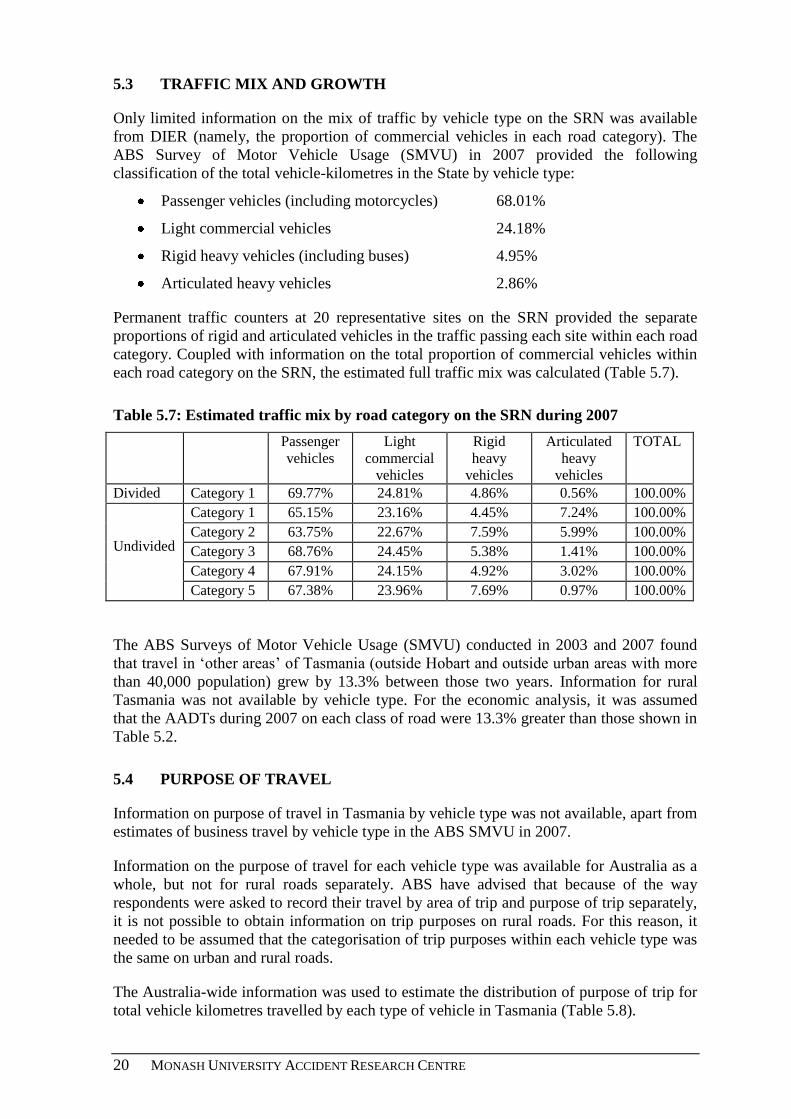
20 MONASH UNIVERSITY ACCIDENT RESEARCH CENTRE
5.3 TRAFFIC MIX AND GROWTH
Only limited information on the mix of traffic by vehicle type on the SRN was available
from DIER (namely, the proportion of commercial vehicles in each road category). The
ABS Survey of Motor Vehicle Usage (SMVU) in 2007 provided the following
classification of the total vehicle-kilometres in the State by vehicle type:
Passenger vehicles (including motorcycles) 68.01%
Light commercial vehicles 24.18%
Rigid heavy vehicles (including buses) 4.95%
Articulated heavy vehicles 2.86%
Permanent traffic counters at 20 representative sites on the SRN provided the separate
proportions of rigid and articulated vehicles in the traffic passing each site within each road
category. Coupled with information on the total proportion of commercial vehicles within
each road category on the SRN, the estimated full traffic mix was calculated (Table 5.7).
Table 5.7: Estimated traffic mix by road category on the SRN during 2007
Passenger
vehicles
Light
commercial
vehicles
Rigid
heavy
vehicles
Articulated
heavy
vehicles
TOTAL
Divided Category 1 69.77% 24.81% 4.86% 0.56% 100.00%
Undivided
Category 1 65.15% 23.16% 4.45% 7.24% 100.00%
Category 2 63.75% 22.67% 7.59% 5.99% 100.00%
Category 3 68.76% 24.45% 5.38% 1.41% 100.00%
Category 4 67.91% 24.15% 4.92% 3.02% 100.00%
Category 5 67.38% 23.96% 7.69% 0.97% 100.00%
The ABS Surveys of Motor Vehicle Usage (SMVU) conducted in 2003 and 2007 found
that travel in „other areas‟ of Tasmania (outside Hobart and outside urban areas with more
than 40,000 population) grew by 13.3% between those two years. Information for rural
Tasmania was not available by vehicle type. For the economic analysis, it was assumed
that the AADTs during 2007 on each class of road were 13.3% greater than those shown in
Table 5.2.
5.4 PURPOSE OF TRAVEL
Information on purpose of travel in Tasmania by vehicle type was not available, apart from
estimates of business travel by vehicle type in the ABS SMVU in 2007.
Information on the purpose of travel for each vehicle type was available for Australia as a
whole, but not for rural roads separately. ABS have advised that because of the way
respondents were asked to record their travel by area of trip and purpose of trip separately,
it is not possible to obtain information on trip purposes on rural roads. For this reason, it
needed to be assumed that the categorisation of trip purposes within each vehicle type was
the same on urban and rural roads.
The Australia-wide information was used to estimate the distribution of purpose of trip for
total vehicle kilometres travelled by each type of vehicle in Tasmania (Table 5.8).

ECONOMIC EVALUATION OF INTRODUCTION OF LOWER RURAL SPEED LIMITS IN TASMANIA
21
Table 5.8: Purpose of trip on travel on Tasmanian roads. (Information for rural
roads not available.) Source: ABS Survey of Motor Vehicle Usage, 2007.
Purpose Passenger
vehicles
Light
commercial
vehicles
Rigid
heavy
vehicles
Articulated
heavy
vehicles
Total all
vehicles
TRAVEL (million veh-km)
Business use 584 585 231 143 1542
To and from work 1006 311 16 913
Personal and other 1805 311 2537
TOTAL 3395 1207 247 143 4992
DISTRIBUTION
Business use 17.2% 48.5% 93.5% 100.0% 30.9%
To and from work 29.6% 25.7% 6.5% 0.0% 18.3%
Personal and other 53.2% 25.8% 0.0% 0.0% 50.8%
TOTAL 100.0% 100.0% 100.0% 100.0% 100.0%
5.5 SPEEDS
DIER provided the results of recent (March 2009) free speed observations collected at 19
representative sites on the SRN, classified into the 12 Austroads classes of type of vehicle.
These results were aggregated into three general classes of vehicle:
Light vehicles (passenger cars and light commercial vehicles): Classes 1 and 2
Rigid heavy vehicles: Classes 3 to 5
Articulated heavy vehicles: Classes 6 to 12
The mean free speeds recorded at the 13 sites in the road categories envisaged for speed
limit reductions were averaged within each category, weighting each by the number of
speed observations, to provide representative mean speeds for each class of vehicle (Table
5.9). These mean speeds provide the baseline speeds for the economic analysis of the
hypothesised changes in free speeds which would result if speed limits were reduced in
each respective road environment.
There were no representative speed survey sites on gravel roads on the SRN, and the speed
observations made at four gravel road sites as part of the evaluation of the Kingborough
Safer Speeds Demonstration (Langford 2009) were not considered to be representative of
gravel roads on the SRN throughout Tasmania because of the limited number of sites and
the proximity of Kingborough to Hobart. For this reason, the baseline speeds on Category
5 unsealed roads on the SRN for the economic analysis were taken to be similar to those on
the sealed Category 5 roads, as shown in Table 5.9 (see Chapter 8 for details).
It is understood that travel speeds on gravel roads not part of the SRN and the
responsibility of Local Councils could be as low as 60 km/h.

22 MONASH UNIVERSITY ACCIDENT RESEARCH CENTRE
Table 5.9: Speed survey sites, vehicles observed, and the weighted-average mean free
speeds for each road category envisaged for a speed limit reduction
Speed surveys Mean free speed 2009 (km/h)
Road category and current speed
limit
No. of
sites
Speed
observations
Cars &
LCVs
Rigid
heavy
vehicles
Artic.
heavy
vehicles
Rural roads with 110 km/h speed limits
Divided Category 1 Trunk Roads 2 50,769 109.7 108.8 100.3
Undivided Cat. 1 Trunk Roads 1 44,467 104.7 99.9 99.0
Undivided rural roads with 100 km/h speed limits
Category 2 Regional Freight Roads 3 134,374 85.3 80.8 77.7
Category 3 Regional Access Roads 5 114,538 87.2 81.6 82.3
Category 4 Feeder Roads 1 18,079 90.7 84.9 75.1
Category 5 “Other” Roads1
1 32,215 83.6 76.2 82.2 1
Sites on sealed roads only. No sites on unsealed gravel roads on State Road Network.

ECONOMIC EVALUATION OF INTRODUCTION OF LOWER RURAL SPEED LIMITS IN TASMANIA
23
6. RURAL ROADS WITH 110 KM/H SPEED LIMITS
Analysis of the total economic cost from road trauma, air pollutants, travel time, and
vehicle operating costs was conducted for those links of Tasmanian rural road with current
speed limits of 110 km/h where it is anticipated that a reduced speed limit of 100 km/h
may be introduced. These links are all on Category 1 Trunk Roads and included both
divided (67.3 km) and undivided (238 km) carriageways. The divided and undivided 110
km/h roads were analysed separately because of their very different current speed profiles
and their casualty crash rates and crash injury severity patterns (see sections 5.2 and 5.5).
This analysis does not include road links currently signed at 110km/h that will retain this
speed limit. Again these are Category 1 Trunk Roads, including both divided (5.02 km)
and undivided (4.51 km) carriageways.
6.1 DIVIDED CATEGORY 1 TRUNK ROADS
6.1.1 Base scenario
The economic impact of reducing the speed limit from 110 to 100 km/h was estimated by
assuming that the average free speed for each type of vehicle would decrease by 5 km/h.
The base scenario valued road trauma using the “human capital” method (see section 4.1).
Details of the analysis are given in Appendix B.
It is estimated that there would be a saving of 0.4 fatal crashes, 0.8 serious injury crashes
and 5.5 less-serious injury crashes per year (Appendix B). Annual vehicle operating costs
would decrease by $1.83 million (2.4%), crash costs by $1.46 million (15.3%) and air
pollution costs by $135,000 (2.4%) on these roads (Table 6.1.1). Travel time costs would
increase by $2.33 million per year (4.8%). The total economic impact was estimated to
decrease by $1.08 million per annum, or 0.8% of the total impact with the 110 km/h speed
limit.
Table 6.1.1: Economic impact of reducing speed limit on divided Category 1 roads
from 110 km/h (before) to 100 km/h (after), assuming 5 km/h reduction in
mean free speeds for each vehicle type. “Human capital” crash costs.
$’000/year Before After Change
Vehicle operating costs 76,949 75,123 -1826 -2.4 %
Time costs 48,915 51,248 2333 4.8 %
Crash costs 9,542 8,087 -1,456 -15.3%
Air pollution costs 5,669 5,534 -135 -2.4 %
Total 141,075 139,992
Change -1,083 -0.8 %

24 MONASH UNIVERSITY ACCIDENT RESEARCH CENTRE
The analysis considered the impacts of different average free speeds below 110 km/h by
modifying the „after‟ average speed in the spreadsheet, in 2 km/h increments between 80
and 110 km/h, and recording each result (section H3 of Appendix B). In this way, the
effect of the reduced speed limit if different average free speeds were to result can be seen
(Table 6.1.2). The contribution to the total economic impact by cars and light commercial
vehicles (LCVs), in contrast to the contribution by heavy vehicles (both rigid and
articulated), was also calculated by analysing their impacts separately (foot of Table 6.1.2).
Table 6.1.2: Economic impact of different mean speeds on divided Category 1 roads
$’000/year 80 km/h 82 km/h 84 km/h 86 km/h 88 km/h 90 km/h 92 km/h 94 km/h
Vehicle op. costs 71,379 71,263 71,235 71,291 71,427 71,636 71,916 72,263
Time costs 67,158 65,520 63,960 62,473 61,053 59,696 58,399 57,156
Crash costs 3,209 3,484 3,777 4,088 4,419 4,771 5,144 5,539
Air pollution costs 4,861 4,915 4,969 5,023 5,077 5,131 5,185 5,239
Total 146,608 145,182 143,941 142,876 141,976 141,235 140,644 140,198
of which:
Cars & LCVs 127,466 126,195 125,082 124,117 123,293 122,602 122,039 121,597
Heavy vehicles 19,142 18,987 18,859 18,759 18,684 18,633 18,606 18,601
Table 6.1.2 (cont.): Economic impact of different mean speeds on divided Category 1
roads
$’000/year 96 km/h 98 km/h 100 km/h 102 km/h 104 km/h 106 km/h 108 km/h 110 km/h
Vehicle op. costs 72,673 73,143 73,671 74,253 74,887 75,571 76,303 77,080
Time costs 55,965 54,823 53,727 52,673 51,660 50,686 49,747 48,843
Crash costs 5,957 6,399 6,867 7,361 7,882 8,431 9,009 9,619
Air pollution costs 5,293 5,348 5,402 5,456 5,510 5,564 5,618 5,672
Total 139,889 139,714 139,666 139,742 139,938 140,251 140,677 141,213
of which:
Cars & LCVs 121,272 121,058 120,952 120,951 121,049 121,246 121,537 121,921
Heavy vehicles 18,618 18,655 18,714 18,792 18,889 19,005 19,140 19,292
The speed which minimises the total economic impact, as valued in this base scenario for
divided Category 1 roads, is 100 km/h. This is also apparent in Figure 6.1.1. (Only impacts
above $60 million are shown in the Figure because of the substantial level of fixed vehicle
operating costs.)

ECONOMIC EVALUATION OF INTRODUCTION OF LOWER RURAL SPEED LIMITS IN TASMANIA
25
Figure 6.1.1: Divided Category 1 roads – Base scenario.
Monetary impacts of different average speeds on rural roads:
Category 1 divided rural roads
60,000
70,000
80,000
90,000
100,000
110,000
120,000
130,000
140,000
150,000
80 82 84 86 88 90 92 94 96 98 100 102 104 106 108 110
Average Speed
$'0
00 p
er
yea
r
Air pollution costs
Crash costs
Time costs
Vehicle operating costs
However, the optimum speed differs substantially by vehicle type (shown in bold at the
foot of Table 6.1.2). It was estimated as 102 km/h for cars and LCVs (Figure 6.1.2), as for
all vehicle types combined, but 94 km/h for heavy vehicles (Figure 6.1.3).
Figure 6.1.2: Divided Category 1 roads – Car and LCV-related costs.
Monetary impacts of different average speeds on rural roads: Car & LCV costs only
Category 1 divided rural roads
50,000
60,000
70,000
80,000
90,000
100,000
110,000
120,000
130,000
140,000
80 82 84 86 88 90 92 94 96 98 100 102 104 106 108 110
Car and LCV Average Speed
$'0
00 p
er
yea
r
Air pollution costs
Crash costs
Time costs
Vehicle operating costs

26 MONASH UNIVERSITY ACCIDENT RESEARCH CENTRE
Figure 6.1.3: Divided Category 1 roads – Heavy vehicle-related costs.
Monetary impacts of different average speeds on rural roads: Heavy vehicle-related costs only
Category 1 divided rural roads
13,000
14,000
15,000
16,000
17,000
18,000
19,000
20,000
80 82 84 86 88 90 92 94 96 98 100 102 104 106 108 110
Heavy Vehicle Average Speed
$'0
00 p
er
yea
r
Air pollution costs
Crash costs
Time costs
Vehicle operating costs
6.1.2 Willingness to pay valuation of road trauma
The base scenario was modified by using „willingness to pay‟ valuations of road trauma
(BTCE 1997), updated to 2007 prices, instead of human capital costs (BTE 2000) to test
the sensitivity of the total economic impact to this assumption (Appendix C).
Under this scenario, the annual crash costs would decrease by $3.47 million on divided
Category 1 roads (Table 6.1.3), compared with an estimated decrease of $1.46 million per
annum using human capital costs. The total economic benefit associated with the decrease
in speed limit would then be about $3.098 million per year, or 2.0% of the total impact
with the 110 km/h speed limit.
Table 6.1.3: Economic impact of reducing speed limit on divided Category 1 roads
from 110 km/h (before) to 100 km/h (after), assuming 5 km/h reduction in
mean free speeds. “Willingness to pay” valuations of crash costs.
$’000/year Before After Change
Vehicle operating costs 76,949 75,123 -1826 -2.4 %
Time costs 48,915 51,248 2333 4.8 %
Crash costs 22,615 19,144 -3,470 -15.3%
Air pollution costs 5,669 5,534 -135 -2.4 %
Total 154,147 151,049
Change -3,098 -2.0 %

ECONOMIC EVALUATION OF INTRODUCTION OF LOWER RURAL SPEED LIMITS IN TASMANIA
27
When a range of average speeds was considered, the speed which minimised the total
economic impact was 92 km/h (Table 6.1.4 and Figure 6.1.4). Using the “willingness to
pay” valuations of road trauma, the optimum speed for cars and LCVs was estimated to be
92 km/h and that for heavy vehicles was estimated to be 90 km/h. The economic impact
related to heavy vehicles reflected the higher valuation of the crash costs associated with
their use (Figure 6.1.5).
Comparison of these results with those in section 6.1.1, using human capital costs of the
road trauma saved by speed reductions, shows the sensitivity of the estimated economic
impacts to the assumptions about the values society is prepared to place on preventing
casualty crashes, especially those resulting in death and serious injury. The high severity of
injury outcome associated with crashes involving heavy vehicles, compared with light
vehicle crashes, together with their high operating costs, results in lower optimum speeds
for this class of vehicle.
Table 6.1.4: Economic impact of different mean speeds on divided Category 1 roads.
“Willingness to pay” valuations of crash costs.
$’000/year 80 km/h 82 km/h 84 km/h 86 km/h 88 km/h 90 km/h 92 km/h 94 km/h 96 km/h 98 km/h 100 km/h
Vehicle op. costs 71,379 71,263 71,235 71,291 71,427 71,636 71,916 72,263 72,673 73,143 73,671
Time costs 67,158 65,520 63,960 62,473 61,053 59,696 58,399 57,156 55,965 54,823 53,727
Crash costs 7,610 8,256 8,945 9,679 10,459 11,288 12,169 13,103 14,093 15,141 16,250
Air pollution costs 4,861 4,915 4,969 5,023 5,077 5,131 5,185 5,239 5,293 5,348 5,402
Total 151,009 149,954 149,110 148,466 148,016 147,752 147,669 147,761 148,025 148,455 149,049
of which:
Cars & LCVs 131,485 130,549 129,792 129,207 128,786 128,525 128,417 128,459 128,646 128,975 129,444
Heavy vehicles 19,524 19,405 19,318 19,259 19,230 19,227 19,252 19,303 19,379 19,480 19,605

28 MONASH UNIVERSITY ACCIDENT RESEARCH CENTRE
Figure 6.1.4: Divided Category 1 roads – ‘Willingness to pay’ valuations of road trauma.
Monetary impacts of different average speeds on rural roads:
Category 1 divided rural roads
60,000
80,000
100,000
120,000
140,000
160,000
80 82 84 86 88 90 92 94 96 98 100
Average Speed
$'0
00 p
er
yea
r
Air pollution costs
Crash costs
Time costs
Vehicle operating costs
Figure 6.1.5: Divided Category 1 roads – ‘Willingness to pay’ valuations of road trauma. Heavy vehicle-related costs.
Monetary impacts of different average speeds on rural roads: Heavy vehicle-related costs only
Category 1 divided rural roads
12,000
13,000
14,000
15,000
16,000
17,000
18,000
19,000
20,000
21,000
80 82 84 86 88 90 92 94 96 98 100
Heavy Vehicle Average Speed
$'0
00 p
er
yea
r
Air pollution costs
Crash costs
Time costs
Vehicle operating costs

ECONOMIC EVALUATION OF INTRODUCTION OF LOWER RURAL SPEED LIMITS IN TASMANIA
29
6.2 UNDIVIDED CATEGORY 1 TRUNK ROADS
6.2.1 Base scenario
The economic impact of reducing the speed limit from 110 to 100 km/h on the 238 km of
undivided Category 1 rural roads was estimated by assuming that the average free speed
for each type of vehicle (see Table 5.9) would decrease by 5 km/h. The average speeds
were lower on these undivided roads than the divided roads in the same category, but the
proportion of articulated heavy vehicle traffic was much higher. The base scenario valued
road trauma using the “human capital” method (see section 4.1). Details of the analysis are
given in Appendix D.
It is estimated that there would be a saving of 1.8 fatal crashes, 1.7 serious injury crashes
and 4.5 less-serious injury crashes per year (Appendix D). Annual vehicle operating costs
would decrease by $4.28 million (1.8%), crash costs by $4.71 million (17.6%) and air
pollution costs by $371,000 (2.4%) on these roads (Table 6.2.1). Travel time costs would
increase by $7.50 million per year (5.1%). The total economic impact was estimated to
decrease by $1.87 million per annum, or 0.4% of the total impact with the 110 km/h speed
limit.
Table 6.2.1: Economic impact of reducing speed limit on undivided Category 1
roads from 110 km/h (before) to 100 km/h (after), assuming 5 km/h
reduction in mean free speeds for each vehicle type. “Human capital”
crash costs.
$’000/year Before After Change
Vehicle operating costs 239,519 235,240 -4280 -1.8 %
Time costs 148,325 155,820 7495 5.1 %
Crash costs 26,769 22,055 -4,714 -17.6%
Air pollution costs 15,146 14,775 -371 -2.4 %
Total 429,759 427,889
Change -1,870 -0.4 %
When a range of average speeds was considered as possible “after” speeds following the
speed limit reduction, the speed which minimised the total economic impact for all vehicle
types combined was 98 km/h (Table 6.2.2 and Figure 6.2.1).

30 MONASH UNIVERSITY ACCIDENT RESEARCH CENTRE
Table 6.2.2: Economic impact of different mean speeds on undivided Category 1
roads
$’000/year 80 km/h 82 km/h 84 km/h 86 km/h 88 km/h 90 km/h 92 km/h 94 km/h
Vehicle op. costs 230,220 229,672 229,422 229,454 229,750 230,298 231,084 232,096
Time costs 192,823 188,120 183,641 179,370 175,294 171,398 167,672 164,105
Crash costs 9,895 10,867 11,912 13,034 14,237 15,525 16,901 18,372
Air pollution costs 13,341 13,489 13,638 13,786 13,934 14,083 14,231 14,379
Total 446,279 442,149 438,613 435,644 433,215 431,304 429,889 428,951
of which:
Cars & LCVs 326,508 323,323 320,552 318,173 316,168 314,518 313,210 312,228
Heavy vehicles 119,772 118,826 118,062 117,471 117,048 116,785 116,679 116,723
Table 6.2.2 (cont.): Economic impact of different mean speeds on undivided Category
1 roads
$’000/year 96 km/h 98 km/h 100 km/h 102 km/h 104 km/h 106 km/h 108 km/h 110 km/h
Vehicle op. costs 233,322 234,754 236,381 238,195 240,188 242,353 244,683 247,172
Time costs 160,686 157,407 154,259 151,234 148,326 145,527 142,832 140,235
Crash costs 19,940 21,611 23,389 25,280 27,287 29,417 31,674 34,065
Air pollution costs 14,527 14,676 14,824 14,972 15,120 15,269 15,417 15,565
Total 428,476 428,447 428,852 429,680 430,921 432,566 434,607 437,037
of which:
Cars & LCVs 311,562 311,199 311,131 311,349 311,845 312,612 313,646 314,941
Heavy vehicles 116,914 117,248 117,721 118,332 119,077 119,953 120,961 122,097

ECONOMIC EVALUATION OF INTRODUCTION OF LOWER RURAL SPEED LIMITS IN TASMANIA
31
Figure 6.2.1: Undivided Category 1 roads – Base scenario.
Monetary impacts of different average speeds on rural roads:
Category 1 undivided rural roads
200,000
250,000
300,000
350,000
400,000
450,000
500,000
80 82 84 86 88 90 92 94 96 98 100 102 104 106 108 110
Average Speed
$'0
00 p
er
yea
r
Air pollution costs
Crash costs
Time costs
Vehicle operating costs
However, the optimum speed differs substantially by vehicle type (shown in bold at the
foot of Table 6.2.2). It was estimated as 100 km/h for cars and LCVs (Figure 6.2.2), but 92
km/h for heavy vehicles (Figure 6.2.3).
Figure 6.2.2: Undivided Category 1 roads – Car and LCV-related costs.
Monetary impacts of different average speeds on rural roads: Car & LCV costs only
Category 1 undivided rural roads
125,000
175,000
225,000
275,000
325,000
375,000
80 82 84 86 88 90 92 94 96 98 100 102 104 106 108 110
Car and LCV Average Speed
$'0
00 p
er
yea
r
Air pollution costs
Crash costs
Time costs
Vehicle operating costs

32 MONASH UNIVERSITY ACCIDENT RESEARCH CENTRE
Figure 6.2.3: Undivided Category 1 roads – Heavy vehicle-related costs.
Monetary impacts of different average speeds on rural roads: Heavy vehicle-related costs only
Category 1 undivided rural roads
80,000
85,000
90,000
95,000
100,000
105,000
110,000
115,000
120,000
125,000
130,000
80 82 84 86 88 90 92 94 96 98 100 102 104 106 108 110
Heavy Vehicle Average Speed
$'0
00 p
er
yea
r
Air pollution costs
Crash costs
Time costs
Vehicle operating costs
6.2.2 Willingness to pay valuation of road trauma
As for the analysis of divided Category 1 roads, the base scenario was modified by using
„willingness to pay‟ valuations of road trauma (Appendix E).
Under this scenario, the annual crash costs would decrease by $11.38 million on undivided
Category 1 roads (Table 6.2.3), compared with an estimated decrease of $4.71 million per
annum using human capital costs. The total economic benefit associated with the decrease
in speed limit would then be about $8.54 million per year, or 1.8% of the total impact with
the 110 km/h speed limit.
Table 6.2.3: Economic impact of reducing speed limit on undivided Category 1
roads from 110 km/h (before) to 100 km/h (after), assuming 5 km/h
reduction in mean free speeds. “Willingness to pay” valuations of crash
costs.
$’000/year Before After Change
Vehicle operating costs 239,519 235,240 -4280 -1.8 %
Time costs 148,325 155,820 7495 5.1 %
Crash costs 62,754 51,373 -11,381 -18.1%
Air pollution costs 15,146 14,775 -371 -2.4 %
Total 465,744 457,207
Change -8,537 -1.8 %

ECONOMIC EVALUATION OF INTRODUCTION OF LOWER RURAL SPEED LIMITS IN TASMANIA
33
When a range of average speeds was considered, the speed which minimised the total
economic impact for all vehicle types combined was 90 km/h (Table 6.2.4 and Figure
6.2.4). Using the “willingness to pay” valuations of road trauma, the optimum speed for
cars and LCVs was estimated to be 90 km/h and that for heavy vehicles was estimated to
be 86 km/h (Figure 6.2.5).
Table 6.2.4: Economic impact of different mean speeds on undivided Category 1
roads. “Willingness to pay” valuations of crash costs.
$’000/year 80 km/h 82 km/h 84 km/h 86 km/h 88 km/h 90 km/h 92 km/h 94 km/h 96 km/h 98 km/h 100 km/h
Vehicle op. costs 230,220 229,672 229,422 229,454 229,750 230,298 231,084 232,096 233,322 234,754 236,381
Time costs 192,823 188,120 183,641 179,370 175,294 171,398 167,672 164,105 160,686 157,407 154,259
Crash costs 22,477 24,767 27,237 29,895 32,754 35,822 39,112 42,634 46,399 50,420 54,709
Air pollution costs 13,341 13,489 13,638 13,786 13,934 14,083 14,231 14,379 14,527 14,676 14,824
Total 458,861 456,048 453,938 452,505 451,732 451,602 452,099 453,213 454,935 457,256 460,173
of which:
Cars & LCVs 335,619 333,368 331,605 330,313 329,476 329,083 329,123 329,586 330,465 331,754 333,450
Heavy vehicles 123,242 122,680 122,333 122,193 122,256 122,518 122,976 123,628 124,470 125,502 126,723
Figure 6.2.4: Undivided Category 1 roads – ‘Willingness to pay’ valuations of road trauma.
Monetary impacts of different average speeds on rural roads:
Category 1 undivided rural roads
200,000
250,000
300,000
350,000
400,000
450,000
500,000
80 82 84 86 88 90 92 94 96 98 100
Average Speed
$'0
00 p
er
year
Air pollution costs
Crash costs
Time costs
Vehicle operating costs

34 MONASH UNIVERSITY ACCIDENT RESEARCH CENTRE
Figure 6.2.5: Undivided Category 1 roads – ‘Willingness to pay’ valuations of road trauma. Heavy vehicle-related costs.
Monetary impacts of different average speeds on rural roads: Heavy vehicle-related costs only
Category 1 undivided rural roads
80,000
85,000
90,000
95,000
100,000
105,000
110,000
115,000
120,000
125,000
130,000
80 82 84 86 88 90 92 94 96 98 100
Heavy Vehicle Average Speed
$'0
00 p
er
yea
r
Air pollution costs
Crash costs
Time costs
Vehicle operating costs

ECONOMIC EVALUATION OF INTRODUCTION OF LOWER RURAL SPEED LIMITS IN TASMANIA
35
7. UNDIVIDED RURAL ROADS WITH 100 KM/H SPEED LIMITS
The economic analysis of rural roads with 100 km/h speed limits envisaged for a speed
limit reduction to 90 km/h focused on the undivided roads. The divided roads with 100
km/h limits in Category 1 (2.78 km) and in Category 3 (9.81 km) were considered too short
for the analysis to be reliable (Table 5.1). There were substantial lengths of undivided 100
km/h limit roads envisaged in Categories 2 to 5, but no undivided 100 km/h roads in
Category 1 were candidates for the speed limit reduction. The undivided 110 km/h
Category 1 roads were analysed in section 6.2.
7.1 CATEGORY 2 REGIONAL FREIGHT ROADS
7.1.1 Base scenario
The economic impact of reducing the speed limit from 100 to 90 km/h on the 263 km of
undivided Category 2 rural roads was estimated by assuming that the average free speed
for each type of vehicle (see Table 5.9) would decrease by 5 km/h.2 The average speeds
were lower than the undivided roads in Category 1, and were already lower than the
envisaged reduced limit. The proportion of heavy vehicle traffic on Category 2 roads was
relatively high, especially rigid heavy vehicles. The base scenario valued road trauma
using the “human capital” method. Details of the analysis are given in Appendix F.
If average speeds were reduced by 5 km/h, it is estimated that there would be a saving of
0.6 fatal crashes, 1.9 serious injury crashes and 5.5 less-serious injury crashes per year
(Appendix F). Annual crash costs would decrease by $2.36 million (19.3%) and air
pollution costs by $158,000 (2.7%) on these roads (Table 7.1.1). Annual vehicle operating
costs would increase by $842,000 (0.8%) and travel time costs would increase by $4.96
million per year (6.3%). The total economic impact was estimated to increase by $3.29
million per annum, or 1.7% of the total impact with the 100 km/h speed limit.
Table 7.1.1: Economic impact of reducing speed limit on undivided Category 2
roads from 100 km/h (before) to 90 km/h (after), assuming 5 km/h
reduction in mean free speeds. “Human capital” crash costs.
$’000/year Before After Change
Vehicle operating costs 102,715 103,557 842 0.8 %
Time costs 78,239 83,201 4962 6.3 %
Crash costs 12,214 9,859 -2,355 -19.3%
Air pollution costs 5,827 5,669 -158 -2.7 %
Total 198,995 202,286
Change 3,291 1.7 %
2 Note there are 134km of undivided Category 2 rural roads where it is envisaged that the current speed limit
will be retained.

36 MONASH UNIVERSITY ACCIDENT RESEARCH CENTRE
The increased economic impact was apparently due to the hypothesised reduced average
speeds after the speed limit reduction being lower than the optimum speed for each class of
vehicle (based on human capital valuation of crash costs). The assumption that average
speeds substantially lower than existing speed limits would decrease further following the
envisaged speed limit reductions is questionable, as is the application of Nilsson-type
relationships linking road trauma reductions only to average free speeds in such
circumstances. An alternative methodology which may be superior is discussed in section
10.4 and recommended for further consideration.
When a range of average speeds was considered as possible “after” speeds following the
speed limit reduction, the speed which minimised the total economic impact for all vehicle
types combined was 90 km/h (Table 7.1.2 and Figure 7.1.1).
Table 7.1.2: Economic impact of different mean speeds on undivided Category 2
roads
$’000/year 80 km/h 82 km/h 84 km/h 86 km/h 88 km/h 90 km/h 92 km/h 94 km/h 96 km/h 98 km/h 100 km/h
Vehicle op. costs 102,634 102,371 102,242 102,239 102,356 102,587 102,924 103,363 103,900 104,528 105,246
Time costs 82,065 80,063 78,157 76,339 74,604 72,947 71,361 69,842 68,387 66,992 65,652
Crash costs 10,497 11,442 12,452 13,530 14,678 15,900 17,200 18,581 20,046 21,599 23,244
Air pollution costs 5,692 5,755 5,818 5,882 5,945 6,008 6,071 6,135 6,198 6,261 6,324
Total 200,887 199,631 198,669 197,990 197,584 197,441 197,556 197,921 198,531 199,380 200,466
of which:
Cars & LCVs 141,040 140,097 139,350 138,791 138,412 138,209 138,174 138,305 138,596 139,045 139,648
Heavy vehicles 59,847 59,535 59,320 59,200 59,171 59,233 59,382 59,616 59,934 60,335 60,818

ECONOMIC EVALUATION OF INTRODUCTION OF LOWER RURAL SPEED LIMITS IN TASMANIA
37
Figure 7.1.1: Undivided Category 2 roads – Base scenario.
Monetary impacts of different average speeds on rural roads:
Category 2 undivided rural roads
100,000
120,000
140,000
160,000
180,000
200,000
220,000
80 82 84 86 88 90 92 94 96 98 100
Average Speed
$'0
00 p
er
yea
r
Air pollution costs
Crash costs
Time costs
Vehicle operating costs
However, the optimum speed differs by vehicle type (shown in bold at the foot of Table
7.1.2). It was estimated as 92 km/h for cars and LCVs (Figure 7.1.2), but 88 km/h for
heavy vehicles (Figure 7.1.3).
Figure 7.1.2: Undivided Category 2 roads – Car and LCV-related costs.
Monetary impacts of different average speeds on rural roads: Car & LCV costs only
Category 2 undivided rural roads
60,000
70,000
80,000
90,000
100,000
110,000
120,000
130,000
140,000
150,000
80 82 84 86 88 90 92 94 96 98 100
Car and LCV Average Speed
$'0
00 p
er
yea
r
Air pollution costs
Crash costs
Time costs
Vehicle operating costs

38 MONASH UNIVERSITY ACCIDENT RESEARCH CENTRE
Figure 7.1.3: Undivided Category 2 roads – Heavy vehicle-related costs.
Monetary impacts of different average speeds on rural roads: Heavy vehicle-related costs only
Category 2 undivided rural roads
40,000
45,000
50,000
55,000
60,000
80 82 84 86 88 90 92 94 96 98 100
Heavy Vehicle Average Speed
$'0
00 p
er
yea
r
Air pollution costs
Crash costs
Time costs
Vehicle operating costs
7.1.2 Willingness to pay valuation of road trauma
The base scenario was modified by using „willingness to pay‟ valuations of road trauma
(Appendix G). Under this scenario, the annual crash costs would decrease by $5.08 million
on undivided Category 2 roads (Table 7.1.3), compared with an estimated decrease of
$2.36 million per annum using human capital costs. The total economic cost associated
with the decrease in speed limit would then be about $565,000 per year, or 0.3% of the
total impact with the 100 km/h speed limit.
Table 7.1.3: Economic impact of reducing speed limit on undivided Category 2
roads from 100 km/h (before) to 90 km/h (after), assuming 5 km/h
reduction in mean speeds. “Willingness to pay” valuations of crash costs.
$’000/year Before After Change
Vehicle operating costs 102,715 103,557 842 0.8 %
Time costs 78,239 83,201 4962 6.3 %
Crash costs 25,365 20,284 -5,081 -20.0%
Air pollution costs 5,827 5,669 -158 -2.7 %
Total 212,145 212,710
Change 565 0.3 %
The optimum speed for cars and LCVs was estimated to be 82 km/h (Figure 7.1.4) and that
for heavy vehicles was estimated to be 80 km/h (Figure 7.1.5).

ECONOMIC EVALUATION OF INTRODUCTION OF LOWER RURAL SPEED LIMITS IN TASMANIA
39
Figure 7.1.4: Undivided Category 2 roads – ‘Willingness to pay’ valuations of road trauma. Car and LCV-related costs.
Monetary impacts of different average speeds on rural roads: Car & LCV costs only
Category 2 undivided rural roads
60,000
80,000
100,000
120,000
140,000
160,000
80 82 84 86 88 90 92 94 96 98 100
Car and LCV Average Speed
$'0
00 p
er
yea
r
Air pollution costs
Crash costs
Time costs
Vehicle operating costs
Figure 7.1.5: Undivided Category 2 roads – ‘Willingness to pay’ valuations of road trauma. Heavy vehicle-related costs.
Monetary impacts of different average speeds on rural roads: Heavy vehicle-related costs only
Category 2 undivided rural roads
40,000
45,000
50,000
55,000
60,000
65,000
70,000
80 82 84 86 88 90 92 94 96 98 100
Heavy Vehicle Average Speed
$'0
00 p
er
yea
r
Air pollution costs
Crash costs
Time costs
Vehicle operating costs
Thus the hypothesised reduced average speeds on Category 2 roads after the speed limit
reduction to 90 km/h are closer to (but still lower than) the optimum speeds based on the
willingness-to-pay valuations of road trauma than the optima based on human capital costs.
If willingness-to-pay valuation of crash cost savings is supported, then the reduction in

40 MONASH UNIVERSITY ACCIDENT RESEARCH CENTRE
current average speeds to a level even further below the envisaged 90 km/h limits for these
Category 2 roads would have economic justification, notwithstanding that current average
free speeds are below the envisaged limit. However, an alternative methodology to link
road trauma changes with reductions in speed limits when average free speeds are already
substantially below existing limits is discussed in section 10.4.
7.2 ROAD CATEGORIES 3 TO 5 WITH 100 KM/H LIMITS
7.2.1 Base scenarios
The economic impacts of reducing the speed limit from 100 to 90 km/h on undivided rural
roads in Categories 3 to 5 were estimated by assuming that the average free speed for each
type of vehicle (see Table 5.9) would decrease by 5 km/h. The detailed results are given in
Appendices H, J, and L and are summarised in Table 7.2.1 together with the results of the
analysis of undivided Category 2 roads from section 7.1.1 above.
The optimum speeds for each class of vehicle on each of Categories 3 to 5 roads are shown
in Figures 7.2.1 to 7.2.3, based on human capital costs of road crashes.
Table 7.2.1: Economic impacts of speed reductions on undivided roads with 100 km/h
speed limits. “Human capital” costs of road trauma.
Effect of 5 km/h mean
speed reductions on total
economic cost
Optimum Speed (km/h)
(speed which minimises total
economic cost)
Road category
Change p.a.
($ million)
Percentage
change
All vehicles
combined
Cars &
LCVs
Heavy
vehicles
Category 2 Regional Freight Roads +3.291 +1.7% 90 92 88
Category 3 Regional Access Roads +2.593 +0.9% 88 90 86
Category 4 Feeder Roads +2.261 +0.8% 90 92 86
Category 5 “Other” Roads
+2.722 +1.4% 88 88 84
Figure 7.2.1: Undivided Category 3 roads
Monetary impacts of different average speeds on rural roads: Car & LCV costs only
Category 3 undivided rural roads
100,000
120,000
140,000
160,000
180,000
200,000
220,000
240,000
260,000
80 82 84 86 88 90 92 94 96 98 100
Car and LCV Average Speed
$'0
00 p
er
yea
r
Monetary impacts of different average speeds on rural roads: Heavy vehicle-related costs only
Category 3 undivided rural roads
32,000
34,000
36,000
38,000
40,000
42,000
44,000
46,000
48,000
50,000
80 82 84 86 88 90 92 94 96 98 100
Heavy Vehicle Average Speed
$'0
00 p
er
yea
r

ECONOMIC EVALUATION OF INTRODUCTION OF LOWER RURAL SPEED LIMITS IN TASMANIA
41
Figure 7.2.2: Undivided Category 4 roads
Monetary impacts of different average speeds on rural roads: Car & LCV costs only
Category 4 undivided rural roads
90,000
110,000
130,000
150,000
170,000
190,000
210,000
230,000
250,000
80 82 84 86 88 90 92 94 96 98 100
Car and LCV Average Speed
$'0
00 p
er
yea
r
Monetary impacts of different average speeds on rural roads: Heavy vehicle-related costs only
Category 4 undivided rural roads
36,000
41,000
46,000
51,000
56,000
80 82 84 86 88 90 92 94 96 98 100
Heavy Vehicle Average Speed
$'0
00 p
er
yea
r
Figure 7.2.3: Undivided Category 5 roads
Monetary impacts of different average speeds on rural roads: Car & LCV costs only
Category 5 undivided rural roads
60,000
80,000
100,000
120,000
140,000
160,000
180,000
80 82 84 86 88 90 92 94 96 98 100
Car and LCV Average Speed
$'0
00 p
er
year
Monetary impacts of different average speeds on rural roads: Heavy vehicle-related costs only
Category 5 undivided rural roads
26,000
28,000
30,000
32,000
34,000
36,000
38,000
40,000
42,000
80 82 84 86 88 90 92 94 96 98 100
Heavy Vehicle Average Speed
$'0
00 p
er
year
7.2.2 Willingness to pay valuation of road trauma
The base scenarios were modified by using „willingness to pay‟ valuations of road trauma
(Appendices I, K and M). The detailed results are summarised in Table 7.2.2 together with
the results for undivided Category 2 roads. The optimum speeds for each class of vehicle
on each of Categories 3 to 5 roads are shown in Figures 7.2.4 to 7.2.6. Where an optimum
speed is indicated as being below 80 km/h in a figure, the estimated optimum (to 2 km/h) is
shown in Table 7.2.2 (78 km/h in each case below 80 km/h).
Table 7.2.2: Economic impacts of speed reductions on undivided roads with 100 km/h
speed limits. “Willingness to pay” valuations of crash costs.
Effect of 5 km/h mean
speed reductions on total
economic cost
Optimum Speed (km/h)
(speed which minimises total
economic cost)
Road category
Change p.a.
($ million)
Percentage
change
All vehicles
combined
Cars &
LCVs
Heavy
vehicles
Category 2 Regional Freight Roads +0.565 +0.3% 82 82 80
Category 3 Regional Access Roads -2.907 -0.9% 80 80 78
Category 4 Feeder Roads -1.831 -0.6% 82 84 80
Category 5 “Other” Roads
-0.486 -0.2% 78 80 78

42 MONASH UNIVERSITY ACCIDENT RESEARCH CENTRE
Figure 7.2.4: Undivided Category 3 roads – ‘Willingness to pay’ valuations of crashes
Monetary impacts of different average speeds on rural roads: Car & LCV costs only
Category 3 undivided rural roads
100,000
120,000
140,000
160,000
180,000
200,000
220,000
240,000
260,000
280,000
300,000
80 82 84 86 88 90 92 94 96 98 100
Car and LCV Average Speed
$'0
00 p
er
yea
r
Monetary impacts of different average speeds on rural roads: Heavy vehicle-related costs only
Category 3 undivided rural roads
32,000
37,000
42,000
47,000
52,000
57,000
80 82 84 86 88 90 92 94 96 98 100
Heavy Vehicle Average Speed
$'0
00 p
er
yea
r
Figure 7.2.5: Undivided Category 4 roads – ‘Willingness to pay’ valuations of crashes
Monetary impacts of different average speeds on rural roads: Car & LCV costs only
Category 4 undivided rural roads
90,000
110,000
130,000
150,000
170,000
190,000
210,000
230,000
250,000
270,000
80 82 84 86 88 90 92 94 96 98 100
Car and LCV Average Speed
$'0
00 p
er
year
Monetary impacts of different average speeds on rural roads: Heavy vehicle-related costs only
Category 4 undivided rural roads
36,000
41,000
46,000
51,000
56,000
61,000
80 82 84 86 88 90 92 94 96 98 100
Heavy Vehicle Average Speed
$'0
00 p
er
year
Figure 7.2.6: Undivided Category 5 roads – ‘Willingness to pay’ valuations of crashes
Monetary impacts of different average speeds on rural roads: Car & LCV costs only
Category 5 undivided rural roads
60,000
80,000
100,000
120,000
140,000
160,000
180,000
80 82 84 86 88 90 92 94 96 98 100
Car and LCV Average Speed
$'0
00 p
er
yea
r
Monetary impacts of different average speeds on rural roads: Heavy vehicle-related costs only
Category 5 undivided rural roads
26,000
31,000
36,000
41,000
46,000
80 82 84 86 88 90 92 94 96 98 100
Heavy Vehicle Average Speed
$'0
00 p
er
yea
r

ECONOMIC EVALUATION OF INTRODUCTION OF LOWER RURAL SPEED LIMITS IN TASMANIA
43
8 UNSEALED RURAL ROADS
The economic analysis of unsealed rural roads with 100 km/h speed limits envisaged for a
speed limit reduction to 80 km/h was focused on the subset of those roads on the State
Road Network. There was an estimated 10,300 km of unsealed roads in Tasmania, and all
but 206 km of these roads were the responsibility of Local Councils. The unsealed rural
roads on the State Road Network were included in the Category 5 “Other” roads analysed
in section 7.2 because crash data could not be separately provided for the unsealed road
links. The unsealed roads in Category 5 represented 18% of their length but only 3% of the
vehicle-kilometres travelled on Category 5 roads. Thus the results in section 7.2 pertain
predominantly to sealed Category 5 roads.
No crash data was available for the unsealed rural roads and only limited estimates of the
traffic levels could derived from NRTC (1996). About 34 vehicles per day use each
unsealed road in Tasmania, resulting in a total of about 128 million vehicle-kilometres per
year and representing about 6.4% of total rural travel in Tasmania. The unsealed rural
roads on the State Road Network that are analysed in this chapter carry about 10.5 million
vehicle-kilometres per year, representing about 8.2% of travel on rural gravel roads
although they constitute only 2% of the total length. It is understood that gravel roads not
part of the State Road Network remain the responsibility of Local Councils and the road
environment generally requires vehicle speeds as low as 60 km/h.
8.1 BASE SCENARIO
The economic impact of reducing the speed limit from 100 to 80 km/h on the 206 km of
unsealed Category 5 rural roads was estimated by assuming that the average free speed for
each type of vehicle would decrease by 5 km/h. Based on the speed surveys on sealed
Category 5 roads during 2009 (Table 5.9), it was estimated that on unsealed roads the
average free speed of light vehicles (passenger cars and light commercial vehicles) was 85
km/h and that of heavy vehicles was 80 km/h. There were no permanent speed survey sites
on unsealed roads during 2009, and the baseline speed surveys carried out at four sites on
gravel roads as part of the Kingborough Safer Speeds Demonstration (Langford 2009)
were not considered representative of speeds on unsealed roads throughout Tasmania
because of the limited number of sites and the proximity of Kingborough to Hobart.
The rate of casualty crashes per 100 million vehicle-kilometres of travel on unsealed roads
was taken as that provided by Perovic et al (2008) for this road type in Australia, namely
35.0 per 100 million vehicle-kilometres. Perovic et al‟s estimates that 5.0% of these
casualty crashes would result in fatal outcome and 27.6% in serious injury were also used
in the absence of real crash data for unsealed roads in Tasmania. The base scenario valued
road trauma using the “human capital” method. Details of the analysis are given in
Appendix N.
If average speeds were reduced by 5 km/h, it is estimated that there would be a saving of
about one casualty crash every two years (Appendix N). Annual crash costs would
decrease by $187,000 (19.1%) and air pollution costs by $6,000 (2.7%) on these roads
(Table 8.1.1). Annual vehicle operating costs would increase by $26,000 (0.7%) and travel
time costs would increase by $194,000 per year (6.3%). The total economic impact was
estimated to increase by $27,000 per annum, or 0.3% of the total impact with the 100 km/h
speed limit.

44 MONASH UNIVERSITY ACCIDENT RESEARCH CENTRE
Table 8.1.1: Economic impact of reducing speed limit on unsealed Category 5 roads
from 100 km/h (before) to 80 km/h (after), assuming 5 km/h reduction in
mean free speeds for each vehicle type. “Human capital” crash costs.
$’000/year Before After Change
Vehicle operating costs 3,918 3,944 26 0.7 %
Time costs 3,069 3,263 194 6.3 %
Crash costs 977 790 -187 -19.1%
Air pollution costs 236 230 -6 -2.7 %
Total 8,200 8,227
Change 27 0.3 %
The increased economic impact was apparently due to the hypothesised reduced average
speeds after the speed limit reduction being lower than the optimum speed for each class of
vehicle (based on human capital valuation of crash costs).
When a range of average speeds was considered as possible “after” speeds following the
speed limit reduction, the speed which minimised the total economic impact for all vehicle
types combined was 82 km/h (Table 8.1.2 and Figure 8.1.1).
Table 8.1.2: Economic impact of different mean speeds on unsealed Category 5 roads
$’000/year 80 km/h 82 km/h 84 km/h 86 km/h 88 km/h 90 km/h 92 km/h 94 km/h 96 km/h 98 km/h 100 km/h
Vehicle op. costs 3,917 3,908 3,904 3,905 3,910 3,920 3,933 3,951 3,972 3,996 4,024
Time costs 3,234 3,155 3,080 3,008 2,940 2,874 2,812 2,752 2,695 2,640 2,587
Crash costs 824 898 976 1,060 1,149 1,244 1,345 1,452 1,565 1,685 1,812
Air pollution costs 231 233 236 238 241 244 246 249 251 254 256
Total 8,206 8,194 8,196 8,211 8,240 8,282 8,336 8,403 8,483 8,575 8,680
of which:
Cars & LCVs 6,225 6,215 6,215 6,225 6,245 6,275 6,313 6,362 6,419 6,485 6,561
Heavy vehicles 1,981 1,979 1,981 1,986 1,995 2,007 2,023 2,042 2,064 2,090 2,119

ECONOMIC EVALUATION OF INTRODUCTION OF LOWER RURAL SPEED LIMITS IN TASMANIA
45
Figure 8.1.1: Unsealed Category 5 roads – Base scenario.
Monetary impacts of different average speeds on rural roads:
Category 5 unsealed rural roads
3,700
4,700
5,700
6,700
7,700
8,700
80 82 84 86 88 90 92 94 96 98 100
Average Speed
$'0
00 p
er
yea
r
Air pollution costs
Crash costs
Time costs
Vehicle operating costs
On unsealed roads the optimum speed did not differ by vehicle type and was estimated as
82 km/h for each class of vehicle (Figure 8.1.2).
Figure 8.1.2: Unsealed Category 5 roads – Optimum speeds by vehicle class.
Monetary impacts of different average speeds on rural roads: Car & LCV costs only
Category 5 unsealed rural roads
2,400
2,900
3,400
3,900
4,400
4,900
5,400
5,900
6,400
6,900
80 82 84 86 88 90 92 94 96 98 100
Car and LCV Average Speed
$'0
00 p
er
yea
r
Monetary impacts of different average speeds on rural roads: Heavy vehicle-related costs only
Category 5 unsealed rural roads
1,200
1,300
1,400
1,500
1,600
1,700
1,800
1,900
2,000
2,100
2,200
80 82 84 86 88 90 92 94 96 98 100
Heavy Vehicle Average Speed
$'0
00 p
er
yea
r
8.2 WILLINGNESS TO PAY VALUATION OF ROAD TRAUMA
The base scenario was modified by using „willingness to pay‟ valuations of road trauma
(Appendix O). Under this scenario, the annual crash costs would decrease by $386,000 on
unsealed Category 5 roads (Table 8.2.1), compared with an estimated decrease of $187,000
per annum using human capital costs. The total economic impact associated with the
decrease in speed limit would then be about $172,000 per year, or 1.9% of the total impact
with the 100 km/h speed limit.

46 MONASH UNIVERSITY ACCIDENT RESEARCH CENTRE
Table 8.2.1: Economic impact of reducing speed limit on unsealed Category 5 roads
from 100 km/h (before) to 80 km/h (after), assuming 5 km/h reduction in
mean speeds. “Willingness to pay” valuations of crash costs.
$’000/year Before After Change
Vehicle operating costs 3,918 3,944 26 0.7 %
Time costs 3,069 3,263 194 6.3 %
Crash costs 1,917 1,531 -386 -20.1%
Air pollution costs 236 230 -6 -2.7 %
Total 9,140 8,968
Change -172 -1.9 %
When a range of average speeds was considered as possible “after” speeds following the
speed limit reduction, the speed which minimised the total economic impact for all vehicle
types combined was 74 km/h. This optimum speed is outside the range of analysed speeds
shown in Figure 8.2.1, but is implied by the continuing decrease in total monetary impact
at 80 km/h compared with higher average speeds.
Figure 8.2.1: Unsealed Category 5 roads – ‘Willingness to pay’ valuations of road trauma.
Monetary impacts of different average speeds on rural roads:
Category 5 unsealed rural roads
3,700
4,700
5,700
6,700
7,700
8,700
9,700
10,700
80 82 84 86 88 90 92 94 96 98 100
Average Speed
$'0
00 p
er
year
Air pollution costs
Crash costs
Time costs
Vehicle operating costs
The estimated optimum speed for each of the two classes of vehicle was also 74 km/h, as
implied by Figure 8.2.2.

ECONOMIC EVALUATION OF INTRODUCTION OF LOWER RURAL SPEED LIMITS IN TASMANIA
47
Figure 8.2.2: Unsealed Category 5 roads – ‘Willingness to pay’ valuations of road trauma.
Monetary impacts of different average speeds on rural roads: Car & LCV costs only
Category 5 unsealed rural roads
2,400
3,400
4,400
5,400
6,400
7,400
80 82 84 86 88 90 92 94 96 98 100
Car and LCV Average Speed
$'0
00 p
er
yea
r
Monetary impacts of different average speeds on rural roads: Heavy vehicle-related costs only
Category 5 unsealed rural roads
1,200
1,400
1,600
1,800
2,000
2,200
2,400
2,600
80 82 84 86 88 90 92 94 96 98 100
Heavy Vehicle Average Speed
$'0
00 p
er
yea
r
Thus the hypothesised reduced average speeds for heavy vehicles on unsealed Category 5
roads after the speed limit reduction to 80 km/h are closer to (but still 1 km/h higher than)
the optimum speed based on the willingness-to-pay valuations of road trauma (74 km/h)
than the optimum based on human capital costs (82 km/h). If willingness-to-pay valuation
of crash cost savings is supported, then the reduction in heavy vehicle average speeds to a
level below the envisaged 80 km/h limits for these unsealed roads would have economic
justification.

48 MONASH UNIVERSITY ACCIDENT RESEARCH CENTRE
9 CURVY ROADS WITH CROSSROADS AND TOWNS
The Tasmanian Speed Zoning Review 2005 indicates that much of Tasmania‟s rural road
system has frequent curved alignments and passes through intersections and towns often
requiring vehicles to slow substantially and stop. On these types of road the average
journey speed over a whole trip will be lower than the cruise speeds that vehicles would do
on straight unimpeded road sections. The average free speeds measured in speed surveys
(see section 5.9) are representative of cruise speeds. The economic analysis in the previous
three chapters has examined the impacts of reducing average free speeds (by 5 km/h in
each case) in response to envisaged reductions in speed limits on each category of road.
Curvy roads with bends requiring slowing and other features requiring traffic to stop
occasionally will reduce the average speed on a given road section below the cruise speed.
This will increase the travel time and the slowing and stopping will increase the fuel
consumption and air pollution emissions of vehicles using the road section. The crash rate
will also increase because of the curved alignment and because of the increased crash risk
associated with cross roads. Adjustments to the base scenarios in Chapters 6-8 to take into
account the economic impact of increased road trauma, operating costs, emissions and
travel times, associated with each cruise speed, have been outlined in sections 3.1.6, 3.4
and 3.5.1.
It was assumed, for the purpose of illustration, that the undivided Category 1-5 rural roads
in Tasmania have 50 sharp bends requiring vehicles to decelerate to 70 km/h, 14 at-grade
crossroads, and three occasions in towns requiring stopping, per 100 kilometres of road,
following the densities of such features recorded on English rural roads (Taylor et al 2002).
It is not known to what extent such road environments occur in Tasmania, nor the
proportion of each rural road category on the State Road Network with such features or
similar. In the following illustrative analyses, it was assumed that 100% of undivided roads
in each road category are through such a road environment. The exception to this
assumption was divided Category 1 roads with current 110 km/h speed limits, where it was
expected that these are primarily freeway standard roads with high design speeds and
controlled access, hence not requiring frequent slowing due to sharp curves and occasional
stops for towns and intersections.
9.1 UNDIVIDED CATEGORY 1 TRUNK ROADS WITH 110 KM/H LIMITS
Assuming the density of sharp curves, at-grade intersections, and stopping points as
outlined above, vehicles travelling on undivided Category 1 roads at the cruise speeds
equal to the average free speeds shown in Table 5.9 are estimated to achieve the following
average journey speeds:
Cars and LCVs 100.65 km/h (based on cruise speed of 105 km/h)
Rigid heavy vehicles 96.82 km/h (based on cruise speed of 100 km/h)
Articulated heavy vehicles 96.02 km/h (based on cruise speed of 99 km/h).
These slower average journey speeds have important implications for the travel times and
their costs for each class of vehicle. If the cruise speeds were reduced by 5 km/h in
response to a reduction in the speed limit to 100 km/h, average journey speeds would also
reduce, but not by the full 5 km/h because the penalty derived from each vehicle type

ECONOMIC EVALUATION OF INTRODUCTION OF LOWER RURAL SPEED LIMITS IN TASMANIA
49
needing to slow for the frequent sharp curves and occasional stops, and then accelerate
again, would not be so severe. Appendix P shows the estimated average journey speeds
associated with each cruise speed 5 km/h lower than current average free speeds, namely:
Cars and LCVs 96.82 km/h (based on new cruise speed of 100 km/h)
Rigid heavy vehicles 92.76 km/h (based on new cruise speed of 95 km/h)
Articulated heavy vehicles 91.92 km/h (based on new cruise speed of 94 km/h).
The reduction in average journey speeds is no more than 3-4 km/h.
However, the need for vehicles to decelerate from high cruise speeds for sharp curves and
stops, and then accelerate again, has a substantial impact on vehicle operating costs on
undivided Category 1 roads through curvy environments compared with straight roads of
the same type on which vehicles can generally always travel at or close to cruise speed.
Comparing Table 9.1.1 with Table 6.2.1 shows that annual vehicle operating costs in a
curvy road environment ($323.5 million) are estimated to be 35% higher than on straight
undivided Category 1 roads ($239.5 million). Air pollution costs ($26.9 million) are also
estimated to be 77% higher, and crash costs ($33.0 million) 23% higher. As expected from
the lower average journey speeds due to the curvy road environment, travel time costs
($170.2 million) were estimated to be 15% higher than on straight undivided Category 1
roads.
As in previous chapters, Nilsson-type relationships have been used to link crashes and their
injury severity with reductions in cruise speeds (represented by average free speeds). It
should be noted that these relationships connect road trauma with average free speeds, not
with average journey speeds. Nilsson-type relationships may be questionable in this
context where cruise speeds are already below existing speed limits (and, for heavy
vehicles, below the envisaged reduced limit). An alternative methodology to link road
trauma changes with reductions in speed limits when average free speeds are already
substantially below existing limits is discussed in section 10.4.
The economic impact of reducing cruise speeds by 5 km/h on the undivided Category 1
roads envisaged for reduction in speed limits from 110 km/h is shown in Table 9.1.1.
Details of the analysis are given in Appendix P. In this and other economic analyses
associated with illustrating the effects of curvy road environments with occasional stops,
road trauma was valued using the “human capital” method. Valuation using the
“willingness to pay” method would result in even higher savings in crash costs and greater
economic benefits associated with speed limit reductions in these road environments.
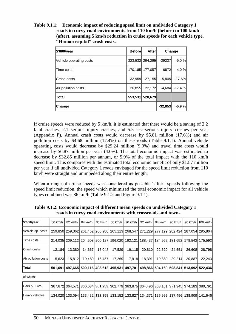
50 MONASH UNIVERSITY ACCIDENT RESEARCH CENTRE
Table 9.1.1: Economic impact of reducing speed limit on undivided Category 1
roads in curvy road environments from 110 km/h (before) to 100 km/h
(after), assuming 5 km/h reduction in cruise speeds for each vehicle type.
“Human capital” crash costs.
$’000/year Before After Change
Vehicle operating costs 323,532 294,295 -29237 -9.0 %
Time costs 170,185 177,057 6872 4.0 %
Crash costs 32,959 27,155 -5,805 -17.6%
Air pollution costs 26,855 22,172 -4,684 -17.4 %
Total 553,531 520,679
Change -32,853 -5.9 %
If cruise speeds were reduced by 5 km/h, it is estimated that there would be a saving of 2.2
fatal crashes, 2.1 serious injury crashes, and 5.5 less-serious injury crashes per year
(Appendix P). Annual crash costs would decrease by $5.81 million (17.6%) and air
pollution costs by $4.68 million (17.4%) on these roads (Table 9.1.1). Annual vehicle
operating costs would decrease by $29.24 million (9.0%) and travel time costs would
increase by $6.87 million per year (4.0%). The total economic impact was estimated to
decrease by $32.85 million per annum, or 5.9% of the total impact with the 110 km/h
speed limit. This compares with the estimated total economic benefit of only $1.87 million
per year if all undivided Category 1 roads envisaged for the speed limit reduction from 110
km/h were straight and unimpeded along their entire length.
When a range of cruise speeds was considered as possible “after” speeds following the
speed limit reduction, the speed which minimised the total economic impact for all vehicle
types combined was 86 km/h (Table 9.1.2 and Figure 9.1.1).
Table 9.1.2: Economic impact of different mean speeds on undivided Category 1
roads in curvy road environments with crossroads and towns
$’000/year 80 km/h 82 km/h 84 km/h 86 km/h 88 km/h 90 km/h 92 km/h 94 km/h 96 km/h 98 km/h 100 km/h
Vehicle op. costs 259,850 259,362 261,452 260,980 265,113 268,547 271,229 277,199 282,424 287,054 295,804
Time costs 214,035 209,112 204,508 200,127 196,020 192,121 188,437 184,952 181,652 178,542 175,592
Crash costs 12,184 13,380 14,667 16,048 17,529 19,115 20,810 22,620 24,551 26,608 28,798
Air pollution costs 15,623 15,812 19,489 16,457 17,269 17,918 18,391 19,389 20,214 20,887 22,243
Total 501,691 497,665 500,116 493,612 495,931 497,701 498,866 504,160 508,841 513,092 522,436
of which:
Cars & LCVs 367,672 364,571 366,684 361,253 362,779 363,875 364,496 368,161 371,345 374,183 380,791
Heavy vehicles 134,020 133,094 133,432 132,358 133,152 133,827 134,371 135,999 137,496 138,909 141,646

ECONOMIC EVALUATION OF INTRODUCTION OF LOWER RURAL SPEED LIMITS IN TASMANIA
51
Figure 9.1.1: Undivided Category 1 roads in curvy road environments
Monetary impacts of different average speeds on rural roads:
Category 1 undivided curvy roads with crossroads and towns
250,000
300,000
350,000
400,000
450,000
500,000
550,000
80 82 84 86 88 90 92 94 96 98 100
Average Speed
$'0
00 p
er
yea
r
Air pollution costs
Crash costs
Time costs
Vehicle operating costs
On the undivided Category 1 roads in curvy road environments, the optimum speed did not
differ by vehicle type and was estimated as 86 km/h for each class of vehicle (Figure
9.1.2).
Figure 9.1.2: Undivided Category 1 roads in curvy road environments – Optimum speeds by vehicle class.
Monetary impacts of different average speeds on rural roads: Car & LCV costs only
Category 1 undivided curvy roads with crossroads and towns
160,000
210,000
260,000
310,000
360,000
80 82 84 86 88 90 92 94 96 98 100
Car and LCV Average Speed
$'0
00 p
er
yea
r
Monetary impacts of different average speeds on rural roads: Heavy vehicle-related costs only
Category 1 undivided curvy roads with crossroads and towns
90,000
100,000
110,000
120,000
130,000
140,000
80 82 84 86 88 90 92 94 96 98 100
Heavy Vehicle Average Speed
$'0
00 p
er
yea
r
9.2 UNDIVIDED CATEGORY 2 ROADS WITH 100 KM/H LIMITS
The economic impact of reducing the speed limit from 100 to 90 km/h on the 263 km of
undivided Category 2 rural roads was estimated by assuming that the cruise speeds
represented by the average free speed for each type of vehicle (see Table 5.9) would
decrease by 5 km/h. The average journey speeds associated with each “before” and “after”
cruise speed on these roads through curvy road environments with occasional stops are
shown in Appendix Q together with details of the economic analysis
If cruise speeds were reduced by 5 km/h, it is estimated that there would be a saving of 0.7
fatal crashes, 2.1 serious injury crashes and 6.1 less-serious injury crashes per year
(Appendix Q). Annual crash costs would decrease by $2.62 million (19.3%) and air
pollution costs by $324,000 (5.1%) on these roads (Table 9.2.1). Annual vehicle operating

52 MONASH UNIVERSITY ACCIDENT RESEARCH CENTRE
costs would decrease by $148,000 (0.1%), but travel time costs would increase by $4.66
million per year (5.9%). The total economic impact was estimated to increase by $1.57
million per annum, or 0.8% of the total impact with the 100 km/h speed limit.
Table 9.2.1: Economic impact of reducing speed limit on undivided Category 2
roads in curvy road environments from 100 km/h (before) to 90 km/h
(after), assuming 5 km/h reduction in cruise speeds for each vehicle type.
“Human capital” crash costs.
$’000/year Before After Change
Vehicle operating costs 105,738 105,590 -148 -0.1 %
Time costs 78,574 83,234 4659 5.9 %
Crash costs 13,609 10,989 -2,620 -19.3%
Air pollution costs 6,333 6,009 -324 -5.1 %
Total 204,255 205,821
Change 1,566 0.8 %
The increased economic cost of $1.57 million can be compared with the estimated
increased cost of $3.29 million per year (Table 7.1.1) if the undivided Category 2 roads
were straight and traffic was unimpeded along their full length, allowing vehicles to cruise
at their average free speed throughout. The higher vehicle operating costs and air pollution
costs on the curvy roads requiring frequent deceleration and acceleration represented
greater potential for these costs to be reduced by the 5 km/h reduction in cruise speeds.
When a range of average speeds was considered as possible “after” speeds following the
speed limit reduction, the speed which minimised the total economic impact for all vehicle
types combined was 86 km/h (Table 9.2.2 and Figure 9.2.1).
Table 9.2.2: Economic impact of different mean speeds on undivided Category 2
roads in curvy road environments
$’000/year 80 km/h 82 km/h 84 km/h 86 km/h 88 km/h 90 km/h 92 km/h 94 km/h 96 km/h 98 km/h 100 km/h
Vehicle op. costs 104,744 104,526 105,315 105,116 106,708 108,035 109,076 111,396 113,434 115,245 118,659
Time costs 82,277 80,385 78,615 76,931 75,352 73,854 72,437 71,098 69,829 68,634 67,499
Crash costs 11,613 12,658 13,773 14,964 16,232 17,582 19,017 20,542 22,160 23,875 25,691
Air pollution costs 6,032 6,105 6,322 6,354 6,667 6,918 7,100 7,486 7,804 8,064 8,588
Total 204,666 203,674 204,026 203,364 204,959 206,388 207,631 210,522 213,227 215,818 220,438
of which:
Cars & LCVs 144,174 143,433 143,649 143,120 144,207 145,162 145,967 147,954 149,792 151,532 154,732
Heavy vehicles 60,492 60,241 60,376 60,245 60,752 61,227 61,664 62,568 63,435 64,286 65,705

ECONOMIC EVALUATION OF INTRODUCTION OF LOWER RURAL SPEED LIMITS IN TASMANIA
53
Figure 9.2.1: Undivided Category 2 roads in curvy road environments
Monetary impacts of different average speeds on rural roads:
Category 2 undivided curvy roads with crossroads and towns
100,000
120,000
140,000
160,000
180,000
200,000
220,000
80 82 84 86 88 90 92 94 96 98 100
Average Speed
$'0
00 p
er
yea
r
Air pollution costs
Crash costs
Time costs
Vehicle operating costs
On the undivided Category 2 roads in curvy road environments, the optimum speed did not
differ by vehicle type and was estimated as 86 km/h for each class of vehicle (Figures 9.2.2
and 9.2.3).
Figure 9.2.2: Undivided Category 2 roads in curvy road environments – Car and LCV-related costs.
Monetary impacts of different average speeds on rural roads: Car & LCV costs only
Category 2 undivided curvy roads with crossroads and towns
60,000
70,000
80,000
90,000
100,000
110,000
120,000
130,000
140,000
150,000
160,000
80 82 84 86 88 90 92 94 96 98 100
Car and LCV Average Speed
$'0
00 p
er
yea
r
Air pollution costs
Crash costs
Time costs
Vehicle operating costs

54 MONASH UNIVERSITY ACCIDENT RESEARCH CENTRE
Figure 9.2.3: Undivided Category 2 roads in curvy road environments – Heavy vehicle-related costs.
Monetary impacts of different average speeds on rural roads: Heavy vehicle-related costs only
Category 2 undivided curvy roads with crossroads and towns
40,000
45,000
50,000
55,000
60,000
65,000
80 82 84 86 88 90 92 94 96 98 100
Heavy Vehicle Average Speed
$'0
00 p
er
yea
r
Air pollution costs
Crash costs
Time costs
Vehicle operating costs
9.3 UNDIVIDED ROAD CATEGORIES 3 TO 5 WITH 100 KM/H LIMITS
The economic impacts of reducing the speed limit from 100 to 90 km/h on undivided rural
roads in Categories 3 to 5 through curvy road environments were estimated by assuming
that the cruise speeds represented by the average free speed for each type of vehicle (see
Table 5.9) would decrease by 5 km/h. Although it was envisaged that the speed limit on
unsealed 100 km/h roads would reduce to 80 km/h, the economic analysis of these roads
through curvy road environments also assumed that cruise speeds would decrease by 5
km/h. The detailed results are given in Appendices R, S, T and U and are summarised in
Table 9.3.1 together with the results of the analysis of undivided Category 2 roads from
section 9.2.1 above.
Table 9.3.1: Economic impacts of speed reductions on undivided roads in curvy road
environments with 100 km/h speed limits. “Human capital” costs of road trauma.
Effect of 5 km/h mean
speed reductions on total
economic cost
Optimum Speed (km/h)
(speed which minimises total
economic cost)
Road category
Change p.a.
($ million)
Percentage
change
All vehicles
combined
Cars &
LCVs
Heavy
vehicles
Category 2 Regional Freight Roads +1.566 +0.8% 86 86 86
Category 3 Regional Access Roads -0.929 -0.3% 82 82 82
Category 4 Feeder Roads -3.021 -1.0% 86 86 82
Category 5 “Other” Roads
+1.000 +0.5% 82 82 82
Unsealed Category 5 “Other” roads -0.049 -0.6% 80 80 80
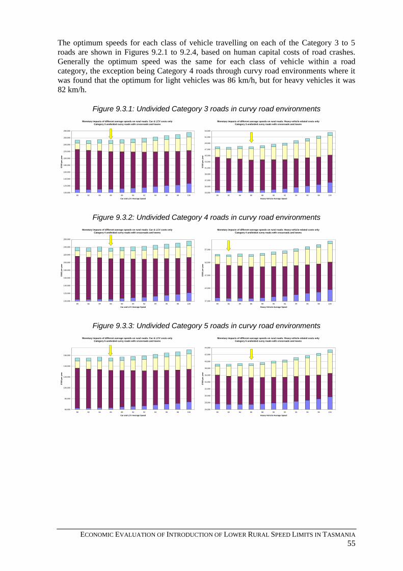
ECONOMIC EVALUATION OF INTRODUCTION OF LOWER RURAL SPEED LIMITS IN TASMANIA
55
The optimum speeds for each class of vehicle travelling on each of the Category 3 to 5
roads are shown in Figures 9.2.1 to 9.2.4, based on human capital costs of road crashes.
Generally the optimum speed was the same for each class of vehicle within a road
category, the exception being Category 4 roads through curvy road environments where it
was found that the optimum for light vehicles was 86 km/h, but for heavy vehicles it was
82 km/h.
Figure 9.3.1: Undivided Category 3 roads in curvy road environments
Monetary impacts of different average speeds on rural roads: Car & LCV costs only
Category 3 undivided curvy roads with crossroads and towns
100,000
120,000
140,000
160,000
180,000
200,000
220,000
240,000
260,000
280,000
80 82 84 86 88 90 92 94 96 98 100
Car and LCV Average Speed
$'0
00 p
er
yea
r
Monetary impacts of different average speeds on rural roads: Heavy vehicle-related costs only
Category 3 undivided curvy roads with crossroads and towns
33,000
35,000
37,000
39,000
41,000
43,000
45,000
47,000
49,000
51,000
53,000
80 82 84 86 88 90 92 94 96 98 100
Heavy Vehicle Average Speed
$'0
00 p
er
yea
r
Figure 9.3.2: Undivided Category 4 roads in curvy road environments
Monetary impacts of different average speeds on rural roads: Car & LCV costs only
Category 4 undivided curvy roads with crossroads and towns
100,000
120,000
140,000
160,000
180,000
200,000
220,000
240,000
260,000
80 82 84 86 88 90 92 94 96 98 100
Car and LCV Average Speed
$'0
00 p
er
year
Monetary impacts of different average speeds on rural roads: Heavy vehicle-related costs only
Category 4 undivided curvy roads with crossroads and towns
37,000
42,000
47,000
52,000
57,000
80 82 84 86 88 90 92 94 96 98 100
Heavy Vehicle Average Speed
$'0
00 p
er
year
Figure 9.3.3: Undivided Category 5 roads in curvy road environments
Monetary impacts of different average speeds on rural roads: Car & LCV costs only
Category 5 undivided curvy roads with crossroads and towns
66,000
86,000
106,000
126,000
146,000
166,000
80 82 84 86 88 90 92 94 96 98 100
Car and LCV Average Speed
$'0
00 p
er
yea
r
Monetary impacts of different average speeds on rural roads: Heavy vehicle-related costs only
Category 5 undivided curvy roads with crossroads and towns
26,000
28,000
30,000
32,000
34,000
36,000
38,000
40,000
42,000
44,000
80 82 84 86 88 90 92 94 96 98 100
Heavy Vehicle Average Speed
$'0
00 p
er
yea
r

56 MONASH UNIVERSITY ACCIDENT RESEARCH CENTRE
Figure 9.3.4: Unsealed Category 5 roads in curvy road environments
Monetary impacts of different average speeds on rural roads: Car & LCV costs only
Category 5 unsealed curvy roads with crossroads and towns
2,500
3,000
3,500
4,000
4,500
5,000
5,500
6,000
6,500
7,000
7,500
80 82 84 86 88 90 92 94 96 98 100
Car and LCV Average Speed
$'0
00 p
er
yea
r
Monetary impacts of different average speeds on rural roads: Heavy vehicle-related costs only
Category 5 unsealed curvy roads with crossroads and towns
1,300
1,400
1,500
1,600
1,700
1,800
1,900
2,000
2,100
2,200
2,300
80 82 84 86 88 90 92 94 96 98 100
Heavy Vehicle Average Speed
$'0
00 p
er
yea
r

ECONOMIC EVALUATION OF INTRODUCTION OF LOWER RURAL SPEED LIMITS IN TASMANIA
57
10 SUMMARY AND DISCUSSION
The economic analysis considered 3,002 km of rural roads on Tasmania‟s State Road
Network for which a reduction in the speed limit was envisaged (Table 10.1). A reduction
in the speed limit on divided Category 1 (National Highway) roads with 110 km/h limits
was included in the analysis, though this was not initially proposed. The analysed roads
represent about 85% of the State Road Network, which in turn represents about 18% of
Tasmania‟s rural road system. The majority of vehicle travel occurs on State Roads. On
local roads the traffic volume is much smaller – around 25% of the level on State Roads.
Table 10.1: State Road Network roads designated for speed limit reductions. Traffic
parameters and mean speeds for each road category.
Traffic parameters Mean free speed 2009 (km/h)
Road category and current speed
limit
Length
(km)
AADT
2007
Cars &
LCVs
Rigid
heavy
vehicles
Artic.
heavy
vehicles
Rural roads with 110 km/h speed limits
Divided Category 1 Trunk Roads 67.3 9,058 110 109 100
Undivided Cat. 1 Trunk Roads 238 7,030 105 100 99
Undivided rural roads with 100 km/h speed limits
Category 2 Regional Freight Roads 263 2,714 85 81 78
Category 3 Regional Access Roads 572 2,012 87 82 82
Category 4 Feeder Roads 825 1,349 91 85 75
Category 5 “Other” Roads1
1,037 712 84 76 82
Unsealed rural roads (100 km/h speed limit)
Category 5 “Other” Roads 206 140 85 80 80 1
Includes unsealed gravel roads on SRN. Estimated 18% of length and 3% of travel on Category 5 roads
Of the estimated 10,300 km of unsealed gravel roads, only 206 km are part of the State
Road Network. Thus the analysis of the reduction of the speed limit on unsealed roads
would underestimate the total impact on such roads in Tasmania, but the relative economic
impact should be indicative of the overall impact on this class of road.
10.1 INITIAL RESULTS OF THE ECONOMIC ANALYSIS
It was not expected that mean free speeds would drop to the same extent as the reduction in
speed limit on each category of rural road. This is especially the case on the Category 2-5
roads where the mean free speeds in 2009 were already lower than the envisaged lower
limits. The economic analyses considered the impacts of a hypothetical 5 km/h reduction in
the mean free speed of each vehicle type as being the likely maximum reduction which
would result. Lower speeds in 2 km/h steps were also analysed to determine the speed
which minimises the total economic impact (“optimum speed”) for each general class of

58 MONASH UNIVERSITY ACCIDENT RESEARCH CENTRE
vehicle. This is the speed which balances the social costs and benefits of increased travel
time with decreased road trauma, vehicle operating costs, emissions and other costs.
Using the “human capital” approach to value road trauma costs, there would be overall
economic benefits from reducing speed limits on divided and undivided Category 1 roads
from 110 km/h to 100km/h (Table 10.2). The optimum speed for all vehicle types
combined on these roads is no more than 100 km/h, so this would support a reduction in
the limit to 100 km/h in each case.
If it is assumed that the majority of the Tasmanian State Road Network consists of straight,
unimpeded road sections, then for the undivided roads in each of Categories 2-5, the
hypothesised 5 km/h reduction in mean free speeds due to a reduction in their current 100
km/h limits would appear to result in an overall economic loss. The optimum speeds on
these roads are generally about the same as the envisaged lower limit proposed for each
class of road (90 km/h for sealed Category 2-5 roads and 80 km/h for the unsealed
Category 5 roads), but the hypothesised reduced mean speeds are substantially less.
However these economic analysis results assume that road trauma (crashes and serious
injuries) should be valued by conservative “human capital” costs; and that vehicles travel
on Category 2-5 roads at their mean free speeds throughout their length without slowing
for sharp curves and stopping occasionally.
Table 10.2: Economic impacts of speed reductions, and estimated optimum speeds.
Straight, unimpeded road environment. “Human capital” costs of road trauma.
Effect of 5 km/h mean
speed reductions on
total economic cost
Optimum Speed (km/h)
(speed which minimises total
economic cost)
Road category and current speed
limit
Change p.a.
($ million)
Percentage
change
All
vehicles
combined
Cars &
LCVs
Heavy
vehicles
Rural roads with 110 km/h speed limits
Divided Category 1 Trunk Roads -1.083 -0.8% 100 102 94
Undivided Cat. 1 Trunk Roads -1.870 -0.4% 98 100 92
Undivided rural roads with 100 km/h speed limits
Category 2 Regional Freight Roads +3.291 +1.7% 90 92 88
Category 3 Regional Access Roads +2.593 +0.9% 88 90 86
Category 4 Feeder Roads +2.261 +0.8% 90 92 86
Category 5 “Other” Roads1
+2.722 +1.4% 88 88 84
Unsealed rural roads (100 km/h speed limit)
Category 5 “Other” Roads2
+0.027 +0.3% 82 82 82 1
Includes unsealed gravel roads on State Road Network. Crash data 2004-2008 not provided separately. 2 Casualty crash rate per 100 million vehicle-kilometres from AGPE04/08 Table 4.1, not real crash data.

ECONOMIC EVALUATION OF INTRODUCTION OF LOWER RURAL SPEED LIMITS IN TASMANIA
59
10.2 WILLINGNESS TO PAY VALUATION OF ROAD TRAUMA
“Willingness to pay” valuations of road trauma are more consistent with the Safe System
approach embodied in the federal government‟s National Road Safety Strategy 2001-2010,
and the Tasmanian Road Safety Strategy 2007-2016. Fatal crashes are valued more than
2.5 times their “human capital” costs and injury crashes are also valued higher. On this
basis, the economic benefits of reducing speed limits on Category 1 roads from 110 km/h
to 100km/h would be even greater, especially on the undivided Category 1 roads (Table
10.3).
Using “willingness to pay” valuations of road trauma, the reduction in mean free speeds on
Category 3-5 roads would result in overall economic benefits and the apparent economic
loss on the Category 2 roads would be substantially reduced. The optimum speeds would
be substantially lower than the envisaged lower limits for each of the Category 2-5 roads,
including the unsealed Category 5 roads. The optimum speed on the undivided Category 1
roads is no more than 90 km/h for each class of vehicle, suggesting that the 90 km/h limit
envisaged for the sealed Category 2-5 roads could be considered for these roads as well.
Table 10.3: Economic impacts of speed reductions, and estimated optimum speeds.
Straight, unimpeded road environment. “Willingness to pay” values of road trauma.
Effect of 5 km/h mean
speed reductions on
total economic cost
Optimum Speed (km/h)
(speed which minimises total
economic cost)
Road category and current speed
limit
Change p.a.
($ million)
Percentage
change
All
vehicles
combined
Cars &
LCVs
Heavy
vehicles
Rural roads with 110 km/h speed limits
Divided Category 1 Trunk Roads -3.098 -2.0% 92 92 90
Undivided Cat. 1 Trunk Roads -8.537 -1.8% 90 90 86
Undivided rural roads with 100 km/h speed limits
Category 2 Regional Freight Roads +0.565 +0.3% 82 82 80
Category 3 Regional Access Roads -2.907 -0.9% 80 80 78
Category 4 Feeder Roads -1.831 -0.6% 82 84 80
Category 5 “Other” Roads -0.486 -0.2% 78 80 78
Unsealed rural roads (100 km/h speed limit)
Category 5 “Other” Roads -0.172 -1.9% 74 74 74
10.3 CURVY ROAD ENVIRONMENTS REQUIRING SLOWING AND STOPS
Much of Tasmania‟s rural road system has frequent curved alignments and passes through
intersections and towns often requiring vehicles to slow substantially and occasionally
stop. On these types of road the average journey speed over a whole trip is lower than the
cruise speeds that vehicles would do on straight unimpeded road sections. This increases
the travel time and the slowing and stopping increases the fuel consumption and air
pollution emissions of vehicles using the road section. The crash rate also increases

60 MONASH UNIVERSITY ACCIDENT RESEARCH CENTRE
because of the curved alignment and because of the increased crash risk associated with
cross roads. Adjustments to the economic analyses were made to take into account the
impact of increased road trauma, operating costs, emissions and travel times, except for
divided Category 1 roads where slowing for sharp curves and stopping is less common.
Assuming that the curvy road environment with frequent slowing and occasional stops
applies along the full length of each of the undivided Category 1-5 roads, the economic
analysis using “human capital” costs of road trauma showed that there were overall
economic benefits from a 5 km/h reduction in cruise speeds (average free speeds) on most
classes of road (Table 10.4). The exceptions were the undivided Category 2 Regional
Freight Roads and the Category 5 “Other” Roads (but not including the separately analysed
unsealed Category 5 roads). However, the optimum speeds on these two classes of road
were below the envisaged 90 km/h limit suggesting that the reduced limit would still be
justified even if the hypothesised 5 km/h reduction in cruise speeds did not result.
The greatest economic benefit was from a reduction in cruise speeds on undivided
Category 1 roads with current 110 km/h speed limit. In curvy road environments, the
optimum speed on these roads was estimated to be 86 km/h for all classes of vehicle. This
supports a lower speed limit than the 100 km/h limit envisaged, at least on the undivided
Category 1 roads through curvy road environments where a 90 km/h limit could be
considered.
Table 10.4: Economic impacts of speed reductions, and estimated optimum speeds.
Curvy road environment with frequent slowing and occasional stops along full length
of the road category (except divided Category 1 roads). “Human capital” costs of
road trauma.
Effect of 5 km/h mean
speed reductions on
total economic cost
Optimum Speed (km/h)
(speed which minimises total
economic cost)
Road category and current speed
limit
Change p.a.
($ million)
Percentage
change
All
vehicles
combined
Cars &
LCVs
Heavy
vehicles
Rural roads with 110 km/h speed limits
Divided Category 1 Trunk Roads1 -1.083 -0.8% 100 102 94
Undivided Cat. 1 Trunk Roads -32.853 -5.9% 86 86 86
Undivided rural roads with 100 km/h speed limits
Category 2 Regional Freight Roads +1.566 +0.8% 86 86 86
Category 3 Regional Access Roads -0.929 -0.3% 82 82 82
Category 4 Feeder Roads -3.021 -1.0% 86 86 82
Category 5 “Other” Roads +1.000 +0.5% 82 82 82
Unsealed rural roads (100 km/h speed limit)
Category 5 “Other” Roads -0.049 -0.6% 80 80 80
1 Assumed to be primarily freeway standard roads with high design speeds and controlled access, not
requiring frequent slowing due to sharp curves and stops for towns and intersections, and hence not analysed
for a curvy road environment. Results assumed to be same as in Table 10.2 for straight unimpeded road
environment.

ECONOMIC EVALUATION OF INTRODUCTION OF LOWER RURAL SPEED LIMITS IN TASMANIA
61
10.4 OVERALL BENEFITS AND COSTS OF REDUCED SPEED LIMITS
The seven road environments summarised in Table 10.4 were considered in aggregate to be
representative of rural State Roads in Tasmania. Ignoring the double-counting of the
economic benefit on unsealed Category 5 roads, the combined results suggest that there
would be a total economic benefit to Tasmania of $35.37 million per annum if the
envisaged reduced speed limits were introduced and a 5 km/h reduction in current free
speeds on the targeted roads were to result. Even if the full 5 km/h reduction in current
speeds was not achieved, the optimum speeds for each road class and vehicle type suggest
that limiting vehicle free speeds to the envisaged speed limits would result in a net
economic benefit.
Table 10.5 shows the estimated crash savings if the 5 km/h reductions in mean free speeds
were to result from the speed limit reductions in each road environment. Again ignoring
the double-counting on unsealed Category 5 roads, it is estimated that there would be 25%
reduction in fatal crashes, 15% reduction is serious injury crashes, and nearly 12%
reduction in minor injury crashes associated with the speed limit reductions. Nearly one-
third of the fatal crashes savings would come from the reduction in the limit on existing
110 km/h undivided Category 1 roads.
Table 10.5: Estimated crash reductions per year. Curvy road environment with
frequent slowing and occasional stops (except divided Category 1 roads).
Estimated crash savings due to
5 km/h mean speed reductions
Road category and current speed
limit
Fatal
crashes
p.a.
Serious
injury
crashes
p.a.
Other
injury
crashes
p.a.
Annual
casualty
crashes
(estimate)
Casualty
crash
saving
(% p.a.)
Rural roads with 110 km/h speed limits
Divided Category 1 Trunk Roads 0.44 0.83 5.54 65.7 10.4%
Undivided Cat. 1 Trunk Roads 2.20 2.08 5.53 81.2 12.1%
Undivided rural roads with 100 km/h speed limits
Category 2 Regional Freight Roads 0.72 2.07 6.08 64.2 13.8%
Category 3 Regional Access Roads 1.45 3.77 12.51 132.3 13.4%
Category 4 Feeder Roads 1.01 4.25 12.38 137.6 12.8%
Category 5 “Other” Roads1
0.80 3.12 9.32 95.7 13.8%
Unsealed rural roads on SRN (100 km/h speed limit)
Category 5 “Other” Roads 0.05 0.18 0.35 4.1 14.1%
TOTAL CRASH SAVINGS p.a. 6.67 16.30 51.71 580.8 12.9%
Annual crashes by severity (est.) 26.7 108.1 446.0
PERCENT CRASH SAVINGS 25.0% 15.1% 11.6% 1
Includes unsealed gravel roads on State Road Network, representing 4.3% of casualty crashes on Cat. 5
roads.

62 MONASH UNIVERSITY ACCIDENT RESEARCH CENTRE
10.5 ALTERNATIVE METHOD FOR ESTIMATING EFFECTS OF SPEED
CHANGES ON CASUALTY CRASHES
The economic analysis results rely on the integrity of the analysis tools, a key part of
which is the use of Nilsson-type relationships to link changes in mean free speeds on rural
roads with the changes in numbers of casualty crashes, at each level of injury outcome of
the crashes (see section 3.1.4). It has been found in the Kingborough Safer Speeds
Demonstration project that the 10 km/h reduction in the 100 km/h limit on sealed roads
resulted in little or no reduction in mean free speeds, but substantial reductions in the
proportion of vehicles travelling above 91 km/h (and commensurate increases in the
proportion travelling 71-90 km/h). Compared with a “control” municipality where there
were no speed limit changes, there was a 51% reduction in casualty crashes on sealed roads
(not statistically significant) and 60% reduction in all reported crashes (statistically
significant). Mean free speeds at six sites on the Kingborough sealed roads before the
speed limit reduction ranged from 52 to 84 km/h, plus 96 km/h measured at one site
(Langford 2009).
It is possible that Nilsson-type relationships may not adequately represent the expected
changes in casualty crashes if speed limits are reduced in rural road environments where
free speeds are already substantially below the current (and reduced) limits on many
targeted roads. A change in the distribution of speeds, instead of or in addition to a
reduction in mean speed, may be expected to produce the reduction in casualty crashes. To
estimate the likely reduction in casualty crashes, it may be possible to weight each of the
observed speeds by the relative risk of a casualty crash, as estimated by Kloeden et al
(2001) for rural roads. A hypothesised change in the speed distribution, based on the
Kingborough experience, could then be estimated and the risk-weighting re-applied to
estimate the changes in casualty crashes. The change in the severity of the casualty crashes
(thus estimating the numbers of fatal and serious injury crashes) may be possible to
estimate based on a modification of the Nilsson-type relationships.
It is recommended that an alternative method of estimating the changes in the numbers of
casualty crashes on the Category 2-5 roads associated with a potential change in the speed
distribution due to a reduction in their 100 km/h limit, based on Kloeden et al‟s (2001)
relative risk relationships, be investigated and if feasible be incorporated in a re-analysis of
the economic benefits of the envisaged speed limit reduction on undivided Category 2-5
roads.
11 CONCLUSIONS
1. The envisaged reduction in the 110 km/h speed limit to 100 km/h on Category 1
(National Highways) roads in Tasmania would be economically justified on both
the divided and undivided sections under consideration.
2. The economic justification is even greater on the undivided Category 1 roads when:
(a) the saving in road trauma is valued by “willingness to pay” estimates; or (b) the
high proportion of road environments with frequent sharp curves, at-grade
intersections, and occasional stops in towns traversed by these roads is recognised.
A 90 km/h limit on undivided Category 1 roads could be considered, particularly
through curvy road environments.

ECONOMIC EVALUATION OF INTRODUCTION OF LOWER RURAL SPEED LIMITS IN TASMANIA
63
3. The envisaged reduction in the default 100 km/h speed limit to 90 km/h on sealed
rural roads would be economically justified when it is recognised that a high
proportion of Category 2-5 roads are through road environments with frequent
sharp curves, at-grade intersections, and occasional stops in towns. The optimum
speed on these roads through curvy environments is below 90 km/h for all classes
of vehicle.
4. The envisaged reduction in the default 100 km/h speed limit to 80 km/h on
unsealed (gravel) roads would be economically justified. The optimum speed on
these roads on the State Road Network is close to the proposed new speed limit for
all classes of vehicle.
5. If mean free speeds were reduced by 5 km/h on each category of road in response
to the envisaged reduced speed limit applicable in each case, there would be an
estimated total economic benefit exceeding $35 million per annum to Tasmania. It
is estimated that there would be 25% reduction in fatal crashes, 15% reduction is
serious injury crashes, and nearly 12% reduction in minor injury crashes on the
roads with the speed limit reductions.
6. It is possible that the relationships developed by Nilsson (1984), linking crashes
and their injury severity with changes in mean free speeds, may not adequately
represent the expected changes in casualty crashes if speed limits are reduced in
rural road environments where free speeds are already substantially below the
current (and reduced) limits on many targeted roads. A change in the distribution of
speeds, instead of, or in addition to a reduction in mean speed, may be expected to
produce a reduction in casualty crashes. It is recommended that an alternative
method of estimating the changes in the numbers of casualty crashes on the
Category 2-5 roads be investigated and if feasible, incorporated in further analysis
of the economic benefits of the envisaged speed limit reductions.

64 MONASH UNIVERSITY ACCIDENT RESEARCH CENTRE
12 REFERENCES
Ahn, K, Trani, AA, Rakha, H, and Van Aerde, M (1999), „Microscopic fuel consumption
and energy emission models‟. Proceedings, 78th
Annual Meeting, Transportation Research
Board, USA.
Andersson, G, Bjoerketurn, U, Bruede, U, Larsson, J, Nilsson, G, and Thulin, H (1991),
„Forecasts of traffic safety and calculated traffic safety effects for a choice of measures‟.
TFB and VTI forskning/research 7:6. Sweden.
Andersson, G, and Nilsson, G (1997), „Speed management in Sweden‟. Swedish National
Road and Transport Research Institute (VTI), Sweden.
BTCE – Bureau of Transport and Communications Economics (1997), „The costs of road
accidents in Victoria – 1988‟. Unpublished monograph. BTCE, Canberra.
BTE – Bureau of Transport Economics (2000), „Road crash costs in Australia‟. Report
102, BTE, Canberra.
Cameron, MH (2000), „Estimation of the optimum speed on urban residential streets‟.
Report to Australian Transport Safety Bureau, Canberra. Monash University Accident
Research Centre.
Cameron, M.H. (2001), „Estimation of the optimum speed on urban residential streets‟.
Proceedings, Road Safety Research, Policing and Education Conference, Melbourne.
Cameron, M.H. (2003), „Potential benefits and costs of speed changes on rural roads‟.
Report No. CR 216, Australian Transport Safety Bureau, Canberra.
Cameron, M.H. (2004), „Potential benefits and costs of speed changes on rural roads‟.
Proceedings, 2004 Road Safety Research, Policing and Education Conference, Perth.
Cameron, M.H., and Elvik, R. (2008), „Nilsson‟s Power Model connecting speed and road
trauma: Does it apply on urban roads?‟. Proceedings, Australasian Road Safety Research,
Policing and Education Conference, Adelaide.
Carlsson, G (1997), „Cost-effectiveness of information campaigns and enforcement and the
costs and benefits of speed changes‟. Proceedings of European Seminar, Cost-Effectiveness
of Road Safety Work and Measures, Luxembourg. PRI, Luxembourg.
Coesel, N, and Rietveld, P (1998), „Time to tame our speed? Costs, benefits and
acceptance of lower speed limits‟. Proceedings, 9th
International Conference, Road Safety
in Europe, Cologne, Germany.
Coleman, JA, et al (1995), „FHWA Study Tour for Speed Management and Enforcement
Technology‟. Federal Highway Administration, US Department of Transportation,
Washington DC.
Corben, B, Newstead, S, Cameron, M, Diamantopoulou, K, and Ryan, P (1994),
„Evaluation of TAC funded accident black spot treatments: Report on Phase 2 – Evaluation
system development‟. Report to Transport Accident Commission. Monash University
Accident Research Centre.

ECONOMIC EVALUATION OF INTRODUCTION OF LOWER RURAL SPEED LIMITS IN TASMANIA
65
Cox, J (1997), „Roads in the community. Part 1: Are they doing their job?‟ Austroads,
Sydney.
Ding, Y. (2000), „Quantifying the impact of traffic-related and driver-related factors on
vehicle fuel consumption and emissions‟. MSc thesis, Civil and Environmental
Engineering, Virginia Polytechnic Institute and State University, Blacksburg VA, USA.
Elvik, R (1998), Draft report on Work Package 5 (cost-benefit analysis) of PROMISING
project. TOI, Norway (unpublished).
Elvik, R (1999), „Cost-benefit analysis of safety measures for vulnerable and
inexperienced road users: Work Package 5 of EU-Project PROMISING‟. TOI, Norway.
Elvik, R., Christensen, P., and Amundsen, A. (2004), „Speed and road accidents. An
evaluation of the Power Model.‟ Report 740/2004, Institute of Transport Economics, Oslo,
Norway.
Haworth, N, Ungers, B, Vulcan, P, and Corben, B (2001), „Evaluation of a 50 km/h default
urban speed limit for Australia‟. Report to National Road Transport Commission. Monash
University Accident Research Centre.
Kallberg, V-P, and Toivanen, S (1998), „Framework for assessing the impacts of speed in
road transport‟. Deliverable 8, MASTER project, European Commission.
Kloeden, CN, Ponte, G, and McLean, AJ (2001), „Travelling speed and the risk of crash
involvement on rural roads‟. Report CR 204, Australian Transport Safety Bureau.
Langford, J (2009), „Kingborough Safer Speeds Demonstration (KiSS) Twelve-Month
Evaluation Report‟. Report to Department of Infrastructure, Energy and Resources,
Tasmania. Monash University Accident Research Centre.
Mclean, J (2001), „Economic evaluation of road investment proposals: Improved
prediction models for road crash savings‟. Report AP-R184, Austroads, Sydney.
NRTC – National Road Transport Commission (1996), „Mass Limits Review –
Appendices to Technical Supplement No. 2: Road and Bridge Statistical Data Tables‟.
NRTC, Melbourne.
Nilsson, G. (1981), „The effects of speed limits on traffic accidents in Sweden‟.
Proceedings, International Symposium, Dublin. OECD.
Nilsson, G (1984), „Speeds, accident rates and personal injury consequences for different
road types‟. Rapport 277, Swedish National Road and Transport Research Institute (VTI),
Sweden.
Nilsson, G. (2004), „Traffic safety dimensions and the Power Model to describe the effect
of speed on safety‟. Bulletin 221, Lund Institute of Technology, Department of
Technology and Society, Traffic Engineering, Lund, Sweden.
Peeters, PM, van Asseldonk, Y, van Binsbergen, AJ, Schoemaker, TJH, van Goevreden,
CD, Vermijs, RGMM, Rietveld, P, and Rienstra, SA (1996), „Time to tame our speed? A
study of the socioeconomic cost and benefits of speed reduction of passenger cars‟. Report
to Research Unit for Integrated Transport Studies, Den Haag, The Netherlands.
66 MONASH UNIVERSITY ACCIDENT RESEARCH CENTRE
Perovic, J, Evans, C, Lloyd, B, and Tsolakis, D (2008), „Guide to project evaluation. Part
4: project evaluation data‟. Austroads Publication No. AGPE04/08, Austroads, Sydney.
Plowden, S, and Hillman, M (1996), „Speed control and transport policy‟. Policy Studies
Institute, London.
Rietveld, P, van Binsbergen, A, Schoemaker, T, and Peeters, P (1996), „Optimum speed
limits for various types of roads: a social cost-benefit analysis for the Netherlands‟.
Tinbergen Institute, Free University Amsterdam, The Netherlands.
Robertson, S, Ward, H, Marsden, G, Sandberg, U, and Hammerstrom, U (1998), „The
effect of speed on noise, vibration and emissions from vehicles‟. Working paper R 1.2.1,
MASTER project, European Commission.
Steadman, LA, and Bryan, RJ (1988), „Cost of road accidents in Australia‟. Occasional
paper 91, Bureau of Transport and Communications Economics. AGPS, Canberra.
Taylor, MC, Baruya, A, and Kennedy, JV (2002), „The relationship between speed and
accidents on rural single-carriageway roads‟. Report TRL511, Transport Research
Laboratory, U.K.
Toivanen, S, and Kallberg, V-P (1998), „Framework for assessing the impacts of speed‟.
Papers, Workshop II on Speed Management, Proceedings, 9th
International Conference,
Road Safety in Europe, Cologne, Germany.
Transportation Research Board (1998), „Managing speed: review of current practices for
setting and enforcing speed limits‟. TRB Special Report 245, Washington DC.
(http://gulliver.trb.org/publications/sr/sr254.pdf)
Ward, H, Robertson, S, and Allsop, R (1998), „Managing speeds of traffic on European
roads: Non-accident external and internal effects of vehicle use and how these depend on
speed‟. Papers, Workshop II on Speed Management, Proceedings, 9th
International
Conference, Road Safety in Europe, Cologne, Germany.

ECONOMIC EVALUATION OF INTRODUCTION OF LOWER RURAL SPEED LIMITS IN TASMANIA
67
APPENDIX A: MASTER FRAMEWORK FOR ANALYSIS OF
IMPACTS OF A SPEED MANAGEMENT POLICY
blanco.xls
MANAGING SPEEDS OF TRAFFIC ON EUROPEAN ROADS
Application of the MASTER framework (see separate instructions) Ver. 01/99
LINK-LEVEL ANALYSIS OF THE IMPACTS OF A SPEED MANAGEMENT POLICY
Name of applier:
Institution:
1. Outlining
A. Policy test
A1. Length of link km
A2. Flow characteristics
Before policy After policy
Traffic attributes Total/
Averag
e
0 0 0 0 0
Total/
Averag
e
Mean speed, km/h #DIV/0! #DIV/0!
AADT* 0 0
Share of traffic #DIV/0! #DIV/0! #DIV/0! #DIV/0! #DIV/0! #DIV/0! #DIV/0! #DIV/0! #DIV/0! #DIV/0! #DIV/0! #DIV/0!
Business trips, % #DIV/0! #DIV/0!
Pers. bus. and commuting. trips, % #DIV/0! #DIV/0!
Leisure trips, % #DIV/0! #DIV/0!
*average annual daily traffic volume, vehicles per day
B. Link/network level analysis
This workbook is best suited for link analysis. However, elastic travel demand can be assumed, for the workbook
contains formulas for consumer surplus calculation.
C. Deciding on relevant impacts
Vehicle operating costs
Travel time
Accidents
Air pollution
Noise
Other
End of sheet

68 MONASH UNIVERSITY ACCIDENT RESEARCH CENTRE
MANAGING SPEEDS OF TRAFFIC ON EUROPEAN ROADS
Application of the MASTER framework Ver. 01/99
2. Measurement of impacts
D. Impact functions
D1. Vehicle operating costs
(describe here)
D2. Travel time
Function: travel time = link length/speed of traffic flow
D3a. Accidents
For example:
Injury accidents before = nIB Average speed before = vB
Injury accidents after = nIA Average speed after = vA
(Andersson & Nilsson, 1997)
D3b. Accident costs
For example:
Total accident costs before = CB, total accident costs after = CA
k = country specific constant 1.75…2.30
(Andersson & Nilsson, 1997)
D4. Air pollutant emission coefficients
Emission factors*0 0 0 0 0 Average 0 0 0 0 0 Average
Carbon monoxide CO #DIV/0! #DIV/0!
Hydrocarbons HC #DIV/0! #DIV/0!
Oxides of nitrogen NOx #DIV/0! #DIV/0!
Particles PM #DIV/0! #DIV/0!
Carbon dioxide CO2 #DIV/0! #DIV/0!
D5. Noise pollution
(specify model used here)
nIA = (vA/vB)2 * nIB
CA = [k*((vA/vB)2-1)+1]*CB
At final speed, g/kmAt initial speed, g/km

ECONOMIC EVALUATION OF INTRODUCTION OF LOWER RURAL SPEED LIMITS IN TASMANIA
69
E. Unit prices
E1. Vehicle operating costs
Petrol Diesel
Fuel price, ECU per litre (inserting prices here is preferred to writing them in formulas with absolute numbers)
ECU per vehicle-km
0 0 0 0 0Average
0 0 0 0 0Average
Vehicle oper. costs* #DIV/0! #DIV/0!
*Without tax
E2a. Time costs per hour
Value of travel time 0 0 0 0 0
Business trips, %
Pers. bus. and commuting. trips, %
Leisure trips, %
Average 0.0 0.0 0.0 0.0 0.0
E2b. Time costs per kilometre ECU per vehicle-km
0 0 0 0 0 Average 0 0 0 0 0 Average
Time costs #DIV/0! #DIV/0! #DIV/0! #DIV/0! #DIV/0! #DIV/0! #DIV/0! #DIV/0! #DIV/0! #DIV/0! #DIV/0! #DIV/0!
E3. Total user costs ECU per vehicle-km
(vehicle operating+ time costs)
0 0 0 0 0 Average 0 0 0 0 0 Average
Total user costs #DIV/0! #DIV/0! #DIV/0! #DIV/0! #DIV/0! #DIV/0! #DIV/0! #DIV/0! #DIV/0! #DIV/0! #DIV/0! #DIV/0!
E4. Accident costs
Before After
Accident typekECU/
accid.
kECU/
accid.
Personal injury accident 316 #DIV/0!
E5a. Air pollution costs E5b. Noise pollution costs
Air pollutants' unit costs ECU/t Unit costs of noise pollution ECU/year
Carbon monoxide CO Noise zone 55 to 65 dB
Hydrocarbons HC Noise zone 65 to 70 dB
Oxides of nitrogen NOx Noise zone >70 dB
Particles PM
Carbon dioxide CO2
ECU per hour
Before policy After policy
Before policy After policy
After policyBefore policy

70 MONASH UNIVERSITY ACCIDENT RESEARCH CENTRE
F. Calculation of impacts
F1. Vehicle operating costs
0 0 0 0 0 Total 0 0 0 0 0 Total
Vehicle operating costs 0 0 0 0 0 0 0 0 0 0 0 0
F2a. Travel time
0 0 0 0 0 Total 0 0 0 0 0 Total
Total travel time on link #DIV/0! #DIV/0! #DIV/0! #DIV/0! #DIV/0! #DIV/0! #DIV/0! #DIV/0! #DIV/0! #DIV/0! #DIV/0! #DIV/0!
F2b. Travel time costs
0 0 0 0 0 Total 0 0 0 0 0 Total
Total travel time costs #DIV/0! #DIV/0! #DIV/0! #DIV/0! #DIV/0! #DIV/0! #DIV/0! #DIV/0! #DIV/0! #DIV/0! #DIV/0! #DIV/0!
F3. Consumer surplus
0 0 0 0 0Average
0 0 0 0 0Average
Total user costs, ECU/veh.km #DIV/0! #DIV/0! #DIV/0! #DIV/0! #DIV/0! #DIV/0! #DIV/0! #DIV/0! #DIV/0! #DIV/0! #DIV/0! #DIV/0!
Mio veh.kms/year 0 0 0 0 0 0 0 0 0 0 0 0
Total
kECU/year #DIV/0! #DIV/0! #DIV/0! #DIV/0! #DIV/0! #DIV/0!
F4a. Accidents
Number of accidents per year
Before
policy
After
policyChange
Personal injury accident #DIV/0! #DIV/0! #DIV/0!
F4b. Accident costs
kECU/year
Cost of accidents
Before
policy
After
policyChange
Personal injury accident #DIV/0! #DIV/0! #DIV/0!
Change in consumer surplus
Input data, after policy
After policy, kECU/yearBefore policy, kECU/year
Input data, before policy
Before policy, kECU/year After policy, kECU/year
Before policy, vehicle-hours/day After policy, vehicle-hours/day
F5a. Air pollution
Emissions 0 0 0 0 0 Total 0 0 0 0 0 Total
Carbon monoxide CO 0 0 0 0 0 0 0 0 0 0 0 0
Hydrocarbons HC 0 0 0 0 0 0 0 0 0 0 0 0
Oxides of nitrogen NOx 0 0 0 0 0 0 0 0 0 0 0 0
Particles PM 0 0 0 0 0 0 0 0 0 0 0 0
Carbon dioxide CO2 0 0 0 0 0 0 0 0 0 0 0 0
F5b. Air pollution costs
Emissions 0 0 0 0 0 Total 0 0 0 0 0 Total
Carbon monoxide CO - - - - - - - - - - - -
Hydrocarbons HC 0 0 0 0 0 0 0 0 0 0 0 0
Oxides of nitrogen NOx 0 0 0 0 0 0 0 0 0 0 0 0
Particles PM - - - - - - - - - - - -
Carbon dioxide CO2 0 0 0 0 0 0 0 0 0 0 0 0
Total 0 0 0 0 0 0 0 0 0 0 0 0
F5c. Noise pollution
No. of residents
Before
policy
After
policyChange
Noise zone 55 to 65 dB 0 #DIV/0!
Noise zone 65 to 70 dB 0 #DIV/0!
Noise zone >70 dB 0 #DIV/0!
F5d. Noise pollution costs kECU/ year
Before
policy
After
policyChange
Noise zone 55 to 65 dB 0 0 0 #DIV/0!
Noise zone 65 to 70 dB 0 0 0 #DIV/0!
Noise zone >70 dB 0 0 0 #DIV/0!
Total 0 0 0 #DIV/0!
G. Non-quantified impacts
(describe here)
At initial speed, t/year At final speed, t/year
At final speed, kECU/yearAt initial speed, kECU/year

ECONOMIC EVALUATION OF INTRODUCTION OF LOWER RURAL SPEED LIMITS IN TASMANIA
71
MANAGING SPEEDS OF TRAFFIC ON EUROPEAN ROADS
Application of the MASTER framework Ver. 01/99
H. Net impacts
H1. Physical impacts
Before After Change
Total travel time on link, hours/day #DIV/0! #DIV/0! #DIV/0! #DIV/0!
Number of accidents per year 0.0 #DIV/0! #DIV/0! #DIV/0!
Emissions, t/year Carbon monoxide CO 0 0 0 #DIV/0!Hydrocarbons HC 0 0 0.0 #DIV/0!Oxides of nitrogen NOx 0 0 0 #DIV/0!Particles PM 0 0 0.00 #DIV/0!Carbon dioxide CO2 0 0 0 #DIV/0!
Residents in area where LAeq,07-22hrs > 55 dB 0 0 0 #DIV/0!
H2. Monetary impacts
kECU/year Before After Change
Consumber surplus (N. A.) (N. A.) (N. A.)
Vehicle operating costs 0 0 0 #DIV/0!
Time costs #DIV/0! #DIV/0! #DIV/0! #DIV/0!
Accident costs 0 #DIV/0! #DIV/0! #DIV/0!
Air pollution costs 0 0 0 #DIV/0!
Noise costs 0 0 0 #DIV/0!
Total #DIV/0! #DIV/0!
Change #DIV/0! #DIV/0!
NB: Table H2 has two alternative appearances depending on whether the traffic volume changes:
If the traffic volume does not change , the difference of the sums of vehicle operating and
time costs is used normally. Without an estimate of the demand curve of traffic as a function of
user costs, the before and after figures for consumer surplus (CS) cannot, however, be presented.
In this case, the change in consumer surplus equals the change in vehicle operating + time costs.
If the traffic volume changes as a result of the policy, change of the user costs cannot
be used as a component of socio-economic costs of the policy. Instead, the change in consumer
surplus is used. But, as stated above, the CS figures for the initial and final situation are not
known, and thus the Total row will only include accident and environmental costs in the before and
after columns. The absolute figure for total change will in all cases include changes in the total costs ,
as this can always be calculated. No percent change is presented in this latter case.
I. Distribution of impacts
Affected GroupsVehicle
costs
Travel
time
Accid-
ents
Pollut-
ion
Private motorists
Coach passengers
Goods traffic
Nearby residents
Animals crossing road
Oth 1
Oth 2
Oth 3
Oth 4
J. Sensitivity tests
(list here)
End of sheet

72 MONASH UNIVERSITY ACCIDENT RESEARCH CENTRE
APPENDIX B: CATEGORY 1 DIVIDED RURAL ROADS 110 KM/H
Cat1DividedFSHC.xls
MANAGING SPEEDS OF TRAFFIC ON EUROPEAN ROADS
Application of the MASTER framework (see separate instructions) Ver. 01/99
LINK-LEVEL ANALYSIS OF THE IMPACTS OF A SPEED MANAGEMENT POLICY
Name of applier: Max Cameron
Institution: Monash University Accident Research Centre
1. Outlining
A. Policy test Category 1 divided rural roads with current 110 km/h speed limit
A1. Length of link 67.3 km
A2. Flow characteristics
Before policy After policy
Traffic attributesCar -
Private
Car -
Business
HV -
Rigid
HV -
Artic.
Light
Comm
Total/
Averag
e
Car -
Private
Car -
Business
HV -
Rigid
HV -
Artic.
Light
Comm
Total/
Averag
e
Cruise speed, km/h 110 110 109 100 110 109.9 105 105 104 95 105 104.9
Average of all speeds on link 110 110 109 100 110 109.9 105 105 104 95 105 104.9
AADT* 5,233 1,087 440 51 2247 9,058 5,233 1,087 440 51 2247 9,058
Share of traffic 58% 12% 5% 1% 25% 100% 58% 12% 5% 1% 25% 100%
Business trips, % 100 93.5 100 48.5 29 100 93.5 100 48.5 29
Pers. bus. and commuting. trips, % 35.7 6.5 25.7 27 35.7 6.5 25.7 27
Leisure trips, % 64.3 25.8 44 64.3 25.8 44
*average annual daily traffic volume, vehicles per day
B. Link/network level analysis
This workbook is best suited for link analysis. However, elastic travel demand can be assumed, for the workbook
contains formulas for consumer surplus calculation.
C. Deciding on relevant impacts
x Vehicle operating costs
x Travel time
x Accidents
x Air pollution
Noise
Other
End of sheet

ECONOMIC EVALUATION OF INTRODUCTION OF LOWER RURAL SPEED LIMITS IN TASMANIA
73
MANAGING SPEEDS OF TRAFFIC ON EUROPEAN ROADS
Application of the MASTER framework Ver. 01/99
Category 1 divided rural roads with current 110 km/h speed limit
2. Measurement of impactsRigid heavy vehicles
D. Impact functions
D1. Vehicle operating costs
Freeway Model for operations of free-running traffic in Table 3.10 of AGPE04/08; June 2007 prices
D2. Travel time
Function: travel time = link length/speed of traffic flow (flat straight roads only; see adjustment factors for curvy roads with cross roads and towns)
D3a. Accidents
Injury accidents before = nIB Average speed before = vB
Injury accidents after = nIA Average speed after = vA
Exponent Value
Fatal accidents F 4.36 Rural highway exponent estimates
Serious injury accidents S 2.78 from Cameron and Elvik (2008), Table 6
Other injury accidents O 2.22
D4. Air pollutant emission coefficients
Emission factors* Car -
Private
Car -
Business
HV -
Rigid
HV -
Artic.
Light
CommAverage
Car -
Private
Car -
Business
HV -
Rigid
HV -
Artic.
Light
CommAverage
Carbon monoxide CO 2.43 2.43 2.41 2.27 2.43 2.43 2.35 2.35 2.33 2.19 2.35 2.35
Hydrocarbons HC 0.43 0.43 0.43 0.40 0.43 0.43 0.42 0.42 0.41 0.38 0.42 0.41
Oxides of nitrogen NOx 1.54 1.54 1.54 1.51 1.54 1.54 1.53 1.53 1.52 1.49 1.53 1.53
Particles PM 0.03 0.03 0.03 0.03 0.03 0.035 0.03 0.03 0.03 0.03 0.03 0.034
Carbon dioxide CO2 240.2 240.2 239.3 231.7 240.2 240.1 235.9 235.9 235.1 227.5 235.9 235.8
Emission coefficients not available by vehicle type, only for mix of traffic close to mix outlined here
Same coefficient assumed for all vehicles at given speed for each pollutant
D5. Noise pollution
No impact function available; noise pollution assumed small because of negligible human population living in vicinity of rural roads considered
nIA = (vA/vB)F * nIB
nIA = (vA/vB)S * nIB
nIA = (vA/vB)O * nIB
At final speed, g/kmAt initial speed, g/km

74 MONASH UNIVERSITY ACCIDENT RESEARCH CENTRE
E. Unit prices
E1. Vehicle operating costs
Petrol Diesel
Fuel price, $ per litre 0.8804 0.8639 Resource prices in Table 2.4 of AGPE04/08 for Hobart, June 2007
$ per vehicle-km
Car -
Private
Car -
Business
HV -
Rigid
HV -
Artic.
Light
Comm Average
Car -
Private
Car -
Business
HV -
Rigid
HV -
Artic.
Light
Comm Average
Vehicle oper. costs* 0.244 0.244 1.220 1.176 0.443 0.346 0.238 0.238 1.193 1.161 0.432 0.338
*Without tax A -16.26 -16.26 -30.00 -30.00 -30.00 -16.26 -16.26 -30.00 -30.00 -30.00
B 1553.78 1553.78 8544.38 8544.38 3396.74 1553.78 1553.78 8544.38 8544.4 3396.7
C 0.23531 0.23531 0.0185 0.0185 0.25629 0.23531 0.23531 0.0185 0.0185 0.2563
D 5E-05 5E-05 0.00603 0.00603 0.00126 5E-05 5E-05 0.00603 0.006 0.0013
Base A -16.262 -16.262 -30 -30 -30 -16.262 -16.262 -30 -30 -30
Fuel A -18.433 -18.433 -65.056 -80 -27.456 -18.433 -18.433 -65.056 -80 -27.46
Fuel B 1306.02 1306.02 4156.75 6342.8 2060.5 1306.02 1306.02 4156.75 6342.8 2060.5
Fuel C 0.15477 0.15477 0.49681 0.48496 0.1911 0.15477 0.15477 0.49681 0.485 0.1911
Fuel D 0.00032 0.00032 0.00068 0.00209 0.00085 0.00032 0.00032 0.00068 0.0021 0.0009
Fuel consumption rate (lt/100km) 14.34 14.34 35.31 52.82 22.59 13.79 13.79 33.93 51.70 21.62
Increase associated with speed 1 1 1 1 1 1 1 1 1 1
E2a. Time costs per hour
Value of travel time Car -
Private
Car -
Business
HV -
Rigid
HV -
Artic.
Light
Comm
Business trips, % 47.8 29.0 40.8 29.9 Travel time values at June 2007 from Table 3.2 of AGPE04/08
Pers. bus. and commuting. trips, % 19.5 23.3 14.9
Leisure trips, % 19.5 14.9
Average 19.5 47.8 28.6 40.8 22.2
E2b. Time costs per kilometre $ per vehicle-km
Car -
Private
Car -
Business
HV -
Rigid
HV -
Artic.
Light
CommAverage
Car -
Private
Car -
Business
HV -
Rigid
HV -
Artic.
Light
CommAverage
Time costs 0.178 0.434 0.263 0.408 0.202 0.2198 0.186 0.455 0.275 0.430 0.211 0.2303
E3. Total user costs $ per vehicle-km
(vehicle operating+ time costs)
Car -
Private
Car -
Business
HV -
Rigid
HV -
Artic.
Light
CommAverage
Car -
Private
Car -
Business
HV -
Rigid
HV -
Artic.
Light
CommAverage
Total user costs 0.421 0.678 1.483 1.584 0.645 0.566 0.424 0.693 1.468 1.591 0.643 0.568
E4. Accident costs
Accident typekA$/
accid.
Fatal accident 2155
Serious injury accident 455
Other injury accident 21.7
Personal injury accident (av.) 167.0 "Human capital" valuation (BTE 2000) for non-urban crashes in Tasmania indexed to June 2007 resource prices; from Table 4.3 of AGPE04/08
E5a. Air pollution costs E5b. Noise pollution costs
Air pollutants' unit costs $/t Unit costs of noise pollution $/year Treated as zero in rural areas in Table 5.1 of AGPE04/08
Carbon monoxide CO 3 Noise zone 55 to 65 dB
Hydrocarbons HC 958 Noise zone 65 to 70 dB
Oxides of nitrogen NOx 1912 Noise zone >70 dB
Particles PM 304298
Carbon dioxide CO2 48
Unit costs in 2007 prices from Table 5.3 in AGPE04/08
$ per hour
Before policy
After policyBefore policy
After policy
Before policy After policy

ECONOMIC EVALUATION OF INTRODUCTION OF LOWER RURAL SPEED LIMITS IN TASMANIA
75
F. Calculation of impacts
F1. Vehicle operating costs
Car -
Private
Car -
Business
HV -
Rigid
HV -
Artic.
Light
CommTotal
Car -
Private
Car -
Business
HV -
Rigid
HV -
Artic.
Light
CommTotal
Vehicle operating costs 31,307 6,504 13,187 1,475 24,476 76,949 30,590 6,355 12,890 1,457 23,831 75,123
F2a. Travel time
Car -
PrivateCar -
Business
HV -
Rigid
HV -
Artic.
Light
CommTotal
Car -
PrivateCar -
Business
HV -
Rigid
HV -
Artic.
Light
CommTotal
Total travel time on link 3,202 665 272 34 1,375 5,548 3,354 697 285 36 1,440 5,812
F2b. Travel time costs
Car -
PrivateCar -
Business
HV -
Rigid
HV -
Artic.
Light
CommTotal
Car -
PrivateCar -
Business
HV -
Rigid
HV -
Artic.
Light
CommTotal
Total travel time costs 22,827 11,603 2,837 512 11,136 48,915 23,914 12,155 2,973 539 11,666 51,248
F3. Consumer surplus
Car -
Private
Car -
Business HV - Rigid HV - Artic.
Light
CommAverage Car -
Private
Car -
Business HV - Rigid
HV -
Artic.
Light
CommAverage
Total user costs, $/veh.km 0.421 0.678 1.483 1.584 0.645 0.566 0.424 0.693 1.468 1.591 0.643 0.568
Mio veh.kms/year 129 27 11 1 55 223 129 27 11 1 55 223
Total
k$/year 370 404 -160 8 -114 508
F4a. Casualty accident rates
Car -
PrivateCar -
Business
HV -
Rigid
HV -
Artic.
Light
CommTotal
Car -
PrivateCar -
Business
HV -
Rigid
HV -
Artic.
Light
CommTotal
Crash rate per million VKT 0.295 0.295 0.295 0.295 0.295 0.295 0.265 0.265 0.263 0.260 0.265 0.265
Fatal crash rate per 100M VKT 1.08 0.89
F4b. Casualty accident severity
Car -
PrivateCar -
Business
HV -
Rigid
HV -
Artic.
Light
CommAverage
Car -
PrivateCar -
Business
HV -
Rigid
HV -
Artic.
Light
CommAverage
Fatal (%) 3.5 3.5 7.3 10.4 3.5 3.7 3.1 3.1 6.6 9.4 3.1 3.3
Serious injury (%) 10.3 10.3 12.0 12.4 10.3 10.4 10.1 10.1 11.8 12.2 10.1 10.2
Minor injury (%) 86.2 86.2 80.8 77.3 86.2 85.9 86.7 86.7 81.6 78.4 86.7 86.4
F4c. Accidents
Car -
PrivateCar -
Business
HV -
Rigid
HV -
Artic.
Light
CommTotal
Car -
PrivateCar -
Business
HV -
Rigid
HV -
Artic.
Light
CommTotal
Fatal accident 1.3 0.3 0.2 0.0 0.6 2.4 1.1 0.2 0.2 0.0 0.5 2.0
Serious injury accident 3.9 0.8 0.4 0.0 1.7 6.9 3.4 0.7 0.3 0.0 1.5 6.0
Minor injury accident 32.7 6.8 2.6 0.3 14.0 56.4 29.5 6.1 2.3 0.3 12.7 50.9
Total casualty accidents 37.9 7.9 3.2 0.4 16.3 65.7 34.0 7.1 2.8 0.3 14.6 58.9
F4d. Accident costs
Car -
PrivateCar -
Business
HV -
Rigid
HV -
Artic.
Light
CommTotal
Car -
PrivateCar -
Business
HV -
Rigid
HV -
Artic.
Light
CommTotal
Fatal accident 2,821 586 499 83 1,211 5,201 2,303 479 407 66 989 4,244
Serious injury accident 1,785 371 174 21 767 3,117 1,569 326 152 18 674 2,739
Minor injury accident 710 147 56 6 305 1,224 640 133 50 6 275 1,104
Total casualty accidents 5,317 1,105 729 110 2,283 9,542 4,512 937 610 90 1,938 8,087
Before policy, k$/year
Before policy, k$/year
After policy, k$/year
Before policy, vehicle-hours/day After policy, vehicle-hours/day
Before policy, crashes/year After policy, crashes/year
Change in consumer surplus
Input data, after policy
After policy, k$/yearBefore policy, k$/year
Input data, before policy
After policy, k$/year
Before policy, crashes/year After policy, crashes/year
Before policy, crashes/year After policy, crashes/year

76 MONASH UNIVERSITY ACCIDENT RESEARCH CENTRE
F5a. Air pollution
Emissions Car -
PrivateCar -
Business
HV -
Rigid
HV -
Artic.
Light
Comm Total
Car -
PrivateCar -
Business
HV -
Rigid
HV -
Artic.
Light
Comm Total
Carbon monoxide CO 312 65 26 3 134 540 302 63 25 3 130 522
Hydrocarbons HC 55 11 5 1 24 96 53 11 4 0 23 92
Oxides of nitrogen NOx 198 41 17 2 85 343 196 41 16 2 84 340
Particles PM 4 1 0 0 2 8 4 1 0 0 2 7
Carbon dioxide CO2 30,872 6,414 2,586 291 13,256 53,418 30,328 6,301 2,540 285 13,022 52,477
F5b. Air pollution costs
Emissions Car -
PrivateCar -
Business
HV -
Rigid
HV -
Artic.
Light
Comm Total
Car -
PrivateCar -
Business
HV -
Rigid
HV -
Artic.
Light
Comm Total
Carbon monoxide CO 0.9 0.2 0.1 0.0 0.4 1.6 0.9 0.2 0.1 0.0 0.4 1.6
Hydrocarbons HC 53 11 4 0 23 92 51 11 4 0 22 88
Oxides of nitrogen NOx 379 79 32 4 163 657 375 78 31 4 161 650
Particles PM 1,361 283 114 12 585 2,355 1,315 273 110 12 565 2,275
Carbon dioxide CO2 1,482 308 124 14 636 2,564 1,456 302 122 14 625 2,519
Total 3,277 681 274 30 1,407 5,669 3,199 665 268 30 1,373 5,534
F5c. Noise pollution
No. of residents
Before
policy
After
policyChange
Noise zone 55 to 65 dB 0 #DIV/0!
Noise zone 65 to 70 dB 0 #DIV/0!
Noise zone >70 dB 0 #DIV/0!
F5d. Noise pollution costs k$/ year
Before
policy
After
policyChange
Noise zone 55 to 65 dB 0 0 0 #DIV/0!
Noise zone 65 to 70 dB 0 0 0 #DIV/0!
Noise zone >70 dB 0 0 0 #DIV/0!
Total 0 0 0 #DIV/0!
G. Non-quantified impacts
Noise pollution
Summary of quantified impacts
Car -
PrivateCar -
Business
HV -
Rigid
HV -
Artic.
Light
CommTotal
Car -
PrivateCar -
Business
HV -
Rigid
HV -
Artic.
Light
CommTotal
Total monetary impact 62,727 19,892 17,027 2,127 39,301 141,075 62,215 20,112 16,741 2,115 38,808 139,992
End of sheet
Before policy, k$/year After policy, k$/year
At initial speed, t/year At final speed, t/year
At final speed, k$/yearAt initial speed, k$/year

ECONOMIC EVALUATION OF INTRODUCTION OF LOWER RURAL SPEED LIMITS IN TASMANIA 77
MANAGING SPEEDS OF TRAFFIC ON EUROPEAN ROADS
Application of the MASTER framework Ver. 01/99
Category 1 divided rural roads with current 110 km/h speed limit
H. Net impacts Cruise Speed (km/h) Average speed on link (km/h) Before After
Cars and LCVs 110 105 Cars and LCVs 110.0 105.0
Rigid heavy vehicles 109 104 Rigid heavy vehicles 109.0 104.0
H1. Physical impacts Artic. heavy vehicles 100 95 Articulated heavy vehicles 100.0 95.0
Before After Change
Total travel time on link, hours/day 5,548 5,812 264 4.8 % Increase/vehicle/100km (mins.) Cars&LCVs: 2.6 Trucks: 2.6
Number of Crashes per year 65.7 58.9 -6.8 -10.4% Saving p.a Fatal: 0.4 Serious Inj: 0.8 Other Inj: 5.5
Emissions, t/year Carbon monoxide CO 540 522 -18 -3.3 %
Hydrocarbons HC 96 92 -3.4 -3.5 %
Oxides of nitrogen NOx 343 340 -4 -1.1 %
Particles PM 7.7 7.5 -0.26 -3.4 %
Carbon dioxide CO2 53418 52477 -941 -1.8 %
Residents in area where LAeq,07-22hrs > 55 dB 0 0 0
H2. Monetary impacts
k$/year Before After Change
Consumer surplus (N. A.) (N. A.) (N. A.)
Vehicle operating costs 76,949 75,123 -1826 -2.4 %
Time costs 48,915 51,248 2333 4.8 %
Crash costs 9,542 8,087 -1,456 -15.3%
Air pollution costs 5,669 5,534 -135 -2.4 %
Noise costs 0 0 0
Total 141,075 139,992
Change -1,083 -0.8 %

78 MONASH UNIVERSITY ACCIDENT RESEARCH CENTRE
H3. Summary of monetary impacts for intermediate and lower cruise speeds
kA$/yearkm/h 80 82 84 86 88 90 92 94 96 98 100 102 104 106 108 110
Consumer surplus (N. A.) (N. A.) (N. A.) (N. A.) (N. A.) (N. A.) (N. A.) (N. A.) (N. A.) (N. A.) (N. A.) (N. A.) (N. A.) (N. A.) (N. A.) (N. A.)
Vehicle operating costs 71,379 71,263 71,235 71,291 71,427 71,636 71,916 72,263 72,673 73,143 73,671 74,253 74,887 75,571 76,303 77,080
Time costs 67,158 65,520 63,960 62,473 61,053 59,696 58,399 57,156 55,965 54,823 53,727 52,673 51,660 50,686 49,747 48,843
Crash costs 3,209 3,484 3,777 4,088 4,419 4,771 5,144 5,539 5,957 6,399 6,867 7,361 7,882 8,431 9,009 9,619
Air pollution costs 4,861 4,915 4,969 5,023 5,077 5,131 5,185 5,239 5,293 5,348 5,402 5,456 5,510 5,564 5,618 5,672
Noise costs 0 0 0 0 0 0 0 0 0 0 0 0 0 0 0 0
Total 146,608 145,182 143,941 142,876 141,976 141,235 140,644 140,198 139,889 139,714 139,666 139,742 139,938 140,251 140,677 141,213
of which:
Cars & light comm. vehs. 127,466 126,195 125,082 124,117 123,293 122,602 122,039 121,597 121,272 121,058 120,952 120,951 121,049 121,246 121,537 121,921
Heavy vehicles (rigid and artic.) 19,142 18,987 18,859 18,759 18,684 18,633 18,606 18,601 18,618 18,655 18,714 18,792 18,889 19,005 19,140 19,292
H4. Monetary impacts for heavy vehicles at intermediate and lower cruise speeds
kA$/yearkm/h 80 82 84 86 88 90 92 94 96 98 100 102 104 106 108 110
Consumer surplus (N. A.) (N. A.) (N. A.) (N. A.) (N. A.) (N. A.) (N. A.) (N. A.) (N. A.) (N. A.) (N. A.) (N. A.) (N. A.) (N. A.) (N. A.) (N. A.)
Vehicle operating costs 14,095 14,021 13,968 13,934 13,919 13,922 13,942 13,979 14,031 14,099 14,181 14,277 14,387 14,510 14,646 14,794
Time costs 4,506 4,396 4,291 4,191 4,096 4,005 3,918 3,835 3,755 3,678 3,604 3,534 3,466 3,400 3,337 3,277
Crash costs 277 304 331 361 393 428 464 503 545 589 635 685 738 793 852 915
Air pollution costs 263 266 269 272 275 278 281 284 287 290 293 296 299 302 304 307
Noise costs 0 0 0 0 0 0 0 0 0 0 0 0 0 0 0 0
Total 19,142 18,987 18,859 18,759 18,684 18,633 18,606 18,601 18,618 18,655 18,714 18,792 18,889 19,005 19,140 19,292
H5. Monetary impacts for cars and LCVs at intermediate and lower cruise speeds
kA$/yearkm/h 80 82 84 86 88 90 92 94 96 98 100 102 104 106 108 110
Consumer surplus (N. A.) (N. A.) (N. A.) (N. A.) (N. A.) (N. A.) (N. A.) (N. A.) (N. A.) (N. A.) (N. A.) (N. A.) (N. A.) (N. A.) (N. A.) (N. A.)
Vehicle operating costs 57,284 57,242 57,267 57,357 57,507 57,714 57,974 58,284 58,642 59,045 59,490 59,976 60,500 61,061 61,657 62,287
Time costs 62,653 61,125 59,669 58,282 56,957 55,691 54,481 53,322 52,211 51,145 50,122 49,139 48,194 47,285 46,410 45,566
Crash costs 2,931 3,180 3,445 3,727 4,026 4,343 4,679 5,036 5,412 5,811 6,232 6,676 7,144 7,637 8,157 8,704
Air pollution costs 4,598 4,649 4,700 4,751 4,802 4,853 4,904 4,955 5,007 5,058 5,109 5,160 5,211 5,262 5,313 5,364
Noise costs 0 0 0 0 0 0 0 0 0 0 0 0 0 0 0 0
Total 127,466 126,195 125,082 124,117 123,293 122,602 122,039 121,597 121,272 121,058 120,952 120,951 121,049 121,246 121,537 121,921

ECONOMIC EVALUATION OF INTRODUCTION OF LOWER RURAL SPEED LIMITS IN TASMANIA
79
APPENDIX C: CATEGORY 1 DIVIDED RURAL ROADS 110 KM/H – ‘WILLINGNESS TO PAY’ VALUATIONS OF ROAD
TRAUMA
Cat1DividedFSwtp.xls
MANAGING SPEEDS OF TRAFFIC ON EUROPEAN ROADS
Application of the MASTER framework (see separate instructions) Ver. 01/99
LINK-LEVEL ANALYSIS OF THE IMPACTS OF A SPEED MANAGEMENT POLICY
Name of applier: Max Cameron
Institution: Monash University Accident Research Centre
1. Outlining
A. Policy test Category 1 divided rural roads with current 110 km/h speed limit. WTP valuation of crash costs.
A1. Length of link 67.3 km
A2. Flow characteristics
Before policy After policy
Traffic attributesCar -
Private
Car -
Business
HV -
Rigid
HV -
Artic.
Light
Comm
Total/
Averag
e
Car -
Private
Car -
Business
HV -
Rigid
HV -
Artic.
Light
Comm
Total/
Averag
e
Cruise speed, km/h 110 110 109 100 110 109.9 105 105 104 95 105 104.9
Average of all speeds on link 110 110 109 100 110 109.9 105 105 104 95 105 104.9
AADT* 5,233 1,087 440 51 2247 9,058 5,233 1,087 440 51 2247 9,058
Share of traffic 58% 12% 5% 1% 25% 100% 58% 12% 5% 1% 25% 100%
Business trips, % 100 93.5 100 48.5 29 100 93.5 100 48.5 29
Pers. bus. and commuting. trips, % 35.7 6.5 25.7 27 35.7 6.5 25.7 27
Leisure trips, % 64.3 25.8 44 64.3 25.8 44
*average annual daily traffic volume, vehicles per day
B. Link/network level analysis
This workbook is best suited for link analysis. However, elastic travel demand can be assumed, for the workbook
contains formulas for consumer surplus calculation.
C. Deciding on relevant impacts
x Vehicle operating costs
x Travel time
x Accidents
x Air pollution
Noise
Other
End of sheet

80 MONASH UNIVERSITY ACCIDENT RESEARCH CENTRE
MANAGING SPEEDS OF TRAFFIC ON EUROPEAN ROADS
Application of the MASTER framework Ver. 01/99
Category 1 divided rural roads with current 110 km/h speed limit. WTP valuation of crash costs.
H. Net impacts Cruise Speed (km/h) Average speed on link (km/h) Before After
Cars and LCVs 110 105 Cars and LCVs 110.0 105.0
Rigid heavy vehicles 109 104 Rigid heavy vehicles 109.0 104.0
H1. Physical impacts Artic. heavy vehicles 100 95 Articulated heavy vehicles 100.0 95.0
Before After Change
Total travel time on link, hours/day 5,548 5,812 264 4.8 % Increase/vehicle/100km (mins.) Cars&LCVs: 2.6 Trucks: 2.6
Number of Crashes per year 65.7 58.9 -6.8 -10.4% Saving p.a Fatal: 0.4 Serious Inj: 0.8 Other Inj: 5.5
Emissions, t/year Carbon monoxide CO 540 522 -18 -3.3 %
Hydrocarbons HC 96 92 -3.4 -3.5 %
Oxides of nitrogen NOx 343 340 -4 -1.1 %
Particles PM 7.7 7.5 -0.26 -3.4 %
Carbon dioxide CO2 53418 52477 -941 -1.8 %
Residents in area where LAeq,07-22hrs > 55 dB 0 0 0
H2. Monetary impacts
k$/year Before After Change
Consumer surplus (N. A.) (N. A.) (N. A.)
Vehicle operating costs 76,949 75,123 -1826 -2.4 %
Time costs 48,915 51,248 2333 4.8 %
Crash costs 22,615 19,144 -3,470 -15.3%
Air pollution costs 5,669 5,534 -135 -2.4 %
Noise costs 0 0 0
Total 154,147 151,049
Change -3,098 -2.0 %

ECONOMIC EVALUATION OF INTRODUCTION OF LOWER RURAL SPEED LIMITS IN TASMANIA 81
H3. Summary of monetary impacts for intermediate and lower cruise speeds
kA$/yearkm/h 80 82 84 86 88 90 92 94 96 98 100
Consumer surplus (N. A.) (N. A.) (N. A.) (N. A.) (N. A.) (N. A.) (N. A.) (N. A.) (N. A.) (N. A.) (N. A.)
Vehicle operating costs 71,379 71,263 71,235 71,291 71,427 71,636 71,916 72,263 72,673 73,143 73,671
Time costs 67,158 65,520 63,960 62,473 61,053 59,696 58,399 57,156 55,965 54,823 53,727
Crash costs 7,610 8,256 8,945 9,679 10,459 11,288 12,169 13,103 14,093 15,141 16,250
Air pollution costs 4,861 4,915 4,969 5,023 5,077 5,131 5,185 5,239 5,293 5,348 5,402
Noise costs 0 0 0 0 0 0 0 0 0 0 0
Total 151,009 149,954 149,110 148,466 148,016 147,752 147,669 147,761 148,025 148,455 149,049
of which:
Cars & light comm. vehs. 131,485 130,549 129,792 129,207 128,786 128,525 128,417 128,459 128,646 128,975 129,444
Heavy vehicles (rigid and artic.) 19,524 19,405 19,318 19,259 19,230 19,227 19,252 19,303 19,379 19,480 19,605
H4. Monetary impacts for heavy vehicles at intermediate and lower cruise speeds
kA$/yearkm/h 80 82 84 86 88 90 92 94 96 98 100
Consumer surplus (N. A.) (N. A.) (N. A.) (N. A.) (N. A.) (N. A.) (N. A.) (N. A.) (N. A.) (N. A.) (N. A.)
Vehicle operating costs 14,095 14,021 13,968 13,934 13,919 13,922 13,942 13,979 14,031 14,099 14,181
Time costs 4,506 4,396 4,291 4,191 4,096 4,005 3,918 3,835 3,755 3,678 3,604
Crash costs 660 722 790 862 939 1,022 1,111 1,205 1,306 1,413 1,527
Air pollution costs 263 266 269 272 275 278 281 284 287 290 293
Noise costs 0 0 0 0 0 0 0 0 0 0 0
Total 19,524 19,405 19,318 19,259 19,230 19,227 19,252 19,303 19,379 19,480 19,605
H5. Monetary impacts for cars and LCVs at intermediate and lower cruise speeds
kA$/yearkm/h 80 82 84 86 88 90 92 94 96 98 100
Consumer surplus (N. A.) (N. A.) (N. A.) (N. A.) (N. A.) (N. A.) (N. A.) (N. A.) (N. A.) (N. A.) (N. A.)
Vehicle operating costs 57,284 57,242 57,267 57,357 57,507 57,714 57,974 58,284 58,642 59,045 59,490
Time costs 62,653 61,125 59,669 58,282 56,957 55,691 54,481 53,322 52,211 51,145 50,122
Crash costs 6,950 7,534 8,155 8,817 9,520 10,266 11,058 11,898 12,787 13,728 14,723
Air pollution costs 4,598 4,649 4,700 4,751 4,802 4,853 4,904 4,955 5,007 5,058 5,109
Noise costs 0 0 0 0 0 0 0 0 0 0 0
Total 131,485 130,549 129,792 129,207 128,786 128,525 128,417 128,459 128,646 128,975 129,444


ECONOMIC EVALUATION OF INTRODUCTION OF LOWER RURAL SPEED LIMITS IN TASMANIA
83
APPENDIX D: CATEGORY 1 UNDIVIDED RURAL ROADS 110 KM/H
Cat1UndividedFSHC.xls
MANAGING SPEEDS OF TRAFFIC ON EUROPEAN ROADS
Application of the MASTER framework (see separate instructions) Ver. 01/99
LINK-LEVEL ANALYSIS OF THE IMPACTS OF A SPEED MANAGEMENT POLICY
Name of applier: Max Cameron
Institution: Monash University Accident Research Centre
1. Outlining
A. Policy test Category 1 undivided rural roads with current 110 km/h speed limit
A1. Length of link 238 km
A2. Flow characteristics
Before policy After policy
Traffic attributesCar -
Private
Car -
Business
HV -
Rigid
HV -
Artic.
Light
Comm
Total/
Averag
e
Car -
Private
Car -
Business
HV -
Rigid
HV -
Artic.
Light
Comm
Total/
Averag
e
Cruise speed, km/h 105 105 100 99 105 104.3 100 100 95 94 100 99.3
Average of all speeds on link 105 105 100 99 105 104.3 100 100 95 94 100 99.3
AADT* 3,792 788 313 509 1628 7,030 3,792 788 313 509 1628 7,030
Share of traffic 54% 11% 4% 7% 23% 100% 54% 11% 4% 7% 23% 100%
Business trips, % 100 93.5 100 48.5 34 100 93.5 100 48.5 34
Pers. bus. and commuting. trips, % 35.7 6.5 25.7 25 35.7 6.5 25.7 25
Leisure trips, % 64.3 25.8 41 64.3 25.8 41
*average annual daily traffic volume, vehicles per day
B. Link/network level analysis
This workbook is best suited for link analysis. However, elastic travel demand can be assumed, for the workbook
contains formulas for consumer surplus calculation.
C. Deciding on relevant impacts
x Vehicle operating costs
x Travel time
x Accidents
x Air pollution
Noise
Other
End of sheet

84 MONASH UNIVERSITY ACCIDENT RESEARCH CENTRE
MANAGING SPEEDS OF TRAFFIC ON EUROPEAN ROADS
Application of the MASTER framework Ver. 01/99
Category 1 undivided rural roads with current 110 km/h speed limit
H. Net impacts Cruise Speed (km/h) Average speed on link (km/h) Before After
Cars and LCVs 105 100 Cars and LCVs 105.0 100.0
Rigid heavy vehicles 100 95 Rigid heavy vehicles 100.0 95.0
H1. Physical impacts Artic. heavy vehicles 99 94 Articulated heavy vehicles 99.0 94.0
Before After Change
Total travel time on link, hours/day 16,039 16,847 808 5.0 % Increase/vehicle/100km (mins.) Cars&LCVs: 2.9 Trucks: 3.2
Number of Crashes per year 66.0 58.0 -8.0 -12.1% Saving p.a Fatal: 1.8 Serious Inj: 1.7 Other Inj: 4.5
Emissions, t/year Carbon monoxide CO 1428 1379 -49 -3.4 %
Hydrocarbons HC 252 243 -9.3 -3.7 %
Oxides of nitrogen NOx 931 921 -10 -1.1 %
Particles PM 20.4 19.7 -0.72 -3.5 %
Carbon dioxide CO2 143732 141149 -2584 -1.8 %
Residents in area where LAeq,07-22hrs > 55 dB 0 0 0
H2. Monetary impacts
k$/year Before After Change
Consumer surplus (N. A.) (N. A.) (N. A.)
Vehicle operating costs 239,519 235,240 -4280 -1.8 %
Time costs 148,325 155,820 7495 5.1 %
Crash costs 26,769 22,055 -4,714 -17.6%
Air pollution costs 15,146 14,775 -371 -2.4 %
Noise costs 0 0 0
Total 429,759 427,889
Change -1,870 -0.4 %

ECONOMIC EVALUATION OF INTRODUCTION OF LOWER RURAL SPEED LIMITS IN TASMANIA 85
H3. Summary of monetary impacts for intermediate and lower cruise speeds
kA$/yearkm/h 80 82 84 86 88 90 92 94 96 98 100 102 104 106 108 110
Consumer surplus (N. A.) (N. A.) (N. A.) (N. A.) (N. A.) (N. A.) (N. A.) (N. A.) (N. A.) (N. A.) (N. A.) (N. A.) (N. A.) (N. A.) (N. A.) (N. A.)
Vehicle operating costs 230,220 229,672 229,422 229,454 229,750 230,298 231,084 232,096 233,322 234,754 236,381 238,195 240,188 242,353 244,683 247,172
Time costs 192,823 188,120 183,641 179,370 175,294 171,398 167,672 164,105 160,686 157,407 154,259 151,234 148,326 145,527 142,832 140,235
Crash costs 9,895 10,867 11,912 13,034 14,237 15,525 16,901 18,372 19,940 21,611 23,389 25,280 27,287 29,417 31,674 34,065
Air pollution costs 13,341 13,489 13,638 13,786 13,934 14,083 14,231 14,379 14,527 14,676 14,824 14,972 15,120 15,269 15,417 15,565
Noise costs 0 0 0 0 0 0 0 0 0 0 0 0 0 0 0 0
Total 446,279 442,149 438,613 435,644 433,215 431,304 429,889 428,951 428,476 428,447 428,852 429,680 430,921 432,566 434,607 437,037
of which:
Cars & light comm. vehs. 326,508 323,323 320,552 318,173 316,168 314,518 313,210 312,228 311,562 311,199 311,131 311,349 311,845 312,612 313,646 314,941
Heavy vehicles (rigid and artic.) 119,772 118,826 118,062 117,471 117,048 116,785 116,679 116,723 116,914 117,248 117,721 118,332 119,077 119,953 120,961 122,097
H4. Monetary impacts for heavy vehicles at intermediate and lower cruise speeds
kA$/yearkm/h 80 82 84 86 88 90 92 94 96 98 100 102 104 106 108 110
Consumer surplus (N. A.) (N. A.) (N. A.) (N. A.) (N. A.) (N. A.) (N. A.) (N. A.) (N. A.) (N. A.) (N. A.) (N. A.) (N. A.) (N. A.) (N. A.) (N. A.)
Vehicle operating costs 83,431 82,992 82,677 82,478 82,390 82,408 82,528 82,745 83,055 83,454 83,940 84,510 85,159 85,887 86,690 87,566
Time costs 32,278 31,491 30,741 30,026 29,343 28,691 28,068 27,470 26,898 26,349 25,822 25,316 24,829 24,361 23,909 23,475
Crash costs 2,503 2,766 3,050 3,356 3,686 4,040 4,420 4,827 5,263 5,729 6,226 6,756 7,321 7,921 8,559 9,237
Air pollution costs 1,560 1,577 1,594 1,612 1,629 1,646 1,664 1,681 1,698 1,716 1,733 1,750 1,768 1,785 1,802 1,820
Noise costs 0 0 0 0 0 0 0 0 0 0 0 0 0 0 0 0
Total 119,772 118,826 118,062 117,471 117,048 116,785 116,679 116,723 116,914 117,248 117,721 118,332 119,077 119,953 120,961 122,097
H5. Monetary impacts for cars and LCVs at intermediate and lower cruise speeds
kA$/yearkm/h 80 82 84 86 88 90 92 94 96 98 100 102 104 106 108 110
Consumer surplus (N. A.) (N. A.) (N. A.) (N. A.) (N. A.) (N. A.) (N. A.) (N. A.) (N. A.) (N. A.) (N. A.) (N. A.) (N. A.) (N. A.) (N. A.) (N. A.)
Vehicle operating costs 146,788 146,679 146,746 146,976 147,361 147,890 148,556 149,351 150,267 151,299 152,440 153,685 155,029 156,466 157,994 159,607
Time costs 160,545 156,630 152,900 149,345 145,950 142,707 139,605 136,634 133,788 131,057 128,436 125,918 123,496 121,166 118,923 116,760
Crash costs 7,392 8,101 8,862 9,678 10,551 11,485 12,482 13,545 14,677 15,882 17,163 18,523 19,966 21,496 23,115 24,828
Air pollution costs 11,782 11,913 12,043 12,174 12,305 12,436 12,567 12,698 12,829 12,960 13,091 13,222 13,353 13,484 13,615 13,746
Noise costs 0 0 0 0 0 0 0 0 0 0 0 0 0 0 0 0
Total 326,508 323,323 320,552 318,173 316,168 314,518 313,210 312,228 311,562 311,199 311,131 311,349 311,845 312,612 313,646 314,941


ECONOMIC EVALUATION OF INTRODUCTION OF LOWER RURAL SPEED LIMITS IN TASMANIA
87
APPENDIX E: CATEGORY 1 UNDIVIDED RURAL ROADS 110 KM/H – ‘WILLINGNESS TO PAY’ VALUATIONS OF ROAD
TRAUMA
Cat1UndividedFSwtp.xls
MANAGING SPEEDS OF TRAFFIC ON EUROPEAN ROADS
Application of the MASTER framework (see separate instructions) Ver. 01/99
LINK-LEVEL ANALYSIS OF THE IMPACTS OF A SPEED MANAGEMENT POLICY
Name of applier: Max Cameron
Institution: Monash University Accident Research Centre
1. Outlining
A. Policy test Category 1 undivided rural roads with current 110 km/h speed limit. WTP valuation of crash costs
A1. Length of link 238 km
A2. Flow characteristics
Before policy After policy
Traffic attributesCar -
Private
Car -
Business
HV -
Rigid
HV -
Artic.
Light
Comm
Total/
Averag
e
Car -
Private
Car -
Business
HV -
Rigid
HV -
Artic.
Light
Comm
Total/
Averag
e
Cruise speed, km/h 105 105 100 99 105 104.3 100 100 95 94 100 99.3
Average of all speeds on link 105 105 100 99 105 104.3 100 100 95 94 100 99.3
AADT* 3,792 788 313 509 1628 7,030 3,792 788 313 509 1628 7,030
Share of traffic 54% 11% 4% 7% 23% 100% 54% 11% 4% 7% 23% 100%
Business trips, % 100 93.5 100 48.5 34 100 93.5 100 48.5 34
Pers. bus. and commuting. trips, % 35.7 6.5 25.7 25 35.7 6.5 25.7 25
Leisure trips, % 64.3 25.8 41 64.3 25.8 41
*average annual daily traffic volume, vehicles per day
B. Link/network level analysis
This workbook is best suited for link analysis. However, elastic travel demand can be assumed, for the workbook
contains formulas for consumer surplus calculation.
C. Deciding on relevant impacts
x Vehicle operating costs
x Travel time
x Accidents
x Air pollution
Noise
Other
End of sheet

88 MONASH UNIVERSITY ACCIDENT RESEARCH CENTRE
MANAGING SPEEDS OF TRAFFIC ON EUROPEAN ROADS
Application of the MASTER framework Ver. 01/99
Category 1 undivided rural roads with current 110 km/h speed limit. WTP valuation of crash costs
H. Net impacts Cruise Speed (km/h) Average speed on link (km/h) Before After
Cars and LCVs 105 100 Cars and LCVs 105.0 100.0
Rigid heavy vehicles 100 95 Rigid heavy vehicles 100.0 95.0
H1. Physical impacts Artic. heavy vehicles 99 94 Articulated heavy vehicles 99.0 94.0
Before After Change
Total travel time on link, hours/day 16,039 16,847 808 5.0 % Increase/vehicle/100km (mins.) Cars&LCVs: 2.9 Trucks: 3.2
Number of Crashes per year 66.0 58.0 -8.0 -12.1% Saving p.a Fatal: 1.8 Serious Inj: 1.7 Other Inj: 4.5
Emissions, t/year Carbon monoxide CO 1428 1379 -49 -3.4 %
Hydrocarbons HC 252 243 -9.3 -3.7 %
Oxides of nitrogen NOx 931 921 -10 -1.1 %
Particles PM 20.4 19.7 -0.72 -3.5 %
Carbon dioxide CO2 143732 141149 -2584 -1.8 %
Residents in area where LAeq,07-22hrs > 55 dB 0 0 0
H2. Monetary impacts
k$/year Before After Change
Consumer surplus (N. A.) (N. A.) (N. A.)
Vehicle operating costs 239,519 235,240 -4280 -1.8 %
Time costs 148,325 155,820 7495 5.1 %
Crash costs 62,754 51,373 -11,381 -18.1%
Air pollution costs 15,146 14,775 -371 -2.4 %
Noise costs 0 0 0
Total 465,744 457,207
Change -8,537 -1.8 %

ECONOMIC EVALUATION OF INTRODUCTION OF LOWER RURAL SPEED LIMITS IN TASMANIA 89
H3. Summary of monetary impacts for intermediate and lower cruise speeds
kA$/yearkm/h 80 82 84 86 88 90 92 94 96 98 100
Consumer surplus (N. A.) (N. A.) (N. A.) (N. A.) (N. A.) (N. A.) (N. A.) (N. A.) (N. A.) (N. A.) (N. A.)
Vehicle operating costs 230,220 229,672 229,422 229,454 229,750 230,298 231,084 232,096 233,322 234,754 236,381
Time costs 192,823 188,120 183,641 179,370 175,294 171,398 167,672 164,105 160,686 157,407 154,259
Crash costs 22,477 24,767 27,237 29,895 32,754 35,822 39,112 42,634 46,399 50,420 54,709
Air pollution costs 13,341 13,489 13,638 13,786 13,934 14,083 14,231 14,379 14,527 14,676 14,824
Noise costs 0 0 0 0 0 0 0 0 0 0 0
Total 458,861 456,048 453,938 452,505 451,732 451,602 452,099 453,213 454,935 457,256 460,173
of which:
Cars & light comm. vehs. 335,619 333,368 331,605 330,313 329,476 329,083 329,123 329,586 330,465 331,754 333,450
Heavy vehicles (rigid and artic.) 123,242 122,680 122,333 122,193 122,256 122,518 122,976 123,628 124,470 125,502 126,723
H4. Monetary impacts for heavy vehicles at intermediate and lower cruise speeds
kA$/yearkm/h 80 82 84 86 88 90 92 94 96 98 100
Consumer surplus (N. A.) (N. A.) (N. A.) (N. A.) (N. A.) (N. A.) (N. A.) (N. A.) (N. A.) (N. A.) (N. A.)
Vehicle operating costs 83,431 82,992 82,677 82,478 82,390 82,408 82,528 82,745 83,055 83,454 83,940
Time costs 32,278 31,491 30,741 30,026 29,343 28,691 28,068 27,470 26,898 26,349 25,822
Crash costs 5,974 6,621 7,321 8,078 8,894 9,773 10,717 11,732 12,819 13,983 15,227
Air pollution costs 1,560 1,577 1,594 1,612 1,629 1,646 1,664 1,681 1,698 1,716 1,733
Noise costs 0 0 0 0 0 0 0 0 0 0 0
Total 123,242 122,680 122,333 122,193 122,256 122,518 122,976 123,628 124,470 125,502 126,723
H5. Monetary impacts for cars and LCVs at intermediate and lower cruise speeds
kA$/yearkm/h 80 82 84 86 88 90 92 94 96 98 100
Consumer surplus (N. A.) (N. A.) (N. A.) (N. A.) (N. A.) (N. A.) (N. A.) (N. A.) (N. A.) (N. A.) (N. A.)
Vehicle operating costs 146,788 146,679 146,746 146,976 147,361 147,890 148,556 149,351 150,267 151,299 152,440
Time costs 160,545 156,630 152,900 149,345 145,950 142,707 139,605 136,634 133,788 131,057 128,436
Crash costs 16,504 18,146 19,916 21,818 23,860 26,050 28,395 30,902 33,580 36,438 39,482
Air pollution costs 11,782 11,913 12,043 12,174 12,305 12,436 12,567 12,698 12,829 12,960 13,091
Noise costs 0 0 0 0 0 0 0 0 0 0 0
Total 335,619 333,368 331,605 330,313 329,476 329,083 329,123 329,586 330,465 331,754 333,450


ECONOMIC EVALUATION OF INTRODUCTION OF LOWER RURAL SPEED LIMITS IN TASMANIA
91
APPENDIX F: CATEGORY 2 UNDIVIDED RURAL ROADS
Cat2UndividedFSHC.xls
MANAGING SPEEDS OF TRAFFIC ON EUROPEAN ROADS
Application of the MASTER framework (see separate instructions) Ver. 01/99
LINK-LEVEL ANALYSIS OF THE IMPACTS OF A SPEED MANAGEMENT POLICY
Name of applier: Max Cameron
Institution: Monash University Accident Research Centre
1. Outlining
A. Policy test Category 2 undivided rural roads with current 100 km/h speed limit
A1. Length of link 263 km
A2. Flow characteristics
Before policy After policy
Traffic attributesCar -
Private
Car -
Business
HV -
Rigid
HV -
Artic.
Light
Comm
Total/
Averag
e
Car -
Private
Car -
Business
HV -
Rigid
HV -
Artic.
Light
Comm
Total/
Averag
e
Cruise speed, km/h 85 85 81 78 85 84.3 80 80 76 73 80 79.3
Average of all speeds on link 85 85 81 78 85 84.3 80 80 76 73 80 79.3
AADT* 1,433 298 206 163 615 2,714 1,433 298 206 163 615 2,714
Share of traffic 53% 11% 8% 6% 23% 100% 53% 11% 8% 6% 23% 100%
Business trips, % 100 93.5 100 48.5 35 100 93.5 100 48.5 35
Pers. bus. and commuting. trips, % 35.7 6.5 25.7 25 35.7 6.5 25.7 25
Leisure trips, % 64.3 25.8 40 64.3 25.8 40
*average annual daily traffic volume, vehicles per day
B. Link/network level analysis
This workbook is best suited for link analysis. However, elastic travel demand can be assumed, for the workbook
contains formulas for consumer surplus calculation.
C. Deciding on relevant impacts
x Vehicle operating costs
x Travel time
x Accidents
x Air pollution
Noise
Other
End of sheet

92 MONASH UNIVERSITY ACCIDENT RESEARCH CENTRE
MANAGING SPEEDS OF TRAFFIC ON EUROPEAN ROADS
Application of the MASTER framework Ver. 01/99
Category 2 undivided rural roads with current 100 km/h speed limit
H. Net impacts Cruise Speed (km/h) Average speed on link (km/h) Before After
Cars and LCVs 85 80 Cars and LCVs 85.0 80.0
Rigid heavy vehicles 81 76 Rigid heavy vehicles 81.0 76.0
H1. Physical impacts Artic. heavy vehicles 78 73 Articulated heavy vehicles 78.0 73.0
Before After Change
Total travel time on link, hours/day 8,474 9,009 535 6.3 % Increase/vehicle/100km (mins.) Cars&LCVs: 4.4 Trucks: 4.9
Number of Crashes per year 57.6 49.7 -8.0 -13.8% Saving p.a Fatal: 0.6 Serious Inj: 1.9 Other Inj: 5.5
Emissions, t/year Carbon monoxide CO 525 505 -21 -4.0 %
Hydrocarbons HC 92 88 -4.0 -4.3 %
Oxides of nitrogen NOx 380 376 -4 -1.1 %
Particles PM 7.5 7.2 -0.31 -4.1 %
Carbon dioxide CO2 56897 55795 -1102 -1.9 %
Residents in area where LAeq,07-22hrs > 55 dB 0 0 0
H2. Monetary impacts
k$/year Before After Change
Consumer surplus (N. A.) (N. A.) (N. A.)
Vehicle operating costs 102,715 103,557 842 0.8 %
Time costs 78,239 83,201 4962 6.3 %
Crash costs 12,214 9,859 -2,355 -19.3%
Air pollution costs 5,827 5,669 -158 -2.7 %
Noise costs 0 0 0
Total 198,995 202,286
Change 3,291 1.7 %

ECONOMIC EVALUATION OF INTRODUCTION OF LOWER RURAL SPEED LIMITS IN TASMANIA 93
H3. Summary of monetary impacts for intermediate and lower cruise speeds
kA$/yearkm/h 80 82 84 86 88 90 92 94 96 98 100
Consumer surplus (N. A.) (N. A.) (N. A.) (N. A.) (N. A.) (N. A.) (N. A.) (N. A.) (N. A.) (N. A.) (N. A.)
Vehicle operating costs 102,634 102,371 102,242 102,239 102,356 102,587 102,924 103,363 103,900 104,528 105,246
Time costs 82,065 80,063 78,157 76,339 74,604 72,947 71,361 69,842 68,387 66,992 65,652
Crash costs 10,497 11,442 12,452 13,530 14,678 15,900 17,200 18,581 20,046 21,599 23,244
Air pollution costs 5,692 5,755 5,818 5,882 5,945 6,008 6,071 6,135 6,198 6,261 6,324
Noise costs 0 0 0 0 0 0 0 0 0 0 0
Total 200,887 199,631 198,669 197,990 197,584 197,441 197,556 197,921 198,531 199,380 200,466
of which:
Cars & light comm. vehs. 141,040 140,097 139,350 138,791 138,412 138,209 138,174 138,305 138,596 139,045 139,648
Heavy vehicles (rigid and artic.) 59,847 59,535 59,320 59,200 59,171 59,233 59,382 59,616 59,934 60,335 60,818
H4. Monetary impacts for heavy vehicles at intermediate and lower cruise speeds
kA$/yearkm/h 80 82 84 86 88 90 92 94 96 98 100
Consumer surplus (N. A.) (N. A.) (N. A.) (N. A.) (N. A.) (N. A.) (N. A.) (N. A.) (N. A.) (N. A.) (N. A.)
Vehicle operating costs 41,349 41,132 40,975 40,877 40,833 40,842 40,902 41,009 41,163 41,361 41,602
Time costs 15,037 14,670 14,321 13,988 13,670 13,366 13,076 12,797 12,531 12,275 12,030
Crash costs 2,688 2,951 3,233 3,536 3,861 4,209 4,580 4,976 5,399 5,849 6,328
Air pollution costs 773 782 790 799 807 816 824 833 842 850 859
Noise costs 0 0 0 0 0 0 0 0 0 0 0
Total 59,847 59,535 59,320 59,200 59,171 59,233 59,382 59,616 59,934 60,335 60,818
H5. Monetary impacts for cars and LCVs at intermediate and lower cruise speeds
kA$/yearkm/h 80 82 84 86 88 90 92 94 96 98 100
Consumer surplus (N. A.) (N. A.) (N. A.) (N. A.) (N. A.) (N. A.) (N. A.) (N. A.) (N. A.) (N. A.) (N. A.)
Vehicle operating costs 61,284 61,239 61,267 61,363 61,523 61,744 62,022 62,354 62,737 63,168 63,644
Time costs 67,028 65,393 63,836 62,352 60,935 59,580 58,285 57,045 55,857 54,717 53,622
Crash costs 7,809 8,491 9,219 9,993 10,817 11,692 12,620 13,604 14,647 15,750 16,916
Air pollution costs 4,919 4,973 5,028 5,083 5,138 5,192 5,247 5,302 5,356 5,411 5,466
Noise costs 0 0 0 0 0 0 0 0 0 0 0
Total 141,040 140,097 139,350 138,791 138,412 138,209 138,174 138,305 138,596 139,045 139,648


ECONOMIC EVALUATION OF INTRODUCTION OF LOWER RURAL SPEED LIMITS IN TASMANIA
95
APPENDIX G: CATEGORY 2 UNDIVIDED RURAL ROADS –
‘WILLINGNESS TO PAY’ VALUATIONS OF ROAD TRAUMA
Cat2UndividedFSwtp.xls
MANAGING SPEEDS OF TRAFFIC ON EUROPEAN ROADS
Application of the MASTER framework (see separate instructions) Ver. 01/99
LINK-LEVEL ANALYSIS OF THE IMPACTS OF A SPEED MANAGEMENT POLICY
Name of applier: Max Cameron
Institution: Monash University Accident Research Centre
1. Outlining
A. Policy test Category 2 undivided rural roads with current 100 km/h speed limit. WTP valuation of crash costs
A1. Length of link 263 km
A2. Flow characteristics
Before policy After policy
Traffic attributesCar -
Private
Car -
Business
HV -
Rigid
HV -
Artic.
Light
Comm
Total/
Averag
e
Car -
Private
Car -
Business
HV -
Rigid
HV -
Artic.
Light
Comm
Total/
Averag
e
Cruise speed, km/h 85 85 81 78 85 84.3 80 80 76 73 80 79.3
Average of all speeds on link 85 85 81 78 85 84.3 80 80 76 73 80 79.3
AADT* 1,433 298 206 163 615 2,714 1,433 298 206 163 615 2,714
Share of traffic 53% 11% 8% 6% 23% 100% 53% 11% 8% 6% 23% 100%
Business trips, % 100 93.5 100 48.5 35 100 93.5 100 48.5 35
Pers. bus. and commuting. trips, % 35.7 6.5 25.7 25 35.7 6.5 25.7 25
Leisure trips, % 64.3 25.8 40 64.3 25.8 40
*average annual daily traffic volume, vehicles per day
B. Link/network level analysis
This workbook is best suited for link analysis. However, elastic travel demand can be assumed, for the workbook
contains formulas for consumer surplus calculation.
C. Deciding on relevant impacts
x Vehicle operating costs
x Travel time
x Accidents
x Air pollution
Noise
Other
End of sheet

96 MONASH UNIVERSITY ACCIDENT RESEARCH CENTRE
MANAGING SPEEDS OF TRAFFIC ON EUROPEAN ROADS
Application of the MASTER framework Ver. 01/99
Category 2 undivided rural roads with current 100 km/h speed limit. WTP valuation of crash costs
H. Net impacts Cruise Speed (km/h) Average speed on link (km/h) Before After
Cars and LCVs 85 80 Cars and LCVs 85.0 80.0
Rigid heavy vehicles 81 76 Rigid heavy vehicles 81.0 76.0
H1. Physical impacts Artic. heavy vehicles 78 73 Artiulated. heavy vehicles 78.0 73.0
Before After Change
Total travel time on link, hours/day 8,474 9,009 535 6.3 % Increase/vehicle/100km (mins.) Cars&LCVs: 4.4 Trucks: 4.9
Number of Crashes per year 57.6 49.7 -8.0 -13.8% Saving p.a Fatal: 0.6 Serious Inj: 1.9 Other Inj: 5.5
Emissions, t/year Carbon monoxide CO 525 505 -21 -4.0 %
Hydrocarbons HC 92 88 -4.0 -4.3 %
Oxides of nitrogen NOx 380 376 -4 -1.1 %
Particles PM 7.5 7.2 -0.31 -4.1 %
Carbon dioxide CO2 56897 55795 -1102 -1.9 %
Residents in area where LAeq,07-22hrs > 55 dB 0 0 0
H2. Monetary impacts
k$/year Before After Change
Consumer surplus (N. A.) (N. A.) (N. A.)
Vehicle operating costs 102,715 103,557 842 0.8 %
Time costs 78,239 83,201 4962 6.3 %
Crash costs 25,365 20,284 -5,081 -20.0%
Air pollution costs 5,827 5,669 -158 -2.7 %
Noise costs 0 0 0
Total 212,145 212,710
Change 565 0.3 %

ECONOMIC EVALUATION OF INTRODUCTION OF LOWER RURAL SPEED LIMITS IN TASMANIA 97
H3. Summary of monetary impacts for intermediate and lower cruise speeds
kA$/yearkm/h 80 82 84 86 88 90 92 94 96 98 100
Consumer surplus (N. A.) (N. A.) (N. A.) (N. A.) (N. A.) (N. A.) (N. A.) (N. A.) (N. A.) (N. A.) (N. A.)
Vehicle operating costs 102,634 102,371 102,242 102,239 102,356 102,587 102,924 103,363 103,900 104,528 105,246
Time costs 82,065 80,063 78,157 76,339 74,604 72,947 71,361 69,842 68,387 66,992 65,652
Crash costs 21,755 23,801 25,996 28,348 30,864 33,553 36,424 39,484 42,743 46,210 49,896
Air pollution costs 5,692 5,755 5,818 5,882 5,945 6,008 6,071 6,135 6,198 6,261 6,324
Noise costs 0 0 0 0 0 0 0 0 0 0 0
Total 212,145 211,990 212,214 212,809 213,770 215,095 216,780 218,824 221,228 223,992 227,118
of which:
Cars & light comm. vehs. 149,049 148,862 148,927 149,240 149,795 150,592 151,626 152,898 154,406 156,151 158,134
Heavy vehicles (rigid and artic.) 63,097 63,128 63,286 63,569 63,975 64,503 65,154 65,926 66,822 67,840 68,983
H4. Monetary impacts for heavy vehicles at intermediate and lower cruise speeds
kA$/yearkm/h 80 82 84 86 88 90 92 94 96 98 100
Consumer surplus (N. A.) (N. A.) (N. A.) (N. A.) (N. A.) (N. A.) (N. A.) (N. A.) (N. A.) (N. A.) (N. A.)
Vehicle operating costs 41,349 41,132 40,975 40,877 40,833 40,842 40,902 41,009 41,163 41,361 41,602
Time costs 15,037 14,670 14,321 13,988 13,670 13,366 13,076 12,797 12,531 12,275 12,030
Crash costs 5,938 6,545 7,200 7,906 8,664 9,479 10,352 11,287 12,287 13,354 14,493
Air pollution costs 773 782 790 799 807 816 824 833 842 850 859
Noise costs 0 0 0 0 0 0 0 0 0 0 0
Total 63,097 63,128 63,286 63,569 63,975 64,503 65,154 65,926 66,822 67,840 68,983
H5. Monetary impacts for cars and LCVs at intermediate and lower cruise speeds
kA$/yearkm/h 80 82 84 86 88 90 92 94 96 98 100
Consumer surplus (N. A.) (N. A.) (N. A.) (N. A.) (N. A.) (N. A.) (N. A.) (N. A.) (N. A.) (N. A.) (N. A.)
Vehicle operating costs 61,284 61,239 61,267 61,363 61,523 61,744 62,022 62,354 62,737 63,168 63,644
Time costs 67,028 65,393 63,836 62,352 60,935 59,580 58,285 57,045 55,857 54,717 53,622
Crash costs 15,817 17,256 18,796 20,442 22,200 24,075 26,072 28,197 30,456 32,856 35,402
Air pollution costs 4,919 4,973 5,028 5,083 5,138 5,192 5,247 5,302 5,356 5,411 5,466
Noise costs 0 0 0 0 0 0 0 0 0 0 0
Total 149,049 148,862 148,927 149,240 149,795 150,592 151,626 152,898 154,406 156,151 158,134


ECONOMIC EVALUATION OF INTRODUCTION OF LOWER RURAL SPEED LIMITS IN TASMANIA
99
APPENDIX H: CATEGORY 3 UNDIVIDED RURAL ROADS
Cat3UndividedFSHC.xls
MANAGING SPEEDS OF TRAFFIC ON EUROPEAN ROADS
Application of the MASTER framework (see separate instructions) Ver. 01/99
LINK-LEVEL ANALYSIS OF THE IMPACTS OF A SPEED MANAGEMENT POLICY
Name of applier: Max Cameron
Institution: Monash University Accident Research Centre
1. Outlining
A. Policy test Category 3 undivided rural roads with current 100 km/h speed limit
A1. Length of link 572 km
A2. Flow characteristics
Before policy After policy
Traffic attributesCar -
Private
Car -
Business
HV -
Rigid
HV -
Artic.
Light
Comm
Total/
Averag
e
Car -
Private
Car -
Business
HV -
Rigid
HV -
Artic.
Light
Comm
Total/
Averag
e
Cruise speed, km/h 87 87 82 82 87 86.7 82 82 77 77 82 81.7
Average of all speeds on link 87 87 82 82 87 86.7 82 82 77 77 82 81.7
AADT* 1,145 238 108 28 492 2,012 1,145 238 108 28 492 2,012
Share of traffic 57% 12% 5% 1% 24% 100% 57% 12% 5% 1% 24% 100%
Business trips, % 100 93.5 100 48.5 30 100 93.5 100 48.5 30
Pers. bus. and commuting. trips, % 35.7 6.5 25.7 27 35.7 6.5 25.7 27
Leisure trips, % 64.3 25.8 43 64.3 25.8 43
*average annual daily traffic volume, vehicles per day
B. Link/network level analysis
This workbook is best suited for link analysis. However, elastic travel demand can be assumed, for the workbook
contains formulas for consumer surplus calculation.
C. Deciding on relevant impacts
x Vehicle operating costs
x Travel time
x Accidents
x Air pollution
Noise
Other
End of sheet

100 MONASH UNIVERSITY ACCIDENT RESEARCH CENTRE
MANAGING SPEEDS OF TRAFFIC ON EUROPEAN ROADS
Application of the MASTER framework Ver. 01/99
Category 3 undivided rural roads with current 100 km/h speed limit
H. Net impacts Cruise Speed (km/h) Average speed on link (km/h) Before After
Cars and LCVs 87 82 Cars and LCVs 87.0 82.0
Rigid heavy vehicles 82 77 Rigid heavy vehicles 82.0 77.0
H1. Physical impacts Artic. heavy vehicles 82 77 Articulated heavy vehicles 82.0 77.0
Before After Change
Total travel time on link, hours/day 13,281 14,095 814 6.1 % Increase/vehicle/100km (mins.) Cars&LCVs: 4.2 Trucks: 4.8
Number of Crashes per year 118.7 102.8 -15.9 -13.4% Saving p.a Fatal: 1.3 Serious Inj: 3.4 Other Inj: 11.2
Emissions, t/year Carbon monoxide CO 863 830 -34 -3.9 %
Hydrocarbons HC 151 145 -6.4 -4.2 %
Oxides of nitrogen NOx 616 609 -7 -1.1 %
Particles PM 12.3 11.8 -0.49 -4.0 %
Carbon dioxide CO2 92572 90795 -1777 -1.9 %
Residents in area where LAeq,07-22hrs > 55 dB 0 0 0
H2. Monetary impacts
k$/year Before After Change
Consumer surplus (N. A.) (N. A.) (N. A.)
Vehicle operating costs 139,977 140,172 195 0.1 %
Time costs 118,001 125,239 7238 6.1 %
Crash costs 24,301 19,715 -4,585 -18.9%
Air pollution costs 9,515 9,260 -255 -2.7 %
Noise costs 0 0 0
Total 291,794 294,386
Change 2,593 0.9 %

ECONOMIC EVALUATION OF INTRODUCTION OF LOWER RURAL SPEED LIMITS IN TASMANIA 101
H3. Summary of monetary impacts for intermediate and lower cruise speeds
kA$/yearkm/h 80 82 84 86 88 90 92 94 96 98 100
Consumer surplus (N. A.) (N. A.) (N. A.) (N. A.) (N. A.) (N. A.) (N. A.) (N. A.) (N. A.) (N. A.) (N. A.)
Vehicle operating costs 139,890 139,635 139,557 139,645 139,889 140,281 140,812 141,476 142,265 143,174 144,196
Time costs 127,649 124,535 121,570 118,743 116,044 113,466 110,999 108,637 106,374 104,203 102,119
Crash costs 18,603 20,277 22,065 23,973 26,006 28,170 30,471 32,916 35,511 38,262 41,175
Air pollution costs 9,176 9,278 9,380 9,482 9,584 9,686 9,788 9,890 9,992 10,094 10,196
Noise costs 0 0 0 0 0 0 0 0 0 0 0
Total 295,318 293,726 292,572 291,843 291,523 291,602 292,070 292,919 294,142 295,732 297,686
of which:
Cars & light comm. vehs. 247,842 246,452 245,421 244,737 244,387 244,362 244,654 245,257 246,163 247,369 248,870
Heavy vehicles (rigid and artic.) 47,475 47,273 47,151 47,106 47,137 47,240 47,416 47,663 47,979 48,363 48,816
H4. Monetary impacts for heavy vehicles at intermediate and lower cruise speeds
kA$/yearkm/h 80 82 84 86 88 90 92 94 96 98 100
Consumer surplus (N. A.) (N. A.) (N. A.) (N. A.) (N. A.) (N. A.) (N. A.) (N. A.) (N. A.) (N. A.) (N. A.)
Vehicle operating costs 33,330 33,155 33,028 32,949 32,914 32,921 32,969 33,056 33,180 33,339 33,533
Time costs 11,102 10,831 10,573 10,327 10,093 9,868 9,654 9,448 9,252 9,063 8,881
Crash costs 2,420 2,658 2,912 3,186 3,479 3,793 4,129 4,487 4,869 5,276 5,709
Air pollution costs 623 630 637 644 651 658 665 672 678 685 692
Noise costs 0 0 0 0 0 0 0 0 0 0 0
Total 47,475 47,273 47,151 47,106 47,137 47,240 47,416 47,663 47,979 48,363 48,816
H5. Monetary impacts for cars and LCVs at intermediate and lower cruise speeds
kA$/yearkm/h 80 82 84 86 88 90 92 94 96 98 100
Consumer surplus (N. A.) (N. A.) (N. A.) (N. A.) (N. A.) (N. A.) (N. A.) (N. A.) (N. A.) (N. A.) (N. A.)
Vehicle operating costs 106,560 106,481 106,529 106,696 106,976 107,360 107,843 108,420 109,086 109,835 110,663
Time costs 116,547 113,704 110,997 108,416 105,952 103,597 101,345 99,189 97,122 95,140 93,238
Crash costs 16,183 17,619 19,152 20,787 22,526 24,377 26,343 28,429 30,642 32,985 35,466
Air pollution costs 8,553 8,648 8,743 8,838 8,933 9,028 9,123 9,218 9,313 9,408 9,503
Noise costs 0 0 0 0 0 0 0 0 0 0 0
Total 247,842 246,452 245,421 244,737 244,387 244,362 244,654 245,257 246,163 247,369 248,870


ECONOMIC EVALUATION OF INTRODUCTION OF LOWER RURAL SPEED LIMITS IN TASMANIA
103
APPENDIX I: CATEGORY 3 UNDIVIDED RURAL ROADS –
‘WILLINGNESS TO PAY’ VALUATIONS OF ROAD TRAUMA
Cat3UndividedFSwtp.xls
MANAGING SPEEDS OF TRAFFIC ON EUROPEAN ROADS
Application of the MASTER framework (see separate instructions) Ver. 01/99
LINK-LEVEL ANALYSIS OF THE IMPACTS OF A SPEED MANAGEMENT POLICY
Name of applier: Max Cameron
Institution: Monash University Accident Research Centre
1. Outlining
A. Policy test Category 3 undivided rural roads with current 100 km/h speed limit. WTP valuation of crash costs
A1. Length of link 572 km
A2. Flow characteristics
Before policy After policy
Traffic attributesCar -
Private
Car -
Business
HV -
Rigid
HV -
Artic.
Light
Comm
Total/
Averag
e
Car -
Private
Car -
Business
HV -
Rigid
HV -
Artic.
Light
Comm
Total/
Averag
e
Cruise speed, km/h 87 87 82 82 87 86.7 82 82 77 77 82 81.7
Average of all speeds on link 87 87 82 82 87 86.7 82 82 77 77 82 81.7
AADT* 1,145 238 108 28 492 2,012 1,145 238 108 28 492 2,012
Share of traffic 57% 12% 5% 1% 24% 100% 57% 12% 5% 1% 24% 100%
Business trips, % 100 93.5 100 48.5 30 100 93.5 100 48.5 30
Pers. bus. and commuting. trips, % 35.7 6.5 25.7 27 35.7 6.5 25.7 27
Leisure trips, % 64.3 25.8 43 64.3 25.8 43
*average annual daily traffic volume, vehicles per day
B. Link/network level analysis
This workbook is best suited for link analysis. However, elastic travel demand can be assumed, for the workbook
contains formulas for consumer surplus calculation.
C. Deciding on relevant impacts
x Vehicle operating costs
x Travel time
x Accidents
x Air pollution
Noise
Other
End of sheet

104 MONASH UNIVERSITY ACCIDENT RESEARCH CENTRE
MANAGING SPEEDS OF TRAFFIC ON EUROPEAN ROADS
Application of the MASTER framework Ver. 01/99
Category 3 undivided rural roads with current 100 km/h speed limit. WTP valuation of crash costs
H. Net impacts Cruise Speed (km/h) Average speed on link (km/h) Before After
Cars and LCVs 87 82 Cars and LCVs 87.0 82.0
Rigid heavy vehicles 82 77 Rigid heavy vehicles 82.0 77.0
H1. Physical impacts Artic. heavy vehicles 82 77 Articulated heavy vehicles 82.0 77.0
Before After Change
Total travel time on link, hours/day 13,281 14,095 814 6.1 % Increase/vehicle/100km (mins.) Cars&LCVs: 4.2 Trucks: 4.8
Number of Crashes per year 118.7 102.8 -15.9 -13.4% Saving p.a Fatal: 1.3 Serious Inj: 3.4 Other Inj: 11.2
Emissions, t/year Carbon monoxide CO 863 830 -34 -3.9 %
Hydrocarbons HC 151 145 -6.4 -4.2 %
Oxides of nitrogen NOx 616 609 -7 -1.1 %
Particles PM 12.3 11.8 -0.49 -4.0 %
Carbon dioxide CO2 92572 90795 -1777 -1.9 %
Residents in area where LAeq,07-22hrs > 55 dB 0 0 0
H2. Monetary impacts
k$/year Before After Change
Consumer surplus (N. A.) (N. A.) (N. A.)
Vehicle operating costs 139,977 140,172 195 0.1 %
Time costs 118,001 125,239 7238 6.1 %
Crash costs 51,691 41,606 -10,085 -19.5%
Air pollution costs 9,515 9,260 -255 -2.7 %
Noise costs 0 0 0
Total 319,184 316,277
Change -2,907 -0.9 %

ECONOMIC EVALUATION OF INTRODUCTION OF LOWER RURAL SPEED LIMITS IN TASMANIA 105
H3. Summary of monetary impacts for intermediate and lower cruise speeds
kA$/yearkm/h 80 82 84 86 88 90 92 94 96 98 100
Consumer surplus (N. A.) (N. A.) (N. A.) (N. A.) (N. A.) (N. A.) (N. A.) (N. A.) (N. A.) (N. A.) (N. A.)
Vehicle operating costs 139,890 139,635 139,557 139,645 139,889 140,281 140,812 141,476 142,265 143,174 144,196
Time costs 127,649 124,535 121,570 118,743 116,044 113,466 110,999 108,637 106,374 104,203 102,119
Crash costs 39,246 42,912 46,844 51,054 55,557 60,369 65,502 70,975 76,801 82,998 89,583
Air pollution costs 9,176 9,278 9,380 9,482 9,584 9,686 9,788 9,890 9,992 10,094 10,196
Noise costs 0 0 0 0 0 0 0 0 0 0 0
Total 315,960 316,361 317,351 318,924 321,075 323,801 327,101 330,978 335,432 340,469 346,094
of which:
Cars & light comm. vehs. 265,492 265,779 266,550 267,799 269,522 271,717 274,382 277,520 281,130 285,218 289,787
Heavy vehicles (rigid and artic.) 50,468 50,582 50,801 51,125 51,553 52,084 52,719 53,458 54,302 55,251 56,308
H4. Monetary impacts for heavy vehicles at intermediate and lower cruise speeds
kA$/yearkm/h 80 82 84 86 88 90 92 94 96 98 100
Consumer surplus (N. A.) (N. A.) (N. A.) (N. A.) (N. A.) (N. A.) (N. A.) (N. A.) (N. A.) (N. A.) (N. A.)
Vehicle operating costs 33,330 33,155 33,028 32,949 32,914 32,921 32,969 33,056 33,180 33,339 33,533
Time costs 11,102 10,831 10,573 10,327 10,093 9,868 9,654 9,448 9,252 9,063 8,881
Crash costs 5,413 5,967 6,563 7,205 7,896 8,637 9,432 10,283 11,192 12,164 13,200
Air pollution costs 623 630 637 644 651 658 665 672 678 685 692
Noise costs 0 0 0 0 0 0 0 0 0 0 0
Total 50,468 50,582 50,801 51,125 51,553 52,084 52,719 53,458 54,302 55,251 56,308
H5. Monetary impacts for cars and LCVs at intermediate and lower cruise speeds
kA$/yearkm/h 80 82 84 86 88 90 92 94 96 98 100
Consumer surplus (N. A.) (N. A.) (N. A.) (N. A.) (N. A.) (N. A.) (N. A.) (N. A.) (N. A.) (N. A.) (N. A.)
Vehicle operating costs 106,560 106,481 106,529 106,696 106,976 107,360 107,843 108,420 109,086 109,835 110,663
Time costs 116,547 113,704 110,997 108,416 105,952 103,597 101,345 99,189 97,122 95,140 93,238
Crash costs 33,832 36,946 40,281 43,849 47,662 51,732 56,071 60,692 65,609 70,834 76,383
Air pollution costs 8,553 8,648 8,743 8,838 8,933 9,028 9,123 9,218 9,313 9,408 9,503
Noise costs 0 0 0 0 0 0 0 0 0 0 0
Total 265,492 265,779 266,550 267,799 269,522 271,717 274,382 277,520 281,130 285,218 289,787


ECONOMIC EVALUATION OF INTRODUCTION OF LOWER RURAL SPEED LIMITS IN TASMANIA
107
APPENDIX J: CATEGORY 4 UNDIVIDED RURAL ROADS
Cat4UndividedFSHC.xls
MANAGING SPEEDS OF TRAFFIC ON EUROPEAN ROADS
Application of the MASTER framework (see separate instructions) Ver. 01/99
LINK-LEVEL ANALYSIS OF THE IMPACTS OF A SPEED MANAGEMENT POLICY
Name of applier: Max Cameron
Institution: Monash University Accident Research Centre
1. Outlining
A. Policy test Category 4 undivided rural roads with current 100 km/h speed limit.
A1. Length of link 825 km
A2. Flow characteristics
Before policy After policy
Traffic attributesCar -
Private
Car -
Business
HV -
Rigid
HV -
Artic.
Light
Comm
Total/
Averag
e
Car -
Private
Car -
Business
HV -
Rigid
HV -
Artic.
Light
Comm
Total/
Averag
e
Cruise speed, km/h 91 91 85 75 91 90.2 86 86 80 70 86 85.2
Average of all speeds on link 91 91 85 75 91 90.2 86 86 80 70 86 85.2
AADT* 759 158 66 41 326 1,349 759 158 66 41 326 1,349
Share of traffic 56% 12% 5% 3% 24% 100% 56% 12% 5% 3% 24% 100%
Business trips, % 100 93.5 100 48.5 31 100 93.5 100 48.5 31
Pers. bus. and commuting. trips, % 35.7 6.5 25.7 27 35.7 6.5 25.7 27
Leisure trips, % 64.3 25.8 42 64.3 25.8 42
*average annual daily traffic volume, vehicles per day
B. Link/network level analysis
This workbook is best suited for link analysis. However, elastic travel demand can be assumed, for the workbook
contains formulas for consumer surplus calculation.
C. Deciding on relevant impacts
x Vehicle operating costs
x Travel time
x Accidents
x Air pollution
Noise
Other
End of sheet
108 MONASH UNIVERSITY ACCIDENT RESEARCH CENTRE
MANAGING SPEEDS OF TRAFFIC ON EUROPEAN ROADS
Application of the MASTER framework Ver. 01/99
Category 4 undivided rural roads with current 100 km/h speed limit.
H. Net impacts Cruise Speed (km/h) Average speed on link (km/h) Before After
Cars and LCVs 91 86 Cars and LCVs 91.0 86.0
Rigid heavy vehicles 85 80 Rigid heavy vehicles 85.0 80.0
H1. Physical impacts Artic. heavy vehicles 75 70 Articulated heavy vehicles 75.0 70.0
Before After Change
Total travel time on link, hours/day 12,352 13,079 727 5.9 % Increase/vehicle/100km (mins.) Cars&LCVs: 3.8 Trucks: 4.4
Number of Crashes per year 123.5 107.6 -15.8 -12.8% Saving p.a Fatal: 0.9 Serious Inj: 3.8 Other Inj: 11.1
Emissions, t/year Carbon monoxide CO 858 826 -32 -3.8 %
Hydrocarbons HC 150 144 -6.2 -4.1 %
Oxides of nitrogen NOx 601 594 -7 -1.1 %
Particles PM 12.2 11.8 -0.48 -3.9 %
Carbon dioxide CO2 90762 89043 -1719 -1.9 %
Residents in area where LAeq,07-22hrs > 55 dB 0 0 0
H2. Monetary impacts
k$/year Before After Change
Consumer surplus (N. A.) (N. A.) (N. A.)
Vehicle operating costs 140,523 140,363 -159 -0.1 %
Time costs 111,285 117,873 6588 5.9 %
Crash costs 22,552 18,631 -3,921 -17.4%
Air pollution costs 9,379 9,133 -247 -2.6 %
Noise costs 0 0 0
Total 283,739 286,000
Change 2,261 0.8 %

ECONOMIC EVALUATION OF INTRODUCTION OF LOWER RURAL SPEED LIMITS IN TASMANIA 109
H3. Summary of monetary impacts for intermediate and lower cruise speeds
kA$/yearkm/h 80 82 84 86 88 90 92 94 96 98 100
Consumer surplus (N. A.) (N. A.) (N. A.) (N. A.) (N. A.) (N. A.) (N. A.) (N. A.) (N. A.) (N. A.) (N. A.)
Vehicle operating costs 139,493 139,219 139,123 139,192 139,419 139,795 140,311 140,960 141,736 142,632 143,643
Time costs 124,746 121,704 118,806 116,043 113,406 110,886 108,475 106,167 103,955 101,834 99,797
Crash costs 15,781 17,120 18,545 20,058 21,663 23,364 25,166 27,072 29,087 31,214 33,460
Air pollution costs 8,875 8,974 9,072 9,171 9,270 9,368 9,467 9,566 9,664 9,763 9,861
Noise costs 0 0 0 0 0 0 0 0 0 0 0
Total 288,895 287,017 285,546 284,464 283,758 283,413 283,419 283,765 284,442 285,443 286,761
of which:
Cars & light comm. vehs. 234,316 232,694 231,389 230,388 229,676 229,244 229,083 229,182 229,536 230,137 230,980
Heavy vehicles (rigid and artic.) 54,580 54,323 54,157 54,077 54,082 54,169 54,336 54,582 54,906 55,305 55,780
H4. Monetary impacts for heavy vehicles at intermediate and lower cruise speeds
kA$/yearkm/h 80 82 84 86 88 90 92 94 96 98 100
Consumer surplus (N. A.) (N. A.) (N. A.) (N. A.) (N. A.) (N. A.) (N. A.) (N. A.) (N. A.) (N. A.) (N. A.)
Vehicle operating costs 37,697 37,499 37,356 37,267 37,227 37,235 37,289 37,387 37,527 37,708 37,927
Time costs 13,410 13,083 12,772 12,475 12,191 11,920 11,661 11,413 11,175 10,947 10,728
Crash costs 2,767 3,028 3,308 3,608 3,928 4,270 4,634 5,023 5,436 5,875 6,342
Air pollution costs 705 713 720 728 736 744 752 760 767 775 783
Noise costs 0 0 0 0 0 0 0 0 0 0 0
Total 54,580 54,323 54,157 54,077 54,082 54,169 54,336 54,582 54,906 55,305 55,780
H5. Monetary impacts for cars and LCVs at intermediate and lower cruise speeds
kA$/yearkm/h 80 82 84 86 88 90 92 94 96 98 100
Consumer surplus (N. A.) (N. A.) (N. A.) (N. A.) (N. A.) (N. A.) (N. A.) (N. A.) (N. A.) (N. A.) (N. A.)
Vehicle operating costs 101,796 101,720 101,766 101,926 102,193 102,560 103,022 103,573 104,208 104,924 105,715
Time costs 111,336 108,621 106,034 103,568 101,215 98,965 96,814 94,754 92,780 90,887 89,069
Crash costs 13,013 14,092 15,237 16,450 17,735 19,095 20,532 22,049 23,651 25,339 27,118
Air pollution costs 8,170 8,261 8,352 8,443 8,534 8,624 8,715 8,806 8,897 8,988 9,078
Noise costs 0 0 0 0 0 0 0 0 0 0 0
Total 234,316 232,694 231,389 230,388 229,676 229,244 229,083 229,182 229,536 230,137 230,980


ECONOMIC EVALUATION OF INTRODUCTION OF LOWER RURAL SPEED LIMITS IN TASMANIA
111
APPENDIX K: CATEGORY 4 UNDIVIDED RURAL ROADS –
‘WILLINGNESS TO PAY’ VALUATIONS OF ROAD TRAUMA
Cat4UndividedFSwtp.xls
MANAGING SPEEDS OF TRAFFIC ON EUROPEAN ROADS
Application of the MASTER framework (see separate instructions) Ver. 01/99
LINK-LEVEL ANALYSIS OF THE IMPACTS OF A SPEED MANAGEMENT POLICY
Name of applier: Max Cameron
Institution: Monash University Accident Research Centre
1. Outlining
A. Policy test Category 4 undivided rural roads with current 100 km/h speed limit. WTP valuation of crash costs
A1. Length of link 825 km
A2. Flow characteristics
Before policy After policy
Traffic attributesCar -
Private
Car -
Business
HV -
Rigid
HV -
Artic.
Light
Comm
Total/
Averag
e
Car -
Private
Car -
Business
HV -
Rigid
HV -
Artic.
Light
Comm
Total/
Averag
e
Cruise speed, km/h 91 91 85 75 91 90.2 86 86 80 70 86 85.2
Average of all speeds on link 91 91 85 75 91 90.2 86 86 80 70 86 85.2
AADT* 759 158 66 41 326 1,349 759 158 66 41 326 1,349
Share of traffic 56% 12% 5% 3% 24% 100% 56% 12% 5% 3% 24% 100%
Business trips, % 100 93.5 100 48.5 31 100 93.5 100 48.5 31
Pers. bus. and commuting. trips, % 35.7 6.5 25.7 27 35.7 6.5 25.7 27
Leisure trips, % 64.3 25.8 42 64.3 25.8 42
*average annual daily traffic volume, vehicles per day
B. Link/network level analysis
This workbook is best suited for link analysis. However, elastic travel demand can be assumed, for the workbook
contains formulas for consumer surplus calculation.
C. Deciding on relevant impacts
x Vehicle operating costs
x Travel time
x Accidents
x Air pollution
Noise
Other
End of sheet

112 MONASH UNIVERSITY ACCIDENT RESEARCH CENTRE
MANAGING SPEEDS OF TRAFFIC ON EUROPEAN ROADS
Application of the MASTER framework Ver. 01/99
Category 4 undivided rural roads with current 100 km/h speed limit. WTP valuation of crash costs
H. Net impacts Cruise Speed (km/h) Average speed on link (km/h) Before After
Cars and LCVs 91 86 Cars and LCVs 91.0 86.0
Rigid heavy vehicles 85 80 Rigid heavy vehicles 85.0 80.0
H1. Physical impacts Artic. heavy vehicles 75 70 Articulated heavy vehicles 75.0 70.0
Before After Change
Total travel time on link, hours/day 12,352 13,079 727 5.9 % Increase/vehicle/100km (mins.) Cars&LCVs: 3.8 Trucks: 4.4
Number of Crashes per year 123.5 107.6 -15.8 -12.8% Saving p.a Fatal: 0.9 Serious Inj: 3.8 Other Inj: 11.1
Emissions, t/year Carbon monoxide CO 858 826 -32 -3.8 %
Hydrocarbons HC 150 144 -6.2 -4.1 %
Oxides of nitrogen NOx 601 594 -7 -1.1 %
Particles PM 12.2 11.8 -0.48 -3.9 %
Carbon dioxide CO2 90762 89043 -1719 -1.9 %
Residents in area where LAeq,07-22hrs > 55 dB 0 0 0
H2. Monetary impacts
k$/year Before After Change
Consumer surplus (N. A.) (N. A.) (N. A.)
Vehicle operating costs 140,523 140,363 -159 -0.1 %
Time costs 111,285 117,873 6588 5.9 %
Crash costs 44,450 36,436 -8,014 -18.0%
Air pollution costs 9,379 9,133 -247 -2.6 %
Noise costs 0 0 0
Total 305,637 303,806
Change -1,831 -0.6 %

ECONOMIC EVALUATION OF INTRODUCTION OF LOWER RURAL SPEED LIMITS IN TASMANIA 113
H3. Summary of monetary impacts for intermediate and lower cruise speeds
kA$/yearkm/h 80 82 84 86 88 90 92 94 96 98 100
Consumer surplus (N. A.) (N. A.) (N. A.) (N. A.) (N. A.) (N. A.) (N. A.) (N. A.) (N. A.) (N. A.) (N. A.)
Vehicle operating costs 139,493 139,219 139,123 139,192 139,419 139,795 140,311 140,960 141,736 142,632 143,643
Time costs 124,746 121,704 118,806 116,043 113,406 110,886 108,475 106,167 103,955 101,834 99,797
Crash costs 30,905 33,630 36,540 39,643 42,950 46,469 50,211 54,186 58,404 62,876 67,613
Air pollution costs 8,875 8,974 9,072 9,171 9,270 9,368 9,467 9,566 9,664 9,763 9,861
Noise costs 0 0 0 0 0 0 0 0 0 0 0
Total 304,020 303,527 303,541 304,050 305,045 306,518 308,464 310,878 313,759 317,104 320,915
of which:
Cars & light comm. vehs. 246,348 245,791 245,624 245,839 246,427 247,381 248,695 250,365 252,390 254,765 257,492
Heavy vehicles (rigid and artic.) 57,672 57,736 57,916 58,210 58,617 59,137 59,769 60,513 61,369 62,339 63,423
H4. Monetary impacts for heavy vehicles at intermediate and lower cruise speeds
kA$/yearkm/h 80 82 84 86 88 90 92 94 96 98 100
Consumer surplus (N. A.) (N. A.) (N. A.) (N. A.) (N. A.) (N. A.) (N. A.) (N. A.) (N. A.) (N. A.) (N. A.)
Vehicle operating costs 37,697 37,499 37,356 37,267 37,227 37,235 37,289 37,387 37,527 37,708 37,927
Time costs 13,410 13,083 12,772 12,475 12,191 11,920 11,661 11,413 11,175 10,947 10,728
Crash costs 5,859 6,441 7,068 7,741 8,463 9,238 10,067 10,953 11,900 12,909 13,984
Air pollution costs 705 713 720 728 736 744 752 760 767 775 783
Noise costs 0 0 0 0 0 0 0 0 0 0 0
Total 57,672 57,736 57,916 58,210 58,617 59,137 59,769 60,513 61,369 62,339 63,423
H5. Monetary impacts for cars and LCVs at intermediate and lower cruise speeds
kA$/yearkm/h 80 82 84 86 88 90 92 94 96 98 100
Consumer surplus (N. A.) (N. A.) (N. A.) (N. A.) (N. A.) (N. A.) (N. A.) (N. A.) (N. A.) (N. A.) (N. A.)
Vehicle operating costs 101,796 101,720 101,766 101,926 102,193 102,560 103,022 103,573 104,208 104,924 105,715
Time costs 111,336 108,621 106,034 103,568 101,215 98,965 96,814 94,754 92,780 90,887 89,069
Crash costs 25,046 27,189 29,472 31,902 34,486 37,231 40,144 43,232 46,504 49,967 53,629
Air pollution costs 8,170 8,261 8,352 8,443 8,534 8,624 8,715 8,806 8,897 8,988 9,078
Noise costs 0 0 0 0 0 0 0 0 0 0 0
Total 246,348 245,791 245,624 245,839 246,427 247,381 248,695 250,365 252,390 254,765 257,492


ECONOMIC EVALUATION OF INTRODUCTION OF LOWER RURAL SPEED LIMITS IN TASMANIA
115
APPENDIX L: CATEGORY 5 UNDIVIDED RURAL ROADS
Cat5UndividedFSHC.xls
MANAGING SPEEDS OF TRAFFIC ON EUROPEAN ROADS
Application of the MASTER framework (see separate instructions) Ver. 01/99
LINK-LEVEL ANALYSIS OF THE IMPACTS OF A SPEED MANAGEMENT POLICY
Name of applier: Max Cameron
Institution: Monash University Accident Research Centre
1. Outlining
A. Policy test Category 5 undivided rural roads with current 100 km/h speed limit (includes gravel roads)
A1. Length of link 1037 km
A2. Flow characteristics
Before policy After policy
Traffic attributesCar -
Private
Car -
Business
HV -
Rigid
HV -
Artic.
Light
Comm
Total/
Averag
e
Car -
Private
Car -
Business
HV -
Rigid
HV -
Artic.
Light
Comm
Total/
Averag
e
Cruise speed, km/h 84 84 76 82 84 83.4 79 79 71 77 79 78.4
Average of all speeds on link 84 84 76 82 84 83.4 79 79 71 77 79 78.4
AADT* 398 83 55 7 171 712 398 83 55 7 171 712
Share of traffic 56% 12% 8% 1% 24% 100% 56% 12% 8% 1% 24% 100%
Business trips, % 100 93.5 100 48.5 31 100 93.5 100 48.5 31
Pers. bus. and commuting. trips, % 35.7 6.5 25.7 27 35.7 6.5 25.7 27
Leisure trips, % 64.3 25.8 42 64.3 25.8 42
*average annual daily traffic volume, vehicles per day
B. Link/network level analysis
This workbook is best suited for link analysis. However, elastic travel demand can be assumed, for the workbook
contains formulas for consumer surplus calculation.
C. Deciding on relevant impacts
x Vehicle operating costs
x Travel time
x Accidents
x Air pollution
Noise
Other
End of sheet

116 MONASH UNIVERSITY ACCIDENT RESEARCH CENTRE
MANAGING SPEEDS OF TRAFFIC ON EUROPEAN ROADS
Application of the MASTER framework Ver. 01/99
Category 5 undivided rural roads with current 100 km/h speed limit (includes gravel roads)
H. Net impacts Cruise Speed (km/h) Average speed on link (km/h) Before After
Cars and LCVs 84 79 Cars and LCVs 84.0 79.0
Rigid heavy vehicles 76 71 Rigid heavy vehicles 76.0 71.0
H1. Physical impacts Artic. heavy vehicles 82 77 Articulated heavy vehicles 82.0 77.0
Before After Change
Total travel time on link, hours/day 8,869 9,436 567 6.4 % Increase/vehicle/100km (mins.) Cars&LCVs: 4.5 Trucks: 5.6
Number of Crashes per year 85.9 74.0 -11.9 -13.8% Saving p.a Fatal: 0.7 Serious Inj: 2.8 Other Inj: 8.4
Emissions, t/year Carbon monoxide CO 540 518 -22 -4.0 %
Hydrocarbons HC 94 90 -4.1 -4.4 %
Oxides of nitrogen NOx 393 388 -4 -1.1 %
Particles PM 7.7 7.4 -0.32 -4.1 %
Carbon dioxide CO2 58687 57546 -1141 -1.9 %
Residents in area where LAeq,07-22hrs > 55 dB 0 0 0
H2. Monetary impacts
k$/year Before After Change
Consumer surplus (N. A.) (N. A.) (N. A.)
Vehicle operating costs 94,676 95,506 829 0.9 %
Time costs 78,951 84,006 5055 6.4 %
Crash costs 15,942 12,944 -2,998 -18.8%
Air pollution costs 6,002 5,838 -164 -2.7 %
Noise costs 0 0 0
Total 195,571 198,294
Change 2,722 1.4 %

ECONOMIC EVALUATION OF INTRODUCTION OF LOWER RURAL SPEED LIMITS IN TASMANIA 117
H3. Summary of monetary impacts for intermediate and lower cruise speeds
kA$/yearkm/h 80 82 84 86 88 90 92 94 96 98 100
Consumer surplus (N. A.) (N. A.) (N. A.) (N. A.) (N. A.) (N. A.) (N. A.) (N. A.) (N. A.) (N. A.) (N. A.)
Vehicle operating costs 94,342 94,149 94,076 94,116 94,263 94,511 94,854 95,288 95,808 96,410 97,090
Time costs 82,086 80,083 78,177 76,359 74,623 72,965 71,379 69,860 68,405 67,009 65,668
Crash costs 14,196 15,427 16,739 18,134 19,617 21,191 22,860 24,629 26,501 28,482 30,574
Air pollution costs 5,892 5,957 6,023 6,088 6,154 6,219 6,284 6,350 6,415 6,481 6,546
Noise costs 0 0 0 0 0 0 0 0 0 0 0
Total 196,515 195,616 195,014 194,696 194,656 194,885 195,377 196,127 197,129 198,381 199,879
of which:
Cars & light comm. vehs. 157,592 156,821 156,280 155,960 155,853 155,955 156,259 156,762 157,459 158,347 159,424
Heavy vehicles (rigid and artic.) 38,923 38,795 38,734 38,737 38,803 38,930 39,118 39,365 39,671 40,034 40,455
H4. Monetary impacts for heavy vehicles at intermediate and lower cruise speeds
kA$/yearkm/h 80 82 84 86 88 90 92 94 96 98 100
Consumer surplus (N. A.) (N. A.) (N. A.) (N. A.) (N. A.) (N. A.) (N. A.) (N. A.) (N. A.) (N. A.) (N. A.)
Vehicle operating costs 27,294 27,151 27,047 26,982 26,954 26,960 26,999 27,070 27,171 27,302 27,461
Time costs 8,754 8,541 8,337 8,143 7,958 7,782 7,612 7,450 7,295 7,146 7,003
Crash costs 2,365 2,588 2,827 3,084 3,358 3,650 3,962 4,295 4,649 5,025 5,424
Air pollution costs 510 516 522 527 533 539 544 550 556 561 567
Noise costs 0 0 0 0 0 0 0 0 0 0 0
Total 38,923 38,795 38,734 38,737 38,803 38,930 39,118 39,365 39,671 40,034 40,455
H5. Monetary impacts for cars and LCVs at intermediate and lower cruise speeds
kA$/yearkm/h 80 82 84 86 88 90 92 94 96 98 100
Consumer surplus (N. A.) (N. A.) (N. A.) (N. A.) (N. A.) (N. A.) (N. A.) (N. A.) (N. A.) (N. A.) (N. A.)
Vehicle operating costs 67,048 66,998 67,028 67,133 67,309 67,551 67,855 68,218 68,637 69,108 69,629
Time costs 73,331 71,543 69,839 68,215 66,665 65,183 63,766 62,410 61,109 59,862 58,665
Crash costs 11,831 12,839 13,911 15,050 16,259 17,540 18,898 20,334 21,853 23,457 25,150
Air pollution costs 5,381 5,441 5,501 5,561 5,621 5,680 5,740 5,800 5,860 5,920 5,980
Noise costs 0 0 0 0 0 0 0 0 0 0 0
Total 157,592 156,821 156,280 155,960 155,853 155,955 156,259 156,762 157,459 158,347 159,424


ECONOMIC EVALUATION OF INTRODUCTION OF LOWER RURAL SPEED LIMITS IN TASMANIA
119
APPENDIX M: CATEGORY 5 UNDIVIDED RURAL ROADS –
‘WILLINGNESS TO PAY’ VALUATIONS OF ROAD TRAUMA
Cat5UndividedFSwtp.xls
MANAGING SPEEDS OF TRAFFIC ON EUROPEAN ROADS
Application of the MASTER framework (see separate instructions) Ver. 01/99
LINK-LEVEL ANALYSIS OF THE IMPACTS OF A SPEED MANAGEMENT POLICY
Name of applier: Max Cameron
Institution: Monash University Accident Research Centre
1. Outlining
A. Policy test Category 5 undivided rural roads with current 100 km/h speed limit (includes gravel roads). WTP valuation of crash costs
A1. Length of link 1037 km
A2. Flow characteristics
Before policy After policy
Traffic attributesCar -
Private
Car -
Business
HV -
Rigid
HV -
Artic.
Light
Comm
Total/
Averag
e
Car -
Private
Car -
Business
HV -
Rigid
HV -
Artic.
Light
Comm
Total/
Averag
e
Cruise speed, km/h 84 84 76 82 84 83.4 79 79 71 77 79 78.4
Average of all speeds on link 84 84 76 82 84 83.4 79 79 71 77 79 78.4
AADT* 398 83 55 7 171 712 398 83 55 7 171 712
Share of traffic 56% 12% 8% 1% 24% 100% 56% 12% 8% 1% 24% 100%
Business trips, % 100 93.5 100 48.5 31 100 93.5 100 48.5 31
Pers. bus. and commuting. trips, % 35.7 6.5 25.7 27 35.7 6.5 25.7 27
Leisure trips, % 64.3 25.8 42 64.3 25.8 42
*average annual daily traffic volume, vehicles per day
B. Link/network level analysis
This workbook is best suited for link analysis. However, elastic travel demand can be assumed, for the workbook
contains formulas for consumer surplus calculation.
C. Deciding on relevant impacts
x Vehicle operating costs
x Travel time
x Accidents
x Air pollution
Noise
Other
End of sheet

120 MONASH UNIVERSITY ACCIDENT RESEARCH CENTRE
MANAGING SPEEDS OF TRAFFIC ON EUROPEAN ROADS
Application of the MASTER framework Ver. 01/99
Category 5 undivided rural roads with current 100 km/h speed limit (includes gravel roads). WTP valuation of crash costs
H. Net impacts Cruise Speed (km/h) Average speed on link (km/h) Before After
Cars and LCVs 84 79 Cars and LCVs 84.0 79.0
Rigid heavy vehicles 76 71 Rigid heavy vehicles 76.0 71.0
H1. Physical impacts Artic. heavy vehicles 82 77 Articulated heavy vehicles 82.0 77.0
Before After Change
Total travel time on link, hours/day 8,869 9,436 567 6.4 % Increase/vehicle/100km (mins.) Cars&LCVs: 4.5 Trucks: 5.6
Number of Crashes per year 85.9 74.0 -11.9 -13.8% Saving p.a Fatal: 0.7 Serious Inj: 2.8 Other Inj: 8.4
Emissions, t/year Carbon monoxide CO 540 518 -22 -4.0 %
Hydrocarbons HC 94 90 -4.1 -4.4 %
Oxides of nitrogen NOx 393 388 -4 -1.1 %
Particles PM 7.7 7.4 -0.32 -4.1 %
Carbon dioxide CO2 58687 57546 -1141 -1.9 %
Residents in area where LAeq,07-22hrs > 55 dB 0 0 0
H2. Monetary impacts
k$/year Before After Change
Consumer surplus (N. A.) (N. A.) (N. A.)
Vehicle operating costs 94,676 95,506 829 0.9 %
Time costs 78,951 84,006 5055 6.4 %
Crash costs 31,860 25,654 -6,207 -19.5%
Air pollution costs 6,002 5,838 -164 -2.7 %
Noise costs 0 0 0
Total 211,490 211,003
Change -486 -0.2 %

ECONOMIC EVALUATION OF INTRODUCTION OF LOWER RURAL SPEED LIMITS IN TASMANIA 121
H3. Summary of monetary impacts for intermediate and lower cruise speeds
kA$/yearkm/h 80 82 84 86 88 90 92 94 96 98 100
Consumer surplus (N. A.) (N. A.) (N. A.) (N. A.) (N. A.) (N. A.) (N. A.) (N. A.) (N. A.) (N. A.) (N. A.)
Vehicle operating costs 94,342 94,149 94,076 94,116 94,263 94,511 94,854 95,288 95,808 96,410 97,090
Time costs 82,086 80,083 78,177 76,359 74,623 72,965 71,379 69,860 68,405 67,009 65,668
Crash costs 28,334 30,895 33,635 36,562 39,685 43,016 46,562 50,334 54,343 58,599 63,114
Air pollution costs 5,892 5,957 6,023 6,088 6,154 6,219 6,284 6,350 6,415 6,481 6,546
Noise costs 0 0 0 0 0 0 0 0 0 0 0
Total 210,653 211,084 211,909 213,124 214,725 216,710 219,079 221,832 224,971 228,499 232,419
of which:
Cars & light comm. vehs. 169,070 169,353 169,942 170,833 172,022 173,507 175,289 177,367 179,743 182,417 185,393
Heavy vehicles (rigid and artic.) 41,583 41,731 41,967 42,292 42,703 43,203 43,790 44,465 45,228 46,082 47,026
H4. Monetary impacts for heavy vehicles at intermediate and lower cruise speeds
kA$/yearkm/h 80 82 84 86 88 90 92 94 96 98 100
Consumer surplus (N. A.) (N. A.) (N. A.) (N. A.) (N. A.) (N. A.) (N. A.) (N. A.) (N. A.) (N. A.) (N. A.)
Vehicle operating costs 27,294 27,151 27,047 26,982 26,954 26,960 26,999 27,070 27,171 27,302 27,461
Time costs 8,754 8,541 8,337 8,143 7,958 7,782 7,612 7,450 7,295 7,146 7,003
Crash costs 5,025 5,524 6,061 6,639 7,258 7,923 8,634 9,395 10,207 11,073 11,995
Air pollution costs 510 516 522 527 533 539 544 550 556 561 567
Noise costs 0 0 0 0 0 0 0 0 0 0 0
Total 41,583 41,731 41,967 42,292 42,703 43,203 43,790 44,465 45,228 46,082 47,026
H5. Monetary impacts for cars and LCVs at intermediate and lower cruise speeds
kA$/yearkm/h 80 82 84 86 88 90 92 94 96 98 100
Consumer surplus (N. A.) (N. A.) (N. A.) (N. A.) (N. A.) (N. A.) (N. A.) (N. A.) (N. A.) (N. A.) (N. A.)
Vehicle operating costs 67,048 66,998 67,028 67,133 67,309 67,551 67,855 68,218 68,637 69,108 69,629
Time costs 73,331 71,543 69,839 68,215 66,665 65,183 63,766 62,410 61,109 59,862 58,665
Crash costs 23,309 25,371 27,574 29,923 32,427 35,093 37,928 40,940 44,137 47,527 51,119
Air pollution costs 5,381 5,441 5,501 5,561 5,621 5,680 5,740 5,800 5,860 5,920 5,980
Noise costs 0 0 0 0 0 0 0 0 0 0 0
Total 169,070 169,353 169,942 170,833 172,022 173,507 175,289 177,367 179,743 182,417 185,393

ECONOMIC EVALUATION OF INTRODUCTION OF LOWER RURAL SPEED LIMITS IN TASMANIA
123
APPENDIX N: CATEGORY 5 UNSEALED RURAL ROADS
Cat5UnsealedFSHC.xls
MANAGING SPEEDS OF TRAFFIC ON EUROPEAN ROADS
Application of the MASTER framework (see separate instructions) Ver. 01/99
LINK-LEVEL ANALYSIS OF THE IMPACTS OF A SPEED MANAGEMENT POLICY
Name of applier: Max Cameron
Institution: Monash University Accident Research Centre
1. Outlining
A. Policy test Category 5 unsealed rural roads with current 100 km/h speed limit
A1. Length of link 206 km
A2. Flow characteristics
Before policy After policy
Traffic attributesCar -
Private
Car -
Business
HV -
Rigid
HV -
Artic.
Light
Comm
Total/
Averag
e
Car -
Private
Car -
Business
HV -
Rigid
HV -
Artic.
Light
Comm
Total/
Averag
e
Cruise speed, km/h 85 85 80 80 85 84.4 80 80 75 75 80 79.4
Average of all speeds on link 85 85 80 80 85 84.4 80 80 75 75 80 79.4
AADT* 76 16 14 2 33 140 76 16 14 2 33 140
Share of traffic 54% 11% 10% 1% 23% 100% 54% 11% 10% 1% 23% 100%
Business trips, % 100 93.5 100 48.5 33 100 93.5 100 48.5 33
Pers. bus. and commuting. trips, % 35.7 6.5 25.7 26 35.7 6.5 25.7 26
Leisure trips, % 64.3 25.8 41 64.3 25.8 41
*average annual daily traffic volume, vehicles per day
B. Link/network level analysis
This workbook is best suited for link analysis. However, elastic travel demand can be assumed, for the workbook
contains formulas for consumer surplus calculation.
C. Deciding on relevant impacts
x Vehicle operating costs
x Travel time
x Accidents
x Air pollution
Noise
Other
End of sheet

124 MONASH UNIVERSITY ACCIDENT RESEARCH CENTRE
MANAGING SPEEDS OF TRAFFIC ON EUROPEAN ROADS
Application of the MASTER framework Ver. 01/99
Category 5 unsealed rural roads with current 100 km/h speed limit
H. Net impacts Cruise Speed (km/h) Average speed on link (km/h) Before After
Cars and LCVs 85 80 Cars and LCVs 85.0 80.0
Rigid heavy vehicles 80 75 Rigid heavy vehicles 80.0 75.0
H1. Physical impacts Artic. heavy vehicles 80 75 Articulated heavy vehicles 80.0 75.0
Before After Change
Total travel time on link, hours/day 343 364 22 6.3 % Increase/vehicle/100km (mins.) Cars&LCVs: 4.4 Trucks: 5.0
Number of Crashes per year 3.7 3.2 -0.5 -14.1% Saving p.a Fatal: 0.05 Serious Inj: 0.16 Other Inj: 0.31
Emissions, t/year Carbon monoxide CO 21 20 -1 -4.0 %
Hydrocarbons HC 4 4 -0.2 -4.3 %
Oxides of nitrogen NOx 15 15 0 -1.1 %
Particles PM 0.3 0.3 -0.01 -4.1 %
Carbon dioxide CO2 2308 2263 -45 -1.9 %
Residents in area where LAeq,07-22hrs > 55 dB 0 0 0
H2. Monetary impacts
k$/year Before After Change
Consumer surplus (N. A.) (N. A.) (N. A.)
Vehicle operating costs 3,918 3,944 26 0.7 %
Time costs 3,069 3,263 194 6.3 %
Crash costs 977 790 -187 -19.1%
Air pollution costs 236 230 -6 -2.7 %
Noise costs 0 0 0
Total 8,200 8,227
Change 27 0.3 %
ECONOMIC EVALUATION OF INTRODUCTION OF LOWER RURAL SPEED LIMITS IN TASMANIA 125
H3. Summary of monetary impacts for intermediate and lower cruise speeds
kA$/yearkm/h 80 82 84 86 88 90 92 94 96 98 100
Consumer surplus (N. A.) (N. A.) (N. A.) (N. A.) (N. A.) (N. A.) (N. A.) (N. A.) (N. A.) (N. A.) (N. A.)
Vehicle operating costs 3,917 3,908 3,904 3,905 3,910 3,920 3,933 3,951 3,972 3,996 4,024
Time costs 3,234 3,155 3,080 3,008 2,940 2,874 2,812 2,752 2,695 2,640 2,587
Crash costs 824 898 976 1,060 1,149 1,244 1,345 1,452 1,565 1,685 1,812
Air pollution costs 231 233 236 238 241 244 246 249 251 254 256
Noise costs 0 0 0 0 0 0 0 0 0 0 0
Total 8,206 8,194 8,196 8,211 8,240 8,282 8,336 8,403 8,483 8,575 8,680
of which:
Cars & light comm. vehs. 6,225 6,215 6,215 6,225 6,245 6,275 6,313 6,362 6,419 6,485 6,561
Heavy vehicles (rigid and artic.) 1,981 1,979 1,981 1,986 1,995 2,007 2,023 2,042 2,064 2,090 2,119
H4. Monetary impacts for heavy vehicles at intermediate and lower cruise speeds
kA$/yearkm/h 80 82 84 86 88 90 92 94 96 98 100
Consumer surplus (N. A.) (N. A.) (N. A.) (N. A.) (N. A.) (N. A.) (N. A.) (N. A.) (N. A.) (N. A.) (N. A.)
Vehicle operating costs 1,359 1,352 1,347 1,343 1,342 1,342 1,344 1,348 1,353 1,359 1,367
Time costs 436 425 415 405 396 387 379 371 363 356 349
Crash costs 161 177 193 211 230 250 272 295 320 347 374
Air pollution costs 25 26 26 26 27 27 27 27 28 28 28
Noise costs 0 0 0 0 0 0 0 0 0 0 0
Total 1,981 1,979 1,981 1,986 1,995 2,007 2,023 2,042 2,064 2,090 2,119
H5. Monetary impacts for cars and LCVs at intermediate and lower cruise speeds
kA$/yearkm/h 80 82 84 86 88 90 92 94 96 98 100
Consumer surplus (N. A.) (N. A.) (N. A.) (N. A.) (N. A.) (N. A.) (N. A.) (N. A.) (N. A.) (N. A.) (N. A.)
Vehicle operating costs 2,558 2,556 2,557 2,561 2,568 2,577 2,589 2,603 2,619 2,637 2,657
Time costs 2,798 2,730 2,665 2,603 2,544 2,487 2,433 2,381 2,332 2,284 2,238
Crash costs 663 721 783 849 919 994 1,073 1,156 1,245 1,339 1,438
Air pollution costs 205 208 210 212 214 217 219 221 224 226 228
Noise costs 0 0 0 0 0 0 0 0 0 0 0
Total 6,225 6,215 6,215 6,225 6,245 6,275 6,313 6,362 6,419 6,485 6,561


ECONOMIC EVALUATION OF INTRODUCTION OF LOWER RURAL SPEED LIMITS IN TASMANIA
127
APPENDIX O: CATEGORY 5 UNSEALED RURAL ROADS –
‘WILLINGNESS TO PAY’ VALUATIONS OF ROAD TRAUMA
Cat5UnsealedFSwtp.xls
MANAGING SPEEDS OF TRAFFIC ON EUROPEAN ROADS
Application of the MASTER framework (see separate instructions) Ver. 01/99
LINK-LEVEL ANALYSIS OF THE IMPACTS OF A SPEED MANAGEMENT POLICY
Name of applier: Max Cameron
Institution: Monash University Accident Research Centre
1. Outlining
A. Policy test Category 5 unsealed rural roads with current 100 km/h speed limit. WTP valuation of crash costs
A1. Length of link 206 km
A2. Flow characteristics
Before policy After policy
Traffic attributesCar -
Private
Car -
Business
HV -
Rigid
HV -
Artic.
Light
Comm
Total/
Averag
e
Car -
Private
Car -
Business
HV -
Rigid
HV -
Artic.
Light
Comm
Total/
Averag
e
Cruise speed, km/h 85 85 80 80 85 84.4 80 80 75 75 80 79.4
Average of all speeds on link 85 85 80 80 85 84.4 80 80 75 75 80 79.4
AADT* 76 16 14 2 33 140 76 16 14 2 33 140
Share of traffic 54% 11% 10% 1% 23% 100% 54% 11% 10% 1% 23% 100%
Business trips, % 100 93.5 100 48.5 33 100 93.5 100 48.5 33
Pers. bus. and commuting. trips, % 35.7 6.5 25.7 26 35.7 6.5 25.7 26
Leisure trips, % 64.3 25.8 41 64.3 25.8 41
*average annual daily traffic volume, vehicles per day
B. Link/network level analysis
This workbook is best suited for link analysis. However, elastic travel demand can be assumed, for the workbook
contains formulas for consumer surplus calculation.
C. Deciding on relevant impacts
x Vehicle operating costs
x Travel time
x Accidents
x Air pollution
Noise
Other
End of sheet

128 MONASH UNIVERSITY ACCIDENT RESEARCH CENTRE
MANAGING SPEEDS OF TRAFFIC ON EUROPEAN ROADS
Application of the MASTER framework Ver. 01/99
Category 5 unsealed rural roads with current 100 km/h speed limit. WTP valuation of crash costs
H. Net impacts Cruise Speed (km/h) Average speed on link (km/h) Before After
Cars and LCVs 85 80 Cars and LCVs 85.0 80.0
Rigid heavy vehicles 80 75 Rigid heavy vehicles 80.0 75.0
H1. Physical impacts Artic. heavy vehicles 80 75 Articulated heavy vehicles 80.0 75.0
Before After Change
Total travel time on link, hours/day 343 364 22 6.3 % Increase/vehicle/100km (mins.) Cars&LCVs: 4.4 Trucks: 5.0
Number of Crashes per year 3.7 3.2 -0.5 -14.1% Saving p.a Fatal: 0.05 Serious Inj: 0.16 Other Inj: 0.31
Emissions, t/year Carbon monoxide CO 21 20 -1 -4.0 %
Hydrocarbons HC 4 4 -0.2 -4.3 %
Oxides of nitrogen NOx 15 15 0 -1.1 %
Particles PM 0.3 0.3 -0.01 -4.1 %
Carbon dioxide CO2 2308 2263 -45 -1.9 %
Residents in area where LAeq,07-22hrs > 55 dB 0 0 0
H2. Monetary impacts
k$/year Before After Change
Consumer surplus (N. A.) (N. A.) (N. A.)
Vehicle operating costs 3,918 3,944 26 0.7 %
Time costs 3,069 3,263 194 6.3 %
Crash costs 1,917 1,531 -386 -20.1%
Air pollution costs 236 230 -6 -2.7 %
Noise costs 0 0 0
Total 9,140 8,968
Change -172 -1.9 %

ECONOMIC EVALUATION OF INTRODUCTION OF LOWER RURAL SPEED LIMITS IN TASMANIA 129
H3. Summary of monetary impacts for intermediate and lower cruise speeds
kA$/yearkm/h 80 82 84 86 88 90 92 94 96 98 100
Consumer surplus (N. A.) (N. A.) (N. A.) (N. A.) (N. A.) (N. A.) (N. A.) (N. A.) (N. A.) (N. A.) (N. A.)
Vehicle operating costs 3,917 3,908 3,904 3,905 3,910 3,920 3,933 3,951 3,972 3,996 4,024
Time costs 3,234 3,155 3,080 3,008 2,940 2,874 2,812 2,752 2,695 2,640 2,587
Crash costs 1,606 1,759 1,922 2,097 2,285 2,485 2,699 2,927 3,170 3,428 3,703
Air pollution costs 231 233 236 238 241 244 246 249 251 254 256
Noise costs 0 0 0 0 0 0 0 0 0 0 0
Total 8,988 9,055 9,142 9,248 9,375 9,522 9,690 9,878 10,087 10,318 10,570
of which:
Cars & light comm. vehs. 6,829 6,879 6,944 7,023 7,117 7,226 7,350 7,489 7,644 7,815 8,001
Heavy vehicles (rigid and artic.) 2,159 2,176 2,198 2,226 2,258 2,296 2,340 2,389 2,443 2,503 2,569
H4. Monetary impacts for heavy vehicles at intermediate and lower cruise speeds
kA$/yearkm/h 80 82 84 86 88 90 92 94 96 98 100
Consumer surplus (N. A.) (N. A.) (N. A.) (N. A.) (N. A.) (N. A.) (N. A.) (N. A.) (N. A.) (N. A.) (N. A.)
Vehicle operating costs 1,359 1,352 1,347 1,343 1,342 1,342 1,344 1,348 1,353 1,359 1,367
Time costs 436 425 415 405 396 387 379 371 363 356 349
Crash costs 339 373 410 451 494 540 590 643 700 760 825
Air pollution costs 25 26 26 26 27 27 27 27 28 28 28
Noise costs 0 0 0 0 0 0 0 0 0 0 0
Total 2,159 2,176 2,198 2,226 2,258 2,296 2,340 2,389 2,443 2,503 2,569
H5. Monetary impacts for cars and LCVs at intermediate and lower cruise speeds
kA$/yearkm/h 80 82 84 86 88 90 92 94 96 98 100
Consumer surplus (N. A.) (N. A.) (N. A.) (N. A.) (N. A.) (N. A.) (N. A.) (N. A.) (N. A.) (N. A.) (N. A.)
Vehicle operating costs 2,558 2,556 2,557 2,561 2,568 2,577 2,589 2,603 2,619 2,637 2,657
Time costs 2,798 2,730 2,665 2,603 2,544 2,487 2,433 2,381 2,332 2,284 2,238
Crash costs 1,268 1,385 1,512 1,647 1,791 1,945 2,109 2,284 2,470 2,668 2,878
Air pollution costs 205 208 210 212 214 217 219 221 224 226 228
Noise costs 0 0 0 0 0 0 0 0 0 0 0
Total 6,829 6,879 6,944 7,023 7,117 7,226 7,350 7,489 7,644 7,815 8,001


ECONOMIC EVALUATION OF INTRODUCTION OF LOWER RURAL SPEED LIMITS IN TASMANIA
131
APPENDIX P: CATEGORY 1 UNDIVIDED RURAL ROADS 110 KM/H
– CURVY ROADS WITH CROSSROADS & TOWNS
Cat1UndividedCCTHC.xls
MANAGING SPEEDS OF TRAFFIC ON EUROPEAN ROADS
Application of the MASTER framework (see separate instructions) Ver. 01/99
LINK-LEVEL ANALYSIS OF THE IMPACTS OF A SPEED MANAGEMENT POLICY
Name of applier: Max Cameron
Institution: Monash University Accident Research Centre
1. Outlining
A. Policy test Category 1 undivided rural roads with current 110 km/h speed limit - curvy road with crossroads and towns
[50 sharp bends, 14 cross roads, and 3 intersections requiring stopping (usually in towns) per 100 kilometres]
A1. Length of link 263 km
A2. Flow characteristics
Before policy After policy
Traffic attributesCar -
Private
Car -
Business
HV -
Rigid
HV -
Artic.
Light
Comm
Total/
Averag
e
Car -
Private
Car -
Business
HV -
Rigid
HV -
Artic.
Light
Comm
Total/
Averag
e
Cruise speed, km/h 105 105 100 99 105 104.3 100 100 95 94 100 99.3
Average of all speeds on link 100.65 100.65 96.82 96.02 100.65 96.82 96.82 92.76 91.92 96.82
AADT* 3,792 788 313 509 1628 7,030 3,792 788 313 509 1628 7,030
Share of traffic 54% 11% 4% 7% 23% 100% 54% 11% 4% 7% 23% 100%
Business trips, % 100 93.5 100 48.5 34 100 93.5 100 48.5 34
Pers. bus. and commuting. trips, % 35.7 6.5 25.7 25 35.7 6.5 25.7 25
Leisure trips, % 64.3 25.8 41 64.3 25.8 41
*average annual daily traffic volume, vehicles per day
B. Link/network level analysis
This workbook is best suited for link analysis. However, elastic travel demand can be assumed, for the workbook
contains formulas for consumer surplus calculation.
C. Deciding on relevant impacts
x Vehicle operating costs
x Travel time
x Accidents
x Air pollution
Noise
Other
End of sheet

132 MONASH UNIVERSITY ACCIDENT RESEARCH CENTRE
MANAGING SPEEDS OF TRAFFIC ON EUROPEAN ROADS
Application of the MASTER framework Ver. 01/99
Category 1 undivided rural roads with current 110 km/h speed limit - curvy road with crossroads and towns
2. Measurement of impactsRigid heavy vehicles
D. Impact functions
D1. Vehicle operating costs
Freeway Model for operations of free-running traffic in Table 3.10 of AGPE04/08; June 2007 prices
D2. Travel time
Function: travel time = link length/speed of traffic flow (flat straight roads only; see adjustment factors for curvy roads with cross roads and towns)
D3a. Accidents
Injury accidents before = nIB Average speed before = vB
Injury accidents after = nIA Average speed after = vA
Exponent Value
Fatal accidents F 4.36 Rural highway exponent estimates
Serious injury accidents S 2.78 from Cameron and Elvik (2008), Table 6
Other injury accidents O 2.22
D4. Air pollutant emission coefficients
Emission factors* Car -
Private
Car -
Business
HV -
Rigid
HV -
Artic.
Light
CommAverage
Car -
Private
Car -
Business
HV -
Rigid
HV -
Artic.
Light
CommAverage
Carbon monoxide CO 4.95 4.95 4.78 4.75 4.95 4.93 3.68 3.68 3.55 3.53 3.68 3.67
Hydrocarbons HC 0.77 0.77 0.74 0.74 0.77 0.77 0.60 0.60 0.58 0.57 0.60 0.60
Oxides of nitrogen NOx 3.38 3.38 3.35 3.34 3.38 3.38 2.53 2.53 2.50 2.50 2.53 2.52
Particles PM 0.05 0.05 0.05 0.05 0.05 0.051 0.04 0.04 0.04 0.04 0.04 0.042
Carbon dioxide CO2 357.9 357.9 351.5 350.2 357.9 357.0 303.9 303.9 298.4 297.3 303.9 303.2
Emission coefficients not available by vehicle type, only for mix of traffic close to mix outlined here
Same coefficient assumed for all vehicles at given speed for each pollutant
D5. Noise pollution
No impact function available; noise pollution assumed small because of negligible human population living in vicinity of rural roads considered
At final speed, g/kmAt initial speed, g/km
nIA = (vA/vB)F * nIB
nIA = (vA/vB)S * nIB
nIA = (vA/vB)O * nIB
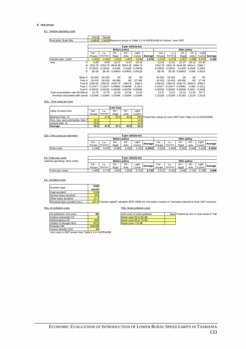
ECONOMIC EVALUATION OF INTRODUCTION OF LOWER RURAL SPEED LIMITS IN TASMANIA
133
E. Unit prices
E1. Vehicle operating costs
Petrol Diesel
Fuel price, $ per litre 0.8804 0.8639 Resource prices in Table 2.4 of AGPE04/08 for Hobart, June 2007
$ per vehicle-km
Car -
Private
Car -
Business
HV -
Rigid
HV -
Artic.
Light
Comm Average
Car -
Private
Car -
Business
HV -
Rigid
HV -
Artic.
Light
Comm Average
Vehicle oper. costs* 0.301 0.301 1.323 1.407 0.530 0.479 0.270 0.270 1.247 1.298 0.479 0.436
*Without tax A -9.99 -9.99 -15.27 -6.53 -20.16 -12.61 -12.61 -21.37 -16.12 -24.30
B 1553.78 1553.78 8544.38 8544.38 3396.74 1553.78 1553.78 8544.38 8544.4 3396.7
C 0.23531 0.23531 0.0185 0.0185 0.25629 0.23531 0.23531 0.0185 0.0185 0.2563
D 5E-05 5E-05 0.00603 0.00603 0.00126 5E-05 5E-05 0.00603 0.006 0.0013
Base A -16.262 -16.262 -30 -30 -30 -16.262 -16.262 -30 -30 -30
Fuel A -18.433 -18.433 -65.056 -80 -27.456 -18.433 -18.433 -65.056 -80 -27.46
Fuel B 1306.02 1306.02 4156.75 6342.8 2060.5 1306.02 1306.02 4156.75 6342.8 2060.5
Fuel C 0.15477 0.15477 0.49681 0.48496 0.1911 0.15477 0.15477 0.49681 0.485 0.1911
Fuel D 0.00032 0.00032 0.00068 0.00209 0.00085 0.00032 0.00032 0.00068 0.0021 0.0009
Fuel consumption rate (lt/100km) 13.79 13.79 32.99 52.56 21.62 13.31 13.31 32.03 51.53 20.77
Increase associated with speed 1.51694 1.51694 1.51694 1.51694 1.51694 1.31183 1.31183 1.31183 1.3118 1.3118
E2a. Time costs per hour
Value of travel time Car -
Private
Car -
Business
HV -
Rigid
HV -
Artic.
Light
Comm
Business trips, % 47.8 29.0 40.8 29.9 Travel time values at June 2007 from Table 3.2 of AGPE04/08
Pers. bus. and commuting. trips, % 19.5 14.9
Leisure trips, % 19.5 14.9
Average 19.5 47.8 27.1 40.8 22.2
E2b. Time costs per kilometre $ per vehicle-km
Car -
Private
Car -
Business
HV -
Rigid
HV -
Artic.
Light
CommAverage
Car -
Private
Car -
Business
HV -
Rigid
HV -
Artic.
Light
CommAverage
Time costs 0.194 0.475 0.280 0.425 0.220 0.2522 0.202 0.494 0.292 0.444 0.229 0.2624
E3. Total user costs $ per vehicle-km
(vehicle operating+ time costs)
Car -
Private
Car -
Business
HV -
Rigid
HV -
Artic.
Light
CommAverage
Car -
Private
Car -
Business
HV -
Rigid
HV -
Artic.
Light
CommAverage
Total user costs 0.495 0.776 1.603 1.832 0.751 0.732 0.471 0.763 1.540 1.742 0.708 0.698
E4. Accident costs
Accident typekA$/
accid.
Fatal accident 2155
Serious injury accident 455
Other injury accident 21.7
Personal injury accident (av.) 167.0 "Human capital" valuation (BTE 2000) for non-urban crashes in Tasmania indexed to June 2007 resource prices; from Table 4.3 of AGPE04/08
E5a. Air pollution costs E5b. Noise pollution costs
Air pollutants' unit costs $/t Unit costs of noise pollution $/year Treated as zero in rural areas in Table 5.1 of AGPE04/08
Carbon monoxide CO 3 Noise zone 55 to 65 dB
Hydrocarbons HC 958 Noise zone 65 to 70 dB
Oxides of nitrogen NOx 1912 Noise zone >70 dB
Particles PM 304298
Carbon dioxide CO2 48
Unit costs in 2007 prices from Table 5.3 in AGPE04/08
After policy
Before policy After policy
After policyBefore policy
$ per hour
Before policy

134 MONASH UNIVERSITY ACCIDENT RESEARCH CENTRE
F. Calculation of impacts
F1. Vehicle operating costs
Car -
Private
Car -
Business
HV -
Rigid
HV -
Artic.
Light
CommTotal
Car -
Private
Car -
Business
HV -
Rigid
HV -
Artic.
Light
CommTotal
Vehicle operating costs 109,460 22,741 39,761 68,714 82,857 323,532 98,141 20,389 37,484 63,385 74,896 294,295
F2a. Travel time
Car -
PrivateCar -
Business
HV -
Rigid
HV -
Artic.
Light
CommTotal
Car -
PrivateCar -
Business
HV -
Rigid
HV -
Artic.
Light
CommTotal
Total travel time on link 9,908 2,059 850 1,393 4,255 18,465 10,300 2,140 888 1,456 4,423 19,206
F2b. Travel time costs
Car -
PrivateCar -
Business
HV -
Rigid
HV -
Artic.
Light
CommTotal
Car -
PrivateCar -
Business
HV -
Rigid
HV -
Artic.
Light
CommTotal
Total travel time costs 70,643 35,906 8,413 20,761 34,462 170,185 73,437 37,327 8,781 21,688 35,825 177,057
F3. Consumer surplus
Car -
Private
Car -
Business HV - Rigid HV - Artic.
Light
CommAverage Car -
Private
Car -
Business HV - Rigid
HV -
Artic.
Light
CommAverage
Total user costs, $/veh.km 0.495 0.776 1.603 1.832 0.751 0.732 0.471 0.763 1.540 1.742 0.708 0.698
Mio veh.kms/year 364 76 30 49 156 675 364 76 30 49 156 675
Total
k$/year -8524 -931 -1909 -4403 -6597 -22364
F4a. Casualty accident rates
Car -
PrivateCar -
Business
HV -
Rigid
HV -
Artic.
Light
CommTotal
Car -
PrivateCar -
Business
HV -
Rigid
HV -
Artic.
Light
CommTotal
Crash rate per million VKT 0.120 0.120 0.120 0.120 0.120 0.120 0.106 0.106 0.104 0.103 0.106 0.106
Fatal crash rate per 100M VKT 1.68 1.35
F4b. Casualty accident severity
Car -
PrivateCar -
Business
HV -
Rigid
HV -
Artic.
Light
CommAverage
Car -
PrivateCar -
Business
HV -
Rigid
HV -
Artic.
Light
CommAverage
Fatal (%) 11.7 11.7 24.6 35.0 11.7 13.9 10.7 10.7 22.8 32.8 10.7 12.8
Serious injury (%) 19.6 19.6 22.7 23.5 19.6 20.0 19.4 19.4 22.7 23.8 19.4 19.8
Minor injury (%) 68.7 68.7 52.8 41.5 68.7 66.0 69.9 69.9 54.5 43.4 69.9 67.4
F4c. Accidents
Car -
PrivateCar -
Business
HV -
Rigid
HV -
Artic.
Light
CommTotal
Car -
PrivateCar -
Business
HV -
Rigid
HV -
Artic.
Light
CommTotal
Fatal accident 5.1 1.1 0.9 2.1 2.2 11.3 4.1 0.9 0.7 1.6 1.8 9.1
Serious injury accident 8.6 1.8 0.8 1.4 3.7 16.2 7.5 1.6 0.7 1.2 3.2 14.2
Minor injury accident 30.1 6.3 1.9 2.4 12.9 53.6 27.0 5.6 1.7 2.2 11.6 48.1
Total casualty accidents 43.8 9.1 3.6 5.9 18.8 81.2 38.6 8.0 3.1 5.0 16.6 71.4
F4d. Accident costs
Car -
PrivateCar -
Business
HV -
Rigid
HV -
Artic.
Light
CommTotal
Car -
PrivateCar -
Business
HV -
Rigid
HV -
Artic.
Light
CommTotal
Fatal accident 11,025 2,291 1,916 4,438 4,734 24,404 8,913 1,852 1,532 3,540 3,827 19,663
Serious injury accident 3,904 811 373 627 1,676 7,392 3,409 708 323 543 1,464 6,447
Minor injury accident 653 136 41 53 281 1,164 586 122 37 47 252 1,044
Total casualty accidents 15,583 3,237 2,330 5,118 6,691 32,959 12,908 2,682 1,892 4,130 5,542 27,155
After policy, k$/year
Before policy, crashes/year After policy, crashes/year
Before policy, crashes/year After policy, crashes/year
Before policy, crashes/year After policy, crashes/year
Change in consumer surplus
Input data, after policy
After policy, k$/yearBefore policy, k$/year
Input data, before policy
After policy, k$/year
Before policy, vehicle-hours/day After policy, vehicle-hours/day
Before policy, k$/year
Before policy, k$/year

ECONOMIC EVALUATION OF INTRODUCTION OF LOWER RURAL SPEED LIMITS IN TASMANIA
135
F5a. Air pollution
Emissions Car -
PrivateCar -
Business
HV -
Rigid
HV -
Artic.
Light
Comm Total
Car -
PrivateCar -
Business
HV -
Rigid
HV -
Artic.
Light
Comm Total
Carbon monoxide CO 1,803 375 144 232 774 3,328 1,341 279 107 172 576 2,474
Hydrocarbons HC 281 58 22 36 121 519 218 45 17 28 94 402
Oxides of nitrogen NOx 1,231 256 101 163 529 2,279 920 191 75 122 395 1,704
Particles PM 19 4 1 2 8 34 15 3 1 2 7 29
Carbon dioxide CO2 130,272 27,065 10,561 17,102 55,937 240,936 110,637 22,986 8,967 14,518 47,506 204,614
F5b. Air pollution costs
Emissions Car -
PrivateCar -
Business
HV -
Rigid
HV -
Artic.
Light
Comm Total
Car -
PrivateCar -
Business
HV -
Rigid
HV -
Artic.
Light
Comm Total
Carbon monoxide CO 5.4 1.1 0.4 0.7 2.3 10.0 4.0 0.8 0.3 0.5 1.7 7.4
Hydrocarbons HC 269 56 21 35 116 497 209 43 17 27 90 385
Oxides of nitrogen NOx 2,354 489 192 312 1,011 4,357 1,760 366 144 233 756 3,258
Particles PM 5,650 1,174 450 726 2,426 10,426 4,715 980 375 605 2,025 8,700
Carbon dioxide CO2 6,253 1,299 507 821 2,685 11,565 5,311 1,103 430 697 2,280 9,821
Total 14,532 3,019 1,171 1,894 6,240 26,855 11,998 2,493 966 1,562 5,152 22,172
F5c. Noise pollution
No. of residents
Before
policy
After
policyChange
Noise zone 55 to 65 dB 0 #DIV/0!
Noise zone 65 to 70 dB 0 #DIV/0!
Noise zone >70 dB 0 #DIV/0!
F5d. Noise pollution costs k$/ year
Before
policy
After
policyChange
Noise zone 55 to 65 dB 0 0 0 #DIV/0!
Noise zone 65 to 70 dB 0 0 0 #DIV/0!
Noise zone >70 dB 0 0 0 #DIV/0!
Total 0 0 0 #DIV/0!
G. Non-quantified impacts
Noise pollution
Summary of quantified impacts
Car -
PrivateCar -
Business
HV -
Rigid
HV -
Artic.
Light
CommTotal
Car -
PrivateCar -
Business
HV -
Rigid
HV -
Artic.
Light
CommTotal
Total monetary impact 210,217 64,903 51,675 96,487 130,250 553,531 196,484 62,890 49,123 90,765 ###### 520,679
End of sheet
At final speed, t/year
At final speed, k$/yearAt initial speed, k$/year
Before policy, k$/year After policy, k$/year
At initial speed, t/year

136 MONASH UNIVERSITY ACCIDENT RESEARCH CENTRE
MANAGING SPEEDS OF TRAFFIC ON EUROPEAN ROADS
Application of the MASTER framework Ver. 01/99
Category 1 undivided rural roads with current 110 km/h speed limit - curvy road with crossroads and towns
H. Net impacts Cruise Speed (km/h) Average speed on link (km/h) Before After
Cars and LCVs 105 100 Cars and LCVs 100.7 96.8
Rigid heavy vehicles 100 95 Rigid heavy vehicles 96.8 92.8
H1. Physical impacts Artic. heavy vehicles 99 94 Articulated heavy vehicles 96.0 91.9
Before After Change
Total travel time on link, hours/day 18,465 19,206 741 4.0 % Increase/vehicle/100km (mins.) Cars&LCVs: 2.4 Trucks: 2.7
Number of Crashes per year 81.2 71.4 -9.8 -12.1% Saving p.a. Fatal: 2.2 Serious Inj: 2.1 Other Inj: 5.5
Emissions, t/year Carbon monoxide CO 3328 2474 -854 -25.7 %
Hydrocarbons HC 519 402 -116.8 -22.5 %
Oxides of nitrogen NOx 2279 1704 -575 -25.2 %
Particles PM 34.3 28.6 -5.67 -16.6 %
Carbon dioxide CO2 240936 204614 -36322 -15.1 %
Residents in area where LAeq,07-22hrs > 55 dB 0 0 0
H2. Monetary impacts
k$/year Before After Change
Consumer surplus (N. A.) (N. A.) (N. A.)
Vehicle operating costs 323,532 294,295 -29237 -9.0 %
Time costs 170,185 177,057 6872 4.0 %
Crash costs 32,959 27,155 -5,805 -17.6%
Air pollution costs 26,855 22,172 -4,684 -17.4 %
Noise costs 0 0 0
Total 553,531 520,679
Change -32,853 -5.9 %

ECONOMIC EVALUATION OF INTRODUCTION OF LOWER RURAL SPEED LIMITS IN TASMANIA 137
H3. Summary of monetary impacts for intermediate and lower cruise speeds
kA$/yearkm/h 80 82 84 86 88 90 92 94 96 98 100
Consumer surplus (N. A.) (N. A.) (N. A.) (N. A.) (N. A.) (N. A.) (N. A.) (N. A.) (N. A.) (N. A.) (N. A.)
Vehicle operating costs 259,850 259,362 261,452 260,980 265,113 268,547 271,229 277,199 282,424 287,054 295,804
Time costs 214,035 209,112 204,508 200,127 196,020 192,121 188,437 184,952 181,652 178,542 175,592
Crash costs 12,184 13,380 14,667 16,048 17,529 19,115 20,810 22,620 24,551 26,608 28,798
Air pollution costs 15,623 15,812 19,489 16,457 17,269 17,918 18,391 19,389 20,214 20,887 22,243
Noise costs 0 0 0 0 0 0 0 0 0 0 0
Total 501,691 497,665 500,116 493,612 495,931 497,701 498,866 504,160 508,841 513,092 522,436
of which:
Cars & light comm. vehs. 367,672 364,571 366,684 361,253 362,779 363,875 364,496 368,161 371,345 374,183 380,791
Heavy vehicles (rigid and artic.) 134,020 133,094 133,432 132,358 133,152 133,827 134,371 135,999 137,496 138,909 141,646
H4. Monetary impacts for heavy vehicles at intermediate and lower cruise speeds
kA$/yearkm/h 80 82 84 86 88 90 92 94 96 98 100
Consumer surplus (N. A.) (N. A.) (N. A.) (N. A.) (N. A.) (N. A.) (N. A.) (N. A.) (N. A.) (N. A.) (N. A.)
Vehicle operating costs 93,759 93,301 93,619 93,247 94,218 95,025 95,655 97,241 98,649 99,924 102,377
Time costs 35,352 34,539 33,779 33,055 32,377 31,733 31,124 30,549 30,004 29,490 29,003
Crash costs 3,082 3,406 3,755 4,132 4,538 4,974 5,442 5,943 6,480 7,053 7,666
Air pollution costs 1,826 1,848 2,278 1,924 2,019 2,095 2,150 2,267 2,363 2,442 2,600
Noise costs 0 0 0 0 0 0 0 0 0 0 0
Total 134,020 133,094 133,432 132,358 133,152 133,827 134,371 135,999 137,496 138,909 141,646
H5. Monetary impacts for cars and LCVs at intermediate and lower cruise speeds
kA$/yearkm/h 80 82 84 86 88 90 92 94 96 98 100
Consumer surplus (N. A.) (N. A.) (N. A.) (N. A.) (N. A.) (N. A.) (N. A.) (N. A.) (N. A.) (N. A.) (N. A.)
Vehicle operating costs 166,091 166,061 167,833 167,732 170,895 173,522 175,574 179,958 183,775 187,130 193,426
Time costs 178,683 174,573 170,730 167,072 163,643 160,388 157,313 154,403 151,648 149,052 146,589
Crash costs 9,101 9,974 10,912 11,916 12,991 14,141 15,368 16,677 18,071 19,555 21,132
Air pollution costs 13,796 13,963 17,210 14,533 15,250 15,824 16,241 17,122 17,851 18,446 19,643
Noise costs 0 0 0 0 0 0 0 0 0 0 0
Total 367,672 364,571 366,684 361,253 362,779 363,875 364,496 368,161 371,345 374,183 380,791

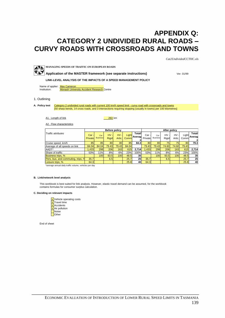
ECONOMIC EVALUATION OF INTRODUCTION OF LOWER RURAL SPEED LIMITS IN TASMANIA
139
APPENDIX Q: CATEGORY 2 UNDIVIDED RURAL ROADS –
CURVY ROADS WITH CROSSROADS AND TOWNS
Cat2UndividedCCTHC.xls
MANAGING SPEEDS OF TRAFFIC ON EUROPEAN ROADS
Application of the MASTER framework (see separate instructions) Ver. 01/99
LINK-LEVEL ANALYSIS OF THE IMPACTS OF A SPEED MANAGEMENT POLICY
Name of applier: Max Cameron
Institution: Monash University Accident Research Centre
1. Outlining
A. Policy test Category 2 undivided rural roads with current 100 km/h speed limit - curvy road with crossroads and towns
[50 sharp bends, 14 cross roads, and 3 intersections requiring stopping (usually in towns) per 100 kilometres]
A1. Length of link 263 km
A2. Flow characteristics
Before policy After policy
Traffic attributesCar -
Private
Car -
Business
HV -
Rigid
HV -
Artic.
Light
Comm
Total/
Averag
e
Car -
Private
Car -
Business
HV -
Rigid
HV -
Artic.
Light
Comm
Total/
Averag
e
Cruise speed, km/h 85 85 80 80 85 84.3 80 80 75 75 80 79.3
Average of all speeds on link 84.04 84.04 79.43 79.43 84.04 79.43 79.43 74.60 74.60 79.43
AADT* 1,433 298 206 163 615 2,714 1,433 298 206 163 615 2,714
Share of traffic 53% 11% 8% 6% 23% 100% 53% 11% 8% 6% 23% 100%
Business trips, % 100 93.5 100 48.5 35 100 93.5 100 48.5 35
Pers. bus. and commuting. trips, % 35.7 6.5 25.7 25 35.7 6.5 25.7 25
Leisure trips, % 64.3 25.8 40 64.3 25.8 40
*average annual daily traffic volume, vehicles per day
B. Link/network level analysis
This workbook is best suited for link analysis. However, elastic travel demand can be assumed, for the workbook
contains formulas for consumer surplus calculation.
C. Deciding on relevant impacts
x Vehicle operating costs
x Travel time
x Accidents
x Air pollution
Noise
Other
End of sheet

140 MONASH UNIVERSITY ACCIDENT RESEARCH CENTRE
MANAGING SPEEDS OF TRAFFIC ON EUROPEAN ROADS
Application of the MASTER framework Ver. 01/99
Category 2 undivided rural roads with current 100 km/h speed limit - curvy road with crossroads and towns
2. Measurement of impactsRigid heavy vehicles
D. Impact functions
D1. Vehicle operating costs
Freeway Model for operations of free-running traffic in Table 3.10 of AGPE04/08; June 2007 prices
D2. Travel time
Function: travel time = link length/speed of traffic flow (flat straight roads only; see adjustment factors for curvy roads with cross roads and towns)
D3a. Accidents
Injury accidents before = nIB Average speed before = vB
Injury accidents after = nIA Average speed after = vA
Exponent Value
Fatal accidents F 4.36 Rural highway exponent estimates
Serious injury accidents S 2.78 from Cameron and Elvik (2008), Table 6
Other injury accidents O 2.22
D4. Air pollutant emission coefficients
Emission factors* Car -
Private
Car -
Business
HV -
Rigid
HV -
Artic.
Light
CommAverage
Car -
Private
Car -
Business
HV -
Rigid
HV -
Artic.
Light
CommAverage
Carbon monoxide CO 2.32 2.32 2.23 2.23 2.32 2.31 2.14 2.14 2.05 2.05 2.14 2.13
Hydrocarbons HC 0.40 0.40 0.38 0.38 0.40 0.40 0.37 0.37 0.35 0.35 0.37 0.37
Oxides of nitrogen NOx 1.68 1.68 1.67 1.67 1.68 1.68 1.60 1.60 1.58 1.58 1.60 1.59
Particles PM 0.03 0.03 0.03 0.03 0.03 0.031 0.03 0.03 0.03 0.03 0.03 0.029
Carbon dioxide CO2 235.7 235.7 231.2 231.2 235.7 235.1 226.1 226.1 221.6 221.6 226.1 225.5
Emission coefficients not available by vehicle type, only for mix of traffic close to mix outlined here
Same coefficient assumed for all vehicles at given speed for each pollutant
D5. Noise pollution
No impact function available; noise pollution assumed small because of negligible human population living in vicinity of rural roads considered
nIA = (vA/vB)F * nIB
nIA = (vA/vB)S * nIB
nIA = (vA/vB)O * nIB
At final speed, g/kmAt initial speed, g/km

ECONOMIC EVALUATION OF INTRODUCTION OF LOWER RURAL SPEED LIMITS IN TASMANIA
141
E. Unit prices
E1. Vehicle operating costs
Petrol Diesel
Fuel price, $ per litre 0.8804 0.8639 Resource prices in Table 2.4 of AGPE04/08 for Hobart, June 2007
$ per vehicle-km
Car -
Private
Car -
Business
HV -
Rigid
HV -
Artic.
Light
Comm Average
Car -
Private
Car -
Business
HV -
Rigid
HV -
Artic.
Light
Comm Average
Vehicle oper. costs* 0.232 0.232 1.189 1.203 0.422 0.406 0.229 0.229 1.207 1.216 0.419 0.405
*Without tax A -15.43 -15.43 -27.95 -26.60 -28.71 -15.69 -15.69 -28.57 -27.61 -29.12
B 1553.78 1553.78 8544.38 8544.38 3396.74 1553.78 1553.78 8544.38 8544.4 3396.7
C 0.23531 0.23531 0.0185 0.0185 0.25629 0.23531 0.23531 0.0185 0.0185 0.2563
D 5E-05 5E-05 0.00603 0.00603 0.00126 5E-05 5E-05 0.00603 0.006 0.0013
Base A -16.262 -16.262 -30 -30 -30 -16.262 -16.262 -30 -30 -30
Fuel A -18.433 -18.433 -65.056 -80 -27.456 -18.433 -18.433 -65.056 -80 -27.46
Fuel B 1306.02 1306.02 4156.75 6342.8 2060.5 1306.02 1306.02 4156.75 6342.8 2060.5
Fuel C 0.15477 0.15477 0.49681 0.48496 0.1911 0.15477 0.15477 0.49681 0.485 0.1911
Fuel D 0.00032 0.00032 0.00068 0.00209 0.00085 0.00032 0.00032 0.00068 0.0021 0.0009
Fuel consumption rate (lt/100km) 12.40 12.40 31.00 51.45 19.18 12.32 12.32 31.45 52.70 19.03
Increase associated with speed 1.07643 1.07643 1.07643 1.07643 1.07643 1.05256 1.05256 1.05256 1.0526 1.0526
E2a. Time costs per hour
Value of travel time Car -
Private
Car -
Business
HV -
Rigid
HV -
Artic.
Light
Comm
Business trips, % 47.8 29.0 40.8 29.9 Travel time values at June 2007 from Table 3.2 of AGPE04/08
Pers. bus. and commuting. trips, % 19.5 14.9
Leisure trips, % 19.5 14.9
Average 19.5 47.8 27.1 40.8 22.2
E2b. Time costs per kilometre $ per vehicle-km
Car -
Private
Car -
Business
HV -
Rigid
HV -
Artic.
Light
CommAverage
Car -
Private
Car -
Business
HV -
Rigid
HV -
Artic.
Light
CommAverage
Time costs 0.232 0.569 0.341 0.514 0.264 0.3016 0.246 0.602 0.363 0.547 0.279 0.3195
E3. Total user costs $ per vehicle-km
(vehicle operating+ time costs)
Car -
Private
Car -
Business
HV -
Rigid
HV -
Artic.
Light
CommAverage
Car -
Private
Car -
Business
HV -
Rigid
HV -
Artic.
Light
CommAverage
Total user costs 0.465 0.801 1.530 1.717 0.686 0.707 0.475 0.830 1.570 1.763 0.699 0.725
E4. Accident costs
Accident typekA$/
accid.
Fatal accident 2155
Serious injury accident 455
Other injury accident 21.7
Personal injury accident (av.) 167.0 "Human capital" valuation (BTE 2000) for non-urban crashes in Tasmania indexed to June 2007 resource prices; from Table 4.3 of AGPE04/08
E5a. Air pollution costs E5b. Noise pollution costs
Air pollutants' unit costs $/t Unit costs of noise pollution $/year Treated as zero in rural areas in Table 5.1 of AGPE04/08
Carbon monoxide CO 3 Noise zone 55 to 65 dB
Hydrocarbons HC 958 Noise zone 65 to 70 dB
Oxides of nitrogen NOx 1912 Noise zone >70 dB
Particles PM 304298
Carbon dioxide CO2 48
Unit costs in 2007 prices from Table 5.3 in AGPE04/08
$ per hour
Before policy
After policyBefore policy
After policy
Before policy After policy

142 MONASH UNIVERSITY ACCIDENT RESEARCH CENTRE
F. Calculation of impacts
F1. Vehicle operating costs
Car -
Private
Car -
Business
HV -
Rigid
HV -
Artic.
Light
CommTotal
Car -
Private
Car -
Business
HV -
Rigid
HV -
Artic.
Light
CommTotal
Vehicle operating costs 31,928 6,633 23,513 18,771 24,893 105,738 31,461 6,536 23,856 18,982 24,755 105,590
F2a. Travel time
Car -
PrivateCar -
Business
HV -
Rigid
HV -
Artic.
Light
CommTotal
Car -
PrivateCar -
Business
HV -
Rigid
HV -
Artic.
Light
CommTotal
Total travel time on link 4,483 931 682 538 1,925 8,560 4,744 986 726 573 2,037 9,065
F2b. Travel time costs
Car -
PrivateCar -
Business
HV -
Rigid
HV -
Artic.
Light
CommTotal
Car -
PrivateCar -
Business
HV -
Rigid
HV -
Artic.
Light
CommTotal
Total travel time costs 31,965 16,247 6,747 8,021 15,594 78,574 33,820 17,190 7,184 8,541 16,499 83,234
F3. Consumer surplus
Car -
Private
Car -
Business HV - Rigid HV - Artic.
Light
CommAverage Car -
Private
Car -
Business HV - Rigid
HV -
Artic.
Light
CommAverage
Total user costs, $/veh.km 0.465 0.801 1.530 1.717 0.686 0.707 0.475 0.830 1.570 1.763 0.699 0.725
Mio veh.kms/year 138 29 20 16 59 261 138 29 20 16 59 261
Total
k$/year 1388 846 780 730 767 4511
F4a. Casualty accident rates
Car -
PrivateCar -
Business
HV -
Rigid
HV -
Artic.
Light
CommTotal
Car -
PrivateCar -
Business
HV -
Rigid
HV -
Artic.
Light
CommTotal
Crash rate per million VKT 0.246 0.246 0.246 0.246 0.246 0.246 0.213 0.213 0.210 0.208 0.213 0.212
Fatal crash rate per 100M VKT 1.17 0.89
F4b. Casualty accident severity
Car -
PrivateCar -
Business
HV -
Rigid
HV -
Artic.
Light
CommAverage
Car -
PrivateCar -
Business
HV -
Rigid
HV -
Artic.
Light
CommAverage
Fatal (%) 3.9 3.9 8.3 11.8 3.9 4.7 3.5 3.5 7.4 10.5 3.5 4.2
Serious injury (%) 20.1 20.1 23.2 24.0 20.1 20.6 19.6 19.6 22.8 23.8 19.6 20.1
Minor injury (%) 76.0 76.0 68.5 64.1 76.0 74.7 76.9 76.9 69.8 65.7 76.9 75.7
F4c. Accidents
Car -
PrivateCar -
Business
HV -
Rigid
HV -
Artic.
Light
CommTotal
Car -
PrivateCar -
Business
HV -
Rigid
HV -
Artic.
Light
CommTotal
Fatal accident 1.3 0.3 0.4 0.5 0.6 3.0 1.0 0.2 0.3 0.3 0.4 2.3
Serious injury accident 6.8 1.4 1.1 0.9 2.9 13.2 5.8 1.2 0.9 0.8 2.5 11.1
Minor injury accident 25.8 5.4 3.3 2.5 11.1 48.0 22.5 4.7 2.9 2.1 9.7 41.9
Total casualty accidents 33.9 7.0 4.9 3.8 14.6 64.2 29.3 6.1 4.1 3.3 12.6 55.3
F4d. Accident costs
Car -
PrivateCar -
Business
HV -
Rigid
HV -
Artic.
Light
CommTotal
Car -
PrivateCar -
Business
HV -
Rigid
HV -
Artic.
Light
CommTotal
Fatal accident 2,878 598 871 980 1,236 6,563 2,209 459 657 740 949 5,014
Serious injury accident 3,097 643 515 421 1,330 6,006 2,616 544 430 352 1,123 5,066
Minor injury accident 559 116 72 54 240 1,041 488 101 63 46 210 909
Total casualty accidents 6,534 1,357 1,458 1,454 2,805 13,609 5,314 1,104 1,151 1,138 2,282 10,989
Before policy, k$/year
Before policy, k$/year
After policy, k$/year
Before policy, vehicle-hours/day After policy, vehicle-hours/day
Before policy, crashes/year After policy, crashes/year
Change in consumer surplus
Input data, after policy
After policy, k$/yearBefore policy, k$/year
Input data, before policy
After policy, k$/year
Before policy, crashes/year After policy, crashes/year
Before policy, crashes/year After policy, crashes/year

ECONOMIC EVALUATION OF INTRODUCTION OF LOWER RURAL SPEED LIMITS IN TASMANIA
143
F5a. Air pollution
Emissions Car -
PrivateCar -
Business
HV -
Rigid
HV -
Artic.
Light
Comm Total
Car -
PrivateCar -
Business
HV -
Rigid
HV -
Artic.
Light
Comm Total
Carbon monoxide CO 319 66 44 35 137 601 295 61 41 32 126 555
Hydrocarbons HC 55 11 8 6 23 103 51 11 7 5 22 95
Oxides of nitrogen NOx 232 48 33 26 99 438 220 46 31 25 94 415
Particles PM 4 1 1 0 2 8 4 1 1 0 2 8
Carbon dioxide CO2 32,420 6,736 4,571 3,608 13,921 61,256 31,089 6,459 4,382 3,459 13,349 58,738
F5b. Air pollution costs
Emissions Car -
PrivateCar -
Business
HV -
Rigid
HV -
Artic.
Light
Comm Total
Car -
PrivateCar -
Business
HV -
Rigid
HV -
Artic.
Light
Comm Total
Carbon monoxide CO 1.0 0.2 0.1 0.1 0.4 1.8 0.9 0.2 0.1 0.1 0.4 1.7
Hydrocarbons HC 52 11 7 6 22 99 48 10 7 5 21 91
Oxides of nitrogen NOx 443 92 63 50 190 838 420 87 60 47 180 794
Particles PM 1,303 271 180 142 559 2,455 1,222 254 168 133 525 2,302
Carbon dioxide CO2 1,556 323 219 173 668 2,940 1,492 310 210 166 641 2,819
Total 3,355 697 469 371 1,441 6,333 3,184 661 445 351 1,367 6,009
F5c. Noise pollution
No. of residents
Before
policy
After
policyChange
Noise zone 55 to 65 dB 0 #DIV/0!
Noise zone 65 to 70 dB 0 #DIV/0!
Noise zone >70 dB 0 #DIV/0!
F5d. Noise pollution costs k$/ year
Before
policy
After
policyChange
Noise zone 55 to 65 dB 0 0 0 #DIV/0!
Noise zone 65 to 70 dB 0 0 0 #DIV/0!
Noise zone >70 dB 0 0 0 #DIV/0!
Total 0 0 0 #DIV/0!
G. Non-quantified impacts
Noise pollution
Summary of quantified impacts
Car -
PrivateCar -
Business
HV -
Rigid
HV -
Artic.
Light
CommTotal
Car -
PrivateCar -
Business
HV -
Rigid
HV -
Artic.
Light
CommTotal
Total monetary impact 73,782 24,935 32,188 28,617 44,733 204,255 73,779 25,492 32,636 29,012 44,903 205,821
End of sheet
Before policy, k$/year After policy, k$/year
At initial speed, t/year At final speed, t/year
At final speed, k$/yearAt initial speed, k$/year

144 MONASH UNIVERSITY ACCIDENT RESEARCH CENTRE
MANAGING SPEEDS OF TRAFFIC ON EUROPEAN ROADS
Application of the MASTER framework Ver. 01/99
Category 2 undivided rural roads with current 100 km/h speed limit - curvy road with crossroads and towns
H. Net impacts Cruise Speed (km/h) Average speed on link (km/h) Before After
Cars and LCVs 85 80 Cars and LCVs 84.0 79.4
Rigid heavy vehicles 80 75 Rigid heavy vehicles 79.4 74.6
H1. Physical impacts Artic. heavy vehicles 80 75 Articulated heavy vehicles 79.4 74.6
Before After Change
Total travel time on link, hours/day 8,560 9,065 505 5.9 % Increase/vehicle/100km (mins.) Cars&LCVs: 4.1 Trucks: 4.9
Number of Crashes per year 64.2 55.3 -8.9 -13.8% Saving p.a. Fatal: 0.7 Serious Inj: 2.1 Other Inj: 6.1
Emissions, t/year Carbon monoxide CO 601 555 -46 -7.7 %
Hydrocarbons HC 103 95 -7.7 -7.5 %
Oxides of nitrogen NOx 438 415 -23 -5.2 %
Particles PM 8.1 7.6 -0.50 -6.2 %
Carbon dioxide CO2 61256 58738 -2518 -4.1 %
Residents in area where LAeq,07-22hrs > 55 dB 0 0 0
H2. Monetary impacts
k$/year Before After Change
Consumer surplus (N. A.) (N. A.) (N. A.)
Vehicle operating costs 105,738 105,590 -148 -0.1 %
Time costs 78,574 83,234 4659 5.9 %
Crash costs 13,609 10,989 -2,620 -19.3%
Air pollution costs 6,333 6,009 -324 -5.1 %
Noise costs 0 0 0
Total 204,255 205,821
Change 1,566 0.8 %

ECONOMIC EVALUATION OF INTRODUCTION OF LOWER RURAL SPEED LIMITS IN TASMANIA 145
H3. Summary of monetary impacts for intermediate and lower cruise speeds
kA$/yearkm/h 80 82 84 86 88 90 92 94 96 98 100
Consumer surplus (N. A.) (N. A.) (N. A.) (N. A.) (N. A.) (N. A.) (N. A.) (N. A.) (N. A.) (N. A.) (N. A.)
Vehicle operating costs 104,744 104,526 105,315 105,116 106,708 108,035 109,076 111,396 113,434 115,245 118,659
Time costs 82,277 80,385 78,615 76,931 75,352 73,854 72,437 71,098 69,829 68,634 67,499
Crash costs 11,613 12,658 13,773 14,964 16,232 17,582 19,017 20,542 22,160 23,875 25,691
Air pollution costs 6,032 6,105 6,322 6,354 6,667 6,918 7,100 7,486 7,804 8,064 8,588
Noise costs 0 0 0 0 0 0 0 0 0 0 0
Total 204,666 203,674 204,026 203,364 204,959 206,388 207,631 210,522 213,227 215,818 220,438
of which:
Cars & light comm. vehs. 144,174 143,433 143,649 143,120 144,207 145,162 145,967 147,954 149,792 151,532 154,732
Heavy vehicles (rigid and artic.) 60,492 60,241 60,376 60,245 60,752 61,227 61,664 62,568 63,435 64,286 65,705
H4. Monetary impacts for heavy vehicles at intermediate and lower cruise speeds
kA$/yearkm/h 80 82 84 86 88 90 92 94 96 98 100
Consumer surplus (N. A.) (N. A.) (N. A.) (N. A.) (N. A.) (N. A.) (N. A.) (N. A.) (N. A.) (N. A.) (N. A.)
Vehicle operating costs 41,992 41,786 41,905 41,744 42,141 42,476 42,741 43,406 44,001 44,545 45,580
Time costs 14,769 14,429 14,111 13,809 13,525 13,256 13,002 12,762 12,534 12,319 12,116
Crash costs 2,913 3,197 3,502 3,829 4,180 4,555 4,956 5,384 5,841 6,327 6,844
Air pollution costs 819 829 859 863 905 939 964 1,017 1,060 1,095 1,166
Noise costs 0 0 0 0 0 0 0 0 0 0 0
Total 60,492 60,241 60,376 60,245 60,752 61,227 61,664 62,568 63,435 64,286 65,705
H5. Monetary impacts for cars and LCVs at intermediate and lower cruise speeds
kA$/yearkm/h 80 82 84 86 88 90 92 94 96 98 100
Consumer surplus (N. A.) (N. A.) (N. A.) (N. A.) (N. A.) (N. A.) (N. A.) (N. A.) (N. A.) (N. A.) (N. A.)
Vehicle operating costs 62,752 62,740 63,410 63,372 64,567 65,559 66,335 67,991 69,433 70,701 73,079
Time costs 67,509 65,956 64,504 63,122 61,827 60,597 59,435 58,336 57,295 56,314 55,384
Crash costs 8,700 9,461 10,272 11,135 12,052 13,027 14,061 15,158 16,319 17,548 18,848
Air pollution costs 5,213 5,276 5,464 5,491 5,762 5,978 6,136 6,469 6,744 6,969 7,422
Noise costs 0 0 0 0 0 0 0 0 0 0 0
Total 144,174 143,433 143,649 143,120 144,207 145,162 145,967 147,954 149,792 151,532 154,732


ECONOMIC EVALUATION OF INTRODUCTION OF LOWER RURAL SPEED LIMITS IN TASMANIA
147
APPENDIX R: CATEGORY 3 UNDIVIDED RURAL ROADS –
CURVY ROADS WITH CROSSROADS AND TOWNS
Cat3UndividedCCTHC.xls
MANAGING SPEEDS OF TRAFFIC ON EUROPEAN ROADS
Application of the MASTER framework (see separate instructions) Ver. 01/99
LINK-LEVEL ANALYSIS OF THE IMPACTS OF A SPEED MANAGEMENT POLICY
Name of applier: Max Cameron
Institution: Monash University Accident Research Centre
1. Outlining
A. Policy test Category 3 undivided rural roads with current 100 km/h speed limit - curvy road with crossroads and towns
[50 sharp bends, 14 cross roads, and 3 intersections requiring stopping (usually in towns) per 100 kilometres]
A1. Length of link 572 km
A2. Flow characteristics
Before policy After policy
Traffic attributesCar -
Private
Car -
Business
HV -
Rigid
HV -
Artic.
Light
Comm
Total/
Averag
e
Car -
Private
Car -
Business
HV -
Rigid
HV -
Artic.
Light
Comm
Total/
Averag
e
Cruise speed, km/h 87 87 82 82 87 86.7 82 82 77 77 82 81.7
Average of all speeds on link 85.84 85.84 81.30 81.30 85.84 81.30 81.30 76.54 76.54 81.30
AADT* 1,145 238 108 28 492 2,012 1,145 238 108 28 492 2,012
Share of traffic 57% 12% 5% 1% 24% 100% 57% 12% 5% 1% 24% 100%
Business trips, % 100 93.5 100 48.5 30 100 93.5 100 48.5 30
Pers. bus. and commuting. trips, % 35.7 6.5 25.7 27 35.7 6.5 25.7 27
Leisure trips, % 64.3 25.8 43 64.3 25.8 43
*average annual daily traffic volume, vehicles per day
B. Link/network level analysis
This workbook is best suited for link analysis. However, elastic travel demand can be assumed, for the workbook
contains formulas for consumer surplus calculation.
C. Deciding on relevant impacts
x Vehicle operating costs
x Travel time
x Accidents
x Air pollution
Noise
Other
End of sheet

148 MONASH UNIVERSITY ACCIDENT RESEARCH CENTRE
MANAGING SPEEDS OF TRAFFIC ON EUROPEAN ROADS
Application of the MASTER framework Ver. 01/99
Category 3 undivided rural roads with current 100 km/h speed limit - curvy road with crossroads and towns
H. Net impacts Cruise Speed (km/h) Average speed on link (km/h) Before After
Cars and LCVs 87 82 Cars and LCVs 85.8 81.3
Rigid heavy vehicles 82 77 Rigid heavy vehicles 81.3 76.5
H1. Physical impacts Artic. heavy vehicles 82 77 Articulated heavy vehicles 81.3 76.5
Before After Change
Total travel time on link, hours/day 13,456 14,214 758 5.6 % Increase/vehicle/100km (mins.) Cars&LCVs: 3.9 Trucks: 4.6
Number of Crashes per year 132.3 114.6 -17.7 -13.4% Saving p.a. Fatal: 1.4 Serious Inj: 3.8 Other Inj: 12.5
Emissions, t/year Carbon monoxide CO 1007 913 -95 -9.4 %
Hydrocarbons HC 172 157 -15.2 -8.8 %
Oxides of nitrogen NOx 725 674 -51 -7.1 %
Particles PM 13.4 12.5 -0.96 -7.1 %
Carbon dioxide CO2 100839 95672 -5168 -5.1 %
Residents in area where LAeq,07-22hrs > 55 dB 0 0 0
H2. Monetary impacts
k$/year Before After Change
Consumer surplus (N. A.) (N. A.) (N. A.)
Vehicle operating costs 145,139 143,253 -1886 -1.3 %
Time costs 119,122 125,840 6719 5.6 %
Crash costs 27,076 21,967 -5,109 -18.9%
Air pollution costs 10,476 9,823 -653 -6.2 %
Noise costs 0 0 0
Total 301,812 300,883
Change -929 -0.3 %

ECONOMIC EVALUATION OF INTRODUCTION OF LOWER RURAL SPEED LIMITS IN TASMANIA 149
H3. Summary of monetary impacts for intermediate and lower cruise speeds
kA$/yearkm/h 80 82 84 86 88 90 92 94 96 98 100
Consumer surplus (N. A.) (N. A.) (N. A.) (N. A.) (N. A.) (N. A.) (N. A.) (N. A.) (N. A.) (N. A.) (N. A.)
Vehicle operating costs 142,898 142,711 143,945 143,756 146,113 148,079 149,624 152,989 155,938 158,551 163,452
Time costs 128,134 125,187 122,431 119,808 117,349 115,015 112,810 110,724 108,748 106,886 105,120
Crash costs 20,727 22,593 24,585 26,710 28,976 31,387 33,951 36,675 39,566 42,631 45,877
Air pollution costs 9,724 9,841 12,130 10,243 10,748 11,152 11,446 12,068 12,581 13,000 13,844
Noise costs 0 0 0 0 0 0 0 0 0 0 0
Total 301,483 300,332 303,091 300,517 303,187 305,634 307,831 312,456 316,833 321,069 328,294
of which:
Cars & light comm. vehs. 253,589 252,579 255,060 252,653 254,888 256,914 258,706 262,579 266,220 269,721 275,789
Heavy vehicles (rigid and artic.) 47,894 47,752 48,031 47,864 48,299 48,720 49,125 49,877 50,613 51,348 52,504
H4. Monetary impacts for heavy vehicles at intermediate and lower cruise speeds
kA$/yearkm/h 80 82 84 86 88 90 92 94 96 98 100
Consumer surplus (N. A.) (N. A.) (N. A.) (N. A.) (N. A.) (N. A.) (N. A.) (N. A.) (N. A.) (N. A.) (N. A.)
Vehicle operating costs 33,786 33,619 33,689 33,566 33,846 34,086 34,282 34,768 35,209 35,618 36,383
Time costs 10,751 10,504 10,273 10,052 9,846 9,650 9,465 9,290 9,124 8,968 8,820
Crash costs 2,697 2,961 3,245 3,550 3,877 4,226 4,600 4,999 5,425 5,879 6,361
Air pollution costs 660 668 824 695 730 757 777 819 854 883 940
Noise costs 0 0 0 0 0 0 0 0 0 0 0
Total 47,894 47,752 48,031 47,864 48,299 48,720 49,125 49,877 50,613 51,348 52,504
H5. Monetary impacts for cars and LCVs at intermediate and lower cruise speeds
kA$/yearkm/h 80 82 84 86 88 90 92 94 96 98 100
Consumer surplus (N. A.) (N. A.) (N. A.) (N. A.) (N. A.) (N. A.) (N. A.) (N. A.) (N. A.) (N. A.) (N. A.)
Vehicle operating costs 109,112 109,092 110,256 110,190 112,267 113,993 115,341 118,221 120,729 122,933 127,069
Time costs 117,383 114,683 112,159 109,756 107,503 105,365 103,345 101,433 99,623 97,918 96,300
Crash costs 18,031 19,631 21,340 23,160 25,099 27,161 29,351 31,676 34,141 36,752 39,516
Air pollution costs 9,063 9,173 11,306 9,547 10,019 10,395 10,669 11,248 11,727 12,118 12,904
Noise costs 0 0 0 0 0 0 0 0 0 0 0
Total 253,589 252,579 255,060 252,653 254,888 256,914 258,706 262,579 266,220 269,721 275,789


ECONOMIC EVALUATION OF INTRODUCTION OF LOWER RURAL SPEED LIMITS IN TASMANIA
151
APPENDIX S: CATEGORY 4 UNDIVIDED RURAL ROADS –
CURVY ROADS WITH CROSSROADS AND TOWNS
Cat4UndividedCCTHC.xls
MANAGING SPEEDS OF TRAFFIC ON EUROPEAN ROADS
Application of the MASTER framework (see separate instructions) Ver. 01/99
LINK-LEVEL ANALYSIS OF THE IMPACTS OF A SPEED MANAGEMENT POLICY
Name of applier: Max Cameron
Institution: Monash University Accident Research Centre
1. Outlining
A. Policy test Category 4 undivided rural roads with current 100 km/h speed limit - curvy road with crossroads and towns
[50 sharp bends, 14 cross roads, and 3 intersections requiring stopping (usually in towns) per 100 kilometres]
A1. Length of link 825 km
A2. Flow characteristics
Before policy After policy
Traffic attributesCar -
Private
Car -
Business
HV -
Rigid
HV -
Artic.
Light
Comm
Total/
Averag
e
Car -
Private
Car -
Business
HV -
Rigid
HV -
Artic.
Light
Comm
Total/
Averag
e
Cruise speed, km/h 91 91 85 75 91 90.2 86 86 80 70 86 85.2
Average of all speeds on link 89.36 89.36 84.04 74.60 89.36 84.95 84.95 79.43 69.78 84.95
AADT* 759 158 66 41 326 1,349 759 158 66 41 326 1,349
Share of traffic 56% 12% 5% 3% 24% 100% 56% 12% 5% 3% 24% 100%
Business trips, % 100 93.5 100 48.5 31 100 93.5 100 48.5 31
Pers. bus. and commuting. trips, % 35.7 6.5 25.7 27 35.7 6.5 25.7 27
Leisure trips, % 64.3 25.8 42 64.3 25.8 42
*average annual daily traffic volume, vehicles per day
B. Link/network level analysis
This workbook is best suited for link analysis. However, elastic travel demand can be assumed, for the workbook
contains formulas for consumer surplus calculation.
C. Deciding on relevant impacts
x Vehicle operating costs
x Travel time
x Accidents
x Air pollution
Noise
Other
End of sheet

152 MONASH UNIVERSITY ACCIDENT RESEARCH CENTRE
MANAGING SPEEDS OF TRAFFIC ON EUROPEAN ROADS
Application of the MASTER framework Ver. 01/99
Category 4 undivided rural roads with current 100 km/h speed limit - curvy road with crossroads and towns
H. Net impacts Cruise Speed (km/h) Average speed on link (km/h) Before After
Cars and LCVs 91 86 Cars and LCVs 89.4 85.0
Rigid heavy vehicles 85 80 Rigid heavy vehicles 84.0 79.4
H1. Physical impacts Artic. heavy vehicles 75 70 Articulated heavy vehicles 74.6 69.8
Before After Change
Total travel time on link, hours/day 12,568 13,233 664 5.3 % Increase/vehicle/100km (mins.) Cars&LCVs: 3.5 Trucks: 4.1
Number of Crashes per year 137.6 119.9 -17.6 -12.8% Saving p.a. Fatal: 1.0 Serious Inj: 4.2 Other Inj: 12.4
Emissions, t/year Carbon monoxide CO 1076 938 -138 -12.8 %
Hydrocarbons HC 182 161 -21.4 -11.8 %
Oxides of nitrogen NOx 763 679 -83 -10.9 %
Particles PM 13.9 12.6 -1.25 -9.0 %
Carbon dioxide CO2 102876 95545 -7331 -7.1 %
Residents in area where LAeq,07-22hrs > 55 dB 0 0 0
H2. Monetary impacts
k$/year Before After Change
Consumer surplus (N. A.) (N. A.) (N. A.)
Vehicle operating costs 148,347 144,596 -3751 -2.5 %
Time costs 112,835 118,847 6012 5.3 %
Crash costs 25,127 20,759 -4,369 -17.4%
Air pollution costs 10,799 9,886 -914 -8.5 %
Noise costs 0 0 0
Total 297,108 294,087
Change -3,021 -1.0 %

ECONOMIC EVALUATION OF INTRODUCTION OF LOWER RURAL SPEED LIMITS IN TASMANIA 153
H3. Summary of monetary impacts for intermediate and lower cruise speeds
kA$/yearkm/h 80 82 84 86 88 90 92 94 96 98 100
Consumer surplus (N. A.) (N. A.) (N. A.) (N. A.) (N. A.) (N. A.) (N. A.) (N. A.) (N. A.) (N. A.) (N. A.)
Vehicle operating costs 142,499 142,291 143,504 143,296 145,631 147,576 149,101 152,443 155,370 157,963 162,837
Time costs 125,261 122,380 119,686 117,122 114,718 112,436 110,280 108,241 106,309 104,490 102,763
Crash costs 17,583 19,076 20,663 22,349 24,137 26,033 28,040 30,164 32,408 34,779 37,281
Air pollution costs 9,405 9,519 11,732 9,907 10,396 10,787 11,071 11,672 12,169 12,574 13,391
Noise costs 0 0 0 0 0 0 0 0 0 0 0
Total 294,747 293,266 295,585 292,674 294,883 296,832 298,493 302,520 306,257 309,806 316,272
of which:
Cars & light comm. vehs. 239,526 238,234 240,248 237,561 239,276 240,757 241,977 245,147 248,054 250,785 255,924
Heavy vehicles (rigid and artic.) 55,221 55,031 55,337 55,113 55,607 56,076 56,515 57,373 58,202 59,021 60,347
H4. Monetary impacts for heavy vehicles at intermediate and lower cruise speeds
kA$/yearkm/h 80 82 84 86 88 90 92 94 96 98 100
Consumer surplus (N. A.) (N. A.) (N. A.) (N. A.) (N. A.) (N. A.) (N. A.) (N. A.) (N. A.) (N. A.) (N. A.)
Vehicle operating costs 38,265 38,077 38,178 38,033 38,384 38,680 38,917 39,508 40,039 40,526 41,450
Time costs 13,126 12,824 12,542 12,273 12,021 11,782 11,556 11,343 11,140 10,950 10,769
Crash costs 3,083 3,374 3,686 4,020 4,376 4,757 5,163 5,596 6,057 6,546 7,066
Air pollution costs 747 756 932 787 825 856 879 927 966 998 1,063
Noise costs 0 0 0 0 0 0 0 0 0 0 0
Total 55,221 55,031 55,337 55,113 55,607 56,076 56,515 57,373 58,202 59,021 60,347
H5. Monetary impacts for cars and LCVs at intermediate and lower cruise speeds
kA$/yearkm/h 80 82 84 86 88 90 92 94 96 98 100
Consumer surplus (N. A.) (N. A.) (N. A.) (N. A.) (N. A.) (N. A.) (N. A.) (N. A.) (N. A.) (N. A.) (N. A.)
Vehicle operating costs 104,233 104,214 105,326 105,263 107,248 108,897 110,184 112,936 115,331 117,436 121,388
Time costs 112,135 109,556 107,144 104,849 102,697 100,654 98,724 96,898 95,169 93,540 91,994
Crash costs 14,499 15,702 16,977 18,329 19,761 21,275 22,877 24,567 26,352 28,233 30,215
Air pollution costs 8,658 8,763 10,801 9,120 9,571 9,930 10,192 10,745 11,203 11,576 12,327
Noise costs 0 0 0 0 0 0 0 0 0 0 0
Total 239,526 238,234 240,248 237,561 239,276 240,757 241,977 245,147 248,054 250,785 255,924


ECONOMIC EVALUATION OF INTRODUCTION OF LOWER RURAL SPEED LIMITS IN TASMANIA
155
APPENDIX T: CATEGORY 5 UNDIVIDED RURAL ROADS –
CURVY ROADS WITH CROSSROADS AND TOWNS
Cat5UndividedCCTHC.xls
MANAGING SPEEDS OF TRAFFIC ON EUROPEAN ROADS
Application of the MASTER framework (see separate instructions) Ver. 01/99
LINK-LEVEL ANALYSIS OF THE IMPACTS OF A SPEED MANAGEMENT POLICY
Name of applier: Max Cameron
Institution: Monash University Accident Research Centre
1. Outlining
A. Policy test Category 5 undivided rural roads with current 100 km/h speed limit - curvy road with crossroads and towns
[50 sharp bends, 14 cross roads, and 3 intersections requiring stopping (usually in towns) per 100 kilometres]
A1. Length of link 1037 km
A2. Flow characteristics
Before policy After policy
Traffic attributesCar -
Private
Car -
Business
HV -
Rigid
HV -
Artic.
Light
Comm
Total/
Averag
e
Car -
Private
Car -
Business
HV -
Rigid
HV -
Artic.
Light
Comm
Total/
Averag
e
Cruise speed, km/h 84 84 76 82 84 83.4 79 79 71 77 79 78.4
Average of all speeds on link 83.13 83.13 75.57 76.54 83.13 78.47 78.47 70.74 76.54 78.47
AADT* 398 83 55 7 171 712 398 83 55 7 171 712
Share of traffic 56% 12% 8% 1% 24% 100% 56% 12% 8% 1% 24% 100%
Business trips, % 100 93.5 100 48.5 31 100 93.5 100 48.5 31
Pers. bus. and commuting. trips, % 35.7 6.5 25.7 27 35.7 6.5 25.7 27
Leisure trips, % 64.3 25.8 42 64.3 25.8 42
*average annual daily traffic volume, vehicles per day
B. Link/network level analysis
This workbook is best suited for link analysis. However, elastic travel demand can be assumed, for the workbook
contains formulas for consumer surplus calculation.
C. Deciding on relevant impacts
x Vehicle operating costs
x Travel time
x Accidents
x Air pollution
Noise
Other
End of sheet

156 MONASH UNIVERSITY ACCIDENT RESEARCH CENTRE
MANAGING SPEEDS OF TRAFFIC ON EUROPEAN ROADS
Application of the MASTER framework Ver. 01/99
Category 5 undivided rural roads with current 100 km/h speed limit - curvy road with crossroads and towns
H. Net impacts Cruise Speed (km/h) Average speed on link (km/h) Before After
Cars and LCVs 84 79 Cars and LCVs 83.1 78.5
Rigid heavy vehicles 76 71 Rigid heavy vehicles 75.6 70.7
H1. Physical impacts Artic. heavy vehicles 82 77 Articulated heavy vehicles 76.5 76.5
Before After Change
Total travel time on link, hours/day 8,964 9,497 533 6.0 % Increase/vehicle/100km (mins.) Cars&LCVs: 4.3 Trucks: 5.4
Number of Crashes per year 95.7 82.4 -13.2 -13.8% Saving p.a. Fatal: 0.8 Serious Inj: 3.1 Other Inj: 9.3
Emissions, t/year Carbon monoxide CO 606 560 -46 -7.6 %
Hydrocarbons HC 104 96 -7.7 -7.4 %
Oxides of nitrogen NOx 443 421 -23 -5.1 %
Particles PM 8.2 7.7 -0.51 -6.2 %
Carbon dioxide CO2 62506 59966 -2540 -4.1 %
Residents in area where LAeq,07-22hrs > 55 dB 0 0 0
H2. Monetary impacts
k$/year Before After Change
Consumer surplus (N. A.) (N. A.) (N. A.)
Vehicle operating costs 97,113 97,082 -31 0.0 %
Time costs 79,405 84,104 4699 5.9 %
Crash costs 17,763 14,422 -3,340 -18.8%
Air pollution costs 6,444 6,117 -327 -5.1 %
Noise costs 0 0 0
Total 200,725 201,725
Change 1,000 0.5 %

ECONOMIC EVALUATION OF INTRODUCTION OF LOWER RURAL SPEED LIMITS IN TASMANIA 157
H3. Summary of monetary impacts for intermediate and lower cruise speeds
kA$/yearkm/h 80 82 84 86 88 90 92 94 96 98 100
Consumer surplus (N. A.) (N. A.) (N. A.) (N. A.) (N. A.) (N. A.) (N. A.) (N. A.) (N. A.) (N. A.) (N. A.)
Vehicle operating costs 96,300 96,151 96,932 96,792 98,315 99,588 100,591 102,784 104,711 106,422 109,628
Time costs 82,280 80,387 78,618 76,933 75,355 73,856 72,440 71,100 69,831 68,636 67,502
Crash costs 15,817 17,189 18,650 20,205 21,857 23,611 25,471 27,441 29,528 31,734 34,066
Air pollution costs 6,243 6,319 7,788 6,577 6,901 7,161 7,349 7,749 8,078 8,347 8,889
Noise costs 0 0 0 0 0 0 0 0 0 0 0
Total 200,641 200,047 201,989 200,507 202,428 204,215 205,851 209,074 212,148 215,140 220,085
of which:
Cars & light comm. vehs. 161,396 160,876 162,557 161,166 162,699 164,104 165,366 167,940 170,372 172,719 176,686
Heavy vehicles (rigid and artic.) 39,245 39,170 39,432 39,341 39,729 40,111 40,485 41,134 41,775 42,420 43,400
H4. Monetary impacts for heavy vehicles at intermediate and lower cruise speeds
kA$/yearkm/h 80 82 84 86 88 90 92 94 96 98 100
Consumer surplus (N. A.) (N. A.) (N. A.) (N. A.) (N. A.) (N. A.) (N. A.) (N. A.) (N. A.) (N. A.) (N. A.)
Vehicle operating costs 27,647 27,511 27,559 27,461 27,676 27,863 28,018 28,399 28,748 29,073 29,677
Time costs 8,422 8,229 8,048 7,875 7,713 7,560 7,415 7,278 7,148 7,026 6,910
Crash costs 2,635 2,884 3,150 3,436 3,741 4,067 4,415 4,785 5,180 5,599 6,044
Air pollution costs 541 547 674 570 598 620 636 671 700 723 770
Noise costs 0 0 0 0 0 0 0 0 0 0 0
Total 39,245 39,170 39,432 39,341 39,729 40,111 40,485 41,134 41,775 42,420 43,400
H5. Monetary impacts for cars and LCVs at intermediate and lower cruise speeds
kA$/yearkm/h 80 82 84 86 88 90 92 94 96 98 100
Consumer surplus (N. A.) (N. A.) (N. A.) (N. A.) (N. A.) (N. A.) (N. A.) (N. A.) (N. A.) (N. A.) (N. A.)
Vehicle operating costs 68,653 68,640 69,373 69,331 70,639 71,725 72,573 74,385 75,963 77,349 79,952
Time costs 73,858 72,159 70,570 69,058 67,641 66,296 65,024 63,822 62,683 61,610 60,592
Crash costs 13,182 14,306 15,500 16,769 18,116 19,543 21,056 22,656 24,348 26,136 28,022
Air pollution costs 5,703 5,772 7,114 6,007 6,304 6,541 6,713 7,077 7,379 7,624 8,119
Noise costs 0 0 0 0 0 0 0 0 0 0 0
Total 161,396 160,876 162,557 161,166 162,699 164,104 165,366 167,940 170,372 172,719 176,686


ECONOMIC EVALUATION OF INTRODUCTION OF LOWER RURAL SPEED LIMITS IN TASMANIA
159
APPENDIX U: CATEGORY 5 UNSEALED RURAL ROADS –
CURVY ROADS WITH CROSSROADS AND TOWNS
Cat5UnsealedCCTHC.xls
MANAGING SPEEDS OF TRAFFIC ON EUROPEAN ROADS
Application of the MASTER framework (see separate instructions) Ver. 01/99
LINK-LEVEL ANALYSIS OF THE IMPACTS OF A SPEED MANAGEMENT POLICY
Name of applier: Max Cameron
Institution: Monash University Accident Research Centre
1. Outlining
A. Policy test Category 5 unsealed undivided rural roads with current 100 km/h speed limit - curvy road with crossroads and towns
[50 sharp bends, 14 cross roads, and 3 intersections requiring stopping (usually in towns) per 100 kilometres]
A1. Length of link 206 km
A2. Flow characteristics
Before policy After policy
Traffic attributesCar -
Private
Car -
Business
HV -
Rigid
HV -
Artic.
Light
Comm
Total/
Averag
e
Car -
Private
Car -
Business
HV -
Rigid
HV -
Artic.
Light
Comm
Total/
Averag
e
Cruise speed, km/h 85 85 80 80 85 84.4 80 80 75 75 80 79.4
Average of all speeds on link 84.04 84.04 79.43 79.43 84.04 79.43 79.43 74.60 74.60 79.43
AADT* 76 16 14 2 33 140 76 16 14 2 33 140
Share of traffic 54% 11% 10% 1% 23% 100% 54% 11% 10% 1% 23% 100%
Business trips, % 100 93.5 100 48.5 33 100 93.5 100 48.5 33
Pers. bus. and commuting. trips, % 35.7 6.5 25.7 26 35.7 6.5 25.7 26
Leisure trips, % 64.3 25.8 41 64.3 25.8 41
*average annual daily traffic volume, vehicles per day
B. Link/network level analysis
This workbook is best suited for link analysis. However, elastic travel demand can be assumed, for the workbook
contains formulas for consumer surplus calculation.
C. Deciding on relevant impacts
x Vehicle operating costs
x Travel time
x Accidents
x Air pollution
Noise
Other
End of sheet

160 MONASH UNIVERSITY ACCIDENT RESEARCH CENTRE
MANAGING SPEEDS OF TRAFFIC ON EUROPEAN ROADS
Application of the MASTER framework Ver. 01/99
Category 5 unsealed undivided rural roads with current 100 km/h speed limit - curvy road with crossroads and towns
H. Net impacts Cruise Speed (km/h) Average speed on link (km/h) Before After
Cars and LCVs 85 80 Cars and LCVs 84.0 79.4
Rigid heavy vehicles 80 75 Rigid heavy vehicles 79.4 74.6
H1. Physical impacts Artic. heavy vehicles 80 75 Articulated heavy vehicles 79.4 74.6
Before After Change
Total travel time on link, hours/day 346 367 20 5.9 % Increase/vehicle/100km (mins.) Cars&LCVs: 4.1 Trucks: 4.9
Number of Crashes per year 4.1 3.5 -0.6 -14.1% Saving p.a. Fatal: 0.1 Serious Inj: 0.2 Other Inj: 0.3
Emissions, t/year Carbon monoxide CO 24 23 -2 -7.7 %
Hydrocarbons HC 4 4 -0.3 -7.5 %
Oxides of nitrogen NOx 18 17 -1 -5.2 %
Particles PM 0.3 0.3 -0.02 -6.2 %
Carbon dioxide CO2 2484 2382 -102 -4.1 %
Residents in area where LAeq,07-22hrs > 55 dB 0 0 0
H2. Monetary impacts
k$/year Before After Change
Consumer surplus (N. A.) (N. A.) (N. A.)
Vehicle operating costs 4,033 4,024 -10 -0.2 %
Time costs 3,083 3,264 182 5.9 %
Crash costs 1,088 880 -208 -19.1%
Air pollution costs 257 244 -13 -5.1 %
Noise costs 0 0 0
Total 8,461 8,412
Change -49 -0.6 %

ECONOMIC EVALUATION OF INTRODUCTION OF LOWER RURAL SPEED LIMITS IN TASMANIA 161
H3. Summary of monetary impacts for intermediate and lower cruise speeds
kA$/yearkm/h 80 82 84 86 88 90 92 94 96 98 100
Consumer surplus (N. A.) (N. A.) (N. A.) (N. A.) (N. A.) (N. A.) (N. A.) (N. A.) (N. A.) (N. A.) (N. A.)
Vehicle operating costs 3,996 3,989 4,019 4,013 4,073 4,124 4,164 4,252 4,330 4,399 4,528
Time costs 3,237 3,163 3,093 3,027 2,965 2,906 2,850 2,797 2,748 2,700 2,656
Crash costs 918 1,000 1,088 1,181 1,281 1,386 1,498 1,618 1,744 1,878 2,019
Air pollution costs 245 247 256 258 270 280 288 303 316 327 348
Noise costs 0 0 0 0 0 0 0 0 0 0 0
Total 8,396 8,399 8,456 8,478 8,589 8,696 8,800 8,970 9,137 9,304 9,551
of which:
Cars & light comm. vehs. 6,394 6,396 6,440 6,455 6,541 6,623 6,701 6,831 6,959 7,084 7,274
Heavy vehicles (rigid and artic.) 2,002 2,003 2,016 2,023 2,048 2,074 2,099 2,139 2,179 2,219 2,277
H4. Monetary impacts for heavy vehicles at intermediate and lower cruise speeds
kA$/yearkm/h 80 82 84 86 88 90 92 94 96 98 100
Consumer surplus (N. A.) (N. A.) (N. A.) (N. A.) (N. A.) (N. A.) (N. A.) (N. A.) (N. A.) (N. A.) (N. A.)
Vehicle operating costs 1,377 1,370 1,372 1,367 1,378 1,387 1,395 1,414 1,431 1,448 1,478
Time costs 419 410 401 392 384 376 369 362 356 350 344
Crash costs 179 197 215 235 256 279 303 329 357 386 417
Air pollution costs 27 27 28 28 30 31 32 33 35 36 38
Noise costs 0 0 0 0 0 0 0 0 0 0 0
Total 2,002 2,003 2,016 2,023 2,048 2,074 2,099 2,139 2,179 2,219 2,277
H5. Monetary impacts for cars and LCVs at intermediate and lower cruise speeds
kA$/yearkm/h 80 82 84 86 88 90 92 94 96 98 100
Consumer surplus (N. A.) (N. A.) (N. A.) (N. A.) (N. A.) (N. A.) (N. A.) (N. A.) (N. A.) (N. A.) (N. A.)
Vehicle operating costs 2,619 2,619 2,647 2,645 2,695 2,737 2,769 2,838 2,898 2,951 3,050
Time costs 2,818 2,753 2,693 2,635 2,581 2,529 2,481 2,435 2,392 2,351 2,312
Crash costs 739 804 873 946 1,024 1,107 1,195 1,288 1,387 1,492 1,602
Air pollution costs 218 220 228 229 241 250 256 270 282 291 310
Noise costs 0 0 0 0 0 0 0 0 0 0 0
Total 6,394 6,396 6,440 6,455 6,541 6,623 6,701 6,831 6,959 7,084 7,274


ECONOMIC EVALUATION OF INTRODUCTION OF LOWER RURAL SPEED LIMITS IN TASMANIA
163
Related Documents