ECONOMIC EFFECTS OF CURRENCY UNIONS - LSE

ECONOMIC EFFECTS OF CURRENCY UNIONS

ROBERT BARRO and SILVANA TENREYRO*

We develop a new instrumental-variable (IV) approach to estimate the effects ofdifferent exchange rate regimes on bilateral outcomes. The basic idea is that thecharacteristics of the exchange rate between two countries are partially related tothe independent decisions of these countries to peg—explicitly or de facto—toa third currency, notably that of a main anchor. This component of the exchangerate regime can be used as an IV in regressions of bilateral outcomes. We applythe methodology to study the economic effects of currency unions. The likelihoodthat two countries independently adopt the currency of the same anchor country isused as an instrument for whether they share a common currency. We find thatsharing a common currency enhances trade, increases price comovements, anddecreases the comovement of real gross domestic product shocks. (JEL C3, F3, F4)

I. INTRODUCTION

A vast empirical literature in internationalfinance investigates the effects of exchangerate regimes on different economic outcomes.For example, several studies have analyzed theeffect of exchange rate variability on bilateraltrade, foreign direct investment, and relativeprices. Other studies have focused on thedifferential effects of pegged-versus-fixed ex-change rates (including stricter forms offixed exchange rate regimes, such us currencyboards or currency unions). The underlyingassumption in most studies is that exchangerate regimes are randomly assigned and,hence, exogenous to the outcome variableunder study. Standard endogeneity problems,however, can hide the true effect of exchangerate regimes in simple ordinary least square(OLS) estimates. For example, the choice ofexchange rate regimes might reflect omittedcharacteristics that can also influence the eco-nomic outcome. Similarly, the adoption of acertain regime might come with other (unmea-sured) policies that also affect the outcome.

The first contribution of this paper is todevelopan instrumental-variable (IV)approachto address the endogeneity problem presentin the estimation of the effects of exchangerate regimes on economic variables, such asbilateral capital flows, trade volumes, andcomovement of business cycles. As an illus-tration, consider two countries that exhibita lowextentof exchangeratevariabilitybetweenthem. There are several reasons for this lowvariability. Some reasons might be related tothe deliberate decision of facilitating tradebetween the two countries, leading to a biasin OLS estimates of the effect of exchangerate variability on the volume of bilateraltrade.1 Another reason, however, might berelated to the independent decisions of thesetwo countries to keep a close parity with athird country’s currency. In this case, thelevel of exchange rate variability betweenthe two countries will be exogenous to theirbilateral trade. The methodology proposed inthis study exploits this triangular relationshipwith third countries to identify the economiceffect of different exchange rate regimes orfeatures of exchange rate regimes (e.g., vari-ability) on bilateral outcomes. In particular,following this example, the methodology iso-lates the motive for low (or high) variability

*We are grateful to Alberto Alesina, Francesco Ca-selli, Doireann Fitzgerald, Kenneth Rogoff, Andy Rose,and Jeffrey Wurgler. This research has been supported,in part, by a grant from the National Science Foundation.

Barro: Department of Economics, Harvard University,Littauer 218, 1805 Cambridge Street, Cambridge,MA 02138. E-mail [email protected]

Tenreyro: Department of Economics, London School ofEconomics, Houghton Street, London WC2A 2AE,United Kingdom. Email [email protected]

1. Typically, two countries that want to foster tradebetween themselves will also be more likely to undertakeother steps, such as reduction of bilateral tariff and non-tariff barriers. To the extent that these steps cannot bemeasured in the data, an OLS estimation will attributeall the credit to the low variability.

Economic Inquiry doi:10.1111/j.1465-7295.2006.00001.x

(ISSN 0095-2583) Online Early publication November 27, 2006

Vol. 45, No. 1, January 2007, 1–23 � 2006 Western Economic Association International

1

that relates to the objective of pegging toa third currency and uses this motivationas an IV for the extent of variability.

While the methodology developed in thispaper can be applied to the analysis of differ-ent exchange rate arrangements, we illustrateit here with one specific application: the effectof currency unions on bilateral trade and onthe extent of comovement of output shocksand price shocks.

Assessing the economic effects of currencyunions is imperative, given the recent develop-ments in international monetary arrange-ments. Twelve Western European countrieshave recently instituted the euro as their com-mon currency. Sweden, Denmark, and Britainhave opted out, but they might join in the nearfuture. Several Eastern European countriesare debating the unilateral adoption of theeuro as legal tender. Ecuador fully dollarizedits economy; El Salvador and Guatemalalegalized the use of the U.S. dollar, and othergovernments in South and Central Americaare giving serious consideration to dollariza-tion. Six West African states are consideringthe adoption of a common currency, and 11members of the SouthernAfricanDevelopmentCommunity are debating whether to adopt theU.S. dollar or to create an independent cur-rency union possibly anchored to the SouthAfrican rand.2 Finally, six oil-producing coun-tries have expressed their intention to forma currency union by 2010.3

A number of recent papers estimate theeffect of currency unions on bilateral trade.Most notably, Rose (2000) and Frankel andRose (2002) report that bilateral tradebetween two countries that use the same cur-rency is, controlling for other effects, over200% larger than bilateral trade betweencountries that use different currencies. Theunderlying assumption in these studies is thatcurrency unions are randomly assigned. Assuggested before, unmeasured characteristics

might create spurious links between currency-union status and bilateral trade. For example,compatibility in legal systems, greater culturallinks, better infrastructure for bilateral trans-portation, and tied bilateral transfers mayincrease the propensity to share a commoncurrency as well as encourage trade betweentwo countries. Similarly, countries willing toshare a common currency may also take addi-tional (unmeasured) policies to foster integra-tion and facilitate trade. These omittedcharacteristics could lead to a positive biasin simple OLS estimates. Other omitted vari-ables may cause a downward bias in OLS esti-mates. As an example, higher levels ofmonopoly distortion in a country’s economymean higher markups, which tend to detertrade. At the same time, high levels of monop-oly distortion may lead to higher inflationrates under discretion and therefore increasethe need to join a currency union as a commit-ment device to reduce inflation.4 In this paperwe revisit previous estimates of the currency-union effect on trade using the new instrumentto address the endogeneity problem.

Trade is not the only interesting variableaffected by currency union. Monetary unionsmight also alter the extent of synchronizationof shocks and the patterns of comovementamong participants. This consideration is rel-evant for determining the suitability of theadoption of a foreign currency or participa-tion into currency unions: countries evaluat-ing the decision to join or not should takeinto account the effect that different currencyarrangements have on the patterns of comove-ment. By adopting a foreign currency or form-ing a currency union, countries lose theindependence to tailor monetary policy tolocal needs. If currency unions lead to highersynchronization of shocks, this change willgenerate greater consensus over the directionof monetary policy and reduce the cost of giv-ing up monetary-policy independence. Theopposite will be true if currency unions induceless synchronization. Hence, this paper alsoinvestigates the effects of currency unions onthe patterns of comovement of prices and realgross domestic product (GDP) shocks.

In order to construct the IV, we first esti-mate the probability that a given countryadopts the currency of a main anchor country.

2. The group ofWest African countries includesGhana,Nigeria, Liberia, Sierra Leone, Gambia, and Guinea.Initial participants in the Southern African currency unionwill be South Africa, Botswana, Lesotho, Malawi, Mauri-tius, Mozambique, Namibia, Swaziland, Tanzania, andZimbabwe. Zambia is expected also to confirm its member-ship. Angola, the Democratic Republic of Congo, and Sey-chelles, also members of the Southern African DevelopmentCommunity, will not join the monetary union.

3. This group includes Saudi Arabia, United ArabEmirates, Bahrain, Oman, Qatar, and Kuwait. 4. Barro and Tenreyro (2006).

2 ECONOMIC INQUIRY

The estimation of the relationship ‘‘client-anchor,’’ in the terminology used by Alesinaand Barro (2002), is interesting in its ownright, as it elucidates part of the reason whycountries adopt a foreign currency or join cur-rency unions. The IV is then obtained by com-puting the joint probability that two countries,independently, adopt the same currency. Theunderlying assumption in the analysis is thatthere exist factors driving the decision toadopt a third country’s currency that are inde-pendent of the bilateral links between twopotential clients. In other words, the basic ideais to isolate the motive that relates to thirdcountries’ currencies and use this motivationas an IV for whether two countries do or donot share a common currency.

The main results of this study are the fol-lowing. First, regarding the motivation toadopt a foreign anchor’s currency, the proba-bility of adoption increases when (1) the clientspeaks the same language as the anchor, (2)the client is geographically closer to theanchor, (3) the client was a former or currentcolony of the anchor, (4) the client is poorer interms of GDP per capita, (5) the client issmaller in terms of population size, and (6)the anchor is richer in terms of per capitaGDP.

Second, the IV estimates of the impact ofcurrency unions on bilateral trade indicate asignificant positive effect, supporting previousfindings by Rose (2000) and coauthors. Inother words, endogeneity bias is not responsi-ble for the large effects previously documented.

Third, while OLS estimates indicate thatcurrency unions do not affect the extent ofcomovement of output shocks, the IV esti-mates suggest that currency unions maydecrease the comovement of output shocks.This finding is consistent with the view thatcurrency unions enhance sectoral specializa-tion, and shocks tend to affect sectors asym-metrically. The bias in OLS is the result ofreverse causality: countries with highercomovement are more likely to form currencyunions. Finally, the comovement of priceshocks increases with currency unions, whichsupports the observation that a large part ofthe fluctuations in real exchange rates is dueto fluctuations in nominal exchange rates.

The paper is organized as follows. SectionII discusses the endogeneity problem in previ-ous empirical analyses of currency unions. Itthen discusses how the IV approach can beapplied to study the economic effects of differ-

ent exchange rate arrangements. Section IIIstudies the motivation to link the currencyto a main anchor. Section IV revisits the cur-rency-union effect on trade. Section V esti-mates the effects of currency unions on theextent of comovement of prices and outputs.Section VI summarizes and concludes.

II. ENDOGENEITY BIAS AND A NEW IV APPROACH

A. Endogeneity

The empirical work on the effects of cur-rency unions (or indeed, other exchange ratearrangements) on trade has been framedwithin the standard ‘‘gravity equation’’model. The model states that bilateral tradebetween a pair of countries increases withthe sizes of the countries and decreases withtheir distance, broadly construed to includeall factors that create ‘‘trade resistance.’’The gravity equation is then augmented witha dummy variable indicating whether or notthe countries share the same currency. In hisseminal paper in the area, Rose (2000) reportsthat bilateral trade between countries that usethe same currency is over 200% larger thanbilateral trade between countries with differ-ent currencies. Subsequent papers, includingFrankel and Rose (2002), Rose and vanWincoop (2001), and Glick and Rose (2002),have expanded the analysis and generally con-firmed the large enhancement effect of cur-rency unions on trade. Alesina, Barro, andTenreyro (2002) summarize and discuss thesefindings.

The implicit assumption in the variousempirical studies is that currency unions (or,more generally, exchange rate arrangements)are randomly formed among countries.5 Stan-dard endogeneity problems, however, canconfound the estimates. For example, coun-tries that would naturally trade more mightshare characteristics that tend to make themmore prone to form a currency union. In addi-tion, countries that decide to join a currencyunion might also be more likely to foster inte-gration through other means, for example, byencouraging the harmonization of standardsto enhance competition and trade and byreducing regulatory barriers. These unmea-sured characteristics—to the extent that theyaffect or are correlated with the propensity

5. For an exception, see Persson (2001).

BARRO & TENREYRO: ECONOMIC EFFECTS OF CURRENCY UNIONS 3

to share a common currency and the volumeof bilateral trade—will bias OLS estimates ofthe currency-union effect. The use of country-pair fixed effects employed in some studiesmay not eliminate the bias because a shift atsome point in time in trade volumes may berelated to a change in the propensity to usea common currency.

B. A New Approach

Two countries may be motivated to sharea common currency for several reasons. Inorder to eliminate the endogeneity bias dis-cussed in the previous section, one needs toisolate the part of the motivation that is exog-enous to the bilateral link between the twocountries. As an example, consider two coun-tries that use a common currency, say SenegalandTogo, both ofwhich belong to theFinancialCommunity of Africa (CFA) franc zone. Partof the reason why they share a common cur-rency is that both countries want to keep theFrench franc (now the euro) as a nominalanchor.6 However, other considerations notrelated to France but to the objective of pro-moting political and economic integrationbetween Senegal and Togo may have influ-enced the decision to share a common cur-rency. These other considerations are likelyto bias OLS estimates of the effects of cur-rency unions on trade. Hence, separatingout the relation with the anchor providesan instrument to estimate the effect of sharinga common currency on bilateral trade.

Alesina and Barro (2002) provide a formalmodel for the anchor-client relationship inthe context of the currency-union decision.The model shows that countries with lackof internal discipline for monetary policy(as revealed by a history of high and variableinflation) stand to gain more from giving uptheir currencies, provided that the anchorcountry is able to commit to sound monetarypolicy. This commitment is best protectedwhen the anchor is large and the client small(otherwise, the anchor may find it advanta-geous to relinquish its commitment). Inaddition, the model shows that, under rea-sonable assumptions, client countries benefitmore from adopting the currency of an

anchor with which they would naturallytrade more, that is, an anchor with whichtrading costs—other than the ones associ-ated with the use of different currencies—aresmall. The model also predicts that smallcountries benefit more from giving up theircurrency, and the benefit increases with thesize of the anchor. These features of the rela-tion between clients and anchors are used toguide the instrumentation.

To construct the instrument, we use a probitanalysis for all country pairings from 1960 to1997 with six potential anchors that fit the the-oretical characterization of Alesina and Barro(2002). Two important characteristics here arecountry size (GDP) and a record of low andstable inflation. The group of potential anchorsthat we use consists of Australia, France,Germany, Japan, the United Kingdom, andthe United States. The probit regressionsinclude various measures of distance betweenclients and anchors (to proxy for tradingcosts) and the sizes of potential clients andanchors.

Suppose that a potential client country, i, isevaluating the adoption of the currency of oneof the six anchors, denoted by k (k 5 1, 2, . . .,6). The probit regression determines the esti-mated probability p(i, k, t) that client i adoptsthe currency of anchor k at time t. If the clientsadopt an anchor currency independently, thejoint probability that countries i and j use thecurrency of a common anchor k at time t isgiven by:

Jkði; j; tÞ 5 pði; k; tÞ � pð j; k; tÞ:

The probability Jk(i, j, t) will be high ifboth countries are ‘‘close enough’’ to thepotential anchor k. The joint probability thatat time t, countries i and j use the same foreigncurrency, among the six candidates consid-ered in this analysis,7 is given by the sumof the joint probabilities over the supportof potential anchors:8

6. The CFA franc has been tied, except for one deval-uation, to the French franc, and the French Treasury hasguaranteed the convertibility of CFA francs into Frenchfrancs.

7. This approach neglects the possibility that country ichooses the infeasible outcome of linking simultaneouslywith more than one of the anchors k. We could modify theanalysis to rule out these outcomes. However, the resultswould not be affected because the probability of choosingtwo anchors simultaneously is negligible, given that eachindividual probability is itself small.

8. As will become clear in the empirical section, in theIV regressions, we exclude all pairs of countries, (i, j), thatinclude one of the anchors.

4 ECONOMIC INQUIRY

Jði; j; tÞ5X6k51

Jkði; j; tÞ5X6k51

pði; k; tÞ

� pðj; k; tÞ:

The variable J(i, j, t) can be used as aninstrument for the currency-union dummyin the regressions for bilateral trade andcomovements. The underlying assumptionfor the validity of the instrument is that thebilateral trade between countries i and jdepends on gravity variables for countries iand j but not on gravity variables involvingthird countries, notably the potential anchors.Gravity variables involving third countriesaffect the likelihood that the clients i and jshare a common currency and thereby influ-ence bilateral trade and comovements betweeni and j through that channel. The assumptionrequires that these variables not influence thebilateral trade or the extent of comovementbetween i and j through other channels.

We should stress that the results are notsensitive to the use of alternative specificationsfor the probability function, such as logit ormultinomial logit models. This last one, inparticular, imposes the constraint that thesum of the probabilities to anchor to one ofthe potential anchors be less or equal to one(the probability of not anchoring is one minusthis sum); this restriction, however, is notbinding in this context, as the estimated prob-ability of anchoring tends to be very small.

As mentioned in Section I, the endogeneityproblem is pervasive in the literature studyingthe economic effects of exchange rate arrange-ments. Although this study focuses on theeconomic effects of currency unions, the meth-odology can also be applied to the study ofdifferent exchange rate arrangements. Forexample, consider the problem of estimatingthe effect of nominal exchange rate variabilityonbilateral trade (or any other bilateral outcomefor which exchange rates cannot be consideredexogenous). One could, in principle, isolate thepart of the exchange rate variability that relatesto the independent decision to peg (explicitlyor de facto) to a low-inflation currency to over-come the lack of discipline in monetary policy.9

In this context, one could instrument theextent of variability between two countriesusing the likelihood that two countries inde-pendently target the exchange rate of a com-mon nominal anchor.

III. DETERMINANTS OF CURRENCY UNIONS:THE ANCHOR-CLIENT RELATIONSHIP

Table 1 has summary statistics for the data.Panel A is for all country pairs, and Panel B isfor pairs that include at least one of the six can-didate anchors: Australia, France, Germany,Japan, United Kingdom, and United States.We use the Panel B sample for the probitregressions in Table 2.

The data come fromGlick andRose (2002),except for real GDP per capita and popula-tion, which come from the World Bank’sWorld Development Indicators. The equationsare for annual data, include year effects, andallow for clustering over time for countrypairs. The dependent variable is based oncountries sharing a common currency.10 Theindependent variables include the measuresof distance that are typically used in the grav-ity equation literature. We also use measuresof size for the anchor and the client.

The second column in Table 2, Panel A,shows the estimated coefficients and their cor-responding (clustered) standard errors. Weuse this probit estimation, which includes allour explanatory variables, as the bench-mark–called, for convenience, P1. The thirdcolumn shows the corresponding estimatesof a probit model, called P2, that excludes yeareffects. As the table shows, there is littlechange in the estimated coefficients when yeareffects are excluded. The fourth column showsthe probit estimates of a model, called P3, withyear effects that exclude the statistically insig-nificant dummy variables for islands and

9. The form of the peg—and, hence, the dividing linefor whether a country is a fixer or a floater—can vary.Crawling pegs, fixed exchange rates with bands of differ-ent widths, currency boards, and currency unions are illus-trations of the range of options.

10. We depart from the definition of currency unionsin Glick and Rose (2002) by treating the CFA countries asin a currency union with France. The main reason to do sois because France has guaranteed free convertibility of theCFA franc into French francs (and now into euros), andthe CFA franc has been tied to the French franc, except forone devaluation in 1994. The French franc and currentlythe euro can and do circulate in the CFA zone. Likewise,we treat the countries in the Eastern Caribbean CurrencyUnion as in a monetary union with the United Kingdombefore 1976 and with the United States after that. In bothperiods, they maintained a strict peg with the Britishpound and the American dollar, respectively.


landlocked status. The last column showsanother probit model, called P4, without yeareffects and the dummy variables for islandsand landlocked status.

Panel B of Table 2 shows the correspond-ing marginal effects evaluated at the mean val-ues of all variables. Since in this sample only3.4% of the pairs share a common currency,

TABLE 1

Summary Statistics

Variable Mean Standard Deviation

Panel A. All country pairs

Log of trade 9.949 3.543

Currency union 0.022 0.147

Log of distance 8.199 0.826

Contiguity dummy 0.026 0.158

Common language dummy 0.215 0.411

Ex-colony/colonizer dummy 0.021 0.143

Common colonizer dummy 0.094 0.291

Current colony (or territory) dummy 0.002 0.041

Regional trade agreement dummy 0.016 0.124

Max(log of per capita GDP in pair) 8.880 1.253

Min(log of per capita GDP in pair) 6.958 1.277

Max(log of population in pair) 16.974 1.495

Min(log of population in pair) 14.727 1.643

Max(log of area in pair) 13.204 1.731

Min(log of area in pair) 10.533 2.339

One landlocked country in pair dummy 0.206 0.405

Two landlocked countries in pair dummy 0.014 0.116

One island in pair dummy 0.290 0.454

Two islands in pair dummy 0.038 0.191

Year 83.203 10.189

Comovement of output shocks �0.061 0.023

Comovement of price shocks �0.156 0.090

Panel B. Subsample of anchor-client pairs

Currency union 0.034 0.180

Log of distance 8.371 0.775

Contiguity dummy 0.022 0.146

Common language dummy 0.209 0.407

Ex-colony/colonizer dummy 0.090 0.286

Common colonizer dummy 0.000 0.000

Current colony (or territory) dummy 0.041 0.104

Regional trade agreement 0.028 0.166

Max(log of per capita GDP in pair) 9.915 0.349

Min(log of per capita GDP in pair) 7.488 1.479

Max(log of population in pair) 18.116 0.854

Min(log of population in pair) 15.155 1.850

Max(log of area in pair) 14.142 1.522

Min(log of area in pair) 11.192 2.261

One landlocked country in pair dummy 0.173 0.378

Two landlocked countries in pair dummy 0.000 0.000

One island in pair dummy 0.402 0.490


Year 80.772 10.825

Notes: In Panel A, the number of observations (N) is N 5 185,580 except for comovement of output shocks (N 5 7,610)and price shocks (N 5 7,218). In Panel B, N 5 29,988.

6 ECONOMIC INQUIRY

evaluating the effects at the mean is almostequivalent to evaluating at the mean of thesubsample of pairs that do not share a com-mon currency. In other words, the typicalcountry in this sample is far from consideringthe adoption of a foreign currency. Given thatthe marginal effects are highly nonlinear, wealso computed the marginal effects at themean of the subsample of pairs sharing a com-mon currency. These values are in Panel C ofTable 2. The relevant effects for the marginalcountry, that is, a country that is close to indif-ferent about adopting the currency of a poten-tial anchor, would lie somewhere in between.

Table 2 shows that the probability thata country uses the currency of one of the mainanchors increases when (1) the client speaksthe same language as the anchor, (2) the clientis geographically closer to the anchor, (3) theclient was a former or current colony of theanchor, (4) the client is poorer in terms ofGDP per capita, (5) the client is smaller interms of population size, and (6) the anchor isricher—among the six anchors considered—interms of per capita GDP. Notice that the exis-tence of regional trade agreements tends todecrease the propensity to form currencyunions.11 Other geographical characteristics,such as access to the ocean or being an island,do not seem relevant for adopting a foreigncurrency, once the other control variablesare included.

Models P1–P4 are used later to constructthe instrument. A question one might ask isto what extent the bilateral variables betweeneach client and the third anchors convey newinformation beyond the bilateral variablesbetween two potential clients. More con-cretely, consider whether the joint probability

of adopting an anchor’s currency, J(i, j, t),adds information, given that the regressionscontrol separately for the bilateral character-istics of the two clients, i and j. The key point isthat the bilateral relations are not transitive.As a first example, the geographical distancefrom client i to anchor k and that from clientj to anchor k do not pin down the distancebetween i and j. This distance depends onthe location of the countries. Similarly,because the language variable recognizes thatcountries can speak more than one main lan-guage, the relation is again nontransitive. Forexample, if anchor k speaks only French andcountry i speaks English and French, k and ispeak the same language. If another country, j,speaks only English, it does not speak thesame language as k. Nevertheless, i and j speakthe same language.

As explained later, we investigate robust-ness of our estimates by using alternative spec-ifications of the instrument. The specificationsdiffer depending on the control variables thatare kept fixed in the computation of J(i, j, t). Inparticular, we allow the instrument to varyonly with ‘‘distance’’ measures, for whichthe nontransitivity is evident.

IV. TRADE

Table 3 shows the regressions of bilateraltrade on the currency-union dummy and thevarious gravity characteristics. The regres-sions use annual data from 1960 to 1997 forall pairs of countries for which data are avail-able. The dependent variable is the logarithmof bilateral trade. The variables included ascontrols are standard in the gravity equationliterature; they comprise various measures ofdistance and size.12 The systems include yeareffects and allow the error terms to be correlatedover time for a given country pair. The secondcolumn differs in that it includes country fixedeffects, which are aimed at controlling forremoteness and other country-specific factors

11. One interpretation of the negative relation can bethe following. Well-functioning economies are less likelyto use import tariffs and seigniorage as sources of fiscalrevenue.Hence, these economies will be more likely to signfree-trade agreements. At the same time, a smaller need forseigniorage revenues reduces the need for commitment(because the inflationary bias stemming from the incen-tives to monetize budget deficits is smaller). A lower infla-tionary bias decreases the value of currency unions ascommitment devices to temper inflation. This may explainwhy, in the data, countries that do not need currencyunions as an external commitment are also more likelyto sign regional trade agreements. Including the EuropeanMonetary Union might change this historical pattern, ascountries in the European Monetary Union have previ-ously signed free-trade agreements and, most likely, thesearch for commitment was not the main motivationfor the union.

12. Information on bilateral trade, distance, contigu-ity, access to water, language, colonial relationships,regional trade agreements, and currency unions come,as before, from Glick and Rose (2002). Data on realper capita GDP and population come from the WorldBank’s World Development Indicators. As alreadyexplained, the currency union dummy ismodified to reflectthe link of the CFA franc to the French franc and the linkof the Eastern Caribbean dollar to the British poundbefore 1976 and the American dollar thereafter.


TABLE 2

Propensity to Adopt the Currency of Main Anchors

Dependent Variable: Currency-Union Dummy

P1 P2 P3 P4

Panel A. Probit estimates

Log of distance �1.15193** (0.20217) �1.21869** (0.20101) �1.14505** (0.18751) �1.23296** (0.19439)

Contiguity dummy �1.74841* (0.69799) �1.70551* (0.68294) �1.99707** (0.65648) �1.89314** (0.63279)

Common language dummy 1.13577** (0.30587) 1.09189** (0.29262) 1.09401** (0.29541) 1.08718** (0.29137)

Ex-colony/colonizer dummy 2.21711** (0.26173) 1.91282** (0.21965) 2.02862** (0.24524) 1.77849** (0.20872)

Current colony (or territory) dummy 0.52011 (0.38357) 0.68842 (0.37978) 0.43407 (0.37894) 0.61972 (0.37858)

Regional trade agreement �0.65006* (0.32972) �1.05111** (0.29073) �0.61510 (0.40982) �1.00622** (0.33950)

Max(log of per capita GDP in pair) 1.90668** (0.45607) 0.45396 (0.28881) 1.70968** (0.45179) 0.40294 (0.28305)

Min(log of per capita GDP in pair) �0.33087** (0.08846) �0.29874** (0.08469) �0.30952** (0.08395) �0.28952** (0.08375)

Max(log of population in pair) 0.11085 (0.14700) 0.18145 (0.14582) 0.03976 (0.15107) 0.11182 (0.14061)

Min(log of population in pair) �0.38498** (0.08602) �0.39318** (0.08556) �0.38101** (0.08002) �0.38586** (0.07996)

Max(log of area in pair) 0.35460** (0.06692) 0.32184** (0.06071) 0.32907** (0.06624) 0.30755** (0.05960)

Min(log of area in pair) 0.02116 (0.07028) 0.06655 (0.07157) 0.02749 (0.06029) 0.07060 (0.06242)

One landlocked country in pair dummy �0.49934 (0.33822) �0.37049 (0.32908)

One island in pair dummy �0.26217 (0.31692) �0.26750 (0.31370)

Two islands in pair dummy 0.40178 (0.37475) 0.32912 (0.38531)

Year effects Yes No Yes No

Observations 29,988 29,988 29,988 29,988

Panel B. Marginal effects evaluated at means

Log of distance �0.00093 �0.00138 �0.00165 �0.00203

Contiguity dummy �0.00025 �0.00035 �0.00047 �0.00053

Common language dummy 0.00426 0.00509 0.00626 0.00686

Ex-colony/colonizer dummy 0.06610 0.04595 0.06572 0.04473

Current colony (or territory) dummy 0.00111 0.00274 0.00134 0.00301

Free-trade agreement dummy �0.00021 �0.00034 �0.00039 �0.00050

8ECONOMIC

INQUIR

Y

Max(log of per capita GDP in pair) 0.00154 0.00051 0.00247 0.00066

Min(log of per capita GDP in pair) �0.00027 �0.00034 �0.00045 �0.00048

Max(log of population in pair) 0.00009 0.00021 0.00006 0.00018

Min(log of population in pair) �0.00031 �0.00045 �0.00055 �0.00063

Max(log of area in pair) 0.00029 0.00036 0.00048 0.00051

Min(log of area in pair) 0.00002 0.00008 0.00004 0.00012

One landlocked country in pair dummy �0.00025 �0.00029

One island in pair dummy �0.00020 �0.00029


Panel C. Marginal effects evaluated at means of currency-union pairs

Log of distance �0.43658 �0.44585 �0.42999 �0.44757

Contiguity dummy �0.36607 �0.33218 �0.36772 �0.33408

Common language dummy 0.34219 0.31197 0.32743 0.30693

Ex-colony/colonizer dummy 0.62178 0.53830 0.58009 0.50672

Current colony (or territory) dummy 0.20382 0.26654 0.16916 0.23903

Free-trade agreement dummy 0.08641 0.05509 0.10632 0.06104

Max(log of per capita GDP in pair) 0.72262 0.16608 0.64202 0.14627

Min(log of per capita GDP in pair) �0.12540 �0.10929 �0.11623 �0.10510

Max(log of population in pair) 0.04201 0.06638 0.01493 0.04059

Min(log of population in pair) �0.14590 �0.14384 �0.14308 �0.14007

Max(log of area in pair) 0.13439 0.11774 0.12357 0.11164

Min(log of area in pair) 0.00802 0.02435 0.01032 0.02563

One landlocked country in pair dummy �0.17537 �0.12714

One island in pair dummy �0.09712 �0.09508


Notes: The sample consists of country pairs that include the six candidate anchors: Australia, France, Germany, Japan, the United Kingdom, and the United States. Theequations are for annual data and allow for clustering over time for country pairs. Constant included. Clustered standard errors are shown in parentheses. The definition ofcurrency union treats the CFA franc countries as linked to France and treats the Eastern Caribbean Currency Area (ECCA) countries as linked to the United States since1976 and to the United Kingdom before 1976. The mean of the currency-union dummy for this sample is 0.034. For dummy variables, the effect refers to a shift from zeroto one. Panel B shows marginal effects evaluated at mean values. Panel C shows marginal effects evaluated at mean values corresponding to the subsample of currency-union pairs.

*Significant at 5%; **significant at 1%.

BARRO

&TENREYRO:ECONOMIC

EFFECTSOFCURRENCY

UNIO

NS

9

that inhibit trade, as in Rose and vanWincoop(2001).13

Most of the gravity variables have theexpected signs: geographical proximity, com-mon border, access to land, common lan-guage, common colonial history, and size;all increase the volume of trade between twocountries. When country fixed effects areincluded, however, free-trade agreementsand population size do not significantly affecttrade.

In the OLS system in Table 3, the estimatedcoefficient on the currency-union dummy is.67 without country fixed effects and .96 withcountry fixed effects. These results are con-sistent with Rose (2000), despite the different

definition of currency union used in thisstudy.14

One problem with standard estimation ofthe gravity equations is that the logarithmicspecification leads to the exclusion of observa-tions with zero values for trade. While thisomission should not, in principle, bias thecoefficient on the currency-union dummy inany particular direction, it suggests that thestandard specification used in the literatureis not entirely appropriate. To address thispotential source of bias, we estimated thegravity equation with a censored maximumlikelihood procedure, which allows for a

TABLE 3

Currency Union and Trade. OLS Estimates. All Country Pairs

OLS

Dependent Variable: log(trade)

Without Fixed Effects With Fixed Effects

Currency union 0.671** (0.112) 0.959** (0.114)

Log of distance �1.147** (0.023) �1.325** (0.024)

Contiguity dummy 0.568** (0.131) 0.366** (0.133)

Common language dummy 0.447** (0.046) 0.305** (0.047)

Ex-colony/colonizer dummy 1.174** (0.132) 1.287** (0.129)

Current colony (or territory) dummy 1.317** (0.195) 1.374** (0.309)

Common colonizer dummy 0.850** (0.075) 0.690** (0.070)

Regional trade agreement 0.450** (0.157) 0.147 (0.177)

Max(log of per capita GDP in pair) 1.072** (0.016) 1.189** (0.039)

Min(log of per capita GDP in pair) 0.908** (0.014) 1.155** (0.036)

Max(log of population in pair) 0.955** (0.016) �0.111 (0.068)

Min(log of population in pair) 0.978** (0.014) �0.030 (0.065)

Max(log of area in pair) �0.064** (0.013)

Min(log of area in pair) �0.047** (0.011)

One landlocked country in pair dummy �0.596** (0.040)

Two landlocked countries in pair dummy �0.699** (0.116)

One island in pair dummy �0.011 (0.044)

Two islands in pair dummy 0.682** (0.108)

Country fixed effects No Yes

Country fixed effects Wald test, p value .000

Year fixed effects Yes Yes

Year fixed effects Wald test, p value .000 .000

Observations 185,580 185,580

R2 .66 .71

Notes:The equations use annual data from 1960 to 1997, include year effects, and allow for clustering of the error termsover time for country pairs. Country effects refer to each member of the pair not to a country pair.


13. Time-invariant country-specific variables areexcluded when the country fixed effects are included.

14. The estimated effect of the currency-union dummyis larger when using Rose’s stricter definition of a union.The estimated coefficients are then 0.99 without fixedeffects and 1.14 with fixed effects.

10 ECONOMIC INQUIRY

second equation that indicates whether tradeis positive or not.15 The estimated coefficientsusing this procedure, shown in Table 4, areclose to those obtained with the logarithmicspecification using OLS.While not conclusive,these findings suggest that the coefficient onthe currency-union dummy is affected littleby the exclusion of the zero-valued observa-tions.16 For the rest of the paper, we use thelogarithmic specification of the gravity equa-tion and include country fixed effects.

Table 5 displays the OLS estimatesobtained by excluding pairs with anchor coun-tries from the estimation. These results will

be helpful as a benchmark to compare theIV estimates, which exclude anchor countriesfrom the estimation. With the exclusion ofpairs that include anchor countries, the co-efficient on the currency-union dummy fallsfrom 0.959 (last column of Table 3) to0.865.

Table 6 shows the basic IV results. The first-stage equation in Panel A relates the presenceof a currency union to the bilateral variablesincluded in the last column of Table 3 and toour key IV, which we call the indirect probabil-ity of currency union. This variable is con-structed as the joint probability of countries iand j sharing the same currency by adoptingthe currency of one of the six candidateanchors. This probability comes from resultsof the form of Table 2. Note that, if i or jare themselves one of the anchors, the indirectprobability would include the same bilateralvariables that also enter separately as explana-tory variables. Therefore, the sample for

TABLE 4

Currency Union and Trade. Censored Maximum Likelihood Estimate. All Country Pairs

Censored Maximum Likelihood Estimates


Without Fixed Effects With Fixed Effects

Currency union 0.644** (0.031) 0.895** (0.031)

Log of distance �1.093** (0.006) �1.240** (0.006)


Common language dummy 0.434** (0.012) 0.300** (0.012)

Ex-colony/colonizer dummy 1.224** (0.031) 1.282** (0.031)

Current colony (or territory) dummy 1.283** (0.106) 1.279** (0.097)


Regional trade agreement 0.497** (0.036) 0.165** (0.034)



Max(log of population in pair) 0.919** (0.004) �0.028 (0.027)

Min(log of population in pair) 0.950** (0.004) 0.118** (0.027)

Max(log of area in pair) �0.060** (0.003)

Min(log of area in pair) �0.043** (0.003)

One landlocked country in pair dummy �0.577** (0.011)

Two landlocked countries in pair dummy �0.700** (0.037)

One island in pair dummy �0.018 (0.011)

Two islands in pair dummy 0.645** (0.024)

Country fixed effects No Yes


Notes: The equations use annual data from 1960 to 1997 and include year effects. The censored maximum likelihoodprocedure consists of two stages, one determining the fixed cost equation and the second determining the trade equation(reported).


15. This procedure was followed by Hallak (2006).The second equation is a proxy for fixed costs and dependson the various measures of distance and size.

16. We also estimated the gravity equation in itsnonlinear formulation using Generalized Method ofMoments, finding no substantial differences in the esti-mated coefficient of the currency-union dummy. Theseresults are available on request from the authors.


Table 6 includes only pairs (i, j) that excludeany of the six candidate anchor countries.

The most important result in Table 6 is thestatistically significant coefficient on the indirectprobability of currency union. The t-statisticfor this coefficient passes the Staiger-Stock testfor not having a weak instrument.

Panel B of Table 6 shows the second-stageregression. The estimated effect of currencyunions on bilateral trade is even larger than thatindicated by OLS: the coefficient on thedummy variable is 1.9.17 Hence, the resultsindicate that endogeneity is not the reasonfor the large effects found by Rose (2000)and coauthors. If anything, OLS results under-estimate the impact of currency union on bilat-eral trade. Barro and Tenreyro (2006) offera possible explanation for the negative bias.Economies with higher degrees of monopolydistortion and therefore higher markups fea-ture lower trade (compared with the value pre-dicted by the standard gravity equation). At thesame time, these economies are more likely to

join currency unions to eliminate the inflation-ary bias stemming from the high distortion.

Table 7 shows a set of robustness checksusing alternative specifications of the instru-ment. Panel A shows the first-stage equationsand Panel B shows the corresponding secondstage. The first instrumental specification,shown in column IV1, is obtained from probitmodel P1, evaluating year effects and the land-locked and island dummies at their mean val-ues in the probit prediction. The idea of thisinstrument is to keep fixed the variables thatenter directly in the gravity equation (or thatare captured by the country fixed effects). Thesecond instrument, shown under IV2, is simi-lar to IV1, with population and income con-trols also evaluated at their mean values.This specification ensures that populationand income are not driving the exogenous var-iation in the instrument. IV3 uses the probitmodel P2, which excludes year effects fromthe estimation. IV4 is similar to IV3, withthe landlocked and island dummies evaluatedat their mean values in the probit prediction.IV5 is similar to IV4, with income and popu-lation variables also evaluated at their mean

TABLE 5

Currency Union and Trade. OLS Estimation. Country Pairs Excluding Anchor Countries

OLS


Currency union 0.865** (0.137)

Log of distance �1.350** (0.026)

Contiguity dummy 0.565** (0.132)

Common language dummy 0.272** (0.051)

Ex-colony/colonizer dummy 1.021** (0.261)

Current colony (or territory) dummy 2.170** (0.327)

Common colonizer dummy 0.712** (0.072)

Regional trade agreement 0.648** (0.206)

Max(log of per capita GDP in pair) 1.153** (0.043)

Min(log of per capita GDP in pair) 1.172** (0.039)

Max(log of population in pair) �0.015 (0.075)

Min(log of population in pair) 0.099 (0.072)

Country fixed effects Yes


Year fixed effects Yes

Year fixed effects Wald test, p value .000

Observations 158,237

R2 .65

Notes:The equations use annual data from 1960 to 1997, include year effects, and allow for clustering of the error termsover time for country pairs. The sample excludes pairs of countries that include at least one anchor.


17. The corresponding estimate with Rose’s definitionof currency union is 3.3.

12 ECONOMIC INQUIRY

values. IV6 is built from the prediction of theprobit model P3, which excludes landlockedand island dummies (but includes year effects).IV7 is similar to IV6, with year effects, popu-

lation, and income evaluated at their meanvalues. IV8 is built from the prediction ofthe probit P4, which excludes year effectsand the landlocked and island dummies.

TABLE 6

Currency Union and Trade. IV Estimation. Country Pairs Excluding Anchor Countries

IV

Panel A. First-stage estimates

Dependent variable: currency union

Indirect probability of currency union 1.224** (0.101)


Contiguity dummy 0.007 (0.015)


Ex-colony/colonizer dummy �0.006 (0.008)

Current colony (or territory) dummy 0.165 (0.168)


Regional trade agreement �0.016 (0.018)

Max(log of per capita GDP in pair) 0.002 (0.003)

Min(log of per capita GDP in pair) 0.006 (0.003)

Max(log of population in pair) �0.006 (0.005)



Country fixed effect Wald test, p value .000




R2 .42

Panel B. Second-stage estimates

Dependent variable: log(trade)





Ex-colony/colonizer dummy 1.039** (0.257)

Current colony (or territory) dummy 2.005** (0.344)


Regional trade agreement 0.648** (0.211)



Max(log of population in pair) 0.014 (0.076)







R2 .65

Wu-Hausman test of exogeneity, p value .000

Notes: The equations use annual data from 1960 to 1997, include year effects, and allow for clustering of the errorterms over time for country pairs. The definition of currency union treats the CFA franc countries as linked to France andthe ECCA countries as linked to the United Kingdom before 1976 and to the United States after 1976. The IV is built fromthe probit prediction (model P1 in Table 4). See formula for the derivation of the instrument in the text.



TABLE 7

Currency Union and Trade. Robustness of IV Estimation to Alternative Instruments. Country Pairs Excluding Anchor Countries

IV1 IV2 IV3 IV4 IV5 IV6 IV7 IV8 IV9

Panel A. First-stage estimates

Probability of currency union 0.879** (0.063) 0.628** (0.076) 1.232** (0.117) 1.416** (0.123) 0.670** (0.092) 1.362** (0.106) 0.654** (0.083) 1.387** (0.124) 0.656** (0.093)

Log of distance �0.012** (0.002) �0.014** (0.002) �0.011** (0.002) �0.012** (0.002) �0.014** (0.002) �0.010** (0.002) �0.014** (0.002) �0.011** (0.002) �0.013** (0.002)

Contiguity dummy 0.008 (0.016) 0.007 (0.017) 0.011 (0.016) 0.008 (0.015) 0.007 (0.017) 0.002 (0.014) 0.007 (0.017) 0.008 (0.015) 0.008 (0.017)

Common language dummy 0.017** (0.004) 0.009* (0.005) 0.016** (0.004) 0.014** (0.004) 0.015** (0.004) 0.015** (0.004) 0.011* (0.005) 0.015** (0.004) 0.016** (0.004)

Ex-colony/colonizer dummy �0.007 (0.008) �0.004 (0.009) �0.006 (0.008) �0.005 (0.008) �0.007 (0.009) �0.005 (0.008) �0.005 (0.009) �0.005 (0.008) �0.008 (0.009)

Current colony (or territory) dummy 0.159 (0.167) 0.170 (0.167) 0.164 (0.168) 0.162 (0.168) 0.169 (0.167) 0.163 (0.168) 0.170 (0.167) 0.162 (0.168) 0.169 (0.167)

Common colonizer dummy 0.055** (0.007) 0.073** (0.007) 0.045** (0.008) 0.039** (0.008) 0.085** (0.008) 0.034** (0.007) 0.074** (0.007) 0.039** (0.008) 0.087** (0.008)

Regional trade agreement �0.064** (0.018) 0.016 (0.020) �0.045* (0.019) �0.071** (0.018) 0.016 (0.020) �0.030 (0.018) 0.016 (0.020) �0.065** (0.018) 0.016 (0.020)

Max(log of per capita GDP in pair) 0.013** (0.003) 0.004 (0.003) 0.008* (0.003) 0.008** (0.003) 0.004 (0.003) 0.002 (0.003) 0.004 (0.003) 0.008* (0.003) 0.004 (0.003)

Min(log of per capita GDP in pair) 0.018** (0.003) 0.010** (0.003) 0.012** (0.003) 0.013** (0.003) 0.010** (0.003) 0.004 (0.003) 0.010** (0.003) 0.012** (0.003) 0.010** (0.003)

Max(log of population in pair) �0.036** (0.006) �0.028** (0.006) �0.021** (0.005) �0.021** (0.005) �0.031** (0.006) �0.007 (0.005) �0.029** (0.006) �0.020** (0.005) �0.033** (0.006)

Min(log of population in pair) �0.028** (0.007) �0.010 (0.006) �0.012 (0.006) �0.015* (0.006) �0.014* (0.006) 0.002 (0.006) �0.011 (0.006) �0.013* (0.006) �0.015* (0.006)

Country fixed effects Yes Yes Yes Yes Yes Yes Yes Yes Yes

Country fixed effects Wald test, p value .000 .000 .000 .000 .000 .000 .000 .000 .000

Year fixed effects Yes Yes Yes Yes Yes Yes Yes Yes Yes

Year fixed effects Wald test, p value .000 .000 .000 .000 .000 .000 .000 .000 .000

Observations 158,237 158,237 158,237 158,237 158,237 158,237 158,237 158,237 158,237

R2 .40 .35 .40 .41 .35 .43 .35 .41 .34

Panel B. Second-stage estimates

Currency union 1.019* (0.414) 1.932** (0.559) 1.999** (0.421) 1.794** (0.386) 1.559* (0.611) 1.795** (0.328) 1.742** (0.578) 1.853** (0.389) 1.265* (0.639)

Log of distance �1.348** (0.026) �1.335** (0.026) �1.335** (0.026) �1.337** (0.026) �1.341** (0.026) �1.337** (0.026) �1.338** (0.026) �1.337** (0.026) �1.345** (0.026)

14

ECONOMIC

INQUIR

Y

Contiguity dummy 0.564** (0.132) 0.553** (0.131) 0.553** (0.131) 0.555** (0.131) 0.558** (0.131) 0.555** (0.131) 0.556** (0.131) 0.554** (0.131) 0.561** (0.131)

Common language dummy 0.267** (0.053) 0.236** (0.055) 0.233** (0.053) 0.240** (0.053) 0.248** (0.056) 0.240** (0.052) 0.242** (0.055) 0.238** (0.053) 0.258** (0.056)

Ex-colony/colonizer dummy 1.024** (0.260) 1.040** (0.258) 1.041** (0.257) 1.037** (0.257) 1.033** (0.259) 1.037** (0.258) 1.036** (0.258) 1.038** (0.257) 1.028** (0.260)

Current colony (or territory) dummy 2.145** (0.325) 1.999** (0.354) 1.989** (0.350) 2.021** (0.337) 2.059** (0.341) 2.021** (0.337) 2.030** (0.345) 2.012** (0.340) 2.106** (0.338)


Regional trade agreement 0.648** (0.207) 0.648** (0.211) 0.648** (0.211) 0.648** (0.210) 0.648** (0.209) 0.648** (0.210) 0.648** (0.210) 0.648** (0.211) 0.648** (0.208)

Max(log of per capita GDP in pair) 1.153** (0.043) 1.150** (0.043) 1.150** (0.043) 1.150** (0.043) 1.151** (0.043) 1.150** (0.043) 1.151** (0.043) 1.150** (0.043) 1.152** (0.043)

Min(log of per capita GDP in pair) 1.170** (0.040) 1.160** (0.040) 1.160** (0.040) 1.162** (0.040) 1.164** (0.040) 1.162** (0.040) 1.162** (0.040) 1.161** (0.040) 1.168** (0.040)

Max(log of population in pair) �0.010 (0.076) 0.015 (0.077) 0.017 (0.076) 0.011 (0.076) 0.004 (0.077) 0.011 (0.076) 0.009 (0.077) 0.013 (0.076) �0.004 (0.078)

Min(log of population in pair) 0.101 (0.072) 0.111 (0.072) 0.112 (0.072) 0.110 (0.072) 0.107 (0.072) 0.110 (0.072) 0.109 (0.072) 0.110 (0.072) 0.104 (0.072)


Country fixed effects Wald test, p value .000 .000 .000 .000 .000 .000 .000 .000 .000

Year fixed effects Yes Yes Yes Yes Yes Yes Yes Yes Yes

Year fixed effects Wald test, p value .000 .000 .000 .000 .000 .000 .000 .000 .000

Observations 158,237 158,237 158,237 158,237 158,237 158,237 158,237 158,237 158,237

R2 .65 .65 .65 .65 .65 .65 .65 .65 .65

Wu-Hausman test of exogeneity, p value .0678 .0495 .0030 .0082 .2476 .0013 .1195 .0053 .5228

Notes: The equations use annual data from 1960 to 1997, include year effects, and allow for clustering of the error terms over time for country pairs. IV1 is built from theprediction of the probit regression (P1 in Table 4), evaluating year effects and the landlocked and island dummies at their mean values. See the formula for the derivation of theinstrument in the text. IV2 is similar to IV1, with the population and income controls also evaluated at their mean values in the probit prediction. IV3 is built from the prediction ofa probit regression that excludes year effects (P2 in Table 4). IV4 is similar to IV3, with the landlocked and island dummies evaluated at their mean values in the probit prediction.IV5 is similar to IV4, with population and income variables also evaluated at their mean values. IV6 is built from the prediction of a probit regression that excludes the landlockedand island dummies (P3 in Table 4). IV7 is similar to IV6, with year effects, population, and income variables evaluated at their mean values in the probit prediction. IV8 is built fromthe prediction of a probit regression that excludes year effects and the landlocked and island dummies (P4 in Table 4). IV9 is similar to IV8, with population and income variablesevaluated at their mean values in the probit prediction.


BARRO

&TENREYRO:ECONOMIC

EFFECTSOFCURRENCY

UNIO

NS

15

Finally, IV9 is similar to IV8, with populationand income evaluated at their mean values.

In all cases, the indirect probability ofcurrency union exhibits high t-statistics inthe first-stage regression, as shown in PanelA of Table 7. Also, the p values from aDurbin-Wu-Hausman test, reported at the bot-tom of the table, in almost all cases, are below10%, indicating that endogeneity of the cur-rency-union variable biases OLS estimatesand the IV technique is required. The sec-ond-stage estimates are displayed in Panel Bof Table 7. The estimated currency-union effecton trades varies between 1.02 and 2.00, depend-ing on the specification, confirming the resultsobtained in our benchmark IV estimation.

The estimated trade effects are extremelylarge and one should exercise caution beforegeneralizing the results. In this sample, mostof the countries in currency unions are smalland poor clients for which the enhancementeffect on trade can be substantial, especiallyin a proportional sense. Therefore, as Rose(2000) warns, the results cannot be directlyextrapolated to more developed countries.

V. SYNCHRONIZATION OF SHOCKS

Currency unions might also alter the extentof synchronization of shocks. These effects areimportant for their own sake. Moreover, sincethe extent of synchronization influences thesuitability of currency adoption, a countrydeciding whether or not to join a union shouldconsider the effect of the union on the patternsof comovement.18 For example, a positiveresponse of comovements to currency unionswill lead to a higher level of consensus over thedirection of monetary policy and will therebyreduce the cost of relinquishing an indepen-dent currency. A negative response of comove-ments will have the opposite effect, generatinga larger loss associated with the lack of mon-etary-policy independence.

In this section, we investigate the effect ofcurrency unions on the extent of comovementsof real per capita GDP and prices. As sug-gested before, the response of comovements

to currency unions can be theoretically posi-tive or negative. On the one hand, sharinga common currency eliminates the fluctua-tions in relative prices driven by nominalexchange rate variation and, hence, can leadto higher price comovement. In addition,the common monetary shocks will inducehigher comovement in consumption behaviorand production decisions. On the other hand,by lowering transaction costs and eliminatingexchange rate uncertainty, currency unionsmight lead to greater specialization. Speciali-zation can take place within a given sector(e.g., different countries producing differentmodels of cars) or between sectors (e.g., onecountry produces cars and the other producesagricultural goods). To the extent that shocksare sector specific and common to all coun-tries, the second type of specialization will leadto less comovement of shocks.19

The standard omitted-variable problem canalso arise in the estimation of the effect of cur-rency unions on the extent of comovement ofshocks. As already mentioned, currencyunions are generally accompanied by parallelefforts to promote integration. For example,two countries adopting a common currencywill tend also to lower tariff and nontariff bar-riers, which are poorly measured in the data.These lower regulatory barriers might increasethe comovement of shocks between two coun-tries and, hence, simple OLS estimates willattribute too much credit to the use of a com-mon currency.

To compute bilateral comovement of priceand output, we follow Alesina, Barro, andTenreyro (2002). Relative prices are measuredusing the real exchange rate calculated fromGDP deflators. The measure used is the pur-chasing power parity (PPP) for GDP dividedby the U.S. dollar exchange rate.20 This mea-sure indicates the price level in country i rela-tive to that in the United States, Pi,t/PUS,t. Therelative price between countries i and j is thencomputed by dividing the value for country iby that for country j.

18. See also Frankel and Rose (1998) for a discussionof the endogeneity of the optimum currency area criteria.They remark that the criteria for optimality of currencyunions should be considered ex post.

19. Krugman (1993) formulated this argument in thecontext of the discussion of the potential unsustainabilityof the European Monetary Union.

20. Measures how many units of U.S. output can bepurchased with one unit of country i’s output, that is, itmeasures the relative price of country i’s output withrespect to that of the United States. By definition, thisprice is always one when i is the United States.

16 ECONOMIC INQUIRY

For every pair of countries, (i, j), we use theannual time series fln Pi;t

Pj;tgt51997t51960 to compute the

second-order autoregression:

lnPit

Pjt

5 b0 þ b1 � lnPi;t�1

Pj;t�1

þ b2 � lnPi;t�2

Pj;t�2

þ etij:

The estimated residual, etij;measures the partof the relative price that could not be predictedfrom the two prior values of relative prices. Theextent of comovement is then measured as thenegative of the root-mean-squared error:

CPij [�

ffiffiffiffiffiffiffiffiffiffiffiffiffiffiffiffiffiffiffiffiffiffiffiffiffi1

T � 3

XTt51

e2tij

vuut :

Similarly, the extent of comovement of out-put comes from the estimated residuals fromthe second-order autoregression on annualdata for relative per capita GDP:

lnYit

Yjt5 c0 þ c1 � ln

Yi;t�1

Yj;t�1

þ c2 � lnYi;t�2

Yj;t�2

þ utij:

The estimated residuals, utij; measure theunpredictable movements in relative per cap-

ita output. The measure of the extent ofcomovement is analogous to the one usedfor prices:

VYij [�

ffiffiffiffiffiffiffiffiffiffiffiffiffiffiffiffiffiffiffiffiffiffiffiffiffiffi1

T � 3

XTt51

utij

vuut :

This measure of comovement is more rele-vant from the perspective of monetary policythan a correlation of output movements. Con-sider two countries i and j whose output move-ments are highly correlated but where thecountries exhibit substantially different varia-bilities of output. Suppose that country i is theone with the lower variability. In this case, thecorrelation of output movements will be high,but the monetary policy response desired bycountry i will be insufficient for country j.In other words, a high correlation is not suf-ficient to ensure that the desired monetary pol-icies are similar. Our measure of comovementcaptures more adequately the criterion forsuitability.

Data on PPPs for the GDPs come from thePenn World Tables and are complementedwith the World Bank’s World DevelopmentIndicators when the first source is missing.

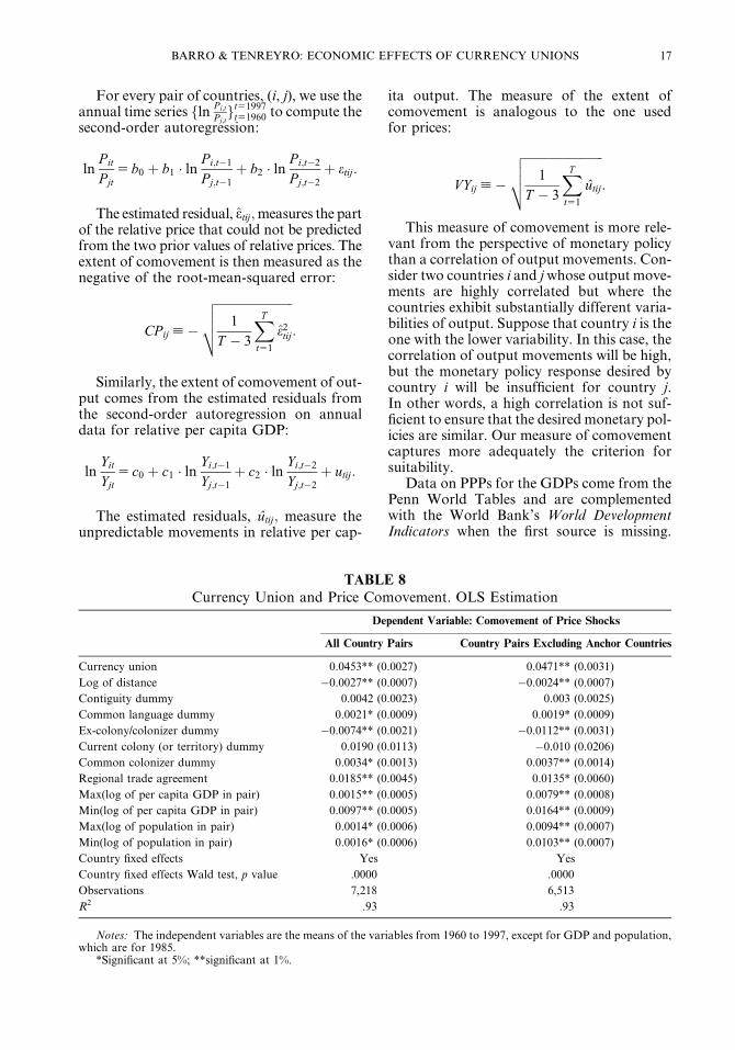
TABLE 8

Currency Union and Price Comovement. OLS Estimation

Dependent Variable: Comovement of Price Shocks

All Country Pairs Country Pairs Excluding Anchor Countries

Currency union 0.0453** (0.0027) 0.0471** (0.0031)

Log of distance �0.0027** (0.0007) �0.0024** (0.0007)

Contiguity dummy 0.0042 (0.0023) 0.003 (0.0025)

Common language dummy 0.0021* (0.0009) 0.0019* (0.0009)

Ex-colony/colonizer dummy �0.0074** (0.0021) �0.0112** (0.0031)

Current colony (or territory) dummy 0.0190 (0.0113) �0.010 (0.0206)

Common colonizer dummy 0.0034* (0.0013) 0.0037** (0.0014)

Regional trade agreement 0.0185** (0.0045) 0.0135* (0.0060)



Max(log of population in pair) 0.0014* (0.0006) 0.0094** (0.0007)

Min(log of population in pair) 0.0016* (0.0006) 0.0103** (0.0007)

Country fixed effects Yes Yes

Country fixed effects Wald test, p value .0000 .0000


R2 .93 .93

Notes: The independent variables are the means of the variables from 1960 to 1997, except for GDP and population,which are for 1985.



Data on real per capita GDP come from theWorld Development Indicators.

Table 8 shows the effect of currency unionson the comovements of prices. The first col-umn displays the regressions for all countrypairs, whereas the second excludes anchorsfrom the sample. This, again, is done to ensurecomparability with our IV estimation. Weinclude all the controls typically incorporatedin gravity regressions, that is, various meas-ures of distance and size. The logic for includ-ing the same controls is that the forces thatdetermine trade will also affect the extent ofprice-arbitrage between countries. There are,however, some differences in the way thatthese forces can influence outcomes. Forexample, countries that are close in terms ofthe gravity variables may be motivated to spe-cialize in different products. In this case,nearby countries will be subject to differentsectoral shocks and will likely exhibit lowercomovements of prices. In any event, it seemsprudent to control for the gravity variables.

In the comovement equations, the sampleconsists of one observation (estimated forthe period 1960–1997) on each country pair,

for pairs that have at least 20 observations.The regressors, as well as the IVs, are the aver-ages over the period.21 The table reports theestimates generated by OLS, including coun-try fixed effects.

The regressions show that price comove-ment rises with regional trade agreementsand falls with geographical distance. Sharinga border does not affect the comovement,once distance is taken into account. Speakingthe same language and sharing the same col-onizer have positive but small effects oncomovement. In contrast, countries exhibitrelatively lower price comovement with theirex-colonizers.

The currency-union estimates are virtuallyidentical in both samples: they indicate a cur-rency-union effect on price comovement of0.046 in the whole sample and 0.047 in thesample that excludes pairs with anchor coun-tries. These estimates are quite large: the

TABLE 9

Currency Union and Price Comovement. IV Estimation. Country Pairs Excluding

Anchor Countries. Second-Stage Estimates

Dependent Variable: CP


Log of distance �0.0019** (0.0007)

Contiguity dummy 0.0018 (0.0025)

Common language dummy 0.0012 (0.0010)

Ex-colony/colonizer dummy �0.0109** (0.0032)

Current colony (or territory) dummy �0.0187 (0.0257)

Common colonizer dummy 0.0001 (0.0018)

Regional trade agreement 0.0134* (0.0059)



Max(log of population in pair) 0.0094** (0.0007)

Min(log of population in pair) 0.0104** (0.0007)



Observations 6,513

R2 .93


Notes: The independent variables are the means of the variables from 1960 to 1997, except for GDP and population,which are for 1985. The IV is built from the probit prediction (model P1 in Table 4). See the formula for the derivation ofthe instrument in the text.


21. For GDP per capita and population, we use thevalue in 1985, because the averages are missing for somecountries. Using different years for GDP or populationdoes not alter the main results.

18 ECONOMIC INQUIRY

mean of the comovement variable (the nega-tive of the root-mean-squared error of theauto-regressive process described before) is�0.16.

Table 9 shows the IV estimation. The first-stage equation (not shown) indicates that thecoefficient on our IV, the indirect probabilityof currency union, again has a high t-statistic.The second-stage regression, shown in thetable, indicates that the presence of a currencyunion significantly raises the extent of pricecomovement. The estimated coefficient is0.068, which is larger than that found withOLS.

The p value from a Durbin-Wu-Hausmantest is reported at the bottom of Table 9. Thenull hypothesis that an OLS estimator of themodel would yield consistent estimates isrejected. In other words, endogeneity of thecurrency-union variable has detrimentaleffects on OLS estimates, and the IV tech-nique is required. As mentioned before, thepositive effect of currency unions on thecomovement of price shocks is most likelyassociated with the decrease in nominalexchange rate volatility stemming from theuse of a common currency.

Table 10 presents a set of robustness testsusing alternative specifications of the IV. Thefirst-stage regressions (not shown) indicatethat again, in all cases, the indirect probabil-ity of currency union has a significantlypositive coefficient. In the second-stageregressions, shown in the table, the estimatedcurrency-union coefficient varies between0.0649 and 0.0782 and is always statisticallysignificant. Moreover, p values from a Dur-bin-Wu-Hausman test are always below.05, suggesting that the IV estimator shouldbe preferred.

The comovement of output shocks is stud-ied in Table 11. Speaking the same language,sharing a border, and sharing the same col-onizer increase the comovement of output,but the ex-colony/colonizer variable doesnot affect the extent of comovement. Size,measured by GDP per capita, tends toincrease the comovement. However, a risein the population of the larger country hasambiguous effects on comovement. In theOLS estimation, the effect of currency unionon output comovement is positive but statis-tically insignificant.

Table 12 has the IVs results for outputcomovement. The first-stage regressions (not

shown) again indicate that the coefficient onthe indirect probability of currency union issignificantly positive. In the benchmark IVestimation shown in the table, the currency-union effect on output comovement is nega-tive, although insignificant at standard criticallevels. The Durbin-Wu-Hausman test yieldsa p value of .22, which implies that the dom-inance of the IV estimator is weaker than thatin the case of price comovement. Alternativespecifications of the instrument in Table 13confirm the negative effect, although in allcases statistical significance is low.

A negative effect of currency union on theextent of comovement of outputs could reflecta positive effect of currency unions on sectoralspecialization, which can then lead toa decrease in the extent of comovement, asKrugman (1993) suggested. The effect—inabsolute values—is not as substantial as theone found for price comovement: the esti-mated coefficient varies between �0.0011and �0.0042, whereas the mean of this vari-able (the negative of the root-mean-squarederror described above) is �0.06. This effect,however, might be different for developedcountries forming a currency union if devel-oped countries tend to specialize in the sameindustries. In this case, countries will tend tobe exposed to similar sectoral shocks and inte-gration will lead to higher comovement.22

VI. CONCLUSION

This paper proposes a new instrumentalvariable to study the effects of differentexchange rate arrangements on economic out-comes. We apply the methodology to investi-gate the impact of currency unions on bilateraltrade and the extent of comovements of pricesand outputs. The instrument relies on the ideathat one reason why two countries sharea common currency is the attractiveness ofa third country’s currency as an anchor. Thevalidity of the instrument requires that themotivation to adopt an external anchor’s cur-rency is exogenous to the bilateral linkbetween two potential client countries. Theresults show that the probability that a client

22. See Frankel and Rose (1998) for a study of therelationship between trade and business cycles for Orga-nization for Economic Cooperation and Developmentcountries.


TABLE 10Currency Union and Price Comovement. Robustness of IV Estimation to Alternative Instruments. Country Pairs

Excluding Anchor Countries. Second-Stage Estimates


Currency union 0.0717** (0.0064) 0.0622** (0.0093) 0.0649** (0.0069) 0.0678** (0.0070) 0.0750** (0.0109) 0.0711** (0.0060) 0.0638** (0.0094) 0.0665** (0.0069) 0.0782** (0.0111)

Log of distance �0.0018** (0.0007) �0.0021** (0.0007) �0.0020** (0.0007) �0.0019** (0.0007) �0.0017* (0.0007) �0.0018** (0.0007) �0.0020** (0.0007) �0.0019** (0.0007) �0.0017* (0.0007)

Contiguity dummy 0.0017 (0.0025) 0.0021 (0.0025) 0.0020 (0.0025) 0.0018 (0.0025) 0.0015 (0.0025) 0.0017 (0.0025) 0.0020 (0.0025) 0.0019 (0.0025) 0.0014 (0.0026)

Common language dummy 0.0011 (0.0010) 0.0014 (0.0010) 0.0013 (0.0010) 0.0012 (0.0010) 0.0010 (0.0010) 0.0011 (0.0010) 0.0014 (0.0010) 0.0013 (0.0010) 0.0009 (0.0010)

Ex-colony/colonizer dummy �0.0109** (0.0032) �0.0110** (0.0032) �0.0110** (0.0032) �0.0110** (0.0032) �0.0109** (0.0033) �0.0109** (0.0032) �0.0110** (0.0032) �0.0110** (0.0032) �0.0108** (0.0033)

Current colony(or territory) dummy

�0.0201 (0.0266) �0.0161 (0.0244) �0.0172 (0.0249) �0.0185 (0.0256) �0.0215 (0.0277) �0.0198 (0.0264) �0.0168 (0.0247) �0.0179 (0.0253) �0.0228 (0.0285)

Common colonizer dummy �0.0005 (0.0017) 0.0011 (0.0021) 0.0007 (0.0018) 0.0002 (0.0018) �0.0010 (0.0024) �0.0004 (0.0017) 0.0008 (0.0021) 0.0004 (0.0018) �0.0016 (0.0024)

Regional trade agreement 0.0133* (0.0059) 0.0134* (0.0059) 0.0134* (0.0059) 0.0134* (0.0059) 0.0133* (0.0059) 0.0133* (0.0059) 0.0134* (0.0059) 0.0134* (0.0059) 0.0133* (0.0059)

Max(log of per capitaGDP in pair)

0.0080** (0.0008) 0.0080** (0.0008) 0.0080** (0.0008) 0.0080** (0.0008) 0.0081** (0.0008) 0.0080** (0.0008) 0.0080** (0.0008) 0.0080** (0.0008) 0.0081** (0.0008)

Min(log of per capitaGDP in pair)

0.0165** (0.0009) 0.0164** (0.0009) 0.0164** (0.0009) 0.0164** (0.0009) 0.0165** (0.0009) 0.0165** (0.0009) 0.0164** (0.0009) 0.0164** (0.0009) 0.0165** (0.0009)

Max(log ofpopulation in pair)

0.0094** (0.0007) 0.0094** (0.0007) 0.0094** (0.0007) 0.0094** (0.0007) 0.0094** (0.0007) 0.0094** (0.0007) 0.0094** (0.0007) 0.0094** (0.0007) 0.0094** (0.0007)

Min(log ofpopulation in pair)

0.0104** (0.0007) 0.0104** (0.0007) 0.0104** (0.0007) 0.0104** (0.0007) 0.0104** (0.0007) 0.0104** (0.0007) 0.0104** (0.0007) 0.0104** (0.0007) 0.0104** (0.0007)

Country fixed effect Yes Yes Yes Yes Yes Yes Yes Yes Yes

Country fixed effectsWald test, p value

.0000 .0000 .0000 .0000 .0000 .0000 .0000 .0000 .0000

Observations 6,513 6,513 6,513 6,513 6,513 6,513 6,513 6,513 6,513

R2 .93 .93 .93 .93 .93 .93 .93 .93 .93

Wu-Hausman test ofexogeneity, p value

.0000 .0866 .0032 .0004 .0063 .0000 .0592 .0007 .0024

Notes: The independent variables are the means of the variables from 1960 to 1997, except for GDP and population which are for 1985. IV1 is built from the prediction of theprobit regression (P1 in Table 4), evaluating year effects and the landlocked and island dummies at their mean values. See the formula for the derivation of the instrument in the text.IV2 is similar to IV1, with the population and income controls also evaluated at their mean values in the probit prediction. IV3 is built from the prediction of a probit regression thatexcludes year effects (P2 in Table 4). IV4 is similar to IV3, with the landlocked and island dummies evaluated at their mean values in the probit prediction. IV5 is similar to IV4, withpopulation and income variables also evaluated at their mean values. IV6 is built from the prediction of a probit regression that excludes the landlocked and island dummies (P3 inTable 4). IV7 is similar to IV6, with year effects, population, and income variables evaluated at their mean values in the probit prediction. IV8 is built from the prediction of a probitregression that excludes year effects and the landlocked and island dummies (P4 in Table 4). IV9 is similar to IV8, with population and income variables evaluated at their meanvalues in the probit prediction.


20

ECONOMIC

INQUIR

Y

TABLE 12

Currency Union and Output Comovement. IV Estimation. Country Pairs

Excluding Anchor Countries. Second-Stage Estimates

Dependent Variable: Comovement of Output Shocks

Currency union �0.0024 (0.0026)

Log of distance �0.0004 (0.0002)


Common language dummy 0.0008* (0.0004)

Ex-colony/colonizer dummy �0.0002 (0.0011)

Current colony (or territory) dummy �0.0066 (0.0095)


Regional trade agreement �0.0005 (0.0016)



Max(log of population in pair) �0.0009** (0.0002)




Observations 6,887

R2 .91


Notes: The independent variables entered are the means of the variables from 1960 to 1997, except for GDP andpopulation, which are for 1985. The IV is built from the probit prediction (model P1 in Table 4). See the formula forthe derivation of the instrument in the text.


TABLE 11

Currency Union and Output Comovement. OLS Estimation

Dependent Variable: Comovement of Output Shocks

All Country Pairs Country Pairs Excluding Anchor Countries

Currency union 0.0001 (0.0011) 0.0008 (0.0012)

Log of distance �0.0003 (0.0002) �0.0003 (0.0002)


Common language dummy 0.0007* (0.0003) 0.0007* (0.0004)

Ex-colony/colonizer dummy �0.0007 (0.0007) �0.0001 (0.0011)

Current colony (or territory) dummy �0.0024 (0.0023) �0.0087 (0.0097)


Regional trade agreement 0.0012 (0.0013) �0.0008 (0.0016)



Max(log of population in pair) 0.0117** (0.0002) �0.0009** (0.0002)

Min(log of population in pair) 0.0128** (0.0002) 0.0001 (0.0002)

Country fixed effects Yes Yes

Country fixed effects Wald test, p value .0000 .0000


R2 .91 .91

Notes: The independent variables are the means of the variables from 1960 to 1997, except for GDP and population,which are for 1985.



TABLE 13

Currency Union and Output Comovement. Robustness of IV Estimation to Alternative Instruments. Country

Pairs Excluding Anchor Countries. Second-Stage Estimates


Currency union �0.0016 (0.0027) �0.0035 (0.0037) �0.0046 (0.0032) �0.0034 (0.0031) �0.0029 (0.0041) �0.0013 (0.0025) �0.0033 (0.0037) �0.0034 (0.0030) �0.0025 (0.0042)

Log of distance �0.0004 (0.0002) �0.0004 (0.0002) �0.0004* (0.0002) �0.0004* (0.0002) �0.0004 (0.0002) �0.0003 (0.0002) �0.0004 (0.0002) �0.0004* (0.0002) �0.0004 (0.0002)

Contiguity dummy 0.0037** (0.0009) 0.0038** (0.0009) 0.0038** (0.0009) 0.0038** (0.0009) 0.0038** (0.0009) 0.0037** (0.0009) 0.0038** (0.0009) 0.0038** (0.0009) 0.0037** (0.0009)

Common language dummy 0.0008* (0.0004) 0.0009* (0.0004) 0.0009* (0.0004) 0.0009* (0.0004) 0.0009* (0.0004) 0.0008* (0.0004) 0.0009* (0.0004) 0.0009* (0.0004) 0.0008* (0.0004)

Ex-colony/colonizer dummy �0.0001 (0.0011) �0.0002 (0.0011) �0.0002 (0.0011) �0.0002 (0.0011) �0.0002 (0.0011) �0.0001 (0.0011) �0.0002 (0.0011) �0.0002 (0.0011) �0.0002 (0.0011)

Current colony(or territory) dummy

�0.0071 (0.0096) �0.0059 (0.0097) �0.0052 (0.0096) �0.0059 (0.0096) �0.0063 (0.0097) �0.0073 (0.0096) �0.0060 (0.0097) �0.0059 (0.0096) �0.0066 (0.0098)


Regional trade agreement �0.0005 (0.0016) �0.0004 (0.0016) �0.0003 (0.0016) �0.0004 (0.0016) �0.0004 (0.0017) �0.0006 (0.0016) �0.0004 (0.0017) �0.0004 (0.0016) �0.0005 (0.0017)

Max(log of per capitaGDP in pair)

0.0021** (0.0003) 0.0021** (0.0003) 0.0021** (0.0003) 0.0021** (0.0003) 0.0021** (0.0003) 0.0021** (0.0003) 0.0021** (0.0003) 0.0021** (0.0003) 0.0021** (0.0003)

Min(log of per capitaGDP in pair)

0.0031** (0.0003) 0.0031** (0.0003) 0.0031** (0.0003) 0.0031** (0.0003) 0.0031** (0.0003) 0.0031** (0.0003) 0.0031** (0.0003) 0.0031** (0.0003) 0.0031** (0.0003)

Max(log ofpopulation in pair)

�0.0009** (0.0002) �0.0009** (0.0002) �0.0009** (0.0002) �0.0009** (0.0002) �0.0009** (0.0002) �0.0009** (0.0002) �0.0009** (0.0002) �0.0009** (0.0002) �0.0009** (0.0002)

Min(log ofpopulation in pair)

0.0001 (0.0002) 0.0001 (0.0002) 0.0001 (0.0002) 0.0001 (0.0002) 0.0001 (0.0002) 0.0001 (0.0002) 0.0001 (0.0002) 0.0001 (0.0002) 0.0001 (0.0002)


Country fixed effectsWald test, p value

.0000 .0000 .0000 .0000 .0000 .0000 .0000 .0000 .0000

Observations 6,887 6,887 6,887 6,887 6,887 6,887 6,887 6,887 6,887

R2 .91 .91 .91 .91 .91 .91 .91 .91 .91

Wu-Hausman test ofexogeneity, p value

.3191 .2230 .0600 .1208 .3540 .3522 .2625 .1142 .4244

Notes: The independent variables are the means of the variables from 1960 to 1997, except for GDP and population which are for 1985. IV1 is built from the prediction of theprobit regression (P1 in Table 4), evaluating year effects and the landlocked and island dummies at their mean values. See the formula for the derivation of the instrument in the text.IV2 is similar to IV1, with the population and income controls also evaluated at their mean values in the probit prediction. IV3 is built from the prediction of a probit regression thatexcludes year effects (P2 in Table 4). IV4 is similar to IV3, with landlocked and island dummies evaluated at their mean values in the probit prediction. IV5 is similar to IV4, withpopulation and income variables also evaluated at their mean values. IV6 is built from the prediction of a probit regression that excludes landlocked and island dummies (P3 inTable 4). IV7 is similar to IV6, with year effects, population, and income variables evaluated at their mean values in the probit prediction. IV8 is built from the prediction of a probitregression that excludes year effects and landlocked and island dummies (P4 in Table 4). IV9 is similar to IV8, with population and income variables evaluated at their mean valuesin the probit prediction.


22

ECONOMIC

INQUIR

Y

adopts the currency of a main anchorincreases when the client is geographicallyclose, speaks the same language, and sharesa colonial relationship with the anchor. It alsoincreases when the client is smaller and poorerand when the anchor is richer. The likelihoodthat two countries share a common currency iscalculated from the probability that each ofthem, independently, uses the currency ofa third country. This likelihood serves as aninstrument for the common currency dummyin the estimation of the economic effects ofcurrency unions.

The IV approach is used to revisit the effectof currency unions on trade and to investigatethe effect of currency unions on the extent ofcomovement of prices and outputs. Threemain findings follow. First, currency unionssignificantly increase bilateral trade, a resultthat supports previous findings by Rose(2000) and coauthors. This finding suggeststhat the large trade effect found previouslyfor currency unions is not due to endogeneitybias. Second, currency unions significantlyincrease the extent of price comovement. Thisresponse most likely reflects the elimination ofnominal exchange rate volatility. Third, the IVresults suggest that currency unions mightdecrease the extent of comovement of output,possibly as a consequence of higher sectoralspecialization.

REFERENCES

Alesina, A., and R. J. Barro. ‘‘Currency Unions.’’ Quar-terly Journal of Economics, 17, May 2002, 409–36.

Alesina, A., R. J. Barro, and S. Tenreyro. ‘‘OptimumCur-rency Unions.’’ National Bureau of EconomicResearch Macroeconomic Annual, 2002.

Barro, R. J., and S. Tenreyro. ‘‘Closed and Open Econ-omy Models of Business Cycles with Marked-Upand Sticky Prices.’’ Economic Journal, 116, 2006,434–56.

Frankel, J., and A. Rose. ‘‘The Endogeneity of the Opti-mum Currency Area Criteria ’’ Economic Journal,108, July 1998, 1009–25.

——— . ‘‘An Estimate of the Effect of Currency Unionson Trade and Income.’’ Quarterly Journal of Eco-nomics, 117, 2002, 437–66.

Glick, R., and A. Rose. ‘‘Does a Currency Union AffectTrade? The Time Series Evidence.’’ European Eco-nomic Review, 46, 2002, 1125–51.

Hallak, J. C. ‘‘Product Quality and the Direction ofTrade.’’ Journal of International Economics, 68,2006, 238–65.

Krugman, P. ‘‘Lessons of Massachusetts for EMU, ’’ inAdjustment and Growth in the European MonetaryUnion, edited by F. Torres and F. Giavazzi. Cam-bridge, United Kingdom: Cambridge UniversityPress, 1993, 241–61.

Persson, T. ‘‘Currency Union and Trade, How Large isthe Treatment Effect? ’’ Economic Policy, 16, 2001,335–48.

Rose, A. ‘‘One Money One Market: Estimating the Effectof Common Currencies on Trade.’’ Economic Policy,15, 2000, 7–46.

Rose, A., andE. vanWincoop. ‘‘NationalMoney as a Bar-rier to International Trade: The Real Case for Cur-rency Union.’’ American Economic Review, 91, May2001, 386–90.


ECONOMIC EFFECTS OF CURRENCY UNIONS - LSE

Documents